Modelling Agents’ Choices in Temporal Linear Logic

Duc Q. Pham, James Harland, and Michael Winikoff

School of Computer Science and Information TechnologyRMIT University

GPO Box 2476V, Melbourne, 3001, Australia{qupham,jah,winikoff}@cs.rmit.edu.au

Abstract. Decision-making is a fundamental feature of agent systems. Agentsneed to respond to requests from other agents, to react to environmental changes,and to prioritize and pursue their goals. Such decisions can have ongoingeffects,as the future behavior of an agent may be heavily dependent on choices made ear-lier. In this paper we investigate a formal framework for modeling the choices ofan agent. In particular, we show how the use of a choices calculus basedon tem-poral linear logiccan be used to capture distribution, temporal and dependencyaspects of choices.

1 Introduction

Agents are increasingly becoming accepted as a suitable paradigm for conceptualizing,designing, and implementing the sorts of distributed complex dynamic systems that canbe found in a range of domains, such as telecommunications, banking, crisis manage-ment, and business transactions [1].

A fundamental theme in agent systems isdecision-making. Agents have to decidewhich resources to use, which actions to perform, which goals and commitments toattend to next etc. in order to fulfill their design objectives as well as to respond toother agents in an open and dynamic operating environment. Very often, agents areconfronted with choices. Decisions on choices made now may very well affect futureachievement of goals or other threads of interactions. In a sense, agents have to makeinformed and wise decisions on choices. This can be thought of as how to enable agentsto act on choices, subject to any possible constraints and with a global consideration tofuture advantages.

Moreover, in open and dynamic environments, changes from the environment occurfrequently and often are unpredictable, which can hinder accomplishment of agents’goals. How agents cope with changes remains an open and challenging problem. Onthe one hand, agents should be enabled to reason about the current changes and actflexibly. On the other hand, agents should be equipped with a reasoning ability to bestpredict changes and act accordingly.

These characteristics are desirable for a single agent. However, no agent is an is-land, and decisions of an agent are not made in isolation, butin the context of decisionsmade by other agents, as part of interactions between the agents. Thus, the challengingsetting here is that in negotiation and other forms of agent interaction, decision mak-ing is distributed. In particular, key challenges in modeling decision makingin agentinteraction are:

– Distribution: choices are distributed among agents, and changes from the envi-ronments affect each agent in different ways. How to capturethese choices, theirdependencies and the effects of different strategies for their decisions as well as toreason about the global changes at the individual level in agent systems are impor-tant.

– Time:decision making by agents occurs in time. So do the choices tobe made andthe changes in the environment. Then it is necessary to deal with them in a timedependent manner.

– Dependencies:i.e. capturing that certain decisions depend on other decisions.

The central importance of decision-making in agent systemsmakes it natural to uselogic as a basis for a formal framework for agents. This meansthat we can model thecurrent state of an agent as a collection of formulas, and theconsequences of a particularaction on a given state can be explored via standard reasoning methods. In this paper,we explore how to extend this approach to include decisions as well as actions. Hence,for logic-based agents, whose reasoning and decision making is based on a declarativelogical formalism, it is important to model the decision making on choices as well ason the environment changes.

This paper tackles the modeling of agent decisions in a way that allows distribution,dependencies, and time of choices to be captured. We discussspecific desirable prop-erties of a formal model of agent choices (section 3) and thenpresent a formalchoicecalculus(section 4). We then consider an application of the choice calculus. Specifi-cally, by ensuring that the choices are made in multiple different formulas consistently,the choice calculus allows us to turn an interaction concerning a goal into multiple con-current and distributed threads of interaction on its subgoals. This is also based on amechanism to split a formulaΓ which containsA into two formulas, one of whichcontainsA, the other contains the results of “subtracting”A from Γ .

In [2], it was shown howTemporal Linear Logic(TLL) can be used to model agentinteractions to achieve flexibility, particularly due to its ability to model resources andchoices, as well as temporal constraints. This paper can be seen as further developingthis line of work to include explicit considerations of the choices of each agent and thestrategies of dealing with them.

The remainder of this paper is structured as follows. Section 2 briefly reviews tem-poral linear logic, and the agent interaction framework. The following two sections mo-tivate and present the choice calculus. Section 5 presents an application of the choicecalculus to distributed concurrent problem solving. We then conclude in section 6.

2 Background

2.1 Temporal Linear Logic

Temporal Linear Logic (TLL ) [3] is the result of introducing temporal logic into lin-ear logic. While linear logic provides advantages to modeling and reasoning about re-sources, temporal logic addresses the description and reasoning about the changes oftruth values of logic expressions over time [4]. Hence, TLL is resource-conscious aswell as dealing with time.

In particular, linear logic [5] is well-known for modeling resources as well as up-dating processes. It has been considered in agent systems tosupport agent negotiationand planning by means of proof search [6, 7].

In multi-agent systems, utilization of resources and resource production and con-sumption processes are of fundamental consideration. In such logic as classical or tem-poral logic, however, a direct mapping of resources onto formulas is troublesome. If wemodel resources like A as “one dollar” and B as “a chocolate bar”, thenA,A ⇒ B inclassical logic is read as “given one dollar we can get a chocolate bar”. The problemis thatA - one dollar - remains afterward. In order to resolve such resource - formulamapping issues, Girard proposed treating formulas as resources and hence they will beused exactly once in derivations.

As a result of such constraint, classical conjunction (and)and disjunction (or) arerecast over different uses of contexts - multiplicative as combining and additive as shar-ing to come up with four connectives. In particular, A⊗ A (multiplicative conjunction)means that one has two As at the same time, which is different fromA∧A = A. Hence,⊗ allows a natural expression of proportion. AO B (multiplicative disjunction) meansthat if not A then B or vice versa but not both A and B.

The ability to specify choices via the additive connectivesis also a particularlyuseful feature of linear logic. If we consider formulas on the left hand side of⊢ aswhat are provided (program formulas), then AN B (additive conjunction) stands forone’s own choice, either of A or B but not both. A⊕ B (additive disjunction) standsfor the possibility of either A or B, but we don’t know which. In other words, whileN refers to inner determinism,⊕ refers to inner non-determinism. Hence,N can beused to model an agent’s own choices (internal choices) whereas⊕ can be used tomodelindeterminate possibilities(or external choices) in the environment. The dualitybetweenN and⊕, being respectively an internal and an external choice, is awell-knownfeature of linear logic [5].

Due to the duality between formulas on two sides of⊢, formulas on the right sidecan be regarded as goal formulas, i.e. what to be derived. A goal A N B means thatafter deriving this goal, one can choose betweenA or B. In order to have this ability tochoose, one must prepare for both cases - being able to deriveA and deriveB. On theother hand, a goalA ⊕ B means that it is not determined which goal betweenA andB. Hence, one can choose to derive either of them. In terms of deriving goals,N and⊕among goal formulas act as introducing indeterminate possibilities and introducing aninternal choice respectively.

The temporal operators used are, (next),@ (anytime), and3 (sometime) [3]. For-mulas with no temporal operators can be considered as being available only at present.Adding , to a formula A, i.e.,A, means that A can be used only at the next timepoint and exactly once. Similarly,@A means that A can be used at any time (exactlyonce, since it is linear).3A means that A can be at some time (also exactly once).Whilst the temporal operators have their standard meanings,the notions of internal andexternal choice can be applied here as well, in that in that@A means thatA can be usedat any time (but exactly once) with the choice of time being internal to the agent, and3A means thatA can be used at some time with the choice of time being externaltothe agent.

The semantics of TLL connectives and operators as above are given via its sequentcalculus, since we take a proof-theoretic approach in modeling agent interaction.

2.2 A Model for Agent Interaction

In [8], an interaction modeling framework which uses TLL as ameans of specifying in-teraction protocols is used as TLL is natural to model resources, internal choices and in-determinate possibilities with respect to time. Various concepts such as resource, capa-bility and commitment/goal are encoded in TLL. The symmetrybetween a formula andits negation in TLL is explored as a way to model resources andcommitments/goals.In particular, formulas to be located on the left hand side of⊢ can be regarded as for-mulas in supply (resources) while formulas to be located on the right hand side of⊢ asformulas in demand (goals).

A unit of consumableresourcesis then modeled as a proposition in linear logicand can be preceded by temporal operators to address time dependency. For example,listening to music after (exactly) three time points is denoted as, , ,music. Ashorthand is,3music.

The capabilitiesof agents refer to producing, consuming, relocating and chang-ing ownership of resources. Capabilities are represented by describing the state beforeand after performing them. The general representation formis Γ ⊸ ∆, in which Γ

describes the conditions before and∆ describes the conditions after. The linear im-plication⊸ ensures that the conditions before will be transformed intothe conditionsafter.

To take an example, consider a capability of producing musicusing music playerto play music files. There are two options available at the agent’s own choice, one isusing mp3 player to play mp3 files, the other is using CD playerto play CD files. Theencoding is:

@[[(mp3 ⊗ mp3 player) ⊕ (CD ⊗ CD player)] ⊸ music]1

where@ means that the capability can be applied at any time,⊕ indicates an internalchoice (notN, as it is located on the left hand side of⊸).

3 Desiderata for a Choice Calculus

Unpredictable changes in the environment can be regarded asa set of possibilities whichthe agents do not know the outcomes. There are several strategies for dealing withunpredictable changes. A safe approach is to prepare for allthe possible scenarios, atthe cost of extra reservation and/or consumption of resources. Other approaches aremore risky in which agents make a closest possible prediction of which possibilities tooccur and act accordingly. If the predictions are correct, agents achieve the goals withresource efficiency. Here, there is a trade-off between resource efficiency and safety.

1 In the modeling, formulas representing media players are consumed away, which does notreflect the persistence of physical objects. However, we focus on modeling how resources areutilized, not their physical existences and hence simplify the encoding since it is not necessaryto have the media players retained for later use.

In contrast to indeterminate possibilities, internal choices are what agents can de-cide by themselves to their own advantage. Decisions on internal choices can be basedon what is best for the agents’ current and local needs. However, it is desirable that theyconsider internal choices in the context of other internal choices that have been or willbe made. This requires an ability to make an informed decision on internal choices. Ifwe put information for decision making on internal choices as constraints associatedwith those internal choices then what required is a modelingof internal choices withtheir associated constraints such that agents can reason about them and decide accord-ingly. Also, in such a distributed environment as multi-agent systems, such a modelingshould take into account as constraints the dependencies among internal choices.

In addition, as agents act in time, decisions can be made precisely at the requiredtime or can be well prepared in advance. When to decide and act on internal choicesshould be at the agents’ autonomy. The advantages of deciding internal choices in ad-vance can be seen in an example as resolving a goal of,3(A⊕B). This goal involvesan internal choice (⊕) to be determined at the third next time point (,3). If the agentdecides now to choose A and commits to making the same decision at the third nexttime point, then from now, the agent only has to focus a goal of,3A. This also meansthat resources used for other goals can be guaranteed to be exclusive from the require-ments of,3(A ⊕ B), which might not be the case otherwise when,3(A ⊕ B) isdecided as,3B at the third next time point.

The following example illustrates various desirable strategies of agents.

Peter intends to organize an outdoor party in two days’ time.He has a goal ofproviding music at the party. He has a CD burner and a blank CD onto which he canburn music in CD or mp3 format. His friend, John, can help by bringing a CD playeror an mp3 player to the party but Peter will not know which until tomorrow. David theninforms Peter that he would like to borrow Peter’s CD burner today.

In this situation, to Peter, there is an internal choice on the music format and anindeterminate possibility regarding the player. We consider two strategies. If Peter doesnot let David borrow the CD burner, he can wait until tomorrowto find out what kindof player John will bring to the party and choose the music format accordingly at thattime. Otherwise, he can not delay burning the CD until tomorrow and so has to makea prediction on which player John will bring to the party and then decide the internalchoice on the music format early (now), burn the CD and let David borrow the CDburner. The question is then how to make such strategies available for Peter to explore.

One solution is using formalisms such as logic to enable agent reasoning on thoseinternal choices and indeterminate possibilities. LinearLogic is highly suitable here,because it allows us to distinguish between internal determinism and non-determinism.Temporallinear logic (TLL) further puts such modeling of them in a time dependentcontext. Indeed, internal choices and external choices (inner non-determinism) havebeen modeled previously using Linear Logic [6, 9] and TLL [8,2].

An important observation is that although (temporal) linear logic captures the no-tions of internal choice and indeterminate possibility, its sequent rules constrain agentsto specific strategies and make each decision on internal choices in isolation (subjectonly to local information). Specifically, consider the following rules of standard sequent

calculus:Γ,A ⊢ ∆ Γ,B ⊢ ∆

Γ,A ⊕ B ⊢ ∆

Γ ⊢ A,∆ Γ ⊢ B,∆

Γ ⊢ A N B,∆

Γ,A ⊢ ∆

Γ,A N B ⊢ ∆

Γ,B ⊢ ∆

Γ,A N B ⊢ ∆

Γ ⊢ A,∆

Γ ⊢ A ⊕ B,∆

Γ ⊢ B,∆

Γ ⊢ A ⊕ B,∆

where for the formulas on the left hand side of⊢, N remarks internal choice and⊕remarks indeterminate possibility and vice versa for the formulas on the right hand sideof ⊢.

The first set of rules require agents to prepare for both outcomes of the indeterminatepossibility. Though this strategy is safe, it demands extraand unnecessary resources andactions. Moreover, this strategy does not take into accountan agents’ prediction of theenvironment or whether it is willing to take risks.

More importantly, according to the last set of rules, the free (internal) choice agentshave is determinedlocally, i.e. without a global awareness. Hence decisions on thesefree choices may not be optimal. In particular, if the formulaANB (on the left hand sideof ⊢) is not used in any proof now, without this kind of local information, the decisionon this internal choice becomes unguided. Hence, if there isfurther information aboutpossible future goals or about dependencies on other internal choices, this informationshould be considered and the agent should be enabled to decide the internal choiceaccordingly. Moreover, the rule does not allow agents to explore the strategy of decidinginternal choices in advance.

Referring to our running example, in the first strategy, Peter does not let Davidborrow the CD burner, and so Peter can then find a proof using standard sequent rulesto achieve the goal of providing music at the party two days later. However, in thesecond strategy, the search using standard TLL sequent calculus for a proof of the goalfails as it requires to have music in both formats (mp3 and CD)so as to be matchedwith the future possibility of the media player.

Hence, in this paper, we investigate how TLL not only allows us to model the differ-ence between internal choice and indeterminate possibility with respect to time, but alsoallows us to capturedependenciesamong internal choices, constraints on how internalchoices can be made as well as predictions and decisions of indeterminate possibil-ities. Such constraints may also reflect global consideration of other goals and otherthreads of interaction. We further consider strategies that can be used to deal with inter-nal choices with respect to time, reflecting how cautious theagents are and whether theagents deal with them in advance. However, we will not discuss how agents can predictthe environment outcomes correctly.

4 A Choice Calculus

If we assume that the order of operants is unchanged throughout the process of formulasmanipulation, in other words, ignoring the commutative property of⊕ andN, then thedecision on choices and indeterminate possibilities can beregarded as selecting the lefthand side or the right hand side of the connective. For simplicity, we shall refer toboth internal choices (choices with inner determinism) andindeterminate possibilities(choices with non-determinism) simply as choices.

As the decision on a choice is revealed at the time point associated with the choice,before that time point, the decision of the choice is unknown. We encode the decisionson choices using TLL constants.

We need to consider the base values for choice decisions, howto specify choices ofthe same decisions, choices that are dependent on other choices and also how standardsequent calculus rules are modified to reflect decisions on choices.

We use the notationNx

→ or⊕x

→ to indicate the result of the decision making ofNx

and⊕x respectively. The subscript indicates the ID of the connective. The base valuesfor their decision can be encoded by TLL constantsL, andR. For example, the result ofthe decision on the choice inA N B is L if A results fromA N B and isR if B results.For internal choices, their decisions can be regarded as variables as agents can decide

the assignment of values. Formally, we write⊢N1

→⊸ L orN1

→⊢ L to denote that the leftsubformula ofN1 was selected.

Decisions on indeterminate possibilities could also be represented as variables.However, we will explicitly represent that agents can not decide the outcomes of in-determinate possibilities and that the decisions on them (by external factors) have notbeen made by using the formL ⊕ R (or L N R). For example, given the indetermi-nate possibility,n(A ⊕x B), we represent their decision by,n(L ⊕x R), wheren

is the time point associated with the choice and⊕x is the same connective as that in,n(A ⊕x B).

By modeling the choices explicitly, we can state constraints between them. For ex-

ample, if two choices,Nx

→ andNy

→, need to be made consistently — either both right or

both left — then this can be stated asNx

→=Ny

→ or, in logic encoding,Nx

→⊢Ny

→,Nx

→⊣Ny

→.More generally, we can state that a given choiceNx should depend on a combinationof other choices or some external constraints. We usecondLx (respectivelycondRx) todenote the condition that should hold for the left (respectively right) side of the choiceto be taken. Clearly,condLx andcondRx should always be mutually exclusive. Theseconditions, in their presence, completely determine the results of the choices’ decisions.In their absence, the internal choices become truly free choices and we are getting backto the normal case as of standard sequent rules. These conditions are encoded as TLLsequents so that sub-conditions (sequents) can be found viaproof search.

Given a formulaΓ which contains a sub-formulaA, we can compress the sequenceof decisions that need to be made in order to obtainA fromΓ into a singlerepresentativechoice. For example, ifΓ = B N1 ,a(,b(A ⊕2 C) N3 D) then, in order to obtainA from Γ we need to decide on the right side ofN1, then,a time units later, decide onthe left side ofN3, andb time units after that, have the left side of⊕2 be selected bythe environment (an indeterminate possibility). Formally, the notion of representative isdefined as below.

Definition 1. A representative choiceNr with respect to a formula A in a compoundprogram formula (respectively goal formula)Γ is a choice,xA Nr ,y1 (respectively,xA ⊕r ,y1) whose decision isL if A is chosen fromΓ and isR otherwise, wherex, x ≥ 0 is the time associated with A inΓ andy, y ≥ 0 is is the time point associatedwith 1.

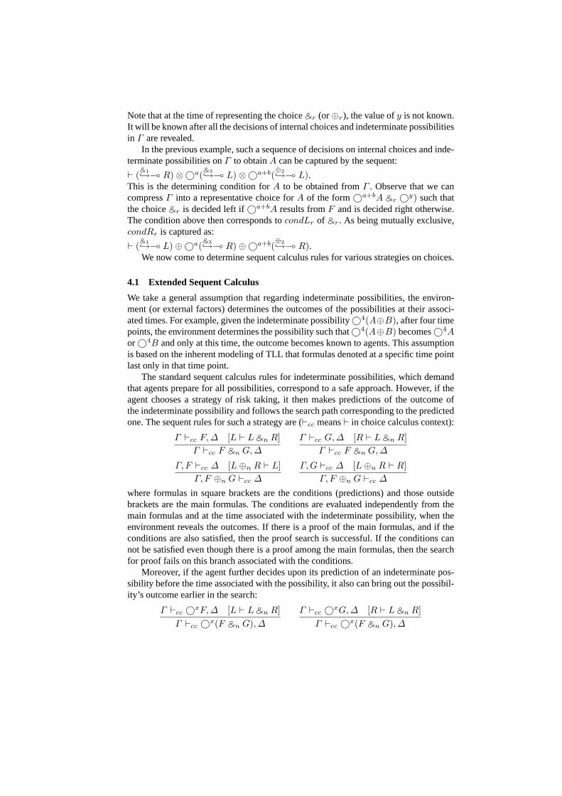
Note that at the time of representing the choiceNr (or⊕r), the value ofy is not known.It will be known after all the decisions of internal choices and indeterminate possibilitiesin Γ are revealed.

In the previous example, such a sequence of decisions on internal choices and inde-terminate possibilities onΓ to obtainA can be captured by the sequent:

⊢ (N1

→⊸ R) ⊗ ,a(N3

→⊸ L) ⊗ ,a+b(⊕2

→⊸ L).This is the determining condition forA to be obtained fromΓ . Observe that we cancompressΓ into a representative choice forA of the form,a+bA Nr ,y) such thatthe choiceNr is decided left if,a+bA results fromF and is decided right otherwise.The condition above then corresponds tocondLr of Nr. As being mutually exclusive,condRr is captured as:

⊢ (N1

→⊸ L) ⊕ ,a(N3

→⊸ R) ⊕ ,a+b(⊕2

→⊸ R).We now come to determine sequent calculus rules for various strategies on choices.

4.1 Extended Sequent Calculus

We take a general assumption that regarding indeterminate possibilities, the environ-ment (or external factors) determines the outcomes of the possibilities at their associ-ated times. For example, given the indeterminate possibility ,4(A⊕B), after four timepoints, the environment determines the possibility such that,4(A⊕B) becomes,4A

or ,4B and only at this time, the outcome becomes known to agents. This assumptionis based on the inherent modeling of TLL that formulas denoted at a specific time pointlast only in that time point.

The standard sequent calculus rules for indeterminate possibilities, which demandthat agents prepare for all possibilities, correspond to a safe approach. However, if theagent chooses a strategy of risk taking, it then makes predictions of the outcome ofthe indeterminate possibility and follows the search path corresponding to the predictedone. The sequent rules for such a strategy are (⊢cc means⊢ in choice calculus context):

Γ ⊢cc F,∆ [L ⊢ L Nn R]

Γ ⊢cc F Nn G,∆

Γ ⊢cc G,∆ [R ⊢ L Nn R]

Γ ⊢cc F Nn G,∆

Γ,F ⊢cc ∆ [L ⊕n R ⊢ L]

Γ, F ⊕n G ⊢cc ∆

Γ,G ⊢cc ∆ [L ⊕n R ⊢ R]

Γ, F ⊕n G ⊢cc ∆

where formulas in square brackets are the conditions (predictions) and those outsidebrackets are the main formulas. The conditions are evaluated independently from themain formulas and at the time associated with the indeterminate possibility, when theenvironment reveals the outcomes. If there is a proof of the main formulas, and if theconditions are also satisfied, then the proof search is successful. If the conditions cannot be satisfied even though there is a proof among the main formulas, then the searchfor proof fails on this branch associated with the conditions.

Moreover, if the agent further decides upon its prediction of an indeterminate pos-sibility before the time associated with the possibility, it also can bring out the possibil-ity’s outcome earlier in the search:

Γ ⊢cc ,xF,∆ [L ⊢ L Nn R]

Γ ⊢cc ,x(F Nn G),∆

Γ ⊢cc ,xG,∆ [R ⊢ L Nn R]

Γ ⊢cc ,x(F Nn G),∆

Γ,,xF ⊢cc ∆ [L ⊕n R ⊢ L]

Γ,,x(F ⊕n G) ⊢cc ∆

Γ,,xG ⊢cc ∆ [L ⊕n R ⊢ R]

Γ,,x(F ⊕n G) ⊢cc ∆

Internal choices are decided by the owner agent at the time associated with the choice,subject to any constraints (condLn or condRn) imposed on them. The following se-quent rules reflect that:

Γ, F ⊢cc ∆ (⊢ condLn)

Γ, F Nn G ⊢cc ∆

Γ,G ⊢cc ∆ (⊢ condRn)

Γ, F Nn G ⊢cc ∆

Γ ⊢cc F,∆ (⊢ condLn)

Γ ⊢cc F ⊕n G,∆

Γ ⊢cc G,∆ (⊢ condRn)

Γ ⊢cc F ⊕n G,∆

wherecondLn andcondRn are conditions imposed on the internal choicen for thechoice to be decided left or right. These conditions may or may not be present.

Moreover, if the agent is to decide the choice priorly, it canbring out the choice’soutcome earlier in the search:

Γ,,xF ⊢cc ∆ (⊢ condLn)

Γ,,x(F Nn G) ⊢cc ∆

Γ,,xG ⊢cc ,x∆ (⊢ condRn)

Γ,,x(F Nn G) ⊢cc ,x∆

Γ ⊢cc ,xF,∆ (⊢ condLn)

Γ ⊢cc ,x(F ⊕n G),∆

Γ ⊢cc G,,x∆ (⊢ condRn)

Γ ⊢cc ,x(F ⊕n G),∆

These above sequent rules, together with standard TLL sequent rules, form thechoicecalculus.

Considering our running example, recall that if Peter is to let David borrow the CDburner now, he needs to decide on the music format (the internal choiceN1) now. Thisinvolves making a prediction on the player that John will possibly bring. For instance,Peter predicts that John will provide an mp3 player (i.e.L⊕3 R ⊢ L). Using the choicecalculus, this is captured by the following inference:

Γ,,2mp3 player ⊢cc ,2music [L ⊕3 R ⊢ L]

Γ,,(,mp3 player ⊕3 ,CD player) ⊢cc ,2music

Based on this prediction, agent Peter decides early on the choice of music formatN1

(mp3 format now) and burns the blank CD accordingly. By taking this risk on the pre-diction, agent Peter then successfully obtains a proof of,2music (given below). If thepredictionL ⊕3 R ⊢ L is provable at the next two days, then the goal is achieved.

For the purposes of presenting the proof we make the following abbreviations.Let B (for “Burn”) denote the formula

@[Blank CD ⊗ CD Burner ⊸ CD Burner ⊗ (@mp3 N1 @CD)]i.e. one can convert a blank CD to either an mp3 or music formatCD (internal choiceof which).

Let P (for “Play”) denote the formula@[[(mp3 ⊗ mp3 player) ⊕2 (CD ⊗ CD player)] ⊸ music]

i.e. at any time, either using mp3 player on mp3 music or CD player on a CD, one canproduce music (the choice⊕2 here is internal).

Let R (for “Resources”) denote the formula@Blank CD ⊗ @CD Burner.

Let J (for “John”, i.e. the music player that John will provide) denote the formula,[,mp3 player ⊕3 ,CD player]

i.e. either an mp3 player or CD player will be provided after two days.⊕3 is an inde-terminate possibility to Peter and will be revealed tomorrow.

We also abbreviatemusic to m, andplayer to p, e.g.mp3 player becomesmp3p,then we have the following proof of,2music where some inferences combine a num-ber of rule applications, and where (for space reasons) we have left out giving the CDburner to David at the rule marked “⊗,@,⊸”. As there is no imposed condition forN1

(condL1 = 1), it is omitted in the proof.

mp3 ⊢ mp3 mp3p ⊢ mp3p

mp3, mp3p ⊢ mp3 ⊗ mp3p⊗

mp3, mp3p ⊢ (mp3 ⊗ mp3p) ⊕2 (cd ⊗ cdp)⊕2

@mp3, P, ,2mp3p ⊢ ,2m,2, @, ⊸

@mp3 N1 @cd, P, ,2mp3p ⊢ ,2mN1

R, P, B, ,2mp3p ⊢ ,2m⊗, @, ⊸

[L ⊕3 R ⊢ L]

R, F, P, B ⊢ ,2m,⊕3

In this example we begin (bottom-most inference) by making an “in-advance” decisionof the choice⊕3, specifically we predict that John will provide an MP3 player. Wethen use standard TLL sequent rules to burn an MP3 format CD. When the time comesto make a decision for⊕2 we can select to use the MP3 player to produce music.As can be seen from the example, internal choices and indeterminate possibilities areproperly modeled with respect to time. Moreover, several strategies are enabled at agentPeter due to the use of choice calculus. If Peter is to take a safe approach, he shoulddelay deciding the music format until tomorrow and ignores David’s request. If Peter iswilling to take risks, he can predict the indeterminate possibility of which player Johnwill bring to the party and act accordingly. Peter can also decide the choice on musicearly so as to lend David the CD burner.

Hence, these sequent calculus rules are in place to equip agents with various strate-gies for reasoning to deal with indeterminate possibilities and internal choices. Thesestrategies make it more flexible to deal with changes and handle exceptions with globalawareness and dependencies among choices. In the next section, we explore an appli-cation of such modeling of choices and their coping strategies, especially dependenciesamong choices, to distributed problem solving in a flexible interaction modeling TLLframework [8]. But first, we show that proofs using the additional rules are, in a sense,equivalent to proofs in the original TLL sequent calculus.

The intuition behind the soundness and completeness properties of proofs usingthese additional rules with respect to proofs which only useoriginal TLL sequent cal-culus is that eventually indeterminate possibilities likebetweenA andB will be re-vealed as the outcome turns out to be one of the two. The soundness and completenessproperties are then evaluated and proved in this context. Inparticular, we introduce theconcept of a revealed proof, which is a proof in which all the internal choices and possi-bilities are revealed and replaced by the actual respectiveoutcomes. As a result of such

replacements, all of the additional rules added in our choice calculus collapse to se-quents, leaving only the standard TLL rules. Note that the proofs using choice calculusrequire that all the assumptions will turn out to be correct.Clearly, if the assumptionsturn out to be unfounded, then the proofs are not valid.

Definition 2. Therevealed proof corresponding to a given proof ofΓ ⊢ ∆ is the proofresulting from replacing all occurrences of choices with the actual outcomes of thesechoices. That is, any formulaF ⊕ G corresponding to an indeterminate possibility isreplaced by eitherF or G, corresponding to the decision that was made by the environ-ment; and any formulaF NG corresponding to an internal choice is replaced by eitherF or G, corresponding to the choice that was made by the agent.

Theorem 1 (Soundness).A revealed proof of a proof using the TLL sequent rules augmented with the addi-

tional choice calculus rules is a valid proof under standardTLL sequent calculus rules.Proof sketch: All of the additional rules introduced by the choice calculus disappearwhen the proof is made into a revealed proof. For example, consider the rules (on theleft) which are replaced in a revealed proof, whereF N G is replaced byF , by theidentities on the right.

Γ ⊢cc F,∆ [L ⊢ L Nn R]

Γ ⊢cc F Nn G,∆

Γ ⊢ F,∆

Γ ⊢ F,∆

Γ ⊢cc ,xF,∆ [L ⊢ L Nn R]

Γ ⊢cc ,x(F Nn G),∆

Γ ⊢ ,xF,∆

Γ ⊢ ,xF,∆

Γ, F ⊢cc ∆

Γ,F Nn G ⊢cc ∆

Γ,F ⊢ ∆

Γ,F ⊢ ∆

As a result of this theorem, it then becomes that a proof underchoice calculus is soundif the assumptions (predictions) it relies on are correct.

Moreover, as choice calculus also contains standard TLL sequent calculus rules, thecompleteness property holds trivially.

Theorem 2 (Completeness).A proof using standard TLL sequent calculus rules is alsoa proof under choice calculus.

5 Splitting a Formula

Interaction between agents is often necessary for the achievement of their goals. In theabove example with Peter and John, if Peter had a CD player of his own, he wouldnot need to interact with John in order to have music at the party. In general, it will benecessary for an agent to co-ordinate interaction with manydifferent agents, the precisenumber and identity of which may not be known in advance. In order to achieve this, inthis section we investigate a mechanism for partial achievement of a goal. In particular,this is a process of decomposing a given TLL goal formula intoconcurrent subgoals.

For example, assume that Peter now has the additional goal ofhaving either Chineseor Thai food at the party. Deriving which goal - Chinese food (abbreviated asC) or Thaifood (abbreviated asT ) - is an internal choice (⊕3). Peter’s goal is then

CD Burner ⊗ ,2[music ⊗ (C ⊕3 T )]However, Peter can not provide food, but his friends, Ming and Chaeng, can make

Chinese food and Thai food respectively. Hence, this goal can not be fulfilled by Peteralone but involves interaction with John and David as above and also Ming or Chaeng.If this goal is sent as a request to any one of them, none would be able to fulfill the goalin its entirety. Hence, it is important that the goal can be split up and achieved partiallyvia concurrent threads of interaction. In this case, we would split this into the sub-goalCD Burner ⊗ ,2music, which is processed as above, the sub-goal,2C ⊕4 ,21,which is sent as a request to Ming, and the sub-goal,21 ⊕4 ,2T , which is sent as arequest to Chaeng. The choice⊕4 will be later determined consistently with⊕3.

Hence we need to be able to split a goal into sub-goals, and to keep track of whichparts have been achieved. In particular, it is useful to isolate a sub-goal from the rest ofthe goal. We do this by taking the overall formulaΓ and separating from it a particularsub-formulaA. We show how this can be done on the fragment which contains theconnectives⊗,⊕,N,,.

The split-ups of a formulaΓ with respect to the formula A thatΓ contains are thetwo formulasΓ − A andA, which are defined below.

Γ − A is the formulaΓ which has undergone a single removal or substitution of(one occurrence of) A by 1 while the rest is kept unchanged. Specifically, where Aresides in the structure ofΓ , the following mapping is applied to A and its directlyconnected formulas∆. ∆ is any TLL formula andx ≥ 0.

1. A 7→ 12. ,xA 7→ ,x13. ,xA op ∆ 7→ ,x1 op ∆ for op ∈ {⊗,N,⊕}

We also apply the equivalence1 ⊗ ∆ ≡ ∆, so that,xA ⊗ ∆ 7→ ∆.The formulaA is determined recursively according to structure ofΓ as below, by

examining the structure ofΓ :

– If Γ 1 = ,xA, thenA1 = ,xA

– If Γ 1 = ,xA opm ∆, thenA1 = ,xA opm 1

– If Γn = ,xΓn−1, thenAn = ,xA(n−1)

– If Γn = Γn−1 opn ∆, thenAn = An−1 opn 1

whereΓ i,∆ are formulas of the fragment andΓ i contains A.opn, opm ∈ {⊗,N,⊕}andn,m are the IDs. We also again apply the equivalence1 ⊗ ∆ ≡ ∆, so that whenΓ 1 = ,xA ⊗ ∆, thenA1 = ,xA.

Another view is thatA is obtained by recursively replacing formulas that rest on theother side of connective (to the formula that contains A) by 1if the connective is⊕ orN and remove them if the connective is⊗.

It can be seen from the formulation ofΓ − A and A that there are requirementsof choice dependencies among the split ups. Indeed, all the corresponding choices and

possibilities in them must be consistent. In particular, decisions made on the corre-sponding choices and possibilities inΓ − A, andA should be the same as those thatwould have been made on the corresponding ones inΓ . Indeed, if A is ever resultedfrom Γ as a result of a sequence of choices and possibilities inΓ being decided, thenthose decisions also makeA become A.

As an example, we return to our running example and consider Peter’s goal formula.The goalG = CD Burner ⊗ ,2[music ⊗ (C ⊕3 T )] can be split into:[G − C] = CD Burner ⊗ ,2[music ⊗ (1 ⊕3 T )] andC = ,2(C ⊕3 1).

Subsequently,G − C can be split into:[ G − C − T ] = CD Burner ⊗ ,2music andT of G − C is ,2(1 ⊕3 T ).

Indeed,A can result in,xA or ,y1, x, y ≥ 0, as a result of having all the choicesin A decided. In the following theorem, we show thatA can be compressed into arepresentative choice (of A inA) of the form,xA Nr ,y1 if A is a program formula,or ,xA ⊕r ,y1 if A is a goal formula.

Theorem 3. A ⊢cc ,xANr ,y1 if A is a program formula, andA ⊢cc ,x(A⊕r 1) ifA is a goal formula, wherex, x ≥ 0 is the time associated with the occurrence of A inA

and for some value ofy ≥ 0. Additionally,,xANr ,y1 ⊢cc A and,x(A⊕r 1) ⊢cc A

(proof omitted).Proof: by induction on the structure ofA. We highlight a few cases of the proof forA ⊢cc ,xA Nr ,y1. The others are similar.

Base step: A = A, hencex = 0, condLr = 1. The choice is decided left and wehaveA ⊢cc A.

Induction step: Assume the hypothesis is true forn, so thatAn ⊢cc ,nA Nn ,y1is provable, which means the following (upper) sequents arealso provable:

cAn ⊢cc ,nA [⊢ condLn]

cAn ⊢cc ,nA Nn ,y1Nn

cAn ⊢cc ,y1 [⊢ condRn]

cAn ⊢cc ,nA Nn ,y1Nn

We show the case forAn+1 = AnN11 below, the others,An, andAn⊕21 are similar.In this case, we need to proveAn N1 1 ⊢cc ,nA Nn+1 ,y1, wherecondLn+1 =

condLn ⊗ (N1

→⊸ L); and condRn+1 = condRn ⊕ (N1

→⊸ R)

cAn ⊢cc ,nA [⊢ condLn]

cAn N1 1 ⊢cc ,nA [⊢ condLn ⊗ (N1→⊸ L)]

N1

cAn N1 1 ⊢cc ,nA Nn+1 ,y1Nn+1

cAn ⊢cc ,y1 [⊢ condRn]

1 ⊢cc 1(y = 0)

1 ⊢cc ,y1

cAn N1 1 ⊢cc ,y1 [⊢ condRn ⊕ (N1→⊸ R)]

N1

cAn N1 1 ⊢cc ,nA Nn+1 ,y1Nn+1

where the value of y is assigned as appropriately in the proof. Both cases of the decisiononN1 are proved.

Applying this theorem to the above example, we can obtain further results:C = ,2(C ⊕3 1) = ,2C ⊕4 ,21,

T (of G − C) = ,2(1 ⊕3 T ) = ,21 ⊕4 ,2T , where⊕4 is the representative choiceand is of the same decision as⊕3 at the next two time points.

The equivalence relationship betweenΓ and its split ups,Γ − A andA, is estab-lished by the following theorems.

Theorem 4. A, Γ − A ⊢cc Γ .(From the multiplicative conjunction of the split ups ofΓ via A — A, Γ − A — we canderiveΓ ).Proof (sketch): by induction on the structure ofΓ . We highlight a few cases of the proof.The others are similar.

Base step:Case Γ = A⊕1 ∆. We need to proveA⊕1 1, 1⊕1 ∆ ⊢cc A⊕1 ∆. Both choices for⊕1

fulfill this, as below.

A ⊢cc A

A, 1 ⊢cc A

A ⊕1 1, 1 ⊕1 ∆ ⊢cc A ⊕1 ∆⊕R

∆ ⊢cc ∆

1, ∆ ⊢cc ∆

A ⊕1 1, 1 ⊕1 ∆ ⊢cc A ⊕1 ∆⊕R

Induction step: Assume the hypothesis is true forn, so thatAn, [Γ − A]n ⊢cc Γn.We need to prove that this holds forn + 1. We show the case forΓn+1 = Γn N1 ∆below; the others (,xΓn, Γn ⊗ ∆ andΓn ⊕2 ∆) are all similar. In this case we have

[Γ − A]n+1 = [Γ − A]n N1 ∆, andAn+1 = An N1 1.

[R ⊢ L N1 R]

cAn, [Γ − A]n ⊢cc Γ n [R ⊢ L N1 R]

cAn N1 1, [Γ − A]n N1 ∆ ⊢cc Γ n N1 ∆NR

[L ⊢ L N1 R]

∆ ⊢cc ∆ [L ⊢ L N1 R]

1, ∆ ⊢cc ∆ [L ⊢ L N1 R]

cAn N1 1, [Γ − A]n N1 ∆ ⊢cc Γ n N1 ∆NR

Hence, both cases of the decision onN1 are proved.

One further point to note is the use of⊥. In our modeling context,⊥ does notproduce any resource nor consume any other resource. We makean assumption that⊥can be removed from agents’ states of resources. This is formalized as a new axiom:

Γ,⊥ �cc Γ

where�cc denotes⊢cc under this assumption. Based on this assumption, we derive

Theorem 5. Γ, A⊥, A �cc Γ − A ⊗ A.

That is, fromΓ and its split up on A,A, as well asA⊥ with the same structure as ofA,we can derive a multiplicative conjunction of its split upsA andΓ − A.

Proof (sketch): by induction on the structure ofΓ , whereA⊥ is obtained fromA byreplacing the single copy of A byA⊥. The proof can be obtained similarly from theproof of theorem 4 and is omitted here for space reason.

Hence,Γ, A⊥, A �cc Γ − A ⊗ A ⊢cc Γ .As A, A⊥ ⊢cc ⊥, in terms of resources, the concurrent presence of bothA and its

consumptionA⊥ does not consume any resource nor produce any. Hence, the presenceof both does not make any effect and hence can be ignored. In terms of resources, usingΓ , one can deriveΓ − A ⊗ A.

Theorems 4 and 5 lay important foundation of splitting up resources and goals inagent interaction. Particularly, if a goalΓ contains a formula A that the current interac-tion can derive, thenΓ can be split intoA andΓ − A. If A is ever chosen inΓ , then the

goalA becomes a goal of A which can be achieved immediately by the current interac-tion. Similarly, if a resourceΓ , which contains A, is available for use in an interactionthat only uses A than the resourceΓ can be split into two resourcesΓ − A andA, ofwhich A can be used right away if A is ever chosen inΓ .

Returning to our example, the above theorems can be applied so that Peter canturn its goal into concurrent sub-goalsCD Burner ⊗,2music⊗ (,2C ⊕4 ,21)⊗(,21⊕4 ,2T ), where the decision on⊕4 now is the same as that of⊕3 at the next twodays. Therefore, agent Peter can achieve the two sub-goalsCD Burner ⊗ ,2music

as above and sends the subgoal(,2C ⊕4 ,21) as a request to Ming and the subgoal(,21 ⊕4 ,2T ) as a request to Chaeng.

If Ming makes Chinese food, then,2C [⊕4

→⊢ L] is resulted. As the choice⊕4 isdecided left, the other subgoal(,21 ⊕4 ,2T ) becomes,21, which is also readily

achievable. If Ming does not make Chinese food, there is a proof of ,21, where[⊕4

→⊢R]. This decision on the choice⊕4 (choosing right) makes the subgoal(,21⊕4 ,2T )becomes,2T . Thus, if all the subgoals are successful, this mechanism ensures thatonly one kind of food is made.

Hence, such splitting up of formulas allows Peter to concurrently and partiallyachieve its goal via different threads of interaction.

6 Discussion and Conclusion

The paper addresses issues in agents’ decision making when it comes to agents’ choicesand indeterminate possibilities in a distributed environment. A modeling of internalchoices and indeterminate possibilities as well as their decisions is presented via choicecalculus. The modeling supports decisions across time, decisions based on predictionsof changes in the environment, as well as dependencies and distribution among choiceswith respect to time.

Temporal linear logic has been used in our modeling due to itsnatural role in sup-porting agent planning in concurrent and resource-conscious agent systems. Its limita-tion that the standard sequent calculus rules only provide astrategy of being safe byalways taking all future options into account is overcome. Indeed, our choice calculusprovides agents with various strategies at each decision making point when it comes tointernal choices and future possibilities. In particular,agents can make predictions offuture events and/or can decide early future decisions and act accordingly. The combina-tions of these strategies reflect how cautious the agents arewhen dealing future changes,how agents strike the balance between safety and resource efficiency, how agents matchup their plans with the future via predictions and how agentsshape their future actionsby early decisions. Moreover, as these strategies add flexibility into agents’ decisionmaking to deal with choices and changes, this is a step forward in providing flexibleagent interaction.

Furthermore, the ability to deal with dependencies among distributed choices opensup another area for enhancing the quality of agents’ decision making. Indeed, consider-ation of other or future choices or events can be specified as constraints to be satisfied oncurrent choices. Hence, decision making by agents on choices is not carried out locallybut with global and temporal awareness, and in a distributedmanner.

Our second contribution is deriving a mechanism for agent reasoning to divide tasksinto multiple subtasks which can be attempted concurrentlyin a distributed manner. Inother words, rather than having human designers specify thedistribution of concurrenttasks for agents, we can have agents construct a distributedmodel of task resolutionby themselves. The mechanism is based on transferring innerdependencies into outerdependencies among distributed formulas. This is well suited to the nature of systemscomposed of multiple independent agents interacting with each other.

The mechanism also supports the notion of arbitrary partialachievement of goalsand partial utilization of resources. This removes the needto pre-specify subgoals forvarious threads of interaction and lets agents work out the partial achievement of thegoals and what remain. Interaction then can take place at agents’ discretion, so longas it is beneficial to agents’ goals. This further provides agents with an autonomy ininteracting in open systems.

Our further work includes extending the choice calculus to other temporal opera-tors like@ and3. We will also explore variations of the splitting up of formulas whichdirectly encode various strategies of agents in dealing with choices. Furthermore, de-riving an implementation platform using choice calculus and splitting up mechanismsfor such a modeling of flexible agent interaction using TLL as[2] is also considered.Finally, there is scope for investigating the relationshipbetween our approach for mod-eling choices, and the use of Computational tree logic (CTL).

Acknowledgments

We would like to acknowledge the support of the Australian Research Council undergrant DP0663147 and also thank the reviewers for their helpful comments.

References

1. Munroe, S., Miller, T., Belecheanu, R.A., Pechoucek, M., McBurney, P., Luck, M.: Cross-ing the agent technology chasm: Experiences and challenges in commercial applications ofagents. Knowledge Engineering Review21(4) (2006)

2. Pham, D.Q., Harland, J.: Temporal linear logic as a basis for flexible agent interactions. In:AAMAS ’07: Proceedings of the Sixth International Joint Conference on Autonomous Agentsand Multiagent Systems. (2007)

3. Hirai, T.: Temporal Linear Logic and Its Applications. PhD thesis, Graduate School of Scienceand Technology, Kobe University (2000)

4. Emerson, E.A.: Temporal and modal logic. Handbook of Theoretical Computer ScienceB,Chapter 16 (1990) 995–1072

5. Girard, J.Y.: Linear logic. Theoretical Computer Science50 (1987) 1–1026. Harland, J., Winikoff, M.: Agent negotiation as proof search in linear logic. In: AAMAS ’02:

Proceedings of the first international joint conference on Autonomousagents and multiagentsystems, New York, NY, USA, ACM Press (2002) 938–939

7. Kungas, P.: Linear logic, partial deduction and cooperative problem solving. In Leite, J.A.,Omicini, A., Sterling, L., Torroni, P., eds.: Declarative Agent Languages and Technologies,First International Workshop, DALT 2003. Melbourne, Victoria, July 15th, 2003. WorkshopNotes. (2003) 97–112

8. Pham, D.Q., Harland, J.: Flexible agent protocols via temporal andresource-based reasoning.In: AAMAS ’06: Proceedings of the fifth international joint conferenceon Autonomous agentsand multiagent systems, New York, NY, USA, ACM Press (2006) 235–237

9. Kungas, P., Matskin, M.: Symbolic negotiation with linear logic. In: CLIMA IV: the FourthInternational Workshop on Computational Logic in Multi-Agent Systems, New York, NY,USA (January 2004)

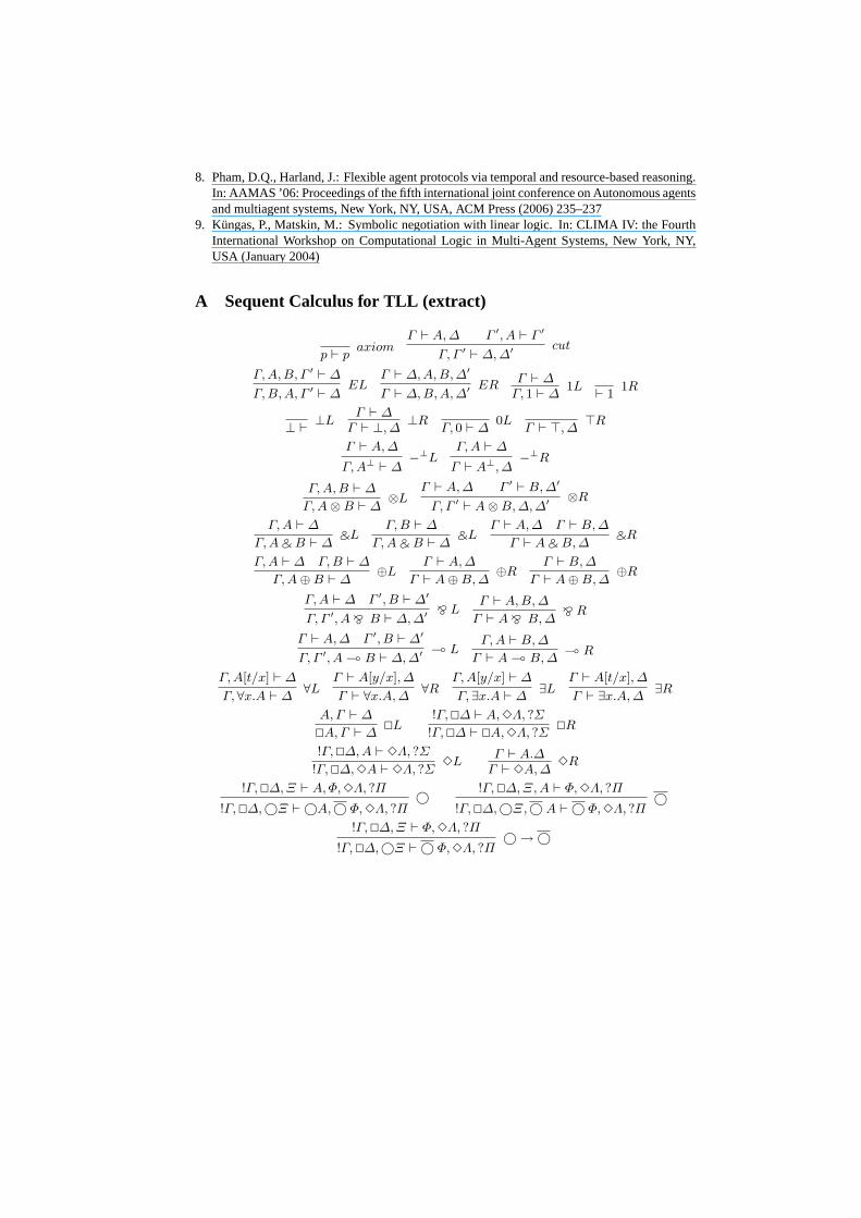
A Sequent Calculus for TLL (extract)

p ⊢ paxiom

Γ ⊢ A, ∆ Γ ′, A ⊢ Γ ′

Γ, Γ ′ ⊢ ∆, ∆′cut

Γ, A, B, Γ ′ ⊢ ∆

Γ, B, A, Γ ′ ⊢ ∆EL

Γ ⊢ ∆, A, B, ∆′

Γ ⊢ ∆, B, A, ∆′ER

Γ ⊢ ∆Γ, 1 ⊢ ∆

1L⊢ 1

1R

⊥ ⊢⊥L

Γ ⊢ ∆Γ ⊢ ⊥, ∆

⊥RΓ, 0 ⊢ ∆

0LΓ ⊢ ⊤, ∆

⊤R

Γ ⊢ A, ∆

Γ, A⊥ ⊢ ∆−⊥L

Γ, A ⊢ ∆

Γ ⊢ A⊥, ∆−⊥R

Γ, A, B ⊢ ∆

Γ, A ⊗ B ⊢ ∆⊗L

Γ ⊢ A, ∆ Γ ′ ⊢ B, ∆′

Γ, Γ ′ ⊢ A ⊗ B, ∆, ∆′⊗R

Γ, A ⊢ ∆

Γ, A N B ⊢ ∆NL

Γ, B ⊢ ∆

Γ, A N B ⊢ ∆NL

Γ ⊢ A, ∆ Γ ⊢ B, ∆

Γ ⊢ A N B, ∆NR

Γ, A ⊢ ∆ Γ, B ⊢ ∆

Γ, A ⊕ B ⊢ ∆⊕L

Γ ⊢ A, ∆

Γ ⊢ A ⊕ B, ∆⊕R

Γ ⊢ B, ∆

Γ ⊢ A ⊕ B, ∆⊕R

Γ, A ⊢ ∆ Γ ′, B ⊢ ∆′

Γ, Γ ′, A O B ⊢ ∆, ∆′O L

Γ ⊢ A, B, ∆

Γ ⊢ A O B, ∆O R

Γ ⊢ A, ∆ Γ ′, B ⊢ ∆′

Γ, Γ ′, A ⊸ B ⊢ ∆, ∆′⊸ L

Γ, A ⊢ B, ∆

Γ ⊢ A ⊸ B, ∆⊸ R

Γ, A[t/x] ⊢ ∆

Γ, ∀x.A ⊢ ∆∀L

Γ ⊢ A[y/x], ∆

Γ ⊢ ∀x.A, ∆∀R

Γ, A[y/x] ⊢ ∆

Γ, ∃x.A ⊢ ∆∃L

Γ ⊢ A[t/x], ∆

Γ ⊢ ∃x.A, ∆∃R

A, Γ ⊢ ∆

@A, Γ ⊢ ∆@L

!Γ, @∆ ⊢ A, 3Λ, ?Σ

!Γ, @∆ ⊢ @A, 3Λ, ?Σ@R

!Γ, @∆, A ⊢ 3Λ, ?Σ

!Γ, @∆, 3A ⊢ 3Λ, ?Σ3L

Γ ⊢ A.∆Γ ⊢ 3A, ∆

3R

!Γ, @∆, Ξ ⊢ A, Φ, 3Λ, ?Π

!Γ, @∆, ,Ξ ⊢ ,A, , Φ, 3Λ, ?Π,

!Γ, @∆, Ξ, A ⊢ Φ, 3Λ, ?Π

!Γ, @∆, ,Ξ, , A ⊢ , Φ, 3Λ, ?Π,

!Γ, @∆, Ξ ⊢ Φ, 3Λ, ?Π

!Γ, @∆, ,Ξ ⊢ , Φ, 3Λ, ?Π, → ,