Model-Based Experimental Design in Electrochemistry

Model-Based Experimental Designin Electrochemistry

Hoang Viet NguyenCentre of Research in Electrochemical Science and Technology

Department of Chemical Engineering and BiotechnologyUniversity of Cambridge

This dissertation is submitted for the degree ofDoctor of Philosophy

Trinity College June 2017

Declaration

I hereby declare that except where specific reference is made to the work of others,the contents of this dissertation are original and have not been submitted in wholeor in part for consideration for any other degree or qualification in this, or any otherUniversity. This dissertation is the result of my own work and includes nothing whichis the outcome of work done in collaboration, except where specifically indicated inthe text. This dissertation contains fewer than 65,000 words including appendices,bibliography, footnotes, tables and equations and has less than 150 figures.

Hoang Viet NguyenJune 2017

Acknowledgements

First and foremost I would like to express sincere gratitude to Dr Adrian Fisher. Hispatience and support, both technically and logistically, help shaping this work.

I also would like to thank our collaborators for their generous supports. Specifically,Professor Frank Marken and his group from Bath University have always welcomedand treated us with great food. Many thanks to Sunyhik and Christopher for theirexperimental data and discussions.

I am grateful for the support from Dr Erik Birgersson and his group at NUS. Heand his students taught me a great deal about the software Comsol, which is usefuland forms a big part of my work. I would like to thank Dr Karthik Somansudaramfor help setting up the simulation in Chapter 4.

I thank all my friends and colleagues at CREST, in particular Hongkai Ma for ourfruitful collaborations in Chapter 5.

And finally and above all to my parents, I am so much indebted to you guys.Thank you gazillion times for everything!

Abstract

The following thesis applies an experimental design framework to investigate propertiesof electron transfer kinetics and homogeneous catalytic reactions. The approach ismodel-based and the classical Butler-Volmer description is chosen to describe thefundamental electrochemical reaction at a conductive interface. The methodologyfocuses on two significant design variables: the applied potential at the electrode andmass transport mode induced by physical arrangement.

An important problem in electrochemistry is the recovery of model parameters fromoutput current measurements. In this work, the identifiability function is proposedas a measure of correspondence between the parameters and output variable. Underdiffusion-limit conditions, plain Monte Carlo optimization shows that the function isglobally non-identifiable, or equivalently the correspondence is generally non-unique.However by selecting linear voltammetry as the applied potential, the primary pa-rameters in the Butler-Volmer description are theoretically recovered from a single setof data. The result is accomplished via applications of Sobol ranking to reduce theparameter set and a sensitivity equation to inverse these parameters.

The use of hydrodynamic tools for investigating electron transfer reactions is nextconsidered. The work initially focuses on the rotating disk and its generalization - therocking disk mechanism. A numerical framework is developed to analyze the latter,most notably the derivation of a Levich-like expression for the limiting current. Theresults are then used to compute corresponding identifiability functions for each ofthe above configurations. Potential effectiveness of each device in recovering kineticparameters are straightforwardly evaluated by comparing the functional values. Fur-thermore, another hydrodynamic device - the rotating drum, which is highly suitablefor viscous and resistive solvents, is theoretically analyzed. Combined with previousresults, this rotating drum configuration shows promising potential as an alternativetool to traditional electrode arrangement.

The final chapter illustrates the combination of modulated input signal and appro-

priate mass transport regimes to express electro-catalytic effects. An AC voltammetrytechnique plays an important role in this approach and is discussed step-by-step fromsimple redox reaction to the complete EC ′ catalytic mechanism. A general algorithmbased on forward and inverse Fourier transform functions for extracting harmoniccurrents from the total current is presented. The catalytic effect is evaluated andcompared for three cases: macro, micro electrodes under diffusion control conditionand in micro fluidic environments. Experimental data are also included to supportthe simulated design results.

iv

Publications

Book Chapter

Section 1.5/Chapter 1 in Song, Cheng and Zhao: Micro Fluidics, Fundamental Devicesand Applications, Wiley Interscience, 2016

Journal

C. E. Hotchen, H. V. Nguyen, A. C. Fisher, F. Marken. Hydrodynamic microgapvoltammetry under couette flow conditions: Electrochemistry at a rotating drum inviscous poly-ethylene glycol (PEG). ChemPhysChem, 16, 2015S. D. Ahn, K. Somasundaram, H. V. Nguyen, E. Birgersson, J. Y. Lee, X. Gao, A.C. Fisher, P. E. Frith, F. Marken. Hydrodynamic Voltammetry at a Rocking DiscElectrode: Theory versus Experiment. Electrochimica Acta, 188, 2016Peng Song, Hongkai Ma, Luwen Meng, Yian Wang, Hoang Viet Nguyen, NathanS. Lawrence and Adrian C. Fisher. Fourier transform large amplitude alternatingcurrent voltammetry investigations of the split wave phenomenon in electrocatalyticmechanisms. PCCP, 19, 2017

In Preparation

H. K. Ma, H. V. Nguyen, A. C. Fisher. Elicitation of homogeneous self-catalytic effectsinside channel electrodes via Fourier Transform large amplitude voltammetry

v

Contents

Contents vi

List of Figures ix

List of Tables xxi

Nomenclature xxv

1 Introduction 11.1 Electrochemistry Fundamentals . . . . . . . . . . . . . . . . . . . . . . 3

1.1.1 Diffusion . . . . . . . . . . . . . . . . . . . . . . . . . . . . . . . 51.1.2 Convection . . . . . . . . . . . . . . . . . . . . . . . . . . . . . 71.1.3 Electrostatic Migration . . . . . . . . . . . . . . . . . . . . . . . 8

1.2 Kinetic Models of Electrochemical Reactions . . . . . . . . . . . . . . . 91.3 Voltammetric Techniques . . . . . . . . . . . . . . . . . . . . . . . . . 161.4 Numerical Modeling in Electrochemistry . . . . . . . . . . . . . . . . . 291.5 Identifiability in Experimental Design . . . . . . . . . . . . . . . . . . . 371.6 Parameter Estimation and Bayesian Statistics . . . . . . . . . . . . . . 411.7 Thesis Outline . . . . . . . . . . . . . . . . . . . . . . . . . . . . . . . . 46

2 Numerical Solution of Redox Processes 472.1 Diffusional Transport in One Dimension . . . . . . . . . . . . . . . . . 482.2 Spatial Meshing and Grid Structure . . . . . . . . . . . . . . . . . . . . 502.3 Temporal Discretization . . . . . . . . . . . . . . . . . . . . . . . . . . 532.4 Treatment of Boundary Conditions . . . . . . . . . . . . . . . . . . . . 562.5 Overview of Numerical Solutions . . . . . . . . . . . . . . . . . . . . . 572.6 Two Dimensional Simulation and ADI Method . . . . . . . . . . . . . . 592.7 Some Numerical Results . . . . . . . . . . . . . . . . . . . . . . . . . . 64

2.8 Chapter Conclusion . . . . . . . . . . . . . . . . . . . . . . . . . . . . . 78

3 Parameter Identifiability and Estimation of Redox processes underDiffusion Control 793.1 The extended Butler-Volmer Model . . . . . . . . . . . . . . . . . . . . 813.2 Identifiability Measure for Model Parameters . . . . . . . . . . . . . . . 873.3 Sobol Global Sensitivity Analysis . . . . . . . . . . . . . . . . . . . . . 923.4 Sensitivity Equation Approach for Parameter Inversion . . . . . . . . . 1003.5 MCMC Simulations . . . . . . . . . . . . . . . . . . . . . . . . . . . . 1083.6 Chapter Conclusion . . . . . . . . . . . . . . . . . . . . . . . . . . . . . 116

4 Hydrodynamic Tools for Model Identifiability and Kinetics Analysis1184.1 The Rocking Electrode - An Investigation . . . . . . . . . . . . . . . . 120

4.1.1 Verification of Levich expression for RDE . . . . . . . . . . . . . 1204.1.2 Derivation of Levich expression for the RoDE . . . . . . . . . . 1234.1.3 Comparison of Parameter Identifiability under RDE and RoDE

Configurations . . . . . . . . . . . . . . . . . . . . . . . . . . . 1314.2 Voltammetric Analysis with Couette flow . . . . . . . . . . . . . . . . . 136

4.2.1 Theoretical Analysis . . . . . . . . . . . . . . . . . . . . . . . . 1374.2.2 Comparison to Experimental Data . . . . . . . . . . . . . . . . 141


5 Elicitation of Electrocatalysis Mechanism via Large amplitude Sinu-soidal signals 1465.1 Signal Processing Concept of AC Voltammetry . . . . . . . . . . . . . 1495.2 Single Electron Transfer under Fast Fourier Transform voltammetry . . 1525.3 Effect of Large Amplitude on Harmonics . . . . . . . . . . . . . . . . . 1625.4 EC’ Mechanism under Fourier Transform AC voltammetry . . . . . . . 167

5.4.1 Macro Planar Electrode . . . . . . . . . . . . . . . . . . . . . . 1695.4.2 Micro Disk Electrode . . . . . . . . . . . . . . . . . . . . . . . . 186

5.5 Self-Catalytic Reaction with Micro Fluidic Flow . . . . . . . . . . . . . 1995.5.1 Levich equation for embedded channel electrode . . . . . . . . . 1995.5.2 Effects of large AC amplitude and catalysis . . . . . . . . . . . 203


6 Conclusions 220

vii

References 223

viii

List of Figures

1 A schematic diagram of model based experimental design (MBED)framework . . . . . . . . . . . . . . . . . . . . . . . . . . . . . . . . . 2

2 A schematic diagram for the three electrode system used to conductelectrochemical measurements . . . . . . . . . . . . . . . . . . . . . . . 3

3 Electron transfer mechanism between a metal surface and electroactivespecies. In this diagram, the analyte receives electrons from metal andis reduced . . . . . . . . . . . . . . . . . . . . . . . . . . . . . . . . . . 5

4 Basic steps in an electrochemical reaction. Species are transported tothe electrode, followed by electron tunnelling under a favourable ther-modynamic potential and the product is then transported away . . . . 6

5 Mass balance under pure diffusion conditions with the denoted controlvolume, leading to the diffusion equation . . . . . . . . . . . . . . . . . 7

6 The Transition State theory applied to the simple electron transfer re-action. The Gibbs free energies vary with the potential (top) and thecorresponding transition state (inside the rectangle) shifts closer to theproduct side if a favourable potential is applied (bottom) . . . . . . . 10

7 A molecular picture of the outer and inner sphere electron transferreactions . . . . . . . . . . . . . . . . . . . . . . . . . . . . . . . . . . 13

8 Parabolic potential energies of reactant (left) and product (right) inMarcus model. Activation energies are now functions of the total reor-ganization energy λ . . . . . . . . . . . . . . . . . . . . . . . . . . . . 14

9 Common voltammetric signals (left to right, top to bottom): PotentialStep, Linear Sweep, Cyclic (composing of forward and backward linearsweeps) and Square Wave (reverse pulses) . . . . . . . . . . . . . . . . 16

ix

10 Typical voltammograms for cyclic voltammetry experiments at increas-ing scan voltage rates for reversible electron transfer reactions. Higherscan rate progressively causes larger peak current . . . . . . . . . . . . 17

11 Differences between macro (top) and micro (bottom) electrodes. Forinert and non-porous substrates (e.g. glass, polymer), there is no chem-ical fluxes (red arrows). For micro electrodes, the fluxes are largest atthe edges and become smaller towards the centre . . . . . . . . . . . . 18

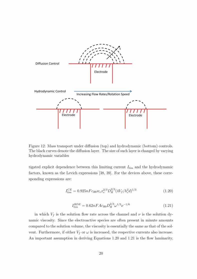
12 Mass transport under diffusion (top) and hydrodynamic (bottom) con-trols. The black curves denote the diffusion layer. The size of such layeris changed by varying hydrodynamic variables . . . . . . . . . . . . . . 20

13 Channel Electrode (top) and Rotating Disk electrode (RDE) (bottom)with the corresponding dimensions. Electroactive areas are coloredblack. Typical steady flow profile for each device is indicated. Parabolicprofile is often observed for channel electrode while swirling flow (topdown view) applies to RDE. In both cases, the Reynold number is suf-ficiently small so that distinct, laminar fluid structures are ensured . . 21

14 In AC voltammetry, the potential is formed by addition of a sin-wavefunction on a linear sweep . . . . . . . . . . . . . . . . . . . . . . . . . 23

15 A typical AC voltammogram (top) and the extracted aperiodic (dc)/harmoniccurrent (bottom). A Fourier transform is applied to the AC current toreveal the frequency spectrum . . . . . . . . . . . . . . . . . . . . . . . 24

16 Cyclic voltammograms for EC mechanism under different reaction con-stants kEC (largest value: purple and smallest value: black). As thereaction constant kEC increases, the backward peak becomes smallerbecause the oxidative species is consumed more quickly by the homoge-nous reaction . . . . . . . . . . . . . . . . . . . . . . . . . . . . . . . . 26

17 Total current (center) and extracted 1st to 8th harmonics in large am-plitude AC voltammetry experiment using Au/Pt channel electrodes . 27

18 In FD, solution process proceeds by breaking down the modeling do-main into discrete points. Boundary nodes are colored black and interiorones are red . . . . . . . . . . . . . . . . . . . . . . . . . . . . . . . . . 30

19 HOPG structures with electrochemically slow (basal) and highly active(edge) planes (top). The structure is modelled by a series of flat bandelectrodes and computational domain is also indicated (bottom) . . . . 31

x

20 In FE, the solution region is meshed into smaller elements (left). Theexample shows an unstructured triangular mesh for 2D problems andthe computed steady-state velocity profiles around a cylinder (right).The main flow is from left to right of page . . . . . . . . . . . . . . . . 33

21 Due to the fabrication process, the final electrode can take many con-figuaration including inlaid, protrude or recess . . . . . . . . . . . . . . 34

22 An example of adaptive mesh refinement for an inlaid disk. The startingmesh (top) is locally refined around the singular point 1 until convergenttolerance is achieved (bottom) . . . . . . . . . . . . . . . . . . . . . . 35

23 Principle of gradient search: the direction is in the steepest direction,i.e. orthogonal to the contour map . . . . . . . . . . . . . . . . . . . . 42

24 The objective is optimized as the temperature cools using simulatedannealing algorithm. In this example, global minimum (i.e. the lowestvalley ) is slowly approached by two artificial neural networks . . . . . 43

25 Modeling region for 1D diffusion. The region is broken down into dis-crete nodes . . . . . . . . . . . . . . . . . . . . . . . . . . . . . . . . . 50

26 Comparisons between Explicit and Implicit formulations. Implicit methodgenerally has more unknowns than explicit one, thus usually requiringmore solution effort . . . . . . . . . . . . . . . . . . . . . . . . . . . . 54

27 Geometrical representation of micro disc (top left) and the reducedrectilinear simulation domain with the boundaries (hatched) . . . . . . 59

28 A typical 2D polar-coordinate grid for FD simulations of micro diskelectrode. The grid is concentrated around the electrode edge (r =1) and becomes sparser towards the bulk. The axis scales are non-dimensional for demonstration purposes . . . . . . . . . . . . . . . . . 60

29 The Alternating Direction Implicit (ADI) in 2D. Nodes in thin-linedrectangles were already solved and those in thick-lined rectangles arecurrently being solved. Grey nodes are unsolved variables. For eachtime iteration, all the nodes in Z direction are first solved, the resultsare then used to solve for nodes in R direction . . . . . . . . . . . . . 62

xi

30 Dimensionless current versus dimensionless potential for a macro elec-trode under fast reversible kinetics. The corresponding dimensionlessexpressions are given by Equations 2.45 and 2.46 respectively. At θ = 0,the dimensional potential E = E0. The analytical values are extractedfrom tables in Reference [1] . . . . . . . . . . . . . . . . . . . . . . . . 66

31 Cyclic voltammograms at different electrochemical reaction rates. Fork0 = 1 cm/s, the potential gap is constant and independent of the scanrate . At much slower kinetics, the gap becomes larger and potentialdependent [2] (All the dimensionless expressions are the same as before) 68

32 Amperometric response at a micro disk. Comparison between the sim-ulation data (continuous line) and theoretical points (red dots) (Ref-erence [3]) shows good agreement. Current and time are normalizedrespectively by Equations 2.51 and 2.52 . . . . . . . . . . . . . . . . . 69

33 Dimensionless current versus dimensionless potential at two differentscan rates (100 and 5 mV/s). A flatter and more steady state responseis obtained at the slower scan rate. Dimensionless current and potentialare given by expressions 2.51 and 2.46 . . . . . . . . . . . . . . . . . . 70

34 Meshing for spherical electrode. The boundary is coloured in red andonly points on and outside the surface of the sphere are considered inthe calculations . . . . . . . . . . . . . . . . . . . . . . . . . . . . . . . 72

35 Limiting current at a sub micron or nano spherical electrode. Theasymtope (at approximately π/2 ≃ 1.57) is colored in red . . . . . . . 73

36 A schematic reaction pathway for an EC’ mechanism (top) and the ori-gin of pre-wave phenomenon in the forward sweep of cyclic voltammetryas a result of shifting of the reaction layer (bottom) . . . . . . . . . . . 74

37 Increasing scan rates lead to an increase in measured currents. No-tice that there are two peaks in the voltammograms. The first peakcorresponds to pre-wave effect and the second is the usual redox reaction 75

38 Effects of changing concentration ratios between substrate and elec-trolytes. The more S is present, the higher the pre-wave peak . . . . . 75

39 Pre-wave peak currents versus the concentration ratios cS0/cR0 showsa linear relationship in Figure 38. Below ratio of 0.2, it is difficult todistinguish the pre-wave in the voltammogram . . . . . . . . . . . . . 76

xii

40 Explicit calculations at two different grid sizes (coarse (black) vs fine(red)). The more accurate result (red) requires more number of timesteps (220 in comparison to 216 of the black curve). The red and blackcurves agree to within 0.67% and 1% of the implicit calculations inChapter 2 respectively. The current and potential are normalized ac-cording to Equations 2.45 and 2.46 . . . . . . . . . . . . . . . . . . . . 84

41 Effect of uncompensated resistance on linear sweep voltammetries. Forsmall resistances (50−500 Ohm), the current response does not changesignificantly. For larger resistances (e.g. 5000 Ohm), the peak currentstarts to decrease and shifts right to compensate for a decrease in reac-tion kinetics. Data are presented in dimensionless (top) and dimensionalformat (bottom) . . . . . . . . . . . . . . . . . . . . . . . . . . . . . . 85

42 Quasi Monte Carlo (left) versus uniform brute force sampling (right).Brute force methods often lead to clumping, large clusters of points,and sparse regions; while quasi-Monte Carlo methods tends to spreadpoints more uniformly across space. . . . . . . . . . . . . . . . . . . . . 96

43 The ratio of SIF irst Order/SIT otal as another useful index to decide andrank the parameters in a given model. For Butler-Volmer, the ordersare [E0, k0, Cdl, α, Ru], the same as concluded from Table. The ratiofor the uncompensated resistance is virtually zero, thus indicating thisparameter’s insignificance in the model (Table 9) . . . . . . . . . . . . 98

44 Summary of steps for model-based parameter estimation and MCMCstatistics calculation. The first 4 steps are carried out in this sectionand the last 2 is completed in the next section . . . . . . . . . . . . . 100

45 Synthetic cyclic voltammogram used in an estimation process. Gaussiannoise is added to the clean data as described in Equation 3.26. Thecurrent is normalized by using the expression 2.45 but the voltage isleft dimensional (V ) to facilitate later discussion . . . . . . . . . . . . . 102

46 Estimation algorithm using the sensitivity approach as described inEquations 3.31-3.38 . . . . . . . . . . . . . . . . . . . . . . . . . . . . 105

47 SSE is progressively minimized as the number of iterations increase.Atthe final iteration, the best two initial sets yield SSE values significantlysmaller in comparison to the rest . . . . . . . . . . . . . . . . . . . . . 106

xiii

48 Histogram for k0. Note that only data from chain no. 5000 − 50000 areused here. The rest are discarded during burn-in process as describedin the text . . . . . . . . . . . . . . . . . . . . . . . . . . . . . . . . . 111

49 Histogram for α. Data from chain no. 5000 − 50000 are used . . . . . . 11250 Histogram for E0. Data from chain no. 5000 − 50000 are used. The

majority of values distribute around 0.25, which is the assumed truevalue for E0 . . . . . . . . . . . . . . . . . . . . . . . . . . . . . . . . . 112

51 A scattering plot for (k0, α) shows a weak statistical correlation betweenthe two parameters . . . . . . . . . . . . . . . . . . . . . . . . . . . . . 113

52 A scattering plot for (k0, E0) also indicates a very weak correlation.For non-identifiable situations, higher k0 should correlate with higherE0 (i.e. a positive correlation) . . . . . . . . . . . . . . . . . . . . . . . 113

53 Scatter plot for (α, E0) indicates a negative correlation . . . . . . . . . 114

54 Computational domain for the rotating electrode. The problem is es-sentially two dimensional due to rotational symmetry around r = 0axis . . . . . . . . . . . . . . . . . . . . . . . . . . . . . . . . . . . . . 121

55 Linear sweep voltammograms for rotating disk electrode at 50 (black),100 (red) and 500 (blue) rpms under scan rate of 10 mV/s (top) andthe steady state currents are proportional to f 0.5

RDE for rpm in range50 − 500 as confirmed in the Levich relation 4.1 . . . . . . . . . . . . . 122

56 A sketch of the equipment and its rocking mechanism (top right) andthe simplified four-bar mechanism used to approximate movements ofthe cranks (bottom) . . . . . . . . . . . . . . . . . . . . . . . . . . . . 124

57 Rocking angle θ4 as a function of time for L2 = 7 (mm),L4 = 10 (mm)and ω2 = 50 rpm. The initial angle is π/2 (dotted line). The variation islike a harmonic function. Consequently, the resulting flow field followsin the same manner . . . . . . . . . . . . . . . . . . . . . . . . . . . . 126

xiv

58 (Top) Numerical (continuous) versus experimental (dashed) linear sweepvoltammetries for different regular rotating rates ω2 (rpm): 50 (black),100 (red) and 500 (blue) at scan rate of 10 mV/s. The numerical dataare obtained by solving the convective-diffusion equation 1.4 coupledwith simple electron transfer reaction. The computational approach isthe same as in the case of RDE. (Bottom) Plot of Ilim,RoDE againstrotating frequencies f 1/2 showing a linear correlation similar to that ofrotating disk (line of best fit (dashed red) has R2 = 0.9998 and slope of1.451 ∗ 10−6) . . . . . . . . . . . . . . . . . . . . . . . . . . . . . . . . 128

59 The numerical ratio between rocking and rotating speeds ω4/ω2 at 50(top) and 500 rpm (bottom). Notice that even though the frequencyis increased, the ratio scale remains the same. In both cases, they areapproximated by L2/L4 . . . . . . . . . . . . . . . . . . . . . . . . . . 129

60 The flow chart for identifiability computation under hydrodynamic con-ditions. Because fluid dynamics and mass transport steps are indepen-dent, the former is carried out outside the iteration loop. The commonparameters for both configurations are listed in Table 15. The calcula-tion is implemented in Comsol Multiphysicsr and Matlabr interfaceenvironment . . . . . . . . . . . . . . . . . . . . . . . . . . . . . . . . 132

61 Calculations of ηtransient for RDE (top-half) and RoDE (bottom-half).Parameter values are listed in following columns in the order [k0, α, E0].Top 7 values are included . . . . . . . . . . . . . . . . . . . . . . . . . 133

62 Calculations of ηsteady for RDE (top-half) and RoDE (bottom-half).Parameter values are listed in following columns in the order [k0, α, E0].Top 7 values are included . . . . . . . . . . . . . . . . . . . . . . . . . . 134

63 The rotating drum equipment. Schematic end-view (right) and enlarge-ment of the central section with associated linear velocity profile (left).The solution is dragged into the gap via the rotating cylinder . . . . . 137

64 Division of circular disk into many thin rectangles and the relation 4.17is applied to each element. The approach is generalized to any closedgeometrical shape . . . . . . . . . . . . . . . . . . . . . . . . . . . . . 142

65 Proposed chemical changes on Pt surface at potetential below 0.45 (V )(left) and above 0.45 (V ) (right). At low potential, there is a weak at-traction between the surface and PEG molecules. At higher potentials,stronger bonds are formed and result in a more regular structure . . . . 143

xv

66 Limiting current versus cube root of frequency at fixed hc = 500 (µm)(top) and inverse cube root of micro gap at fixed ω = 50 (rpm). Blackpoints are calculated using the expression 4.18 and red points are ex-perimental values. Dashed line is the fitted Levich expression . . . . . 144

67 Linear sweep voltammetry at a flow channel for increasing catalyticreaction rates K and a slow scan rate . . . . . . . . . . . . . . . . . . 148

68 SISO “Black Box”’ representation used to demonstrate the general con-cept of AC voltammetry. When a DC signal is applied, the usual cyclicvoltammetry (CV) current is obtained (top). However, the superposi-tion of perturbed AC signals combined with the DC part causes theoutput to contain and extra sinusoidal varying current, thus the ACcurrent output (bottom) . . . . . . . . . . . . . . . . . . . . . . . . . . 150

69 A typical one dimensional finite element meshing for macro electrodecalculations . . . . . . . . . . . . . . . . . . . . . . . . . . . . . . . . . 153

70 Applied AC Potential under amplitude E = 10 mV and f = 3 Hz.The base-line (CV) potential is plotted as the dark dash line. Theequilibrium potential E0 is also included. Whilst the CV potential fun-damentally drives the reaction, AC signal perturbs the process arounda given potential and enhances the harmonics . . . . . . . . . . . . . . 154

71 Simulated total current in time domain using the settings from Table 19 15672 Single Sided Power spectrum of the simulated current above. This one-

sided spectrum is derived directly from the two-sided counter-part byscaling with respect to the frequency . . . . . . . . . . . . . . . . . . . 157

73 Recovered DC signal from the AC current in Figure 71 . . . . . . . . . 15874 Recovered 1st harmonic signal from the AC current . . . . . . . . . . . 15975 Recovered 2nd harmonic signal from the AC current . . . . . . . . . . 15976 1st harmonic in Figure 74 plotted in the envelope format . . . . . . . . 16077 2nd harmonic in Figure 75 plotted in the envelope format. Notice large

fringes at the beginning and end of the voltammogram . . . . . . . . . 16078 Comparison of 1st harmonic current under 10 mV (black line) and 40 mV

(red line). Notice that the base line shift upwards as the amplitude isincreased . . . . . . . . . . . . . . . . . . . . . . . . . . . . . . . . . . . 163

79 Comparison of 2nd harmonic current under 10 mV (black) and 40 mV

(red) . . . . . . . . . . . . . . . . . . . . . . . . . . . . . . . . . . . . . 163

xvi

80 Power spectrum for harmonic signal at E = 40 mV . Note that underlarger sinusoidal amplitude, higher frequencies start to appear. In thiscase, even the 4th harmonic (i.e. f4 = 12 Hz) is weakly visible on thespectrum . . . . . . . . . . . . . . . . . . . . . . . . . . . . . . . . . . 164

81 3rd harmonic current (full form) under E = 40 mV . There are 3 peaksin both forward and backward scans . . . . . . . . . . . . . . . . . . . 165

82 4thharmonic current (full form) with 4 peaks in each direction of scan . 16583 3rd harmonic in envelope format . . . . . . . . . . . . . . . . . . . . . 16684 4th harmonic in envelope format . . . . . . . . . . . . . . . . . . . . . . 16685 The pre-wave phenomenon under DC signal (black) for a macro elec-

trode. The first peak is due to the substrate diffusion limitation and thesecond peak corresponds to the usual E reaction. The overall current in-creases substantially in comparison to the lower kinetic case (red). Thescan rate is 10 mV/s and the substrate concentration is cS0 = 1.0 mM

(or substrate concentration ratio cS0/cR0 = 1.0) . . . . . . . . . . . . . 16986 The CV diagrams for EC ′ mechanism under various combinations of

reaction kinetic (vertical axis) and concentration ratio (horizontal axis)factors . . . . . . . . . . . . . . . . . . . . . . . . . . . . . . . . . . . . 170

87 1st (top) and 2nd (bottom) harmonics at at cS0 = 0.5 mM or substrateratio cS0/cR0 = 0.5 at various frequencies between f = 1 and 6 Hz . . . 172

88 3rd (top) and 4th (bottom) harmonics at at cS0 = 0.5 mM or substrateratio cS0/cR0 = 0.5 at various frequencies between f = 1 and 6 Hz . . . 173

89 1st (top) and 2nd (bottom) harmonics at at cS0 = 4 mM or substrateratio cS0/cR0 = 4 at various frequencies between f = 1 and 6 Hz . . . . 174

90 3rd (top) and 4th (bottom) harmonics at at cS0 = 4 mM or substrateratio cS0/cR0 = 4 at various frequencies between f = 1 and 6 Hz . . . . 175

91 1st (right) and 2nd (left) harmonics at different substrate ratios 0.5, 1.0,2.0 and 4.0 (the frequency is fixed at 1 Hz) . . . . . . . . . . . . . . . 176

92 1st (right) and 2nd (left) harmonics at different substrate ratios 0.5, 1.0,2.0 and 4.0 (the frequency is fixed at 2 Hz) . . . . . . . . . . . . . . . 177

93 Plots of the pre-wave peak currents in the 1st (right) and 2nd (left) har-monics versus the substrate concentrations for f = 1 Hz. The Pearson(unadjusted) R2 coefficients are 0.9999 and 0.9997 respectively. Thecalculations are done with Origin Labr (version 9.1) . . . . . . . . . . 178

xvii

94 Plots of the pre-wave peak currents in the 1st (right) and 2nd (left) har-monics versus the substrate concentrations for f = 2 Hz. The Pearson(unadjusted) R2 coefficients are 0.9999 and 0.9991 respectively. Thecalculations are done with Origin Labr (version 9.1) . . . . . . . . . . 179

95 2nd harmonic current under different sinusoidal amplitudes (top) andplot of pre-wave peak currents versus the sinusoidal amplitude (bot-tom). At higher amplitudes, the pre-waves becomes less distinct anddifficult to find within the current. Consequently, the linear fit (redline) is not very good . . . . . . . . . . . . . . . . . . . . . . . . . . . 180

96 Extract of pre-wave currents in the harmonics from Figure 99 (dots)and relatively good linear fits (dash lines) are confirmed . . . . . . . . 181

97 Experimental data for first and second harmonics using FCA (cR0 =2 mM) and L-cysteine (cS0 = 0.5 mM) (excess factor is 0.5/2 = 0.25).Scan rate: 11.8 mV/s, E = 50 mV and glassy carbon (GC) electrodeof diameter 3 mm . . . . . . . . . . . . . . . . . . . . . . . . . . . . . 183

98 Experimental data for 1st and 2nd harmonics with FCA (cR0 = 2 mM)and L-cysteine (cS0 = 4 mM) (excess factor is now 4/2 = 2). Scan rate11.8 mV/s, amplitude 50 mV and 3 mm GC electrode . . . . . . . . . . 184

99 Experiment results for 1st and 2nd harmonics with different L-cysteinelevels 1 − 4 mM . The pre-wave current increases along with the sub-strate concentration (scan rate 11.8 mV/s, sinusoidal amplitude 50 mV ,frequency 1 Hz and FCA concentration cR0 = 2 mM , GC electrode3 mm diameter) . . . . . . . . . . . . . . . . . . . . . . . . . . . . . . . 185

100 1st and 2nd harmonics for a micro disk under simple E reaction . . . . 187101 3rd and 4th harmonics for a micro disk under simple E reaction . . . . 188102 Finite element mesh used for the calculations. Tetrahedral shape is

applied instead of triangular ones in order to save some degree of free-doms. Respective boundary conditions are also included. Towards thebulk, a more regular mesh is used . . . . . . . . . . . . . . . . . . . . . 189

103 1st and 2nd harmonics under EC ′ reaction and substrate ratio of 0.5 fora micro electrode . . . . . . . . . . . . . . . . . . . . . . . . . . . . . . 191

104 3rd and 4th harmonics under EC ′ reaction and substrate ratio of 0.5 fora micro electrode . . . . . . . . . . . . . . . . . . . . . . . . . . . . . . 192


xviii






111 Structured rectangular mesh used for channel electrode calculations.Edge, distribution and mapping operations in Comsol Multiphysicsr

are combined to produce this mesh . . . . . . . . . . . . . . . . . . . . 201112 Comparison between numerical values and the Levich prediction ICE

lim =0.925nFcR0wex

2/3e D

2/3R (4Vf/h2

cd)1/3 for the channel electrode at vari-ous flow rates Vf . There is a good convergence between simulationand theory. Numerical differences are largest at small flow rates (e.g.0.001 cm3/s) and decrease as Vf is increased . . . . . . . . . . . . . . . 203

113 Cross sectional concentration profile at large over potential and variousflow rates Vf = 10−6, 10−5, 10−4 and 10−3 cm3/s (direction: left toright, top to bottom). Red colour indicates high concentrations whilstblue colour is 0 (mM). The contour is sharp near the leading edge ofthe electrode and becomes flatter down-stream. As a consequence, thecurrent flux peaks at the front and then tends to a lower constant value 204

114 Extracted DC current in time domain at various flow rates between 0.1and 0.6 mL/min (top). The Levich relation is confirmed in the bottomfigure . . . . . . . . . . . . . . . . . . . . . . . . . . . . . . . . . . . . . 207

115 Extracted 1st (top) and 2nd (bottom) harmonics for the same range offlow rates as in Figure114 . . . . . . . . . . . . . . . . . . . . . . . . . 208

116 Extracted 3rd (top) and 4th (bottom) harmonics for the same range offlow rates as in Figure 114 . . . . . . . . . . . . . . . . . . . . . . . . . 209

117 Empirical correlation between 1st harmonic peaks and V 0.286f . The ex-

ponent 0.286 is less than that of Levich expression (0.333), implyingthat the harmonic currents are less flow-rate dependent than the DCcomponent . . . . . . . . . . . . . . . . . . . . . . . . . . . . . . . . . . 210

xix

118 The DC Current for a EC ′ reaction with cR0 = 2 mM and cS0 = 0.3 mM

between flow rate 0.1 and 0.6 mL/min (top). Comparison of steadycurrents using the Equation 5.21 and direct data from Figure 118. FromEquation 5.21, the efficiency factor is fixed and the steady currentstherefore follow the Levich relation 112 . . . . . . . . . . . . . . . . . . 211

119 1st(top) and 2nd (bottom) harmonics for EC ′ reaction with cR0 = 2 mM

and cS0 = 0.3 mM . Notice the relatively weak shoulder in 2nd harmonicsunder the smallest flow rate Vf = 0.1 mL/min . . . . . . . . . . . . . . 212

120 (Top) DC current for various substrate concentrations cS0 = 0.1 −0.6 mM (corresponding to rS between 5% and 30%). The flow rateis fixed at Vf = 0.1 mL/min and inlet electroactive concentration iscR0 = 2 mM . (Bottom) Counting the charge for the 2nd harmonic ateach substrate concentration in Figure 121. The unit of charge is µC.Numerical values are included up to 3 decimal places. It is clear thatthe same amount of charge is transferred during both time periods . . 213

121 2nd(top) and 1st (bottom) harmonics for different substrate concentra-tions (0.1 − 0.6 mM) and cR0 = 2 mM, Vf = 0.1 mL/min and νscan =10 mV/s. There is an evolution of split-wave in second harmonic butthis is not observed in the first . . . . . . . . . . . . . . . . . . . . . . . 215

122 Comparison of 2nd harmonics (top) and plot of the pre-wave peak versusthe substrate concentrations (bottom). Linear correlation (black dash)is fitted with Pearson coefficient of 0.9999 . . . . . . . . . . . . . . . . 216

123 Experimental data for 1st (top) and 2nd (bottom) harmonic under L-cysteine concentrations of 0.1 (black) and 0.3 mM (red) respectively(scan rate: 14.9 mV/s, amplitude 50 mV , volumetric flow rate 0.1 mL/min,gold electrode of length 100 µm). Note that only half of the voltammo-grams is shown in each figure . . . . . . . . . . . . . . . . . . . . . . . 218

xx

List of Tables

1 The Ritchmyer Coeffcients for discretization of time derivative (Equa-tion 2.22) . . . . . . . . . . . . . . . . . . . . . . . . . . . . . . . . . . 55

2 Boundary conditions associated with micro disk problem. The bound-aries are shown in Figure 27 . . . . . . . . . . . . . . . . . . . . . . . . 60

3 Parameters for simulations of macro disk (Figures 30 and 31) . . . . . 654 Parameter settings for micro disk simulation. The disk radius is 10 µm.

The dimensionless potential starts and ends at −20 and 20 respectively.The bulk concentrations for reduced and oxidized species are the sameas in Table 3 . . . . . . . . . . . . . . . . . . . . . . . . . . . . . . . . 69

5 Parameters settings for EC’ calculations in Figures 30 and 38 . . . . . 73

6 Summary of parameter values for simulations with uncompensated re-sistance. The controlled parameters are kept the same throughout thischapter . . . . . . . . . . . . . . . . . . . . . . . . . . . . . . . . . . . 83

7 Upper and lower bounds for each model parameter. These are typicalvalues for experiments conducted in aqueous solution. Electrode areais fixed at 0.01 cm2 . . . . . . . . . . . . . . . . . . . . . . . . . . . . . 89

8 Maximum value of identifiability function H, the corresponding num-ber η∗ and respective dimensional parameter sets using a scan rate of100 mV/s. The orders in each set are [DO, DR, k0, α, E0, Ru, Cdl] . . . . 90

9 Sobol Sentivity Indicies: First Order (top table) and Total (bottomtable). Since the current dynamically changes with time, computationsare carried out at 4 different time points t = 1/4∗ tmax, 1/2∗ tmax, 3/4∗tmax and tmax. These values are then averaged out and shown in thecorresponding columns. . . . . . . . . . . . . . . . . . . . . . . . . . . 95

xxi

10 Parameter values used to generate the synthetic data. Uncompensatedresistance is neglected from the model as concluded in Section 3.3. Tokeep the generality, diffusivities of species R and O are assumed to bedifferent . . . . . . . . . . . . . . . . . . . . . . . . . . . . . . . . . . . 101

11 Initial guesses and final optimal sets. In Levenberg-Marquardt, κ =0.01, maximum iteration is set to 200 and λ is decreased by 1.5 every-time SSE is reduced to maintain stability of the updating step 3.37.The orders in each set are [k0, α, E0]. Since Eguess

0 is estimated to beabout 0.28 from Figure 45 so initial guesses are taken to be smaller thanthat value. Note that the true values are [0.001, 0.65, 0.25] . . . . . . 106

12 95% Credible Intervals for the Butler-Volmer model. Mean values arecomputed from the burn-in chain. Note that the mean value of eachparameter is considerably closer to the true value [0.001, 0.650, 0.25] aslisted in Table 10 . . . . . . . . . . . . . . . . . . . . . . . . . . . . . . 111

13 (Top) Parameter settings in rotating disk simulation. Electrochemicalvalues are for the electron transfer reaction Fe(CN)4−

6 ↔ Fe(CN)3−6 +

e−. The capacitive effect is ignored. Diffusion coefficients are assumedto be equal at 0.65∗10−9 m2/s in aqueous medium. (Bottom) Respectiveboundary conditions for fluid and mass transport calculations . . . . . 121

14 Geometric lengths used for simulations of rocking mechanism in Figure56 . . . . . . . . . . . . . . . . . . . . . . . . . . . . . . . . . . . . . . 123

15 Bounds and simulation settings for Monte Carlo estimation of identi-fiability numbers ηtransient and ηsteady. Nsample = 200 is used in theAlgorithm 3.11, which is the same for both RDE and RoDE calculations 131

16 List of experimental variables in the rotating drum experiment. Theelectrode material is Platinum (Pt) . . . . . . . . . . . . . . . . . . . . 136

17 Comparisons of numerical and analytical values for ICouettelim . Numbers

in the 3rd column are results from Comsol Multiphysicsr and values inthe 4th column are calculated using the expression 4.17. Units of bothcurrents are A/m . . . . . . . . . . . . . . . . . . . . . . . . . . . . . . 141

18 Calculating the numerical sums of the form W X2/3e for an unit circle.

As expected, the sum quickly converges as the number of divisions areincreased . . . . . . . . . . . . . . . . . . . . . . . . . . . . . . . . . . 141

xxii

19 Parameters for numerical calculations of the E reaction. The simula-tion is carried out in Comsol Multiphysicsr using the dedicated Elec-trochemistry module . . . . . . . . . . . . . . . . . . . . . . . . . . . . 153

20 Additional parameters for the EC ′ mechanism. The rest of parame-ters are the same as in the Table 19. Reaction constant kEC′ of thehomogenous reaction 5.9 is assumed to be sufficiently large . . . . . . 167

21 Parameters used in verification of Levich expression for channel elec-trode . . . . . . . . . . . . . . . . . . . . . . . . . . . . . . . . . . . . 202

22 Simulation parameters for micro fluidic channel. A small scan rateand sinusoidal frequency are employed to manifest the split-wave effect.Electrode size is length de and width we with a channel height hc andwidth dc) . . . . . . . . . . . . . . . . . . . . . . . . . . . . . . . . . . 205

xxiii

Nomenclature

Physical Symbols

F Faraday Constant

R Boltzmann Constant

T0 Room Temperature

Greek Symbols

α Butler-Volmer Charge Transfer Coefficient

ν Solution Dynamic Viscosity

ω Number of revolution per second or minute

ρ Solution Density

Mathematical Symbols

φ/E Electrical Potential

E Sinusoidal Signal Amplitude

v Velocity Vector Field

A Electrode Geometric Area

c Species Solution Concentration

Cdl Butler-Volmer Double Layer Specific Capacitance

D Generic Diffusion Coefficient

DR/DO Diffusivity of Reduced/Oxidized Species

xxiv

E Applied Potential

E0 Butler-Volmer Equilibrium Potential/Formal Potential

f Rotation Frequency

FD/FE Finite Difference/Finite Element

G Gibbs Free Energy

hc/dc or d Channel Height/Width

Ic Capacitive Current

If Faradaic Current

Ilim Levich Limiting Current

J Species Flux

k0 Butler-Volmer Kinetic Constant

kEC/kEC′ Homogeneous Kinetic Constant in EC/EC’ mechanism

kf/kb Butler-Volmer Forward/Backward Kinetic

n Number of Electrons transferred in a Redox reaction

ODE/PDE Ordinary/Partial Differential Equation

Ru Butler-Volmer Uncompensated Resistance

t Time

Vf Volumetric Flow Rate

vscan Voltage Scan Rate

xe/we Electrode Length/Width

xxv

Chapter 1

Introduction

Thanks to the recent advances in computational power, the use of model based ex-perimental design (MBED) has become ubiquitous in almost every field of scienceand engineering. Primary advantages of using this approach include an improvedunderstanding of experimental measurements (e.g. qualitative and/or quantitative in-sights into underpinning physical mechanism in place) and supporting the design ofadditional experiments.

The general practice of MBED is briefly summarized in Figure 1 [4]. The method-ology can be divided into two main stages. The first stage is concerned with theselection of models to describe the physical process. Model discrimination is a criticalstep in this stage. After a realistic mathematical model is selected, it is subjectedto several experimental designs in the subsequent stage. Often a major aim of suchexperiments is to extract the accurate parameters of a proposed model. This pro-cess usually involves regression of parameters and computations of relevant statisticalmetrics from existing data. Finally, the final model will be validated against newlyacquired information before being implemented in further applications.

In the second stage of the experimental design procedure, the issue of identifiabilitybecomes significant. This concept essentially expresses the direct correspondence be-tween model’s measurable outputs and its parameter inputs. A model structure, withhigh identifiability characteristics, implies that parameters are theoretically estimablewith higher precision. In addition, the choice of model inputs or controlled variablessignificantly influences the identifiability outcome. In complex and non-linear modelshowever, the interaction among parameters may lead to non-identifiability, no matterhow well-designed the controlled variables are. Therefore, smaller group(s) of param-eters should be carefully selected to improve the regression procedure and statistical

1

test.

Figure 1: A schematic diagram of model based experimental design (MBED) frame-work

In an electrochemical context, experimental design involve two primary factors:i) the applied voltage at electrical interface and ii) the physical cell arrangement toconduct measurements. The overall aim of this thesis is to investigate the role of thesecomponents on the identifiability of a specific electrochemical model, namely in thiscase the classical Butler-Volmer description (Section 1.2). In addition, the implicationof identifiability is not just limited to problems of parameter regression and statis-tics, but also the ability to elicit the underlying physical and chemical aspects of thephysical process. Such an ability can be accomplished via applications of appropriatevoltage-based waveforms, and in combination with micro-fluidic device - a novel wayof conducting electrochemical measurements. Before going into further details, the fol-lowing sections serve as a review of relevant literature and topics which are extensivelycovered in this work.

2

1.1 Electrochemistry Fundamentals

Electrochemistry is a branch of physical chemistry studying chemical reactions in-duced by electrical effects [2]. The field encompasses a wide range of phenomena andindustrial applications. Examples of large scale applications include electroplating ofmetals and the production of aluminium, chlorine and the corrosion-protection of ma-terials [5]. In addition, operations of many important technological devices are basedon electrochemical principles such as energy storage (e.g. Lithium-ion batteries andsuper capacitors [6][7]) and generators (i.e. dye sensitized solar and fuel cells [8][9]).In chemical analysis, electrochemical-based sensors have gained popularity due to itsability to detect very low concentration (∼ µM) and its reusability [10–12]. Anotherwell-known example is the glucose sensor; these sensors are used for personal point ofcare with annual sale amounting to millions of dollars [13].

Wo

rking Electro

de

Referen

ce Electrod

e

Co

un

ter Electrod

e

Current Measurement Controlled Potential

Electrolyte Solution

Figure 2: A schematic diagram for the three electrode system used to conduct elec-trochemical measurements

3

The most basic example of an electrochemical reaction is the generic redox process:

O + ne− R (1.1)

Reaction 1.1 involves the transfer of electrons between a reductive/oxidative pair(R/O) and a conductive surface, e.g. an electrode. Common electrodes are oftentraditional metals such as gold or platinum, however carbon-based surfaces are nowbecoming popular [14, 15]. In practice, the charge transfer reaction is conducted byusing a three-electrode system (Figure 2). An external input is applied to the workingelectrode and the resulting output is measured. If the input is a varying potential,the output is a current. This technique is often called potentiometry or voltammetry.On the other hand, in the galvanostatic mode, a constant current is applied at theworking electrode and a potential is then recorded, although this technique is far lesscommon in chemical analysis. Generally speaking, counter electrodes should have alarge surface area so that reaction 1.1, of the working electrode, is not limited bythe complementary reaction occuring at the counter itself. In addition, the referenceelectrode should have a low impedance and be maintained at a constant potential.

For any given redox pair R/O, there is an associated equilibrium potential E0

(relative to reference electrode) at which there is no current flow. Therefore, at thatpotential, the rates of oxidation and reduction balance, and no current flows to theexternal circuit.

The electron transfer step is quantum-mechanical in nature [16]. Physically, thistype of process involves the electron tunnelling phenomenon between electrolyte moleculesand the conductive surface. Therefore, the process depends on the distance betweenthese objects, meaning that the molecules must be around the surface (e.g. at a fewA). Secondly, the thermodynamics must be favourable for the reaction to occur (Fig-ure 3). Considering the Fermi level EF of a metal surface, if that level is raised to oneabove the LUMO (lowest unoccupied molecular orbital) of the analyte, then the elec-tron is thermodynamically transferred from the metal to the molecule, i.e. a reductivereaction. On the other hand, if the Fermi level is depressed below the analyte’s HOMO(highest occupied molecular orbital), then oxidation is favoured. Furthermore, the actof raising or depressing EF can be effectively achieved by an applying external voltageto the conductive electrode.

There are two primary ways for electrolytes to interact with conductors. The firstmethod is to adsorb directly the species onto the surface. The adsorption can be

4

LUMO

HOMO

Metal

𝐸𝐹

Ener

gy

Metal

𝐸𝐹

Applied Reductive Potential

Electron Tunnelling is thermodynamically infeasible

Electron Transfer is feasible

Figure 3: Electron transfer mechanism between a metal surface and electroactivespecies. In this diagram, the analyte receives electrons from metal and is reduced

either physisorption or chemisorption. In the second method, electrolytes freely moveinside the medium and the electron transfer is divided into the following sub-steps(Figure 4): (1) R is transported to electrode’s neighbourhood, (2) O is then formedand transported away and the process repeats. In the delineation above, some meansof mass transport is required. The following subsections review major mass transportmechanisms encoutered within solution.

1.1.1 Diffusion

Transport by diffusion occurs due to uneven spatial distribution of chemical concen-tration. Thus, without external restrictions, a species tends to move from regions ofhigher concentrations to low. The driving force here is the concentration gradient asexpressed by Fick’s first law:

JR = −DR∇cR (1.2)

5

Electrod

e

O

R

Bu

lk Solu

tion

Mass Transport Electrochemical Kinetic

Further Reactions

Figure 4: Basic steps in an electrochemical reaction. Species are transported to theelectrode, followed by electron tunnelling under a favourable thermodynamic potentialand the product is then transported away

where JR the flux, DR the species diffusivity and the ∇cR the concentration gradientwith respect to space coordinates. Diffusivity has a complex dependence on solutesizes, solution properties and temperature, as expressed via the Stoke-Einstein relation[17]. For a general time-dependent diffusional process, applying the mass balance toa fixed control volume (Figure 5) leads to the well-known Fick’s second law:

∂cR

∂t= ∇.(DR∇cR) (1.3)

With the appropriate initial and boundary conditions, Equation 1.3 is completelysolved for the concentration evolution. Relation 1.3 holds well for low concentrations ofsolute since the majority of the medium can be taken as stationary relative to solutemolecules’ movement. At higher concentrations, the more general Stefan-Maxwellequation should be used to account for the relative motion between solute and solventmolecules [18].

6

J(x)

J(x+dx)

x

Figure 5: Mass balance under pure diffusion conditions with the denoted controlvolume, leading to the diffusion equation

1.1.2 Convection

Convection refers to the movement of a material inside a medium caused by mechani-cal forces. There are two types of convection: natural and forced. Natural convectionoften arises due to density differences within the bulk solution. Such effects are uncon-trollable and difficult to analyze. Forced convection, by contrast, is significantly largerand often designed to be more controllable. This effect can be induced via pumpingor stirring of the solution. To take into account effects of convection, the originaldiffusion equation is modified to:

∂cR

∂t= DR∇2cR − v.∇cR (1.4)

whereas the second term on the RHS accounts for convective flux. Because fluxescaused by forced convection is usually much higher than those by natural convection,one can safely neglect the latter in analysis. Finally, the velocity field v is generallycomputable from the Navier-Stoke equations , subjecting to certain restrictions [19,20]. It is further evident that the concentration field cR, which is responsible for masstransport phenomena, and the velocity field v can be calculated independently of each

7

other. This fact is advantageous and is exploited in later chapters of this work.

1.1.3 Electrostatic Migration

If the electrolyte species is charged and an electric field is present, then mass trans-port can also be induced via electrostatic interactions. Migratory fluxes are primarilydependent on species ionic charge z, the potential gradient ∇φ, mobility factor u andpotential difference between the solid (e.g. electrode) and solvent phase φ = φS − φL:

JM ∝ zucR∇φ (1.5)

Fortunately, the complexity caused by electrostatic migrations can be suppressedby adding an excess amount of electro-inactive electrolyte [21, 22]. For example, tostudy redox reaction of ferro/ferri cyanide in aqueous solution:

Fe(CN)3−6(aq) + e− Fe(CN)4−

6(aq) (1.6)

one often adds excess amounts of supporting inert such as KCl, KNO3, etc. to theprepared solution. Consequently, migration fluxes are mainly due to supporting speciesand those due to electroactive species can thus be ignored. The addition of supportingelectrolyte has another beneficial effect. This helps to reduce the potential gradient∇φ between the two phases and therefore JM (Equation 1.5) also becomes smaller.

However, in some cases, the addition of supporting electrolytes is not desirablebecause of side reactions or damage to the samples, especially sensitive biologicalcompounds. Also, the effect of migration flux can be considered mathematically,albeit additional complications may arise in the analysis [23, 24]. All the above mass-transport processes can be summarized in the general Poisson-Nernst-Planck equation[25]:

∂cR

∂t= ∇.NR + rR (1.7)

NR = −DR∇cR + vcR − zuFcR∇φ

where rR is the rate of consumption or generation of the species due to chemicalreactions. The factor NR therefore accounts for the possible modes of mass transportdiscussed above.

8

1.2 Kinetic Models of Electrochemical Reactions

To apply the experimental design procedure to study of electrochemical reactions, itis necessary to have a rate law for the elementary process 1.1. This section reviewsthe two most commonly used models in the literature: Butler-Volmer [26] and theMarcus-Hush [27].

In general, the electron transfer rate is assumed to be first order with respect tothe reactant and product concentration at the electrode surface (corresponding tocoordinate x = 0):

If

nFA= kf (cR)x=0 − kb(cO)x=0 (1.8)

where terms kf (cR)x=0 and kb(cO)x=0 are respectively referred to as the anodic andcathodic currents. Faradaic current If accounts for the number of electrons n beingexchanged, A is taken as the geometric area. and the parameter F denotes the Faradaicconstant.

Both Butler-Volmer and Marcus-Hush models focus on deriving the forward andbackward rate constants kf and kb. A detailed derivation can be found in manyexcellent references and only the main points are summarized here for both cases. ForButler-Volmer description, Transition State theory states that (Figure 6):

k ∝ exp(−G

RT) (1.9)

The applied potential E changes the relative positions of the curves, hence accel-erating or decelerating the reactions. Linerization of free energy curves around theoperating point leads to:

Gf (E) = Gf (E0) − (1 − α)F (E − E0)

Gb(E) = Gb(E0) + αF (E − E0)

The transfer coefficient α represents the similarity between the transition state andthe product. A value closer to 1 signifies that the transition state lies closer to productstate and vice versa. Since at the equilibrium potential E0, kf = kb = k0, the rates

9

O+e-

R

∆𝐺𝑓 E0 ∆𝐺𝑏 E0

∆𝐺𝑓 E

∆𝐺𝑓 E

Reaction Coordinate

𝐹(𝐸 − 𝐸0)

O+e-

R

Reaction Coordinate

At 𝐸0

At 𝐸

TS at 𝐸0TS at 𝐸

Figure 6: The Transition State theory applied to the simple electron transfer reaction.The Gibbs free energies vary with the potential (top) and the corresponding transitionstate (inside the rectangle) shifts closer to the product side if a favourable potential isapplied (bottom)

10

are therefore as follows:

kf = k0exp((1 − α)nF (E − E0)RT0

) (1.10)

kb = k0exp(−αnF (E − E0)RT0

) (1.11)

If mass transport gradient does not exist, then Equation 1.8 assumes a simplerform:

If

nFA= i0(exp((1 − α)nF (E − E0)

RT0) − exp(−αnF (E − E0)

RT0)) (1.12)

where the constant i0 is called the equilibrium exchange current density (i.e. theanodic or cathodic current at E = E0). Linearization of 1.12 leads to the Tafelequation which is frequently used to extract i0. Furthermore because i0 = nFk0,kinetic constant k0 can also be estimated from i0.

In Butler-Volmer kinetics, there are three important factors: the rate constant atequilbrium k0, the dimensionless transfer coefficient α and the equilibrium potentialE0. If the reaction is very fast (typically k0 ≥ 10 cm/s), then an instant equilibriumis established and the species behave in a classical manner predicted by the Nernstequation [28]:

cR

cO

= exp(−nF (E − E0)RT0

) (1.13)

The above equation implies that under Nernstian conditions, the recovery of pa-rameters k0 and α from the current output is not possible. In other words, the pa-rameter set (k0, α, E0) become non-identifiable at this limit. This subject is discussedfurther in Chapter 3 of the work.

The Marcus-Hush formulation refines the Butler-Volmer model for the electrontransfer process. Theoretical studies show that this step proceeds via either an inner-sphere or outer-sphere mechanism [29]. Whilst the latter only involves the direct elec-tron exchange between two species (e.g. the metal surface and electrolyte molecules)via quantum mechanical tunnelling, the former includes significant changes in molec-ular geometries and desolvation processes to facilitate such exchanges.

Under Marcus-Hush formulation, the corresponding anodic and cathodic rates arederived as follows [30]. Essentially, this model has 4 parameters (k0, λ and γ and E0)

11

compared to 3 (k0,α and E0) of Butler-Volmer. The parameters λ and γ representintrinsic chemical properties of the reaction along with the external potential θ.

kMHf = k0

If (θ, Λ, γ)If (0, Λ, γ) (1.14)

kMHb = k0

Ib(θ, Λ, γ)Ib(0, Λ, γ) (1.15)

Λ = λF

RT0(1.16)

θ = nF (E − E0)RT0

(1.17)

Gred/ox(ε)RT

= Λ

4 (1 ± θ + ε

Λ)2 + γ

θ + ε

4 (1 − (θ + ε

Λ)2) + Λ

16γ2 (1.18)

for each energy value ε, the activation energies for the reductive and oxidate statesis calculated by Eyring equations 1.9. Therefore the total activation energies aresummations across all energy continuum in a metal electrode (i.e. I(θ, Λ, γ)’s areintegrations of the Eyring expressions) [31].

In Marcus-Hush, the first additional parameter λ = λi + λo is the total reorgani-zation energy required to distort the reactant’s molecular arrangements (λi) and thesolvation shell (λo). These organization energies respectively correspond to the inner-sphere and outer-sphere electron transfer mechanisms (Figure 7). In a outer-spheremechanism, the electron transfer takes place between two separate and intact chemi-cal entities, however the outer structures of these species are reorganized to facilitatethe electron exchange. On the other hand, a chemical bridge (e.g. bridging ligands)is formed between the oxidative and reductive species during inner-sphere electrontransfers.

The second dimensionless parameter γ accounts for the asymmetry of the vibrationforce constants between the oxidative and reductive species. The symmetric Marcus-Hush model corresponds to γ = 0. In this case, it is evident from Eyring expressions1.18 that activation energies of the redox couple are parabolic and independent of γ

(Figure 8 [32]). Since both curves have the same curvature or shape at all potentials,their corresponding intramolecular force constants are also the same. In addition,at equilibrium potential E0, the transition state energy lies symmetrically betweenreactant and product configurations. Therefore the symmetric Marcus-Hush model is

12

Figure 7: A molecular picture of the outer and inner sphere electron transfer reactions

equivalent to Butler-Volmer formulation at α = 0.5. The asymmetric transition statecorresponds to the case γ < 0 or γ > 0. When γ > 0, the transition state lies closer tothe oxidative state because the force constant corresponding to that state is strongerand vice versa.

To compare the Butler-Volmer and Marcus-Hush models, the literature focuseson two aspects, i) the numerical differences in current responses derived from eachmodel for an elementary redox couple and ii) the individual model’s ability to fit theexperimental data. In the first aspect, by applying various pulse signals, the currentsare shown numerically to be similar under both slow and fast kinetic regimes k0 andlarge limits of λ [33]. However, they tend to diverge as the total reorganization energydecreases. Under special circumstances, a current peak-split was predicted for Butler-Volmer, but not observed in Marcus-Hush.

In terms of data-fitting capability, Butler-Volmer appears to be both a simplerand better choice. Using square-wave voltammetry, experimental data for Europium(III) reaction was satisfactorily described by the 3 parameter model [34]. A thorough

13

Figure 8: Parabolic potential energies of reactant (left) and product (right) in Marcusmodel. Activation energies are now functions of the total reorganization energy λ

and critical review of Marcus-Hush-Chidsey model concluded that for a few selectedsingle electron transfers, the symmetric formulation (γ = 0) exhibits the inability to fitreal voltammetric measurements [35]. Conversely, data can be fitted well with Butler-Volmer kinetics using the symmetric transfer coefficient (α = 0.5). Nevertheless,the refined asymmetric Marcus-Hush formulation was observed to produce similarresponses to those of Butler-Volmer, even under significantly non-symmetric α as largeas 0.6 [36]. Finally, reductions of 2-Nitrotoluene and 1-Nitrobutane at gold electrodesin ionic liquids were well described by both models [37].

Physicochemically, it is evident that Marcus-Hush is a more sophisticated model;however for practical purposes, the Butler-Volmer formulation is often satisfactory

14

as a first approximation. The main benefits of Butler-Volmer are the relative ease incomputation and better flexibility in data fitting, which by contrast often requires morecomplex versions for the Marcus-Hush apporach. Therefore, Butler-Volmer model issubsequently assumed throughout this thesis without further justifications.

15

1.3 Voltammetric Techniques

Since the electrode potential is an important thermodynamic factor in driving hetero-geneous electron reactions, its selection must be carefully considered in the design ofelectrochemical experiments. The first and simplest class of voltammetry is the singlepotential step. In this technique, the voltage is raised rapidly from well below to wellabove E0, consequently pushing the reaction in one direction. Under diffusion control,the induced current follows the Cottrell relation [2]:

i(t) = nFACbulkR

√DR√

πt(1.19)

Evertex

Estart

E0

E(t)

Evertex

Estart

E0

E(t)

Evertex

Estart

E0

E(t)

E0

E(t)

t

t

t

t

Figure 9: Common voltammetric signals (left to right, top to bottom): Potential Step,Linear Sweep, Cyclic (composing of forward and backward linear sweeps) and SquareWave (reverse pulses)

Simply stated, the current first spikes to a large value and then varies as the inverse

16

-0.4 -0.2 0.0 0.2 0.4

-20

0

20

40

Mea

sure

d C

urre

nt I/

µA

Applied Voltage/V

0.02 V/s 0.05 V/s 0.10 V/s 0.50 V/s

Figure 10: Typical voltammograms for cyclic voltammetry experiments at increasingscan voltage rates for reversible electron transfer reactions. Higher scan rate progres-sively causes larger peak current

square root of time. The large spike in current is attributed to instant conversion ofreactants just above the electrode surface. Afterwards, the fresh reactants from thebulk take more and more time to diffuse towards the electrode surface. The speciesflux consequently decreases and so does the current. In practice, Equation 1.19 isapplied in a short time period and particularly useful for estimating species diffusivityDR.

In the second class of voltammetry, which is by far the most popular, the potentialis moderated in a linear fashion by fixing a scan rate (Figure 9). They can be eitherlinear sweep or cyclic voltammetry. As a consequence, the reaction is induced moreslowly, leading to a completely different response. A typical current-voltage graph forlinear sweep voltammetry is shown in Figure 10. When the voltage is considerablybelow E0, small electrochemical conversions are induced and results in small currents

17

(according to Butler-Volmer relation 1.8). As larger voltage is applied, the reactantabove the electrode is gradually depleted and replaced by fresh supply from the bulk.Therefore, a diffusion layer in which there exists a concentration gradient between theelectrode and bulk is formed. At potential well above E0, the electron transfer reactionis very fast. However, the diffusion layer also becomes thick enough so that the wholeprocess is now mass-transport limited. Consequently, the current first rises but thendrops to form a peak as in Figure 10. Furthermore, at higher scan rates, the potentialis varied more quickly. At the same time, the diffusion layer stays comparatively thinto the lower scan rate cases. Therefore, the current tends to be larger for at largervoltage scan rates.

Active Electrode

Species Fluxes

Inert Substrate

Inert Section

Figure 11: Differences between macro (top) and micro (bottom) electrodes. For inertand non-porous substrates (e.g. glass, polymer), there is no chemical fluxes (redarrows). For micro electrodes, the fluxes are largest at the edges and become smallertowards the centre

The Faradaic current If depends to a large extent on the diffusional behaviour ofspecies flux, which is in turn influenced by the electrode dimension (Figure 11). Thisdimension could be broadly categorized into macro and micro sizes. For a circular

18

disk of diameter de, a macro electrode corresponds to de ≥ 100 µm. Micro electrodesoften has de ∼ 1 − 10 µm and nano spheres have de ∼ 100 nm.

For large electrodes, the species flux tends to follow uniformly straight lines. Con-sequently, the diffusion layer grows in mono direction orthogonal to the substratesurface (ignoring small variation around edges). The diffusion layer size is estimatedby the expression ∼ (Dt)1/2, in which D is the diffusivity and t is the elapsed timefor the diffusion process. If de is much larger than (Dt)1/2 then macro behavior isobserved. Generally, macro electrodes tend to exhibit the mass transport limitationbehavior as shown in Figure 10 above.

Conversely a micro-electrode-based diffusion layer is now circular and completelycovers the electrode surface. The fluxes are now dependent on position: they aregreatest around the edge due to plentiful supply of reactants and smaller towards thecentre. Because micro electrodes have higher fluxes than their macro counterpart, thecurrent is less limited by diffusion. In fact, under reasonably slow scan rates, a pseudosteady state is achieved - a behavior demonstrated in later chapters of this work.

Although many of electrochemical measurements are still conducted under thediffusion control regime, hydrodynamics-based techniques have also become popular.A primary reason for applying these techniques is the ability to control the diffusionlayer’s thickness (Figure 12). In the diffusion mode, this layer keeps growing with timeand subsequently leads to a drop in measured current; however when forced convectionis present, the layer is not permanently attached and grows over the surface as before.Instead due to the flow or rotation, fresh electrolytes are brought to the surface, reactsand forms a new diffusion layer. This layer is then swiftly swept away and the processrepeats. Hence over time, the thickness becomes constant and the current reaches alimiting value which is typically dependent on hydrodynamic variables. Furthermore,by varying these variables, this layer can be altered, leading to an even larger limitingcurrent.

Figure 13 depicts two devices which are commonly used to conduct electrochem-ical studies under flow condition. The first device is the channel electrode, which isessentially a rectangular channel with a single or multiple electrodes embedded onthe sides. The electrolyte solution is then forced over the static electrode. The otherdevice is the rotating disk electrode which conveys the flow by regularly rotating acylinder submerged inside a solution.

As discussed earlier, due to the constant size of the diffusion layer, the currentreaches a pseudo limiting value in linear sweep voltammetry. Early work has inves-

19

Electrode

t

Electrode Electrode

Increasing Flow Rates/Rotation Speed

Diffusion Control

Hydrodynamic Control

Figure 12: Mass transport under diffusion (top) and hydrodynamic (bottom) controls.The black curves denote the diffusion layer. The size of such layer is changed by varyinghydrodynamic variables

tigated explicit dependence between this limiting current Ilim and the hydrodynamicfactors, known as the Levich expressions [38, 39]. For the devices above, these corre-sponding expressions are:

ICElim = 0.925nFcR0wex

2/3e D

2/3R (4Vf/h2

cd)1/3 (1.20)

IRDElim = 0.62nFAcR0D

2/3R ω1/2ν−1/6 (1.21)

in which Vf is the solution flow rate across the channel and ν is the solution dy-namic viscosity. Since the electroactive species are often present in minute amountscompared to the solution volume, the viscosity is essentially the same as that of the sol-vent. Furthermore, if either Vf or ω is increased, the respective currents also increase.An important assumption in deriving Equations 1.20 and 1.21 is the flow laminarity,

20

e.g. it is possible to deterministically solve for the flow profile from Navier-Stoke equa-tions. Under turbulent regimes, these equations serve as first order approximationsrather than exact results. Another critical assumption is that the time scale for masstransport is much larger than that of fluid dynamics. This is usually achieved whenthe hydrodynamic flow reaches a steady state profile as seen in Figure 13.

d

ℎ𝑐

𝑥𝑒 𝑤

Channel Cross Section

Solution Inlet

Solution Outlet

Electrode Casing

𝜔

l

2𝑟𝑒

r

z

z y

x

Figure 13: Channel Electrode (top) and Rotating Disk electrode (RDE) (bottom)with the corresponding dimensions. Electroactive areas are colored black. Typicalsteady flow profile for each device is indicated. Parabolic profile is often observed forchannel electrode while swirling flow (top down view) applies to RDE. In both cases,the Reynold number is sufficiently small so that distinct, laminar fluid structures areensured

Neglecting the background signal, the current recorded from linear sweep voltam-metry composes of two parts. The first component is due to the pure charge transferreaction and is thus associated with If (Equation 1.8). The second component Ic

arises due to charging and discharging of the electrical double layer [40]. This layer isformed above the electrode to counter the imbalance of charge which occurs very closeto the surface. The presence of this double layer and the potential gradient causes thecapacitive current to flow to and away from the electrode, in the similar manner as a

21

normal capacitor charges and discharges.Since exact details of the double layer are generally not accessible and dynamically

changing throughout experiments, the capacitive current Ic is usually viewed as extracomplication and leads to difficulty in extracting If . Furthermore, both linear sweepsand cyclic techniques are not always reliable methods to separate these two componentsfrom each other. In principle, the capacitive current can be reduced by either i) usinga small electrode area, which effectively reduces its total capacitance or ii) decreasingthe potential gradient, which is achieved via reduction of the scan rates.

A popular technique which helps to eliminate the capacitive component from elec-trochemical signals is Square Wave voltammetry [41] (Figure 9). In this method, thepotential is stepped up and down but follows the same path of the linear sweep. Thebackward currents (black dots) are then subtracted from the forward ones (red dots).This subtraction effectively eliminates Ic at each time point and thus only the dif-ference between Faradaic currents is recorded. Theoretical foundations for chemicalanalysis were also well established [42, 43]. Square Wave techniques have been ap-plied to diverse problems, ranging from diagnostic bio-sensors (e.g. antigens, DNA,human hormone, etc.) to environmental sensing (e.g. heavy metals and arsenic com-pounds) and analysis of food ingredients [44]. In electroanalysis, the technique is usedto investigate electron transfer processes at liquid/liquid interface and characterizesurface-bound reactions [45].

A more general class of voltammetry, termed AC voltammetry, is also popular. Inthis method, a sinusoidal perturbation of different frequencies are superimposed onto the linear input (Figure 14) [46]. Several important arguments for the techniquewere put forward by Bond et al. [47]. Firstly, from a mathematical point of view,the technique is more fundamental in comparison to Square Wave or other similarwaveforms. This conclusion stems from the fact that periodic and well-behaved func-tions can be decomposed into Fourier series of sins and cosines [48]. The effects ofdifferent transient waveforms were compared numerically and at low sinusoidal am-plitude all responses are inherently similar when being expressed in the frequencydomain [49]. Furthermore, the output from a typical AC experiment does not justcontain the usual aperiodic DC component, but additional currents called harmonics(Figure 15). Because the 2nd and higher harmonics are theoretically less influencedby capacitive currents (Section 5.1), they are analytically valuable. In other words, asingle experiment carried out with AC signals generate a vast amount of data, whichcan then be used for many purposes. Finally, to enhance harmonics higher than 4th

22

Figure 14: In AC voltammetry, the potential is formed by addition of a sin-wavefunction on a linear sweep

and eliminate the influence of background effects, sinusoidal perturbations with largeamplitude were employed [50].

In electroanalysis, AC voltammetry is most commonly applied to estimate param-eters involved with electron transfer reactions, typically the equilibrium kinetics anduncompensated solution resistance. The AC harmonics offer a simultaneous evalua-tion of these parameters as well as the discrimination of slow kinetics and high resis-tances [51]. A heuristic, pattern-recognition algorithm to estimate electrode kinetic forelectroactive pair ferro/ferri-cyanide in highly resistive organic solvent was developed[52, 53]. This is accomplished by i) selecting the (higher) harmonics most sensitive todesired parameters and ii) systematically varying the parameters until a satisfactoryagreement between numerical and experimental harmonics is achieved. Similar workswere also carried out to investigate ferrocene oxidation at a glassy carbon electrode

23

Figure 15: A typical AC voltammogram (top) and the extracted aperiodic(dc)/harmonic current (bottom). A Fourier transform is applied to the AC current toreveal the frequency spectrum

in acetone nitrile [54] and tetracyanoquinodimethane in ionic liquid [55] using variousconductive materials. Both studies reveal that the interested reactions are reversibleor close to reversible limits. An automated version of the above method was recentlyintroduced using a combination between the simulation suite MONASH and simplexoptimization toolbox NimRod [56, 57].

Another important application of AC voltammetry is to evaluate coupled homoge-nous kinetics. Single redox reaction sometimes does not occur alone, but is followed

24

by other reactions in bulk medium. A simple example is the EC mechanism:

R ↔ O (E)

OkEC→ P (C)

In this scheme, the reactant is first electrochemically converted to products, whichthen decays irreversibly to electrochemically nonreactive final product P . The presenceof coupled kinetics changes the appearance of the voltammogram (Figure 16). As thehomogeneous kinetics increases, more O is readily converted to P , which leaves littlestarting material for the backward scan. Consequently, the backward peak becomesnoticeably smaller in comparison to forward peak at high kEC .

The above mechanism was applied to the study of tungsten complex [W (CO)2(dpe)2]+

(dpe = 1,2-diphenylphosphinoethane) cis to trans isomerization [58]. Although the re-action is rapid at room temperature, a range of kinetic values were obtained by fittingexperimental data to multiple harmonics generated from numerical solutions. It wasalso observed that the resolution of chemical kinetics became better as higher frequen-cies are applied. A more complicated mechanism, involving catalytic reactions wasstudied by [59]:

R ↔ O + e−

O + Xk1→ R + X+

O + X+ k2→ R + X2+

here X denotes mediator (ascorbic acid in this case) and R is Ferrocenemethanol(C11H12FeO). From simulation results, it is noted that if k2 ≫ k1 (i.e. the secondreaction is the limiting step) and the electron transfer is fast, the obtained harmonicsare independent of the presence or absence of these catalytic steps. Under a fastheterogeneous transfer step, the species concentrations at the electrode interface aregoverned by the Nernst relation 1.13. In addition, since the magnitudes of harmonicsare primarily determined by the these concentrations, the presence of catalytic stepsdo not influence those harmonics.

A similar mechanism, termed EC ′, is particularly relevant for glucose sensors, and

25

-0.45 -0.30 -0.15 0.00 0.15 0.30 0.45

-10

-5

0

5

10

15

Current/µA

Potential/V

kEC=10-3

kEC=10-1

kEC=101

kEC=103

Figure 16: Cyclic voltammograms for EC mechanism under different reaction con-stants kEC (largest value: purple and smallest value: black). As the reaction constantkEC increases, the backward peak becomes smaller because the oxidative species isconsumed more quickly by the homogenous reaction

the simplified scheme is described as follows [60]:

2FcR 2FcR+ + 2e− (1.22)

Enz + 2FcR+ → Enz2+ + 2FcR (1.23)

Glucose + Enz2+ → Enz + P (1.24)

Here the catalytic reactions are 1.23 and 1.24 which respectively regenerate elec-

26

Figure 17: Total current (center) and extracted 1st to 8th harmonics in large amplitudeAC voltammetry experiment using Au/Pt channel electrodes

troactive species FcR and the enzymes Enz. By making certain assumptions such asi) a fast heterogeneous step ii) fast and irreversible catalytic reactions and iii) an exces-sive amount of Glucose is present relative to Enz so that the turn-over rate of Ezn iskept essentially constant, it is possible to calibrate the measured current with respectto the concentration of glucose [61]. The EC ′ mechanism is of great interest due toits promising applications in detecting sulphide species in oil and gas wells. Micro re-actor systems for sensing sulphide-based species were developed using the traditionalcyclic voltammetry and channel electrodes [62]. The possibility of harvesting energyfrom this mechanism using current-controlled (galvanostatic) technique was initiallyproposed by Cooper [63]. Despite extensive works, applications and benefits of ACtechnique to analysis of this mechanism has not been reported in literature.

Combination between hydrodynamic devices and sinusoidal waveform to study

27

electrochemical reactions is a relatively new research area. The dependence of har-monic peak heights on flow rate inside a channel was first investigated by Matthews[64] (Figure 17). It was concluded that for a simple and reversible redox couple, thepeaks of higher harmonics are independent of flow rates and they converge towardsthe same values under diffusion controlled conditions. In addition, as higher frequen-cies were applied, these peaks tend to be constant versus V

1/3f rather than increase

linearly as expressed in Levich relation 1.20. Furthermore, an estimation of doublelayer capacitance is feasible by using the fundamental charging current, which cor-responds to the magnitude of the base-line in the 1st harmonic (Equation 5.7). 2nd

and higher harmonics are also demonstrated to be less sensitive to rotation rate underrotating electrode [65]. Using this observation, kinetic parameters of the redox cou-ples [Ru(NH3)6]3+/2+ and [Fe(CN)6]3−/4− at glassy carbon/platinum electrodes areevaluated.

28

1.4 Numerical Modeling in Electrochemistry

In any model-based approach, numerical solution plays a critical role. A primarymotivation for using this method is exact analytical results are often limited in scopeand/or not available. Cheaper computing costs and reliable programming recipes alsomotivate the interest in applying the methodology to complex problems.

In the field of electrochemistry, numerical methods have been extensively applied,especially to the solution of mass transport equations. Though each method differsslightly in detail, these procedures share the same underlying steps [66]:

1. Propose a physical model and corresponding conservative equations2. Discretize the problem, which leads to finite number of unknowns3. Solve the equation system4. Post-process the result and derive the desired valuesThe oldest and perhaps simplest method is Finite Difference (FD). In this approach,

the modeling domain is divided into discrete nodes (Figure 18). From conservativeequations (mass, energy or momentum balances), one requires solving for the corre-sponding field variables (concentration or temperature) at these nodes. Using Taylorexpansions, these equations are then discretized and the field values at neighbour-hood nodes are related [67]. To close the problem, boundary conditions, being eitherDirichlet (fixed constant) or Neumann (fixed flux), are supplied and lead to a system ofequations. Routine solution methods are then applied (step 3 above) and the processis repeated until convergence or other conditions are satisfied.

Because FD is simple both in terms of concept and implementation, it has beenthe method of choice for practitioners both in electrochemistry and other areas suchas biology and finance [68, 69]. A fast and reliable simulation methods for macro elec-trode, which rely on implicit time formulation was proposed by [70–72]. The methodis general and allows for coupling between any homogenous and electron transfer re-actions.

Theory for electrochemical responses at micro electrodes was developed by [73, 74].A digital procedure for computing such responses, using the “Alternating DirectionImplicit” (ADI) approach was implemented in [75]. Performance comparisons of majormethods for micro disk, namely ADI, “Fully Implicit Finite Difference” (FIFD) andthe use of Ritch Myer coefficients (FIRM) were thoroughly reviewed by Gavaghan[76, 77].

For some biological compounds, low supporting electrolytes are required to main-

29

Figure 18: In FD, solution process proceeds by breaking down the modeling domaininto discrete points. Boundary nodes are colored black and interior ones are red

tain their integrity. Under such circumstance, the effects of migration flux (Equation1.5) should be taken into account. A number of studies have been reported in this di-rection. The zero-field approximation commonly applied in those studies was criticallyevaluated by Dickinson et al. [24]. Threshold concentrations of supporting electrolytewhich produce the diffusional cyclic voltammogram for a given redox system wereestimated in Compton et al. [23]. Using potential step voltammetry, stripping ofThalium ion at micro-sized spherical particles was studied [78]. In addition, the sametechnique was applied to chronoamperometry of strong acids and deviations from theusual Cottrell behavior were noted at low amounts of salt [79].

For periodic structures, a common modeling approach is the use of diffusion-domainunit cell. An interesting problem reported the investigation of the anisotropic electro-chemical behaviour of highly ordered pyrolytic graphite (HOPG) surface [30]. Severaladvantages of carbon-based electrodes are reviewed in Reference [80]. Flat structuressuch as 2D graphene are open to chemical and physical modifications as well as formedinto other geometries such as single wall or multiple walls tube [81]. The edge planein HOPG is much more electrochemically active (i.e. having higher k0) than those of

30

Figure 19: HOPG structures with electrochemically slow (basal) and highly active(edge) planes (top). The structure is modelled by a series of flat band electrodes andcomputational domain is also indicated (bottom)

large and flatter planes (Figure 19). This structure is modelled after a series of bandelectrodes and voltammetric responses are then studied as functions of geometricalsurface coverage [82]. A very similar line of work, involving partially blocked electrode(PBE) surfaces was also investigated [83, 84]. The behaviour of porous electroactivestructures was approximated by stacking layers of homogenous spherical electrodes ontop of each other [85].

Though the above problems predominantly consider diffusion-controlled processes,FD were also applied to flow conditions. For example, FD models of electrochemilu-minescent (ECL) activated processes inside micro-fluidic channel were demonstratedby Qui [86], showing the dependence of ECL intensity on hydrodynamic flow ratesand cell geometry such as in generator/collector configurations. However, a drawbackof FD is limited applicability to complex shapes. The Finite Element (FE) method

31

elegantly addresses this problem though the formulation is considerably more sophis-ticated than FD. Instead of dividing the domain into points, FE discretize it intosmaller elements (Figure 20). The final solution is then approximated as polynomialcombination of the field values at element’s nodes and shape functions. The FE ap-proach involves an integration across the elements and regions as opposed to the localapproximation in FD. Furthermore, boundary conditions are naturally accounted forduring the integration process. Thanks to improvements in mathematical formulationand computer power, FE has become a standard analysis tool in many areas such asstructural/fluid mechanics, heat transport and soil erosion. Its strength lies in theflexibility to generate any mesh structure and adaptability to shapes with differentcurvatures [87].

Simulation of two dimensional inlaid-electrodes were considered by various authors[88, 89] (Figure 21). The main difficulty is the presence of a singularity point at theinterface between electrode surfaces and substrate layers as the flux increases fromalmost 0 to a large finite value across this point. A common solution to this problem isappropriate mesh refinement without incurring excessive computational cost. The usesof protruded or recessed electrodes remove such singularity issue because boundaryconditions are now compatible at the inter facial point. The effects of protrusionheights and recession depths on current responses were compared to that of inlaiddisks using simulations [90, 91]. While there is no significant difference due to recessioneffects, a similar protrusion height leads to a considerable increase in current.

The subject of adaptive mesh refinement has been considered by many authors[92]. The underlying principle behind this approach is straightforward: if errors insome elements exceed certain tolerances, these elements are then locally refined toachieve better solutions. A series of work [93–95] simulate the current of inlaid diskunder both diffusion and flow control for simple redox reaction as well as non-linearhomogeneous kinetics (such as EC ′, ECE and EC2E). An obvious issue with thisapproach comparing to the fixed-mesh approach is generally higher computationalexpense.

Microfluidic devices have become increasingly popular in chemical applications.The main reasons are due to small sizes, ease for maintenance, higher mass transferrates and lower production costs compared to traditionally larger devices. Becausethere is a presence of flow, numerical solutions to convection-diffusion equation arerequired (Equation 1.4). The methodology for channel electrode with 2D and partially3D models were first demonstrated by Stevens [96, 97]. This work considers the

32

Figu

re20

:In

FE,t

heso

lutio

nre

gion

ism

eshe

din

tosm

alle

rele

men

ts(le

ft).

The

exam

ple

show

san

unst

ruct

ured

tria

ngul

arm

esh

for2

Dpr

oble

ms

and

the

com

pute

dst

eady

-sta

teve

loci

typr

ofile

sar

ound

acy

linde

r(rig

ht).

The

mai

nflo

wis

from

left

torig

htof

page

33

Electrode Material

Substrate

Inlaid

Protrude

Recess

Figure 21: Due to the fabrication process, the final electrode can take many configua-ration including inlaid, protrude or recess

effects of fast chemical reactions, which is a step beyond previous FD works. FE wassubsequently applied to study hydro modulation effects, notably the modulations ofthe inlet pressure and periodical oscillations of electrode disk, taking into account thetime-variant nature of the fluid flow from Navier-Stoke equations [98]. Other complexproblems, such as reaction profile imaging or voltammetric responses resulting fromion-transfer across two immiscible flows in a confluence reactor was tackled by Henley[66].

Besides FD and FE, other numerical methods are available to solve partial differ-ential equations describing the mass transport effect. Finite volume (FV) for solvingdiffusion equations was proposed by Feldberg [99]. The method was earlier appliedto diffusional heat transport and solution of Navier-Stoke equations [100]. Essentiallyin FV, conservative equations are written for control volumes surrounding individualnodes. A much less common method is Lattice-Boltzmann. Implementations andconsistency with previous results in FD and FE were documented by Du [101, 102].Interestingly, solutions to the problem of particle sizing and tracking were exploredvia a 3D Lattice-Boltzmann model [103].

34

Figure 22: An example of adaptive mesh refinement for an inlaid disk. The startingmesh (top) is locally refined around the singular point 1 until convergent tolerance isachieved (bottom)

Nowadays there is a wide selection of numerical implementations for the abovemethods in many programming languages. Because of its mathematical simplicity,most of FD codes can be implemented in-house. For FE or FV, implementations areconsiderable more complex and although in-house codes are possible, significant focushas been shifted to commercial software. Open source code or proprietary packages

35

offers automatic generation of geometry, meshing, solutions, post-processing as well asvisual graphics. In addition, they are able to couple and solve multiphysics problemsthanks to extensive and well-developed physics modules.

With commercial codes, the user concentrates on physical understanding of theproblem and solution prototype rather than mathematical details. Thus it tendsto require less time and labour to solve a problem. However, the software cannotcompletely substitute the user’s role. Since these methods are very general, in orderto obtain good solutions it still requires certain inputs from end users, such as themesh refinement and selection of suitable physics interfaces.

36

1.5 Identifiability in Experimental Design

The subject of model identifiability has one of its origins from biological sciences. Be-cause typical models in this subject often have many parameters and limited observ-able outputs, it is reasonable to determine whether these parameters can be uniquelydetermined given the output information [104].

To form a more concrete discussion, consider the generic dynamic model expressedin equations 1.25-1.27:

f( .x(t), x(t), u(t), θ, t) = 0 (1.25)

x(t0) = x0 (1.26)

y = h(x(t), u(t), θ) (1.27)

System 1.25 represents the collections of ordinary differential equations, partialdifferential equations or the general Differential Algebraic Equations which describethe time evolution of the physical system under investigation. Condition 1.26 is thestarting or initial condition for the field variables x. The final equation 1.27 links themodel variables to a response (or responses) y which is observable or measurable. Notethat both x and u can be vectors. In addition, one may have controllable variables u(t)and the parameter vector θ = (θ1, θ2, ..., θp) which might not be completely known atthe time. The function h is assumed to be an analytical and can be strongly non-linear.Though y can also be a vector of responses (i.e. multiple outputs), for simplicity atthe moment assuming that y is a single observable and the data set is thus in the formof a time series ym = y(t0 ≤ t ≤ tf ).

The concept of structural identifiability is proposed by [105] using the integral:

V (θ) =tf∫

to

(y(θ, u) − ym)T Wy(y(θ, u) − ym)dt (1.28)

where Wy is the weighting vector (taken to be unit vector for simplicity). 1.28 measuresthe differences or losses between model response and measured data for a given set ofθ. The system 1.25-1.27 is locally identifiable if there is θ0 at which V (θ) attains aminimum. If the local optimum is also the global one, then the structure is declaredto be globally identifiable.

37

Another similar definition was suggested in [106], for two sets of parameters lyingwithin the their respective bounds, the distance between them is computed as :

Φθ,θ∗ = (θ − θ∗)T Wθ(θ − θ∗) (1.29)

and the corresponding distance between two resulted responses are:

Φy =tf∫

to

(y(θ, u) − y(θ∗, u))T Wy(y(θ, u) − y(θ∗, u))dt (1.30)

From matrix theory and by definition, Φy ≥ 0 for any pair (θ, θ∗). Now givento small abitrary values εy and εθ, the trajectory y(θ, u) is globally identifiable ifmaxarg (θ,θ∗) Φθ,θ∗ ≤ ϵθ subjecting to condition that Φy ≤ εy. Although the definitionis more complicated, the basic intuition is the model response is globally identifiableif and only if for the same control and starting conditions, the two parameter setsneed to produce non-overlying responses (i.e. Φy > 0). In other words, if εy = 0(thus forcing Φy = 0) then the necessary condition for identifiability is Φθ,θ∗ = 0 orequivalently θ = θ∗.

From a practical point of view, the above definitions are rather complicated. Asignificantly more straightforward alternative was given by [107]:

y(x, u, θ1) = y(x, u, θ2) ↔ θ1 = θ2 (1.31)

Equation 1.31 represents the fact that if under the same starting condition andcontrolled variables, there is only a single set of parameters corresponding to eachpossible response. In other words, the model is identifiable if and only if the statedcorrespondence is 1 to 1.

Assessment of model identifiability has been a challenging subject in the literature.Detailed studies for linear structure were carried out in [108] and others. However,since a large number of models in engineering and science are non-linear, the previ-ous results had limited implications. To deal with non-linearity, a popular approachis partial linearization of the equations so that techniques developed for linear anal-ysis are applicable. The main drawback however is that any result only has localsignificance and identifiability of the original model cannot be proven definitely. Ap-proaches to tackle general non-linear model were proposed (for example based onTaylor or generating-series expansions) [109], but so far they suffer from either limitedscope (e.g. moderate models with a few parameters and state responses) or demanding

38

computational resources [107, 109].Another important topic associated with identifiability is parameter estimability.

Due to interactions (e.g. correlations) among the parameters, they can be structurallyidentifiable but poorly estimable. Consequently a large portion of experimental designliterature was dedicated to development of methods which aim to i) minimize thecorrelations and ii) improve the precision of parameter estimates. These methodsoften require computation of sensitivity vectors or matrices, which measure rates ofchange with respect to one parameter while keeping others constant:

Sθ = ∂y

∂θ= [ ∂y

∂θ1,

∂y

∂θ2, ...,

∂y

∂θp

] (1.32)

If a derivative in 1.32 is a linear combination of any other derivatives, then thegroup of involved parameters is clearly not estimable. From an optimization perspec-tive, each gradient represents a search direction in each dimension θi, therefore if theyare not all independent then it is not possible to estimate all of them at once. Anelegant approach is to calculate the rank of Fisher Information Matrix (FIM) [110] andif this rank is less than p then all the parameters are not estimatable. The matrix con-dition number, expressed by ratio between the largest and smallest eigenvalues yieldssimilar information [111]. However, these methods alone does not guarantee accurateparameter estimates as actual magnitudes of sensitivity elements in Sθ also matter.For example, even if ∂y/∂θi is linearly independent from the rest but its numericalvalue is small then the search step in dimension θi is also small and this does not leadto useful results. A similar method is based on A, D and E (i.e. alphabetical) optimaldesign criterion which concerns with different scalar measurements of the FIM [112].An improved version of these methods, relying on multi objective optimization (MOO)was presented by Maheshwari et al. [4]. The AMOO, DMOO or EMOO considersthe Pareto optimal front for two objectives: minimum correlation and maximum in-formation measures and select appropriate points on the curve as the experimentalconditions. A comprehensive review of the alphabetical designs and their applicationsin biology and engineering was given by Franceschini [113].

If the whole parameter set is not estimable, then a sensible approach is to se-lect a subset of them and perform estimability tests above. It can be seen that thecomputational cost grows in a worst-case scenario as Ck

p where k = 1, 2, ..., p. Forlarge p, this combinatorial approach quickly becomes infeasible. Another promisingapproach is parameter ranking, which orders parameters according to their influences

39

on the model outputs. It is straightforward that the most important sub-sets arethe ones containing most significant parameters and estimability procedure should beapplied to them first. By combining orthogonolisation algorithm [114] and rankingthe result using minimum square errors, the ability to identify subset of parametersfor estimation was demonstrated [115]. Without reference to experimental data, asimilar method was proposed using the Monte Carlo method [116]. However, since themethod is Monte Carlo based, computational cost is scaled with the number of modelcalls. A conceptually simpler and more intuitive approach to determine parameterinfluence was based on the ANOVA framework and developed by Sobol [117]. Twonumbers of particular interest are “Total” and “First Order” sensitivity indicies. Thelatter index accounts for the parameter’s own contribution towards output variancewhilst the former includes both individual and correlational effects between param-eters. Unfortunately, higher indicies are cumbersome to calculate and consequentlydo not contain useful interpretations [118]. The method is also Monte-Carlo basedand has been applied to pharmacological model [119], biochemical network [120], heatdissipation in battery [121] and design of engineering compressor [122]. Improvementsin accuracy and convergence of these indicies were also achieved using quasi randomsampling [117]. Further reductions in computational cost were achieved via the useof meta-models analytically linking explanatory variables with model outputs, thoughsuch constructions are not always feasible [118].

In electrochemistry, both the subjects of identifiability and estimability were re-cently explored. Identifiability of simple electrochemical system was examined byemploying highly modulated waveforms [123]. The same approach was earlier appliedto study of reaction-diffusion system [124]. Both works proposed an identifiability testwhich utilizes the simplified definition 1.31. However, related topics such as parameterselection and discussion of estimability were not pursued, which renders the investi-gation somewhat incomplete. Identifiability studies were earlier applied to surface-bounded Volmer-Heyrovsky mechanisms by using impedance spectroscopy [125]. Theresults indicate minor improvements in parameter identification, which is in line withconclusions from Vikhansky [123].

40

1.6 Parameter Estimation and Bayesian Statistics

In the final phase of an experimental design iteration, it is often necessary to carryout a parameter estimation procedure. The main purpose of this step is to providethe best possible fit between theoretical predictions and collected data. This sectionreviews major classes of optimization methods and their relevant applications.

Optimization search plays an important role in many areas, ranging from chemicalproduction to economic consumption of resources [126, 127]. Considering a genericformulation of an optimization problem:

min H(x) (1.33)

subjecting to conditions:

F (x) = 0 (1.34)

G(x) ≤ 0 (1.35)

xL ≤ x ≤ xU (1.36)

Each equation in 1.34, 1.35 and 1.36 can be a single or set of equations, andoptimizing variables x can be a scalar or a vector of numbers. Methods in optimizationcan be broadly divided into two classes: deterministic and stochastic. Deterministicapproaches generally require at least the information of first order gradient with respectto x (quasi-Newton) or even second order derivatives (Newton methods) [128]. Thusa clear disadvantage of deterministic approaches is when it is difficult or expensive tocompute those derivatives. However, gradient-based methods are very good at locatinglocal optimum and theoretically faster than any other methods. The reason for itsspeed is because the search direction is always in the steepest direction with respect tofunction contours (Figure 23) [129]. Finally, in order to find a global optimum usinggradient-based search, multiple starting points are usually required.

Conversely, gradient-less approaches do not require gradient information. In thesemethods, one first searches for a few directions which improve values of H(x) [130–132].New search directions are then generated by linear combinations of the best availabledirections. The approach resembles the famous simplex algorithm which was developed

41

Figure 23: Principle of gradient search: the direction is in the steepest direction, i.e.orthogonal to the contour map

to globally optimize linear objectives and constraints of variables [133]. However, someobvious drawbacks are i) many functional evaluations are required and ii) some newsearch directions are often inefficient in comparison to gradient approaches.

Stochastic methods are mathematically simpler than deterministic counterparts.They are based heavily on the generation of random numbers and concept of ac-ceptance probability. Starting with Monte Carlo optimization, one simply generatesmultiple points lying inside a hypercube defined by the bounds 1.36 then check for sat-isfaction of 1.34 , 1.35 and select the optimal value from 1.33. However, the “curse ofdimensions” renders Monte Carlo method impossible for problems with many variables[134, 135]. Inspired by thermodynamic cooling of materials, “Simulated Annealing”method (Figure 24) was proposed [136–138]. In simulated annealing, one starts with apoint (or collection of points) and begins to explore the region around them. If a newlyfound neighbor satisfies the acceptance probability, it is appended to the list and thecurrent worst performing member will be discarded. Critical issues with simulatedannealing are usually the choices of acceptance probability and movement directions

42

around a given point . However, the ideas in simulated annealing are fairly generaland a host of genetic or evolutionary algorithms [135, 139] were also based on this con-cept. In general, stochastic search is often employed to quickly survey landscape of theobjective function and yields information on possible bounds of the global optimum,especially in problems where deterministic methods are not directly applicable.

Figure 24: The objective is optimized as the temperature cools using simulated an-nealing algorithm. In this example, global minimum (i.e. the lowest valley ) is slowlyapproached by two artificial neural networks

In parameter estimation, a set of scalars within hypercube space 1.36 are searchedin order to minimize the measure between measured and model data (for exampleEquation 1.28). The parameters of a given model become x in the above formulation.In addition, there are usually no additional constraints between parameters since theyare assumed to be independent of each other. Therefore constraints 1.34 and 1.35 areignored.

Solutions to problems of estimating parameters have been well-developed. Gradient-based approach is implemented via the use of “Sensitivity Equations” . In this ap-proach, the gradient of model response with respect to each parameter is described byanother set of ODEs. The method thus allows computation of such gradients with highdegree of accuracy and results in better estimation of local solutions in comparison tosimple Finite Difference approximations [140, 141]. Problems in reaction engineeringand petroleum reservoir management were solved by extending the approach to PDEs[142]. Sensitivity equation approach was also adapted to fit a multi-parametric charg-ing/discharging models for polymer fuel cells [143] and Li-Ion batteries [144], with

43

excellent results obtained for both case studies. Notably both works chose to employLevenberg-Marquardt, a well-known quasi-Newton method [145] which only requiresfirst derivative information. Levenberg-Marquardt is also employed in commercialpackages such as Matlab® for non-linear fitting routine [? ].

Parameter estimation results provide a point estimate and a reasonable agreementbetween model and data. In addition, one may want to obtain statistical distributionsof these parameters. In other words, it is useful to find out about mean values orcredible intervals of the fitting parameters. These problems are addressed via theuse of Bayesian frameworks. Bayesian theorem in continuous form is define by thefollowing formula [146, 147]:

π(θ|data) = p(data|θ) p(θ)/∫

p(data|θ)p(θ)dθ (1.37)

where the function p(.) is the probability density of the variable θ. The denominator in1.37 is considered constant due to integration across all possible space of the parameterset θ. Consequentially, the relation is rewritten as:

π(θ|data)∝p(data|θ) p(θ) (1.38)

Factor p(θ) is termed a prior probability distribution, or simply “prior”. In essence,the prior contains all the knowledge about the parameter space before the inclusionof data. For example, a uniform distribution is interpreted as a uninformed priorbecause all the values within the range have the same probability of occurrence. Theposterior-probability π(θ|data) is computed from RHS 1.38 (up to a constant) andreveals the “corrected” or “informed” distribution after inclusion of data. It is notedthat the choice of priors significantly affects posterior outcomes. For example, if theparameter distribution is expected to be single-modal then a sensible prior is thenormal distribution (i.e. a single-modal distribution itself) instead of the uninformedflat distribution. In addition, the term p(data|θ) is called the likelihood probability.In the simplest form, the likelihood is expressed as a normally distributed functionof square errors between the data and model responses. Thus the aim of minimizingthe difference is equivalent to maximizing the likelihood function. As a consequence,parameter estimation should be carried out prior to Bayesian computations so as toprovide a sensible starting point for computing sub-optimal likelihood probability.

A popular method to compute the distribution π(θ|data) is Monte Carlo MarkovChain (MCMC). Each version of MCMC fundamentally comprises of two parts: Monte

44

Carlo involving repetitive model calculations, and Markov Chain which generates newparameter sets from the previous ones via the transition probability matrix. Thenew set of parameter is also rejected or accepted by calculating the probability ofacceptance. Properties of Markov chain in general ensures that the true posterioris approximated given a sufficient chain length. Metropolis-Hasting algorithm - thesimplest version of MCMC is in fact based on simulated annealing. More sophisticated(e.g. slice sampler, Gibbs sampler or Multistage Gibbs samplers) have been proposed,but require additional knowledge which is unique to problems at hand [148].

Arrival time of weakly interacting muon particles is modeled by adaptive Metropolis-Hasting algorithm [149]. The plain version of Metropolis-Hasting is applied to esti-mate parameters in Li-Ion battery model and reduce computational time by propos-ing a meta model based on the most significant parameter [150]. Capacity loss dueto regular discharge and formations of solid electrolyte interface is also modeled viacombination of Bayesian Monte Carlo and exponential functions [151]. A number ofcase studies in reaction engineering such as esterification and hydrogenation processesusing both original and adaptive versions of Metropolis-Hasting are documented in[152]. MCMC is also applied to quantitative models exploring effects of parameterdistributions on cardiological beat-to-beat variations [153]. Other examples involvingelection pooling, population toxicokinetics and surveys of babies births and deaths areoutlined in [146].

45

1.7 Thesis Outline

The thesis is structured as follows. Chapter 2 details Finite Difference approachand illustrates this methodology with results from the literature. There are two mainbenefits of doing so. Firstly, it provides the basic foundation of numerical methodology.Second, the method is then readily applicable to different inquiries of the Butler-Volmer model in the following chapters.

Chapter 3 focuses on the use of Monte Carlo sampling to study identifiability,sensitivity analysis and computational statistics problems. For Butler-Volmer model,the identifiability function conveniently reveals the compensation effects among theparameters. In addition, the influence of individual parameter on the model output isassessed by the Sobol analysis. This parameter ranking serves to simplify the modelformulation and assists subsequent steps in parameter optimization and Bayesian cal-culation. Another goal here is to demonstrate some advantages of this stochasticapproach, which is intuitively simple and amendable to different applications.

Chapter 4 studies the role of hydrodynamics on model identifiability. A new con-figuration - the rocking disk, is introduced, analyzed and compared with the morecommon rotating disk. A special factor involving hydrodynamic devices is the compu-tation of fluid flow. The chapter also introduces and applies the simulation softwareComsol Multiphysicsr, which is highly suitable for solving transport equations andinvestigating advanced hydrodynamic voltammetries.

The final chapter illustrates the application of fundamental harmonic signals toidentify the effect of homogeneous self-catalytic reactions. The work builds up on thebackground of AC (or Fast Fourier Transform) voltammetry, which is a very recentelectrochemical technique. Finally, AC signals are then combined with the mechanicalfactor, namely the parabolic flow inside a micro-channel to permit the resolution ofcatalytic effects at lower harmonic components.

As a whole, the work demonstrates the application of an experimental design pro-cedure to an electrochemical model. The two major design variables: applied voltageand mode of mass-transport, are utilized to study properties of heterogeneous electrontransfer and homogeneous chemical reactions.

46

Chapter 2

Numerical Solution of RedoxProcesses

This chapter introduces a numerical approach for solving the mass tranport equationcoupled with redox reaction in a stagnant electrolyte. The approach is based onFinite Difference (FD), which is the most popular method to this type of problemin electrochemistry literature. There are two motivations behind the application ofFD in this work: firstly, since most electrochemical measurements are carried out insolution and stagnant conditions, then any experimental design scheme should havea reliable mechanism for solving the diffusion equation. In addition, by developingthe methodology, useful insights, which are applicable to not only FD but also FE insubsequent chapters, are gained. Secondly, the work here also lays the foundation forfurther investigations in Chapter 3 on different topics of parameter identification.

There are many excellent references that comprehensively describe the mathemat-ical foundations of FD [154, 155], thus such details are not repeated here for practicalreasons. Only important results about the FD method are noted when relevant. Acomprehensive survey of the generalized FD method and its related electrochemicalsimulation algorithms was outlined by Britz [156].

47

2.1 Diffusional Transport in One Dimension

This section discusses the diffusion equation in one dimension. Although this is asimplified form, the subject is particularly relevant to any redox processes at macroelectrodes (Figure 11). Furthermore, the solution process in higher dimensions can beeasily generalized from that in one dimension. First considering the simple redox E

reaction:

O ↔ R + e− (2.1)

and the one-dimensional PDEs (Equation 1.3) with isotropic diffusion coefficients:

∂cR

∂t= DR

∂2cR

∂x2 (2.2)

∂cO

∂t= DO

∂2cO

∂x2 (2.3)

subject to boundary conditions:

t = 0, cR = cR0, cO = cO0 (2.4)

t > 0, x → ∞, cR = cR0, cO = cO0 (2.5)

t > 0, DR(∂cR

∂x)x=0 = −DO(∂cO

∂x)x=0 = kf (cR)x=0 − kb(cO)x=0 (2.6)

where kf and kb is defined as:

kf = k0exp((1 − α)F (E − E0)RT0

) (2.7)

kb = k0exp(−αF (E − E0)RT0

) (2.8)

and E is applied electrode potential.Equations 2.2 and 2.3 describe the diffusion of each species over time and space

domain. Equation 2.4 states the initial conditions and condition. Relation 2.5 imposesthat the concentrations maintain their initial bulk values very far from the electrode.Relation 2.6 expresses the Butler-Volmer electrode kinetics. In addition, the solution

48

is well-supported, meaning that migration fluxes are ignored. The Faradaic current iscalculated by expression 2.9:

If = FADR(∂cR

∂x)x=0 (2.9)

During voltammetric measurements, there is also presence of the capacitive current,which is calculated by the expression:

Ic = CdlAdE

dt(2.10)

where Cdl is the approximate capacitance of the double layer. The total current is thesum of the Faradaic and capactive currents:

I = If + Ic (2.11)

Subsequent sections also assume a negligible capacitance or Cdl = 0. Therefore,the total current is effectively due to the charge-transfer Faradaic component.

For the set of equations 2.2-2.11, the solutions are generally approached by numer-ical methods. Closed form solutions exist for simple cases such as linear sweep/cyclicvoltammetries and reversible electron transfer, though their expressions are com-plicated and numerical steps are still required to fully evaluate these expressions[157, 158].

49

2.2 Spatial Meshing and Grid Structure

As previously discussed, an important step in FD is the discretization of the spacedomain. From 2.5, it is clearly not possible and necessary to cover very large x.To approximately represent this semi-infinite boundary condition, a diffusion lengthscales is often used. This length scale is straightforwardly estimated from dimensionalanalysis [156]:

ldif ∼ (max(DR, DO) t)1/2 (2.12)

To be conservative, a value of 6 ldif is often recommended in the literature and thisconvention is followed here. The bounded simulation region is illustrated in Figure 25.

Ele

ctro

de

Su

rface

ℎ0 ℎ1 ℎ2 ℎ𝑋𝑚𝑎𝑥−1

Infin

ite B

oundary

Appro

xim

atio

n

x

6𝑙𝑑𝑖𝑓

Figure 25: Modeling region for 1D diffusion. The region is broken down into discretenodes

Next the spatial derivative needs to be discretised as a function of node points.A simple but effective apporoach is the Taylor series expansions. For a given node0 < i < Xmax − 1 in the domain, forward and backward applications of the Taylor

50

formular result in the following:

ci+1 = ci + hi(∂c

∂x)i + h2

i (∂2c

∂x2 )i (2.13)

ci−1 = ci − hi−1(∂c

∂x)i + h2

i−1(∂2c

∂x2 )i (2.14)

and the first and second derivatives are solved for, which results in the well-knownthree point approximations:

( ∂c

∂x)i = h2

i−1ci+1 − (h2i−1 − h2

i )ci − h2i ci−1

hi−1hi(hi−1 + hi)(2.15)

( ∂2c

∂x2 )i = 2hi−1ci+1 − (hi−1 + hi)ci + hici−1

hi−1hi(hi−1 + hi)(2.16)

In Equations 2.15 and 2.16, variable c stand for both cR and cO to avoid repetitions.By Taylor-expanding to include more points around ci, the derivatives 2.15 and 2.16can be approximated with more terms (e.g. four-point approximation [159]). Tocompletely specify the grid, the values of hi would be required. An exponential meshis most commonly used, and has the following structure:

hi+1 = f hi, i = 1, 2, ... (2.17)

that is the distance between each node increases geometrically. Note that f = 1 leadsto an equal spacing or the common regular mesh. The smallest spacing h0 and spatialexponent f > 1 can then be freely specified. However, a requirement is that the pointsmust completely cover the supposed domain and the number of points Xmax shouldsatisfy the condition:

h0 + h1 + ... + hXmax−1 ≥ 6ldif

or using 2.17, this can be written as:

h0fXmax − 1

f − 1 ≥ 6ldif

and for given values of h0 and f , Xmax can be straightforwardly solved as:

Xmax ∼ log( 6ldif

h0/(f − 1))/log(f)

51

As a general rule, small spacings are placed where the maximum gradient occurs,and larger spacings are where the condition is constant. For the above example, morenodes would be placed around the electrode surface (small h0) and less points areneeded near the semi-infinite boundary because the concentrations stay constant atbulk values. Hence the major benefit of an exponential mesh is its economical value:cell points are placed where large gradients occur and reduced where the gradientsbecome negligible.

The grid in Figure 25 is static, meaning that once hi and f are specifed, they arekept the same throughout the simulation course. On the other hand, an adaptive gridallows intermediate modifications of hi, which is highly relevent for short time scaleprocesses (e.g. very fast chemical reactions). However for simple linear diffusion, astatic grid is known to be sufficient and adequate for the solution process by carefulselection of the variables h0 and f .

52

2.3 Temporal Discretization

Since the diffusion process evolves with time, temporal expressions in Equations 2.2and 2.3 also need to be discretized. The simplest formula is the first order approxi-mation:

dci

dt≃ ct+dt

i − cti

dt(2.18)

Fundamentally, there are two types of formulations with respect to time. If all theconcentrations are made known in the spatial derivatives, then this results in explicitformulation:

ct+dti − ct

i

dt= 2D

hi−1cti+1 − (hi−1 + hi)ct

i + hicti−1

hi−1hi(hi−1 + hi)(2.19)

It is evident that there is only one unknown in 2.19, which can be easily determined.Implicit formulations are more complex and depend on the choice of time step, whichcontains known concentration values for all but one terms:

ct+dti − ct

i

dt= 2D

hi−1ct+dti+1 − (hi−1 + hi)ct+dt

i + hict+dti−1

hi−1hi(hi−1 + hi)(2.20)

By moving the unknowns in Equation 2.20 to left hand side (LHS):

−γict+dti+1 + (1 + γi + αi)ct+dt

i − αict+dti−1 = ct

i, i = 1, 2, ..., Xmax − 1 (2.21)

αi = 2Ddt

hi−1(hi−1 + hi)

γi = 2Ddt

hi(hi−1 + hi)Equation 2.21 is the system of equations associating the node values from the

current (unknown) to the previous (known) time level. To model the diffusion oftwo species, 2Xmax variables need to be solved at each time step. This implies thatimplicit methods are more computationally expensive. Figure 26 summarizes the maindifferences between the two methods.

As with space derivative, it is also possible to approximate the time derivative withmore terms. The most generalized approach is the use of Ritchmyer coefficients [160],

53

x

t

Explicit Method

Implicit Method

t

t+dt

t

t+dt

Figure 26: Comparisons between Explicit and Implicit formulations. Implicit methodgenerally has more unknowns than explicit one, thus usually requiring more solutioneffort

in which the time derivative is expressed as:

dci

dt≃ 1

dt

m∑0

aicm−i (2.22)

where m denotes the time level. Level m is the current level (i.e. containing theunknowns) and m − i corresponds to earlier time steps and concentrations at theselevels are all known. Coefficients ai associated with each level are constants and pre-calculated in the literature (Table 1) [161]. It is further recognized that the level 2corresponds to Equation 2.18.

Implicit and explicit methods differ significantly in terms of numerical stability. Anumerical solution is mathematically stable if its value remain bounded or finite at alltimes. Explicit methods usually place restriction on the time step t and minimum

54

Level a0 a1 a2 a3 a4 a5

2 1 −1 - - - -3 3/2 −2 1/2 - - -5 25/12 −4 3 −4/3 1/4 -6 137/60 −5 5 −10/3 5/4 −1/57 147/60 −6 15/2 −20/3 15/4 1/6

Table 1: The Ritchmyer Coeffcients for discretization of time derivative (Equation2.22)

spatial spacing h such that the following condition must be satisfied:

D t

h2 ∼ 1 (2.23)

The implicit method on the other hand does not require such condition in orderto be mathematically stable. This fact implies that one can choose finer spacings andlarger time steps in implicit calculations, which results in better accuracy and shortersimulation time.

There are many ways to discretise space and time, which implies that the sameproblem can be solved in many ways. The diminishing return argument applies heresince convergence and accuracy are concerned. Firstly, since computational resultsare largely affected by the grid quality, it is usually better to refine the grid thanusing more point approximations. A similar argument applies to the choice of timederivative. Though it is possible to use more levels in Ritchmyer approximation, areasonable small time step and level 2 approximation were observed to be the mostcommon combination in the literature.

Finally, it is noted that both implicit and explicit formulations have their strengthsand weaknesses and the final choice is mostly problem dependent. Although implicitformulations often offer higher accuracy/shorter computational time and are thereforefavored in most cases, explicit methods are a much simpler and more effective approachto very non-linear problems.

55

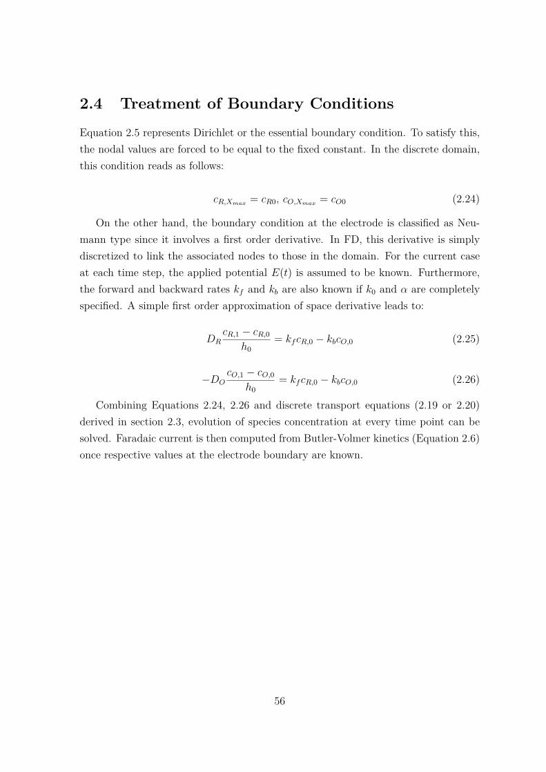
2.4 Treatment of Boundary Conditions

Equation 2.5 represents Dirichlet or the essential boundary condition. To satisfy this,the nodal values are forced to be equal to the fixed constant. In the discrete domain,this condition reads as follows:

cR,Xmax = cR0, cO,Xmax = cO0 (2.24)

On the other hand, the boundary condition at the electrode is classified as Neu-mann type since it involves a first order derivative. In FD, this derivative is simplydiscretized to link the associated nodes to those in the domain. For the current caseat each time step, the applied potential E(t) is assumed to be known. Furthermore,the forward and backward rates kf and kb are also known if k0 and α are completelyspecified. A simple first order approximation of space derivative leads to:

DRcR,1 − cR,0

h0= kfcR,0 − kbcO,0 (2.25)

−DOcO,1 − cO,0

h0= kfcR,0 − kbcO,0 (2.26)

Combining Equations 2.24, 2.26 and discrete transport equations (2.19 or 2.20)derived in section 2.3, evolution of species concentration at every time point can besolved. Faradaic current is then computed from Butler-Volmer kinetics (Equation 2.6)once respective values at the electrode boundary are known.

56

2.5 Overview of Numerical Solutions

In numerical methods, the following generic system of equations is often encountered:

F (x) = 0 (2.27)

where F (x) are the functions and x are vector of multi-variate unknowns. If all F

is made up of linear combinations of the variable x, then 2.27 is a linear system.Numerical solutions in this case have been well developed. The two main approachesare direct and iterative solvers. These methods are briefly discussed below. Elaboratedetails are found in excellent references [162, 163].

Direct methods are generally based on the method of “Lower-Upper” decomposi-tion (LU decomposition). By rewriting Equation 2.27 specifically for linear equations:

Ax = b (2.28)

In 2.28, A is the matrix containing the coeffients and b is the vector containingthe known values. If the matrix A is non-singular, then LU decomposition essentiallytransforms A into the product of two matrices:

A = LU (2.29)

where vector L is the lower-triangular matrix (i.e zero elements above the maindiagonal) and U is the upper-triangular matrix (i.e. zero elements below the maindiagonal). The solution x is then found by solving two sets of equations:

Ly = b

Ux = y

Due to special structures of L and U , these two equation sets can be solved easilyby simple back-substitution scheme. In fact, the solution is very fast when A is a“tri-diagonal” matrix because the decomposition step 2.29 is almost instant in time.Direct methods are usually the fastest way to solve linear equations. However, theseapproaches require memory storage capacity during computation steps. Thus thecomputation becomes prohibitively expensive if there are many variables (e.g. a fewmillions) are to be solved.

57

Iterative methods on the other hand require less memory and are adaptable tomulti-million variables cases. A major drawback is the amount of iteration time re-quired in order to achieve certain convergences. Iterative methods usually start withan initial guess x0 and progressively updates this guess until a reasonable closenessAx ∼ b is achieved. Well-known methods are “Gauss-Seidel” and “Successive OverRelaxation” [164].

If the system F (x) is non-linear, then the solution process is more complex. Themost common approach is Newton-Raphson. Applying Taylor expansion to the equa-tion functions:

F (x + δx) = F (x) + J(x)(δx) (2.30)

where J(x) is the Jacobian (i.e. the first derivative of the equation function withrespect to the variables). Thus in order to approach the correct solution, the followingupdate is required x → x + δx and δx is the solution to the following:

J(x)δx = −F (x) (2.31)

Equation 2.31 is effectively another system of linear equations and previous solutionmethods then apply. As with iterative methods, the solution process starts with aninitial guess and Equation 2.31 is repeated until satisfactory convergences are achieved.Furthermore, convergence of Newton-Raphson scheme depends to a large extent onthe quality of the initial guess.

58

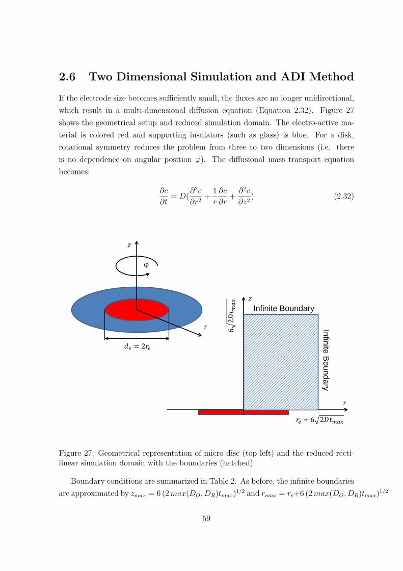
2.6 Two Dimensional Simulation and ADI Method

If the electrode size becomes sufficiently small, the fluxes are no longer unidirectional,which result in a multi-dimensional diffusion equation (Equation 2.32). Figure 27shows the geometrical setup and reduced simulation domain. The electro-active ma-terial is colored red and supporting insulators (such as glass) is blue. For a disk,rotational symmetry reduces the problem from three to two dimensions (i.e. thereis no dependence on angular position ϕ). The diffusional mass transport equationbecomes:

∂c

∂t= D(∂2c

∂r2 + 1r

∂c

∂r+ ∂2c

∂z2 ) (2.32)

φ

𝑧

𝑟

𝑟

𝑧

Infinite Boundary

𝑑𝑒 = 2𝑟𝑒

𝑟𝑒 + 6 2𝐷𝑡𝑚𝑎𝑥

62𝐷𝑡 𝑚

𝑎𝑥

Infin

ite B

ou

nd

ary

Figure 27: Geometrical representation of micro disc (top left) and the reduced recti-linear simulation domain with the boundaries (hatched)

Boundary conditions are summarized in Table 2. As before, the infinite boundariesare approximated by zmax = 6 (2 max(DO, DR)tmax)1/2 and rmax = re+6 (2 max(DO, DR)tmax)1/2

59

Infinte Boundaries (z = zmax, r = rmax) cO = cO0, cR = cR0Electrode Surface (z = 0, red region) B-V Kinetics

Insulating Substrate (z = 0, blue region) No FluxSymmetry Plane at r = 0 (vertical line) No Flux

Table 2: Boundary conditions associated with micro disk problem. The boundariesare shown in Figure 27

respectively. Using the exponential mesh, this domain is divided as shown in Figure28. The smallest spacing is placed around the electrode edge (r = 1) and expandedexponentially towards the main bulk (r, z → ∞) and the central axis at r = 0. Thereason for doing so is to take into account the presence of the singularity point at theedge - where there is a big change in species flux.

0.5 1 1.5 2 2.50

0.5

1

1.5

2

2.5

r

z

Figure 28: A typical 2D polar-coordinate grid for FD simulations of micro disk elec-trode. The grid is concentrated around the electrode edge (r = 1) and becomes sparsertowards the bulk. The axis scales are non-dimensional for demonstration purposes

Applying three-point formulations (Equations 2.15 and 2.16) (note the indicies i, j

corresponds respectively to dimensions r, z):

1r

∂ci,j

∂r= 1∑

hi

h2i−1ci+1,j − (h2

i−1 − h2i )ci,j − h2

i ci−1,j

hi−1hi(hi−1 + hi)

60

∂2ci,j

∂r2 = 2hi−1ci+1,j − (hi−1 + hi)ci,j + hici−1,j

hi−1hi(hi−1 + hi)

∂2ci,j

∂z2 = 2kj−1ci,j+1 − (kj−1 + kj)ci,j + kjci,j−1

kj−1kj(kj−1 + kj)(2.33)

Define the spatial differential operator to simplify the equation notation [76, 77]:

Lrci,j = (1r

∂

∂r+ ∂2

∂r2 )ci,j

Lzci,j = ( ∂2

∂z2 )ci,j (2.34)

By including the temporal differential operator Lt = ∂/∂t, the 2.32 is casted:

Lt(ci,j) = Lr(ci,j) + Lz(ci,j) (2.35)

A simple 1st order approximation (or 2-level Ritchmyer) for LHS is:

ct+dti,j − ct

i,j

dt= L()

r ci,j + Lzc()i,j

where the brackets () above the operators indicate either implicit or explicit for-mulations. Explicit calculations are straightforward:

ct+dti,j − ct

i,j

dt= Lt

rci,j + Lzcti,j (2.36)

Implicit calculations are not as simple. If a method like the 1D case is applied,then one obtains:

ct+dti,j − ct

i,j

dt= Lt+dt

r ci,j + Lzct+dti,j (2.37)

In Equation 2.37, there are 1 known and 5 unknowns because there are 3 unknownsin r direction and extra 2 unknowns in z direction. The system of equations is stillsolvable, but is significantly more complicated comparing to the 1D case.

In electrochemistry, a useful approach to solving the 2D diffusion equations isAlternating Direction Implicit (ADI) [30]. ADI belongs to a more general classcommonly referred to as “Operator Splitting” methods. Instead of solving the wholeproblem at once, the problem is split into smaller sub-problems based on individualoperators in the original equation [165, 166]. From Equation 2.35, it is noted that the

61

concentration evolution is essentially driven by diffusions in 2 directions (r and z),thus considering the following splitting scheme:

ct+dt/2i,j − ct

i,j

dt/2 = Lt+dt/2r ci,j + Lzct

i,j (2.38)

ct+dti,j − c

t+dt/2i,j

dt/2 = Lt+dt/2r ci,j + Lzct+dt

i,j (2.39)

Z

R R

Z

Z-Sweep R-Sweep

Figure 29: The Alternating Direction Implicit (ADI) in 2D. Nodes in thin-lined rectan-gles were already solved and those in thick-lined rectangles are currently being solved.Grey nodes are unsolved variables. For each time iteration, all the nodes in Z directionare first solved, the results are then used to solve for nodes in R direction

The original equation has been split into two sub-problems with respect to Lr

and Lz respectively. In Equation 2.38, the known concentrations at time t are usedto implicitly solve for the diffusion operator in r direction (i.e. r-sweep). Note here

62

that the time is incremented by dt/2. Similarly in Equation 2.39, concentrations att + dt/2 are then used to solve for the diffusion operator in z direction (z-sweep)and complete the full time step dt (see Figure 29). In fact, the idea of operatorsplitting is also applicable to 1D case, but it is more interesting and useful for higherdimensions. The total error of this splitting scheme is Esplitting + Ediscretization. Thefirst component Esplitting is due to errors in solving each set 2.38 and 2.39 whilstEdiscretizing is the error associated with space and time discretization schemes. Thusthese errors can be both reduced by employing a sufficiently small time step andappropriate spatial meshing. Finally, the order of splitting mathematically does notaffect the convergence and final solutions. Using ADI, the current problem is reducedto solving a series of 1D equations in each spatial dimension. In addition, the ADI

scheme above is unconditionally stable in 2D but not generally in 3D. Due to itsadvantageous mathematical and numerical properties, the method has been widelyapplied in electrochemistry literature.

63

2.7 Some Numerical Results

This section illustrates some important results in electrochemistry using a FD ap-proach. A major goal is to demonstrate that the methods and algorithms discussedin earlier sections are robust. This is accomplished by solving a number of interestingand well-known problems in the literature.

All the code in this work were written in C++ and Matlabr. A partial reason forusing Matlabr is due to its robust linear equation solver as well as the ease in ma-nipulating matrices. A strong advantage of C++ is the speed of execution. However,for additional purposes (linear algebra, optimization, etc.), the use of C++ requiresexternal libraries. All of the programs were executed on a Windows work station withIntel Core i7 and 16GB RAM.

First consider simple linear sweep voltammetry in which the applied voltage isvaried as:

E = Estart + vscant, 0 < t < tscan (2.40)

tscan = (Evertex − Escan)/vscan (2.41)

For a cyclic voltammetry, a backward scan potential is then included:

E = Evertex − vscan(t − tmax), tscan < t < 2tscan (2.42)

In addition, the capacitive current is computed as:

Idcc = CdlAvscan, 0 < t < tmax (2.43)

Idcc = CdlA(−vscan), tmax < t < 2tmax (2.44)

is the time taken for a complete forward sweep. Parameter setting for the simulationis listed in Table 3 and Figure 30 shows the theoretical response at a macro electrodefor very fast electrochemical kinetics (i.e. large k0). In Table 3, diffusion coefficients ofboth reduced and oxidized species are assumed to be equal. However, this simplifyingassumption is easily modified to account for different diffusivities. Furthermore, thediffusion coefficients in water differ from species to one another but commonly usedchemicals are known to have those values lying within the range 10−6 − 10−5 cm2/s.

64

Exact values generally depend on solution temperatures, solvent molecules, chemicalstructures and the ambient surroundings. To approach fast kinetics regime, a suffi-ciently large value of k0 is assumed (0.1 m/s in this case). It is noted that a precisevalue of k0 is not important and any larger value would lead to virtually the sameresult. This is because a fast kinetics would lead to Nernst relation 1.13 which is inde-pendent of both α and k0, the current is therefore not sensitive to these parameters.

Parameter Name Notation Numerical Value UnitsDiffusion Coefficient DR 9 ∗ 10−10 m2/sDiffusion Coefficient DO 9 ∗ 10−10 m2/s

Electrochemical Kinetics k0 0.1 m/sCharge Transfer Coefficient α 0.55 −

Equilibrium Potential E0 0.2 VElectrode Area A 10−2 cm2

Specific Capacitance Cdl 0 µA/cm2

Scan Rate vscan 0.1 V/sStarting Potential Estart −0.2 VFinishing Potential Evertex 0.6 VBulk Concentration cR0 1 mol/m3

Bulk Concentration cO0 0 mol/m3

Smallest Spacing h0 10−7 mSpatial Exponential Factor f 1.05 −

Number of Time Steps − 210 −

Table 3: Parameters for simulations of macro disk (Figures 30 and 31)

Spatial grid parameters are listed in the last three rows of the Table 3. A smallspacing is chosen for h0. The value is selected per the diffusion layer estimate (∼10−4(m)) and the smallest spacing of the order 10−7(m) should therefore ensure goodconvergences to a high degree of accuracy (as confirmed in Figure 30). A ratherconservative space expansion (f =1.05) is chosen, but higher values such as 1.1 or 1.2yield exactly identical results. This fact underlines the importance of choosing correctmesh configuration in order to obtain adequate convergence.

The current and voltage in the Figure 30 above is non-dimensionalized by thefollowing expression:

J = Itotal

(nF )3/2/(RT0)1/2AD1/2R cR0v

1/2scan

(2.45)

65

-20 -15 -10 -5 0 5 10 15 20

0.0

0.1

0.2

0.3

0.4

0.5D

imen

sion

less

Cur

rent

J

Dimensionless Potential

Simulated Data Analytical Data

Figure 30: Dimensionless current versus dimensionless potential for a macro electrodeunder fast reversible kinetics. The corresponding dimensionless expressions are givenby Equations 2.45 and 2.46 respectively. At θ = 0, the dimensional potential E = E0.The analytical values are extracted from tables in Reference [1]

θ = nF

RT0(E − E0) (2.46)

At the peak potential, the Randles-Sevcik relation holds:

Jp = Ip

(nF )3/2/(RT0)1/2AD1/2R cR0v

1/2scan

= 0.446 (2.47)

This relation is analytically valuable since by measuring the peak current, informa-tion about diffusion coefficient of the species can be derived. In addition, because theexpression involves species concentration, this forms the basis of many electrochemicalsensors.

It is straightforward to confirm that diffusion at this electrode should follow macrobehaviour by dimensional analysis. Firstly, the corresponding diameter de assuming a

66

disk shape is:

de ∼ (4/π.10−6)1/2 ∼ 0.001(m) (2.48)

which is obviously not in the micro range. In addition, over the course of the experi-ment, which lasts about tmax = (Evertex −Estart)/vscan = 8 (s), the size of the diffusionlayer over the electrode surface is approximately:

ldif ∼ ((9 ∗ 10−10).8)1/2 ∼ 0.0001(m) (2.49)

Thus the diffusion later is still fairly thin compared to the electrode dimension.Even at significantly slower scan rates such as 0.01 V/s or even 0.001V/s, diffusionlayer is still either smaller or just comparable to the electrode dimension. This factensures that for most practical situations, the above electrode is considered to be large.

The simulation result can be qualitatively explained as follows. At voltage signifi-cantly less than E0, no oxidation (Equation 2.1) occurs and and the solution is mainlycomposed of the reductive species R. As the potential becomes higher, more reactionsoccur which translates into the rising current. At the electrode surface, species R

starts being depleted and a mass-transfer gradient is gradually established. At po-tentials significantly above E0, the whole process becomes mass transport controlledand thus current drops because the amount of fresh species R that move towards theelectrode surface is reduced significantly.

The effect of reaction kinetics on the voltammogram is next considered. By vary-ing k0 and keeping the rest of the parameters the same, Figure 31 is obtained. Eachvoltammogram now includes forward and backward waves. In a typical cyclic voltam-mogram, there are two peaks. The forward peak associates with oxidation R → O+e−

whilst the backward peak is attributed to the reduction O + e− → R. For the caseof k0 = 1 cm/s, the locations of these peaks are indicated by dotted lines in Figure31. Because kinetics of 1 cm/s still results in reversible reaction, the relation 2.47 stillholds. At slower kinetic rates, the separation between peaks broadens and the peaksize decreases. Using the reversible reaction (Figure 30) as the reference, this obser-vation is explained as follows. For smaller k0, Butler-Volmer relation (Equation 2.6)requires a larger thermodynamic factor to drive the same rates of reactions. Therefore,a larger potential is needed compared to the fast kinetic case, and the peak is shiftedaccordingly. In addition, the peak size is also smaller because the reaction rates arereduced.

67

-20 -15 -10 -5 0 5 10 15 20

-0.4

-0.2

0.0

0.2

0.4

0.6D

imen

sion

less

Cur

rent

J


k0=1 k0=0.01 k0=0.0001

Figure 31: Cyclic voltammograms at different electrochemical reaction rates. Fork0 = 1 cm/s, the potential gap is constant and independent of the scan rate . Atmuch slower kinetics, the gap becomes larger and potential dependent [2] (All thedimensionless expressions are the same as before)

The next discussion focuses on micro disk electrodes. As previously noted, ADI

is applied to solve the angular symmetric 2D diffusion equation 2.32. The setting islisted in Table 4. Before proceeding to the results, there are a few technical notes.Firstly in the simulation, dimensionless spacings dR and dZ are scaled with respect tothe disk radius re. Secondly, the Faradaic current is now computed from the integral:

If = 2πF

re∫0

D(∂c

∂z)z=0rdr (2.50)

to account for multi-directional variations of the fluxes. Expression 2.50 is computedat each time step using the simple Trapezoidal rule [167]. The derivative at z = 0 isapproximated by the simple two-point formula and a fine meshing (small spacings andspatial exponential factor) ensures adequate convergence.

A classical problem in the literature is the simulation of amperometric response atmicro electrodes. In amperometry, the potential is held at a constant value such that

68

Parameter Name Notation Numerical Value UnitsDiffusion Coefficient DR, DO 10−9 m2/s

Electrochemical Kinetics k0 0.1 m/sCharge Transfer Coefficient α 0.60 −

Equilibrium Potential E0 0.2 VDisk Radius re 10 µmScan Rates vscan 0.1 and 0.005 V/s

Dimensionless Spacing in r direction dR 10−6 −Dimensionless Spacing in z direction dZ 10−6 −

Spatial Exponential Factor f 1.05 −

Table 4: Parameter settings for micro disk simulation. The disk radius is 10 µm.The dimensionless potential starts and ends at −20 and 20 respectively. The bulkconcentrations for reduced and oxidized species are the same as in Table 3

0 20 40 60 80 100

1.0

1.2

1.4

1.6

1.8

2.0

2.2

2.4

Non

-dim

ensi

onal

Cur

rent

i

Dimensionless Time

Simulation Data Theoretical Values

Figure 32: Amperometric response at a micro disk. Comparison between the simu-lation data (continuous line) and theoretical points (red dots) (Reference [3]) showsgood agreement. Current and time are normalized respectively by Equations 2.51 and2.52

complete oxidation (or reduction) is induced at the electrode surface. For the currentcase, a value of 0.6 (V ) is chosen, which is well above the equilibrium E0. Furthermore,

69

-20 -10 0 10 20-0.2

0.0

0.2

0.4

0.6

0.8

1.0

1.2

Dim

ensi

onle

ss C

urre

nt i


0.1 V/s 0.005 V/s

Figure 33: Dimensionless current versus dimensionless potential at two different scanrates (100 and 5 mV/s). A flatter and more steady state response is obtained at theslower scan rate. Dimensionless current and potential are given by expressions 2.51and 2.46

it is customary to non-dimensionlize the current as follows:

i = Itotal

4FDRcR0re

(2.51)

and the dimensionless time is expressed as:

τ = Dt

r2e

(2.52)

Figure 32 compares the simuled current with theoretical data. An expression relat-ing i and τ developed by [3] is widely used as the benchmark comparison for diffrerentnumerical methods. As the time becomes large, it is shown that the dimensionlesscurrent approches 1 and the current is said to reach a limiting value Iss:

Iss = 4FDRcR0re (2.53)

70

Equation 2.53 is useful in analytical chemistry because this relation can be used todetermine either the diffusion coefficient DR or bulk concentration cR0. Anotherway ofapproaching the steady state current is by performing cyclic voltammetries as shown inFigure 33. Two scan rates 0.1 and 0.005 V/s are used to demonstrate the principles. Athigh scan rates, the current response shows a peak similar to that of a macro electrode,but the feature is significantly less sharp. This is because the small electrode sizesconsiderably enhance fluxes towards the electrode surface and it is therefore possibleto sustain high reaction rates. At small scan rates, the current shape follows the classicsigmoidal behavior. Theoretically as the scan rates becomes infinitely small, a steadystate (Equation 2.53) is achieved [73]. In practice, values such as 5 or 1 mV/s areusually sufficient to induce such behaviour.

It is also instructive to estimate the size of the steady state current from Expression2.53:

Iss ∼ 4.96485 C

mol10−9 m2

s1mol

m3 10−5m ∼ 4 nA

which is much smaller in comparison to that of a macro electrode (typically in orderof µA). This magnitude is nevertheless still significantly larger than the non-Faradaiccomponent, which is estimated from Expression 2.10 as:

CdlAvscan ∼ 100 µF

cm2 (π 10−6)cm2 0.005V

s∼ 1.6 10−3 nA

assuming a relatively large double layer capacitance (100 µF/cm2). This fact confirmsthat for micro electrodes, capacitive currents can be safely ignored during analysis.Furthermore, computational time in 2D is also noted to be significantly more thanthat of one dimensional calculations (e.g. several minutes vs several seconds).

Thirdly, spherical-shaped electrodes are not so commonly encoutered at microsizes. They are more often encountered in problems dealing with nano particles (re ∼50 nm). Because spherical electrodes also have the rotational symmetry around centreaxis, the problem is again reduced to 2D. This effect may also be seen when wetransform the equation from spherical to cylindrical coordinates and integrate alongthe z-axis. Therefore, the solution process described for a micro-disk is also applicablefor spherical nano-electrodes. A mapping complication arises when modelling curvedelectrode surfaces. In theory, FD formulation can be adapted to any curvature thatcan be analytically expressed [154, 155]. For spherical shapes, a simple discretizationis shown in Figure 34. Structurally, the red circular boundary is broken down into

71

0 0.5 1 1.5 2 2.5 30

0.5

1

1.5

2

2.5

3

r

z

Figure 34: Meshing for spherical electrode. The boundary is coloured in red and onlypoints on and outside the surface of the sphere are considered in the calculations

discrete points and the expanding mesh is then applied at each of these locations.To illustrate the method, an amperometric calculation for spherical electrodes is

performed. For an ultra small hemi-spheres, the current can be written as the sum oftwo components [2]:

Ihemi−sphere = π

2(FDRcR0re) + IMacro

where IMacro is the Cotrellian response 1.19 at a macro electrode. Over a long period oftime, this component tends to 0, leaving out the limiting current of (π/2)FDRcR0re asshown in Figure 35. Finally,nano-spheres expectedly behaves in the same way as microdisks, which can be validated by linearly-swept cyclic voltammetry measurements..

Beside the basic E mechanism, it is interesting to consider additional homogenousreactions. The following section focuses on the EC ′ mechanism, which is schematicallydepicted in Figure 36. Initially the solution contains only substrate S and reductiveform R. At the electrode surface, R is oxidized to O, which reacts with S to reformR and in-active products. It was briefly discussed in chapter 1 that EC ′ mechanismplays an important role in operating principles of Glucose sensors. However, theinterest in studying the mechanism remains strong because of its potential application

72

0 5 1 0 1 5 2 0 2 5 3 01

2

3

4

5

6

7

8I/(F

D Rc R0r e)

D R t / r 2e

N u m e r i c a l T h e o r e t i c a l A s y m t o p

Figure 35: Limiting current at a sub micron or nano spherical electrode. The asymtope(at approximately π/2 ≃ 1.57) is colored in red

in detection of Hydrogen Sulphide (H2S) in oil wells. Essentially, H2S plays the role ofsubstrate S in Figure 36 whilst the electrochemical pairs can be Fe(CN)2−

6 /Fe(CN)3−6

compounds in aqueous solutions.

Parameter Name Notation Value UnitsDiffusion Coefficients DR, DO 10−5 cm2/s

Substrate Diffusion Coefficient Ds 10−5 cm2/sInitial Electroactive Concentrations cR0, cO0 2, 0 mol/m3

Initial Substrate Concentrations cS0 2 mol/m3

Electrode Area A 0.01 cm2

Homogenous Reaction Rate kEC′ 5 ∗ 105 M−1s−1

Smallest Spacing h0 10−6 mSpatial Exponential Factor f 1.05 −

Time Step dt 0.001 sElectrochemical Kinetics k0 0.1 cm/s

Table 5: Parameters settings for EC’ calculations in Figures 30 and 38

73

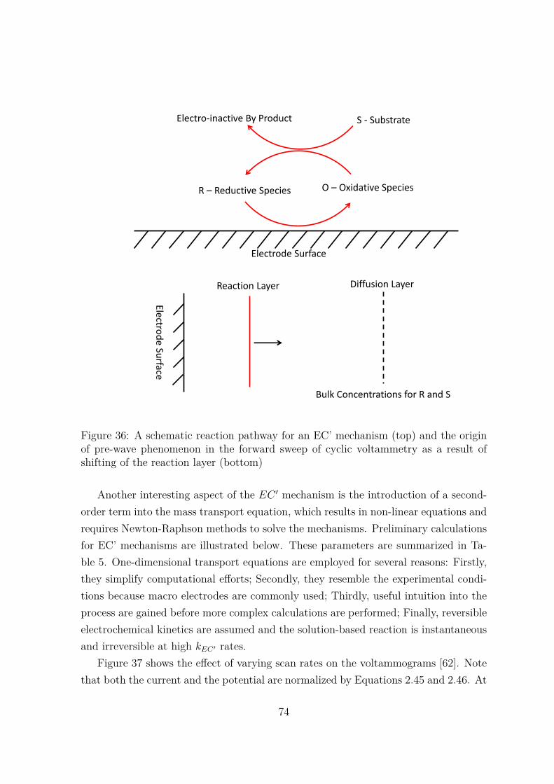
R – Reductive Species O – Oxidative Species

S - Substrate Electro-inactive By Product

Electrode Surface

Electrod

e Surface

Reaction Layer Diffusion Layer

Bulk Concentrations for R and S

Figure 36: A schematic reaction pathway for an EC’ mechanism (top) and the originof pre-wave phenomenon in the forward sweep of cyclic voltammetry as a result ofshifting of the reaction layer (bottom)

Another interesting aspect of the EC ′ mechanism is the introduction of a second-order term into the mass transport equation, which results in non-linear equations andrequires Newton-Raphson methods to solve the mechanisms. Preliminary calculationsfor EC’ mechanisms are illustrated below. These parameters are summarized in Ta-ble 5. One-dimensional transport equations are employed for several reasons: Firstly,they simplify computational efforts; Secondly, they resemble the experimental condi-tions because macro electrodes are commonly used; Thirdly, useful intuition into theprocess are gained before more complex calculations are performed; Finally, reversibleelectrochemical kinetics are assumed and the solution-based reaction is instantaneousand irreversible at high kEC′ rates.

Figure 37 shows the effect of varying scan rates on the voltammograms [62]. Notethat both the current and the potential are normalized by Equations 2.45 and 2.46. At

74

-10 -5 0 5 10

0

1

2

Nor

mal

ized

Cur

rent

Normalized Potential

100 mV/s 10 mV/s 5 mV/s 1 mV/s

Figure 37: Increasing scan rates lead to an increase in measured currents. Notice thatthere are two peaks in the voltammograms. The first peak corresponds to pre-waveeffect and the second is the usual redox reaction

-10 -5 0 5 10-0.5

0.0

0.5

1.0

1.5

Nor

mal

ized

Cur

rent

Normalized Potential

Ratio = 0.1 Ratio = 0.2 Ratio = 0.5 Ratio = 1.0 Ratio = 2.0

Figure 38: Effects of changing concentration ratios between substrate and electrolytes.The more S is present, the higher the pre-wave peak

75

higher scan rates, the scanning time is now smaller, therefore the size of the diffusionlayer, which is proportional to t1/2, also becomes smaller . A smaller diffusion layer alsoleads to an increase of electroactive species flux and consequentially higher currents.Thus in conclusion, a higher scan rate induces a larger current.

0.0 0.2 0.4 0.6 0.8 1.0 1.2 1.4 1.6 1.8 2.0 2.20.0

0.2

0.4

0.6

0.8

1.0

1.2

1.4

1.6

Peak

Cur

rent

(Nor

mal

ized

)

Concentration Ratio

Equation y = a + b*x

Weight No Weighting

Residual Sum of Squares1.04677E-4

Pearson's r 0.99995Adj. R-Square 0.99986

Value Standard Error

BIntercept 0.00744 0.00609Slope 0.78493 0.00529

Figure 39: Pre-wave peak currents versus the concentration ratios cS0/cR0 shows alinear relationship in Figure 38. Below ratio of 0.2, it is difficult to distinguish thepre-wave in the voltammogram

An additional interesting feature is the presence of a “pre-wave” peak before theusual peak (around the dimensionless potential 1). This fact can be reasoned byreferring to the bottom figure in 36. At very high kEC′ , species R is re-formed at amuch closer distance to the electrode surface. Between the reaction layer and usualdiffusion layer (i.e. without EC ′), the concetration of R remains essentially constantat the bulk value. The “pre-wave” current initially rises because there is initiallyplentiful supply of S inside the reaction layer, which quickly regenerates R and thusproduces more current. However, after some time, S is depleted at the position ofreaction layer and it takes sometimes for the transport of S into the reaction layer.

76

The regeneration of R becomes slower and the reaction layer shifts right due to mass-transport limitation. As a consequence, the current falls and a peak is formed.

To investigate the effect of substrate concentration, the scan rate is fixed at 25 mV/s.Calculations are then performed at different ratios of cS0/cR0 and the results are pre-sented in Figure 38. An observable trend is a rise in concetration ratio would lead toan increase in pre-wave current peak. Furthermore, as S increases, the pre-wave tendsto shift right. This is due to the fact that a higher substrate concentration sustainsthe reaction layer position for longer, which decreases pre-wave occurrence at laterpotentials (as opposed for lower cS0 concentrations).

Because the pre-wave is dependent on substrate level, a strong correlation is ex-pected between these variables (Figure 39). Note that the size of the other peaks arealso influenced by the presence of S, but less pronounced comparing to the first one.Finally because the relationship is linear [168], these measurements are useful as asensing method for the substrate. However the method becomes ineffective at verylow substrate concentrations due to diminishing pre-wave magnitude.

77

2.8 Chapter Conclusion

This chapter described the basic numerical approach, namely FD, to the solution ofdiffusion equation coupled with electrochemical Butler-Volmer kinetics. Importantaspects of FD, such as explicit/implicit time derivatives, mesh generation and linearsolvers were discussed. These discussions are however not only limited to FD butapplied to FE in later chapters.

The FD approach is then applied to several basic problems considering macro andmicro electrodes. Good agreement between numerical data and analytical solutionsis demonstrated for both cases. FD can also be extended to more complex curva-ture boundaries, as in the case of semi-hemispherical electrode. Finally, 2nd orderhomogeneous kinetics case is considered. Since the PDEs are highly non-linear, theNewton-Raphson is considered to solve the problem. An interesting phenomenon,referred to as the pre-wave, is demonstrated and important physical insights for itsorigin discussed. This phenomenon is the subject of further investigation in Chapter5.

Chapter 3 employs the linear sweep voltammetry as an experimental design factorto investigate different aspects of the Butler-Volmer model. This work requires repet-itive computation of the model for diffusion transport coupled with electrochemicalkinetics, thus FD method developed so far is useful. By using an extended version ofthe Butler-Volmer formulation, the investigation aims to identify the most significantparameters and then estimate them as accurately as possible. In addition, MonteCarlo approach is flexibly employed to different problems of optimization and multi-dimensional intergrations.

78

Chapter 3

Parameter Identifiability andEstimation of Redox processesunder Diffusion Control

This chapter introduces the concept of identifiability measure and applies it to electro-chemistry context. Special emphasis is placed on interpretations of the result, whichhave important implication for subsequent sections in the chapter. The extent ofthe investigation is however not limited to identifiability study but also encompassesparameter ranking, selection and estimation. Since the topics of estimability and es-timation share virtually the same mathematical framework, this work focuses on thestudy of the later for practical reasons.

The following work presents a theoretical case study in which the traditional lin-ear sweep and cyclic voltammetric techniques are heavily utilized as an experimentaldesign variable. The work aims to determine whether this voltammetry method canadequately retrieve electron transfer kinetic information instead of employing moreconceptually complex voltage designs. Furthermore, because these techniques are socommonly used, the results of this study provide a useful theoretical foundation forsuch practice. It is also intuitively clear that any other synthetic signal should includelinear sweep and/or cyclic voltammetry, since these signal are readily available in mostexperimental equipments and effective at inducing redox reaction.

The chapter is structured as follows. First the Butler-Volmer formulation, fromthe previous chapter, is extended to account for two additional parameters: uncom-pensated resistance and double layer capacitance. The identifiability calculation is

79

then applied to this model to observe the potential compensating effects among themodel parameters. By carefully selecting other experimental variables and applyingglobal sensitivity analysis, the intrinsic electron transfer kinetic, equilibrium potentialand double layer capacitance are determined as the most significant parameters in themodel. To complement this result, it is shown that the first two of these parametersalong with the charge transfer coefficient can be reliably estimated without the de-tailed knowledge of the third one. In addition, Monte Carlo Markov Chain (MCMC)statistical calculations demonstrate that the mean values for those parameters fall re-spectively within 4% (for k0) and less than 1% (for α and E0) of the assumed truevalues.

80

3.1 The extended Butler-Volmer Model

Throughout the chapter, a one-dimensional model is assumed. The system of equationscan be shown compactly via Equations 3.1 and 3.2 for the redox transfer O + e ↔ R.The spatial operator represents second order differentation Lx = ∂2/∂x2:

∂ci

∂t= DiLxci, i = R, O (3.1)

If/FA = DR(∂cR

∂x)x=0 = −DO(∂cO

∂x)x=0 = kf (cR)x=0 − kb(cO)x=0 (3.2)

where the forward and backward rates kf and kb are defined as in Equations 1.10 and1.11. The model has three major parameters: k0, α and E0. In addition to thesethree parameters, the total current I (or the model output) is influenced by doublelayer capacitance Cdl according to Equation 2.11. In general, the exact value of Cdl isunknown and it usually varies throughout the voltammetric experiments and in somecases exhibits potential-dependent behaviour.

Extra complication is caused by the uncompensated solution resistance Ru. Thisresistance is mainly due to the solution between the working and reference/counterelectrodes, with other resistances (e.g. metal contacts) being negligible. The presenceof Ru leads to losses of the driving potential, and thus requires the rates kf and kb tobe modified as follows:

kf = k0exp((1 − α)F (E − E0 − IRu)RT0

) (3.3)

kb = k0exp(−αF (E − E0 − IRu)RT0

) (3.4)

Dielectric polarization within the solution also leads to extra losses, which is at-tributed to the potential difference between solid and fluid phase [24, 30]. In addition,it can be seen that the gradient of this potential is associated with electrostatic mi-gration fluxes (Equation 1.5). As remarked earlier, this phenomenon is importantat low supporting electrolyte concentrations . It is assumed in this chapter that thesolution is well-supported, hence the potential loss caused by ion migrations can besafely ignored.

Considering Equations 3.1,3.2, 3.3 and 3.4 along with the boundary conditions 2.4and 2.5, it is evident that additional non-linearity is introduced by the “Ohmic drop”

81

component IRu. Because the total current I = If + Ic now appears in the exponentialterm, this fact discourages the application of fully implicit formulations. This is thecase because these formulations are compactly expressed as:

ct+dt − ct

dt= DLxct+dt (3.5)

where the operator Lx is approximated by second or higher order finite differenceformular. The set of equations 3.5 at each concentration point i is then coupled withnon-linear boundary condition at the electrode surface. A general solution approachis the Newton-Raphson, which can be used to determine species concentrations andthe total current simultaneously. A major drawback is the exact computation of theJacobian matrix, which is cumbersome and expensive in this case.

A straightforward way of dealing with the non-linearity in this case is to use anexplicit formulation. In the current case, the concentration at a new point in time isdirectly computed by Equation 3.6:

ct+dti − ct

i

dt= DiLxct

i (3.6)

Thus the only unknown after solving Equation 3.6 is the total current I. Ultimately,this is the only non-linear equation to be solved. Multiplying both sides by nFA,Equation 3.2 now assumes a generalized form::

If = f(If ) (3.7)

where Ic is known at each potential point (Equation 2.10).A simple method to solve Equation 3.7 uses a binary (or bisection) search method.

It belongs to a class of interval searches which is a discrete version of the Newton-Raphson. Some other well-known related methods include the Regula-Falsi Method orSecant Method [162]. The bisection search is described in Algorithm 3.1. In general,the bisection search works by reducing the interval size by half at each iteration. Itguarantees to converge quickly if the initial interval [a, b] is well chosen to contain theexact root of the equation. This requirement also implies that f(a) f(b) < 0.

To easily implement Algorithm 3.1, Equation 3.7 is re-arranged:

If − f(If ) = 0

and treat the LHS as the function f in the Algorithm. A summary of parameters

82

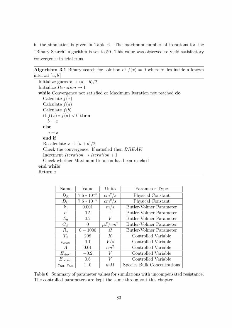
in the simulation is given in Table 6. The maximum number of iterations for the“Binary Search” algorithm is set to 50. This value was observed to yield satisfactoryconvergence in trial runs.

Algorithm 3.1 Binary search for solution of f(x) = 0 where x lies inside a knowninterval [ a, b ]

Initialize guess x → (a + b)/2Initialize Iteration → 1while Convergence not satisfied or Maximum Iteration not reached do

Calculate f(x)Calculate f(a)Calculate f(b)if f(x) ∗ f(a) < 0 then

b = xelse

a = xend ifRecalculate x → (a + b)/2Check the convergence. If satisfied then BREAKIncrement Iteration → Iteration + 1Check whether Maximum Iteration has been reached

end whileReturn x

Name Value Units Parameter TypeDR 7.6 ∗ 10−6 cm2/s Physical ConstantDO 7.6 ∗ 10−6 cm2/s Physical Constantk0 0.001 m/s Butler-Volmer Parameterα 0.5 − Butler-Volmer ParameterE0 0.2 V Butler-Volmer ParameterCdl 0 µF/cm2 Butler-Volmer ParameterRu 0 − 1000 Ω Butler-Volmer ParameterT0 298 K Controlled Variable

vscan 0.1 V/s Controlled VariableA 0.01 cm2 Controlled Variable

Estart −0.2 V Controlled VariableEvertex 0.6 V Controlled VariablecR0, cO0 1, 0 mM Species Bulk Concentrations

Table 6: Summary of parameter values for simulations with uncompensated resistance.The controlled parameters are kept the same throughout this chapter

83

To illustrate the explicit method, two calculations are compared and shown inFigure 40. The red curve agrees very well with the previous implicit calculations inFigure 30. In the explicit method, a larger number of time steps are required in or-der to maintain numerical stability. Equation 2.23 requires the non-dimensional valueDR t/(x)2 ∼ 1 . When a smaller grid size is employed, the time step is correspond-ingly decreased. Therefore, the computing times for the curves are considerably largerfor the red curve. Finally, from a numerical stand point, the black curve reasonablyapproximates the red curve for most constraints since around the peak region, thedifference between the two curves is around 1%.

-20 -15 -10 -5 0 5 10 15 20

0.0

0.1

0.2

0.3

0.4

0.5

Dim

ensi

onle

ss C

urre

nt J


Coarse Grid Finer Grid

Figure 40: Explicit calculations at two different grid sizes (coarse (black) vs fine (red)).The more accurate result (red) requires more number of time steps (220 in comparisonto 216 of the black curve). The red and black curves agree to within 0.67% and 1%of the implicit calculations in Chapter 2 respectively. The current and potential arenormalized according to Equations 2.45 and 2.46

The effects of increasing resistance are shown in Figure 41. The Butler-Volmer

84

-20 -15 -10 -5 0 5 10 15 20

0.0

0.1

0.2

0.3

0.4

0.5D

imen

sion

less

Cur

rent

J


Ru=0 Ru=50 Ru=500 Ru=5000

-0.2 -0.1 0.0 0.1 0.2 0.3 0.4 0.5 0.6 0.7

0.0

0.5

1.0

1.5

2.0

2.5

Tota

l Cur

rent

/A

Applied Potential/V

Ru=0 Ru=50 Ru=500 Ru=5000

Figure 41: Effect of uncompensated resistance on linear sweep voltammetries. Forsmall resistances (50 − 500 Ohm), the current response does not change significantly.For larger resistances (e.g. 5000 Ohm), the peak current starts to decrease and shiftsright to compensate for a decrease in reaction kinetics. Data are presented in dimen-sionless (top) and dimensional format (bottom)

85

parameters are kept constant and Ru is increased between 50 − 5000. A rising uncom-pensated resistance leads to an additional loss in the applied potential, which requiresa larger oxidative potential to drive the reaction. The peak therefore shifts rightwardto compensate for such effects. In addition, since the exponents in Equations 3.3 and3.4 are now smaller in comparison to the zero resistance case, resulting in a smallercurrent and peak height. However, the effect is only significant at very large resis-tances, suggesting that higher resistances do not significantly influence the currentoutput.

From the dimensional current (bottom Figure 41), a direct way of reducing theeffect of Ohmic drop IRu is to reduce the current I. This is in fact achieved by em-ploying an electrode area A = 0.01 cm2, which is small enough to reduce the potentialloss, but is still sufficiently big so that the macro electrode conditions still apply. Aqualitative reason is given as follows. Considering the expression for the effectiveoverpotential:

η = (E − E0) − IRu

If Ru = 500 Ω and I ∼ 2 (µA), the Ohmic drop is in the order of 10−3 V . Thiscomponent becomes significant when E is close to E0, but under that condition, thecurrent is still relatively small since the exponents in Butler-Volmer expression are alsosmall. Thus under this experimental design condition, the effect of solution resistanceon the current is negligible in the range 0−500 Ω. Having developed a robust computa-tion method for the extended Butler-Volmer formulation, the subject of identifiabilityis discussed next.

86

3.2 Identifiability Measure for Model Parameters

Section 1.5 of chapter 1 introduces the basic concepts in identifiability. One of theearly definitions (Equation 1.28) defines identifiability with respect to data. Thisconcept captures the idea of identifiability and estimability altogether. Another wayof defining identifiability without referencing to external data was proposed by otherauthors [106] [124]. This definition is more intuitive and used in this work. Applyingthis definition to Butler-Volmer model, the model is identifiable if and only if thefollowing equality occurs:

I(θ1, u) = I(θ2, u) ↔ θ1 = θ2 (3.8)

,that is if the same current response is obtained then the underlying sets (θ, u) mustbe the same. Vectors θ and u denote the parameter set and experimental variablesrespectively:

θ = [DR, DO, k0, α, E0, Ru, Cdl] (3.9)

u = [T0, vscan, A] (3.10)

The electrode area is usually fixed, and since a homogenous temperature is as-sumed, the most significant variable in the relation is the scan rate u = [vscan]. Theidentifiability problem was earlier studied using highly modulated signals. The resultsshow aninvariance to the waveforms (e.g. triangular,sawtooth, square) being used[123]. In addition, it was concluded that a single set of data is not sufficient enoughto allow all parameters in θ to be uniquely estimated. It also highlights the issue ofparameter compensation in which groups of parameters compensate each other (dueto non-linear interaction) and result in similar current responses I ′s.

The major aim of this section is to show that the model is not globally identifiableunder linear sweep voltammetry. From a mathematical perspective, a locally non-identifiable model is desired. The problem is formulated as an optimization function,i.e. identifiability test:

maxθ1,θ2H(θ1, θ2) = η2 = (θ1 − θ2)2

(I(θ1, u) − I(θ2, u))2 (3.11)

where optimizing variables are the pairs (θ1, θ2). The interpretation of 3.11 is as

87

follows. Assuming finite maximal η∗ (or the identifiability number) exists, the followinginequality applies:

|θ1-θ2| ≤ η∗|I(θ1, u) − I(θ2, u)| (3.12)

Equation 3.12 measures changes in the total current caused by the differences inparameter sets. If two different sets lead to very similar response, then a consequen-tially large η∗ reflects the non-identifiability of the model. The larger it is, the lessunique the model parameters are. Therefore one expects η∗ to be as small as possiblefor a highly identifiable system. In addition, η∗ generally depends not only on themodel structure but also the experimental variables u.

Algorithm 3.2 Monte Carlo sampling for optimization of Identifiability functionH(θ1, θ2)

Initialize Iteration → 1Initialize hsol → 0while Maximum Iteration not reached do

Generate a matrix of random number between 0 and 1 with size NParameterx2.Each column corresponds to a parameter setConvert each column into parameter set valuesCalculate the corresponding Identifiability function hnewif hnew > hsol then

hsol = hnewUpdate the new pair as the current solution

end ifIncrement Iteration → Iteration + 1Check whether Maximum Iteration has been reached

end whileOutput the value hsol and solution pair

To optimize the function 3.11, previous work used semi-gradient approaches suchas the Simultaneous Pertubation Stochastic Approximation (SPSA). SPSA approxi-mates the gradient of H(θ1, θ2) using a simple first order finite difference formula andis a semi-gradient approach. For each specific problem, SPSA requires tuning of pa-rameters to ensure good performance. This work opts to use Monte Carlo sampling.In this approach, many pairs of (θ1, θ2) are generated and H(θ1, θ2) is computed. Thelargest value of all is kept as the final solution. For complicated functions, the optimalvalue may become trapped in the local solution; the Monte Carlo method reduces thelikelihood of this occurrence by searching the proximity of the global optimum [148].

88

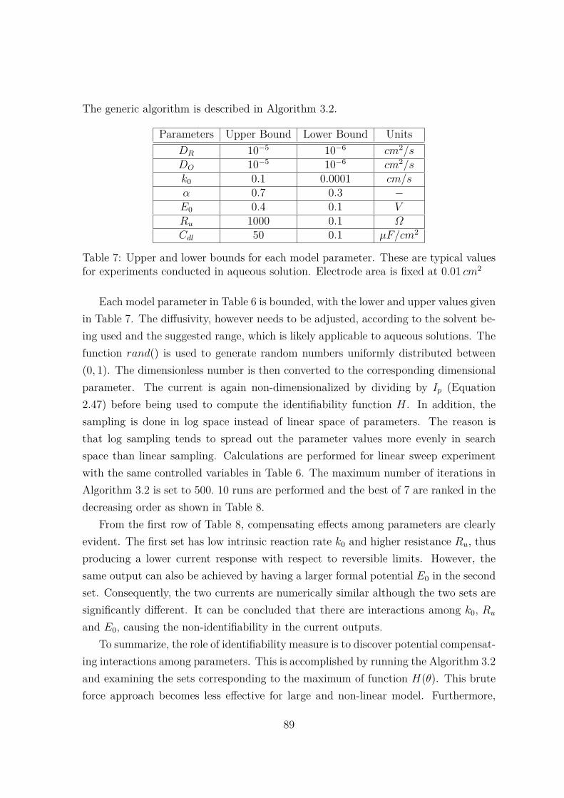
The generic algorithm is described in Algorithm 3.2.

Parameters Upper Bound Lower Bound UnitsDR 10−5 10−6 cm2/sDO 10−5 10−6 cm2/sk0 0.1 0.0001 cm/sα 0.7 0.3 −E0 0.4 0.1 VRu 1000 0.1 ΩCdl 50 0.1 µF/cm2

Table 7: Upper and lower bounds for each model parameter. These are typical valuesfor experiments conducted in aqueous solution. Electrode area is fixed at 0.01 cm2

Each model parameter in Table 6 is bounded, with the lower and upper values givenin Table 7. The diffusivity, however needs to be adjusted, according to the solvent be-ing used and the suggested range, which is likely applicable to aqueous solutions. Thefunction rand() is used to generate random numbers uniformly distributed between(0, 1). The dimensionless number is then converted to the corresponding dimensionalparameter. The current is again non-dimensionalized by dividing by Ip (Equation2.47) before being used to compute the identifiability function H. In addition, thesampling is done in log space instead of linear space of parameters. The reason isthat log sampling tends to spread out the parameter values more evenly in searchspace than linear sampling. Calculations are performed for linear sweep experimentwith the same controlled variables in Table 6. The maximum number of iterations inAlgorithm 3.2 is set to 500. 10 runs are performed and the best of 7 are ranked in thedecreasing order as shown in Table 8.

From the first row of Table 8, compensating effects among parameters are clearlyevident. The first set has low intrinsic reaction rate k0 and higher resistance Ru, thusproducing a lower current response with respect to reversible limits. However, thesame output can also be achieved by having a larger formal potential E0 in the secondset. Consequently, the two currents are numerically similar although the two sets aresignificantly different. It can be concluded that there are interactions among k0, Ru

and E0, causing the non-identifiability in the current outputs.To summarize, the role of identifiability measure is to discover potential compensat-

ing interactions among parameters. This is accomplished by running the Algorithm 3.2and examining the sets corresponding to the maximum of function H(θ). This bruteforce approach becomes less effective for large and non-linear model. Furthermore,

89

Sam

ple

No.

Hη

∗Pa

ram

eter

Sets

11.

671.

29[1

.50

∗10

−6 ,

1.15

∗10

−6 ,

2.86

∗10

−4 ,

0.41

5,0.

102,

727,

7.22

∗10

−7 ]

[9.0

3∗

10−

6 ,1.

07∗

10−

6 ,1.

55∗

10−

3 ,0.

38,

0.16

5,13

2,1.

6∗

10−

6 ]

21.

111.

05[1

.37

∗10

−6 ,

1.83

∗10

−6 ,

1.43

∗10

−2 ,

0.45

9,0.

125,

2.83

,2.

12∗

10−

7 ][5

.42

∗10

−6 ,

1.87

∗10

−6 ,

1.09

∗10

−2 ,

0.53

2,0.

144,

8.54

,2.

01∗

10−

6 ]

30.

800.

85[7

.62

∗10

−6 ,

1.11

∗10

−6 ,

3.74

∗10

−3 ,

0.32

8,0.

378,

249,

6.61

∗10

−6 ]

[2.1

8∗

10−

6 ,1.

17∗

10−

6 ,2.

9∗

10−

3 ,0.

363,

0.36

9,45

,1.

1∗

10−

6 ]

40.

770.

88[1

.15

∗10

−6 ,

1.88

∗10

−6 ,

5.03

∗10

−3 ,

0.57

8,0.

137,

9.69

,3.

76∗

10−

7 ][9

.39

∗10

−6 ,

1.98

∗10

−6 ,

1.14

∗10

−2 ,

0.41

1,0.

171,

3.32

,3.

15∗

10−

6 ]

50.

670.

82[1

.92

∗10

−6 ,

1.43

∗10

−6 ,

1∗

10−

4 ,0.

381,

0.21

5,30

5,1.

3∗

10−

7 ][8

.03

∗10

−6 ,

1.35

∗10

−6 ,

3.17

∗10

−2 ,

0.59

1,0.

357,

0.35

4,2.

3∗

10−

6 ]

60.

50.

7[1

.79

∗10

−6 ,

2.38

∗10

−6 ,

4.32

∗10

−2 ,

0.31

2,0.

159,

162,

2.15

∗10

−6 ]

[1.8

1∗

10−

6 ,1.

93∗

10−

6 ,2.

82∗

10−

2 ,0.

495,

0.17

3,0.

278,

48.9

∗10

−6 ]

70.

450.

67[5

.26

∗10

−6 ,

3.66

∗10

−6 ,

4.14

∗10

−3 ,

0.46

7,0.

174,

0.43

4,20

.9∗

10−

6 ][1

∗10

−6 ,

3.71

∗10

−6 ,

2.53

∗10

−2 ,

0.31

,0.

168,

44.5

,1.

13∗

10−

6 ]

Tabl

e8:

Max

imum

valu

eof

iden

tifiab

ility

func

tion

H,t

heco

rres

pond

ing

num

ber

η∗

and

resp

ectiv

edi

men

siona

lpar

amet

erse

tsus

ing

asc

anra

teof

100m

V/s

.T

heor

ders

inea

chse

tar

e[D

O,D

R,k

0,α

,E0,

Ru,C

dl]

90

the correlated parameter pairs are not evident from the calculation results.The next section introduces a method which determines the subset of parame-

ters having a the most influence on the model output. By focusing on this aspect,highly correlated but non-important parameters are excluded from the model details,which further simplifies subsequent analysis (e.g. parameter estimation). Theoreticalfoundation of this approach is based on Sobol sensitivity indices.

91

3.3 Sobol Global Sensitivity Analysis

Sobol’s approach is based on the analysis of variance (ANOVA) framework. In thisapproach, the importance of a parameter is assessed based on its contribution to thevariance of the output variable. The larger the contribution, the more important theparameter becomes, and effort will be directed by the toward studying this parame-ter. The basic theory and details of the proof were provided in the seminal work bySobol [117]. The objectives of this section are: i) to summarize the basic notionsandequations, ii) to apply the method to the generalized Butler-Volmer model, and iii) toillustrate the results and their respective interpretations.

Assuming a vector x = [x1, x2, ..., xi, ..., xN ] consisting of N variables. Each vari-ables xi, i = 1, 2, ..., N has its own probability distribution. To simplify the work, itis assumed that all the variables are uniformly distributed inside the interval [0, 1].Numbers distribute inside other intervals [a, b] can be directly sampled from [0, 1] usinga linear mapping as in Equation 3.13:

U[a,b] = (1 − U[0,1]) a + U[0,1] b (3.13)

The choice for uniform distributions are conservative and un-informed, thereforeif more exact distributions are known then they should be applied. If x is a modelinput, the output is then computed via the general function:

f(x) ≡ f(x1, x2, ..., xN) (3.14)

Because the variables are statistically distributed, so is the value of function f inEquation 3.14. Consequently the mean f0 and variance D of f(x) exist which impliesthat the following decomposition theoretically applies:

f(x) = f0 +∑

i

fi(xi) +∑i<j

fi,j(xi, xj) + ... + f1,2,...,N(x1, x2, ..., xN) (3.15)

such that each combinatorial function fi, fi,j, fi,j,k, etc. has a zero mean. Each ofthose function will have corresponding variances Di, Di,j, etc. The following relationthen applies:

D =∑

i

Di +∑i,j

Di,j + ... + D1,2,...,N (3.16)

92

The first order sensitivity index for variable xi is defined as follows:

SIi = Di/D (3.17)

which is simply due to the first order term Di. The total sensitivity index ishowever includes all other interactions with other parameters and Di itself:

SIT otali = (Di +

∑Di,j +

∑Di,j,k + D1,2,...,N)/D (3.18)

The major objective of the Sobol analysis to calculate the indicies Si and ST otali for

each model variable xi. To simplify the notation, the complementary vector is definedas:

x−i = [x1, x2, xi−1..., xi+1, xN ] (3.19)

in which the variable xi is deleted from the original vector x. Thus x = [x−i, xi]and x

′ = [x−i, x′i] in which x

′i is sampled from the same distribution as xi. Using the

above notation, the Sobol formula states:

DT otali = 1

2

∫(f(x−i, xi) − f(x−i, x

′

i))2dxdx′

i (3.20)

and a similar can be written for the complimentary variance DT otal−i = D − DT otal

i :

DT otal−i = 1

2

∫(f(x−i, xi) − f(x′

−i, xi))2dxdx−i (3.21)

In Equation 3.20, only the variation of xi is taken into account, whilst relation 3.21only counts the contribution of all variables except xi. Finally, the total index DT otal

i

is directly computed and then ST otali = DT otal

i /D and from 3.21 as Si = 1 − DT otal−i /D.

In general, numerical methods are employed to calculate 3.20 and 3.21 since an-alytical solutions are not viable. This work employs the simple and highly efficientMonte Carlo integration. The main reason for choosing the Monte Carlo approachis because the integration of a multi-dimensional problem poses significant challengesto traditional numerical methods such as trapezoidal rule or Gaussian quadratures.Monte Carlo numerical approximations are listed below for the mean (Equation 3.22),variance (Equation 3.23), and indicies D′s (Equations 3.24 and 3.25):

f0 ∼=1

Nsample

Nsample∑1

f(x) (3.22)

93

D ∼=1

Nsample

Nsample∑1

f 2(x) − f 20 (3.23)

DT otali

∼=1

2Nsample

Nsample∑1

(f(x−i, xi) − f(x−i, x′

i))2 (3.24)

DT otal−i

∼=1

2Nsample

Nsample∑1

(f(x′

−i, xi) − f(x−i, xi))2 (3.25)

The basic Monte Carlo integration converges fairly slow and the error varies with1/N

1/2sample, therefore a large number of samples is required to guarantee a good ap-

proximation of the true integral value. The Quasi-Monte Carlo approach aims toimprove the convergence by using an improved sampling of the variables based ontheir distributions. Intuitively, by considering the hypercube space [0, 1]N , a goodsampling procedure spreads out the vector point x as uniformly as possible. A uni-form distribution of a set of sampling points leads to the cancellation of errors in thesummation and results in more accurate approximations. Figure 42 compares a resultfrom Quasi-Monte Carlo sampling to that of the usual brute force (uniform) sampling.

There are three common quasi Monte Carlo methods: Halton and Sobol sets andLinear Hypercube Sampling (LHS). The Sobol sequence construction involves a base2 number system. It has successive partitions and reorders the points. A Haltonsequence is like Sobol sampling in terms of construction, but instead uses prime-basednumbers. The LHS method, tends to be less effective than the former approachesfor producing random sequences with minimal discrepancy. In this work, the Sobolsequence sampling is preferred. Computation of Sensitivity Indices (SI) of the FirstOrder, and the Total for each parameter is summarized in Algorithm 3.3. Note thatfor dimensional variables, the random numbers in each column generated should beconverted respectively before calculating the functional value f(x). For Butler-Volmerkinetics, Sobol analysis is carried out with Nsample = 1000 and Nrun = 5 and theindicies are presented in Table 9. Time points are sampled at 1/4∗tmax, 1/2∗tmax, 3/4∗tmax and tmax in a forward linear sweep to calculate the indicies DT otal

i , DT otal−i and the

results are subsequently averaged.The following discussion focuses on the set [k0, α, E0, Ru, Cdl]. Considering the top

half of Table 9, which computes contributions of individual parameters, and takinginto account the current components If and Ic, one can rank the set in the follow-ing order [E0, k0, α, Ru] and [Cdl]. As a whole, the order of importance would be

94

Sam

ple

No.

DO

DR

k0

αE

0R

uC

dl

13.

66∗

10−

21.

16∗

10−

15.

54∗

10−

25.

04∗

10−

32.

48∗

10−

14.

67∗

10−

62.

37∗

10−

2

23.

53∗

10−

21.

16∗

10−

15.

27∗

10−

25.

86∗

10−

32.

30∗

10−

15.

28∗

10−

62.

20∗

10−

2

33.

00∗

10−

21.

09∗

10−

15.

58∗

10−

25.

44∗

10−

32.

34∗

10−

18.

17∗

10−

62.

30∗

10−

2

43.

45∗

10−

21.

14∗

10−

15.

54∗

10−

25.

76∗

10−

32.

62∗

10−

16.

28∗

10−

62.

20∗

10−

2

52.

67∗

10−

21.

11∗

10−

16.

26∗

10−

27.

15∗

10−

32.

23∗

10−

17.

17∗

10−

62.

26∗

10−

2

16.

31∗

10−

16.

42∗

10−

15.

65∗

10−

15.

56∗

10−

17.

67∗

10−

15.

52∗

10−

15.

59∗

10−

1

26.

32∗

10−

16.

72∗

10−

15.

86∗

10−

15.

66∗

10−

17.

45∗

10−

15.

70∗

10−

15.

88∗

10−

1

36.

20∗

10−

16.

20∗

10−

15.

67∗

10−

15.

45∗

10−

17.

80∗

10−

15.

41∗

10−

15.

52∗

10−

1

45.

92∗

10−

15.

89∗

10−

15.

26∗

10−

14.

87∗

10−

17.

65∗

10−

14.

91∗

10−

15.

29∗

10−

1

56.

30∗

10−

16.

58∗

10−

15.

74∗

10−

15.

57∗

10−

17.

70∗

10−

15.

56∗

10−

15.

76∗

10−

1

Tabl

e9:

Sobo

lSen

tivity

Indi

cies

:Fi

rst

Ord

er(t

opta

ble)

and

Tota

l(bo

ttom

tabl

e).

Sinc

eth

ecu

rren

tdy

nam

ical

lych

ange

sw

ithtim

e,co

mpu

tatio

nsar

eca

rrie

dou

tat

4di

ffere

nttim

epo

ints

t=

1/4

∗t m

ax,

1/2

∗t m

ax,

3/4

∗t m

ax

and

t ma

x.

The

seva

lues

are

then

aver

aged

out

and

show

nin

the

corr

espo

ndin

gco

lum

ns.

95

Figure 42: Quasi Monte Carlo (left) versus uniform brute force sampling (right). Bruteforce methods often lead to clumping, large clusters of points, and sparse regions; whilequasi-Monte Carlo methods tends to spread points more uniformly across space.

[E0, k0, Cdl, α, Ru]. The ranking complements a priory insights into the model. Firstlythe total current are composed of If and Ic. In addition, the magnitude of If is pri-marily dependent on k0 and thermodynamic equilibrium potential E0. On the otherhand, capacitive current Ic is largely influenced by Cdl. Therefore, the output I shouldbe affected mainly by these three parameters.

The first order sensitivity index of α is less than that of both k0 and E0. By referringto Figure 6, it is clear that changing α in the range [0, 1] effectively moves the transitionstate of the redox reaction only in the horizontal direction. However, such horizontalmovement does not directly affect the generation of Faradaic component. On the otherhand, k0 directly influences the current magnitude because this parameter representsthe intrinsic reaction rate at the formal potential. Furthermore, the relative positionbetween the transition state and product, which also affects the Faradaic current, isdecided by the magnitude of E0. Therefore, k0 and E0 should have a larger influenceon If than α, which is reflected in their relative values of the first order indices.

96

Algorithm 3.3 The general algorithm for calculating SIF irst Order and SIT otal usingSobol sequencing

Initialize NSampleGenerate matrix of size (NParameter, 2 ∗ NSample) using Sobol sequence functionfor i = 1 : 2 : 2 ∗ NSample − 1 do

Select every two columns from the matrix and form two vectors of parametersfrom these columnsPick either of the columns and calculate the functional values f(x)Accummulate the value f(x) to variable Sum and f 2(x) to variable SumofSquare

for Each Parameter doReplace the Parameter in the first vector with the corresponding value fromthe second and form a new vectorCalculate the new function f(xnew)Calculate the first variance 1/2 ∗ (f(x) − f(xnew))2

Accummulate the previously calculated value to FirstV arianceSumKeep the Parameter and replace the others in the first vector with correspondingvalues from the second and form a new vectorCalculate the new function f(xnew)Calculate the second variance sum 1/2 ∗ (f(x) − f(xnew))2

Accummulate the previous calculated value to SecondV arianceSumend for

end forCalculate the mean f0 → Sum/NSampleCalculate the variance D → SumofSquare/NSampleCalculate the first order index SIFirst Order → FirstV arianceSum/DCalculate the total index SITotal → 1 − SecondV arianceSum/DPost processing sensitivity indicies and plot in column diagram

Because the first order index for Ru is considerably smaller than other indices,this parameter is interpreted as insignificant in comparison to other parameters. Con-sequently under this circumstance, Ru can be ignored from the model formulation.Furthermore the insignificant effect of Ru was confirmed in Figure 41, but this appliesto only moderate range Ru < 1000 Ω (Table 7). Had a larger upper bound been chosen(e.g. 5000 Ω), Ru would have had a more significant influence on the output and thecorresponding 1st order index would have become larger. In addition, the eliminationof Ru is not entirely theoretical but relies on a careful design of experiments. Firstly, asufficient amount of supporting electrolytes would help reduce the solution resistance.Secondly, a reasonably small size electrode was used, thus the current magnitude issmaller and Ohmic drop IRu becomes negligible.

97

From the bottom half of Table 9, it is clear that there is a strong interactionbetween parameters because their numerical values are considerably larger than thecorresponding first-order counterparts. However, it is not possible at this stage toinfer exactly which pairwise interactions are most significant.

Kinetic Constant

Charge Transfer Coefficient

Equilibrium Potential

Uncompensated Resistance

Double Layer Capacitance

0.00

0.05

0.10

0.15

0.20

0.25

0.30

0.35

SIFi

rst O

rder

/SITo

tal

Figure 43: The ratio of SIF irst Order/SIT otal as another useful index to decide and rankthe parameters in a given model. For Butler-Volmer, the orders are [E0, k0, Cdl, α, Ru],the same as concluded from Table. The ratio for the uncompensated resistance isvirtually zero, thus indicating this parameter’s insignificance in the model (Table 9)

The previous ranking of parameters can also be obtained by calculating the re-spective ratio between the first order and the total indices. A larger ratio implies thatthe parameters contribute more to the index than its interaction components, andtherefore assumes a higher ranking. Figure 43 plots the ratio for each parameter andnumerical comparisons reveal the same parameter ranking as discussed above. As acautionary note, the sensitivity indices should not be viewed as absolute quantities,

98

but rather serve as measures of relative importance of the associated parameters ineach model.

To summarize, this section illustrates the application of Sobol sensitivity analy-sis to Butler-Volmer model. The main outcomes are i) ranking of the parameter setand ii) elimination of the solution resistance. The second result was aided by exper-imental choices of adding supporting electrolytes and using small electrode areas. Inpost-analysis, the most significant parameter set is determined to be [E0, k0, Cdl, α].However, at this point any existing correlations are not known. Despite this fact, asthe next section shows, these parameters are still estimable.

99

3.4 Sensitivity Equation Approach for ParameterInversion

This section continues the analysis from section 3.3 above, with the aim to determinethe parameters in the [E0, k0, Cdl, α] set. The work chose to by-pass the estimabilitystudy and proceed towards the estimation process for two practical reasons. Firstly,practitioners are often more interested in the latter than the former. Secondly, asfundamental mathematics shows, they two share similar framework. In addition, sincethe current parameter set is small, these parameters are expected to be all estimable.

Generate synthetic data from the model

Add random noise to the synthetic data

Estimate the parameters from the data using optimization

Compute the MCMC distributions

Assign values for parameters

Compare information from MCMC results to true parameter values

Figure 44: Summary of steps for model-based parameter estimation and MCMC statis-tics calculation. The first 4 steps are carried out in this section and the last 2 iscompleted in the next section

The estimation problem carried out in this section is theoretical in nature. Nu-merical data are first generated from an original parameter set and random noisesare added to mimic experimental conditions. Estimation (or inversion) process isthereafter applied in order to recover the original set (Figure 44).

The estimation process illustrates that it is possible to recover parameters of inter-

100

est from a single data set, which is a useful capability since performing experimentsthat can yield the most meaningful information is highly desirable. In addition, thisprocess also stresses the issue of selecting models which adequately describes real datasince a bad model returns poor information, no matter how sophisticated the estima-tion process.

In this section, an automated method based on sensitivity equations is imple-mented. This choice stems from the fact that Butler-Volmer model is both continuousand analytical. The problem was earlier tackled via Kalman filter approach [169]. Themethod starts with an initial guess of the parameters and then dynamically updatesthem as more information (e.g. data points) becomes available. After the data hasbeen taken into account, the final solution is the stationary state. On the other hand,the sensitivity equation is a more holistic approach since all the data are used at eachestimation step.

It is also important to note the role of heuristic optimization. Heuristic methodsare based on well-known rules-of-thumb that practitioners use to manually adjustsystem parameters until a reasonable fit is achieved. Although automated approachesare mathematically rigorous and faster, they are not always guaranteed to work withreal complex data. Consequently, heuristics still plays an important role when guidingthe optimization search.

Parameters True Value Units CommentDO 5.4 ∗ 10−6 cm2/s Assumed known valueDR 7.6 ∗ 10−6 cm2/s Assumed known valuek0 0.001 cm/s To be estimatedα 0.65 − To be estimatedE0 0.25 V To be estimatedRu 500 Ω Ignored from the modelCdl 50 µF/cm2 Included but not estimated

σ2current 10−8 A Gaussian Noise Variance

Table 10: Parameter values used to generate the synthetic data. Uncompensated resis-tance is neglected from the model as concluded in Section 3.3. To keep the generality,diffusivities of species R and O are assumed to be different

The parameter set used to generate the synthetic data are summarized in 10.Firstly, the diffusion coefficients for each species are assumed to be known constants.This assumption is reasonable since such information can be predetermined using otherelectrochemical methods; for example, the single and double potential steps. Secondly,

101

the solution resistance (or more precisely the Ohmic drop IRu) is left out of the modelbecause, as previously shown, its presence does not influence the current response. Thesame electrode size A = 0.01 cm2 is used in order to maintain the validity of the ap-proximation. Finally, the double layer capacitance is still included, but the aim of themethod is to estimate the main Butler-Volmer parameters [k0, α, E0] as accurately aspossible without considering detailed variations of Cdl. This perspective is significantsince other work in the literature often need to approximate Cdl via empirical-basedmethods. Furthermore, simple Gaussian noise is added to the simulated data at eachvoltage or time point, according to Equation 3.26. The synthetic data is shown inFigure 45.

Isynthetic = Isimulation + N(0, σ2current) (3.26)

-0.2 0.0 0.2 0.4 0.6 0.8

-0.3

-0.2

-0.1

0.0

0.1

0.2

0.3

Nor

mal

ized

Cur

rent

Dimensional Potential

Epb Epf

Figure 45: Synthetic cyclic voltammogram used in an estimation process. Gaussiannoise is added to the clean data as described in Equation 3.26. The current is normal-ized by using the expression 2.45 but the voltage is left dimensional (V ) to facilitatelater discussion

102

The estimation method is outlined below, starting with the original diffusion equa-tion:

∂ci

∂t= Di

∂2ci

∂x2 (3.27)

and the parameter set is θ = [k0, α, E0] with θ1 = k0, θ2 = α, θ3 = E0. In addition,the variables ci are called the state variables, differentiating the state variables withrespect to each parameter θi, i = 1, 2, 3 which leads to the equation:

∂sR,θi

∂t= Di

∂2sR,θi

∂x2 (3.28)

∂sO,θi

∂t= Di

∂2sO,θi

∂x2 (3.29)

with sensitivity variables, defined as follows:

sc,θi= ∂c

∂θi

(3.30)

Finally, BCs are required for system of Equations 3.28 and 3.29. This is achievedby simply differentiating the Butler-Volmer boundary conditions of Equation 3.27.The gradients of the current with respect to θi and used in an optimization procedureat a later time. Explicit calculations are given in Equations 3.31- 3.33:

1nFA

∂If

∂k0= kf

k0(cR)x=0 − kb

k0(cO)x=0 + kf (scR,k0)x=0 − kb(scO,k0)x=0 (3.31)

1nFA

∂If

∂α= (kf (cR)x=0−kb(cO)x=0)

−nF (E − E0)RT

+kf (scR,α)x=0−kb(scO,α)x=0 (3.32)

1nFA

∂If

∂E0= (−kf (cR)x=0

(1 − α)nF

RT+ kb(cO)x=0

αnF

RT) + kf (scR,E0)x=0 − kb(scO,E0)x=0

(3.33)and because the state variables are constant in the bulk term, then Equation 3.34

applies for each ci:

(sc,θi)x→∞ = 0, i = 1, 2, 3 (3.34)

103

Since the total current is the sum of If , Ic and Ic which is independent of θ:

∂I

∂θi

= ∂If

∂θi

which are already calculated. Finally, for the sake of completion, the gradient w.r.tCdl is written as 3.35 though it is not used in the subsequent calculations:

∂I

∂Cdl

= ∂Ic

∂Cdl

= vscanA (3.35)

once the derivatives are calculated and grouped together to form the correspondingJacobian J . Each corresponding row of J contains the derivatives with respect to θ.Then the Levenberg-Marquardt formula is used to calculate the correction vector,namely:

θ = (JT J + λI)−1JT (Y ∗ − Y ) (3.36)

and the parameters are updated as follows:

θ = θ + κθ (3.37)

In the formula 3.36, Y ∗ and Y are respectively the column vectors containing thesynthetic data and numerical values, which are calculated using the current parameterset. In addition, the dimensions of J and vectors Y ∗, Y should be compatible so thatthe matrix operations in 3.36 work. The constant κ serves as an adjustment factor so asto keep θ physically bounds. Exact values are problem-dependent, but a conservativevalue of 0.01 is found to be adequate for this work.

When λ = 0, Levenberg-Marquardt formular reduces to the Newton-Raphson equa-tion described in chapter 2. However, the former is preferred because the inclusionof the term λI generally permits the calculation of θ even when J is close to sin-gular. Without such terms, the matrix inversion step could lead to large numericalvalues in the correction vector and consequently can interfere the updating step 3.37.In addition, Levenberg-Marquardt is computationally economical in the sense that itrequires only upto the first order derivative (i.e. the Jacobian J) rather than both J

and second order derivatives Hessian as in Newton method. In fact, it is an illustrousexample of Gauss-Newton or more generally quasi-Newton optimization.

To speed up the convergence towards the solution, one starts with a large value ofλ (say 100). Then after every iteration step, the (non-weighted) sum of square errors

104

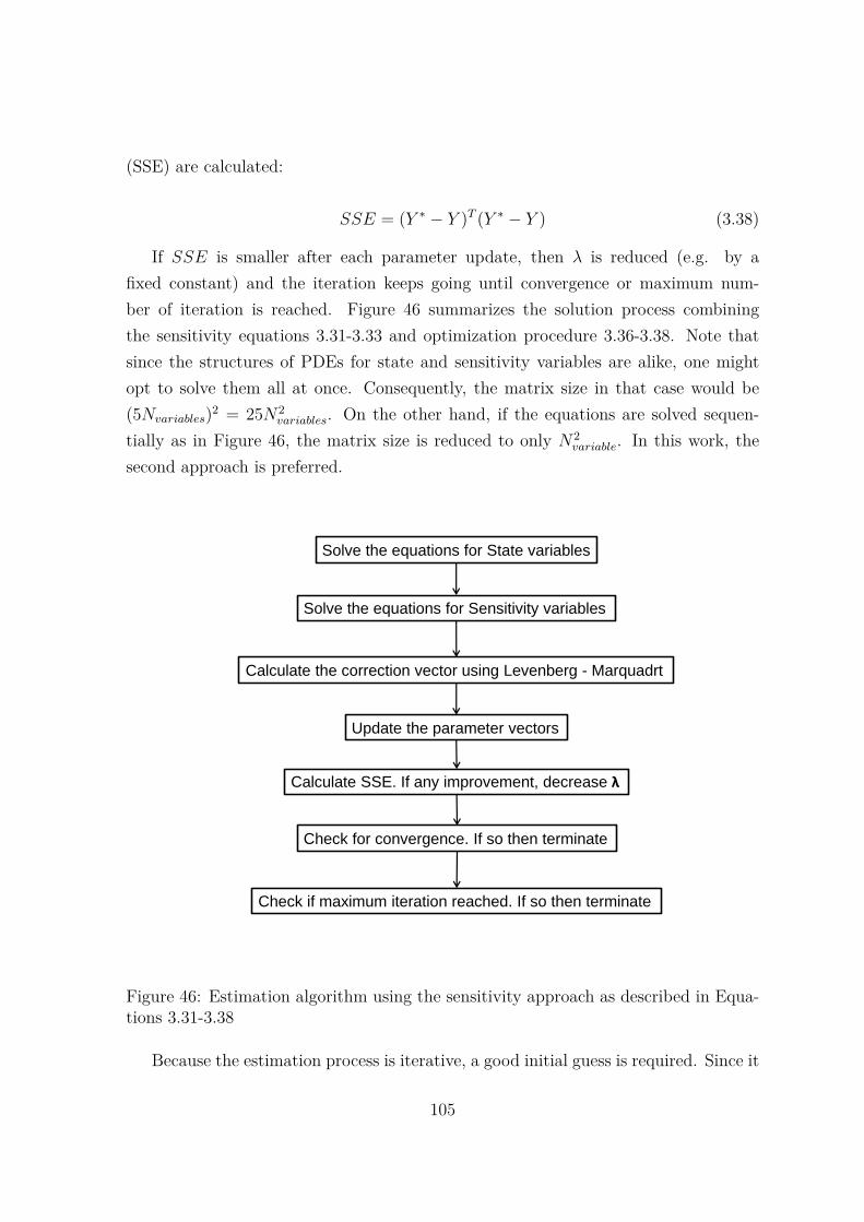
(SSE) are calculated:

SSE = (Y ∗ − Y )T (Y ∗ − Y ) (3.38)

If SSE is smaller after each parameter update, then λ is reduced (e.g. by afixed constant) and the iteration keeps going until convergence or maximum num-ber of iteration is reached. Figure 46 summarizes the solution process combiningthe sensitivity equations 3.31-3.33 and optimization procedure 3.36-3.38. Note thatsince the structures of PDEs for state and sensitivity variables are alike, one mightopt to solve them all at once. Consequently, the matrix size in that case would be(5Nvariables)2 = 25N2

variables. On the other hand, if the equations are solved sequen-tially as in Figure 46, the matrix size is reduced to only N2

variable. In this work, thesecond approach is preferred.

Solve the equations for State variables

Solve the equations for Sensitivity variables

Calculate the correction vector using Levenberg - Marquadrt

Update the parameter vectors

Calculate SSE. If any improvement, decrease λ

Check for convergence. If so then terminate

Check if maximum iteration reached. If so then terminate

Figure 46: Estimation algorithm using the sensitivity approach as described in Equa-tions 3.31-3.38

Because the estimation process is iterative, a good initial guess is required. Since it

105

Initial Value Final Value Starting SSE Optimized SSE

[0.01, 0.5, 0.23] [0.00144, 0.705, 0.234] 9.27 0.91[0.01, 0.5, 0.24] [0.00135, 0.662, 0.245] 9.70 0.508[0.01, 0.5, 0.25] [0.00129, 0.607, 0.257] 10.17 0.58[0.01, 0.5, 0.26] [0.00125, 0.545, 0.268] 10.69 1.13[0.01, 0.5, 0.27] [0.00123, 0.482, 0.278] 11.34 1.99

Table 11: Initial guesses and final optimal sets. In Levenberg-Marquardt, κ = 0.01,maximum iteration is set to 200 and λ is decreased by 1.5 everytime SSE is reducedto maintain stability of the updating step 3.37. The orders in each set are [k0, α, E0].Since Eguess

0 is estimated to be about 0.28 from Figure 45 so initial guesses are takento be smaller than that value. Note that the true values are [0.001, 0.65, 0.25]

0 50 100 150 200

0

2

4

6

8

10

12

SSE

Number of Iterations

Best 2nd Best

Figure 47: SSE is progressively minimized as the number of iterations increase.Atthe final iteration, the best two initial sets yield SSE values significantly smaller incomparison to the rest

106

is not possible to quantify the goodness of a guess, a common method is to use multi-starting points and record the best solution. Furthermore, physical intuition is alsouseful in constructing these initial guesses. For the current problem, this constructionprocess is described as below.

From Sobol analysis that the initial guess of E0 influences the outcome of theestimation process most significantly. For fast electrochemical kinetics, E0 can beapproximated by the potential at the mid-point between the two peaks:

Eguess0 = (Epf + Epb)/2 (3.39)

however, the wide peak separation (Figure 45) signifies slower kinetics and this mid-point value should therefore be larger than E0. For k0, a large value (i.e. fast kinetics)is simply assumed. Furthermore, for the charge transfer coefficient, a symmetricalprocess is initially chosen , i.e. α = 0.5. Table 11 summarizes the initial guesses andresults of applying 46 to the synthetic data generated. Figure 47 shows the decreaseof SSE as a function of iteration number. Using the original values listed in Table10, rows 2 and 3 of Table 11 differ from these correct values by [35%, 1.85%, 2%] and[29%, 6.61%, 2.8%] respectively. In addition to SSE, based on the parameter rankingresult from Sobol’s analysis, row 2 contains the better result because the parameter E0

is closer to the presummed true value. In practice, the true values of these parametersare rarely known, so a good rule-of-thumb is to average the best 2 results.

In conclusion, the above results show that it is possible theoretically to recover[k0, α, E0] to a fair degree of accuracy. This can be accomplished using only a singleset of data and neglecting detailed knowledge about the capacitive current. At thispoint, it is verified that [k0, α, E0] parameters are estimable as suggested at beginningof this section. However, due to inherent non-identifiability, all these estimations areobtained with some degree of error. Finally depending on circumstances, one mightbe interested in parameter Cdl but the above analysis emphasizes role of primaryparameters in Butler-Volmer model. To complete the experimental design study for adiffusional system, the final section considers the computation of parameter statisticsvia MCMC Bayesian-framework.

107

3.5 MCMC Simulations

Section 3.4 shows that it is possible to recover the Butler-Volmer model parametersfrom a single set of data using optimization approach. The underlying assumption hereis that each parameter is a single-valued scalar which minimizes SSE function. Yetmost optimization routines only produce point estimates in parameter space, namely asingle set of parameters which optimize the error function SSE, where each parameterhas an associated distribution or interval. Such information is also more representativeand informative than the original point estimate.

In the Levenberg-Marquardt equation, co-variances and standard deviations aredetermined by using the optimal SSE. If a Jacobian matrix is available, these credibleintervals can be constructed via the use of t-distribution[143, 170]. It is noted thatthese calculations require a linear model, which is usually achievable by linearizing thecurrent non-linear model around the optimum set.

Another popular approach is based on Bayesian inference framework [171]. Equa-tion 1.38 states that:

π(θi|data) ∝ p(data|θ) πi(θi)

for each parameter θi. If the error ϵ = ydatai − ymodel

i is assumed to be normally dis-tributed with constant variance σ2, the maximum likelihood estimate (MLE) p(data|θ)is usually expressed as:

p(data|θ) ∝ (σ2)Ndata/2 exp(− 12σ2

Ndata∑1

(ydatai − ymodel

i )2) (3.40)

recognizing the summation as the SSE function, this simplifies to:

p(data|θ) ∝ exp(−SSE

2σ2 ) (3.41)

The overall objective is to compute π(θi|data) given the MLE 3.41 and prior dis-tributions πi(θi). Since no analytical formula is generally available for the posteriors,Monte Carlo calculations is often employed to calculate p(data|θ). However, thereare more options in sampling parameter samples from the priors πi(θi). A reliablemethodology is based on Markov Chain sampling [172].

Considering each collection θ as a “state”, in Markov Chain theory, θ(n+1) is de-pendent only on the previous state θ(n) where n denotes the time step or sampling

108

number. Theoretically after sufficient number of sampling steps, θ would converge toa stationary state which can be viewed as the representative of the chain θ(i). It iscomputationally efficient to use Markov Chain framework because i) only the mostrecent state is relevant and ii) the chain is guaranteed (at least in theory) to con-verge, comparing to the brute-force strategies in which the samples are completelyrandomized at each iteration n.

Algorithm 3.4 The Random Walk Metropolis Algorithm to calculate the posteriordistributions π(θ|data). Markovian property is assumed so that θnew is sampled onlyfrom θold at each step

Initialize the set θ∗ which minimizes the SSE. θ∗ can be taken directly from theoptimization routineEstimate the variance σ2

Calculate SSEold = SSE(θ∗)Calculate the Jacobian J either numerically or analytically. Using the sensitivityapproach, J can be taken directly from the final stepCalculate the Covariance Matrix C = (JT J)−1 ∗ σ2

Decompose C using Cholesky factorization C = RT ∗ Rfor n = 1 : NChain Length do

Sample vector z = [zi], i = 1, 2, ..., Nparameter and zi ∼ N(0, 1) (N(0, 1) is thenormal distribution with mean 0 and variance 1Compute the new parameter set θnew → θnew + R ∗ zSample a random variable u from the uniform distribution U(0, 1)Solve the forward problem using θnewCalculate SSEnew using data from the forward problem aboveCalcuate Acceptance Probability Paccept = min(1, exp(−1

2SSEnew−SSEold

σ2 ))if u < Paccept then

Set θold → θnewSet SSEold → SSEnewSet θn → θnew

elseSet θn → θoldSet SSEnew → SSEold

end ifend for

The basic algorithm is presented in Algorithm 3.4. This algorithm is largely basedon reference [152] and often refereed to as the “Random Walk Metropolis”. The actualdata variance is assumed to be unknown and can be estimated by the following formula:

σ2est = SSE(θ∗)

Ndata

109

which can be easily seen by differentiating 3.40 with respect to σ2 and setting thederivative to 0. A slightly different computation is used in this work:

σ2est = SSE(θ∗)

Ndata − Nparameter

and when Ndata ≫ Nparameter (such as the present case) then the two formulaeagree with almost no significant numerical difference.

In Algorithm 3.4, the sampling steps assumes the new sample θ(n+1) is normallydistributed around the previous set θ(n). This choice implies that each individual pa-rameter has a unimodal distribution. The priors (normal distributions in this case) willconsequently lead to posteriors which are also single modes. This fact illustrates theimportance of gaining some external knowledge about the parameter before proposingits corresponding prior. For example, a parameter with a potential bi-modal distribu-tion could have its priors constructed from a mixture of two normal distributions 3.42(p is a scalar factor satisfying 0 < p < 1):

p N(µ1, σ2) + (1 − p) N(µ2, σ2) (3.42)

which signifies that the parameter has two means. However, it is clear that multi-modal cases will struggle to locate a sensible start θ∗ in the optimization routine.Furthermore, the physical mechanism for the existence of such multi-mode behaviourmust also be explained. The current work opts for single modal distributions for eachparameter under consideration.

The Algorithm 3.4 uses a chain length of NChain Length = 50000. The bottle neckis probably due to the repetition when solving the diffusion equations with every newset of parameters generated. The starting sample are taken from row 2 of Table 11along with relevant information of Jacobian matrix and SSEold. An important issuewith any post-MCMC calculations is to decide a “burn-in” length. This means acertain number of samples, especially those at the beginning of the chain need to bediscarded. This practice reduces the auto-correlation so that later samples are notinfluenced by earlier ones. Furthermore, by using a burn-in length, the focus is placedon the chain section exhibiting convergent behavior. In the current case, 10% or5000 samples are discarded. The practice of “chain thinning”, which saves every fixednumber of samples rather than the whole chain, is not pursued in this study becausechain burn-in is believed to be more important.

The computational results are summarized in Figures 48-50. The histogram in each

110

figure confirms that the convergent parameter sample is significantly closer to theiroriginal values. The corresponding means and credible intervals are included in Table12. In addition, the strength of correlation among parameter pairs is visualized inscatter diagrams 51- 53. While there are weak correlations in pairs (k0, α) and (k0, E0),there is a strong negative correlation between E0 and α. The observation is confirmedby calculating the corresponding correlation efficient, which is approximately −0.97.Although some of the credible intervals did not contain the true values, the differencesbetween the means and the true values are all within 6%.

Parameter Mean 2.5% Quantile 97.5% Quantile 95% Credible Intervalk0 0.00104(6) 0.00103(4) 0.00105(8) [0.00103, 0.00106]α 0.652(8) 0.652(0) 0.653(7) [0.652, 0.654]E0 0.250(4) 0.249(8) 0.250(9) [0.250, 0.251]

Table 12: 95% Credible Intervals for the Butler-Volmer model. Mean values arecomputed from the burn-in chain. Note that the mean value of each parameter isconsiderably closer to the true value [0.001, 0.650, 0.25] as listed in Table 10

0.00103 0.00104 0.00105 0.001060

1000

2000

3000

4000

5000

6000

7000

8000

Freq

uenc

y

Electrochemical Kinetic

Figure 48: Histogram for k0. Note that only data from chain no. 5000 − 50000 areused here. The rest are discarded during burn-in process as described in the text

111

0.6520 0.6525 0.6530 0.6535 0.65400

1000

2000

3000

4000

5000

6000

Freq

uenc

y

Charge Transfer Coeffcient

Figure 49: Histogram for α. Data from chain no. 5000 − 50000 are used

0.2496 0.2498 0.2500 0.2502 0.2504 0.2506 0.2508 0.25100

1000

2000

3000

4000

5000

6000

7000

8000

Freq

uenc

y

Equilibrium Potential

Figure 50: Histogram for E0. Data from chain no. 5000 − 50000 are used. Themajority of values distribute around 0.25, which is the assumed true value for E0

112

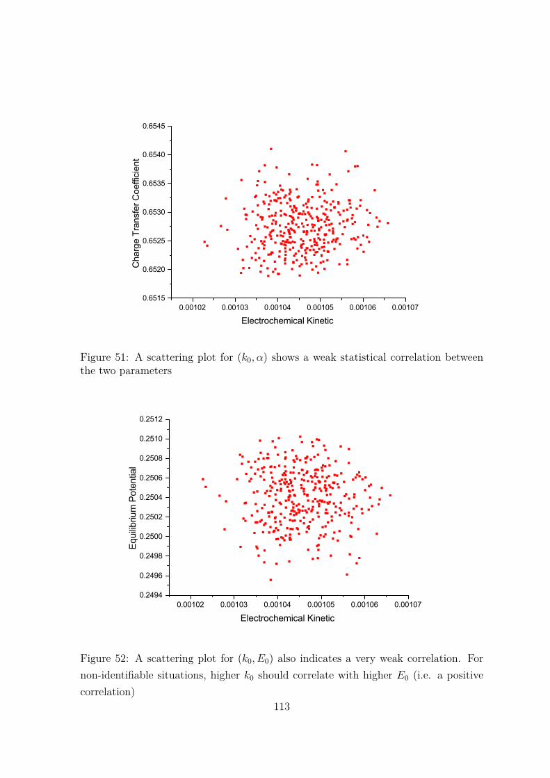
0.00102 0.00103 0.00104 0.00105 0.00106 0.001070.6515

0.6520

0.6525

0.6530

0.6535

0.6540

0.6545C

harg

e Tr

ansf

er C

oeffi

cien

t


Figure 51: A scattering plot for (k0, α) shows a weak statistical correlation betweenthe two parameters

0.00102 0.00103 0.00104 0.00105 0.00106 0.001070.2494

0.2496

0.2498

0.2500

0.2502

0.2504

0.2506

0.2508

0.2510

0.2512

Equi

libriu

m P

oten

tial


Figure 52: A scattering plot for (k0, E0) also indicates a very weak correlation. Fornon-identifiable situations, higher k0 should correlate with higher E0 (i.e. a positivecorrelation)

113

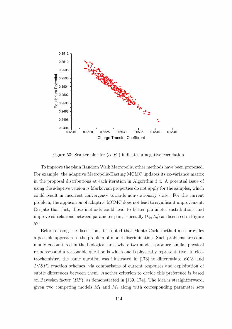
0.6515 0.6520 0.6525 0.6530 0.6535 0.6540 0.65450.2494

0.2496

0.2498

0.2500

0.2502

0.2504

0.2506

0.2508

0.2510

0.2512Eq

uilb

rium

Pot

entia

l

Charge Transfer Coefficient

Figure 53: Scatter plot for (α, E0) indicates a negative correlation

To improve the plain Random Walk Metropolis, other methods have been proposed.For example, the adaptive Metropolis-Hasting MCMC updates its co-variance matrixin the proposal distributions at each iteration in Algorithm 3.4. A potential issue ofusing the adaptive version is Markovian properties do not apply for the samples, whichcould result in incorrect convergence towards non-stationary state. For the currentproblem, the application of adaptive MCMC does not lead to significant improvement.Despite that fact, those methods could lead to better parameter distributions andimprove correlations between parameter pair, especially (k0, E0) as discussed in Figure52.

Before closing the discussion, it is noted that Monte Carlo method also providesa possible approach to the problem of model discrimination. Such problems are com-monly encountered in the biological area where two models produce similar physicalresponses and a reasonable question is which one is physically representative. In elec-trochemistry, the same question was illustrated in [173] to differentiate ECE andDISP1 reaction schemes, via comparisons of current responses and exploitation ofsubtle differences between them. Another criterion to decide this preference is basedon Bayesian factor (BF ), as demonstrated in [139, 174]. The idea is straightforward,given two competing models M1 and M2 along with corresponding parameter sets

114

θ1, θ2 and identical vector outputs y, the BF is defined as:

BF = p(y|M1)p(y|M2)

=∫

p(y|θ1, M1)p(θ1|M1)dθ1∫p(y|θ2, M2)p(θ2|M2)dθ2

Essentially, BF averages out vector y of each model over the specified parameterspace. Under equal prior preference, if BF ≫ 1 then M1 is posterior favored andthe reverse conclusion applies when BF ≪ 1. Factor p(y|θ1, M1) is computed fromthe same likelihood function 3.41. Future work therefore might reconsider ECE andDISP1 problem from this approach.

115


This chapter evaluates, from a theoretical perspective, the use of linear signals asan experimental design variable. By fixing the mass transport mode under diffusioncontrol, several aspects of Butler-Volmer kinetics were investigated.

Firstly, the model was extended to include the effects of solution resistance anddouble layer capacitance. The proposed solution is the combination of the explicittime formulation and a binary search. The identifiability function, η were then de-fined and optimized by stochastic sampling. The result shows that different sets canoften lead to very similar outputs. The large value of η reveals model non-linearityas well as compensating effects among parameter pairs, which in this case involveprimarily (k0, Ru), (E0, Ru) and (k0, E0). Monte Carlo optimization is employed dueto its implementation simplicity. The method further avoids the need for calculatingcomplicated derivatives.

To weigh the importance of each parameter, Sobol sensitivity indices were com-puted. The results indicate that equilibrium potential, kinetic constant and doublelayer capacitance (in that order) have the most influence on the the current output.Under the designed condition, namely small electrode areas and highly supportingionic electrolytes, uncompensated solution resistance is the least significant parameterand consequently eliminated from the model. In addition, quasi-Monte Carlo is appliedproperly in the sample hyper cube of the parameter space and better approximatesthe integration.

Using the simplified model, a theoretical problem involving parameter regressionwas proposed. The solution approach is deterministic, based on sensitivity equationsand gradients of the error function. Satisfactory results were obtained: the point-estimate was close to the presumed true value. Thus, even though the model isgenerally non-identifiable, the parameters are still uniquely estimated. A Bayesianframework was then applied to compute relevant statistics such asparameter meansand credible intervals. As a result, the plain Metropolis random walk was implementedand yielded improved final estimates. The method also allowed correlations betweenparameter pairs to be visually displayed.

The chapter results provide theoretical support for the use of a linear sweep as atool to retrieve the primary set [k0, α, E0] in the Butler-Volmer model, and this factis illustrated in inversion and MCMC computation steps. It is concluded that theapplication of this simple signal should yield reliable estimates of these parameters.

116

In addition, the signal’s conceptual simplicity, from both an experimental and simula-tion perspective, explains its popular use in practice. Another implication from theseresults is that the use of more complicated signals aims to improve the accuracy ofparameter estimates and statistics. However, it is emphasized that in reality, the for-ward model does not often describe data precisely, which undermines the effectivenessof both simple linear and complex waveforms.

Chapter 4 reconsiders the identifiability problem from a different viewpoint. Thelinear sweep voltammetry is fixed but the mass transport mode is now modified toinclude forced convective components. Because the identifiability function measuresthe one-to-one correspondence between the current output and the model parameters,the chapter’s goal is to investigate the influence of hydrodynamics on such correspon-dences.

117

Chapter 4

Hydrodynamic Tools for ModelIdentifiability and Kinetics Analysis

In previous chapters, the dominant mass transport mode was static diffusion, inducedby a local concentration difference. Hydrodynamic devices have proved popular dueto several reasons. Firstly, forced convection is more easily controlled and the con-vective flux is several times larger than the diffusion component. Furthermore, theseconditions often lead to establishment of the Levich equation, which is analyticallyuseful.

There are various configurations of hydrodynamic devices investigated in the lit-erature: most notably the rotating disk (RDE) and channel (CE) electrodes. Theselection of a configuration for a research study depends, to a significant degree, onthe ability to analyse the resulting flow pattern in such devices. Traditionally, RDEand CE are the most common because fluid mechanics theory for these devices arewell developed and analytically tractable [39].

This chapter has two parts. The first part continues the investigation into the iden-tifiability of Butler-Volmer kinetics using a model of rocking disk electrode (RoDE) - ageneralized mechanism of the RDE. A major objective is to compare the identifiabilityvalues of RoDE and RDE in the experimental design process and consequently illus-trate the role of the geometrical/mechanical factor. Model identifiability, as discussedearlier, measures the one-to-one correspondence between the current output and itsrespective parameter set. A large identifiability value signifies a poor correspondenceand implies difficulties with estimations and larger credible intervals. For Butler-Volmer model, though principal parameters (i.e. k0, α and E0) can be estimated asshown in Chapter 3, the added value here is to evaluate in advance the reliability of

118

such parameter estimates.The second part introduces a new hydrodynamic tool for studying electrochemical

transfer under viscous medium - the rotating drum electrode. Recent literature workhas paid special attention to unusual solvent environments such as ionic liquids, whichare both highly resistive and viscous. CE is not an ideal device choice, since pumping aviscous solution through a micro-sized channel is usually difficult. As we demonstratelater, a rotating drum device offers a convenient experimental mean and the solvent’seffect on the model identifiability is straightforwardly eliminated, which forms thebasis for an electron transfer kinetic study using various media.

Regarding the computational aspect, this chapter introduces the simulation soft-ware Comsol Multiphysicsr. This PDE engine is specifically designed to solve com-mon equations in physical sciences and engineering. Its strength lies in the user-friendly interface and a wide selection of libraries for different physics-based simula-tions. The package is based on Finite Element formulation, whose meshing procedureis completely automated and easily fine-tuned according to user requirements. Fur-thermore, the software possesses up-to-date and powerful linear algebra solvers, whichare the “bread and butter” of any numerical technique. Another major motivationfor using Comsol Multiphysicsr is the availability of the Computational Fluid Dy-namics (CFD) module. Because solutions of Navier-Stoke equations are required fordiffusion-convection transport 1.4, this module is evidently important and useful.

119

4.1 The Rocking Electrode - An Investigation

4.1.1 Verification of Levich expression for RDE

The rotating disk is a common hydrodynamic device used in electrochemical studies.In this configuration, the electrode casing is rotated at regular rates and the theoreticallimiting current is expressed by Equation 1.21:

IRDElim = 1.55 FAcR0D

2/3R f

1/2RDEν−1/6 (4.1)

The theoretical Levich expression is derived in two steps. Firstly, the velocityprofile is analytically approximated by von Karman and Cochran treatment. By con-sidering the section of flow near the electrode surface, the convection-diffusion equationis simplified to a 2nd order differential equation [2]. This equation is straightforwardlyintegrated to obtain the concentration field around the surface, which in turn permitsthe derivation of the current from Butler-Volmer expression 2.6.

The software Comsol Multiphysicsr is first used to validate the relation. Theaim of this confirmation step is to ensure an adequate set-up of the physics problemand convergence towards Equation 4.1. This test is common practice as it examinesthe previously developed in-house codes [66, 98]. Assuming sufficient supporting elec-trolytes are present, a migration flux in Equation1.7 is ignored. The computationalscheme using the software is as follows. Firstly, the velocity field is calculated fromthe incompressible Navier-Stoke equations using a CFD module. The field is thenexported to the convection-diffusion equation with electrochemical boundaries imple-mented in the dedicated Electrochemistry module. Furthermore, because the problemis rotationally symmetric, only a cross-section is considered (Figure 54).

Simulation parameters are summarized in Table 13. Because rb is much larger thanre, the electrode is essentially immersed in infinite solution. The respective boundaryconditions are listed in the bottom part of Table 13. Figure 55 shows linear sweepvoltammograms at different ωRDE’s. At large polarizing potentials, the total currentreaches a steady state, which is proportional to f 0.5

RDE according to Equation 4.1. This isattributed to the hydrodynamic influence which causes the diffusion layer thickness toremain constant. In addition, capacitive current Ic is ignored due to a combination ofa small electrode area (∼ 2 µm2) and slow scan rates (e.g. 10 mV/s). For the designedconditions, Sobol analysis from Chapter 3 applies, hence the solution resistance Ru

can be ignored from the model.

120

Name Symbol Value Units CommentElectrode Radius re 0.8 mm -

Holder Radius ro 4 mm -Beaker Radius rb 30 mm -Kinetic Rate k0 0.008 cm/s Quasi-reversible reaction

Equilibrium Potential Eeq 0.21 V -Boundary Fluid Dynamic Mass Transport

Beaker Wall/Bottom Zero Flux Zero FluxSymmetric Axis/Solution Interface No Flux No Flux

Electrode Holder Rotating Condition No FluxElectrode Surface - Butler-Volmer

Table 13: (Top) Parameter settings in rotating disk simulation. Electrochemical valuesare for the electron transfer reaction Fe(CN)4−

6 ↔ Fe(CN)3−6 + e−. The capacitive

effect is ignored. Diffusion coefficients are assumed to be equal at 0.65 ∗ 10−9 m2/sin aqueous medium. (Bottom) Respective boundary conditions for fluid and masstransport calculations

Symmetric Axis

Electrode Surface

Beaker Bottom

Beaker Wall

Solution-Air Interface

Electrode Holder

Insulator

Computation Domain

r

z

θ

Figure 54: Computational domain for the rotating electrode. The problem is essen-tially two dimensional due to rotational symmetry around r = 0 axis

121

-0.1 0.0 0.1 0.2 0.3 0.4 0.5-1

0

1

2

3

4

5

6

7Current/A

Potential/V

1.0 1.5 2.0 2.5 3.0

2

3

4

5

6

7

Stea

dy C

urre

nt/

f 0.5RDE/Hz0.5

Figure 55: Linear sweep voltammograms for rotating disk electrode at 50 (black),100 (red) and 500 (blue) rpms under scan rate of 10 mV/s (top) and the steady statecurrents are proportional to f 0.5

RDE for rpm in range 50−500 as confirmed in the Levichrelation 4.1

122

4.1.2 Derivation of Levich expression for the RoDE

The rocking electrode is a generalization of the above configuration. Instead of havinga fixed angular speed, the holder’s movement is modulated in an approximately har-monical fashion. A schematic drawing of this mechanism is shown in Figure 56. Theheart of this construction is the four-bar mechanism [175]. The blue circle is rotatedregularly as in the RDE, using the motor assembly. Such motions are then impartedto the red circle via a connecting crank. The red circle then moves back and forth,causing a rocking action. In this representation, the driver crank is L2 and the rockingdriver’s crank is L4. By setting L2 = L4, crank L4 motion reduces to the previousregular rotating pattern. Due to the constant acceleration and deceleration of theholder, the flow field is consequently non-steady and time-dependent.

Concept and applications of rocking electrodes were recently introduced into theliterature [176, 177].This work focuses on electro-deposition of copper metal and itsalloys onto different substrate materials. We demonstrate that such a back-and-forthmotion also leads to uniform mass transport effects. Compare this to the rotatingelectrode, the rocking mechanism does not require the contact brush. In addition,it allows a larger electrode area (to the order of several cm2) to be used. Thirdly,in electro-deposition, the presence of turbulent flow is noted to help dislodge the airbubbles which impede the deposition process.

This section has two aims. The first goal is to semi-analytically derive the Levichexpression for the rocking mechanism. It is evident that this expression is not onlyuseful for analytical purposes but also serves as a first comparison to the rotatingdisk. In addition, the expression is used as a normalizing factor for computing modelidentifiability in the following section. This fact is important to ensure the number iscompletely dimensionless according to Equation 3.11.

Name Symbol Value UnitsDistance between supports L1 40 mm

Rotating Crank L2 7 mmConnecting Crank L3 40 mm

Rocking Crank L4 10 mm

Table 14: Geometric lengths used for simulations of rocking mechanism in Figure 56

Because the electrode is now attached to the rocking section of the equipment, itis necessary to derive a relation between the rocking angular speed ω4 = dθ4/dt andωRDE = ω2 = dθ2/dt. Using the vector identity:

123

Figure 56: A sketch of the equipment and its rocking mechanism (top right) and thesimplified four-bar mechanism used to approximate movements of the cranks (bottom)

124

−→AB + −−→

BC + −−→CD + −−→

DA = −→0

and projecting the above equation onto x and y axis respectively, one obtains:

L2cosθ2 + L3cosθ3 − L4cosθ4 − L1 = 0

L2sinθ2 + L3sinθ3 − L4sinθ4 = 0

taking the time derivatives of these equations leading to:

−L2ω2sinθ2 − L3ω3sinθ3 + L4ω4sinθ4 = 0

L2ω2cosθ2 + L3ω3cosθ3 − L4ω4cosθ4 = 0

and after simple manipulations, the connecting and rocking angular velocities are:

ω3 = dθ3

dt= L2

L3ω2

sin(θ2 − θ4)sin(θ4 − θ3)

(4.2)

ω4 = dθ4

dt= L2

L4ω2

sin(θ2 − θ3)sin(θ4 − θ3)

(4.3)

and because L2 is rotated at a constant speed:

θ2 = ω2t (4.4)

Equations 4.2, 4.3 and 4.4 together with initial conditions for angles θ2, θ3 and θ4

completely describe the four bar mechanism.Because the flow field is no-longer steady, the computation scheme is modified as

follows. Using a global ODE module, differential equations for the rocking mechanismare first solved. As a first approximation, the boundary velocity of the electrodeholder is expressed by ω4r and ω4 values are derived from ODE solutions. Because ω4

is time-dependent, so is the resulting flow profile. Finally, concentrations and currentsare computed from the convection-diffusion equation as in the case of the RDE.

The following calculations are carried out with a 2D axi-symmetric domain as seenearlier in the rotating disk. The implicit assumption is therefore the rocking action,which still retains some symmetric properties. This assumption is clearly not accurate

125

due to the time-varying nature of both flow and species fields. A proper calculationshould be three dimensional. After constructing the full 3D model and implementingseveral trial runs, it is realized that the computation was too demanding for thecurrent work station. Consequently, the axi-symmetric model is used in subsequentcalculations by default despite its theoretical incompleteness.

Geometric lengths for the mechanism are given in Table 14 . Other parametersare kept the same as in Table 13. Figure 57 shows rocking angle θ4 as a function oftime for ω2 = 50 rpm. As expected, the angle oscillates around the initial condition ofπ/2 in an approximately harmonic fashion. The frequency of the oscillation is not thesame as that of the rotating crank because for every full 360o rotation of L2, crank L4

completes the maximum rocking angle approximately twice. The rocking frequency istherefore about twice as large as the rotating frequency. This relationship is discussedin more detail below.

0 5 10 15 200.6

0.8

1.0

1.2

1.4

1.6

1.8

2.0

2.2

2.4

2.6

4/rad

Time/s

Figure 57: Rocking angle θ4 as a function of time for L2 = 7 (mm),L4 = 10 (mm) andω2 = 50 rpm. The initial angle is π/2 (dotted line). The variation is like a harmonicfunction. Consequently, the resulting flow field follows in the same manner

Figure 58 demonstrates a good agreement between the computational results andthe experimental data at various rotating rates ω2 = 50, 100 and 500 rpm. At large

126

excess potentials, the currents also become steady. The plot of limiting current versusf

1/2RDE confirms a linear correlation. There are two implications following this observa-

tion. Firstly, the plot confirms that the structure of mass transport layer under rockingand rotating motions must be similar, at least up to the rotation speed of 500 rpm. Asa consequence, an approximate expression for Ilim,RoDE should differ from Equation1.21 by only a constant.

To derive Ilim,RoDE, a semi-empirical form of 1.21 is first assumed:

Ilim,RoDE = kFAcR0D2/3R f

1/2RoDEν−1/6 (4.5)

whereas fRoDE is the rocking frequency and k is the unknown proportionalityconstant. The relation Ilim,RoDE ∝ ν−1/6 and Ilim,RoDE ∝ D2/3 are experimentallyconfirmed in [178], hence the proposed equation is dimensionally consistent. BetweenfRoDE = f4 and fRDE = f2, the following relation is used (because each expression isequal to π):

ω2 T2/2 = ω4 T4

where T2 and T4 are rotating and rocking periods respectively. Using the relationf = 1/T , one obtains:

f4 = 2f2 (ω4/ω2) (4.6)

Figure 59 shows the variation of the ratio ω4/ω2 at two rotation speeds 50 and 500rpms. Though there are more variations at higher frequencies, the numerical rangeremains constant. It therefore means that the average scale of the ratio depends onlyon the rocking mechanism geometry:

Π = avg|ω4/ω2| = f(L2, L4) (4.7)

Regarding the top graph in Figure 59, the upper and lower sections reach 0.7 andabs(−0.77) = 0.77 respectively, yielding an average value of Π = (0.7 + 0.77)/2 =0.74. A similar figure is obtained for the bottom graph. It is noted that this scalecan also be approximated by simply taking the ratio between rotating and rockingcranks L2/L4 = 0.7, which further confirms the relation 4.7. Equation 4.6 is moreappropriately written using the scale notation Π = Π(L2, L4):

127

0.0 0.1 0.2 0.3 0.4 0.5-1

0

1

2

3

4

5

Col

lect

ed C

urre

nt/µ

A

Applied Voltage/V

1.0 1.5 2.0 2.5 3.01.0

1.5

2.0

2.5

3.0

3.5

4.0

4.5

Num

eric

al L

imiti

ng C

urre

nt/µ

A

Rotating Frequency 1/2/(Hz)1/2

Figure 58: (Top) Numerical (continuous) versus experimental (dashed) linear sweepvoltammetries for different regular rotating rates ω2 (rpm): 50 (black), 100 (red) and500 (blue) at scan rate of 10 mV/s. The numerical data are obtained by solving theconvective-diffusion equation 1.4 coupled with simple electron transfer reaction. Thecomputational approach is the same as in the case of RDE. (Bottom) Plot of Ilim,RoDE

against rotating frequencies f 1/2 showing a linear correlation similar to that of rotatingdisk (line of best fit (dashed red) has R2 = 0.9998 and slope of 1.451 ∗ 10−6)

128

0 2 4 6 8 10

-0.8

-0.6

-0.4

-0.2

0.0

0.2

0.4

0.6

0.8

Time/s

0 2 4 6 8 10

-0.8

-0.6

-0.4

-0.2

0.0

0.2

0.4

0.6

0.8

Time/s

Figure 59: The numerical ratio between rocking and rotating speeds ω4/ω2 at 50 (top)and 500 rpm (bottom). Notice that even though the frequency is increased, the ratioscale remains the same. In both cases, they are approximated by L2/L4

129

fRoDE = 2ΠfRDE

Ilim,RoDE = k ∗ (2Π)1/2FAcR0D2/3R f

1/2RDEν−1/6 (4.8)

The k value is estimated from the line slope in Figure 58 [179]:

k(2Π)1/2FAcR0D2/3R ν−1/6 = 1.451 ∗ 10−6

with A = 2 ∗ 10−6 m2, cR0 = 1mM, DR = 0.65 ∗ 10−9 m2/s and ν = 10−6 m2/s

yielding k = 0.82. The Levich-like expression (in terms of rotating frequency) underthe current set-up is therefore [178]:

Ilim,RoDE = FAcR0D2/3R f

1/2RDEν−1/6 (4.9)

It is clear that k is strongly dependent on Π. Furthermore, k can also be treated asa calibration factor from experiments. Because k = 1 < 1.55,the limiting current forrocking electrodes is less than that of rotating ones. In terms of analytical sensitivity,the rotating configuration has the advantage. However, a different proportionalityconstant shows that the rocking system allows for modifications of Levich form, whichcan be viewed as a benefit.

It is further argued that the constant 1.55 is the upper bound of all possible valuesfor k. If L2 < L4, then this case follows above calculations, which confirms thatk < 1.55. On the other hand if L2 > L4, the rocking angle θ4 is increased. In thiscase, a larger slope is expected for the factor k (2Π)0.5. Because Π = L2/L4 is now alsolarger, the resulting k is again less than 1.55. Another way of reasoning is that whenL2 > L4, rocking crank covers an angle which is complementary (by 2π) to the anglein the case L2 < L4. However, since the flow field is essentially the derivative of theangle, it should be the same regardless. Because the flow field does not change, theresulting mass transport and Levich equation is the same as before. In conclusion, therotating disk is the limiting case for all possible configurations of rocking mechanism,as far as Levich relations are concerned.

130

4.1.3 Comparison of Parameter Identifiability under RDE andRoDE Configurations

The goal of this section is to evaluate the hydrodynamic effect induced in RDE andRoDE configurations on parameter identifiability, specifically the set θ = [k0, α, E0].Because the electrode area is in the micro range and the scan rate is slow, the influenceof uncompensated resistance is thus insignificant from the Sobol sensitivity analysis.Furthermore, the magnitude of capacitive current is estimated as:

Ic = CdlAvscan ∼ 100 µF

cm2 (2 10−6cm2) 0.01V

s= 2 ∗ 10−12(A)

which leads to further exclusion of parameter Cdl.From Figure 43, Butler-Volmer parameters consequently remain the most signif-

icant. In addition, it is also known from chapter 3 that the total current is mainlyinfluenced by the pair (k0, E0). The identifiability calculation is carried out as out-lined in Algorithm 3.2. Two samples θ1 and θ2 are randomly generated from parameterspace. The current response corresponding to each sample is then computed and theresult is used to compute the identifiability number (Equation 3.11). Since currentsare dimensional, they are non-dimensionalized by the corresponding Levich expres-sions 4.1 and 4.9. Bounds for each parameter and simulation settings are listed inTable 15. Combinations of slow scan rate 10 mV/s, large end voltage Eend and ro-tating rate 100 rpm are to ensure the Levich limiting current is achieved under bothRDE and RoDE conditions (Figures 55 and 58).

Parameter Symbol Upper Bound Lower Bound Fixed Value Unitk0 10−3 10−6 - m/sα 0.7 0.3 - -E0 0.3 0.1 - V

Estart - - −0.1 VEend - - 0.6 Vvscan - - 0.01 V/sωRDE - - 100 rpm

Table 15: Bounds and simulation settings for Monte Carlo estimation of identifiabilitynumbers ηtransient and ηsteady. Nsample = 200 is used in the Algorithm 3.11, which isthe same for both RDE and RoDE calculations

A more detailed computational scheme for parameter identifiability is presentedin Figure 60. Since fluid and mass transport steps are uncoupled, the fluid dynamic

131

Generate Parameter pairs θ1 and θ2

Compute the flow field using CFD module

Compute mass transport for each parameter set θ

Compute current response from Butler-Volmer kinetics

Calculate Identifiability number from each current response

Record the number and parameter set into matrix result

Itera

tion

Figure 60: The flow chart for identifiability computation under hydrodynamic condi-tions. Because fluid dynamics and mass transport steps are independent, the formeris carried out outside the iteration loop. The common parameters for both configura-tions are listed in Table 15. The calculation is implemented in Comsol Multiphysicsr

and Matlabr interface environment

part is computed first. This minor change is insignificant for the RDE because thesteady state calculation is observed to be fast. On the other hand, for RoDE, thetime-dependent calculation requires considerably longer time to complete, hence themodification results in a significantly shorter time for each sample iteration. In ad-dition, two identifiability numbers are computed. The first is the usual number con-sidering the whole current curve. The second number only considers the steady statesection at high polarizing potentials. Tables 61 and 62 contain calculation results.

Considering first Table 61, RoDE configuration offers a better identifiability than

132

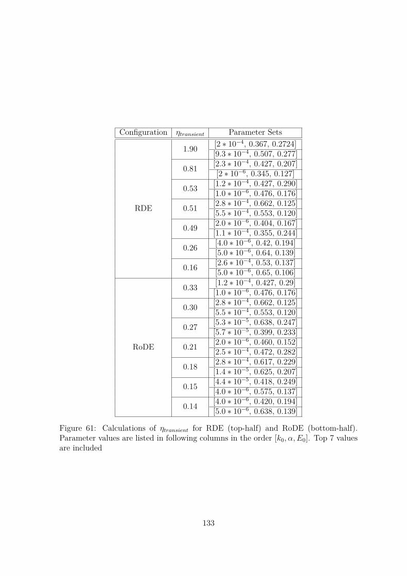
Configuration ηtransient Parameter Sets

RDE

1.90 [2 ∗ 10−4, 0.367, 0.2724][9.3 ∗ 10−4, 0.507, 0.277]

0.81 [2.3 ∗ 10−4, 0.427, 0.207][2 ∗ 10−6, 0.345, 0.127]

0.53 [1.2 ∗ 10−4, 0.427, 0.290][1.0 ∗ 10−6, 0.476, 0.176]

0.51 [2.8 ∗ 10−4, 0.662, 0.125][5.5 ∗ 10−4, 0.553, 0.120]

0.49 [2.0 ∗ 10−6, 0.404, 0.167][1.1 ∗ 10−4, 0.355, 0.244]

0.26 [4.0 ∗ 10−6, 0.42, 0.194][5.0 ∗ 10−6, 0.64, 0.139]

0.16 [2.6 ∗ 10−4, 0.53, 0.137][5.0 ∗ 10−6, 0.65, 0.106]

RoDE

0.33 [1.2 ∗ 10−4, 0.427, 0.29][1.0 ∗ 10−6, 0.476, 0.176]

0.30 [2.8 ∗ 10−4, 0.662, 0.125][5.5 ∗ 10−4, 0.553, 0.120]

0.27 [5.3 ∗ 10−5, 0.638, 0.247][5.7 ∗ 10−5, 0.399, 0.233]

0.21 [2.0 ∗ 10−6, 0.460, 0.152][2.5 ∗ 10−4, 0.472, 0.282]

0.18 [2.8 ∗ 10−4, 0.617, 0.229][1.4 ∗ 10−5, 0.625, 0.207]

0.15 [4.4 ∗ 10−5, 0.418, 0.249][4.0 ∗ 10−6, 0.575, 0.137]

0.14 [4.0 ∗ 10−6, 0.420, 0.194][5.0 ∗ 10−6, 0.638, 0.139]

Figure 61: Calculations of ηtransient for RDE (top-half) and RoDE (bottom-half).Parameter values are listed in following columns in the order [k0, α, E0]. Top 7 valuesare included

133

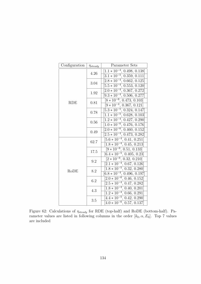
Configuration ηsteady Parameter Sets

RDE

4.26 [1.1 ∗ 10−4, 0.498, 0.138][3.1 ∗ 10−5, 0.359, 0.111]

3.04 [2.8 ∗ 10−4, 0.662, 0.125][5.5 ∗ 10−4, 0.553, 0.120]

1.92 [2.0 ∗ 10−4, 0.367, 0.272][9.3 ∗ 10−4, 0.506, 0.277]

0.81 [8 ∗ 10−6, 0.473, 0.103][9 ∗ 10−4, 0.367, 0.121]

0.78 [5.3 ∗ 10−5, 0.324, 0.147][1.1 ∗ 10−5, 0.628, 0.103]

0.56 [1.2 ∗ 10−4, 0.427, 0.290][1.0 ∗ 10−6, 0.476, 0.176]

0.49 [2.0 ∗ 10−6, 0.460, 0.152][2.5 ∗ 10−4, 0.473, 0.282]

RoDE

62.7 [5.6 ∗ 10−4, 0.41, 0.251][1.8 ∗ 10−4, 0.45, 0.213]

17.5 [9 ∗ 10−6, 0.51, 0.133][6.4 ∗ 10−5, 0.405, 0.23]

9.2 [2 ∗ 10−6, 0.32, 0.210][2.1 ∗ 10−4, 0.67, 0.126]

8.2 [1.8 ∗ 10−5, 0.32, 0.280][6.8 ∗ 10−4, 0.496, 0.197]

6.2 [2.0 ∗ 10−6, 0.46, 0.152][2.5 ∗ 10−4, 0.47, 0.282]

4.3 [1.8 ∗ 10−4, 0.40, 0.201][1.2 ∗ 10−4, 0.66, 0.291]

3.5 [4.4 ∗ 10−5, 0.42, 0.290][4.0 ∗ 10−6, 0.57, 0.137]

Figure 62: Calculations of ηsteady for RDE (top-half) and RoDE (bottom-half). Pa-rameter values are listed in following columns in the order [k0, α, E0]. Top 7 valuesare included

134

its RDE counterpart. This is because the largest ηtransient value corresponding to theformer is 0.33, which is significantly less than the maximum (i.e. 1.90) correspondingto the latter. A possible explanation is that the rising section in the voltammogram isvery sensitive to the parameter set [k0, E0]. In this case, introduction of the rockingflow increases this sensitivity and leads to better differentiation between two similarsets. Therefore, the analysis of electron transfer reactions using RoDE and the wholecurrent-voltage curve should yield a better result than that of RDE. On the other hand,the opposite trend is observed for ηsteady. From Table 62, it is evident that the deter-mination of Butler-Volmer parameters using the steady section of the voltammogramdoes not lead to a unique solution. This non-identifiability is demonstrated in rows2nd and 3rd as even totally different sets cause remarkably similar current responsesand consequently very large ηsteady. In addition, given that overall small identifiabilitynumbers were observed for RDE, this mode of hydrodynamic modulation provides areliable parameter differentiation and justifies its application in earlier work [65].

135

4.2 Voltammetric Analysis with Couette flow

This section analyses a new hydrodynamic device which is highly suitable for con-ducting measurements with viscous media. The outline of the experimental set-up isillustrated in Figure 63. A cylinder is part immersed in a solution and rotated byconnecting it to a motor at the back. A frequency controller then changes the rotationrates of the drum cylinder. The drum rotates and drags the solution into the gapbetween itself and the working electrode. In addition, the gap size can be adjustedby using a piezo-electric positioner. Physical dimensions of the devices are includedin Table 16.

This arrangement has several advantages over the rotating or channel electrode.Firstly, it does not require a large amount of solution to be transported during exper-iments. For solvent such as Polyethylene Glycol (PEG) or ionic liquids, such benefitstranslate into efficient use of energy. Thanks to the hydrodynamic effect, the currentresponse follows similar behaviour to that of rotating or rocking system, in addition,tunable micro gap facilitates direct transport of electroactive species to and from elec-trode surface. Finally, as shown below, the current magnitude is sufficiently smalland independent of solvent properties. This independence is to be in contrast withrotating configurations (Equations 4.1 and 4.8). Such benefits promise potential useof rotating drum in studies of electron transfer reactions for different redox couples,solvent and electrode materials, which so far has been limited to diffusional regime inprevious studies [37, 180].

Parameters Range of Values Units Explanationhc 50 − 500 µm Gap between cylinder and electrodeω 50 − 500 rpm Cylinder rotating frequencyhd 2 cm Cylinder Thicknessde 250 µm Electrode Diameterdc 4000 µm Electrode Casing Diameterd 5 cm Cylinder Diameterρ 1127 kg/m3 PEG Solution Densityµ 0.043 Pa ∗ s PEG Solution Viscosity

DF c(CH2OH)2 1.4 ∗ 10−11 m2/s Diffusivity of Ferrocene Methanol in PEG

Table 16: List of experimental variables in the rotating drum experiment. The elec-trode material is Platinum (Pt)

136

Solution

Working Electrode

PiezoPositioner

Voltammetric Equipments

y

x

Figure 63: The rotating drum equipment. Schematic end-view (right) and enlargementof the central section with associated linear velocity profile (left). The solution isdragged into the gap via the rotating cylinder

4.2.1 Theoretical Analysis

Because the micro gap hc is considerably smaller than both casing diameter dc andcylinder thickness hd, it is reasonable to simplify the geometry to 2D as shown inFigure 63. Next it is useful to check the induced flow is indeed laminar within theparameter ranges. Comparing to water, PEG solution is highly viscous (about 40 timeswater’s viscosity) while the density is only about 13% higher, this fact thus permitsuses of rotation as high as 500 rpm. Taking the largest ω = 500 rpm = 52.36 rad/s.The maximum velocity at the drum tip is hence vmax = ωd/2 = 1.3 m/s and Reynoldnumber is estimated to be:

Remax = ρvmaxhc/µ = 1127 1.3 (500 10−6)/0.043 = 17

137

which is well below the threshold of 1000 for turbulent regimes and laminar flow istherefore expected under the above parameter ranges. Under Couette flow (enlargedsection of Figure 63), the top plane (cylinder) is slid at constant velocity U (m/s),whilst the bottom plane (electrode casing) is stationary. This results in a linear flowprofile which is expressed as:

u = Uy

hc

(4.10)

where the coordinates are as in Figure 13. Although Couette flow is conceptuallydifferent from the parabolic profile in CE (Figure 13), they are implicitly related. Bylinearizing the parabolic profile very close to the electrode plane, one obtains the exactEquation 4.10.

This section first derives an expression for ICouettelim assuming a rectangular geome-

try and uniform plane width, which can then be extended to other closed geometries.The derivation is essentially based on early works by References [181, 182]. Althoughsuch work considers both reversible and quasi-reversible limits, the limiting current isindependent of kinetic factors since at sufficiently high voltages, a uniform diffusionlayer is always formed. Consequently, the following derivation assumes fast electro-chemical reaction and only the voltage range in which mass transport has reachedsteady-state is considered. Under this assumption, the convective diffusion Equation4.11-4.14 becomes:

Uy

hc

∂ci

∂x= Di

∂2ci

∂y2 (4.11)

y → ∞ : cR = cR0 > 0, cO = cO0 = 0 (4.12)

y = 0 : DR∂cR

∂y+ DO

∂cO

∂y= 0 (4.13)

y = 0 : cR

cO

= exp(−nF (E − E0)RT

) = exp(−θ) (4.14)

Nernst relation (Equation 4.14) is assumed since the electrode kinetics is fast.Applying the variable transformation 4.15 (as suggested in References [181, 182]):

η = ( U

xhc

)1/3y (4.15)

138

and calculate each derivation in 4.11 in terms of η:

∂c

∂x= − ∂c

∂η(U

h)1/3 1

3y−1/3x−4/3

∂2c

∂y2 = ∂2c

∂η2 ( U

hcx)2/3

substituting the above expressions into 4.11 and simplifying:

13Di

η2 ∂ci

∂η+ ∂2ci

∂η2 = 0

Each of the above equation can be reduced to ODE by setting y = ∂ci/∂η. Solvingthese ODEs subjecting to 4.12:

cR − (cR)y=0

cR0 − (cR)y=0=

∫ η0 exp(− η3

9DR)dη∫ ∞

0 exp(− η3

9DR)dη

and a similar expression for cO. The integrals in denominator is calculated bychanging the variable again z = η3/9Di, i = R, O leading to Gamma function:

∞∫0

exp(− η3

9Di

)dη = (Di

3 )1/3∫ ∞

0z−2/3exp(−z)dz = (Di

3 )1/3Γ (1/3) = 1.857D1/3i

The numerator can be treated by series-expanding the exponent and integratingterm-by-term:

η∫0

exp(− η3

9DR

)dη = η − η4

36Di

+ O(η7)

Considering only the first order effect, the expressions for ci finally become:

cR − (cR)y=0

cR0 − (cR)y=0=

( Uxhc

)1/3y

1.857D1/3R

cO − (cO)y=0

cO0 − (cO)y=0=

( Uxhc

)1/3y

1.857D1/3O

Differentiating the above expression and calculating the flux at y = 0:

139

DR(∂cR

∂y)y=0 = 0.5384D

2/3R ( U

xhc

)1/3(cR0 − (cR)y=0)

DO(∂cO

∂y)y=0 = −0.5384D

2/3O ( U

xhc

)1/3(cO)y=0

Combining the last two expressions with 4.14:

DR(∂cR

∂y)y=0 = 0.5384D

2/3R ( U

xhc

)1/3cR0exp(θ)

exp(θ) + (DR/DO)2/3 (4.16)

Finally integrating 4.16 across the electrode surface:

I = nFw

xe∫0

DR(∂cR

∂y)y=0dx = 0.8076nFwD

2/3R U1/3h−1/3

c x2/3e cR0

exp(θ)exp(θ) + (DR/DO)2/3

taking the limit as exp(θ) → ∞:

ICouettelim = 0.8076nFwD

2/3R U1/3h−1/3

c x2/3e cR0 (4.17)

Expression 4.17 applies to the rectangular electrode and Comsol Multiphysicsr

was then used to confirm this relationship. The narrow gap is divided into two sectionscorresponding to the electrode section and upstream of the flow. These sections arethen discretized into rectangular elements with Nelectrode = 250 points to cover thesurface and Nupstream = 50 for the rest. The minimum elemental size is set at 10 nm toadequately resolve the diffusion layer. From Table 16, only the combinations (50 rpm,50 µm), (50 rpm, 500 µm), (500 rpm, 50 µm), (500 rpm, 500 µm) need to be simulatedand the rest is simply interpolation of these limiting combinations. Table 17 confirmsgood agreement between numerical and analytical currents. In all four cases, thepercentage difference is no more than 2%. Consequently for other combinations of(ω, hc), these currents do not differ significantly from each other.

For a common geometry such as circles, in order to apply Equation 4.17, thecircular shape is divided into many small rectangles as shown in Figure 64. If thediameter is 2r0, then the total current would become:

ICouette Circlelim = 0.8076nFD

2/3R U1/3h−1/3

c

∑Nrectangle→∞

wx2/3e

where Nrectangle denotes the number of rectangles and common factors have been

140

ω/rpm hc/µm Inumericallim Ianalytical

lim Inumericallim /Ianalytical

lim

50 50 2.53 ∗ 10−4 2.48 ∗ 10−4 1.0250 500 1.15 ∗ 10−4 1.15 ∗ 10−4 1.00500 50 5.47 ∗ 10−4 5.34 ∗ 10−4 1.007500 500 2.49 ∗ 10−4 2.48 ∗ 10−4 1.004

Table 17: Comparisons of numerical and analytical values for ICouettelim . Numbers in the

3rd column are results from Comsol Multiphysicsr and values in the 4th column arecalculated using the expression 4.17. Units of both currents are A/m

moved outside the sum, leaving only the terms which are relevant to the geometry.By normalizing W = w/r0 and Xe = xe/r0, the above equation is written as:


2/3R U1/3h−1/3

c r5/30

∑n→∞

WX2/3e

for a unit circle. By dividing the diameter into an even number of n pieces, thisis numerically calculated. Table 18 shows that the convergent value is 2.67 by upto 2significant figures. The limiting current for a circular disk thus becomes 4.18:


2/3R U1/3h−1/3

c r5/30 (4.18)

In general, the theoretical limiting current is independent of the medium viscositybut depends on the rotation frequency of the drum via tip speed U .

Number of Rectangular Divisions Total Sum ∑WX2/3

e

1000 2.6692000 2.6705000 2.67010000 2.670

Table 18: Calculating the numerical sums of the form W X2/3e for an unit circle. As

expected, the sum quickly converges as the number of divisions are increased

4.2.2 Comparison to Experimental Data

Two main experiments were carried out to verify the theory developed earlier. In thefirst experiment, the gap is held constant at 500 µm and the cylinder had varyingrotating rates within the range 50 − 500 rpm. The second experiment, on the otherhand, fixes the rotation rate at 50 rpm and systematically increases the gap size from

141

𝑥𝑒

𝑤𝑒 2𝑟0

Figure 64: Division of circular disk into many thin rectangles and the relation 4.17 isapplied to each element. The approach is generalized to any closed geometrical shape

50 to 500 µm. Equation 4.18 is used to compute theoretical currents. Results for theexperiment are shown in Figure 66. Note that both currents shown are the steadystate values. In addition, the current’s small magnitude is attributed to the fact thatthe diffusion coefficient in PEG solution is at least two orders of magnitude below thatin water. Furthermore the nA scale also implies that the effect of resistance will beessentially ignored. Considering the applied potential including Ohmic resistance:

Eapply = (E − E0) − IRu

The magnitude of this loss term for a highly resistive media is estimated as:

IRu ∼ 60 (nA) ∗ 10000(Ω) = 6 ∗ 10−4 (V )

142

thus for most of the potential point reasonably far away from E0, the overpotentialE − E0 ≫ IRu the applied potential is thus effectively the same as in the case ofRu = 0. Combining with Equation 4.18, it can be concluded that the voltammogramis not sensitive to solvent choice, apart from sections very close to E0.

Figure 65: Proposed chemical changes on Pt surface at potetential below 0.45 (V )(left) and above 0.45 (V ) (right). At low potential, there is a weak attraction betweenthe surface and PEG molecules. At higher potentials, stronger bonds are formed andresult in a more regular structure

It is evident from Figure 66 that theoretical values overestimate actual data byabout a factor of 2 [183]. A possible explanation was proposed as follows (Figure 65)[184]. At low potentials, the solution remains a uniformly fluid. At potentials above0.45 (V ), the electrode layer is positively charged, which then forms a bond with theoxygen atom in PEG molecules. Consequently, a thin layer of semi-fluid materialis formed and the diffusivity of 1-1 Ferrocene Dimethanol is further reduced insidethis layer. Another reason for correction of species diffusivity is as follows. Inside aninfinite medium, the diffusion coefficient is DF c(CH2OH)2 (Table 16) because diffusionprocess is three-dimensional. Due to the applied flow, the process now occurs mainlyin the direction orthogonal to the electrode surface. Despite this discrepancy, thetheoretical result still serves as an upper estimates of the actual data as the two setsfollow similar trends. Consequently, the above discussions regarding solvent effectsstill apply. The device is therefore potentially useful as an alternative hydrodynamictool beside the traditional diffusion-controlled micro disk.

143

0.8 1.0 1.2 1.4 1.6 1.8 2.0 2.2

20

25

30

35

40

45

50

55Current/nA

f1/3/Hz1/3

12 14 16 18 20 22 24 26 2815

20

25

30

35

40

45

50

55

Current/nA

h-1/3c /m-1/3

Figure 66: Limiting current versus cube root of frequency at fixed hc = 500 (µm) (top)and inverse cube root of micro gap at fixed ω = 50 (rpm). Black points are calculatedusing the expression 4.18 and red points are experimental values. Dashed line is thefitted Levich expression

144


This chapter examines the influence of hydrodynamic factors on the identifiability ofprimary parameters in Butler-Volmer model. First a computational package based onFE formulation, is introduced to verify the theoretical limiting current with RDE. Thework then focuses on the analysis of a recent RoDE device, which allows approximateharmonic modulations of the electrode movement. The mechanism was analysed usingthe well-known 4-bar geometry. Characteristic equation, namely the Levich relationfor the configuration, was derived from combinations of simulation and scaling analysis.Furthermore, the result was in good agreement with experimental data, confirming theadequacy of simplified 2D axisymmetric model instead of using a full 3D construction.However, for higher rpms, the latter is required due to increasing turbulence and theflow dependence on angular positions.

By employing small electrode areas and a slow scan rate, the effects of solutionresistance and capacitive currents became negligible. These factors were consequentlyleft out in the model by the same argument from Sobol analysis in Chapter 3. Identi-fiability values were computed and compared for RDE and RoDE using two numbersηtransient and ηsteady. It was evident that RoDE offers a better differentiation of theButler-Volmer parameter set when the whole current curve is considered. On the otherhand, for the steady state section, RoDE’s ηsteady was much bigger than that of RDE,showing the induced non-steady flow field leads to poor identifiability. Therefore, toregress the Butler-Volmer model parameters, RoDE is suitable using the total currentresponse while RDE produces more reliable results for the steady part of the curve.

The last section investigates the rotating drum electrode as an alternative analyti-cal device for highly viscous and resistive media. The Levich equation was derived fromfirst principles using mass transport and simplified Nernstian kinetics. Comparisonswere made against experimental results, whilst some discrepancy was observed, thedata sets agree qualitatively in terms of trends and magnitudes. The rotating drumis thus a promising tool in experimental design due to two main reasons. Firstly, thecurrent response is theoretically independent of solvent properties, apart from speciesdiffusion coefficient. Secondly the developed flow is also steady state, which sharessimilar characteristics of RDE. Consequently, the device should perform similarly asRDE regarding the identifiability and estimation aspects. The work here forms atheoretical basis for future studies, especially those involving heterogeneous electrontransfers in ionic liquids.

145

Chapter 5

Elicitation of ElectrocatalysisMechanism via Large amplitudeSinusoidal signals

The work thus far has focused exclusively on experimental design methods to analysethe simple redox reaction. Chapters 3 and 4 covered two major experimental tools,namely the applied potential (i.e. linear sweep and cyclic voltammetries) and controlof mass transport (diffusion versus induced mechanical convections). Although E

mechanism is often studied, other associated homogeneous reactions can also occurand are useful for analytical purposes.

A special focus of this chapter is the self-catalytic EC ′ mechanism. There areseveral motivations for this investigation. The first reason is due to the promisingapplication of the mechanism to detect H2S in commercial oil wells. This applica-tion is valuable when monitoring the crude feed quality, product control as well as rigsafety. H2S is a highly flammable and toxic gas under normal conditions. In addition,concentrations at levels above 1000 parts per million could cause fatal death. Hy-drogen sulphide often biologically originates from the decay of organic matter underthe presence of anaerobic bacteria. Furthermore, geochemical conditions (i.e. hightemperature and pressure) also produce the gas by reactions of methane with calciumsulphate [185]:

CaSO4(s) + CH4(g) → H2S(g) + CaCO3(s) + H2O(l), T ∼ 285°F

Classically, H2S is often detected using iodometric titration, which proceeds via

146

the following reaction scheme [186]:

H2S + I2 → 2HI + S

2S2O2−3 + I3− → S4O

4−6 + 3I−

Modern approaches include kinematic spectroscopy, chromatography [187] andelectrochemical techniques. Electrochemical methods have recently become more pop-ular, which is attributed to their sensitivity and reliability. Amperometry and poten-tiometric are most commonly used for sulphide sensing purposes [188]. Efforts havealso been directed towards the modifications of electrode materials as well as care-ful selection of electrocatalysts to improve reaction kinetics [189, 190]. Because ofits molecular structure, H2S, is generally electro-inactive, hence detections via directoxidation or reduction (i.e. E mechanism) is not feasible. The EC ′ scheme offers asimple but elegant route for such a detection that is still based entirely on previousknowledge of electrochemistry.

The second motivation lies in the use of sinusoidal signal as a mean to elicit theeffects of catalytic reactions. As in Figure 38, under normal cyclic voltammetry andplanar diffusion, a well-known phenomenon termed split-wave is observed and theeffect is considered as the signature of catalytic kinetics. Recently, the same phe-nomenon was reported for square wave [191]. Furthermore, square wave signals can,in theory, be decomposable into the sums of harmonic components. These observa-tions, therefore, lead to a question of whether simple harmonic signal could producethe similar effect. The question implies two interesting points. Firstly, it demonstratesthe inclusion of sinusoidal pertubation is a useful analytical complement to the tradi-tional voltammetry. Second, given the fact that AC technique was previously appliedto evaluate single electron transfers, EC and similar catalytic mechanisms [58][59],it should also be applicable to EC ′ mechanism. However, to our best knowledge, nosuch study was carried out in previous literature.

A series of papers studies general theory of self-catalytic process EC ′ in greatdetails [192–194]. A notable result is the split polarography waves, which were subse-quently confirmed by experiments [195]. The split-wave under micro-fluidic conditionswas numerically simulated and current enhancement was confirmed as a result of highcatalytic turnovers [196]. Unlike diffusion-limited cases, a “shoulder” is observed andvery large homogeneous kinetics are required (Figure 67) [62]. The same mechanism

147

and responses were again observed for an array of nano-spherical electrodes under awide range of reaction kinetics, surface coverages and substrate concentrations [168].

Figure 67: Linear sweep voltammetry at a flow channel for increasing catalytic reactionrates K and a slow scan rate

The chapter is structured as follows. Firstly, additional background on AC voltam-metry, based on signal processing concept, is provided. Next the technique is appliedto study the basic E reaction. The section explains the fundamentals of the simula-tion methodology, data analysis and the importance of the FFT algorithm to extractharmonic currents. Subsequent sections focus on the EC ′ mechanism under large-amplitude AC modulation at different electrode sizes under diffusion control. Finally,the investigation is shifted to hydrodynamic conditions using channel electrodes. Todemonstrate the technique’s effectiveness under both diffusion and micro-fluidic condi-tions, relevant experimental data are supplemented to support the simulation results.

148

5.1 Signal Processing Concept of AC Voltammetry

The work explores the use of the AC voltammetry technique as an experimental de-sign tool. Another less commonly used term is FFT voltammetry, but the two shallbe used interchangeably. In the simplest form, FFT voltammetry utilizes a single-frequency sinusoidal-signal as a perturbation, on top of the traditional voltammetricsignal. Expressed in time domain, the AC signal is often generated via the followingsuperposition:

Eapply = Edc + Eac (5.1)

Eac = E sin(2πft) = E sin(ωt) (5.2)

E and f determine the perturbing signal amplitude and frequency respectively.The usual linear voltage, Edc, whose expressions are denoted by Equations 2.40 and2.42:

Edc = Estart + vscant, 0 ≤ t < tscan

Edc = Evertex − vscan(t − tscan), tscan ≤ t < 2tscan

The potential Edc serves as a “base-line” signal to drive electrochemical reactionsback and forth, and its presence is essential in AC voltammetric technique. SinceEac only varies slightly in comparison to Edc, application of such sinusoidal signalalone cannot significantly affect the electron transfer kinetics and consequently theassociated diffusion layer.

Under presence of Eac, the resulting current is considerably altered. The totalcurrent now contains the usual current due to Edc (which will be referred to as IdcorDC current) and several sinusoidal varying currents at the same or higher frequencies.The real value of the AC technique is due to the presence of these additional currents,which are commonly referred to as harmonics.

Consider a Single Input Single Output (SISO) black box model of electrochemicalsystem in Figure 68. If the DC signal or Edc is input to the box, one obtains the usualIdc output. Notice that this DC current contains two components: The Faradaic andcapacitive currents as remarked in Chapter 1:

149

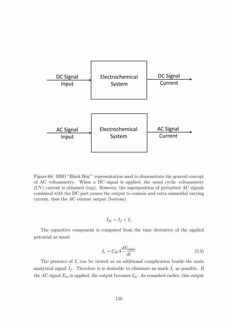
Electrochemical System

DC Signal Input

DC Signal Current

Electrochemical System

AC Signal Input

AC Signal Current

Figure 68: SISO “Black Box”’ representation used to demonstrate the general conceptof AC voltammetry. When a DC signal is applied, the usual cyclic voltammetry(CV) current is obtained (top). However, the superposition of perturbed AC signalscombined with the DC part causes the output to contain and extra sinusoidal varyingcurrent, thus the AC current output (bottom)

Idc = If + Ic

The capacitive component is computed from the time derivative of the appliedpotential as usual:

Ic = CdlAdEapply

dt(5.3)

The presence of Ic can be viewed as an additional complication beside the mainanalytical signal If . Therefore it is desirable to eliminate as much Ic as possible. Ifthe AC signal Eac is applied, the output becomes Iac. As remarked earlier, this output

150

can be decomposed component-wise in time domain as follows:

Iac = Idc + I1(ωt) + I2(2ωt) + I3(3ωt) + ... (5.4)

where the currents I1(ωt), I2(2ωt), I3(3ωt), etc. are called the first, second, third har-monic respectively.Another reason for these names is because I1, I2, I3 has periodicalappearance at the principle frequency (f) and then multiple frequencies 2f, 3f andso on. The origin of currents at higher frequencies is worth further elaboration. Sup-pose that the (black box) electrochemical model is completely linear, then from linearresponse theorem [197, 198], Equation 5.4 is simplified to:

Iac = Idc + I1(ωt)

because there is only one input Eac at single frequency f and Idc is the same asbefore. Consequently the second, third and higher harmonic currents must be dueto non-linearity of the electrochemical model. This fact is easily verified because theboundary condition (e.g. Butler-Volmer equation) is the source of such non-linearity.

If Eac = 0 then all the capacitive current is caused by the gradient of the potentialEdc:

Idcc = CdlA

dEdc

dt

This capacitive current is clearly contained in Idc. Now if Eac is included, additionalcapacitive current arises due to sinusoidal potentials:

Iacc = CdlA

dEac

dt

For a linear system, it is evident that I1(ωt) must contain Iacc since the total

current is composed of Idc and I1(ωt) while Idc must contain Idcc . Now if the model

becomes non-linear, Iacc tends to be shared among the harmonics. Numerical and

experimental observations show that the current magnitude decreases as the harmonicorder increases. Therefore, it is expected that the distributon of Iac

c becomes smallerfor higher components. In other words, 2nd, 3rd, 4th etc. harmonics are less influencedby this sinusoidal capacitive current and more Faradaic in nature.

151

5.2 Single Electron Transfer under Fast Fourier Trans-form voltammetry

This section lays the theoretical foundation of the technique, which includes the basicsimulation methodology and outline of the FFT algorithm to extract the harmoniccurrents. Calculations are first performed with macro electrode to demonstrate themethod before more elaborate cases are considered. The simulation parameters arelisted in Table 19 for the generic redox reaction.

From the Table, the reaction is assumed to be reversible (i.e. fast kinetics). Undersuch conditions, the Butler-Volmer relation is reduced to the Nernstian equation,which is independent of either k0 or α. In addition, a medium value for the double-layer capacitance is selected, which is typical for the case of aqueous solution. Asusual, to minimize the effect of extra resistance, a small electrode area is used. In thesinusoidal perturbation, the work starts with relatively small amplitude E (10 mV inthis case) and the frequency is set at 3 Hz. The simulation scans through a potentialwindow between −0.1 and 0.6 V . The ratio between E and the potential range istherefore about 10 ∗ 10−3/0.7 ≈ 1%. A larger amplitude might be within 5 − 10% ofthe scanning potential range.

A typical expanding 1D meshing for the simulation is shown in Figure 69. As usual,nodes are concentrated near the left end where the electrode boundary condition isapplied. The smallest element size is set to be about 100 (nm) with the expandingcoefficient of 1.2. Given the parameters in Table 19, the diffusion layer is estimated tobe of the size 6 ∗ 10−4 (m) and thus adequate convergence is ensured with the currentsettings. In addition, the time stepping scheme is chosen to be “Strict”, meaningthat the time step is fixed at a constant value. The number of time points are thenselected to be power of 2, for example 216 in this case. The reason for this choice istwo-fold. First it speeds up the FFT analysis of Iac in the time domain. Secondly, theappropriate number of points need to be sampled for each wave cycle to distinguishbetween different frequencies. For example, considering two frequencies f1 and f2,and one of them is the multiple integral of the other (say f2 = 2f1), for convergentsimulations, more points are required per wave cycle for f2. This relation can beexpressed more precisely as follows. Assuming Ncycle is the number of points coveringeach sinusoidal cycle, then the minimum required number of time points is:

Nsimulation point ≥ Ncycle f tscan (5.5)

152

From 5.5, by assuming a fixed value for Ncycle (e.g. 100), the higher the frequencyand/or longer the scanning time, the more points will be needed. This also meansthat the total computational time also increases. Of course, other factors such ascomplexity of the governing equations, number of dimensions, non-linear sources etc.also contribute to such an increase.

Parameter Symbol Value UnitsDR 7.6 ∗ 10−10 m2/sDO 7.6 ∗ 10−10 m2/sk0 0.001 m/sα 0.5 −

Cdl 50 µF/cm2

E0 0.25 Vvscan 50 mV/scR0 1 mMcO0 0 mMA 0.01 cm2

Estart −0.1 VEvertex 0.6 VE 10 mV

ffundamental 3 Hz

Table 19: Parameters for numerical calculations of the E reaction. The simulation iscarried out in Comsol Multiphysicsr using the dedicated Electrochemistry module

Figure 69: A typical one dimensional finite element meshing for macro electrode cal-culations

Figure 71 presents the simulated current with the above settings. Algorithm 5.1presents the detail of extracting individual components from this total current. A criti-cal point in this algorithm is determining the NF irst Harmonic Index, NSecond Harmonic Index

and so on. These indices are found by simply plotting the absolute value (or two-sided power spectrum) of the vector Y after the FFT. Such two-sided spectrum notonly reveals the peaks corresponding to current components, but also their relativestrengths. The numerical positions of these peaks can then be taken as the harmonicindices (note that DC current has an index of 0). Currently, these numbers are man-ually read off the spectrum but future work could automate the process, for example

153

0 5 10 15 20 25 30-0.2

-0.1

0.0

0.1

0.2

0.3

0.4

0.5

0.6

0.7AC

Pot

entia

l (V)

Time (s)

E0

Figure 70: Applied AC Potential under amplitude E = 10 mV and f = 3 Hz. Thebase-line (CV) potential is plotted as the dark dash line. The equilibrium potentialE0 is also included. Whilst the CV potential fundamentally drives the reaction, ACsignal perturbs the process around a given potential and enhances the harmonics

via peak detection algorithm in time series [199].The numbers Ndc, NF irst, NSecond, etc. are simply heuristic choices. They are

selected so that all the elements corresponding to respective harmonics are completelycovered. The current work uses the following settings: Ndc = 20 and other Ns areset at 40. Although retrieval of only up to 4th harmonic is shown in the code, thesame procedure can be repeated to extract higher harmonics. Furthermore, the FFTand iFFT computations are extremely fast if the lengths L of the respective vectorsare powers of 2. In that case, the numerical computation is easily carried out viathe binary “dividing and conquer” approach [200, 201]. It should be noted that FFTcomputations are also available when the vector length is product of other primenumbers, but the power of 2 is the simplest and most intuitive case.

Figure 72 shows the single-sided spectrum obtaining from the FFT of the totalcurrent from Figure 71. By scaling the indices of the two-sided power spectrum, theone-sided power plot is easily obtained. In Figure 72, the first cluster at around 0

154

Algorithm 5.1 Harmonic Current extraction using FFT and inverse FFT (iFFT)functions. The algorithm is implemented in Matlabr, which already has the built-in routines for FFT and iFFT. Variable L denotes the length of the current vector.Harmonic up to the 4th is extracted but the methodology is easily extended to anyharmonic number

Extract the current vector from storage fileApply the FFT function Y → fft(current)Set Ydc = YSet the elements between Ndc and L − Ndc to 0Apply the iFFT function Idc → ifft(Ydc)Set YFirst Harmonic = YSet the elements of YFirst Harmonic in the following intervals to 0:[1, NFirst Harmonic Index − NFirst], [NFirst Harmonic Index + NFirst, L − NFirst Harmonic Index −NFirst] and [L − NFirst Harmonic Index + NFirst, L]Apply the iFFT function IFirst Harmonic → ifft(YFirst Harmonic)Set YSecond Harmonic = YSet the elements of YSecond Harmonic in the following intervals to 0:[1, NSecond Harmonic Index − NSecond], [NSecond Harmonic Index + NSecond, L −NSecond Harmonic Index − NSecond] and [L − NSecond Harmonic Index + NSecond, L]Apply the iFFT function ISecond Harmonic → ifft(YSecond Harmonic)Set YThird Harmonic = YSet the elements of YThird Harmonic in the following intervals to 0:[1, NThird Harmonic Index−NThird], [NThird Harmonic Index+NThird, L−NThird Harmonic Index−NThird] and [L − NThird Harmonic Index + NThird, L]Apply the iFFT function IThird Harmonic → ifft(YThird Harmonic)Set YFourth Harmonic = YSet the elements of YFourth Harmonic in the following intervals to 0:[1, NFourth Harmonic Index − NFourth], [NFourth Harmonic Index + NFourth, L −NFourth Harmonic Index − NFourth] and [L − NFourth Harmonic Index + NFourth, L]Apply the iFFT function IFourth Harmonic → ifft(YFourth Harmonic)Post-processing the data and plot the harmonics from Idc to IFourth Harmonic in timedomainConvert the harmonics in envelope format using Hilbert and Absolute functions andreplot them

155

0 5 10 15 20 25 30-3

-2

-1

0

1

2

3

Tota

l Cur

rent

/A

Time/s

Figure 71: Simulated total current in time domain using the settings from Table 19

frequency evidently corresponds to the DC component. In addition, there are signalsat the applied fundamental frequency of 3 Hz and the secondary (due to non-lineareffects) at 6 Hz. The secondary frequency is evidently very weak relative to the rest.

Closer inspection of Figure 72 reveals that the frequency peaks are not sharpbut instead spread over a narrow neighborhood of each frequency. These clusters offrequencies do not overlap, implying that harmonic currents are distinct and exclusiveof each other. Considering the principle f = 3 Hz, the signal power axis shows thatfrequencies in range 2.5 − 3.5 Hz are also present albeit at smaller magnitudes. Henceto be rigorous, the first harmonic I1(ωt) is not composed of a single frequency, buta sum of many waves with frequencies close to each other f ± f (f = 0.5 Hz).Physically, this phenomenon results in acoustics beat and I1 is essentially a beat ratherthan a pure sinusoidal wave. However to keep the context simple, this complication isnot considered further.

156

-1 0 1 2 3 4 5 6 7 8 9 10

0

10

20

30

40

50

60Si

gnal

Pow

er (A

bitra

ry U

nit)

Frequency/Hz

Figure 72: Single Sided Power spectrum of the simulated current above. This one-sided spectrum is derived directly from the two-sided counter-part by scaling withrespect to the frequency

By separating each element corresponding to the currents and applying iFFT func-tion as outlined in algorithm above, these harmonics are recovered and plotted out inFigures 73, 74 and 75. As noted earlier, the signal magnitude for the 2nd harmonic isconsiderably smaller than that of the 1st harmonic. There is a negligible peak at the3rd harmonic so the current is essentially 0. The fundamental harmonic possesses 1peak for the forward sweep between 0 and 14 (s) and an extra peak in the backwardscan (between 14 and 28 (s)). For the 2nd harmonic, the forward wave contains 2 peaksand so does the backward wave.

Figures 74 and 75 above are usually referred to as the full plots. Another way ofrepresenting these currents is to plot out just the envelope. A main advantage of theenvelope plots is the simplicity in information representation by retaining only the

157

0 5 10 15 20 25 30-1.5

-1.0

-0.5

0.0

0.5

1.0

1.5

2.0D

C S

igna

l/A

Time/s

Figure 73: Recovered DC signal from the AC current in Figure 71

main feature of the graphs. For a sinusoidal function, an envelope can be constructedby simply joining its local extremes [202]. In the current case, the hilbert functionis applied to the sinusoidal function in order to calculate the corresponding envelope.Furthermore, it is visible that the upper and lower parts of each harmonic figure arecompletely symmetrical. Consequently, it is more economical to only plot the positivesection (i.e. upper part) of each envelope. By applying the above operations to theharmonic currents, Figures 76 and 77 are obtained. From this section onwards, all theharmonics will be plotted in envelopes instead of full formats.

The base line of 1st harmonic is above 0. This characteristic can be attributed tothe sinusoidal capacitive current. The size of such current can be calculated by thefollowing expression:

Iacc = ACdl

dEac

dt= ACdlEωcos(ωt) (5.6)

thus the maximum value of Iacc is attained when cos(ωt) = 1 which is the base-line

158

0 5 10 15 20 25 30-1.5

-1.0

-0.5

0.0

0.5

1.0

1.5Fi

rst H

arm

onic

Cur

rent

/A

Time/s

Figure 74: Recovered 1st harmonic signal from the AC current

0 5 10 15 20 25 30

-0.06

-0.04

-0.02

0.00

0.02

0.04

0.06

Seco

nd H

arm

onic

Cur

rent

/A

Time/s

Figure 75: Recovered 2nd harmonic signal from the AC current

159

0 5 10 15 20 25 300.0

0.2

0.4

0.6

0.8

1.0

1.21st

Har

mon

ic C

urre

nt/

A

Time/s

Figure 76: 1st harmonic in Figure 74 plotted in the envelope format

0 5 10 15 20 25 30

0.00

0.01

0.02

0.03

0.04

0.05

0.06

2nd H

arm

onic

Cur

rent

/A

Time/s

Figure 77: 2nd harmonic in Figure 75 plotted in the envelope format. Notice largefringes at the beginning and end of the voltammogram

160

in the Figure 76:

max Iacc = ACdlEω = ACdlE (2πf) (5.7)

Using the parameters in Table 19, Equation 5.7 is estimated to be:

0.01 cm2 ∗ 50.10−6 F

cm2 10 10−3 (V ) ∗ 2π 3 (Hz) ∼ 9.2 ∗ 10−8 (A)

which is in good agreement with the reading from the Figure 76 (about 0.1 µA).On the other hand, the 2nd or higher harmonics are essentially free of the capacitivecurrent, hence the base line for these currents should be at 0 (A). However, this appearsnot to be the case from Figure 75. The main reason for this unexpected behavior isdue to inverse transform of the vector YSecond Harmonic. Since this vector contains verysmall numbers, the procedure introduces some numerical errors. Furthermore, sucherrors are not negligible when being compared to the peak current in the 2nd harmonic(almost 40% of the maximum value). The next section shows that by simply increasingthe amplitude E, this problem is effectively eliminated.

161

5.3 Effect of Large Amplitude on Harmonics

The last section concludes that under small AC amplitude, the 2nd harmonic currentbecomes very small. When this occurs, it could become difficult to separate theactual harmonics from the background current. In real experiments, such problemcan complicate data analysis step. Furthermore, numerical errors can arise duringthe inverse FFT step and the base-line for higher harmonics are not well defined.Effects such as fringes at the beginning, end and middle of the AC voltammogramsare indicative signs of such problem.

To eliminate the fringe effects, a general strategy is to increase E. Such changeenhances the signal strength of the 2nd harmonic. However, the signal power spectrumstill follows the decreasing pattern as shown in Figure 72. Thus at some high frequen-cies, the harmonic becomes small enough that the fringe effect becomes significantagain. To extract these higher harmonics, one can simply increase the amplitude evenfurther. In literature and practice, up to 7th harmonic has been reported. In thiswork, however, attention here is restricted upto the 4th harmonic.

Figure 80 shows the single sided power spectrum under the increased amplitudeE = 40 mV . Under this new circumstance, signal power of the 1st harmonic isnow larger than that of the DC component. This is to be contrasted with Figure72, in which DC current has larger power magnitude. A possible explanation is thatwhen the amplitude of the perturbing signal is increased, signal strength enhancementdistributes mainly to the harmonics and little to the DC current. The conclusion isself-evident, given the fact that the DC current corresponding only to the DC signalinput and it should therefore be the same regardless of E being 10 or 40 mV .

Figures 78 and 79 show the effect of larger amplitude on harmonic currents. For the1st harmonic, notice that both the peak and the baseline shift upwards. The base-lineshifting can again be explained by using Equation 5.7. Because E is increased by 4times, the magnitude of the base line should also increase by the same amount, fromabout 0.09 µA to about 0.36 µA as shown in the Figure 78. In the 2nd harmonic, thepeak becomes much larger than the fringes caused by the numerical computation andthe base-line is considered to be well-defined at 0. In addition, the voltammograms for3rd and 4th harmonics are also included. The 3rd component is fairly well recoveredwith minor fringe effects. On the other hand, the last harmonic is not well resolvedand thus requires a further increase in E.

As an additional note, when E is increased, the perturbation signal around a

162

0 5 10 15 20 25 300.0

0.5

1.0

1.5

2.0

2.5

3.0

3.5

4.0

4.5

1st H

arm

onic

Cur

rent

/A

Time/s

E = 10mV E = 40mV

Figure 78: Comparison of 1st harmonic current under 10 mV (black line) and 40 mV(red line). Notice that the base line shift upwards as the amplitude is increased

0 5 10 15 20 25 30-0.1

0.0

0.1

0.2

0.3

0.4

0.5

0.6

0.7

0.8

E = 10mV E = 40mV

2nd

Har

mon

ic C

urre

nt/

A

Time/s

Figure 79: Comparison of 2nd harmonic current under 10 mV (black) and 40 mV (red)

163

-2 0 2 4 6 8 10 12 14 16

0

20

40

60

80

100

120

140

Sign

al P

ower

(Abi

trary

Uni

t)

Frequency/Hz

Figure 80: Power spectrum for harmonic signal at E = 40 mV . Note that underlarger sinusoidal amplitude, higher frequencies start to appear. In this case, even the4th harmonic (i.e. f4 = 12 Hz) is weakly visible on the spectrum

given potential is also larger. Therefore, in order to converge the PDEs solutions,either smaller time steps or extra iterations is required. In this study, the formerapproach is preferred. Usually this process can be done via trial-and-error. Oneusually starts with a reasonably large number of time points and small amplitudefirst. The amplitude is then increased and the simulation is performed again. Thenumber of time points are afterwards doubled and the run is repeated, often withslight improvements in convergence. The procedure is reiterated until satisfactoryconvergence level is achieved.

164

0 5 10 15 20 25 30

-0.3

-0.2

-0.1

0.0

0.1

0.2

0.33rd

Har

mon

ic C

urre

nt/

A

Time/s

Figure 81: 3rd harmonic current (full form) under E = 40 mV . There are 3 peaksin both forward and backward scans

0 5 10 15 20 25 30

-0.06

-0.04

-0.02

0.00

0.02

0.04

0.06

4th H

arm

onic

Cur

rent

/A

Time/s

Figure 82: 4thharmonic current (full form) with 4 peaks in each direction of scan

165

0 5 10 15 20 25 30

0.00

0.05

0.10

0.15

0.20

0.25

0.303rd

Har

mon

ic C

urre

nt/

A

Time/s

Figure 83: 3rd harmonic in envelope format

0 5 10 15 20 25 30

0.00

0.01

0.02

0.03

0.04

0.05

0.06

4th H

arm

onic

Cur

rent

/A

Time/s

Figure 84: 4th harmonic in envelope format

166

5.4 EC’ Mechanism under Fourier Transform ACvoltammetry

The self-catalytic EC ′ mechanism is introduced earlier in Chapter 2. The reactionscheme is repeated here for the sake of clarity:

R ↔ O + e− (E) (5.8)

O + S → R + P (C ′) (5.9)

Species S is often referred to as the substrate. In experiments, a similar com-pounded called L-cysteine is often used to mimic the sulphide molecule. L-cysteine isa crystalline compound and has good solubility in water. Due to its bulky molecularstructure, a representative value of 6 ∗ 10−6 m2/s is assumed for the substrate diffu-sivity. Additional parameter settings for simulations in this section are summarizedin Table 20.

Parameter Symbol (Range of) Value Unitsvscan 10 mV/scS0 1 − 4 mMDS 6 ∗ 10−10 m2/sE 40 − 50 mVkEC′ 1000 (Ms)−1

ffundamental 1 − 6 Hz

Table 20: Additional parameters for the EC ′ mechanism. The rest of parameters arethe same as in the Table 19. Reaction constant kEC′ of the homogenous reaction 5.9is assumed to be sufficiently large

The reaction-diffusion PDEs corresponding to the above mechanism are as follows(assuming negligible migration flux):

∂cR

∂t= DR∇2cR + kEC′cOcS

∂cO

∂t= DO∇2cO − kEC′cOcS

∂cS

∂t= DS∇2cS − kEC′cOcS (5.10)

167

For a macro electrode, a typical linear cyclic voltammetry at slow scan rates ispresented in Figure 85. An interesting phenomenon is the pre-wave during forwardscan of the voltammogram. In order to the pre-wave to manifest, it requires a fast C ′

step, a slow scan rate and a reasonably fast E reaction. The first and third conditionsensure maximum regeneration (and re-oxidization) of species R at early potentialand therefore more current is generated in comparison to the non-catalytic cases. Inaddition, fast C ′ kinetics exhausts substrate near the electrode surface and the currentbecomes limited by substrate diffusion from the bulk, thus forming the pre-wave. Inaddition, if a larger scan rate is used and the applied potential varies more quickly,the current has less time to become substrate-limited. Under such circumstance, thepre-wave does not appear in the voltammogram. Finally, it was demonstrated thatthere is a linear relation between the pre-wave peak and the substrate concentration(Figure 39).

In general, the pre-wave phenomenon occurs under a special circumstance calledtotal catalysis (Figure 86) [203]. The vertical axis represents homogenous reactionkinetics (C ′) step while the horizontal axis denotes the substrate concentration ratiocS0/cR0. Restricted conditions are required for the phenomenon, namely the large C ′

kinetics and the right-level substrate ratio. Because λ is defined as:

λ = RT

F

kEC′cR0

υscan

hence a slow scan rate is required to compensate for possibly slow kinetics kEC′ .Since pre-wave contains useful analytical information, a great deal of experimentaleffort is invested in finding the right chemicals to increase λ and consequently shiftingthe electrochemical responses towards zone KT2.

The above discussion demonstrates that a simple Edc signal can be used to evokethe effect of EC ′ reaction, i.e. the pre-wave phenomenon as seen in the aperiodic Idc

component. Under Nernstian reactions, the AC components are dependent on thediffusion layer. Consequently, a similar phenomenon is expected for the harmonics ifthe sinusoidal component 5.2 is included.

The subsequent sections focus on the applications of AC voltammetry to examinethe pre-wave effects in harmonic currents. To compare the effects of mass transport,macro and micro electrodes are used. Whilst diffusion limit control is easily attainedusing the former device, the enhanced mass transport under micro electrodes wouldpossibly lead to different current responses.

168

-0.2 -0.1 0.0 0.1 0.2 0.3 0.4 0.5 0.6 0.7

-0.6

-0.4

-0.2

0.0

0.2

0.4

0.6

0.8

1.0

1.2

DC

Cur

rent

/A

Edc/V

Fast chemical kinetic Very slow kinetic

Figure 85: The pre-wave phenomenon under DC signal (black) for a macro electrode.The first peak is due to the substrate diffusion limitation and the second peak corre-sponds to the usual E reaction. The overall current increases substantially in com-parison to the lower kinetic case (red). The scan rate is 10 mV/s and the substrateconcentration is cS0 = 1.0 mM (or substrate concentration ratio cS0/cR0 = 1.0)

5.4.1 Macro Planar Electrode

The first calculation aims to investigate whether total catalysis is observable with ACsignals. A large amplitude of E = 50 mV is used to enhance the harmonics. Thescan rate is fixed at 10 mV/s and given the voltage window between −0.1 and 0.6 V

the total scanning time is now 2 tscan = 140 (s). From Equation 5.5, the total pointsNsimulation points should be higher to maintain the solution convergence. For the currentcase, Nsimulation point = 217 (compared to 216 for the simple E reaction) is selected. Toensure concentration convergence, the reaction layer zone (Figure 36) is estimated tobe:

Lrxn = ( DR

kEC′cR0)1/2 (5.11)

169

Figure 86: The CV diagrams for EC ′ mechanism under various combinations of reac-tion kinetic (vertical axis) and concentration ratio (horizontal axis) factors

From Equation 5.11, the layer size is about 6 ∗ 10−7 (m). Thus in generating themesh, the smallest element is set at 100 (nm) with the exponential growth rate of 1.2.Different substrate ratios cS0/cR0 are used, ranging between 0.5 and 4. Because cR0 isfixed at 1 mM , the setting corresponds to cS0 between 0.5 and 4 mM . The results arepresented in two sets of Figures 87, 88 and 89, 90 below.

Two observations are evident from the above set of figures. Firstly, the split-waveis present in all harmonics. In addition, the split-wave is clearest at low frequencies(f = 1 and 2 Hz) and only a single peak is present at higher frequencies. However, theeffect is sustained at substrate ratio as high as cS0/cR0 = 4.0 at all frequencies. Thanksto the use of large amplitude, all the harmonics from 2nd onwards are well resolved with

170

base-lines of 0. Therfore in order to manifest the pre-wave, slow modulation of ACsignal is recommended. Another interpretation is suggested as follows. Consideringthe scan rate corresponding to sinusoidal current, which is computed from Eac as:

vacscan = E ω = 2πfE (5.12)

thus increasing f leads to a larger vacscan and this has the same effect of larger vscan as

discussed from Figure 85, which is to dampen the pre-wave current.It was also shown in Chapter 2 that under the DC signal, the pre-wave peak current

is proportional to the substrate ratio (Figure 39). This information is analyticallyuseful as it can be used to calibrate sensors for the substrate. To investigate thesimilar correlation, the 1st and 2nd harmonics under frequencies of 1 and 2 Hz are firstplotted out (Figures 91 and 92). Correlation between the peak currents and substrateconcentrations are plotted in Figures respectively. Similar to the pre-wave in DCcurrent, there is a strong linear correlation between the pre-wave peaks in the 1st and2nd harmonics and the substrate levels (all the unadjusted Pearson R2 are all around0.999). For the 1st harmonic since the frequency is fixed, the value of the base-linedoes not affect the shown correlations.

When the substrate ratio falls below 0.5, the pre-wave diminish, thus making sub-strate calibration using the harmonics difficult. The effect of increasing E is investi-gated for substrate ratio of 0.5 as shown in Figure 95. The pre-wave does not becomemore distinct at higher amplitudes (e.g. 80 mV ). This observation indicates thatit may not be possible to express the fundamental chemistry just by amplifying theamplitude. Finally, though similar analytical correlations can be derived for the 3rd

and 4th harmonics, the first two harmonics are adequate to demonstrate the principle.More importantly for the 2nd harmonic, the confirmed linear relationship is evidentlyuseful because the current is less influenced by the electrical double layer.

Selected experimental results are also included to illustrate the design choice above.The experiments first use Ferrocene Carboxylic Acid (FCA) as electroactive species.A primary reason for using FCA is because the electrochemical behavior of the specieswas known to be close to reversible and is therefore suitable for EC ′ reaction. Theraw data are first collected and a simple procedure is then implemented in Matlabr

to decimate sections of data points which helps reduce the file size.Figures 97 and 98 confirm important features of the harmonics shown in simula-

tions. Firstly, the pre-waves increase with the substrate ratio and becomes subdued

171

-20 0 20 40 60 80 100 120 140 160

0

1

2

3

4

5

6

7

81st

Har

mon

ic/

A

Time/s

f = 1Hz f = 2Hz f = 3Hz f = 4Hz f = 5Hz f = 6Hz

-20 0 20 40 60 80 100 120 140 160-0.2

0.0

0.2

0.4

0.6

0.8

1.0

1.2

1.4

1.6

1.8 f = 1Hz f = 2Hz f = 3Hz f = 4Hz f = 5Hz f = 6Hz

2nd H

arm

onic

/A

Time/s

Figure 87: 1st (top) and 2nd (bottom) harmonics at at cS0 = 0.5 mM or substrateratio cS0/cR0 = 0.5 at various frequencies between f = 1 and 6 Hz

172

-20 0 20 40 60 80 100 120 140 160-0.1

0.0

0.1

0.2

0.3

0.4

0.5

0.6

0.7

0.8

3rd H

arm

onic

/A

Time/s


-20 0 20 40 60 80 100 120 140 160

0.00

0.05

0.10

0.15

0.20

4th H

arm

onic

/A

Time/s


Figure 88: 3rd (top) and 4th (bottom) harmonics at at cS0 = 0.5 mM or substrateratio cS0/cR0 = 0.5 at various frequencies between f = 1 and 6 Hz

173

-20 0 20 40 60 80 100 120 140 160

0

1

2

3

4

5

6

7

8 f = 1Hz f = 2Hz f = 3Hz f = 4Hz f = 5Hz f = 6Hz

1st H

arm

onic

/A

Time/s

-20 0 20 40 60 80 100 120 140 160-0.2

0.0

0.2

0.4

0.6

0.8

1.0

1.2

1.4

1.6

1.8


2nd H

arm

onic

/A

Time/s

Figure 89: 1st (top) and 2nd (bottom) harmonics at at cS0 = 4 mM or substrate ratiocS0/cR0 = 4 at various frequencies between f = 1 and 6 Hz

174

-20 0 20 40 60 80 100 120 140 160-0.1

0.0

0.1

0.2

0.3

0.4

0.5

0.6

0.7

0.8

3rd H

arm

onic

/A

Time/s


-20 0 20 40 60 80 100 120 140 160

0.00

0.05

0.10

0.15

0.20

4th H

arm

onic

/A

Time/s


Figure 90: 3rd (top) and 4th (bottom) harmonics at at cS0 = 4 mM or substrate ratiocS0/cR0 = 4 at various frequencies between f = 1 and 6 Hz

175

-20

020

4060

8010

012

014

016

0

-0.10.0

0.1

0.2

0.3

0.4

0.5

0.6

0.7

0.8

0.9

1.0

1.1

1.2

1.3

1.4

Sub

stra

te R

atio

= 0

.5 S

ubst

rate

Rat

io =

1.0

Sub

stra

te R

atio

= 2

.0 S

ubst

rate

Rat

io =

4.0

Current/A

Tim

e/s

-20

020

4060

8010

012

014

016

0

0.0

0.5

1.0

1.5

2.0

2.5

3.0

3.5

4.0

4.5

Current/A

Tim

e/s

Sub

stra

te R

atio

= 0

.5 S

ubst

rate

Rat

io =

1.0

Sub

stra

te R

atio

= 2

.0 S

ubst

rate

Rat

io =

4.0

Figu

re91

:1st

(rig

ht)

and

2nd

(left)

harm

onic

sat

diffe

rent

subs

trat

era

tios

0.5,

1.0,

2.0

and

4.0

(the

frequ

ency

isfix

edat

1Hz)

176

-20

020

4060

8010

012

014

016

0-0

.20.0

0.2

0.4

0.6

0.8

1.0

1.2

1.4

1.6

Sub

stra

te R

atio

= 0

.5 S

ubst

rate

Rat

io =

1.0

Sub

stra

te R

atio

= 2

.0 S

ubst

rate

Rat

io =

4.0

Current/A

Tim

e/s

-20

020

4060

8010

012

014

016

00.

0

0.5

1.0

1.5

2.0

2.5

3.0

3.5

4.0

4.5

Sub

stra

te R

atio

= 0

.5 S

ubst

rate

Rat

io =

1.0

Sub

stra

te R

atio

= 2

.0 S

ubst

rate

Rat

io =

4.0

Current/A

Tim

e/s

Figu

re92

:1st

(rig

ht)

and

2nd

(left)

harm

onic

sat

diffe

rent

subs

trat

era

tios

0.5,

1.0,

2.0

and

4.0

(the

frequ

ency

isfix

edat

2Hz)

177

0.0

0.5

1.0

1.5

2.0

2.5

3.0

3.5

4.0

4.5

0.2

0.4

0.6

0.8

1.0

1.2

1.4

Subs

trate

Con

cent

ratio

n c

S0/c

R0

2nd

Harmonic Prewave Peak/A

0.0

0.5

1.0

1.5

2.0

2.5

3.0

3.5

4.0

4.5

0.5

1.0

1.5

2.0

2.5

3.0

3.5

4.0

1st Harmonic Prewave Peak/A

Subs

trate

Con

cent

ratio

n c

S0/c

R0

Figu

re93

:Plo

tsof

the

pre-

wave

peak

curr

ents

inth

e1st

(rig

ht)a

nd2n

d(le

ft)ha

rmon

icsv

ersu

sthe

subs

trat

eco

ncen

trat

ions

for

f=

1Hz.

The

Pear

son

(una

djus

ted)

R2

coeffi

cien

tsar

e0.

9999

and

0.99

97re

spec

tivel

y.T

heca

lcul

atio

nsar

edo

new

ithO

rigin

Labr

(ver

sion

9.1)

178

0.0

0.5

1.0

1.5

2.0

2.5

3.0

3.5

4.0

4.5

0.2

0.4

0.6

0.8

1.0

1.2

1.4

1.6

Subs

trate

Con

cent

ratio

n c

S0/c

R0

2nd

Harmonic Prewave/A

0.0

0.5

1.0

1.5

2.0

2.5

3.0

3.5

4.0

4.5

0.5

1.0

1.5

2.0

2.5

3.0

3.5

4.0

4.5

Subs

trate

Con

cent

ratio

n c

S0/c

R0

1st Harmonic Prewave/A

Figu

re94

:Plo

tsof

the

pre-

wave

peak

curr

ents

inth

e1st

(rig

ht)a

nd2n

d(le

ft)ha

rmon

icsv

ersu

sthe

subs

trat

eco

ncen

trat

ions

for

f=

2Hz.

The

Pear

son

(una

djus

ted)

R2

coeffi

cien

tsar

e0.

9999

and

0.99

91re

spec

tivel

y.T

heca

lcul

atio

nsar

edo

new

ithO

rigin

Labr

(ver

sion

9.1)

179

-20 0 20 40 60 80 100 120 140 160

0.0

0.2

0.4

0.6

0.8

1.0

1.2

1.4

2nd H

arm

onic

/A

Time/s

40 mV 50 mV 60 mV 70 mV 80 mV

40 50 60 70 80

0.15

0.20

0.25

0.30

0.35

0.40

Pre-

wav

e Pe

ak/

A

Sinusoidal Amplitude/mV

Figure 95: 2nd harmonic current under different sinusoidal amplitudes (top) and plotof pre-wave peak currents versus the sinusoidal amplitude (bottom). At higher am-plitudes, the pre-waves becomes less distinct and difficult to find within the current.Consequently, the linear fit (red line) is not very good

180

1.0 1.5 2.0 2.5 3.0 3.5 4.00

5

10

15

20

25

30

35 1st Harmonic 2nd Harmonic

Pre-

wav

e Pe

ak/

A

L-cysteine Concentration (mol/m 3)

Figure 96: Extract of pre-wave currents in the harmonics from Figure 99 (dots) andrelatively good linear fits (dash lines) are confirmed

with increasing frequency. For larger substrate ratio, split-wave is maintained at 6 Hz

at higher frequencies (not shown). Additionally, it was also observed that higher am-plitudes cause the pre-wave to become less distinguishable from the normal oxidationpeak (Figure 95).

By fixing the frequency at 1 Hz and varying L-cysteine concentrations, Figure99shows the increase in pre-wave current with rising substrate levels. This variation isin line with prediction from Figure 91. The linear correlation from simulation results(Figure 93) is also confirmed in Figure 96 for both the first and second harmonics.Therefore the proposed diffusion model is adequate to describe the trend in real data.

Overall, the above results demonstrate a simple design of the potential signal toexpress the effect of the EC ′ mechanism (i.e. the pre-wave phenomenon). Such phe-nomenon is previously observed in only aperiodic component, but it is now extendedfor multiple harmonics (e.g. 1st and 2nd). The phenomenon is mainly attributed tothe mass transport limitation of the substrate around electrode surface. In addition,the relation between pre-wave peaks and substrate concentrations is confirmed to be

181

linear, thus demonstrating the potential value for sensing or analytical applications.Finally, preliminary experimental data have shown qualitative agreement with thesimulations, which reaffirms the efficacy of this voltage design in both theoretical andpractical settings.

182

0 20 40 60 80 100 120

0

10

20

30

40

50

60

70

801st

Har

mon

ic/

A

Time/s


0 20 40 60 80 100 120-2

0

2

4

6

8

10

12

14

16

2nd H

arm

onic

/A

Time/s


Figure 97: Experimental data for first and second harmonics using FCA (cR0 = 2 mM)and L-cysteine (cS0 = 0.5 mM) (excess factor is 0.5/2 = 0.25). Scan rate: 11.8 mV/s,E = 50 mV and glassy carbon (GC) electrode of diameter 3 mm

183

0 20 40 60 80 100 120

0

10

20

30

40

50

60

70

1st H

arm

onic

/A

Time/s


0 20 40 60 80 100 120-2

0

2

4

6

8

10

12

14

2nd H

arm

onic

/A

Time/s


Figure 98: Experimental data for 1st and 2nd harmonics with FCA (cR0 = 2 mM)and L-cysteine (cS0 = 4 mM) (excess factor is now 4/2 = 2). Scan rate 11.8 mV/s,amplitude 50 mV and 3 mm GC electrode

184

0 20 40 60 80 1000

5

10

15

20

25

30

351st

Har

mon

ic C

urre

nt /

A

Time / s

1mM L-Cysteine

2mM L-Cysteine

3mM L-Cysteine

4mM L-Cysteine

a

0 20 40 60 80 1000

2

4

6

8

10 1mM L-Cysteine

2mM L-Cysteine

3mM L-Cysteine

4mM L-Cysteine

2nd H

arm

onic

Cur

rent

/ A

Time / s

b

Figure 99: Experiment results for 1st and 2nd harmonics with different L-cysteine levels1−4 mM . The pre-wave current increases along with the substrate concentration (scanrate 11.8 mV/s, sinusoidal amplitude 50 mV , frequency 1 Hz and FCA concentrationcR0 = 2 mM , GC electrode 3 mm diameter)

185

5.4.2 Micro Disk Electrode

The previous section shows that the pre-wave phenomenon are observable in harmoniccurrents using large amplitude AC voltammetry. The underlying reason for such effectis i) the dependence of harmonics on the diffusion and reaction layers and ii) thesubstrate’s mass transport limitation. This section reinvestigates this result for a 2Daxisymmetric micro disk. The disk radius is set to be r0 = 30 µm, which a typical valuein laboratory experiments. The structure of the mesh used for the simulation is shownin Figure 102. Exponentially expanding mesh is applied at the interface between theelectrode and insulator. Smallest element size and expanding factor are kept the sameas before. Towards the bulk, the mesh is composed of tetrahedral instead of triangularelements. Such choice is made to decrease the number of degree of freedoms. Finally,the mesh is composed of two parts: the unstructured (inner section of tetrahedralsegments) and structured parts [204].

Algorithm 5.1 is first tested by setting KEC′ = 0, which reduces EC ′ to the familiarE mechanism. The first to fourth harmonics are presented in Figures 100 and 101. Forthe first harmonic, since the electrode area is shrunk considerably in comparison to theprevious section, the capacitive currents become much smaller and thus the base-lineis effectively 0 for all harmonics. As a consequence, all harmonics are extracted andinsignificantly influenced by the double layer capacitance.

The same calculations are then repeated for different substrate ratios of 0.5, 1.0, 2.0and 4.0 and the same KEC′ as in the case of macro electrode. Due to additionaldimension, the average computing time is now considerably larger than for the one-dimensional situation. Nsimulation point is set to be 216, which is observed to yieldsatisfactory convergence in trial runs. The sinusoidal amplitude is set at 50 mV andfrequencies are also varied between 1 and 6 Hz. Results are shown in Figures 103 -110 respectively.

Comparing to the data on macro electrode, there are several significant differ-ences. Firstly, for the 1st and 2nd harmonics, the split-wave effect is only observedat low substrate concentration ratios (i.e. 0.5 and 1.0) in Figures 103 and 105, whilethe phenomenon completely disappears at higher ratios (Figures 107 and 109). Suchdisappearance can be explained as follows. With micro electrodes, diffusion transportis now multi-directional and therefore considerably enhanced in comparison to macroelectrode conditions. Because the pre-wave is primarily attributed to the mass trans-port limit of substrate S, the effect is consequently not expected at high concentration

186

-20 0 20 40 60 80 100 120 140 160

0

5

10

15

20

1st H

arm

onic

/nA

Time/s

f=1Hz f=2Hz f=3Hz f=4Hz f=5Hz f=6Hz

-20 0 20 40 60 80 100 120 140 160

0

1

2

3

4

5

2nd H

arm

onic

/nA

Time/s


Figure 100: 1st and 2nd harmonics for a micro disk under simple E reaction

187

-20 0 20 40 60 80 100 120 140 160

0.0

0.5

1.0

1.5

2.0

2.53rd

Har

mon

ic/n

A

Time/s


-20 0 20 40 60 80 100 120 140 160

0.0

0.1

0.2

0.3

0.4

0.5

0.6

4th H

arm

onic

/nA

Time/s


Figure 101: 3rd and 4th harmonics for a micro disk under simple E reaction

188

Electrode (Nernst Equation) Insulator (No Flux)

Symmetry

Bulk Conditions

Figure 102: Finite element mesh used for the calculations. Tetrahedral shape is ap-plied instead of triangular ones in order to save some degree of freedoms. Respectiveboundary conditions are also included. Towards the bulk, a more regular mesh is used

limits. As a consequence, the split-wave is only possible at low concentration condi-tions, although due to the efficient mass transfer mechanism it is weakly observed.In addition, it is therefore not possible to calibrate correlations for peak currents andconcentrations using 1st and 2nd harmonics. Another salient feature is at high sub-strate ratios, only single peaks corresponding to the E reaction are present but withincreasing magnitude. Such increase in current is attributed to the catalytic step C ′ inthe mechanism. Furthermore, the increase is considerably larger in the forward scanthan the backward scan. Such asymmetrical difference is explained by the fact thatduring the backward scan, there is less of species O present in EC ′ in comparison toE, thus the reductive current is less than the oxidative counterpart.

Regarding the 3rd and 4th harmonic, the split-wave re-appears at higher substrateratios. At ratio of 0.5, there is no pre-wave and only a weak shoulder emerges at ratio

189

1.0 (Figures 104 and 106). At 2.0 and 4.0 ratios, the very first E peak (top Figure101) is split into two smaller waves (Figures 108 and 110). It is further noted thatthe splitting occurs both in forward and backward sections of the voltammograms(although the effect is again asymmetrical). This observation is to be contrastedwith the results from macro case, in which the splitting only occurs in the first halfof the voltammograms. It is thus inferred that the increased mass transport effectbecomes less significant in higher harmonics due to re-emergence of split-waves. As aconsequence, the phenomenon is expected for 5th or later harmonics, though this mightbe very difficult to discern due to complex variations in time domain representations.

In conclusion, this section demonstrates interesting insights into the EC ′ mecha-nism under enhanced mass transport. The split-wave phenomenon appears only atlow substrate ratios in 1st and 2nd harmonics, which somehow limits their analyticalvalues. In addition, at even lower substrate ratios, the pre-wave is expected to disap-pear due to transition from zone KT2 to zones KG∗/KG (Figure 86), thus severalylimiting the applications for substrate sensoring. Secondly, higher harmonics are ob-served to be less influenced by the mass transfer effects since pre-waves are noticed intheir voltammograms. The analytical applications of these higher harmonics shouldbe used critically because it is not straightforward to extract simple information fromtheir time domain representations. They are however, still valuable as comparisonsto real data and serve as an indicator of model adequacy. In the next section, thesplit-wave phenomenon is examined under a similarly enhanced but more controllablemass transport environment, namely the channel electrode.

190

-20 0 20 40 60 80 100 120 140 160

0

5

10

15

20


1st H

arm

onic

/nA

Time/s

-20 0 20 40 60 80 100 120 140 160

0

1

2

3

4

5


2nd H

arm

onic

/nA

Time/s

Figure 103: 1st and 2nd harmonics under EC ′ reaction and substrate ratio of 0.5 for amicro electrode

191

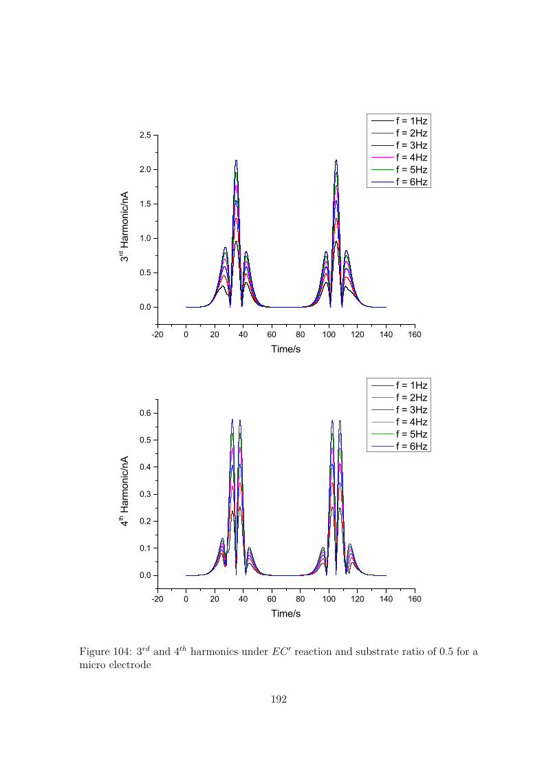
-20 0 20 40 60 80 100 120 140 160

0.0

0.5

1.0

1.5

2.0

2.53rd

Har

mon

ic/n

A

Time/s


-20 0 20 40 60 80 100 120 140 160

0.0

0.1

0.2

0.3

0.4

0.5

0.6

4th H

arm

onic

/nA

Time/s


Figure 104: 3rd and 4th harmonics under EC ′ reaction and substrate ratio of 0.5 for amicro electrode

192

-20 0 20 40 60 80 100 120 140 160

0

5

10

15

20

1st H

arm

onic

/nA

Time/s


-20 0 20 40 60 80 100 120 140 160

0

1

2

3

4

5

6 f = 1 Hz f = 2 Hz f = 3 Hz f = 4 Hz f = 5 Hz f = 6 Hz

2nd H

arm

onic

/nA

Time/s


193

-20 0 20 40 60 80 100 120 140 160

0.0

0.5

1.0

1.5

2.0

2.5

3rd H

arm

onic

/nA

Time/s

f = 1 Hz f = 2 Hz f = 3 Hz f = 4 Hz f = 5 Hz f = 6 Hz

-20 0 20 40 60 80 100 120 140 160

0.0

0.1

0.2

0.3

0.4

0.5

0.6

4th H

arm

onic

/nA

Time/s



194

-20 0 20 40 60 80 100 120 140 160

0

5

10

15

20

25

1st H

arm

onic

/nA

Time/s


-20 0 20 40 60 80 100 120 140 160

0

1

2

3

4

5

6

2nd H

arm

onic

/nA

Time/s



195

-20 0 20 40 60 80 100 120 140 160

0.0

0.5

1.0

1.5

2.0

2.5

3rd H

arm

onic

/nA

Time/s


-20 0 20 40 60 80 100 120 140 160-0.1

0.0

0.1

0.2

0.3

0.4

0.5

0.6

0.7

4th H

arm

onic

/nA

Time/s



196

-20 0 20 40 60 80 100 120 140 160-5

0

5

10

15

20

25

30

35

1st H

arm

onic

/nA

Time/s


-20 0 20 40 60 80 100 120 140 160

0

2

4

6

8

10

2nd H

arm

onic

/nA

Time/s



197

-20 0 20 40 60 80 100 120 140 160

0.0

0.5

1.0

1.5

2.0

2.5

3rd H

arm

onic

/nA

Time/s


-20 0 20 40 60 80 100 120 140 160

0.0

0.2

0.4

0.6

0.8

1.0

4th H

arm

onic

/nA

Time/s



198

5.5 Self-Catalytic Reaction with Micro Fluidic Flow

Section 5.4 demonstrate two interesting points. Firstly, the characteristic pre-wave iselicited via the use of slowly modulating signals for macro electrode. Secondly underenhanced transport conditions with micro disk, the split-wave disappears at earlyharmonics and then re-emerge at higher components - a behaviour similar to that ata planar electrode. Thus in order to observe such behavior, it is important to controlthe mass transport factor.

Early investigation using micro fluidic channel has suggested that experimentallyextracted harmonics follow the same behavior as discussed above [64]. That is, thesecomponents are essentially unchanged under both diffusion and flow conditions. Thisobservation suggests that micro fluidic is a possible tool to express the split-wavebehavior because mass transport conditions are now controllable by varying flow rate.

This section is divided into two sub-parts. The first part numerically verifies Levichequation for channel flow. The goal is to set up a reliable framework for subsequentcalculations including the EC ′ catalysis. As before, large amplitude AC voltammetryis introduced and the extraction algorithm 5.1 is applied extensively. A major aimhere is to observe whether pre-wave appears in early harmonics, rather than at highercomponents as seen in micro disk calculations.

5.5.1 Levich equation for embedded channel electrode

Considering the 2D cross-section of the channel and assuming uniformity across theelectrode in z direction (Figure 13). This assumption only applies if d ≫ w. Twoimplied consequences are i) the flow is parabolic at every cross-section of the electrodeand ii) diffusion is z direction can be ignord due to translational symmetry. In addition,since the flow is uni-directional (i.e. in x direction). These results lead to the simplifiedversion of Equation 1.4:

∂c

∂t= D( ∂2c

∂x2 + ∂2c

∂y2 ) − vx∂c

∂x(5.13)

where the velocity field is dominantly in x direction with parabolic profile:

vx = 4v0(y

hc

− ( y

hc

)2) (5.14)

199

v0 = 32

Vf

dchc

Since the top and bottom surfaces of the channel are impermeable to the solution,this condition leads to zero-flux conditions. At the electrode surface, since the bottomplane is stationary, the velocity diminishes to 0 and the applied Butler-Volmer equationonly has the diffusion component and assumes the form 1.8 as before.

Under special conditions, equation 5.13 can be further simplified. By analyzingthe scales of the diffusion and convection terms in x direction:

D∂2c

∂x2 ∼ Dc

l2x

(5.15)

vx∂c

∂x∼ vx

c

lx(5.16)

and the velocity component can be scaled as:

vx ∼ v0 = Vf

dhc

taking lx ∼ l then the diffusion term in the x-direction can be ignored (relative tothe convection term) if:

Vf l

dhcD≫ 1 (5.17)

At fairly slow flow rates, diffusion process is multi-directional while at larger flows,the contribution primarily comes from direction orthogonal to the electrode surface.However for all calculations in this section, diffusion components in x and y directionsare both included, which also accounts for the effects of Taylor dispersion at large flowrates [205].

The parameters for simulation are listed in Table 21. It is also important to keeptrack of the laminarity of the flow, which is expressed via the Reynold’s number:

Re = v0hc

ν= Vf

dν(5.18)

If Re < 103 then it is usually safe to assume that the flow is laminar and thevelocity field has a parabolic profile. It is also important to discuss FE meshing andrelevant numerical aspects for the current case. First , a structured rectangular meshis used (Figure 111). Similar to FD, the mesh is exponentially expanded away from the

200

bottom plane where the electrode is located. The simulation domain can be dividedinto three rectangles. The first rectangle corresponds to up-stream flow, the secondpart contains the electrode and the final corresponds to the down-stream. Finer meshis put at the edge between the 1st and 2nd rectangles, whilst such condition is notrequired for the interface between 2nd and 3rd domains since the concentration fieldalready becomes steady at that position. Finally, an estimate of the diffusion layersize under flow condition is:

ldif ∼ (DRhcxe/v0)1/3 (5.19)

which clearly depends on Vf . In simulation practice, the smallest spacing is typicallyat least 10 times smaller than ldiff to ensure adequate resolution of the layer.

Electrode Surface

Insulating Glass

Inle

t O

utlet

x

y

Figure 111: Structured rectangular mesh used for channel electrode calculations. Edge,distribution and mapping operations in Comsol Multiphysicsr are combined to pro-duce this mesh

The time-dependent Equation 5.13 can be solved in Comsol Multiphysicsr in two

201

Symbol Value Units CommentDR, DO 10−5 cm2/s Oxidative species diffusivity

xe 500 µm Electrode Lengthl 1000 µm Channel Length

hc 200 µm Channel Heightdc 0.6 cm Channel Widthwe 0.04 cm Electrode Width

cR0, cO0 1, 0 mM Species Bulk Concentrationsk0 10−4 m/s Reversible electrode kineticsE0 0.25 V Equilibrium Potential for the oxidation reactionα 0.6 - Charge Transfer Numberρ 1000 kg/m3 Solution density (assumed water)ν 10−6 m2/s Solution dynamic viscosity (assumed water)

Table 21: Parameters used in verification of Levich expression for channel electrode

ways. The first and most general approach is using the Time-Dependent solver, whichis based on the backward implicit formulation. However, if the electrochemical kineticsis fast, there is another approach called Parameter Sweep which is more convenientand produces solutions at similar level of accuracy. Parameter Sweep is particularlyuseful for problems having multiple steady states. The method is as follows: thevoltage range is first divided into discrete points as before. The limiting current isthen calculated at each of these fixed potentials. Thus the current-voltage curve of theoriginal problem becomes a collection of the points (Ilim, Eapply) in which Eapply is theapplied potential and Ilim is the corresponding steady state current. In this section,the usual time-dependent solver is however used because of its generality.

Different flow rates between 0.001 and 1 cm3/s are used for the calculations. Themaximum Re numbers are 250 which are well below the turbulent condition. Com-parison between limiting currents and Levich expressions are shown in Figure 112. Itshould be noted here that the flow rates between 0.1 − 1 cm3/s are fairly large (theaverage velocity v0 in the order of cm/s) and are therefore not so commonly used inpractice due to high possibility of solution leakage. However, numerical observationsshow that the higher the flow rates, the smaller the percentage differences betweennumerical values and the Levich expression 1.20. Figure 113 shows the effect of so-lution flow rate on concentration profiles across electrode surface. At very small flowrate (e.g. 10−6 cm3/s), the profile is almost symmetrical akin to that of a micro disk.As higher volummetric rates are applied, the contour is distorted and skewed in thesame direction of flow and the diffusion layer’s thickness decreases.

202

0.0 0.2 0.4 0.6 0.8 1.00

1

2

3

4

5

6

Current/(

A)

Vf1/3/(cm3/s)1/3

Numerical Results Levich Predictions

Figure 112: Comparison between numerical values and the Levich prediction ICElim =

0.925nFcR0wex2/3e D

2/3R (4Vf/h2

cd)1/3 for the channel electrode at various flow rates Vf .There is a good convergence between simulation and theory. Numerical differences arelargest at small flow rates (e.g. 0.001 cm3/s) and decrease as Vf is increased

5.5.2 Effects of large AC amplitude and catalysis

This section investigates the EC ′ mechanism via the use of channel electrode. Basedon results from section 5.4, f = 1 Hz is chosen for all following simulations. Thischoice stems from the observation that the wave-splitting phenomenon is most clearlyshown under the slowest sinusoidal modulation. For the micro fluidic calculations, theelectroactive species concentration is raised to cR0 = 2 mM . Such choice is purposelymade for later comparisons with experiments. The parameter setting is summarizedin Table 22.

Under channel flow, Equation 5.10 is modified to include the convective component:

∂cR

∂t= DR

∂2cR

∂y2 − vx∂cR

∂x+ kEC′cOcS

203

Figure 113: Cross sectional concentration profile at large over potential and variousflow rates Vf = 10−6, 10−5, 10−4 and 10−3 cm3/s (direction: left to right, top to bot-tom). Red colour indicates high concentrations whilst blue colour is 0 (mM). Thecontour is sharp near the leading edge of the electrode and becomes flatter down-stream. As a consequence, the current flux peaks at the front and then tends to alower constant value

∂cO

∂t= DO

∂2cO

∂y2 − vx∂cO

∂x− kEC′cOcS

∂cS

∂t= DS

∂2cS

∂y2 − vx∂cS

∂x− kEC′cOcS (5.20)

In arriving at Equation 5.20, the diffusion component in x and convective term iny directions are ignored. In earlier analysis, Equation 5.17 shows that this assumptionapplies at sufficiently large flow rate Vf . Using the criteria and the above dimensionalvalues:

204

Parameter Symbol Value UnitsDR 0.76 ∗ 10−9 m2/sDO 0.76 ∗ 10−9 m2/sk0 0.001 m/sα 0.5 −

Cdl 50 µF/cm2

E0 0.25 Vvscan 10 mV/scR0 2 mMcO0 0 mMcS0 0.1 − 1 mMDS 6 ∗ 10−10 m2/s

kEC′ 106 M−1s−1

de 100 µmwe 600 µmhc 1000 µmdc 670 µm

E 50 mVVf 0.1 − 0.6 mL/min

ffundamental 1 Hz

Table 22: Simulation parameters for micro fluidic channel. A small scan rate andsinusoidal frequency are employed to manifest the split-wave effect. Electrode size islength de and width we with a channel height hc and width dc)

Vfde

dchcDR

∼ (0.1 10−6/60) (100 10−6)(670 10−6) (1000 10−6) (10−9) ∼ 250

which is well above 1 and therefore justifies the above assumption. Another way ofchecking is to estimate the average speed v0, which comes out to be:

v0 ∼ 0.1 10−6/60(670 10−6) (1000 10−6) ∼ 2500 µm

s

and considering the channel length is xe = 100 µm, the fluid dynamic time scale is100/2500 = 0.04 (s) and the flow is thus very fast compared to the time scale of masstransport process. Consequently, the steady-state flow profile 5.14 is assumed to beuniform across electrode width.

Figure 111 illustrates the structured mesh for the simulation. Regarding the bound-ary conditions, Nernstian relation 1.13 is applied at electrode level and at insulatingglass, zero flux is imposed. For the inlet condition, fresh (i.e. bulk concentration)

205

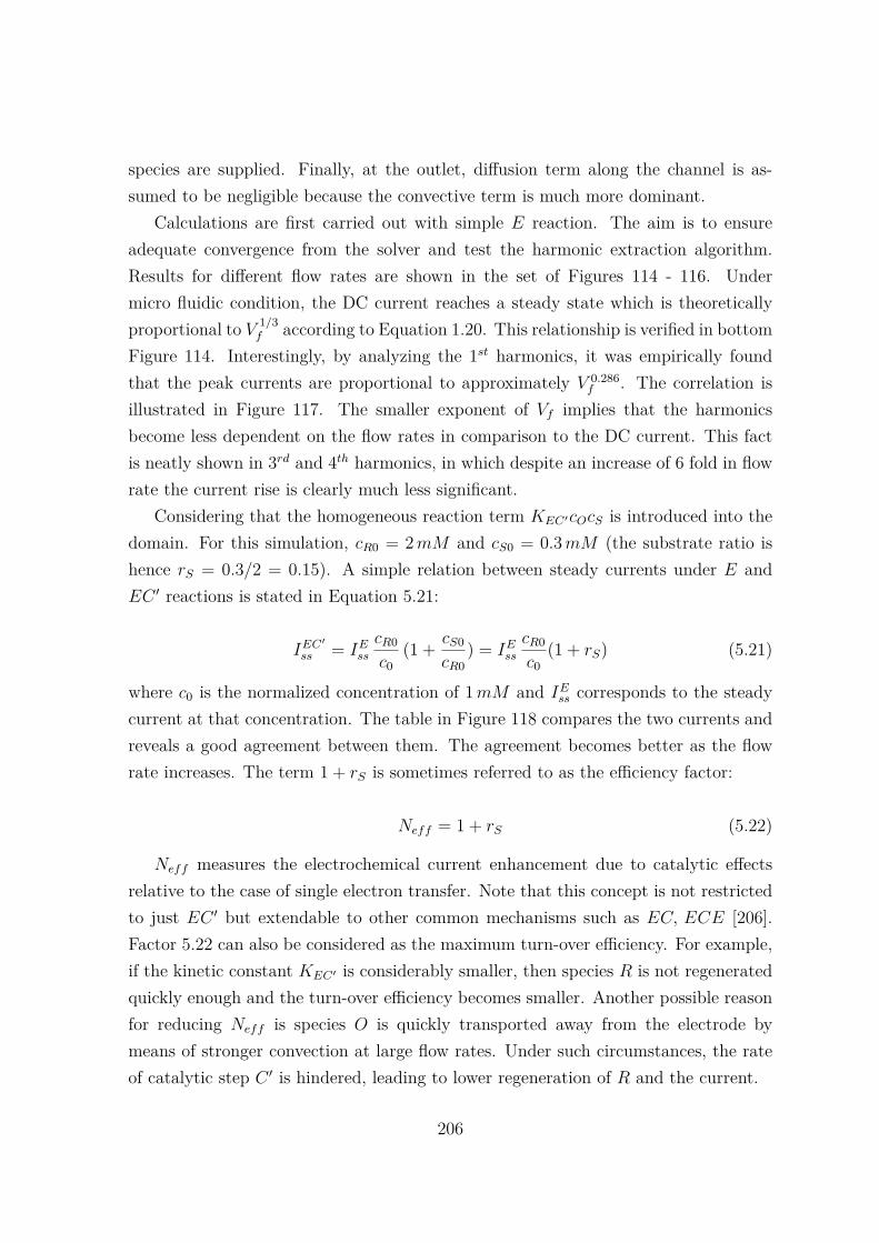
species are supplied. Finally, at the outlet, diffusion term along the channel is as-sumed to be negligible because the convective term is much more dominant.

Calculations are first carried out with simple E reaction. The aim is to ensureadequate convergence from the solver and test the harmonic extraction algorithm.Results for different flow rates are shown in the set of Figures 114 - 116. Undermicro fluidic condition, the DC current reaches a steady state which is theoreticallyproportional to V

1/3f according to Equation 1.20. This relationship is verified in bottom

Figure 114. Interestingly, by analyzing the 1st harmonics, it was empirically foundthat the peak currents are proportional to approximately V 0.286

f . The correlation isillustrated in Figure 117. The smaller exponent of Vf implies that the harmonicsbecome less dependent on the flow rates in comparison to the DC current. This factis neatly shown in 3rd and 4th harmonics, in which despite an increase of 6 fold in flowrate the current rise is clearly much less significant.

Considering that the homogeneous reaction term KEC′cOcS is introduced into thedomain. For this simulation, cR0 = 2 mM and cS0 = 0.3 mM (the substrate ratio ishence rS = 0.3/2 = 0.15). A simple relation between steady currents under E andEC ′ reactions is stated in Equation 5.21:

IEC′

ss = IEss

cR0

c0(1 + cS0

cR0) = IE

ss

cR0

c0(1 + rS) (5.21)

where c0 is the normalized concentration of 1 mM and IEss corresponds to the steady

current at that concentration. The table in Figure 118 compares the two currents andreveals a good agreement between them. The agreement becomes better as the flowrate increases. The term 1 + rS is sometimes referred to as the efficiency factor:

Neff = 1 + rS (5.22)

Neff measures the electrochemical current enhancement due to catalytic effectsrelative to the case of single electron transfer. Note that this concept is not restrictedto just EC ′ but extendable to other common mechanisms such as EC, ECE [206].Factor 5.22 can also be considered as the maximum turn-over efficiency. For example,if the kinetic constant KEC′ is considerably smaller, then species R is not regeneratedquickly enough and the turn-over efficiency becomes smaller. Another possible reasonfor reducing Neff is species O is quickly transported away from the electrode bymeans of stronger convection at large flow rates. Under such circumstances, the rateof catalytic step C ′ is hindered, leading to lower regeneration of R and the current.

206

-20 0 20 40 60 80 100 120 140 160

0.0

0.2

0.4

0.6

0.8

DC

Cur

rent

/A

Time/s

0.1 mL/min 0.2 mL/min 0.3 mL/min 0.4 mL/min 0.5 mL/min 0.6 mL/min

0.45 0.50 0.55 0.60 0.65 0.70 0.75 0.80 0.850.40

0.45

0.50

0.55

0.60

0.65

0.70

0.75

0.80

0.85

Stea

dy S

tate

Cur

rent

/A

Vf1/3/(mL/min)1/3

Figure 114: Extracted DC current in time domain at various flow rates between 0.1and 0.6 mL/min (top). The Levich relation is confirmed in the bottom figure

207

-20 0 20 40 60 80 100 120 140 160-0.05

0.00

0.05

0.10

0.15

0.20

0.25

0.30

0.35

1st H

arm

onic

/A

Time/s


-20 0 20 40 60 80 100 120 140 160

0

10

20

30

40

50

60

2nd H

arm

onic

/nA

Time/s


Figure 115: Extracted 1st (top) and 2nd (bottom) harmonics for the same range offlow rates as in Figure114

208

-20 0 20 40 60 80 100 120 140 160

0

5

10

15

20

3rd H

arm

onic

/nA

Time/s


-20 0 20 40 60 80 100 120 140 160

0

1

2

3

4

5

4th H

arm

onic

/nA

Time/s


Figure 116: Extracted 3rd (top) and 4th (bottom) harmonics for the same range offlow rates as in Figure 114

209

0.50 0.55 0.60 0.65 0.70 0.75 0.80 0.85 0.90

0.18

0.20

0.22

0.24

0.26

0.28

0.30

0.321st

Har

mon

ic P

eak/

A

Vf0.286/(mL/min)0.286

Figure 117: Empirical correlation between 1st harmonic peaks and V 0.286f . The expo-

nent 0.286 is less than that of Levich expression (0.333), implying that the harmoniccurrents are less flow-rate dependent than the DC component

From Figure 119, no split-wave effect is evident in the first harmonic. This be-haviour resembles that of the micro electrode. However, there is a weak shoulderin second harmonic at the slowest flow rate. This phenomenon can be explained asfollows. Under diffusion control and macro electrodes, the split-wave is present in har-monics. Assuming that the flow is very small (which mimics the diffusion condition),a pre-wave is expected on this channel electrode. At higher flow rates, the mass trans-port effect is enhanced to an extent that the condition now is closer to that of a microelectrode and the effect consequently is subdued. Thus the behaviour at the channelelectrode can be viewed as an intermediate between the macro and micro limits. Thebiggest advantage of using channel is the ability to control the flow rate, which is afactor in manifesting the split-wave. Consequently, the channel electrode should ex-hibit similar behavior to that of macro electrodes if the volumetric flow is not too high.In addition, because subsequent harmonics are less flow-rate dependent than the DCand 1st harmonic, the pre-wave is therefore expected from 2nd components onwards.

The discussion implies that the flow-rate should be set large enough so that steadyDC current is reached, but not so high that the pre-wave disappears in the 2nd har-

210

-20 0 20 40 60 80 100 120 140 160

0.0

0.5

1.0

1.5

2.0

DC/A

Time/s

0.1 mL/min 0.2mL/min 0.3mL/min 0.4mL/min 0.5mL/min 0.6mL/min

Flow Rate (mL/min) Relation 5.21 Figure 118 Percentage Difference0.1 1.041 1.022 1.80.2 1.311 1.322 0.80.3 1.494 1.506 0.80.4 1.647 1.655 0.50.5 1.776 1.778 0.10.6 1.888 1.890 0.1

Figure 118: The DC Current for a EC ′ reaction with cR0 = 2 mM and cS0 = 0.3 mMbetween flow rate 0.1 and 0.6 mL/min (top). Comparison of steady currents using theEquation 5.21 and direct data from Figure 118. From Equation 5.21, the efficiencyfactor is fixed and the steady currents therefore follow the Levich relation 112

211

-20 0 20 40 60 80 100 120 140 160-0.1

0.0

0.1

0.2

0.3

0.4

0.5

0.6

0.7

Firs

t Har

mon

ic/

A

Time/s


-20 0 20 40 60 80 100 120 140 160

0.00

0.02

0.04

0.06

0.08

0.10

0.12

Seco

nd H

arm

onic

/A

Time/s


Figure 119: 1st(top) and 2nd (bottom) harmonics for EC ′ reaction with cR0 = 2 mMand cS0 = 0.3 mM . Notice the relatively weak shoulder in 2nd harmonics under thesmallest flow rate Vf = 0.1 mL/min

212

-20 0 20 40 60 80 100 120 140 160

0.0

0.2

0.4

0.6

0.8

1.0

1.2

DC/A

Time/s

cS0 = 0.1 cS0 = 0.2 cS0 = 0.3 cS0 = 0.4 cS0 = 0.5 cS0 = 0.6

Substrate Concentration Charge Count in (0, 35) Charge Count in (35, 70)0.1 1.135(9) 1.135(6)0.2 1.141(0) 1.140(0)0.3 1.147(7) 1.146(9)0.4 1.156(0) 1.154(9)0.5 1.165(6) 1.164(2)0.6 1.176(6) 1.175(0)

Figure 120: (Top) DC current for various substrate concentrations cS0 = 0.1−0.6 mM(corresponding to rS between 5% and 30%). The flow rate is fixed at Vf = 0.1 mL/minand inlet electroactive concentration is cR0 = 2 mM . (Bottom) Counting the chargefor the 2nd harmonic at each substrate concentration in Figure 121. The unit of chargeis µC. Numerical values are included up to 3 decimal places. It is clear that the sameamount of charge is transferred during both time periods

213

monic. For the current situation, Vf = 0.1 mL/min is a sensible choice. The flowrate is then fixed at this level and computations are performed for different substrateconcentrations. Figure 120 illustrates that as the substrate concentration increases, sodoes the steady current (by Equation 5.21). In addition, the split-wave effect is clearlyseen in the 2nd harmonic (top Figure 121) at sufficiently high substrate concentrationscS0 = 0.6 mM (or ratios rs = 30%). Note that at cS0 = 0.3 mM (rS = 15%), theshoulder is fairly apparent and therefore can be taken as the lower detection limitunder the current set-up.

The voltammograms for micro fluidic channel are highly symmetric. The first rea-son is convection is a much faster mean of mass transport than diffusion. In addition,a slow scan rate means that a quasi-steady diffusion layer is formed at each appliedpotential. Finally, since the forward and backward potentials are approximately sym-metrical, the diffusion layer profile should also be symmetrical and consequently so isthe current. This feature is to be contrasted with results for macro electrodes in whichthe current profiles are strongly asymmetric favouring the forward current.

For the 2nd harmonic, as soon as the pre-wave is formed, the associated E peakdecreases in magnitude in comparison to the second E peak (Figure 121). However,the total amount of charge under each portion of the diagram should be equal. Thecumulative charge is expressed as the area under the current-time graph:

Q(t1, t2) =∫ t2

t1I ∗ dt (5.23)

where (t1, t2) is the time interval. For each concentration level in Figure 121, theexpression 5.23 is calculated for intervals (0, 35) and (35, 70) respectively. The com-putation is conveniently carried out using the simple trapezoidal rule to numericallyintegrate the current. The table in Figure 120 shows that charge balance is maintainedat all concentration levels.

As before, it is analytically useful to check the correlation between the pre-wavepeaks in the 2nd harmonics and the substrate concentrations. A linear relation is indeedconfirmed in bottom Figure 122. Statistical analysis further shows that the line doesnot strictly pass through the (0, 0) coordinate. However, because current magnitudeis smaller in this case (order ∼ 10 nA) than that of macro electrode (order ∼ 100 nA),the mentioned anomaly is not a critical issue. Experimental results also show thatthe pre-wave phenomenon is present in the 2nd but not the 1st harmonic (Figure123). In accordance with the simulation (Figure 119), a slight shoulder is present

214

-20 0 20 40 60 80 100 120 140 160-10

0

10

20

30

40

50

60

70

802nd

Har

mon

ic/n

A

Time/s

cS0 = 0.1 cS0 = 0.2 cS0 = 0.3 cS0 = 0.4 cS0 = 0.5 cS0 = 0.6

-20 0 20 40 60 80 100 120 140 160-0.05

0.00

0.05

0.10

0.15

0.20

0.25

0.30

0.35

0.40

1st H

arm

onic

/A

Time/s

cS0 = 0.1 cS0 = 0.2 cS0 = 0.3 cS0 = 0.4 cS0 = 0.5 cS0 = 0.6

Figure 121: 2nd(top) and 1st (bottom) harmonics for different substrate concentrations(0.1 − 0.6 mM) and cR0 = 2 mM, Vf = 0.1 mL/min and νscan = 10 mV/s. There is anevolution of split-wave in second harmonic but this is not observed in the first

215

-20 0 20 40 60 80 100 120 140 160-10

0

10

20

30

40

50

60

70

802nd

Har

mon

ic/n

A

Time/s

cS0 = 0.5 cS0 = 0.6 cS0 = 0.8 cS0 = 1.0

0.2 0.3 0.4 0.5 0.6 0.7 0.8 0.9 1.0 1.1

25

30

35

40

45

50

55

Pre-

wav

e C

urre

nt/n

A

Subtrate Concentration (mol/m 3)

Figure 122: Comparison of 2nd harmonics (top) and plot of the pre-wave peak versusthe substrate concentrations (bottom). Linear correlation (black dash) is fitted withPearson coefficient of 0.9999

216

at cS0 = 0.3 mM and disappears completely at 0.1 mM . In terms of magnitude,it is observed that currents are smaller in experiments than in simulations for bothharmonics. One possible reason is because species diffusivities R, S in Table 22 wasset larger than their actual values inside the channel.

In addition, it is acknowledged that acquiring reliable data under flow conditionshas been very challenging. A frequently observed issue is the gold electrode surfaceis turns black and consequently corrupts the measurement signals. It is thereforespeculated that the fabricated gold layer is unstable, slowly oxidized and worn off asthe flow is applied over a period of time. This problem is traced back to dirty glasssurface on which the gold crystals grows and thus a possible solution is to improveconditions inside the fabrication room.

To summarize, this section illustrates a novel combination between sinusoidal sig-nal and forced convection to manifest the split-wave phenomenon in the 2nd harmonics.As in the case of micro disk, strong mass transport inside the channel leads to disap-pearance of the split-wave in the 1st component. The study also reaffirms the fact thatharmonic components tend to be less flow-rate dependent and resemble those harmon-ics under diffusion control. The results also reveal the linear relationship between thepre-wave currents and concentration ratios, which is useful for analytical calibrations.More interestingly, for the current set-up, both theoretical and observable detectionlimits were shown to be around 0.3 mM .

217

0 10 20 30 40 500

50

100

150

200

250C

urre

nt /

nA

Time / s

0.1 0.3

0 10 20 30 40 500

10

20

30

40

0.1 0.3

Cur

rent

/ nA

Time / s

Figure 123: Experimental data for 1st (top) and 2nd (bottom) harmonic under L-cysteine concentrations of 0.1 (black) and 0.3 mM (red) respectively (scan rate:14.9 mV/s, amplitude 50 mV , volumetric flow rate 0.1 mL/min, gold electrode oflength 100 µm). Note that only half of the voltammograms is shown in each figure

218


This chapter studies the design of fundamental harmonic signals and their applica-tion to elicit the effects of electro-catalysis, namely the EC ′ mechanism. The primarymotivation was due to earlier investigations on similar mechanisms and uses of morecomplex voltammetry, but none considered the basic sinusoidal as a tool to achievesimilar results. The work then proceeds to build up the background of the FFT (orAC) voltammetric technique as well as simulation methodology. Two major outcomesfrom this development are the algorithm to extract any harmonic component andthe recognition of large amplitude sinusoidal as a convenient mean to improve sig-nal to noise ratio. Simulation was then carried for diffusion-limit situation for macroand micro disks. For the former case, it was evident that the characteristic split-wave due to catalytic reaction was present in all harmonics. The effect is howeverfrequency-dependent, as higher frequencies tend to subdue the pre-wave. In addition,the current magnitude also forms a linear correlation with substrate levels - a relation-ship confirmed in earlier chapter for the anharmonic or DC component. In addition,experimental measurements show a good agreement with simulation findings. Theseresults illustrate an example for the use of AC perturbation to study effects of chem-ical catalysis. Finally, since any periodic signal can be decomposed into the sum ofharmonics, the result here is theoretically more fundamental.

The same chemistry was re-examined under the enhanced mass transport condi-tion with micro disk and rather different results were obtained. Firstly, the split-waveis no-longer observed in the first two harmonics both for low and high substrate lev-els. However, the effect is manifested weakly in subsequent higher harmonics. Theseobservations lead to the conclusion that effect of mass transport was reduced forhigher components and a proper control of such effect could reproduce the pre-wavebehaviour in lower harmonics. The above hypothesis was then studied via the ap-plication of micro-fluidic devices. Using a combination of reasonably slow flow ratesand large amplitude AC voltammetry, simulation study predicts the split-wave in 2nd

component as well as the same linear correlation observed for macro electrode. Theformer result was confirmed by experiments whilst the latter has not been checkeddue to technical difficulties in obtaining data and stabilizing electrode surface condi-tions. Furthermore, the fact that higher harmonics were weakly flow-rate dependentwas supported by numerical data.

219

Chapter 6

Conclusions

This thesis applies a experimental design framework to the analysis of electron transferkinetics and self-catalytic mechanism. The classical Butler-Volmer model is assumedto describe the fundamental electrochemical reaction. Though more sophisticatedmodels, such as the Marcus-Hush-Chidsey, is available, Butler-Volmer model is pre-ferred due to its simplicity and known effectiveness for describing the majority of redoxreactions.

Since the work favours the model-based approach, numerical solutions to the for-ward problem were emphasized and thoroughly developed. Chapter 2 details FDmethod for solution of electron transfer processes. This is motivated by the fact thatmost experiments in electrochemistry are still conducted under diffusion-limited con-ditions. The chapter’s results show good agreement between simulated data and thetheory , thus confirming the reliability of FD in solving this forward problem. Based onthe foundation in chapter 2, chapter 3 examines the use of linear sweep voltammetryas an experimental design variable to regress primary parameters in the Butler-Volmermodel: the kinetic constant, charge transfer coefficient and the equilibrium voltage.By fixing the mass transport mode as diffusion control, a sequence of investigationsconcerning model parameters (identifiability, Sobol ranking, inversion and statisticscomputations) were carried out. From the identifiability test, potential compensatingeffects and correlations among the parameters were noticed. By employing reasonablysmall electrode areas as an additional design variable, solution resistance factors wereshown to be insignificant and were subsequently excluded from the generalized formu-lation. Finally, a theoretical inversion under a quasi-reversible regime proves primaryparameters can be recovered with a satisfactory degree of accuracy. Furthermore, aMCMC simulation was observed to improve the point estimate statistics as well as

220

detail correlations among parameter pairs. A major conclusion from this chapter isa simple linear signal that is adequate for parameter estimation purposes, which isin line with previous results stating that more complex waveforms only yield minorimprovement in parameter identification. A possible research direction is the synthesisof voltage signal which improves the identifiability number. Though such work waspartially undertaken, a complete answer is yet to be reached.

Because hydrodynamic devices have become common in electrochemistry, chapter4 investigates the role of mechanical convection in model identifiability. The signalfactor was fixed by employing only linear sweep voltammetry. The recent RoDE device,was studied because it is a generalized configuration of the well-known rotating disk.The rocking mechanism was approximated by the four-bar geometry and yielded goodagreement with experimental data, despite the over-simplified 2D axisymmetric modelfor both fluid and mass transports. In addition, the limiting Levich expression wasderived from numerical considerations, showing RDE is the limiting case for all possiblecombination of RoDE. Identifiability calculation was carried out to further comparethe two configurations. An important result is RoDE provides a better differentiationof the parameter set when the whole current response was considered. On the otherhand, if only the limiting responses were concerned, then RDE is a much better choiceto determine these parameters. The final section introduces the rotating drum as apotential device to study electrochemical reaction in viscous media such as PEG andionic liquids and future considerations should pursue these studies. Due to the timeconstraint, comparison of model identifiability between a rotating drum and rotatingdisk was not undertaken, though similar results, especially the number ηsteady for theseconfigurations are expected. In addition, future work should consider the reducedeffective diffusivity under flow driven conditions.

Chapter 5 explores the application of large amplitude harmonic disturbances toprobe the effects of homogeneous catalytic reactions. The EC ′ mechanism was se-lected due to promising chemical applications in detecting sulphide compounds. TheAC voltammetry relies on the combination of the common linear sweep (to drivethe fundamental electron transfer reaction) and a single sinusoidal term. This termthen produces extra currents, called the harmonics, in addition to the usual aperiodiccurrent. Algorithms based on FFT and iFFT operations were implemented to auto-matically extract harmonics from the total current response. The calculation was firstcarried out for diffusion control conditions. For a large planar electrode, the signaturesplit-wave was observed in all harmonics as well as in the DC current. In addition,

221

the pre-wave current peak shows a linear relationship with the species concentrations,thus confirming analytical values of the method. For micro electrode, because of strongmass-transport enhancement, these pre-waves were prominent in only higher (e.g. 3rd,4th) harmonics. Consequently, to control the transport factor, micro-fluidic channelwas used because the flow rate is more easily controlled than in the diffusion mode.By carefully adjusting the flow rate, both the split-wave phenomenon and linear cor-relation were again confirmed for the 2nd harmonics, though it was not the case forthe 1st harmonics due to large residues of mass-transport effect. Overall, harmonicpertubations prove to be a useful tool to extract additional information on chemicalkinetics. A potential future direction is to re-evaluate the above mechanism usingthe combination of rocking condition and FFT voltammetry to compare the resultswith channel electrode. Electro-catalysis under hydro dynamic conditions is a rela-tively new topic and recent work only experimentally studies alcohol oxidations usingTEMPO as the mediator [207]. Though the harmonic currents are not expected to besignificantly different among these devices, their characteristic fluid dynamic effectsmight give rise to subtle and potentially useful differences.

222

References

[1] J. C. Myland et al. An analytical expression for the current-voltage relationshipduring reversible cyclic voltammetry. Journal of Electroanalytical Chemistry,153:43–54, 1983.

[2] A. J. Bard and L. R. Faulkner. Electrochemical Methods, Fundamentals andApplications. Wiley-Interscience, 2001.

[3] D. Shoup and A. Szabo. Chronoamperometric current at finite disk electrodes.Journal of Electroanalytical Chemistry, 14:237–245, 1984.

[4] V. Maheshwari et al. Multiobjective framework for model-based design of ex-periments to improve parameter precision and minimize parameter correlation.Industrial and Engineering Chemistry Research, 52:8289–8304, 2013.

[5] G. Grundmeier et al. Corrosion protection by organic coatings: electrochemicalmechanism and novel methods of investigation. Electrochimica Acta, 45:2515–2533, 2000.

[6] J. B. Goodenough et al. The Li-Ion rechargable battery: A perspective review.Journal of the American Chemical Society, 135:1167–1176, 2013.

[7] G. Wang et al. A review of electrode materials for electrochemical supercapaci-tors. Chem. Soc. Rev, 41:797–828, 2012.

[8] A. Kirubakaran et al. A review on fuel cell technologies and power electronicinterface. Renewable and Sustainable Energy Reviews, 13:2430–2440, 2009.

[9] Z. Li et al. Photoelectrochemical cells for solar hydrogen production: currentstate of promising photoelectrodes, methods to improve their properties andoutlook. Energy and Environmental Science, 6:347–370, 2013.

223

[10] B. Privett et al. Electrochemical sensors. Anal. Chem., 80:4499–4517, 2008.

[11] E. Bakker. Electrochemical sensors. Anal. Chem., 76:3285–3298, 2004.

[12] J. Janata. Principles of Chemical Sensors, 2nd Edition. Springer, 2009.

[13] R. F. Taylor and J. S. Schultz. Handbook of Chemical and Biological Sensors.IoP Publishing, 1996.

[14] M. Pumera et al. Graphene for electrochemical sensing and biosensing. TrACTrends in Analytical Chemistry, 29:954–965, 2010.

[15] H. E. Zittel and F. J. Miller. A glassy carbon electrode for voltammetry. Anal.Chem., 37:200–202, 1965.

[16] A. C. Fisher. Electrode Dynamics. Oxford University Press, 1996.

[17] P. Atkins. Physical Chemistry. Oxford University Press, 2006.

[18] R. B. Bird et al. Transport Phenomena. Wiley Inter-Science, 2007.

[19] R. Fox et al. Introduction to Fluid Mechanics. John Wiley and Sons, 2003.

[20] B. R. Munson. Fundamentals of Fluid Mechanics, 7th Edition. Wiley Science,2013.

[21] Southampton Electrochemistry Group. Instrumental Methods in Electrochem-istry. Horwood Publishing Chichester, 1985.

[22] C. M. A. Brett and A. M. O. Brett. Electrochemistry: Principles, Methods andApplications. Oxford University Press, 1994.

[23] E. J. F. Dickinson and R. G. Compton. How much supporting electrolytes isrequired to make a cyclic voltammetry experiment quantitatively diffusional? atheoretical and experimental investigation. J. Phys. Chem. C, 113:11157–11171,2009.

[24] E. J. F. Dickinson and R. G. Compton. The zero-field approximation for weaklysupported voltammetry: A critical evaluation. Chemistry Physical Letter, 497:173–183, 2010.

224

[25] S. Schofer. Numerical solution of the Poisson-Nernst-Planck equation system.Master’s thesis, Friederich-Alexander-University, 2013.

[26] M. Lyons. Molecular thermodynamics and kinetics lecture 6: Phenomenologicalelectrode kinetics, 2013.

[27] R. A. Marcus. On the theory of electrochemical and chemical electron transferprocesses. Can. J. Chem., 37:155–163, 1959.

[28] H. Girault. Analytical and Physical Electrochemistry. E P F L Press, 2004.

[29] L. M. Torres et al. Understanding the difference between inner- and outer-spheremechanisms: An electrochemical experiment. Journal Of Chemical Education,73, 1996.

[30] R. G. Compton, E. Larboda, and K. R. Ward. Understanding Voltamme-try:Simulation of Electrode Processes. Imperial College Press, 2013.

[31] E. Larboda et al. Asymmetric marcus-hush theory for voltammetry. Chem. Soc.Rev., 42:4894–4905, 2013.

[32] F. Marken. Basics in electrode kinetics, advanced electrochemistry summercourse, 2016.

[33] E. Laborda et al. A comparison of Marcus-Hush versus Butler-Volmer electrodekinetics using potential pulse voltammetric techniques. Journal of Electroana-lytical Chemistry, 660:169–177, 2011.

[34] Y. Wang et al. The use of differential pulse voltammetries to discriminate be-tween the Butler-Volmer and the simple Marcus-Hush models for heterogeneouselectron transfer: The electro-reduction of europium (iii) in aqueous solution.Journal of Electroanalytical Chemistry, 668:7–12, 2012.

[35] M. C. Henstridge et al. Marcus-hush-chidsey theory of electron transfer appliedto voltammetry: A review. Electrochimica Acta, 84:12–20, 2012.

[36] E. Larboda et al. Asymmetric marcus theory: Application to electrode kinetics.Journal of Electroanalytical Chemistry, 67:48–53, 2012.

225

[37] E. L. Tanner et al. One-electron reduction of 2-nitrotoluene, nitrocyclopentane,and 1-nitrobutane in room temperature ionic liquids: A comparative study ofButler-Volmer and Marcus-Hush theories using microdisk electrodes. J. Phys.Chem. C, 119:2716–2726, 2014.

[38] V. G. Levich. Physicochemical Hydrodynamics. Prentice-Hall, Inc., EnglewoodCliffs, 1962.

[39] J. Alden. Computational Electrochemistry. PhD thesis, University of Oxford,1998.

[40] J. Newman and K. E. T. Alyea. Electrochemical Systems. Wiley-Interscience,2004.

[41] G. C. Barker et al. Square-wave polarography. Analyst, 77:685–696, 1952.

[42] B. A. Brookes et al. Simulation of square wave voltammetry: Reversible elec-trode processes. Journal of Physical Chemistry B, 103:5289–5295, 1999.

[43] L. Ramaley et al. Theory of square wave voltammetry. Analytical Chemistry,41:1362–1365, 1969.

[44] A. Chen and B. Shah. Electrochemical sensing and biosensing based on squarewave voltammetry. Anal. Methods, 37:2158–2173, 2013.

[45] V. Mirceski et al. Square-wave voltammetry: A review on the recent progress.Electroanalysis, 25:2411–2422, 2013.

[46] D. J. Gavaghan and A. M. Bond. A complete numerical simulation of the tech-niques of alternating current linear sweep and cyclic voltammetry: analysis of areversible process by conventional and fast fourier transform methods. Journalof Electroanalytical Chemistry, 480:133–149, 2000.

[47] A. M. Bond et al. Changing the look of voltammetry: Can ft revolutionizevoltammetric techniques as it did for NMR. Analytical Chemistry, 77:186–195,2005.

[48] M. K. Hobson. Mathematical Methods for Physics and Engineering. CambridgeUniversity Press, 1997.

226

[49] D. J. Gavaghan et al. A comparison of sinusoidal, square wave, sawtooth, andstaircase forms of transient ramped voltammetry when a reversible process isanalysed in the frequency domain. Journal of Electroanalytical Chemistry, 513:73–86, 2001.

[50] S. O. Engblom et al. Large amplitude AC voltammetry: A comparison betweentheory and experiment. Electroanalysis, 13:626–630, 2001.

[51] J. Zhang and A. M. Bond. Discrimination and evaluation of the effects of un-compensated resistance and slow electrode kinetics from the higher harmoniccomponents of a fourier transformed large-amplitude alternating current voltam-mogram. Anal. Chem., 57:2276–2288, 2007.

[52] A. Sher et al. Resistance, capacitance and electrode kinetic effects in fourier-transformed large-amplitude sinusoidal voltammetry: Emergence of powerfuland intuitively obvious tools for recognition of patterns of behavior. Analyticalchemistry, 76:6214–6228, 2004.

[53] A. Sher et al. Fourier transformed large amplitude square-wave voltammetry asan alternative to impedance spectroscopy: Evaluation of resistance, capacitanceand electrode kinetic effects via an heuristic approach. Electroanalysis, 17:1450–1462, 2005.

[54] E. Mashkina and A. M. Bond. Implementation of a statistically supported heuris-tic approach to alternating current voltammetric harmonic component analysis:Re-evaluation of the macrodisk glassy carbon electrode kinetics for oxidation offerrocene in acetonitrile. Analytical Chemistry, 83:1791–1799, 2011.

[55] K. Bano et al. Investigations of fast electrode kinetics for reduction of 2,3,5,6-tetrafluoro-7,7,8,8-tetracyanoquinodimethane in conventional solvents and ionicliquids using fourier transformed large amplitude alternating current voltamme-try. J. Phys. Chem. C, 118:9560–9569, 2014.

[56] A. M. Bond et al. An integrated instrumental and theoretical approach to quan-titative electrode kinetic studies based on large amplitude fourier transformedAC voltammetry: A mini review. Electrochemistry Communications, 57:78–83,2015.

227

[57] E. Mashkina et al. Estimation of electrode kinetic and uncompensated resis-tance parameters and insights into their significance using fourier transformedAC voltammetry and e-science software tools. Journal of Electroanalytical Chem-istry, 690:104–110, 2013.

[58] C. Y. Lee et al. Effects of coupled homogeneous chemical reactions on theresponse of large-amplitude AC voltammetry: Extraction of kinetic and mech-anistic information by fourier transform analysis of higher harmonic data. J.Phys. Chem. A, 114:10122–10134, 2010.

[59] B. Lertanantawong et al. Investigation of mediated oxidation of ascorbic acidby ferrocenemethanol using large-amplitude fourier transformed AC voltamme-try under quasi-reversible electron-transfer conditions at an indium tin oxideelectrode. Anal. Chem., 80:6515–6525, 2008.

[60] A. C. Fisher. Fundamentals of electrochemical engineering: Lecture notes, cebpart iib, 2013.

[61] K. Yokoyama and Y. Kayanuma. Cyclic voltammetric simulation for electro-chemically mediated enzyme reaction and determination of enzyme kinetic con-stants. Anal. Chem., 70:3368–3376, 1998.

[62] S. Peng. Microengineered Electrochemical Reactors. PhD thesis, University ofCambridge, 2015.

[63] J. Cooper. Energy harvesting from sulphurous environment, master thesis. Mas-ter’s thesis, University of Hull, 2013.

[64] S. M. Matthews et al. Attributes of direct current aperiodic and alternatingcurrent harmonic components derived from large amplitude fourier transformedvoltammetry under microfluidic control in a channel electrode. Analytical Chem-istry, 84:6686–6692, 2012.

[65] K. Bano et al. Large amplitude fourier transformed AC voltammetry at a rotat-ing disc electrode: a versatile technique for covering levich and flow rate insen-sitive regimes in a single experiment. Phys. Chem. Chem. Phys, 14:4742–4752,2012.

[66] I. Henley. Computational Electrochemistry. PhD thesis, University of Bath,2004.

228

[67] G. D. Smith. Numerical Solution of Partial Differential Equations: Finite Dif-ference Methods 3rd Edition. Oxford University Press, 1985.

[68] H. A. Obaid et al. An unconditionally stable nonstandard finite differencemethod applied to a mathematical model of hiv infection. Int. J. Appl. Math.Comput. Sci., 23:357–372, 2013.

[69] J. Zhao. A highly accurate compact finite difference method and its applicationsin financial mathematics and computational biology. PhD thesis, University ofWestern Ontario, 2006.

[70] M. Rudolph. A fast implicit finite difference algorithm for the digital simula-tion of electrochemical processes. Journal of Electroanalytical Chemistry andInterfacial Electrochemistry, 314:13–22, 1991.

[71] M. Rudolph. A fast implicit finite difference algorithm for the digital simulationof electrochemical processes, part ii. an improved treatment of electrochemicalmechanisms with second-order reactions. Journal of Electroanalytical Chemistry,338:85–98, 1992.

[72] S. W. Feldberg. A fast quasi-explicit finite difference method for simulatingelectrochemical phenomena Part I. Application to cyclic voltammetric problems.Journal of Electroanalytical Chemistry, 290:49–65, 1990.

[73] K. Aoki et al. Linear sweep voltammetry at very small stationary disk elec-trode. Journal of Electroanalytical Chemistry and Interfacial Electrochemistry,171:219–230, 1984.

[74] K. Aoki, K. Tokuda, and H. Matsuda. Theory of chronoamperometric curves atmicroband electrodes. Journal of Electroanalytical Chemistry, 225:19–32, 1987.

[75] J. Heinze. Diffusion processes at finite (micro) disk electrodes solved by digitalsimulation. Journal of Electroanalytical Chemistry and Interfacial Electrochem-istry, 124:73–86, 1981.

[76] D.J. Gavaghan. An exponentially expanding mesh ideally suited to the fast andefficient simulation of diffusion processes at microdisc electrodes. 2. applicationto chronoamperometry. Journal of Electroanalytical Chemistry, 456:13–23, 1998.

229

[77] D.J. Gavaghan. An exponentially expanding mesh ideally suited to the fast andefficient simulation of diffusion processes at microdisc electrodes. 3. applicationto voltammetry. Journal of Electroanalytical Chemistry, 456:25–35, 1998.

[78] J. G. L. Peterson et al. Cyclic voltammetry in weakly supported media: Thestripping of thallium from a hemispherical amalgam drop. J. Phys. Chem. C,112:17175–17182, 2008.

[79] K. Aoki et al. Chronoamperometry of strong acids without supporting elec-trolyte. Journal of Electroanalytical Chemistry, 472:1–6, 1999.

[80] C. C. Dai. Fabrications and Applications of pH Sensors. PhD thesis, Universityof Cambridge, 2015.

[81] S. Iijima. Helical microtubules of graphitic carbon. Nature, 354:56–58, 1991.

[82] K. R. Ward et al. The theory of cyclic voltammetry of electrochemically het-erogeneous surfaces: comparison of different models for surface geometry andapplications to highly ordered pyrolytic graphite. Phys. Chem. Chem. Phys.,14:7264–7275, 2012.

[83] B. A. Brookes et al. A computational and experimental study of cyclic voltam-metry response of partially blocked electrodes part i: Non overlapping uniformlydistributed blocking systems. J. Phys. Chem. B, 107:6431–6444, 2003.

[84] T. J. Davies et al. A computational and experimental study of cyclic voltamme-try response of partially blocked electrodes part ii: Randomly distributed andoverlapping blocking systems. J. Phys. Chem. B, 107:6431–6444, 2003.

[85] E. O. Barnes et al. Voltammetry at porous electrodes: A theoretical study.Journal of Electroanalytical Chemistry, 720-721:92–100, 2014.

[86] F. Qiu. Numerical Methods in Electrochemistry. PhD thesis, University of Bath,1999.

[87] F. Hecht. New development in freefem++. J. Numer. Math., 20(3-4):251–265,2012.

[88] M. Penczek and Z. Stojek. Current distribution at a submicrodisc electrode.Journal of Electroanalytical Chemistry, 227:271–274, 1987.

230

[89] J. Galceran et al. Voltammetric currents for any ligand-to-metal concentrationratio in fully labile metal-macromolecular complexation. Journal of Electroana-lytical Chemistry, 472:42–52, 1999.

[90] R. Ferrigno et al. Finite element simulation of the chronoamperometric responseof recessed and protruding microdisc electrodes. Electrochimica Acta, 42:1895–1903, 1997.

[91] R. Ferrigno et al. Finite element simulation of electrochemical ac diffusionalimpedance. Application to recessed microdiscs. Journal of ElectroanalyticalChemistry, 492:1–6, 2000.

[92] D. J. Gavaghan et al. Adaptive finite element methods in electrochemistry.Langmuir, 22:10666–10682, 2006.

[93] K. Harriman et al. Adaptative finite element simulation of currents at micro-electrodes to a guaranteed accuracy. Application to a simple model problem.Electrochemistry Communication, 2:150–156, 2000.

[94] K. Harriman et al. Adaptative finite element simulation of currents at micro-electrodes to a guaranteed accuracy. first-order EC’ mechanism at inlaid andrecessed discs. Electrochemistry Communication, 2:163–170, 2000.

[95] K. Harriman et al. Adaptive finite element simulation of currents at micro-electrodes to a guaranteed accuracy. ECE and EC2E mechanisms at channelmicroband electrodes. Electrochemistry Communication, 2:576–585, 2000.

[96] N. P. C. Stevens, K. E. Gooch, and A. C. Fisher. Computational electrochemstry:Simulation of homogeneous chemical reactions in the confluence reactor andchannel flow cell. Journal of Physical Chemistry, 104:1241–1248, 2000.

[97] N. P. C. Stevens et al. Finite element simulations in electrochemistry. Hydrody-namic Voltammetry. J. Phys. Chem. B, 101:8259–8263, 1997.

[98] K. A. Gooch. Numerical Electrochemistry. PhD thesis, University of Cambridge,2003.

[99] S. W. Feldberg and C. I. Goldstein. Examination of the behavior of the fullyimplicit finite-difference algorithm with the richtmyer modification: Behaviour

231

with an exponentially expanding time grid. Journal of Electroanalytical Chem-istry, 397:1–10, 1995.

[100] S. V. Patankar. Numerical Heat Transfer and Fluid Flow. McGraw-Hill BookCompany, 1980.

[101] G. Q. Du, S. M. Matthews, M. L. Johns, and A. C. Fisher. Computational elec-trochemistry: Lattice boltzmann simulation of voltammetry at microelectrodes.Electrochemistry Communication, 9:2519–2524, 2007.

[102] G. Q. Du. Lattice Boltzmann Approach in Numerical Electrochemistry. PhDthesis, University of Cambridge, 2007.

[103] N. Fietkau et al. Voltammetric sizing and locating of spherical particles viacyclic voltammetry. J. Phys. Chem. C, 111:13905–13911, 2007.

[104] J. A. Jacquez et al. Numerical parameter identifiability and estimability: Inte-grating identifiability, estimability and optimal sampling design. MathematicalBiosciences, 77:201–227, 1985.

[105] R. Bellman et al. On structural identifiability. Mathematical Biosciences, 7:329–339, 1970.

[106] S. P. Asprey et al. Statistical tools for optimal dynamic model building. Com-puter and Chemical Engineering, 24:1261–1267, 2000.

[107] A. P. M. Kevin et al. Mathematical modelling of chemical processes, obtainingthe best model predictions and parameter estimates using identifiability andestimability procedures. Canadian Journal of Chemical Engineering, 90:351–366, 2012.

[108] A. Ben-Zvi et al. Identifiability of linear time-invariant differential-algebraicsystems. i. the generalized markov parameter approach. Ind. Eng. Chem. Res.,42:6607–6618, 2003.

[109] E. August and A. Papachristodoulou. A new computational tool for establishingmodel parameter identifiability. Journal of Computational Biology, 16:875–885,2009.

[110] B. K. Petersen et al. Practical identifiability of model parameters by combinedrespirometric-titrimetric measurements. Water Sci. Technol, 43:347–355, 2001.

232

[111] D. Dochain and P. A. Vanrolleghem. Dynamical Modelling and Estimation inWastewater Treatment Processes. IWA Publishing, 2001.

[112] S. P. Asprey and S. Macchietto. Designing robust optimal dynamic experiments.Journal of Process Control, 12:545–556, 2002.

[113] G. Franceschini et al. Model-based design of experiments for parameter precision:State of the art. Chemical Engineering Science, 63:4846–4872, 2008.

[114] K. Z. Yao et al. Modeling ethylene/butene copolymerisation with multi-sitecatalysts: Parameter estimability and experimental design. Polym. React. Eng.,11:563–588, 2003.

[115] S. K. Wu et al. Selection of optimal parameter set using estimability analysis andmse-based model-selection criterion. Int. J. Adv. Mechatronic Syst., 3:188–197,2011.

[116] Z. Chu, Y. et al. Improving prediction capabilities of complex dynamic modelsvia parameter selection and estimation. Chem. Eng. Sci., 64:4178–4185, 2009.

[117] I. M. Sobol. Global sensitivity indices for nonlinear mathematical models andtheir monte carlo estimates. Mathematics and Computers in Simulation, 55:271–280, 2001.

[118] B. Iooss et al. A review on global sensitivity analysis methods, 2015.

[119] X. Y. Zhang et al. Sobol sensitivity analysis: A tool to guide the developmentand evaluation of systems pharmacology models, 2015.

[120] M. Rodriguez-Fernandez et al. Novel global sensitivity analysis methodologyaccounting for the crucial role of the distribution of input parameters: applica-tion to systems biology models. International Journal of Robust and NonlinearControl, 22:1082–1102, 2012.

[121] X. Zhang. Multiscale Modeling of Li-ion Cells: Mechanics, Heat Generation andElectrochemical Kinetics. PhD thesis, University of Michigan, 2009.

[122] N. Bilal. Implementation of sobol’s method of global sensitivity analysis to acompressor simulation model. Master’s thesis, Purdue University, 2014.

233

[123] A. Vikhansky et al. Numerical analysis of alternating current voltammetry:Identifiability, parameter selection and experimental design. Industrial and En-gineering Chemistry Research, 50:2831–2838, 2011.

[124] A. Vikhansky. Numerical analysis of the global identifiability of reaction anddiffusion systems. Computers and Chemical Engineering, 35:1978–1982, 2011.

[125] F. Berthier et al. Identifiability and distinguishability concepts in electrochem-istry. International Journal of Robust and Nonlinear Control, 32:973–984, 1996.

[126] L. T. Biegler. Nonlinear Programming Concepts, Algorithms, and Applicationsto Chemical Processes. Society for Industrial and Applied Mathematics Philadel-phia, 2010.

[127] E. T. Dowling. Schaum’s Outline of Introduction to Mathematical Economics,3rd Edition. Schaum’s Outline Series, 2012.

[128] T. F. Edgar, D. M. Himmelblau, and L. S. Lasdon. Optimization of ChemicalProcess. McGraw-Hill Higher Education, 2001.

[129] S. Boyd and L. Vandenberghe. Convex Optimization. Cambridge UniversityPress, 2004.

[130] M. J. D. Powell. A method for nonlinear constraints in minimization problems.Optimization, 257:283–298, 1969.

[131] M. J. D. Powell. On search directions for minimization algorithms. MathematicalProgramming, 4:193–201, 1973.

[132] J. A. Nelder and R. Mead. A simplex method for function minimization. TheComputer Journal, 4:308–313, 1965.

[133] G. B. Dantzig. Maximization of a linear function of variables subject to linearinequalities. Wiley and Chapman-Hall, 1951.

[134] V. S. Vassiliadis. Linear and non-linear optimization: Lecture notes, ceb partiib, 2013.

[135] X. H. Yang. Engineering Optimization: An Introduction with MetaheuristicApplication. Wiley Inter-Science, 2010.

234

[136] S. Kirkpatrick et al. Optimization by simulated annealing. Science, 220:671–680,1983.

[137] D. Bertsimas and J. Tsitsiklis. Simulated annealing. Statistical Science, 8:10–15,1993.

[138] L. Sergio et al. Simulated Annealing Evolution. INTECH, 2012.

[139] K. J. Beers. Numerical Methods for Chemical Engineering with Applications inMatlab. Cambridge University Press, 2007.

[140] J. R. Leis and M. A. Krame. The simultaneous solution and sensitivity analysisof systems described by ordinary differential equations. ACM Transactions onMathematical Software, 14:45–60, 1988.

[141] Y. Bard. Nonlinear Parameter Estimation. Academic Press, New York, 1974.

[142] W. H. Chen. Estimation of Parameters in Partial Differential Equations-WithApplications to Petroleum Reservoir Description. PhD thesis, California Insti-tute of Technology, 1973.

[143] Q. Guo et al. Parameter estimates for a pemfc cathode. Journal of The Elec-trochemical Society, 151:983–993, 2004.

[144] S. Santhanagopalan et al. Parameter estimation and model discrimination for alithium-ion cell. Journal of The Electrochemical Society, 154:198–206, 2007.

[145] H. P. Gavin. The levenberg-marquardt method for nonlinear least squares curve-fitting problems, 2013.

[146] A. Gelman et al. Bayesian Data Analysis 3rd Edition. Chapman and Hall, 2014.

[147] C. E. Rasmussen and C. K. I. Williams. Gaussian Processes for Machine Learn-ing. MIT Press, 2006.

[148] C. P. Robert and G. Casella. Monte Carlo Statistical Method. Springer Texts inStatistics, 2004.

[149] R. Bardenet. Lecture note on monte carlo methods, 2012.

[150] J. Lee et al. Metamodel for efficient estimation of capacity-fade uncertainty inli-ion batteries for electric vehicles. Energies, 8:5538–5554, 2015.

235

[151] H. Wei et al. Prognostics of Li-Ion batteries based on dempster-shafer theory andthe bayesian monte carlo method. Journal of Power Sources, 196:10314–10321,2011.

[152] A. Solonen. Monte carlo methods in parameter estimation of nonlinear models.Master’s thesis, Lappeenrante University of Technology, 2006.

[153] R. H. Johnstone et al. Uncertainty and variability in models of the cardiac actionpotential: Can we build trustworthy models? Journal of Molecular and CellularCardiology, 96:49–62, 2015.

[154] L. Lapidus and G. F. Pinder. Numerical Solution of Partial Differential Equa-tions in Science and Engineering. John Wiley and Sons, 1982.

[155] K. Morton and D. Mayer. Numerical Solutions of Partial Differential Equations- An Introduction. Cambridge University Press, 2005.

[156] D. Britz. Digital Simulation in Electrochemistry, 3rd Edition. Springer, 2009.

[157] H. Matsuda et al. The theory of the cathode-ray polarography of randles-sevcik.Zeitschrift fuer Elektrochmie and Angewandte Physikalische Chemie, 59:494–503,1955.

[158] R. S. Nicholson et al. Theory of stationary electrode polarography. single scanand cyclic methods applied to reversible, irreversible, and kinetic systems. Anal.Chem., 36:706–723, 1964.

[159] D. Britz, K. Poulsen, and J. Strutwolf. Reference values of the diffusion-limitedchronoamperometric current at a microband electrode. Electrochimica Acta, 51:333–339, 2005.

[160] J. Mocak and S. W. Feldberg. The richtmyer modification of the fully implicitfinite difference algorithm for simulations of electrochemical problems. Journalof Electroanalytical Chemistry, 378:31–37, 1994.

[161] S. W. Feldberg and C. I. Goldstein. Examination of the behavior of the fullyimplicit finite-difference algorithm with the richtmyer modification: Behaviourwith an exponentially expanding time grid. Journal of Electroanalytical Chem-istry, 397:1–10, 1995.

236

[162] W. H. Press et al. Numerical Recipes The Art of Scientific Computing. Cam-bridge University Press, 2007.

[163] J. Kiusalaas. Numerical Methods in Engineering with MATLAB. CambridgeUniversity Press, 2007.

[164] G. Strang. Linear Algebra and Its Applications, 4th Edition. Cengage Learning,2006.

[165] P. Delgado. Operator splitting methods for Partial Differential Equations, 2013.

[166] D. Kuzmin. Lecture 11: Operator splitting techniques, introduction to cfd, 2010.

[167] R. L. Burden and J. D. Faires. Numerical Analysis 9th Edition. Brooks ColeCENGAGE Learning, 2010.

[168] K. R. Ward, L. Nathan, R. S. Harthshone, and R. G. Compton. Cyclic voltam-metry of the ec’ mechanism at hemispherical particles and their arrays: Thesplit wave. The Journal of Physical Chemistry C, 115:11204–11215, 2011.

[169] T. F. Brown et al. Estimation of electrochemical charge transfer parameterswith the kalman filter. Analytical Chemistry, 56:1214–1221, 1984.

[170] A. Constantinides and N. Mostoufi. Numerical Methods for Chemical Engineerswith MATLAB Applications. Prentice Hall, 1999.

[171] D. S. Sivia. Data Analysis: A Bayesian Tutorial. Oxford University Press, 2006.

[172] Cambridge Mathematics Tripos Part IB. Markov chain lecture notes, 2010.

[173] E. O. Barnes et al. Electrochemical reactions where the variation of supportingelectrolyte concentration is mechanistically revealing: ECE-DISP1 processes inwhich the chemical step is an isomerisation. Journal of Electroanalytical Chem-istry, 660:185–194, 2011.

[174] J. Kim et al. Model discrimination in dynamic molecular systems: Applicationto parotid de-differentiation network. Journal of Computational Biology, 20:524–539, 2013.

[175] P. E. Nikravesh. Analytical kinetimatics, aerospace and mechanical engineeringcourse notes, 2014.

237

[176] C. Y. Cummings, P. E. Frith, G. Zoppi, I. Forbes, K. D. Rogers, D. W. Lane, andF. Marken. Rocking disc electro-deposition of copper films on Mo and MoSe2substrates. Thin Solid Films, 519:7458–7463, 2011.

[177] C. Y. Cummings, G. Zoppi, I. Forbes, D. Colombara, L. M. Peter, andF. Marken. Rocking disc electro-deposition of CuIn alloys, selenisation andpinhole effect minimisation in CISe solar absorber layers. Electrochimica Acta,79:141–147, 2012.

[178] S. D. Ahn. Carbon Based Nano-Composite Interfaces for Electro-Catalysis. PhDthesis, University of Bath, 2016.

[179] S. D. Ahn et al. Hydrodynamic voltammetry at a rocking disc electrode: Theoryversus experiment. Electrochimica Acta, 188:837–844, 2016.

[180] C. L. Bentley et al. Mass-transport and heterogeneous electron-transfer kineticsassociated with the ferrocene/ferrocenium process in ionic liquids. Journal ofPhysical Chemistry C, 120:16516–16525, 2016.

[181] W. J. Blaedel and L. N. Klatt. Reversible charge transfer at the tubular platinumelectrode. Analytical Chemistry, 38:879–883, 1966.

[182] W. J. Blaedel and L. N. Klatt. Quasi-reversible and irreversible charge transferat the turbular electrode. Analytical Chemistry, 39:1065–1072, 1967.

[183] C. E. Hotchen. Hydrodynamic microgap voltammetry under couette flow con-ditions: Electrochemistry at a rotating drum in viscous poly-ethylene glycol.ChemPhysChem, 16:2789–2796, 2015.

[184] C. E. Hotchen. Electrochemical methods for processes in polymer solvents, PhDThesis Submitted. PhD thesis, University of Bath, 2015.

[185] J. Gaspar et al. Biogenic versus thermogenic h2s source determination in bakkenwells: Considerations for biocide application. 3:127–132, 2016.

[186] Z. Pawlak and A. S. Pawlak. Modification of iodometric determination of totaland reactive sulfide in environmental samples. Talanta, 48:347–353, 1999.

[187] P. R. Haddad and A. L. Heckenberg. Trace determination of sulfide by reversed-phase ion-interaction chromatography using pre-column derivatization. Journalof Chromatography, 447:415–420, 1988.

238

[188] N. S. Lawrence, J. Davis, and R. G. Compton. Analytical strategies for thedetection of sulfide: a review. Talanta, 52:771–784, 2000.

[189] J. B. Raoof, R. Ojani, and H. Beitollahi. L-cysteine voltammetry at a carbonpaste electrode bulk-modified with ferrocenedicarboxylic acid. Electroanalysis,19:1822–1830, 2007.

[190] K. I. Ozoemena and T. Nyokong. Electrocatalytic oxidation and detection ofhydrazine at gold electrode modified with iron phthalocyanine complex linkedto mercaptopyridine self-assembled monolayer. Talanta, 67:162–168, 2005.

[191] S. Peng et al. A mechanistic study of the ec prime mechanism - the split wavein cyclic voltammetry and square wave voltammetry. RSC Advances, 6:70237–70242, 2016.

[192] C. P. Andrieux et al. Homogeneous redox catalysis of electrochemical reactions:Part i. Journal of Electroanalytical Chemistry and Interfacial Electrochemistry,87:39–53, 1978.

[193] C. P. Andrieux et al. Homogeneous redox catalysis of electrochemical reactions:Part ii. Journal of Electroanalytical Chemistry and Interfacial Electrochemistry,87:55–65, 1978.

[194] C. P. Andrieux et al. Homogeneous redox catalysis of electrochemical reactions:Part iii. Journal of Electroanalytical Chemistry and Interfacial Electrochemistry,88:43–48, 1978.

[195] C. P. Andrieux et al. Homogeneous redox catalysis of electrochemical reactions:Part iv. cyclic voltammetry. Journal of Electroanalytical Chemistry and Inter-facial Electrochemistry, 113:1–18, 1980.

[196] A. C. Fisher and R. G. Compton. The EC’ mechanism: Split waves at thechannel electrode. Electroanalysis, 4:311–315, 1992.

[197] D. G. Manolakis and V. K. Ingle. Applied Digital Signal Processing. CambridgeUniversity Press, 2011.

[198] V. K. Ingle and J. G. Proakis. Digital Signal Processing Using Matlab. CEN-GAGE Leaning, 2012.

239

[199] G. Palshikar. Simple algorithms for peak detection in time series, 2009.

[200] J. W. Cooley and J. W. Tukey. An algorithm for the machine calculation ofcomplex fourier series. 19:297–301, 1965.

[201] T. Cormen et al. Introduction to Algorithms. The MIT Press, 2009.

[202] https://en.wikipedia.org/wiki/envelope waves, 2016.

[203] E. S. Rountree, B. D. McCarthy, T. T. Eisenhart, and J. L. Dempsey. Evaluationof homogeneous electrocatalysts by cyclic voltammetry. Inorganic Chemistry, 53:9983–10002, 2014.

[204] D. Trinh et al. Numerical simulation of the far-field boundaries onto a microdiscelectrode by using the infinite element. Journal of Electroanalytical Chemistry,729:1–8, 2014.

[205] University of Michigan. Models for nonideal reactors, 2015.

[206] A. M. Bond. Broadening Electrochemical Horizons. Oxford University Press,2002.

[207] S. D. Ahn et al. Hydrodynamic rocking disc electrode study of the tempo-mediated catalytic oxidation of primary alcohols. Electroanalysis, 28:2093–2103,2016.

240

Model-Based Experimental Design in Electrochemistry

Documents

Transcript of Model-Based Experimental Design in Electrochemistry