Model Based Control of Soft Robots: - arXiv

Model Based Control of Soft Robots:A Survey of the State of the Art and Open Challenges

Cosimo Della Santina, Christian Duriez, Daniela Rus

POC: C. Della Santina ([email protected])

October 5, 2021

From a functional standpoint, classic robots are not at all similar to biological systems.If compared with rigid robots, animals’ body looks overly redundant, imprecise, and weak.Nevertheless, animals can still perform a vast range of activities with unmatched effectiveness.Many studies in bio-mechanics have pointed to the elastic and compliant nature of the muscle-skeletal system as a fundamental ingredient explaining this gap. Thus, to reach performancecomparable to the natural ones, elastic elements have been introduced in rigid bodied robotsleading to articulated soft robotics [1]. In continuum soft robotics, this concept is brought to anextreme. Here, softness is not concentrated at the joint level but instead distributed across thewhole structure. As a result, soft robots (from now on, we will omit the adjective continuum) areentirely made of continuously deformable elements. This design solution aims to bring robotscloser to invertebrate animals and soft appendices of vertebrate animals (e.g., an elephant’strunk, the tail of a monkey). Several soft robotic hardware platforms have been proposed, withincreasingly higher reliability and functionalities. In this process, considerable attention hasbeen devoted to the technological side of the problem, leading to a large assortment of hardwaresolutions. In turn, this abundance opened up to the challenge of developing effective controlstrategies that can manage the soft body and exploit its embodied intelligence.

Historically and across many application domains, model-based techniques are the firstadvanced control algorithms to appear and substitute heuristic rules. Data-driven and machinelearning approaches usually come later when moving to more extreme control scenarios. This hasalso been the case for standard robotics, whose history proceeded parallel to the development ofcontrol theory: from the frequency domain to linear state space control, to fully nonlinear domain,and only recently to machine learning. Vice versa, the development of control algorithms in softrobotics has followed a reversed path. In the early days, machine learning strategies have been theway to control soft robots - except for the quasi-static and purely kinematic scenarios. Indeed, ithas been long believed that model-based strategies were unfeasible for the soft robotic applicationdue to the large variability of technological solutions and the overwhelming complexity of themodeling task.

1

arX

iv:2

110.

0135

8v1

[ee

ss.S

Y]

4 O

ct 2

021

Over the past few years, two main factors have been challenging this view. First,theoretical and experimental investigations have shown that feedback schemes are robust torough approximations of the soft robot dynamics. Interestingly, even vastly simplified descriptionsalready provide enough information to improve the performance significantly compared to themodel-free baseline. Second, a new wave of finite-dimensional modeling techniques tailored tosoft robots has appeared in the literature, which are simultaneously accurate, manageable, andinterpretable. Even if a complete application to closed-loop control has yet to come for someof these models, these theoretical works identify an underlying mathematical structure in softrobotics. Therefore, they lay a solid ground on which to study the control problem.

This work aims to introduce the control theorist perspective to this novel development inrobotics. We aim to remove the barriers to entry into this field by presenting existing results andfuture challenges using a unified language and within a coherent framework. Indeed, the maindifficulty in entering this field is the wide variability of terminology and scientific backgrounds,making it quite hard to acquire a comprehensive view on the topic. Another limiting factoris that it is not obvious where to draw a clear line between the limitations imposed by thetechnology not being mature yet and the challenges intrinsic to this class of robots. In this work,we consider as intrinsic the continuum or multi-body dynamics, the presence of a non-negligibleelastic potential field, and the variability in sensing and actuation strategies. The hystereses andnon-ideal behaviors affecting sensors, actuators, and main body are considered relevant but notintrinsic - since we believe that with the advance of the technology, these aspects should beovercome. Of the many review papers about soft robotics [1]–[10], only [11] is focused on thecontrol challenge, which is, however, not focused on the model-based approach.

Finite Dimensional Models for Control Purposes

In its exact formulation, continuum soft robots belong to the domain of continuummechanics. As such, their dynamics is formulated as an infinite-dimensional system, i.e., viapartial differential equations (PDEs). Yet, recent work has clearly shown that finite-dimensionalapproximations of the robot’s dynamics can be formulated that assume the form of standardordinary differential equations (ODEs). These formulations are simultaneously tractable andprecise enough to describe the soft robot behavior with the necessary precision. Contrary tothe rigid case, developing models is an integral part of the control design process in softrobotics. Usual models of rigid robots can serve as a base for simulating and controlling thesesystems. Instead, with soft robots, simulation models and algorithm design models come fromdifferent assumptions and approximations. The former must be accurate, possibly at the cost ofcomputational efficiency and simplicity of interpretation. In contrast, the latter must be lower-dimensional. They must capture the core essence of the dynamics - possibly neglecting the finer

2

{S0}

{Ss}

{S1}

Undeformablecross-sections

Backbone orcentral axis

Tip

<latexit sha1_base64="MFWnoF0SavaLJzu10r8Y96gHgoo=">AAAB63icbVBNS8NAEJ3Ur1q/qh69LBahp5IURY8FLx4r9AvaUDbbabt0dxN2N0IJ/QtePCji1T/kzX9j0uagrQ8GHu/NMDMviAQ31nW/ncLW9s7uXnG/dHB4dHxSPj3rmDDWDNssFKHuBdSg4ArblluBvUgjlYHAbjC7z/zuE2rDQ9Wy8wh9SSeKjzmjNpNaPCoNyxW35i5BNomXkwrkaA7LX4NRyGKJyjJBjel7bmT9hGrLmcBFaRAbjCib0Qn2U6qoROMny1sX5CpVRmQc6rSUJUv190RCpTFzGaSdktqpWfcy8T+vH9vxnZ9wFcUWFVstGseC2JBkj5MR18ismKeEMs3TWwmbUk2ZTePJQvDWX94knXrNu67dPNYrjWoeRxEu4BKq4MEtNOABmtAGBlN4hld4c6Tz4rw7H6vWgpPPnMMfOJ8/cumNxQ==</latexit>

Base

<latexit sha1_base64="CfziOiPkrQiEe3mcoseaRtqSUyo=">AAAB7HicbVBNSwMxFHypX7V+VT16CRahp7JbFD0WvXis4LaFdinZNNuGZrNLkhXK0t/gxYMiXv1B3vw3Zts9aOtAYJh5Q96bIBFcG8f5RqWNza3tnfJuZW//4PCoenzS0XGqKPNoLGLVC4hmgkvmGW4E6yWKkSgQrBtM73K/+8SU5rF8NLOE+REZSx5ySoyVvFsbrQyrNafhLIDXiVuQGhRoD6tfg1FM04hJQwXRuu86ifEzogyngs0rg1SzhNApGbO+pZJETPvZYtk5vrDKCIexsk8avFB/JzISaT2LAjsZETPRq14u/uf1UxPe+BmXSWqYpMuPwlRgE+P8cjziilEjZpYQqrjdFdMJUYQa209egrt68jrpNBvuZePqoVlr1Ys6ynAG51AHF66hBffQBg8ocHiGV3hDEr2gd/SxHC2hInMKf4A+fwAPUo4d</latexit>

Base

<latexit sha1_base64="CfziOiPkrQiEe3mcoseaRtqSUyo=">AAAB7HicbVBNSwMxFHypX7V+VT16CRahp7JbFD0WvXis4LaFdinZNNuGZrNLkhXK0t/gxYMiXv1B3vw3Zts9aOtAYJh5Q96bIBFcG8f5RqWNza3tnfJuZW//4PCoenzS0XGqKPNoLGLVC4hmgkvmGW4E6yWKkSgQrBtM73K/+8SU5rF8NLOE+REZSx5ySoyVvFsbrQyrNafhLIDXiVuQGhRoD6tfg1FM04hJQwXRuu86ifEzogyngs0rg1SzhNApGbO+pZJETPvZYtk5vrDKCIexsk8avFB/JzISaT2LAjsZETPRq14u/uf1UxPe+BmXSWqYpMuPwlRgE+P8cjziilEjZpYQqrjdFdMJUYQa209egrt68jrpNBvuZePqoVlr1Ys6ynAG51AHF66hBffQBg8ocHiGV3hDEr2gd/SxHC2hInMKf4A+fwAPUo4d</latexit>

{S0}

{S1}

{Sn1}

<latexit sha1_base64="R/Vc42UcQQaDcxV+PbuhSqzLqgE=">AAAB/XicbVDLSsNAFJ34rPUVHzs3g0XoqiRS0WXBjcuK9gFNCJPppB06MwkzE6GG4K+4caGIW//DnX/jpM1CWw8MHM65l3vmhAmjSjvOt7Wyura+sVnZqm7v7O7t2weHXRWnEpMOjlks+yFShFFBOppqRvqJJIiHjPTCyXXh9x6IVDQW93qaEJ+jkaARxUgbKbCPvewuyDyO9FjyTOSBm3t5YNechjMDXCZuSWqgRDuwv7xhjFNOhMYMKTVwnUT7GZKaYkbyqpcqkiA8QSMyMFQgTpSfzdLn8MwoQxjF0jyh4Uz9vZEhrtSUh2ayiKkWvUL8zxukOrryMyqSVBOB54eilEEdw6IKOKSSYM2mhiAsqckK8RhJhLUprGpKcBe/vEy65w232bi4bdZa9bKOCjgBp6AOXHAJWuAGtEEHYPAInsEreLOerBfr3fqYj65Y5c4R+APr8wcgcZWW</latexit>

{Sn2}

<latexit sha1_base64="2JhpUoxKhY7929appI/deUu+suo=">AAAB/XicbVDLSgMxFM3UV62v8bFzEyxCV2WmVHRZcOOyon1AZxgyadqGJpkhyQh1GPwVNy4Ucet/uPNvzLSz0NYDgcM593JPThgzqrTjfFultfWNza3ydmVnd2//wD486qookZh0cMQi2Q+RIowK0tFUM9KPJUE8ZKQXTq9zv/dApKKRuNezmPgcjQUdUYy0kQL7xEvvgtTjSE8kT0UWNDIvC+yqU3fmgKvELUgVFGgH9pc3jHDCidCYIaUGrhNrP0VSU8xIVvESRWKEp2hMBoYKxIny03n6DJ4bZQhHkTRPaDhXf2+kiCs146GZzGOqZS8X//MGiR5d+SkVcaKJwItDo4RBHcG8CjikkmDNZoYgLKnJCvEESYS1KaxiSnCXv7xKuo2626xf3DarrVpRRxmcgjNQAy64BC1wA9qgAzB4BM/gFbxZT9aL9W59LEZLVrFzDP7A+vwBIfiVlw==</latexit>

T n10

<latexit sha1_base64="B2dziJl51poGfyacD+N9LMoQf78=">AAAB+3icbVDLSsNAFL2pr1pfsS7dBIvgqiRS0WXBjcsKfUEbw2Q6bYfOTMLMRCwhv+LGhSJu/RF3/o2TNgttPTBwOOde7pkTxowq7brfVmljc2t7p7xb2ds/ODyyj6tdFSUSkw6OWCT7IVKEUUE6mmpG+rEkiIeM9MLZbe73HolUNBJtPY+Jz9FE0DHFSBspsKvth3TIkZ5Knoos8LLADeyaW3cXcNaJV5AaFGgF9tdwFOGEE6ExQ0oNPDfWfoqkppiRrDJMFIkRnqEJGRgqECfKTxfZM+fcKCNnHEnzhHYW6u+NFHGl5jw0k3lMterl4n/eINHjGz+lIk40EXh5aJwwR0dOXoQzopJgzeaGICypyergKZIIa1NXxZTgrX55nXQv616jfnXfqDXdoo4ynMIZXIAH19CEO2hBBzA8wTO8wpuVWS/Wu/WxHC1Zxc4J/IH1+QMS9ZRp</latexit>

T n2n1

<latexit sha1_base64="bCgSLvy1gMOsZLe5RFanPa+7fAk=">AAACCHicbVC7TsMwFHXKq5RXgJEBiwqJqUqqIhgrsTAWqS+pDZHjOq1V24lsB6mKMrLwKywMIMTKJ7DxNzhtBmg5kqXjc+7VvfcEMaNKO863VVpb39jcKm9Xdnb39g/sw6OuihKJSQdHLJL9ACnCqCAdTTUj/VgSxANGesH0Jvd7D0QqGom2nsXE42gsaEgx0kby7dP2fTrkSE8kT0Xm1zP/99fNfLvq1Jw54CpxC1IFBVq+/TUcRTjhRGjMkFID14m1lyKpKWYkqwwTRWKEp2hMBoYKxIny0vkhGTw3ygiGkTRPaDhXf3ekiCs144GpzJdUy14u/ucNEh1eeykVcaKJwItBYcKgjmCeChxRSbBmM0MQltTsCvEESYS1ya5iQnCXT14l3XrNbdQu7xrVplPEUQYn4AxcABdcgSa4BS3QARg8gmfwCt6sJ+vFerc+FqUlq+g5Bn9gff4AA9iajw==</latexit>

T 1n2

<latexit sha1_base64="BFRVviTCzpzpX9az+QHAvsriT74=">AAAB+3icbVDLSsNAFL3xWesr1qWbYBFclaRUdFlw47JCX9DGMJlO2qEzkzAzEUvIr7hxoYhbf8Sdf+O0zUJbDwwczrmXe+aECaNKu+63tbG5tb2zW9or7x8cHh3bJ5WuilOJSQfHLJb9ECnCqCAdTTUj/UQSxENGeuH0du73HolUNBZtPUuIz9FY0IhipI0U2JX2gxdkQ470RPJM5EE9D+yqW3MXcNaJV5AqFGgF9tdwFOOUE6ExQ0oNPDfRfoakppiRvDxMFUkQnqIxGRgqECfKzxbZc+fCKCMniqV5QjsL9fdGhrhSMx6ayXlIterNxf+8QaqjGz+jIkk1EXh5KEqZo2NnXoQzopJgzWaGICypyergCZIIa1NX2ZTgrX55nXTrNa9Ru7pvVJtuUUcJzuAcLsGDa2jCHbSgAxie4Ble4c3KrRfr3fpYjm5Yxc4p/IH1+QMSCpRr</latexit>

Tip

<latexit sha1_base64="MFWnoF0SavaLJzu10r8Y96gHgoo=">AAAB63icbVBNS8NAEJ3Ur1q/qh69LBahp5IURY8FLx4r9AvaUDbbabt0dxN2N0IJ/QtePCji1T/kzX9j0uagrQ8GHu/NMDMviAQ31nW/ncLW9s7uXnG/dHB4dHxSPj3rmDDWDNssFKHuBdSg4ArblluBvUgjlYHAbjC7z/zuE2rDQ9Wy8wh9SSeKjzmjNpNaPCoNyxW35i5BNomXkwrkaA7LX4NRyGKJyjJBjel7bmT9hGrLmcBFaRAbjCib0Qn2U6qoROMny1sX5CpVRmQc6rSUJUv190RCpTFzGaSdktqpWfcy8T+vH9vxnZ9wFcUWFVstGseC2JBkj5MR18ismKeEMs3TWwmbUk2ZTePJQvDWX94knXrNu67dPNYrjWoeRxEu4BKq4MEtNOABmtAGBlN4hld4c6Tz4rw7H6vWgpPPnMMfOJ8/cumNxQ==</latexit>

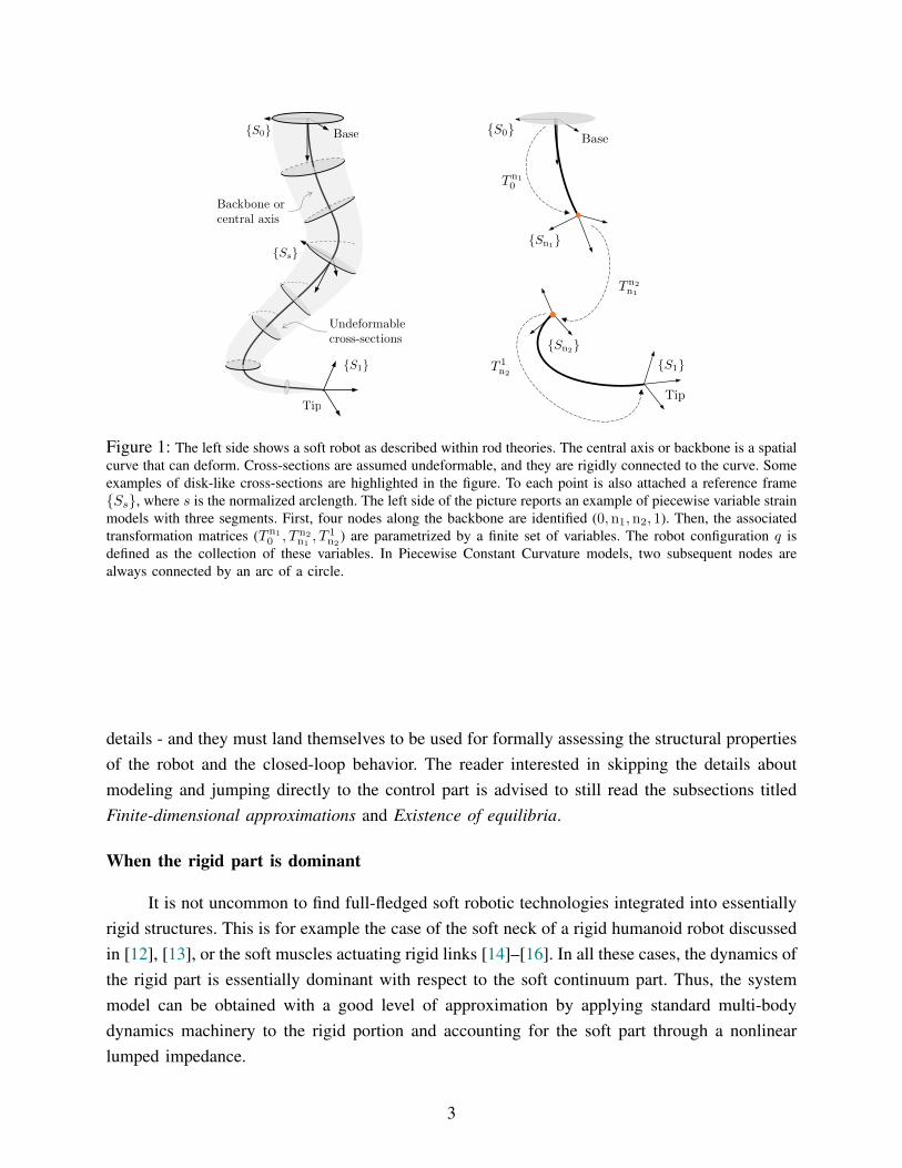
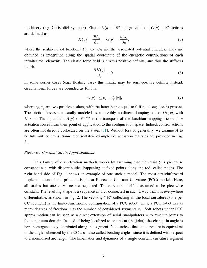
Figure 1: The left side shows a soft robot as described within rod theories. The central axis or backbone is a spatialcurve that can deform. Cross-sections are assumed undeformable, and they are rigidly connected to the curve. Someexamples of disk-like cross-sections are highlighted in the figure. To each point is also attached a reference frame{Ss}, where s is the normalized arclength. The left side of the picture reports an example of piecewise variable strainmodels with three segments. First, four nodes along the backbone are identified (0,n1,n2, 1). Then, the associatedtransformation matrices (T n1

0 , T n2n1, T 1

n2) are parametrized by a finite set of variables. The robot configuration q is

defined as the collection of these variables. In Piecewise Constant Curvature models, two subsequent nodes arealways connected by an arc of a circle.

details - and they must land themselves to be used for formally assessing the structural propertiesof the robot and the closed-loop behavior. The reader interested in skipping the details aboutmodeling and jumping directly to the control part is advised to still read the subsections titledFinite-dimensional approximations and Existence of equilibria.

When the rigid part is dominant

It is not uncommon to find full-fledged soft robotic technologies integrated into essentiallyrigid structures. This is for example the case of the soft neck of a rigid humanoid robot discussedin [12], [13], or the soft muscles actuating rigid links [14]–[16]. In all these cases, the dynamics ofthe rigid part is essentially dominant with respect to the soft continuum part. Thus, the systemmodel can be obtained with a good level of approximation by applying standard multi-bodydynamics machinery to the rigid portion and accounting for the soft part through a nonlinearlumped impedance.

3

{Ss}

<latexit sha1_base64="l62h4jrWS8PaX6ZXsko1XjPkRm4=">AAAB8HicbVBNS8NAEJ3Ur1q/qh69LBbBU0lKRY8FLx4r2lZpQtlsN+3S3U3Y3Qgl5Fd48aCIV3+ON/+N2zYHbX0w8Hhvhpl5YcKZNq777ZTW1jc2t8rblZ3dvf2D6uFRV8epIrRDYh6rhxBrypmkHcMMpw+JoliEnPbCyfXM7z1RpVks7800oYHAI8kiRrCx0qOf3Q0ynfv5oFpz6+4caJV4BalBgfag+uUPY5IKKg3hWOu+5yYmyLAyjHCaV/xU0wSTCR7RvqUSC6qDbH5wjs6sMkRRrGxJg+bq74kMC62nIrSdApuxXvZm4n9ePzXRVZAxmaSGSrJYFKUcmRjNvkdDpigxfGoJJorZWxEZY4WJsRlVbAje8surpNuoe836xW2z1moUcZThBE7hHDy4hBbcQBs6QEDAM7zCm6OcF+fd+Vi0lpxi5hj+wPn8ASc7kJk=</latexit>

{Ss+✏}

<latexit sha1_base64="HJAu8SzeWlSCCfjrqxCJCo6QXAE=">AAAB/XicbVDLSsNAFJ3UV62v+Ni5GSyCIJSkVHRZcOOyon1AE8JkOmmHTmbCzESoIfgrblwo4tb/cOffOG2z0NYDFw7n3Mu994QJo0o7zrdVWlldW98ob1a2tnd29+z9g44SqcSkjQUTshciRRjlpK2pZqSXSILikJFuOL6e+t0HIhUV/F5PEuLHaMhpRDHSRgrsIy+7CzIFz6FHEkWZ4LmXB3bVqTkzwGXiFqQKCrQC+8sbCJzGhGvMkFJ910m0nyGpKWYkr3ipIgnCYzQkfUM5ionys9n1OTw1ygBGQpriGs7U3xMZipWaxKHpjJEeqUVvKv7n9VMdXfkZ5UmqCcfzRVHKoBZwGgUcUEmwZhNDEJbU3ArxCEmEtQmsYkJwF19eJp16zW3ULm4b1Wa9iKMMjsEJOAMuuARNcANaoA0weATP4BW8WU/Wi/VufcxbS1Yxcwj+wPr8ARz0lPk=</latexit>

{Ss}


{Ss+✏}


{Ss}


{Ss+✏}


{Ss}


{Ss+✏}


{Ss}


{Ss+✏}


Torsion

<latexit sha1_base64="wJsR6mSc3Gy996xF4z78H7iXvyY=">AAAB7nicdVBNSwMxEM3Wr1q/qh69BIvgacnWare3ghePFVpbaJeSTbNtaDZZkqxQlv4ILx4U8erv8ea/Md1WUNEHA4/3ZpiZFyacaYPQh1NYW9/Y3Cpul3Z29/YPyodHd1qmitAOkVyqXog15UzQjmGG016iKI5DTrvh9Hrhd++p0kyKtpklNIjxWLCIEWys1G3L3BqWK8htIM9reBC5NeRf1GuWeDUf+VfQc1GOClihNSy/D0aSpDEVhnCsdd9DiQkyrAwjnM5Lg1TTBJMpHtO+pQLHVAdZfu4cnlllBCOpbAkDc/X7RIZjrWdxaDtjbCb6t7cQ//L6qYn8IGMiSQ0VZLkoSjk0Ei5+hyOmKDF8ZgkmitlbIZlghYmxCZVsCF+fwv/JXdXG4l7eVivN6iqOIjgBp+AceKAOmuAGtEAHEDAFD+AJPDuJ8+i8OK/L1oKzmjkGP+C8fQLvUo/u</latexit>

Elongation

<latexit sha1_base64="OEyLfNWv4E+WVNIlhlVu+QAq1oY=">AAAB8XicdVDLSgMxFM3UV62vqks3wSK4GjK12umuIILLCvaB7VAyadqGZpIhyQhl6F+4caGIW//GnX9jOq2gogcuHM65l3vvCWPOtEHow8mtrK6tb+Q3C1vbO7t7xf2DlpaJIrRJJJeqE2JNORO0aZjhtBMriqOQ03Y4uZz77XuqNJPi1kxjGkR4JNiQEWysdHfFpRhltF8sIbeGPK/mQeRWkH9WrVjiVXzkX0DPRRlKYIlGv/jeG0iSRFQYwrHWXQ/FJkixMoxwOiv0Ek1jTCZ4RLuWChxRHaTZxTN4YpUBHEplSxiYqd8nUhxpPY1C2xlhM9a/vbn4l9dNzNAPUibixFBBFouGCYdGwvn7cMAUJYZPLcFEMXsrJGOsMDE2pIIN4etT+D9plW0s7vlNuVQvL+PIgyNwDE6BB6qgDq5BAzQBAQI8gCfw7Gjn0XlxXhetOWc5cwh+wHn7BB7mkS4=</latexit>

Curvature

<latexit sha1_base64="iC3mLk3suCVH+R+vLhb7Vq124vc=">AAAB8HicdVDJSgNBEO1xjXGLevTSGARPQ0+MZnIL5OIxglkkGUJPpydp0j0z9BIIQ77CiwdFvPo53vwbO4ugog8KHu9VUVUvTDlTGqEPZ219Y3NrO7eT393bPzgsHB23VGIkoU2S8ER2QqwoZzFtaqY57aSSYhFy2g7H9bnfnlCpWBLf6WlKA4GHMYsYwdpK93UjJ1gbSfuFInKryPOqHkRuGfmXlbIlXtlH/jX0XLRAEazQ6Bfee4OEGEFjTThWquuhVAcZlpoRTmf5nlE0xWSMh7RraYwFVUG2OHgGz60ygFEibcUaLtTvExkWSk1FaDsF1iP125uLf3ldoyM/yFicGk1jslwUGQ51AuffwwGTlGg+tQQTyeytkIywxETbjPI2hK9P4f+kVbKxuFe3pWKttIojB07BGbgAHqiAGrgBDdAEBAjwAJ7AsyOdR+fFeV22rjmrmRPwA87bJ38akNU=</latexit>

Not deformed

<latexit sha1_base64="qXaUtvBEdCCWDJsts2f6CbbW+/8=">AAAB83icdVDJSgNBEO1xjXGLevTSGARPQ0+MZnILePEkEcwCyRB6emqSJj0L3T1CGPIbXjwo4tWf8ebf2FkEFX1Q8Hiviqp6fiq40oR8WCura+sbm4Wt4vbO7t5+6eCwrZJMMmixRCSy61MFgsfQ0lwL6KYSaOQL6Pjjq5nfuQepeBLf6UkKXkSHMQ85o9pI/ZtE4wDCREYQDEplYteJ49QdTOwqcc9rVUOcqkvcS+zYZI4yWqI5KL33g4RlEcSaCapUzyGp9nIqNWcCpsV+piClbEyH0DM0phEoL5/fPMWnRgmw2Wwq1niufp/IaaTUJPJNZ0T1SP32ZuJfXi/ToevlPE4zDTFbLAozgXWCZwHggEtgWkwMoUxycytmIyop0yamognh61P8P2lXTCz2xW2l3Kgs4yigY3SCzpCDaqiBrlETtRBDKXpAT+jZyqxH68V6XbSuWMuZI/QD1tsnPB6RyQ==</latexit>

Shear strain

<latexit sha1_base64="/x5VSiDfoCY02MGkHP7nHXB5rN4=">AAAB83icdVDLSgNBEJz1GeMr6tHLYBA8hdkYzeYW8OIxonlAsoTZSW8yZHZ2mZkVwpLf8OJBEa/+jDf/xslDUNGChqKqm+6uIBFcG0I+nJXVtfWNzdxWfntnd2+/cHDY0nGqGDRZLGLVCagGwSU0DTcCOokCGgUC2sH4aua370FpHss7M0nAj+hQ8pAzaqzUux0BVVgbRbnsF4qkVCOuW3MxKVWId16tWOJWPOJdYrdE5iiiJRr9wntvELM0AmmYoFp3XZIYP6PKcCZgmu+lGhLKxnQIXUsljUD72fzmKT61ygCHsbIlDZ6r3ycyGmk9iQLbGVEz0r+9mfiX101N6PkZl0lqQLLFojAV2MR4FgAecAXMiIkllClub8VsRBVlxsaUtyF8fYr/J62yjaV0cVMu1svLOHLoGJ2gM+SiKqqja9RATcRQgh7QE3p2UufReXFeF60rznLmCP2A8/YJUEmR1g==</latexit>

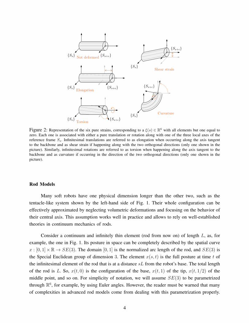
Figure 2: Representation of the six pure strains, corresponding to a ξ(s) ∈ R6 with all elements but one equal tozero. Each one is associated with either a pure translation or rotation along with one of the three local axes of thereference frame Ss. Infinitesimal translations are referred to as elongation when occurring along the axis tangentto the backbone and as shear strain if happening along with the two orthogonal directions (only one shown in thepicture). Similarly, infinitesimal rotations are referred to as torsion when happening along the axis tangent to thebackbone and as curvature if occurring in the direction of the two orthogonal directions (only one shown in thepicture).

Rod Models

Many soft robots have one physical dimension longer than the other two, such as thetentacle-like system shown by the left-hand side of Fig. 1. Their whole configuration can beeffectively approximated by neglecting volumetric deformations and focusing on the behavior oftheir central axis. This assumption works well in practice and allows to rely on well-establishedtheories in continuum mechanics of rods.

Consider a continuum and infinitely thin element (rod from now on) of length L, as, forexample, the one in Fig. 1. Its posture in space can be completely described by the spatial curvex : [0, 1]×R→ SE(3). The domain [0, 1] is the normalized arc length of the rod, and SE(3) isthe Special Euclidean group of dimension 3. The element x(s, t) is the full posture at time t ofthe infinitesimal element of the rod that is at a distance sL from the robot’s base. The total lengthof the rod is L. So, x(t, 0) is the configuration of the base, x(t, 1) of the tip, x(t, 1/2) of themiddle point, and so on. For simplicity of notation, we will assume SE(3) to be parametrizedthrough R6, for example, by using Euler angles. However, the reader must be warned that manyof complexities in advanced rod models come from dealing with this parametrization properly.

4

To each point s along the rod, we can associate a mass density m(s) ∈ R+, an external loadin the form of a generic wrench f(s, t) ∈ R6, and a velocity x(s, t) ∈ R6 . The total mass ofthe segment is

∫ 1

0m(s)ds. The configuration is described by the local strains: curvatures, twist,

elongation, and shear. These are the variations of x for the infinitesimal element s with respectto the previous one. As such, they are a function ξ : [0, 1]→ R6 (or to a smaller space in casesome of the deformations are not considered). Visualizations of pure strains are provided in Fig.2. The rod posture x can always be recovered from the strains ξ by integration. The result is acontinuous version of what in classic robotics would be regarded as the forward kinematics ofthe robot.

It is worth stressing that, despite the formulation referring to an infinitely thin structure(the rod), these models can and are commonly applied every time a central axis can be identified.In this case, we say that the curve x is the backbone of the soft robot. Under the assumptionthat the cross-section of the soft robot changes negligibly during deformations, the contributionof the area can be included by associating an infinitesimal rotational inertia J (s) ∈ R3×3 toeach point along the rod.

At this point, the main ingredients necessary to describe a soft robot within the rodmodeling framework have been laid down. The following subsections will focus on reviewingalternative solutions for formulating the dynamics of these systems. We will start from exactinfinite formulations, then quickly move to survey the various existing alternative to introducingexpert intuitions into the problem and getting to a finite-dimensional model of the robot thatcan be used for control purposes. We will often refer to Piecewise Constant Curvature modelswhen providing examples. This is done for simplicity and because most of the properties ofmore complex models are already present in this more straightforward and widespread solution.

Infinite Dimensional Models

Thanks to their capability of exactly describing continuum structures, and in virtue of theirsolid theoretical foundations, Kirchhoff-Clebsch-Love and Cosserat rod theories [17]–[20] area natural choice for describing soft robots having rod-like structures (see Fig. 1). Leveragingthese frameworks, the statics and dynamics of tendon actuated continuum and soft robots arederived and experimentally validated in [21], [22] and [23] respectively. Multiple Cosserat-rodmodels can be combined together through coupled boundary conditions to describe the kinematicsof parallel soft robots [24], [25]. A tutorial on the dynamic Cosserat model for tendon-drivencontinuum robots is provided in [26]. These models have infinite-dimensional states, and as such,they are formulated as PDEs. This makes it hard to use them directly for control (see sidebarxx for more details). Nonetheless, they can be profitably used to extract steady-state solutions.

5

The use of the Magnus expansion to solve the kinematics of Cosserat rods is discussed in [27],[28]. Also, the direct application to simulation is arduous but not impossible. For example, [29]performs a time discretization, which transforms the PDE into an ODE in the s variable only.The latter is then solved at every time step to find the robot’s shape. Nonlinear observers canbe used to speed up the convergence [30].

Finite dimensional approximations

The alternative to PDE formulations is to restrict the range of possible strains ξ to a finite-dimensional functional space. Two classes of strategies exist to achieve this goal: piecewiseconstant strain models and functional parametrizations. Both of them will be discussed in detailbelow. At the current stage, what is essential to keep in mind is that using these techniques, thestrain ξ can be approximated as a function of the vector q ∈ Rn that serves as the configurationof the soft robot. This critical step enables the recasting of concepts from classic discrete roboticsto the new continuum context. For a start, the kinematics of a soft robot can now be defined asfollows

x(s, q(t)) = J(s, q(t)) q(t), J(s, q) =∂h(s, q)

∂q, (1)

where h(s, q) ∈ R6 is the map - called forward kinematics - connecting the configuration q(t)

to the posture x(s, t) for each point s along the backbone. The matrix-valued function J isthe Jacobian of h. The following set of ODEs can be directly derived from (1) via standardLagrangian mechanics machinery

M(q)q + C(q, q)q +G(q)︸︷︷︸Multi-body dynamics

+ D(q)q +K(q)︸︷︷︸Elastic and dissipative forces

= A(q)τ︸︷︷︸Model of underactuation

, (2)

where (q, q) forms the robot state.

The inertia matrix M(q) ∈ Rn×n is evaluated as follows

M(q) =

∫ 1

0

J>(q, s)

[m(s)I 0

0 J (s)

]J(q, s) ds � 0, (3)

where m(s) and J (s) are the mass and inertia distributions respectively. Note that M(q) maybecome singular in some configurations. This however can always be avoided by properlyparametrizing the configurations space. As for a rigid robot, the inertia matrix verifies

||M(q)|| ≤ cm + c′m||q||2, (4)

where cm, c′m are two positive scalars. If the elongation is considered negligible, then c′m = 0.

Coriolis and centrifugal forces C(q, q)q ∈ Rn can be evaluated using the standard mathematical

6

machinery (e.g. Christoffel symbols). Elastic K(q) ∈ Rn and gravitational G(q) ∈ Rn actionsare defined as

K(q) =∂UK

∂q, G(q) =

∂UG

∂q, (5)

where the scalar-valued functions UK and UG are the associated potential energies. They areobtained as integration along the spatial coordinate of the energetic contributions of eachinfinitesimal elements. The elastic force field is always positive definite, and thus the stiffnessmatrix

∂K(q)

∂q� 0. (6)

In some corner cases (e.g., floating base) this matrix may be semi-positive definite instead.Gravitational forces are bounded as follows

||G(q)|| ≤ cg + c′g||q||, (7)

where cg, c′g are two positive scalars, with the latter being equal to 0 if no elongation is present.

The friction losses are usually modeled as a possibly nonlinear damping action D(q)q, withD � 0. The input field A(q) ∈ Rn×m is the transpose of the Jacobian mapping the m ≤ n

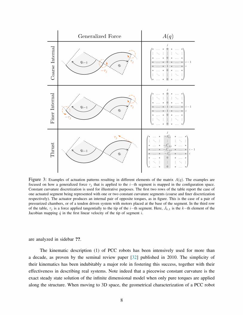
actuation forces from their point of application to the configuration space. Indeed, control actionsare often not directly collocated on the states [31]. Without loss of generality, we assume A tobe full rank columns. Some representative examples of actuation matrices are provided in Fig.3.

Piecewise Constant Strain Approximations

This family of discretization methods works by assuming that the strain ξ is piecewiseconstant in s, with discontinuities happening at fixed points along the rod, called nodes. Theright hand side of Fig. 1 shows an example of one such a model. The most straightforwardimplementation of this principle is planar Piecewise Constant Curvature (PCC) models. Here,all strains but one curvature are neglected. The curvature itself is assumed to be piecewiseconstant. The resulting shape is a sequence of arcs connected in such a way that x is everywheredifferentiable, as shown in Fig. 2. The vector q ∈ Rn collecting all the local curvatures (one perCC segment) is the finite-dimensional configuration of a PCC robot. Thus, a PCC robot has asmany degrees of freedom n as the number of considered segments nS. Soft robots under PCCapproximation can be seen as a direct extension of serial manipulators with revolute joints tothe continuum domain. Instead of being localized to one point (the joint), the change in angle ishere homogeneously distributed along the segment. Note indeed that the curvature is equivalentto the angle subtended by the CC arc - also called bending angle - since it is defined with respectto a normalized arc length. The kinematics and dynamics of a single constant curvature segment

7

qi

qi�1

0

A(q) =

j0BBBBBBBBBBBBB@

1CCCCCCCCCCCCCA

? . . . ? 0 ? . . . ?... . . . ...

...... . . . ...

? . . . ? 0 ? . . . ?

? . . . ? 1 ? . . . ? i � 1

? . . . ? 1 ? . . . ? i

? . . . ? 0 ? . . . ?... . . . ...

...... . . . ...

? . . . ? 0 ? . . . ?

(1)

A(q) =

j0BBBBBBBBBBBBB@

1CCCCCCCCCCCCCA

? . . . ? 0 ? . . . ?... . . . ...

...... . . . ...

? . . . ? 0 ? . . . ?

? . . . ? 0 ? . . . ? i � 1

? . . . ? 1 ? . . . ? i

? . . . ? 0 ? . . . ?... . . . ...

...... . . . ...

? . . . ? 0 ? . . . ?

(2)

A(q) =

j0BBBBBBBBBBBBB@

1CCCCCCCCCCCCCA

? . . . ? �J>1,1 ? . . . ?

... . . . ......

... . . . ...? . . . ? �J>

i�2,1 ? . . . ?

? . . . ? �J>i�1,1 ? . . . ? i � 1

? . . . ? �J>i,1 ? . . . ? i

? . . . ? 0 ? . . . ?... . . . ...

...... . . . ...

? . . . ? 0 ? . . . ?

, (3)

July 10, 2021 DRAFT

A(q)

qi

qi�1

�⌧j

⌧j

0

A(q) =

j0BBBBBBBBBBBBB@

1CCCCCCCCCCCCCA

? . . . ? 0 ? . . . ?... . . . ...

...... . . . ...

? . . . ? 0 ? . . . ?

? . . . ? 1 ? . . . ? i � 1

? . . . ? 1 ? . . . ? i

? . . . ? 0 ? . . . ?... . . . ...

...... . . . ...

? . . . ? 0 ? . . . ?

(1)

A(q) =

j0BBBBBBBBBBBBB@

1CCCCCCCCCCCCCA

? . . . ? 0 ? . . . ?... . . . ...

...... . . . ...

? . . . ? 0 ? . . . ?

? . . . ? 0 ? . . . ? i � 1

? . . . ? 1 ? . . . ? i

? . . . ? 0 ? . . . ?... . . . ...

...... . . . ...

? . . . ? 0 ? . . . ?

(2)

A(q) =

j0BBBBBBBBBBBBB@

1CCCCCCCCCCCCCA

? . . . ? �J>1,1 ? . . . ?

... . . . ......

... . . . ...? . . . ? �J>

i�2,1 ? . . . ?

? . . . ? �J>i�1,1 ? . . . ? i � 1

? . . . ? �J>i,1 ? . . . ? i

? . . . ? 0 ? . . . ?... . . . ...

...... . . . ...

? . . . ? 0 ? . . . ?

, (3)

July 10, 2021 DRAFT

qi

qi�1⌧j

�⌧j

0

A(q) =

j0BBBBBBBBBBBBB@

1CCCCCCCCCCCCCA

? . . . ? 0 ? . . . ?... . . . ...

...... . . . ...

? . . . ? 0 ? . . . ?

? . . . ? 1 ? . . . ? i � 1

? . . . ? 1 ? . . . ? i

? . . . ? 0 ? . . . ?... . . . ...

...... . . . ...

? . . . ? 0 ? . . . ?

(1)

A(q) =

j0BBBBBBBBBBBBB@

1CCCCCCCCCCCCCA

? . . . ? 0 ? . . . ?... . . . ...

...... . . . ...

? . . . ? 0 ? . . . ?

? . . . ? 0 ? . . . ? i � 1

? . . . ? 1 ? . . . ? i

? . . . ? 0 ? . . . ?... . . . ...

...... . . . ...

? . . . ? 0 ? . . . ?

(2)

A(q) =

j0BBBBBBBBBBBBB@

1CCCCCCCCCCCCCA

? . . . ? �J>1,1 ? . . . ?

... . . . ......

... . . . ...? . . . ? �J>

i�2,1 ? . . . ?

? . . . ? �J>i�1,1 ? . . . ? i � 1

? . . . ? �J>i,1 ? . . . ? i

? . . . ? 0 ? . . . ?... . . . ...

...... . . . ...

? . . . ? 0 ? . . . ?

, (3)

July 10, 2021 DRAFT

Generalized Force

Thru

stFin

erIn

tern

al

Coar

seIn

tern

al

⌧j

Figure 3: Examples of actuation patterns resulting in different elements of the matrix A(q). The examples arefocused on how a generalized force τj that is applied to the i−th segment is mapped in the configuration space.Constant curvature discretization is used for illustrative purposes. The first two rows of the table report the case ofone actuated segment being represented with one or two constant curvature segments (coarse and finer discretizationrespectively). The actuator produces an internal pair of opposite torques, as in figure. This is the case of a pair ofpressurized chambers, or of a tendon driven system with motors placed at the base of the segment. In the third rowof the table, τj is a force applied tangentially to the tip of the i−th segment. Here, Jk,1 is the k−th element of theJacobian mapping q in the first linear velocity of the tip of segment i.

are analyzed in sidebar ??.

The kinematic description (1) of PCC robots has been intensively used for more thana decade, as proven by the seminal review paper [32] published in 2010. The simplicity oftheir kinematics has been indubitably a major role in fostering this success, together with theireffectiveness in describing real systems. Note indeed that a piecewise constant curvature is theexact steady state solution of the infinite dimensional model when only pure torques are appliedalong the structure. When moving to 3D space, the geometrical characterization of a PCC robot

8

as a sequence of arcs remains unvaried, but this time the plane of bending can change. Thiseffectively introduces two degrees of freedom per segment, i.e. n = 2nS. The usual way inwhich this motion is represented in the literature is by including into q the orientation of the nrelative orientations of the planes of bending. Although intuitive, this representation introducessingularities and discontinuities [33] which can be avoided with alternative parametrizations [34]–[37]. Occasionally piecewise constant elongation is also considered, with discontinuity pointscoincident to the curvature ones, thus leading to n = 2nS for the planar case and n = 3nS forthe 3D one.

As discussed for the general case, the dynamic model (2) of a PCC robot is obtainedcombining (1) with the physical characteristics of the system through standard Lagrangianformalism [38]. Yet, when multiple segments are considered it is unpractical to derive closedform expressions of M and G. Approximations of the mass distribution are thus often imposedto simplify the model derivations. Models having the mass of each segment lumped into a singlealong the rod are discussed in [39], [40]. Alternatively a lumped mass and inertia can be placedat the center of mass [41], [42], therefore neglecting only the change in rotational inertia. Underthis hypothesis, the soft robot can be represented through an augmented rigid robot model,therefore enabling the use of standard tools for calculating the expression of dynamic forces[43]–[45].

A simpler alternative to PCC which can be used to model robots bending and elongatingare rigid link approximations [46], [47]. The rod is here approximated through a sequence oflinks connected with standard independent joints. This is equivalent to considering a ξ whichis null everywhere, except for a finite set of points where it assumes the value of a Dirac’sdelta. Lumped springs are added in parallel to each joint to describe the robot’s impedance. Theresulting structure is a standard rigid robot with parallel elasticity, and it is therefore describedby a set of ODE as (2). Kinematic model of parallel soft manipulators based on these strategiesare discussed in [48]–[50].

PCC models can be extended further by adding also piecewise constant shear deformationand twist. This is done by the piecewise constant strain models proposed in [51], [52], whichdefine procedures for extracting models in the form (2), where q ∈ R6ns . The inertia matrixM(q) implements a full dynamic coupling within the six strains. On the contrary, the elasticpart of the potential forces K(q) is usually either diagonal or block diagonal. Thanks to theircapability of describing complex strain conditions naturally arising in closed kinematic chains,these models can be used to describe soft parallel structures [53].

9

How Fine Should the Discretization Be?

For a given soft robot to be modeled under a piecewise constant strain approximation, thenumber of segments ns to be considered is up to the designer of the model to decide as a resultof application-specific considerations. First, the mechanics of the robot imposes a lower boundin case the robot is obtained as a sequence of actuated modules, since considering less than oneconstant strain segment for each actuated one would generate incoherent behaviors (e.g. actuatingone segment would result in a motion in the following one). Also, it is in general inconvenientto have constant strain segments shared between more than one actuated segment. If the robot isused for simulation, then a trade-off between accuracy and simplicity must be established. Forns →∞ the model converges to the exact continuum representation, but the computational costfor the simulation will increase as O(n2

s ) at the best [54]. In case the model is used for controldesign, then the amount and the location of the segments may change the structural properties of(2). It is for example common to place segments in such a way that the resulting model is fullyactuated, i.e. A(q) is square and full rank. For planar PCC models, if τ are torques applied atthe tip of each CC segment then A(q) = I - therefore further strengthening the parallelism withstandard serial rigid robots. Most of existing actuation technologies will satisfy this hypothesis(e.g. tendons, fluids).

Functional Parametrizations

Instead of discretizing along the arclength, the reduction of dimensionality can happen byprojecting onto a low dimensional functional subspace as follows

ξ(s, t) =n∑

i=1

πi(s)qi(t), (8)

where {π1(s), . . . , πn(s)} is a base of the subspace, and the weights qi(t) can be taken asthe configuration of the robot. One simple way of selecting πi(s) is to truncate an infinitedimensional basis of a regular-enough functional space. In this way, it is ensured/guaranteedthat the approximation converges to the exact model for n→∞. It is also convenient to includeconstant functions, so that the model is a proper extension of the constant curvature or constantstrain ones. For example, in the case of inextensible planar soft robots (i.e. ξ contains only thecurvature), polynomials πi(s) = si−1 are a basis that satisfies both conditions. This modelingtechnique is widely used in flexible link robots [55] to represent link vibrations. In this case, thebase functions πi(s) are selected as the n slowest modes of the Euler Bernoulli beam modelingthe link [56], [57]. Functional expansions are also used in continuum mechanics to approximatethe equilibria of rods and beams [58], [59]. The application to rod-like structures originated fromthe field of hyper-redundant robots [60]. Here, the rod serves as a continuum approximation of

10

(qi, qi+1)

<latexit sha1_base64="FGxyzLAzl13VQSxAiK+eJFUagec=">AAAB9HicbVBNS8NAEJ3Ur1q/qh69LBahopSkVPRY8OKxgv2ANoTNdtMu3WzS3U2hhP4OLx4U8eqP8ea/cdvmoK0PBh7vzTAzz485U9q2v63cxubW9k5+t7C3f3B4VDw+aakokYQ2ScQj2fGxopwJ2tRMc9qJJcWhz2nbH93P/faESsUi8aSnMXVDPBAsYARrI7nlsceux17KrpzZpVcs2RV7AbROnIyUIEPDK371+hFJQio04ViprmPH2k2x1IxwOiv0EkVjTEZ4QLuGChxS5aaLo2fowih9FETSlNBoof6eSHGo1DT0TWeI9VCtenPxP6+b6ODOTZmIE00FWS4KEo50hOYJoD6TlGg+NQQTycytiAyxxESbnAomBGf15XXSqlacWuXmsVaq21kceTiDcyiDA7dQhwdoQBMIjOEZXuHNmlgv1rv1sWzNWdnMKfyB9fkDeP2RNQ==</latexit>

Mesh

<latexit sha1_base64="bdwkSWUinx0aqFjPTFlQHy+K21U=">AAAB63icbVBNS8NAEJ34WetX1aOXxSJ4KklR9Fjw4kWoYD+gDWWznTRLdzdhdyOU0r/gxYMiXv1D3vw3Jm0O2vpg4PHeDDPzgkRwY13321lb39jc2i7tlHf39g8OK0fHbROnmmGLxSLW3YAaFFxhy3IrsJtopDIQ2AnGt7nfeUJteKwe7SRBX9KR4iFn1ObSPZpoUKm6NXcOskq8glShQHNQ+eoPY5ZKVJYJakzPcxPrT6m2nAmclfupwYSyMR1hL6OKSjT+dH7rjJxnypCEsc5KWTJXf09MqTRmIoOsU1IbmWUvF//zeqkNb/wpV0lqUbHFojAVxMYkf5wMuUZmxSQjlGme3UpYRDVlNounnIXgLb+8Str1mndZu3qoVxtuEUcJTuEMLsCDa2jAHTShBQwieIZXeHOk8+K8Ox+L1jWnmDmBP3A+fwD3j44j</latexit>

Pointmass

<latexit sha1_base64="l0IQBnOKtsiJNJPXmOBP7/oreK0=">AAAB8nicbVDLSgMxFM3UVx1fVZdugkVwVWaKosuCG5cV7APaoWTSTBuax5DcEcrQz3DjQhG3fo07/8a0nYW2Hggczrn35t4Tp4JbCIJvr7SxubW9U9719/YPDo8qxydtqzNDWYtqoU03JpYJrlgLOAjWTQ0jMhasE0/u5n7niRnLtXqEacoiSUaKJ5wScFKvqbkC35fE2kGlGtSCBfA6CQtSRQWag8pXf6hpJpkCKtyAXhikEOXEAKeCzfx+ZllK6ISMWM9RRSSzUb5YeYYvnDLEiTbuKcAL9XdHTqS1Uxm7SklgbFe9ufif18sguY1yrtIMmKLLj5JMYNB4fj8ecsMoiKkjhBrudsV0TAyh4FLyXQjh6snrpF2vhVe164d6tREUcZTRGTpHlyhEN6iB7lETtRBFGj2jV/TmgffivXsfy9KSV/Scoj/wPn8Ae7mQrg==</latexit>

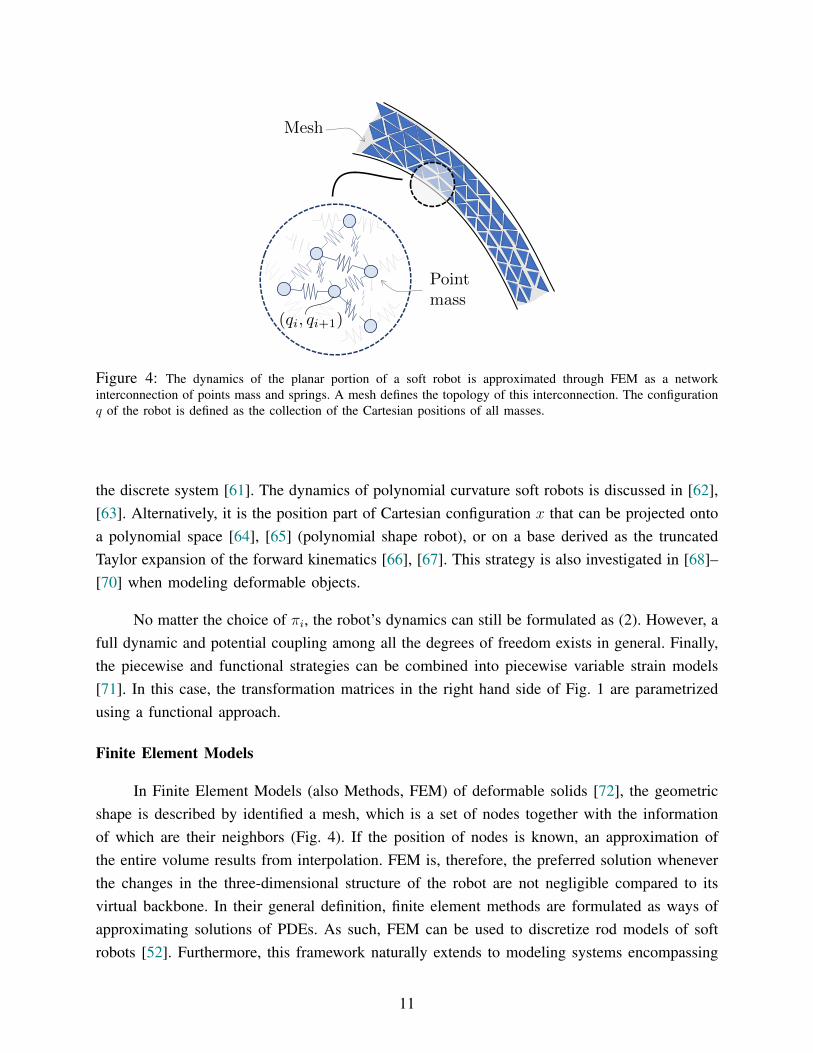
Figure 4: The dynamics of the planar portion of a soft robot is approximated through FEM as a networkinterconnection of points mass and springs. A mesh defines the topology of this interconnection. The configurationq of the robot is defined as the collection of the Cartesian positions of all masses.

the discrete system [61]. The dynamics of polynomial curvature soft robots is discussed in [62],[63]. Alternatively, it is the position part of Cartesian configuration x that can be projected ontoa polynomial space [64], [65] (polynomial shape robot), or on a base derived as the truncatedTaylor expansion of the forward kinematics [66], [67]. This strategy is also investigated in [68]–[70] when modeling deformable objects.

No matter the choice of πi, the robot’s dynamics can still be formulated as (2). However, afull dynamic and potential coupling among all the degrees of freedom exists in general. Finally,the piecewise and functional strategies can be combined into piecewise variable strain models[71]. In this case, the transformation matrices in the right hand side of Fig. 1 are parametrizedusing a functional approach.

Finite Element Models

In Finite Element Models (also Methods, FEM) of deformable solids [72], the geometricshape is described by identified a mesh, which is a set of nodes together with the informationof which are their neighbors (Fig. 4). If the position of nodes is known, an approximation ofthe entire volume results from interpolation. FEM is, therefore, the preferred solution wheneverthe changes in the three-dimensional structure of the robot are not negligible compared to itsvirtual backbone. In their general definition, finite element methods are formulated as ways ofapproximating solutions of PDEs. As such, FEM can be used to discretize rod models of softrobots [52]. Furthermore, this framework naturally extends to modeling systems encompassing

11

multiple continuous behaviors - e.g. magnetic, thermal, fluid [73].

The discussed space interpolation naturally leads to a kinematic description in the formof (1). The configuration q ∈ Rn is the collection of the nodes location in the space. So, n isin general three times the number of nodes. Since the full volume is explicitly considered, theforward kinematics h(s, q) is to be parametrized with s ∈ R3, rather than a scalar. Similarly torod models, FEM have the advantageous property of converging to the exact model when n tendsto infinity. Using several thousand nodes, in general, produces a very accurate model at the costof a quite large configuration space. Note however that measuring or observing the whole state ofa FEM model is often not needed when implementing closed loop controls. Dynamic equationsin the form (2) result from the application of Lagrangian machinery to (1), in a similar fashionas for the rod case. Discretization in strain space ξ usually results in a linear K(q) and constantD(q), at the cost of a configuration dependent inertia M(q). On the contrary, in FEM analysisthe following simplifications are introduced whenever the mass is assumed concentrated to thenodes: ∂M(q)/∂q = 0, C(q, q) = 0, and ∂G(q)/∂q = 0. Thus, the multi-body dynamic part of(2) simplifies into Mq+G. Furthermore, M is diagonal if q represents the nodes’ configurationin the space, which implies that there is no dynamic coupling. On the downside K(q) is usuallynonlinear, and D(q) and A(q) are rarely constant.

Model order reduction

The high dimensional configuration space of a FEM model can be compressed by selectinga set of nr << n directions of interest [74]. In practice, nr is usual in the order of a few dozens,and thus n/nr & 102. The reduced order configuration is defined as qr = Φq, where for simplicityit is assumed that the configuration q is defined such that q = 0 is the system equilibrium forτ = 0. This projection is conceptually similar to the functional parametrizations discussed abovefor rod dynamics. The resulting dynamics in qr space is

(Φ>MΦ

)qr + Φ>G+

(Φ>D(Φqr)Φ

)qr + Φ>K(Φqr) = Φ>A(Φqr)τ, (9)

which is again in the general form (2). Note that Φ>MΦ is diagonal if M is diagonal and ifΦ is orthogonal. The matrix Φ should be selected in such a way that the solution of (9) isrepresentative of the evolution of (2) for the full FEM model, as soon as the initial conditionsatisfies (qr(0), qr(0)) = (Φq(0),Φq(0)). Modal analysis is a well known tool in FEM theory toachieve this goal [74, Ch. 12]. The linear modes of the linearized system about the equilibriumconfiguration are calculated. The eigenvectors associated to the smallest eigenvalues (slowestmodes) are used to build Φ. The value of nR can be defined according to the frequency rangeof vibrations that the designer is interested in capturing. This procedure implicitly operates aregularization of the FEM model, getting rid of many numerical vibrations happening at high

12

frequency, which can be assimilated to numerical noise. Alternatively, the columns of Φ can beevaluated from the singular value decomposition of a dataset of representative evolutions of thesystem [75]. These analyses can be extended to nonlinear deformations [76]–[78]. The extensionto the modeling of soft robot with self-contact forces is discussed in [79]. One reason for n toreach high values - up to hundreds of thousands - is that the robot geometry has many details(thinned areas, holes, small grooves). This issue can be tamed through several methods as forexample X-FEM [80], [81], which however does not radically reduce the size of the models.Condensation is another widely used approach. It operates model reduction by partitioning theconfiguration space in loaded - directly actuated - and unloaded variables. The loading conditionsare modeled as holonomic constraints and solved with Lagrangian multipliers [74], [82], [83].Condensation has also been used to connect FEM and rod models in [84]. A recent review paperon model reduction techniques is also available [85].

⌧

K(q) + G(q)

A(q)

K(q)

A(q)

q

K(q) � cg

c+a

K(q) + cg

c�a

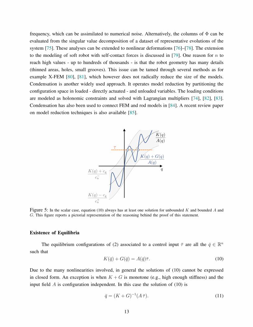
Figure 5: In the scalar case, equation (10) always has at least one solution for unbounded K and bounded A andG. This figure reports a pictorial representation of the reasoning behind the proof of this statement.

Existence of Equilibria

The equilibrium configurations of (2) associated to a control input τ are all the q ∈ Rn

such thatK(q) +G(q) = A(q)τ . (10)

Due to the many nonlinearities involved, in general the solutions of (10) cannot be expressedin closed form. An exception is when K +G is monotone (e.g., high enough stiffness) and theinput field A is configuration independent. In this case the solution of (10) is

q = (K +G)−1(A τ). (11)

13

So, a single equilibrium always exists for any choice of actuation. If K + G is not monotoneor if the actuation field A is configuration dependent, the existence of at least one equilibriumfor any given τ is to be expected if K(q) is radially unbounded (i.e. stiffness not vanishing).Several solutions to this equation may in general exist. Consider for example the case of n = 1

and c−a < A < c+a . Thus, if K(q) is radially unbounded and G(q) is limited, then also K/A and

G/A are. Thus, (K + G)/A is radially unbounded, even if in general not monotonic. It is alsoa continuous function. As a consequence, there is always at least one equilibrium configuration,that is a configuration q that verifies (K(q) +G(q))/A(q) = τ . This sketch of proof is visuallyrepresented by Fig. 5. The existence of at least one equilibrium for any constant actuation is insharp contrast with classic rigid robots, for which a constant actuation can never result in anequilibrium configuration unless gravity is involved.

Actuators dynamics

Soft robots are actuated through a wide variety of strategies. Yet, relatively few attentionhas been devoted so far to incorporating the dynamics of actuators in dynamic models used forcontrol. Nonetheless, we can still provide a model based on similar formulations from classicrobotics [86], [87], which holds for actuation strategies where the main function components ofthe actuators are themselves mechanical (e.g. tendons actuated through electric motors, fluidspressurized through pistons)

M(q)q + C(q, q)q +D(q)q +K(q) +G(q) +∂Uc

∂q(q, η) = 0, (12)

B(η)η +H(η, η)η +∂Uc

∂η(q, η) = τ, (13)

where we not include dissipation in the actuation system for simplicity. The configuration of allthe actuators is collected in η ∈ Rm, and B,H ∈ Rm×m are the associated inertia and Coriolismatrices. The former is usually diagonal and configuration independent, and in turn H = 0.This is however not always the case, an exception being magnetically actuated soft robots withmagnets moved by a rigid robot [88].

The coupling between the dynamics (12) and (13) is purely mediated by the potentialfield Uc, which models elasticity of tendons, molecular interactions in compressible fluids, orelectro-magnetic fields, just to cite a few. In case the dynamics of η is fast compared to q, aswell as robustly globally stable, then (13) can be approximated with its steady state behaviorη ' η(q, τ). In this case ∂Uc(q, η(q, τ))/∂q serves as a generalization of the input field A(q)τ

appearing in (2). Alternatively, singular perturbation theory can be used to separate the fastactuator dynamics from the slow soft robot one, without applying quasi-static approximations[89].

14

Simulators

A bottleneck to entering into the field of soft robots control has been the need to implementthe simulator of the soft robot. This is especially troublesome when considering that the modelsused for simulation are typically way more sophisticated than the ones used for control. Luckily,there are now several open-source solutions available: SOFA [90], [91] and ChainQueen [92] usevelumetric FEM techniques, while Elastica [93], TMTDyn [94], SimSOFT [52], and SoRoSim[95] implement discretizations of rod modes. More details on simulators for soft robots can befound in [96, Sec. VII]. Still, selecting the right model among all the available ones is a taskwith no clear solution. Experimental comparisons as the ones provided in [97], [98] can be auseful tool in this context.

Shape Control in the Fully Actuated Approximation

The primary task of control architectures in classic robotics is to accurately manage theposture of the robot - i.e. state space control. In the case of soft robots, this translates into devisingstrategies to control the whole shape of the system, that is controlling q. Depending on the modelused for control design, this task may translate into different goals - as for example curvature,strain, or volume control - which however share a same set of characteristics. The importanceof carefully selecting the model used for control design becomes therefore apparent. Indeed,applying a same control solution with different models will in general produce substantiallydifferent closed loop behaviors - both in terms of transient and steady state. We start in thissections with robots that can be effectively modeled as fully actuated - i.e., m = n and withoutloss of generality A(q) = I . We will see how this approximation allows to already acquireimportant insight on the behavior of soft robots.

Posture regulation

Posture regulation is defined as follows: given a desired constant configuration q ∈ Rn

find a control action τ ∈ Rm such that the configuration of the soft robot q ∈ Rn eventuallyconverges to the desired one, i.e.,

limt→∞

q(t) = q. (14)

It has been already discussed in the previous section that an equilibrium is always associatedto any constant control input - as exemplified by (11). We show here that this equilibrium isalso asymptotically stable under opportune conditions on the mechanical impedance of the robot.

15

q

<latexit sha1_base64="P5gv480mjd0QU6h6Uqtw2vlNBPA=">AAAB7nicbVDLSgNBEOyNrxhfUY9eBoPgKexKfBwDXjxGMA9IljA7mU2GzM6uM71CWPIRXjwo4tXv8ebfOEn2oIkFDUVVN91dQSKFQdf9dgpr6xubW8Xt0s7u3v5B+fCoZeJUM95ksYx1J6CGS6F4EwVK3kk0p1EgeTsY38789hPXRsTqAScJ9yM6VCIUjKKV2r2A6uxx2i9X3Ko7B1klXk4qkKPRL3/1BjFLI66QSWpM13MT9DOqUTDJp6VeanhC2ZgOeddSRSNu/Gx+7pScWWVAwljbUkjm6u+JjEbGTKLAdkYUR2bZm4n/ed0Uwxs/EypJkSu2WBSmkmBMZr+TgdCcoZxYQpkW9lbCRlRThjahkg3BW355lbQuql6tenlfq9Sv8jiKcAKncA4eXEMd7qABTWAwhmd4hTcncV6cd+dj0Vpw8plj+APn8weYUY+2</latexit>

+

<latexit sha1_base64="xs1yn/ztIlAsYb8XaKbJ+eK8cmI=">AAAB6HicbVDLSgNBEOyNrxhfUY9eBoMgCGFX4uMY8OIxAfOAZAmzk95kzOzsMjMrhJAv8OJBEa9+kjf/xkmyB00saCiquunuChLBtXHdbye3tr6xuZXfLuzs7u0fFA+PmjpOFcMGi0Ws2gHVKLjEhuFGYDtRSKNAYCsY3c381hMqzWP5YMYJ+hEdSB5yRo2V6he9Ysktu3OQVeJlpAQZar3iV7cfszRCaZigWnc8NzH+hCrDmcBpoZtqTCgb0QF2LJU0Qu1P5odOyZlV+iSMlS1pyFz9PTGhkdbjKLCdETVDvezNxP+8TmrCW3/CZZIalGyxKEwFMTGZfU36XCEzYmwJZYrbWwkbUkWZsdkUbAje8surpHlZ9irlq3qlVL3O4sjDCZzCOXhwA1W4hxo0gAHCM7zCm/PovDjvzseiNedkM8fwB87nD3CBjKs=</latexit>

+


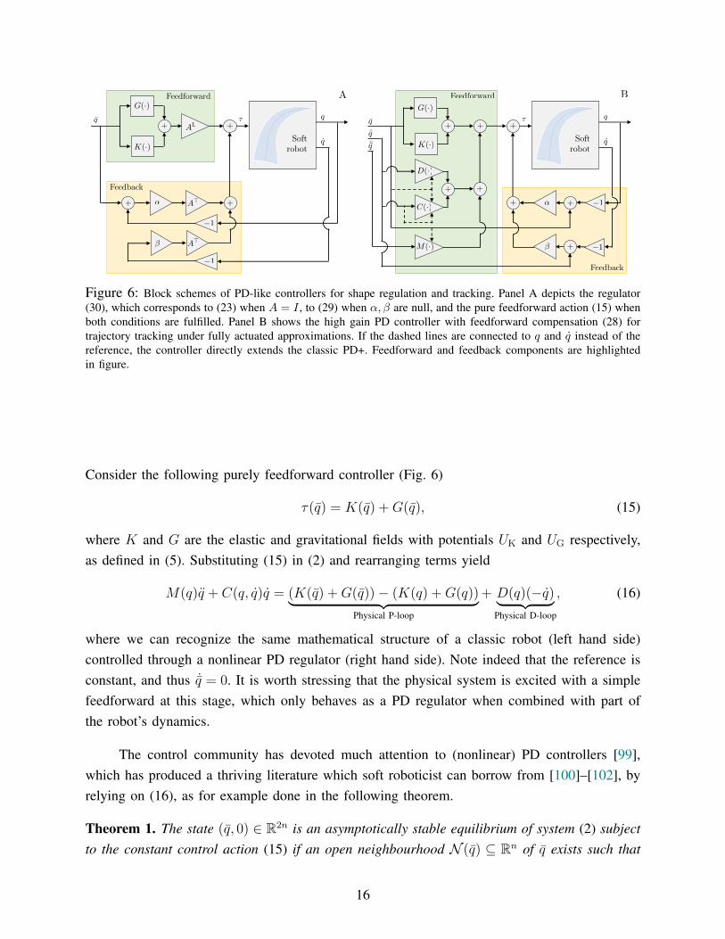
Feedforward

<latexit sha1_base64="IzBADie5PxoOE7Zv1eq1U0nNV6o=">AAAB8nicbVDLSsNAFJ34rPVVdelmsAiuSlJ8LQuCuKxgH5CGMpnctEMnM2FmopTQz3DjQhG3fo07/8Zpm4W2HrhwOOde7r0nTDnTxnW/nZXVtfWNzdJWeXtnd2+/cnDY1jJTFFpUcqm6IdHAmYCWYYZDN1VAkpBDJxzdTP3OIyjNpHgw4xSChAwEixklxkr+LUAUS/VEVNSvVN2aOwNeJl5BqqhAs1/56kWSZgkIQznR2vfc1AQ5UYZRDpNyL9OQEjoiA/AtFSQBHeSzkyf41CoRtqttCYNn6u+JnCRaj5PQdibEDPWiNxX/8/zMxNdBzkSaGRB0vijOODYST//HEVNADR9bQqhi9lZMh0QRamxKZRuCt/jyMmnXa9557eK+Xm1cFnGU0DE6QWfIQ1eoge5QE7UQRRI9o1f05hjnxXl3PuatK04xc4T+wPn8AWSwkUs=</latexit>

Feedback

<latexit sha1_base64="NK3/2RZIdNdVVhggqglijgxm4xk=">AAAB73icbVDLSgNBEOz1GeMr6tHLYBA8hd3g6xgQxGME84BkCbOzvcmQ2dl1ZlYIIT/hxYMiXv0db/6Nk2QPmlgwUFR193RXkAqujet+Oyura+sbm4Wt4vbO7t5+6eCwqZNMMWywRCSqHVCNgktsGG4EtlOFNA4EtoLhzdRvPaHSPJEPZpSiH9O+5BFn1FipfYsYBpQNe6WyW3FnIMvEy0kZctR7pa9umLAsRmmYoFp3PDc1/pgqw5nASbGbaUztYNrHjqWSxqj98WzfCTm1SkiiRNknDZmpvzvGNNZ6FAe2MqZmoBe9qfif18lMdO2PuUwzg5LNP4oyQUxCpseTkCtkRowsoUxxuythA6ooMzaiog3BWzx5mTSrFe+8cnFfLdcu8zgKcAwncAYeXEEN7qAODWAg4Ble4c15dF6cd+djXrri5D1H8AfO5w/PFo/J</latexit>

AL

<latexit sha1_base64="4xGqKQqtfYAUsqSioU/jHlDiUSk=">AAAB9XicbVC7TsMwFL0pr1JeBUYWiwqJqUpQeYxFLAwMRaIPqU0rx3Vaq44T2Q6oivIfLAwgxMq/sPE3OG0GaDmSpaNz7tU9Pl7EmdK2/W0VVlbX1jeKm6Wt7Z3dvfL+QUuFsSS0SUIeyo6HFeVM0KZmmtNOJCkOPE7b3uQm89uPVCoWigc9jagb4JFgPiNYG6l/3U96AdZjGSR3aTooV+yqPQNaJk5OKpCjMSh/9YYhiQMqNOFYqa5jR9pNsNSMcJqWerGiESYTPKJdQwUOqHKTWeoUnRhliPxQmic0mqm/NxIcKDUNPDOZRVSLXib+53Vj7V+5CRNRrKkg80N+zJEOUVYBGjJJieZTQzCRzGRFZIwlJtoUVTIlOItfXiats6pTq57f1yr1i7yOIhzBMZyCA5dQh1toQBMISHiGV3iznqwX6936mI8WrHznEP7A+vwB6p6Swg==</latexit>

+


↵

<latexit sha1_base64="p1F3YXIefsKb25G8/sHruOQ77VM=">AAAB7XicbVDLSgNBEOyNrxhfUY9eBoPgKexKfBwDXjxGMA9IltA7mU3GzM4uM7NCWPIPXjwo4tX/8ebfOEn2oIkFDUVVN91dQSK4Nq777RTW1jc2t4rbpZ3dvf2D8uFRS8epoqxJYxGrToCaCS5Z03AjWCdRDKNAsHYwvp357SemNI/lg5kkzI9wKHnIKRortXookhH2yxW36s5BVomXkwrkaPTLX71BTNOISUMFat313MT4GSrDqWDTUi/VLEE6xiHrWioxYtrP5tdOyZlVBiSMlS1pyFz9PZFhpPUkCmxnhGakl72Z+J/XTU1442dcJqlhki4WhakgJiaz18mAK0aNmFiCVHF7K6EjVEiNDahkQ/CWX14lrYuqV6te3tcq9as8jiKcwCmcgwfXUIc7aEATKDzCM7zCmxM7L86787FoLTj5zDH8gfP5A4p9jxQ=</latexit>

�

<latexit sha1_base64="AXGInZt6WAEDpCX8SR9HzB+KhQc=">AAAB7HicbVBNS8NAEJ3Ur1q/qh69LBbBU0nEr2PBi8cKpi20oWy2m3bpZhN2J0IJ/Q1ePCji1R/kzX/jts1BWx8MPN6bYWZemEph0HW/ndLa+sbmVnm7srO7t39QPTxqmSTTjPsskYnuhNRwKRT3UaDknVRzGoeSt8Px3cxvP3FtRKIecZLyIKZDJSLBKFrJ74Ucab9ac+vuHGSVeAWpQYFmv/rVGyQsi7lCJqkxXc9NMcipRsEkn1Z6meEpZWM65F1LFY25CfL5sVNyZpUBiRJtSyGZq78nchobM4lD2xlTHJllbyb+53UzjG6DXKg0Q67YYlGUSYIJmX1OBkJzhnJiCWVa2FsJG1FNGdp8KjYEb/nlVdK6qHuX9auHy1rjuoijDCdwCufgwQ004B6a4AMDAc/wCm+Ocl6cd+dj0Vpyiplj+APn8wfC0o6g</latexit>

+


�1

<latexit sha1_base64="mh0rJaPzqMcouhyMxWBwcLEUo8U=">AAAB6XicbVDLSgNBEOz1GeMr6tHLYBC8GHYlPo4BLx6jmAckS5id9CZDZmeXmVkhLPkDLx4U8eofefNvnCR70MSChqKqm+6uIBFcG9f9dlZW19Y3Ngtbxe2d3b390sFhU8epYthgsYhVO6AaBZfYMNwIbCcKaRQIbAWj26nfekKleSwfzThBP6IDyUPOqLHSw7nXK5XdijsDWSZeTsqQo94rfXX7MUsjlIYJqnXHcxPjZ1QZzgROit1UY0LZiA6wY6mkEWo/m106IadW6ZMwVrakITP190RGI63HUWA7I2qGetGbiv95ndSEN37GZZIalGy+KEwFMTGZvk36XCEzYmwJZYrbWwkbUkWZseEUbQje4svLpHlR8aqVy/tquXaVx1GAYziBM/DgGmpwB3VoAIMQnuEV3pyR8+K8Ox/z1hUnnzmCP3A+fwDi3ozo</latexit>

�1


A>

<latexit sha1_base64="lfhVBhpQqsTfouuNPV+XTUCdyEs=">AAAB73icbVDLTgJBEOzFF+IL9ehlIzHxRHYNPo4YLx4xkUcCK5kdBpgwO7PO9JqQDT/hxYPGePV3vPk3DrAHBSvppFLVne6uMBbcoOd9O7mV1bX1jfxmYWt7Z3evuH/QMCrRlNWpEkq3QmKY4JLVkaNgrVgzEoWCNcPRzdRvPjFtuJL3OI5ZEJGB5H1OCVqpdf2QdlDFk26x5JW9Gdxl4mekBBlq3eJXp6doEjGJVBBj2r4XY5ASjZwKNil0EsNiQkdkwNqWShIxE6SzeyfuiVV6bl9pWxLdmfp7IiWRMeMotJ0RwaFZ9Kbif147wf5VkHIZJ8gknS/qJ8JF5U6fd3tcM4pibAmhmttbXTokmlC0ERVsCP7iy8ukcVb2K+Xzu0qpepHFkYcjOIZT8OESqnALNagDBQHP8ApvzqPz4rw7H/PWnJPNHMIfOJ8/MqmQDA==</latexit>

A>

<latexit sha1_base64="lfhVBhpQqsTfouuNPV+XTUCdyEs=">AAAB73icbVDLTgJBEOzFF+IL9ehlIzHxRHYNPo4YLx4xkUcCK5kdBpgwO7PO9JqQDT/hxYPGePV3vPk3DrAHBSvppFLVne6uMBbcoOd9O7mV1bX1jfxmYWt7Z3evuH/QMCrRlNWpEkq3QmKY4JLVkaNgrVgzEoWCNcPRzdRvPjFtuJL3OI5ZEJGB5H1OCVqpdf2QdlDFk26x5JW9Gdxl4mekBBlq3eJXp6doEjGJVBBj2r4XY5ASjZwKNil0EsNiQkdkwNqWShIxE6SzeyfuiVV6bl9pWxLdmfp7IiWRMeMotJ0RwaFZ9Kbif147wf5VkHIZJ8gknS/qJ8JF5U6fd3tcM4pibAmhmttbXTokmlC0ERVsCP7iy8ukcVb2K+Xzu0qpepHFkYcjOIZT8OESqnALNagDBQHP8ApvzqPz4rw7H/PWnJPNHMIfOJ8/MqmQDA==</latexit>

G(·)

<latexit sha1_base64="es/3JEgokfcRc7y1sTzU6Tn0WcE=">AAAB73icbVDLSgNBEOz1GeMr6tHLYBDiJexKfBwDHvQYwTwgWcLs7GwyZHZmnZkVwpKf8OJBEa/+jjf/xkmyB00saCiquunuChLOtHHdb2dldW19Y7OwVdze2d3bLx0ctrRMFaFNIrlUnQBrypmgTcMMp51EURwHnLaD0c3Ubz9RpZkUD2acUD/GA8EiRrCxUue20iOhNGf9UtmtujOgZeLlpAw5Gv3SVy+UJI2pMIRjrbuemxg/w8owwumk2Es1TTAZ4QHtWipwTLWfze6doFOrhCiSypYwaKb+nshwrPU4DmxnjM1QL3pT8T+vm5ro2s+YSFJDBZkvilKOjETT51HIFCWGjy3BRDF7KyJDrDAxNqKiDcFbfHmZtM6rXq16cV8r1y/zOApwDCdQAQ+uoA530IAmEODwDK/w5jw6L8678zFvXXHymSP4A+fzBzI1j2Q=</latexit>

K(·)

<latexit sha1_base64="aDrhA7AGwKWN5XTfa227UAAidbU=">AAAB73icbVDLSgNBEOz1GeMr6tHLYBDiJexKfBwDXgQvEcwDkiXMzs4mQ2Zn1plZISz5CS8eFPHq73jzb5wke9DEgoaiqpvuriDhTBvX/XZWVtfWNzYLW8Xtnd29/dLBYUvLVBHaJJJL1QmwppwJ2jTMcNpJFMVxwGk7GN1M/fYTVZpJ8WDGCfVjPBAsYgQbK3XuKj0SSnPWL5XdqjsDWiZeTsqQo9EvffVCSdKYCkM41rrruYnxM6wMI5xOir1U0wSTER7QrqUCx1T72ezeCTq1SogiqWwJg2bq74kMx1qP48B2xtgM9aI3Ff/zuqmJrv2MiSQ1VJD5oijlyEg0fR6FTFFi+NgSTBSztyIyxAoTYyMq2hC8xZeXSeu86tWqF/e1cv0yj6MAx3ACFfDgCupwCw1oAgEOz/AKb86j8+K8Ox/z1hUnnzmCP3A+fwA4YY9o</latexit>

Softrobot

<latexit sha1_base64="91Rw6M+EYUBqN/cS2Zuk/QTTq1w=">AAACAXicbVDLSsNAFJ3UV42vqBvBzWARXJWkKLosuHFZ0T6gDWUynTRDJ5kwcyOUUDf+ihsXirj1L9z5N07bLLT1wL0czrmXmXuCVHANrvttlVZW19Y3ypv21vbO7p6zf9DSMlOUNakUUnUCopngCWsCB8E6qWIkDgRrB6Prqd9+YEpzmdzDOGV+TIYJDzklYKS+c9QLRaYjxYcR2PadDE1XMpDQdypu1Z0BLxOvIBVUoNF3vnoDSbOYJUAF0brruSn4OVHAqWATu5dplhI6IkPWNTQhMdN+Prtggk+NMsChVKYSwDP190ZOYq3HcWAmYwKRXvSm4n9eN4Pwys95kmbAEjp/KMwEBomnceABV4yCGBtCqOLmr5hGRBEKJjTbhOAtnrxMWrWqd169uK1V6m4RRxkdoxN0hjx0ieroBjVQE1H0iJ7RK3qznqwX6936mI+WrGLnEP2B9fkDSf2WFQ==</latexit>

⌧

<latexit sha1_base64="6+goFdsbOdFPyu3WoIVAIiooY+8=">AAAB63icbVBNS8NAEJ3Ur1q/qh69LBbBU0nEr2PBi8cK9gPaUDbbTbt0dxN2J0IJ/QtePCji1T/kzX9j0uagrQ8GHu/NMDMviKWw6LrfTmltfWNzq7xd2dnd2z+oHh61bZQYxlsskpHpBtRyKTRvoUDJu7HhVAWSd4LJXe53nrixItKPOI25r+hIi1AwirnUR5oMqjW37s5BVolXkBoUaA6qX/1hxBLFNTJJre15box+Sg0KJvms0k8sjymb0BHvZVRTxa2fzm+dkbNMGZIwMllpJHP190RKlbVTFWSdiuLYLnu5+J/XSzC89VOh4wS5ZotFYSIJRiR/nAyF4QzlNCOUGZHdStiYGsowi6eSheAtv7xK2hd177J+9XBZa1wXcZThBE7hHDy4gQbcQxNawGAMz/AKb45yXpx352PRWnKKmWP4A+fzByApjkQ=</latexit>

q

<latexit sha1_base64="mOk384yWd6yQZCZu2kVlEdWvfqw=">AAAB6HicbVDLTgJBEOzFF+IL9ehlIjHxRHYNPo4kXjxCIo8ENmR26IWR2dl1ZtaEEL7AiweN8eonefNvHGAPClbSSaWqO91dQSK4Nq777eTW1jc2t/LbhZ3dvf2D4uFRU8epYthgsYhVO6AaBZfYMNwIbCcKaRQIbAWj25nfekKleSzvzThBP6IDyUPOqLFS/bFXLLlldw6ySryMlCBDrVf86vZjlkYoDRNU647nJsafUGU4EzgtdFONCWUjOsCOpZJGqP3J/NApObNKn4SxsiUNmau/JyY00nocBbYzomaol72Z+J/XSU1440+4TFKDki0WhakgJiazr0mfK2RGjC2hTHF7K2FDqigzNpuCDcFbfnmVNC/KXqV8Wa+UqldZHHk4gVM4Bw+uoQp3UIMGMEB4hld4cx6cF+fd+Vi05pxs5hj+wPn8AdqZjPE=</latexit>

q

<latexit sha1_base64="n6BF9oeRRT+WiFV/P7xySR9P/zw=">AAAB7nicbVDLSgMxFL1TX7W+qi7dBIvgqsxIfSwLblxWsA9oh5JJM21oJjMmd4Qy9CPcuFDErd/jzr8xbWehrQcCh3PuIfeeIJHCoOt+O4W19Y3NreJ2aWd3b/+gfHjUMnGqGW+yWMa6E1DDpVC8iQIl7ySa0yiQvB2Mb2d++4lrI2L1gJOE+xEdKhEKRtFK7d4gxuxx2i9X3Ko7B1klXk4qkKPRL3/ZJEsjrpBJakzXcxP0M6pRMMmnpV5qeELZmA5511JFI278bL7ulJxZZUDCWNunkMzV34mMRsZMosBORhRHZtmbif953RTDGz8TKkmRK7b4KEwlwZjMbicDoTlDObGEMi3sroSNqKYMbUMlW4K3fPIqaV1UvVr18r5WqV/ldRThBE7hHDy4hjrcQQOawGAMz/AKb07ivDjvzsditODkmWP4A+fzB7Phj8g=</latexit>

A

Softrobot


⌧


q

<latexit sha1_base64="P5gv480mjd0QU6h6Uqtw2vlNBPA=">AAAB7nicbVDLSgNBEOyNrxhfUY9eBoPgKexKfBwDXjxGMA9IljA7mU2GzM6uM71CWPIRXjwo4tXv8ebfOEn2oIkFDUVVN91dQSKFQdf9dgpr6xubW8Xt0s7u3v5B+fCoZeJUM95ksYx1J6CGS6F4EwVK3kk0p1EgeTsY38789hPXRsTqAScJ9yM6VCIUjKKV2r2A6uxx2i9X3Ko7B1klXk4qkKPRL3/1BjFLI66QSWpM13MT9DOqUTDJp6VeanhC2ZgOeddSRSNu/Gx+7pScWWVAwljbUkjm6u+JjEbGTKLAdkYUR2bZm4n/ed0Uwxs/EypJkSu2WBSmkmBMZr+TgdCcoZxYQpkW9lbCRlRThjahkg3BW355lbQuql6tenlfq9Sv8jiKcAKncA4eXEMd7qABTWAwhmd4hTcncV6cd+dj0Vpw8plj+APn8weYUY+2</latexit>

+


+


Feedforward

<latexit sha1_base64="IzBADie5PxoOE7Zv1eq1U0nNV6o=">AAAB8nicbVDLSsNAFJ34rPVVdelmsAiuSlJ8LQuCuKxgH5CGMpnctEMnM2FmopTQz3DjQhG3fo07/8Zpm4W2HrhwOOde7r0nTDnTxnW/nZXVtfWNzdJWeXtnd2+/cnDY1jJTFFpUcqm6IdHAmYCWYYZDN1VAkpBDJxzdTP3OIyjNpHgw4xSChAwEixklxkr+LUAUS/VEVNSvVN2aOwNeJl5BqqhAs1/56kWSZgkIQznR2vfc1AQ5UYZRDpNyL9OQEjoiA/AtFSQBHeSzkyf41CoRtqttCYNn6u+JnCRaj5PQdibEDPWiNxX/8/zMxNdBzkSaGRB0vijOODYST//HEVNADR9bQqhi9lZMh0QRamxKZRuCt/jyMmnXa9557eK+Xm1cFnGU0DE6QWfIQ1eoge5QE7UQRRI9o1f05hjnxXl3PuatK04xc4T+wPn8AWSwkUs=</latexit>

Feedback

<latexit sha1_base64="NK3/2RZIdNdVVhggqglijgxm4xk=">AAAB73icbVDLSgNBEOz1GeMr6tHLYBA8hd3g6xgQxGME84BkCbOzvcmQ2dl1ZlYIIT/hxYMiXv0db/6Nk2QPmlgwUFR193RXkAqujet+Oyura+sbm4Wt4vbO7t5+6eCwqZNMMWywRCSqHVCNgktsGG4EtlOFNA4EtoLhzdRvPaHSPJEPZpSiH9O+5BFn1FipfYsYBpQNe6WyW3FnIMvEy0kZctR7pa9umLAsRmmYoFp3PDc1/pgqw5nASbGbaUztYNrHjqWSxqj98WzfCTm1SkiiRNknDZmpvzvGNNZ6FAe2MqZmoBe9qfif18lMdO2PuUwzg5LNP4oyQUxCpseTkCtkRowsoUxxuythA6ooMzaiog3BWzx5mTSrFe+8cnFfLdcu8zgKcAwncAYeXEEN7qAODWAg4Ble4c15dF6cd+djXrri5D1H8AfO5w/PFo/J</latexit>

+


q


q


G(·)

<latexit sha1_base64="es/3JEgokfcRc7y1sTzU6Tn0WcE=">AAAB73icbVDLSgNBEOz1GeMr6tHLYBDiJexKfBwDHvQYwTwgWcLs7GwyZHZmnZkVwpKf8OJBEa/+jjf/xkmyB00saCiquunuChLOtHHdb2dldW19Y7OwVdze2d3bLx0ctrRMFaFNIrlUnQBrypmgTcMMp51EURwHnLaD0c3Ubz9RpZkUD2acUD/GA8EiRrCxUue20iOhNGf9UtmtujOgZeLlpAw5Gv3SVy+UJI2pMIRjrbuemxg/w8owwumk2Es1TTAZ4QHtWipwTLWfze6doFOrhCiSypYwaKb+nshwrPU4DmxnjM1QL3pT8T+vm5ro2s+YSFJDBZkvilKOjETT51HIFCWGjy3BRDF7KyJDrDAxNqKiDcFbfHmZtM6rXq16cV8r1y/zOApwDCdQAQ+uoA530IAmEODwDK/w5jw6L8678zFvXXHymSP4A+fzBzI1j2Q=</latexit>

K(·)

<latexit sha1_base64="aDrhA7AGwKWN5XTfa227UAAidbU=">AAAB73icbVDLSgNBEOz1GeMr6tHLYBDiJexKfBwDXgQvEcwDkiXMzs4mQ2Zn1plZISz5CS8eFPHq73jzb5wke9DEgoaiqpvuriDhTBvX/XZWVtfWNzYLW8Xtnd29/dLBYUvLVBHaJJJL1QmwppwJ2jTMcNpJFMVxwGk7GN1M/fYTVZpJ8WDGCfVjPBAsYgQbK3XuKj0SSnPWL5XdqjsDWiZeTsqQo9EvffVCSdKYCkM41rrruYnxM6wMI5xOir1U0wSTER7QrqUCx1T72ezeCTq1SogiqWwJg2bq74kMx1qP48B2xtgM9aI3Ff/zuqmJrv2MiSQ1VJD5oijlyEg0fR6FTFFi+NgSTBSztyIyxAoTYyMq2hC8xZeXSeu86tWqF/e1cv0yj6MAx3ACFfDgCupwCw1oAgEOz/AKb86j8+K8Ox/z1hUnnzmCP3A+fwA4YY9o</latexit>

+


+


�

<latexit sha1_base64="AXGInZt6WAEDpCX8SR9HzB+KhQc=">AAAB7HicbVBNS8NAEJ3Ur1q/qh69LBbBU0nEr2PBi8cKpi20oWy2m3bpZhN2J0IJ/Q1ePCji1R/kzX/jts1BWx8MPN6bYWZemEph0HW/ndLa+sbmVnm7srO7t39QPTxqmSTTjPsskYnuhNRwKRT3UaDknVRzGoeSt8Px3cxvP3FtRKIecZLyIKZDJSLBKFrJ74Ucab9ac+vuHGSVeAWpQYFmv/rVGyQsi7lCJqkxXc9NMcipRsEkn1Z6meEpZWM65F1LFY25CfL5sVNyZpUBiRJtSyGZq78nchobM4lD2xlTHJllbyb+53UzjG6DXKg0Q67YYlGUSYIJmX1OBkJzhnJiCWVa2FsJG1FNGdp8KjYEb/nlVdK6qHuX9auHy1rjuoijDCdwCufgwQ004B6a4AMDAc/wCm+Ocl6cd+dj0Vpyiplj+APn8wfC0o6g</latexit>

↵

<latexit sha1_base64="p1F3YXIefsKb25G8/sHruOQ77VM=">AAAB7XicbVDLSgNBEOyNrxhfUY9eBoPgKexKfBwDXjxGMA9IltA7mU3GzM4uM7NCWPIPXjwo4tX/8ebfOEn2oIkFDUVVN91dQSK4Nq777RTW1jc2t4rbpZ3dvf2D8uFRS8epoqxJYxGrToCaCS5Z03AjWCdRDKNAsHYwvp357SemNI/lg5kkzI9wKHnIKRortXookhH2yxW36s5BVomXkwrkaPTLX71BTNOISUMFat313MT4GSrDqWDTUi/VLEE6xiHrWioxYtrP5tdOyZlVBiSMlS1pyFz9PZFhpPUkCmxnhGakl72Z+J/XTU1442dcJqlhki4WhakgJiaz18mAK0aNmFiCVHF7K6EjVEiNDahkQ/CWX14lrYuqV6te3tcq9as8jiKcwCmcgwfXUIc7aEATKDzCM7zCmxM7L86787FoLTj5zDH8gfP5A4p9jxQ=</latexit>

M(·)

+


�1


�1


C(·)

D(·)

+


+


˙q

¨q

B

Figure 6: Block schemes of PD-like controllers for shape regulation and tracking. Panel A depicts the regulator(30), which corresponds to (23) when A = I , to (29) when α, β are null, and the pure feedforward action (15) whenboth conditions are fulfilled. Panel B shows the high gain PD controller with feedforward compensation (28) fortrajectory tracking under fully actuated approximations. If the dashed lines are connected to q and q instead of thereference, the controller directly extends the classic PD+. Feedforward and feedback components are highlightedin figure.

Consider the following purely feedforward controller (Fig. 6)

τ(q) = K(q) +G(q), (15)

where K and G are the elastic and gravitational fields with potentials UK and UG respectively,as defined in (5). Substituting (15) in (2) and rearranging terms yield

M(q)q + C(q, q)q = (K(q) +G(q))− (K(q) +G(q))︸︷︷︸Physical P-loop

+ D(q)(−q)︸︷︷︸Physical D-loop

, (16)

where we can recognize the same mathematical structure of a classic robot (left hand side)controlled through a nonlinear PD regulator (right hand side). Note indeed that the reference isconstant, and thus ˙q = 0. It is worth stressing that the physical system is excited with a simplefeedforward at this stage, which only behaves as a PD regulator when combined with part ofthe robot’s dynamics.

The control community has devoted much attention to (nonlinear) PD controllers [99],which has produced a thriving literature which soft roboticist can borrow from [100]–[102], byrelying on (16), as for example done in the following theorem.

Theorem 1. The state (q, 0) ∈ R2n is an asymptotically stable equilibrium of system (2) subjectto the constant control action (15) if an open neighbourhood N (q) ⊆ Rn of q exists such that

16

∀q ∈ N (q)/{q},

(UG(q) + UK(q)) > (UG(q) + UK(q)) +

(∂

∂q(UG(q) + UK(q))

)∣∣∣∣>

q=q

(q − q), (17)

andG(q) +K(q) 6= G(q) +K(q). (18)

These two conditions also imply that N (q) is fully included within the region of asymptoticstability of q.

Proof. Consider as Lyapunov candidate the following generalization of the energy of the robot

V (q, q) =1

2q>M(q)q︸︷︷︸Kinetic energy

+UG(q)− UG(q) + UK(q)− UK(q)︸︷︷︸Centered potential energy

+ (G(q) +K(q))>(q − q)︸︷︷︸Correction term

. (19)

The kinetic energy is always strictly positive definite in q since M � 0. Thus, a necessary andsufficient condition for V to be positive definite in (q, q) is that V − q>M(q)q/2 is positivedefinite in q, which is equivalent to (17). The next step is to study the sign of the time derivativeof (19), which is

V (q, q) = q>M(q)q +1

2q>M(q)q − q> ((K(q) +G(q))− (K(q) +G(q)))

= −q>C(q, q)q + q>D(q)(−q) +1

2q>M(q)q

= −q>D(q)q,

(20)

where the first step exploits (16) to express Mq, and the second the passivity of the systemq>(M(q)− 2C(q, q))q = 0. Eq. (20) is only semi-positive definite despite D(q) being a strictlypositive matrix, since V (q, 0) = 0 for all q. Thanks to LaSalle’s principle, the system convergesto the set of (q, 0) such that q = 0. To conclude the proof it is therefore sufficient to show thatq is the only configuration in N (q) such that q 6= 0 for q = 0, i.e.,

G(q) +K(q) 6= τ , (21)

which thanks to (15) is equivalent to the hypothesis (18), thus yielding thesis.

Eq. (17) is a convexity condition on the total potential energy UG(q) +UK(q). As such, itcan be locally checked by looking at the sign of the Hessian matrix. This results in the condition

(∂K(q)

∂q+∂G(q)

∂q

)∣∣∣∣q=q

� 0, (22)

which is to say that the force field linearized at the desired equilibrium is attractive. In turn,

17

this also implies that the potential force field is locally not constant, therefore implying alsothat hypothesis (18) is true at least in an infinitesimal neighborhood of q. Additionally, (22)becomes a necessary condition for (17) when � is used instead of �. The two terms in (22) arethe stiffness matrices associated to elastic and potential fields. While the first is always positivedefinite - see (6) - the second is in general not definite in sign. Gravity may serve either asa destabilizing (∂G(q)/∂q � 0) or as stabilizing force (∂G(q)/∂q � 0). For the CC segmentdescribed in sidebar ??, these two conditions corresponds to the robot pointing upwards (φ = π)or downwards (φ = 0) when in straight configuration (q = 0) respectively.

Thus, as already pointed out for the analysis of equilibria, the presence of an elastic fieldmakes the control problem simpler to solve compared to the standard rigid case. This can beregarded as an instance of the so-called self stabilization property of soft robots, which hasbeen recognized by several works in the literature [103], [104]. However, even if a feedforwardaction has proven to be sufficient for stiff enough systems, it is still interesting to considerwhat happens when a further feedback loop is introduced. This may serve several purposes, asfor example enlarge the basin of attraction, shape the transient, and reject disturbances. Furtherfollowing along with the analogy with nonlinear PDs, (15) can be extended as follows for thefully actuated case (Fig. 6)

τ(q, q, q) = K(q) +G(q)︸︷︷︸Feedforward

+α(q − q)− βq︸︷︷︸PD

. (23)

Here, α, β ∈ Rn×n are two gain matrices weighting the proportional and derivative actionsrespectively.

Corollary 1. The state (q, 0) ∈ R2n is an asymptotically stable equilibrium of the closed loop (2)-(23) if D(q) � −β, and an open neighbourhoodN (q) ⊆ Rn of q exists such that ∀q ∈ N (q)/{q},

(UG(q) + UK(q)) +1

2(q− q)>α(q− q) > (UG(q) + UK(q)) +

(∂

∂q(UG(q) + UK(q))

)∣∣∣∣>

q=q

(q− q),(24)

andG(q) +K(q) + α(q − q) 6= G(q) +K(q). (25)

These two conditions also imply that N (q) is fully included within the region of asymptoticstability of q.

Proof. The closed loop dynamics is M(q)q+C(q, q)q = (K(q)−K(q))+(G(q)−G(q))+α(q−q)−(D(q)+β)q. The previously discussed proof generalizes to this case by adding (q−q)>α(q−q)/2 to (19). The time derivative of this new Lyapunov candidate is V = −q> (D(q) + β) q,

18

which is semi-negative definite if D(q) + β � 0. So any β � 0 implements a damping injectionthat does not destabilize the closed loop. The rest of the proof follows as in the feedforwardcase.

The sufficient condition for local asymptotic stability is(∂K(q)

∂q+∂G(q)

∂q

)∣∣∣∣q=q

+ α � 0, (26)

which becomes necessary when only semi-positiveness is required. Note that (26) can always befulfilled through a large enough proportional gain α. Yet, large gains may result in a stiffening ofthe soft robot [105], and in amplification of noise or excitation of neglected dynamics. Possiblynonlinear integral actions can also be added to (23) for compensating steady state errors andachieve global stabilization, as discussed in [102].

Trajectory tracking

In trajectory tracking the desired behavior is specified as an evolution of the full robotshape in time. Consider a twice differentiable function of time q : R → Rn, then the controlgoal is to find a control strategy τ such that

limt→∞

(q(t), q(t))− (q(t), ˙q(t)) = 0. (27)

Usually the reference is considered bounded in norm ||(q(t), ˙q(t))|| < ct, for some positive ct. Intheory, under the fully actuated approximation n = m, (2) can be completely feedback linearizedwith a computed torque scheme. However, such a strategy would be hardly applicable on a realsystem. This section will focus on controllers achieving the trajectory tracking goal by relyingminimally on direct model cancellations. For the sake of space, proof of convergence will notbe provided. All of them can be obtained by adapting proofs from the nonlinear PD literatureso to work for a system as (16), similarly as what it has been shown in Theorem 1.

If the reference trajectory is slow varying (i.e. || ˙q|| small enough) then (15) and (23) canstill be applied as they are, possibly with the inclusion of damping feedforward compensationterms - i.e., D(q) ˙q and (D(q) + β) ˙q respectively. The state will not converge to (q, ˙q) at steadystate, but to a neighborhood of it [106], [107]. Higher the gains and slower the reference, smalleris the neighborhood.

Explicit compensation of dynamic forces is needed for achieve null steady state error.

19

Again, this can happen by largely relying on feedforward actions (Fig. 6)

τ(q, ˙q, ¨q, q, q) = M(q)¨q + C(q, ˙q) ˙q +D(q) ˙q +K(q) +G(q)︸︷︷︸Feedforward

+α(q − q) + β( ˙q − q)︸︷︷︸PD

. (28)

By adapting the results in [108], we can prove that (28) leads to local exponential stabilizationof the desired trajectory if α + ∂K/∂q and β + D are larger than two bounds which increasewith the increase of ||∂G/∂q||, || ˙q||, and ||¨q||. Purely feedforward dynamic controllers for softrobots are experimentally validated in [109], [110]. Thus, if the reference is slowly-varying orthe natural impedance is high enough, then the feedback gains α, β can be selected null and thecontroller is once more purely feedforward. Yet, for generic trajectories the discussed conditionwill be hardly verified by the physical properties and the extra feedback will be necessary. As analternative to high gains, Eq. (28) can be further evolved into a partially nonlinear closed loop.This is done by evaluating M , C, and G on the measured state (q, q) rather than on the reference(q, ˙q). This produces a closed loop which is equivalent to a rigid robot controlled through a PD+controller [111]. In this case we can achieve perfect tracking even when α = 0 and β = 0. Thiscontrol strategy is discussed and experimentally validated on a soft robotic platform in [43]. Arobust version of this controller which does not require direct measurement of q is proposed andtested in [112], which is close to the robust PD controller proposed in [113]. Thanks to (16),latest advancements in PD control of mechanical systems [114]–[116] can be also adapted tofurther improve performances and robustness.

Several other works in the soft robotics literature deal with the trajectory tracking challengeby relying on fully actuated approximations. A computed torque controller built on a planarPCC model, and a sliding mode variation are experimentally tested in [117]. A model baseddecentralized controller is proposed in [118], and applied to a fully actuated discretization of theCosserat model. Finally, [119] derives model based controllers under a first order approximation- i.e. when ||D(q)q|| >> ||M(q)q + C(q, q)q||. This is for example the case of lightweight softrobots moving in viscous fluids [120].

Advanced Control Challenges:Underactuation, Actuators Dynamics, and Task Execution

This section discusses challenges that are largely unexplored, and still in need of generalsolutions and formulations.

20

Dealing with undearctuation in shape control

Fully actuated approximations have proven to be effective in practice, despite being aclear over-simplification of th e control problem. By bringing under-actuation into the picture,the degrees of freedom not directly affected by the control action can be analyzed and potentiallyused in the design of the controller, towards solutions with improved performance and certifiablereliability. Thus, consider a non-square actuation matrix A(q) with m < n. The first difficultythat arises is that the desired shape q may not be an attainable equilibrium of the system, i.e.K(q) + G(q) /∈ Span(A(q)). In other terms, for a generic shape it will not exists a controlaction which makes it an equilibrium configuration. Similarly, in general it will not necessarilyexist a control input evolution τ(t) such as a generic state (q, ˙q) can be reached from any initialcondition. Authors of [121] discuss how different actuation patterns may affect the accessibleset [122] of a soft robot.

Let us assume that the equilibrium q is attainable with the given under-actuation matrixA(q). Under this assumption, then (15) can be generalized in (Fig. 6)

τ = AL(q)(K(q) +G(q)), (29)

with AL left-inverse of A, as for example the Moore-Penrose pseudoinverse(A>A

)−1A>. If

A is configuration independent, this leads to the same closed loop equation (16). Thus thephysical impedance acts as a stabilizing action not only on the collocated part, but also on thevariables which are not directly reached by the actuation. If A is configuration dependent thenits local changes may have destabilizing effects that must be considered in a modified Eq. (22),as discussed in the appendix of [123]. When dealing with slowly varying trajectories, similarconsiderations can be applied to the trajectory tracking problem. However, extending the resultsinvolving feedback actions - as for example (28) - is a substantially more complex challenge thatis still to be addressed. Relying on linearized models can be a practically effective alternative,either when linearizing around the equilibrium [124] or around the desired trajectory [125].

Control design and analysis get substantially more complex when it comes to stabilizingunstable equilibria of underactuated models. In this case, (22) is not verified, and feedback actionsmust be necessarily involved. A discussion and experimental validation on combining local linearcontrol, an accurate FEM model, and a Luenberger Observer, for designing a damping injectionloop is provided in [126], [127]. A FEM-Based Gain-Scheduling Controller is used in [128]to cover the state space of the robot with linear set-point regulators including integral actions.Moving a step towards the nonlinear domain, the simple controller (23) can be extended to (Fig.6)

τ(q, q, q) = AL(K(q) +G(q)) + αA>(q − q)− βA>q, (30)

21

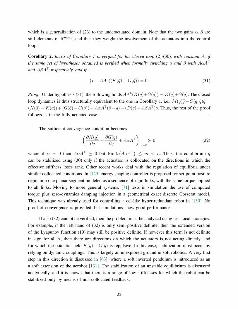
which is a generalization of (23) to the underactuated domain. Note that the two gains α, β arestill elements of Rm×m, and thus they weight the involvement of the actuators into the controlloop.

Corollary 2. thesis of Corollary 1 is verified for the closed loop (2)-(30), with constant A, ifthe same set of hypotheses obtained is verified when formally switching α and β with AαA>

and AβA> respectively, and if

(I − AAL)(K(q) +G(q)) = 0. (31)

Proof. Under hypothesis (31), the following holds AAL(K(q)+G(q)) = K(q)+G(q). The closedloop dynamics is thus structurally equivalent to the one in Corollary 1, i.e., M(q)q+C(q, q)q =

(K(q)−K(q)) + (G(q)−G(q)) +AαA>(q− q)− (D(q) +AβA>)q. Thus, the rest of the prooffollows as in the fully actuated case.

The sufficient convergence condition becomes(∂K(q)

∂q+∂G(q)

∂q+ AαA>

)∣∣∣∣q=q

� 0, (32)

where if α � 0 then AαA> � 0 but Rank(AαA>

)≤ m < n. Thus, the equilibrium q

can be stabilized using (30) only if the actuation is collocated on the directions in which theeffective stiffness loses rank. Other recent works deal with the regulation of equilibria undersimilar collocated conditions. In [129] energy shaping controller is proposed for set-point postureregulation one planar segment modeled as a sequence of rigid links, with the same torque appliedto all links. Moving to more general systems, [71] tests in simulation the use of computedtorque plus zero-dynamics damping injection in a geometrical exact discrete Cosserat model.This technique was already used for controlling a eel-like hyper-redundant robot in [130]. Noproof of convergence is provided, but simulations show good performance.

If also (32) cannot be verified, then the problem must be analyzed using less local strategies.For example, if the left hand of (32) is only semi-positive definite, then the extended versionof the Lyapunov function (19) may still be positive definite. If however this term is not definitein sign for all α, then there are directions on which the actuators is not acting directly, andfor which the potential field K(q) +G(q) is repulsive. In this case, stabilization must occur byrelying on dynamic couplings. This is largely an unexplored ground in soft robotics. A very firststep in this direction is discussed in [63], where a soft inverted pendulum is introduced as ana soft extension of the acrobot [131]. The stabilization of an unstable equilibrium is discussedanalytically, and it is shown that there is a range of low stiffnesses for which the robot can bestabilized only by means of non-collocated feedback.

22

Actuators dynamics and constraints

Actuators dynamics plays a much important role in shaping the soft robot behavior,especially if compared to classic rigid robots. Nonetheless, few are the works so far that haveexplicitly taken into account a dynamics formulation as (13) in the design of the controller.Some actuation technologies require already to accurately consider the control problem for asingle isolated actuator. This is the case of electro-thermally-active materials [132]–[135], and ofmagnetic actuation of micro and nano robots [136], [137]. If a clear separation exists betweenthe response time of actuators (13) and the robot (12), then singular perturbation approach[138] could be used to improve the performance of the model based controllers introducedabove. Alternatively, backstepping design achieves the same goal without any assumption onthe relative time scales [139], but at the cost of a more complex control architecture. Bothtechniques have been extensively used to control flexible robots actuated with similar modalitiesas typically found in soft robotics, as tendon driven [140], pistons [141], and artificial muscles[142], [143]. Nonetheless, the only example of application in soft robotics that we are aware ofis a backstepping controller for a single segment approximated with a linear model of the robotand of the air flow [144].

In soft robotic actuation, it is often the case that the input space can only take values ina subset of Rm. This may be due to upper bounds to the maximum force, and to unilateralconstraints induced by tendons that can only pull, or pressure chambers that can only push.These constraints are usually dealt with heuristics which mask their existence to controllerscarefully tuned to not exceed the limits of actuation. As an alternative to heuristics, themasking can also be devised through model based techniques as closed form solution ofoptimal control allocation problems [145]. Alternatively, Model Predictive Controllers (MPC)can generate control actions that inherently verify the constraints. In [146] linear MPC isused to control a pneumatically actuated humanoid robot, with joint-like localized bending andunder a decentralized approximation. In [147] the strategy is extended to nonlinear MPC, andEvolutionary algorithms are used to solve the nonlinear optimization. In [148] nonlinear orderreduction techniques are used to generate accurate relaxations of a nonlinear finite horizonoptimal control problem, including state and input constraints, and formulated on nonlinearFEM models.

Task space regulation and tracking

The task space of a robot is usually identified with the configuration of its end effector.In soft robots this corresponds to the configuration of the tip x(1, t) = h(1, q(t)). For simplicityof notation we will drop the s coordinate in this section. This also allows to stress that the

23

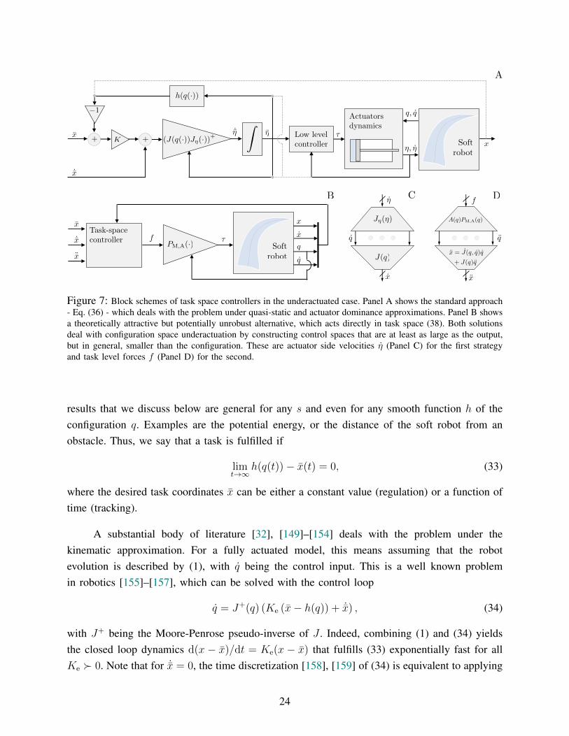
Softrobot


A

+


⌘

<latexit sha1_base64="DnTw2xRwZKLpzEPl7A6c2M2qObA=">AAAB73icbVDLSgNBEOyNrxhfUY9eBoPgKexKfBwDXjxGMA/ILqF3MpsMmZ1dZ2aFEPITXjwo4tXf8ebfOEn2oIkFDUVVN91dYSq4Nq777RTW1jc2t4rbpZ3dvf2D8uFRSyeZoqxJE5GoToiaCS5Z03AjWCdVDONQsHY4up357SemNE/kgxmnLIhxIHnEKRordfwQlc8M9soVt+rOQVaJl5MK5Gj0yl9+P6FZzKShArXuem5qggkqw6lg05KfaZYiHeGAdS2VGDMdTOb3TsmZVfokSpQtachc/T0xwVjrcRzazhjNUC97M/E/r5uZ6CaYcJlmhkm6WBRlgpiEzJ4nfa4YNWJsCVLF7a2EDlEhNTaikg3BW355lbQuql6tenlfq9Sv8jiKcAKncA4eXEMd7qABTaAg4Ble4c15dF6cd+dj0Vpw8plj+APn8wcEAI/t</latexit>

Z

<latexit sha1_base64="p4u+qzZQWNIkhM4+POIBM+Qvcg4=">AAAB63icbVBNS8NAEJ3Ur1q/qh69LBbBU0nEr2PBi8cK9gPaUDbbTbt0dxN2J0IJ/QtePCji1T/kzX9j0uagrQ8GHu/NMDMviKWw6LrfTmltfWNzq7xd2dnd2z+oHh61bZQYxlsskpHpBtRyKTRvoUDJu7HhVAWSd4LJXe53nrixItKPOI25r+hIi1AwirnUFxoH1Zpbd+cgq8QrSA0KNAfVr/4wYoniGpmk1vY8N0Y/pQYFk3xW6SeWx5RN6Ij3Mqqp4tZP57fOyFmmDEkYmaw0krn6eyKlytqpCrJORXFsl71c/M/rJRje+qnQcYJcs8WiMJEEI5I/TobCcIZymhHKjMhuJWxMDWWYxVPJQvCWX14l7Yu6d1m/erisNa6LOMpwAqdwDh7cQAPuoQktYDCGZ3iFN0c5L86787FoLTnFzDH8gfP5AyGkjkU=</latexit>

˙⌘

<latexit sha1_base64="Tsid+Jl+T9on+4ijCVkZ88iVS3E=">AAAB+HicbVDLSsNAFL2pr1ofjbp0EyyCq5KIr2XBjcsK9gFNKJPptB06mYSZG6GGfokbF4q49VPc+TdO2iy09cCFwzn3ztx7wkRwja77bZXW1jc2t8rblZ3dvf2qfXDY1nGqKGvRWMSqGxLNBJeshRwF6yaKkSgUrBNObnO/88iU5rF8wGnCgoiMJB9yStBIfbvqD2LM/JAonyGZVfp2za27czirxCtIDQo0+/aXeYGmEZNIBdG657kJBhlRyKlgs4qfapYQOiEj1jNUkojpIJsvPnNOjTJwhrEyJdGZq78nMhJpPY1C0xkRHOtlLxf/83opDm+CjMskRSbp4qNhKhyMnTwFZ8AVoyimhhCquNnVoWOiCEWTVR6Ct3zyKmmf172L+uX9Ra1xVcRRhmM4gTPw4BoacAdNaAGFFJ7hFd6sJ+vFerc+Fq0lq5g5gj+wPn8AoMGTCQ==</latexit>

+


�1


(J(q(·))J⌘(·))+

<latexit sha1_base64="dUEH5Bf35lpYm9BvkcSzWYycteY=">AAACHnicbVBNS8NAEN34bf2qevSyWIQWoSTSqkfBi/RUwarQxLLZTtrFzYe7E6GE/BIv/hUvHhQRPOm/Mak5aOuDgcd7M8zMcyMpNJrmlzEzOze/sLi0XFpZXVvfKG9uXeowVhw6PJShunaZBikC6KBACdeRAua7Eq7c29Pcv7oHpUUYXOAoAsdng0B4gjPMpF65aUvwsNqq3lVt3g+xVqOtXmL7DIfKT2xAlqaFYysxGGLtZr9U6pUrZt0cg04TqyAVUqDdK3/Y/ZDHPgTIJdO6a5kROglTKLiEtGTHGiLGb9kAuhkNmA/aScbvpXQvU/rUC1VWAdKx+nsiYb7WI9/NOvO79aSXi/953Ri9YycRQRQjBPxnkRdLiiHNs6J9oYCjHGWEcSWyWykfMsU4ZonmIViTL0+Ty4O61ag3zxuVk8MijiWyQ3ZJlVjkiJyQM9ImHcLJA3kiL+TVeDSejTfj/ad1xihmtskfGJ/f8h6hFg==</latexit>

K

<latexit sha1_base64="T7gNA5Cwuf5wS7XYCqmiWsZfwkM=">AAAB6XicbVDLSgNBEOyNrxhfUY9eBoPgKeyKr2PAi+AlinlAsoTZSW8yZHZ2mZkVwpI/8OJBEa/+kTf/xkmyB00saCiquunuChLBtXHdb6ewsrq2vlHcLG1t7+zulfcPmjpOFcMGi0Ws2gHVKLjEhuFGYDtRSKNAYCsY3Uz91hMqzWP5aMYJ+hEdSB5yRo2VHu5KvXLFrbozkGXi5aQCOeq98le3H7M0QmmYoFp3PDcxfkaV4UzgpNRNNSaUjegAO5ZKGqH2s9mlE3JilT4JY2VLGjJTf09kNNJ6HAW2M6JmqBe9qfif10lNeO1nXCapQcnmi8JUEBOT6dukzxUyI8aWUKa4vZWwIVWUGRvONARv8eVl0jyreufVi/vzSu0yj6MIR3AMp+DBFdTgFurQAAYhPMMrvDkj58V5dz7mrQUnnzmEP3A+fwDVWIzf</latexit>

x

<latexit sha1_base64="Y/jB06Slxrqw7V0pPaCz4eA4CUA=">AAAB73icbVDLSgNBEOyNrxhfUY9eBoPgKeyKr2PAi8cI5gHJEmYnnWTI7Ow6MyuGJT/hxYMiXv0db/6Ns8keNLGgoajqprsriAXXxnW/ncLK6tr6RnGztLW9s7tX3j9o6ihRDBssEpFqB1Sj4BIbhhuB7VghDQOBrWB8k/mtR1SaR/LeTGL0QzqUfMAZNVZqdwOq0qdpqVeuuFV3BrJMvJxUIEe9V/7q9iOWhCgNE1TrjufGxk+pMpwJnJa6icaYsjEdYsdSSUPUfjq7d0pOrNIng0jZkobM1N8TKQ21noSB7QypGelFLxP/8zqJGVz7KZdxYlCy+aJBIoiJSPY86XOFzIiJJZQpbm8lbEQVZcZGlIXgLb68TJpnVe+8enF3Xqld5nEU4QiO4RQ8uIIa3EIdGsBAwDO8wpvz4Lw4787HvLXg5DOH8AfO5w/aDY/R</latexit>

˙x

<latexit sha1_base64="95cBFp5gIIUanrL3+OSPOayLHos=">AAAB9XicbVDLSsNAFL2pr1pfVZdugkVwVRKpj2XBjcsK9gFtLJPppB06mYSZG7WE/ocbF4q49V/c+TdO2iy09cCFwzn3ztx7/FhwjY7zbRVWVtfWN4qbpa3tnd298v5BS0eJoqxJIxGpjk80E1yyJnIUrBMrRkJfsLY/vs789gNTmkfyDicx80IylDzglKCR7nuDCNOeT1T6NJ2W+uWKU3VmsJeJm5MK5Gj0y1/mAZqETCIVROuu68TopUQhp4JNS71Es5jQMRmyrqGShEx76WzrqX1ilIEdRMqURHum/p5ISaj1JPRNZ0hwpBe9TPzP6yYYXHkpl3GCTNL5R0EibIzsLAJ7wBWjKCaGEKq42dWmI6IIRRNUFoK7ePIyaZ1V3Vr1/LZWqV/kcRThCI7hFFy4hDrcQAOaQEHBM7zCm/VovVjv1se8tWDlM4fwB9bnD8WIkqg=</latexit>

x

<latexit sha1_base64="Jv6ig7xgfwnpA2wSujyX+ffI4qI=">AAAB6XicbVDLSgNBEOyNrxhfUY9eBoPgKeyKr2PAi8co5gHJEmYnvcmQ2dllZlYMIX/gxYMiXv0jb/6Ns8keNLGgoajqprsrSATXxnW/ncLK6tr6RnGztLW9s7tX3j9o6jhVDBssFrFqB1Sj4BIbhhuB7UQhjQKBrWB0k/mtR1Sax/LBjBP0IzqQPOSMGivdP5V65YpbdWcgy8TLSQVy1Hvlr24/ZmmE0jBBte54bmL8CVWGM4HTUjfVmFA2ogPsWCpphNqfzC6dkhOr9EkYK1vSkJn6e2JCI63HUWA7I2qGetHLxP+8TmrCa3/CZZIalGy+KEwFMTHJ3iZ9rpAZMbaEMsXtrYQNqaLM2HCyELzFl5dJ86zqnVcv7s4rtcs8jiIcwTGcggdXUINbqEMDGITwDK/w5oycF+fd+Zi3Fpx85hD+wPn8ARnIjQw=</latexit>

h(q(·))

<latexit sha1_base64="1+8bUoN9XmLig/I+wlyRUCh/JAU=">AAAB9HicbVBNT8JAEN3iF9Yv1KOXjcQELqQ1+HEk8eIRE0ESaMh2u4UN223ZnZKQht/hxYPGePXHePPfuEAPCr5kkpf3ZjIzz08E1+A431ZhY3Nre6e4a+/tHxwelY5P2jpOFWUtGotYdXyimeCStYCDYJ1EMRL5gj35o7u5/zRhSvNYPsI0YV5EBpKHnBIwkjesjCs9GsRQrdp2v1R2as4CeJ24OSmjHM1+6asXxDSNmAQqiNZd10nAy4gCTgWb2b1Us4TQERmwrqGSREx72eLoGb4wSoDDWJmSgBfq74mMRFpPI990RgSGetWbi/953RTCWy/jMkmBSbpcFKYCQ4znCeCAK0ZBTA0hVHFzK6ZDoggFk9M8BHf15XXSvqy59drVQ73cuM7jKKIzdI4qyEU3qIHuURO1EEVj9Ixe0Zs1sV6sd+tj2Vqw8plT9AfW5w9x75CN</latexit>

q, q

<latexit sha1_base64="AnaEqtB+JGvKv48zP3uUt8y9Mn8=">AAAB8nicbVDLSsNAFJ3UV42vqks3g0VwISWR+lgW3LisYB+QhjKZTtqhk0k6cyOU0M9w40IRt36NO//GSZuFth4YOJxzD3PvCRLBNTjOt1VaW9/Y3Cpv2zu7e/sHlcOjto5TRVmLxiJW3YBoJrhkLeAgWDdRjESBYJ1gfJf7nSemNI/lI0wT5kdkKHnIKQEjeZOL3iCGbDKz7X6l6tScOfAqcQtSRQWa/cqXydI0YhKoIFp7rpOAnxEFnAo2s3upZgmhYzJknqGSREz72XzlGT4zygCHsTJPAp6rvxMZibSeRoGZjAiM9LKXi/95XgrhrZ9xmaTAJF18FKYCQ4zz+/GAK0ZBTA0hVHGzK6YjoggF01Jegrt88ippX9bceu3qoV5tXBd1lNEJOkXnyEU3qIHuURO1EEUxekav6M0C68V6tz4WoyWryByjP7A+fwBgJ5Ch</latexit>

⌘, ⌘

<latexit sha1_base64="GA0td7TKmDkz0Td38eQnYuGW/x4=">AAAB+XicbVDLSsNAFL2pr1pfUZdugkVwISWR+lgW3LisYG2hDWUynbRDJ5Mwc1MooX/ixoUibv0Td/6NkzYLbT0wcDjnHu6dEySCa3Tdb6u0tr6xuVXeruzs7u0f2IdHTzpOFWUtGotYdQKimeCStZCjYJ1EMRIFgrWD8V3utydMaR7LR5wmzI/IUPKQU4JG6tt2jyG56A1izHI2q/Ttqltz53BWiVeQKhRo9u0vk6ZpxCRSQbTuem6CfkYUcirYrNJLNUsIHZMh6xoqScS0n80vnzlnRhk4YazMk+jM1d+JjERaT6PATEYER3rZy8X/vG6K4a2fcZmkyCRdLApT4WDs5DU4A64YRTE1hFDFza0OHRFFKJqy8hK85S+vkqfLmlevXT3Uq43roo4ynMApnIMHN9CAe2hCCyhM4Ble4c3KrBfr3fpYjJasInMMf2B9/gATWpNE</latexit>

⌧


Softrobot


x

<latexit sha1_base64="Y/jB06Slxrqw7V0pPaCz4eA4CUA=">AAAB73icbVDLSgNBEOyNrxhfUY9eBoPgKeyKr2PAi8cI5gHJEmYnnWTI7Ow6MyuGJT/hxYMiXv0db/6Ns8keNLGgoajqprsriAXXxnW/ncLK6tr6RnGztLW9s7tX3j9o6ihRDBssEpFqB1Sj4BIbhhuB7VghDQOBrWB8k/mtR1SaR/LeTGL0QzqUfMAZNVZqdwOq0qdpqVeuuFV3BrJMvJxUIEe9V/7q9iOWhCgNE1TrjufGxk+pMpwJnJa6icaYsjEdYsdSSUPUfjq7d0pOrNIng0jZkobM1N8TKQ21noSB7QypGelFLxP/8zqJGVz7KZdxYlCy+aJBIoiJSPY86XOFzIiJJZQpbm8lbEQVZcZGlIXgLb68TJpnVe+8enF3Xqld5nEU4QiO4RQ8uIIa3EIdGsBAwDO8wpvz4Lw4787HvLXg5DOH8AfO5w/aDY/R</latexit>

˙x

<latexit sha1_base64="95cBFp5gIIUanrL3+OSPOayLHos=">AAAB9XicbVDLSsNAFL2pr1pfVZdugkVwVRKpj2XBjcsK9gFtLJPppB06mYSZG7WE/ocbF4q49V/c+TdO2iy09cCFwzn3ztx7/FhwjY7zbRVWVtfWN4qbpa3tnd298v5BS0eJoqxJIxGpjk80E1yyJnIUrBMrRkJfsLY/vs789gNTmkfyDicx80IylDzglKCR7nuDCNOeT1T6NJ2W+uWKU3VmsJeJm5MK5Gj0y1/mAZqETCIVROuu68TopUQhp4JNS71Es5jQMRmyrqGShEx76WzrqX1ilIEdRMqURHum/p5ISaj1JPRNZ0hwpBe9TPzP6yYYXHkpl3GCTNL5R0EibIzsLAJ7wBWjKCaGEKq42dWmI6IIRRNUFoK7ePIyaZ1V3Vr1/LZWqV/kcRThCI7hFFy4hDrcQAOaQEHBM7zCm/VovVjv1se8tWDlM4fwB9bnD8WIkqg=</latexit>

¨x

<latexit sha1_base64="TL53fyYIaViVf/pQvOENjSI3UQw=">AAAB9XicbVDLSsNAFJ3UV62vqks3wSK4KonUx7LgxmUF+4Amlslk0g6dzISZG7WE/IcbF4q49V/c+TdO2yy09cCFwzn3cu89QcKZBsf5tkorq2vrG+XNytb2zu5edf+go2WqCG0TyaXqBVhTzgRtAwNOe4miOA447Qbj66nffaBKMynuYJJQP8ZDwSJGMBjp3gtDCZkXYJU95fmgWnPqzgz2MnELUkMFWoPqlxdKksZUAOFY677rJOBnWAEjnOYVL9U0wWSMh7RvqMAx1X42uzq3T4wS2pFUpgTYM/X3RIZjrSdxYDpjDCO96E3F/7x+CtGVnzGRpEAFmS+KUm6DtKcR2CFTlACfGIKJYuZWm4ywwgRMUBUTgrv48jLpnNXdRv38tlFrXhRxlNEROkanyEWXqIluUAu1EUEKPaNX9GY9Wi/Wu/Uxby1Zxcwh+gPr8wdNb5MC</latexit>

PM,A(·)

<latexit sha1_base64="/1jfxyKBuJwCDtiURbU8JoStY5k=">AAACAXicbVDLSsNAFJ3UV62vqBvBTbAIFaQkUh/Lihs3QgX7gCaEyWTSDp3MhJmJUELc+CtuXCji1r9w5984abvQ6oELh3Pu5d57goQSqWz7yygtLC4tr5RXK2vrG5tb5vZOR/JUINxGnHLRC6DElDDcVkRR3EsEhnFAcTcYXRV+9x4LSTi7U+MEezEcMBIRBJWWfHOv5WduDNVQxNnN8WWe11wUcnVU8c2qXbcnsP4SZ0aqYIaWb366IUdpjJlCFErZd+xEeRkUiiCK84qbSpxANIID3NeUwRhLL5t8kFuHWgmtiAtdTFkT9edEBmMpx3GgO4tj5bxXiP95/VRFF15GWJIqzNB0UZRSS3GriMMKicBI0bEmEAmib7XQEAqIlA6tCMGZf/kv6ZzUnUb99LZRbZ7N4iiDfXAAasAB56AJrkELtAECD+AJvIBX49F4Nt6M92lryZjN7IJfMD6+AXanljY=</latexit>

Task-spacecontroller

<latexit sha1_base64="rOcEPrabNUDhYdRAa2ihJaR8Yng=">AAACAHicbVA9SwNBEN2LX/H8OrWwsFkMgo3hLvhVBmwsIyQmkBxhbzOXLNnbPXb3hBDS+FdsLBSx9WfY+W/cJFdo4oOBx3szzMyLUs608f1vp7Cyura+Udx0t7Z3dve8/YMHLTNFoUEll6oVEQ2cCWgYZji0UgUkiTg0o+Ht1G8+gtJMiroZpRAmpC9YzCgxVup6R3Wih+c6JRSw61IpjJKcg+p6Jb/sz4CXSZCTEspR63pfnZ6kWQLCUE60bgd+asIxUYZRDhO3k2mwW4akD21LBUlAh+PZAxN8apUejqWyJQyeqb8nxiTRepREtjMhZqAXvan4n9fOTHwTjplIMwOCzhfFGcdG4mkauMcUUMNHlhCqmL0V0wFRhBqbmWtDCBZfXiYPlXJwUb68r5SqV3kcRXSMTtAZCtA1qqI7VEMNRNEEPaNX9OY8OS/Ou/Mxby04+cwh+gPn8we0X5XP</latexit>

⌧


f

<latexit sha1_base64="PScSasaySvzN11DnTParxJhIgp8=">AAAB6HicbVBNS8NAEJ3Ur1q/qh69LBbBU0mkfhwLXjy2YGuhDWWznbRrN5uwuxFK6C/w4kERr/4kb/4bt20O2vpg4PHeDDPzgkRwbVz32ymsrW9sbhW3Szu7e/sH5cOjto5TxbDFYhGrTkA1Ci6xZbgR2EkU0igQ+BCMb2f+wxMqzWN5byYJ+hEdSh5yRo2VmmG/XHGr7hxklXg5qUCORr/81RvELI1QGiao1l3PTYyfUWU4Ezgt9VKNCWVjOsSupZJGqP1sfuiUnFllQMJY2ZKGzNXfExmNtJ5Ege2MqBnpZW8m/ud1UxPe+BmXSWpQssWiMBXExGT2NRlwhcyIiSWUKW5vJWxEFWXGZlOyIXjLL6+S9kXVq1Uvm7VK/SqPowgncArn4ME11OEOGtACBgjP8ApvzqPz4rw7H4vWgpPPHMMfOJ8/ye2M5g==</latexit>

q


q


x

<latexit sha1_base64="Jv6ig7xgfwnpA2wSujyX+ffI4qI=">AAAB6XicbVDLSgNBEOyNrxhfUY9eBoPgKeyKr2PAi8co5gHJEmYnvcmQ2dllZlYMIX/gxYMiXv0jb/6Ns8keNLGgoajqprsrSATXxnW/ncLK6tr6RnGztLW9s7tX3j9o6jhVDBssFrFqB1Sj4BIbhhuB7UQhjQKBrWB0k/mtR1Sax/LBjBP0IzqQPOSMGivdP5V65YpbdWcgy8TLSQVy1Hvlr24/ZmmE0jBBte54bmL8CVWGM4HTUjfVmFA2ogPsWCpphNqfzC6dkhOr9EkYK1vSkJn6e2JCI63HUWA7I2qGetHLxP+8TmrCa3/CZZIalGy+KEwFMTHJ3iZ9rpAZMbaEMsXtrYQNqaLM2HCyELzFl5dJ86zqnVcv7s4rtcs8jiIcwTGcggdXUINbqEMDGITwDK/w5oycF+fd+Zi3Fpx85hD+wPn8ARnIjQw=</latexit>

x

<latexit sha1_base64="sCfWJZTcri60anFJRKCYbQU1xlk=">AAAB7nicbVDLSgMxFL1TX7W+qi7dBIvgqsxIfSwLblxWsA9oh5JJM21oJjMkd8Qy9CPcuFDErd/jzr8xbWehrQcCh3PuIfeeIJHCoOt+O4W19Y3NreJ2aWd3b/+gfHjUMnGqGW+yWMa6E1DDpVC8iQIl7ySa0yiQvB2Mb2d++5FrI2L1gJOE+xEdKhEKRtFK7d4gxuxp2i9X3Ko7B1klXk4qkKPRL3/ZJEsjrpBJakzXcxP0M6pRMMmnpV5qeELZmA5511JFI278bL7ulJxZZUDCWNunkMzV34mMRsZMosBORhRHZtmbif953RTDGz8TKkmRK7b4KEwlwZjMbicDoTlDObGEMi3sroSNqKYMbUMlW4K3fPIqaV1UvVr18r5WqV/ldRThBE7hHDy4hjrcQQOawGAMz/AKb07ivDjvzsditODkmWP4A+fzB76Ej88=</latexit>

⌘

<latexit sha1_base64="OLYvA4HpW9M4rf4pbqhp1aDjbKM=">AAAB8XicbVDLSgMxFM3UV62vqks3wSK4KjNSH8uCG5cV7APboWTSO21oJjMkd4Qy9C/cuFDErX/jzr8xbWehrQcCh3PuIfeeIJHCoOt+O4W19Y3NreJ2aWd3b/+gfHjUMnGqOTR5LGPdCZgBKRQ0UaCETqKBRYGEdjC+nfntJ9BGxOoBJwn4ERsqEQrO0EqPvUGMWQ+QTfvlilt156CrxMtJheRo9MtfNszTCBRyyYzpem6CfsY0Ci5hWuqlBhLGx2wIXUsVi8D42XzjKT2zyoCGsbZPIZ2rvxMZi4yZRIGdjBiOzLI3E//zuimGN34mVJIiKL74KEwlxZjOzqcDoYGjnFjCuBZ2V8pHTDOOtqSSLcFbPnmVtC6qXq16eV+r1K/yOorkhJySc+KRa1Ind6RBmoQTRZ7JK3lzjPPivDsfi9GCk2eOyR84nz/oupEL</latexit>

q


x

<latexit sha1_base64="sCfWJZTcri60anFJRKCYbQU1xlk=">AAAB7nicbVDLSgMxFL1TX7W+qi7dBIvgqsxIfSwLblxWsA9oh5JJM21oJjMkd8Qy9CPcuFDErd/jzr8xbWehrQcCh3PuIfeeIJHCoOt+O4W19Y3NreJ2aWd3b/+gfHjUMnGqGW+yWMa6E1DDpVC8iQIl7ySa0yiQvB2Mb2d++5FrI2L1gJOE+xEdKhEKRtFK7d4gxuxp2i9X3Ko7B1klXk4qkKPRL3/ZJEsjrpBJakzXcxP0M6pRMMmnpV5qeELZmA5511JFI278bL7ulJxZZUDCWNunkMzV34mMRsZMosBORhRHZtmbif953RTDGz8TKkmRK7b4KEwlwZjMbicDoTlDObGEMi3sroSNqKYMbUMlW4K3fPIqaV1UvVr18r5WqV/ldRThBE7hHDy4hjrcQQOawGAMz/AKb07ivDjvzsditODkmWP4A+fzB76Ej88=</latexit>

J(q)

<latexit sha1_base64="0pLUhsTqXrAtRgNnBNxuJUgLaD4=">AAAB63icbVDLSgNBEOz1GeMr6tHLYBDiJexKfBwDXsRTBPOAZAmzk9lkyMzsOjMrhCW/4MWDIl79IW/+jbPJHjSxoKGo6qa7K4g508Z1v52V1bX1jc3CVnF7Z3dvv3Rw2NJRoghtkohHqhNgTTmTtGmY4bQTK4pFwGk7GN9kfvuJKs0i+WAmMfUFHkoWMoJNJt1VHs/6pbJbdWdAy8TLSRlyNPqlr94gIomg0hCOte56bmz8FCvDCKfTYi/RNMZkjIe0a6nEgmo/nd06RadWGaAwUrakQTP190SKhdYTEdhOgc1IL3qZ+J/XTUx47adMxomhkswXhQlHJkLZ42jAFCWGTyzBRDF7KyIjrDAxNp6iDcFbfHmZtM6rXq16cV8r1y/zOApwDCdQAQ+uoA630IAmEBjBM7zCmyOcF+fd+Zi3rjj5zBH8gfP5AzX0jao=</latexit>

J⌘(⌘)

<latexit sha1_base64="CkNF9mnzSFxFoDppbUL052dWHjs=">AAACAHicbVC7TsMwFHXKq5RXgIGBxaJCKkuVoPIYK7EgpiLRh9REkeO6rVXbiWwHqYqy8CssDCDEymew8Tc4bQZoOZLlo3Pu1b33hDGjSjvOt1VaWV1b3yhvVra2d3b37P2DjooSiUkbRyySvRApwqggbU01I71YEsRDRrrh5Cb3u49EKhqJBz2Nic/RSNAhxUgbKbCP7oLU40iPJU89olGW1fLvLLCrTt2ZAS4TtyBVUKAV2F/eIMIJJ0JjhpTqu06s/RRJTTEjWcVLFIkRnqAR6RsqECfKT2cHZPDUKAM4jKR5QsOZ+rsjRVypKQ9NZb6rWvRy8T+vn+jhtZ9SESeaCDwfNEwY1BHM04ADKgnWbGoIwpKaXSEeI4mwNplVTAju4snLpHNedxv1i/tGtXlZxFEGx+AE1IALrkAT3IIWaAMMMvAMXsGb9WS9WO/Wx7y0ZBU9h+APrM8f2HGWiA==</latexit>

x

<latexit sha1_base64="+wEsldUhTpmVbxy+0Qky3XI+eEQ=">AAAB73icbVDLSgNBEOyNrxhfUY9eBoPgKeyKr2PAi8cI5gHJEmZnJ8mQ2dl1plcMS37CiwdFvPo73vwbJ8keNLGgoajqprsrSKQw6LrfTmFldW19o7hZ2tre2d0r7x80TZxqxhsslrFuB9RwKRRvoEDJ24nmNAokbwWjm6nfeuTaiFjd4zjhfkQHSvQFo2ildjcMY8yeJr1yxa26M5Bl4uWkAjnqvfJXN4xZGnGFTFJjOp6boJ9RjYJJPil1U8MTykZ0wDuWKhpx42ezeyfkxCoh6cfalkIyU39PZDQyZhwFtjOiODSL3lT8z+uk2L/2M6GSFLli80X9VBKMyfR5EgrNGcqxJZRpYW8lbEg1ZWgjKtkQvMWXl0nzrOqdVy/uziu1yzyOIhzBMZyCB1dQg1uoQwMYSHiGV3hzHpwX5935mLcWnHzmEP7A+fwBfceQPQ==</latexit>

A(q)PM,A(q)

<latexit sha1_base64="OWyFj4tkcUgxsZJprv6On1FKYP8=">AAACAXicbVDLSsNAFJ3UV62vqBvBzWARKkhJpD6WLW7cCBXsA9oQJtNJO3QyiTMToYS48VfcuFDErX/hzr9x0mah1QMXDufcy733eBGjUlnWl1FYWFxaXimultbWNza3zO2dtgxjgUkLhywUXQ9JwignLUUVI91IEBR4jHS88WXmd+6JkDTkt2oSESdAQ059ipHSkmvuNSp3R7DpJv0AqZEIkuvjRppqzTXLVtWaAv4ldk7KIEfTNT/7gxDHAeEKMyRlz7Yi5SRIKIoZSUv9WJII4TEakp6mHAVEOsn0gxQeamUA/VDo4gpO1Z8TCQqknASe7szulPNeJv7n9WLlXzgJ5VGsCMezRX7MoAphFgccUEGwYhNNEBZU3wrxCAmElQ6tpEOw51/+S9onVbtWPb2pletneRxFsA8OQAXY4BzUwRVoghbA4AE8gRfwajwaz8ab8T5rLRj5zC74BePjG6s2lbo=</latexit>

x = J(q, q)q

+ J(q)q

<latexit sha1_base64="fH8ChXFL4hODSVrKtAUmUxW9Z1Q=">AAACIXicbZDLSgMxFIYz9VbHW9Wlm2CxtChlplTsRii4ka4q2At0SsmkaRuauTTJiGWYV3Hjq7hxoUh34suYmc5CqwdCPv5zSc5v+4wKaRifWmZtfWNzK7ut7+zu7R/kDo/awgs4Ji3sMY93bSQIoy5pSSoZ6fqcIMdmpGNPb+J854FwQT33Xs590nfQ2KUjipFU0iBXs4ZDT4aPESxcQyvGRlScXSQ0i0rpDS1LL5zDRnFWWtbPokEub5SNJOBfMFPIgzSag9xCDcOBQ1yJGRKiZxq+7IeIS4oZiXQrEMRHeIrGpKfQRQ4R/TDZMIJnShnCkcfVcSVM1J8dIXKEmDu2qnSQnIjVXCz+l+sFclTrh9T1A0lcvHxoFDAoPRjbBYeUEyzZXAHCnKq/QjxBHGGpTNWVCebqyn+hXSmb1fLlXTVfr6R2ZMEJOAVFYIIrUAe3oAlaAIMn8ALewLv2rL1qH9piWZrR0p5j8Cu0r2/bYaKn</latexit>

q

<latexit sha1_base64="uEyUJJ8nnsRfwJJ+PYZbngBDP9s=">AAAB73icbVDLSgNBEOyNrxhfUY9eBoPgKeyKr2PAi8cI5gHJEmZnJ8mQ2dnNTK8QlvyEFw+KePV3vPk3TpI9aGJBQ1HVTXdXkEhh0HW/ncLa+sbmVnG7tLO7t39QPjxqmjjVjDdYLGPdDqjhUijeQIGStxPNaRRI3gpGdzO/9cS1EbF6xEnC/YgOlOgLRtFK7W4YxpiNp71yxa26c5BV4uWkAjnqvfJXN4xZGnGFTFJjOp6boJ9RjYJJPi11U8MTykZ0wDuWKhpx42fze6fkzCoh6cfalkIyV39PZDQyZhIFtjOiODTL3kz8z+uk2L/1M6GSFLlii0X9VBKMyex5EgrNGcqJJZRpYW8lbEg1ZWgjKtkQvOWXV0nzoupdVq8eLiu16zyOIpzAKZyDBzdQg3uoQwMYSHiGV3hzxs6L8+58LFoLTj5zDH/gfP4AcySQNg==</latexit>

C

<latexit sha1_base64="xOKpX3NIXIluYFQnyfl7NQvs/NU=">AAAB6HicbVA9SwNBEJ2LXzF+RS1tFoNgFe6CooVFII1lAuYDkiPsbeaSNXt7x+6eEEJ+gY2FIrb+JDv/jZvkCk18MPB4b4aZeUEiuDau++3kNja3tnfyu4W9/YPDo+LxSUvHqWLYZLGIVSegGgWX2DTcCOwkCmkUCGwH49rcbz+h0jyWD2aSoB/RoeQhZ9RYqVHrF0tu2V2ArBMvIyXIUO8Xv3qDmKURSsME1brruYnxp1QZzgTOCr1UY0LZmA6xa6mkEWp/ujh0Ri6sMiBhrGxJQxbq74kpjbSeRIHtjKgZ6VVvLv7ndVMT3vpTLpPUoGTLRWEqiInJ/Gsy4AqZERNLKFPc3krYiCrKjM2mYEPwVl9eJ61K2bsqXzcqpepdFkcezuAcLsGDG6jCPdShCQwQnuEV3pxH58V5dz6WrTknmzmFP3A+fwCWD4zH</latexit>

B

<latexit sha1_base64="LUwMH2KOFMzZIDj76+fdfMzN/gk=">AAAB6HicbVA9SwNBEJ2LXzF+RS1tFoNgFe6CooVF0MYyAfMByRH2NnPJmr29Y3dPCCG/wMZCEVt/kp3/xk1yhSY+GHi8N8PMvCARXBvX/XZya+sbm1v57cLO7t7+QfHwqKnjVDFssFjEqh1QjYJLbBhuBLYThTQKBLaC0d3Mbz2h0jyWD2acoB/RgeQhZ9RYqX7bK5bcsjsHWSVeRkqQodYrfnX7MUsjlIYJqnXHcxPjT6gynAmcFrqpxoSyER1gx1JJI9T+ZH7olJxZpU/CWNmShszV3xMTGmk9jgLbGVEz1MveTPzP66QmvPYnXCapQckWi8JUEBOT2dekzxUyI8aWUKa4vZWwIVWUGZtNwYbgLb+8SpqVsndRvqxXStWbLI48nMApnIMHV1CFe6hBAxggPMMrvDmPzovz7nwsWnNONnMMf+B8/gCUi4zG</latexit>

D

<latexit sha1_base64="cCCDHY57AujDKM4IETC6/b1HkM4=">AAAB6HicbVA9SwNBEJ2LXzF+RS1tFoNgFe6CooVFQAvLBMwHJEfY28wla/b2jt09IYT8AhsLRWz9SXb+GzfJFZr4YODx3gwz84JEcG1c99vJra1vbG7ltws7u3v7B8XDo6aOU8WwwWIRq3ZANQousWG4EdhOFNIoENgKRrczv/WESvNYPphxgn5EB5KHnFFjpfpdr1hyy+4cZJV4GSlBhlqv+NXtxyyNUBomqNYdz02MP6HKcCZwWuimGhPKRnSAHUsljVD7k/mhU3JmlT4JY2VLGjJXf09MaKT1OApsZ0TNUC97M/E/r5Oa8NqfcJmkBiVbLApTQUxMZl+TPlfIjBhbQpni9lbChlRRZmw2BRuCt/zyKmlWyt5F+bJeKVVvsjjycAKncA4eXEEV7qEGDWCA8Ayv8OY8Oi/Ou/OxaM052cwx/IHz+QOXk4zI</latexit>

f

<latexit sha1_base64="PScSasaySvzN11DnTParxJhIgp8=">AAAB6HicbVBNS8NAEJ3Ur1q/qh69LBbBU0mkfhwLXjy2YGuhDWWznbRrN5uwuxFK6C/w4kERr/4kb/4bt20O2vpg4PHeDDPzgkRwbVz32ymsrW9sbhW3Szu7e/sH5cOjto5TxbDFYhGrTkA1Ci6xZbgR2EkU0igQ+BCMb2f+wxMqzWN5byYJ+hEdSh5yRo2VmmG/XHGr7hxklXg5qUCORr/81RvELI1QGiao1l3PTYyfUWU4Ezgt9VKNCWVjOsSupZJGqP1sfuiUnFllQMJY2ZKGzNXfExmNtJ5Ege2MqBnpZW8m/ud1UxPe+BmXSWpQssWiMBXExGT2NRlwhcyIiSWUKW5vJWxEFWXGZlOyIXjLL6+S9kXVq1Uvm7VK/SqPowgncArn4ME11OEOGtACBgjP8ApvzqPz4rw7H4vWgpPPHMMfOJ8/ye2M5g==</latexit>

Actuatorsdynamics

<latexit sha1_base64="l8kfpeCI+nnepcdMy/ehSPb0UfM=">AAAB/HicbVBNS8NAEN3Urxq/oj16WSxCTyUpih4rXjxWsB/QhrLZbNqlm03YnQih1L/ixYMiXv0h3vw3btsctPXBwOO9GWbmBangGlz32yptbG5t75R37b39g8Mj5/iko5NMUdamiUhULyCaCS5ZGzgI1ksVI3EgWDeY3M797iNTmifyAfKU+TEZSR5xSsBIQ6dyQyEjkCht22EuScypHjpVt+4ugNeJV5AqKtAaOl+DMKFZzCRQQbTue24K/pQo4FSwmT3INEsJnZAR6xtqtjDtTxfHz/C5UUIcJcqUBLxQf09MSax1HgemMyYw1qveXPzP62cQXftTLtMMmKTLRVEmMCR4ngQOuWIURG4IoYqbWzEdE0UomLxsE4K3+vI66TTq3kX98r5RbdaKOMroFJ2hGvLQFWqiO9RCbURRjp7RK3qznqwX6936WLaWrGKmgv7A+vwBS7CUdw==</latexit>

Low levelcontroller

<latexit sha1_base64="dFLqTCXAvDXSRRAF5bto808H8JE=">AAAB/nicbVDJSgNBEO2JWxy3qHjy0hgET2EmuB0DXjx4iGAWSIbQ06lJmvR0D909kTAE/BUvHhTx6nd482/sLAdNfFDweK+Kqnphwpk2nvft5FZW19Y38pvu1vbO7l5h/6CuZaoo1KjkUjVDooEzATXDDIdmooDEIYdGOLiZ+I0hKM2keDCjBIKY9ASLGCXGSp3C0Z18xByGwF2XSmGU5BxUp1D0St4UeJn4c1JEc1Q7ha92V9I0BmEoJ1q3fC8xQUaUYZTD2G2nGhJCB6QHLUsFiUEH2fT8MT61ShdHUtkSBk/V3xMZibUexaHtjInp60VvIv7ntVITXQcZE0lqQNDZoijl2Eg8yQJ3mQJq+MgSQhWzt2LaJ4pQYxNzbQj+4svLpF4u+eeli/tysXI5jyOPjtEJOkM+ukIVdIuqqIYoytAzekVvzpPz4rw7H7PWnDOfOUR/4Hz+AJdKlTk=</latexit>

Figure 7: Block schemes of task space controllers in the underactuated case. Panel A shows the standard approach- Eq. (36) - which deals with the problem under quasi-static and actuator dominance approximations. Panel B showsa theoretically attractive but potentially unrobust alternative, which acts directly in task space (38). Both solutionsdeal with configuration space underactuation by constructing control spaces that are at least as large as the output,but in general, smaller than the configuration. These are actuator side velocities η (Panel C) for the first strategyand task level forces f (Panel D) for the second.

results that we discuss below are general for any s and even for any smooth function h of theconfiguration q. Examples are the potential energy, or the distance of the soft robot from anobstacle. Thus, we say that a task is fulfilled if

limt→∞

h(q(t))− x(t) = 0, (33)

where the desired task coordinates x can be either a constant value (regulation) or a function oftime (tracking).

A substantial body of literature [32], [149]–[154] deals with the problem under thekinematic approximation. For a fully actuated model, this means assuming that the robotevolution is described by (1), with q being the control input. This is a well known problemin robotics [155]–[157], which can be solved with the control loop

q = J+(q) (Ke (x− h(q)) + ˙x) , (34)

with J+ being the Moore-Penrose pseudo-inverse of J . Indeed, combining (1) and (34) yieldsthe closed loop dynamics d(x − x)/dt = Ke(x − x) that fulfills (33) exponentially fast for allKe � 0. Note that for ˙x = 0, the time discretization [158], [159] of (34) is equivalent to applying

24

the Newton-Raphson method to solve the following quadratic programming problem

minq∈Rn

||h(q)− x||22. (35)

Soft and hard constrains can be explicitly included in (35), and possibly reflected in (34) usingmulti-task prioritization. In practice, (34) is integrated numerically, and the result serves asreference q for a low level controller which regulates q. This can happen entirely in feedforwardor as a high level feedback loop. In the latter case, q and h(q) are directly measured. Alternatively,the kinematic behavior can be forced on the system using based cancellations [160]. Therefore,the use of a kinematic controller implicitly lies on the assumption that all configurations q areattainable through a low level controller as the ones discussed in previous sections.

To extend (34) to the underactuated case, one has to introduce some extra assumptions.First, it must be assumed that a low level feedback loop τ(η, η, η, q, q) is available such thatif applied to (13) then η converges to η fast enough. Under this assumption η and η can beused interchangeably. This is a strong assumption in general. However, if the robot dynamicsis negligible compared to the actuators one - e.g., lightweight robot with strongly reducedactuation - standard actuator-side regulation τ(η, η, η) is sufficient. This is for example the caseof lightweight continuum medical devices [161], [162]. Second, it has to be assumed that therobot is drawn to a stable equilibrium q, whenever a constant η is imposed. This is equivalent tosay that the feedforward action (29) generates a stable equilibrium. See the previous subsectionfor more discussions on the topic. Third, a one-to-one map must exist from η to q, which werefer to as q(η). We call Jη(η) the Jacobian of this map.

If these three hypotheses are simultaneously verified, then a differential kinematic modelcan be constructed, which goes directly from actuators space η to task space x

x =

Ent-to-end Jacobian︷︸︸︷J(q(η)) Jη(η)η︸︷︷︸

q

. (36)

This is formally equivalent to (1) from a mathematical standpoint. Thus, a kinematic controllercan be constructed by following the same line of reasoning of (34), resulting in the control action(Fig. 7 A)

η = (J(q(η))Jη(η))+ (Ke (x− h(q(η))) + ˙x) . (37)

This formulation is quite powerful since J(η)Jη(q(η)) is in general full rows rank even ifJη(q(η)) is a strongly higher rectangular matrix (strong underactuaiton of the state), as soonas the dimension of x is smaller or equal than m. This is for example the case of a long softtentacle (Fig. 1) being actuated with three tendons, and controlled to reach a goal location withthe tip. This condition is visually represented by Fig. 7 C. Finally, it is worth underlying that

25

similar steps can be followed by bypassing the actuators models, and directly reasoning on (2).This can be achieved by focusing on τ rather than on η. In this case Ja can be derived from(11). A similar loop as (37) can thus be used to evaluate the control action in (29).

Several variations on the kinematic inversion strategies has been proposed in the literature.The Cosserat kinematic model is combined with linearized task space control in [163], and withsliding mode control in [164], [165]. Visual servoing based kinematic PCC model, where thecamera looks the robot, is used to devise the closed loop [166]. The inverse kinematics problemis tackled for parallel soft robots by relying on rigid link discretization in [48], on FEM modelsin [167], and on Cosserat parallel kinematics in [25], [168].

As an alternative to the many assumptions required by the kinematic approximation, taskspace control of under-actuated dynamic models can be directly embedded in the dynamiccontroller by relying on the operational space formulation [123], [169]. As for classic rigidrobots, this can be done by differentiating one more time (34), and combining the result with(16). Algebraic manipulations yield the operational or task space dynamics

Λ(q) x+ η(q, q) + J+>M (q) (G(q)︸︷︷︸

Terms commonly found in rigid robots

+K(q) +D(q)q) = J+>M (q)A(q)τ, (38)

where the inertia matrix in the task space is Λ = (JM−1J>)−1 ∈ Rm×m, Coriolis and centrifugalterms are collected in η(q, q) = Λ(JM−1C − J)q, and J+

M = M−1J>Λ ∈ Rn×m is thedynamically consistent pseudo-inverse. Eq. (38) resembles the task space dynamics of a rigidrobot, with two differences: the robot’s impedance K(q) +D(q)q and the task space input fieldJ+>M (q)A(q). The former does not introduce major differences since in any case the integrability

of the potential field is lost in task coordinates. The latter can be solved in general, since itadmits the following right hand side inverse

PM,A(q) =(J(q)M−1(q)A(q)

)−1J(q)M−1(q), (39)

for all configurations q such that J(q)M−1(q)A(q) is full rank [123]. As a result τ =

PM,A(q)J>(q)f generates a fully actuated task space dynamics. Thus, direct extensions ofstandard operational space controllers [170] can be used to ensure that (33) holds for the fulldynamic model (2) and possibly in presence of strong underactuation (m << n). This controlstrategy is depicted in Figs. 7 B,D. Note however that this is not sufficient to ensure that thefull state (q, q) converges to a steady state. How to design a provably stable task space dynamiccontroller in presence of underaction remains therefore an open problem. This is a challengewhich is far from being solved also for classic articulated robots [171].

26

Interaction with the environment

Due to their inherent compliance, soft robots promise to revolutionize how robotic systemsinteract with the environment by bringing into the picture a new level of safety and robustnesscompared to standard rigid robots. Yet, most of the works on soft robot control deal with softrobots moving in free space. Moreover, planning algorithms are usually devised so to explicitlyavoid any interaction with the environment [47], [145], [172], [173]. In practice, the controllersdiscussed above appear to work well also when interactions with a passive environment occur.Yet, the literature analyzing interactions between the robot and an unstructured environment froma model based perspective is limited.

Assume that the soft robot is interacting with the environment through a contact area, as forexample in Fig. 8. Then, a single point c can be identified called the contact centroid [174], suchthat the net effect of the contact pressure distributions is an equivalent wrench fext, τext ∈ R3 inc. This can be included in (2) as follows

M(q)q + C(q, q)q +G(q) +D(q)q +K(q) =[A(q) J>c (q)

]τ

fext

τext

, (40)

where Jc(q) ∈ R6×n is the Jacobian mapping q to the linear and angular velocities of the robotin c. A way of characterizing interactions is to look at the Cartesian stiffness matrix, whichquantifies the change of reaction forces as a result of a perturbation of the contact location.In unloaded conditions [175], [176] the physical Cartesian stiffness generated by the robot’ssoftness is

Kx(q) = Jc(q)

(∂K(q)

∂q+∂G(q)

∂q

)

︸︷︷︸Stiffness in configuration space

J>c (q) ∈ R6×6. (41)

Note that (26) requires that the stiffness in q space is as high as possible for maximum openloop stability. On the contrary, (41) requires to keep it small if the robot is required to behavecompliantly in interaction with the environment. There is therefore a trade-off between softnessand stability which must be carefully considered during the robot’s design phase. One way toresolve it is to consider ways of changing joint stiffness in time. Configuration space stiffnesscan be varied actively by relying on feedback control [105], [177], or passively by changingphysical properties of the system [178]–[180]. The inversion of (41) is investigated in [181], andin [182], [183]. In the first authors discuss how to prescribe stiffness in configuration space soto achieve a desired Cartesian stiffness, while in the latter is the configuration q to be optimized.Direct Cartesian impedance control schemes have been proposed and experimentally validated byrelying on the kinematic approximation (37) in [184], and on the task space dynamic formulation

27

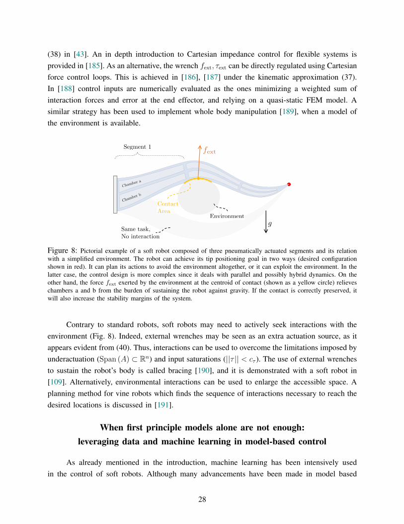
(38) in [43]. An in depth introduction to Cartesian impedance control for flexible systems isprovided in [185]. As an alternative, the wrench fext, τext can be directly regulated using Cartesianforce control loops. This is achieved in [186], [187] under the kinematic approximation (37).In [188] control inputs are numerically evaluated as the ones minimizing a weighted sum ofinteraction forces and error at the end effector, and relying on a quasi-static FEM model. Asimilar strategy has been used to implement whole body manipulation [189], when a model ofthe environment is available.

ContactArea

Same task,No interaction

Segment 1

Chamber a

Chamber b

Environment

fext

g

<latexit sha1_base64="/u9F/3CaJbts3iVsC52aqC2vayQ=">AAAB6HicbVBNS8NAEJ3Ur1q/qh69LBbBU0mkfhwLXjy2YGuhDWWznbRrN5uwuxFK6C/w4kERr/4kb/4bt20O2vpg4PHeDDPzgkRwbVz32ymsrW9sbhW3Szu7e/sH5cOjto5TxbDFYhGrTkA1Ci6xZbgR2EkU0igQ+BCMb2f+wxMqzWN5byYJ+hEdSh5yRo2VmsN+ueJW3TnIKvFyUoEcjX75qzeIWRqhNExQrbuemxg/o8pwJnBa6qUaE8rGdIhdSyWNUPvZ/NApObPKgISxsiUNmau/JzIaaT2JAtsZUTPSy95M/M/rpia88TMuk9SgZItFYSqIicnsazLgCpkRE0soU9zeStiIKsqMzaZkQ/CWX14l7YuqV6teNmuV+lUeRxFO4BTOwYNrqMMdNKAFDBCe4RXenEfnxXl3PhatBSefOYY/cD5/AMtxjOc=</latexit>

Figure 8: Pictorial example of a soft robot composed of three pneumatically actuated segments and its relationwith a simplified environment. The robot can achieve its tip positioning goal in two ways (desired configurationshown in red). It can plan its actions to avoid the environment altogether, or it can exploit the environment. In thelatter case, the control design is more complex since it deals with parallel and possibly hybrid dynamics. On theother hand, the force fext exerted by the environment at the centroid of contact (shown as a yellow circle) relieveschambers a and b from the burden of sustaining the robot against gravity. If the contact is correctly preserved, itwill also increase the stability margins of the system.

Contrary to standard robots, soft robots may need to actively seek interactions with theenvironment (Fig. 8). Indeed, external wrenches may be seen as an extra actuation source, as itappears evident from (40). Thus, interactions can be used to overcome the limitations imposed byunderactuation (Span (A) ⊂ Rn) and input saturations (||τ || < cτ ). The use of external wrenchesto sustain the robot’s body is called bracing [190], and it is demonstrated with a soft robot in[109]. Alternatively, environmental interactions can be used to enlarge the accessible space. Aplanning method for vine robots which finds the sequence of interactions necessary to reach thedesired locations is discussed in [191].

When first principle models alone are not enough:leveraging data and machine learning in model-based control

As already mentioned in the introduction, machine learning has been intensively usedin the control of soft robots. Although many advancements have been made in model based

28

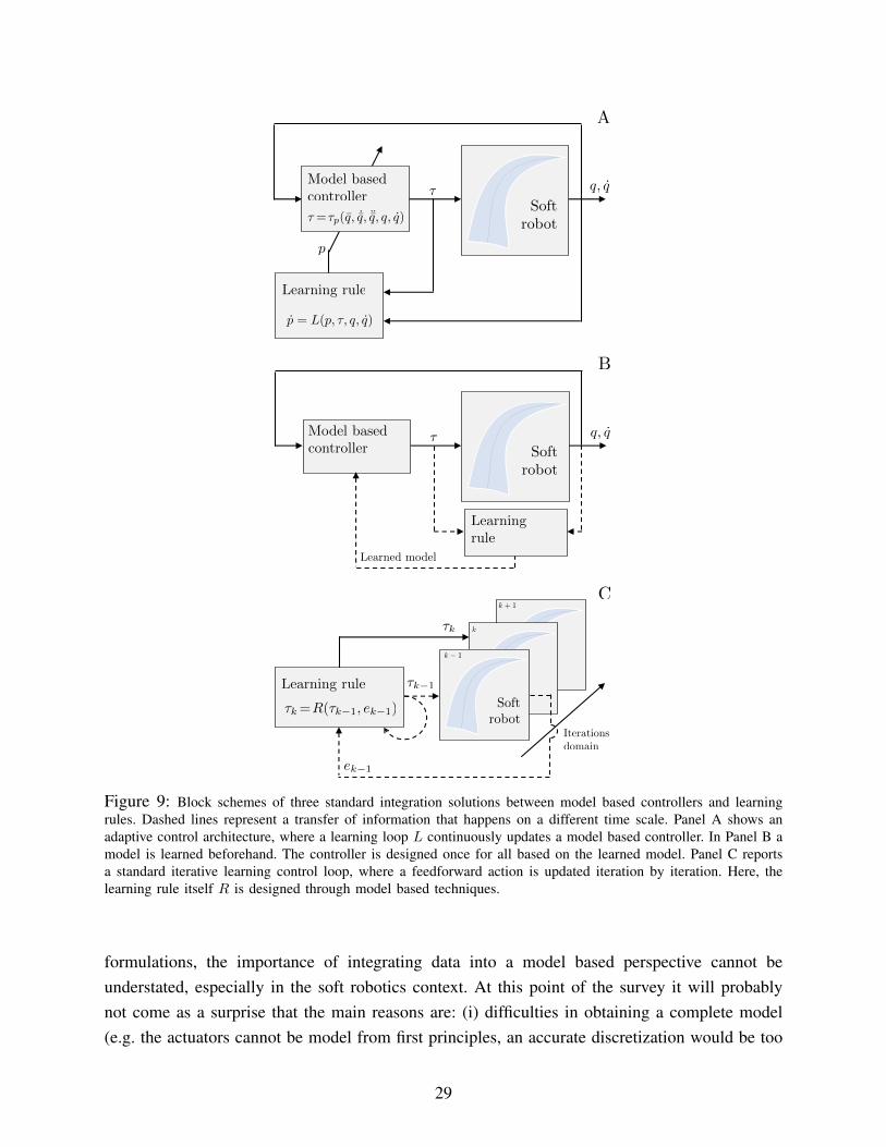
Softrobot


⌧ =⌧p(q, ˙q, ¨q, q, q)

<latexit sha1_base64="XUQ1lujbbTor6mqTIl1wGSzU7uE=">AAACLnicbVDLSgMxFM3UV62vqks30SJUkDIjFd0IRRFcVrAP6JSSSdM2NPNockcow3yRG39FF4KKuPUzzLSzsK0XEs7jXpJ7nEBwBab5bmSWlldW17LruY3Nre2d/O5eXfmhpKxGfeHLpkMUE9xjNeAgWDOQjLiOYA1neJP4jUcmFfe9BxgHrO2Svsd7nBLQUid/awMJsX2Ir5IrIZ0oiIv2NZHRKD61uz5EKUnYDB1N7VF80skXzJI5KbwIrBQUUFrVTv5Vj9LQZR5QQZRqWWYA7YhI4FSwOGeHigWEDkmftTT0iMtUO5qsG+NjrXRxz5f6eIAn6t+JiLhKjV1Hd7oEBmreS8T/vFYIvct2xL0gBObR6UO9UGDwcZId7nLJKIixBoRKrv+K6YBIQkEnnNMhWPMrL4L6Wckql87vy4VKOY0jiw7QESoiC12gCrpDVVRDFD2hF/SBPo1n4834Mr6nrRkjndlHM2X8/AJRlqjH</latexit>

p = L(p, ⌧, q, q)

<latexit sha1_base64="Ek5sp3w7mK761imuiQmcmPehplQ=">AAACCnicbVC7SgNBFJ31GeNr1dJmNAgRQtiViDZCwMbCIoJ5QLKE2clsMmT2kZm7QlhS2/grNhaK2PoFdv6Ns8kWmnhg4HDOPdy5x40EV2BZ38bS8srq2npuI7+5tb2za+7tN1QYS8rqNBShbLlEMcEDVgcOgrUiyYjvCtZ0h9ep33xgUvEwuIdxxByf9APucUpAS13zqNMLIYkm+ArfFqMS7gCJS3ikSaqPJqf5rlmwytYUeJHYGSmgDLWu+aWzNPZZAFQQpdq2FYGTEAmcCjbJd2LFIkKHpM/amgbEZ8pJpqdM8IlWetgLpX4B4Kn6O5EQX6mx7+pJn8BAzXup+J/XjsG7dBIeRDGwgM4WebHAEOK0F9zjklEQY00IlVz/FdMBkYSCbi8twZ4/eZE0zsp2pXx+VylUK1kdOXSIjlER2egCVdENqqE6ougRPaNX9GY8GS/Gu/ExG10ysswB+gPj8wcdIJiV</latexit>

Model basedcontroller

<latexit sha1_base64="qJUug0OcXptFJmcnC2qBFNcV3W4=">AAACAXicbVDLSsNAFJ34rPFVdSO4GSyCq5IUX8uCGzdCBfuANpTJ5KYdOpkJMxOhhLrxV9y4UMStf+HOvzFps9DWAwOHc+5j7vFjzrRxnG9raXlldW29tGFvbm3v7Jb39ltaJopCk0ouVccnGjgT0DTMcOjECkjkc2j7o+vcbz+A0kyKezOOwYvIQLCQUWIyqV8+vJUBcJyPCLBtUymMkpyD6pcrTtWZAi8StyAVVKDRL3/1AkmTCIShnGjddZ3YeClRhlEOE7uXaIgJHZEBdDMqSATaS6cXTPBJku8PpcqeMHiq/u5ISaT1OPKzyoiYoZ73cvE/r5uY8MpLmYgTA4LOFoUJx0biPA4cMAXU8HFGCFUs+yumQ6IINVlodhaCO3/yImnVqu5Z9fyuVqlfFHGU0BE6RqfIRZeojm5QAzURRY/oGb2iN+vJerHerY9Z6ZJV9BygP7A+fwBHRpYd</latexit>

Learning rule

<latexit sha1_base64="2bRiMENqPifMDJBlxuWIqPJP0GU=">AAAB9HicbVDLSgNBEOyNrxhfUY9eBoPgKewGX8eAFw8eIpgHJEuYnfQmQ2Zn15nZQAj5Di8eFPHqx3jzb5wke9DEgoaiqpvuriARXBvX/XZya+sbm1v57cLO7t7+QfHwqKHjVDGss1jEqhVQjYJLrBtuBLYShTQKBDaD4e3Mb45QaR7LRzNO0I9oX/KQM2qs5N8jVZLLPlGpwG6x5JbdOcgq8TJSggy1bvGr04tZGqE0TFCt256bGH9CleFM4LTQSTUmlA1pH9uWShqh9ifzo6fkzCo9EsbKljRkrv6emNBI63EU2M6ImoFe9mbif147NeGNP+EySQ1KtlgUpoKYmMwSID2ukBkxtoQyxe2thA2ooszYnAo2BG/55VXSqJS9i/LlQ6VUvcriyMMJnMI5eHANVbiDGtSBwRM8wyu8OSPnxXl3PhatOSebOYY/cD5/AKhVkf4=</latexit>

p

<latexit sha1_base64="562gW5nWouOB0E2CaaY0JCfSAlE=">AAAB6HicbVBNS8NAEJ3Ur1q/qh69LBbBU0mkfhwLXjy2YGuhDWWznbRrN5uwuxFK6C/w4kERr/4kb/4bt20O2vpg4PHeDDPzgkRwbVz32ymsrW9sbhW3Szu7e/sH5cOjto5TxbDFYhGrTkA1Ci6xZbgR2EkU0igQ+BCMb2f+wxMqzWN5byYJ+hEdSh5yRo2Vmkm/XHGr7hxklXg5qUCORr/81RvELI1QGiao1l3PTYyfUWU4Ezgt9VKNCWVjOsSupZJGqP1sfuiUnFllQMJY2ZKGzNXfExmNtJ5Ege2MqBnpZW8m/ud1UxPe+BmXSWpQssWiMBXExGT2NRlwhcyIiSWUKW5vJWxEFWXGZlOyIXjLL6+S9kXVq1Uvm7VK/SqPowgncArn4ME11OEOGtACBgjP8ApvzqPz4rw7H4vWgpPPHMMfOJ8/2RWM8A==</latexit>

⌧


q, q

<latexit sha1_base64="rtenOioOMN/SnAK4kfANZgm5Ed0=">AAAB8XicbVDLSgMxFL3js9ZX1aWbYBFcSJmR+lgW3LisYB/YDiWTpm1oJjNN7ghl6F+4caGIW//GnX9j2s5CWw8EDufcQ+49QSyFQdf9dlZW19Y3NnNb+e2d3b39wsFh3USJZrzGIhnpZkANl0LxGgqUvBlrTsNA8kYwvJ36jSeujYjUA45j7oe0r0RPMIpWehydk3Y3wnQ06RSKbsmdgSwTLyNFyFDtFL5skiUhV8gkNabluTH6KdUomOSTfDsxPKZsSPu8ZamiITd+Ott4Qk6t0iW9SNunkMzU34mUhsaMw8BOhhQHZtGbiv95rQR7N34qVJwgV2z+US+RBCMyPZ90heYM5dgSyrSwuxI2oJoytCXlbQne4snLpH5R8sqly/tysXKV1ZGDYziBM/DgGipwB1WoAQMFz/AKb45xXpx352M+uuJkmSP4A+fzB0eCkKM=</latexit>

Softrobot


Model basedcontroller

<latexit sha1_base64="qJUug0OcXptFJmcnC2qBFNcV3W4=">AAACAXicbVDLSsNAFJ34rPFVdSO4GSyCq5IUX8uCGzdCBfuANpTJ5KYdOpkJMxOhhLrxV9y4UMStf+HOvzFps9DWAwOHc+5j7vFjzrRxnG9raXlldW29tGFvbm3v7Jb39ltaJopCk0ouVccnGjgT0DTMcOjECkjkc2j7o+vcbz+A0kyKezOOwYvIQLCQUWIyqV8+vJUBcJyPCLBtUymMkpyD6pcrTtWZAi8StyAVVKDRL3/1AkmTCIShnGjddZ3YeClRhlEOE7uXaIgJHZEBdDMqSATaS6cXTPBJku8PpcqeMHiq/u5ISaT1OPKzyoiYoZ73cvE/r5uY8MpLmYgTA4LOFoUJx0biPA4cMAXU8HFGCFUs+yumQ6IINVlodhaCO3/yImnVqu5Z9fyuVqlfFHGU0BE6RqfIRZeojm5QAzURRY/oGb2iN+vJerHerY9Z6ZJV9BygP7A+fwBHRpYd</latexit>

⌧


q, q

<latexit sha1_base64="rtenOioOMN/SnAK4kfANZgm5Ed0=">AAAB8XicbVDLSgMxFL3js9ZX1aWbYBFcSJmR+lgW3LisYB/YDiWTpm1oJjNN7ghl6F+4caGIW//GnX9j2s5CWw8EDufcQ+49QSyFQdf9dlZW19Y3NnNb+e2d3b39wsFh3USJZrzGIhnpZkANl0LxGgqUvBlrTsNA8kYwvJ36jSeujYjUA45j7oe0r0RPMIpWehydk3Y3wnQ06RSKbsmdgSwTLyNFyFDtFL5skiUhV8gkNabluTH6KdUomOSTfDsxPKZsSPu8ZamiITd+Ott4Qk6t0iW9SNunkMzU34mUhsaMw8BOhhQHZtGbiv95rQR7N34qVJwgV2z+US+RBCMyPZ90heYM5dgSyrSwuxI2oJoytCXlbQne4snLpH5R8sqly/tysXKV1ZGDYziBM/DgGipwB1WoAQMFz/AKb45xXpx352M+uuJkmSP4A+fzB0eCkKM=</latexit>

Learned model

<latexit sha1_base64="Qx2j97knQZc9MJV+TXc+PW2aS1Q=">AAAB9HicbVDLSgNBEJyNrxhfUY9eBoPgKewGX8eAFw8eIpgHJEuYne1NhszOrDOzgbDkO7x4UMSrH+PNv3GS7EETCxqKqm66u4KEM21c99sprK1vbG4Vt0s7u3v7B+XDo5aWqaLQpJJL1QmIBs4ENA0zHDqJAhIHHNrB6Hbmt8egNJPi0UwS8GMyECxilBgr+fdAlIAQxzIE3i9X3Ko7B14lXk4qKEejX/7qhZKmMQhDOdG667mJ8TOiDKMcpqVeqiEhdEQG0LVUkBi0n82PnuIzq4Q4ksqWMHiu/p7ISKz1JA5sZ0zMUC97M/E/r5ua6MbPmEhSA4IuFkUpx0biWQI4ZAqo4RNLCFXM3orpkChCjc2pZEPwll9eJa1a1buoXj7UKvWrPI4iOkGn6Bx56BrV0R1qoCai6Ak9o1f05oydF+fd+Vi0Fpx85hj9gfP5A30skeI=</latexit>

Learningrule

<latexit sha1_base64="RV8WbRADquqKNPwBqOyYkHy8OnE=">AAAB9XicbVBNS8NAEJ3Urxq/qh69BIvgqSTFr2PBiwcPFewHtLFstpN26WYTdjdKCf0fXjwo4tX/4s1/47bNQVsfDDzem2FmXpBwprTrfluFldW19Y3ipr21vbO7V9o/aKo4lRQbNOaxbAdEIWcCG5ppju1EIokCjq1gdD31W48oFYvFvR4n6EdkIFjIKNFGerhFIgUTA9uWKcdeqexW3BmcZeLlpAw56r3SV7cf0zRCoSknSnU8N9F+RqRmlOPE7qYKE0JHZIAdQwWJUPnZ7OqJc2KUvhPG0pTQzkz9PZGRSKlxFJjOiOihWvSm4n9eJ9XhlZ8xkaQaBZ0vClPu6NiZRuD0mUSq+dgQQiUztzp0SCSh2gRlmxC8xZeXSbNa8c4q53fVcu0ij6MIR3AMp+DBJdTgBurQAAoSnuEV3qwn68V6tz7mrQUrnzmEP7A+fwC+K5H8</latexit>

Iterationsdomain

<latexit sha1_base64="2hMUigcj8qrMWMZIh8Vr4/Xhvi0=">AAAB+3icbZDLSsNAFIYn9Vbjrdalm8EiuCpJ8bYsuNFdBXuBNpTJZNIOnUuYmYgl9FXcuFDErS/izrdxmmahrT8MfPznHM6ZP0wY1cbzvp3S2vrG5lZ5293Z3ds/qBxWO1qmCpM2lkyqXog0YVSQtqGGkV6iCOIhI91wcjOvdx+J0lSKBzNNSMDRSNCYYmSsNaxU7wxROWvXjSRH1Jo1r+7lgqvgF1ADhVrDytcgkjjlRBjMkNZ930tMkCFlKGZk5g5STRKEJ2hE+hYF4kQHWX77DJ5aJ4KxVPYJA3P390SGuNZTHtpOjsxYL9fm5n+1fmri6yCjIkkNEXixKE4ZNBLOg4ARVQQbNrWAsKL2VojHSCFsA9GuDcFf/vIqdBp1/7x+cd+oNS+LOMrgGJyAM+CDK9AEt6AF2gCDJ/AMXsGbM3NenHfnY9FacoqZI/BHzucPdQaUBw==</latexit>

Softrobot


Learning rule

<latexit sha1_base64="2bRiMENqPifMDJBlxuWIqPJP0GU=">AAAB9HicbVDLSgNBEOyNrxhfUY9eBoPgKewGX8eAFw8eIpgHJEuYnfQmQ2Zn15nZQAj5Di8eFPHqx3jzb5wke9DEgoaiqpvuriARXBvX/XZya+sbm1v57cLO7t7+QfHwqKHjVDGss1jEqhVQjYJLrBtuBLYShTQKBDaD4e3Mb45QaR7LRzNO0I9oX/KQM2qs5N8jVZLLPlGpwG6x5JbdOcgq8TJSggy1bvGr04tZGqE0TFCt256bGH9CleFM4LTQSTUmlA1pH9uWShqh9ifzo6fkzCo9EsbKljRkrv6emNBI63EU2M6ImoFe9mbif147NeGNP+EySQ1KtlgUpoKYmMwSID2ukBkxtoQyxe2thA2ooszYnAo2BG/55VXSqJS9i/LlQ6VUvcriyMMJnMI5eHANVbiDGtSBwRM8wyu8OSPnxXl3PhatOSebOYY/cD5/AKhVkf4=</latexit>

⌧k =R(⌧k�1, ek�1)

<latexit sha1_base64="eg/WDIx4uX5vmysDrJVmrnJC+r0=">AAACDXicbVC7TsMwFHV4lvIKMLIYClKRoEpQeSxIlVgYC6IPqYkix3VaK85DtoNURf0BFn6FhQGEWNnZ+BucNAO0HMm+R+fcK/seN2ZUSMP41ubmFxaXlksr5dW19Y1NfWu7LaKEY9LCEYt410WCMBqSlqSSkW7MCQpcRjquf535nQfCBY3CezmKiR2gQUg9ipFUkqMfWBIljg+tPXiVXXfVXEj9E3N8TCb1yNErRs3IAWeJWZAKKNB09C+rH+EkIKHEDAnRM41Y2inikmJGxmUrESRG2EcD0lM0RAERdppvM4aHSulDL+LqhBLm6u+JFAVCjAJXdQZIDsW0l4n/eb1Eepd2SsM4kSTEk4e8hEEZwSwa2KecYMlGiiDMqforxEPEEZYqwLIKwZxeeZa0T2tmvXZ2W680zos4SmAX7IMqMMEFaIAb0AQtgMEjeAav4E170l60d+1j0jqnFTM74A+0zx+MhplQ</latexit>

⌧k�1

<latexit sha1_base64="HcWkduTge2zdyecEFSgEjpdz+og=">AAAB8XicbVDLSgNBEOz1GeMr6tHLYBC8GHYlPo4BLx4jmAcmS5idzCZDZmeXmV4hLPkLLx4U8erfePNvnCR70MSChqKqm+6uIJHCoOt+Oyura+sbm4Wt4vbO7t5+6eCwaeJUM95gsYx1O6CGS6F4AwVK3k40p1EgeSsY3U791hPXRsTqAccJ9yM6UCIUjKKVHrtI0142OvcmvVLZrbgzkGXi5aQMOeq90le3H7M04gqZpMZ0PDdBP6MaBZN8UuymhieUjeiAdyxVNOLGz2YXT8ipVfokjLUthWSm/p7IaGTMOApsZ0RxaBa9qfif10kxvPEzoZIUuWLzRWEqCcZk+j7pC80ZyrEllGlhbyVsSDVlaEMq2hC8xZeXSfOi4lUrl/fVcu0qj6MAx3ACZ+DBNdTgDurQAAYKnuEV3hzjvDjvzse8dcXJZ47gD5zPH0X2kKA=</latexit>

⌧k

<latexit sha1_base64="5v/96xEqYzfhg/y5MGyJwYLlZ9E=">AAAB73icbVDLSgNBEOyNrxhfUY9eBoPgKexKfBwDXjxGMA9IljA7mU2GzM6uM71CWPITXjwo4tXf8ebfOEn2oIkFDUVVN91dQSKFQdf9dgpr6xubW8Xt0s7u3v5B+fCoZeJUM95ksYx1J6CGS6F4EwVK3kk0p1EgeTsY38789hPXRsTqAScJ9yM6VCIUjKKVOj2kaT8bT/vlilt15yCrxMtJBXI0+uWv3iBmacQVMkmN6Xpugn5GNQom+bTUSw1PKBvTIe9aqmjEjZ/N752SM6sMSBhrWwrJXP09kdHImEkU2M6I4sgsezPxP6+bYnjjZ0IlKXLFFovCVBKMyex5MhCaM5QTSyjTwt5K2IhqytBGVLIheMsvr5LWRdWrVS/va5X6VR5HEU7gFM7Bg2uowx00oAkMJDzDK7w5j86L8+58LFoLTj5zDH/gfP4AZyiQLg==</latexit>

ek�1

<latexit sha1_base64="4bVMCFQiGj67HuzDVavk72o9z6s=">AAAB7nicbVDLSgNBEOyNrxhfUY9eBoPgxbAr8XEMePEYwTwgWcLspDcZMju7zMwKYclHePGgiFe/x5t/4yTZgyYWNBRV3XR3BYng2rjut1NYW9/Y3Cpul3Z29/YPyodHLR2nimGTxSJWnYBqFFxi03AjsJMopFEgsB2M72Z++wmV5rF8NJME/YgOJQ85o8ZKbexn4wtv2i9X3Ko7B1klXk4qkKPRL3/1BjFLI5SGCap113MT42dUGc4ETku9VGNC2ZgOsWuppBFqP5ufOyVnVhmQMFa2pCFz9fdERiOtJ1FgOyNqRnrZm4n/ed3UhLd+xmWSGpRssShMBTExmf1OBlwhM2JiCWWK21sJG1FFmbEJlWwI3vLLq6R1WfVq1auHWqV+ncdRhBM4hXPw4AbqcA8NaAKDMTzDK7w5ifPivDsfi9aCk88cwx84nz/mjI9B</latexit>

k � 1

<latexit sha1_base64="tCZrHJwP7nFrCwpR0TGbvZzSpxo=">AAAB7HicbVBNS8NAEJ3Ur1q/qh69LBahF0siFT0WvHisYNpCG8pmO22XbjZhdyOU0N/gxYMiXv1B3vw3btsctPXBwOO9GWbmhYng2rjut1PY2Nza3inulvb2Dw6PyscnLR2niqHPYhGrTkg1Ci7RN9wI7CQKaRQKbIeTu7nffkKleSwfzTTBIKIjyYecUWMlP5tcerN+ueLW3AXIOvFyUoEczX75qzeIWRqhNExQrbuem5ggo8pwJnBW6qUaE8omdIRdSyWNUAfZ4tgZubDKgAxjZUsaslB/T2Q00noahbYzomasV725+J/XTc3wNsi4TFKDki0XDVNBTEzmn5MBV8iMmFpCmeL2VsLGVFFmbD4lG4K3+vI6aV3VvHrt+qFeaVTzOIpwBudQBQ9uoAH30AQfGHB4hld4c6Tz4rw7H8vWgpPPnMIfOJ8/aySOWw==</latexit>

k

<latexit sha1_base64="lSR/5y+KDCeU9J+R2797MCHPSow=">AAAB6nicbVBNS8NAEJ3Ur1q/qh69LBahp5JIRY8FLx4r2g9oQ9lsN+3SzSbsToQS+hO8eFDEq7/Im//GbZuDtj4YeLw3w8y8IJHCoOt+O4WNza3tneJuaW//4PCofHzSNnGqGW+xWMa6G1DDpVC8hQIl7yaa0yiQvBNMbud+54lrI2L1iNOE+xEdKREKRtFKD9lkNihX3Jq7AFknXk4qkKM5KH/1hzFLI66QSWpMz3MT9DOqUTDJZ6V+anhC2YSOeM9SRSNu/Gxx6oxcWGVIwljbUkgW6u+JjEbGTKPAdkYUx2bVm4v/eb0Uwxs/EypJkSu2XBSmkmBM5n+TodCcoZxaQpkW9lbCxlRThjadkg3BW315nbQva169dnVfrzSqeRxFOINzqIIH19CAO2hCCxiM4Ble4c2Rzovz7nwsWwtOPnMKf+B8/gCQdI3p</latexit>

k + 1

<latexit sha1_base64="Nd4oH8gm3/XPoXzci6cpWRQ+1AU=">AAAB7HicbVBNS8NAEJ3Ur1q/qh69LBahIJREKnosePFYwX5AG8pmu2mXbjZhdyKU0N/gxYMiXv1B3vw3btsctPXBwOO9GWbmBYkUBl332ylsbG5t7xR3S3v7B4dH5eOTtolTzXiLxTLW3YAaLoXiLRQoeTfRnEaB5J1gcjf3O09cGxGrR5wm3I/oSIlQMIpWak3IJfEG5Ypbcxcg68TLSQVyNAflr/4wZmnEFTJJjel5boJ+RjUKJvms1E8NTyib0BHvWapoxI2fLY6dkQurDEkYa1sKyUL9PZHRyJhpFNjOiOLYrHpz8T+vl2J462dCJSlyxZaLwlQSjMn8czIUmjOUU0so08LeStiYasrQ5lOyIXirL6+T9lXNq9euH+qVRjWPowhncA5V8OAGGnAPTWgBAwHP8ApvjnJenHfnY9lacPKZU/gD5/MHT/eNoQ==</latexit>

A

C

<latexit sha1_base64="xOKpX3NIXIluYFQnyfl7NQvs/NU=">AAAB6HicbVA9SwNBEJ2LXzF+RS1tFoNgFe6CooVFII1lAuYDkiPsbeaSNXt7x+6eEEJ+gY2FIrb+JDv/jZvkCk18MPB4b4aZeUEiuDau++3kNja3tnfyu4W9/YPDo+LxSUvHqWLYZLGIVSegGgWX2DTcCOwkCmkUCGwH49rcbz+h0jyWD2aSoB/RoeQhZ9RYqVHrF0tu2V2ArBMvIyXIUO8Xv3qDmKURSsME1brruYnxp1QZzgTOCr1UY0LZmA6xa6mkEWp/ujh0Ri6sMiBhrGxJQxbq74kpjbSeRIHtjKgZ6VVvLv7ndVMT3vpTLpPUoGTLRWEqiInJ/Gsy4AqZERNLKFPc3krYiCrKjM2mYEPwVl9eJ61K2bsqXzcqpepdFkcezuAcLsGDG6jCPdShCQwQnuEV3pxH58V5dz6WrTknmzmFP3A+fwCWD4zH</latexit>

B

<latexit sha1_base64="LUwMH2KOFMzZIDj76+fdfMzN/gk=">AAAB6HicbVA9SwNBEJ2LXzF+RS1tFoNgFe6CooVF0MYyAfMByRH2NnPJmr29Y3dPCCG/wMZCEVt/kp3/xk1yhSY+GHi8N8PMvCARXBvX/XZya+sbm1v57cLO7t7+QfHwqKnjVDFssFjEqh1QjYJLbBhuBLYThTQKBLaC0d3Mbz2h0jyWD2acoB/RgeQhZ9RYqX7bK5bcsjsHWSVeRkqQodYrfnX7MUsjlIYJqnXHcxPjT6gynAmcFrqpxoSyER1gx1JJI9T+ZH7olJxZpU/CWNmShszV3xMTGmk9jgLbGVEz1MveTPzP66QmvPYnXCapQckWi8JUEBOT2dekzxUyI8aWUKa4vZWwIVWUGZtNwYbgLb+8SpqVsndRvqxXStWbLI48nMApnIMHV1CFe6hBAxggPMMrvDmPzovz7nwsWnNONnMMf+B8/gCUi4zG</latexit>

Figure 9: Block schemes of three standard integration solutions between model based controllers and learningrules. Dashed lines represent a transfer of information that happens on a different time scale. Panel A shows anadaptive control architecture, where a learning loop L continuously updates a model based controller. In Panel B amodel is learned beforehand. The controller is designed once for all based on the learned model. Panel C reportsa standard iterative learning control loop, where a feedforward action is updated iteration by iteration. Here, thelearning rule itself R is designed through model based techniques.

formulations, the importance of integrating data into a model based perspective cannot beunderstated, especially in the soft robotics context. At this point of the survey it will probablynot come as a surprise that the main reasons are: (i) difficulties in obtaining a complete model(e.g. the actuators cannot be model from first principles, an accurate discretization would be too

29

computationally expensive, the environment cannot be known in advance), and (ii) uncertaintiesare inherit in any soft robotic application (e.g. unreliability of sensors and actuators, change ofphysical parameters over time and over several iterations of the same device).

This section focuses on how learning can be integrated into a model-based framework totackle the control of soft robots. Combining model with data is a quite active topic in the controlcommunity, and many solutions are currently being developed that will most probably eventuallyfind useful application in the soft robotic field [192]–[196]. It is however beyond the scope ofthis work to discuss these new advancements. Moreover, the same special issue contains anothersurvey paper fully focused on machine learning strategies for soft robots [197].

Using models to drive learning

The acquisition of new information and its transformation into a control action can bedriven by the knowledge of (an approximation of) the model itself. This can be done whilelearning a feedback control, a feedforward action, or by serving as source of synthetic data formore standard machine learning approaches.

Adaptive control

Adaptive control (Fig. 9 A) is an established technique in control theory [198], whichallows to augment feedback controllers with an online learning loop. The typical structure of anadaptive controller is

p = L(p, τ, q, q), τ = τp(q, ˙q, ¨q, q, q). (42)

The uncertainty is represented as a set of unknown parameters p ∈ Ro appearing linearly in (1)or (2). The control action τ is generated through a model based controller τp parametrized inp. For example, the dynamics of the constant curvature segment discussed in sidebar ?? can belinearly parametrized in mL2, mgL,

∫ 1

0k(s)ds, and

∫ 1

0s d(s)ds. The second and the third would

for example appear as parameters in an adaptive version of (23). The model structure can guidethe design of a learning rule L, such that p is moved towards values that better explain the data.If L learns the parameters p that describe the real system, then from there p = 0 and τp behavesas a standard model based controller.

Classic results in adaptive PD [199] and PD+ [200] control can be potentially applied tothe soft robotic case, by leveraging the equivalence exemplified by (16). Yet, the transfer is lessdirect than for the non adaptive case. An adaptive visual servoing scheme is proposed in [201],by relying on a kinematic PCC approximation. Linear adaptive control is used in [202] to controla single bending actuator. A similar strategy is applied to the control of a soft hand exoskeleton

30

in [203], [204], where also the parameters of the human fingers are learned. An adaptive versionof MPC is discussed in [205], [206], and experimentally validated against a non-adaptive MPC.A nonlinear adaptive controller originally developed for rigid robots is applied to soft robots in[45], by relying on an augmented rigid robot approximation. Adaptive control can be extendedbeyond known-unknowns by including in p generic disturbances acting on the system. High gainobservers are used in [207] to estimate and compensate for the mismatch between a simplifiedlinear model of a parallel soft robot and the real system. Also, [208] discusses the positionregulation in Cartesian space for a soft robot with discretized but uncertain kinematics, includingadaptive compensation of disturbances. An adaptive loop that learns the gains of a sliding modecontroller is proposed in [209]. In classic robotics, this concept has been pushed even furtherby adding nonlinear black box approximators borrowed from machine learning to the originaldynamics, and including their weights in the p vector [210]–[212].

Iterative Learning Control

As an alternative to learning the feedback loop, models can be used to guide the learningof a feedforward action (Fig. 9 C). This can be done under the hypothesis that a same task canbe tried out multiple times by the robot, by using iterative learning control [213] (ILC). Callk ∈ N the iteration index, which captures how many times the robot has attempted the executionof the task. Then, in this context a learning rule R is a way of updating the feedforward action

τk(t) = R(τk−1([0, tf ]), ek−1([0, tf ])), (43)

where e(t) is a measure of how well the task has been executed at time t. Note that the learningrule R can in general combine information from the whole error and control evolution at thestep k− 1. The design of R is driven by the knowledge of the nominal model, and it is definedis such a way that eventually the robot learns a feedforward action τ∞(t) implementing a perfectexecution of the task (||e∞|| = 0). ILC is particularly suited for soft robots since: (i) the learningprocess is robust to uncertainties in the model, (ii) purely feedforward actions do not disruptthe physical softness of the system [105], and (iii) they are inherently stable if the robot is nottoo soft. The actuation patterns necessary to track an optimal trajectory are learned using thistechnique in [109]. Crawling motions of soft worms have been improved via ILC in [214], [215].A linear discrete learning rule is used in [216], [217] to control a soft spherical joint. NonlinearILC is used in [218] to control a soft finger. ILC is combined with MPC in [219] and used tocontrol a soft bending actuator mounted on an human finger. A continuous feedback-feedforwardrule is proposed in [220] and applied to the swing up of a soft inverted pendulum.

31

Simulators as virtual environments

A more indirect way of using models to drive learning is by building simulators. Modelsdeveloped from first principles can be used to create virtual environments where robots can evolve[221], [222] or learn new skills [93], [223], [224]. Differentiable simulators are particularly suitedto be used in this context, as discussed in [225]. Indeed, having gradients available allows tobackpropagate through the simulator, which opens up the possibility of apply supervised machinelearning and directly optimize for a desired behavior.

Control loops based on learned models

Directly learning an end-to-end controller using standard machine learning techniquescan present several disadvantages, as limited explainability [226] and difficulties in ensuringperformance and stability of the closed loop. Moreover, the learning process may be illconditioned due to highly redundant nature of soft robots. An alternative to learning the controlleris to learn the model and then using it within a model-based control framework.

Learning the model, by using the model

Approximation of dynamical systems is discussed in [227], [228], and model learning forrobot control is surveyed in [229]. When using fully black box approximators, first principlemodels can still be used to generate a warm start for the learning process. For example, [230]uses a liner model of pneumatic actuator for pre-training a neural network, which is then finetuned with experimental data. A nonlinear model of multi-segment soft robot is used in [231]to train a recurrent neural network. Even when a good model is already available, it can still bethe case that learning strategies are used to better its performance. A method for learning onlythe nonlinear stiffness characteristics of a soft robot is discussed in [232]. The acquisition ofdata is driven by a FEM model of the elastic part. An optimal estimation strategy of geometricalquantities describing the robot kinematics is discussed in [233].

Closing the loop

Once learned, the models can be used as a base for model based control loops (Fig. 9B). In [234] a shallow neural network is used to learn the forward kinematics of a soft robot.Then (37) is used to solve the inverse problem. Neural networks are fully differentiable, andthus Jacobian can be easily calculated. This is advantageous if compared to directly learning theinverse kinematics, since (37) resolves automatically those redundancies that would make thedirect learning of an inverse kinematics ill posed. Visual servoing under kinematic approximationfor controlling the shape of a soft object is extended in [235] to the case where the Jacobian is

32

estimated online. Similar strategies can be employed also in a dynamic setting. Whenever (22) isverified, learned models can be used to produce open loop control actions which are ineherentlystable [103], [236], [237]. Learned models can be used also when feedback is needed to stabilizethe desired behavior. For example, a neural network is trained to approximate the update functionof a soft segment in [238], and its input-output gradient is used to run a linear MPC algorithm.A similar strategy is used in [230], but here the neural network is directly incorporated into anMPC control loop. Alternatively, Koopman theory enables learning directly a linear dynamicsevolving within an high dimensional lifted space [239]–[241]. The resulting model has beenused as a base for LQR [242] and linear MPC [243].

Conclusions

This article has surveyed control strategies for soft robots that rely on model basedformulations. Special attention has been devoted to organizing this large body of literaturewithin a coherent framework and with a common terminology inspired by classic robotics androbot control. Thanks to the latter, once the discretization of the infinite-dimensional space isintroduced, the similarities between rigid, flexible, soft robots become apparent. Connectionswith existing results developed outside the soft robotic could therefore be drawn, and controllersported from the rigid to the soft continuum world. On the other hand, using a common languageclearly pinpoint the fundamental differences between soft robotics and other related fields. Themost apparent one is a large number of degrees of freedom, making soft robots intrinsicallyunderactuated. These characteristics would make the control challenge too complex to be solved,if not in straightforward cases. Nonetheless, the positive definite elastic potential and the strictlydissipative force field that is always present, no matter the discretization, simplify the controlproblem enormously.

Notwithstanding the significant advancements achieved so far, the research community hasbarely scratched the model-based view’s surface to soft robotics. Many are indeed the challengesthat remain open and the questions unanswered. How to take underactuation into account? Towhich extent the non-actuated dynamics can or can not be neglected? Can generic unstableequilibria be stabilized? How to implement motions which are simultaneously compliant, fast,and precise? And controlled movements involving continuous interactions with an unstructuredenvironment? Can a complete integration of embodied intelligence and control design be reachedwithin the model based framework? And so on.

Finally, it should not be forgotten that soft robotics has been born as an experimentaldiscipline, which aims to revolutionize how robots are entering our lives. Thus, all thesetheoretical advancements should contribute to realizing this grand vision by endowing real soft

33

robots with unmatched motor capabilities.

34

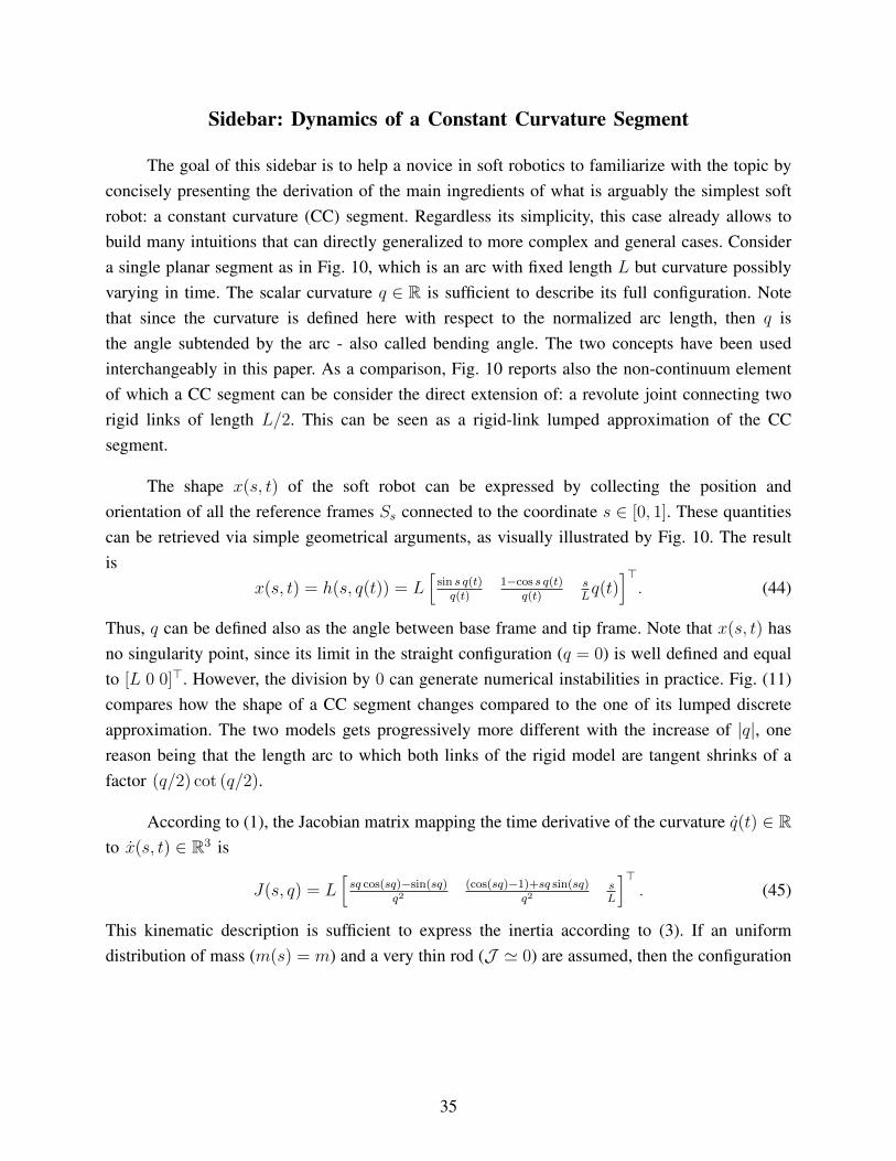
Sidebar: Dynamics of a Constant Curvature Segment

The goal of this sidebar is to help a novice in soft robotics to familiarize with the topic byconcisely presenting the derivation of the main ingredients of what is arguably the simplest softrobot: a constant curvature (CC) segment. Regardless its simplicity, this case already allows tobuild many intuitions that can directly generalized to more complex and general cases. Considera single planar segment as in Fig. 10, which is an arc with fixed length L but curvature possiblyvarying in time. The scalar curvature q ∈ R is sufficient to describe its full configuration. Notethat since the curvature is defined here with respect to the normalized arc length, then q isthe angle subtended by the arc - also called bending angle. The two concepts have been usedinterchangeably in this paper. As a comparison, Fig. 10 reports also the non-continuum elementof which a CC segment can be consider the direct extension of: a revolute joint connecting tworigid links of length L/2. This can be seen as a rigid-link lumped approximation of the CCsegment.

The shape x(s, t) of the soft robot can be expressed by collecting the position andorientation of all the reference frames Ss connected to the coordinate s ∈ [0, 1]. These quantitiescan be retrieved via simple geometrical arguments, as visually illustrated by Fig. 10. The resultis

x(s, t) = h(s, q(t)) = L[

sin s q(t)q(t)

1−cos s q(t)q(t)

sLq(t)

]>. (44)

Thus, q can be defined also as the angle between base frame and tip frame. Note that x(s, t) hasno singularity point, since its limit in the straight configuration (q = 0) is well defined and equalto [L 0 0]>. However, the division by 0 can generate numerical instabilities in practice. Fig. (11)compares how the shape of a CC segment changes compared to the one of its lumped discreteapproximation. The two models gets progressively more different with the increase of |q|, onereason being that the length arc to which both links of the rigid model are tangent shrinks of afactor (q/2) cot (q/2).

According to (1), the Jacobian matrix mapping the time derivative of the curvature q(t) ∈ Rto x(s, t) ∈ R3 is

J(s, q) = L[sq cos(sq)−sin(sq)

q2(cos(sq)−1)+sq sin(sq)

q2sL

]>. (45)

This kinematic description is sufficient to express the inertia according to (3). If an uniformdistribution of mass (m(s) = m) and a very thin rod (J ' 0) are assumed, then the configuration

35

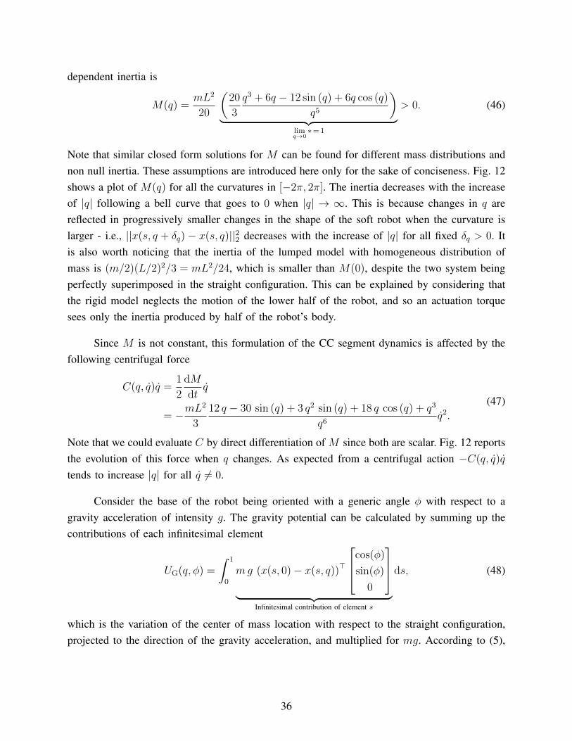
dependent inertia is

M(q) =mL2

20

(20

3

q3 + 6q − 12 sin (q) + 6q cos (q)

q5

)

︸︷︷︸limq→0∗= 1

> 0. (46)

Note that similar closed form solutions for M can be found for different mass distributions andnon null inertia. These assumptions are introduced here only for the sake of conciseness. Fig. 12shows a plot of M(q) for all the curvatures in [−2π, 2π]. The inertia decreases with the increaseof |q| following a bell curve that goes to 0 when |q| → ∞. This is because changes in q arereflected in progressively smaller changes in the shape of the soft robot when the curvature islarger - i.e., ||x(s, q + δq) − x(s, q)||22 decreases with the increase of |q| for all fixed δq > 0. Itis also worth noticing that the inertia of the lumped model with homogeneous distribution ofmass is (m/2)(L/2)2/3 = mL2/24, which is smaller than M(0), despite the two system beingperfectly superimposed in the straight configuration. This can be explained by considering thatthe rigid model neglects the motion of the lower half of the robot, and so an actuation torquesees only the inertia produced by half of the robot’s body.

Since M is not constant, this formulation of the CC segment dynamics is affected by thefollowing centrifugal force

C(q, q)q =1

2

dM

dtq

= −mL2

3

12 q − 30 sin (q) + 3 q2 sin (q) + 18 q cos (q) + q3

q6q2.

(47)

Note that we could evaluate C by direct differentiation of M since both are scalar. Fig. 12 reportsthe evolution of this force when q changes. As expected from a centrifugal action −C(q, q)q

tends to increase |q| for all q 6= 0.

Consider the base of the robot being oriented with a generic angle φ with respect to agravity acceleration of intensity g. The gravity potential can be calculated by summing up thecontributions of each infinitesimal element

UG(q, φ) =

∫ 1

0

mg (x(s, 0)− x(s, q))>

cos(φ)

sin(φ)

0

︸︷︷︸Infinitesimal contribution of element s

ds, (48)

which is the variation of the center of mass location with respect to the straight configuration,projected to the direction of the gravity acceleration, and multiplied for mg. According to (5),

36

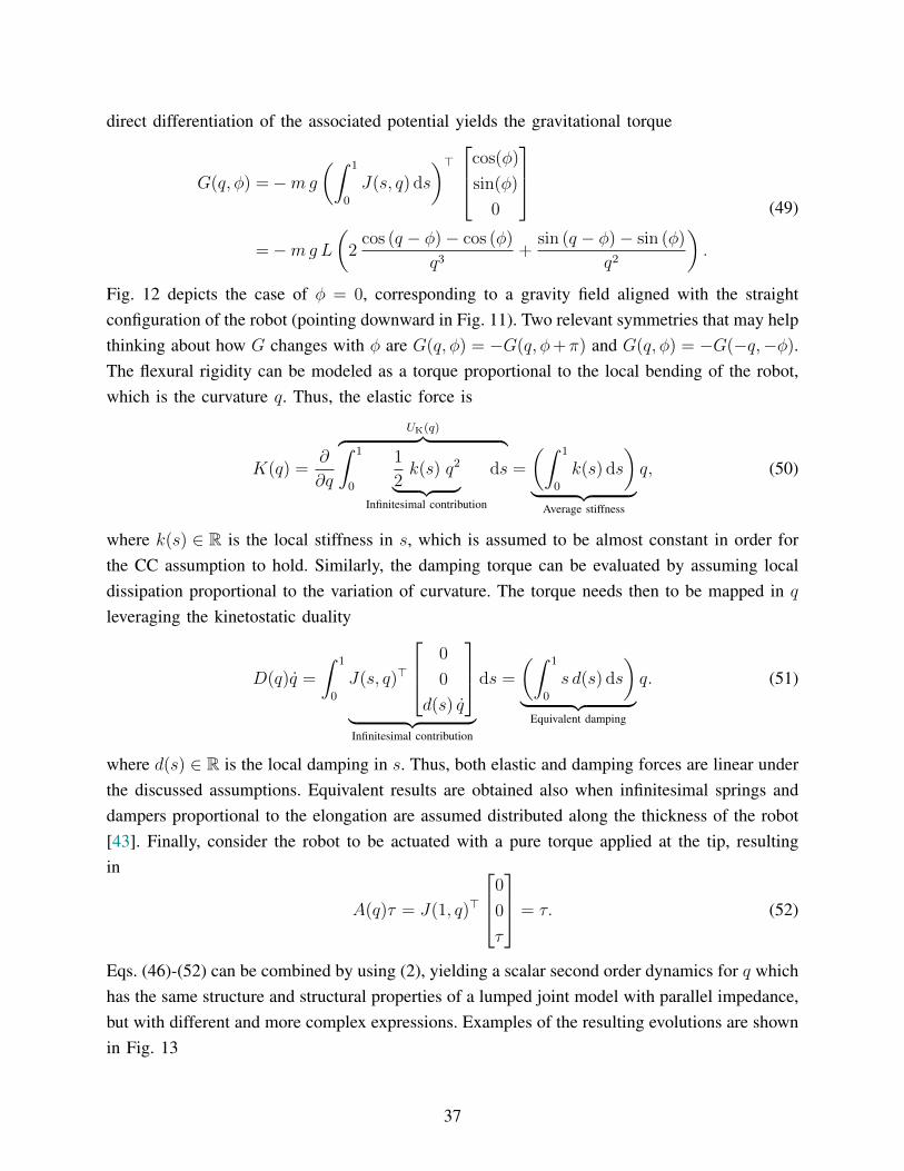
direct differentiation of the associated potential yields the gravitational torque

G(q, φ) =−mg

(∫ 1

0

J(s, q) ds

)>

cos(φ)

sin(φ)

0

=−mg L

(2

cos (q − φ)− cos (φ)

q3+

sin (q − φ)− sin (φ)

q2

).

(49)

Fig. 12 depicts the case of φ = 0, corresponding to a gravity field aligned with the straightconfiguration of the robot (pointing downward in Fig. 11). Two relevant symmetries that may helpthinking about how G changes with φ are G(q, φ) = −G(q, φ+π) and G(q, φ) = −G(−q,−φ).The flexural rigidity can be modeled as a torque proportional to the local bending of the robot,which is the curvature q. Thus, the elastic force is

K(q) =∂

∂q

UK(q)︷︸︸︷∫ 1

0

1

2k(s) q2

︸︷︷︸Infinitesimal contribution

ds =

(∫ 1

0

k(s) ds

)

︸︷︷︸Average stiffness

q, (50)

where k(s) ∈ R is the local stiffness in s, which is assumed to be almost constant in order forthe CC assumption to hold. Similarly, the damping torque can be evaluated by assuming localdissipation proportional to the variation of curvature. The torque needs then to be mapped in qleveraging the kinetostatic duality

D(q)q =

∫ 1

0

J(s, q)>

0

0

d(s) q

︸︷︷︸Infinitesimal contribution

ds =

(∫ 1

0

s d(s) ds

)

︸︷︷︸Equivalent damping

q. (51)

where d(s) ∈ R is the local damping in s. Thus, both elastic and damping forces are linear underthe discussed assumptions. Equivalent results are obtained also when infinitesimal springs anddampers proportional to the elongation are assumed distributed along the thickness of the robot[43]. Finally, consider the robot to be actuated with a pure torque applied at the tip, resultingin

A(q)τ = J(1, q)>

0

0

τ

= τ. (52)

Eqs. (46)-(52) can be combined by using (2), yielding a scalar second order dynamics for q whichhas the same structure and structural properties of a lumped joint model with parallel impedance,but with different and more complex expressions. Examples of the resulting evolutions are shownin Fig. 13

37

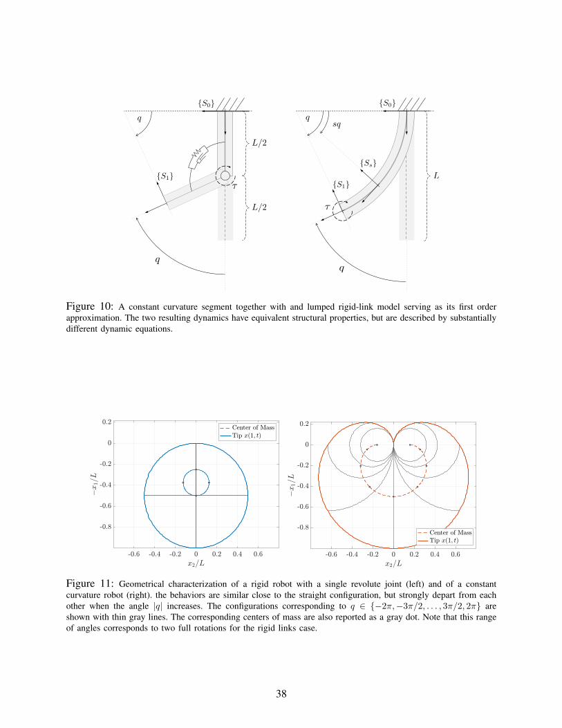
{S0}

{S1}

q

q

⌧

L/2

L/2 ⌧

{S0}

{Ss}

{S1}

sqq

L

q

Figure 10: A constant curvature segment together with and lumped rigid-link model serving as its first orderapproximation. The two resulting dynamics have equivalent structural properties, but are described by substantiallydifferent dynamic equations.

Figure 11: Geometrical characterization of a rigid robot with a single revolute joint (left) and of a constantcurvature robot (right). the behaviors are similar close to the straight configuration, but strongly depart from eachother when the angle |q| increases. The configurations corresponding to q ∈ {−2π,−3π/2, . . . , 3π/2, 2π} areshown with thin gray lines. The corresponding centers of mass are also reported as a gray dot. Note that this rangeof angles corresponds to two full rotations for the rigid links case.

38

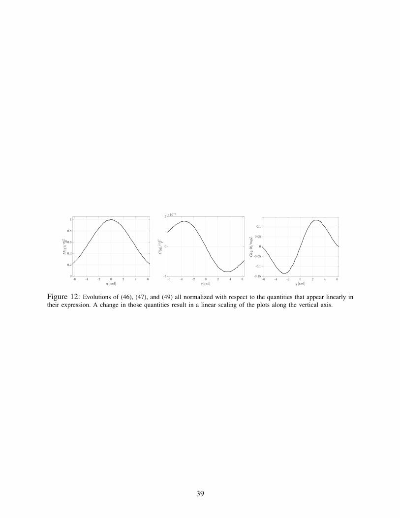
Figure 12: Evolutions of (46), (47), and (49) all normalized with respect to the quantities that appear linearly intheir expression. A change in those quantities result in a linear scaling of the plots along the vertical axis.

39

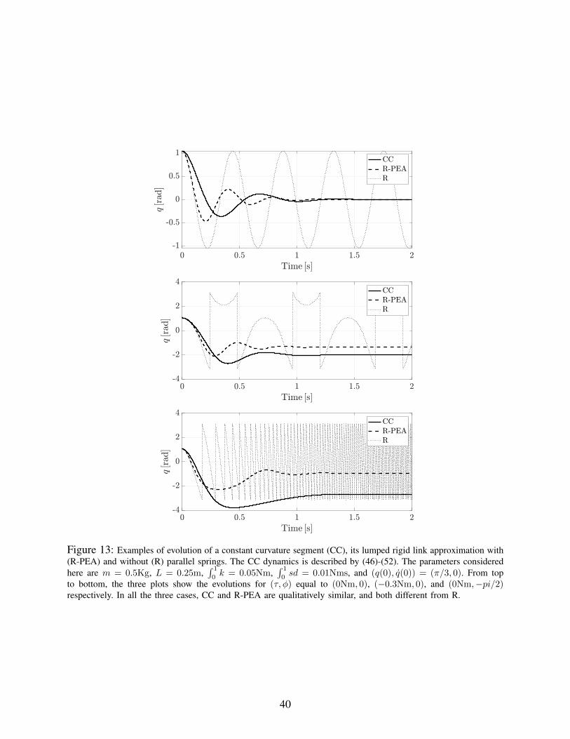
Figure 13: Examples of evolution of a constant curvature segment (CC), its lumped rigid link approximation with(R-PEA) and without (R) parallel springs. The CC dynamics is described by (46)-(52). The parameters consideredhere are m = 0.5Kg, L = 0.25m,

∫ 1

0k = 0.05Nm,

∫ 1

0sd = 0.01Nms, and (q(0), q(0)) = (π/3, 0). From top

to bottom, the three plots show the evolutions for (τ, φ) equal to (0Nm, 0), (−0.3Nm, 0), and (0Nm,−pi/2)respectively. In all the three cases, CC and R-PEA are qualitatively similar, and both different from R.

40

Better than Rigid Robots: Exploiting Softness in Model-Based Control

A natural way of understanding physical intelligence generated by a soft body within amodel based setting is to look at the impedance K(q) + D(q)q in (2) as a low level feedbackaction. One obvious advantage of implementing such an action physically rather than digitallyis that in this way it does not require any additional sensors and actuators. Another importantfeature is that it acts simultaneously and in a decentralized manner along the whole infinitedimensional structure. In other words, ∂K/∂q and D are always full rank almost everywhereno matter the level of democratization. The number of independent directions in which standardcontrol can be produced is instead limited, as concisely represented by the fact that the numberof columns m of the matrix A(q) in (2) is independent from the size n of the configurationspace q. The consequence in terms of self-stabilization of the robot and control simplificationare extensively discussed in the main body of the paper.

Physical elasticity can also be used to better the execution of dynamic tasks. For example[244], [245] prove that lumped join-spring-link systems admit optimal control actions thatmaximize velocity or forces beyond what can be achieved by a rigid robot of equivalent inertia.During these tasks the potential UK(q) serves as a tank in which energy can be stored and releasedwhen necessary. Thanks to multi-stabilities and bucklings, continuum structures can lead to evenextremer behaviors concerning pick performances, which have be thoroughly investigated in amodel based fashion [246]–[248]. However, the proposed descriptions are generally not in thelanguage of dynamical systems, and as such using them for control purposes is still an openchallenge. Another benefit of physical elasticity is to endow the robot with the capability ofperforming regular oscillations [249], which can be excited by means of model based control[250]–[252]. This is especially useful in efficient and robust locomotion [7], [253], [254]. Itis worth underlying that all these capabilities are implicitly exploited by the vast range ofapproaches using numerical optimization for controlling soft robots [109], [146]–[148], [255],[256].

For an in depth analysis on how the body of a soft robot can generate intelligent behaviorswe refer to another paper within the same special issue discussing embodied intelligence [257].

41

Sidebar: Model-based Perception of Shape and Forces

Despite the many advances in designing and fabricating soft sensors [9], the perceptionproblem remains an open one in soft robotics. The use of models can help connecting a finitenumber of sensor measurements to the virtually infinite amount of degrees of freedom. Yet, formost of existing models, there exist no sensor capable of directly measuring the configurationspace q. At the best, a nonlinear combination of the state variables h(q) can be measured,where h is the forward kinematics of the sensor location. This is the dual to the collocationproblem that we have encountered in control. Indeed, retrieving a configuration q compatiblewith the measurements x = h(q) is formally equivalent to the task space regulation (33), and assuch it can be solved by using (34). Alternative kinematic inversion solutions can also be used.For example, constant curvature models admit closed form inverse kinematics [258]. Nonlinearconstrained optimization is used in [259] for soft robot with lumped joints. The knowledge of therobot dynamics can also be taken into account when using nonlinear observers, as the ExtendedKalman filter [260], [261].

The persistence of the potential field K(q) + G(q) allows to connect forces and config-urations - especially at steady state - as described by (10). The static inversion of a rigid-linkapproximations of a soft rod is used in [262] to extract posture information from a six-axisforce/torque sensor place place at the base. Yet, this relationship is most often used in the otherdirection: from posture measurements to force sensing. Static models can be used to regress anequivalent wrench applied at the end effector from posture information [263], [264] under thehypothesis that the robot is lightweight. Disturbance observers can be used to detect interactionswhen the robot mass is not negligible [265]. The location and intensity of the external forcecan be simultaneously regressed when enough information on the current shape of the robotis available. This is achieved in [266] by using a piecewise constant curvature model, and in[267] through modal expansion. Numerical inversion of a static Cosserat model can providean estimation of the whole force distribution through functional expansion of the force profile[268]. Static FEM models inversion is used in [269] to detect and characterize contacts integratingcapacitive and pneumatic sensing. The method can also be applied to soft surfaces. Tip forcesand robot’s shape can also be estimated simultaneously integrating measurements of the baseload with a static Cosserat model [270].

42

Sidebar: Robust control

Models for soft robots always come with some degree of uncertainty. The nature of thematerials used and the manufacturing process are such that the mechanical characteristics of a softsystems can vary dramatically even when starting from a similar original design. Moreover thestate discretization that is at the base of all the discussed control strategies implies that part of thedynamics is ignored. Both sources of uncertainty will most probably mitigated by advancementsin material science and modeling. Yet, these improvements will hardly be sufficient to completelyeliminate the issue, which must be taken into account while devising model based strategies. Oneway of achieving this goal is to integrate learning loops into the controller. Alternatively, controlloops can be devised in such a way that they are intrinsically robust to uncertainties. This is oftendone implicitly in soft robotics, by avoiding to strongly rely on feedback model cancellationsor on high gains. These are indeed characteristics shared by almost all the techniques discussedin this paper. Alternatively, robustness to uncertainties can be implemented by explicitly relyingon robust control design [271]. For example, linear robust H∞ control is used in [272] and[273] for controlling a single segment and a planar soft robot respectively. Interval arithmeticsis used in [274] to design a nonlinear model based controller which can achieve prescribedtracking performance in presence uncertainties. Robust sliding model control is considered in[112], [165], [275]. Fractional order control is used [13], [276]. The latter is discussed in detailby the survey paper [277], part of the same special issue.

43

Sidebar: Infinite Dimensional Control

The question of if infinite dimensional models should be directly used in the design offeedback controllers is a long lasting one, which extends much prior and far beyond the softrobotics field [278], [279]. Indeed, working with a finite dimensional approximation of thedynamics substantially simplifies the control design, and already allows to take into account someimportant features of the robot’s dynamics to any desired level of precision. From a practicalstandpoint having results which can be proven for any level of discretization (1 << nS < ∞)is de facto equivalent to dealing with the continuum case (nS →∞). Even if appealing, it mustbe stressed that this approach is not mathematically accurate since it disregards important issuesconnected to convergence and well-definiteness. Also, for this line of reasoning to hold the levelof discretization of the controller must be kept constant while increasing the discretization ofthe model. As a simple example, consider the feedforward controller (15). Different levels ofdiscretization in general imply that the feedforward action does not perfectly match the exactone, i.e. τ = G(q) + K(q), with ||G − G|| + ||K −K|| < δ for some 0 < δ < ∞. As a resulta different equilibrium ˆq is attained, which is close to q if δ is small enough compared to thelipschitz constants of A, K, and G. The robot’s configuration converges locally to ˆq if a versionof (22) centered around the new equilibrium is verified. This analysis becomes more and morecomplex as soon as non trivial feedback actions are involved [62], [126].

On the other hand, even if it requires an arguably substantially more complex formalism, alltogether avoiding state space discretizations can have two major benefits. First, it is the only wayto exclude that the controller will generate control spillover [280], [281]. This is a degradation ofperformance that can eventually bring to instability, due to excitation of high order and otherwisestable dynamics operated by controllers designed using finite dimensional approximations.Second, infinite dimensional analysis can result in more compact and interpretable solutionscompared to the ones based on high dimensional ODEs. However, the classic theory of PDEcontrol have been mostly focused on linear systems [282]–[284], with extensions to the fullynonlinear case being a topic that is currently being actively researched [285], [286]. Consequently,the large majority of applications of PDE control to continuum mechanics [287, Secs. 4,5]deal with systems that for our goals could be consider as a small displacement approximationof the nonlinear rod dynamics [288]: Euler-Bernoulli and Timoshenko–Ehrenfest beams. Thesetheories study continuum elements undergoing small planar deformations as a result of an externalload. Under these assumption, their configuration is described as displacement from a neutralconfiguration and their dynamics is described by linear PDEs. The suppression of vibrations in anEuler-Bernoulli beam subject to boundary actuation can be achieved using local linear feedback[289], [290]. This strategy can be extended to simultaneously verifying constraints in the outputby means of barrier Lyapunov function theory [291], and to deal with disturbances and input

44

constrains by using adaptive iterative learning control [292]. Similarly, linear damping injectioncan be used to absorb vibrations in a Timoshenko beam subject to boundary [293] or point-wise [294] actuation. Damping injection can be combined with energy shaping for configurationcontrol [295]. The contact force regulation of a Timoshenko actuated at the base is discussed in[296], under the hypothesis that the environment provides dissipative damping forces

Even if the vast majority of works deal with linear beam models, attention has been alsodevoted to nonlinear cases. In [297] a numerical approximation of an optimal passivity basedcontrol is used to stabilize an Euler-Bernulli beam undergoing deformations comparable to theones of a soft robot. A practically stable boundary regulator for a nonlinear Timoshenko beamwith large deformations is proposed in [298]. A boundary feedback control have been proposedin [299] for a beam undergoing large deflections and rotations and small strains, by relyingon the fact this system can be mapped to a one-dimensional first-order semilinear hyperbolicsystem. Moving a further step towards the soft robot case we can find works dealing withKirchhoff rods: [300] discusses the open loop stability of some configurations, [301] proposesa purely experimental validation of a kinematic controller, and [302] proposes a quasi-staticmanipulation strategy for soft objects by proving that the set of equilibria corresponding tochanges in boundary position and orientation constraints is a smooth manifold parametrizablewith a single chart. Finally [303], [304] use energy shaping and damping injection for postureregulation of soft robots modeled through Cosserat theory and with infinite dimensional inputspace. Convergence is discussed under finite element approximation.

45

Authors Biography

Cosimo Della Santina is Assistant Professor at TU Delft and Research Scientist at theGerman Aerospace Institute (DLR). He received his Ph.D. in robotics (cum laude, 2019) fromthe University of Pisa. He was a visiting Ph.D. student and a postdoc (2017 to 2019) at theComputer Science and Artificial Intelligence Laboratory (CSAIL), Massachusetts Institute ofTechnology (MIT). He was also a postdoc (2020) at the Department of Mathematics andInformatics, Technical University of Munich (TUM). He is now a guest lecturer at the sameuniversity. Cosimo has been awarded euRobotics Georges Giralt Ph.D. Award (2020), and the“Fabrizio Flacco” Young Author Award of the RAS Italian chapter (2019). He also has been afinalist of the European Embedded Control Institute Ph.D. award (2020). His research interestsinclude model based control of soft robots and other elastic systems, combining machine learningand model based strategies with application to mechanical systems, grasping and manipulation.

Christian Duriez received an engineering degree from the Institut Catholique d’Arts etMetiers of Lille, France, and a Ph.D. degree in robotics from the University of Evry, France.His thesis was realized at CEA/Robotics and Interactive Systems Technologies, followed by apostdoctoral position at the CIMIT SimGroup in Boston. He arrived at INRIA in 2006 in theALCOVE team to work on the interactive simulation of deformable objects and haptic rendering.In 2009, He was the vice-head of the SHACRA team and focused on medical simulation. He isnow the head of DEFROST team, created in January 2015. His research topics are Soft Robotmodels and control, Fast Finite Element Methods, simulation of contact response, and othercomplex mechanical interactions. All his research results are developed in SOFA, a frameworkthat he co-develops with other INRIA teams. He was also one of the founders of the start-upcompany InSimo.

Daniela Rus is the Andrew (1956) and Erna Viterbi Professor of Electrical Engineeringand Computer Science; Director of the Computer Science and Artificial Intelligence Laboratory(CSAIL); and Deputy Dean of Research for Schwarzman College of Computing at MIT. Rus’research interests are in robotics, artificial intelligence, and data science. Rus serves as Directorof the Toyota-CSAIL Joint Research Center. She is a MITRE senior visiting fellow, serves as aUSA expert member for GPAI (Global Partnerships in AI), a member of the board of advisersfor Scientific American, a member of the Defense Innovation Board, and a member of severalother boards of technology companies. Rus is a Class of 2002 MacArthur Fellow, a fellowof ACM, AAAI, and IEEE, and a member of the National Academy of Engineering and theAmerican Academy of Arts and Sciences. She is the recipient of the 2017 Engelberger RoboticsAward from the Robotics Industries Association. She earned her Ph.D. in Computer Sciencefrom Cornell University.

46

References

[1] C. Della Santina, M. G. Catalano, and A. Bicchi, “Soft robots,” Encyclopedia of Robotics,2021.

[2] D. Trivedi, C. D. Rahn, W. M. Kier, and I. D. Walker, “Soft robotics: Biological inspiration,state of the art, and future research,” Applied bionics and biomechanics, vol. 5, no. 3, pp.99–117, 2008.

[3] R. Pfeifer, M. Lungarella, and F. Iida, “The challenges ahead for bio-inspired’soft’robotics,” Communications of the ACM, vol. 55, no. 11, pp. 76–87,2012.

[4] S. Kim, C. Laschi, and B. Trimmer, “Soft robotics: a bioinspired evolution in robotics,”Trends in biotechnology, vol. 31, no. 5, pp. 287–294, 2013.

[5] D. Rus and M. T. Tolley, “Design, fabrication and control of soft robots,” Nature, vol.521, no. 7553, pp. 467–475, 2015.

[6] C. Laschi, B. Mazzolai, and M. Cianchetti, “Soft robotics: Technologies and systemspushing the boundaries of robot abilities,” Science Robotics, vol. 1, no. 1, 2016.

[7] M. Calisti, G. Picardi, and C. Laschi, “Fundamentals of soft robot locomotion,” Journalof The Royal Society Interface, vol. 14, no. 130, p. 20170101, 2017.

[8] M. Cianchetti, C. Laschi, A. Menciassi, and P. Dario, “Biomedical applications of softrobotics,” Nature Reviews Materials, vol. 3, no. 6, pp. 143–153, 2018.

[9] H. Wang, M. Totaro, and L. Beccai, “Toward perceptive soft robots: Progress andchallenges,” Advanced Science, vol. 5, no. 9, p. 1800541, 2018.

[10] F. Chen and M. Y. Wang, “Design optimization of soft robots: A review of the state ofthe art,” IEEE Robotics & Automation Magazine, 2020.

[11] T. George Thuruthel, Y. Ansari, E. Falotico, and C. Laschi, “Control strategies for softrobotic manipulators: A survey,” Soft robotics, vol. 5, no. 2, pp. 149–163, 2018.

[12] B. Deutschmann, A. Dietrich, and C. Ott, “Position control of an underactuated continuummechanism using a reduced nonlinear model,” in 2017 IEEE 56th Annual Conference onDecision and Control (CDC). IEEE, 2017, pp. 5223–5230.

[13] J. Munoz, D. S. Copaci, C. A. Monje, D. Blanco, and C. Balaguer, “Iso-m based adaptivefractional order control with application to a soft robotic neck,” IEEE Access, vol. 8, pp.198 964–198 976, 2020.

[14] R. Niiyama, A. Nagakubo, and Y. Kuniyoshi, “Mowgli: A bipedal jumping and landingrobot with an artificial musculoskeletal system,” in Proceedings 2007 IEEE InternationalConference on Robotics and Automation. IEEE, 2007, pp. 2546–2551.

[15] P. Brochu and Q. Pei, “Dielectric elastomers for actuators and artificial muscles,”Electroactivity in polymeric materials, pp. 1–56, 2012.

47

[16] N. Kellaris, P. Rothemund, Y. Zeng, S. K. Mitchell, G. M. Smith, K. Jayaram, andC. Keplinger, “Spider-inspired electrohydraulic actuators for fast, soft-actuated joints,”Advanced Science, p. 2100916, 2021.

[17] B. D. Coleman, E. H. Dill, M. Lembo, Z. Lu, and I. Tobias, “On the dynamics of rodsin the theory of kirchhoff and clebsch,” Archive for rational mechanics and analysis, vol.121, no. 4, pp. 339–359, 1993.

[18] J. Spillmann and M. Teschner, “Corde: Cosserat rod elements for the dynamic sim-ulation of one-dimensional elastic objects,” in Proceedings of the 2007 ACM SIG-GRAPH/Eurographics symposium on Computer animation, 2007, pp. 63–72.

[19] H. Lang, J. Linn, and M. Arnold, “Multi-body dynamics simulation of geometrically exactcosserat rods,” Multibody System Dynamics, vol. 25, no. 3, pp. 285–312, 2011.

[20] M. Gazzola, L. Dudte, A. McCormick, and L. Mahadevan, “Forward and inverse problemsin the mechanics of soft filaments,” Royal Society open science, vol. 5, no. 6, p. 171628,2018.

[21] D. Trivedi, A. Lotfi, and C. D. Rahn, “Geometrically exact models for soft roboticmanipulators,” IEEE Transactions on Robotics, vol. 24, no. 4, pp. 773–780, 2008.

[22] D. C. Rucker and R. J. Webster III, “Statics and dynamics of continuum robots withgeneral tendon routing and external loading,” IEEE Transactions on Robotics, vol. 27,no. 6, pp. 1033–1044, 2011.

[23] F. Renda, M. Giorelli, M. Calisti, M. Cianchetti, and C. Laschi, “Dynamic model of amultibending soft robot arm driven by cables,” IEEE Transactions on Robotics, vol. 30,no. 5, pp. 1109–1122, 2014.

[24] C. E. Bryson and D. C. Rucker, “Toward parallel continuum manipulators,” in 2014 IEEEInternational Conference on Robotics and Automation (ICRA). IEEE, 2014, pp. 778–785.

[25] C. B. Black, J. Till, and D. C. Rucker, “Parallel continuum robots: Modeling, analysis,and actuation-based force sensing,” IEEE Transactions on Robotics, vol. 34, no. 1, pp.29–47, 2017.

[26] F. Janabi-Sharifi, A. Jalali, and I. Walker, “Cosserat rod-based dynamic modeling oftendon-driven continuum robots: A turorial,” IEEE Access, 2021.

[27] F. Renda, C. Armanini, V. Lebastard, F. Candelier, and F. Boyer, “A geometric variable-strain approach for static modeling of soft manipulators with tendon and fluidic actuation,”IEEE Robotics and Automation Letters, vol. 5, no. 3, pp. 4006–4013, 2020.

[28] A. L. Orekhov and N. Simaan, “Solving cosserat rod models via collocation and themagnus expansion,” arXiv preprint arXiv:2008.01054, 2020.

[29] J. Till, V. Aloi, and C. Rucker, “Real-time dynamics of soft and continuum robots basedon cosserat rod models,” The International Journal of Robotics Research, vol. 38, no. 6,pp. 723–746, 2019.

48

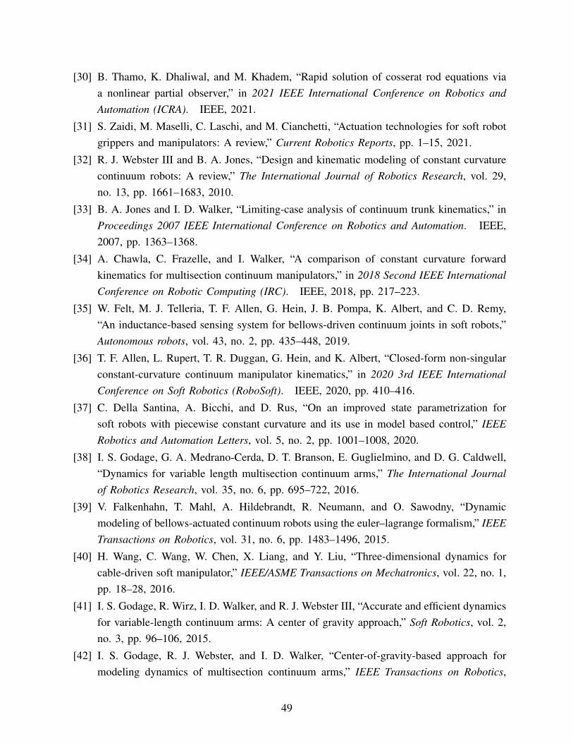
[30] B. Thamo, K. Dhaliwal, and M. Khadem, “Rapid solution of cosserat rod equations viaa nonlinear partial observer,” in 2021 IEEE International Conference on Robotics andAutomation (ICRA). IEEE, 2021.

[31] S. Zaidi, M. Maselli, C. Laschi, and M. Cianchetti, “Actuation technologies for soft robotgrippers and manipulators: A review,” Current Robotics Reports, pp. 1–15, 2021.

[32] R. J. Webster III and B. A. Jones, “Design and kinematic modeling of constant curvaturecontinuum robots: A review,” The International Journal of Robotics Research, vol. 29,no. 13, pp. 1661–1683, 2010.

[33] B. A. Jones and I. D. Walker, “Limiting-case analysis of continuum trunk kinematics,” inProceedings 2007 IEEE International Conference on Robotics and Automation. IEEE,2007, pp. 1363–1368.

[34] A. Chawla, C. Frazelle, and I. Walker, “A comparison of constant curvature forwardkinematics for multisection continuum manipulators,” in 2018 Second IEEE InternationalConference on Robotic Computing (IRC). IEEE, 2018, pp. 217–223.

[35] W. Felt, M. J. Telleria, T. F. Allen, G. Hein, J. B. Pompa, K. Albert, and C. D. Remy,“An inductance-based sensing system for bellows-driven continuum joints in soft robots,”Autonomous robots, vol. 43, no. 2, pp. 435–448, 2019.

[36] T. F. Allen, L. Rupert, T. R. Duggan, G. Hein, and K. Albert, “Closed-form non-singularconstant-curvature continuum manipulator kinematics,” in 2020 3rd IEEE InternationalConference on Soft Robotics (RoboSoft). IEEE, 2020, pp. 410–416.

[37] C. Della Santina, A. Bicchi, and D. Rus, “On an improved state parametrization forsoft robots with piecewise constant curvature and its use in model based control,” IEEERobotics and Automation Letters, vol. 5, no. 2, pp. 1001–1008, 2020.

[38] I. S. Godage, G. A. Medrano-Cerda, D. T. Branson, E. Guglielmino, and D. G. Caldwell,“Dynamics for variable length multisection continuum arms,” The International Journalof Robotics Research, vol. 35, no. 6, pp. 695–722, 2016.

[39] V. Falkenhahn, T. Mahl, A. Hildebrandt, R. Neumann, and O. Sawodny, “Dynamicmodeling of bellows-actuated continuum robots using the euler–lagrange formalism,” IEEETransactions on Robotics, vol. 31, no. 6, pp. 1483–1496, 2015.

[40] H. Wang, C. Wang, W. Chen, X. Liang, and Y. Liu, “Three-dimensional dynamics forcable-driven soft manipulator,” IEEE/ASME Transactions on Mechatronics, vol. 22, no. 1,pp. 18–28, 2016.

[41] I. S. Godage, R. Wirz, I. D. Walker, and R. J. Webster III, “Accurate and efficient dynamicsfor variable-length continuum arms: A center of gravity approach,” Soft Robotics, vol. 2,no. 3, pp. 96–106, 2015.

[42] I. S. Godage, R. J. Webster, and I. D. Walker, “Center-of-gravity-based approach formodeling dynamics of multisection continuum arms,” IEEE Transactions on Robotics,

49

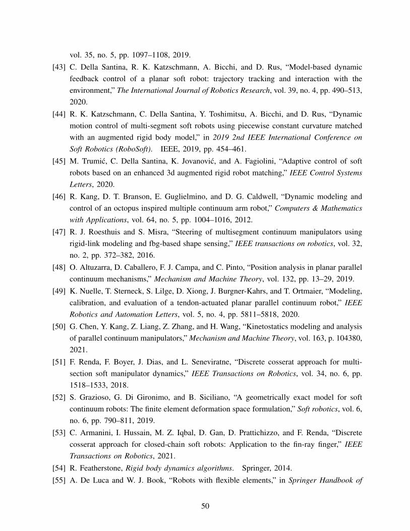
vol. 35, no. 5, pp. 1097–1108, 2019.

[43] C. Della Santina, R. K. Katzschmann, A. Bicchi, and D. Rus, “Model-based dynamicfeedback control of a planar soft robot: trajectory tracking and interaction with theenvironment,” The International Journal of Robotics Research, vol. 39, no. 4, pp. 490–513,2020.

[44] R. K. Katzschmann, C. Della Santina, Y. Toshimitsu, A. Bicchi, and D. Rus, “Dynamicmotion control of multi-segment soft robots using piecewise constant curvature matchedwith an augmented rigid body model,” in 2019 2nd IEEE International Conference onSoft Robotics (RoboSoft). IEEE, 2019, pp. 454–461.

[45] M. Trumic, C. Della Santina, K. Jovanovic, and A. Fagiolini, “Adaptive control of softrobots based on an enhanced 3d augmented rigid robot matching,” IEEE Control SystemsLetters, 2020.

[46] R. Kang, D. T. Branson, E. Guglielmino, and D. G. Caldwell, “Dynamic modeling andcontrol of an octopus inspired multiple continuum arm robot,” Computers & Mathematicswith Applications, vol. 64, no. 5, pp. 1004–1016, 2012.

[47] R. J. Roesthuis and S. Misra, “Steering of multisegment continuum manipulators usingrigid-link modeling and fbg-based shape sensing,” IEEE transactions on robotics, vol. 32,no. 2, pp. 372–382, 2016.

[48] O. Altuzarra, D. Caballero, F. J. Campa, and C. Pinto, “Position analysis in planar parallelcontinuum mechanisms,” Mechanism and Machine Theory, vol. 132, pp. 13–29, 2019.

[49] K. Nuelle, T. Sterneck, S. Lilge, D. Xiong, J. Burgner-Kahrs, and T. Ortmaier, “Modeling,calibration, and evaluation of a tendon-actuated planar parallel continuum robot,” IEEERobotics and Automation Letters, vol. 5, no. 4, pp. 5811–5818, 2020.

[50] G. Chen, Y. Kang, Z. Liang, Z. Zhang, and H. Wang, “Kinetostatics modeling and analysisof parallel continuum manipulators,” Mechanism and Machine Theory, vol. 163, p. 104380,2021.

[51] F. Renda, F. Boyer, J. Dias, and L. Seneviratne, “Discrete cosserat approach for multi-section soft manipulator dynamics,” IEEE Transactions on Robotics, vol. 34, no. 6, pp.1518–1533, 2018.

[52] S. Grazioso, G. Di Gironimo, and B. Siciliano, “A geometrically exact model for softcontinuum robots: The finite element deformation space formulation,” Soft robotics, vol. 6,no. 6, pp. 790–811, 2019.

[53] C. Armanini, I. Hussain, M. Z. Iqbal, D. Gan, D. Prattichizzo, and F. Renda, “Discretecosserat approach for closed-chain soft robots: Application to the fin-ray finger,” IEEETransactions on Robotics, 2021.

[54] R. Featherstone, Rigid body dynamics algorithms. Springer, 2014.

[55] A. De Luca and W. J. Book, “Robots with flexible elements,” in Springer Handbook of

50

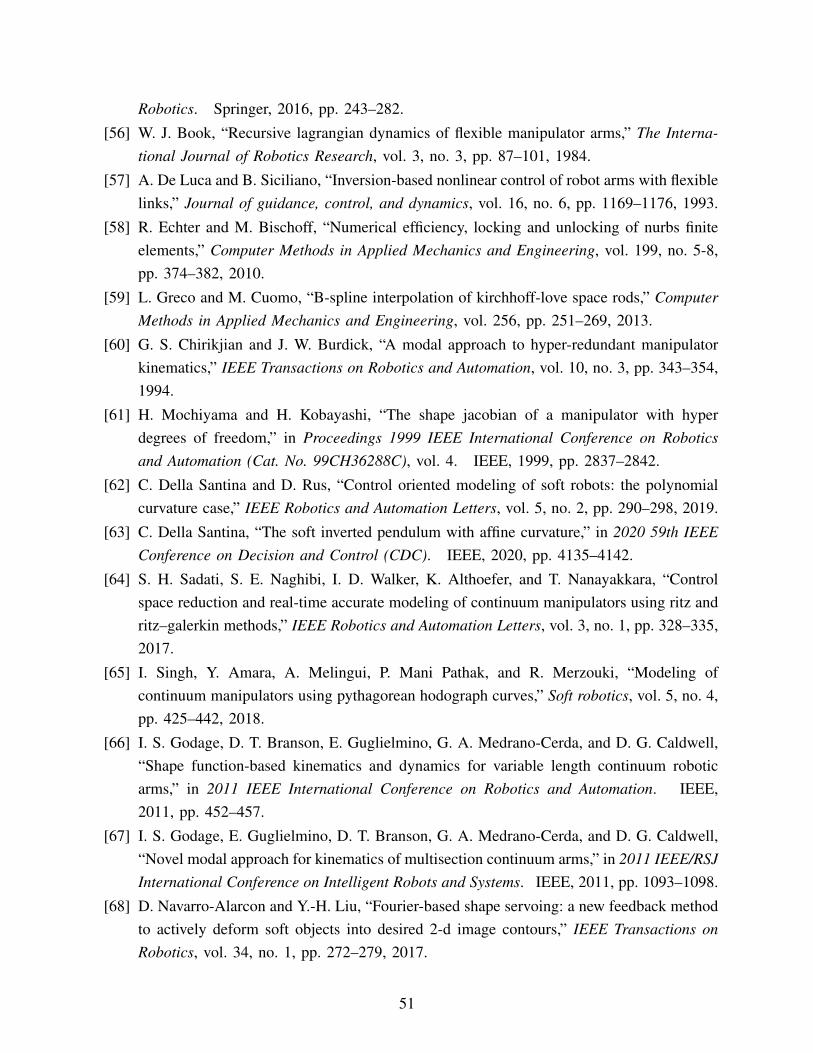
Robotics. Springer, 2016, pp. 243–282.

[56] W. J. Book, “Recursive lagrangian dynamics of flexible manipulator arms,” The Interna-tional Journal of Robotics Research, vol. 3, no. 3, pp. 87–101, 1984.

[57] A. De Luca and B. Siciliano, “Inversion-based nonlinear control of robot arms with flexiblelinks,” Journal of guidance, control, and dynamics, vol. 16, no. 6, pp. 1169–1176, 1993.

[58] R. Echter and M. Bischoff, “Numerical efficiency, locking and unlocking of nurbs finiteelements,” Computer Methods in Applied Mechanics and Engineering, vol. 199, no. 5-8,pp. 374–382, 2010.

[59] L. Greco and M. Cuomo, “B-spline interpolation of kirchhoff-love space rods,” ComputerMethods in Applied Mechanics and Engineering, vol. 256, pp. 251–269, 2013.

[60] G. S. Chirikjian and J. W. Burdick, “A modal approach to hyper-redundant manipulatorkinematics,” IEEE Transactions on Robotics and Automation, vol. 10, no. 3, pp. 343–354,1994.

[61] H. Mochiyama and H. Kobayashi, “The shape jacobian of a manipulator with hyperdegrees of freedom,” in Proceedings 1999 IEEE International Conference on Roboticsand Automation (Cat. No. 99CH36288C), vol. 4. IEEE, 1999, pp. 2837–2842.

[62] C. Della Santina and D. Rus, “Control oriented modeling of soft robots: the polynomialcurvature case,” IEEE Robotics and Automation Letters, vol. 5, no. 2, pp. 290–298, 2019.

[63] C. Della Santina, “The soft inverted pendulum with affine curvature,” in 2020 59th IEEEConference on Decision and Control (CDC). IEEE, 2020, pp. 4135–4142.

[64] S. H. Sadati, S. E. Naghibi, I. D. Walker, K. Althoefer, and T. Nanayakkara, “Controlspace reduction and real-time accurate modeling of continuum manipulators using ritz andritz–galerkin methods,” IEEE Robotics and Automation Letters, vol. 3, no. 1, pp. 328–335,2017.

[65] I. Singh, Y. Amara, A. Melingui, P. Mani Pathak, and R. Merzouki, “Modeling ofcontinuum manipulators using pythagorean hodograph curves,” Soft robotics, vol. 5, no. 4,pp. 425–442, 2018.

[66] I. S. Godage, D. T. Branson, E. Guglielmino, G. A. Medrano-Cerda, and D. G. Caldwell,“Shape function-based kinematics and dynamics for variable length continuum roboticarms,” in 2011 IEEE International Conference on Robotics and Automation. IEEE,2011, pp. 452–457.

[67] I. S. Godage, E. Guglielmino, D. T. Branson, G. A. Medrano-Cerda, and D. G. Caldwell,“Novel modal approach for kinematics of multisection continuum arms,” in 2011 IEEE/RSJInternational Conference on Intelligent Robots and Systems. IEEE, 2011, pp. 1093–1098.

[68] D. Navarro-Alarcon and Y.-H. Liu, “Fourier-based shape servoing: a new feedback methodto actively deform soft objects into desired 2-d image contours,” IEEE Transactions onRobotics, vol. 34, no. 1, pp. 272–279, 2017.

51

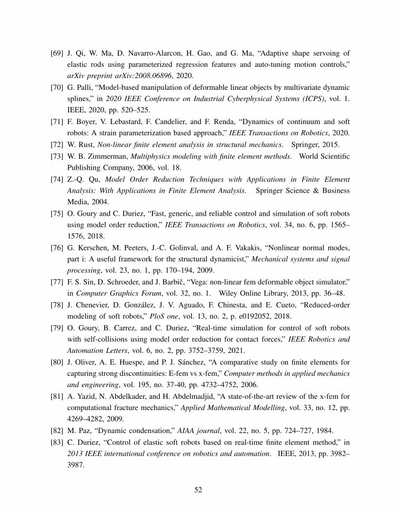
[69] J. Qi, W. Ma, D. Navarro-Alarcon, H. Gao, and G. Ma, “Adaptive shape servoing ofelastic rods using parameterized regression features and auto-tuning motion controls,”arXiv preprint arXiv:2008.06896, 2020.

[70] G. Palli, “Model-based manipulation of deformable linear objects by multivariate dynamicsplines,” in 2020 IEEE Conference on Industrial Cyberphysical Systems (ICPS), vol. 1.IEEE, 2020, pp. 520–525.

[71] F. Boyer, V. Lebastard, F. Candelier, and F. Renda, “Dynamics of continuum and softrobots: A strain parameterization based approach,” IEEE Transactions on Robotics, 2020.

[72] W. Rust, Non-linear finite element analysis in structural mechanics. Springer, 2015.

[73] W. B. Zimmerman, Multiphysics modeling with finite element methods. World ScientificPublishing Company, 2006, vol. 18.

[74] Z.-Q. Qu, Model Order Reduction Techniques with Applications in Finite ElementAnalysis: With Applications in Finite Element Analysis. Springer Science & BusinessMedia, 2004.

[75] O. Goury and C. Duriez, “Fast, generic, and reliable control and simulation of soft robotsusing model order reduction,” IEEE Transactions on Robotics, vol. 34, no. 6, pp. 1565–1576, 2018.

[76] G. Kerschen, M. Peeters, J.-C. Golinval, and A. F. Vakakis, “Nonlinear normal modes,part i: A useful framework for the structural dynamicist,” Mechanical systems and signalprocessing, vol. 23, no. 1, pp. 170–194, 2009.

[77] F. S. Sin, D. Schroeder, and J. Barbic, “Vega: non-linear fem deformable object simulator,”in Computer Graphics Forum, vol. 32, no. 1. Wiley Online Library, 2013, pp. 36–48.

[78] J. Chenevier, D. Gonzalez, J. V. Aguado, F. Chinesta, and E. Cueto, “Reduced-ordermodeling of soft robots,” PloS one, vol. 13, no. 2, p. e0192052, 2018.

[79] O. Goury, B. Carrez, and C. Duriez, “Real-time simulation for control of soft robotswith self-collisions using model order reduction for contact forces,” IEEE Robotics andAutomation Letters, vol. 6, no. 2, pp. 3752–3759, 2021.

[80] J. Oliver, A. E. Huespe, and P. J. Sanchez, “A comparative study on finite elements forcapturing strong discontinuities: E-fem vs x-fem,” Computer methods in applied mechanicsand engineering, vol. 195, no. 37-40, pp. 4732–4752, 2006.

[81] A. Yazid, N. Abdelkader, and H. Abdelmadjid, “A state-of-the-art review of the x-fem forcomputational fracture mechanics,” Applied Mathematical Modelling, vol. 33, no. 12, pp.4269–4282, 2009.

[82] M. Paz, “Dynamic condensation,” AIAA journal, vol. 22, no. 5, pp. 724–727, 1984.

[83] C. Duriez, “Control of elastic soft robots based on real-time finite element method,” in2013 IEEE international conference on robotics and automation. IEEE, 2013, pp. 3982–3987.

52

[84] Y. Adagolodjo, F. Renda, and C. Duriez, “Coupling numerical deformable models in globaland reduced coordinates for the simulation of the direct and the inverse kinematics of softrobots,” IEEE Robotics and Automation Letters, 2021.

[85] S. Sadati, S. E. Naghibi, L. Da Cruz, and C. Bergeles, “Reduced-order modeling andmodel order reduction for soft robots,” 2021.

[86] M. W. Spong, “Modeling and control of elastic joint robots,” 1987.

[87] C. Della Santina, “Flexible manipulators,” Encyclopedia of Robotics, 2021.

[88] G. Pittiglio, L. Barducci, J. W. Martin, J. C. Norton, C. A. Avizzano, K. L. Obstein, andP. Valdastri, “Magnetic levitation for soft-tethered capsule colonoscopy actuated with asingle permanent magnet: A dynamic control approach,” IEEE robotics and automationletters, vol. 4, no. 2, pp. 1224–1231, 2019.

[89] P. V. Kokotovic, R. E. O’Malley Jr, and P. Sannuti, “Singular perturbations and orderreduction in control theory—an overview,” Automatica, vol. 12, no. 2, pp. 123–132, 1976.

[90] J. Allard, S. Cotin, F. Faure, P.-J. Bensoussan, F. Poyer, C. Duriez, H. Delingette, andL. Grisoni, “Sofa-an open source framework for medical simulation,” in MMVR 15-Medicine Meets Virtual Reality, vol. 125. IOP Press, 2007, pp. 13–18.

[91] E. Coevoet, T. Morales-Bieze, F. Largilliere, Z. Zhang, M. Thieffry, M. Sanz-Lopez,B. Carrez, D. Marchal, O. Goury, J. Dequidt et al., “Software toolkit for modeling,simulation, and control of soft robots,” Advanced Robotics, vol. 31, no. 22, pp. 1208–1224, 2017.

[92] Y. Hu, J. Liu, A. Spielberg, J. B. Tenenbaum, W. T. Freeman, J. Wu, D. Rus, andW. Matusik, “Chainqueen: A real-time differentiable physical simulator for soft robotics,”in 2019 International conference on robotics and automation (ICRA). IEEE, 2019, pp.6265–6271.

[93] N. Naughton, J. Sun, A. Tekinalp, T. Parthasarathy, G. Chowdhary, and M. Gazzola,“Elastica: A compliant mechanics environment for soft robotic control,” IEEE Roboticsand Automation Letters, vol. 6, no. 2, pp. 3389–3396, 2021.

[94] S. H. Sadati, S. E. Naghibi, A. Shiva, B. Michael, L. Renson, M. Howard, C. D.Rucker, K. Althoefer, T. Nanayakkara, S. Zschaler et al., “Tmtdyn: A matlab packagefor modeling and control of hybrid rigid–continuum robots based on discretized lumpedsystems and reduced-order models,” The International Journal of Robotics Research, p.0278364919881685, 2019.

[95] A. T. Mathew, I. B. Hmida, C. Armanini, F. Boyer, and F. Renda, “Sorosim: a matlabtoolbox for soft robotics based on the geometric variable-strain approach,” arXiv preprintarXiv:2107.05494, 2021.

[96] J. Collins, S. Chand, A. Vanderkop, and D. Howard, “A review of physics simulators forrobotic applications,” IEEE Access, 2021.

53

[97] M. T. Chikhaoui, S. Lilge, S. Kleinschmidt, and J. Burgner-Kahrs, “Comparison ofmodeling approaches for a tendon actuated continuum robot with three extensiblesegments,” IEEE Robotics and Automation Letters, vol. 4, no. 2, pp. 989–996, 2019.

[98] P. Rao, Q. Peyron, S. Lilge, and J. Burgner-Kahrs, “How to model tendon-drivencontinuum robots and benchmark modelling performance,” Frontiers in Robotics and AI,vol. 7, p. 223, 2021.

[99] K. J. Astrom and T. Hagglund, “The future of pid control,” Control engineering practice,vol. 9, no. 11, pp. 1163–1175, 2001.

[100] R. Kelly and R. Carelli, “A class of nonlinear pd-type controllers for robot manipulators,”Journal of Robotic Systems, vol. 13, no. 12, pp. 793–802, 1996.

[101] R. Kelly, “Pd control with desired gravity compensation of robotic manipulators: a review,”The International Journal of Robotics Research, vol. 16, no. 5, pp. 660–672, 1997.

[102] ——, “Global positioning of robot manipulators via pd control plus a class of nonlinearintegral actions,” IEEE Transactions on Automatic Control, vol. 43, no. 7, pp. 934–938,1998.

[103] T. G. Thuruthel, E. Falotico, M. Manti, and C. Laschi, “Stable open loop control of softrobotic manipulators,” IEEE Robotics and Automation Letters, vol. 3, no. 2, pp. 1292–1298, 2018.

[104] F. Bosi, D. Misseroni, F. Dal Corso, S. Neukirch, and D. Bigoni, “Asymptotic self-restabilization of a continuous elastic structure,” Physical Review E, vol. 94, no. 6, p.063005, 2016.

[105] C. Della Santina, M. Bianchi, G. Grioli, F. Angelini, M. Catalano, M. Garabini, andA. Bicchi, “Controlling soft robots: balancing feedback and feedforward elements,” IEEERobotics & Automation Magazine, vol. 24, no. 3, pp. 75–83, 2017.

[106] S. Kawamura, F. Miyazaki, and S. Arimoto, “Is a local linear pd feedback control laweffective for trajectory tracking of robot motion?” in Proceedings. 1988 IEEE InternationalConference on Robotics and Automation. IEEE, 1988, pp. 1335–1340.

[107] I. Cervantes and J. Alvarez-Ramirez, “On the pid tracking control of robot manipulators,”Systems & control letters, vol. 42, no. 1, pp. 37–46, 2001.

[108] R. Kelly and R. Salgado, “Pd control with computed feedforward of robot manipulators:A design procedure,” IEEE Transactions on Robotics and Automation, vol. 10, no. 4, pp.566–571, 1994.

[109] A. D. Marchese, R. Tedrake, and D. Rus, “Dynamics and trajectory optimization for asoft spatial fluidic elastomer manipulator,” The International Journal of Robotics Research,vol. 35, no. 8, pp. 1000–1019, 2016.

[110] V. Falkenhahn, A. Hildebrandt, R. Neumann, and O. Sawodny, “Model-based feedforwardposition control of constant curvature continuum robots using feedback linearization,” in

54

2015 IEEE International Conference on Robotics and Automation (ICRA). IEEE, 2015,pp. 762–767.

[111] B. Paden and R. Panja, “Globally asymptotically stable ‘pd+’controller for robot manip-ulators,” International Journal of Control, vol. 47, no. 6, pp. 1697–1712, 1988.

[112] G. Cao, B. Huo, L. Yang, F. Zhang, Y. Liu, and G.-B. Bian, “Model-based robust trackingcontrol without observers for soft bending actuators,” IEEE Robotics and AutomationLetters, 2021.

[113] P. Ouyang, J. Acob, and V. Pano, “Pd with sliding mode control for trajectory trackingof robotic system,” Robotics and Computer-Integrated Manufacturing, vol. 30, no. 2, pp.189–200, 2014.

[114] Y. Su, “Global continuous finite-time tracking of robot manipulators,” InternationalJournal of Robust and Nonlinear Control: IFAC-Affiliated Journal, vol. 19, no. 17, pp.1871–1885, 2009.

[115] Y. Su and J. Swevers, “Finite-time tracking control for robot manipulators with actuatorsaturation,” Robotics and Computer-Integrated Manufacturing, vol. 30, no. 2, pp. 91–98,2014.

[116] M. Zhang, P. Borja, R. Ortega, Z. Liu, and H. Su, “Pid passivity-based control of port-hamiltonian systems,” IEEE Transactions on Automatic Control, vol. 63, no. 4, pp. 1032–1044, 2017.

[117] A. D. Kapadia, K. E. Fry, and I. D. Walker, “Empirical investigation of closed-loop controlof extensible continuum manipulators,” in 2014 IEEE/RSJ International Conference onIntelligent Robots and Systems. IEEE, 2014, pp. 329–335.

[118] A. Doroudchi and S. Berman, “Configuration tracking for soft continuum robotic armsusing inverse dynamic control of a cosserat rod model,” in 2021 IEEE InternationalConference on Soft Robotics, RoboSoft, 2021.

[119] T. George Thuruthel, F. Renda, and F. Iida, “First-order dynamic modeling and control ofsoft robots,” 2020.

[120] E. Milana, B. Gorissen, S. Peerlinck, M. De Volder, and D. Reynaerts, “Artificial soft ciliawith asymmetric beating patterns for biomimetic low-reynolds-number fluid propulsion,”Advanced Functional Materials, vol. 29, no. 22, p. 1900462, 2019.

[121] G. Zheng, O. Goury, M. Thieffry, A. Kruszewski, and C. Duriez, “Controllability pre-verification of silicone soft robots based on finite-element method,” in 2019 InternationalConference on Robotics and Automation (ICRA). IEEE, 2019, pp. 7395–7400.

[122] E. Sontag, “From linear to nonlinear: some complexity comparisons,” in Proceedings of1995 34th IEEE Conference on Decision and Control, vol. 3. IEEE, 1995, pp. 2916–2920.

[123] C. Della Santina, L. Pallottino, D. Rus, and A. Bicchi, “Exact task execution in highlyunder-actuated soft limbs: an operational space based approach,” IEEE Robotics and

55

Automation Letters, vol. 4, no. 3, pp. 2508–2515, 2019.

[124] M. Thieffry, A. Kruszewski, T.-M. Guerra, and C. Duriez, “Trajectory tracking controldesign for large-scale linear dynamical systems with applications to soft robotics,” IEEETransactions on Control Systems Technology, 2019.

[125] ——, “Lpv framework for non-linear dynamic control of soft robots using finite elementmodel,” 2020.

[126] ——, “Reduced order control of soft robots with guaranteed stability,” in 2018 EuropeanControl Conference (ECC). IEEE, 2018, pp. 635–640.

[127] M. Thieffry, A. Kruszewski, C. Duriez, and T.-M. Guerra, “Control design for soft robotsbased on reduced-order model,” IEEE Robotics and Automation Letters, vol. 4, no. 1, pp.25–32, 2018.

[128] K. Wu and G. Zheng, “Fem-based gain-scheduling control of a soft trunk robot,” IEEERobotics and Automation Letters, vol. 6, no. 2, pp. 3081–3088, 2021.

[129] E. Franco and A. Garriga-Casanovas, “Energy-shaping control of soft continuum manipu-lators with in-plane disturbances,” The International Journal of Robotics Research, vol. 40,no. 1, pp. 236–255, 2021.

[130] F. Boyer, M. Porez, and W. Khalil, “Macro-continuous computed torque algorithm fora three-dimensional eel-like robot,” IEEE Transactions on Robotics, vol. 22, no. 4, pp.763–775, 2006.

[131] M. W. Spong, “Partial feedback linearization of underactuated mechanical systems,” inProceedings of IEEE/RSJ International Conference on Intelligent Robots and Systems(IROS’94), vol. 1. IEEE, 1994, pp. 314–321.

[132] G. Rizzello, D. Naso, B. Turchiano, and S. Seelecke, “Robust position control of dielectricelastomer actuators based on lmi optimization,” IEEE Transactions on Control SystemsTechnology, vol. 24, no. 6, pp. 1909–1921, 2016.

[133] G.-Y. Gu, J. Zhu, L.-M. Zhu, and X. Zhu, “A survey on dielectric elastomer actuators forsoft robots,” Bioinspiration & biomimetics, vol. 12, no. 1, p. 011003, 2017.

[134] J. van der Weijde, H. Vallery, and R. Babuska, “Closed-loop control through self-sensingof a joule-heated twisted and coiled polymer muscle,” Soft robotics, vol. 6, no. 5, pp.621–630, 2019.

[135] D. Copaci, J. Munoz, I. Gonzalez, C. A. Monje, and L. Moreno, “Sma-driven soft roboticneck: Design, control and validation,” IEEE Access, vol. 8, pp. 199 492–199 502, 2020.

[136] A. Pedram, H. N. Pishkenari, and M. Sitti, “Optimal controller design for 3d manipulationof buoyant magnetic microrobots via constrained linear quadratic regulation approach,”Journal of Micro-Bio Robotics, vol. 15, no. 2, pp. 105–117, 2019.

[137] S. Jeon, A. K. Hoshiar, K. Kim, S. Lee, E. Kim, S. Lee, J.-y. Kim, B. J. Nelson, H.-J.Cha, B.-J. Yi et al., “A magnetically controlled soft microrobot steering a guidewire in

56

a three-dimensional phantom vascular network,” Soft robotics, vol. 6, no. 1, pp. 54–68,2019.

[138] B. Siciliano and W. J. Book, “A singular perturbation approach to control of lightweightflexible manipulators,” The International Journal of Robotics Research, vol. 7, no. 4, pp.79–90, 1988.

[139] M. Bridges, D. M. Dawson, and C. Abdallah, “Contril of rigid-link, flexible-joint robots:a survey of backstepping approaches,” Journal of Robotic Systems, vol. 12, no. 3, pp.199–216, 1995.

[140] M. A. Khosravi and H. D. Taghirad, “Dynamic modeling and control of parallel robots withelastic cables: singular perturbation approach,” IEEE Transactions on Robotics, vol. 30,no. 3, pp. 694–704, 2014.

[141] B. Taheri, D. Case, and E. Richer, “Force and stiffness backstepping-sliding modecontroller for pneumatic cylinders,” IEEE/ASME Transactions on Mechatronics, vol. 19,no. 6, pp. 1799–1809, 2014.

[142] S. B. F. Asl and S. S. Moosapour, “Adaptive backstepping fast terminal sliding modecontroller design for ducted fan engine of thrust-vectored aircraft,” Aerospace Scienceand Technology, vol. 71, pp. 521–529, 2017.

[143] P. Carbonell, Z. Jiang, and D. Repperger, “Nonlinear control of a pneumatic muscleactuator: backstepping vs. sliding-mode,” in Proceedings of the 2001 IEEE InternationalConference on Control Applications (CCA’01)(Cat. No. 01CH37204). IEEE, 2001, pp.167–172.

[144] T. Wang, Y. Zhang, Z. Chen, and S. Zhu, “Parameter identification and model-basednonlinear robust control of fluidic soft bending actuators,” IEEE/ASME Transactions onMechatronics, vol. 24, no. 3, pp. 1346–1355, 2019.

[145] C. Della Santina, A. Bicchi, and D. Rus, “Dynamic control of soft robots with internalconstraints in the presence of obstacles,” in 2019 IEEE/RSJ International Conference onIntelligent Robots and Systems (IROS). IEEE, 2019, pp. 6622–6629.

[146] C. M. Best, M. T. Gillespie, P. Hyatt, L. Rupert, V. Sherrod, and M. D. Killpack, “A newsoft robot control method: Using model predictive control for a pneumatically actuatedhumanoid,” IEEE Robotics & Automation Magazine, vol. 23, no. 3, pp. 75–84, 2016.

[147] P. Hyatt and M. D. Killpack, “Real-time nonlinear model predictive control of robotsusing a graphics processing unit,” IEEE Robotics and Automation Letters, vol. 5, no. 2,pp. 1468–1475, 2020.

[148] S. Tonkens, J. Lorenzetti, and M. Pavone, “Soft robot optimal control via reduced orderfinite element models,” arXiv preprint arXiv:2011.02092, 2020.

[149] Y. Bailly and Y. Amirat, “Modeling and control of a hybrid continuum active catheter foraortic aneurysm treatment,” in Proceedings of the 2005 IEEE International Conference

57

on Robotics and Automation. IEEE, 2005, pp. 924–929.

[150] D. B. Camarillo, C. R. Carlson, and J. K. Salisbury, “Configuration tracking for continuummanipulators with coupled tendon drive,” IEEE Transactions on Robotics, vol. 25, no. 4,pp. 798–808, 2009.

[151] T. Mahl, A. Hildebrandt, and O. Sawodny, “A variable curvature continuum kinematicsfor kinematic control of the bionic handling assistant,” IEEE transactions on robotics,vol. 30, no. 4, pp. 935–949, 2014.

[152] J. M. Bern, G. Kumagai, and S. Coros, “Fabrication, modeling, and control of plushrobots,” in 2017 IEEE/RSJ International Conference on Intelligent Robots and Systems(IROS). IEEE, 2017, pp. 3739–3746.

[153] T. M. Bieze, F. Largilliere, A. Kruszewski, Z. Zhang, R. Merzouki, and C. Duriez,“Finite element method-based kinematics and closed-loop control of soft, continuummanipulators,” Soft robotics, vol. 5, no. 3, pp. 348–364, 2018.

[154] M. T. Chikhaoui, J. Granna, J. Starke, and J. Burgner-Kahrs, “Toward motion coordinationcontrol and design optimization for dual-arm concentric tube continuum robots,” IEEERobotics and Automation Letters, vol. 3, no. 3, pp. 1793–1800, 2018.

[155] P. Chiacchio, S. Chiaverini, L. Sciavicco, and B. Siciliano, “Closed-loop inverse kinematicsschemes for constrained redundant manipulators with task space augmentation and taskpriority strategy,” The International Journal of Robotics Research, vol. 10, no. 4, pp.410–425, 1991.

[156] S. R. Buss, “Introduction to inverse kinematics with jacobian transpose, pseudoinverseand damped least squares methods,” IEEE Journal of Robotics and Automation, vol. 17,no. 1-19, p. 16, 2004.

[157] S. Chiaverini, G. Oriolo, and A. A. Maciejewski, “Redundant robots,” in SpringerHandbook of Robotics. Springer, 2016, pp. 221–242.

[158] B. Benhabib, A. A. Goldenberg, and R. G. Fenton, “A solution to the inverse kinematicsof redundant manipulators,” Journal of robotic systems, vol. 2, no. 4, pp. 373–385, 1985.

[159] P. Falco and C. Natale, “On the stability of closed-loop inverse kinematics algorithms forredundant robots,” IEEE Transactions on Robotics, vol. 27, no. 4, pp. 780–784, 2011.

[160] A. Kapadia and I. D. Walker, “Task-space control of extensible continuum manipulators,”in 2011 IEEE/RSJ International Conference on Intelligent Robots and Systems. IEEE,2011, pp. 1087–1092.

[161] J. Burgner-Kahrs, D. C. Rucker, and H. Choset, “Continuum robots for medical applica-tions: A survey,” IEEE Transactions on Robotics, vol. 31, no. 6, pp. 1261–1280, 2015.

[162] T. da Veiga, J. H. Chandler, P. Lloyd, G. Pittiglio, N. J. Wilkinson, A. K. Hoshiar, R. A.Harris, and P. Valdastri, “Challenges of continuum robots in clinical context: A review,”Progress in Biomedical Engineering, vol. 2, no. 3, p. 032003, 2020.

58

[163] F. Campisano, S. Calo, A. A. Remirez, J. H. Chandler, K. L. Obstein, R. J. Webster III,and P. Valdastri, “Closed-loop control of soft continuum manipulators under tip followeractuation,” The International Journal of Robotics Research, vol. 40, no. 6-7, pp. 923–938,2021.

[164] D. C. Rucker, J. Das, H. B. Gilbert, P. J. Swaney, M. I. Miga, N. Sarkar, and R. J. Webster,“Sliding mode control of steerable needles,” IEEE Transactions on Robotics, vol. 29, no. 5,pp. 1289–1299, 2013.

[165] A. A. Alqumsan, S. Khoo, and M. Norton, “Robust control of continuum robots usingcosserat rod theory,” Mechanism and Machine Theory, vol. 131, pp. 48–61, 2019.

[166] F. Xu, H. Wang, W. Chen, and Y. Miao, “Visual servoing of a cable-driven soft robotmanipulator with shape feature,” IEEE Robotics and Automation Letters, 2021.

[167] Z. Zhang, T. M. Bieze, J. Dequidt, A. Kruszewski, and C. Duriez, “Visual servoing controlof soft robots based on finite element model,” in 2017 IEEE/RSJ International Conferenceon Intelligent Robots and Systems (IROS). IEEE, 2017, pp. 2895–2901.

[168] J. Till, C. E. Bryson, S. Chung, A. Orekhov, and D. C. Rucker, “Efficient computation ofmultiple coupled cosserat rod models for real-time simulation and control of parallelcontinuum manipulators,” in 2015 IEEE International Conference on Robotics andAutomation (ICRA). IEEE, 2015, pp. 5067–5074.

[169] O. Khatib, “A unified approach for motion and force control of robot manipulators: Theoperational space formulation,” IEEE Journal on Robotics and Automation, vol. 3, no. 1,pp. 43–53, 1987.

[170] J. Nakanishi, R. Cory, M. Mistry, J. Peters, and S. Schaal, “Operational space control: Atheoretical and empirical comparison,” The International Journal of Robotics Research,vol. 27, no. 6, pp. 737–757, 2008.

[171] A. Dietrich and C. Ott, “Hierarchical impedance-based tracking control of kinematicallyredundant robots,” IEEE Transactions on Robotics, vol. 36, no. 1, pp. 204–221, 2019.

[172] I. S. Godage, D. T. Branson, E. Guglielmino, and D. G. Caldwell, “Path planning formultisection continuum arms,” in 2012 IEEE International Conference on Mechatronicsand Automation. IEEE, 2012, pp. 1208–1213.

[173] A. D. Marchese, R. K. Katzschmann, and D. Rus, “Whole arm planning for a soft andhighly compliant 2d robotic manipulator,” in 2014 IEEE/RSJ International Conference onIntelligent Robots and Systems. IEEE, 2014, pp. 554–560.

[174] A. Bicchi, “Intrinsic contact sensing for soft fingers,” in Proceedings., IEEE InternationalConference on Robotics and Automation. IEEE, 1990, pp. 968–973.

[175] J. K. Salisbury, “Active stiffness control of a manipulator in cartesian coordinates,” in1980 19th IEEE conference on decision and control including the symposium on adaptiveprocesses. IEEE, 1980, pp. 95–100.

59

[176] S.-F. Chen and I. Kao, “Conservative congruence transformation for joint and cartesianstiffness matrices of robotic hands and fingers,” The International Journal of RoboticsResearch, vol. 19, no. 9, pp. 835–847, 2000.

[177] K. Suzumori, S. Iikura, and H. Tanaka, “Applying a flexible microactuator to roboticmechanisms,” IEEE Control systems magazine, vol. 12, no. 1, pp. 21–27, 1992.

[178] M. T. Gillespie, C. M. Best, and M. D. Killpack, “Simultaneous position and stiffnesscontrol for an inflatable soft robot,” in 2016 IEEE international conference on roboticsand automation (ICRA). IEEE, 2016, pp. 1095–1101.

[179] S. M. Mustaza, C. M. Saaj, F. J. Comin, W. A. Albukhanajer, D. Mahdi, and C. Lekakou,“Stiffness control for soft surgical manipulators,” International Journal of HumanoidRobotics, vol. 15, no. 05, p. 1850021, 2018.

[180] G. Rizzello, P. Serafino, D. Naso, and S. Seelecke, “Towards sensorless soft robotics: Self-sensing stiffness control of dielectric elastomer actuators,” IEEE Transactions on Robotics,vol. 36, no. 1, pp. 174–188, 2019.

[181] A. Albu-Schaffer, M. Fischer, G. Schreiber, F. Schoeppe, and G. Hirzinger, “Soft robotics:what cartesian stiffness can obtain with passively compliant, uncoupled joints?” in 2004IEEE/RSJ International Conference on Intelligent Robots and Systems (IROS)(IEEE Cat.No. 04CH37566), vol. 4. IEEE, 2004, pp. 3295–3301.

[182] A. Ajoudani, N. G. Tsagarakis, J. Lee, M. Gabiccini, and A. Bicchi, “Natural redundancyresolution in dual-arm manipulation using configuration dependent stiffness (cds) control,”in 2014 IEEE International Conference on Robotics and Automation (ICRA). IEEE, 2014,pp. 1480–1486.

[183] J. M. Bern and D. Rus, “Soft ik with stiffness control,” in 2021 IEEE 4th InternationalConference on Soft Robotics (RoboSoft). IEEE, 2021, pp. 465–471.

[184] M. Mahvash and P. E. Dupont, “Stiffness control of surgical continuum manipulators,”IEEE Transactions on Robotics, vol. 27, no. 2, pp. 334–345, 2011.

[185] C. Ott, Cartesian impedance control of redundant and flexible-joint robots. Springer,2008.

[186] A. Bajo and N. Simaan, “Hybrid motion/force control of multi-backbone continuumrobots,” The International journal of robotics research, vol. 35, no. 4, pp. 422–434, 2016.

[187] R. Yasin and N. Simaan, “Joint-level force sensing for indirect hybrid force/positioncontrol of continuum robots with friction,” The International Journal of Robotics Research,vol. 40, no. 4-5, pp. 764–781, 2021.

[188] Z. Zhang, J. Dequidt, J. Back, H. Liu, and C. Duriez, “Motion control of cable-drivencontinuum catheter robot through contacts,” IEEE Robotics and Automation Letters, vol. 4,no. 2, pp. 1852–1859, 2019.

[189] E. Coevoet, A. Escande, and C. Duriez, “Soft robots locomotion and manipulation control

60

using fem simulation and quadratic programming,” in 2019 2nd IEEE InternationalConference on Soft Robotics (RoboSoft). IEEE, 2019, pp. 739–745.

[190] W. J. Book, S. Le, and V. Sangveraphunsiri, “Bracing strategy for robot operation,” inTheory and Practice of Robots and Manipulators. Springer, 1985, pp. 179–185.

[191] M. Selvaggio, L. Ramirez, N. Naclerio, B. Siciliano, and E. Hawkes, “An obstacle-interaction planning method for navigation of actuated vine robots,” in 2020 IEEEInternational Conference on Robotics and Automation (ICRA). IEEE, 2020, pp. 3227–3233.

[192] S. P. Nageshrao, G. A. Lopes, D. Jeltsema, and R. Babuska, “Port-hamiltonian systemsin adaptive and learning control: A survey,” IEEE Transactions on Automatic Control,vol. 61, no. 5, pp. 1223–1238, 2015.

[193] L. Busoniu, T. de Bruin, D. Tolic, J. Kober, and I. Palunko, “Reinforcement learningfor control: Performance, stability, and deep approximators,” Annual Reviews in Control,vol. 46, pp. 8–28, 2018.

[194] C. De Persis and P. Tesi, “Formulas for data-driven control: Stabilization, optimality, androbustness,” IEEE Transactions on Automatic Control, vol. 65, no. 3, pp. 909–924, 2019.

[195] J. Berberich, J. Kohler, M. A. Muller, and F. Allgower, “Data-driven model predictivecontrol with stability and robustness guarantees,” IEEE Transactions on Automatic Control,2020.

[196] M. Sznaier, “Control oriented learning in the era of big data,” IEEE Control SystemsLetters, 2020.

[197] C. Laschi and et al., “A survey on learning based control in soft robots (provisional title),”IEEE Control Magazine, Under Review (invited paper in the same special issue).

[198] K. J. Astrom and B. Wittenmark, Adaptive control. Courier Corporation, 2013.

[199] P. Tomei, “Adaptive pd controller for robot manipulators,” IEEE Transactions on Roboticsand Automation, vol. 7, no. 4, pp. 565–570, 1991.

[200] J.-J. E. Slotine and W. Li, “On the adaptive control of robot manipulators,” Theinternational journal of robotics research, vol. 6, no. 3, pp. 49–59, 1987.

[201] H. Wang, B. Yang, Y. Liu, W. Chen, X. Liang, and R. Pfeifer, “Visual servoing of softrobot manipulator in constrained environments with an adaptive controller,” IEEE/ASMETransactions on Mechatronics, vol. 22, no. 1, pp. 41–50, 2016.

[202] E. H. Skorina, M. Luo, W. Tao, F. Chen, J. Fu, and C. D. Onal, “Adapting toflexibility: model reference adaptive control of soft bending actuators,” IEEE Roboticsand Automation Letters, vol. 2, no. 2, pp. 964–970, 2017.

[203] Z. Q. Tang, H. L. Heung, K. Y. Tong, and Z. Li, “Model-based online learning and adaptivecontrol for a “human-wearable soft robot” integrated system,” The International Journalof Robotics Research, p. 0278364919873379, 2019.

61

[204] ——, “Model-based online learning and adaptive control for a “human-wearable softrobot” integrated system,” The International Journal of Robotics Research, vol. 40, no. 1,pp. 256–276, 2021.

[205] J. S. Terry, J. Whitaker, R. W. Beard, and M. D. Killpack, “Adaptive control oflarge-scale soft robot manipulators with unknown payloads,” in Dynamic Systems andControl Conference, vol. 59162. American Society of Mechanical Engineers, 2019, p.V003T20A003.

[206] P. Hyatt, C. Johnson, and M. D. Killpack, “Model reference predictive adaptive controlfor large-scale soft robots,” Frontiers in Robotics and AI, vol. 7, p. 132, 2020.

[207] G. Zheng, “Control of a silicone soft tripod robot via uncertainty compensation,” IEEERobotics and Automation Letters, vol. 5, no. 2, pp. 2801–2807, 2020.

[208] E. Franco, A. G. Casanovas, J. Tang, F. R. y Baena, and A. Astolfi, “Position regulationin cartesian space of a class of inextensible soft continuum manipulators with pneumaticactuation,” Mechatronics, vol. 76, p. 102573, 2021.

[209] G. Cao, Y. Liu, Y. Jiang, F. Zhang, G. Bian, and D. H. Owens, “Observer-based continuousadaptive sliding mode control for soft actuators,” Nonlinear Dynamics, pp. 1–16, 2021.

[210] R. M. Sanner and J.-J. E. Slotine, “Gaussian networks for direct adaptive control,” in 1991American control conference. IEEE, 1991, pp. 2153–2159.

[211] M. M. Polycarpou, “Stable adaptive neural control scheme for nonlinear systems,” IEEETransactions on Automatic control, vol. 41, no. 3, pp. 447–451, 1996.

[212] C. Yang, T. Teng, B. Xu, Z. Li, J. Na, and C.-Y. Su, “Global adaptive tracking controlof robot manipulators using neural networks with finite-time learning convergence,”International Journal of Control, Automation and Systems, vol. 15, no. 4, pp. 1916–1924,2017.

[213] D. A. Bristow, M. Tharayil, and A. G. Alleyne, “A survey of iterative learning control,”IEEE control systems magazine, vol. 26, no. 3, pp. 96–114, 2006.

[214] S. Seok, C. D. Onal, K.-J. Cho, R. J. Wood, D. Rus, and S. Kim, “Meshworm: a peristalticsoft robot with antagonistic nickel titanium coil actuators,” IEEE/ASME Transactions onmechatronics, vol. 18, no. 5, pp. 1485–1497, 2012.

[215] H. Chi, X. Li, W. Liang, J. Cao, and Q. Ren, “Iterative learning control for motiontrajectory tracking of a circular soft crawling robot,” Frontiers in Robotics and AI, vol. 6,p. 113, 2019.

[216] M. Hofer and R. D’Andrea, “Design, fabrication, modeling and control of a fabric-basedspherical robotic arm,” Mechatronics, vol. 68, p. 102369, 2020.

[217] J. Zughaibi, M. Hofer, and R. D’Andrea, “A fast and reliable pick-and-place applicationwith a spherical soft robotic arm,” arXiv preprint arXiv:2011.04624, 2020.

[218] G. Cao, B. Chu, and Y. Liu, “Analytical modeling and control of soft fast pneumatic

62

networks actuators,” in IECON 2020 The 46th Annual Conference of the IEEE IndustrialElectronics Society. IEEE, 2020, pp. 2760–2765.

[219] Z. Q. Tang, H. L. Heung, K. Y. Tong, and Z. Li, “A novel iterative learning modelpredictive control method for soft bending actuators,” in 2019 International Conferenceon Robotics and Automation (ICRA). IEEE, 2019, pp. 4004–4010.

[220] L. Cenceschi, F. Angelini, C. Della Santina, and A. Bicchi, “Pi σ-pi σ continuous iterativelearning control for nonlinear systems with arbitrary relative degree,” in 2021 IEEEEuropean Control Conference (ECC). IEEE, 2021.

[221] J. Rieffel, D. Knox, S. Smith, and B. Trimmer, “Growing and evolving soft robots,”Artificial life, vol. 20, no. 1, pp. 143–162, 2014.

[222] N. Cheney, J. Bongard, and H. Lipson, “Evolving soft robots in tight spaces,” inProceedings of the 2015 annual conference on Genetic and Evolutionary Computation,2015, pp. 935–942.

[223] J. Tobin, R. Fong, A. Ray, J. Schneider, W. Zaremba, and P. Abbeel, “Domain random-ization for transferring deep neural networks from simulation to the real world,” in 2017IEEE/RSJ international conference on intelligent robots and systems (IROS). IEEE, 2017,pp. 23–30.

[224] J. Rojas, E. Sifakis, and L. Kavan, “Differentiable implicit soft-body physics,” arXivpreprint arXiv:2102.05791, 2021.

[225] M. Bacher, E. Knoop, and C. Schumacher, “Design and control of soft robots usingdifferentiable simulation,” Current Robotics Reports, pp. 1–11, 2021.

[226] W. Samek, T. Wiegand, and K.-R. Muller, “Explainable artificial intelligence: Understand-ing, visualizing and interpreting deep learning models,” arXiv preprint arXiv:1708.08296,2017.

[227] J. Sjoberg, Q. Zhang, L. Ljung, A. Benveniste, B. Delyon, P.-Y. Glorennec, H. Hjalmars-son, and A. Juditsky, “Nonlinear black-box modeling in system identification: a unifiedoverview,” Automatica, vol. 31, no. 12, pp. 1691–1724, 1995.

[228] J. Schoukens and L. Ljung, “Nonlinear system identification: A user-oriented road map,”IEEE Control Systems Magazine, vol. 39, no. 6, pp. 28–99, 2019.

[229] D. Nguyen-Tuong and J. Peters, “Model learning for robot control: a survey,” Cognitiveprocessing, vol. 12, no. 4, pp. 319–340, 2011.

[230] C. C. Johnson, T. Quackenbush, T. Sorensen, D. Wingate, and M. D. Killpack, “Usingfirst principles for deep learning and model-based control of soft robots,” Frontiers inRobotics and AI, vol. 8, p. 100, 2021.

[231] A. Tariverdi, V. K. Venkiteswaran, M. Richter, O. J. Elle, J. Tørresen, K. Mathiassen,S. Misra, and Ø. G. Martinsen, “A recurrent neural-network-based real-time dynamicmodel for soft continuum manipulators,” Frontiers in Robotics and AI, vol. 8, p. 45,

63

2021.

[232] B. Deutschmann, T. Liu, A. Dietrich, C. Ott, and D. Lee, “A method to identify thenonlinear stiffness characteristics of an elastic continuum mechanism,” IEEE Roboticsand Automation Letters, vol. 3, no. 3, pp. 1450–1457, 2018.

[233] L. Wang and N. Simaan, “Geometric calibration of continuum robots: Joint space andequilibrium shape deviations,” IEEE Transactions on Robotics, vol. 35, no. 2, pp. 387–402, 2019.

[234] J. M. Bern, Y. Schnider, P. Banzet, N. Kumar, and S. Coros, “Soft robot control with alearned differentiable model,” in 2020 3rd IEEE International Conference on Soft Robotics(RoboSoft). IEEE, 2020, pp. 417–423.

[235] R. Lagneau, A. Krupa, and M. Marchal, “Active deformation through visual servoing ofsoft objects,” in 2020 IEEE International Conference on Robotics and Automation (ICRA).IEEE, 2020, pp. 8978–8984.

[236] T. G. Thuruthel, E. Falotico, F. Renda, and C. Laschi, “Learning dynamic models foropen loop predictive control of soft robotic manipulators,” Bioinspiration & biomimetics,vol. 12, no. 6, p. 066003, 2017.

[237] S. Satheeshbabu, N. K. Uppalapati, G. Chowdhary, and G. Krishnan, “Open loop positioncontrol of soft continuum arm using deep reinforcement learning,” in 2019 InternationalConference on Robotics and Automation (ICRA). IEEE, 2019, pp. 5133–5139.

[238] M. T. Gillespie, C. M. Best, E. C. Townsend, D. Wingate, and M. D. Killpack, “Learningnonlinear dynamic models of soft robots for model predictive control with neuralnetworks,” in 2018 IEEE International Conference on Soft Robotics (RoboSoft). IEEE,2018, pp. 39–45.

[239] D. Bruder, B. Gillespie, C. D. Remy, and R. Vasudevan, “Modeling and control ofsoft robots using the koopman operator and model predictive control,” arXiv preprintarXiv:1902.02827, 2019.

[240] E. Kamenar, N. Crnjaric-Zic, D. Haggerty, S. Zelenika, E. Hawkes, and I. Mezic,“Prediction of the behavior of a pneumatic soft robot based on koopman operator theory,”in 2020 43rd International Convention on Information, Communication and ElectronicTechnology (MIPRO). IEEE, pp. 1169–1173.

[241] M. L. Castano, A. Hess, G. Mamakoukas, T. Gao, T. Murphey, and X. Tan, “Control-oriented modeling of soft robotic swimmer with koopman operators,” in 2020 IEEE/ASMEInternational Conference on Advanced Intelligent Mechatronics (AIM). IEEE, 2020, pp.1679–1685.

[242] D. A. Haggerty, M. J. Banks, P. C. Curtis, I. Mezic, and E. W. Hawkes, “Modeling,reduction, and control of a helically actuated inertial soft robotic arm via the koopmanoperator,” arXiv preprint arXiv:2011.07939, 2020.

64

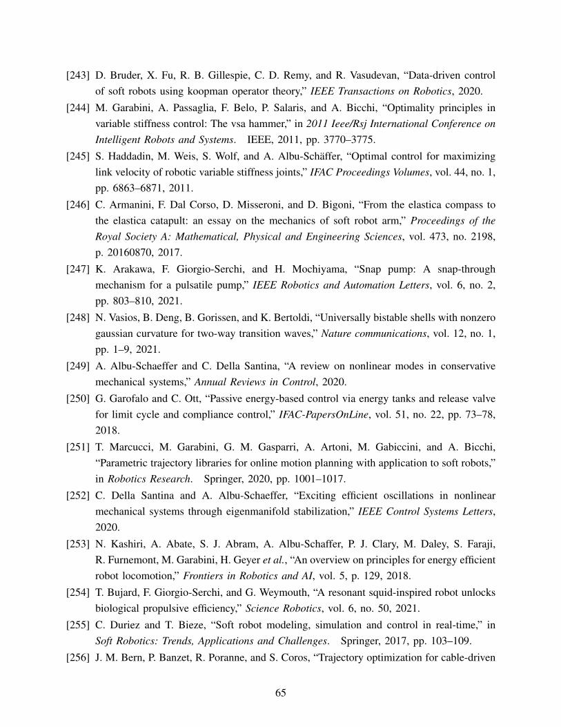
[243] D. Bruder, X. Fu, R. B. Gillespie, C. D. Remy, and R. Vasudevan, “Data-driven controlof soft robots using koopman operator theory,” IEEE Transactions on Robotics, 2020.

[244] M. Garabini, A. Passaglia, F. Belo, P. Salaris, and A. Bicchi, “Optimality principles invariable stiffness control: The vsa hammer,” in 2011 Ieee/Rsj International Conference onIntelligent Robots and Systems. IEEE, 2011, pp. 3770–3775.

[245] S. Haddadin, M. Weis, S. Wolf, and A. Albu-Schaffer, “Optimal control for maximizinglink velocity of robotic variable stiffness joints,” IFAC Proceedings Volumes, vol. 44, no. 1,pp. 6863–6871, 2011.

[246] C. Armanini, F. Dal Corso, D. Misseroni, and D. Bigoni, “From the elastica compass tothe elastica catapult: an essay on the mechanics of soft robot arm,” Proceedings of theRoyal Society A: Mathematical, Physical and Engineering Sciences, vol. 473, no. 2198,p. 20160870, 2017.

[247] K. Arakawa, F. Giorgio-Serchi, and H. Mochiyama, “Snap pump: A snap-throughmechanism for a pulsatile pump,” IEEE Robotics and Automation Letters, vol. 6, no. 2,pp. 803–810, 2021.

[248] N. Vasios, B. Deng, B. Gorissen, and K. Bertoldi, “Universally bistable shells with nonzerogaussian curvature for two-way transition waves,” Nature communications, vol. 12, no. 1,pp. 1–9, 2021.

[249] A. Albu-Schaeffer and C. Della Santina, “A review on nonlinear modes in conservativemechanical systems,” Annual Reviews in Control, 2020.

[250] G. Garofalo and C. Ott, “Passive energy-based control via energy tanks and release valvefor limit cycle and compliance control,” IFAC-PapersOnLine, vol. 51, no. 22, pp. 73–78,2018.

[251] T. Marcucci, M. Garabini, G. M. Gasparri, A. Artoni, M. Gabiccini, and A. Bicchi,“Parametric trajectory libraries for online motion planning with application to soft robots,”in Robotics Research. Springer, 2020, pp. 1001–1017.

[252] C. Della Santina and A. Albu-Schaeffer, “Exciting efficient oscillations in nonlinearmechanical systems through eigenmanifold stabilization,” IEEE Control Systems Letters,2020.

[253] N. Kashiri, A. Abate, S. J. Abram, A. Albu-Schaffer, P. J. Clary, M. Daley, S. Faraji,R. Furnemont, M. Garabini, H. Geyer et al., “An overview on principles for energy efficientrobot locomotion,” Frontiers in Robotics and AI, vol. 5, p. 129, 2018.

[254] T. Bujard, F. Giorgio-Serchi, and G. Weymouth, “A resonant squid-inspired robot unlocksbiological propulsive efficiency,” Science Robotics, vol. 6, no. 50, 2021.

[255] C. Duriez and T. Bieze, “Soft robot modeling, simulation and control in real-time,” inSoft Robotics: Trends, Applications and Challenges. Springer, 2017, pp. 103–109.

[256] J. M. Bern, P. Banzet, R. Poranne, and S. Coros, “Trajectory optimization for cable-driven

65

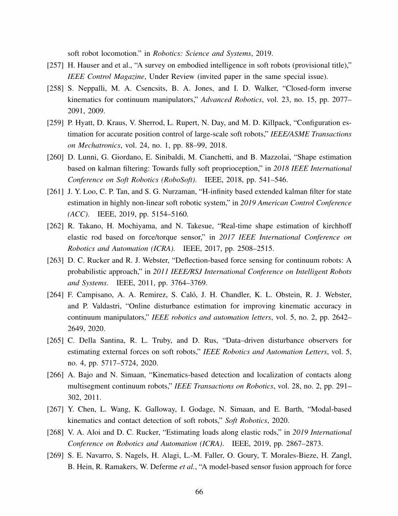
soft robot locomotion.” in Robotics: Science and Systems, 2019.

[257] H. Hauser and et al., “A survey on embodied intelligence in soft robots (provisional title),”IEEE Control Magazine, Under Review (invited paper in the same special issue).

[258] S. Neppalli, M. A. Csencsits, B. A. Jones, and I. D. Walker, “Closed-form inversekinematics for continuum manipulators,” Advanced Robotics, vol. 23, no. 15, pp. 2077–2091, 2009.

[259] P. Hyatt, D. Kraus, V. Sherrod, L. Rupert, N. Day, and M. D. Killpack, “Configuration es-timation for accurate position control of large-scale soft robots,” IEEE/ASME Transactionson Mechatronics, vol. 24, no. 1, pp. 88–99, 2018.

[260] D. Lunni, G. Giordano, E. Sinibaldi, M. Cianchetti, and B. Mazzolai, “Shape estimationbased on kalman filtering: Towards fully soft proprioception,” in 2018 IEEE InternationalConference on Soft Robotics (RoboSoft). IEEE, 2018, pp. 541–546.

[261] J. Y. Loo, C. P. Tan, and S. G. Nurzaman, “H-infinity based extended kalman filter for stateestimation in highly non-linear soft robotic system,” in 2019 American Control Conference(ACC). IEEE, 2019, pp. 5154–5160.

[262] R. Takano, H. Mochiyama, and N. Takesue, “Real-time shape estimation of kirchhoffelastic rod based on force/torque sensor,” in 2017 IEEE International Conference onRobotics and Automation (ICRA). IEEE, 2017, pp. 2508–2515.

[263] D. C. Rucker and R. J. Webster, “Deflection-based force sensing for continuum robots: Aprobabilistic approach,” in 2011 IEEE/RSJ International Conference on Intelligent Robotsand Systems. IEEE, 2011, pp. 3764–3769.

[264] F. Campisano, A. A. Remirez, S. Calo, J. H. Chandler, K. L. Obstein, R. J. Webster,and P. Valdastri, “Online disturbance estimation for improving kinematic accuracy incontinuum manipulators,” IEEE robotics and automation letters, vol. 5, no. 2, pp. 2642–2649, 2020.

[265] C. Della Santina, R. L. Truby, and D. Rus, “Data–driven disturbance observers forestimating external forces on soft robots,” IEEE Robotics and Automation Letters, vol. 5,no. 4, pp. 5717–5724, 2020.

[266] A. Bajo and N. Simaan, “Kinematics-based detection and localization of contacts alongmultisegment continuum robots,” IEEE Transactions on Robotics, vol. 28, no. 2, pp. 291–302, 2011.

[267] Y. Chen, L. Wang, K. Galloway, I. Godage, N. Simaan, and E. Barth, “Modal-basedkinematics and contact detection of soft robots,” Soft Robotics, 2020.

[268] V. A. Aloi and D. C. Rucker, “Estimating loads along elastic rods,” in 2019 InternationalConference on Robotics and Automation (ICRA). IEEE, 2019, pp. 2867–2873.

[269] S. E. Navarro, S. Nagels, H. Alagi, L.-M. Faller, O. Goury, T. Morales-Bieze, H. Zangl,B. Hein, R. Ramakers, W. Deferme et al., “A model-based sensor fusion approach for force

66

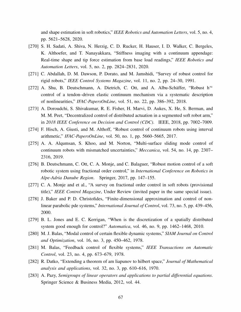
and shape estimation in soft robotics,” IEEE Robotics and Automation Letters, vol. 5, no. 4,pp. 5621–5628, 2020.

[270] S. H. Sadati, A. Shiva, N. Herzig, C. D. Rucker, H. Hauser, I. D. Walker, C. Bergeles,K. Althoefer, and T. Nanayakkara, “Stiffness imaging with a continuum appendage:Real-time shape and tip force estimation from base load readings,” IEEE Robotics andAutomation Letters, vol. 5, no. 2, pp. 2824–2831, 2020.

[271] C. Abdallah, D. M. Dawson, P. Dorato, and M. Jamshidi, “Survey of robust control forrigid robots,” IEEE Control Systems Magazine, vol. 11, no. 2, pp. 24–30, 1991.

[272] A. Shu, B. Deutschmann, A. Dietrich, C. Ott, and A. Albu-Schaffer, “Robust h∞

control of a tendon–driven elastic continuum mechanism via a systematic descriptionof nonlinearities,” IFAC-PapersOnLine, vol. 51, no. 22, pp. 386–392, 2018.

[273] A. Doroudchi, S. Shivakumar, R. E. Fisher, H. Marvi, D. Aukes, X. He, S. Berman, andM. M. Peet, “Decentralized control of distributed actuation in a segmented soft robot arm,”in 2018 IEEE Conference on Decision and Control (CDC). IEEE, 2018, pp. 7002–7009.

[274] F. Hisch, A. Giusti, and M. Althoff, “Robust control of continuum robots using intervalarithmetic,” IFAC-PapersOnLine, vol. 50, no. 1, pp. 5660–5665, 2017.

[275] A. A. Alqumsan, S. Khoo, and M. Norton, “Multi-surface sliding mode control ofcontinuum robots with mismatched uncertainties,” Meccanica, vol. 54, no. 14, pp. 2307–2316, 2019.

[276] B. Deutschmann, C. Ott, C. A. Monje, and C. Balaguer, “Robust motion control of a softrobotic system using fractional order control,” in International Conference on Robotics inAlpe-Adria Danube Region. Springer, 2017, pp. 147–155.

[277] C. A. Monje and et al., “A survey on fractional order control in soft robots (provisionaltitle),” IEEE Control Magazine, Under Review (invited paper in the same special issue).

[278] J. Baker and P. D. Christofides, “Finite-dimensional approximation and control of non-linear parabolic pde systems,” International Journal of Control, vol. 73, no. 5, pp. 439–456,2000.

[279] B. L. Jones and E. C. Kerrigan, “When is the discretization of a spatially distributedsystem good enough for control?” Automatica, vol. 46, no. 9, pp. 1462–1468, 2010.

[280] M. J. Balas, “Modal control of certain flexible dynamic systems,” SIAM Journal on Controland Optimization, vol. 16, no. 3, pp. 450–462, 1978.

[281] M. Balas, “Feedback control of flexible systems,” IEEE Transactions on AutomaticControl, vol. 23, no. 4, pp. 673–679, 1978.

[282] R. Datko, “Extending a theorem of am liapunov to hilbert space,” Journal of Mathematicalanalysis and applications, vol. 32, no. 3, pp. 610–616, 1970.

[283] A. Pazy, Semigroups of linear operators and applications to partial differential equations.Springer Science & Business Media, 2012, vol. 44.

67

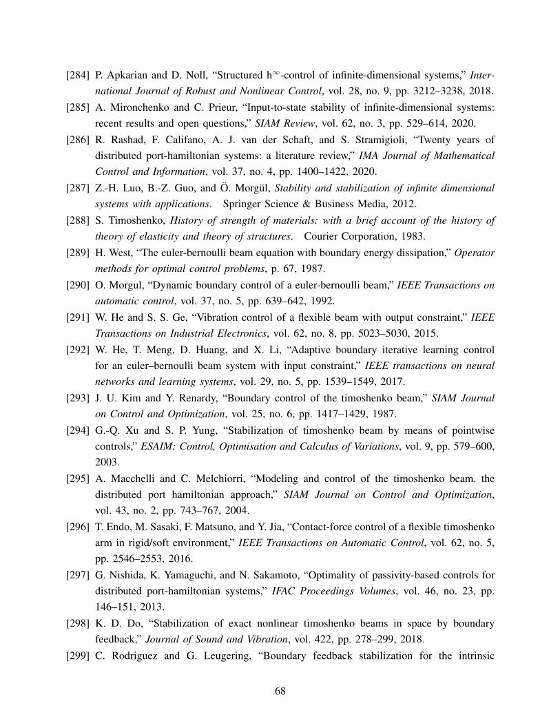
[284] P. Apkarian and D. Noll, “Structured h∞-control of infinite-dimensional systems,” Inter-national Journal of Robust and Nonlinear Control, vol. 28, no. 9, pp. 3212–3238, 2018.

[285] A. Mironchenko and C. Prieur, “Input-to-state stability of infinite-dimensional systems:recent results and open questions,” SIAM Review, vol. 62, no. 3, pp. 529–614, 2020.

[286] R. Rashad, F. Califano, A. J. van der Schaft, and S. Stramigioli, “Twenty years ofdistributed port-hamiltonian systems: a literature review,” IMA Journal of MathematicalControl and Information, vol. 37, no. 4, pp. 1400–1422, 2020.

[287] Z.-H. Luo, B.-Z. Guo, and O. Morgul, Stability and stabilization of infinite dimensionalsystems with applications. Springer Science & Business Media, 2012.

[288] S. Timoshenko, History of strength of materials: with a brief account of the history oftheory of elasticity and theory of structures. Courier Corporation, 1983.

[289] H. West, “The euler-bernoulli beam equation with boundary energy dissipation,” Operatormethods for optimal control problems, p. 67, 1987.

[290] O. Morgul, “Dynamic boundary control of a euler-bernoulli beam,” IEEE Transactions onautomatic control, vol. 37, no. 5, pp. 639–642, 1992.

[291] W. He and S. S. Ge, “Vibration control of a flexible beam with output constraint,” IEEETransactions on Industrial Electronics, vol. 62, no. 8, pp. 5023–5030, 2015.

[292] W. He, T. Meng, D. Huang, and X. Li, “Adaptive boundary iterative learning controlfor an euler–bernoulli beam system with input constraint,” IEEE transactions on neuralnetworks and learning systems, vol. 29, no. 5, pp. 1539–1549, 2017.

[293] J. U. Kim and Y. Renardy, “Boundary control of the timoshenko beam,” SIAM Journalon Control and Optimization, vol. 25, no. 6, pp. 1417–1429, 1987.

[294] G.-Q. Xu and S. P. Yung, “Stabilization of timoshenko beam by means of pointwisecontrols,” ESAIM: Control, Optimisation and Calculus of Variations, vol. 9, pp. 579–600,2003.

[295] A. Macchelli and C. Melchiorri, “Modeling and control of the timoshenko beam. thedistributed port hamiltonian approach,” SIAM Journal on Control and Optimization,vol. 43, no. 2, pp. 743–767, 2004.

[296] T. Endo, M. Sasaki, F. Matsuno, and Y. Jia, “Contact-force control of a flexible timoshenkoarm in rigid/soft environment,” IEEE Transactions on Automatic Control, vol. 62, no. 5,pp. 2546–2553, 2016.

[297] G. Nishida, K. Yamaguchi, and N. Sakamoto, “Optimality of passivity-based controls fordistributed port-hamiltonian systems,” IFAC Proceedings Volumes, vol. 46, no. 23, pp.146–151, 2013.

[298] K. D. Do, “Stabilization of exact nonlinear timoshenko beams in space by boundaryfeedback,” Journal of Sound and Vibration, vol. 422, pp. 278–299, 2018.

[299] C. Rodriguez and G. Leugering, “Boundary feedback stabilization for the intrinsic

68

geometrically exact beam model,” SIAM Journal on Control and Optimization, vol. 58,no. 6, pp. 3533–3558, 2020.

[300] A. Majumdar and A. Goriely, “Static and dynamic stability results for a class of three-dimensional configurations of kirchhoff elastic rods,” Physica D: Nonlinear Phenomena,vol. 253, pp. 91–101, 2013.

[301] L. B. Kratchman, T. L. Bruns, J. J. Abbott, and R. J. Webster, “Guiding elastic rods witha robot-manipulated magnet for medical applications,” IEEE Transactions on Robotics,vol. 33, no. 1, pp. 227–233, 2016.

[302] T. Bretl and Z. McCarthy, “Quasi-static manipulation of a kirchhoff elastic rod based on ageometric analysis of equilibrium configurations,” The International Journal of RoboticsResearch, vol. 33, no. 1, pp. 48–68, 2014.

[303] H.-S. Chang, U. Halder, E. Gribkova, A. Tekinalp, N. Naughton, M. Gazzola, and P. G.Mehta, “Controlling a cyberoctopus soft arm with muscle-like actuation,” arXiv preprintarXiv:2010.03368, 2020.

[304] H.-S. Chang, U. Halder, C.-H. Shih, A. Tekinalp, T. Parthasarathy, E. Gribkova, G. Chowd-hary, R. Gillette, M. Gazzola, and P. G. Mehta, “Energy shaping control of a cyberoctopussoft arm,” in 2020 59th IEEE Conference on Decision and Control (CDC). IEEE, 2020,pp. 3913–3920.

69

Model Based Control of Soft Robots: - arXiv

Documents

Transcript of Model Based Control of Soft Robots: - arXiv