Mixing of the Storfjorden overflow (Svalbard Archipelago) inferred from density overturns

Mixing of the Storfjorden overflow (Svalbard Archipelago) inferred

from density overturns

Ilker FerGeophysical Institute, University of Bergen, Bergen, Norway

Ragnheid SkogsethUniversity Centre in Svalbard, Longyearbyen, Norway

Peter M. HauganGeophysical Institute, University of Bergen, Bergen, Norway

Bjerknes Centre for Climate Research, Bergen, Norway

Received 19 May 2003; revised 29 August 2003; accepted 14 October 2003; published 3 January 2004.

[1] Observations were made of the dense overflow from Storfjorden from a surveyconducted at closely spaced stations in August 2002. The field data set consists ofconventional conductivity-temperature-depth profiles and short-term moored currentmeters and thermistor strings. Finestructure estimates were made by calculating Thorpescales over identified overturns using 0.1-dbar vertically averaged density profiles.Dissipation rate of turbulent kinetic energy per unit mass, e, is estimated assumingproportionality between Thorpe and Ozmidov length scales. Vertical eddy diffusivity Kz isestimated using Osborn’s model assuming a constant mixing efficiency. Survey-averagedprofiles suggest enhanced mixing near the bottom with values of Kz and e, when averagedwithin the overflow, equal to 10 � 10�4 m2 s�1 and 3 � 10�8 W kg�1, respectively.Kz is found to decrease with increasing buoyancy frequency as N

�1.2 (±0.3), albeit values ofN covered only 0.5–8 cph (1 cph = 2p/3600 s�1). Values of heat flux obtained using Kz

suggest that the plume gains a considerable amount of heat, 45 ± 25 W m�2, whenaveraged over the thickness of the plume, from overlying waters of Atlantic origin. Thisvalue is lower than but, considering the errors in estimates of Kz, comparable with100 W m�2, the rate of change of heat in the overflow derived from sections across the silland 80 km downstream. INDEX TERMS: 4568 Oceanography: Physical: Turbulence, diffusion, and

mixing processes; 4207 Oceanography: General: Arctic and Antarctic oceanography; 4219 Oceanography:

General: Continental shelf processes; 4243 Oceanography: General: Marginal and semienclosed seas;

KEYWORDS: mixing, Storfjorden overflow, Thorpe scale

Citation: Fer, I., R. Skogseth, and P. M. Haugan (2004), Mixing of the Storfjorden overflow (Svalbard Archipelago) inferred from

density overturns, J. Geophys. Res., 109, C01005, doi:10.1029/2003JC001968.

1. Introduction

[2] The broad continental shelves of the Arctic Ocean, inwinter, are sites of active water mass transformations,particularly in their coastal polynyas. Polynyas are ice-freeareas, in a typically ice-covered region, due to climatologicconditions, formed and maintained by advection of ice byoffshore winds and currents (latent heat polynyas) ormelting due to upwelling warm water (sensible heatpolynyas). They are distinguishable by their persistenceand long durations from the short-lived leads [see, e.g.,Wadhams, 2000]. When a latent heat polynya opens, intenseheat loss to the atmosphere can lead to rapid and persistentice formation, unlike sensible heat polynyas which requiremore intensive heat loss due to upwelled warm water.

Subsequent brine rejection and shelf convection form dense,brine-enriched shelf waters (BSW) that help to maintain thecold upper halocline of the Arctic Ocean [Aagaard et al.,1981]. Deep and bottom waters of the world ocean arepartly formed through shelf convection [for a review seeKillworth, 1983]. According to Rudels and Quadfasel[1991], shelf convection contributes about 0.5 Sv (Sv �106 m3 s�1) to the Arctic deep water. Cavalieri and Martin[1994] estimate 0.7–1.2 Sv of BSW produced by the entireArctic coastal polynyas, comparable to open ocean convec-tion in the Greenland Sea [Smethie et al., 1986]. The BSWproduced in basins of the Arctic continental shelves accu-mulates near the bottom and eventually spills toward thedeep sea. Upon reaching the shelf edge, the dense plumedescends the continental slope following a path governed bythe combined effects of pressure gradient, frictional forcesand the Coriolis force [Griffiths, 1986; Price and Baringer,1994]. During its descent, the dense layer entrains and

JOURNAL OF GEOPHYSICAL RESEARCH, VOL. 109, C01005, doi:10.1029/2003JC001968, 2004

Copyright 2004 by the American Geophysical Union.0148-0227/04/2003JC001968$09.00

C01005 1 of 14

mixes with ambient water. Such high-latitude overflows arebottom-intensified density currents with energetic and dis-sipative behavior and are a major element of the large-scalethermohaline circulation. They are, in general, poorly rep-resented in ocean circulation models because of theirassociated small spatial scales, which can be improved bydetailed process studies.[3] Observations in Storfjorden in the southeastern Sval-

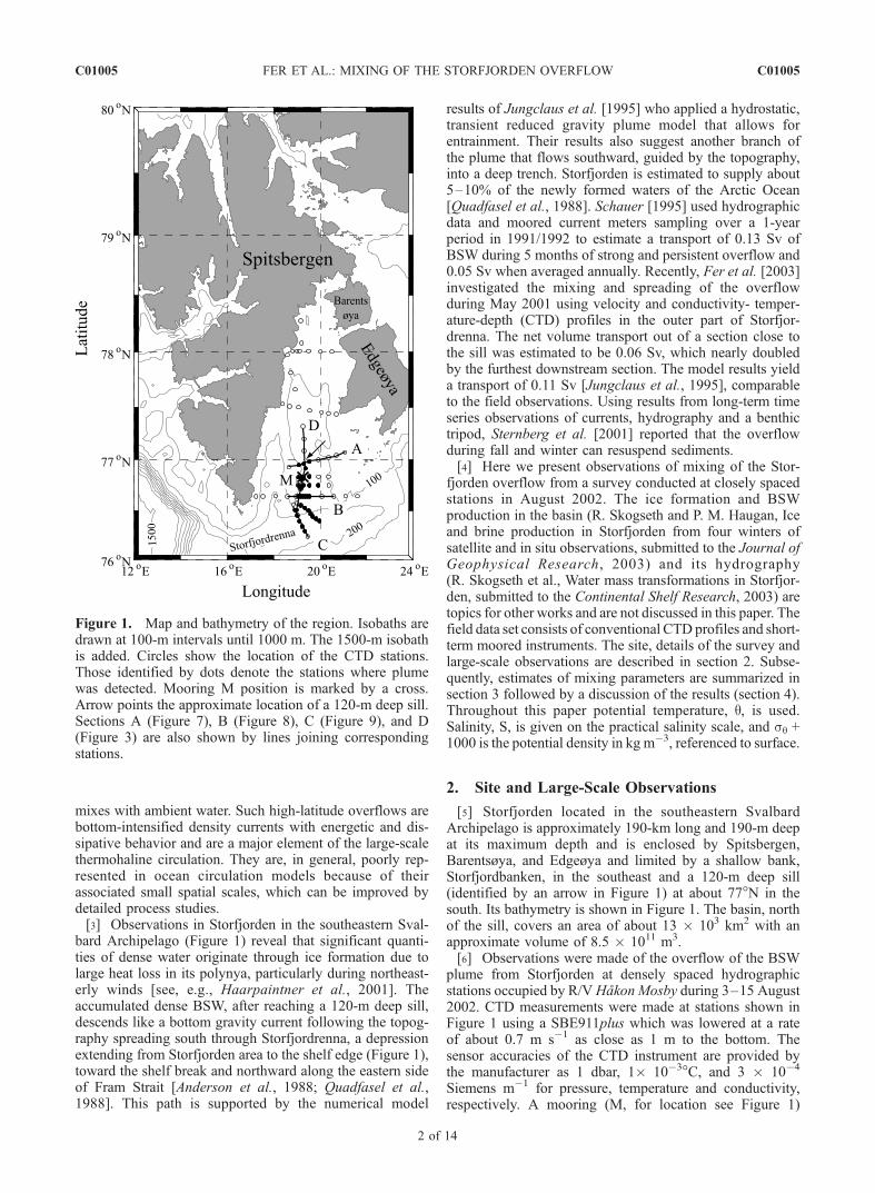
bard Archipelago (Figure 1) reveal that significant quanti-ties of dense water originate through ice formation due tolarge heat loss in its polynya, particularly during northeast-erly winds [see, e.g., Haarpaintner et al., 2001]. Theaccumulated dense BSW, after reaching a 120-m deep sill,descends like a bottom gravity current following the topog-raphy spreading south through Storfjordrenna, a depressionextending from Storfjorden area to the shelf edge (Figure 1),toward the shelf break and northward along the eastern sideof Fram Strait [Anderson et al., 1988; Quadfasel et al.,1988]. This path is supported by the numerical model

results of Jungclaus et al. [1995] who applied a hydrostatic,transient reduced gravity plume model that allows forentrainment. Their results also suggest another branch ofthe plume that flows southward, guided by the topography,into a deep trench. Storfjorden is estimated to supply about5–10% of the newly formed waters of the Arctic Ocean[Quadfasel et al., 1988]. Schauer [1995] used hydrographicdata and moored current meters sampling over a 1-yearperiod in 1991/1992 to estimate a transport of 0.13 Sv ofBSW during 5 months of strong and persistent overflow and0.05 Sv when averaged annually. Recently, Fer et al. [2003]investigated the mixing and spreading of the overflowduring May 2001 using velocity and conductivity- temper-ature-depth (CTD) profiles in the outer part of Storfjor-drenna. The net volume transport out of a section close tothe sill was estimated to be 0.06 Sv, which nearly doubledby the furthest downstream section. The model results yielda transport of 0.11 Sv [Jungclaus et al., 1995], comparableto the field observations. Using results from long-term timeseries observations of currents, hydrography and a benthictripod, Sternberg et al. [2001] reported that the overflowduring fall and winter can resuspend sediments.[4] Here we present observations of mixing of the Stor-

fjorden overflow from a survey conducted at closely spacedstations in August 2002. The ice formation and BSWproduction in the basin (R. Skogseth and P. M. Haugan, Iceand brine production in Storfjorden from four winters ofsatellite and in situ observations, submitted to the Journal ofGeophysical Research, 2003) and its hydrography(R. Skogseth et al., Water mass transformations in Storfjor-den, submitted to the Continental Shelf Research, 2003) aretopics for other works and are not discussed in this paper. Thefield data set consists of conventional CTD profiles and short-term moored instruments. The site, details of the survey andlarge-scale observations are described in section 2. Subse-quently, estimates of mixing parameters are summarized insection 3 followed by a discussion of the results (section 4).Throughout this paper potential temperature, q, is used.Salinity, S, is given on the practical salinity scale, and sq +1000 is the potential density in kg m�3, referenced to surface.

2. Site and Large-Scale Observations

[5] Storfjorden located in the southeastern SvalbardArchipelago is approximately 190-km long and 190-m deepat its maximum depth and is enclosed by Spitsbergen,Barentsøya, and Edgeøya and limited by a shallow bank,Storfjordbanken, in the southeast and a 120-m deep sill(identified by an arrow in Figure 1) at about 77�N in thesouth. Its bathymetry is shown in Figure 1. The basin, northof the sill, covers an area of about 13 � 103 km2 with anapproximate volume of 8.5 � 1011 m3.[6] Observations were made of the overflow of the BSW

plume from Storfjorden at densely spaced hydrographicstations occupied by R/VHakon Mosby during 3–15 August2002. CTD measurements were made at stations shown inFigure 1 using a SBE911plus which was lowered at a rateof about 0.7 m s�1 as close as 1 m to the bottom. Thesensor accuracies of the CTD instrument are provided bythe manufacturer as 1 dbar, 1� 10�3�C, and 3 � 10�4

Siemens m�1 for pressure, temperature and conductivity,respectively. A mooring (M, for location see Figure 1)

Figure 1. Map and bathymetry of the region. Isobaths aredrawn at 100-m intervals until 1000 m. The 1500-m isobathis added. Circles show the location of the CTD stations.Those identified by dots denote the stations where plumewas detected. Mooring M position is marked by a cross.Arrow points the approximate location of a 120-m deep sill.Sections A (Figure 7), B (Figure 8), C (Figure 9), and D(Figure 3) are also shown by lines joining correspondingstations.

C01005 FER ET AL.: MIXING OF THE STORFJORDEN OVERFLOW

2 of 14

C01005

consisting of a water level recorder at 2-m height abovebottom (hab), two RCM7Aanderaa current meters at 3 and 7-m hab, and a 50-m thermistor string with 11 sensors of 5-mvertical separation, covering 10–60-m hab, was deployed at76�49.80N, 19�15.50E over 132-m isobath, approximately 16km downstream of the sill (Figure 2). Data were recorded for104 h starting from 7 August 2002, 1600 UTC, every 5 minfor the thermistor string and 10 min for the other instruments.Both current meters were equipped with temperature andpressure sensors and that at 3-m hab also had a conductivitysensor. Salinity and temperature data recorded by the mooredinstruments were calibrated against those of the CTD castsmade prior to and after the deployment and recovery of themoorings.[7] The overflow of dense BSW shows interannual var-

iability and its path and strength depends mainly on theinitial salinity in the basin, the dynamics of the polynya andresulting rate of ice formation. Variability of the surfacesalinity in the western Barents Sea associated with the ice

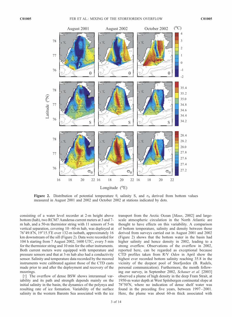
transport from the Arctic Ocean [Maus, 2002] and large-scale atmospheric circulation in the North Atlantic arethought to have effects on this variability. A comparisonof bottom temperature, salinity and density between thosederived from surveys carried out in August 2001 and 2002(Figure 2) shows that the bottom water in the basin hadhigher salinity and hence density in 2002, leading to astrong overflow. Observations of the overflow in 2002,reported here, can be regarded as exceptional becauseCTD profiles taken from R/V Oden in April show thehighest ever recorded bottom salinity reaching 35.8 in thevicinity of the deepest pool of Storfjorden (B. Rudels,personal communication). Furthermore, the month follow-ing our survey, in September 2002, Schauer et al. [2003]observed a plume of high density in the deep Fram Strait, at1950-m water depth at West Spitsbergen continental slope at78�500N, where no indication of dense shelf water wasfound in the preceding five years, between 1997–2001.Here, the plume was about 60-m thick associated with

Figure 2. Distribution of potential temperature q, salinity S, and sq derived from bottom valuesmeasured in August 2001 and 2002 and October 2002 at stations indicated by dots.


3 of 14

C01005

anomalies in salinity and temperature of 0.03 and 0.25�C,respectively. Approximately one month later, in October,the dense water at the bottom was trapped behind the sillafter the overflow has ceased prior to the survey (Figure 2).The previous incident when Storfjorden overflow could betraced down into the Fram Strait was in August 1986[Quadfasel et al., 1988] and the corresponding maximumsalinity in the basin was 35.4. This is 0.1 units less than thatobserved in August 2002 (Figure 2), hence the ice produc-tion and maximum salinity in April 1986 could be compa-rable to that in 2002. In August 2000, a survey worked byR/V Hakon Mosby showed S = 35.45 at the deepest part ofStorfjorden, and deep reaching overflow to the Fram Straitmight be expected when compared with 1986 and 2002.However, no evidence of Storfjorden plume was observedwest of Spitsbergen in 2000 by Schauer et al. [2003],probably because of difficulties in detecting the plumebecause of small spatial scale and intermittent occurrence.

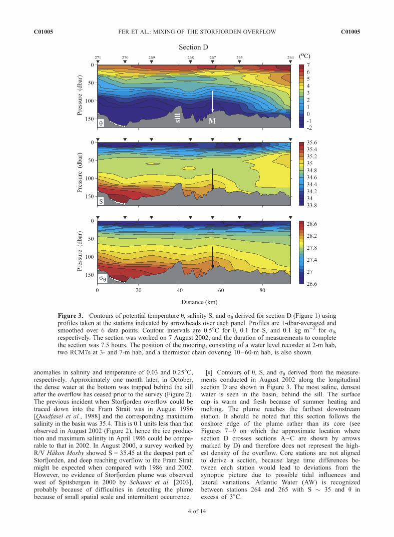
[8] Contours of q, S, and sq derived from the measure-ments conducted in August 2002 along the longitudinalsection D are shown in Figure 3. The most saline, densestwater is seen in the basin, behind the sill. The surfacecap is warm and fresh because of summer heating andmelting. The plume reaches the farthest downstreamstation. It should be noted that this section follows theonshore edge of the plume rather than its core (seeFigures 7–9 on which the approximate location wheresection D crosses sections A–C are shown by arrowsmarked by D) and therefore does not represent the high-est density of the overflow. Core stations are not alignedto derive a section, because large time differences be-tween each station would lead to deviations from thesynoptic picture due to possible tidal influences andlateral variations. Atlantic Water (AW) is recognizedbetween stations 264 and 265 with S � 35 and q inexcess of 3�C.

Figure 3. Contours of potential temperature q, salinity S, and sq derived for section D (Figure 1) usingprofiles taken at the stations indicated by arrowheads over each panel. Profiles are 1-dbar-averaged andsmoothed over 6 data points. Contour intervals are 0.5�C for q, 0.1 for S, and 0.1 kg m�3 for sq,respectively. The section was worked on 7 August 2002, and the duration of measurements to completethe section was 7.5 hours. The position of the mooring, consisting of a water level recorder at 2-m hab,two RCM7s at 3- and 7-m hab, and a thermistor chain covering 10–60-m hab, is also shown.


4 of 14

C01005

[9] Time series recorded by the moored instruments aredetided using tidal harmonic analysis [Pawlowicz et al.,2002] and are illustrated in Figure 4. The data show thepresence of a cold, close to the freezing point, and saline(S > 35) plume associated with downslope flow for the firstthree days of the record. When defined as water with q <0�C, the height of the plume at the mooring location variesbetween 20 and 60 m and equal to 40 ± 8 m, on the mean (±one standard deviation). After 84 h, AW with q in excess of4.5�C penetrates across the mooring. Its signature is ob-served as close as 3-m hab as can be seen from the salinityrecord with values of S gradually decreasing to 34.9(Figure 4b) and the temperature record with q > 0�C(Figure 5). Assuming that this is the tongue of AW seenin Figure 3, observed at the start of the recording period (seethe time of occupation of section D in Figure 4a), it coversapproximately 25 km giving a propagation speed of 8 cms�1 toward the sill. In Storfjordrenna, AW circulates in acyclonic sense following the topography [Schauer, 1995;Fer et al., 2003] as can be seen from the data recorded bythe current meter at 3-m hab with westward velocity whenq > 0�C (Figure 5).[10] The mean velocity derived over the duration of the

plume is 10 cm s�1 at 7-m hab directed 159� from truenorth. Corresponding values derived from the data recordedby the bottommost current meter at 3-m hab are 8 cm s�1

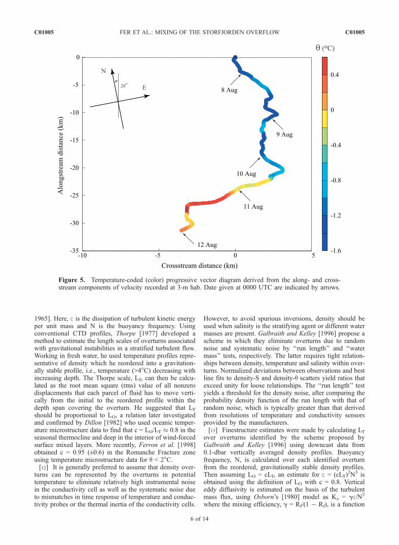
and 152�. A progressive vector diagram produced from thealong and cross-stream components at 3-m hab suggests thatwater with q < 0�C reaches �25 km downstream of themooring position (Figure 5). Streamwise coordinates areobtained after rotating the velocity 28� counterclockwisefrom north. Using the average thickness, h = 40 m, andspeed, u = 0.1 m s�1 observed from the thermistor stringand the current meter at 7-m hab, respectively, an estimatefor transport equal to 0.12 (±0.04) Sv can be obtainedprovided that the cross section is rectangular with anapproximate width of 30 km (see Figures 7c and 8c). Theuncertainty here is derived from the variability in height andthe uncertainty in width of the plume. Higher uncertaintywill arise if the section-averaged downstream velocity issignificantly different than 0.1 m s�1. The volumetransport compares well with those reported in the literature(section 1).

3. Estimation of Turbulence Quantities FromDensity Overturns

3.1. Methods

[11] In a stratified fluid, a parcel of fluid has to move avertical distance which as a statistical mean can be repre-sented by the Ozmidov scale, LO = (e/N3)1/2, in order toconvert all its kinetic energy into potential energy [Ozmidov,

Figure 4. Detided time series of (a) east (black) and north (red) components of velocity recorded at 7-mhab, (b) salinity at 3-m hab, and (c) isotherms. Isotherms are derived from the temperature recorded bythe thermistor chain, two Aanderaa current meters and a water level recorder. White isotherm is 0�C.Duration of sections A–D are also shown in Figure 4a.


5 of 14

C01005

1965]. Here, e is the dissipation of turbulent kinetic energyper unit mass and N is the buoyancy frequency. Usingconventional CTD profiles, Thorpe [1977] developed amethod to estimate the length scales of overturns associatedwith gravitational instabilities in a stratified turbulent flow.Working in fresh water, he used temperature profiles repre-sentative of density which he reordered into a gravitation-ally stable profile, i.e., temperature (>4�C) decreasing withincreasing depth. The Thorpe scale, LT, can then be calcu-lated as the root mean square (rms) value of all nonzerodisplacements that each parcel of fluid has to move verti-cally from the initial to the reordered profile within thedepth span covering the overturn. He suggested that LTshould be proportional to LO, a relation later investigatedand confirmed by Dillon [1982] who used oceanic temper-ature microstructure data to find that c = LO/LT � 0.8 in theseasonal thermocline and deep in the interior of wind-forcedsurface mixed layers. More recently, Ferron et al. [1998]obtained c = 0.95 (±0.6) in the Romanche Fracture zoneusing temperature microstructure data for q < 2�C.[12] It is generally preferred to assume that density over-

turns can be represented by the overturns in potentialtemperature to eliminate relatively high instrumental noisein the conductivity cell as well as the systematic noise dueto mismatches in time response of temperature and conduc-tivity probes or the thermal inertia of the conductivity cells.

However, to avoid spurious inversions, density should beused when salinity is the stratifying agent or different watermasses are present. Galbraith and Kelley [1996] propose ascheme in which they eliminate overturns due to randomnoise and systematic noise by ‘‘run length’’ and ‘‘watermass’’ tests, respectively. The latter requires tight relation-ships between density, temperature and salinity within over-turns. Normalized deviations between observations and bestline fits to density-S and density-q scatters yield ratios thatexceed unity for loose relationships. The ‘‘run length’’ testyields a threshold for the density noise, after comparing theprobability density function of the run length with that ofrandom noise, which is typically greater than that derivedfrom resolutions of temperature and conductivity sensorsprovided by the manufacturers.[13] Finestructure estimates were made by calculating LT

over overturns identified by the scheme proposed byGalbraith and Kelley [1996] using downcast data from0.1-dbar vertically averaged density profiles. Buoyancyfrequency, N, is calculated over each identified overturnfrom the reordered, gravitationally stable density profiles.Then assuming LO = cLT, an estimate for e = (cLT)

2N3 isobtained using the definition of LO with c = 0.8. Verticaleddy diffusivity is estimated on the basis of the turbulentmass flux, using Osborn’s [1980] model as Kz = ge/N2

where the mixing efficiency, g = Rf/(1 � Rf), is a function

Figure 5. Temperature-coded (color) progressive vector diagram derived from the along- and cross-stream components of velocity recorded at 3-m hab. Date given at 0000 UTC are indicated by arrows.


6 of 14

C01005

of the flux Richardson number, Rf. Osborn’s modelassumes steady, homogeneous turbulence field where theproduction of turbulent kinetic energy by the Reynoldsstress working against the mean shear is balanced by e andthe production of buoyancy. Mixing efficiency indicatesthe conversion efficiency of turbulent kinetic energy intopotential energy of the system. It is commonly taken to be0.2 [Gregg, 1987], however can vary depending on thedynamics generating turbulence (section 3.2). We use g =0.15 in our calculations. The uncertainties associated withthe estimates are discussed in the following section.[14] The standard sampling rate of the CTD is 24 Hz and

with the nominal descent rate of 0.7 m s�1, this correspondsto a sampling greater than 3 data per 0.1 dbar. Whencalculated over all profiles, 91% of the bins comprise �2data points. In order to avoid nonmonotonic pressure seriesas a result of ship roll in the surface wave field, pressuredata are low-pass filtered with a time constant of 0.15 s andscans were flagged and excluded from bin averaging whenCTD descent rate was less than 0.25 m s�1. On the basis ofcombined statistics of all profiles, a cutoff run length of 6was chosen below which overturns are assumed to becreated by noise. The noise level in density measurementsbased on this run length is 0.0016 kg m�3. The threshold forwater mass test was set to 0.75. This is larger than thethreshold of 0.5 suggested by Galbraith and Kelley [1996]which was obtained by visual inspections of loops in

q-S diagrams. This threshold was relaxed in this study sinceno prominent loops were observed. Furthermore, in our casewhere q is close to the freezing point, the variation indensity with temperature alone is not significant.[15] The necessity of using profiles of density as dis-

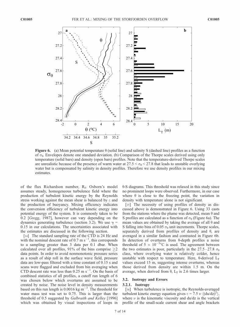
cussed above is demonstrated in Figure 6. Using 33 castsfrom the stations where the plume was detected, mean q andS profiles are calculated as a function of sq (Figure 6a). Themean values are obtained by taking the average of all q andS falling into bins of 0.05 sq unit increments. Thorpe scales,separately derived from profiles of density and q, areaveraged in a similar fashion and contrasted in Figure 6b.In detection of overturns from q-depth profiles a noisethreshold of 5 � 10�3�C is used. The agreement betweenthe two estimates is poor, particularly in the 27.5–27.8 sqclass, where overlying water is relatively colder, henceunstable with respect to temperature. Here, q-derived LTvalues exceed 15 m, suggesting intense overturns, whereasthose derived from density are within 1.5 m. On theaverage, when derived from q, LT is 2.6 times larger.

3.2. Isotropy and Errors

3.2.1. Isotropy[16] When turbulence is isotropic, the Reynolds-averaged

turbulent kinetic energy equation gives e = 7.5 n h(du/dz)2i,where n is the kinematic viscosity and du/dz is the verticalprofile of the small-scale current shear and angle brackets

Figure 6. (a) Mean potential temperature q (solid line) and salinity S (dashed line) profiles as a functionof sq. Envelopes denote one standard deviation. (b) Comparison of the Thorpe scales derived using onlytemperature (solid bars) and density (open bars) profiles. Note that the temperature-derived Thorpe scalesare unrealistic because of the presence of warm water at 27.5 < sq < 27.8 that leads to unstable overlyingwater but is compensated by salinity in density profiles. Therefore we use density profiles in our mixingestimates.


7 of 14

C01005

denote ensemble, or spatial as practically applied in oceanicmicrostructure studies, averaging [Batchelor, 1953]. In astratified flow, the dimensionless ratio e/nN2, often referredto as buoyancy Reynolds number (or index for activity ofturbulence), gives an indication of departures from small-scale isotropy, which is also assumed to be achieved in ourestimates of turbulence quantities. When e/nN2 > 20,estimates approach to the isotropic formula [Yamazaki andOsborn, 1990] with error limited to less than 35% for lowervalues. This is also roughly the threshold below whichmixing can no longer sustain the negative buoyancy fluxnecessary for a net increase in potential energy. Theturbulence field can be considered isotropic for e/nN2 �200 [Gargett et al., 1984; Yamazaki and Osborn, 1990].The average values of e and N within the plume are 3 �10�8 W kg�1 and 2.5 cph (1 cph = 2p3600�1 s�1), respect-ively. Using n = 1.8 � 10�6 m2 s�1, this leads to a buoyancyReynolds number of about 900, and we can use Osborn’smodel with confidence. Again using the average value of e inthe plume, an estimate of h(du/dz)2i of O(10�3) s�2 can beobtained for the small-scale shear. This is an order ofmagnitude greater than that of larger scale reported for theoverflow in Storfjordrenna derived from profiles of currentas well as geostrophy over 10-m vertical separations whenthe density excess of the plume was lower [Fer et al., 2003].3.2.2. Errors[17] Dissipation rate of turbulent kinetic energy per unit

mass is estimated from e = (cLT)2N3, where c is the constant

of proportionality between LO and LT, here taken as c = 0.8.The above expression for e is sensitive to N, which isestimated from the reordered density profile over a depthrange enclosing each particular overturn. Minor errors arisein N, associated with resolutions in density and depth.However, a comparison between values of N derived fromthe same vertical intervals as the overturn and those derivedoutside it, representative of the background N (Nb), mani-fests how much mixing the observed turbulent patch mayhave undergone at the time it was observed. We calculatedNb including 0.5-m on either side of each overturn. Theratio of N to Nb is approximately normally distributedcovering a range 0.3–1 and equals to 0.65 ± 0.16 (± onestandard deviation). The broad range suggests that theoverturns, when observed, are at varying stages of theirlifetimes. The variability in e over all events increases by afactor of 3 when derived using Nb. As discussed by Dillon[1982], fluctuation in the interior of an overturn can be quiteinsensitive to the stratification only a small distance away,provided that the mixing regime is different there. In orderto be representative of the stratification against which theoverturn is straining, N should be calculated over the depthrange of the overturn. Another source of uncertainty in e isthe choice of c. According to results of Ferron et al. [1998]given in section 3.1, the variability in c can be �60%. Asystematic error of 10% in finding LT together with thevariability in c results in 140% error in e. Furthermore,consideration of accuracy and assumption of isotropy mayintroduce additional errors, and e can be estimated to withina factor of 3.[18] The diffusivity, Kz = g(cLT)

2N is less sensitive to N,but additional errors arise because of the mixing efficiencywhich is taken as g = 0.15. The application of Nb increasesthe variability in Kz by a factor of 1.2. The uncertainty

introduced by the choice of g is insignificant compared tothat arising from the LO - LT relationship. As reportedelsewhere [see Peltier and Caulfield, 2003], g may varystrongly depending on the type of instability and thedifferent stages of turbulence transition, i.e., initial stageof instability amplification, development of secondary insta-bilities and three-dimensional collapse of turbulence.Neglecting values derived for tidal channel flows, typicalvalues in the literature span a range of 0.15–0.3. As a result,Kz can be estimated within a factor of 4. While this level ofuncertainties in the present study may seem high, it shouldbe noted that it is comparable to that of other turbulentstudies in oceans or lakes. Furthermore, our conclusions onenhanced mixing within the overflow are drawn on the basisof variations that exceed one order of magnitude, wellabove the level of uncertainties.

4. Results and Discussion

4.1. Downstream Development

[19] The overflow is subject to mixing with overlyingwarmer waters of Atlantic origin and the extent to which theoverflow water can retain its identity will depend on theintensity of mixing. Estimates of mixing parameters inferredfrom Thorpe-scale analysis for three representative sectionsacross the overflow, looking in the upstream direction withSpitsbergen on the left, are presented in Figures 7–9,together with contours of q, S, and sq. In each figure,overturns are represented by boxes at the correspondingdepth, with vertical length equal to the height of theoverturn. Estimates of log(Kz) and log(e) are color-codedin panels (a) and (b), respectively. The section at the sill(Figure 7) shows the weakest turbulent activity with a totalof 8 distinguishable overturns, two of which are near theinterface between the overflow and the ambient water.Thickness and extent of the plume is approximately shownby the isopycnal corresponding to sq = 27.95, consistentwith Fer et al. [2003]. Farther downstream, at section B, theplume is well developed and is associated with enhanced Kz

and e with values one order of magnitude greater than thosein the ambient. Turbulent patches associated with theoverflow are more pronounced on the sloping side of thesection where isopycnals are tilted, indicative of a geo-strophically balanced overflow into Storfjordrenna. At sec-tion B, water of density exceeding 28.3 is no longer presentcompared to the transect at the sill where sq reaches 28.6immediately adjacent to the bottom. This is because of theintense mixing with the ambient water as the plumedescends. The initial part of the overflow is particularlyimportant since, until the rotational effects are well estab-lished within a Rossby radius of deformation (�4 km), theplume accomplishes most of its entrainment flowing down-slope before it is slowed down by friction and deviatedalong the isobaths. Around the core of AW, which here canbe identified by the S = 35 isohaline between 50–100-mdepth, mixing may be due to frontal instabilities. As theplume propagates away from the sill toward the farthestdownstream section (Figure 9), the vertical gradient of itsdensity gradually decreases. This is consistent with the factthat encountered vertical mixing acts to homogenize theplume vertically. It is noteworthy that the last transectprovides evidence for episodes of denser overflow encoun-


8 of 14

C01005

Figure 7. Distribution of (a) q and vertical diffusivity Kz (colored), (b) S and e (colored), and (c) sqderived for section A (Figure 1). Each colored box in Figures 7a and 7b represents a detected overturnspanned by its height. The width of the boxes is arbitrary. The additional thick isopycnal in Figure 7c issq = 27.95 and roughly represents the extent of the plume [Fer et al., 2003]. Profiles are taken at thestations numbered in Figure 7a and indicated by arrowheads over each panel. The arrow marked by Dshows the approximate location where section D (Figure 3) crosses the section. The 1-dbar-averagedvalues are interpolated into a regular grid of 1-dbar bins in vertical and 150 distance bins in horizontaland smoothed over 6 data points. Contour intervals are 0.5�C for q, 0.1 for S, and 0.1 kg m�3 for sq,respectively. Bottom topography is derived from echo sounding after correcting for the sound velocity.


9 of 14

C01005

tered prior to the survey since deep water with sq > 28.3 wasnot observed in section B.

4.2. Averaged Properties

[20] In order to get a survey-averaged picture, the estimatesfrom 33 casts were sorted into 0.1 sq unit bins and averaged.The average depth for each bin when sq 27.9, i.e., fromsurface to slightly above the plume, and the average hab forsq > 27.9, comprising the plume, are calculated to obtain adensity profile (Figure 10a). This approach was necessary toobtain a representative profile, which otherwise if depth-

averaged would have removed the signature of the overflowwhich descends from the sill depth of 120 m down to greaterdepths, adjacent to the bottom. Survey-averaged profiles oflog(Kz) and log(e) are calculated accordingly and shown inFigure 10 as a function of depth and hab. Here, errorbarsshow 95% confidence intervals of the mean over 200bootstrap sampled populations. Dissipation rate typicallydecreases with depth from surface but increases substantiallywithin the overflow. Vertical diffusivity remains fairly con-stant with depth until it increases by an order of magnitudewithin the plume. The heat flux is calculated using Q =

Figure 8. SameasFigure 7but for sectionB.Note the enhancedmixingwithin the outflowwheresq>27.9.


10 of 14

C01005

rCpKzdq/dz, where r is the density and Cp is the specific heatof seawater, both calculated using the averaged temperatureand salinity in each bin, dq/dz is the average vertical temper-ature gradient. Values of heat flux obtained using Kz suggestthat the plume gains considerable amount of heat from theoverlying AW. This can be compared to the rate of change ofheat gain from section A to C. The change in section-averaged plume temperature between the two sections is�q = 0.5�C. The heat gain, �H = rCp�qh, is about 8 �107 J m�2 provided that the mean thickness of the plume h =

40 m. Assuming a constant speed of 10 cm s�1, the plumewill cover its path of x� 80 km in 8� 105 s which yields therate of change of heat of about 100 W m�2. This compareswell, considering the uncertainty in Kz (see section 3.2), withthe values within the plume shown in Figure 10d.

4.3. Effects of Stratification

[21] The stratification modifies the dynamics of turbu-lence which is suppressed in strong stable stratificationsince more turbulent energy is needed to act against larger

Figure 9. Same as Figure 7 but for section C.


11 of 14

C01005

Figure 10. Survey-averaged profiles of sq, Kz, e, and heat flux Q derived using 33 plume stations (dotsin Figure 1), as a function of depth below surface (circles) until above the plume and hab (solid squares)within the plume. Averaged properties are calculated using 0.1 sq unit bins, and error bars denote 95%bootstrap confidence intervals. Dots show the law of the wall estimates for e within 5 m to the bottom.Heat flux is positive when heat is transferred to deeper layers.

Figure 11. Variation of vertical diffusivity Kz by buoyancy frequency N. Dots are the average valuesderived for each 1-cph bin, and error bars are 95% bootstrap confidence intervals. Best fit power lawcurve (thin line) shows �1.2 dependency.


12 of 14

C01005

vertical gradients of density. The ensemble of plumestations indicates a power law dependence of Kz �N�1.2 (Figure 11). The 95% confidence interval for theexponent is ±0.3. This dependence is not conclusive sincethe variation in N is limited to less than one decade.Furthermore, time variability in small-scale shear cancause variability in Kz which may appear related to N[Rehmann and Duda, 2000]. However, the decay of Kz

with increasing N is comparable to e � Nm with 1 m 2, a range comprising that predicted for the midlat-itude thermocline of the open ocean from six diverse sites[Gregg, 1989] and that obtained using observations ofoceanic internal wave field in the literature [Gargett andHolloway, 1984]. This corresponds to Kz � Nn with �1 n 0 using Kz = ge/N2. However, using more extensivemeasurements with considerably more range in stratifica-tion and wave properties than has been previously avail-able, Polzin et al. [1995] subsequently suggested e � N2

scaling as characteristic of the stratified interior of the deepsea. D’Asaro and Lien [2000] have recently offered aninterpretation of two forms in terms of turbulence gener-ated by different physics depending on the large-scaleRichardson number (Ri = N2/shear2). They define a waveturbulence transition which separates two regimes: mixingcontrolled by interactions between internal wave modes(large Ri) and mixing controlled by instabilities of large-scale wave modes (Ri of order 1). For energies above thistransition, Kz � N�1 which is appropriate for diffusivitiesin lakes and fjords which are mixed by strong turbulentprocesses (e.g., mixing at the vicinity of a sill in fjords,rapid breakdown of intermittent seiches in lakes). Forenergies below the transition, diffusivity is independentof N (i.e., e � N2 consistent with the scaling of thestratified interior of the deep sea), and proportional to thesquared internal wave spectral level. Our observationsyield a scaling not significantly different than Kz � N�1,and suggest that the mixing of the overflow is controlledby localized instability of large-scale motions, rather thantransfer of energy from large-scale to smaller-scale turbu-lence due to wave-wave interactions. Inferring from scalarmicrostructure measurements, Rehmann and Duda [2000]examined the effect of stratification on Kz for near-bottommixing and for mixing throughout the water column. Nearthe bottom, they found a decay with N corresponding ton = �3.1, significantly larger than the values cited above.The discrepancy was attributed to different mechanismsdriving the turbulence, as well as possible effects ofentrainment. For mixing throughout the water column,they found n = �1.3 ± 0.8 comparable to our observations.[22] Far from boundaries, turbulent fields are believed to

be generated by random superposition of shear fields varyingin time and space because of, for example, internal waves,leading to instabilities and turbulence provided that the fieldpersists long enough to allow for a small-amplitude pertur-bation to grow. In case of a density current, if it is thinenough, i.e., comparable to the vertical length scale ofturbulence, the mixing is determined by the turbulencegenerated near the boundary. Eddies will cover the entiredense layer leading to a homogeneous, mixed layer withsmall mixing across the interface [see Turner, 1973,section 4.3]. On the other hand, if the dense layer is thick,turbulent energy will decay away from the wall because of

viscous dissipation; hence wall effects on the interface willbe negligible. The mixing at the interface is governed mainlyby internal mixing mechanisms due to shear between theoverflow and the ambient water, comparable to shear-in-duced mixing of internal waves in the thermocline. TheThorpe scale adjacent to the bottom is order of severalmeters (Figure 6b) and we might expect bottom-generatedturbulence to decay within the overflow leading to the nearlyhomogeneous bottom layer (Figure 10a) consistent with thebottom layer defined by Fer et al. [2003, layer 1]. Enhancedmixing at the interface is due to internal mixing. When thevelocity of inflow entrained into a turbulent gravity current isassumed proportional to the velocity of the current, withconstant of proportionality equal to entrainment coefficient,E [Ellison and Turner, 1959], the buoyancy flux can beestimated by EuhN2 [Rehmann and Duda, 2000]. Here, u isthe mean speed relative to the ambient and h is the thicknessof the dense layer. The buoyancy flux is also, by definition,equal to KzN

2. Hence an estimate of E = Kz (uh)�1 can be

derived. Using the mean value of Kz within the overflowequal to 10 � 10�4 m2 s�1 and u = 0.1 m s�1, h = 40 m,we obtain E � 3 � 10�4, which compares well with theearlier estimates for the Storfjorden overflow [Schauer andFahrbach, 1999; Fer et al., 2003].[23] Considerable work has been devoted to get reliable

estimates of small-scale mixing through easily accessibleand conventional methods. Direct measurements of turbulentshear, thus dissipation rate for homogeneous turbulence, orindirect estimates of turbulence parameters through scalarmicrostructure profiles, for example, via spectral methods,require large efforts to acquire highly specialized data. Onthe basis of temperature microstructure data covering 5 and4 orders of magnitude in stratification and Thorpe scales,respectively, Lorke and Wuest [2002] provide strong evi-dence on universality of overturning-length-scale distribu-tions, encouraging estimates of mixing from conventional,low-resolution profiles. In this study, observations by con-ventional profiling techniques highlight some of the mixingprocesses associated with the Storfjorden overflow. Thevertical profiles allow distinctions to be made betweenmixing near the bottom, at the interface between the over-flow and the ambient waters and off-slope waters at similardepths, using identical sampling and analysis techniques.

[24] Acknowledgments. This work was funded by the NorwegianResearch Council, through grants 147493/432 for IF and 138525/410 forRS. The fieldwork was supported through the NOClim (Norwegian OceanClimate) project funded by the Norwegian Research Council, grant 139815/720. This is publication A0018 of the Bjerknes Centre for ClimateResearch. Comments from Dan E. Kelley and an anonymous reviewerwere helpful to improve this work. The authors thank the captain and crewof R/V Hakon Mosby.

ReferencesAagaard, K., L. K. Coachman, and E. Carmack (1981), On the halocline ofthe Arctic Ocean, Deep Sea Res., Part A, 28, 529–545.

Anderson, L. G., E. P. Jones, R. Lindegren, B. Rudels, and P. I. Sehlstedt(1988), Nutrient regeneration in cold, high salinity bottom water of theArctic shelves, Cont. Shelf Res., 8, 1345–1355.

Batchelor, G. K. (1953), The Theory of Homogeneous Turbulence, 197 pp.,Cambridge Univ. Press, New York.

Cavalieri, D. J., and S. Martin (1994), The contribution of Alaskan, Siber-ian and Canadian coastal polynyas to the halocline layer of the ArcticOcean, J. Geophys. Res., 99, 18,343–18,362.

D’Asaro, E. A., and R.-C. Lien (2000), The wave-turbulence transition forstratified flows, J. Phys. Oceanogr., 30, 1669–1678.


13 of 14

C01005

Dillon, T. M. (1982), Vertical overturns: A comparison of Thorpe andOzmidov length scales, J. Geophys. Res., 87, 9601–9613.

Ellison, T. H., and J. S. Turner (1959), Turbulent entrainment in stratifiedflows, J. Fluid Mech., 6, 423–448.

Fer, I., R. Skogseth, P. M. Haugan, and P. Jaccard (2003), Observations ofthe Storfjorden overflow, Deep Sea Res., Part I, 50, 1283–1303.

Ferron, B., H. Mercier, K. G. Speer, A. Gargett, and K. L. Polzin (1998),Mixing in the Romanche Fracture Zone, J. Phys. Oceanogr., 28, 1929–1945.

Galbraith, P. S., and D. E. Kelley (1996), Identifying overturns in CTDprofiles, J. Atmos. Oceanic Technol., 13, 688–702.

Gargett, A. E., and G. Holloway (1984), Dissipation and diffusion byinternal wave breaking, J. Mar. Res., 42, 15–27.

Gargett, A. E., T. R. Osborn, and P. W. Nasmyth (1984), Local isotropy andthe decay of turbulence in a stratified fluid, J. Fluid Mech., 144, 231–280.

Gregg, M. C. (1987), Diapycnal mixing in the thermocline—A review,J. Geophys. Res., 92, 5249–5286.

Gregg, M. C. (1989), Scaling turbulent dissipation in the thermocline,J. Geophys. Res., 94, 9686–9698.

Griffiths, R. W. (1986), Gravity currents in rotating systems, Annu. Rev.Fluid. Mech., 18, 59–89.

Haarpaintner, J., P. M. Haugan, and J.-C. Gascard (2001), Interannualvariability of the Storfjorden (Svalbard) ice cover and ice productionobserved by ERS-2 SAR, Ann. Glaciol., 33, 430–436.

Jungclaus, J. H., J. O. Backhaus, and H. Fohrmann (1995), Outflow ofdense water from the Storfjord in Svalbard: A numerical model study,J. Geophys. Res., 100, 24,719–24,728.

Killworth, P. D. (1983), Deep convection in the world ocean, Rev. Geo-phys., 21, 1–26.

Lorke, A., and A. Wuest (2002), Probability density of displacement andoverturning length scales under diverse stratification, J. Geophys. Res.,107(C12), 3214, doi:10.1029/2001JC001154.

Maus, S. (2002), Interannual variability of dense shelf water salinities in theBarents Sea, Polar Res., 22, 59–66.

Osborn, T. R. (1980), Estimates of the local rate of vertical diffusion fromdissipation measurements, J. Phys. Oceanogr., 10, 83–89.

Ozmidov, R. V. (1965), On the turbulent exchange in a stably stratifiedocean, Atmos. Oceanic Phys., 8, 853–860.

Pawlowicz, R., B. Beardsley, and S. Lenz (2002), Classical tidal harmonicanalysis including error estimates in MATLAB using T-TIDE, Comput.Geosci., 284, 929–937.

Peltier, W. R., and C. P. Caulfield (2003), Mixing efficiency in stratifiedshear flows, Annu. Rev. Fluid Mech., 35, 135–167.

Polzin, K. L., J. M. Toole, and R. W. Schmitt (1995), Finescale parameter-izations of turbulent dissipation, J. Phys. Oceanogr., 25, 306–328.

Price, J. F., and M. O. Baringer (1994), Outflows and deep water productionby marginal seas, Prog. Oceanogr., 33, 161–200.

Quadfasel, D., B. Rudels, and K. Kurz (1988), Outflow of dense water froma Svalbard Fjord into the Fram Strait, Deep Sea Res., Part A, 35, 1143–1150.

Rehmann, C. R., and T. F. Duda (2000), Diapycnal diffusivity inferred fromscalar microstructure measurements near the New England Shelf/Slopefront, J. Phys. Oceanogr., 30, 1354–1371.

Rudels, B., and D. Quadfasel (1991), Convection and deep water formationin the Arctic Ocean-Greenland Sea system, J. Mar. Syst., 2, 435–450.

Schauer, U. (1995), The release of brine-enriched shelf water from Storfjordinto the Norwegian Sea, J. Geophys. Res., 100, 16,015–16,028.

Schauer, U., and E. Fahrbach (1999), A dense bottom water plume in thewestern Barents Sea: Downstream modification and interannual variabil-ity, Deep Sea Res., Part I, 46, 2095–2108.

Schauer, U., B. Rudels, I. Fer, P. M. Haugan, R. Skogseth, G. Bjork, andP. Winsor (2003), Return of deep shelf/slope convection in the westernBarents Sea?, paper presented at the 7th Conference on Polar Meteorol-ogy and Oceanography and Joint Symposium on High-Latitude ClimateVariations, Am. Meteorol. Soc., Hyannis, Mass.

Smethie, W. M., H. G. Ostlund, and H. H. Loosli (1986), Ventilation ofthe deep Greenland and Norwegian Seas: Evidence from Krypton-85,tritium, carbon-14, and argon-39, Deep Sea Res., Part A, 33, 675–703.

Sternberg, R. W., K. Aagaard, D. Cacchione, R. A. Wheatcroft, R. A.Beach, A. T. Roach, and M. A. H. Marsden (2001), Long-term near-bed observations of velocity and hydrographic properties in the northeastBarents Sea with implications for sediment transport, Cont. Shelf Res.,21, 509–529.

Thorpe, S. A. (1977), Turbulence and mixing in a Scottish loch, Philos.Trans. R. Soc. London, Ser. A, 286, 125–181.

Turner, J. S. (1973), Buoyancy Effects in Fluids, 367 pp., Cambridge Univ.Press, New York.

Wadhams, P. (2000), Ice in the Ocean, 351 pp., Gordon and Breach, Newark,N. J.

Yamazaki, H., and T. Osborn (1990), Dissipation estimates for stratifiedturbulence, J. Geophys. Res., 95, 9739–9744.

��I. Fer and P. M. Haugan, Geophysical Institute, University of Bergen,

Allegaten 70, N-5007, Bergen, Norway. ([email protected])R. Skogseth, University Centre in Svalbard, P.O. Box 156, N-9171

Longyearbyen, Norway.


14 of 14

C01005

Mixing of the Storfjorden overflow (Svalbard Archipelago) inferred from density overturns

Documents

Transcript of Mixing of the Storfjorden overflow (Svalbard Archipelago) inferred from density overturns