Ice shelf water overflow and bottom water formation in the southern

Weddell Sea

A. Foldvik,1 T. Gammelsrød,1 S. Østerhus,1 E. Fahrbach,2 G. Rohardt,2 M. Schroder,2

K. W. Nicholls,3 L. Padman,4 and R. A. Woodgate5

Received 17 June 2003; revised 5 October 2003; accepted 10 December 2003; published 17 February 2004.

[1] Cold shelf waters flowing out of the Filchner Depression in the southern Weddell Seamake a significant contribution to the production of Weddell Sea Bottom Water (WSBW),a precursor to Antarctic Bottom Water (AABW). We use all available current meterrecords from the region to calculate the flux of cold water (<�1.9�C) over the sill at thenorthern end of the Filchner Depression (1.6 ± 0.5 Sv), and to determine its fate. Theestimated fluxes and mixing rates imply a rate of WSBW formation (referenced to�0.8�C) of 4.3 ± 1.4 Sv. We identify three pathways for the cold shelf waters to enter thedeep Weddell Sea circulation. One path involves flow constrained to follow the shelfbreak. The other two paths are down the continental slope, resulting from the cold densewater being steered northward by prominent ridges that cross the continental slope near36�W and 37�W. Mooring data indicate that the deep plumes can retain their corecharacteristics to depths greater than 2000 m. Probably aided by thermobaricity, the plumewater at this depth can flow at a speed approaching 1 m s�1, implying that the flow isoccasionally supercritical. We postulate that such supercriticality acts to limit mixingbetween the plume and its environment. The transition from supercritical to slower, moreuniform flow is associated with very efficient mixing, probably as a result of hydraulicjumps. INDEX TERMS: 4207 Oceanography: General: Arctic and Antarctic oceanography; 4568

Oceanography: Physical: Turbulence, diffusion, and mixing processes; 4512 Oceanography: Physical:

Currents; 4594 Oceanography: Physical: Instruments and techniques; 4520 Oceanography: Physical: Eddies

and mesoscale processes; KEYWORDS: bottom water formation, mixing processes, hydraulic jump, current

meters, Ice Shelf Water

Citation: Foldvik, A., T. Gammelsrød, S. Østerhus, E. Fahrbach, G. Rohardt, M. Schroder, K. W. Nicholls, L. Padman, and R. A.

Woodgate (2004), Ice shelf water overflow and bottom water formation in the southern Weddell Sea, J. Geophys. Res., 109, C02015,

doi:10.1029/2003JC002008.

1. Introduction

[2] Cold, dense and oxygenated Antarctic Bottom Water(AABW) is one of the Antarctic’s most important exports.Production of AABW is routinely cited as being one of thedrivers of the global thermohaline circulation (GTHC) andits influence on the properties of the World Ocean is widelyaccepted. Understanding the mechanisms for the productionof AABW, and any sensitivity in those mechanisms to pastor future climate change, is therefore important if we are tounderstand the controls on the GTHC. More than half of thetotal flux of AABW is believed to have its origins in theWeddell Sea [Orsi et al., 1999].

[3] In today’s climatic regime the majority of AABWproduction begins with the formation of High Salinity ShelfWater (HSSW) in Antarctica’s marginal seas. HSSW is aby-product of sea-ice formation over many of the broaderportions of the Antarctic continental shelf. One of theacknowledged hot spots for the production of HSSW is thewestern and southern margin of the Weddell Sea (Figure 1).A combination of winds blowing from the Filchner-RonneIce Shelf and tidal divergence at its seaward boundarymaintains latent heat polynyas along the ice front for mostof the year [Foldvik et al., 2001; Renfrew et al., 2002].Intense heat loss from these polynyas, and also throughleads in the pack ice over the continental shelf to the north,results in high rates of sea-ice production and HSSWformation. There are various pathways by which theHSSW can arrive in the deep Weddell Sea as Weddell SeaBottom Water (WSBW), the Weddell Sea’s precursor toAABW. One such pathway involves circulation in theocean cavity beneath Filchner-Ronne Ice Shelf [Foldvikand Gammelsrød, 1988; Nicholls et al., 2001].[4] Although HSSW has a temperature close to the

freezing point at the surface (�1.9�C) the depression ofthe freezing point of seawater with an increase in pressure

JOURNAL OF GEOPHYSICAL RESEARCH, VOL. 109, C02015, doi:10.1029/2003JC002008, 2004

1Geophysical Institute, University of Bergen, Bergen, Norway.2Alfred-Wegener-Institut fur Polar und Meeresforschung, Bremerhaven,

Germany.3British Antarctic Survey, Cambridge, UK.4Earth and Space Research, Seattle, Washington, USA.5Applied Physics Laboratory, University of Washington, Seattle,

Washington, USA.

Copyright 2004 by the American Geophysical Union.0148-0227/04/2003JC002008$09.00

C02015 1 of 15

means that, even at �1.9�C, HSSW retains the capacity tomelt ice at depth. At the base of an ice shelf with a draft of1500 m, for example, the freezing point is about �3.0�C[Millero, 1978], over a degree lower than the temperature ofany HSSW that flows into the sub-ice shelf cavity. Theinteraction with the ice shelf causes HSSW to be cooledfurther and slightly diluted to form Ice Shelf Water (ISW,defined as water with potential temperature below itssurface freezing point, � �1.9�C), which is observed toflow out from beneath Filchner Ice Shelf at mid-waterdepths and at potential temperatures as low as �2.3�C[e.g., Gammelsrød et al., 1994].[5] The ISW that finally escapes the Filchner Depression

(Figure 1) descends the continental slope north of FilchnerIce Shelf. Here cross-slope advection by high-frequencyprocesses such as tides [Middelton et al., 1987; Foldvik etal., 1990] and shelf waves [Middelton et al.,1982] inaddition to local wind conditions and the strength andlocation of the Antarctic Slope Front may determinewhether the cold plumes remain near the shelf break orrapidly sink west of the sill. It will be shown that the fate ofthe cold plumes also depends on two prominent ridges thatact to steer the flows toward the north, aided by thethermobaric effect [Killworth, 1977]. The cold plumesultimately contribute to the formation of WSBW by mixingwith overlying Weddell Deep Water (WDW).[6] WSBW derived from ISW has properties that differ

from WSBW formed with no direct participation of iceshelves [Gordon, 1998; Mensch et al., 1998; Schlosser etal., 1990]. The properties of the AABW ultimately formedfrom WSBW are therefore sensitive to the nature andvolume flux of the ISW-derived component. Since the1970s there have been several attempts to assess thecontribution made by Filchner-Ronne ISW to the WSBWbudget. Many recent mooring programs and cruises to thesouthern Weddell Sea have significantly increased theavailable data in this region.[7] The primary purpose of the present study was to

estimate the contribution of Filchner-Ronne ISW to WSBW

production in the southern Weddell Sea, drawing on allavailable data. These data include hitherto unpublished timeseries of currents, temperature and salinity. The time seriesare up to 30 months in length and are from various mooringsdeployed over a 31-year period. In the following section wesummarize the available data; in section 3 we describe thebasic characteristics of the distribution of plumes of coldwater in different years, and their fundamental characteristicsof temperature and velocity. In section 4 we quantify thevolume flux of cold water flowing out of the FilchnerDepression, and in section 5 we use mixing relationships toestimate the associated production rate of WSBW. Weconclude with a discussion and summary in section 6.

2. Data, Instruments and Methods

[8] We present results from 20 current meter mooringsthat have been deployed in the study area at various times

Figure 1a. Bathymetric map of the Weddell Sea with 100 m isobath intervals (data from GEBCO). Thestudy area is indicated by a box.

Figure 1b. Bathymetric map of the study area, includingmooring names. The dashed line indicates the line of theCTD section shown in Figure 10. The shaded arrowsindicate the pathways of cold shelf water identified insection 6.

C02015 FOLDVIK ET AL.: ICE SHELF WATER OVERFLOW

2 of 15

C02015

between 1968 and 1999. The moorings are described inTable 1, and their locations shown in Figure 1. Note thatmoorings were deployed at position S2 on three differentoccasions. Aanderaa current meters (models RCM4, RCM5,RCM7 and RCM8) were used on the moorings, 44 instru-ments in total. The accuracy of the individual speed anddirection measurements is ±1 cm s�1 and ±5�, respectively.Systematic errors may occur at very low speeds (<1cm s�1),but as the speeds in the present time series are always wellabove this threshold level we assume errors from this sourceto be negligible. The observation depths, average velocitycomponents and potential temperatures, together with theirstandard deviations, are given in Table 2.[9] For the purpose of error estimates the RCM time

series were de-tided and assumed to be first order autore-gressive processes. The degrees of freedom (M) weredetermined by the time taken for the autocorrelation func-tion to fall to 1/e (usually about 5 days). The standard errorwas obtained by dividing the standard deviations (Table 2)by

pM. This error was then combined with other sources of

error (width and height of plume) to produce the final errorestimates for the transports.[10] The F1–F4 moorings also carried Seabird Micro-

CAT (SBE-37) conductivity-temperature (CT) sensors at aheight of 9 m above bottom (mab). The average results forthose are given in Table 3. Tables 2 and 3 show thatthe MicroCAT temperature sensors agree well (0.04�C orbetter) with the temperature sensors mounted on currentmeters at the same positions on the moorings. The accuracyof the MicroCAT sensors is <0.01�C for temperature and<0.004 S m�1 for conductivity.[11] The compass at the lowermost current meter at

mooring F2 (10 mab) functioned for a 10-day period only.The average current values given in Table 2 are based onthis period. During this 10-day period the directions givenby the 10 mab instrument and the 56 mab instrumentdiffered by only a few degrees at most. We have thereforereconstructed the 10 mab current vectors for the entireobservation period using the observed speed together with

the current direction from the 56 mab instrument above. It isthis reconstructed record that is used in the transportcalculations (section 4). If we assume that the error intro-duced by this procedure corresponds to the observed differ-ences in direction between 10 mab and 56 mab at F1 thenthe error in the mean normal component 10 mab at F2 is atmost 3%. At mooring F3 the current meter at 10 mab didnot work at all. Assuming the same strong correlationbetween the currents at 10 mab and 56 mab for F3 as wesee for F2, we synthesized the velocity at 10 mab on F3from the F3 current meter record at 56 mab using linearregression. The temperature record from the F3 MicroCATat 9 mab was used. We assume the error in the transportestimate from F3 at 10 mab to be similar to that from F2 at10 mab, about 3%.[12] The CTD temperatures presented here were obtained

using a Neil Brown system in 1985 and 1990 on board ‘‘RVAndenes’’, and a Seabird system in 1999 on board ‘‘FSPolarstern’’. Typically the errors are within ±0.005�C.[13] Throughout this paper salinities are measured on the

Practical Salinity Scale 1978 [United Nations Educational,Scientific and Cultural Organization (UNESCO), 1981].[14] The measurements presented here were obtained

over a period of 30 years. It is therefore possible that directcomparison of the records might be compromised byinterannual variability. For the most part we have assumedthis part of the variability can be ignored, but we willdiscuss and justify this assumption in section 6.

3. Characteristics of the Filchner Overflow

3.1. Average Currents and Temperatures

[15] The average current velocities from the instruments oneach mooring are shown in Figure 2 and Table 2. The deepestinstruments are usually located at 10 mab or 25 mab (seeTable 2). The average potential temperatures of the deepestinstruments are also shown in Figure 2. Note that for severalmoorings near the sill of the Filchner Depression (the S andFR moorings) the average potential temperature is below the

Table 1. Current Meter Moorings Used in This Studya

MooringName

DeployedYear

Position BottomDepth, m

DeploymentVessel ReferenceLat. Lon.

B1 1968 �74 07 �39 18 657 Glacier Foldvik et al. [1985b]B2 1968 �74 08 �39 23 663B3 1977 �74 06 �39 22 600 Polarsirkel Foldvik et al. [1985a]C 1977 �74 26 �39 24 475S2 1977 �74 40 �33 56 558F 1977 �74 23 �37 39 470A 1978 �73 43 �38 36 1939 Glacier Middleton et al. [1982]D1 1985 �74 04 �35 45 2100 Andenes Nordlund [1992]D2 1985 �74 15 �35 22 1800S2 1985 �74 40 �33 56 545S3 1985 �74 39 �32 56 610S2 1987 �74 40 �34 00 558 Polarstern Østerhus and Krause [1990]S5 1990 �74 39 �30 07 450 Andenes Unpublished data obtained 1990‘‘S3’’ 1992 �74 35 �32 39 659 Aurora Nygaard [1994]FR1 1995 �75 01 �31 46 610 Polarstern Woodgate et al. [1998]FR2 1995 �75 02 �33 33 574F1 1998 �74 31 �36 36 647 Endurance Fahrbach and El Naggar [2001]F2 1998 �74 25 �36 22 1180F3 1998 �74 17 �36 04 1637F4 1998 �74 09 �35 42 1984aColumns indicate the mooring name, year of deployment, position and bottom depth. The appropriate references are also shown.

C02015 FOLDVIK ET AL.: ICE SHELF WATER OVERFLOW

3 of 15

C02015

surface freezing point (��1.9�C), showing that these instru-ments are most of the time immersed in ISW. At S2 a totalof 7 vectors are shown, obtained from deployments in 1977,1985 and 1987. The flow has a mean northward componentat positions S2 and S3 slightly north of the sill, and at FR1south of the sill. At FR2 and at ‘‘S3’’, however, the flow isdeflected slightly southward as a result of local topography.

Table 2. Summary of Current Meter Dataa

Moor. nameInst.

NumberDepl.Year

RecoDays

Obs.Depth, m

mab,m

u,cm s�1

fu,cm s�1

v,cm s�1

fv,cm s�1 q, �C fq, �C

B1 67 1968 265 634 23 �6.2 8.8 0.5 9.9 �1.05 0.33B2 70 1968 460 640 23 �6.8 9.6 1.7 10.5 �0.95 0.25B3 2393 1977 259 500 100 �6.0 7.5 1.6 8.3 �0.93 0.32C 2391 1977 631 350 125 �3.3 4.8 2.2 5.2 �1.52 0.36C 2390 1977 630 450 25 �3.3 4.3 2.5 4.5 �1.41 0.38S2 2172 1977 257 458 100 �6.1 11 4.3 10 �1.93 0.34S2 2174 1977 411 533 25 �5.7 8.9 5.4 8.3 �2.15 0.15F 2388 1977 32 445 25 �19.6 18.5 4.9 22.3 �0.94 0.46A 1360 1978 440 1814 125 �4.9 7.2 6 5.1 �1.25 0.14A 1361 1978 65 1914 25 �7.7 5.8 5.5 5 �1.37 0.11D1 7539 1985 352 2000 100 16.1 12 16.2 11.5 �0.63 0.44D1 7540 1985 352 2075 25 27.2 14.6 24.4 12 �1.10 0.46D2 7537 1985 52 1700 100 �6.1 9.1 �3.7 12 0.02 0.3D2 7538 1985 281 1775 25 �15.7 16.8 �3.4 10.2 �0.47 0.63S2 3160 1985 258 355 190 �3.6 9.9 2.4 10.2 �1.66 0.31S2 4223 1985 283 445 100 �3.7 9.9 4.1 10.4 �1.96 0.17S2 7716 1985 371 520 25 �4.8 9.4 6 9.7 �2.01 0.05S3 3164 1985 212 510 100 �21.2 12.1 6.2 10.6 �1.92 0.25S3 4277 1985 205 585 25 �23.5 11.8 7.4 9.7 �1.92 0.06S2 8481 1987 407 459 100 �6.2 11.1 3.5 11.7 �2.02 0.17S2 3160 1987 352 533 25 �4.6 9 4.2 9.4 �1.96 0.17S5 39 1990 15 265 185 �0.2 3.5 0 4.1 �1.81 0.04‘‘S3’’ 3160 1992 356 489 170 �10.1 10.7 0.1 11.6 �1.44 0.38‘‘S3’’ 6796 1992 165 589 70 �12.0 12.5 �0.6 11 �1.92 0.33FR1 10929 1995 828 257 353 �1.7 6 3.9 6.6 �1.80 0.22FR1 10928 1995 828 378 232 �3.0 6.8 5.2 7.4 �2.00 0.09FR1 9390 1995 837 484 126 �3.7 6.9 5.6 7.4 �2.03 0.04FR1 1281 1995 691 590 20 �2.9 6.6 7 7.5 �2.05 0.03FR2 10925 1995 829 191 383 3.0 7.3 �0.3 7.6 �1.78 0.12FR2 10005 1995 829 342 232 1.5 6.6 �0.2 7 �1.88 0.22FR2 9185 1995 837 448 126 0.7 6.4 0 6.5 �1.99 0.09FR2 1285 1995 683 554 20 1.1 6.1 0 6.2 �2.03 0.01F1 9192 1998 393 440 207 �26.8 16.7 7.4 11.5 �1.04 0.71F1 7717 1998 277 591 56 �47.7 15 21.5 12.6 �1.04 0.77F1 10909 1998 327 637 10 �38.4 13.9 22.8 13.4 �1.17 0.71F2 4040 1998 348 747 433 �2.2 11.2 0.2 10.8 0.31 0.55F2 5294 1998 326 978 202 �9.3 15.7 2.1 13.8 �0.37 0.78F2 9193 1998 390 1124 56 �17.4 12.2 3.7 10.5 �1.46 0.53F2 10907 1998 309 1170 10 �19.1b 11.9b 4.4b 11.5b �1.67 0.4F3 7066 1998 395 1224 413 �1.8 6.9 �0.1 9.2 0.35 0.1F3 9403 1998 395 1581 56 �15.9 11.6 1.9 11 �1.09 0.68F4 9708 1998 332 1777 207 �2.1 5.7 �1 7.2 0.07 0.04F4 9194 1998 390 1928 56 �2.6 5.6 �0.5 7.1 �0.14 0.24F4 9195 1998 376 1974 10 �6.3 7.2 1.8 7.4 �0.54 0.51aThe columns show: mooring name, instrument number, deployment year, length of record, instrument depth, instrument height above the bottom, mean

velocity components (u positive eastward, v positive northward) and mean potential temperature with standard deviations.bCompass malfunction. See discussion in text.

Table 3. MicroCAT Summary Dataa

Moor.Name

Instr.Number

RecordDays

ObsDepth mab, m

q,�C

fq,�C S, psu fS, psu

F1 137 393 638 9 �1.17 0.71 34.589 0.038F2 138 391 1171 9 �1.63 0.39 34.592 0.024F3 139 396 1628 9 �1.52 0.50 34.607 0.024F4 140 390 1975 9 �0.57 0.52 34.642 0.027aThe columns show mooring name, instrument number, length of record,

instrument depth, instrument height above the bottom, mean potentialtemperature and mean salinity with standard deviations.

Figure 2. Themean current vector for each instrument. Thenumbers show the mean potential temperature (�C) of thedeepest current-meter on each mooring. See also Table 2.

C02015 FOLDVIK ET AL.: ICE SHELF WATER OVERFLOW

4 of 15

C02015

The mean northward speed component of the ISWat S2 wasabout 6 cm s�1 during 1985 (see Table 2).[16] Further west, at the ‘‘F-section’’ across the slope, we

note high velocities at F1 with an average speed >50 cm s�1

at 56 mab. The average speeds at 56 mab at F2 and F3 arealso high, 19 cm s�1 and 16 cm s�1 respectively, while at F4the average speed is 6.3 cm s�1. At F1 there is a bottomlayer more than 200 m thick with an average potentialtemperature <�1�C (see Table 2). The lowest averagebottom potential temperature on the section, <�1.6�C, isfound at F2. At 56 mab at F3 the average potentialtemperature is below �1.5�C, while the bottom layer atF4 is warmer, �0.5�C. Mooring F, positioned 34 kmalong the slope to the west of F1 and in water almost180 m shallower (Figure 2), recorded an average speed of20 cm s�1, which is smaller than but comparable to thatrecorded by the upper F-section moorings. Even furtherwest, at upper-slope moorings B1–B3 and C, the currentspeeds are much lower (�6 cm s�1).[17] Further down-slope, at station D1 (2100 m depth),

we again find high average velocities, �36 cm s�1. Here theflow is northeastward, presumably diverted along isobathsby the ridge west of the D1 mooring. Even this far down theslope D1 instruments recorded an average potential temper-ature <�1�C. Mooring A, at �39�W near the 1900 misobath �100 km west of D1, recorded an average currentspeed of �9 cm s–1 and a markedly lower average potentialtemperature (�1.37�C).

3.2. Temperature Variability

[18] Frequency distributions of potential temperature arehighly informative about the water masses and mixingprocesses on the slope. Below we give a detailed descriptionof these plots (shown in Figure 3), focusing on the instru-ments closest to the bottom.3.2.1. Filchner Depression and Sill[19] The FR1 and FR2 moorings south of the Filchner

Depression sill, and the S2 and S3 moorings at the sillrecorded ISW most of the time and only small temperaturevariance. The histograms for FR1 and S2 are shown inFigure 3.3.2.2. Continental Slope, F1––F4[20] At mooring F1, located on the shelf break �80 km

west of S2 and only about 100 m deeper, the situation is quitedifferent (Figure 3). The variance in temperature is large, witha sharp lower cut-off (�2.0�C) set by the potential temper-ature of the coldest ISW flowing over the sill, and amaximumpotential temperature determined by the ambient WDW/MWDW at the depth of the instrument (0.5�C at 10 mab).[21] At mooring F2 the average bottom potential temper-

ature (�1.6�C) was distinctly lower than at F1, and waterclose to the freezing point was sometimes seen even at433 mab (not shown). There is a sharp lower cut-off with amarked frequency peak at 10 mab but no upper cut-off,indicating less interaction of the cold plumes with theoverlying WDW than at F1. The temperature variability atthe F3 mooring is similar to F2, whereas the F4 mooring isdominated by the WDW and shows only a weak contribu-tion from the plume waters.3.2.3. Deep Moorings[22] Potentially super-cooled waters were occasionally

observed at D1 (2100 m depth) and D2 (1800 m depth)

on the continental slope, showing that plumes of ISW cansometimes reach these depths almost without mixing(Figure 3). The peak in the distribution of T near 0�C atD2 suggests the frequent presence of unmodified WDW:this peak is missing at D1, further downstream and 300 mdeeper than D2. We tentatively interpret this observation asindicating substantial mixing of the plume water andambient water between these two locations.[23] Data from mooring A at 1915 m depth and about

100 km further west (Figure 2), show, in dramatic contrastto the other deep moorings (D1, D2, F3 and F4) that thecold plume does not reach this location (Figure 3), at least inthis year. The water at mooring A is well mixed with anaverage potential temperature �1.37�C at 25 mab and onlyslightly higher (�1.25�C) at 100 mab, see Table 2. There isno sign of ISW or WDW at this location.3.2.4. Continental Shelf West of 38��W[24] The B1, B2, B3 moorings are located a few miles

apart on the upper slope at 600–660 m depth. The mean

Figure 3. Histograms of the frequency of potentialtemperature from the deepest current meter at selectedmoorings. The temperature interval is 0.05�C except at Fwhere it is 0.1�C. The numbers within the frames refer toyear of deployment, depth of instrument and height abovethe bottom. The thin vertical line in each panel indicates�1.9�C. (Note at FR1 and S2 the maximum frequencyexceeds 0.25).

C02015 FOLDVIK ET AL.: ICE SHELF WATER OVERFLOW

5 of 15

C02015

potential temperatures here are around �1�C and the plotfrom the instrument at B2 in Figure 3 shows that thepotential temperature rarely drops below �1.9�C. Thepotential temperature distribution at B2 (and at B1 andB3, not shown) shows little resemblance to the distributionat the F1 mooring, further east and at nearly the same(647 m) depth. The bell-shaped distribution looks more likethat at mooring A, indicating that highly efficient mixingprocesses have taken place, see discussion section 6. Theshort duration F-mooring (32 days) located betweenF1and B1–B3 (see Figure 2) shows the same potentialtemperature distribution as the B-moorings.[25] The C-mooring is located at 475 m depth on the shelf

south of the B-moorings. The mean speed (4 cm s�1) islower than at B1–B3 and the mean potential temperature ismarkedly lower (��1.4�C). The C-record is distinctlydifferent from the B1�B3 records, see Figure 3. Thetemperature record shows a lower cut-off set by the tem-perature of HSSW/WW, with a small fraction of ISW.

3.3. MicroCAT Q-S Observations at F-Section

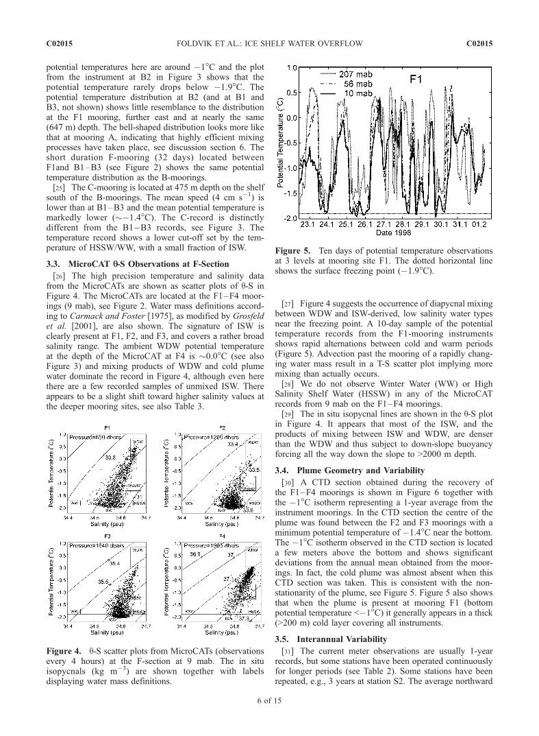
[26] The high precision temperature and salinity datafrom the MicroCATs are shown as scatter plots of q-S inFigure 4. The MicroCATs are located at the F1–F4 moor-ings (9 mab), see Figure 2. Water mass definitions accord-ing to Carmack and Foster [1975], as modified by Grosfeldet al. [2001], are also shown. The signature of ISW isclearly present at F1, F2, and F3, and covers a rather broadsalinity range. The ambient WDW potential temperatureat the depth of the MicroCAT at F4 is �0.0�C (see alsoFigure 3) and mixing products of WDW and cold plumewater dominate the record in Figure 4, although even herethere are a few recorded samples of unmixed ISW. Thereappears to be a slight shift toward higher salinity values atthe deeper mooring sites, see also Table 3.

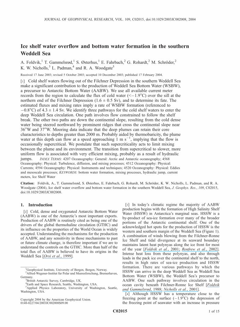
[27] Figure 4 suggests the occurrence of diapycnal mixingbetween WDW and ISW-derived, low salinity water typesnear the freezing point. A 10-day sample of the potentialtemperature records from the F1-mooring instrumentsshows rapid alternations between cold and warm periods(Figure 5). Advection past the mooring of a rapidly chang-ing water mass result in a T-S scatter plot implying moremixing than actually occurs.[28] We do not observe Winter Water (WW) or High

Salinity Shelf Water (HSSW) in any of the MicroCATrecords from 9 mab on the F1–F4 moorings.[29] The in situ isopycnal lines are shown in the q-S plot

in Figure 4. It appears that most of the ISW, and theproducts of mixing between ISW and WDW, are denserthan the WDW and thus subject to down-slope buoyancyforcing all the way down the slope to >2000 m depth.

3.4. Plume Geometry and Variability

[30] A CTD section obtained during the recovery ofthe F1–F4 moorings is shown in Figure 6 together withthe �1�C isotherm representing a 1-year average from theinstrument moorings. In the CTD section the centre of theplume was found between the F2 and F3 moorings with aminimum potential temperature of �1.4�C near the bottom.The �1�C isotherm observed in the CTD section is locateda few meters above the bottom and shows significantdeviations from the annual mean obtained from the moor-ings. In fact, the cold plume was almost absent when thisCTD section was taken. This is consistent with the non-stationarity of the plume, see Figure 5. Figure 5 also showsthat when the plume is present at mooring F1 (bottompotential temperature <�1�C) it generally appears in a thick(>200 m) cold layer covering all instruments.

3.5. Interannual Variability

[31] The current meter observations are usually 1-yearrecords, but some stations have been operated continuouslyfor longer periods (see Table 2). Some stations have beenrepeated, e.g., 3 years at station S2. The average northward

Figure 4. q-S scatter plots from MicroCATs (observationsevery 4 hours) at the F-section at 9 mab. The in situisopycnals (kg m�3) are shown together with labelsdisplaying water mass definitions.

Figure 5. Ten days of potential temperature observationsat 3 levels at mooring site F1. The dotted horizontal lineshows the surface freezing point (�1.9�C).

C02015 FOLDVIK ET AL.: ICE SHELF WATER OVERFLOW

6 of 15

C02015

component at the lower two current meters at the S2 sitein 1977, 1985 and 1987 was 4.9 cm s�1, 5.1 cm s�1 and3.9 cm s�1, respectively. The difference of 1 cm s�1

between these records are within the standard error,�±1.3 cm s�1, see Table 2 and section 2. We are thereforeunable to detect interannual variability in the current on thebasis of the S2 data series. The three years of measurementsat the S2 site may not, however, be strictly comparable. The1987 position was located �2 km west of the 1977 and1985 position, see Table 1. Because of the strong topo-graphical steering on the sill even small differences inposition may cause differences in the current, masking trueinterannual variations.[32] The B1, B2 moorings from 1968 were discussed by

Foldvik et al. [1985b] who noted the total breakdown at bothmoorings of the generally dominant diurnal tidal constitu-ents in July 1968. The moorings were replaced by B3 in1977. The record from B3 showed no collapse of the diurnaltide. On the basis of the temperature records, Foldvik et al.[1985b] speculated that the shelf waters in 1968 were almosthomogenized and thus not able to sustain the baroclinicdiurnal tide; see also the discussion by Middelton et al.[1987]. There was no significant difference in the averagewater speed at the B-moorings between 1968 and 1977.[33] In Figure 7 we have presented one of the longest

records available: the series from FR1, south of the FilchnerSill. This record demonstrates that northward flowing ISWoccupies the deepest layer (below 232 mab) at all times. Theupper instrument (353 mab) shows the influence of intrud-ing MWDW in winter with a corresponding minimum in thenorthward velocity component. The seasonal differences in

Figure 6. Potential temperature distribution at the F-sectionobtained during the recovery of the moorings (ANT XVI/2).The positions of the current meters (circles) and theMicroCATs (squares) are indicated. The one-year averageof the �1�C isotherm obtained from the current-meters isshown by the thick, dashed curve. The average potentialtemperatures (�C) from the MicroCATs are indicated inparentheses. The horizontal distances Li used for transportcalculations are indicated. Tick-marks on the top axis markthe location of the CTD casts.

Figure 7. Time series of filtered (721 hour running average) meridional velocity component (upperpanel) and potential temperature (lower panel) at mooring FR1 south of the Filchner Sill.

C02015 FOLDVIK ET AL.: ICE SHELF WATER OVERFLOW

7 of 15

C02015

the temperature of the ISW are <0.1�C, but the speed variesconsiderably, with a minimum in winter. The average speedat the lower current meter was 6.8 cm s�1 in 1995 and7.2 cm s�1 in 1996. Again, the difference between the yearsis within our estimate of the standard error in the series.[34] In Figure 8 we also show the potential temperature

and salinity records for the MicroCATs on slope mooringsF1–F4 and note the distinct salinity minimum at all moor-ings in winter. We do not see a similarly clear seasonalsignal in the temperature except at F1, which shows atemperature minimum in winter. A direct consequence ofthe seasonal signal in the salinity of the overflow water isthat a corresponding variability would be imprinted on anyWSBW formed by mixing between plume water and theoverlying MWDW/WDW. With typical deep water veloci-ties of 1 cm s�1 the seasonal variability in salinity would bespread over 300 km.

4. Transport of Filchner Overflow Waters

[35] Our main motivation for this study was to calculatethe rate of formation of WSBW that results from theoverflow of cold, dense water from the Filchner region.We use the data sets from the F-section (F1–F4) and theS-section (S2, S3) to determine the volume flux from theshelf.

4.1. Method

[36] In order to compare the transport estimates fromdifferent sections all current meter measurements must bereferred to a common temperature. The water mass in theS-section is almost undiluted ISW, whereas the F-section

shows considerable mixing with MWDW or WDW. Weshall assume that all plume water on the slope is formed bythe mixing of cold shelf water originally at potentialtemperature qI with warmer water (WDW or MWDW) ofpotential temperature qw. A water parcel of temperature qithen consists of Ri parts of cold water and (1 � Ri) parts ofWDW, where

Ri ¼qw � qiqw � qI

The flux of dense, cold water converted to potentialtemperature qI is then vn,iRi where vn,i denotes the observedvelocity component normal to the section. Thus the time-averaged flux of this cold water measured by a currentmeter (per unit area) becomes

fn ¼1

N

Xvn;i � Ri ð1Þ

where N denotes the number of observations. The values ofqw for the F-section have been obtained from the potentialtemperature plots in Figure 3 (the high temperature cut-off)and CTD sections. Table 4 lists the values for qw and fn. Thecalculated fluxes are relatively insensitive to qw: a variationin qw of 0.1�C changes the calculated transport by <2%. Forthe S-section we have derived qw from CTD sections only.High variability on the shelf makes the determination of qwdifficult and somewhat arbitrarily we have put qw = 0.0�C.However, at the S section the temperatures are close to qIand the choice of qw is not important. The results are more

Figure 8. Time series of filtered (721 hour running average) potential temperature and salinity fromMicroCAT instruments on section F.

C02015 FOLDVIK ET AL.: ICE SHELF WATER OVERFLOW

8 of 15

C02015

sensitive, however, to the reference temperature selected forthe cold water. We use a value for qI of �1.9�C, the freezingpoint of seawater at surface pressure. If this referencetemperature had instead been set at �2�C then the flux ofcold shelf water would be reduced by approximately 10%.The calculated rate of bottom water production is unaffectedby the value of qI.[37] The flux of cold q = qI water recorded at a current

meter mooring (per unit width) then becomes

Fn ¼Z

fndz ð2Þ

[38] The vertical integration was carried out using anobjective but necessarily arbitrary approach in which eachinstrument is taken to represent the section of water columnfrom halfway to the instrument below to halfway to theinstrument above. For the deepest instrument the integrationstarts at the bottom, whereas the upper instrument isassumed to represent a water column equal to the distancebetween the two upper instruments. Note that we haveassumed that all plumes are derived from cold shelf waterof potential temperature �1.9�C. All plumes with potentialtemperature below the ambient temperature qw contribute tothe flux of the cold shelf water. This model does notdiscriminate between ISW and HSSW.[39] Finally, the transport of cold shelf water, F, is

obtained from the flux vectors Fn,j(2), thus

F ¼X

LjFn;j ð3Þ

The summation in (3) goes over the number of current metermoorings and Lj denotes the length of the section to berepresented by that mooring. The values of Lj aredetermined by the midpoints between moorings (Figure 6).The choice of the Lj at the flanks is discussed below. Theerror bars on the transport calculations are related to the

geometry of the plume and are additional to the standarderrors of the time series of water velocity (see section 2).

4.2. Transport Estimate for the S-Section

[40] We estimate the northward transport of cold water atthe sill of the Filchner Depression using the S-section datafor 1985, when records from the S2 and the S3 mooringswere available simultaneously. Data from the S2-mooringare also available for 1977 and 1987; see our remarks insection 3.5 on interannual variability.[41] Figure 9 shows the extent of ISW, defined by the

�1.9�C isotherm, from CTD measurements made along theS-section during several Antarctic summer cruises. Thesesnapshots suggest that the border of cold water is locatedbetween the 400- and 500-m isobaths on the west side of theFilchner Depression and between the 500- and 600-misobaths on the east side. We use these observations todetermine the L1 and L2 parameters for the S-section (seeFigure 9 and Table 4). Figure 9 gives the impression of asloshing motion of the ISW in the Depression, that is, there

Table 4. Transport of Cold Shelf Water Through the S-Section (1985) and the F-Section (1998)a

Mooring Name Instr. Number Obs Dep., m mab, m qw, �C D, m Fn, cm/s L, km Transport, Sv

S2 3160 355 190 0.0 90 2.1 0.1S2 4223 445 100 0.0 83 4.1 0.2S2 7716 520 25 0.0 63 6 65 0.2S3 3164 510 100 0.0 173 6.3 0.8S3 4277 580 25 0.0 63 7.2 72 0.3Transport S-section 1.7

F1 9192 440 207 0.7 150 14.5 0.2F1 7717 591 56 0.6 98 28.9 0.3F1 10909 637 10 0.6 33 26.5 11 0.1F2 4040 747 433 0.6 230 0.5 0.0F2 5294 978 207 0.5 188 4.0 0.1F2 9193 1124 56 0.5 98 13.2 0.2F2 10907 1170 10 0.5 33 16.0 14 0.1F3 7066 1224 413 0.4 358 0.1 0.0F3 9403 1581 56 0.3 208 10.1 0.4F3SC 139 1630 9 0.2 33 13.0 18 0.1F4 9708 1777 207 0.2 150 0.2 0.0F4 9194 1928 56 0.1 98 0.2 0.0F4 9195 1974 10 0.1 33 2.0 20 0.0Transport F-section 1.5

aThe columns show: mooring name, instrument number, depth of instrument, distance of instrument above bottom, qw is the environmental potentialtemperature used for transport calculations, D denotes the thickness of the water column assigned to each instrument, Fn is the flux vector according toequation (1), L is the distance assigned to each mooring and the transport is given in Sverdrup (106 m3 s�1).

Figure 9. Position of the �1.9�C isotherms at the FilchnerSill along the S-section obtained from different summerexpeditions. The current meter positions are indicated, andL1, L2 show the lengths used for transport calculations.

C02015 FOLDVIK ET AL.: ICE SHELF WATER OVERFLOW

9 of 15

C02015

is a tendency for the cold water to be located higher on thewestern side when it is lower on the eastern side, and viceversa. This implies a certain reduction of the combined errorbounds on L1 + L2, although this is not taken into account inthe error estimates below.[42] The data from the upper instrument (190 mab) on the

S2 mooring show that about 15% of the measurements arebelow �1.9�C whereas at the instrument below (100 mab)85% of the measurements are below �1.9�C. For thepurposes of this calculation, therefore, we assume that theaverage position of the �1.9�C isotherm is around 145 mab.This position is in reasonable agreement with the CTDobservations in Figure 9.[43] The two current meters at S3 are not sufficient to

resolve the thickness of the cold-water layer at that site.From Figure 9, however, it seems reasonable to assume theaverage thickness of ISW to be the same as at S2. To reflectthis argument the upper instrument at S3 has been takento represent a correspondingly thicker water column (seeTable 4). Since the upper instrument at S2 shows smallervelocities than below it, this procedure might lead to aslight overestimate of the transport at S3.[44] Using the above methodology, we estimate that the

transport across the S-section (Table 4) during 1985 was1.7 ± 0.5 Sv. The error estimate is related to the Lj values onthe flanks, the thickness allocated to the upper instrumentand the standard error of the mean current.

4.3. Transport Estimate for the F-Section

[45] The in situ isopycnal lines (referenced to 650 m) atF1 are shown in the q-S plot in Figure 4a. It appears thatISW and its mixing products are usually denser than WDWand thus capable of sinking further down the continentalslope. However, some of the cold, low salinity water atmooring F1 appears to be slightly lighter than the core ofWDW. In order not to overestimate the contribution of coldshelf water at F1 we eliminate from the transport estimateall water appearing lighter than the core value of the WDW,�30.89 kg m�3. Thus all observations having in situdensities less than 30.89 kg m�3 are excluded from theintegration (2). This excludes 17% of the observations. Thesensitivity of the choice for the limiting isopycnal wastested by bracketing the selection: choosing 30.88 kg m�3

and 30.90 kg m�3 results in excluding 7% and 24% ofobservations, respectively.[46] As seen from Figure 2 and Table 2, the velocities are

very high at the F1 mooring. This implies that our calcu-lation of cold-water flux using equation (3) is quite sensitiveto the determination of the assigned cross-slope length L1.As mentioned above, the border of cold shelf water at theS-section was located between the 400- and 500-m isobaths.Since the flow on the shelf is so strongly controlled bytopography, and since the distance between the shallow sideof these two sections is rather short, we shall assume thatthe same borders apply to the S- and F-sections: i.e., sincethe out-flowing cold water resides over the 400-m isobathat the S-section, we assume that the edge of the cold waterplume is near the 400-m isobath at the F- section. Theconsequent choices of L-values are shown in Figure 6.[47] With these choices (3) implies that the flux of

�1.9�C water leaving the shelf through the F-section in1998 was 1.5 ± 0.3 Sv (see Table 4). In addition to the

standard error of the mean current (section 2) the largestcomponents in the estimated error are the value of L1 andthe choice of isopycnal determining the data points thatcontribute to the estimate of the F1 flux. Within the errorbounds, the transport of ISW over the Filchner sill is thesame as through the F-section, however flow rates are muchhigher in the latter section. The weak stratification suggeststhat most of the flow will follow lines of constant f/H: theacceleration arises because the isobaths converge dramati-cally between the sill and the F-section.

5. Production of WSBW

[48] Having computed the flux of cold (<�1.9�C) waterleaving the shelf we may now estimate the rate of change ofmass flux based on the observed hydrography. We assumethat WDW is entrained into the cold plume and that noplume water is detrained into the overlying WDW. Thisassumption is supported by CTD measurements from thearea over several field seasons (see, for example, the 1990measurements shown in Figure 10). The general impressionfrom CTD measurements, from the yearlong MicroCATrecords shown in Figure 4 and from the potential temper-ature records from D1 (Figure 3) is that the cold shelf watersometimes reaches depths greater than 2000 m with littlemixing with the overlying water.[49] We denote the plume properties with the index p, the

properties of the WDW with the index w and entrainmentwith the index e. As a result of entrainment of me of theoverlying WDW, a parcel of plume water mp increases itsmass by dmp and its temperature by dqp. Continuity of heatand mass is then expressed by

mpqp þ meqw ¼ qp þ dqp� �

mp þ dmp

� �ð4Þ

where

me ¼ dmp

thus

qw � qp � dqp� �

dmp ¼ mpdqp ð5Þ

In (5) the second order term will be neglected. The equationmay then be integrated to obtain

mp;1 ¼ mp;0e

R10

dqpqw�qp

: ð6Þ

(A similar equation applies based on the continuity of salt).[50] Here index 0 and 1 refer to the initial and to the end

state, respectively. The integral in (6) may easily be calcu-lated by stepwise integration since the temperatures of theWDW and the plume are known (see Figure 10). Since thetemperature of the WDW decreases with depth it followsthat the production of deep-water is more efficient when themixing takes place at large depths.[51] Note that if qw is constant (6) takes the form

mp;1 ¼ mp;0

qw � qp� �

0

qw � qp� �

1

: ð7Þ

C02015 FOLDVIK ET AL.: ICE SHELF WATER OVERFLOW

10 of 15

C02015

If all mixing did take place at 2000 m depth then Figure 10gives qw as 0.0�C, qp,0 = �1.9�C, and qp,1 = �0.8�C.Thus we obtain mp,1 = 2.5 mp,0, that is, the production ofbottom water referenced to �0.8�C is 2.5 times the flux ofcold water leaving the shelf. If the mixing took place at3000 m depth, however, where qw = �0.2�C, we obtainmp,1 = 3mp,0. Stepwise integration of (6) using values ofqw from Figure 10 gives mp,1 = 2.7mp,0. This compareswell with model experiments by Killworth [1977] andAlendal et al. [1994] who found that the volume flux at2000 m depth should increase by 2 to 3 times the initialvalue. In the following we apply the factor 2.7 to estimatethe production of WSBW. In a recent theoretical studyHolland et al. [2002] find that the volume flux should

increase by a factor close to two due to mixing in a singlestrong hydraulic jump. When the effects of increasedbuoyancy due to thermobaricity, boundary layer mixing,and shear instability are considered, the factor 2.7 adoptedabove seem reasonable.

6. Discussion

[52] The broad picture that emerges from the data pre-sented here is that large volumes of cold shelf water flownorthward over the sill in the Filchner Depression andtoward the continental shelf break. At moorings S2 andS3, located on Filchner Sill, the deepest instruments indicatepure ISW with very small temperature variance. The flowaccelerates as it descends the upper slope, turns to the left(westward) under the influence of the Coriolis force andaccelerates further as the continental slope from 400–700 mdepth steepens (isobaths converge) between the FilchnerDepression and the F-section. The further fate of the flowdepends on both internal plume dynamics and the localforcing, such as the phase of time dependent phenomenalike tides, shelf waves, the position of the Antarctic SlopeFront, and weather forcing. Below we consider some factorsthat determine the pathways of cold shelf waters enteringthe deep Weddell Sea circulation.

6.1. Short-Term Variability

[53] The B1, B2 and B3 records were discussed byFoldvik et al. [1985b] who noted the exceptionally strongdiurnal tidal currents near the shelf break. Tides in the areaare also discussed by Middelton et al. [1987], Foldvik et al.[1990], Robertson et al. [1998] and Padman and Kottmeier[2000]. In addition to the strong tidal regime we observemarked wave disturbances at lower frequency on the slope.Figures 11a and 11b show 10- and 12-day segments of thede-tided current meter records from the F1 and F4 moor-ings, respectively. At F1 the average current dominates andhas wave disturbances superimposed. At F4 the meancurrent is weaker and the flow is dominated by strong shelfwaves with periods of �3–6 days. Such waves may causecross-slope advection and thus be important for the fate ofthe cold plumes. The structure of low-frequency (weatherband) shelf waves on the southern Weddell Sea continental

Figure 10. Ensemble of q-S profiles at the slope obtainedduring the Norwegian Antarctic Expedition 1990. Thelocation of the section is shown in Figure 1b.

Figure 11. Twelve days of the de-tided current vectors10 mab, displayed at 4-hour intervals, at F1 (upper panel)and F4 (lower panel).

C02015 FOLDVIK ET AL.: ICE SHELF WATER OVERFLOW

11 of 15

C02015

slope was discussed by Middelton et al. [1982], whileFoster et al. [1987] discussed the potential role ofthese waves on water mass transformation along the shelfbreak.

6.2. Comments on Plume Dynamics

[54] The frequency of ISW at the F1, F2, F3 and F4moorings, defined by the relative number of observationsof potential temperature below the surface freezing point, is8%, 27%, 28% and 1%, respectively. These observations areconsistent with ISW flowing over the sill and being turnedwestward by the Coriolis force. They also show that thecoldest plumes rapidly advance down, as well as along theslope.[55] There are two main dynamical reasons why the cold

plumes occasionally may reach the deepest current metersites (F4 and D1) without significant water mass modifica-tion. First, the decrease in buoyancy as a result of mixing iscounteracted by the thermobaric effect [Killworth, 1977], thatis, the increase in density with increasing pressure is larger inthe cold plumes than in the adjacent WDW. This effect isclearly revealed by comparing the MicroCAT plots inFigure 4, where the density contrast between the WDW andthe bulk of the ISW is seen to increase with depth. Second,from density profiles calculated from CTDmeasurements wemay estimate the phase speed, c =

p(g0H), for long waves at

the ISW-WDW interface. Here H denotes the thickness ofthe plume, g0 = g�r/r is the reduced gravity and�r/r denotesthe interfacial relative density anomaly. We find maximumphase speeds of about 0.4 m s�1, obtained for a plumethickness 200 m (indicated by the cold water events inFigure 5) and interfacial relative density anomaly of 1.0 10�4 kg m�3 (as defined by the typical difference betweenobserved density and the WDW density in Figure 4). InFigure 12 we show the joint distribution of q and |U| nearthe sea-bed at 4 moorings, F1, F2, D2 and D1. Dependingon the actual thickness of the plume, the distribution of |U|suggests that at each site, the flow is supercritical (that is,the plume speed is larger than the internal phase speed) forsome fraction of each total record. For supercritical flows,resonance waves (lee waves) do not form. Thus theassociated mesoscale mixing behind irregularities in thebottom topography is strongly reduced [Long, 1954]. Thesedense plumes may therefore reach great depths with littlemixing and much reduced friction. The strong correlationbetween high speed and low temperature at D1 and D2(Figure 12) supports our view of the efficiency of thismechanism.

6.3. Supercritical Flows and Mixing

[56] On the continental slope the overflowing shelf watersmay attain supercritical speed as a result of flow conver-gence and/or down-slope buoyancy forcing aided by ther-mobaricity. Flow convergence accelerates the entire watercolumn and does not discriminate between water types,whereas down-slope buoyancy forcing aided by thermobar-icity acts only on the cold plumes. This is clearly demon-strated in the potential temperature-speed plots in Figure 12where a strong correlation is clearly visible between highspeed and low temperatures at moorings D1 and D2, but notat moorings F1 and F2. The transition to sub-critical speedtakes place when the slope becomes less steep and may be

accompanied by violent mixing associated with a hydraulicjump, [Long, 1954; Holland et al., 2002].[57] The average speed at F1 is very high (45 cm s�1)

and much of the flow at F1 is believed to be supercrit-ical. At mooring F the speed is reduced but still high(20 cm s�1) whereas at the B-moorings the speed is low(6 cm s�1). These differences seem to be governed byisobath divergence (Figure 2). The temperature distribu-tion at F1 is quite different from that at the S-moorings(Figure 3). The variance is large, with a sharp lower cut-off at �2.0�C determined by the parent ISW, and apotential temperature maximum (0.5�C at 10 mab) deter-mined by the temperature of the overlying WDW/MWDW. The temperature distributions at the F-mooring(only 32 days long) and the B-moorings are entirelydifferent to that from F1. The lower cut-off is absent,the frequency distribution is nearly bell-shaped and themean temperature is close to �1.0�C. Since much of theflow changes from supercritical to sub-critical between F1and the F we believe that this shift in temperaturedistribution accomplished over such a very short distance(�20 nm) is mostly due to mixing by hydraulic jumps.Such mixing of plume water with overlying WDW willsystematically increase the temperature of the watersamples, as observed. Cross-slope advection may alsoaffect the temperature distributions, but cross-slope ad-vection of (sharp) frontal gradients tends to produce atwo-peak distribution with upper and lower cut-offs.[58] The C- mooring on the nearby shelf (Figure 2)

yielded a temperature distribution (Figure 3) with a sharplower cut-off and a mean potential temperature close to�1.5�C. This is shelf water, WW or HSSW with a minorcontribution of ISW, and does not reveal the samemixing history as that at the neighboring F- and theB-moorings.[59] Much of the overflow descends as bottom-trapped

cold plumes east of �37�W. The highest fraction of ISW

Figure 12. Scatter plots of potential potential tempera-ture versus speed for selected current-meter records closeto the bottom. See Figure 1b and Table 2 for locationsand details.

C02015 FOLDVIK ET AL.: ICE SHELF WATER OVERFLOW

12 of 15

C02015

is found in the F-section at moorings F2 and F3, that is,between the �1200- and �1600-m isobaths (see Figure 6),with an average potential temperature of �1.67�C and�1.52�C, respectively. At the continental slope east of38�W the variability of currents and temperature is high(Table 2 and Figures 3, 11 and 12). The temperaturedistributions at F2 and F3 show a sharp lower cut-off setby the temperature of the ISW at the sill, but no clearupper cut-off at the temperature of the WDW. Thisindicates that very little mixing has taken place betweenthe plume and the overlying water during the journeyfrom the sill to the F2- and F3-moorings. As discussed insection 6.2, a low level of mixing is consistent with thesuppression of resonance wave-induced meso-scale mix-ing in the often-supercritical flow observed at F2 and F3(Figure 12). West of the F-section the cold flow encoun-ters rough topography, including two prominent ridges.On the basis of the map in Figure 2 we anticipate thatmost of the flow passing between F2 and F3 will besteered by the ridge between 38�W and 37�W. On thewestern side of that ridge the topography appears lesssteep and a transition from supercritical to sub-criticalflow is likely, with consequent mixing in hydraulicjumps. Mooring A is located near the 2000-m isobathand �100 km downstream from F2–F3. Temperaturesrecorded at this mooring are consistent with the abovepicture, indicating only the product of mixing betweenWDW and ISW, and not the parent water masses them-selves (Figure 3). The cold plume therefore never reachesthis location. At mooring A the water is well mixed withan average potential temperature of �1.37�C at 25 maband only slightly higher (�1.25�C) at 125 mab. Thetemperature distribution at A is the signature of a newboundary layer water mass: Newly Formed WSBW,produced by mixing of cold shelf water plumes (ISW/HSSW) and warmer WDW. Since there is no sign ofWDW at the upper instrument (125 mab) the averagethickness of this boundary layer must be well above125 m, say �200 m thick. The width of the layer must belarger than the horizontal excursion from shelf waves, onthe order of 70 km in the example in Figure 11b. At anaverage speed of �9 cm s�1, the above figures indicate atransport within this boundary layer of �0.8 Sv whenreferenced to �1.9�C.[60] The high north-eastward mean speed at mooring D1

(see Figure 2) is surprising, given its proximity to mooringF4 which has a much weaker mean flow. The ridgeextending across the slope near 36�W (see Figure 2) mustplay a major role in steering this benthic flow. On the basisof local topography, CTD observations and observed ve-locities (Table 2) we have estimated the volume transport atD1 to be �0.2 Sv. The bell-shaped temperature distributionat D1 is similar to that at F and B1-3 which we attributed tomixing during hydraulic jumps. However, a large portion ofthe observations at D1 show supercritical flow which mayindicate the subsequent acceleration by flow convergence asthe flow encountered the ridge at 36�W. The temperaturedistribution at mooring D2 shows clear upper and lower cut-offs set by the temperatures of WDWand ISW, respectively.The minimum separating the two peaks in Figure 3 suggeststhat little mixing has taken place. The average potentialtemperature at D2 (�0.47�C) is higher than at D1

(�1.10�C), indicating that the flow at D2 has a lowercontribution from cold plumes. This suggests that thelocation of mooring D2 is near the deep limit for coldplumes on the slope.

6.4. Plume Pathways

[61] On the basis of the above interpretation of observa-tions we have identified three pathways for the FilchnerOverflow (FO) waters (Figure 1b):[62] The FO1 path involves flow crossing the F-section

near mooring F1 and being constrained to flow along theshelf break and upper slope. The FO1 plume is presumablylocated slightly down-slope of the F- and B1–B3 mooringsand was detected by the dense network of five CTD sectionscovering the shelf and slope between 37�W and 40�W[Foster et al., 1987]. These sections show cold water(��1�C) centred on the slope, located between approxi-mately 600 and 800 m depth. Presumably, the water in FO1will continue westward in quasi-geostrophic balance withonly a slow down-slope migration.[63] The FO2 path is taken by cold plumes crossing the

F-section in the area of F2 and F3 and arriving in the area ofthe mooring A as a well-mixed boundary layer water mass.FO2 appears in the CTD section reported by Foster andCarmack [1976] as a distinct, cold (<�0.8�C) layer locatedbetween 2000 m and 3500 m depth. FO2 also appears in allfive CTD sections reported by Foster et al. [1987] as a cold,low salinity boundary current located around 2000 m depth.Like FO1, the well-mixed FO2 waters may continue west-ward in quasi-geostrophic balance, only slowly increasingin depth.[64] The FO3 path is represented by the high speed

current at mooring D1, directed toward the NE by theridge close to 36�W (Figure 2). Since the flow at D1 ispartly supercritical further strong mixing must be expecteddownstream as the slope becomes less steep.[65] The width of the arrows in Figure 1b is not indicative

of the relative strength of these currents, although thevolume flux of FO3 is probably the smallest. The highvariability on the slope implies variability in the location ofthese pathways (see also the CTD sections of Foster et al.[1987]). In addition to the pathways identified above (andpossibly others that have escaped our sparse network ofinstruments) an Ekman mass flux is directed downslope inthe benthic layer, aided by thermobaricity. This thin, cold,bottom layer is observed in almost every CTD cast in theoverflow area in which the instrument is lowered close tothe sea floor. Tanaka and Akitomo [2000] find that theEkman transport in the Weddell Sea contributes �1 Sv tothe formation rate of WSBW.[66] The above interpretation of currents suggests that

the ultimate fate of cold shelf waters emanating from theFilchner Depression depends upon the depth that theplume reaches shortly after crossing the sill. This in turndepends on such factors as the location (depth) the plumecrosses the sill, high-frequency variability due to tidalmotion, shelf waves and instabilities in the AntarcticSlope Front. Processes such as these are able to advectfluid parcels across a wide range of depths, so that theflow of ISW may quickly be switched between a ‘‘shelf-break’’ path and a mid-slope path. Once advected to acritical depth on the slope thermobaricity takes hold and

C02015 FOLDVIK ET AL.: ICE SHELF WATER OVERFLOW

13 of 15

C02015

an ISW parcel is unable to return. The possibility thathigh-frequency processes determine the fate of ISWsuggests that ISW ‘‘plumes’’ may be better consideredas variable streams of ISW filaments or eddies. If this isthe case, simple steady state models of plumes [e.g.,Killworth, 1977] may not correctly represent the pathwaysand mixing of shelf-derived cold water.

6.5. Transport of Cold Shelf Water

[67] The calculated transport of cold shelf water cross-ing the S-section (Figure 9), 1.7 ± 0.5 Sv, is notsignificantly different from the 1.5 ± 0.3 Sv calculatedfor the F-section (Figure 6). The agreement between theseestimates is remarkable considering they have beenobtained for different sections and for different years.The implications of this agreement are firstly, that all thewater leaving the sill (via the S-section) later passesthrough the F-section, none passing higher or lower onthe slope, and second, that the transport has not changedsignificantly over the 13-years that separated the S- andF-section deployments. A large fraction of the overflow atthe Filchner Sill originates as HSSW formed north ofRonne Ice Front (Figure 1) and flows around BerknerIsland before arriving at the sill of the Filchner Depres-sion [Foldvik et al., 2001; Nicholls et al., 2001]. Datafrom moorings installed beneath the ice shelf at thesouthern tip of Berkner Island indicate large interannualvariability in the flow, which could lead to a similarsignal in the overflow [Nicholls and Østerhus, 2003]. Amajor geophysical event occurred in the Filchner Depres-sion in August 1986, between the two S2 deployments in1985 and 1987. Giant icebergs broke away from FilchnerIce Shelf and subsequently grounded north of BerknerIsland. Some change in the outflow would therefore beexpected between 1985 and 1987 [Nøst and Østerhus,1998; Grosfeld et al., 2001]. However, as discussed insection 3.5 the estimated fluxes for 1985 and 1987 agreewithin the error bounds. We are not able to detectsignificant inter annual variations in the outflow.

[68] We conclude that the volume transport of the cold(�1.9�C) shelf water plume leaving the area of the FilchnerDepression in the southern Weddell Sea is

F ¼ 1:6� 0:5Sv: ð8Þ

6.6. Production of WSBW

[69] Production of WSBW by mixing cold and denseshelf waters (ISW) with overlying WDW was discussed insection 5. From (8), and using the conversion factor of 2.7found in section 5, the production of newly formed WSBW,referenced to �0.8�C, becomes:

FWSBW ¼ 4:3� 1:4Sv: ð9Þ

[70] Table 5 lists estimates of WSBW production ratesobtained by different authors using widely differentapproaches. Our estimate lies near the upper end of previ-ously published assessments.[71] Our estimate of the formation rate of WSBW is a

lower bound on the rate of production from the region as awhole, as it does not account for sources other than theFilchner outflow (for example, shelves in the westernWeddell Sea) [Gordon et al., 1993]. We assume, however,that the FO1 plume identified at �40�W and at 600–800 mdepth descends slowly along the western continental marginand therefore is likely to cross the section with long termmoorings on the continental slope off the Antarctic Penin-sula where a transport of WSBW of 1.3 ± 0.4 Sv wasestimated by Fahrbach et al. [2001]. Also, the FO1 is likelyto cross from west to east the track of Ice Station Weddell[Muench and Gordon, 1995], consistent with the observa-tions and analysis of Weppernig et al. [1996]. Some of the2–3 Sv of newly formed WSBW detected at the driftingstation might therefore originate in the Filchner area.

[72] Acknowledgments. The authors wish to express their gratitudeto the researchers and ship crews from all the expeditions to the region ofthe Filchner overflow that have contributed to this study. The oceanography

Table 5. Estimate of WSBW Production Ratesa

Authors MethodProductionRate Sv

WSBWTemperature

Carmack and Foster [1975] Deep sea current measurements, geostrophy and budget estimates. 2–5 �0.8�Cb

Foster and Carmack [1976] Heat and salt budget and shelf break mixing model 3.6 �1.3�CWeiss et al. [1979] Isotope data: d18O (Tritium) 5 (2.9) <�0.9�CFoldvik et al. [1985a] Currentmeter moorings at Filchner sill and hydrography 2–5 �0.8�CGordon et al. [1993] Ice Station Weddell, hydrography 3 <�0.8�CFahrbach et al. [1995] Joinville - Kap Norvegia transect, currentmeter moorings and hydrography 2.2c <�0.7�CMuench and Gordon [1995] Ice Station Weddell, current measurements and hydrography 2.5–3 �0.8�CWeppernig et al. [1996] Ice Station Weddell drift track. Isotope data. 5 �0.7�CMensch et al. [1997] Tritium and CFC data. Southern and western Weddell Sea. 3.5 <�1�CMensch et al. [1998] Tritium and CFC data from Ice Station Weddell drift track. 5e �0.8�CGordon [1998] Ice Station Weddell, hydrography and current measurements. 3–4 < �0.7�Cd

Fahrbach et al. [2001] Joinville - Kap Norvegia transect, multi year currentmeter moorings and hydrography 1.1–1.5 �0.7�CGordon et al. [2001] Current profiler and hydrography. Ice Station Weddell and DOVETAIL data. 5 <�0.7�CNaveira Garabato et al. [2002] Current profiler and hydrography 4.5 ± 0.9 <�0.7�CThis study Current measurements and hydrography 4.3 ± 1.4 <�0.8�C

aUpdated from Orsi et al. [1999].bProduced with shelf water temperature between �1.2�C and �1.4�C.cVarying between 0.8 Sv and 3.9 Sv.dAverage temp. �1.1�C.eProduced west of the drift track.

C02015 FOLDVIK ET AL.: ICE SHELF WATER OVERFLOW

14 of 15

C02015

programmes on all Norwegian Antarctic Research Expeditions have beensupported by the Norwegian Research Council who also supported partic-ipation in other expeditions. We gratefully acknowledge this long-termsupport. L.P. was funded by the National Science Foundation, grant OPP-9896006.

ReferencesAlendal, G., H. Drange, and P. M. Haugan (1994), Modelling of Deep-Seagravity currents using an integrated plume model, in The Polar Oceansand their Role in Shaping the Global Environment, Geophys. Monogr.Ser., vol. 84, edited by O. M. Johannessen, R. D. Muench and J. E.Overland, pp. 237–246, AGU, Washington, D. C.

Carmack, E. C., and T. D. Foster (1975), Circulation and distribution ofoceanographic properties near the Filchner Ice Shelf, Deep Sea Res., 22,77–99.

Fahrbach, E., and S. el Naggar (2001), The Expeditions ANTARKTIS XVI/1–2 of the Research Vessel ‘‘POLARSTERN’’ in 1998/1999, Ber. Polar-und Meeresforsch., 380, 177 pp.

Fahrbach, E., G. Rohardt, N. Scheele, M. Schroder, V. Strass, andA. Wisotzki (1995), Formation and discharge of deep and bottom waterin the northwestern Weddell Sea, J. Mar. Res., 53, 515–538.

Fahrbach, E., S. Harms, G. Rohardt, M. Schroder, and R. A. Woodgate(2001), Flow of bottom water in the Weddell Sea, J. Geophys. Res., 106,761–778.

Foldvik, A., and T. Gammelsrød (1988), Notes on southern-ocean hydro-graphy, sea-ice and bottom water formation, Paleogeogr. Paleoclimatol.Paleoecol., 67, 3–17.

Foldvik, A., T. Gammelsrød, and T. Tørresen (1985a), Circulation andwater masses on the southern Weddell Sea shelf, in Oceanology of theAntarctic Continental Shelf, Antarct. Res. Ser., vol. 43, edited by S. S.Jacobs, pp. 5–20, AGU, Washington, D. C.

Foldvik, A., T. Kvinge, and T. Tørresen (1985b), Bottom currents near thecontinental shelf break in the Weddell Sea, in Oceanology of the Antarc-tic Continental Shelf, Antarct. Res. Ser., vol. 43, edited by S. S. Jacobs,pp. 21–34, AGU, Washington, D. C.

Foldvik, A., J. H. Middleton, and T. D. Foster (1990), The tides of thesouthern Weddell Sea, Deep Sea Res., 37, 1345–1362.

Foldvik, A., T. Gammelsrød, E. Nygaard, and S. Østerhus (2001), Currentmeasurements near Ronne Ice Shelf: Implications for circulation andmelting, J. Geophys. Res., 106, 4463–4477.

Foster, T. D., and E. C. Carmack (1976), Frontal zone mixing and AntarcticBottom Water formation in the southern Weddell Sea, Deep Sea Res., 23,301–317.

Foster, T. D., A. Foldvik, and J. H. Middleton (1987), Mixing and bottomwater formation in the shelf break region of the southern Weddell Sea,Deep Sea Res., 34, 1771–1794.

Gammelsrød, T., A. Foldvik, O. A. Nøst, Ø. Skagseth, L. G. Anderson,E. Fogelqvist, K. Olsson, T. Tanhua, E. P. Jones, and S. Østerhus(1994), Distribution of water masses on the continental shelf in thesouthern Weddell Sea, in The Polar Oceans and Their Role in Shapingthe Global Environment, Geophys. Monogr. Ser., vol. 84, edited by O. M.Johannessen, R. D. Muench, and J. E. Overland, pp. 159–176, AGU,Washington, D. C.

Gordon, A. L. (1998), Western Weddell Sea thermohaline stratification, inOcean, Ice and Atmosphere: Interactions at the Antarctic ContinentalMargin, Antarct. Res. Ser., vol. 75, edited by S. S. Jacobs and R. F.Weiss, pp. 215–240, AGU, Washington, D. C.

Gordon, A. L., B. A. Huber, H. H. Hellmer, and A. Ffield (1993), Deep andbottom water of the Weddell Sea’s western rim, Science, 262, 95–97.

Gordon, A. L., M. Visbeck, and B. Huber (2001), Export of Weddell Seadeep and bottom water, J. Geophys. Res., 106, 9005–9017.

Grosfeld, K., M. Schroder, E. Fahrbach, R. Gerdes, and A. Mackensen(2001), How iceberg calving and grounding change the circulation andhydrography in the Filchner Ice shelf: Ocean system, J. Geophys. Res.,106, 9039–9055.

Holland, D. M., R. R. Rosales, D. Stefanica, and E. G. Tabak (2002),Internal hydraulic jumps and mixing in two-layer flows, J. Fluid Mech.,470, 63–83.

Killworth, P. D. (1977), Mixing on the Weddell Sea continental slope, DeepSea Res., 24, 427–448.

Long, R. R. (1954), Some aspects of the flow of stratified fluids: II. Ex-periments with a two- fluid system, Tellus, 2, 97–115.

Mensch, M., R. Bayer, J. L. Bullister, P. Schlosser, and R. F. Weiss (1997),The distribution of Tritium and CFCs in the Weddell Sea during the Mid1980s, Progr. Oceanogr., 38, 377–414.

Mensch, M., W. M. Smethie Jr., P. Schlosser, R. Weppernig, and R. Bayer(1998), Transient tracer observations from the western Weddell Sea dur-ing the drift and recovery of Ice Station Weddell, Antarctic Res. Ser., 75,241–256.

Middelton, J. H., T. D. Foster, and A. Foldvik (1982), Low-frequencycurrents and continental shelf waves in the Southern Weddell Sea,J. Phys. Oceanogr., 12, 618–634.

Middelton, J. H., T. D. Foster, and A. Foldvik (1987), Diurnal Shelf Wavesin the Southern Weddell Sea, J. Phys. Oceanogr., 17, 784–791.

Millero, F. J. (1978), Freezing point of sea water, Eighth Report of the JointPanel of Oceanographic Tables and Standards, Appendix 6, UNESCOTech. Pap. Mar. Sci., 28, 29–31.

Muench, R. D., and A. L. Gordon (1995), Circulation and transport of wateralong the western Weddell Sea margin, J. Geophys. Res., 100, 18,503–18,515.

Naveira Garabato, A. C., E. L. McDonagh, D. P. Stevens, K. J. Heywood,and R. J. Sanders (2002), On the export of Antarctic Bottom water fromthe Weddell Sea, Deep Sea Res., 49, 4715–4742.

Nicholls, K. W., and S. Østerhus (2003), Interannual variability beneathFilchner - Ronne Ice Shelf, Antarctica, in Filchner Ronne Ice Shelf Pro-gramme, Rep. 14, edited by H. Oerter, Alfred-Wegener-Inst. for Polar andMarine Res, Bremerhaven, Germany.

Nicholls, K. W., S. Østerhus, K. Makinson, and M. R. Johnson (2001),Oceanographic conditions south of Berkner Island, beneath Filchner-Ronne Ice Shelf, Antarctica, J. Geophys. Res., 106, 481–492.

Nordlund, N. (1992), Bottom currents at the Continental slope in theSouthern Weddell Sea (in Norwegian), Cand.Sci. thesis, Univ. of Bergen,Bergen.

Nøst, O. A., and S. Østerhus (1998), Impact of grounded icebergs on thehydrographic conditions near the Filchner Ice Shelf, in Ocean, Ice andAtmosphere: Interactions at the Antarctic Continental Margin, Antarct.Res. Ser., vol. 75, edited by S. S. Jacobs, and R. F. Weiss, pp. 267–284,AGU, Washington, D. C.

Nygaard, E. (1994), Transport of ice shelf water in the Weddell Sea (inNorwegian), Can. Sci. thesis, Univ. of Bergen, Bergen.

Orsi, A. H., G. C. Johnson, and J. L. Bullister (1999), Circulation, mixingand production of Antarctic bottom water, Prog. Oceanogr., 43, 55–109.

Østerhus, S., and R. A. Krause (1990), Ausbringung und Bergung vonozeanographischen Verankerungen. Die Expedition ANTARKTIS-Vmit FS ‘‘Polarstern’’ 1986/87, Ber. zur Polarforschung, 57.

Padman, L., and C. Kottmeier (2000), High-frequency ice motion anddivergence in the Weddell Sea, J. Geophys. Res., 105, 3379–3400.

Renfrew, I. A., J. C. King, and T. Markus (2002), Coastal polynyas in thesouthern Weddell Sea: Variability of the surface energy budget, J. Geo-phys. Res., 107(C6), 3063, doi:10.1029/2000JC000720.

Robertson, R., L. Padman, and G. D. Egbert (1998), Tides in the WeddellSea, in Ocean, Ice and Atmosphere: Interactions at the Antarctic Con-tinental Margin, Antarct. Res. Ser., vol. 75, edited by S. S. Jacobs andR. F. Weiss, pp. 341–369, AGU, Washington, D. C.

Schlosser, P., R. Bayer, A. Foldvik, T. Gammelsrød, G. Rohardt, and K. O.Munnich (1990), Oxygen 18 and Helium as tracers of Ice Shelf Water andwater/ice interaction in the Weddell Sea, J. Geophys. Res., 95, 3253–3263.

Tanaka, K., and K. Akitomo (2001), Baroclinic instability of density currentalong a sloping bottom and the associated transport process, J. Geophys.Res., 106, 2621–2638.

United Nations Educational, Scientific and Cultural Organization(UNESCO) (1981), The Practical Salinity Scale 1978 and the InternationalEquation of State of Seawater 1980, Unesco Tech. Pap. Mar., 36.

Weiss, R. F., H. G. Østlund, and H. Craig (1979), Geochemical studies inthe Weddell Sea, Deep Sea Res., 26A, 1093–1120.

Weppernig, R., P. Schlosser, S. Khatiwala, and R. G. Fairbanks (1996),Isotope data from Ice Station Weddell: Implications for deep water for-mation in the Weddell Sea, J. Geophys. Res., 101, 25,723–25,739.

Woodgate, R. A., M. Schroder, and S. Østerhus (1998), Moorings fromthe Filchner trough and the Ronne Ice Shelf Front: PreliminaryResults, in Filchner Ronne Ice Shelf Programme, 12, edited byH. Oerter, pp. 85–90, Alfred-Wegener-Inst. for Polar and Mar. Res,Bremerhaven, Germany.

�����������������������E. Fahrbach, G. Rohardt, and M. Schroder, Alfred-Wegener-Institut fur

Polar und Meeresforschung, Postfach 120162, 27512, Bremerhaven,Germany.A. Foldvik, T. Gammelsrød, and S. Østerhus, Geophysical Institute,

University of Bergen, 5008 Bergen, Norway. (arne.foldvik@uib.no)K. W. Nicholls, British Antarctic Survey, High Cross, Madingley Road,

Cambridge CB3 0ET, UK.L. Padman, Earth and Space Research, 1910 Fairview Avenue East, Suite

210, Seattle, WA 98102, USA.R. A. Woodgate, Applied Physics Laboratory, University of Washington,

1013 NE 40th Street, Seattle, WA 98105, USA.

C02015 FOLDVIK ET AL.: ICE SHELF WATER OVERFLOW

15 of 15

C02015