Mixed LICORS: A Nonparametric Algorithm for Predictive State

Reconstruction∗

Georg M. Goerg and Cosma Rohilla ShaliziDepartment of Statistics, Carnegie Mellon University, Pittsburgh, PA 15213

{ gmg, cshalizi } @stat.cmu.edu

May 6, 2013

Abstract

We introduce mixed LICORS, an algorithm for learn-ing nonlinear, high-dimensional dynamics from spatio-temporal data, suitable for both prediction and sim-ulation. Mixed LICORS extends the recent LICORSalgorithm (Goerg and Shalizi, 2012) from hard clus-tering of predictive distributions to a non-parametric,EM-like soft clustering. This retains the asymptoticpredictive optimality of LICORS, but, as we show insimulations, greatly improves out-of-sample forecastswith limited data. The new method is implemented inthe publicly-available R package LICORS.

1 Introduction

Recently Goerg and Shalizi (2012) introduced lightcone reconstruction of states (LICORS), a nonpara-metric procedure for recovering predictive states fromspatio-temporal data. Every spatio-temporal processhas an associated, latent prediction process, whosemeasure-valued states are the optimal local predictionsof the future at each point in space and time (Shalizi,2003). LICORS consistently estimates this predictionprocess from a single realization of the manifest space-time process, through agglomerative clustering in thespace of predictive distributions; estimated states areclusters. This converges on the minimal set of statescapable of optimal prediction of the original process.

Experience with other clustering problems showsthat soft-threshold techniques often predict much bet-ter than hard-threshold methods. Famously, while k-means (Lloyd, 1982) is very fast and robust, the ex-pectation maximization (EM) algorithm (Dempster,Laird, and Rubin, 1977) in Gaussian mixture modelsgives better clustering results. Moreover, mixture mod-els allow clusters to be interpreted probabilistically,and new data to be assigned to old clusters.

With this inspiration, we introduce mixed LICORS,a soft-thresholding version of (hard) LICORS. This em-

∗Appears in the Proceedings of AISTATS 2013.

beds the prediction process framework of Shalizi (2003)in a mixture-model setting, where the predictive statescorrespond to the optimal mixing weights on extremaldistributions, which are themselves optimized for fore-casting. Our proposed nonparametric, EM-like algo-rithm then follows naturally.

After introducing the prediction problem and fixingnotation, we explain the mixture-model and hidden-state-space interpretations of predictive states (§2).We then present our nonparametric EM algorithm forestimation, with automatic selection of the number ofpredictive states (§3), and the corresponding predic-tion algorithm (§4). After demonstrating that mixedLICORS predicts better out of sample than hard-clustering procedures (§5), we review the proposedmethod and discuss future work (§6).

2 A Predictive States Model forSpatio-temporal Processes

We fix notation and the general set-up for pre-dicting spatio-temporal processes, following Shalizi(2003). We observe a random field X(r, t), discrete- orcontinuous-valued, at each point r on a regular spatiallattice S, at each moment t of discrete time T = 1 : T ,or N = T |S| observational in all. The field is (d+ 1)Dif space S is d dimensional (plus 1 for time); video is(2 + 1)D. ‖r − u‖ is a norm (e.g., Euclidean) on thespatial coordinates r,u ∈ S.

To optimally predict an unknown (future) X(r, t)given (past) observed data D = {X(s, u)}s∈S,u∈T, weneed to know P (X(r, t) | D). Estimating this condi-tional distribution is quite difficult if X(r, t) can de-pend on all variables in D. Since information in aphysical system can typically only propagate at a fi-nite speed c, X(r, t) can only depend on a subset ofD. We therefore only have to consider local, spatio-temporal neighborhoods of (r, t) as possibly relevantfor prediction.

1

arX

iv:1

211.

3760

v2 [

stat

.ME

] 3

May

201

3

Time t

Spacer

present t = t0

past t < t0PLC

future t > t0FLC

(a) (1 + 1)D field

Time t

Space r

present t = t0past t < t0

PLC

future t > t0FLC

(b) (2 + 1)D field

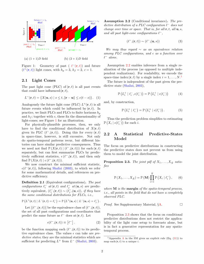
Figure 1: Geometry of past ( `−(r, t)) and future(`+(r, t)) light cones, with hp = 3, hf = 2, c = 1.

2.1 Light Cones

The past light cone (PLC) of (r, t) is all past eventsthat could have influenced(r, t),

L−(r, t) = {X(u, s) | s ≤ t, ‖r− u‖ ≤ c(t− s)} . (1)

Analogously the future light cone (FLC) L+(r, t) is allfuture events which could be influenced by (r, t). Inpractice, we limit PLCs and FLCs to finite horizons hpand hf ; together with c, these fix the dimensionality oflight-cones; see Figure 1 for an illustration.

For physically-plausible processes, then, we onlyhave to find the conditional distribution of X(r, t)given its PLC (`−,(r, t)). Doing this for every (r, t)in space-time, however, is still excessive. Not onlydo spatio-temporal patterns recur, but different his-tories can have similar predictive consequences. Thuswe need not find P (X(r, t) | (`−,(r, t))) for each (r, t)separately, but can first summarize PLCs by predic-tively sufficient statistics, ε (`−,(r, t)), and then onlyfind P (X(r, t) | ε (`−,(r, t))).

We now construct the minimal sufficient statistic,ε(`−(r, t)), following Shalizi (2003), to which we referfor some mathematical details, and references on pre-dictive sufficiency.

Definition 2.1 (Equivalent configurations). The pastconfigurations `−i at (r, t) and `−j at (u, s) are predic-

tively equivalent, (`−i ,(r, t)) ∼ (`−j ,(u, s)), if they havethe same conditional distributions for FLCs, i.e.,

P(L+(r, t) | L−(r, t) = `−i

)= P

(L+(u, s) | L−(u, s) = `−j

).

Let [(`−,(r, t))] be the equivalence class of (`−,(r, t)),the set of all past configurations and coordinates thatpredict the same future as `− does at(r, t). Let

ε(`−,(r, t)) ≡[`−]. (2)

be the function mapping each (`−,(r, t)) to its predic-tive equivalence class. The values ε can take are pre-dictive states; they are the minimal statistics which aresufficient for predicting L+ from L− (Shalizi, 2003).

Assumption 2.2 (Conditional invariance). The pre-dictive distribution of a PLC configuration `− does notchange over time or space. That is, for all r, t, all u, s,and all past light-cone configurations `−,

(`−,(r, t)) ∼ (`−,(u, s)) (3)

We may thus regard ∼ as an equivalence relationamong PLC configurations, and ε as a function over`− alone.

Assumption 2.2 enables inference from a single re-alization of the process (as opposed to multiple inde-pendent realizations). For readability, we encode thespace-time index(r, t) by a single index i = 1, . . . , N .1

The future is independent of the past given the pre-dictive state (Shalizi, 2003),

P(L+i | `−i , ε(`−i )

)= P

(L+i | ε(`−i )

)(4)

and, by construction,

P(L+i | `−i

)= P

(L+i | ε(`−i )

). (5)

Thus the prediction problem simplifies to estimatingP(Xi | ε(`−i )

)for each i.

2.2 A Statistical Predictive-StatesModel

The focus on predictive distributions in constructingthe predictive states does not prevent us from usingthem to model the joint distribution.

Proposition 2.3. The joint pdf of X1, . . . , XN satis-fies

P (X1, . . . , XN ) = P (M)

N∏i=1

P(Xi | `−i

), (6)

where M is the margin of the spatio-temporal process,i.e., all points in the field that do not have a completelyobserved PLC.

Proof. See Supplementary Material, §A.

Proposition 2.3 shows that the focus on conditionalpredictive distributions does not restrict the applica-bility of the light cone setup to forecasts alone, butis in fact a generative representation for any spatio-temporal process.

1Appendix A in the SM gives an explicit rule (Eq. (31)) tomap each(r, t) to a unique i.

2

2.2.1 Minimal Sufficient Statistical Model

Given ε(`−i ) Eq. (6) simplifies to (omitting P (M))

P (X1, . . . , XN |M, ε) =

N∏i=1

P(Xi | `−i ; ε(`−i )

)=

N∏i=1

P(Xi | ε(`−i )

), (7)

using (4). Any particular ε implicitly specifies the num-ber of predictive states K, and all K predictive distri-butions P

(Xi | ε(`−i )

). However, in practice only Xi

and `−i are observed; the mapping ε is exactly what weare trying to estimate.

2.3 Predictive States as Hidden Vari-ables

Since there is a one-to-one correspondence between themapping ε and the set of equivalence classes / predic-tive states ε(`−) which are its range, Shalizi (2003)and Goerg and Shalizi (2012) do not formally distin-guish between them. Here, however, it is importantto keep distinction between the predictive state spaceS and the mapping ε : `−i → S. Our EM algorithmis based on the idea that the predictive state is a hid-den variable, Si, taking values in the finite state spaceS = {s1, . . . , sK}, and the mixture weights of PLC `−iare the soft-threshold version of the mapping ε(`−i ).It is this hidden variable interpretation of predictivestates that we use to estimate the minimal sufficientstatistic ε, the hidden state space S, and the predic-tive distributions P (Xi | Si = sj).

Introducing the abbreviation Pj (·) for P (· | Si = sj),the latent variable approach lets (7) be written as

N∏i=1

P (Xi | Si) =

N∏i=1

K∑j=1

1 (Si = sj)Pj (Xi). (8)

Eq. (8) is the pdf of a K component mixture modelwith complete data, and 1 (Si = sj) is a randomizedversion of ε : `−i 7→ Si.

2.4 Log-likelihood of ε

From (8) the complete data log-likelihood is, neglectinga logP (M) term,

`(ε;D, SN1 ) =

N∑i=1

log

(K∑

j=1

1 (Si = sj)P(Xi | ε(`−i ) = sj

))

=

N∑i=1

K∑j=1

1 (Si = sj) log P(Xi | ε(`−i ) = sj

),

(9)

where SN1 := {S1, . . . , SN} and the second equalityfollows since 1 (Si = sj) = 1 for one and only one j,and 0 otherwise.

The “parameters” in (9) are ε and K; Xi and `−iare observed, and Si is a hidden variable. The optimalmapping ε : L− → S is the one that maximizes (9):

ε∗ = arg maxε

`(ε;D, Si). (10)

Without any constraints on K or ε the maximum isobtained for K = N and ε(`−i ) = `−i ; “the most faithfuldescription of the data is the data”.2 As this tells usnothing about the underlying dynamics, we must putsome constraints on K and/or ε to get a useful solution.For now, assume that K � N is fixed and we only haveto estimate ε; in Section 3.3, we will give a data-drivenprocedure to choose K.

2.5 Nonparametric Likelihood Approx-imation

To solve (10) with K � N we need to evaluate(9) for candidate solutions ε. We cannot do this di-rectly, since (9) involves the unobserved Si. Moreover,predictive distributions can have arbitrary shapes, sowe want to use nonparametric methods, but this in-hibits direct evaluation of the component distributionsP(Xi | ε(`−i ) = sj

).

We solve both difficulties together by using a non-parametric variant of the expectation-maximization(EM) algorithm (Dempster et al., 1977). Following therecent nonparametric EM literature (Benaglia, Chau-veau, and Hunter, 2011; Bordes, Chauveau, and Van-dekerkhove, 2007; Hall, Neeman, Pakyari, and Elmore,2005), we approximate the P

(Xi | ε(`−i ) = sj

)in the

log-likelihood with kernel density estimators (KDEs)using a previous estimate ε(n). That is we approximate(9) with (n)(ε;D, Si):

N∑i=1

K∑j=1

1 (Si = sj) log f(Xi | ε(n)(`−i ) = sj

), (11)

where an equivalent version of f(Xi | ε(n)(`−i ) = sj

)is

given below in (20).

3 EM Algorithm for PredictiveState Space Assignment

Since ε maps to S, the hidden state variable Si and the“parameter” ε play the same role. This in turn resultsin similar E and M steps. Figure 2 gives an overviewof the proposed algorithm.

2On the other extreme is a field with only K = 1 predictivestate, i.e. the iid case.

3

3.1 Expectation Step

The E-step requires the expected log-likelihood

Q(ε | ε(n)) = ES|D;ε(n)`(ε;D, Si), (12)

where expectation is taken with respect toP(Si = sj | D; ε(n)

), the conditional distribution

of the hidden variable Si given the data D and thecurrent estimate ε(n). Using (9) we obtain

Q(ε | ε(n)) =

N∑i=1

K∑j=1

P(Si = sj | Xi, `

−i ; ε(n)(`−i )

)× logP

(Xi | ε(n)(`−i ) = sj

).

(13)

As for `(ε;D) we use KDEs and obtain an approxi-mate expected log-likelihood

Q(n)(ε | ε(n)) =

N∑i=1

K∑j=1

P(Si = sj | Xi, `

−i ; ε(n)(`−i )

)× log f

(Xi | ε(n)(`−i ) = sj

)(14)

The conditional distribution of Si given its FLC andPLC, {Xi, `

−i }, comes from Bayes’ rule,

P(Si = sj | Xi, `

−i

)∝ P

(Xi, `

−i | Si = sj

)P (Si = sj)

= Pj (Xi)Pj(`−i)P (Si = sj) ,

(15)

the second equality following from the conditional in-dependence of Xi and `−i given the state Si.

For brevity, let wij := P(Si = sj | Xi, `

−i

), an N×K

weight matrix W, whose rows are probability distri-butions over states. This wi is the soft-thresholdingversion of ε(`−i ), so we can write the expected log-likelihood in terms of W,

Q(n)(W | W(n)) =

N∑i=1

K∑j=1

wij · logP(Xi | W(n)

j

)(16)

The current W(n) can be used to update (condi-tional) probabilities in (15) by

w(n+1)ij ∝ f(xi | Si = sj ; W

(n)) (17)

×N(`−i | µ

(n)j , Σ

(n)

j ; W(n)

)(18)

×N

(n)j

N, (19)

where i) N(n)j =

∑Ni=1 W

(n)ij is the effective sample size

of state sj , ii) µ(n)j and Σ

(n)

j are weighted mean and

covariance matrix estimators of the PLCs using the

jth column of W(n), and iii) the FLC distribution isestimated with a weighted3 KDE (wKDE)

f(x | S = sj ; W(n)) =

1

N(n)j

N∑r=1

W(n)rj Khj

(‖xr − x‖),

(20)

Here the weights are again the jth column of W(n),and Khj

is a kernel function with a state-dependentbandwidth hj . We used a Gaussian kernel, and toget a good, cluster-adaptive bandwidth hj , we pickout on those xi for which arg maxk wik = j (hard-thresholding of weights; cf. Benaglia et al. 2011) andapply Silverman’s rule-of-thumb-bandwidth (bw.ndr0in the R function density). After estimation, we nor-

malize each wi in (17), w(n+1)ij ← w

(n+1)ij∑K

j=1 w(n+1)ij

.

Ideally, we would use a non-parametric estimate forthe PLC distribution, e.g., forest density estimators(Chow and Liu, 1968; Liu, Xu, Gu, Gupta, Lafferty,and Wasserman, 2011). Currently, however, such esti-mators are too slow to handle many iterations at largeN , so we model state-conditional PLC distributions asmultivariate Gaussians. Simulations suggest that thisis often adequate in practice.

3.2 Approximate Maximization Step

In parametric problems, the M-step solves

ε(n+1) = arg maxε

Q(n)(ε | ε(n)), (21)

to improve the estimate. Starting from a guess ε(0), theEM algorithm iterates (12) and (21) to convergence.

In nonparametric problems, finding an ε(n+1) thatincreases Q(n)(ε | ε(n)) is difficult, since wKDEs withnon-zero bandwidth are not maximizing the likelihood;they are not even guaranteed to increase it. Optimiz-ing (14) by brute force isn’t computationally feasibleeither, as it would mean searching KN state assign-ments (cf. Bordes et al. 2007).

However, in our particular setting the parameterspace and the expectation of the hidden variable co-incide, since wi is a soft-thresholding version of ε(`−i ).Furthermore, none of the estimates above requires adeterministic ε mapping; they are all weighted MLEsor KDEs. Thus, like Benaglia, Chauveau, and Hunter

(2009), we take the weights from the E-step, W(n+1),to update each component distribution using (20).This in turn can then be plugged into (11) to updatethe likelihood function, and in (17) for the next E-step.

The wKDE update does not solve (21) nor does itprovably increase the log-likelihood (although in simu-lations it often does so). We thus use cross-validation

3We also tried a hard-threshold estimator, but we found thatthe soft-threshold KDE performed better.

4

(CV) to select the best W∗, and henceforth do not relyon an ever-increasing log-likelihood as the usual stop-ping rule in EM algorithms (see Section 5 for details).

3.3 Data-driven Choice of K: MergeStates To Obtain Minimal Suffi-ciency

One advantage of the mixture model in (8) is that pre-dictive states have, by definition, comparable condi-tional distributions. Since conditional densities can betested for equality by a nonparametric two-sample test(or using a distribution metric), we can merge nearbyclasses. We thus propose a data-driven automatic se-lection of K, which solves this key challenge in fittingmixture models: 1) start with a sufficiently large num-ber of clusters, Kmax < N ; 2) test for equality of pre-dictive distribution each time the EM reaches a (local)

0. Initialization: Set n = 0. Split data D ={Xi, `

−i }Ni=1 in Dtrain and Dtest. Initialize states

randomly from {s1, . . . , sK} → Boolean W(0).

1. E-step: Obtain updated W(n+1) via (17).

2. Approximate M-step: Update mixture pdfs

P (xi | Si = sj) via (20) with W(n+1).

3. Out-of-sample Prediction: Evaluate out-of-

sample MSE for W(n+1) by predicting FLCsfrom PLCs in Dtest. Set n = n+ 1.

4. Temporary convergence: Iterate 1 - 3 until

‖W(n) − W(n−1)‖ < δ (22)

5. Merging: Estimate pairwise distances (or test)

djk = dist(f(n)j , f

(n)k

)∀j, k = 1, . . . ,K. (23)

(a) If K > 1: determine (j(min), k(min)) =

arg minj 6=k djk and merge these columns

W(n)

j(min) ←W(n)

j(min) + W(n)

k(min) (24)

Omit column k(min) from W(n)

k(min) , set K =K − 1, and re-start iterations at 1.

(b) If K = 1: return W∗ with lowest out-of-sample MSE.

Figure 2: Mixed LICORS: nonparametric EM algo-rithm for predictive state recovery.

optimum; 3) merge until K = 1 (iid case) – step 5 in

Fig. 2; 4) choose the best model W∗ (and thus K∗) byCV.

4 Forecasting Given New Data

The estimate W∗ can be used to forecast X given anew ˜−. Integrating out Si yields a mixture

P(X | ˜−

)=

K∑j=1

P(S = sj | ˜−

)· Pj

(X). (25)

As Pj(X)

= P(X = x | S = sj

)is independent of ˜−

we do not have to re-estimate them for each ˜−, butcan use the wKDEs in (20) from the training data.

The mixture weights wj := P(S = sj | ˜−

)are in

general different for each PLC and can again be esti-mated using Bayes’s rule (with the important differ-ence that now we only condition on ˜−, not on X):

wj(˜−; W∗) ∝ P(

˜− | S = sj ; W∗)× P

(S = sj ; W

∗)

= N(

˜−; µ∗(j), Σ∗(j); W

∗)×N∗jN. (26)

After re-normalization of w = ( w∗1, . . . , w∗K), the pre-dictive distribution (25) can be estimated via

P(X = x | ˜−

)=

K∑j=1

w∗j · f (X = x | Si = sj ; W(∗)).

(27)

A point forecast can then be obtained by a weightedcombination of point estimates in each component (e.g.weighted mean), or by the mode of the full distribution.In the simulations we use the weighted average fromeach component as the prediction of X.

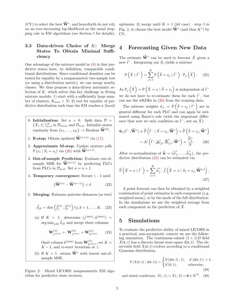
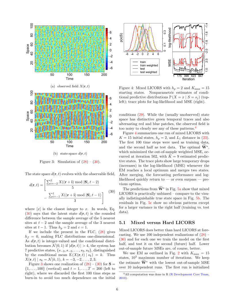
5 Simulations

To evaluate the predictive ability of mixed LICORS ina practical, non-asymptotic context we use the follow-ing simulation. The continuous-valued (1 + 1)D fieldX(r, t) has a discrete latent state space d(r, t). The ob-servable field X(r, t) evolves according to a conditionalGaussian distribution,

P (X(r, t) | d(r, t)) =

{N (d(r, t) , 1), if |d(r, t) | < 4,

N (0, 1), otherwise,

(28)

and initial conditions: X(·, 1) = X(·, 2) = 0 ∈ R|S|. (29)

5

50 100 150 200

2040

6080

100

Time

Space

-6

-4

-2

0

2

4

6

(a) observed field X(r, t)

50 100 150 200

2040

6080

100

Time

Space

-6

-4

-2

0

2

4

6

(b) state-space d(r, t)

Figure 3: Simulation of (28) – (30).

The state space d(r, t) evolves with the observable field,

d(r, t) =

[∑2i=−2X((r + i) mod |S|, t− 2)

5

−∑1i=−1X((r + i) mod |S|, t− 1)

3

] (30)

where [x] is the closest integer to x. In words, Eq.(30) says that the latent state d(r, t) is the roundeddifference between the sample average of the 5 nearestsites at t − 2 and the sample average of the 3 nearestsites at t− 1. Thus hp = 2 and c = 1.

If we include the present in the FLC, (28) giveshf = 0, making FLC distributions one-dimensional.As d(r, t) is integer-valued and the conditional distri-bution becomes N (0, 1) if |d(r, t) | > 4, the system has7 predictive states, {s−3, s−2, . . . , s2, s3}, distinguishedby the conditional mean E (X(r, t) | sk) = k. ThusX(r, t) | sk = N (k, 1), k = −3,−2, . . . , 2, 3.

Figure 3 shows one realization of (28) – (30) for S ={1, . . . , 100} (vertical) and t = 1, . . . , T = 200 (left toright), where we discarded the first 100 time steps asburn-in to avoid too much dependence on the initial

-6 -4 -2 0 2 4 6

00.

10.

3

p(x|

S)

traintrain weightedtesttest weighted

-2.0

-1.8

-1.6

-1.4

log-

likel

ihoo

d

1.0

2.0

1 175 399 623 847Iteration

MS

E

Figure 4: Mixed LICORS with hp = 2 and Kmax = 15starting states. Nonparametric estimates of condi-tional predictive distributions P (X = x | S = sj) (top-left); trace plots for log-likelihood and MSE (right).

conditions (29). While the (usually unobserved) statespace has distinctive green temporal traces and alsoalternating red and blue patches, the observed field istoo noisy to clearly see any of these patterns.4

Figure 4 summarizes one run of mixed LICORS withK = 15 initial states, hp = 2, and L1 distance in (23).The first 100 time steps were used as training data,

and the second half as test data. The optimal W∗,which minimized the out-of-sample weighted MSE, oc-curred at iteration 502, with K = 9 estimated predic-tive states. The trace plots show large temporary drops(increases) in the log-likelihood (MSE) whenever theEM reaches a local optimum and merges two states.After merging, the forecasting performance and log-likelihood quickly return to — or even surpass — pre-vious optima.

The predictions from W∗ in Fig. 5a show that mixedLICORS is practically unbiased – compare to the visu-ally indistinguishable true state space in Fig. 5b. Theresiduals in Fig. 5c show no obvious patterns exceptfor a larger variance in the right half (training vs. testdata).

5.1 Mixed versus Hard LICORS

Mixed LICORS does better than hard LICORS at fore-casting. We use 100 independent realizations of (28) –(30) and for each one we train the model on the firsthalf, and test it on the second (future) half. Lowerout-of-sample future MSEs are, of course, better.

We use EM as outlined in Fig. 2 with Kmax = 15states, 103 maximum number of iterations. We keep

the estimate W∗ with the lowest out-of-sample MSEover 10 independent runs. The first run is initialized

4All computation was done in R (R Development Core Team,2010).

6

50 100 150 200

2040

6080

100

Time

Space

-3

-2

-1

0

1

2

3

(a) estimated predictive states S(r, t)

50 100 150 200

2040

6080

100

Time

Space

-3

-2

-1

0

1

2

3

(b) true predictive states S(r, t)

50 100 150 200

2040

6080

100

Time

Space

-4

-2

0

2

4

(c) residuals

Figure 5: Mixed LICORS model fit and residual check.

with a K-means++ clustering (Arthur and Vassilvit-skii, 2007) on the PLC space; state initializations in theremaining nine runs were uniformly at random fromS = {s1, . . . , s15}.

To test whether mixed LICORS accurately estimatesthe mapping ε : `− 7→ S, we also predict FLCs of an in-dependently generated realization of the same process.If the out-of-sample MSE for the independent field isthe same as the out-of-sample MSE for the future evo-lution of the training data, then mixed LICORS is notjust memorizing fluctuations in any given realization,but estimates characteristics of the random field. Wecalculated both weighted-mixture forecasts, and theforecast of the state with the highest weight.

Figure 6 shows the results. Mixed LICORS greatlyimproves upon the hard LICORS estimates, with upto 34% reduction in out-of-sample MSE. As with hardLICORS, the MSE for future and independent real-izations are essentially the same, showing that mixedLICORS generalizes from one realization to the wholeprocess. As the weights often already are 0/1 assign-

trut

h

in-s

ampl

e

in-s

ampl

e (w

)

futu

re

futu

re (

w)

inde

pend

ent

inde

pend

ent (

w)

in-s

ampl

e m

in

in-s

ampl

e C

V

futu

re m

in

futu

re C

V

inde

pend

ent m

in

inde

pend

ent C

V

0.8

1.0

1.2

1.4

1.6

1.8

2.0

MS

E

mixed LICORS K = 15 starting states

λ= 0

truth

LICORS knn for each PLC k = 50 neighbors

Figure 6: Comparing mixed and hard LICORS byforecast MSEs.

0. Initialize field {X(·, 1− τ)}hp

τ=1. Set t = 1.

1. Fetch all PLCs at time t: Pt = {`−(r, t)}r∈Snew

2. For each `−(r, t) ∈ Pt:

(a) draw state sj ∼ P (S = sj | `−(r, t))

(b) draw X(r, t) ∼ P (x | S = sj)

3. If t < tmax, set t = t + 1 and go to step 1.Otherwise return simulation {X(·, t)}tmax

t=1 .

Figure 7: Simulate new realization from spatio-temporal process on Snew × {1, . . . , tmax} using trueand estimated dynamics (use (26) in 2a; (20) in 2b).

ments, weighted-mixture prediction is only slightly bet-ter than using the highest-weight state.

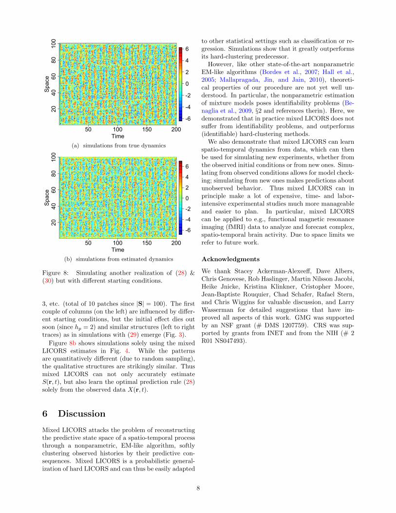
5.2 Simulating New Realizations ofThe Underlying System

Recall that all simulations use (29) as initial conditions.If we want to know the effect of different starting con-ditions, then we can simply use Eqs. (28) & (30) tosimulate that process, since they fully specify the evo-lution of the stochastic process. In experimental stud-ies, however, researchers usually lack such generativemodels; learning one is often the point of the experi-ment in the first place.

Since mixed LICORS estimates joint and conditionalpredictive distributions, and not only the conditionalmean, it is possible to simulate a new realization froman estimated model. Figure 7 outlines this simula-tion procedure. We will now demonstrate that mixedLICORS can be used instead to simulate from differentinitial conditions without knowing Eqs. (28) & (30).

For example, Fig. 8a shows a simulation using thetrue mechanisms in (28) & (30) with starting condi-tions X(·, 1) = −1 and X(·, 2) = ±3 ∈ R|S| in alter-nating patches of ten times 3, ten times −3, ten times

7

50 100 150 200

2040

6080

100

Time

Space

-6

-4

-2

0

2

4

6

(a) simulations from true dynamics

50 100 150 200

2040

6080

100

Time

Space

-6

-4

-2

0

2

4

6

(b) simulations from estimated dynamics

Figure 8: Simulating another realization of (28) &(30) but with different starting conditions.

3, etc. (total of 10 patches since |S| = 100). The firstcouple of columns (on the left) are influenced by differ-ent starting conditions, but the initial effect dies outsoon (since hp = 2) and similar structures (left to righttraces) as in simulations with (29) emerge (Fig. 3).

Figure 8b shows simulations solely using the mixedLICORS estimates in Fig. 4. While the patternsare quantitatively different (due to random sampling),the qualitative structures are strikingly similar. Thusmixed LICORS can not only accurately estimateS(r, t), but also learn the optimal prediction rule (28)solely from the observed data X(r, t).

6 Discussion

Mixed LICORS attacks the problem of reconstructingthe predictive state space of a spatio-temporal processthrough a nonparametric, EM-like algorithm, softlyclustering observed histories by their predictive con-sequences. Mixed LICORS is a probabilistic general-ization of hard LICORS and can thus be easily adapted

to other statistical settings such as classification or re-gression. Simulations show that it greatly outperformsits hard-clustering predecessor.

However, like other state-of-the-art nonparametricEM-like algorithms (Bordes et al., 2007; Hall et al.,2005; Mallapragada, Jin, and Jain, 2010), theoreti-cal properties of our procedure are not yet well un-derstood. In particular, the nonparametric estimationof mixture models poses identifiability problems (Be-naglia et al., 2009, §2 and references therin). Here, wedemonstrated that in practice mixed LICORS does notsuffer from identifiability problems, and outperforms(identifiable) hard-clustering methods.

We also demonstrate that mixed LICORS can learnspatio-temporal dynamics from data, which can thenbe used for simulating new experiments, whether fromthe observed initial conditions or from new ones. Simu-lating from observed conditions allows for model check-ing; simulating from new ones makes predictions aboutunobserved behavior. Thus mixed LICORS can inprinciple make a lot of expensive, time- and labor-intensive experimental studies much more manageableand easier to plan. In particular, mixed LICORScan be applied to e.g., functional magnetic resonanceimaging (fMRI) data to analyze and forecast complex,spatio-temporal brain activity. Due to space limits werefer to future work.

Acknowledgments

We thank Stacey Ackerman-Alexeeff, Dave Albers,Chris Genovese, Rob Haslinger, Martin Nilsson Jacobi,Heike Jnicke, Kristina Klinkner, Cristopher Moore,Jean-Baptiste Rouquier, Chad Schafer, Rafael Stern,and Chris Wiggins for valuable discussion, and LarryWasserman for detailed suggestions that have im-proved all aspects of this work. GMG was supportedby an NSF grant (# DMS 1207759). CRS was sup-ported by grants from INET and from the NIH (# 2R01 NS047493).

8

References

D. Arthur and S. Vassilvitskii. k-means++: The ad-vantages of careful seeding. In H. Gabow, editor,Proceedings of the 18th Annual ACM-SIAM Sympo-sium on Discrete Algorithms [SODA07], pages 1027–1035, Philadelphia, 2007. Society for Industrial andApplied Mathematics. URL http://www.stanford.

edu/~darthur/kMeansPlusPlus.pdf.

T. Benaglia, D. Chauveau, and D. R. Hunter. AnEM-like algorithm for semi- and non-parametricestimation in multivariate mixtures. Journal ofComputational and Graphical Statistics, 18:505–526, 2009. URL http://sites.stat.psu.edu/

~dhunter/papers/mvm.pdf.

T. Benaglia, D. Chauveau, and D. R. Hunter.Bandwidth selection in an EM-like algorithm fornonparametric multivariate mixtures. In D. R.Hunter, D. S. P. Richards, and J. L. Rosen-berger, editors, Nonparametric Statistics and Mix-ture Models: A Festschrift in Honor of ThomasP. Hettmansperger. World Scientific, Singapore,2011. URL http://hal.archives-ouvertes.fr/

docs/00/35/32/97/PDF/npEM_bandwidth.pdf.

L. Bordes, D. Chauveau, and P. Vandekerkhove. Astochastic EM algorithm for a semiparametric mix-ture model. Computational Statistics and DataAnalysis, 51:5429–5443, 2007. doi: 10.1016/j.csda.2006.08.015.

C. K. Chow and C. N. Liu. Approximating discreteprobability distributions with dependence trees.IEEE Transactions on Information Theory, IT-14:462–467, 1968.

A. P. Dempster, N. M. Laird, and D. B. Rubin. Maxi-mum likelihood from incomplete data via the EM al-gorithm. Journal of the Royal Statistical Society B,39:1–38, 1977. URL http://www.jstor.org/pss/

2984875.

G. M. Goerg and C. R. Shalizi. LICORS: Light cone re-construction of states for non-parametric forecastingof spatio-temporal systems. Technical report, De-partment of Statistics, Carnegie Mellon University,2012. URL http://arxiv.org/abs/1206.2398.

P. Hall, A. Neeman, R. Pakyari, and R. Elmore.Nonparametric inference in multivariate mixtures.Biometrika, 92:667–678, 2005.

S. L. Lauritzen. Sufficiency, prediction and extrememodels. Scandinavian Journal of Statistics, 1:128–134, 1974. URL http://www.jstor.org/pss/

4615564.

S. L. Lauritzen. Extreme point models in statistics.Scandinavian Journal of Statistics, 11:65–91, 1984.URL http://www.jstor.org/pss/4615945. Withdiscussion and response.

H. Liu, M. Xu, H. Gu, A. Gupta, J. Lafferty, andL. Wasserman. Forest density estimation. Jour-nal of Machine Learning Research, 12:907–951,2011. URL http://jmlr.csail.mit.edu/papers/

v12/liu11a.html.

S. Lloyd. Least squares quantization in PCM. Infor-mation Theory, IEEE Transactions on, 28(2):129 –137, 1982. ISSN 0018-9448. doi: 10.1109/TIT.1982.1056489.

P. K. Mallapragada, R. Jin, and A. K. Jain. Non-parametric mixture models for clustering. In E. R.Hancock, R. C. Wilson, T. Windeatt, I. Ulusoy,and F. Escolano, editors, Structural, Syntactic, andStatistical Pattern Recognition [SSPR//SPR 2010],pages 334–343, New York, 2010. Springer-Verlag.doi: 10.1007/978-3-642-14980-1 32.

R Development Core Team. R: A Language and Envi-ronment for Statistical Computing. R Foundation forStatistical Computing, Vienna, Austria, 2010. URLhttp://www.R-project.org/. ISBN 3-900051-07-0.

C. R. Shalizi. Optimal nonlinear prediction of randomfields on networks. Discrete Mathematics and Theo-retical Computer Science, AB(DMCS):11–30, 2003.URL http://arxiv.org/abs/math.PR/0305160.

9

APPENDIX – SUPPLEMENTARYMATERIAL

A Proofs

Here we will show that the joint pdf of the entire fieldconditioned on its margin (Figure 9, gray area) equalsthe product of the predictive conditional distributions.

Proof of Proposition 2.3. To simplify notation, we as-sign index numbers i ∈ 1, . . . N to the space-time grid(s, t) to ensure that the PLC of i1 cannot contain Xi2

if i2 > i1. We can do this by iterating through spaceand time in increasing order over time (and, for fixedt, any order over space):

(s, t) , s ∈ S, t ∈ T→(i(t−1)·|S|+1, . . . , i(t−1)·|S|+|S|)

)= (t− 1) · |S|+ (1, . . . , |S|).

(31)

We assume that the process we observed is part of alarger field on an extended grid S× T, with S ⊃ S andT = {−(hp − 1), . . . , 0, 1, . . . T , for a total of N > Nspace-time points, X1, . . . , XN . The margin M are all

points X(s, u), (s, u) ∈ S × T that do not have a fullyobserved past light cone. Formally,

M = {X(s, u) | `−(s, u) /∈ {X(r, t) ,(r, t) ∈ S× T}},(32)

The size of M depends on the past horizon hp as wellas the speed of propagation c, M = M (hp, c).

In Figure 9, the part of the field with fully observedPLCs are marked in red. Points in the margin, in gray,have PLCs extending into the fully unobserved region(blue). Points in the red area have a PLC that liesfully in the red or partially in the gray, but never in theblue area. As can be see in Fig. 9 the margin at each

Time t

Spacer

margin M

data with fullyobserved PLC:

XN1 = X1, . . . , XN

unobserved

observeddata

XN1

=X 1, .. ., X

N

(r, t) ∈ XN1 and `−(r, t) ⊂ XN

1

(r, t) ∈ XN1 , but `−(r, t) ⊂ XN

1 ∪M

(r, t) ∈ XN1 \XN

1 , but `−(r, t) * D

Figure 9: Margin of spatio-temporal field in (1 + 1)D.

t is a constant fraction of space, thus overall M growslinearly with T ; it does not grow with an increasing S,but stays constant.

For simplicity, assume that X1, . . . , XN are from thetruncated (red) field, such that all their PLCs are ob-served (they may lie in M), and the remaining N −NXjs lie in M (with a PLC that is only partially unob-served). Furthermore let Xk

1 := {X1, . . . , Xk}. Thus

P({X(s, t) |(s, t) ∈ S× T}

)= P

(XN

1

)= P

(XN

1 ,M)

= P(XN

1 |M)P (M)

The first term factorizes as

P(XN

1 |M)

= P(XN | XN−1

1 ,M)P(XN−1

1 |M)

= P(XN | `−N ∪ {XN−1

1 ,M} \ {`−N})P(XN−1

1 |M)

= P(XN | `−N

)P(XN−1

1 |M)

where the second-to-last equality follows since by (31),`−N ⊂ {Xk | 1 ≤ k < N} ∪M, and the last equalityholds since Xi is conditional independent of the restgiven its own PLC (due to limits in information prop-agation over space-time).

By induction,

P (X1, . . . , XN |M) =

N−1∏j=0

P(XN−j | `−N−j

)(33)

=

N∏i=1

P(Xi | `−i

)(34)

This shows that the conditional log-likelihood max-imization we use for our estimators is equivalent (upto a constant) to full joint maximum likelihood estima-tion.

B Predictive States and Mix-ture Models

Another way to understand predictive states is as theextremal distributions of an optimal mixture model(Lauritzen, 1974, 1984).

To predict any variable L+, we have to know itsdistribution P (L+). If, as often happens, that distri-bution is very complicated, we may try to decomposeit into a mixture of simpler “base” or “extremal” dis-tributions, P (L+ | θ), with mixing weights π(θ),

P(L+)

=

∫π(θ)P

(L+ | θ

)dθ . (35)

The familiar Gaussian mixture model, for instance,makes the extremal distributions to be Gaussians

10

(with θ indexing both expectations and variances), andmakes the mixing weights π(θ) a combination of deltafunctions, so that P (L+) becomes a weighted sum offinitely-many Gaussians.

The conditional predictive distribution of L+ | `− in(35) is a weighted average over the extremal conditionaldistributions P (L+ | θ, `−),

P(L+ | `−

)=

∫π(θ|`−)P

(L+ | θ, `−

)dθ (36)

This only makes the forecasting problem harder, unless

P (L+ | θ, `−)π(θ | `−) = P(L+ | θ(`−)

)δ(θ − θ(`−)),

that is, unless θ(`−) is a predictively sufficient statis-tic for L+. The most parsimonious mixture model isthe one with the minimal sufficient statistic, θ = ε(`−).This shows that predictive states are the best “param-eters” in (35) for optimal forecasting. Using them,

P(L+)

=

K∑j=1

P(ε(`−) = sj

)P(L+ | ε(`−) = sj

)(37)

=

K∑j=1

πj(`−) · Pj

(L+), (38)

where πj(`−) is the probability that the predictive state

of `− is sj , and Pj (L+) = P (L+ | S = sj). Since eachlight cone has a unique predictive state,

πj(`−) =

{1, if ε(`−) = sj ,

0 otherwise.(39)

Thus the predictive distribution given `−i is just

P(L+ | `−i

)=

K∑j=1

πj(`−i ) · Pj

(L+)

= Pε(`−i )

(L+).

(40)

Now the forecasting problem simplifies to mapping`−i to its predictive state, ε(`−i ) = sj ; the appropriatedistribution-valued forecast is pj(L

+), and pointforecasts are derived from it as needed.

This mixture-model point of view highlights howprediction benefits from grouping points by their pre-dictive consequences, rather than by spatial proxim-ity (as a Gaussian mixture would do). For us, thismeans clustering past light-cone configurations accord-ing to the similarity of their predictive distributions,not according to (say) the Euclidean geometry. MixedLICORS thus learns a new geometry for the system,which is optimized for forecasting.

11