Mission Planning for Wave Driven Autonomous Surface Vessels
118
Sindre Løining Skaar NTNU Norwegian University of Science and Technology Faculty of Information Technology and Electrical Engineering Department of Engineering Cybernetics Master’s thesis Sindre Løining Skaar Mission Planning for Wave Driven Autonomous Surface Vessels Master’s thesis in Cybernetics and Robotic Supervisor: Tor Arne Johansen, Alberto Dallolio November 2020
-
Upload
khangminh22 -
Category
Documents
-
view
4 -
download
0
Transcript of Mission Planning for Wave Driven Autonomous Surface Vessels
Sindre Løining Skaar
NTN
UN
orw
egia
n U
nive
rsity
of S
cien
ce a
nd T
echn
olog
yFa
culty
of I
nfor
mat
ion
Tech
nolo
gy a
nd E
lect
rical
Engi
neer
ing
Dep
artm
ent o
f Eng
inee
ring
Cybe
rnet
ics
Mas
ter’s
thes
is
Sindre Løining Skaar
Mission Planning for Wave DrivenAutonomous Surface Vessels
Master’s thesis in Cybernetics and Robotic
Supervisor: Tor Arne Johansen, Alberto Dallolio
November 2020


Sindre Løining Skaar
Mission Planning for Wave DrivenAutonomous Surface Vessels
Master’s thesis in Cybernetics and RoboticSupervisor: Tor Arne Johansen, Alberto DallolioNovember 2020
Norwegian University of Science and TechnologyFaculty of Information Technology and Electrical EngineeringDepartment of Engineering Cybernetics


1 Abstract
Increased autonomy within the ocean vessel sector is expected to drasticallychange how both humans, goods and research is conducted in the coming future.Due to the increased capabilities of autonomous vehicles, they have become amore viable alternative. The vehicles have also gotten increasingly more afford-able due to the reduced cost in both hardware and software. A reduction in sizeof many important components have also drastically increased the capabilitiesof smaller autonomous vessels, allowing a much broader adoption of the tech-nology within research and the industrial sectors.
The Institute of Cybernetics and Robotics at NTNU, Trondheim is involvedin the development of a broad spectre of autonomous seagoing vessels, spanningfrom dynamic positioning of large supply vessels to autonomous snake robots.NTNU is also involved in ocean sampling to further the understanding in aqua-culture and the environmental impact of the future Norwegian development atsea. NTNU is developing self sufficient autonomous vessels capable of perform-ing missions previously done by large and costly vessels closer to 400 tons. Smallautonomous vessels still have problems navigating and staying safe in changingweather conditions. Manually planning missions often creates unfeasible mis-sions not possible for the autonomous vessels to conduct. Too strong weathercan displace small autonomous vessels hundreds of kilometres off course, leadingto costly rescue missions or loss of the vessel.
This thesis has focused on increasing the capabilities of smaller autonomousvessels and reducing the chance of the vessel being carried off course. A missionplanner has been developed that plans a vessel path and sensor sampling totake into account challenging weather. This allows the algorithm to create apath feasible for the vessel to conduct, while also optimising the monetary costof the mission. To be able to predict feasible paths, the thesis has focused onfinding a model for wave propelled surface vehicles to be able to better pre-dict vessel dynamics and take account for how weather affects vessel movement.This model was then used in conjunction with a custom binary-continuous par-ticle swarm optimisation algorithm to optimise the total estimated mission cost.
The model was tested and fitted to real life testing of a wave powered vesselcalled AutoNaut. Parameter estimations were conducted for both on shore lo-cations shielded from the off shore environment and off shore environments toget a better understanding of model parameter validity.
Using the optimisation algorithm, the system was able to find feasible op-timised paths where the manually created paths would not have been feasible,therefore drastically improving the vessel capabilities even in environments nor-mally deemed too challenging for the vessel to complete.
1

[This page is intentionally left blank]
2

2 Sammendrag
En økt bruk av autonome sjøfarende fartøy er forventet a drastisk forandrehvordan bade mennesker, gods og forskning blir handtert i fremtiden. Den øktekapabiliteten til autonome fartøy har gjort dem til et mer aktuelt alternativ.Fartøyene har ogsa blitt rimeligere grunnet en reduksjon i pris pa maskinvareog programvare. En reduksjon i størrelsen pa mange viktige komponenter harogsa drastisk økt kapabilitetene til mindre fartøy, som tillater fartøyene a kunnebli brukt i en mye større skala innenfor bade forskning og industri.
Institutt for Teknisk Kybernetikk hos NTNU, Trondheim, er involvert iutviklingen av et bredt spekter av fartøy fra dynamisk posisjonering av forsyn-ingsfartøy til slangeroboter. NTNU er ogsa involvert i forskning innen akvakul-tur for a øke forstaelsen av hvordan norges utvikling innen havbruk og akvakul-tur pavirker sjøen og det biologiske mangfoldet. For a støtte forskningen utviklerNTNU selvforsynte autonome fartøy som kan utføre oppdrag som før var utførtav ekspidisjonsfartøy pa opptil 400 tonn. Sma autonome fartøy har derimot fort-satt problemer med a navigere og holde seg unna farlige situasjoner i vanskeligeværforhold. Manuelt planlagte oppdrag er ofte umulige for autonome fartøy agjennomføre. For sterk strøm kan for eksempel føre fartøy hundrevis av kilo-meter ut av kurs, noe som kan føre til dyre redningsoppdrag eller tap av fartøyet.
Denne avhandlingen har fokusert pa a øke kapabilitetene til mindre au-tonome fartøy og redusere sannsynligheten for at fartøyene ikke kan gjennomføreoppdragene sine. For a fa til dette har en oppdragsplanlegger blitt utviklet somplanlegger bade rute og sensorbruk i hensyn til værforhold. Dette tillater al-goritmen a finne en praktisk gjennomførbar rute og samtidig optimalisere denmonetære kostnaden av oppdraget. For a kunne planlegge ruter til fartøyet taravhandlingen ogsa for seg en matematisk modell for a beskrive dynamikkentil bølgedrevne fartøy. Dette gjør det mulig a kunne forutsi hvordan værpavirker dynamikken. Denne modellen, sammen med en egenprodusert Binær-Kontinuerlig partikkel sverm optimalisering algoritme, ble brukt for a optimalis-ere den estimerte oppdragskostnaden.
Den matematiske modellen ble testet og tilpasset tester av et virkelig bølgedrevetfartøy kalt AutoNaut. Parameterestimeringer av modellen ble gjort bade i nærekystomrader i Trondheimsfjorden, skjermet for tungt vær, og ute i apen sjø vedMausund.
Ved a bruke optimaliseringsalgoritmen, klarte algoritmen a finne gjennomførbareruter hvor den manuelle metoden ikke ville være gjennomførbar. Dette øker ka-pabiliteten under forhold som tidligere var for utfordrende.
3

[This page is intentionally left blank]
4
3 Acknowledgements
First and foremost, I would like to thank my supervisor, Professor Tor ArneJohansen, for giving me the opportunity to explore a field I am very passionateabout and giving me the opportunity to help out in testing the AutoNaut inthe sea trails. He has also been a great help in verifying and discussing differentapproaches and methods for conducting the master project. I would also liketo thank my co supervisor Alberto Dallolio who has helped in both planningof the thesis, giving helpful feedback and giving me a greater understandingof the inner workings and practical use of the AutoNaut vessel. Furthermore,I want to thank researchers at Norsk Institutt for Vannforskning (NIVA) andMeteorologisk Institutt for providing relevant information on prevailing ASVresearch and detailed weather data, respectively. I also want to thank friendsand family for invaluable support. Lastly, I want to thank NTNU for the greatopportunity I got to pursue an education within automation and robotics, whichhas been a dream come true.
5

[This page is intentionally left blank]
6
List of Figures
1 Wind driven ASVs . . . . . . . . . . . . . . . . . . . . . . . . . . 212 Odin ASV . . . . . . . . . . . . . . . . . . . . . . . . . . . . . . . 223 A* results . . . . . . . . . . . . . . . . . . . . . . . . . . . . . . . 244 A* Real Time Varying . . . . . . . . . . . . . . . . . . . . . . . . 255 Bathymetry Path Planning . . . . . . . . . . . . . . . . . . . . . 266 Potential Field Planning . . . . . . . . . . . . . . . . . . . . . . . 287 AUV Genetic Path Planning . . . . . . . . . . . . . . . . . . . . 298 AutoNaut Rendering . . . . . . . . . . . . . . . . . . . . . . . . . 359 AutoNaut Hardware . . . . . . . . . . . . . . . . . . . . . . . . . 3610 Vessel Velocity Model . . . . . . . . . . . . . . . . . . . . . . . . 4111 Timeinvariant Optimal Path . . . . . . . . . . . . . . . . . . . . . 5912 Timeinvariant Particle Paths . . . . . . . . . . . . . . . . . . . . 6013 Particle Costs Timeinvariant . . . . . . . . . . . . . . . . . . . . 6214 Three sub-floats. . . . . . . . . . . . . . . . . . . . . . . . . . . . 6315 TimeVariant Results . . . . . . . . . . . . . . . . . . . . . . . . . 6616 Mission Solution . . . . . . . . . . . . . . . . . . . . . . . . . . . 6917 Parameter Estimation Trondheim - Half second frequency . . . . 7218 Parameter Estimation Trondheim - One second frequency . . . . 7319 Parameter Estimation Trondheim - Two second frequency . . . . 7420 Parameter Estimation Mausund - One second frequency . . . . . 7621 Parameter Estimation Trondheim - One second frequency . . . . 7722 Figure showing the evolution of particle costs for every iteration.
When used in real weather situations the results seem to have amuch more sporadic behaviour than in the analytical case . . . . 82
23 Particle Cost Real Life Test . . . . . . . . . . . . . . . . . . . . . 8324 Optimal Path Real Time Path . . . . . . . . . . . . . . . . . . . 8425 All Particle Paths Real Life Tests . . . . . . . . . . . . . . . . . . 8526 Sensor Usage - Trondheim Fjord . . . . . . . . . . . . . . . . . . 8627 Figure showing the evolution of particle costs for every iteration
with time invariant forecast. . . . . . . . . . . . . . . . . . . . . . 8828 Particle Cost Real Life Test . . . . . . . . . . . . . . . . . . . . . 8929 Optimal Path Real Time Cost . . . . . . . . . . . . . . . . . . . . 9030 All Particle Paths Real Life Tests with time invariant forecast . . 9131 Feasibility North Map Trondheim Fjord . . . . . . . . . . . . . . 9632 Feasibility East Map Trondheim Fjord . . . . . . . . . . . . . . . 9733 Feasibility South Map Trondheim Fjord . . . . . . . . . . . . . . 9834 Feasibility West Map Trondheim Fjord . . . . . . . . . . . . . . . 9935 Current Map Trondheim Fjord . . . . . . . . . . . . . . . . . . . 10036 Wind Map Trondheim Fjord . . . . . . . . . . . . . . . . . . . . 10137 Wave Map Trondheim Fjord . . . . . . . . . . . . . . . . . . . . . 10238 Feasibility North Map Trondheim Fjord - Increased Hydrofoil
Forces . . . . . . . . . . . . . . . . . . . . . . . . . . . . . . . . . 10339 Feasibility East Map Trondheim Fjord - Increased Hydrofoil Forces104
7

40 Feasibility South Map Trondheim Fjord - Increased HydrofoilForces . . . . . . . . . . . . . . . . . . . . . . . . . . . . . . . . . 105
41 Feasibility West Map Trondheim Fjord - Increased Hydrofoil Forces106
8

List of Tables
1 Table showing parameters used for velocity function for time in-variant analytical current . . . . . . . . . . . . . . . . . . . . . . 61
2 Table showing PSO parameters for time invariant analytical current 613 Table showing parameters used for velocity function for time vari-
ant analytical current . . . . . . . . . . . . . . . . . . . . . . . . 654 Table showing PSO parameters for time variant analytical current 655 Table showing parameters used for velocity function for analytical
mission with area of interest . . . . . . . . . . . . . . . . . . . . . 686 Table showing PSO parameters for analytical mission with area
of interest . . . . . . . . . . . . . . . . . . . . . . . . . . . . . . . 687 Table showing parameters used for velocity function for analytical
for real life tests in Trondheim . . . . . . . . . . . . . . . . . . . 818 Table showing PSO parameters for real life tests in Trondheim . 81
9

[This page is intentionally left blank]
10

List of Algorithms
1 Particle Swarm Optimisation . . . . . . . . . . . . . . . . . . . . 312 Parameter Estimation . . . . . . . . . . . . . . . . . . . . . . . . 463 Vessel Velocity . . . . . . . . . . . . . . . . . . . . . . . . . . . . 524 Cost Function . . . . . . . . . . . . . . . . . . . . . . . . . . . . . 555 Hybrid Particle Swarm Optimisation . . . . . . . . . . . . . . . . 57
11

[This page is intentionally left blank]
12
Contents
1 Abstract 1
2 Sammendrag 3
3 Acknowledgements 5
I Background 16
4 Introduction 174.1 Motivation . . . . . . . . . . . . . . . . . . . . . . . . . . . . . . 174.2 Project and Context . . . . . . . . . . . . . . . . . . . . . . . . . 184.3 Previous Related Work . . . . . . . . . . . . . . . . . . . . . . . . 184.4 Types of Autonomous Surface Vessels . . . . . . . . . . . . . . . 19
4.4.1 Self Sustained ASVs . . . . . . . . . . . . . . . . . . . . . 194.4.2 Wind Powered ASVs . . . . . . . . . . . . . . . . . . . . . 204.4.3 Wave Powered ASVs . . . . . . . . . . . . . . . . . . . . . 21
5 Methodological Approach 22
6 State of the Art 236.1 Mission Planning . . . . . . . . . . . . . . . . . . . . . . . . . . . 23
6.1.1 Time and Energy Optimal Path Planning in General Flows 236.1.2 Time Varying Flows . . . . . . . . . . . . . . . . . . . . . 246.1.3 Seabed Coverage . . . . . . . . . . . . . . . . . . . . . . . 256.1.4 Evolutionary Based Path Planning of an Autonomous Sur-
face Vehicle . . . . . . . . . . . . . . . . . . . . . . . . . . 276.1.5 Artificial Potential Fields For Real Time Path Planning . 27
6.2 A comparison of Optimization Techniques for AUV Path Planning 286.3 Neptus . . . . . . . . . . . . . . . . . . . . . . . . . . . . . . . . . 296.4 Genetic Algorithms . . . . . . . . . . . . . . . . . . . . . . . . . . 30
6.4.1 Particle Swarm Algorithm . . . . . . . . . . . . . . . . . . 30
II Theory for Vessel Modelling and Estimation 33
7 Modelling and Implementation of Wave Propulsion ASV 347.1 AutoNaut . . . . . . . . . . . . . . . . . . . . . . . . . . . . . . . 347.2 Autonaut Description . . . . . . . . . . . . . . . . . . . . . . . . 34
7.2.1 Energy storage and distribution . . . . . . . . . . . . . . . 357.2.2 Communication . . . . . . . . . . . . . . . . . . . . . . . . 36
13
8 Vessel Dynamics Model 378.1 Assumptions . . . . . . . . . . . . . . . . . . . . . . . . . . . . . 378.2 Model Fitting . . . . . . . . . . . . . . . . . . . . . . . . . . . . . 388.3 Wave Propulsion Modelling . . . . . . . . . . . . . . . . . . . . . 398.4 Implementation of Parameter Estimation . . . . . . . . . . . . . 44
8.4.1 Implementation . . . . . . . . . . . . . . . . . . . . . . . . 468.4.2 Estimating parameters with vessel sensors . . . . . . . . . 47
III Optimal Mission Planner Implementation 48
9 Velocity Model Use in Optimisation Algorithms 499.1 Bearing, Courses and the Great Circle . . . . . . . . . . . . . . . 499.2 Finding Path Duration for a way-point Path . . . . . . . . . . . . 509.3 Weather . . . . . . . . . . . . . . . . . . . . . . . . . . . . . . . . 529.4 Binary operations . . . . . . . . . . . . . . . . . . . . . . . . . . . 539.5 Areas of interest . . . . . . . . . . . . . . . . . . . . . . . . . . . 53
9.5.1 Communication . . . . . . . . . . . . . . . . . . . . . . . . 549.6 Final Cost Function . . . . . . . . . . . . . . . . . . . . . . . . . 559.7 Particle Swarm Optimisation . . . . . . . . . . . . . . . . . . . . 56
IV Analytical Tests of Optimisation Algorithm 58
10 Analytical Tests - Particle Swarm Optimisation 5910.1 Time Invariant Current . . . . . . . . . . . . . . . . . . . . . . . 5910.2 Results - Time Invariant Current . . . . . . . . . . . . . . . . . . 6110.3 Analytical Test - Time Varying . . . . . . . . . . . . . . . . . . . 6410.4 Results - Time Varying Discontinious Current . . . . . . . . . . . 6510.5 Binary Decision Optimisation . . . . . . . . . . . . . . . . . . . . 6810.6 Results - Binary Decision Optimisation . . . . . . . . . . . . . . 7010.7 Analytical PSO Tests -Conclusion . . . . . . . . . . . . . . . . . 70
V Parameter Estimation of Real Mission Data 70
11 Real life Parameter Estimation 7111.1 Parameter Estimation - Trondheim Fjord . . . . . . . . . . . . . 71
11.1.1 Conditions . . . . . . . . . . . . . . . . . . . . . . . . . . 7111.1.2 Estimated Parameters . . . . . . . . . . . . . . . . . . . . 71
11.2 Parameter Estimation Result . . . . . . . . . . . . . . . . . . . . 7211.3 Tests in Mausund . . . . . . . . . . . . . . . . . . . . . . . . . . . 7511.4 Mausund Results . . . . . . . . . . . . . . . . . . . . . . . . . . . 76
VI Test of Mission Planner With Real Forecast Data 79
14
12 Optimal Mission Planning using real Weather Forecasts 8012.1 Optimal Planning Issues . . . . . . . . . . . . . . . . . . . . . . . 8112.2 Real Forecasts - Results . . . . . . . . . . . . . . . . . . . . . . . 82
13 Time Invariant Mission Planning 8713.1 Real Time Invariant Forecasts - Results . . . . . . . . . . . . . . 92
VII Discussion and Concluding Remarks 93
14 Discussion 94
15 Summary 107
16 Direction for Future Research 108
17 Appendix 10917.1 Use of Included Code . . . . . . . . . . . . . . . . . . . . . . . . . 109
17.1.1 File Structure . . . . . . . . . . . . . . . . . . . . . . . . . 10917.1.2 Weather Folder . . . . . . . . . . . . . . . . . . . . . . . . 10917.1.3 Optimal Path Planning Folder . . . . . . . . . . . . . . . 10917.1.4 Parameter estimation Folder . . . . . . . . . . . . . . . . 110
15

Part I
Background
16
4 Introduction
4.1 Motivation
Autonomy at sea has seen a large influx of interest following the technologicaladvances within computational power and the reduced price of computer com-ponents together with a broadened experience in autonomous vessels. Guidancesystems assisting the crew in manoeuvring and planning voyages are already agiven for most modern shipping vessels today, but fully autonomous vessels haveyet to be adopted. Unmanned seagoing vessels have for decades been tested andproven within the academic circle, yet has only seen limited use within industryand defence. In later years however, the use of autonomous underwater vehicles,like Hugin, has been successfully used to search and locate sea mines and lostsubmarines, which were not found using other alternative systems, thus showingthe capabilities of autonomous vessels [1, 2].
In the later years there has been an increased interest in using autonomousseagoing vessels for long term surveillance and data collection. These long-termmissions bring about new challenges for the autonomous vessels. Traditional en-ergy sources for long term sea missions such as combustion engines or in somecases nuclear powerplants are not fit for use without some degree of humansupervision. These power plants also increase the minimum size of the vessel,increasing the cost of operations. Alternative propulsion methods such as wind,wave and solar energy allows for a larger payload and increased endurance thancomparable non renewable autonomous vessels of similar size. Renewable energyvessels allow for a displacement of a couple hundred litres and down to half ametre of draft. Making them capable of entering shallower waters and minimis-ing the environmental footprint. Serving both the environment and decreasingthe disturbance of sensors attached to the vessel. The use of external uncontrol-lable energy sources such as weather does however reduce control authority ofthe vessel due to limited peak power. The limitation in peak power reduces thevessels capability of compensating for external forces working against the vessel.
Planning a long-term mission for renewable energy vessels can become diffi-cult in certain situations. A planned path might be impossible to complete dueto too strong current or headwinds. Vessels might get carried hundreds of kilo-metres off course or become uncontrollable given certain weather conditions. Away of solving this is to increase the capabilities by increasing complexity or sizeof the vessels. This will however drastically increase cost and reduce the usabil-ity of the vessel. Instead an algorithm is proposed that takes into account theweather effects on the vessel allowing small autonomous vessels to perform mis-sions previously only being able to be performed by much larger vessels. Ideallythe algorithm will be able to stay out of areas that slows down the vessel whileexploiting winds and current that carries the vessel in the right direction. If anaccurate model of the vessel is implemented, the algorithm should be able tooptimise the path and sensor usage for the given vessel and mission. Optimising
17

the mission around vessel limitations allows for smaller and cheaper vessels to beused while increasing the efficiency of the route. There is also a potential to in-sert limitations to assure that the risk of vessel loss is within a predefined safetymargin. This allows the user to increase the scientific yield of a mission withoutincreasing the size or equipment of the vessel. Such an algorithm could alsobe expanded to include multiple autonomous vessels cooperating on a commongoal. With the increase of broadband communication, computing power and re-duction of unit cost, the capabilities are expected to expand in the coming years.
4.2 Project and Context
In this master project, the student is expected to develop a mission plannerfor the vessel AutoNaut that is capable of optimising the research and speed ofconducting a mission.
This thesis is divided into seven parts. The first part includes a theoreticalbackground, motivation and state of the art research within autonomous surfacevessels. The second part focuses on creating a model of the vessel and fittingthe model to recorded data. This helps to understand how different parametersaffects the vessel and increases the accuracy of the optimisation. The third partdebates the use of a genetic optimisation algorithm to optimise the cost functionfor the vessel. Part four, five and six presents an analysis of the developedmethods on both real life data and analytical scenarios to validate solutions totheoretical and real life tests. Part seven presents a discussion of the results,some final remarks, and directions for future research.
4.3 Previous Related Work
The master thesis is based on previous work done by the author in a semesterproject. In the previous work a proposal for ship model was created to modelthe novel hydrofoil propulsion used by the AutoNaut vessel. A cost function es-timating the monetary mission cost was also suggested. The suggested missioncost included communication costs and risk of vessel loss, as well as shortesttime optimisation. Given these models of the vessel dynamics, an estimatedmonetary mission cost was made dependent on duration of mission, missiongoals, communication and weather. For the master project, the vessel modeldeveloped in previous work was used as a base to develop a more computation-ally efficient vessel model. The complexity of cost function was also reduced tomake a clearly defined cost function.
The master project is a part of a project for NTNU to create their ownautonomous vessels capable of performing scientific research for a long durationwithout human intervention. Thus, drastically reducing cost of missions andincreasing the volume of scientific research. The Hull and propulsion hardware
18

is made by AutoNaut, while all internals are designed by NTNU.
4.4 Types of Autonomous Surface Vessels
There are currently multiple autonomous surface vessels used in research atsea. Different types of ASVs are used, depending on mission goals and theworking environment. Some vessels are focused on onshore operations last-ing hours, while other vessels are made for offshore missions lasting multiplemonths. It should be noted that ”Autonomous surface vessel” and ”Unmannedsurface vessel” as well as ”Autonomous Marine Vessels” tend to be used onboth autonomous vessels and unmanned remotely operated vessels. By defini-tion ”ASV” is a vessel that can operate without human intervention, while USVis an unmanned vessel but not necessarily autonomous. A remotely operatedvessel could therefore be defined as an USV. Autonomous marine vessels entailsboth autonomous surface vessels and underwater vessels. For this master thesis”ASV” will be used due to the autonomy of the vessel being in focus, however,this distinction is not always made.
4.4.1 Self Sustained ASVs
Refuelling and consumption of supplies becomes a bottleneck for how long a ves-sel can stay self sufficient. A vessel dependent on refuelling during its missionswill be limited in reach as a refuelling depot has to always be withing range.To increase the operational range, normal vessels use a large energy storage.Human operated vessels can also use the large network of fuel pumps along theshore, and are therefore not limited by their fuel reserve. Small autonomousvessels can not be supplied by the current fuel network without external aid,and has a limited capacity for energy storage due to their small size and needfor a large payload. Smaller vessels therefore have to use alternative methodsto store and refill energy.
The main power consumption on small vessels normally comes form thepropulsion actuators. A 250 kg boat needs a couple hundred watts to get suffi-cient control of the vessel. Other sources of power consumption is not expectedto be much more than 50 Watts max[3]. Long duration ASVs therefore rely onwind and waves to create the power for propulsion, while using solar panels tosupply power to vessel computers, sensors, communication and other electricalcomponents.
The first autonomous vehicle to cross the Atlantic ocean was the sail drivenautonomous vehicle Sailbouey by Offshore Sensing AS that completed the 2900Km journey in 2018. The Sailbouey is a solar powered vessel that uses a sail tocreate propulsion. The transatlantic crossing from Newfoundland in Canada tothe finish-line north of Ireland took the vessel 80 days to complete. This was
19

the first autonomous vessel to cross the Atlantic, and the first vessel to completethe Micortransat Challenge[4]. Thus proving the robust capabilities of state ofthe art autonomous vessels.
4.4.2 Wind Powered ASVs
Wind powered ASVs use wind to create propulsion for the vessel. Normallyby the help of a sail with a controllable yaw. The vessels are also equippedwith a rudder to control the heading of the ASV. These ASVs act very muchlike normal sailboats, by using difference of pressure on the two sides of thesail and keel to create forward propulsion. It does however often differ slightlyform normal sailboats that the sail is normally trimmed relative to the windand not the boat (freely rotating). This is because of multiple reasons, but themain reason is that it simplifies control as the sail and rudder control can bemostly decoupled, and is also more robust[5]. Due to the low density of air,wind powered vessels need a large surface area to create a sufficient force. Thisis achieved by having a long mast. The long mast creates much torque, andis vulnerable in bad weather. Examples of vehicles that uses wind to propelthemselves are Saildrone and Sailbouey. Both using sails to generate forwardpropulsion. The large wings needed for the vessels reduce the max payload ofthe vessel, which means that the vessels have to be larger. This complicateslogistics and costs associated with the use of the vessels.
20
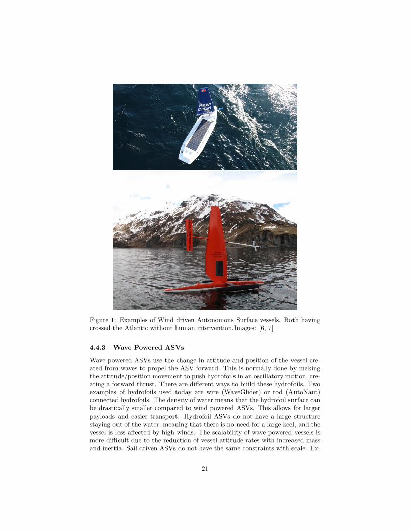
Figure 1: Examples of Wind driven Autonomous Surface vessels. Both havingcrossed the Atlantic without human intervention.Images: [6, 7]
4.4.3 Wave Powered ASVs
Wave powered ASVs use the change in attitude and position of the vessel cre-ated from waves to propel the ASV forward. This is normally done by makingthe attitude/position movement to push hydrofoils in an oscillatory motion, cre-ating a forward thrust. There are different ways to build these hydrofoils. Twoexamples of hydrofoils used today are wire (WaveGlider) or rod (AutoNaut)connected hydrofoils. The density of water means that the hydrofoil surface canbe drastically smaller compared to wind powered ASVs. This allows for largerpayloads and easier transport. Hydrofoil ASVs do not have a large structurestaying out of the water, meaning that there is no need for a large keel, and thevessel is less affected by high winds. The scalability of wave powered vessels ismore difficult due to the reduction of vessel attitude rates with increased massand inertia. Sail driven ASVs do not have the same constraints with scale. Ex-
21
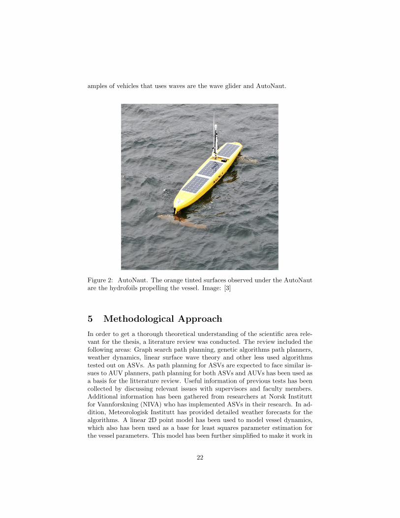
amples of vehicles that uses waves are the wave glider and AutoNaut.
Figure 2: AutoNaut. The orange tinted surfaces observed under the AutoNautare the hydrofoils propelling the vessel. Image: [3]
5 Methodological Approach
In order to get a thorough theoretical understanding of the scientific area rele-vant for the thesis, a literature review was conducted. The review included thefollowing areas: Graph search path planning, genetic algorithms path planners,weather dynamics, linear surface wave theory and other less used algorithmstested out on ASVs. As path planning for ASVs are expected to face similar is-sues to AUV planners, path planning for both ASVs and AUVs has been used asa basis for the litterature review. Useful information of previous tests has beencollected by discussing relevant issues with supervisors and faculty members.Additional information has been gathered from researchers at Norsk Instituttfor Vannforskning (NIVA) who has implemented ASVs in their research. In ad-dition, Meteorologisk Institutt has provided detailed weather forecasts for thealgorithms. A linear 2D point model has been used to model vessel dynamics,which also has been used as a base for least squares parameter estimation forthe vessel parameters. This model has been further simplified to make it work in
22
conjunction with a particle swarm algorithm (PSO) to calculate pseudo optimalpaths and sensor usage for the wave driven vessel AutoNaut.
6 State of the Art
6.1 Mission Planning
Movement and positioning of the surface vessel affects both on board sensor,sample quality and mission progression, as most constraints to a mission is po-sition and time oriented. An optimised mission is therefore highly dependenton the vessel path. Multiple articles have mapped different approaches to opti-mal path planning. Multiple problem descriptions and optimisation algorithmshave been proposed and implemented to solve different problems. For this mas-ter thesis, the goal is to take the optimisation one step further by implementingdiscrete decisions into the problem description. These discrete decisions willmainly focus on sensor sampling, but can also be extended to other areas thatcan implement the same problem structures.
6.1.1 Time and Energy Optimal Path Planning in General Flows
In Dhanushka Kularatne et.al. (2016) a novel method of finding time and energyoptimal paths was discussed and a graph based algorithm proposed to find anoptimal path between two way-points [8]. To be able to increase the efficiencyin use of autonomous vessels, it is proposed that the vessel path should bedependent on vessel inertial velocity together with ocean currents, to get abetter description of vessel velocity and energy expenditure. The ocean currentis described as a 2D vector field, v. The vessel velocity compared to the currentis described as vstill and the vessel velocity to an earth fixed coordinate systemis called vnet = v + vstill the vessel course is described by θ. The kinematicmodel of the vessel is modelled as:
X = vstill cos θ + vx, Y = Vstill sin θ + vy (1)
To simplify equations another coordinate system is made where x axis followsalong current direction, and y is orthogonal to current direction. Vnet can thenbe described as [dx, dy]T /dt. vstill thus becomes:
||vstill|| =
((dx
dt− v
)2
+
(dy
dt
)2) 12
(2)
Given a set vstill the duration from one point to another given constant currentbecomes:
dt =v
v2v2stilldx−
√v2still(dx
2 + dy2)− v2dy2v2 − v2still
(3)
A simple estimation of energy expenditure can be described by the vstill velocity,which describes vessel velocity relative to the ocean. Multiplying drag force
23
times duration we get the energy expenditure. e = κ||vstill||2dt which becomes:
e = κ
((dx
dt− v
)2
+
(dy
dt
)2)dt (4)
Minimising energy consumption with regards to the dt parameter, we get:
eopt = 2κv(√dx2 + dy2 − dx) (5)
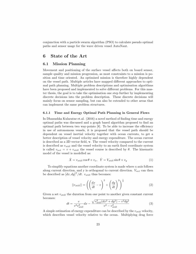
The model of the area is turned into a graph g, where each node on thegraph represents a point on a 2D surface grid covering the area of operations.The cost of the edges between two different nodes is described by the energyand time equations. An A* search algorithm is then used to describe the costfrom a starting position to the end goal.
The results in the article showed how the algorithm implemented managedto take advantage of ocean currents to optimise the path from a start point toan end point. Using a graph to describe the optimisation problem also simplifiescollision avoidance in the optimisation algorithm, by not including any vertexesover land. To avoid any edges crossing land, one can dilate the surface areas orerode ocean maps and reducing the neighbour hood of vertexes. The createdpaths were also tested by using small vessels trans versing currents similar to theanalytical currents tested. The small vessels were able to follow the preplannedpath.
Figure 3: Image showing path results for A* algorithm. Image: [8]
6.1.2 Time Varying Flows
Most optimisation algorithms discretises the optimisation algorithm into dis-crete steps either time wise, position wise or both. To be able to accurately
24

represent a continuous system, it is normal to include assumptions for the sys-tem dynamics between the time steps. Examples of such assumptions can beconstant speed or non changing weather between the time steps. The accuracyof these assumptions greatly depend on the systems discretised. In an articleby Dhanushka Kularatne et.al. (2017) the previous path optimisation methodwas extended to include time varying flows into the optimisation [9]. This isnecessary for autonomous vessels at sea, often spending months at a time in theocean. To try to minimise the error from assuming constant current velocity,the time step between each position was automatically adjusted depending oncurrent gradient to keep the estimation error within a certain bound. Areaswhere the current had a large gradient, the time step was reduced, by onlyallowing neighbours close to the node during graph search. At areas with lessgradient the neighbours were allowed to be further away.
Figure 4: Image showing results of algorithm for time varying current generatedfrom forecasts. Image: [9]
In both these articles the velocity of the vessel relative to the current wasassumed to be very limited. This approach allows the optimisation algorithmto limit the amount of possible neighbours, meaning that the use of an A*algorithm does not take an unreasonable amount of time. This can be a goodrepresentation for vessels with limited controlability, but might not be suitablefor vessels that are capable of moving independent of weather, as this wouldresult in a computationally expensive graph search.
6.1.3 Seabed Coverage
A common task for autonomous vessels is to create bathymetric maps of theocean floor. This is done by moving a sensor over all points in a desired area.This is a tedious, yet simple task, which makes it suitable for ASVs. In Glaceranet al., 2012, [10] a novel method for covering the area of interest was described.A common method used is the Morse-based cellular decomposition method. Theworking area is dividend into simply connected domains with a Morse based al-gorithm. In each simply connected domain a lawn-mower pattern path is thencreated to cover the entire area. A node network describing neighbouring do-mains are then created and a travelling salesman algorithm decides in which
25
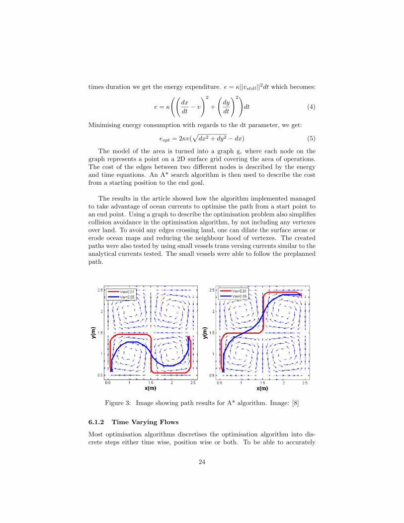
order the different domains are covered. An A* algorithm is made to find theshortest path between the end path of the previous domain and the start pathof the next domain.
Figure 5: Seabed coverage method described in glaceran et al., 2012 [10]1) Upper left: Working area divided into different regions of similar depth.2) Lower left: region divided into smaller simple regions via the Moore method.3) Upper right: Every simple region covered with a lawn-mower pattern.4) Lower right: Entire region path connected together.
This simple method however does potentially create unnecessary overlap ofsensor data. On most bathymetric sensors the field of view resembles a fan orcone. Area covered by the sensor will therefore change with distance betweenseabed and sensor. Seabed gradient also changes sensor coverage due to similareffects. To assure sufficient coverage, the planner has to create the lawn-mowerpattern to fit the shallowest depth in the area. This however creates large over-lap in deeper areas. To compensate for this a K means algorithm is used todivide the bathymetric map in k different areas of roughly similar depth. Thecreated areas are then smoothed out by dilating and eroding the edges of theclusters. The Moore algorithm is then used for each for the clusters. To min-imise change in elevation along the lawn mower patterns the paths are madeperpendicular to the seabed gradient. Interlap spacing is also made to fit theshallowest part of the next sweep. A test comparing the two algorithms showeda reduction in path length form 15646.08 meters to 10349.63 meters. [10]
This example of adapting a mission to suit sensor use is a great example ofhow sensor data is implemented in path planning. This algorithm does however
26

not take much into account vessel limitations, as the vessel expected to performsuch a mission is expected to have close to full control of vessel position andvelocity. This assumption is not always realistic for all types of vessels, as thecontrolability of self sufficient vessels is highly weather dependent.
6.1.4 Evolutionary Based Path Planning of an Autonomous SurfaceVehicle
Using genetic algorithms to solve path planning problems have been successfullyused in previous scenarios. In Arzamendia et.al. 2019 [11] the use of genetic al-gorithms for optimal area coverage was explored and compared to earlier studiesand result.
In the example used, an autonomous vessel was to try to cover YpacaraiLake by moving between beacons spread evenly around the lake edge. The Ves-sel coverage score was described by length of path L times a certain estimatedwidth S. To prevent duplicate sampling of a same area, we subtract S2 for everyintersection of a previous path.
The vessel was constrained to follow either a Hamiltonian circuit, meaningthat it can only go to each beacon once before returning to starting beacon, thuscreating a travelling salesman problem. The other possible path was a Euleriancircuit, where the vessel is allowed to visit a beacon multiple times, but not thesame path twice, as this would be a complete overlap.
Due to the high complexity of the optimisation problem, genetic algorithmshave shown to be great at finding Quasi optimal solutions, meaning seeminglyoptimal solutions, but without any real proof of it being optimal. The firstobstacle to overcome when using genetic algorithms is to start with a feasiblepopulation. Arzamendia uses an algorithm to find a feasible population whichis then iterated until some condition is met.
The results showed that the genetic algorithm was capable of optimising theinitial guessed paths. The Assumption of knowing all way-points of the vesselbeforehand however is not applicable for the missions planned at NTNU, whereoffshore situations is of higher importance.
6.1.5 Artificial Potential Fields For Real Time Path Planning
In Yogang Singh et. al.(2017)[12] it was attempted to use potential fields to finda feasible path from a start to end position in an environment changing withtime. A vector field is created by summing appropriate repelling and attractingvector fields into a complete vector field describing the work space. Repellingforces are placed at areas that the vessel has to stay away from. An attractingforce is also place to incentivise the vector field to flow against the goal position.By summing the forces up you get a vector field, where the vessel can followthe field to ideally the desired point. Potential fields do not however guaranteea global minimum. Multiple geometries can create local minimums, making it
27
hard for potential fields to work in the general case. The pro however is that itis not as computationally intensive as many other operations, which allows formore dynamic and reactive control. This also allows for a real time guidancealgorithm.
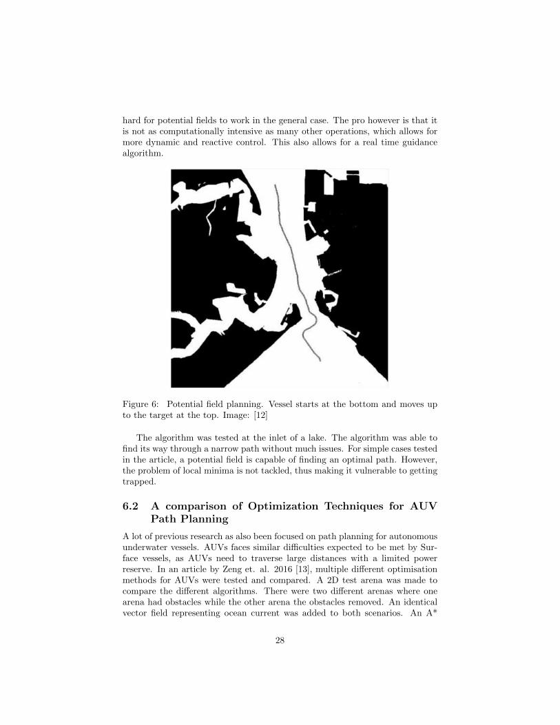
Figure 6: Potential field planning. Vessel starts at the bottom and moves upto the target at the top. Image: [12]
The algorithm was tested at the inlet of a lake. The algorithm was able tofind its way through a narrow path without much issues. For simple cases testedin the article, a potential field is capable of finding an optimal path. However,the problem of local minima is not tackled, thus making it vulnerable to gettingtrapped.
6.2 A comparison of Optimization Techniques for AUVPath Planning
A lot of previous research as also been focused on path planning for autonomousunderwater vessels. AUVs faces similar difficulties expected to be met by Sur-face vessels, as AUVs need to traverse large distances with a limited powerreserve. In an article by Zeng et. al. 2016 [13], multiple different optimisationmethods for AUVs were tested and compared. A 2D test arena was made tocompare the different algorithms. There were two different arenas where onearena had obstacles while the other arena the obstacles removed. An identicalvector field representing ocean current was added to both scenarios. An A*
28
algorithm, RRT* algorithm and three different evolutionary algorithms, namelyParticle swarm algorithm, quantum particle swarm algorithm, and a geneticalgorithm were then tested on the two different scenarios.
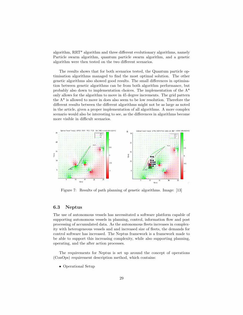
The results shows that for both scenarios tested, the Quantum particle op-timisation algorithms managed to find the most optimal solution. The othergenetic algorithms also showed good results. The small differences in optimisa-tion between genetic algorithms can be from both algorithm performance, butprobably also down to implementation choices. The implementation of the A*only allows for the algorithm to move in 45 degree increments. The grid patternthe A* is allowed to move in does also seem to be low resolution. Therefore thedifferent results between the different algorithms might not be as large as notedin the article, given a proper implementation of all algorithms. A more complexscenario would also be interesting to see, as the differences in algorithms becomemore visible in difficult scenarios.
Figure 7: Results of path planning of genetic algorithms. Image: [13]
6.3 Neptus
The use of autonomous vessels has necessitated a software platform capable ofsupporting autonomous vessels in planning, control, information flow and postprocessing of accumulated data. As the autonomous fleets increases in complex-ity with heterogeneous vessels and and increased size of fleets, the demands forcontrol software has increased. The Neptus framework is a framework made tobe able to support this increasing complexity, while also supporting planning,operating, and the after action processes.
The requirements for Neptus is set up around the concept of operations(ConOps) requirement description method, which contains:
• Operational Setup
29

• Mission programming
• Mission execution
• Mission analysis
Operational setup, entails implementing a map of the Area f Operationsand different constraints associated with the mission. Mission Programmingcontains programming of mission logic and plan to get the desired mission ex-ecution. Mission Execution: During a mission Neptus can be used to monitorthe vessels an interact with the vessels while out on mission. Mission Analysis:After the mission Neptus can be used to analyse mission data.
Neptus can also be used to simulate missions, to that way be able to testout and preemptively iterate on the mission before real life testing[14]. Neptusis also the system used to control the AutoNaut and many other vessels usedby NTNU.
6.4 Genetic Algorithms
6.4.1 Particle Swarm Algorithm
Due to the capabilities and adaptability of Particle swarm algorithms, this ap-proach will also be the main approach for this master thesis.
Particle swarm optimisation is an evolutionary optimisation algorithm inwhich an optimal solution to a function is found by moving a set of particlesaround a parameter space. The position of the particles in the parameter spacerepresent the parameters in an objective function. The parameters described byeach particle gives each particle a score determined by the objective function.The particle are moved around in the parameter space in search of the parame-ters that gives an optimal score for the objective function. The movement speedand direction of the particles are given by the particles previous velocities andattraction forces that pulls the particles against the particles with the best localand/or global objective scores. [15]
Let v = (v1, ..., vn) be a vector describing particle velocities, where each vi isthe velocity of particle i. The velocity and position of each particle is determinedfor each iteration by the equation:
v(n+ 1) = ωv(n) + α(pbest − x(n)) + β(gbest − x(n)) (6)
x(n+ 1) = x(n) + v(n+ 1) (7)
Where ω, α, β are continuous variables between 0 and 1. They can alsobe random variables from an even distribution from 0 to 1. The main issueis that the particles start to converge toward either a local or global optimalsolution. This is a basic description of a particle swarm iteration. Many different
30

equations and philosophies can be used to iterate the velocities. Particles swarmoptimisation can also be used with mixed binary-continuous input parameters.This allows for binary operations to be implemented into the objective function.In binary particle swarms, binary operations such as AND ∩, OR ∪ and XOR ⊕are used to iterate thorough different solutions. Similar to continuous particleswarm, the personal, local and global best solutions are used as attraction forcesto make the solutions converge toward an optimal solutions. [16]
v(n+ 1) =ω ∩ v(n) ∪ c1 ∩ (pbest ⊕ x(n)) ∪ c2 ∩ (gbest ⊕ x(n)) (8)
x(n+ 1) =x(n)⊕ v(n+ 1) (9)
A full description of an implemented particle swarm algorithm can be foundbelow. An actual implementation should however not be implemented directlyas described. There is large computational gains possible from parallelising thealgorithm.
Algorithm 1 Particle Swarm Optimisation
n = numInputsm = numParticlest = maxIterations
Require: x ∈ RnXRm
xi,j , i ∈ n, j ∈ mpbest,p, p ∈ mgbest ∈ R1
for k = 1 : t dofor j = 1 : m do
for i = 1 : n dovi,j = ωvi,j + α(pbest − xi,j) + β(gbest − xi,j)xi,j = xi,j + vi,j
end forend forfor j = 1 : m do
if costFunction(x[:, j]) < pbest,j thenpbest,j = costFunction(x[:, j])xpBest,j = x[:, j]
end ifend forif min(pbest) < gbest theni = indexMin(pbest)gbest = pbest[:, i]xgBest = xpBest[:, i]
end ifend forreturn gbest, xgBest
31

Particles swarm algorithms do not need to calculate derivatives. In opti-misations algorithms such as SQP or newton method necessitates derivativesand double derivative, either by direct calculation or by estimation. Both arecomputationally expensive and not always feasible depending on the problem.Nonlinearities in a cost function may also throw off algorithms using derivativesto find a solution.
32
Part II
Theory for Vessel Modelling andEstimation
33
7 Modelling and Implementation of Wave Propul-sion ASV
7.1 AutoNaut
The AutoNaut is an autonomous surface vessel that is made for long endurancemissions up to two months at sea. The vessel is made by AutoNaut Ltd[17].AutoNaut gathers energy during missions from solar panels placed on top of thevessel, and uses the wave induced change in attitude and height of the vesselto create propulsion. The product is a complete package including proprietaryhardware and software. Scientific equipment, guidance and mission executionis all made by AutoNaut Ltd. The reasoning for NTNU to order the AutoNautwas the large payload available on the ASV compared to its size and weight.The AutoNaut 7 has the capacity of around 130 Kg of payload for 250 kg dis-placement, which gives a 0.52 payload to weight ratio compared to a competitorlike Saildrone at around 0.2 payload to weight ratio[6].
NTNU wanted to build a open architecture research vessel to base theirresearch for both oceanic and cybernetic research to be published. Thereforethe AutoNaut was gutted of its internal hardware, and replaced with an opensource architecture carefully described in multiple articles and the AutoNautWiki [18]. To get a good introduction to the NTNU version of the autonaut, atranscript form Dallolio et al.,2019 [3] page 3-8.
7.2 Autonaut Description
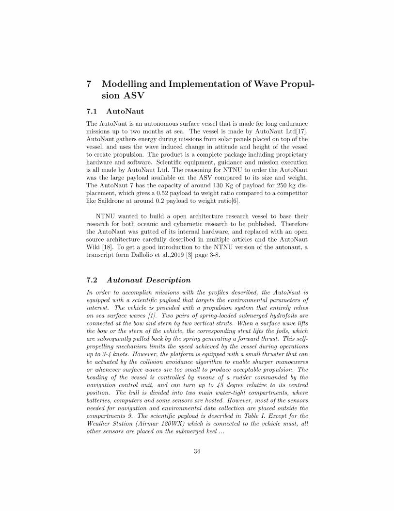
In order to accomplish missions with the profiles described, the AutoNaut isequipped with a scientific payload that targets the environmental parameters ofinterest. The vehicle is provided with a propulsion system that entirely relieson sea surface waves [1]. Two pairs of spring-loaded submerged hydrofoils areconnected at the bow and stern by two vertical struts. When a surface wave liftsthe bow or the stern of the vehicle, the corresponding strut lifts the foils, whichare subsequently pulled back by the spring generating a forward thrust. This self-propelling mechanism limits the speed achieved by the vessel during operationsup to 3-4 knots. However, the platform is equipped with a small thruster that canbe actuated by the collision avoidance algorithm to enable sharper manoeuvresor whenever surface waves are too small to produce acceptable propulsion. Theheading of the vessel is controlled by means of a rudder commanded by thenavigation control unit, and can turn up to 45 degree relative to its centredposition. The hull is divided into two main water-tight compartments, wherebatteries, computers and some sensors are hosted. However, most of the sensorsneeded for navigation and environmental data collection are placed outside thecompartments 9. The scientific payload is described in Table I. Except for theWeather Station (Airmar 120WX) which is connected to the vehicle mast, allother sensors are placed on the submerged keel ...
34

Figure 8: A CAD model of the AutoNaut
7.2.1 Energy storage and distribution
The upper surface of the hull is covered with three Solbian SP 104 solar pan-els, whose maximum output power rating is 104W each. The onboard batterybank is made of four 12V 70Ah Lead Gel batteries, wired in parallel as most ofthe components require around 12V. In order to control the power produced bythe panels, two Maximum Power Point Tracking (MPPT) controllers are cho-sen. These have built-in inverters and can step the voltage up or down priorto supplying the batteries. This is required as the solar panel output varies withthe observed load impedance. Two step-down MPPT controllers is used in thepower system. Panel 3, which is furthest from the mast, is connected to onecontroller because it is unlikely that the internal bypass diodes are activated dueto shading, meaning that the panel output always will be higher than the requiredinput voltage for the controller. The panels near the mast which are likely sub-ject to partial shading, are connected in series to another step-down MPPTcontroller. The chargers input will thus always be higher than the minimumvoltage requirement, even if both arrays in one panel are bypassed. The unitsselected are Victron BlueSolar MPPT 75/15. Fig. 5 provides an overview ofthe structural design of the power management system implemented into Level1 unit housing. An external toggle switch allows to disconnect the load powerline that provides power to all components. This means that when a mission iscompleted and the user turns off the computers and sensors, the batteries canstill be recharged by the solar panels through the controllers. Fig. 5 also shows
35

how the power is distributed to the whole system. The CR6 Campbell ScientificDatalogger, compass GPS, Iridium and Rudder Servo are directly connected tothe load port of BlueSolar 1, through the switch. However, they are controlled bythe CR6. Level 2, Level 3, AIS transceiver, 4G/LTE Modem, SentiBoard timingunit, Radar Reflector and Pumps are instead powered through solid state relaysthat are digitally controlled by CR6 GPIOs. The OWL VHF radio is the onlycomponent being directly powered by a 12V output port of the CR6. Historicdata for solar radiation during fall in Trondheim ...
Figure 9: The different compartments and hardware in the AutoNaut
7.2.2 Communication
B. Iridium Communication: The vessel is equipped with two separate IridiumRock- block+ units that host an Iridium 9602 transceiver, an antenna and avoltage regulator. As shown in Fig. 4, both Level 1 and Level 2 can send areceive messages over satellite. This communication link supports the missionwhen 4G/LTE coverage is absent and involves less mission flexibility and highercosts. Level 1 periodically sends a message reporting the overall state of the sys-tem: Time and location, power settings, battery voltage, consumed and producedpower. The operator is therefore able to communicate changes in the power set-tings of the vehicle and restart sensors and components. The Rockblock+ unitconnected to Level 2 is instead used to communicate new or modified plans to theonboard software (Dune). The vehicle acknowledges the reception of the plan andlater its outcome. This solution has a limited bandwidth and is therefore onlysuitable for simple control monitoring or tracking applications. The maximumpackage sizes are 340 bytes for sending and 270 bytes for receiving. Although
36

the latency is typically a few seconds, it may increase to up to a minute or moredepending on the remoteness of the area and the available satellites.
C. VHF Radio Communication Onboard the vehicle, an OWL VHF radiotransceiver allows efficient point-to-point communication between the operatorsand Level 1. It supports a large variety of modulation types and encoding, thatcan be configured through a serial port. A Java GUI (Fig. 10) enables man-ual control and direct monitoring of the vehicle, over VHF. During a mission,this link is turned off in order to save energy. It is however turned on whenmanual control of the vehicle is needed. An automatic routine enables the radiowhenever a fault is detected. The radio transmits the location and power set-tings, allowing the operators to find the vehicle and manually control it to shore.A passive duplexer allows the OWL VHF radio to share one antenna with theAIS. Unlike an active splitter, the duplexer has a notch filter in each port thatattenuates the frequency used by the other port. This means that both radioscan always transmit without hearing each other and everything is sent out onthe antenna. The filters are tuned to specific frequencies, so the radios cannotchange frequency. The selected cut- off frequency of the AIS port is 162MHz(center of AIS frequencies 161,975MHz and 162,025MHz) ...
8 Vessel Dynamics Model
8.1 Assumptions
In Fossen et.al. [19] A full rigid body dynamics model for ships include surge,sway and heave, as well as pitch, yaw and roll. Pitch, roll and heave are selfstabilising under normal conditions, and therefore often set to 0. This sim-plification comes at the expense of removing the dynamics AutoNaut uses forpropulsion. The propulsion dynamics are instead modelled as a force indepen-dent of the vessel modelling. By setting Pitch, roll and heave to 0, dynamicssimplifies down to surge, sway and yaw. Yaw is controlled by a rudder on boardthe AutoNaut. Given that the rudder is capable of accurately controlling yaw,we can expect that heading equals desired heading within the expected timestep of the simulations, which are expected to range between minutes to hours.Yaw dynamics are therefore neglected. Movement on the surge sway plane canbe described by Newtons second law. If it is assumed that the only forces act-ing on the vessel is current, wind and forces form the AutoNaut hydrofoils, theequation becomes:
M~v =~Fwaves + ~Fwind + ~Fcurrents (10)
Wind and current forces can be described by the drag equation. From Fos-sen et.al. [19] a drag equation is explained as the equation −sgn(V ) 1
2ρCdAV2.
ρ kgm3 describes the density of the medium being passed through. Cd is the ad-
justable variable fitting the measured drag forces to the model. A m2 describesthe cross-section of the object as projected onto a plane orthogonal to the force
37
direction.CdA changes depending on what angle the vessel passes through themedium. As the vessel is moving at velocities between 0 - 1 m/s it can beassumed that the flow passing the vessel will be close to laminar. The opera-tional range of the velocity is also relatively small, therefore a linear drag modelis assumed to be a sufficient assumption. This will also simplify parameterestimation and the ease computation.
8.2 Model Fitting
Making an accurate model for the vessel allows the model to predict vesselbehaviour in different conditions. This predictability enables an algorithm tocalculate the duration of a path given weather conditions either measured orgathered from weather forecasts. It will also be able to predict unfeasible paths,which is a vital part of path planning. The Linear model can be described by:
m~a = Dw(~V nw − ~V n) +Dc(~V
nc − ~V n) + Fwaves
The drag coefficients Dw and Dc is expected to depend on the angle betweenvessel and fluid. The drag force is expected to be largest when orthogonal tothe vessel and smallest along the surge direction. To recreate this propertythe relative current and relative wind will be decomposed to two velocities torelative velocity parallel and orthogonal to the bow-stern line. This coordinatesystem is normally described as the body coordinate system. Given relativevelocity in body coordinates drag forces can be set as two parameters. Thedrag forces can then be described in body coordinates as:
F bd =
[Dx 00 Dy
] [V brx
V bry
](11)
The relative velocity has to be changed to a description of Earth fixed Vesseland weather velocities to be able to us forecast and vessel data:
~V br = (~V b
w − ~V b) (12)
If we want to describe dynamics In NED earth fixed coordinates, the equationchanges to:
Fnd = Rn
b
[Dx 00 Dy
]Rb
n
[V nwx − V n
x
V nwy − V n
y
](13)
This can be implemented for both wind an current forces. By inserting dragand wave forces into equation, we get:
38
m~an = RnbDwR
bn(~V n
w − ~V n) +RnbDcR
bn(~V n
c − ~V n) +Rnb
[Ff
0
](14)
mRbn~an = DwR
bn(~V n
w − ~V n) +DcRbn(~V n
c − ~V n) +
[Ff
0
](15)
Equation 15 can be further used to estimate the parameters for the Auto-Naut. Current model is dependent on vessel heading for all estimated parame-ter. Using a model explicitly dependent on vessel heading creates an unwantedcomplexity. If the vessel wants to follow a predefined course, the vessel needto find a correct creep angle. To avoid the need of directly calculating creepangle, a simpler model is needed. As previously commented the timesteps areexpected to be between minutes to hours. The vessel is therefore expected toreach a steady state velocity, therefore setting acceleration to 0. Given that thedrag forces from wind are low compared to current forces, the force generatedfrom the ocean will be perpendicular to the forces generated by the hydrofoils.in this case the only relevant drag parameter will be the forward drag of thevessel, as there will be no sideways movement relative to the current. It is stillhowever important to estimate sideways and forward drag separately, otherwisea parameter estimation algorithm will estimate the drag as a sum of forward andsideways drag. If the difference between sideways and forward drag is large, theerror in the parameter estimate will also be large, and highly dependent at whichangle the relative current will be during parameter estimation. Replacing theheading dependent drag coefficients with with Dw, Dc and setting accelerationto 0, we get:
0 = Dw(~V nw − ~V n) +Dc(~V
nc − ~V n) + Fwave (16)
(Dw +Dc)~Vn = Dw
~V nw +Dc
~V nc + Fwaves (17)
~V n =1
(Dw +Dc)(Dw
~V nw +Dc
~V nc + Fwaves) (18)
~V n =1
(Dw +Dc)(Dw
~V nw +Dc
~V nc ) +
1
(Dw +Dc)Fwaves (19)
Thus, the resulting earth fixed NED velocity can be described as the sumof the velocity gained from drag forces and the hydrofoil forces. To simplifynotation the velocity generated from weather will be called disturbance velocity,and velocity gained from hydrofoil forces will be called wave velocity.
8.3 Wave Propulsion Modelling
The AutoNaut uses a novel propulsion method, where the roll and pitch ofthe vessel is converted into forward propulsion. Equipping the AutoNaut withsufficient solar panels for on board components gives the vessel almost unlimitedoperational range. Fouling and components wearing out do however limit thepractical limits of the missions to a couple of months[17]. The wave propulsion
39

hardware consist of two vertical rods connected to the bow and stern of thevessel. There are one hydrofoil on the port and starboard at the bottom of eachrod. These hydrofoils are connected to the rod via a rotating shaft with a springforcing the foils to the neutral position. The centre of pressure on the hydrofoilsare slightly aft of the rotation centre-line, thus when the AutoNaut rolls orpitches, the pressure from the surrounding water will offset the hydrofoils formthe neutral position. In this offset position the pressure forces point forwardat an angle. Gravity and buoyancy neutralisers all vertical forces, while thehorizontal forces in the surge direction pushes the AutoNaut forward. Thehydrofoils surface is orthogonal to the sway axis, thus there are no forces in thesway axis. Vessel symmetry around the Surge, Heave plane also nullifies anysideways forces. Propulsion forces in the body frame therefore simplifies downto:
F bwav =
[Fwav
0
](20)
The hydrofoils on the AutoNaut only create forces when the waves inducea roll, pitch or heave motion on the vessel. Given that wave velocity and cur-vature is highly dependent on wave frequency, thus it can be assumed that theenergy transferred from the wave to the AutoNaut can be described by a trans-fer function.
The velocity generated from the hydrofoils is assumed to be largest whenthe heading is parallel with wave direction. The smallest velocity is generatedwhen the waves are orthogonal to the heading. When the angle is betweenthese positions the velocity is somewhere between forward and side ward forceas well. The generated wave velocity is therefore expected to represent an oval ifplotted in a polar diagram. Given that the polar diagram plots for relative anglebetween vessel heading and wave direction, the polar plot will be represented byan oval with largest radius along the 0 and 180 degree angle. The smallest radiuswill be along the 90 and 270 degree angle. The resulting earth fixed velocity willthen be represented by the sum of the disturbance and wave velocity vector, asrepresented in figure 10.
The coordinate system used in figure 10 is a plane coordinate system alongthe water surface. X axis being parallel to the wave direction. The motivationbehind rotating the coordinate system along the wave direction is to simplifyequations that calculates the given velocity for a certain course. The main sim-plification being the equation representing the hydrofoil force can be describedby an oval with c radius along the x axis and d radius along the y axis:
1 =x2
c2+y2
d2(21)
If you want to to centre the oval on (x0,y0) you can replace x and y with(x− x0) and (y − y0). Let Vwave be described by an oval with radii Vf and Vs.
40
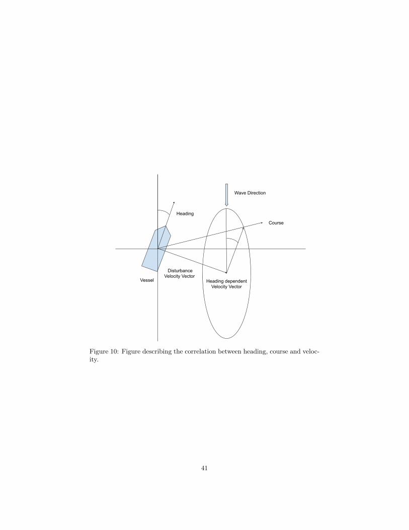
Figure 10: Figure describing the correlation between heading, course and veloc-ity.
41
Since the radii should change with the amplitude and frequency ω of the waves,we multiply the radii with the function Kwaves. Thus Vwave can be describedas the vector from the origin to the perimeter of the oval:
1 =(x− vwx,ned)2
c2+
(y − vwy,ned)2
d2(22)
c = Kf (ω)1
(Dw +Dc)(23)
d = Ks(ω)1
(Dw +Dc)(24)
(25)
The energy harvested form the hydrofoils to only push along the surge bodyaxis, as previously discussed. An exact model for hydrofoil forces are howeverharder to come by. Rolling to hydrofoil forces have not been in much focus. Toget an understanding of wave propulsion, a short introduction to wave energyis needed.
In linear wave theory a one dimensional wave is described by the equation:
η(t, x) = a cos(ωt− kx) (26)
Where x defines the position along the one dimensional wave, t defines thetime, η(t, x) defines the height of the surface of the wave. ω and k depends onthe depth of the ocean. Assuming that we have a irrotational incompressiblefluid, it is a descent assumption that the waves can be described by a potentialfield. Given the velocity potential field Φ(x, z, t) velocity in x and z directionshould be given by the directional derivative of the Velocity potential field, thus
∂Φ
∂x= ux,
∂Φ
∂z= uz (27)
The rest of the constraints are linearised and and it is assumed that thewave amplitude is small compared to the wavelength of the waves. Given theseassumptions the constraints can later be solved.
Due to the fact that water is an incompressible fluid, the divergence of thepotential field will equal zero at all points, thus
∂2Φ
∂x2+∂2Φ
∂z2= 0 (28)
The bottom of the ocean is assumed to be impermeable, thus any verticalmotion at the sea bottom is impossible, giving us the constraint
∂Φ
∂z= 0, at z = −h (29)
42
Given the scale of the ocean, it is assumed that waves height to ocean depthis infinitesimal, thus the vertical motion of the wave surface equals the verticalflow velocity.
∂η
∂t=∂Φ
∂z, at z = η(t, x) (30)
The air pressure over the wave surface is assumed to be constant. Via theunsteady Bernoulli’s equation you get the linearised final constraint for smallwaves:
∂Φ
∂t+ gη = 0 (31)
A general solution for these constraints has until now been impossible tosolve, but for more specific situations a solution has been found. Given ourdescription of a wave η(x, t) a solution for Φ can be described by
Φ =ω
ka
cosh(k (z + h)
)sinh (k h)
sin (kx − ωt), (32)
ω2 = g k tanh (kh) (33)
From the constraints one can observe that wave frequency and velocity de-pend on eachother. Given that depth of the ocean is much larger than thewavelength (1 << kh) we get
ω2 = gk (34)
Thus the wave can be described by only wave height and frequency. Formost wave forecasts you normally only get wave height and frequency, whichgiven smaller waves is enough to describe the whole wave system.
The energy contained in a wave can be roughly described as:
Ew =1
2ρgh2 (35)
The amount of energy extracted from the waves via hydrofoils has from testsnot been observed to increase quadratic with wave height. The limited lengthof the Hydrofoil rod also limits the achievable energy gained from the increasedheight of waves. A linear correlation between wave height and hydrofoil forcewill therefore be a placeholder until a better understanding of the hydrofoils canbe made. The resulting wave velocity model will be described as:
43
1 =(x− vwx,ned)2
c2+
(y − vwy,ned)2
d2(36)
c = Kfh
(Dw +Dc)(37)
d = Ksh
(Dw +Dc)(38)
(39)
8.4 Implementation of Parameter Estimation
Equation 15 has six unknown parameters. Dw, Dc, Kf (ω) and Ks(ω), as Dw
and Dc are diagonal 2x2 matrices. This system is a linear time varying model,thus a linear least squares estimate can be used to estimate the parameters,given enough equations. The AutoNaut tracks velocity for every second, thus alarge representative data set is therefore available. To estimate the unknowns,we want to set the unknowns as x in an Ax=b equation. If we want to to writethis as a linear equation we set A, x and b as such:
V bwi =diag
(Rz(ψi)(~V
nwi − ~V n)
)(40)
V bci =diag
(Rz(ψi)(~V
nci − ~V n)
)(41)
The hydrofoil forces are estimated to be the radius of an ellipse for a certainangle. This is however hard to the directly estimate, as the radius of an ellipsein polar coordinates can be described as:
r =ab√
(a cos(θ))2 + (b sin(θ))2(42)
where a and b is maximum and minimum radius of the ellipse and θ is thepolar angle. It is hard to explicitly estimate a and b, thus there is easier touse a similar form to estimate the force. The discrepancy from using a slightlydissimilar model to an oval, is expected to be trivial due to the ellipse alreadybeing an estimate created from deductions during ocean tests. To simplifymanners the ellipse will be estimated by a ellipse lookalike form. A slightlysimilar shape to an ellipse is the model:
r = a cos(ηi)2 + b sin(ηi)
2 (43)
As discussed in the linear wave theory chapter, the forces created from a waveis estimated to be modelled as the the wave height multiplied by a constant.
44
The frequency of the wave is also expected to affect the vessel velocity, but tokeep the model simple, it is assumed to be frequency invariant. If the forcesare not frequency invariant, the estimated forces should differ for different wavefrequencies, so it should be possible to spot during parameter estimation. Thewave forces were therefore implemented as follows:
ri =
[cos(ηi)
2W (t)2 sin(ηi)2W (t)2
0 0
](44)
Then A, x and b can be described as :
Ai =[V bwi V b
ci ri]
(45)
x =
Dwf
Dws
Dcf
Dcs
Kf (ω)Ks(ω)
(46)
bi =mRz(ψi)(~Vni+1 − ~V n
i ) (47)
Since we want a least square estimate we want to have as many equations aspossible. For the least squares to be able estimate the parameters, the systemwill have to be observable, meaning that the system should only have one uniquesolution. For this to be correct, A has to be full rank, and b to be nonzero.Thus, at least 3 unique time steps to be able to find a solution, but the morethe better. The resulting equation can be set up as:
A =
A1
A2
...AN
(48)
x =x (49)
b =
b1b2...bN
(50)
(51)
Due to the rotation matrices and uncertainties in both measurements andforecasts, the result does not necessarily converge to the true parameters. Whentesting out the least squares solution, on simulated analytical models testsshowed that the method was hard pressed to find correct parameters whennoise was included into the measurements. Especially when included to theGPS data. For those interested, the estimation simulation is added with thecode attached to the thesis.
45
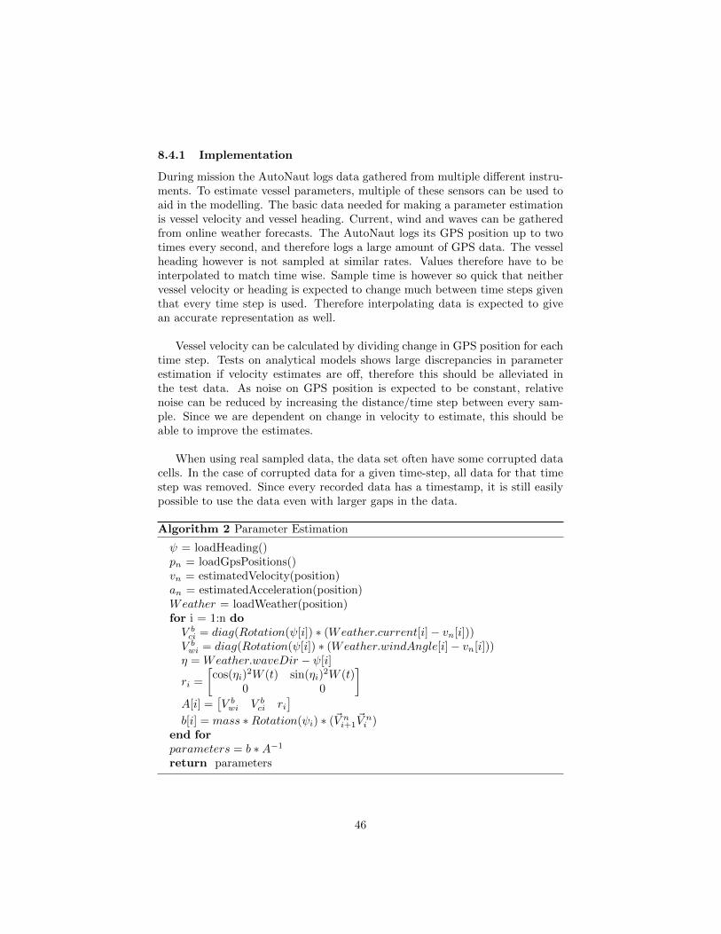
8.4.1 Implementation
During mission the AutoNaut logs data gathered from multiple different instru-ments. To estimate vessel parameters, multiple of these sensors can be used toaid in the modelling. The basic data needed for making a parameter estimationis vessel velocity and vessel heading. Current, wind and waves can be gatheredfrom online weather forecasts. The AutoNaut logs its GPS position up to twotimes every second, and therefore logs a large amount of GPS data. The vesselheading however is not sampled at similar rates. Values therefore have to beinterpolated to match time wise. Sample time is however so quick that neithervessel velocity or heading is expected to change much between time steps giventhat every time step is used. Therefore interpolating data is expected to givean accurate representation as well.
Vessel velocity can be calculated by dividing change in GPS position for eachtime step. Tests on analytical models shows large discrepancies in parameterestimation if velocity estimates are off, therefore this should be alleviated inthe test data. As noise on GPS position is expected to be constant, relativenoise can be reduced by increasing the distance/time step between every sam-ple. Since we are dependent on change in velocity to estimate, this should beable to improve the estimates.
When using real sampled data, the data set often have some corrupted datacells. In the case of corrupted data for a given time-step, all data for that timestep was removed. Since every recorded data has a timestamp, it is still easilypossible to use the data even with larger gaps in the data.
Algorithm 2 Parameter Estimation
ψ = loadHeading()pn = loadGpsPositions()vn = estimatedVelocity(position)an = estimatedAcceleration(position)Weather = loadWeather(position)for i = 1:n doV bci = diag(Rotation(ψ[i]) ∗ (Weather.current[i]− vn[i]))V bwi = diag(Rotation(ψ[i]) ∗ (Weather.windAngle[i]− vn[i]))η = Weather.waveDir − ψ[i]
ri =
[cos(ηi)
2W (t) sin(ηi)2W (t)
0 0
]A[i] =
[V bwi V b
ci ri]
b[i] = mass ∗Rotation(ψi) ∗ (~V ni+1
~V ni )
end forparameters = b ∗A−1return parameters
46
8.4.2 Estimating parameters with vessel sensors
The AutoNaut is equipped with a Doppler current sensor, wind sensor and andIMU, that should give the AutoNaut the possibility of estimating all neededmeasurements to estimate the parameters[3]. Wave estimation is still not fin-ished on the AutoNaut, but relative wind and relative current can already bemeasured by the wind and current sensor. Therefore instead of using weatherforecasts for wind and current it can be calculated relative to vessel body. Thesemeasurements will be in body frame, thus the equations changes slightly to:
V bwi = diag
(Vwmi
)V bci = diag
(Vcmi
)(52)
where Vwmi is measured wind relative to vessel, and Vcmi is measured currentrelative to vessel. If the estimates are good, one should expect measurementsto be similar in both cases, so it will be interesting to see. If they are different,it does not discredit any of the methods, but but it is likely that one of themare erroneous.
47

Part III
Optimal Mission PlannerImplementation
48

9 Velocity Model Use in Optimisation Algorithms
When optimising for an optimal path, multiple approaches can be made. Dif-ferent approaches have different pros and cons. Adjustable parameters for op-timisation could be vessel heading, rudder angle, vessel course or way-points.There are however definitive properties that makes way-points the best solution.
Parameters using vessel dependent input-parameters is an intuitive startingassumption. Normal control inputs for a seagoing vessel is often rudder angle,heading, or course. However, vessel dependent inputs are not able to predictvessel positions, as the vessel position will depend both on vessel inputs, as wellas unknown parameters such as weather and duration of time step. Changes inweather or time steps can change resulting vessel position, thus finding a pa-rameter input that takes the vessel to a predefined destination, is a complex task.
To alleviate this problem way-points are used as parameter input. Usingway-points to determine vessel course means that the path for the vessel ispredetermined explicitly. A drawback for this type of path description is thatnot all parameter inputs are feasible. If weather prevents the vessel from beingable to follow a path between two way-points, the estimated duration betweenpoints will not be solvable. This infeasibility does however represent reality, asan infeasible solution represents an impossible path.
For optimisation algorithms using derivatives to find feasible solutions, dis-continuitites in the objective function will lead to problems. For evolutionaryalgorithms however this is a desirable property. Infeasible solutions are easilydiscarded and replaced with other feasible solutions. The large nonlinear chaoticproperties of weather [20, 21] and cost function makes derivatives complex andprone to errors. Thus genetic algorithms are already the desired optimisationalgorithm for the problem.
9.1 Bearing, Courses and the Great Circle
When planning paths traversing large distances, the curvature of the earth be-gins to come into effect. AutoNaut is expected to travel for long distancescovering large areas of the Norwegian coast. A pane linearisation of the oceansurface begins to become inaccurate. One degree change in longitude at 60degree latitude equals around 56 kilometres. At 70 degrees latitude howeverone degree in longitude equates to 38 kilometres. This keeps decreasing untilyou get at 90 degree latitude where one degree change in longitude equals 0meters. There are multiple ways of taking into account the curvature of theearth. One solution is to linearise for each way-point in the path. This willhowever introduce changing errors depending on the distance and on angle be-tween way-points. Another solution is to model vessel position by Quaternions,or using rotational velocity to estimate and simulate position. However, sincethe raw data generated in the vessel sampling is in longitude and latitude, the
49

algorithms will have to include calculation with latitude and longitude. way-points in longitude and latitude are also a user friendly format for operators touse and is readily available on most maps, including google maps and similarservices. For these reasons the great circle calculation method was used.
In great circle calculations, one take advantage of the property that theshortest path between two way-points is equal to the path described by a cir-cle with origin at the earth centre intersecting the two way-points. Thereforethe shortest path between two way-points can be described accurately by ananalytical function. If a vessel follows the shortest distance path between twopoints, the bearing will not stay constant either. This is also able to accuratelycalculate using great circle mathematics, simplifying overlaying of weather fore-casts to position depending on vessel heading. The method is also shown to beaccurate even at small changes in latitude and longitude. [22, 23]
To calculate the distance between two way-points (ϕ1, λ1) and (ϕ2, λ2),where ϕi is latitude, λi is longitude, and r is radius of the earth, the distancewill be:
d = 2r arcsin
(√sin2
(ϕ2 − ϕ1
2
)+ cos(ϕ1) cos(ϕ2) sin2
(λ2 − λ1
2
))(53)
To calculate the bearing at the starting way-point, also called the forwardAzimuth, the angle can be calculated as:
θ = atan2(sin(λ2 − λ1) cos(ϕ2), cos(ϕ1) sin(ϕ2)− sin(ϕ1) cos(ϕ2) cos(λ2 − λ1))(54)
These calculations are more computationally heavy than many other meth-ods. There are however not currently any external factors setting limits forcomputational time, and a large part of the computational is is focused aroundloading and slicing large weather forecast maps spanning the entire Norwegianmainland coast. Future tests may look further into ways of simplifying thesecalculations, but at the moment, accuracy was deemed more important.
9.2 Finding Path Duration for a way-point Path
Given two way-points P1 and P2, an estimate for the time needed for the vesselto travel from P1 to P2 has to be found. First step calculate the course thattakes the vessel from P1 to P2. Since the earth is a sphere, longitude andlatitude is used to describe position. The great circle equations is then usedto calculate course and distance between two way-points. When the desiredcourse is found, the velocity for the course is calculated. For the vessel to movestraight between the two way-points, the vessel velocity vector has to be parallelto the desired course. Given the velocity model explained in figure 10, it can be
50
observed that velocity vectors parallel to the desired course will be described bythe intersection between the course line, and the wave velocity oval. Intuitivelyone might also see that not all course will give an intersection between thecourse line and the oval. In these cases, it will not be possible for the vessel totravel straight between the two different way-points. However, given that thereis an intersection between the line and oval, the intersection can be described
by the following equations. 1 = (x−x0)2
c2 + (y−y0)2
d2 describes the oval, and y =ax + b describes the desired course line. a can be found by: a = tan(θ), wheretheta is the desired course in the wave coordinate system. in the case where agoes to infinity the solution can be found by setting x=0. By inserting ax for yin the oval equation we get a second order polynomial equation describing theintersection points:
1 =(x− x0)2
c2+
(y − y0)2
d2, y = ax+ b (55)
1 =(x− x0)2
c2+
(ax+ b− y0)2
d2(56)
1 =x2 − 2xx0 + x20
c2+
(ax+ b)2 − 2(ax+ b)y0 + y20d2
(57)
1 =x2 − 2xx0 + x20
c2+a2x2 + 2abx+ b2 − 2axy0 − 2by0 + y20
d2(58)
0 = x2(
1
c2+a2
d2
)+ x
(− 2x0
c2+
2ab− 2ay0d2
)+x20c2
+b2 − 2by0 + y20
d2− 1
(59)
The equation will give us two solutions for x. If there are complex solutions,the course is considered infeasible. Given that there are two solutions, theresulting velocity vector can be calculated by:
~V nw =
[xax
]The a can be found by using the equation To get the velocity along the course,we can multiply the velocity vector with a course unit vector:
V = ~V n>w
[cos(ψn
w)sin(ψn
w)
]If both speeds are negative, it is considered to be infeasible. If there are one
or more positive speeds, the fastest speed will be used. Given the special casewhere there is only one solution, the algorithm will handle the solution as twosimilar solutions, and work as normal.
To find the duration needed to travel from P1 to P2 we now calculate thedistance by using the great circle distance equation. The duration is calculatedby dividing distance on the velocity. For a path with multiple way-points, theprocedure is done successively for each pair of way-points describing the path.
51

This can not be done in parallel, since the velocity is weather dependent, andtherefore also time dependent. Thus all previous way-points have to be calcu-lated before the correct velocity can be calculated. Total duration can then befound by summing the duration between each way-point. If any of the stepsare unfeasible the whole path will become unfeasible. Thus when calculatingthe duration of a path, it can be discarded if any part of the path is unfeasible.This way of calculating Earth fixed velocity is similar to equations described in[8], but modified to fit with wave propulsion modelling.
Algorithm 3 Vessel Velocity
DisturbanceVelocityNed = (Dc*current + Dw*wind)/(Dc + Dw)DisturbanceVelocityWave = Rotation(waveAngle)*DisturbanceVelocityNedx0 = DisturbanceVelocityWave(1)y0 = DisturbanceVelocityWave(2)relativeCourse = nedCourse - waveCoursea = tan(relativeCourse)fFront = Kf/(fCurrent + fWind)fSide = Ks/(fCurrent + fWind)c = fFront*waveHeightd = fSide*waveHeightb = 0a0 = (1/(c**2)) + (a**2)/(d**2)b0 = (-2*x0)/(c**2) + (2*a*b ‘- 2*a*y0)/(d**2)c0 = (x0)**2/(c**2) + (b**2 - 2*b*y0 + (y0)**2)/(d**2) - 1solution = quadrticRoots(a0, b0, c0)v1 = [solution(1),a*solution(1)]v2 = [solution(2),a*solution(2)]vCourse = [cos(course),sin(course)]velocity = max(dot(v1,vCourse ),dot(v2,vCourse ))
9.3 Weather
For the simulations three different parameters are of interest. Current, windand waves, met.thredds.no have many different weather and ocean forecasts.The met.no ROMS NorKyst800m coastal ocean forecasting system gives a 24to 66 hour forecast on Multiple weather forecasting parameters including windand current [24]. Forecasts for the current day forecast 66 hours into the future,while, any previous forecasts have a 24 hour horizon. The forecast covers theentire ocean coast of mainland Norway. The forecast has a resolution of 800x800metre squares for each data point. These forecasts are based on larger globalECEW forecasts generated by European Centre for Medium Range WeatherForecasts[25]. These forecasts have a much lower resolution between around4000x4000 metre. The Norwegian meteorological institute uses these forecasts
52
as boundary conditions for their own more accurate model ROMS NorKystforecasts. A similar approach is done for the wave foreacsts which also have a800x800 metre resolution[26]. The forecasts are however divided into differentareas of Norway, namely Finnmark, NordNorge, MidtNorge, Vestlandet and Sk-agerak. Both forecasts have over 20 different parameters, but the parametersthat will be used for this project is wave height and wave direction, current andwind. Other parameters such as wave frequency is also of interest, but is notincluded because of uncertainty to effect of frequency. A proposal for inclusionof frequency will be made, but not included in the calculations and final results.To simplify implementation and to be able to create forecasts stretching overmultiple days, an algorithm was created that stitched together the different 24hour forecasts into continuous forecasts over multiple days. All current, windand wave data is combined in a .mat file, to simplify the movement for forecastdata and increase the ease of implementing and using Forecast data both foruse in this thesis and future use.
9.4 Binary operations
Binary operations can be described as situation where the input of the opera-tion is either 1/0 or true/false, depending on the context. These operations canbe a part of the propulsion system like a constant thrust thruster or a descrip-tion of the state of a sensor or instrument. Optimisation of binary operationsdoes either need its own binary optimisation methods, or a re-description ofthe binary states to a continuous description. One can for example describethe interval you want the thruster to be. That way a binary operator can beoptimised through a continuous optimisation algorithm. This however is notalways possible.
During a mission the AutoNaut is expected to perform many actions thatcan be described as binary operations. Turning on and off sensors, sendingmessages and enabling and disabling different modes. For this thesis, the sensorusage will be implemented as a binary operation. The optimisation algorithmwill therefore be a continuous-binary hybrid optimisation algorithm, that willbe able to optimise both the binary and continuous parameters.
9.5 Areas of interest
When gathering scientific data over a prolonged time it is normally desired totake samples at the same location to be able to observe change in the envi-ronment over time. It is therefore expected that the mission for the AutoNautwill have some predetermined positions that the vessel has to enter during themission. The cost function will therefore implement ”Areas of interest” whichare predetermined positions where it is desirable for the vessel to go and do aspecific action. Areas of interest are defined as an area described either by a
53
map, function or just a circle with a radius and origin at a set position. Withinthis area the vessel is capable of gaining a cost by doing a predefined action.If we set the cost of sampling in a correct area to negative, the vessel will beincentivised to perform an action in the area of interest to minimise the costfunction. Another possibility is to implement a hard constraint to the path toforce it to a desired point, but in situations where the point is infeasible, theoptimisation will not be feasible. Instead, Soft constraints opens for the vesselto skip mission goals if the gain from sampling at a point does not outweigh thecost of reaching it. It can therefore autonomously skip points if it is deemednon optimal.
For this master, the optimisation of sensor usage will be implemented andshowcased as a part of the cost function. To simplify the optimisation, it isexpected that a sampling will take shorter time than the duration of a timestep. Therefore there will only be needed to take one sample inside every area ofinterest to get the score associated with the point. A more complex descriptioncould be implemented if needed. The implemented cost function will describepoints of interest as follows:
• Map out N point of interest
• Describe a cost/score to the points and a radius around the points
• Initialise different paths between all points to seed the optimisation algo-rithm
• Introduce cost to using sensors
• Add constraint to the amount of times a sampling can be done in an areaof interest.
9.5.1 Communication
Communication with the AutoNaut normally goes via VHF, 4G cellular or Irid-ium satellite communication. All these different communication methods have aset of predefined messages that is normally sent at fixed intervals. It is howevernot always necessary to send redundant messages. When sending message overIridium you pay for each 50 bytes sent, thus it is sometimes of interest to reservelong messages to when it is necessary. For communication such as cellular, thevessel will need to be within the coverage of the base stations to send a mes-sage. By letting the coverage area be the area of interest and the message bethe action, a binary operation can be used to describe the message sending inthe cost function. The vessel will therefore be incentivised to go to an area withcellular service to send a message, instead of sending it over iridium. Some dataalso looses value over time. This should incentiveise the cost function to sendthe data before the monetary value is too low. This is however not prioritisedin this thesis, due to uncertainty in practical implementation, and is thereforenot implemented.
54
9.6 Final Cost Function
For the Masters project the final variables that will be implemented will be therunning costs of running the vessel and the sensor data. For the moment theseare the variables that mostly affects the mission planning. An additional dan-ger cost could also be easily implemented. However, there is no description ofdanger of loss of vessel yet. For hard constraints it is mostly about constrainingthe vessel from crashing into land or going into restricted areas. Implementinghard constraints to the parameter space is complex to implement, thus the con-straints will be implemented as an infinite cost if a constraint is broken. Thisalso allows for a lot of different nonlinear constraints to be tested out withoutany need for changing the cost function. The weather forecasts for ocean datahas NaN values at areas that cover land. The algorithm will therefore notice ifit has crashed into land by checking the forecast data. The 800x800m resolutionforecast should give a descent description of land, but the final implementationinto a vessel should introduce a refined/conservative map to assure that thevessel will not crash into land. A suggestion for such a map would be to dilatethe areas of the weather map with NaN values to assure that the vessel staysaway from the shore line. Another potential solution is to use the cross sectionof land at a certain ocean depth, and that way limiting how shallow waters thevessel is allowed to traverse.
Algorithm 4 Cost Function
time = 0cost = 0for i = 1:listLength do
lat = latitudeList(i)long = longitudeList(i)nextLat = latitudeList(i+1)nextLong = longitudeList(i+1)current = getCurrent(Latitude, Longitude)wind = getWind(Latitude, Longitude)waveHeight = getWaveHeight(Latitude, Longitude)waveDirection = getWaveDirection(Latitude, Longitude)distance = greatCircle(lat,long,nextLat,nextLong)speed = vesselVelocity(current, wind, waveHeight, waveDi course)time = time + distance/speedcourse = course(lat,long,nextLat,nextLong)cost = cost + missionGoals(sensorList(i))cost = cost + hasCrashed(lat, long)
end forcost = cost + time*timeCostreturn cost
55
9.7 Particle Swarm Optimisation
To implement both binary and continuous parameter optimisation, a hybrid bi-nary continuous particle swarm algorithm is implemented that is capable of op-timising both input types. The implementation is made by having a continuousparticle velocity be calculated on the continuous paramours and using a binaryvelocity calculation be used on the binary part of the parameter input. This is asolution simple to implement and effective in use. It has also been used in multi-ple articles to find solutions in similar hybrid binary-continuous cost functions,especially withing antenna and phased array problems. [27, 28].As previouslydescribed, the input parameters will be both way-points in latitude and longi-tude, and sensor state for each way-point. The algorithm was implemented asfollows:
56

Algorithm 5 Hybrid Particle Swarm Optimisation
n = numInputsm = numParticlest = maxIterationsxcont ∈ RnXRm
xbool ∈ RnXRm
pbest,p, p ∈ Rm
gbest ∈ R1
for k = 1 : t dofor j = 1 : m do
for i = 1 : n dovcont,i,j = ωvcont,i,j + α(pbest − xcont,i,j) + β(gbest − xcont,i,j)xcont,i,j = xcont,i,j + vcont,i,jvbool,i,j = ωvbool,i,j + α(pbest − xbool,i,j) + β(gbest − xbool,i,j)xbool,i,j = xbool,i,j + vbool,i,j
end forend forfor j = 1 : m do
if costFunction(xcont[:, j], xbool[:, j]) < pbest,j thenpbest,j = costFunction(xcont[:, j], xbool[:, j])xpBestCont,j = xcont[:, j]xpBestBool,j = xbool[:, j]
end ifend forif min(pbest) < gbest theni = indexMin(pbest)gbest = pbest[:, i]xgBestCont = xpBestCont[:, i]xgBestBool = xpBestBool[:, i]
end ifend forreturn gbest, xgBestCont, xgBestBool
57

Part IV
Analytical Tests of OptimisationAlgorithm
58
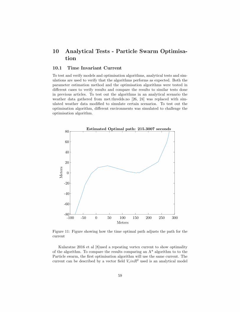
10 Analytical Tests - Particle Swarm Optimisa-tion
10.1 Time Invariant Current
To test and verify models and optimisation algorithms, analytical tests and sim-ulations are used to verify that the algorithms performs as expected. Both theparameter estimation method and the optimisation algorithms were tested indifferent cases to verify results and compare the results to similar tests donein previous articles. To test out the algorithms in an analytical scenario theweather data gathered from met.thredds.no [26, 24] was replaced with sim-ulated weather data modified to simulate certain scenarios. To test out theoptimisation algorithm, different environments was simulated to challenge theoptimisation algorithm.
-100 -50 0 50 100 150 200 250 300Meters
-80
-60
-40
-20
0
20
40
60
80
Met
ers
Estimated Optimal path: 215.3007 seconds
Figure 11: Figure showing how the time optimal path adjusts the path for thecurrent
Kularatne 2016 et al [8]used a repeating vortex current to show optimalityof the algorithm. To compare the results comparing an A* algorithm to to theParticle swarm, the first optimisation algorithm will use the same current. Thecurrent can be described by a vector field VcinR
2 used is an analytical model
59
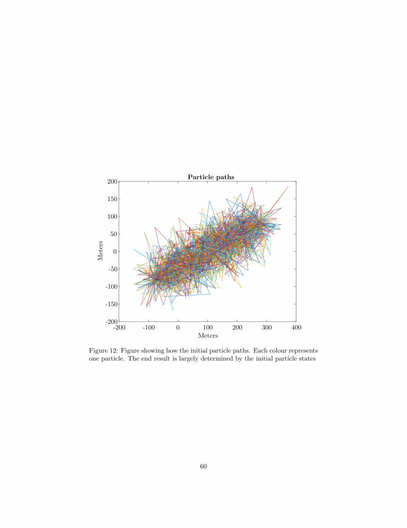
-200 -100 0 100 200 300 400Meters
-200
-150
-100
-50
0
50
100
150
200
Met
ers
Particle paths
Figure 12: Figure showing how the initial particle paths. Each colour representsone particle. The end result is largely determined by the initial particle states
60
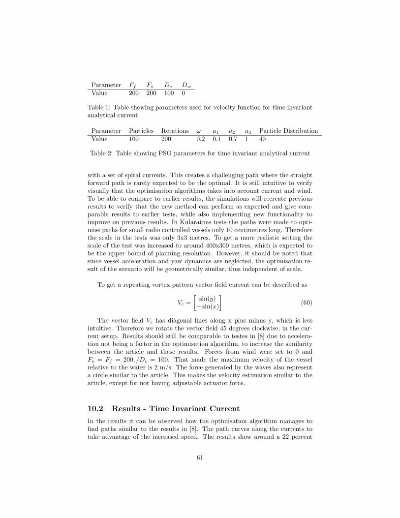
Parameter Ff Fs Dc Dw
Value 200 200 100 0
Table 1: Table showing parameters used for velocity function for time invariantanalytical current
Parameter Particles Iterations ω a1 a2 a3 Particle DistributionValue 100 200 0.2 0.1 0.7 1 40
Table 2: Table showing PSO parameters for time invariant analytical current
with a set of spiral currents. This creates a challenging path where the straightforward path is rarely expected to be the optimal. It is still intuitive to verifyvisually that the optimisation algorithms takes into account current and wind.To be able to compare to earlier results, the simulations will recreate previousresults to verify that the new method can perform as expected and give com-parable results to earlier tests, while also implementing new functionality toimprove on previous results. In Kularatnes tests the paths were made to opti-mise paths for small radio controlled vessels only 10 centimetres long. Thereforethe scale in the tests was only 3x3 metres. To get a more realistic setting thescale of the test was increased to around 400x300 metres, which is expected tobe the upper bound of planning resolution. However, it should be noted thatsince vessel acceleration and yaw dynamics are neglected, the optimisation re-sult of the scenario will be geometrically similar, thus independent of scale.
To get a repeating vortex pattern vector field current can be described as
Vc =
[sin(y)− sin(x)
](60)
The vector field Vc has diagonal lines along x plus minus y, which is lessintuitive. Therefore we rotate the vector field 45 degrees clockwise, in the cur-rent setup. Results should still be comparable to testes in [8] due to accelera-tion not being a factor in the optimisation algorithm, to increase the similaritybetween the article and these results. Forces from wind were set to 0 andFs = Ff = 200, /Dc = 100. That made the maximum velocity of the vesselrelative to the water is 2 m/s. The force generated by the waves also representa circle similar to the article. This makes the velocity estimation similar to thearticle, except for not having adjustable actuator force.
10.2 Results - Time Invariant Current
In the results it can be observed how the optimisation algorithm manages tofind paths similar to the results in [8]. The path curves along the currents totake advantage of the increased speed. The results show around a 22 percent
61
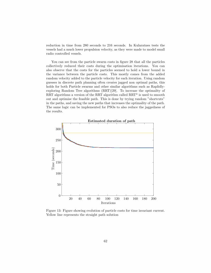
reduction in time from 280 seconds to 216 seconds. In Kularatnes tests thevessels had a much lower propulsion velocity, as they were made to model smallradio controlled vessels.
You can see from the particle swarm costs in figure 28 that all the particlescollectively reduced their costs during the optimisation iterations. You canalso observe that the costs for the particles seemed to hold a lower bound inthe variance between the particle costs. This mostly comes from the addedrandom velocity added to the particle velocity for each iteration. Using randomguesses in discrete path planning often creates jagged non optimal paths, thisholds for both Particle swarms and other similar algorithms such as Raplidly-exploring Random Tree algorithms (RRT)[29]. To increase the optimality ofRRT algorithms a version of the RRT algorithm called RRT* is used to smoothout and optimise the feasible path. This is done by trying random ”shortcuts”in the paths, and saving the new paths that increases the optimality of the path.The same logic can be implemented for PSOs to also reduce the jaggedness ofthe results.
20 40 60 80 100 120 140 160 180 200Iterations
0
50
100
150
200
250
300
Tim
e(s
econ
ds)
Estimated duration of path
Figure 13: Figure showing evolution of particle costs for time invariant current.Yellow line represents the straight path solution
62
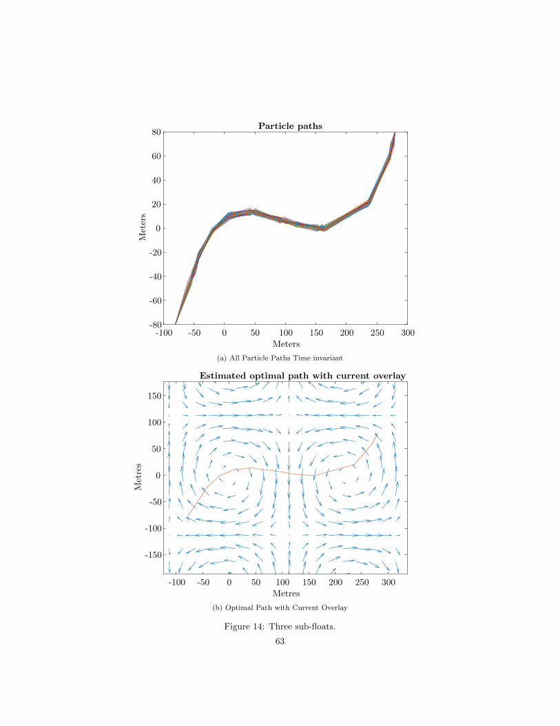
-100 -50 0 50 100 150 200 250 300Meters
-80
-60
-40
-20
0
20
40
60
80M
eter
s
Particle paths
(a) All Particle Paths Time invariant
-100 -50 0 50 100 150 200 250 300Metres
-150
-100
-50
0
50
100
150
Met
res
Estimated optimal path with current overlay
(b) Optimal Path with Current Overlay
Figure 14: Three sub-floats.
63

10.3 Analytical Test - Time Varying
To test out how the algorithm handles difficult scenarios, the tested analyti-cal mission was expanded to include time invariant currents. Under normalconditions the weather is expected to be continuous both in time and space.Many path planners, like time varying A* algorithms [9] and potential fieldalgorithms [12] use the assumption of continuous velocity fields for current toimprove the results. However, even if discontinuities are rare, they are not im-possible. The discrete nature of weather forecasts can introduce discontinuitiesinto the data used for mission planning. Discontinuity in the weather data willcreate problems for many algorithms, as an algorithm will not be able to esti-mate the optimal solution given only local knowledge. A particle swarm howeverweighs optimality of a particle given the entire mission cost. This should allowa particle swarm to more easily find an primal solution under conditions withdiscontinuities. Discontinuities are however expected to increase the necessaryparticle density, as discontinuous environments have a larger tendency to ”hide”potentially beneficial spots.
To test the optimisation algorithm the current will be described by a timevarying discontinuous current. The current vector field is made where y ¡ 0has opposite current of y¡0 where both currents are time varying. To set upa fitting mission, the vessel will have to travel along y=0 line which splits thecurrent vector field. The current will be set to 0.8m/s maximum. This willmake the straight forward path inefficient. Ideally the optimisation algorithmshould constantly switch bellow and above the Y=0 to take advantage of thecurrent when the current flows towards the goal. The wave is set to 1 metre, thewind drag set to 0 and Fs = Ff = 200, /Dc = 100. The distance to be travelledis around 400 meters, which would mean 200 seconds if there is no current. Letx(0) = (0,0) and the end point be x(T) = (400,0). The time varying currentfield is set to:
Vc =
[0.8 sin(0.02πt)
0
], y > 0Vc =
−0.8 sin(0.02πt)0
,≤ 0 (61)
64
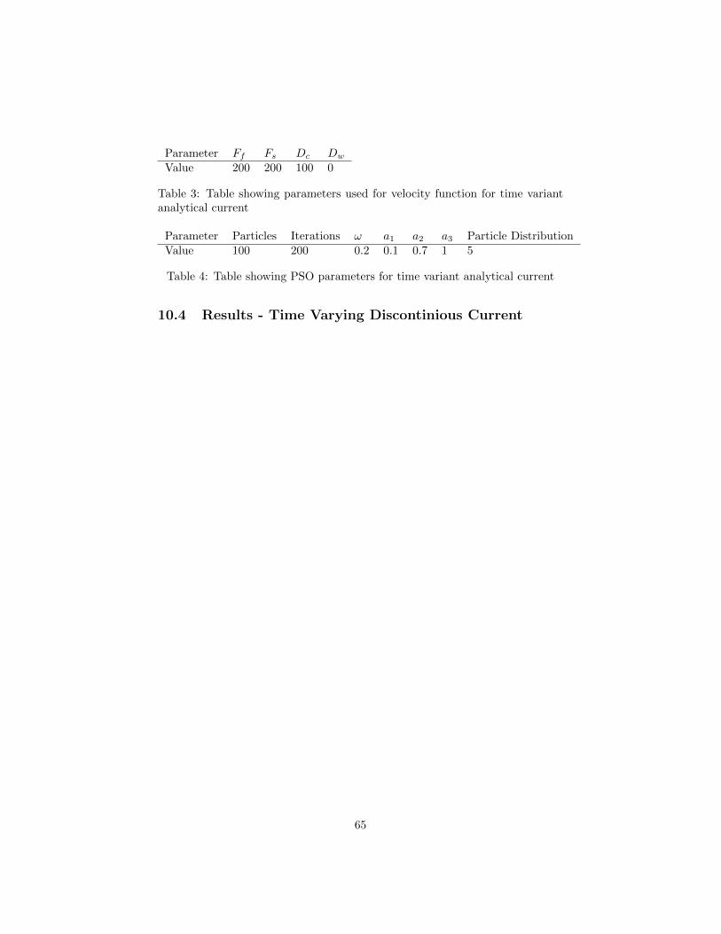
Parameter Ff Fs Dc Dw
Value 200 200 100 0
Table 3: Table showing parameters used for velocity function for time variantanalytical current
Parameter Particles Iterations ω a1 a2 a3 Particle DistributionValue 100 200 0.2 0.1 0.7 1 5
Table 4: Table showing PSO parameters for time variant analytical current
10.4 Results - Time Varying Discontinious Current
65
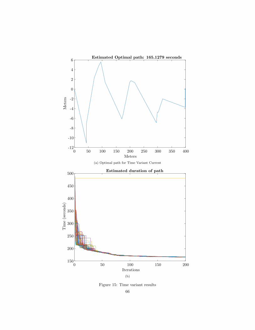
0 50 100 150 200 250 300 350 400Meters
-12
-10
-8
-6
-4
-2
0
2
4
6M
eter
s
Estimated Optimal path: 165.1279 seconds
(a) Optimal path for Time Variant Current
0 50 100 150 200Iterations
150
200
250
300
350
400
450
500
Tim
e(s
econ
ds)
Estimated duration of path
(b)
Figure 15: Time variant results
66
In figure 15 you can observe that the path switches below and above y = 0 asthe path progresses towards the end position. One of the defects of discretisa-tion can also be observed in the path plots. This most likely comes from a defectof discretising the problem. When the vessel velocity between way-points arecalculated, the current is estimated to stay constant between the way-points.Therefore, by matching the way-points with the times when current is at itsmaximum velocity, the resulting vessel velocity is maximised. This is not rep-resentative of the actual system, and are therefore unwanted defects from thediscretisation process. You can also see that the next to last way-point is notevenly spaced between the last and the second to last way-point. This is ex-pected to be a similar effect where the optimisation tries to skip the non optimalcurrent flows. These defects do not seem to create unreasonable results, andis considered to be within acceptable error margins. A possible solution to fixthe problem would be to add intermediate steps between the adjustable way-points to estimated vessel velocity. It is worth noting the axes dimentions infigure 15 as the x axis is 400 metres long and y axis only 18 metres. The paththerefore looks much more jagged than the real result. In the Estimated dura-tion you can see how the algorithm managed to reduce the path duratin from489 seconds to around 166 seconds. Reducing the path duration to less than half
It is worth noting that the particle swarm optimisation algorithm does notneed any changes to the optimisation algorithm when going from a time invariantto time variant system. Only the cost function describing the system neededto change some variables from time invariant to time variant. This is a largepro when comparing the optimisation algorithm to an A* algorithm where theneighbours of the vertexes have to be calculated for each timestep. parameters[9]which needs extra complexity to be able to solve.
67
Parameter Ff Fs Dc Dw
Value 200 200 100 0
Table 5: Table showing parameters used for velocity function for analyticalmission with area of interest
Parameter Particles Iterations ω a1 a2 a3 Particle DistributionValue 100 400 0.2 0.1 0.7 1 40
Table 6: Table showing PSO parameters for analytical mission with area ofinterest
10.5 Binary Decision Optimisation
The unique part of the optimisation algorithm that separates it from previousalgorithms, is the addition of areas of interest. In these areas the vessel has anadded functionality to set a parameter from 0 to 1, representing a sensor beingturned on. This allows the optimisation algorithm to optimise both the pathand the sensor usage. The need for being conservative with sampling might notbe intuitive. However in situations where all samples are to for example be sentover satellite communication, the cost of transferring sample data might be alarge part of the mission budget. In this simulation the cost of using the sensoris set to 20 for each way-point where the sensor is on. If the vessel managesto turn the sensor on withing the area of interest situated at (100, -100), themission cost will be reduced by 500. The cost for turning the sensor on was setto 20. There is also 1 cost added for every second of mission duration. All otherparameters were set similar to the analytical time invariant current test, exceptfor iterations, which were set to 400 to allow for the particle swarm to set allsensor states.
68
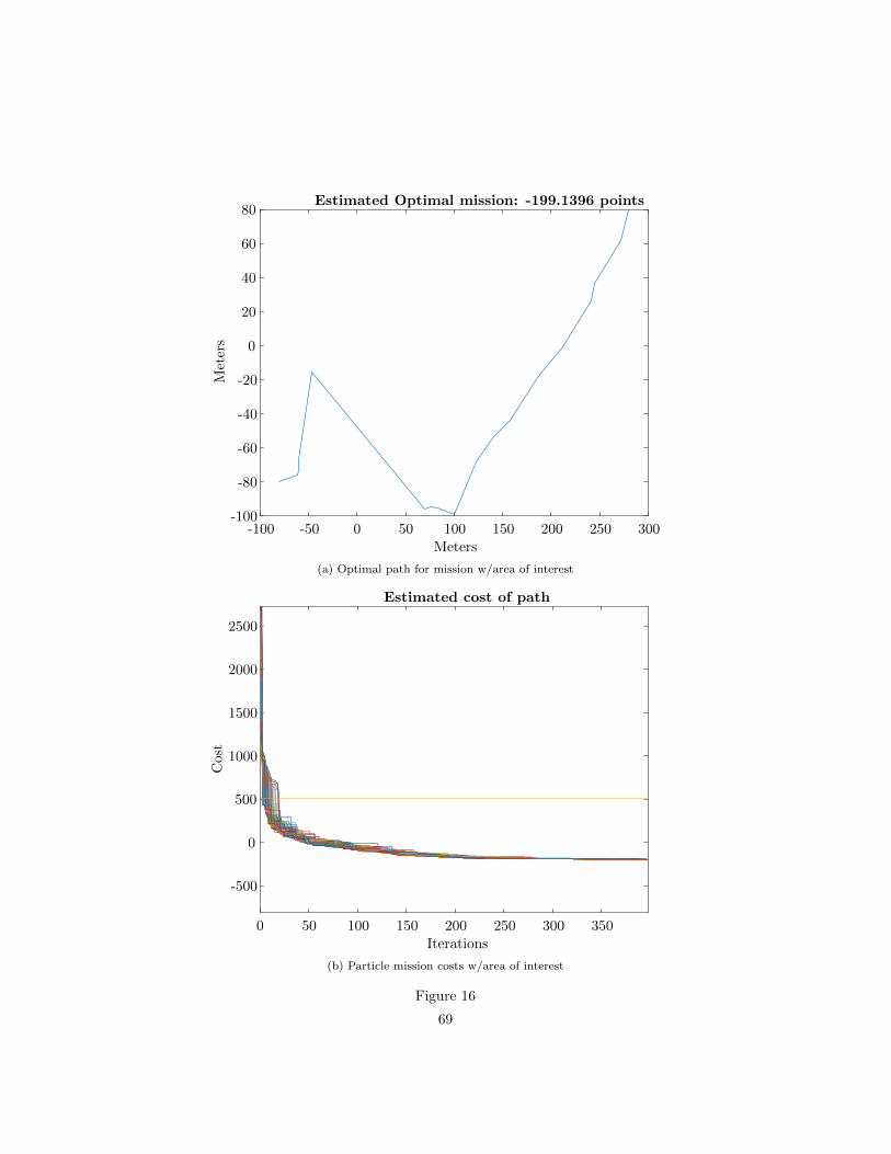
-100 -50 0 50 100 150 200 250 300Meters
-100
-80
-60
-40
-20
0
20
40
60
80M
eter
s
Estimated Optimal mission: -199.1396 points
(a) Optimal path for mission w/area of interest
0 50 100 150 200 250 300 350Iterations
-500
0
500
1000
1500
2000
2500
Cos
t
Estimated cost of path
(b) Particle mission costs w/area of interest
Figure 16
69

10.6 Results - Binary Decision Optimisation
When looking at the results in figure 16, One can observe that The algorithm iscapable of finding a path that also includes the area of interest at (100,-100). Itcan however be seen that the optimal path has large jumps and spikes similar toresults with the discontinuous time variant current. The algorithm managed areduction of mission cost from 500 to -199 16. Since the cost does not representtime anymore, the optimal cost can be negative.
10.7 Analytical PSO Tests -Conclusion
For both Time invariant currents , time variant discontinious currents and mis-sions with areas of interest. The algorithm was able to find solutions to theproblem, more optimal than the naive straight line paths. This shows how thePSO is capable of handling situations pushing boundaries. However, it can alsobe seen that the algorithm shows undesired behaviours. As a proof of concepthowever, the results are deemed sufficient.
Part V
Parameter Estimation of RealMission Data
70
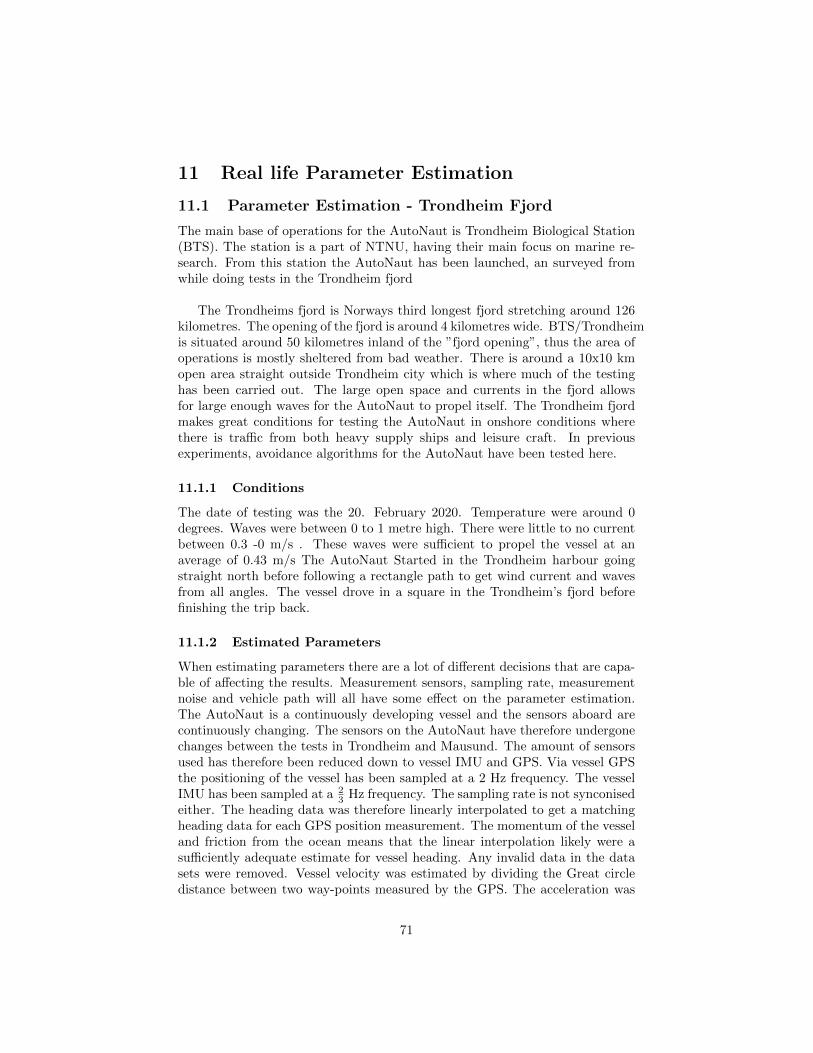
11 Real life Parameter Estimation
11.1 Parameter Estimation - Trondheim Fjord
The main base of operations for the AutoNaut is Trondheim Biological Station(BTS). The station is a part of NTNU, having their main focus on marine re-search. From this station the AutoNaut has been launched, an surveyed fromwhile doing tests in the Trondheim fjord
The Trondheims fjord is Norways third longest fjord stretching around 126kilometres. The opening of the fjord is around 4 kilometres wide. BTS/Trondheimis situated around 50 kilometres inland of the ”fjord opening”, thus the area ofoperations is mostly sheltered from bad weather. There is around a 10x10 kmopen area straight outside Trondheim city which is where much of the testinghas been carried out. The large open space and currents in the fjord allowsfor large enough waves for the AutoNaut to propel itself. The Trondheim fjordmakes great conditions for testing the AutoNaut in onshore conditions wherethere is traffic from both heavy supply ships and leisure craft. In previousexperiments, avoidance algorithms for the AutoNaut have been tested here.
11.1.1 Conditions
The date of testing was the 20. February 2020. Temperature were around 0degrees. Waves were between 0 to 1 metre high. There were little to no currentbetween 0.3 -0 m/s . These waves were sufficient to propel the vessel at anaverage of 0.43 m/s The AutoNaut Started in the Trondheim harbour goingstraight north before following a rectangle path to get wind current and wavesfrom all angles. The vessel drove in a square in the Trondheim’s fjord beforefinishing the trip back.
11.1.2 Estimated Parameters
When estimating parameters there are a lot of different decisions that are capa-ble of affecting the results. Measurement sensors, sampling rate, measurementnoise and vehicle path will all have some effect on the parameter estimation.The AutoNaut is a continuously developing vessel and the sensors aboard arecontinuously changing. The sensors on the AutoNaut have therefore undergonechanges between the tests in Trondheim and Mausund. The amount of sensorsused has therefore been reduced down to vessel IMU and GPS. Via vessel GPSthe positioning of the vessel has been sampled at a 2 Hz frequency. The vesselIMU has been sampled at a 2
3 Hz frequency. The sampling rate is not synconisedeither. The heading data was therefore linearly interpolated to get a matchingheading data for each GPS position measurement. The momentum of the vesseland friction from the ocean means that the linear interpolation likely were asufficiently adequate estimate for vessel heading. Any invalid data in the datasets were removed. Vessel velocity was estimated by dividing the Great circledistance between two way-points measured by the GPS. The acceleration was
71
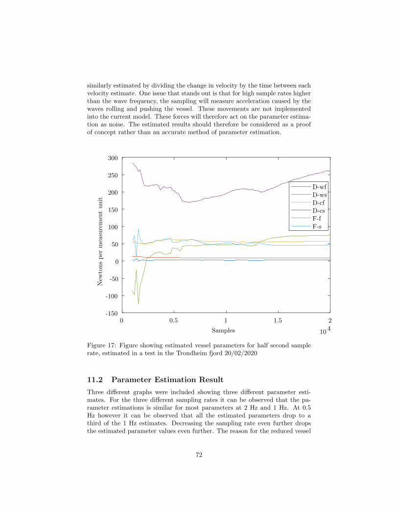
similarly estimated by dividing the change in velocity by the time between eachvelocity estimate. One issue that stands out is that for high sample rates higherthan the wave frequency, the sampling will measure acceleration caused by thewaves rolling and pushing the vessel. These movements are not implementedinto the current model. These forces will therefore act on the parameter estima-tion as noise. The estimated results should therefore be considered as a proofof concept rather than an accurate method of parameter estimation.
0 0.5 1 1.5 2
Samples 104
-150
-100
-50
0
50
100
150
200
250
300
New
ton
sp
erm
easu
rem
ent
un
it
D-wfD-wsD-cfD-csF-fF-s
Figure 17: Figure showing estimated vessel parameters for half second samplerate, estimated in a test in the Trondheim fjord 20/02/2020
11.2 Parameter Estimation Result
Three different graphs were included showing three different parameter esti-mates. For the three different sampling rates it can be observed that the pa-rameter estimations is similar for most parameters at 2 Hz and 1 Hz. At 0.5Hz however it can be observed that all the estimated parameters drop to athird of the 1 Hz estimates. Decreasing the sampling rate even further dropsthe estimated parameter values even further. The reason for the reduced vessel
72
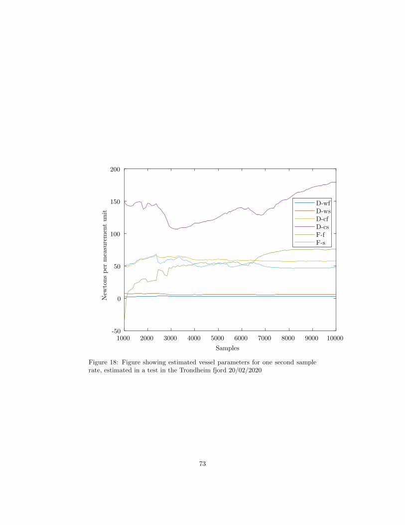
1000 2000 3000 4000 5000 6000 7000 8000 9000 10000
Samples
-50
0
50
100
150
200
New
ton
sp
erm
easu
rem
ent
un
it
D-wfD-wsD-cfD-csF-fF-s
Figure 18: Figure showing estimated vessel parameters for one second samplerate, estimated in a test in the Trondheim fjord 20/02/2020
73
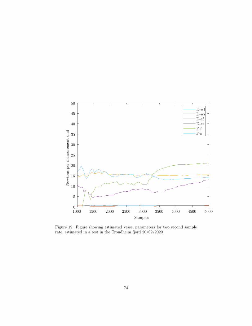
1000 1500 2000 2500 3000 3500 4000 4500 5000
Samples
0
5
10
15
20
25
30
35
40
45
50
New
ton
sp
erm
easu
rem
ent
un
it
D-wfD-wsD-cfD-csF-fF-s
Figure 19: Figure showing estimated vessel parameters for two second samplerate, estimated in a test in the Trondheim fjord 20/02/2020
74
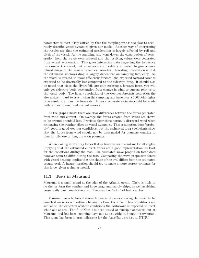
parameters is most likely caused by that the sampling rate is too slow to accu-rately describe vessel dynamics given our model. Another way of interpretingthe results are that the estimated acceleration is largely affected by roll andpitch of the vessel. As the sampling rate went down, the contribution of accel-eration from the waves were reduced and the resulting values were generatedfrom actual acceleration. This gives interesting data regarding the frequencyresponse of the vessel, but more accurate models are needed to give a morerefined image of the vessels dynamics. Another interesting observation is thatthe estimated sideways drag is largely dependent on sampling frequency. Asthe vessel is created to move efficiently forward, the expected forward force isexpected to be drastically less compared to the sideways drag. It should alsobe noted that since the Hydrofoils are only creating a forward force, you willonly get sideways body acceleration from change in wind or current relative tothe vessel body. The hourly resolution of the weather forecasts resolution thealso makes it hard to trust, when the sampling rate have over a 1000 fold highertime resolution than the forecasts. A more accurate estimate could be madewith on board wind and current sensors.
As the graphs shows there are clear differences between the forces generatedfrom wind and current. On average the forces created from waves are shownto be around a tenfold less. Previous algorithms normally disregard wind whenestimating the weather effect on vessel dynamics. This assumption does ”proba-bly” good in good weather conditions, but the estimated drag coefficients showthat the forces from wind should not be disregarded for planners wanting toplan for offshore or long duration planning.
When looking at the drag forces It does however seem constant for all angles.Implying that the estimated current forces are a good representation, at leastfor the conditions during the test. The estimated wave propulsion force doeshowever seem to differ during the test. Comparing the wave propulsion forceswith vessel heading implies that the shape of the oval differs from the estimatedpseudo oval. A future iteration should try to make a more correct estimate forthis force, given a similar model.
11.3 Tests in Mausund
Mausund is a small island at the edge of the Atlantic ocean. There is little tono shelter form the weather and large cargo and supply ships, as well as fishingvessel daily pass trough the area. The area has ”a lot” of bad weather.
Mausund has a biological research base in the area allowing the vessel to belaunched an retrieved without having to leave the area. These conditions aresimilar to the expected offshore conditions the AutoNaut is expected to meetwhile out at sea. The AutoNaut has been tested at multiple occasions out atMausund and has been spanning days out at sea without human intervention.This alone has been a large milestone for the AutoNaut project at NTNU.
75
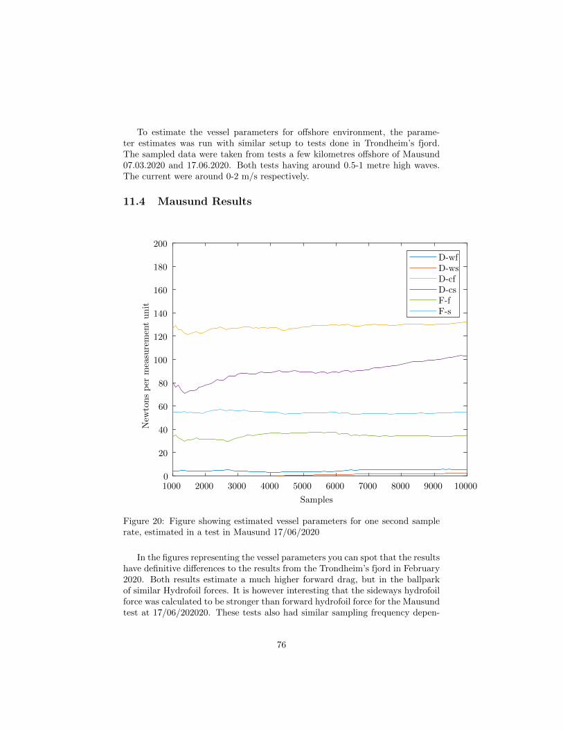
To estimate the vessel parameters for offshore environment, the parame-ter estimates was run with similar setup to tests done in Trondheim’s fjord.The sampled data were taken from tests a few kilometres offshore of Mausund07.03.2020 and 17.06.2020. Both tests having around 0.5-1 metre high waves.The current were around 0-2 m/s respectively.
11.4 Mausund Results
1000 2000 3000 4000 5000 6000 7000 8000 9000 10000
Samples
0
20
40
60
80
100
120
140
160
180
200
New
ton
sp
erm
easu
rem
ent
un
it
D-wfD-wsD-cfD-csF-fF-s
Figure 20: Figure showing estimated vessel parameters for one second samplerate, estimated in a test in Mausund 17/06/2020
In the figures representing the vessel parameters you can spot that the resultshave definitive differences to the results from the Trondheim’s fjord in February2020. Both results estimate a much higher forward drag, but in the ballparkof similar Hydrofoil forces. It is however interesting that the sideways hydrofoilforce was calculated to be stronger than forward hydrofoil force for the Mausundtest at 17/06/202020. These tests also had similar sampling frequency depen-
76

1000 1500 2000 2500 3000 3500 4000 4500
Samples
0
50
100
150
New
ton
sp
erm
easu
rem
ent
un
it
D-wfD-wsD-cfD-csF-fF-s
Figure 21: Figure showing estimated vessel parameters for one second samplerate, estimated in a test in Mausund 03/07/2020
77

dency in estimated parameter forces where the estimated forces reduced witha reduced sampling rate. The average velocity however was about 50 percentfaster than tests in the Trondheim Fjord. One might suspect that the increaseddrag comes from quadratic drag forces. However, due to previous commentsabout doubts about the method, these results should be used more as a guidefor further development, than a benchmark for actual vessel parameters.
78

Part VI
Test of Mission Planner WithReal Forecast Data
79

12 Optimal Mission Planning using real WeatherForecasts
To test out the vessel planner, a short mission in the Trondheim’s fjord is testedout. Vessel will start a few kilometres outside the Trondheim harbour. Thevessel will then go to the western part of the fjord where there is a samplepoint. After reaching the western sample point, the vessel will head east to theEastern sample point before having to return to the start point. The weatherthat will be used, is the similar forecast to the forecast used estimating the ves-sel parameters in the Trondheim’s fjord 20/02/2020 18. The mission is similarto short range missions previously performed to test The vessel. Each area ofinterest gives a 5000 reduction in mission cost, and each use of the sensor gains100 to the mission cost. Each area of interest can only be sampled one time.
80

Parameter Ff Fs Dc Dw
Value 200 200 100 0
Table 7: Table showing parameters used for velocity function for analytical forreal life tests in Trondheim
Parameter Particles Iterations ω a1 a2 a3 Particle DistributionValue 100 200 0.0004 0.1 0.7 1 0.005
Table 8: Table showing PSO parameters for real life tests in Trondheim
12.1 Optimal Planning Issues
During testing, one main issue was not possible to overcome, using the currentparticle swarm optimisation methods. When using estimated vessel parametersin particle optimisation, the particle swarm was not able to find any feasiblepath. The time varying current and wind forecasts seemed to be too complexto be able to find any start path to start the optimisation. To have a closerlook at the challenge, a grid test was done to map out the feasibility of movingin different directions. A 30X30 grid between 63.458249 - 63.577489 degreeslatitude, 10.292981 - 10.585492 degrees longitude. For each point in the gridthe estimated velocity for going North, East, South and west was calculated.These plots together with the current, wind and wave height plots are includedin figures 31 to 37. The estimated velocities are made by using weather forecastsat 20/02/2020 at 12 noon. From the different plots it can be observed that alldirections have dead spots, or close to dead spots where the estimated velocity is0 or less. Any non positive or unfeasible area is set to 0 to make the graph easierto understand. These dead spots often cover almost the entire fjord, thereforemaking it hard for the path planner to find a path to ”penetrate the currentbelts”. In theory the use of random deviations from the straight line path shouldbe able to find a path given infinite particles and large enough spread. However,due to the limited particles used the algorithm has more limited capabilities.
81
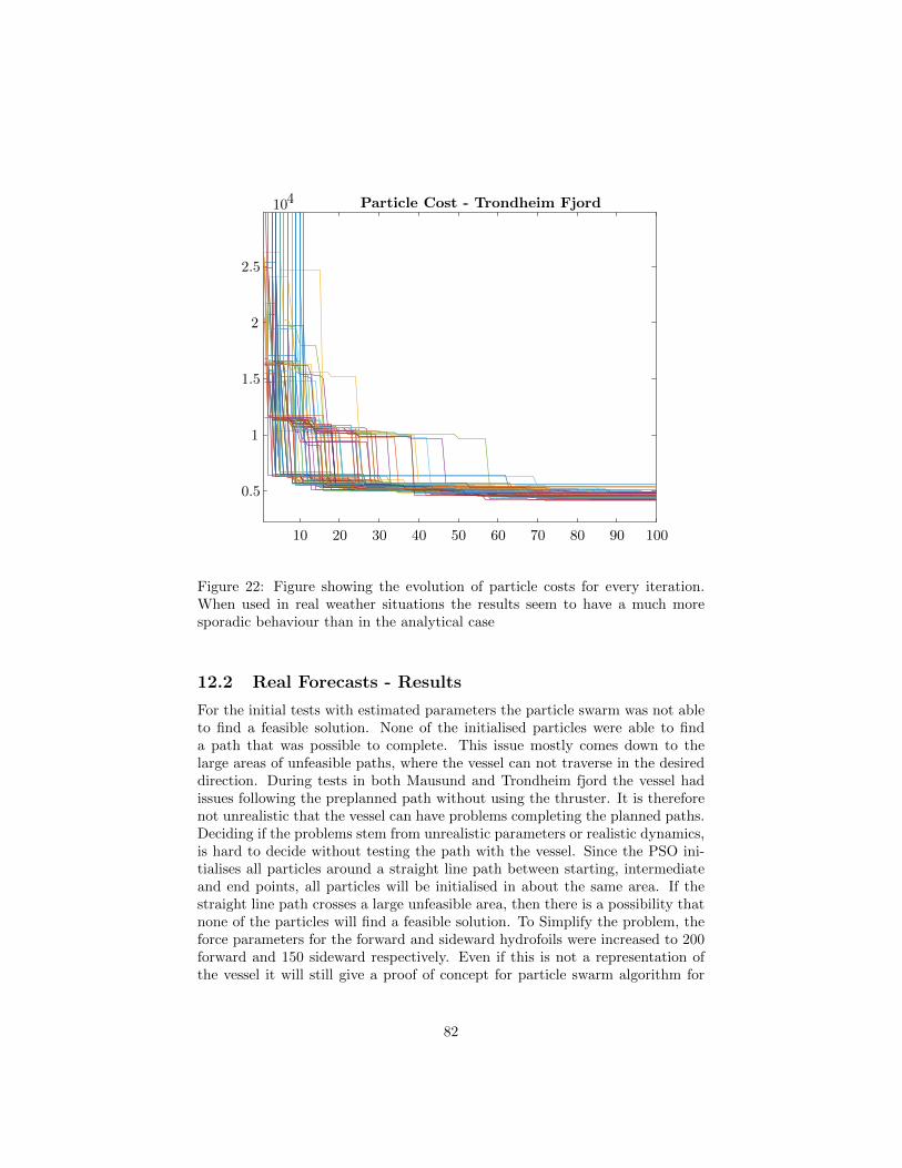
10 20 30 40 50 60 70 80 90 100
0.5
1
1.5
2
2.5
104 Particle Cost - Trondheim Fjord
Figure 22: Figure showing the evolution of particle costs for every iteration.When used in real weather situations the results seem to have a much moresporadic behaviour than in the analytical case
12.2 Real Forecasts - Results
For the initial tests with estimated parameters the particle swarm was not ableto find a feasible solution. None of the initialised particles were able to finda path that was possible to complete. This issue mostly comes down to thelarge areas of unfeasible paths, where the vessel can not traverse in the desireddirection. During tests in both Mausund and Trondheim fjord the vessel hadissues following the preplanned path without using the thruster. It is thereforenot unrealistic that the vessel can have problems completing the planned paths.Deciding if the problems stem from unrealistic parameters or realistic dynamics,is hard to decide without testing the path with the vessel. Since the PSO ini-tialises all particles around a straight line path between starting, intermediateand end points, all particles will be initialised in about the same area. If thestraight line path crosses a large unfeasible area, then there is a possibility thatnone of the particles will find a feasible solution. To Simplify the problem, theforce parameters for the forward and sideward hydrofoils were increased to 200forward and 150 sideward respectively. Even if this is not a representation ofthe vessel it will still give a proof of concept for particle swarm algorithm for
82

0 20 40 60 80 100Iterations
0
1
2
3
4
5
6
7
8
9
10
Mis
sion
Cos
t
106 Particle Cost - Trondheim Fjord
Figure 23: Figure showing evolution of particle costs for every iteration. Inthis figure, the graph is drastically zoomed out to get a better view of how theparticles work. Notice how some particles move from the max value (9999999)down to the other particle costs as the unfeasible particles become feasible.
83
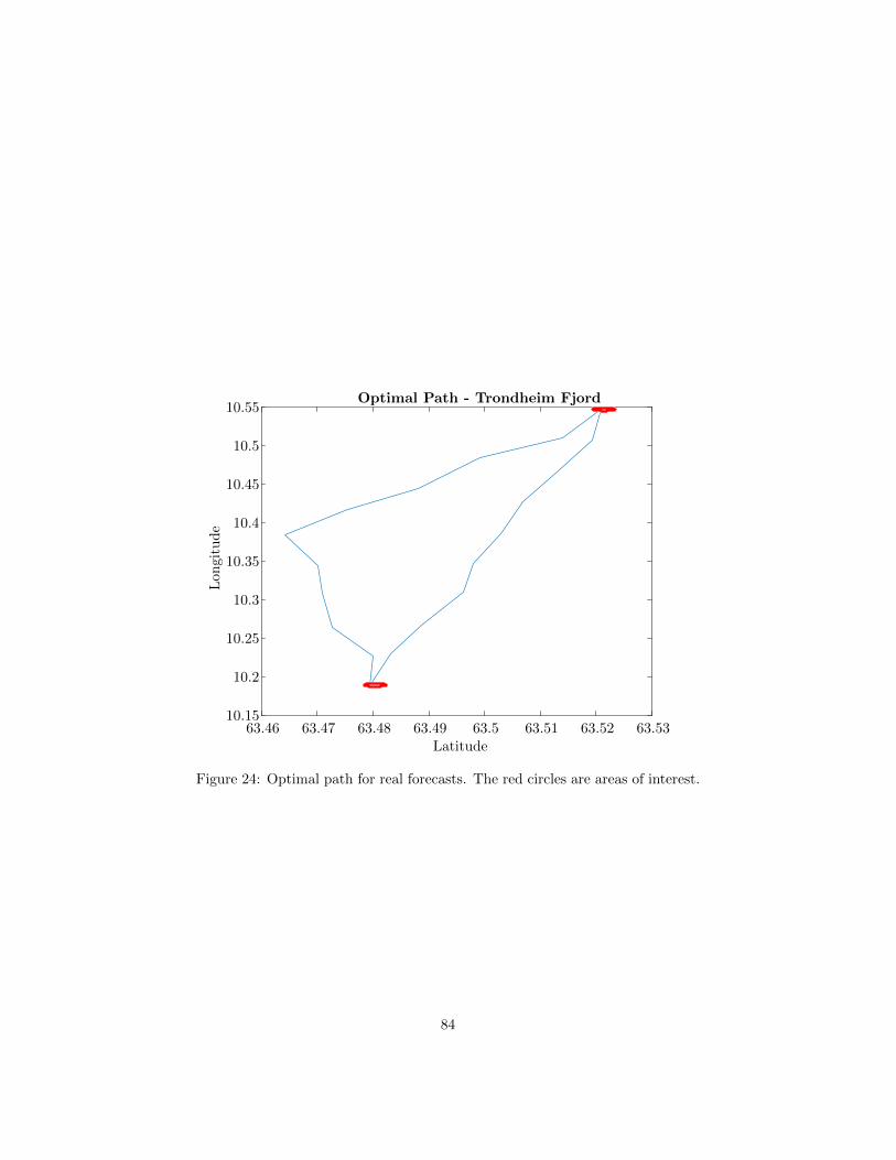
63.46 63.47 63.48 63.49 63.5 63.51 63.52 63.53Latitude
10.15
10.2
10.25
10.3
10.35
10.4
10.45
10.5
10.55
Lon
gitu
de
Optimal Path - Trondheim Fjord
Figure 24: Optimal path for real forecasts. The red circles are areas of interest.
84
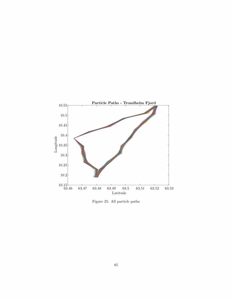
63.46 63.47 63.48 63.49 63.5 63.51 63.52 63.53Latitude
10.15
10.2
10.25
10.3
10.35
10.4
10.45
10.5
10.55
Lon
gitu
de
Particle Paths - Trondheim Fjord
Figure 25: All particle paths
85

Sensor Usage - Trondheim Fjord
0 5 10 15 20Waypoint
0
0.2
0.4
0.6
0.8
1
1.2
1.4
1.6
1.8
2
Figure 26: Sensor usage for each way-point.
86
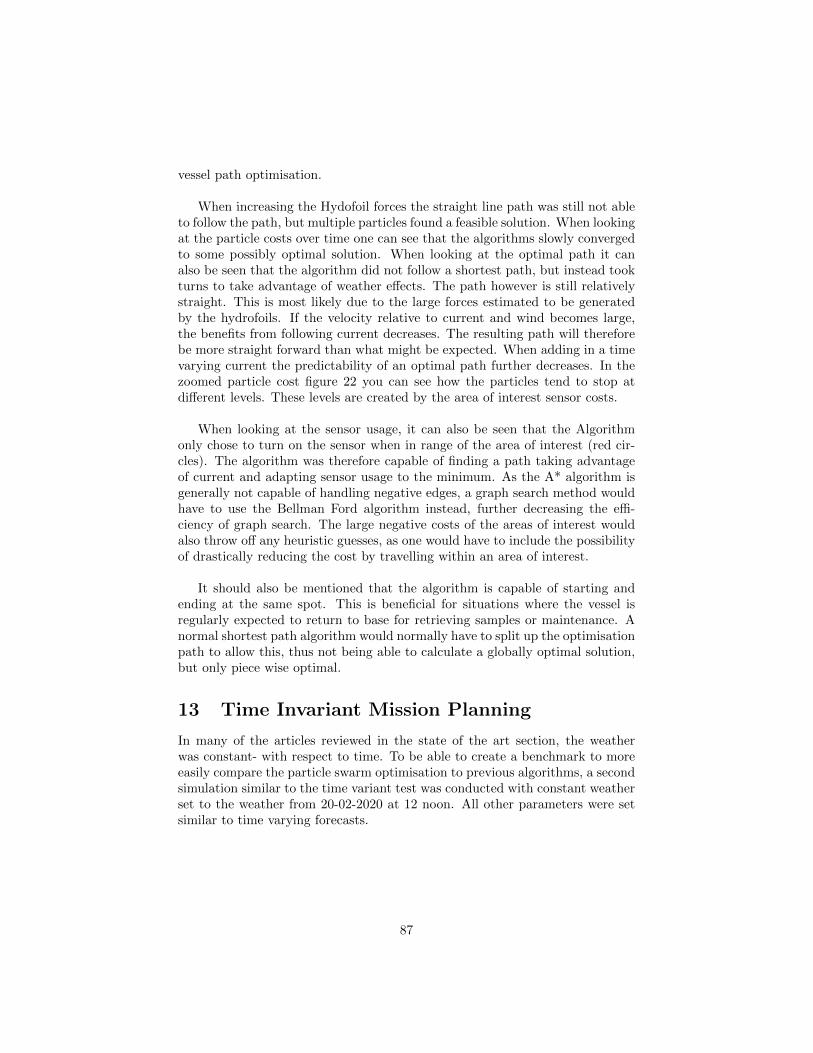
vessel path optimisation.
When increasing the Hydofoil forces the straight line path was still not ableto follow the path, but multiple particles found a feasible solution. When lookingat the particle costs over time one can see that the algorithms slowly convergedto some possibly optimal solution. When looking at the optimal path it canalso be seen that the algorithm did not follow a shortest path, but instead tookturns to take advantage of weather effects. The path however is still relativelystraight. This is most likely due to the large forces estimated to be generatedby the hydrofoils. If the velocity relative to current and wind becomes large,the benefits from following current decreases. The resulting path will thereforebe more straight forward than what might be expected. When adding in a timevarying current the predictability of an optimal path further decreases. In thezoomed particle cost figure 22 you can see how the particles tend to stop atdifferent levels. These levels are created by the area of interest sensor costs.
When looking at the sensor usage, it can also be seen that the Algorithmonly chose to turn on the sensor when in range of the area of interest (red cir-cles). The algorithm was therefore capable of finding a path taking advantageof current and adapting sensor usage to the minimum. As the A* algorithm isgenerally not capable of handling negative edges, a graph search method wouldhave to use the Bellman Ford algorithm instead, further decreasing the effi-ciency of graph search. The large negative costs of the areas of interest wouldalso throw off any heuristic guesses, as one would have to include the possibilityof drastically reducing the cost by travelling within an area of interest.
It should also be mentioned that the algorithm is capable of starting andending at the same spot. This is beneficial for situations where the vessel isregularly expected to return to base for retrieving samples or maintenance. Anormal shortest path algorithm would normally have to split up the optimisationpath to allow this, thus not being able to calculate a globally optimal solution,but only piece wise optimal.
13 Time Invariant Mission Planning
In many of the articles reviewed in the state of the art section, the weatherwas constant- with respect to time. To be able to create a benchmark to moreeasily compare the particle swarm optimisation to previous algorithms, a secondsimulation similar to the time variant test was conducted with constant weatherset to the weather from 20-02-2020 at 12 noon. All other parameters were setsimilar to time varying forecasts.
87
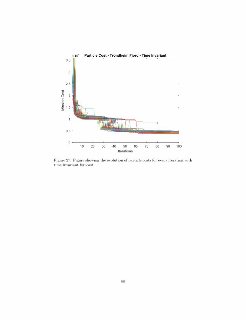
Figure 27: Figure showing the evolution of particle costs for every iteration withtime invariant forecast.
88

Figure 28: Figure showing evolution of particle costs for every iteration withthe time invariant forecast. In this figure, the graph is drastically zoomed outto get a better view of how the particles work. Straght yellow line representsstraight path cost
89
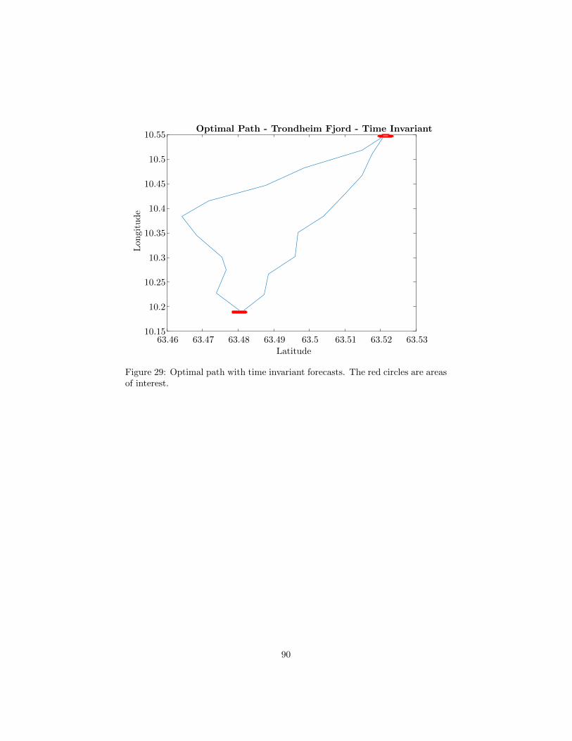
63.46 63.47 63.48 63.49 63.5 63.51 63.52 63.53Latitude
10.15
10.2
10.25
10.3
10.35
10.4
10.45
10.5
10.55L
on
git
ud
eOptimal Path - Trondheim Fjord - Time Invariant
Figure 29: Optimal path with time invariant forecasts. The red circles are areasof interest.
90
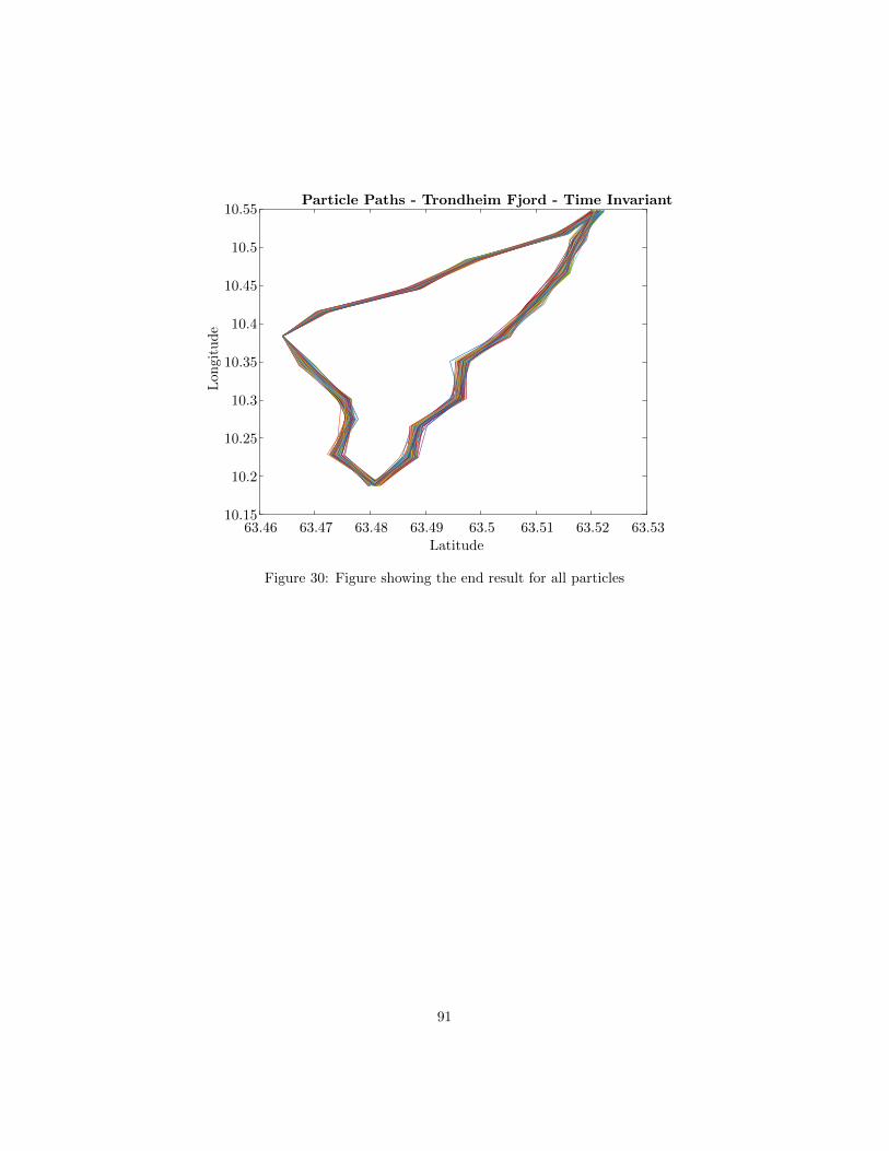
63.46 63.47 63.48 63.49 63.5 63.51 63.52 63.53Latitude
10.15
10.2
10.25
10.3
10.35
10.4
10.45
10.5
10.55L
on
git
ud
eParticle Paths - Trondheim Fjord - Time Invariant
Figure 30: Figure showing the end result for all particles
91

13.1 Real Time Invariant Forecasts - Results
The optima path found for the Time invariant forecasts displays many of thesame properties as the time variant forecasts. It does however seem to takeslightly more advantage of currents at some areas. None of the paths howeverseem to have any drastically different results. The time invariant system werealso able to sample within both areas of interest.
92

Part VII
Discussion and ConcludingRemarks
93

14 Discussion
During this master project it was attempted to create a start to finish missionplanner including both optimal paths as well as adaptive sampling. To achievethis, both a mission cost model, vessel model and an optimisation algorithm wascreated to be able to achieve the end result. The end results shows promise,but the path to a final implementation still needs work. The further work canbe divided into three different parts.
For all the analytical results it was proven that the optimisation algorithmis capable of solving the problem the algorithm was designed to tackle. For themission cost model, there is still not any model for communication, or for riskof vessel loss. Ideally, the vessel should be able to estimate the risk of a mission,to be better able to preserve itself without human intervention. To achieve this,the vessel will also have to prevent the risk of running out of energy. For thevessel to be left without supervision, the vessel will have to assure that it willnot run out of energy before heading back home. The cost of communicationcan also become a large expense if the vessel uses exclusively satellite commu-nication.
The vessel model also have room for improvement. The hydrofoil model wasbased mostly on observations. A thorough inverstigation into hydrofoil dynam-ics would greatly benefit the parameter estimation. If the vessel is not expectedto face too harsh conditions, a pure current wave model might aslo be a betterfit. The parameter estimation could also be further improved by using on boardsensors to measure weather instead of using forecasts with one hour resolution.
One path that would especially benefit from further work is the optimisationalgorithm. Currently the optimisation algorithm is not good enough at travers-ing difficult terrain with unknown unfeasible areas. In figures 31 to 34. thefeasibility of path directions was mapped out to create a better understandingof the issue preventing the optimisation algorithm from finding a possible path.A grid of points was evenly spread over the fjord outside Trondheim city. Fourdifferent graphs were created describing the feasible vessel NED velocity for eachpoint in the grid in the four different cardinal directions, North, East, Southand West. The dark blue/purple areas are areas where it is not feasible forthe vessel to move in the direction specified in the figure title 31 and onwards.Graphs representing current35, wind 36 and wave height 37 are also included togive a better understanding of how wind, current and waves affects feasibilityof paths. Feasibility maps for the increased hydrofoil forces were also included,to show the difference between the estimated parameters and the parametersused in the optimisation algorithm. From figure 38 to figure41 the increasedfeasibility maps are calculated from the same weather forecast. The feasibilitymap was created by using the estimated parameters from 20. February 2020.The weather data used were the weather forecasts for 20. February, 2020, 12:00.
94

From the data in the different feasibility graphs, it can be observed thatthere can often be large areas where it is not feasible for the vessel to travel inthe cardinal direction. The areas feasible are also not convex, creating possi-ble traps for greedy algorithms only focusing on local conditions, for examplepotential fields. These feasible areas will also be time varying, increasing thedifficulty of creating good heuristic estimates for feasible paths. The currentmethod of using the straight line path between way-points has many problemswhen being faced with unfeasible areas, as the particle swarm only searches fora predefined area around the heuristic guess. In theory you could broaden theparticle search, however, particle swarms needs a certain density to prevent theoptimisation algorithm from overlooking good solutions. An increased searchwould therefore increase computation time. A good place to start would foreinstance be to implement an RRT algorithm to find a feasible path or multiplefeasible paths, which then could be used as a seed for the optimal path plan-ner to find a more optimal path. This would both increase the robustness offinding a feasible path and assure a pseudo optimal path with adaptive sampling.
Currently the algorithm uses the ocean forecast to figure out where land is,as areas of land has NaN values at areas covering land. This does create a correctmap, but the way the optimisation algorithm works, it tends to create problems.To find an optimal path, the algorithm wants to ”cut corners” to try to findthe shortest path possible. This sets the optimal path very close to the shore.This is both a unsafe path for the vessel to try to follow, but also problematic,as the algorithm searches in the area around the most optimal path to try tofind other paths. The result is that the algorithm tries many paths that crashesinto land giving the particles infinite cost. This is not directly an issue, buteach particle that creates an unfeasible path uses computing power without anybenefit to the algorithm. Therefore the algorithm becomes inefficient and unsafeclose to shore. It should therefore be a more conservative map representing theshore, that prevents the vessel from coming within a predefined distance closeto shore. Paths being too close to shore on the conservative shore map but notthe weather map, could add a penalty cost instead of an infinite cost. That wayless particles becomes useless. It would also allow the algorithm to cross narrowstraights that are technically not allowed on a conservative shore map.
When comparing results of the optimisation algorithm to related work, thereare situations where the algorithm performs better and situations where thealgorithms performs worse. The implementation of sensor usage in the missioncost does allow for a more dynamic sensor sampling. In the current tests, thesensor areas have a binary dynamics. The expansion of a continuous sensorcost model further expands the possibilities of the mission description. Whenlooking at the robustness of the algorithm, previous A* algorithms seem to showa more robust behaviour[9] The A* algorithms have a good capability that givencertain constraints the A* algorithm is guaranteed to find a globally optimalsolution. Adapting an A* algorithm to work with the models and mission costadapted for graph search could create a much more robust planner, but at thecost of a larger computational cost, as well as new issues that had to be solved.
95
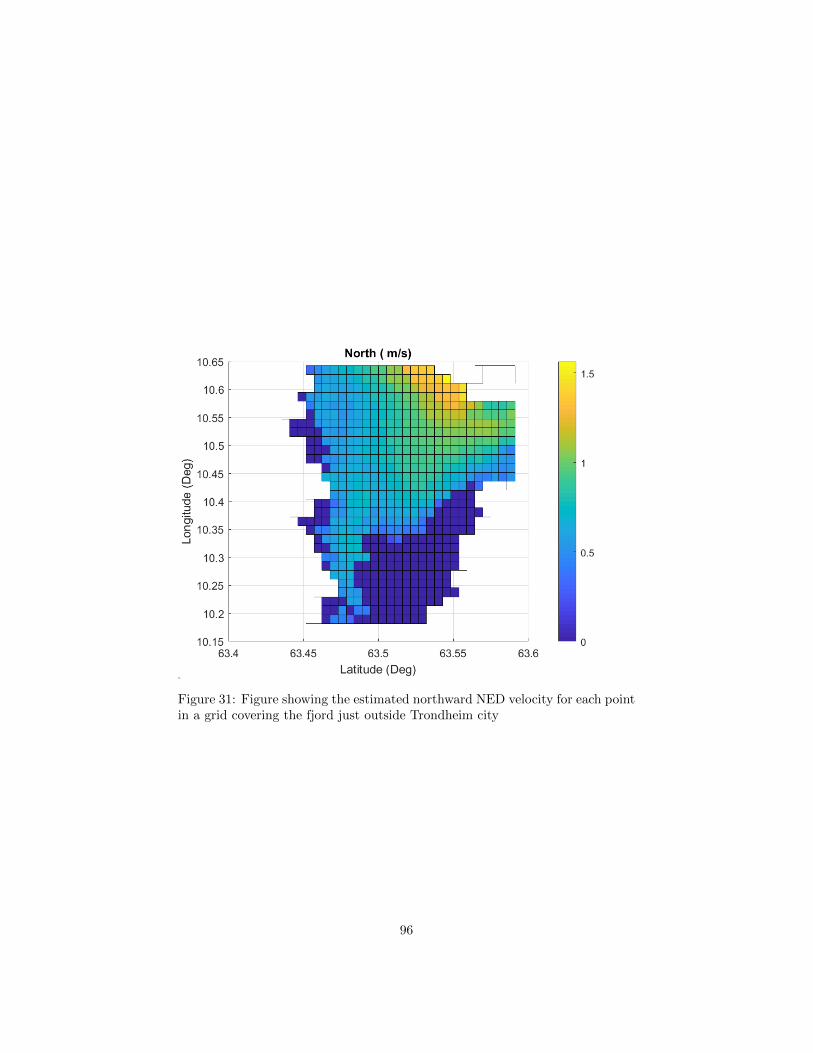
Figure 31: Figure showing the estimated northward NED velocity for each pointin a grid covering the fjord just outside Trondheim city
96
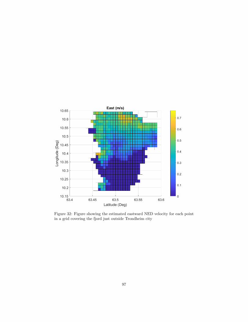
Figure 32: Figure showing the estimated eastward NED velocity for each pointin a grid covering the fjord just outside Trondheim city
97

Figure 33: Figure showing the estimated southward NED velocity for each pointin a grid covering the fjord just outside Trondheim city
98
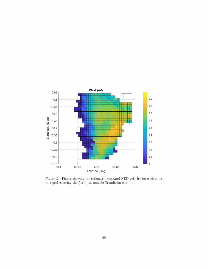
Figure 34: Figure showing the estimated westward NED velocity for each pointin a grid covering the fjord just outside Trondheim city
99
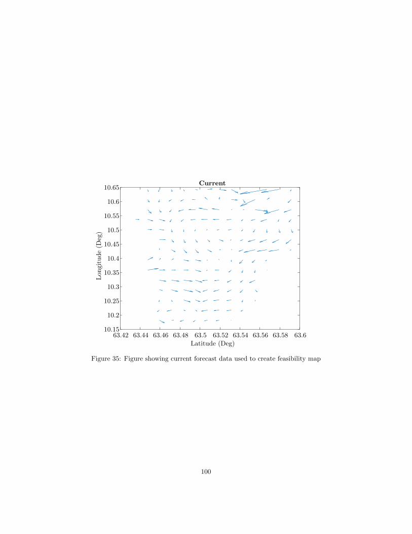
63.42 63.44 63.46 63.48 63.5 63.52 63.54 63.56 63.58 63.6Latitude (Deg)
10.15
10.2
10.25
10.3
10.35
10.4
10.45
10.5
10.55
10.6
10.65
Lon
gitu
de
(Deg
)
Current
Figure 35: Figure showing current forecast data used to create feasibility map
100

63.4 63.45 63.5 63.55 63.6 63.65Latitude (Deg)
10.1
10.2
10.3
10.4
10.5
10.6
10.7
Lon
gitu
de
(Deg
)
Wind
Figure 36: Figure showing wind forecast data used to create feasibility map
101
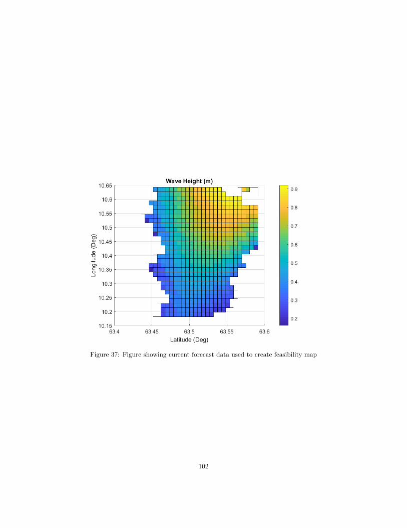
Figure 37: Figure showing current forecast data used to create feasibility map
102

Figure 38: Figure showing the estimated northward NED velocity for each pointin a grid covering the fjord just outside Trondheim city with increased hydrofoilforces
103

Figure 39: Figure showing the estimated eastward NED velocity for each pointin a grid covering the fjord just outside Trondheim city with increased hydrofoilforces
104

Figure 40: Figure showing the estimated southward NED velocity for each pointin a grid covering the fjord just outside Trondheim city with increased hydrofoilforces
105
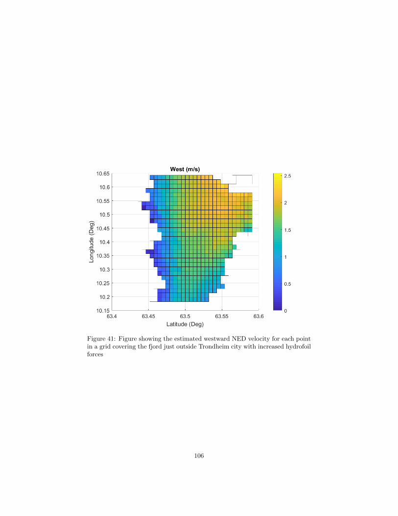
Figure 41: Figure showing the estimated westward NED velocity for each pointin a grid covering the fjord just outside Trondheim city with increased hydrofoilforces
106
15 Summary
As stated in the start of the thesis, optimal path planning for smaller au-tonomous vessels allow for the autonomous vessels to more effectively use al-ternative propulsion methods taking advantage of weather instead of on boardpower to propel the vessel. To accurately describe how weather affects suchvessels, an estimated model of the vessel was made which then were used inconjunction with a mission cost function to describe the cost of a mission. Tobe able to both optimise path and mission execution, a particle swarm was thenused to optimise the cost function, allowing the optimisation algorithm to planboth vessel and sensor behaviour during a mission. Overall the structuring ofthe optimisation problem and optimisation showed promise for a mission plan-ner for autonomous vessels. However, the end product was not able to findsufficient solutions given the estimated vessel parameters. A further develop-ment both in optimisation, mission cost and vessel modelling is needed to createa robust mission planner capable of guiding an autonomous vessel for monthsat a time.
107
16 Direction for Future Research
The designing of the vessel model was made using assumption for both vesseldrag, hydrofoil coefficient, and weather effects on the model. Due to the lim-ited velocities, the models was also linearised. These assumptions were madebased on personal experiences. A more thorough development with a quickerfeedback from tests to model modification could be beneficial. An interestingtopic for future research would be to further the understanding and modellingof the hydrofoil propulsion. A more focused study on how pitch and yaw, aswell as wave frequency and wave height affects vessel propulsion would greatlybenefit any path planner or mission planner.
Currently, the weather forecasts are assumed to be deterministic, mean-ing that it is assumed that the weather forecasts are exact. One main issueis that weather forecasts today are mainly made form machine learning algo-rithms. Therefore, the probability distribution of the estimated parameters arenot readily available. It is however possible to implement.
Another section of the thesis that can benefit from further research opti-misation algorithms. The most important property of a mission planner isrobustness. It is not important the vessel performs the fastest paths, but thatit performs a safe and feasible path. The currently implemented particle swarmalgorithm, needs manual tuning for each mission. If the tuning parameters arewrong, the algorithm will start to show undesirable behaviour, and might havedifficulties finding a feasible solution. A suggestion for a more robust optimalpath planner would be to combine the search capabilities of a graph search al-gorithm like A* or RRT* with the efficient optimisation of a particle swarmalgorithm. A particle swarm could for example use a graph search to find afeasible path that could be used as a seed for the optimal path planner. It couldalso be interesting to test out different versions of genetic algorithms or machinelearning to further the optimisation results.
108
17 Appendix
17.1 Use of Included Code
Together with the Thesis there is also attached the code used in the thesis. Toease the tests and use of the code for those interested, a a small tutorial forsimple use of the different algorithms will be explained.
17.1.1 File Structure
The codes used can be divided into three different parts. Which is also how thecode is divided. In the Master folder there is three sub folders:
• Weather
• Optimal path planning
• Parameter estimation
The different folders contain different code files and sub folders needed to achieveresults relevant to the folder it is situated in.
17.1.2 Weather Folder
The weather folder contains only one matlab script, download-weather.m. Thisscript downloads weather forecast for wind, current and waves for the areaaround Trondheim. The forecast horizon is predefined at the top of the matlabscript. By setting startDate = [year, month, day] endDate = [year, month, day].The forecasts can only stitch weather forecasts from end 2019 until current day.By setting correct start date and end date, the algorithm will crate an .m filewith weather data between the two selected dates. Be warned, the data quicklybecomes large, be therefore careful not including too many days in the forecast.
17.1.3 Optimal Path Planning Folder
N.B. For the algorithms to work, the weather forecasts have to be included.they are however half a gigabyte per day of data, so it might not be possible toupload to inspera.
The optimal path planning folder contains the optimal path planner itselfPSO-testing.m. It also contains all supporting functions mission-cost.m, weath-erToVelocity.m and many other algorithms to test out different parts of thealgorithm. For real life tests run the PSO-testing.m file. It will run the twoway-point goal mission for the date 02-20-2020. PSO-testing.m sets up the mis-sion and runs the hybrid-PSO.m optimisation algorithm. If you want to changevessel dynamics, the different parameters are adjusted in weaterToVelocity.mfile and mission cost parameters are adjusted in the mission-cost.m file.
109

FeasabilityMapCreator.m creates the feasibility maps and uses weaterToVe-locity.m to estimate feasibility. The map limits are adjusted on line 2 and 3where, start, end and number of intermediate points are selected. This shouldwork for the midt-Norge area.
To test out the analytical tests, run the analytical-PSO-testing.m. . Thesub folder ”Analytical models” contains the analytical currents and analyticalmission cost models. Analytical-PSO-testing.m does however use similar weater-ToVelocity.m and hybryd pso function as the real life Optimisation algorithm,which has to be tuned to work with analytical tests.
17.1.4 Parameter estimation Folder
In the ”Parameter estimation” folder the main file is the parameterEstimation.mfile. If you run this file you will get the parameter estimation for the AutoNautin the Trondheim fjord 20-02-2020. Most of the other files are mainly files,but there is also an analytical model where the least squares estimation canbe compared to a test where you know the parameter results beforehand calledanalytical.m. By running this file you get the estimated parameter results withnoise on the current and wind. It can also be observed that introducing noiseto the GPS data ruins the parameter estimation. Therefore the parameterestimation in the thesis should be taken with a spoonful of salt.
110
References
[1] KYLE MIZOKAMI. Hugin san french ves-sell. https://www.popularmechanics.com/military/navy-ships/a28472065/minerve-submarine-found/. Accessed: 2020-11-17.
[2] Elaine Maslin. Hugin san juan vessel.https://www.maritimeprofessional.com/news/ocean-infinity-hunt-submarine-juan-356809. Accessed: 2020-11-17.
[3] Alberto Dallolio, Bendik Agdal, Artur Zolich, Jo Arve Alfredsen, andTor Arne Johansen. Long-endurance green energy autonomous surface ve-hicle control architecture.
[4] Dr. Mark Neal. Microtransat challenge history.https://www.microtransat.org/history.php. Accessed: 2019-20-12.
[5] Claes Tretow. Design of a free-rotating wing sail for an autonomous sail-boat, 2017.
[6] Saildrone homepage. https://www.saildrone.com/. Accessed: 2020-14-11.
[7] Sailbouey site. http://www.sailbuoy.no/. Accessed: 2019-23-12.
[8] Dhanushka Kularatne, Subhrajit Bhattacharya, and M Ani Hsieh. Timeand energy optimal path planning in general flows. In Robotics: Scienceand Systems, 2016.
[9] Dhanushka Kularatne, Subhrajit Bhattacharya, and M Ani Hsieh. Optimalpath planning in time-varying flows using adaptive discretization. IEEERobotics and Automation Letters, 3(1):458–465, 2017.
[10] Enric Galceran and Marc Carreras. Efficient seabed coverage path plan-ning for asvs and auvs. In 2012 IEEE/RSJ International Conference onIntelligent Robots and Systems, pages 88–93. IEEE, 2012.
[11] Mario Arzamendia, I Espartza, DG Reina, SL Toral, and Derlis Gre-gor. Comparison of eulerian and hamiltonian circuits for evolutionary-based path planning of an autonomous surface vehicle for monitoringypacarai lake. Journal of Ambient Intelligence and Humanized Comput-ing, 10(4):1495–1507, 2019.
[12] Yogang Singh, Sanjay Sharma, Robert Sutton, and Daniel Hatton. Pathplanning of an autonomous surface vehicle based on artificial potential fieldsin a real time marine environment. 2017.
[13] Zheng Zeng, Karl Sammut, Lian Lian, Fangpo He, Andrew Lammas, andYouhong Tang. A comparison of optimization techniques for auv pathplanning in environments with ocean currents. Robotics and AutonomousSystems, 82:61–72, 2016.
111

[14] FL Pereira, J Pinto, JB Sousa, RMF Gomes, Gil Manuel Goncalves, andPS Dias. Mission planning and specification in the neptus framework. InProceedings 2006 IEEE International Conference on Robotics and Automa-tion, 2006. ICRA 2006., pages 3220–3225. IEEE, 2006.
[15] Diogo Freitas, Luiz Guerreiro Lopes, and Fernando Morgado-Dias. Particleswarm optimisation: A historical review up to the current developments.Entropy, 22(3):362, 2020.
[16] Alireza Marandi, Farzaneh Afshinmanesh, Mahmoud Shahabadi, andFariba Bahrami. Boolean particle swarm optimization and its applica-tion to the design of a dual-band dual-polarized planar antenna. In 2006IEEE international conference on evolutionary computation, pages 3212–3218. IEEE, 2006.
[17] Autonaut homepage. https://www.autonautusv.com/home. Accessed:2020-14-11.
[18] Dalollio. Autonaut wiki. http://autonaut.itk.ntnu.no/doku.php?id=start.Accessed: 2019-20-12.
[19] Thor I Fossen. Handbook of marine craft hydrodynamics and motion con-trol. John Wiley & Sons, 2011.
[20] Anna Trevisan and Luigi Palatella. Chaos and weather forecasting: the roleof the unstable subspace in predictability and state estimation problems.International Journal of Bifurcation and Chaos, 21(12):3389–3415, 2011.
[21] BW Shen, RA Pielke Sr, X Zeng, JJ Baik, S Faghih-Naini, J Cui, R Atlas,and TA Reyes. Is weather chaotic? coexisting chaotic and non-chaotic at-tractors within lorenz models. In The 13th Chaos International Conference(CHAOS2020), pages 9–12, 2020.
[22] Benny Dwi Kifana and Maman Abdurohman. Great circle distance meth-ode for improving operational control system based on gps tracking system.International Journal on Computer Science and Engineering, 4(4):647,2012.
[23] R Bullock. Great circle distances and bearings between two locations.MDT, June, 5, 2007.
[24] Forecastsnorwaycurrentwind. https://thredds.met.no/thredds/catalog/fou-hi/norkyst800m-1h/catalog.html. Accessed: 2020-11-21.
[25] Forecasts. https://www.ecmwf.int/en/forecasts. Accessed: 2020-11-21.
[26] Forecastsnorwaywave. https://thredds.met.no/thredds/catalog/fou-hi/mywavewam800mhf/catalog.html. Accessed: 2020-11-21.
112
[27] You-Feng Cheng, Xiao Ding, Wei Shao, and Bing-Zhong Wang. Planarwide-angle scanning phased array with pattern-reconfigurable windmill-shaped loop elements. IEEE Transactions on Antennas and Propagation,65(2):932–936, 2016.
[28] Nanbo Jin and Yahya Rahmat-Samii. Hybrid real-binary particle swarmoptimization (hpso) in engineering electromagnetics. IEEE Transactionson Antennas and Propagation, 58(12):3786–3794, 2010.
[29] Sertac Karaman, Matthew R Walter, Alejandro Perez, Emilio Frazzoli,and Seth Teller. Anytime motion planning using the rrt. In 2011 IEEEInternational Conference on Robotics and Automation, pages 1478–1483.IEEE, 2011.
113

Sindre Løining Skaar
NTN
UN
orw
egia
n U
nive
rsity
of S
cien
ce a
nd T
echn
olog
yFa
culty
of I
nfor
mat
ion
Tech
nolo
gy a
nd E
lect
rical
Engi
neer
ing
Dep
artm
ent o
f Eng
inee
ring
Cybe
rnet
ics
Mas
ter’s
thes
is
Sindre Løining Skaar
Mission Planning for Wave DrivenAutonomous Surface Vessels
Master’s thesis in Cybernetics and Robotic
Supervisor: Tor Arne Johansen, Alberto Dallolio
November 2020