Minimal standards for the compilation of hazard maps of ...

mmaassssmmoovvee

MMiinniimmaall ssttaannddaarrddss

ffoorr tthhee ccoommppiillaattiioonn ooff hhaazzaarrdd mmaappss

ooff llaannddsslliiddeess aanndd rroocckk ffaallll

1

GUIDELINES OF GEOLOGICAL LANDSLIDE SUSCEPTIBILITY / HAZARD MAPPING

PART A : Introduction

PART B : Handbook for Landslides Susceptibility/Hazard Mapping

PART C : ANNEX 1 Glossary

PART C : ANNEX2 Description of types of processes

TABLE OF CONTENT

PART C : ANNEX3 1 Methodology regarding landslide hazard mapping

2 Methodology regarding rockfall hazard mapping

PART C : ANNEX4 Data Collection

PART C : ANNEX5 References

2

PART A : INTRODUCTION

1. Introduction

As a result of progressive settlement in alpine areas, as well as the fact that in modern times mountain areas are used increasingly for recreational and touristic activities, land use in these areas has chan-ged greatly in comparison to the past. The-se manmade changes overlap with climate change, therefore increasing the vulnerability of alpine regions and with this the people li-ving there.

For ensuring the safety of people and infra-structure, as well as for a foundation for ade-quate territorial and land use planning, it is

essential to gain knowledge about areas prone to landsliding.

Landslide related maps greatly differ betwe-en countries, and also between regions within the same country regarding scale, considered landslide type and purpose. In this context, this handbook as a fi nal conclusion of the MassMove project is an attempt to provide a tool for landslide susceptibility and hazard mapping towards a unique identifi cation and classifi cation of hazard areas regarding rock fall and (shallow) landslides.

3

2. Purpose of the guidelinesThe guidelines are an operative tool for the generation of susceptibility and ha-

zard maps. It states in short the necessary parameters that have to be collected for the aimed purpose (regional or local) and illustrates how to progress and reach the intended target, depending on the in-tended scale of the project. It also states clearly the minimal results that need to be achieved to fulfi ll the task.

The guidelines provide a framework to be applied by the authors of susceptibility and hazard maps (e.g. geologists, civil engineers, etc.). Thus generated maps intend

to supply regional/ territorial planners and stakeholders with fundamental informa-tion, so that appropriate spatial or action planning can be carried out.

4

Natural hazards like fl oods, avalanches, landslides and rock fall are causing great damages in the alpine regions. Due to the geological hazards and the associated damages the reduction of the risk potential is a necessity.

Landslide susceptibility maps and hazard maps represent a powerful instrument for this.

Because of the restrictions (prohibitions and regulations) concerning land use in hazard zones, the process of map compilation must be transparent and compre-hensible to get acceptance by affected land owners and stakeholders. That means minimal requirements for susceptibility/ hazard mapping must be defi ned, gui-delines for landslide susceptibility/ hazard mapping should be created. Minimal requirements for hazard mapping are necessary for objective comparability of the maps created by different persons or institutions.

For alpine hazards such as fl oods and avalanches in Italy and in Austria guidelines for hazard mapping already exist.

For the evaluation of the hazard potential (individual case evaluation) of landsli-des and rock fall different approaches are in practice: in Austria no regulations are available, in Italy hazard mapping is regulated by law; in Veneto and Friuli Vene-zia Giulia a modifi ed BUWAL method for hazard assessment is in practice (Bäk et al. 2011).

In the partner regions (Carinthia, Friuli Venezia Giulia, Veneto) geological in-formation systems are established: In the geological information system of Carinthia the event documentation is supplemented by a landslide inventory map; in connection with the event documentation a general susceptibility map was created. However, this general map is insuffi cient due to the quality of the available data for the hazard assessment. More detailed susceptibility/ hazard maps should be provided to assess the hazard potential to infrastructure and

3. Aim of the guidelinesthe need of measurements.

The GIS based system to inventory mass movements in Veneto and Friuli Venezia Giulia takes part in the national inventory landslide project IFFI (Kranitz et al. 2007, Ba-glioni et al. 2007). In Veneto and Friuli Venezia Giulia geological hazard assessment is made in accordance with the National authority for river basins.Because of the effects of landslides to roads, villages and infrastructures, a methodology to evaluate hazard in more detail is necessary for land use planning and protection measurements.

In Friuli Venezia Giulia the collection and classifi cation of data on landslides, ava-lanches and fl oods was carried out by different entities: the regional departments, municipalities, mountain communities, etc. Each of these offi ces used their specifi c systems for collecting, organizing and storing information. Since the second half of 2010 an information system called SIDS has been implemented to homogenize the various information and databases to make the data available for regional hazard management.

A guideline of minimal requirements for landslide susceptibility/ hazard mapping should be a tool for reduction of the risk potential under consideration of hazards in land use planning and planning of preventive measurements: The minimal requi-

rements for the input data (ne-cessary for the description of the phenomena of the mass movements) and for the re-sults (evaluation of the hazard potential, spatial description of hazard by maps) were derived

from the insights gained by the systematic investigations in the model areas.

5

4. Scope of investigationThe idea is to provide a simple Toolbox in the form of a table-driven “expert sy-

stem”, for the defi nition of minimal data requirements and methodologies.

By defi nition a set of minimal requirements defi nes the lowest acceptable level of investigation for a consistent landslide susceptibility/ hazard assessment.

In this paper the minimal requirements are defi ned regarding

• The collection of basic data and parameters for the categories geology, ge-omorphology, topography, hydrogeology, vegetation and anthropogenic in-fl uence;

• The evaluation of the hazard potential;

• The products: landslide inventory maps, susceptibility maps, hazard maps.

The basic elements considered and illustrated in the following are:

1. A minimal susceptibility/ hazard assessment methodology should provide results sound enough for a given scale and scope of the landslide study;

2. Each methodology suggested in the guidelines can be implemented using different tools for landslide onset and runout simulation or estimation, pro-vided that they satisfy the minimum requirements;

3. Each methodology requires specifi c input and validation data that can be collected using different approaches depending on the required accuracy.

Data for a specifi c area can be available at very different scales and levels of quality. In any case when data with higher resolution than the standard fi xed in

the minimal requirements are available, these data should be the input data to be used for the analyses at any level. This approach will guarantee that the study is always considering the most up-to-date and high quality information available for

the study area.

Validation of the produced maps and studies is mandatory. Validation and ve-rifi cation of reports and maps regarding landslide susceptibility and hazard fulfi ll their intended purpose to confi rm the adaptation of the products to the needs of the stakeholders and users. Data validation is suggested to ensure that data introduced into a model or used for an analysis satisfi es defi ned formats and other input criteria.

Finally, to the aims of these guidelines it is considered fundamental to defi ne clearly the minimal requirements to reach the demanded results.

6

5. Basis of the guidelineTo defi ne the minimal requirements for creating susceptibility/ hazard maps, the

partner regions Carinthia, Friuli Venezia Giulia and Veneto investigated model are-as systematically. The cooperation was funded by INTERREG IV A program Italy/Austria 2007 - 2013.

The systematic investigations of 12 model areas in the partner regions are the basis for the conclusions documented in this issue. The guidelines are supplemen-

ted by literature studies, comparison of existing data structures and examples of maps. Experiences from other INTERREG projects (Falaises, AdaptAlp) were incor-porated.

A project glossary of relevant terms has been l created for better understanding (Annex 1).

7

6. Method of project operationAt the beginning of the project the model areas tending to landslides and rock

fall were chosen. Susceptibility to landslides and rock fall results from geological and geomorphologic conditions in these areas. The parameters useful to describe mass movements were defi ned in categories: geology, geomorphology, topogra-phy, hydrogeology, vegetation and anthropogenic infl uence. The availability of the-se parameters for hazard assessment was examined by systematic investigations in the model areas (data acquisition, fi eld work, remote sensing and simulation).

In the partner regions landsli-de inventories (inventory maps) exist. Susceptibility maps at dif-ferent scales and contents are in use. One of the project activities was the comparison of existing data structures. This contributes to the project objective – de-velopment of minimal require-ments regarding susceptibility/ hazard mapping.

After the collection of basic data (DTM, topography including slope inclination classes, expo-sition, cliffs, land use, geological maps, process index maps a.s.o.) the possible processes were eva-luated with the aid of recorded events of the past (e.g. causes, effects) using the landslide in-

ventories supplemented by the local authorities. For DTM airborne laser scan and terrestrial laser scan was be used.

Systematic investigations in model areas included geological mapping under consideration of mass movement aspects and lithology, remote sensing using la-ser scan data and aerial photographs as well as simulations using different softwa-re. Susceptibility/ hazard maps of model areas are the fi nal results of the investiga-

tions. The technical reports to the model areas and the common re-port will be available by download from the project homepage www.massmove.at or the homepages of the partner regions’ admini-strations in the future.

The results of the systematic investigations of the model areas can be the basis for an improve-ment of hazard assessment rules in both countries.

8

7. Model areas - Geological/Geotechnical situationThe selection of the study areas had to be adjusted between the priorities of the

partners and the common goal of the project, the guideline. Also as many pheno-mena and processes as possible had to be taken into account. The selection of the study areas was based on the following criteria: The areas had to be adjusted to the variability of the phenomena (e.g. shallow landslides, earth fl ows, rock fall), to documented events and geological structures of old events, to different geological formations, to different processes, effects and existing informations (e.g. remote sensing).

In Carinthia two model areas were investigated. In one area (Auental) landslides were worked on predominantly, whereas in the second area (Mölltal) falling pro-cesses prevailed.

In Friuli Venezia Giulia two partners worked on different processes: One partner worked exclusively on shallow landslides. For this purpose three areas (in the muni-cipal territories of Paularo, Pontebba and Castelnovo del Friuli) have been chosen. The second partner studied rock fall phenomena in 3 study areas (in the municipal territories of Paluzza, Venzone and Villa Santina-Tolmezzo).

In Veneto rock fall was studied in four model areas (Perarolo di Cadore e Valle di Cadore (Belluno), Alleghe and Colle S. Lucia (Belluno), Rocca Pietore (Belluno) and Valstagna (Vicenza).

9

7.1 CarinthiaBoth investigation areas are situated in metamorphic rocks that are tectonically

stressed and therefore severely disjointed. Also an alternate bedding of compe-tent and incompetent rocks is developed in large areas.

AuentalSituated in the Northeast of Carinthia the main topic of investigation in this area

(around 50 km2) was the assessment of hazard due to landslides. Many small shal-low landslides occurred in the region during the last 50 years; one of the known old landslides was reactivated in 2005. Rock fall happens only rarely in this region. The underground consists mainly of mica schist with layers of marble weakened by weathering to greater depth.

MölltalSituated in the Northwest of Carinthia the main topic of investigation of this

area (approximately 100 km2) was the assessment of hazard due to rock fall. Old huge rock fall events are documented in the process index map. Rock fall events also occurred in the recent past.

There are high cliffs with rock fall potential in the area. Some old huge landsli-des with deep slide surfaces are known. The underground consists of metamorphic rocks with deep disaggregation in consequence of glacial debuttressing.

10

7.2 Friuli Venezia Giulia

PaularoIn this region two areas tend to shallow landslides. The affected slope is formed

by alterated Permian sandstone and moraine deposits. One area is already defi ned as a P2 hazard level (within a scale ranging from P1, lowest, to P4, highest). There is a good documentation of alluvial events on September 11, 1983 and June 22, 1996, that triggered many shallow landslides.

Studena (Pontebba)This test site was affected by many shallow landslides during two quite well-

documented alluvial events on June 22, 1996 and August 29, 2003; another little event occurred on September 4, 2009. The “moving” material is formed by the alte-ration of carbonatic rocks from the Werfen Formation (Scythian stage, Triassic) and carbonatic and conglomeratic rocks from Serla, Ugovizza and Sciliar Formations (from Anisic to Ladinic stage, Triassic): the-se formations are in tectonic contact. The test site is shaped into two areas with dif-ferent exposures, with defi ned hazard le-vels of P2 and P3 respectively.

Castelnovo del FriuliThis choice was dictated by the fact that almost every year this area is affected

by various phenomena of shallow landslides. The hilly territory of this municipali-ty is located in front of the chain of the Carnian Prealps. The bedrock consists of conglomerates, sandstones and marls of the Miocene, often intensely folded and fractured by the presence of an important thrust to the North; this thrust positio-ned the limestones of the Cretaceous onto ductile lithologies of the Miocene.

The system of forces resulted in the formation of a series of anticlines, synclines and secondary faults that fractured the involved lithologies, predisposing them for landslide phenomena.

Timau (Paluzza)In the area of Timau, massive limestone

(upper Devonian), and in the northwestern part of the area Quartz-rich sandstones (Carboniferous sup.) can be found. Pro-tection measurements like embankments and elastic barriers have been realized. Ba-sed on the actual method of hazard asses-sment hazard zone was reduced by these protection measurements.

11

Venzone

This area consists of m-thick stratifi ed dolomites, interstratifi ed with dm-thick stromatolithic dolomites (“Dolomia Principale”, upper Trias). Especially during the earthquakes in 1976 rock fall was triggered. Several protection measurements have been realized such as embankments, elastic barriers and road tunnelling. Ba-sed on the actual method of hazard assessment the hazard zone has not been reduced by these measurements.

Villa Santina - Caneva di Tol-mezzoThe slope between Villa Santina and Caneva di Tolmezzo consists of massive or

well stratifi ed dolomites (“Dolomia dello Schlern”, upper Trias). The main rock fall of this area was activated by the earthquakes in 1976. Several protection measure-ments such as reinforced concrete walls, embankments and high energy absorbing elastic barriers has been built. Actually two high hazard areas are identifi ed. Betwe-en these two areas, there is a rocky slope with the same morphological condition, but no event has ever been documented there up to now.

12

7.3 Veneto

Perarolo di Cadore and Valle di Cadore (Belluno)This area is located in Boite basin in the municipality Perarolo di Cadore affected

by rock fall. Characterized by a complex tectonic system the rock mass (massi-ve dolomites from the upper Triassic) is intense fractured. Recently a rock fall of 4.000m3 occurred in this area. The geological hazard is very high (P4), especially along an old district road “la Cavallera”, used for local traffi c.

Pilot areas of Veneto Region have different geological geomorphological and li-

thological features, but represent the regional problem very well concerning rock fall.

Alleghe and Colle S. Lucia (Bel-luno)This area is located in Cordevole ba-

sin in the municipality Alleghe. Volca-nic rocks (Middle-Triassic) form the cliff above the village, the geological hazard in view of rock fall is very high (P4) and affects both the village road and the pro-vincial road.

Rocca Pietore (Belluno)This area includes the SE oriented cliff of Pizzo - Serrauta and the SW oriented

cliff of Monte Guda, consisting of calcareous and volcanic rocks of triassic age. Related to the rock fall hazard a camping area below the cliffs is threatened by debris fl ow.

Valstagna (Vicenza)This area is located in Valbrenta in the municipality Valstagna. The glacial formed

Valbrenta valley has an high difference in altitude between bottom and the top of the rocky wall. The proximity of Valsugana thrust locally causes intense fracturing (dolomites – upper Triassic and in the upper part jurrasic limestone). Rock fall phe-nomena are frequent and widely spread, the test area is classifi ed with a very high degree of geological hazard (P4). This area was suitable for the planned analyses

(laser scanning, infrared analysis, back analysis, etc.) in view of morphological and geological features as well as of available historical data.

14

This Guideline provides a fl exible, hands-on framework, a defi nition of data qua-lity and choice of assessment methods for creation of landslide susceptibility/ha-zard maps as a function of the scale related accuracy of the results. It defi nes the minimum requirements in terms of

• minimum required level of accuracy of input data and

• most cost and time effective methodology to guarantee the required scale related accuracy.

A landslide system may be decomposed into three components: an initiation zone (onset), a transport and a deposition zone (collectively termed “runout” in the following sections).

The basic conditions are:

1. A minimal susceptibility/hazard assessment methodology should provide results accurate enough for a given scale and scope of the rockfall and lan-dslide study.

2. Each minimal methodology suggested in the handbook can be implemented using different tools for rockfall/landslide onset and runout simulation or estimation, on condition that they satisfy some minimum requirements.

3. Each minimal methodology requires specifi c input and validate data, that can be collected using different approaches depending on the required accuracy.

PART B : HANDBOOK FOR LANDSLIDES

Susceptibility/Hazard Mapping

Preface

The quality of hazard analysis depends on the data quality and processing depth (Table 1): Data quality is content-related and spatially, that means for hazard maps greater than for susceptibility maps.

It is very important and also essential for the authorities to have appropriate maps describing landslide/rockfall hazard. The expressiveness of output maps de-pends on the chosen scale of investigation.

Data quality(R)

Regional scale(L)

Local scale(S)

Site specific scale

Process data / Basic

data low / low low / low low / low

low / medium low / medium low / medium

medium / low medium / low medium / low

high / high high / high high / high

obligatory for susceptibility assessment

is also suitable, but an economic choice is necessary

not recommendedTable 1: Data quality

15

B.1. Handbook for landslides

1.1 Toolbox for landslide su-sceptibility and hazard mapping (range of validity)The proposed methodology brings the user through some tables, which defi ne

the minimal methodology which should be used. Each methodology is a specifi c combination of:

• a landslide onset modelling method

• a landslide runout modelling method

• a method to combine the two components for susceptibility zonation

• a method to introduce temporal probability for hazard zonation

Use of the toolbox requires the following steps:

1. choose a scale and a scope for the analysis according to the following table 2.

2. for each scale, choose the analysis level (minimal or advanced) according to the require-ments of the assignment.

3. for each sca-le and level, tables pro-vide a com-bination of onset su-sceptibi l ity

assessment methodologies (and related zonation), runout modelling me-thodologies, susceptibility zonation methodologies, and hazard zonation methodologies. Each methodology is referred to a short acronym;

4. for each acronym, a brief explanation of basics, related procedures and avai-lable tools, required data, and suitability for different applications is provided in chapter B 1.2, B 1.3, B 1.4 and in Annex 3 (Methodologies). The suitability of different methodologies for specifi c applications (e.g. susceptibility for land-use planning, linear infrastructures, countermeasure design, very detailed hazard zonation etc.) is also reported in Annex 3. Only the essential informa-tion is given in the guideline, and the user will refer to the cited references for the practical details of the adopted procedures.

Table 2: Defi nition of study scale and scope

Table 2: Definition of study scale and scope

Analysis Scale Scope Type of maps Map scale DEM cell size

R Regional

Recognition of potentially

endangered areas

Inventory maps / Susceptibility maps

1:50.000 – 1:10.000 30 m

L Local

(e.g. municipality) Land-use planning

Susceptibility maps / Landslide susceptibility

maps 1:10.000 – 1:5.000 5 m

S Specific areas or slope-scale

(site specific study)

Hazard and risk analysis, design of countermeasures

Hazard map / Hazard zone maps

1:5.000 – 1:500 2 m

16

The use of the proposed methodology (Table 3) depends on the scale of analysis (Table 2).

Table 3: Scales and usability of the methodologiesOnset Runout

Methodology Advantage Disadvantage Regional Local

Specified study

Regional Local Specified study

Geomorphological field analysis

Analysis of many parameters; detailed

Very subjective and time consuming

- x x - x x

Index Method

Standardisation Subjective indexing x x x x x

Statistics Objective, automation,

standardisation

Extensive data collection and processing

x x (x) - - -

Process-based Objective, quantitative

Very detailed knowledge of area

neccesary x x x - x x

17

1.2 Regional scale study

Table 4 :– Methodologies for regional-scale landslide assessment

ONSET RUNOUT SUSCEPTIBILITY

ZONING HAZARD

Minimum: characterisation of landslide susceptibility with ranking into 2 classes

R_O1 R_R1 R_S1 -

Advanced: characterisation of landslide susceptibility with ranking into >2 classes

R_O2 R_R1 R_S2 -

ONSET

R_O1: susceptibility to landslide on the basis of topography, lithology and landuse

R_O2: susceptibility to landslide on the basis of topography, lithology, landuse and inventory maps (event map, event cadastre, landslide inventory map)

Check point: Both end products will be verified against inventories of observed landslides testing the quality of the product both on observed landslides and on non-failing areas.

SUSCEPTIBILITY ZONING

R_S1 only for shallow landslides on base of cell size < 20 m

RUNOUT

R_R1: susceptibility for shallow landslides on base of simulation under using cell size < 20 m (topography)

Table 4: Methodologies for regional-scale landslide assessment

18

1.3 Local scale studyTable 5: Methodologies for local-scale landslide assessment


ZONING HAZARD

Minimum: characterisation of source and runout susceptibility L_S1 -

Advanced: characterisation of source and runout susceptibility + susceptibility zoning based on field mapping

L_0 L_R

L_S2 -

ONSET

L_O: On the basis of event register, engineering geology parameters, topography, lithology and landuse;


L_S1: Simple combination based on superimposing layers of onset and runout,

L_S2: Combination of onset and runout information with the support from engineering mapping. The intersection of susceptibility map and runout map with “layer of assets” which should be protected (roads, settlements) may be used to indicate endangered areas under consideration of mapped and known deposition areas; at least ranking to endangered, possible endangered and not endangered areas.

Check point: End products of onset susceptibility will be verified against inventories of observed landslides testing the quality of the product both on observed landslides and on non-failing areas. The output for the runout assessment should be checked with field evidences.

RUNOUT

L_R: Simulation of shallow landslide trajectories, runout map

Table 5: Methodologies for local-scale landslide assessment

19

1.4 Site specifi c (slope) scale study

Table 6: Methodologies for site-specific landslide assessment


ZONING HAZARD

Standard: Susceptibility and hazard zoning S_0 S_R - S_H

The difference between local and site specific scales will be mostly on the density of the information to be surveyed.

ONSET

S_O: On the basis of event register, engineering geology parameters, topography, lithology, landuse and temporal information. It will provide information about volume of mass movements linked to return time for a certain site.

Check point: End products of onset susceptibility will be verified against inventories of observed landslides (in a wider area than the study area where enough observed landsides have been surveyed) testing the quality of the product both on observed landslides and on non-failing areas. Volume estimation bases on statistic analysis.


No susceptibility analysis because of hazard analysis directly

RUNOUT

S_R: Dynamic modelling

Check point: The output from the dynamic modelling should be checked with field evidences.

HAZARD

S-H: Hazard zoning on the basis of onset and runout analysis where a certain volume of sediment will occur and will be deposited within the recurrence period

Table 6: Methodologies for site-specifi c landslide assessment

20

1.5 Basic data and parameter

1.5.1 Regional scale study

For landslide analysis (susceptibility map) the usage of the following data are necessary as minimal requirement:

DEM (30 m or better) derived parameter maps: Slope inclination map (10° or 5°), Slope aspect map, curvature

Geological map (1:50.000 – 1:10:000) derived parameter map: Lithological map

Landuse map (at least differentiation of forest and grassland)

1.5.2 Local scale study

Input data:

DEM (5 m or better) derived parameter maps: Slope inclination map (10° or 5°), Slope aspect map, curvature

Geological map (1:10.000 – 1:5:000) derived parameter map: Lithological map

Landuse map (at least differentiation of forest and grassland)

Engineering geological mapping At least mapping representative areas.

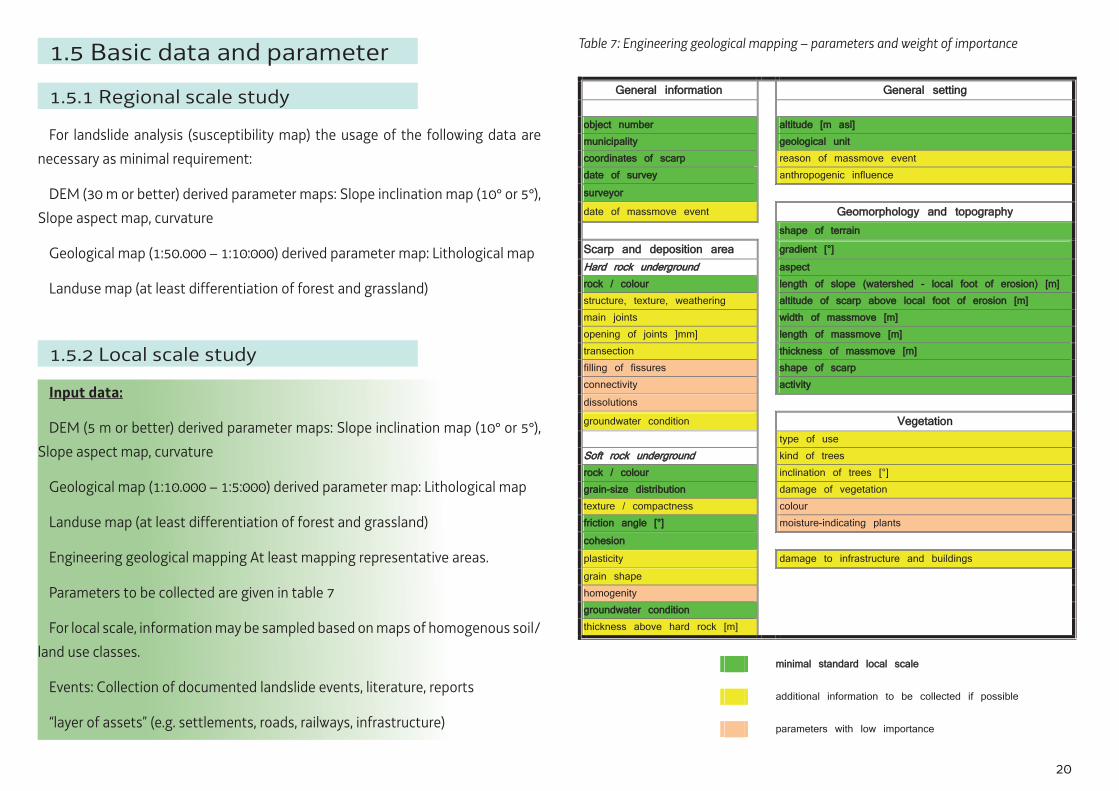
Parameters to be collected are given in table 7

For local scale, information may be sampled based on maps of homogenous soil/land use classes.

Events: Collection of documented landslide events, literature, reports

“layer of assets” (e.g. settlements, roads, railways, infrastructure)

Table 7: Engineering geological mapping – parameters and weight of importance

General information General setting object number altitude [m asl] municipality geological unit coordinates of scarp reason of massmove event date of survey anthropogenic influence surveyor date of massmove event Geomorphology and topography shape of terrain Scarp and deposition area gradient [°] Hard rock underground aspect rock / colour length of slope (watershed - local foot of erosion) [m] structure, texture, weathering altitude of scarp above local foot of erosion [m] main joints width of massmove [m] opening of joints ]mm] length of massmove [m] transection thickness of massmove [m] filling of fissures shape of scarp connectivity activity dissolutions groundwater condition Vegetation type of use Soft rock underground kind of trees rock / colour inclination of trees [°] grain-size distribution damage of vegetation texture / compactness colour friction angle [°] moisture-indicating plants cohesion plasticity damage to infrastructure and buildings grain shape homogenity groundwater condition thickness above hard rock [m]

mminimal standard local scale additional information to be collected if possible parameters with low importance


21

Additional data for verifi cation and/or interpretation (plausibility check)

Topographic map, Orthophotos: GIS-analyses of DEM (morphological disconti-

nuities) will produce anthropogenic lineaments too, which should be verifi ed with topographic maps and orthophotos.

Digital cadastral map: This maps may provide additional information to the “layer of assets”.

Digital road path: This layer can help to eliminate anthropogenic lineaments (ro-ads).

Derived data from input data

Slope inclination – parameter map (indexed for steps 5° or 10°), necessary

Slope aspect – parameter map (indexed for steps 45°), optional

Curvature

Contributing area

Lithological map – (indexed for lithological units)

Landslide inventory map – from documented and mapped events used for stati-stical analysis and check of the quality of results

Land use map (indexed for land use classes)

Output data

For traceability of the results the used input data and derived data should be documented

Slope inclination map (classifi ed): Classifi ed slope map (raster data or polygons) in digital format in the required scale

Slope aspect map (classifi ed): Classifi ed aspect map in digital format in the re-

quired scale, optional

Lithological map – Map of lithological units derived from the geological map (ra-ster data or polygons) in digital format with the used map scale

Land use map – Map of land use classes derived from the land use map (raster data or polygons) in digital format in the required scale

Landslide inventory map – Map of the documented landslides (mapped and from the event cadastre)

Landslide susceptibility map – Combination of onset and runout susceptibility (susceptibility zoning, raster data or polygons) in digital format

Runout map (modelling result) – map of modelling results (raster data or poly-gons) in digital format)

Map of endangered areas - intersection of onset susceptibility map and runout susceptibility map with layer of assets (raster data or polygons) in digital format

22

1.5.3 Site specifi c scale study

Input data:

DEM (2 m or better) derived parameter maps: Slope inclination map (10° or 5°), slope aspect map, curvature

Geological map (≥ 1:5:000) derived parameter map: Lithological map

Land use map (at least differentiation of forest and grassland)

Engineering geological mapping: Parameters to be collected are given in table 8

The difference between local and site specifi c scales will be mostly on the density of the information to be surveyed.

Checking the quality of the classifi cation into homogenous soil classes is required.

Events: Collection of documented landslide events, literature, reports

“layer of assets” (e.g. settlements, roads, railways, infrastructure)

Additional data for verifi cation and/or interpretation (plausibility check)

Plausibility check by engineering geological mapping

Derived data from input data

Slope inclination map (indexed for steps 5° or 10°), necessary

Slope aspect map (indexed for steps 45°), optional

Curvature

Contributing area

Lithological map – (indexed for lithological units)

Landslide inventory map – from documented and mapped events used for statisti-


General information General setting object number altitude [m asl] municipality geological unit coordinates of scarp reason of massmove event date of survey anthropogenic influence surveyor date of massmove event Geomorphology and topography shape of terrain Scarp and deposition area gradient [°] Hard rock underground aspect rock / colour length of slope (watershed - local foot of erosion) [m] structure, texture, weathering altitude of scarp above local foot of erosion [m] main joints width of massmove [m] opening of joints ]mm] length of massmove [m] transection thickness of massmove [m] filling of fissures shape of scarp connectivity activity dissolutions groundwater condition Vegetation type of use Soft rock underground kind of trees rock / colour inclination of trees [°] grain-size distribution damage of vegetation texture / compactness colour friction angle [°] moisture-indicating plants cohesion plasticity damage to infrastructure and buildings grain shape homogenity groundwater condition thickness above hard rock [m]

mminimal standard local scale additional information to be collected if possible parameters with low importance


23

cal analysis and checking of quality of results

Land use map (indexed for land use classes)

Output data

For traceability of the results the used input data and derived data should be do-cumented

Slope inclination map (classifi ed) – Classifi ed slope map in digital format in the required scale (raster data or polygons)

Slope aspect map (classifi ed) -. Classifi ed aspect map in digital format in the required scale (raster data or polygons) Lithological map – Map of lithological units derived from the geological map in digital for-mat in the required scale (raster data or polygons)

Land use map – Map of used land use classes de-rived from the land use map in digital format in the required scale (raster data or polygons)

Landslide inventory map – Map of the documented landslides (mapped and from event cadastre)

Landslide susceptibility map – Combination of on-set and runout susceptibility in digital format (raster data or polygons)

Runout map – map of modelling results in digital format (raster data or polygons)

Map of endangered areas (intersection of landslide susceptibility map with layer of assets) in digital for-mat (raster data or polygons)

24

Table 9: Minimum Requirements for Landslide processes

Susceptibility Map, Susceptibility zoning R

Regional extent L

Local extent S

Slope extent Minimum Requirements for Landslide Processes

Onset Runout Onset Runout Onset Runout

Hazard Zoning

lithology

hard rock underground, orientation of discontinuities, dipping

soft rock underground, soil information Geological Information

tectonic structures /lineaments

archive data on past and current events Landslide inventory field work data

Topographic data optical, aerial photos, topographic maps

cell size 30m

cell size 5m Digital Elevation Model

(DEM) cell size 2m

scale 1:50.000

scale 1:25.000 – 1:5.000

Basic Data

Land use map scale 1:5.000

low

low -medium Source area high – excellent

low

low - medium

Process data quality Transport and runout

area high – excellent

information

advisory Scopestatutory basis - design

geomorph. method

index method

statistical methods Modelling Approach

process based methods

Evaluation

Element at risk

necessary (red)

recommended (yellow)

auxiliary information for advanced study (green)

white: not relevant

Table 9: Minimum Requirements for Landslide processes

25

B.2. Handbook for rockfall

2.1 Toolbox for rockfall suscep-tibility and hazard mappingThe proposed methodology brings the user through some tables, which defi ne

the minimal methodology which should be used. Each methodology is a specifi c combination of:

• a rockfall onset modelling method

• a rockfall runout modelling method

• a method to combine the two components for susceptibility zonation

• a method to introduce temporal probability for hazard zonation

Use of the toolbox requires the following steps:

1. choose a scale and a scope for the analysis according to the following table 10;

2. for each scale, choose the analysis level (minimal or advanced) according to the requirements of the as-signment;

3. for each scale and level, ta-bles provide a combination of onset susceptibility as-sessment methodology (and related zonation), runout modelling methodology, su-sceptibility zonation me-thodology, and hazard zona-

tion methodology. Each methodology is referred to a short acronym;

4. for each acronym, a brief explanation of basics, related procedures and avai-lable tools, required data, and suitability for different applications is provided in chapter B 2.2, B 2.3, B 2.4 and in Annex 3 (Methodologies). The suita-bility of different methodologies for specifi c applications (e.g. susceptibility for land-use planning, linear infrastructures, countermeasure design, very detailed hazard zonation, etc.) is also reported in Annex 3. Only the essential information is given in the guideline, and the user will refer to the cited refe-rences for the practical details of the adopted procedures.

Table 10: Definition of study scale and scope

Analysis Scale Scope Type of maps Map scale DEM cell size

R Regional

Recognition of potentially

endangered areas

Inventory maps / Susceptibility maps

1:50.000 – 1:10.000 30 m

L Local

(e.g. municipality) Land-use planning

Susceptibility maps / Landslide

susceptibility maps 1:10.000 – 1:5.000 5 m

S Specific areas or slope-scale

(site specific study)

Hazard and risk analysis, design of countermeasures

Hazard map / Hazard zone maps

1:5.000 – 1:500 2 m

Table 10: Defi nition of study scale and scopes

26

Table 11: Scales and usability of the methodologies

Onset Runout Methodology Advantage Disadvantage






- x x - x (x)

Index Method

Simple Subjective indexing x x (x) - - - Empirical approach

Simple - - - - x x

Statistics Objectiv, automation


x x - x - -

Process-based Objectiv,

deterministic or stochastic

Detailed knowledge required (x) x x - x x

Table 11: Scales and usability of the methods

27

2.2 Regional scale study (R)

1

Table 12: Methodologies for regional-scale rockfall assessment

ANALYSIS LEVEL ONSET RUNOUT SUSCEPTIBILITY

ZONING HAZARD

Minimal: susceptibility with source areas identification + most conservative runout

R_O1 R_R1 R_S1 -

Advanced: susceptibility zoning with onset susceptibility + transit susceptibility

R_O2 R_R1 R_S2 -

ONSET

R_O1 rockfall sources: identification based geomorphological mapping, location and height of cliffs

R_O2 rockfall source ranking: categorisation of the cliffs in terms of rock fall potential (potential processes, rockfall inventories ))


R_S1: maximum runout and recognition of potential conflicts between rockfall processes and human activities steering the more detailed investigation

R_S2: run-out reclassified according to transit frequency of boulders or nr. of simulated deposited blocks, also considering rockfall source ranking

RUNOUT

R_R1 conservative runout: map of the maximal run-out zone using simple methods (e.g. energy line principle, shadow angle)

R_R2 runout with transit frequency: intersection of the max run out zone with the location of blocks from past events and/or 3D run-out modelling at regional-scale resolution with assessment of transit frequency

Table 12: Methodologies for regional-scale rockfall assessment

28


ZONING HAZARD

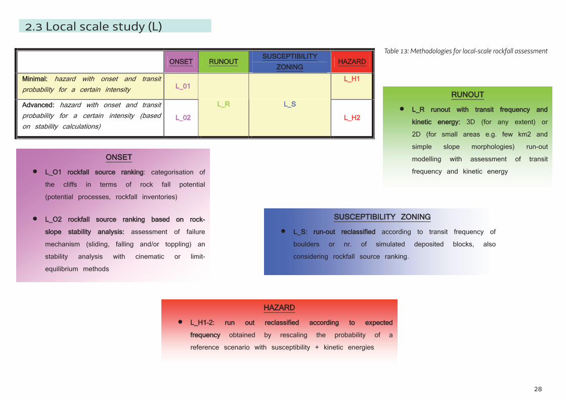
Minimal: hazard with onset and transit probability for a certain intensity L_01

L_H1

Advanced: hazard with onset and transit probability for a certain intensity (based on stability calculations)

L_02

L_R L_S

L_H2

ONSET

L_O1 rockfall source ranking: categorisation of the cliffs in terms of rock fall potential (potential processes, rockfall inventories)

L_O2 rockfall source ranking based on rock-slope stability analysis: assessment of failure mechanism (sliding, falling and/or toppling) an stability analysis with cinematic or limit-equilibrium methods


L_S: run-out reclassified according to transit frequency of boulders or nr. of simulated deposited blocks, also considering rockfall source ranking.

RUNOUT

L_R runout with transit frequency and kinetic energy: 3D (for any extent) or 2D (for small areas e.g. few km2 and simple slope morphologies) run-out modelling with assessment of transit frequency and kinetic energy

HAZARD

L_H1-2: run out reclassified according to expected frequency obtained by rescaling the probability of a reference scenario with susceptibility + kinetic energies

2.3 Local scale study (L)

Table 13: Methodologies for local-scale rockfall assessment

29

2.4 Site specifi c study (S)

Table 14: Methodologies for site-specifi c rockfall assessment

1

Table 14: Methodologies for site-specific rockfall assessment


ZONING HAZARD

Minimal: source and runout susceptibility classified by intensity (with onset and runout susceptibility ranking)

S_01 - S_H1

Advanced: source and runout susceptibility classified by intensity –“probabilistic” hazard (with onset and runout susceptibility ranking)

S_02

S_R

- S_H2

ONSET

S_O1 rockfall source ranking: categorisation of the cliffs in terms of rock fall potential (potential processes, rockfall inventories)

S_O2 rockfall source ranking based on rock-slope stability analysis: assessment of failure mechanism (sliding, falling and/or toppling) an stability analysis with cinematic or limit-equilibrium methods

RUNOUT

S_R runout with transit frequency and kinetic energy: 3D (for any extent) or 2D (for small areas e.g. few km2 and simple slope morphologies) run-out modelling with assessment of transit frequency and kinetic energy

HAZARD

S_H1: run out reclassified according to expected frequency obtained by rescaling the probability of a reference scenario with susceptibility + kinetic energies

S_H2: Magnitude dependent frequency combined with onset susceptibility ranking

30

2.5 Basic data and parameter

2.5.1 Regional scale study

Input data:

DEM (≤ 30 m), generated from optical aerial photos (DTM – DSM cell size ≤ 10 m)

Orthophotos.

Geologic and tectonic maps (scale ≥ 1:50.000)

Collection of documented rock fall past events, literature, reports

Output data (derived parameter maps and documents):

Slope angle and slope aspect maps from DTM; Land use (differentiation of forest and grassland) and soil texture maps from DSM and orthophotos.

Lithologic, tectonic, geomorphologic and out crop / soil type maps from DTM, DSM, orthophotos, geologic and tectonic maps.

Documented data base of major rock fall past events in data sheets and/or GIS environment.

2.5.2 Local scale study

Input data:

DEM (≤ 5 m), generated from optical aerial photos and LIDAR Approach (DTM – DSM cell size ≤ 5m)

Orthophotos.

Geological and tectonic maps (scale ≥ 1:10.000)

Collection of documented rock fall past events, literature, reports.

Geomechanical survey in the fi eld and with ALS oblique.

Main existing rock fall protection methods collection and mapping.

Output data, derived parameter maps and documents (scale ≥ 1:10.000) in digi-tal format (GIS) (raster data or polygons/shape fi les):

Slope angle (indexed for steps 5° or 10°) and slope aspect maps (indexed for steps 10° or 30°) from DTM.

Cross sections from DTM from the source area ending beyond the runout / im-pact zone.

Land use (differentiation of main forest and grassland types) and soil texture maps from DSM and orthophotos.

Lithologic map with lithologic description (indexed for geotechnical lithotype units).

Tectonic map with main tectonic lineaments.

Geomorphologic and out crop / soil type maps with active processes and form, talus / scree characteristics maps from GIS-analyses of DTM, DSM, orthophotos, geologic and tectonic maps, on site investigation.

Rock mass characterisation from on site geomechanical investigation with as-sessment of main structural domains, block shape and volume identifi cation and rock mass classifi cation (BRMR and GSI indexes).

Kinematic rock mass slope stability analysis.

Rock fall source area (scarp) and potentially critical volumes assessment and data sheets compilation.

Rock fall inventory map from documented and mapped events used for back analysis and check of the quality of results

31

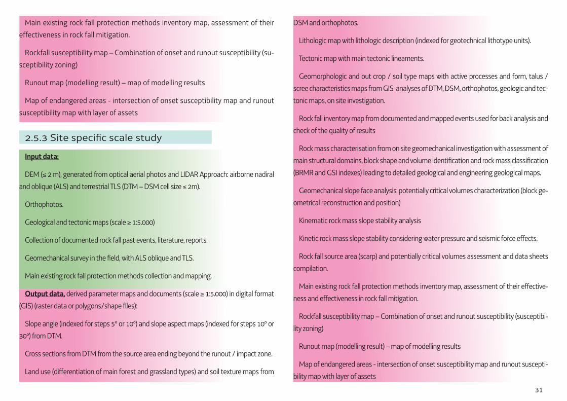
Main existing rock fall protection methods inventory map, assessment of their effectiveness in rock fall mitigation.

Rockfall susceptibility map – Combination of onset and runout susceptibility (su-sceptibility zoning)

Runout map (modelling result) – map of modelling results

Map of endangered areas - intersection of onset susceptibility map and runout susceptibility map with layer of assets

2.5.3 Site specifi c scale study

Input data:

DEM (≤ 2 m), generated from optical aerial photos and LIDAR Approach: airborne nadiral and oblique (ALS) and terrestrial TLS (DTM – DSM cell size ≤ 2m).

Orthophotos.

Geological and tectonic maps (scale ≥ 1:5.000)

Collection of documented rock fall past events, literature, reports.

Geomechanical survey in the fi eld, with ALS oblique and TLS.

Main existing rock fall protection methods collection and mapping.

Output data, derived parameter maps and documents (scale ≥ 1:5.000) in digital format (GIS) (raster data or polygons/shape fi les):

Slope angle (indexed for steps 5° or 10°) and slope aspect maps (indexed for steps 10° or 30°) from DTM.

Cross sections from DTM from the source area ending beyond the runout / impact zone.

Land use (differentiation of main forest and grassland types) and soil texture maps from

DSM and orthophotos.

Lithologic map with lithologic description (indexed for geotechnical lithotype units).

Tectonic map with main tectonic lineaments.

Geomorphologic and out crop / soil type maps with active processes and form, talus / scree characteristics maps from GIS-analyses of DTM, DSM, orthophotos, geologic and tec-tonic maps, on site investigation.

Rock fall inventory map from documented and mapped events used for back analysis and check of the quality of results

Rock mass characterisation from on site geomechanical investigation with assessment of main structural domains, block shape and volume identifi cation and rock mass classifi cation (BRMR and GSI indexes) leading to detailed geological and engineering geological maps.

Geomechanical slope face analysis: potentially critical volumes characterization (block ge-ometrical reconstruction and position)

Kinematic rock mass slope stability analysis

Kinetic rock mass slope stability considering water pressure and seismic force effects.

Rock fall source area (scarp) and potentially critical volumes assessment and data sheets compilation.

Main existing rock fall protection methods inventory map, assessment of their effective-ness and effectiveness in rock fall mitigation.

Rockfall susceptibility map – Combination of onset and runout susceptibility (susceptibi-lity zoning)

Runout map (modelling result) – map of modelling results

Map of endangered areas - intersection of onset susceptibility map and runout suscepti-bility map with layer of assets

32

Table 15: Minimum requirements for rockfall processes

Susceptibility Map R

Regional extent L

Local extent S

Slope extent Minimum Requirements for Rockfall Processes

Onset Runout Suscept. zoning

Onset Runout Suscept. zoning

Onset Runout Hazard zoning

lithology (GTL) orientation of discontinuities, type of rock mass structure Geology tectonic structures / lineaments archive data on past and current events Rockfall

inventoryy field work data aerial photos, topographic maps

inclined image LIDAR-airborne scanning vertical image

Topography

LIDAR -terrestrial

cell size 30m

cell size 5m Digital Elevation Model cell size 2m

scale 1:50.000 scale 1:25.000 – 1:5.000

Basic D

ata

Land use

scale 1:5.000 low low - medium source area high – excellent low low - medium Pr

ocess data

quality

run-out area high – excellent

information - screening land planning Scope countermeasure design

Evaluation

necessary (red)

recommended (yellow)

auxiliary information for advanced study (green)

white: not relevant

2

Accumulation (Ablagerung, Accumulo): The volume of the displaced material, which lies above the original ground surface. (Cruden, 1993).

Disaster (Katastrophe, Disastro): An event in which a society incurs, or is threatened to incur, such losses to persons and/or property that the entire society is affected and extraordinary resources and skills are re-quired, some of which must come from other nations.

Crown (Krone, Coronamento): The practically undi-splaced material still in place and adjacent to the hi-ghest parts of the main scarp. (Cruden, 1993).

Danger (Gefahr, Pericolo): The natural phenomenon that could lead to damage, described in terms of its geometry, mechanical and other characteristics. The danger can be an existing one (such as a creeping slo-pe) or a potential one (such as a rockfall). The charac-terisation of a danger or threat does not include any forecasting. (Hungr et al, 2005).

Depleted mass (Gleitmasse, Massa asportata): The volume of the displaced material, which overlies the rupture surface but underlies the original ground sur-face. (Cruden, 1993).

Displaced material (Verlagertes Material, Materiale spostato): Material displaced from its original position on the slope by movement of the landslide. It forms both the depleted mass and the accumulation. (Cru-den, 1993).

Element at risk (Gefährdetes Element, Elemento a rischio): Population, property, economic activity, public

services or environmental goods situated in a location exposed to risk.

Event map (Ereigniskarte, Inventario di evento – componente geometrica): Event maps exclusively comprise process information which has a known date assigned to it. They mostly cover damage-related in-formation and details on the area affected, based on the 5 key questions of event inquiries (who-what-whe-re-when-why). Redundant information of one event, such as that obtained when dealing with inconsistent sources, is compiled.

Event registers (Ereigniskataster, Inventario di evento – componente logica): According to event maps, event registers only cover process information for which a date is known. They mostly cover damage-related information and details on the area affected, based on the 5 key questions of event inquiries (who-what-where-when-why). As opposed to event maps, however, event registers are independent of scale and can include non-locatable information.

Foot (Rutschungsfuß, Piede): The portion of the lan-dslide that has moved beyond the toe of the surface of rupture and overlies the original ground surface. (Cru-

den, 1993).

Frequency (Häufi gkeit, Frequenza): A measure of li-kelihood expressed as the number of occurrences of

an event in a given time or in a given number of trials (see also probability) (Hungr et al, 2005).

Gravitational mass movement (Gravitative Mas-senbewegung, Movimento in massa gravitativo): Gra-vitational mass movement refers to all those proces-ses by which soil, debris, and rock move downslope discontinuous or continuous under the force of gravity, neglecting a transport medium (water, ice, air).

Hazard (Gefahr, Pericolosità):

1. Probability of occurrence of a landslide of a given magnitude, in a given period of time, and within a given area (Varnes et al., 1984; Fell, 1994; Fell and Hartford, 1997; Guzzetti et al., 1999). The description of landslide hazard should include the classifi cation, location, intensity and the pro-bability of their occurrence within a given period of time (Fell et al., 2008). Different intensity de-scriptors (e.g. volume, area, velocity, energy) can be used depending on the landslide type and the expected runout potential.

2. Probability that a specifi c location on a slope is reached/affected by a landslide of given intensi-ty (volume and/or energy) and temporal proba-bility of occurrence.

Hazard map (Gefahrenkarte, Carta della pericolo-sità): Map portraying, for each considered slope unit (pixel, unique condition unit, basin), a quantitative de-scription of either the probability of reach/occurrence

3

of landslides of given magnitude and temporal proba-bility of occurrence, or their intensity.

Hazard zone map (Gefahrenzonenkarte, Carta di zonazione della pericolosità): Map portraying the ge-ographical location of zones of different intensity of effects by a given hazard (given magnitude and fre-quency of events).

Head (Rutschungskopf, Testata): The upper parts of the landslide along the contact between the displaced material and the main scarp. (Cruden, 1993).

Inventory map > Landslide inventory map

Intensity > Landslide Intensity

Landslide (Rutschung, Frana): It is a geological phe-nomenon which includes a wide range of ground mo-vement, such as rock falls, deep failure of slopes and shallow debris fl ows, which can occur in offshore, co-astal and onshore environments. Although the action of gravity is the primary driving force for a landslide to occur, there are other contributing factors affecting the original slope stability. Typically, pre-conditional factors build up specifi c sub-surface conditions that make the area/slope prone to failure, whereas the actual landslide often requires a trigger before being released.

Landslide Intensity: (Intensität, Intensità di frana): synonym of, or a proxy for, landslide magnitude is a measure of the destructive potential of a landslide, ba-

sed on a set of physical parameters, such as downslo-pe velocity, thickness of the landslide debris, volume, energy and impact forces, total and differential displa-cement, peak discharge per unit width, kinetic energy per unit area. Intensity can be expressed qualitatively or quantitatively. Intensity varies with location along and across the path of the landslide and it should ide-ally be described using a spatial distribution function or an appropriate map. In geomorphological risk as-sessment, it is defi ned as a function of the landslide volume and of the landslide velocity.

Landslide inventory (Rutschungskataster, inven-tario delle frane – componente logica): An inventory for landslides (slides, debris fl ows, rock falls and other mass movements) is a collection of data on past and current landslide occurrences. Content, symbology (map representation) and scale of available landsli-de inventories differ signifi cantly (Schweigl & Hervas, 2009).

Landslide inventory map (Karte der Phänomene, inventario delle frane – componente geometrica): The inventory map shows the location of occurrences of landslides and rockfalls of the landslide inventory at different scales.

Landslide magnitude (Magnitude, Magnitudo del-

la frana): A synonym of landslide intensity. Measured by the size (area or volume), speed, momentum or de-structiveness of the landslide.

Landslide susceptibility (Rutschungsanfälligkeit, Suscettibilità da frana): Spatial probability (suscep-tibility; Brabb, 1984) that any given slope unit will be affected by the occurrence of a landslide of given type, given a set of conditions including topography, geolo-gy, hydrogeology, landuse, vegetation, geomechanics, etc. (modifi ed after Brabb, 1984).

Landslide susceptibility assessment (Gefahren-hinweis, Valutazione della scuscettibilità da frana): A quantitative or qualitative assessment of the spatial distribution of landslides that exist or potentially may occur in an area. Susceptibility may also include a de-scription of the velocity and intensity of the existing or potential landsliding. Although it is expected that landsliding will occur more frequently in the most su-sceptible areas, in the susceptibility analysis, time fra-me is explicitly not taken into account. Landslide su-sceptibility includes landslides which have their source in the area, or may have their source outside the area but may travel onto or regress into the area (after Fell et al., 2008).

Landslide susceptibility map (Gefahrenhinwei-skarte, Carta di suscettibilità): A susceptibility map di-splays the spatial distribution and rating of the terrain units (e.g. pixels, polygons) classifi ed according to their spatial probability / propensity to be affected or rea-ched by a certain landslide type (after Fell 2008).

Comments:

4

• susceptibility is not a ranking or the degree of slope stability, but a description of the relative (spatial) propensity /probability of a landslide of a given type and magnitude to occur;

• “Susceptibility” is not a synonym of “danger”. According to Einstein (1988) a “danger” is a po-tentially hazardous process characterised by its intensity (e.g. “potentially hazardous process”: rockfall; “danger”: a 10m3 rockfall). Thus we be-lieve that “danger” here should be discarded by the defi nition

• Susceptibility can/should be assessed using qualitative and/or quantitative (not only qualita-tive) criteria, even if it is expressed by susceptibi-lity classes. The difference with respect to hazard is that temporal probability of occurrence is not taken into account.

Magnitude > Landslide magnitude

Main body (Haupt - Rutschkörper, Corpo di frana): The part of the displaced material of the landslide that overlies the surface of rupture between the main scarp and the toe of the surface of rupture. (Cruden, 1993).

Main scarp (Hauptanriss, Scarpata principale): A steep surface on the undisturbed ground at the upper edge of the landslide, caused by movement of the di-splaced material away (Cruden, 1993).

Mitigation (Gefahrenminderung, mitigazione): ac-

tivities that reduce or eliminate the probability of oc-currence of a disaster and/or activities that dissipate or lessen the effects of emergencies or disasters when they actually occur. (Jochim et al, 1988).

Mitigation map (Karte über Verbauungsmaßnah-men, carta delle opere di mitigazione): displays the spatial distribution of measures/activities.

Moved body (Rutschörper, Massa spostata): The di-splaced material of the landslide that overlies the sur-face of rupture and the original ground surface betwe-en the main scarp and the toe of landslide.

Mudfl ow (Mure, Colata detritica): When a slope is so heavily saturated with water that it rushes downhill as a muddy river, carrying down debris and spreading out at the base of the slope; the water content may range up to 60%.

Parameter (Parameter, Parametro): Point, linear and areal information that describes the phenomena, parameters have to be specifi ed by values or defi ned classes, parameters have to be located.

Parameters are measurable values, which mostly re-quire a dimension unit. Here, one should differentiate between geometrical (e.g. width of scar [m], block vo-lume [m³]), physical (e.g. friction angle [°]) and chemi-cal parameters (pH value [-]).

Phenomenon (Phänomen, Indizio/ Evidenza): Phe-nomena are signs or indicators for historic, recent or

future processes (points, linear and areal informa-tions). They can be of geological (e.g. zones of special rock anisotropy), geomorphological (e.g. scarps/scars, bulging), vegetation-related (e.g. tilted trees, disturbed forest), hydrological (saturation zones) or damage-re-lated (e.g. impact marks, damage to buildings) type.

Probability (Wahrscheinlichkeit, Probabilità): A me-asure of the degree of certainty. This measure has a value between zero (impossibility) and 1.0 (certainty). It is an estimation of the likelihood of the magnitude of the uncertain quantity, or the likelihood of the occur-rence of the uncertain future event. (Hungr et al, 2005).

Probability of rock failure (Bruchwahrscheinli-chkeit einer Instabilität, Probabilità di rottura): Proba-bility of failure of a portion of rock mass, with a specifi c volume, within a given time unit and within the consi-dered cliff.

Probability of propagation (Ausbreitung-swahrscheinlichkeit, Probabilità di propagazione): Pro-bability that a portion of rock mass, with given charac-teristics, and coming from a given portion of the cliff, transits across a considered area. Characteristics such as height of fl ight, velocity, mass, and energy can be described by statistical distributions.

Process (Prozess, Evento): A process is a happening initiated at a certain location in dependence of tempo-rally and spatially varying conditions (e.g. state of the subsurface, anthropological infl uence on slope statics,

5

progressive weathering) and other causative factors (e.g. precipitation, pore water pressure). The further development of the process is affected by movement controlling factors in the process area (e.g. vegetation, composition of the moving mass).

Register (Kataster, Catasto): Registers are inde-pendent of scale and, contrary to maps, they can also include information which is not tied to a specifi c lo-cation.

Risk (Risiko, Rischio): Measure of the probability and severity of an adverse effect to life, health, property, or the environment. Quantitatively, Risk = Hazard x Potential Worth of Loss. This can be also expressed as “Probability of an adverse event times the consequen-ces if the event occurs”. (Hungr et al, 2005).

Risk is defi ned in ISO 31000 as the effect of uncer-tainty on objectives (whether positive or negative).

Risk analysis (Risikoanalyse, Analisi di rischio): The use of available information to estimate the risk to in-dividuals or populations, property or the environment, from hazards. Risk analyses generally contain the following steps: defi nition of scope, danger (threat) identifi cation, estimation of probability of occurrence to estimate hazard, evaluation of the vulnerability of the element(s) at risk, consequence identifi cation and risk estimation. Consistent with the common dictio-nary defi nition of analysis, “A detailed examination of anything complex made in order to understand its na-

ture or to determine its essential feature “, risk analy-sis involves the disaggregation or decomposition of the system and sources of risk into their fundamental parts. (Hungr et al, 2005).

Risk assessment (Risikobewertung, Valutazione del rischio): It is a step in a risk management process. Risk assessment is the determination of quantitative or qualitative value of risk related to a concrete situation and a recognized threat (also called hazard). Quantita-tive risk assessment requires calculations of two com-ponents of risk: R, the magnitude of the potential loss L, and the probability p, that the loss will occur.

Risk management (Risiko-management, Gestione del rischio): The systematic application of manage-ment policies, procedures and practices to the tasks of identifying analysing, assessing, mitigation and moni-toring risk. (Hungr et al, 2005).

Risk mitigation (Risikominimierung, Mitigazione del rischio): A selective application of appropriate techni-ques and management principles to reduce either like-lihood of an occurrence or its adverse consequences, or both. (Hungr et al, 2005)

Rockfall (Steinschlag, Crollo in roccia/ Caduta mas-si): Instability phenomenon that involves the detach-ment of rock blocks, from a slope and their following movement (by free fall, bouncing, rolling, sliding) along the slope until they reach equilibrium.

Rock avalanche (Bergsturz, Valanga di roccia): Rock

mass falling from a cliff splitting in blocks, for which the movement is like a fl uid.

Shallow landslide (Oberfl ächennahe Rutschung,

Frana superfi ciale): Based on the typological classifi -cation of landslides advanced by Hungr et al. (2001), shallow landslides can be defi ned as reported below. Even though typological, this classifi cation includes also taxonomical elements (material type; movement mechanism).

“Shallow landslides are a gravitational movement of soil down a slope. The movement mechanism can be classifi ed as a slide, not involving signifi cant internal distorsion of the moving mass. The material involved in shallow landslides includes both earth (material smal-ler than 2 mm) and debris (material larger than 2 mm). The corresponding depth is generally not exceeding 3 m. Precipitation-induced shallow landslides are trig-gered during rainstorms or periods of rapid snowmelt when shear strength is reduced because of an increase in pore-water pressure.” (Hungr et al, 2001)

Susceptibilty > Landslide Susceptibility

Vulnerability (Verwundbarkeit, Vulnerabilità): The degree of loss to a given element or set of elements within the area affected by a hazard.

Worth of element at risk (Wert der gefährdeten Elemente, Valore degli elementi a rischio): Economic value, or number of units of each element at risk situa-ted in a given location.

2

PART C : ANNEX2 - DESCRIPTION OF TYPES OF PROCESSES

1. What is a landslide?

A landslide is a downslope movement of rock or soil, or both, occurring on the surface of rupture—either curved (rotational slide) or planar (translational slide) rupture—in which much of the material often moves as a coherent or semicoherent mass with little internal deformation.

It should be noted that, in some cases, land slides may also in-volve other types of movement, either at the inception of the fai-lure or later, if properties change as the displaced material moves downslope.

3

1.1 Classifi cation factors: type of movement and involved material

The most important criteria of classifi cation is the type of movement; the table below shows the classifi cation Varnes (1978); Cruden, Varnes (1996) with some integration using the defi nitions of Hutchinson (1988) and Hungr et al. (2001).

The identifi cation of the movement is not always easy because the mechanism of the landslides are often complex to understand.

TYPE OF MATERIAL

ENGINEERING SOIL TYPE OF MOVEMENT BEDROCK PREDOMINANTLY

COARSE PREDOMINANTLY

FINE

Falls Rock fall Debris fall Earth fall

Topples Rock topple Debris topple Earth topple

Rotational Slides

Translational Rock slide Debris slide Earth slide

Lateral spread Rock spread Debris spread Earth spread

Rock flow Debris flow Earth flow

Rock avalanche

Debris avalanche / Flows

(deep creep) (soil creep)

Complex Combination of two or more principal types of

movement Table 16: Classifi cation of landslides

4

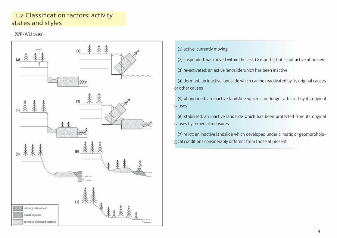
1.2 Classifi cation factors: activity states and styles

(WP/WLI 1993)

(1) active: currently moving

(2) suspended: has moved within the last 12 months, but is not active at present

(3) re-activated: an active landslide which has been inactive

(4) dormant: an inactive landslide which can be reactivated by its original causes or other causes

(5) abandoned: an inactive landslide which is no longer affected by its original causes

(6) stabilised: an inactive landslide which has been protected from its original causes by remedial measures

(7) relict: an inactive landslide which developed under climatic or geomorpholo-gical conditions considerably different from those at present

5

1.3 Classifi cation factors: velocity

Cruden and Varnes (1996)

6

1.4 Description of features

Based on Cruden and Varnes (1996)

1. Crown: The practically undisplaced material still in place and adjacent to the highest parts of the main scarp.

2. Main Scarp: A steep surface on the undisturbed ground at the upper edge of the landslide, caused by movement of the displaced material away from the undi-sturbed ground. It is the visible part if the surface of rupture.

3. Top: The highest point of contact between the displaced material and the main scarp.

4. Head: The upper parts of the landslide along the contact between the displa-ced material and the main scarp.

5. Minor Scarp: A steep surface on the displaced material of the landslide produ-ced by differential movements within the displaced material.

6. Main Body: The part of the displaced material of the landslide that overlies the surface of rupture between the main scarp and the toe of the surface of rupture.

7. Foot: The portion of the landslide that has moved beyond the toe of the surfa-ce of rupture and overlies the original ground surface.

8. Tip: The point of the toe farthest from the top of the landslide.

9. Toe: The lower, usually curved margin of the displaced material of a landslide, it is the most distant from the main scarp.

10. Surface of Rupture: The surface which forms (or which has formed) the lower boundary of the displaced material below the original ground surface.

11. Toe of the Surface of Rupture: The intersection (usually buried) between the lower part of the surface of rupture of a landslide and the original ground surface.

7

12. Surface of Separation: The part of the original ground surface overlain by the foot of the landslide.

13. Displaced Material: Material displaced from its original position on the slope by movement in the landslide. It forms both the depleted mass and the accumu-lation.

14. Zone of Depletion: The area of the landslide within which the displaced ma-terial lies below the original ground surface.

15. Zone of Accumulation: The area of the landslide within which the displaced material lies above the original ground surface.

16. Depletion: The volume bounded by the main scarp, the depleted mass and the original ground surface.

17. Depleted Mass: The volume of the displaced material, which overlies the rup-ture surface but underlies the original ground surface.

18. Accumulation: The volume of the displaced material, which lies above the original ground surface.

19. Flank: The undisplaced material adjacent to the sides of the rupture surface. Compass directions are preferable in describing the fl anks but if left and right are used, they refer to the fl anks as viewed from the crown.

20. Original Ground Surface: The surface of the slope that existed before the landslide took place.

8

2.1 Natural Occurrences

2. What causes landslides?There are two primary categories of causes of landslides: natural and human-caused; often, landslides are caused by a combination of both factors.

This category has three major triggering mechanisms that can occur either singly or in combination:

Geological causes

Weak materials, such as some volcanic slopes or unconsolidated marine sedi-ments, for example

Susceptible materials

Weathered materials

Sheared materials

Jointed or fi ssured materials

Adversely oriented mass disconti nuity (bedding, schistosity, and so forth)

Adversely oriented structural discontinuity (fault, unconformity, contact, and so forth)

Contrast in permeability

Contrast in stiffness (stiff, dense material over plastic materials)

WATER SEISMIC ACTIVITY VOLCANIC ACTIVITY

Morphological causes

Tectonic or volcanic uplift

Glacial rebound

Glacial meltwater outburst

Fluvial erosion of slope toe

Wave erosion of slope toe

Glacial erosion of slope toe

Erosion of lateral margins

Subterranean erosion (solution, piping)

Deposition loading slope or its crest

Vegetation removal (by forest fi re, drought)

Weight of the trees and/or wind stress on the treetops

9

Effects of all of these causes vary widely and depend on factors such as steep-ness of slope, morphology or shape of terrain, soil type, underlying geology, and

whether there are people or structures on the affected areas.

Triggers

Intense rainfall

Rapid snowmelt

Prolonged intense precipitation

Rapid drawdown (of fl oods and tides) or fi lling

Earthquake

Volcanic eruption

Thawing

Freeze-and-thaw weathering

Shrink-and-swell weathering

Flooding

10

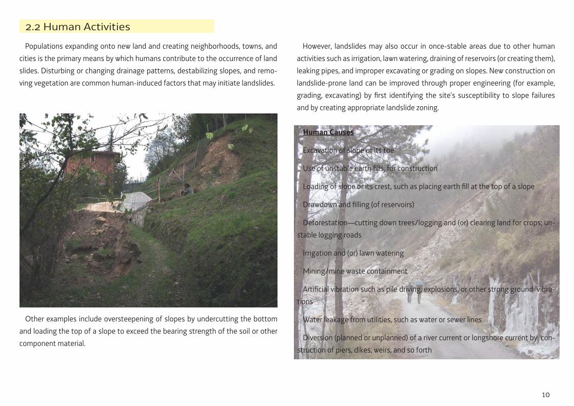
2.2 Human Activities

Populations expanding onto new land and creating neighborhoods, towns, and cities is the primary means by which humans contribute to the occurrence of land slides. Disturbing or changing drainage patterns, destabilizing slopes, and remo-ving vegetation are common human-induced factors that may initiate landslides.

Other examples include oversteepening of slopes by undercutting the bottom and loading the top of a slope to exceed the bearing strength of the soil or other component material.

However, landslides may also occur in once-stable areas due to other human

activities such as irrigation, lawn watering, draining of reservoirs (or creating them), leaking pipes, and improper excavating or grading on slopes. New construction on landslide-prone land can be improved through proper engineering (for example, grading, excavating) by fi rst identifying the site’s susceptibility to slope failures and by creating appropriate landslide zoning.

Human Causes

Excavation of slope or its toe

Use of unstable earth fi lls, for construction

Loading of slope or its crest, such as placing earth fi ll at the top of a slope

Drawdown and fi lling (of reservoirs)

Deforestation—cutting down trees/logging and (or) clearing land for crops; un-stable logging roads

Irrigation and (or) lawn watering

Mining/mine waste containment

Artifi cial vibration such as pile driving, explosions, or other strong ground vibra-tions

Water leakage from utilities, such as water or sewer lines

Diversion (planned or unplanned) of a river current or longshore current by con-struction of piers, dikes, weirs, and so forth

11

Falls are abrupt, downward movements of rock or earth, or both, that detach from steep slopes or cliffs. The falling material usually strikes the lower slope at angles less than the angle of fall, causing bouncing. The falling mass may break on impact, may begin rolling on steeper slopes, and may continue until the terrain fl attens.

3. What is a rock fall?

Occurrence and relative size/range

Common worldwide on steep or vertical slopes—also in coastal areas, and along rocky banks of rivers and streams. The volume of material in a fall can vary sub-stantially, from individual rocks or clumps of soil to massive blocks thousands of cubic meters in size.

Velocity of travel

Very rapid to extremely rapid, free-fall; bouncing and rolling of detached soil, rock, and boulders. The rolling velocity depends on slope steepness.

Triggering mechanism

Undercutting of slope by natural processes such as streams and rivers or diffe-rential weathering (such as the freeze/thaw cycle), human activities such as ex-cavation during road building and (or) maintenance, and earth quake shaking or other intense vibration.

12

A topple is recognised as the forward rotation out of a slope of a mass of soil or rock around a point or axis below the center of gravity of the displaced mass.

4. What is a topple?

Occurrence

Know to occur globally, often prevalent in columnar jointed terrain, as well as long stream and river courses where the banks are steep.

Velocity of travel

Extremely slow to e extremely rapid to extremely rapid.


Sometimes driven by gravity exerted by material located upslope from the di-splaced mass and sometimes by water or ice occurring in cracks within the mass; also vibration, undercutting, differential weathering, excavation, or stream erosion.

13

The mass in a translational landslide moves out, or down and outward, along a relatively planar surface with little rotational movement or backward tilting. This type of slide may progress over considerable distances if the surface of rupture is suffi ciently inclined, in contrast to rotational slides, which tend to restore the slide equilibrium. The material in the slide may range from loose, unconsolidated soils to extensive slabs of rock, or both. Translational slides commonly fail along geolo-gic discontinuities such as faults, joints, bedding surfaces, or the contact between rock and soil. In northern environments the slide may also move along the perma-frost layer.

5. What is a translational landslide?

Occurrence

One of the most common types of landslides, worldwide. They are found globally in all types of environ-ments and conditions.

The surface of rupture has a distance-to-length ratio of less than 0.1 and can range from small (residen-tial lot size) failures to very large, regional landslides that are kilometers wide.

Velocity of travel

Movement may initially be slow (1.5 meters per month) but many are moderate in velocity (1.5 meters per day) to extremely rapid. With increased velocity, the landslide mass of translational failures may disin-tegrate and develop into a debris fl ow.


Primarily intense rainfall, rise in ground water within the slide due to rainfall, snowmelt, fl ooding, or other inundation of water resulting from irrigation, or leakage from pipes or human-related disturbances such as undercutting. These types of landslides can be earthquake-induced.

14

In this case surface of ropture is curved upvard (spoon-shaped) and the move-ment is more or less rotational around an axis parallel to the countour of the slope. The displaced mass may, under certain circumstances, move as a relatively cohe-rent mass along the rupture surface with little internal deformation. The head of the displaced material may move almost vertically downward, and the upper sur-face of the displaced material may tilt backwards toward the scarp. If the slide is rotational and has several parallel curved planes of movement, it is called a slump.

6. What is a rotational landslide?

Occurrence

Because rotational slides occur most frequently in homogeneous materials, they are the most common landslide occurring in “fi ll” material.

Velocity of travel

Extremely slow (less than 0.3 meter or 1 foot every 5 years) to moder ately fast (1.5 meters or 5 feet per month) to rapid


Intense and (or) sustained rainfall or rapid snowmelt can lead to the saturation of slopes and increased groundwater levels within the mass; rapid drops in river level following fl oods, ground-water levels rising as a result of fi lling reservoirs, or the rise in level of streams, lakes, and rivers, which cause erosion at the base of slopes. These types of slides can also be earthquake-induced.

2

PART C : ANNEX3 - 1 METHODOLOGY REGARDING LANDSLIDE HAZARD MAPPING

1.1 Onset

1.1.1 Geomorphological fi eld analy-sis (L_O, S_O)

Geomorphological fi eld analysis methods are based on the subjective asses-sment of landslide onset susceptibility based on expert- knowledge. This approach requires experience of prior events and direct knowledge of landslide triggering control factors in the study area, and it is usually suitable for site-specifi c to local scale analysis.

Table 17: Scales and usability of the me-thods

OOnset Runout Methodology Advantage Disadvantage






- x x - x x

Index Method

Standardisation Subjective indexing x x x x x

Statistics Objectiv, automation,

standardisation


x x (x) - - -

Process-based Objectiv, quantitative

Very detailed knowledge of area

neccesary x x x - x x

1.1.2 Index method R_O1, R_O2, (L_O, S_O)

From the literature many different evaluation methods are known. Keeping to the problem - due to the expected present available data - most likely qualitative methods are useful. Within these methods the use of parameter maps or indexed maps seems to be suitable. The advantages are the automation in the processing, the drawbacks are the subjectivity in indexing.

3

Index method combined with engineering geological mapping and statistical analysis are appropriate for regional and local scale landslide susceptibility stu-dies. For weighting the index of the parameter maps statistical analysis of mapped events are useful. For example indexing the slope inclination classes can be done by knowledge from literature or if enough available data of events are present by statistical analysis.

1.1.3 Statistical methods (R_O1, R_O2, L_O, S_O)

Statistical methods are based on the defi nition of a statistical relationships between geo-environmental controlling parameters and landslide onset suscepti-bility. The most well-known approaches (Carrara et al., 1991) are based on the use of available morphological, structural, lithological, and land-use maps and landsli-de information (Guzzetti et al, 2005). These maps are normally available at regional scale; this approach is well suitable for regional scale analysis. The statistical rela-tionships between geo-environmental controlling parameters (litho logy, structu-ral parameters, slope gradient, slope aspect, slope curvature, etc.) and onset su-sceptibility can be defi ned using multivariate statistical approaches. An example has been presented in for a regional scale analysis. This approach bases on the use of discriminant analysis to classify the percentage of landslides based on several geo-environmental parameters (Guzzetti et al. 2005).

1.1.4 Process-based methods

Process-based methods are mostly based on numerical simulation of the hill slope failure processes (Borga et alii, 2002). Limit equilibrium theory is often used to analyse the stability of natural slopes. A number of methods and procedures based on limit equilibrium principles have been developed for this purpose. Re-gardless of the specifi c procedures, the following principles are common to all me-thods of limit equilibrium analysis:

1. a failure surface or mechanism is postulated;

2. the shearing resistance required to equilibrate the failure mass is calculated by means of statics;

3. the calculated shearing resistance required for equilibrium is compared with the available shear strength. This comparison is made in terms of the factor of safety, which is defi ned as the factor by which the shear strength para-meter must be reduced in order to bring the slope into a state of limiting equilibrium along a given slip surface;

4. the mechanism or slip surface with the lowest factor of safety is found by iteration.

Use of the method at regional, local or site-specifi c scales and available data dictates the assumptions used in the modelling of hill slope stability:

1.1.4.1 Planar infi nite stability analysis (L_O, S_O)

Planar infi nite slope analysis has been applied to the determine landslide su-sceptibility, particularly where the thickness of the soil cover is small compared with the slope length and where landslides are due to the failure of a soil cover overlying a drainage barrier. The drainage barrier may be bedrock or a denser soil mass. In this case, soil thickness corresponds to the depth of the drainage barrier. A translational failure plane may develop at any hydraulic conductivity contrast where positive pore water pressure can develop. Examples of such conditions in-clude loose near-surface soil in thick glacial deposit, loose volcanics overlying den-ser soil layers, loose colluvial soil overlying decomposed residual soil common in granitic terrain.

The static determinacy and mathematical simplicity that results from the as-sumptions embedded into this model make infi nite slope analysis uniquely well

4

suited for drawing unambiguous conclusions about the effects of ground water fl ow on slope stability. The principal disadvantage of infi nite-slope analysis is that mechanical one-dimensionality precludes accurate assessments of slopes in which ground water fl ow or topography produces forces that vary in directions other than the slope-normal direction.

1.1.4.2 2D slope stability modelling (S_O)

If there is a need to analyse slopes and where the potential slip surface cannot be assumed to be parallel to the hill slope, 2D slope stability models are used. Conventional 2D slope stability analyses investigate the equilibrium of a mass of soil margined by an assumed potential slip surface and the surface of the slope, assuming a two-dimensional (2-D) cross section and plane strain conditions for analysis. Forces and moments tending to cause instability of the mass are com-pared to those tending to resist instability. Successive assumptions are made re-garding the potential slip surface until the most critical surface (lowest factor of

safety) is found. As for the infi nite slope stability case, the stability or instability of the mass depends on its weight, the external forces acting on it (such as surchar-ges or accelerations caused by dynamic loads), the shear strengths and pore water

pressures along the slip surface, and the strength of any internal reinforcement crossing potential slip surfaces. Many of the 2D methods are denominated “limit equilibrium” methods. In these methods, the factor of safety is calculated using one or more of the equations of static equilibrium applied to the soil mass mar-gined by an assumed, potential slip surface and the surface of the slope (as it is done for the Infi nite Slope Stability Case). These methods require that a potential slip surface be assumed in order to calculate the factor of safety. Calculations are repeated for a suffi cient number of trial slip surfaces to ensure that the minimum factor of safety has been calculated. For computational simplicity the candidate slip surface is often assumed to be circular or composed of a few straight lines. The limit equilibrium methods (Ordinary Method of Slices (OMS), Simplifi ed Bishop, Spencer) address static equilibrium by dividing the soil mass above the assumed slip surface into a fi nite number of vertical slices.

1.2 Runout

1.2.1 Empirical approaches (L_R, S_R)

The empirical approaches are developed by reference to actual landslide data and include the angle of reach method and the volume change method.

The angle of reach method (Corominas, 1996) establishes a relationship betwe-en the angle of reach and other indexes expressing the mobility of landslides and vertical drop, horizontal reach and volume of landslide mass by means of simplifi ed plots and regression equations. Predicted by this approach, whatever the mecha-nism of motion, all kinds of landslides experience a continuous reduction of the

angle of reach with volume increase. The angle of reach is found independent of the vertical drop.

The volume-change method (Cannon, 1993; Fannin and Wise, 2001) estimates the potential travel distance of debris fl ows by establishing an averaged volume-change formula through dividing the volumes of mobilized materials of landslide by the lengths of the debris trail. The initial mobilized volume is progressively re-duced during downslope fl ows until movement stops where the volume of actively fl owing debris becomes negligible. This approach is sensitive to the initial mobili-zed volume and traveling path geometry.

5

1.2.2 Dynamic modeling (L_R, S_R)

Generally speaking, regardless of the rheological scheme used, it is possible to obtain a set of differential equations that is valid for debris fl ows by depth inte-gration of the mass and momentum conservation equations. These mathemati-cal models are nowadays frequently applied to various real cases of debris fl ows, however, the scientifi c literature on the limits of the numerical, physical and ma-thematical assumptions of these models is rather sparse. The mathematical mo-dels suitable to describe the propagation and the stopping of the fl ow differ in the structure of the equations, in the closure relationship linked to the rheology of the fl ow and to the nature of the bed shear stresses (Iverson, 1997; Hungr, 1995; Brufau et al., 2000).

If an appropriate rheological model is selected, the required rheological parame-

ters are determined either through laboratory experiments or via back-analysis of fi eld observations, geological investigations and weather conditions. The fl exibility of easy association with versatile rheological formulas makes the continuum mo-dels attractive in reproducing the runout process and in predicting some of the key kinematic parameters during motion. The continuum models are hence more sophisticated and they provide more information required for landslide hazard as-sessment.

Table 19: Empirical approaches available for landslide runout modeling

Approach Methods/Models Merits Limitations References

Mass Change

Evaluates the influence of slope, vegetation types and channel morphology by multivariate regression analysis

Does not explicitly account for the mechanics of the processes involved Empirical

Angle of reach

Derives a linear relationship between factors influencing the angle of reach and the volume of materials.

The method affords only a preliminary quantification of the travel distance

Corominas, 1996 Cannon, 1993 Fannin and Bowman, 2008;

Table 18: Empirical approa-ches available for landslide runout modeling

6

1.3 HazardThe defi nition of landslide hazard incorporates the concepts of location, time

and size: Hazard assessment requires the quantitative prediction where a landsli-de will occur, when or how often it will occur, and how large the landslide will be.

The probability function for landslide size may be estimated from the analysis of the frequency–area distribution of known landslides, obtained from landslide inventory maps.

The temporal probability of slope failures may be based on the availability of a

multi-temporal landslide inventory map, which are analyzed to estimate the fre-quency of landslide occurrence in each mapping unit. To obtain an estimate of the frequency of landslide occurrence the number of landslides in each mapping unit can be used. For each mapping unit landslide recurrence can be obtained by past landslide occurrence.

Finally, the quantitative estimate of the probability of spatial landslide occurren-ce may be obtained by using the approaches reported above.

7

PART C : ANNEX3 - 2 METHODOLOGY REGARDING ROCKFALL HAZARD MAPPING

2.1 Rockfall onset susceptibilityIn this section it is assumed that rockfall detachment zones (i.e. rockfall sources)

have already been identifi ed by suitable approaches (i.e. morphometric, geomor-phological, geomechanical parameters). Necessary data acquisition is reported in chapter 4. Once rockfall sources have been identifi ed, they can be ranked accor-ding to their onset susceptibility (i.e. propensity to fail) or not (method R_O1).

If required, susceptibility ranking of rockfall sources can be performed according to heuristic, statistical, or rock-slope stability analysis methodologies.

2.1.1 Heuristic or statistical suscepti-bility ranking (R_O2, L_O1, S_O1)

Heuristic ranking can be performed using many different approaches. Three main families of methods are available:

• direct methods

• indirect heuristic methods

• indirect statistical methods

2.1.1.1 Direct methods

Direct methods consist in subjective assessment of onset susceptibility based on expert- knowledge. This approach requires a direct experience of the study area, and is usually suitable for site-specifi c to local scale analysis.

8

2.1.1.2 Indirect heuristic methods

Indirect heuristic methods are based on the defi nition of functional relationships between geo-environmental controlling parameters and onset susceptibility. The most simple approach (e.g. for L_O1) is based on the use of available topographi-cal, geological, land-use and infrastructure maps (e.g., Baillifard et al, 2003). Being these maps normally available also at regional scale, this approach is well suitable for regional scale analysis.

More advanced heuristic methods (e.g. for S_O1) make use of geomechanical

data for the defi nition of onset susceptibility. A possible approach is the RHAP me-thod (Mazzoccola and Sciesa, 2000) presented within the Falaise Interreg Project (Figures 1 to 2). For characterization of the onset susceptibility, the fi rst step con-sists in the identifi cation of homogeneous sectors of the rocky cliff, according to rock mass properties and slope morphology along the runout zone. The identifi -cation is performed through fi eld surveys, with the help of appropriate check lists.

The rocky cliff is successively analyzed through a geomechanical survey in order to attribute a different onset susceptibility to each homogeneous area. First, the cliff is divided into a regular squared grid. For each grid element, the number of unstable elements is assessed, and a relative susceptibility index is calculated as the number of unstable elements normalized by the maximum number, assumed to be 5. Then, the onset susceptibility for each homogeneous area is calculated as the mean susceptibility of all the included squared elements.

Figures 1: Example of local scale onset su-sceptibility ranking (ref: L_O1) with a sim-ple heuristic approach for the Venzone-Carnia study area (Friuli Vene-zia giulia).

Figures 2: Example of site-specifi c scale onset susceptibility ranking (ref: S_O1) with RHAP approach for a sub-area of Timau study area (Friuli Venezia Giulia).

9

2.1.1.3 Indirect statistical methods

The functional relationships between geo-environmental controlling parameters and onset susceptibility can be defi ned using bivariate or multivariate statistical approaches. An example has been presented in Frattini et al. (2008) for a regional scale analysis. The approach is based on the use of discriminant analysis to classify the activity of rocky cliffs based on several geo-environmental parameters (litholo-gy, density of lineaments, slope gradient, slope aspect, slope curvature, etc.).

2.1.2 Stability analysis (L_O2, S_O2)

Distributed kinematic analysis of rock block stability (Guenther, 2003; Guenther et al., 2004) includes several methods to check the kinematic feasibility for planar, wedge, and toppling failure of rock blocks bounded by discontinuities of known orientations. Methods combining all measured discontinuity orientations (Mathe-son, 1983) or the modal orientation values for different sets (to be characterised by preliminary stereographic analysis) exist. The methods assume planar and per-sistent discontinuities, pure frictional shear strength, and generally provide con-servative results. Given a number of feasible failure mechanisms, a rockfall onset susceptibility can be assessed depending on the total number of possible failure modes for each slope unit, or the ratio between the number of feasible failure mo-des and the total theoretical failure modes.

Figures 3: Example of site-specifi c scale onset susceptibility ranking (ref: S_O2) with spatially-distributed kinematic stability analysis of plane, wedge and toppling failure of rock blocks, for a sub-area of Villa Santina study area (Friuli Venezia Giulia).

Rock-slope stability analysis allows either to estimate a kinematic feasibility of specifi ed block failure modes (Hoek and Bray, 1981) or to compute the Factor of Safety of blocks subjected to specifi c sets of driving and resisting forces. For rock-fall susceptibility assessment purposes, this allows to discrimi-nate sectors of a rocky cliff that are kinematically more suitable to fail, or more close to critical (limit-equilibrium) conditions, and classify their “susceptibility” accordingly. Two main families of stability analysis can be distinguished and considered suitable:

• kinematic analysis;

• limit-equilibrium analysis.

2.1.2.1 Kinematic analysis

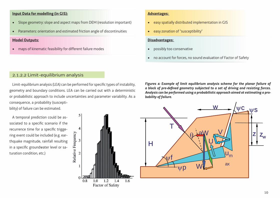
10

Input Data for modelling (in GIS):

• Slope geometry: slope and aspect maps from DEM (resolution important)

• Parameters: orientation and estimated friction angle of discontinuities

Model Outputs:

• maps of kinematic feasibility for different failure modes

Advantages:

• easy spatially distributed implementation in GIS

• easy zonation of “susceptibility”

Disadvantages:

• possibly too conservative

• no account for forces, no sound evaluation of Factor of Safety

2.1.2.2 Limit-equilibrium analysis

Limit-equilibrium analysis (LEA) can be performed for specifi c types of instability, geometry and boundary conditions. LEA can be carried out with a deterministic or probabilistic approach to include uncertainties and parameter variability. As a consequence, a probability (suscepti-bility) of failure can be estimated.

A temporal prediction could be as-sociated to a specifi c scenario if the recurrence time for a specifi c trigge-ring event could be included (e.g. ear-thquake magnitude, rainfall resulting in a specifi c groundwater level or sa-turation condition, etc.)

zw

W

VU

z

fp

H

c sw

um

ax

TaW zw

W

VU

z

fp

H

c sw

um

ax

TaW

Figures 4: Example of limit equilibrium analysis scheme for the planar failure of a block of pre-defi ned geometry subjected to a set of driving and resisting forces. Analysis can be performed using a probabilistic approach aimed at estimating a pro-bability of failure.

11

Input Data for modelling:

• Slope geometry: slope and aspect maps from DEM (resolution important)

• Block size and geometry

• Driving and resisting forces magnitude and orientation

Model Outputs:

• Factor of Safety (deterministic), Probability of Failure (probabilistic)

Advantages:

• More sound assessment of slope stability, probabilistic analysis of suscep-tibility

Disadvantages:

• Diffi cult spatially-distributed implementation, lumped use in site-specifi c si-tuation

2.2 Rockfall Runout modelling

Currently, a large variety of models for calculating runout zones of rockfall events exist. All existing rockfall models may be categorized in two main groups: empirical models and process- based models (Dorren 2003).

2.2.1 Empirical methods (R_01)

Empirical models are based on simplifi ed assumptions in rockfall scenarios and generally consist on data acquired in a study area which are analysed by statistical methods. Process-based models describe or simulate the physical processes of motion of falling rocks over slope surfaces.

For the determination of rockfall runout zones on a regional scale, several empi-rical measures have been suggested (Domaas, 1994, Keylock and Domaas (1999). The most widely adopted method for analysing the travel distance of rockfalls are based on geometrical approaches: the angle of the shortest line between the top

of the rockfall source scar and the stopping point of the landslide (“Fahrböschung” Heim, 1932; reach angle, Corominas, 1996; geometrical slope angle, Meissl, 1998) and the minimum of the line between the talus apex and the stopping point of the landslide (Lied, 1977; minimum shadow angle, Evans and Hungr, 1993) (Fig. XX)

12

Figures 5: Sketch of the characteristic rokfall path profi le. Geometrical slope angle-α; shadow angle - β (modifi ed after Meißl 1998).

Empirical methods can be applied in practice using several approaches:

• analysis along selected profi les for which the maximum runout distance is calculated using α or β angle, and then manual interpolation of results along ptofi les in order to defi ne a rockfall runout zone.

• application of a GIS-based models to defi ne the shadow area between the source zone (or talus apex) and the α (or β) angle (CONEFALL, Jaboyedoff and Labiouse, 2003).

2.2.1.1 α angle (reach angle, geometrical slope angle)

The angle of the shortest line between the top of the rockfall source scar and the stopping point is based on the “energy line” approach (Heim, 1932).

From the geometric relationship between a point on the cliff C with coordinates (x0, y0, z0) and a random subjacent (z <z0) point P with coordinates (x, y, z) gives the following mathematical relationship (Jaboyedoff, 2003):

Several values have been reported in the literature: 28.5° (Onofri e Candian, 1979); 32° (Toppe, 1987); 37° (Meißl, 1998); 33° (Heinimann et al. 1998); 36.9° (Co-pons et al., 2009); 34°-40° (Melzner, 2009).

These values can be very different according to the cliff height, the use of actual

versus straigth-line path, the percentage of blocks enveloped within a certain an-gle. Hence, the applicability of the reach angle approach is limited by these pro-blems, and values need to be calibrated for each single case-study.

Figures 6: Geometrical sketch for energy-line ap-proach (Heim, 1932).

13


• Slope geometry: DEM (resolution not very important)

• Source areas: points, lines or polygons

• Parameters: angle α, (optional) cone aperture with respect to slope direction

Model Outputs:

• maximum runout distance and/or zone,

• (optional) count of source cells potentially contributing to rock fall, velocity calculated with the energy-line approach.

Advantages:

• low sensitivity to DTM resolution,

• easy implementation over large areas,


Disadvantages:

• angles need calibration site by site, especially in relation to the cliff height,

• impossibility to assign an onset susceptibility to each cell

2.2.1.2 β angle (minimum shadow angle)

The minimum shadow angle is based on the idea that travel distnace is control-led by the propagation along the talus, because the kinetic energy acquired during fall from the cliff is largely lost at the fi rst impact with the talus (Hungr and Evans, 2003). The advantage of the minimum shadow angle is that it is less sensitive to

cliff height. However, values reported in the literature are signifi cantly different also for this angle: 28-30° (Lied, 1977); 17° (Domaas, 1994); 31.5° (Meißl, 1998); 22° (Wieczorek et al., 1998); 24°-27.5 (Evans and Hungr, 1993); 25.5° (Copons and Villaplana, 2008), 21° (Holm and Jakob, 2009).


• Slope geometry: DEM (resolution not very important)

• Talus apex: points, lines or polygons

• Parameters: angle β, (optional) cone aperture with respect to slope direction

Model Outputs:

• maximum runout distance and/or zone,

• (optional) count of source cells potentially contributing to rock fall.

Advantages:

• low sensitivity to DTM resolution,

• easy implementation over large areas,


Disadvantages:

• impossibility to assign an onset susceptibility to each cell

14

2.2.2 2D modelling

2D models simulate the motion (fall, rebound and rolling) of blocks along a profi -le (Bozzolo and Pamini, 1986; Pfeiffer and Bowen, 1989; Stevens, 1998; Jones et al, 2000). When analysing large areas, it is necessary to identify a number of “repre-sentative” profi les and to perform a simulation for each profi le. The results can be

spatially distributed by expert-knowledge geomorphological interpretation or by interpolation of output data about energy or about the frequency of block arrested along the slope.


• Slope geometry: Cross sections along most probable paths

• Slope materials: Restitution coeffi cients for impact and friction coeffi cients for rolling. Possibility to introduce a stochastic variation of parameters

Model Outputs:

• 2D Trajectories, velocity profi les, distribution of arrest points

Advantages:

• easy implementation with slope profi les,

• easy visualization of trajectory impacts and bounces,

Disadvantages:

• not possible to account for 3D effects,

• diffi culty to interpolate among different profi les

• subjectivity in the choice of profi le position, spacing and geometry

Figures 7: Example of Site.specifi c 2D modelling (ref: S_R) for a sub-area of Villa Santina study area (Friuli Venezia Giulia).

15

2.2.3 3D modelling

3D models are able to simulate block motion along a slope by including late-ral dispersion of trajectories due to morphological complexity (Descoeudres and Zimmermann, 1987: Guzzetti et al., 2002; Agliardi and Crosta, 2003; Crosta et al., 2004; Dorren et al., 2006; Lan et al., 2007) The results are distributed over the enti-re study area, without need for interpolation of data.

3D modelling requires a complete spatial coverage of data are more complex and diffi cult to handle. The reliability of these models depends on the quality of the algorithms used for the simulation of physical processes, the introduced as-sumptions, etc.


• Slope geometry: DEM (resolution very important)

• Source areas: raster theme with location of source cells

• Parameters: restitution coeffi cients, rolling friction coeffi cient, block mass, volume and shape, other parameters for complex phenomena

Model Outputs:

• 3D trajectories, statistics for each cell (e.g. for number of transits, velocity, height, energy)

Advantages:

• simulation of 3D effects,

• possibility to implement a quantitative hazard assessment,

• easy zonation of “hazard”,

• possibility to simulate complex phenomena

Disadvantages:

• strong sensitivity to DEM resolution,

• need for calibration of parameters that are frequently unknown,

• need for robust and meaningful algorithms

• assumptions depending on adopted algorithms

• more diffi cult calibration, data analysis/visualization

16

Figures 8: Example of local scale 3D modelling (ref: L_R) for the Timau stduy area (Friuli Venezia Giulia).

17

2.3 Susceptibility zoning

The simplest form of rockfall susceptibility zoning involves mapping the largest area po-tentially affected by rockfall runout trajectories. In this case, no further zonation is provided with respect to the reach probability in different parts of the runout area, and nothing is said about the spatial distribution of intensity (i.e. velocity, kinetic energy, height). A further step towards a more sound susceptibility assessment would require the runout area ac-cording to the probability that a given distance from the source (or, more general, a given point on the slope) is reached by rockfall trajectories. This can be best accomplished by the used of 2D and 3D modelling tools, as better explained in the following two sections.

Nevertheless, a simple evaluation of rockfall runout (without further zoning) could be considered useful only as a “minimum requirement” approach for regional scale studies, where 2D modelling is not feasible and 3D modelling could be too time consuming for the aims of a simple analysis for rockfall reconnaissance / prioritization. In these simple cases, a fi rst estimation of rockfall runout can be made using the shadow angle approach, with or without a simple zoning based on the number of “shadow cones” (each emanating from a source cell) contributing to each location in the runout area (Jaboyedoff and Labiouse, 2003).

2.3.1 Max runout, classifi ed runout (R_S1, R_S2)

In 2D modeling, a typical approach to susceptibility assessment to classify the runout

and to defi ne a reach probability is the analysis of the percentage of blocks passing through a certain distance. This approach allows to trace a line of equal probability of transit and arrest by interpolation or subjective extension of 2D modelling results betwe-en adjoining analysis sections. The most important limitation is that a 2D model cannot

2.3.2 Onset susceptibility + reach probability (L_S)

account for lateral deviation of trajectories, thus overestimating the frequency of blocks which pass through each slope unit. Using 3D models, according to a conceptually simi-lar approach it is possible to defi ne a transit frequency for each slope unit accounting for longitudinal and lateral separation of block trajectories. Normally, the frequency analysis is performed by simulating a large number of blocks starting from each source area, and introducing uncertainty of parameters (block volume, restitution coeffi cients, rolling fric-tion coeffi cients, etc.) through a stochastic approach. Runout distance can change as a function of some assumptions (eg. maximum local slope control on the trajectory).

An example of this approach is given by the RHAP methodology (Mazzoccola and Scie-sa, 2000).

Conceived for use with 2D modelling, applies to rockfalls ranging from single blocks to rock masses up to 1000 m3 in volume, and it is suitable for local scale studies. The me-thod allows to rank the susceptibility level with respect to a specifi c site. For this reason, susceptibility ranking from different sites are not comparable in absolute value. The me-thodology allows to combine an heuristic susceptibility zonation with a 2D runout analy-sis. From each source zone characterized by a different susceptibility value, one or more representative trajectories are used to perform 2D rockfall stochastic simulation in order to perform a preliminary longitudinal zonation of rockfall arrests along the slope. The simulations are performed considering modal block volumes and shape, and calibrating restitution coeffi cients using historical data and extent of scree slope deposits. From the percentage of block passing through a certain distance, the slope is zoned in 4 zones with different preliminary susceptibility levels: 4 (75% of the blocks), 3 (90%), 2 (100%), 1 (extent of exceptional blocks). The preliminary (transit) susceptibility classifi cation is modifi ed based on the onset susceptibility in a simple manner. Onset susceptibility is reclassifi ed into three classes of activity: low, medium, high. This classifi cation is then used to modify the preliminary susceptibility map by incrementing (high onset activity) or decrementing (low onset activity) the hazard level of one class.

18

2.3.3 Onset susceptibility+reach probability+runout intensity (L_S)

Using 2D or 3D models allows to calculate a reach or transit frequency for each slope unit (usually a pixel) accounting for longitudinal and lateral separation of block trajectories, as well as a set of intensity descriptors of rockfall phenomena (e.g. velocity, kinetic energy, height). Normally, the analysis is performed by simu-lating a large number of blocks starting from each source area, and introducing uncertainty of parameters (block volume, restitution coeffi cients, rolling friction coeffi cients, etc.) through a stochastic approach. A conceptually similar approach (i.e, combining reach probability and intensity) has been implemented with 2D modelling by Jaboyedoff et al. (2005) in order to allow susceptibility assessment according to the Swiss Guidelines.

In the RHV approach (Crosta and Agliardi, 2003), rockfall susceptibility/hazard at a given location on a rockfall-prone slope is assumed to be a function of rockfall re-ach probability (transit frequency), block kinetic energy and trajectory height. The approach thus assesses susceptibility/hazard by taking into account both rockfall frequency and in-tensity. The required para-meters can be computed for each slope unit by per-forming 3D numerical mo-delling at suitable level of detail (depending on the analysis scale).

Figures 9: Main assumptions and parameter defi nitions of the RHV rockfall suscepti-bility assessment methodology (after Crosta and Agliardi, 2003).

The methodology follows these steps:

• identifi cation of potential rockfall sources and characterisation of their onset susceptibility;

• rockfall runout modelling by using a 3D numerical modelling tool;

• for each model cell (i.e. slope unit), extraction and reclassifi cation of the simulated: a) frequency of reach (c), b) height (h), and kinetic energy (k) of blocks/trajectories;

• calculation of the modulus of the “rockfall hazard vector” (RHV) defi ned as:

222 hecRHV c

19

Figures 11: Example of Local scale rockfall su-sceptibility with RHV approach (ref: L_S) for Villa Santina study area (Friuli Venezia Giulia).

Figures 10: Parameter reclassifi cation scheme used in the RHV rockfall su-sceptibility assessment methodology (after Crosta and Agliardi, 2003).

20

2.4 Susceptibility zoning

2.4.1 Expected frequency associated to a reference scenario

The heuristic assessment of probability is performed through a subjective esti-mation of event frequency based on:

• expert knowledge regarding the geological setting;

• frequency of past events;

• similarity with other areas where data are available.

The most simple and simplistic approach for the assessment of temporal pro-bability is to assign an expected frequency to a scenario which is considered the most “representative” for the study area. This is a strong simplifi cation, since it is well known that frequency depends on the volume of rockfall.

The expected frequency can be defi ned using both heuristic and statistical ap-proaches.

2.4.1.1 Heuristic approach (L-H1, L-H2, S_H1)

An example of heuristic temporal probability is the approach used in BUWAL (Bundesamt für Umwelt, Wald und Landschaft, 1998) methodology. This methodo-logy accounts for frequency and intensity, thus allowing to perform, although in a simplifi ed manner, a real hazard assessment. BUWAL methodology fi rstly requires the identifi cation of areas potentially impacted by an expected rockfall scenario. Normally, only a single scenario is considered, this being the most “representative” scenario. For this scenario, the intensity is estimated in terms of both expected vo-lume and velocity, using tables that allows to assign classes of intensity based on ranges of values for these two parameters. Regarding the velocity, rockfall always belongs to class 3 according to the BUWAL classifi cation.

For the same scenario, the frequency of the “representative” events is estimated using four classes or recurrence time, Tr: high (Tr < 30 years), medium (30 < Tr < 100 yr), low (100 < Tr < 300 yr), very low (Tr > 300 yr). Table xxx provides a link between the activity of landslides and the expected recurrence time. The width of the fre-quency intervals allows to incorporate the uncertainty in the estimation.

Table 20 - definition of frequency classes in BUWAL methodology

Frequency

class

Recurrence time: Tr

(yr) Landslide activity

1 < 30 active landslides and dormant landslides with high frequency reactivations

2 30 – 100 dormant landslides with medium frequency reactivations 3 100 – 300 dormant landslides with low frequency reactivations 4 > 300 relict landslides

Table 19: defi nition of fre-quency classes in BUWAL me-thodology.

21

Advantages:

• the method is simple

• the method allows to assign different frequencies to different sectors of the study area

Disadvantages:

• the method is subjective

• given the uncertainty, frequency is roughly esti-mated for classes of recurrence times defi ned using large range of values.

Applicability:

the method requires a direct experience of the expert with regard to a rockfall problems at a specifi c loca-tion. Hence, the approach is suitable for local scale analysis. When applied to regional scale studies the estimation becomes very uncertain and arbitrary.

A statistical approach is based on the analysis of historical events aimed at iden-tifying an average recurrence time of events, independently from the volume of possible rockfalls. Since the number of events usually available is limited, the statistics need to be calculated using data for large regions, assuming that the frequency is equal for the entire area.

2.4.1.2 Statistics of historical data (L_H2)

Advantages:

• the method is data driven and objective

• the method is simple

Disadvantages:

• rockfall events are rarely collected for small vo-lumes and for events occurring in rural areas wi-thout damages to infrastructures; hence, the ave-rage frequency is normally underestimated.

• Frequency is assumed constant over large areas

Applicability:

the method is suitable for large areas, where the number of events is suffi cient to estimate a reliable (although underestimated) recurrence time.

22

2.4.2 Magnitude-frequency relation-ships (S-H2)

In order to obtain a fully quantitative evaluation of the hazard related to rockfall occurrence, the annual frequency of rockfall events should be estimated with refe-rence to specifi c event magnitudes (i.e. volumes) classes, as for fl ood or earthqua-ke events. This requires knowing or assuming the relationship which describes the magnitude-frequency distribution of rockfall events in a given area characterised by specifi c geological and geomorphological features. For rockfalls, several authors (Hungr et al., 1999; Dussauge et al., 2003; Malamud et al., 2004) demonstrated that the magnitude-cumulative frequency (MCF) distribution of events in given volume classes j can be described by a power law in the form:

logN(V ) = N0 + b logV

where N(V) is the cumulative annual frequency of rockfall events exceeding a given volume, N0 is the total annual number of rockfall events, and b is the power law exponent.

The annual frequency of rockfall events in a given volume class can be derived from MCF curves by subtracting the cumulative frequencies for each considered volume class (Hungr et al., 1999). The parameters of MCF curves themselves have no universal signifi cance, although the exponent b has been found to vary in a quite narrow range, i.e. −0.7<b<−0.4 (Hungr et al., 1999; Dussauge et al., 2003), and should be based on complete local rockfall inventories.

Unfortunately, historical databases and inventories of landslide events (i.e. the preferred source of M-F information) are rarely available, and site-specifi c data collection may be unfeasible for large areas or when budget constraints exits. Mo-

reover, landslide size values reported in historical databases may be incomplete or estimated at the order-of-magnitude level of accuracy (Hungr et al., 1999). Data may be incomplete both in space (i.e. data sampling only in specifi c sub-areas) and

in time (i.e. data recorded only for specifi c time windows), due to undersampling and censoring effects.

When available, magnitude-frequency relationships would provide a means to estimate the return period of landslide events exceeding a given magnitude , T(V)=1 / N(V), and then the probability of a specifi ed number of events to occur in a given reference time, thus allowing a full probabilistic evaluation of landslide onset hazard.

Figures 12: Example of MCF (magnitude-cumu-lative frequency) curve for rockfalls (Hungr et al., 1999).

23

2.4.3 Combining frequency with su-sceptibility

When attempting to assess rockfall “hazard” (including the expected frequency of events) at different levels (see previous sub-sections), the frequency of event onset must be integrated with the onset and runout susceptibility in order to ob-tain hazard maps accounting for all these components.

Possible approaches (at different levels of complexity) to do this could include:

1. producing “scenario-based susceptibility maps” by modelling rockfalls invol-ving block volumes corresponding to specifi ed return periods (either single “design volume” if only a heuristic or statistical hazard assessment is possi-ble, different maps for different volumes if a M-F curve is available);

2. adapting RHAP-type and RHV-type approaches by scaling the probability of reach at any point of the slope with the onset probability corresponding to specifi ed return periods (by multiplication);

3. modifying the “modifi ed BUWAL approach” often used by administrations and basin authorities in Italy in order to incorporate (as matrix input data) the event frequency (estimated by heuristic, statistical and M-F approaches) and the intensity (kinetic energy) obtained by numerical modelling with volumes consistent with onset frequency. In this case, the separate use of “modifi ed BUWAL” Tables 1 (velocity) and 2 (size) would be not necessary, and kinetic energy could be directly used. This approach could also allow using the me-thod for each slope unit, accounting for the variability of rockfall intensity along the slope.

24

ROCKFALL STRUCTURAL COUNTERMEASURE SURVEY FORM

Province Municipality ID Date

Survey map scale Photo ID

NOTENOTE KEYS TO ATTRIBUTES

Point Line Polygon (1)

B) SOURCE AREA

NOTENOTE

DESCRIPTION (2)

C) COUNTERMEASURE DATA SHEET

NOTENOTE Efficacy (5)

9: Draped steel wire mesh (double-twisted hezagonal mesh)

10: Reinforced draped steel wire mesh (armed by steel cables)

DIMENSIONS QUANTITY 11: Draped wire panels / plates (reinforces square mesh)

(3)

D) ADDITIONAL NOTES AND SKETCHES

(4) 1: Wooden (5) 1: Poor/bad2: Steel 2: Fair3: Earth fill 3: Very good4: Reinforced earth fill5: Reinforced concrete

(6)2: Industrial buildings (NOTE: specify number, size)

3: Public interest buildings (e.g. school, hospital)

4: Road (NOTE: specify type, span length, width)

5: Railway (NOTE: specify type, span length, number of tracks)

6: Lifelines (NOTE: specify type)7: Other (specify)

1: Very fractured/disrupted rocky cliff2: Rocky cliff

Type of countermeasure (2)Minimum elevation (m. a.s.l.)Maximum elevation (m. a.s.l.)

2: Flexible barrier - low capacity (<500 kJ; no upslope ropes / brakes)

Evidence of activity (Y / N)

Type of source (3)Maximum extent (m, m2)

1: Rocky cliff (NOTE: specify approximate haight from base)

2: Chute / channel (NOTE: specify width / cross-section area / slope estimates)

3: Talus (NOTE: specify grain size / slope / vegetation estimates)

Average heigth/depth (m)Maximum heigth/depth (m)

Area (m2) 5: Rockslide scarp/accumulation4: Unstable scree (secondary rockfalls)3: Discontinuous outcrops

Minimum heigth/depth (m)

Description of damages

3: Flexible barrier - medium capacity (500-3000 kJ; upslope ropes / brakes)

4: Flexible barrier - high capacity (>3000 kJ; additional ropes / brakes)

6: Reinforced concrete wall (NOTE: specify spessore indicativo e particolari)

Average base width (m)

5: Gabion wall (NOTE: specify size and number of modules)

Length (m)12: Rock bolts / anchors (NOTE: specify type)

5: Valley floor

Map topology

1: Rigid barrier (wooden beams or steel girders)

Average top width (m)

State of efficiency (5)Materials (4) 7: Ditch (excavated)

8: Embankment (fill)

A) GENERAL DATA

Topographic map

Location on the slope (1)

1: Housing buildings (NOTE: specify number, size, #stories)

SurveyorExisting inventory (Y / N)

ELEMENTS AT RISK (6)

6: Other (specify)

4: Talus base (NOTE: specify approximate local slope and distance from base)

2

PART C : ANNEX4 - DATA COLLECTION

1.1 Data collection for landslides

REGIONAL EXTENT analysis scale 1:10.000 - 1:50.000 GRID 30m

Data Direct information Data collection and analysis Required

accuracy Output

slope angle slope angle map

slope aspect slope aspect map DTM-AL topography

slope profile

grid 30m

geological map Geological map lithologies

lithological map

data sheet or map of historical landslide Landslide data historical landslides

landslide inventory map

Topographic map, orthophotos land use - vegetation - massmove events - verification

Land use land use landuse map

3

LOCAL EXTENT analysis scale 1:5.000 - 1:10.000 GRID 5m


accuracy Output

slope angle slope angle map


slope profile

grid 5m

geological map

Geological map lithologies lithological map (define geotechnical lithotype units)

Tectonic map structural elements

survey scale = analysis scale

tectonic map (in geological map)

Landslide data historical landslide data availability

landslide inventory map

land use orthophoto map

Orthophoto soil type

vegetation

land use – soil type – vegetation

from laserscan and digital

camera accuracy

.landuse map

landslide source area (scarp) parameters from engineering geological mapping Observation points

landslide deposition area

for homeogenious

area

Land use land use survey scale = analysis scale landuse map

4

SITE SPECIFIC EXTENT analysis scale 1:500 - 1:5.000 GRID 2m


accuracy Output

slope angle slope angle map (>50°, >60°, >70°)


slope profile

grid 2m

geological map

Geological map litologies lithological map (breakdown in geotechnical litho type)

Tectonic map structural elements tectonic map (in geological map)

geomorphologic map Geomorphologic map active processes and form


Landslide data historical landslide data availability landslide inventory map

land use orthophoto map Orthophotos soil type

vegetation

land use – soil type – vegetation from laserscan accuracy

landslide source area (scarp) parameters from engineering geological mapping Observation points

landslide deposition area

as many as possible

Land use land use survey scale = analysis scale

landuse map

5

1.1.1 Field mapping

It should be noted that the landslide inventory is often the basis for all the lan-dslide susceptibility zoning, and it is important that this activity is done thoroughly.

For precipitation-induced shallow landslides the data will usually need to cover 10, 20 or more years so a number of signifi cant rainfall events can be sampled in the inventory (this is particularly important if the inventory is to be used as the basis for frequency assessment) (Frattini et al., 2010). In many cases it will not be possi-ble to create a good inventory from past records, so the inventory has limitations. These can be overcome with time if responsible authorities establish a system for gathering data which can then be incorporated in later zoning studies.

Historical data or record of temporal distribution of landslides and triggering rainfall should also be added to the inventory. Landslide inventories should include information on where and when the landslides occurred, the type, size and the re-gional extent of the landslides as well as information on triggering conditions usa-ble to test results from deterministic models. Triggering conditions are not easily determined from aerial photographs and their defi nition requires nearby measu-rement of rainfall and observations of soil moisture conditions. For testing deter-ministic shallow landslide initiation model landslide sources, tracks and deposits should be mapped separately.

Techniques that are applicable for developing landslide inventories include: i) fi eld observations; ii) aerial photo interpretation; iii) analysis of high resolution op-tical and infrared imagery (Ikonos, Quickbird, IRS CartoSat-1), satellite-based in-terferometric SAR (InSAR, and DlnSAR of Radarsat, ERS, Envisat, TerraSAR-X, CO-Smo/SkyMed, ALOS); iv) use of airborneLIDAR. These techniques are examined in the following sections.

Field mapping involves conventional surveying methods or by using mobile GIS and GPS for the collection of landslide attributes. Field mapping has been applied also together with photo-interpretation to determine landslide distribution and

1.1.2 Aerial photograph interpreta-tion

Aerial photograph interpretation (API) still remains the most applicable techni-que for landslide mapping (Metternicht et al., 2005). Interpretation of single - and multicolored aerial photos is used intensively for the mapping and monitoring of landslide characteristics (e.g. distribution and classifi cation) and factors (e.g. slope, lithology, geostructure, landuse/land cover, rock anomalies). In some cases lan-dslide features are often hidden or obscured by tree cover on aerial photographs. This means a limited usability of this technique. A combined approach of visual in-terpretation using aerial photos together with fi eld based observation is recogni-zed as labour-intensive and time-consuming. Nichol et al., (2006) reported that for a complete stereo cover of an area of 1000 km2 approximately 400 photo prints at a scale of 1:10,000 were needed. Furthermore previous research regarding the usability of aerial photos in complex environment did not show reliable results for landslide identifi cation. Brardinoni et al. (2003) reported that 85% of the Vancou-ver landslides which were mapped in the fi eld and were located in densely forested regions could not be recognized on aerial photographs.

classifi cation relatively to age, degree of activity and typology (Carrara et al. 1999). Field-based approach is extraordinarily time intensive, required more labour. In-ventory map updating is connected with diffi culties, especially in forested area. It

is very precise to pointing out smaller landslide features and recent active slides.

1.1.3 Satellite and radar-based ima-gery

Satellite imagery has been used intensively for the landslide inventory mapping. Using optical imagery system recognition of a landslide can be carried out by con-sidering the size of the features, the contrast between landslides and surrounding areas and the morphological expression. Optical imagery has also demonstrated

6

the diffi culty for mapping landslides in heavily forested terrain. Issues of detecting landslides in multi-temporal satellite imagery have still not been overcome due to persistent cloud and forest cover.

Radar technique can be performed either by airborne or satellite-based. Pla-tforms in space are particularly diverse because of the large areas that can be captured within a short span of time. Recently Interferometric Synthetic Aperture Radar (InSAR) has become a preferable technique for landslide mapping and many studies have been conducted in order to produce a suitable method which can de-lineate landslide features. However there are some diffi culties of InSAR, especially related to geometric noise due to the difference in satellite look angles, the vege-tation affect on the signal and the atmospheric factors (Catani et al., 2005). InSAR shows to be unsuitable for landslide mapping in forested terrain due to the dense vegetation effect which causes decorrelation (Rott, 2004) and the movement ve-locities are too high.

1.1.4 LIDAR techniques

Laser-based technology is capable of delivering very dense and accurate point clouds of a landscape in a relatively short time. Thus all the data are inherently in three-dimensional and completely digital models (Kerle et al., 2008). Semi-au-thomatic methodologies are available to detect and interpret individual objects in landscapes including landslides (Tarolli et al., 2010). Many tasks of LIDAR pre-processing are required to achieve of the required data quality for landslide iden-tifi cation. Bare earth extraction (i.e. the process of identifying landscape surface without the objects such as buildings, trees and others) is one of them. This pro-cess is important, because the extracted data has a direct impact on the quality of the inventories. Currently available fi ltering algorithms which are embedded in a number of commercial software produce reliable terrain models and preserve important landslide features (e.g. main scarps that occur on steep slopes) (Tarolli et al., 2010).

A range of methods for estimation of shallow landslide susceptibility and hazard requires availability of a medium to high resolution digital elevation model (DEM). Other digital data structures exist to represent topography (e.g. Triangular Irregu-lar Networks — TINs), however we restrict our discussion here to DEMs because of their wide availability and use. The accuracy of the DEM is a function of the accu-racy and spacing of the original source data and the accuracy of the interpolation of those data to a regularly-spaced grid.

DEMs are generated from a variety of original topographic data sources inclu-ding photogrammetrically generated contour maps, ground-based surveys and remote sensing data. At this time, DEMs interpolated from topographic contour data are probably most commonly used for landslide hazard mapping mainly be-cause large scale topographic maps are widely available for many localities. Howe-

1.2 Topographyver elevation data from airborne and spaceborne sensors are increasingly available and have been used in a variety of landslide applications. Of the remote-sensing technologies Light Detection and Ranging (LiDAR) has had arguably on the grea-test infl uence over landslide hazard mapping and modeling (e.g. McKean and Roe-ring, 2004; Schulz, 2007). LiDAR-derived DEMs have a very high spatial resolution (1 to 5 m) with low elevation (Z) errors (typically <20 cm in low-slope landscapes without vegetation). In vegetated steeplands LiDAR errors are usually much grea-ter (e.g. Haneberg, 2008). Because tens or hundreds of thousands of laser pulses per second are made during a LiDAR survey, data processing algorithms have been

designed to discriminate between returns from vegetation and those from the ground surface (e.g. Haugerud et al., 2003). Thus LiDAR can provide DEMs with a much more accurate depiction of the topographic surface than DEMs derived from

7

Maps of the soil depth on steep hillsides are required for deterministic shallow landslide models that include the effects of infi ltration or soil cohesion (Dietrich et al., 1995; Baum et al., 2002). Three methodologies are available to estimate soil depths for landslide assessment: i) manual fi eld methods, such as augering or excavation; ii) use of either soil development models or relationships with topogra-phy; iii) geophysical methods. These are summarized below.

photogrammetrically mapped contours even in heavily vegetated areas.

Deterministic shallow landslide susceptibility modeling requires DEMs of ade-quate resolution to capture landslide features in a given study area. Since most of these study areas are likely to be in highly dissected terrain with high relief, high-resolution data (5–10 m) are typically required (Zhang and Montgomery, 1994). Slope angle calculations and other elevation derivatives such as curvature and

contributing area are dependent on the scale of the source elevation data and the grid-cell spacing of the DEM (Garbrecht and Martz, 1994; Zhang and Montgomery, 1994; Thieken et al., 1999; Claessens et al., 2005). Finer grid spacing typically pro-duces steeper slope angles and at very fi ne spacing (e.g. 5 m) large local variability of curvature.

1.3 Soil thickness

1.3.1 Field methods

Augering operations are described in standard handbook for soil properties sam-pling (Dent and Young, 1981). However, common augering methods to estimate soil depth are time-consuming and expensive (i.e., high sample size) for accurate determination of soil depth (Collins and Doolittle 1987). These methods also re-sult in high levels of soil disturbance. Furthermore, information on soil depth using these methods is often collected only at discrete locations across the landscape.

1.3.2 Topographic relationships and soil mantle evolution models

Since collecting suffi cient measurements to map soil thickness compatible with the scale of high-resolution DEMs is very diffi cult at a regional scale, deterministic modeling efforts have relied on empirical or theoretical models to create soil depth maps (e.g. Casadei et al., 2003; Godt et al., 2008). Field observations of soil depth in

landslide-prone areas indicate that colluvium tends to collect in areas of topogra-phic convergence (hollows) and is periodically removed by shallow landsliding du-ring heavy rainfall (Reneau et al., 1990; DeRose, 1991). Attempts to correlate fi eld measurements of soil depth with topographic attributes such as total topographic curvature and topographic slope have met with varying success and provide so-mewhat contradictory results. Topographic curvature was shown to be positively correlated with the thickness of colluvial soils in areas of topographic divergence (noses) on low gradient (0–25°) slopes in both Marin County, California (Heimsath et al., 1999) and the eastern Australian escarpment (Heimsath et al., 2000); ho-wever little or no correlation with curvature or other topographic attributes was identifi ed on divergent topography in steeper terrain. In convergent steep (gene-rally greater than about 20°) landslide source areas, the colluvial depth is generally poorly correlated with topographic slope. However DeRose et al. (1991) showed that at the scale of shallow landslides, soil thickness in hollows steeper than 20° decreases exponentially with slope angle.

Heimsath et al. (1999) proposed a model for vertical soil depth in temperate, soilmantled landscapes with well-developed dendritic drainage patterns assuming

that 1) biogenic activity and moisture content variation is responsible for the pro-duction of colluvial soils on hillsides, 2) any mass loss due to solution processes is negligible, and 3) that the net downslope transport of colluvium is proportional

8

to the local slope of the ground. For low-slope environments the net downslope fl ux of soil is often assumed to be a linear function of slope and analogous to a diffusion process. Numerical solutions to produce maps of soil thickness (Dietrich et al.,1995; Heimsath et al., 1999) require estimates of soil production rates from cosmogenic nuclide or other dating techniques (e.g. Heimsath et al., 1999).

1.3.3 Geophysical methods

In the last decade, the application of geophysics to the investigation of slopes and landslides has widely increased, with specifi c attention to the characteriza-tion of the soil thickness. In such a context, great attention has been dedicated to seismic, electrical and electromagnetic methods (Jongmans et al., 2000). Electrical and electromagnetic methods are based on the observation of the spatial change of the electromagnetic constitutive parameters (electrical resistivity or electrical permittivity) of the subsoil; AC low frequency methods or DC measurements are mainly affected by changes in the electrical conductivity. The conductivity takes place through the moisture-fi lled pore of the subsoil; therefore, the conductivity value of the subsoil depends on the porosity in terms of the shape size of the pores and the characteristic of the interconnecting pathways, the total amount of pores fi lled with fl uids, the concentration and the mobility of the electrolytes in the moi-sture and the temperature.

Based on these principles, several methods have been developed. As an exam-ple, 2D - 3D Electrical Resistivity Tomography is a high-resolution electrical image which reports the spatial distribution of the subsoil resistivity and allows: 1) to re-construct the geometry of landslide body (lateral extension and thickness); 2) to identify possible sliding surfaces; 3) to locate areas with high water content (Godio and Bottino, 2001).

Ground-penetrating radar (GPR) is a geophysical tool that is easy to use in the fi eld and can provide an accurate estimate of soil depth as a well-defi ned three-dimensional representation of soil volume. The applicability of GPR is heavily dependent on the electrical conductivity of soil. Soil properties such as clay mi-neralology, soil moisture, and soluble salt content are the primary factors affec-ting soil conductivity (Doolittle et al. 2006). Clay particles have high surface areas, waterholding capacity, and cation exchange capacity (CEC) compared with sandy textured soil. As CEC increases, the electrical conductivity also increases, resulting in an overall increase in signal attenuation. The chemical and physical properties of high activity 2:1 clays (i.e., high CEC and shrink-swell potential), such as smecti-tic and montmorillic clays, greatly attenuate the GPR signal, making it diffi cult to observe features at great depths. On the other hand, 1:1 low activity clays (i.e., low CEC and shrink-swell potential), such as highly weathered kaolinitic clays, do not attenuate the GPR signal as strongly, allowing for more accurate interpretations.

9

1.4 Hydraulic and soil-mechanical properties of the hillside materials

The soil-mechanical and hydraulic properties of hillside materials and an esti-mate of their spatial distribution are typically required for deterministic models of shallow landsliding. Coulomb shearing resistence parameters (angle of internal friction and cohesion) can be obtained from standard geotechnical tests (e.g. Das, 2000; Savage and Baum, 2005). Plant roots are thought to impart shearing resi-stence to hillside soils signifi cantly (e.g. Schmidt et al., 2001; Borga et al., 2002; Sidle and Ochiai, 2006); however the resisting forces imparted by plant roots are dependent typically on failure depth and are not necessarily effective . It is possi-ble to show that lumping this contribution with cohesion in infi nite-slope stability analysis is physically incorrect. Three-dimensional solutions are needed (Dietrich et al., 2006) to represent accurately lateral resisting forces typically associated with vegetation roots.

Hydraulic properties of hillside materials that are required for analyses include the saturated hydraulic conductivity and saturated hydraulic diffusivity. Unlike material strength properties the saturated hydraulic conductivity of soils with si-milar textures derived from the same parent material can vary over several orders of magnitude. Laboratory tests using either constant or falling head instruments

are used for measuring saturated conductivity. Because diffusion solutions to groundwater infi ltration are sensitive to the diffusivity term some understanding of the unsaturated hydraulic characteristics of hillside materials is needed to esti-mate accurately this parameter and to defi ne the range of soil-moisture conditions for which the approximate solution can be applied. Loose, coarse-grained colluvial soils typically involved in shallow landslides exhibit pronounced hysteresis among the relations between moisture content, pressure head and hydraulic conductivity.

In-situ tests on hillside materials in fi eld areas probably provide the most re-presentative estimates of material properties at the scale of shallow landslides. Data from well and ring permeameter tests of unsaturated materials can be used to estimate the saturated fi eld hydraulic conductivity (Reynolds et al., 2002). The term fi eld saturated is often used for these types of tests because air is usually entrapped in the soil by infi ltrating water, which is typically the case during natural rainfall. Permeameter data can also be reduced to estimate unsaturated- zone pa-rameters as well. Disc permeameters provide measurements of hydraulic conduc-tivity at small negative pressures and data can be reduced to estimate soil–water characteristic curves and diffusivity (Clothier and Scotter, 2002).

10

2.1 Data collection for rockfall

REGIONAL EXTENT analysis scale 1:10.000 - 1:50.000 GRID 30m


accuracy Output

DTM-AL topography slope angle slope aspect slope profile

grid 30m slope angle map slope aspect map

DSM-AL vegetation

land use soil type

land use (tree heights) block volume on talus

verify on land use map texture on lithological map

Geological map lithologies geological map lithological map

Tectonic map structural elements tectonic map

Geomorphologic map active processes and form – talus characteristic geomorphologic map

Rockfall data main historical rockfall events data sheet or map of main historical rockfall events

Orthophoto land use – soil type – vegetation – active talus orthophoto map

Out crop - soil type Land use

soil type land use rolling / bouncing / sliding coefficients

outcrop and soil type map

11

LOCAL EXTENT analysis scale 1:5.000 - 1:10.000 GRID 5m


accuracy Output

DTM-AL topography slope angle slope aspect slope profile

grid 5 m slope angle map (>50°, >60°, >70°) slope aspect map

DSM-AL vegetation

land use soil type

land use (tree heights) block volume on talus

grid 5 m verify on land use map texture on lithological map

Geological map lithologies geological map lithological map (define geotechnical lithotype units)


Geomorphologic map

active processes and form – talus characteristic


geomorphologic map talus / scree characteristics (in geomorphological map)

Rockfall data historical rockfall events data availability data sheet or map of historical rockfall in gis

Orthophoto

land use soil type

vegetation active talus

land use – soil type – vegetation – active talus from laser scan

and digital camera accuracy

orthophoto map compare talus / scree at various years

Observation points

rockfall source area (scarp) potentially critical volumes estimate of jv, vb from gsi index and compare with data 9 and data 10

as many as possible

rockfall source area (scarp) data sheet potentially critical volumes data sheet map of jv / vb and gsi in agreement with data 9 and 10

12

Geomechanical survey

characterization of discontinuities - joint set and block shape identification brmr; q gsi, jv, vb and compare with data 8 and data 10

3 per homogeneous rock mass type

data sheet for geomechanical rock mass characterization: survey stations rock mass classification: block size measurements – compare with rock fall sources - map of jv / vb in agreement with data 8 and 10 quantification of gsi – map of gsi in agreement with data 8 and 10

Als nadiral Als oblique

estimate of jv, vb from gsi and compare with data 8 and data 9 critical volume cubage

0,1 ÷ 0,2 m

map of jv / vb and gsi in agreement with data 8 and 9 3d model and/or section every 2 ÷ 5 meter of potential critical volumes

Joint set (dip dir / dip aspect)

joint set (dip dir / dip aspect) through lidar analysis directly from the dem grid 5 m complete joint set of data 9

Potential sliding zone potential sliding zone for each joint set (planar and

intersection) grid 5 m map of potential sliding zone and compare with slope angle map (>50°, >60°, >70°) and rockfall source area



grid 5 m outcrop and soil type map

Existing rock fall mitigation /

protection methods DSM – DEM

draped mesh (effectiveness) rock net (effectiveness) wall (effectiveness) ditch (effectiveness) rock shed (effectiveness)

in specific field check list

effectiveness of existing rock fall mitigation / protection methods in specific map

13

SITE SPECIFIC EXTENT analysis scale 1:500 - 1:5.000 GRID 2m

DATA DIRECT INFORMATION DATA COLLECTION AND ANALYSIS REQUIRED

ACCURACY OUTPUT

DTM-AL topography

slope angle

slope aspect

slope profile

grid 2m slope angle map (>50°, >60°, >70°)

slope aspect map

DSM-AL

vegetation

land use

soil type

land use (tree heights)

block volume on talus grid 2m

verify on land use map

texture on lithological map

Geological map litologies geological map

lithological map (breakdown in geotechnical litho type)


Geomorphologic map active processes and form – talus characteristic


geomorphologic map

talus / scree characteristics (in geomorphological map)

Rockfall data historical rockfall events data availability map of historical rockfall events with gis database

14

Orthophotos

land use

soil type vegetation

active talus

land use – soil type – vegetation – active talus from laser scan accuracy

orthophoto map

compare talus / scree at various years

Observation points

rockfall source area (scarp)

potentially critical volumes

estimate of jv, vb using gsi and compare with data 9 and data 10

as many as possible

rockfall source area (scarp) data shett

potentially critical volumes data sheet

map of jv / vb and gsi in agreement with data 9 and 10

Geomechanical survey

characterization of discontinuities -

joint set identification and block shape

brmr

gsi, jv, vb and compare with data 8 and data 10

3 per homogeneous rock mass type

data sheet for geomechanical rock mass characterization: survey stations

rock mass classification: block size measurements – compare with rock fall sources - map of jv / vb in agreement with data 8 and 10

quantification of gsi – map of gsi in agreement with data 8 and 10

Als nadiral and oblique

Terrestrial laser tls

estimate of jv, vb from gsi and compare with data 8 and data 9

critical volume cubage

0,10 ÷ 0,20 m (als)

0,02 ÷ 0,10 m (tls)

map of jv / vb and gsi in agreement with data 8 and 9

3d model and/or section every 2-5m of potential critical volumes

Joint set

(dip dir / dip aspect) joint set (dip dir / dip aspect) through lidar analysis

directly from the dem – tls grid 2 m

complete joint set of data 9

Potential sliding zone potential sliding zone for each joint set (planar and intersection )

grid 2 m

map of potential sliding zone and compare with slope angle map (>50°, >60°, >70°) and rockfall source area

15

Joint set domain

Dip dir/dip combination

Slope height

Wedge scale

Water pressure

Seismic force

altitude difference or height slope from subjective analysis

slope>50°+slope aspect combination map (dip dir/dip combination)

homogeneous zone (joint set domain + height slope + scale wedge + water pressure + seismic force)

wedge analysis – ed/rd for homogeneous zone and dip dir/dip slope combination

toppling analysis for homogeneous zone and dip dir/dip slope combination

slope>50°+slope aspect combination map (dip dir/dip combination)

homogeneous zone map??

wedge analysis – ed/rd map

plot wedge volume vs ed/rd – determination for homogeneous zone and dip dir/dip slope combination

toppling analysis – ed/rd map

for all simulation - frequency distribution ed/rd for dip dir / dip slope combination and wedge / block volume - for ed/rd < 1 to failure map

probability of failure map

volume of detachable blocks map (compare vb from wedge analysis and survey)



grid 2 m outcrop and soil type map

Existing rock fall mitigation /

protection methods

DSM – DEM – field survey

draped mesh (efficiency and effectiveness) rock net (efficiency and effectiveness) wall (efficiency and effectiveness) ditch (efficiency and effectiveness) rock shed (efficiency and effectiveness)

in specific field check list

effectiveness and effectiveness of exiting rock fall mitigation / protection methods in specific map / chart

16

The stability of rock slope is mainly dependent upon geological characteristics, such as discontinuities in rock mass and morphological characteristics, such slope gradient, height and orientation and therefore assessing rockfall onset suscepti-

3.1 Methodology regarding rock slope map-ping for rock fall

bility requires a detailed characterization of topography, rock mass characteristics (lithology, structure, rock mass features) and rock mass failure (past rockfall evi-dence)

3.1.1 Topography (contour maps, existing DEM-DSM, TLS/LIDAR data)

Physically based rockfall models require a medium to high resolution digital ele-vation model (DEM) where input data are provided in a spatially distributed form and rock fall sources are defi ned as points, lines and polygons. The quality of a DTM is a measure of how accurate elevation is at each pixel (absolute accuracy) and how accurately is the morphology presented (relative accuracy). Several factors play an important role for quality of DEM-derived products: terrain roughness; sampling density (elevation data collection method); grid resolution or pixel size; interpola-tion algorithm; vertical resolution and terrain analysis algorithm. The presence of 3D variations in slope morphology (ridges, convex talus cones, micro-topography) exerts a considerable infl uence on rockfall trajectories and the increase of resolu-tion of the DEM (HRDEM - ALS DEM) leads to dispersion in the propagation and to modify the kinetic energy profi le.

3.1.1.1 Basic, low-resolution, topographic map

The basic, low-resolution, topographic map is built from digital photogrammetric techniques available in electronic format as a 3D CAD fi le; using the 3D contour

3.1.1.2 Main, medium to high resolution topographic map

In recent years considerable advances have been made in the analysis of rockfall susceptibility, in the modelling of rock trajectories on a 3D slope, as well as in the risk management of rockfalls. These advances need topographical maps and Di-gital Elevation Models (DEMs) derived from aerial sensors, i.e. aerial photography and airborne LiDAR (Light detection and Ranging). These sensors achieve maxi-mum density of information when the incident ray is perpendicular to topography, typically sub horizontal surfaces. By contrast, the instabilities due to rockfall usual-ly occur on vertical slopes with the result that a greater density of information using terrestrial sensors is obtained. The main, medium to high resolution, topo-graphic map is generated from LiDAR1 , Airborne (ALS)2 survey, the scale is 1: 100 ÷ 1.000. The use of this method allows modeling the topographic surface in a very accurate way, obtaining a Digital Elevation Models (DEMs) and their derivatives in 2.5D3 or even 3D.

1LiDAR (Light Detection and Ranging), also often referred to as “3D laser scanning”, laser scanning was developed in two ways, depending on the position of the sensor: airborne-based for ALS and ground-based for TLS. Ground-based or terrestrial LiDAR (T.L.S.) refers to tripod-based measurements, as opposed to airborne LiDAR measurements made from airplanes or helicopters.

2Range resolution is typically 1 cm. Range & elevation accuracy is related to fl ying height: 5÷ 10 cm @ 500 m; 10 ÷ 15 cm @ 1 km; 15 ÷ 20 cm @ 2 km; > 20 cm @ 3 km.

3Elevation models (and especially surface models) may have 2.5D (every XY point have only one Z value stored, usually the topmost surface), or 3D (every XY point may have several Z values) data structure.

lines is possible to obtain the Digital Terrain Models (DTM), the maximum scale is: 1: 5.000 ÷ 25.000. The quality of DTM grid (horizontal and vertical resolution) allow for a mesh size of: 20 x 20 meters if derived from the 1:25.000 scale and 5 x 5 m from the 1:5.000 scale.

17

• Maximum fl ying height: 500 m (helicopter) with an horizontal - vertical ac-curacy of data acquisition ± 100 mm; 1.000 m (airplane) with an horizontal - vertical accuracy of data acquisition of ± 150 mm.

• Density of sampling points: 1 ÷ 5 pts/m2 (points per square meter).

• Parallel strips with 20% overlap.

• The half scan angle of the main strips is 5% ÷ 10% in the mountain regions.

Steep and vertical cliffs and slope could be captured from an optimal scan angle using a helicopter-based system that can be mounted obliquely. The oblique con-fi guration offer the optimum data collection solution, where a standard airborne laser scan would leave the vertical areas poorly covered, as well as degrading the accuracy of data points at the edges of the peak. With an oblique LiDAR and came-ra system, data can be captured normal to the outcrop, giving good processing re-sults. In addition, because of the rapid data acquisition it is possible to cover wide

areas and high cliffs in much shorter time than when using a ground-based scanner. Di-gital Terrain Model (DTM) and Digital Surface Model (DSM) generated after processing of LiDAR point clouds, having a mesh size for the grid 0,5 ÷ 2,0 meters depending on the fl ying height.

Figures 13: Monte Zucco – Point cloud image from ALS oblique with 3D color scheme (Coltop3D) (Jaboyedoff M. et al., 2007).

18

3.1.1.3 Local / specifi c slope face topogra-phic map

The local / specifi c slope face topographic map is generated from Terrestrial Li-DAR (TLS)4 , survey, the scale is 1: 50 ÷ 100 (Figure xx). The use of this method allows modeling the topographic surface in a very accurate way, obtaining a DEM (Digital Elevation Model) in 2.5D or even 3D. Digital Terrain Model (DTM) and Di-gital Surface Model (DSM) are generated, after processing of LiDAR point clouds having a mesh size for the grid 0,1 ÷ 1,0 meters depending on the target distance.

Figures 14: Principles of laser scanner data acquisition, showing the example of TLS (Jaboyedoff M. et al., 2010).

4Resolution is in the order of 5 mm to 1 cm. Accuracy and precision: can be in the order of 25 to 10 mm for a single shot or 15 to 5 mm for averaged multi-ple shot measurements. Range precision is independent of the distance to the object

Figures 15: Caprile (Bus del Diaol) – fullwave form analysis on rockfall fence.

Figures 16: Caprile (Bus del Diaol) – fullwave form analysis on tree.

19

Figures 17: Caprile (Bus del Diaol) – Point cloud data displayed using assigned colour values from a high resolution digital camera (TLS).

Figures 18: Valstagna (Contrada Pieretti) – Point cloud data displayed using assig-ned colour values from a high resolution digital camera (TLS).

Figures 19: Valstagna (Contrada Pieretti) – TLS data mesh and cross section traces.

Figures 20: Valstagna (Contrada Pieretti) – Fusion of TLS data mesh with ALS oblique point cloud.

20

Figures 21: Valstagna (Contrada Pieretti) – TLS data mesh of a roof with cross section traces.

3.1.2 Guidance on specifi c and ap-propriate procedures involved to con-duct TLS LiDAR surveys

Before undertaking a fi eld campaign using TLS techniques the following essen-tial planning components should be considered:

• specifying the resolution (ground point spacing – ground pixel size) neces-sary for the purpose of a project and the required accuracy and precision for mapping,

• defi ning the area to be mapped, taking into account physical/topographic constraints and the potential for occlusion and /or orientation bias.

Occlusion (shadow)5 of the scanned rock face occurs when parts of a rock face cannot be sampled because it is obscured by protruding features and the laser beam is obstructed and not able to hit the target surface. It may create holes (shadow zones) with missing spatial points in a 3D model. This issue becomes more important in scans of highly irregular rock faces, particularly where the sur-veyed rock faces are high and steep or very wide.

Orientation bias occurs when the scanner line of sight is sub-parallel to a di-scontinuity, resulting in a linear trace if viewed from the camera/scanner posi-tion. Orientation bias is reduced when the trace appears with signifi cant relief on a 3D model. 5The portion of the surface that is not in the scanner’s line of site is referred to as the

scanner “shadow zone”.

21

If an entire joint set is in the scanner shadow zone several scans need to be taken at different angles

to the face in order to adequately represent the structural conditions at the site.

Figures 22: Monte Zucco – Fusion of ALS data mesh (grey) with TLS data mesh (magenta).

Figures 23: Illustration of the horizontal sampling bias due to the effects of sha-dowing and the presence of (semi-) parallel surfaces (a) and of the vertical sampling bias due to occlusion (b) (Slob S., 2008)

22

3.1.2.1 Data quality

The most important data quality parameters of 3D laser scanning devices are:

• Resolution: the minimum distance between measured points (mostly in the order of 5 mm to 1 cm), depending on the range to the object and size of the object; it determines what level of detail can be recognized from the scanned scene or object.

• Accuracy and precision: the range precision is independent of the distance to the object and determines how well the data represents the actual geometry of the scanned scene of object.

• Scanning speed: Depending on the scanner type, resolution, size of the object or scene, scanning speeds can range between a few minutes to half an hour.

• Laser beam divergence: A laser beam is never perfectly parallel, but always has a certain amount of divergence6 and results in an averaging of the mea-surement over a larger area. It also decreases the amount of refl ected energy and thus limits the range at which objects or scenes can be scanned.

6A laser beam that is the size of a small dot (15 mm) at around 20 meters, may be the size of a large dish (30 cm) at 100 meters distance (3 mrad = 3 m per 100 m ).

3.1.2.2 Field work planning

In the fi eld, appropriate procedures concern:

a. the suitability of a site for LiDAR surveying (i.e. a safe distance from steep cliffs);

b. the procedures for scanning (i.e. scanner fi eld of view , number of scans7 , point spacing, resolution, etc., using the TLS manufacturer’s software;

c. establishing surveying control points (i.e. scanner registration)

d. scanning is conducted and point clouds are produced, this generally requires 5÷25 minutes per scan to produce a point cloud with one to three million points;

e. taking high-resolution digital images, most scanners automatically capture the images using a built in camera; by knowing the position of the camera relative to the laser and the camera characteristics, a color point cloud can be produced, and also the digital images can be draped onto the point cloud using texture-mapping techniques;

f. collecting non-digital types of information.

7In general, 5 ÷ 10 scans can be conducted in a day, depending on terrain, scan area, and the travel time to each site. A typical scan is taken from 20 to 100 meters from the rock outcrop, and a typical scan area can vary from 15 x 15 m2 to over 300x300 m2.

23

3.1.2.3 Scanner Placement, Field of View, Point Spacing and number of Scans

The point cloud must have a uniform point spacing with an average point spa-cing optimized depending for a particular application:

• geotechnical applications (rock mass characterization, rockfall chute cha-racterization): the point spacings must be of 2 cm or less and point cloud spacings greater than 5 cm are not recommended for any geotechnical ap-plications;

• non-geotechnical applications involving the generation of a 3D digital terrain model, point cloud spacings up to 10 cm could be acceptable.

Depending on the size of the area to be mapped, several scans will need to be taken and individual scans should be merged together, using the over-lap between adjacent ones. The di-stance from the scanner to the slope should be at least as great as the height of the slope of interest. The distance between scans: the scanner horizontal fi eld of view should be 50 degrees or less and at least a 20% overlap between scans should be maintained. Multiple scans of a face taken at different angles should be made: if the site conditions are com-

plex and/or high risk, then taking multiple scans to eliminate potential scanner shadow zones is recommended; if the orientation of discontinuities relative to the scanning direction could give rise to obscure (in the scanner shadow zone) one or more joint sets. Also, a joint set that is subject to scanner shadow zone is likely to show traces, from which the orientation can be picked up with tracing on a draped photo.

Figures 24: Plan view with recommended distances between scanning loca-tions (Kemeny and Turner, 2008).

24

3.1.2.4 Establishing surveying control points

In the registered point cloud area there must be at least three targets of known position, placed in different planes and distributed across all the study areas.

The scanner orientation by measuring the orientation of the scanner together with an accurate GPS of the scanner origin (i.e. sighting over a known bench-mark) must be registered.

The process of bringing 3D models into a local or global reference / coordinate system is called “registration”. It could be the most time-consuming part of a terrestrial remote sensing fi eld survey and is the most important factors affecting TLS 3D model accuracy and precision. TLS 3D models can be registered in a va-riety of coordinate systems: Universal Transverse Mer-cator (UTM) Geographic Coordinate System; Relati-ve (local) systems oriented with respect to North.

Depending on the accura-cy/precision required for a specifi c project, various amounts of time, cost and effort are necessary and several approaches can be adopted:

Approach A Compass measurement of the trend and plunge of the camera/scanner line-of-sight. Using TDP, the scale is provided by measurement of the distance between the two camera positions. The tilt must be zeroed. No access to the rock slope is required. The point precision and accuracy of this approach has not been tested over a distance larger than 300 m.

Approach B Three or more scans are taken from three different positions and merged together; these positions are surveyed with the TS. No access to the rock slope is required. The point accuracy of this approach is lower than approach C-1 and C-2 as, since there is no control point in the neighborhood of the rock slope, a small inaccuracy in the survey of the camera/scanner positions will propagate with the distance.

Approach C C1Survey of about 6 targets on the rock slope, using a DGPS or TS. The position(s) of the scanner can be incorporated, if available. This approach is the most accurate and precise.C2Survey using the reflectorless TS of about 6 natural recognizable and scattered features on the rock face. The position(s) of the scanner can be incorporated, if available. No access to the rock slope is required.

• Compass clinometer can provide an angular measurement up to 1 ÷ 2°, used for some rapid and practical approaches where rock slope characterization is requested and to orientate the 3D model relative to north in a local reference system is adequate;

• Total station (TS) can provide millimetre accuracy; if used in refl ectorless mode on natural features in a rock slope located a few hundreds metres away, the expected precision of the TS is in the order of a few centimetres

and its maximum range under optimal conditions is 1200 me-tres.

• Differential Global Positio-ning System (DGPS) can provide an absolute or relative positio-nal accuracy in the order of a few centimetres.

Table 20: Registration approach set-up on high mountain rock slopes: the squares represent camera/scanner positions and the stars control points. The fi lled symbols or lines indicate measu-rement locations (Sturzenegger M.and Stead D. 2009).

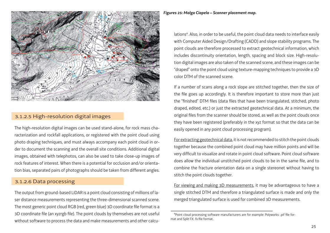
25

Figures 25: Malga Ciapela – Scanner placement map.

3.1.2.5 High-resolution digital images

The high-resolution digital images can be used stand-alone, for rock mass cha-racterization and rockfall applications, or registered with the point cloud using photo draping techniques, and must always accompany each point cloud in or-der to document the scanning and the overall site conditions. Additional digital images, obtained with telephotos, can also be used to take close-up images of rock features of interest. When there is a potential for occlusion and/or orienta-tion bias, separated pairs of photographs should be taken from different angles.

3.1.2.6 Data processing

The output from ground-based LiDAR is a point cloud consisting of millions of la-

ser distance measurements representing the three-dimensional scanned scene. The most generic point cloud RGB (red, green blue) 3D coordinate fi le format is a 3D coordinate fi le (an xyzrgb fi le). The point clouds by themselves are not useful without software to process the data and make measurements and other calcu-

8Point cloud processing software manufacturers are for example: Polyworks: .pif fi le for-mat and Split FX: .fx fi le format.

lations8. Also, in order to be useful, the point cloud data needs to interface easily with Computer Aided Design/Drafting (CADD) and slope stability programs. The point clouds are therefore processed to extract geotechnical information, which includes discontinuity orientation, length, spacing and block size. High-resolu-tion digital images are also taken of the scanned scene, and these images can be “draped” onto the point cloud using texture-mapping techniques to provide a 3D color DTM of the scanned scene.

If a number of scans along a rock slope are stitched together, then the size of the fi le goes up accordingly. It is therefore important to store more than just the “fi nished” DTM fi les (data fi les that have been triangulated, stitched, photo draped, edited, etc.) or just the extracted geotechnical data. At a minimum, the original fi les from the scanner should be stored, as well as the point clouds once they have been registered (preferably in the xyz format so that the data can be easily opened in any point cloud processing program).

For extracting geotechnical data, it is not recommended to stitch the point clouds together because the combined point cloud may have million points and will be very diffi cult to visualize and rotate in point cloud software. Point cloud software does allow the individual unstitched point clouds to be in the same fi le, and to combine the fracture orientation data on a single stereonet without having to stitch the point clouds together.

For viewing and making 3D measurements, it may be advantageous to have a single stitched DTM and therefore a triangulated surface is made and only the merged triangulated surface is used for combined 3D measurements.

26

3.1.3 Rock fall source characteriza-tion and identifi cation

The characterization of the rock mass is an important criteria for the recogni-tion and evaluation of the detachment area / line / point. Site characterization is required: initially to determine the potential for slope instability; periodically because changes in the stability of rock slopes can occur as slopes weather and deteriorate.

3.1.3.1 Rock mass characterization

Rock masses can be viewed as being com-posed of blocks of intact rocks and joints or discontinuities; rockfall is produced by the joints in the bedrock, it is therefore impor-tant to characterize these joints to be able to determine block volume and rockfall suscep-tibility in different areas of the rock slope.

Figures 26: Diagram illustrating rock mass pro-perties and paremeters describing rock mass characteristics (Willye et. Al, 2004).

27

Figure 26 illustrates the parameters that characterize the rock mass, and shows how they can be divided into six classes related to the rock materia! and its strength, the discontinuity characteristics, infi lling properties, the dimensions and shape of the blocks of rock, and ground water conditions. Each of the para-meters is discussed in the procedures drawn up by the International Society of Rock Mechanics (1981).

The mapping sheets included with the appendix provide a means of recording the qualitative geological data.

Rockfall can be infl uenced by other, external, factors like: climate, tree roots ac-tion, external stress relief and vibration from earthquake.

Several climatic conditions contribute to the instability of a rock or rock slope. Temperature variations, rain, snow, freeze-thaw and erosion conditions can act independently or in conjunction to cause stability problems. Ice on the slope face can induce a wide range of hydrostatic pressures in the slope, potentially enough to cause small failures along pre-existing cracks. Frost action also can contribute to rockfalls, since the frizzed water volume expansion can create large pressures in a confi ned space.

Where trees exist on the slope or at the crest and the roots have developed into the discontinuities, tree-root leverage is a common cause of rockfall. High winds acting on isolated trees can lever movement of large rocks.

Rocks are not only subjected to vertical forces due to their weight, but also can be subjected to horizontal stresses caused by tectonic forces, deep surface ero-sion, or glacioisostatic rebound; high horizontal stresses can cause differential rebound in adjacent rock of different.

Long-period vibrations with prolonged durations during an earthquake can cau-se excessive vibrations of a rock slope and may cause excessive pore water pres-sures and local rock ravelling.

Rock mass site characterization involves the collection of geotechnical data, in-cluding information about rock structure, geology, intact rock strength, hydrolo-gy, climate, and earthquakes. In the current practice, much of this data is collected by hand directly at exposed slopes and rock outcrops, including measurements of discontinuity orientation, roughness, fi ll, length, and spacing. There are many issues with the collection of data in the fi eld, including:

• safety hazards associated with the collection of this data;

• diffi culties in accessing rock outcrops on large slopes or cliffs;

• human bias and accuracy issues associated with selecting areas for measu-rement and the accuracy of the hand-collected measurements themselves;

• relatively slow data collection and manpower intensive;

• because of the issue above, slope stability calculations with relatively small data sets;

• the lack of three dimensional information about the slope (other than surve-yed points) that could be used for comparison as slopes weather and dete-riorate.

28

3.1.3.2 LiDAR applications to rock mass characterization

In the case of steep rock slopes in alpine terrain, limited accessibility for fi eld in-vestigations presents a major problem, since outcrops yielding most information are often too steep or dangerous to investigate in situ. Remote sensing techni-ques, such as TLS and ALS techniques have proven to be appropriate tools for characterizing the structure of rock masses, slope and morphology. LiDAR can be used to assist with rock slope stability analyses allowing for: rock mass characte-rization, rockfall characterization, and detailed 3D measurements.

TLS can produce high resolution DEMs, which can be employed for inventory of rockfalls, monitoring of mass movement time evolution and more accurate nu-merical simulation of rockfall trajectories and velocities. Furthermore, data ob-tained from TLS allows the reconstruction of joint geometry and an estimation of the volume of blocks that can fall from steep inaccessible rock slopes.

Geological and geotechnical information can be extracted from the DTM that would be diffi cult to observe in the point cloud using the only dedicated point cloud software, Split FX software9, developed specifi cally for extracting geotech-nical information from point clouds of exposed rock surfaces and has the ability:

• to automatically delineate fracture surfaces in a point cloud and determine the orientation, area, and roughness of each fracture;

• to plot fracture orientations on a stereonet (pole and contour plots);

• to pick joint sets, and determine statistical properties of each set;

• to delineate joint traces (automatic and manual) and determine joint spa-cing, length and orientation (true spacing and orientation if digital image is draped);

• to trace fractures on draped photos to determine fracture orientations;

• to subtract two point clouds to determine rockfall volume and rate;

• to estimate a rockfall hazard rating from a point cloud.

Many of the above items can still be analyzed using the “generic” point cloud software. For instance, to determine the orientation of a fracture in a point cloud, the points making up the fracture can be selected by hand, and the software will determine the orientation of the best-fi t plane through the points. This can be done many times throughout the point cloud, and the orientations can be plot-ted using a separate stereonet program. In a similar fashion, the generic softwa-re can be used to estimate fracture length and spacing, roughness, etc.

At the present time, rock mass information that is being obtained from LiDAR includes discontinuity orientation, length, spacing and block size. In addition, re-search is presently being conducted to obtain additional information, including roughness, geology, weathering and discontinuity fi ll. Discontinuity characteriza-tion can be achieved, from high resolution10 and quality of data set, by manually fi tting planes on individual recognizable surface or traces in 3D models. The typi-cal workfl ow for discontinuity characterization is presented in Figure xy.

Discontinuity Orientation Collection. The principal steps are:

1. With standard hand-editing features in point cloud processing software:

9Split FX (Split Engineering, www.spliteng.com). 9TLS point density from 500 to 10.000 pts/m2.

29

• to scan a fi eld site of interest, produce a point cloud, and register the scan into a terre-strial coordinate system;

• to create a surface mesh from the point cloud data;

2. With either signifi cant hand-edi-ting or the development of special vegetation or other types of fi lters in the process of creating a surfa-ce mesh, erroneous data points in the point cloud can be fi ltered by removing of non-rock objects on the rock slope.

3. By using the basic property that fractures are fl at11, delineation of fracture “patches”12 from the triangulated surface mesh.

4. Once the patch has been found, his average orientations can be plotted as one point on the stereonet.

5. Once the sets are identifi ed, the statistical properties of each set can be de-termined.

11Flat surfaces are automatically found in the triangulated mesh by fi rst calculating the normal to each triangle, and then fi nding groups of adjacent triangles that satisfy a fl atness criterion.

12The term “patch” is used rather than fracture, because a single large fracture may be delineated into several smaller patches, depending on the fl atness and roughness of the fracture.

A particularly useful feature of point cloud processing software is the inte-raction it allows between the stereonet and the point cloud. Delineating joint sets from stereonet data is diffi cult and necessitates professional expertise. Normally the data is taken in the fi eld

and the compilation and defi nition of joint sets is accomplished at a later time. Therefore, any diffi culties with interpretation of the data cannot be resolved wi-thout additional fi eld work. With access to the point cloud, however, additional analysis can easily be conducted off site. For instance, a group of patches can be selected on the stereonet and then viewed on the point cloud. This allows the user to go back and forth between the stereonet and the point cloud to deter-mine with a great deal of precision the delineation of important fractures and fracture sets. The orientation of a single critical structure such as a fault can be more clearly identifi ed on the digital image rather than the point cloud; because a fault is weak, it may not show any three dimensional surfaces where the orien-tation could be extracted from the point cloud alone and therefore the fault can be traced on the digital image and the orientation determined from both the trace and the point cloud.

Figures 27: Workfl ow of discontinuity analysis based on LiDAR data (Hu H. et al., 2010).

30

Figures 28: Caprile (Bus del Diaol) – Geomechanical feature identifi cation from a high resolution digital camera (TLS) (Split-FX, 2011)

Figures 29: Caprile (Bus del Diaol) – Detail of geomechanical feature identifi cation (the patch color correspond with pole color in stereonet) (Split-FX, 2011)

Figures 30: Caprile (Bus del Diaol) – Stereonet illustrating the geomechanical feature extracted from a high resolution digital camera (TLS) (the pole color in stereonet cor-respond with patch color in point cloud) (Split-FX, 2011)

31

Determination of fracture length and discontinuity spacing distributions. Ano-ther very important aspect in rock mass characterization is the determination of discontinuity set spacing and spacing distribution. Together with the orientation of the discontinuity sets, this determines the variation in size and shape of the blocks that make up the fabric of the rock mass. For most engineering appli-cations dealing with rock masses, this is crucial information. By separating the individual discontinuity sets and surfaces from the entire data set, it becomes possible to analyze these surfaces in 3D space and subsequently derive the di-stances (spacings) between them. Fracture length and spacing can be measu-red from either digital images or point clouds. In two dimensions, the measured fracture spacing is referred to as the “apparent” spacing, and can be corrected if the true average orientation of the set is known. In three dimensions (measured from a point cloud or a draped photo), the true spacing can be measured directly if the measurement is made perpendicular to the average strike of the set. Even though automatic trace delineation algorithms are available in many image-pro-cessing programs (including Split FX), they are not recommended.

Fracture length and spacing are interrelated, if the fractures are: persistent (frac-tures long in relation to the spacing), then the measurement of fracture spacing for a given set is well defi ned and measured perpendicular to the average orien-tation of the set by a single scanline; non-persistent (fractures short in relation to spacing), then the measurement of fracture spacing need several scanlines perpendicular the average orientation. In either case, a histogram of fracture spacing is produced for each set.

Block Size. Block size is a parameter that depends on the interaction of all the joint sets together, into a fracture network and it can be manually measured from either a digital image or a point cloud.

Discontinuity Roughness, Weathering and Fill: LiDAR and digital image proces-sing have the potential for providing information on discontinuity roughness, weathering and fi ll but, at present, this area is only at a research phase

Figures 31: Caprile (Bus del Dia-ol) – Delineated trace with Split-FX – On the right a histogram of all trace rake angles (clockwise from horizontal) where the ranke angles displayed in the histogram are weighted according to trace length (Split-FX, 2011).

Figures 32: Caprile (Bus del Diaol) – Detail of a manual delineated trace with Split-FX and relative di-mensions (Split-FX, 2011).

32

3.1.3.3 Adequacy of TLS for extracting Rock Mass Characterization Information

For extracting fracture information from point clouds, a key measure of accuracy is the error in the estimation of a fracture’s strike and dip (or dip and dip direc-tion). Errors in the LiDAR results are due to three primary sources:

1. Instrument accuracy and fi eld settings. Errors in the strike and dip less than one degree could be attained even with small fracture surfaces intersected by less laser points (i.e. 50) than large fracture surfaces. Some others sources of possible error are due to atmospheric and temperature errors.

2. Procedures and accuracy of point cloud registration. This error affects the calculated fracture orientations for all fractures regardless of their size. The error in the estimation of fracture orientation will depend on the method of scanner registration that is used.

3. Software and procedures used for processing point clouds. Differences in how the point cloud is analyzed to determine fracture orientation results in large differences in the estimation of the strike and dip of a fracture sur-face. One method is to pick three points on a fracture and determine the orientation of the plane made by these three points. Because actual rock fracture surfaces are not fl at planes, this technique will show large variations depending on the roughness of the surface and which three points are se-lected. A better method is to select all the points that make up the fracture and calculate the best-fi t plane through those points. This method will also show variations because “selecting all the points that make up a fracture” is not a straightforward task, particularly near the edge of the fracture. If an automated routine is used to select the points that make up the fractures, then changing the parameters in the routine13 will result in differences in the calculated best-fi t orientations.

3.1.3.4 LiDAR techniques advantages

The LiDAR techniques are ideal for: characterizing rockfall source areas, i.e. to defi ne the size and initial location of rock blocks, that are often diffi cult to access, i.e. because located in steep remote areas, and characterize using traditional methods involving rappelling down the slope, which is costly and poses safety hazards; determining the number and sizes of the boulders into the slope that pose a rockfall hazard; determining the characteristics and topographic profi le of rockfall chutes that often determine the location, velocity and other aspects of a rockfall event; rockfall monitoring conducted by taking LiDAR scans of the same scene at some interval of time (i.e. once every six months or more often in areas with high rockfall risk) the point clouds of these periodic scans must be ali-gned as accurately as possible and then are processed to evaluate rockfall using “change algorithms”14; fi eld test sites determined that the movement of boul-ders as small as 15 cm can be detected when the scans at the site were taken from a distance of about 60 m. Such approaches allow for the quantifi cation of the magnitude and activity of rockfalls in a cliff, eventually quantifi ed the increa-se in rockfall activity some months previous to the occurrence of larger events or can be used to detect the most active areas.

13i.e. the automated routine in Split FX.14The change algorithms subtract two point clouds and produce a “difference cloud”; from

the change, the movement of a rock block can be tracked, or the size of a block that has move can be monitored.

33

LiDAR has the following advantages: no physical access is needed to or near the rock surface to

measure discontinuity orientations, which has obvious advantages in terms of safety; inaccessible rock faces can be analyzed, particularly for slope stability and block size analysis this has obvious advantages; the human bias in determining rock mass discontinuities is mostly removed; more discontinuity data can be ga-thered than using traditional (manual) techniques, which allows proper applica-tion of statistical tools; higher accuracy of the orientation measurements can be

achieved due to much better statistical sampling and the measuring the average orientation of a fracture rather than the specifi c location where the geological stratum compass is placed.

Figures 33: The methodology used for the application of TLS in our rockfall study (Abellan et alii., 2006).

34

3.2 Flow chart for rockfall data collection and analysis

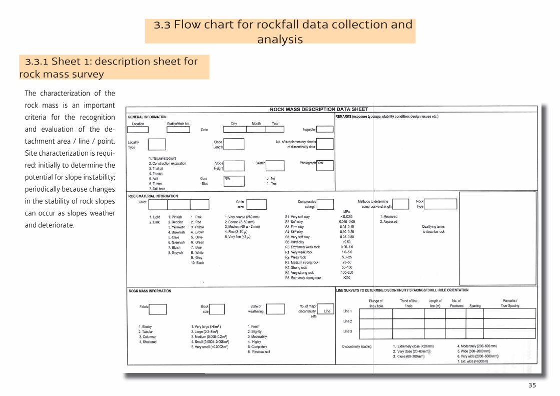
35

3.3 Flow chart for rockfall data collection and analysis

3.3.1 Sheet 1: description sheet for rock mass survey

The characterization of the rock mass is an important criteria for the recognition and evaluation of the de-tachment area / line / point. Site characterization is requi-red: initially to determine the potential for slope instability; periodically because changes in the stability of rock slopes can occur as slopes weather and deteriorate.

36

3.3.2 Sheet 2: discontinuity survey data sheet

It describes the characteristics of each discontinuity in terms of its type, orienta-tion, persistence, aperture/width, fi lling, surface roughness and water fl ow. This sheet can be used for recording outcrop mapping data (GCO, 1991)

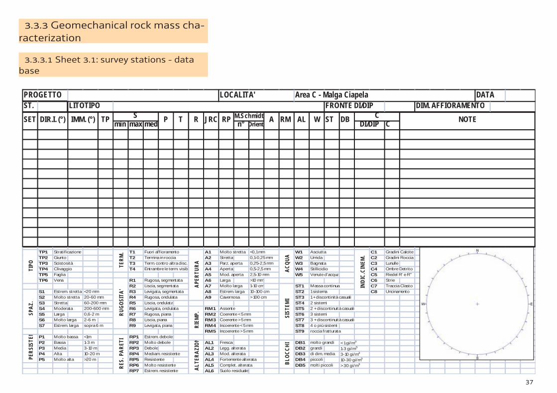
37

3.3.3 Geomechanical rock mass cha-racterization

3.3.3.1 Sheet 3.1: survey stations - data base

ST.

min max med n° Orient. C

TP1 Stratificazione T1 Fuori affioramento A1 Molto stretta <0,1 mm W1 Asciutta C1 Gradini CalciteTP2 Giunto T2 Termina in roccia A2 Stretta 0,1-0,25 mm W2 Umida C2 Gradini RocciaTP3 Scistosità T3 Term. contro altra disc. A3 Parz. aperta 0,25-2,5 mm W3 Bagnata C3 LunulleTP4 Clivaggio T4 Entrambre le term. visib A4 Aperta 0,5-2,5 mm W4 Stillicidio C4 Ombre DetritoTP5 Faglia A5 Mod. aperta 2,5-10 mm W5 Venute d'acqua C5 Riedel R' e R''TP6 Vena R1 Rugosa, segmentata A6 Larga >10 mm C6 Strie

R2 Liscia, segmentata A7 Molto larga 1-10 cm ST1 Massa continua C7 Traccia ClastoS1 Estrem. stretta <20 mm R3 Levigata, segmentata A8 Estrem. larga 10-100 cm ST2 1 sistema C8 UncinamentoS2 Molto stretta 20-60 mm R4 Rugosa, ondulata A9 Cavernosa > 100 cm ST3 1 + discontinità casualiS3 Stretta 60-200 mm R5 Liscia, ondulata ST4 2 sistemiS4 Moderata 200-600 mm R6 Levigata, ondulata RM1 Assente ST5 2 + discontinuità casualiS5 Larga 0,6-2 m R7 Rugosa, piana RM2 Coerente < 5 mm ST6 3 sistemiS6 Molto larga 2-6 m R8 Liscia, piana RM3 Coerente > 5 mm ST7 3 + discontinuità casualiS7 Estrem. larga sopra 6 m R9 Levigata, piana RM4 Incoerente < 5 mm ST8 4 o più sistemi

RM5 Incoerente > 5 mm ST9 roccia fratturataP1 Molto bassa <1m RP1 Estrem. deboleP2 Bassa 1-3 m RP2 Molto debole AL1 Fresca DB1 molto grandi < 1 gi/m3

P3 Media 3-10 m RP3 Debole AL2 Legg. alterata DB2 grandi 1-3 gi/m3

P4 Alta 10-20 m RP4 Mediam. resistente AL3 Mod. alterata DB3 di dim. media 3-10 gi/m3

P5 Molto alta >20 m RP5 Resistente AL4 Fortemente alterata DB4 piccoli 10-30 gi/m3

RP6 Molto resistente AL5 Complet. alterata DB5 molti piccoli > 30 gi/m3

RP7 Estrem. resistente AL6 Suolo residuale

INDI

C.CI

NEM

.

LOCALITA' Area C - Malga Ciapela DATA

A

SIST

EMI

FRONTE DI/DIP DIM. AFFIORAMENTO

DI/DIP

BLOC

CHI

RIEM

P.

ACQU

A

SET RP

PERS

ISTE

N

TERM

.

TIPO

SPAZ

.

RUGO

SITA

'

ALTE

RAZI

ONAP

ERTU

RA

RES.

PAR

ETI

PROGETTOLITOTIPO

IMM. (°)DIR.I. (°) STP P T R W ST DB NOTEJRC M.Schmidt RM AL C

38

3.3.3.2 Sheet 3.2: data analysis - rock mass classifi cation

39

3.3.3.3 Sheet 3.3: data analysis – block size measurements

40

3.3.3.4 Rock fall sources (palmström, 2005)

41

3.3.3.5 Talus / scree characteristics (palm-ström, 1982)

42

3.3.3.6 Quantifi cation of gsi chart (sonmez et al. , 2004)

43

3.3.3.7 Quantifi cation of gsi chart (cai et al.., 2004)

2

PART C : ANNEX5 - REFERENCES

Agliardi F. and Crosta G. ,2003: High resolution three-dimensional numerical mo-delling of rockfalls. International Journal of Rock Mechanics and Mining Sciences, 40(4), 455-471.

Abellán A., Vilaplana J.M., Martínez J., 2006: Application of a long-range Terre-strial Laser Scanner to a detailed rockfall study at Vall de Núria (Eastern Pyrenees, Spain). Engineering Geology 88, p.p. 136–148.

ASTER (cell-size 30m) http://www.gdem.aster.ersdac.or.jp/search.jsp

AA.VV., 2005: Mitigation of hydro-geological Risk in alpine catchments “CatchRi-sk” Program Interreg III B – Alpine Space.- Final Report, 189 S.

AA.VV., 2005: Mitigation of hydro-geological Risk in alpine catchments “CatchRi-sk” Program Interreg III B – Alpine Space.- Guidelines, 299 S.

www.alpine-space.org/uploads/media/Catchrisk_Mitigation_of_Risk.pdf

Baglioni A., Tosoni D., De Marco P., Arziliero L., 2007: Analisi del dissesto da frana in Veneto, APAT dipartimento della Difesa del Suolo, Rapporto sulle frane in Italia, 78/2007, pp. 227-260. Roma.

Baillifard F, Jaboyedoff M, and Sartori M, 2003: Rockfall hazard mapping along a mountainous road in CH using a GIS-based parameter rating approach. NHESS 3, 431–438.

Bäk R. , Kranitz F., Torresin M., Mariani R., 2011: Minimal standard for creation of hazard maps for land slides and rock fall as a tool for preventive disaster reduction (INTERREG IV A Italy/Austria, Project Nr. 1381-302, Akronym MassMove), Wild-bach- und Lawinenverbau, Nr. 166, 176 – 197.

Baum, R.L., Savage, W.Z., Godt, J.W., 2002: TRIGRS: a Fortran program for tran-

sient rainfall infi ltration and grid-based slope-stability analysis. U.S. Geological Survey Open-File Report 2002-424. 38 pp.

Bayrisches Landesamt für Umwelt (2009): Gefahrenhinweiskarte Bayerische Alpen, Alpenanteil Landkreis Miesbach.- Abschlussbericht UmweltSpezial, 52 S., Augsburg.

http://www.lfu.bayern.de/geologie/massenbewegungen/gefahrenhinweiskarten/

doc/bericht_gefahrenhinweiskarte_lkr_miesbach.pdf

Blythe D. 1999: Advanced Graphics Programming Techniques Using OpenGL. Siggraph 1999. http://www.opengl.org/resources/code/samples/sig99/advan-

ced99/notes/notes.html

Borga, M., G. Dalla Fontana, C. Gregoretti, and L. Marchi, 2002: Assessment of shallow landsliding by using a physically based model of hillslope stability. Hydro-logical Processes, 16, 2833-2851.

Bozzolo D. and Pamini R., 1986: Simulation of rock falls down a valley side. Acta Mechanica, 63, 113–130.

Brabb E.E., 1984.: “Innovative approach to landslide hazard and risk mapping”. in Proceedings of the 4th International Symposium on Landslides Toronto, pp. 307– 324.

Brardinoni, F., Slaymaker, O., Hassan, M.A., 2003: Landslide inventory in a rugged forested watershed: a comparison between air-photo and fi eld survey data. Geo-morphology 54, 179-196.

Brufau, P.,Garcia-Navarro,P.,Ghilardi,P.,Natale,L.,Savi,F., 2000: Mathematical mo-delling of debrisfl ow. Journal of Hydraulic Research38,435–446.

3

Buckley S. J., Vallet J., Braathen A., Wheeler W., 2008: Oblique helicopter-based la-ser scanning for digital terrain modelling and visualisation of geological outcrops. International Archives of Photogrammetry, Remote Sensing and Spatial Informa-tion Sciences, vol. XXXVII (Part B4), Beijing, China, pp. 493-498.

BUWAL, 1998: Amt für Raumplanung Graubünden. Uffi cio Cantonale di Pianifi -cazione. Grundlage zur FAN-Tagung vom 13-16 October 1998 in Ittingen, 15 pp.

Cai M., Kaiser P.K., Uno H., Tasaka Y., Minami M., 2004: Estimation of rock mass deformation modulus and strength of jointed hard rock masses using the GSI sy-stem, International Journal of Rock Mechanics and Mining Sciences, vol. 41, pp. 3-19.

Carere K., Ratto S. & Zanoli F., 2001: Prevenzione Dei Fenomeni Di Instabilita Delle Pareti Rocciose.- Programma INTERREG II C – “FALAISES”, 239 S.

Cannon S.H., 1993: An empirical model for the volume-change behavior of debris fl ows. Proc. ASCE National Conference on Hydraulic Engineering, San Francisco, CA, pp. 1768–1773.

Carrara A., 1983: A multivariate model for landslide hazard evaluation. Mathema-tical Geology 15, 403–426.

Carrara, A., Cardinali, M., Detti, R., Guzzetti, F., Pasqui, V., Reichenbach, P., 1991: GIS techniques and statistical models in evaluating landslide hazard. Earth Surface Processes and Landform 16 (5), 427–445.

Carrara, A., Guzzetti, F., Cardinali, M., Reichenbach, P., 1999: Use of GIS technolo-gy in the prediction and monitoring of landslide hazard. Natural Hazards 20 (2–3), 117–135.

Casadei, M., Deitrich, W.E., Miller, N.L., 2003: Testing a model for predicting the ti-ming and location of shallow landslide initiation in soil-mantled landscapes. Earth Surface Processes and Landforms 28, 925–950.

Cascini L., 2009: Analisi e mitigazione del rischio frana. Dispensa Master AVAMI-RI, Gorizia.

Catani, F., Farina, P., Moretti, S., Nico, G., Strozzi, T., 2005: On the application of SAR interferometry to geomorphological studies: estimation of landforms attribu-tes and mass movements. Geomorphology 66, 119- 131.

Claessens, L., Heuvelink, G.B.M., Schoorl, J.M., Veldkamp, A., 2005: DEM resolution effects on shallow landslide hazard and soil distribution modeling. Earth Surface Processes and Landforms 30, 461–477.

Clothier, B., Scotter, D., 2002: Unsaturated water transmission parameters obtai-ned from infi ltration. In: Dane, J.H., Topp, G.C. (Eds.), Methods of Soil Analysis — Part 4 Physical Methods. Soil Science Society of America, Madison, WI, pp. 879–898.

Collins, M.E., and J.A. Doolittle. 1987: Using ground penetrating radar to study soil microvariability. Soil Sci. Soc. Am. J. 51:491– 493.

Cooper, R.G. 2007: Mass Movements in Great Britain, Geological Conservation Review Series, No. 33, Joint Nature Conservation Committee, Peterborough, 348 pp.

www.ukgeohazards.info/pages/eng_geol/landslide_geohazard/eng_geol_landsli-

des_classifi cation.htm

Copons R., Vilaplana J.M., 2008: Rockfall susceptibility zoning at a large scale: From geomorphological inventory to preliminary land use planning. Engineering Geology, 102, 142–151.

Copons R., Vilaplana J.M., Linares R., 2009: Rockfall travel distance analysis by using empirical models (Solà d’Andorra la Vella, Central Pyrenees). Natural Hazards

and Earth System Sciences, 9, 6, 2107-2118.

Corominas J., 1996: The angle of reach as a mobility index for small and large landslides. Can. Geotech. J. 33, 260–271.

4

Crosta G.B. and Agliardi F., 2003: A new methodology for physically-based rock-fall hazard assessment. Natural Hazards and Earth System Sciences, 3, 407–422.

Crosta G. B., Agliardi, F., Frattini P. and Imposimato S., 2004: A three-dimensional hybrid numerical model for rockfall simulation. Geophysical Research Abstracts, 6, 04502.

Crosta G.B., Frattini P., 2008: Rainfall induced landslides and debris fl ows. Hydro-logical Processes, 22:473-477. doi:10.1002/hyp.6885.

Cruden D.M., 1993: The Multilingual Landslide Glossary, Bitech Publishers, Rich-mond., British Columbia, for the UNESCO Working Party on World Landslide Inven-tory.

Das, B.M., 2000: Fundamentals of Geotechnical Engineering. Brooks/Cole, Paci-fi c Grove, CA. 593 pp.

Dent, D and Young, A.,1981: Soil Survey and Land Evaluation. Goerge Allen and Unwin, London.

DeRose, R.C., 1991: Geomorphic change implied by regolith–slope relationships on steep land hillslopes, Taranaki, New Zealand. Catena 18, 489–514.

Descoeudres F., Zimmermann T., 1987: Three-dimensional dynamic calculation of rockfalls, In Herget, G. and Vongpaisal, S., editors, Proceedings of the Sixth In-ternational Congress on Rock Mechanics. Montreal. Rotterdam: Balkema, 37–42.

Dietrich, W.E., Dunne, T., 1978: Sediment budget for a small catchment in mountainous terrain. Zeitschrift für Geomorphologie Supplementband 29, 191–206.

Dietrich, W.E., McKean, J., Bullugi, D., 2006: The prediction of landslide size using a

multi-dimensional stability analysis. Eos Transactions of the American Geophysical Union 87 (52) H54B-01.

Dietrich, W.E., Reiss, R., Hsu, M., Montgomery, D.R., 1995: A process-based model for colluvial soil depth and shallow landsliding using digital elevation data. Hydro-logical Processes 9, 383–400.

Domaas U., 1994: Geometrical methods of calculating rockfall range, Norwegian Geotechnical Institute, Report 585910-1, 21 pp.

Doolittle, J.A., F.E. Minzemayer, S.W. Waltman, E.C. Benham, J.W. Tuttle, and S. Peaslee. 2006: State ground-penetrating radar soil suitability maps. In Proc. of the 11th International conference on ground penetrating radar, Columbus, OH, June 19–22, 2006.

Dorren L.K.A., 2003: A review of rockfall mechanics and modelling approaches, Progress in Physical Geography, 27, 1, 69–87.

Dorren L.K.A., Berger, F., Putters, U.S., 2006: Real size experiments and 3D simu-lation of rockfall on forested and non-forested slopes. Natural Hazards and Earth System Sciences, 6, 145–153.

Dussauge C., Grasso, J.R., Helmstetter, A., 2003: Statistical analysis of rockfall volume distributions: implications for rockfall dynamics. Journal of Geophysical Re-search, 108(B6), 2286.

Doratti M., McColl Ch., Tweeddale C., 2002: Landslide Prediction Study.- 47 S., giswww1.bcit.ca/giscentre/projects/projects2002/prj_09_fi nal_report.pdf

Einstein H.H., 1988.: Special Lecture, Landslide risk assessment. Proc. 5th Int. Symp. On Landslides, Lausanne, Switzerland. A.A. Balkema, Rotterdam, The Ne-therlands, Vol.2, 1075-1090.

Einstein H.H., 1996: Risk and risk analysis in rock engineering. Tunn. Undergr.

Space Technol. 11 (2), 141– 155.

Evans S.G., Hungr O., 1993: The assessment of rock fall hazard at the base of talus slopes. Canadian Geotechnical Journal, 30, pp. 620–636.

5

Fannin R.J. and Bowman, E.T., 2008: Debris Flows – Entrainment, deposition and travel distance. Geotechnical News, 25(4), 3-6.

Fannin R.J., Wise M.P., 2001: An empirical-statistical model for debris fl ow travel distance. Can. Geotech. J. 38, 982– 994.

Fell R., 1994: Landslide risk assessment and acceptable risk, Canadian Geotech-nical Journal, 31:(2) 261-272,

Fell R., Corominas, J., Bonnard, C., Cascini, L., Leroi, E., and Savage,W., 2008: Gui-delines for landslide susceptibility, hazard and risk zoning for land use planning, Eng. Geol., 102, 85–98.

Fell R., Hartford D., 1997: Landslide risk management. In: Cruden D.M. & Fell R. (eds.) Landslide Risk Assessment. Proc. Int. Workshop Landslide Risk Assessment, Balkema, 51-109.

Frattini P., Crosta G.B., Carrara A., 2010: Techniques for evaluating the perfor-mance of landslide susceptibility models. Engineering Geology, 111(1-4):62-72. doi:10.1016/j.enggeo.2009.12.004

Frattini P., Crosta G.B., Carrara A., Agliardi F., 2008: Assessment of rockfall su-sceptibility by integrating statistical and physically-based approaches. Geomor-phology, 94:419-437.

Garbrecht, J., Martz, L., 1994: Grid size dependency of parameters extracted from digital elevation models. Computers and Geosciences 20 (1), 85–87.

Geotechnical Control Offi ce (GCO), 1991: Geotechnical manual for slopes. Engi-neering Development Department, Hong Kong, 301 pp.

Godio, A. and G. Bottino, 2001: Electrical and Electromagnetic Investigation for Landslide Characterisation. Phys. Chem. Earth (C). Vol. 26, No. 9, pp. 705-710.

Godt, J.W., McKenna, J.P., 2008: Numerical modeling of rainfall thresholds for

shallow landsliding in the Seattle, Washington, area. In: Baum, R.L., Godt, J.W., Hi-ghland, L.M. (Eds.), Landslides and Engineering Geology of the Seattle Washing-ton Area. Geological Society of America Reviews in Engineering Geology, vol. 20. doi:10.1130/2008.4020(07).

Günther A, Carstensen A, and Pohl W, 2004: Automated sliding susceptibility mapping of rock slopes, NHESS 4 (2004), 95–102.

Günther A., 2003. SLOPEMAP: programs for automated mapping of geometrical and kinematical properties of hard rock hill slopes. Computers & Geosciences 29, 865–875.

Guzzetti F., Carrara A., Cardinali M. & Reichenbach P. , 1999: Landslide hazard evaluation: an aid to a sustainable development. Geomorphology, 31,181-216.

Guzzetti F., Crosta G., Detti R. and Agliardi F., 2002: STONE: a computer program for the three-dimensional simulatation of rock-falls. Computers and Geosciences, 28 (9), 1081-1095.

Guzzetti F., Reichenbach P., Cardinali M., Galli M., Ardizzone F., 2005: Probabilistic landslide hazard assessment at the basin scale. Geomorphology, 72, 272-299.

Haneberg, W.C., 2008: Elevation errors in a LiDAR Digital Elevation Model of West Seattle and their effects on slope stability calculations. In: Baum, R.L., Godt, J.W., Highland, L.M. (Eds.), Landslides and Engineering Geology of the Seattle Wa-shington Area. Geological Society of America Reviews in Engineering Geology, vol. 20. doi:10.1130/2008.4020(03).

Haugerud, R.A., Harding,D.J., Johnson, S.Y., Harless, J.L., Weaver, C.S., Sherrod, B.L., 2003: High resolution Lidar topography of the Puget Lowland, Washington. GSA Today 13, 4–10.

Heim A., 1932: Bergsturz und Menschenleben. Zurich: Fretz and Wasmuth Verlag, 218 pp.

6

Heimsath, A.M., Chappell, J., Dietrich,W.E.,Nishiizumi,K., Finkel, R.C., 2000: Soil production on a retreating escarpment in southeastern Australia. Geology 28 (9), 787–790.

Heimsath, A.M., Dietrich, W.E., Nishiizumi, K., Finkel, R.C., 1999: Cosmogenic nu-clides, topography, and the spatial variation of soil depth. Geomorphology 27, 151–172.

Heinimann H.R., Holtenstein K., Kienholz H., Krummenhacher B., Mani P., 1998: Methoden zur Analyse und Bewertung von Naturgefahren. Umwelt-Materialien 85, Naturgefahren, BUWAL, Bern (in German).

Highland L. M., Bobrowsky P., 2008: The Landslide Handbook—A Guide to Un-derstanding Landslides. U.S. Geological Survey Circular 1325. www.pubs.usgs.gov/

circ/1325

Hoek E., Bray J.W., 1981: Rock Slope Engineering (5th edn), The Institution of Mi-ning and Metallurgy, London.

Holm K., Jakob M., 2009: Long rockfall runout, Pascua Lama, Chile. Canadian Ge-otechnical Journal, 46, 225–230.

Hu H., Fernandez-Steeger T.M., Dong, M., Nguyen H.T., Azzam R., 2010: 3D Mo-deling using LiDAR Data and its Geological and Geotechnical Applications, In:The 18th International Conference on Geoinformatics, June. 18-20, 2010. Beijing (Chi-na), pp. 1-6

Hungr O., 1995: A model for the runout analysis of rapid fl ow slides, debris fl ows, and avalanches. Canadian Geotechnical Journal 32, 610–623.

Hungr O., Evans, S.G. 1988: Engineering evaluation of fragmental rockfall ha-zards. Proceedings of the Fifth International Symposium on Landslides, Lausanne, Switzerland, 1, 685–690.

Hungr O., Evans S. G. and Hazzard J., 1999: Magnitude and frequency of rockfalls

and rock slides along the main transportation corridors of south-western British Columbia. Canadian Geotechnical Journal, 36, 224–238.

Hungr O., Evans SG., Bovis M. and Hutchinson JN., 2001: Review of the classifi -cation of landslides of the fl ow type. Environmental and Engineering Geoscience, VII, 221-238.

Hungr O., Fell R., Couture R., Eberhardt E. (Eds.), 2005: Landslide Risk Manage-ment. Taylor and Francis, London.

International Society of Rock Mechanics (ISRM), 1981: Suggested methods for quantitative description of discontinuities in rock masses (ed. E.T. Brown). Pergamn Oress, Oxford, UK, 211 pp.

Iverson R.M., 1997: The physics of debris fl ows. Reviews of Geophysics 35: 245-296.

Jaboyedoff M., Dudt J.P., and Labiouse V., 2005: An attempt to refi ne rockfall hazard zoning based on the kinetic energy, frequency and fragmentation degree, Natural Hazards and Earth System Sciences 5, pp. 621–632.

Jaboyedoff M., Metzger R., Oppikofer T., Couture R., Derron M.H., Locat J., Durmel D., 2007: New insight techniques to analyze rock-slope relief using DEM and 3D-imaging clouds points: COLTOP-3D software. In: Eberhardt E., Stead D., Morrison T. (eds) Rock mechanics: meeting society’s challenges and demands. Taylor & Fran-cis, London, pp 61–68.

Jaboyedoff M., Oppikofer T., Abellàn A., Derron M.H, Loye A., Metzger R., Pedraz-zini A., 2010: Use of LIDAR in landslide investigations: a review. Nat Hazards DOI 10.1007/s11069-010-9634-2.

Jaboyedoff M. and Labiouse V., 2003: Preliminary assessment of rockfall hazard based on GIS data, in: 10th International Congress on Rock Mechanics ISRM 2003 – Technology roadmap for rock mechanics, South African Institute of Mining and

7

Metallurgy, Johannesburg, South Africa, 575–578.

Jochim Candice L., Rogers William P., Truby John O., Wold, Robert L. Jr., Weber, George, and Sally P. Brown, 1988: Colorado Landslide Hazard Mitigation Plan, Co-lorado Geological Survey, Bulletin 48.

Jones C.L., Higgins J.D., Andrew R.D., 2000: Colorado Rock fall Simulation Pro-gram Version 4.0. Colorado Department of Transportation, Colorado Geological Survey, 127 pp.

Jongmans, D., Hemroulle, P., Demanet, D., Renardy, F., Vanbrabant, Y., 2000: Ap-plication of 2D electrical and seismic tomography techniques for investigating lan-dslides, European Journal of Env. and Eng. Geophysics, 5, 75-89.

Kemeny J. and Turner K., 2008: Ground-Based LiDAR: Rock Slope Mapping and Assesment. Federal Highway Administration, Technical Report No. FHWA-CFL/TD-08-006, 103 p.

Kerle, N., Heuel, S., Pfeifer, N., 2008. Real-time data collection and information generation using airborne sensors. Geospatial Information Technology for Emer-gency Response – Zlatanova & Li (eds). pp.43-74.

Keylock, C. and Domaas, U. 1999: Evaluation of topographic models of rockfall travel distance for use in hazard applications. Arctic, Antarctic, and Alpine Research 31(3), 312–20.

Kranitz, F., Manca P., Oberti S., Piano C., 2007: Analisi del dissesto da frana in Friuli Venezia Giulia. APAT dipartimento della Difesa del Suolo, Rapporto sulle frane in Italia, 78/2007, pp. 261-305. Roma.

Lan H.X., Martin C.D. and Lim C.H., 2007: RockFall analyst: a GIS extension for three-dimensional and spatially distributed rockfall hazard modeling, Computers & Geosciences 33, pp. 262–279.

Lied K., 1977: Rockfall problems in Norway. In: Rock fall dynamics and protective

work effectiveness, 90. Bergamo, Italy: ISMES, 51-53.

Matheson G.C., 1983: Rock Stability Assessment in Preliminary Site Investiga-tions - Graphical Methods. Transport and Road Research Laboratory, Report 1039, Crowthorne, Berkshire.

Mazzoccola D., and Sciesa E., 2000: Implementation and comparison of different methods for rockfall hazard assessment in the Italian Alps, Proc. 8th Int. Symp. on Landslides, Cardiff, Balkema, Rotterdam, 2, 1035-1040.

Malamud B.D., Turcotte D.L. Guzzetti F. and Reichenbach P., 2004: Landslide in-ventories and their statistical properties. Earth Surface Processes and Landforms, 29 (6), 687-711.

McKean, J., Roering, J., 2004: Objective landslide detection and surface morpho-logy mapping using high-resolution airborne laser altimetry. Geomorphology 57, 331–351.

Meißl G., 2001: Modelling the runout distances of rockfalls using a geographic information system. Zeitschrift fur Geomorphologie, 125, 129-137.

Meißl G. 1998: Modellierung der Reichweite von Felsstürzen. Fallbeispeile zur GISgestützten Gefahrenbeurteilung aus dem Beierischen und Tiroler Alpenraum. Innsbrucker Geografi schen Studien 28. Ph.D. Thesis, Universität Innsbruck, Inn-sbruck, 249 pp.

Metternicht G, Hurni L, Gogu R. 2005: Remote sensing of landslides: An analy-sis of the potential contribution to geo-spatial systems for hazard assessment in mountainous environments. Remote Sensing of Environment 98, 284-303.

Naturgefahren im Kanton Schwyz -Kantonale Naturgefahrenstrategie, Revision 2010, RRB Nr. 324/2010 vom 23. März 2010, Schwyz. 16. www.sz.ch/documents/

Natgefstrat_rev10_def_Internet.pdf

Nichol, J.E., Shaker, A., Wong, M-S., 2006: Application of high-resolution stereo

8

satellite images to detailed landslide hazard assessment. Geomorphology 76, 68-75.

Onofri R., Candian C., 1979: Indagine sui limiti di massima invasione dei blocchi rocciosi franati durante il sisma del Friuli del 1976. Regione Autonoma Friuli-Vene-zia-Giulia: CLUET, 42 pp.

Oswalder H., 2008: „Naturgefahren Kärnten“ Laserscanning, geogene Risiken und Geologisches InformationsSystem GInS.- Master Thesis im Rahmen des Uni-versitätslehrganges „Geographical Information Science & Systems“ (UNIGIS MSc) am Zentrum für GeoInformatik (Z_GIS) der Paris Lodron-Universität Salzburg, 135 S. + Anhang, Klagenfurt.

Palmström A., 1982: The volumetric joint count - A useful and simple measure of the degree of rock mass jointing. IAEG Congress, New Delhi, 1982. V. 221 – V.228.

Palmstrom A.. 2005: Measurements of and correlations between block size and rock quality designation (RQD). Published in Tunnels and Underground Space Technology, Vol. 20, 2005, pp. 362-377.

Pfeiffer T.J., Bowen, T.D., 1989: Computer simulations of rockfalls. Bulletin of the Association of Engineering Geologists, 26, 135–146.

Priest S.D., 1993: Discontinuity analysis for rock engineering. Chapman and Hall, London, 473 pp.

Reneau, S.L., Dietrich, W.E., Donahue, D.J., Jull, A.J.T., Rubin, M., 1990: Later Qua-ternary history of colluvial deposition and erosion in hollows, central California Co-ast Ranges. Geological Society of America Bulletin 102, 969–982.

Reynolds, W.D., Elrick, D.E., Youngs, E.G., Amoozegar, A., 2002: Field methods (Va-dose and saturated zone techniques). In: Dane, J.H., Topp, G.C. (Eds.), Methods of Soil Analysis — Part 4 Physical Methods. Soil Science Society of America, Madison, WI, pp. 817–858.

Rott, H., 2004: Requirements and applications of satellite techniques for monito-ring slope instability in Alpine areas. Workshop on risk mitigation of slope instabili-ty. Ispra, Italy’ JRC-Institute for the Protection and Security of the Citizen.

Ruff M., Kühn M. & K. Czurda, 2005: Gefährdungsanalyse für Hangbewegungen.- ©inatura Dornbirn, Austria, download unter www.biologiezentrum.at, 96 S.

Ruff M., 2005: GIS gestützte Risikoanalyse für Rutschungen und Felsstürze in den Ostalpen (Vorarlberg, Österreich).- Diss., 132 S. mit Anhang, Universitätsver-lag Karlsruhe.

Savage,W.Z., Baum, R.L., 2005: Instability of steep slopes. In: Jakob, M., Hungr, O. (Eds.), Debris-Flow Hazards and Related Phenomena. Springer, Berlin, pp. 53–77.

Schmidt, K.M., Roering, J.J., Stock, J.D., Dietrich,W.E., Montgomery, D.R., Schaub, T., 2001: The variability of root cohesion as an infl uence on shallow landslide suscep-tibility in the Oregon Coast Range. Canadian Geotechnical Journal 38, 995–1024.

Schulz, W.H., 2007: Landslide susceptibility revealed by LiDAR imagery and histo-rical records, Seattle, Washington. Engineering Geology 89, 67–87.

Schweigl J.; Hervas J., 2009: Landslide Mapping in Austria. JRC Scientifi c and Tech-nical Report EUR 23785 EN, Offi ce for Offi cial Publications of the European Com-munities, 61 pp. ISBN 978.92.79.11776.3, Luxembourg.

SGD, 2007: Geogene Naturgefahren in Deutschland.- 17 S., + Anhang, Freiburg. www.lfu.bayern.de/geologie/massenbewegungen/.../fi nalreport_adaptalp.pdf

Sidle, R.C., Ochiai, 2006: Landslides Processes, Prediction, and Land Use. Ameri-can Geophysical Union, Washington D.C., p. 312.

Slob S., 2008: Automated rock mass characterization using 3-D terrestrial laser scanning. Ph.D. Thesis – Delft University, 282 pp.

Slob S., Van Knapen B., Hack R., Turner K., Kemeny J., 2005: Method for automa-

9

ted discontinuity analysis of rock slopes with three-dimensional laser scanning. In Proceedings: Transportation Research Board 84th Annual Meeting, January 9-13, Washington D.C., 16 pp.

Sönmez H., Gökçeolu C., Ulusay R., 2004: Indirect Determination of the Modulus of Deformation of Rock Masses Based on the GSI System, International Journal of Rock Mechanics and Mining Sciences, Vol. 41, pp. 849-857.

Split Engineering LLC, 2011: Split FX. www.spliteng.com.

Stevens W., 1998. RockFall: a tool for probabilistic analysis, design of remedial measures and prediction of rockfalls. M.A.Sc. Thesis. Department of Civil Enginee-ring, University of Toronto. Canada, 105 pp.

Sturzenegger M., Stead D., 2009: Quantifying discontinuity orientation and per-sistence on high mountain rock slopes and large landslides using terrestrial remo-te sensing techniques. Nat Hazards Earth Syst Sci 9: 267–287.

Tarolli, P., Sofi a, G., Dalla Fontana, G., 2010: Geomorphic features extraction from high-resolution topography: landslide crowns and bank erosion, Natural Hazards, ISSN: 0921-030X. doi:10.1007/s11069-010-9695-2.

Thieken, A.H., Lücke, A., Diekkrüger, B., Richter, O., 1999: Scaling input data by GIS for hydrological modeling. Hydrological Processes 13, 611–630.

Toppe R., 1987: Terrain models as a tool for natural hazard mapping. In Avalanche Formation, Movement and Effects, ed. B. Salm and H. Gubler. International asso-ciation of Hydrological Sciences, Wallingford, UK, Publication No. 162, 629–638.

Varnes D.J. and IAEG, 1984: Commission on Landslides and other Mass Move-ments: Landslide hazard zonation: a review of principles and practice. The UNESCO Press, Paris.

Wieczorek G.F., Snyder, J.B., 1999: Rock falls from Glacier Point above Camp Cur-ry, Yosemite National Park, California. US Geol. Surv., Open-File Report 99–385,

13, 1999.

Wyllie D.C. and Mah C.W, 2004: Rock slope engineering. Spon Press, London, UK, 431 pp.

www.berkeleynaturally.wordpress.com/2010/01/25/berkeley-hills-landslide

www.en.wikipedia.org/wiki/File:Rockfall.jpg

www.it.wikipedia.org/wiki/Disastro_del_Vajont

www.paintball-tips-and-tricks.com/paintball-tool-box.html

www.sesto-moso.com/frana-a-sesto-in-alta-pusteria

Zhang, R.S., Montgomery, D.R., 1994: Digital elevation model grid size, landscape representation, and hydrologic simulations. Water Resources Research 30,1019–1028.

Zemp M., 2002: GIS-basierte Modellierung der glazialen Sedimentbilanz.- Diplo-marbeit, 99 S., Zürich.

www.geo.uzh.ch/~mzemp/Docs/Zemp_DA_2002.pdf

Minimal standards for the compilation of hazard maps of ...

Documents

Transcript of Minimal standards for the compilation of hazard maps of ...