Reverse Compilation TechniquesbyCristina CifuentesBc.App.Sc { Computing Honours, QUT (1990)Bc.AppSc { Computing, QUT (1989)Submitted to the School of Computing Sciencein partial ful�lment of the requirements for the degree ofDoctor of Philosophyat theQUEENSLAND UNIVERSITY OF TECHNOLOGYJuly 1994c Cristina Cifuentes, 1994The author hereby grants to QUT permission to reproduce andto distribute copies of this thesis document in whole or in part.

iiStatement of Original AuthorshipThe work contained in this thesis has not been previously submitted for a degree or diplomaat any other higher education institution. To the best of my knowledge and belief, the thesiscontains no material previously published or written by another person except where duereference is made.Signed : : : : : : : : : : : : : : : : : : : : : : : : : : : : : : : : : : : : : : : : : : : : : : : : : : : : : : : : : : : : : : : : : : : : : : : : : : : : : : : : :Date : : : : : : : : : : : : : : : : : : : : : : : : : : : : : : : : : : : : : : : : : : : : : : : : : : : : : : : : : : : : : : : : : : : : : : : : : : : : : : : : : : :

iiiQUEENSLAND UNIVERSITY OF TECHNOLOGYDOCTOR OF PHILOSOPHY THESIS EXAMINATIONCANDIDATE NAME Cristina Nicole CifuentesCENTRE/RESEARCH CONCENTRATION Programming Languages and SystemsPRINCIPAL SUPERVISOR Professor K J GoughASSOCIATE SUPERVISOR Professor W J CaelliTHESIS TITLE Reverse Compilation TechniquesUnder the requirements of PhD regulation 9.2, the above candidate was examined orallyby the Faculty. The members of the panel set up for this examination recommend thatthe thesis be accepted by the University and forwarded to the appointed Committee forexamination.Name : : : : : : : : : : : : : : : : : : : : : : : : : : : : : : : : : : : : Signature : : : : : : : : : : : : : : : : : : : : : : : : : : : : : : : : : : : :Panel Chairperson (Principal Supervisor)Name : : : : : : : : : : : : : : : : : : : : : : : : : : : : : : : : : : : : Signature : : : : : : : : : : : : : : : : : : : : : : : : : : : : : : : : : : : :Panel MemberName : : : : : : : : : : : : : : : : : : : : : : : : : : : : : : : : : : : : Signature : : : : : : : : : : : : : : : : : : : : : : : : : : : : : : : : : : : :Panel Member **********Under the requirements of PhD regulation 9.15, it is hereby certi�ed that the thesis of theabove-named candidate has been examined. I recommend on behalf of the ExaminationCommittee that the thesis be accepted in ful�lment of the conditions for the award of thedegree of Doctor of Philosophy.Name : : : : : : : : : : : : : : : : : : : : : : : : : : : : : : : : : : : : Signature : : : : : : : : : : : : : : : : : : : : : : : : : : : : : : : : : : : :Examination Committee Chairperson Date : : : : : : : : : : : : : : : : : : : : : : : : : : : : : : : : : : : : : : : : :

vReverse Compilation TechniquesbyCristina CifuentesAbstractTechniques for writing reverse compilers or decompilers are presented in this thesis. Thesetechniques are based on compiler and optimization theory, and are applied to decompilationin a unique way; these techniques have never before been published.A decompiler is composed of several phases which are grouped into modules dependent onlanguage or machine features. The front-end is a machine dependent module that parsesthe binary program, analyzes the semantics of the instructions in the program, and gen-erates an intermediate low-level representation of the program, as well as a control owgraph of each subroutine. The universal decompiling machine is a language and machineindependent module that analyzes the low-level intermediate code and transforms it into ahigh-level representation available in any high-level language, and analyzes the structure ofthe control ow graph(s) and transform them into graphs that make use of high-level con-trol structures. Finally, the back-end is a target language dependent module that generatescode for the target language.Decompilation is a process that involves the use of tools to load the binary program intomemory, parse or disassemble such a program, and decompile or analyze the program togenerate a high-level language program. This process bene�ts from compiler and librarysignatures to recognize particular compilers and library subroutines. Whenever a compilersignature is recognized in the binary program, all compiler start-up and library subroutinesare not decompiled; in the former case, the routines are eliminated from the �nal targetprogram and the entry point to the main program is used for the decompiler analysis, inthe latter case the subroutines are replaced by their library name.The presented techniques were implemented in a prototype decompiler for the Intel i80286architecture running under the DOS operating system, dcc, which produces target C pro-grams for source .exe or .com �les. Sample decompiled programs, comparisons against theinitial high-level language program, and an analysis of results is presented in Chapter 9.Chapter 1 gives an introduction to decompilation from a compiler point of view, Chap-ter 2 gives an overview of the history of decompilation since its appearance in the early1960s, Chapter 3 presents the relations between the static binary code of the source binaryprogram and the actions performed at run-time to implement the program, Chapter 4 de-scribes the phases of the front-end module, Chapter 5 de�nes data optimization techniquesto analyze the intermediate code and transform it into a higher-representation, Chapter 6de�nes control structure transformation techniques to analyze the structure of the control ow graph and transform it into a graph of high-level control structures, Chapter 7 describesthe back-end module, Chapter 8 presents the decompilation tool programs, Chapter 9 givesan overview of the implementation of dcc and the results obtained, and Chapter 10 givesthe conclusions and future work of this research.

viParts of this thesis have been published or have been submitted to international jour-nals. Two papers were presented at the XIX Conferencia Latinoamericana de Inform�aticain 1993: \A Methodology for Decompilation"[CG93], and \A Structuring Algorithm forDecompilation"[Cif93]. The former paper presented the phases of the decompiler as de-scribed in Chapter 1, Section 1.3, the front-end (Chapter 4), initial work on the control owanalysis phase (Chapter 6), and comments on the work done with dcc. The latter paperpresented the structuring algorithms used in the control ow analysis phase (Chapter 6).One journal paper, \Decompilation of Binary Programs"[CG94], has been accepted for pub-lication by Software { Practice & Experience; this paper gives an overview of the techniquesused to build a decompiler (summaries of Chapters 4, 5, 6, and 7), how a signature gen-erator tool can help in the decompilation process (Chapter 8, Section 8.2), and a sampledecompiled program by dcc (Chapter 9). Two papers are currently under consideration forpublication in international journals. \Interprocedural Data Flow Decompilation"[Cif94a]was submitted to the Journal of Programming Languages and describes in full the opti-mizations performed by the data ow analyzer to transform the low-level intermediate codeinto a high-level representation. \Structuring Decompiled Graphs"[Cif94b] was submittedto The Computer Journal and gives the �nal, improved method of structuring control owgraphs (Chapter 6), and a sample decompiled program by dcc (Chapter 9).The techniques presented in this thesis expand on earlier work described in the literature.Previous work in decompilation did not document on the interprocedural register analysisrequired to determine register arguments and register return values, the analysis required toeliminate stack-related instructions (i.e. push and pop), or the structuring of a generic set ofcontrol structures. Innovative work done for this research is described in Chapters 5, 6, and8. Chapter 5, Sections 5.2 and 5.4 illustrate and describe nine di�erent types of optimiza-tions that transform the low-level intermediate code into a high-level representation. Theseoptimizations take into account condition codes, subroutine calls (i.e. interprocedural anal-ysis) and register spilling, eliminating all low-level features of the intermediate instructions(such as condition codes and registers) and introducing the high-level concept of expressionsinto the intermediate representation. Chapter 6, Sections 6.2 and 6.6 illustrate and describealgorithms to structure di�erent types of loops and conditional, including multi-way branchconditionals (e.g. case statements). Previous work in this area has concentrated in thestructuring of loops, few papers attempt to structure 2-way conditional branches, no workon multi-way conditional branches is described in the literature. This thesis presents acomplete method for structuring all types of structures based on a predetermined, genericset of high-level control structures. A criterion for determining the generic set of controlstructures is given in Chapter 6, Section 6.4. Chapter 8 describes all tools used to decompileprograms, the most important tool is the signature generator (Section 8.2) which is used todetermine compiler and library signatures in architectures that have an operating systemthat do not share libraries, such as the DOS operating system.

viiAcknowledgmentsThe feasibility of writing a decompiler for a contemporary machine architecture was raisedby Professors John Gough and Bill Caelli in the early 1990s. Since this problem appearedto provide a challenge in the areas of graph and data ow theory, I decided on pursuing aPhD with the aim at determining techniques for the reverse compilation of binary programs.This thesis is the answer to the many questions asked about how to do it; and yes, it isfeasible to write a decompiler.I would like to acknowledge the time and resources provided by a number of people inthe computing community. Professor John Gough provided many discussions on data owanalysis, and commented on each draft chapter of this thesis. Sylvia Willie lent me a PCand an o�ce in her lab in the initial stages of this degree. Pete French provided me withan account on a Vax BSD 4.2 machine in England to test a Vax decompiler available onthe network. Je� Ledermann rewrote the disassembler. Michael Van Emmerik wrote thelibrary signature generator program, generated compiler and library signatures for severalPC compilers, ported dcc to the DOS environment, and wrote the interactive user interfacefor dcc. Jinli Cao translated a Chinese article on decompilation to English while studyingat QUT. Geo� Olney proof-read each chapter, pointed out inconsistencies, and suggestedthe layout of the thesis. I was supported by an Australian Postgraduate Research Award(APRA) scholarship during the duration of this degree.Je� Ledermann and Michael Van Emmerik were employed under Australian Research Coun-cil ARC grant No. A49130261.This thesis was written with the LaTEX document preparation system. All �gures wereproduced with the x�g facility for interactive generation of �gures under X11.Cristina CifuentesJune 1994The author acknowledges that any Trade Marks, Registered Names, or Proprietary Terms used inthis thesis are the legal property of their respective owners.

Contents1 Introduction to Decompiling 11.1 Decompilers : : : : : : : : : : : : : : : : : : : : : : : : : : : : : : : : : : : : 11.2 Problems : : : : : : : : : : : : : : : : : : : : : : : : : : : : : : : : : : : : : : 11.2.1 Recursive Undecidability : : : : : : : : : : : : : : : : : : : : : : : : : 21.2.2 The von Neumann Architecture : : : : : : : : : : : : : : : : : : : : : 31.2.3 Self-modifying code : : : : : : : : : : : : : : : : : : : : : : : : : : : : 31.2.4 Idioms : : : : : : : : : : : : : : : : : : : : : : : : : : : : : : : : : : : 31.2.5 Virus and Trojan \tricks" : : : : : : : : : : : : : : : : : : : : : : : : 41.2.6 Architecture-dependent Restrictions : : : : : : : : : : : : : : : : : : : 61.2.7 Subroutines included by the compiler and linker : : : : : : : : : : : : 61.3 The Phases of a Decompiler : : : : : : : : : : : : : : : : : : : : : : : : : : : 71.3.1 Syntax Analysis : : : : : : : : : : : : : : : : : : : : : : : : : : : : : : 81.3.2 Semantic Analysis : : : : : : : : : : : : : : : : : : : : : : : : : : : : 91.3.3 Intermediate Code Generation : : : : : : : : : : : : : : : : : : : : : : 101.3.4 Control Flow Graph Generation : : : : : : : : : : : : : : : : : : : : : 101.3.5 Data Flow Analysis : : : : : : : : : : : : : : : : : : : : : : : : : : : : 101.3.6 Control Flow Analysis : : : : : : : : : : : : : : : : : : : : : : : : : : 111.3.7 Code Generation : : : : : : : : : : : : : : : : : : : : : : : : : : : : : 111.4 The Grouping of Phases : : : : : : : : : : : : : : : : : : : : : : : : : : : : : 121.5 The Context of a Decompiler : : : : : : : : : : : : : : : : : : : : : : : : : : 131.6 Uses of Decompilation : : : : : : : : : : : : : : : : : : : : : : : : : : : : : : 151.6.1 Legal Aspects : : : : : : : : : : : : : : : : : : : : : : : : : : : : : : : 152 Decompilation { What has been done? 172.1 Previous Work : : : : : : : : : : : : : : : : : : : : : : : : : : : : : : : : : : 173 Run-time Environment 313.1 Storage Organization : : : : : : : : : : : : : : : : : : : : : : : : : : : : : : : 313.1.1 The Stack Frame : : : : : : : : : : : : : : : : : : : : : : : : : : : : : 333.2 Data Types : : : : : : : : : : : : : : : : : : : : : : : : : : : : : : : : : : : : 333.2.1 Data Handling in High-level Languages : : : : : : : : : : : : : : : : : 343.3 High-Level Language Interface : : : : : : : : : : : : : : : : : : : : : : : : : : 363.3.1 The Stack Frame : : : : : : : : : : : : : : : : : : : : : : : : : : : : : 363.3.2 Parameter Passing : : : : : : : : : : : : : : : : : : : : : : : : : : : : 383.4 Symbol Table : : : : : : : : : : : : : : : : : : : : : : : : : : : : : : : : : : : 393.4.1 Data Structures : : : : : : : : : : : : : : : : : : : : : : : : : : : : : : 40

x CONTENTS4 The Front-end 434.1 Syntax Analysis : : : : : : : : : : : : : : : : : : : : : : : : : : : : : : : : : : 434.1.1 Finite State Automaton : : : : : : : : : : : : : : : : : : : : : : : : : 444.1.2 Finite State Automatons and Parsers : : : : : : : : : : : : : : : : : : 464.1.3 Separation of Code and Data : : : : : : : : : : : : : : : : : : : : : : 464.2 Semantic Analysis : : : : : : : : : : : : : : : : : : : : : : : : : : : : : : : : : 564.2.1 Idioms : : : : : : : : : : : : : : : : : : : : : : : : : : : : : : : : : : : 564.2.2 Simple Type Propagation : : : : : : : : : : : : : : : : : : : : : : : : 644.3 Intermediate Code Generation : : : : : : : : : : : : : : : : : : : : : : : : : : 674.3.1 Low-level Intermediate Code : : : : : : : : : : : : : : : : : : : : : : : 684.3.2 High-level Intermediate Code : : : : : : : : : : : : : : : : : : : : : : 694.4 Control Flow Graph Generation : : : : : : : : : : : : : : : : : : : : : : : : : 734.4.1 Basic Concepts : : : : : : : : : : : : : : : : : : : : : : : : : : : : : : 734.4.2 Basic Blocks : : : : : : : : : : : : : : : : : : : : : : : : : : : : : : : : 744.4.3 Control Flow Graphs : : : : : : : : : : : : : : : : : : : : : : : : : : : 765 Data Flow Analysis 835.1 Previous Work : : : : : : : : : : : : : : : : : : : : : : : : : : : : : : : : : : 845.1.1 Elimination of Condition Codes : : : : : : : : : : : : : : : : : : : : : 845.1.2 Elimination of Redundant Loads and Stores : : : : : : : : : : : : : : 845.2 Types of Optimizations : : : : : : : : : : : : : : : : : : : : : : : : : : : : : : 855.2.1 Dead-Register Elimination : : : : : : : : : : : : : : : : : : : : : : : : 855.2.2 Dead-Condition Code Elimination : : : : : : : : : : : : : : : : : : : : 875.2.3 Condition Code Propagation : : : : : : : : : : : : : : : : : : : : : : : 875.2.4 Register Arguments : : : : : : : : : : : : : : : : : : : : : : : : : : : : 885.2.5 Function Return Register(s) : : : : : : : : : : : : : : : : : : : : : : : 885.2.6 Register Copy Propagation : : : : : : : : : : : : : : : : : : : : : : : : 895.2.7 Actual Parameters : : : : : : : : : : : : : : : : : : : : : : : : : : : : 905.2.8 Data Type Propagation Across Procedure Calls : : : : : : : : : : : : 915.2.9 Register Variable Elimination : : : : : : : : : : : : : : : : : : : : : : 925.3 Global Data Flow Analysis : : : : : : : : : : : : : : : : : : : : : : : : : : : : 925.3.1 Data Flow Analysis De�nitions : : : : : : : : : : : : : : : : : : : : : 925.3.2 Taxonomy of Data Flow Problems : : : : : : : : : : : : : : : : : : : : 945.3.3 Solving Data Flow Equations : : : : : : : : : : : : : : : : : : : : : : 1025.4 Code-improving Optimizations : : : : : : : : : : : : : : : : : : : : : : : : : : 1025.4.1 Dead-Register Elimination : : : : : : : : : : : : : : : : : : : : : : : : 1025.4.2 Dead-Condition Code Elimination : : : : : : : : : : : : : : : : : : : : 1055.4.3 Condition Code Propagation : : : : : : : : : : : : : : : : : : : : : : : 1065.4.4 Register Arguments : : : : : : : : : : : : : : : : : : : : : : : : : : : : 1085.4.5 Function Return Register(s) : : : : : : : : : : : : : : : : : : : : : : : 1095.4.6 Register Copy Propagation : : : : : : : : : : : : : : : : : : : : : : : : 1115.4.7 Actual Parameters : : : : : : : : : : : : : : : : : : : : : : : : : : : : 1165.4.8 Data Type Propagation Across Procedure Calls : : : : : : : : : : : : 1175.4.9 Register Variable Elimination : : : : : : : : : : : : : : : : : : : : : : 1175.4.10 An Extended Register Copy Propagation Algorithm : : : : : : : : : : 1185.5 Further Data Type Propagation : : : : : : : : : : : : : : : : : : : : : : : : : 120

CONTENTS xi6 Control Flow Analysis 1236.1 Previous Work : : : : : : : : : : : : : : : : : : : : : : : : : : : : : : : : : : 1236.1.1 Introduction of Boolean Variables : : : : : : : : : : : : : : : : : : : : 1236.1.2 Code Replication : : : : : : : : : : : : : : : : : : : : : : : : : : : : : 1246.1.3 Multilevel Exit Loops and Other Structures : : : : : : : : : : : : : : 1256.1.4 Graph Transformation System : : : : : : : : : : : : : : : : : : : : : : 1266.2 Graph Structuring : : : : : : : : : : : : : : : : : : : : : : : : : : : : : : : : 1266.2.1 Structuring Loops : : : : : : : : : : : : : : : : : : : : : : : : : : : : : 1276.2.2 Structuring Conditionals : : : : : : : : : : : : : : : : : : : : : : : : : 1286.3 Control Flow Analysis : : : : : : : : : : : : : : : : : : : : : : : : : : : : : : 1306.3.1 Control Flow Analysis De�nitions : : : : : : : : : : : : : : : : : : : : 1306.3.2 Relations : : : : : : : : : : : : : : : : : : : : : : : : : : : : : : : : : 1316.3.3 Interval Theory : : : : : : : : : : : : : : : : : : : : : : : : : : : : : : 1316.3.4 Irreducible Flow Graphs : : : : : : : : : : : : : : : : : : : : : : : : : 1356.4 High-Level Language Control Structures : : : : : : : : : : : : : : : : : : : : 1356.4.1 Control Structures - Classi�cation : : : : : : : : : : : : : : : : : : : : 1356.4.2 Control Structures in 3rd Generation Languages : : : : : : : : : : : : 1386.4.3 Generic Set of Control Structures : : : : : : : : : : : : : : : : : : : : 1406.5 Structured and Unstructured Graphs : : : : : : : : : : : : : : : : : : : : : : 1416.5.1 Loops : : : : : : : : : : : : : : : : : : : : : : : : : : : : : : : : : : : 1416.5.2 Conditionals : : : : : : : : : : : : : : : : : : : : : : : : : : : : : : : : 1426.5.3 Structured Graphs and Reducibility : : : : : : : : : : : : : : : : : : : 1446.6 Structuring Algorithms : : : : : : : : : : : : : : : : : : : : : : : : : : : : : : 1446.6.1 Structuring Loops : : : : : : : : : : : : : : : : : : : : : : : : : : : : : 1456.6.2 Structuring 2-way Conditionals : : : : : : : : : : : : : : : : : : : : : 1516.6.3 Structuring n-way Conditionals : : : : : : : : : : : : : : : : : : : : : 1566.6.4 Application Order : : : : : : : : : : : : : : : : : : : : : : : : : : : : : 1577 The Back-end 1637.1 Code Generation : : : : : : : : : : : : : : : : : : : : : : : : : : : : : : : : : 1637.1.1 Generating Code for a Basic Block : : : : : : : : : : : : : : : : : : : 1637.1.2 Generating Code from Control Flow Graphs : : : : : : : : : : : : : : 1677.1.3 The Case of Irreducible Graphs : : : : : : : : : : : : : : : : : : : : : 1788 Decompilation Tools 1818.1 The Loader : : : : : : : : : : : : : : : : : : : : : : : : : : : : : : : : : : : : 1828.2 Signature Generator : : : : : : : : : : : : : : : : : : : : : : : : : : : : : : : 1838.2.1 Library Subroutine Signatures : : : : : : : : : : : : : : : : : : : : : : 1848.2.2 Compiler Signature : : : : : : : : : : : : : : : : : : : : : : : : : : : : 1868.2.3 Manual Generation of Signatures : : : : : : : : : : : : : : : : : : : : 1878.3 Library Prototype Generator : : : : : : : : : : : : : : : : : : : : : : : : : : : 1888.4 Disassembler : : : : : : : : : : : : : : : : : : : : : : : : : : : : : : : : : : : : 1898.5 Language Independent Bindings : : : : : : : : : : : : : : : : : : : : : : : : : 1908.6 Postprocessor : : : : : : : : : : : : : : : : : : : : : : : : : : : : : : : : : : : 191

xii CONTENTS9 dcc 1959.1 The Loader : : : : : : : : : : : : : : : : : : : : : : : : : : : : : : : : : : : : 1979.2 Compiler and Library Signatures : : : : : : : : : : : : : : : : : : : : : : : : 1989.2.1 Library Prototypes : : : : : : : : : : : : : : : : : : : : : : : : : : : : 1999.3 The Front-end : : : : : : : : : : : : : : : : : : : : : : : : : : : : : : : : : : : 1999.3.1 The Parser : : : : : : : : : : : : : : : : : : : : : : : : : : : : : : : : : 1999.3.2 The Intermediate Code : : : : : : : : : : : : : : : : : : : : : : : : : 2029.3.3 The Control Flow Graph Generator : : : : : : : : : : : : : : : : : : : 2049.3.4 The Semantic Analyzer : : : : : : : : : : : : : : : : : : : : : : : : : : 2049.4 The Disassembler : : : : : : : : : : : : : : : : : : : : : : : : : : : : : : : : : 2109.5 The Universal Decompiling Machine : : : : : : : : : : : : : : : : : : : : : : : 2109.5.1 Data Flow Analysis : : : : : : : : : : : : : : : : : : : : : : : : : : : : 2109.5.2 Control Flow Analysis : : : : : : : : : : : : : : : : : : : : : : : : : : 2129.6 The Back-end : : : : : : : : : : : : : : : : : : : : : : : : : : : : : : : : : : : 2129.6.1 Code Generation : : : : : : : : : : : : : : : : : : : : : : : : : : : : : 2139.7 Results : : : : : : : : : : : : : : : : : : : : : : : : : : : : : : : : : : : : : : : 2149.7.1 Intops.exe : : : : : : : : : : : : : : : : : : : : : : : : : : : : : : : : : 2149.7.2 Byteops.exe : : : : : : : : : : : : : : : : : : : : : : : : : : : : : : : : 2199.7.3 Longops.exe : : : : : : : : : : : : : : : : : : : : : : : : : : : : : : : : 2249.7.4 Benchsho.exe : : : : : : : : : : : : : : : : : : : : : : : : : : : : : : : 2359.7.5 Benchlng.exe : : : : : : : : : : : : : : : : : : : : : : : : : : : : : : : 2429.7.6 Benchmul.exe : : : : : : : : : : : : : : : : : : : : : : : : : : : : : : : 2519.7.7 Benchfn.exe : : : : : : : : : : : : : : : : : : : : : : : : : : : : : : : : 2569.7.8 Fibo.exe : : : : : : : : : : : : : : : : : : : : : : : : : : : : : : : : : : 2639.7.9 Crc.exe : : : : : : : : : : : : : : : : : : : : : : : : : : : : : : : : : : 2689.7.10 Matrixmu : : : : : : : : : : : : : : : : : : : : : : : : : : : : : : : : : 2799.7.11 Overall Results : : : : : : : : : : : : : : : : : : : : : : : : : : : : : : 28410 Conclusions 285A i8086 { i80286 Architecture 289A.1 Instruction Format : : : : : : : : : : : : : : : : : : : : : : : : : : : : : : : : 290A.2 Instruction Set : : : : : : : : : : : : : : : : : : : : : : : : : : : : : : : : : : 292B Program Segment Pre�x 303C Executable File Format 305C.1 .exe Files : : : : : : : : : : : : : : : : : : : : : : : : : : : : : : : : : : : : : : 305C.2 .com Files : : : : : : : : : : : : : : : : : : : : : : : : : : : : : : : : : : : : : 306D Low-level to High-level Icode Mapping 307E Comments and Error Messages displayed by dcc 311F DOS Interrupts 313Bibliography 317

List of Figures1-1 A Decompiler : : : : : : : : : : : : : : : : : : : : : : : : : : : : : : : : : : : 11-2 Turing Machine Representation : : : : : : : : : : : : : : : : : : : : : : : : : 21-3 Sample self-modifying Code : : : : : : : : : : : : : : : : : : : : : : : : : : : 31-4 Sample Idioms : : : : : : : : : : : : : : : : : : : : : : : : : : : : : : : : : : : 41-5 Modify the return address : : : : : : : : : : : : : : : : : : : : : : : : : : : : 41-6 Self-modifying Code Virus : : : : : : : : : : : : : : : : : : : : : : : : : : : : 51-7 Self-encrypting Virus : : : : : : : : : : : : : : : : : : : : : : : : : : : : : : : 51-8 Self-generating Virus : : : : : : : : : : : : : : : : : : : : : : : : : : : : : : : 61-9 Architecture-dependent Problem : : : : : : : : : : : : : : : : : : : : : : : : : 71-10 Phases of a Decompiler : : : : : : : : : : : : : : : : : : : : : : : : : : : : : : 81-11 Parse tree for cx := cx - 50 : : : : : : : : : : : : : : : : : : : : : : : : : : : : 81-12 Generic Constructs : : : : : : : : : : : : : : : : : : : : : : : : : : : : : : : : 111-13 Decompiler Modules : : : : : : : : : : : : : : : : : : : : : : : : : : : : : : : 121-14 A Decompilation System : : : : : : : : : : : : : : : : : : : : : : : : : : : : : 133-1 General Format of a Binary Program : : : : : : : : : : : : : : : : : : : : : : 313-2 Skeleton Code for a \hello world" Program : : : : : : : : : : : : : : : : : : : 323-3 The Stack Frame : : : : : : : : : : : : : : : : : : : : : : : : : : : : : : : : : 333-4 The Stack Frame : : : : : : : : : : : : : : : : : : : : : : : : : : : : : : : : : 343-5 Size of Di�erent Data Types in the i80286 : : : : : : : : : : : : : : : : : : : 343-6 Register Conventions for Return Values : : : : : : : : : : : : : : : : : : : : : 373-7 Return Value Convention : : : : : : : : : : : : : : : : : : : : : : : : : : : : : 383-8 Register Parameter Passing Convention : : : : : : : : : : : : : : : : : : : : : 393-9 Unordered List Representation : : : : : : : : : : : : : : : : : : : : : : : : : : 403-10 Ordered List Representation : : : : : : : : : : : : : : : : : : : : : : : : : : : 413-11 Hash Table Representation : : : : : : : : : : : : : : : : : : : : : : : : : : : : 413-12 Symbol Table Representation : : : : : : : : : : : : : : : : : : : : : : : : : : 424-1 Phases of the Front-end : : : : : : : : : : : : : : : : : : : : : : : : : : : : : 434-2 Interaction between the Parser and Semantic Analyzer : : : : : : : : : : : : 444-3 Components of a FSA Transition Diagram : : : : : : : : : : : : : : : : : : : 454-4 FSA example : : : : : : : : : : : : : : : : : : : : : : : : : : : : : : : : : : : 464-5 Sample Code for a \hello world" Program : : : : : : : : : : : : : : : : : : : 474-6 Counter-example : : : : : : : : : : : : : : : : : : : : : : : : : : : : : : : : : 484-7 Initial Parser Algorithm : : : : : : : : : : : : : : : : : : : : : : : : : : : : : 514-8 Final Parser Algorithm : : : : : : : : : : : : : : : : : : : : : : : : : : : : : : 574-9 Interaction of the Semantic Analyzer : : : : : : : : : : : : : : : : : : : : : : 584-10 High-level Subroutine Prologue : : : : : : : : : : : : : : : : : : : : : : : : : 584-11 Register Variables : : : : : : : : : : : : : : : : : : : : : : : : : : : : : : : : : 584-12 Subroutine Trailer Code : : : : : : : : : : : : : : : : : : : : : : : : : : : : : 594-13 C Calling Convention - Uses pop : : : : : : : : : : : : : : : : : : : : : : : : 59

xiv LIST OF FIGURES4-14 C Calling Convention - Uses add : : : : : : : : : : : : : : : : : : : : : : : : 604-15 Pascal Calling Convention : : : : : : : : : : : : : : : : : : : : : : : : : : : : 604-16 Long Addition : : : : : : : : : : : : : : : : : : : : : : : : : : : : : : : : : : : 604-17 Long Subtraction : : : : : : : : : : : : : : : : : : : : : : : : : : : : : : : : : 614-18 Long Negation : : : : : : : : : : : : : : : : : : : : : : : : : : : : : : : : : : : 614-19 Shift Long Variable Left by 1 : : : : : : : : : : : : : : : : : : : : : : : : : : 624-20 Shift Signed Long Variable Right by 1 : : : : : : : : : : : : : : : : : : : : : 624-21 Shift Unsigned Long Variable Right by 1 : : : : : : : : : : : : : : : : : : : : 624-22 Assign Zero : : : : : : : : : : : : : : : : : : : : : : : : : : : : : : : : : : : : 634-23 Shift Left by n : : : : : : : : : : : : : : : : : : : : : : : : : : : : : : : : : : 634-24 Bitwise Negation : : : : : : : : : : : : : : : : : : : : : : : : : : : : : : : : : 634-25 Sign Determination According to Conditional Jump : : : : : : : : : : : : : : 654-26 Long Conditional Graphs : : : : : : : : : : : : : : : : : : : : : : : : : : : : : 674-27 Long Equality Boolean Conditional Code : : : : : : : : : : : : : : : : : : : : 674-28 Long Non-Equality Boolean Conditional Code : : : : : : : : : : : : : : : : : 684-29 Interaction of the Intermediate Code Generator : : : : : : : : : : : : : : : : 684-30 Low-level Intermediate Instructions - Example : : : : : : : : : : : : : : : : : 694-31 General Representation of a Quadruple : : : : : : : : : : : : : : : : : : : : : 694-32 General Representation of a Triplet : : : : : : : : : : : : : : : : : : : : : : : 714-33 Interaction of the Control Flow Graph Generator : : : : : : : : : : : : : : : 734-34 Sample Directed, Connected Graph : : : : : : : : : : : : : : : : : : : : : : : 744-35 Node Representation of Di�erent Types of Basic Blocks : : : : : : : : : : : : 774-36 Control Flow Graph for Example 10 : : : : : : : : : : : : : : : : : : : : : : : 794-37 Basic Block De�nition in C : : : : : : : : : : : : : : : : : : : : : : : : : : : 795-1 Context of the Data Flow Analysis Phase : : : : : : : : : : : : : : : : : : : : 835-2 Sample Flow Graph : : : : : : : : : : : : : : : : : : : : : : : : : : : : : : : : 865-3 Flow graph After Code Optimization : : : : : : : : : : : : : : : : : : : : : : 935-4 Data Flow Analysis Equations : : : : : : : : : : : : : : : : : : : : : : : : : : 955-5 Data Flow Problems - Summary : : : : : : : : : : : : : : : : : : : : : : : : : 975-6 Live Register Example Graph : : : : : : : : : : : : : : : : : : : : : : : : : : 995-7 Flow Graph Before Optimization : : : : : : : : : : : : : : : : : : : : : : : : 1035-8 Dead Register Elimination Algorithm : : : : : : : : : : : : : : : : : : : : : : 1045-9 Update of du-chains : : : : : : : : : : : : : : : : : : : : : : : : : : : : : : : 1055-10 Dead Condition Code Elimination Algorithm : : : : : : : : : : : : : : : : : : 1065-11 Condition Code Propagation Algorithm : : : : : : : : : : : : : : : : : : : : : 1085-12 BNF for Conditional Expressions : : : : : : : : : : : : : : : : : : : : : : : : 1085-13 Register Argument Algorithm : : : : : : : : : : : : : : : : : : : : : : : : : : 1105-14 Function Return Register(s) : : : : : : : : : : : : : : : : : : : : : : : : : : : 1125-15 Register Copy Propagation Algorithm : : : : : : : : : : : : : : : : : : : : : : 1155-16 Expression Stack : : : : : : : : : : : : : : : : : : : : : : : : : : : : : : : : : 1165-17 Potential High-Level Instructions that De�ne and Use Registers : : : : : : : 1185-18 Extended Register Copy Propagation Algorithm : : : : : : : : : : : : : : : : 1215-19 Matrix Addition Subroutine : : : : : : : : : : : : : : : : : : : : : : : : : : : 1226-1 Context of the Control Flow Analysis Phase : : : : : : : : : : : : : : : : : : 1236-2 Sample Control Flow Graph : : : : : : : : : : : : : : : : : : : : : : : : : : : 127

LIST OF FIGURES xv6-3 Post-tested Loop : : : : : : : : : : : : : : : : : : : : : : : : : : : : : : : : : 1286-4 Pre-tested Loop : : : : : : : : : : : : : : : : : : : : : : : : : : : : : : : : : : 1286-5 2-way Conditional Branching : : : : : : : : : : : : : : : : : : : : : : : : : : 1296-6 Single Branch Conditional : : : : : : : : : : : : : : : : : : : : : : : : : : : : 1296-7 Compound Conditional Branch : : : : : : : : : : : : : : : : : : : : : : : : : 1306-8 Interval Algorithm : : : : : : : : : : : : : : : : : : : : : : : : : : : : : : : : 1326-9 Intervals of a Graph : : : : : : : : : : : : : : : : : : : : : : : : : : : : : : : 1336-10 Derived Sequence Algorithm : : : : : : : : : : : : : : : : : : : : : : : : : : : 1346-11 Derived Sequence of a Graph : : : : : : : : : : : : : : : : : : : : : : : : : : 1346-12 Canonical Irreducible Graph : : : : : : : : : : : : : : : : : : : : : : : : : : : 1356-13 High-level Control Structures : : : : : : : : : : : : : : : : : : : : : : : : : : 1366-14 Control Structures Classes Hierarchy : : : : : : : : : : : : : : : : : : : : : : 1386-15 Classes of Control Structures in High-Level Languages : : : : : : : : : : : : 1406-16 Structured Loops : : : : : : : : : : : : : : : : : : : : : : : : : : : : : : : : : 1416-17 Sample Unstructured Loops : : : : : : : : : : : : : : : : : : : : : : : : : : : 1426-18 Structured 2-way Conditionals : : : : : : : : : : : : : : : : : : : : : : : : : : 1436-19 Structured 4-way Conditional : : : : : : : : : : : : : : : : : : : : : : : : : : 1436-20 Abnormal Selection Path : : : : : : : : : : : : : : : : : : : : : : : : : : : : : 1436-21 Unstructured 3-way Conditionals : : : : : : : : : : : : : : : : : : : : : : : : 1446-22 Graph Grammar for the Class of Structures DRECn : : : : : : : : : : : : : : 1456-23 Intervals of the Control Flow Graph of Figure 6-2 : : : : : : : : : : : : : : : 1466-24 Derived Sequence of Graphs G2 : : :G4 : : : : : : : : : : : : : : : : : : : : : : 1476-25 Loop Structuring Algorithm : : : : : : : : : : : : : : : : : : : : : : : : : : : 1486-26 Multiexit Loops - 4 Cases : : : : : : : : : : : : : : : : : : : : : : : : : : : : 1496-27 Algorithm to Mark all Nodes that belong to a Loop induced by (y; x) : : : : 1496-28 Algorithm to Determine the Type of Loop : : : : : : : : : : : : : : : : : : : 1516-29 Algorithm to Determine the Follow of a Loop : : : : : : : : : : : : : : : : : 1526-30 Control Flow Graph with Immediate Dominator Information : : : : : : : : : 1536-31 2-way Conditional Structuring Algorithm : : : : : : : : : : : : : : : : : : : : 1546-32 Compound Conditional Graphs : : : : : : : : : : : : : : : : : : : : : : : : : 1556-33 Subgraph of Figure 6-2 with Intermediate Instruction Information : : : : : : 1566-34 Compound Condition Structuring Algorithm : : : : : : : : : : : : : : : : : : 1576-35 Unstructured n-way Subgraph with Abnormal Exit : : : : : : : : : : : : : : 1586-36 Unstructured n-way Subgraph with Abnormal Entry : : : : : : : : : : : : : 1586-37 n-way Conditional Structuring Algorithm : : : : : : : : : : : : : : : : : : : : 1596-38 Unstructured Graph : : : : : : : : : : : : : : : : : : : : : : : : : : : : : : : 1596-39 Multientry Loops - 4 Cases : : : : : : : : : : : : : : : : : : : : : : : : : : : : 1606-40 Canonical Irreducible Graph with Immediate Dominator Information : : : : 1617-1 Relation of the Code Generator with the UDM : : : : : : : : : : : : : : : : : 1637-2 Sample Control Flow Graph After Data and Control Flow Analyses : : : : : 1647-3 Abstract Syntax Tree for First Instruction of B9 : : : : : : : : : : : : : : : : 1657-4 Algorithm to Generate Code from an Expression Tree : : : : : : : : : : : : : 1667-5 Algorithm to Generate Code from a Basic Block : : : : : : : : : : : : : : : : 1677-6 Control Flow Graph with Structuring Information : : : : : : : : : : : : : : : 1687-7 Algorithm to Generate Code for a Loop Header Rooted Graph : : : : : : : : 1717-8 Algorithm to Generate Code for a 2-way Rooted Graph : : : : : : : : : : : : 174

xvi LIST OF FIGURES7-9 Algorithm to Generate Code for an n-way Rooted Graph : : : : : : : : : : : 1757-10 Algorithm to Generate Code for 1-way, Call, and Fall Rooted Graphs : : : : 1767-11 Algorithm to Generate Code from a Control Flow Graph : : : : : : : : : : : 1767-12 Algorithm to Generate Code from a Call Graph : : : : : : : : : : : : : : : : 1777-13 Final Code for the Graph of Figure 7.2 : : : : : : : : : : : : : : : : : : : : : 1787-14 Canonical Irreducible Graph with Structuring Information : : : : : : : : : : 1798-1 Decompilation System : : : : : : : : : : : : : : : : : : : : : : : : : : : : : : 1818-2 General Format of a Binary Program : : : : : : : : : : : : : : : : : : : : : : 1828-3 Loader Algorithm : : : : : : : : : : : : : : : : : : : : : : : : : : : : : : : : : 1838-4 Partial Disassembly of Library Function fseek() : : : : : : : : : : : : : : : : 1858-5 Signature for Library Function fseek() : : : : : : : : : : : : : : : : : : : : : 1858-6 Signature Algorithm : : : : : : : : : : : : : : : : : : : : : : : : : : : : : : : 1868-7 Disassembler as part of the Decompiler : : : : : : : : : : : : : : : : : : : : : 1919-1 Structure of the dcc Decompiler : : : : : : : : : : : : : : : : : : : : : : : : : 1959-2 Main Decompiler Program : : : : : : : : : : : : : : : : : : : : : : : : : : : : 1969-3 Program Information Record : : : : : : : : : : : : : : : : : : : : : : : : : : : 1989-4 Front-end Procedure : : : : : : : : : : : : : : : : : : : : : : : : : : : : : : : 2009-5 Procedure Record : : : : : : : : : : : : : : : : : : : : : : : : : : : : : : : : : 2019-6 Machine Instructions that Represent more than One Icode Instruction : : : : 2029-7 Low-level Intermediate Code for the i80286 : : : : : : : : : : : : : : : : : : : 2059-7 Low-level Intermediate Code for the i80286 - Continued : : : : : : : : : : : : 2069-7 Low-level Intermediate Code for the i80286 - Continued : : : : : : : : : : : : 2079-8 Basic Block Record : : : : : : : : : : : : : : : : : : : : : : : : : : : : : : : : 2089-9 Post-increment or Post-decrement in a Conditional Jump : : : : : : : : : : : 2099-10 Pre Increment/Decrement in Conditional Jump : : : : : : : : : : : : : : : : 2099-11 Procedure for the Universal Decompiling Machine : : : : : : : : : : : : : : : 2119-12 Back-end Procedure : : : : : : : : : : : : : : : : : : : : : : : : : : : : : : : : 2139-13 Bundle Data Structure De�nition : : : : : : : : : : : : : : : : : : : : : : : : 2149-14 Intops.a2 : : : : : : : : : : : : : : : : : : : : : : : : : : : : : : : : : : : : : : 2169-15 Intops.b : : : : : : : : : : : : : : : : : : : : : : : : : : : : : : : : : : : : : : 2179-16 Intops.c : : : : : : : : : : : : : : : : : : : : : : : : : : : : : : : : : : : : : : 2189-17 Intops Statistics : : : : : : : : : : : : : : : : : : : : : : : : : : : : : : : : : : 2189-18 Byteops.a2 : : : : : : : : : : : : : : : : : : : : : : : : : : : : : : : : : : : : : 2209-18 Byteops.a2 { Continued : : : : : : : : : : : : : : : : : : : : : : : : : : : : : 2219-19 Byteops.b : : : : : : : : : : : : : : : : : : : : : : : : : : : : : : : : : : : : : 2229-20 Byteops.c : : : : : : : : : : : : : : : : : : : : : : : : : : : : : : : : : : : : : 2239-21 Byteops Statistics : : : : : : : : : : : : : : : : : : : : : : : : : : : : : : : : : 2239-22 Longops.a2 : : : : : : : : : : : : : : : : : : : : : : : : : : : : : : : : : : : : 2259-22 Longops.a2 { Continued : : : : : : : : : : : : : : : : : : : : : : : : : : : : : 2269-22 Longops.a2 { Continued : : : : : : : : : : : : : : : : : : : : : : : : : : : : : 2279-22 Longops.a2 { Continued : : : : : : : : : : : : : : : : : : : : : : : : : : : : : 2289-22 Longops.a2 { Continued : : : : : : : : : : : : : : : : : : : : : : : : : : : : : 2299-22 Longops.a2 { Continued : : : : : : : : : : : : : : : : : : : : : : : : : : : : : 2309-23 Longops.b : : : : : : : : : : : : : : : : : : : : : : : : : : : : : : : : : : : : : 2319-23 Longops.b { Continued : : : : : : : : : : : : : : : : : : : : : : : : : : : : : : 232

LIST OF FIGURES xvii9-23 Longops.b { Continued : : : : : : : : : : : : : : : : : : : : : : : : : : : : : : 2339-24 Longops.c : : : : : : : : : : : : : : : : : : : : : : : : : : : : : : : : : : : : : 2349-25 Longops Statistics : : : : : : : : : : : : : : : : : : : : : : : : : : : : : : : : : 2349-26 Control Flow Graph for Boolean Assignment : : : : : : : : : : : : : : : : : : 2359-27 Benchsho.a2 : : : : : : : : : : : : : : : : : : : : : : : : : : : : : : : : : : : : 2379-27 Benchsho.a2 { Continued : : : : : : : : : : : : : : : : : : : : : : : : : : : : : 2389-27 Benchsho.a2 { Continued : : : : : : : : : : : : : : : : : : : : : : : : : : : : : 2399-28 Benchsho.b : : : : : : : : : : : : : : : : : : : : : : : : : : : : : : : : : : : : 2409-29 Benchsho.c : : : : : : : : : : : : : : : : : : : : : : : : : : : : : : : : : : : : : 2419-30 Benchsho Statistics : : : : : : : : : : : : : : : : : : : : : : : : : : : : : : : : 2419-31 Benchlng.a2 : : : : : : : : : : : : : : : : : : : : : : : : : : : : : : : : : : : : 2439-31 Benchlng.a2 { Continued : : : : : : : : : : : : : : : : : : : : : : : : : : : : : 2449-31 Benchlng.a2 { Continued : : : : : : : : : : : : : : : : : : : : : : : : : : : : : 2459-31 Benchlng.a2 { Continued : : : : : : : : : : : : : : : : : : : : : : : : : : : : : 2469-31 Benchlng.a2 { Continued : : : : : : : : : : : : : : : : : : : : : : : : : : : : : 2479-32 Benchlng.b : : : : : : : : : : : : : : : : : : : : : : : : : : : : : : : : : : : : : 2489-32 Benchlng.b { Continued : : : : : : : : : : : : : : : : : : : : : : : : : : : : : 2499-33 Benchlng.c : : : : : : : : : : : : : : : : : : : : : : : : : : : : : : : : : : : : : 2509-34 Benchlng Statistics : : : : : : : : : : : : : : : : : : : : : : : : : : : : : : : : 2509-35 Benchmul.a2 : : : : : : : : : : : : : : : : : : : : : : : : : : : : : : : : : : : : 2529-35 Benchmul.a2 { Continued : : : : : : : : : : : : : : : : : : : : : : : : : : : : 2539-36 Benchmul.b : : : : : : : : : : : : : : : : : : : : : : : : : : : : : : : : : : : : 2549-37 Benchmul.c : : : : : : : : : : : : : : : : : : : : : : : : : : : : : : : : : : : : 2559-38 Benchmul Statistics : : : : : : : : : : : : : : : : : : : : : : : : : : : : : : : : 2559-39 Benchfn.a2 : : : : : : : : : : : : : : : : : : : : : : : : : : : : : : : : : : : : : 2579-39 Benchfn.a2 { Continued : : : : : : : : : : : : : : : : : : : : : : : : : : : : : 2589-39 Benchfn.a2 { Continued : : : : : : : : : : : : : : : : : : : : : : : : : : : : : 2599-40 Benchfn.b : : : : : : : : : : : : : : : : : : : : : : : : : : : : : : : : : : : : : 2609-40 Benchfn.b { Continued : : : : : : : : : : : : : : : : : : : : : : : : : : : : : : 2619-41 Benchfn.c : : : : : : : : : : : : : : : : : : : : : : : : : : : : : : : : : : : : : 2629-42 Benchfn Statistics : : : : : : : : : : : : : : : : : : : : : : : : : : : : : : : : : 2629-43 Fibo.a2 : : : : : : : : : : : : : : : : : : : : : : : : : : : : : : : : : : : : : : : 2649-43 Fibo.a2 { Continued : : : : : : : : : : : : : : : : : : : : : : : : : : : : : : : 2659-44 Fibo.b : : : : : : : : : : : : : : : : : : : : : : : : : : : : : : : : : : : : : : : 2669-45 Fibo.c : : : : : : : : : : : : : : : : : : : : : : : : : : : : : : : : : : : : : : : 2679-46 Fibo Statistics : : : : : : : : : : : : : : : : : : : : : : : : : : : : : : : : : : : 2679-47 Crc.a2 : : : : : : : : : : : : : : : : : : : : : : : : : : : : : : : : : : : : : : : 2699-47 Crc.a2 { Continued : : : : : : : : : : : : : : : : : : : : : : : : : : : : : : : : 2709-47 Crc.a2 { Continued : : : : : : : : : : : : : : : : : : : : : : : : : : : : : : : : 2719-47 Crc.a2 { Continued : : : : : : : : : : : : : : : : : : : : : : : : : : : : : : : : 2729-48 Crc.b : : : : : : : : : : : : : : : : : : : : : : : : : : : : : : : : : : : : : : : : 2739-48 Crc.b { Continued : : : : : : : : : : : : : : : : : : : : : : : : : : : : : : : : 2749-48 Crc.b { Continued : : : : : : : : : : : : : : : : : : : : : : : : : : : : : : : : 2759-49 Crc.c : : : : : : : : : : : : : : : : : : : : : : : : : : : : : : : : : : : : : : : : 2769-49 Crc.c { Continued : : : : : : : : : : : : : : : : : : : : : : : : : : : : : : : : : 2779-49 Crc.c { Continued : : : : : : : : : : : : : : : : : : : : : : : : : : : : : : : : : 2789-50 Crc Statistics : : : : : : : : : : : : : : : : : : : : : : : : : : : : : : : : : : : 278

xviii LIST OF FIGURES9-51 Matrixmu.a2 : : : : : : : : : : : : : : : : : : : : : : : : : : : : : : : : : : : : 2809-51 Matrixmu.a2 { Continued : : : : : : : : : : : : : : : : : : : : : : : : : : : : 2819-52 Matrixmu.b : : : : : : : : : : : : : : : : : : : : : : : : : : : : : : : : : : : : 2829-53 Matrixmu.c : : : : : : : : : : : : : : : : : : : : : : : : : : : : : : : : : : : : 2839-54 Matrixmu Statistics : : : : : : : : : : : : : : : : : : : : : : : : : : : : : : : : 2839-55 Results for Tested Programs : : : : : : : : : : : : : : : : : : : : : : : : : : : 284A-1 Register Classi�cation : : : : : : : : : : : : : : : : : : : : : : : : : : : : : : 289A-2 Structure of the Flags Register : : : : : : : : : : : : : : : : : : : : : : : : : : 290A-3 Compound Opcodes' Second Byte : : : : : : : : : : : : : : : : : : : : : : : : 290A-4 The Fields Byte : : : : : : : : : : : : : : : : : : : : : : : : : : : : : : : : : : 291A-5 Algorithm to Interpret the Fields Byte : : : : : : : : : : : : : : : : : : : : : 291A-6 Mapping of r/m �eld : : : : : : : : : : : : : : : : : : : : : : : : : : : : : : : 291A-7 Default Segments : : : : : : : : : : : : : : : : : : : : : : : : : : : : : : : : : 292A-8 Segment Override Pre�x : : : : : : : : : : : : : : : : : : : : : : : : : : : : : 292A-9 1-byte Opcodes : : : : : : : : : : : : : : : : : : : : : : : : : : : : : : : : : : 294A-9 1-byte opcodes { Continued : : : : : : : : : : : : : : : : : : : : : : : : : : : 295A-9 1-byte Opcodes { Continued : : : : : : : : : : : : : : : : : : : : : : : : : : : 296A-9 1-byte Opcodes { Continued : : : : : : : : : : : : : : : : : : : : : : : : : : : 297A-9 1-byte Opcodes { Continued : : : : : : : : : : : : : : : : : : : : : : : : : : : 298A-9 1-byte Opcodes { Continued : : : : : : : : : : : : : : : : : : : : : : : : : : : 299A-9 1-byte Opcodes { Continued : : : : : : : : : : : : : : : : : : : : : : : : : : : 300A-10 Table1 Opcodes : : : : : : : : : : : : : : : : : : : : : : : : : : : : : : : : : : 300A-11 Table2 Opcodes : : : : : : : : : : : : : : : : : : : : : : : : : : : : : : : : : : 301A-12 Table3 Opcodes : : : : : : : : : : : : : : : : : : : : : : : : : : : : : : : : : : 301A-13 Table4 Opcodes : : : : : : : : : : : : : : : : : : : : : : : : : : : : : : : : : : 301B-1 PSP Fields : : : : : : : : : : : : : : : : : : : : : : : : : : : : : : : : : : : : : 303C-1 Structure of an .exe File : : : : : : : : : : : : : : : : : : : : : : : : : : : : : 305C-2 Fixed Formatted Area : : : : : : : : : : : : : : : : : : : : : : : : : : : : : : 306D-1 Icode Opcodes : : : : : : : : : : : : : : : : : : : : : : : : : : : : : : : : : : : 308D-1 Icode Opcodes { Continued : : : : : : : : : : : : : : : : : : : : : : : : : : : 309D-1 Icode Opcodes { Continued : : : : : : : : : : : : : : : : : : : : : : : : : : : 310F-1 DOS Interrupts : : : : : : : : : : : : : : : : : : : : : : : : : : : : : : : : : : 314F-1 DOS Interrupts { Continued : : : : : : : : : : : : : : : : : : : : : : : : : : : 315F-1 DOS Interrupts { Continued : : : : : : : : : : : : : : : : : : : : : : : : : : : 316

Chapter 1Introduction to DecompilingC ompiler-writing techniques are well known in the computer community; decompiler-writing techniques are not as well yet known. Interestingly enough, decompiler-writingtechniques are based on compiler-writing techniques, as explained in this thesis. Thischapter introduces the subject of decompiling by describing the components of a decompilerand the environment in which a decompilation of a binary program is done.1.1 DecompilersA decompiler is a program that reads a program written in a machine language { the sourcelanguage { and translates it into an equivalent program in a high-level language { the tar-get language (see Figure 1-1). A decompiler, or reverse compiler, attempts to reverse theprocess of a compiler which translates a high-level language program into a binary or exe-cutable program. -- (high-level language)(machine language) target programDecompilersource program Figure 1-1: A DecompilerBasic decompiler techniques are used to decompile binary programs from a wide variety ofmachine languages to a diversity of high-level languages. The structure of decompilers isbased on the structure of compilers; similar principles and techniques are used to performthe analysis of programs. The �rst decompilers appeared in the early 1960s, a decadeafter their compiler counterparts. As with the �rst compilers, much of the early work ondecompilation dealt with the translation of scienti�c programs. Chapter 2 describes thehistory of decompilation.1.2 ProblemsA decompiler writer has to face several theoretical and practical problems when writing adecompiler. Some of these problems can be solved by use of heuristic methods, others cannotbe determined completely. Due to these limitations, a decompiler performs automaticprogram translation of some source programs, and semi-automatic program translation of

2 Introduction to Decompilingother source programs. This di�ers from a compiler, which performs an automatic programtranslation of all source programs. This section looks at some of the problems involved.1.2.1 Recursive UndecidabilityThe general theory of computability tries to solve decision problems, that is, problems whichinquire on the existence of an algorithm for deciding the truth or falsity of a whole class ofstatements. If there is a positive solution, an algorithm must be given; otherwise, a proofof non-existence of such an algorithm is needed, in this latter case we say that the prob-lem is unsolvable, undecidable, or non-computable. Unsolvable problems can be partiallycomputable if an algorithm can be given that answers yes whenever the program halts, butotherwise loops forever.In the mathematical world, an abstract concept has to be described and modelled in termsof mathematical de�nitions. The abstraction of the algorithm has to be described in termsof what is called a Turing machine. A Turing machine is a computing machine that printssymbols on a linear tape of in�nite length in both directions, possesses a �nite numberof states, and performs actions speci�ed by means of quadruples based upon its currentinternal con�guration and current symbol on the tape. Figure 1-2 shows a representationof a Turing machine. tape?6controlunit read-write deviceFigure 1-2: Turing Machine RepresentationThe halting problem for a Turing machine Z consists of determining, of a given instan-taneous description �, whether or not there exists a computation of Z that begins with�. In other words, we are trying to determine whether or not Z will halt if placed in aninitial state. It has been proved that this problem is recursively unsolvable and partiallycomputable[Dav58, GL82].Given a binary program, the separation of data from code, even in programs that do notallow such practices as self-modifying code, is equivalent to the halting problem, since it isunknown in general whether a particular instruction will be executed or not (e.g. considerthe code following a loop). This implies that the problem is partially computable, andtherefore an algorithm can be written to separata data from code in some cases, but notall.

1.2 Problems 31.2.2 The von Neumann ArchitectureIn von Neumann machines, both data and instructions are represented in the same wayin memory. This means that a given byte located in memory is not known to be dataor instruction (or both) until that byte is fetched from memory, placed on a register, andused as data or instruction. Even on segmented architectures where data segments holdonly data information and code segments hold only instructions, data can still be storedin a code segment in the form of a table (e.g. case tables in the Intel architecture), andinstructions can still be stored in the form of data and later executed by interpreting suchinstructions. This latter method was used as part of a Modula-2 compiler for the PC thatinterprets an intermediate code for an abstract stack machine. The intermediate code wasstored as data and the o�set for a particular procedure was pointed to by es:di[GCC+92].1.2.3 Self-modifying codeSelf-modifying code refers to instructions or preset data that are modi�ed during executionof the program. A memory byte location for an instruction can be modi�ed during programexecution to represent another instruction or data. This method has been used throughoutthe years for di�erent purposes. In the 60s and 70s, computers did not have much memory,and thus it was di�cult to run large programs. Computers with a maximum of 32Kb and64Kb were available at the time. Since space was a constraint, it had to be utilized in thebest way. One way to achieve this was by saving bytes in the executable program, by reusingdata locations as instructions or vice versa. In this way, a memory cell held an instructionat one time, and data or another instruction at another time. Also, instructions modi�edother instructions once they were not needed, and therefore executed di�erent code nexttime the program executed that section of code.Nowadays there are few memory limitations on computers, and therefore self-modifyingcode is not used as often. It is still used though when writing encrypting programs or viruscode (see Section 1.2.5). A sample self-modifying code for the Intel architecture is given inFigure 1-3. The inst de�nition is modi�ed by the mov instruction to the data bytes E920.After the move, inst is treated as yet another instruction, which is now 0E9h 20h; that is,an unconditional jump with o�set 20h. Before the mov, the inst memory location held a9090, which would have been executed as two nop instructions.... ; other codemov [inst], E920 ; E9 == jmp, 20 == offsetinst db 9090 ; 90 == nopFigure 1-3: Sample self-modifying Code1.2.4 IdiomsAn idiom or idiomatic expression is a sequence of instructions which form a logical entity,and which taken together have a meaning that cannot be derived by considering the primarymeanings of the instructions[Gai65].

4 Introduction to DecompilingFor example, the multiplication or division by powers of 2 is a commonly known idiom:multiplication is performed by shifting to the left, while division is performed by shiftingto the right. Another idiom is the way long variables are added. If the machine has a wordsize of 2 bytes, a long variable has 4 bytes. To add two long variables, the low two bytesare added �rst, followed by the high two bytes, taking into account the carry from the �rstaddition. These idioms and their meaning are illustrated in Figure 1-4. Most idioms areknown in the computer community, but unfortunately, not all of them are widely known.shl ax, 2 add ax, [bp-4]adc dx, [bp-2]+mul ax, 4 add dx:ax, [bp-2]:[bp-4]Figure 1-4: Sample Idioms1.2.5 Virus and Trojan \tricks"Not only have virus programs been written to trigger malicious code, but also hide thiscode by means of tricks. Di�erent methods are used in viruses to hide their malicious code,including self-modifying and encrypting techniques.Figure 1-5 illustrates code for the Azusa virus, which stores in the stack a new return ad-dress for a procedure. As can be seen, the segment and o�set addresses of the virus codeare pushed onto the stack, followed by a return far instruction, which transfers control tothe virus code. When disassembling code, most disassemblers would stop at the far returninstruction believing an end of procedure has been met; which is not the case.... ; other code, ax holds segment SEG valueSEG:00C4 push ax ; set up segmentSEG:00C5 mov ax, 0CAh ; ax holds an offsetSEG:00C8 push ax ; set up offsetSEG:00C9 retf ; jump to virus code at SEG:00CASEG:00CA ... ; virus code is hereFigure 1-5: Modify the return addressOne frequently used trick is the use of self-modifying code to modify the target addresso�set of an unconditional jump which has been de�ned as data. Figure 1-6 illustrates therelevant code of the Cia virus before execution. As can be seen, cont and conta de�ne data

1.2 Problems 5items 0E9h and 0h respectively. During execution of this program, procX modi�es the con-tents of conta with the o�set of the virus code, and after procedure return, the instructionjmp virusOffset (0E9h virusOffset) is executed, treating data as instructions.start: call procX ; invoke procedurecont db 0E9h ; opcode for jmpconta dw 0procX: mov cs:[conta],virusOffsetretvirus: ... ; virus codeend. Figure 1-6: Self-modifying Code VirusVirus code can be present in an encrypted form, and decryption of this code is only per-formed when needed. A simple encryption/decryption mechanism is performed by the xorfunction, since two xors of a byte against the same constant are equivalent to the originalbyte. In this way, encryption is performed with the application of one xor through the code,and decryption is performed by xoring the code against the same constant value. This virusis illustrated in Figure 1-7, and was part of the LeprosyB virus.encrypt_decrypt:mov bx, offset virus_code ; get address of start encrypt/decryptxor_loop:mov ah, [bx] ; get the current bytexor ah, encrypt_val ; encrypt/decrypt with xormov [bx], ah ; put it back where we got it frominc bx ; bx points to the next bytecmp bx, offset virus_code+virus_size ; are we at the end?jle xor_loop ; if not, do another cycleret Figure 1-7: Self-encrypting VirusRecently, polymorphic mutation is used to encrypt viruses. The idea of this virus is to self-generate sections of code based on the regularity of the instruction set. Figure 1-8 illustratesthe encryption engine of the Nuke virus. Here, a di�erent key is used each time around theencryption loop (ax), and the encryption is done by means of an xor instruction.

6 Introduction to DecompilingEncryption_Engine:07AB mov cx,770h07AE mov ax,7E2Ch07B1 encryption_loop:07B1 xor cs:[si],ax07B4 inc si07B5 dec ah07B7 inc ax07B8 loop encryption_loop07BA retnFigure 1-8: Self-generating VirusIn general, virus programs make use of any aw in the machine language set, self-modifyingcode, self-encrypting code, and undocumented operating system functions. This typeof code is hard to disassemble automatically, given that most of the modi�cations toinstructions/data are done during program execution. In these cases, human interventionis required.1.2.6 Architecture-dependent RestrictionsMost of the contemporary machine architectures make use of a prefetch bu�er to fetchinstructions while the processor is executing instructions. This means that instructions thatare prefetched are stored in a di�erent location from the instructions that are already in mainmemory. When a program uses self-modifying code to attempt to modify an instruction inmemory, if the instruction has already been prefetched, it is modi�ed in memory but not inthe pipeline bu�er; therefore, the initial, unmodi�ed instruction is executed. This examplecan be seen in Figure 1-9. In this case, the jmpDef data de�nition is really an instruction,jmp codeExecuted. This de�nition appears to be modi�ed by the previous instruction,mov [jumpDef],ax, which places two nop instructions in the de�nition of jmpDef. Thiswould mean that the code at codeNotExecuted is executed, displaying \Hello world!" andexiting. When running this program on an i80386 machine, \Share and Enjoy!" is displayed.The i80386 has a prefetch bu�er of 4 bytes, so the jmpDef de�nition is not modi�ed becauseit has been prefetched, and therefore the jump to codeExecuted is done, and \Share andEnjoy!" is displayed. This type of code cannot be determined by normal straight line stepdebuggers, unless a complete emulation of the machine is done.1.2.7 Subroutines included by the compiler and linkerAnother problem with decompilation is the great number of subroutines introduced by thecompiler and the number of routines linked in by the linker. The compiler will alwaysinclude start-up subroutines that set up its environment, and runtime support routineswhenever required. These routines are normally written in assembler and in most casesare untranslatable into a higher-level representation. Also, most operating systems do notprovide a mechanism for sharing libraries, consequently, binary programs are self-contained

1.3 The Phases of a Decompiler 7mov ax, 9090 ; 90 == nopmov [jumpDef], axjmpDef db 0EBh 09h ; jmp codeExecutedcodeNotExecuted:mov dx, helloStrmov ah,09int 21 ; display stringint 20 ; exitcodeExecuted:mov dx, shareStrmov ah, 09int 21 ; display stringint 20 ; exitshareStr db "Share and Enjoy!", 0Dh, 0Ah, "$"helloStr db "Hello World!", 0Dh, 0Ah, "$"Figure 1-9: Architecture-dependent Problemand library routines are bound into each binary image. Library routines are either writtenin the language the compiler was written in or in assembler. This means that a binaryprogram contains not only the routines written by the programmer, but a great numberof other routines linked in by the linker. For example, a program written in C to display\hello world" and compiled on a PC has over 25 di�erent subroutines in the binary program.A similar program written in Pascal and compiled on the PC generates more than 40subroutines in the executable program. Out of all these routines, the reverse engineer isnormally interested in just the one initial subroutine; the main program.1.3 The Phases of a DecompilerConceptually, a decompiler is structured in a similar way to a compiler, by a series of phasesthat transform the source machine program from one representation to another. The typ-ical phases of a decompiler are shown in Figure 1-10. These phases represent the logicalorganization of a decompiler. In practice, some of the phases will be grouped together, asseen in Section 1.4.A point to note is that there is no lexical analysis or scanning phase in the decompiler. Thisis due to the simplicity of machine languages; all tokens are represented by bytes or bitsof a byte. Given a byte, it is not possible to determine whether that byte forms the startof a new token or not; for example, the byte 50 could represent the opcode for a push axinstruction, an immediate constant, or an o�set to a data location.

8 Introduction to Decompiling?????Control Flow Graph Generator???Semantic Analyzerbinary programSyntax AnalyzerIntermediate Code GeneratorData Flow AnalyzerCode GeneratorControl Flow AnalyzerHLL programFigure 1-10: Phases of a Decompiler1.3.1 Syntax AnalysisThe parser or syntax analyzer groups bytes of the source program into grammatical phrases(or sentences) of the source machine language. These phrases can be represented in a parsetree. The expression sub cx, 50 is semantically equivalent to cx := cx - 50. This latterexpression can be represented in a parse tree as shown in Figure 1-11. There are two phrasesin this expression: cx - 50 and cx := <exp>. These phrases form a hierarchy, but due tothe nature of machine language, the hierarchy will always have a maximum of two levels.HHHHH������XXXXXXXXXX������� 50constantcxidenti�er -expressioncxidenti�er :=assignment statement

Figure 1-11: Parse tree for cx := cx - 50The main problem encountered by the syntax analyzer is determining what is data andwhat is an instruction. For example, a case table can be located in the code segment andit is unknown to the decompiler that this table is data rather than instructions, due tothe architecture of the von Neumann machine. In this case, instructions cannot be parsed

1.3 The Phases of a Decompiler 9sequentially assuming that the next byte will always hold an instruction. Machine dependentheuristics are required in order to determine the correct set of instructions. Syntax analysisis covered in Chapter 4.1.3.2 Semantic AnalysisThe semantic analysis phase checks the source program for the semantic meaning of groupsof instructions, gathers type information, and propagates this type across the subroutine.Given that binary programs were produced by a compiler, the semantics of the machinelanguage is correct in order for the program to execute. It is rarely the case in which abinary program does not run due to errors in the code generated by a compiler. Thus,semantic errors are not present in the source program unless the syntax analyzer has parsedan instruction incorrectly or data has been parsed instead of instructions.In order to check for the semantic meaning of a group of instructions, idioms are looked for.The idioms from Figure 1-4 can be transformed into semantically equivalent instructions:the multiplication of ax by 4 in the �rst case, and the addition of long variables in the secondcase. [bp-2]:[bp-4] represent a long variable for that particular subroutine, and dx:axholds the value of a long variable temporarily in this subroutine. These latter registers donot have to be used as a long register throughout the subroutine, only when needed.Type propagation of newly found types by idiomatic expressions is done throughout thegraph. For example, in Figure 1-4, two stack locations of a subroutine were known tobe used as a long variable. Therefore, anywhere these two locations are used or de�nedindependently must be converted to a use or de�nition of a long variable. If the followingtwo statements are part of the code for that subroutineasgn [bp-2], 0asgn [bp-4], 14hthe propagation of the long type on [bp-2] and [bp-4] would merge these two statementsinto one that represents the identi�ers as longs, thusasgn [bp-2]:[bp-4], 14hFinally, semantic errors are normally not produced by the compiler when generating code,but can be found in executable programs that run on a more advanced architecture thanthe one that is under consideration. For example, say we are to decompile binaries of thei80286 architecture. The new i80386 and i80486 architectures are based on this i80286architecture, and their binary programs are stored in the same way. What is di�erent inthese new architectures, with respect to the machine language, is the use of more registersand instructions. If we are presented with an instructionadd ebx, 20the register identi�er ebx is a 32-bit register not present in the old architecture. Therefore,although the instruction is syntactically correct, it is not semantically correct for themachine language we are decompiling, and thus an error needs to be reported. Chapter 4covers some of the analysis done in this phase.

10 Introduction to Decompiling1.3.3 Intermediate Code GenerationAn explicit intermediate representation of the source program is necessary for the decompilerto analyse the program. This representation must be easy to generate from the sourceprogram, and must also be a suitable representation for the target language. Thesemantically equivalent representation illustrated in Section 1.3.1 is ideal for this purpose:it is a three-address code representation in which an instruction can have at most threeoperands. These operands are all identi�ers in machine language, but can easily beextended to expressions to represent high-level language expressions (i.e. an identi�er isan expression). In this way, a three-address representation is used, in which an instructioncan have at most three expressions. Chapter 4 describes the intermediate code used by thedecompiler.1.3.4 Control Flow Graph GenerationA control ow graph of each subroutine in the source program is also necessary for thedecompiler to analyse the program. This representation is suited for determining the high-level control structures used in the program. It is also used to eliminate intermediate jumpsthat the compiler generated due to the o�set limitations of a conditional jump in machinelanguage. In the following code... ; other codejne x ; x <= maximum offset allowed for jne... ; other codex: jmp y ; intermediate jump... ; other codey: ... ; final target addresslabel x is the target address of the conditional jump jne x. This instruction is limited bythe maximum o�set allowed in the machine architecture, and therefore cannot execute aconditional jump to y on the one instruction; it has to use an intermediate jump instruction.In the control ow graph, the conditional jump to x is replaced with the �nal target jumpto y.1.3.5 Data Flow AnalysisThe data ow analysis phase attempts to improve the intermediate code, so that high-levellanguage expressions can be found. The use of temporary registers and condition ags iseliminated during this analysis, as these concepts are not available in high-level languages.For a series of intermediate language instructionsasgn ax, [bp-0Eh]asgn bx, [bp-0Ch]asgn bx, bx * 2asgn ax, ax + bxasgn [bp-0Eh], axthe �nal output should be in terms of a high-level expressionasgn [bp-0Eh], [bp-0Eh] + [bp-0Ch] * 2

1.3 The Phases of a Decompiler 11The �rst set of instructions makes use of registers, stack variables and constants; expressionsare in terms of identi�ers, with a maximum tree level of 2. After the analysis, the �nalinstruction makes use of stack variable identi�ers, [bp-0Eh], [bp-0Ch], and an expressiontree of 3 levels, [bp-0Eh] := [bp-0Eh] + [bp-0Ch] * 2. The temporary registers usedby the machine language to calculate the high-level expression, ax and bx, along with theloading and storing of these registers, has been eliminated. Chapter 5 presents an algorithmto perform this analysis, and to eliminate other intermediate language instructions such aspush and pop.1.3.6 Control Flow AnalysisThe control ow analyzer phase attempts to structure the control ow graph of eachsubroutine of the program into a generic set of high-level language constructs. Thisgeneric set must contain control instructions available in most languages; such as loopingand conditional transfers of control. Language-speci�c constructs should not be allowed.Figure 1-12 shows two sample control ow graphs: an if..then..else and a while().Chapter 6 presents an algorithm for structuring arbitrary control ow graphs.���nnnnnn nn -��?

while()�� @@R��@@@R ???if..then..elseFigure 1-12: Generic Constructs1.3.7 Code GenerationThe �nal phase of the decompiler is the generation of target high-level language code, basedon the control ow graph and intermediate code of each subroutine. Variable names areselected for all local stack, argument, and register-variable identi�ers. Subroutine namesare also selected for the di�erent routines found in the program. Control structures andintermediate instructions are translated into a high-level language statement.For the example in Section 1.3.5, the local stack identi�ers [bp-0Eh] and [bp-0Ch] aregiven the arbitrary names loc2 and loc1 respectively, and the instruction is translated tosay the C language asloc2 = loc2 + (loc1 * 2);Code generation is covered in Chapter 7.

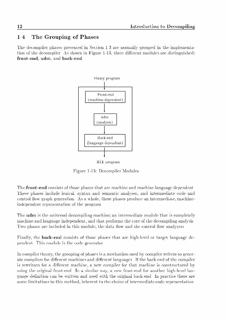
12 Introduction to Decompiling1.4 The Grouping of PhasesThe decompiler phases presented in Section 1.3 are normally grouped in the implementa-tion of the decompiler. As shown in Figure 1-13, three di�erent modules are distinguished:front-end, udm, and back-end. ????HLL program(language dependent)Back-end(analysis)udm(machine dependent)Front-endbinary program

Figure 1-13: Decompiler ModulesThe front-end consists of those phases that are machine and machine-language dependent.These phases include lexical, syntax and semantic analyses, and intermediate code andcontrol ow graph generation. As a whole, these phases produce an intermediate, machine-independent representation of the program.The udm is the universal decompiling machine; an intermediate module that is completelymachine and language independent, and that performs the core of the decompiling analysis.Two phases are included in this module, the data ow and the control ow analyzers.Finally, the back-end consists of those phases that are high-level or target language de-pendent. This module is the code generator.In compiler theory, the grouping of phases is a mechanism used by compiler writers to gener-ate compilers for di�erent machines and di�erent languages. If the back-end of the compileris rewritten for a di�erent machine, a new compiler for that machine is constructured byusing the original front-end. In a similar way, a new front-end for another high-level lan-guage de�nition can be written and used with the original back-end. In practice there aresome limitations to this method, inherent to the choice of intermediate code representation.

1.5 The Context of a Decompiler 13In theory, the grouping of phases in a decompilermakes it easy to write di�erent decompilersfor di�erent machines and languages; by writing di�erent front-ends for di�erent machines,and di�erent back-ends for di�erent target languages. In practical applications, this resultis always limited by the generality of the intermediate language used.1.5 The Context of a DecompilerIn practice, several programs can be used with the decompiler to create the target high-level language program. In general, source binary programs have a relocation table ofaddresses that are to be relocated when the program is loaded into memory. This task isaccomplished by the loader. The relocated or absolute machine code is then disassembledto produce an assembly representation of the program. The disassembler can use help fromcompiler and library signatures to eliminate the disassembling of compiler start-up code andlibrary routines. The assembler program is then input to the decompiler, and a high-leveltarget program is generated. Any further processing required on the target program, suchas converting while() loops into for loops can be done by a postprocessor. Figure 1-14shows the steps involved in a typical \decompilation". The user could also be a source ofinformation, particularly when determining library routines and separation of data frominstructions. Whenever possible, it is more reliable to use automatic tools. Decompilerhelper tools are covered in Chapter 8. This section brie y explains their task.???????? � ??� XXXXXXy ������9 ?library signatures?assembler program library bindingsabsolute machine codeloaderdisassemblerdecompilerHLL programpostprocessorHLL programrelocatable machine code prototype generatorlibrary prototypeslibrary headerscompiler signatureslibrariessignature generator

Figure 1-14: A Decompilation SystemLoaderThe loader is a program that loads a binary program into memory, and relocates the machinecode if it is relocatable. During relocation, instructions are altered and placed back inmemory.

14 Introduction to DecompilingSignature GeneratorA signature generator is a program that automatically determines compiler and library sig-natures; a binary pattern that uniquely identi�es each compiler and library subroutine. Theuse of these signatures attempts to reverse the task performed by the linker, which linksin library and compiler start-up code into the program. In this way, the analyzed programconsist only of user subroutines; the ones that the user compiled in the initial high-levellanguage program.For example, in the compiled C program that displays \hello world" and has over 25 dif-ferent subroutines in the binary program, 16 subroutines were added by the compiler toset-up its environment, 9 routines that form part of printf() were added by the linker,and 1 subroutine formed part of the initial C program.The use of a signature generator not only reduces the number of subroutines to analyze,but also increases the documentation of the target programs by using library names ratherthan arbitrary subroutine names.Prototype GeneratorThe prototype generator is a program that automatically determines the types of thearguments of library subroutines, and the type of the return value in the case of functions.These prototypes are derived from the library header �les, and are used by the decompilerto determine the type of the arguments to library subroutines and the number of sucharguments.DisassemblerA disassembler is a program that transforms a machine language into assembler language.Some decompilers transform assembler programs to a higher representation (see Chapter 2).In these cases, the assembler program has been produced by a disassembler, was written inassembler, or the compiler compiled to assembler.Library BindingsWhenever the target language of the decompiler is di�erent to the original language usedto compile the binary source program, if the generated target code makes use of librarynames (i.e. library signatures were detected), although this program is correct, it cannotbe recompiled in the target language since it does not use library routines for that languagebut for another one. The introduction of library bindings solves this problem, by bindingthe subroutines of one language to the other.PostprocessorA postprocessor is a program that transforms a high-level language program into asemantically equivalent high-level program written in the same language. For example,if the target language is C, the following code

1.6 Uses of Decompilation 15loc1 = 1;while (loc1 < 50) {/* some code in C */loc1 = loc1 + 1;}would be converted by a postprocessor intofor (loc1 = 1; loc1 < 50; loc1++) {/* some code in C */}which is a semantically equivalent program that makes use of control structures availablein the C language, but not present in the generic set of structures decompiled by thedecompiler.1.6 Uses of DecompilationDecompilation is a tool for a computer professional. There are two major areas wheredecompilation is used: software maintenance and security. In the former area, decompilationis used to recover lost or inaccessible source code, translate code written in an obsoletelanguage into a newer language, structure old code written in an unstructured way (i.e.spaghetti code) into a structured program, migrate applications to a new hardware platform,and debug binary programs that are known to have bugs but for which the source code isunavailable. In the latter area, decompilation is used as a tool to verify the object codeproduced by a compiler in software-critical systems, since the compiler cannot be trustedin these systems, and to check for the existence of malicious code such as viruses.1.6.1 Legal AspectsSeveral questions have been raised in the last years regarding the legality of decompilation.A debate between supporters of decompilation who claim fair competition is possible withthe use of decompilation tools, and the opponents of decompilation who claim copyrightis infringed by decompilation, is currently being held. The law in di�erent countries isbeing modi�ed to determine in which cases decompilation is lawful. At present, commercialsoftware is being sold with software agreements that ban the user from disassembling ordecompiling the product. For example, part of the Lotus software agreement reads like this:You may not alter, merge, modify or adapt this Sofware in any way includingdisassembling or decompiling.It is not the purpose of this thesis to debate the legal implications of decompilation. Thistopic is not further covered in this thesis.

Chapter 2Decompilation { What has been done?D i�erent attempts at writing decompilers have been made in the last 20 years. Due tothe amount of information lost in the compilation process, to be able to regeneratehigh-level language code all of these experimental decompilers have limitations in one wayor another, including decompilation of assembly �les[Hou73, Fri74, Wor78, Hop78, Bri81] orobject �les with or without symbolic debugging information[Reu88, PW93], simpli�ed high-level language[Hou73], and the requirement of the compiler's speci�cation[BB91, BB93].Assembly programs have helpful data information in the form of symbolic text, such asdata segments, data and type declarations, subroutine names, subroutine entry point, andsubroutine exit statement. All this information can be collected in a symbol table and thenthe decompiler would not need to address the problem of separating data from instructions,or the naming of variables and subroutines. Object �les with debugging information containthe program's symbol table as constructed by the compiler. Given the symbol table, it iseasy to determine which memory locations are instructions, as there is a certainty on whichmemory locations represent data. In general, object �les contain more information thanbinary �les. Finally, knowledge of the compiler's speci�cations is impractical, as thesespeci�cations are not normally disclosed by compiler manufacturers.2.1 Previous WorkDecompilers have been considered a useful software tool since they were �rst used in the1960s. At that time, decompilers were used to aid in the program conversion process fromsecond to third generation computers; in this way, manpower would not be spent in thetime-consuming task of rewriting programs for the third generation machines. During the70s and 80s, decompilers were used for the portability of programs, documentation, de-bugging, re-creation of lost source code, and the modi�cation of existing binaries. In the90s, decompilers have become a reverse engineering tool capable of helping the user withsuch tasks as checking software for the existence of illegal code, checking that a compilergenerates the right code, and translation of binary programs from one machine to another.It is noted that decompilation is not being used for software piracy or breach of copyright,as the process is incomplete in general, and can be used only as a tool to help develop atask.The following descriptions illustrate the best-known decompilers and/or research performedinto decompiler topics by individual researchers or companies:D-Neliac decompiler, 1960. As reported by Halstead in [Hal62], the Donnelly-Neliac(D-Neliac) decompiler was produced by J.K.Donnelly and H.Englander at the Navy

18 Decompilation { What has been done?Electronics Laboratory (NEL) in 1960. Neliac is an Algol-type language developedat the NEL in 1955. The D-Neliac decompiler produced Neliac code from machinecode programs; di�erent versions were written for the Remington Rand Univac M-460Countess computer and the Control Data Corporation 1604 computer.D-Neliac proved useful for converting non-Neliac compiled programs into Neliac, andfor detecting logic errors in the original high-level program. This decompiler proved thefeasibility of writing decompilers.W.Sassaman, 1966. Sassaman developed a decompiler at TRW Inc., to aid in theconversion process of programs from 2nd to 3rd generation computers. This decompilertook as input symbolic assembler programs for the IBM 7000 series and producedFortran programs. Binary code was not chosen as input language because theinformation in the symbolic assembler was more useful. Fortran was a standardlanguage in the 1960s and ran on both 2nd and 3rd generation computers. Engineeringapplications which involved algebraic algorithms were the type of programs decompiled.The user was required to de�ne rules for the recognition of subroutines. The decompilerwas 90% accurate, and some manual intervention was required[Sas66].This is the �rst decompiler that makes use of assembler input programs rather thanpure binary code. Assembler programs contain useful information in the form of names,macros, data and instructions, which are not available in binary or executable programs,and therefore eliminate the problem of separating data from instructions in the parsingphase of a decompiler.M.Halstead, 1967. The Lockheed Missiles and Space Company (LMSC) added someenhancements to the Neliac compiler developed at the Navy Electronics Laboratory, tocater for decompilation[Hal67]. The LMSC Neliac decompiler took as input machinecode for the IBM 7094 and produced Neliac code for the Univac 1108. It provedsuccessful by decompiling over 90% of instructions and leaving the programmer todecompile the other 10%. This decompiler was used at LMSC and under contract forcustomers in the U.S.A. and Canada[Hal70].Halstead analyzed the implementation e�ort required to raise the percentage of correctlydecompiled instructions half way to 100%, and found that it was approximately equal tothe e�ort already spent[Hal70]. This was because decompilers from that time handledstraightforward cases, but the harder cases were left for the programmer to consider.In order to handle more cases, more time was required to code these special cases intothe decompiler, and this time was proportionately greater than the time required to codesimple cases.Autocoder to Cobol Conversion Aid Program, 1967. Housel reported on a set ofcommercial decompilers developed by IBM to translate Autocoder programs, whichwere business data processing oriented, to Cobol. The translation was a one-to-one mapping and therefore manual optimization was required. The size of the �nalprograms occupied 2.1% times the core storage of the original program[Hou73].This decompiler is really a translation tool of one language to another. No attemptis made to analyze the program and reduce the number of instructions generated.Ine�cient code was produced in general.

2.1 Previous Work 19C.R.Hollander, 1973. Hollander's PhD dissertation[Hol73] describes a decompiler de-signed around a formal syntax-oriented metalanguage, and consisting of 5 cooperatingsequential processes; initializer, scanner, parser, constructor, and generator; each im-plemented as an interpreter of sets of metarules. The decompiler was a metasystemthat de�ned its operations by implementing interpreters.The initializer loads the program and converts it into an internal representation. Thescanner interacts with the initializer when �nding the �elds of an instruction, andinteracts with the parser when matching source code templates against instructions.The parser establishes the correspondence between syntactic phrases in the sourcelanguage and their semantic equivalents in the target language. Finally, the constructorand generator generate code for the �nal program.An experimental decompiler was implemented to translate a subset of IBM's Sys-tem/360 assembler into an Algol-like target language. This decompiler was written inAlgol-W, a compiler developed at Stanford University, and worked correctly on the 10programs it was tested against.This work presents a novel approach to decompilation, by means of a formal syntax-oriented metalanguage, but its main drawback is precisely this methodology, which isequivalent to a pattern-matching operation of assembler instructions into high-levelinstructions. This limits the amount of assembler instructions that can be decompiled,as instructions that belong to a pattern need to be in a particular order to be recognized;intermediate instructions, di�erent control ow patterns, or optimized code is notallowed. In order for syntax-oriented decompilers to work, the set of all possible patternswould need to be enumerated for each high-level instruction of each di�erent compiler.Another approach would be to write a decompiler for a speci�c compiler, and makeuse of the speci�cations of that compiler; this approach is only possible if the compilerwriter is willing to reveal the speci�cations of his compiler. It appears that Hollander'sdecompiler worked because the compiler speci�cations for the Algol-W compiler thathe was using were known, as this compiler was written at the University where hewas doing this research. The set of assembler instructions generated for a particularAlgol-W instruction were known in this case.B.C.Housel, 1973. Housel's PhD dissertation[Hou73] describes a clear approach to de-compilation by borrowing concepts from compiler, graph, and optimization theory. Hisdecompiler involves 3 major phases: partial assembly, analyzer, and code generation.The partial assembly phase separates data from instructions, builds a control owgraph, and generates an intermediate representation of the program. The analyzeranalyzes the program in order to detect program loops and eliminate unnecessaryintermediate instructions. Finally, the code generator optimizes the translation ofarithmetic expressions, and generates code for the target language.An experimental decompiler was written for Knuth's MIX assembler (MIXAL), pro-ducing PL/1 code for the IBM 370 machines. 6 programs were tested, 88% of theinstructions were correct, and the remaining 12% of the instructions required manualintervention[HH73].This decompiler proved that by using known compiler and graph methods, a decompilercould be written that produced good high-level code. The use of an intermediate

20 Decompilation { What has been done?representation made the analysis completely machine independent. The main objectionto this methodology is the choice of source language, MIX assembler, not only for thegreater amount of information available in these programs, but for being a simpli�ednon-real-life assembler language.The Piler System, 1974. Barbe's Piler system attempts to be a general decompiler thattranslates a large class of source{target language pairs to help in the automatictranslation of computer programs. The Piler system was composed of three phases:interpretation, analysis, and conversion. In this way, di�erent interpreters couldbe written for di�erent source machine languages, and di�erent converters could bewritten for di�erent target high-level languages, making it simple to write decompilersfor di�erent source{target language pairs. Other uses for this decompiler includeddocumentation, debugging aid, and evaluation of the code generated by a compiler.During interpretation, the source machine program was loaded into memory, parsedand converted into a 3-address microform representation. This meant that eachmachine instruction required one or more microform instructions. The analyzerdetermined the logical structure of the program by means of data ow analysis, andmodi�ed the microform representation to an intermediate representation. A owchartof the program after this analysis was made available to users, and they could evenmodify the owchart, if there were any errors, on behalf of the decompiler. Finally,the converter generated code for the target high-level language[Bar74].Although the Piler system attempted to be a general decompiler, only an interpreterfor machine language of the GE/Honeywell 600 computer was written, and skeletalconverters for Univac 1108's Fortran and Cobol were developed. The main e�ort ofthis project concentrated on the analyzer.The Piler system was a �rst attempt at a general decompiler for a large class of sourceand target languages. Its main problem was to attempt to be general enough with theuse of a microform representation, which was even lower-level than an assembler-typerepresentation.F.L.Friedman, 1974. Friedman's PhD dissertation describes a decompiler used for thetransfer of mini-computer operating systems within the same architectural class[Fri74].Four main phases are described: pre-processor, decompiler, code generator, andcompiler.The pre-processor converts assembler code into a standard form (descriptive assemblerlanguage). The decompiler takes the standard assembler form, analyses it, anddecompiles it into an internal representation, from which FRECL code is then generatedby the code generator. Finally, a FRECL compiler compiles this program into machinecode for another machine. FRECL is a high-level language for program transport anddevelopment; it was developed by Friedman, who also wrote a compiler for it. Thedecompiler used in this project was an adaptation of Housel's decompiler[Hou73].Two experiments were performed; the �rst one involved the transport of a small butself-contained portion of the IBM 1130 Disk Monitor System to Microdata 1600/21; upto 33%manual intervention was required on the input assembler programs. Overall, theamount of e�ort required to prepare the code for input to the transport system was toogreat to be completed in a reasonable amount of time; therefore, a second experiment

2.1 Previous Work 21was conducted. The second experiment decompiled Microdata 1621 operating systemprograms into FRECL and compiled them back again into Microdata 1621 machinecode. Some of the resultant programs were re-inserted into the operating system andtested. On average, only 2% of the input assembler instructions required manualintervention, but the �nal machine program had a 194% increase in the number ofmachine instructions.This dissertation is a �rst attempt at decompiling operating system code, and itillustrates the di�culties faced by the decompiler when decompiling machine-dependentcode. Input programs to this transport system require a large amount of e�ort to bepresented in the format required by the system, and the �nal produced programs appearto be ine�cient; both in the size of the program and the time to execute many moremachine instructions.Ultrasystems, 1974. Hopwood reported on a decompilation project at Ultrasystems, Inc.,in which he was a consultant for the design of the system[Hop78]. This decompilerwas to be used as a documentation tool for the Trident submarine �re control softwaresystem. It took as input Trident assembler programs, and produced programs in theTrident High-Level Language (THLL) that was being developed at this company. Fourmain stages were distinguished: normalization, analysis, expression condensation, andcode generation.The input assembler programs were normalized so that data areas were distinguishedwith pseudo-instructions. An intermediate representation was generated, and the dataanalyzed. Arithmetic and logical expressions were built during a process of expressioncondensation, and �nally, the output high-level language program was generated bymatching control structures to those available in THLL.This project attempts to document assembler programs by converting them into high-level language. The fact is, given the time constraints of the project, the expressioncondensation phase was not coded, and therefore the output programs were hard toread, as several instructions were required for a single expression.V.Schneider and G.Winiger, 1974. Schneider and Winiger presented a notation forspecifying the compilation and decompilation of high-level languages. By de�ninga context-free grammar for the compilation process (i.e. describe all possible 2-address object code produced from expressions and assignments), the paper showshow this grammar can be inverted to decompile the object code into the originalsource program[SW74]. Even more, an ambiguous compilation grammar will produceoptimal object code, and will generate an unambiguous decompilation grammar. Acase study showed that the object code produced by the Algol 60 constructs couldnot be decompiled deterministically. This work was part of a future decompiler, butfurther references in the literature about this work were not found.This work presents, in a di�erent way, a syntax-oriented decompiler[Hol73]; that is, adecompiler that uses pattern matching of a series of object instructions to reconstructthe original source program. In this case, the compilation grammar needs to be knownin order to invert the grammar and generate a decompilation grammar. Note that nooptimization is possible if it is not de�ned as part of the compilation grammar.

22 Decompilation { What has been done?Decompilation of Polish code, 1977, 1981, 1988. Two papers in the area of decom-pilation of Polish code into Basic code are found in the literature. The problem arisesin connection with highly interactive systems, where a fast response is required toevery input from the user. The user's program is kept in an intermediate form, andthen \decompiled" each time a command is issued. An algorithm for the translationof reverse Polish notation to expressions is given[BP79].The second paper presents the process of decompilation as a two step problem: theneed to convert machine code to Polish representation, and the conversion of Polishcode to source form. The paper concentrates on the second step of the decompilationproblem, but yet claims to be decompiling Polish code to Basic code by means of acontext-free grammar for Polish notation and a left-to-right or right-to-left parsingscheme[BP81].This technique was recently used in a decompiler that converted reverse Polish codeinto spreadsheet expressions[May88]. In this case, the programmers of a product thatincluded a spreadsheet-like component wanted to speed up the product by storing user'sexpressions in a compiled form, reverse Polish notation in this case, and decompile theseexpressions whenever the user wanted to see or modify them. Parentheses were left aspart of the reverse Polish notation to reconstruct the exact same expression the userhad input to the system.The use of the word decompilation in this sense is a misuse of the term. All thatis being presented in these papers is a method for re-constructing or deparsing theoriginal expression (written in Basic or Spreadsheet expressions) given an intermediatePolish representation of a program. In the case of the Polish to Basic translators, noexplanation is given as to how to arrive at such an intermediate representation givena machine program.G.L.Hopwood, 1978. Hopwood's PhD dissertation[Hop78] describes a 7-step decompilerdesigned for the purposes of transferability and documentation. It is stated thatthe decompilation process can be aided by manual intervention or other externalinformation.The input program to the decompiler is formatted by a preprocessor, then loadedinto memory, and a control ow graph of the program is built. The nodes of thisgraph represent one instruction. After constructing the graph, control patterns arerecognized, and instructions that generate a goto statement are eliminated by the useof either node splitting or the introduction of synthetic variables. The source programis then translated into an intermediate machine independent code, and analysis ofvariable usage is performed on this representation in order to �nd expressions andeliminate unnecessary variables by a method of forward substitution. Finally, code isgenerated for each intermediate instruction, functions are implemented to representoperations not supported by the target language, and comments are provided. Manualintervention was required to prepare the input data, provide additional informationthat the decompiler needed during the translation process, and to make modi�cationsto the target program.An experimental decompiler was written for the Varian Data machines 620/i. It de-compiled assembler into MOL620, a machine-oriented language developed at Universityof California at Irvine by M.D.Hopwood and the author. The decompiler was tested

2.1 Previous Work 23with a large debugger program, Isadora, which was written in assembler. The gener-ated decompiled program was manually modi�ed to recompile it into machine code, asthere were calls to interrupt service routines, self-modifying code, and extra registersused for subroutine calls. The �nal program was better documented than the originalassembler program.The main drawbacks of this research are the granularity of the control ow graph andthe use of registers in the �nal target program. In the former case, Hopwood chose tobuild control ow graphs that had one node per instruction; this means that the sizeof the control ow graph is quite large for large programs, and there is no bene�tgained as opposed to using nodes that are basic blocks (i.e. the size of the nodesis dependent on the number of changes of ow of control). In the latter case, theMOL620 language allows for the use of machine registers, and sample code illustratedin Hopwood's dissertation shows that registers were used as part of expressions andarguments to subroutine calls. The concept of registers is not a high-level conceptavailable in high-level languages, and it should not be used if wanting to generate high-level code.D.A.Workman, 1978. This work describes the use of decompilation in the design of ahigh-level language suitable for real time training device systems, in particular theF4 trainer aircraft[Wor78]. The operating system of the F4 was written in assembler,and it was therefore the input language to this decompiler. The output languagewas not determined as this project was to design one, thus code generation was notimplemented.Two phases of the decompiler were implemented: the �rst phase, which mappedthe assembler to an intermediate language and gathered statistics about the sourceprogram, and the second phase, which generated a control ow graph of basicblocks, classi�ed the instructions according to their probable type, and analyzedthe ow of control in order to determine high-level control structures. The resultsindicated the need of a high-level language that handled bit strings, supported loopingand conditional control structures, and did not require dynamic data structures orrecursion.This work presents a novel use of decompilation techniques, although the input languagewas not machine code but assembler. A simple data analysis was done by classifyinginstructions, but did not attempt to analyze them completely as there was no need togenerate high-level code. The analysis of the control ow is complete and considers 8di�erent categories of loops and 2-way conditional statements.Zebra, 1981. The Zebra prototype was developed at the Naval Underwater SystemsCentre in an attempt to achieve portability of assembler programs. Zebra took as inputa subset of the ULTRA/32 assembler, called AN/UYK-7, and produced assembler forthe PDP11/70. The project was described by D.L.Brinkley in [Bri81].The Zebra decompiler was composed of 3 passes: a lexical and ow analysis pass, whichparsed the program and performed control ow analysis in the graph of basic blocks.The second pass was concerned with the translation of the program to an intermediateform, and the third pass simpli�ed the intermediate representation by eliminatingextraneous loads and stores, in much the same way described by Housel[Hou73, HH73].

24 Decompilation { What has been done?It was concluded that it was hard to capture the semantics of the program and thatdecompilation was economically impractical, but it could aid in the transportationprocess.This project made use of known technology to develop a decompiler of assemblerprograms. No new concepts were introduced by this research, but it raised the pointthat decompilation is to be used as a tool to aid in the solution of a problem, but notas tool that will give all solutions to the problem, given that a 100% correct decompilercannot be built.Decompilation of DML programs, 1982. A decompiler of database code was designedto convert a subset of Codasyl DML programs, written with procedural operations, intoa relational system with a nonprocedural query speci�cation. An Access Path Modelis introduced to interpret the semantic accesses performed by the program. In orderto determine how FIND operations implement semantic accesses, a global data owreaching analysis is performed on the control ow graph, and operations are matchedto templates. The �nal graph structures are remapped into a relational structure.This method depends on the logical order of the objects and a standard ordering ofthe DML statements[KW82].Another decompiler of database code was proposed to decompile well-coded applicationprograms into a proposed semantic representation is described in [DS82]. This workwas induced by changes in the use requirements of a Database Management System(DBMS), where application programs were written in Cobol-DML. A decompiler ofCobol-DML programs was written to analyse and convert application programs into amodel and schema-independent representation. This representation was later modi�edor restructured to account for database changes. Language templates were used tomatch against key instructions of a Cobol-DML programs.In the context of databases, decompilation is viewed as the process of grouping a se-quence of statements which represent a query into another (nonprocedural) speci�ca-tion. Data ow analysis is required, but all other stages of a decompiler are not imple-mented for this type of application.Forth Decompiler, 1982, 1984. A recursive Forth decompiler is a tool that scansthrough a compiled dictionary entry and decompiles words into primitives andaddresses[Dud82]. Such a decompiler is considered one of the most useful tools inthe Forth toolbox[HM84]. The decompiler implements a recursive descent parser sothat decompiled words can be decompiled in a recursive fashion.These works present a deparsing tool rather than a decompiler. The tool recursivelyscans through a dictionary table and returns the primitives or addresses associated witha given word.Software Transport System, 1985. C.W.Yoo describes an automatic Software Trans-port System (STS) that moves assembler code from one machine to another. Theprocess involves the decompilation of an assembler program for machine m1 to a high-level language, and the compilation of this program in a machine m2 to assembler. Anexperimental decompiler was developed on the Intel 8080 architecture; it took as inputassembler programs and produced PL/M programs. The recompiled PL/M programswere up to 23% more e�cient than their assembler counterpart. An experimental

2.1 Previous Work 25STS was developed to develop a C cross-compiler for the Z-80 processor. The projectencountered problems in the lack of data type in the STS[Yoo85].The STS took as input an assembler program for machine m1 and an assemblergrammar for machine m2, and produced an assembler program for machine m2. Theinput grammar was parsed and produced tables used by the abstract syntax tree parserto parse the input assembler program and generate an abstract syntax tree (AST)of the program. This AST was the input to the decompiler, which then performedcontrol and data ow analyses, in much the same way described by Hollander[Hol73],Friedman[Fri74], and Barbe[Bar74], and �nally generated high-level code. The high-level language was then compiled for machine m2.This work does not present any new research into the decompilation area, but it doespresent a novel approach to the transportation of assembler programs by means of agrammar describing the assembler instructions of the target architecture.Decomp, 1988. J.Reuter wrote decomp, a decompiler for the Vax BSD 4.2 which tookas input object �les with symbolic information and produced C-like programs. Thenature of this decompiler was to port the Empire game to the VMS environment,given that source code was not available. The decompiler is freely available on theInternet[Reu88].Decomp made use of the symbol table to �nd the entry points to functions, determinedata used in the program, and the names of that data. Subroutines were decompiledone at a time, in the following way: a control ow graph of basic blocks was builtand optimised by the removal of arcs leading to intermediate unconditional branches.Control ow analysis was performed in the graph to �nd high-level control constructs,converting the control ow graph into a tree of generic constructs. The algorithm usedby this analysis was taken from the struct program, a program that structures graphsproduced by Fortran programs, which was based on the structuring algorithm describedby B.Baker in [Bak77]. Finally, the generic constructs in the tree were converted toC-speci�c constructs, and code was generated. The �nal output programs requiredmanual modi�cations to place the arguments on the procedure's argument list, anddetermine that a subroutine returned a value (i.e. was a function). This decompilerwas written in about 5 man-months[Reu91].Sample programs were written and compiled in C in a Vax BSD 4.2 machine, thanksto the collaboration of Pete French[Fre91], who provided me with an account in a VaxBSD 4.2 machine. The resulting C programs are not compilable, but require somehand editing. The programs have the correct control structures, due to the structuringalgorithm implemented, and the right data type of variables, due to the embedded symboltable in the object code. The names of library routines and procedures, and the user'sprogram entry point are also known from the symbol table; therefore, no extraneousprocedures (e.g. compiler start up code, library routines) are decompiled. The need fora data ow analysis stage is vital, though, as neither expressions, actual arguments,nor function return value are determined. An interprocedural data ow analysis wouldeliminate much of the hand-editing required to recompile the output programs.exe2c, 1990. The Austin Code Works sponsored the development of the exe2c decompiler,targetted at the PC compatible family of computers running the DOS operating

26 Decompilation { What has been done?system[Wor91]. The project was announced in April 1990[Gut90], tested by about20 people, and it was decided that it needed some more work to decompile inC. A year later, the project reached a � operational level[Gut91a], but was never�nished[Gut91b]. I was a beta tester of this release.exe2c is a multipass decompiler that consists of 3 programs: e2a, a2aparse, ande2c. e2a is the disassembler. It converts executable �les to assembler, and producesa commented assembler listing as well. e2aparse is the assembler to C front-endprocessor, which analyzes the assembler �le produced by e2a and generates .cod and.glb �les. Finally, the e2c program translates the �les prepared by a2aparse andgenerates pseudo-C. An integrated environment, envmnu, is also provided.Programs decompiled by exe2c make use of a header �le that de�nes registers,types and macros. The output C programs are hard to understand because theyrely on registers and condition codes (represented by Boolean variables). Normally,one machine instruction is decompiled into one or more C instructions that performthe required operation on registers, and set up condition codes if required by theinstruction. Expressions and arguments to subroutines are not determined, and a localstack is used for the �nal C programs. It is obvious from this output code that adata ow analysis was not implemented in exe2c. This decompiler has implemented acontrol ow analysis stage; looping and conditional constructs are available. The choiceof control constructs is generally adequate. Case tables are not detected correctly,though. The number and type of procedures decompiled shows that all library routines,and compiler start-up code and runtime support routines found in the program aredecompiled. The nature of these routines is normally low-level, as they are normallywritten in assembler. These routines are hard to decompile as, in most cases, there isno high-level counterpart (unless it is low-level type C code).This decompiler is a �rst e�ort in many years to decompile executable �les. The resultsshow that a data ow analysis and heuristics are required to produce better C code. Also,a mechanism to skip all extraneous code introduced by the compiler and to detect librarysubroutines would be bene�cial.PLM-80 Decompiler, 1991. The Information Technology Division of the AustralianDepartment of Defence researched into decompilation for defence applications, suchas maintenance of obsolete code, production of scienti�c and technical intelligence,and assessment of systems for hazards to safety or security. This work was describedby S.T. Hood in [Hoo91].Techniques for the construction of decompilers using de�nite-clause grammars, anextension of context-free grammars, in a Prolog environment are described. A Prologdatabase is used to store the initial assembler code and the recognised syntacticstructures of the grammar. A prototype decompiler for Intel 8085 assembler programscompiled by a PLM-80 compiler was written in Prolog. The decompiler producedtarget programs in Small-C, a subset of the C language. The de�nite-clause grammargiven in this report was capable of recognizing if..then type structures, and while()loops, as well as static (global) and automatic (local) variables of simple types (i.e.character, integers, and longs). A graphical user interface was written to display theassembler and pseudo-C programs, and to enable the user to assign variable names,

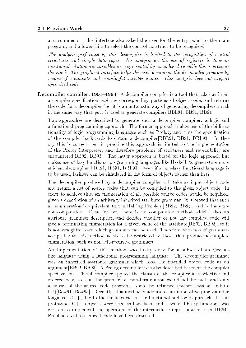
2.1 Previous Work 27and comments. This interface also asked the user for the entry point to the mainprogram, and allowed him to select the control construct to be recognized.The analysis performed by this decompiler is limited to the recognition of controlstructures and simple data types. No analysis on the use of registers is done ormentioned. Automatic variables are represented by an indexed variable that representsthe stack. The graphical interface helps the user document the decompiled program bymeans of comments and meaningful variable names. This analysis does not supportoptimized code.Decompiler compiler, 1991{1994. A decompiler compiler is a tool that takes as inputa compiler speci�cation and the corresponding portions of object code, and returnsthe code for a decompiler; i.e. it is an automatic way of generating decompilers, muchin the same way that yacc is used to generate compilers[BBL91, BB91, BB94].Two approaches are described to generate such a decompiler compiler: a logic anda functional programming approach. The former approach makes use of the bidirec-tionality of logic programming languages such as Prolog, and runs the speci�cationof the compiler backwards to obtain a decompiler[BBL91, BB91, BBL93]. In the-ory this is correct, but in practice this approach is limited to the implementationof the Prolog interpreter, and therefore problems of strictness and reversibility areencountered[BB92, BB93]. The latter approach is based on the logic approach butmakes use of lazy functional programming languages like Haskell, to generate a moree�cient decompiler[BBL91, BB91, BBL93]. Even if a non-lazy functional language isto be used, laziness can be simulated in the form of objects rather than lists.The decompiler produced by a decompiler compiler will take as input object codeand return a list of source codes that can be compiled to the given object code. Inorder to achieve this, an enumeration of all possible source codes would be required,given a description of an arbitrary inherited attribute grammar. It is proved that suchan enumeration is equivalent to the Halting Problem[BB92, BB93], and is thereforenon-computable. Even further, there is no computable method which takes anattribute grammar description and decides whether or not the compiled code willgive a terminating enumeration for a given value of the attribute[BB92, BB93], so itis not straightforward which grammars can be used. Therefore, the class of grammarsacceptable to this method needs to be restricted to those that produce a completeenumeration, such as non left-recursive grammars.An implementation of this method was �rstly done for a subset of an Occam-like language using a functional programming language. The decompiler grammarwas an inherited attribute grammar which took the intended object code as anargument[BB92, BB93]. A Prolog decompiler was also described based on the compilerspeci�cation. This decompiler applied the clauses of the compiler in a selective andordered way, so that the problem of non-termination would not be met, and onlya subset of the source code programs would be returned (rather than an in�nitelist)[Bow91, Bow93]. Recently, this method made use of an imperative programminglanguage, C++, due to the ine�ciencies of the functional and logic approach. In thisprototype, C++ object's were used as lazy lists, and a set of library functions waswritten to implement the operators of the intermediate representation used[BB94].Problems with optimized code have been detected.

28 Decompilation { What has been done?As illustrated by this research, decompiler compilers can be constructed automaticallyif the set of compiler speci�cations and object code produced for each clause of thespeci�cation is known. In general, this is not the case as compiler writers do notdisclose their compiler speci�cations. Only customized compilers and decompilers canbe built by this method. It is also noted that optimizations produced by the optimizationstage of a compiler are not handled by this method, and that real executable programscannot be decompiled by the decompilers generated by the method described. Theproblem of separating instructions from data is not addressed, nor is the problem ofdetermining the data types of variables used in the executable program. In conclusion,decompiler compilers can be generated automatically if the object code produced by acompiler is known, but the generated decompilers cannot decompile arbitrary executableprograms.8086 C Decompiling System, 1991{1993. This decompiler takes as input executable�les from a DOS environment and produces C programs. The input �les need tobe compiled with Microsoft C version 5.0 in the small memory model[FZL93]. Fivephases were described: recognition of library functions, symbolic execution, recognitionof data types, program transformation, and C code generation. The recognition oflibrary functions and intermediate language was further described in [FZ91, HZY91].The recognition of library functions for Microsoft C was done to eliminate subroutinesthat were part of a library, and therefore produce C code for only the user routines.A table of C library functions is built-into the decompiling system. For each libraryfunction, its name, characteristic code (sequence of instructions that distinguish thisfunction from any other function), number of instructions in the characteristic code,and method to recognize the function were stored. This was done manually bythe decompiler writer. The symbolic execution translated machine instructions tointermediate instructions, and represented each instruction in terms of its symboliccontents. The recognition of data types is done by a set of rules for the collection ofinformation on di�erent data types and analysis rules to determine the data type in use.The program transformation transforms storage calculation into address expressions,e.g. array addressing. Finally, the C code generator transforms the program structureby �nding control structures, and generates C code.This decompiling system makes use of library function recognition to generate morereadable C programs. The method of library recognition is hand-crafted, and thereforeine�cient if other versions of the compiler, other memory models, or other compilerswere used to compile the original programs. The recognition of data types is a �rstattempt to recognize types of arrays, pointers and structures, but not much detail isgiven in the paper. No description is given as to how an address expression is reachedin the intermediate code, and no examples are given to show the quality of the �nal Cprograms.Alpha AXP Migration Tools, 1993. When Digital Equipment Corporation designedthe Alpha AXP architecture, the AXP team got involved in a project to run existingVAX and MIPS code on the new Alpha AXP computers. They opted for a binarytranslator which would convert a sequence of instructions of the old architectureinto a sequence of instructions of the new architecture. The process needed to befully automatic and to cater for code created or modi�ed during execution. Two

2.1 Previous Work 29parts to the migration process were de�ned: a binary translation, and a runtimeenvironment[SCK+93].The binary translation phase took binary programs and translated them into AXPopcodes. It made use of decompilation techniques to understand the underlyingmeaning of the machine instructions. Condition code usage analysis was performedas these conditions do not exist on the Alpha architecture. The code was also analyzedto determine function return values and �nd bugs (e.g. uninitialized variables). MIPShas standard library routines which are embedded in the binary program. In this case,a pattern matching algorithm was used to detect routines that were library routines,such routines were not analysed but replaced by their name. Idioms were also foundand replaced by an optimal instruction sequence. Finally, code was generated in theform of AXP opcodes. The new binary �le had both, the new code and the old code.The runtime environment executes the translated code and acts as a bridge between thenew and old operating systems (e.g. di�erent calling standards, exception handling).It had a built-in interpreter of old code to run old code not discovered or nonexistentat translation time. This was possible because the old code was also saved as part ofthe new binary �le.Two binary translators were written: VEST, to translate from the OpenVMS VAXsystem to the OpenVMS AXP system, and mx, to translate ULTRIX MIPS images toDEC OSF/1 AXP images. The runtime environments for these translators were TIEand mxr respectively.This project illustrates the use of decompilation techniques in a modern translationsystem. It proved successful for a large class of binary programs. Some of the programsthat could not be translated were programs that were technically infeasible to translate,such as programs that use privileged opcodes, or run with superuser privileges.Source/PROM Comparator, 1993. A tool to demonstrate the equivalence of sourcecode and PROM contents was developed at the Nuclear Electric plc, UK, to verifythe correct translation of PL/M-86 programs into PROM programs executed by safetycritical computer controlled systems[PW93].Three stages are identi�ed: the reconstitution of object code �les from the PROM�les, the disassembly of object code to an assembler-like form with help from a name-table built up from the source code, and decompilation of assembler programs andcomparison with the original source code. In the decompiling stage, it was notedthat it was necessary to eliminate intermediate jumps, registers and stack operations,identify procedure arguments, resolve indexes of structures, arrays and pointers, andconvert the expresssions to a normal form. In order to compare the original programand the decompiled program, an intermediate language was used. The source programwas translated to this language with the use of a commercial product, and the outputof the decompilation stage was written in the same language. The project proved tobe a practical way of verifying the correctness of translated code, and to demonstratethat the tools used to create the programs (compiler, linker, optimizer) behave reliablyfor the particular safety system analyzed.This project describes a use of decompilation techniques, to help demonstrate the equiv-alence of high-level and low-level code in a safety-critical system. The decompilation

30 Decompilation { What has been done?stage performs much of the analysis, with help from a symbol table constructed fromthe original source program. The task is simpli�ed by the knowledge of the compilerused to compile the high-level programs.In the last years, commercial vendor-speci�c decompilers have been manufactured. Thesedecompilers are targetted at the decompilation of binary �les produced by databaselanguages, such as Clipper and FoxPro. No information on the techniques used to decompilethese programs is given by their manufacturers. The following list mentions some of thesecommercial decompilers:Valkyrie, 1993. Visual decompiler for Clipper Summer '87, manufactured by CodeWorks[Val93].OutFox, 1993. Decompiler for encrypted FoxBASE+ programs [Out93].ReFox, 1993. Decompiles encrypted FoxPro �les, manufactured by Xitech Inc [HHB+93].DOC, 1993. COBOL decompiler for AS/400 and System/38. Converts object programsinto COBOL source programs which can be modi�ed by the programmer. Manufac-tured by Harman Resources [Cob93].Uniclip, 1993. Decompiler for Clipper Summer '87 EXE �les, manufactured by Stro Ware[Unc93].Clipback, 1993. Decompiler for Summer '87 executables, manufactured by IntelligentInformation Systems [Unc93].Brillig, 1993. Decompiler for Clipper 5.X .exe and .obj �les, manufactured by APTware[Bri93].

Chapter 3Run-time EnvironmentB efore considering decompilation, the relations between the static binary code of the pro-gram and the actions performed at run-time to implement the program are presented.The representation of objects in a binary program di�ers between compilers; elementarydata types such as integers, characters, and reals are often represented by an equivalentdata object in the machine (i.e. a �xed size number of bytes), whereas aggregate objectssuch as arrays, strings, and structures are represented in various di�erent ways.Throughout this thesis, the word subroutine is used as a generic word to denote a procedureor a function; the latter two words are used only when there is certainty as to what thesubroutine really is, that is, a subroutine that returns a value is a function, and a subroutinethat does not return a value is a procedure.3.1 Storage OrganizationA high-level language program is composed of one or more subroutines, called the user sub-routines. The corresponding binary program is composed of the user subroutines, libraryroutines that were invoked by the user program, and other subroutines linked in by thelinker to provide support for the compiler at run-time. The general format of the binarycode of a program is shown in Figure 3-1. The program starts by invoking compiler start-upsubroutines that set up the environment for the compiler; this is followed by the user's mainprogram subroutine, which invokes library routines linked in by the linker; and is �nalizedby a series of compiler subroutines that restore the state of the machine before programtermination. user programstart-up codeexit code(including librarysubroutines)Figure 3-1: General Format of a Binary Program

32 Run-time EnvironmentFor example, a \hello world" C program compiled with Borland Turbo C v2.01 has over 25di�erent subroutines. The start-up code invokes up to 16 di�erent subroutines to set upthe compiler's environment. The user's main program is composed of one procedure. Thisprocedure invokes the printf() procedure which then invokes up to 8 di�erent subroutinesto display the formatted string. Finally, the exit code invokes 3 subroutines to restore theenvironment and exit back to DOS. Sample skeleton code for this program is shown inFigure 3-2.helloc proc farmov dx,DGROUP ; dx == GROUP segment adrmov cs:DGROUP@@,dx; save several vectors and install default divide by zero handlercall SaveVectors; calculate environment size, determine amount of memory needed,; check size of the stack, return to DOS memory allocated in excess,; set far heap and program stack, reset uninitialized data area,; install floating point emulatorpush cscall ds:[__emu1st]; prepare main argumentscall _setargv@call _setenvp@; initialize window sizescall ds:[__crt1st]; invoke main(argc,argv,envp)push word ptr environ@push word ptr _argv@push word ptr _argc@call main@ ; user's main() program; flush and close streams and filespush axcall exit@helloc endp Figure 3-2: Skeleton Code for a \hello world" ProgramIn a binary program, subroutines are identi�ed by their entry address; there are no namesassociated with subroutines, and it is unknown whether the subroutine is a procedure or afunction before performing a data ow analysis on the registers de�ned and used by thesesubroutines. It is said that a subroutine that invokes another subroutine is the caller, andthe invoked subroutine is the callee.

3.2 Data Types 333.1.1 The Stack FrameEach subroutine is associated with a stack frame during run-time. The stack frame is theset of parameters, local variables, and return address of the caller subroutine, as shown inFigure 3-3. The parameters in the stack frame represent the actual parameters of a partic-ular invocation of the subroutine: information on the formal parameters of the subroutineare not stored elsewhere in the binary �le. The stack mark represents the return address ofthe caller (so that control can be transferred to the caller once the callee is �nished), andthe caller's frame pointer (register bp in the Intel architecture), which is a reference pointfor o�sets into the stack frame. The local variables represent the space allocated by thesubroutine once control has been transferred to it; this space is available to the subroutineonly while it is active (i.e. not terminated).? �� 6?6? bp + o�setlow memoryhigh memory Local variablesStack markParameters bp - o�setbpspFigure 3-3: The Stack FrameOnce the frame pointer has been set (i.e. register bp), positive o�sets from the framepointer access parameters and the stack mark, and negative o�sets access local variables.The convention used in diagrams relating to the stack frame is as follows: the stack growsdownwards from high to low memory, as in the Intel architecture.The stack frame may also contain other �elds, as shown in Figure 3-4. These �elds are notused by all languages nor all compilers[ASU86a]. The return value �eld is used in somelanguages by the callee to return the value of a function back to the caller; these values aremore often returned in registers for e�ciency. The control link points to the stack frameof the caller, and the access link points to the stack frame of an enclosing subroutine thatholds non-local data that is accessible from this subroutine.3.2 Data TypesData objects are normally stored in contiguous memory locations. Elementary data typessuch as characters, integers, and longs, can be held in registers while an operation is per-formed on them. Aggregate data types such as arrays, strings, and records, cannot be heldin registers in their entirety because their size is normally beyond the size of a register,therefore it is easier to access them through a pointer to their starting address.

34 Run-time EnvironmentLocal variablesReturn valueStack markAccess linkControl linkParameters

Figure 3-4: The Stack FrameThe sizes of di�erent data types for the i80286 architecture are shown in Figure 3-5. Thismachine has a word size of 16 bits. Sizes are given in 8-bit bytes.Data Type Size (bytes)character 1integer 2long 4real 4long real 8near pointer 2far pointer 4other types � 1Figure 3-5: Size of Di�erent Data Types in the i802863.2.1 Data Handling in High-level LanguagesAggregate data types are handled in several di�erent ways by di�erent compilers. Thissection describes di�erent formats used by C, Pascal, Fortran, and Basic compilers,according to [Mic87].ArrayAn array is a contiguous piece of memory that holds one or more items of a certain type.Arrays are implemented in memory as a series of rows or columns, depending on the orderused by the language:� Row-major order: the elements of a multidimensional array are stored by row order;that is, one row after the other. This order is used by C and Pascal compilers.

3.2 Data Types 35� Column-major order: the elements of a multidimensional array are stored in columnorder rather than row order. This order is used by Fortran and Basic compilers. SomeBasic compilers have a compile option to use row-major order.In most languages, the size of the array is known at compile time; this is the case of C,Pascal and Fortran. Basic allows for run-time declared array sizes, therefore an array needsto have an array-descriptor to hold the size of the array and a pointer to the physicallocation in memory where the array is stored.StringA string is a sequence of characters. Di�erent languages use di�erent representations for astring, such as the following:� C format: a string is an array of bytes terminated by a null character (i.e. 0).� Fortran format: a string is a series of bytes at a a �xed memory location, hence nodelimiter is used or needed at the end of the string.� Pascal format: common Pascal compilers have 2 types of strings: STRING andLSTRING. The former is a �xed-length string and is implemented in the Fortranformat. The latter is a variable-length string and is implemented as an array ofcharacters that holds the length of the string in the �rst byte of the array. StandardPascal does not have a STRING or LSTRING type.� Basic format: a string is implemented as a 4-byte string-descriptor; the �rst 2 byteshold the length of the string, and the next 2 bytes are an o�set into the default dataarea which holds the string. This area is assigned by Basic's string-space managementroutines, and therefore is not a �xed location in memory.RecordA record is a contiguous piece of memory that holds related items of one or more data types.Di�erent names are used for records in di�erent languages; struct in C, record in Pascal,and user-de�ned type in Basic. By default, C and Pascal store structures in unpackedstorage, word-aligned, except for byte-sized objects and arrays of byte-sized objects. Basicand some C and Pascal compilers store structures in packed storage.Complex NumbersThe Fortran COMPLEX data type stores oating point numbers in the following way:� COMPLEX*8: 4 bytes represent the real part, and the other 4 bytes represent the oating point number of the imaginary part.� COMPLEX*16: 8 bytes represent the real part, and the other 8 bytes the imaginarypart.

36 Run-time EnvironmentBooleanThe Fortran LOGICAL data type stores Boolean information in the following way:� LOGICAL*2: 1 byte holds the Boolean value (0 or 1), and the other byte is left unused.� LOGICAL*4: 1 byte holds the Boolean value, and the other 3 bytes are left unused.3.3 High-Level Language InterfaceCompilers of high-level languages use a series of conventions to allow mixed-languageprogramming, so that a program can have some subroutines written in one language, andother subroutines written in a di�erent language, and all these subroutines are linked intogether in the same program. The series of conventions relate to the way the stack frameis set up, and the calling conventions used to invoke subroutines.3.3.1 The Stack FrameThe stack mark contains the caller's return address and frame pointer. The return addressvaries in size depending on whether the callee is invoked using a near or far call. Near callsare within the same segment and therefore can be referenced by an o�set from the currentsegment base address. Far calls are in a di�erent segment, so both segment and o�set ofthe callee are stored. For a 2-byte machine word architecture, the near call stores 2 bytesfor the o�set of the caller, whereas the far call stores 4 bytes for the segment and o�setof the caller. Register bp is used as the frame pointer, the contents of the caller's framepointer is pushed onto the stack at subroutine entry so that it can be restored at subroutinetermination.Entering a SubroutineRegister bp is established as the frame pointer by pushing its address onto the stack (i.e.storing the frame pointer of the caller on the stack), and copying the current stack pointerregister (sp) to bp. The following code is used in the i80286 architecture:push bp ; save old copy of bpmov bp, sp ; bp == frame pointerAllocating Local DataA subroutine may reserve space on the stack for local variables. This is done by decrementingthe contents of the stack register sp by an even amount of bytes. For example, to allocatespace for 2 integer variables, 4 bytes are reserved on the stack:sub sp, 4

3.3 High-Level Language Interface 37Preserving Register ValuesThe most widely used calling convention for DOS compilers demands that a subroutineshould always preserve the values of registers si, di, ss, ds, and bp. If any of these registersis used in the callee subroutine, their values are pushed onto the stack, and restored beforesubroutine return. For example, if si and di are used by a subroutine, the following codeis found after local data allocation:push sipush diAccessing ParametersParameters are located at positive o�sets from the frame pointer register, bp. In order toaccess a parameter n, the o�set from bp is calculated by adding the size of the stack mark,plus the size of the parameters between bp and parameter n, plus the size of parameter n.Returning a ValueFunctions returning a value in registers use di�erent registers according to the size of thereturned value. Data values of 1 byte are returned in the al register, 2 bytes are returnedin the ax register, and 4 bytes are returned in the dx:ax registers, as shown in Figure 3-6.Data Size (bytes) Register1 AL2 AX4 DX = high byteAX = low byteFigure 3-6: Register Conventions for Return ValuesLarger data values are returned using the following conventions:� Function called by C: the callee must allocate space from the heap for the return valueand place its address in dx:ax.� Function called by Pascal, Fortran or Basic: the caller reserves space in the stacksegment for the return value, and pushes the o�set address of the allocated space onthe stack as the last parameter. Therefore, the o�set address of the return value is atbp + 6 for far calls, and bp + 4 for near calls, as shown in Figure 3-7.Exiting the SubroutineThe stack frame is restored by popping any registers that were saved at subroutine entry,deallocating any space reserved for local variables, restoring the old frame pointer (bp), andreturning according to the convention in use.� C convention: the caller adjusts the stack for any parameters pushed on the stack. Aret instruction is all that is needed to end the subroutine.

38 Run-time Environment�� and o�setReturn value o�setParametersLocal variablesReturn o�setReturn value o�setParameters bp + 4Old bp bp + 6Local variablesOld bpReturn segmentFigure 3-7: Return Value Convention� Pascal, Fortran, Basic convention: the callee adjusts the stack by cutting back the stackwith the required number of parameter bytes. A ret n instruction is used, where n isthe number of bytes of the parameters.For example, the following code restores the registers di and si from the stack, deallocatesthe space of the local variables by copying bp to sp, restores the frame pointer by poppingbp from the stack, and returns using the C convention:pop di ; restore registerspop simov sp, bp ; deallocate local variablespop bp ; restore bpret3.3.2 Parameter PassingThree di�erent methods are used to pass parameters on the Intel architecture under theDOS operating system; C, Pascal, and register calling conventions. Mixtures of these callingconventions are available in other operating systems and architectures. For example, inOS/2, the standard call uses C ordering to pass parameters, but the callee cuts back theparameters from the stack in system calls.C Calling ConventionThe caller is responsible for pushing the parameters on the stack, and restoring themafter the callee returns. The parameters are pushed in right to left order, so thata variable number of parameters can be passed to the callee. For example, for a Cfunction prototype void procX (int, char, long), and a caller procedure that invokesthe procX() procedure:procN(){ int i; /* bp - 8 */char c; /* bp - 6 */long l; /* bp - 4 */procX (i, c, l);}

3.4 Symbol Table 39the following assembler code is produced:push word ptr [bp-2] ; high word of lpush word ptr [bp-4] ; low word of lpush [bp-6] ; cpush word ptr [bp-8] ; icall procX ; call functionadd sp, 8 ; restore the stackNote that due to word alignment, the character c is stored as 2 bytes on the stack eventhough its size is one byte only.Pascal Calling ConventionThe caller is responsible for pushing the arguments on the stack, and the callee adjusts thestack before returning. Arguments are pushed on the stack in left to right order, hencea �xed number of arguments are used in this convention. For the previous example, thecalling of procX (i, c, l) produces the following assembler code in Pascal convention:push word ptr [bp-8] ; ipush [bp-6] ; cpush word ptr [bp-2] ; high word of lpush word ptr [bp-4] ; low word of lcall procX ; call procX (procX restores stack)Register Calling ConventionThis convention does not push arguments on the stack but passes them in registers, thereforethe generated code is faster. Predetermined registers are used to pass arguments betweensubroutines, and di�erent registers are used for di�erent argument sizes. Figure 3-8 showsthe set of registers used by Borland Turbo C++ [Bor92]; a maximum of 3 parameters canbe passed in registers. Far pointers, unions, structures, and real numbers are pushed on thestack. Parameter Type RegisterCharacter al, dl, blInteger ax, dx, bxLong dx:axNear pointer ax, dx, bxFigure 3-8: Register Parameter Passing Convention3.4 Symbol TableA decompiler uses a symbol table to store information on variables used throughout theprogram. In a binary program, variables are identi�ed by their address; there are no names

40 Run-time Environmentassociated with variables. Variables that have a physical memory address are global vari-ables; their segment and o�set are used to access them. Variables that are located at anegative o�set from the frame pointer are local variables to the corresponding stack frame'ssubroutine, and variables at positive o�sets are actual arguments to the subroutine. Sinceregister variables are used by compilers for e�ciency purposes, all registers are also con-sidered variables initially; further analysis on registers determines whether they representregister variables or not (see Chapter 5, Section 5.2.9). Variables are assigned unique namesduring code generation, as explained in Chapter 7.The symbol table must be able to provide information on an entry e�ciently, and handle avarying number of variables; hence, a symbol table that grows dynamically if necessary isdesirable. The performance of the symbol table is measured in terms of the time taken toaccess an entry and insert a new item to the table.3.4.1 Data StructuresSymbol tables are represented by a variety of data structures. Some are more e�cient thanothers, at the expense of more coding. To illustrate the di�erences between the various datastructures, let us assume the following data items are to be placed in the symbol table:cs:01F8 ; global variablebp + 4 ; parameterbp - 6 ; local variableax ; register axbp - 2 ; local variableUnordered ListAn unordered list is a linked-list or an array of data items. Items are stored in the list ina �rst-in basis (i.e. on the next available position). An array implementation presents thelimitation of size; these limitations are avoided by the use of a linked-list implementation.An access to this symbol table, for a list of n items is O(n). Figure 3-9 shows the list builtfor our example. - - - - bp - 2cs:01F8 bp + 4 bp - 6 axFigure 3-9: Unordered List RepresentationOrdered ListAn ordered list is easier to access, since not all items of the list need to be checked todetermine whether an item is already in the list or not. Ordered lists can be searched usinga binary search, which provides an access time of O(log n). Insertion of an item is costly,since the list needs to remain ordered.

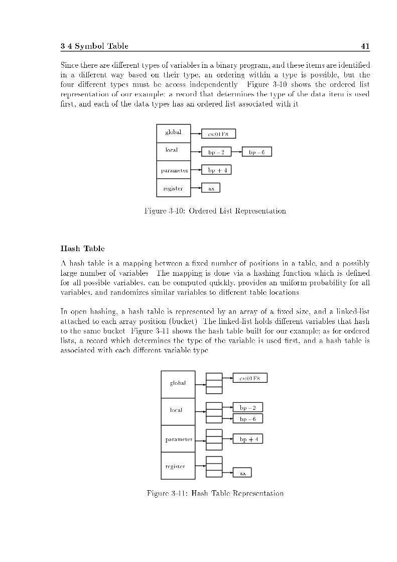
3.4 Symbol Table 41Since there are di�erent types of variables in a binary program, and these items are identi�edin a di�erent way based on their type, an ordering within a type is possible, but thefour di�erent types must be access independently. Figure 3-10 shows the ordered listrepresentation of our example: a record that determines the type of the data item is used�rst, and each of the data types has an ordered list associated with it.bp - 2cs:01F8 bp - 6bp + 4axregister -- ---globallocalparameterFigure 3-10: Ordered List RepresentationHash TableA hash table is a mapping between a �xed number of positions in a table, and a possiblylarge number of variables. The mapping is done via a hashing function which is de�nedfor all possible variables, can be computed quickly, provides an uniform probability for allvariables, and randomizes similar variables to di�erent table locations.In open hashing, a hash table is represented by an array of a �xed size, and a linked-listattached to each array position (bucket). The linked-list holds di�erent variables that hashto the same bucket. Figure 3-11 shows the hash table built for our example; as for orderedlists, a record which determines the type of the variable is used �rst, and a hash table isassociated with each di�erent variable type. cs:01F8bp - 2bp - 6bp + 4local ax---- -

----globalparameterregisterFigure 3-11: Hash Table Representation

42 Run-time EnvironmentSymbol Table Representation for DecompilationA combination of the abovementioned methods is used for the purposes of decompilation.The symbol table is de�ned in terms of the di�erent types of variables; global, local, pa-rameter, and register. Each of these types is implemented in a di�erent way. For globalvariables, since their address range is large, a hash table implementation is most suited. Forlocal variables and parameters, since these variables are o�sets from the frame pointer, andare always allocated in an ordered way (i.e. there are no \gaps" in the stack frame), theyare implemented by an ordered list on the o�set; the register bp does not need to be storedsince it is always the same. Finally, for registers, since there is a �xed number of registers,an array indexed by register number can be implemented; array positions that have an as-sociated item represent registers that are de�ned in the symbol table. This representationis shown in Figure 3-12. cs:01F8- -6---- -2 -globalparameterregisterlocal ax...4Figure 3-12: Symbol Table RepresentationSymbol tables are widely discussed in the literature, refer to [ASU86a, FJ88a, Gou88] formore information on symbol tables from a compiler point of view.

Chapter 4The Front-endT he front-end is a machine dependent module which takes as input the binary sourceprogram, parses the program, and produces as output the control ow graph and inter-mediate language representation of the program. The phases of the front-end are shown inFigure 4-1. ?????binary programcontrol ow graphSyntax analyzerSemantic analyzerIntermediate code generatorintermediate codeControl ow graph generatorFigure 4-1: Phases of the Front-endUnlike compilers, there is no lexical analysis phase in the front-end of the decompiler. Thelexical analyzer or scanner is the phase that groups characters from the input stream intotokens. Specialized tools such as lex and scanGen have been designed to help automate theconstruction of scanners for compilers[FJ88a]. Given the simplicity of machine language,there is no need to scan the input bytes to recognize di�erent words that belong to thelanguage; all information is stored in terms of bytes or bits from a byte, and it is notpossible to determine what a particular byte represents (i.e. opcode, register, o�set) outof context. The syntax analyzer determines what a series of bytes represent based on thelanguage description of the machine language.4.1 Syntax AnalysisThe syntax analyzer is the �rst phase of the decompiler. Its role is to group a sequenceof bytes into a phrase or sentence of the language. This sequence of bytes is checked forsyntactic structure, that is, that the string belongs to the language. Valid strings are rep-resented by a parse tree, which is input into the next phase, the semantic analyzer. The

44 The Front-endrelation between the syntax analyzer and the semantic analyzer is shown in Figure 4-2. Thesyntax analyzer is also known as the parser. -- I@@@@@R >������= . . . . . . . . . .. . . . . . . . . ...... .....-. . . .parse treeParserprogramsource binary Table SemanticAnalyzer front-endrest ofSymbolFigure 4-2: Interaction between the Parser and Semantic AnalyzerThe syntax of a machine language can be precisely speci�ed by a grammar. In machinelanguages, only instructions or statements are speci�ed; there are no control structures asin high-level languages. In general, a grammar provides a precise notation for specifyingany language.The main di�culty of a decompiler parser is the separation of code from data, that is, thedetermination of which bytes in memory represent code and which ones represent data.This problem is inherent to the von Neumann architecture, and thus, needs to be addressedby means of heuristic methods.Syntax ErrorsSyntax errors are seldom found in binary programs, as compilers generate correct code for acompiled program to run on a machine. But, given that upgrades of a machine architectureresult in new machines that support all predecessor machines, the machine instruction setof the new architecture is an extension of the instruction set of the old architecture. Thisis the case of the i80486, which supports all predecessor i8086, i80186, i80286, and i80386instruction sets. Therefore, if a parser is written for the i8086, all new machine instructionsare not recognized by the parser and must result in an error. On the other hand, if theparser is written for the newest machine, the i80486, all instructions should be recognizedand no syntactic errors are likely to be encountered.4.1.1 Finite State AutomatonA Finite State Automaton (FSA) is a recognizer for a language. It takes as input a string,and answers yes if the string belongs to the language and no otherwise. A string is asequence of symbols of a given alphabet. Given an arbitrary string, an FSA can determinewhether the string belongs to the language or not.De�nition 1 A Finite State Automaton is a mathematical model that consists of:� A �nite set of states S� An initial state s0

4.1 Syntax Analysis 45� A set of �nal or accept states F� An alphabet of input symbols �� A transition function T : state � symbol ! stateAn FSA can be graphically represented by transition diagrams. The components of thesediagrams are shown in Figure 4-3. The symbols from the alphabet label the transitions.Error transitions are not explicitly represented in the diagram, and it is assumed that anynon-valid symbol out of a state labels a transition to an error state.���� ����m- -����sx accept state snstate sx s0initial state s0 a transition snFigure 4-3: Components of a FSA Transition DiagramA wildcard language is a meta-language used to specify wildcard conditions in alanguage[Gou88]. Two meta-symbols are used `*' and `%'. The meta-symbol `*' representsany sequence of zero or more symbols from the alphabet �, and `%' represents any singlesymbol from �.Example 1 Let � = fa, b, cg. The language that accepts all strings starting with an ais described by the wildcard expression aa*, and is represented in an FSA in the followingway: �������� m� ���- %-aNon-deterministic Finite State AutomatonAn FSA is said to be non-deterministic (NFSA) whenever there are two or more transitionsout of a state labelled with the same symbol, or when the empty string (") labels a transition.In these cases, the next state is not uniquely identi�ed by a (state, symbol) tuple.Deterministic Finite State AutomatonA deterministic �nite state automaton (DFSA) is a FSA that has no transitions labelled bythe " string, and that uniquely identi�es or determines the next state of a (state, symbol)tuple.Any NFSA can be converted into an equivalent DFSA by a method of subset construction.This method has been explained in the literature, for example, refer to [ASU86b, Gou88,FJ88a] for details. A method to construct a minimum-state DFSA is also described in[ASU86b].

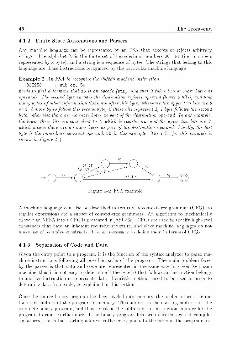
46 The Front-end4.1.2 Finite State Automatons and ParsersAny machine language can be represented by an FSA that accepts or rejects arbitrarystrings. The alphabet � is the �nite set of hexadecimal numbers 00..FF (i.e. numbersrepresented by a byte), and a string is a sequence of bytes. The strings that belong to thislanguage are those instructions recognized by the particular machine language.Example 2 An FSA to recognize the i80286 machine instruction83E950 ; sub cx, 50needs to �rst determine that 83 is an opcode (sub), and that it takes two or more bytes asoperands. The second byte encodes the destination register operand (lower 3 bits), and howmany bytes of other information there are after this byte: whenever the upper two bits are 0or 2, 2 more bytes follow this second byte, if these bits represent 1, 1 byte follows the secondbyte, otherwise there are no more bytes as part of the destination operand. In our example,the lower three bits are equivalent to 1, which is register cx, and the upper two bits are 3,which means there are no more bytes as part of the destination operand. Finally, the lastbyte is the immediate constant operand, 50 in this example. The FSA for this example isshown in Figure 4-4. ���� ���� ���� ���� ����m- - �����* -���� QQQQs68..6F -�����������: -83 28..2FA8..AF E8..EF% % %Figure 4-4: FSA exampleA machine language can also be described in terms of a context-free grammar (CFG); asregular expressions are a subset of context-free grammars. An algorithm to mechanicallyconvert an NFSA into a CFG is presented in [ASU86a]. CFGs are used to specify high-levelconstructs that have an inherent recursive structure, and since machine languages do notmake use of recursive constructs, it is not necessary to de�ne them in terms of CFGs.4.1.3 Separation of Code and DataGiven the entry point to a program, it is the function of the syntax analyzer to parse ma-chine instructions following all possible paths of the program. The main problem facedby the parser is that data and code are represented in the same way in a von Neumannmachine, thus it is not easy to determine if the byte(s) that follows an instruction belongsto another instruction or represents data. Heuristic methods need to be used in order todetermine data from code, as explained in this section.Once the source binary program has been loaded into memory, the loader returns the ini-tial start address of the program in memory. This address is the starting address for thecomplete binary program, and thus, must be the address of an instruction in order for theprogram to run. Furthermore, if the binary program has been checked against compilersignatures, the initial starting address is the entry point to the main of the program; i.e.

4.1 Syntax Analysis 47the start address of the user-written program, skipping all compiler start up code. Fig-ure 4-5 illustrates sample code for a \hello world" program. The entry point returned bythe loader is CS:0000, which is the entry point to the complete program (including compilerstart up code). The entry point given by the compiler signature analyzer is CS:01FA, whichis the start address of the main program. Throughout this thesis we will assume the entrypoint is the one given by the compiler signature analyzer without loss of generality. Theexplained methods are applicable to both cases, but more interesting examples are foundin the latter case. The technique for generating compiler signatures and detecting them isgiven in Chapter 8. helloc proc farCS:0000 start: mov dx,*CS:0003 mov cs:*,dx... ... ; start-up codeCS:011A call _mainCS:011D ... ; exit codehelloc endp... ..._main proc nearCS:01FA push bpCS:01FB mov bp,spCS:01FD mov ax,194hCS:0200 push axCS:0201 call _printfCS:0204 pop cxCS:0205 pop bpCS:0206 ret_main endpFigure 4-5: Sample Code for a \hello world" ProgramA paper by R.N. Horspool and N. Marovac focused on the problem of separation of codefrom data. This paper mentioned that this problem is equivalent to the halting problem,as it is impossible to separate data from instructions in a von Neumann architecture thatcomputes both data addresses and branch destination addresses at execution time[HM79].An algorithm to �nd the maximum set of locations holding instructions was given. Thismodi�cation of the original problem is equivalent to a combinatorial problem of searchingfor a maximal set of trees out of all the candidate trees, for which a branch-and-boundmethod is applied. The algorithm is proved to be NP-Complete.As it turns out, in dense machine instruction sets (such as in the Intel architecture), thegiven algorithm does not work, as almost any byte combination is a valid machine instruc-tion, and therefore it is hard to determine the bounds of the code since it is hard to knowwhen data has been reached. A simple counter-example to this algorithm is given by a case

48 The Front-endtable stored in the code segment (see Figure 4-6). After the indexed jump instruction atCS:0DDB, which indexes into the case table, the table itself is de�ned starting at CS:0DE0,but yet it is treated as code by the algorithm as it includes valid bytes for instructions. Inthis i80286 code example, 0E is equivalent to push CS, 2B is equivalent to sub which takesone other byte as argument, 0E in this case, to result in sub ax,[bp], and so on. Theproduced code is therefore wrong.CS:0DDB jmp CS:0DE0[bx]CS:0DE0 0E2B ; push CSCS:0DE2 0E13 ; sub ax,[bp]...Figure 4-6: Counter-exampleThis section presents a di�erent method to determine code from instructions in a binaryprogram that has been loaded into memory. It provides heuristic methods to determinespecial cases of data found in between sections of code.The ProcessAs previously mentioned, the process of determining data from code is based on the knowl-edge that the initial entry point to the program is an instruction. From this instructiononwards, instructions are parsed sequentially along this path, until a change in the owof control or an end of path is reached. In the former case, the target address(es) acts asnew entry points into memory, as the address must hold a valid instruction in order for theprogram to continue execution. In the latter case, the end of the current path is reachedand no more instructions are scanned along this path as we cannot determine whether thesenext bytes are code or data.Changes in the ow of control are due to jumps and procedure calls. A conditional jumpbranches the ow of control in two: the target branch address is followed whenever the con-dition is true, otherwise the address following the conditional branch is followed. Both pathsare followed by the parser in order to get all possibly executable code. An unconditionaljump transfers the ow of control to the target address; this unique path is followed by theparser. A procedure call transfers control to the invoked procedure, and once it returns, theinstructions following the procedure call are parsed. In the case that the procedure doesnot return, the bytes following the procedure call are not parsed as it is not certain whatthese bytes are (code or data).An end of path is reached whenever a procedure return instruction or an end of programis met. The end of program is normally speci�ed by a series of instructions that makethe operating system terminate the current process (i.e. the program). This sequence ofinstructions varies between operating systems, so they need to be coded for the speci�csource machine. Determining whether the end of program is met (i.e. the program �nishes

4.1 Syntax Analysis 49or halts) is not equivalent to solving the halting problem though, as the path that isbeing followed is not necessarily a path that the executable program will follow, i.e. thecondition that branches onto this path might never become true during program execution;for example, programs in an in�nite loop.Example 3 On the Intel architecture, the end of a program is speci�ed via interruptinstructions. There are di�erent methods to terminate a program, some of these methodsmake use of the program segment pre�x, commonly referred to as the PSP; refer toAppendix B for more information on the PSP. There are 7 di�erent ways of terminating aprogram under DOS:1. Terminate process with return code: int 21h, function 4Ch. This is the mostcommonly used method in .exe �les.2. Terminate process: int 20h. The code segment, cs, needs to be pointing to the PSP.This method is normally used in .com �les as cs already points to the PSP segment.3. Warm boot/Terminate vector: o�set 00h in the PSP contains an int 20h instruction.Register cs must be pointing to the PSP segment.4. Return instruction: the return address is placed on the stack before the program starts.When the program is to be �nished, it returns to this address on the stack. This methodwas used in the CP/M operating system as the address of the warm boot vector was onthe stack. Initial DOS .com programs made use of this technique.5. Terminate process function: int 21h, function 00h. Register cs must point to thePSP.6. Terminate and stay resident: int 27h. Register cs must point to the PSP.7. Terminate and stay resident function: int 21h, function 31h.Determining whether a procedure returns (i.e. �nishes or halts) or not is di�cult, as theprocedure could make use of self-modifying code or execute data as code and terminate inan instruction within this data. In general, we are interested in a solution for normal cases,as aberrant cases require a step debugger tool and user input to solve the problem. A pro-cedure does not return if it reaches the end of program or invokes a procedure that reachesthe end of program (e.g. a procedure that invokes exit(.) in C). Determining whether aprocedure has reached the end of program is possible by emulation of the contents of theregisters that are involved in the sequence of instructions that terminate the program. Inthe case of Example 3, keeping track of registers ah, and cs in most cases.This initial algorithm for separation of code from data is shown in Figure 4-7. In order tokeep track of registers, a machState record of register values is used. A state variable ofthis type holds the current values of the registers (i.e. the current state of the machine).A bitmap of 2 bits per memory byte is used to store information regarding each byte thatwas loaded into memory:� 0: represents an unknown value (i.e. the memory location has not been analyzed).� 1: represents a code byte.

50 The Front-end� 2: represents a data byte.� 3: represents a byte that is used as both, data and code.The algorithm is implemented recursively. Each time a non fall-through path needs to befollowed, a copy of the current state is made, and the path is followed by a recursive callto the parse procedure with the copy of the state.Indirect Addressing ModeThe indirect addressing mode makes use of the contents of a register or memory locationto determine the target address of an instruction that uses this addressing mode. Indirectaddressing mode can be used with the unconditional jump (e.g. to implement indexed casetables) and the procedure call instructions. The main problem with this addressing mode isthat the contents of memory can be changed during program execution, and thus, a staticanalysis of the program will not provide the right value, and is not able to determine ifthe memory location has been modi�ed. The same applies to register contents, unless thecontents of registers is being emulated, but again, if the register is used within a loop, thecontents of the register will most likely be wrong (unless loops are emulated also).In the i80286, an indirect instruction can be intra-segment or inter-segment. In the formercase, the contents of the register or memory location holds a 16-bit o�set address, in thelatter case, a 32-bit address (i.e. segment and o�set) is given.Indirect procedure calls are used in high-level languages like C to implement pointers tofunction invocation. Consider the following C program:typedef char (*tfunc)();tfunc func[2] = {func1, func2};char func1() {/* some code here */}char func2() {/* some code here */}main(){ func[0]();func[1]();}In the main program, functions func1() and func2() are invoked by means of a functionpointer and an index into the array of such functions. The disassembled code of this programlooks like this:CS:0094 B604 ; address of proc1 (04B6)CS:0098 C704 ; address of proc2 (04C7)... proc_1 PROC FARCS:04B6 55 push bp... ...CS:04C6 CB retf

4.1 Syntax Analysis 51procedure parse (machState *state)done = FALSE;while (! done)getNextInst (state, &inst);if (alreadyParsed (inst)) /* check if instruction already parsed */done = TRUE;break;end ifsetBitmap (CODE, inst);case (inst.opcode) ofconditional jump:*stateCopy = *state;parse (stateCopy); /* fall-through */state->ip = targetAdr (inst); /* target branch address */if (hasBeenParsed (state->ip)) /* check if code already parsed */done = TRUE;end ifunconditional jump:state->ip = targetAdr (inst); /* target branch address */if (hasBeenParsed (state->ip)) /* check if code already parsed */done = TRUE;end ifprocedure call:/* Process non-library procedures only */if (! isLibrary (targetAdr (inst)))*stateCopy = *state;stateCopy->ip = targetAdr (inst);parse (stateCopy); /* process target procedure */end ifprocedure return:done = TRUE; /* end of procedure */move:if (destination operand is a register)updateState (state, inst.sourceOp, inst.destOp);end ifinterrupt:if (end of program via interrupt)done = TRUE; /* end of program */end ifend caseend whileend procedure Figure 4-7: Initial Parser Algorithm

52 The Front-endproc_1 ENDPproc_2 PROC FARCS:04C7 55 push bp... ...CS:04D7 CB retfproc_2 ENDPmain PROC FARCS:04D8 55 push bpCS:04D9 8BEC mov bp, spCS:04DB FF1E9400 call 0094 ; intra-segment indirect callCS:04DF FF1E9800 call 0098 ; intra-segment indirect callCS:04E3 5D pop bpCS:04E4 CB retfmain ENDPThe function pointers have been replaced by the memory o�set of the address that holdsthe address of each procedure (i.e. 04B6 and 04C7 respectively). If these addresses have notbeen modi�ed during program execution, checking the contents of these memory locationsprovides us with the target address of the function(s). This is the implementation that weuse. The target address of the function is replaced in the procedure call instruction, and aninvocation to a normal procedure is done in our decompiled C program, as follows:void proc_1() {/* some code */}void proc_2() {/* some code */}void main(){ proc_1();proc_2();}Case StatementsHigh-level languages implement multiway (or n-way) branches via a high-level constructknown as a case statement. In this construct, there are n di�erent possible paths to beexecuted (i.e. n di�erent branches). There is no low-level machine instruction to representthis construct, therefore di�erent methods are used by compiler writers to de�ne a casetable.If the number of cases is not too great (i.e. less than 10), a case is implemented by asequence of conditional jumps, each of which tests for an individual value and transferscontrol to the code for the corresponding statement. Consider the following fragment ofcode in assemblercmp al, 8 ; start of caseje lab1cmp al, 7Fh

4.1 Syntax Analysis 53je lab2cmp al, 4je lab3cmp al, 18hje lab4cmp al, 1Bhje lab5jmp endCaselab1: ......lab5: ......endCase: ... ; end of caseIn this code fragment, register al is compared against 5 di�erent byte values, if the result isequal, an unconditional jump is performed to the label that handles the case. If the registeris not equal to any of the 5 options, the program unconditionally jumps to the end of thecase.A more compact way to implement a case statement is to use an indexed table that holds ntarget label addresses; one for each of the corresponding n statements. The table is indexedinto by an indexed jump instruction. Before indexing into the table, the lower and upperbounds of the table are checked for, so that no erroneous indexing is done. Once it has beendetermined that the index is within the bound, the indexed jump instruction is performed.Consider the following fragment of code:cs:0DCF cmp ax, 17h ; 17h == 24cs:0DD2 jbe startCasecs:0DD4 jmp endCasecs:0DD7 startCase:mov bx, axcs:0DD9 shl bx, 1cs:0DDB jmp word ptr cs:0DE0[bx] ; indexed jumpcs:0DE0 0E13 ; dw lab1 ; start of indexed tablecs:0DE2 0E1F ; dw lab2...cs:0EOE 11F4 ; dw lab24 ; end of indexed tablecs:0E10 lab1: ...cs:11C7 lab24:...cs:11F4 endCase: ; end of case...The case table is de�ned in the code segment as data, and is located immediately afterthe indexed jump and before any target branch labels. Register ax holds the index into thetable. This register is compared against the upper bound, 24. If the register is greater than24, the rest of the sequence is not executed and the control is transferred to labZ, the �rstinstruction after the end of the case. On the other hand, if the register is less or equal to

54 The Front-end24, labA is reached and register bx is set up as the o�set into the table. Since the size ofthe word is 2, the case table has o�set labels of size 2, so the initial index into the tableis multiplied by two to get the correct o�set into the 2-byte table. Once this is done, theindexed jump instruction determines that the case table is in segment cs and o�set 0DE0(i.e. the next byte in memory in this case). Therefore, the target jump address is any ofthe 24 di�erent options available in this table.A very similar implementation of case statements is given by a case table that is locatedafter the end of the procedure, and the index register into the table is the same as theregister that holds the o�set into the table (register bx in the following fragment of code):cs:0BE7 cmp bx, 17h ; 17h == 24cs:0BEA jbe startCasecs:0BEC jmp jumpEndcs:0BEF startCase:shl bx, 1cs:0BF1 jmp word ptr cs:0FB8[bx] ; indexed jumpcs:0BF6 jumpEnd:jmp endCasecs:0BF9 lab1: ...cs:0F4C lab24:...cs:0F88 endCase: ; end of case...cs:0FB5 ret ; end of procedurecs:0FB8 0BF9 ; dw lab1 ; start of indexed tablecs:0FBA 0C04 ; dw lab2...cs:0FE6 0F4C ; dw lab24 ; end of indexed tableA third way to implement a case statement is to have the case table following all indexedbranches. In this way, the code jumps over all target jump addresses, checks for upperbounds of the indexed table (31 in the following fragment of code), adjusts the register thatindexes into the table, and branches to this location:cs:0C65 jmp startCasecs:0C68 lab5:... ...cs:1356 lab31:... ...cs:1383 lab2:... ...cs:13B8 1403 ; dw endCase ; Start of indexed tablecs:13BA 1383 ; dw lab2... ...cs:13F4 1356 ; dw lab31 ; End of indexed tablecs:13F6 startCase:

4.1 Syntax Analysis 55cmp ax, 1Fh ; 1Fh == 31cs:13F9 jae endCasecs:13FB xchg ax, bxcs:13FC shl bx, 1cs:13FE jmp word ptr cs:13B8[bx] ; indexed jumpcs:1403 endCase:...cs:1444 retA di�erent implementation of case statements is by means of a string of character options,as opposed to numbers. Consider the following code fragment:cs:246A 4C6C68464E6F 785875646973 ; db 'LlhFNoxXudiscpneEfgG%'cs:2476 63706E654566 674725cs:247F 256C ; dw lab1 ; start of tablecs:2481 2573 ; dw lab2... ...cs:24A7 24DF ; dw lab21... ...cs:24C4 procStart:push bp... ...cs:2555 mov di, cscs:2557 mov es, di ; es = cscs:2559 mov di, 246Ah ; di = start of stringcs:255C mov cx, 15h ; cx = upper boundcs:255F repne scasbcs:2561 sub di, 246Bhcs:2565 shl di, 1cs:2567 jmp word ptr cs:247F[di] ; indexed jumpcs:256C lab1:... ...cs:26FF lab12:... ...cs:2714 retThe string of character options is located at cs:246A. Register al holds the current charac-ter option to be checked, es:di points to the string in memory to be compared against, andthe repne scasb instruction �nds the �rst match of register al in the string pointed to byes:di. Register di is left pointing to the character after the match. This register is thensubtracted from the string's initial address plus one, and it now indexes into an indexedjump table located before the procedure on the code segment. This method is compact andelegant.Unfortunately, there is no �xed representation of a case statement, and thus, the binarycode needs to be manually examined in the �rst instance to determine how the case state-ment was implemented. Di�erent compilers use di�erent implementations, but normallya speci�c vendor's compiler uses only one or two di�erent representations of case tables.

56 The Front-endThe determination of a case table is a heuristic method that handles a prede�ned set ofgeneralized implementations. The more implementation methods that are handled by thedecompiler, the better output it can generate. As heuristic methods are used, the rightpreconditions need to be satis�ed before applying the method; i.e. if and indexed tableis met and the bound of the indexed table cannot be determined, the proposed heuristicmethod cannot be applied.Final AlgorithmThe �nal algorithm used for data/code separation is shown in Figure 4-8. The algorithmis based on the algorithm of Figure 4-7, but expands on the cases of indexed jumps andindirect jumps and calls.4.2 Semantic AnalysisThe semantic analysis phase determines the meaning of a group of machine instructions,collects information on the individual instructions of a subroutine, and propagates thisinformation across the instructions of the subroutine. In this way, base data types such asintegers and long integers are propagated across the subroutine. The relation of this phasewith the syntax analyzer and intermediate code generator is shown in Figure 4-9.De�nition 2 An identi�er (<ident>) is either a register, local variable (negative o�setfrom the stack), parameter (positive o�set from the stack), or a global variable (location inmemory).4.2.1 IdiomsThe semantic meaning of a series of instructions is sometimes given by an idiom. These aresequences of instructions that represent a high-level instruction.De�nition 3 An idiom is a sequence of instructions that has a logical meaning whichcannot be derived from the individual instructions.Most idioms are widely known to the compiler community, as they are a series of instructionsthat perform an operation in a unique or more e�cient way than doing it with di�erentinstructions. The following sections illustrate some of the best known idioms.Subroutine IdiomsWhen entering a subroutine, the base register, bp, is established to be the frame pointerby copying the value of the stack pointer (sp) into bp. The frame pointer is used to accessparameters and local data from the stack within that subroutine. This sequence of instruc-tions is shown in Figure 4-10. The high-level language subroutine prologue sets up registerbp to point to the current stack pointer, and optionally allocates space on the stack for localstatic variables, by decreasing the contents of the stack pointer sp by the required numberof bytes. This idiom is represented by an enter instruction that takes the number of bytesreserved for local storage.

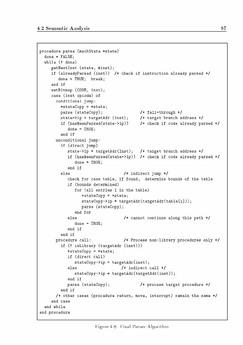
4.2 Semantic Analysis 57procedure parse (machState *state)done = FALSE;while (! done)getNextInst (state, &inst);if (alreadyParsed (inst)) /* check if instruction already parsed */done = TRUE; break;end ifsetBitmap (CODE, inst);case (inst.opcode) ofconditional jump:*stateCopy = *state;parse (stateCopy); /* fall-through */state->ip = targetAdr (inst); /* target branch address */if (hasBeenParsed(state->ip)) /* check if code already parsed */done = TRUE;end ifunconditional jump:if (direct jump)state->ip = targetAdr(inst); /* target branch address */if (hasBeenParsed(state->ip)) /* check if code already parsed */done = TRUE;end ifelse /* indirect jump */check for case table, if found, determine bounds of the table.if (bounds determined)for (all entries i in the table)*stateCopy = *state;stateCopy->ip = targetAdr(targetAdr(table[i]));parse (stateCopy);end forelse /* cannot continue along this path */done = TRUE;end ifend ifprocedure call: /* Process non-library procedures only */if (! isLibrary (targetAdr (inst)))*stateCopy = *state;if (direct call)stateCopy->ip = targetAdr(inst);else /* indirect call */stateCopy->ip = targetAdr(targetAdr(inst));end ifparse (stateCopy); /* process target procedure */end if/* other cases (procedure return, move, interrupt) remain the same */end caseend whileend procedure Figure 4-8: Final Parser Algorithm

58 The Front-endIntermediateCode Generator6? --}ZZZZZZZ~ ����������*-. . . . -. . . . rest of. . . . . . . . . .. . . . . . . . . ...... .....source binaryprogram Parser SymbolTabletreeparse AnalyzerSemantic front-endFigure 4-9: Interaction of the Semantic Analyzerpush bpmov bp, sp[sub sp, immed]+enter immed, 0Figure 4-10: High-level Subroutine PrologueOnce the subroutine prologue is encountered, any pushes on the stack represent registerswhose values are to be preserved during this subroutine. These registers could act as regis-ter variables (i.e. local variables) in the current subroutine, and thus are agged as possiblybeing register variables. Figure 4-11 shows registers si and di begin pushed on the stack.push sipush diFigure 4-11: Register VariablesFinally, to exit a subroutine, any registers saved on the stack need to be popped, any dataspace that was allocated needs to be freed, bp needs to be restored to point to the old framepointer, and the subroutine then returns with a near or far return instruction. Figure 4-12shows sample trailer code.Calling ConventionsThe C calling convention is also known as the C parameter-passing sequence. In this con-vention, the caller pushes the parameters on the stack, in the reverse order in which theyappear in the source code (i.e. right to left order), and then invokes the procedure. Afterprocedure return, the caller restores the stack by either popping the parameters from the

4.2 Semantic Analysis 59pop di ; Restore registerspop simov sp,bp ; Restore sppop bp ; Restore bpret(f) ; ReturnFigure 4-12: Subroutine Trailer Codestack, or adding the number of parameter bytes to the stack pointer. In either case, thetotal number of bytes used in arguments is known, and is stored for later use. The instruc-tion(s) involved in the restoring of the stack are eliminated from the code. The C callingconvention is used when passing a variable number of arguments, as the callee does notneed to restore the stack. Figure 4-13 shows the case in which pop instructions are usedto restore the stack. The total number of bytes is computed by multiplying the number ofpops by 2. call(f) proc_Xpop reg[pop reg] reg in {ax, bx, cx, dx}+proc_X.numArgBytes = 2 * numPopssets CALL_C flagFigure 4-13: C Calling Convention - Uses popFigure 4-14 shows the case in which the stack is restored by adding the number of argumentbytes to the stack. This value is stored for later use, and the instruction that restores thestack is eliminated for further analysis. It has been found that when 2 or 4 bytes were usedfor arguments, the stack is restored by popping these bytes from the stack. This is dueto the number of cycles involved in the two di�erent operations: each pop reg instructiontakes 1 byte, and an add sp,immed instruction takes 3 bytes. Most likely, the binary codehad been optimized for space rather than speed, because a pop reg instruction on the i8086takes 8 cycles, where as an add sp,immed instruction takes 4 cycles.The Pascal calling convention is also known as the Pascal parameter-passing sequence. Inthis convention, the caller pushes the parameters on the stack in the same order as theyappear in the source code (i.e. left to right order), the callee procedure is invoked, and thecallee is responsible for adjusting the stack before returning. It is therefore necessary for thecallee to know how many parameters are passed, and thus, it cannot be used for variableargument parameters. Figure 4-15 shows this convention.

60 The Front-endcall(f) proc_Xadd sp, immed+proc_X.numArgBytes = immedsets CALL_C flagFigure 4-14: C Calling Convention - Uses addret(f) immed +proc_X.numArgBytes = immedsets CALL_PASCAL flagFigure 4-15: Pascal Calling ConventionLong Variable OperationsLong variables are stored in memory as two consecutive memory or stack locations. Thesevariables are normally identi�ed when simple addition or subtraction operations are per-formed on them. The idioms used for these operations are generally used due to theirsimplicity in number of instructions.Figure 4-16 shows the instructions involved in long addition. The low parts of the longvariable(s) are added with an add instruction, which sets up the carry ag if there is anover ow. The high parts are then added taken into account the carry ag, as if there werean over ow of 1 in the low part, this 1 needs to be added to the high part. Thus, a adc(add with carry) instruction is used to add the high parts.add ax, [bp-4]adc dx, [bp-2]+dx:ax = dx:ax + [bp-2]:[bp-4]Figure 4-16: Long Addition

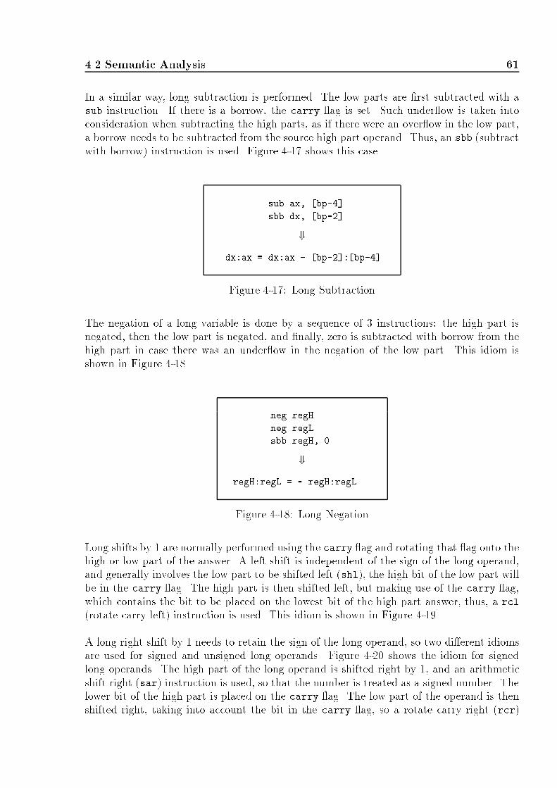
4.2 Semantic Analysis 61In a similar way, long subtraction is performed. The low parts are �rst subtracted with asub instruction. If there is a borrow, the carry ag is set. Such under ow is taken intoconsideration when subtracting the high parts, as if there were an over ow in the low part,a borrow needs to be subtracted from the source high part operand. Thus, an sbb (subtractwith borrow) instruction is used. Figure 4-17 shows this case.sub ax, [bp-4]sbb dx, [bp-2]+dx:ax = dx:ax - [bp-2]:[bp-4]Figure 4-17: Long SubtractionThe negation of a long variable is done by a sequence of 3 instructions: the high part isnegated, then the low part is negated, and �nally, zero is subtracted with borrow from thehigh part in case there was an under ow in the negation of the low part. This idiom isshown in Figure 4-18. neg regHneg regLsbb regH, 0+regH:regL = - regH:regLFigure 4-18: Long NegationLong shifts by 1 are normally performed using the carry ag and rotating that ag onto thehigh or low part of the answer. A left shift is independent of the sign of the long operand,and generally involves the low part to be shifted left (shl), the high bit of the low part willbe in the carry ag. The high part is then shifted left, but making use of the carry ag,which contains the bit to be placed on the lowest bit of the high part answer, thus, a rcl(rotate carry left) instruction is used. This idiom is shown in Figure 4-19.A long right shift by 1 needs to retain the sign of the long operand, so two di�erent idiomsare used for signed and unsigned long operands. Figure 4-20 shows the idiom for signedlong operands. The high part of the long operand is shifted right by 1, and an arithmeticshift right (sar) instruction is used, so that the number is treated as a signed number. Thelower bit of the high part is placed on the carry ag. The low part of the operand is thenshifted right, taking into account the bit in the carry ag, so a rotate carry right (rcr)

62 The Front-endshl regL, 1rcl regH, 1+regH:regL = regH:regL << 1Figure 4-19: Shift Long Variable Left by 1instruction is used. sar regH, 1rcr regL, 1+regH:regL = regH:regL >> 1 (regH:regL is signed long)Figure 4-20: Shift Signed Long Variable Right by 1In a similar way, a long shift right by 1 of an unsigned long operand is done. In this case,the high part is shifted right, moving the lower bit into the carry ag. This bit is thenshifted into the low part by a rotate carry right instruction. See Figure 4-21.shr regH, 1rcr regL, 1+regH:regL = regH:regL >> 1 (regH:regL is unsigned long)Figure 4-21: Shift Unsigned Long Variable Right by 1Miscellaneous IdiomsA widely known machine idiom is the assignment of zero to a variable. Rather than usinga mov instruction, an xor is used: whenever a variable is xored to itself, the result is zero.This machine idiom uses fewer machine cycles and bytes than its counterpart, and is shownin Figure 4-22.

4.2 Semantic Analysis 63xor reg/stackOff, reg/stackOff+reg/stackOff = 0Figure 4-22: Assign ZeroDi�erent machine architectures restrict the number of bits that are shifted in the one shiftinstruction. In the case of the i8086, the shift instruction allows only one bit to be shiftedin the one instruction, thus, several shift instructions have to be coded when shifting twoor more bits. Figure 4-23 shows this idiom. In general, a shift by constant n can be doneby n di�erent shift 1 instructions.shl reg, 1 --\[...] | n timesshl reg, 1 --/+reg = reg << nFigure 4-23: Shift Left by nBitwise negation of an integer/word variable is done as shown in Figure 4-24. This idiomnegates (2's complement) the register, then subtracts it from itself with borrow in case therewas an under ow in the initial negation of the register, and �nally increments the registerby one to get a 0 or 1 answer. neg regsbb reg, reginc reg+reg = !regFigure 4-24: Bitwise Negation

64 The Front-end4.2.2 Simple Type PropagationThe sign of elementary data types such as byte and integer is easily determined by thetype of conditional jump used to compare an operand. Such a technique is also used todetermine the sign of more complex elementary data types such as long and real. Thefollowing sections illustrate the techniques used to determine whether a word-sized operandis a signed or unsigned integer, and whether a two word-sized operand is a signed or unsignedlong. These techniques are easily extended to other elementary data types.Propagation of IntegersA word-sized operand can be a signed integer or an unsigned integer. Most instructionsthat deal with word-sized operands do not make any distinction between signed or unsignedoperands; conditional jump instructions are an exception. There are di�erent types ofconditional jumps for most relational operations, for example, the following code:cmp [bp-0Ah], 28hjg Xchecks whether the word operand at bp-0Ah is greater than 28h. The following code:cmp [bp-0Ah], 28hja Xchecks whether the word operand at bp-0Ah is above 28h. This latter conditional jumptests for unsigned word operands, while the former conditional jump tests for signed wordoperands; hence, the local variable at bp-0Ah is a signed integer in the former case, and anunsigned integer in the latter case. This information is stored as an attribute of the localvariable bp-0Ah in the symbol table.In the same way, whenever the operands of a conditional jump deal with registers, theregister is determined to be a signed or unsigned integer register, and this information ispropagated backwards on the basic block to which the register belongs, up to the de�nitionof the register. Consider the following code:1 mov ax, [bp-0Ch]2 cmp ax, 28h3 ja XBy instruction 3 the operands of the conditional jump are determined to be unsigned inte-gers; hence, register ax and constant 28h are unsigned integer operands. Since register axis not a local variable, this information is propagated backwards until the de�nition of ax isfound. In this example, instruction 1 de�nes ax in terms of local variable bp-0Ch, therefore,this local variable represents an unsigned integer and this attribute is stored in the symboltable entry for bp-0Ch.The set of conditional jumps used to distinguish a signed from an unsigned integer areshown in Figure 4-25. These conditional jumps are for the Intel architecture.

4.2 Semantic Analysis 65Signed Conditional Unsigned Conditionaljg jajge jaejl jbjle jbeFigure 4-25: Sign Determination According to Conditional JumpPropagation of Long VariablesThe initial recognition of long variables is determined by idiom analysis, as described inSection 4.2.1. Once a pair of identi�ers is known to be a long variable, all references tothese identi�ers must be changed to re ect them being part of a long variable (i.e. thehigh or low part of the long variable). Also, couples of instructions that deal with the highand low parts of the long variable can be merged into the one instruction. Consider thefollowing code:108 mov dx, [bp-12h]109 mov ax, [bp-14h]111 add dx:ax, [bp-0Ah]:[bp-0Ch]112 mov [bp-0Eh], dx113 mov [bp-10h], axInstructions 110 and 111 were merged into the one add instruction by idiom analysis, leadingto the identi�ers bp-0Ah and bp-0Ch to become a long variable, as well as the registersdx:ax. Identi�ers other than registers are propagated throughout the whole subroutineintermediate code, in this example, no other references to bp-0Ah are done. Registers arepropagated within the basic block they were used in, by backward propagation until theregister de�nition is found, and forward propagation until a rede�nition of the register isdone. In this example, by backward propagation of dx:ax, we arrive at the following code:109 mov dx:ax, [bp-12h]:[bp-14h]111 add dx:ax, [bp-0Ah]:[bp-0Ch]112 mov [bp-0Eh], dx113 mov [bp-10h], axwhich merges instructions 108 and 109 into the one mov instruction. Also, this merge hasdetermined that the local identi�ers bp-12h and bp-14h are a long variable, and hence, thisinformation is stored in the symbol table. By forward propagation of dx:ax within the basicblock we arrive at the following code:109 mov dx:ax, [bp-12h]:[bp-14h]111 add dx:ax, [bp-0Ah]:[bp-0Ch]113 mov [bp-0Eh]:[bp-10h], dx:axwhich merges instructions 112 and 113 into the one mov instruction. In this case, the localidenti�ers bp-0Eh and bp-10h are determined to be a long variable, and this information isalso stored in the symbol table and propagated.

66 The Front-endPropagation of long variables across conditional jumps is done in two or more steps. Thehigh and low part of the long identi�er are compared against another identi�er in di�erentbasic blocks. The notion of basic block is simple: a sequence of instructions that have oneentry and one exit point; this notion is explained in more detail in Section 4.4.3. Considerthe following code:115 mov dx:ax, [bp-0Eh]:[bp-10h]116 cmp dx, [bp-0Ah]117 jl L21118 jg L22119 cmp ax, [bp-0Ch]120 jbe L21At instruction 115, registers dx:ax are determined to be a long register, hence, the cmpopcode at instruction 116 is only checking for the high part of this long register, a furtherinstruction (119) checks for the low part of the long register. By analysing the instructionsit is seen that whenever dx:ax are less or equal to the identi�er [bp-0Ah]:[bp-0Ch], thelabel L21 is reached; otherwise the label L22 is reached. These three basic blocks can betransformed into a unique basic block that contains this condition, as follows:115 mov dx:ax, [bp-0Eh]:[bp-10h]116 cmp dx:ax, [bp-0Ah]:[bp-0Ch]117 jle L21This basic block branches to label L21 whenever the condition is true, and branches to labelL22 whenever the condition is false. The presence of label L22 is not made explicit in theinstructions, but is implicit in the out-edges of this basic block.In general, long conditional branches are identi�ed by their graph structure. Figure 4-26shows �ve graphs. Four of these represent six di�erent conditions. Graphs (a) and (b)represent the same condition. These graphs represent di�erent long conditions dependingon the instructions in the nodes associated with these graphs, the conditions are: <=, <,>, and >=. Graphs (c) and (d) present equality and inequality of long variables. Thesefour graphs are translated into graph (e) when the following conditions are satis�ed:� Graphs (a) and (b):{ Basic block x is a conditional node that compares the high parts of the longidenti�ers.{ Basic block y is a conditional node that has one instruction ; a conditional jump,and has one in-edge; the one from basic block x.{ Basic block z is a conditional node that has two instructions; a compare of thelow parts of the long identi�ers, and a conditional jump.� Graphs (c) and (d):{ Basic block x is a conditional node that compares the high parts of the longidenti�ers.

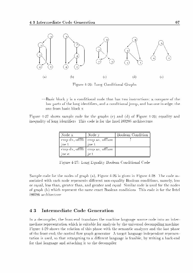
4.3 Intermediate Code Generation 67n nnnn?@@@R ??���x yzte � %nn nn��?@@@Rxy te���nnn nn ��� n (e)n nn nn n�� ???SSSw ��? CCCCCCW@@@R ����� AAAAUxyze t xye t xe t(a) (b) (c) (d)Figure 4-26: Long Conditional Graphs{ Basic block y is a conditional node that has two instructions; a compare of thelow parts of the long identi�ers, and a conditional jump, and has one in-edge; theone from basic block x.Figure 4-27 shows sample code for the graphs (c) and (d) of Figure 4-26; equality andinequality of long identi�ers. This code is for the Intel i80286 architecture.Node x Node y Boolean Conditioncmp dx, o�Hi cmp ax, o�Low ! =jne t jne tcmp dx, o�Hi cmp ax, o�Low ==jne e je tFigure 4-27: Long Equality Boolean Conditional CodeSample code for the nodes of graph (a), Figure 4-26 is given in Figure 4-28. The code as-sociated with each node represents di�erent non-equality Boolean conditions, namely, lessor equal, less than, greater than, and greater and equal. Similar code is used for the nodesof graph (b) which represent the same exact Boolean conditions. This code is for the Inteli80286 architecture.4.3 Intermediate Code GenerationIn a decompiler, the front-end translates the machine language source code into an inter-mediate representation which is suitable for analysis by the universal decompiling machine.Figure 4-29 shows the relation of this phase with the semantic analyzer and the last phaseof the front-end; the control ow graph generator. A target language independent represen-tation is used, so that retargeting to a di�erent language is feasible, by writing a back-endfor that language and attaching it to the decompiler.

68 The Front-endNode x Node y Node z Boolean Conditioncmp dx, o�Hi jg e cmp ax, o�Low <=jl t jbe tcmp dx, o�Hi jne e cmp ax, o�Low <jl t jb tcmp dx, o�Hi jne e cmp ax, o�Low >jg t ja tcmp dx, o�Hi jl e cmp ax, o�Low >=jg t jae tFigure 4-28: Long Non-Equality Boolean Conditional CodejY. . . . . . . . . . . . . . . . . .-. . . . -~ZZZZZ} >�����= - . . . . . . .. . . . . . ...... .....-. . . .. . . . . . . .. . . . . . . ..... ....Parser UDMSymbolIntermediateCodeGenerationAnalyzerSemantic intermediatecode ControlFlow GraphGenerationTableFigure 4-29: Interaction of the Intermediate Code GeneratorA two-step approach is taken for decompilation: a low-level intermediate representation is�rst used to represent the machine language program. Idiom analysis and type propagationcan be done in this representation, as well as generating assembler code from it (i.e. itis an intermediate code suitable for a disassembler, which does not perform high-levelanalysis on the code). This representation is then converted into a high-level intermediaterepresentation that is suitable for high-level language generation. The representation needsto be general enough to generate code for any high-level language.4.3.1 Low-level Intermediate CodeA low-level intermediate representation that resembles the assembler language for themachine that is being decompiled is a good choice of low-level intermediate code, as it ispossible to perform semantic analysis on the code, as well as generate assembler programsfrom it. The intermediate code must have a one instruction for each complete instructionof the machine language. Compound machine instructions must also be represented by oneintermediate instruction. For example, in Figure 4-30, the machine instruction B720 is amov bh,20 intermediate instruction. The machine instruction 2E followed by FFEFC006 (ajmp with a cs segment override) is replaced by a jmp instruction that makes explicit the useof register cs. And �nally, the compound machine instructions F3A4 are equivalent to theassembler instructions rep and movs di,si. These two instructions are represented by theunique intermediate instruction rep_movs, which makes explicit the destination and sourceregisters of the move.

4.3 Intermediate Code Generation 692E F3B720 FFEFC006 A4+mov bh,20 jmp cs:06C0[bx] rep_movs di,siFigure 4-30: Low-level Intermediate Instructions - ExampleImplementation of Low-Level Intermediate CodeThe low-level intermediate representation is implemented in quadruples which make explicitthe operands use in the instruction, as shown in Figure 4-31. The opcode �eld holds thelow-level intermediate opcode, the dest �eld holds the destination operand (i.e. an iden-ti�er), and the src1 and src2 �elds hold the source operands of the instruction. Someinstructions do not use two source operands, so only the src1 �eld is used.opcode src2dest src1Figure 4-31: General Representation of a QuadrupleExample 4 An add bx,3 machine instruction is represented in a quadruple in the follow-ing way: add 3bx bxwhere register bx is source and destination operand, and constant 3 is the second sourceoperand.Example 5 A push cx machine instruction is represented in the following way:HHHsppush cxwhere register cx is the source operand and register sp is the destination operand.4.3.2 High-level Intermediate CodeThree-address code is a generalized form of assembler code for a three-address machine.This intermediate code is most suited for a decompiler, given that the three-address codeis a linearized representation of an abstract syntax tree (AST) of the program. In this way,the complete AST of the program can be reconstructed during the data ow analysis. Athree-address instruction has the general form:x := y op zwhere x, y, and z are identi�ers, and op is an arithmetic or logic operation. The resultaddress is x, and the two operand addresses are y and z.

70 The Front-endTypes of Three-Address StatementsThree-address statements are similar to high-level language statements. Given that the data ow analysis will reconstruct the AST of the program, a three-address instruction is goingto represent not only individual identi�ers, but expressions. An identi�er can be viewed asthe minimal form of an expression. The di�erent types of instructions are:1. asgn <exp>, <arithExp>The asgn instruction assigns an arithmetic expression to an identi�er or an expression(i.e. an identi�er that is represented by an expression, such as indexing into an array).This statement represents three di�erent types of high-level assignment instructions:� x := y op z. Where x, y, and z are identi�ers, and op is a binary arithmeticoperator.� x := op y. Where x and y are identi�ers, and op is a unary arithmetic operator.� x := y. Where x and y are identi�ers.After data ow analysis, the arithmetic expression represents not only a binaryoperation, but holds a complete parse tree of arithmetic operators and identi�ers.This transformation is described in Chapter 5.In this context, a subroutine that returns a value (i.e. a function), is also consideredan identi�er, as its invocation returns a result that is assigned to another identi�er(e.g. a := sum(b,c)).2. jmpThe unconditional jump instruction has no associated expression attached to it, otherthan the target destination address of the jump. This instruction transfers control tothe target address. Since the address is coded in the out-edge of the basic block thatincludes this instruction, it is not explicitly described as part of the instruction. Thisinstruction is equivalent to the high-level instruction:goto Lwhere L is the target address of the jump.3. jcond <boolExp>The conditional jump instruction has a Boolean expression associated with it, whichdetermines whether the branch is taken or not. The Boolean expression is of the formx relop y, where x and y are identi�ers, and relop is a relational operator, such as<;�;=. This statement is equivalent to the high-level statement:if x relop y goto LIn this intermediate instruction, the target branch address (L) and the fall-throughaddress (i.e. address of the next instruction) are not part of the instruction as theseare coded in the out-edges from the basic block that has this instruction in the control ow graph.4. call <procId> <actual parameters>The call instruction represents a subroutine call. The procedure identi�er (<procId>)is a pointer to the ow graph of the invoked procedure. The actual parameter list is

4.3 Intermediate Code Generation 71constructed during data ow analysis. If the subroutine called is a function, it alsode�nes the registers that hold the returned value. In this case, the instruction isequivalent to asgn <regs>, <procId> <actual parameters>.5. ret [<arithExp>]The return instruction determines the end of a procedure along a path. If there isnothing to return, the subroutine is a procedure, otherwise it is a function.There are also two pseudo high-level intermediate instructions that are used as intermediateinstructions in the data ow analysis, but are eliminated by the end of the analysis. Theseinstructions are:1. push <arithExp>The push instruction places the associated arithmetic expression on a temporary stack.2. pop <ident>The pop instruction takes the expression or identi�er at the top of the temporary stackand assigns it to the identi�er ident.Implementation of High-Level Intermediate CodeThe high-level intermediate representation is implemented by triplets. In a triplet, the twoexpressions are made explicit, as well as the instruction opcode, such as shown in Figure 4-32. The result and arg �elds are pointers to an expression, which in its minimal form isan identi�er which points to the symbol table.op argresultFigure 4-32: General Representation of a TripletAn assignment statement x := y op z is represented in a triplet in the following way: theop �eld is the asgn opcode, the result �eld has a pointer to the identi�er x (which in turnhas a pointer to the identi�er in the symbol table), and the arg �eld has a pointer to abinary expression; this expression is represented by an abstract syntax tree with pointersto the symbol table entries of y and z, as follows:? ?��/ op@@RASGN Symbol Tableid1 xid1 id3 zid2 yid2 id3In a similar way, a conditional jump statement if a relop b is represented in a triplet inthe following way: the op �eld is the jcond opcode, the result �eld has a pointer to theabstract syntax tree of the relational test, and the arg �eld is left empty, as follows:

72 The Front-endXXXXX?�� id2@@RJCOND Symbol Tableid2 bid1 arelopid1An unconditional jump statement goto L does not use the result or arg �eld. The op�eld is set to jmp, and the other �elds are left empty, as follows:HHHJMP HHHA procedure call statement procX (a,b) uses the op �eld for the call opcode, the result�eld for the procedure's name, which is pointed to in the symbol table, and the arg �eldfor the procedure arguments, which is a list of arguments that point to the symbol table,as follows: ? ?? ? id3 bCALL id2 id3id1 Symbol Tableid1 procXid2 aA procedure return statement ret a uses the op �eld for the ret opcode, the result �eldfor the identi�er/expression that is being returned, and the arg �eld is left empty, as fol-lows: ? HHH id1 aRET id1 Symbol TableThe pseudo high-level instruction push a is stored in a triplet by using the op �eld as thepush opcode, the arg �eld as the identi�er that is being pushed, and the result �eld isleft empty, as follows: ?id1HHH Symbol Tableid1 aPUSHIn a similar way, the pop a instruction is stored in a triplet, using the op �eld for the popopcode, the result �eld for the identi�er, and eventually (during data ow analysis), thearg �eld is �lled with the expression that is being popped. Initially, this �eld is left empty.The triplet representation is as follows:

4.4 Control Flow Graph Generation 73? HHHPOP id1 Symbol Tableid1 a4.4 Control Flow Graph GenerationThe control ow graph generation phase constructs a call graph of the source program, anda control ow graph of basic blocks for each subroutine of the program. These graphs areused to analyze the program in the universal decompiling machine (UDM) module. Theinteraction of this phase with the intermediate code generator and the udm is shown inFigure 4-33. -. . . . . . . . . . . . .. . . . . . . . ...... .....-. . . .iPPPPPPPq- -. . . . . . . . .. . . . . . . . ...... ..... *��������SymbolSemanticAnalyzer Back-endControl FlowIntermediate UDMCode Generator Graph GeneratorTableFigure 4-33: Interaction of the Control Flow Graph Generator4.4.1 Basic ConceptsThis section describes de�nitions of mathematical and graph theory. These terms are de�nedhere to eliminate any ambiguity of terminology.De�nition 4 A graph G is a tuple (V;E; h) where V is a set of nodes, E is a set of edges,and h is the root of the graph. An edge is a pair of nodes (v;w), with v;w 2 V .De�nition 5 A directed graph G = (N;E; h) is a graph that has directed edges; i.e.each (ni; nj) 2 E has a direction, and is represented by ni ! nj .De�nition 6 A path from n1 to nm in graph G = (N;E; h), represented n1 !� nn, is asequence of edges (n1; n2); (n2; n3); : : : ; (nn�1; nm) 2 N;m � 1.De�nition 7 If G = (V;E; h) is a graph, 9! h 2 V , and E = ;, then G is called a trivialgraph.De�nition 8 If G = (N;E; h) is a graph, and 8n 2 N;h !� n, then G is a connectedgraph.A connected graph is a graph in which all nodes can be reached from the header node. Asample directed, connected graph is shown in Figure 4-34.

74 The Front-endv1 v2

v4

e3

v3

e1

e2 e6

e8

e5

e7

e4Figure 4-34: Sample Directed, Connected GraphGraph RepresentationA graph G = (V;E; h) is represented in several di�erent ways, including, incidence matrices,adjacency matrices, and predecessor-successor tables.De�nition 9 The incidence matrix for a graph G = (V;E; h) is the v � e matrix M(G) =[mij], where mij is the number of times (0, 1 or 2) that vertex vi and edge ej are incident.De�nition 10 The adjacency matrix for a graph G = (V;E; h) is the v � v matrixA(G) = [aij], where aij is the number of edges joining vertices vi and vj.De�nition 11 The predecessor-successor table for a graph G = (V;E; h) is the v � 2 tableT (G) = [ti1; ti2], where ti1 is the list of predecessor vertices of vertex vi, and ti2 is the list ofsuccessor vertices of vertex vi.Example 6 The graph in Figure 4-34 is represented by the following matrices:� Incidence matrix: e1 e2 e3 e4 e5 e6 e7 e8v1 1 1 1 0 0 0 0 0v2 1 0 0 1 1 1 0 0v3 0 1 0 1 0 0 1 2v4 0 0 1 0 1 1 1 0� Adjacency matrix: v1 v2 v3 v4v1 0 1 1 1v2 1 0 1 2v3 1 1 1 1v4 1 2 1 0� Predecessor successor table: Predecessor Successorv1 ; fv2; v3; v4gv2 fv1; v4g fv3; v4gv3 fv1; v2; v3g fv3; v4gv4 fv1; v2; v3g fv2g4.4.2 Basic BlocksIn this section we formalize the de�nition of basic blocks. In order to characterize it, weneed some more de�nitions of program structure. We start by de�ning the componentsof a program, that is, data and instructions. Note that this de�nition does not associateinstructions or data to memory locations.

4.4 Control Flow Graph Generation 75De�nition 12 Let� P be a program� I = fi1; : : : ; ing be the instructions of P� D = fd1; : : : ; dmg be the data of PThen P = I S DFor the purpose of this research, programs are restricted to containing no self-modifyingcode, and make no use of data as instructions or vice versa (I(P )TD(P ) = ;). Aninstruction sequence is a set of instructions physically located one after the other in memory.De�nition 13 Let� P be a program� I = fi1; : : : ; ing be the instructions of PThen S is an instruction sequence if and only ifS = [ij; ij+1; : : : ; ij+k] � 1 � j < j + k � n ^ ij+1 is in a consecutive memory location toij;8 1 � j � k � 1.Intermediate instructions are classi�ed in two sets for the purposes of control ow graphgeneration:� Transfer Instructions (TI): the set of instructions that transfer ow of control toan address in memory di�erent from the address of the next instruction. Theseinstructions are:{ Unconditional jumps: the ow of control is transferred to the target jump address.{ Conditional jumps: the ow of control is transferred to the target jump address ifthe condition is true, otherwise the control is transferred to the next instructionin the sequence.{ Indexed jumps: the ow of control is transferred to one of many target addresses.{ Subroutine call: the ow of control is transferred to the invoked subroutine.{ Subroutine return: the ow of control is transferred to the subroutine that invokedthe subroutine with the return instruction.{ End of program: the program ends.� Non transfer instructions (NTI): the set of instructions that transfer control to thenext instruction in the sequence, i.e. all instructions that do not belong to the TI set.Having classi�ed the intermediate instructions, a basic block is de�ned in terms of itsinstructions:De�nition 14 A basic block b = [i1; : : : ; in�1; in]; n � 1 is an instruction sequence thatsatis�es the following conditions:1. [i1; : : : ; in�1] 2 NTI

76 The Front-end2. in 2 TIor1. [i1; : : : ; in�1; in] 2 NTI2. in+1 is the �rst instruction of another basic block.A basic block is a sequence of instructions that has one entry point and one exit point. Ifone instruction of the basic block is executed, all other instructions are executed as well.The set of instructions of a program can be uniquely partioned into a set of non-overlappingbasic blocks, starting from the program's entry point.De�nition 15 Let� I be the instructions of program P� h be P's entry pointThen 9B = fb1; : : : ; bng � b1T b2 : : :T bn = ; ^ I = b1S b2S : : :S bn ^ b1's entry point = h.4.4.3 Control Flow GraphsA control ow graph is a directed graph that represents the ow of control of a program,thus, it only represents the instructions of such a program. The nodes of this graph representbasic blocks of the program, and the edges represent the ow of control between nodes. Moreformally,De�nition 16 A control ow graph G = (N;E; h) for a program P is a connected,directed graph, that satis�es the following conditions:� 8n 2 N;n represents a basic blocks of P .� 8e = (ni; nj) 2 E; e represents ow of control from one basic block to another andni; nj 2 N .� 9 f : B ! N � 8 bi 2 B; f(bi) = nk for some nk 2 N ^ 69 bj 2 B � f(bj) = nkFor the purpose of control ow graph (cfg) generation, basic blocks are classi�ed intodi�erent types, according to the last instruction of the basic block. The available typesof basic blocks are:� 1-way basic block: the last instruction in the basic block is an unconditional jump.The block has one out-edge.� 2-way basic block: the last instruction is a conditional jump, thus, the block has twoout-edges.� n-way basic block: the last instruction is an indexed jump. The n branches located inthe case table become the n out-edges of this node.

4.4 Control Flow Graph Generation 77� call basic block: the last instruction is a call to a subroutine. There are two out-edgesfrom this block: one to the instruction following the subroutine call (if the subroutinereturns), and the other to the subroutine that is called.� return basic block: the last instruction is a procedure return or an end of program.There are no out-edges from this basic block.� fall basic block: the next instruction is the target address of a branching instruction(i.e. the next instruction has a label). This node is seen as a node that falls throughthe next one, thus, there is only one out-edge.The di�erent types of basic block are represented in a control ow graph by named nodes,as shown in Figure 4-35. Whenever a node is not named in a graph, it means that thetype of the basic block is irrelevant, or obvious from the context (i.e. the exact number ofout-edges are speci�ed in the graph). ���� �������� ���� ����? �� SSw ���= ZZZ~��� SSw?����- ...?1w 2w nwcall ret fall1-way 2-way fall-throughreturncall n-wayFigure 4-35: Node Representation of Di�erent Types of Basic BlocksExample 7 Consider the following fragment of code:0 PUSH bp1 MOV bp, sp2 SUB sp, 43 MOV ax, 0Ah4 MOV [bp-2], ax5 MOV [bp-4], ax6 LEA ax, [bp-4]7 PUSH ax8 CALL near ptr proc_19 POP cx10 L1: MOV ax, [bp-4]11 CMP ax, [bp-2]12 JNE L213 PUSH word ptr [bp-4]14 MOV ax, 0AAh15 PUSH ax16 CALL near ptr printf

78 The Front-end17 POP cx18 POP cx19 MOV sp, bp20 POP bp21 RET22 L2: MOV ax, [bp-4]23 CMP ax, [bp-2]24 JGE L125 LEA ax, [bp-2]26 PUSH ax27 CALL near ptr proc_128 POP cx29 JMP L1This code has the following basic blocks:Basic Block Type Instruction Extentcall 0 to 8fall 92w 10 to 12call 13 to 16ret 17..212w 22..24call 25..271w 28, 29The control ow graph that represents these instructions is shown in Figure 4-36.From here onwards, the word graph is used to represent a control ow graph, and the wordnode is used to represent a basic block, unless otherwise stated.ImplementationControl ow graphs have on average close 2 out edges per node, thus, a matrix repre-sentation (e.g. incident and adjacent matrices) is very sparse and memory ine�cient (i.e.most of the matrix is zero). It is therefore better to implement control ow graphs inpredecessor-successor tables, so that only the existing edges in the graph are representedin this relationship. Note that the successor is all that is needed to represent the completegraph; the predecessor is also stored to make access to the graph easily during di�erenttraversals of the graph.If the size of the graph is unknown (i.e. the number of nodes is not �xed), it is possible toconstruct the graph dynamically as a pointer to a basic block, which has a list of predecessorand a list of successors attached to it. The predecessors and successors are pointers to basicblock nodes as well; in this way, a basic block is only represented once. This representation isplausible in any high-level language that allows dynamic allocation of memory. Consider theC de�nition of a basic block in Figure 4-37. The BB structure de�nes a basic block node,the numInEdges and numOutEdges hold the number of predecessor and successor nodes,

4.4 Control Flow Graph Generation 79$����������������� �������� ��������

��������??��� @@@R %

$�?ret� ??����������7QQQQQQQQQQQs?call proc1printf fall2wcall 2wcall1wFigure 4-36: Control Flow Graph for Example 10respectively, the **inEdges is a dynamically allocated array of pointers to predecessorbasic blocks, and the **outEdges is a dynamically allocated array of pointers to successorbasic blocks. In this representation, a graph is a pointer to the header basic block (i.e. aPBB). typedef struct _BB{byte nodeType; /* Type of node */int numInEdges; /* Number of in edges */struct _BB **inEdges; /* Array of pointers to predecessors */int numOutEdges; /* Number of out-edges */struct _BB **outEdges; /* Array of pointers to successors *//* other fields go here */} BB;typedef BB *PBB; /* Pointer to a basic block */Figure 4-37: Basic Block De�nition in C

80 The Front-endGraph OptimizationOne pass compilers generate machine code that makes use of redundant or unnecessaryjumps in the form of jumps to jumps, conditional jumps to jumps, and jumps to condi-tional jumps. These unnecessary jumps can be eliminated by a peephole optimization on ow-of-control. This optimization is not always used, though.Peephole optimization is a method for improving the performance of the target program byexamining a short sequence of target instructions (called the peephole) and replacing theseinstructions by a shorter or faster sequence of instructions. The peephole is a small, movingwindow of target code; the code in the peephole does not need to be contiguous. Each im-provement made through a peephole optimization may spawn opportunities for additionalimprovements, thus, repeated passes over the code is necessary.Flow-of-control optimization is the method by which redundant jumps are eliminated. Fordecompilation, we are interested in eliminating all jumps to jumps, and conditional jumpsto jumps, as the target jump holds the address of the target branch, and makes use of anintermediate basic blocks that can be removed from the graph. The removal of jumps toconditional jumps is not desired, as it involves the rearrangement of several instructions,not just the modi�cation of one target branch address.The following jump sequence jumps to label Lx to jump to label Ly afterwards, without anyother instructions executed between the jumps:jmp Lx... ; other code hereLx: jmp LyThis sequence is replaced by the sequencejmp Ly... ; other code hereLx: jmp Lywhere the �rst jump branches to the target Ly label, rather than the intermediate Lx label.The number of predecessors to basic block starting at Lx is decremented by one, and thenumber of predecessors to block startin at Ly is incremented by one, to re ect the change ofedges in the graph. If at any one time the number of predecessors to the basic block startingat label Lx becomes zero, the node is removed from the graph because it is unreachable,and thus was unnecessary in the �rst place.In a similar way, an unconditional jump to a jump sequence like the followingjZ Lx... ; other code hereLx: jmp Lyis replaced by the code sequencejZ Ly... ; other code hereLx: jmp Ly

4.4 Control Flow Graph Generation 81The Call GraphThe call graph is a mathematical representation of the subroutines of a program. Eachnode represents a subroutine, and each edge represents a call to another subroutine. Moreformally,De�nition 17 Let P= fp1; p2; : : :g be the �nite set of procedures of a program. A call graphC is a tuple (N;E; h), where N is the set of procedures and ni 2 N represents one and onlyone pi 2 P, E is the set of edges and (ni; nj) 2 E represents one or more references of pito pj, and h is the main procedure.The construction of the call graph is simple if the invoked subroutines are statically boundto subroutine constants, that is, the program does not make use of procedure parametersor procedure variables. The presence of recursion introduces cycles in the call graph. Ane�cient algorithm to construct the call graph in the presence of procedure parameters, forlanguages that do not have recursion is given in [Ryd79]. This method was later extended tosupport recursion, and is explained in [CCHK90]. Finally, a method that handles procedureparameters and a limited type of procedure variables is described in [HK92].It should be noted that this method is not able to reconstruct all graphs to their originalform, as a compiler optimisation could have changed an implicit call instruction into anunconditional jump. In these cases, the call graph (and hence the decompiler) will treat thecode of both subroutines as being one, unless the invoked subroutine is also called elsewherevia an implicit call instruction.

Chapter 5Data Flow AnalysisT he low-level intermediate code generated by the front-end is an assembler-type repre-sentation that makes use of registers and condition codes. This representation can betransformed into a higher level representation that does not make use of such low-levelconcepts, and that regenerates the high-level concept of expression. The transformationof low-level to high-level intermediate code is done by means of program transformations,traditionally referred to as optimizations. These transformations are applied to the low-level intermediate code, to transform it into the high-level intermediate code described inChapter 4, Section 4.3.2. The relation of this phase with the front-end and the control owanalysis phase is shown in Figure 5-1.6?- -yXXXXXXXXXXXXXz -. . . . . . . . . . . . .. . . . . . . . ...... .....Low-levelintermediate code Control FlowAnalysisData FlowSymbolTable Back-endFront-end intermediate codeHigh-level AnalysisFigure 5-1: Context of the Data Flow Analysis PhaseThe types of transformations that are required by the data ow analysis phase include,the elimination of useless instructions, the elimination of condition codes, the determina-tion of register arguments and function return register(s), the elimination of registers andintermediate instructions by the regeneration of expressions, the determination of actualparamaters, and the propagation of data type across subroutine calls. Most of these trans-formations are required to improve the quality of the low-level intermediate code, and toreconstruct some of the information lost during the compilation process. In the case of theelimination of useless instructions, this step is required even for optimising compilers whenthere exist machine instructions that perform more than one function at a time (for anexample, refer to Section 5.2.1).Conventional data ow analysis is the process of collecting information about the wayvariables are used in a program, and summarizing it in the form of sets. This informationis used by the decompiler to transform and improve the quality of the intermediate code.Several properties are required by code-improving transformations, including[ASU86b]:1. A transformation must preserve the meaning of programs.

84 Data Flow Analysis2. A transformation must be worth the e�ort.Techniques for decompilation optimization of the intermediate code are presented in thischapter. The transformations are �rstly illustrated by means of examples, and algorithmsare later provided for each optimization.5.1 Previous WorkNot much work has been done in the area of data ow analysis of a decompiler, mainly due tothe limitations placed on many of the decompilers available in the literature; decompilationof assembler source �les[Hou73, Fri74, Wor78, Bri81], decompilation of object �les withsymbolic debugging information[Reu88], and the compiler speci�cation requirements tobuild a decompiler[BB91, Bow93, BB93]. Data ow analysis is essential when decompilingpure binary �les, as there is no extra information on the way data is used, and the type ofit. The following sections summarize all the work that has been done in this area.5.1.1 Elimination of Condition CodesA program which translates microprocessor object code (i8085) into a behaviorally equiv-alent PL/1 program was described by Marshall and Zobrist[MZBR85], and was used forelectronic system simulation. The �nal PL/1 programs contained a large number of state-ments that de�ned ags, even if these ags were not used or referenced later on the program.This prompted DeJean and Zobrist to formulate an optimization of ag de�nitions by meansof a reach algorithm[DZ89]. This method eliminated over 50% of the ag de�nitions in thetranslation process, generating PL/1 programs that de�ned only the necessary ags for alater condition.The method presented in this thesis goes beyond this optimization of ag de�nitions, in thatit not only determines which ag de�nitions are extraneous and therefore unnecessary, butalso determines which Boolean conditional expression is represented by the combined set ofinstructions that de�ne and use the ag. In this way, the target HLL program does not relyon the use and concept of ags, as any real HLL program does not.5.1.2 Elimination of Redundant Loads and StoresA method of text compression was presented by Housel[Hou73] for the elimination of inter-mediate loads and stores. This method works on a 3-address intermediate representation ofthe program, and consists of two stages: forward-substitution and backward-substitution.The former stage substitutes the source operand of an assignment instruction into a subse-quent instruction that uses the same result operand, if the result is found to be not busywithin the same basic block. The latter stage substitutes the result operand of an assign-ment instruction into a previous instruction (other than an assignment instruction) thatde�nes as result operand the source operand of the assignment instruction under consid-eration. This method provided a reduction of instruction of up to 40% in assembly codecompiled by Knuth's MIXAL compiler.

5.2 Types of Optimizations 85A method of expression condensation was described by Hopwood[Hop78] to combine 2 ormore intermediate instructions into an equivalent expression by means of forward substitu-tion. This method speci�es 5 necessary conditions and 6 su�cient conditions under whichforward substitution of a variable or register can be performed. This method was based onvariable usage analysis. The great number of conditions is inherent to the choice of control ow graph: one node per intermediate instruction, rather than basic blocks. This meantthat variables were forward substituted across node boundaries, making the whole processmuch more complex than required.The interprocedural data ow analyses presented in this thesis de�ne two su�cient condi-tions under which a register can be substituted or replaced into another instruction, includingsuch intermediate instructions as push and pop. This method not only �nds expressions byeliminating intermediate registers and instruction de�nitions, but also determines actualparameters of subroutines, values returned from functions, and eliminates pseudo high-levelinstructions. The method is based on the initial high-level intermediate representation ofthe binary program, which is semantically equivalent to the low-level intermediate represen-tation, and transforms it into a HLL representation.5.2 Types of OptimizationsThis section presents the code-improving transformations used by a decompiler. The tech-niques used to implement these transformations are explained in Sections 5.3 and 5.4. Theoptimizations presented in this section make use of the example ow graph in Figure 5-2,where basic blocks B1 : : : B4 belong to the main program, and blocks B5 : : : B7 belongto the subroutine _aNlshl (a runtime support routine). In the main program, registers siand di are used as register variables, and have been agged by the parser as possibly beingso (see Chapter 4, Section 4.2.1).The aim of these optimizations is to eliminate the low-level language concepts of conditioncodes, registers, and intermediate instructions, and introduce the high-level concept ofexpressions of more than two operands. For this purpose, it is noted that push instructionsare used in a variety of ways by today's compilers. Parameter passing is the most commonuse of this instruction, by pushing them before the subroutine call, in the order speci�edby the calling convention in use. Register spilling is used whenever the compiler runs outof registers to compute an expression. push and pop are also used to preserve the contentsof registers across procedure calls, and to copy values into registers.5.2.1 Dead-Register EliminationAn identi�er is dead at a point in a program if its value is not used following the de�nitionof the variable. It is said that the instruction that de�nes a dead identi�er is useless, andthus can be eliminated or removed from the code. Consider the following code from basicblock B1, Figure 5-2:6 ax = tmp / di7 dx = tmp % di8 dx = 39 dx:ax = ax * dx

86 Data Flow Analysis

?XXXXXXXXXz

?-�����9? ?�����9

XXXXXz B5B6 B7aNlshl1 si = 202 di = 803 ax = si4 dx:ax = ax5 tmp = dx:ax6 ax = tmp / di7 dx = tmp % di8 dx = 39 dx:ax = ax * dx10 si = ax

���11 [bp-6]:[bp-8] = 4000

38 ret14 cmp [bp-6]:[bp-8], dx:ax15 jg B213 dx:ax = [bp-2]:[bp-4]12 [bp-2]:[bp-4] = 2000

B116 dx:ax = [bp-6]:[bp-8]17 dx:ax = dx:ax - [bp-2]:[bp-4]18 [bp-6]:[bp-8] = dx:ax19 cx = 420 dx:ax = [bp-6]:[bp-8]21 call aNlshl24 push [bp-6]:[bp-8]25 ax = si26 dx = 527 dx:ax = ax * dx28 push ax29 ax = 6630 push ax31 call printf32 ret 22 [bp-6]:[bp-8] = dx:ax23 jmp B4 B2B3B4 33 ch = 034 jcxz B735 dx:ax = dx:ax << 136 cx = cx - 137 jncxz B6

Figure 5-2: Sample Flow Graph10 si = axInstruction 6 de�nes register ax, instruction 7 de�nes register dx, and instruction 8 rede�nesregister dx. There is no use of register dx between the de�nition at instruction 7 andinstruction 8, thus, the de�nition of register dx at instruction 7 is dead, and this instructionbecomes useless since it de�nes only register dx. The previous sequence of instructions isreplaced by the following code:6 ax = tmp / di8 dx = 39 dx:ax = ax * dx10 si = axThe de�nition of register dx at instruction 8 is used in the multiplication of instruction 9,where the register is rede�ned, as well as register ax. Instruction 10 uses register ax, and

5.2 Types of Optimizations 87there are no further uses of register dx before rede�nition of this register at instruction 13,thus, this last de�nition of dx is dead and must be eliminated. Since instruction 9 de�nesnot only dx but also ax, and ax is not dead, the instruction is not useless as it still de�nesa live register; therefore, the instruction is modi�ed to re ect the fact that only register axis de�ned, as follows:6 ax = tmp / di8 dx = 39 ax = ax * dx10 si = ax5.2.2 Dead-Condition Code EliminationIn a similar way to dead-register elimination, a condition code is dead at a point in a programif its value is not used before rede�nition. In this case, the de�nition of the condition codeis useless, and is not required, but the instruction that de�nes this condition code is stilluseful if the identi�ers that the instruction de�nes are not dead, hence, the instruction itselfis not necessarily eliminated. Consider the following code from basic block B1, Figure 5-2:14 cmp [bp-6]:[bp-8], dx:ax ; cc-def = ZF, CF, SF15 jg B2 ; cc-use = SFInstruction 14 de�nes the condition codes zero (ZF), carry (CF) and sign (SF). Instruction15 uses the sign condition code. Neither of the following two basic blocks make use ofthe condition codes carry or zero before rede�nition, thus, the de�nition of these conditioncodes in instruction 14 is useless and can be eliminated. We replace the information ofinstruction 14 to hold the following information:14 cmp [bp-6]:[bp-8], dx:ax ; cc-def = SF5.2.3 Condition Code PropagationCondition codes are ags used by the machine to signal the occurrence of a condition. Ingeneral, several machine instructions set these ags, ranging from 1 to 3 di�erent ags beingset by the one instruction, and fewer instructions make use of those ags, only using 1 or2 ags. After dead-condition code elimination, the excess de�nitions of condition codesare eliminated, thus, all remaining ags are used by subsequent instructions. Consider thefollowing code from basic block B1, Figure 5-2 after dead-condition code elimination:14 cmp [bp-6]:[bp-8], dx:ax ; cc-def = SF15 jg B2 ; cc-use = SFInstruction 14 de�nes the sign ag by comparing two operands, and instruction 15 usesthis ag to determine whether the �rst operand of the previous instruction was greaterthan the second operand. These two instructions are functionally equivalent to a high-level conditional jump instruction that checks for an operand being greater than a secondoperand. The instructions can be replaced by:15 jcond ([bp-6]:[bp-8] > dx:ax) B2eliminating instruction 14 and all references to the condition codes.

88 Data Flow Analysis5.2.4 Register ArgumentsSubroutines use register arguments to speed the access to those arguments and remove theoverhead placed by the pushing of arguments on the stack before subroutine invocation.Register arguments are used by many runtime support routines, and by user routinescompiled with the register calling convention (available in some compilers). Consider thefollowing code of basic block B2, Figure 5-2:19 cx = 4 ; def = {cx}20 dx:ax = [bp-6]:[bp-8] ; def = {dx, ax}21 call _aNlshlInstruction 19 de�nes register cx, instruction 20 de�nes registers dx:ax , and instruction21 invokes the subroutine _aNlshl. The �rst basic block of the subroutine _aNlshl, B5 inFigure 5-2, uses register cx after de�ning the high part of this register (i.e. register ch),thus, the low part of this register (i.e. register cl) contains whatever value the register hadbefore the subroutine was invoked. In a similar way, basic block B6 uses registers dx:axbefore they are de�ned within the subroutine, thus, the values of these registers beforesubroutine invocation are used. These three registers are used before being de�ned in thesubroutine, and are de�ned by the caller, thus, they are register arguments to the _aNlshlsubroutine. The formal argument list of this subroutine is modi�ed to re ect this fact:formal_arguments(_aNlshl) = {arg1 = dx:ax, arg2 = cl}Within the subroutine, these registers are replaced by their formal argument name.5.2.5 Function Return Register(s)Subroutines that return a value are called functions. Functions usually return values inregisters, and these registers are then used by the caller subroutine. Consider the followingcode from basic blocks B2 and B3, Figure 5-2:20 dx:ax = [bp-6]:[bp-8] ; def = {dx, ax} use = {}21 call _aNlshl ; def = {} use = {dx, ax, cl}22 [bp-6]:[bp-8] = dx:ax ; def = {} use = {dx, ax}Instruction 21 invokes the subroutine _aNlshl. After subroutine return, instruction 22uses registers dx:ax. These registers have been de�ned in the previous basic block atinstruction 20, but since there is a subroutine invocation in between these two instructions,the subroutine needs to be checked for any modi�cation(s) to registers dx:ax. Consider thecode of basic block B6, Figure 5-2 after dead-register elimination:35 dx:ax = dx:ax << 136 cx = cx - 137 jcond (cx <> 0) B6Recall from Section 5.2.4 that dx:ax are register arguments. These registers are modi�edin instruction 35 by a shift left. Actually, they form part of a loop as instruction 37 jumpsback to the initial instruction 35 if register cx is not equal to zero. After the loop is �nished,the ow of control is transfered to basic block B7, which returns from this subroutine. Thereference to registers dx:ax in instruction 22 are the modi�ed versions of these registers. Wecan think of subroutine _aNlshl as a function that returns both these registers, so the callto function _aNlshl in instruction 21 is replaced by:

5.2 Types of Optimizations 8921 dx:ax = call _aNlshl ; def = {dx, ax} use = {dx, ax, cl}Instruction 22 uses the two registers de�ned in instruction 21, so, by register copypropagation, we arrive to the following code:22 [bp-6]:[bp-8] = call _aNlshlThe return instruction of the function _aNlshl (instruction 38) is modi�ed to return theregisters dx:ax, leading to the following code:38 ret dx:ax5.2.6 Register Copy PropagationAn instruction is intermediate if it de�nes a register value that is used by a uniquesubsequent instruction. In machine language, intermediate instructions are used to movethe contents of operands into registers, move the operands of an instruction into the registersthat are used by a particular instruction, and to store the computed result in registers to alocal variable. Consider the following code from basic block B2, Figure 5-2:16 dx:ax = [bp-6]:[bp-8] ; def = {dx, ax} use = {}17 dx:ax = dx:ax - [bp-2]:[bp-4] ; def = {dx, ax} use = {dx, ax}18 [bp-6]:[bp-8] = dx:ax ; def = {} use = {dx, ax}Instruction 16 de�nes the long register dx:ax by copying the contents of the long localvariable at bp-6. This long register is then used in instruction 17 as an operand of asubtraction. The result is placed in the same long register, which is then copied to the longlocal variable at bp-6 in instruction 18. As seen, instruction 16 de�nes the temporary longregister dx:ax to be used in instruction 17, and this instruction rede�nes the register, and isthen copied to the �nal local variable in instruction 18. These intermediate registers can beeliminated by replacing them with the local variable that was used to de�ne them, thus, ininstruction 17, registers dx:ax are replaced by the long local variable at bp-6 which de�nedthese registers in the previous instruction:17 dx:ax = [bp-6]:[bp-8] - [bp-2]:[bp-4]and instruction 16 is removed. In a similar way, the resultant long register dx:ax frominstruction 17 is replaced in instruction 18, leading to the following code:18 [bp-6]:[bp-8] = [bp-6]:[bp-8] - [bp-2]:[bp-4]and instruction 17 is eliminated. The �nal instruction 18 is a reconstruction of the originalhigh-level expression.High-level language expressions are represented by parse trees of one or more operands,whereas machine language expressions allow only for at most two operands. In most cases,one of these operands needs to be in a register(s), and the result is also placed in a register(s).The �nal result is then copied to the appropriate identi�er (i.e. local variable, argument,global variable). Consider the following code from basic block B1, Figure 5-2 after dead-register elimination:

90 Data Flow Analysis3 ax = si ; def = {ax} use = {}4 dx:ax = ax ; def = {dx, ax} use = {ax}5 tmp = dx:ax ; def = {tmp} use = {dx, ax}6 ax = tmp / di ; def = {ax} use = {tmp}8 dx = 3 ; def = {dx} use = {}9 ax = ax * dx ; def = {ax} use = {ax, dx}10 si = ax ; def = {} use = {ax}Instruction 3 de�nes register ax by copying the contents of the integer register variablesi. Register variables are treated as local variables rather than registers in this context.Instruction 4 uses register ax to de�ne register dx by sign extension of register ax.Instruction 5 then uses these sign-extended registers to copy them to register tmp, whichis used in instruction 6 as the dividend of a divide instruction. The local integer registervariable di is used as the divisor, and the result is placed on register ax. This result isused in the multiplication in instruction 9, which also uses register dx and rede�nes registerax. Finally, the result is placed on the local register variable si. As seen, most of theseinstructions can be folded into a subsequent instruction, eliminatingmost of them as follows:instruction 3 is replaced into instruction 4, leading to:4 dx:ax = siand instruction 3 is eliminated. Instruction 4 is replaced into instruction 5, leading to:5 tmp = siand instruction 4 is eliminated. Instruction 5 is replaced into instruction 6, leading to:6 ax = si / diand instruction 5 is eliminated. Instruction 6 is replaced into instruction 9, leading to:9 ax = (si / di) * dxand instruction 6 is eliminated. Instruction 7 is replaced into instruction 9, leading to:9 ax = (si / di) * 3and instruction 7 is eliminated. Finally, instruction 9 is replaced into instruction 10, leadingto the following �nal code:10 si = (si / di) * 3This �nal instruction 10 replaces all previous instructions 3 : : : 10.5.2.7 Actual ParametersActual parameters to a subroutine call are either pushed on the stack or placed on registers(for register arguments) before the subroutine is invoked. These arguments can be mappedagainst the formal argument list of the subroutine, and placed in the actual parameter listof the call instruction. Consider the following code from basic block B4, Figure 5-2 afterregister copy propagation:24 push [bp-6]:[bp-8]28 push (si * 5)30 push 6631 call printf

5.2 Types of Optimizations 91After parsing, the formal argument list of printf has one �xed argument of size 2 bytes, anda variable number of other arguments. The calling convention used for this procedure hasbeen set to C. Instruction 31 has also saved the information regarding the number of bytespopped from the stack after subroutine call: 8 bytes in this case, thus, there are 8 bytesof actual arguments for this subroutine; the �rst 2 bytes are �xed. Instruction 24 pushes4 bytes on the stack, instruction 28 pushes 2 bytes on the stack, and instruction 30 pushesanother 2 bytes on the stack, for a total of 8 bytes required by printf in this instance.These identi�ers can be replaced on the actual argument list of printf at instruction 31,in reverse order due to the C calling convention (i.e. last instruction pushed is the �rst onein the argument list). The modi�cations lead to the following code:31 call printf (66, si * 5, [bp-6]:[bp-8])and instructions 24, 28 and 30 are eliminated.In a similar way, register arguments are placed on the actual argument list of the invokedsubroutine. Consider the following code of basic blocks B2 and B3, Figure 5-2 after registerargument and function return register detection and dead-register elimination:19 cl = 4 ; def = {cl}20 dx:ax = [bp-6]:[bp-8] ; def = {dx, ax}22 [bp-6]:[bp-8] = call _aNlshl ; use = {dx, ax, cl}Instruction 19 and 20 de�ne the register arguments used by function _aNlshl, the associatedregister de�nitions are placed in the function's actual argument list in the following way:22 [bp-6]:[bp-8] = call _aNlshl ([bp-6]:[bp-8], 4)eliminating instructions 19 and 20, and intermediate registers dx, ax, and cl.5.2.8 Data Type Propagation Across Procedure CallsThe type of the actual arguments of a subroutine needs to be the same as the type of theformal arguments. In the case of library subroutines, the formal argument types are knownwith certainty, and thus, these types need to be matched against the actual types. If thereare any di�erences, the formal type is to be propagated to the actual argument. Considerthe following code from basic block B4, Figure 5-2 after register copy propagation and thedetection of actual parameters:31 call printf (66, si * 5, [bp-6]:[bp-8])The �rst formal argument type of printf is a string (i.e. a char * in C). Strings arestored in machine language as data constants in the data or code segment. These stringsare referenced by accessing the desired segment and an o�set within that segment. In ourexample, 66 is a constant, and since it is the �rst argument to printf it is really an o�set toa string located in the data segment. The string type is propagated to this �rst argument,the string is found in memory, and replaced in the actual argument list, leading to thefollowing code:31 call printf ("c * 5 = %d, a = %ld\n", si * 5, [bp-6]:[bp-8])All other arguments to printf have undetermined type from the point of view of the formalargument list, so the types that the actual arguments have are trusted (i.e. the types usedin the caller) and are not modi�ed.

92 Data Flow Analysis5.2.9 Register Variable EliminationThe register copy propagation optimization �nds high-level expressions and eliminatesintermediate instructions by eliminating most of the intermediate registers used in thecomputation of the expression, as seen in Section 5.2.6. After this optimization has beenapplied, there are only a few registers left (if any) in the intermediate code. These remainingregisters represent register variables or common subexpressions, used by the compiler orthe optimizer to speed up access time. These registers are equivalent to local variables in ahigh-level program, and are therefore replaced by new local variables in the correspondingsubroutine that uses them. Consider the following code from basic block B1, Figure 5-2after register copy propagation:1 si = 202 di = 8010 si = si / di * 3Registers si and di are used as register variables in this procedure. These registers areinitialized in instructions 1 and 2, and are later used in the expression of instruction 10.Let us rename register si by loc1 and register di by loc2, then the previous code wouldlook like:1 loc1 = 202 loc2 = 8010 loc1 = loc1 / loc2 * 3and all references to registers have been eliminated.After applying all of the previously explained transformations, the �nal intermediate codefor Figure 5-2 is shown in Figure 5-3.5.3 Global Data Flow AnalysisIn order to perform code-improving transformations on the intermediate code, the decom-piler needs to collect information on registers and condition codes about the whole program,and propagate this information across the di�erent basic blocks. The information is collectedby a data ow analysis process, which solves systems of equations that relate informationat various points in the program. This section de�nes data ow problems and equationsavailable in the literature; refer to [All72, AC76, ASU86b, FJ88b] for more information.5.3.1 Data Flow Analysis De�nitionsDe�nition 18 A register is de�ned if the content of the register is modi�ed (i.e. it isassigned a new value). In a similar way, a ag is de�ned if it is modi�ed by an instruction.De�nition 19 A register is used if the register is referenced (i.e. the value of the registeris used). In a similar way, a ag is used if it is referenced by an instruction.De�nition 20 A locally available de�nition d in a basic block Bi is the last de�nitionof d in Bi.

5.3 Global Data Flow Analysis 93? - ?���������9XXXXXXXz�������9 XXXXXXz

?[bp-6]:[bp-8] = 4000[bp-6]:[bp8] = aNlshl ([bp-6]:[bp-8], 4) arg1 = arg1 << 1arg2 = arg2 - 1 ���jcond (arg2 <> 0) B6ret arg2 = arg2 & 0x00FFjcond (arg2 = 0) B7loc1 = 20loc2 = 80loc1 = (loc1 / loc2) * 3 B1 B2B4 B5B6 B7ret arg2[bp-2]:[bp-4] = 2000jcond ([bp-6]:[bp-8] > [bp-2]:[bp-4]) B2[bp-6]:[bp-8] = [bp-6]:[bp-8] - [bp-2]:[bp-4]printf ("c * 5 = %d, a = %ld n",loc1 * 5, [bp-6]:[bp-8])Figure 5-3: Flow graph After Code OptimizationDe�nition 21 A locally upwards exposed use u in a basic block Bi is a use which hasnot been previously de�ned in Bi.De�nition 22 A de�nition d in basic block Bi reaches basic block Bj if 11. d is a locally available de�nition from Bi.2. 9Bi ! Bj .3. 9Bi ! Bj � 8Bk 2 (Bi ! Bj); k 6= i ^ k 6= j;Bk does not rede�ne d.De�nition 23 Any de�nition of a register/ ag in a basic block Bi is said to kill allde�nitions of the same register/ ag that reach Bi.De�nition 24 A de�nition d in a basic block Bi is preserved if d is not rede�ned in Bi.De�nition 25 The de�nitions available at the exit of a basic block Bi are either:1. The locally available de�nitions of the register/ ag.2. The de�nitions of the register/ ag reaching Bi.De�nition 26 A use u of a register/ ag is upwards exposed in a basic block Bi if either:1. u is locally upwards exposed from Bi.2. 9Bi ! Bk � u is locally upwards exposed from Bk ^ 6 9Bj ; i � j < k, which contains ade�nition of u.1The symbol ! is used in this Chapter to represent a path. This symbol is de�ned in Chapter 6,Section 6.3.1.

94 Data Flow AnalysisDe�nition 27 A de�nition d is live or active at basic block Bi if:1. d reaches Bi2. There is an upwards exposed use of d at Bi.De�nition 28 A de�nition d in basic block Bi is busy (sometimes called very busy) if dis used before being rede�ned along all paths from Bi.De�nition 29 A de�nition d in basic block Bi is dead if d is not used before being rede�nedalong all paths from Bi (i.e. d is not busy or live).De�nition 30 A de�nition-use chain (du-chain) for a de�nition d at instruction i isthe set of instructions j where d could be used before being rede�ned (i.e. the instructionswhich can be a�ected by d).De�nition 31 A use-de�nition chain (ud-chain) for a use u at instruction j is the setof instructions i where u was de�ned (i.e. the statements which can a�ect u).De�nition 32 A path is d-clear if there is no de�nition of d along that path.5.3.2 Taxonomy of Data Flow ProblemsData ow problems are solved by a series of equations that uses information collected ineach basic block, and propagates it across the complete control ow graph. Informationpropagated within the ow graph of a procedure is called intraprocedural data ow anal-ysis, and information propagated across procedure calls is called interprocedural data ow analysis.Information on registers de�ned or killed is collected from within the basic block in the formof sets (e.g. gen() and kill()), and is then summarized at basic block entrance and exit inthe form of sets (e.g. in() and out() sets). A typical data ow equation for basic block Bihas the following form: out(Bi) = gen(Bi) [ (in(Bi)� kill(Bi))and stands for \the information at the end of basic block Bi is either the informationgenerated on Bi, or the information that entered the basic block and was not killed withinthe basic block". The summary in() information is collected from the predecessor nodes ofthe graph, by an equation of the form:in(Bi) = [p2Pred(Bi)out(p)which collects information that is available at the exit of any predecessor node. This data ow problem is classi�ed as an any-path problem, since the information collected from pre-decessors is derived from any path (i.e. not all paths need to have the same information).Any-path problems are represented in equations by a union of predecessors or successors,depending on the problem.In a similar way, an all-paths problem is a data ow problem that is speci�ed by an equationthat collects information available in all paths from the current basic block to the successorsor predecessors, depending on the type of problem.

5.3 Global Data Flow Analysis 95De�nition 33 A data ow problem is said to be forward- ow if1. The out() set is computed in terms of the in() set within the same basic block.2. The in() set is computed from the out() set of predecessor basic blocks.De�nition 34 A data ow problem is said to be backward- ow if1. The in() set is computed in terms of the out() set within the same basic block.2. The out() set is computed from the in() set of successor basic blocks.This classi�cation of data ow problems derives the taxonomy shown in Figure 5-4. Foreach forward- and backward- ow problem, all-path and any-path equations are de�ned interms of successors and predecessors. This table is taken from [FJ88b].Forward-Flow Backward-FlowAny Out(Bi) = Gen(Bi) [ (In(Bi) - Kill(Bi)) In(Bi) = Gen(Bi) [ (Out(Bi) - Kill(Bi))path In(Bi) = [p2Pred(Bi) Out(p) Out(Bi) = [s2Succ(Bi) In(s)All Out(Bi) = Gen(Bi) [ (In(Bi) - Kill(Bi)) In(Bi) = Gen(Bi) [ (Out(Bi) - Kill(Bi))paths In(Bi) = \p2Pred(Bi) Out(p) Out(Bi) = \s2Succ(Bi) In(s)Figure 5-4: Data Flow Analysis EquationsData Flow EquationsData ow equations do not, in general, have unique solutions; but in data ow problemseither the minimum or maximum �xed-point solution that satis�es the equations is the oneof interest. Finding this solution is done by setting a boundary condition on the initialvalue of the in(B) set of the header basic block for forward- ow problems, and the valueof the out(B) set of the exit basic block for backward- ow problems. Depending on theinterpretation of the problem, these boundary condition sets are initialized to the empty orthe universal set (i.e. all possible values).Intraprocedural data ow problems solve equations for a subroutine without taking intoaccount the values used or de�ned by other subroutines. As these problems are ow in-sensitive, the boundary conditions are set for all initial (for forward- ow problems) or allexit (for backward- ow problems) nodes. Interprocedural data ow problems solve equa-tions for the subroutines of a program taking into account values use or de�ned by invokedsubroutines. Information ows between subroutines of the call graph. These ow sensi-tive problems set the boundary condition only for the main subroutine of the program'scall graph, all other subroutines summarize information from all predecessor (in the case offorward- ow problems) or all successor (for backward- ow problems) nodes in the call graph(i.e. the caller node). This section presents data ow equations used to solve reaching, live,available, and busy registers.The reaching register de�nition analysis determines which registers reach a particular basicblock along some path, thus, the following forward- ow, any-path equations are used:

96 Data Flow AnalysisDe�nition 35 Let� Bi be a basic block� ReachIn(Bi) be the set of registers that reach the entrance to Bi� ReachOut(Bi) be the set of registers that reach the exit from Bi� Kill(Bi) be the set of registers killed in Bi� Def(Bi) be the set of registers de�ned in BiThen ReachIn(Bi) = ( Sp2Pred(Bi)ReachOut(p) if Bi is not the header node; otherwiseReachOut(Bi) = Def(Bi) [ (ReachIn(Bi)�Kill(Bi))Live register analysis determines whether a register is to be used along some path, thus,the following backward- ow, any-path equations are used:De�nition 36 Let� Bi be a basic block� LiveIn(Bi) be the set of registers that are live on entrance to Bi� LiveOut(Bi) be the set of registers that are live on exit from Bi� Use(Bi) be the set of registers used in Bi� Def(Bi) be the set of registers de�ned in BiThen LiveOut(Bi) = ( Ss2Succ(Bi) LiveIn(s) if Bi is not a return node; otherwiseLiveIn(Bi) = Use(Bi) [ (LiveOut(Bi)�Def(Bi))Available register analysis determines which registers are available along all paths of thegraph, thus, the following forward- ow, all-paths equations are used:De�nition 37 Let� Bi be a basic block� AvailIn(Bi) be the set of the registers that are available on entrance to Bi� AvailOut(Bi) be the set of the registers that are available on exit from Bi� Compute(Bi) be the set of the registers in Bi computed and not killed� Kill(Bi) be the set of the registers in Bi that are killed due to an assignment

5.3 Global Data Flow Analysis 97Then AvailIn(Bi) = ( Tp2Pred(Bi)AvailOut(p) if Bi is not the header node; otherwiseAvailOut(Bi) = Compute(Bi) [ (AvailIn(Bi)�Kill(Bi))Busy register analysis determines which registers are busy along all paths of the graph,thus, the following backward- ow, all-paths equations are used:De�nition 38 Let� Bi be a basic block� BusyIn(Bi) be the set of the registers that are busy on entrance to Bi� BusyOut(Bi) be the set of the registers that are busy on exit from Bi� Use(Bi) be the set of the registers that are used before killed in Bi� Kill(Bi) be the set of the registers that are killed before used in BiThen BusyOut(Bi) = ( Ts2Succ(Bi)BusyIn(s) if Bi is not a return node; otherwiseBusyIn(Bi) = Use(Bi) [ (BusyOut(Bi)�Kill(Bi))The problem of �nding the uses of a register de�nition, i.e. a du-chain problem, is solvedby a backward- ow, any-path problem. Similarly, the problem of �nding all de�nitions fora use of a register, i.e. a ud-chain problem, is solved by a forward- ow, any-path problem.The previous data ow problems are summarized in the table in Figure 5-5.Forward-Flow Backward-FlowAny-path Reach Liveud-chains du-chainsAll-path Available BusyCopy propagation DeadFigure 5-5: Data Flow Problems - SummaryRecently, precise interprocedural live variable equations were presented as part of a codeoptimization at link-time system [SW93]. A two-phase approach is used in order to removeinformation propagation across unrelated subroutines that call the same other subroutine.The call graph has two nodes for each call node; the call node as such, which has an out-edgeto the header node of the callee subroutine, and the ret call node, which has an in-edge fromthe return node of the callee subroutine. In the �rst phase, information ows across normalnodes and call edges only; return edges are removed from the call graph. In the secondphase, information ows across normal nodes and return edges only; call edges are removed

98 Data Flow Analysisfrom the call graph. This phase makes use of the summary information calculated in the�rst phase. Because the information ows from the caller to the callee, and viceversa, thismethod provides a more precise information than other methods presented in the literature.De�nition 39 presents the equations used for precise interprocedural register analysis.Live and dead register equations are solved for the �rst phase, and summarized for eachsubroutine of the call graph in the PUse() and PDef() sets. Since live register equationsare also solved in the second phase, these equations have been associated with the phasenumber to di�erentiate them (e.g. LiveIn1() for the �rst phase, and LiveIn2() for the secondphase). Separate equations are given for call, and ret call basic blocks. The initial boundaryconditions for both live and dead equations is the empty set.De�nition 39 Let� Bi be a basic block other than call and ret call� LiveIn1(Bj) be the set of registers that are live on entrace to Bj during phase one� LiveOut1(Bj) be the set of registers that are live on exit from Bj during phase one� DeadIn(Bj) be the set of registers that have been killed on entrance to Bj� DeadOut(Bj) be the set of registers that have been killed on exit from Bj� Use(Bj) be the set of registers used in Bj� Def(Bj) be the set of registers de�ned in Bj� LiveIn2(Bj) be the set of registers that are live on entrace to Bj during phase two� LiveOut2(Bj) be the set of registers that are live on exit from Bj during phase twoThen precise interprocedural live register analysis is calculated as follows:� Phase 1:LiveOut1(Bi) = ( Ss2Succ(Bi) LiveIn1(s) if Bi is not a return node; otherwiseLiveIn1(Bi) = Use(Bi) [ (LiveOut1(Bi)�Def(Bi))DeadOut(Bi) = ( Ts2Succ(Bi)DeadIn(s) if Bi is not a return node; otherwiseDeadIn(Bi) = Def(Bi) [ (DeadOut(Bi)� Use(Bi))LiveOut1(ret call) = [s2Succ(ret call)LiveIn1(s)LiveIn1(ret call) = LiveOut1(ret call)LiveOut1(call) = LiveIn1(entry) [ (LiveOut1(ret call) �DeadIn(entry))LiveIn1(call) = LiveOut1(call)DeadOut(ret call) = \s2Succ(ret call)DeadIn(s)DeadIn(ret call) = DeadOut(ret call)DeadOut(call) = DeadIn(entry) [ (DeadOut(ret call) � LiveIn1(entry))DeadIn(call) = DeadOut(call)

5.3 Global Data Flow Analysis 99� Subroutine summary: 8p subroutine,PUse(p) = LiveIn1(entry)PDef(p) = DeadIn1(entry)� Phase 2:LiveOut2(Bi) = ( Ss2Succ(Bi) LiveIn2(s) if Bi is not the return node of main; otherwiseLiveIn2(Bi) = Use(Bi) [ (LiveOut2(Bi)�Def(Bi))LiveOut2(ret call) = [s2Succ(ret call)LiveIn2(s)LiveIn2(ret call) = LiveOut2(ret call)LiveOut2(call) = PUse(p) [ (LiveOut2(ret call) � PDef(p))LiveIn2(call) = LiveOut2(call)ret

ret

def dxdef bx

ret

def ax

1

2

4

5

7

9 10

11

12

13

14

15

8

mainP1

6

3

call

call

def dx

P2

use ax

call

def ax

use cx

def cx

16

use dx

use axuse bx

ret_call

ret_call

ret_call

Figure 5-6: Live Register Example GraphExample 8 Consider the call graph of Figure 5-6. This program has a main procedure andtwo subroutines. Interprocedural live register analysis, as explained in De�nition 39 providesthe following summary information for its nodes:

100 Data Flow Analysis� Phase 1:Subroutine Node Def Use LiveIn1 LiveOut1 DeadIn DeadOutP1 12 ; ; ; ; ; ;11 ; fcxg fcxg ; ; ;10 fax,cxg ; ; fcxg fax,cxg ;9 faxg ; ; ; faxg ;8 ; fdxg fdxg ; faxg faxgP2 16 ; faxg faxg ; ; ;15 ; ; faxg faxg ; ;14 ; ; fdxg fdxg faxg faxg13 fdxg ; ; fdxg fax,dxg faxgmain 7 ; ; ; ; ; ;6 ; ; ; ; ; ;5 ; ; ; ; fax,dxg fax,dxg4 ; fax,bxg fax,bxg ; fdxg fax,dxg3 ; ; fax,bxg fax,bxg fdxg fdxg2 ; ; fbx,dxg fbx,dxg faxg faxg1 fbx,dxg ; ; fbx,dxg fax,bx,dxg faxg� Subroutine summary:Subroutine PUse PDefP1 fdxg faxgP2 ; fax,dxgmain ; fax,bx,dxg� Phase 2:Subroutine Node Def Use LiveIn2 LiveOut2P1 12 ; ; fax,bxg fax,bxg11 ; fcxg fax,bx,cxg fax,bxg10 fax,cxg ; fbxg fax,bx,cxg9 faxg ; fbxg fax,bxg8 ; fdxg fbx,dxg fbxgP2 16 ; faxg faxg ;15 ; ; faxg faxg14 ; ; fdxg fdxg13 fdxg ; ; fdxgmain 7 ; ; ; ;6 ; ; ; ;5 ; ; ; ;4 ; fax,bxg fax,bxg ;3 ; ; fax,bxg fax,bxg2 ; ; fbx,dxg fbx,dxg1 fbx,dxg ; ; fbx,dxg

5.3 Global Data Flow Analysis 101Other types of data ow equations are also used to solve data ow problems. Considerthe problem of �nding all reaching register de�nitions to a basic block Bi according toDe�nition 22. In this de�nition, the reaching problem is de�ned in terms of the availableproblem; a register reaches a basic block if that register is available along some path froma predecessor node to the current node. This problem is equivalent to �nding the setReachIn(). The following equation is used to solve this problem:De�nition 40 Let1. Bi be a basic block2. Reach(Bi) be the set of reaching registers to Bi3. Avail(Bi) be the set of available registers from BiThen Reach(Bi) = [p2Pred(Bi)Avail(p)The problem of �nding available registers out of a basic block is de�ned in terms of locallyavailable and reaching de�nitions (see De�nition 25). This problem is equivalent to �ndingthe set AvailOut(). The following equation is used:De�nition 41 Let1. Bi be a basic block2. Avail(Bi) be the set of available registers from Bi3. Reach(Bi) be the set of reaching registers to Bi4. Propagate(Bi) be the set of the registers that are propagated across Bi5. Def(Bi) be the set of locally available de�nitions in BiThen Avail(Bi) = Def(Bi) [ (Reach(Bi) \ Propagate(Bi))Finally, De�nition 27 de�nes the live register problem in terms of reaching de�nitions andupwards exposed uses. This problem is equivalent to solving the equation to the LiveIn()set. The following equation is used:De�nition 42 Let1. Bi be a basic block2. Live(Bi) be the set of live registers on entrance to Bi3. Reach(Bi) be the set of reaching registers to Bi4. UpwardExp(Bi) be the set of the registers that are upwards exposed in BiThen Live(Bi) = Reach(Bi) \ UpwardExp(Bi)

102 Data Flow Analysis5.3.3 Solving Data Flow EquationsGiven the control ow graph of a subroutine, data ow equations can be solved by twodi�erent methods: the iterative method, where a solution is recomputed until a �xed-point ismet; and the interval method, where a solution is found for an interval and then propagatedacross the nodes in that interval. These equations do not have a unique solution, but theminimal solution is taken as the answer. Iterative algorithms are explained in [ASU86b],and interval algorithms are given in [All72, AC76].5.4 Code-improving OptimizationsThis section describes how data ow information is used to solve code-improving optimiza-tions for a decompiler. The aim of these optimizations is to eliminate all references tocondition codes and registers as they do not exist in high-level languages, and to regen-erate the high-level expressions available in the decompiled program. This section makesreferences to the initial Figure 5-2, which is replicated here for convenience as Figure 5-7.5.4.1 Dead-Register EliminationA register is dead if it is de�ned by an instruction and it is not used before being rede�nedby a subsequent instruction. If the instruction that de�nes a dead register de�nes only thisone register, it is said that the instruction is useless, and thus, is eliminated. On the otherhand, if the instruction also de�nes other register(s), the instruction is still useful but shouldnot de�ne the dead register any more. In this case, the instruction is modi�ed to re ectthis fact. Dead register analysis is solved with the use of de�nition-use chains on registers,as the de�nition-use chain states which instructions use the de�ned register; if there are noinstructions that use this register, the register is dead. Consider the following code frombasic block B1, Figure 5-7 with de�nition-use (du) chains for all registers de�ned. Notethat register variables do not have a du-chain as they represent local variables rather thantemporary registers.6 ax = tmp / di ; du(ax) = {9}7 dx = tmp % di ; du(dx) = {}8 dx = 3 ; du(dx) = {9}9 dx:ax = ax * dx ; du(ax) = {10} du(dx) = {}10 si = axFrom inspection, register dx at instruction 7 and 9 is de�ned but not subsequently usedbefore rede�nition, so it is dead in both instructions. Instruction 7 de�nes only this register,thus, it is redundant and can be eliminated. Instruction 9 also de�nes register ax, so theinstruction is modi�ed to re ect the fact that dx is not de�ned by the instruction any more.The resulting code looks like this:6 ax = tmp / di ; du(ax) = {9}8 dx = 3 ; du(dx) = {9}9 ax = ax * dx ; du(ax) = {10}10 si = ax

5.4 Code-improving Optimizations 103

?XXXXXXXXXz

?-�����9? ?�����9

XXXXXz B5B6 B7aNlshl1 si = 202 di = 803 ax = si4 dx:ax = ax5 tmp = dx:ax6 ax = tmp / di7 dx = tmp % di8 dx = 39 dx:ax = ax * dx10 si = ax

���11 [bp-6]:[bp-8] = 4000

38 ret14 cmp [bp-6]:[bp-8], dx:ax15 jg B213 dx:ax = [bp-2]:[bp-4]12 [bp-2]:[bp-4] = 2000

B116 dx:ax = [bp-6]:[bp-8]17 dx:ax = dx:ax - [bp-2]:[bp-4]18 [bp-6]:[bp-8] = dx:ax19 cx = 420 dx:ax = [bp-6]:[bp-8]21 call aNlshl24 push [bp-6]:[bp-8]25 ax = si26 dx = 527 dx:ax = ax * dx28 push ax29 ax = 6630 push ax31 call printf32 ret 22 [bp-6]:[bp-8] = dx:ax23 jmp B4 B2B3B4 33 ch = 034 jcxz B735 dx:ax = dx:ax << 136 cx = cx - 137 jncxz B6Figure 5-7: Flow Graph Before OptimizationThe algorithm in Figure 5-8 �nds all registers that are dead and removes them from thecode.For the purposes of decompilation optimization, du-chains are to be used again later on,so the du-chains needs to be updated to re ect the elimination of some instructions: if aninstruction i is to be eliminated due to a dead register de�nition r de�ned in terms of otherregisters (i.e. r = f(r1; : : : ; rn); n � 1), the uses of these registers at instruction i no longerexist, and thus, the corresponding du-chains of the instructions that de�ne the registersused at i are to be modi�ed so that they no longer have a reference to i. This problemis solved by checking the use-de�nition chain of i, which states which instructions j de�neregisters used in i. Consider again the piece of code from basic block B1 with du and ud(use-de�nition) chains on registers:

104 Data Flow Analysisprocedure DeadRegElim/* Pre: du-chains on registers have been computed for all instructions.* Post: dead registers and instructions are eliminated */for (each basic block b) dofor (each instruction i in b) dofor (each register r defined in i) doif (du(r) = {}) thenif (i defines only register r) theneliminate instruction ielsemodify instruction i not to define register rdef(i) = def(i) - {r}end ifend ifend forend forend forend procedure Figure 5-8: Dead Register Elimination Algorithm5 tmp = dx:ax ; du(tmp) = {6,7} ; ud(dx) = {4} ud(ax) = {4}6 ax = tmp / di ; du(ax) = {9} ; ud(tmp) = {5}7 dx = tmp % di ; du(dx) = {} ; ud(tmp) = {5}8 dx = 3 ; du(dx) = {9}9 dx:ax = ax * dx ; du(ax) = {10} du(dx)={} ; ud(ax) = {6} ud(dx) = {8}10 si = ax ; ; ud(ax) = {9}When instruction 7 is detected to be redundant, its ud-chain is checked for any instruction(s)that de�ned the register(s) involved in the computation of the dead register dx. As seen,register tmp is used at instruction 7 and was de�ned in instruction 5 (ud(tmp) = f5g),which has a du-chain of instructions 6 and 7. Since instruction 7 is going to be eliminated,the du-chain of instruction 5 must be updated to reach only instruction 6, leading to thefollowing code after dead register elimination and du-chain update:5 tmp = dx:ax ; du(tmp) = {6} ; ud(dx) = {4} ud(ax) = {4}6 ax = tmp / di ; du(ax) = {9} ; ud(tmp) = {5}8 dx = 3 ; du(dx) = {9}9 ax = ax * dx ; du(ax) = {10} ; ud(ax) = {6} ud(dx) = {8}10 si = ax ; ; ud(ax) = {9}The algorithm in Figure 5-9 solves the problem of updating du-chains while doing dead-register elimination. This algorithm should be invoked by the deadRegElim procedure once

5.4 Code-improving Optimizations 105an instruction is detected to be redundant, and before it is removed. Note that the du-chain for a particular register might become empty, leading to further dead registers thatare recursively eliminated from the code.procedure UpdateDuChain (i: instructionNumber)/* Pre: ud and du-chains on registers have been computed for all instructions.* instruction i is to be eliminated.* Post: no du-chain references instruction i any more */for (each register r used in instruction i) dofor (each instruction j in ud(r)) doif (i in du(r) at instruction j) thendu(r) = du(r) - {i}if (du(r) = {}) thenif (j defines only register r) thenupdateDuChain (j)eliminate instruction jelsemodify instruction j not to define register rdef(j) = def(j) - {r}end ifend ifend ifend forend forend procedure Figure 5-9: Update of du-chains5.4.2 Dead-Condition Code EliminationA condition code (or ag) is dead if it is de�ned by an instruction and is not used beforerede�nition. Since the de�nition of a condition code is a side e�ect of an instruction (i.e.the instruction has another function), eliminating dead- ags does not make an instructionredundant, therefore, instructions are not eliminated by dead- ag elimination. In thisanalysis, once a condition code has been determined to be dead, it is no longer necessaryfor it to be de�ned by an instruction, so this information is removed from the instruction.Information on condition codes is kept in an instruction in the form of sets: a set of de�nedconditions and a set of used conditions (i.e. bitsets). The analysis used to �nd whichcondition codes are dead is similar to dead-register analysis in that du-chains are used. Inthis case there is no need of ud-chains, since no instruction is eliminated. Consider thefollowing code from basic block B1, Figure 5-7, with du-chains on condition codes:14 cmp [bp-6]:[bp-8], dx:ax ; def={ZF,CF,SF} ; du(SF)={15} du(CF,ZF)={}15 jg B2 ; use={SF}

106 Data Flow AnalysisInstruction 14 de�nes condition codes ZF (zero), CF (carry), and SF (sign). Checking thedu-chains of these conditions we �nd that only ag SF is used later on, thus, the other agsare not used after this de�nition, and are therefore dead. The de�nition of these ags isremoved from the code associated with instruction 14, leading to the following code:14 cmp [bp-6]:[bp-8], dx:ax ; def = {SF} ; du(SF)={15}15 jg B2 ; use = {SF}The algorithm in Figure 5-10 �nds all condition codes that are dead and eliminates them.procedure DeadCCElim/* Pre: du-chains on condition codes have been computed for all instructions.* Post: dead condition codes are eliminated */for (each basic block b) dofor (each instruction i in b) dofor (each condition code c in def(i)) doif (du(c) = {}) thendef(i) = def(i) - {c}end ifend forend forend forend procedureFigure 5-10: Dead Condition Code Elimination Algorithm5.4.3 Condition Code PropagationDead-condition code elimination removes all de�nitions of condition codes that are notused in the program. All remaining condition code de�nitions have a use in a subsequentinstruction, and are to be eliminated after capturing the essence of the condition. Theproblem can be solved by means of du-chains or ud-chains in condition codes; either wayprovides an equivalent solution. Consider the following code from basic block B1, Figure 5-7with ud-chains on condition codes:14 cmp [bp-6]:[bp-8], dx:ax ; def = {SF}15 jg B2 ; use = {SF} ; ud(SF) = {14}For a particular ag(s) use, we �nd the instruction that de�ned the ag(s) and merge thesetwo instructions according to the Boolean condition implicit in the instruction that uses the ag. Instruction 15 uses ag SF, and implicitly checks for a greater-than Boolean condition.Instruction 14 de�nes the ag used in instruction 15, and it compares the �rst identi�er([bp-6]:[bp-8]) against the second identi�er (dx:ax). If the �rst identi�er is greater thanthe second identi�er, the SF is set. Other ags that were originally set by this instructionhave been eliminated via dead-condition code elimination, so are not considered. It is

5.4 Code-improving Optimizations 107obvious from the function of these two instructions that the propagation of the conditionthat sets the SF (i.e. comparing two identi�ers) to the instruction that uses this conditionwill eliminate the instruction that de�nes the condition, and will generate a Booleancondition for the instruction that uses the condition. In our example, the propagationof the SF leads to the following code:15 jcond ([bp-6]:[bp-8] > dx:ax) B2thus, eliminating all ag references.Condition Code Uses within Extended Basic BlocksDe�nition 43 An extended basic block is a sequence of basic blocks B1; : : : ; Bn such thatfor 1 � i < n;Bi is the only predecessor of Bi+1, and for 1 < i � n;Bi has only a conditionaljump instruction.Flag de�nition and uses occur in the same basic block in most programs. In some standardcases, the ag de�nition is not within the same block of the ag use, but is within the sameextended basic block, as in the following code:1 cmp ax, dx ; def = {SF,ZF} ; du(SF) = {2} du(ZF) = {3}2 jg Bx ; use = {SF} ; ud(SF) = {1}3 je By ; use = {ZF} ; ud(ZF) = {1}In this case, instruction 1 de�nes two ags: SF and ZF. The sign ag is used by instruction2 (within the same basic block), and the zero ag is used by instruction 3 (in a di�erentbasic block but within the same extended basic block). The sign condition from instruction1 is propagated to instruction 2, which checks for a greater-than Boolean condition, andinstruction 2 is replaced by:1 cmp ax, dx ; def = {ZF} ; du(ZF) = {3}2 jcond (ax > dx) Bx3 je By ; use = {ZF} ; ud(ZF) = {1}Since instruction 1 also de�nes the zero ag, which is used at instruction 3, the instructionis not removed yet, as the identi�ers that form part of the Boolean condition need to beknown. Following the analysis, when instruction 3 is analyzed, the de�nition of the zero ag in instruction 1 is propagated to the use of this ag in instruction 3, and generates aBoolean condition that checks for the equality of the two registers. Since there are no otherde�nitions of condition codes in instruction 1, this instruction is now safely eliminated,leading to the following code:2 jcond (ax > dx) Bx3 jcond (ax = dx) ByThe algorithm can be extended to propagate condition codes that are de�ned in two ormore basic blocks (i.e. by doing an and of the individual Boolean conditions), but it hasnot been required in practice, since it is almost unknown for even optimising compilers toattempt to track ag de�nitions across basic block boundaries[Gou93]. The algorithm inFigure 5-11 propagates the condition codes within an extended basic block.The Boolean conditional expressions derived from this analysis generate expressions of theform described by the BNF in Figure 5-12. These expressions are saved as parse trees inthe intermediate high-level representation.

108 Data Flow Analysisprocedure CondCodeProp/* Pre: dead-condition code elimination has been performed.* the sets of defined and used flags has been computed for all* instructions.* ud-chains on condition codes have been computed for all instructions.* Post: all references to condition codes have been eliminated */for (all basic blocks b in postorder)for (all instructions i in b in last to first order)if (use(i) <> {}) then /* check for a flag use */for (all flags f in use(i)) doj = ud(f)def(j) = def(j) - {f} /* remove it from the set */propagate identifiers from instruction j to the Booleancondition in instruction i (do not store repetitions).if (def(j) = {}) theneliminate instruction j.end ifend forend ifend forend forend procedure Figure 5-11: Condition Code Propagation AlgorithmCond ::= (Cond ^ RelTerm) j (Cond j RelTerm) j RelTermRelTerm ::= Factor op FactorFactor ::= register j localVar j literal j parameter j globalop ::= � j<j = j> j � j<>Figure 5-12: BNF for Conditional Expressions5.4.4 Register ArgumentsThe register calling convention is used by compilers to speed up the invocation of asubroutine. It is an option available in most contemporary compilers, and is also usedby the compiler runtime support routines. Given a subroutine, register arguments translateto registers that are used by the subroutine before being de�ned in the subroutine; i.e.upwards exposed uses of registers overall the whole subroutine. Consider the followingcode from basic blocks B5 and B6, Figure 5-7, subroutine _aNlshl after condition codeelimination:

5.4 Code-improving Optimizations 10933 ch = 034 jcond (cx = 0) B7 ; ud(ch) = {33} ud(cl) = {}35 dx:ax = dx:ax << 1 ; ud(dx:ax) = {}Instruction 34 uses register cx, which has not been completely de�ned in this subroutine:the high part, register ch is de�ned in instruction 33, but the low part is not de�ned atall. A similar problem is encountered in instruction 35: the registers dx:ax are not de�nedin the subroutine before being used. Information on registers used before being de�ned issummarized by an intraprocedural live register analysis: a register is live on entrance to thebasic block that uses it. This analysis is done by solving the intraprocedural live registerequations of De�nition 36, or the equations for the �rst phase of precise interprocedurallive register analysis (De�nition 39). Performing live register analysis on subrotine _aNlshlleads to the following LiveIn and LiveOut sets:Basic Block LiveIn LiveOutB5 fdx,ax,clg fdx,axgB6 fdx,axg fgB7 fg fgThe set of LiveIn registers summarized for the header basic block B5 is the set of registerarguments used by the subroutine; dx, ax, and cl in this example. The formal argumentlist of this subroutine is updated to re ect these two arguments:formal_arguments(_aNlshl) = (arg1 = dx:ax, arg2 = cl)It is said that the _aNlshl subroutine uses these registers. In general, any subroutine thatmakes use of register arguments uses those registers, thus, an invocation to one of thesesubroutines (i.e. a call instruction) is also said to use those registers, as in the followinginstruction:21 call _aNlshl ; use = {dx, ax, cl}The algorithm in Figure 5-13 �nds the set of register arguments (if any) to a subroutine.5.4.5 Function Return Register(s)Functions return results in registers, and there is no machine instruction that states whichregisters are being returned by the function. After function return, the caller uses theregisters returned by the function before they are rede�ned (i.e. these registers are liveon entrance to the basic block that follows the function call). This register information ispropagated across subroutine boundaries, and is solved with a reaching and live registeranalysis. Consider the following code from basic blocks B2 and B3, Figure 5-7:20 dx:ax = [bp-6]:[bp-8] ; def = {dx, ax} use = {}21 call _aNlshl ; def = {} use = {dx, ax, cl}22 [bp-6]:[bp-8] = dx:ax ; def = {} use = {dx, ax}

110 Data Flow Analysisprocedure FindRegArgs (s: subroutineRecord)/* Pre: intraprocedural live register analysis has been performed on* subroutine s.* Post: uses(s) is the set of register arguments of subroutine s. */if (LiveIn(headerNode(s)) <> {}) thenuses(s) = LiveIn(headerNode(s))elseuses(s) = {}end ifend procedure Figure 5-13: Register Argument AlgorithmInstruction 22 uses registers dx:ax; these registers are de�ned in instruction 20, but betweenthis de�nition and the use a subroutine call occurs. Since it is not known whether thissubroutine is a procedure or a function, it is not safe to assume that the de�nition ininstruction 20 is the one reaching the use in instruction 22. Summary information isneeded to determine which de�nition reaches instruction 22. Performing an intraproceduralreaching register analysis on subroutine _aNlshl leads to the following ReachIn andReachOut sets: Basic Block ReachIn ReachOutB5 fg fchgB6 fchg fcx,dx,axgB7 fcx,dx,axg fcx,dx,axgThis analysis states that the last de�nitions of registers cx, dx, and ax reach the end ofthe subroutine (i.e. ReachOut set of basic block B7). The caller subroutine uses only someof these reaching registers, thus it is necessary to determine which registers are upwardsexposed in the successor basic block(s) to the subroutine invocation. This information iscalculated by solving the interprocedural live register equations of De�nition 36, or thesecond phase of precise interprocedural live register analysis (De�nition 39). Since theinformation needs to be accurate, the live register analysis equations are solved in anoptimistical way; i.e. a register is live if a use of that register is seen in a subsequentnode. The following LiveIn and LiveOut sets are calculated for the example of Figure 5-7:Basic Block LiveIn LiveOutB1 fg fgB2 fg fdx,axgB3 fdx,axg fgB4 fg fgB5 fdx,ax,clg fdx,axgB6 fdx,axg fdx,axgB7 fdx,axg fdx,axg

5.4 Code-improving Optimizations 111From the three registers that reach basic block B3, only two of these registers are used (i.e.belong to LiveIn of B3): dx:ax, thus, these registers are the only registers of interest oncethe called subroutine has been �nished, and are the registers returned by the function. Thecondition that checks for returned registers is:ReachOut(B7) T LiveIn(B3) = fdx,axgIn general, a subroutine can have one or more return nodes, therefore, the ReachOut() setof the subroutine must have all registers that reach each single exit. The following equationsummarizes the ReachOut information for a subroutine s:ReachOut(s) = \Bi=returnReachOut(Bi)Once a subroutine has been determined to be a function, and the register(s) that the functionreturns has been determined, this information is propagated to two di�erent places: thereturn instruction(s) from the function, and the instructions that call this function. In theformer case, all return basic blocks have a ret instruction; and this instruction is modi�edto return the registers that the function returns. In our example, instruction 38 of basicblock B7, Figure 5-7 is modi�ed to the following code:38 ret dx:axIn the latter case, any function invocation instruction (i.e. call instruction) is replacedby an asgn instruction that takes as left-hand side the de�ned register(s), and takes thefunction call as the right-hand side of the instruction, as in the following code:21 dx:ax = call _aNlshl ; def = {dx,ax} use = {dx, ax, cl}The instruction is transformed into an asgn instruction, and de�nes the registers on theleft-hand side (lhs).The algorithm in Figure 5-14 determines which subroutines are functions (i.e. return a valuein a register(s)). It is important to note that in the case of library functions whose returnregister(s) is not used, the call is not transformed into an asgn instruction but remains asa call instruction.5.4.6 Register Copy PropagationRegister copy propagation is the method by which a de�ned register in an assignmentinstruction, say ax = cx, is replaced in a subsequent instruction(s) that references or usesthis register, if neither register is modi�ed (i.e. rede�ned) after the assignment (i.e. neitherax nor cx is modi�ed). If this is the case, references to register ax are replaced by referencesto register cx, and, if all uses of ax are replaced by cx then ax becomes dead and theassignment instruction is eliminated. A use of ax can be replaced with a use of cx ifax = cx is the only de�nition of ax that reaches the use of ax and if no assignments to cxhave occurred after the instruction ax = cx. The former condition is checkedwith ud-chainson registers. The latter condition is checked with an r-clear condition (i.e. a forward- ow,all-paths analysis). Consider the following code from basic block B2, Figure 5-7 with ud-chains and du-chains:

112 Data Flow Analysisprocedure FindRetRegs/* Pre: interprocedural live register analysis has been performed.* intraprocedural reaching register definition has been performed.* Post: def(f) is the set of registers returned by a function f.* call instruction to functions are modified to asgn instructions.* ret instructions of functions return the function return registers.*/for (all subroutines s) dofor (all basic blocks b in postorder) dofor (all instructions i in b) doif (i is a call instruction to subroutine f) thenif (function(f) == False) then /* f is not a function so far */def(i) = LiveIn(succ(b)) intersect ReachOut(f)if (def(i) <> {}) then /* it is a function */def(f) = def(i)function(f) = Truerhs(i) = i /* convert i into an asgn inst */lhs(i) = def(f)opcode(i) = asgnfor (all ret instructions j of function f) doexp(j) = def(f) /* propagate return register(s) */end forend ifelse /* f is a function */rhs(i) = i /* convert i into an asgn inst */lhs(i) = def(f)opcode(i) = asgndef(i) = def(f) /* registers defined by i */end ifend ifend forend forend forend procedure Figure 5-14: Function Return Register(s)16 dx:ax = [bp-6]:[bp-8] ; du(dx:ax) = {17}17 dx:ax = dx:ax - [bp-2]:[bp-4] ; ud(dx:ax) = {16} du(dx:ax) = {18}18 [bp-6]:[bp-8] = dx:ax ; ud(dx:ax) = {17}Following the ud-chains of these instructions, instruction 17 uses registers dx:ax, which werede�ned in instruction 16. Since these registers have not been rede�ned between instructions16 and 17, the right-hand side of the instruction is replaced in the use of the registers asfollows:17 dx:ax = [bp-6]:[bp-8] - [bp-2]:[bp-4] ; du(dx:ax)={18}

5.4 Code-improving Optimizations 113Since there is only one use of these registers at instruction 16 (i.e. du(dx:ax) = 17), theregisters are now dead and thus, the instruction is eliminated. In a similar way, instruction18 uses registers dx:ax, which are de�ned in instruction 17. Since these registers havenot been rede�ned between those two instructions, the right-hand side of instruction 17 isreplaced into the use of the registers in instruction 18, leading to:18 [bp-6]:[bp-8] = [bp-6]:[bp-8] - [bp-2]:[bp-4]Since there was only one use of the registers de�nition at instruction 17, these registersbecome dead and the instruction is eliminated. As noticed in this example, the right-handside of an instruction i can be replaced into a further use of the left-hand side of instructioni, building expressions on the right-hand side of an assignment instruction.Consider another example from basic block B1, Figure 5-7, after dead-register elimination,and with ud-chains and du-chains on registers (excluding register variables):3 ax = si ; ; du(ax) = {4}4 dx:ax = ax ; ud(ax) = {3} ; du(dx:ax) = {5}5 tmp = dx:ax ; ud(dx:ax) = {4} ; du(tmp) = {6}6 ax = tmp / di ; ud(tmp) = {5} ; du(ax) = {9}8 dx = 3 ; ; du(dx) = {8}9 ax = ax * dx ; ud(ax) = {6} ud(dx) = {8} ; du(ax) = {10}10 si = ax ; ud(ax) = {9}The use of register ax in instruction 4 is replaced with a use of the register variable si,making the de�nition of ax in 3 dead. The use of dx:ax in instruction 5 is replaced with a useof si (from instruction 4), making the de�nition of dx:ax dead. The use of tmp in instruction6 is replaced with a use of si (from instruction 5), making the de�nition of tmp dead at5. The use of ax at instruction 9 is replaced with a use of (si / di) from instruction 6,making the de�nition of ax dead. In the same instruction, the use of dx is replaced with ause of constant 3 from instruction 8, making the de�nition of dx at 8 dead. Finally, the useof ax at instruction 10 is replaced with a use of (si / di) * 3 from instruction 9, makingthe de�nition of ax at 9 dead. Since the register(s) de�ned in instructions 3 ! 9 were usedonly once, and all these registers became dead, the instructions are eliminated, leading tothe �nal code:10 si = (si / di) * 3When propagating registers across assignment instructions, a register is bound to be de�nedin terms of an expression of other registers, local variables, arguments, and constants. Sinceany of these identi�ers (besides constants) can be rede�ned, it is necessary to check thatnone of these identi�ers is rede�ned across the path from the instruction that de�nes theregister to the instruction that uses it. Thus, the following necessary conditions are checkedfor register copy propagation:1. Uniqueness of register de�nition for a register use: registers that are used before beingrede�ned translate to temporary registers that hold an intermediate result for themachine. This condition is checked by means of ud-chains on registers used in aninstruction.

114 Data Flow Analysis2. rhs-clear path: the identi�ers x in an expression that de�nes a register r (i.e. the rhsof the instruction) that satis�es condition 1 are checked to have an x-clear path to theinstruction that uses the register r. The rhs-clear condition for an instruction j thatuses a register r which is uniquely de�ned at instruction i is formally de�ned as:rhs-cleari!j = \x2rhs(i)x-cleari!jwhere rhs(i) = the right hand side of instruction iand x = an identi�er that belong to the rhs(i)and x-cleari!j = ( True if there is no de�nition of x along the path i! jFalse otherwiseThe algorithm in Figure 5-15 performs register copy propagation on assignment instructions.For this analysis, registers that can be used as both word and byte registers (e.g. ax, ah,al) are treated as di�erent registers in the live register analysis. Whenever register ax isde�ned, it also de�nes registers ah and al, but, if register al is de�ned, it de�nes onlyregisters al and ax, but not register ah. This is needed so that uses of part of a register(e.g. high or low part) can be detected and treated as a byte operand rather than an integeroperand.Extension to Non-Assignment Register Usage InstructionsThe algorithm given in Figure 5-15 is general enough to propagate registers that are used ininstructions other than assignments, such as push, call, and jcond instructions. Considerthe following code from basic block B1, Figure 5-7 after condition code propagation:13 dx:ax = [bp-2]:[bp-4] ; du(dx:ax) = {15}15 jcond ([bp-6]:[bp-8] > dx:ax) B2 ; ud(dx:ax) = {13}Instruction 15 uses registers dx:ax, which are uniquely de�ned in instruction 13. The rhsof instruction 13 is propagated to the use of these registers, leading to the elimination ofinstruction 13. The �nal code looks as follows:15 jcond ([bp-6]:[bp-8] > [bp-2]:[bp-4]) B2In a similar way, a use of a register in a push instruction is replaced by a use of the rhsof the instruction that de�nes the register, as in the following code from basic block B4,Figure 5-7 after dead-register elimination:25 ax = si ; du(ax) = {27}26 dx = 5 ; du(dx) = {27}27 ax = ax * dx ; ud(dx) = {26} du(ax) = {28}28 push ax ; ud(ax) = {27}Applying the register copy propagation algorithm we arrive at the following code:28 push (si * 5)and instruction 25, 26, and 27 are eliminated.A call instruction that has been modi�ed into an asgn instruction due to a function beinginvoked rather than a procedure is also a candidate for register copy propagation. Considerthe following code after function return register determination:

5.4 Code-improving Optimizations 115procedure RegCopyProp/* Pre: dead-register elimination has been performed.* ud-chains and du-chains have been computed for all instructions.* Post: most references to registers have been eliminated.* high-level language expression have been found. */for (all basic blocks b in postorder) dofor (all instructions j in basic block b) dofor (all registers r used by instruction j) doif (ud(r) = {i}) then /* r is uniquely defined at instruction i */prop = Truefor (all identifiers x in rhs(i)) do /* compute rhs-clear */if (not x-clear(i, j)) thenprop = Falseend ifend forif (prop == True) then /* propagate rhs(i) */replace the use of r in instruction j with rhs(i)du(r) = du(r) - {j} /* at instruction i */if (du(r) = {}) thenif (i defines only register r) theneliminate ielsemodify instruction i not to define register rdef(i) = def(i) - {r}end ifend ifend if /* end propagate */end ifend forend forend forend procedure Figure 5-15: Register Copy Propagation Algorithm21 dx:ax = call _aNlshl ; ud(dx:ax) = {20} ud(cl) = {19}; du(dx:ax) = {22}22 [bp-6]:[bp-8] = dx:ax ; ud(dx:ax) = {21}The function _aNlshl returns a value in registers dx:ax. These registers are used in the�rst instruction of the basic block that follows the current one, and are copied to the �nallocal long variable at o�set -6. Performing copy propagation leads to the following code:22 [bp-6]:[bp-8] = call _aNlshleliminating instruction 21 as dx:ax become dead.

116 Data Flow Analysis5.4.7 Actual ParametersActual parameters to a subroutine are normally pushed on the stack before invocation tothe subroutine. Since nested subroutine calls are allowed in most languages, the argumentspushed on the stack represent those arguments of two or more subroutines, thus, it isnecessary to determine which arguments belong to which subroutine. To do this, anexpression stack is used, which stores the expressions associated with push instructions.Whenever a call instruction is met, the necessary number of arguments are popped fromthe stack. Consider the following code from basic block B4, Figure 5-7 after dead-registerelimination and register copy propagation:24 push [bp-6]:[bp-8]28 push (si * 5)30 push 6631 call printfInstructions 24, 28, and 30 push the expressions associated with each instruction into astack, as shown in Figure 5-16. When the call to printf is reached, information on thisfunction is checked to determine how many bytes of arguments the function call takes; inthis case it takes 8 bytes. Expressions from the stack are then popped, checking the typeof the expressions to determine how many bytes are used by each. The �rst expressionis an integer constant which takes 2 bytes, the second expression is an integer expressionwhich takes 2 bytes, and the third expression is a long variable which takes 4 bytes; for atotal of 8 bytes needed by this function call. The expressions are popped from the stackand placed on the actual parameter list of the invoked subroutine according to the callingconvention used by the subroutine. In our example, the library function printf uses Ccalling convention, leading to the following code:31 call printf (66, si * 5, [bp-6]:[bp-8])Instructions 24, 28, and 30 are eliminated from the intermediate code when they are placedon the stack. - 66si * 5tos [bp-6]:[bp-8]Figure 5-16: Expression StackRegister arguments are not pushed on the stack, but have been de�ned in the use set of thesubroutine that uses them. In this case, placing the actual arguments to a subroutine in theactual argument list is an extension of the register copy propagation algorithm. Considerthe following code from basic blocks B2 and B3, Figure 5-7 after dead register elimination,and register argument detection:19 cl = 4 ; du(cl) = {21}20 dx:ax = [bp-6]:[bp-8] ; du(dx:ax) = {21}21 dx:ax = call _aNlshl ; ud(dx:ax) = {20} ud(cl) = {19}

5.4 Code-improving Optimizations 117Instruction 21 uses registers dx:ax, de�ned in instruction 20, and register cl, de�ned ininstruction 19. These uses are replaced with uses of the rhs of the corresponding instructions,and placed on the actual argument list of _aNlshl in the order de�ned by the formalargument list, leading to the following code:21 dx:ax = call _aNlshl ([bp-6]:[bp-8], 4)Instruction 19 and 20 are eliminated since they now de�ne dead registers.5.4.8 Data Type Propagation Across Procedure CallsDuring the instantiation of actual arguments to formal arguments, data types for thesearguments needs to be veri�ed, as if they are di�erent, one of the data types needs to bemodi�ed. Consider the following code from basic block B4, Figure 5-7 after all previousoptimizations:31 call printf (66, si * 5, [bp-6]:[bp-8])where the actual argument list has the following data types: integer constant, integer, andlong variable. The formal argument list of printf has a pointer to a character string asthe �rst argument, and a variable number of unknown data type arguments following it.Since there is information on the �rst argument only, the �rst actual argument is checked,and it is found that it has a di�erent data type. Given that the data types used by thelibrary subroutines must be right (i.e. they are trusted), it is safe to say that the actualinteger constant must be an o�set into memory, pointing to a character string. By checkingmemory, it is found that at location DS:0066 there is a string; thus, the integer constantis replaced by the string itself. The next two arguments have unknown formal type, so thetype given by the caller is trusted, leading to the following code:31 call printf ("c * 5 = %d, a = %ld\n", si * 5, [bp-6]:[bp-8])Other cases of type propagation include the conversion of two integers into one long variable(i.e. the callee has determined that one of the arguments is a long variable, but the callerhas so far used the actual argument as two separate integers).5.4.9 Register Variable EliminationRegister variables translate to local variables in a high-level language program. Theseregisters are replaced by new local variable names. This name replacement can be doneduring data ow analysis, or by the code generator. In our example, if registers si and diare replaced by the local names loc1 and loc2, the following code fragment will be derivedfor part of basic block B1, Figure 5-7:1 loc1 = 202 loc2 = 809 loc1 = (loc1 / loc2) * 3

118 Data Flow Analysis5.4.10 An Extended Register Copy Propagation AlgorithmThe optimizations of register copy propagation, actual parameter detection, and data typepropagation across procedure calls can be performed during the one pass that propagatesregister information to other instructions, including arguments. Figure 5-17 lists thedi�erent high-level instructions that de�ne and use registers. Only 3 instructions cande�ne registers: an asgn, which is eliminated via register copy propagation as explained inSection 5.2.6, a function call, which is translated into an equivalent asgn instruction andeliminated by the register copy propagation method, and a pop instruction, which has notbeen addressed yet. De�ne Useasgn (lhs) asgn (rhs)call (function) call (register arguments)pop jcondret (function return registers)pushFigure 5-17: Potential High-Level Instructions that De�ne and Use RegistersA pop instruction de�nes the associated register with whatever value is found on the topof stack. Given that pop instructions used to restore the stack after a subroutine call, orduring subroutine return have already been eliminated from the intermediate code duringidiom analysis (see Chapter 4, Sections 4.2.1 and 4.2.1), the only remaining use of a popinstruction is to get the last value pushed onto the stack by a previous push instruction (i.e.a spilled value). Since expressions associated with push instructions were being pushed ontoan expression stack for the detection of actual arguments (see Section 5.4.7), whenever apop instruction is reached, the expression on the top of stack is associated with the registerof the pop instruction, converting the instruction into an asgn instruction. Consider thefollowing code from a matrix addition procedure that spills the partially computed answeronto the stack at instructions 27 and 38, after dead-register elimination. In this example,three arrays have been passed as arguments to the procedure: the arrays pointed to by bp+4and bp+6 are the two array operands, and the array pointed to by bp+8 is the resultantarray. The three arrays are arrays of integers (i.e. 2 bytes):18 ax = si ; ud(ax) = {20}19 dx = 14h ; ud(dx) = {20}20 ax = ax * dx ; ud(ax) = {21}21 bx = ax ; ud(bx) = {22}22 bx = bx + [bp+4] ; ud(bx) = {25}23 ax = di ; ud(ax) = {24}24 ax = ax << 1 ; ud(ax) = {25}25 bx = bx + ax ; ud(bx) = {26}26 ax = [bx] ; ud(ax) = {27}27 push ax ; spill ax28 ax = si ; ud(ax) = {30}29 dx = 14h ; ud(dx) = {30}

5.4 Code-improving Optimizations 11930 ax = ax * dx ; ud(ax) = {31}31 bx = ax ; ud(bx) = {32}32 bx = bx + [bp+6] ; ud(bx) = {35}33 ax = di ; ud(ax) = {34}34 ax = ax << 1 ; ud(ax) = {35}35 bx = bx + ax ; ud(bx) = {37}36 pop ax ; ud(ax) = {37}37 ax = ax + [bx] ; ud(ax) = {38}38 push ax ; spill ax39 ax = si ; ud(ax) = {41}40 dx = 14h ; ud(dx) = {41}41 ax = ax * dx ; ud(ax) = {42}42 bx = ax ; ud(bx) = {43}43 bx = bx + [bp+8] ; ud(bx) = {46}44 ax = di ; ud(ax) = {45}45 ax = ax << 1 ; ud(ax) = {46}46 bx = bx + ax ; ud(bx) = {48}47 pop ax ; ud(ax) = {48}48 [bx] = axAfter register copy propagation on instructions 18 ! 27, instruction 27 holds the contentsof the array pointed to by bp+4 o�set by si and di (row and column o�sets), representedby the following expression:27 push [(si*20) + [bp+4] + (di*2)]this expression is pushed on the stack, and register ax is rede�ned in the next instruction.Following extended register copy propagation, instruction 36 pops the expression on thestack, and is modi�ed to the following asgn instruction:36 ax = [(si*20) + [bp+4] + (di*2)] ; ud(ax) = {37}this instruction is replaced into instruction 37, and register ax is spilled at instruction 38holding the addition of the contents of the two arrays at o�sets si and di, represented bythe following expression:38 push [(si*20) + [bp+4] + (di*2)] + [(si*20) + [bp+6] + (di*2)]Finally, this expression is popped in instruction 47, replacing the pop by the following asgninstruction:47 ax = [(si*20) + [bp+4] + (di*2)] + [(si*20) + [bp+6] + (di*2)]and register bx holds the o�set into the result array at o�sets si and di. The registers ininstruction 48 are replaced by the expressions calculated in instructions 46 and 47, leadingto the following code:48 [(si*20) + [bp+8] + (di*2)] = [(si*20) + [bp+4] + (di*2)] +[(si*20) + [bp+6] + (di*2)]

120 Data Flow AnalysisNote that this instruction does not de�ne any registers, only uses them, therefore, thisinstruction is �nal in the sense that it cannot be replaced into any subsequent instruction.As seen, the rhs and lhs hold expressions that calculate an address of an array. Theseexpressions can be further analyzed to determine that they calculate an array o�set, andthus, the arguments passed to this subroutine are pointers to arrays; this information canthen be propagated to the caller subroutine.Figure 5-18 is a description of the �nal algorithm used for extended register copy propaga-tion.5.5 Further Data Type PropagationFurther data type determination can be done once all program expressions have been found,since data types such as arrays use address computation to reference an object in the array.This address computation is represented by an expression that needs to be simpli�ed in orderto arrive to a high-level language expression. Consider the array expression of Section 5.4.10:48 [(si*20) + [bp+8] + (di*2)] = [(si*20) + [bp+4] + (di*2)] +[(si*20) + [bp+6] + (di*2)]A heuristic method can be used to determine that the integer pointer at bp+8 is a 2-dimensional array given that 2 o�set expressions are used to compute an address. Theo�set di*2 is adjusting the index di by the size of the array element type (2 in this casefor an integer), and the o�set si*20 is adjusting the index si by the size of the row timesthe size of the array element (i.e. 20 = 2 = 10 elements in a row, or the number of columnsin the array); therefore, the expression could be modi�ed to the following code:48 [bp+8][si][di] = [bp+4][si][di] + [bp+6][si][di]and the type of the arguments are modi�ed to array (i.e. a pointer to an integer array).In order to determine the bounds of the array, more heuristic intervention is needed. Thenumber of elements in the one row was determined by the previous heuristic, the numberof rows can be determined if the array is within a loop or any other structure that givesinformation regarding the number of rows. Consider the matrix addition subroutine in Fig-ure 5-19.This subroutine has two loops, one for the rows and one for the columns. By checking allconditional jumps for references to index si, the upper bound on the number of rows canbe determined. In basic block B2, si is compared against 5; if si is greater or equal to 5,the loop is not executed (i.e. the array is not indexed into); therefore, we can assume thatthis is the upper bound on rows. The number of columns can also be checked by �ndingconditional jump instructions that use register di. In this case, basic block B5 comparesthis register against 10; if the register is greater or equal to this constant, the inner loop isnot executed (i.e. the array is not indexed into). Therefore, this constant can be used asthe upper bound for the number of columns. Note that this number is the same as the onethat was already known from the heuristics in determining an array address computation,therefore, we assume the number is right. This leads to the following formal argumentdeclaration:

5.5 Further Data Type Propagation 121procedure ExtRegCopyProp (p: subroutineRecord)/* Pre: dead-register analysis has been performed.* dead-condition code analysis has been performed.* register arguments have been detected.* function return registers have been detected.* Post: temporary registers are removed from the intermediate code. */initExpStk().for (all basic blocks b of subroutine p in postorder) dofor (all instructions j in b) dofor (all registers r used by instruction j) doif (ud(r) = {i}) then /* uniquely defined at instruction i */case (opcode(i))asgn: if (rhsClear (i, j))case (opcode(j))asgn: propagate (r, rhs(i), rhs(j)).jcond, push, ret: propagate (r, rhs(i), exp(j)).call: newRegArg (r, actArgList(j)).end caseend ifpop: exp = popExpStk().case (opcode(j))asgn: propagate (r, exp, rhs(j)).jcond, push, ret: propagate (r, exp, exp(j)).call: newRegArg (exp, actArgList(j)).end casecall: case (opcode(j))asgn: rhs(j) = i.push, ret, jcond: exp(j) = i.call: newRegArg (i, actArgList(j)).end caseend caseend ifend forif (opcode(i) == push) thenpushExpStk (exp(i)).elsif (opcode(i) == call) and (invoked routine uses stack arguments) thenpop arguments from the stack.place arguments on actual argument list.propagate argument type.end ifend forend forend procedureFigure 5-18: Extended Register Copy Propagation Algorithm

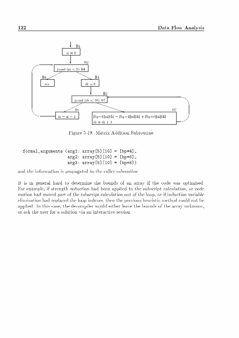
122 Data Flow Analysis%$

??������ HHHHHj?������ PPPPPPPPq-'& �B2jcond (si < 5) B4 [bp+8][si][di] = [bp+4][si][di] + [bp+6][si][di]ret di = 0jcond (di < 10) B7si = si + 1 di = di + 1

si = 0 B4 B5 B7B6B3 B1Figure 5-19: Matrix Addition Subroutineformal_arguments (arg1: array[5][10] = [bp+4],arg2: array[5][10] = [bp+6],arg3: array[5][10] = [bp+8])and the information is propagated to the caller subroutine.It is in general hard to determine the bounds of an array if the code was optimised.For example, if strength reduction had been applied to the subscript calculation, or codemotion had moved part of the subscript calculation out of the loop, or if induction variableelimination had replaced the loop indexes, then the previous heuristic method could not beapplied. In this case, the decompiler would either leave the bounds of the array unknown,or ask the user for a solution via an interactive session.

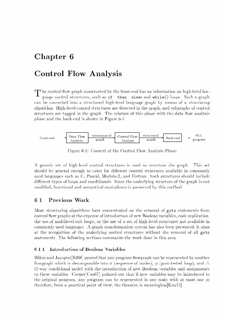
Chapter 6Control Flow AnalysisT he control ow graph constructed by the front-end has no information on high-level lan-guage control structures, such as if..then..elses and while() loops. Such a graphcan be converted into a structured high-level language graph by means of a structuringalgorithm. High-level control structures are detected in the graph, and subgraphs of controlstructures are tagged in the graph. The relation of this phase with the data ow analysisphase and the back-end is shown in Figure 6-1.-. . . . -. . . .- -Front-end program. . . . . . . . . .. . . . . . . . . ...... ..... HLLAnalysis unstructuredgraph Control FlowAnalysis Back-endgraphstructuredData FlowFigure 6-1: Context of the Control Flow Analysis PhaseA generic set of high-level control structures is used to structure the graph. This setshould be general enough to cater for di�erent control structures available in commonlyused languages such as C, Pascal, Modula-2, and Fortran. Such structures should includedi�erent types of loops and conditionals. Since the underlying structure of the graph is notmodi�ed, functional and semantical equivalence is preserved by this method.6.1 Previous WorkMost structuring algorithms have concentrated on the removal of goto statements fromcontrol ow graphs at the expense of introduction of new Boolean variables, code replication,the use of multilevel exit loops, or the use of a set of high-level structures not available incommonly used languages. A graph transformation system has also been presented, it aimsat the recognition of the underlying control structures without the removal of all gotostatements. The following sections summarize the work done in this area.6.1.1 Introduction of Boolean VariablesB�ohm and Jacopini[BJ66] proved that any program owgraph can be represented by another owgraph which is decomposable into � (sequence of nodes), � (post-tested loop), and 4(2-way conditional node) with the introduction of new Boolean variables and assignmentsto these variables. Cooper[Coo67] pointed out that if new variables may be introduced tothe original program, any program can be represented in one node with at most one �;therefore, from a practical point of view, the theorem is meaningless[Knu74].

124 Control Flow AnalysisAshcroft and Manna[AM71] demonstrated that goto programs cannot be converted intowhile() programs without the introduction of new variables, and presented an algorithmfor the conversion of these programs with the introduction of new Boolean variables. Theconversion preserves the topology of the original owchart program, but performs compu-tations in di�erent order.Williams and Ossher[WO78] presented an iterative algorithm to convert a multiexit loopinto a single exit loop, with the introduction of one Boolean variable and a counter integervariable for each loop.Baker and Zweben[BZ80] reported on the structuring of multiexit loops with the introduc-tion of new Boolean variables. The structuring of multiple exit loops is considered a control ow complexity issue, and is measured in this paper.Williams and Chen[WG85] presented transformations to eliminate goto statements fromPascal programs. Gotos were classi�ed according to the positioning of the target label: atthe same level as the corresponding label, branch out of a structure, transferral of a labelout of a structure, and abnormal exits from subroutines. All these transformations requiredthe introduction of one or more Boolean variables, along with the necessary assignment andtest statements to check on the value of a Boolean. The algorithm was implemented inProlog on a PDP11/34.Erosa and Hendren[EH93] present an algorithm to remove all goto statements from C pro-grams. The method makes use of goto-elimination and goto-movement transformations,and introduces one new Boolean variable per goto. On average, three new instructions areintroduced to test for each new Boolean, and di�erent loop and if conditionals are modi�edto include the new Boolean. This method was implemented as part of the McCAT paral-lelizing decompiler.The introduction of new (Boolean) variables modi�es the semantics of the underlyingprogram, as these variables do not form part of the original program. The resultant programis functionally equivalent to the original program, thus it produces the same results.6.1.2 Code ReplicationKnuth and Floyd[KF71] presented di�erent methods to avoid the use of goto statementswithout the introductions of new variables. Four methods were given: the introduc-tion of recursion, the introduction of new procedures, node splitting, and the use of arepeat..until() construct. The use of the node splitting technique replicates code in the�nal program. It is also proved that there exist programs whose goto statements cannotbe eliminated without the introduction of new procedure calls.Williams[Wil77] presents �ve subgraphs which lead to unstructured graphs: abnormal selec-tion paths, multiple exit loops, multiple entry loops, overlapping loops, and parallel loops.In order to transform these subgraphs into structured graphs, code duplication is performed.

6.1 Previous Work 125Williams and Ossher[WO78] presented an algorithm to replace multiple entry loops by sin-gle entry while() loop. The method made use of code duplication of all nodes that couldbe reached from abnormal entries into the loop.Baker and Zweben[BZ80] reported on the use of the node splitting technique to generateexecutionally equivalent owgraphs by replicating one or more nodes of the graph. Nodesplitting was considered a control ow complexity issue, and was measured.Oulsnam[Oul82] presented transformations to convert six types of unstructured graphs tostructured equivalent graphs. The methodology made use of node duplication, but no func-tion duplication. It was demonstrated that the time overhead produced by the duplicationof nodes was an increased time factor of 3 for at least one path.Code replication modi�es the original program/graph by replicating code/node one ormore times, therefore, the �nal program/graph is functionally equivalent to the originalprogram/graph, but its semantics and structure have been modi�ed.6.1.3 Multilevel Exit Loops and Other StructuresBaker[Bak77] presented an algorithm to structure owgraphs into equivalent owgraphsthat made use of the following control structures: if..then..else, multilevel break, mul-tilevel next, and endless loops. Gotos were used whenever the graph could not be structuredusing the previous structures. The algorithm was extended to irreducible graphs as well.It was demonstrated that the algorithm generated well-formed and properly nested pro-grams, and that any goto statements in the �nal graph jumped forward. This algorithmwas implemented in the struct program on a PDP11/54 running under Unix. It was usedto rewrite Fortran programs into Ratfor, an extended Fortran language that made use ofcontrol structures. The struct program was later used by J.Reuter in the decomp decom-piler to structure graphs built from object �les with symbol information.Sharir[Sha80] presented an algorithm to �nd the underlying control structures in a owgraph. This algorithm detected normal conditional and looping constructs, but also de-tected proper and improper strongly-connected intervals, and proper and improper outer-most intervals. The �nal ow graph was represented by a hierarchical ow structure.Ramshaw[Ram88] presented a method to eliminate all goto statements from programs, bymeans of forward and backward elimination rules. The resultant program was a structurallyequivalent program that made use of multilevel exits from endless-type, named loops. Thisalgorithm was used to port the Pascal version of Knuth's TEX compiler into the PARC/CSL,which uses Mesa. Both these languages allow the use of goto statements, but outward gotosare not allowed in Mesa.The use of multilevel exits or high-level constructs not available in most languages restrictsthe generality of the structuring method and the number of languages in which the structuredversion of the program can be written. Currently, most 3rd generation languages (e.g.Pascal, Modula-2, C) do not make use of multilevel exits; only Ada allows them.

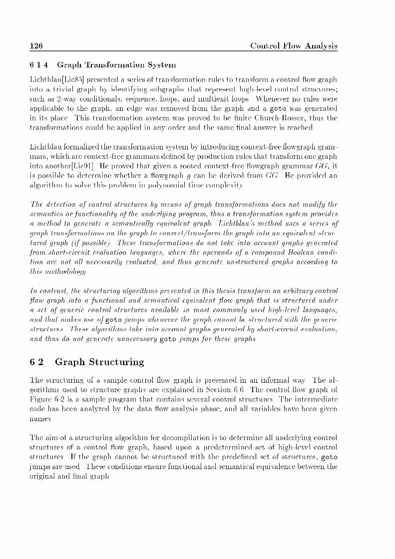
126 Control Flow Analysis6.1.4 Graph Transformation SystemLichtblau[Lic85] presented a series of transformation rules to transform a control ow graphinto a trivial graph by identifying subgraphs that represent high-level control structures;such as 2-way conditionals, sequence, loops, and multiexit loops. Whenever no rules wereapplicable to the graph, an edge was removed from the graph and a goto was generatedin its place. This transformation system was proved to be �nite Church-Rosser, thus thetransformations could be applied in any order and the same �nal answer is reached.Lichtblau formalized the transformation system by introducing context-free owgraph gram-mars, which are context-free grammars de�ned by production rules that transform one graphinto another[Lic91]. He proved that given a rooted context-free owgraph grammar GG, itis possible to determine whether a owgraph g can be derived from GG. He provided analgorithm to solve this problem in polynomial time complexity.The detection of control structures by means of graph transformations does not modify thesemantics or functionality of the underlying program, thus a transformation system providesa method to generate a semantically equivalent graph. Lichtblau's method uses a series ofgraph transformations on the graph to convert/transform the graph into an equivalent struc-tured graph (if possible). These transformations do not take into account graphs generatedfrom short-circuit evaluation languages, where the operands of a compound Boolean condi-tion are not all necessarily evaluated, and thus generate unstructured graphs according tothis methodology.In contrast, the structuring algorithms presented in this thesis transform an arbitrary control ow graph into a functional and semantical equivalent ow graph that is structured undera set of generic control structures available in most commonly used high-level languages,and that makes use of goto jumps whenever the graph cannot be structured with the genericstructures. These algorithms take into account graphs generated by short-circuit evaluation,and thus do not generate unnecessary goto jumps for these graphs.6.2 Graph StructuringThe structuring of a sample control ow graph is presented in an informal way. The al-gorithms used to structure graphs are explained in Section 6.6. The control ow graph ofFigure 6-2 is a sample program that contains several control structures. The intermediatecode has been analyzed by the data ow analysis phase, and all variables have been givennames.The aim of a structuring algorithm for decompilation is to determine all underlying controlstructures of a control ow graph, based upon a predetermined set of high-level controlstructures. If the graph cannot be structured with the prede�ned set of structures, gotojumps are used. These conditions ensure functional and semantical equivalence between theoriginal and �nal graph.

6.2 Graph Structuring 127

loc1 = loc1 + 1loc2 = loc2 + 1printf ("...", loc1, loc2)loc2 = loc1jcond (loc3 < loc4) B9jcond ((loc4 * 2) <= loc3) B10loc3 = loc3 + loc4 - 10loc4 = loc4 / 2loc1 = 0 loc4 = loc4 << 3loc3 = loc3 * loc4jcond ((loc3 * 4) <= loc4) B4loc3 = 5loc4 = loc3 * 5jcond (loc3 >= loc4) B5

printf ("...", loc3, loc4)ret %$�� %$%$�

??�����9B3 XXXXXzXXXXXz �����)?�����9 XXXXXXz��������+ PPPPPq ???AAAAAAUAAAAA�����9?

B1B2 B4B5B6B7B8 B9 B10 B11 B15B14B13B12jcond (loc1 < 10) B12 jcond (loc2 < 5) B13loc3 = loc3 << 3

Figure 6-2: Sample Control Flow Graph6.2.1 Structuring LoopsIn graphs, loops are detected by the presence of a back-edge; that is, an edge from a \lower"node to a \higher" node. The notion of lower and higher are not formally de�ned yet, butcan be thought as the nodes that are lower and higher up in the diagram (for a graph thatis drawn starting at the top). In the graph of Figure 6-2 there are 2 back-edges: (B14,B13),and (B15,B6). These back-edges represent the extent of 2 di�erent loops.The type of the loop is detected by checking the header and the last node of the loop.The loop (B14,B13) has no conditional check on its header node, but the last node of theloop tests whether the loop should be executed again or not; thus, this is a post-testedloop, such as a do..while() in C, or a repeat..until() in Modula-2. The subgraph thatrepresents this loop can be logically transformed into the subgraph of Figure 6-3, where theloop subgraph was replaced by one node that holds all the intermediate code instructions,as well as information on the type of loop.The loop (B15,B6) has a conditional header node that determines whether the loop isexecuted or not. The last node of this loop is a 1-way node that transfers control back

128 Control Flow Analysis?loc2 = loc2 + 1printf ("...", loc1, loc2)?do /* start of loop */ ,while (loc2 < 5) B15B14Figure 6-3: Post-tested Loopto the header of the loop. This loop is clearly a pre-tested loop, such as a while() loopin a variety of languages. The subgraph of this loop can be logically transformed into thesubgraph of Figure 6-4, where the loop subgraph has been replaced with the one node thatholds all information on the loop and its instructions.??loc2 = loc2 + 1printf ("...", loc1, loc2)while (loc2 < 5)do /* start of loop */B6,B13..B16loc2 = loc1while (loc1 < 10)loc1 = loc1 + 1end whileFigure 6-4: Pre-tested Loop6.2.2 Structuring ConditionalsThe 2-way conditional node B2 branches control to node B4 if the condition(loc3 * 2) <= loc4 is true, otherwise it branches to node B3. Both these nodes arefollowed by the node B5, in other words, the conditional branch that started at node B2 is�nished at node B5. This graph is clearly an if()then..else structure, and can be logi-cally transformed into the subgraph of Figure 6-5, where the node represents basic blocksB2, B3, and B4. Note that all instructions before the conditional jump that belong to thesame basic block are not modi�ed.The 2-way conditional node B1 transfers control to node B5 if the condition loc3 >= loc4is true, otherwise it transfers control to node B2. From out previous example, node B2has been merged with nodes B3 and B4, and transformed into an equivalent node with anout-edge to node B5; thus, there is a path from node B2 ! B5. Since B5 is one of thetarget branch nodes of the conditional at node B1, and it is reached by the other branch ofthe conditional, this 2-way node represents a single branch conditional (i.e. an if()then).This subgraph can be transformed into the node of Figure 6-6, where the condition at nodeB1 has been negated since the false branch is the single branch that forms part of the if.

6.2 Graph Structuring 129??loc3 = loc3 * loc4if ((loc3 * 2) <= loc4) thenelse B5loc3 = loc3 << 3loc4 = loc4 << 3end if B2..B4Figure 6-5: 2-way Conditional Branching??loc3 = 5loc4 = loc3 * 5if (loc3 < loc4) thenloc3 = loc3 * loc4if ((loc3 * 2) <= loc4) thenB1..B4elseloc3 = loc3 << 3loc4 = loc4 << 3end ifend if B5Figure 6-6: Single Branch ConditionalThe 2-way conditional nodes B7 and B8 are not trivially structured, since, if node B8 isconsidered the head of an if..then..else �nishing at node B10, and node B7 is consid-ered head of an if..then, we do not enter the subgraph headed by B8 at its entry point,but in one of the clauses of the conditional branch. If we structure node B7 �rst as anif..then, then node B8 branches out of the subgraph headed at B7 through another nodeother than the exit node B9; thus, the graph cannot be structured with the if..then, andif..then..else structures. But since both B7 and B8 only have a conditional branchinstruction, these two conditions could be merged into a compound conditional in the fol-lowing way: node B9 is reached whenever the condition in node B7 is true, or when thecondition at B7 is false and the condition at B8 is false as well. Node B10 is reachedwhenever the condition at node B7 is false and the one at B8 is true, or by a path fromnode B9. This means that node B9 is reached whenever the condition at node B7 is trueor the condition at node B8 is false, and the �nal end node is basic block B10. The �nalcompound condition is shown in Figure 6-7, along with the transformed subgraph.

130 Control Flow Analysis??if ((loc3 < loc4) or ((loc4 * 2) > loc3)) thenloc3 = loc3 + loc4 - 10 B7..B9loc4 = loc4 = 2end if B10Figure 6-7: Compound Conditional Branch6.3 Control Flow AnalysisInformation on the control structures of a program is available through control ow analysisof the program's graph. Information is collected in the di�erent nodes of the graph, whetherthey belong to a loop and/or conditional, or are not part of any structure. This sectionde�nes control ow terminology available in the literature; for more information refer to[All72, Tar72, Tar74, HU75, Hec77, ASU86b].6.3.1 Control Flow Analysis De�nitionsThe following de�nitions de�ne basic concepts used in control ow analysis. Thesede�nitions make use of a directed graph G = (N;E; h).De�nition 44 A path from n1 to nv; n1; nv 2 N , represented n1 ! nv, is a sequence ofedges (n1; n2); (n2; n3); : : : ; (nv�1; nv) such that (ni; ni+1) 2 E;8 1 � i < v; v � 1.De�nition 45 A closed path or cycle is a path n1 ! nv where n1 = nv.De�nition 46 The successors of ni 2 N are fnj 2 N j ni ! njg (i.e. all nodes reachablefrom ni).The immediate successors of ni 2 N are fnj 2 N j (ni; nj) 2 Eg.De�nition 47 The predecessors of nj 2 N are fni 2 N j ni ! njg (i.e. all nodes thatreach nj).The immediate predecessors of nj 2 N are fni 2 N j (ni; nj) 2 Eg.De�nition 48 A node ni 2 N back dominates or predominates a node nk 2 N if niis on every path h! nk. It is said that ni dominates nk.De�nition 49 A node ni 2 N immediately back dominates nk 2 N if 6 9nj � nj backdominates nk ^ni back dominates nj (i.e. ni is the closest back dominator to nk). It is saidthat ni is the immediate dominator of nk.De�nition 50 A strongly connected region (SCR) is a subgraph S = (NS; ES ; hS) suchthat 8ni; nj 2 NS � 9ni ! nj ^ nj ! ni.

6.3 Control Flow Analysis 131De�nition 51 A strongly connected component of G is a subgraph S = (NS ; ES; hS)such that� S is a strongly connected region.� 69S2 strongly connected region of G � S � S2.De�nition 52 Depth �rst search (DFS) is a traversal method that selects edges totraverse emanating from the most recently visited node which still has unvisited edges.A DFS algorithm de�nes a partial ordering of the nodes of G. The reverse postorder is thenumbering of nodes during their last visit; the numbering starts with the maximumnumberof nodes in the graph, and �nishes at 1. Throughout this chapter, all numbered graphs usethe reverse postorder numbering scheme.De�nition 53 A depth �rst spanning tree (DFST) of a ow graph G is a directed,rooted, ordered spanning tree of G grown by a DFS algorithm. A DFST T can partition theedges in G into three sets:1. Back edges = f(v;w) : w! v 2 Tg.2. Forward edges = f(v;w) : v ! w 2 Tg.3. Cross edges = f(v;w) : 6 9 (v ! w or w! v) and w � v in preorderg.6.3.2 RelationsDe�nition 54 Let R be a relation on a set S,Then xRy denotes (x; y) 2 R.De�nition 55 Let R be a relation on a set S,Then� the re exive closure of R is R� = R [ f(x; x)jx 2 Sg� the transitive closure of R is R� = R1 [ R2 [ : : :, where R1 = R and Ri = RRi�1for i � 2� the re exive transitive closure of R is R� = R� [ R�� the completion of R is R = f(x; y) 2 S � S jxR�y ^ 69 z 2 S � yRzg.De�nition 56 Let R be a relation on a set S,Then (S,R) is �nite Church-Rosser (fcr) if and only if:1. R is �nite, i.e. 8 p 2 S � 9 kp� pRiq ) i � kp.2. R is a function, i.e. pRq ^ pRr ) q = r.6.3.3 Interval TheoryAn interval is a graph theoretic construct de�ned by J.Cocke in [Coc70], and widely used byF.Allen for control ow analysis[All70, AC72] and data ow analysis[All72, All74, AC76].The following sections summarize interval theory concepts.

132 Control Flow AnalysisIntervalsDe�nition 57 Given a node h, an interval I(h) is the maximal, single-entry subgraph inwhich h is the only entry node and in which all closed paths contain h. The unique intervalnode h is called the interval head or simply the header node.By selecting the correct set of header nodes, G can be partitioned into a unique set ofdisjoint intervals I = fI(h1); I(h2); : : : ; I(hn)g, for some n � 1. The algorithm to �nd theunique set of intervals of a graph is described in Figure 6-8. This algorithm makes use ofthe following variables: H (set of header nodes), I(i) (set of nodes of interval i), and I (listof intervals of the graph G), as well as the function immedPred(n) which returns the nextimmediate predecessor of n.procedure intervals (G = (N;E; h))/* Pre: G is a graph.* Post: the intervals of G are contained in the list I. */I := fg.H := fhg.for (all unprocessed n 2 H) doI(n) := fng.repeatI(n) := I(n) + fm 2 N j 8p 2 immedPred(m) � p 2 I(n)g.untilno more nodes can be added to I(n).H := H + fm 2 N jm 62 H ^m 62 I(n) ^ (9 p 2 immedPred(m) � p 2 I(n))g.I := I + I(n).end forend procedure Figure 6-8: Interval AlgorithmThe example in Figure 6-9 shows a graph G with its intervals in dotted boxes. This graphhas two intervals, I(1) and I(2). Interval I(2) contains a loop, the extent of this loop is givenby the back-edge (4,2).De�nition 58 The interval order is de�ned as the order of nodes in an interval list,given by the intervals algorithm of Figure 6-8.Some interval properties:1. The header node back dominates each node in the interval.2. Each strongly connected region in the interval must contain the header node.

6.3 Control Flow Analysis 133-'& ��$mmmmmm????

-�&. . . . . . . . . . . . . .. . . . . . . . . . . . . ..................................

....................

.............G

. . . . . . . . . . . . .. . . . . . . . . . . . ...... .....?123456 I(2)I(1) I(1) = f1gI(2) = f2,3,4,5,6g

Figure 6-9: Intervals of a Graph3. The interval order is such that if all nodes are processed in the order given, then allinterval predecessors of a node reachable along loop free paths from the header willhave been processed before the given node.De�nition 59 A latching node is any node in the interval which has the header node asan immediate successor.Derived Sequence ConstructionThe derived sequence of graphs, G1 : : :Gn, was described by F.Allen[All70, All72] basedon the intervals of graph G. The construction of graphs is an iterative method that col-lapses intervals into nodes. G is the �rst order graph, represented G1. The second ordergraph, G2, is derived from G1 by collapsing each interval in G1 into a node. The immediatepredecessors of the collapsed node are the immediate predecessors of the original headernode which are not part of the interval. The immediate successors are all the immediate,non-interval successors of the original exit nodes. Intervals for G2 are computed with theinterval algorithm, and the graph construction process is repeated until a limit ow graphGn is reached. Gn has the property of being a trivial graph (i.e. single node) or an irre-ducible graph. Figure 6-10 describes this algorithm.De�nition 60 The n-th order graph or limit ow graph, Gn, of a graph G is de�nedas the graph Gi�1, i � 1, constructed by the derivedSequence algorithm of Figure 6-10, suchthat Gi�1 = Gi.De�nition 61 A graph G is reducible if its n-th order graph Gn is trivial.

134 Control Flow Analysisprocedure derivedSequence (G = (N,E,h))/* Pre: G is a graph.* Post: the derived sequence of G, G1 : : :Gn; n � 1 has been constructed. */G1 = G.I1 = intervals(G1).i = 2.repeat /* Construction of Gi */N i = fni j I i�1(ni�1) 2 Ii�1g8n 2 N i � p 2 immedPred(n), (9m 2 N i�1 �m 2 I i�1(m)^p 2 immedPred(m)^ p 62 I i�1(m)).(hij ; hik) 2 Ei , (9n;m; hi�1j ; hi�1k 2 N i�1 � hi�1j = I i�1(hi�1j )^hi�1k = I i�1(hi�1k ) ^m 2 I i�1(hi�1j ) ^ n 2 I i�1(hi�1k ) ^ (m;n) 2 Ei�1.i = i + 1.untilGi == Gi�1.end procedure Figure 6-10: Derived Sequence AlgorithmThe construction of the derived sequence is illustrated in Figure 6-11. The graph G1 is theinitial control ow graph G. G1 has 2 intervals, previously described in Figure 6-9. GraphG2 represents the intervals of G1 as nodes. G2 has a loop in its unique interval. This looprepresents the loop extended by the back-edge (5,1). Finally, G3 has no loops and is a trivialgraph. -��-'& ��� -��jjjjjj � ��� �� � ��????. . . . . . . . . . . . . .. . . . . . . . . . . . . ..................................

.........................

......... . . . . . . . . . . . .. . . . . . . . . . . . ...... ..... ? ?. . . . . . . . . . . . . . .. . . . . . . . . . . . . . ................ ...............?? . . . . . . . . . . . .. . . . . . . . . . . ......... ........123456G1 I(2)I(1) 2-61 1-6I(1) I(1)G3G2

Figure 6-11: Derived Sequence of a Graph

6.4 High-Level Language Control Structures 135Implementation ConsiderationsTo compute the intervals of a graph G, G needs to be de�ned in terms of its predecessorsand successors (i.e. an adjacency-type graph representation). With the aid of extra datastructures, Hecht presented an optimized algorithm to �nd intervals[Hec77], of complexityO(e), j E j= e.6.3.4 Irreducible Flow GraphsAn irreducible ow graph is a graph such that its n-th order graph is not a trivial graph(by interval reduction). Irreducible ow graphs are characterized by the existence of aforbidden canonical irreducible graph [HU72, HU74, Hec77]. The absence of this graph ina ow graph is enough for the graph to be reducible. The canonical irreducible graph isshown in Figure 6-12. mm@@@Rm ���� ? -Figure 6-12: Canonical Irreducible GraphTheorem 1 A ow graph is irreducible if and only if it has a subgraph of the form canonicalirreducible graph.6.4 High-Level Language Control StructuresDi�erent high-level languages use di�erent control structures, but in general, no high-levellanguage uses all di�erent available control structures. This section illustrates di�erentcontrol structures, gives a classi�cation, and analyses the structures available in commonlyused high-level languages such as C, Pascal, and Modula-2.6.4.1 Control Structures - Classi�cationControl structures have been classi�ed into di�erent classes according to the complexity ofthe class. An initial classi�cation was provided by Kosaraju in [Kos74], and was used todetermine which classes were reducible to which other classes. This classi�cation was ex-panded by Ledgard and Marcotty in [LM75], and was used to present a hierarchy of classesof control structures under semantical reducibility.Figure 6-13 shows all the di�erent control structures that are under consideration in thisclassi�cation; these structures are:1. Action: a single basic block node is an action.2. Composition: a sequence of 2 structures is a composition.

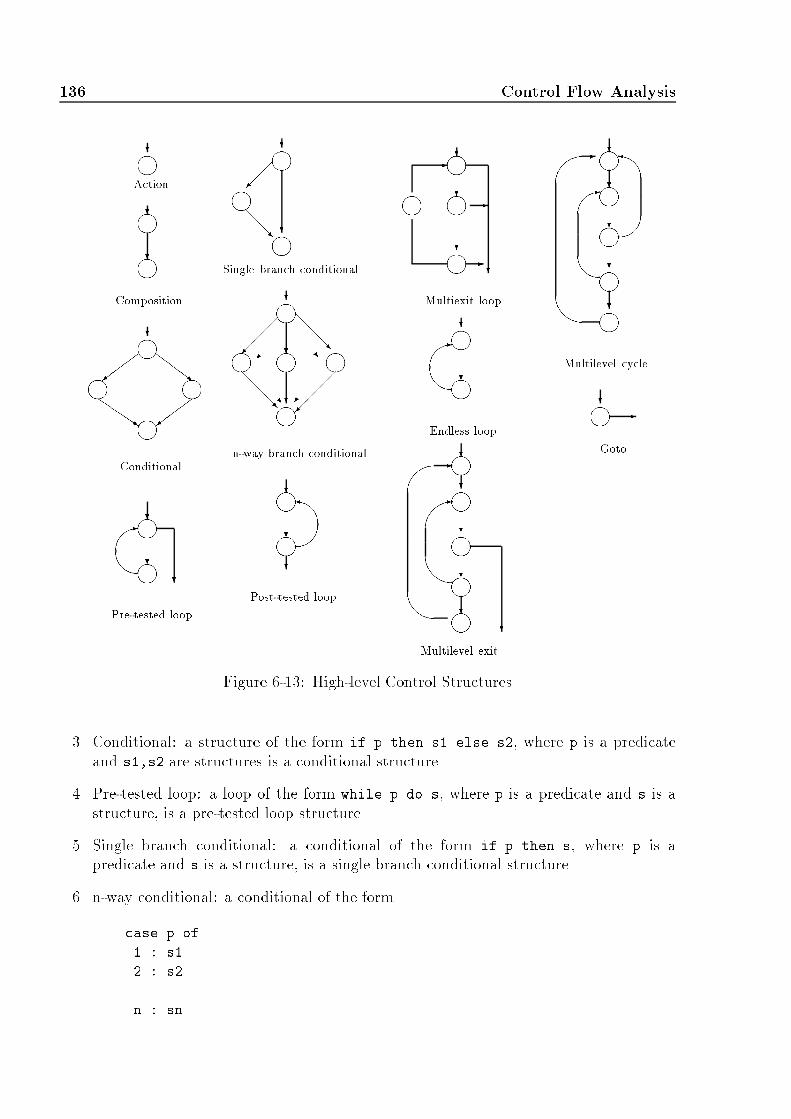
136 Control Flow Analysis-'&-'&

���-'&-��-�����mmm

mmmm mm mmmm mm mmmm

mmmm mmmmmmm

mmmmmm?���= ZZZ~���=QQQQs ? ??...??

-��

?Goto

��� ??@@@R��� ??/ ...... @@@Rw. . . . . .@@@R ?/. . . . . .����w...... ??...?

??...?....- ?--??....???.. ??...?

???...?...?? -Pre-tested loopConditional

ActionComposition Single branch conditionaln-way branch conditionalPost-tested loop

Multiexit loopEndless loopMultilevel exit

Multilevel cycleFigure 6-13: High-level Control Structures3. Conditional: a structure of the form if p then s1 else s2, where p is a predicateand s1,s2 are structures is a conditional structure.4. Pre-tested loop: a loop of the form while p do s, where p is a predicate and s is astructure, is a pre-tested loop structure.5. Single branch conditional: a conditional of the form if p then s, where p is apredicate and s is a structure, is a single branch conditional structure.6. n-way conditional: a conditional of the formcase p of1 : s12 : s2...n : sn

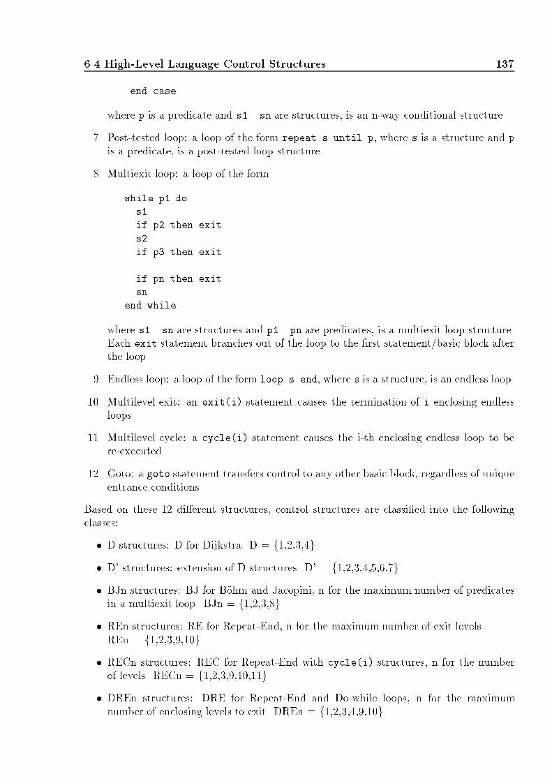
6.4 High-Level Language Control Structures 137end casewhere p is a predicate and s1..sn are structures, is an n-way conditional structure.7. Post-tested loop: a loop of the form repeat s until p, where s is a structure and pis a predicate, is a post-tested loop structure.8. Multiexit loop: a loop of the formwhile p1 dos1if p2 then exits2if p3 then exit...if pn then exitsnend whilewhere s1..sn are structures and p1..pn are predicates, is a multiexit loop structure.Each exit statement branches out of the loop to the �rst statement/basic block afterthe loop.9. Endless loop: a loop of the form loop s end, where s is a structure, is an endless loop.10. Multilevel exit: an exit(i) statement causes the termination of i enclosing endlessloops.11. Multilevel cycle: a cycle(i) statement causes the i-th enclosing endless loop to bere-executed.12. Goto: a goto statement transfers control to any other basic block, regardless of uniqueentrance conditions.Based on these 12 di�erent structures, control structures are classi�ed into the followingclasses:� D structures: D for Dijkstra. D = f1,2,3,4g� D' structures: extension of D structures. D' = f1,2,3,4,5,6,7g� BJn structures: BJ for B�ohm and Jacopini, n for the maximum number of predicatesin a multiexit loop. BJn = f1,2,3,8g� REn structures: RE for Repeat-End, n for the maximum number of exit levels.REn = f1,2,3,9,10g� RECn structures: REC for Repeat-End with cycle(i) structures, n for the numberof levels. RECn = f1,2,3,9,10,11g� DREn structures: DRE for Repeat-End and Do-while loops, n for the maximumnumber of enclosing levels to exit. DREn = f1,2,3,4,9,10g

138 Control Flow Analysis� DRECn structures: DREC for Repeat-End, Do-while, and cycle(i) structures, n forthe maximum number of enclosing endless loops. DRECn = f1,2,3,4,9,10,11g� GPn structures: any structure that has one-in, one-out substructures that have atmost n di�erent predicates. GPn = f1..7,9g� L structures: any well-formed structure. There are no restrictions on the number ofpredicates, actions, and transfers of control; therefore, goto statements are allowed.L = f1..12gDe�nition 62 Let s1 and s2 be two structures, then s1 is a semantical conversion of s2if and only if� For every input, s2 computes the same function as s1.� The primitive actions and predicates of s2 are precisely those of s1.In other words, no new semantics such as variables, actions, or predicates, are allowed bythis conversion.Based on semantical conversion, the classes of control structures form a hierarchy, as shownin Figure 6-14. The classes higher up in the hierarchy are a semantical conversion of thelower classes. ......................... .....D=D'=BJ1REC1

RE1=REC1= DRE1=GP1

DREC1= GP1= LREn = RECnRE1 =BJ1 = DRECnDREn =DRE1 DREC1BJ2 =Figure 6-14: Control Structures Classes Hierarchy6.4.2 Control Structures in 3rd Generation LanguagesIn this section, di�erent high-level languages are analysed and classi�ed in terms of theircontrol structures. The selected languages are used in a variety of applications, includingsystems programming, numerical or scienti�cal applications, and multipurpose applications;these languages are: Modula-2, Pascal, C, Fortran, and Ada.

6.4 High-Level Language Control Structures 139Modula-2 [Wir85, PLA91] does not allow for the use of goto statements, therefore, thecontrol ow graphs generated by this language are structured and reducible. Modula-2 hasall D'-type structures: 2-way conditionals (IF p THEN s1 {ELSE s2}), n-way conditional(CASE p OF ... END, pre-tested loop (WHILE p DO), post-tested loop (REPEAT s UNTIL p),and in�nite loop (LOOP s END). An endless loop can be terminated by one or more EXITstatements within the statement sequence body of the loop. This construct can be usedto simulate other loop structures, such as a multiexit loop with n predicates (BJn struc-ture). An EXIT statement terminates the execution of the immediately enclosing endlessloop statement, and the execution resumes at the statement following the end of the loop.If an EXIT occurs within a pre-tested or post-tested loop nested within an endless loop, boththe inner loop and enclosing endless loop are terminated; therefore, an EXIT statement isequivalent to an exit(1) statement, and belongs to the RE1 class of structures.Pascal [Coo83] is not as strict as Modula-2, in the sense that it allows goto statements to beused. All D'-type structures are allowed: 2-way conditionals (if p then s1 [else s2]),n-way conditional (case p of ... end), pre-tested loop (while p do), post-tested loop(repeat s until p), and the endless loop is simulated by a while() with a true condition(while (True) do). Gotos can be used to simulate multiexit and multilevel loops, but canalso be used in an unstructured way, to enter in the middle of a structure; therefore, L classstructures are permitted in this language.C [KR88] allows for structured and unstructured transfer of control. D' structures arerepresented by the following statements: 2-way conditional (if (p) s1 [else s2]), n-way conditional (switch (p) {...}), pre-tested loop (while (p) {s}), post-tested loop(do s while (p)), and endless loop (for (;;;) or while (1) {s}). 1 level exit of controlis allowed by the use of break statements, and 1 level cycle transfer of control is allowed bythe use of the continue statement; therefore, C contains structures of the RE1 and REC1classes. The use of goto statements can model any structure from the DRECn class, butcan also produce unstructured graphs; therefore C allows for L class structures.Fortran [Col81] has di�erent types of conditionals which include: 2-way conditional(IF (p) s1,s2), arithmetic if or 3-way conditional (IF (p) s1,s2,s3), and computedgoto statements or n-way conditionals (GOTO (s1,s2,...,sn) p). Pre-tested, post-testedand endless loops are all simulated by use of the DO statement; therefore, all D'-type struc-tures are allowed in Fortran. Finally, goto statements are allowed, producing structured orunstructured transfers of control, allowing for L type structures.Ada [DoD83] allows most D'-type structures, including: 2-way conditionals (if p then s1[else s2]), n-way conditional (case p is ... end), pre-tested loop (while p and forloops), and endless loop (loop s end loop). Ada also allows the use of the exit statementsto exit from within named endless loops; therefore, several nested loops can be terminatedwith this instruction (i.e. REn class type structure). Goto statements are allowed in arestricted way; they can transfer control only to a statement of an enclosing sequence ofstatements, but not the reverse. Also, it is prohibited to transfer control into the alterna-tives of a case statement, or an if..then..else statement. These restrictions on the useof gotos makes them simulate multilevel exits and multilevel continues, but do not permitunstructured transfers of control; therefore, up to DRECn-type structures can be built in

140 Control Flow Analysisthis language.Figure 6-15 summarizes the di�erent types of classes of structures available in the set ofdistinguished languages. It must be pointed out that all of these languages make use ofD'-type structures, plus one or more structures that belong to di�erent types of classes.Unstructured languages allow for the unstructured use of goto, which is the case of Pascaland Fortran. Structured uses of goto, such as in Ada, permit the construction of structuredcontrol ow graphs, since up to DRECn-type structures can be simulated by these gotos.Language Control Structure Classi�cationModula-2 D' + BJn + RE1Pascal D' + LC D' + BJn + DREC1 + LFortran D' + LAda D' + DRECnFigure 6-15: Classes of Control Structures in High-Level Languages6.4.3 Generic Set of Control StructuresIn order to structure a graph, a set of generic control structures needs to be selected. Thisset must be general enough to cater for commonly used structures in a variety of languages.From the review of some 3rd generation languages in the previous section, it is clear thatmost languages have D' class structures, plus some type of structured or unstructuredtransfer of control (i.e. multilevel exits or gotos). Structures from the REn, RECn, DREn,and DRECn classes can all be simulated by the use of structured transfers of control via agoto statement. Since most of the languages allow the use of goto, and not all languageshave the same multilevel exit or multilevel continue structures, goto is a better choice of ageneric construct than exit(i) or cycle(i). It is therefore desirable to structure a control ow graph using the following set of generic structures:� Action� Composition� Conditional� Pre-tested loop� Single branching conditional� n-way conditional� Post-tested loop� Endless loop� GotoIn other words, the generic set of control structures has all D' and L class structures.

6.5 Structured and Unstructured Graphs 1416.5 Structured and Unstructured GraphsA structured control ow graph is a graph generated from programs that use structuresof up to the DRECn class; i.e. a graph that is decomposable into subgraphs with oneentry and one or more exits. Languages that allow the use of goto can still generatestructured graphs, if the gotos are used to transfer control in a structured way (i.e. totransfer control to the start or the end of a structure). Unstructured graphs are generatedby the unstructured transfer of control of goto statements, that is, a transfer of controlin the middle of a structured graph, which breaks the previously structured graph into anunstructured one since there is more than one entry into this subgraph. Unstructurednesscan also be introduced by the optimization phase of the compiler when code motion isperformed (i.e. code is moved).6.5.1 LoopsA loop is a strongly connected region in which there is a path between any two nodes ofthe directed subgraph. This means that there must be at least one back-edge to the loop'sheader node.A structured loop is a subgraph that has one entry point, one back-edge, and possiblyone or more exit points that transfer control to the same node. Structured loops include allnatural loops (pre-tested and post-tested loops), endless loops, and multiexit loops. Theseloops are shown in Figure 6-16. -�����mm mm mmm mmm??... ?-�� ?Post-tested loop ?.... - ??...?.... ?--??...? In�nite loopPre-tested loop Multiexit loopFigure 6-16: Structured LoopsAn unstructured loop is a subgraph that has one or more back-edges, one or more entrypoints, and one or more exit points to di�erent nodes. Figure 6-17 illustrates four di�erenttypes of unstructured loops:� Multientry loop: a loop with two or more entry points.� Parallel loop: a loop with two or more back-edges to the same header node.� Overlapping loops: two loops that overlap in the same strongly connected region.� Multiexit loop: a loop with two or more exits to di�erent nodes.

142 Control Flow Analysis�$��-'� %$�-'& %$� '?- mnn nnn nnnnnnnn%$� n Multiexitn??....?.....? ??.... @@R�� ??....?....???....?....?....?Multientry Parallel OverlappingFigure 6-17: Sample Unstructured LoopsThe follow node of a structured or unstructured loop is the �rst node that is reached fromthe exit of the loop. In the case of unstructured loops, one node is considered the loop exitnode, and the �rst node that follows it is the follow node of the loop.6.5.2 ConditionalsA structured 2-way conditional is a directed subgraph with a 2-way conditional headernode, one entry point, two or more branch nodes, and a common end node that is reachedby both branch nodes. This �nal common end node is referred to as the follow node, andhas the property of being immediately dominated by the header node.In an if..then conditional, one of the two branch nodes of the header node is the follownode of the subgraph. In an if..then..else conditional, neither branch node is the follownode, but they both converge to a common end node. Figure 6-18 shows these two genericconstructs, with the values of the out-edges of the header node; true or false. In the case ofan if..then, either the true or the false edge leads to the follow node, thus, there are twodi�erent graphs to represent such a structure; whereas in the case of an if..then..else,the graph representation is unique.In a similar way, a structured n-way conditional is a directed subgraph with one n-wayentry header node (i.e. n successor nodes from the header node), and a common end nodethat is reached by the n successor nodes. This common end node is referred to as the follownode, and has the property of being dominated by the header node of the structure. Asample 4-way conditional is shown in Figure 6-19.Unstructured 2-way conditionals are 2-way node header subgraphs, with two or moreentries into the branches of the header node, or two or more exits from branches of theheader node. These graphs are represented in the abnormal selection path graph, shown inFigure 6-20 (a). It is known from the graph structure that an if..then..else subgraphcan start at nodes 1 and 2, generating the two subgraphs in Figure 6-20 (b) and (c). The

6.5 Structured and Unstructured Graphs 143� %$nnn nnn n nnn? ?'&- ? T? ? ZZZ~���=?.... ?.... ~. . . . . . = ......F T F T FFigure 6-18: Structured 2-way Conditionals� ��� �� � �� � ��� ��� ��?������� � SSSwHHHHHHjQQQQQQsJJJ � ������+Figure 6-19: Structured 4-way Conditionalgraph (b) assumes a 2-way conditional starting at node 2, with an abnormal entry at node5. The graph (c) assumes a 2-way conditional starting at node 1, with an abnormal exitfrom node 2.n n nnn nn nnnn n n���= ZZZ~? ���= ���=ZZZ~ ZZZ~ ZZZ~ ?���= ZZZ~n ���=6 ZZ~ZZZ~?���= ZZZ~ZZZ~ ���=ZZ~1 2 34 5 6(a) (c)1 24 5(b)2 35Figure 6-20: Abnormal Selection PathIn a similar way, unstructured n-way conditionals allow for two or more entries or exitsto/from one or more branches of the n-way header node. Figure 6-21 shows four di�erentcases of unstructured 3-way graphs: graph (a) has an abnormal forward out-edge from one

144 Control Flow Analysisof the branches, graph (b) has an abnormal backward out-edge from one of the branches,graph (c) has an abnormal forward in-edge into one of the branches, and graph (d) has anabnormal backward in-edge into one of the branches.$� ?$ %6n nn nnn nnn nnn nn nnnn n nn nnn���= ZZZ~? ���=� %ZZZ~ (d)???.... ���= ZZZ~���=??ZZZ~ ?...? ���= ZZZ~���=??ZZZ~ ?...? ���= ZZZ~? ���=ZZZ~ ???....(a) (b) (c)Figure 6-21: Unstructured 3-way Conditionals6.5.3 Structured Graphs and ReducibilityA structured graph is one that is composed of structured subgraphs that belong to the classof graphs generated by DRECn structures. An informal demonstration is given to provethat all structured graphs of the class DRECn are reducible. Consider the informal graphgrammar given in Figure 6-22. There are 11 production rules, each de�ning a di�erentstructured subgraph S. Each production rule indicates that a structured subgraph canbe generated by replacing a node S with the associated right-hand side subgraph of theproduction.Theorem 2 The class DRECn of graphs is reducible.Demonstration: The class DRECn of graphs is de�ned by the informal graph grammar ofFigure 6-22. All the subgraphs in the right-hand side of the productions have the commonproperty of having one entry point, and one or more exit points to a common target endpoint; in this way, transfers of control are done in a structured way. By theorem 1, it isknown that a graph is irreducible if and only if it has a subgraph of the form of the canonicalirreducible graph (see Figure 6-12). This canonical irreducible graph is composed of twosubgraphs: a conditional branching graph, and a loop. The former subgraph has one entrypoint, and the latter subgraph has two (or more) entry points; which is what makes thegraph irreducible. Since none of the productions of the graph grammar generate subgraphsthat have more than one entry point, this graph grammar cannot generate an irreduciblegraph; thus, the graphs that belong to the DRECn class are reducible.6.6 Structuring AlgorithmsIn decompilation, the aim of a structuring algorithm is to determine the underlying controlstructures of an arbitrary graph, thus converting it into a functional and semantical

6.6 Structuring Algorithms 145-'&-��

-'&-'&-��

-����� mmmmm

mmmmmmm

mmmmmmmmmm mm mmmmm mmm

mmmmm m

mmmmm

mmm

m???...?...????.. ??...???....

??...?....- ?--??...?��� ??@@@R��� ??/ ...... @@@Rw. . . . . .@@@R ?/. . . . . .

�������S

w......���= ZZZ~���=QQQQs ????

???? ??????

? ??...

? ----

----

--- HHj

SSS

SSSS SSSS 123

45678

91011

SS SS SSSS

SS SSS S SSSS SSSS

SSSSSSS SSSSSFigure 6-22: Graph Grammar for the Class of Structures DRECnequivalent graph. Arbitrary graph stands for any control ow graph; reducible or irreducible,from a structured or unstructured language. Since it is not known what language the initialprogram was written in, and what compiler was used (e.g. what optimizations were turnedon), the use of goto jumps must be allowed in case the graph cannot be structured into aset of generic high-level structures. The set of generic control structures of Section 6.4.3 isthe one chosen for the structuring algorithm presented in this section.6.6.1 Structuring LoopsIn order to structure loops, a loop in terms of a graph representation needs to be de�ned.This representation must be able to not only determine the extent of a loop, but also pro-vide a nesting order for the loops. As pointed out by Hecht in [Hec77], the representationof a loop by means of cycles is too �ne a representation since loops are not necessarily prop-erly nested or disjoint. The use of strongly connected components as loops is too coarse arepresentation as there is no nesting order. The use of strongly connected regions does not

146 Control Flow Analysisprovide a unique cover of the graph, and does not cover the entire graph. Finally, the useof intervals does provide a representation that satis�es the abovementioned conditions: oneloop per interval, and a nesting order provided by the derived sequence of graphs.� %$

��������������� ������������������������ ������������ ������������

??���= ZZZ~���=ZZZ~ ?����� HHHHj���?@@RBBBBBBBN �������� ? ???. . . . . . . . . . . . . . . . . . . . . . . . . .. . . . . . . . . . . . . . . . . . . . . . . . . ..........................

....................

.....

%$�

. . . . . . . . . . . . .. . . . . . . . . . . . ..................... .................... I3 = f8..10g................................................... . . . . . . . . . . . . . ............................... . . . . . . . . . . . . . . . . . . . ......................

B15

B1B2B3 B4B5B6B7B8B9 B10B11 B14B13B12I2

I1

I3

124 356111213 141578910

I1 = f1..5gI2 = f6,7,11..15gFigure 6-23: Intervals of the Control Flow Graph of Figure 6-2Given an interval I(hj) with header hj, there is a loop rooted at hj if there is a back-edgeto the header node hj from a latching node nk 2 I(hj). Consider the graph in Figure 6-23,which is the same graph from Figure 6-2 without intermediate instruction information, andwith intervals delimitered by dotted lines. There are 3 intervals: I1 rooted at basic blockB1, I2 rooted at node B6, and I3 rooted at node B13.In this graph, interval I3 contains the loop (B14,B13) in its entirety, and interval I2 containsthe header of the loop (B15,B6), but its latching node is in interval I3. If each of the inter-vals are collapsed into individual nodes, and the intervals of that new graph are found, theloop that was between intervals I3 and I2 must now belong to the same interval. Consider

6.6 Structuring Algorithms 147the derived sequence of graphs G2 : : :G4 in Figure 6-24. In graph G2, the loop betweennodes I3 and I2 is in interval I5 in its entirety. This loop represents the corresponding loopof nodes (B15,B6) in the initial graph. It is noted that there are no more loops in thesegraphs, and that the initial graph is reducible since the trivial graph G4 was derived by thisprocess. It is noted that the length of the derived sequence is proportional to the maximumdepth of nested loops in the initial graph.I5 = f6..15g m?I6G4���mmm mm??? I4 = f1..5g. . . . . . . . . . . .. . . . . . . . . . . ...... ..... I6 = f1..15g. . . . . . . . . . . . .. . . . . . . . . . . . ............ ........... ??. . . . . . . . . .. . . . . . . . . ............ ...........I1I2I3 I4I5G2 I4I5 I6G3Figure 6-24: Derived Sequence of Graphs G2 : : : G4Once a loop has been found, the type of loop (e.g. pre-tested, post-tested, endless) is deter-mined according to the type of header and latching nodes. Also, the nodes that belong tothe loop are agged as being so, in order to prevent nodes from belonging to two di�erentloops, such as in overlapping, or multientry loops. These methods are explained in thefollowing sections, for now we assume there are two procedures that determine the type ofthe loop, and mark the nodes that belong to that loop.Given a control ow graph G = G1 with interval information, the derived sequence ofgraphs G1; : : : ; Gn of G, and the set of intervals of these graphs, I1 : : :In, an algorithmto �nd loops is as follows: each header of an interval in G1 is checked for having a back-edge from a latching node that belong to the same interval. If this happens, a loop hasbeen found, so its type is determined, and the nodes that belong to it are marked. Next,the intervals of G2, I2 are checked for loops, and the process is repeated until intervalsin In have been checked. Whenever there is a potential loop (i.e. a header of an intervalthat has a predecessor with a back-edge) that has its header or latching node marked asbelonging to another loop, the loop is disregarded as it belongs to an unstructured loop.These loops always generate goto jumps during code generation. In this algorithm no gotojumps and target labels are determined. The complete algorithm is given in Figure 6-25.This algorithm �nds the loops in the appropriate nesting level, from innermost to outermostloop.Finding the Nodes that Belong to a LoopGiven a loop induced by (y; x); y 2 I(x), it is noted that the two di�erent loops that arepart of the sample program in Figure 6-23 satisfy the following condition:8n 2 loop(y; x) � n 2 fx : : : yg

148 Control Flow Analysisprocedure loopStruct (G = (N;E; h))/* Pre: G1 : : :Gn has been constructed.* I1 : : :In has been determined.* Post: all nodes of G that belong to a loop are marked.* all loop header nodes have information on the type of loop and the latching node. */for (Gi := G1 : : :Gn)for (I i(hj) := I1(h1) : : : Im(hm))if ((9x 2 N i � (x; hj) 2 Ei)^ (inLoop(x) == False))for (all n 2 loop (x; hj))inLoop(n) = Trueend forloopType(hj) = �ndLoopType ((x; hj)).loopFollow(hj) = �ndLoopFollow ((x; hj)).end ifend forend forend procedure Figure 6-25: Loop Structuring AlgorithmIn other words, the loop is formed of all nodes that are between x and y in terms of nodenumbering. Unfortunately, it is not that simple to determine the nodes that belong to aloop. Consider the multiexit graphs in Figure 6-26, where each loop has one abnormal exit,and each di�erent graph has a di�erent type of edge being used in the underlying DFST.As can be seen, loops with forward edges, back edges, or cross edges satisfy the abovementioned condition. The graph with the tree edge includes more nodes though, as nodes 4and 5 are not really part of the loop, but have a number between nodes 2 and 6 (the boundof the loop). In this case, an extra condition is needed to be satis�ed, and that is, that thenodes belong to the same interval, since the interval header (i.e. x) dominates all nodes ofthe interval, and in a loop, the loop header node dominates all nodes of the loop. If a nodebelongs to a di�erent interval, it is not dominated by the loop header node, thus it cannotbelong to the same loop. In other words, the following condition needs to be satis�ed:8n 2 loop(y; x) � n 2 I(x)Given an interval I(x) with a loop induced by (y; x); y 2 I(x), the nodes that belong tothis loop satisfy two conditions: In other words, a node n belongs to the loop induced by(y; x) if it belongs to the same interval (i.e. it is dominated by x), and its order (i.e. reversepostorder number) is greater than the header node and lesser than the latching node (i.e. itis a node from the \middle" of the loop). These conditions can be simpli�ed in the followingexpression: n 2 loop(y; x), n 2 (I(x) \ fx : : : yg)

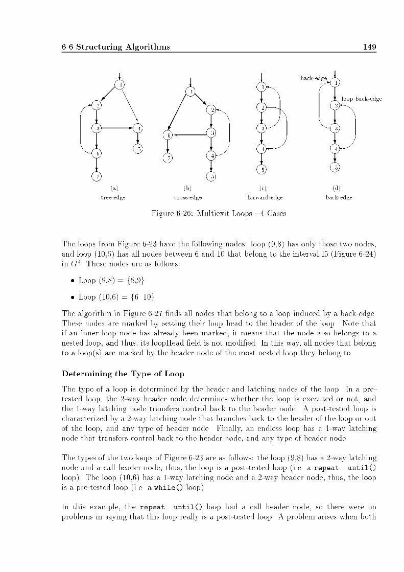
6.6 Structuring Algorithms 149%$�-��%$� %$�� %$m mmmmmmm mmm m mmmmmm mmmmmm ������� @@R ???

?AAAAAU���??? - ?? ?-�� ?1???�? ????

?(a) (d)(b) (c)tree-edge forward-edgecross-edge back-edge

back-edge loop back-edge176 5432 76 5432

1 54321 5432Figure 6-26: Multiexit Loops - 4 CasesThe loops from Figure 6-23 have the following nodes: loop (9,8) has only those two nodes,and loop (10,6) has all nodes between 6 and 10 that belong to the interval I5 (Figure 6-24)in G2. These nodes are as follows:� Loop (9,8) = f8,9g� Loop (10,6) = f6..10gThe algorithm in Figure 6-27 �nds all nodes that belong to a loop induced by a back-edge.These nodes are marked by setting their loop head to the header of the loop. Note thatif an inner loop node has already been marked, it means that the node also belongs to anested loop, and thus, its loopHead �eld is not modi�ed. In this way, all nodes that belongto a loop(s) are marked by the header node of the most nested loop they belong to.Determining the Type of LoopThe type of a loop is determined by the header and latching nodes of the loop. In a pre-tested loop, the 2-way header node determines whether the loop is executed or not, andthe 1-way latching node transfers control back to the header node. A post-tested loop ischaracterized by a 2-way latching node that branches back to the header of the loop or outof the loop, and any type of header node. Finally, an endless loop has a 1-way latchingnode that transfers control back to the header node, and any type of header node.The types of the two loops of Figure 6-23 are as follows: the loop (9,8) has a 2-way latchingnode and a call header node, thus, the loop is a post-tested loop (i.e. a repeat..until()loop). The loop (10,6) has a 1-way latching node and a 2-way header node, thus, the loopis a pre-tested loop (i.e. a while() loop).In this example, the repeat..until() loop had a call header node, so there were noproblems in saying that this loop really is a post-tested loop. A problem arises when both

150 Control Flow Analysisprocedure markNodesInLoop (G = (N;E; h), (y; x))/* Pre: (y; x) is a back-edge.* Post: the nodes that belong to the loop (y; x) are marked. */nodesInLoop = fxgloopHead(x) = xfor (all nodes n 2 fx+ 1 : : :yg)if (n 2 I(x))nodesInLoop = nodesInLoop [fngif (loopHead(n) == No Node)loopHead(n) = x.end ifend ifend forend procedureFigure 6-27: Algorithm to Mark all Nodes that belong to a Loop induced by (y; x)the header and latching nodes are 2-way conditional nodes, since it is not known whetherone or both branches of the header 2-way node branch into the loop or out of the loop; i.e.the loop would be an abnormal loop in the former case, and a post-tested loop in the lattercase. It is therefore necessary to check whether the nodes of the branches of the headernode belong to the loop or not, if they do not, the loop can be coded as a while() loopwith an abnormal exit from the latching node. Figure 6-28 gives an algorithm to determinethe type of loop based on the nodesInLoop set constructed in the algorithm of Figure 6-27.Finding the Loop Follow NodeThe loop follow node is the �rst node that is reached after the loop is terminated. In thecase of natural loops, there is only one node that is reached after loop termination, butin the case of multiexit and multilevel exit loops, there can be more than one exit, thus,more than one node can be reached after the loop. Since the structuring algorithm onlystructured natural loops, all multiexit loops are structured with one \real" exit, and one ormore abnormal exits. In the case of endless loops that have exits in the middle of the loop,several nodes can be reached after the di�erent exits. It is the purpose of this algorithm to�nd only one follow node.In a pre-tested loop, the follow node is the successor of the loop header that does not belongto the loop. In a similar way, the follow node of a post-tested loop is the successor of theloop latching node that does not belong to the loop. In endless loops there are no follownodes initially, as neither the header nor the latching node jump out of the loop. But sincean endless loop can have a jump out of the loop in the middle of the loop (e.g. a break inC), it can too have a follow node. Since the follow node is the �rst node that is reachedafter the loop is ended, it is desirable to �nd the closest node that is reached from the loop

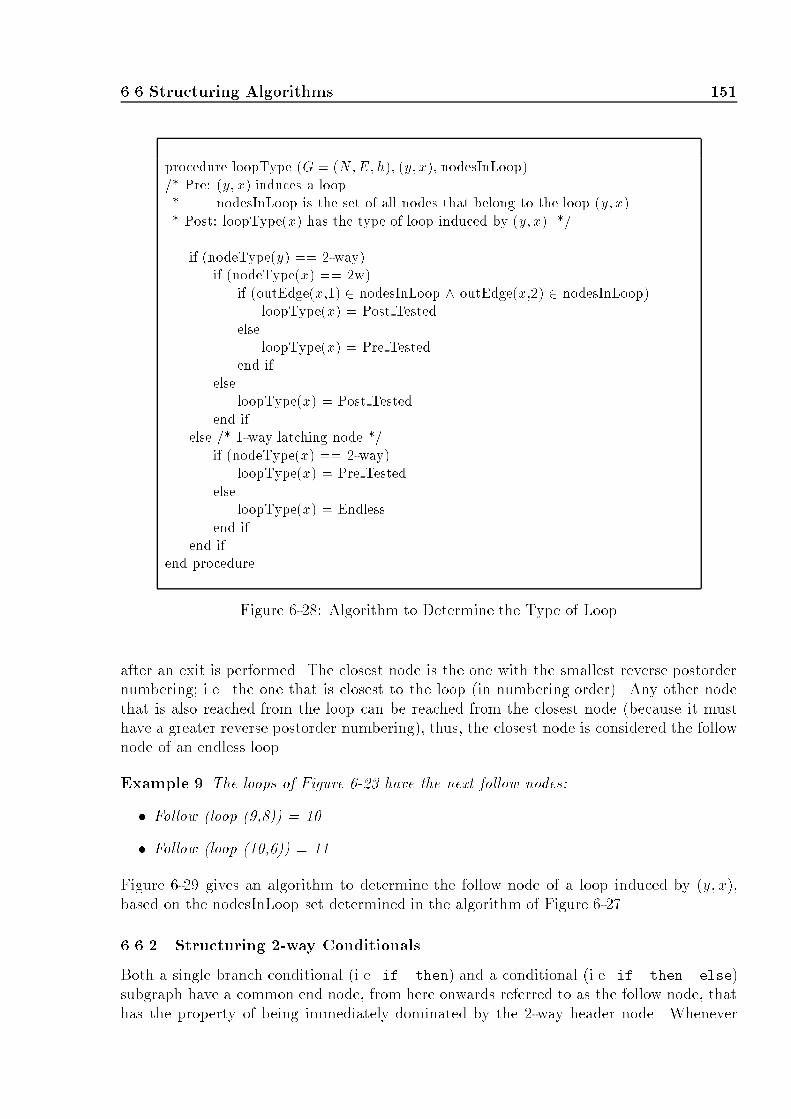
6.6 Structuring Algorithms 151procedure loopType (G = (N;E; h), (y; x), nodesInLoop)/* Pre: (y; x) induces a loop.* nodesInLoop is the set of all nodes that belong to the loop (y; x).* Post: loopType(x) has the type of loop induced by (y; x). */if (nodeType(y) == 2-way)if (nodeType(x) == 2w)if (outEdge(x,1) 2 nodesInLoop ^ outEdge(x,2) 2 nodesInLoop)loopType(x) = Post Tested.else loopType(x) = Pre Tested.end ifelse loopType(x) = Post Tested.end ifelse /* 1-way latching node */if (nodeType(x) == 2-way)loopType(x) = Pre Tested.else loopType(x) = Endless.end ifend ifend procedureFigure 6-28: Algorithm to Determine the Type of Loopafter an exit is performed. The closest node is the one with the smallest reverse postordernumbering; i.e. the one that is closest to the loop (in numbering order). Any other nodethat is also reached from the loop can be reached from the closest node (because it musthave a greater reverse postorder numbering), thus, the closest node is considered the follownode of an endless loop.Example 9 The loops of Figure 6-23 have the next follow nodes:� Follow (loop (9,8)) = 10� Follow (loop (10,6)) = 11Figure 6-29 gives an algorithm to determine the follow node of a loop induced by (y; x),based on the nodesInLoop set determined in the algorithm of Figure 6-27.6.6.2 Structuring 2-way ConditionalsBoth a single branch conditional (i.e. if..then) and a conditional (i.e. if..then..else)subgraph have a common end node, from here onwards referred to as the follow node, thathas the property of being immediately dominated by the 2-way header node. Whenever

152 Control Flow Analysisprocedure loopFollow (G = (N;E; h), (y; x), nodesInLoop)/* Pre: (y; x) induces a loop.* nodesInLoop is the set of all nodes that belong to the loop (y; x).* Post: loopFollow(x) is the follow node to the loop induced by (y; x). */if (loopType(x) == Pre Tested)if (outEdges(x,1) 2 nodesInLoop)loopFollow(x) = outEdges(x,2).else loopFollow(x) = outEdges(x,1).end ifelse if (loopType(x) == Post Tested)if (outEdges(y,1) 2 nodesInLoop)loopFollow(x) = outEdges(y,2).else loopFollow(x) = outEdges(y,1).end ifelse /* endless loop */fol = Max /* a large constant */for (all 2-way nodes n 2 nodesInLoop)if ((outEdges(x,1) 62 nodesInLoop) ^ (outEdges(x,1) < fol))fol = outEdges(x,1).else if ((outEdges(x,2) 62 nodesInLoop) ^ (outEdges(x,2) < fol))fol = outEdges(x,2).end ifend forif (fol 6= Max)loopFollow(x) = fol.end ifend ifend procedureFigure 6-29: Algorithm to Determine the Follow of a Loopthese subgraphs are nested, they can have di�erent follow nodes or share the same commonfollow node. Consider the graph in Figure 6-30, which is the same graph from Figure 6-2without intermediate instruction information, and with immediate dominator information.The nodes are numbered in reverse postorder.In this graph there are six 2-way nodes, namely, nodes 1, 2, 6, 9, 11, and 12. As seenduring loop structuring (Section 6.6.1), a 2-way node that belongs to either the headeror the latching node of a loop is marked as being so, and must not be processed during2-way conditional structuring given that it already belongs to another structure. Hence,the nodes 6 and 9 in Figure 6-30 are not considered in this analysis. Whenever two or moreconditionals are nested, it is always desirable to analyze the most nested conditional �rst,and then the outer ones. In the case of the conditionals at nodes 1 and 2, node 2 must be

6.6 Structuring Algorithms 153� %$���nn nnn nnnnn nnn

n n??�� @@R��@@R ?���+ HHHj��/?@@R ������ ? ???BBBBBN15124

%$� 3 Node56 78910111213 14

Immediate Dominator123456789101112131415-122156789611111114Figure 6-30: Control Flow Graph with Immediate Dominator Informationanalyzed �rst than node 1 since it is nested in the subgraph headed by 1; in other words,the node that has a greater reverse postorder numbering needs to be analyzed �rst sinceit was last visited �rst in the depth �rst search traversal. In this example, both subgraphsshare the common follow node 5; therefore, there is no node that is immediately dominatedby node 2 (i.e. the inner conditional), but 5 is immediately dominated by 1 (i.e. the outerconditional), and this node is the follow node for both conditionals. Once the follow nodehas been determined, the type of the conditional can be known by checking whether one ofthe branches of the 2-way header node is the follow node, in which case, the subgraph is asingle branching conditional, otherwise it is an if..then..else. In the case of nodes 11and 12, node 12 is analyzed �rst and no follow node is determined since no node takes itas immediate dominator. This node is left in a list of unresolved nodes, because it can benested in another conditional structure. When node 11 is analyzed, nodes 12, 13, and 14are possible candidates for follow node, since nodes 12 and 13 reach node 14, this last nodeis taken as the follow (i.e. the node that encloses the most number of nodes in a subgraph,the largest node). Node 12, that is in the list of unresolved follow nodes, is also marked ashaving a follow node of 14. It is seen from the graph that these two conditionals are notproperly nested, and a goto jump can be used during code generation.A generalization of this example provides the algorithm to structure conditionals. The ideaof the algorithm is to determine which nodes are header nodes of conditionals, and whichnodes are the follow of such conditionals. The type of the conditional can be determinedafter �nding the follow node by checking whether one of the branches of the header nodeis equivalent to the follow node. Inner conditionals are traversed �rst, then outer ones, so

154 Control Flow Analysisa descending reverse postorder traversal is performed (i.e. from greater to smaller nodenumber). A set of unresolved conditional follow nodes is kept throughout the process. Thisset holds all 2-way header nodes for which a follow has not been found. For each 2-waynode that is not part of the header or latching node of a loop, the follow node is calculatedas the node that takes it as an immediate dominator and has two or more in-edges (sinceit must be reached by at least two di�erent paths from the header). If there is more thanone such node, the one that encloses the maximum number of nodes is selected (i.e. theone with the largest number). If such a node is not found, the 2-way header node is placedon the unresolved set. Whenever a follow node is found, all nodes that belong to the setof unresolved nodes are set to have the same follow node as the one just found (i.e. theyare nested conditionals or unstructured conditionals that reach this node). The completealgorithm is shown in Figure 6-31.procedure struct2Way (G=(N,E,h))/* Pre: G is a graph.* Post: 2-way conditionals are marked in G.* the follow node for all 2-way conditionals is determined. */unresolved = fgfor (all nodes m in descending order)if ((nodeType(m) == 2-way) ^ (inHeadLatch(m) == False))if (9 n � n = maxfi j immedDom(i) = m^ #inEdges(i) � 2g)follow(m) = nfor (all x 2 unresolved)follow(x) = nunresolved = unresolved - fxgend forelseunresolved = unresolved [ fmgend ifend ifend forend procedureFigure 6-31: 2-way Conditional Structuring AlgorithmCompound ConditionsWhen structuring graphs in decompilation, not only the structure of the underlying con-structs is to be considered, but also the underlying intermediate instructions information.Most high-level languages allow for short-circuit evaluation of compound Boolean conditions(i.e. conditions that include and and or). In these languages, the generated control owgraphs for these conditional expressions become unstructured since an exit can be performedas soon as enough conditions have been checked and determined the expression is true orfalse as a whole. For example, if the expression x and y is compiled with short-circuit

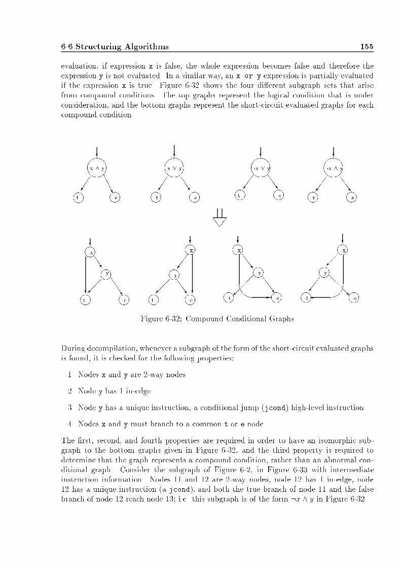
6.6 Structuring Algorithms 155evaluation, if expression x is false, the whole expression becomes false and therefore theexpression y is not evaluated. In a similar way, an x or y expression is partially evaluatedif the expression x is true. Figure 6-32 shows the four di�erent subgraph sets that arisefrom compound conditions. The top graphs represent the logical condition that is underconsideration, and the bottom graphs represent the short-circuit evaluated graphs for eachcompound condition.� %n nn n

n n����n nn nn n����

nn nn n���� nnnn n����

nnJJ��� JJJ??� AAAU?

���/��� SSSw ??� JJJ?

&-tSS�� SSSw SSSw? ���/ SSSw?�����/ ?���/ SSSw?

���� @@@@Rx yt ex ^ yt e xyt e

x _ yt e x y e:x _ yt e xyt

:x ^ yt eeFigure 6-32: Compound Conditional GraphsDuring decompilation, whenever a subgraph of the form of the short-circuit evaluated graphsis found, it is checked for the following properties:1. Nodes x and y are 2-way nodes.2. Node y has 1 in-edge.3. Node y has a unique instruction, a conditional jump (jcond) high-level instruction.4. Nodes x and y must branch to a common t or e node.The �rst, second, and fourth properties are required in order to have an isomorphic sub-graph to the bottom graphs given in Figure 6-32, and the third property is required todetermine that the graph represents a compound condition, rather than an abnormal con-ditional graph. Consider the subgraph of Figure 6-2, in Figure 6-33 with intermediateinstruction information. Nodes 11 and 12 are 2-way nodes, node 12 has 1 in-edge, node12 has a unique instruction (a jcond), and both the true branch of node 11 and the falsebranch of node 12 reach node 13; i.e. this subgraph is of the form :x ^ y in Figure 6-32.

156 Control Flow Analysisjcond (loc3 < loc4) B9jcond ((loc4 * 2) <= loc3) B10loc3 = loc3 + loc4 - 10loc4 = loc4 / 2printf ("...", loc3, loc4)ret����� B11���+ PPPPPq AAAAAAUAAAAA�����9??B7B8 B9 B10Figure 6-33: Subgraph of Figure 6-2 with Intermediate Instruction InformationThe algorithm to structure compound conditionals makes use of a traversal from top tobottom of the graph, as the �rst condition in a compound conditional expression is higherup in the graph (i.e. it is tested �rst). For all 2-way nodes, the then and else nodes arechecked for a 2-way condition. If either of these nodes represents one high-level conditionalinstruction (jcond), and the node has no other entries (i.e. the only in-edge to this nodecomes from the header 2-way node), and the node forms one of the 4 subgraphs illustrated inFigure 6-32, these two nodes are merged into a unique node that has the equivalent semanticmeaning of the compound condition (i.e. depends on the structure of the subgraph), andthe node is removed from the graph. This process is repeated until no more compoundconditions are found (i.e. there could be 3 or more compound ands and ors, so the processis repeated with the same header node until no more conditionals are found). The �nalalgorithm is shown in Figure 6-34.6.6.3 Structuring n-way ConditionalsN-way conditionals are structured in a similar way to 2-way conditionals. Nodes are tra-versed from bottom to top of the graph in order to �nd nested n-way conditionals �rst,followed by the outer ones. For each n-way node, a follow node is determined. This nodewill optimally have n in-edges coming from the n successor nodes of the n-way header node,and be immediately dominated by such header node.The determination of the follow node in an unstructured n-way conditional subgraph makesuse of modi�ed properties of the abovementioned follow node. Consider the unstructuredgraph in Figure 6-35, which has an abnormal exit from the n-way conditional subgraph.Candidate follow nodes are all nodes that have the header node 1 as immediate dominator,and that are not successors of this node, thus, nodes 5 and 6 are candidate follow nodes.Node 5 has 3 in-edges that come from paths from the header node, and node 6 has 2 in-edgesfrom paths from the header node. Since node 5 has more paths from the header node thatreach it, this node is considered the follow of the complete subgraph.

6.6 Structuring Algorithms 157procedure structCompConds (G=(N,E,h))/* Pre: G is a graph.* 2-way, n-way, and loops have been structured in G.* Post: compound conditionals are structured in G. */change = Truewhile (change)change = Falsefor (all nodes n in postorder)if (nodeType(n) = 2-way)t = succ[n, 1]e = succ[n, 2]if ((nodeType(t) = 2-way) ^ (numInst(t) = 1) ^ (numInEdges(t) = 1))if (succ[t, 1] = e)modifyGraph (:n ^ t)change = Trueelse if (succ[t, 2] = e)modifyGraph (n _ t)change = Trueend ifelse if ((nodeType(e) = 2-way) ^ (numInst(e) = 1) ^ (numInEdges(e) = 1))if (succ[e, 1] = t)modifyGraph (n ^ e)change = Trueelse if (succ[e, 2] = t)modifyGraph (:n _ e)change = Trueend ifend ifend ifend forend whileend procedureFigure 6-34: Compound Condition Structuring AlgorithmUnfortunately, abnormal entries into an n-way subgraph are not covered by the abovemethod. Consider the graph in Figure 6-36, which has an abnormal entry into one ofthe branches of the header n-way node. In this case, node 6 takes node 1 as immediatedominator, due to the abnormal entry (1,2), instead of 2 (the n-way header node). In otherwords, the follow node takes as immediate dominator the common dominator of all in-edgesto node 3; i.e. node 1. In this case, the node that performs an abnormal entry into thesubgraph needs to be determined, in order to �nd a follow node that takes it as immediatedominator. The complete algorithm is shown in Figure 6-37.

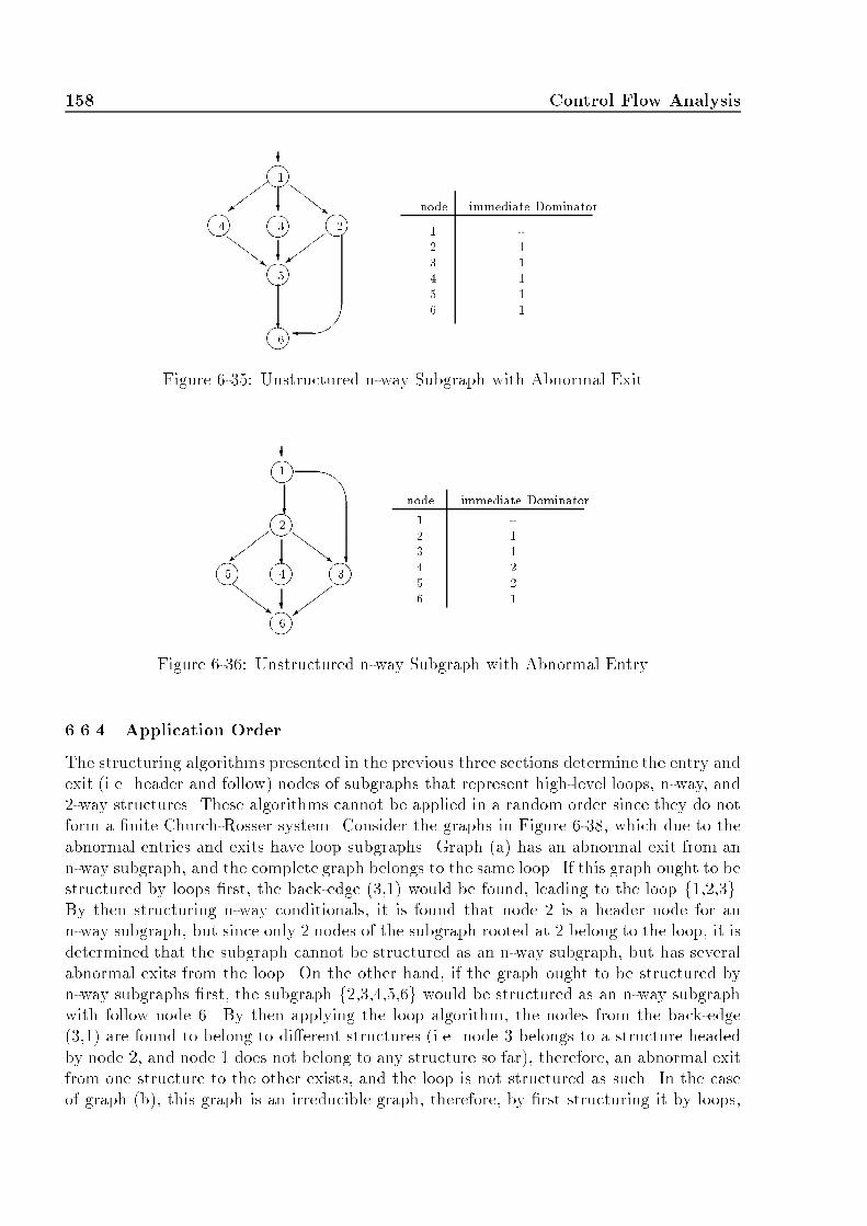
158 Control Flow Analysis11111node immediate Dominator123456� %n -n2n nnn���= ZZZ~? ���=ZZZ~ ???1654 3Figure 6-35: Unstructured n-way Subgraph with Abnormal Exit11221node immediate Dominator123456?$n -n 1 nnnn���= ZZZ~���=??ZZZ~ ??65 4 32Figure 6-36: Unstructured n-way Subgraph with Abnormal Entry6.6.4 Application OrderThe structuring algorithms presented in the previous three sections determine the entry andexit (i.e. header and follow) nodes of subgraphs that represent high-level loops, n-way, and2-way structures. These algorithms cannot be applied in a random order since they do notform a �nite Church-Rosser system. Consider the graphs in Figure 6-38, which due to theabnormal entries and exits have loop subgraphs. Graph (a) has an abnormal exit from ann-way subgraph, and the complete graph belongs to the same loop. If this graph ought to bestructured by loops �rst, the back-edge (3,1) would be found, leading to the loop f1,2,3g.By then structuring n-way conditionals, it is found that node 2 is a header node for ann-way subgraph, but since only 2 nodes of the subgraph rooted at 2 belong to the loop, it isdetermined that the subgraph cannot be structured as an n-way subgraph, but has severalabnormal exits from the loop. On the other hand, if the graph ought to be structured byn-way subgraphs �rst, the subgraph f2,3,4,5,6g would be structured as an n-way subgraphwith follow node 6. By then applying the loop algorithm, the nodes from the back-edge(3,1) are found to belong to di�erent structures (i.e. node 3 belongs to a structure headedby node 2, and node 1 does not belong to any structure so far), therefore, an abnormal exitfrom one structure to the other exists, and the loop is not structured as such. In the caseof graph (b), this graph is an irreducible graph, therefore, by �rst structuring it by loops,

6.6 Structuring Algorithms 159procedure structNWay (G = (N,E,h))/* Pre: G is a graph.* Post: n-way conditionals are structured in G.the follow node is determined for all n-way subgraphs. */unresolved = fgfor (all nodes m 2 N in postorder)if (nodeType(m) == n-way)if (9 s: succ(m)� immedDom(s) 6= m)n = commonImmedDom(fs j s = succ(m)g)elsen = mend ifif (9 j� #inEdges(j) =maxfi j immedDom(i) = n^ #inEdges(i) � 2� #inEdges(i)g)follow(m) = jfor (all i 2 unresolved)follow(i) = junresolved = unresolved - figend forelseunresolved = unresolved [ fmgend ifend ifend forend procedureFigure 6-37: n-way Conditional Structuring Algorithma multiexit loop will be found, with abnormal exits coming from the nodes of the n-waysubgraph (which is not structured as such due to the abnormal exits). On the other hand,if this graph was structured as an n-way subgraph �rst, the loop would not be structuredas such, but as a goto jump.These examples illustrate that the series of structuring algorithms presented in the previoussections is not �nite Church-Rosser. This implies that an ordering is to be followed, andit is: structure n-way conditionals, followed by loop structuring, and 2-way conditionalstructuring last. Loops are structured �rst than 2-way conditionals to ensure the Booleancondition that form part of pre-tested or post-tested loops is part of the loop, rather thanthe header of a 2-way conditional subgraph. Once a 2-way conditional has been marked asbeing in the header or latching node of a loop, it is not considered for further structuring.

160 Control Flow Analysis%6nnnn nn n nn nnn���= ZZZ~���=??ZZZ~ ? ���=$� ZZZ~ 6? ���=ZZZ~ ??? ?(a) (b)

12 345 6 123 45Figure 6-38: Unstructured GraphThe Case of Irreducible GraphsThe examples presented so far in this Chapter deal with reducible graphs. Recall fromSection 6.3.4 that a graph is irreducible if it contains a subgraph of the form of the canon-ical irreducible owgraph. In essence, a graph is irreducible if it has 2 or more entries (i.e.a multientry loop), at least 2 entries are dominated by the same common node, and thiscommon node dominates the entrance nodes to the loop. Consider the multientry graphsin Figure 6-39. These graphs represent di�erent classes of multientry graphs according tothe underlying edges in a depth-�rst tree of the graph. As can be seen, graphs that havea tree-edge, cross-edge, and forward-edge are irreducible, but the graph with the back-edgecoming into the loop is not irreducible since there is no common node that dominates allentries into the loop. This later loop is equivalent to an overlapping loop, much in the sameway as a multiexit loop with a back-edge out of the loop (Figure 6-26, graph (d)).-'& %$�%$���$���mm mmm mmmmmmmm mmmm

mmmmm? ?�����=-'& ?

back-edge?�� ?QQQQQs ?@@R ��?? @@R? ? ???? ????(d)(c)(b)(a) loop back-edgeback-edgetree-edge forward-edgecross-edgeFigure 6-39: Multientry Loops - 4 Cases

6.6 Structuring Algorithms 161Since it is the purpose of a decompiler structuring algorithm not to modify the semanticsand functionality of the control ow graph, node splitting is not used to structure irreduciblegraphs, since the addition of new nodes modi�es the semantics of the program. It is thereforedesired to structure the graph without node replication, i.e. leave the graph as an irreduciblegraph that has goto jumps. Consider the graph in Figure 7-14 with immediate dominatorinformation. Since the graph is irreducible, there is no loop that is contained entirely inan interval, therefore, the loop structuring algorithm determines that there are no naturalloops as such. When structuring 2-way conditionals, the conditional at node 1 is determinedto have the follow node 3, since this node is reached from both paths from the header nodeand has a greater numbering than node 2. This means that the graph is structured as a2-way subgraph with follow node 3, and no natural loop. During code generation, gotojumps are used to simulate the loop, and the multientries (see Chapter 7, Section 7.1.3).mm@@@R��� ? -� 1m2 F 3 immediate dominator123 -11nodeTFigure 6-40: Canonical Irreducible Graph with Immediate Dominator Information

Chapter 7The Back-endT he high-level intermediate code generated by the data ow analyzer, and the structuredcontrol ow graph generated by the control ow analyzer, are the input to the back-end.This module is composed in its entirety by the code generator, which generates code for thetarget high-level language. This relationship is shown in Figure 7-1.-. . . . - -YHHHHHHHj. . . . . . . . . .. . . . . . . . . ..... .... �������������: HLL programFront-end Code Generatorhigh-level intermediate codeTableSymbolstructured control ow graphUDMFigure 7-1: Relation of the Code Generator with the UDM7.1 Code GenerationThe code generator generates code for a prede�ned target high-level language. The followingexamples make use of the C language as target language, and the examples are based onthe sample control ow graph of Chapter 6, Figure 6-2 after structuring information hasbeen summarized on the graph.7.1.1 Generating Code for a Basic BlockAfter data ow analysis, the intermediate instructions in a basic block are all high-levelinstructions; pseudo high-level instructions must have been eliminated from the code beforethis point. Consider the control ow graph in Figure 7-2 after data and control ow analyses.For each basic block, the instructions in the basic block are mapped to an equivalentinstruction of the target language. Transfer of control instructions (i.e. jcond and jmpinstructions) are dependent on the structure of the graph (i.e. they belong to a loopor a conditional jump (2 and n ways), or be equivalent to a goto), and hence, code isgenerated for them according to the control ow information, described in the next Section(Section 7.1.2). This section illustrates how code is generated for all other instructions of abasic block.

164 The Back-endasgn loc4, loc3 * 5jcond (loc3 >= loc4) B5asgn loc3, loc3 * loc4jcond ((loc3 * 4) <= loc4) B4� %$�%$� � %��

??�����9 XXXXXz?�����9 XXXXXXz ????PPPPPq ?XXXXXz �����)asgn loc3, 5

call printf ("...", loc3, loc4)AAAAAAAUB5B6jcond (loc1 < 10) B12((loc4 * 2) <= loc3)) B10jcond ((loc3 >= loc4) andB7

B11retB2 asgn loc4, loc4 << 3asgn loc1, 0asgn loc3, loc3 << 3 asgn loc2, loc1jcond (loc2 < 5) B13asgn loc1, loc1 + 1asgn loc4, loc4 / 2asgn loc3, (loc3 + loc4) - 10 call printf ("...", loc1, loc2)asgn loc2, loc2 + 1B9 B13B12B14B15

B3 B4B1B10Figure 7-2: Sample Control Flow Graph After Data and Control Flow AnalysesGenerating Code for asgn InstructionsThe asgn instruction assigns to an identi�er an arithmetic expression or another identi�er.Expressions are stored by the decompiler in abstract syntax trees, therefore, a tree walker isused to generate code for them. Consider the �rst instruction of basic block B1, Figure 7-2:asgn loc3, 5The left hand side is the local identi�er loc3 and the right hand side is the constant identi�er5. Since both expressions are identi�ers, the code is trivially translated to:loc3 = 5;The �rst instruction of basic block B9, Figure 7-2 uses an expression in its right hand side:asgn loc3, (loc3 + loc4) - 10This instruction is represented by the abstract syntax tree of Figure 7-3; only the righthand side of the instruction is stored in the abstract syntax tree format (�eld arg of theintermediate triplet (see Figure 4-32, Chapter 4)). From the tree, the right hand side isequivalent to the expression (loc3 + loc4) - 10, and the C code for this instruction is:loc3 = (loc3 + loc4) - 10;

7.1 Code Generation 165��� QQQ��� QQQ��� HHHH:=loc3 loc3 loc4+ 10-Figure 7-3: Abstract Syntax Tree for First Instruction of B9Generating code from an abstract syntax tree is solved in a recursive way according tothe type of operator; binary or unary. For binary operators, the left branch of the treeis traversed, followed by the operator, and the traversal of the right branch. For unaryoperators, the operator is �rst displayed, followed by its subtree expression. In both cases,the recursion ends when an identi�er is met (i.e. the leaves of the tree).Example 10 Expressions are de�ned in an intermediate language using the following typesof expressions:� Binary expressions: all expressions that use a binary operator. The binary operatorsand their C counterparts are:{ Less or equal to (<=).{ Less than (<).{ Equal (==).{ Not equal (!=).{ Greater (>).{ Greater or equal to (>=).{ Bitwise and (&).{ Bitwise or (|).{ Bitwise xor (^).{ Not (1's complement) (~).{ Add (+).{ Subtract (-).{ Multiply (*).{ Divide (/).{ Modulus (%).{ Shift right (>>).{ Shift left (<<).{ Compound and (&&).{ Compound or (||).

166 The Back-end� Unary expressions: all expression that use a unary operator. The unary operators andtheir C counterparts are:{ Expression negation (!).{ Address of (&).{ Dereference (*).{ Post and pre increment (++).{ Post and pre decrement (--).� Identi�ers: an identi�er is the minimum type of expression. Identi�ers are classi�edaccording to their location in memory and/or in registers, in the following way:{ Global variable.{ Local variable (negative o�sets from the stack frame).{ Formal parameter (positive o�set from the stack frame).{ Constant.{ Register.{ Function (function name and actual argument list).The algorithm of Figure 7-4 generates code for an expression that uses the above operatortypes, by walking the tree recursively.procedure walkCondExp (e: expression)/* Pre: e points to an expression tree (abstract syntax tree).* Post: the code for the expression tree pointed to by e is written. */case (expressionType(e))Boolean: write ("(%s %s %s)", walkCondExp (lhs(e)), operatorType(e),walkCondExp (rhs(e))).Unary: write ("%s (%s)", operatorType(e), walkCondExp (exp(e))).Identi�er: write ("%s", identi�erName(e)).end caseend procedureFigure 7-4: Algorithm to Generate Code from an Expression TreeThe identi�erName(e) function returns the name of the identi�er in the identi�er nodee; this name is taken from the appropriate symbol table (i.e. global, local or argument).Whenever the identi�er is a register, the register is uniquely named by generating a newlocal variable; the next in the sequence of local variables. The new variable is placed at theend of the subroutine's local variables de�nition.

7.1 Code Generation 167Generating Code for call InstructionsThe call instruction invokes a procedure with the list of actual arguments. This list isstored in the arg �eld and is a sequential list of expressions (i.e. arithmetic expressionsand/or identi�ers). The name of the procedure is displayed followed by the actualarguments, which are displayed using the tree walker algorithm of Figure 7-4.Generating Code for ret InstructionsThe ret instruction returns an expression/identi�er in a function. If the return instructiondoes not take any arguments, the procedure is �nished at that statement. The return of anexpression is optional.The complete algorithm to generate code for a basic block (excluding transfer instructions)is shown in Figure 7-5. In this algorithm the function indent() is used; this function returnsone or more spaces depending on the indentation level (3 spaces per indentation level).procedure writeBB (BB: basicBlock, indLevel: integer)/* Pre: BB is a basic block.* indLevel is the indentation level to be used in this basic block.* Post: the code for all instructions, except transfer instructions, is displayed. */for (all high-level instructions i of BB) docase (instType(i))asgn: write ("%s%s = %s;\n", indent(indLevel), walkCondExp (lhs(i)),walkCondExp (rhs(i))).call: fa = "".for (all actual arguments f 2 formalArgList(i)) doappend (fa, "%s,", walkCondExp (f)).end forwrite ("%s%s (%s);\n", indent (indLevel), invokedProc (i), fa).ret: write ("%sreturn (%s);\n", indent(indLevel), exp(i)).end caseend forend procedure Figure 7-5: Algorithm to Generate Code from a Basic Block7.1.2 Generating Code from Control Flow GraphsThe information collected during control ow analysis of the graph is used in code genera-tion to determine the order in which code should be generated for the graph. Consider thegraph in Figure 7-6 with structuring information. This graph is the same graph of Figure 7-2 without intermediate instruction information; nodes are numbered in reverse postorder.The generation of code from a graph can be viewed as the problem of generating code forthe root node, recursing on the successor nodes that belong the structure rooted at the root

168 The Back-endnn@@R ?1513 14

loopType loopFollow1110pre testpost test ifFollow5514%$�� %$���

nn nnn nnnn

n n??�� @@R��@@Rn ? 15���+ HHHj��/ ????124 356 7891011 node12345678910111314Figure 7-6: Control Flow Graph with Structuring Informationnode (if any), and continue code generation with the follow node of the structure. Recallfrom Chapter 6 that the follow node is the �rst node that is reached from a structure (i.e.the �rst node that is executed once the structure is �nished). Follow nodes for loops, 2-wayand n-way conditionals are calculated during the control ow analysis phase. Other trans-fer of control nodes (i.e. 1-way, fall-through, call) transfer control to the unique successornode; hence the follow is the successor, and termination nodes (i.e. return) are leaves inthe underlying depth-�rst search tree of the graph, and hence terminate the generation ofcode along that path.This section describes the component algorithms of the algorithm to generate code for aprocedure, writeCode(). To make the explanation easier, we will assume that this routineexists; therefore, we concentrate only on the generation of code for a particular structureand let the writeCode() routine generate code for the components of the structure. Afterenough algorithms have been explained, the algorithm for writeCode() is given.Generating Code for LoopsGiven a subgraph rooted at a loop header node, code for this loop is generated based onthe type of loop. Regardless of type of loop, all loops have the same structure: loop header,loop body, and loop trailer. Both the loop header and trailer are generated depending onthe type of loop, and the loop body is generated by generating code for the subgraph rootedat the �rst node of the loop body. Consider the loops in the graph of Figure 7-6. The looprooted at node 6 is a pre-tested loop, and the loop rooted at node 8 is a post-tested loop.

7.1 Code Generation 169In the case of the pre-tested loop, when the loop condition is True (i.e. the jcond Booleanconditional in node 6), the loop body is executed. If the branch into the loop was the Falsebranch, the loop condition has to be negated since the loop is executed when the conditionis False. The loop body is generated by the writeCode() routine, and the loop trailerconsists only of an end of loop bracket (in C). Once this code has been generated, codefor the loop follow node is generated by invoking the writeCode() routine. The followingskeleton is used:write ("%s while (loc1 < 10) {\n", indent(indLevel))writeCode (7, indLevel + 1, 10, ifFollow, nFollow)write ("%s }\n", indent(indLevel))writeCode (11, indLevel, latchNode, ifFollow, nFollow)where the �rst instruction generates code for the loop header, the second instruction gen-erates code for the loop body; rooted at node 7 and having a latching node 10, the thirdinstruction generates code for the loop trailer, and the fourth instruction generates code forthe rest of the graph rooted at node 11.In the post-tested loop, the loop condition is true when the branch is made to the loopheader node. The following skeleton is used:write ("%s do {\n", indent(indLevel))writeBB (8, indLevel + 1)writeCode (9, indLevel + 1, 9, ifFollow, nFollow)write ("%s } while (loc2 < 5); \n", indent(indLevel))writeCode (10, indLevel, latchNode, ifFollow, nFollow)where the �rst instruction generates code for the loop header, the second instruction gener-ates code for the instruction in the root node, the third instruction generates code for theloop body rooted at node 9 and ended at the loop latching node 9, the fourth instructiongenerates the loop trailer, and the �fth instruction generates code for the remainder of thegraph rooted at node 10. Code is generated in a similar way for endless loops, with thedistinction that there may or may not be a loop follow node.Normally pre-tested loop header nodes have only one instruction associated with them,but in languages that allow for several logical instructions to be coded in the one physicalinstruction, such as in C, these instructions will be in the header node but not all of themwould form part of the loop condition. For example, in the following C loop:while ((a += 11) > 50){ printf ("greater than 50\n");a = a - b;}the while() statement has two purposes: to add 11 to variable a, and to check that afterthis assignment a is greater than 50. Since our choice of intermediate code allows foronly one instruction to be stored in an intermediate instruction, the assignment and thecomparison form part of two di�erent instructions, as shown in the following intermediatecode:

170 The Back-endB3:asgn a, a + 11jcond (a <= 50) B5B4:call printf ("greater than 50\n")asgn a, a - bjmp B3B5:/* other code */Two solutions are considered for this case: preserve the while() loop structure by repeatingthe extra instructions in the header basic block at the end of the loop, or transform thewhile() loop into an endless for (;;) loop that breaks out of the loop whenever theBoolean condition associated with the while() is False. In our example, the former caseleads to the following code in C:a = a + 11;while (a > 50) {printf ("greater than 50\n");a = a - b;a = a + 11;}and the latter case leads to the following C code:for (;;) {a = a + 11;if (a <= 50)break;printf ("greater than 50\n");a = a - b;}Either approach generates correct code for the graph; the former method replicates code(normally a few instructions, if any) and preserves the while() structure, the latter methoddoes not replicate code but modi�es the structure of the original loop. In this thesis theformer method is used in preference to the latter, since this solution provides code that iseasier to understand than the latter solution.When generating code for the loop body or the loop follow node, if the target node hasalready been traversed by the code generator, it means that the node has already beenreached along another path, therefore, a goto label needs to be generated to transfer controlto the target code. The algorithm in Figure 7-7 generates code for a graph rooted at a loopheader node. This algorithm generates code in C, and assumes the existence of the functioninvExp() which returns the inverse of an expression (i.e. negates the expression), and theprocedure emitGotoLabel()which generates a unique label, generates a goto to that label,and places the label at the appropriate position in the �nal C code.

7.1 Code Generation 171procedure writeLoop (BB: basicBlock; i, latchNode, ifFollow, nFollow: Integer)/* Pre: BB is a pointer to the header basic block of a loop.* i is the indentation level used for this basic block.* latchNode is the number of the latching node of the enclosing loop (if any).* ifFollow is the number of the follow node of the enclosing if structure (if any).* nFollow is the number of the follow node of the enclosing n-way structure (if any).* Post: code for the graph rooted at BB is generated. */traversedNode(BB) = True.case (loopType(BB)) /* Write loop header */Pre Tested:writeBB (BB, i).if (succ (BB, Else) == loopFollow(BB)) thenwrite ("%s while (%s) f\n", indent(i), walkCondExp (loopExp(BB))).elsewrite ("%s while (%s) f \n", indent(i), walkCondExp (invExp(loopExp(BB)))).end ifPost Tested: write ("%s do\n f", indent(i)).writeBB (BB, i+1).Endless: write ("%s for (;;) f \n", indent(i)).writeBB (BB, i+1).end caseif ((nodeType(BB) == Return) _ (revPostorder(BB) == latchNode)) then return.if (latchNode(BB) 6= BB) then /* Loop is several basic blocks */for (all successors s of BB) doif (loopType(BB) 6= Pre Tested) _ (s 6= loopFollow(BB)) thenif (traversedNode(BB) == False) thenwriteCode (s, i+1, latchNode (BB), ifFollow, nFollow).else /* has been traversed */emitGotoLabel (�rstInst(s)).end ifend ifend forend ifcase (loopType(BB)) /* Write loop trailer */Pre Tested: writeBB (BB, i+1).write ("%s g\n", indent(i)).Post Tested: write ("%s g while (%s); \n", indent(i), walkCondExp (loopExp(BB))).Endless: write ("%s g \n", indent(i)).end caseif (traversedNode(loopFollow(BB)) == False) then /* Continue with follow */writeCode (loopFollow(BB), i, latchNode, ifFollow, nFollow).elseemitGotoLabel (�rstInst(loopFollow(BB))).end ifend procedureFigure 7-7: Algorithm to Generate Code for a Loop Header Rooted Graph

172 The Back-endGenerating Code for 2-way Rooted GraphsGiven a graph rooted at a 2-way node that does not form part of a loop conditional expres-sion, code for this graph is generated by determining whether the node is the header of anif..then or an if..then..else condition. In the former case, code is generated for thecondition of the if, followed by the code for the then clause, and �nalized with the code forthe if follow subgraph. In the latter case, code is generated for the if condition, followedby the then and else clauses, and �nalized with the code for the follow node. Considerthe two 2-way nodes in Figure 7-6 which do not form part of loop expressions; nodes 1, 2and 11.Node 1 is the root of an if..then structure since the follow node (node 5) is one of theimmediate successors of node 1. The other immediate successor, node 2, is the body of thethen clause, which is reached when the condition in node 1 is False; i.e. the condition needsto be negated, as in the following code:write ("%s if (loc3 < loc4) {\n", indent(indLevel))writeCode (2, indLevel+1, latchNode, 5, nFollow)write ("%s }\n", indent(indLevel))writeCode (5, indLevel, latchNode, ifFollow, nFollow)where the �rst instruction generates code for the negated condition of the if, the secondinstruction generates code for the then clause subgraph which is rooted at node 2 and has 5as a follow node, the third instruction generates the trailer of the if, and the last instructiongenerates code for the follow subgraph rooted at node 5.Node 2 is the root of an if..then..else structure. In this case, neither immediatesuccessors of the header node are equivalent to the follow node. The True branch is reachedwhen the condition is True, and the False branch is reached when the condition is False,leading to the following code:write ("%s if ((loc3 * 4) <= loc4) {\n", indent(indLevel))writeCode (3, indLevel+1, latchNode, 5, nFollow)write ("%s }\n else {\n", indent(indLevel))writeCode (4, indLevel+1, latchNode, 5, nFollow)write ("%s }\n", indent(indLevel))where the �rst instruction generates code for the if condition, the second instruction gener-ates code for the then clause, the third instruction generates the else, the fourth instructiongenerates code for the else clause, and the last instruction generates the if trailer. Codefor the follow node is not generated in this case because this conditional is nested in anotherconditional that also takes 5 as the follow node. This is easily checked with the ifFollowparameter, which speci�es the follow of the enclosing if, if it is the same, code for this nodeis not yet generated.In a similar way, code is generated for the subgraph rooted at node 11. In this case, theTrue branch leads to the follow node, hence, the Boolean condition associated with this ifhas to be negated, and the False branch becomes the then clause. The following skeletalcode is used:

7.1 Code Generation 173write ("%s if ((loc3<loc4) || ((loc4*2)>loc3)) {\n", indent(indLevel))writeCode (13, indLevel+1, latchNode, 14, nFollow)write ("%s }\n", indent(indLevel))writeCode (14, indLevel, latchNode, ifFollow, nFollow)As with loops, goto jumps are generated when certain nodes in the graph have been visitedbefore the current subgraph visits them. In this case, whenever the branches of a 2-waynode have already been visited, a goto to such branch(es) is generated. Also, whenever a2-way rooted subgraph does not have a follow node it means that the two branches of thegraph do not lead to a common node because the branches are ended (i.e. a return node ismet) before met. In this case, code is generated for both branches, and the end of the pathwill ensure that the recursion is ended. The algorithm in Figure 7-8 generates code for agraph rooted at a 2-way node that does not form part of a loop Boolean expression.Generating Code for n-way Rooted GraphsGiven a graph rooted at an n-way node, code for this graph is generated in the followingway: the n-way header code is emitted (a switch() is used in C), and for each successor ofthe header node the n-way option is emitted (a case is used in C), followed by the genera-tion of code of the subgraph rooted at that successor and ended at the n-way follow node.Once the code for all successors has been generated, the n-way trailer is generated, andcode is generated for the rest of the graph by generating code for the graph rooted at thefollow node of the n-way header node. Whenever generating code for one of the branchesor the follow node of the n-way structure, if the target node has already been traversed, agoto jump is generated to transfer control to the code associated with that node.The algorithm in Figure 7-9 generates code for a graph rooted at an n-way node.Generating Code for 1-way, Fall, and Call Rooted GraphsGiven a graph rooted at a 1-way, fall-through, or call node, the code for the basic block isgenerated, followed by the unique successor of such node. Even though call nodes have 2successors, one of the successor edges points to the subroutine invoked by this instruction;since code is generated on a subroutine at a time basis, this branch is disregarded for codegeneration purposes, and the node is thought of as having a unique successor.The algorithm in Figure 7-10 generates code for nodes that have a unique successor node.If code has already been generated for the unique follow node, it means that the graph wasreached along another path and hence a goto jump is generated to transfer control to thecode associated with that subgraph.A Complete AlgorithmThe �nal algorithm to generate C code from a subroutine's graph is shown in Figure 7-11.The writeCode() procedure takes as arguments a pointer to a basic block, the indentationlevel to be used, the latching node of an enclosing loop (if any), and the follow nodes ofenclosing 2-way and n-way conditionals (if any). Initially, the basic block pointer points tothe start of the subroutine's graph, the indentation level is 1, and there are no latching or

174 The Back-endprocedure write2way (BB: basicBlock; i, latchNode, ifFollow, nFollow: Integer)/* Pre: BB is a 2-way basic block.* i is the indentation level.* latchNode is the latching node of the enclosing loop (if any).* ifFollow is the follow node of the enclosing 2-way structure (if any).* nFollow is the number of the follow node of the enclosing n-way structure (if any).* Post: the code for the tree rooted at BB is generated. */if (ifFollow(BB) 6= MAX) thenemptyThen = False.if (traversedNode(succ(BB,Then)) == False) then /* Process then clause */if (succ(BB,Then) 6= ifFollow(BB)) thenwrite ("\n %s if (%s) \n f", indent(i+1), walkCondExp (ifExp(BB)).writeCode (succ(BB,Then), i+1, latchNode, ifFollow(BB), nFollow).else /* empty then clause; negate else clause */write ("\n %s if (%s) \n f", indent(i+1), walkCondExp (invExp(ifExp(BB))).writeCode (succ(BB,Else), i+1, latchNode, ifFollow(BB), nFollow).emptyThen = True.end ifelseemitGotoLabel (�rstInst(succ(BB,Then))).end ifif (traversedNode(succ(BB,Else)) == False) then /* Process else clause */if (succ(BB,Else) 6= ifFollow(BB)) thenwrite ("%s g \n %s else \n f", indent(i), indent(i)).writeCode (succ(BB,Else), i+1, latchNode, ifFollow(BB), nFollow).end ifelse if (emptyThen == False)write ("%s g \n %s else \n f", indent(i), indent(i)).emitGotoLabel (�rstInst(succ(BB,Else))).end ifwrite ("%s g \n", indent(i)).if (traversedNode(ifFollow(BB)) == False)) thenwriteCode (ifFollow(BB), i, latchNode, ifFollow, nFollow).end ifelse /* No follow, emit if..then..else */write ("\n %s if (%s) f \n", indent(i), walkCondExp(ifExp(BB)).writeCode (succ(BB,Then), i, latchNode, ifFollow, nFollow).write ("%s g \n %s else \n f", indent(i), indent(i)).writeCode (succ(BB,Else), i, latchNode, ifFollow, nFollow).write ("%s g \n", indent(i)).end ifend procedureFigure 7-8: Algorithm to Generate Code for a 2-way Rooted Graph

7.1 Code Generation 175procedure writeNway (BB: basicBlock; i, latchNode, ifFollow, nFollow: Integer)/* Pre: BB is an n-way basic block.* i is the indentation level.* latchNode is the number of the enclosing loop latching node (if any).* ifFollow is the number of the enclosing if terminating node (if any).* nFollow is the number of the enclosing n-way terminating node (if any).* Post: code is generated for the graph rooted at BB. */write ("%s switch (%s) f \n", indent(i), nwayExp(BB)).for (all successors s of BB) do /* Generate Code for each Branch */if (traversedNode(s) == False) thenwrite ("%s case %s: \n", indent(i+1), index(s)).writeCode (s, i+2, latchNode, ifFollow, nwayFollow(BB)).write ("%s break; \n", indent(i+2)).elseemitGotoLabel (�rstInst(s)).end ifend forif (traversedNode(nwayFollow(BB)) == False) /* Generate code for the follow node */writeCode (nwayFollow(BB), i, latchNode, ifFollow, nFollow).else emitGotoLabel (�rstInst(nwayFollow(BB))).end ifend procedureFigure 7-9: Algorithm to Generate Code for an n-way Rooted Graphfollow nodes to check upon (these values are set to a predetermined value). Whenever afollow node is met, no more code is generated along that path, and the procedure returnsto the invoking procedure which is able to handle the code generation of the follow node.This is done so that the trailer of a conditional is generated before the code that followsthe conditional. In the case of loops, the latching node is the last node for which code isgenerated along a path, after which recursion is ended and the invoked procedure handlesthe loop trailer code generation and the continuation of the follow of the loop.The procedure order in which code is generated is determined by the call graph of the pro-gram. We like to generate code for the nested procedures �rst, followed by the ones thatinvoke them; hence, a depth-�rst search ordering on the call graph is followed, markingeach subroutine graph as being traversed once it has been considered for code generation.C code for each subroutine is written by generating code for the header of the subroutine,followed by the local variables de�nition, and the body of the subroutine. The algorithmin Figure 7-12 shows the ordering used, and the generation of code for the subroutine. TheisLib() function is used in this algorithm to determine whether a subroutine is a library ornot; code is not generated for library routines that were detected by the signature method ofChapter 8. The writeComments() procedure writes information collected from the analysis

176 The Back-endprocedure write1way (BB: basicBlock; i, latchNode, ifFollow, nFollow: Integer)/* Pre: BB is a pointer to a 1-way, call, or fall-through basic block.* i is the indentation level used for this basic block.* latchNode is the number of the latching node of the enclosing loop (if any).* ifFollow is the number of the follow node of the enclosing 2-way structure (if any).* nFollow is the number of the follow node of the enclosing n-way structure (if any).* Post: code for the graph rooted at BB is generated. */writeBB (BB, i).if (traversedNode(succ(BB,1)) == False) thenwriteCode (succ(BB,1), i, latchNode, ifFollow, nFollow).elseemitGotoLabel (�rstInst(succ(BB,1))).end ifend procedureFigure 7-10: Algorithm to Generate Code for 1-way, Call, and Fall Rooted Graphsprocedure writeCode (BB: basicBlock; i, latchNode, ifFollow, nFollow: Integer)/* Pre: BB is a pointer to a basic block. Initially it points to the head of the graph.* i is the indentation level used for this basic block.* latchNode is the number of the latching node of the enclosing loop (if any).* ifFollow is the number of the follow node of the enclosing 2-way structure (if any).* nFollow is the number of the follow node of the enclosing n-way structure (if any).* Post: code for the graph rooted at BB is generated. */if ((revPostorder(BB) == (ifFollow _ nFollow)) _ (traversedNode(BB) == True)) thenreturn.end iftraversedNode(BB) = True.if (isLoopHeader(BB)) then /* ... for loops */writeLoop (BB, i, latchNode, ifFollow).else /* ... for other nodes */case (nodeType(BB))2-way: write2way (BB, i, latchNode, ifFollow, nFollow).n-way: writeNway (BB, i, latchNode, ifFollow, nFollow).default: write1way (BB, i, latchNode, ifFollow, nFollow).end caseend ifend procedureFigure 7-11: Algorithm to Generate Code from a Control Flow Graph

7.1 Code Generation 177of the subroutine, such as the type of arguments that were used (stack arguments or registerarguments), whether a high-level prologue was detected in the subroutine, the number ofarguments the subroutine takes, whether the subroutine generates an irreducible graph ornot, and many more.procedure writeProc (p: procedure)/* Pre: p is a procedure pointer; initially the start node of the call graph.* Post: C code is written for the program rooted at p in a depth-�rst fashion. */if (traversedProc(p) _ isLib(p)) thenreturn.end iftraversedProc(p) = True.for (all successors s 2 succ(p)) do /* Dfs on Successors */writeProc (s).end for/* Generate code for this procedure */if (isFunction(p)) then /* Generate Subroutine Header */write ("%s %s (%s) \n f", returnType(p), funcName(p), formalArgList(p)).elsewrite ("void %s (%s) \n f", procName(p), formalArgList(p)).end ifwriteComments(p). /* Generate Subroutine Comments */for (all local variables v 2 localStkFrame(p)) do /* Local Variable De�nitions */write ("%s %s;\n", varType(v), genUniqueName(v)).end forif (isHighLevel(p)) then /* Generate Code for Subroutine */writeCode (controlFlowGraph(p), 1, Max, Max, Max).else /* low-level subroutine, generate assembler */disassemble(p).end ifwrite ("g\n").end procedureFigure 7-12: Algorithm to Generate Code from a Call GraphUsing the algorithms described in this section, the C code in Figure 7-13 is generated forthe graph of Figure 7-2. Local variables are uniquely named in a sequential order startingfrom one, and making use of the pre�x loc (for local).

178 The Back-endvoid main ()/* Takes no parameters.* High-level language prologue code.*/{int loc1;int loc2;int loc3;int loc4;loc3 = 5;loc4 = (loc3 * 5);if (loc3 < loc4) {loc3 = (loc3 * loc4);if ((loc3 << 2) > loc4) {loc3 = (loc3 << 3);}else {loc4 = (loc4 << 3);}}loc1 = 0;while ((loc1 < 10)) {loc2 = loc1;do {loc2 = (loc2 + 1);printf ("i = %d, j = %d\n", loc1, loc2);} while ((loc2 < 5));loc1 = (loc1 + 1);}if ((loc3 >= loc4) && ((loc4 << 1) <= loc3)) {loc3 = ((loc3 + loc4) - 10);loc4 = (loc4 / 2);}printf ("a = %d, b = %d\n", loc3, loc4);} Figure 7-13: Final Code for the Graph of Figure 7.27.1.3 The Case of Irreducible GraphsAs pointed out in Chapter 6, Section 6.6.4, loops of irreducible graphs are not structured asnatural loops since the nodes of the loop do not form part of a complete interval. Considerthe canonical irreducible ow graph of Figure 7-14 with structuring information.

7.1 Code Generation 179mm@@@R��� ? -�m 1 32 3 123TF ifFollownodeFigure 7-14: Canonical Irreducible Graph with Structuring InformationDuring code generation, code for the if in node 1 is generated �rst, since the True branchleads to the follow node of the if (node 3), the False branch of node 1 is the then clause(negating the Boolean condition associated with node 1). Code for the then clause isgenerated, and the if..then is followed by the code generated for node 3. Since node 3transfers control to node 2, which has already been visited during code generation, a gotojump is generated to the associated code of node 2. This goto simulates the loop andprovides an unstructured if..then structure by transferring control to the then clause ofthe if. The skeletal code for this graph in C is as follows:if (! 1) {L: 2;}3;goto L;where the numbers represent the basic blocks and code for each basic block is generated bythe writeBB() procedure.

Chapter 8Decompilation ToolsT he decompiler tools are a series of programs that help the decompiler generate targethigh-level language programs. Given a binary �le, the loader determines where thebinary image starts, and whether there is any relocation information for the �le. Once thebinary image has been loaded into memory (and possibly relocated), a disassembler canbe used to parse the binary image and produce an assembler form of the program. Theparsing process can bene�t from the use of a compiler and library signature recognizer,which determines whether a subroutine is a library subroutine or not, according to a setof prede�ned signatures generated by another program. In this way, only the original codewritten by the user is disassembled and decompiled. The disassembler can be consideredpart of the decompiler, as it parses only the binary image (i.e. it is a phase of the front-endmodule). Once the program has been parsed, it can be decompiled using the methods ofChapters 4,5, 6, and 7, generating the target high-level program. Finally, a postprocessorprogram can improve the quality of the high-level code. Figure 8-1 shows the di�erentstages involved in a decompilation system.???????? � ??� XXXXXXy ������9 ?library signatures?assembler program library bindingsabsolute machine codeloaderdisassemblerdecompilerHLL programpostprocessorHLL programrelocatable machine code prototype generatorlibrary prototypeslibrary headerscompiler signatureslibrariessignature generator

Figure 8-1: Decompilation System

182 Decompilation Tools8.1 The LoaderThe loader is an operating system program that loads an executable or binary programinto memory if there is su�cient free memory for the program to be loaded and run. Mostbinary programs contain information on the amount of memory that is required to run theprogram, relocation addresses, and initial segment register values. Once the program isloaded into memory, the loader transfers control to the binary program by setting up thecode and instruction segments.The structure of binary programs di�ers from one operating system to another, therefore,the loading of a program is dependent on the operating system and the machine the binaryprogram runs in. The simplest form of binary programs contains only the binary image ofthe program, that is, a fully linked image of the program that is loaded into memory as is,without any changes made to the binary image. The .com �les under the DOS operatingsystem use this binary structure. Most binary programs contain not only the binary image,but also header information to determine the type of binary program (i.e. there can bedi�erent types of executable programs for the same operating system, or for di�erent oper-ating systems that run on the same machine) and initial register values, and a relocationtable that holds word o�sets from the start of the binary image which need to be relocatedaccording to the address were the program is loaded into memory. This type of binary �leis used in the .exe �les under DOS and Windows. The general format of a binary programis shown in Figure 8-2. headerbinary imagerelocation tableFigure 8-2: General Format of a Binary ProgramThe algorithm used to load a program into memory is as follows: the type of binary �le isdetermined (on systems that allow for di�erent types of binary �les), if the �le is a binaryimage on its own, the size of memory to be allocated is the size of the �le, therefore, a blockof memory of the size of the �le is allocated, the �le is loaded into the block of memoryas is, without any modi�cations, and the default segment registers are set. In the case ofbinary �les with header and relocation table information, the header is read to determinehow much memory is needed to load the program, were the relocation table is, and to getother information to set up registers. A memory block of the size given in the header isallocated, the binary image of the �le is then loaded into the memory block, the elementsin the relocation table are relocated in memory, and segment registers are set up accordingto the information in the header. The algorithm is shown in Figure 8-3.

8.2 Signature Generator 183procedure loader (name: �leName)/* Pre: name is the name of a binary �le.* Post: the binary program name has been loaded into memory. */determine type of binary program.if (only binary image) thenS = size of the binary �le.allocate free block of memory of size S.load �le into allocated memory block, at a prede�ned o�set.setup default segment registers.else read header information.S = size of the binary image (from the header information).allocate free block of memory of size S.load binary image into allocated memory block.relocate all items from the relocation table in memory.setup segment registers with information from the header.end ifend procedure Figure 8-3: Loader Algorithm8.2 Signature GeneratorA signature generator is a program that automatically generates signatures for an input�le. A signature is a binary pattern used to recognize viruses, compilers, and library sub-routines. The aim of signatures in decompilation is to undo the process performed by thelinker, that is, to determine which subroutines are libraries and compiler start-up code, andreplace them by their name (in the former case) or eliminate them from the target outputcode (in the latter case). This is the case for operating systems that do not share libraries,and therefore bind the library subroutine's object code into the program's binary image.No information on the subroutine's name or arguments is stored in the binary program,hence, without a method to distinguish them from user-written subroutines, it is impos-sible to di�erentiate them from other subroutines. In the case of operating systems thatshare library subroutines, the subroutine does not form part of the binary program, and areference to the subroutine is made in the program, hence, the subroutine's name is storedas part of the binary �le (most likely in the header section). The methods presented inthis section are targetted at operating systems that do not share library subroutines, andtherefore include them in the binary program.Once a signature �le has been generated for a set of library subroutines, an interfaceprocedure is called to check a particular subroutine that is to be parsed by the decom-piler/disassembler against the library signatures. If a subroutine is matched against one ofthe signatures, the subroutine is replaced by its name (i.e. the name of the subroutine in thelibrary, such as printf) and is marked as not needing any more analysis. In this way the

184 Decompilation Toolsnumber of subroutines to be analyzed is reduced, but even better, the quality of the targethigh-level program is improved considerably since some subroutine calls will make use ofreal library names rather than arbitrary names. Also, since some of the library subrou-tines are written in assembler for performance reasons or due to low-level machine accesses,these routines do not have a high-level representation in most cases, and thus, can only bedisassembled as opposed to decompiled; the use of a library signature recognition methodeliminates the need to analyze this type of subroutines, producing better target code.The ideas presented in this and the next section (Sections 8.2, and 8.3) were developed byMichael Van Emmerik while working at the Queensland University of Technology. Theseideas are expressed in [Emm94]. Figure 8-4 has been reproduced with permission from theauthor.8.2.1 Library Subroutine SignaturesA standard library �le is a relocatable object �le that implements di�erent subroutinesavailable in a particular language/compiler. A library subroutine signature is a binary pat-tern that uniquely identi�es a subroutine in the library from any other subroutine in thatsame library. Since all subroutines perform di�erent functions, a signature that containsthe complete binary pattern of the subroutine will uniquely identify the subroutine fromany other subroutine. The main problem with this approach is the size of the signature andthe overhead created by that size. It is therefore ideal to check only a minimum numberof bytes in the subroutine, hence, the signature is as small as possible. Given the greatnumber of subroutines in a library, it is not hard to realize that for some subroutines thereis need for n bytes in the signature to uniquely identify them, but n could be greater thanthe complete size of small subroutines; therefore, for small subroutines, the remaining bytesneed to be padded with a predetermined value in order to avoid running into bytes thatbelong to another library subroutine. For example, if n is 23, the library function cos has10 bytes, and cos is followed by the library function strcpy; the 10 bytes of cos form partof its signature, along with 13 bytes of padded predetermined value; otherwise, the 13 byteswould be part of strcpy.Given the �rst n bytes of a subroutine, machine instructions that use operands which cannotbe determined to be constants or o�sets, or that depend on the address where the modulewas loaded, are considered variant bytes that can have a di�erent value in the library �leand the binary program that contains such a subroutine. It is therefore necessary to wild-card these variant byte locations, in order to generate an address-independent signature.Consider the code for a library routine fseek() in Figure 8-4. The call at instruction108 has an o�set to the subroutine that is being called. Called subroutines are not alwayslinked at the same position, therefore, this o�set address is variant; thus it is wildcarded.The mov at instruction 110 takes as one of its arguments a constant or o�set operand; sinceit is not known whether this location is invariant (i.e. a constant), it is wildcarded as well.The choice of wildcard value is dependent on the machine assembler. A good candidate isa byte that is hardly used in the machine, such as halt in this example (opcode F4), or abyte that is not used in the assembler of the machine. Similar considerations are done forthe padding bytes used when the signature is too small. In this example, 00 was used.

8.2 Signature Generator 1850100 55 push bp0101 8BEC mov bp, sp0103 56 push si0104 8B7604 mov si, [bp+4]0107 56 push si0108 E8F4F4 call **** ; destination wildcarded010B 59 pop cx010C 0BC0 or ax, ax010E 7405 jz 01150110 B8F4F4 mov ax, **** ; operand wildcarded0113 EB4C jmp 01610115 0000 ; paddingFigure 8-4: Partial Disassembly of Library Function fseek()It is noted in this example that although the function fseek() has more bytes in its image,the signature is cut after 21 bytes due to the unconditional jump in instruction 113. This isdone since it is unknown whether the bytes that follow the unconditional jump form part ofthe same library subroutine or not. In general, whenever a return or (un)conditional jumpis met, the subroutine is considered �nished for the purposes of library signatures, and anyremaining bytes are padded. The �nal signature for this example is given in Figure 8-5. Itshould be noted that this method has some small probability of being in error since di�er-ent subroutines may have the same starting code up to the �rst (un)conditional transfer ofcontrol. 558BEC568B760456E8F4F4590BC07405B8F4F4EB4C0000Figure 8-5: Signature for Library Function fseek()The algorithm to automatically generate library subroutine signatures is shown in Fig-ure 8-6. This algorithm takes as arguments a standard library �le, the name of the outputsignature �le, and the size of the signature (in bytes), which has been experimentally foundin advance.Since di�erent library �les are provided by the compiler vendor in machines that use di�erentmemory models, a di�erent signature �le needs to be generated for each memory model. Itis ideal to use a naming convention to determine the compiler vendor and memory model ofthe signature library, in that way, eliminating any need for extra header information savedon the signature �le.

186 Decompilation Toolsprocedure genLibrarySignature (lib:libraryFile, signLib:�le, n:integer)/* Pre: lib is a standard library �le.* signLib is the name of the output library signature �le.* n is the size of the signature in bytes.* Post: the signLib �le is created, and contains all library subroutine signatures. */openFile (signLib).for (all subroutines s 2 lib) doif (s has n consecutive bytes) thensign[1..n] = �rst n bytes of s.else /* s has only m < n bytes */sign[1..m] = �rst m bytes of s.sign[m+1..n] = paddingValue.end iffor (all variant bytes b 2 sign[1..n]) dosign[b] = wildcardValue.end forwrite (name(s), sign[1..n]) to the �le signLib.end forcloseFile (signLib).end procedure Figure 8-6: Signature AlgorithmIntegration of Library Signatures and the DecompilerGiven the entry point to a subroutine, the parser disassembles instructions following allpaths from the entry point. If it is known that a particular compiler was used to compilethe source binary program that is currently being analyzed, the parser can check whetherthe subroutine is one that belongs to a library (for that particular compiler) or not. If itdoes, the code does not need to be parsed since it is known which subroutine was invoked,and hence, the name of the subroutine is used.Due to the large number of subroutines present in a library, a linear search is very ine�cientfor checking against all possible signatures in a �le. Hashing is a good technique to use inthis case, and even better, perfect hashing can be used since the signatures are unique foreach subroutine in a given library, and have a �xed size. Perfect hashing information can bestored in the header of the library signature �le, and used by the parser whenever needingto determine whether a subroutine belongs to the library or not.8.2.2 Compiler SignatureIn order to determine which library signature �le to use with a binary program, the compilerthat was used to compile the original user program needs to be determined. Since di�erentbinary patterns in the compiler start-up code are used by di�erent compiler vendors, these

8.2 Signature Generator 187patterns can be manually examined and stored in a signature that uses wildcards, in thesame way as done for library subroutine signatures. Di�erent memory models will providedi�erent compiler signatures for the same compiler, and most likely, di�erent versions of thesame compiler have di�erent signatures, therefore, a di�erent signature for each (compilervendor, memory model, compiler version) is stored. Again, a naming scheme can be usedto di�erentiate di�erent compiler signatures.Determining the Main ProgramThe entry point given by the loader is the entry to the compiler start-up code, which invokesat least a dozen subroutines to set-up its environment before invoking the main subroutineof the program; i.e. the main in any C program, or the BEGIN in a Modula-2 program.The main entry point to a program compiled with a prede�ned compiler is determined bymanual examination of the start-up code. In all C compilers, the parameters to the main()function (i.e. argv, argc, envp) are pushed before the main function is invoked; therefore,it is not very hard to determine the main entry point. Most C compilers provide the sourcecode for their start-up code, in the interest of interoperability, hence the detection of themain entry point can be done in this way too. Once it is known how to determine the mainentry point, this method is stored in the compiler signature �le for that particular compiler.Integration of Compiler Signatures with the DecompilerBefore the parser analyzes any instructions at the entry point given by the loader, aninterface procedure is invoked to check for di�erent compiler signatures. This proceduredetermines whether the �rst bytes of the loaded program are equivalent to a knowncompiler signature, and if so, the compiler vendor, compiler version, and memory modelare determined, and stored in a global structure. Once this is done, the main entry pointis determined by the signature, and that entry point is treated as the starting point for theparser. From there onwards, any subroutines called by the program can be checked againstthe library signature �le for the appropriate compiler vendor, compiler version, and memorymodel.8.2.3 Manual Generation of SignaturesAutomatic generation of signatures is ideal, but it has the problem of �nding a uniquebinary pattern that uniquely identi�es all di�erent subroutines in a library. Experimentalresults have shown that the number of repeated signatures across a standard library �levaries from as low as 5.3% to as high as 29.7% [Emm94]. Most of the repeated signaturesare due to functions that have di�erent names but the same implementation, or due tounconditional jumps after a few bytes that force the signature to be cut short early.A manual method for the generation of signatures was described in [FZ91], and used in an8086 C decompiling system [FZL93]. A library �le for the Microsoft C version 5.0 was an-alyzed by manual inspection of each function, and the following information was stored foreach function: function name, binary pattern for the complete function (including variantbytes), and matching method to determine whether an arbitrary subroutine matches it ornot. The matching method is a series of instructions that determines how many �xed bytesof information there are starting at an o�set in the binary pattern for the function, and

188 Decompilation Toolswhat subroutines are called by the function. Whenever an operand cannot be determined tobe an o�set or a constant, those bytes are skipped (i.e. they are not compared against thebytes in the binary pattern since they are variant bytes), and when a subroutine is called,the o�set address of the subroutine is not tested, but the call to the routine is performed;which in turn is matched against the patterns in the signature. In this way, all paths of thesubroutine are followed and checked against the signature.The disadvantage of the manual generation of signatures is the time involved in generatingthem; typically a library has over 300 subroutines, and numbers increase to over 1300 forobject oriented languages. Manual generation of signatures for the one library can take days,up to a week in large library �les. Also, when a new version of the compiler is available,the signatures have to be reanalyzed manually, hence, the time overhead is great. Using anautomatic signature generator reduces the amount of time to generate the signatures for acomplete library to a few seconds (less than a minute), with the inconvenience of repeatedsignatures for a percentage of the functions. These repeated functions can be manuallychecked, and unique signatures generated for them if necessary.8.3 Library Prototype GeneratorA library prototype generator is a program that automatically generates information on theprototypes of library subroutines; that is, the type of the arguments used by the subroutine,and the type of the return value for functions. Determining prototype information on librarysubroutines helps the decompiler check for the right type and number of arguments, andpropagate any type information that has wrongly been considered another type due to lackof information in the analysis. Consider the following code:mov ax, 42push axcall printfDuring data ow analysis, this code is transformed into the following code after extendedregister copy propagation:call printf (42)Without knowing the type of arguments that printf takes, the constant argument 42 isconsidered the right argument to this function call. But, if prototype information exists onthis function, the function's formal argument list would have a �xed pointer to a character(i.e. a string in C) argument, and a variable number of other parameters of unknown type.Hence, the constant 42 could be determined to be an o�set into the data segment ratherthan a constant, and replaced by that o�set. This method provides the decompiler withthe following improved code:printf (``Hello world\n'');and the disassembly version of the program could be improved to:mov ax, offset szHelloWorldpush axcall printf

8.4 Disassembler 189where szHelloWorld is the o�set 42 into the data segment which points to the null termi-nated string.It is therefore useful for the decompiler to use library prototypes. Unlike library signatures,there is a need for only one library prototype �le for each high-level language (i.e. thestandard functions of the language must all have the same prototypes). Compiler-dependentlibraries require extra prototype �les. Languages like C and Modula-2 have the advantage ofusing header �les that de�ne all library prototypes. These prototypes can be easily parsedby a program and stored in a �le in a predetermined format. Languages such as Pascal storethe library prototype information in their libraries, therefore, a special parser is required toread these �les.Comment on Runtime Support RoutinesCompiler runtime support routines are subroutines used by the compiler to perform a par-ticular task. These subroutines are stored in the library �le, but do not have functionprototypes available to the user (i.e. they are not in the header �le of the library), hencethey are used only by the compiler and do not follow high-level calling conventions. Mostruntime subroutines have register arguments, and return the result in registers too. Sincethere is no prototype available for these subroutines, it is in the interest of the decompilerto analyze them in order to determine the register argument(s) that are being used, andthe return register(s) (if any).Runtime support routines are distinguished from any other library routine by checkingthe library prototypes: a subroutine that forms part of the library but does not have aprototype is a runtime routine. These routines have a name (e.g. LXMUL) but the typeof the argument(s) and return value is unknown. During decompilation, these subroutinesare analyzed, and the name from the library �le is used to name the subroutine. Registerarguments are mapped to formal arguments.Integration of the Library Prototypes and the DecompilerWhenever the type of compiler used to compile the original source program is determined bymeans of compiler signatures, the type of language used to compile that program is known;hence, the appropriate library prototype �le can be used to determine more information onlibrary subroutines used in the program. During parsing of the program, if a subroutine isdetermined to be one of the subroutines in a library signature �le, the prototype �le for thatlanguage is accessed, and this information along with the subroutine's name is stored inthe subroutine's summary information record. This process provides the data ow analyzerwith a complete certainty on the types of arguments to library subroutines, therefore, thesetypes can be back-propagated to caller subroutines whenever found to be di�erent to theones in the prototype. Also, if the subroutine has a return type de�ned, it means that thesubroutine is really a function, and hence, should be treated as one.8.4 DisassemblerA disassembler is a program that converts a source binary program to a target assemblerprogram. Assembly code uses mnemonics which represent machine opcodes; one or more

190 Decompilation Toolsmachine opcodes are mapped to the same assembly mnemonic (e.g. all machine instructionsthat add two operands are mapped to the add mnemonic).Disassemblers are used as tools to modify existing binary �les for which there is no sourceavailable, to clarify undocumented code, to recreate lost source code, and to �nd out how aprogram works[Flu89, Com91]. In recent years, disassemblers are used as debugging toolsin the process of determining the existence of virus code in a binary �le, and the disassem-bly of such a virus; selective disassembly techniques are used to detect potential maliciouscode [Gar88].A disassembler is composed of two phases: the parsing of the binary program, and thegeneration of assembler code. The former phase is identical to the parsing phase of the de-compiler (see Chapter 4, Section 4.1), and the code generator produces assembler code onthe y or from an internal representation of the binary program. Symbol table informationis also stored, in order to declare all strings and constants in the data segment.Most public domain DOS disassemblers [Zan85, GD83, Cal, Mak90, Sof88, Chr80] performone pass over the binary image without constructing a control ow graph of the program.In most cases, parsing errors are introduced by assumptions made on memory locations,considering them code when they represent data. Some of these disassemblers comment ondi�erent DOS interrupts, and are able to disassemble not only binary �les, but blocks ofmemory and system �les. Commercial disassemblers like Sourcer [Com91] perform severalpasses through the binary image, re�ning the symbol table on each pass, and assuring abetter distinction between data and code. An internal simulator is used to resolve indexedjumps and calls, by keeping track of register contents. Cross-reference information is alsocollected by this disassembler.In decompilation, the disassembler can be considered part of the decompiler by adding anextra assembler code generator phase, such as in Figure 8-7, or can be used as a tool togenerate an assembler program that is taken as the source input program to the decompiler,such as in the initial Figure 8-1.8.5 Language Independent BindingsThe decompiler generates code for the particular target language it was written for.Binary programs decompiled with the aid of compiler and library signatures produce targetlanguage programs that use the names of the library routines de�ned in the library signature�le. If the language in which the binary program was originally written in is di�erent tothe target language of the decompiler, the target program cannot be re-compiled for thislanguage since it uses library routines de�ned in another language/compiler. Consider thefollowing fragment of decompiled code in C:WriteString ("Hello Pascal");CrLf();These two statements invoke Pascal library routines that implement the original Pascalstatement writeln ("Hello Pascal"); the �rst routine displays the string and the secondperforms a carriage return, line feed. In other words, since there is no writeln library

8.6 Postprocessor 191??????- ???binary program Assembler Code GeneratorSyntax AnalyzerSemantic AnalyzerIntermediate Code GeneratorControl Flow Graph GeneratorData Flow AnalysisControl Flow AnalysisCode GeneratorHLL program

assembler programFigure 8-7: Disassembler as part of the Decompilerroutine in the Pascal libraries, this call is replaced by the calls to WriteString and CrLf.The decompiled code is correct, but since the target language is C, it cannot be re-compiledgiven that WriteString and CrLf do not belong to the C library routines.The previous problem can be solved with the use of Pascal to C bindings for libraries. Inthis way, rather than generating the previous two statements, a call to printf is used, asfollows:printf ("Hello Pascal\n");ISO committee SC22 of Working Group 11 is concerned with the creation of standardsfor language independent access to service facilities. This work can be used to de�nelanguage independent bindings for languages such as C and Modula-2. Information onlibrary bindings can be placed in a �le and used by the code generator of the decompiler toproduce target code that uses the target language's library routines.8.6 PostprocessorThe quality of the target high-level language program generated by the decompiler can beimproved by a postprocessor phase that replaces generic control structures by language-speci�c structures. Language-speci�c structures were not considered in the structuringanalysis of Chapter 6 because these constructs are not general enough to be used acrossseveral languages.In C, the for() loop is implemented by a while() loop that checks for the terminatingcondition. The induction variable is initialized before the loop, and is updated each time

192 Decompilation Toolsaround the loop in the last statement of the while(). Consider the following code in Cafter decompilation:1 loc1 = 0;2 while (loc1 < 8){3 if (loc1 != 4){4 printf ("%d", loc1);}5 loc1 = loc1 + 1;}The while() loop at statement 2 checks the local variable loc1 against constant 8. Thisvariable was initialized in statement 1, and is also updated in the last statement of the loop(i.e. statement 5); therefore, this variable is an induction variable, and the while() loopcan be replaced by a for loop, leading to the following code:2 for (loc1 = 0; loc1 < 8; loc1 = loc1 + 1){3 if (loc1 != 4){4 printf ("%d", loc1);}}which eliminates instructions 1 and 5, replacing them into instruction 2. Pre and postincrement instructions are used in C as well, hence, the previous code can be improved tothe following:2 for (loc1 = 0; loc1 < 8; loc1++){3 if (loc1 != 4){4 printf ("%d", loc1);}}A break statement in C terminates the execution of the current loop, branching control tothe �rst instruction that follows the loop. Consider the following code after decompilation:1 loc1= 0;2 while (loc1 < 8){3 printf ("%d", loc1);4 if (loc1 == 4)5 goto L1;6 loc1 = loc1 + 1;}7 L1:

8.6 Postprocessor 193Instruction 4 checks local variable loc1 against 4, and if they are equal, a goto jump isexecuted, which transfers control to label L1; the �rst instruction after the loop. Thistransfer of control is equivalent to a break, which removes the need for the label and thegoto. Also, the loop is transformed into a for loop, leading to the following code:2 for (loc1 = 0; loc1 < 8; loc1++){3 printf ("%d", loc1);4 if (loc1 == 4)5 break;}In a similar way, continue statements can be found in the code. If the target languagewas Ada, labelled multiexit loops are allowed. These would have been structured by thedecompiler as loops with several goto jump exits out of the loop. The target statements ofthese goto jumps can be checked for enclosing loop labels, and replaced by the appropriateexit loopName statement.In general, any language-speci�c construct can be represented by the generic set ofconstructs used in the structuring algorithm of Chapter 6, Section 6.4.3; these constructs canbe replaced by a postprocessor, but it is not strictly necessary to do so since the constructsare functionally equivalent.

Chapter 9dccd cc is a prototype decompiler written in C for the DOS operating system. dcc was initiallydeveloped on a DecStation 3000 running Ultrix, and was ported to the PC architectureunder DOS. dcc takes as input .exe and .com �les for the Intel i80286 architecture, andproduces target C and assembler programs. This decompiler was built using the techniquesdescribed in this thesis (Chapters 4,5,6,7, and 8), and is composed of the phases shown inFigure 9-1. As can be seen, the decompiler has a built-in loader and disassembler, and thereis no postprocessing phase. The following sections describe speci�c aspects about dcc, anda series of decompiled programs are given in Section 9.7.- ?--- ????????

?Intermediate codebinary programParser Assembler code generationassembler programCompiler signaturesLibrary signaturesLibrary prototypes LoadergeneratorC program

Semantic analyzerData ow analyzerControl ow analyzerC code generatorgeneratorControl ow graph

Figure 9-1: Structure of the dcc Decompiler

196 dccThe main decompiler program is shown in Figure 9-2, with �ve major modules identi�ed:the initArgs() which reads the user options from the command line argv[] and placesthem in a global program options variable; the Loader() which reads the binary programand loads it into memory; the FrontEnd() which parses the program building a call graph;the udm() which analyses the control and data ow of the program; and the BackEnd()which generates C code for the di�erent routines in the call graph.Int main(int argc, char *argv[]){ char *filename; /* Binary file name */CALL_GRAPH *callGraph; /* Pointer to the program's call graph */filename = initArgs(argc, argv);/* Read a .exe or .com file and load it into memory */Loader (filename);/* Parse the program, generate Icode while building the call graph */FrontEnd (filename, &callGraph);/* Universal Decompiling Machine: process the Icode and call graph */udm (callGraph);/* Generates C for each subroutine in the call graph */BackEnd(filename, callGraph);} Figure 9-2: Main Decompiler ProgramThe DOS operating system uses a segmented machine representation. Compilers writtenfor this architecture make use of 6 di�erent memory models: tiny, small, medium, compact,large, and huge. Memory models are derived from the choice of 16- or 32-bit pointersfor code and data. Appendix A provides information on the i80286 architecture, andAppendix B provides information on the PSP. This chapter assumes familiarization withthis architecture.Decompiler Optionsdcc is executed from the command line by specifying the binary �le to be decompiled. Forexample, to decompile the �le test.exe the following command is entered:dcc test.exeThis command produces the test.b �le, which is the target C �le. There are several optionsavailable to the user to get more information on the program. These options are:

9.1 The Loader 197� a1: produces an assembler �le after parsing (i.e. before graph optimization).� a2: produces an assembler �le after graph optimization.� o <fileName>: uses the fileName as the name for the output assembler �le.� m: produces a memory map of the program.� s: produces statistics on the number of basic blocks before and after optimization foreach subroutine's control ow graph.� v: verbose option, displays information on the loaded program (default register values,image size, etc), basic blocks of each subroutine's graph, de�ned and used registersof each instruction, and the liveIn, liveOut, liveUse, and de�ned register sets of eachbasic block.� V: veryVerbose option, displays the information displayed by the verbose option, plusinformation on the program's relocation table (if any), basic blocks of the control owgraph of each subroutine before graph optimization, and the derived sequence of graphsof each subroutine.� i: text user interface for dcc. This interface was written by Michael Van Emmerikusing the curses library. It allows the user to step the program, including subroutinecalls. The right arrow is used to follow jumps and subroutine calls, the left arrow isusedto step back to where you were before using the right arrow, up and down arrows areused to move up/down a line at a time, page up and page down are used to scroll apage up or down, and ctrl-X is used to exit the interactive interface.9.1 The LoaderThe DOS loader is an operating system program called exec. Exec checks for su�cientavailable memory to load the program, allocates a block of memory, builds the PSP at itsbase, reads the program into the allocated memory block after the PSP, sets up the segmentregisters and the stack, and transfers control to the program[Dun88a].Since the decompiler needs to have control of the program, the exec program was not used,but a loader that performs a similar task was written. For .exe programs, the programheader is checked for the amount of memory required and the location of the relocation ta-ble, the size of the image in bytes is dynamically allocated and the program is then loadedinto memory and relocated. For .com programs, the amount of memory required is calcu-lated from the size of the �le, memory is dynamically allocated, and the program is loadedinto memory as is. The format of these �les is given in Appendix C.Memory is represented in dcc by an array of bytes; a large enough array is dynamicallyallocated once the size of the program's image is determined. For historical reasons, .comprograms are loaded at o�set 0100h. The loader also stores information relating to theprogram in a PROG record, de�ned in Figure 9-3. This record stores not only the informationthat was on the binary �le, but also the memory map, and the address (segment, o�set)

198 dccwhere the program was loaded (this address is �xed but dependent on the type of binaryprogram).typedef struct {int16 initCS; /* Initial CS register value */int16 initIP; /* Initial IP register value */int16 initSS; /* Initial SS register value */int16 initSP; /* Initial SP register value */boolT fCOM; /* Flag set if COM program (else EXE) */Int cReloc; /* # of relocation table entries */dword *relocTable; /* Pointer to relocation table */Int cProcs; /* Number of subroutines */Int offMain; /* The offset of the main() proc */word segMain; /* The segment of the main() proc */boolT libSigs; /* True if library signatures loaded */Int cbImage; /* Length of image in bytes */byte *Image; /* Entire program image */byte *map; /* Memory bitmap pointer */} PROG; Figure 9-3: Program Information Record9.2 Compiler and Library SignaturesThe DOS operating system does not provide a method to share libraries, therefore libraryroutines are bound to the program's image. Compiler and library signatures were generatedfor several compilers due to this reason; Section 9.3.1 explains how they are used in dcc.An automatic signature generator was written to generate library signatures for standard.lib �les, as described in Chapter 8, Section 8.2.1. The length of the signature was set to23 bytes, which was proved to be a reasonable size by experimental results. The wildcardbyte was F4 (the opcode for HALT) since this opcode is rarely used, and the padding bytewas set to 00. Library signatures were generated for the following C compilers: MicrosoftC 5.1, Microsoft Visual C++ V1.00, Turbo C 2.01, and Borland C V3.0. A separate librarysignature �le was used for each triplet of compiler vendor, memory model, and compilerversion. Signatures were generated in a few seconds.Since automatic signature generation was used, repeated signatures were detected. Thenumbers varied from as low as 5.3% for Turbo C 2.01, to as high as 29.7% for MicrosoftVisual C++ V1.00. In the former case, 19 out of 357 routines had repeated signatures.These were mainly due to identical representation of routines with di�erent names, suchas spawnvp, spawnvpe, spawnve, spawnv, spawnlp, and spawnl. A few signatures wereidentical for similar functions, such as tolower and toupper. In only one case unrelatedfunctions had the same signature; these functions are brk and atoi. In the latter case, 440out of 1327 routines had the same signature. Most of these duplicates were due to internal

9.3 The Front-end 199public names that are not accessable by the user, such as _CIcosh and _CIfabs. Other sig-natures use di�erent names for the same routines, especially due to the naming conventionused by di�erent memory models (i.e. the same routine works in di�erent memory models)[Emm94].Pascal compilers do not use standard library �les. In the case of the Borland Pascal compil-ers, all library information is stored in a .tpl �le, which has information on library routinesand prototypes. A modi�ed signature generator was written for .tpl �les, and signatureswere generated for Turbo Pascal version 4.0 and 5.0.On average, the library signature �les occupy 50Kb of disk space, which is moderate for theamount of library routines' information stored in them.Compiler signatures for the above compilers were generated manually and stored as part ofdcc. These signatures are checked for when the parser is �rst invoked.The implementation of the signature and prototype generator is due to Michael VanEmmerik while working for the Queensland University of Technology. This work is reportedin [Emm94].9.2.1 Library PrototypesA program called parsehdr was written to parse C library header �les, isolate prototypes,and store the information about the argument types and the return type to a �le. Proto-types were generated for the standard libraries used in C.In the case of Pascal, prototype information is stored as part of the .tpl library �le. Theseprototypes were not generated due to missing information regarding the exact structure ofthe prototype information.9.3 The Front-endThe front-end constructs a call graph of the program while parsing the loaded program inmemory. For each subroutine, the intermediate code and control ow graph are attachedto the subroutine node in the call graph; hence, the parsing, intermediate code generation,and the construction of the ow graph are done in the same pass through the program'simage. Data information is stored in global and local symbol tables. If the user requestsfor disassembly, an assembler �le is written out to a �le with extension .a1, and if theuser requested interactive interface, an interactive window is displayed and the user canfollow the program by stepping through the instructions. Semantic analysis is done last,followed by the displaying of the bitmap (if user requested). Figure 9-4 shows the code forthe FrontEnd() procedure.9.3.1 The ParserThe parser determines whether the code reached from the entry point provided by theloader is equivalent to one of the compiler signatures stored in the program, if so, the mainto the program is determined and used as the entry point for the analysis. Whenever a

200 dccvoid FrontEnd (char *filename, CALL_GRAPH *callGraph){ /* Parse image while building call graph and generating Icode */parse (callGraph);/* Transform basic block list into a graph */constructGraph (callGraph);/* Check for bytes used as both data and code */checkDataCode (callGraph);if (option.asm1) /* disassembly of the program */{ printf ("dcc: writing assembler file %s.a1\n", filename);disassemble (1, callGraph, filename);}if (option.Interact) /* interactive option, display window */interactWin (callGraph);/* Idiom analysis */semAnalyzer (callGraph);/* Remove redundancies from the graph */compressCFG (callGraph);if (option.stats) /* statistics on the basic blocks */displayStats (callGraph);if (option.asm2) /* disassembly after graph compression */disassemble (2, callGraph, filename);if (option.map) /* display memory bitmap */displayMemMap();} Figure 9-4: Front-end Procedurecompiler signature is recognized, the associated library signature �le is loaded. The parsingprocess is not a�ected in any way if a compiler signature is not found. In these cases, allcode reached from the entry point provided by the loader is decompiled, and no libraryroutine recognition is done. It is important to point out that some compilers have set-uproutines that are hard to parse since they use indirect jumps; in these cases, the completecode cannot be parsed, and the decompilation is jeopardized.

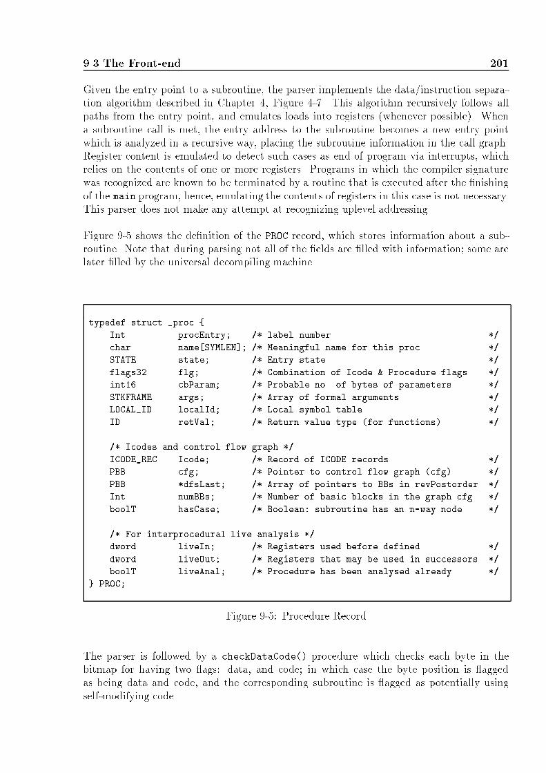
9.3 The Front-end 201Given the entry point to a subroutine, the parser implements the data/instruction separa-tion algorithm described in Chapter 4, Figure 4-7. This algorithm recursively follows allpaths from the entry point, and emulates loads into registers (whenever possible). Whena subroutine call is met, the entry address to the subroutine becomes a new entry pointwhich is analyzed in a recursive way, placing the subroutine information in the call graph.Register content is emulated to detect such cases as end of program via interrupts, whichrelies on the contents of one or more registers. Programs in which the compiler signaturewas recognized are known to be terminated by a routine that is executed after the �nishingof the main program, hence, emulating the contents of registers in this case is not necessary.This parser does not make any attempt at recognizing uplevel addressing.Figure 9-5 shows the de�nition of the PROC record, which stores information about a sub-routine. Note that during parsing not all of the �elds are �lled with information; some arelater �lled by the universal decompiling machine.typedef struct _proc {Int procEntry; /* label number */char name[SYMLEN]; /* Meaningful name for this proc */STATE state; /* Entry state */flags32 flg; /* Combination of Icode & Procedure flags */int16 cbParam; /* Probable no. of bytes of parameters */STKFRAME args; /* Array of formal arguments */LOCAL_ID localId; /* Local symbol table */ID retVal; /* Return value type (for functions) *//* Icodes and control flow graph */ICODE_REC Icode; /* Record of ICODE records */PBB cfg; /* Pointer to control flow graph (cfg) */PBB *dfsLast; /* Array of pointers to BBs in revPostorder */Int numBBs; /* Number of basic blocks in the graph cfg */boolT hasCase; /* Boolean: subroutine has an n-way node *//* For interprocedural live analysis */dword liveIn; /* Registers used before defined */dword liveOut; /* Registers that may be used in successors */boolT liveAnal; /* Procedure has been analysed already */} PROC; Figure 9-5: Procedure RecordThe parser is followed by a checkDataCode() procedure which checks each byte in thebitmap for having two ags: data, and code; in which case the byte position is aggedas being data and code, and the corresponding subroutine is agged as potentially usingself-modifying code.

202 dcc9.3.2 The Intermediate CodeThe intermediate code used in dcc is called Icode, of which there are two types: low-leveland high-level. The low-level Icode is a mapping of i80286 machine instructions to assemblermnemonics, ensuring that every Icode instruction performs one logical instruction only. Forexample, the instruction:DIV bxassigns to ax the quotient of dx:ax divided by bx, and assigns to dx the reminder ofthe previous quotient; hence, two logical instructions are performed by the DIV machineinstruction. In Icode instructions, DIV is separated into two di�erent instructions: iDIVand iMOD. The former performs the division of the operands, and the latter performs themodulus of the operands. Since both instructions use the registers that are overwrittenby the result of the instruction (i.e. dx and ax in this example), these registers need tobe placed in a temporary register before the instructions are performed. dcc uses registertmp as a temporary register. This register is forward substituted into another instructionand eliminated during data ow analysis. The above machine instruction is translated intothree Icode instructions as follows:iMOV tmp, dx:ax ; tmp = dx:axiDIV bx ; ax = tmp / bxiMOD bx ; dx = tmp % bxwhere the dividend of both iDIV and iMOD is set to the tmp register rather than dx:ax.Figure 9-6 shows the di�erent machine instructions that are represented by more than oneIcode instruction. An example is given for each instruction.Machine Instruction Icode Instructions MeaningDIV cl iMOV tmp, ax tmp = axiDIV cl al = tmp / cliMOD cl ah = tmp % clLOOP L iSUB cx, 1 cx = cx - 1iJNCXZ L cx <> 0 goto LLOOPE L iSUB cx, 1 cx = cx - 1iCMP cx, 0 cx == 0?iJZ L zeroFlag == 1 goto LiJNCXZ L if cx <> 0 goto LLOOPNE L iSUB cx, 1 cx = cx = 1iCMP cx, 0 cx == 0?iJNE L zeroFlag == 0 goto LiJNCXZ L if cx <> 0 goto LXCHG cx, bx iMOV tmp, cx tmp = cxiMOV cx, bx cx = bxiMOV bx, tmp bx = tmpFigure 9-6: Machine Instructions that Represent more than One Icode Instruction

9.3 The Front-end 203Compound instructions such as rep movsb are represented by two di�erent machine instruc-tions but perform one logical string function; repeat while not end-of-string in this case.These instructions are represented by one Icode instruction; iREP_MOVS in this example.Machine instructions that perform low-level tasks, such as input and output from a port,are most likely never generated by a compiler whilst compiling high-level language code(i.e. embedded assembler code can make use of these instructions but the high-level codedoes not generate these instructions). These instructions are agged in the Icode as beingnon high-level, and the subroutine that makes use of these instructions is agged as well sothat assembler is generated for the subroutine. The following instructions are considerednot to be generated by compilers; the instructions marked with an asterisk are sometimesnon high-level, depending on the register operands used:AAA, AAD, AAM, AAS, CLI, DAA, DAS, *DEC, HLT, IN, *INC, INS,INT, INTO, IRET, JO, JNO, JP, JNP, LAHF, LOCK, *MOV, OUT, OUTS,*POP, POPA, POPF, *PUSH, PUSHA, PUSHF, SAHF, STI, *XCHG, XLATIcode instructions have a set of Icode ags associated with them to acknowledge propertiesfound during the parsing of the instruction. The following ags are used:� B: byte operands (default is word operands).� I: immediate (constant) source operand.� No Src: no source operand.� No Ops: no operands.� Src B: source operand is byte, destination is word.� Im Ops: implicit operands.� Im Src: implicit source operand.� Im Dst: implicit destination operand.� Seg Immed: instruction has a relocated segment value.� Not Hll: non high-level instruction.� Data Code: instruction modi�es data.� Word O�: instruction has a word o�set (i.e. could be an address).� Terminates: instruction terminates the program.� Target: instruction is the target of a jump instruction.� Switch: current indirect jump determines the start of an n-way statement.� Synthetic: instruction is a synthetic (i.e. does not exist in the binary �le).� Float Op: the next instruction is a oating point instruction.

204 dccdcc implements the mapping of i80286 machine instructions to low-level Icodes by meansof a static table indexed by machine instruction, which has information on the associatedIcode, used and de�ned condition codes, ags, and procedures that determine the sourceand destination operands (di�erent procedures are used for di�erent operand types, thus,the same procedures are used by several di�erent instructions). The mapping of machineinstructions to Icode instructions converts 250 instructions into 108 Icode instructions. Thismapping is shown in Figure 9-7.9.3.3 The Control Flow Graph Generatordcc implements the construction of the control ow graph for each subroutine by placingbasic blocks on a list and then converting that list to a proper graph. While parsing, when-ever an end of basic block instruction is met, the basic block is constructed, and the startand �nish instruction indexes into the Icode array for that subroutine are stored. Instruc-tions for which it is not possible to determine where they transfer control to (i.e. indexedjumps that are not recognized as a known n-way structure header, indirect calls, etc) aresaid to terminate the basic block since no more instructions are parsed along the path thatcontains that instruction. These nodes are called no-where nodes in dcc. The other typesof basic blocks are the standard 1-way, 2-way, n-way, fall-through, call, and return nodes.The de�nition record of a basic block is shown in Figure 9-8. Most of this information islater �lled in by the universal decompiling machine.The control ow graph of each subroutine is optimized by ow-of-control optimizationswhich remove redundant jumps to jumps, and conditional jumps to jumps. These optimiza-tions have the potential of removing basic blocks from the graph, therefore the numberingof the graph is left until all possible nodes are removed from the graph. At the same time,the predecessors to each basic block are determined and placed in the *inEdges[] array.9.3.4 The Semantic Analyzerdcc's semantic analyzer determines idioms and replaces them with another Icode instruc-tion(s). The idioms checked for in dcc are the ones described in Chapter 4, Section 4.2.1,and grouped into the following categories: subroutine idioms, calling conventions, long vari-able operations, and miscellaneous idioms.There is a series of idioms available only in C. In C, a variable can be pre and post incre-mented, and pre and post decremented. The machine code that represents these instructionsmakes use of an extra register to hold the value of the pre or post incremented/decrementedvariable when it is being checked against some value/variable. This extra register can beeliminated by using an idiom to transform the set of instructions into one that uses thepre/post increment/decrement operand.In the case of a post increment/decrement variable in a conditional jump, the value of thevariable is copied to a register, the variable then gets incremented or decremented, and�nally, the register that holds the copy of the initial variable (i.e. before increment ordecrement) is compared against the other identi�er. The use of the extra register can beeliminated by using the post increment/decrement operator available in C. Therefore, theseidioms can be checked for only if code is to be generated in C. Figure 9-9 shows this case.

9.3 The Front-end 205Low-level Instruction Machine Instruction(s)iAAA 37iAAD D5iAAM D4iAAS 3FiADC 10..15, (80..83)(50..57,90..97,D0..D7)iADD 00..05, (80..83)(40..47,80..87,C0..C7)iAND 20..25, (80..83)(60..67,A0..A7,E0..E7)iBOUND 62iCALL E8, FE50..FE57, FE90..FE9F, FED0..FED7, FF50..FF57,FF90..FF9F, FFD0..FFD7iCALLF 9A, FE58..FE5F, FE98..FE9F, FED8..FEDF, FF58..FF5F,FF98..FF9F, FFD8..FFDFiCLC F8iCLD FCiCLI FAiCMC F5iCMP 38..3D, (80..83)(78..7F,B8..BF,F8..FF)iCMPS A6, A7iREPNE CMPS F2A6, F2A7iREPE CMPS F3A6, F3A7iDAA 27iDAS 2FiDEC 48..4F, FE48..FE4F, FE88..FE8F, FEC8..FECF, FF48..FF4F,FF88..FF8F, FFC8..FFCFiDIV F670..F677, F6A0..F6A7, F6F0..F6F7, F770..F777, F7A0..F7A7,F7F0..F7F7iMOD F670..F677, F6A0..F6A7, F6F0..F6F7, F770..F777, F7A0..F7A7,F7F0..F7F7, F678..F67F, F6A8..F6AF, F6F8..F6FF, F778..F77F,F7A8..F7AF, F7F8..F7FFiENTER C8iESC D8..DFiHLT F4iIDIV F678..F67F, F6A8..F6AF, F6F8..F6FF, F778..F77F, F7A8..F7AF,F7F8..F7FFiIMUL 69, 6B, F668..F66F, F6A8..F6AF, F6E8..F6EF, F768..F76F,F7A8..F7AF, F7E8..F7EFiIN E4, E5, EC, EDiINC 40..47, FE40..FE47, FE80..FE87, FEC0..FEC7, FF40..FF47,FF80..FF87, FFC0..FFC7iINS 6C, 6DiREP INS F36C, F36DiINT CC, CDFigure 9-7: Low-level Intermediate Code for the i80286

206 dccLow-level Instruction Machine Instruction(s)iINTO CEiIRET CFiJB 72iJBE 76iJAE 73iJA 77iJE 74iJNE 75iJL 7CiJGE 7DiJLE 7EiJG 7FiJS 78iJNS 79iJO 70iJNO 71iJP 7AiJNP 7BiJCXZ E3iJNCXZ E0..E2iJMP E9, EB, FE60..FE67, FEA0..FEA7, FEE0..FEE7, FF60..FF67,FFA0..FFA7, FFE0..FFE7iJMPF EA, FE68..FE6F, FEA8..FEAF, FEE8..FEEF, FF68..FF6F,FFA8..FFAF, FFE8..FFEFiLAHF 9FiLDS C5iLEA 8DiLEAVE C9iLES C4iLOCK F0iLODS AC, ADiREP LODS F3AC, F3ADiMOV 88..8C, 8E, A0..A3, B0..BF, C6, C7iMOVS A4, A5iREP MOVS F3A4, F3A5iMUL F660..F667, F6A0..F6A7, F6E0..F6E7, F760..F767, F7A0..F7A7,F7E0..F7E7iNEG F658..F65F, F698..F69F, F6D8..F6DF, F758..F75F, F798..F79F,F7D8..F7DFiNOT F650..F657, F690..F697, F6D0..F6D7, F750..F757, F790..F797,F7D0..F7D7iNOP 90iOR 08..0D, (80..83)(48..4F,88..8F,C8..CF)Figure 9-7: Low-level Intermediate Code for the i80286 - Continued

9.3 The Front-end 207Low-level Instruction Machine Instruction(s)iOUT E6, E7, EE, EFiOUTS 6E, 6FiREP OUTS F36E, F36FiPOP 07, 17, 1F, 58..5F, 8FiPOPA 61iPOPF 9DiPUSH 06, 0E, 16, 1E, 50..57, 68, 6A, FE70..FE77, FEB0..FEB7,FEF0..FEF7, FF70..FF77, FFB0..FFB7, FFF0..FFF7iPUSHA 60iPUSHF 9CiRCL (C0,C1,D0..D3)(50..57,90..97,D0..D7)iRCR (C0,C1,D0..D3)(58..5F,98..9F,D8..DF)iREPE F3iREPNE F2iRET C2, C3iRETF CA, CBiROL (C0,C1,DO..D3)(40..47,80..87,C0..C7)iROR (C0,C1,D0..D3)(48..4F,88..8F,C8..CF)iSAHF 9EiSAR (C0,C1,D0..D3)(78..7F,B8..BF,F8..FF)iSHL (C0,C1,D0..D3)(60..67,A0..A7,E0..E7)iSHR (C0,C1,D0..D3)(68..6F,A8..AF,E8..EF)iSBB 18..1D, (80..83)(58..5F,98..9F,D8..DF)iSCAS AE, AFiREPE SCAS F3AE, F3AFiREPNE SCAS F2AE, F2AFiSIGNEX 98, 99iSTC F9iSTD FDiSTI FBiSTOS AA, ABiREP STOS F3AA, F3ABiSUB 28..2D, (80..83)(68..6F,A8..AF,E8..EF)iTEST 84, 85, A8, A9, F640..F647, F680..F687, F6C0..F6C7, F740..F747,F780..F787, F7C0..F7C7iWAIT 9BiXCHG 86, 87, 91..97iXLAT D7iXOR 30..35, (80..83)(70..77,B0..B7,F0..F7)Figure 9-7: Low-level Intermediate Code for the i80286 - Continued

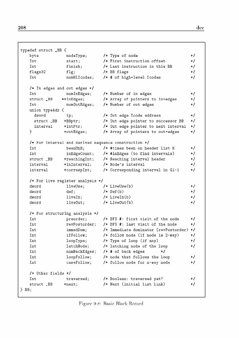
208 dcctypedef struct _BB {byte nodeType; /* Type of node */Int start; /* First instruction offset */Int finish; /* Last instruction in this BB */flags32 flg; /* BB flags */Int numHlIcodes; /* # of high-level Icodes *//* In edges and out edges */Int numInEdges; /* Number of in edges */struct _BB **inEdges; /* Array of pointers to in-edges */Int numOutEdges; /* Number of out edges */union typeAdr {dword ip; /* Out edge Icode address */struct _BB *BBptr; /* Out edge pointer to successor BB */interval *intPtr; /* Out edge pointer to next interval */} *outEdges; /* Array of pointers to out-edges *//* For interval and derived sequence construction */Int beenOnH; /* #times been on header list H */Int inEdgeCount; /* #inEdges (to find intervals) */struct _BB *reachingInt; /* Reaching interval header */interval *inInterval; /* Node's interval */interval *correspInt; /* Corresponding interval in Gi-1 *//* For live register analysis */dword liveUse; /* LiveUse(b) */dword def; /* Def(b) */dword liveIn; /* LiveIn(b) */dword liveOut; /* LiveOut(b) *//* For structuring analysis */Int preorder; /* DFS #: first visit of the node */Int revPostorder; /* DFS #: last visit of the node */Int immedDom; /* Immediate dominator (revPostorder) */Int ifFollow; /* follow node (if node is 2-way) */Int loopType; /* Type of loop (if any) */Int latchNode; /* latching node of the loop */Int numBackEdges; /* # of back edges */Int loopFollow; /* node that follows the loop */Int caseFollow; /* follow node for n-way node *//* Other fields */Int traversed; /* Boolean: traversed yet? */struct _BB *next; /* Next (initial list link) */} BB; Figure 9-8: Basic Block Record

9.3 The Front-end 209mov reg, var mov reg, varinc var or dec varcmp var, Y cmp var, YjX label jX label+jcond (var++ X Y) jcond (var-- X Y)Figure 9-9: Post-increment or Post-decrement in a Conditional JumpIn a similar way, a pre increment/decrement makes use of an intermediate register. Thevariable is �rst incremented/decremented, then it is moved onto a register, which is com-pared against another identi�er, and then the conditional jump occurs. In this case, theintermediate register is used because identi�ers other than a register cannot be used inthe compare instruction. This intermediate register can be eliminated by means of a preincrement/decrement operator, as shown in Figure 9-10.inc var dec varmov reg, var or mov reg, varcmp reg, Y cmp reg, YjX lab jX lab+jcond (++var X Y) jcond (--var X Y)Figure 9-10: Pre Increment/Decrement in Conditional JumpC-dependent idioms are implemented in dcc. As seen in the general format of these idioms,a series of low-level Icode instructions is replaced by one high-level jcond instruction. Thisinstruction is agged as being a high-level instruction so that it is not processed again bythe data ow analyzer. Also, all other instructions involved in these idioms are agged asnot representing high-level instructions.After idiom recognition, simple type propagation is done on signed integers, signed bytes,and long variables. When propagating long variables across conditionals, the propagationmodi�es the control ow graph by removing a node from the graph, as described inChapter 4, Section 4.2.2. Since the high-level condition is determined from the type ofgraph, the corresponding high-level jcond instruction is written and that instruction is agged as being a high-level instruction.

210 dcc9.4 The Disassemblerdcc implements a built-in disassembler that generates assembler �les. The assembly �lecontains only information on the assembler mnemonics of the program (i.e. the code seg-ment) and does not display any information relating to data. All the information used bythe disassembler is collected by the parser and intermediate code phases of the decompiler;since there is almost a 1:1 mapping of low-level Icodes to assembler mnemonics, the assem-bler code generator is mostly concerned with output formatting.The disassembler handles one subroutine at a time; given a call graph, the graph is traversedin a depth-�rst search to generate assembler for nested subroutines �rst. The user has twooptions for generating assembler �les: to generate assembler straight after the parsing phase,and to generate assembler after graph optimization. The former case generates assemblerthat is as close as possible to the binary image; the latter case may miss certain jumpinstructions that were considered redundant by the graph optimizer. The disassembler isalso used by the decompiler when generating target C code; if a subroutine is agged asbeing a non high-level subroutine, assembler code is generated for that subroutine aftergenerating the subroutine's header and comments in C.9.5 The Universal Decompiling MachineThe universal decompiling machine (udm) is composed of two phases; the data ow analysisphase which transforms the low-level Icode to an optimal high-level Icode representation,and the control ow analysis phase which traverses the graph of each subroutine to determinethe bounds of loops and conditionals; these bounds are later used by the code generator.Figure 9-11 shows the code for the udm() procedure.9.5.1 Data Flow AnalysisThe �rst part of the data ow analysis is the removal of condition codes. Condition codesare classi�ed into two sets as follows: the set of condition codes that are likely to have beengenerated by a compiler (the HLCC set), and the set of conditions that are likely to havebeen hand-crafted in assembler (the NHLCC set). From the 9 condition codes availablein the Intel i80286[Int86] (over ow, direction, interrupt enable, trap, sign, zero, auxiliarycarry, parity and carry), only 4 ags are likely to be high-level; these are, carry, direction,zero and sign. These ags are modi�ed by instructions that are likely to be high-level (i.ethe ones that were not agged as being non high-level), and thus this set is the one that isanalyzed for condition code removal. From the probable high-level instructions, 30 instruc-tions de�ne ags in the HLCC set; ranging from 1 to 3 ags de�ned by an instruction, and25 instruction use ags; normally using one or two ags per instruction. dcc implementsdead-condition code elimination and condition code propagation, as described in Chapter 5,Sections 5.4.2 and 5.4.3. These optimizations remove all references to condition codes andcreates jcond instructions that have an associated Boolean conditional expression. Thisanalysis is overlapped with the initial mapping of all other low-level Icodes to high-levelIcodes in terms of registers. The initial mapping of Icodes is explained in Appendix D.

9.5 The Universal Decompiling Machine 211void udm (CALL_GRAPH *callGraph){ derSeq *derivedG;/* Data flow analysis - optimizations on Icode */dataFlow (callGraph);/* Control flow analysis -- structure the graphs *//* Build derived sequences for each subroutine */buildDerivedSeq (callGraph, &derivedG);if (option.VeryVerbose) /* display derived sequence for each subroutine */displayDerivedSeq (derivedG);/* Graph structuring */structure (callGraph, derivedG);} Figure 9-11: Procedure for the Universal Decompiling MachineThe second part of the analysis is the generation of summary information on the operandsof the Icode instructions and basic blocks in the graph. For each subroutine a de�nition-useand use-de�nition analysis is done; the associated chains are constructed for each instruc-tion. While constructing these chains, dead-register elimination is performed, as describedin Chapter 5, Section 5.4.1. Next, an intraprocedural live register analysis is performed foreach subroutine to determine any register arguments used by the subroutine. This analysisis described in Chapter 5, Section 5.4.4. Finally, an interprocedural live register analysis isdone next to determine registers that are returned by functions; the analysis is described inChapter 5, Section 5.4.5.Dead-register elimination determines the purpose of the DIV machine instructions, as thisinstruction is used for both quotient and remainder of operands. The following intermediatecode1 asgn tmp, dx:ax ; ud(tmp) = {2,3}2 asgn ax, tmp / bx ; ud(ax) = {}3 asgn dx, tmp % bx ; ud(dx) = {4}4 asgn [bp-2], dx /* no further use of ax before redefinition */determines that register ax is not used before rede�nition as its use-de�nition chain ininstruction 2 is empty. Since this de�nition is dead, the instruction is eliminated, henceeliminating the division of the operands, and leading to the following code:1 asgn tmp, dx:ax ; ud(tmp) = {2,3}3 asgn dx, tmp % bx ; ud(dx) = {4}4 asgn [bp-2], dx

212 dccAll instructions that had instruction 2 in their use-de�nition chain need to be updated tore ect the fact that the register is not used any more since it was used to de�ne a deadregister; hence, the ud() chain in instruction 1 is updated in this example, leading to the�nal code:1 asgn tmp, dx:ax ; ud(tmp) = {3}3 asgn dx, tmp % bx ; ud(dx) = {4}4 asgn [bp-2], dxThe third and last part of the analysis is the usage of the use-de�nition chains on registers toperform extended register copy propagation, as described in Chapter 5, Section 5.4.10. Thisanalysis removes redundant register references, determines high-level expressions, places ac-tual parameters on the subroutine's list, and propagates argument types across subroutinecalls. A temporary expression stack is used throughout the analysis to eliminate the inter-mediate pseudo high-level instructions push and pop.In the previous example, forward substitution determines that the initial DIV instructionwas used to determine the modulus between two operands (which are placed in registersdx:ax and bx in this case):4 asgn [bp-2], dx:ax % bx9.5.2 Control Flow AnalysisThere are two parts to the control ow analyzer: the �rst part constructs a derived sequenceof graphs for each subroutine in the call graph and calculates intervals. This sequence isused by the structuring algorithm to determine the bounds of loops and the nesting level ofsuch loops. Once the derived sequence of graphs is built for the one subroutine, the graphis tested for reducibility; if the limit n-th order graph is not a trivial graph, the subroutineis irreducible.The second part of the analysis is the structuring of the control ow graphs of the program.The structuring algorithm determines the bounds of loops and conditionals (2-way and n-way structures); these bounds are later used during code generation. Loops are structuredby means of intervals, and their nesting level is determined by the order in which they arefound in the derived sequence of graphs, as described in Chapter 6, Section 6.6.1. Pre-tested, post-tested and endless loops are determined by this algorithm. Conditionals arestructured by means of a reverse traversal of the depth-�rst search tree of the graph; inthis way nested conditionals are found �rst. The method for structuring 2-way and n-wayconditionals is described in Chapter 6, Sections 6.6.2 and 6.6.3. This method takes intoaccount compound Boolean conditions, and removes some nodes from the graph by storingthe Boolean conditional information of two or more nodes in the one node.9.6 The Back-endThe back-end is composed in its entirety of the C code generator. This module opens theoutput �le and gives it an extension .b (b for beta), writes the program header to it, and

9.6 The Back-end 213then invokes the code generator. Once code has been generated for the complete graph, the�le is closed. Figure 9-12 shows code for the back-end procedure.void BackEnd (char *fileName, CALL_GRAPH *callGraph){ FILE *fp; /* Output C file *//* Open output file with extension .b */openFile (fp, filename, ".b", "wt");printf ("dcc: Writing C beta file %s.b\n", fileName);/* Header information */writeHeader (fp, fileName);/* Process each procedure at a time */writeCallGraph (fileName, callGraph, fp);/* Close output file */fclose (fp);printf ("dcc: Finished writing C beta file\n");} Figure 9-12: Back-end Procedure9.6.1 Code Generationdcc implements the C code generator described in Chapter 7, Section 7.1. The program'scall graph is traversed in a depth-�rst fashion to generate C code for the leaf subroutines�rst (i.e. in reverse invocation order if the graph is reducible). For each subroutine, code forthe control ow graph is generated according to the structures in the graph; the bounds ofloops and conditional structures have been marked in the graph by the structuring phase.Code is generated in a recursive way, so if a node is reached twice along the recursion, agoto jump is used to transfer control to the code associated with such a node.Since registers that are found in leaves of an expression are given a name during code gener-ation (i.e. after all local variables have been de�ned in the local variable de�nition section),and instructions for which code has been generated may have a label associated with themif a goto jump is generated later on, code cannot be generated directly to a �le but needsto be stored in an intermediate data structure until the code for a complete subroutinehas been generated; then it can be copied to the target output �le, and the structure isreused for the next subroutine in the call graph. The data structure used by dcc to handlesubroutine declarations and code is called a bundle. A bundle is composed of two arraysof lines, one for subroutine declarations, and the other for the subroutine code. Subroutinedeclarations include not only the subroutine header, but also the comments and the localvariable de�nitions. The array of lines can grow dynamically if the initial allocated arraysize is too small. The de�nition of the bundle data structure is shown in Figure 9-13.

214 dcctypedef struct {Int numLines; /* Number of lines in the table */Int allocLines; /* Number of lines allocated in the table */char **str; /* Table of strings */} strTable;typedef struct {strTable decl; /* Declarations */strTable code; /* C code */} bundle; Figure 9-13: Bundle Data Structure De�nitionThe comments and error messages displayed by dcc are listed in Appendix E.9.7 ResultsThis section presents a series of programs decompiled by dcc. The original programs werewritten in C, and compiled with Borland Turbo C under DOS. These programs make useof base type variables (i.e. byte, integer and long), and illustrate di�erent aspects of thedecompilation process. These programs were run in batch mode, generating the disassembly�le .a2, the C �le .b, the call graph of the program, and statistics on the intermediate codeinstructions. The statistics re ect the percentage of intermediate instruction reduction onall subroutines for which C is generated; subroutines which translate to assembler are notconsidered in the statistics. For each program, a total count on low-level and high-levelinstructions, and a total percentage reduction is given.The �rst three programs illustrate operations on the di�erent three base types. The originalC programs have the same code, but their variables have been de�ned as a di�erenttype. The next four programs are benchmark programs from the Plum-Hall benchmarksuite. These programs were written by Eric S. Raymond and are freely available on thenetwork [Ray89]. These programs were modi�ed to ask for the arguments to the programwith scanf() rather than scanning for them in the argv[] command line array since arraysare not supported by dcc. Finally, the last three programs calculate Fibonacci numbers,compute the cyclic redundancy check (CRC) for a character, and multiply two matrixes.This last program is introduced to show how array expressions are derived from the low-levelintermediate code.9.7.1 Intops.exeIntops is a program that computes di�erent operations on two integer variables, and displaysthe �nal result of these variables. The disassembly C program is shown in Figure 9-14, thedecompiled C program in Figure 9-15, and the initial C program in Figure 9-16. Theprogram has the following call graph:

9.7 Results 215mainprintfAs can be seen in the disassembly of the program, the second variable was placed in registersi, and the �rst variable was placed on the stack at o�set -2. Synthetic instructions weregenerated by the parser for the IDIV machine instruction; this instruction was used as adivision in one case, and as a modulus in the other. The intermediate code makes use of thetemporary register tmp, as previously explained in Section 9.3.2; this register is eliminatedduring data ow analysis. For each operation, the operands of the instruction are movedto registers, the operation is performed on registers, and the result is placed back on thevariables. There are no control structures in the program. The idioms and data ow analysesreduce the number of intermediate instructions by 77.78%, as shown in Figure 9-17.

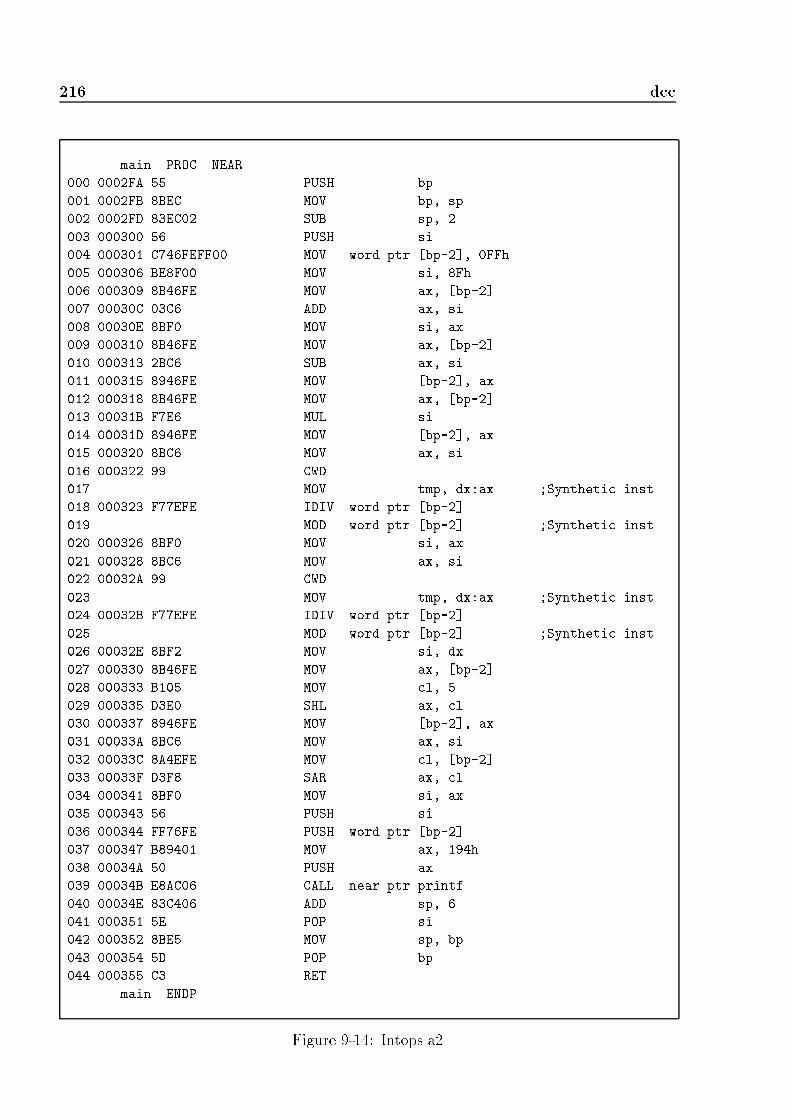
216 dccmain PROC NEAR000 0002FA 55 PUSH bp001 0002FB 8BEC MOV bp, sp002 0002FD 83EC02 SUB sp, 2003 000300 56 PUSH si004 000301 C746FEFF00 MOV word ptr [bp-2], 0FFh005 000306 BE8F00 MOV si, 8Fh006 000309 8B46FE MOV ax, [bp-2]007 00030C 03C6 ADD ax, si008 00030E 8BF0 MOV si, ax009 000310 8B46FE MOV ax, [bp-2]010 000313 2BC6 SUB ax, si011 000315 8946FE MOV [bp-2], ax012 000318 8B46FE MOV ax, [bp-2]013 00031B F7E6 MUL si014 00031D 8946FE MOV [bp-2], ax015 000320 8BC6 MOV ax, si016 000322 99 CWD017 MOV tmp, dx:ax ;Synthetic inst018 000323 F77EFE IDIV word ptr [bp-2]019 MOD word ptr [bp-2] ;Synthetic inst020 000326 8BF0 MOV si, ax021 000328 8BC6 MOV ax, si022 00032A 99 CWD023 MOV tmp, dx:ax ;Synthetic inst024 00032B F77EFE IDIV word ptr [bp-2]025 MOD word ptr [bp-2] ;Synthetic inst026 00032E 8BF2 MOV si, dx027 000330 8B46FE MOV ax, [bp-2]028 000333 B105 MOV cl, 5029 000335 D3E0 SHL ax, cl030 000337 8946FE MOV [bp-2], ax031 00033A 8BC6 MOV ax, si032 00033C 8A4EFE MOV cl, [bp-2]033 00033F D3F8 SAR ax, cl034 000341 8BF0 MOV si, ax035 000343 56 PUSH si036 000344 FF76FE PUSH word ptr [bp-2]037 000347 B89401 MOV ax, 194h038 00034A 50 PUSH ax039 00034B E8AC06 CALL near ptr printf040 00034E 83C406 ADD sp, 6041 000351 5E POP si042 000352 8BE5 MOV sp, bp043 000354 5D POP bp044 000355 C3 RETmain ENDP Figure 9-14: Intops.a2

9.7 Results 217/** Input file : intops.exe* File type : EXE*/#include "dcc.h"void main ()/* Takes no parameters.* High-level language prologue code.*/{int loc1;int loc2;loc1 = 255;loc2 = 143;loc2 = (loc1 + loc2);loc1 = (loc1 - loc2);loc1 = (loc1 * loc2);loc2 = (loc2 / loc1);loc2 = (loc2 % loc1);loc1 = (loc1 << 5);loc2 = (loc2 >> loc1);printf ("a = %d, b = %d\n", loc1, loc2);} Figure 9-15: Intops.b

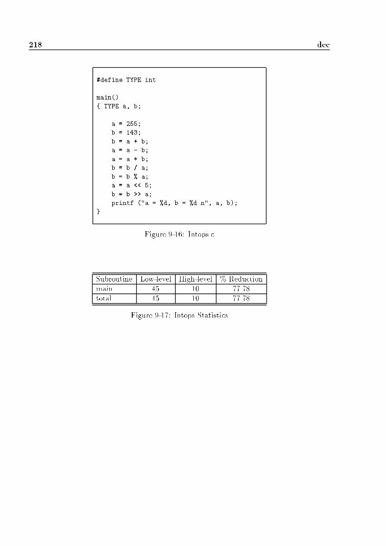
218 dcc#define TYPE intmain(){ TYPE a, b;a = 255;b = 143;b = a + b;a = a - b;a = a * b;b = b / a;b = b % a;a = a << 5;b = b >> a;printf ("a = %d, b = %d\n", a, b);} Figure 9-16: Intops.cSubroutine Low-level High-level % Reductionmain 45 10 77.78total 45 10 77.78Figure 9-17: Intops Statistics

9.7 Results 2199.7.2 Byteops.exeByteops is a similar program to intops, with the di�erence that the two variables are bytesrather than integers. The disassembly program is shown in Figure 9-18, the decompiledC version in Figure 9-19, and the initial C program in Figure 9-20. The program has thefollowing call graph:mainprintfAs can be seen in the disassembly of the program, the local variables are placed on the stackat o�sets -1 and -2. There are 22.41% more instructions in this program when comparedagainst the intops.a2 program since some machine instructions such as IDIV take wordregisters as operands rather than byte registers; hence, the byte registers are either paddedor sign-extended to form a word register. The �nal number of high-level instructions is thesame in both programs, hence the reduction in the number of intermediate instructions isgreater in this program. It reached 82.76%, as shown in Figure 9-21.

220 dccmain PROC NEAR000 0002FA 55 PUSH bp001 0002FB 8BEC MOV bp, sp002 0002FD 83EC02 SUB sp, 2003 000300 C646FEFF MOV byte ptr [bp-2], 0FFh004 000304 C646FF8F MOV byte ptr [bp-1], 8Fh005 000308 8A46FE MOV al, [bp-2]006 00030B 0246FF ADD al, [bp-1]007 00030E 8846FF MOV [bp-1], al008 000311 8A46FE MOV al, [bp-2]009 000314 2A46FF SUB al, [bp-1]010 000317 8846FE MOV [bp-2], al011 00031A 8A46FE MOV al, [bp-2]012 00031D B400 MOV ah, 0013 00031F 8A56FF MOV dl, [bp-1]014 000322 B600 MOV dh, 0015 000324 F7E2 MUL dx016 000326 8846FE MOV [bp-2], al017 000329 8A46FF MOV al, [bp-1]018 00032C B400 MOV ah, 0019 00032E 8A56FE MOV dl, [bp-2]020 000331 B600 MOV dh, 0021 000333 8BDA MOV bx, dx022 000335 99 CWD023 MOV tmp, dx:ax ;Synthetic inst024 000336 F7FB IDIV bx025 MOD bx ;Synthetic inst026 000338 8846FF MOV [bp-1], al027 00033B 8A46FF MOV al, [bp-1]028 00033E B400 MOV ah, 0029 000340 8A56FE MOV dl, [bp-2]030 000343 B600 MOV dh, 0031 000345 8BDA MOV bx, dx032 000347 99 CWD033 MOV tmp, dx:ax ;Synthetic inst034 000348 F7FB IDIV bx035 MOD bx ;Synthetic inst036 00034A 8856FF MOV [bp-1], dl037 00034D 8A46FE MOV al, [bp-2]038 000350 B105 MOV cl, 5039 000352 D2E0 SHL al, cl040 000354 8846FE MOV [bp-2], al041 000357 8A46FF MOV al, [bp-1]042 00035A 8A4EFE MOV cl, [bp-2]043 00035D D2E8 SHR al, cl044 00035F 8846FF MOV [bp-1], alFigure 9-18: Byteops.a2

9.7 Results 221045 000362 8A46FF MOV al, [bp-1]046 000365 B400 MOV ah, 0047 000367 50 PUSH ax048 000368 8A46FE MOV al, [bp-2]049 00036B B400 MOV ah, 0050 00036D 50 PUSH ax051 00036E B89401 MOV ax, 194h052 000371 50 PUSH ax053 000372 E8AB06 CALL near ptr printf054 000375 83C406 ADD sp, 6055 000378 8BE5 MOV sp, bp056 00037A 5D POP bp057 00037B C3 RETmain ENDP Figure 9-18: Byteops.a2 { Continued

222 dcc/** Input file : byteops.exe* File type : EXE*/#include "dcc.h"void main ()/* Takes no parameters.* High-level language prologue code.*/{int loc1;int loc2;loc1 = 255;loc2 = 143;loc2 = (loc1 + loc2);loc1 = (loc1 - loc2);loc1 = (loc1 * loc2);loc2 = (loc2 / loc1);loc2 = (loc2 % loc1);loc1 = (loc1 << 5);loc2 = (loc2 >> loc1);printf ("a = %d, b = %d\n", loc1, loc2);} Figure 9-19: Byteops.b

9.7 Results 223#define TYPE unsigned charmain(){ TYPE a, b;a = 255;b = 143;b = a + b;a = a - b;a = a * b;b = b / a;b = b % a;a = a << 5;b = b >> a;printf ("a = %d, b = %d\n", a, b);} Figure 9-20: Byteops.cSubroutine Low-level High-level % Reductionmain 58 10 82.76total 58 10 82.76Figure 9-21: Byteops Statistics

224 dcc9.7.3 Longops.exeThe longops programs is similar to the intops and byteops programs, but makes use oftwo long variables. The disassembly program is shown in Figure 9-22, the decompiled Cprogram in Figure 9-23, and the initial C program in Figure 9-24. The program has thefollowing call graph:mainLXMUL@LDIV@LMOD@LXLSH@LXRSH@printfOperations performed on long variables make use of idioms and run-time support routines ofthe compiler. In this program, long addition and subtraction are performed by the idiomsof Chapter 4, Section 4.2.1, and the run-time routines LXMUL@, LDIV@, LMOD@, LXLSH@,and LXRSH@ are used for long multiplication, division, modulus, left-shift, and right-shiftaccordingly. From these run-time routines, long multiplication, left-shift, and right-shift aretranslatable into C; macros are used to access the low or high part of a variable in some cases.The division and modulus routines are untranslatable into C, so assembler is generated forthem. The long variables are placed on the stack at o�sets -4 and -8 (see main subroutine).The main program has 28.57% more instructions than the intops program, and 7.9% moreinstructions than the byteops program. The increase in the number of instructions has twocauses: �rst, the transfer of long variables to registers now takes two instructions ratherthan one (i.e. the high and low part are transfered to di�erent registers), and second,the subroutine call instructions to run-time support routines. The �nal decompiled mainprogram still generates the same number of high-level instructions as in the previous twoprograms, with a reduction in the number of intermediate instructions of 84.13%, as shownin Figure 9-25. Overall, the reduction in the number of instructions is 58.97%, which is lowdue to the run-time routines that were translated to C, which did not make use of a lot ofregister movement since the arguments were in registers and these routines were initiallywritten in assembler.

9.7 Results 225LXRSH@ PROC FAR000 001269 80F910 CMP cl, 10h001 00126C 7310 JAE L1002 00126E 8BDA MOV bx, dx003 001270 D3E8 SHR ax, cl004 001272 D3FA SAR dx, cl005 001274 F6D9 NEG cl006 001276 80C110 ADD cl, 10h007 001279 D3E3 SHL bx, cl008 00127B 0BC3 OR ax, bx009 00127D CB RETF010 00127E 80E910 L1: SUB cl, 10h011 001281 8BC2 MOV ax, dx012 001283 99 CWD013 001284 D3F8 SAR ax, cl014 001286 CB RETFLXRSH@ ENDPLXLSH@ PROC FAR000 001287 80F910 CMP cl, 10h001 00128A 7310 JAE L2002 00128C 8BD8 MOV bx, ax003 00128E D3E0 SHL ax, cl004 001290 D3E2 SHL dx, cl005 001292 F6D9 NEG cl006 001294 80C110 ADD cl, 10h007 001297 D3EB SHR bx, cl008 001299 0BD3 OR dx, bx009 00129B CB RETF010 00129C 80E910 L2: SUB cl, 10h011 00129F 8BD0 MOV dx, ax012 0012A1 33C0 XOR ax, ax013 0012A3 D3E2 SHL dx, cl014 0012A5 CB RETFLXLSH@ ENDPLMOD@ PROC FAR000 0011CF B90200 MOV cx, 2002 0011D7 55 PUSH bp003 0011D8 56 PUSH si004 0011D9 57 PUSH di005 0011DA 8BEC MOV bp, sp006 0011DC 8BF9 MOV di, cx007 0011DE 8B460A MOV ax, [bp+0Ah]008 0011E1 8B560C MOV dx, [bp+0Ch]009 0011E4 8B5E0E MOV bx, [bp+0Eh]Figure 9-22: Longops.a2

226 dcc010 0011E7 8B4E10 MOV cx, [bp+10h]011 0011EA 0BC9 OR cx, cx012 0011EC 7508 JNE L3013 0011EE 0BD2 OR dx, dx014 0011F0 7469 JE L4015 0011F2 0BDB OR bx, bx016 0011F4 7465 JE L4017 0011F6 F7C70100 L3: TEST di, 1018 0011FA 751C JNE L5019 0011FC 0BD2 OR dx, dx020 0011FE 790A JNS L6021 001200 F7DA NEG dx022 001202 F7D8 NEG ax023 001204 83DA00 SBB dx, 0024 001207 83CF0C OR di, 0Ch025 00120A 0BC9 L6: OR cx, cx026 00120C 790A JNS L5027 00120E F7D9 NEG cx028 001210 F7DB NEG bx029 001212 83D900 SBB cx, 0030 001215 83F704 XOR di, 4031 001218 8BE9 L5: MOV bp, cx032 00121A B92000 MOV cx, 20h033 00121D 57 PUSH di034 00121E 33FF XOR di, di035 001220 33F6 XOR si, si036 001222 D1E0 L7: SHL ax, 1037 001224 D1D2 RCL dx, 1038 001226 D1D6 RCL si, 1039 001228 D1D7 RCL di, 1040 00122A 3BFD CMP di, bp041 00122C 720B JB L8042 00122E 7704 JA L9043 001230 3BF3 CMP si, bx044 001232 7205 JB L8045 001234 2BF3 L9: SUB si, bx046 001236 1BFD SBB di, bp047 001238 40 INC ax048 001239 E2E7 L8: LOOP L7049 00123B 5B POP bx050 00123C F7C30200 TEST bx, 2051 001240 7406 JE L10052 001242 8BC6 MOV ax, si053 001244 8BD7 MOV dx, di054 001246 D1EB SHR bx, 1Figure 9-22: Longops.a2 { Continued

9.7 Results 227055 001248 F7C30400 L10: TEST bx, 4056 00124C 7407 JE L11057 00124E F7DA NEG dx058 001250 F7D8 NEG ax059 001252 83DA00 SBB dx, 0060 001255 5F L11: POP di061 001256 5E POP si062 001257 5D POP bp063 001258 CA0800 RETF 8064 L4: MOV tmp, dx:ax ;Synthetic inst065 00125B F7F3 DIV bx066 MOD bx ;Synthetic inst067 00125D F7C70200 TEST di, 2068 001261 7402 JE L12069 001263 8BC2 MOV ax, dx070 001265 33D2 L12: XOR dx, dx071 001267 EBEC JMP L11LMOD@ ENDPLDIV@ PROC FAR000 0011C6 33C9 XOR cx, cx002 0011D7 55 PUSH bp003 0011D8 56 PUSH si004 0011D9 57 PUSH di005 0011DA 8BEC MOV bp, sp006 0011DC 8BF9 MOV di, cx007 0011DE 8B460A MOV ax, [bp+0Ah]008 0011E1 8B560C MOV dx, [bp+0Ch]009 0011E4 8B5E0E MOV bx, [bp+0Eh]010 0011E7 8B4E10 MOV cx, [bp+10h]011 0011EA 0BC9 OR cx, cx012 0011EC 7508 JNE L13013 0011EE 0BD2 OR dx, dx014 0011F0 7469 JE L14015 0011F2 0BDB OR bx, bx016 0011F4 7465 JE L14017 0011F6 F7C70100 L13: TEST di, 1018 0011FA 751C JNE L15019 0011FC 0BD2 OR dx, dx020 0011FE 790A JNS L16021 001200 F7DA NEG dx022 001202 F7D8 NEG ax023 001204 83DA00 SBB dx, 0024 001207 83CF0C OR di, 0Ch025 00120A 0BC9 L16: OR cx, cxFigure 9-22: Longops.a2 { Continued

228 dcc026 00120C 790A JNS L15027 00120E F7D9 NEG cx028 001210 F7DB NEG bx029 001212 83D900 SBB cx, 0030 001215 83F704 XOR di, 4031 001218 8BE9 L15: MOV bp, cx032 00121A B92000 MOV cx, 20h033 00121D 57 PUSH di034 00121E 33FF XOR di, di035 001220 33F6 XOR si, si036 001222 D1E0 L17: SHL ax, 1037 001224 D1D2 RCL dx, 1038 001226 D1D6 RCL si, 1039 001228 D1D7 RCL di, 1040 00122A 3BFD CMP di, bp041 00122C 720B JB L18042 00122E 7704 JA L19043 001230 3BF3 CMP si, bx044 001232 7205 JB L18045 001234 2BF3 L19: SUB si, bx046 001236 1BFD SBB di, bp047 001238 40 INC ax048 001239 E2E7 L18: LOOP L17049 00123B 5B POP bx050 00123C F7C30200 TEST bx, 2051 001240 7406 JE L20052 001242 8BC6 MOV ax, si053 001244 8BD7 MOV dx, di054 001246 D1EB SHR bx, 1055 001248 F7C30400 L20: TEST bx, 4056 00124C 7407 JE L21057 00124E F7DA NEG dx058 001250 F7D8 NEG ax059 001252 83DA00 SBB dx, 0060 001255 5F L21: POP di061 001256 5E POP si062 001257 5D POP bp063 001258 CA0800 RETF 8064 L14: MOV tmp, dx:ax ;Synthetic inst065 00125B F7F3 DIV bx066 MOD bx ;Synthetic inst067 00125D F7C70200 TEST di, 2068 001261 7402 JE L22069 001263 8BC2 MOV ax, dx070 001265 33D2 L22: XOR dx, dx071 001267 EBEC JMP L21LDIV@ ENDP Figure 9-22: Longops.a2 { Continued

9.7 Results 229LXMUL@ PROC FAR000 0009C3 56 PUSH si001 MOV tmp, ax ;Synthetic inst002 MOV ax, si ;Synthetic inst003 MOV si, tmp ;Synthetic inst004 MOV tmp, ax ;Synthetic inst005 MOV ax, dx ;Synthetic inst006 MOV dx, tmp ;Synthetic inst007 0009C6 85C0 TEST ax, ax008 0009C8 7402 JE L23009 0009CA F7E3 MUL bx010 L23: MOV tmp, ax ;Synthetic inst011 MOV ax, cx ;Synthetic inst012 MOV cx, tmp ;Synthetic inst013 0009CD 85C0 TEST ax, ax014 0009CF 7404 JE L24015 0009D1 F7E6 MUL si016 0009D3 03C8 ADD cx, ax017 L24: MOV tmp, ax ;Synthetic inst018 MOV ax, si ;Synthetic inst019 MOV si, tmp ;Synthetic inst020 0009D6 F7E3 MUL bx021 0009D8 03D1 ADD dx, cx022 0009DA 5E POP si023 0009DB CB RETFLXMUL@ ENDPmain PROC NEAR000 0002FA 55 PUSH bp001 0002FB 8BEC MOV bp, sp002 0002FD 83EC08 SUB sp, 8003 000300 C746FA0000 MOV word ptr [bp-6], 0004 000305 C746F8FF00 MOV word ptr [bp-8], 0FFh005 00030A C746FE0000 MOV word ptr [bp-2], 0006 00030F C746FC8F00 MOV word ptr [bp-4], 8Fh007 000314 8B56FA MOV dx, [bp-6]008 000317 8B46F8 MOV ax, [bp-8]009 00031A 0346FC ADD ax, [bp-4]010 00031D 1356FE ADC dx, [bp-2]011 000320 8956FE MOV [bp-2], dx012 000323 8946FC MOV [bp-4], ax013 000326 8B56FA MOV dx, [bp-6]014 000329 8B46F8 MOV ax, [bp-8]015 00032C 2B46FC SUB ax, [bp-4]016 00032F 1B56FE SBB dx, [bp-2]017 000332 8956FA MOV [bp-6], dxFigure 9-22: Longops.a2 { Continued

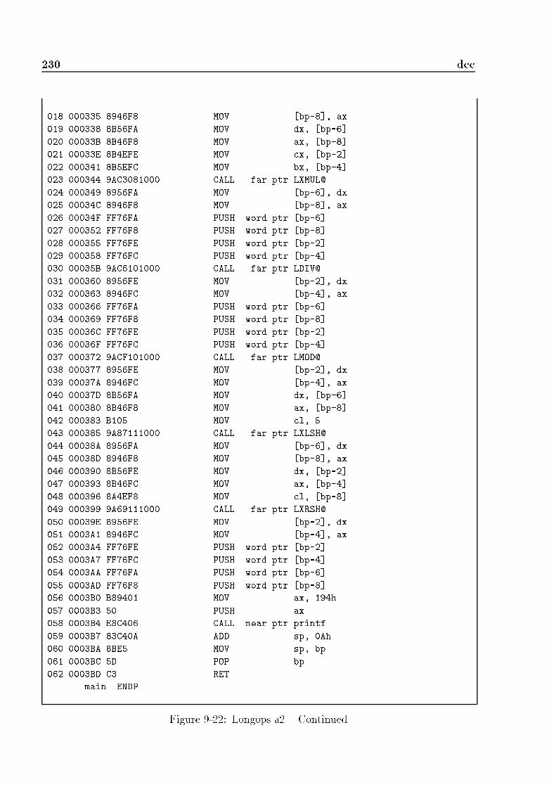
230 dcc018 000335 8946F8 MOV [bp-8], ax019 000338 8B56FA MOV dx, [bp-6]020 00033B 8B46F8 MOV ax, [bp-8]021 00033E 8B4EFE MOV cx, [bp-2]022 000341 8B5EFC MOV bx, [bp-4]023 000344 9AC3081000 CALL far ptr LXMUL@024 000349 8956FA MOV [bp-6], dx025 00034C 8946F8 MOV [bp-8], ax026 00034F FF76FA PUSH word ptr [bp-6]027 000352 FF76F8 PUSH word ptr [bp-8]028 000355 FF76FE PUSH word ptr [bp-2]029 000358 FF76FC PUSH word ptr [bp-4]030 00035B 9AC6101000 CALL far ptr LDIV@031 000360 8956FE MOV [bp-2], dx032 000363 8946FC MOV [bp-4], ax033 000366 FF76FA PUSH word ptr [bp-6]034 000369 FF76F8 PUSH word ptr [bp-8]035 00036C FF76FE PUSH word ptr [bp-2]036 00036F FF76FC PUSH word ptr [bp-4]037 000372 9ACF101000 CALL far ptr LMOD@038 000377 8956FE MOV [bp-2], dx039 00037A 8946FC MOV [bp-4], ax040 00037D 8B56FA MOV dx, [bp-6]041 000380 8B46F8 MOV ax, [bp-8]042 000383 B105 MOV cl, 5043 000385 9A87111000 CALL far ptr LXLSH@044 00038A 8956FA MOV [bp-6], dx045 00038D 8946F8 MOV [bp-8], ax046 000390 8B56FE MOV dx, [bp-2]047 000393 8B46FC MOV ax, [bp-4]048 000396 8A4EF8 MOV cl, [bp-8]049 000399 9A69111000 CALL far ptr LXRSH@050 00039E 8956FE MOV [bp-2], dx051 0003A1 8946FC MOV [bp-4], ax052 0003A4 FF76FE PUSH word ptr [bp-2]053 0003A7 FF76FC PUSH word ptr [bp-4]054 0003AA FF76FA PUSH word ptr [bp-6]055 0003AD FF76F8 PUSH word ptr [bp-8]056 0003B0 B89401 MOV ax, 194h057 0003B3 50 PUSH ax058 0003B4 E8C406 CALL near ptr printf059 0003B7 83C40A ADD sp, 0Ah060 0003BA 8BE5 MOV sp, bp061 0003BC 5D POP bp062 0003BD C3 RETmain ENDP Figure 9-22: Longops.a2 { Continued

9.7 Results 231/** Input file : longops.exe* File type : EXE*/#include "dcc.h"long LXMUL@ (long arg0, long arg1)/* Uses register arguments:* arg0 = dx:ax.* arg1 = cx:bx.* Runtime support routine of the compiler.*/{int loc1;int loc2; /* tmp */loc2 = LO(arg0);LO(arg0) = loc1;loc1 = loc2;loc2 = LO(arg0);LO(arg0) = HI(arg0);if ((LO(arg0) & LO(arg0)) != 0) {LO(arg0) = (LO(arg0) * LO(arg1));}loc2 = LO(arg0);LO(arg0) = HI(arg1);HI(arg1) = loc2;if ((LO(arg0) & LO(arg0)) != 0) {LO(arg0) = (LO(arg0) * loc1);HI(arg1) = (HI(arg1) + LO(arg0));}loc2 = LO(arg0);LO(arg0) = loc1;loc1 = loc2;arg0 = (LO(arg0) * LO(arg1));HI(arg0) = (HI(arg0) + HI(arg1));return (arg0);} Figure 9-23: Longops.b

232 dcclong LDIV@ (long arg0, long arg2)/* Takes 8 bytes of parameters.* Runtime support routine of the compiler.* Untranslatable routine. Assembler provided.* Return value in registers dx:ax.* Pascal calling convention.*/{ /* disassembly code here */}long LMOD@ (long arg0, long arg2)/* Takes 8 bytes of parameters.* Runtime support routine of the compiler.* Untranslatable routine. Assembler provided.* Return value in registers dx:ax.* Pascal calling convention.*/{ /* disassembly code here */}long LXLSH@ (long arg0, char arg1)/* Uses register arguments:* arg0 = dx:ax.* arg1 = cl.* Runtime support routine of the compiler.*/{int loc1; /* bx */if (arg1 < 16) {loc1 = LO(arg0);LO(arg0) = (LO(arg0) << arg1);HI(arg0) = (HI(arg0) << arg1);HI(arg0) = (HI(arg0) | (loc1 >> (!arg1 + 16)));return (arg0);}else {HI(arg0) = LO(arg0);LO(arg0) = 0;HI(arg0) = (HI(arg0) << (arg1 - 16));return (arg0);}} Figure 9-23: Longops.b { Continued

9.7 Results 233long LXRSH@ (long arg0, char arg1)/* Uses register arguments:* arg0 = dx:ax.* arg1 = cl.* Runtime support routine of the compiler.*/{int loc1; /* bx */if (arg1 < 16) {loc1 = HI(arg0);LO(arg0) = (LO(arg0) >> arg1);HI(arg0) = (HI(arg0) >> arg1);LO(arg0) = (LO(arg0) | (loc1 << (!arg1 + 16)));return (arg0);}else {arg0 = HI(arg0);LO(arg0) = (LO(arg0) >> (arg1 - 16));return (arg0);}}void main ()/* Takes no parameters.* High-level language prologue code.*/{long loc1;long loc2;loc2 = 255;loc1 = 143;loc1 = (loc2 + loc1);loc2 = (loc2 - loc1);loc2 = LXMUL@ (loc2, loc1);loc1 = LDIV@ (loc1, loc2);loc1 = LMOD@ (loc1, loc2);loc2 = LXLSH@ (loc2, 5);loc1 = LXRSH@ (loc1, loc1);printf ("a = %ld, b = %ld\n", loc2, loc1);} Figure 9-23: Longops.b { Continued

234 dcc#define TYPE longmain(){ TYPE a, b;a = 255;b = 143;b = a + b;a = a - b;a = a * b;b = b / a;b = b % a;a = a << 5;b = b >> a;printf ("a = %ld, b = %ld\n", a, b);} Figure 9-24: Longops.cSubroutine Low-level High-level % ReductionLXMUL@ 24 19 20.83LDIV@ 72 - -LMOD@ 72 - -LXLSH@ 15 10 33.33LXRSH@ 15 9 40.00main 63 10 84.13total 117 48 58.97Figure 9-25: Longops Statistics

9.7 Results 2359.7.4 Benchsho.exeBenchsho is a program from the Plum-Hall benchmark suite, which benchmarks shortintegers. The program makes use of two long variables to iterate through the loop, andthree (short) integer variables to execute 1000 operations. The disassembly program isshown in Figure 9-27, the decompiled C program in Figure 9-28, and the initial C programin Figure 9-29. The program has the following call graph:mainscanfprintfAs seen in the disassembly of the program, the long variables are located in the stack ato�sets -4 and -8, and the integer variables are located at o�sets -14, -12, and -10. The�nal C code makes use of the integer variable loc6 to hold the result of a Boolean expression(i.e. 0 or 1) and assign it to the corresponding variable. This Boolean variable is a registervariable (register ax) and could have been eliminated from the code with further analysisof the control ow graph, in a similar way to the structuring of compound conditions.locX = ax;/* no further use of ax */ /* other code */?������) PPPPPPqPPPPPPPq �������) - ?/* no further use of ax */?/* other code */<Boolean expression>ax = 1 ax = 03 24 1

(b)(a) 4 1locX = <Boolean expression>;Figure 9-26: Control Flow Graph for Boolean AssignmentFor example, graph (a) in Figure 9-26 can be reduced to graph (b) if the following conditionsare satis�ed:1. Node 1 is a 2-way node.2. Nodes 2 and 3 have one in-edge from node 1 only, and lead to a common node 4.3. Nodes 2 and 3 have one instruction only. This instruction assigns 0 and 1 respectivelyto a register.4. Node 4 assigns the register of nodes 2 and 3 to a local variable. The register is notfurther used before rede�nition in the program.Since the register is used only once to store the intermediate result of a Boolean expressionevaluation, it is eliminated from the �nal code by assigning the Boolean expression to the

236 dcctarget variable. This transformation not only removes the involved register, but also thetwo nodes that assigned a value to it (i.e. nodes 2 and 3 in the graph of Figure 9-26).It is clear that the two Boolean assignments of Figure 9-28 can be transformed into thefollowing code:loc1 = (loc2 == loc3);/* other code */loc1 = (loc2 > loc3);which would make the �nal C program an exact decompilation of the original C program.Without this transformation, the generated C code is functionally equivalent to the initialC code, and structurally equivalent to the decompiled graph. Since the graph of a Booleanassignment is structured by nature, the non-implementation of this transformation does notgenerate unstructured code in any way, unlike the case of compound conditions, which areunstructured graphs by nature that are transformed into structured graphs.Without the graph optimization, the �nal decompiled code generated by dcc produces a75.25% reduction on the number of intermediate instructions, as shown in Figure 9-30. Foreach Boolean assignment of the initial C code, there are three extra instructions due to theuse of a temporary local variable (loc6 in this case).

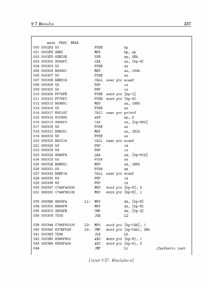
9.7 Results 237main PROC NEAR000 0002FA 55 PUSH bp001 0002FB 8BEC MOV bp, sp002 0002FD 83EC0E SUB sp, 0Eh003 000300 8D46FC LEA ax, [bp-4]004 000303 50 PUSH ax005 000304 B89401 MOV ax, 194h006 000307 50 PUSH ax007 000308 E8E914 CALL near ptr scanf008 00030B 59 POP cx009 00030C 59 POP cx010 00030D FF76FE PUSH word ptr [bp-2]011 000310 FF76FC PUSH word ptr [bp-4]012 000313 B89801 MOV ax, 198h013 000316 50 PUSH ax014 000317 E8510C CALL near ptr printf015 00031A 83C406 ADD sp, 6016 00031D 8D46F2 LEA ax, [bp-0Eh]017 000320 50 PUSH ax018 000321 B8B201 MOV ax, 1B2h019 000324 50 PUSH ax020 000325 E8CC14 CALL near ptr scanf021 000328 59 POP cx022 000329 59 POP cx023 00032A 8D46F4 LEA ax, [bp-0Ch]024 00032D 50 PUSH ax025 00032E B8B601 MOV ax, 1B6h026 000331 50 PUSH ax027 000332 E8BF14 CALL near ptr scanf028 000335 59 POP cx029 000336 59 POP cx030 000337 C746FA0000 MOV word ptr [bp-6], 0031 00033C C746F80100 MOV word ptr [bp-8], 1033 0003BD 8B56FA L1: MOV dx, [bp-6]034 0003C0 8B46F8 MOV ax, [bp-8]035 0003C3 3B56FE CMP dx, [bp-2]036 0003C6 7D03 JGE L2038 000344 C746F60100 L3: MOV word ptr [bp-0Ah], 1040 0003AF 837EF628 L4: CMP word ptr [bp-0Ah], 28h041 0003B3 7E96 JLE L5042 0003B5 8346F801 ADD word ptr [bp-8], 1043 0003B9 8356FA00 ADC word ptr [bp-6], 0044 JMP L1 ;Synthetic instFigure 9-27: Benchsho.a2

238 dcc045 00034B 8B46F2 L5: MOV ax, [bp-0Eh]046 00034E 0346F4 ADD ax, [bp-0Ch]047 000351 0346F6 ADD ax, [bp-0Ah]048 000354 8946F2 MOV [bp-0Eh], ax049 000357 8B46F2 MOV ax, [bp-0Eh]050 00035A D1F8 SAR ax, 1051 00035C 8946F4 MOV [bp-0Ch], ax052 00035F 8B46F4 MOV ax, [bp-0Ch]053 000362 BB0A00 MOV bx, 0Ah054 000365 99 CWD055 MOV tmp, dx:ax ;Synthetic inst056 000366 F7FB IDIV bx057 MOD bx ;Synthetic inst058 000368 8956F2 MOV [bp-0Eh], dx059 00036B 8B46F4 MOV ax, [bp-0Ch]060 00036E 3B46F6 CMP ax, [bp-0Ah]061 000371 7505 JNE L6062 000373 B80100 MOV ax, 1064 00037A 8946F2 L7: MOV [bp-0Eh], ax065 00037D 8B46F2 MOV ax, [bp-0Eh]066 000380 0B46F6 OR ax, [bp-0Ah]067 000383 8946F4 MOV [bp-0Ch], ax068 000386 8B46F4 MOV ax, [bp-0Ch]069 000389 F7D8 NEG ax070 00038B 1BC0 SBB ax, ax071 00038D 40 INC ax072 00038E 8946F2 MOV [bp-0Eh], ax073 000391 8B46F2 MOV ax, [bp-0Eh]074 000394 0346F6 ADD ax, [bp-0Ah]075 000397 8946F4 MOV [bp-0Ch], ax076 00039A 8B46F4 MOV ax, [bp-0Ch]077 00039D 3B46F6 CMP ax, [bp-0Ah]078 0003A0 7E05 JLE L8079 0003A2 B80100 MOV ax, 1081 0003A9 8946F2 L9: MOV [bp-0Eh], ax082 0003AC FF46F6 INC word ptr [bp-0Ah]083 JMP L4 ;Synthetic inst084 0003A7 33C0 L8: XOR ax, ax085 JMP L9 ;Synthetic inst086 000378 33C0 L6: XOR ax, ax087 JMP L7 ;Synthetic inst088 0003CB 7F08 L2: JG L10089 0003CD 3B46FC CMP ax, [bp-4]090 0003D0 7703 JA L10Figure 9-27: Benchsho.a2 { Continued

9.7 Results 239092 0003D5 FF76F2 L10: PUSH word ptr [bp-0Eh]093 0003D8 B8BA01 MOV ax, 1BAh094 0003DB 50 PUSH ax095 0003DC E88C0B CALL near ptr printf096 0003DF 59 POP cx097 0003E0 59 POP cx098 0003E1 8BE5 MOV sp, bp099 0003E3 5D POP bp100 0003E4 C3 RETmain ENDP Figure 9-27: Benchsho.a2 { Continued

240 dcc/** Input file : benchsho.exe* File type : EXE*/#include "dcc.h"void main ()/* Takes no parameters.* High-level language prologue code.*/{ int loc1; int loc2; int loc3;long loc4; long loc5; int loc6; /* ax */scanf ("%ld", &loc5);printf ("executing %ld iterations\n", loc5);scanf ("%ld", &loc1);scanf ("%ld", &loc2);loc4 = 1;while ((loc4 <= loc5)) {loc3 = 1;while ((loc3 <= 40)) {loc1 = ((loc1 + loc2) + loc3);loc2 = (loc1 >> 1);loc1 = (loc2 % 10);if (loc2 == loc3) {loc6 = 1;}else {loc6 = 0;}loc1 = loc6;loc2 = (loc1 | loc3);loc1 = !loc2;loc2 = (loc1 + loc3);if (loc2 > loc3) {loc6 = 1;}else {loc6 = 0;}loc1 = loc6;loc3 = (loc3 + 1);}loc4 = (loc4 + 1);}printf ("a=%d\n", loc1);} Figure 9-28: Benchsho.b

9.7 Results 241/* benchsho - benchmark for short integers* Thomas Plum, Plum Hall Inc, 609-927-3770* If machine traps overflow, use an unsigned type* Let T be the execution time in milliseconds* Then average time per operator = T/major usec* (Because the inner loop has exactly 1000 operations)*/#define STOR_CL auto#define TYPE short#include <stdio.h>main (int ac, char *av[]){ STOR_CL TYPE a, b, c;long d, major;scanf ("%ld", &major);printf("executing %ld iterations\n", major);scanf ("%ld", &a);scanf ("%ld", &b);for (d = 1; d <= major; ++d){ /* inner loop executes 1000 selected operations */for (c = 1; c <= 40; ++c){ a = a + b + c;b = a >> 1;a = b % 10;a = b == c;b = a | c;a = !b;b = a + c;a = b > c;}}printf("a=%d\n", a);} Figure 9-29: Benchsho.cSubroutine Low-level High-level % Reductionmain 101 25 75.25total 101 25 75.25Figure 9-30: Benchsho Statistics

242 dcc9.7.5 Benchlng.exeBenchlng is a program from the Plum-Hall benchmark suite, which benchmarks longvariables. The program is exactly the same as the benchsho.exe program, but makes use oflong variables rather than short integers. The disassembly program is shown in Figure 9-31,the decompiled C program in Figure 9-32, and the initial C program in Figure 9-33. Theprogram has the following call graph:mainscanfprintfLMOD@As seen from the disassembly of the program, the long variables are located in the stackat o�sets -4, -20, -16, -8, and -12. The �nal C decompiled code makes use of �ve longvariables and an integer variable loc6. This latter variable is used as a Boolean variable tohold the contents of a Boolean expression evaluation. Three Boolean expression evaluationsare seen in the �nal C code:loc1 == loc2LO(loc1) | HI(loc1)loc1 > loc2All these expressions can be transformed into Boolean assignment by means of thetransformation described in the previous Section. The generated code would look like this:loc4 = (loc1 == loc2);/* other code here */loc4 = (LO(loc1) | HI(loc1));/* other code here */loc4 = (loc1 > loc2);The second Boolean expression checks the low and high part of a long variable and orsthem together; this is equivalent to a logical negation of the long variable, which would leadto the following �nal code:loc4 = !loc1;The benchlng program as compared to the benchsho program has 27.34% more low-levelinstructions in the main program (the LMOD@ subroutine calculates the modulus of longvariables and is untranslatable to a high-level language), three more instructions in thehigh-level representation of main (due to the logical negation of a long variable, whichmakes use of the temporary Boolean variable loc6), and performs a reduction of 79.86%instructions as shown in Figure 9-34.

9.7 Results 243LMOD@ PROC FAR000 001EEB B90200 MOV cx, 2002 001EF3 55 PUSH bp003 001EF4 56 PUSH si004 001EF5 57 PUSH di005 001EF6 8BEC MOV bp, sp006 001EF8 8BF9 MOV di, cx007 001EFA 8B460A MOV ax, [bp+0Ah]008 001EFD 8B560C MOV dx, [bp+0Ch]009 001F00 8B5E0E MOV bx, [bp+0Eh]010 001F03 8B4E10 MOV cx, [bp+10h]011 001F06 0BC9 OR cx, cx012 001F08 7508 JNE L1013 001F0A 0BD2 OR dx, dx014 001F0C 7469 JE L2015 001F0E 0BDB OR bx, bx016 001F10 7465 JE L2017 001F12 F7C70100 L1: TEST di, 1018 001F16 751C JNE L3019 001F18 0BD2 OR dx, dx020 001F1A 790A JNS L4021 001F1C F7DA NEG dx022 001F1E F7D8 NEG ax023 001F20 83DA00 SBB dx, 0024 001F23 83CF0C OR di, 0Ch025 001F26 0BC9 L4: OR cx, cx026 001F28 790A JNS L3027 001F2A F7D9 NEG cx028 001F2C F7DB NEG bx029 001F2E 83D900 SBB cx, 0030 001F31 83F704 XOR di, 4031 001F34 8BE9 L3: MOV bp, cx032 001F36 B92000 MOV cx, 20h033 001F39 57 PUSH di034 001F3A 33FF XOR di, di035 001F3C 33F6 XOR si, si036 001F3E D1E0 L5: SHL ax, 1037 001F40 D1D2 RCL dx, 1038 001F42 D1D6 RCL si, 1039 001F44 D1D7 RCL di, 1040 001F46 3BFD CMP di, bp041 001F48 720B JB L6042 001F4A 7704 JA L7043 001F4C 3BF3 CMP si, bx044 001F4E 7205 JB L6Figure 9-31: Benchlng.a2

244 dcc045 001F50 2BF3 L7: SUB si, bx046 001F52 1BFD SBB di, bp047 001F54 40 INC ax048 001F55 E2E7 L6: LOOP L5049 001F57 5B POP bx050 001F58 F7C30200 TEST bx, 2051 001F5C 7406 JE L8052 001F5E 8BC6 MOV ax, si053 001F60 8BD7 MOV dx, di054 001F62 D1EB SHR bx, 1055 001F64 F7C30400 L8: TEST bx, 4056 001F68 7407 JE L9057 001F6A F7DA NEG dx058 001F6C F7D8 NEG ax059 001F6E 83DA00 SBB dx, 0060 001F71 5F L9: POP di061 001F72 5E POP si062 001F73 5D POP bp063 001F74 CA0800 RETF 8064 L2: MOV tmp, dx:ax ;Synthetic inst065 001F77 F7F3 DIV bx066 MOD bx ;Synthetic inst067 001F79 F7C70200 TEST di, 2068 001F7D 7402 JE L10069 001F7F 8BC2 MOV ax, dx070 001F81 33D2 L10: XOR dx, dx071 001F83 EBEC JMP L9LMOD@ ENDPmain PROC NEAR000 0002FA 55 PUSH bp001 0002FB 8BEC MOV bp, sp002 0002FD 83EC14 SUB sp, 14h003 000300 8D46FC LEA ax, [bp-4]004 000303 50 PUSH ax005 000304 B89401 MOV ax, 194h006 000307 50 PUSH ax007 000308 E85D15 CALL near ptr scanf008 00030B 59 POP cx009 00030C 59 POP cx010 00030D FF76FE PUSH word ptr [bp-2]011 000310 FF76FC PUSH word ptr [bp-4]012 000313 B89801 MOV ax, 198h013 000316 50 PUSH ax014 000317 E8C50C CALL near ptr printfFigure 9-31: Benchlng.a2 { Continued

9.7 Results 245015 00031A 83C406 ADD sp, 6016 00031D 8D46EC LEA ax, [bp-14h]017 000320 50 PUSH ax018 000321 B8B201 MOV ax, 1B2h019 000324 50 PUSH ax020 000325 E84015 CALL near ptr scanf021 000328 59 POP cx022 000329 59 POP cx023 00032A 8D46F0 LEA ax, [bp-10h]024 00032D 50 PUSH ax025 00032E B8B601 MOV ax, 1B6h026 000331 50 PUSH ax027 000332 E83315 CALL near ptr scanf028 000335 59 POP cx029 000336 59 POP cx030 000337 C746FA0000 MOV word ptr [bp-6], 0031 00033C C746F80100 MOV word ptr [bp-8], 1033 00042D 8B56FA L11: MOV dx, [bp-6]034 000430 8B46F8 MOV ax, [bp-8]035 000433 3B56FE CMP dx, [bp-2]036 000436 7D03 JGE L12038 000344 C746F60000 L13: MOV word ptr [bp-0Ah], 0039 000349 C746F40100 MOV word ptr [bp-0Ch], 1041 000411 837EF600 L14: CMP word ptr [bp-0Ah], 0042 000415 7D03 JGE L15044 000351 8B56EE L16: MOV dx, [bp-12h]045 000354 8B46EC MOV ax, [bp-14h]046 000357 0346F0 ADD ax, [bp-10h]047 00035A 1356F2 ADC dx, [bp-0Eh]048 00035D 0346F4 ADD ax, [bp-0Ch]049 000360 1356F6 ADC dx, [bp-0Ah]050 000363 8956EE MOV [bp-12h], dx051 000366 8946EC MOV [bp-14h], ax052 000369 8B56EE MOV dx, [bp-12h]053 00036C 8B46EC MOV ax, [bp-14h]054 00036F D1FA SAR dx, 1055 000371 D1D8 RCR ax, 1056 000373 8956F2 MOV [bp-0Eh], dx057 000376 8946F0 MOV [bp-10h], ax058 000379 33D2 XOR dx, dx059 00037B B80A00 MOV ax, 0AhFigure 9-31: Benchlng.a2 { Continued

246 dcc060 00037E 52 PUSH dx061 00037F 50 PUSH ax062 000380 FF76F2 PUSH word ptr [bp-0Eh]063 000383 FF76F0 PUSH word ptr [bp-10h]064 000386 9AEB1D1000 CALL far ptr LMOD@065 00038B 8956EE MOV [bp-12h], dx066 00038E 8946EC MOV [bp-14h], ax067 000391 8B56F2 MOV dx, [bp-0Eh]068 000394 8B46F0 MOV ax, [bp-10h]069 000397 3B56F6 CMP dx, [bp-0Ah]070 00039A 750A JNE L17071 00039C 3B46F4 CMP ax, [bp-0Ch]072 00039F 7505 JNE L17073 0003A1 B80100 MOV ax, 1075 0003A8 99 L18: CWD076 0003A9 8956EE MOV [bp-12h], dx077 0003AC 8946EC MOV [bp-14h], ax078 0003AF 8B56EE MOV dx, [bp-12h]079 0003B2 8B46EC MOV ax, [bp-14h]080 0003B5 0B46F4 OR ax, [bp-0Ch]081 0003B8 0B56F6 OR dx, [bp-0Ah]082 0003BB 8956F2 MOV [bp-0Eh], dx083 0003BE 8946F0 MOV [bp-10h], ax084 0003C1 8B46F0 MOV ax, [bp-10h]085 0003C4 0B46F2 OR ax, [bp-0Eh]086 0003C7 7505 JNE L19087 0003C9 B80100 MOV ax, 1089 0003D0 99 L20: CWD090 0003D1 8956EE MOV [bp-12h], dx091 0003D4 8946EC MOV [bp-14h], ax092 0003D7 8B56EE MOV dx, [bp-12h]093 0003DA 8B46EC MOV ax, [bp-14h]094 0003DD 0346F4 ADD ax, [bp-0Ch]095 0003E0 1356F6 ADC dx, [bp-0Ah]096 0003E3 8956F2 MOV [bp-0Eh], dx097 0003E6 8946F0 MOV [bp-10h], ax098 0003E9 8B56F2 MOV dx, [bp-0Eh]099 0003EC 8B46F0 MOV ax, [bp-10h]100 0003EF 3B56F6 CMP dx, [bp-0Ah]101 0003F2 7C0C JL L21102 0003F4 7F05 JG L22103 0003F6 3B46F4 CMP ax, [bp-0Ch]104 0003F9 7605 JBE L21Figure 9-31: Benchlng.a2 { Continued

9.7 Results 247105 0003FB B80100 L22: MOV ax, 1107 000402 99 L23: CWD108 000403 8956EE MOV [bp-12h], dx109 000406 8946EC MOV [bp-14h], ax110 000409 8346F401 ADD word ptr [bp-0Ch], 1111 00040D 8356F600 ADC word ptr [bp-0Ah], 0112 JMP L14 ;Synthetic inst113 000400 33C0 L21: XOR ax, ax114 JMP L23 ;Synthetic inst115 0003CE 33C0 L19: XOR ax, ax116 JMP L20 ;Synthetic inst117 0003A6 33C0 L17: XOR ax, ax118 JMP L18 ;Synthetic inst119 00041A 7F09 L15: JG L24120 00041C 837EF428 CMP word ptr [bp-0Ch], 28h121 000420 7703 JA L24123 000425 8346F801 L24: ADD word ptr [bp-8], 1124 000429 8356FA00 ADC word ptr [bp-6], 0125 JMP L11 ;Synthetic inst126 00043B 7F08 L12: JG L25127 00043D 3B46FC CMP ax, [bp-4]128 000440 7703 JA L25130 000445 FF76EE L25: PUSH word ptr [bp-12h]131 000448 FF76EC PUSH word ptr [bp-14h]132 00044B B8BA01 MOV ax, 1BAh133 00044E 50 PUSH ax134 00044F E88D0B CALL near ptr printf135 000452 83C406 ADD sp, 6136 000455 8BE5 MOV sp, bp137 000457 5D POP bp138 000458 C3 RETmain ENDP Figure 9-31: Benchlng.a2 { Continued

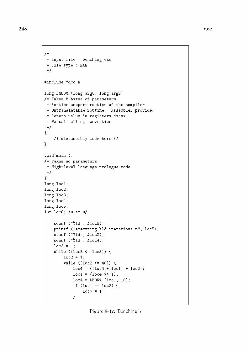
248 dcc/** Input file : benchlng.exe* File type : EXE*/#include "dcc.h"long LMOD@ (long arg0, long arg2)/* Takes 8 bytes of parameters.* Runtime support routine of the compiler.* Untranslatable routine. Assembler provided.* Return value in registers dx:ax.* Pascal calling convention.*/{ /* disassembly code here */}void main ()/* Takes no parameters.* High-level language prologue code.*/{long loc1;long loc2;long loc3;long loc4;long loc5;int loc6; /* ax */scanf ("%ld", &loc5);printf ("executing %ld iterations\n", loc5);scanf ("%ld", &loc2);scanf ("%ld", &loc4);loc3 = 1;while ((loc3 <= loc5)) {loc2 = 1;while ((loc2 <= 40)) {loc4 = ((loc4 + loc1) + loc2);loc1 = (loc4 >> 1);loc4 = LMOD@ (loc1, 10);if (loc1 == loc2) {loc6 = 1;} Figure 9-32: Benchlng.b

9.7 Results 249else {loc6 = 0;}loc4 = loc6;loc1 = (loc4 | loc2);if ((LO(loc1) | HI(loc1)) == 0) {loc6 = 1;}else {loc6 = 0;}loc4 = loc6;loc1 = (loc4 + loc2);if (loc1 > loc2) {loc6 = 1;}else {loc6 = 0;}loc4 = loc6;loc2 = (loc2 + 1);}loc3 = (loc3 + 1);}printf ("a=%d\n", loc4);} Figure 9-32: Benchlng.b { Continued

250 dcc/* benchlng - benchmark for long integers* Thomas Plum, Plum Hall Inc, 609-927-3770* If machine traps overflow, use an unsigned type* Let T be the execution time in milliseconds* Then average time per operator = T/major usec* (Because the inner loop has exactly 1000 operations)*/#define TYPE long#include <stdio.h>main (int ac, char *av[]){ TYPE a, b, c;long d, major;scanf ("%ld", &major);printf("executing %ld iterations\n", major);scanf ("%ld", &a);scanf ("%ld", &b);for (d = 1; d <= major; ++d){ /* inner loop executes 1000 selected operations */for (c = 1; c <= 40; ++c){ a = a + b + c;b = a >> 1;a = b % 10;a = b == c;b = a | c;a = !b;b = a + c;a = b > c;}}printf("a=%d\n", a);} Figure 9-33: Benchlng.cSubroutine Low-level High-level % ReductionLMOD@ 72 - -main 139 28 79.86total 139 28 79.86Figure 9-34: Benchlng Statistics

9.7 Results 2519.7.6 Benchmul.exeBenchmul is another program from the Plum-Hall benchmarks. This program benchmarksinteger multiplication by executing 1000 multiplications in a loop. The disassembly programis shown in Figure 9-35, the decompiled C program in Figure 9-36, and the initial C programin Figure 9-37. This program has the following call graph:mainscanfprintfBenchmul makes use of two long variables to loop a large number of times through theprogram, and three integer variables that perform the operations; one of these variablesis not actually used in the program. As seen from the disassembly, the long variables arelocated on the stack at o�sets -4 and -8, and the integer variables are at o�sets -12, -10,and on the register variable si. The �nal C code is identical to the initial C code, and areduction of 86.36% of instructions was achieved by this program, as seen in Figure 9-38.

252 dccmain PROC NEAR000 0002FA 55 PUSH bp001 0002FB 8BEC MOV bp, sp002 0002FD 83EC0C SUB sp, 0Ch003 000300 56 PUSH si004 000301 8D46FC LEA ax, [bp-4]005 000304 50 PUSH ax006 000305 B89401 MOV ax, 194h007 000308 50 PUSH ax008 000309 E8D014 CALL near ptr scanf009 00030C 59 POP cx010 00030D 59 POP cx011 00030E FF76FE PUSH word ptr [bp-2]012 000311 FF76FC PUSH word ptr [bp-4]013 000314 B89801 MOV ax, 198h014 000317 50 PUSH ax015 000318 E8380C CALL near ptr printf016 00031B 83C406 ADD sp, 6017 00031E 8D46F4 LEA ax, [bp-0Ch]018 000321 50 PUSH ax019 000322 B8B201 MOV ax, 1B2h020 000325 50 PUSH ax021 000326 E8B314 CALL near ptr scanf022 000329 59 POP cx023 00032A 59 POP cx024 00032B 8D46F6 LEA ax, [bp-0Ah]025 00032E 50 PUSH ax026 00032F B8B501 MOV ax, 1B5h027 000332 50 PUSH ax028 000333 E8A614 CALL near ptr scanf029 000336 59 POP cx030 000337 59 POP cx031 000338 C746FA0000 MOV word ptr [bp-6], 0032 00033D C746F80100 MOV word ptr [bp-8], 1034 0003AA 8B56FA L1: MOV dx, [bp-6]035 0003AD 8B46F8 MOV ax, [bp-8]036 0003B0 3B56FE CMP dx, [bp-2]037 0003B3 7C8F JL L2038 0003B5 7F05 JG L3039 0003B7 3B46FC CMP ax, [bp-4]040 0003BA 7688 JBE L2041 0003BC FF76F4 L3: PUSH word ptr [bp-0Ch]042 0003BF B8B801 MOV ax, 1B8h043 0003C2 50 PUSH ax044 0003C3 E88D0B CALL near ptr printfFigure 9-35: Benchmul.a2

9.7 Results 253045 0003C6 59 POP cx046 0003C7 59 POP cx047 0003C8 5E POP si048 0003C9 8BE5 MOV sp, bp049 0003CB 5D POP bp050 0003CC C3 RET051 000344 BE0100 L2: MOV si, 1053 00039D 83FE28 L4: CMP si, 28h054 0003A0 7EA7 JLE L5055 0003A2 8346F801 ADD word ptr [bp-8], 1056 0003A6 8356FA00 ADC word ptr [bp-6], 0057 JMP L1 ;Synthetic inst058 000349 8B46F4 L5: MOV ax, [bp-0Ch]059 00034C F766F4 MUL word ptr [bp-0Ch]060 00034F F766F4 MUL word ptr [bp-0Ch]061 000352 F766F4 MUL word ptr [bp-0Ch]062 000355 F766F4 MUL word ptr [bp-0Ch]063 000358 F766F4 MUL word ptr [bp-0Ch]064 00035B F766F4 MUL word ptr [bp-0Ch]065 00035E F766F4 MUL word ptr [bp-0Ch]066 000361 F766F4 MUL word ptr [bp-0Ch]067 000364 F766F4 MUL word ptr [bp-0Ch]068 000367 F766F4 MUL word ptr [bp-0Ch]069 00036A F766F4 MUL word ptr [bp-0Ch]070 00036D F766F4 MUL word ptr [bp-0Ch]071 000370 F766F4 MUL word ptr [bp-0Ch]072 000373 F766F4 MUL word ptr [bp-0Ch]073 000376 F766F4 MUL word ptr [bp-0Ch]074 000379 F766F4 MUL word ptr [bp-0Ch]075 00037C F766F4 MUL word ptr [bp-0Ch]076 00037F F766F4 MUL word ptr [bp-0Ch]077 000382 F766F4 MUL word ptr [bp-0Ch]078 000385 F766F4 MUL word ptr [bp-0Ch]079 000388 F766F4 MUL word ptr [bp-0Ch]080 00038B F766F4 MUL word ptr [bp-0Ch]081 00038E F766F4 MUL word ptr [bp-0Ch]082 000391 F766F4 MUL word ptr [bp-0Ch]083 000394 BA0300 MOV dx, 3084 000397 F7E2 MUL dx085 000399 8946F4 MOV [bp-0Ch], ax086 00039C 46 INC si087 JMP L4 ;Synthetic instmain ENDP Figure 9-35: Benchmul.a2 { Continued

254 dcc/** Input file : benchmul.exe* File type : EXE*/#include "dcc.h"void main ()/* Takes no parameters.* High-level language prologue code.*/{int loc1;int loc2;long loc3;long loc4;int loc5;scanf ("%ld", &loc4);printf ("executing %ld iterations\n", loc4);scanf ("%d", &loc1);scanf ("%d", &loc2);loc3 = 1;while ((loc3 <= loc4)) {loc5 = 1;while ((loc5 <= 40)) {loc1 = (((((((((((((((((((((((((loc1 * loc1) * loc1) * loc1)* loc1) * loc1) * loc1) * loc1) * loc1) * loc1) *loc1) * loc1) * loc1) * loc1) * loc1) * loc1) * loc1)* loc1) * loc1) * loc1) * loc1) * loc1) * loc1) *loc1) * loc1) * 3);loc5 = (loc5 + 1);}loc3 = (loc3 + 1);}printf ("a=%d\n", loc1);} Figure 9-36: Benchmul.b

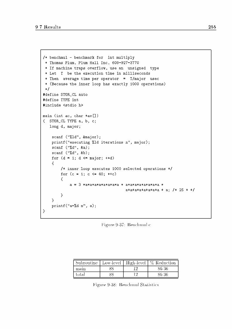
9.7 Results 255/* benchmul - benchmark for int multiply* Thomas Plum, Plum Hall Inc, 609-927-3770* If machine traps overflow, use an unsigned type* Let T be the execution time in milliseconds* Then average time per operator = T/major usec* (Because the inner loop has exactly 1000 operations)*/#define STOR_CL auto#define TYPE int#include <stdio.h>main (int ac, char *av[]){ STOR_CL TYPE a, b, c;long d, major;scanf ("%ld", &major);printf("executing %ld iterations\n", major);scanf ("%d", &a);scanf ("%d", &b);for (d = 1; d <= major; ++d){ /* inner loop executes 1000 selected operations */for (c = 1; c <= 40; ++c){ a = 3 *a*a*a*a*a*a*a*a * a*a*a*a*a*a*a*a *a*a*a*a*a*a*a*a * a; /* 25 * */}}printf("a=%d\n", a);} Figure 9-37: Benchmul.cSubroutine Low-level High-level % Reductionmain 88 12 86.36total 88 12 86.36Figure 9-38: Benchmul Statistics

256 dcc9.7.7 Benchfn.exeBenchfn is a program from the Plum-Hall benchmark suite, which benchmarks functioncalls; 1000 subroutine calls are done each time around the loop. The disassembly programis shown in Figure 9-39, the decompiled C program in Figure 9-40, and the initial C programin Figure 9-41. This program has the following call graph:mainscanfprintfproc_1proc_2proc_3proc_4Benchfn has four procedures and a main program. Three of the four procedures invoke otherprocedure, and the fourth procedure is empty. The percentage of reduction on the numberof intermediate instructions is not as high in this program as compared to the previousprograms since there are not many expressions in the program (which is not normally thecase with high-level programs). As seen in the statistics of this program (see Figure 9-42),the empty procedure has a 100% reduction since the procedure prologue and trailer low-levelinstructions are eliminated in the C program; the other three procedures have an averageof 29.30% reduction of instructions on 29 procedure calls performed by them, and the mainprogram has an 81.08% reduction of instructions since expressions and assignments are usedin this procedure. The overall average for the program is low, 56.10%, and is due to thelack of assignment statements in this program.

9.7 Results 257proc_4 PROC NEAR000 0002FA 55 PUSH bp001 0002FB 8BEC MOV bp, sp002 0002FD 5D POP bp003 0002FE C3 RETproc_4 ENDPproc_3 PROC NEAR000 0002FF 55 PUSH bp001 000300 8BEC MOV bp, sp002 000302 E8F5FF CALL near ptr proc_4003 000305 E8F2FF CALL near ptr proc_4004 000308 E8EFFF CALL near ptr proc_4005 00030B E8ECFF CALL near ptr proc_4006 00030E E8E9FF CALL near ptr proc_4007 000311 E8E6FF CALL near ptr proc_4008 000314 E8E3FF CALL near ptr proc_4009 000317 E8E0FF CALL near ptr proc_4010 00031A E8DDFF CALL near ptr proc_4011 00031D E8DAFF CALL near ptr proc_4012 000320 5D POP bp013 000321 C3 RETproc_3 ENDPproc_2 PROC NEAR000 000322 55 PUSH bp001 000323 8BEC MOV bp, sp002 000325 E8D7FF CALL near ptr proc_3003 000328 E8D4FF CALL near ptr proc_3004 00032B E8D1FF CALL near ptr proc_3005 00032E E8CEFF CALL near ptr proc_3006 000331 E8CBFF CALL near ptr proc_3007 000334 E8C8FF CALL near ptr proc_3008 000337 E8C5FF CALL near ptr proc_3009 00033A E8C2FF CALL near ptr proc_3010 00033D E8BFFF CALL near ptr proc_3011 000340 E8BCFF CALL near ptr proc_3012 000343 5D POP bp013 000344 C3 RETproc_2 ENDPproc_1 PROC NEAR000 000345 55 PUSH bp001 000346 8BEC MOV bp, sp002 000348 E8D7FF CALL near ptr proc_2Figure 9-39: Benchfn.a2

258 dcc003 00034B E8D4FF CALL near ptr proc_2004 00034E E8D1FF CALL near ptr proc_2005 000351 E8CEFF CALL near ptr proc_2006 000354 E8CBFF CALL near ptr proc_2007 000357 E8C8FF CALL near ptr proc_2008 00035A E8C5FF CALL near ptr proc_2009 00035D E8C2FF CALL near ptr proc_2010 000360 E8BFFF CALL near ptr proc_2011 000363 5D POP bp012 000364 C3 RETproc_1 ENDPmain PROC NEAR000 000365 55 PUSH bp001 000366 8BEC MOV bp, sp002 000368 83EC08 SUB sp, 8003 00036B 8D46FC LEA ax, [bp-4]004 00036E 50 PUSH ax005 00036F B89401 MOV ax, 194h006 000372 50 PUSH ax007 000373 E85614 CALL near ptr scanf008 000376 59 POP cx009 000377 59 POP cx010 000378 FF76FE PUSH word ptr [bp-2]011 00037B FF76FC PUSH word ptr [bp-4]012 00037E B89801 MOV ax, 198h013 000381 50 PUSH ax014 000382 E8BE0B CALL near ptr printf015 000385 83C406 ADD sp, 6016 000388 C746FA0000 MOV word ptr [bp-6], 0017 00038D C746F80100 MOV word ptr [bp-8], 1019 00039F 8B56FA L1: MOV dx, [bp-6]020 0003A2 8B46F8 MOV ax, [bp-8]021 0003A5 3B56FE CMP dx, [bp-2]022 0003A8 7CEA JL L2023 0003AA 7F05 JG L3024 0003AC 3B46FC CMP ax, [bp-4]025 0003AF 76E3 JBE L2026 0003B1 B8B201 L3: MOV ax, 1B2h027 0003B4 50 PUSH ax028 0003B5 E88B0B CALL near ptr printf029 0003B8 59 POP cx030 0003B9 8BE5 MOV sp, bpFigure 9-39: Benchfn.a2 { Continued

9.7 Results 259031 0003BB 5D POP bp032 0003BC C3 RET033 000394 E8AEFF L2: CALL near ptr proc_1034 000397 8346F801 ADD word ptr [bp-8], 1035 00039B 8356FA00 ADC word ptr [bp-6], 0036 JMP L1 ;Synthetic instmain ENDP Figure 9-39: Benchfn.a2 { Continued

260 dcc/** Input file : benchfn.exe* File type : EXE*/#include "dcc.h"void proc_4 ()/* Takes no parameters.* High-level language prologue code.*/{}void proc_3 ()/* Takes no parameters.* High-level language prologue code.*/{ proc_4 ();proc_4 ();proc_4 ();proc_4 ();proc_4 ();proc_4 ();proc_4 ();proc_4 ();proc_4 ();proc_4 ();}void proc_2 ()/* Takes no parameters.* High-level language prologue code.*/{ proc_3 ();proc_3 ();proc_3 ();proc_3 ();proc_3 ();proc_3 ();proc_3 (); Figure 9-40: Benchfn.b

9.7 Results 261proc_3 ();proc_3 ();proc_3 ();}void proc_1 ()/* Takes no parameters.* High-level language prologue code.*/{ proc_2 ();proc_2 ();proc_2 ();proc_2 ();proc_2 ();proc_2 ();proc_2 ();proc_2 ();proc_2 ();}void main ()/* Takes no parameters.* High-level language prologue code.*/{long loc1;long loc2;scanf ("%ld", &loc2);printf ("executing %ld iterations\n", loc2);loc1 = 1;while ((loc1 <= loc2)) {proc_1 ();loc1 = (loc1 + 1);}printf ("finished\n");} Figure 9-40: Benchfn.b { Continued

262 dcc/* benchfn - benchmark for function calls* Thomas Plum, Plum Hall Inc, 609-927-3770* Let T be the execution time in milliseconds* Then average time per operator = T/major usec* (Because the inner loop has exactly 1000 operations)*/#include <stdio.h>f3() { ;}f2() { f3();f3();f3();f3();f3();f3();f3();f3();f3();f3();} /* 10 */f1() { f2();f2();f2();f2();f2();f2();f2();f2();f2();f2();} /* 10 */f0() { f1();f1();f1();f1();f1();f1();f1();f1();f1();} /* 9 */main (int ac, char *av[]){ long d, major;scanf ("%ld", &major);printf("executing %ld iterations\n", major);for (d = 1; d <= major; ++d)f0(); /* executes 1000 calls */printf ("finished\n");} Figure 9-41: Benchfn.cSubroutine Low-level High-level % Reductionproc 4 4 0 100.00proc 3 14 10 28.57proc 2 14 10 28.57proc 1 13 9 30.77main 37 7 81.08total 82 36 56.10Figure 9-42: Benchfn Statistics

9.7 Results 2639.7.8 Fibo.exeFibo is a program that calculates the Fibonacci of input numbers. The computation of theFibonacci number is done in a recursive function (two recursions are used). The disassemblyprogram is shown in Figure 9-43, the decompiled C program in Figure 9-44, and the initialC program in Figure 9-45. Fibo has the following call graph:mainscanfprintfexitproc_1proc_1The main of the decompiled C program has the same number of instructions as the initialC program; the for() loop is represented by a while() loop. The recursive Fibonaccifunction, proc_1 in the decompiled program, makes use of �ve instructions as opposed tothree instructions in the initial code. These extra instructions are due to a copy of theargument to a local variable (loc1 = arg0;), and the placement of the result in a registervariable along two di�erent paths (i.e. two di�erent possible results) before returning thisvalue. The code is functionally equivalent to the initial code in all ways. Note that on thesecond recursive invocation of proc_1, the actual parameter expression is (loc1 + -2);which is equivalent to (loc1 - 2). The former expression comes from the disassembly ofthe program which makes use of the addition of a local variable and a negative number,rather than the subtraction of a positive number. As seen in the statistics of the program (seeFigure 9-46, the individual and overall reduction on the number of intermediate instructionis 80.77%.

264 dccproc_1 PROC NEAR000 00035B 55 PUSH bp001 00035C 8BEC MOV bp, sp002 00035E 56 PUSH si003 00035F 8B7604 MOV si, [bp+4]004 000362 83FE02 CMP si, 2005 000365 7E1C JLE L1006 000367 8BC6 MOV ax, si007 000369 48 DEC ax008 00036A 50 PUSH ax009 00036B E8EDFF CALL near ptr proc_1010 00036E 59 POP cx011 00036F 50 PUSH ax012 000370 8BC6 MOV ax, si013 000372 05FEFF ADD ax, 0FFFEh014 000375 50 PUSH ax015 000376 E8E2FF CALL near ptr proc_1016 000379 59 POP cx017 00037A 8BD0 MOV dx, ax018 00037C 58 POP ax019 00037D 03C2 ADD ax, dx021 000388 5E L2: POP si022 000389 5D POP bp023 00038A C3 RET024 000383 B80100 L1: MOV ax, 1025 000386 EB00 JMP L2proc_1 ENDPmain PROC NEAR000 0002FA 55 PUSH bp001 0002FB 8BEC MOV bp, sp002 0002FD 83EC04 SUB sp, 4003 000300 56 PUSH si004 000301 57 PUSH di005 000302 B89401 MOV ax, 194h006 000305 50 PUSH ax007 000306 E8080C CALL near ptr printf008 000309 59 POP cx009 00030A 8D46FC LEA ax, [bp-4]010 00030D 50 PUSH ax011 00030E B8B101 MOV ax, 1B1h012 000311 50 PUSH ax013 000312 E88514 CALL near ptr scanf014 000315 59 POP cx015 000316 59 POP cxFigure 9-43: Fibo.a2

9.7 Results 265016 000317 BE0100 MOV si, 1018 000349 3B76FC L3: CMP si, [bp-4]019 00034C 7ECE JLE L4020 00034E 33C0 XOR ax, ax021 000350 50 PUSH ax022 000351 E87300 CALL near ptr exit023 000354 59 POP cx024 000355 5F POP di025 000356 5E POP si026 000357 8BE5 MOV sp, bp027 000359 5D POP bp028 00035A C3 RET029 00031C B8B401 L4: MOV ax, 1B4h030 00031F 50 PUSH ax031 000320 E8EE0B CALL near ptr printf032 000323 59 POP cx033 000324 8D46FE LEA ax, [bp-2]034 000327 50 PUSH ax035 000328 B8C301 MOV ax, 1C3h036 00032B 50 PUSH ax037 00032C E86B14 CALL near ptr scanf038 00032F 59 POP cx039 000330 59 POP cx040 000331 FF76FE PUSH word ptr [bp-2]041 000334 E82400 CALL near ptr proc_1042 000337 59 POP cx043 000338 8BF8 MOV di, ax044 00033A 57 PUSH di045 00033B FF76FE PUSH word ptr [bp-2]046 00033E B8C601 MOV ax, 1C6h047 000341 50 PUSH ax048 000342 E8CC0B CALL near ptr printf049 000345 83C406 ADD sp, 6050 000348 46 INC si051 JMP L3 ;Synthetic instmain ENDP Figure 9-43: Fibo.a2 { Continued

266 dcc/** Input file : fibo.exe* File type : EXE*/#include "dcc.h"int proc_1 (int arg0)/* Takes 2 bytes of parameters.* High-level language prologue code.* C calling convention.*/{int loc1;int loc2; /* ax */loc1 = arg0;if (loc1 > 2) {loc2 = (proc_1 ((loc1 - 1)) + proc_1 ((loc1 + -2)));}else {loc2 = 1;}return (loc2);}void main ()/* Takes no parameters.* High-level language prologue code.*/{int loc1; int loc2;int loc3; int loc4;printf ("Input number of iterations: ");scanf ("%d", &loc1);loc3 = 1;while ((loc3 <= loc1)) {printf ("Input number: ");scanf ("%d", &loc2);loc4 = proc_1 (loc2);printf ("fibonacci(%d) = %u\n", loc2, loc4);loc3 = (loc3 + 1);}exit (0);} Figure 9-44: Fibo.b

9.7 Results 267#include <stdio.h>int main(){ int i, numtimes, number;unsigned value, fib();printf("Input number of iterations: ");scanf ("%d", &numtimes);for (i = 1; i <= numtimes; i++){ printf ("Input number: ");scanf ("%d", &number);value = fib(number);printf("fibonacci(%d) = %u\n", number, value);}exit(0);}unsigned fib(x) /* compute fibonacci number recursively */int x;{ if (x > 2)return (fib(x - 1) + fib(x - 2));elsereturn (1);} Figure 9-45: Fibo.cSubroutine Low-level High-level % Reductionproc 1 26 5 80.77main 52 10 80.77total 78 15 80.77Figure 9-46: Fibo Statistics

268 dcc9.7.9 Crc.exeCrc is a program that calculates the cyclic redundancy check (CRC) for a 1-charactermessage block, and then passes the resulting CRC back into the CRC functions to see if the\received" 1-character message and CRC are correct. The disassembly program is shownin Figure 9-47, the decompiled C program in Figure 9-48, and the initial C program inFigure 9-49. Crc has the following call graph:mainproc_1proc_2LXLSH@LXRSH@proc_3proc_2printfAs seen in the initial C program, crc has three functions and a main procedure. Thedecompiled version of the program has �ve functions and a main program; the two extrafunctions are runtime support routines to support long right and left shifts (LXRSH@ andLXLSH@ respectively). These two routines were initially written in assembler, and aretranslated into C by accessing the low and high parts of the long argument. As seen in thestatistics of the program (see Figure 9-50), the user functions have a reduction of over 80%intermediate instructions. These functions have the same number of high-level instructionswhen compared with the original program. Function proc_1 is the crc_clear functionthat returns zero. This function has a 83.33% reduction of intermediate instructions dueto the overhead provided by the procedure prologue and trailer code. Function proc_2 isthe crc_update function that calculates the CRC for the input argument according to theCCITT recommended CRC generator function. This function uses 32 bits to compute theresult, and returns the lower 16 bits as the function's value. The decompiled version ofthis function propagates the fact that only 16 bits are used for the result to the invokedruntime routine LXRSH@, and hence this latter function only returns an integer (16 bits)rather than a long integer; the code is much simpler than its homologous LXLSH@ (whichreturns a long integer). The reduction in the number of instruction is of 84.62%. Functionproc_3 is the crc_finish function which returns the �nal two CRC characters that areto be transmitted at the end of the block. This function calls the crc_update functiontwice; one as an argument of the other. The reduction on the number of instructions ishigh (93.75%) since all 16 low-level instructions are transformed into 1 high-level returninstruction. Finally, the main program invokes the functions in the right order; a reductionof 82.09% is achieved. Note that integers are used in this program rather than characterssince there is no use of the character variables as such characters (i.e. an unsigned charactergenerates the same code). The overall intermediate instruction reduction on the programis of 77.78%, which is less than 80% due to the runtime routines.

9.7 Results 269proc_3 PROC NEAR000 000385 55 PUSH bp001 000386 8BEC MOV bp, sp002 000388 33C0 XOR ax, ax003 00038A 50 PUSH ax004 00038B 33C0 XOR ax, ax005 00038D 50 PUSH ax006 00038E FF7604 PUSH word ptr [bp+4]007 000391 E86FFF CALL near ptr proc_2008 000394 59 POP cx009 000395 59 POP cx010 000396 50 PUSH ax011 000397 E869FF CALL near ptr proc_2012 00039A 8BE5 MOV sp, bp014 00039E 5D POP bp015 00039F C3 RETproc_3 ENDPLXRSH@ PROC FAR000 001585 80F910 CMP cl, 10h001 001588 7310 JAE L1002 00158A 8BDA MOV bx, dx003 00158C D3E8 SHR ax, cl004 00158E D3FA SAR dx, cl005 001590 F6D9 NEG cl006 001592 80C110 ADD cl, 10h007 001595 D3E3 SHL bx, cl008 001597 0BC3 OR ax, bx009 001599 CB RETF010 00159A 80E910 L1: SUB cl, 10h011 00159D 8BC2 MOV ax, dx012 00159F 99 CWD013 0015A0 D3F8 SAR ax, cl014 0015A2 CB RETFLXRSH@ ENDPproc_1 PROC NEAR000 0002FA 55 PUSH bp001 0002FB 8BEC MOV bp, sp002 0002FD 33C0 XOR ax, ax004 000301 5D POP bp005 000302 C3 RETproc_1 ENDP Figure 9-47: Crc.a2

270 dccLXLSH@ PROC FAR000 0015A3 80F910 CMP cl, 10h001 0015A6 7310 JAE L2002 0015A8 8BD8 MOV bx, ax003 0015AA D3E0 SHL ax, cl004 0015AC D3E2 SHL dx, cl005 0015AE F6D9 NEG cl006 0015B0 80C110 ADD cl, 10h007 0015B3 D3EB SHR bx, cl008 0015B5 0BD3 OR dx, bx009 0015B7 CB RETF010 0015B8 80E910 L2: SUB cl, 10h011 0015BB 8BD0 MOV dx, ax012 0015BD 33C0 XOR ax, ax013 0015BF D3E2 SHL dx, cl014 0015C1 CB RETFLXLSH@ ENDPproc_2 PROC NEAR000 000303 55 PUSH bp001 000304 8BEC MOV bp, sp002 000306 83EC06 SUB sp, 6003 000309 8B4604 MOV ax, [bp+4]004 00030C 99 CWD005 00030D B108 MOV cl, 8006 00030F 9AA3141000 CALL far ptr LXLSH@007 000314 52 PUSH dx008 000315 50 PUSH ax009 000316 8A4606 MOV al, [bp+6]010 000319 98 CWD011 00031A 99 CWD012 00031B 5B POP bx013 00031C 59 POP cx014 00031D 03D8 ADD bx, ax015 00031F 13CA ADC cx, dx016 000321 894EFC MOV [bp-4], cx017 000324 895EFA MOV [bp-6], bx018 000327 C746FE0000 MOV word ptr [bp-2], 0020 000365 837EFE08 L3: CMP word ptr [bp-2], 8021 000369 7CC3 JL L4022 00036B 8B56FC MOV dx, [bp-4]023 00036E 8B46FA MOV ax, [bp-6]024 000371 2500FF AND ax, 0FF00h025 000374 81E2FF00 AND dx, 0FFh026 000378 B108 MOV cl, 8027 00037A 9A85141000 CALL far ptr LXRSH@Figure 9-47: Crc.a2 { Continued

9.7 Results 271029 000381 8BE5 MOV sp, bp030 000383 5D POP bp031 000384 C3 RET032 00032E 8B56FC L4: MOV dx, [bp-4]033 000331 8B46FA MOV ax, [bp-6]034 000334 D1E0 SHL ax, 1035 000336 D1D2 RCL dx, 1036 000338 8956FC MOV [bp-4], dx037 00033B 8946FA MOV [bp-6], ax038 00033E 8B56FC MOV dx, [bp-4]039 000341 8B46FA MOV ax, [bp-6]040 000344 250000 AND ax, 0041 000347 81E20001 AND dx, 100h042 00034B 0BD0 OR dx, ax043 00034D 7413 JE L5044 00034F 8B56FC MOV dx, [bp-4]045 000352 8B46FA MOV ax, [bp-6]046 000355 350021 XOR ax, 2100h047 000358 81F21001 XOR dx, 110h048 00035C 8956FC MOV [bp-4], dx049 00035F 8946FA MOV [bp-6], ax050 000362 FF46FE L5: INC word ptr [bp-2]051 JMP L3 ;Synthetic instproc_2 ENDPmain PROC NEAR000 0003A0 55 PUSH bp001 0003A1 8BEC MOV bp, sp002 0003A3 83EC06 SUB sp, 6003 0003A6 C646FD41 MOV byte ptr [bp-3], 41h004 0003AA E84DFF CALL near ptr proc_1005 0003AD 8946FA MOV [bp-6], ax006 0003B0 8A46FD MOV al, [bp-3]007 0003B3 98 CWD008 0003B4 50 PUSH ax009 0003B5 FF76FA PUSH word ptr [bp-6]010 0003B8 E848FF CALL near ptr proc_2011 0003BB 59 POP cx012 0003BC 59 POP cx013 0003BD 8946FA MOV [bp-6], ax014 0003C0 FF76FA PUSH word ptr [bp-6]015 0003C3 E8BFFF CALL near ptr proc_3016 0003C6 59 POP cx017 0003C7 8946FA MOV [bp-6], ax018 0003CA 8B46FA MOV ax, [bp-6]019 0003CD 2500FF AND ax, 0FF00h020 0003D0 B108 MOV cl, 8Figure 9-47: Crc.a2 { Continued

272 dcc021 0003D2 D3E8 SHR ax, cl022 0003D4 8846FE MOV [bp-2], al023 0003D7 8A46FA MOV al, [bp-6]024 0003DA 24FF AND al, 0FFh025 0003DC 8846FF MOV [bp-1], al026 0003DF FF76FA PUSH word ptr [bp-6]027 0003E2 B89401 MOV ax, 194h028 0003E5 50 PUSH ax029 0003E6 E8FC08 CALL near ptr printf030 0003E9 59 POP cx031 0003EA 59 POP cx032 0003EB E80CFF CALL near ptr proc_1033 0003EE 8946FA MOV [bp-6], ax034 0003F1 8A46FD MOV al, [bp-3]035 0003F4 98 CWD036 0003F5 50 PUSH ax037 0003F6 FF76FA PUSH word ptr [bp-6]038 0003F9 E807FF CALL near ptr proc_2039 0003FC 59 POP cx040 0003FD 59 POP cx041 0003FE 8946FA MOV [bp-6], ax042 000401 8A46FE MOV al, [bp-2]043 000404 98 CWD044 000405 50 PUSH ax045 000406 FF76FA PUSH word ptr [bp-6]046 000409 E8F7FE CALL near ptr proc_2047 00040C 59 POP cx048 00040D 59 POP cx049 00040E 8946FA MOV [bp-6], ax050 000411 8A46FF MOV al, [bp-1]051 000414 98 CWD052 000415 50 PUSH ax053 000416 FF76FA PUSH word ptr [bp-6]054 000419 E8E7FE CALL near ptr proc_2055 00041C 59 POP cx056 00041D 59 POP cx057 00041E 8946FA MOV [bp-6], ax058 000421 FF76FA PUSH word ptr [bp-6]059 000424 B89A01 MOV ax, 19Ah060 000427 50 PUSH ax061 000428 E8BA08 CALL near ptr printf062 00042B 59 POP cx063 00042C 59 POP cx064 00042D 8BE5 MOV sp, bp065 00042F 5D POP bp066 000430 C3 RETmain ENDP Figure 9-47: Crc.a2 { Continued

9.7 Results 273/** Input file : crc.exe* File type : EXE*/#include "dcc.h"int proc_1 ()/* Takes no parameters.* High-level language prologue code.*/{ return (0);}long LXLSH@ (long arg0, char arg1)/* Uses register arguments:* arg0 = dx:ax.* arg1 = cl.* Runtime support routine of the compiler.*/{int loc1; /* bx */if (arg1 < 16) {loc1 = LO(arg0);LO(arg0) = (LO(arg0) << arg1);HI(arg0) = (HI(arg0) << arg1);HI(arg0) = (HI(arg0) | (loc1 >> (!arg1 + 16)));return (arg0);}else {HI(arg0) = LO(arg0);LO(arg0) = 0;HI(arg0) = (HI(arg0) << (arg1 - 16));return (arg0);}} Figure 9-48: Crc.b

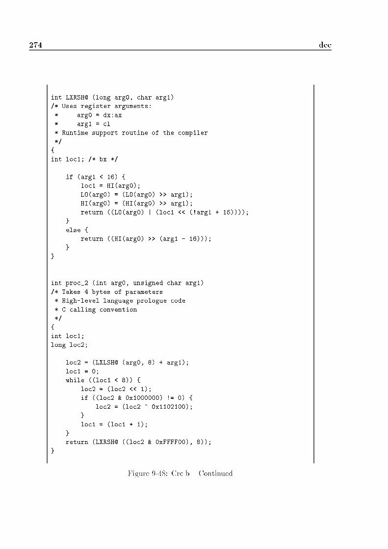
274 dccint LXRSH@ (long arg0, char arg1)/* Uses register arguments:* arg0 = dx:ax.* arg1 = cl.* Runtime support routine of the compiler.*/{int loc1; /* bx */if (arg1 < 16) {loc1 = HI(arg0);LO(arg0) = (LO(arg0) >> arg1);HI(arg0) = (HI(arg0) >> arg1);return ((LO(arg0) | (loc1 << (!arg1 + 16))));}else {return ((HI(arg0) >> (arg1 - 16)));}}int proc_2 (int arg0, unsigned char arg1)/* Takes 4 bytes of parameters.* High-level language prologue code.* C calling convention.*/{int loc1;long loc2;loc2 = (LXLSH@ (arg0, 8) + arg1);loc1 = 0;while ((loc1 < 8)) {loc2 = (loc2 << 1);if ((loc2 & 0x1000000) != 0) {loc2 = (loc2 ^ 0x1102100);}loc1 = (loc1 + 1);}return (LXRSH@ ((loc2 & 0xFFFF00), 8));} Figure 9-48: Crc.b { Continued

9.7 Results 275int proc_3 (int arg0)/* Takes 2 bytes of parameters.* High-level language prologue code.* C calling convention.*/{ return (proc_2 (proc_2 (arg0, 0), 0));}void main ()/* Takes no parameters.* High-level language prologue code.*/{int loc1;int loc2;int loc3;int loc4;loc1 = 65;loc2 = proc_1 ();loc2 = proc_2 (loc2, loc1);loc2 = proc_3 (loc2);loc3 = ((loc2 & 0xFF00) >> 8);loc4 = (loc2 & 255);printf ("%04x\n", loc2);loc2 = proc_1 ();loc2 = proc_2 (loc2, loc1);loc2 = proc_2 (loc2, loc3);loc2 = proc_2 (loc2, loc4);printf ("%04x\n", loc2);} Figure 9-48: Crc.b { Continued

276 dcc/** crc_clear:* This function clears the CRC to zero. It should be called prior to* the start of the processing of a block for both received messages,* and messages to be transmitted.** Calling sequence:** short crc;* crc = crc_clear();*/short crc_clear(){ return(0);}/** crc_update:* this function must be called once for each character which is* to be included in the CRC for messages to be transmitted.* This function is called once for each character which is included* in the CRC of a received message, AND once for each of the two CRC* characters at the end of the received message. If the resulting* CRC is zero, then the message has been correctly received.** Calling sequence:** crc = crc_update(crc,next_char);*/short crc_update(crc,crc_char)short crc;char crc_char;{ long x;short i;/* "x" will contain the character to be processed in bits 0-7 and the CRC *//* in bits 8-23. Bit 24 will be used to test for overflow, and then cleared *//* to prevent the sign bit of "x" from being set to 1. Bits 25-31 are not *//* used. ("x" is treated as though it is a 32 bit register). */x = ((long)crc << 8) + crc_char; /* Get the CRC and the character *//* Repeat the following loop 8 times (for the 8 bits of the character). */for(i = 0;i < 8;i++){ Figure 9-49: Crc.c

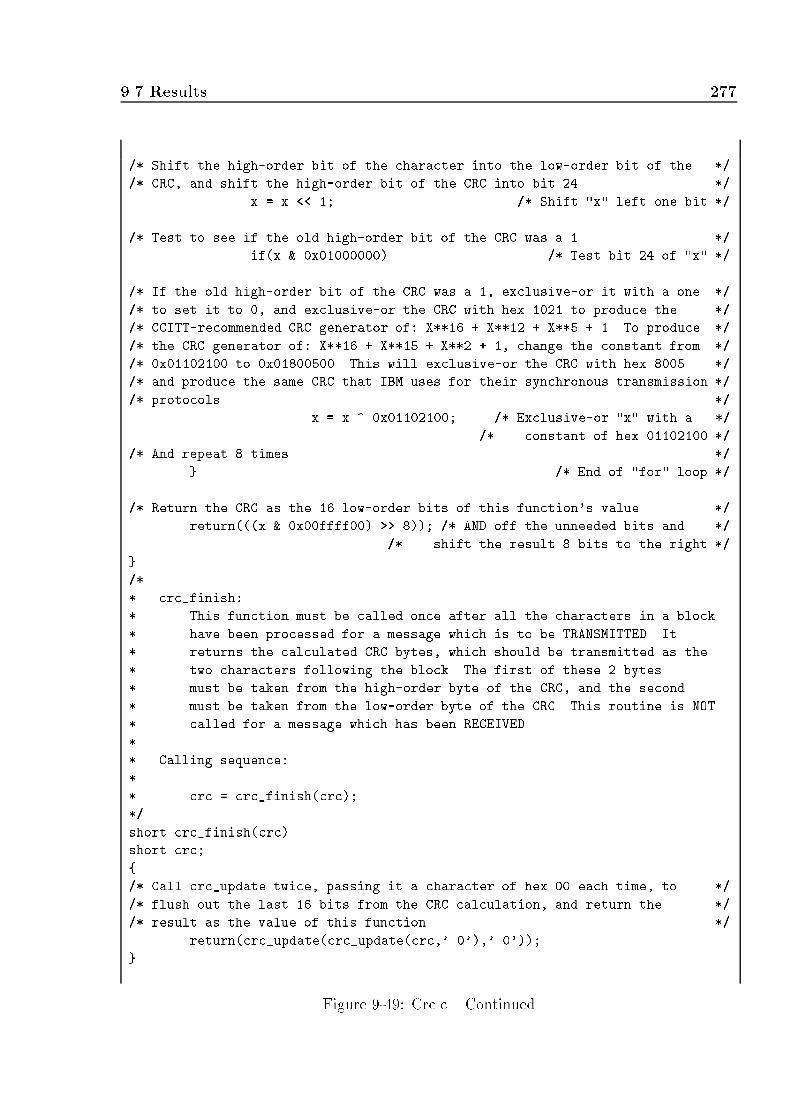
9.7 Results 277/* Shift the high-order bit of the character into the low-order bit of the *//* CRC, and shift the high-order bit of the CRC into bit 24. */x = x << 1; /* Shift "x" left one bit *//* Test to see if the old high-order bit of the CRC was a 1. */if(x & 0x01000000) /* Test bit 24 of "x" *//* If the old high-order bit of the CRC was a 1, exclusive-or it with a one *//* to set it to 0, and exclusive-or the CRC with hex 1021 to produce the *//* CCITT-recommended CRC generator of: X**16 + X**12 + X**5 + 1. To produce *//* the CRC generator of: X**16 + X**15 + X**2 + 1, change the constant from *//* 0x01102100 to 0x01800500. This will exclusive-or the CRC with hex 8005 *//* and produce the same CRC that IBM uses for their synchronous transmission *//* protocols. */x = x ^ 0x01102100; /* Exclusive-or "x" with a...*//* ...constant of hex 01102100 *//* And repeat 8 times. */} /* End of "for" loop *//* Return the CRC as the 16 low-order bits of this function's value. */return(((x & 0x00ffff00) >> 8)); /* AND off the unneeded bits and... *//* ...shift the result 8 bits to the right */}/** crc_finish:* This function must be called once after all the characters in a block* have been processed for a message which is to be TRANSMITTED. It* returns the calculated CRC bytes, which should be transmitted as the* two characters following the block. The first of these 2 bytes* must be taken from the high-order byte of the CRC, and the second* must be taken from the low-order byte of the CRC. This routine is NOT* called for a message which has been RECEIVED.** Calling sequence:** crc = crc_finish(crc);*/short crc_finish(crc)short crc;{/* Call crc_update twice, passing it a character of hex 00 each time, to *//* flush out the last 16 bits from the CRC calculation, and return the *//* result as the value of this function. */return(crc_update(crc_update(crc,'\0'),'\0'));} Figure 9-49: Crc.c { Continued

278 dcc/** This is a sample of the use of the CRC functions, which calculates the* CRC for a 1-character message block, and then passes the resulting CRC back* into the CRC functions to see if the "received" 1-character message and CRC* are correct.*/main(){ short crc; /* The calculated CRC */char crc_char; /* The 1-character message */char x, y; /* 2 places to hold the 2 "received" CRC bytes */crc_char = 'A'; /* Define the 1-character message */crc = crc_clear(); /* Reset the CRC to "transmit" a new message */crc = crc_update(crc,crc_char); /* Update the CRC for the first... *//* ...(and only) character of the message */crc = crc_finish(crc); /* Finish the transmission calculation */x = (char)((crc & 0xff00) >> 8); /* Extract the high-order CRC byte */y = (char)(crc & 0x00ff); /* And extract the low-order byte */printf("%04x\n",crc); /* Print the results */crc = crc_clear(); /* Prepare to "receive" a message */crc = crc_update(crc,crc_char); /* Update the CRC for the first... *//* ...(and only) character of the message */crc = crc_update(crc,x); /* Pass both bytes of the "received"... */crc = crc_update(crc,y); /* ...CRC through crc_update, too */printf("%04x\n",crc); /* If the result was 0, then the message... *//* ...was received without error */} Figure 9-49: Crc.c { ContinuedSubroutine Low-level High-level % Reductionproc 1 6 1 83.33LXLSH@ 15 10 33.33LXRSH@ 15 6 60.00proc 2 52 8 84.62proc 3 16 1 93.75main 67 12 82.09total 171 38 77.78Figure 9-50: Crc Statistics

9.7 Results 2799.7.10 MatrixmuMatrixmu is a program that multiplies two matrixes. This program is incomplete in thesense that it does not initialize the matrixes, but was decompiled to show that the forwardsubstitution method of Chapter 5, Section 5.4.10 is able to �nd array expressions. Theconversion of this expression into an array was not done in dcc, but was explained inChapter 5, Section 5.5. The disassembly program is shown in Figure 9-51, the decompiledC program in Figure 9-52, and the initial C program in Figure 9-53. The call graph for thisprogram is as follows:mainproc_1Both user procedures are decompiled with the same number of high-level instructions; 10for the matrix multiplication procedure, and 1 for the main program. The reduction on thenumber of instructions is over 85% due to the large number of low-level instructions involvedon the computation of an array o�set. In the disassembled version of the program, the basicblock at lines 026 to 069 of procedure proc_1 has 44 instructions which are converted intotwo high-level instructions; a reduction of 95.45% intermediate instructions. Overall, thisprogram has a 86.90% reduction of intermediate instructions, as shown in Figure 9-54.

280 dccproc_1 PROC NEAR000 0002FA 55 PUSH bp001 0002FB 8BEC MOV bp, sp002 0002FD 83EC02 SUB sp, 2003 000300 56 PUSH si004 000301 57 PUSH di005 000302 33F6 XOR si, si007 000378 83FE05 L1: CMP si, 5008 00037B 7C89 JL L2009 00037D 5F POP di010 00037E 5E POP si011 00037F 8BE5 MOV sp, bp012 000381 5D POP bp013 000382 C3 RET014 000306 33FF L2: XOR di, di016 000372 83FF04 L3: CMP di, 4017 000375 7C93 JL L4018 000377 46 INC si019 JMP L1 ;Synthetic inst020 00030A C746FE0000 L4: MOV word ptr [bp-2], 0022 00036B 837EFE04 L5: CMP word ptr [bp-2], 4023 00036F 7CA0 JL L6024 000371 47 INC di025 JMP L3 ;Synthetic inst026 000311 8BDE L6: MOV bx, si027 000313 D1E3 SHL bx, 1028 000315 D1E3 SHL bx, 1029 000317 D1E3 SHL bx, 1030 000319 035E04 ADD bx, [bp+4]031 00031C 8B46FE MOV ax, [bp-2]032 00031F D1E0 SHL ax, 1033 000321 03D8 ADD bx, ax034 000323 8B07 MOV ax, [bx]035 000325 50 PUSH ax036 000326 8B46FE MOV ax, [bp-2]037 000329 BA0A00 MOV dx, 0Ah038 00032C F7E2 MUL dx039 00032E 8BD8 MOV bx, ax040 000330 035E06 ADD bx, [bp+6]041 000333 8BC7 MOV ax, di042 000335 D1E0 SHL ax, 1043 000337 03D8 ADD bx, ax044 000339 58 POP axFigure 9-51: Matrixmu.a2

9.7 Results 281045 00033A F727 MUL word ptr [bx]046 00033C 50 PUSH ax047 00033D 8BC6 MOV ax, si048 00033F BA0A00 MOV dx, 0Ah049 000342 F7E2 MUL dx050 000344 8BD8 MOV bx, ax051 000346 035E08 ADD bx, [bp+8]052 000349 8BC7 MOV ax, di053 00034B D1E0 SHL ax, 1054 00034D 03D8 ADD bx, ax055 00034F 58 POP ax056 000350 0307 ADD ax, [bx]057 000352 50 PUSH ax058 000353 8BC6 MOV ax, si059 000355 BA0A00 MOV dx, 0Ah060 000358 F7E2 MUL dx061 00035A 8BD8 MOV bx, ax062 00035C 035E08 ADD bx, [bp+8]063 00035F 8BC7 MOV ax, di064 000361 D1E0 SHL ax, 1065 000363 03D8 ADD bx, ax066 000365 58 POP ax067 000366 8907 MOV [bx], ax068 000368 FF46FE INC word ptr [bp-2]069 JMP L5 ;Synthetic instproc_1 ENDPmain PROC NEAR000 000383 55 PUSH bp001 000384 8BEC MOV bp, sp002 000386 83EC78 SUB sp, 78h003 000389 8D46D8 LEA ax, [bp-28h]004 00038C 50 PUSH ax005 00038D 8D46B0 LEA ax, [bp-50h]006 000390 50 PUSH ax007 000391 8D4688 LEA ax, [bp-78h]008 000394 50 PUSH ax009 000395 E862FF CALL near ptr proc_1010 000398 83C406 ADD sp, 6011 00039B 8BE5 MOV sp, bp012 00039D 5D POP bp013 00039E C3 RETmain ENDP Figure 9-51: Matrixmu.a2 { Continued

282 dcc/** Input file : matrixmu.exe* File type : EXE*/#include "dcc.h"void proc_1 (int arg0, int arg1, int arg2)/* Takes 6 bytes of parameters.* High-level language prologue code.* C calling convention.*/{int loc1;int loc2;int loc3;loc2 = 0;while ((loc2 < 5)) {loc3 = 0;while ((loc3 < 4)) {loc1 = 0;while ((loc1 < 4)) {*((((loc2 * 10) + arg2) + (loc3 << 1))) =((*((((loc2 << 3) + arg0) + (loc1 << 1))) **((((loc1 * 10) + arg1) + (loc3 << 1)))) +*((((loc2 * 10) + arg2) + (loc3 << 1))));loc1 = (loc1 + 1);}loc3 = (loc3 + 1);}loc2 = (loc2 + 1);}}void main ()/* Takes no parameters.* High-level language prologue code.*/{int loc1;int loc2;int loc3;proc_1 (&loc3, &loc2, &loc1);} Figure 9-52: Matrixmu.b

9.7 Results 283#define n 5#define m 4static void multMatrix (int a[n][m], int b[m][n], int c[n][n]){ int i,j,k;for (i=0; i<n; i++)for (j=0; j<m; j++)for (k=0; k<m; k++)c[i][j] = a[i][k] * b[k][j] + c[i][j];}main(){ int a[n][m], b[n][m], c[n][m];multMatrix (a, b, c);} Figure 9-53: Matrixmu.cSubroutine Low-level High-level % Reductionproc 1 70 10 85.71main 14 1 92.86total 84 11 86.90Figure 9-54: Matrixmu Statistics

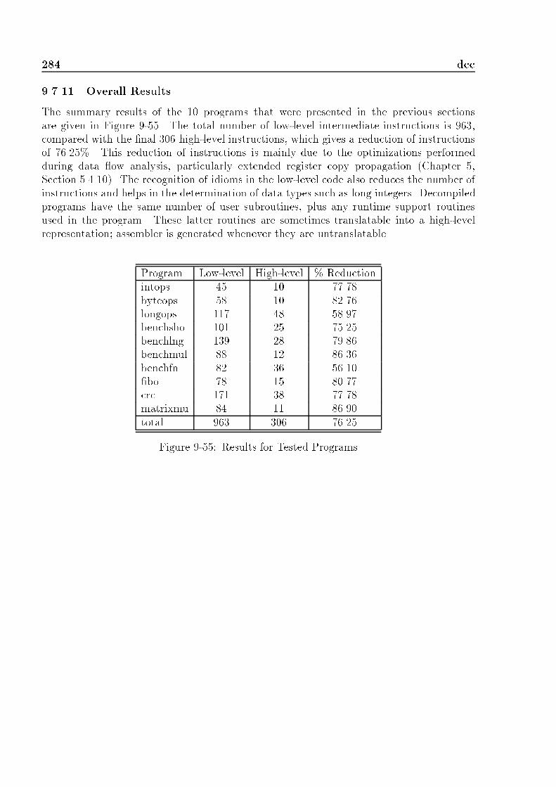
284 dcc9.7.11 Overall ResultsThe summary results of the 10 programs that were presented in the previous sectionsare given in Figure 9-55. The total number of low-level intermediate instructions is 963,compared with the �nal 306 high-level instructions, which gives a reduction of instructionsof 76.25%. This reduction of instructions is mainly due to the optimizations performedduring data ow analysis, particularly extended register copy propagation (Chapter 5,Section 5.4.10). The recognition of idioms in the low-level code also reduces the number ofinstructions and helps in the determination of data types such as long integers. Decompiledprograms have the same number of user subroutines, plus any runtime support routinesused in the program. These latter routines are sometimes translatable into a high-levelrepresentation; assembler is generated whenever they are untranslatable.Program Low-level High-level % Reductionintops 45 10 77.78byteops 58 10 82.76longops 117 48 58.97benchsho 101 25 75.25benchlng 139 28 79.86benchmul 88 12 86.36benchfn 82 36 56.10�bo 78 15 80.77crc 171 38 77.78matrixmu 84 11 86.90total 963 306 76.25Figure 9-55: Results for Tested Programs

Chapter 10ConclusionsT his thesis has presented techniques for the reverse compilation or decompilation of bi-nary programs, and provided algorithms for the implementation of the di�erent phasesof the decompiler. The methodology was implemented and tested in a prototype decom-piler, dcc, which runs under DOS and Unix.Decompilers use similar principles and techniques used in compilers. A decompiler hasseven di�erent phases, which incorporate compiler and optimization phases. There is nolexical analysis phase due to the simplicity of the source machine language. The syntaxanalysis phase parses the source binary program separating code from data, and placingdata references in the symbol table. The main di�culty with the separation of code fromdata is that they are represented in the same way in von Neumann machines. The in-termediate code generation phase generates a low-level intermediate representation of theprogram. The semantic analysis phase checks the semantic meaning of groups of low-levelinstructions (idioms), gathers type information, and propagates it across the intermediaterepresentation. The control ow graph generation phase generates a control ow graph ofeach subroutine of the program, and attaches the intermediate representation informationto the nodes of the graph. The data ow analysis phase analyzes the low-level intermediatecode and converts it into a high-level intermediate representation available in any high-levellanguage. The transformation of instructions eliminates all low-level references to conditioncodes and registers, and introduces the high-level concept of expression. Subroutines thatare not representable in a high-level language are agged. The structure of the programis analyzed in the control ow analysis phase, which structures the control ow graphs ofeach subroutine in the program. Finally, the code generation phase generates high-levelcode based on the high-level intermediate representation and the structured graph of eachsubroutine.A complete decompilation of a program makes use of not only the decompiler but otherrelated tools: the loader, the signature generator, the prototype generator, the disassembler,and the postprocessor. The loader loads the source binary program into memory, the signa-ture generator generates signatures for known compilers and their libraries (if required), theprototype generator determines the formal argument types for library subroutines, the dis-assembler parses the program and produces an assembler output �le, the decompiler makesuse of the signature information to reduce the number of subroutines to decompile (i.e. itdoes not attempt to decompile library routines if they are recognized by a signature or theloader), and the postprocessor transforms the output decompiled high-level program intoa semantically equivalent program that makes use of speci�c control structures available

286 Conclusionsin the target language. In practice, a decompiler can take as input a binary program oran assembler program, and produce a high-level language output program. Most literatureavailable on decompilers make use of the latter approach; an assembler source program.This thesis concentrates on source binary programs, which have far less information thanassembler programs.The techniques described in this thesis are general enough to construct decompilers for dif-ferent machine architectures. The phases are grouped into 3 di�erent modules that separatemachine and language dependent features: the front-end is a machine dependent modulethat parses the source binary program and produces a low-level intermediate representationof the program and a control ow graph of each subroutine; the universal decompiling ma-chine is a machine and language independent module that analyzes the intermediate codeand the structure of the graph(s) and generates a high-level intermediate representation ofthe program and a structured graph(s); and the back-end is a target language dependentmodule that generates high-level target code from the intermediate representation and thestructure of the graph. In this way, a decompiler for a di�erent machine can be built bywriting a new front-end for that machine, and a decompiler for a di�erent target high-levellanguage can be built by writing a new back-end for the target language. This approach islimited in practice by the choice of low-level intermediate language representation.The signi�cant contributions of this thesis are the types of analyses done in the universaldecompiling machine: data ow analysis and control ow analysis, which transform thelow-level (machine-like) intermediate code into a high-level (HLL-like) intermediate rep-resentation. The data ow analyzer describes optimization techniques based on compileroptimization principles, which eliminate the low-level concepts of condition codes and regis-ters, and introduces the high-level concept of expression. These techniques take into accountinterprocedural analysis, register spilling, and type propagation. The control ow analyzerdescribes structuring algorithms to determine the underlying high-level control structuresof the program. These algorithms structure the graph according to a prede�ned, genericset of control structures available in most commonly used languages.The implementation of these techniques in the prototype decompiler dcc demonstrates thefeasibility of the presented techniques. dcc is a decompiler for the DOS operating systemand the Intel i80286 machine architecture which generates target C programs. This decom-piler runs on a DecStation 3100 under Unix, and on Intel machines under DOS. dcc makesuse of compiler and library signature recognition to decompile user routines only (wheneverpossible), rather than decompiling compiler start-up and library routines as well. When-ever a compiler signature is not determined, all subroutines available in the source binaryprogram are decompiled; several of the library and compiler start-up routines are untrans-latable into a high-level language representation and hence are disassembled only. dccprovides comments for each subroutine, and has command switches to generate the bitmapof the program, the call graph, an output assembler �le, statistics on the number of low-leveland high-level instructions in each subroutine, and information on the control ow graphof each subroutine.Decompilation is used in two main areas of computer science: software maintenance andsecurity. A decompiler is used in software maintenance to recover lost or inaccessible source

Conclusions 287code, translate code written in an obsolete language into a newer language, structure oldcode written in an unstructured way (i.e. spaghetti code), migrate applications to a newhardware platform, and debug binary programs that are known to have a bug. In security,a decompiler is used to verify binary programs and the correctness of the code produced bya compiler for safety-critical systems; where the compiler is not trusted to generate correctcode; and to check for the existence of malicious code such as viruses.Further work on decompilation can be done in two areas: the separation of code and data,and the determination of data types such as arrays, records, and pointers. The formerarea needs a robust method of determining n-way branch statements (i.e. indexed jumps)and indirect subroutine calls. The latter area needs heuristic methods to identify di�erenttypes of compound data types and propagate their values. E�cient implementation of thealgorithms would provide a faster decompiler, although the speed of decompilation is not aconcern given that a program is normally decompiled once only.

Appendix Ai8086 { i80286 ArchitectureT he Intel iAPX 8086, 8088, 80186 and 80286 machine architectures consist of the sametype of registers, memory structure and input/output port organization[Int86, Int87].These architectures are downwards compatible, hence the 80286 supports all machine in-structions supported by the 8086 architecture. The registers of these 16-bit word machinesare classi�ed into �ve di�erent sets according to their usage: data, pointer, index, control,and segment registers; this classi�cation is shown in Figure A-1.Type Register FunctionData ax accumulatorbx base register in some addressing modescx counterdx general purposePointer sp stack pointerbp base pointerIndex si sourcedi destinationControl ip instruction pointer ags ags or status wordSegment cs code segmentds data segmentss stack segmentes extra segmentFigure A-1: Register Classi�cationData or general purpose registers can be accessed as word or byte registers. Each registerhas a high and low byte with the following naming convention: register names that replacethe x by a h access the high byte of that register; and register names that replace the xby an l access the low byte of that register. The ags register is a special purpose registerthat keeps track of the condition codes set up by di�erent instructions. The structure ofthis register is shown in Figure A-2. As can be seen, not all bits are used; unused bits arereserved by Intel.Memory is structured as an array of 8-bit bytes stored in little-endian convention (i.e. mostsigni�cant byte of a word is stored at the highest memory address). Memory is divided

290 i8086 { i80286 Architecturecpo: over ow azstido 015 c: carryp: paritya: auxiliary carryz: zeros: signt: trapi: interruptd: directionFigure A-2: Structure of the Flags Registerinto banks of segments, each segment is a linear sequence of 64K bytes; therefore memoryis addressed via a segment and o�set pair.Input/output port organization consists of up to 64Kb of 8-bit ports or 32Kb of 16-bitports, located in a separate addressing space from the memory space.A.1 Instruction FormatThe length of an 80286 instruction varies from 1 up to 6 bytes. There are two types ofopcodes: 1-byte opcodes and compound opcodes. 1-byte opcodes use the �rst byte of aninstruction as the opcode, followed by the �elds byte, at most 2 bytes of displacement, andat most 2 bytes of data. The �elds byte contains information about registers, immediateoperands, and/or displacement data. Compound opcodes store part of the opcode in the�rst byte of the instruction, and part in three bits of the second byte of the instruction (seeFigure A-3). The �rst byte determines the group table to which the instruction belongs,and the 3-bit opcode of the second byte determines the index into the table (i.e. there are8 entries into the table). The remaining bits of the second byte are used as the �elds byte.The rest of the instruction is structured in the same way as for 1-byte opcodes[LG86].opcodeFigure A-3: Compound Opcodes' Second ByteIn the 80286, almost all byte combinations are valid opcodes. There are 229 1-byte opcodes,29 compound-opcodes and 6 pre�x instructions. A complete list of the machine languageinstructions, mnemonics and operands is found in Section A.2.The �elds byte is used to calculate the e�ective address (EA) of the operand. This byte ismade up of 3 �elds: the reg 3-bit �eld which takes the value of a register, the r/m 3-bit�eld which is used as a second register or a memory operand, and the mod 2-bit �eld which

A.1 Instruction Format 291r/mregmodFigure A-4: The Fields Bytedetermines the number of displacement bytes (DISP), whether r/m is used as a register ora memory operand, or the e�ective address of instructions that are not indexed nor based-indexed. The structure of this byte is shown in Figure A-4. An algorithm to interpret the�elds byte is shown in Figure A-5.case (mod) of {0: if (r/m == 6) /* get 2 bytes displacement */EA = dispHi:dispLo;else /* no extra bytes */DISP = 0;1: /* get 1 byte displacement */DISP = dispLo sign-extended to 16 bits;2: /* get 2 bytes displacement */DISP = dispHi:dispLo;3: /* Indexed */r/m is treated as a register field;} Figure A-5: Algorithm to Interpret the Fields ByteThe EA for indexed and based-indexed operands is calculated according to the r/m �eld;each value is mapped to an indexed register or a combination of indexed and based registers,as shown in Figure A-6. Value of r/m Indexed register(s)0 bx + si1 bx + di2 bp + si3 bp + di4 si5 di6 bp7 bxFigure A-6: Mapping of r/m �eld

292 i8086 { i80286 ArchitectureThe �nal e�ective address is calculated as the addition of the displacement (DISP) and theregister(s) given by the r/m bits.Each combination of mod, r/m values uses a default segment register for its addressing,these default segments are shown in Figure A-7. Although the e�ective address of anoperand is determined by the combination of the mod, r/m �elds, the �nal physical addressis calculated by adding the EA to the contents of the default segment register multipliedby 16. As a general rule, when the bp register is used, the default segment is ss, otherwisethe default segment is ds. r/m / mod 0 1 20 DS DS DS1 DS DS DS2 SS SS SS3 SS SS SS4 DS DS DS5 DS DS DS6 DS SS SS7 DS DS DSFigure A-7: Default SegmentsThe segment override pre�x is a 1 byte opcode that permits exceptions to the default seg-ment register to be used by the next instruction (i.e. it is only valid for 1 instruction; theone that follows it). The segment is determined by a 2-bit �eld (bits 3 and 4) of the pre�xbyte. All other �elds take constant values, as illustrated in Figure A-8.0 1 seg 1 1 00Figure A-8: Segment Override Pre�xThere are two repeat pre�x opcodes, repne and repe. These opcodes repeat the executionof the next instruction while register cx is not equal or equal to zero. They are normallyused with string instructions such as movs and ins to repeat a condition while it is not endof string.A.2 Instruction SetThe instruction set of the i80286 is described in terms of the machine opcode, the assemblermnemonic, and the assembler operands to the instruction. The following conventions areused to describe such an instruction set:

A.2 Instruction Set 293� reg8: 8-bit register.� reg16: 16-bit register.� mem8: 8-bit memory value.� mem16: 16-bit memory value.� immed8: 8-bit immediate value.� immed16: 16-bit immediate value.� immed32: 32-bit immediate value.� segReg: 16-bit segment register.Figure A-9 show all 1-byte opcodes. Compound opcodes are referenced as indexes into atable, each table has 8 posible values. The tables are shown in Figures A-10, A-11, A-12,and A-13. These �gures are summaries of �gures described in [Int86, Int87].

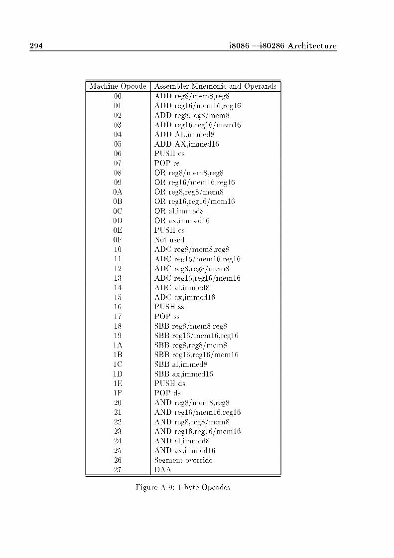
294 i8086 { i80286 ArchitectureMachine Opcode Assembler Mnemonic and Operands00 ADD reg8/mem8,reg801 ADD reg16/mem16,reg1602 ADD reg8,reg8/mem803 ADD reg16,reg16/mem1604 ADD AL,immed805 ADD AX,immed1606 PUSH es07 POP es08 OR reg8/mem8,reg809 OR reg16/mem16,reg160A OR reg8,reg8/mem80B OR reg16,reg16/mem160C OR al,immed80D OR ax,immed160E PUSH cs0F Not used10 ADC reg8/mem8,reg811 ADC reg16/mem16,reg1612 ADC reg8,reg8/mem813 ADC reg16,reg16/mem1614 ADC al,immed815 ADC ax,immed1616 PUSH ss17 POP ss18 SBB reg8/mem8,reg819 SBB reg16/mem16,reg161A SBB reg8,reg8/mem81B SBB reg16,reg16/mem161C SBB al,immed81D SBB ax,immed161E PUSH ds1F POP ds20 AND reg8/mem8,reg821 AND reg16/mem16,reg1622 AND reg8,reg8/mem823 AND reg16,reg16/mem1624 AND al,immed825 AND ax,immed1626 Segment override27 DAAFigure A-9: 1-byte Opcodes

A.2 Instruction Set 295Machine Opcode Assembler Mnemonic and Operands28 SUB reg8/mem8,reg829 SUB reg16/mem16,reg162A SUB reg8,reg8/mem82B SUB reg16,reg16/mem162C SUB al,immed82D SUB ax,immed162E Segment override2F DAS30 XOR reg8/mem8,reg831 XOR reg16/mem16,reg1632 XOR reg8,reg8/mem833 XOR reg16,reg16/mem1634 XOR al,immed835 XOR ax,immed1636 Segment override37 AAA38 CMP reg8/mem8,reg839 CMP reg16/mem16,reg163A CMP reg8,reg8/mem83B CMP reg16,reg16/mem163C CMP al,immed83D CMP ax,immed163E Segment override3F AAS40 INC ax41 INC cx42 INC dx43 INC bx44 INC sp45 INC bp46 INC si47 INC di48 DEC ax49 DEC cx4A DEC dx4B DEC bx4C DEC sp4D DEC bp4E DEC si4F DEC diFigure A-9: 1-byte opcodes { Continued

296 i8086 { i80286 ArchitectureMachine Opcode Assembler Mnemonic and Operands50 PUSH ax51 PUSH cx52 PUSH dx53 PUSH bx54 PUSH sp55 PUSH bp56 PUSH si57 PUSH di58 POP ax59 POP cx5A POP dx5B POP bx5C POP sp5D POP bp5E POP si5F POP di60 PUSHA61 POPA62 BOUND reg16/mem16,reg1663 Not used64 Not used65 Not used66 Not used67 Not used68 PUSH immed1669 IMUL reg16/mem16,immed166A PUSH immed86B IMUL reg8/mem8,immed86C INSB6D INSW6E OUTSB6F OUTSW70 JO immed871 JNO immed872 JB immed873 JNB immed874 JZ immed875 JNZ immed876 JBE immed877 JA immed8Figure A-9: 1-byte Opcodes { Continued

A.2 Instruction Set 297Machine Opcode Assembler Mnemonic and Operands78 JS immed879 JNS immed87A JP immed87B JNP immed87C JL immed87D JNL immed87E JLE immed87F JG immed880 Table2 reg881 Table2 reg1682 Table2 reg883 Table2 reg8, reg1684 TEST reg8/mem8,reg885 TEST reg16/mem16,reg1686 XCHG reg8,reg887 XCHG reg16,reg1688 MOV reg8/mem8,reg889 MOV reg16/mem16,reg168A MOV reg8,reg8/mem88B MOV reg16,reg16/mem168C MOV reg16/mem16,segReg8D LEA reg16,reg16/mem168E MOV segReg,reg16/mem168F POP reg16/mem1690 NOP91 XCHG ax,cx92 XCHG ax,dx93 XCHG ax,bx94 XCHG ax,sp95 XCHG ax,bp96 XCHG ax,si97 XCHG ax,di98 CBW99 CWD9A CALL immed329B WAIT9C PUSHF9D POPF9E SAHF9F LAHFFigure A-9: 1-byte Opcodes { Continued

298 i8086 { i80286 ArchitectureMachine Opcode Assembler Mnemonic and OperandsA0 MOV al,[mem8]A1 MOV ax,[mem16]A2 MOV [mem8],alA3 MOV [mem16],axA4 MOVSBA5 MOVSWA6 CMPSBA7 CMPSWA8 TEST al,[mem8]A9 TEST ax,[mem16]AA STOSBAB STOSWAC LODSBAD LODSWAE SCASBAF SCASWB0 MOV al,immed8B1 MOV cl,immed8B2 MOV dl,immed8B3 MOV bl,immed8B4 MOV ah,immed8B5 MOV ch,immed8B6 MOV dh,immed8B7 MOV bh,immed8B8 MOV ax,immed16B9 MOV cx,immed16BA MOV dx,immed16BB MOV bx,immed16BC MOV sp,immed16BD MOV bp,immed16BE MOV si,immed16BF MOV di,immed16C0 Table1 reg8C1 Table1 reg8, reg16C2 RET immed16C3 RETC4 LES reg16/mem16,mem16C5 LDS reg16/mem16,mem16C6 MOV reg8/mem8,immed8C7 MOV reg16/mem16,immed16Figure A-9: 1-byte Opcodes { Continued

A.2 Instruction Set 299Machine Opcode Assembler Mnemonic and OperandsC8 ENTER immed16, immed8C9 LEAVECA RET immed16CB RETCC INT 3CD INT immed8CE INTOCF IRETD0 Table1 reg8D1 Table1 reg16D2 Table1 reg8D3 Table1 reg16D4 AAMD5 AADD6 Not usedD7 XLAT [bx]D8 ESC immed8D9 ESC immed8DA ESC immed8DB ESC immed8DC ESC immed8DD ESC immed8DE ESC immed8DF ESC immed8E0 LOOPNE immed8E1 LOOPE immed8E2 LOOP immed8E3 JCXZ immed8E4 IN al,immed8E5 IN ax,immed16E6 OUT al,immed8E7 OUT ax,immed16E8 CALL immed16E9 JMP immed16EA JMP immed32EB JMP immed8EC IN al,dxED IN ax,dxEE OUT al,dxEF OUT ax,dxFigure A-9: 1-byte Opcodes { Continued

300 i8086 { i80286 ArchitectureMachine Opcode Assembler Mnemonic and OperandsF0 LOCKF1 Not usedF2 REPNEF3 REPF4 HLTF5 CMCF6 Table3 reg8F7 Table3 reg16F8 CLCF9 STCFA CLIFB STIFC CLDFD STDFE Table4 reg8FF Table4 reg16Figure A-9: 1-byte Opcodes { ContinuedIndex Assembler Mnemonic0 ROL1 ROR2 RCL3 RCR4 SHL5 SHR6 Not used7 SARFigure A-10: Table1 Opcodes

A.2 Instruction Set 301Index Assembler Mnemonic0 ADD1 OR2 ADC3 SBB4 AND5 SUB6 XOR7 CMPFigure A-11: Table2 OpcodesIndex Assembler Mnemonic0 TEST1 Not used2 NOT3 NEG4 MUL5 IMUL6 DIV7 IDIVFigure A-12: Table3 OpcodesIndex Assembler Mnemonic0 INC1 DEC2 CALL3 CALL4 JMP5 JMP6 PUSH7 Not usedFigure A-13: Table4 Opcodes

Appendix BProgram Segment Pre�xT he program segment pre�x or PSP is a 256-byte block of information, apparently aremnant of the CP/M operating system, that was adopted to assist in porting CP/Mprograms to the DOS environment[Dun88b]. When a program is loaded into memory, aPSP is built on the �rst 256 bytes of the allocated memory block. The �elds of the PSPare shown in Figure B-1.Segment o�set Description00h terminate vector: interrupt 20h (transfer to DOS)02h last segment allocated04h reserved05h call vector function: far call to DOS's function request handler0Ah copy of the parent's program termination handler vector0Eh copy of the parent's control-c/control-break handler vector12h copy of the parent's critical error handler vector16H reserved2Ch address of the �rst paragraph of the DOS environment2Eh reserved50h interrupt 21h, return far (retf) instruction53h reserved5Ch �rst parameter from the command line6Ch second parameter from the command line80h command tail; used as a bu�erFigure B-1: PSP FieldsThe terminate vector (o�set 00h of the PSP) used to be the warm boot/terminate(WBOOT) vector under CP/M. The call vector function (o�set 05h of the PSP) usedto be the basic disk operating system (BDOS) vector under CP/M.

Appendix CExecutable File FormatT he DOS operating system supports two di�erent types of executable �les: .exe and .com�les. The former allows for large programs and multiple segments to be used in memory,the latter for small programs that �t into one segment (i.e. 64Kb maximum) [Dun88b].C.1 .exe FilesThe .exe �le consists of a header and a load module, as shown in Figure C-1. The �leheader consists of 28 bytes of �xed formatted area, and a relocation table which varies insize. The load module is a fully linked image of the program; there is no information onhow to separate segments in the module since DOS ignores how the program is segmented.��Formatted area end of �leRelocation tableLoad module start of �leFigure C-1: Structure of an .exe FileThe structure of the header's formatted area is shown in Figure C-2. The size of a page is512 bytes, and the size of a paragraph is 16 bytes. The program image size is calculatedfrom the value in the formatted area as the di�erence between the �le size and the headersize. The �le size is given by the number of �le pages (rounded up) and the size in bytes ofthe last page.The relocation table is a list of pointers to words within the load module that must beadjusted. These words are adjusted by adding the start segment address where the programis to be loaded. Pointers in this table are stored as 2 words relative to the start of the loadmodule.

306 Executable File FormatBytes Description00-01h .exe signature (4Dh, 5Ah)02-03h number of bytes in the last page04-05h number of pages (rounded up)06-07h number of entries in the relocation table08-09h number of paragraphs in the header0A-0Bh minimum number of paragraphs required for data and stack0C-0Dh maximum number of memory paragraphs0E-0Fh pre-relocated initial ss value10-11h initial sp value (absolute value)12-13h complemented checksum (1's complement)14-15h initial ip value16-17h pre-relocated initial value of cs18-19h relocation table o�set1A-1B overlay number (default: 0000h)Figure C-2: Fixed Formatted AreaC.2 .com FilesA .com �le is an image program without a header (i.e. equivalent to the load module of an.exe �le), hence the program is loaded into memory \as is". As opposed to .exe programs,.com programs can only use one segment (up to 64Kb). These programs were designed totransport programs from CP/M into the DOS environment.

Appendix DLow-level to High-level Icode MappingT he mapping between low-level and high-level Icodes is shown in the following pages (Fig-ure D-1). A dash (-) in the high-level Icode column means that there is no high-levelcounter part to the low-level icode, an asterisk (*) means that the low-level Icode forms partof a high-level instruction only when in an idiom, an f means that an Icode ag is set andthe instruction is not considered any further, a cc means that the low-level instruction setsa condition code, it does not have a high-level counterpart, and is eliminated by conditioncode propagation, and an n means that the low-level Icode instruction was not consideredin the analysis. Instructions marked with an n deal with machine string instructions, andwere not considered in the analysis performed by dcc.The initial mapping of low-level to high-level Icodes is expressed in terms of registers.Further data ow analysis on the Icodes transforms these instructions into expressions thatdo not make use of temporary registers, only variables and register variables (if any).

308 Low-level to High-level Icode MappingLow-level Icode High-level IcodeiAAA -iAAD -iAAM -iAAS -iADC *iADD asgn (+)iAND asgn (&)iBOUND fiCALL calliCALLF calliCLC cciCLD cciCLI -iCMC cciCMP cciCMPS niREPNE CMPS niREPE CMPS niDAA -iDAS -iDEC asgn (- 1)iDIV asgn (/)iENTER fiESC fiHLT -iIDIV asgn (/)iIMUL asgn (*)iIN -iINC asgn (+ 1)iINS -iREP INS -iINT -iINTO -iIRET -iJB jcond (<)iJBE jcond (<=)iJAE jcond (>=)iJA jcond (>)iJE jcond (==)iJNE jcond (<>)Figure D-1: Icode Opcodes

Low-level to High-level Icode Mapping 309Low-level Icode High-level IcodeiJL jcond (<)iJGE jcond (>=)iJLE jcond (<=)iJG jcond (>)iJS jcond (> 0)iJNS jcond (< 0)iJO -iJNO -iJP -iJNP -iJCXZ jcond (cx == 0)iJNCXZ jcond (cx <> 0)iJMP jmpiJMPF jmpiLAHF -iLDS asgn (far pointer)iLEA asgn (near pointer)iLEAVE retiLES asgn (far pointer)iLOCK -iLODS niREP LODS niMOV asgn (=)iMOVS niREP MOVS niMOD asgn (%)iMUL asgn (*)iNEG asgn (-)iNOT !iNOP -iOR asgn (|)iOUT -iOUTS -iREP OUTS -iPOP popiPOPA -iPOPF -iPUSH pushiPUSHA -iPUSHF -Figure D-1: Icode Opcodes { Continued

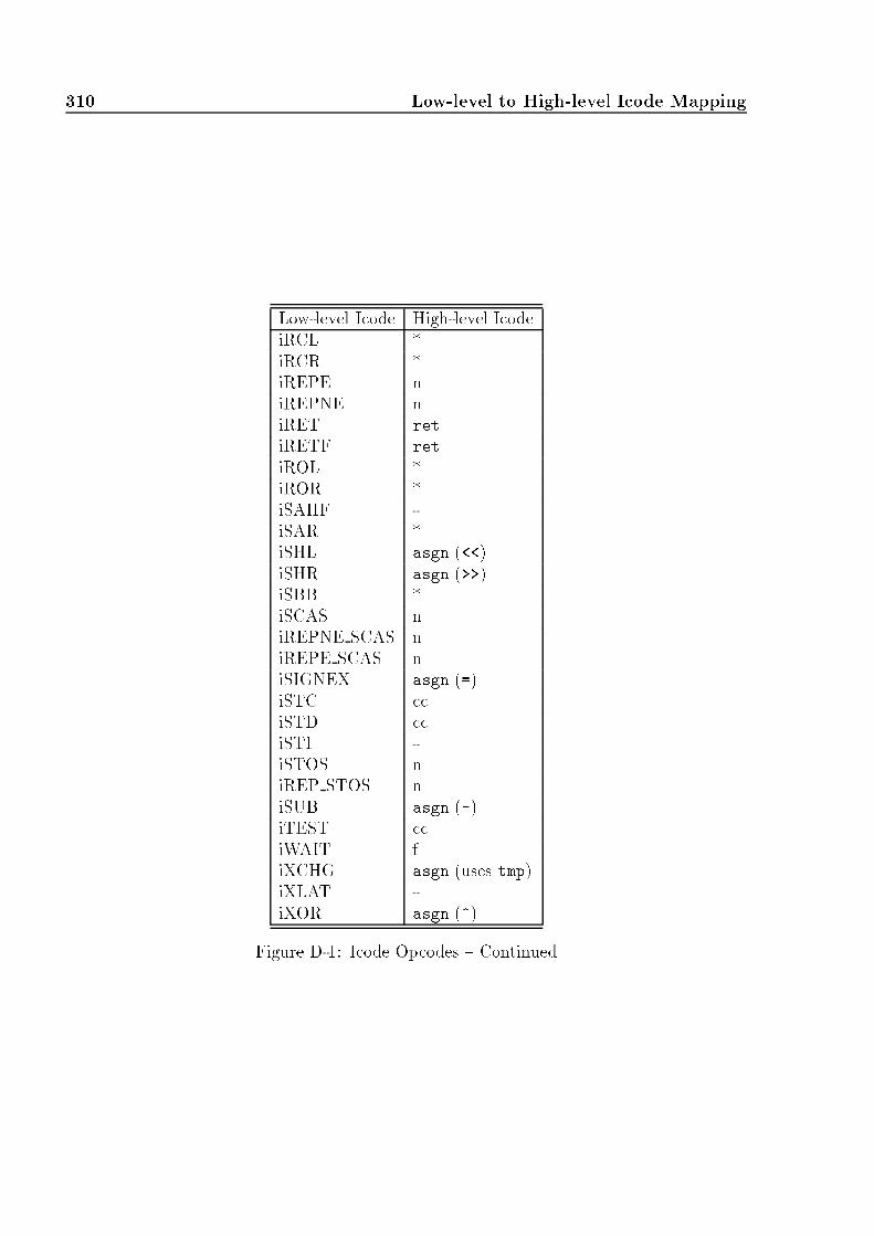
310 Low-level to High-level Icode MappingLow-level Icode High-level IcodeiRCL *iRCR *iREPE niREPNE niRET retiRETF retiROL *iROR *iSAHF -iSAR *iSHL asgn (<<)iSHR asgn (>>)iSBB *iSCAS niREPNE SCAS niREPE SCAS niSIGNEX asgn (=)iSTC cciSTD cciSTI -iSTOS niREP STOS niSUB asgn (-)iTEST cciWAIT fiXCHG asgn (uses tmp)iXLAT -iXOR asgn (^)Figure D-1: Icode Opcodes { Continued

Appendix EComments and Error Messages displayed bydccd cc displays a series of comments in the output C and assembler �les, on informationcollected during the analysis of each subroutine. This information is displayed beforeeach subroutine. The following comments are supported by dcc:� \Takes %d bytes of parameters."� \Uses register arguments:" (and lists the registers and the formal argument name).� \Takes no parameters."� \Runtime support routine of the compiler."� \High-level language prologue code."� \Untranslatable routine. Assembler provided."� \Return value in register %s." (register(s) provided).� \Pascal calling convention."� \C calling convention."� \Unknown calling convention."� \Incomplete due to an unstranslatable opcode"� \Incomplete due to an indirect jump"� \Indirect call procedure."� \Contains self-modifying code."� \Contains coprocessor instructions."� \Irreducible control ow graph."Assembler subroutines are also commented, as well as all DOS kernel services; interrupts20h to 2Fh. Appendix F contains a list of all DOS interrupts supported by dcc.dcc also displays two di�erent types of errors: fatal and non fatal errors. Fatal errors termi-nate the execution of dcc, displaying the error with enough information to determine what

312 Comments and Error Messages displayed by dcchappened. Non fatal errors do not cause dcc to terminate, and are treated as warnings tothe user.The fatal errors supported by dcc are:� \Invalid option -%c."� \Usage: dcc [-a1a2mpsvV][-o asm�le] DOS executable"� \New EXE format not supported."� \Cannot open �le %s."� \Error while reading �le %s."� \Invalid instruction %02X at location %06lX."� \Don't understand 80386 instruction %02X at location %06lX."� \Instruction at location %06lX goes beyond loaded image."� \malloc of %ld bytes failed."� \Failed to �nd a basic block for jump to %ld in subroutine %s."� \Basic Block is a synthetic jump."� \Failed to �nd a basic block for interval."� \De�nition not found for condition code usage at opcode %d."The non fatal errors supported by dcc are:� \Segment override with no memory operand at location %06lX."� \REP pre�x without a string instruction at location %06lX."� \Conditional jump use, de�nition not supported at opcode %d."� \De�nition-use not supported. De�nition opcode = %d, use opcode = %d."� \Failed to construct do..while() condition."� \Failed to construct while() condition."

Appendix FDOS InterruptsT he DOS kernel provides services to application programs via software interrupts20h..2Fh. Interrupt 21h deals with character input/output, �les, records, directoryoperations, disk, processes, memory management, network functions, and miscellaneoussystem functions; the function number is held in register ah. Figure F-1 lists the di�erentinterrupts provided by DOS [Dun88a]. These interrupts are commented by dcc whenproducing the disassembly of a subroutine.

314 DOS InterruptsInterrupt Function Function name20h Terminate process21h 0h Terminate process21h 1h Character input with echo21h 2h Character output21h 3h Auxiliary input21h 4h Auxiliary output21h 5h Printer output21h 6h Direct console input/output21h 7h Un�ltered character input without echo21h 8h Character input without echo21h 9h Display string21h Ah Bu�ered keyboard input21h Bh Check input status21h Ch Flush input bu�er and then input21h Dh Disk reset21h Eh Select disk21h Fh Open �le21h 10h Close �le21h 11h Find �rst �le21h 12h Find next �le21h 13h Delete �le21h 14h Sequential read21h 15h Sequential write21h 16h Create �le21h 17h Rename �le21h 18h Reserved21h 19h Get current disk21h 1Ah Set DTA address21h 1Bh Get default drive data21h 1Ch Get drive data21h 1Dh Reserved21h 1Eh Reserved21h 1Fh Reserved21h 20h Reserved21h 21h Random read21h 22h Random write21h 23h Get �le size21h 24h Set relative record number21h 25h Set interrupt vector21h 26h Create new PSP21h 27h Random block read21h 28h Random block writeFigure F-1: DOS Interrupts

DOS Interrupts 315Interrupt Function Function name21h 29h Parse �lename21h 2Ah Get date21h 2Bh Set date21h 2Ch Get time21h 2Dh Set time21h 2Eh Set verify ag21h 2Fh Get DTA address21h 30h Get DOS version number21h 31h Terminate and stay resident21h 32h Reserved21h 33h Get or set break ag21h 34h Reserved21h 35h Get interrupt vector21h 36h Get drive allocation info21h 37h Reserved21h 38h Get or set country info21h 39h Create directory21h 3Ah Delete directory21h 3Bh Set current directory21h 3Ch Create �le21h 3Dh Open �le21h 3Eh Close �le21h 3Fh Read �le or device21h 40h Write �le or device21h 41h Delete �le21h 42h Set �le pointer21h 43h Get or set �le attributes21h 44h IOCTL (input/output control)21h 45h Duplicate handle21h 46h Redirect handle21h 47h Get current directory21h 48h Alloate memory block21h 49h Release memory block21h 4Ah Resize memory block21h 4Bh Execute program (exec)21h 4Ch Terminate process with return code21h 4Dh Get return code21h 4Eh Find �rst �le21h 4Fh Find next �le21h 50h Reserved21h 51h Reserved21h 52h Reserved21h 53h ReservedFigure F-1: DOS Interrupts { Continued

316 DOS InterruptsInterrupt Function Function name21h 54h Get verify ag21h 55h Reserved21h 56h Rename �le21h 57h Get or set �le date and time21h 58h Get or set allocation strategy21h 59h Get extended error info21h 5Ah Create temporary �le21h 5Bh Create new �le21h 5Ch Lock or unlock �le region21h 5Dh Reserved21h 5Eh Get machine name21h 5Fh Device redirection21h 60h Reserved21h 61h Reserved21h 62h Get PSP address21h 63h Get DBCS lead byte table21h 64h Reserved21h 65h Get extended country info21h 66h Get or set code page21h 67h Set handle count21h 68h Commit �le21h 69h Reserved21h 6Ah Reserved21h 6Bh Reserved21h 6Ch Extended open �le22h Terminate handler address23h Ctrl-C handler address24h Critical-error handler address25h Absolute disk read26h Absolute disk write27h Terminate and stay resident28h Reserved29h Reserved2Ah Reserved2Bh Reserved2Ch Reserved2Dh Reserved2Eh Reserved2Fh 1h Print spooler2Fh 2h Assign2Fh 10h Share2Fh B7h AppendFigure F-1: DOS Interrupts { Continued

Bibliography[AC72] F.E. Allen and J. Cocke. Graph theoretic constructs for program control owanalysis. Technical Report RC 3923 (No. 17789), IBM, Thomas J. WatsonResearch Center, Yorktown Heights, New York, July 1972.[AC76] F.E. Allen and J. Cocke. A program data ow analysis procedure. Communica-tions of the ACM, 19(3):137{147, March 1976.[All70] F.E. Allen. Control ow analysis. SIGPLAN Notices, 5(7):1{19, July 1970.[All72] F.E. Allen. A basis for program optimization. In Proc. IFIP Congress, pages385{390, Amsterdam, Holland, 1972. North-Holland Pub.Co.[All74] F.E. Allen. Interprocedural data ow analysis. In Proc. IFIP Congress, pages398{402, Amsterdam, Holland, 1974. North-Holland Pub.Co.[AM71] E. Ashcroft and Z. Manna. The translation of `go to' programs to `while'programs. Technical report, Stanford University, Department of ComputerScience, 1971.[ASU86a] A.V. Aho, R. Sethi, and J.D. Ullman. Compilers: Principles, Techniques, andTools. Addison-Wesley Publishing Company, 1986.[ASU86b] A.V. Aho, R. Sethi, and J.D. Ullman. Compilers: Principles, Techniques, andTools, chapter 10, pages 585{722. Addison-Wesley Publishing Company, 1986.[Bak77] B.S. Baker. An algorithm for structuring owgraphs. Journal of the ACM,24(1):98{120, January 1977.[Bar74] P. Barbe. The Piler system of computer program translation. Technical report,Probe Consultants Inc., September 1974.[BB91] J. Bowen and P. Breuer. Decompilation techniques. Internal to ESPRIT REDOproject no. 2487 2487-TN-PRG-1065 Version 1.2, Oxford University ComputingLaboratory, 11 Keble Road, Oxford OX1 3QD, March 1991.[BB92] P.T. Breuer and J.P. Bowen. Decompilation: The enumeration of types andgrammars. Technical Report PRG-TR-11-92, Oxford University ComputingLaboratory, 11 Keble Road, Oxford OX1 3QD, 1992.[BB93] P.T. Breuer and J.P. Bowen. Decompilation: the enumeration of types andgrammars. To appear in Transaction of Programming Languages and Systems,1993.[BB94] P.T. Breuer and J.P. Bowen. Generating decompilers. To appear in Informationand Software Technology Journal, 1994.

318 BIBLIOGRAPHY[BBL91] J.P. Bowen, P.T. Breuer, and K.C. Lano. The REDO project: Final report.Technical Report PRG-TR-23-91, Oxford University Computing Laboratory, 11Keble Road, Oxford OX1 3QD, December 1991.[BBL93] J. Bowen, P. Breuer, and K. Lano. A compendium of formal techniques forsoftware maintenance. Software Engineering Journal, pages 253{262, September1993.[BJ66] C. B�ohm and G. Jacopini. Flow diagrams, Turing machines and languages withonly two formation rules. Communications of the ACM, 9(5):366{371, May 1966.[Bor92] Borland. Borland C++ Version 3.1 - User's Guide. Borland International, 1800Green Hills Road, Scotts Valley, CA 95066, 1992.[Bow91] J. Bowen. From programs to object code using logic and logic programming.In R. Giegerich and S.L. Graham, editors, Code Generation { Concepts, Tools,Techniques, Workshops in Computing, pages 173{192, Dagstuhl, Germany, May1991. Springer Verlag.[Bow93] J. Bowen. From programs to object code and back again using logic program-ming: Compilation and decompilation. Journal of Software Maintenance: Re-search and Practice, 5(4):205{234, 1993.[BP79] D. Balbinot and L. Petrone. Decompilation of Polish code in Basic. Rivista diInformatica, 9(4):329{335, October 1979.[BP81] M.N. Bert and L. Petrone. Decompiling context-free languages from their Polish-like representations. pages 35{57, 1981.[Bri81] D.L. Brinkley. Intercomputer transportation of assembly language softwarethrough decompilation. Technical report, Naval Underwater Systems Center,October 1981.[Bri93] Brillo brillig. EXE, 8(5):6, October 1993.[BZ80] A.L. Baker and S.H. Zweben. A comparison of measures of control owcomplexity. IEEE Transactions on Software Engineering, SE-6(6):506{512,November 1980.[Cal] C.A. Calkins. Masterful disassembler. Public domain software. Anonymous ftpoak.oakland.edu:SimTel/msdos/disasm/md86.zip.[CCHK90] D. Callahan, A. Carle, M.W. Hall, and K. Kennedy. Constructing the procedurecall multigraph. IEEE Transactions on Software Engineering, 16(4):483{487,April 1990.[CG93] C. Cifuentes and K.J. Gough. A methodology for decompilation. In Proceedingsof the XIX Conferencia Latinoamericana de Inform�atica, pages 257{266, BuenosAires, Argentina, 2-6 August 1993. Centro Latinoamericano de Estudios enInform�atica.

BIBLIOGRAPHY 319[CG94] C. Cifuentes and K.J Gough. Decompilation of binary programs. TechnicalReport 3/94, Faculty of Information Technology, Queensland University ofTechnology, GPO Box 2434, Brisbane 4001, Australia, April 1994. (To appearin 1995, Software { Practice & Experience).[Chr80] W. Christensen. Resource for the 8086. Public domain software. Anonymous ftpoak.oakland.edu:SimTel/msdos/disasm/res86.zip, 1980. Translated to the 8086by Larry Etienne.[Cif93] C. Cifuentes. A structuring algorithm for decompilation. In Proceedings ofthe XIX Conferencia Latinoamericana de Inform�atica, pages 267{276, BuenosAires, Argentina, 2-6 August 1993. Centro Latinoamericano de Estudios enInform�atica.[Cif94a] C. Cifuentes. Interprocedural data ow decompilation. Technical Report 4/94,Faculty of Information Technology, Queensland University of Technology, GPOBox 2434, Brisbane 4001, Australia, April 1994. (Submitted to Journal ofProgramming Languages).[Cif94b] C. Cifuentes. Structuring decompiled graphs. Technical Report 5/94, Faculty ofInformation Technology, Queensland University of Technology, GPO Box 2434,Brisbane 4001, Australia, April 1994. (Submitted to The Computer Journal).[Cob93] Cobol decompiler. Midrange Systems, 6(13):66, July 1993.[Coc70] J. Cocke. Global common subexpression elimination. SIGPLAN Notices,5(7):20{25, July 1970.[Col81] J.W. Perry Cole. ANSI Fortran IV, A structured programming approach.WM.C.Brown, 2460 Kerper Boulevard, Dubuque, Iowa 52001, 8 edition, 1981.[Com91] V Communications. Sourcer - Commenting Disassembler, 8088 to 80486 In-struction Set Support. V Communications, Inc, 4320 Stevens Creek Blvd., Suite275, San Jose, CA 95129, 1991.[Coo67] D.C. Cooper. B�ohm and Jacopini's reduction of ow charts. Communicationsof the ACM, 10(8):463,473, August 1967.[Coo83] D. Cooper. Standard Pascal, User Reference Manual. W.W.Norton & Company,500 Fifth Avenue, New York, N.Y. 10110, 1 edition, 1983.[Dav58] M. Davis. Computability and Unsolvability, chapter 5, pages 69{70. McGraw-Hill, 1958.[DoD83] American National Standards Institute, Inc., Department of Defense,OUSD(R&E), Washington, DC 20301, USA. Reference Manual for the AdaProgramming Language, ANSI/MIL-STD-1815A-1983, February 1983.[DS82] L.M. Dorsey and S.Y. Su. The decompilation of COBOL-DML programs forthe purpose of program conversion. In Proceedings of COMPSAC 82. IEEEComputer Society's Sixth International Computer Software and ApplicationsConference, pages 495{504, Chicago, USA, November 1982. IEEE.

320 BIBLIOGRAPHY[Dud82] R. Dudley. A recursive decompiler. FORTH Dimensions, 4(2):28, Jul{Aug 1982.[Dun88a] R. Duncan. Advanced MSDOS programming. Microsoft Press, 16011 NE 36thWay, Box 97017, Redmond, Washington 98073-9717, 2 edition, 1988.[Dun88b] R. Duncan. The MSDOS Encyclopedia, chapter 4, pages 107{147. MicrosoftPress, 1988.[DZ89] D.M. Dejean and G.W. Zobrist. A de�nition optimization technique used in acode translation algorithm. Communications of the ACM, 32(1):94{104, January1989.[EH93] A.M. Erosa and L.J. Hendren. Taming control ow: A structured approachto eliminating goto statements. Technical Report ACAPS Technical Memo 76,School of Computer Science, McGill University, 3480 University St, Montreal,Canada H3A 2A7, September 1993.[Emm94] M. Van Emmerik. Signatures for library functions in executable �les. TechnicalReport 2/94, Faculty of Information Technology, Queensland University ofTechnology, GPO Box 2434, Brisbane 4001, Australia, April 1994.[FJ88a] C.N. Fischer and R.J. LeBlanc Jr. Crafting a Compiler. Benjamin Cummings,2727 Sand Hill Road, Menlo Park, California 94025, 1988.[FJ88b] C.N. Fischer and R.J. LeBlanc Jr. Crafting a Compiler, chapter 16, pages 609{680. Benjamin Cummings, 2727 Sand Hill Road, Menlo Park, California 94025,1988.[Flu89] B.H. Flusche. The art of disassembly; getting to the source of the problem whenthe object's the data. Micro Cornucopia, (46):8{14, March { April 1989.[Fre91] P. French. Private communication. Email, 1991.[Fri74] F.L. Friedman. Decompilation and the Transfer of Mini-Computer OperatingSystems. PhD dissertation, Purdue University, Computer Science, August 1974.[FZ91] C. Fuan and L. Zongtian. C function recognition technique and its implemen-tation in 8086 C decompiling system. Mini-Micro Systems, 12(11):33{40,47,1991.[FZL93] C. Fuan, L. Zongtian, and L. Li. Design and implementation techniques of the8086 C decompiling system. Mini-Micro Systems, 14(4):10{18,31, 1993.[Gai65] R.S. Gaines. On the translation of machine language programs. Communicationsof the ACM, 8(12):737{741, December 1965.[Gar88] P.D. Garnett. Selective disassembly: a �rst step towareds developing a virus�lter. Fourth Aerospace Computing Security Appl Conference, pages 2{6,December 1988.

BIBLIOGRAPHY 321[GCC+92] K.J. Gough, C. Cifuentes, D. Corney, J. Hynd, and P. Kolb. An experimentin mixed compilation/interpretation. In G.K.Gupta and C.D.Keen, editors,Proceedings of the Fifteenth Australian Computer Science Conference (ACSC-15), pages 315{327, University of Tasmania, Hobart, Australia, 29-31 January1992. Australian Computer Society.[GD83] J. Gersbach and J. Damke. Asmgen, version 2.01. Public domain software.Anonymous ftp oak.oakland.edu:SimTel/msdos/disasm/asmgen3.zip, 1983.[GL82] L. Goldschlager and A. Lister. Computer Science: A modern introduction.Prentice-Hall International, 1982.[Gou88] K.J. Gough. Syntax Analysis and Software Tools. Addison Wesley PublishingCompany, Reading, U.K., 1988.[Gou93] K.J. Gough. Private communication, 1993.[Gut90] S. Guthery. exe2c. News item in comp.compilers USENET newsgroup, 30 Apr1990.[Gut91a] S. Guthery. exe2c. News item in comp.compilers USENET newsgroup, 23 Apr1991.[Gut91b] S. Guthery. Private communication. Austin Code Works, 11100 Leafwood Lane,Austin, TX 78750-3587, 14 Dec 1991.[Hal62] M.H. Halstead. Machine-independent computer programming, chapter 11, pages143{150. Spartan Books, 1962.[Hal67] M.H. Halstead. Machine independence and third generation computers. InProceedings SJCC (Sprint Joint Computer Conference), pages 587{592, 1967.[Hal70] M.H. Halstead. Using the computer for program conversion. Datamation, pages125{129, May 1970.[Hec77] M.S. Hecht. Flow Analysis of Computer Programs. Elsevier North-Holland, Inc,52 Vanderbilt Avenue, New York, New York 10017, 1977.[HH73] B.C. Housel and M.H. Halstead. A methodology for machine language decom-pilation. Technical Report RJ 1316 (#20557), Purdue University, Departmentof Computer Science, December 1973.[HHB+93] P. Heiser, D. Hanson, C. Berntson, K. Everett, and A. Schwartz. Feedback. DataBased Advisor, 11(6):14{15, June 1993.[HK92] M.W. Hall and K. Kennedy. E�cient call graph analysis. Letters on Program-ming Languages and Systems, 1(3):227{242, September 1992.[HM79] R.N. Horspool and N. Marovac. An approach to the problem of detranslation ofcomputer programs. The Computer Journal, 23(3):223{229, 1979.[HM84] N.L. Hills and D. Moines. Revisited: Recursive decompiler. FORTH Dimensions,5(6):16{18, Mar{Apr 1984.

322 BIBLIOGRAPHY[Hol73] C.R. Hollander. Decompilation of Object Programs. PhD dissertation, StanfordUniversity, Computer Science, January 1973.[Hoo91] S.T. Hood. Decompiling with de�nite clause grammars. Technical Report ERL-0571-RR, Electronics Research Laboratory, DSTO Australia, PO Box 1600,Salisbury, South Australia 5108, September 1991.[Hop78] G.L. Hopwood. Decompilation. PhD dissertation, University of California,Irvine, Computer Science, 1978.[Hou73] B.C. Housel. A Study of Decompiling Machine Languages into High-Level Ma-chine Independent Languages. PhD dissertation, Purdue University, ComputerScience, August 1973.[HU72] M.S. Hecht and J.D. Ullman. Flow graph reducibility. SIAM Journal ofComputing, 1(2):188{202, June 1972.[HU74] M.S. Hecht and J.D. Ullman. Characterizations of reducible ow graphs. Journalof the ACM, 21(3):367{375, July 1974.[HU75] M. Hecht and J. Ullman. A simple algorithm for global data ow analysisproblems. SIAM Journal of Computing, 4(4):519{532, December 1975.[HZY91] L. Hungmong, L. Zongtian, and Z. Yifen. Design and implementation ofthe intermediate language in a PC decompiler system. Mini-Micro Systems,12(2):23{28,46, 1991.[Int86] Intel. iAPX 86/88, 186/188 User's Manual. Intel Corporation, 3065 BowersAvenue, Santa Clara, CA 95051, 1986.[Int87] Intel. 80286 and 80287 Programmer's Reference Manual. Intel Corporation,3065 Bowers Avenue, Santa Clara, CA 95051, 1987.[KF71] D.E. Knuth and R.W. Floyd. Notes on avoiding go to statements. InformationProcessing Letters, 1(1):23{31, 1971.[Knu74] D.E. Knuth. Structured programming with go to statements. ComputingSurveys, 6(4):261{301, December 1974.[Kos74] S.R. Kosaraju. Analysis of structured programs. Journal of Computer andSystem Sciences, 9(3):232{255, 1974.[KR88] B.W. Kernighan and D.M. Ritchie. The C Programming Language. Prentice-Hall, Inc, Englewood Cli�s, N.J., 2 edition, 1988.[KW82] R.H. Katz and E. Wong. Decompiling CODASYL DML into relational queries.ACM Transactions on Database Systems, 7(1):1{23, March 1982.[LG86] Y.C. Liu and G.A. Gibson. Microcomputer Systems: the 8086/8088 family.Prentice-Hall International, New Jersey, 2 edition, 1986.

BIBLIOGRAPHY 323[Lic85] U. Lichtblau. Decompilation of control structures by means of graph transfor-mations. In Proceedings of the International Joint Conference on Theory andPractice of Software Development (TAPSOFT), Berlin, 1985.[Lic91] U. Lichtblau. Recognizing rooted context-free owgraph languages in polynomialtime. In G. Rozenberg H. Ehrig, H.J. Kreowski, editor, Graph Grammars andtheir application to Computer Science, number 532 in Lecture Notes in ComputerScience, pages 538{548. Springer-Verlag, 1991.[LM75] H.F. Ledgard and M. Marcotty. A genealogy of control structures. Communi-cations of the ACM, 18(11):629{639, November 1975.[Mak90] O.J. Makela. Intelligent disassembler, version 1.2. Public domain software.Anonymous ftp oak.oakland.edu:SimTel/msdos/disasm/id12.zip, 1990.[May88] W. May. A simple decompiler. Dr.Dobb's Journal, pages 50{52, June 1988.[Mic87] Microsoft. Mixed-Language Programming Guide. Microsoft Corporation, 16011NE 36th Way, Box 97017, Redmond, WA 98073-9717, 1987.[MZBR85] W.K. Marshall, G.W. Zobrist, W. Bach, and A. Richardson. A functionalmapping for a microprocessor system simulation. In Proceedings of the 1985IEEE Microprocessor Forum (Atlantic City, N.J., Apr.2-4). IEEE Piscataway,N.J. pp.37-39, 1985.[Oul82] G. Oulsnam. Unravelling unstructured programs. The Computer Journal,25(3):379{387, 1982.[Out93] Tools and utilities. DBMS, 6(7):63{92, June 1993.[PLA91] Programming Languages and Systems Group { Queensland University of Tech-nology, GPO Box 2434, Brisbane, QLD 4001, Australia. Gardens Point Modula-2, 1991.[PW93] D.J. Pavey and L.A. Winsborrow. Demonstrating equivalence of source codeand PROM contents. The Computer Language, 36(7):654{667, 1993.[Ram88] L. Ramshaw. Eliminating go to's while preserving program structure. Journalof the ACM, 35(4):893{920, October 1988.[Ray89] E.S. Raymond. Plum-hall benchmarks. URL: ftp//plaza.aarnet.edu.au/usenet/comp.sources.unix/volume20/plum-benchmarks.gz, 1989.[Reu88] J. Reuter. URL: ftp//cs.washington.edu/ pub/decomp.tar.z. Public domainsoftware, 1988.[Reu91] J. Reuter. Private communication. Email, 1991.[Ryd79] B.G. Ryder. Constructing the call graph of a program. IEEE Transactions onSoftware Engineering, 5(3):216{226, May 1979.[Sas66] W.A. Sassaman. A computer program to translate machine language intofortran. In Proceedings SJCC, pages 235{239, 1966.

324 BIBLIOGRAPHY[SCK+93] R.L. Sites, A. Cherno�, M.B. Kirk, M.P. Marks, and S.G. Robinson. Binarytranslation. Communications of the ACM, 36(2):69{81, February 1993.[Sha80] M. Sharir. Structural analysis: A new approach to ow analysis in optimizingcompilers. Computer Languages, 5:141{153, 1980.[Sof88] RH Factor Software. Bubble chamber installation. Public domain software,beta release. Anonymous ftp oak.oakland.edu:SimTel/msdos/disasm/bubble.zip,1988.[SW74] V. Schneider and G. Winiger. Translation grammars for compilation anddecompilation. BIT, 14:78{86, 1974.[SW93] A. Srivastava and D.W. Wall. A practical system for intermodule code opti-mization at link-time. Journal of Programming Languages, 1(1):1{18, March1993.[Tar72] R.E. Tarjan. Depth-�rst search and linear graph algorithms. SIAM Journal ofComputing, 1(2):146{160, June 1972.[Tar74] R.E. Tarjan. Testing ow graph reducibility. Journal of Computer and SystemSciences, pages 355{365, September 1974.[Unc93] Your guide to clipper add-ons. Data Based Advisor, 11(8):47{67, August 1993.[Val93] Slicing thru source code. Data Based Advisor, 11(3):28, March 1993.[WG85] M.H. Williams and G.Chen. Restructuring pascal programs containing gotostatements. The Computer Journal, 28(2):134{137, 1985.[Wil77] M.H. Williams. Generating structured ow diagrams: the nature of unstruc-turedness. The Computer Journal, 20(1):45{50, 1977.[Wir85] N. Wirth. Programming in Modula-2. Springer-Verlag, Berlin Heidelberg, 3edition, 1985.[WO78] M.H. Williams and H.L. Ossher. Conversion of unstructured ow diagrams tostructured form. The Computer Journal, 21(2):161{167, 1978.[Wor78] D.A. Workman. Language design using decompilation. Technical report,University of Central Florida, December 1978.[Wor91] Austin Code Works. exe2c. � release, 1991. Email: info@acw.com.[Yoo85] C.W. Yoo. An approach to the transportation of computer software. InformationProcessing Letters, 21:153{157, September 1985.[Zan85] J.R. Van Zandt. Interactive 8086 disassembler, version 2.21. Public domainsoftware. Anonymous ftp oak.oakland.edu:SimTel/msdos/disasm/dis86221.zip,1985.