Mineral Resource Upgrade - Hawsons Iron

Hawsons Iron: Mineral Resource Upgrade

Hawsons Iron Ltd (ASX: HIO) is very pleased to announce an updated Mineral Resource

for the Hawsons Iron Ore Project. The key outcomes of the upgrade are increases in the

Mineral Resources which include:

Category Mt DTR % DTR Concentrate Mt

Indicated 960 13.7 132

Inferred 2,100 12.9 268

Total 3,060 13.1 400

• 9% increase in Indicated Resources to 132 Mt; and

• 18% increase in Inferred Resources to 268 Mt.

This Mineral Resources estimate has been completed by independent geological experts - H&S

Consultants (“H&SC”). The H&SC Report (the H&SC Report) is attached to this announcement

and the Mineral Resources have been reported in accordance with the 2012 JORC Code &

Guidelines. The updated Mineral Resources are based on the new optimised cut-off grade

determined in the KPS Study, referenced below. All economic parameters used in the KPS study

are consistent with those used in the PFS.

Concentrate Grades

Importantly, the updated Mineral Resources confirmed the following outstanding concentrate

grades:

Mining Study Findings

As outlined in our ASX Company Update dated 30 September 2021, HIO engaged KPS

Innovation who have now completed a pit optimisation study (KPS Study). This study

utilised sophisticated mining optimization software and expertise to improve the mining

analyses, with highlights below.

• Confirmed that the outer boundary of the total resource hasn’t yet been fully

identified. This means that there is still more iron ore to be drilled out within the

Category Fe % SiO2 % Al2O3 % S % P % LOI %

Indicated 69.9 2.6 0.19 0.002 0.003 -3.0

Inferred 69.7 2.8 0.20 0.003 0.004 -3.1

Total 69.8 2.8 0.20 0.003 0.004 -3.0

Hawsons’ tenement area, and this is in addition to the abovementioned Mineral

Resource.

• Recommended and validated a reduction of the commercial cut-off grade from

9.5% recovered magnetic fraction (DTR) to 6%, significantly improving mining

options and the above updated Mineral Resource.

• Concluded that the economic pit shell is significantly larger than the one that was

used in the Prefeasibility Study (2017).

• Determined the 10 year and 20-year pit shells (representing the required

Measured and Indicated resource areas) which allows HIO to target the current

drilling program to better define these areas for the Bankable Feasibility Study.

• Concluded that the south-eastern pit area has shallow high-grade mineralisation

(with minimal overburden). This has the potential to be a low cost and efficient

entry point to mining and processing that will be assessed further following the

current drilling program.

Commenting on this excellent geological and economic update, HIO’s Executive Chair Mr

Bryan Granzien stated that HIO’s asset base is very significant, high quality and of low

impurity. More importantly, it clearly shows that life of mine tonnages will increase

further at the Hawsons Iron Ore Project with the planned resource extension drilling. We

are extremely excited by this new development and the opportunities emerging in taking

the mine into production.

Released by authority of the Board

Hawsons Iron Limited

19 October 2021

H&S CONSULTANTS Pty. Ltd. www.hsconsultants.net.au

ABN 72 155 972 080 6/3 Trelawney St, Eastwood, NSW 2122 Level 4, 46 Edward St Brisbane, QLD 4000 P | +61 2 9858 3863 P.O. Box 16116, City East, Brisbane, QLD 4002 E | [email protected] P | +61 7 3012 9393

14th October 2021

Justin Haines

Hawsons Iron

(by email)

Updated Resource Estimates for the Hawsons Magnetite Project, Western NSW

H&S Consultants Pty Ltd (“H&SC”) completed updated Mineral Resource estimates (“MRE”) at a

10% DTR cut off for Hawsons Iron’s (“HIO” formerly Carpentaria Exploration (“CAP”)) namesake

Hawsons Magnetite Project in western New South Wales in March 2017. Based on subsequent work

completed by CAP for its then PFS, 9.5% DTR was identified as a suitable cut off grade for the

resource and new estimates were reported in June 2017. Recent pit optimisation studies by

independent consultants KPS have now identified that 6% DTR represents a suitable cut off grade.

As a result of this work the MRE are now re-reported for that cut off grade.

The new Mineral Resources are reported from the June 2017 model for a 6% DTR cut off grade, with

no constraints for oxidation level. There has been no new drilling since that date.

Category Mt DTR %

DTR

Concentrate Mt Density t/m3 Fe Head %

Indicated 960 13.7 132 3.03 17.3

Inferred 2,100 12.9 268 3.02 16.6

Total 3,060 13.1 400 3.02 16.8

Concentrate Grades

Category Fe % SiO2 % Al2O3 % S % P % LOI %

Indicated 69.9 2.6 0.19 0.002 0.003 -3.0

Inferred 69.7 2.8 0.20 0.003 0.004 -3.1

Total 69.8 2.8 0.20 0.003 0.004 -3.0

The estimates have been reported using the 2012 JORC Code and Guidelines and the author has the

requisite experience to act as a Competent Person under the code.

In addition an Exploration Target has be identified based on a nominal 150m down dip and across

strike extrapolation of the existing drilling results and is immediately peripheral to the MRE.

Exploration Target:

1,200Mt to 1,800Mt at 12.5 to 13.5% DTR for 150 to 250Mt of DTR concentrate (6% DTR cut off)

Hawsons, Revised Resource Estimates October 2021

Page 2

The potential quantity and grade of the Exploration Target is conceptual in nature, that there has

been insufficient exploration to estimate a Mineral Resource and that it is uncertain if further

exploration will result in the estimation of a Mineral Resource.

More details are supplied in Appendix 1, which comprises extracts of the original MRE report

published in June 2017.

Simon Tear Director and Consulting Geologist

H&S Consultants Pty Ltd

The data in this report that relates to Exploration Results, Mineral Resource Estimates and Exploration

Targets is based on information evaluated by Mr Simon Tear who is a Member of The Australasian Institute

of Mining and Metallurgy (MAusIMM). Mr Tear has sufficient experience relevant to the style of

mineralisation and type of deposit under consideration and to the activity which he is undertaking to qualify

as a Competent Person as defined in the 2012 Edition of the Australasian Code for Reporting of Exploration

Results, Mineral Resources and Ore Reserves (the “JORC Code”). Mr Tear is a Director of H&S Consultants

Pty Ltd and he consents to the inclusion in the report of the Mineral Resources in the form and context in

which they appear.


Page 3

Appendix 1

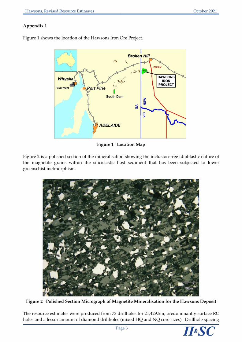
Figure 1 shows the location of the Hawsons Iron Ore Project.

Figure 1 Location Map

Figure 2 is a polished section of the mineralisation showing the inclusion-free idioblastic nature of

the magnetite grains within the siliciclastic host sediment that has been subjected to lower

greenschist metmorphism.

Figure 2 Polished Section Micrograph of Magnetite Mineralisation for the Hawsons Deposit

The resource estimates were produced from 73 drillholes for 21,429.5m, predominantly surface RC

holes and a lessor amount of diamond drillholes (mixed HQ and NQ core sizes). Drillhole spacing


Page 4

ranges between 150m and 300m in both section and plan (Figure 3). RC drilling encountered

predominantly dry samples; some samples were slightly damp but there were no reports of any

groundwater inflows (<5% wet samples). Table 1 provides information of the drilling used in the

resource estimation.

Table 1 Drillhole Information

Company Year Hole Type No of Holes Metres DTR Analysis DH Geophys

CRAE 1986 Perc 4 634.6 No 2 holes

1988 DD 1 100.0 No None

HIO 2009 RC 3 761.1 Yes 99% of drilling

2010 DD 3 761.3 Yes 65% of drilling

2010 RC 42 10,141.0 Yes 68% of drilling

2010 DD Tails 17 3,068.5 Yes 40% of drilling

2016 RC 20 5,963.0 Yes 88% of drilling

Total 73 21,429.5

A plan of the drillholes in national grid GDA94 Zone 54 projection is included as Figure 3.

Figure 3 Core & Fold Targets Geology & Drillhole Location Map

(extent of resource over reduced to the pole magnetics)

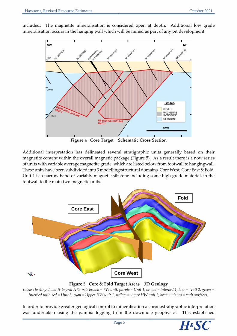
From drilling intersections the magnetite mineralisation is interpreted to extend to a vertical depth

of 400m below surface over a 4km strike length. A schematic cross section interpretation of the

drilling from an earlier report is included as Figure 4. It shows the two substantial bodies of

magnetite mineralisation (Units 2 and 3) with an interstitial lower grade zone known as the Interbed

Unit. It is HIO’s intention to mine the complete package of magnetite material, interstitial zone


Page 5

included. The magnetite mineralisation is considered open at depth. Additional low grade

mineralisation occurs in the hanging wall which will be mined as part of any pit development.

Figure 4 Core Target Schematic Cross Section

Additional interpretation has delineated several stratigraphic units generally based on their

magnetite content within the overall magnetic package (Figure 5). As a result there is a now series

of units with variable average magnetite grade, which are listed below from footwall to hangingwall.

These units have been subdivided into 3 modelling/structural domains, Core West, Core East & Fold.

Unit 1 is a narrow band of variably magnetic siltstone including some high grade material, in the

footwall to the main two magnetic units.

Figure 5 Core & Fold Target Areas 3D Geology

(view : looking down & to grid NE; pale brown = FW unit, purple = Unit 1, brown = interbed 1, blue = Unit 2, green =

Interbed unit, red = Unit 3, cyan = Upper HW unit 1, yellow = upper HW unit 2; brown planes = fault surfaces)

In order to provide greater geological control to mineralisation a chronostratigraphic interpretation

was undertaken using the gamma logging from the downhole geophysics. This established

Core East

Core West

Fold


Page 6

stratigraphic markers that were used to ascertain magnetite grade continuity between the drillholes

and which resulted in very low coefficients of variation within the different units. This information

was used subsequently to assist with the resource classification.

Unconstrained 5m downhole composites were generated from the drillhole database for the

downhole mag_sus, short spaced density, hand held magnetic susceptibility, DTR analysis and

concentrate grades (iron, alumina, phosphorous, sulphur, silica, titanium and loss on ignition).

Where there were no DTR values the downhole mag_sus or hand-held mag sus data was used, via

a regression equation, to populate the peripheral low grade and barren areas to the main magnetite

mineralisation with DTR values.

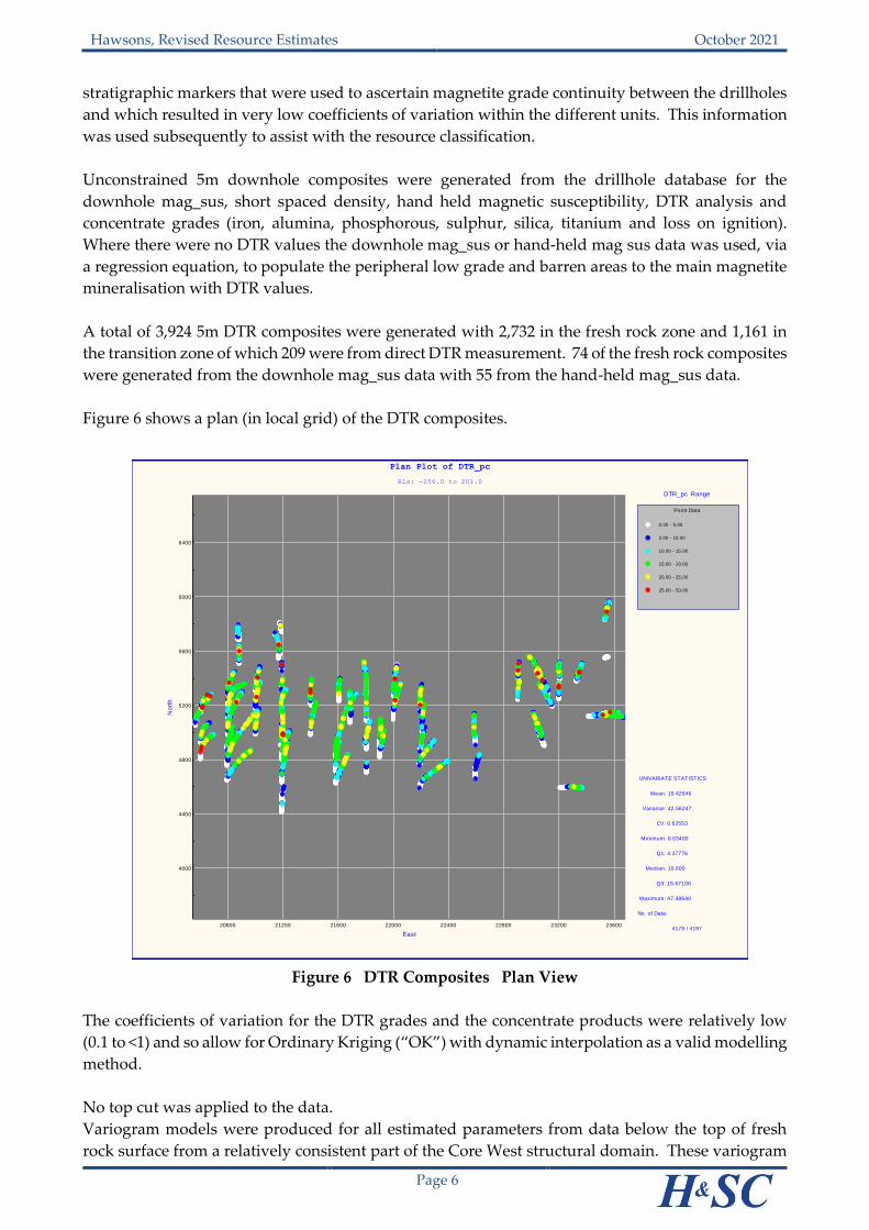
A total of 3,924 5m DTR composites were generated with 2,732 in the fresh rock zone and 1,161 in

the transition zone of which 209 were from direct DTR measurement. 74 of the fresh rock composites

were generated from the downhole mag_sus data with 55 from the hand-held mag_sus data.

Figure 6 shows a plan (in local grid) of the DTR composites.

Figure 6 DTR Composites Plan View

The coefficients of variation for the DTR grades and the concentrate products were relatively low

(0.1 to <1) and so allow for Ordinary Kriging (“OK”) with dynamic interpolation as a valid modelling

method.

No top cut was applied to the data.

Variogram models were produced for all estimated parameters from data below the top of fresh

rock surface from a relatively consistent part of the Core West structural domain. These variogram

20800 21200 21600 22000 22400 22800 23200 23600

4000

4400

4800

5200

5600

6000

6400

Plan Plot of DTR_pc

RLs: -256.0 to 201.0

East

No

rth

0.00 - 5.00

5.00 - 10.00

10.00 - 15.00

15.00 - 20.00

20.00 - 25.00

25.00 - 50.00

DTR_pc Range

Point Data

UNIVARIATE STATISTICS

Mean: 10.42946

Variance: 42.56247

CV: 0.62553

Minimum: 0.03400

Q1: 4.37776

Median: 10.600

Q3: 15.67100

Maximum: 47.38640

No. of Data:

4179 / 4197


Page 7

models showed longest ranges in the strike orientation, moderately long ranges in the down dip

orientation and short ranges in the orientation perpendicular to strike and dip ie downhole.

The OK modelling used a 4 pass search strategy with the composites. A Pass 5 search was used to

provide information on the Exploration Potential. Details of the search parameters are included in

Table 2.

Table 2 Search Ellipse Parameters

Axis Pass 1 Pass 2 Pass 3 Pass 4 Pass 5

Along Strike 250m 300m 450m 450m 900m

Down Dip 150m 150m 225m 225m 450m

Across Strike 40m 50m 75m 75m 75m

Composite Data

Requirements

Min Data 16 16 16 8 8

Max points per sector 8 8 8 16 16

Sectors 4 4 4 2 2

Hole Count 3 2 2 1 1

Contact plot analysis of the estimated elements were conducted in order to investigate how the Base

of partial oxidation (“BOPO”) and the top of fresh rock (“TOFR”) surfaces should be treated in

resource estimation. The TOFR surface was found to coincide with a marked difference in density

and DTR and was therefore used as a hard boundary. The structural domain surfaces were used as

hard boundaries, but the lithological subdivisions were used as soft boundaries.

Block dimensions are 100m by 50m by 15m (X, Y & Z directions).

The classification of the resource estimates is based primarily on the data distribution which is a

function of the drillhole spacing. Other factors involved in the classification include the style of

mineralisation, the geological model, the QAQC programme and results and comparison with

previous resource estimates. HIO has informed H&SC that the mining method will be a bulk mining

method via an open pit operation and the resources have been classified according to this

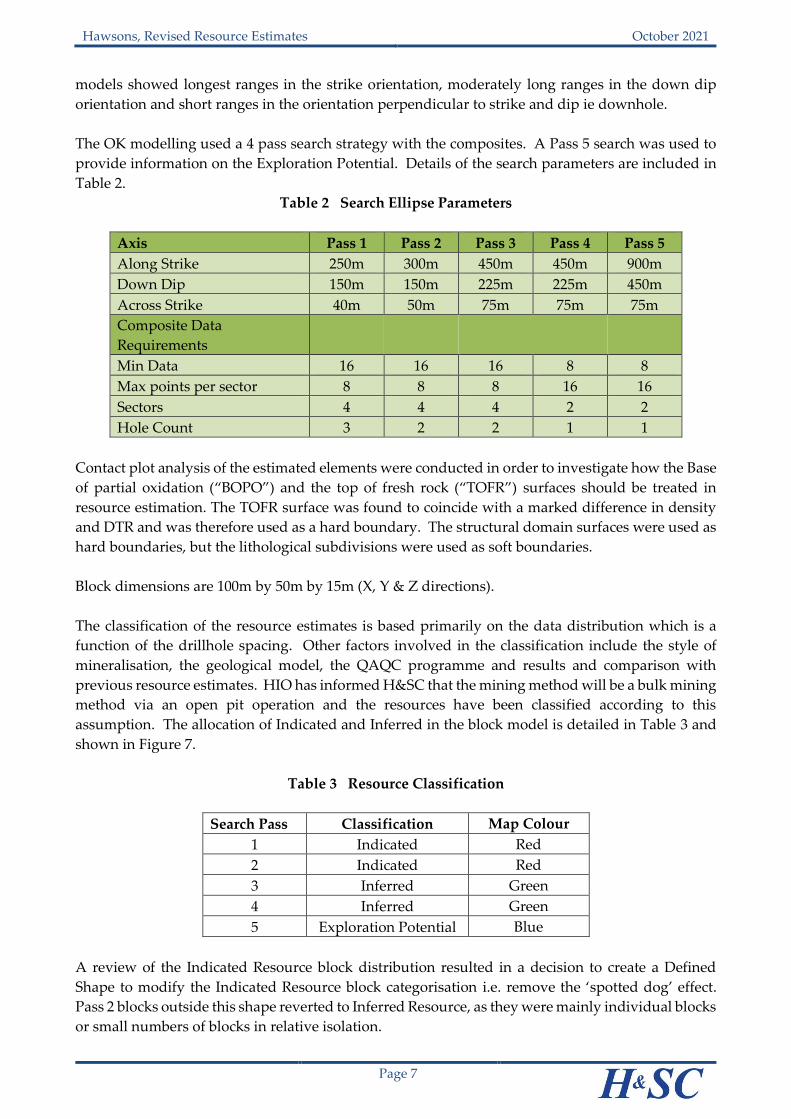
assumption. The allocation of Indicated and Inferred in the block model is detailed in Table 3 and

shown in Figure 7.

Table 3 Resource Classification

Search Pass Classification Map Colour

1 Indicated Red

2 Indicated Red

3 Inferred Green

4 Inferred Green

5 Exploration Potential Blue

A review of the Indicated Resource block distribution resulted in a decision to create a Defined

Shape to modify the Indicated Resource block categorisation i.e. remove the ‘spotted dog’ effect.

Pass 2 blocks outside this shape reverted to Inferred Resource, as they were mainly individual blocks

or small numbers of blocks in relative isolation.


Page 8

Figure 7 Resource Classification

(view looking down to grid north east)(green circles & lines = drillhole traces)

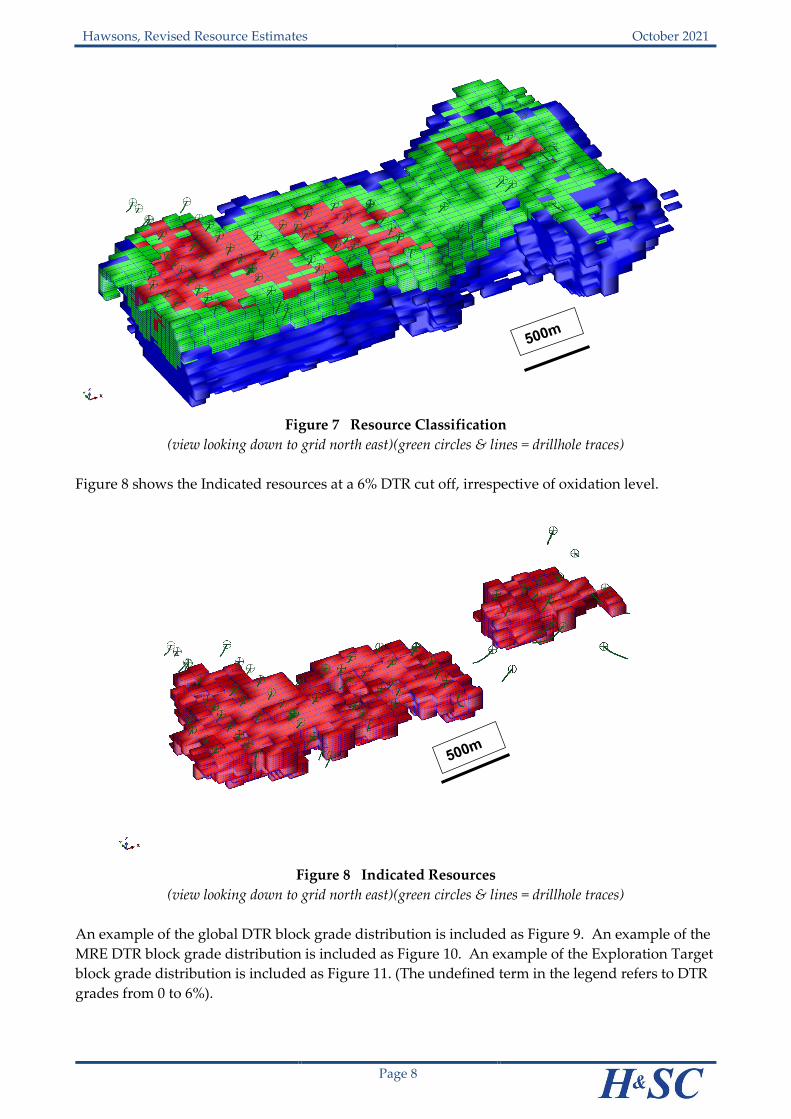
Figure 8 shows the Indicated resources at a 6% DTR cut off, irrespective of oxidation level.

Figure 8 Indicated Resources

(view looking down to grid north east)(green circles & lines = drillhole traces)

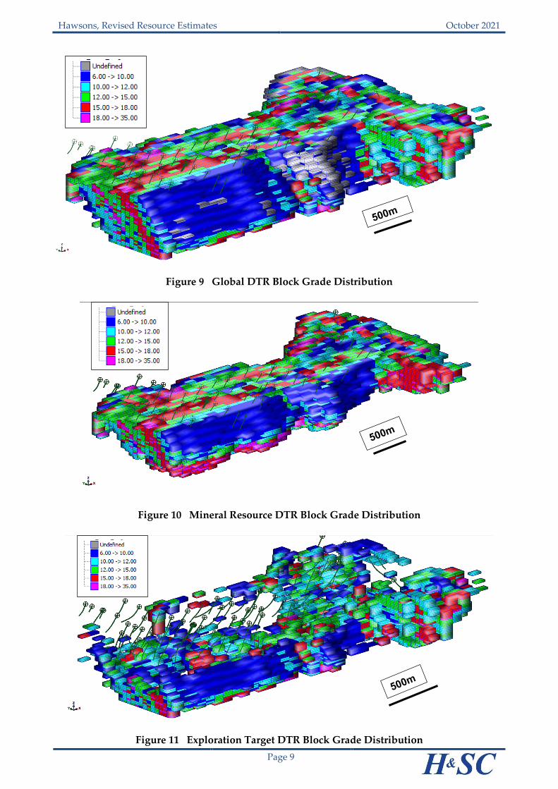
An example of the global DTR block grade distribution is included as Figure 9. An example of the

MRE DTR block grade distribution is included as Figure 10. An example of the Exploration Target

block grade distribution is included as Figure 11. (The undefined term in the legend refers to DTR

grades from 0 to 6%).


Page 9

Figure 9 Global DTR Block Grade Distribution

Figure 10 Mineral Resource DTR Block Grade Distribution

Figure 11 Exploration Target DTR Block Grade Distribution

1

JORC Code, 2012 Edition – Table 1 Hawsons Magnetite Project

Section 1 Sampling Techniques and Data

(Criteria in this section apply to all succeeding sections.)(All work was completed by Carpentaria Exploration (“CAP”), predecessor to Hawsons Iron (“HIO”)

Criteria JORC Code explanation Commentary

Sampling techniques

• Nature and quality of sampling (e.g. cut channels, random chips, or specific specialised industry standard measurement tools appropriate to the minerals under investigation, such as down hole gamma sondes, or handheld XRF instruments, etc). These examples should not be taken as limiting the broad meaning of sampling.

• Include reference to measures taken to ensure sample representivity and the appropriate calibration of any measurement tools or systems used.

• Aspects of the determination of mineralisation that are Material to the Public Report.

• In cases where ‘industry standard’ work has been done this would be relatively simple (e.g. ‘reverse circulation drilling was used to obtain 1 m samples from which 3 kg was pulverised to produce a 30 g charge for fire assay’). In other cases, more explanation may be required, such as where there is coarse gold that has inherent sampling problems. Unusual commodities or mineralisation types (e.g. submarine nodules) may warrant disclosure of detailed information.

• Sampling consisted of drillholes with a mixture of reverse circulation

(RC) from surface, diamond tails to RC precollars (PD) and diamond

from surface (DD).

• A total of 73 drillholes for 21,429.5m, were drilled by CAP in two

main phases i.e. 2010 (RC & DD) and 2016 (RC).

• RC drillholes were drilled to obtain 1m bulk samples with sample

compositing (various lengths under geological control) via spear

sampling applied in order to obtain manageable sample sizes for

laboratory sample prep and assaying

• For the 2010 RC drilling, sampling comprised 2m to 10m 3kg

c o m p o s i t e samples. The 2016 sampling comprised 5m composites

generating 6kg of sample. All samples were pulverized to produce

150g aliquot for X-Ray Fluorescence (XRF) and Davis Tube

Recovery (DTR) analysis

• Diamond core sampling involved sawing half core samples to

produce an 8m composite sample (predominantly NQ core) which

was pulverized to produce a 150g aliquot for XRF and DTR analysis.

• Geophysical logging was completed for a majority of holes and

consisted of natural gamma, magnetic susceptibility, density and

calliper readings.

• Mineralisation comprises bands of variable thickness of disseminated,

idioblastic magnetite in low metamorphic grade fine grained

siliciclastics and diamictites. Siliciclastic grain size tends to provide a

strong control to mineralisation. Substantial regional deformation has

occurred but locally the main mineral units are relatively

straightforward moderately dipping units.

• Consistency of sampling method was maintained.

• The sampling technique is considered appropriate for deposit type with

2


all sampling to industry standard practices.

Drilling techniques

• Drill type (e.g. core, reverse circulation, open-hole hammer, rotary air blast, auger, Bangka, sonic, etc) and details (e.g. core diameter, triple or standard tube, depth of diamond tails, face-sampling bit or other type, whether core is oriented and if so, by what method, etc).

• The RC drilling for 2010 was carried out using a truck mounted Schramm and truck mounted KWL 1600H. Both rigs used 4.5” rods and 5.5” face bits.

• PD and DD drilling was carried out using a truck mounted UDR650 using NQ2 and standard HQ diameters. Core orientation used the Ace Core orientation tool.

• For the 2016 drilling (all RC drilling) truck-mounted Sandvik DE 840 (UDR1200), UDR1000 and Metzke rigs were used. All rigs used 4.5” rods with 5.5” face bits.

Drill sample recovery

• Method of recording and assessing core and chip sample recoveries and results assessed.

• Measures taken to maximise sample recovery and ensure representative nature of the samples.

• Whether a relationship exists between sample recovery and grade and whether sample bias may have occurred due to preferential loss/gain of fine/coarse material.

• The 2010 RC sampling was on 1m intervals into green plastic bags. Sample recoveries for RC were visually estimated by the geologist at the time of drilling and recorded.

• Because no numerical RC chip recovery data existed it was not possible to conclude if there was a relationship between sample recovery and mineral grade

• The 2016 RC drilling recorded sample weights for 272 1m samples with recoveries of 80-90% for dry samples and 40 to 50% for wet samples. Plotting of recoveries versus DTR grade indicated no sampling bias.

• Core recoveries were recorded by measuring the length of core recovered in each dr i l l run divided by the drilled length of the individual core runs; average recovery >97%.

• A handheld XRF orientation study by CAP for the 2010 RC drilling concluded that there was no sample bias with loss or gain of fine/coarse material with the RC drilling.

• A very modest number of wet samples were recorded in the 2010 RC drilling and for the 2016 drilling, <5% of samples were logged as wet.

• A study by Keith Hannan of Geochem Pacific Pty Ltd, an independent geochemist/consultant determined, “at the deposit scale, average magnetite recoveries of complete intercepts of ore units 2 and 3, corresponding to 180-245 m lengths of continuous data, are indistinguishable by drill sample type (i.e., RC versus NQ core samples). By implication, the magnetite recoveries for the composited intervals of individual samples are not systematically influenced (biased) by method of drilling and type of recovered sample”.

Logging • Whether core and chip samples have been geologically and • Every RC, PD and DD drillhole was logged by a geologist &

3


geotechnically logged to a level of detail to support appropriate Mineral Resource estimation, mining studies and metallurgical studies.

• Whether logging is qualitative or quantitative in nature. Core (or costean, channel, etc) photography.

• The total length and percentage of the relevant intersections logged.

entered into Excel spreadsheets recording; Recovery, Moisture content, Magnetic susceptibility, Oxidation state, Colour, % of Magnetite, Gangue Min, Sulphide Min, Veins and Structure. Data was uploaded to a customised Access database.

• Handheld magnetic susceptibility measurements and geological logging was completed for every metre of every drillhole.

• Logging used a mixture of qualitative and quantitative codes.

• All RC sample metres were sub-sampled, sieved, washed and stored in a labelled plastic chip tray. All remaining drill core after sampling was stored in labelled plastic core trays and subsequently stored at the company’s offices in Broken Hill.

• Processing of drillcore included core orientation, metre marking, magnetic susceptibility measurements (every 0.5m), core recoveries, rock quality designation (RQD). All drill core was photographed wet and dry after logging and before cutting.

• All relevant intersections were logged.

• Geological logging was of sufficient detail to allow the creation of a geological model.

Sub-sampling techniques and sample preparation

• If core, whether cut or sawn and whether quarter, half or all core taken.

• If non-core, whether riffled, tube sampled, rotary split, etc and whether sampled wet or dry.

• For all sample types, the nature, quality and appropriateness of the sample preparation technique.

• Quality control procedures adopted for all sub-sampling stages to maximise representivity of samples.

• Measures taken to ensure that the sampling is representative of the in-situ material collected, including for instance results for field duplicate/second-half sampling.

• Whether sample sizes are appropriate to the grain size of the material being sampled.

• The 2010 RC samples were composited using geological control via the spear sampling method of the 1m bulk sample bags. The spear method was concluded by CAP to be adequate based on the results of a handh e ld XRF orientation exercise. The green plastic bags were speared from a range of angles to the bottom of the bag to ensure a representative sample. The compositing produced a 2m to 10m 3kg sample for laboratory analysis at ALS Labs in Perth.

• The 2016 RC samples were split using a riffle splitter (no details of type used) that produced a 1/16th split taken from the rig every metre and then composited to 5m intervals by splitting again using a 50/50 splitter to give a 6-7kg sample.

• DD core was cut into half core using a brick saw and diamond blade. The core was cut using the orientation line or perpendicular to bedding. to produce an 8m composite sample (predominantly NQ core). Half core was sent to ALS Perth for analysis, whilst remaining half core was retained for reference.

• Sample Prep was completed at ALS Laboratories Perth

o Crush the sample to 100% below 3.35 mm. o A 150 g sub-sample for pulverizing in a C125 ring pulveriser

(record weight) – DTR SAMPLE.

4


o Initially pulverize the 150 g sample for nominal 30 seconds – the sample is unusually soft for a ferro-silicate rock.

o Wet screen the DTR sample at 38 micron pressure filter and dry, screen at 1 mm to de-clump and re-homogenize.

o Record the oversize weights – if less than approximately 20 g is oversize, stop the procedure – failure.

o If failure - select another 150 g DTR Sample and reduce the initial pulverization time by 5 secs, repeat until initial grind pass returns greater than approximately 20 g oversize. Once achieved retain the – 38 micron undersize.

o Regrind only the oversize for 4 seconds of every 5 g weight of oversize.

o Repeat the wet screening, drying, de-clumping & weighing stages until less than 5g above 38micron remains.

o Ensure the remaining < 5 g oversize is returned back into the previously retained -38 micron product.

o Report the times and weights for each grind pass phase.

o Combine and homogenize all retained -38 micron aliquots and <5 g oversize –final pulverized product. Sub-sample the final pulverized product to give a 20 g feed sample for DTR work and a ~10 g sample for HEAD analysis via XRF fusion.

• The 2010 work employed field duplicates (23 5m samples) using the spear sampling technique which on analysis produced acceptable results.

• The 2016 work had a much more comprehensive QAQC programme which included 87 field pairs (not actual duplicates unfortunately) at an insertion rate of 1 in 10, 111 lab duplicates and 39 blanks (river sand) at an insertion rate of 1 in 20, 58 2nd lab checks (Intertek Labs in Perth), pulp duplicates for XRF analysis and sample prep checks.

• For the 2016 work the field pair results produced a slightly sub-optimal outcome, but were still acceptable for the current resource classification and seemed to be less precise than the spear sampling method used in 2010. The lab duplicates (a second 150g split) produced good results indicating acceptable sample preparation procedures. The 2nd lab checks on 150g sub-samples produced results indistinguishable from the original lab results. Pulp duplicates demonstrated chemically homogeneity with the XRF analysis.

• 30 Primary crush and sub-sample checks were completed by Aussam Geotechnical Services (Broken Hill) which concluded that no

5


evidence of bias with the oversize mineralogy.

• Blank samples comprising river sand produced results that indicated no contamination of the samples during the sample prep process.

• An additional check on the field sub-sampling and compositing procedure used a Jones 3 tier riffle splitter (1/8) and a free-standing 1:1 splitter to match the 1/16 rig splitter. A total of 30 5m composite intervals were utilised. Noting that all samples were dry, slightly better results were achieved than the original field pair process. However under full field conditions it was thought that there was likely to be no difference between the riffle splitting and spear sub-sampling methods. Both are at risk to human errors, which perhaps can be better managed with the riffle splitting.

• All sampling methods and samples sizes are deemed appropriate.

Quality of assay data and laboratory tests

• The nature, quality and appropriateness of the assaying and laboratory procedures used and whether the technique is considered partial or total.

• For geophysical tools, spectrometers, handheld XRF instruments, etc, the parameters used in determining the analysis including instrument make and model, reading times, calibrations factors applied and their derivation, etc.

• Nature of quality control procedures adopted (e.g. standards, blanks, duplicates, external laboratory checks) and whether acceptable levels of accuracy (i.e. lack of bias) and precision have been established.

• Davis Tube Recovery (DTR) Analysis

o Pulveriser bowl 150 ml

o Stroke Frequency - 60/minute

o Stroke length – 38mm

o Magnetic field strength – 3000 gauss

o Tube Angle – 45 degrees

o Tube Diameter – 40mm

o Water flow rate – 540-590 ml/min o Washing time 20 minutes o Collect the concentrate in small collector (magnetic fraction)

and discard tails.

o Dry the DTR concentrate and report the weight of the concentrate as a percentage of measured feed and report – DTR Mass Recovery.

• X-Ray Fluorescence (XRF) Assaying

o Using the Head Sample, analyse by XRF fusion method for the

following elements: Al2O3%, As%, Ba%, CaO%, Cl%, Co%, Cr%,

Cu%, Fe%, K2O%, MgO%, Mn% Na2O%, Ni%, P%, Pb%, S %,

SiO2%, Sn%, Sr%, TiO2%, V%, Zn%, Zr% & LOI.

o Using the DTR concentrate sample analyse by XRF fusion method

for the following elements: Al2O3%, As%, Ba%, CaO%, Cl%,

Co%, Cr%, Cu%, Fe%, K2O%, MgO%, Mn% Na2O%, Ni%, P%,

Pb%, S %, SiO2%, Sn%, Sr%, TiO2%, V%, Zn%, Zr% & LOI

• JH8 and KT5 magnetic susceptibility meters were used to record

6


magnetic susceptibility. A laboratory standard was used each day to

calibrate each metre. A Niton XL3T Gold handheld XRF machine was

used. A laboratory analysed sample was used to calibrate for Fe.

• QAQC procedures consisted of the use of 3 certified reference

materials for DTR (head and high grades) and XRF analysis at a

frequency of 1 per 15 for the 2016 drilling. The reported results for the

standards meet industry accepted criteria for accuracy, both for DTR

magnetite recoveries and XRF analyses of the critical elements (Fe,

Si, Al, and P).

• It is uncertain if certified reference materials were used for the 2010

drilling. In CAP’s documented drilling procedures it was indicated that

a standard insertion rate of 1 in 30 should be used. In a QAQC review

of procedures Keith Hannan noted that CAP utilises a ‘monitor’

standard consisting of crushed magnetite-rich rock derived from local

outcrops but without commenting on any results.

• Keith Hannan of Geochem Pacific Pty Ltd, an independent

geochemist/consultant reviewed the QAQC results for both the 2010

and 2016 drilling and expressed satisfaction with precision, accuracy

and any lack of bias in the data, making it fit for purpose for resource

estimation.

• All assay methods are deemed appropriate.

Verification of sampling and assaying

• The verification of significant intersections by either independent or alternative company personnel.

• The use of twinned holes.

• Documentation of primary data, data entry procedures, data verification, data storage (physical and electronic) protocols.

• Discuss any adjustment to assay data.

• Data was stored in a customised Access database.

• Database checks were completed by S. Tear of H&SC on 5 randomly

selected drillholes. Checks included comparing database values with

original collar survey reports, downhole survey reports and assay

certificates.

• Two DD holes were used as twin holes to verify the results for 2 pairs of RC holes and the DTR performance.

• The results are reasonable but there is some potential ambiguity mainly due to a fundamental lack of assay data (mainly with the diamond drilling) and the separation distance of the relative mineral intercepts. It was concluded by Keith Hannan that “the ‘twin hole’ site data that, although there is demonstrable variation in average magnetite grades within several metres along-strike, there is no evidence of a consistent positive bias in the magnetite levels

7


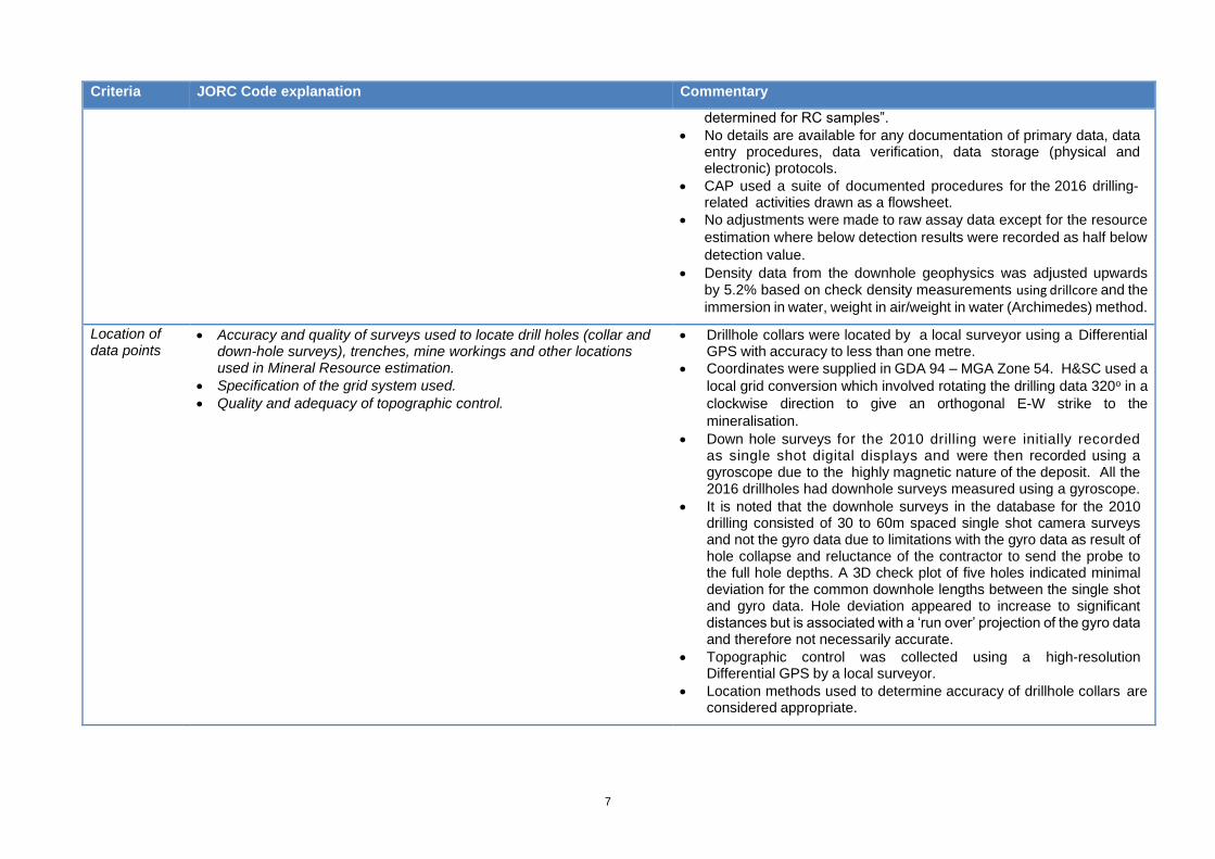
determined for RC samples”.

• No details are available for any documentation of primary data, data entry procedures, data verification, data storage (physical and electronic) protocols.

• CAP used a suite of documented procedures for the 2016 drilling-related activities drawn as a flowsheet.

• No adjustments were made to raw assay data except for the resource

estimation where below detection results were recorded as half below

detection value.

• Density data from the downhole geophysics was adjusted upwards by 5.2% based on check density measurements using drillcore and the

immersion in water, weight in air/weight in water (Archimedes) method.

Location of data points

• Accuracy and quality of surveys used to locate drill holes (collar and down-hole surveys), trenches, mine workings and other locations used in Mineral Resource estimation.

• Specification of the grid system used.

• Quality and adequacy of topographic control.

• Drillhole collars were located by a local surveyor using a Differential GPS with accuracy to less than one metre.

• Coordinates were supplied in GDA 94 – MGA Zone 54. H&SC used a

local grid conversion which involved rotating the drilling data 320o in a

clockwise direction to give an orthogonal E-W strike to the

mineralisation.

• Down hole surveys for the 2010 drilling were initially recorded as single shot digital displays and were then recorded using a gyroscope due to the highly magnetic nature of the deposit. All the 2016 drillholes had downhole surveys measured using a gyroscope.

• It is noted that the downhole surveys in the database for the 2010 drilling consisted of 30 to 60m spaced single shot camera surveys and not the gyro data due to limitations with the gyro data as result of hole collapse and reluctance of the contractor to send the probe to the full hole depths. A 3D check plot of five holes indicated minimal deviation for the common downhole lengths between the single shot and gyro data. Hole deviation appeared to increase to significant distances but is associated with a ‘run over’ projection of the gyro data and therefore not necessarily accurate.

• Topographic control was collected using a high-resolution Differential GPS by a local surveyor.

• Location methods used to determine accuracy of drillhole collars are considered appropriate.

8


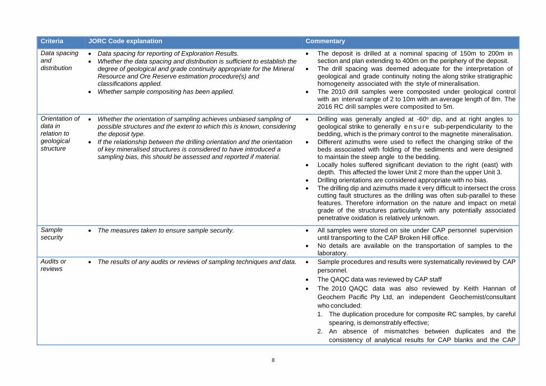
Data spacing and distribution

• Data spacing for reporting of Exploration Results.

• Whether the data spacing and distribution is sufficient to establish the degree of geological and grade continuity appropriate for the Mineral Resource and Ore Reserve estimation procedure(s) and classifications applied.

• Whether sample compositing has been applied.

• The deposit is drilled at a nominal spacing of 150m to 200m in section and plan extending to 400m on the periphery of the deposit.

• The drill spacing was deemed adequate for the interpretation of geological and grade continuity noting the along strike stratigraphic homogeneity associated with the style of mineralisation.

• The 2010 drill samples were composited under geological control with an interval range of 2 to 10m with an average length of 8m. The 2016 RC drill samples were composited to 5m.

Orientation of data in relation to geological structure

• Whether the orientation of sampling achieves unbiased sampling of possible structures and the extent to which this is known, considering the deposit type.

• If the relationship between the drilling orientation and the orientation of key mineralised structures is considered to have introduced a sampling bias, this should be assessed and reported if material.

• Drilling was generally angled at -60o dip, and at right angles to geological strike to generally e n s u r e sub-perpendicularity to the bedding, which is the primary control to the magnetite mineralisation.

• Different azimuths were used to reflect the changing strike of the beds associated with folding of the sediments and were designed to maintain the steep angle to the bedding.

• Locally holes suffered significant deviation to the right (east) with depth. This affected the lower Unit 2 more than the upper Unit 3.

• Drilling orientations are considered appropriate with no bias.

• The drilling dip and azimuths made it very difficult to intersect the cross cutting fault structures as the drilling was often sub-parallel to these features. Therefore information on the nature and impact on metal grade of the structures particularly with any potentially associated penetrative oxidation is relatively unknown.

Sample security

• The measures taken to ensure sample security. • All samples were stored on site under CAP personnel supervision until transporting to the CAP Broken Hill office.

• No details are available on the transportation of samples to the laboratory.

Audits or reviews

• The results of any audits or reviews of sampling techniques and data. • Sample procedures and results were systematically reviewed by CAP

personnel.

• The QAQC data was reviewed by CAP staff

• The 2010 QAQC data was also reviewed by Keith Hannan of

Geochem Pacific Pty Ltd, an independent Geochemist/consultant

who concluded:

1. The duplication procedure for composite RC samples, by careful

spearing, is demonstrably effective;

2. An absence of mismatches between duplicates and the

consistency of analytical results for CAP blanks and the CAP

9


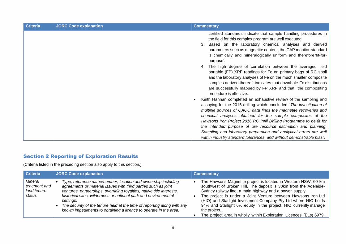
certified standards indicate that sample handling procedures in

the field for this complex program are well executed

3. Based on the laboratory chemical analyses and derived

parameters such as magnetite content, the CAP monitor standard

is chemically and mineralogically uniform and therefore ‘fit-for-

purpose’.

4. The high degree of correlation between the averaged field

portable (FP) XRF readings for Fe on primary bags of RC spoil

and the laboratory analyses of Fe on the much smaller composite

samples derived thereof, indicates that downhole Fe distributions

are successfully mapped by FP XRF and that the compositing

procedure is effective.

• Keith Hannan completed an exhaustive review of the sampling and

assaying for the 2016 drilling which concluded “The investigation of

multiple sources of QAQC data finds the magnetite recoveries and

chemical analyses obtained for the sample composites of the

Hawsons Iron Project 2016 RC Infill Drilling Programme to be fit for

the intended purpose of ore resource estimation and planning.

Sampling and laboratory preparation and analytical errors are well

within industry standard tolerances, and without demonstrable bias”.

Section 2 Reporting of Exploration Results

(Criteria listed in the preceding section also apply to this section.)


Mineral tenement and land tenure status

• Type, reference name/number, location and ownership including agreements or material issues with third parties such as joint ventures, partnerships, overriding royalties, native title interests, historical sites, wilderness or national park and environmental settings.

• The security of the tenure held at the time of reporting along with any known impediments to obtaining a licence to operate in the area.

• The Hawsons Magnetite project is located in Western NSW, 60 km southwest of Broken Hill. The deposit is 30km from the Adelaide-Sydney railway line, a main highway and a power supply.

• The project is under a Joint Venture between Hawsons Iron Ltd (HIO) and Starlight Investment Company Pty Ltd where HIO holds 94% and Starlight 6% equity in the project. HIO currently manage the project.

• The project area is wholly within Exploration Licences (ELs) 6979,

10


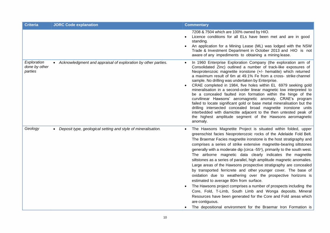
7208 & 7504 which are 100% owned by HIO.

• Licence conditions for all ELs have been met and are in good standing.

• An application for a Mining Lease (ML) was lodged with the NSW Trade & Investment Department in October 2013 and HIO is not aware of any impediments to obtaining a mining lease.

Exploration done by other parties

• Acknowledgment and appraisal of exploration by other parties. • In 1960 Enterprise Exploration Company (the exploration arm of Consolidated Zinc) outlined a number of track-like exposures of Neoproterozoic magnetite ironstone (+/- hematite) which returned a maximum result of 6m at 49.1% Fe from a cross- strike channel sample. No drilling was undertaken by Enterprise.

• CRAE completed in 1984, five holes within EL 6979 seeking gold mineralisation in a second-order linear magnetic low interpreted to be a concealed faulted iron formation within the hinge of the curvilinear Hawsons’ aeromagnetic anomaly. CRAE’s program failed to locate significant gold or base metal mineralisation but the drilling intersected concealed broad magnetite ironstone units interbedded with diamictite adjacent to the then untested peak of the highest amplitude segment of the Hawsons aeromagnetic anomaly.

Geology • Deposit type, geological setting and style of mineralisation. • The Hawsons Magnetite Project is situated within folded, upper

greenschist facies Neoproterozoic rocks of the Adelaide Fold Belt.

The Braemar Facies magnetite ironstone is the host stratigraphy and

comprises a series of strike extensive magnetite-bearing siltstones

generally with a moderate dip (circa -55o), primarily to the south west.

The airborne magnetic data clearly indicates the magnetite

siltstones as a series of parallel, high amplitude magnetic anomalies.

Large areas of the Hawsons prospective stratigraphy are concealed

by transported ferricrete and other younger cover. The base of

oxidation due to weathering over the prospective horizons is

estimated to average 80m from surface.

• The Hawsons project comprises a number of prospects including the

Core, Fold, T-Limb, South Limb and Wonga deposits. Mineral

Resources have been generated for the Core and Fold areas which

are contiguous.

• The depositional environment for the Braemar Iron Formation is

11


believed to be a subsiding basin, with initial rapid subsidence

related to rifting possibly in a graben setting as indicated by the

occurrence of diamictites in the lower part of the sequence (Unit 2).

A possible sag phase of cyclical subsidence followed with deposition

of finer grained sediments with more consistent, as compared to

the diamictite units, bed thicknesses, style and clast composition (Unit

3). The top of the Interbed Unit marks the transition from high (Unit

2) to lower (Unit 3) energy sediment deposition

• The distribution of disseminated, inclusion-free magnetite in the

Braemar Iron Formation at Hawsons is related to the composition

and nature of the sedimentary beds. The idioblastic nature of the of

the magnetite is believed due to one or more of a range of possible

processes including in situ recrystallisation of primary detrital grains,

chemical precipitation from seawater, permeation of iron-rich

metamorphic fluids associated with regional greenschist

metamorphism. Grain size generally ranges from 10microns to 0.2mm

but tends to average around the 40microns. The sediment

composition and grain size appear to provide the main control on

the mineralisation. There is no evidence for structural control in

the form of veins or veinlets coupled with the lack of a strong

structural fabric

• In the majority of the Core and Fold deposits the units strike

southeast and dip between 45 and 65o to the south west. The

eastern part of the Fold deposit comprises a relatively tight

synclinal fold structure resulting in a 90o strike rotation.

Drill hole Information

• A summary of all information material to the understanding of the exploration results including a tabulation of the following information for all Material drill holes: o easting and northing of the drill hole collar o elevation or RL (Reduced Level – elevation above sea level in

metres) of the drill hole collar o dip and azimuth of the hole o down hole length and interception depth o hole length.

• If the exclusion of this information is justified on the basis that the

• Exploration results not being reported

12


information is not Material and this exclusion does not detract from the understanding of the report, the Competent Person should clearly explain why this is the case.

Data aggregation methods

• In reporting Exploration Results, weighting averaging techniques, maximum and/or minimum grade truncations (e.g. cutting of high grades) and cut-off grades are usually Material and should be stated.

• Where aggregate intercepts incorporate short lengths of high grade results and longer lengths of low grade results, the procedure used for such aggregation should be stated and some typical examples of such aggregations should be shown in detail.

• The assumptions used for any reporting of metal equivalent values should be clearly stated.


Relationship between mineralisation widths and intercept lengths

• These relationships are particularly important in the reporting of Exploration Results.

• If the geometry of the mineralisation with respect to the drill hole angle is known, its nature should be reported.

• If it is not known and only the down hole lengths are reported, there should be a clear statement to this effect (e.g. ‘down hole length, true width not known’).

• Drilling has tended to be at a steep angle to the dip angle of the sedimentary beds.

Diagrams • Appropriate maps and sections (with scales) and tabulations of intercepts should be included for any significant discovery being reported These should include, but not be limited to a plan view of drill hole collar locations and appropriate sectional views.


Balanced reporting

• Where comprehensive reporting of all Exploration Results is not practicable, representative reporting of both low and high grades and/or widths should be practiced to avoid misleading reporting of Exploration Results.


Other substantive exploration data

• Other exploration data, if meaningful and material, should be reported including (but not limited to): geological observations; geophysical survey results; geochemical survey results; bulk samples – size and method of treatment; metallurgical test results; bulk density, groundwater, geotechnical and rock characteristics; potential deleterious or contaminating substances.

• A substantial amount of polished and thin section work has been completed on both RC chips and diamond core. This work has confirmed the nature and style of both the original sediment and the iron minerals including magnetite, hematite, chlorite and ferroan dolomite.

• Downhole geophysics comprises magnetic susceptibility, gamma and density and has been completed for a majority of the holes. This has resulted in the definition of a magnetic (and density- related) stratigraphy that is coincident with a chronostratigraphic interpretation.

Further work • The nature and scale of planned further work (e.g. tests for lateral • Infill drilling is planned to upgrade the current Mineral Resources to

13


extensions or depth extensions or large-scale step-out drilling).

• Diagrams clearly highlighting the areas of possible extensions, including the main geological interpretations and future drilling areas, provided this information is not commercially sensitive.

Measured and Indicated, upgrade a portion of the Exploration Target

to Inferred, and to provide geotechnical and hydrogeological data.

Section 3 Estimation and Reporting of Mineral Resources

(Criteria listed in section 1, and where relevant in section 2, also apply to this section.)


Database integrity

• Measures taken to ensure that data has not been corrupted by, for example, transcription or keying errors, between its initial collection and its use for Mineral Resource estimation purposes.

• Data validation procedures used.

• Independently customised Access database by GR-FX Pty Ltd

• Validation of database undertaken by Keith Hannan of Geochem

Pacific Pty Ltd, an independent consultant.

• Database validation was conducted by H&S Consultants (H&SC) to

ensure the drill hole database is internally consistent. Validation

included checking that no assays, density measurements or

geological logs occur beyond the end of hole and that all drilled

intervals have been geologically logged. The minimum and maximum

values of assays and density measurements were checked to ensure

values are within expected ranges. Further checks include testing for

duplicate samples and overlapping sampling or logging intervals

• H&SC takes responsibility for the accuracy and reliability of the data

used to estimate the Mineral Resources.

• H&SC created a local E-W orthogonal grid for all interpretation and

modelling work.

Site visits • Comment on any site visits undertaken by the Competent Person and the outcome of those visits.

• If no site visits have been undertaken indicate why this is the case.

• Regular site visits were completed by CAP management for the period

2009 to 2017.

• A site visit has been undertaken in 2012 by Simon Tear of H&SC,

Competent Person for the Exploration Results and the reporting of the

Mineral Resources. The visit including geological logging of diamond

drillhole DD10BRP023 covering over 500m of stratigraphy and an

inspection of drill sites and outcropping mineralisation.

14


Geological interpretation

• Confidence in (or conversely, the uncertainty of) the geological interpretation of the mineral deposit.

• Nature of the data used and of any assumptions made.

• The effect, if any, of alternative interpretations on Mineral Resource estimation.

• The use of geology in guiding and controlling Mineral Resource estimation.

• The factors affecting continuity both of grade and geology.

• The broad geological interpretation of the Hawsons deposit is

relatively straightforward and reasonably well constrained by drilling

and the high amplitude airborne and ground magnetic anomalies.

• The mineralisation is stratabound as disseminated grains of magnetite

with no obvious structural remobilisation or overprint. Mineralisation

exhibits relatively poor downhole continuity with zones of variable

magnetite grade (a function of the clastic grain size and composition)

but in most instance the contacts between higher and lower grade

mineralisation are gradational and precludes the use of hard

boundaries as stratigraphic control to mineral grade interpolation.

• The downhole geophysical data, gamma and magnetic susceptibility,

has been used in conjunction with DTR recovered magnetic fraction

grades to produce a detailed geological interpretation and to the

generation of a set of 3D wireframes representing variously

mineralised units and provide a stratigraphic framework.

• The consistency of the geophysical patterns for the sediments

provides for a high level of confidence in the stratigraphic

interpretation.

• Two main cross faults, possibly a conjugate pair, have been

interpreted and are believed to have caused small offsets in the

mineral-bearing stratigraphy. The faults have been used to delineate

three structural domains.

• H&SC used the geological logs of the drill holes to create a wireframe

surface representing the base of colluvium.

• H&SC also used the geological logs of the drill holes to create

wireframe surfaces representing the base of complete oxidation

(BOCO) and the top of fresh rock (TOFR). Contact plot analysis of the

estimated elements were conducted in order to investigate how these

surfaces should be treated in the resource estimation.

• Any additional faulting in the deposit is assumed to be insignificant

relative to the resource estimation.

• H&SC is aware that alternative interpretations of the mineralised

zones and faults are possible but consider the wireframes to

adequately approximate the locations of the mineralised zones for the

15


purposes of resource estimation. Alternative interpretations may have

a limited impact on the resource estimates.

Dimensions • The extent and variability of the Mineral Resource expressed as length (along strike or otherwise), plan width, and depth below surface to the upper and lower limits of the Mineral Resource.

• The Mineral Resources have a strike length of around 3.3km in a

south easterly direction. The plan width of the resource varies from

700m to 1.9km with an average of around 1.1km (noting the relatively

modest dip angle of the beds). The upper limit of the mineralisation

occurs between 25 and 80m below surface (average 65m) and the

lower limit of the Mineral Resource extends to a depth of 440m below

surface. The lower limit to the Mineral Resource is a direct function of

the depth limitations to the drilling in conjunction with the search

parameters. The mineralisation is open at depth.

Estimation and modelling techniques

• The nature and appropriateness of the estimation technique(s) applied and key assumptions, including treatment of extreme grade values, domaining, interpolation parameters and maximum distance of extrapolation from data points. If a computer assisted estimation method was chosen include a description of computer software and parameters used.

• The availability of check estimates, previous estimates and/or mine production records and whether the Mineral Resource estimate takes appropriate account of such data.

• The assumptions made regarding recovery of by-products.

• Estimation of deleterious elements or other non-grade variables of economic significance (e.g. sulphur for acid mine drainage characterisation).

• In the case of block model interpolation, the block size in relation to the average sample spacing and the search employed.

• Any assumptions behind modelling of selective mining units.

• Any assumptions about correlation between variables.

• Description of how the geological interpretation was used to control the resource estimates.

• Discussion of basis for using or not using grade cutting or capping.

• The process of validation, the checking process used, the comparison of model data to drill hole data, and use of reconciliation data if available.

• Ordinary Kriging with dynamic interpolation was used to complete the

estimation in the Micromine software. H&SC considers Ordinary

Kriging to be an appropriate estimation technique for the type of

mineralisation and extent of data available from the Core and Fold

prospects. All data have low coefficients of variation generally <1.

• A total of 3,924 unconstrained 5m composites were generated from

the drillhole database and modelled for Davis Tube recovered

magnetic fraction (“DTR”), iron head grade and the concentrate

elements of Al2O3, P, S, SiO2, TiO2 and LOI,

• 2,862 composites were in fresh rock and 1,161 in the transition zone

of which 209 were from direct DTR measurement. 74 of the fresh rock

composites were generated from the downhole mag_sus data with 55

from the hand-held mag_sus data via regression equations,

particularly peripheral to the main mineralisation and the transition

zone.

• A regression based on downhole magnetic susceptibility was used to

calculate likely DTR values for untested intervals. A regression based

on the handheld magnetic susceptibility data was used to estimate the

DTR values where downhole magnetic susceptibility was not

available. Missing Fe concentrate grades were calculated using a

regression based on the DTR grades and the remaining concentrate

elements were calculated using a regression based on the iron

concentrate grade. Most of the missing DTR grades were on the

16


periphery of the mineralisation (often unsampled areas) and the

missing concentrate grades the result of insufficient sample being

available for XRF analysis mainly from the Interbed Unit.

• The base of colluvium was used to control the upper limit of the

resource estimation. Drill hole data from above the colluvium surface

were not used in the resource estimates.

• Two main cross faults have been delineated and have caused small

offsets in the mineral-bearing stratigraphy. These faults were treated

as hard boundaries during estimation so that data from within a

particular fault block were only used to estimate blocks in that fault

block.

• H&SC created nine surfaces representing the margins of eight

conformable lithological units based on drill hole data. These surfaces

were combined to produce eight wireframe solids, the outer boundary

of which was used to constrain the Mineral Resource Estimate. In

order to reflect local variations of dip and strike, the orientation of the

triangles that make up the nine surfaces were used to locally control

the orientation of the search ellipse and variogram axes – the dynamic

interpolation method.

• The TOFR surface was found to coincide with a marked difference in

density and DTR and was therefore used as a hard boundary. The

density and DTR values in the volume above the TOFR surface were

estimated using a flattened search ellipse. All other parameters did

not take account of the top of fresh rock surface and the orientation of

the search ellipse and variogram axes are controlled by the orientation

of the lithological unit surfaces.

• No recovery of any by-products has been considered in the resource

estimates as no products beyond iron are considered to exist in

economic concentrations.

• No top-cutting was applied as extreme values were not present and

top-cutting was considered by H&SC to be unnecessary

• No check estimate was carried out though the estimates were in line

with previous estimates. Hellman & Schofield, the predecessor to

H&SC, estimated the Mineral Resources for Hawsons in 2010 and

17


updated in 2010. The resource estimates were further updated in

2013 by H&SC following an in-depth analysis and interpretation of

downhole geophysical data resulting in the delineation of Indicated

Resources. The 2017 Mineral Resources showed a modest increase

in size at the same grade. but contain considerably more Indicated

Resource which was the aim of the infill drilling. The extra Mineral

Resources are primarily from peripheral areas in the Core and the

Fold areas. The marked lowering of the cut off grade used for reporting

the 2021 Mineral Resources has resulted in a substantial increase in

size with a nominal 10% drop in DTR grade.

• Block dimensions are 100m x 50m x 15m (Local E, N, RL

respectively). The east and north dimensions were chosen as they are

around half to a third of the nominal drillhole distances. The vertical

dimension was chosen to reflect the sample spacing and possible

mining bench heights.

• Each element was estimated separately. Four search passes were

employed with progressively larger radii or decreasing search criteria.

The first pass used radii of 250x150x40m, the second pass used

300x150x50m, the third and fourth used 450x225x75m (along strike,

down dip and across mineralisation respectively). All passes used a

four-sector search with a maximum number of data points per sector

of 8 (total 32). The first pass required a minimum of 20 data points

from at least three different drill holes whereas the second and third

passes required a minimum of 16 data points from at least two

different drill holes. The fourth pass required a minimum of eight data

points and had no restriction on the number of drill holes required.

• The new block model was reviewed visually by H&SC and CAP

geologists and it was concluded that the block model fairly represents

the grades observed in the drill holes. H&SC also validated the block

model using a variety of summary statistics and statistical plots.

Moisture • Whether the tonnages are estimated on a dry basis or with natural moisture, and the method of determination of the moisture content.

• Tonnages of the Mineral Resources are estimated on a dry weight basis.

Cut-off parameters

• The basis of the adopted cut-off grade(s) or quality parameters applied.

• The resources are reported at a cut-off of 6% DTR based on the

outcome of a recently completed pit optimisation study by

18


independent consultants KPS Innovation of Brisbane.

• The cut-off grade at which the resource is quoted reflects the intended

bulk-mining approach.

Mining factors or assumptions

• Assumptions made regarding possible mining methods, minimum mining dimensions and internal (or, if applicable, external) mining dilution. It is always necessary as part of the process of determining reasonable prospects for eventual economic extraction to consider potential mining methods, but the assumptions made regarding mining methods and parameters when estimating Mineral Resources may not always be rigorous. Where this is the case, this should be reported with an explanation of the basis of the mining assumptions made.

• The Mineral Resources were estimated on the assumption that the

material is to be mined by open pit using a bulk mining method.

• Minimum mining dimensions are envisioned to be around 25m x 10m

x 10m (strike, across strike, vertical respectively). The block size is

significantly larger than the likely minimum mining dimensions.

• The resource estimation includes internal mining dilution.

• A 2017 PFS completed by GHD developed a mine plan to produce

10Mtpa of magnetite concentrates via on site processing.

• The proposed mining method would use a combination of In-Pit

Crushing and Conveying as well as truck and shovel opertions.

Metallurgical factors or assumptions

• The basis for assumptions or predictions regarding metallurgical amenability. It is always necessary as part of the process of determining reasonable prospects for eventual economic extraction to consider potential metallurgical methods, but the assumptions regarding metallurgical treatment processes and parameters made when reporting Mineral Resources may not always be rigorous. Where this is the case, this should be reported with an explanation of the basis of the metallurgical assumptions made.

• The idioblastic nature of the magnetite lends itself to relatively easy

liberation.

• The ROM material is relatively soft for a magnetite deposit with a bond

work index much lower than typical Banded Iron Formation deposits.

• Initial laboratory testwork by the CSIRO in Brisbane identified that the

ROM material could readily be reduced to a particle size less than

1mm in an impact crusher.

• hrlTesting completed metallurgical testwork that showed better than

50% rejection can be achieved in the rougher stages. The ball mill

operational power is lower than expected and at a P100 of 38µm a

concentrate of ~69% Fe can be achieved.

Environmental factors or assumptions

• Assumptions made regarding possible waste and process residue disposal options. It is always necessary as part of the process of determining reasonable prospects for eventual economic extraction to consider the potential environmental impacts of the mining and processing operation. While at this stage the determination of potential environmental impacts, particularly for a greenfields project, may not always be well advanced, the status of early consideration of these potential environmental impacts should be reported. Where these aspects have not been considered this should be reported with an explanation of the environmental assumptions made.

• The deposit lies within flat, open country typical of Western NSW.

• Predominantly scrub vegetation that allows for sheep grazing.

• There are large flat areas for waste and tailings disposal.

• Small number of creeks with only seasonal flows.

• Baseline data collection of a variety of environmental parameters is in

progress e.g. dust monitoring, surface water, weather records

• Preliminary Ecology Assessments have led to field ecology studies

under the guidance of the Office of Environment and Heritage in NSW.

• A Water Optimisation Study identified ways to reduce water

19


consumption in the plant and has led to a new process design

considering paste thickening in the metallurgical plant instead of the

original conventional thickeners.

Bulk density • Whether assumed or determined. If assumed, the basis for the assumptions. If determined, the method used, whether wet or dry, the frequency of the measurements, the nature, size and representativeness of the samples.

• The bulk density for bulk material must have been measured by methods that adequately account for void spaces (vugs, porosity, etc), moisture and differences between rock and alteration zones within the deposit.

• Discuss assumptions for bulk density estimates used in the evaluation process of the different materials.

• The short-spaced density (SSD) data from the downhole geophysics

was used for the density of the Mineral Resources. The SSD data was

collected using a FDS50 down hole tool containing a 3500CO

radioactive source.

• This data had a correction factor of +5.2% applied based on testwork

completed on 194 NQ core samples using the immersion-in-water

weight in air/weight in water (Archimedes) method.

• The data was composited to 5m prior to modelling.

• The density at Hawsons was estimated using Ordinary Kriging for

search passes 1 to 3 and the remaining blocks were populated from

values estimated from the Fe head grade of each block using a

regression created from blocks where both variables had been

estimated.

Classification • The basis for the classification of the Mineral Resources into varying confidence categories.

• Whether appropriate account has been taken of all relevant factors (i.e. relative confidence in tonnage/grade estimations, reliability of input data, confidence in continuity of geology and metal values, quality, quantity and distribution of the data).

• Whether the result appropriately reflects the Competent Person’s view of the deposit.

• The classification of the resource estimates is based on the data

distribution which is a function of the drillhole spacing

• Other aspects have been considered including, the style of

mineralisation, the geological model, sampling method and recovery,

coherency of the downhole geophysics including density, the QAQC

programme and results and comparison with previous resource

estimates.

• The resources were initially classified on the search criteria with

blocks populated by Passes 1 and 2 being Indicated and Passes 3

and 4 being classed as Inferred.

• Upon review of the Indicated resources a defined shape was

delineated which reverted individual or small numbers of isolated

blocks from Indicated to Inferred.

• A detailed sedimentological review using gamma and magnetic

susceptibility downhole data demonstrated strong stratigraphic

continuity of the DTR grades with the sediment packages.

• H&SC believes the confidence in tonnage and grade estimates, the

continuity of geology and grade, and the distribution of the data reflect

20


Indicated and Inferred categorisation. The estimates appropriately

reflect the Competent Person’s view of the deposit. H&SC has

assessed the reliability of the input data and takes responsibility for

the accuracy and reliability of the data used to estimate the Mineral

Resources.

Audits or reviews

• The results of any audits or reviews of Mineral Resource estimates. • The estimation procedure was reviewed as part of an internal H&S

Consultants peer review and the block model was reviewed visually

by CAP geologists.

• Mining Associates Limited (“MA”) completed a technical review in

2016 on the 2014 Inferred and Indicated Resources. MA concluded

that the model is a good global representation of the magnetite

resource and considers Ordinary Kriging to be an appropriate

estimating technique for the type of mineralisation with very low

coefficients of variation.

• In a follow up report in 2020 MA concluded that for the 2017 Mineral

Resources: “Following [a] review of the geology, MRE and Reserve,

MA does not consider the current approach to the geology model and

MRE suitable. A much higher level of detail needs to be incorporated

into the Geological Model and MRE” and strongly proposed its own

methodology of using implicit modelling “with much smaller blocks”

incorporating upwards of 20+ stratigraphic boundaries, as being more

suitable.

• Behre Dolbear Australia (“BDA”) completed a technical review for

CAP in 2010 based on a GHD study. BDA considered that the broad

geology and geological controls on mineralisation, the sampling

methodology and the geological database were generally adequately

defined for estimation of Inferred [2010] Resources.

Discussion of relative accuracy/ confidence

• Where appropriate a statement of the relative accuracy and confidence level in the Mineral Resource estimate using an approach or procedure deemed appropriate by the Competent Person. For example, the application of statistical or geostatistical procedures to quantify the relative accuracy of the resource within stated confidence limits, or, if such an approach is not deemed appropriate, a qualitative discussion of the factors that could affect the relative accuracy and confidence of the estimate.

• No statistical or geostatistical procedures were used to quantify the

relative accuracy of the resource. The global Mineral Resource

estimates of the Hawsons deposit are moderately sensitive to higher

cut-off grades but does not vary significantly at lower cut-offs.

• The relative accuracy and confidence level in the Mineral Resource

estimates are considered to be in line with the generally accepted

accuracy and confidence of the nominated Mineral Resource

21


• The statement should specify whether it relates to global or local estimates, and, if local, state the relevant tonnages, which should be relevant to technical and economic evaluation. Documentation should include assumptions made and the procedures used.

• These statements of relative accuracy and confidence of the estimate should be compared with production data, where available.

categories. This has been determined on a qualitative, rather than

quantitative, basis, and is based on the Competent Person’s

experience with similar deposits and geology

• The Mineral Resource estimates are considered to be accurate

globally, but there is some uncertainty in the local estimates due to the

current drillhole spacing, a lack of geological definition in certain

places and some ambiguity with the QAQC procedures and

outcomes.

• No mining of the deposit has taken place, so no production data is

available for comparison.

PIT OPTIMISATION STUDY

OCTOBER 2021

ii

Disclaimer

This report has been prepared for Hawsons Iron and is based on the information currently

available. Several assumptions have been made in this report all of which have been disclosed and

agreed to by Hawsons Iron. These assumptions can have a material impact on outcomes presented in

this report. Much of the analysis has been done on exploration targets and are not adequate to be

classified as JORC reserves or resources, the analysis is to be used to identify value adding areas of the

potential deposit for the upcoming drill campaign of Hawsons. Financial outcomes in this report are for

illustrative purposes only and are not to be relied upon for investment decisions.

i

SUMMARY

KPS was engaged by Hawsons Iron to complete a preliminary pit optimisation on both it’s

JORC’d and potential resource as defined by its current block model. KPS calculated a cut-off

grade of 4% Davis Tube Recovery (DTR) which enabled the first pass of pit optimisations to

be run. This is similar to other feasibility studies on magnetite projects that have recently been

completed using similar iron ore pricing assumptions.

Following the initial analysis of pit optimisations, the models were then rerun to at a variety of

cut-off grades from 2.5% to 14.5% to model the effect on material movement and DCF of the

pits. Utilising a discount rate of 8% it was decided that 6% be used as the optimum cut-off

grade for the pit shells. Further work around scheduling and stockpiling of ore will likely

further increase the NPV of this project. With current defined resources ore above 6% will

produce 392MT of concentrate at a grade of 69.8% Fe, extending this across to potential

resource increases the tonnage of concentrate to 576MT at a grade of 69.7% Fe.

To produce a 20 year mine life at 10Mtpa of concentrate in a model that includes indicated,

inferred and potential resource only factors in 6-7% of potential resource with the rest of the

ore feed being made up of an equal proportion of indicated and inferred resources. Thus,

roughly 100Mt of ore is needed to be brought from inferred to measured (or conversely 100Mt

from indicated to measured and 100Mt from inferred to measured). There is no shortage of ore

however investigations should be made into potentially outcropping and shallow ore to feed

the mill.

The project has enormous potential to produce a low carbon feedstock for the steel market and

should be actively investigating new technologies which can develop this concept. Many of the

concepts investigated in this report have the ability not only to reduce CO2 emissions but also

costs, most retain the flexibility of a traditional truck and shovel operation apart from

continuous miners and conveyors. A high-level assessment of this technology should be carried

out to see if it has any impact on the upcoming drill campaign.

ii

CONTENTS

SUMMARY……………………………………………………………………………………………………i

CONTENTS………………….………………………………………………………………………………ii

LIST OF FIGURES………….……………………………………………………………………………iii

LIST OF TABLES...……………………………………………………………………………………....v

1 INTRODUCTION .................................................................................................................... 9

1.1 Pit Optimisation .................................................................................................................... 9

1.2 Cutoff Grade Optimisation ................................................................................................ 9

1.3 Commentary on Methods to Optimise the long term pit ...................................... 9

1.4 Pit Area Definition ............................................................................................................ 10

2 PIT OPTIMISATION ........................................................................................................... 15

2.1 Introduction ........................................................................................................................ 15

2.2 Classification of Parameters ......................................................................................... 15

2.3 Global Optimisation ......................................................................................................... 18

2.4 JORC Only Optimisation .................................................................................................. 22

3 CUT-OFF ANALYSIS ........................................................................................................... 26

3.1 Introduction ........................................................................................................................ 26

3.2 100Mt Concentrate Pits .................................................................................................. 27

3.3 200Mt Concentrate Pits .................................................................................................. 32

4 FUTURE OPTIMISATION ................................................................................................. 38

4.1 Introduction ........................................................................................................................ 38

4.2 Available Proven Technologies.................................................................................... 39

4.2.1 Autonomous Haulage ......................................................................................... 40

4.2.2 Ultra-class Equipment. ...................................................................................... 41

4.2.3 In Pit Crushing and Conveying (IPCC) ......................................................... 43

4.2.4 Truck Trolley Assist ............................................................................................ 43

4.2.5 Continuous Surface Miners .............................................................................. 44

4.3 New Possible Technologies ........................................................................................... 46

4.3.1 Hydrogen Powered Trucks .............................................................................. 46

4.3.2 Battery Powered Trucks ................................................................................... 47

5 CONCLUSIONS ..................................................................................................................... 49

iii

6 RECOMMENDATIONS ....................................................................................................... 50

6.1 Cost Definition .................................................................................................................... 50

6.2 Future Drilling .................................................................................................................... 50

6.3 Tailings Strategy ................................................................................................................ 51

6.4 Pit Scheduling ..................................................................................................................... 53

6.5 Surface Miner ...................................................................................................................... 53

7 REFERENCES ....................................................................................................................... 55

8 APPENDIX ............................................................................................................................ 58

iv

LIST OF FIGURES

Figure 1. Resource modelling overlayed with the pole magnetics of the deposit. .................. 10

Figure 2. Showing HIP ore body with filter of DTR >4.5%.................................................... 11

Figure 3. Showing HIP ore body with filter of DTR >9.5%.................................................... 12

Figure 4 HIP Ore body on a 45o angle with filter of DTR > 4.5% .......................................... 13

Figure 5 HIP Ore body on a 45o angle with filter of DTR > 9.5% .......................................... 13

Figure 6. HIP Ore body on a 45o angle with filter of DTR > 15% .......................................... 14

Figure 7. Production cost per tonne of Super grade concentrate driven by DTR. ................... 18

Figure 8. Pit Optimisation by revenue factor (Pit number) for entire deposit ......................... 19

Figure 9. Ore and Waste profile by Pit shell for entire deposit ............................................... 20

Figure 10. Concentrate tonnage and grade by pit shell for entire deposit ............................... 21

Figure 11. Net Present Value by Pit number (AUD) for non JORC constrained .................... 22

Figure 12. Pit Optimisation by revenue factor (Pit Number) for JORC portion of deposit ..... 23

Figure 13. Ore and Waste profile by Pit shell for JORC component of deposit...................... 23

Figure 14. Concentrate tonnage and grade by pit shell for JORC component of deposit........ 24

Figure 15. Net Present Value by Pit number (AUD) for JORC component of deposit ........... 25

Figure 16. Distribution of DTR values in the block model ..................................................... 27

Figure 17. Strip ratio and average feed grade against the DTR Cut-off used 100Mt Con ...... 29

Figure 18. Cashflow, discounted cashflow and total tonnage in pit shell vs DTR Cut-off 100Mt

Con ........................................................................................................................................... 30

v

Figure 19. Discounted Cashflow and mine life (70Mtpa ore feed) vs DTR Cut-Off 100Mt Con

.................................................................................................................................................. 30

Figure 20. Ore mined and average depth against DTR Cut-off 100Mt Con ............................ 31

Figure 21. Proportion of feedstock by ore classification 100Mt Con ...................................... 32

Figure 22. Strip ratio and average feed grade against the DTR Cut-off used 200Mt Con ...... 34

Figure 23. Cashflow, discounted cashflow and total tonnage in pitshell vs DTR Cut-off 200Mt

Con ........................................................................................................................................... 35


.................................................................................................................................................. 35

Figure 25. Ore mined and average depth against DTR Cut-off 200Mt Con ............................ 36

Figure 26. Proportion of feedstock by ore classification 200Mt Con ...................................... 37

Figure 27. Consolidated mining costs by sub section (extrapolated) ...................................... 39

Figure 28. Cost-benefit analysis of implementation of an Autonomous Haulage System on a

Copper/Gold ore body (Whittle Consulting, 2018) ................................................................. 40

Figure 29. Haulage cost by class of truck (McKinsey, 2019) .................................................. 42

Figure 30. Economic benefit for a Truck and Trolley installation on a mining operation in

Canada. Source: (St-Onge, 2014) ............................................................................................ 44

Figure 31. Comparison of process chains in open pits ............................................................ 45

Figure 32. Wirtgen 4200SM when compared to coal mining fleet utilising 130-190t trucks . 46

Figure 33. Hydrogen competitiveness in targeted application (CSIRO, 2021) ....................... 47

Figure 34. Photo showing the ore body and high density of surface expression of iron in Fold

area ........................................................................................................................................... 51

vi

Figure 35. 100Mt of concentrate pit for a DTR cut-off of 6% ................................................ 52

Figure 36. 200Mt of concentrate pit for a DTR cut-off of 6% ................................................ 53

Figure 37. 100MT Concentrate pit shell for JORC Resource .................................................. 58

Figure 38. 200MT Concentrate pit shell for JORC Resource .................................................. 59

Figure 39. Ultimate Pit limit for JORC resource (372MT) ..................................................... 60

Figure 40. 100MT Concentrate pit shell for Global Resource................................................. 61

Figure 41. 200MT Concentrate pit shell for Global Resource................................................. 62

Figure 42. Ultimate Pit limit for Global resource (576MT) .................................................... 63

Figure 43. White lines indicate drilling (Visible only above ore body) .................................. 64

Figure 44. Ore body with overburden and <4.5% DTR set to transparent. To be used as

overview window for cross sections. ....................................................................................... 65

Figure 45. Grid System used for cross sections. ...................................................................... 66

Figure 46. 1-1’ Showing the pit shells for unconstrained ore (including potential). ............... 67

Figure 47. 2-2’ Showing the pit shells for unconstrained ore (including potential). ............... 68

Figure 48. A-A’ Showing the pit shells for unconstrained ore (including potential). ............. 69

Figure 49. B-B’ Showing the pit shells for unconstrained ore (including potential). .............. 70

Figure 50. C-C’ Showing the pit shells for unconstrained ore (including potential). .............. 71

Figure 51. D-D’ Showing the pit shells for unconstrained ore (including potential). ............. 72

Figure 52. E-E’ Showing the pit shells for unconstrained ore (including potential). .............. 73

Figure 53. F-F’ Showing the pit shells for unconstrained ore (including potential). .............. 74

vii

Figure 54. G-G’ Showing the pit shells for unconstrained ore (including potential). ............. 75

Figure 55. 1-1’ Showing the JORC pit shells for global ore. .................................................. 76

Figure 56. 2-2’ Showing the JORC pit shells for global ore. .................................................. 77

Figure 57. A-A’ Showing the JORC pit shells for global ore. ................................................. 78

Figure 58. B-B’ Showing the JORC pit shells for global ore. ................................................. 79

Figure 59. C-C’ Showing the JORC pit shells for global ore. ................................................. 80

Figure 60. D-D’ Showing the JORC pit shells for global ore. ................................................. 81

Figure 61. E-E’ Showing the JORC pit shells for global ore. ................................................. 82

Figure 62. F-F’ Showing the JORC pit shells for global ore. .................................................. 83

Figure 63. G-G’ Showing the JORC pit shells for global ore. ................................................. 84

viii

LIST OF TABLES

Table 1. DTR Cut-off grade for mining and processing against 62% Fe Benchmark pricing ... 16

Table 2. Summary of results from 100Mt Concentrate Scenarios ........................................... 28

Table 3. Summary of costs and sources of ore from 100Mt Concentrate Scenarios ............... 31

Table 4. Summary of results from 200Mt Concentrate Scenarios ........................................... 33

Table 5. Summary of costs and sources of concentrate from 200Mt Concentrate Scenarios .. 37

Table 6. Breakdown of mining costs as per (GHD, August, 2017) ......................................... 39

9

1 INTRODUCTION

Hawsons Iron Limited (ASX:HIO) (“HIO”) has completed a ~$35M capital raise to complete

the Bankable Feasibility Study (BFS) on its Hawsons Iron Project (HIP). The HIP was subject

to a PFS by GHD in 2017, and HIO is currently completing a gap analysis on the PFS and

defining the BFS plan. One key element identified is the cut-off grade used in the resource

calculations, which was not rerun post the PFS outcomes. This may impact the potential

location of the waste rock dump which is currently located on sub-economic ores. The HIP is

nominally to produce 10 Mtpa of a magnetite iron ore product from c. 70 Mtpa of ROM ore.

Small incremental improvement in the load and haul system will have a major impact on the

project outcomes, so a review of potential haulage systems is proposed.

1.1 PIT OPTIMISATION

A pit optimisation to take account of all key project parameters identified in the 2017 PFS to

define a pit shell that will maximise value for these assumptions. Define possible staging –

starting with a small higher-value shell and then pushing back to successively lower value

shells, in order to maximise DCF.

1.2 CUTOFF GRADE OPTIMISATION

The project parameters defined in 1.1 will define the marginal economic cutoff that will

maximise the undiscounted cash value. However, where the mine life is more than six to eight

years, as is the case at Hawsons, an elevated cutoff grade is likely to give a higher DCF and

project NPV.

1.3 COMMENTARY ON METHODS TO OPTIMISE THE LONG TERM PIT

Provide a brief discussion on each of the following alternatives to conventional load and haul

by excavator/shovel and haul truck. For each option note the pros and cons, key considerations

and qualitative assessment of potential to add value:

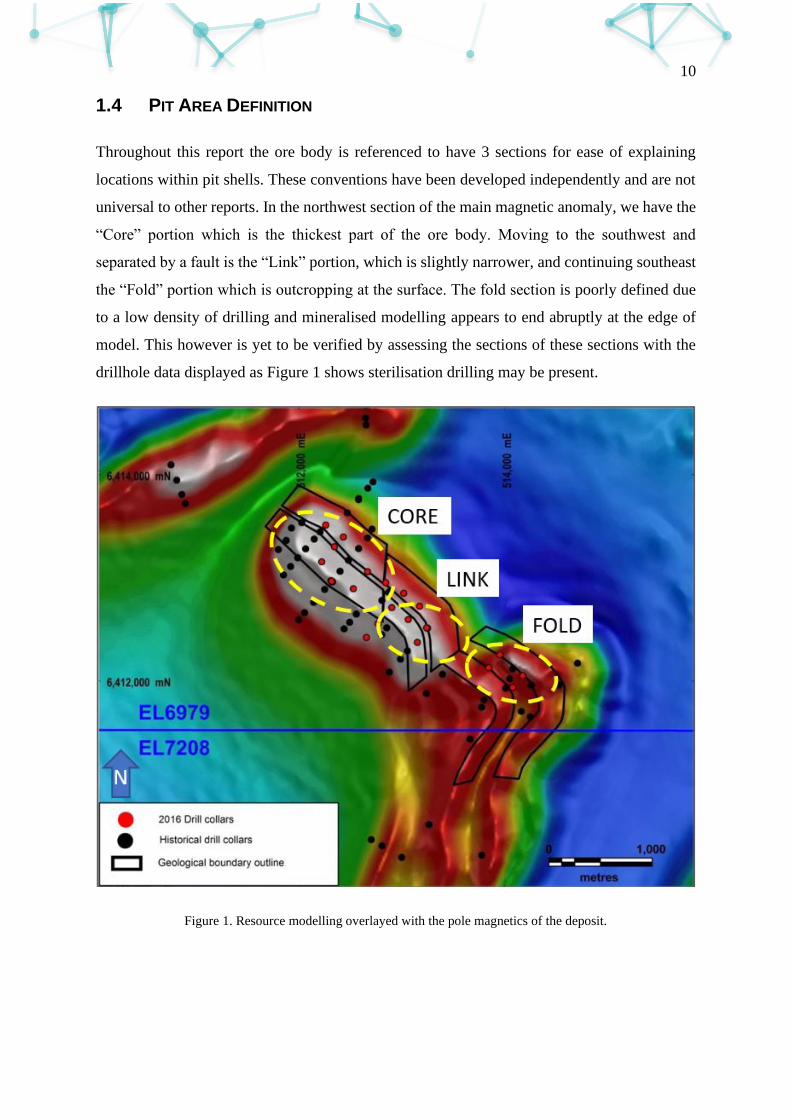
10

1.4 PIT AREA DEFINITION

Throughout this report the ore body is referenced to have 3 sections for ease of explaining

locations within pit shells. These conventions have been developed independently and are not

universal to other reports. In the northwest section of the main magnetic anomaly, we have the

“Core” portion which is the thickest part of the ore body. Moving to the southwest and

separated by a fault is the “Link” portion, which is slightly narrower, and continuing southeast

the “Fold” portion which is outcropping at the surface. The fold section is poorly defined due

to a low density of drilling and mineralised modelling appears to end abruptly at the edge of

model. This however is yet to be verified by assessing the sections of these sections with the

drillhole data displayed as Figure 1 shows sterilisation drilling may be present.

Figure 1. Resource modelling overlayed with the pole magnetics of the deposit.

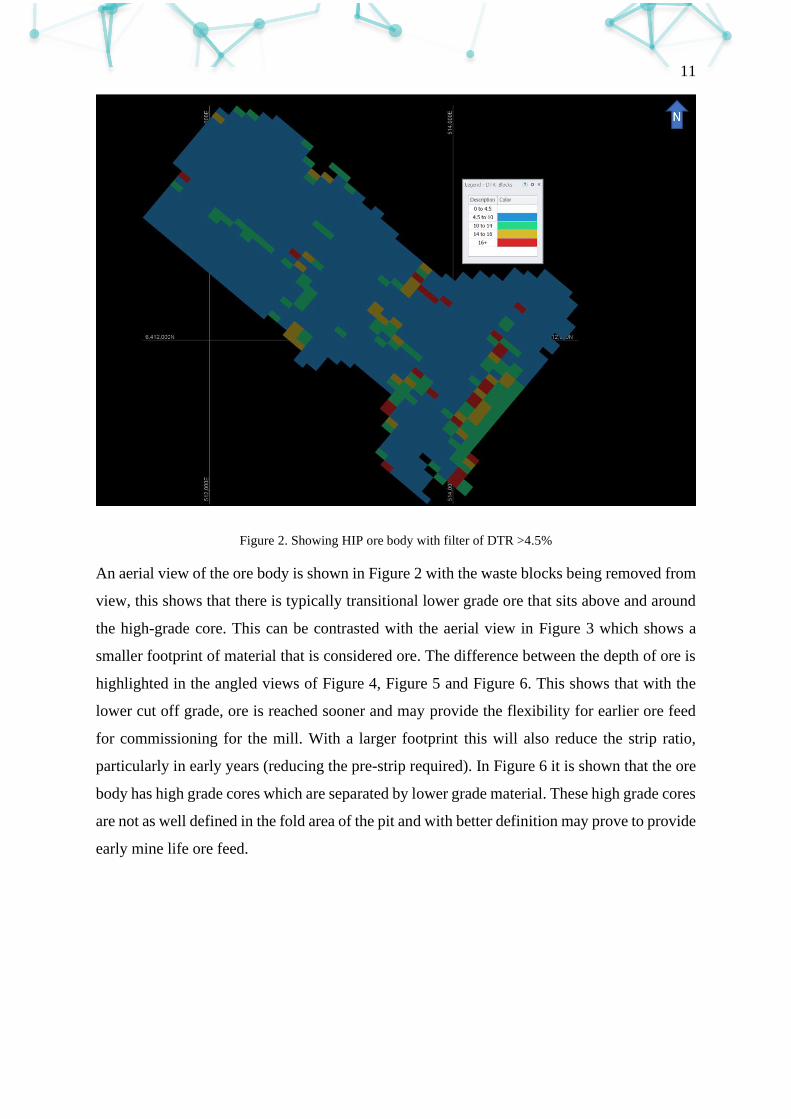
11

Figure 2. Showing HIP ore body with filter of DTR >4.5%

An aerial view of the ore body is shown in Figure 2 with the waste blocks being removed from

view, this shows that there is typically transitional lower grade ore that sits above and around

the high-grade core. This can be contrasted with the aerial view in Figure 3 which shows a

smaller footprint of material that is considered ore. The difference between the depth of ore is

highlighted in the angled views of Figure 4, Figure 5 and Figure 6. This shows that with the

lower cut off grade, ore is reached sooner and may provide the flexibility for earlier ore feed

for commissioning for the mill. With a larger footprint this will also reduce the strip ratio,

particularly in early years (reducing the pre-strip required). In Figure 6 it is shown that the ore

body has high grade cores which are separated by lower grade material. These high grade cores

are not as well defined in the fold area of the pit and with better definition may prove to provide

early mine life ore feed.

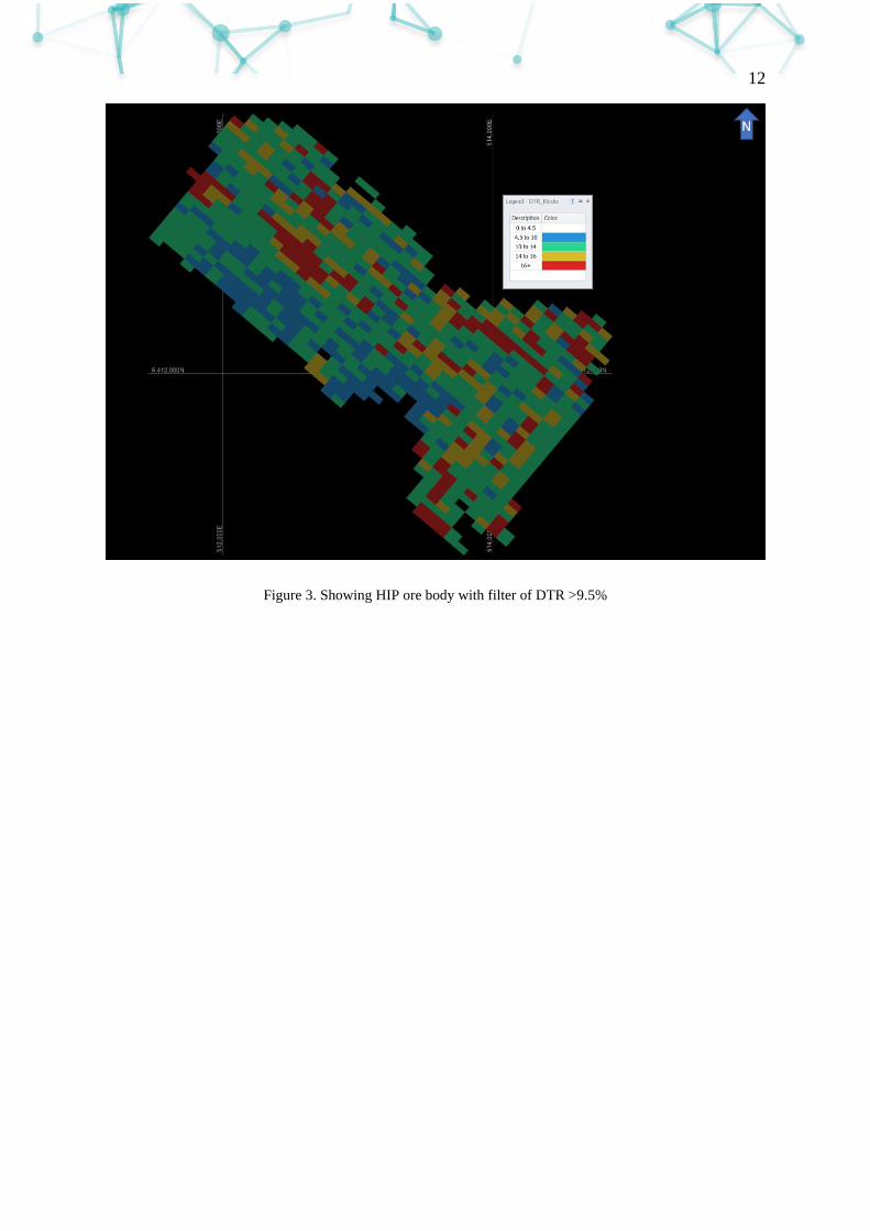
12

Figure 3. Showing HIP ore body with filter of DTR >9.5%

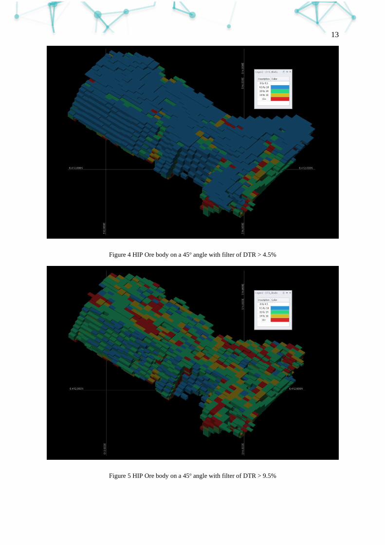
13

Figure 4 HIP Ore body on a 45o angle with filter of DTR > 4.5%

Figure 5 HIP Ore body on a 45o angle with filter of DTR > 9.5%

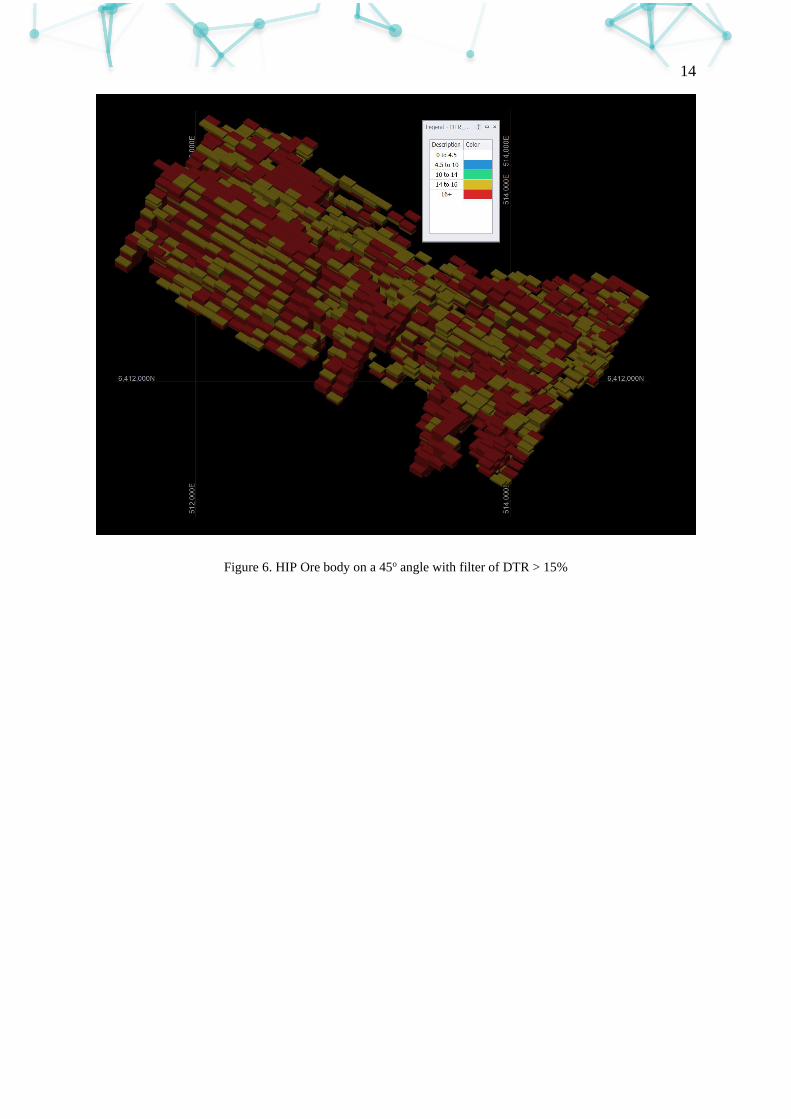
14

Figure 6. HIP Ore body on a 45o angle with filter of DTR > 15%

15

2 PIT OPTIMISATION

2.1 INTRODUCTION

Broadly before a block model can be optimised, cost and revenue variables must be assigned

to each block after which they can be fed into a network flow algorithm. Whilst the Lerchs-

Grossmann algorithm is typically used, for this project we have applied Deswik’s Pseudoflow

algorithm which is computationally more efficient whilst delivering the same result. This has

enabled many scenarios to be run in a far shorter timeframe, whilst also allowing for a greater

degree of control over the variables. Industry standards have been used for the definition of

these variables which will save time going forward once finer optimisation is applied.

2.2 CLASSIFICATION OF PARAMETERS

Before the algorithm can be run the software must assign an ore or waste property to each

block. This can be done several ways however in this model we have assumed a mandatory

10% margin is required on each block. This is done on a twofold basis, the first determining if

an ore block is economic (via a mining Lerchs Grossman 3-d algorithm) and then once a pit

envelope has been determined off the raw economics defining if it is more economic for a block

to be treated as ore or as waste.

𝐶𝑢𝑡𝑜𝑓𝑓 𝐿𝐺 𝑆ℎ𝑒𝑙𝑙 ($

𝑡𝑜𝑟𝑒) =

𝐶+𝑀+𝑃+𝐼+𝑇+𝐴+𝑅

𝐷𝑇𝑅 (1)

Where all costs are on a per tonne of rock processed basis:

• C = Capital Cost ($0.62/t ore) (Source: Calculated from page 8 of PFS using assumptions from PFS*)

• M = Mining Cost ($2.29/t ore) (Source: Calculated from page 8 of PFS using assumptions from PFS*)

• P = Processing Cost ($1.56/t ore) (Source: Calculated from page 8 of PFS using assumptions from PFS*)

• I = Infrastructure Cost ($0.18/t ore) (Source: Calculated from page 8 of PFS using assumptions from PFS*)

• T = Transport Cost ($1.66/t ore) (Source: Calculated from page 8 of PFS using assumptions from PFS*)

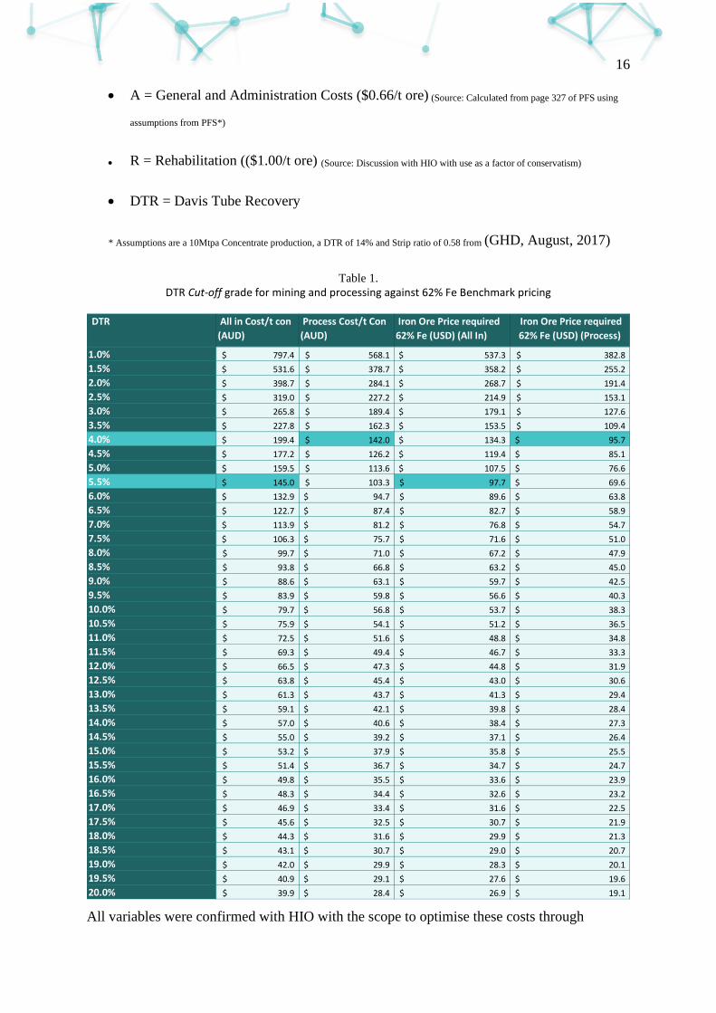
16

• A = General and Administration Costs ($0.66/t ore) (Source: Calculated from page 327 of PFS using

assumptions from PFS*)

• R = Rehabilitation (($1.00/t ore) (Source: Discussion with HIO with use as a factor of conservatism)

• DTR = Davis Tube Recovery

* Assumptions are a 10Mtpa Concentrate production, a DTR of 14% and Strip ratio of 0.58 from (GHD, August, 2017)

Table 1.

DTR Cut-off grade for mining and processing against 62% Fe Benchmark pricing

All variables were confirmed with HIO with the scope to optimise these costs through

DTR All in Cost/t con

(AUD)

Process Cost/t Con

(AUD)

Iron Ore Price required

62% Fe (USD) (All In)

Iron Ore Price required

62% Fe (USD) (Process)

1.0% 797.4$ 568.1$ 537.3$ 382.8$

1.5% 531.6$ 378.7$ 358.2$ 255.2$

2.0% 398.7$ 284.1$ 268.7$ 191.4$

2.5% 319.0$ 227.2$ 214.9$ 153.1$

3.0% 265.8$ 189.4$ 179.1$ 127.6$

3.5% 227.8$ 162.3$ 153.5$ 109.4$

4.0% 199.4$ 142.0$ 134.3$ 95.7$

4.5% 177.2$ 126.2$ 119.4$ 85.1$

5.0% 159.5$ 113.6$ 107.5$ 76.6$

5.5% 145.0$ 103.3$ 97.7$ 69.6$

6.0% 132.9$ 94.7$ 89.6$ 63.8$

6.5% 122.7$ 87.4$ 82.7$ 58.9$

7.0% 113.9$ 81.2$ 76.8$ 54.7$

7.5% 106.3$ 75.7$ 71.6$ 51.0$

8.0% 99.7$ 71.0$ 67.2$ 47.9$

8.5% 93.8$ 66.8$ 63.2$ 45.0$

9.0% 88.6$ 63.1$ 59.7$ 42.5$

9.5% 83.9$ 59.8$ 56.6$ 40.3$

10.0% 79.7$ 56.8$ 53.7$ 38.3$

10.5% 75.9$ 54.1$ 51.2$ 36.5$

11.0% 72.5$ 51.6$ 48.8$ 34.8$

11.5% 69.3$ 49.4$ 46.7$ 33.3$

12.0% 66.5$ 47.3$ 44.8$ 31.9$

12.5% 63.8$ 45.4$ 43.0$ 30.6$

13.0% 61.3$ 43.7$ 41.3$ 29.4$

13.5% 59.1$ 42.1$ 39.8$ 28.4$

14.0% 57.0$ 40.6$ 38.4$ 27.3$

14.5% 55.0$ 39.2$ 37.1$ 26.4$

15.0% 53.2$ 37.9$ 35.8$ 25.5$

15.5% 51.4$ 36.7$ 34.7$ 24.7$

16.0% 49.8$ 35.5$ 33.6$ 23.9$

16.5% 48.3$ 34.4$ 32.6$ 23.2$

17.0% 46.9$ 33.4$ 31.6$ 22.5$

17.5% 45.6$ 32.5$ 30.7$ 21.9$

18.0% 44.3$ 31.6$ 29.9$ 21.3$

18.5% 43.1$ 30.7$ 29.0$ 20.7$

19.0% 42.0$ 29.9$ 28.3$ 20.1$

19.5% 40.9$ 29.1$ 27.6$ 19.6$

20.0% 39.9$ 28.4$ 26.9$ 19.1$

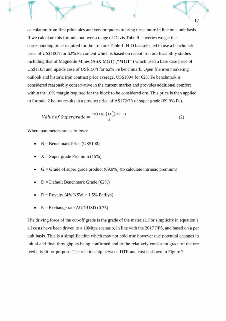
17

calculation from first principles and vendor quotes to bring these more in line on a unit basis.

If we calculate this formula out over a range of Davis Tube Recoveries we get the

corresponding price required for the iron ore Table 1. HIO has selected to use a benchmark

price of US$100/t for 62% Fe content which is based on recent iron ore feasibility studies

including that of Magnetite Mines (ASX:MGT) (“MGT”) which used a base case price of

US$110/t and upside case of US$150/t for 62% Fe benchmark. Open file iron marketing

outlook and historic iron contract price average, US$100/t for 62% Fe benchmark is

considered reasonably conservative in the current market and provides additional comfort

within the 10% margin required for the block to be considered ore. This price is then applied

to formula 2 below results in a product price of A$172/7/t of super grade (69.9% Fe).

𝑉𝑎𝑙𝑢𝑒 𝑜𝑓 𝑆𝑢𝑝𝑒𝑟𝑔𝑟𝑎𝑑𝑒 =𝐵∗(1+X)∗(1+

G

D)∗(1−R)

𝐸 (2)

Where parameters are as follows:

• B = Benchmark Price (US$100)

• X = Super grade Premium (15%)

• G = Grade of super grade product (69.9%) (to calculate intrinsic premium)

• D = Default Benchmark Grade (62%)

• R = Royalty (4% NSW + 1.5% Perilya)

• E = Exchange rate AUD:USD (0.75)

The driving force of the cut-off grade is the grade of the material. For simplicity in equation 1

all costs have been driven to a 10Mtpa scenario, in line with the 2017 PFS, and based on a per

unit basis. This is a simplification which may not hold true however due potential changes in

initial and final throughputs being confirmed and to the relatively consistent grade of the ore

feed it is fit for purpose. The relationship between DTR and cost is shown in Figure 7.

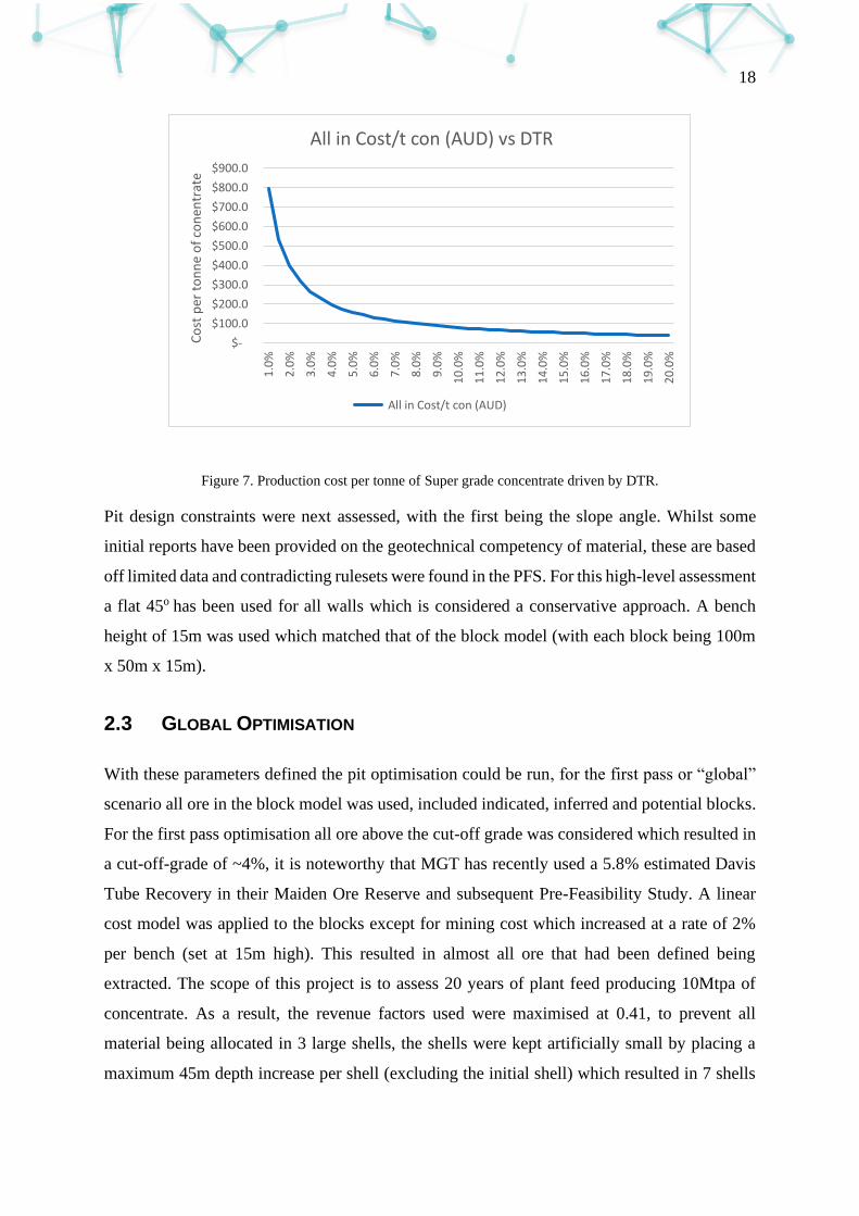
18

Figure 7. Production cost per tonne of Super grade concentrate driven by DTR.

Pit design constraints were next assessed, with the first being the slope angle. Whilst some

initial reports have been provided on the geotechnical competency of material, these are based

off limited data and contradicting rulesets were found in the PFS. For this high-level assessment

a flat 45o has been used for all walls which is considered a conservative approach. A bench

height of 15m was used which matched that of the block model (with each block being 100m

x 50m x 15m).

2.3 GLOBAL OPTIMISATION

With these parameters defined the pit optimisation could be run, for the first pass or “global”

scenario all ore in the block model was used, included indicated, inferred and potential blocks.

For the first pass optimisation all ore above the cut-off grade was considered which resulted in

a cut-off-grade of ~4%, it is noteworthy that MGT has recently used a 5.8% estimated Davis

Tube Recovery in their Maiden Ore Reserve and subsequent Pre-Feasibility Study. A linear

cost model was applied to the blocks except for mining cost which increased at a rate of 2%

per bench (set at 15m high). This resulted in almost all ore that had been defined being

extracted. The scope of this project is to assess 20 years of plant feed producing 10Mtpa of

concentrate. As a result, the revenue factors used were maximised at 0.41, to prevent all

material being allocated in 3 large shells, the shells were kept artificially small by placing a

maximum 45m depth increase per shell (excluding the initial shell) which resulted in 7 shells

$-

$100.0

$200.0

$300.0

$400.0

$500.0

$600.0

$700.0

$800.0

$900.0

1.0

%

2.0

%

3.0

%

4.0

%

5.0

%

6.0

%

7.0

%

8.0

%

9.0

%

10

.0%

11

.0%

12

.0%

13

.0%

14

.0%

15

.0%

16

.0%

17

.0%

18

.0%

19

.0%

20

.0%

Co

st p

er t

on

ne

of

con

entr

ate

All in Cost/t con (AUD) vs DTR

All in Cost/t con (AUD)

19

to give the result. The first shell is in the fold region which gives a total concentrate tonnage of

just under 3Mt. This could prove to be a good ore source for commissioning of the processing

plant.

To meet the 20 year, mine life at a production rate of 10Mtpa concentrate a revenue factor of

0.41 was used. This resulted in 224 Mt of concentrate with a grade of 69.77%, requiring the

mining of 515.6Mt of waste and 1,692Mt of ore for a total material movement of 2,208Mt,

which results in a strip ratio of 0.3. The outcomes are shown below in Figure 8.

Figure 8. Pit Optimisation by revenue factor (Pit number) for entire deposit

There is a minor amount of material which is sourced from a starter pit in the Fold region in

the top right corner. Following this a larger pit is then sunk (Pit shell number 2) in the Core

area of the ore body which is progressively developed to a total depth of 510m through to pit

shell number 6. The next significant development is in pit shell number 7 where the two

separate pits are linked (this is indicated by the light grey pit in Figure 8). The amount of ore

and waste is detailed in Figure 9, it should be noted that whilst the optimiser has shown two

major pushbacks (being that of pit 2 and 7) in reality these can be done incrementally such that

excessive waste won’t have to be moved in single years. This will be able to be optimised under

a scheduling with real world constraints scenario, following mine design.

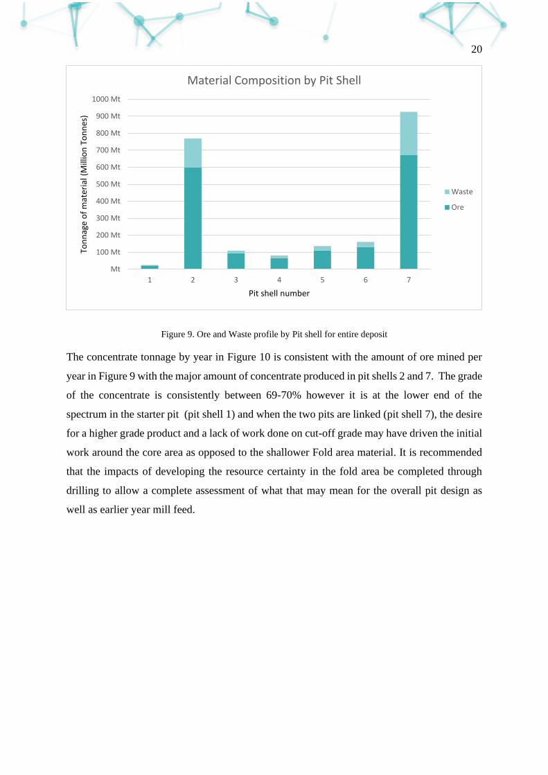
20

Figure 9. Ore and Waste profile by Pit shell for entire deposit

The concentrate tonnage by year in Figure 10 is consistent with the amount of ore mined per

year in Figure 9 with the major amount of concentrate produced in pit shells 2 and 7. The grade

of the concentrate is consistently between 69-70% however it is at the lower end of the

spectrum in the starter pit (pit shell 1) and when the two pits are linked (pit shell 7), the desire

for a higher grade product and a lack of work done on cut-off grade may have driven the initial

work around the core area as opposed to the shallower Fold area material. It is recommended

that the impacts of developing the resource certainty in the fold area be completed through

drilling to allow a complete assessment of what that may mean for the overall pit design as

well as earlier year mill feed.

Mt

100 Mt

200 Mt

300 Mt

400 Mt

500 Mt

600 Mt

700 Mt

800 Mt

900 Mt

1000 Mt

1 2 3 4 5 6 7

Ton

nag

e o

f m

ater

ial (

Mill

ion

To

nn

es)

Pit shell number

Material Composition by Pit Shell

Waste

Ore

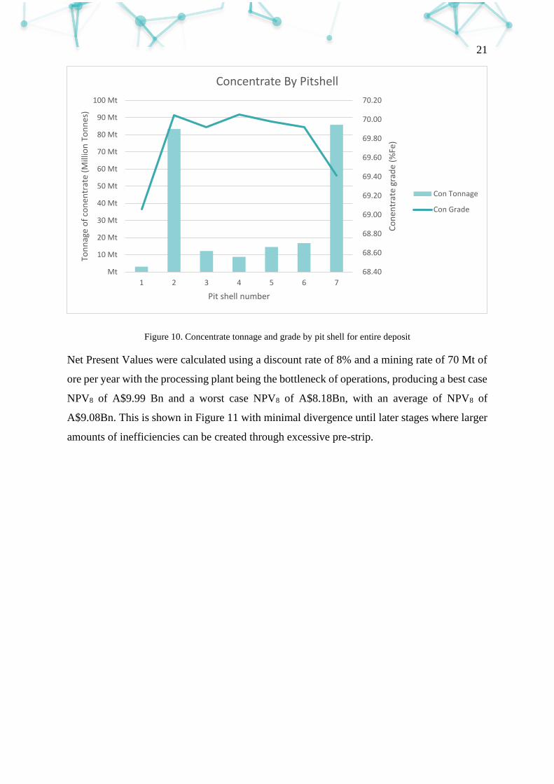
21

Figure 10. Concentrate tonnage and grade by pit shell for entire deposit

Net Present Values were calculated using a discount rate of 8% and a mining rate of 70 Mt of

ore per year with the processing plant being the bottleneck of operations, producing a best case

NPV8 of A$9.99 Bn and a worst case NPV8 of A$8.18Bn, with an average of NPV8 of

A$9.08Bn. This is shown in Figure 11 with minimal divergence until later stages where larger

amounts of inefficiencies can be created through excessive pre-strip.

68.40

68.60

68.80

69.00

69.20

69.40

69.60

69.80

70.00

70.20

Mt

10 Mt

20 Mt

30 Mt

40 Mt

50 Mt

60 Mt

70 Mt

80 Mt

90 Mt

100 Mt

1 2 3 4 5 6 7

Co

nen

trat

e gr

ade

(%Fe

)

Ton

nag

e o

f co

nen

trat

e (M

illio

n T

on

nes

)

Pit shell number

Concentrate By Pitshell

Con Tonnage

Con Grade

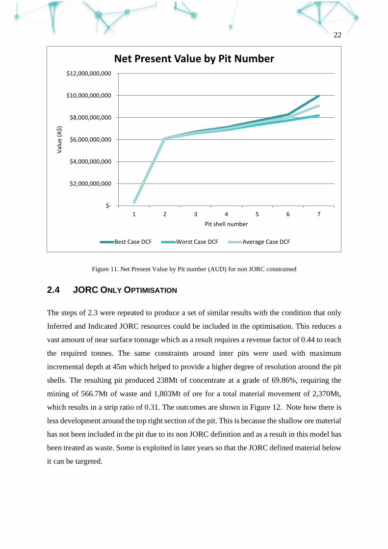
22

Figure 11. Net Present Value by Pit number (AUD) for non JORC constrained

2.4 JORC ONLY OPTIMISATION

The steps of 2.3 were repeated to produce a set of similar results with the condition that only

Inferred and Indicated JORC resources could be included in the optimisation. This reduces a

vast amount of near surface tonnage which as a result requires a revenue factor of 0.44 to reach

the required tonnes. The same constraints around inter pits were used with maximum

incremental depth at 45m which helped to provide a higher degree of resolution around the pit

shells. The resulting pit produced 238Mt of concentrate at a grade of 69.86%, requiring the

mining of 566.7Mt of waste and 1,803Mt of ore for a total material movement of 2,370Mt,

which results in a strip ratio of 0.31. The outcomes are shown in Figure 12. Note how there is

less development around the top right section of the pit. This is because the shallow ore material

has not been included in the pit due to its non JORC definition and as a result in this model has

been treated as waste. Some is exploited in later years so that the JORC defined material below

it can be targeted.

$-

$2,000,000,000

$4,000,000,000

$6,000,000,000

$8,000,000,000

$10,000,000,000

$12,000,000,000

1 2 3 4 5 6 7

Val

ue

(A$

)

Pit shell number

Net Present Value by Pit Number

Best Case DCF Worst Case DCF Average Case DCF

23

Figure 12. Pit Optimisation by revenue factor (Pit Number) for JORC portion of deposit

As a result the starter pit, shown in green in Figure 12 has a smaller footprint and does not

extend as far as the pit in Figure 8 due to the exclusion of exploration target. This also has the

consequence of a smaller tonnage leading to a larger revenue factor having to be used for

pitshell 2 in Figure 13 with a higher proportion of waste.

Figure 13. Ore and Waste profile by Pit shell for JORC component of deposit

Mt

100 Mt

200 Mt

300 Mt

400 Mt

500 Mt

600 Mt

700 Mt

800 Mt

1 2 3 4 5 6 7 8 9 10

Ton

nag

e o

f m

ater

ial (

Mill

ion

To

nn

es)

Pit shell number

Material Composition by Pitshell

Waste

Ore

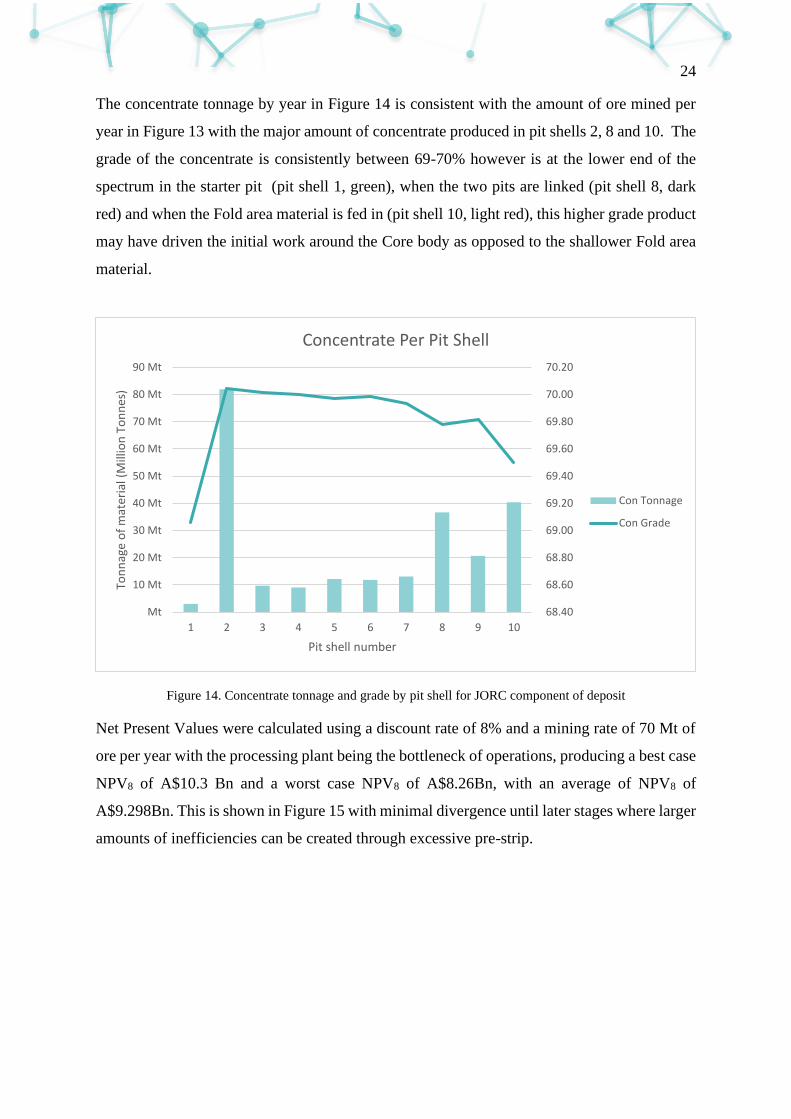
24

The concentrate tonnage by year in Figure 14 is consistent with the amount of ore mined per

year in Figure 13 with the major amount of concentrate produced in pit shells 2, 8 and 10. The

grade of the concentrate is consistently between 69-70% however is at the lower end of the

spectrum in the starter pit (pit shell 1, green), when the two pits are linked (pit shell 8, dark

red) and when the Fold area material is fed in (pit shell 10, light red), this higher grade product

may have driven the initial work around the Core body as opposed to the shallower Fold area

material.

Figure 14. Concentrate tonnage and grade by pit shell for JORC component of deposit

Net Present Values were calculated using a discount rate of 8% and a mining rate of 70 Mt of

ore per year with the processing plant being the bottleneck of operations, producing a best case

NPV8 of A$10.3 Bn and a worst case NPV8 of A$8.26Bn, with an average of NPV8 of

A$9.298Bn. This is shown in Figure 15 with minimal divergence until later stages where larger

amounts of inefficiencies can be created through excessive pre-strip.

68.40

68.60

68.80

69.00

69.20

69.40

69.60

69.80

70.00

70.20

Mt

10 Mt

20 Mt

30 Mt

40 Mt

50 Mt

60 Mt

70 Mt

80 Mt

90 Mt

1 2 3 4 5 6 7 8 9 10

Ton

nag

e o

f m

ater

ial (

Mill

ion

To

nn

es)

Pit shell number

Concentrate Per Pit Shell

Con Tonnage

Con Grade

25

Figure 15. Net Present Value by Pit number (AUD) for JORC component of deposit

$-

$2,000,000,000

$4,000,000,000

$6,000,000,000

$8,000,000,000

$10,000,000,000

$12,000,000,000

1 2 3 4 5 6 7 8 9 10

Val

ue

(A$

)

Pit shell number

Net Present Value by Pit Number

Best Case DCF Worst Case DCF Average Case DCF

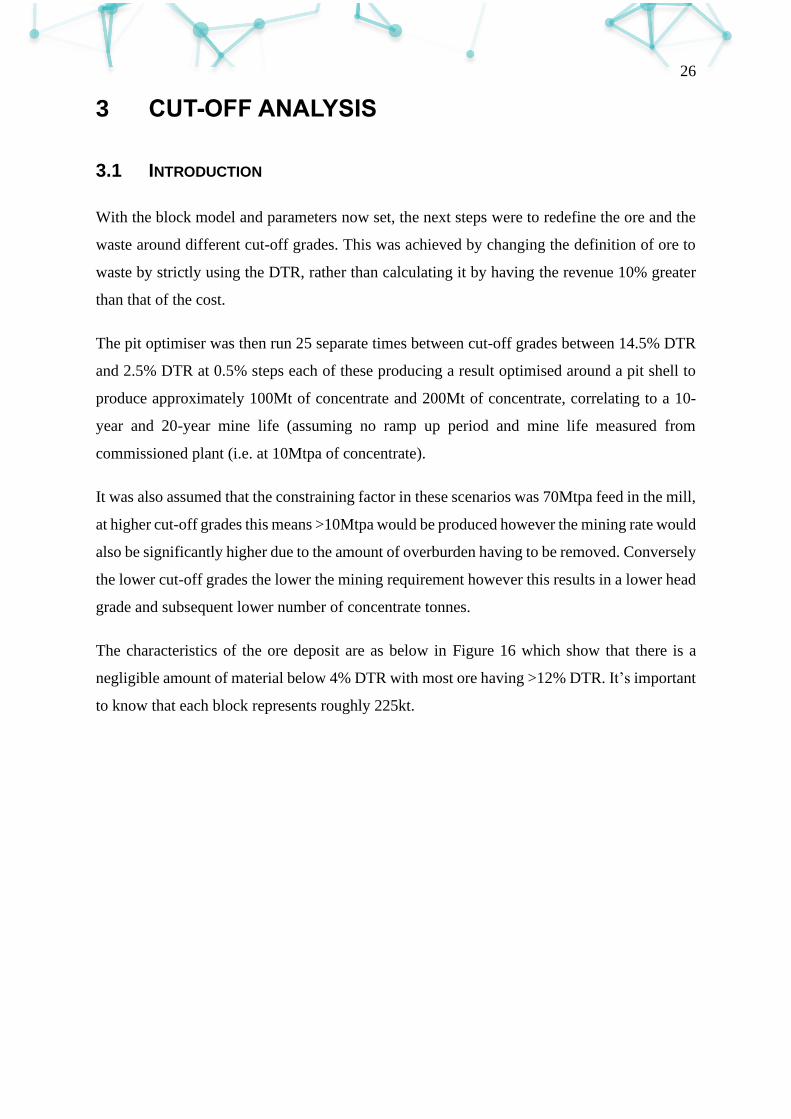
26

3 CUT-OFF ANALYSIS

3.1 INTRODUCTION

With the block model and parameters now set, the next steps were to redefine the ore and the

waste around different cut-off grades. This was achieved by changing the definition of ore to

waste by strictly using the DTR, rather than calculating it by having the revenue 10% greater

than that of the cost.

The pit optimiser was then run 25 separate times between cut-off grades between 14.5% DTR

and 2.5% DTR at 0.5% steps each of these producing a result optimised around a pit shell to

produce approximately 100Mt of concentrate and 200Mt of concentrate, correlating to a 10-

year and 20-year mine life (assuming no ramp up period and mine life measured from

commissioned plant (i.e. at 10Mtpa of concentrate).

It was also assumed that the constraining factor in these scenarios was 70Mtpa feed in the mill,

at higher cut-off grades this means >10Mtpa would be produced however the mining rate would

also be significantly higher due to the amount of overburden having to be removed. Conversely

the lower cut-off grades the lower the mining requirement however this results in a lower head

grade and subsequent lower number of concentrate tonnes.

The characteristics of the ore deposit are as below in Figure 16 which show that there is a

negligible amount of material below 4% DTR with most ore having >12% DTR. It’s important

to know that each block represents roughly 225kt.

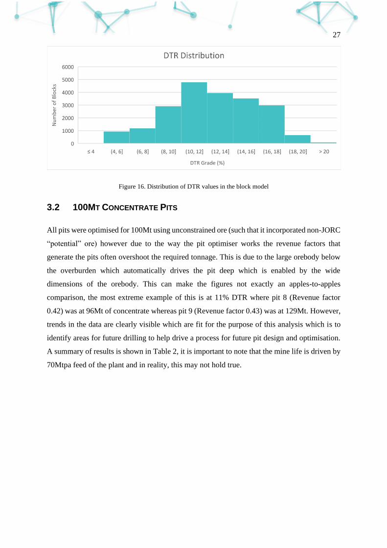
27

Figure 16. Distribution of DTR values in the block model

3.2 100MT CONCENTRATE PITS

All pits were optimised for 100Mt using unconstrained ore (such that it incorporated non-JORC

“potential” ore) however due to the way the pit optimiser works the revenue factors that

generate the pits often overshoot the required tonnage. This is due to the large orebody below

the overburden which automatically drives the pit deep which is enabled by the wide

dimensions of the orebody. This can make the figures not exactly an apples-to-apples

comparison, the most extreme example of this is at 11% DTR where pit 8 (Revenue factor

0.42) was at 96Mt of concentrate whereas pit 9 (Revenue factor 0.43) was at 129Mt. However,

trends in the data are clearly visible which are fit for the purpose of this analysis which is to

identify areas for future drilling to help drive a process for future pit design and optimisation.

A summary of results is shown in Table 2, it is important to note that the mine life is driven by

70Mtpa feed of the plant and in reality, this may not hold true.

28

Table 2.

Summary of results from 100Mt Concentrate Scenarios

One of the biggest drivers the cut-off grade has is moving the average grade of the material up

and increasing the strip ratio (and therefore the total amount of material movement required).

This is shown in Figure 17 which holds true despite the varying total concentrate tonnage. The

average grade varies from 12.9% to 16.6% from a DTR cut-off of 2.5% to 14.5% respectfully.

Cutoff Average

Depth

Mine

Life Cash Flow DCF

Total Material

Movement Ore Waste

Strip

Ratio DTR Concentrate

2.5% 171 11.1 10,507,070,918$ 6,750,648,330$ 899,572,284 779,633,635 119,938,649 0.15 13% 100,504,870

3.0% 176 12.0 11,460,603,003$ 6,820,824,954$ 991,698,085 837,248,936 154,449,149 0.18 13% 109,694,663

3.5% 175 11.8 11,506,903,267$ 6,418,898,845$ 1,000,249,360 825,295,736 174,953,624 0.21 13% 109,936,140

4.0% 174 11.4 11,337,525,001$ 5,931,761,833$ 984,427,585 797,518,586 186,908,999 0.23 14% 107,972,055

4.5% 174 11.2 11,277,787,362$ 5,597,130,815$ 984,427,585 781,488,911 202,938,674 0.26 14% 107,289,440

5.0% 174 11.0 11,255,215,430$ 5,301,113,484$ 988,593,460 770,123,936 218,469,524 0.28 14% 107,014,531

5.5% 174 10.8 11,169,779,508$ 5,015,344,611$ 986,833,960 756,084,911 230,749,049 0.31 14% 106,172,047

6.0% 174 10.6 11,085,218,228$ 7,106,279,357$ 986,467,210 743,701,136 242,766,074 0.33 14% 105,403,527

6.5% 174 10.5 11,017,946,558$ 7,112,845,202$ 986,033,860 734,377,886 251,655,974 0.34 14% 104,796,519

7.0% 173 10.1 10,700,397,427$ 7,028,581,264$ 964,576,210 706,990,211 257,585,999 0.36 14% 101,802,117

7.5% 173 10.0 10,634,409,575$ 7,026,585,036$ 964,576,210 699,282,386 265,293,824 0.38 14% 101,244,435

8.0% 179 11.0 11,702,314,726$ 7,480,977,460$ 1,073,305,510 772,169,112 301,136,399 0.39 14% 111,846,683

8.5% 174 9.7 10,376,199,009$ 6,990,537,873$ 960,786,310 678,951,686 281,834,624 0.42 15% 99,168,011

9.0% 177 10.3 11,028,042,762$ 7,291,706,512$ 1,035,523,585 722,155,212 313,368,374 0.43 15% 105,820,828

9.5% 175 9.7 10,431,260,551$ 7,064,768,791$ 991,643,860 679,260,911 312,382,949 0.46 15% 100,260,321

10.0% 175 9.9 10,738,475,044$ 7,159,182,734$ 1,036,251,461 695,936,187 340,315,274 0.49 15% 103,533,169

10.5% 177 10.3 11,029,695,407$ 7,331,145,152$ 1,109,522,336 719,872,287 389,650,049 0.54 15% 107,532,617

11.0% 171 12.3 13,000,775,175$ 8,023,837,280$ 1,416,755,713 863,029,740 553,725,973 0.64 15% 129,406,957

11.5% 177 9.9 10,710,486,117$ 7,195,891,513$ 1,148,764,211 693,647,937 455,116,273 0.66 15% 105,961,406

12.0% 177 9.4 10,136,731,626$ 6,963,927,763$ 1,132,847,860 654,583,737 478,264,124 0.73 15% 101,310,193

12.5% 169 10.3 11,024,108,868$ 7,266,747,603$ 1,352,174,636 723,073,063 629,101,573 0.87 16% 113,065,551

13.0% 162 10.0 10,524,912,028$ 7,015,185,284$ 1,405,406,860 698,110,661 707,296,199 1.01 16% 110,758,283

13.5% 175 9.3 9,807,010,748$ 6,693,571,924$ 1,371,179,858 651,693,309 719,486,549 1.10 16% 105,035,549

14.0% 149 9.7 9,690,614,917$ 6,463,477,991$ 1,654,279,880 680,544,907 973,734,973 1.43 16% 110,913,991

14.5% 153 8.8 8,510,577,986$ 5,873,724,694$ 1,635,415,204 617,046,756 1,018,368,448 1.65 17% 102,175,645

Cutoff

Maximum

Depth

Mine

Life Cash Flow DCF

Total Material

Movement Ore Waste

Strip


2.5% 495 11.1 10,507,070,918$ 6,750,648,330$ 899,572,284 779,633,635 119,938,649 0.15 13% 100,504,870

3.0% 525 12.0 11,460,603,003$ 6,820,824,954$ 991,698,085 837,248,936 154,449,149 0.18 13% 109,694,663

3.5% 525 11.8 11,506,903,267$ 6,418,898,845$ 1,000,249,360 825,295,736 174,953,624 0.21 13% 109,936,140

4.0% 510 11.4 11,337,525,001$ 5,931,761,833$ 984,427,585 797,518,586 186,908,999 0.23 14% 107,972,055

4.5% 510 11.2 11,277,787,362$ 5,597,130,815$ 984,427,585 781,488,911 202,938,674 0.26 14% 107,289,440

5.0% 510 11.0 11,255,215,430$ 5,301,113,484$ 988,593,460 770,123,936 218,469,524 0.28 14% 107,014,531

5.5% 510 10.8 11,169,779,508$ 5,015,344,611$ 986,833,960 756,084,911 230,749,049 0.31 14% 106,172,047

6.0% 510 10.6 11,085,218,228$ 7,106,279,357$ 986,467,210 743,701,136 242,766,074 0.33 14% 105,403,527

6.5% 510 10.5 11,017,946,558$ 7,112,845,202$ 986,033,860 734,377,886 251,655,974 0.34 14% 104,796,519

7.0% 510 10.1 10,700,397,427$ 7,028,581,264$ 964,576,210 706,990,211 257,585,999 0.36 14% 101,802,117

7.5% 510 10.0 10,634,409,575$ 7,026,585,036$ 964,576,210 699,282,386 265,293,824 0.38 14% 101,244,435

8.0% 540 11.0 11,702,314,726$ 7,480,977,460$ 1,073,305,510 772,169,112 301,136,399 0.39 14% 111,846,683

8.5% 510 9.7 10,376,199,009$ 6,990,537,873$ 960,786,310 678,951,686 281,834,624 0.42 15% 99,168,011

9.0% 525 10.3 11,028,042,762$ 7,291,706,512$ 1,035,523,585 722,155,212 313,368,374 0.43 15% 105,820,828

9.5% 510 9.7 10,431,260,551$ 7,064,768,791$ 991,643,860 679,260,911 312,382,949 0.46 15% 100,260,321

10.0% 510 9.9 10,738,475,044$ 7,159,182,734$ 1,036,251,461 695,936,187 340,315,274 0.49 15% 103,533,169

10.5% 555 10.3 11,029,695,407$ 7,331,145,152$ 1,109,522,336 719,872,287 389,650,049 0.54 15% 107,532,617

11.0% 555 12.3 13,000,775,175$ 8,023,837,280$ 1,416,755,713 863,029,740 553,725,973 0.64 15% 129,406,957

11.5% 540 9.9 10,710,486,117$ 7,195,891,513$ 1,148,764,211 693,647,937 455,116,273 0.66 15% 105,961,406

12.0% 540 9.4 10,136,731,626$ 6,963,927,763$ 1,132,847,860 654,583,737 478,264,124 0.73 15% 101,310,193

12.5% 540 10.3 11,024,108,868$ 7,266,747,603$ 1,352,174,636 723,073,063 629,101,573 0.87 16% 113,065,551

13.0% 540 10.0 10,524,912,028$ 7,015,185,284$ 1,405,406,860 698,110,661 707,296,199 1.01 16% 110,758,283

13.5% 540 9.3 9,807,010,748$ 6,693,571,924$ 1,371,179,858 651,693,309 719,486,549 1.10 16% 105,035,549

14.0% 465 9.7 9,690,614,917$ 6,463,477,991$ 1,654,279,880 680,544,907 973,734,973 1.43 16% 110,913,991

14.5% 510 8.8 8,510,577,986$ 5,873,724,694$ 1,635,415,204 617,046,756 1,018,368,448 1.65 17% 102,175,645

29

Figure 17. Strip ratio and average feed grade against the DTR Cut-off used 100Mt Con

The most important outcome of this exercise was assessing the discounted cashflow to assess

if there is a major change in NPV and what the best Cut-off grade is. This produced some

interesting results which are shown in Figure 18 and Figure 19. Most noticeably that there was

minimal effect on the NPV between a cut-off of 6.5% to 12.5% (the variations being driven by

larger or smaller pit shells). At 5.5% there is a sharp drop in NPV however as the breakeven

price for an ore block is approached (at 3.5% DTR) there is a boost in NPV. This is likely a

trade-off between early year feeding and not incurring the prestrip without revenue and reduced

revenue/opportunity cost of not feeding the mill with higher quality material. This trade-off

will be better understood with scheduling although it clearly shows the benefit of a dynamic

cut-off grade depending on the commodity price, and when combined with strategic stockpiling

will enable a boosted NPV.

12.0%12.5%13.0%13.5%14.0%14.5%15.0%15.5%16.0%16.5%17.0%

0.00

0.20

0.40

0.60

0.80

1.00

1.20

1.40

1.60

1.80

2.5 3

3.5 4

4.5 5

5.5 6

6.5 7

7.5 8

8.5 9

9.5 10

10

.5 11

11

.5 12

12

.5 13

13

.5 14

14

.5 Ave

rage

Fee

d G

rad

e (%

DTR

)

Stri

p R

atio

DTR Cut-off (%)

Strip Ratio by Cut-Off (100Mt Con)

Strip Ratio DTR

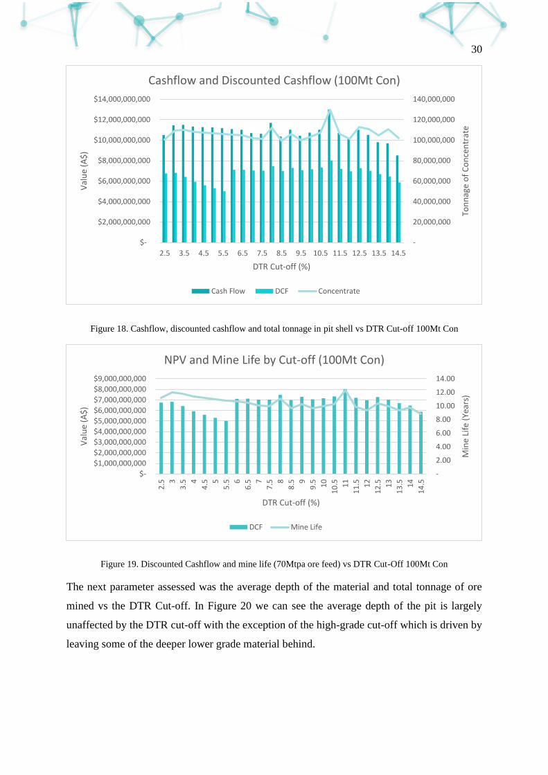
30

Figure 18. Cashflow, discounted cashflow and total tonnage in pit shell vs DTR Cut-off 100Mt Con


The next parameter assessed was the average depth of the material and total tonnage of ore

mined vs the DTR Cut-off. In Figure 20 we can see the average depth of the pit is largely

unaffected by the DTR cut-off with the exception of the high-grade cut-off which is driven by

leaving some of the deeper lower grade material behind.

-

20,000,000

40,000,000

60,000,000

80,000,000

100,000,000

120,000,000

140,000,000

$-

$2,000,000,000

$4,000,000,000

$6,000,000,000

$8,000,000,000

$10,000,000,000

$12,000,000,000

$14,000,000,000

2.5 3.5 4.5 5.5 6.5 7.5 8.5 9.5 10.5 11.5 12.5 13.5 14.5

Ton

nag

e o

f C

on

cen

trat

e

Val

ue

(A$

)

DTR Cut-off (%)

Cashflow and Discounted Cashflow (100Mt Con)

Cash Flow DCF Concentrate

-

2.00

4.00

6.00

8.00

10.00

12.00

14.00

$-

$1,000,000,000

$2,000,000,000

$3,000,000,000

$4,000,000,000

$5,000,000,000

$6,000,000,000

$7,000,000,000

$8,000,000,000

$9,000,000,000

2.5 3

3.5 4

4.5 5

5.5 6

6.5 7

7.5 8

8.5 9

9.5 10

10

.5 11

11

.5 12

12

.5 13

13

.5 14

14

.5

Min

e Li

fe (

Year

s)

Val

ue

(A$

)

DTR Cut-off (%)

NPV and Mine Life by Cut-off (100Mt Con)

DCF Mine Life

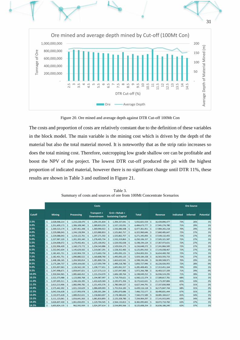
31

Figure 20. Ore mined and average depth against DTR Cut-off 100Mt Con

The costs and proportion of costs are relatively constant due to the definition of these variables

in the block model. The main variable is the mining cost which is driven by the depth of the

material but also the total material moved. It is noteworthy that as the strip ratio increases so

does the total mining cost. Therefore, outcropping low grade shallow ore can be profitable and

boost the NPV of the project. The lowest DTR cut-off produced the pit with the highest

proportion of indicated material, however there is no significant change until DTR 11%, these

results are shown in Table 3 and outlined in Figure 21.

Table 3.

Summary of costs and sources of ore from 100Mt Concentrate Scenarios

-

50

100

150

200

-

200,000,000

400,000,000

600,000,000

800,000,000

1,000,000,000

2.5 3

3.5 4

4.5 5

5.5 6

6.5 7

7.5 8

8.5 9

9.5 10

10

.5 11

11

.5 12

12

.5 13

13

.5 14

14

.5

Ave

rage

Dep

th o

f M

ater

ial M

ined

(m

)

Ton

nag

e o

f O

re

DTR Cut-off (%)

Ore mined and average depth mined by Cut-off (100Mt Con)

Ore Average Depth

Cutoff Mining Processing Transport +

Downstream

G+A + Rehab +

Sustaining Capital Total Revenue Indicated Inferred Potential

2.5% 2,028,068,214$ 1,216,228,470$ 1,294,191,834$ 1,394,337,041$ 5,932,825,559$ 16,439,896,477$ 73% 26% 1%

3.0% 2,251,600,173$ 1,306,108,340$ 1,389,833,233$ 1,537,132,031$ 6,484,673,777$ 17,945,276,780$ 71% 29% 1%

3.5% 2,269,523,174$ 1,287,461,348$ 1,369,990,922$ 1,550,386,508$ 6,477,361,951$ 17,984,265,218$ 70% 29% 1%

4.0% 2,229,088,043$ 1,244,128,994$ 1,323,880,853$ 1,525,862,757$ 6,322,960,646$ 17,660,485,647$ 72% 27% 1%

4.5% 2,229,088,043$ 1,219,122,701$ 1,297,271,592$ 1,525,862,757$ 6,271,345,093$ 17,549,132,455$ 72% 27% 1%

5.0% 2,237,987,220$ 1,201,393,340$ 1,278,405,734$ 1,532,319,863$ 6,250,106,157$ 17,505,321,587$ 72% 27% 1%

5.5% 2,234,008,072$ 1,179,492,461$ 1,255,100,952$ 1,529,592,638$ 6,198,194,124$ 17,367,973,631$ 72% 27% 1%

6.0% 2,232,906,439$ 1,160,173,772$ 1,234,543,886$ 1,529,024,175$ 6,156,648,272$ 17,241,866,500$ 72% 27% 1%

6.5% 2,232,042,634$ 1,145,629,502$ 1,219,067,291$ 1,528,352,483$ 6,125,091,910$ 17,143,038,467$ 72% 27% 1%

7.0% 2,182,401,751$ 1,102,904,729$ 1,173,603,750$ 1,495,093,125$ 5,954,003,355$ 16,654,400,782$ 72% 27% 1%

7.5% 2,182,401,751$ 1,090,880,522$ 1,160,808,760$ 1,495,093,125$ 5,929,184,158$ 16,563,593,733$ 72% 27% 1%

8.0% 2,448,186,165$ 1,204,583,814$ 1,281,800,726$ 1,663,623,541$ 6,598,194,246$ 18,300,508,971$ 70% 29% 1%

8.5% 2,175,284,737$ 1,059,164,630$ 1,127,059,799$ 1,489,218,780$ 5,850,727,946$ 16,226,926,955$ 72% 28% 0%

9.0% 2,355,007,063$ 1,126,562,130$ 1,198,777,651$ 1,605,061,557$ 6,285,408,401$ 17,313,451,164$ 70% 29% 1%

9.5% 2,247,998,671$ 1,059,647,021$ 1,127,573,113$ 1,537,047,983$ 5,972,266,788$ 16,403,527,339$ 71% 29% 0%

10.0% 2,350,944,965$ 1,085,660,452$ 1,155,254,070$ 1,606,189,764$ 6,198,049,252$ 16,936,524,295$ 71% 28% 1%

10.5% 2,522,373,988$ 1,123,000,768$ 1,194,987,997$ 1,719,759,621$ 6,560,122,374$ 17,589,817,781$ 68% 31% 1%

11.0% 3,197,695,511$ 1,346,326,395$ 1,432,629,369$ 2,195,971,356$ 8,172,622,631$ 21,173,397,806$ 65% 33% 2%

11.5% 2,613,213,906$ 1,082,090,782$ 1,151,455,576$ 1,780,584,527$ 6,627,344,791$ 17,337,830,908$ 67% 31% 2%

12.0% 2,575,442,302$ 1,021,150,629$ 1,086,609,003$ 1,755,914,183$ 6,439,116,118$ 16,575,847,744$ 68% 31% 2%

12.5% 3,042,556,628$ 1,127,993,978$ 1,200,301,284$ 2,095,870,686$ 7,466,722,577$ 18,490,831,444$ 67% 31% 2%

13.0% 3,133,975,628$ 1,089,052,631$ 1,158,863,697$ 2,178,380,633$ 7,560,272,589$ 18,085,184,617$ 65% 34% 1%

13.5% 3,111,123,061$ 1,016,641,563$ 1,081,810,893$ 2,125,328,780$ 7,334,904,297$ 17,141,915,045$ 63% 34% 3%

14.0% 3,626,607,430$ 1,061,650,055$ 1,129,704,545$ 2,564,133,813$ 8,382,095,843$ 18,072,710,760$ 63% 37% 1%

14.5% 3,603,824,135$ 962,592,939$ 1,024,297,614$ 2,534,893,566$ 8,125,608,254$ 16,636,186,240$ 62% 37% 1%

Costs Ore Source

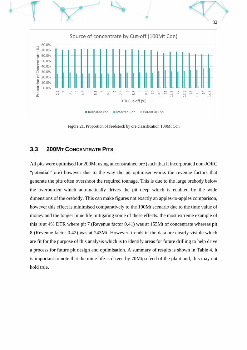
32

Figure 21. Proportion of feedstock by ore classification 100Mt Con

3.3 200MT CONCENTRATE PITS

All pits were optimised for 200Mt using unconstrained ore (such that it incorporated non-JORC

“potential” ore) however due to the way the pit optimiser works the revenue factors that

generate the pits often overshoot the required tonnage. This is due to the large orebody below

the overburden which automatically drives the pit deep which is enabled by the wide

dimensions of the orebody. This can make figures not exactly an apples-to-apples comparison,

however this effect is minimised comparatively to the 100Mt scenario due to the time value of

money and the longer mine life mitigating some of these effects. the most extreme example of

this is at 4% DTR where pit 7 (Revenue factor 0.41) was at 155Mt of concentrate whereas pit

8 (Revenue factor 0.42) was at 243Mt. However, trends in the data are clearly visible which

are fit for the purpose of this analysis which is to identify areas for future drilling to help drive

a process for future pit design and optimisation. A summary of results is shown in Table 4, it

is important to note that the mine life is driven by 70Mtpa feed of the plant and, this may not

hold true.

0.0%

10.0%

20.0%

30.0%

40.0%

50.0%

60.0%

70.0%

80.0%

2.5 3

3.5 4

4.5 5

5.5 6

6.5 7

7.5 8

8.5 9

9.5 10

10

.5 11

11

.5 12

12

.5 13

13

.5 14

14

.5

Pro

po

rtio

n o

f C

on

cen

trat

e (%

)

DTR Cut-off (%)

Source of concentrate by Cut-off (100Mt Con)

Indicated con Inferred Con Potential Con

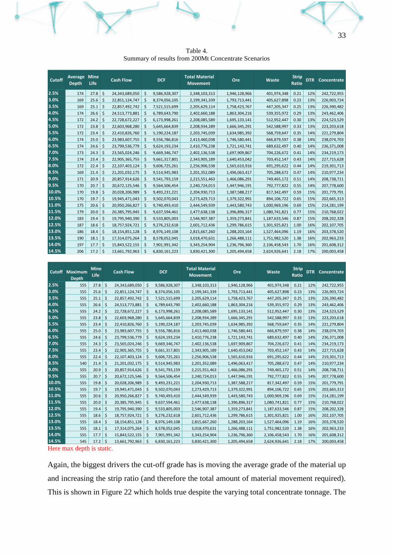
33

Table 4.

Summary of results from 200Mt Concentrate Scenarios

Here max depth is static.

Again, the biggest drivers the cut-off grade has is moving the average grade of the material up

and increasing the strip ratio (and therefore the total amount of material movement required).

This is shown in Figure 22 which holds true despite the varying total concentrate tonnage. The

Cutoff Average

Depth

Mine

Life Cash Flow DCF

Total Material

Movement Ore Waste

Strip


2.5% 174 27.8 24,343,689,050$ 9,586,928,307$ 2,348,103,313 1,946,128,966 401,974,348 0.21 12% 242,722,955

3.0% 169 25.6 22,851,124,747$ 8,374,056,105$ 2,199,341,339 1,793,713,441 405,627,898 0.23 13% 226,903,724

3.5% 169 25.1 22,857,492,742$ 7,521,515,699$ 2,205,629,114 1,758,423,767 447,205,347 0.25 13% 226,390,482

4.0% 174 26.6 24,513,773,881$ 6,789,643,790$ 2,402,660,188 1,863,304,216 539,355,972 0.29 13% 243,462,406

4.5% 172 24.2 22,728,672,227$ 6,173,998,261$ 2,208,085,589 1,695,133,141 512,952,447 0.30 13% 224,523,529

5.0% 172 23.8 22,603,968,280$ 5,645,664,839$ 2,208,934,289 1,666,345,291 542,588,997 0.33 13% 223,203,618

5.5% 172 23.4 22,410,826,760$ 5,190,224,187$ 2,203,745,039 1,634,985,392 568,759,647 0.35 14% 221,279,804

6.0% 174 25.0 23,983,607,755$ 9,556,786,816$ 2,413,460,038 1,746,580,441 666,879,597 0.38 14% 238,074,703

6.5% 174 24.6 23,799,536,779$ 9,624,193,234$ 2,410,776,238 1,721,143,741 689,632,497 0.40 14% 236,371,008

7.0% 173 24.3 23,565,024,246$ 9,669,346,747$ 2,402,136,538 1,697,909,867 704,226,672 0.41 14% 234,219,173

7.5% 174 23.4 22,905,365,755$ 9,661,317,801$ 2,343,905,189 1,640,453,042 703,452,147 0.43 14% 227,715,628

8.0% 172 22.4 22,107,403,124$ 9,606,725,261$ 2,256,906,538 1,565,610,916 691,295,622 0.44 14% 219,301,713

8.5% 169 21.4 21,201,032,175$ 9,514,945,983$ 2,201,352,089 1,496,063,417 705,288,672 0.47 14% 210,977,234

9.0% 171 20.9 20,857,914,626$ 9,541,793,159$ 2,215,551,463 1,466,086,291 749,465,172 0.51 14% 208,738,711

9.5% 170 20.7 20,672,125,546$ 9,564,506,454$ 2,240,724,013 1,447,946,191 792,777,822 0.55 14% 207,778,600

10.0% 170 19.8 20,028,206,989$ 9,493,231,221$ 2,204,930,713 1,387,588,217 817,342,497 0.59 15% 201,779,791

10.5% 170 19.7 19,945,471,043$ 9,502,070,043$ 2,273,429,713 1,379,322,991 894,106,722 0.65 15% 202,665,313

11.0% 175 20.6 20,950,266,827$ 9,740,493,410$ 2,444,549,939 1,443,580,743 1,000,969,196 0.69 15% 214,281,199

11.5% 179 20.0 20,385,795,945$ 9,637,594,461$ 2,477,638,138 1,396,896,317 1,080,741,821 0.77 15% 210,768,022

12.0% 183 19.4 19,795,940,390$ 9,533,805,003$ 2,546,907,387 1,359,273,841 1,187,633,546 0.87 15% 208,202,328

12.5% 187 18.6 18,757,924,721$ 9,276,232,618$ 2,601,712,436 1,299,786,615 1,301,925,821 1.00 16% 202,107,705

13.0% 186 18.4 18,154,851,128$ 8,976,149,108$ 2,815,667,260 1,288,203,164 1,527,464,096 1.19 16% 203,378,520

13.5% 190 18.1 17,314,075,264$ 8,578,052,045$ 3,018,470,631 1,266,488,111 1,751,982,520 1.38 16% 202,963,233

14.0% 197 17.7 15,843,522,155$ 7,901,991,342$ 3,343,254,904 1,236,796,360 2,106,458,543 1.70 16% 201,608,312

14.5% 206 17.2 13,661,792,963$ 6,830,161,223$ 3,830,421,300 1,205,494,658 2,624,926,641 2.18 17% 200,003,458

Cutoff

Maximum

Depth

Mine

Life Cash Flow DCF

Total Material

Movement Ore Waste

Strip


2.5% 555 27.8 24,343,689,050$ 9,586,928,307$ 2,348,103,313 1,946,128,966 401,974,348 0.21 12% 242,722,955

3.0% 555 25.6 22,851,124,747$ 8,374,056,105$ 2,199,341,339 1,793,713,441 405,627,898 0.23 13% 226,903,724

3.5% 555 25.1 22,857,492,742$ 7,521,515,699$ 2,205,629,114 1,758,423,767 447,205,347 0.25 13% 226,390,482

4.0% 555 26.6 24,513,773,881$ 6,789,643,790$ 2,402,660,188 1,863,304,216 539,355,972 0.29 13% 243,462,406

4.5% 555 24.2 22,728,672,227$ 6,173,998,261$ 2,208,085,589 1,695,133,141 512,952,447 0.30 13% 224,523,529

5.0% 555 23.8 22,603,968,280$ 5,645,664,839$ 2,208,934,289 1,666,345,291 542,588,997 0.33 13% 223,203,618

5.5% 555 23.4 22,410,826,760$ 5,190,224,187$ 2,203,745,039 1,634,985,392 568,759,647 0.35 14% 221,279,804

6.0% 555 25.0 23,983,607,755$ 9,556,786,816$ 2,413,460,038 1,746,580,441 666,879,597 0.38 14% 238,074,703

6.5% 555 24.6 23,799,536,779$ 9,624,193,234$ 2,410,776,238 1,721,143,741 689,632,497 0.40 14% 236,371,008

7.0% 555 24.3 23,565,024,246$ 9,669,346,747$ 2,402,136,538 1,697,909,867 704,226,672 0.41 14% 234,219,173

7.5% 555 23.4 22,905,365,755$ 9,661,317,801$ 2,343,905,189 1,640,453,042 703,452,147 0.43 14% 227,715,628

8.0% 555 22.4 22,107,403,124$ 9,606,725,261$ 2,256,906,538 1,565,610,916 691,295,622 0.44 14% 219,301,713

8.5% 540 21.4 21,201,032,175$ 9,514,945,983$ 2,201,352,089 1,496,063,417 705,288,672 0.47 14% 210,977,234

9.0% 555 20.9 20,857,914,626$ 9,541,793,159$ 2,215,551,463 1,466,086,291 749,465,172 0.51 14% 208,738,711

9.5% 555 20.7 20,672,125,546$ 9,564,506,454$ 2,240,724,013 1,447,946,191 792,777,822 0.55 14% 207,778,600

10.0% 555 19.8 20,028,206,989$ 9,493,231,221$ 2,204,930,713 1,387,588,217 817,342,497 0.59 15% 201,779,791

10.5% 555 19.7 19,945,471,043$ 9,502,070,043$ 2,273,429,713 1,379,322,991 894,106,722 0.65 15% 202,665,313

11.0% 555 20.6 20,950,266,827$ 9,740,493,410$ 2,444,549,939 1,443,580,743 1,000,969,196 0.69 15% 214,281,199

11.5% 555 20.0 20,385,795,945$ 9,637,594,461$ 2,477,638,138 1,396,896,317 1,080,741,821 0.77 15% 210,768,022

12.0% 555 19.4 19,795,940,390$ 9,533,805,003$ 2,546,907,387 1,359,273,841 1,187,633,546 0.87 15% 208,202,328

12.5% 555 18.6 18,757,924,721$ 9,276,232,618$ 2,601,712,436 1,299,786,615 1,301,925,821 1.00 16% 202,107,705

13.0% 555 18.4 18,154,851,128$ 8,976,149,108$ 2,815,667,260 1,288,203,164 1,527,464,096 1.19 16% 203,378,520

13.5% 555 18.1 17,314,075,264$ 8,578,052,045$ 3,018,470,631 1,266,488,111 1,751,982,520 1.38 16% 202,963,233

14.0% 555 17.7 15,843,522,155$ 7,901,991,342$ 3,343,254,904 1,236,796,360 2,106,458,543 1.70 16% 201,608,312

14.5% 545 17.2 13,661,792,963$ 6,830,161,223$ 3,830,421,300 1,205,494,658 2,624,926,641 2.18 17% 200,003,458

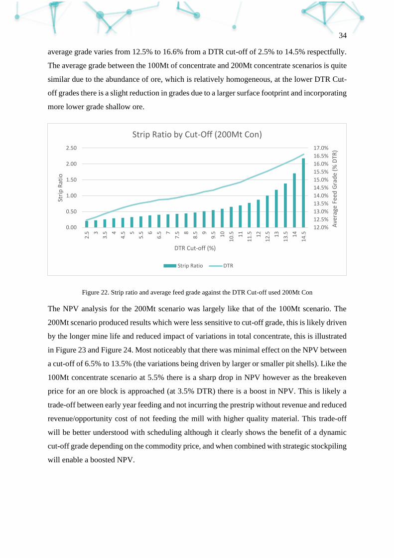
34

average grade varies from 12.5% to 16.6% from a DTR cut-off of 2.5% to 14.5% respectfully.

The average grade between the 100Mt of concentrate and 200Mt concentrate scenarios is quite

similar due to the abundance of ore, which is relatively homogeneous, at the lower DTR Cut-

off grades there is a slight reduction in grades due to a larger surface footprint and incorporating

more lower grade shallow ore.

Figure 22. Strip ratio and average feed grade against the DTR Cut-off used 200Mt Con

The NPV analysis for the 200Mt scenario was largely like that of the 100Mt scenario. The

200Mt scenario produced results which were less sensitive to cut-off grade, this is likely driven

by the longer mine life and reduced impact of variations in total concentrate, this is illustrated

in Figure 23 and Figure 24. Most noticeably that there was minimal effect on the NPV between

a cut-off of 6.5% to 13.5% (the variations being driven by larger or smaller pit shells). Like the

100Mt concentrate scenario at 5.5% there is a sharp drop in NPV however as the breakeven

price for an ore block is approached (at 3.5% DTR) there is a boost in NPV. This is likely a

trade-off between early year feeding and not incurring the prestrip without revenue and reduced

revenue/opportunity cost of not feeding the mill with higher quality material. This trade-off

will be better understood with scheduling although it clearly shows the benefit of a dynamic

cut-off grade depending on the commodity price, and when combined with strategic stockpiling

will enable a boosted NPV.

12.0%

12.5%

13.0%

13.5%

14.0%

14.5%

15.0%

15.5%

16.0%

16.5%

17.0%

0.00

0.50

1.00

1.50

2.00

2.50

2.5 3

3.5 4

4.5 5

5.5 6

6.5 7

7.5 8

8.5 9

9.5 10

10

.5 11

11

.5 12

12

.5 13

13

.5 14

14

.5

Ave

rage

Fee

d G

rad

e (%

DTR

)

Stri

p R

atio

DTR Cut-off (%)

Strip Ratio by Cut-Off (200Mt Con)

Strip Ratio DTR

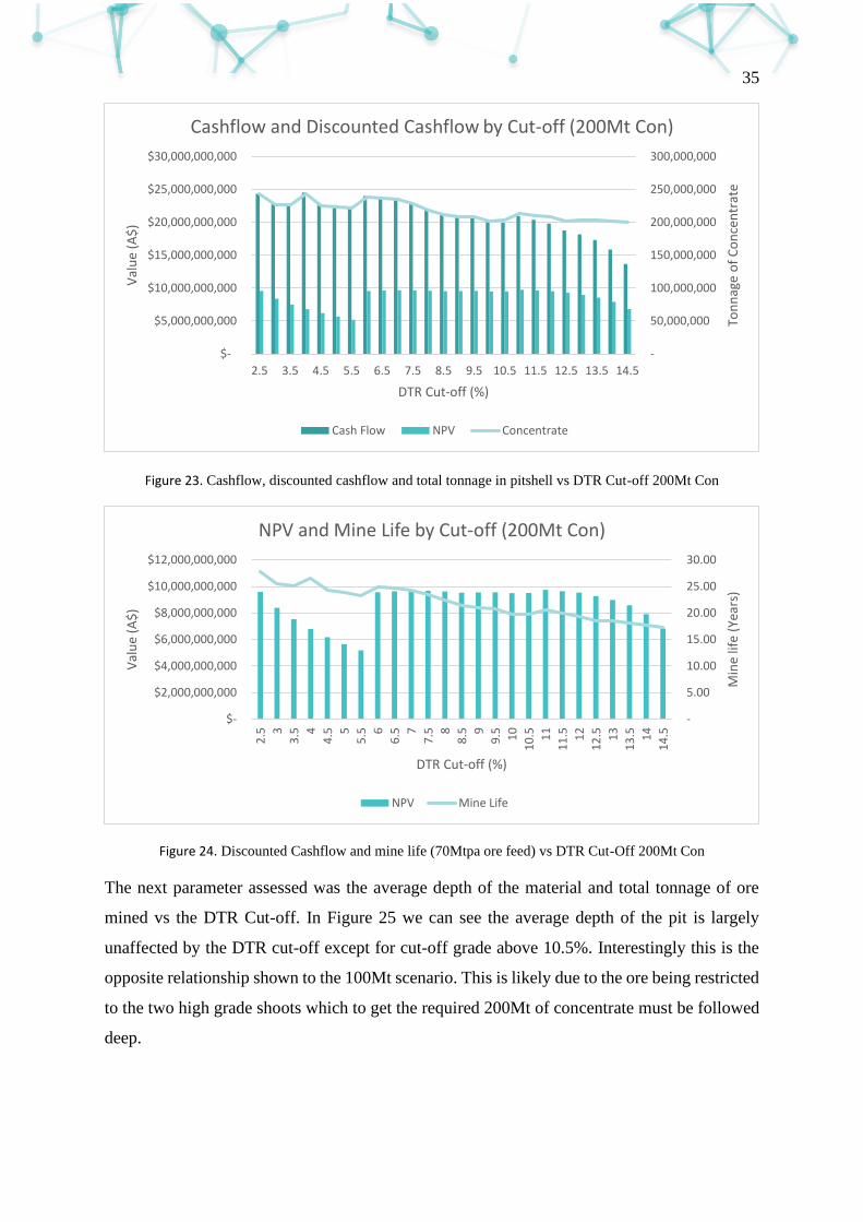
35

Figure 23. Cashflow, discounted cashflow and total tonnage in pitshell vs DTR Cut-off 200Mt Con


The next parameter assessed was the average depth of the material and total tonnage of ore

mined vs the DTR Cut-off. In Figure 25 we can see the average depth of the pit is largely

unaffected by the DTR cut-off except for cut-off grade above 10.5%. Interestingly this is the

opposite relationship shown to the 100Mt scenario. This is likely due to the ore being restricted

to the two high grade shoots which to get the required 200Mt of concentrate must be followed

deep.

-

50,000,000

100,000,000

150,000,000

200,000,000

250,000,000

300,000,000

$-

$5,000,000,000

$10,000,000,000

$15,000,000,000

$20,000,000,000

$25,000,000,000

$30,000,000,000

2.5 3.5 4.5 5.5 6.5 7.5 8.5 9.5 10.5 11.5 12.5 13.5 14.5

Ton

nag

e o

f C

on

cen

trat

e

Val

ue

(A$

)

DTR Cut-off (%)

Cashflow and Discounted Cashflow by Cut-off (200Mt Con)

Cash Flow NPV Concentrate

-

5.00

10.00

15.00

20.00

25.00

30.00

$-

$2,000,000,000

$4,000,000,000

$6,000,000,000

$8,000,000,000

$10,000,000,000

$12,000,000,000

2.5 3

3.5 4

4.5 5

5.5 6

6.5 7

7.5 8

8.5 9

9.5 10

10

.5 11

11

.5 12

12

.5 13

13

.5 14

14

.5

Min

e lif

e (Y

ears

)

Val

ue

(A$

)

DTR Cut-off (%)

NPV and Mine Life by Cut-off (200Mt Con)

NPV Mine Life

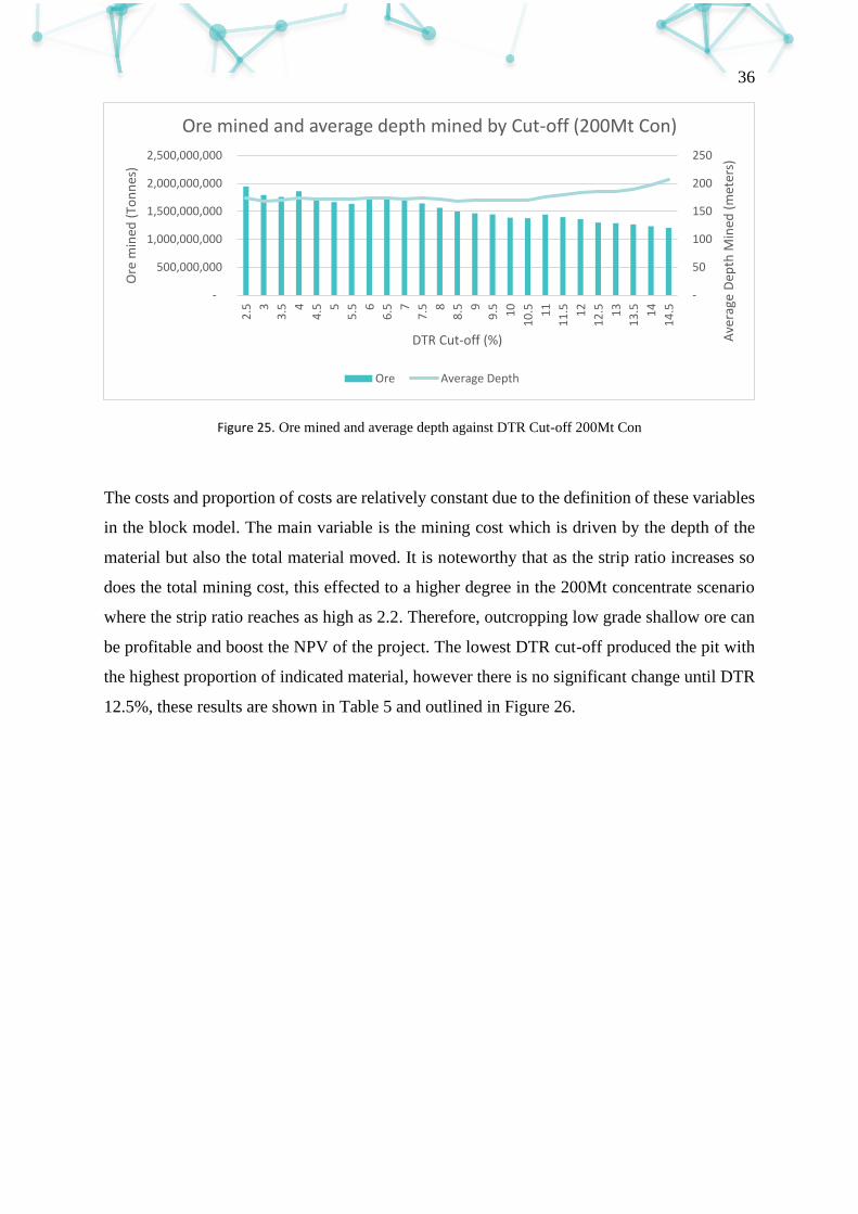
36

Figure 25. Ore mined and average depth against DTR Cut-off 200Mt Con

The costs and proportion of costs are relatively constant due to the definition of these variables

in the block model. The main variable is the mining cost which is driven by the depth of the

material but also the total material moved. It is noteworthy that as the strip ratio increases so

does the total mining cost, this effected to a higher degree in the 200Mt concentrate scenario

where the strip ratio reaches as high as 2.2. Therefore, outcropping low grade shallow ore can

be profitable and boost the NPV of the project. The lowest DTR cut-off produced the pit with

the highest proportion of indicated material, however there is no significant change until DTR

12.5%, these results are shown in Table 5 and outlined in Figure 26.

-

50

100

150

200

250

-

500,000,000

1,000,000,000

1,500,000,000

2,000,000,000

2,500,000,000

2.5 3

3.5 4

4.5 5

5.5 6

6.5 7

7.5 8

8.5 9

9.5 10

10

.5 11

11

.5 12

12

.5 13

13

.5 14

14

.5

Ave

rage

Dep

th M

ined

(m

eter

s)

Ore

min

ed (

Ton

nes

)

DTR Cut-off (%)

Ore mined and average depth mined by Cut-off (200Mt Con)

Ore Average Depth

37

Table 5.

Summary of costs and sources of concentrate from 200Mt Concentrate Scenarios

Figure 26. Proportion of feedstock by ore classification 200Mt Con

Cutoff Mining Processing Transport +

Downstream

G+A + Rehab +

Sustaining Capital Total Revenue Indicated Inferred Potential

2.5% 5,318,189,786$ 3,035,961,186$ 3,230,574,083$ 3,639,560,135$ 15,224,285,191$ 39,567,974,241$ 46% 48% 6%

3.0% 4,948,218,237$ 2,798,192,969$ 2,977,564,313$ 3,408,979,076$ 14,132,954,594$ 36,984,079,341$ 48% 46% 6%

3.5% 4,963,675,137$ 2,743,141,076$ 2,918,983,453$ 3,418,725,127$ 14,044,524,794$ 36,902,017,536$ 48% 46% 6%

4.0% 5,444,310,601$ 2,906,754,577$ 3,093,084,998$ 3,724,123,291$ 15,168,273,466$ 39,682,047,347$ 45% 48% 7%

4.5% 4,986,345,232$ 2,644,407,701$ 2,813,921,015$ 3,422,532,662$ 13,867,206,609$ 36,595,878,836$ 48% 47% 6%

5.0% 4,988,061,724$ 2,599,498,655$ 2,766,133,184$ 3,423,848,147$ 13,777,541,710$ 36,381,509,989$ 48% 47% 6%

5.5% 4,977,359,553$ 2,550,577,211$ 2,714,075,750$ 3,415,804,810$ 13,657,817,323$ 36,068,644,083$ 48% 46% 6%

6.0% 5,463,645,993$ 2,724,665,488$ 2,899,323,532$ 3,740,863,058$ 14,828,498,071$ 38,812,105,826$ 45% 48% 7%

6.5% 5,457,149,795$ 2,684,984,236$ 2,857,098,610$ 3,736,703,168$ 14,735,935,810$ 38,535,472,588$ 45% 48% 7%

7.0% 5,432,371,094$ 2,648,739,392$ 2,818,530,379$ 3,723,311,635$ 14,622,952,500$ 38,187,976,746$ 46% 48% 7%

7.5% 5,307,538,912$ 2,559,106,745$ 2,723,152,049$ 3,633,053,043$ 14,222,850,749$ 37,128,216,505$ 47% 47% 7%

8.0% 5,098,096,570$ 2,442,353,029$ 2,598,914,121$ 3,498,205,134$ 13,637,568,853$ 35,744,971,977$ 45% 48% 6%

8.5% 4,950,107,783$ 2,333,858,930$ 2,483,465,272$ 3,412,095,737$ 13,179,527,722$ 34,380,559,897$ 47% 47% 6%

9.0% 4,996,703,047$ 2,287,094,614$ 2,433,703,243$ 3,434,104,768$ 13,151,605,672$ 34,009,520,298$ 47% 47% 6%

9.5% 5,048,256,062$ 2,258,796,058$ 2,403,590,677$ 3,473,122,220$ 13,183,765,016$ 33,855,890,562$ 47% 47% 6%

10.0% 4,967,473,441$ 2,164,637,618$ 2,303,396,440$ 3,417,642,606$ 12,853,150,104$ 32,881,357,093$ 48% 46% 5%

10.5% 5,123,777,421$ 2,151,743,866$ 2,289,676,165$ 3,523,816,055$ 13,089,013,508$ 33,034,484,551$ 47% 48% 5%

11.0% 5,545,422,295$ 2,251,985,959$ 2,396,344,033$ 3,789,052,406$ 13,982,804,692$ 34,933,071,519$ 47% 48% 5%

11.5% 5,651,285,202$ 2,179,158,254$ 2,318,847,886$ 3,840,339,113$ 13,989,630,455$ 34,375,426,400$ 47% 48% 5%

12.0% 5,840,662,915$ 2,120,467,192$ 2,256,394,576$ 3,947,706,450$ 14,165,231,134$ 33,961,171,524$ 46% 49% 5%

12.5% 5,991,469,858$ 2,027,667,120$ 2,157,645,782$ 4,032,654,276$ 14,209,437,035$ 32,967,361,756$ 45% 49% 6%

13.0% 6,480,049,864$ 2,009,596,935$ 2,138,417,251$ 4,364,284,253$ 14,992,348,304$ 33,147,199,432$ 44% 50% 7%

13.5% 6,981,264,626$ 1,975,721,454$ 2,102,370,265$ 4,678,629,479$ 15,737,985,823$ 33,052,061,087$ 41% 51% 8%

14.0% 7,810,052,950$ 1,929,402,322$ 2,053,081,958$ 5,182,045,100$ 16,974,582,330$ 32,818,104,484$ 38% 52% 10%

14.5% 9,054,012,198$ 1,880,571,667$ 2,001,121,132$ 5,937,153,014$ 18,872,858,011$ 32,534,650,974$ 35% 49% 16%

Costs Ore Source

0.0%

10.0%

20.0%

30.0%

40.0%

50.0%

60.0%

2.5 3

3.5 4

4.5 5

5.5 6

6.5 7

7.5 8

8.5 9

9.5 10

10

.5 11

11

.5 12

12

.5 13

13

.5 14

14

.5Pro

po

rtio

n o

f C

on

cen

trat

e (%

)

DTR Cut-off (%)

Source of concentrate by Cut-off (200Mt Con)

Indicated con Inferred Con Potential Con

38

4 FUTURE OPTIMISATION

4.1 INTRODUCTION

As this is a new Greenfields project it is important to assess all methodologies and technologies

in the execution of this project such that it remains competitive with other tier 1 assets around

the world. To this end a list of considerations are made below which should be more thoroughly

investigated throughout the Bankable Feasibility Study.

The ability to reduce greenhouse gases is becoming an ever more important aspect to the

obtaining of project financing. The project has a unique value proposition in that its magnetite

(Fe3O4) the project produces has a lower energy intensity compared to conventionally mined

hematite (Fe2O3) to create steel giving it a competitive advantage (Sparrow, 1983). This

advantage is exacerbated by the extremely high grade of the product as well as the relative

energy intensity to liberate the magnetite when compared to other ores (GHD, August, 2017).

The total material movement in the Pre-Feasibility report by GHD was 2,140 Mt to produce

202Mt of concentrate (p.110) (GHD, August, 2017). The unit costs for these mining

parameters are shown in Table 6. These costs have been simplified in Figure 27 where grade

control, fragmented ore and fragmented waste have been rounded into Drill and Blast costs

comprising 17% of the costs, T&S ore and T&S waste rounded into Load and Haul costs

comprising 58% of the costs and the remaining costs to be rounded into pit maintenance

comprising 25% of the costs. This shows that reducing the load and haul costs will deliver the

most leverage to driving down the mining cost on a proportionate basis.

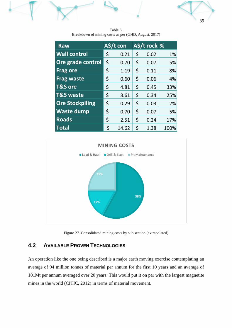
39

Table 6.

Breakdown of mining costs as per (GHD, August, 2017)

Figure 27. Consolidated mining costs by sub section (extrapolated)

4.2 AVAILABLE PROVEN TECHNOLOGIES

An operation like the one being described is a major earth moving exercise contemplating an

average of 94 million tonnes of material per annum for the first 10 years and an average of

101Mt per annum averaged over 20 years. This would put it on par with the largest magnetite

mines in the world (CITIC, 2012) in terms of material movement.

Raw A$/t con A$/t rock %

Wall control 0.21$ 0.02$ 1%

Ore grade control 0.70$ 0.07$ 5%

Frag ore 1.19$ 0.11$ 8%

Frag waste 0.60$ 0.06$ 4%

T&S ore 4.81$ 0.45$ 33%

T&S waste 3.61$ 0.34$ 25%

Ore Stockpiling 0.29$ 0.03$ 2%

Waste dump 0.70$ 0.07$ 5%

Roads 2.51$ 0.24$ 17%

Total 14.62$ 1.38$ 100%

58%

17%

25%

MINING COSTS

Load & Haul Drill & Blast Pit Maintenance

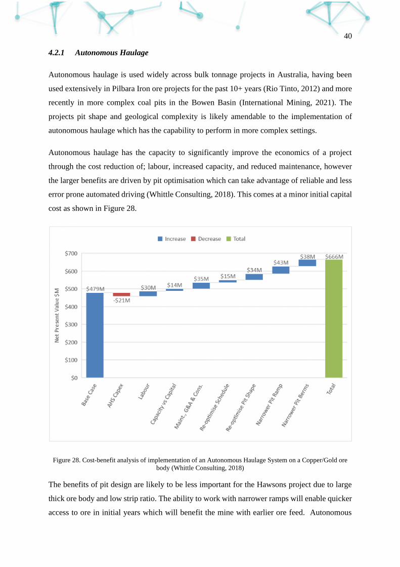
40

4.2.1 Autonomous Haulage

Autonomous haulage is used widely across bulk tonnage projects in Australia, having been

used extensively in Pilbara Iron ore projects for the past 10+ years (Rio Tinto, 2012) and more

recently in more complex coal pits in the Bowen Basin (International Mining, 2021). The

projects pit shape and geological complexity is likely amendable to the implementation of

autonomous haulage which has the capability to perform in more complex settings.

Autonomous haulage has the capacity to significantly improve the economics of a project

through the cost reduction of; labour, increased capacity, and reduced maintenance, however

the larger benefits are driven by pit optimisation which can take advantage of reliable and less

error prone automated driving (Whittle Consulting, 2018). This comes at a minor initial capital

cost as shown in Figure 28.

Figure 28. Cost-benefit analysis of implementation of an Autonomous Haulage System on a Copper/Gold ore

body (Whittle Consulting, 2018)

The benefits of pit design are likely to be less important for the Hawsons project due to large

thick ore body and low strip ratio. The ability to work with narrower ramps will enable quicker

access to ore in initial years which will benefit the mine with earlier ore feed. Autonomous

41

haulage is becoming more common place in conjunction with Ultra Class equipment and is

beginning to be used with trolley assist (International Mining, 2021). Whilst not common place

using an aggregation of these technologies, they should be strongly considered for the Hawson

project as it’s development timeline will coincide with the maturity of this technology.

4.2.2 Ultra-class Equipment.

In the original PFS a 220-240t dump truck size was selected with the Komatsu 830E used as

an indicative haulage vehicle (GHD, August, 2017). When the preliminary work for this project

was done for this project ultra-class haul trucks (with >300t payload) were still in the process

of becoming more widely adopted in Australia outside of a select few mine sites (Australian

Mining, 2019). With the amount of material being moved each year the economies of scale of

ultra-class gear should be investigated, particularly if used in conjunction with other capital

items such as autonomous haulage.

It is noteworthy that in the similar deposit of Magnetite Mines, that they have elected to use to

use 150-190t medium class haul trucks. This was primarily driven by the need to achieve 1m

selectivity which led to the decision of a 350t excavator (Magnetite Mines Limited, 2021). The

Alderon Iron Ore Corp used CAT 794 with a nominal payload of 292t in their full feasibility

study (43-101) which was used to deliver 23 Mtpa of ore to their processing plant on the

Kamistiatusset iron ore project in Labrador (BBA, 2018). Black Iron opted for the CAT 793

with a nominal payload of 228t in their preliminary economic assessment (43-101) which was

used to deliver up to 28.7 Mtpa of ore to their processing plant on the Shymanivske Iron ore

project in Ukraine (BBA, 2017). Experienced magnetite miner Champion Iron opted for a

similar middle class of truck with a payload of 218t in their preliminary economic assessment

(43-101) which was used to deliver up to 41.9 Mtpa of ore to their processing plant on the

Bloom Lake Mine project in Quebec (BBA, 2019). These smaller haul trucks can be contrasted

with CITIC which uses the Bucyrus MT6300AC which has a 360t payload and is used at the

Sino Mine in Western Australia (CITIC, 2021). s

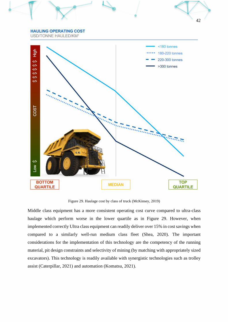
42

Figure 29. Haulage cost by class of truck (McKinsey, 2019)

Middle class equipment has a more consistent operating cost curve compared to ultra-class

haulage which perform worse in the lower quartile as in Figure 29. However, when

implemented correctly Ultra class equipment can readily deliver over 15% in cost savings when

compared to a similarly well-run medium class fleet (Shea, 2020). The important

considerations for the implementation of this technology are the competency of the running

material, pit design constraints and selectivity of mining (by matching with appropriately sized

excavators). This technology is readily available with synergistic technologies such as trolley

assist (Caterpillar, 2021) and automation (Komatsu, 2021).

43

4.2.3 In Pit Crushing and Conveying (IPCC)

In Pit Crushing and Conveying (IPCC) has long been known to significantly reduce costs (20-

60%) and emissions of a mine site, this however does come at a significant cost to operational

flexibility and redundancy (McEwing, 2019). Using IPCC is effective in dynamic weather

environments working continuously, however due to the low number of rain days in Broken

Hill this benefit is unlikely to be realised. IPCC problems typically stem from inconsistent

material feed which can result in a stoppage in the system, with a single point of failure stopping

production from the mine.

One of the benefits of IPCC is that the machinery used to transport the material from the mine

is far more efficient then using haul trucks. This is because haul trucks must apply energy to

transport the mass of the truck along with the material to final destination and then come back

to the source of the material using energy to transport the mass of the truck back empty (Scales,

2017). Utilising solar powered in pit crushing and conveying systems can dramatically reduce

energy costs, currently crushing, milling, and grinding account for 2.7% of all electrical energy

consumed (FLSmidth, 2020).

As the transport cost for material can be significantly less than that of conventionally hauled

material the cut-off grade can be lowered and mine design further optimised (Johnson, 2015).

The reliance on a fixed conveyor reduces the operational flexibility but also creates a single

bottleneck in the operation which if fails stops the entire production. The other important

consideration is with the friability of the material (GHD, August, 2017) there could be

excessive dust creation in the pit which must be controlled or could have other operational

impacts. Overall IPCC will have diminishing returns when combined with other haulage

benefits, the opex savings are significant and should be further investigated. The benefits of

IPCC are stronger with deeper pits and the capital could be incurred once a deep pit and final

wall are established. This has the added benefit of reducing the impact on NPV through delayed

capital expenditure.

4.2.4 Truck Trolley Assist

Truck and Trolley systems have the ability to lower fuel consumption by 90% whilst connected

to the grid on diesel electric hybrid systems (Hitachi Construction, 2018) if this grid power is

competitively priced it can significantly reduce operating costs. This system again works best

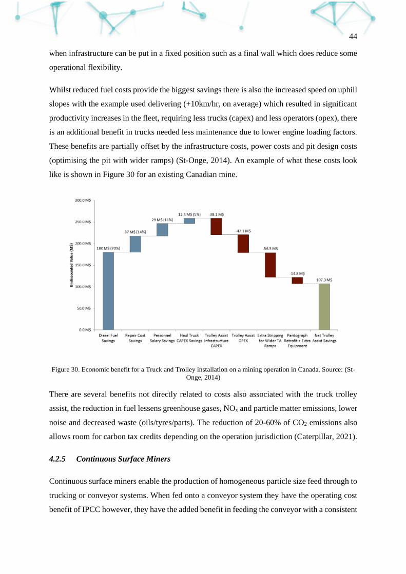
44

when infrastructure can be put in a fixed position such as a final wall which does reduce some

operational flexibility.

Whilst reduced fuel costs provide the biggest savings there is also the increased speed on uphill

slopes with the example used delivering (+10km/hr, on average) which resulted in significant

productivity increases in the fleet, requiring less trucks (capex) and less operators (opex), there

is an additional benefit in trucks needed less maintenance due to lower engine loading factors.

These benefits are partially offset by the infrastructure costs, power costs and pit design costs

(optimising the pit with wider ramps) (St-Onge, 2014). An example of what these costs look

like is shown in Figure 30 for an existing Canadian mine.

Figure 30. Economic benefit for a Truck and Trolley installation on a mining operation in Canada. Source: (St-

Onge, 2014)

There are several benefits not directly related to costs also associated with the truck trolley

assist, the reduction in fuel lessens greenhouse gases, NOx and particle matter emissions, lower

noise and decreased waste (oils/tyres/parts). The reduction of 20-60% of CO2 emissions also

allows room for carbon tax credits depending on the operation jurisdiction (Caterpillar, 2021).

4.2.5 Continuous Surface Miners

Continuous surface miners enable the production of homogeneous particle size feed through to

trucking or conveyor systems. When fed onto a conveyor system they have the operating cost

benefit of IPCC however, they have the added benefit in feeding the conveyor with a consistent

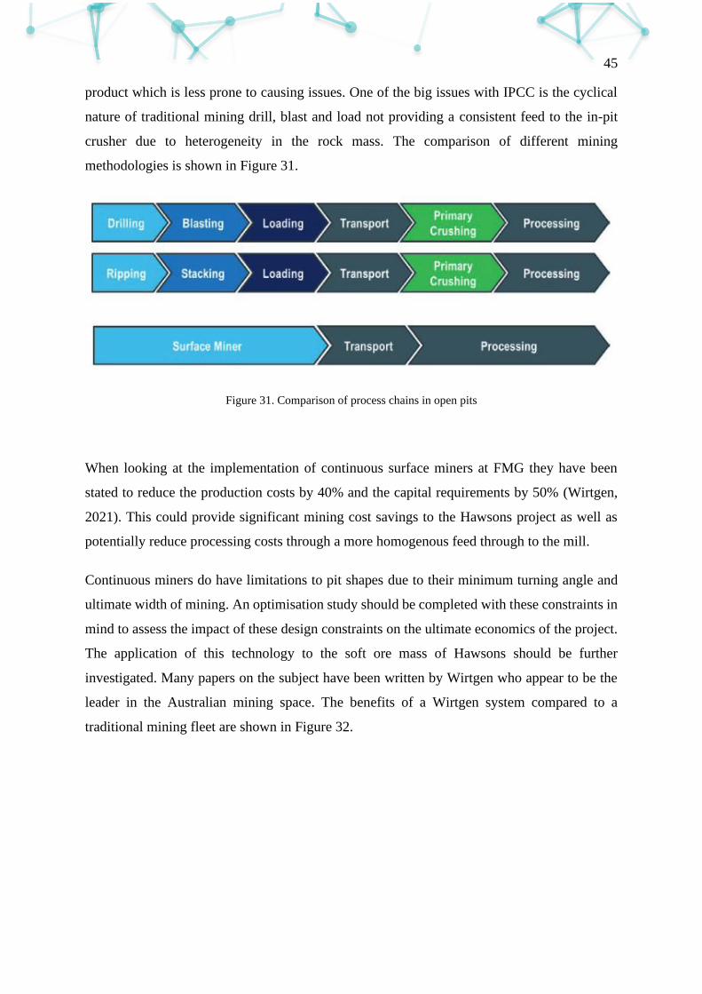
45

product which is less prone to causing issues. One of the big issues with IPCC is the cyclical

nature of traditional mining drill, blast and load not providing a consistent feed to the in-pit

crusher due to heterogeneity in the rock mass. The comparison of different mining

methodologies is shown in Figure 31.

Figure 31. Comparison of process chains in open pits

When looking at the implementation of continuous surface miners at FMG they have been

stated to reduce the production costs by 40% and the capital requirements by 50% (Wirtgen,

2021). This could provide significant mining cost savings to the Hawsons project as well as

potentially reduce processing costs through a more homogenous feed through to the mill.

Continuous miners do have limitations to pit shapes due to their minimum turning angle and

ultimate width of mining. An optimisation study should be completed with these constraints in

mind to assess the impact of these design constraints on the ultimate economics of the project.

The application of this technology to the soft ore mass of Hawsons should be further

investigated. Many papers on the subject have been written by Wirtgen who appear to be the

leader in the Australian mining space. The benefits of a Wirtgen system compared to a

traditional mining fleet are shown in Figure 32.

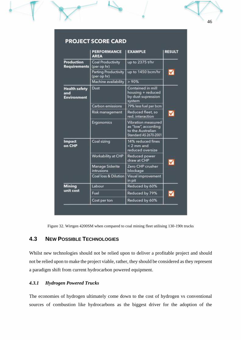
46

Figure 32. Wirtgen 4200SM when compared to coal mining fleet utilising 130-190t trucks

4.3 NEW POSSIBLE TECHNOLOGIES

Whilst new technologies should not be relied upon to deliver a profitable project and should

not be relied upon to make the project viable, rather, they should be considered as they represent

a paradigm shift from current hydrocarbon powered equipment.

4.3.1 Hydrogen Powered Trucks

The economies of hydrogen ultimately come down to the cost of hydrogen vs conventional

sources of combustion like hydrocarbons as the biggest driver for the adoption of the

47

technology. Australian companies are actively assessing the viability of hydrogen at different

price points, the largest driver for green hydrogen (hydrogen derived from the hydrolysis of

water and not hydrocarbons) is power price (CSIRO, 2021). Abundant cheap solar power

particularly when the duck curve is peaking provide opportunity for hydrogen creation at

competitive rates. The adoption of hydrogen in different industries is shown in Figure 33.

Figure 33. Hydrogen competitiveness in targeted application (CSIRO, 2021)

Another barrier to hydrogen adoption in mining is currently getting the required energy density

vehicles such that refuelling is not prohibitive to productivity of vehicles. This is currently

being researched by a range of mining companies with the current fuel cell technologies

showing promise, Anglo American says large haul trucks account for over 70% of diesel

consumption on site and has committed to carbon neutrality by 2040. Large miners across the

world have committed to carbon neutrality by 2050 and supply chain logistics may demand

this be the case for all steel production (NPROXX, 2021). Given the long life of the project

and the encroaching deadlines many organisations face, hydrogen or other green technologies

should be strongly considered by HAW. Early adoption could have the duel benefit of

government incentives and additional product premium.

4.3.2 Battery Powered Trucks

Electric Vehicle (EV) Haul trucks offer an alternative for utilising solar energy to provide the

haulage of material on a mine site. Trucks using battery systems are currently only viable is a

select number of locations where the location of the ore has a significant height advantage

compared to its destination. In these environments the trucks can use the gravitational potential

48

energy of the ore to recharge the battery system on decent of the hill and use that energy to

carry the truck back up the hill empty using batteries. As the geography of the HIP is very flat

it is unlikely that a pure battery powered truck would be viable without a step change in battery

energy density and cost.

This technology however could be combined with trolley assist infrastructure providing the

advantage of cheap power delivered to the vehicle with the benefit of “last mile” flexibility to

the trucks. This is currently being investigated as it removes many moving parts from

traditional diesel electric trucks. Currently electric battery equipment is two to three times more

expensive compared to diesel equipment, however the price of this equipment is quickly falling

and is expected to meet cost parity (King-Abadi, 2020). This adoption may reach parity faster

with many ultra-class mining equipment already employing the use of large electric drive

motors.

Whilst stand-alone battery powered trucks may not be ready for the mine by start of

construction, a system of battery powered, and trolley assisted trucks are already being adopted

around the world (Guthrie, 2021). Their performance should be closely monitored to observe

what degree of cost saving is possible.

49

5 CONCLUSIONS

From a resource perspective the project is in a good position. If inferred and potential resources

can be increased in size and confidence whilst maintaining similar characteristics to that which

has been used then the project will easily meet the requirement of having 20 years of ore feed.

It is noteworthy that current modelling only factors in 6-7% of potential resource with the rest

of the ore feed being made up of an equal proportion of indicated and inferred resources. Thus,

roughly 100Mt of ore is needed to be brought from inferred to measured (or conversely 100Mt

from indicated to measured and 100Mt from inferred to indicated). There is no shortage of ore

however investigations should be made into potentially outcropping and shallow ore to feed

the mill.

The most interesting area is around the Fold section of the ore body which is currently poorly

defined. Although this material produces a slightly lower grade concentrate (69% vs 70% of

the main zone) it is the most economic part of the entire ore body and under all scenarios this

area was targeted first with the early ore driving NPV north. With better definition around these

ore bodies (particularly in areas on the edge of current modelling) there exists opportunity for

economic ore close to surface which may play a role in reducing the projects NPV. Sterilising

this area may also prove beneficial for placement of critical infrastructure such as processing

plants, tailings, waste dumps or stockpiles.

The project has enormous potential to produce a low carbon feedstock for the steel market and

should be actively investigating new technologies which can develop this concept. Many of the

concepts investigated in this report have the ability not only to reduce CO2 emissions but

alsocosts, most retain the flexibility of a traditional truck and shovel operation apart from

continuous miners and conveyors. A high-level assessment of this technology should be carried

out to see if it has any impact on the upcoming drill campaign.

50

6 RECOMMENDATIONS

6.1 COST DEFINITION

KPS Innovations strongly recommends building up a model from first principals. To ensure

accuracy this should be benchmarked against similar projects of scale around Australia. To add

validity these costs and operating metrics should be compared to contractor rates if possible

and firsthand quotes. This should culminate in a market appropriate variable which will allow

a more accurate pit optimisation study to be completed.

6.2 FUTURE DRILLING

The Fold area of the pit should be delineated with further drilling and any potential area which

is proposed to be used for significant infrastructure should be sterilised with drilling, as should

and prospective dump areas. In Figure 34 we can see a high surface expression of iron from

XRF analysis. This is correlated with siltstone with iron interbeds, this material should be

checked for Davis Tube Recovery numbers however if consistent with the Core ore body, then

could prove to be advantageous with early mine life exploitation.

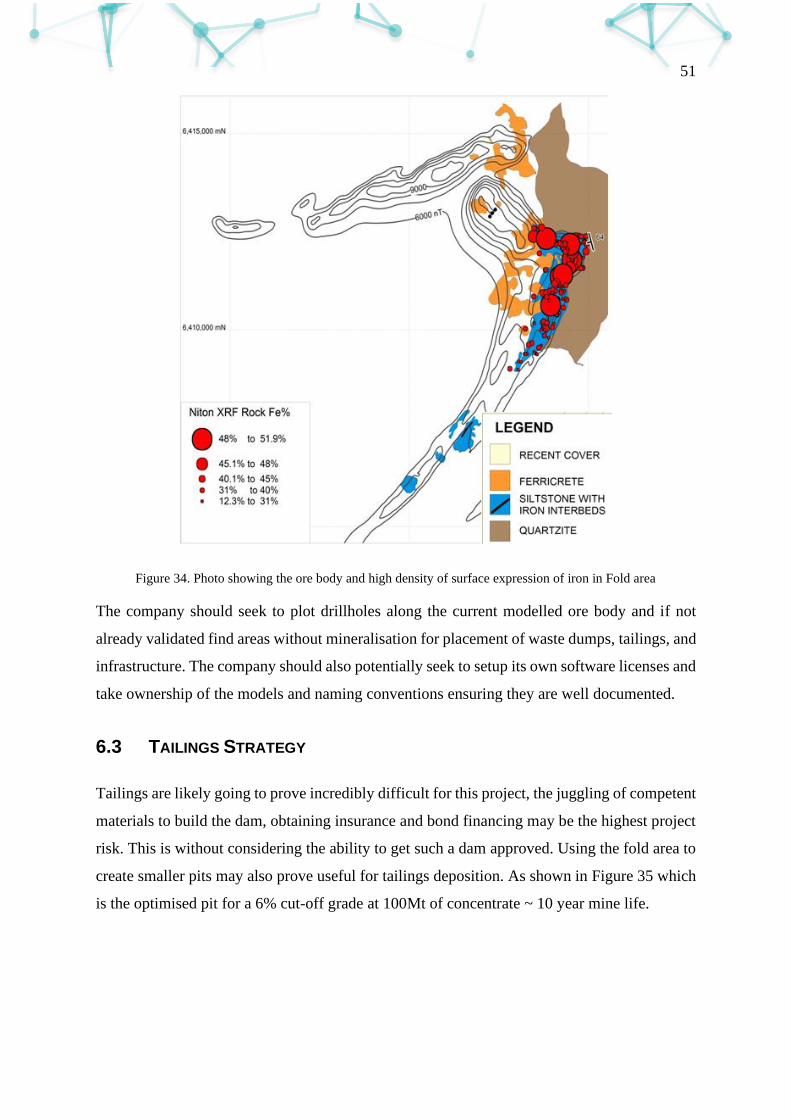
51

Figure 34. Photo showing the ore body and high density of surface expression of iron in Fold area

The company should seek to plot drillholes along the current modelled ore body and if not

already validated find areas without mineralisation for placement of waste dumps, tailings, and

infrastructure. The company should also potentially seek to setup its own software licenses and

take ownership of the models and naming conventions ensuring they are well documented.

6.3 TAILINGS STRATEGY

Tailings are likely going to prove incredibly difficult for this project, the juggling of competent

materials to build the dam, obtaining insurance and bond financing may be the highest project

risk. This is without considering the ability to get such a dam approved. Using the fold area to

create smaller pits may also prove useful for tailings deposition. As shown in Figure 35 which

is the optimised pit for a 6% cut-off grade at 100Mt of concentrate ~ 10 year mine life.

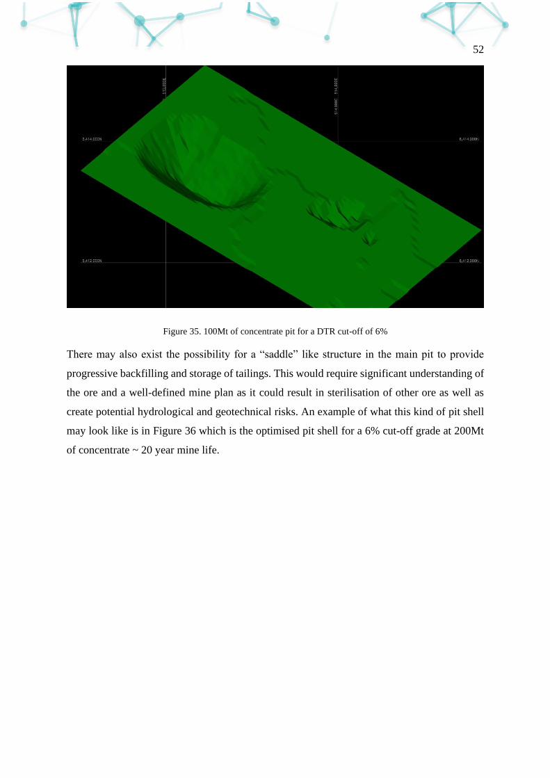
52

Figure 35. 100Mt of concentrate pit for a DTR cut-off of 6%

There may also exist the possibility for a “saddle” like structure in the main pit to provide

progressive backfilling and storage of tailings. This would require significant understanding of

the ore and a well-defined mine plan as it could result in sterilisation of other ore as well as

create potential hydrological and geotechnical risks. An example of what this kind of pit shell

may look like is in Figure 36 which is the optimised pit shell for a 6% cut-off grade at 200Mt

of concentrate ~ 20 year mine life.

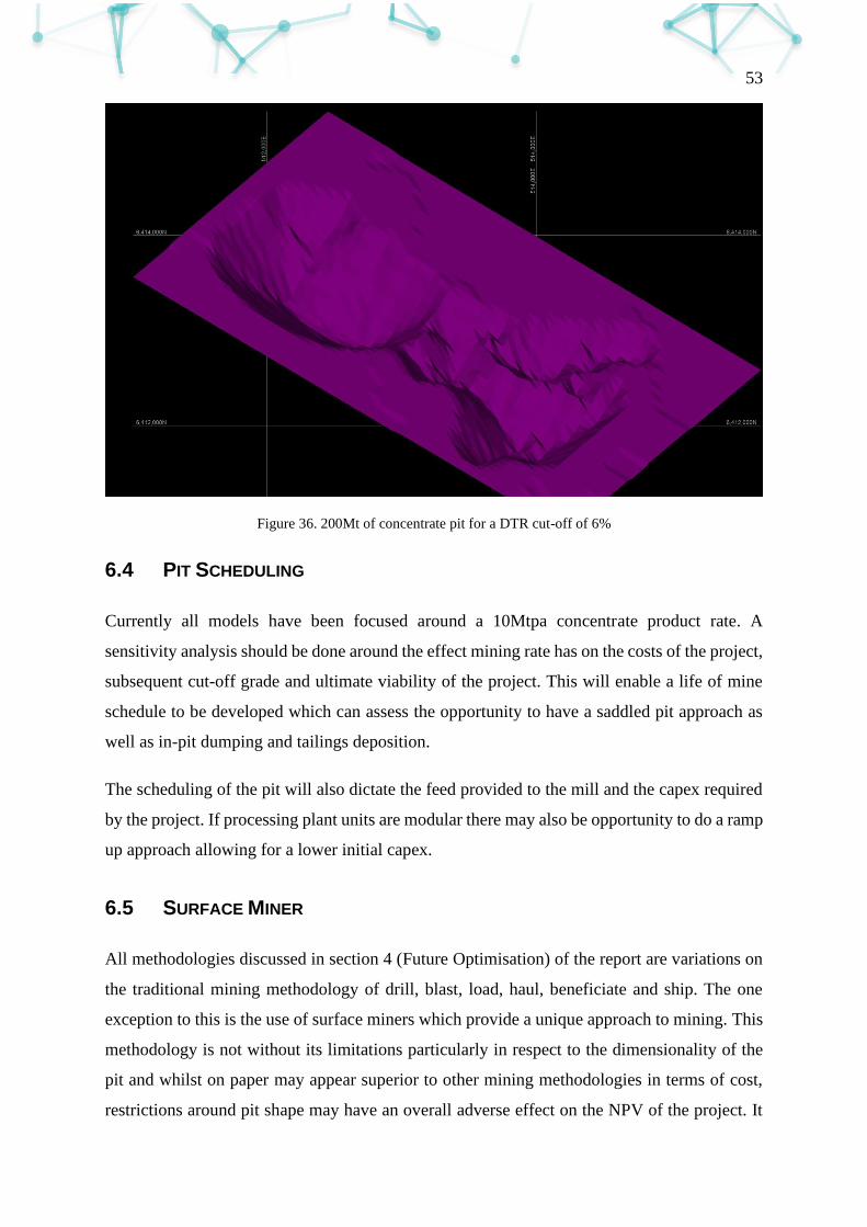
53

Figure 36. 200Mt of concentrate pit for a DTR cut-off of 6%

6.4 PIT SCHEDULING

Currently all models have been focused around a 10Mtpa concentrate product rate. A

sensitivity analysis should be done around the effect mining rate has on the costs of the project,

subsequent cut-off grade and ultimate viability of the project. This will enable a life of mine

schedule to be developed which can assess the opportunity to have a saddled pit approach as

well as in-pit dumping and tailings deposition.

The scheduling of the pit will also dictate the feed provided to the mill and the capex required

by the project. If processing plant units are modular there may also be opportunity to do a ramp

up approach allowing for a lower initial capex.

6.5 SURFACE MINER

All methodologies discussed in section 4 (Future Optimisation) of the report are variations on

the traditional mining methodology of drill, blast, load, haul, beneficiate and ship. The one

exception to this is the use of surface miners which provide a unique approach to mining. This

methodology is not without its limitations particularly in respect to the dimensionality of the

pit and whilst on paper may appear superior to other mining methodologies in terms of cost,

restrictions around pit shape may have an overall adverse effect on the NPV of the project. It

54

is recommended rough costs and design constraints using equipment from Wirtgen and/or

Vermeer are obtained, and another pit optimisation study is run to assess the viability and

impact on the drill campaign.

55

7 REFERENCES

Australian Mining. (2019, February 7). The rise of the ultra class. Retrieved from

https://www.australianmining.com.au/features/the-rise-of-the-ultra-class/

BBA. (2017). Preliminary Economic Assessment of the Re-scoped Shymanivske Iron Ore

Deposit DNEPROPETROVSK REGION, UKRAINE. Toronto: Black Iron Inc.

BBA. (2018). NI 43-101 TECHNICAL REPORT UPDATED FEASIBILITY STUDY of the

KAMISTIATUSSET (KAMI) IRON ORE PROPERTY, LABRADOR. Vancouver: Alderon Iron

Ore Corp.

BBA. (2019). Bloom Lake Mine Feasibility Study Phase 2. Montreal: Quebec Iron Ore Inc. on

behalf of Champion Iron Limited.

Caterpillar. (2021, September 2). Retrieved from Electrigying mines with Cat trolley assist:

https://www.cat.com/en_US/by-industry/mining/surface-mining/surface-

equipment/lm-trucks/trolley.html

CITIC. (2021, September 3). Retrieved from Our Operation - Mining:

https://citicpacificmining.com/our-operation/mining

CSIRO. (2021). National Hydrogen Roadmap - Pathways to an economically sustainable

hydrogen industry in Australia. Retrieved from https://www.csiro.au/-/media/Do-

Business/Files/Futures/18-00314_EN_NationalHydrogenRoadmap_WEB_180823.pdf

FLSmidth. (2020, September 25). Towards zero emissions in mining. Retrieved from

https://www.youtube.com/watch?v=PMJyqsRWasE

GHD. (August, 2017). Report for Carpentaria Exploration Ltd - Hawsons Iron Project, 4130679.

Brisbane: GHD.

Guthrie, C. (2021, April 26). Copper Mountain Mining to install ABB trolley assist. Retrieved

from Mining Magazine:

https://www.miningmagazine.com/transport/news/1408958/copper-mountain-

mining-to-install-abb-trolley-assist

56

Hitachi Construction. (2018, May 24). Hitachi dump truck trolley technology boosts

productivity. Retrieved from https://www.youtube.com/watch?v=oNTm-jd_4lE

International Mining. (2021, May 11). BHP Mitsubishi Alliance moves first material with

Komatsu 930E-5 autonomous trucks at BMA Goonyella Riverside coal mine. Retrieved

from https://im-mining.com/2021/05/11/bhp-mitsubishi-jv-bma-moves-first-

material-komatsu-930e-5-autonomous-trucks-bma-goonyella-riverside-coal-mine/

International Mining. (2021, August 4). Ferrexpo to decide on trolley assist-backed haulage

project by year-end. Retrieved from https://im-mining.com/2021/08/04/ferrexpo-

decide-trolley-assist-backed-haulage-project-year-end/

Johnson, M. (2015, October). Impact of In-Pit Crushing and Conveying on pit shell

optimisation. Retrieved from Deswik: https://www.deswik.com/wp-

content/uploads/2015/10/Impact-of-IPCC-on-Pit-Shell-Optimization.pdf

King-Abadi, S. (2020, March 26). Global drive to the electric mine. Retrieved from GMG Group:

https://gmggroup.org/global-drive-to-the-electric-mine/

Komatsu. (2021, September 2). 930E-5 Dump Trucks. Retrieved from

https://www.komatsu.com.au/equipment/dump-trucks/electric-mining-

trucks/930e-5

Magnetite Mines Limited. (2021). Positive PFS Results for Razorback High Grade Iron .

Wayville: ASX.

McEwing, S. (2019, July). Finding the right fit. Retrieved from SRK Consulting, Global Mining

Review:

https://dxi97tvbmhbca.cloudfront.net/upload/user/image/SMcEwing_Finding_the_r

ight_fit20191128191146195.pdf

NPROXX. (2021, April 7). Case Study: Hydrogen powered mine truck for Anglo American Mine.

Retrieved from https://www.nproxx.com/case-study-hydrogen-powered-mine-truck-

for-anglo-american-mine/

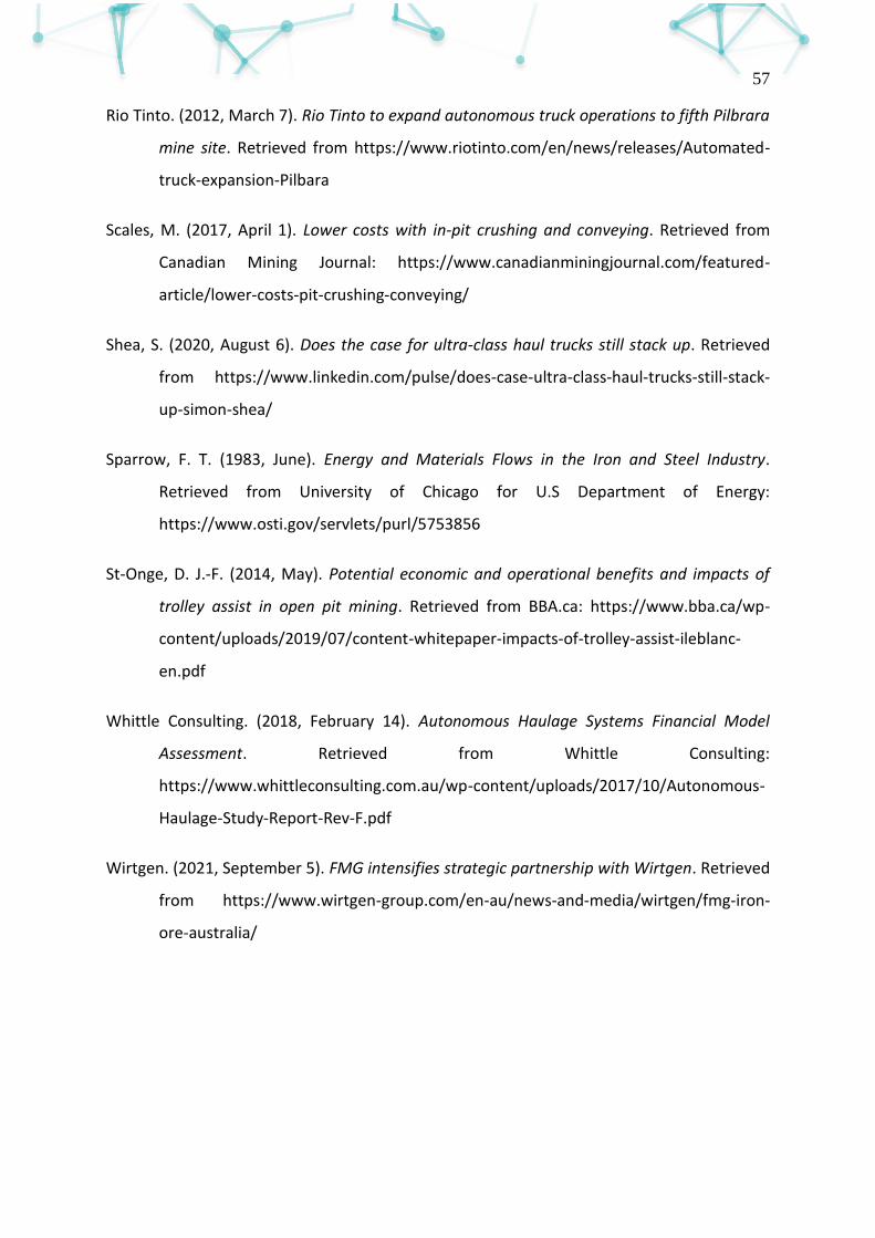
57

Rio Tinto. (2012, March 7). Rio Tinto to expand autonomous truck operations to fifth Pilbrara

mine site. Retrieved from https://www.riotinto.com/en/news/releases/Automated-

truck-expansion-Pilbara

Scales, M. (2017, April 1). Lower costs with in-pit crushing and conveying. Retrieved from

Canadian Mining Journal: https://www.canadianminingjournal.com/featured-

article/lower-costs-pit-crushing-conveying/

Shea, S. (2020, August 6). Does the case for ultra-class haul trucks still stack up. Retrieved

from https://www.linkedin.com/pulse/does-case-ultra-class-haul-trucks-still-stack-

up-simon-shea/

Sparrow, F. T. (1983, June). Energy and Materials Flows in the Iron and Steel Industry.

Retrieved from University of Chicago for U.S Department of Energy:

https://www.osti.gov/servlets/purl/5753856

St-Onge, D. J.-F. (2014, May). Potential economic and operational benefits and impacts of

trolley assist in open pit mining. Retrieved from BBA.ca: https://www.bba.ca/wp-

content/uploads/2019/07/content-whitepaper-impacts-of-trolley-assist-ileblanc-

en.pdf

Whittle Consulting. (2018, February 14). Autonomous Haulage Systems Financial Model

Assessment. Retrieved from Whittle Consulting:

https://www.whittleconsulting.com.au/wp-content/uploads/2017/10/Autonomous-

Haulage-Study-Report-Rev-F.pdf

Wirtgen. (2021, September 5). FMG intensifies strategic partnership with Wirtgen. Retrieved

from https://www.wirtgen-group.com/en-au/news-and-media/wirtgen/fmg-iron-

ore-australia/

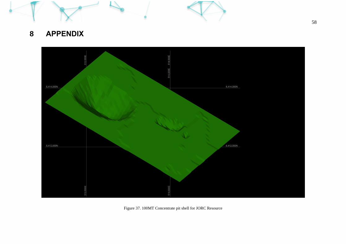
58

8 APPENDIX

Figure 37. 100MT Concentrate pit shell for JORC Resource

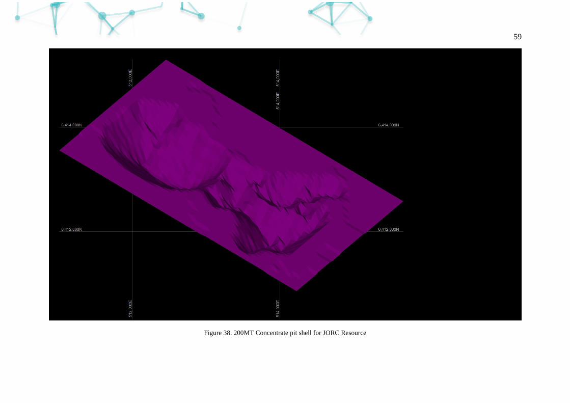
59

Figure 38. 200MT Concentrate pit shell for JORC Resource

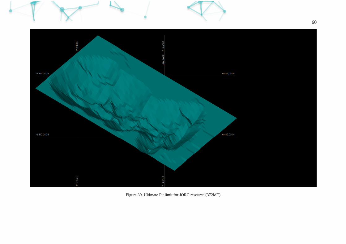
60

Figure 39. Ultimate Pit limit for JORC resource (372MT)

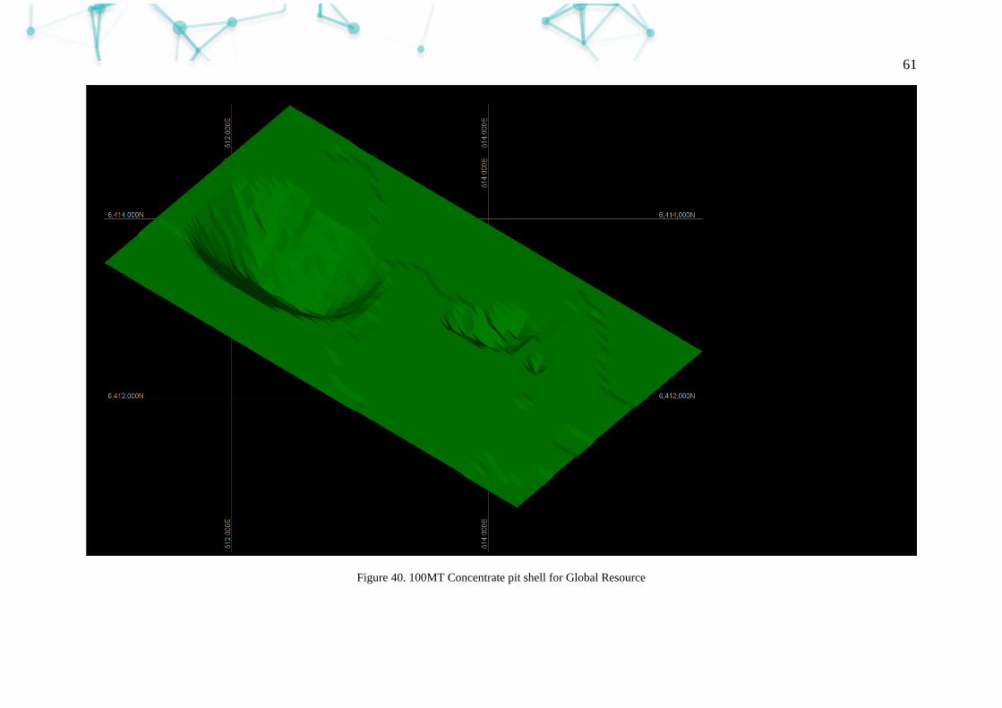
61

Figure 40. 100MT Concentrate pit shell for Global Resource

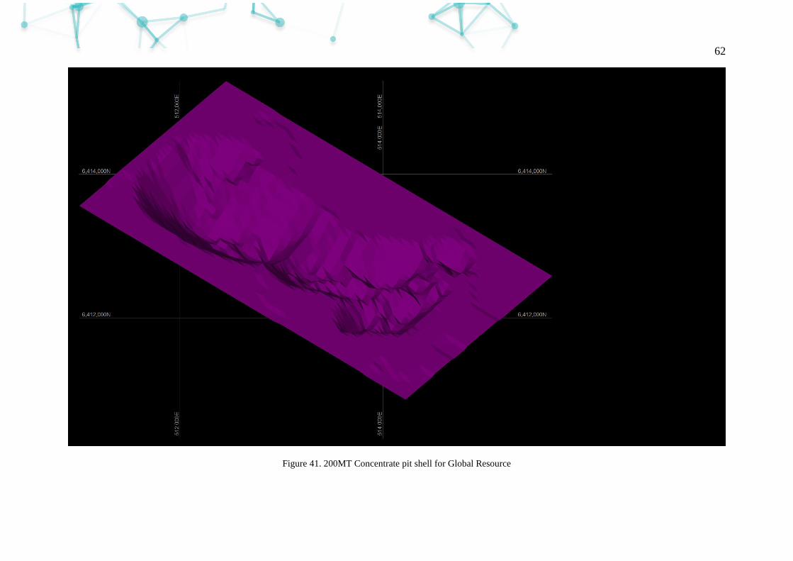
62

Figure 41. 200MT Concentrate pit shell for Global Resource

63

Figure 42. Ultimate Pit limit for Global resource (576MT)

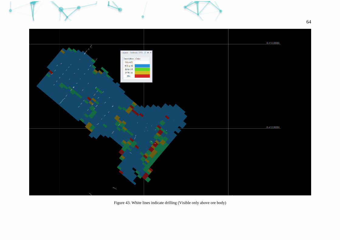
64

Figure 43. White lines indicate drilling (Visible only above ore body)

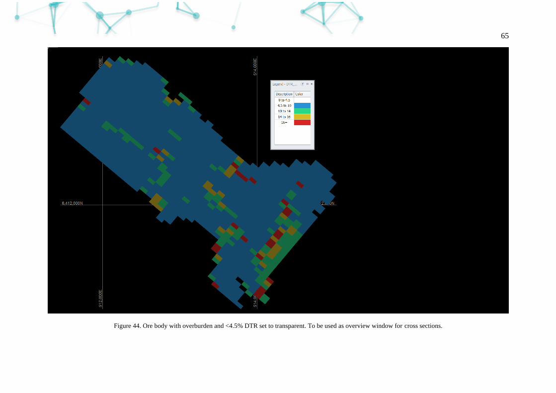
65

Figure 44. Ore body with overburden and <4.5% DTR set to transparent. To be used as overview window for cross sections.

66

Figure 45. Grid System used for cross sections.

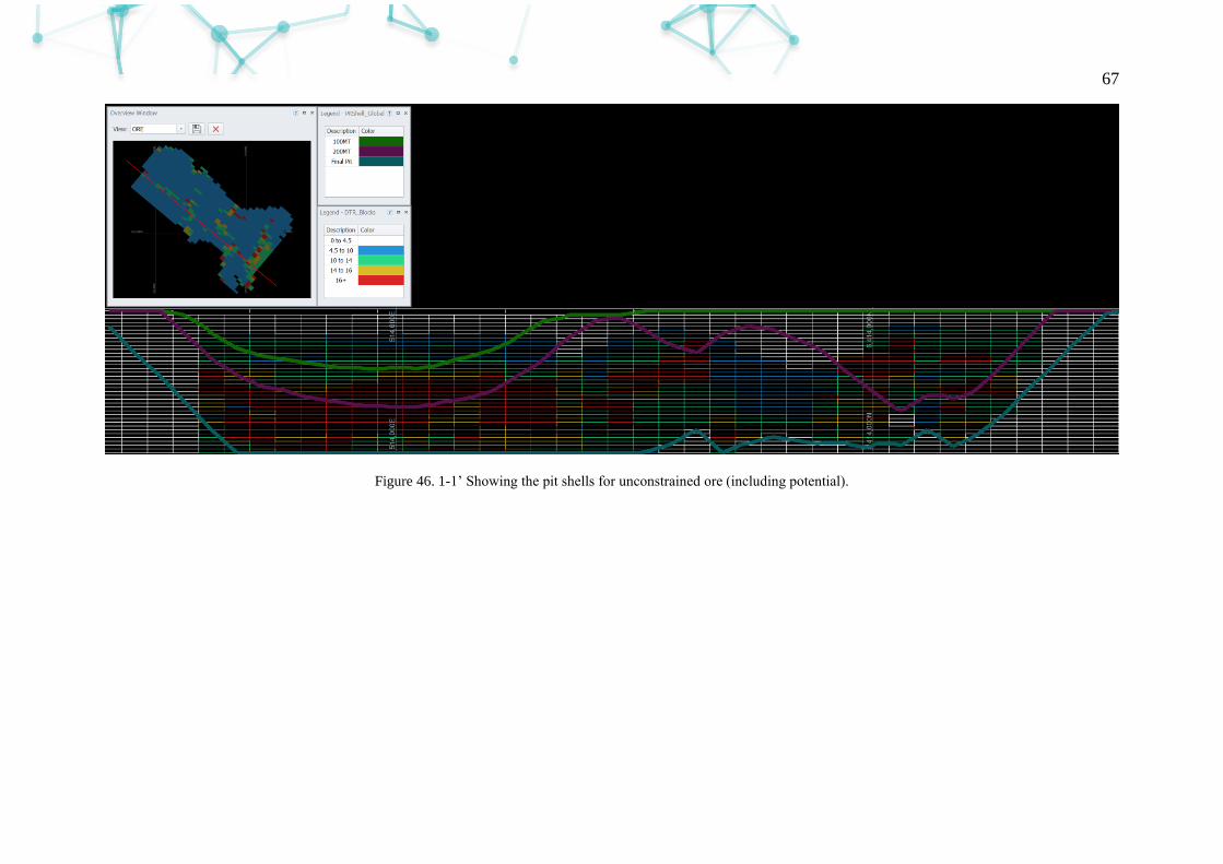
67

Figure 46. 1-1’ Showing the pit shells for unconstrained ore (including potential).

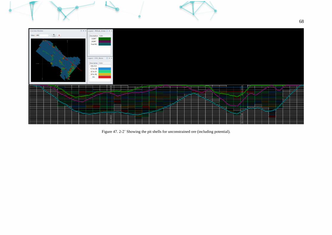
68

Figure 47. 2-2’ Showing the pit shells for unconstrained ore (including potential).

69

Figure 48. A-A’ Showing the pit shells for unconstrained ore (including potential).

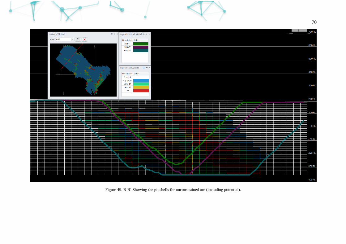
70

Figure 49. B-B’ Showing the pit shells for unconstrained ore (including potential).

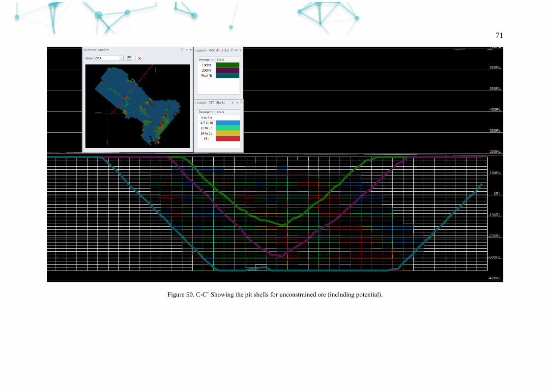
71

Figure 50. C-C’ Showing the pit shells for unconstrained ore (including potential).

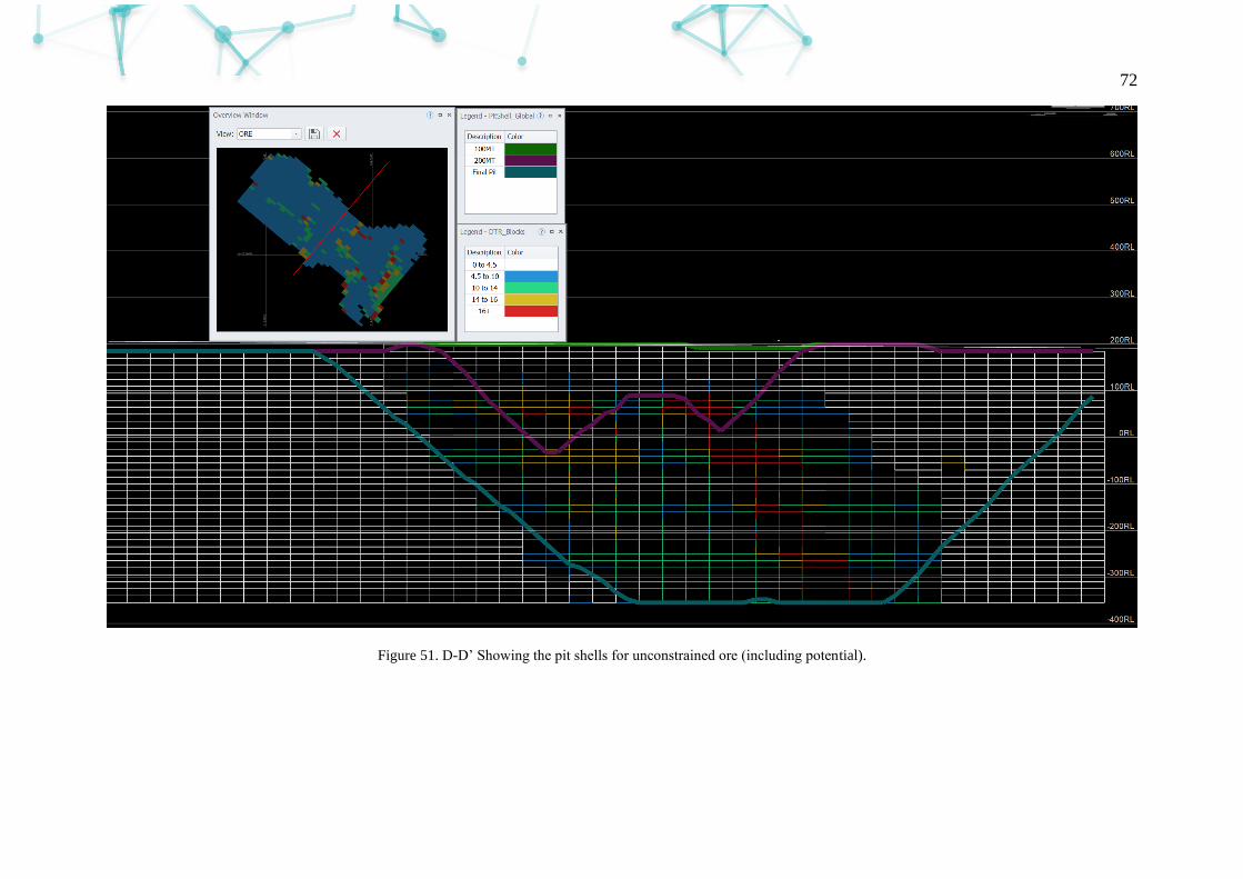
72

Figure 51. D-D’ Showing the pit shells for unconstrained ore (including potential).

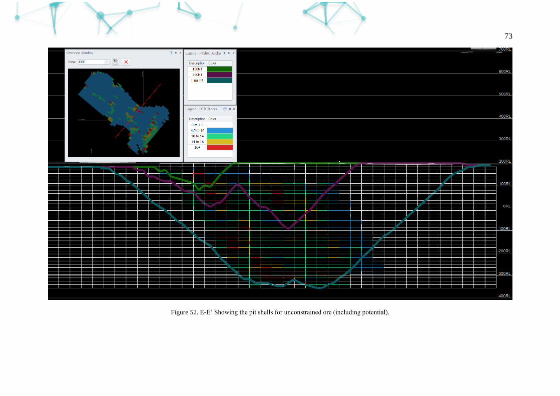
73

Figure 52. E-E’ Showing the pit shells for unconstrained ore (including potential).

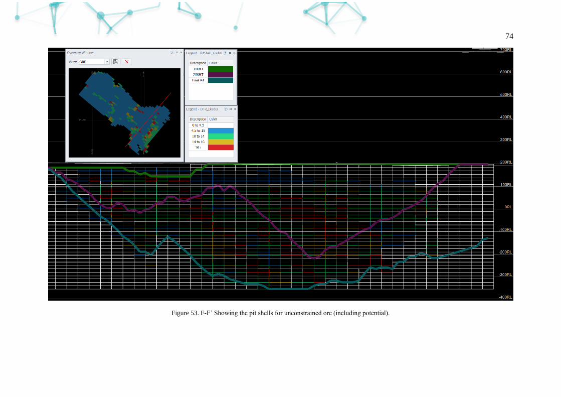
74

Figure 53. F-F’ Showing the pit shells for unconstrained ore (including potential).

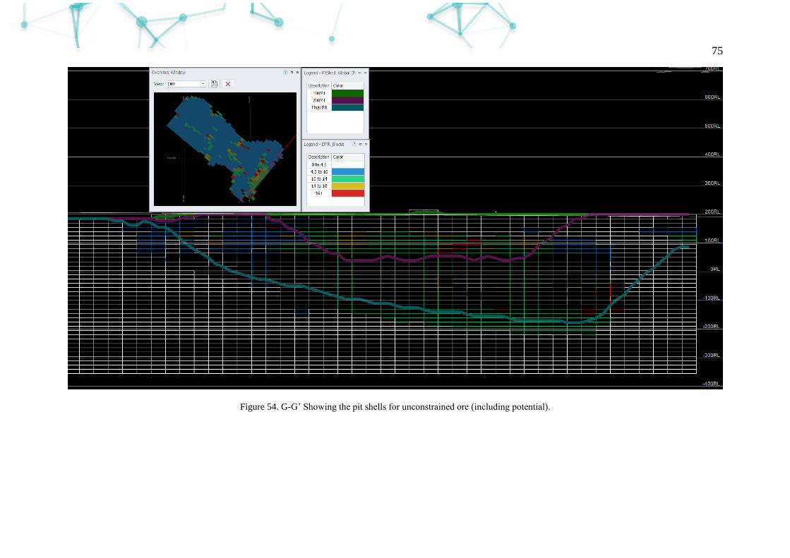
75

Figure 54. G-G’ Showing the pit shells for unconstrained ore (including potential).

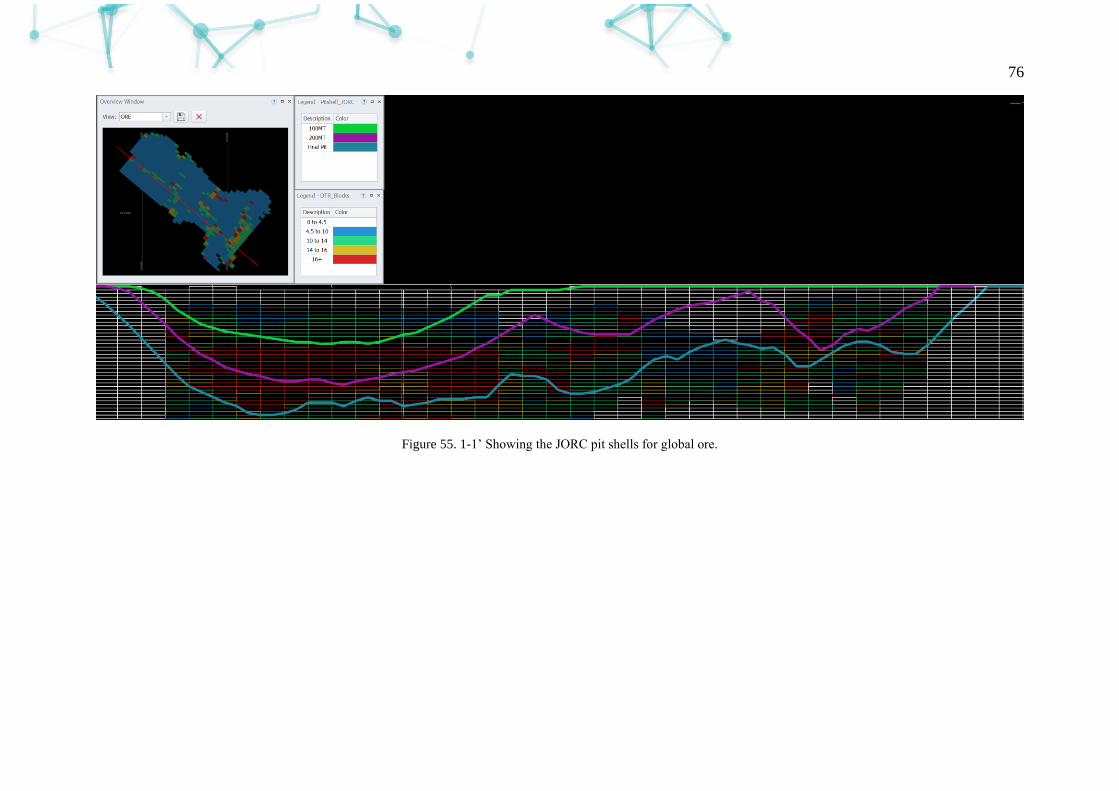
76

Figure 55. 1-1’ Showing the JORC pit shells for global ore.

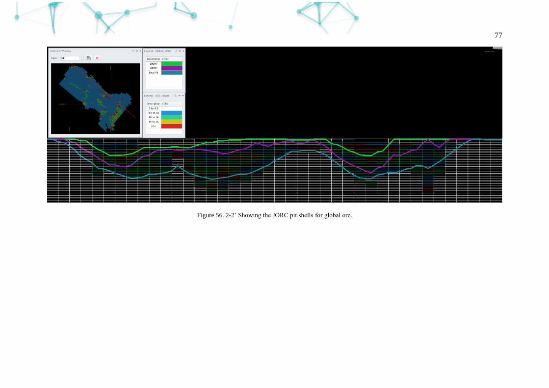
77

Figure 56. 2-2’ Showing the JORC pit shells for global ore.

78

Figure 57. A-A’ Showing the JORC pit shells for global ore.

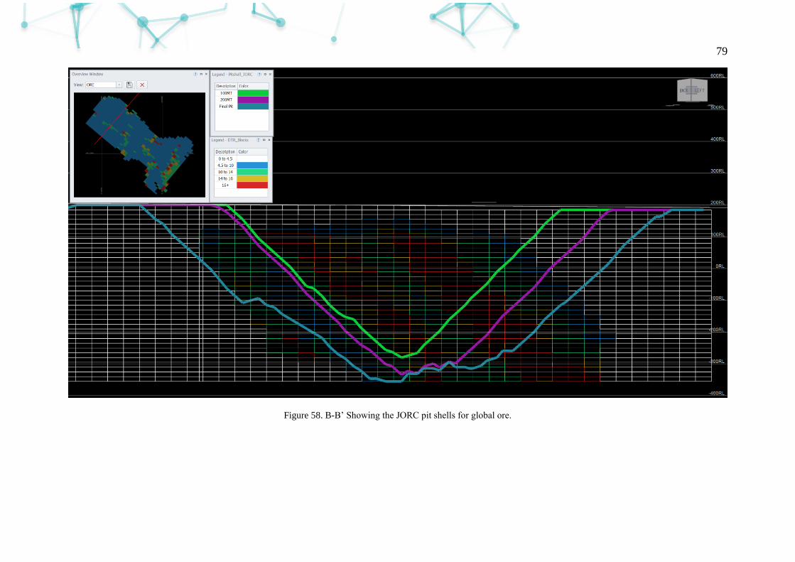
79

Figure 58. B-B’ Showing the JORC pit shells for global ore.

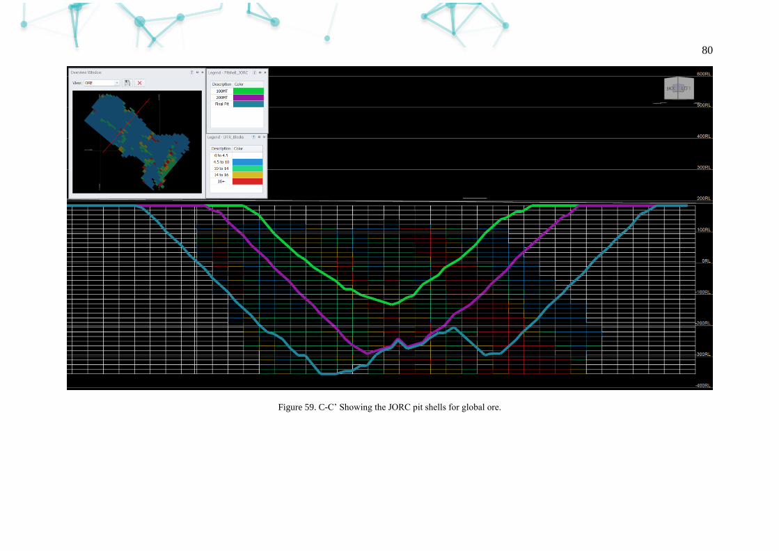
80

Figure 59. C-C’ Showing the JORC pit shells for global ore.

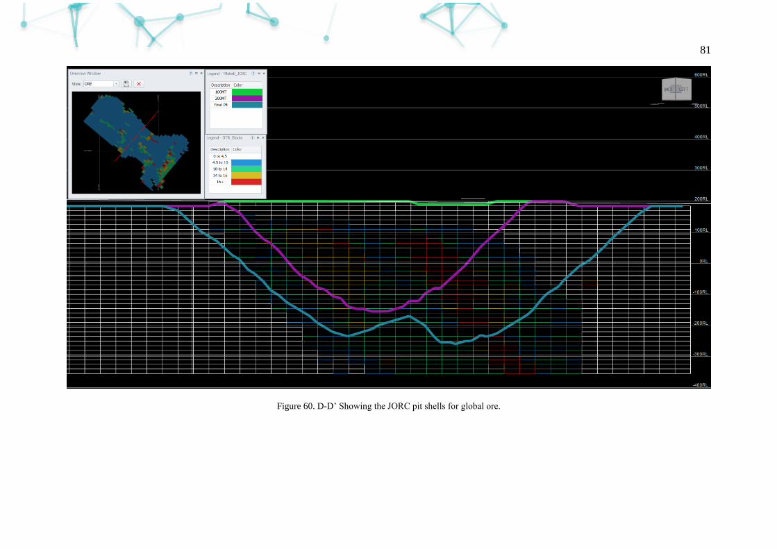
81

Figure 60. D-D’ Showing the JORC pit shells for global ore.

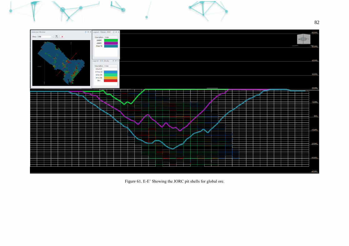
82

Figure 61. E-E’ Showing the JORC pit shells for global ore.

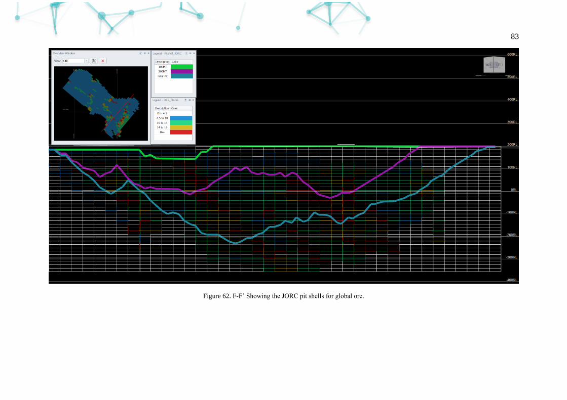
83

Figure 62. F-F’ Showing the JORC pit shells for global ore.

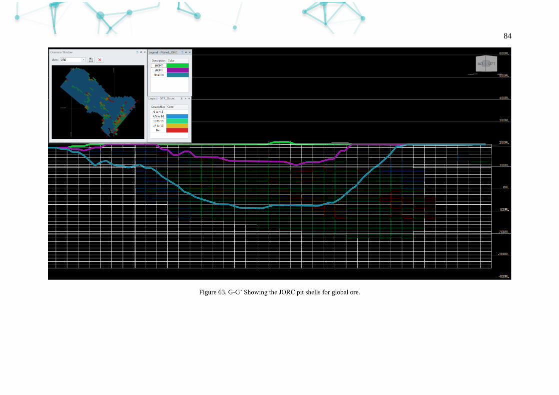
84

Figure 63. G-G’ Showing the JORC pit shells for global ore.

Mineral Resource Upgrade - Hawsons Iron

Documents

Transcript of Mineral Resource Upgrade - Hawsons Iron