
Minage de règles rapide, exact et exhaustif dans de larges ...
156
HAL Id: tel-03237830 https://tel.archives-ouvertes.fr/tel-03237830 Submitted on 26 May 2021 HAL is a multi-disciplinary open access archive for the deposit and dissemination of sci- entific research documents, whether they are pub- lished or not. The documents may come from teaching and research institutions in France or abroad, or from public or private research centers. L’archive ouverte pluridisciplinaire HAL, est destinée au dépôt et à la diffusion de documents scientifiques de niveau recherche, publiés ou non, émanant des établissements d’enseignement et de recherche français ou étrangers, des laboratoires publics ou privés. Minage de règles rapide, exact et exhaustif dans de larges bases de connaissances Jonathan Lajus To cite this version: Jonathan Lajus. Minage de règles rapide, exact et exhaustif dans de larges bases de connaissances. Artificial Intelligence [cs.AI]. Institut Polytechnique de Paris, 2021. English. NNT: 2021IPPAT002. tel-03237830
-
Upload
khangminh22 -
Category
Documents
-
view
1 -
download
0
Transcript of Minage de règles rapide, exact et exhaustif dans de larges ...
HAL Id: tel-03237830https://tel.archives-ouvertes.fr/tel-03237830
Submitted on 26 May 2021
HAL is a multi-disciplinary open accessarchive for the deposit and dissemination of sci-entific research documents, whether they are pub-lished or not. The documents may come fromteaching and research institutions in France orabroad, or from public or private research centers.
L’archive ouverte pluridisciplinaire HAL, estdestinée au dépôt et à la diffusion de documentsscientifiques de niveau recherche, publiés ou non,émanant des établissements d’enseignement et derecherche français ou étrangers, des laboratoirespublics ou privés.
Minage de règles rapide, exact et exhaustif dans delarges bases de connaissances
Jonathan Lajus
To cite this version:Jonathan Lajus. Minage de règles rapide, exact et exhaustif dans de larges bases de connaissances.Artificial Intelligence [cs.AI]. Institut Polytechnique de Paris, 2021. English. NNT : 2021IPPAT002.tel-03237830
626
NN
T:2
021I
PPA
T002 Fast, Exact, and Exhaustive Rule Mining
in Large Knowledge BasesThese de doctorat de l’Institut Polytechnique de Paris
preparee a Telecom Paris
Ecole doctorale n626Ecole doctorale de l’Institut Polytechnique de Paris (ED IP Paris)
Specialite de doctorat : Informatique, donnees, IA
These presentee et soutenue a Palaiseau, le 16 fevrier 2021, par
JONATHAN LAJUS
Composition du Jury :
Thomas BonaldProfessor, Telecom Paris President
Paolo PapottiAssociate Professor, EURECOM Rapporteur
Heiko PaulheimProfessor, University of Mannheim Rapporteur
Hannah BastProfessor, University of Freiburg Examinatrice
Luis GalarragaResearcher, INRIA Rennes Examinateur
Fatiha SaısProfessor, Paris Saclay University (LRI) Examinatrice
Fabian SuchanekProfessor, Telecom Paris Directeur de these

To my parents, my family and Minou.
1
Acknowlegements
Une these est un circuit de longue haleine. Tout a commence il y a cinq ansquand Fabian a accepte de me faire rejoindre l’equipe DIG. A l’epoque, j’aicommence par me mettre dans la roue de Luis durant un stage de 6 mois.Puis apres son echappee, il m’a fallu prendre le vent.
Heureusement, je pu faire partie d’un formidable peloton, comprenantLuis, Thomas, Thomas, Julien, Ned, Antoine, Marc, Marie, Pierre-Alexandre,Jean-Louis, Mauro et tant d’autres avec qui j’ai pu partager cette aventure.Je souhaite remercier particulierement Fabian, qui en bon capitaine de routea toujours su etre a l’ecoute. Je remercie egalement Bruno Defude, BerndAmann et Arnaud Soulet pour leur conseils en cours de route.
Le parcours etait bien escarpe, avec des hauts et des bas, parfois en dan-seuse mais souvent a mouliner. Je ne peux que remercier mes parents, toutema famille qui m’ont soutenu mais aussi mes colocataires qui m’ont supporte.Sans oublier les Nadine, Samy, Sarah, Simon, Emilie, Romaing, Joris, Seya,Doc, Guillaume, Malfoy et Camille pour les japs et les soirees jeux qui m’ontpermis de sortir la tete du guidon.
Bien que les reves de maillot jaune ont disparu, j’ai pu au moins finir lacourse. Il a fallu changer de braquet pour cette derniere etape de 153 pages.Je remercie tous les membres du jury de donner de leur temps pour considererson homologation.
A thesis is a long ride. Everything started, five years ago, when Fabian mademe join the team. I first sat in the wheels of Luis during my master thesis.Then, after he made a breakaway, I had to set my own pace.
Fortunately, I was part of a terrific peloton, including Luis, Thomas,Thomas, Julien, Ned, Antoine, Marc, Marie, Pierre-Alexandre, Jean-Louis,Mauro and many others, with who I could share this adventure. I wouldlike to particularly thank Fabian, who made a great raod captain, alwaysreceptive and responsive. I would also like to thank Bruno Defude, BerndAmann and Arnaud Soulet for their valuable input along the road.
2

Fast, Exact, and Exhaustive Rule Mining in Large Knowledge Bases
The journey was steep, with ups and downs. I have to thank my parentsand my whole family for their support, and my roommates who were ableto put up with me. I also thank the Nadine, Samy, Sarah, Simon, Emilie,Romaing, Joris, Seya, Doc, Guillaume, Malfoy et Camille for dining out andthe game night that made me keep my head over the water.
If the dreams of the yellow jersey have faded away, I did at least finishthe race. I had to pick up an higher pace for this last stage of 153 pages.I thank all the member of the jury for the time they spend as they have todecide whether they certify this run.
3
Contents
1 Introduction 7
1.1 Motivation . . . . . . . . . . . . . . . . . . . . . . . . . . . . . 7
1.2 Contribution . . . . . . . . . . . . . . . . . . . . . . . . . . . . 8
2 Introduction to Knowledge Bases and Rule Mining 11
2.1 Introduction . . . . . . . . . . . . . . . . . . . . . . . . . . . . 11
2.2 Knowledge Representation . . . . . . . . . . . . . . . . . . . . 11
2.2.1 Entities . . . . . . . . . . . . . . . . . . . . . . . . . . 11
2.2.2 Classes . . . . . . . . . . . . . . . . . . . . . . . . . . . 14
2.2.3 Relations . . . . . . . . . . . . . . . . . . . . . . . . . 17
2.2.4 Completeness and Correctness . . . . . . . . . . . . . . 21
2.2.5 The Semantic Web . . . . . . . . . . . . . . . . . . . . 21
2.3 Rule Mining . . . . . . . . . . . . . . . . . . . . . . . . . . . . 22
2.3.1 Rules . . . . . . . . . . . . . . . . . . . . . . . . . . . . 22
2.3.2 Rule Mining . . . . . . . . . . . . . . . . . . . . . . . . 25
2.3.3 Rule Mining Approaches . . . . . . . . . . . . . . . . . 29
2.3.4 Related Approaches . . . . . . . . . . . . . . . . . . . . 35
2.4 Conclusion . . . . . . . . . . . . . . . . . . . . . . . . . . . . . 37
3 AMIE 3: Fast Computation of Quality Measures 38
3.1 Introduction . . . . . . . . . . . . . . . . . . . . . . . . . . . . 38
3.2 AMIE 3 . . . . . . . . . . . . . . . . . . . . . . . . . . . . . . 39
3.2.1 The AMIE Approach . . . . . . . . . . . . . . . . . . . 39
3.2.2 AMIE 3 . . . . . . . . . . . . . . . . . . . . . . . . . . 40
3.2.3 Quality Metrics . . . . . . . . . . . . . . . . . . . . . . 44
3.3 Experiments . . . . . . . . . . . . . . . . . . . . . . . . . . . . 45
3.3.1 Experimental Setup . . . . . . . . . . . . . . . . . . . . 45
3.3.2 Effect of our optimizations . . . . . . . . . . . . . . . . 46
3.3.3 Comparative Experiments . . . . . . . . . . . . . . . . 49
3.4 Conclusion . . . . . . . . . . . . . . . . . . . . . . . . . . . . . 53
4
Fast, Exact, and Exhaustive Rule Mining in Large Knowledge Bases
4 Star patterns: Reducing the Search Space 544.1 Introduction . . . . . . . . . . . . . . . . . . . . . . . . . . . . 544.2 Star patterns . . . . . . . . . . . . . . . . . . . . . . . . . . . 55
4.2.1 Patterns . . . . . . . . . . . . . . . . . . . . . . . . . . 554.2.2 Star patterns . . . . . . . . . . . . . . . . . . . . . . . 564.2.3 Related work . . . . . . . . . . . . . . . . . . . . . . . 574.2.4 Languages of star patterns . . . . . . . . . . . . . . . . 58
4.3 Mining star patterns . . . . . . . . . . . . . . . . . . . . . . . 604.4 Combining the star patterns into rules . . . . . . . . . . . . . 62
4.4.1 Compatibility of the star patterns . . . . . . . . . . . . 624.4.2 Selection of compatible star patterns . . . . . . . . . . 66
4.5 Conclusion . . . . . . . . . . . . . . . . . . . . . . . . . . . . . 67
5 Star patterns and path rules 685.1 Introduction . . . . . . . . . . . . . . . . . . . . . . . . . . . . 685.2 Path rules . . . . . . . . . . . . . . . . . . . . . . . . . . . . . 69
5.2.1 Path queries . . . . . . . . . . . . . . . . . . . . . . . . 695.2.2 Path rules . . . . . . . . . . . . . . . . . . . . . . . . . 725.2.3 Other path rules . . . . . . . . . . . . . . . . . . . . . 73
5.3 Pruning the search space . . . . . . . . . . . . . . . . . . . . . 735.3.1 Star patterns and path rules . . . . . . . . . . . . . . . 745.3.2 Generating all path rules . . . . . . . . . . . . . . . . . 765.3.3 Incremental generation of candidates . . . . . . . . . . 76
5.4 The bipattern graph and other rules . . . . . . . . . . . . . . . 775.5 Conclusion . . . . . . . . . . . . . . . . . . . . . . . . . . . . . 79
6 Pathfinder: Efficient Path Rule Mining 806.1 Introduction . . . . . . . . . . . . . . . . . . . . . . . . . . . . 806.2 Heritable information . . . . . . . . . . . . . . . . . . . . . . . 81
6.2.1 Notation . . . . . . . . . . . . . . . . . . . . . . . . . . 816.2.2 The sets of possible values . . . . . . . . . . . . . . . . 826.2.3 The iterated provenance . . . . . . . . . . . . . . . . . 866.2.4 Backtracking the iterated provenance . . . . . . . . . . 886.2.5 Measure computation strategies . . . . . . . . . . . . . 89
6.3 The bounds on the iterated provenance . . . . . . . . . . . . . 896.3.1 Computing the lower bounds . . . . . . . . . . . . . . . 906.3.2 Bounding the value of the quality measures . . . . . . 91
6.4 The complete Pathfinder algorithm . . . . . . . . . . . . . . . 926.5 Experiments . . . . . . . . . . . . . . . . . . . . . . . . . . . . 95
6.5.1 Experimental Setup . . . . . . . . . . . . . . . . . . . . 956.5.2 Pathfinder generation methods . . . . . . . . . . . . . 96
5
Fast, Exact, and Exhaustive Rule Mining in Large Knowledge Bases
6.5.3 Pathfinder measure computation strategies . . . . . . . 986.5.4 Scaling experiments . . . . . . . . . . . . . . . . . . . . 100
6.6 Conclusion . . . . . . . . . . . . . . . . . . . . . . . . . . . . . 101
7 Identifying obligatory attributes in a KB 1037.1 Introduction . . . . . . . . . . . . . . . . . . . . . . . . . . . . 1037.2 Related Work . . . . . . . . . . . . . . . . . . . . . . . . . . . 1057.3 Preliminaries . . . . . . . . . . . . . . . . . . . . . . . . . . . 1067.4 Model . . . . . . . . . . . . . . . . . . . . . . . . . . . . . . . 107
7.4.1 Problem Definition . . . . . . . . . . . . . . . . . . . . 1077.4.2 Our Approach . . . . . . . . . . . . . . . . . . . . . . . 1087.4.3 Assumptions . . . . . . . . . . . . . . . . . . . . . . . . 1117.4.4 Random sampling model . . . . . . . . . . . . . . . . . 112
7.5 Algorithm . . . . . . . . . . . . . . . . . . . . . . . . . . . . . 1147.5.1 Confidence Ratio . . . . . . . . . . . . . . . . . . . . . 1147.5.2 Algorithm . . . . . . . . . . . . . . . . . . . . . . . . . 1157.5.3 Variations . . . . . . . . . . . . . . . . . . . . . . . . . 117
7.6 Experiments . . . . . . . . . . . . . . . . . . . . . . . . . . . . 1177.6.1 Datasets . . . . . . . . . . . . . . . . . . . . . . . . . . 1177.6.2 Gold Standard . . . . . . . . . . . . . . . . . . . . . . 1187.6.3 Evaluation Metric . . . . . . . . . . . . . . . . . . . . . 1197.6.4 YAGO Experiment . . . . . . . . . . . . . . . . . . . . 1197.6.5 Wikidata Experiment . . . . . . . . . . . . . . . . . . . 1217.6.6 Artificial Classes . . . . . . . . . . . . . . . . . . . . . 122
7.7 Conclusion . . . . . . . . . . . . . . . . . . . . . . . . . . . . . 123
8 Conclusion 1278.1 Summary . . . . . . . . . . . . . . . . . . . . . . . . . . . . . 1278.2 Outlook . . . . . . . . . . . . . . . . . . . . . . . . . . . . . . 1298.3 Conclusion . . . . . . . . . . . . . . . . . . . . . . . . . . . . . 130
A Computation of Support and Confidence 131
B Number of items per relation 133
C Compatibility of a set of star patterns: Algorithm 136
D Resume de la these en Francais 141D.1 Position du probleme . . . . . . . . . . . . . . . . . . . . . . . 141D.2 Contribution . . . . . . . . . . . . . . . . . . . . . . . . . . . . 143D.3 Conclusion . . . . . . . . . . . . . . . . . . . . . . . . . . . . . 145
6

Chapter 1
Introduction
1.1 Motivation
When we send a query to Google or Bing, we obtain a set of Web pages.However, in some cases, we also get more information. For example, whenwe ask “When was Steve Jobs born?”, the search engine replies directly with“February 24, 1955”. When we ask just for “Steve Jobs”, we obtain a shortbiography, his birth date, quotes, and spouse. All of this is possible becausethe search engine has a huge repository of knowledge about people of commoninterest. This knowledge takes the form of a knowledge base (KB).
The KBs used in such search engines are entity-centric: they know indi-vidual entities (such as Steve Jobs, the United States, the Kilimanjaro, or theMax Planck Society), their semantic classes (such as SteveJobs is-a computer-Pioneer, SteveJobs is-a entrepreneur), relationships between entities (e.g.,SteveJobs founded AppleInc, SteveJobs hasInvented iPhone, SteveJobs has-WonPrize NationalMedalOfTechnology, etc.) as well as their validity times(e.g., SteveJobs wasCEOof Pixar [1986,2006]).
The idea of such KBs is not new. It goes back to seminal work in Artifi-cial Intelligence on universal knowledge bases in the 1980s and 1990s, mostnotably, the Cyc project [47] at MCC in Austin and the WordNet project [24]at Princeton University. These knowledge collections were hand-crafted andmanually curated. In the last ten years, in contrast, KBs are often builtautomatically by extracting information from the Web or from text doc-uments. Salient projects with publicly available resources include Know-ItAll (UW Seattle, [22]), ConceptNet (MIT, [49]), DBpedia (FU Berlin, UMannheim, & U Leipzig, [46]), NELL (CMU, [12]), BabelNet (La Sapienza,[67]), Wikidata (Wikimedia Foundation, [84]), and YAGO (Telecom Paris &Max Planck Institute, [78]). Commercial interest in KBs has been strongly
7

Fast, Exact, and Exhaustive Rule Mining in Large Knowledge Bases
growing, with projects such as the Google Knowledge Graph [19] (includ-ing Freebase [9]), Microsoft’s Satori, Amazon’s Evi, LinkedIn’s KnowledgeGraph, and the IBM Watson KB [26]. These KBs contain many millionsof entities, organized in hundreds to hundred thousands of semantic classes,and hundred millions of relational facts between entities. Many public KBsare interlinked, forming the Web of Linked Open Data [8].
This large interlinked Knowledge can itself be mined for information. Thepattern or correlation found are expressed as rules such as:
married(x, y) ∧ livesIn(x, z)⇒ livesIn(y, z)
This rule expresses that “If X and Y are married, and X lives in Z, then Yalso lives in Z”, or in other words, that two married people usually live inthe same place. Such rules usually come with confidence scores that expressto what degree a rule holds.
Rule mining is the task of automatically finding logical rules in a givenKB. It usually focus on outputting the rules of highest quality, i.e the rulesthat have a confidence score superior to a given user-defined parameter.
The rules can serve several purposes: First, they serve to complete theKB. If we do not know the place of residence of a person, we can proposethat the person lives where their spouse lives. Second, they can serve todebug the KB. If the spouse of someone lives in a different city, then this canindicate a problem. Finally, rules are useful in downstream applications suchas fact checking [2], ontology alignment [28] or predicting completeness [29].
The difficulty in finding such rules lies in the exponential size of thesearch space: every relation can potentially be combined with every otherrelation in a rule. This is why early approaches (such as AMIE [31]) wereunable to run on large KBs such as Wikidata in less than a day. Since then,several approaches have resorted to sampling or approximate confidence cal-culations [30, 94, 63, 14]. The more the approach samples, the faster itbecomes, but the less accurate the results will be. Another common tech-nique [63, 58, 94, 66] (from standard inductive logic programming) is to minenot all rules, but only enough rules to cover the positive examples. This, like-wise, speeds up the computation, but does not mine all rules that hold inthe KB.
1.2 Contribution
The main goal of this thesis is to study optimizations and novel approachesto develop efficient rule mining algorithms that scale to large KBs, computethe quality measures exactly, and are exhaustive with regard to user-defined
8

Fast, Exact, and Exhaustive Rule Mining in Large Knowledge Bases
parameters. Such algorithms can serve as a baseline for other approximaterule mining algorithms, and to produce a gold standard of mined rules.
Preliminaries. In Chapter 2, we define the main notions of entity-centricKnowledge Bases and explain their principal characteristics. Then we intro-duce the task of Rule Mining as an Inductive Logic Programming problemand describe the multiple rule mining algorithms that apply on KnowledgeBases. This chapter is based on our following tutorial paper:
- Fabian M Suchanek, Jonathan Lajus, Armand Boschin, and GerhardWeikum. Knowledge representation and rule mining in entity-centricknowledge bases. In Reasoning Web. Explainable Artificial Intelligence,pages 110–152. Springer, 2019
AMIE 3. In Chapter 3, we present AMIE 3, an improved version of therule mining algorithm AMIE+ [30]. In this new version we introduce newoptimizations on the computation of the quality measures, allowing AMIEto once again become an exact and exhaustive rule mining algorithm. Thisnew version is also more efficient, allowing AMIE to scale to large KBs thatwere previously beyond reach. This chapter is based on our following fullpaper:
- Jonathan Lajus, Luis Galarraga, and Fabian Suchanek. Fast and exactrule mining with AMIE 3. In European Semantic Web Conference, pages36–52. Springer, 2020
Pruning the search space. In Chapter 4, we further address the problemof the exponential search that prevents AMIE from efficiently mining morecomplex rules, for example rules of size 4 on large KBs. In particular, westudy how the decomposition of the rules into smaller entity-centric patterns,the “star patterns”, can be used to identify and prune unsatisfiable rulesbefore any costly computation. This chapter is based on unpublished work.
Path rule mining. In Chapter 5, we restrict our study of efficient rulemining to a certain type of rules, the path rules. In particular, we show thatall closed path rules can be generated without duplicates using a specific re-finement operator, and that the star patterns introduced in Chapter 4 can beused constructively to efficiently prune the search space of path rules. Fromthis, we deduce the “Pathfinder vanilla” algorithm, an exact and exhaustivepath rule mining algorithm.
9
Fast, Exact, and Exhaustive Rule Mining in Large Knowledge Bases
In Chapter 6, we study the consequences of a fundamental dependencyin the Pathfinder vanilla algorithm: every rule comes from a unique parentrule. In particular, we show that a parent rule can pass information to itschild rules and we use this idea to improve the computation of the qual-ity measures and perform early pruning. Finally, we present the complete“Pathfinder” algorithm, a refined version of the Pathfinder vanilla algorithmwhich outperforms AMIE on path rules on most datasets, and by multipleorders of magnitudes when mining longer rules. This part is also based onunpublished work.
Rule mining about the real world. In Chapter 7 we present work thatcan automatically determine the obligatory attributes of a class. For exam-ple, our algorithm mines that every singer sings in the real world, even ifour KB is largely incomplete. In particular, we introduce a statistical mod-elization of the incompleteness of the KB and deduce a metric to identifyobligatory attributes. This chapter is based on our following full paper:
- Jonathan Lajus and Fabian M. Suchanek. Are all people married? deter-mining obligatory attributes in knowledge bases. In WWW, pages 1115–1124. International World Wide Web Conferences Steering Committee,2018
Conclusion. Chapter 8 concludes this thesis and present furtherprospects.
10
Chapter 2
Introduction to KnowledgeBases and Rule Mining
2.1 Introduction
The field of knowledge representation has a long history, and goes back tothe early days of Artificial Intelligence. It has developed numerous knowl-edge representation models, from frames and KL-ONE to recent variants ofdescription logics. The reader is referred to survey works for comprehen-sive overviews of historical and classical models [73, 76]. In the first part ofthis chapter, we discuss the knowledge representation that has emerged as apragmatic consensus in the research community of entity-centric knowledgebases.
In the second part of this chapter, we discuss logical rules on knowledgebases. A logical rule can tell us, e.g., that if two people are married, thenthey (usually) live in the same city. Such rules can be mined automaticallyfrom the knowledge base, and they can serve to correct the data or fill inmissing information. We discuss first classical Inductive Logic Programmingapproaches, and then show how these can be applied to the case of knowledgebases.
2.2 Knowledge Representation
2.2.1 Entities
Entities of Interest
The most basic element of a KB is an entity. An entity is any abstract orconcrete object of fiction or reality, or, as Bertrand Russell puts it in his
11
Fast, Exact, and Exhaustive Rule Mining in Large Knowledge Bases
Principles of Mathematics [86]:
Definition 2.2.1 (Entity). An entity is whatever may be an object ofthought.
This definition is completely all-embracing. Steve Jobs, the Declaration ofIndependence of the United States, the Theory of Relativity, and a moleculeof water are all entities. Events (such as the French Revolution), are entities,too. An entity does not even have to exist: Harry Potter, e.g., is a fictionalentity. Phlogiston was presumed to be the substance that makes up heat. Itturned out to not exist – but it is still an entity.
KBs model a part of reality. This means that they choose certain entitiesof interest, give them names, and put them into a structure. Thus, a KB isa structured view on a selected part of the world. KBs typically model onlydistinct entities. This cuts out a large portion of the world that consists ofvariations, flows and transitions between entities. Drops of rain, for instance,fall down, join in a puddle and may be splattered by a passing car to formnew drops [75]. KBs will typically not model these phenomena. This choiceto model only discrete entities is a projection of reality; it is a grid throughwhich we see only distinct things. Many entities consist of several differententities. A car, for example, consists of wheels, a bodywork, an engine, andmany other pieces. The engine consists of the pistons, the valves, and thespark plug. The valves consist again of several parts, and so on, until weultimately arrive at the level of atoms or below. Each of these componentsis an entity. However, KBs will typically not be concerned with the lowerlevels of granularity. A KB might model a car, possibly its engine and itswheels, but most likely not its atoms. In all of the following, we will only beconcerned with the entities that a KB models.
Entities in the real world can change gradually. For example, the Greekphilosopher Eubilides asks: If one takes away one molecule of an object, willthere still be the same object? If it is still the same object, this invites oneto take away more molecules until the object disappears. If it is anotherobject, this forces one to accept that two distinct objects occupy the samespatio-temporal location: The whole and the whole without the molecule. Arelated problem is the question of identity. The ancient philosopher Theseususes the example of a ship: Its old planks are constantly being substituted.One day, the whole ship has been replaced and Theseus asks, “Is it still thesame ship?”. To cope with these problems, KBs typically model only atomicentities. In a KB, entities can only be created and destroyed as wholes.
12
Fast, Exact, and Exhaustive Rule Mining in Large Knowledge Bases
Identifiers and Labels
In computer systems (as well as in writing of any form), we refer to entitiesby identifiers.
Definition 2.2.2 (Identifier). An identifier for an entity is a string of char-acters that represents the entity in a computer system.
Typically, these identifiers take a human-readable form, such as Elvis-Presley for the singer Elvis Presley. However, some KBs use abstract identi-fiers. Wikidata, e.g., refers to Elvis Presley by the identifier Q303, and Free-base by /m/02jq1. This choice was made so as to be language-independent,and so as to provide an identifier that is stable in time. If, e.g., Elvis Presleyreincarnates in the future, then Q303 will always refer to the original ElvisPresley. It is typically assumed that there exists exactly one identifier perentity in a KB. For what follows, we will not distinguish identifiers fromentities, and just talk of entities instead.
Entities have names. For example, the city of New York can be called“city of New York”, “Big Apple”, or “Nueva York”. As we see, one entity canhave several names. Vice versa, the same name can refer to several entities.“Paris”, e.g., can refer to the city in France, to a city of that name in Texas,or to a hero of Greek mythology. Hence, we need to carefully distinguishnames – single words or entire phrases – from their senses – the entities thatthey denote. This is done by using labels.
Definition 2.2.3 (Label). A label for an entity is a human-readable stringthat names the entity.
If an entity has several labels, the labels are called synonymous. If thesame label refers to several entities, the label is polysemous. Not all entitieshave labels. For example, your kitchen chair is clearly an entity, but itprobably does not have any particular label. An entity that has a label iscalled a named entity. KBs typically model mainly named entities. There isone other type of entities that appears in KBs: literals.
Definition 2.2.4 (Literal). A literal is a fixed value that takes the form ofa string of characters.
Literals can be pieces of text, but also numbers, quantities, or timestamps.For example, the label “Big Apple” for the city of New York is a literal, asis the number of its inhabitants (8,175,133).
13
Fast, Exact, and Exhaustive Rule Mining in Large Knowledge Bases
2.2.2 Classes
Classes and Instances
KBs model entities of the world. They usually group entities together toform a class :
Definition 2.2.5 (Class). A class (also: concept, type) is a named set ofentities that share a common trait. An element of that set is called aninstance of the class.
Under this definition, the following are classes: The class of singers (i.e.,the set of all people who sing professionally), the class of historical events inLatin America, and the class of cities in Germany. Some instances of theseclasses are, respectively, Elvis Presley, the independence of Argentina, andBerlin. Since everything is an entity, a class is also an entity. It has (bydefinition) an identifier and a label.
Theoretically, KBs can form classes based on arbitrary traits. We can,e.g., construct the class of singers whose concerts were the first to be broad-cast by satellite. This class has only one instance (Elvis Presley). We canalso construct the class of left-handed guitar players of Scottish origin, or ofpieces of music that the Queen of England likes. There are several theoriesas to whether humans actually build and use classes, too [51]. Points of dis-cussion are whether humans form crisp concepts, and whether all elementsof a concept have the same degree of membership. For the purpose of KBs,however, classes are just sets of entities.
It is not always easy to decide whether something should be modeledas an instance or as a class. We could construct, e.g., for every instancea singleton class that contains just this instance (e.g., the class of all ElvisPresleys). Some things of the world can be modeled both as instances andas classes. A typical example is iPhone. If we want to designate the type ofsmartphone, we can model it as an instance of the class of smartphone brands.However, if we are interested in the iPhones owned by different people andwant to capture them individually, then iPhone should be modeled as a class.A similar observation holds for abstract entities such as love. Love can bemodeled as an instance of the class emotion, where it resides together withthe emotions of anger, fear, and joy. However, when we want to modelindividual feelings of love, then love would be a class. Its instances are thedifferent feelings of love that different people have. It is our choice how wewish to model reality.
Some KBs do not make the distinction between classes and instances (e.g.,the SKOS vocabulary, [89]). In these KBs, everything is an entity. There is,
14

Fast, Exact, and Exhaustive Rule Mining in Large Knowledge Bases
however, usually a “is more general than” link between a more special entityand a more general entity. Such a KB may contain, e.g., the knowledge thatiPhone is more special than smartphone, without worrying whether one ofthem is a class. The distinction between classes and instances adds a layer ofgranularity. This granularity is used, e.g., to define the domains and rangesof relations, as we shall see in Section 2.2.3.
Taxonomies
Definition 2.2.6 (Subsumption). Class A is a subclass of class B if A is asubset of B.
For example, the class of singers is a subclass of the class of persons,because every singer is a person. We also say that the class of singers isa specialization of the class of persons, or that singer is subsumed by orincluded in person. Vice versa, we say that person is a superclass or ageneralization of the class of singers. Technically speaking, two equivalentclasses are subclasses of each other. This is the way the RDFS standardmodels subclasses [88]. We say that a class is a proper subclass of anotherclass, if the second contains more entities than the first. We use the notionof subclass here to refer to proper subclasses only.
It is important not to confuse class inclusion with the relationship betweenparts and wholes. For example, an arm is a part of the human body. Thatdoes not mean, however, that every arm is a human body. Hence, arm is nota subclass of body. In a similar manner, New York is a part of the US. Thatdoes not mean that New York would be a subclass of the US. Neither NewYork nor the US are classes, so they cannot be subclasses of each other.
Class inclusion is transitive: If A is a subclass of B, and B is a subclass ofC, then A is a subclass of C. For example, viper is a subclass of snake, andsnake is a subclass of reptile. Hence, by transitivity, viper is also a subclass ofreptile. We say that a class is a direct subclass of another class, if there is noclass in the KB that is a superclass of the former and a subclass of the latter.When we talk about subclasses, we usually mean only direct subclasses. Theother subclasses are transitive subclasses. Since classes can be included inother classes, they can form an inclusion hierarchy – a taxonomy.
Definition 2.2.7 (Taxonomy). A taxonomy is a directed graph, where thenodes are classes and there is an edge from class X to class Y if X is a properdirect subclass of Y.
The notion of taxonomy is known from biology. Zoological or botanicspecies form a taxonomy: tiger is a subclass of cat. cat is a subclass of mam-mal, and so on. This principle carries over to all other types of classes. We
15
Fast, Exact, and Exhaustive Rule Mining in Large Knowledge Bases
say, e.g., that internetCompany is a subclass of company, and that companyis a subclass of organization, etc. Since a taxonomy models proper inclusion,it follows that the taxonomic graph is acyclic: If a class is the subclass ofanother class, then the latter cannot be a subclass of the former. Thus, ataxonomy is a directed acyclic graph. A taxonomy does not show the tran-sitive subclass edges. If the graph contains transitive edges, we can alwaysremove them. Given a finite directed acyclic graph with transitive edges, theset of direct edges is unique [4].
Transitivity is often essential in applications. For example, consider aquestion-answering system where a user asks for artists that are married toactors. If the KB only knew about Elvis Presley and Priscilla Presley beingin the classes rockSinger and americanActress, the question could not beanswered. However, by reasoning that rockSingers are also singers, who inturn are artists and americanActresses being actresses, it becomes possibleto give this correct answer.
Usually (but not necessarily), taxonomies are connected graphs: Everynode in the graph is, directly or indirectly, linked to every other node. Usu-ally, the taxonomies have a single root, i.e., a single node that has no outgoingedges. This node identifies the most general class, of which every other classis a subclass. In zoological KBs, this may be class animal. In a persondatabase, it may be the class person. In a general-purpose KB, this class hasto be the most general possible class. In YAGO and Wordnet, the class isentity. In the RDF standard, it is called resource [87]. In the OWL stan-dard [90], the highest class that does not include literals is called thing.
Some taxonomies have at most one outgoing edge per node. Then, thetaxonomy forms a tree. The biological taxonomy, e.g., forms a tree, as doesthe Java class hierarchy. However, there can be taxonomies where a classhas two distinct direct superclasses. For example, if we have the class singerand the classes of woman and man, then the class femaleSinger has twosuperclasses: singer and woman. Note that it would be wrong to makesinger a subclass of man and woman (as if to say that singers can be menor women). This would actually mean that all singers are at the same timemen and women.
When a taxonomy includes a “combination class” such as FrenchFe-maleSingers, then this class can have several superclasses. FrenchFe-maleSingers, e.g., can have as direct superclasses FrenchPeople, Women, andSingers. In a similar manner, one entity can be an instance of several classes.Albert Einstein, e.g., is an instance of the classes physicist, vegetarian, andviolinPlayer.
When we populate a KB with new instances, we usually try to assign themto the most specific suitable class. For example, when we want to place Bob
16
Fast, Exact, and Exhaustive Rule Mining in Large Knowledge Bases
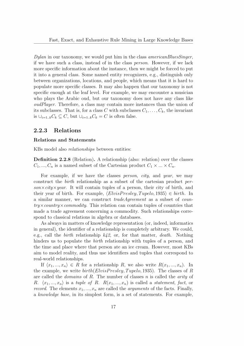
Dylan in our taxonomy, we would put him in the class americanBluesSinger,if we have such a class, instead of in the class person. However, if we lackmore specific information about the instance, then we might be forced to putit into a general class. Some named entity recognizers, e.g., distinguish onlybetween organizations, locations, and people, which means that it is hard topopulate more specific classes. It may also happen that our taxonomy is notspecific enough at the leaf level. For example, we may encounter a musicianwho plays the Arabic oud, but our taxonomy does not have any class likeoudPlayer. Therefore, a class may contain more instances than the union ofits subclasses. That is, for a class C with subclasses C1, . . . , Ck, the invariantis ∪i=1..kCk ⊆ C, but ∪i=1..kCk = C is often false.
2.2.3 Relations
Relations and Statements
KBs model also relationships between entities:
Definition 2.2.8 (Relation). A relationship (also: relation) over the classesC1, ..., Cn is a named subset of the Cartesian product C1 × ...× Cn.
For example, if we have the classes person, city, and year, we mayconstruct the birth relationship as a subset of the cartesian product per-son×city×year. It will contain tuples of a person, their city of birth, andtheir year of birth. For example, 〈ElvisPresley, Tupelo, 1935〉 ∈ birth. Ina similar manner, we can construct tradeAgreement as a subset of coun-try×country×commodity. This relation can contain tuples of countries thatmade a trade agreement concerning a commodity. Such relationships corre-spond to classical relations in algebra or databases.
As always in matters of knowledge representation (or, indeed, informaticsin general), the identifier of a relationship is completely arbitrary. We could,e.g., call the birth relationship k42, or, for that matter, death. Nothinghinders us to populate the birth relationship with tuples of a person, andthe time and place where that person ate an ice cream. However, most KBsaim to model reality, and thus use identifiers and tuples that correspond toreal-world relationships.
If 〈x1, ..., xn〉 ∈ R for a relationship R, we also write R(x1, ..., xn). Inthe example, we write birth(ElvisPresley, Tupelo, 1935). The classes of Rare called the domains of R. The number of classes n is called the arity ofR. 〈x1, ..., xn〉 is a tuple of R. R(x1, ..., xn) is called a statement, fact, orrecord. The elements x1, ..., xn are called the arguments of the facts. Finally,a knowledge base, in its simplest form, is a set of statements. For example,
17
Fast, Exact, and Exhaustive Rule Mining in Large Knowledge Bases
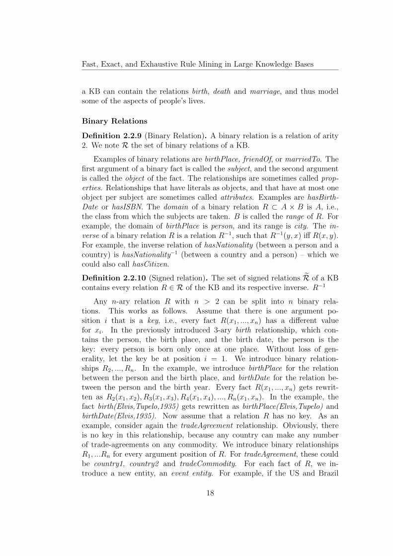
a KB can contain the relations birth, death and marriage, and thus modelsome of the aspects of people’s lives.
Binary Relations
Definition 2.2.9 (Binary Relation). A binary relation is a relation of arity2. We note R the set of binary relations of a KB.
Examples of binary relations are birthPlace, friendOf, or marriedTo. Thefirst argument of a binary fact is called the subject, and the second argumentis called the object of the fact. The relationships are sometimes called prop-erties. Relationships that have literals as objects, and that have at most oneobject per subject are sometimes called attributes. Examples are hasBirth-Date or hasISBN. The domain of a binary relation R ⊂ A × B is A, i.e.,the class from which the subjects are taken. B is called the range of R. Forexample, the domain of birthPlace is person, and its range is city. The in-verse of a binary relation R is a relation R−1, such that R−1(y, x) iff R(x, y).For example, the inverse relation of hasNationality (between a person and acountry) is hasNationality−1 (between a country and a person) – which wecould also call hasCitizen.
Definition 2.2.10 (Signed relation). The set of signed relations R of a KBcontains every relation R ∈ R of the KB and its respective inverse. R−1
Any n-ary relation R with n > 2 can be split into n binary rela-tions. This works as follows. Assume that there is one argument po-sition i that is a key, i.e., every fact R(x1, ..., xn) has a different valuefor xi. In the previously introduced 3-ary birth relationship, which con-tains the person, the birth place, and the birth date, the person is thekey: every person is born only once at one place. Without loss of gen-erality, let the key be at position i = 1. We introduce binary relation-ships R2, ..., Rn. In the example, we introduce birthPlace for the relationbetween the person and the birth place, and birthDate for the relation be-tween the person and the birth year. Every fact R(x1, ..., xn) gets rewrit-ten as R2(x1, x2), R3(x1, x3), R4(x1, x4), ..., Rn(x1, xn). In the example, thefact birth(Elvis,Tupelo,1935) gets rewritten as birthPlace(Elvis,Tupelo) andbirthDate(Elvis,1935). Now assume that a relation R has no key. As anexample, consider again the tradeAgreement relationship. Obviously, thereis no key in this relationship, because any country can make any numberof trade-agreements on any commodity. We introduce binary relationshipsR1, ...Rn for every argument position of R. For tradeAgreement, these couldbe country1, country2 and tradeCommodity. For each fact of R, we in-troduce a new entity, an event entity. For example, if the US and Brazil
18
Fast, Exact, and Exhaustive Rule Mining in Large Knowledge Bases
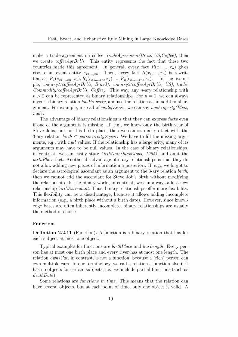
make a trade-agreement on coffee, tradeAgreement(Brazil,US,Coffee), thenwe create coffeeAgrBrUs. This entity represents the fact that these twocountries made this agreement. In general, every fact R(x1, ..., xn) givesrise to an event entity ex1,...,xn. Then, every fact R(x1, ..., xn) is rewrit-ten as R1(ex1,...,xn, x1), R2(ex1,...,xn, x2), ..., Rn(ex1,...,xn, xn). In the exam-ple, country1(coffeeAgrBrUs, Brazil), country2(coffeeAgrBrUs, US), trade-Commodity(coffeeAgrBrUs, Coffee). This way, any n-ary relationship withn > 2 can be represented as binary relationships. For n = 1, we can alwaysinvent a binary relation hasProperty, and use the relation as an additional ar-gument. For example, instead of male(Elvis), we can say hasProperty(Elvis,male).
The advantage of binary relationships is that they can express facts evenif one of the arguments is missing. If, e.g., we know only the birth year ofSteve Jobs, but not his birth place, then we cannot make a fact with the3-ary relation birth ⊂ person×city×year. We have to fill the missing argu-ments, e.g., with null values. If the relationship has a large arity, many of itsarguments may have to be null values. In the case of binary relationships,in contrast, we can easily state birthDate(SteveJobs, 1955), and omit thebirthPlace fact. Another disadvantage of n-ary relationships is that they donot allow adding new pieces of information a posteriori. If, e.g., we forgot todeclare the astrological ascendant as an argument to the 3-ary relation birth,then we cannot add the ascendant for Steve Job’s birth without modifyingthe relationship. In the binary world, in contrast, we can always add a newrelationship birthAscendant. Thus, binary relationships offer more flexibility.This flexibility can be a disadvantage, because it allows adding incompleteinformation (e.g., a birth place without a birth date). However, since knowl-edge bases are often inherently incomplete, binary relationships are usuallythe method of choice.
Functions
Definition 2.2.11 (Function). A function is a binary relation that has foreach subject at most one object.
Typical examples for functions are birthPlace and hasLength: Every per-son has at most one birth place and every river has at most one length. Therelation ownsCar, in contrast, is not a function, because a (rich) person canown multiple cars. In our terminology, we call a relation a function also if ithas no objects for certain subjects, i.e., we include partial functions (such asdeathDate).
Some relations are functions in time. This means that the relation canhave several objects, but at each point of time, only one object is valid. A
19

Fast, Exact, and Exhaustive Rule Mining in Large Knowledge Bases
typical example is isMarriedTo. A person can go through several marriages,but can only have one spouse at a time (in most systems). Another exampleis hasNumberOfInhabitants for cities. A city can grow over time, but at anypoint of time, it has only a single number of inhabitants. Every function isa function in time.
A binary relation is an inverse function, if its inverse is a function. Typicalexamples are hasCitizen (if we do not allow double nationality) or hasEmail-Address (if we talk only about personal email addresses that belong to a singleperson). Some relations are both functions and inverse functions. These areidentifiers for objects, such as the social security number. A person hasexactly one social security number, and a social security number belongsto exactly one person. Functions and inverse functions play a crucial role inentity matching: If two KBs talk about the same entity with different names,then one indication for this is that both entities share the same object of aninverse function. For example, if two people share an email address in a KBabout customers, then the two entities must be identical.
Some relations are “nearly functions”, in the sense that very few subjectshave more than one object. For example, most people have only one nation-ality, but some may have several. This idea is formalized by the notion offunctionality [79]. The functionality of a relation r in a KB is the number ofsubjects, divided by the number of facts with that relation:
fun(r) :=|x : ∃y : r(x, y)||x, y : r(x, y)|
The functionality is always a value between 0 and 1, and it is 1 if r is afunction. It is undefined for an empty relation.
We usually have the choice between using a relation and its inverse rela-tion. For example, we can either have a relationship isCitizenOf (betweena person and their country) or a relationship hasCitizen (between a countryand its citizens). Both are valid choices. In general, KBs tend to choosethe relation with the higher functionality, i.e., where the subject has fewerobjects. In the example, the choice would probably be isCitizenOf, becausepeople have fewer citizenships than countries have citizens. The intuition isthat the facts should be “facts about the subject”. For example, the factthat the author of this thesis is a citizen of France is clearly an importantproperty for this author.Vice versa, the fact that France is fortunate enoughto count this author among its citizens is a much less important property ofFrance (it does not appear on the Wikipedia page of France).
20

Fast, Exact, and Exhaustive Rule Mining in Large Knowledge Bases
2.2.4 Completeness and Correctness
Knowledge bases model only a part of the world. In order to make thisexplicit, one imagines a complete knowledge baseW that contains all entitiesand facts of the real world in the domain of interest. A given KB K is correct,if K ⊆ W . Usually, KBs aim to be correct. In real life, however, large KBstend to contain also erroneous statements. YAGO, e.g., has an accuracy of95%, meaning that 95% of its statements are inW (or, rather, in Wikipedia,which is used as an approximation of W). This means that YAGO stillcontains hundreds of thousands of wrong statements. For most other KBs,the degree of correctness is not even known.
A knowledge base is complete, if W ⊆ K (always staying within thedomain of interest). The closed world assumption (CWA) is the assumptionthat the KB at hand is complete. Thus, the CWA says that any statementthat is not in the KB is not in W either. In reality, however, KBs arehardly ever complete. Therefore, KBs typically operate under the open worldassumption (OWA), which says that if a statement is not in the KB, thenthis statement can be either true or false in the real world.
KBs usually do not model negative information. They may say thatCaltrain serves the city of San Francisco, but they will not say that thistrain does not serve the city of Moscow. While incompleteness tells us thatsome facts may be missing, the lack of negative information prevents usfrom specifying which facts are missing because they are false. This posesconsiderable problems, because the absence of a statement does not allowany conclusion about the real world [71].
2.2.5 The Semantic Web
The common exchange format for knowledge bases is RDF/RDFS [87]. Itspecifies a syntax for writing down statements with binary relations. Mostnotably, it prescribes URIs as identifiers, which means that entities can beidentified in a globally unique way. To query such RDF knowledge bases,one can use the query language SPARQL [91]. SPARQL borrows its syntaxfrom SQL, and allows the user to specify graph patterns, i.e., triples wheresome components are replaced by variables. For example, we can ask forthe birth date of Elvis by saying “SELECT ?birthdate WHERE 〈Elvis〉〈bornOnDate〉 ?birthdate ”.
To define semantic constraints on the data, RDF is extended by OWL [90].This language allows specifying constraints such as functions or disjointnessof classes, as well as more complex axioms. The formal semantics of theseaxioms is given by Description Logics [7]. These logics distinguish facts about
21
Fast, Exact, and Exhaustive Rule Mining in Large Knowledge Bases
instances from facts about classes and axioms. The facts about instances arecalled the A-Box (“Assertions”), and the class facts and axioms are called theT-Box (“Theory”). Sometimes, the term ontology is used to mean roughlythe same as T-Box. Description Logics allow for automated reasoning on thedata.
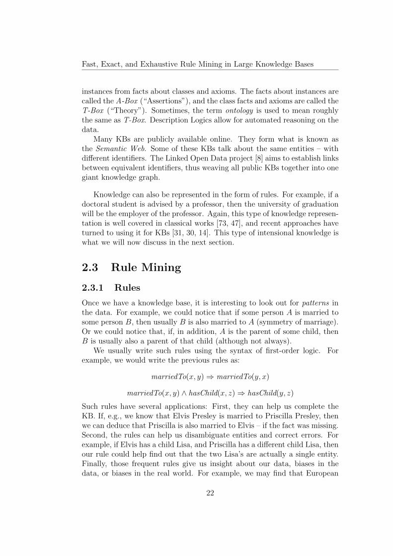
Many KBs are publicly available online. They form what is known asthe Semantic Web. Some of these KBs talk about the same entities – withdifferent identifiers. The Linked Open Data project [8] aims to establish linksbetween equivalent identifiers, thus weaving all public KBs together into onegiant knowledge graph.
Knowledge can also be represented in the form of rules. For example, if adoctoral student is advised by a professor, then the university of graduationwill be the employer of the professor. Again, this type of knowledge represen-tation is well covered in classical works [73, 47], and recent approaches haveturned to using it for KBs [31, 30, 14]. This type of intensional knowledge iswhat we will now discuss in the next section.
2.3 Rule Mining
2.3.1 Rules
Once we have a knowledge base, it is interesting to look out for patterns inthe data. For example, we could notice that if some person A is married tosome person B, then usually B is also married to A (symmetry of marriage).Or we could notice that, if, in addition, A is the parent of some child, thenB is usually also a parent of that child (although not always).
We usually write such rules using the syntax of first-order logic. Forexample, we would write the previous rules as:
marriedTo(x, y)⇒ marriedTo(y, x)
marriedTo(x, y) ∧ hasChild(x, z)⇒ hasChild(y, z)
Such rules have several applications: First, they can help us complete theKB. If, e.g., we know that Elvis Presley is married to Priscilla Presley, thenwe can deduce that Priscilla is also married to Elvis – if the fact was missing.Second, the rules can help us disambiguate entities and correct errors. Forexample, if Elvis has a child Lisa, and Priscilla has a different child Lisa, thenour rule could help find out that the two Lisa’s are actually a single entity.Finally, those frequent rules give us insight about our data, biases in thedata, or biases in the real world. For example, we may find that European
22

Fast, Exact, and Exhaustive Rule Mining in Large Knowledge Bases
presidents are usually male or that Ancient Romans are usually dead. Thesetwo rules are examples of rules that have not just variables, but also entities:
type(x,AncientRoman)⇒ dead(x)
We are now interested in discovering such rules automatically in the data.This process is called Rule Mining. Let us start with some definitions. Thecomponents of a rule are called atoms:
Definition 2.3.1 (Atom). An atom is of the form r(t1, . . . , tn), where r is arelation of arity n (for KBs, usually n = 2) and t1, . . . tn are either variablesor entities.
In our example, marriedTo(x, y) is an atom, as is marriedTo(Elvis, y). Wesay that an atom is instantiated, if it contains at least one entity. We say thatit is grounded, if it contains only entities and no variables. A conjunction isa set of atoms, which we write as ~A = A1 ∧ ... ∧ An. We are now ready tocombine atoms to rules:
Definition 2.3.2 (Rule). A Horn rule (rule, for short) is a formula of the
form ~B ⇒ h, where ~B is a conjunction of atoms, and h is an atom. ~B iscalled the body of the rule, and h its head.
For example, marriedTo(x, y)⇒ marriedTo(y, x) is a rule. Such a rule isusually read as “If x is married to y, then y is married to x”. In order toapply such a rule to specific entities, we need the notion of a substitution:
Definition 2.3.3 (Substitution). A substitution is a function that mapsvariables to entities or to other variables.
For example, a substitution σ can map σ(x) = Elvis and σ(y) = z– but not σ(Elvis) = z. A substitution can be generalized straight-forwardly to atoms, sets of atoms, and rules: if σ(x) = Elvis, thenσ(marriedTo(Priscilla, x)) = marriedTo(Priscilla, Elvis). With this, an in-stantiation of a rule is a variant of the rule where all variables have beensubstituted by entities (so that all atoms are grounded). If we substitutex = Elvis and y = Priscilla in our example rule, we obtain the followinginstantiation:
marriedTo(Elvis, Priscilla)⇒ marriedTo(Priscilla, Elvis)
Thus, an instantiation of a rule is an application of the rule to one concretecase. Let us now see what rules can predict:
23
Fast, Exact, and Exhaustive Rule Mining in Large Knowledge Bases
Lisa
PriscillaElvis Barack Michelle
Sasha Malia
hasChild hasChild hasChild hasChild
marriedTo marriedTo
Figure 2.1 – Example KB
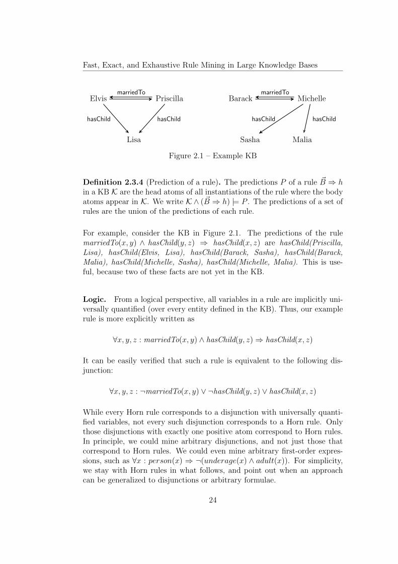
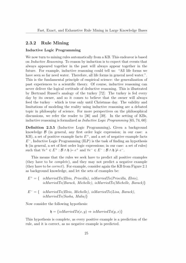
Definition 2.3.4 (Prediction of a rule). The predictions P of a rule ~B ⇒ hin a KB K are the head atoms of all instantiations of the rule where the bodyatoms appear in K. We write K∧ ( ~B ⇒ h) |= P . The predictions of a set ofrules are the union of the predictions of each rule.
For example, consider the KB in Figure 2.1. The predictions of the rulemarriedTo(x, y) ∧ hasChild(y, z) ⇒ hasChild(x, z) are hasChild(Priscilla,Lisa), hasChild(Elvis, Lisa), hasChild(Barack, Sasha), hasChild(Barack,Malia), hasChild(Michelle, Sasha), hasChild(Michelle, Malia). This is use-ful, because two of these facts are not yet in the KB.
Logic. From a logical perspective, all variables in a rule are implicitly uni-versally quantified (over every entity defined in the KB). Thus, our examplerule is more explicitly written as
∀x, y, z : marriedTo(x, y) ∧ hasChild(y, z)⇒ hasChild(x, z)
It can be easily verified that such a rule is equivalent to the following dis-junction:
∀x, y, z : ¬marriedTo(x, y) ∨ ¬hasChild(y, z) ∨ hasChild(x, z)
While every Horn rule corresponds to a disjunction with universally quanti-fied variables, not every such disjunction corresponds to a Horn rule. Onlythose disjunctions with exactly one positive atom correspond to Horn rules.In principle, we could mine arbitrary disjunctions, and not just those thatcorrespond to Horn rules. We could even mine arbitrary first-order expres-sions, such as ∀x : person(x) ⇒ ¬(underage(x) ∧ adult(x)). For simplicity,we stay with Horn rules in what follows, and point out when an approachcan be generalized to disjunctions or arbitrary formulae.
24
Fast, Exact, and Exhaustive Rule Mining in Large Knowledge Bases
2.3.2 Rule Mining
Inductive Logic Programming
We now turn to mining rules automatically from a KB. This endeavor is basedon Inductive Reasoning. To reason by induction is to expect that events thatalways appeared together in the past will always appear together in thefuture. For example, inductive reasoning could tell us: “All life forms wehave seen so far need water. Therefore, all life forms in general need water.”.This is the fundamental principle of empirical science: the generalization ofpast experiences to a scientific theory. Of course, inductive reasoning cannever deliver the logical certitude of deductive reasoning. This is illustratedby Bertrand Russel’s analogy of the turkey [72]: The turkey is fed everyday by its owner, and so it comes to believe that the owner will alwaysfeed the turkey – which is true only until Christmas day. The validity andlimitations of modeling the reality using inductive reasoning are a debatedtopic in philosophy of science. For more perspectives on the philosophicaldiscussions, we refer the reader to [36] and [39]. In the setting of KBs,inductive reasoning is formalized as Inductive Logic Programming [65, 74, 60]:
Definition 2.3.5 (Inductive Logic Programming). Given a backgroundknowledge B (in general, any first order logic expression; in our case: aKB), a set of positive example facts E+, and a set of negative example factsE−, Inductive Logic Programming (ILP) is the task of finding an hypothesish (in general, a set of first order logic expressions; in our case: a set of rules)such that ∀e+ ∈ E+ : B ∧ h |= e+ and ∀e− ∈ E− : B ∧ h 6|= e−.
This means that the rules we seek have to predict all positive examples(they have to be complete), and they may not predict a negative example(they have to be correct). For example, consider again the KB from Figure 2.1as background knowledge, and let the sets of examples be:
E+ = isMarriedTo(Elvis, Priscilla), isMarriedTo(Priscilla, Elvis),isMarriedTo(Barack, Michelle), isMarriedTo(Michelle, Barack)
E− = isMarriedTo(Elvis, Michelle), isMarriedTo(Lisa, Barack),isMarriedTo(Sasha, Malia)
Now consider the following hypothesis:
h = isMarriedTo(x, y)⇒ isMarriedTo(y, x)
This hypothesis is complete, as every positive example is a prediction of therule, and it is correct, as no negative example is predicted.
25
Fast, Exact, and Exhaustive Rule Mining in Large Knowledge Bases
The attentive reader will notice that the difficulty is now to correctlydetermine the sets of positive and negative examples. In the ideal case thepositive examples should contain any fact that is true in the real world andthe negative examples contain any other fact. Thus, in a correct KB, everyfact is a positive example.
Definition 2.3.6 (Rule Mining). Given a KB, Rule Mining is the ILP taskwith the KB as background knowledge, and every single atom of the KB asa positive example.
This means that the rule mining will find several rules, in order to explainall facts of the KB. Three problems remain: First, we have to define the setof negative examples. Second, we have to define what types of rules we areinterested in. Finally, we have to adapt our mining to cases where the ruledoes not always hold.
The Set of Negative Examples
Rule mining needs negative examples (also called counter-examples). Theproblem is that KBs usually do not contain negative information. We canthink of different ways to generate negative examples.
Closed World Assumption. The Closed World Assumption (CWA) saysthat any statement that is not in the KB is wrong (Section 2.2.4). Thus,under the Closed-World Assumption, any fact that is not in the KB canserve as a negative example. The problem is that these may be exactly thefacts that we want to predict. In our example KB from Figure 2.1, we maywant to learn the rule marriedTo(x, y)∧hasChild(y, z)⇒ hasChild(x, z). Forthis rule, the fact hasChild(Barack, Malia) is a counter-example. However,this fact is exactly what we want to predict, and so it would be a counter-productive counter-example.
Open World Assumption. Under the Open-World Assumption (OWA),any fact that is not in the KB can be considered either a negative or apositive example (see again Section 2.2.4). Thus the OWA does not helpin establishing counter-examples. Without counter-examples, we can learnany rule. For example, in our KB, the rule type(x, person) ⇒ marriedTo(x,Barack) has a single positive example (for x = Michelle), and no counter-examples under the Open World Assumption. Therefore, we could deducethat everyone is married to Barack.
26
Fast, Exact, and Exhaustive Rule Mining in Large Knowledge Bases
Partial Completeness Assumption. Another strategy to generate neg-ative examples is to assume that entities are complete for the relations theyalready have. For example, if we know that Michelle has the children Sashaand Malia, then we assume (much like Barack) that Michelle has no otherchildren. If, in contrast, Barack does not have any children in the KB, thenwe do not conclude anything. This idea is called the Partial-CompletenessAssumption (PCA) or the Local Closed World Assumption [31]. It holdstrivially for functions (such as hasBirthDate), and usually [30] for relationswith a high functionality (such as hasNationality). The rationale is that ifthe KB curators took the care to enter some objects for the relation, thenthey will most likely have entered all of them, if there are few of them. Incontrast, the assumption does usually not hold for relations with low func-tionality (such as starsInMovie). Fortunately, relations usually have a higherfunctionality than their inverses (see Section 2.2.3). If that is not the case,we can apply the PCA to the object of the relation instead.
Random Examples. Another strategy to find counter-examples is to gen-erate random statements [59]. Such random statements are unlikely to becorrect, and can thus serve as counter-examples. This is one of the meth-ods used by DL-Learner [38]. It is not easy to generate helpful randomcounter-examples. If, e.g., we generate the random negative example mar-riedTo(Barack,USA), then it is unlikely that a rule will try to predict thisexample. Thus, the example does not actually help in filtering out any rule.The challenge is hence to choose counter-examples that are false, but stillreasonable. The authors of [63] describe a method to sample negative state-ments about semantically connected entities by help of the PCA.
The Language Bias
After solving the problem of negative examples, the next question is whatkind of rules we should consider. This choice is called the language bias,because it restricts the “language” of the hypothesis. We have already lim-ited ourselves to Horn Rules, and in practice we even restrict ourselves toconnected and closed rules.
Definition 2.3.7 (Connected rules). Two atoms are connected if they sharea variable, and a rule is connected if every non-ground atom is transitivelyconnected to one another.
For example, the rule presidentOf(x, America) ⇒ hasChild(Elvis, y) isnot connected. It is an uninteresting and most likely wrong rule, because itmakes a prediction about arbitrary y.
27

Fast, Exact, and Exhaustive Rule Mining in Large Knowledge Bases
Definition 2.3.8 (Closed rules). A rule is closed if every variable appearsin at least two atoms.
For example the rule marriedTo(x, y) ∧ worksAt(x, z) ⇒ marriedTo(y,x) is not closed. It has a “dangling edge” that imposes that x works some-where. While such rules are perfectly valid, they are usually less interestingthan the more general rule without the dangling edge.
Finally, one usually imposes a limit on the number of atoms in the rule.Rules with too many atoms tend to be very convoluted [30]. That said,mining rules without such restrictions is an interesting field of research, andwe will come back to it in Chapters 4 to 6.
Support and Confidence
One problem with classical ILP approaches is that they will find rules thatapply to very few entities, such as marriedTo(x, Elvis) ⇒ hasChild(x, Lisa).To avoid this type of rules, we define the support of a rule:
Definition 2.3.9 (Support). The support of a rule in a KB is the numberof positive examples predicted by the rule.
Usually, we are interested only in rules that have a support higher thana given threshold (say, 100). Alternatively, we can define a relative versionof support, the head coverage [31], which is the number of positive examplespredicted by the rule divided by the number of all positive examples withthe same relation. Another problem with classical ILP approaches is thatthey will not find rules if there is a single counter-example. To mitigate thisproblem, we define the confidence:
Definition 2.3.10 (Confidence). The confidence of a rule is the number ofpositive examples predicted by the rule (i.e., the support of the rule), dividedby the number of examples predicted by the rule.
This notion depends on how we choose our negative examples. Forinstance, under the CWA, the rule marriedTo(x, y) ∧ hasChild(y, z) ⇒hasChild(x, z) has a confidence of 4/6 in Figure 2.1. We call this value thestandard confidence. Under the PCA, in contrast, the confidence for the ex-ample rule is 4/4. We call this value the PCA confidence. While the standardconfidence tends to “punish” rules that predict many unknown statements,the PCA confidence will permit more such rules. We present in Appendix Athe exact mathematical formula of these measures.
In general, the support of a rule quantifies its completeness, and theconfidence quantifies its correctness. A rule with low support and high con-fidence indicates a conservative hypothesis and may be overfitting, i.e. it
28
Fast, Exact, and Exhaustive Rule Mining in Large Knowledge Bases
will not generalize to new positive examples. A rule with high support andlow confidence, in contrast, indicates a more general hypothesis and may beovergeneralizing, i.e., it does not generalize to new negative examples. Inorder to avoid these effects we are looking for a trade-off between supportand confidence.
Definition 2.3.11 (Frequent Rule Mining). Given a KB K, a set of positiveexamples (usually K), a set of negative examples (usually according to anassumption above) and a language of rules, Frequent rule mining is the taskof finding all rules in the language with a support and a level of confidencesuperior to given thresholds.
2.3.3 Rule Mining Approaches
Using substitutions (see Definition 2.3.3), we can define a syntactical orderon rules:
Definition 2.3.12 (Rule order). A rule R ≡ ( ~B ⇒ h) subsumes a rule
R′ ≡ ( ~B′ ⇒ h′), or R is “more general than” R′, or R′ “is more specific
than” R, if there is a substitution σ such that σ( ~B) ⊆ ~B′ and σ(h) = h′. Ifboth rules subsume each other, the rules are called equivalent.
For example, consider the following rules:
hasChild(x, y) ⇒ hasChild(z, y) (R0)hasChild(Elvis, y) ⇒ hasChild(Priscilla, y) (R1)
hasChild(x, y) ⇒ hasChild(z, Lisa) (R2)hasChild(x, y) ∧marriedTo(x, z) ⇒ hasChild(z, y) (R3)
marriedTo(v1, v2) ∧ hasChild(v1, v3) ⇒ hasChild(v2, v3) (R4)hasChild(x, y) ∧marriedTo(z, x) ⇒ hasChild(z, y) (R5)
The rule R0 is more general than the rule R1, because we can rewrite thevariables x and z to Elvis and Priscilla respectively. However R0 and R2
are incomparable as we cannot choose to bind only one y and not the otherin R0. The rules R3, R4 and R5 are more specific than R0. Finally R3 isequivalent to R4 but not to R5.
Proposition 2.3.13 (Prediction inclusion). If a rule R is more general thana rule R′, then the predictions of R′ on a KB are a subset of the predictionsof R. As a corollary, R′ cannot have a higher support than R.
This observation gives us two families of rule mining algorithms: top-down rule mining starts from very general rules and specializes them un-til they become too specific (i.e., no longer meet the support threshold).
29
Fast, Exact, and Exhaustive Rule Mining in Large Knowledge Bases
Bottom-up rule mining, in contrast, starts from multiple ground rules andgeneralizes them until the rules become too general (i.e., too many negativeexamples are predicted).
Top-Down Rule Mining
The concept of specializing a general rule to more specific rules can betraced back to [74] in the context of an exact ILP task (under theCWA). Such approaches usually employ a refinement operator, i.e. a func-tion that takes a rule (or a set of rules) as input and returns a set ofmore specific rules. For example, a refinement operator could take therule hasChild(y, z) ⇒ hasChild(x, z) and produce the more specific rulemarriedTo(x, y) ∧ hasChild(y, z) ⇒ hasChild(x, z). This process is iterated,and creates a set of rules that we call the search space of the rule miningalgorithm. On the one hand, the search space should contain every rule of agiven rule mining task, so as to be complete. On the other hand, the smallerthe search space is, the more efficient the algorithm is.
Usually, the search space is pruned, i.e., less promising areas of the searchspace are cut away. For example, if a rule does not have enough support,then any refinement of it will have even lower support (Proposition 2.3.13).Hence, there is no use refining this rule.
AMIE. AMIE [31] is a top-down rule mining algorithm that aims to mineany connected rule composed of binary atoms for a given support and mini-mum level of confidence in a KB. AMIE starts with rules composed of onlya head atom for all possible head atoms (e.g., ⇒ marriedTo(x, y)). It usesthree refinement operators, each of which adds a new atom to the body ofthe rule.
The first refinement operator, addDanglingAtom, adds an atom composedof a variable already present in the input rule and a new variable.
Some refinements of: ⇒ hasChild(z, y) (Rh)
are:
hasChild(x, y) ⇒ hasChild(z, y) (R0)
marriedTo(x, z) ⇒ hasChild(z, y) (Ra)marriedTo(z, x) ⇒ hasChild(z, y) (Rb)
The second operator, addInstantiatedAtom, adds an atom composed of avariable already present in the input rule and an entity of the KB.
Some refinements of: ⇒ hasChild(Priscilla, y) (R′h)
are:
hasChild(Elvis, y) ⇒ hasChild(Priscilla, y) (R1)
hasChild(Priscilla, y) ⇒ hasChild(Priscilla, y) (R>)marriedTo(Barack, y) ⇒ hasChild(Priscilla, y) (R⊥)
30
Fast, Exact, and Exhaustive Rule Mining in Large Knowledge Bases
The final refinement operator, addClosingAtom, adds an atom composed oftwo variables already present in the input rule.
Some refinements of: marriedTo(x, z) ⇒ hasChild(z, y) (Ra)
are:
hasChild(x, y) ∧marriedTo(x, z) ⇒ hasChild(z, y) (R3)
marriedTo(z, y) ∧marriedTo(x, z) ⇒ hasChild(z, y) (Rα)marriedTo(x, z) ∧marriedTo(x, z) ⇒ hasChild(z, y) (R2
a)
As every new atom added by an operator contains at least a variable presentin the input rule, the generated rules are connected. The last operator isused to close the rules (for example R3), although it may have to be appliedseveral times to actually produce a closed rule (cf. Rules Rα or R2
a).The AMIE algorithm works on a queue of rules. Initially, the queue
contains one rule of a single head atom for each relation in the KB. At eachstep, AMIE dequeues the first rule, and applies all three refinement operators.The resulting rules are then pruned: First, any rule with low support (suchas R⊥) is discarded. Second, different refinements may generate equivalentrules (using the closing operator on R0 or Ra, e.g., generates among otherstwo equivalent “versions” of R3). AMIE prunes out these equivalent versions.AMIE+ [30] also detects equivalent atoms as in R> or R2
a and rewrites orremoves those rules. There are a number of other, more sophisticated pruningstrategies that estimate bounds on the support or confidence. The rules thatsurvive this pruning process are added to the queue. If one of the rules is aclosed rule with a high confidence, it is also output as a result. In this way,AMIE enumerates the entire search space.
The top-down rule mining method is generic, but its result depends onthe initial rules and on the refinement operators. The operators directlyimpact the language of rules we can mine (see Section 2.3.2) and the per-formance of the method. We can change the refinement operators to minea completely different language of rules. For example, if we don’t use theaddInstantiatedAtom operator, we restrict our search to any rule withoutinstantiated atoms, which also drastically reduce the size of the search space1.
Apriori Algorithm. There is an analogy between top-down rule miningand the Apriori algorithm [1]. The Apriori algorithm considers a set oftransactions (sales, products bought in a supermarket), each of which is aset of items (items bought together, in the supermarket analogy). The goalof the Apriori algorithm is to find a set of items that are frequently boughttogether.
1Let |K| be the number of facts and |r(K)| the number of relations in a KB K. Let dbe the maximal length of a rule. The size of the search space is reduced from O(|K|d) toO(|r(K)|d) when we remove the addInstantiatedAtom operator.
31
Fast, Exact, and Exhaustive Rule Mining in Large Knowledge Bases
These are frequent patterns of the form ~P ≡ I1(x)∧· · ·∧In(x), where I(t)is in our transaction database if the item I has been bought in the transactiont. Written as the set (called an “itemset”) ~P ≡ I1, . . . , In, any subset of ~P
forms a “more general” itemset than ~P , which is at least as frequent as P .The Apriori algorithm uses the dual view of the support pruning strategy:Necessarily, all patterns more general than ~P must be frequent for ~P to befrequent2. The refinement operator of the Apriori algorithm takes as inputall frequent itemsets of size n and generate all itemsets of size n + 1 suchthat any subset of size n is a frequent itemset. Thus, Apriori can be seenas a top-down rule mining algorithm over a very specific language where allatoms are unary predicates.
The WARMR algorithm [17], an ancestor of AMIE, was the first to adaptthe Apriori algorithm to rule mining over multiple (multidimensional) rela-tions.
Ontological Pathfinding. AMIE (and its successor AMIE+) [31, 30] wasthe first approach to explicitly target large KBs. While AMIE+ is at least3 orders of magnitude faster than the first-generation systems, it can stilltake hours, even days, to find rules in very large KBs such as Wikidata. Onthese grounds, more recent approaches [13, 14] have proposed new strategies(parallelism, approximations, etc.) to speed up rule mining on the largestKBs. The Ontological Pathfinding method (OP) [13, 14] resorts to a highlyconcurrent architecture based on Spark3 to calculate the support and theconfidence of a set of candidate rules. The candidates are computed byenumerating all conjunctions of atoms that are allowed by the schema. LikeAMIE, OP calculates the exact scores of the rules and supports both theCWA and the PCA for the generation of counter-evidence. At the sametime, the system supports only path rules of up to 3 atoms. Other types ofrules require the user to implement a new mining procedure.
RudiK. RudiK [63] is a recent rule mining method that applies the PCAto generate explicit counter-examples that are semantically related. Forexample, when generating counter-facts for the relation hasChild and a givenperson x, RudiK will sample among the non-children of x who are children ofsomeone else (x′ 6= x). RudiK’s strategy is to find all rules that are necessaryto predict the positive examples, based on a greedy heuristic that at each stepadds the most promising rule (in terms of coverage of the examples) to theoutput set. Thus, differently from exhaustive rule mining approaches [13, 31,
2instead of: if a rule is not frequent, none of its refinements can be frequent3https://spark.apache.org
32
Fast, Exact, and Exhaustive Rule Mining in Large Knowledge Bases
30, 34], RudiK aims to find rules that make good predictions, not all rulesabove a given confidence threshold. This non-exhaustivity endows RudiKwith comparable performance to AMIE+ and OP. Note that RudiK is alsocapable of mining negative rules, rules that predicts the absence of a fact, anovel prospect that have not yet been studied by the other approaches.
Bottom-Up Rule Mining
As the opposite of a refinement operator, one can define a generalizationoperator that considers several specific rules, and outputs a rule that is moregeneral than the input rules. For this purpose, we will make use of the ob-servation from Section 2.3.1 that a rule b1 ∧ ... ∧ bn ⇒ h is equivalent tothe disjunction ¬b1 ∨ · · · ∨ ¬bn ∨ h. The disjunction, in turn, can be writ-ten as a set ¬b1, . . . ,¬bn, h – which we call a clause. For example, therule marriedTo(x, y) ∧ hasChild(y, z)⇒ hasChild(x, z) can be written as theclause ¬marriedTo(x, y),¬hasChild(y, z), hasChild(x, z). Bottom-up rulemining approaches work on clauses. Thus, they work on universally quanti-fied disjunctions – which are more general than Horn rules. Two clauses canbe combined to a more general clause using the “least general generalization”operator [65]:
Definition 2.3.14 (Least general generalization). The least general gener-alization (lgg) of two clauses is computed in the following recursive manner:
– The lgg of two terms (i.e., either entities or variables) t and t′ is t ift = t′ and a new variable xt/t′ otherwise.
– The lgg of two negated atoms is the negation of their lgg.
– The lgg of r(t1, . . . , tn) and r(t′1, . . . , t′n) is r(lgg(t1, t
′1), . . . , lgg(tn, t
′n)).
– The lgg of a negated atom with a positive atom is undefined.
– Likewise, the lgg of two atoms with different relations is undefined.
– The lgg of two clauses R and R′ is the set of defined pair-wise general-izations:
lgg(R,R′) = lgg(li, l′j) : li ∈ R, l′j ∈ R′, and lgg(li, l
′j) is defined
For example, let us consider the following two rules:
hasChild(Michelle, Sasha) ∧ marriedTo(Michelle, Barack)⇒ hasChild(Barack, Sasha) (R)
hasChild(Michelle,Malia) ∧ marriedTo(Michelle, x)⇒ hasChild(x,Malia) (R′)
33
Fast, Exact, and Exhaustive Rule Mining in Large Knowledge Bases
In the form of clauses, these are
¬hasChild(Michelle, Sasha), ¬marriedTo(Michelle, Barack),hasChild(Barack, Sasha) (R)
¬hasChild(Michelle,Malia), ¬marriedTo(Michelle, x),hasChild(x,Malia) (R′)
Now, we have to compute the lgg of every atom of the first clause with everyatom of the second clause. As it turns out, there are only 3 pairs where thelgg is defined:
lgg(¬hasChild(Michelle, Sasha),¬hasChild(Michelle,Malia))= ¬lgg(hasChild(Michelle, Sasha), hasChild(Michelle,Malia))= ¬hasChild(lgg(Michelle,Michelle), lgg(Sasha,Malia))= ¬hasChild(Michelle, xSasha/Malia)
lgg(¬marriedTo(Michelle, Barack),¬marriedTo(Michelle, x))= ¬marriedTo(Michelle, xBarack/x)
lgg(hasChild(Barack, Sasha), hasChild(x,Malia))= hasChild(xBarack/x, xSasha/Malia)
This yields the clause
¬hasChild(Michelle, xSasha/Malia), ¬marriedTo(Michelle, xBarack/x),hasChild(xBarack/x, xSasha/Malia)
This clause is equivalent to the rule
hasChild(Michelle, y) ∧ marriedTo(Michelle, x)⇒ hasChild(x, y)
Note that the generalization of two different terms in an atom should resultin the same variable as the generalization of these terms in another atom.In our example, we obtain only two new variables xSasha/Malia and xBarack/x.In this way, we have generalized the two initial rules to a more general rule.This can be done systematically with an algorithm called GOLEM.
GOLEM. The GOLEM/RLGG algorithm [60] creates, for each positiveexample e ∈ E+, the rule B ⇒ e, where B is the background knowledge. Inour case, B is the entire KB, and so a very long conjunction of facts. Thealgorithm will then generalize these rules to shorter rules. More precisely, therelative lgg (rlgg) of a tuple of ground atoms (e1, . . . , en) is the rule obtained
34
Fast, Exact, and Exhaustive Rule Mining in Large Knowledge Bases
by computing the lgg of the rules B ⇒ e1, ..., B ⇒ en. We will call a rlggvalid if it is defined and does not predict any negative example.
The algorithm starts with a randomly sampled pair of positive examples(e1, e2) and selects the pair for which the rlgg is valid and predicts (“covers”)the most positive examples. It will then greedily add positive examples,chosen among a sample of “not yet covered positive examples”, to the tuple– as long as the corresponding rlgg is valid and covers more positive examples.The resulting rule will still contain ground atoms from B. These are removed,and the rule is output. Then the process starts over to find other rules foruncovered positive examples.
Progol and others. More recent ILP algorithms such as Progol [57],HAIL [68], Imparo [41] and others [92, 40] use inverse entailment to com-pute the hypothesis more efficiently. This idea is based on the observationthat a hypothesis h that satisfies B ∧ h |= E+ should equivalently satisfyB∧¬E+ |= ¬h (by logical contraposition). The algorithms work in two steps:they will first construct an intermediate theory F such that B∧¬E+ |= F andthen generalize its negation ¬F to the hypothesis h using inverse entailment.
2.3.4 Related Approaches
This chapter cannot give a full review of the field of rule mining. However,it is interesting to point out some other approaches in other domains thatdeal with similar problems:
OWL. OWL is a Description logic language designed to define rules andconstraints on the KB. For example, an OWL rule can say that every personmust have a single birth date. Such constraints are usually defined upfrontby domain experts and KB architects when they design the KB. They arethen used for automatic reasoning and consistency checks. Thus, constraintsprescribe the shape of the data, while the rules we mine describe the shapeof the data. In other words, constraints are used deductively – instead ofbeing found inductively. As such, they should suffer no exception. However,rule mining can provide candidate constraints to experts when they want toaugment their theory [38].
Probabilistic ILP. As an extension of the classic ILP problem, Proba-bilistic ILP [16] aims to find the logical hypothesis h that, given probabilisticbackground knowledge, maximizes the probability to observe a positive ex-ample, and minimizes the probability to observe a negative example. In our
35
Fast, Exact, and Exhaustive Rule Mining in Large Knowledge Bases
case, it would require a probabilistic model of the real world. Such modelshave been proposed for some specific use cases [44, 95], but they remain anongoing subject of research.
Graph Mining and Subgraph Discovery. Subgraph discovery is a wellstudied problem in the graph database community (see [32] Part 8 for aquick overview). Given a set of graphs, the task is to mine a subgraph thatappears in most of them. Rule mining, in contrast, is looking for patternsthat are frequent in the same graph. This difference may look marginal, butthe state-of-the-art algorithms are very different and further work would beneeded to determine how to translate one problem to the other.
Link Prediction. Rules can be used for link prediction, i.e., to predictwhether a relation links two entities. This task can also be seen as a classi-fication problem ([32] Part 7): given two entities, predict whether there is arelation between them. A notable work that unites both views [45] uses everyconjunction of atoms (a possible body for a rule, which they call a “path”)as a feature dimension for this classification problem.
Representation learning, another link prediction approach based on ma-chine learning, aims to represent entities and relations between those entitiesin some vector space Rd. For example, given a fact r(s, o) in our KB, theTransE model [10] will attempt to map r, s and o to vectors r, s and o inRd such that s + r ≈ o. For example, in the Example KB Figure 2.1, wewould have:
Elvis + marriedTo ≈ PriscillaElvis + hasChild ≈ LisaBarack + marriedTo ≈Michelle
Here, the task of fact prediction can be seen as finding the entity o suchthat:
Barack + hasChild ≈ o
The “embeddings” s, r and o are learned by maximizing the scoringfunction:
fr(s, o) = ||s + r − o||1 or 2
for any positive example r(s, o) of the KB, and minimizing the same scoringfunction for any negative example (cf. the discussion Section 2.3.2 on howto choose those negative examples).
The main problem of the TransE model is that, on 1-to-N relationships,several entities will be mapped to the same vectors:
Michelle + hasChild ≈Malia ≈ Sasha
36

Fast, Exact, and Exhaustive Rule Mining in Large Knowledge Bases
Several other models such as DistMult [93], ComplEX [82] or ConvE [18],have been proposed to address these issues. A comprehensive survey on thedomain of KB embeddings techniques can be found in [85].
Recent studies have shown that KB embeddings approaches do not per-form significantly better than the rule mining approaches on the task of factprediction [52, 5].
2.4 Conclusion
In this chapter, we have investigated how entities, relations, and facts in aknowledge base can be represented. We have seen the standard knowledgerepresentation model of instances and classes. We have also seen how torepresent more complex relationships between the entities in the form ofrules and presented classical and contemporary rule mining approaches.
However, many challenges persist. First, as the KBs grow larger andlarger, the scalability of the rule mining approaches remains a permanentproblem. Second, new approaches use custom quality metrics or new pruningstrategies to discover more productive rules for specialized purposes (factprediction notably). In terms of usability, bridging the gap between generalILP-based and purpose-oriented rule mining approaches would be profitablefor both approaches.
37
Chapter 3
AMIE 3: Fast Computation ofQuality Measures
3.1 Introduction
In order to be able to process larger and larger Knowledge Bases, the pre-vious version of AMIE, AMIE+ [30], resorts to use a sophisticated prun-ing strategy called the functionality heuristic. As a result, AMIE+ is waymore performant than the original AMIE algorithm but this pruning heuris-tic is not exact and may prune perfectly legitimate rules. For example, onDBPedia 3.8, AMIE+ will wrongfully prune around 1.6% of the rules. Otherrecent approaches, such as Ontological Pathfinding [13], use similar pruningstrategies, producing incomplete results.
Scaling is important but it should not be at the expense of the generalityof the result. Without any guarantee on the results, a rule mining algorithmis just a tool that mines some rules, among many others. An exact andexhaustive rule mining algorithm would be the rule mining algorithm parexcellence, as it provides a gold standard the other rule mining algorithmscan be compared against.
A first difficulty in mining exhaustively the rules from a KB lies in theexponential size of the search space: every relation can potentially be com-bined with every other relation in a rule. The second difficulty comes fromthe exact computation of the quality measures, as the algorithm must con-sider more predictions the larger the KB is. For example, to compute exactlythe confidence of the rule:
livesIn(x, Paris) ∧ livesIn(y, Paris)⇒ marriedTo(x, y)
the algorithm must consider every pair of person living in Paris, whichamounts to roughly 106 × 106 pairs for a complete KB.
38

Fast, Exact, and Exhaustive Rule Mining in Large Knowledge Bases
In this chapter, we present AMIE 3, a successor of AMIE [31] andAMIE+ [30]. Our system employs a number of sophisticated strategies tospeed up rule mining: pruning strategies, parallelization, and a lazy compu-tation of confidence scores. This allows our system to scale effortlessly tolarge KBs. At the same time, the system still computes the exact confidenceand support values for each rule, without resorting to approximations. Fur-thermore, unlike its predecessor [30] and other systems, AMIE 3 exhaustivelycomputes all rules that hold in the KB for a given confidence and supportthreshold.
Our experiments show that AMIE 3 beats the state of the art by a factorof 15 in terms of runtime. We believe that the techniques that we havediscovered can be of use for other systems as well — no matter whether theycompute the exhaustive set of rules or not.
3.2 AMIE 3
In this section, we first recap the original AMIE algorithm [31] (Section 3.2.1).Then we present a series of optimizations that give rise to AMIE 3 (Sec-tion 3.2.2). Finally, we show different quality metrics that AMIE 3 cancompute (Section 3.2.3).
3.2.1 The AMIE Approach
The AMIE algorithm [31, 30] is a method to mine closed Horn rules on largeKBs. AMIE (Algorithm 1) takes as input a knowledge base K, and thresholdsl for the maximal number of atoms per rule, minHC for the minimum headcoverage, and minC for the minimum PCA confidence. AMIE uses a classicalbreadth-first search: Line 1 initializes a queue with all possible rules of size 1,i.e., rules with an empty body. The search strategy then dequeues a rule R ata time and adds it to the output list (Line 6) if it meets certain criteria (Line5), namely, (i) the rule is closed, (ii) its PCA confidence is higher than minC,and (iii) its PCA confidence is higher than the confidence of all previouslymined rules with the same head atom as R and a subset of its body atoms.If the rule R has less than l atoms and its confidence can still be improved(Line 7), AMIE refines it. The refinement operator refine (Line 8) derivesnew rules from R by considering all possible atoms that can be added to thebody of the rule, and creating one new rule for each of them, as described insection 2.3.3.
AMIE iterates over all the non-duplicate refinements of rule R and addsthose with enough head coverage (Lines 10-11). The routine finishes when
39
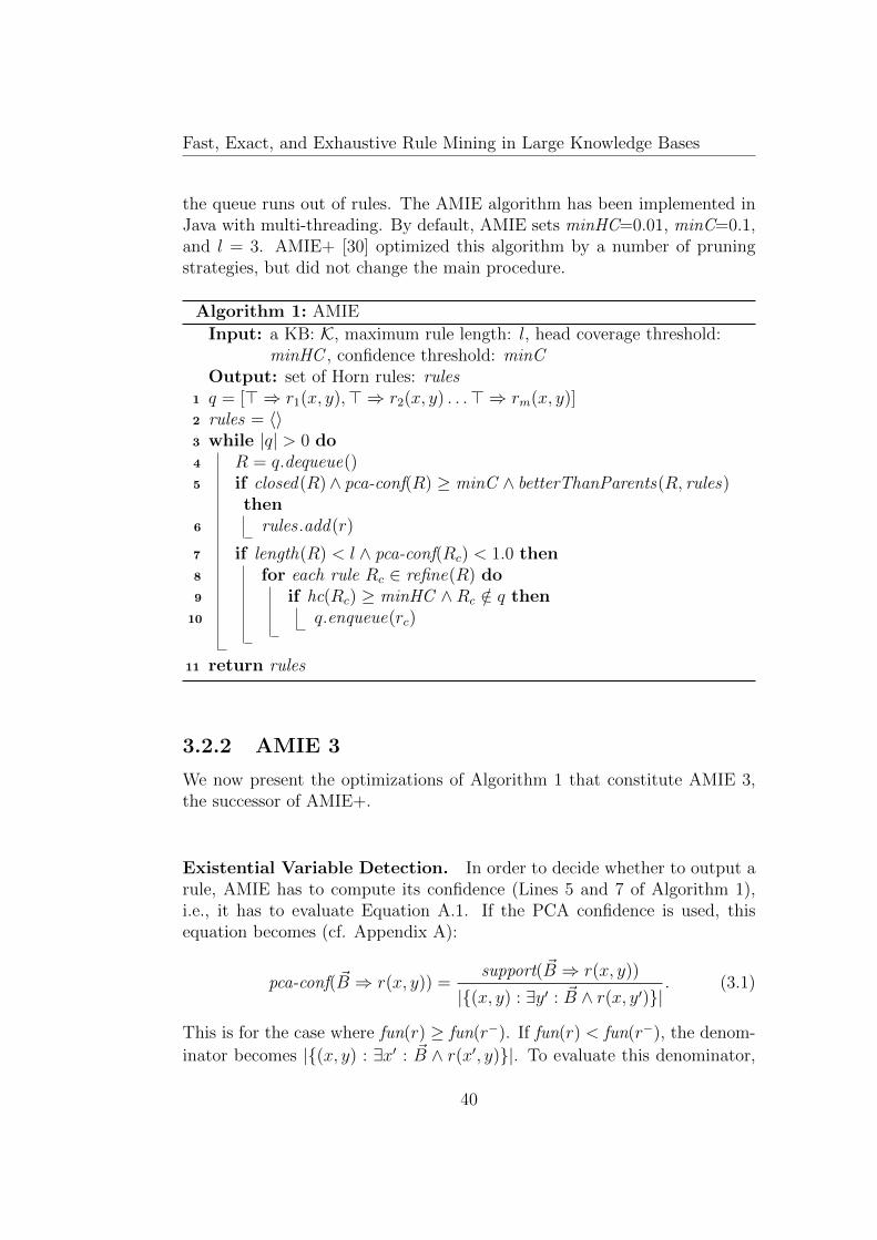
Fast, Exact, and Exhaustive Rule Mining in Large Knowledge Bases
the queue runs out of rules. The AMIE algorithm has been implemented inJava with multi-threading. By default, AMIE sets minHC=0.01, minC=0.1,and l = 3. AMIE+ [30] optimized this algorithm by a number of pruningstrategies, but did not change the main procedure.
Algorithm 1: AMIE
Input: a KB: K, maximum rule length: l, head coverage threshold:minHC , confidence threshold: minC
Output: set of Horn rules: rules1 q = [> ⇒ r1(x, y),> ⇒ r2(x, y) . . .> ⇒ rm(x, y)]2 rules = 〈〉3 while |q| > 0 do4 R = q.dequeue()5 if closed(R)∧ pca-conf(R) ≥ minC ∧ betterThanParents(R, rules)
then6 rules .add(r)
7 if length(R) < l ∧ pca-conf(Rc) < 1.0 then8 for each rule Rc ∈ refine(R) do9 if hc(Rc) ≥ minHC ∧Rc /∈ q then
10 q.enqueue(rc)
11 return rules
3.2.2 AMIE 3
We now present the optimizations of Algorithm 1 that constitute AMIE 3,the successor of AMIE+.
Existential Variable Detection. In order to decide whether to output arule, AMIE has to compute its confidence (Lines 5 and 7 of Algorithm 1),i.e., it has to evaluate Equation A.1. If the PCA confidence is used, thisequation becomes (cf. Appendix A):
pca-conf( ~B ⇒ r(x, y)) =support( ~B ⇒ r(x, y))
|(x, y) : ∃y′ : ~B ∧ r(x, y′)|. (3.1)
This is for the case where fun(r) ≥ fun(r−). If fun(r) < fun(r−), the denom-
inator becomes |(x, y) : ∃x′ : ~B ∧ r(x′, y)|. To evaluate this denominator,
40
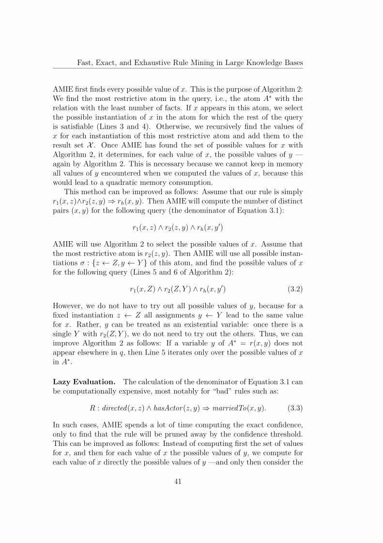
Fast, Exact, and Exhaustive Rule Mining in Large Knowledge Bases
AMIE first finds every possible value of x. This is the purpose of Algorithm 2:We find the most restrictive atom in the query, i.e., the atom A∗ with therelation with the least number of facts. If x appears in this atom, we selectthe possible instantiation of x in the atom for which the rest of the queryis satisfiable (Lines 3 and 4). Otherwise, we recursively find the values ofx for each instantiation of this most restrictive atom and add them to theresult set X . Once AMIE has found the set of possible values for x withAlgorithm 2, it determines, for each value of x, the possible values of y —again by Algorithm 2. This is necessary because we cannot keep in memoryall values of y encountered when we computed the values of x, because thiswould lead to a quadratic memory consumption.
This method can be improved as follows: Assume that our rule is simplyr1(x, z)∧r2(z, y)⇒ rh(x, y). Then AMIE will compute the number of distinctpairs (x, y) for the following query (the denominator of Equation 3.1):
r1(x, z) ∧ r2(z, y) ∧ rh(x, y′)
AMIE will use Algorithm 2 to select the possible values of x. Assume thatthe most restrictive atom is r2(z, y). Then AMIE will use all possible instan-tiations σ : z ← Z, y ← Y of this atom, and find the possible values of xfor the following query (Lines 5 and 6 of Algorithm 2):
r1(x, Z) ∧ r2(Z, Y ) ∧ rh(x, y′) (3.2)
However, we do not have to try out all possible values of y, because for afixed instantiation z ← Z all assignments y ← Y lead to the same valuefor x. Rather, y can be treated as an existential variable: once there is asingle Y with r2(Z, Y ), we do not need to try out the others. Thus, we canimprove Algorithm 2 as follows: If a variable y of A∗ = r(x, y) does notappear elsewhere in q, then Line 5 iterates only over the possible values of xin A∗.
Lazy Evaluation. The calculation of the denominator of Equation 3.1 canbe computationally expensive, most notably for “bad” rules such as:
R : directed(x, z) ∧ hasActor(z, y)⇒ marriedTo(x, y). (3.3)
In such cases, AMIE spends a lot of time computing the exact confidence,only to find that the rule will be pruned away by the confidence threshold.This can be improved as follows: Instead of computing first the set of valuesfor x, and then for each value of x the possible values of y, we compute foreach value of x directly the possible values of y —and only then consider the
41
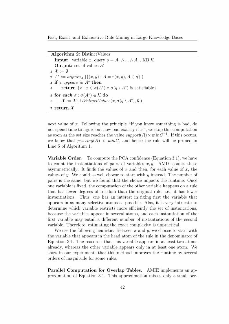
Fast, Exact, and Exhaustive Rule Mining in Large Knowledge Bases
Algorithm 2: DistinctValues
Input: variable x, query q = A1 ∧ ... ∧ An, KB K,Output: set of values X
1 X := ∅2 A∗ := argminA(|(x, y) : A = r(x, y), A ∈ q|)3 if x appears in A∗ then4 return x : x ∈ σ(A∗) ∧ σ(q \ A∗) is satisfiable5 for each σ : σ(A∗) ∈ K do6 X := X ∪ DistinctValues(x, σ(q \ A∗),K)
7 return X
next value of x. Following the principle “If you know something is bad, donot spend time to figure out how bad exactly it is”, we stop this computationas soon as the set size reaches the value support(R)×minC−1. If this occurs,we know that pca-conf(R) < minC , and hence the rule will be pruned inLine 5 of Algorithm 1.
Variable Order. To compute the PCA confidence (Equation 3.1), we haveto count the instantiations of pairs of variables x, y. AMIE counts theseasymmetrically: It finds the values of x and then, for each value of x, thevalues of y. We could as well choose to start with y instead. The number ofpairs is the same, but we found that the choice impacts the runtime: Onceone variable is fixed, the computation of the other variable happens on a rulethat has fewer degrees of freedom than the original rule, i.e., it has fewerinstantiations. Thus, one has an interest in fixing first the variable thatappears in as many selective atoms as possible. Alas, it is very intricate todetermine which variable restricts more efficiently the set of instantations,because the variables appear in several atoms, and each instantiation of thefirst variable may entail a different number of instantiations of the secondvariable. Therefore, estimating the exact complexity is unpractical.
We use the following heuristic: Between x and y, we choose to start withthe variable that appears in the head atom of the rule in the denominator ofEquation 3.1. The reason is that this variable appears in at least two atomsalready, whereas the other variable appears only in at least one atom. Weshow in our experiments that this method improves the runtime by severalorders of magnitude for some rules.
Parallel Computation for Overlap Tables. AMIE implements an ap-proximation of Equation 3.1. This approximation misses only a small per-
42
Fast, Exact, and Exhaustive Rule Mining in Large Knowledge Bases
centage of rules (maximally 5% according to [30]), but speeds up the cal-culation drastically. In AMIE 3, this feature can be switched off (to haveexact results) or on (to have faster results). Here, we show how to furtherspeed up this heuristic. The method finds an efficient approximation of thedenominator of Equation 3.1 for a rule R. This approximation uses the joinstructure of the query in combination with the functionality scores and theoverlaps of the different relations to estimate the total number of examples(both positive and negative) of a rule. The exact formula and the rationalebehind it can be found in [30]. The functionality, domain and overlaps withother relations are pre-computed for all relations. This pre-calculation canbe significant for large KBs with many predicates. In our experiments withDBpedia, e.g., precomputing all overlaps takes twice as much time as themining. In AMIE 3, we exploit the fact that this task is easy parallelizable,and start as many threads as possible in parallel, each treating one pair ofrelations. This reduces the precomputation time linearly with the number ofthreads (by a factor of 40 in our experiments).
Integer-based in-memory database. AMIE uses an in-memorydatabase to store the entire KB. Each fact is indexed by subject, by object,by relation, and by pairs of relation/subject and relation/object. In order tobe able to load also large KBs into memory, AMIE compresses strings intocustom-made ByteStrings, where each character takes only 8 bits. AMIEmakes sure that ByteString variables holding equivalent ByteStrings pointto the same physical object (i.e., the ByteString exists only once). This notjust saves space, but also makes hashing and equality tests trivial. Still,we incur high costs of managing these objects and the indexes: ByteStringshave to be first created, and then checked for duplicity; unused ByteStringshave to be garbage-collected; equality checks still require casting checks;and HashMaps create a large memory overhead. Built-in strings suffer fromthe same problems. Therefore, we migrated the in-memory database to aninteger-based system, where entities and relations are mapped to an integerspace and represented by the primitive datatype int. This is in compliancewith most RDF engines and popular serialization formats such as [25]. Weuse the fastutil library1 to store the indexes. This avoids the overhead ofstandard HashMaps. It also reduces the number of objects that the garbagecollector has to treat, leading to a significant speedup.
1http://fastutil.di.unimi.it/
43

Fast, Exact, and Exhaustive Rule Mining in Large Knowledge Bases
3.2.3 Quality Metrics
AMIE is a generic exhaustive rule miner, and thus its output consists ofrules. These rules can serve as input to other applications, for example,to approaches that predict facts [20, 63]. By default, AMIE uses the PCAconfidence to assess the quality of a rule, because it has been shown to rankrules closer to the quality of their predictions than classical metrics suchas the CWA confidence [31]. However, the PCA cannot generate counter-examples for functional relations, which is problematic for rules such as:
hasChild(z, x) ∧ politicianOf(z, y)⇒ politicianOf(x, y)
This rule has a high PCA confidence as the children of a politician thatare not politician are not counted as a counter-examples of the rule2. Thusthe rule actually represents the fact that every child of a politician who ispolitician of some country is politician of the same country as their parentsbut the same rule would be used to predict that every child of a politicianis a politician. We specifically give directions to address this problem inSection 8.2.
AMIE 3 is not limited to the PCA and can compute any of the followingquality metrics that can be enabled by command lines switches:
Support & head coverage. Support is a standard quality metric that in-dicates the significance of a rule. Due to the anti-monotonicity prop-erty, most approaches use support to prune the search space of rules.AMIE [31, 30] uses by default the head coverage (the relative variantof support) for pruning.
PCA Confidence. The default confidence metric.
CWA confidence. This confidence is used in OP [13, 14]. Many link pre-diction methods are evaluated under the closed world assumption aswell [80].
GPRO confidence. The work of [20] noted that the PCA confidence canunderestimate the likelihood of a prediction in the presence of non-injective mappings. Therefore, the authors propose a refinement ofthe PCA confidence, the GPRO confidence, which excludes instancescoming from non-injective mappings in the confidence computation. Tojudge the quality of a predicted fact, the approach needs the GPROconfidence both on the first and second variable of the head atom.AMIE is not designed to judge the quality of a predicted fact, but cancompute the GPRO confidence on both variables.
2as they are not subject of a politicianOf relation.
44
Fast, Exact, and Exhaustive Rule Mining in Large Knowledge Bases
GRANK confidence. This refinement of the GPRO metric is proposedby [20] in order to take into account the number of instances of thevariables of the rule that are not in the head atom.
The rules mined by AMIE can be used to support task such as data clean-ing or reasoning but can also be added to an open rule repository as proposedin [3] to facilitate sharing and comparison between different approaches andquality metrics.
3.3 Experiments
We conducted two series of experiments to evaluate AMIE 3: In the firstseries we study the impact of our optimizations on the system’s runtime.In the second series, we compare AMIE 3 with two scalable state-of-the-artapproaches, namely RudiK [63] and Ontological Pathfinding (OP) [13, 14](also known as ScaleKB) on 6 different datasets.
3.3.1 Experimental Setup
Data. We evaluated AMIE 3 and its competitors on YAGO (2 and 2s), DB-pedia (2.0 and 3.8) and a dump of Wikipedia from December 2014. Thesedatasets were used in evaluations of AMIE+ [30], OP [13] and Rudik [63].In addition, we used a recent dump of Wikidata from July 1st, 20193. Ta-ble 3.1 shows the numbers of facts, relations, and entities of our experimentaldatasets.
Configurations. All experiments were run on a Ubuntu 18.04.3 LTS with40 processing cores (Intel Xeon CPU E5-2660 v3 at 2.60GHz) and 500Go ofRAM. AMIE 3 and RudiK are implemented in Java 1.8. AMIE 3 uses itsown in-memory database to store the KB, whereas RudiK relies on VirtuosoOpen Source 06.01.3127, accessed via a local endpoint. OP was implementedin Scala 2.11.12 and Spark 2.3.4.
Unless otherwise noted, the experiments were run using the default set-tings of AMIE: We used the PCA confidence, computed lazily with a thresh-old of 0.1, with all the lossless optimizations (no approximations). Thethreshold on the head coverage is 0.01 and the maximal rule length is 3 [31].
3Selecting only facts between two Wikidata entities, and excluding literals.
45
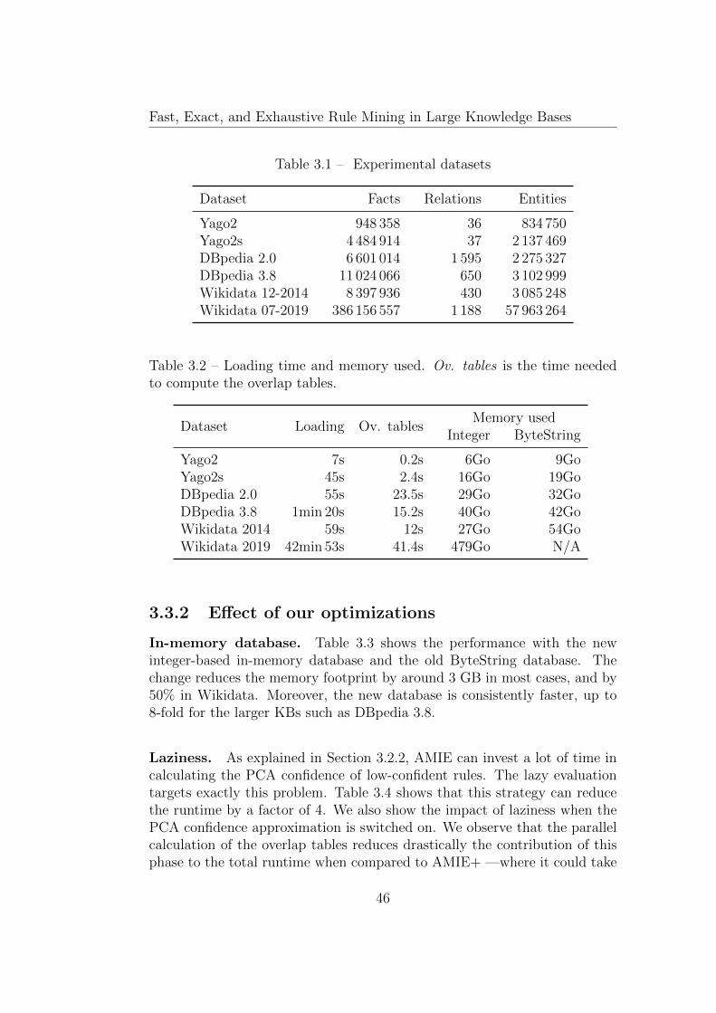
Fast, Exact, and Exhaustive Rule Mining in Large Knowledge Bases
Table 3.1 – Experimental datasets
Dataset Facts Relations Entities
Yago2 948 358 36 834 750Yago2s 4 484 914 37 2 137 469DBpedia 2.0 6 601 014 1 595 2 275 327DBpedia 3.8 11 024 066 650 3 102 999Wikidata 12-2014 8 397 936 430 3 085 248Wikidata 07-2019 386 156 557 1 188 57 963 264
Table 3.2 – Loading time and memory used. Ov. tables is the time neededto compute the overlap tables.
Dataset Loading Ov. tablesMemory used
Integer ByteString
Yago2 7s 0.2s 6Go 9GoYago2s 45s 2.4s 16Go 19GoDBpedia 2.0 55s 23.5s 29Go 32GoDBpedia 3.8 1min 20s 15.2s 40Go 42GoWikidata 2014 59s 12s 27Go 54GoWikidata 2019 42min 53s 41.4s 479Go N/A
3.3.2 Effect of our optimizations
In-memory database. Table 3.3 shows the performance with the newinteger-based in-memory database and the old ByteString database. Thechange reduces the memory footprint by around 3 GB in most cases, and by50% in Wikidata. Moreover, the new database is consistently faster, up to8-fold for the larger KBs such as DBpedia 3.8.
Laziness. As explained in Section 3.2.2, AMIE can invest a lot of time incalculating the PCA confidence of low-confident rules. The lazy evaluationtargets exactly this problem. Table 3.4 shows that this strategy can reducethe runtime by a factor of 4. We also show the impact of laziness when thePCA confidence approximation is switched on. We observe that the parallelcalculation of the overlap tables reduces drastically the contribution of thisphase to the total runtime when compared to AMIE+ —where it could take
46
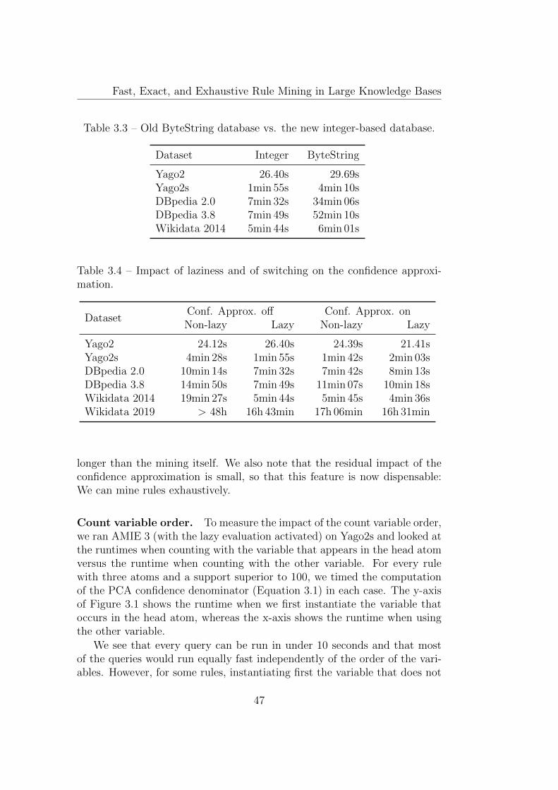
Fast, Exact, and Exhaustive Rule Mining in Large Knowledge Bases
Table 3.3 – Old ByteString database vs. the new integer-based database.
Dataset Integer ByteString
Yago2 26.40s 29.69sYago2s 1min 55s 4min 10sDBpedia 2.0 7min 32s 34min 06sDBpedia 3.8 7min 49s 52min 10sWikidata 2014 5min 44s 6min 01s
Table 3.4 – Impact of laziness and of switching on the confidence approxi-mation.
DatasetConf. Approx. off Conf. Approx. onNon-lazy Lazy Non-lazy Lazy
Yago2 24.12s 26.40s 24.39s 21.41sYago2s 4min 28s 1min 55s 1min 42s 2min 03sDBpedia 2.0 10min 14s 7min 32s 7min 42s 8min 13sDBpedia 3.8 14min 50s 7min 49s 11min 07s 10min 18sWikidata 2014 19min 27s 5min 44s 5min 45s 4min 36sWikidata 2019 > 48h 16h 43min 17h 06min 16h 31min
longer than the mining itself. We also note that the residual impact of theconfidence approximation is small, so that this feature is now dispensable:We can mine rules exhaustively.
Count variable order. To measure the impact of the count variable order,we ran AMIE 3 (with the lazy evaluation activated) on Yago2s and looked atthe runtimes when counting with the variable that appears in the head atomversus the runtime when counting with the other variable. For every rulewith three atoms and a support superior to 100, we timed the computationof the PCA confidence denominator (Equation 3.1) in each case. The y-axisof Figure 3.1 shows the runtime when we first instantiate the variable thatoccurs in the head atom, whereas the x-axis shows the runtime when usingthe other variable.
We see that every query can be run in under 10 seconds and that mostof the queries would run equally fast independently of the order of the vari-ables. However, for some rules, instantiating first the variable that does not
47
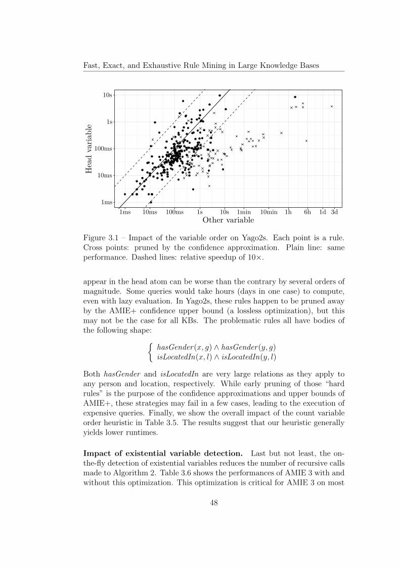
Fast, Exact, and Exhaustive Rule Mining in Large Knowledge Bases
1ms
10ms
100ms
1s
10s
1ms 10ms 100ms 1s 10s 1min 10min 1h 6h 1d 3dOther variable
Hea
d va
riabl
e
Figure 3.1 – Impact of the variable order on Yago2s. Each point is a rule.Cross points: pruned by the confidence approximation. Plain line: sameperformance. Dashed lines: relative speedup of 10×.
appear in the head atom can be worse than the contrary by several orders ofmagnitude. Some queries would take hours (days in one case) to compute,even with lazy evaluation. In Yago2s, these rules happen to be pruned awayby the AMIE+ confidence upper bound (a lossless optimization), but thismay not be the case for all KBs. The problematic rules all have bodies ofthe following shape:
hasGender(x, g) ∧ hasGender(y, g)isLocatedIn(x, l) ∧ isLocatedIn(y, l)
Both hasGender and isLocatedIn are very large relations as they apply toany person and location, respectively. While early pruning of those “hardrules” is the purpose of the confidence approximations and upper bounds ofAMIE+, these strategies may fail in a few cases, leading to the execution ofexpensive queries. Finally, we show the overall impact of the count variableorder heuristic in Table 3.5. The results suggest that our heuristic generallyyields lower runtimes.
Impact of existential variable detection. Last but not least, the on-the-fly detection of existential variables reduces the number of recursive callsmade to Algorithm 2. Table 3.6 shows the performances of AMIE 3 with andwithout this optimization. This optimization is critical for AMIE 3 on most
48
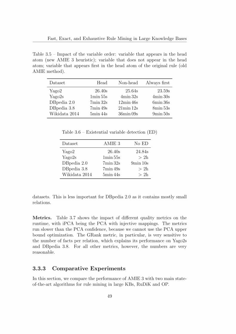
Fast, Exact, and Exhaustive Rule Mining in Large Knowledge Bases
Table 3.5 – Impact of the variable order: variable that appears in the headatom (new AMIE 3 heuristic); variable that does not appear in the headatom; variable that appears first in the head atom of the original rule (oldAMIE method).
Dataset Head Non-head Always first
Yago2 26.40s 25.64s 23.59sYago2s 1min 55s 4min 32s 4min 30sDBpedia 2.0 7min 32s 12min 46s 6min 36sDBpedia 3.8 7min 49s 21min 12s 8min 53sWikidata 2014 5min 44s 36min 09s 9min 50s
Table 3.6 – Existential variable detection (ED)
Dataset AMIE 3 No ED
Yago2 26.40s 24.84sYago2s 1min 55s > 2hDBpedia 2.0 7min 32s 9min 10sDBpedia 3.8 7min 49s > 2hWikidata 2014 5min 44s > 2h
datasets. This is less important for DBpedia 2.0 as it contains mostly smallrelations.
Metrics. Table 3.7 shows the impact of different quality metrics on theruntime, with iPCA being the PCA with injective mappings. The metricsrun slower than the PCA confidence, because we cannot use the PCA upperbound optimization. The GRank metric, in particular, is very sensitive tothe number of facts per relation, which explains its performance on Yago2sand DBpedia 3.8. For all other metrics, however, the numbers are veryreasonable.
3.3.3 Comparative Experiments
In this section, we compare the performance of AMIE 3 with two main state-of-the-art algorithms for rule mining in large KBs, RuDiK and OP.
49
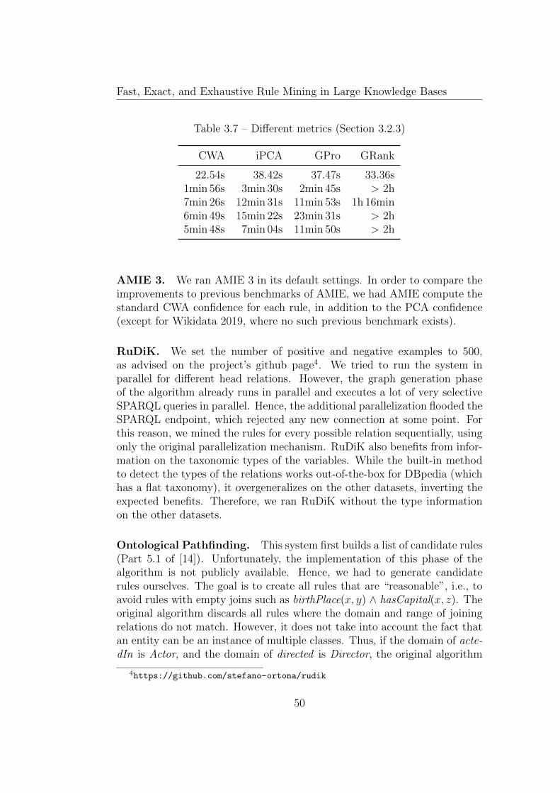
Fast, Exact, and Exhaustive Rule Mining in Large Knowledge Bases
Table 3.7 – Different metrics (Section 3.2.3)
CWA iPCA GPro GRank
22.54s 38.42s 37.47s 33.36s1min 56s 3min 30s 2min 45s > 2h7min 26s 12min 31s 11min 53s 1h 16min6min 49s 15min 22s 23min 31s > 2h5min 48s 7min 04s 11min 50s > 2h
AMIE 3. We ran AMIE 3 in its default settings. In order to compare theimprovements to previous benchmarks of AMIE, we had AMIE compute thestandard CWA confidence for each rule, in addition to the PCA confidence(except for Wikidata 2019, where no such previous benchmark exists).
RuDiK. We set the number of positive and negative examples to 500,as advised on the project’s github page4. We tried to run the system inparallel for different head relations. However, the graph generation phaseof the algorithm already runs in parallel and executes a lot of very selectiveSPARQL queries in parallel. Hence, the additional parallelization flooded theSPARQL endpoint, which rejected any new connection at some point. Forthis reason, we mined the rules for every possible relation sequentially, usingonly the original parallelization mechanism. RuDiK also benefits from infor-mation on the taxonomic types of the variables. While the built-in methodto detect the types of the relations works out-of-the-box for DBpedia (whichhas a flat taxonomy), it overgeneralizes on the other datasets, inverting theexpected benefits. Therefore, we ran RuDiK without the type informationon the other datasets.
Ontological Pathfinding. This system first builds a list of candidate rules(Part 5.1 of [14]). Unfortunately, the implementation of this phase of thealgorithm is not publicly available. Hence, we had to generate candidaterules ourselves. The goal is to create all rules that are “reasonable”, i.e., toavoid rules with empty joins such as birthPlace(x, y) ∧ hasCapital(x, z). Theoriginal algorithm discards all rules where the domain and range of joiningrelations do not match. However, it does not take into account the fact thatan entity can be an instance of multiple classes. Thus, if the domain of acte-dIn is Actor, and the domain of directed is Director, the original algorithm
4https://github.com/stefano-ortona/rudik
50

Fast, Exact, and Exhaustive Rule Mining in Large Knowledge Bases
Table 3.8 – Performances and output of Ontological Pathfinding (OP),RuDiK and AMIE 3. *: rules with support ≥ 100 and CWA confidence≥ 0.1.
Dataset System Rules Runtime
Yago2s
OP (their candidates) 429 (52*) 18min 50sOP (our candidates) 1 348 (96*) 3h 20minRuDiK 17 37min 30sAMIE 3 97 1min 50sAMIE 3 (support=1) 1 596 7min 6s
DBpedia 3.8
OP (our candidates) 7 714 (220*) > 45hRuDiK 650 12h 10minRuDiK + types 650 11h 52minAMIE 3 5 084 7min 52sAMIE 3 (support=1) 132 958 32min 57s
Wikidata 2019OP (our candidates) 15 999 (326*) > 48hRuDiK 1 145 23hAMIE 3 8 662 16h 43min
would discard any rule that contains actedIn(x, y) ∧ directed(x, z) —eventhough it may have a non-empty support. Hence, we generated all candidaterules where the join between two connected atoms is not empty in the KB.This produces more candidate rules than the original algorithm (around 10times more for Yago2s, i.e., 29762), but in return OP can potentially mineall rules that the other systems mine.
Results
It is not easy to compare the performance of OP, AMIE 3, and Rudik, becausethe systems serve different purposes, have different prerequisites, and minedifferent rules. Therefore, we ran all systems in their default configurations,and discuss the results (Table 3.8) qualitatively in detail.
Ontological Pathfinding. We ran OP both with a domain-based candi-date generation (which finds fewer rules) and with our candidate generation.In general, OP has the longest running times, but the largest number ofrules. This is inherent to the approach: OP will prune candidate rules using
51
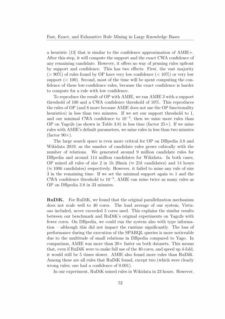
Fast, Exact, and Exhaustive Rule Mining in Large Knowledge Bases
a heuristic [13] that is similar to the confidence approximation of AMIE+.After this step, it will compute the support and the exact CWA confidence ofany remaining candidate. However, it offers no way of pruning rules upfrontby support and confidence. This has two effects: First, the vast majority(> 90%) of rules found by OP have very low confidence (< 10%) or very lowsupport (< 100). Second, most of the time will be spent computing the con-fidence of these low-confidence rules, because the exact confidence is harderto compute for a rule with low confidence.
To reproduce the result of OP with AMIE, we ran AMIE 3 with a supportthreshold of 100 and a CWA confidence threshold of 10%. This reproducesthe rules of OP (and 8 more because AMIE does not use the OP functionalityheuristics) in less than two minutes. If we set our support threshold to 1,and our minimal CWA confidence to 10−5, then we mine more rules thanOP on Yago2s (as shown in Table 3.8) in less time (factor 25×). If we minerules with AMIE’s default parameters, we mine rules in less than two minutes(factor 90×).
The large search space is even more critical for OP on DBpedia 3.8 andWikidata 2019, as the number of candidate rules grows cubically with thenumber of relations. We generated around 9 million candidate rules forDBpedia and around 114 million candidates for Wikidata. In both cases,OP mined all rules of size 2 in 1h 20min (≈ 21k candidates) and 14 hours(≈ 100k candidates) respectively. However, it failed to mine any rule of size3 in the remaining time. If we set the minimal support again to 1 and theCWA confidence threshold to 10−5, AMIE can mine twice as many rules asOP on DBpedia 3.8 in 33 minutes.
RuDiK. For RuDiK, we found that the original parallelization mechanismdoes not scale well to 40 cores. The load average of our system, Virtu-oso included, never exceeded 5 cores used. This explains the similar resultsbetween our benchmark and RuDiK’s original experiments on Yago2s withfewer cores. On DBpedia, we could run the system also with type informa-tion —although this did not impact the runtime significantly. The loss ofperformance during the execution of the SPARQL queries is more noticeabledue to the multitude of small relations in DBpedia compared to Yago. Incomparison, AMIE was more than 20× faster on both datasets. This meansthat, even if RuDiK were to make full use of the 40 cores, and speed up 4-fold,it would still be 5 times slower. AMIE also found more rules than RuDiK.Among these are all rules that RuDiK found, except two (which were clearlywrong rules; one had a confidence of 0.001).
In our experiment, RuDiK mined rules in Wikidata in 23 hours. However,
52
Fast, Exact, and Exhaustive Rule Mining in Large Knowledge Bases
RuDiK was not able to mine rules for 22 of the relations as Virtuoso was notable to compute any of the positive or the negative examples RuDiK requiresto operate. This is because RuDiK would timeout any SPARQL query after20 seconds of execution5. Virtuoso failed to compute the examples duringthis time frame on the 22 relations, which are the largest ones in our Wikidatadataset: They cover 84% of the facts. Interestingly, RuDiK did also not findrules that contain these relations in the body (except one, which covered0.5% of the KB).
In comparison, AMIE mined 1703 rules with at least one of these relations,computing the support, confidence and PCA confidence exactly on thesehuge relations —in less time. For example, it found the rule inRegion(x, y) ∧inCountry(y, z) ⇒ inCountry(x, z), which is not considered by RuDiK, buthas a support of over 7 million and a PCA confidence of over 99%.
AMIE 3. outperformed both OP and RuDiK in terms of runtime andthe number of rules. Moreover, it has the advantage of being exact andcomplete. Then again, the comparisons have to be seen in context: RuDiK,e.g., is designed to run on a small machine. For this, it uses a disk-baseddatabase and sampling. AMIE, in contrast, loads all data into memory, andthus has a large memory footprint (the 500GB were nearly used up for theWikidata experiment). In return, it computes all rules exactly and is fast.
3.4 Conclusion
We have presented AMIE 3, the newest version of the rule mining systemAMIE (available at https://github.com/lajus/amie/). The new systemuses a range of optimization and pruning strategies, which allow scaling tolarge KBs that were previously beyond reach. In particular, AMIE 3 canexhaustively mine all rules above given thresholds on support and confidence,without resorting to sampling or approximations.
5Increasing the timeout parameter is not necessarily a good solution for two reasons:First, we cannot predict the optimal value so that all queries finish. Second, it would in-crease the runtime of queries succeeding with partial results thanks to Virtuoso’s AnytimeQuery capability. This would largely increase RuDiK’s runtime with no guarantee to solvethe issue.
53
Chapter 4
Star patterns: Reducing theSearch Space
4.1 Introduction
The improvements of Chapter 3 were focused on improving the performancesof the computation of the support and confidence measures of a specific rule.AMIE 3 still relies on the original base algorithm for exploring the searchspace. This algorithm, however, shows clear limitations when we want tomine more complex rules on large Knowledge Bases. For example, AMIE 3is neither able to mine every rule of size 4 nor the rules of size 3 with constantswithin 12 hours on Yago2s.
Instantiations are critical to handle properly some relations and recovervaluable rules. For example, using instantiations on the type relation allowsto get schema information about the rule, i.e the types of the variables used inthe rule. In contrast, without the instantiations, AMIE is able to mine onlythat a variable “has a type” (and eventually, that two variables have the sametype). As for longer rules, they can model more complex relationships andin practice the interest for such rules is appreciable among AMIE’s userbase,according to the recent exchanges we had on AMIE’s project page.
To mine longer rules and rules with constants efficiently, we must addresshow AMIE handles the search space directly. More precisely, for any rule,AMIE computes the support of any refinements of this rule and potentiallyprune it if it is a duplicate or if its support does not meet the requiredthreshold. In both cases, the computation of the support is, a posteriori,superfluous. We propose in this chapter a method to discard, a priori, anunwanted rule, without computing the support of the rule at all. Such anearly pruning process should speed up AMIE exploration significantly.
54
Fast, Exact, and Exhaustive Rule Mining in Large Knowledge Bases
Contribution. In particular, we will decompose the rules into simpler pat-terns, the star patterns, that will be used to identify, a priori, unsatisfiablerules.
This chapter is structured as follows: In Section 4.2 we define the starpatterns and introduce the necessary condition used to prune the rules earlyon. Then, in Section 4.3 we show how frequent pattern mining can be used toextract from the KB all the star patterns that satisfy the necessary condition.Finally, in Section 4.4 we present a method to combine the star patterns intorules that satisfy the necessary condition, thus achieving the construction ofour pruned search space. However, we also show in this last section that thenaive generation of all rules is not tractable in the general case.
In Chapter 5, we will show that in the specific case of path rules, thenecessary condition can be used constructively to efficiently prune the searchspace.
4.2 Star patterns
4.2.1 Patterns
A Knowledge Base can be seen as a directed graph with labelled edges be-tween entities. The task of rule mining can thus be seen as the task of findingfrequent closed subgraphs in this huge graph. We can represent these sub-graphs using patterns, a graph representation of a rule with variables in placeof vertices. For example the pattern in Figure 4.1a represents the rule
marriedTo(y, x)⇒ marriedTo(x, y)
In the Elvis KB (represented as a labeled graph in Figure 2.1), we canfind four couples of values for (x, y) that satisfy this rule: (Elvis, Priscilla),(Priscilla, Elvis), (Barack, Michelle) and (Michelle, Barack). Finding thosecouples is equivalent to finding where the pattern matches on the labeledgraph representation of the KB, printing the pattern over a tracing paperand trying to find matches on the KB graph.
The patterns are just representations of the rules, and there are just asexpressive. Some apply on a KB and others do not. Some are simple andothers are ridiculously complex. But even a more complex pattern can bebroken into smaller patterns, simpler to find, to help localize where the biggerpattern applies. It is as if you cut the tracing paper into smaller pieces.
To match the pattern of Figure 4.1a1, AMIE also breaks it into smaller
1to find the set of pair of entities (x, y) of the KB satisfying marriedTo(y, x) ∧marriedTo(x, y)
55

Fast, Exact, and Exhaustive Rule Mining in Large Knowledge Bases
yxmarriedTo
marriedTo
(a) Pattern for marriedTo(y, x) ∧marriedTo(x, y)
yx yxmarriedTo
marriedTo
(b) Relational sub-patterns for marriedTo(y, x) ∧marriedTo(x, y)
x
?? ? ?
ymarriedTo marriedTo marriedTo marriedTo
(c) Star (sub-)patterns for marriedTo(y, x) ∧marriedTo(x, y)
Figure 4.1 – Patterns and sub-patterns on a simple example
patterns. These patterns are centered around the relation, as AMIE willtry out all the pairs (x, y) satisfying marriedTo(y, x) against the conditionmarriedTo(x, y) (or the opposite depending on the most restrictive relation).Thus it will consider the sub-patterns represented in Figure 4.1b.
In order to find a necessary condition, we will consider the other set ofsmaller pieces: the star patterns, i.e the patterns centered on a single variableas in Figure 4.1c.
4.2.2 Star patterns
Definition 4.2.1 (Star pattern). For a rule R and any variable x of thisrule, we can construct the star patterns of x in the rule R, noted sp(x,R) asfollows:
• First we identify in the rule the relations [ri1 , . . . rin ] where x appearsin the subject position and the relations [rj1 , . . . rjm ] where x appearsin the object position.
• Then we pose:
sp(x,R) =n∧k=1
∃yk.rik(x, yk) ∧m∧k=1
∃zk.rjk(zk, x)
As such, a star pattern is a conjunctive query where only one variable is openand the other variables are existentially quantified.
56
Fast, Exact, and Exhaustive Rule Mining in Large Knowledge Bases
For example, in the rule R = marriedTo(y, x) ⇒ marriedTo(x, y), x isin the subject position of the relation marriedTo and in the object positionof another marriedTo atom. Thus we have:
sp(x,R) = ∃a.marriedTo(x, a) ∧ ∃b.marriedTo(b, x)
The star patterns capture the pattern of relations around a single variable.Represented as in Figure 4.1c, we can directly identify that the variable xmust be in the subject position and in the object position of the marriedTorelation.
Set notation. To simplify the notation, we denote every atom of the form∃y.r(x, y) by the item r and represent a conjunction of such atoms as a setof items. Finally, we use signed relations to represent the atoms where xappears in the object position. Using this notation, we have:
sp(x,R) = marriedTo,marriedTo−1
Definition 4.2.2 (Support and Satisfiability of a star pattern). By substitu-tion, we can identify the entities that satisfy a star pattern (seen as a simpleconjunctive query) in a KB K. The number of such entities in K is calledthe support of the star pattern, and we say that a star pattern is satisfiableif its support is at least one.
Proposition 4.2.3 (Necessary condition). In a KB K an entity E can be avalid substitution for x in the rule R only if E satisfies sp(x,R) in K.
As a consequence, a rule is satisfiable in a KB K only if every one of itsstar patterns is satisfiable in this KB.
Proof. Syntactically, sp(x,R) is more general than R.
Proposition 4.2.3 gives us a necessary condition for a rule to be satisfiable.In Section 4.2.4, we will introduce the language of star patterns consideredand a systematic way to decompose a rule into star patterns of this language.
The first observation of Proposition 4.2.3 will also be used in order torestrict the set of possible instantiations for any variable x and speed up thecomputation of the quality measures of a rule in Section 6.2.5.
4.2.3 Related work
Star patterns have already been introduced in [62] under the name of Char-acteristic sets in order to compute cardinality estimations of a Sparql query.
57
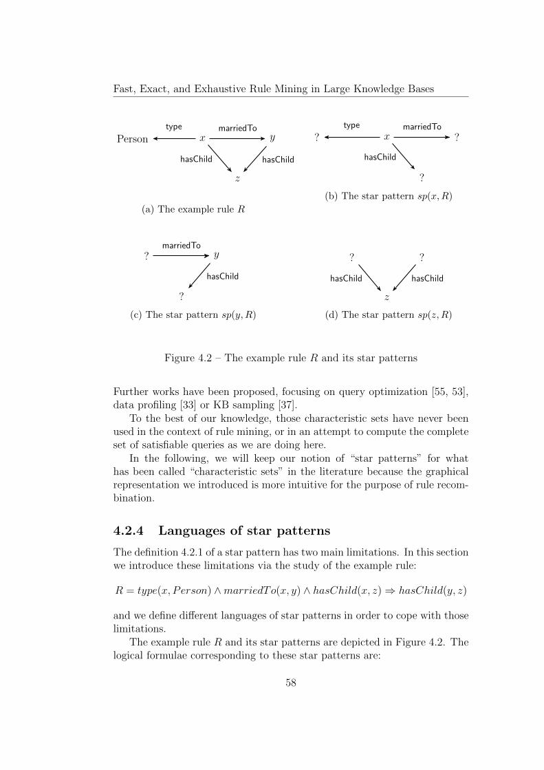
Fast, Exact, and Exhaustive Rule Mining in Large Knowledge Bases
z
yxPerson
hasChild hasChild
marriedTotype
(a) The example rule R
?
?x?
hasChild
marriedTotype
(b) The star pattern sp(x,R)
?
y?
hasChild
marriedTo
(c) The star pattern sp(y,R)
z
??
hasChild hasChild
(d) The star pattern sp(z,R)
Figure 4.2 – The example rule R and its star patterns
Further works have been proposed, focusing on query optimization [55, 53],data profiling [33] or KB sampling [37].
To the best of our knowledge, those characteristic sets have never beenused in the context of rule mining, or in an attempt to compute the completeset of satisfiable queries as we are doing here.
In the following, we will keep our notion of “star patterns” for whathas been called “characteristic sets” in the literature because the graphicalrepresentation we introduced is more intuitive for the purpose of rule recom-bination.
4.2.4 Languages of star patterns
The definition 4.2.1 of a star pattern has two main limitations. In this sectionwe introduce these limitations via the study of the example rule:
R = type(x, Person) ∧marriedTo(x, y) ∧ hasChild(x, z)⇒ hasChild(y, z)
and we define different languages of star patterns in order to cope with thoselimitations.
The example rule R and its star patterns are depicted in Figure 4.2. Thelogical formulae corresponding to these star patterns are:
58
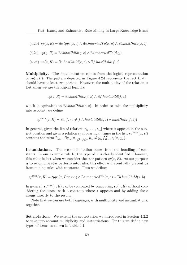
Fast, Exact, and Exhaustive Rule Mining in Large Knowledge Bases
(4.2b) sp(x,R) = ∃c.type(x, c) ∧ ∃a.marriedTo(x, a) ∧ ∃b.hasChild(x, b)
(4.2c) sp(y,R) = ∃c.hasChild(y, c) ∧ ∃d.marriedTo(d, y)
(4.2d) sp(z, R) = ∃e.hasChild(e, z) ∧ ∃f.hasChild(f, z)
Multiplicity. The first limitation comes from the logical representationof sp(z,R). The pattern depicted in Figure 4.2d represents the fact that zshould have at least two parents. However, the multiplicity of the relation islost when we use the logical formula:
sp(z,R) = ∃e.hasChild(e, z) ∧ ∃f.hasChild(f, z)
which is equivalent to ∃e.hasChild(e, z). In order to take the multiplicityinto account, we define:
spmult(z,R) = ∃e, f. (e 6= f ∧ hasChild(e, z) ∧ hasChild(f, z))
In general, given the list of relation [ri1 , . . . , rin ] where x appears in the sub-ject position and given a relation ri appearing m times in the list, spmult(x,R)contains the term ∃yi1 ...∃yim
∧1≤k<j≤m yik 6= yij
∧mk=1 ri(x, yik).
Instantiations. The second limitation comes from the handling of con-stants. In our example rule R, the type of x is clearly identified. However,this value is lost when we consider the star-pattern sp(x,R). As our purposeis to recombine star patterns into rules, this effect will eventually prevent usfrom mining rules with constants. Thus we define:
spinst(x,R) = type(x, Person) ∧ ∃a.marriedTo(x, a) ∧ ∃b.hasChild(x, b)
In general, spinst(x,R) can be computed by computing sp(x,R) without con-sidering the atoms with a constant where x appears and by adding theseatoms directly to the result.
Note that we can use both languages, with multiplicity and instantiations,together.
Set notation. We extend the set notation we introduced in Section 4.2.2to take into account multiplicity and instantiations. For this we define newtypes of items as shown in Table 4.1.
59
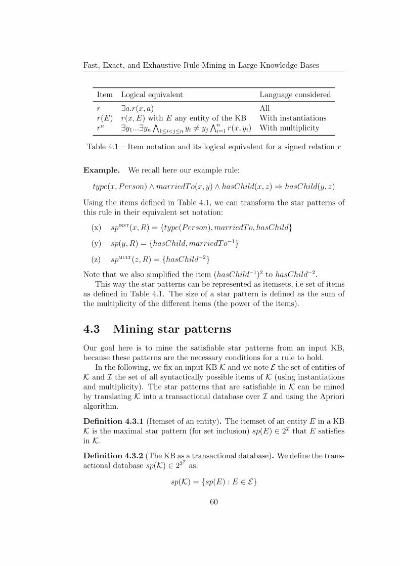
Fast, Exact, and Exhaustive Rule Mining in Large Knowledge Bases
Item Logical equivalent Language considered
r ∃a.r(x, a) Allr(E) r(x,E) with E any entity of the KB With instantiationsrn ∃y1...∃yn
∧1≤i<j≤n yi 6= yj
∧ni=1 r(x, yi) With multiplicity
Table 4.1 – Item notation and its logical equivalent for a signed relation r
Example. We recall here our example rule:
type(x, Person) ∧marriedTo(x, y) ∧ hasChild(x, z)⇒ hasChild(y, z)
Using the items defined in Table 4.1, we can transform the star patterns ofthis rule in their equivalent set notation:
(x) spinst(x,R) = type(Person),marriedTo, hasChild
(y) sp(y,R) = hasChild,marriedTo−1
(z) spmult(z, R) = hasChild−2
Note that we also simplified the item (hasChild−1)2 to hasChild−2.This way the star patterns can be represented as itemsets, i.e set of items
as defined in Table 4.1. The size of a star pattern is defined as the sum ofthe multiplicity of the different items (the power of the items).
4.3 Mining star patterns
Our goal here is to mine the satisfiable star patterns from an input KB,because these patterns are the necessary conditions for a rule to hold.
In the following, we fix an input KB K and we note E the set of entities ofK and I the set of all syntactically possible items of K (using instantiationsand multiplicity). The star patterns that are satisfiable in K can be minedby translating K into a transactional database over I and using the Apriorialgorithm.
Definition 4.3.1 (Itemset of an entity). The itemset of an entity E in a KBK is the maximal star pattern (for set inclusion) sp(E) ∈ 2I that E satisfiesin K.
Definition 4.3.2 (The KB as a transactional database). We define the trans-actional database sp(K) ∈ 22I as:
sp(K) = sp(E) : E ∈ E
60
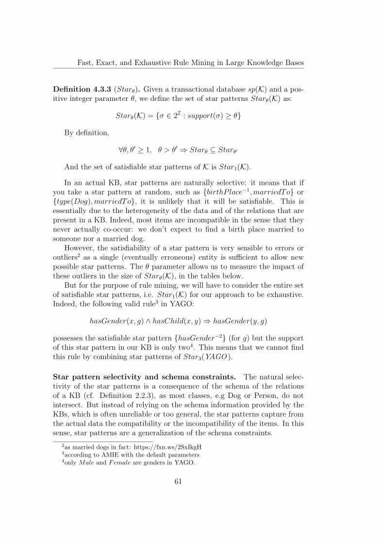
Fast, Exact, and Exhaustive Rule Mining in Large Knowledge Bases
Definition 4.3.3 (Starθ). Given a transactional database sp(K) and a pos-itive integer parameter θ, we define the set of star patterns Starθ(K) as:
Starθ(K) = σ ∈ 2I : support(σ) ≥ θ
By definition,
∀θ, θ′ ≥ 1, θ > θ′ ⇒ Starθ ⊆ Starθ′
And the set of satisfiable star patterns of K is Star1(K).
In an actual KB, star patterns are naturally selective: it means that ifyou take a star pattern at random, such as birthP lace−1,marriedTo ortype(Dog),marriedTo, it is unlikely that it will be satisfiable. This isessentially due to the heterogeneity of the data and of the relations that arepresent in a KB. Indeed, most items are incompatible in the sense that theynever actually co-occur: we don’t expect to find a birth place married tosomeone nor a married dog.
However, the satisfiability of a star pattern is very sensible to errors oroutliers2 as a single (eventually erroneous) entity is sufficient to allow newpossible star patterns. The θ parameter allows us to measure the impact ofthese outliers in the size of Starθ(K), in the tables below.
But for the purpose of rule mining, we will have to consider the entire setof satisfiable star patterns, i.e. Star1(K) for our approach to be exhaustive.Indeed, the following valid rule3 in YAGO:
hasGender(x, g) ∧ hasChild(x, y)⇒ hasGender(y, g)
possesses the satisfiable star pattern hasGender−2 (for g) but the supportof this star pattern in our KB is only two4. This means that we cannot findthis rule by combining star patterns of Star3(YAGO ).
Star pattern selectivity and schema constraints. The natural selec-tivity of the star patterns is a consequence of the schema of the relationsof a KB (cf. Definition 2.2.3), as most classes, e.g Dog or Person, do notintersect. But instead of relying on the schema information provided by theKBs, which is often unreliable or too general, the star patterns capture fromthe actual data the compatibility or the incompatibility of the items. In thissense, star patterns are a generalization of the schema constraints.
2as married dogs in fact: https://fxn.ws/2SxIkgH3according to AMIE with the default parameters4only Male and Female are genders in YAGO.
61
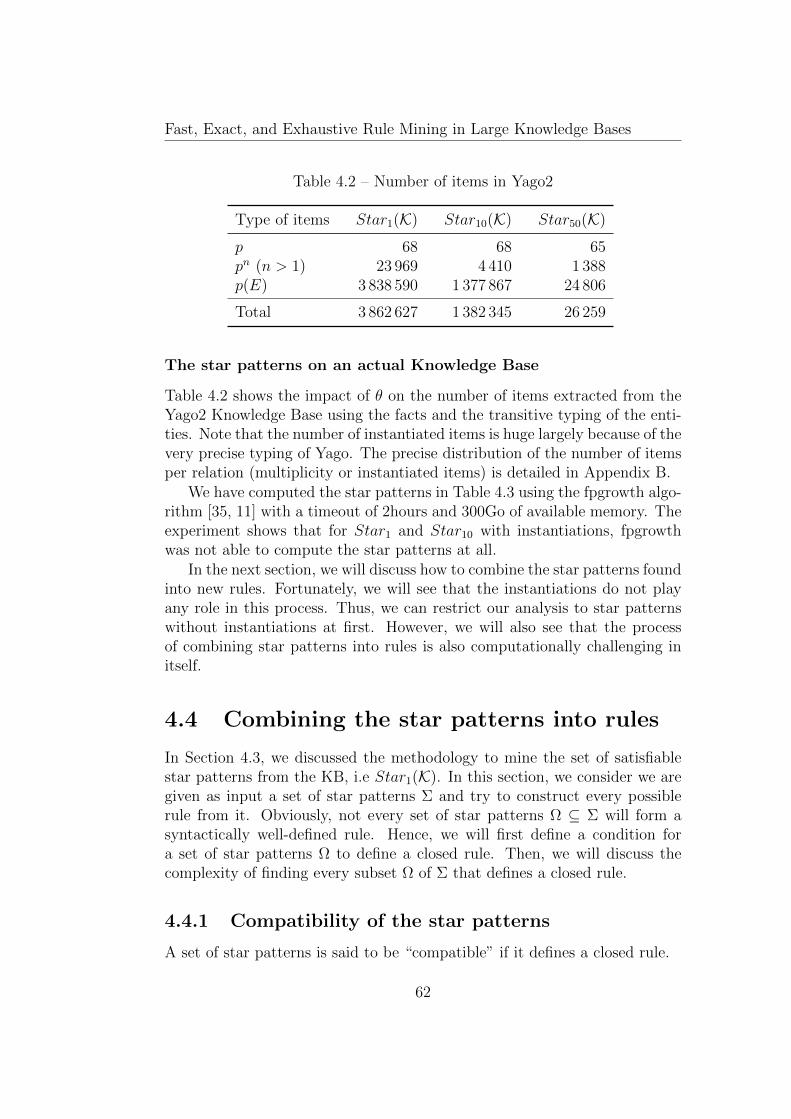
Fast, Exact, and Exhaustive Rule Mining in Large Knowledge Bases
Table 4.2 – Number of items in Yago2
Type of items Star1(K) Star10(K) Star50(K)
p 68 68 65pn (n > 1) 23 969 4 410 1 388p(E) 3 838 590 1 377 867 24 806
Total 3 862 627 1 382 345 26 259
The star patterns on an actual Knowledge Base
Table 4.2 shows the impact of θ on the number of items extracted from theYago2 Knowledge Base using the facts and the transitive typing of the enti-ties. Note that the number of instantiated items is huge largely because of thevery precise typing of Yago. The precise distribution of the number of itemsper relation (multiplicity or instantiated items) is detailed in Appendix B.
We have computed the star patterns in Table 4.3 using the fpgrowth algo-rithm [35, 11] with a timeout of 2hours and 300Go of available memory. Theexperiment shows that for Star1 and Star10 with instantiations, fpgrowthwas not able to compute the star patterns at all.
In the next section, we will discuss how to combine the star patterns foundinto new rules. Fortunately, we will see that the instantiations do not playany role in this process. Thus, we can restrict our analysis to star patternswithout instantiations at first. However, we will also see that the processof combining star patterns into rules is also computationally challenging initself.
4.4 Combining the star patterns into rules
In Section 4.3, we discussed the methodology to mine the set of satisfiablestar patterns from the KB, i.e Star1(K). In this section, we consider we aregiven as input a set of star patterns Σ and try to construct every possiblerule from it. Obviously, not every set of star patterns Ω ⊆ Σ will form asyntactically well-defined rule. Hence, we will first define a condition fora set of star patterns Ω to define a closed rule. Then, we will discuss thecomplexity of finding every subset Ω of Σ that defines a closed rule.
4.4.1 Compatibility of the star patterns
A set of star patterns is said to be “compatible” if it defines a closed rule.
62
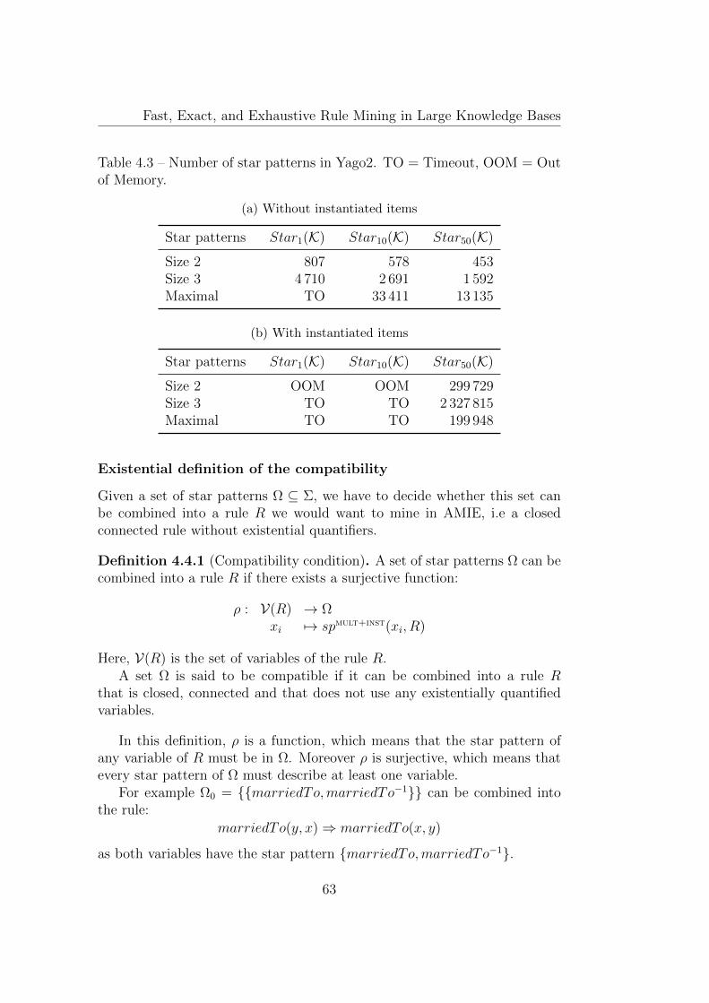
Fast, Exact, and Exhaustive Rule Mining in Large Knowledge Bases
Table 4.3 – Number of star patterns in Yago2. TO = Timeout, OOM = Outof Memory.
(a) Without instantiated items
Star patterns Star1(K) Star10(K) Star50(K)
Size 2 807 578 453Size 3 4 710 2 691 1 592Maximal TO 33 411 13 135
(b) With instantiated items
Star patterns Star1(K) Star10(K) Star50(K)
Size 2 OOM OOM 299 729Size 3 TO TO 2 327 815Maximal TO TO 199 948
Existential definition of the compatibility
Given a set of star patterns Ω ⊆ Σ, we have to decide whether this set canbe combined into a rule R we would want to mine in AMIE, i.e a closedconnected rule without existential quantifiers.
Definition 4.4.1 (Compatibility condition). A set of star patterns Ω can becombined into a rule R if there exists a surjective function:
ρ : V(R) → Ωxi 7→ spmult+inst(xi, R)
Here, V(R) is the set of variables of the rule R.A set Ω is said to be compatible if it can be combined into a rule R
that is closed, connected and that does not use any existentially quantifiedvariables.
In this definition, ρ is a function, which means that the star pattern ofany variable of R must be in Ω. Moreover ρ is surjective, which means thatevery star pattern of Ω must describe at least one variable.
For example Ω0 = marriedTo,marriedTo−1 can be combined intothe rule:
marriedTo(y, x)⇒ marriedTo(x, y)
as both variables have the star pattern marriedTo,marriedTo−1.
63
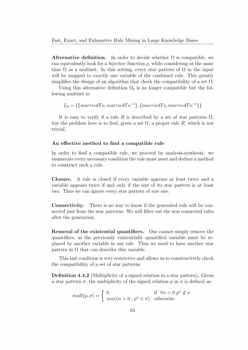
Fast, Exact, and Exhaustive Rule Mining in Large Knowledge Bases
Alternative definition. In order to decide whether Ω is compatible, wecan equivalently look for a bijective function ρ, while considering at the sametime Ω as a multiset. In this setting, every star pattern of Ω in the inputwill be mapped to exactly one variable of the combined rule. This greatlysimplifies the design of an algorithm that check the compatibility of a set Ω.
Using this alternative definition Ω0 is no longer compatible but the fol-lowing multiset is:
L0 = marriedTo,marriedTo−1, marriedTo,marriedTo−1
It is easy to verify if a rule R is described by a set of star patterns Ω,but the problem here is to find, given a set Ω, a proper rule R, which is nottrivial.
An effective method to find a compatible rule
In order to find a compatible rule, we proceed by analysis-synthesis: weenumerate every necessary condition the rule must meet and deduce a methodto construct such a rule.
Closure. A rule is closed if every variable appears at least twice and avariable appears twice if and only if the size of its star pattern is at leasttwo. Thus we can ignore every star pattern of size one.
Connectivity. There is no way to know if the generated rule will be con-nected just from the star patterns. We will filter out the non connected rulesafter the generation.
Removal of the existential quantifiers. One cannot simply remove thequantifiers, as the previously existentially quantified variable must be re-placed by another variable in our rule. Thus we need to have another starpattern in Ω that can describe this variable.
This last condition is very restrictive and allows us to constructively checkthe compatibility of a set of star patterns.
Definition 4.4.2 (Multiplicity of a signed relation in a star pattern). Givena star pattern σ, the multiplicity of the signed relation p in σ is defined as:
mult(p, σ) =
0 if ∀n > 0 pn /∈ σmax(n > 0 : pn ∈ σ) otherwise.
64
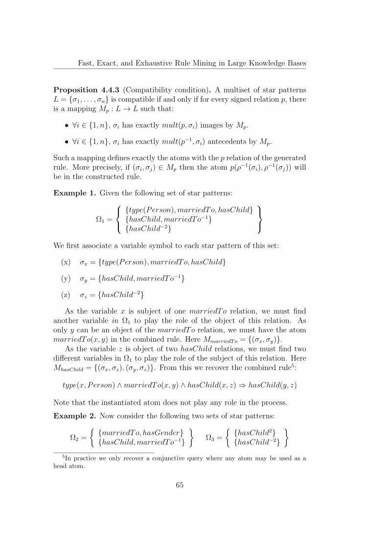
Fast, Exact, and Exhaustive Rule Mining in Large Knowledge Bases
Proposition 4.4.3 (Compatibility condition). A multiset of star patternsL = σ1, . . . , σn is compatible if and only if for every signed relation p, thereis a mapping Mp : L→ L such that:
• ∀i ∈ 1, n, σi has exactly mult(p, σi) images by Mp.
• ∀i ∈ 1, n, σi has exactly mult(p−1, σi) antecedents by Mp.
Such a mapping defines exactly the atoms with the p relation of the generatedrule. More precisely, if (σi, σj) ∈ Mp then the atom p(ρ−1(σi), ρ
−1(σj)) willbe in the constructed rule.
Example 1. Given the following set of star patterns:
Ω1 =
type(Person),marriedTo, hasChildhasChild,marriedTo−1hasChild−2
We first associate a variable symbol to each star pattern of this set:
(x) σx = type(Person),marriedTo, hasChild
(y) σy = hasChild,marriedTo−1
(z) σz = hasChild−2
As the variable x is subject of one marriedTo relation, we must findanother variable in Ω1 to play the role of the object of this relation. Asonly y can be an object of the marriedTo relation, we must have the atommarriedTo(x, y) in the combined rule. Here MmarriedTo = (σx, σy).
As the variable z is object of two hasChild relations, we must find twodifferent variables in Ω1 to play the role of the subject of this relation. HereMhasChild = (σx, σz), (σy, σz). From this we recover the combined rule5:
type(x, Person) ∧marriedTo(x, y) ∧ hasChild(x, z)⇒ hasChild(y, z)
Note that the instantiated atom does not play any role in the process.
Example 2. Now consider the following two sets of star patterns:
Ω2 =
marriedTo, hasGenderhasChild,marriedTo−1
Ω3 =
hasChild2hasChild−2
5In practice we only recover a conjunctive query where any atom may be used as a
head atom.
65
Fast, Exact, and Exhaustive Rule Mining in Large Knowledge Bases
In Ω2, we can deduce that both variables are married together, but we canassociate neither the gender of the first variable nor the child of the secondvariable to a star pattern of the set. Ω2 is thus incompatible.
In Ω3, the multiplicity enforces that the first variable must have twodifferent children and the second variable must have two different parents.Thus even if we make the first variable the parent of the second, we cannotfind a second child nor a second parent in our set. Thus Ω3 is incompatible.
In Appendix C, we present an efficient6 algorithm that decides construc-tively the compatibility of a set of star patterns and we prove its correctness.
Remark 1. A star pattern may contain a relation and its inverse (asmarriedTo,marriedTo−1). This means the mapping may map a starpattern to itself and those mappings would produce reflexive atoms in thecorresponding rule.
Remark 2. Compatibility requires the existence of a mapping for everyrelation. However, there may exist multiple valid mappings for a relation.As such, every combination of valid mappings across the different relationsgenerates a new candidate rule. Moreover, nothing prevents multiple combi-nations of mappings to generate equivalent rules.
4.4.2 Selection of compatible star patterns
Even if we can decide efficiently if a set of star patterns is compatible, theenumeration of all compatible subsets of Σ may remain intractable.
Proposition 4.4.4 (Necessary condition for the compatibility). A list ofstar patterns (σ1, . . . , σn) is compatible only if for every relation p:
n∑i=1
mult(p, σi) =n∑j=1
mult(p−1, σj)
If we index every unsigned relation of our KB as (p1, . . . , p|R|) we canmap every star pattern σ ∈ Σ into a multidimensional integer space, usingthe function:
f : Σ → Z|R|
σ 7→
mult(r1, spi)−mult(r−11 , spi)...
mult(r|R|, spi)−mult(r−1|R|, spi)
6O(n× log(n)) where n is the sum of the sizes of the different star patterns.
66

Fast, Exact, and Exhaustive Rule Mining in Large Knowledge Bases
Doing so, we can recognize an instance of the zero sum subset problemin a multidimensional setting, which is NP-Complete.
Proposition 4.4.5 (As a zero sum subset problem). A set Σ of star patternscontains a compatible subset only if:
∃σi1 , . . . , σim ⊆ Σ :m∑k=1
f(σik) = 0Z|R|
This proposition does not constitute a proof of complexity, but it stronglysuggests that our problem is hard and given the size of our input (cf Ta-ble 4.3), probably intractable.
4.5 Conclusion
In this chapter, we defined the star patterns: simple patterns that can beextracted from a rule. We showed how these star patterns, that can be minedwith relative efficiency using frequent itemset mining algorithms, can thenbe used to prune unsatisfiable rules.
Then, we introduced the compatibility condition that decides if a set ofstar patterns can describe a rule or not and presented a polynomial algorithmthat decides the compatibility in Appendix C. However, we also showed thatdifferent compatible sets of star patterns can represent duplicate rules andthat finding all compatible sets of star patterns is intractable. Thus, wecannot use this approach to generate uniquely all satisfiable rules in thegeneral case.
That said, we will see in the next chapter how star patterns can be usedto efficiently explore, and prune, the search space of rules of a specific shape:the path rules.
67
Chapter 5
Star patterns and path rules
5.1 Introduction
We showed in the previous chapter that generating the entire search space ofrules using star patterns is not tractable in the general case. This is becausethe general case is too general and considers all satisfiable star patterns inde-pendently of their sizes. In practice, the bigger star patterns represent ruleswith a large number of atoms, which are rarely usable rules. Thus, in thischapter, we study simpler star patterns, those of size 2, and the simpler typeof rules they generate: the path rules. The goal here is still to propose amethod that will discard a priori unwanted rules, but this time working onlyon path rules.
Efficient path rule mining should greatly benefit the general task of rulemining for two reasons. First, the path rules are the hardest type of querieswhen it comes to computing the support and the confidence [30]. Second, aswe will see in Section 5.4, a divide-and-conquer approach can be implementedas any rule can be decomposed into multiple conjunctive path queries (pathsin a connected graph). Moreover, path rules constitute most of the output ofAMIE in practice. For example on Yago2s, only 1 over the 97 output rulesis not a path rule1. This is why multiple works in the literature also addressspecifically the problem of path rule mining [45, 13].
Contribution. In this chapter, we identify the two instrumental propertiesof path rules. First, we can produce all path rules without generating anyduplicate if we enforce a simple constraint on the refinement operator. Sec-
1This is also mainly due to the skyline pruning strategy [31] that prevents a rule to beoutput if it does not have a better confidence than its output parents, the parent being amore general rule.
68
Fast, Exact, and Exhaustive Rule Mining in Large Knowledge Bases
ond, given the simplicity of the star patterns of the path rules, the necessarycondition and the compatibility condition of those star patterns can be usedefficiently and constructively to generate a pruned search space. These twoproperties allow us to devise the “Pathfinder vanilla” algorithm that exploresincrementally and efficiently the pruned search space of path rules, withoutduplicates to eliminate.
This chapter is structured as follows: In Section 5.2 we introduce pathrules and describe our refinement operator that does not introduce any du-plicate rule. From this, we derive the Pathfinder vanilla algorithm. In Sec-tion 5.3 we present the bipattern graph that represents the compatibilitycondition of the satisfiable star patterns of size 2. Then we demonstrate howit can be used a priori, to generate all satisfiable path rules, or incrementally,in the Pathfinder vanilla algorithm. Finally, in Section 5.4 we discuss howwe could generalize the usage of the bipattern graph to other types of rulesin future work.
In Chapter 6 we will further enhance the Pathfinder vanilla algorithm andexperimentally compare the performance of this new approach with AMIE.
5.2 Path rules
Definition 5.2.1 (Path rules and path queries). Path rules are connectedrules where every variable appears at most twice. Path queries are connectedconjunctive queries where every variable appears at most twice.
5.2.1 Path queries
Theorem 5.2.2 (Forms of path queries). Any closed path query has one ofthe following forms:
Rc[r1, . . . , rn] := r1(x0, x1) ∧ r2(x1, x2) ∧ · · · ∧ rn(xn−1, x0) (close)Ri(E1, E2)[r1, . . . , rn] := r1(E1, x1) ∧ r2(x1, x2) ∧ · · · ∧ rn(xn−1, E2) (inst)
Here r1, . . . rn are signed relations, x0, . . . , xn are variables and E1 and E2 areentities of the KB. They can be seen as refinements of an open path query,which has the form:
Ro[r1, . . . , rn] := r1(x0, x1) ∧ r2(x1, x2) ∧ · · · ∧ rn(xn−1, xn) (open)
Proof. We can transform any path query into a graph where the vertices arethe variables of the rule (or the entities E1 and E2) and where the labeled
69
Fast, Exact, and Exhaustive Rule Mining in Large Knowledge Bases
directed edges between the vertices represent the atoms. As this graph rep-resents a path query, it must be connected and the degree of each vertice isat most 2. Thus it is either a simple path or a simple cycle.
Reading one simple path from one end to another and using the signedrelations to enforce the increasing order of the variables, we recover the openpath queries. We proceed similarly with the simple cycles, choosing anyvertice for the role of the extremity of the path, recovering the closed pathqueries.
Closed variant. The path query Rc[r1, . . . , rn] will also be called the closedvariant of the path query Ro[r1, . . . , rn].
Remark 3. There is actually a second form for the open path query, a halfinstantiated form but we will not consider this edge case here:
Roi(E1)[r1, . . . , rn] := r1(E1, x1) ∧ r2(x1, x2) ∧ · · · ∧ rn(xn−1, xn) (oi)
Corollary 5.2.3 (Reduced notation). All path queries can be representedas Rc[r1, . . . , rn], Ri(E1, E2)[r1, . . . , rn] or Ro[r1, . . . , rn]. In other words, theform (Rc, Ri(E1, E2) and Ro) and the list of signed relation used [r1, . . . , rn]totally describes the path query.
Examples. The open path query:
hasChild(x, y) ∧ hasChild(z, w) ∧marriedTo(x, z)
has two extremities, y and w. We first rename the variables choosing oneextremity, here y, as x0 and rename the following variable linked to y, herex, as x1, the other variable linked to x, here z, as x2 and so on. Then wereorder the atoms and the variables in the atoms using the signed relations torecover the desired order on the variables ((x0, x1), (x1, x2), . . . , (xn−1, xn)):
hasChild(x, y) ∧ hasChild(z, w) ∧marriedTo(x, z)hasChild(x1, x0) ∧ hasChild(x2, x3) ∧marriedTo(x1, x2) (rename)hasChild(x1, x0) ∧marriedTo(x1, x2) ∧ hasChild(x2, x3) (reorder)
hasChild−1(x0, x1) ∧marriedTo(x1, x2) ∧ hasChild(x2, x3) (switch)Ro[ hasChild
−1, marriedTo, hasChild ] (as list)
For the closed path query:
hasChild(x, y) ∧ hasChild(z, y) ∧marriedTo(x, z)
70
Fast, Exact, and Exhaustive Rule Mining in Large Knowledge Bases
we proceed similarly, here also choosing y as the “extremity” x0:
hasChild(x, y) ∧ hasChild(z, y) ∧marriedTo(x, z)hasChild(x1, x0) ∧ hasChild(x2, x0) ∧marriedTo(x1, x2) (rename)hasChild(x1, x0) ∧marriedTo(x1, x2) ∧ hasChild(x2, x0) (reorder)
hasChild−1(x0, x1) ∧marriedTo(x1, x2) ∧ hasChild(x2, x0) (switch)Rc[ hasChild
−1, marriedTo, hasChild ] (as list)
Theorem 5.2.4 (Equivalent path queries). For any list of signed relations[r1, . . . , rn] and any circular permutation ς, the following path queries aresyntactically equivalent:
Rc[r1, . . . , rn] ≡ Rc[r−1n , . . . , r−11 ]
Rc[r1, . . . , rn] ≡ Rc[ ς(r1, . . . , rn) ]Ro[r1, . . . , rn] ≡ Ro[r
−1n , . . . , r−11 ]
Ri(E1, E2)[r1, . . . , rn] ≡ Ri(E2, E1)[r−1n , . . . , r−11 ]
Moreover, this list is exhaustive. Two path queries are not syntacticallyequivalent if they are not equivalent under these transformations2.
Proof. The choice of the extremity in the proof of Theorem 5.2.2 is notenforced and the different possibilities still represent the same initial rule.
The exhaustivity comes from the fact that a path query, or any of itsequivalent rewritings, will be represented by the same graph in the construc-tion of the proof of Theorem 5.2.2.
Examples. Consider the previous example query:
hasChild(x, y) ∧ hasChild(z, w) ∧marriedTo(x, z)
Using w as the extremity we recover the equivalent query:
Ro[ hasChild−1, marriedTo−1, hasChild ]
Consider the previous closed query:
hasChild(x, y) ∧ hasChild(z, y) ∧marriedTo(x, z)
We can still choose the extremity y but now choosing z as x1 whichgives us the equivalent rule Rc[ hasChild
−1, marriedTo−1, hasChild ].Choosing z as extremity (and x as x1) gives us the equivalent ruleRc[ marriedTo
−1, hasChild, hasChild−1 ].
2or for the closed path queries, under any combination of the two transformations.
71
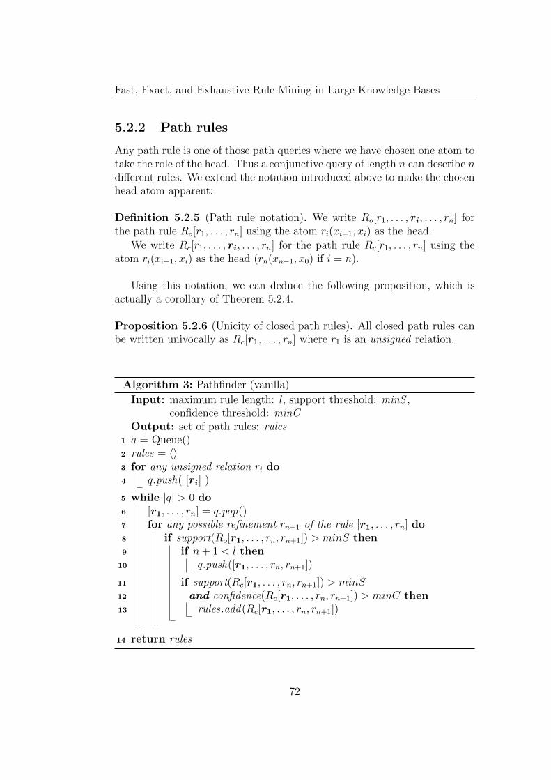
Fast, Exact, and Exhaustive Rule Mining in Large Knowledge Bases
5.2.2 Path rules
Any path rule is one of those path queries where we have chosen one atom totake the role of the head. Thus a conjunctive query of length n can describe ndifferent rules. We extend the notation introduced above to make the chosenhead atom apparent:
Definition 5.2.5 (Path rule notation). We write Ro[r1, . . . , ri, . . . , rn] forthe path rule Ro[r1, . . . , rn] using the atom ri(xi−1, xi) as the head.
We write Rc[r1, . . . , ri, . . . , rn] for the path rule Rc[r1, . . . , rn] using theatom ri(xi−1, xi) as the head (rn(xn−1, x0) if i = n).
Using this notation, we can deduce the following proposition, which isactually a corollary of Theorem 5.2.4.
Proposition 5.2.6 (Unicity of closed path rules). All closed path rules canbe written univocally as Rc[r1, . . . , rn] where r1 is an unsigned relation.
Algorithm 3: Pathfinder (vanilla)
Input: maximum rule length: l, support threshold: minS ,confidence threshold: minC
Output: set of path rules: rules1 q = Queue()2 rules = 〈〉3 for any unsigned relation ri do4 q.push( [ri] )
5 while |q| > 0 do6 [r1, . . . , rn] = q.pop()7 for any possible refinement rn+1 of the rule [r1, . . . , rn] do8 if support(Ro[r1, . . . , rn, rn+1]) > minS then9 if n+ 1 < l then
10 q.push([r1, . . . , rn, rn+1])
11 if support(Rc[r1, . . . , rn, rn+1]) > minS12 and confidence(Rc[r1, . . . , rn, rn+1]) > minC then13 rules .add(Rc[r1, . . . , rn, rn+1])
14 return rules
72
Fast, Exact, and Exhaustive Rule Mining in Large Knowledge Bases
Algorithm. We present the Pathfinder vanilla algorithm in Algorithm 3.In this algorithm, every rule is represented as a list of signed relations andrefining a rule only consists of adding a signed relation to the end of thislist. The queue of rules is initialized with all the rules containing only thehead atom, using every possible unsigned relation. This way, according toProposition 5.2.6, every closed path rule will be considered at most once, i.eno duplicate rules are generated.
5.2.3 Other path rules
In its current form, the Pathfinder vanilla algorithm only outputs the closedpath rules satisfying the given thresholds minS and minC. On one hand,it is straightforward to adapt this algorithm to mine the path rules havingthe head atom as an extremity, i.e the rules of the form Ro[r1, . . . , rn] orRi(E1, E2)[r1, . . . , rn]3, and it should be implemented in the near future.
On the other hand, mining the other path rules, i.e rules of the formRo[r1, . . . , ri, . . . , rn] or Ri(E1, E2)[r1, . . . , ri, . . . , rn] is not easy with this al-gorithm. However, we should also point out that these rules can be consideredless interesting than the former, in particular for fact prediction [5]. Indeed,those rules are “product rules” and would predict the head fact based ontwo independent conditions on the head variables. For example, the ruleRo[r1, . . . , ri, . . . , rn] stands for:
ri(xi−1, xi)⇐i−1∧j=1
rj(xj−1, xj)︸ ︷︷ ︸independent condition on xi−1
∧n∧
j=i+1
rj(xj−1, xj)︸ ︷︷ ︸independent condition on xi
5.3 Pruning the search space
Proposition 5.2.6 ensures that every possible closed path rule is consideredat most once by Algorithm 3 (i.e there are no duplicates). Thus, we can useany signed relation as a “possible refinement rn+1” (Line 7 of the algorithm)to ensure that all closed path rules are considered exactly once.
In this section, we will see how we can further restrict the “possiblerefinements rn+1” using the star patterns to prune the search space before thecomputation of the support of the rules while still outputting every satisfiableclosed path rule.
3On the specific case of instantiated rules, refining the rules of the form Roi(E1)[r1]instead of the more general rules Ro[r1] is also a promising strategy.
73
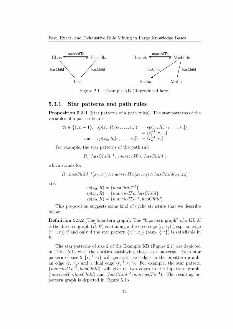
Fast, Exact, and Exhaustive Rule Mining in Large Knowledge Bases
Lisa
PriscillaElvis Barack Michelle
Sasha Malia
hasChild hasChild hasChild hasChild
marriedTo marriedTo
Figure 2.1 – Example KB (Reproduced here)
5.3.1 Star patterns and path rules
Proposition 5.3.1 (Star patterns of a path rules). The star patterns of thevariables of a path rule are:
∀i ∈ 1, n− 1, sp(xi, Rc[r1, . . . , rn]) = sp(xi, Ro[r1, . . . , rn])= r−1i , ri+1
and sp(x0, Rc[r1, . . . , rn]) = r−1n , r0
For example, the star patterns of the path rule:
Rc[ hasChild−1, marriedTo, hasChild ]
which stands for:
R : hasChild−1(x0, x1) ∧marriedTo(x1, x2) ∧ hasChild(x2, x0)
are:sp(x0, R) = hasChild−2sp(x1, R) = marriedTo, hasChildsp(x2, R) = marriedTo−1, hasChild
This proposition suggests some kind of cyclic structure that we describebelow.
Definition 5.3.2 (The bipattern graph). The “bipattern graph” of a KB Kis the directed graph (R, E) containing a directed edge (ri, rj) (resp. an edge(r−1, r)) if and only if the star pattern r−1i , rj (resp. r2) is satisfiable inK.
The star patterns of size 2 of the Example KB (Figure 2.1) are depictedin Table 5.1a with the entities satisfaying those star patterns. Each starpattern of size 2 r−1i , rj will generate two edges in the bipattern graph:an edge (ri, rj) and a dual edge (r−1j , r−1i ). For example, the star patternmarriedTo−1, hasChild will give us two edges in the bipattern graph:(marriedTo, hasChild) and (hasChild−1,marriedTo−1). The resulting bi-pattern graph is depicted in Figure 5.1b.
74
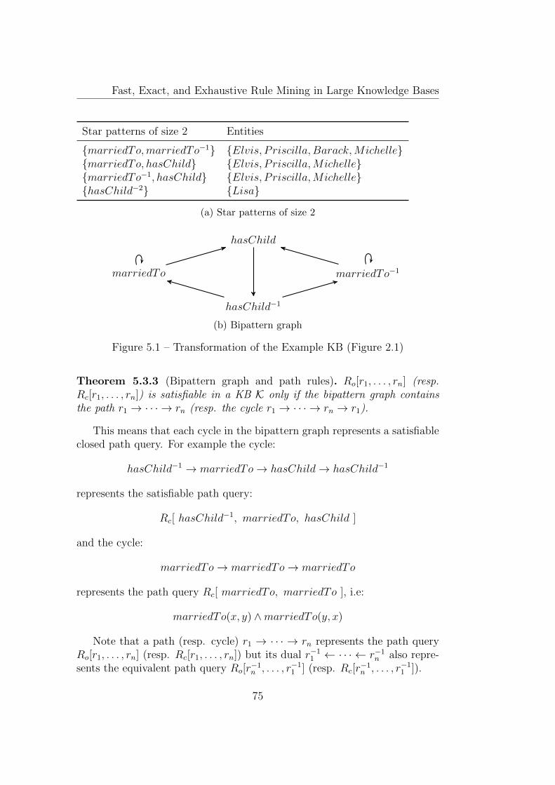
Fast, Exact, and Exhaustive Rule Mining in Large Knowledge Bases
Star patterns of size 2 Entities
marriedTo,marriedTo−1 Elvis, Priscilla, Barack,MichellemarriedTo, hasChild Elvis, Priscilla,MichellemarriedTo−1, hasChild Elvis, Priscilla,MichellehasChild−2 Lisa
(a) Star patterns of size 2
hasChild
hasChild−1
marriedTo marriedTo−1
(b) Bipattern graph
Figure 5.1 – Transformation of the Example KB (Figure 2.1)
Theorem 5.3.3 (Bipattern graph and path rules). Ro[r1, . . . , rn] (resp.Rc[r1, . . . , rn]) is satisfiable in a KB K only if the bipattern graph containsthe path r1 → · · · → rn (resp. the cycle r1 → · · · → rn → r1).
This means that each cycle in the bipattern graph represents a satisfiableclosed path query. For example the cycle:
hasChild−1 → marriedTo→ hasChild→ hasChild−1
represents the satisfiable path query:
Rc[ hasChild−1, marriedTo, hasChild ]
and the cycle:
marriedTo→ marriedTo→ marriedTo
represents the path query Rc[ marriedTo, marriedTo ], i.e:
marriedTo(x, y) ∧marriedTo(y, x)
Note that a path (resp. cycle) r1 → · · · → rn represents the path queryRo[r1, . . . , rn] (resp. Rc[r1, . . . , rn]) but its dual r−11 ← · · · ← r−1n also repre-sents the equivalent path query Ro[r
−1n , . . . , r−11 ] (resp. Rc[r
−1n , . . . , r−11 ]).
75
Fast, Exact, and Exhaustive Rule Mining in Large Knowledge Bases
From the star pattern perspective, an edge in the bipattern graph repre-sents a star pattern of size 2 from our KB and the cyclic structure is the com-patibility condition of a set of star patterns. Indeed, a path ri−1 → ri → ri+1
resolves the assignments for ri as it necessarily introduces a bipattern con-taining r−1i (the edge ri → ri+1) and another one containing ri (the edgeri−1 → ri). As the compatibility condition must also be solved for the rela-tion ri+1 we must follow a new edge from ri+1 and so on. Only cycles ensurecompatibility for every pattern.
From a KB perspective, computing the possible bipatterns amounts tocomputing which relation range or domain effectively intersects with anotherrelation range or domain, which is already done by AMIE+.
5.3.2 Generating all path rules
As sought out in Chapter 4, we can use the bipattern graph to generate,a priori, all satisfiable path rules (open or closed). More precisely, we canextract every path or cycle of the bipattern graph to find every satisfiablepath query. Then, we just need to distinguish a query from its dual andchoose a head atom as in Section 5.2.2.
We used this approach in the AMIE 3 experiments (Section 3.3) to gener-ate the set of all possible closed path rules on Yago, DBPedia and Wikidata,generating “our” set of candidate rules for the Ontological Pathfinding al-gorithm. Originally, the Ontological Pathfinding algorithm uses the schemaconstraints to compute the set of possible rules. “Our” set of candidate rulesis generated using the star patterns instead, which is more general than theseschema constraints (cf. discussion in Section 4.3).
In Section 6.5, we will also define in our benchmark the “Star pattern”approach as a generate-and-test rule mining algorithm, that will generate allclosed path rules using this approach and test their support and confidenceusing AMIE’s methods.
5.3.3 Incremental generation of candidates
In practice, we propose three different methods to generate the “possible re-finements rn+1” in Line 7 of the Pathfinder vanilla algorithm (Algorithm 3).The method can be chosen using a command line option. The possible re-finements of Ro[r1, . . . , rn] are, depending on the method:
Naive (ALL): Any signed relation is used as a possible refinement.
BiPattern existence (BP): Any signed relation rn+1 such that the edge(rn, rn+1) exists in the bipattern graph.
76
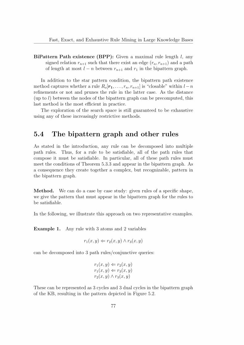
Fast, Exact, and Exhaustive Rule Mining in Large Knowledge Bases
BiPattern Path existence (BPP): Given a maximal rule length l, anysigned relation rn+1 such that there exist an edge (rn, rn+1) and a pathof length at most l − n between rn+1 and r1 in the bipattern graph.
In addition to the star pattern condition, the bipattern path existencemethod captures whether a rule Ro[r1, . . . , rn, rn+1] is “closable” within l−nrefinements or not and prunes the rule in the latter case. As the distance(up to l) between the nodes of the bipattern graph can be precomputed, thislast method is the most efficient in practice.
The exploration of the search space is still guaranteed to be exhaustiveusing any of these increasingly restrictive methods.
5.4 The bipattern graph and other rules
As stated in the introduction, any rule can be decomposed into multiplepath rules. Thus, for a rule to be satisfiable, all of the path rules thatcompose it must be satisfiable. In particular, all of these path rules mustmeet the conditions of Theorem 5.3.3 and appear in the bipattern graph. Asa consequence they create together a complex, but recognizable, pattern inthe bipattern graph.
Method. We can do a case by case study: given rules of a specific shape,we give the pattern that must appear in the bipattern graph for the rules tobe satisfiable.
In the following, we illustrate this approach on two representative examples.
Example 1. Any rule with 3 atoms and 2 variables
r1(x, y)⇐ r2(x, y) ∧ r3(x, y)
can be decomposed into 3 path rules/conjunctive queries:
r1(x, y)⇐ r2(x, y)r1(x, y)⇐ r3(x, y)r2(x, y) ∧ r3(x, y)
These can be represented as 3 cycles and 3 dual cycles in the bipattern graphof the KB, resulting in the pattern depicted in Figure 5.2.
77
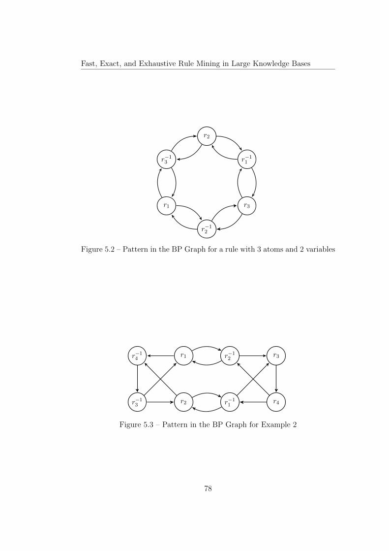
Fast, Exact, and Exhaustive Rule Mining in Large Knowledge Bases
r1
r−12
r3
r−11
r2
r−13
Figure 5.2 – Pattern in the BP Graph for a rule with 3 atoms and 2 variables
r−13
r−14
r2
r1
r−11
r−12
r4
r3
Figure 5.3 – Pattern in the BP Graph for Example 2
78
Fast, Exact, and Exhaustive Rule Mining in Large Knowledge Bases
Example 2. Any rule with 4 atoms and 3 variables
r1(x, y)⇐ r2(x, y) ∧ r3(x, z) ∧ r4(z, y)
can be decomposed into two path rules/queries of size 3:
r−11 (y, x)⇐ r3(x, z) ∧ r4(z, y)r−12 (y, x) ∧ r3(x, z) ∧ r4(z, y)
and a path rule of size 2:
r1(x, y)⇐ r2(x, y)
These can be represented as 2 cycles of size 3, one cycle of size 2 and theirrespective dual cycles in the bipattern graph, resulting in the pattern depictedin Figure 5.3.
Note that the bipattern graph cannot represent completely the star pat-terns of the rules above as it only represents their subsets of size 2. Forexample the star pattern of x in the rule of Example 1 is r1, r2, r3 but thepattern in the bipattern graph only ensures that r1, r2, r1, r3 and r2, r3are satisfiable which is a weaker necessary condition.
5.5 Conclusion
In this chapter we showed how the shape of the path rules allows us to devisea lean generation method that considers every path rule only once, gettingrid of the need to eliminate duplicates. In addition, we demonstrated howthe star patterns can be used to efficiently prune the search space.
Unfortunately, we will see in the experimental section of the next chap-ter (section 6.5) that this fine-tuned exploration method alone is not quiteenough to make Pathfinder Vanilla significantly better than AMIE. However,we will see in the next chapter how some improvements on the computationof the quality measures can make this algorithm faster. These improvementsare possible only through the Pathfinder vanilla approach that generates eachcandidate rule independently.
79
Chapter 6
Pathfinder: Efficient Path RuleMining
6.1 Introduction
The Pathfinder Vanilla algorithm that we have seen in the last chapter is notconsistently faster than AMIE on path rules. This is because AMIE performsthe computation of the support of all the refinements of a rule as a whole andthus benefits from some data reusage. In Pathfinder Vanilla, there are lesspossible refinements to consider but the algorithm recomputes the supportof each of them independently.
However, in a rule mining process the rules considered are not indepen-dent. Exploiting the dependencies between the rules can significantly speedup the computation of the different quality measures, as AMIE does forthe computation of the support of the refinements of a rule. In particular,reusing information between related rules can not only helps computing thesupport of a rule but also the confidence of this rule or the support of itsrefinements. Moreover, the reused data can also provide quantitative boundson the value of the different quality metrics, avoiding unnecessary and costlycomputations.
Instead of using the dependencies between the different refinements of arule only once, as AMIE does during the bulk computation of the support,we propose to go even further: we will carry over the information used inthe computation of the quality metrics of a rule to all the refinements of thisrule. This way a refined rule will inherit data from its parent that will bereused to speed up the computation, or bound the value, of its own qualitymeasures. In this sense, data can be passed on to the next generation. Asa consequence, the longer a rule is, the more it should benefit from this
80
Fast, Exact, and Exhaustive Rule Mining in Large Knowledge Bases
approach.
Contribution. In this chapter we define three different type of heritableinformation from a rule to its refinements: the set of possible values of thevariables, the iterated provenance and some bounds on the size of the former.The first two allow us to design more efficient measure computation strate-gies, which use the locally stored information to speed up the computationof the quality measures of the rules. The bounds on the size of the iteratedprovenance give us bounds on the value of the quality measures of the rules,allowing us to bypass the exact computation of those measures (a very costlyoperation) when it is not necessary. Then, using these optimizations, wedevelop the full Pathfinder algorithm, which consistently outperforms AMIEand its precursor Pathfinder Vanilla, by multiple orders of magnitude onlonger rules.
This chapter is structured as follows: First, in Section 6.2 we describehow to efficiently compute the set of possible values of the variables and theiterated provenance from a path rule and we present the different measurecomputation strategies that make use of this data. Then, in Section 6.3we introduce the local bounds used to speed up the Pathfinder algorithm,an algorithm that we extensively describe in Section 6.4 and experimentallyevaluate in Section 6.5.
6.2 Heritable information
6.2.1 Notation
Here we define the functions image and prov in a KB K and introduce theequivalent “diamond” notation (that uses the symbol ). Given any signedrelation r, we define the image of an entity x by r as:
image(x, r) ≡ y ∈ K : r(x, y) ≡ r(x, )
We extend this function and notation to a set X of entities:
image(X, r) ≡ y ∈ K : ∃x ∈ X, r(x, y) ≡ r(X, )
As such the domain and range of r can also be written as:
dom(r) = r(,K) = image(K, r−1)rng(r) = r(K, ) = image(K, r)
81
Fast, Exact, and Exhaustive Rule Mining in Large Knowledge Bases
The provenance of Y ⊆ image(X, r) is defined as the subset of X thatgenerated Y :
prov(X, r, Y ) ≡ x ∈ X : ∃y ∈ Y, r(x, y) = r(, Y ) ∩X
When we use this notation, we always consider we use a known KB Kgiven as input to the program.
6.2.2 The sets of possible values
The AMIE and Pathfinder Vanilla algorithms always consider every ruleindependently and never remember more than the value of the quality metricsfor each given rule. This means that, for each new rule considered, theymust recompute those quality metrics by testing possible instantiations ofeach variable.
But as stated in the introduction, rules are not created independently ofeach other and those algorithms do not exploit the core dependency betweena rule and its further generation: every variable of a specialized rule can onlytake its value among the values the same variable took in the parent rule.
Example. Consider a rule and one of its refinements:
hasChild(x, y)⇐ marriedTo(x, z)hasChild(x, y)⇐ marriedTo(x, z) ∧ hasChild(z, v)
In order to compute the support of the first rule, AMIE first determinesthe set of possible value of the variable x, and for every possible value of thethis variable, it counts the number of corresponding values of the variable y.For the PCA body size, it counts the number of corresponding values of thevariable z.
For the second rule, it will also compute the set of possible value of thevariable x and count the corresponding y. But the possible values of x (ory or z) in the second rule must also be a solution of the less restrictive firstrule to be solution of the second. We can reduce the strain of looking forcandidate in the whole KB in the second rule by looking only among thecandidates of the first rule.
Propagation. For any path rule
Ro[r1, . . . , rn] = · · · ∧ rn−1(xn−2, xn−1) ∧ rn(xn−1, xn)
we denote by X0, . . . , Xn the sets of possible values of the variables x0, . . . , xn.During the refinement of this rule, i.e when the atom rn(xn−1, xn) is added,
82
Fast, Exact, and Exhaustive Rule Mining in Large Knowledge Bases
Rule Local Set Provenance
Ro[r1] X1 ← r1(K, ) X0 ← prov(K, r1, X1)Ro[r1, r2] X2 ← r2(X1, ) X1 ← prov(X1, r2, X2)
· · ·Ro[r1, . . . , rn] Xn ← rn(Xn−1, ) Xn−1 ← prov(Xn−1, rn, Xn)
Table 6.1 – Computation of the local sets for Ro[r1] and its refinements
Pathfinder computes the set of possible values for xn in Ro[r1, . . . , rn] asthe image of Xn−1 by rn: Xn = rn(Xn−1, ). Moreover, it also restrictsfurther the values of Xn−1 to the provenance of Xn: prov(Xn−1, rn, Xn)) =Xn−1∩ rn(, Xn) in the refined rule. This process is summarized in Table 6.1and illustrated in Figure 6.1, where the ellipses represent the different sets ofentities and the arcs between ellipses represent the computation of the imageof the different sets by a relation.
For example, in order to form the rule:
Ro[ hasChild−1, marriedTo, hasChild ]
on the Example KB (Figure 2.1), the Pathfinder algorithm will first considerthe rule Ro[ hasChild−1 ]1 and compute the sets:
X1 = hasChild(,K) = Elvis, Priscila,MichelleX0 = prov(K, hasChild−1, X1) = Lisa,Malia, Sasha
Then, for the refined rule Ro[ hasChild−1, marriedTo ], it will computethe set:
X2 = marriedTo(X1, ) = Elvis, Priscilla, Barack
As every entity of X1 is subject of the marriedTo relation, the set X1 isunchanged. Finally, for the path rule
Ro[ hasChild−1, marriedTo, hasChild ]
Pathfinder computes the sets:
X3 = hasChild(X2, ) = LisaX2 = prov(X2, hasChild,X3) = Elvis, Priscilla
1the rule hasChild(x1, x0)⇐.
83

Fast, Exact, and Exhaustive Rule Mining in Large Knowledge Bases
Figure 6.1 – Illustration of the computation of candidate sets
Lisa
PriscillaElvis Barack Michelle
Sasha Malia
hasChild hasChild hasChild hasChild
marriedTo marriedTo
Figure 2.1 – Example KB (Reproduced here)
To conclude, the possible values of the variables of the last rule are, for theExample KB:
X0 = Lisa,Malia, SashaX1 = Elvis, Priscilla,MichelleX2 = Elvis, PriscillaX3 = Lisa
First, these sets can be used for early pruning because if a set Xi is emptythen the rule is unsatisfiable. Second, they will be used in Section 6.2.5 tospeed up the computation of the quality measures of this rule: using these
84
Fast, Exact, and Exhaustive Rule Mining in Large Knowledge Bases
sets, we know we do not need to consider Barack as a possible value for x2during the computation of the quality measures for example. In particular,for the closed rule
Rc[ hasChild−1, marriedTo, hasChild ]
the possible values of x0 are further reduced to X0 ∩X3.Note that Pathfinder needs to know only the set Xn−1 to compute
the new set Xn and that the same set Xn−1 can be used for any re-finement of the rule Ro[r1, . . . , rn−1]. In our previous example, the ruleRo[ hasChild−1, marriedTo ] can also be refined as
Ro[ hasChild−1, marriedTo, marriedTo ]
Knowing that we had X2 = Elvis, Priscilla, Barack, the set X3 for thisnew refinement would be marriedTo(X2, ).
Proposition 6.2.1 (Path existence). Given a rule Ro[r1, . . . , rn], the setXn and the provenance sets X0, . . . , Xn−1 computed as in Table 6.1, Xn isexactly the set of entities xn such that:
∃x0, . . . , xn−1 ∈ K : r1(x0, x1) ∧ r2(x1, x2) ∧ · · · ∧ rn(xn−1, xn)
And for any entities x0, . . . , xn−1 satisfying this relation, we have in particu-lar: x0 ∈ X0, . . . , xn−1 ∈ Xn−1. We say that “there exists a path from a x1(in rng(r1)) to xn” or that “x1 generated xn”.
Note that the possible values of the other variables x0, . . . , xn−2 are alsoimpacted by the addition of the new atom rn(xn−1, xn), i.e the sets of possiblevalues X0, . . . , Xn−2 are not tight for the refined rule. However, recomput-ing those stricter restrictions would result in a prohibitive overhead in usedmemory and computation time with no guarantee those restrictions wouldbe significantly tighter.
Overhead. Even computing just the new image Xn+1 can be a high costoperation, and there is no guarantee that the computed set would be of anyusage at all, for example if the generated rule is pruned right away.
In terms of space, those sets cannot be larger than the size of the domain(or range) of the relation the variable appears in, which is usually relativelysmall. However, we need to maintain one set per atom for each rule that isyet to be refined or yet to be considered for output, i.e for any rule in theworking queue. That is the main reason we use a stack for q in Algorithm 4
85

Fast, Exact, and Exhaustive Rule Mining in Large Knowledge Bases
instead of a queue. The depth-first search ensures these local sets are freedas soon as possible.
The sets of possible values can be used to reduce the scope of the countqueries, but the count queries still have to be performed. In the next section,we introduce the iterated provenance which contains enough information initself to compute the confidence metrics without querying the KB.
6.2.3 The iterated provenance
In this section, we show that if we know all the pairs (x1, xn) that satisfythe query: r1(x0, x1) ∧ · · · ∧ rn(xn−1, xn) then we can compute the qualitymetrics of Ro[r1, . . . , rn] and Rc[r1, . . . , rn] directly (Proposition 6.2.4). Wewill also show that this information, which we call the iterated provenanceof xn, is heritable.
Definition 6.2.2 (Iterated provenance). We define the iterated provenanceof a rule Ro[r1, . . . , rn], given the sets X2, . . . , Xn computed as in Table 6.1,as:
∀x2 ∈ X2, prov2(x2) = prov(X1, r2, x2)∀i ∈ 3, . . . , n, ∀xi ∈ Xi, provi(xi) =
⋃xi−1∈prov(Xi−1,ri,xi)
provi−1(xi−1)
Propagation. For a rule Ro[r1, . . . , rn] we compute locally and incremen-tally the sets:
Xprov2 = (x2, prov2(x2)) : x2 ∈ X2
. . .Xprovn = (xn, provn(xn)) : xn ∈ Xn
by computing unions of the iterated provenance of the entities of the previousgeneration as in the formula of Definition 6.2.2.For example, we have for the rule Ro[ hasChild−1, marriedTo, hasChild ]:
Xprov2 =
(Elvis, prov(X1,marriedTo, Elvis) = Priscilla),(Priscilla, prov(X1,marriedTo, Priscilla) = Elvis),(Barack, prov(X1,marriedTo, Barack) = Michelle)
Xprov
3 = (Lisa, Priscilla ∪ Elvis)
as prov(X2, hasChild, Lisa) = Elvis, Priscilla and Priscilla is theprovenance of Elvis in Xprov
2 and Elvis is the provenance of Priscilla inXprov
2 .
86
Fast, Exact, and Exhaustive Rule Mining in Large Knowledge Bases
Proposition 6.2.3 (Iterated provenance and path existence). Given a ruleRo[r1, . . . , rn], the “iterated provenance” provi(xi) of any element xi ∈ Xi
is the subset of X1 that generated xi, i.e all the entities x1 ∈ X1 for whichthere exists a path r1(x0, x1) ∧ · · · ∧ ri(xi−1, xi).
This means that there are two pairs of values for the variables (x1, x3) suchthat we have:
hasChild−1(x0, x1) ∧marriedTo(x1, x2) ∧ hasChild(x2, x3)
in the Example KB. These pairs are: (Elvis, Lisa), (Priscilla, Lisa)
Proposition 6.2.4 (Iterated provenance and quality measures). The iter-ated provenance is sufficient to compute directly the support and confidenceof a rule Ro[r1, . . . , rn] and its closed variant, as we have:
support(Ro[r1, . . . , rn]) =∑
x1∈⋃provn(xn)
‖r1(, x1)‖
support(Rc[r1, . . . , rn]) =∑
xn∈Xn∩X0
‖provn(xn) ∩ r1(xn, )‖
pca-body(Ro[r1, . . . , rn]) =∑
xn∈Xn
‖provn(xn)‖
In our example, knowing that Xprov3 = (Lisa, Priscilla ∪ Elvis), we
can compute:
support(Ro[ hasChild−1, marriedTo, hasChild ])=
∑x1∈Elvis,Priscilla
‖hasChild(x1, )‖ = 2
support(Rc[ hasChild−1, marriedTo, hasChild ])= ‖prov3(Lisa) ∩ hasChild(, Lisa)‖ = 2
pca-body(Ro[ hasChild−1, marriedTo, hasChild ])= ‖prov3(Lisa)‖ = 2
Overhead. If we consider the size of the sets provi(xi) that need to becomputed and maintained locally, we notice that they are, taken together,as large as the PCA Body Size (cf. the formula to compute the PCA Bodysize above).
This value can be huge and the whole point of the lazy strategy introducedin Chapter 3 was to bypass the exact computation of this value when it growstoo large. Here we have to compute all the sets provi(xi) exactly, which iscostly and cannot be lazy.
87
Fast, Exact, and Exhaustive Rule Mining in Large Knowledge Bases
6.2.4 Backtracking the iterated provenance
Since computing and storing the iterated provenance a priori may be toocostly, we can also recompute the sets provi(xi) on the rules of interest, aposteriori. This way, it will prevent unnecessary computations while stilltaking advantage of Proposition 6.2.4.
Proposition 6.2.5 (Iterated provenance backtracking). We define recur-sively the function back-provi such that:
∀i ≥ 3, ∀Ai ⊆ Xi, back-provi(Ai) = back-provi−1(prov(Xi−1, ri, Ai))∀A2 ⊆ X2, back-prov2(A2) = prov(X1, r2, A2)
This way we have: ∀i ≥ 2, ∀xi ∈ Xi, provi(xi) = back-provi(xi)
In the previous example:
back-prov3( Lisa)= back-prov2(prov(Elvis, Priscilla, hasChild, Lisa))= back-prov2(Elvis, Priscilla)= prov(Elvis, Priscilla,marriedTo, Elvis, Priscilla)= Elvis, Priscilla
To compute the iterated provenance of Lisa, we need to compute theiterated provenance of its provenance, i.e Elvis, Priscilla. This set, andonly this set, is required to compute the iterated provenance of Lisa: theprovenance of a subset (for example Elvis) may return a the partial re-sult (here Priscilla) while the provenance of a superset (for exampleElvis, Priscilla, Barack) may return a wrong result (here the supersetElvis, Priscilla,Michelle). In this sense this backtracking method is validand tight2.
Thus we can compute the quality measures of any rule using Proposi-tion 6.2.4 by backtracking the iterated provenance when necessary. Usingthis method, we no longer need to propagate the iterated provenance as inSection 6.2.3, which has a large overhead, and we can even compute PCAbody size lazily.
Mixed strategy. However, computing the support of the closed rule usingbacktracking underperforms compared to the other approaches due to theadditional join. Indeed, computing provn(xn) ∩ r1(xn, ) is not the optimal
2this is due to the fact that we consider for the provenance only the entities thatcontributed to a path in the first place, cf Proposition 6.2.1.
88
Fast, Exact, and Exhaustive Rule Mining in Large Knowledge Bases
way to compute the subset of entities of X1 that contributes to the support.This is why we introduce in the next section a mixed strategy which usesbacktracking to compute all the quality measures of a rule except for thesupport of the closed rule.
6.2.5 Measure computation strategies
In our proposed algorithm Pathfinder, described in Section 6.4, the followingmeasure computation strategies are available, via command line options:
Legacy: The legacy strategy uses the methods of AMIE 3 (Algorithm 2) toperform every count query, without using any of the local informationcomputed above.
Restricted: The restricted strategy also uses the methods of AMIE 3. AsAlgorithm 2 performs recursively on the different instantiations of therule, we restrict the values of the instantiations used to the possiblevalues of each variables, limiting this way the number of recursive calls.
Restricted (Vanilla setting): We can also use the restricted strategy withthe Pathfinder Vanilla algorithm (that does not compute any local set)using the star patterns to restrict the possible values of the variables(as in Proposition 4.2.3).
FullSet: The FullSet strategy computes and stores locally the iteratedprovenance for each rule and computes the different quality metricsusing the formulae of Proposition 6.2.4.
Backtrack: The Backtrack strategy computes the quality measures usingthe formulae of Proposition 6.2.4, backtracking the iterated provenancewhen necessary.
Mixed Restricted: It uses the Restricted strategy to compute the supportof the closed rule and the Backtrack strategy for the other measures.
The Legacy and Restricted computation strategies can also be used withthe option “Laziest”. Using this option, the algorithm will compute thesupport of the open rule lazily, up to the required support threshold.
6.3 The bounds on the iterated provenance
Approach. For a rule Ro[r1, . . . , rn], we compute two weights for everyentity xn ∈ Xn:
89
Fast, Exact, and Exhaustive Rule Mining in Large Knowledge Bases
1. the lower bound w1n on the number of entities x1 of X1 that generated
xn (i.e the entities x1 for which there exists a path r1(x0, x1) ∧ · · · ∧rn(xn−1, xn) in the KB);
2. the lower bound wyn on the number of pairs (x0, x1) ∈ X0 × X1 suchthat x1 generated xn and r1(x0, x1) ∈ K.
We will see how these weights can be used to bound the value of the qualitymeasures of Ro[r1, . . . , rn] and Rn[r1, . . . , rn] in Section 6.3.2.
6.3.1 Computing the lower bounds
Definition 6.3.1 (The weights w1i and wyi ). During the computation of
the local sets X1, . . . , Xn of a rule Ro[r1, . . . , rn] (as in Section 6.2.2), weadditionally compute the following weights:
∀x1 ∈ X1, w11(x1) = 1
wy1(x1) = ‖r1(, x1)‖
and we use the following propagation formula for both weights w1 and wy:
∀i ≥ 2,∀xi ∈ Xi, wi(xi) =∑
xi−1∈prov(Xi−1,ri,xi)
wi−1(xi−1)
‖ri(xi−1, )‖
Propagation. In the same manner as for the iterated provenance, for arule Ro[r1, . . . , rn] we compute locally and iteratively the sets:
Xw1 = (x1, w1
1(x1), wy1(x1) : x1 ∈ X1
. . .Xwn = (xn, w1
n(xn), wyn(xn) : xn ∈ Xn
computing the weights of a generation using the propagation formula of Defi-nition 6.3.1 on the weights of the previous generation. In Algorithm 4 below,we will actually store a map, mapping an entity to its corresponding weights.
Now, we will prove that these weights actually are the desired lowerbounds, for this we introduce the following theorem:
Theorem 6.3.2 (Bound on the weights). The sum of a weight over a set ofentities is bounded by the sum of its weight on its provenance, i.e for eachweight:
∀Y ⊆ Xi,∑xi∈Y
wi(xi) ≤∑
xi−1∈prov(Xi−1,ri,Y )
wi−1(xi−1)
with equality if Y = Xi.
90
Fast, Exact, and Exhaustive Rule Mining in Large Knowledge Bases
Proof. By construction, every element of prov(Xi−1, ri, Y ) and only thoseelements will contribute to the weights of the elements of Y .
For any element xi−1 of prov(Xi−1, ri, Y ), Y contains at most (if Y = Xi,exactly) ‖ri(xi−1, )‖ entities that are the images of xi−1 by ri. Each of these
will receive a contribution of wi−1(xi−1)‖ri(xi−1,)‖ from xi−1 to their respective weight.
Thus the total contribution of xi−1 to the sum of weights of Y is at most (ifY = Xi, exactly) wi−1(xi−1).
Corollary 6.3.3 (Lower bounds). We have the desired lower bounds:
∀Y ⊆ Xi,∑xi∈Y
w1i (xi) ≤ ‖x1 : xi ∈ Y, r1(x0, x1) ∧ · · · ∧ ri(xi−1, xi)‖
∀Y ⊆ Xi,∑xi∈Y
wyi (xi) ≤ ‖(x0, x1) : xi ∈ Y, r1(x0, x1) ∧ · · · ∧ ri(xi−1, xi)‖
Proof. With prov(Xi−1, ri, Y ) taking the role of Y , we can recursively boundthe right term in Theorem 6.3.2 to deduce:
∀Y ⊆ Xi,∑xi∈Y
wi(xi) ≤∑
x1∈back-provi(Y )
w1(x1)
Overhead. Those weights can be computed directly when we compute theimage of a local set Xi as above. Thus this computation does not change thecomputational complexity of our approach.
6.3.2 Bounding the value of the quality measures
Support of the open rule. The second result of Corollary 6.3.3 gives usa lower bound on the support of any path rule:∑
xn∈Xn
wyn(xn) ≤ support(Ro[r1, . . . , rn])
If the lower bound is superior to the support threshold then we can di-rectly proceed and refine the rule. Otherwise, we need to actually computethe support in order to decide whether to prune the rule or not.
91
Fast, Exact, and Exhaustive Rule Mining in Large Knowledge Bases
Support of the closed rule. We deduce this bound directly from Propo-sition 6.2.4 which states:
support(Rc[r1, . . . , rn]) =∑
xn∈Xn∩r1(,X1)
‖provn(xn) ∩ r1(xn, )‖
Thus we have in particular the following weaker upper bound:
support(Rc[r1, . . . , rn]) ≤∑
xn∈Xn∩r1(,X1)
‖r1(xn, )‖
Then we can discard the rule if the computed upper bound does not meetthe support threshold.
PCA confidence. The PCA body size is the number of pairs (x1, xn)such that there exists a path from x1 to xn. We can take as lower boundeither the number of xn or the number of x1 for which such a path exists.The first number is simply the size of Xn and the second is, according toCorollary 6.3.3, superior to
∑xn∈Xn
w1n(xn):
max(|Xn|,∑xn∈Xn
w1n(xn)) ≤ pca-body(Ro[r1, . . . , rn])
This gives us an upper bound of the PCA confidence, allowing us to discardthe rules which do not pass the confidence threshold before computing theexact value of the confidence.
6.4 The complete Pathfinder algorithm
The Pathfinder algorithm presented as Algorithm 4 is based on the PathfinderVanilla algorithm (Algorithm 3). As such, its refinement method (Line 23 ofAlgorithm 4) can also be implemented using the different strategies presentedin Chapter 5 (ALL, BP, or BPP).
The main additions compared to the vanilla version are the computationof the local information and the usage of the local weights for early pruning.
The sets of possible values of the variables are stored in the Atom struc-ture defined Lines 1 to 5 of our algorithm. Any rule R is a list of suchatoms. At each step of the exploration, the function computeWeightedImage(Line 26) computes the image of the last atom of the rule by a signed relationri and stores the computed sets Xw
i and prov(Xi−1, ri, Xi) in a new Atom.This atom is then pushed to the end of the list of atoms of the initial rule
92
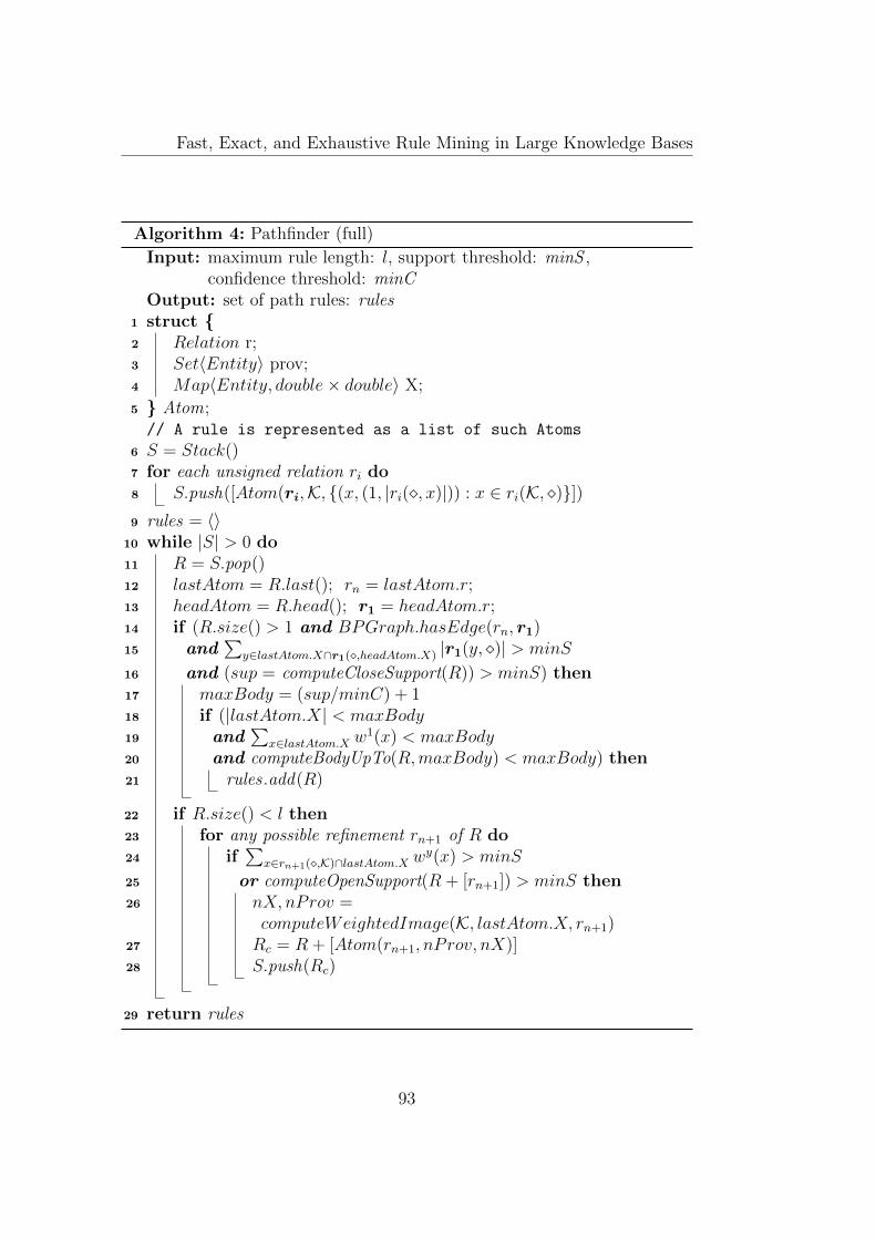
Fast, Exact, and Exhaustive Rule Mining in Large Knowledge Bases
Algorithm 4: Pathfinder (full)
Input: maximum rule length: l, support threshold: minS ,confidence threshold: minC
Output: set of path rules: rules1 struct 2 Relation r;3 Set〈Entity〉 prov;4 Map〈Entity, double× double〉 X;
5 Atom;// A rule is represented as a list of such Atoms
6 S = Stack()7 for each unsigned relation ri do8 S.push([Atom(ri,K, (x, (1, |ri(, x)|)) : x ∈ ri(K, )])9 rules = 〈〉
10 while |S| > 0 do11 R = S.pop()12 lastAtom = R.last(); rn = lastAtom.r;13 headAtom = R.head(); r1 = headAtom.r;14 if (R.size() > 1 and BPGraph.hasEdge(rn, r1)15 and
∑y∈lastAtom.X∩r1(,headAtom.X) |r1(y, )| > minS
16 and (sup = computeCloseSupport(R)) > minS) then17 maxBody = (sup/minC) + 118 if (|lastAtom.X| < maxBody19 and
∑x∈lastAtom.X w
1(x) < maxBody20 and computeBodyUpTo(R,maxBody) < maxBody) then21 rules .add(R)
22 if R.size() < l then23 for any possible refinement rn+1 of R do24 if
∑x∈rn+1(,K)∩lastAtom.X w
y(x) > minS
25 or computeOpenSupport(R + [rn+1]) > minS then26 nX, nProv =
computeWeightedImage(K, lastAtom.X, rn+1)27 Rc = R + [Atom(rn+1, nProv, nX)]28 S.push(Rc)
29 return rules
93
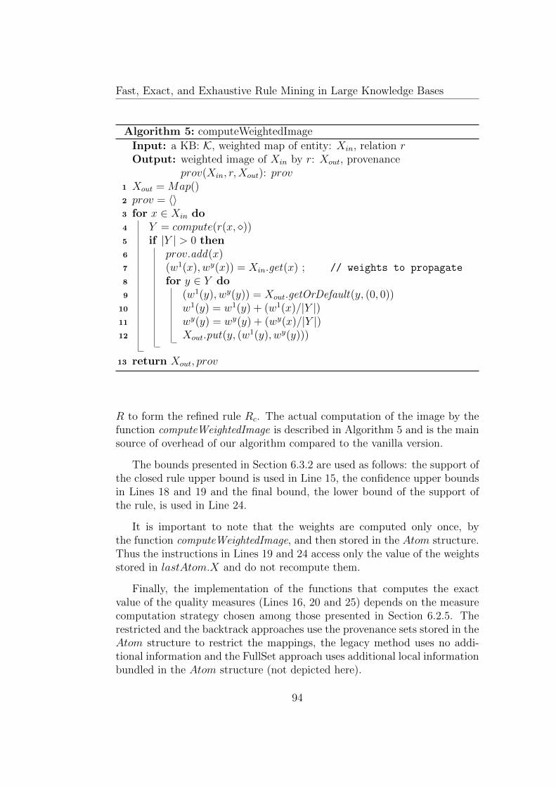
Fast, Exact, and Exhaustive Rule Mining in Large Knowledge Bases
Algorithm 5: computeWeightedImage
Input: a KB: K, weighted map of entity: Xin, relation rOutput: weighted image of Xin by r: Xout, provenance
prov(Xin, r,Xout): prov1 Xout = Map()2 prov = 〈〉3 for x ∈ Xin do4 Y = compute(r(x, ))5 if |Y | > 0 then6 prov.add(x)7 (w1(x), wy(x)) = Xin.get(x) ; // weights to propagate
8 for y ∈ Y do9 (w1(y), wy(y)) = Xout.getOrDefault(y, (0, 0))
10 w1(y) = w1(y) + (w1(x)/|Y |)11 wy(y) = wy(y) + (wy(x)/|Y |)12 Xout.put(y, (w1(y), wy(y)))
13 return Xout, prov
R to form the refined rule Rc. The actual computation of the image by thefunction computeWeightedImage is described in Algorithm 5 and is the mainsource of overhead of our algorithm compared to the vanilla version.
The bounds presented in Section 6.3.2 are used as follows: the support ofthe closed rule upper bound is used in Line 15, the confidence upper boundsin Lines 18 and 19 and the final bound, the lower bound of the support ofthe rule, is used in Line 24.
It is important to note that the weights are computed only once, bythe function computeWeightedImage, and then stored in the Atom structure.Thus the instructions in Lines 19 and 24 access only the value of the weightsstored in lastAtom.X and do not recompute them.
Finally, the implementation of the functions that computes the exactvalue of the quality measures (Lines 16, 20 and 25) depends on the measurecomputation strategy chosen among those presented in Section 6.2.5. Therestricted and the backtrack approaches use the provenance sets stored in theAtom structure to restrict the mappings, the legacy method uses no addi-tional information and the FullSet approach uses additional local informationbundled in the Atom structure (not depicted here).
94
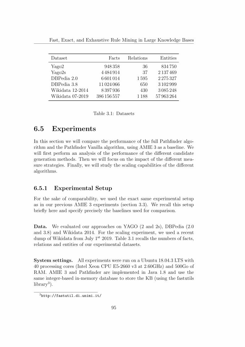
Fast, Exact, and Exhaustive Rule Mining in Large Knowledge Bases
Dataset Facts Relations Entities
Yago2 948 358 36 834 750Yago2s 4 484 914 37 2 137 469DBPedia 2.0 6 601 014 1 595 2 275 327DBPedia 3.8 11 024 066 650 3 102 999Wikidata 12-2014 8 397 936 430 3 085 248Wikidata 07-2019 386 156 557 1 188 57 963 264
Table 3.1: Datasets
6.5 Experiments
In this section we will compare the performance of the full Pathfinder algo-rithm and the Pathfinder Vanilla algorithm, using AMIE 3 as a baseline. Wewill first perform an analysis of the performance of the different candidategeneration methods. Then we will focus on the impact of the different mea-sure strategies. Finally, we will study the scaling capabilities of the differentalgorithms.
6.5.1 Experimental Setup
For the sake of comparability, we used the exact same experimental setupas in our previous AMIE 3 experiments (section 3.3). We recall this setupbriefly here and specify precisely the baselines used for comparison.
Data. We evaluated our approaches on YAGO (2 and 2s), DBPedia (2.0and 3.8) and Wikidata 2014. For the scaling experiment, we used a recentdump of Wikidata from July 1st 2019. Table 3.1 recalls the numbers of facts,relations and entities of our experimental datasets.
System settings. All experiments were run on a Ubuntu 18.04.3 LTS with40 processing cores (Intel Xeon CPU E5-2660 v3 at 2.60GHz) and 500Go ofRAM. AMIE 3 and Pathfinder are implemented in Java 1.8 and use thesame integer-based in-memory database to store the KB (using the fastutilslibrary3).
3http://fastutil.di.unimi.it/
95
Fast, Exact, and Exhaustive Rule Mining in Large Knowledge Bases
Baseline: AMIE-Path. We want to use AMIE 3 as a baseline. However,as AMIE 3 computes exhaustively all rules given some quality thresholds,it seems unfair to compare it with an algorithm that reports only a subsetof these rules: the path rules. Thus, we use as baseline a modified versionof AMIE 3, “AMIE-Path”, that refines only the open rules4. In this way,AMIE-Path produces only path rules.
6.5.2 Pathfinder generation methods
Configurations
We use here the legacy methods to compute the quality measures for everyalgorithm and we report the total running time (wall time) taken to mineevery closed path rule with the default parameters (maximal length of 3,minimal head coverage of 0.01, minimal PCA confidence of 0.1).
AMIE-Path. As AMIE, AMIE-Path computes the support of every ruleof a new generation using bulk computation (cf Section 6.1), selects the rulesabove the support thresholds and performs duplicate elimination.
Star pattern. Here we first use the bipattern graph to generate all thepossible path rules in our KB. Then we use AMIE to compute the supportand the confidence of each rule, one-by-one. We expect this approach tounderperform compared to an incremental approach.
Pathfinder-vanilla. We compare the performance of our three generationmethods: ALL, BP and BPP. As those methods are increasingly selective, weexpect our algorithm to be increasingly faster (BP faster than ALL and BPPfaster than BP). It will also allow us to measure the tradeoff between the bulkcomputation of the support in AMIE and the independent computation ofthe support on smartly selected candidate relations of Pathfinder vanilla.
Pathfinder. We compare the performances of our three generation meth-ods and expect similar speedup between the different methods than thevanilla algorithm. The variation of performances between the vanilla andthe full version will come exclusively from the difference between the over-head of the computation of the weighted images and the speedup of usingthe bounds on the quality measures.
4We add the condition ¬closed(R) to the test line 7 in Algorithm 1
96
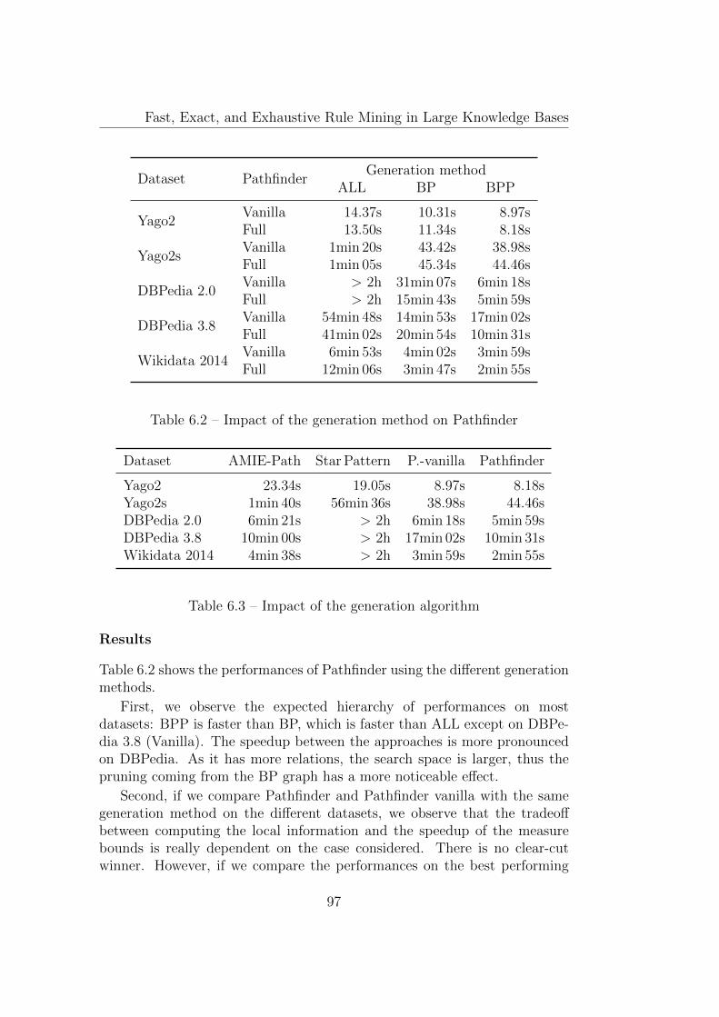
Fast, Exact, and Exhaustive Rule Mining in Large Knowledge Bases
Dataset PathfinderGeneration method
ALL BP BPP
Yago2Vanilla 14.37s 10.31s 8.97sFull 13.50s 11.34s 8.18s
Yago2sVanilla 1min 20s 43.42s 38.98sFull 1min 05s 45.34s 44.46s
DBPedia 2.0Vanilla > 2h 31min 07s 6min 18sFull > 2h 15min 43s 5min 59s
DBPedia 3.8Vanilla 54min 48s 14min 53s 17min 02sFull 41min 02s 20min 54s 10min 31s
Wikidata 2014Vanilla 6min 53s 4min 02s 3min 59sFull 12min 06s 3min 47s 2min 55s
Table 6.2 – Impact of the generation method on Pathfinder
Dataset AMIE-Path Star Pattern P.-vanilla Pathfinder
Yago2 23.34s 19.05s 8.97s 8.18sYago2s 1min 40s 56min 36s 38.98s 44.46sDBPedia 2.0 6min 21s > 2h 6min 18s 5min 59sDBPedia 3.8 10min 00s > 2h 17min 02s 10min 31sWikidata 2014 4min 38s > 2h 3min 59s 2min 55s
Table 6.3 – Impact of the generation algorithm
Results
Table 6.2 shows the performances of Pathfinder using the different generationmethods.
First, we observe the expected hierarchy of performances on mostdatasets: BPP is faster than BP, which is faster than ALL except on DBPe-dia 3.8 (Vanilla). The speedup between the approaches is more pronouncedon DBPedia. As it has more relations, the search space is larger, thus thepruning coming from the BP graph has a more noticeable effect.
Second, if we compare Pathfinder and Pathfinder vanilla with the samegeneration method on the different datasets, we observe that the tradeoffbetween computing the local information and the speedup of the measurebounds is really dependent on the case considered. There is no clear-cutwinner. However, if we compare the performances on the best performing
97
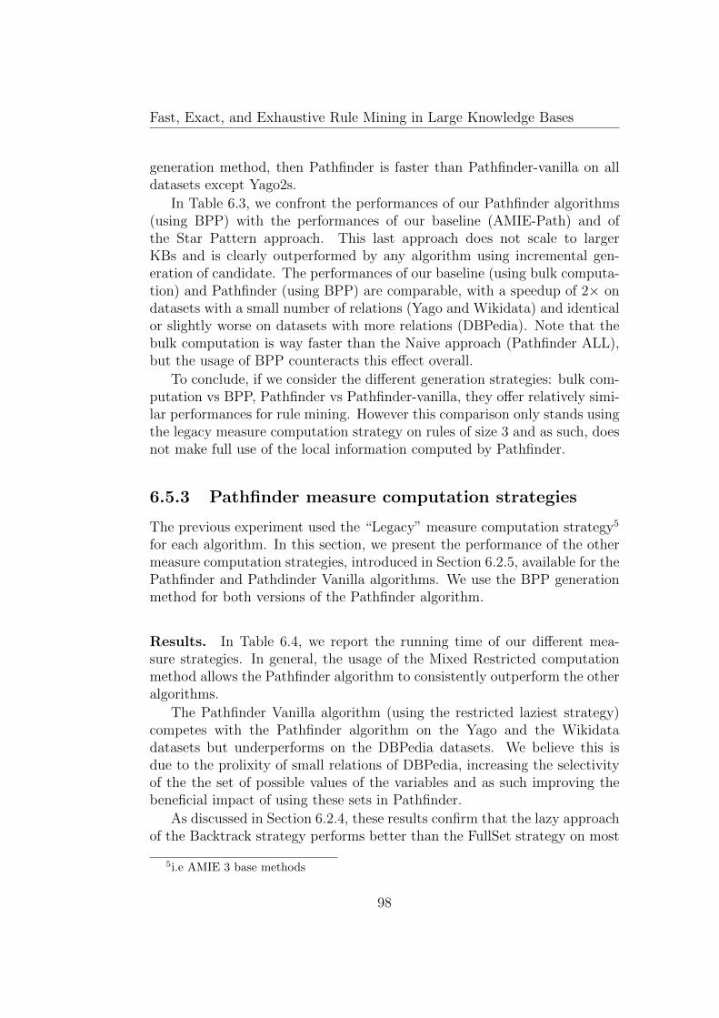
Fast, Exact, and Exhaustive Rule Mining in Large Knowledge Bases
generation method, then Pathfinder is faster than Pathfinder-vanilla on alldatasets except Yago2s.
In Table 6.3, we confront the performances of our Pathfinder algorithms(using BPP) with the performances of our baseline (AMIE-Path) and ofthe Star Pattern approach. This last approach does not scale to largerKBs and is clearly outperformed by any algorithm using incremental gen-eration of candidate. The performances of our baseline (using bulk computa-tion) and Pathfinder (using BPP) are comparable, with a speedup of 2× ondatasets with a small number of relations (Yago and Wikidata) and identicalor slightly worse on datasets with more relations (DBPedia). Note that thebulk computation is way faster than the Naive approach (Pathfinder ALL),but the usage of BPP counteracts this effect overall.
To conclude, if we consider the different generation strategies: bulk com-putation vs BPP, Pathfinder vs Pathfinder-vanilla, they offer relatively simi-lar performances for rule mining. However this comparison only stands usingthe legacy measure computation strategy on rules of size 3 and as such, doesnot make full use of the local information computed by Pathfinder.
6.5.3 Pathfinder measure computation strategies
The previous experiment used the “Legacy” measure computation strategy5
for each algorithm. In this section, we present the performance of the othermeasure computation strategies, introduced in Section 6.2.5, available for thePathfinder and Pathdinder Vanilla algorithms. We use the BPP generationmethod for both versions of the Pathfinder algorithm.
Results. In Table 6.4, we report the running time of our different mea-sure strategies. In general, the usage of the Mixed Restricted computationmethod allows the Pathfinder algorithm to consistently outperform the otheralgorithms.
The Pathfinder Vanilla algorithm (using the restricted laziest strategy)competes with the Pathfinder algorithm on the Yago and the Wikidatadatasets but underperforms on the DBPedia datasets. We believe this isdue to the prolixity of small relations of DBPedia, increasing the selectivityof the the set of possible values of the variables and as such improving thebeneficial impact of using these sets in Pathfinder.
As discussed in Section 6.2.4, these results confirm that the lazy approachof the Backtrack strategy performs better than the FullSet strategy on most
5i.e AMIE 3 base methods
98
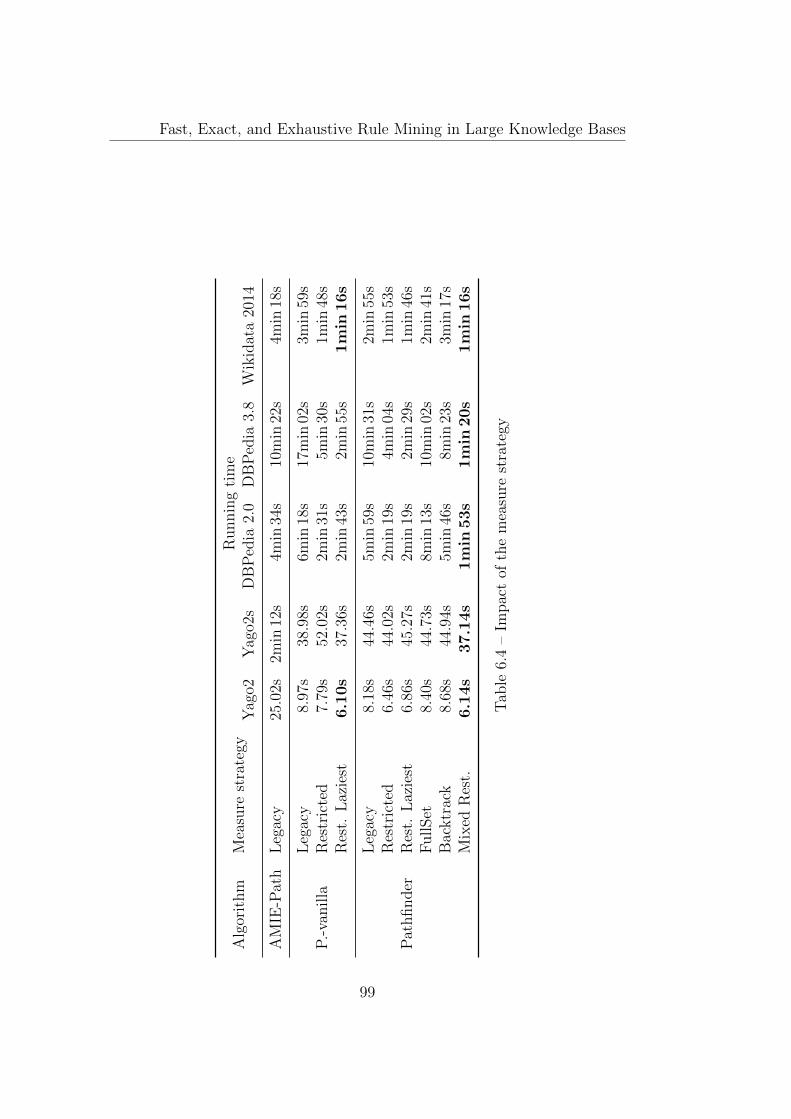
Fast, Exact, and Exhaustive Rule Mining in Large Knowledge Bases
Alg
orit
hm
Mea
sure
stra
tegy
Runnin
gti
me
Yag
o2Y
ago2
sD
BP
edia
2.0
DB
Ped
ia3.
8W
ikid
ata
2014
AM
IE-P
ath
Leg
acy
25.0
2s2m
in12
s4m
in34
s10
min
22s
4min
18s
P.-
vanilla
Leg
acy
8.97
s38
.98s
6min
18s
17m
in02
s3m
in59
sR
estr
icte
d7.
79s
52.0
2s2m
in31
s5m
in30
s1m
in48
sR
est.
Laz
iest
6.1
0s
37.3
6s2m
in43
s2m
in55
s1m
in16s
Pat
hfinder
Leg
acy
8.18
s44
.46s
5min
59s
10m
in31
s2m
in55
sR
estr
icte
d6.
46s
44.0
2s2m
in19
s4m
in04
s1m
in53
sR
est.
Laz
iest
6.86
s45
.27s
2min
19s
2min
29s
1min
46s
FullSet
8.40
s44
.73s
8min
13s
10m
in02
s2m
in41
sB
acktr
ack
8.68
s44
.94s
5min
46s
8min
23s
3min
17s
Mix
edR
est.
6.1
4s
37.1
4s
1m
in53s
1m
in20s
1m
in16s
Tab
le6.
4–
Impac
tof
the
mea
sure
stra
tegy
99
Fast, Exact, and Exhaustive Rule Mining in Large Knowledge Bases
AMIE-Path P.-vanilla Pathfinder
Yago2 25.02s 6.10s 6.14sYago2s 2min 12s 37.36s 37.14sDBPedia 2.0 4min 34s 2min 43s 1min 53sDBPedia 3.8 10min 22s 2min 55s 1min 20sWikidata 2014 4min 18s 1min 16s 1min 16sWikidata 2019 16h 43min > 48h 36h 12min
Table 6.5 – Running time on increasingly large datasets
AMIE-Path P.-vanilla Pathfinder
Yago2 3min 55s 1min 15s 10.77sYago2s > 6h 7min 00s 1min 53sDBPedia 2.0 > 6h 2h 35min 47min 31sDBPedia 3.8 > 6h 3h 20min 23min 22sWikidata 2014 > 6h > 6h 14min 20s
Table 6.6 – Rule mining of rules with maximal length of 4
datasets and that the computation of the support of the closed rule is in-deed the bottleneck of both approaches. This is why the mixed strategyconsistently outperforms both of these approaches.
6.5.4 Scaling experiments
We distinguish two distinct scaling factors: the size of the Knowledge Baseand the size of the search space. This last factor is mostly impacted bythe number of relations of the KB and the length of the rules we aim tomine. Both have a significant impact on the performances of AMIE and ofour proposed Pathfinder algorithms as they are exact and exhaustive rulemining algorithms.
In particular, we expect that an increasing number of facts per relationwould have a negative impact on the performances of Pathfinder as it in-creases significantly the overhead of computing the image of the sets. How-ever, the extensive reusage of the data between a rule and its refinementshould greatly benefit the Pathfinder algorithm while mining longer rulesand allow it to scale in the size of the search space as no other algorithmshas achieved before.
100

Fast, Exact, and Exhaustive Rule Mining in Large Knowledge Bases
Results. In Table 6.5, we present the performance of our approaches onincreasingly large datasets. The Pathfinder algorithm outperforms AMIE-Path on all datasets except the bigger one Wikidata 2019, which has a largenumber of facts per relation. Interestingly, the Pathfinder algorithm per-forms better than the Pathfinder Vanilla algorithm on this dataset, whichmeans that computing the sets of possible values of the variables is actuallybeneficial overall and that the main overhead comes from the independentcomputation of the support of the refined rules (in comparison to AMIE-Path).
On a larger search space however, the Pathfinder algorithm achieves tocompute all the path rules of length 4 on all datasets within less than hour,which is unprecedented. In comparison, we show in Table 6.6 that AMIE-Path cannot complete in less than 6 hours on all datasets except Yago2 andthe Pathfinder Vanilla algorithm cannot complete in less than 1 hour an alldatasets except the Yago datasets. This demonstrates the impact of ouroptimizations in the Pathfinder algorithm: the lower bounds on the iteratedprovenance, the restricted computation of the support of the closed rule andthe backtracking of the iterated provenance for the computation of the othermetrics.
Finally, the Pathfinder algorithm can scale to even longer rules: for ex-ample it mines all path rules of length at most 5 in 2 minutes and 30 secondson Yago2 and in less than 37 minutes on Yago2s.
6.6 Conclusion
In this chapter presented the algorithm Pathfinder which mines exactly andexhaustively all the path rules from a KB. It uses the unique generationprocess and the pruning capabilities of the bipattern graph presented in thelast chapter and exploits a data reusage technique introduced in this chapterto deduce an optimal measure computation strategy and local bounds on thequality measures. This allows Pathfinder to outperform other rule miningapproaches on most datasets, by orders of magnitude on longer rules.
Future works. The direct followup of this work would be to use thePathfinder algorithm to mine path rules with instantiatied extremities (rulesof the form Ri(E1, E2)[r1, . . . , rn]). We expect an even more significantspeedup on these rules than on longer rules.
However, more work is required to make Pathfinder scale to KnowledgeBases with a large number of facts per relations such as Wikidata 2019.Multiple directions can be considered: the usage of caching during the back-
101

Fast, Exact, and Exhaustive Rule Mining in Large Knowledge Bases
tracking process or the implementation of an hybrid algorithm that computesthe sets of possible values only if those sets are selective enough comparedto the star patterns.
102
Chapter 7
Identifying obligatoryattributes in a KB
In this chapter, we use the incomplete KB to mine rules about the real-world.This chapter is based on our following full paper:
- Jonathan Lajus and Fabian M. Suchanek. Are all people married? deter-mining obligatory attributes in knowledge bases. In WWW, pages 1115–1124. International World Wide Web Conferences Steering Committee,2018
7.1 Introduction
Knowledge Bases find applications in information retrieval, machine transla-tion, and question answering. The usefulness of these applications dependson the data quality of the knowledge base. One important dimension ofquality is the correctness of the data. But there is another important dimen-sion: the completeness of the data – i.e., whether or not a statement aboutan entity is missing from the KB. Data completeness affects queries aboutcardinalities, about existence, and about top-ranked entities. For example,if the population of Tokyo is missing from the KB, then a query about thetop-10 most populous cities in the world will return a factually wrong result.
If we knew that every city has to have a population, we could know thatthe reason for Tokyo’s missing population is not that Tokyo does not have apopulation in the real world, but that the number was not added to the KB.We could thus alert the user that the data on which the query is computed isknown to be incomplete. We say that the population is an obligatory attributefor the class city. Not all attributes are obligatory. For example, not every
103
Fast, Exact, and Exhaustive Rule Mining in Large Knowledge Bases
city has to be the capital of a region. The same goes for other classes: Everyperson has to have a birth date, but not every person has to be married.
If we were able to distinguish obligatory attributes from optional ones, wecould easily identify where information is missing in the KB. This, in turn,could help the designers of the knowledge base focus their effort on completionon this particular data. For example, collaborative knowledge bases such asWikidata could ask contributors specifically for the obligatory attributes of anew entity. Moreover, the obligatory attributes can give semantics to classes.For example, the characteristics of actors is that they act in a movie. Suchinformation can help decide whether an entity belongs to a class or not, itcan guide the process of taxonomy design, and it can help define schemaconstraints [42]. We note that even obligatory attributes with a few counter-examples would be helpful for these goals. For example, it is good to knowthat people generally have a nationality – even if there are some people whodo not have one. Our goal is to find the rule rather than the exception.
It is not easy to determine whether an attribute is obligatory or not.Today’s KBs contain not just people and cities, but literally hundreds ofthousands of other classes. They also contain hundreds, if not thousands ofattributes. It is thus infeasible to specify the obligatory attributes manually.It is also hard to find them automatically: In YAGO, e.g., 2% of soccerplayers have a club – and that is an obligatory attribute for professionalsoccer players. At the same time, 2% of people have a spouse – and thatis an optional attribute. Using the available data to determine obligatoryattributes thus amounts to generalizing from a few instances to all instancesof a class. This is a very difficult endeavor – even for humans. The case ofKBs is even more intricate, because most KBs do not explicitly say that astatement does not hold in reality. For example, the KBs do not say thatPope Francis is not married. Rather, they operate under the Open WorldAssumption: A statement may be missing from the KB either because it wasnot added, or because it does not hold in reality. Thus, we find ourselveswith the task of generalizing from a few instances in the absence of counter-examples.
In this chapter, we present methods that can detect obligatory attributesautomatically. Our key idea is to use the class hierarchy: Most modern KBscontain extensive class hierarchies (YAGO, e.g., contains 650,000 classes;DBpedia and Wikidata have manually designed taxonomies). And yet, theKBs use the class hierarchy mainly to specify domain and range constraints.They do not exploit the semantics of the hierarchy any further. Our idea isto make use of the classes to determine obligatory attributes. More precisely,our contributions are as follows:
104
Fast, Exact, and Exhaustive Rule Mining in Large Knowledge Bases
• a formal definition of the problem of obligatory attributes
• a probabilistic model for the incompleteness of a KB
• an algorithm that can determine obligatory attributes automatically
• extensive experiments on different datasets with different competitors,showing that obligatory attributes can be detected with a precision ofup to 90%.
We first present our approach discuss related work in Section 7.2 andthe preliminaries in Section 7.3. Then we present a formal definition of ourproblem, describe our approach and define the probabilistic model it is basedupon in Section 7.4. Finally we present our algorithm in section 7.5 and howit performs on actual datasets in section 7.6.
7.2 Related Work
Query Completeness. Much recent work [56, 48, 70] has investigated thecompleteness of queries when the completeness of the data is known. Theseapproaches are orthogonal to our work, which aims to establish whether thedata is complete in the first place.
Measuring Incompleteness. Several studies have confirmed that KBsare incomplete. A watermarking study [77] reports that 69%–99% of in-stances in YAGO and DBpedia lack at least one property that other entitiesin the same class have. In Freebase, 71% of people have no known placeof birth, and 75% have no known nationality [19]. Wikidata is aware ofthe problem of incompleteness, and has developed tools to specify complete-ness [21], as well as tools to manually add completeness information [15].Unlike our work, these approaches do not aim at determining completenessautomatically.
Determining Incompleteness. Closest to our work, several approacheshave recently taken to measure the incompleteness in knowledge bases [71,29]. However, these works determine whether a particular subject (suchas Emmanuel Macron) is incomplete with respect to a particular attribute(such as birthDate). Our work, in contrast, aims at determining whetheran attribute is obligatory or not for a given class. It thus operates on theschema level.
105

Fast, Exact, and Exhaustive Rule Mining in Large Knowledge Bases
Schema Mining. Other work has investigated the more general problemof schema mining [64, 83, 38, 6, 31]. The work of [64] mines domain andrange constraints for relations. Our work, in contrast, mines relations thatare obligatory for classes. [38] uses machine learning to find OWL classdescriptions. However, they rely on negative facts given by the user, or onprior knowledge about the schema – while we require none of these. [83]mines Horn rules on a KB. However, this approach is not targeted towardssparse obligatory attributes. We use it as a baseline in our experiments. [31]also mines Horn rules, and can deal with sparse data. At the same time, itcannot mine rules with existential variables in the head. Any such rule wouldtrivially have a confidence of 100% in their model, because the model makesthe Partial Completeness Assumption. Another work [6] mines definitions ofclasses. This approach comes closer to our goal, but is not exactly targetedtowards obligatory attributes. We use such an approach as a baseline in ourexperiments.
7.3 Preliminaries
Notations. Given a Knowledge Base K and a signed relation p, we notepK the set of entities of K that satisfies the star pattern p in K. Forexample, presidentOfYAGO represents the set of subjects of the presidentOfrelation in Y AGO, containing notably the entities Macron or Obama. Aclass CK
1 of K is the set of entities satisfying the star pattern type(C) inK. For example Macron and Obama are members of the classes PersonYAGO
or PresidentYAGO. We note CK the set of classes of the KB K.
Ideal KB. As in Section 2.2.4, we consider a (hypothetical) ideal KB W ,which contains all facts of the real world. With this, our work is in line withthe other work in the area [56, 48, 70, 71, 29], which also assumes an idealKB. The problems of determining how such a KB could look are discussedin [71].
Generalization Rules. A generalization rule for a KB K is a formula ofthe form A ⊆ B, where A and B are classes of K, signed relations of K, orintersections thereof. For example, if PresidentW is the class of presidents inthe real world, then the following generalization rule says that all presidentsare presidents of some country:
PresidentW ⊆ presidentOfW1always capitalized to distinguish it from the signed relations.
106
Fast, Exact, and Exhaustive Rule Mining in Large Knowledge Bases
With this, we can already make a simple observation:
Proposition 7.3.1 (Heredity). In any KB K, for every class CK ∈ CK, anysubclass DK ⊆ CK, and every property p: if CK ⊆ pK then DK ⊆ pK.
This proposition tells us that if a generalization rule holds for a class, it alsoholds for all subclasses. The confidence of a generalization rule is defined as
conf(A ⊆ B) =|A ∩B||A|
Finally, we can make a second simple observation:
Proposition 7.3.2 (Separation). If CK ⊆ pK for some class CK of some KBK and some property p, then the following holds for any class DK of K:
conf(CK ∩ pK ⊆ DK) = conf(CK ⊆ DK)
7.4 Model
7.4.1 Problem Definition
Goal. In this chapter, we aim to find generalization rules of the form CW ⊆pW . Such a rule says that every instance of the class C in the real world musthave the property p in the real world. We call p an obligatory attribute ofthe class C. For example, we aim to mine
FilmW ⊆ directed−1W
Here, directed−1 is an obligatory attribute for the class Film, i.e., every filmhas to have a director. The difficulty is to find such a rule in W by lookingonly at the data of a given KB K. In the following, we write CW for the classC in the real world, and CK for the corresponding class in K.
Baseline 1. One way to find obligatory attributes is assume that the KB iscomplete (Closed World Assumption) and correct. Under these assumptions,we can predict that an attribute p is obligatory for a class C if and only ifall instances of C have p in the KB K:
(CK ⊆ pK)?⇒ (CW ⊆ pW)
This is how a rule mining system under the Closed World Assumption wouldproceed [83], if applied naively to our problem. In practice, however, KBs arerarely complete. They operate under the Open World Assumption. Therewill be hardly any property p that all instances of class C have.
107
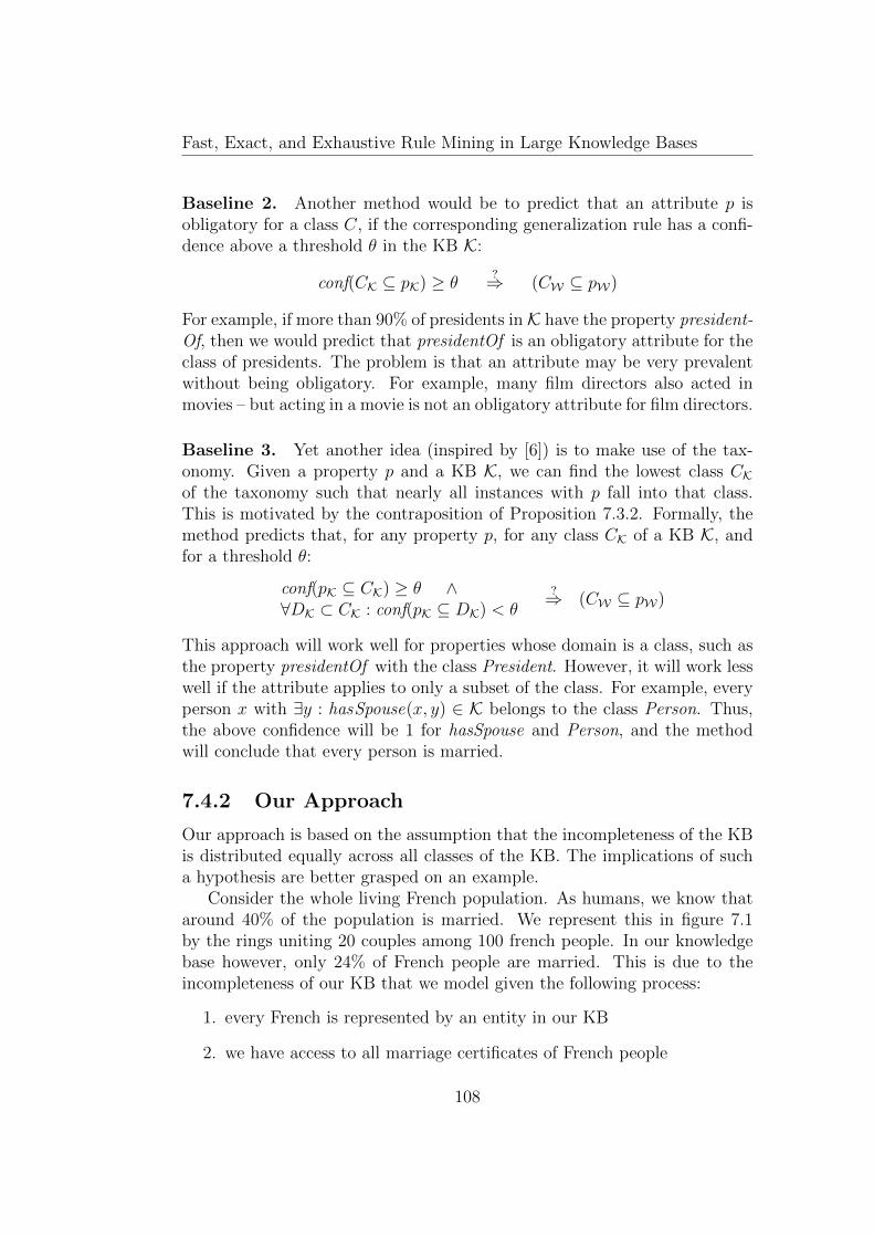
Fast, Exact, and Exhaustive Rule Mining in Large Knowledge Bases
Baseline 2. Another method would be to predict that an attribute p isobligatory for a class C, if the corresponding generalization rule has a confi-dence above a threshold θ in the KB K:
conf(CK ⊆ pK) ≥ θ?⇒ (CW ⊆ pW)
For example, if more than 90% of presidents in K have the property president-Of, then we would predict that presidentOf is an obligatory attribute for theclass of presidents. The problem is that an attribute may be very prevalentwithout being obligatory. For example, many film directors also acted inmovies – but acting in a movie is not an obligatory attribute for film directors.
Baseline 3. Yet another idea (inspired by [6]) is to make use of the tax-onomy. Given a property p and a KB K, we can find the lowest class CKof the taxonomy such that nearly all instances with p fall into that class.This is motivated by the contraposition of Proposition 7.3.2. Formally, themethod predicts that, for any property p, for any class CK of a KB K, andfor a threshold θ:
conf(pK ⊆ CK) ≥ θ ∧∀DK ⊂ CK : conf(pK ⊆ DK) < θ
?⇒ (CW ⊆ pW)
This approach will work well for properties whose domain is a class, such asthe property presidentOf with the class President. However, it will work lesswell if the attribute applies to only a subset of the class. For example, everyperson x with ∃y : hasSpouse(x, y) ∈ K belongs to the class Person. Thus,the above confidence will be 1 for hasSpouse and Person, and the methodwill conclude that every person is married.
7.4.2 Our Approach
Our approach is based on the assumption that the incompleteness of the KBis distributed equally across all classes of the KB. The implications of sucha hypothesis are better grasped on an example.
Consider the whole living French population. As humans, we know thataround 40% of the population is married. We represent this in figure 7.1by the rings uniting 20 couples among 100 french people. In our knowledgebase however, only 24% of French people are married. This is due to theincompleteness of our KB that we model given the following process:
1. every French is represented by an entity in our KB
2. we have access to all marriage certificates of French people
108
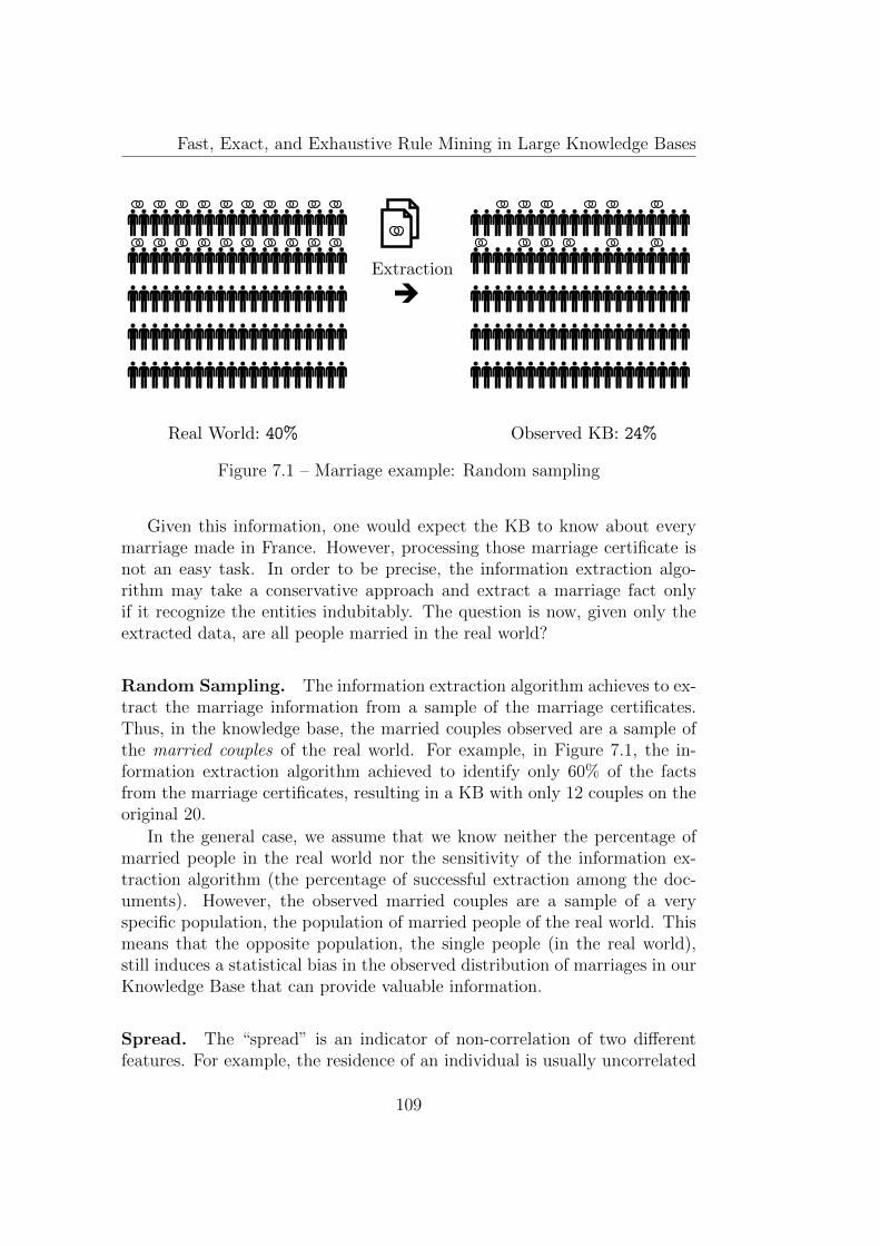
Fast, Exact, and Exhaustive Rule Mining in Large Knowledge Bases
Real World: 40% Observed KB: 24%
Extraction
Figure 7.1 – Marriage example: Random sampling
Given this information, one would expect the KB to know about everymarriage made in France. However, processing those marriage certificate isnot an easy task. In order to be precise, the information extraction algo-rithm may take a conservative approach and extract a marriage fact onlyif it recognize the entities indubitably. The question is now, given only theextracted data, are all people married in the real world?
Random Sampling. The information extraction algorithm achieves to ex-tract the marriage information from a sample of the marriage certificates.Thus, in the knowledge base, the married couples observed are a sample ofthe married couples of the real world. For example, in Figure 7.1, the in-formation extraction algorithm achieved to identify only 60% of the factsfrom the marriage certificates, resulting in a KB with only 12 couples on theoriginal 20.
In the general case, we assume that we know neither the percentage ofmarried people in the real world nor the sensitivity of the information ex-traction algorithm (the percentage of successful extraction among the doc-uments). However, the observed married couples are a sample of a veryspecific population, the population of married people of the real world. Thismeans that the opposite population, the single people (in the real world),still induces a statistical bias in the observed distribution of marriages in ourKnowledge Base that can provide valuable information.
Spread. The “spread” is an indicator of non-correlation of two differentfeatures. For example, the residence of an individual is usually uncorrelated
109

Fast, Exact, and Exhaustive Rule Mining in Large Knowledge Bases
Paris Lyon Toulouse
40% 40% 40%Real World: 40%
Paris Lyon Toulouse
25% 30% 20%Observed KB: 24%
Extraction
Figure 7.2 – Marriage example: Spread
with its marital status: the proportion of married Parisians should also beroughly 40% of all Parisians, the same for natives of Marseille or Toulouse.But as the observed marital status is a random sample of the actual maritalstatus, the observed proportion of married Parisians should be similar tothe observed proportion of married French, married Marseillais and marriedToulousain, as in Figure 7.2. The observed proportion of married people“spreads” across the different place of residence, indicating that the latterand the marital status are uncorrelated.
Amplification. In contrast, when two features are correlated, for examplethe marital status and the age, we can observe a relative increase (or decrease)in the relative representation of married people in the different age group,as in Figure 7.3. As the proportion of married french teenagers is really lowcompared to the whole population, it is even lower in the observed sample,but more importantly, lower than the observed proportion in the population(0% versus 24%). On the contrary, the observed proportion of married adultsis larger than in the whole population (40% versus 24%), we observe an“amplification” of the density.
To sum up, under the random sampling assumption, the observed relativeproportion of married people in different classes follows the actual proportionof married people in that class. In particular, if the attribute is obligatory ina class, this proportion must be maximal: there should be an amplificationcompared to any superclass and a spread towards any subclass.
In our example, the spread of the “marriages” across all places of resi-dence is a signal that being married may be obligatory for all french, more
110
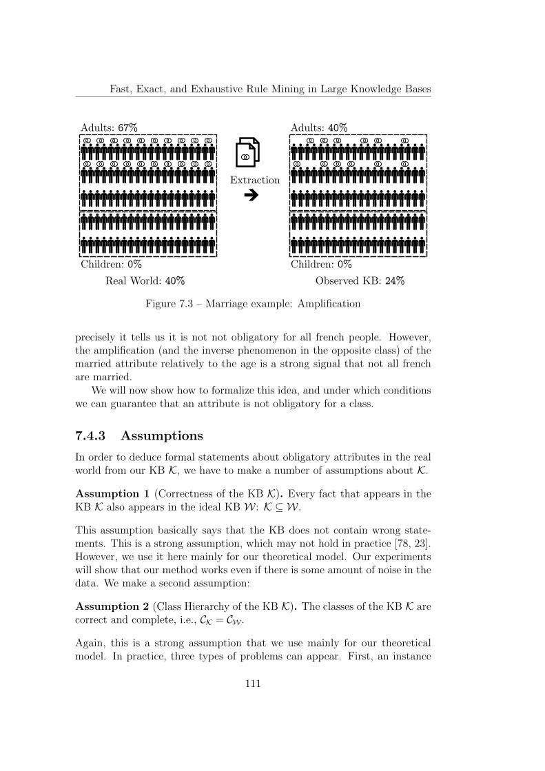
Fast, Exact, and Exhaustive Rule Mining in Large Knowledge Bases
Adults: 67%
Children: 0%Real World: 40%
Adults: 40%
Children: 0%Observed KB: 24%
Extraction
Figure 7.3 – Marriage example: Amplification
precisely it tells us it is not not obligatory for all french people. However,the amplification (and the inverse phenomenon in the opposite class) of themarried attribute relatively to the age is a strong signal that not all frenchare married.
We will now show how to formalize this idea, and under which conditionswe can guarantee that an attribute is not obligatory for a class.
7.4.3 Assumptions
In order to deduce formal statements about obligatory attributes in the realworld from our KB K, we have to make a number of assumptions about K.
Assumption 1 (Correctness of the KB K). Every fact that appears in theKB K also appears in the ideal KB W : K ⊆ W .
This assumption basically says that the KB does not contain wrong state-ments. This is a strong assumption, which may not hold in practice [78, 23].However, we use it here mainly for our theoretical model. Our experimentswill show that our method works even if there is some amount of noise in thedata. We make a second assumption:
Assumption 2 (Class Hierarchy of the KB K). The classes of the KB K arecorrect and complete, i.e., CK = CW .
Again, this is a strong assumption that we use mainly for our theoreticalmodel. In practice, three types of problems can appear. First, an instance
111
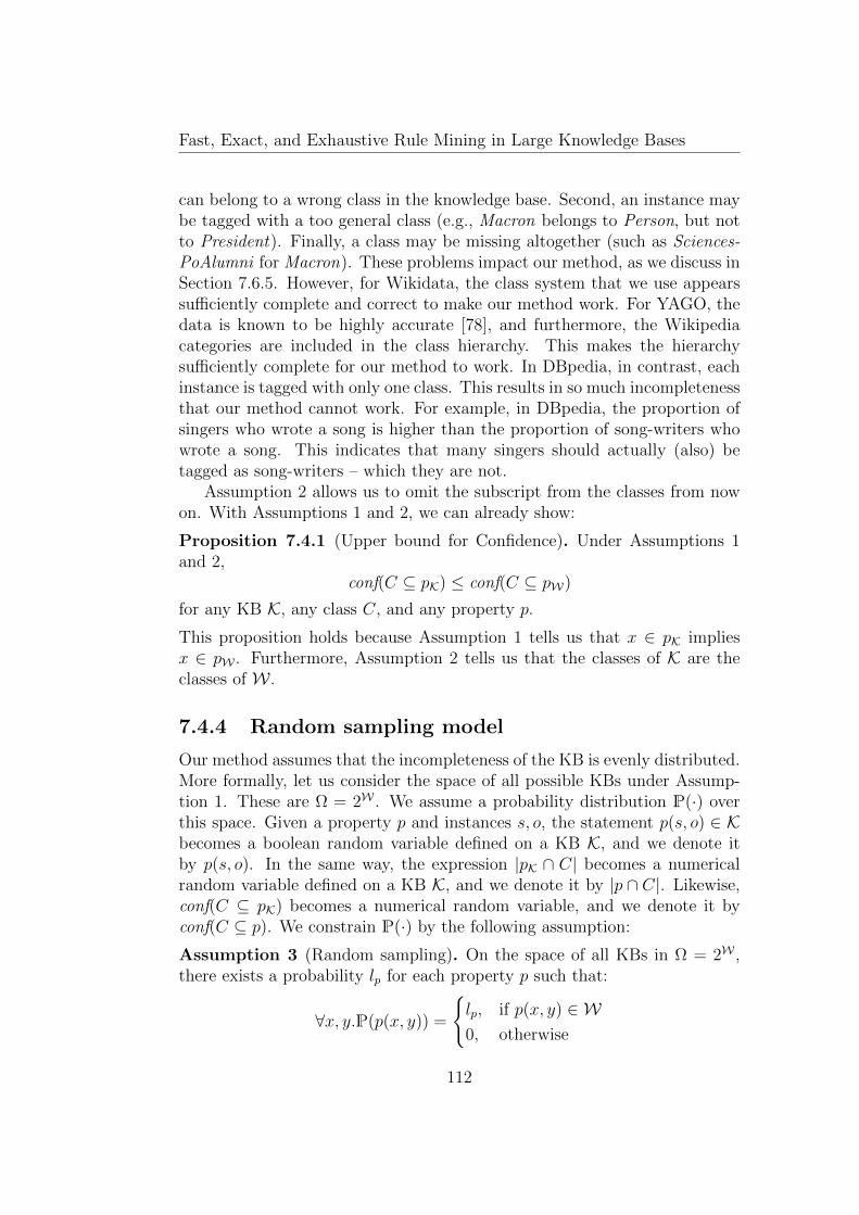
Fast, Exact, and Exhaustive Rule Mining in Large Knowledge Bases
can belong to a wrong class in the knowledge base. Second, an instance maybe tagged with a too general class (e.g., Macron belongs to Person, but notto President). Finally, a class may be missing altogether (such as Sciences-PoAlumni for Macron). These problems impact our method, as we discuss inSection 7.6.5. However, for Wikidata, the class system that we use appearssufficiently complete and correct to make our method work. For YAGO, thedata is known to be highly accurate [78], and furthermore, the Wikipediacategories are included in the class hierarchy. This makes the hierarchysufficiently complete for our method to work. In DBpedia, in contrast, eachinstance is tagged with only one class. This results in so much incompletenessthat our method cannot work. For example, in DBpedia, the proportion ofsingers who wrote a song is higher than the proportion of song-writers whowrote a song. This indicates that many singers should actually (also) betagged as song-writers – which they are not.
Assumption 2 allows us to omit the subscript from the classes from nowon. With Assumptions 1 and 2, we can already show:
Proposition 7.4.1 (Upper bound for Confidence). Under Assumptions 1and 2,
conf(C ⊆ pK) ≤ conf(C ⊆ pW)
for any KB K, any class C, and any property p.
This proposition holds because Assumption 1 tells us that x ∈ pK impliesx ∈ pW . Furthermore, Assumption 2 tells us that the classes of K are theclasses of W .
7.4.4 Random sampling model
Our method assumes that the incompleteness of the KB is evenly distributed.More formally, let us consider the space of all possible KBs under Assump-tion 1. These are Ω = 2W . We assume a probability distribution P(·) overthis space. Given a property p and instances s, o, the statement p(s, o) ∈ Kbecomes a boolean random variable defined on a KB K, and we denote itby p(s, o). In the same way, the expression |pK ∩ C| becomes a numericalrandom variable defined on a KB K, and we denote it by |p ∩ C|. Likewise,conf(C ⊆ pK) becomes a numerical random variable, and we denote it byconf(C ⊆ p). We constrain P(·) by the following assumption:
Assumption 3 (Random sampling). On the space of all KBs in Ω = 2W ,there exists a probability lp for each property p such that:
∀x, y.P(p(x, y)) =
lp, if p(x, y) ∈ W0, otherwise
112
Fast, Exact, and Exhaustive Rule Mining in Large Knowledge Bases
The second case follows from Assumption 1. The first case states that factswith the property p in our KB come from a uniform random sampling of alltrue facts with property p in the real-world.
Several factors can thwart this assumption. First, the KB may be biasedtowards popular instances. For example, Wikipedia contains more informa-tion about American actors than about Polish actors, and people magazinesare more concerned about the extra-marital affairs of actors than about theaffairs of an architect. Thus, any KB that extracts from these sources willbe biased. Second, the information extraction itself may have a bias. Forexample, several information extraction methods feed from the Wikipediainfoboxes. These infoboxes come in a number of pre-defined templates, andthese templates define the properties. This entails that the presence or ab-sence of a property in the KB depends on whether the instance happens tobelong to an infobox template that defines this property or not. That said,making such simplifying assumptions about the probability distribution offacts is not unusual [19, 45, 61]. Our experiments will show that our modelworks also in cases where this assumption is violated to some degree.
We constrain P(·) further by adding in the PCA (Equation A.2).
Assumption 4 (PCA). On the space of all KBs in Ω = 2W , P(K) = 0 ifthere exists a property p (which is not an inverse) and instances x, y, y′ withp(x, y) ∈ K, p(x, y′) /∈ K and p(x, y′) ∈ W .
The PCA is a common assumption for the KBs we consider [31, 19]. It hasbeen experimentally shown to be correct in a large number of cases [30].Again, we need the PCA mainly for our model. Our experiments will showthat our method gracefully translates to scenarios where the PCA does nothold for all properties. In particular, our method is robust enough to workalso with the inverses of properties, for which the PCA usually does not hold.In the appendix, we prove:
Theorem 7.4.2 (Random sampling under PCA). Under Assumptions 3and 4, for each property p with probability lp (as given by Assumption 3),
∀x : P(∃y : p(x, y)) =
lp, if x ∈ pW0, otherwise
Theorem 7.4.2 tells us that the truth value of ∃y : p(x, y) ∈ K for an instancex in a KB K can be seen as a random draw of a Bernoulli variable with aparameter lp. This allows us to derive
|p ∩ C| ∼∑
x∈c,x∈pW
Bernoulli(lp) = Binom(|pW ∩ C|, lp)
113
Fast, Exact, and Exhaustive Rule Mining in Large Knowledge Bases
This allows for the following proposition.
Proposition 7.4.3 (Biased estimator). The confidence of a generalizationrule in Ω follows a binomial distribution divided by a constant:
conf(C ⊆ p) ∼ Binom(|C ∩ pW |, lp)|C|
Hence, the expected confidence of the rule in Ω is a biased estimator for theconfidence of the rule in W :
E[conf(C ⊆ p)] = lp × conf(C ⊆ pW)
This proposition confirms that, in our model, the confidence of C ⊆ pWcannot be estimated from the data in our KB alone, as long as lp remainsunknown. The proposition also allows us to predict the behavior of Baseline2 with parameter θ (see again Section 7.4.1). For a predicate p, if θ > lp,then the baseline is less likely to find all the correct classes for the predicatep, but the classes it finds have a high probability of being correct. We showin the appendix:
Proposition 7.4.4 (Unbiased estimator). Given two classes C,D and aproperty p, the expected confidence of C ∩ p ⊆ D in Ω is an unbiased esti-mator for the confidence in W :
E[conf(C ∩ p ⊆ D)] = conf(C ∩ pW ⊆ D)
This proposition finally establishes a link between the (expected) observedconfidence in our KB and the confidence in the real world.
7.5 Algorithm
In this section, we first define our main indicator score for obligatory at-tributes. We then present our algorithm and propose some variations of thisalgorithm.
7.5.1 Confidence Ratio
Our main indicator score for obligatory attributes is defined as follows:
Definition 7.5.1 (Confidence ratio). Given a KB K, a property p, and twoclasses C and C ′ with |C ∩ C ′| 6= 0 and |C \ C ′| 6= 0, the confidence ratio is
sKp (C,C ′) =conf(C \ C ′ ⊆ pK)
conf(C ∩ C ′ ⊆ pK)
114
Fast, Exact, and Exhaustive Rule Mining in Large Knowledge Bases
This expression compares the ratio of instances with p in C ∩C ′ to the ratioof instances with p in C \C ′. It represents the influence of being in the classC ′ for the instances of a class C on p. This ratio is similar to the relativerisk that is used in clinical tests. We can now make the following observation(which we prove in the appendix):
Proposition 7.5.2 (Main observation). If p is an obligatory attribute forsome class C, then for every class C ′ with |C ∩ C ′| 6= 0 and |C \ C ′| 6= 0,
E[sp(C,C′)] = 1
Here, sp(C,C′) is a random variable, and hence does not carry the K. The
observation tells us that the density of p in C should not be influenced byC ′ if p is obligatory for C. The probability of a KB where C ′ influences p islow in our probability space.
Measure instability. Our confidence ratio estimate will suffer from in-stability when the expected number of instances with a property p in anintersection is inferior to 1. In that case, there might be no instance withthe property p in the intersection, and the confidence ratio will be infinite.In practice, this happens in small intersections for highly incomplete prop-erties. Therefore, we decide to consider only stable classes. Given a class Cand a property p in a KB K, an intersecting class C ′ is stable if either theexpected number of instances (conf(C ⊆ pK)×|C∩C ′|) or the actual number(|C ∩ C ′ ∩ pK |) is at least 1. The same has to hold for class differences.
7.5.2 Algorithm
Proposition 7.5.2 allows us to make statements about a generalization ruleC ⊆ pW in the real world purely by observing an incomplete knowledgebase K. All we have to do is to check the classes C ′ that intersect with theclass C. If the ratio of instances of pK in C ∩ C ′ is very different from theratio in C \ C ′, then it is very unlikely that C ⊆ pW holds. Furthermore, ifsKp (C ′, C) 1, then p cannot be obligatory for C ∩ C ′. Thus, it cannot beobligatory for C and C ′.
These considerations give us Algorithm 6. This algorithm takes as inputa KB K, a class C, and a property p. The algorithm also uses two thresholds:θ is the margin that we allow sKp to deviate from 1. The larger the threshold,the more obligatory attributes the algorithm will find – and the more likely itis that some of them will be wrong. The threshold θ′ is the minimum supportallowed for the rule C ⊆ p to be considered. In practice, we set θ′ to 100, asin AMIE [31]. Our algorithm returns false if the generalization rule C ⊆ pW
115
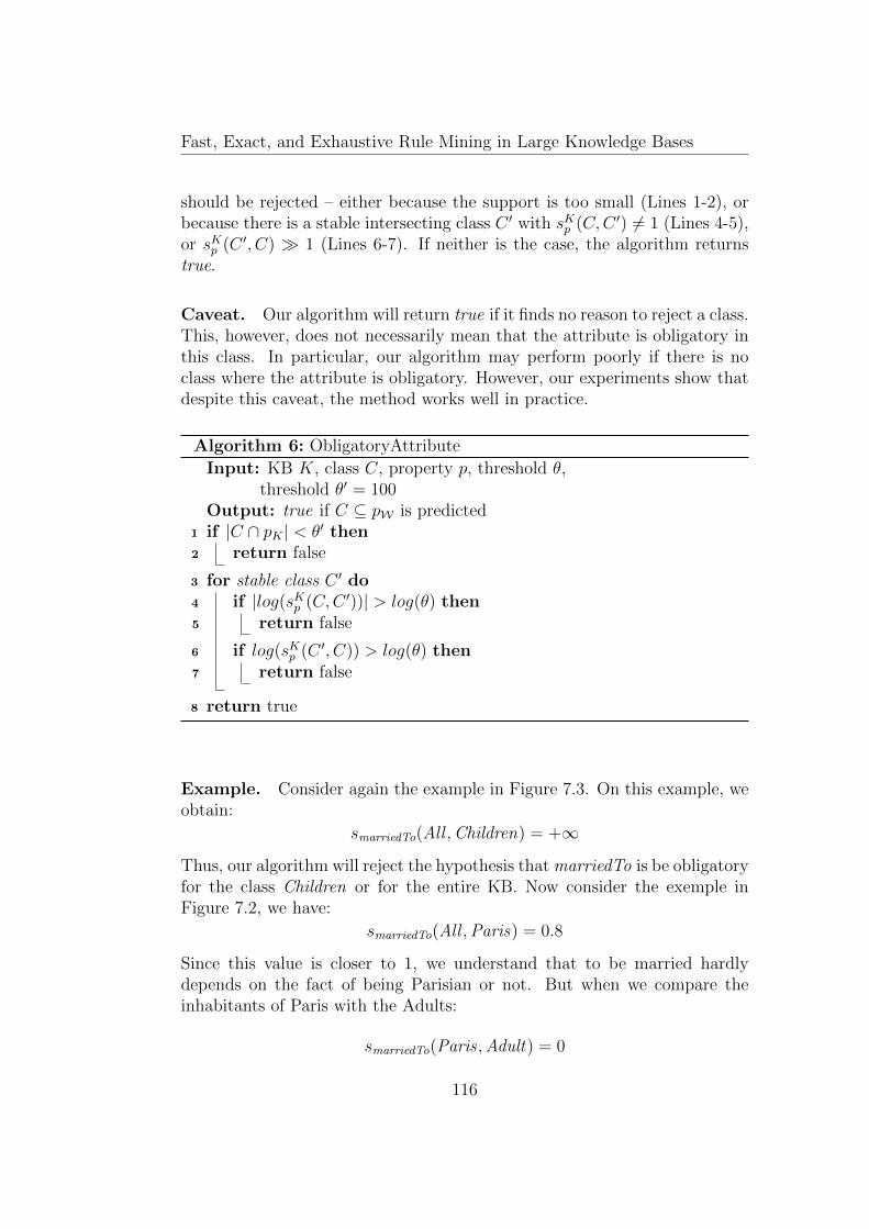
Fast, Exact, and Exhaustive Rule Mining in Large Knowledge Bases
should be rejected – either because the support is too small (Lines 1-2), orbecause there is a stable intersecting class C ′ with sKp (C,C ′) 6= 1 (Lines 4-5),or sKp (C ′, C) 1 (Lines 6-7). If neither is the case, the algorithm returnstrue.
Caveat. Our algorithm will return true if it finds no reason to reject a class.This, however, does not necessarily mean that the attribute is obligatory inthis class. In particular, our algorithm may perform poorly if there is noclass where the attribute is obligatory. However, our experiments show thatdespite this caveat, the method works well in practice.
Algorithm 6: ObligatoryAttribute
Input: KB K, class C, property p, threshold θ,threshold θ′ = 100
Output: true if C ⊆ pW is predicted1 if |C ∩ pK | < θ′ then2 return false
3 for stable class C ′ do4 if |log(sKp (C,C ′))| > log(θ) then5 return false
6 if log(sKp (C ′, C)) > log(θ) then7 return false
8 return true
Example. Consider again the example in Figure 7.3. On this example, weobtain:
smarriedTo(All ,Children) = +∞
Thus, our algorithm will reject the hypothesis that marriedTo is be obligatoryfor the class Children or for the entire KB. Now consider the exemple inFigure 7.2, we have:
smarriedTo(All ,Paris) = 0.8
Since this value is closer to 1, we understand that to be married hardlydepends on the fact of being Parisian or not. But when we compare theinhabitants of Paris with the Adults:
smarriedTo(Paris ,Adult) = 0
116
Fast, Exact, and Exhaustive Rule Mining in Large Knowledge Bases
We deduce that not all Parisians are married. We need to consider everyother intersection in order to conclude for the class Adult, for example wehave:
smarriedTo(Adult ,Paris) = 0.66
7.5.3 Variations
Relaxation. In practice, classes in a KB intersect only in small areas.Thus, when sKφ (C,C ′) 1, we decided to reject only C ′. In this relaxedvariant, the condition in Line 4 of Algorithm 6 becomes log(sKp (C,C ′)) <−log(θ).
Fisher’s Exact Test. We also experimented the Fisher’s Exact Test [27]instead of the confidence ratio. We replace the logarithm of the confidenceratio s in Line 4 of Algorithm 6 by the probability that C ∩ C ′ has highervalues, and in Line 6 with the probability that it has lower values over theset of possible contingency tables with fixed marginals.
7.6 Experiments
In this section, we evaluate our approach experimentally on large real-worldKBs. We first evaluate our approach on YAGO, a KB for which we know thatour Assumptions 1 and 2 hold by and large. Then, we submit our approachto a stress test: We run it on Wikidata, where less is known about ourassumptions. Finally, we investigate how our approach could be generalizedto composite classes.
7.6.1 Datasets
YAGO. We chose the YAGO3 knowledge base [50] for our experiments,because the data is of good quality (Assumption 1) and the taxonomy is ex-tensive (Assumption 2). We use the facts of all instances, the full taxonomy,and the transitive closure of types. With this, our dataset contains morethan 5 million instances and around 54,000 classes with more than 50 (director indirect) instances.
Wikidata. As a stress-test, we also evaluated our approach in Wikidata,where less is known about our Assumptions 1-4. We used the version from2017-06-07, which contains more than 16,000 properties. This makes a man-ual evaluation impractical. Hence, we reduced the dataset to only people.
117
Fast, Exact, and Exhaustive Rule Mining in Large Knowledge Bases
However, all people are in only one class: Human. Therefore, we used the oc-cupation property (P106) to define classes. For example, in Wikidata, ElvisPresley (Q303) has the occupations FilmActor, Actor, Singer, Screenwriter,Guitarist and Soldier. These occupations form their own hierarchy, whichwe use as class hierarchy. For example, FilmActor is a sub-occupation ofActor, and thus becomes a subclass of it. This subset of Wikidata contains1023 classes, around 1.6 million instances, and 2569 properties.
7.6.2 Gold Standard
Since our problem is novel, there is no previously published gold standard forit. Therefore, we had to construct a gold standard manually. For YAGO, weconsidered 68 properties (37 properties and their inverses), we determinedthe classes where more than 100 instances have the property, and we manu-ally evaluated whether the attribute is obligatory or not. For Wikidata, werandomly selected 100 properties, and evaluated the output of each methodmanually. Our manual evaluation gives us an estimate for precision. SinceBaseline 3 has a recall of 100% at maximal θ, we can use it to estimate ourrecall.
It is not always easy to determine manually whether an attribute is oblig-atory. For example, consider the attribute isAffiliatedTo. Is it obligatory foran artist to be affiliated to a museum, for a football player to be affiliated toa football club, or for people in general to be affiliated to their relatives? Forour gold standard, we restricted ourselves to cases where we could clearlyestablish whether an attribute is obligatory or not, and removed all othercases.
Another problem arises for classes where the huge majority of instanceshave a particular attribute. For example, should we discard hasNationalityas an obligatory attribute for Person because there exist stateless people?In such cases, we decided that the absence of the attribute is an excep-tion to the rule that our method should not predict. Hence, we consideredhasNationality obligatory. A related problem is that an attribute may notnecessarily be obligatory for a class, but that de facto all instances have it.For example, we expect all instances of the class RomanEmperor to be deadby now, but what if a renewed Roman empire arises in the future? In suchcases, we considered an attribute obligatory if de facto all known instanceshave it.
We constructed our gold standard according to these principles, and referthe reader to [71] for a more detailed discussion of such evaluations. All ourdatasets, as well as the gold standard and the evaluation results, are availableat https://suchanek.name/work/publications/www-2018-data.
118
Fast, Exact, and Exhaustive Rule Mining in Large Knowledge Bases
7.6.3 Evaluation Metric
The most intuitive way to evaluate the prediction of obligatory attributeswould be to consider each predicted pair of a class and an attribute, and tocompare this set to the gold standard. However, this comparison would nottake into account the size of the class. For example, it is more importantto predict that all organizations have a headquarters than that all Qatariski champions have a gender, because there are many more of the formerthan of the latter. However, weighting each class by the number of instancescauses another problem. Consider, e.g., the classes Man and Woman, whichpartition the class Person in our data2. If we predict that an attribute isobligatory for Man and for Woman, but not for Person, we would obtain arecall of only 50% – even though we predicted the attribute correctly for allinstances.
To mitigate this problem, we compare, for each class C and for eachproperty p, the actual set of predicted instances with the instances in thegold standard, i.e., we compare
Pp = x ∈ c|c ⊆ pW predicted by our algorithm
with
Gp = x ∈ c|c ⊆ pW in the gold standard
The true positives are the instances in the intersection of these sets. Thenwe compute the precision and recall as follows:
precision =
∑p |Pp ∩Gp|∑
p |Pp|
recall =
∑p |Pp ∩Gp|∑
p |Gp|
The F1-measure is computed as the harmonic mean of these.
7.6.4 YAGO Experiment
We ran all three baselines (Section 7.4) as well as our approaches (Section 7.5)on our YAGO dataset. Figure 7.4 shows the recall over the precision for eachapproach, with varying threshold θ.
2We are talking about a property of our data, not about genders in the real world.
119

Fast, Exact, and Exhaustive Rule Mining in Large Knowledge Bases
Baseline 1. Recall that this baseline (inspired by [83]) labels an attributeas obligatory in a class, if all instances of the class have this attribute in theKB. This baseline performs like Baseline 2 at θ = 1. Unsurprisingly, it hasa very good precision, but a very bad recall: Only very few attributes (suchas label) appear on all instances.
Baseline 2. This baseline relaxes Baseline 1 by labeling an attribute asobligatory if it is very prevalent in the class. For smaller θ, this method hasa better recall than Baseline 1. However, it cannot exceed an F1 value of45%. This is because there is no global threshold θ that would work well forall attributes. The baseline will work better if the KB is more complete. Atthe same time, the more complete the KB is, the less novel information thereis to predict.
Baseline 3. This baseline (inspired by [6]) considers an attribute obliga-tory for a class if the vast majority of instances with that attribute fall inthat class. The somewhat unusual curve comes from the fact that the base-line chooses the deepest class in the taxonomy where the target rule holds.While the method achieves slightly better F1 values (55%), its precision neverexceeds 42%.
Confidence Ratio (Strict). This is our approach, based on the ratio of anattribute in a class and its intersections with the other classes (Algorithm 6).Different from Baseline 2, it delivers a very high precision (always > 80%) –at the expense of somewhat lower recall. The best F1 measure is 37%.
Confidence Ratio (Relaxed). The relaxed variant of our method is lessconservative. It trades off precision for higher recall. Indeed, we see thatrecall increases steadily with growing θ, while precision decreases gently.This allows for very good trade-offs between the two, with the maximum F1value easily surpassing 55%. It is thus our method of choice.
Fisher’s Test. This variation of our approach aims to make the ConfidenceRatio less vulnerable to small data sizes. This is indeed what happens.However, the method errs on the side of caution: it has a very good precision(always > 90%), but a mediocre recall. Hence, the best F1 value is quitelow (12%). To increase this recall, the significance level of this test wouldhave to be increased by a factor of several orders of magnitude, which woulddefy its purpose. The method should thus be seen as a stable, but inherentlyprecision-oriented method.
120
Fast, Exact, and Exhaustive Rule Mining in Large Knowledge Bases
Comparison. Figure 7.5 plots precision and recall for each of the methodsacross the spectrum of parameter values.3 Baseline 3 achieves the highestrecall. However, its precision never exceeds 42%, which makes the methodunusable in practice. On the other side of the spectrum, Baseline 2 offers verygood precision – but it cannot achieve good recall. Our relaxed confidenceratio occupies a sweet spot between the two: a precision between 75% and95%, at a recall of 45% and 10%, respectively. It thus dominates the othermethods in the mid-range between good recall and good precision.
Completeness of the attributes. By identifying classes in which an at-tribute is obligatory, our method identifies the entities that should have thisattribute. If we compute the proportion of these entities that actually havethe attribute in the data, we get an approximation of the completeness ofthe data. Table 7.1 shows the estimated completeness of the data accordingto different methods: the gold standard, Baseline 2 at different thresholds,and our method at different thresholds. We show 3 attributes that are oblig-atory in certain classes, and the deviation from the gold standard across allattributes. The small deviation for our method shows that we can approxi-mate the real completeness quite well.
We can now also algorithmically answer the question raised in the intro-duction of our approach: No, not all people are married (in the real world).Our method finds that isMarriedTo is an optional attribute for the classPerson. However, marriage is obligatory for the classes Spouse and Royal-Consort.
Table 7.1 – Approximation of completeness of attributes
Baseline 2 CR (Relaxed)Attribute Gold Standard 0.5 0.9 1.5 3
hasGender 0.58 0.51 0.91 0.79 0.58wasBornIn 0.14 0.47 0.93 0.46 0.25isMarriedTo 0.57 0.51 0.93 0.59 0.23Avg-Squared error to GS (all p) 0.21 0.59 0.17 0.08
7.6.5 Wikidata Experiment
As a stress test, we also evaluated our method on Wikidata, where less isknown about our assumptions. Figure 7.6 shows our results. We first note
3Different values for θ can give the same combination of precision and recall, whencethe “loop” of Baseline 3.
121
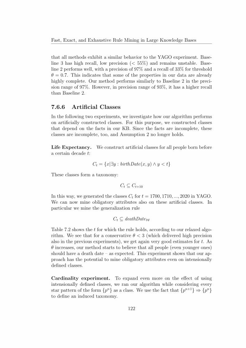
Fast, Exact, and Exhaustive Rule Mining in Large Knowledge Bases
that all methods exhibit a similar behavior to the YAGO experiment. Base-line 3 has high recall, low precision (< 55%) and remains unstable. Base-line 2 performs well, with a precision of 97% and a recall of 33% for thresholdθ = 0.7. This indicates that some of the properties in our data are alreadyhighly complete. Our method performs similarly to Baseline 2 in the preci-sion range of 97%. However, in precision range of 93%, it has a higher recallthan Baseline 2.
7.6.6 Artificial Classes
In the following two experiments, we investigate how our algorithm performson artificially constructed classes. For this purpose, we constructed classesthat depend on the facts in our KB. Since the facts are incomplete, theseclasses are incomplete, too, and Assumption 2 no longer holds.
Life Expectancy. We construct artificial classes for all people born beforea certain decade t:
Ct = x|∃y : birthDate(x, y) ∧ y < t
These classes form a taxonomy:
Ct ⊆ Ct+10
In this way, we generated the classes Ct for t = 1700, 1710, ..., 2020 in YAGO.We can now mine obligatory attributes also on these artificial classes. Inparticular we mine the generalization rule
Ct ⊆ deathDateW
Table 7.2 shows the t for which the rule holds, according to our relaxed algo-rithm. We see that for a conservative θ < 3 (which delivered high precisionalso in the previous experiments), we get again very good estimates for t. Asθ increases, our method starts to believe that all people (even younger ones)should have a death date – as expected. This experiment shows that our ap-proach has the potential to mine obligatory attributes even on intensionallydefined classes.
Cardinality experiment. To expand even more on the effect of usingintensionally defined classes, we ran our algorithm while considering everystar pattern of the form pn as a class. We use the fact that pn+1 ⇒ pnto define an induced taxonomy.
122
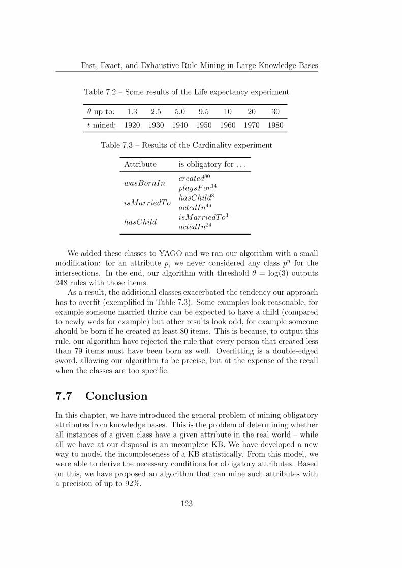
Fast, Exact, and Exhaustive Rule Mining in Large Knowledge Bases
Table 7.2 – Some results of the Life expectancy experiment
θ up to: 1.3 2.5 5.0 9.5 10 20 30
t mined: 1920 1930 1940 1950 1960 1970 1980
Table 7.3 – Results of the Cardinality experiment
Attribute is obligatory for . . .
wasBornIncreated80
playsFor14
isMarriedTohasChild8
actedIn49
hasChildisMarriedTo3
actedIn24
We added these classes to YAGO and we ran our algorithm with a smallmodification: for an attribute p, we never considered any class pn for theintersections. In the end, our algorithm with threshold θ = log(3) outputs248 rules with those items.
As a result, the additional classes exacerbated the tendency our approachhas to overfit (exemplified in Table 7.3). Some examples look reasonable, forexample someone married thrice can be expected to have a child (comparedto newly weds for example) but other results look odd, for example someoneshould be born if he created at least 80 items. This is because, to output thisrule, our algorithm have rejected the rule that every person that created lessthan 79 items must have been born as well. Overfitting is a double-edgedsword, allowing our algorithm to be precise, but at the expense of the recallwhen the classes are too specific.
7.7 Conclusion
In this chapter, we have introduced the general problem of mining obligatoryattributes from knowledge bases. This is the problem of determining whetherall instances of a given class have a given attribute in the real world – whileall we have at our disposal is an incomplete KB. We have developed a newway to model the incompleteness of a KB statistically. From this model, wewere able to derive the necessary conditions for obligatory attributes. Basedon this, we have proposed an algorithm that can mine such attributes witha precision of up to 92%.
123
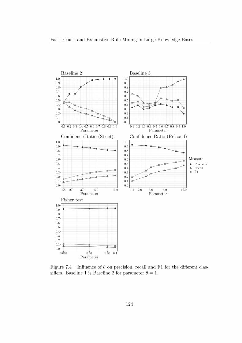
Fast, Exact, and Exhaustive Rule Mining in Large Knowledge Bases
0.00.10.20.30.40.50.60.70.80.91.0
0.1 0.2 0.3 0.4 0.5 0.6 0.7 0.8 0.9 1.0Parameter
Baseline 2
0.00.10.20.30.40.50.60.70.80.91.0
0.1 0.2 0.3 0.4 0.5 0.6 0.7 0.8 0.9 1.0Parameter
Baseline 3
0.00.10.20.30.40.50.60.70.80.91.0
1.5 2.0 3.0 5.0 10.0Parameter
Confidence Ratio (Strict)
0.00.10.20.30.40.50.60.70.80.91.0
1.5 2.0 3.0 5.0 10.0Parameter
Confidence Ratio (Relaxed)
0.00.10.20.30.40.50.60.70.80.91.0
0.001 0.01 0.05 0.1Parameter
Fisher test
MeasurePrecisionRecallF1
0.00.10.20.30.40.50.60.70.80.91.0
0.1 0.2 0.3 0.4 0.5 0.6 0.7 0.8 0.9 1.0Parameter
Baseline 2
0.00.10.20.30.40.50.60.70.80.91.0
0.1 0.2 0.3 0.4 0.5 0.6 0.7 0.8 0.9 1.0Parameter
Baseline 3
0.00.10.20.30.40.50.60.70.80.91.0
1.5 2.0 3.0 5.0 10.0Parameter
Confidence Ratio (Strict)
0.00.10.20.30.40.50.60.70.80.91.0
1.5 2.0 3.0 5.0 10.0Parameter
Confidence Ratio (Relaxed)
0.00.10.20.30.40.50.60.70.80.91.0
0.001 0.01 0.05 0.1Parameter
Fisher test
MeasurePrecisionRecallF1
Figure 7.4 – Influence of θ on precision, recall and F1 for the different clas-sifiers. Baseline 1 is Baseline 2 for parameter θ = 1.
124

Fast, Exact, and Exhaustive Rule Mining in Large Knowledge Bases
0.0
0.1
0.2
0.3
0.4
0.5
0.6
0.7
0.8
0.9
1.0
0.2 0.3 0.4 0.5 0.6 0.7 0.8 0.9 1.0Precision
Rec
all
ClassifierConfidence Ratio (Relaxed)Baseline 2Baseline 3Confidence Ratio (Strict)Fisher test
Figure 7.5 – Precision and Recall on YAGO
125
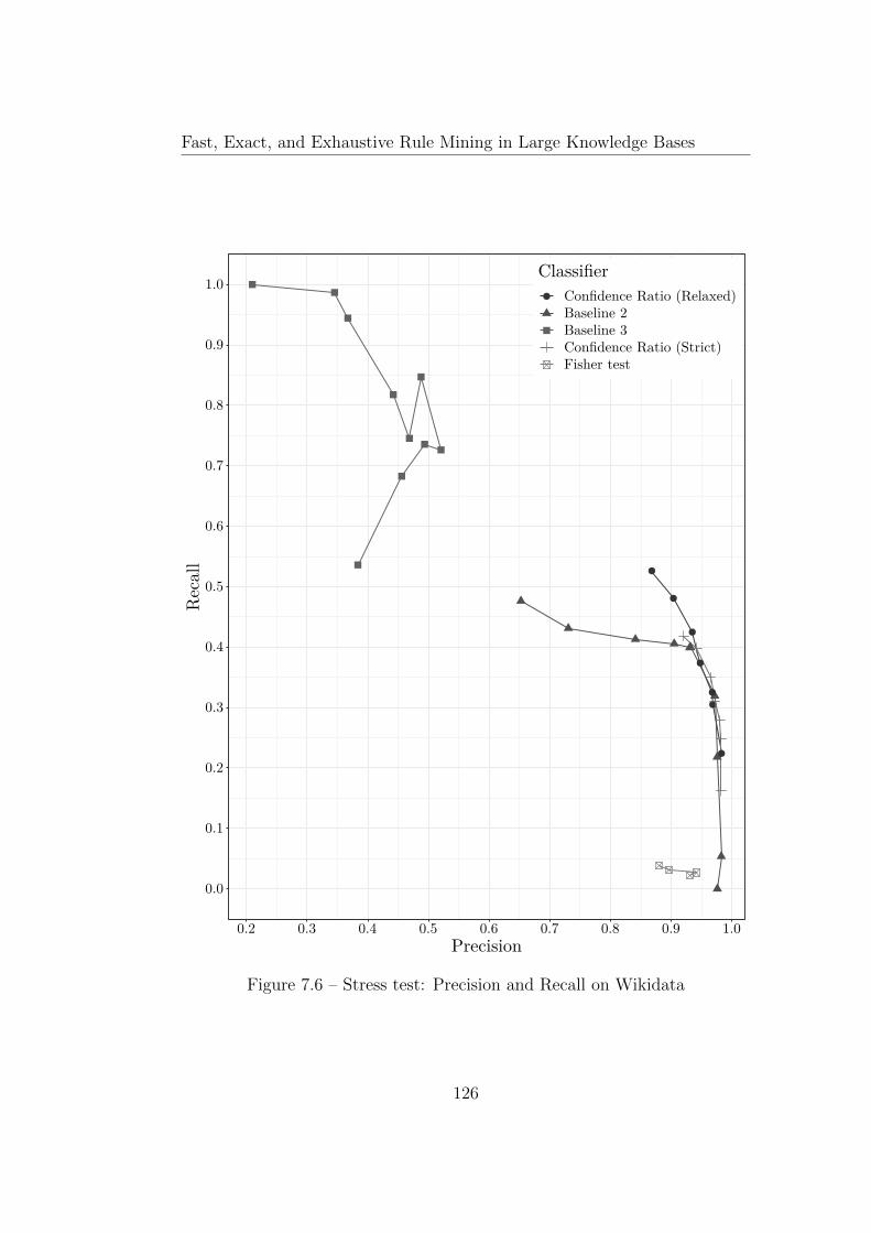
Fast, Exact, and Exhaustive Rule Mining in Large Knowledge Bases
0.0
0.1
0.2
0.3
0.4
0.5
0.6
0.7
0.8
0.9
1.0
0.2 0.3 0.4 0.5 0.6 0.7 0.8 0.9 1.0Precision
Rec
all
ClassifierConfidence Ratio (Relaxed)Baseline 2Baseline 3Confidence Ratio (Strict)Fisher test
Figure 7.6 – Stress test: Precision and Recall on Wikidata
126

Chapter 8
Conclusion
8.1 Summary
In this thesis, we introduced novel approaches and optimizations designedto speed up the process of rule mining on large Knowledge Bases. We de-veloped and presented two algorithms to demonstrate the efficiency of thoseoptimizations on real datasets: the AMIE 3 algorithm (the successor of theexact rule mining algorithm AMIE+) and the Pathfinder algorithm, a novelalgorithm specialized in mining path rules. These two algorithms are exhaus-tive with regard to the parameters provided by the user, compute the qualitymeasures of each rule exactly and scale to large KB and longer rules.
Rule Mining. In Chapter 2 we presented the task of rule mining as anInductive Logic Programming problem and described multiple rule miningalgorithms that apply on Knowledge Bases. Among them was the exact rulemining algorithm AMIE+, which use a pruning heuristic to speed up theprocessing of large KBs at the cost of the completeness of the result.
In Chapter 3, we improved the method that AMIE uses to compute thequality metrics of the rules. We introduced the lazy strategy, some queryoptimizations and more efficient data structures. These optimizations makethe pruning heuristic obsolete and make AMIE 3 exhaustive once again. Inour experiments, AMIE 3 is around 50× faster than its predecessor AMIE+on some datasets (Yago2s or DBPedia 3.8) and scales to large KBs that werepreviously beyond reach.
Pruning the search space. In Chapter 4, we decomposed the rules intostar patterns and outlined that every star pattern of a rule must be satisfiablefor the rule to be satisfiable. We discussed how to extract all satisfiable star
127
Fast, Exact, and Exhaustive Rule Mining in Large Knowledge Bases
patterns of a KB and introduced the compatibility condition that decides ifa set of star patterns can be combined into a rule. However, we also showedthat the combinatorial problem of enumerating every compatible set of starpatterns can be seen as a zero sum subset problem, which is NP-complete.
Path Rule Mining. In Chapters 5 and 6, we aimed to mine every closedpath rule from a KB. We introduced two increasingly refined algorithmsto solve this problem: the Pathfinder Vanilla algorithm and the (Full)Pathfinder algorithm.
In Chapter 5, we showed that the shape of the path rules and of theof star patterns (introduced in Chapter 4) allows us to design a refinementoperator for both algorithms that does not produce any duplicate rule andthat efficiently prunes unsatisfiable rules early.
In Chapter 6, we discussed how data can be reused between a rule andits refinements to speed up the computation of the quality measures or avoidunnecessary computations. In particular, the Pathfinder algorithm main-tains the set of possible values of the variables of a rule and the bounds onthe iterated provenance1 between a rule and its refinements. In our experi-ments, we showed that the overhead of computing the additional informationis usually compensated by the efficient pruning of the propagated bounds andthe improved computation of the quality measures, making the Pathfinderalgorithm faster than AMIE on most datasets. This is particularly notice-able when mining longer rules: the Pathfinder algorithm is capable of miningevery rule of length 4 within one hour on datasets where this task was pre-viously intractable, and it can scale even further and mine even longer rulesat incredible speed.
Mining rules about the real world. In Chapter 7, we presented a novelapproach to mine rules about the real world from an incomplete KB. In par-ticular, we addressed the problem of mining automatically which attributeshould be obligatory for a class, such as “every singer should sing”. We in-troduced a statistical model of incompleteness, the random sampling modeland presented two signals in this model: the “spread” and the “amplifica-tion”. We translated these signals in a new metric, the confidence ratio, usedto discriminate if an attribute is obligatory in a class or not. In our exper-iments, the confidence ratio is capable of identifying obligatory attributeswith a precision of up to 90% in Yago and Wikidata.
1or the iterated provenance itself depending on the strategy used
128
Fast, Exact, and Exhaustive Rule Mining in Large Knowledge Bases
8.2 Outlook
We describe here an outlook of broader directions in continuation of thisthesis.
Query optimization. Most of the optimizations on the computation ofthe quality measures we proposed in this thesis rely on some particularitiesof the rule mining process (laziness, data reusage between multiple rules).However, it would be interesting to study how the optimizations and sub-tleties introduced in this thesis can carry over to other databases, othersystems or more generally to the field of query optimization.
Rule and Oracle. In Section 3.2.3, we described a limitation of the PCAConfidence when it comes to make prediction with a rule having a functionalhead relation. For example, the rule:
hasChild(z, x) ∧ politicianOf(z, y)⇒ politicianOf(x, y)
would predict that every child of a politician is a politician. A solution of thisproblem would be to make a prediction only when we know that the childof a politician is also politician. We model this using an oracle capable ofdeciding whether any child x should have the attribute politicianOf or not,i.e an oracle deciding for every entity E of the KB if this entity E has theattribute politicianOf in the real world or not.
Using this oracle, we would be able to use the rules to make predictionsonly on incomplete portions of the KB and as such this approach solves theproblem of the PCA confidence. However, the problem is now on how todesign such an oracle. In an unpublished experiment, we built an oracleusing the obligatory attributes mined in Chapter 7, but the results whereinconclusive as the the obligatory condition is too restrictive for the task.
The completeness information mined in [29, 81, 54, 69] or a model basedon KB embeddings could be used to built such an oracle. Note that theidea of using completeness information to reduce the scope of the predictionsis already used in [29] and introduced in [81]. However, it has never beenproperly formalized, as we propose here, using two distinct objects: a ruleand an oracle. We believe that this representation is clearer and more flexible.
Comparative Rule Mining. In order to mine obligatory attributes in aKB, we used in Chapter 7 a comparative approach that can be describedas: “what characterizes best people who sing: being a singer or being a gui-tarist?”. This comparative analysis allows to discriminate mere correlations
129

Fast, Exact, and Exhaustive Rule Mining in Large Knowledge Bases
(the guitarist who sings because he is also a singer) from interesting rules.We investigated, during this thesis, how to push this analysis further, usingmore complex tools such as decision trees. This approach was not conclusiveas the more selective the approach was, the harder it became to distinguishthe features from the noise.
An approach to overcome this obstacle would be to construct some sortof “null model” of the KB to compare to. In other words, to generate arandom KB that shares some statistical properties with the original KB.These statistical properties are yet to be defined, but we believe that thestudy of KB sampling techniques might provide some directions.
8.3 Conclusion
The Semantic Web has quickly become a constellation of large and intercon-nected entity-centric Knowledge Bases. These KBs contain domain-specificknowledge that can be used for multiple applications such as question an-swering or automatic reasoning. But in order to take full advantage of thisdata, it is essential to understand the schema and the patterns of the KB. Asimple and expressive manner to describe the dependencies in a KB is to userules. Thus it is crucial to be able to perform rule mining at scale.
With this thesis, we have made a step towards this objective. We pro-posed novel approaches to improve rule mining and new algorithms thatefficiently process large KBs without resorting to sampling or approxima-tions. With this, we provide tools for data scientists to understand, exploitand complete this interconnected knowledge. We hope this work will helpanalyze complex and momentous datasets, such as KG-Covid19, carry overto connected fields such as query optimization, and give rise to new prospectsin the study of Knowledge Bases and their completion.
130
Appendix A
Computation of Support andConfidence
Notation. Given a logical formula φ with some free variables x1, . . . , xn,all other variables being by default existentially quantified, we define:
#(x1, . . . , xn) : φ := |(x1, . . . , xn) : φ(x1, . . . , xn) is true|
We remind the reader of the two following definitions:
Definition 2.3.4 (Prediction of a rule). The predictions P of a rule ~B ⇒ hin a KB K are the head atoms of all instantiations of the rule where the bodyatoms appear in K. We write K ∧ ( ~B ⇒ h) |= P .
Definition 2.3.9 (Support). The support of a rule in a KB is the numberof positive examples predicted by the rule.
A prediction of a rule is a positive example if and only if it is in the KB.This observation gives rise to the following property:
Proposition A.1 (Support in practice). The support of a rule ~B ⇒ h is the
number of instantiations of the head variables that satisfy the query ~B ∧ h.This value can be written as:
support( ~B ⇒ h(x, y)) = #(x, y) : ~B ∧ h(x, y)
Definition 2.3.10 (Confidence). The confidence of a rule is the number ofpositive examples predicted by the rule (the support of the rule), divided bythe number of examples predicted by the rule.
Under the CWA, all the predicted examples are either positive examplesor negative examples. Thus, the standard confidence of a rule is the support
131
Fast, Exact, and Exhaustive Rule Mining in Large Knowledge Bases
of the rule divided by the number of prediction of the rule, written:
std-conf( ~B ⇒ h(x, y)) =#(x, y) : ~B ∧ h(x, y)
#(x, y) : ~B(A.1)
Assume h is more functional than inverse functional. Under the PCA, apredicted negative example is a prediction h(x, y) that is not in the KB, suchthat, for this x there exists another entity y′ such that h(x, y′) is in the KB.When we add the predicted positive examples, the denominator of the PCAconfidence becomes:
#(x, y) : ( ~B ∧ h(x, y)) ∨ ( ~B ∧ ¬h(x, y) ∧ ∃y′.h(x, y′))
We can simplify this logical formula to deduce the following formula forcomputing the PCA confidence:
pca-conf( ~B ⇒ h(x, y)) =#(x, y) : ~B ∧ h(x, y)
#(x, y) : ~B ∧ ∃y′.h(x, y′)(A.2)
132
Appendix B
Number of items per relation
133
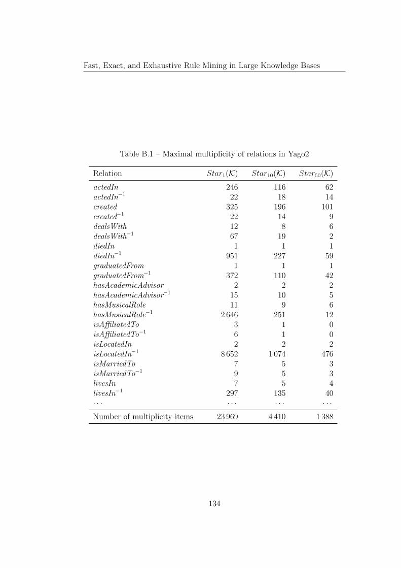
Fast, Exact, and Exhaustive Rule Mining in Large Knowledge Bases
Table B.1 – Maximal multiplicity of relations in Yago2
Relation Star1(K) Star10(K) Star50(K)
actedIn 246 116 62actedIn−1 22 18 14created 325 196 101created−1 22 14 9dealsWith 12 8 6dealsWith−1 67 19 2diedIn 1 1 1diedIn−1 951 227 59graduatedFrom 1 1 1graduatedFrom−1 372 110 42hasAcademicAdvisor 2 2 2hasAcademicAdvisor−1 15 10 5hasMusicalRole 11 9 6hasMusicalRole−1 2 646 251 12isAffiliatedTo 3 1 0isAffiliatedTo−1 6 1 0isLocatedIn 2 2 2isLocatedIn−1 8 652 1 074 476isMarriedTo 7 5 3isMarriedTo−1 9 5 3livesIn 7 5 4livesIn−1 297 135 40· · · · · · · · · · · ·Number of multiplicity items 23 969 4 410 1 388
134
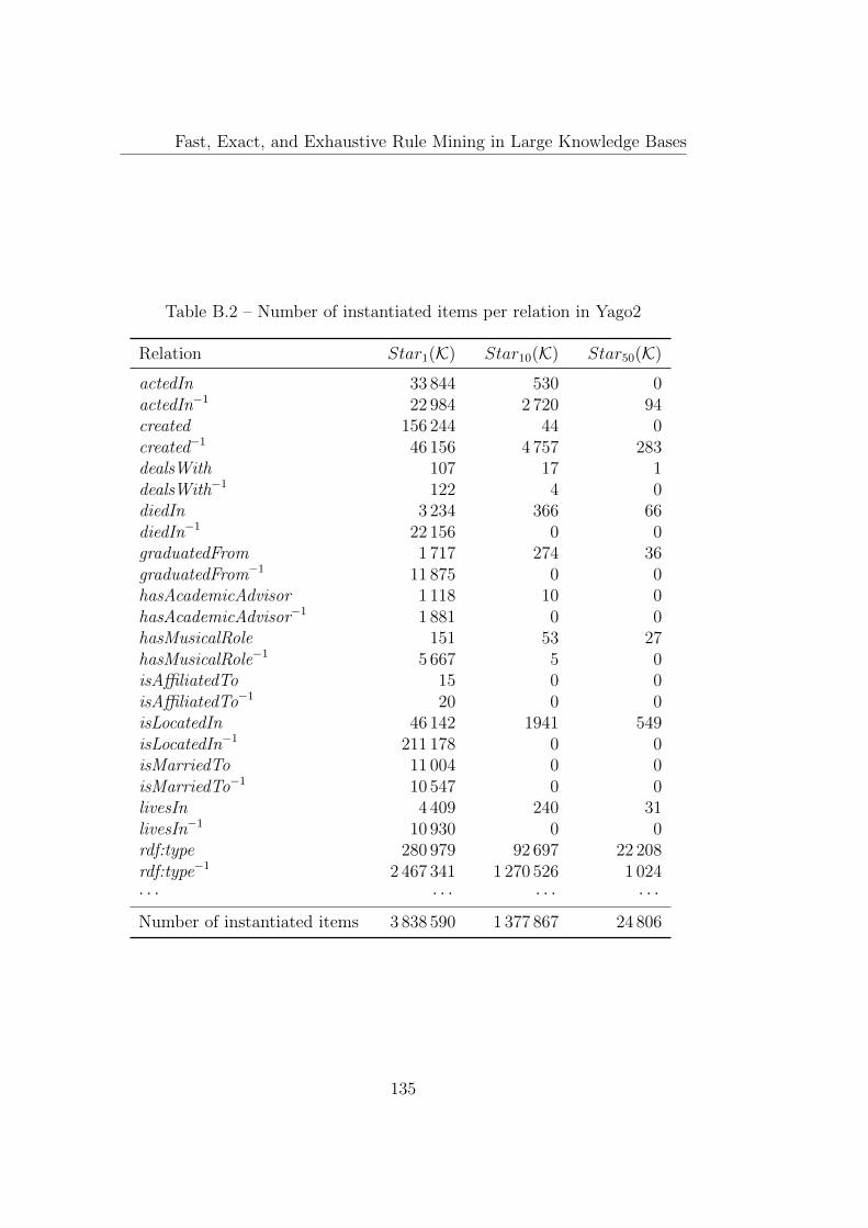
Fast, Exact, and Exhaustive Rule Mining in Large Knowledge Bases
Table B.2 – Number of instantiated items per relation in Yago2
Relation Star1(K) Star10(K) Star50(K)
actedIn 33 844 530 0actedIn−1 22 984 2 720 94created 156 244 44 0created−1 46 156 4 757 283dealsWith 107 17 1dealsWith−1 122 4 0diedIn 3 234 366 66diedIn−1 22 156 0 0graduatedFrom 1 717 274 36graduatedFrom−1 11 875 0 0hasAcademicAdvisor 1 118 10 0hasAcademicAdvisor−1 1 881 0 0hasMusicalRole 151 53 27hasMusicalRole−1 5 667 5 0isAffiliatedTo 15 0 0isAffiliatedTo−1 20 0 0isLocatedIn 46 142 1941 549isLocatedIn−1 211 178 0 0isMarriedTo 11 004 0 0isMarriedTo−1 10 547 0 0livesIn 4 409 240 31livesIn−1 10 930 0 0rdf:type 280 979 92 697 22 208rdf:type−1 2 467 341 1 270 526 1 024· · · · · · · · · · · ·Number of instantiated items 3 838 590 1 377 867 24 806
135
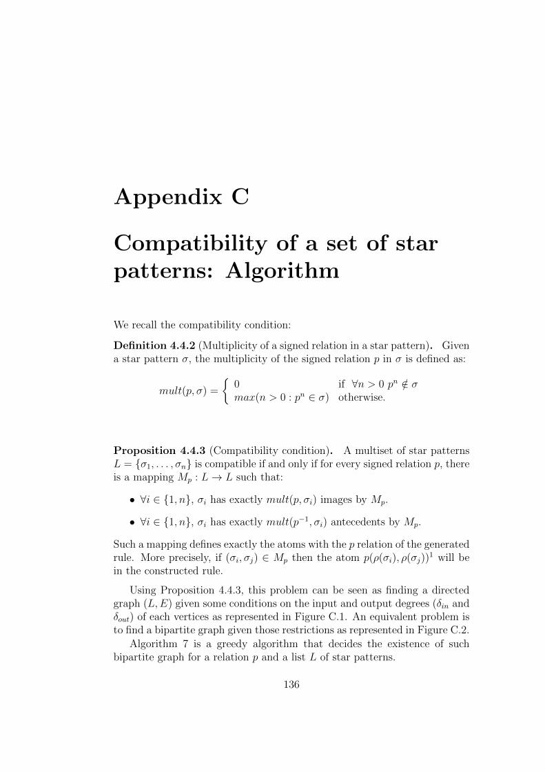
Appendix C
Compatibility of a set of starpatterns: Algorithm
We recall the compatibility condition:
Definition 4.4.2 (Multiplicity of a signed relation in a star pattern). Givena star pattern σ, the multiplicity of the signed relation p in σ is defined as:
mult(p, σ) =
0 if ∀n > 0 pn /∈ σmax(n > 0 : pn ∈ σ) otherwise.
Proposition 4.4.3 (Compatibility condition). A multiset of star patternsL = σ1, . . . , σn is compatible if and only if for every signed relation p, thereis a mapping Mp : L→ L such that:
• ∀i ∈ 1, n, σi has exactly mult(p, σi) images by Mp.
• ∀i ∈ 1, n, σi has exactly mult(p−1, σi) antecedents by Mp.
Such a mapping defines exactly the atoms with the p relation of the generatedrule. More precisely, if (σi, σj) ∈ Mp then the atom p(ρ(σi), ρ(σj))
1 will bein the constructed rule.
Using Proposition 4.4.3, this problem can be seen as finding a directedgraph (L,E) given some conditions on the input and output degrees (δin andδout) of each vertices as represented in Figure C.1. An equivalent problem isto find a bipartite graph given those restrictions as represented in Figure C.2.
Algorithm 7 is a greedy algorithm that decides the existence of suchbipartite graph for a relation p and a list L of star patterns.
136
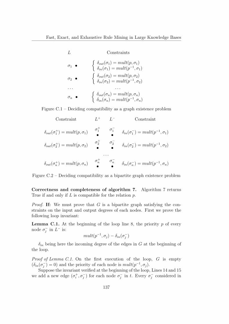
Fast, Exact, and Exhaustive Rule Mining in Large Knowledge Bases
L Constraints
σ1 •δout(σ1) = mult(p, σ1)δin(σ1) = mult(p−1, σ1)
σ2 •δout(σ2) = mult(p, σ2)δin(σ2) = mult(p−1, σ2)
· · · · · ·
σn •δout(σn) = mult(p, σn)δin(σn) = mult(p−1, σn)
Figure C.1 – Deciding compatibility as a graph existence problem
Constraint L+ L− Constraint
δout(σ+1 ) = mult(p, σ1)
σ+1
•σ−1• δin(σ−1 ) = mult(p−1, σ1)
δout(σ+2 ) = mult(p, σ2)
σ+2
•σ−2• δin(σ−2 ) = mult(p−1, σ2)
· · ·
δout(σ+n ) = mult(p, σn)
σ+n
•σ−n• δin(σ−n ) = mult(p−1, σn)
Figure C.2 – Deciding compatibility as a bipartite graph existence problem
Correctness and completeness of algorithm 7. Algorithm 7 returnsTrue if and only if L is compatible for the relation p.
Proof. If: We must prove that G is a bipartite graph satisfying the con-straints on the input and output degrees of each nodes. First we prove thefollowing loop invariant:
Lemma C.1. At the beginning of the loop line 8, the priority p of everynode σ−j in L− is:
mult(p−1, σj)− δin(σ−j )
δin being here the incoming degree of the edges in G at the beginning ofthe loop.
Proof of Lemma C.1. On the first execution of the loop, G is empty(δin(σ−j ) = 0) and the priority of each node is mult(p−1, σj).
Suppose the invariant verified at the beginning of the loop, Lines 14 and 15we add a new edge (σ+
i , σ−j ) for each node σ−j in t. Every σ−j considered in
137
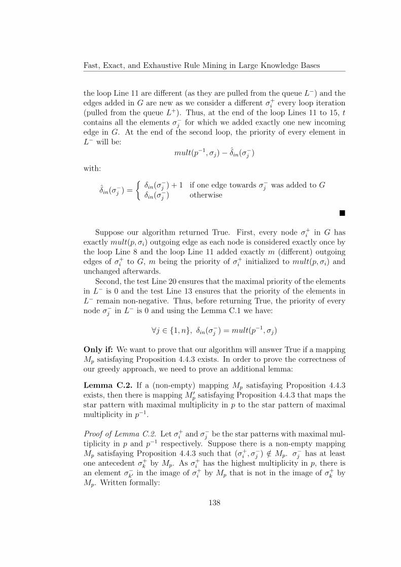
Fast, Exact, and Exhaustive Rule Mining in Large Knowledge Bases
the loop Line 11 are different (as they are pulled from the queue L−) and theedges added in G are new as we consider a different σ+
i every loop iteration(pulled from the queue L+). Thus, at the end of the loop Lines 11 to 15, tcontains all the elements σ−j for which we added exactly one new incomingedge in G. At the end of the second loop, the priority of every element inL− will be:
mult(p−1, σj)− δin(σ−j )
with:
δin(σ−j ) =
δin(σ−j ) + 1 if one edge towards σ−j was added to Gδin(σ−j ) otherwise
Suppose our algorithm returned True. First, every node σ+i in G has
exactly mult(p, σi) outgoing edge as each node is considered exactly once bythe loop Line 8 and the loop Line 11 added exactly m (different) outgoingedges of σ+
i to G, m being the priority of σ+i initialized to mult(p, σi) and
unchanged afterwards.
Second, the test Line 20 ensures that the maximal priority of the elementsin L− is 0 and the test Line 13 ensures that the priority of the elements inL− remain non-negative. Thus, before returning True, the priority of everynode σ−j in L− is 0 and using the Lemma C.1 we have:
∀j ∈ 1, n, δin(σ−j ) = mult(p−1, σj)
Only if: We want to prove that our algorithm will answer True if a mappingMp satisfaying Proposition 4.4.3 exists. In order to prove the correctness ofour greedy approach, we need to prove an additional lemma:
Lemma C.2. If a (non-empty) mapping Mp satisfaying Proposition 4.4.3exists, then there is mapping M ′
p satisfaying Proposition 4.4.3 that maps thestar pattern with maximal multiplicity in p to the star pattern of maximalmultiplicity in p−1.
Proof of Lemma C.2. Let σ+i and σ−j be the star patterns with maximal mul-
tiplicity in p and p−1 respectively. Suppose there is a non-empty mappingMp satisfaying Proposition 4.4.3 such that (σ+
i , σ−j ) /∈ Mp. σ
−j has at least
one antecedent σ+k by Mp. As σ+
i has the highest multiplicity in p, there isan element σ−k′ in the image of σ+
i by Mp that is not in the image of σ+k by
Mp. Written formally:
138
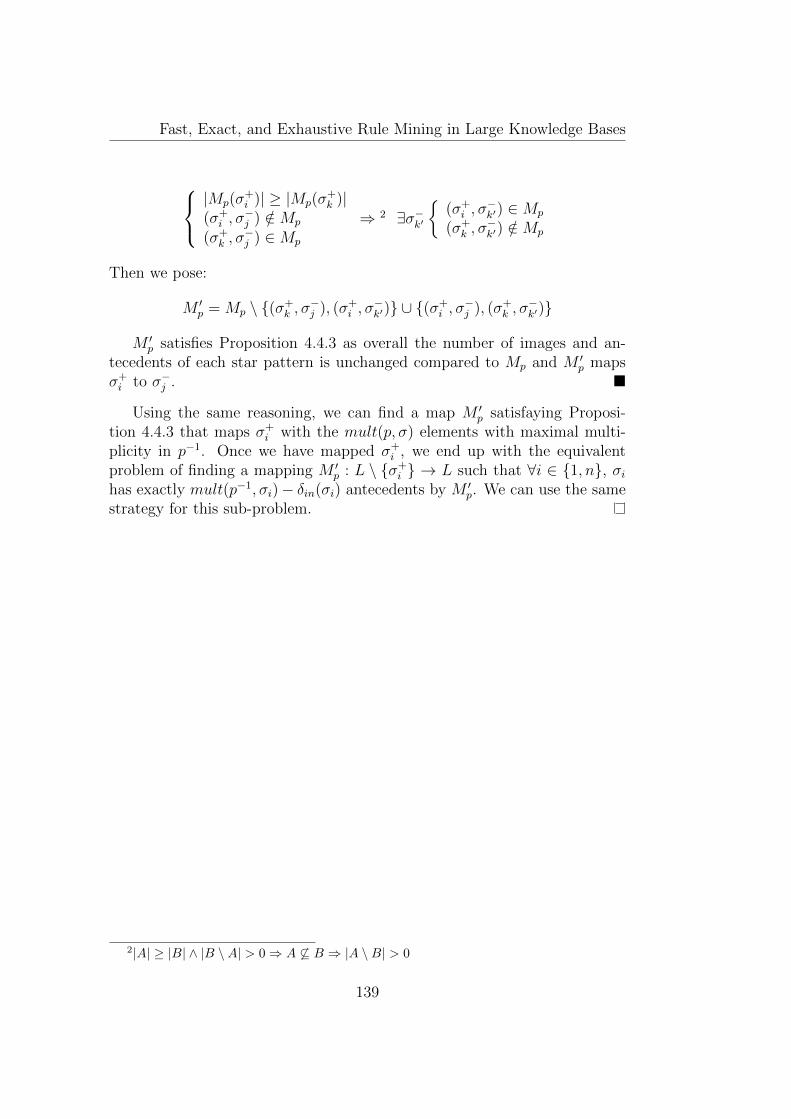
Fast, Exact, and Exhaustive Rule Mining in Large Knowledge Bases
|Mp(σ
+i )| ≥ |Mp(σ
+k )|
(σ+i , σ
−j ) /∈Mp
(σ+k , σ
−j ) ∈Mp
⇒ 2 ∃σ−k′
(σ+i , σ
−k′) ∈Mp
(σ+k , σ
−k′) /∈Mp
Then we pose:
M ′p = Mp \ (σ+
k , σ−j ), (σ+
i , σ−k′) ∪ (σ
+i , σ
−j ), (σ+
k , σ−k′)
M ′p satisfies Proposition 4.4.3 as overall the number of images and an-
tecedents of each star pattern is unchanged compared to Mp and M ′p maps
σ+i to σ−j .
Using the same reasoning, we can find a map M ′p satisfaying Proposi-
tion 4.4.3 that maps σ+i with the mult(p, σ) elements with maximal multi-
plicity in p−1. Once we have mapped σ+i , we end up with the equivalent
problem of finding a mapping M ′p : L \ σ+
i → L such that ∀i ∈ 1, n, σihas exactly mult(p−1, σi)− δin(σi) antecedents by M ′
p. We can use the samestrategy for this sub-problem.
2|A| ≥ |B| ∧ |B \A| > 0⇒ A 6⊆ B ⇒ |A \B| > 0
139
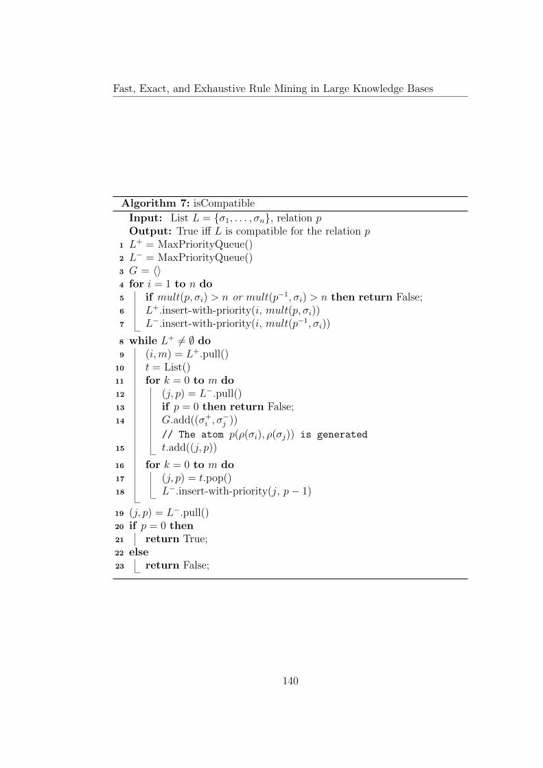
Fast, Exact, and Exhaustive Rule Mining in Large Knowledge Bases
Algorithm 7: isCompatible
Input: List L = σ1, . . . , σn, relation pOutput: True iff L is compatible for the relation p
1 L+ = MaxPriorityQueue()2 L− = MaxPriorityQueue()3 G = 〈〉4 for i = 1 to n do5 if mult(p, σi) > n or mult(p−1, σi) > n then return False;6 L+.insert-with-priority(i, mult(p, σi))7 L−.insert-with-priority(i, mult(p−1, σi))
8 while L+ 6= ∅ do9 (i,m) = L+.pull()
10 t = List()11 for k = 0 to m do12 (j, p) = L−.pull()13 if p = 0 then return False;14 G.add((σ+
i , σ−j ))
// The atom p(ρ(σi), ρ(σj)) is generated
15 t.add((j, p))
16 for k = 0 to m do17 (j, p) = t.pop()18 L−.insert-with-priority(j, p− 1)
19 (j, p) = L−.pull()20 if p = 0 then21 return True;22 else23 return False;
140

Appendix D
Resume de la these en Francais
D.1 Position du probleme
Lorsqu’on effectue une recherche sur Google ou sur Bing, on obtient une listede sites webs en reponse. Mais dorenavant, dans certains cas, on obtient unereponse structuree. Par exemple, lorqu’on pose la question “Quand est-ceque Steve Jobs est ne ?”, le moteur de recherche nous repond directement le“24 fevrier 1955”. Si on recherche seulement “Steve Jobs”, on obtient unepetite biographie, sa date de naissance, de mort, un lien vers son epouse etsa famille. Tout cela est possible parce que le moteur de recherche disposede donnees specifiques sur les personnes les plus connues. Ces donnees sontnotamment stockees dans des Bases de Connaissances.
Les bases de connaissances utilisees par les moteurs de recherche utilisentun modele entites/relations. Les individus (Steve Jobs), ou plus generalementn’importe quel objet reel ou imaginable (les Etats-Unis, le Kilimanjaro,Telecom Paris) sont representes en tant qu’entites, et les relations entreles differentes entites sont stockees sous la forme de “faits”. Ces faits sontdes declarations sujet-verbe-complement simples (telles que : SteveJobs foun-ded AppleInc, SteveJobs hasWonPrize NationalMedalOfTechnology, etc.).Les entites sont aussi rangees dans differents categories appelees “classessemantiques”. Par exemple on a les relations : SteveJobs is-a person, Steve-Jobs is-a entrepreneur, etc.
Cette representation des connaissances n’est pas nouvelle. Elle s’ins-pire des avancees des annees 80-90 dans le domaine de l’intelligence arti-ficielle, plus particulierement, le projet Cyc [47] ou le projet WordNet [24].A l’epoque, ces bases de connaissances etaient crees et maintenues manuel-lement, mais durant la derniere decennie, de nouvelles bases de connais-sances ont pu se developper grace a l’extraction automatique de donnees.
141
Fast, Exact, and Exhaustive Rule Mining in Large Knowledge Bases
Des projets tels que KnowItAll [22], ConceptNet [49], DBPedia [46], NELL[12], BabelNet [67], Wikidata [84] et YAGO [78] contiennent des connais-sances diverses et variees, en libre acces, maintenus automatiquement ou demaniere collaborative. Les entreprises privees ont ensuite emboite le pas, avecle developpement du Google Knowledge Graph [19] (contenant Freebase [9]),de Satori (Microsoft), Evi (Amazon), LinkedIn’s Knowledge Graph, et IBMWatson [26]. Au total, ces bases de connaissances contiennent plusieurs mil-lions d’entites, organisees dans des centaines de milliers de classes, et descentaines de millions de faits reliant ces entites. De plus les donnees de mul-tiples bases sont reliees entre elles, permettant le croisement d’informations,et forment ainsi ce qu’on appelle le Web Semantique [8].
Ces immenses rassemblements de connaissances inter-connectes peuventalors etre eux-meme analyses. Les motifs recurrents et correlations peuventetre representees sous la forme de regles logiques simples. Par exemple, laregle :
married(x, y) ∧ livesIn(x, z)⇒ livesIn(y, z)
se lisant “Si X et Y sont maries, et que X vit dans un lieu Z, alors Y vit aussidans Z. En d’autres termes, cette regle exprime le fait que deux personnesmariees vivent generalement au meme endroit. A chaque regle est associe unindice de confiance, un score, permettant de jauger la validite de cette regle.
Les bases de connaissances peuvent donc etre analysees pour trouver au-tomatiquement l’ensemble des regles logiques s’appliquant a cette base. C’estce qu’on appelle l’extraction de regles. Plus precisement, les algorithmes d’ex-traction de regles veulent extraire les regles de meilleure qualite, c’est-a-direles regles ayant un indice de confiance eleve, ou superieur a une valeur definiepar l’utilisateur.
Les regles trouvees ont ensuite plusieurs utilites : Premierement, ellespeuvent permettrent de completer les donnees manquantes d’une base deconnaissances. Par exemple, si on ne connaıt le lieu de residence d’unepersonne, le lieu de residence de son epoux peut etre une propositioninteressante. Deuxiemement, elles peuvent permettre d’identifier des donneeserronees ou incompletes. Si deux epoux vivent dans differentes villes, celapeut indiquer un probleme. Enfin, ces regles peuvent etre utiles pour d’autrestaches sous-jacentes, telles que la verification de faits [2], l’alignement d’on-tologies [28] ou pour determiner si les donnees sont completes ou non [29].
Neanmoins, la difficulte du probleme d’extraction de regle reside dans lataille exponentielle de l’espace de recherche : chaque relation peut etre com-binee avec n’importe quelle relation pour former une regle, de qualite variable.C’est pourquoi les premieres approches (par exemple AMIE [31]) etaient in-capables d’analyser de grandes bases de connaissances telle que Wikidata
142

Fast, Exact, and Exhaustive Rule Mining in Large Knowledge Bases
en moins d’une journee. Depuis, les bases de connaissances ont continuees as’agrandir, et les approches d’extraction de regles se sont multipliees. Cer-taines approches utilisent l’echantillonnage ou diverses approximations pourestimer la qualite d’une regle [30, 94, 63, 14]. Plus une approche approxime,plus elle est rapide, mais moins precis sont ses resultats. Une autre strategiecourament employee [63, 58, 94, 66] est de limiter la recherche a un sous-ensemble de regles qui reussisent a predire un ensemble de faits donne. Celapermet aussi d’accelerer la recherche, mais ne permet pas de trouver toutesles regles ayant un indice de confiance eleve de notre base de connaissances.
D.2 Contribution
L’objectif pricipal de cette these a ete d’etudier et de developper de nou-velles approches permettant d’extraire efficacement les regles de qualite de-puis d’enormes bases de connaissances. En particulier, nous avons œuvre aconcevoir un algorithme d’extraction de regles qui calcule de maniere exactela qualite d’une regle et qui soit exhaustif, c’est-a-dire qui soit capable d’ex-traire toutes les regles de qualite de nos donnees. Un tel algorithme, generantun ensemble complet et exact de regles, deviendrait alors un referentiel pourd’autres algorithmes d’extraction de regles.
Preliminaires. Dans le chapitre 2 de cette these, nous definissons la no-tion de base de connaissances et expliquons leur principales caracteristiques.Ensuite, nous introduisons formellement le probleme d’extraction de regleset decrivons les differents algorithmes d’extractions s’appliquant aux basesde connaissances. Ce chapitre se base notre article de presentation (“tutorialpaper”) :
- Fabian M Suchanek, Jonathan Lajus, Armand Boschin, and Gerhard Wei-kum. Knowledge representation and rule mining in entity-centric know-ledge bases. In Reasoning Web. Explainable Artificial Intelligence, pages110–152. Springer, 2019
AMIE 3. Dans le chapitre 3, nous presentons AMIE 3, une versionamelioree de AMIE+ [30], un algorithme d’extraction de regles. Dans cetteversion, nous introduisons de multiples ameliorations dans la facon de cal-culer la qualite d’une regle, permettant a AMIE de redevenir un algorithmeexact et exhaustif d’extractions de regles. Cette nouvelle version est aussiplus rapide et peut maintenant analyser des bases de connaissances trentefois plus grande. Ce chapitre est base sur notre article de recherche :
143

Fast, Exact, and Exhaustive Rule Mining in Large Knowledge Bases
- Jonathan Lajus, Luis Galarraga, and Fabian Suchanek. Fast and exactrule mining with AMIE 3. In European Semantic Web Conference, pages36–52. Springer, 2020
Reduire l’espace de recherche. La taille exponentielle de l’espace derecherche demeure un probleme lorsque nous voulons utiliser AMIE pour ex-traire des regles plus complexes, telle que des regles possedant 4 atomes. Dansle chapitre 4, nous etudions comment la decomposition de regles complexesen motifs simples pourrait nous permettre d’identifier et d’ecarter des reglesimpossibles sans avoir a effectuer de longs calculs.
Extraction de regles chaınees. Dans le chapitre 5, nous nous concen-trons sur l’extraction de regles d’une forme particuliere, les regles chaınees.Nous montrons que ces regles peuvent etre generees de maniere unique viaune methode particuliere et que les motifs simples introduits au chapitre 4peuvent etre utilises pour efficacement reduire l’espace de recherche des regleschaınees. A partir de ses resultats, nous construisons l’algorithme “PathfinderVanilla”, un algorithme, exact et exhaustif, d’extraction de regles chaınees.
Cependant, ce nouvel algorithme calcule la qualite de chaque regleindependamment et la plupart des calculs sont donc redondants. Mais dansun algorithme d’extraction de regles, chaque regle est derivee d’une regleparente et les donnees necessaires au calcul de la qualite de la regle parentepeuvent etre reutilisees pour le calcul d’une regle derivee. Dans le chapitre 6,nous utilisons cette strategie pour accelerer le calcul des mesures de qualitede toutes nos regles, ainsi que pour determiner statistiquement des bornesexactes permettant d’identifier et d’ecarter precocement de mauvaises regles.Enfin, nous presentons l’algorithme “Pathfinder”, une version amelioree del’algorithme Pathfinder Vanilla, qui extrait les regles chaınees d’une base deconnaissances de maniere exacte et exhaustive, plus efficacement que AMIEsur la plupart des jeux de donnees. Notre algorithme est d’autant plus ef-ficace que les regles a extraire sont longues. Ces chapitres sont des travauxnon publies.
Au-dela des donnees... Les bases de connaissances representent nosconnaissances du monde reel mais sont souvent incompletes. Cela entraınedes biais consequents lors de l’extraction de regles : il est difficile de sa-voir si une regle extraite est tout le temps vraie ou s’il s’agit d’une simplecorrelation. Neanmoins, ces biais peuvent etre analyses statistiquement. Dansle chapitre 7, nous introduisons un modele statistique, et un algorithme cor-respondant, permettant de determiner les relations obligatoires d’une classe.
144
Fast, Exact, and Exhaustive Rule Mining in Large Knowledge Bases
Par exemple, notre algorithme est capable de determiner que tous les chan-teurs doivent chanter, a partir de nos donnees, meme si celles-ci sont tresincompletes. Ce chapitre est base sur notre article de recherche :
- Jonathan Lajus and Fabian M. Suchanek. Are all people married? deter-mining obligatory attributes in knowledge bases. In WWW, pages 1115–1124. International World Wide Web Conferences Steering Committee,2018
D.3 Conclusion
Au fil des ans, le Web Semantique s’est agrandi pour regrouper une constella-tion d’enormes bases de connaissances interconnectees. Ces bases repertorientnos connaissances du monde sous la forme de faits structures et sont utiliseespour la reponse automatique de questions ainsi que pour le raisonnementautomatique. Mais pour tirer pleinement avantage de ce vivier d’informa-tions, il est essentiel de comprendre le schema et les interdependances in-trinseques a ces donnees. En particulier, les dependances fonctionnelles entreles differentes relations peuvent etre representees sous la forme de reglessimples. Il est donc crucial de pouvoir extraire ces regles efficacement a par-tir de nos donnees.
Dans cette these, nous avons fait un pas de plus vers cet objectif. Nousavons propose des approches novatrices permettant d’ameliorer l’extractionde regles et des nouveaux algorithmes qui traitent efficacement de largesquantites de donnees sans avoir recours a l’echantillonage ou l’approximation.Ainsi, nous fournissons aux analystes des outils pour comprendre, exploiteret completer cette representation structuree de nos connaissances actuelles.Nous esperons que ces travaux aideront a l’analyse de jeux de donnees com-plexes et actuels (tel que KG-Covid19, repertoriant nos connaissances liees al’epidemie de Covid-19), qu’ils permettront des avancees dans des domainesde recherche voisins (tel que l’optimisation de requetes), et ouvriront desperspectives nouvelles dans l’etude des bases de connaissances et de leurcompletion.
145
Bibliography
[1] Rakesh Agrawal, Ramakrishnan Srikant, et al. Fast algorithms for min-ing association rules. In VLDB, volume 1215, 1994.
[2] Naser Ahmadi, Joohyung Lee, Paolo Papotti, and Mohammed Saeed.Explainable fact checking with probabilistic answer set programming.In Conference for Truth and Trust online, 2019.
[3] Naser Ahmadi, Thi-Thuy-Duyen Truong, Le-Hong-Mai Dao, StefanoOrtona, and Paolo Papotti. Rulehub: A public corpus of rules forknowledge graphs. Journal of Data and Information Quality (JDIQ),12(4):1–22, 2020.
[4] Alfred V. Aho, Michael R Garey, and Jeffrey D. Ullman. The transitivereduction of a directed graph. SIAM Journal on Computing, 1(2), 1972.
[5] Farahnaz Akrami, Mohammed Samiul Saeef, Qingheng Zhang, Wei Hu,and Chengkai Li. Realistic re-evaluation of knowledge graph completionmethods: An experimental study. In Proceedings of the 2020 ACM SIG-MOD International Conference on Management of Data, pages 1995–2010, 2020.
[6] Mehwish Alam, Aleksey Buzmakov, Victor Codocedo, and AmedeoNapoli. Mining definitions from RDF annotations using formal conceptanalysis. In IJCAI, 2015.
[7] Franz Baader, Diego Calvanese, Deborah L. McGuinness, Daniele Nardi,and Peter F. Patel-Schneider, editors. The Description Logic Handbook.Springer, 2003.
[8] Christian Bizer, Tom Heath, Kingsley Idehen, and Tim Berners-Lee.Linked data on the Web. In WWW, 2008.
[9] Kurt Bollacker, Colin Evans, Praveen Paritosh, Tim Sturge, and JamieTaylor. Freebase: a collaboratively created graph database for structur-ing human knowledge. In SIGMOD. ACM, 2008.
146
Fast, Exact, and Exhaustive Rule Mining in Large Knowledge Bases
[10] Antoine Bordes, Nicolas Usunier, Alberto Garcia-Duran, Jason Weston,and Oksana Yakhnenko. Translating embeddings for modeling multi-relational data. In Advances in neural information processing systems,pages 2787–2795, 2013.
[11] Christian Borgelt. An implementation of the FP-growth algorithm. InProceedings of the 1st international workshop on open source data min-ing: frequent pattern mining implementations, pages 1–5, 2005.
[12] A. Carlson, J. Betteridge, B. Kisiel, B. Settles, E. R Hruschka, and T. MMitchell. Toward an architecture for never-ending language learning. InAAAI, 2010.
[13] Yang Chen, Sean Goldberg, Daisy Zhe Wang, and Soumitra SiddharthJohri. Ontological Pathfinding. In SIGMOD, 2016.
[14] Yang Chen, Daisy Zhe Wang, and Sean Goldberg. ScaLeKB: Scalablelearning and inference over large knowledge bases. VLDB Journal, 25(6),2016.
[15] F. Darari, S. Razniewski, R. Prasojo, and W. Nutt. Enabling fine-grained RDF data completeness assessment. In ICWE, 2016.
[16] Luc De Raedt and Kristian Kersting. Probabilistic inductive logicprogramming. In Probabilistic Inductive Logic Programming. Springer,2008.
[17] Luc Dehaspe and Luc De Raedt. Mining association rules in multiplerelations. In International Conference on Inductive Logic Programming,1997.
[18] Tim Dettmers, Pasquale Minervini, Pontus Stenetorp, and SebastianRiedel. Convolutional 2d knowledge graph embeddings. In Thirty-Second AAAI Conference on Artificial Intelligence, 2018.
[19] X. Dong, E. Gabrilovich, G. Heitz, W. Horn, N. Lao, K. Murphy,T. Strohmann, S. Sun, and W. Zhang. Knowledge vault: A web-scaleapproach to probabilistic knowledge fusion. In SIGKDD, 2014.
[20] Takuma Ebisu and Ryutaro Ichise. Graph pattern entity ranking modelfor knowledge graph completion. In NAACL-HLT, 2019.
[21] F. Erxleben, M. Gunther, M. Krotzsch, J. Mendez, and D. Vrandecic.Introducing Wikidata to the linked data web. In ISWC, 2014.
147
Fast, Exact, and Exhaustive Rule Mining in Large Knowledge Bases
[22] Oren Etzioni, Michael Cafarella, Doug Downey, Stanley Kok, Ana-MariaPopescu, Tal Shaked, Stephen Soderland, Daniel S. Weld, and Alexan-der Yates. Web-scale information extraction in knowitall: (preliminaryresults). In WWW, 2004.
[23] Michael Farber, Frederic Bartscherer, Carsten Menne, and Achim Ret-tinger. Linked data quality of DBpedia, Freebase, Opencyc, Wikidata,and Yago. Semantic Web, 2016.
[24] C. Fellbaum, editor. WordNet: An Electronic Lexical Database. MITPress, 1998.
[25] Javier D. Fernandez, Miguel A. Martınez-Prieto, Claudio Gutierrez,Axel Polleres, and Mario Arias. Binary RDF Representation (HDT).Web Semantics, 19, 2013.
[26] David Ferrucci, Eric Brown, Jennifer Chu-Carroll, James Fan, DavidGondek, Aditya A Kalyanpur, Adam Lally, J William Murdock, Eric Ny-berg, John Prager, et al. Building Watson: An overview of the DeepQAproject. AI magazine, 31(3), 2010.
[27] R. A. Fisher. On the interpretation of chi square from contingencytables, and the calculation of p. Journal of the Royal Statistical Society,85(1), Jan 1922.
[28] Luis Galarraga, Nicoleta Preda, and Fabian M Suchanek. Mining rulesto align knowledge bases. In AKBC, 2013.
[29] Luis Galarraga, Simon Razniewski, Antoine Amarilli, and Fabian MSuchanek. Predicting completeness in knowledge bases. In Proceedingsof the Tenth ACM International Conference on Web Search and DataMining, pages 375–383, 2017.
[30] Luis Galarraga, Christina Teflioudi, Katja Hose, and Fabian M.Suchanek. Fast rule mining in ontological knowledge bases with AMIE+.In VLDBJ, 2015.
[31] Luis Galarraga, Christina Teflioudi, Katja Hose, and Fabian M.Suchanek. AMIE: Association rule mining under incomplete evidence inontological knowledge bases. In WWW, 2013.
[32] Lise Getoor and Christopher P Diehl. Link mining: a survey. ACMSIGKDD Explorations Newsletter, 7(2), 2005.
148
Fast, Exact, and Exhaustive Rule Mining in Large Knowledge Bases
[33] Francois Goasdoue, Pawe l Guzewicz, and Ioana Manolescu. Incrementalstructural summarization of RDF graphs. 2019.
[34] Bart Goethals and Jan Van den Bussche. Relational Association Rules:Getting WARMER. In Pattern Detection and Discovery, volume 2447.Springer Berlin / Heidelberg, 2002.
[35] Jiawei Han, Jian Pei, and Yiwen Yin. Mining frequent patterns withoutcandidate generation. ACM sigmod record, 29(2):1–12, 2000.
[36] James Hawthorne. Inductive logic. In Edward N. Zalta, editor, TheStanford Encyclopedia of Philosophy. Metaphysics Research Lab, Stan-ford University, 2018.
[37] Lars Heling and Maribel Acosta. Estimating characteristic sets for RDFdataset profiles based on sampling. In European Semantic Web Confer-ence, pages 157–175. Springer, 2020.
[38] Sebastian Hellmann, Jens Lehmann, and Soren Auer. Learning of OWLclass descriptions on very large knowledge bases. International Journalon Semantic Web and Information Systems (IJSWIS), 5(2):25–48, 2009.
[39] Leah Henderson. The problem of induction. In Edward N. Zalta, editor,The Stanford Encyclopedia of Philosophy. Metaphysics Research Lab,Stanford University, 2019.
[40] Katsumi Inoue. Induction as consequence finding. Machine Learning,55(2), 2004.
[41] Tim Kimber, Krysia Broda, and Alessandra Russo. Induction on failure:Learning connected horn theories. In International Conference on LogicProgramming and Nonmonotonic Reasoning. Springer, 2009.
[42] Holger Knublauch and Dimitris Kontokostas. Shapes constraint lan-guage (SHACL). W3C recommendation, W3C, July 2017.
[43] Jonathan Lajus, Luis Galarraga, and Fabian Suchanek. Fast and exactrule mining with AMIE 3. In European Semantic Web Conference, pages36–52. Springer, 2020.
[44] Jonathan Lajus and Fabian M. Suchanek. Are all people married? de-termining obligatory attributes in knowledge bases. In WWW, pages1115–1124. International World Wide Web Conferences Steering Com-mittee, 2018.
149
Fast, Exact, and Exhaustive Rule Mining in Large Knowledge Bases
[45] Ni Lao, Tom Mitchell, and William W Cohen. Random walk inferenceand learning in a large scale knowledge base. In EMNLP, 2011.
[46] Jens Lehmann, Robert Isele, Max Jakob, Anja Jentzsch, Dimitris Kon-tokostas, Pablo N. Mendes, Sebastian Hellmann, Mohamed Morsey,Patrick van Kleef, Soren Auer, and Christian Bizer. DBpedia - a large-scale, multilingual knowledge base extracted from Wikipedia. SemanticWeb Journal, 6(2), 2015.
[47] Douglas B Lenat and Ramanathan V Guha. Building large knowledge-based systems; representation and inference in the Cyc project. Addison-Wesley Longman Publishing Co., Inc., 1989.
[48] A. Y. Levy. Obtaining complete answers from incomplete databases. InVLDB, 1996.
[49] Hugo Liu and Push Singh. ConceptNet—a practical commonsense rea-soning tool-kit. BT technology journal, 22(4):211–226, 2004.
[50] Farzaneh Mahdisoltani, Joanna Asia Biega, and Fabian M. Suchanek.Yago3: A knowledge base from multilingual Wikipedias. In CIDR, 2015.
[51] Eric Margolis and Stephen Laurence. Concepts. In Edward N. Zalta,editor, The Stanford Encyclopedia of Philosophy. Stanford, 2014.
[52] Christian Meilicke, Manuel Fink, Yanjie Wang, Daniel Ruffinelli, RainerGemulla, and Heiner Stuckenschmidt. Fine-grained evaluation of rule-and embedding-based systems for knowledge graph completion. In In-ternational Semantic Web Conference, pages 3–20. Springer, 2018.
[53] Marios Meimaris, George Papastefanatos, Nikos Mamoulis, and Ioan-nis Anagnostopoulos. Extended characteristic sets: graph indexing forSPARQL query optimization. In 2017 IEEE 33rd International Confer-ence on Data Engineering (ICDE), pages 497–508. IEEE, 2017.
[54] Paramita Mirza, Simon Razniewski, Fariz Darari, and Gerhard Weikum.Enriching knowledge bases with counting quantifiers. In InternationalSemantic Web Conference, pages 179–197. Springer, 2018.
[55] Gabriela Montoya, Hala Skaf-Molli, and Katja Hose. The Odyssey ap-proach for optimizing federated SPARQL queries. In International Se-mantic Web Conference, pages 471–489. Springer, 2017.
[56] A. Motro. Integrity = Validity + Completeness. TODS, 1989.
150
Fast, Exact, and Exhaustive Rule Mining in Large Knowledge Bases
[57] Stephen Muggleton. Inverse entailment and Progol. New generationcomputing, 13(3-4), 1995.
[58] Stephen Muggleton. Learning from positive data. In ILP, 1997.
[59] Stephen Muggleton and Luc De Raedt. Inductive logic programming:Theory and methods. The Journal of Logic Programming, 19, 1994.
[60] Stephen Muggleton and Cao Feng. Efficient induction of logic programs.1990.
[61] Ndapandula Nakashole, Gerhard Weikum, and Fabian M. Suchanek.PATTY: A taxonomy of relational patterns with semantic types. InEMNLP, 2012.
[62] Thomas Neumann and Guido Moerkotte. Characteristic sets: Accuratecardinality estimation for RDF queries with multiple joins. In 2011IEEE 27th International Conference on Data Engineering, pages 984–994. IEEE, 2011.
[63] Stefano Ortona, Venkata Vamsikrishna Meduri, and Paolo Papotti. Ro-bust Discovery of Positive and Negative Rules in Knowledge Bases. InICDE, 2018.
[64] Heiko Paulheim and Christian Bizer. Type inference on noisy RDF data.In ISWC, 2013.
[65] Gordon Plotkin. Automatic methods of inductive inference. 1972.
[66] J. R. Quinlan. Learning logical definitions from relations. MachineLearning, 5(3), Aug 1990.
[67] S. Ponzetto R. Navigli. BabelNet: The automatic construction, evalua-tion and application of a wide-coverage multilingual semantic network.Artificial Intelligence, 193, 2012.
[68] Oliver Ray, Krysia Broda, and Alessandra Russo. Hybrid abductive in-ductive learning: A generalisation of Progol. In International Conferenceon Inductive Logic Programming. Springer, 2003.
[69] Simon Razniewski, Nitisha Jain, Paramita Mirza, and Gerhard Weikum.Coverage of information extraction from sentences and paragraphs. InProceedings of the 2019 Conference on Empirical Methods in NaturalLanguage Processing and the 9th International Joint Conference on Nat-ural Language Processing (EMNLP-IJCNLP), pages 5775–5780, 2019.
151
Fast, Exact, and Exhaustive Rule Mining in Large Knowledge Bases
[70] Simon Razniewski, Flip Korn, Werner Nutt, and Divesh Srivastava.Identifying the extent of completeness of query answers over partiallycomplete databases. In Proceedings of the 2015 ACM SIGMOD Inter-national Conference on Management of Data, pages 561–576, 2015.
[71] Simon Razniewski, Fabian M. Suchanek, and Werner Nutt. But whatdo we actually know? In AKBC workshop, 2016.
[72] Bertrand Russell. The Problems of Philosophy. Barnes & Noble, 1912.
[73] S. Russell and P. Norvig. Artificial Intelligence: a Modern Approach.Prentice Hall, 2002.
[74] Ehud Y Shapiro. Inductive inference of theories from facts. Yale Uni-versity, Department of Computer Science, 1981.
[75] J. F. Sowa. Knowledge Representation: Logical, Philosophical, and Com-putational Foundations. Brooks/Cole, 2000.
[76] Steffen Staab and Rudi Studer, editors. Handbook on Ontologies. Inter-national Handbooks on Information Systems. Springer, 2004.
[77] F. M. Suchanek, D. Gross-Amblard, and S. Abiteboul. Watermarkingfor Ontologies. In ISWC, 2011.
[78] F. M. Suchanek, G. Kasneci, and G. Weikum. Yago: a core of semanticknowledge. In WWW, 2007.
[79] Fabian M Suchanek, Serge Abiteboul, and Pierre Senellart. PARIS:Probabilistic alignment of relations, instances, and schema. Proceedingsof the VLDB Endowment, 5(3), 2011.
[80] Fabian M Suchanek, Jonathan Lajus, Armand Boschin, and GerhardWeikum. Knowledge representation and rule mining in entity-centricknowledge bases. In Reasoning Web. Explainable Artificial Intelligence,pages 110–152. Springer, 2019.
[81] Thomas Pellissier Tanon, Daria Stepanova, Simon Razniewski, ParamitaMirza, and Gerhard Weikum. Completeness-aware rule learning fromknowledge graphs. In International Semantic Web Conference, pages507–525. Springer, 2017.
[82] Theo Trouillon, Johannes Welbl, Sebastian Riedel, Eric Gaussier, andGuillaume Bouchard. Complex embeddings for simple link prediction.International Conference on Machine Learning (ICML), 2016.
152
Fast, Exact, and Exhaustive Rule Mining in Large Knowledge Bases
[83] Johanna Volker and Mathias Niepert. Statistical schema induction. InESWC, 2011.
[84] Denny Vrandecic and Markus Krotzsch. Wikidata: a free collaborativeknowledgebase. Communications of the ACM, 57(10), 2014.
[85] Quan Wang, Zhendong Mao, Bin Wang, and Li Guo. Knowledge graphembedding: A survey of approaches and applications. IEEE Transac-tions on Knowledge and Data Engineering, 29(12):2724–2743, 2017.
[86] Alfred North Whitehead and Bertrand Russell. Principia mathematica.1913.
[87] Word Wide Web Consortium. RDF Primer, 2004.
[88] Word Wide Web Consortium. RDF Vocabulary Description Language1.0: RDF Schema, 2004.
[89] Word Wide Web Consortium. SKOS Simple Knowledge OrganizationSystem, 2009.
[90] Word Wide Web Consortium. OWL 2 Web Ontology Language, 2012.
[91] Word Wide Web Consortium. SPARQL 1.1 Query Language, 2013.
[92] Akihiro Yamamoto. Hypothesis finding based on upward refinement ofresidue hypotheses. Theoretical Computer Science, 298(1), 2003.
[93] Bishan Yang, Wen-tau Yih, Xiaodong He, Jianfeng Gao, and Li Deng.Embedding entities and relations for learning and inference in knowledgebases. 2015.
[94] Qiang Zeng, Jignesh M. Patel, and David Page. QuickFOIL: ScalableInductive Logic Programming. VLDB, 8(3), November 2014.
[95] Kaja Zupanc and Jesse Davis. Estimating rule quality for knowledgebase completion with the relationship between coverage assumption. InWWW, 2018.
153
Titre : Extraction de Regles Rapide, Exact et Exhaustif dans de Larges Bases de Connais-sances
Mots cles : Bases de Connaissances, Web Semantique, Ontologie, Extraction de Regles
Resume : Au fil des ans, le Web Semantiques’est agrandi pour regrouper une constel-lation d’enormes Bases de Connaissancesinterconnectees. Ces bases repertorientnos connaissances du monde sous laforme de faits structures et sont utiliseespour la reponse automatique de questionsainsi que pour le raisonnement automa-tique. Mais pour tirer pleinement avan-tage de ce vivier d’informations, il estessentiel de comprendre le schema etles interdependances intrinseques a cesdonnees. En particulier, les dependancesfonctionnelles entre les differentes relationspeuvent etre representees sous la forme deregles simples. Il est donc crucial de pouvoir
extraire ces regles efficacement a partir denos donnees.Dans cette these, on introduit de nouvellesapproches et optimisations pour accelererl’extraction de regles dans de larges Basesde Connaissances. On presente deux nou-veaux algorithmes implementant ces optimi-sations: AMIE 3 (le successeur de l’algo-rithme exact AMIE+) et Pathfinder, un nou-vel algorithme specialise dans l’extraction deregles chaınees. Ces deux algorithmes sontexhaustifs, ils calculent la qualite des reglesde maniere exacte et passent a l’echelle demaniere efficace sur un plus grand volumede donnees et sur des regles plus com-plexes.
Title : Fast, Exact, and Exhaustive Rule Mining in Large Knowledge Bases
Keywords : Knowledge Bases, Semantic Web, Ontology, Rule Mining
Abstract : The Semantic Web has quicklybecome a constellation of large and inter-connected entity-centric Knowledge Bases.These KBs contain domain-specific know-ledge that can be used for multiple applica-tion such as question answering or automaticreasoning. But in order to take full advantageof this data, it is essential to understand theschema and the patterns of the KB. A simpleand expressive manner to describe the de-pendencies in a KB is to use rules. Thus itis crucial to be able to perform rule mining atscale.
In this thesis, we introduce novel approachesand optimizations designed to speed up theprocess of rule mining on large KnowledgeBases. We present two algorithms that im-plements these optimizations: the AMIE 3 al-gorithm (the successor of the exact rule mi-ning algorithm AMIE+) and the Pathfinder al-gorithm, a novel algorithm specialized in mi-ning path rules. These two algorithms are ex-haustive with regard to the parameters pro-vided by the user, they compute the qualitymeasures of each rule exactly and efficientlyscale to large KB and longer rules.
Institut Polytechnique de Paris91120 Palaiseau, France