1252 IEEE TRANSACTIONS ON GEOSCIENCE AND REMOTE SENSING, VOL. 42, NO. 6, JUNE 2004

Microwave L-Band Emission of Freezing SoilMike Schwank, Manfred Stähli, Hannes Wydler, Joerg Leuenberger, Christian Mätzler, Senior Member, IEEE,

and H. Flühler

Abstract—We report on field-measured microwave emission in aperiod of frost penetration into a grassland soil. The measurementswere recorded with a high temporal resolution using an L-bandradiometer mounted on a 7-m high tower. The observation period(December 2002 to March 2003) included two cycles of soil freezingand thawing with maximum frost depth of 25 cm. In situ soil tem-perature and liquid water content were measured at five depthsdown to 45 cm. Soil moisture profiles were calculated using theCOUP numerical soil water and heat model in combination withmeasured soil properties and meteorological data monitored at thesite. The L-band radiation data clearly showed the penetration andthawing of seasonal soil frost. We calculated soil reflectivities basedon in situ measured and modeled soil moisture profiles by applyinga coherent radiative transfer model. The calculated reflectivitieswere compared with the radiometrically determined soil reflec-tivities. It was demonstrated that the quantitative consistency be-tween these reflectivities was significantly improved by applyingan impedance matching approach accounting for surface effects.In this particular case, the dielectric structure of the uppermostsoil horizon was largely influenced by soil roughness, vegetation,and snow cover. The radiometrically measured soil reflectivitieswere fitted using a radiative transfer model in combination witha roughness model assuming a soil surface roughness of 25 mm.The analysis during a period of frost penetration shows coherentbehavior of the soil reflectivity. Temporal oscillation of the mea-sured L-band radiation appears to be a coherent effect. This effecthas the potential to be used for estimating the frost penetrationvelocity.

Index Terms—Dielectric measurements, frozen soil, ice, mi-crowave radiometry, remote sensing, soil measurements, soilwater content.

I. INTRODUCTION

MORE THAN one third of the earth’s land surface is sub-ject to seasonal or permanent soil frost. This has a sig-

nificant impact on many agricultural, engineering, and environ-mental issues and applications. A frozen land surface tends toreduce or—in the worst case—impede water infiltration, whichmay promote water ponding on fields, surface runoff, and soilerosion [1]. Frost-induced soil heaving poses a problem to con-structors of roads, railroads, pipelines, and buildings. Land sur-face heat exchange is strongly influenced by the presence offrozen soil and needs, therefore, to be considered in meteorolog-ical models [2]. Also, the root water uptake in boreal forests [3]or the stability of slopes [4] may be affected by frozen soil. Forthese reasons, there is a great demand for techniques to mon-

Manuscript received October 14, 2003; revised January 20, 2004.M. Schwank, H. Wydler, J. Leuenberger and H. Flühler are with the Institute

of Terrestrial Ecology, ETH Zürich, 8952 Schlieren, Switzerland.M. Stähli is with the Swiss Federal Institute for Forest, Snow and Landscape

Research, 8903 Birmensdorf, Switzerland.C. Mätzler is with the Institute of Applied Physics, University of Bern, 3012

Bern, Switzerland.Digital Object Identifier 10.1109/TGRS.2004.825592

itor the spatial and temporal extent of soil frost as well as itscharacteristics (e.g., frost depth). In the field of remote sensing,some studies have been presented on soil frost detection andmapping. Since a frozen soil is (hydrologically speaking) sim-ilar to a very dry soil, it appears that remote sensing methodsfor determining liquid water content are likely to be useful fordetecting soil frost. One of the most promising approaches formeasuring the large-scale soil moisture distribution is passivemicrowave remote sensing [5], particularly when observed atthe L-band (1.4 GHz). At this low frequency of the microwaverange, the measurements are not influenced by weather condi-tions, and the penetration depth of the radiation is quite deep [6].Microwave emission has already been used to map soil frost (al-beit very qualitatively) at the continental scale [7] using SpecialSensor Microwave/Imager (SSM/I) data. The potential of mi-crowave emission remote sensing to detect frozen ground wasdemonstrated, but also the urgent need for an improved quanti-tative understanding of microwave emission from frozen soils inrelation to, for example frost depth and ice/liquid water contents,overlaying snow cover, or vegetation and roughness effects.

L-band microwave emission of soil under irrigation was in-vestigated by Schmugge and Jackson [8]. They observed anoscillatory behavior in time, which was attributed to interfer-ences between reflections from the air–soil interface and the wetsoil–dry soil interface as the latter moved down in the soil.

This paper contributes to a better quantitative understandingof the L-band microwave emission of agricultural grassland soilas measured during one winter season including two major frostevents. For this purpose, we used the newly developed ETHL-band radiometer (ELBARA) [9] mounted on a 7-m towerfacing aslant to the soil surface. This instrument was originallybuilt to measure the near-surface moisture content and was ex-tensively used on arable land in spring and summer [10]. In theseexperiments, different models for interpreting the microwavesignal in terms of water content were investigated.

In this paper, we present for the first time high temporal res-olution radiometric L-band data showing the penetration andthawing of seasonal soil frost. The radiometer data were com-pared with in situ soil moisture profile measurements of liquidwater and temperature.

The objectives of this work are as follows:

• to demonstrate the sensitivity of microwave emission tothe presence of soil frost;

• to investigate the possibility to determine the soil frostpenetration velocity from coherent effects affecting themeasured brightness temperature;

• to identify major influences and limits for the use ofL-band microwave emission for monitoring frozenground.

0196-2892/04$20.00 © 2004 IEEE

SCHWANK et al.: MICROWAVE L-BAND EMISSION OF FREEZING SOIL 1253

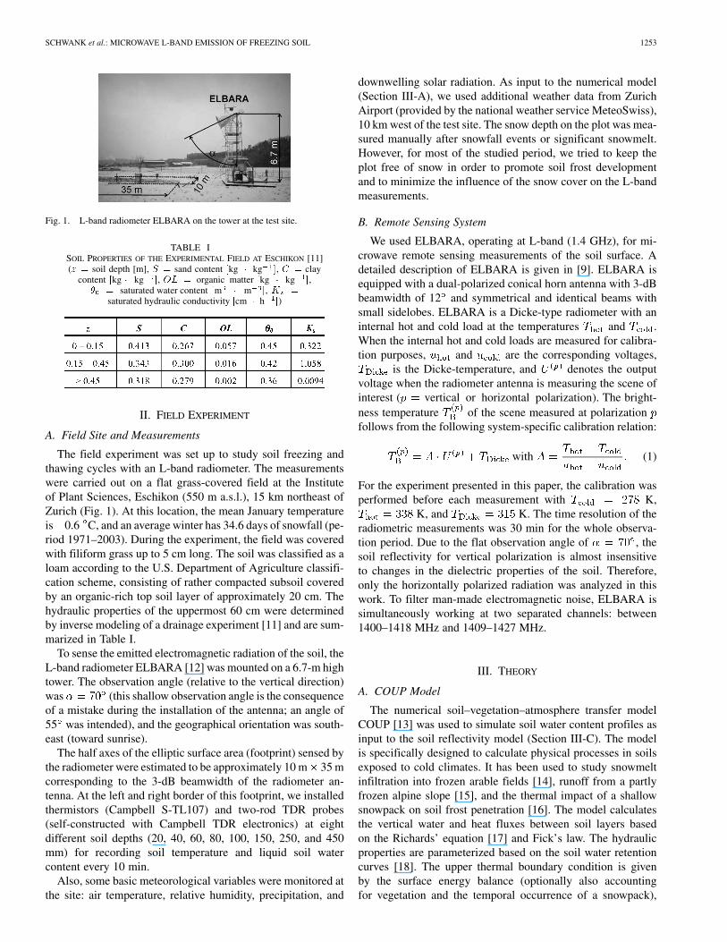
Fig. 1. L-band radiometer ELBARA on the tower at the test site.

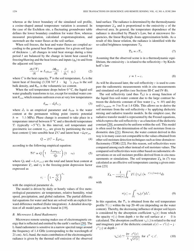
TABLE ISOIL PROPERTIES OF THE EXPERIMENTAL FIELD AT ESCHIKON [11](z = soil depth [m], S = sand content [kg � kg ], C = clay

content [kg � kg ], OL = organic matter [kg � kg ],� = saturated water content [m � m ], K =

saturated hydraulic conductivity [cm � h ])

II. FIELD EXPERIMENT

A. Field Site and Measurements

The field experiment was set up to study soil freezing andthawing cycles with an L-band radiometer. The measurementswere carried out on a flat grass-covered field at the Instituteof Plant Sciences, Eschikon (550 m a.s.l.), 15 km northeast ofZurich (Fig. 1). At this location, the mean January temperatureis 0.6 C, and an average winter has 34.6 days of snowfall (pe-riod 1971–2003). During the experiment, the field was coveredwith filiform grass up to 5 cm long. The soil was classified as aloam according to the U.S. Department of Agriculture classifi-cation scheme, consisting of rather compacted subsoil coveredby an organic-rich top soil layer of approximately 20 cm. Thehydraulic properties of the uppermost 60 cm were determinedby inverse modeling of a drainage experiment [11] and are sum-marized in Table I.

To sense the emitted electromagnetic radiation of the soil, theL-band radiometer ELBARA [12] was mounted on a 6.7-m hightower. The observation angle (relative to the vertical direction)was (this shallow observation angle is the consequenceof a mistake during the installation of the antenna; an angle of55 was intended), and the geographical orientation was south-east (toward sunrise).

The half axes of the elliptic surface area (footprint) sensed bythe radiometer were estimated to be approximately 10 m 35 mcorresponding to the 3-dB beamwidth of the radiometer an-tenna. At the left and right border of this footprint, we installedthermistors (Campbell S-TL107) and two-rod TDR probes(self-constructed with Campbell TDR electronics) at eightdifferent soil depths (20, 40, 60, 80, 100, 150, 250, and 450mm) for recording soil temperature and liquid soil watercontent every 10 min.

Also, some basic meteorological variables were monitored atthe site: air temperature, relative humidity, precipitation, and

downwelling solar radiation. As input to the numerical model(Section III-A), we used additional weather data from ZurichAirport (provided by the national weather service MeteoSwiss),10 km west of the test site. The snow depth on the plot was mea-sured manually after snowfall events or significant snowmelt.However, for most of the studied period, we tried to keep theplot free of snow in order to promote soil frost developmentand to minimize the influence of the snow cover on the L-bandmeasurements.

B. Remote Sensing System

We used ELBARA, operating at L-band (1.4 GHz), for mi-crowave remote sensing measurements of the soil surface. Adetailed description of ELBARA is given in [9]. ELBARA isequipped with a dual-polarized conical horn antenna with 3-dBbeamwidth of 12 and symmetrical and identical beams withsmall sidelobes. ELBARA is a Dicke-type radiometer with aninternal hot and cold load at the temperatures and .When the internal hot and cold loads are measured for calibra-tion purposes, and are the corresponding voltages,

is the Dicke-temperature, and denotes the outputvoltage when the radiometer antenna is measuring the scene ofinterest ( vertical or horizontal polarization). The bright-ness temperature of the scene measured at polarizationfollows from the following system-specific calibration relation:

with (1)

For the experiment presented in this paper, the calibration wasperformed before each measurement with K,

K, and K. The time resolution of theradiometric measurements was 30 min for the whole observa-tion period. Due to the flat observation angle of , thesoil reflectivity for vertical polarization is almost insensitiveto changes in the dielectric properties of the soil. Therefore,only the horizontally polarized radiation was analyzed in thiswork. To filter man-made electromagnetic noise, ELBARA issimultaneously working at two separated channels: between1400–1418 MHz and 1409–1427 MHz.

III. THEORY

A. COUP Model

The numerical soil–vegetation–atmosphere transfer modelCOUP [13] was used to simulate soil water content profiles asinput to the soil reflectivity model (Section III-C). The modelis specifically designed to calculate physical processes in soilsexposed to cold climates. It has been used to study snowmeltinfiltration into frozen arable fields [14], runoff from a partlyfrozen alpine slope [15], and the thermal impact of a shallowsnowpack on soil frost penetration [16]. The model calculatesthe vertical water and heat fluxes between soil layers basedon the Richards’ equation [17] and Fick’s law. The hydraulicproperties are parameterized based on the soil water retentioncurves [18]. The upper thermal boundary condition is givenby the surface energy balance (optionally also accountingfor vegetation and the temporal occurrence of a snowpack),

1254 IEEE TRANSACTIONS ON GEOSCIENCE AND REMOTE SENSING, VOL. 42, NO. 6, JUNE 2004

whereas at the lower boundary of the simulated soil profile,a cosine-shaped annual temperature variation is assumed. Inthe case of the Eschikon site, a fluctuating groundwater tabledefines the lower boundary condition for water flow, whereasmeasured precipitation, calculated evapotranspiration, andsnowmelt are the water fluxes at the soil surface.

When soil freezes, the heat and water fluxes are coupled ac-cording to the general heat flow equation: for a given soil layerof thickness , all changes in total heat storage during a timeperiod are balanced by the change in latent heat caused byfreezing/thawing and the heat losses and inputs ( ) to and fromthe adjacent soil layers

(2)

where is the heat capacity, is the soil temperature, is thelatent heat of freezing (3.338 J kg ), is the soilbulk density, and is the volumetric ice content.

When the soil temperature drops below 0 C, the liquid soilwater gradually transforms to ice, except for residual water con-tent , which remains unfrozen even at very low temperatures

(3)

where is an empirical parameter and is the watercontent at the permanent wilting point (metric potential

MPa). Phase change is assumed to take place in atemperature interval between 0 C and a threshold temperature

(typically 5 C). In this interval, soil temperature andgravimetric ice content are given by partitioning the totalheat content into sensible heat and latent heat

(4)

according to the following empirical equation:

(5)

where and are the total and latent heat content attemperature , and is the freezing-point depression factorexpressed as

(6)

with the empirical parameter .The model is driven by daily or hourly values of five mete-

orological parameters: air temperature, relative humidity, windspeed, precipitation, and global radiation. The partial differen-tial equations for water and heat are solved with an explicit for-ward difference method (Euler integration). A detailed descrip-tion of all model parts can be found in [19].

B. Microwave L-Band Radiometry

Microwave remote sensing makes use of electromagnetic en-ergy that is reflected and emitted by the earth’s surface [20]. TheL-band radiometer is sensitive in a narrow spectral range aroundthe frequency of 1.4 GHz (corresponding to the wavelength of21 cm). At L-band, the main contribution of the electromagneticradiance is given by the thermal self-emission of the observed

land surface. The radiance is determined by the thermodynamictemperature and is proportional to the emissivity of theobserved area. In general, the temperature dependence of theradiance is described by Planck’s Law, but at microwave fre-quencies, the linear Rayleigh–Jeans approximation holds. As aresult of this linear relation, the radiance is identified with theso-called brightness temperature

(7)

Assuming that the observed scene is in a thermodynamic equi-librium, the emissivity is related to the reflectivity by Kirch-hoff’s law

(8)

As will be discussed later, the soil reflectivity is used to com-pare the radiometric measurements with in situ measurementsand simulated soil profiles (see Sections III-C and IV-B).

The soil reflectivity (and thus ) is a strong function ofthe liquid free-soil-water content due to the large contrast be-tween the dielectric constant of free water ( ) and drysoil ( 3 to 5) at 1.4 GHz. This allows us to derive thesoil moisture from the soil reflectivity by applying dielectricmixing and radiative transfer models. In the simplest case, theradiative transfer model is represented by the Fresnel equations,which express the soil reflectivity as a function of the dielectricconstant [20], assumed to be uniform within the soil. This modelis often used for the determination of the soil moisture from ra-diometric data [21]. However, the water content derived in thisway is in many cases not comparable to the values obtained fromother soil moisture detection techniques such as time-domain re-flectometry (TDR) [22]. For this reason, soil reflectivities werecompared among each other instead of soil moisture values. Thecompared soil reflectivities were either based on radiometric ob-servations or on soil moisture profiles derived from in situ mea-surements or simulations. The soil temperature in (7) wascalculated as an effective soil temperature causing a given emis-sion [23]

with

(9)

In this equation, the is obtained from the soil temperatureprofile within the top 20–40 cm (depending on the watercontent). Thereby, the decreasing influence of deeper soil layersis considered by the absorption coefficient from whichthe opacity from depth to the soil surface at iscalculated. The absorption coefficient is related to the realand imaginary part of the dielectric constant

at depth

for (10)

SCHWANK et al.: MICROWAVE L-BAND EMISSION OF FREEZING SOIL 1255

C. Calculation of Soil Reflectivity

In this paper, soil reflectivity is the crucial quantity used tocompare radiometric data with TDR- and modeled soil data.Therefore, we calculated three different reflectivities: 1)based on the in situ measured TDR and temperature data; 2)

based on soil water content profiles simulated with anumerical soil water and heat model (COUP; see Section III-A);and 3) the radiometric soil reflectivity as derived from theL-band radiometer and the in situ measured temperature data.

To calculate and , we implemented a coherentradiative transfer model representing the soil as a stratifieddielectric medium consisting of layers with uniform thickness

. The radiative model is based on a matrix formulation ofthe boundary conditions at the layer boundaries derived fromMaxwell’s equations [24]. The output of this algorithm is thesoil reflectivity. The expected inputs are two soil profile vectorscontaining layer thickness and complex dielectric constants ofthe layer stack, wavelength, polarization, and observation angle

.Due to the poor depth resolution of the measured in situ data

(TDR water content and temperature measurements) and of thesoil profiles from the COUP model, it was necessary to increasethe resolution of these profiles to be used as input for the ra-diative transfer model. This was achieved by fitting third-orderpolynomials to the low-resolution profiles, from which soil pro-file vectors were constructed with a virtually increased depthresolution mm.

As will be discussed later (Section IV-B), the radiometricallydetermined soil reflectivity for horizontal polarization issystematically smaller than the reflectivities and ,which were calculated using the radiative transfer model. Abetter fit can be achieved if the radiative model is supplementedby an air-to-soil transition model considering dielectric mixingeffects due to the small-scale surface structure [22] of the ob-served site. In a wider understanding, this model can also ac-count for low plant canopy and thin snow layers on bare soil orfor cavities and stones within the uppermost soil horizon.

Calculation of : The dielectric profile vector requiredfor calculating the reflectivity was generated using thevolumetric liquid water contents measured with the TDRprobes and the temperatures measured at the same depths (seeSection II-A). For any the dielectric constant of thesoil was deduced by applying the dielectric mixing model ofWang and Schmugge [25]. The depth-dependent soil propertiesused in the mixing model are the water content at saturation( ) in cubic millimeters per cubic millimeter and claycontent and in cubic kilograms per cubic kilogram,respectively

(11)

The above profiles were deduced by linear fitting to the soilproperties listed in Table I.

The frequency and temperature dependence of the dielectricconstant of pure free water used in the Wang and Schmugge

model was calculated according to the model of Cole and Cole[26].

Calculation of : The dielectric profile vector requiredfor calculating was generated from the soil water contentprofiles calculated with the numerical soil water and heat trans-port model COUP (see Section III-A). The COUP model yieldsprofiles for the total volumetric water content (frozen plusunfrozen water), volumetric liquid water content , and the soiltemperature profiles . To calculate the soil dielectric constant

from these profiles, the semiempirical mixing model ofDobson [27] was applied. In addition to the three phases liquidwater, air, and soil matrix [28], ice was considered in the mixingmodel as the fourth phase [29]

(12)

The dielectric constants of the air, ice, and soil matrix were as-sumed to be , and

. The exponent was set to 0.5, which is theoreti-cally valid for an isotropic two-phase medium [30]. For the soilporosity , the profile given by (11) was chosen, and the di-electric constant of free water was calculated according toCole and Cole [26].

Calculation of : The soil reflectivity was de-rived from the brightness temperature measured with theradiometer pointing toward the area of observation. The reflec-tivity is related to the soil emissivity by Kirchhoff’slaw [(8)], and is derived from the soil temperature and thebrightness temperature [(7)]. The soil temperature wascalculated according to (9), using the in situ measured tempera-ture profile with improved resolution as described above.

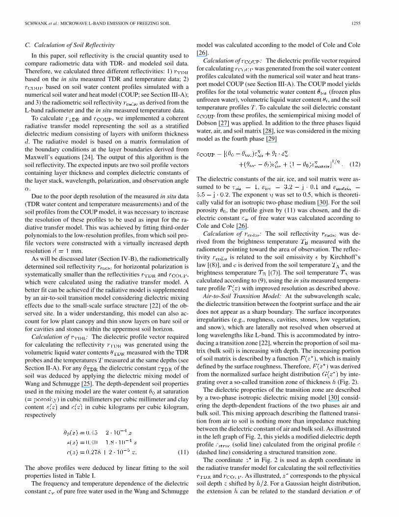
Air-to-Soil Transition Model: At the subwavelength scale,the dielectric transition between the footprint surface and the airdoes not appear as a sharp boundary. The surface incorporatesirregularities (e.g., roughness, cavities, stones, low vegetation,and snow), which are laterally not resolved when observed atlong wavelengths like L-band. This is accommodated by intro-ducing a transition zone [22], wherein the proportion of soil ma-trix (bulk soil) is increasing with depth. The increasing portionof soil matrix is described by a function , which is mainlydefined by the surface roughness. Therefore, was derivedfrom the normalized surface height distribution by inte-grating over a so-called transition zone of thickness (Fig. 2).

The dielectric properties of the transition zone are describedby a two-phase isotropic dielectric mixing model [30] consid-ering the depth-dependent fractions of the two phases air andbulk soil. This mixing approach describing the flattened transi-tion from air to soil is nothing more than impedance matchingbetween the dielectric constant of air and bulk soil. As illustratedin the left graph of Fig. 2, this yields a modified dielectric depthprofile (solid line) calculated from the original profile(dashed line) considering a structured transition zone.

The coordinate in Fig. 2 is used as depth coordinate inthe radiative transfer model for calculating the soil reflectivities

and . As illustrated, corresponds to the physicalsoil depth shifted by . For a Gaussian height distribution,the extension can be related to the standard deviation of

1256 IEEE TRANSACTIONS ON GEOSCIENCE AND REMOTE SENSING, VOL. 42, NO. 6, JUNE 2004

Fig. 2. Illustration of the impedance matching approach applied in theair-to-soil transition model. G = surface height distribution, F = transitionfunction, " (") = dielectric profile considering (no) surface structure.

the surface height, which corresponds to the measurable surfaceroughness within the footprint

(13)

In general, has to be interpreted as the characteristic thicknessof the near-surface layer in which the features roughness, cavi-ties, stones, low vegetation, and snow occur. This interpretationmakes a quantity that can be measured or estimated for theradiometrically observed site.

The small squares in the left graph of Fig. 2 indicate the localTDR measurements at the depths 2 and 4 cm. These depths aregiven relative to the depth representing the average heightof a laterally not resolved area of the order of within theradiometer footprint.

It has been proven that the application of this model yieldssimilar results to those of the roughness model based on physicaloptics [31]. However, the scope of application of the air-to-soiltransition model is broader because it is not limited to pure sur-face roughness but can be applied to incorporate any dielectricinhomogeneities within a soil surface layer.

IV. RESULTS

A. Soil Profile Simulations

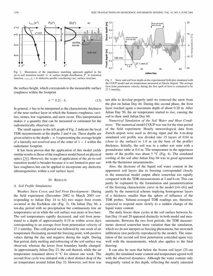
Weather, Snow Cover, and Soil Frost Development: Duringthe field experiment (December 2002 to March 2003 cor-responding to Julian Day 14 to 62) two major frost eventsoccurred at the Eschikon site (Fig. 3). On Julian Day 04, aten-day period with no precipitation but continuously low airtemperatures set in while the soil surface was more or less bare.The soil temperatures rapidly decreased, and soil frost pene-trated to a depth of approximately 0.19 m within seven dayscorresponding to an average frost front penetration velocity of27.1 mm/day. This cold period was followed by one week of airtemperature fluctuating around the freezing point, with positivevalues during the day and negative during the night. Duringthat period, daily melting and refreezing of the soil surface wasobserved, whereas the lower frost boundary hardly changed.At approximately Julian Day 23, the soil thawed, while the airtemperature remained above 0 C for almost one week. Thesecond frost cycle was initiated with a short distinct drop of theair temperature around Julian Day 32. However, soil frost was

Fig. 3. Snow and soil frost depth on the experimental field plot simulated withthe COUP model and air temperature measured at Zürich-Airport. The averagefrost front penetration velocity during the first spell of frost is estimated to be27.1 mm/day.

not able to develop properly until we removed the snow fromthe plot on Julian Day 44. During this second phase, the frostlayer reached again a maximum depth of about 0.20 m. AfterJulian Day 50, the air temperature started to rise, causing thesoil to thaw until Julian Day 60.

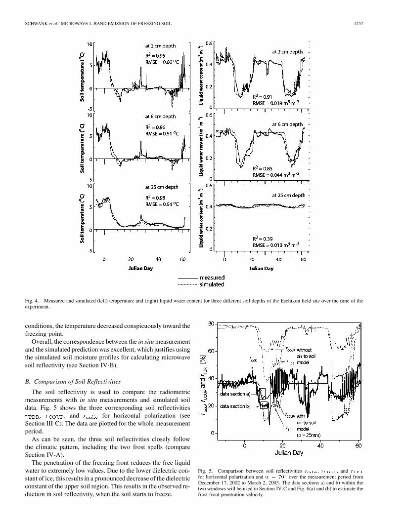
Numerical Simulation of the Soil Water and Heat Condi-tions: The numerical model COUP was run for the time periodof the field experiment. Hourly meteorological data fromZurich airport were used as driving input and the 4-m-deepsimulated soil profile was divided into 15 layers of 0.04 m(close to the surface) to 1.0 m (at the base of the profile)thickness. Initially, the soil was in a rather wet state with agroundwater table at 0.4 m. The temperature in the uppermostmeter of the profile was about 5 C (Fig. 4). The simulatedcooling of the soil after Julian Day 04 was in good agreementwith the thermistor measurements.

Also, the decrease of the liquid soil water content in theuppermost soil layers due to freezing corresponded closelyto the numerical model output albeit somewhat too rapidlycompared with the TDR-measurements at 2 and 6 cm. This canpartly be explained by the formulation and parameterizationof the freezing characteristic curve in the model [(4)–(6)] andpartly by the numerical scheme implying homogenous layersof a thickness smaller than the sphere of influence of theTDR probes. Volume-averaged TDR readings are, therefore,expected to respond more slowly to a sudden change of theliquid water content.

The daily freeze–thaw cycles at the soil surface between Ju-lian Day 14 and 20 appeared distinctly in both model and mea-surements. Between the two frost periods, the TDR measure-ments showed somewhat more variation than the simulation,which we do not interpret as freezing phenomena, but snowmeltinfiltration (not perfectly reproduced by the model). The simu-lation of the second soil frost penetration coincided again verywell with the measurements, which also applies to the finalthawing.

It can also be seen that below the frozen soil layer (25-cmdepth), the simulated water content and temperature agreed wellwith the observed dynamics. Although the water content onlymarginally varied at this depth, reflecting the nearly saturated

SCHWANK et al.: MICROWAVE L-BAND EMISSION OF FREEZING SOIL 1257

Fig. 4. Measured and simulated (left) temperature and (right) liquid water content for three different soil depths of the Eschikon field site over the time of theexperiment.

conditions, the temperature decreased conspicuously toward thefreezing point.

Overall, the correspondence between the in situ measurementand the simulated prediction was excellent, which justifies usingthe simulated soil moisture profiles for calculating microwavesoil reflectivity (see Section IV-B).

B. Comparison of Soil Reflectivities

The soil reflectivity is used to compare the radiometricmeasurements with in situ measurements and simulated soildata. Fig. 5 shows the three corresponding soil reflectivities

, , and for horizontal polarization (seeSection III-C). The data are plotted for the whole measurementperiod.

As can be seen, the three soil reflectivities closely followthe climatic pattern, including the two frost spells (compareSection IV-A).

The penetration of the freezing front reduces the free liquidwater to extremely low values. Due to the lower dielectric con-stant of ice, this results in a pronounced decrease of the dielectricconstant of the upper soil region. This results in the observed re-duction in soil reflectivity, when the soil starts to freeze.

Fig. 5. Comparison between soil reflectivities r , r , and r

for horizontal polarization and � = 70 over the measurement period fromDecember 17, 2002 to March 2, 2003. The data sections a) and b) within thetwo windows will be used in Section IV-C and Fig. 6(a) and (b) to estimate thefrost front penetration velocity.

1258 IEEE TRANSACTIONS ON GEOSCIENCE AND REMOTE SENSING, VOL. 42, NO. 6, JUNE 2004

Qualitatively spoken, the reflectivities and cal-culated without considering the air-to-soil transition model arein good agreement for wet periods (thin dashed and solid lines).When the topsoil is frozen, the observed reduction in thedata is more pronounced than the reduction in the data.This difference in the dynamics of the data can be explained bythe following considerations. As a consequence of the reductionof the liquid water content within the topsoil, the cylindricallyshaped measurement volumes of the TDR probes are extendedin their radial direction. Therefore, the measurement volume ofthe uppermost probe may even include air from above the soilsurface. This results in a systematic underestimation of the top-soil dielectric constant (and water content) at frozen (dry) con-ditions. Since the soil reflectivity is mostly affected by thetopsoil dielectric constant, it is systematically underestimated atfrozen (dry) conditions.

The radiometrically determined reflectivity (bold grayline) is systematically lower than and (thin dashedand solid lines) calculated without considering the air-to-soiltransition model. This deviation can be diminished by consid-ering structural features occurring within a superficial layer ofthe site by applying the air-to-soil transition model described inSection III-C. In this model extension, the transition betweenthe footprint surface and the air is described as a gradual transi-tion (impedance matching approach) from air to bulk soil. Asidefrom soil surface roughness, this approach may also account forlow plant canopy, thin snow layers, or for cavities and stoneswithin the near-surface layer. The characteristic thickness ofthis surface layer in which these features occur was obtainedby an arbitrary guess to be mm. However, this estima-tion was compatible with the visual inspection of the footprintsurface. The resulting reduction of the dielectric gradient at thesurface (compare left graph of Fig. 2) yields a reduction of thecalculated reflectivities and thus a better agreement with the ra-diometric soil reflectivity (see bold dotted and solid linesin Fig. 5).

The daily fluctuations in the radiometrically determined soilreflectivity during the two thawing periods (Julian Day15–22 and 50–60) are much more pronounced compared to thesoil reflectivities and . This could be explained bythe daily occurrence of a thin liquid water layer at the very top ofthe soil, affecting the radiometric soil reflectivities moredistinctly.

Just after Julian day 13, a short-time drop in the air temper-ature and the simultaneous occurrence of a snow layer (Fig. 3)might be the reason for the observed drop in depicted inFig. 5.

The radiometric reflectivities included daily occurring sharpdrops, which were identified to be caused by solar radiationreflected by the site surface and transmitted to the radiometerfacing toward the sunset. These spikes were eliminated from thedata to enable the following discussion of coherent effects.

C. Estimation of Frost Front Penetration Velocity

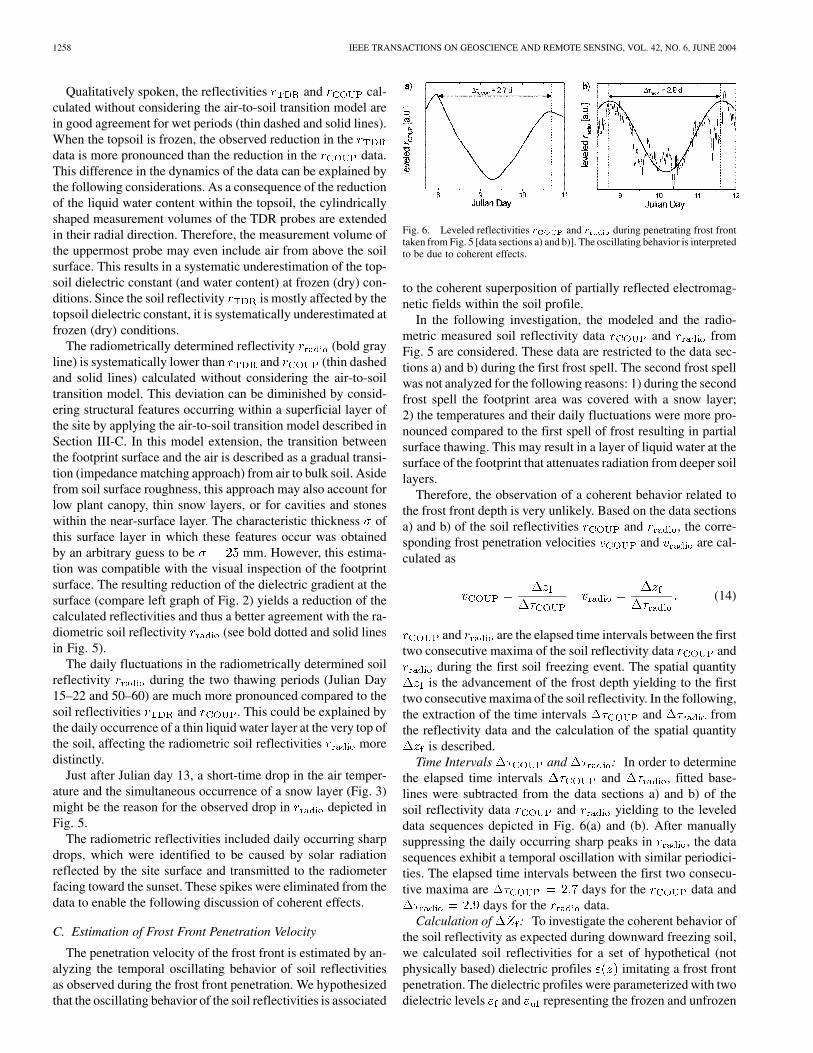
The penetration velocity of the frost front is estimated by an-alyzing the temporal oscillating behavior of soil reflectivitiesas observed during the frost front penetration. We hypothesizedthat the oscillating behavior of the soil reflectivities is associated

Fig. 6. Leveled reflectivities r and r during penetrating frost fronttaken from Fig. 5 [data sections a) and b)]. The oscillating behavior is interpretedto be due to coherent effects.

to the coherent superposition of partially reflected electromag-netic fields within the soil profile.

In the following investigation, the modeled and the radio-metric measured soil reflectivity data and fromFig. 5 are considered. These data are restricted to the data sec-tions a) and b) during the first frost spell. The second frost spellwas not analyzed for the following reasons: 1) during the secondfrost spell the footprint area was covered with a snow layer;2) the temperatures and their daily fluctuations were more pro-nounced compared to the first spell of frost resulting in partialsurface thawing. This may result in a layer of liquid water at thesurface of the footprint that attenuates radiation from deeper soillayers.

Therefore, the observation of a coherent behavior related tothe frost front depth is very unlikely. Based on the data sectionsa) and b) of the soil reflectivities and , the corre-sponding frost penetration velocities and are cal-culated as

(14)

and are the elapsed time intervals between the firsttwo consecutive maxima of the soil reflectivity data and

during the first soil freezing event. The spatial quantityis the advancement of the frost depth yielding to the first

two consecutive maxima of the soil reflectivity. In the following,the extraction of the time intervals and fromthe reflectivity data and the calculation of the spatial quantity

is described.Time Intervals and : In order to determine

the elapsed time intervals and , fitted base-lines were subtracted from the data sections a) and b) of thesoil reflectivity data and yielding to the leveleddata sequences depicted in Fig. 6(a) and (b). After manuallysuppressing the daily occurring sharp peaks in , the datasequences exhibit a temporal oscillation with similar periodici-ties. The elapsed time intervals between the first two consecu-tive maxima are days for the data and

days for the data.Calculation of : To investigate the coherent behavior of

the soil reflectivity as expected during downward freezing soil,we calculated soil reflectivities for a set of hypothetical (notphysically based) dielectric profiles imitating a frost frontpenetration. The dielectric profiles were parameterized with twodielectric levels and representing the frozen and unfrozen

SCHWANK et al.: MICROWAVE L-BAND EMISSION OF FREEZING SOIL 1259

Fig. 7. Hypothetical dielectric profile "(z) imitating a frost front located atthe depth z .

soil state, the depth of the transition between frozen and un-frozen state, and the steepness parameter describing the widthof the transition zone

(15)

The term in the squared brackets is the Fermi-distribution cen-tered at the with steepness . Fig. 7 shows a plot of the profilegiven by (15) with mm, mm and the dielectricconstants and , which are reasonable values forwet frozen and unfrozen soils [32].

From a set of dielectric profiles with variable , we cal-culated L-band reflectivities at the observation angle 70for horizontal polarization using the coherent radiative transfermodel described in Section III-C. Fig. 8 shows the dependenceof the reflectivity from the frost depth parameter . The firsttwo consecutive local maxima occur at mm and

mm. This corresponds to an advancement of the frost frontdepth from the first to the second maximum of mm.

Further calculations showed that the dielectric constant ofthe frozen soil is the dominant parameter affecting of thefrost depth propagation. The parameters and as well asan imaginary part of affect the amplitude of the oscillatingbehavior of the reflectivity, but play only a subsidiary role forthe spatial periodicity . For example, the variation of the lesssensitive parameter with and mmyields to the narrow range of mm mm. Thevariation of the sensitive parameter with and

mm within a reasonable range of for thedielectric constant of the frozen soil covers the wider range of

mm mm.Assuming that the temporal periods and

and the spatial period are assigned to the same advance-ment of the frost front enables calculation of the frost penetra-tion velocities and according to (14)

mm/day mm/day (16)

From the COUP simulations of the frost depths during the firstfreezing period, the frost penetration velocity was estimated to

Fig. 8. Reflectivity r for horizontal polarization and � = 70 calculated for aset of hypothetical dielectric profiles "(z) as a function of the frost front depthparameter z .

be 27.1 mm/day (Fig. 3) by linear approximation to the ad-vancing frost front. This is in good agreement with the pene-tration velocities and calculated above.

It should be mentioned that the data during the pene-trating frost front showed no coherent behavior. It is supposedthat this is due to the deterioration of the depth resolution ofthe TDR water content profiles because of the increase of theTDR measurement volume. This leads to an overestimation ofthe TDR measured liquid water content within the frozen soilpart, which reduces the dielectric gradient to the unfrozen soil,hindering the occurrence of coherent effects.

V. CONCLUSION

The L-band radiometer measurements obtained during awinter period at a field site clearly revealed the high sensitivityof microwave emission to ground surface freezing.

We demonstrated that the quantitative consistency betweenthe radiometrically observed reflectivity and the reflectivitiesbased on in situ measured and modeled profiles was signifi-cantly improved by applying an impedance matching approach.With this approach, we took structural effects into account suchas soil surface roughness, low plant canopy, thin snow layers,cavities, and stones showing up within a near-surface layer ofcharacteristic thickness . With mm, we obtained thebest agreement between the soil reflectivities. The value forwas obtained through an arbitrary guess, which is consistentwith the visual inspection of the footprint surface.

The potential of estimating the soil frost penetration velocityfrom the radiometrically measured L-band radiation wasdemonstrated by means of evaluating the observed coherentbehavior of the soil reflectivity during an advancing frost front.The time period between the first two maxima of the observedoscillation was determined to be 2.9 days. The calculatedsoil reflectivities based on the hypothetical dielectric profilesimitating a superficial frozen soil revealed an advancement ofthe frost front of 72 mm to generate the first two consecutivemaxima. From this, we estimated the radiometrically observedpenetration velocity of the frost front to be 25 mm/day. Thiswas in good agreement with the frost penetration velocityestimated with the numerical soil water and heat model.

1260 IEEE TRANSACTIONS ON GEOSCIENCE AND REMOTE SENSING, VOL. 42, NO. 6, JUNE 2004

ACKNOWLEDGMENT

The authors are grateful to C. Stamm for the initiation of thepresented experiment. Special thanks to K. Schneeberger whocontributed to this work with her extensive experience in radio-metric remote sensing of soil moisture.

REFERENCES

[1] L. Oygarden, “Rill and gully development during an extreme winterrunoff event in Norway,” CATENA, vol. 50, no. 2–4, pp. 217–242, 2003.

[2] Y. Kerr, P. Waldteufel, J.-P. Wigneron, J.-M. Martinuzzi, J. Front, andM. Berger, “Soil moisture retrieval from space: The soil Moisture andOcean Salinity (SMOS) mission,” IEEE Trans. Geosci. Remote Sensing,vol. 39, pp. 1729–1735, Aug. 2001.

[3] P.-E. Mellander, K. Bishop, and T. Lundmark, “The influence of soiltemperature on transpiration: A plot scale manipulation in a young Scotspine stand,” Forest Ecol. Manage., to be published.

[4] M. Phillips, S. M. Springman, and L. U. Arenson, Permafrost—Proc. 8thInt. Conf. Permafrost, vol. 1380, Zurich, Switzerland, July 21–25, 2003,p. 2003.

[5] E. Njoku and J.-A. Kong, “Theory for passive microwave remote sensingof near-surface soil moisture,” J. Geophys. Res., vol. 82, pp. 3108–3118,1977.

[6] T. Jackson and T. Schmugge, “Passive microwave remote sensing systemfor soil moisture: Some supporting research,” IEEE Trans. Geosci. Re-mote Sensing, vol. 27, pp. 225–235, Mar. 1989.

[7] T. Zhang and R. L. Armstrong, “Soil freeze/thaw cycles over snow-freeland detected by passive microwave remote sensing,” Geophys. Res.Lett., vol. 28, no. 5, pp. 763–766, 2001.

[8] T. J. Schmugge and T. J. Jackson, “Observation of coherent emissionsfrom soils,” Radio Sci., vol. 33, no. 2, pp. 267–272, 1998.

[9] C. Mätzler, D. Weber, M. Wüthrich, K. Schneeberger, C. Stamm, H.Wydler, and H. Flühler, “ELBARA, the ETH L-band radiometer for soil-moisture research,” in Procs. IGARSS, Toulouse, France, July 2003.

[10] K. Schneeberger, C. Stamm, C. Mätzler, and H. Flühler, “Estimating soilhydraulic properties from time-series of L-band measured water con-tents,” in Procs. IGARSS, Toulouse, July 21–25, 2003.

[11] A. Fehlmann, “Preliminary experiments in Eschikon to determine soilproperties,” Inst. Terrestrial Ecol., ETH Zürich, Zürich, Switzerland, Int.Rep., 2001.

[12] K. Schneeberger, C. Stamm, C. Mätzler, and H. Flühler, “Ground-baseddual-frequency radiometry of bare soil at high temporal resolution,”IEEE Trans. Geosci. Remote Sensing, vol. 42, pp. 588–595, Mar. 2004.

[13] P.-E. Jansson and D. Moon, “A coupled model of water, heat and masstransfer using object orientation to improve flexibility and function-ality,” Environ. Model. Software, vol. 16, no. 1, pp. 37–46, 2001.

[14] M. Stähli, P.-E. Jansson, and L.-C. Lundin, “Soil moisture redistributionand infiltration in frozen sandy soils,” Water Resources Res., vol. 35, pp.95–103, 1999.

[15] D. Stadler, H. Flühler, and P.-E. Jansson, “Modeling vertical and lat-eral water flow in frozen and sloped forest soil plots,” Cold Reg. Sci.Technol., vol. 26, no. 3, pp. 181–194, 1997.

[16] D. Gustafsson, M. Stähli, and P.-E. Jansson, “The surface energy balanceof a snow cover: Two different simulation models and measurements,”Theoret. Appl. Climat., vol. 70, no. 1–4, pp. 81–96, 2001.

[17] L. A. Richards, “Capillary conduction of liquids in porous mediums,”Physics, vol. 1, pp. 318–333, 1931.

[18] M. T. Van Genuchten, “A closed form equation for predicting the hy-draulic conductivity of unsaturated soils,” Soil Sci. Soc. Amer. J., vol.44, pp. 892–898, 1980.

[19] P.-E. Jansson and L. Karlberg, “Coupled heat and mass transfer modelfor soil-plant-atmosphere systems,” Div. Land and Water Resources,Royal Inst. Technol., Stockholm, Sweden, ISSN 1400–1306, 2001.

[20] F. Ulaby, R. Moore, and A. Fung, Microwave Remote Sensing Active andPassive. Microwave Remote Sensing and Fundamentals and Radiom-etry. Reading, MA: Addison-Wesley, 1981, vol. I.

[21] T. Schmugge, “Remote sensing of soil moisture,” in Hydrological Fore-casting, M. Anderson and T. Burt, Eds. New York: Wiley, 1985, pp.101–124.

[22] K. Schneeberger, M. Schwank, C. Stamm, P. de Rosnay, C. Mätzler,and H. Flühler, “Topsoil properties influencing soil moisture retrievalby microwave radiometry,” Water Resources Res., to be published.

[23] F. Ulaby, R. Moore, and A. Fung, Microwave Remote Sensing Active andPassive. Norwood, MA: Artech House, 1986, vol. III, From Theory toApplications.

[24] Handbook of Optics, vol. 1, M. Bass, E.W. Van Stryland, R. Williams,and W. L. Wolfe, Eds., McGraw-Hill, New York, 1995, pp. 42.9–42.14.

[25] J. Wang and T. Schmugge, “An empirical model for complex dielectricpermittivity of soils as a function of water content,” IEEE Trans. Geosci.Remote Sensing, vol. GE-18, pp. 288–295, 1980.

[26] K. S. Cole and R. H. Cole, “Dispersion and absorption in dielectrics,” J.Chem. Phys., vol. 9, pp. 341–351, 1941.

[27] M. C. Dobson, F. T. Ulaby, M. T. Hallikainen, and M. A. El-Rayes, “Mi-crowave dielectric behavior of wet soil, II: Dielectric mixing models,”IEEE Trans. Geosci. Remote Sensing, vol. GE-23, pp. 35–46, Jan. 1985.

[28] K. Roth, R. Schulin, H. Flühler, and W. Attinger, “Calibration oftime domain reflectometry for water content measurement using acomposite dielectric approach,” Water Resources Res., vol. 26, no. 10,pp. 2267–2273, 1990.

[29] M. Stähli and D. Stadler, “Measurement of water and solute dynamics infreezing soil columns with time domain reflectometry,” J. Hydrol., vol.195, pp. 352–369, 1997.

[30] J. R. Birchak, C. G. Gardner, J. E. Hipp, and J. M. Victor, “High dielec-tric constant microwave probes for sensing soil moisture,” Proc. IEEE,vol. 62, pp. 93–98, 1974.

[31] F. Ulaby, R. Moore, and A. Fung, Microwave Remote Sensing Activeand Passive. Reading, MA: Addison-Wesley, 1981, vol. II, MicrowaveRemote Sensing and Fundamentals and Radiometry, p. 1009.

[32] C. Mätzler, “Passive microwave signature catalog 1989 –1992 (vol. 1),”Univ. Bern, Bern, Switzerland, IAP-Rep., 1993.

Mike Schwank received the Ph.D. degree in physicsfrom the Swiss Federal Institute of TechnologyZürich (ETH), Zürich, Switzerland, in 1999. Thetopic of his Ph.D. dissertation was “nano-lithog-raphy using a high-pressure scanning-tunnelingmicroscope.”

From 2000 to 2002, he was a Research and Devel-opment Engineer in the field of micro-optics. He iscurrently a Senior Research Assistant with the Insti-tute of Terrestrial Ecology, ETH-Zürich. His researchinvolves practical and theoretical aspects of radiom-

etry applied to soil moisture detection

Manfred Stähli received the Ph.D. degree inenvironmental physics from the Swedish Universityof Agricultural Sciences, Uppsala, Sweden, in 1998.His research focused on heat and water transportprocesses in seasonally frozen soils.

In 1998, he became a Postdoc with the Institute ofTerrestrial Ecology, Swiss Federal Institute of Tech-nology Zürich, Zürich, Switzerland, and since 2001,he has been working with the Swiss Federal ResearchInstitute WSL in the Forest Hydrology Team. He iscurrently studying snow hydrological issues, some of

them related to frozen soil conditions.

Hannes Wydler is an Electrical Engineering Tech-nician. Since 1983, he has been supporting the SoilPhysics Group of the Institute of Terrestrial Ecology,Swiss Federal Institute of Technology Zürich, Zürich,Switzerland, in developing experimental setups.

SCHWANK et al.: MICROWAVE L-BAND EMISSION OF FREEZING SOIL 1261

Joerg Leuenberger is a skilled Forester and has beena member of the technical staff of the Institute of Ter-restrial Ecology (Soil Physics), ETH Zürich, Zürich,Switzerland, since 1971. His main working tasks areto support the group in designing field experimentalsetups. He is currently involved in planning the exper-imental setup for ongoing radiometric experiments.

Christian Mätzler (M’96–SM’03) studied physicsat the University of Bern, Bern, Switzerland, withsubsidiaries in mathematics and geography.

After his doctoral thesis (1974) in solar radio as-tronomy, he made Postdoctoral Studies at the NASAGoddard Space Flight Center, Greenbelt, MD, andat the Swiss Federal Institute of Technology Zürich,Zürich, Switzerland. He is currently Titularprofessorin applied physics and remote sensing, leading theProject Group on Radiometry for EnvironmentalMonitoring, Institute of Applied Physics, Univer-

sity of Bern. His experimental studies have concentrated on surface-basedmicrowave (1–100 GHz) signatures for active and passive microwave remotesensing of snow, ice, soil, vegetation, and atmosphere, including precipitation,clouds, and the boundary layer, and on the development of methods fordielectric measurements of these media, with complementary work at opticalwavelengths. He is interested in meteorological applications of remote sensingand in improvements of the physical understanding of the processes involved.Based on the experimental work of his group, he has developed and testedmicrowave (1–100 GHz) propagation, transmission, emission, scattering, anddielectric models of snowpacks and of the atmosphere.

Dr. Mätzler is a member of the International Glaciological Society.

H. Flühler studied at the Department of Forest Sci-ences, Swiss Federal Institute of Technology (ETH)Zürich, Zürich, Switzerland, and received the Ph.D.degree in 1972. He did his postgraduate studies in soilphysics at the ETH Zürich, in 1973, and at the Uni-versity of California, Riverside, from 1974 to 1976.

From 1977 to 1980, he led the Biophysics Group atthe Federal Institute for Forestry Research, and from1980 to 1983, he chaired the Vegetation and Soil Sec-tion at this institute. Since 1983, he has been a Pro-fessor of soil physics at ETH Zürich. His research is

focused on transport processes in soil, specifically in methodology, but also inrelation to environmental applications.