https://doi.org/10.15388/vu.thesis.220

https://orcid.org/0000-0001-8035-3938

VILNIUS UNIVERSITY

Mindaugas

JUSIS

Method of data synchronization of

autonomous port handling processes

DOCTORAL DISSERTATION

Technological Sciences

Informatics Engineering (T 007)

VILNIUS 2021

The dissertation was prepared in 2016 – 2020 at Vilnius University.

Scientific supervisor:

Prof. Dr. Saulius Gudas (Vilnius University, Technological Sciences,

Informatics Engineering – T 007)

Scientific consultant:

Prof. Dr. Arūnas Andziulis (Klaipėda University, Technological Sciences,

Informatics Engineering – T 007)

https://doi.org/10.15388/vu.thesis.220

https://orcid.org/0000-0001-8035-3938

VILNIAUS UNIVERSITETAS

Mindaugas

JUSIS

Uosto autonominių krovos procesų

duomenų sinchronizavimo metodas

DAKTARO DISERTACIJA

Technologijos mokslai,

Informatikos inžinerija (T 007)

VILNIUS 2021

Disertacija parengta 2016 – 2020 metais Vilniaus universitete.

Mokslinis vadovas:

prof. dr. Saulius Gudas (Vilniaus universitetas, technologijos mokslai,

Informatikos inžinerija – T 007)

Mokslinis konsultantas:

prof. dr. Arūnas Andziulis (Klaipėdos universitetas, technologijos mokslai,

Informatikos inžinerija – T 007)

5

LIST OF TERMS AND ABBREVIATIONS

AGV – Automated Guided Vehicles.

ABP – Activation by Personalization.

AS – Application Server.

BPMN – Business Process Model and Notation is a graphical

representation for specifying business processes in a business process model.

ED – End Device.

BLE – Bluetooth Low Energy.

4G – 4th generation cellular network technologies such as LTE.

FIS – Fuzzy Interference System.

GPS – Global Positioning System.

GW – Gateway.

ICT – Information and Communication Technology.

IEEE – Institute of Electrical and Electronics Engineers.

IoT – Internet of Things.

IP – Internet Protocol.

IR sensor – an electronic device, that emits light to sense some object of

the surroundings.

LoRa – is a low-power wide-area network modulation technique.

LoRaWAN – Low Power, Wide Area (LPWA) networking protocol

designed to wirelessly connect battery-operated things to the internet in

regional, national, or global networks, and targets key Internet of Things (IoT)

requirements such as bi-directional communication, end-to-end security, etc.

LPWAN – Low Power Wide Area Networks.

LTE – Long-Term Evolution. A mobile communication standard. In the

cellular network, mobile data can be transferred over the air in larger amounts

and at higher speeds than was possible under previous wireless

communication standards.

MAC – Media Access Control.

MCP – Monte Carlo particle.

NB-IoT – Narrow Band IoT.

NS – Network Server.

OCR – Optical character recognition.

OTAA – Over-The-Air-Activation.

PI – proportional-integral controller.

PID – proportional-integral-derivative controller.

QC – quay cranes.

PWM – Pulse Width Modulation.

RFID – Radio Frequency Identification.

6

RTLS – Real-Time Location System.

SIM – Subscriber Identification Module.

STS – Ship-To-Shore gantry crane.

UHF – Ultra High Frequency.

UKF – Unscented Kalman filter.

Wi-Fi – (shortened form of Wireless Fidelity). A family of wireless

network protocols, based on the IEEE 802.11 family of standards, which are

commonly used for local area networking of devices and Internet access.

WSN – Wireless Sensor Network.

7

LIST OF FIGURES

Figure 1. Visualization of a container terminal in the case of operation

synchronization area. ................................................................................ 21

Figure 2. Crane control model using PID regulator (MATLAB Simulink)

[13]. .......................................................................................................... 25

Figure 3. Metal strip with a very low-frequency generator [66]. ............ 29

Figure 4. Antenna interaction with magnetic field [67]. ........................ 29

Figure 5. BPMN diagram of electromagnetic reference point navigation

method...................................................................................................... 30

Figure 6. Working principle of the transponder [65]. ............................ 31

Figure 7. BPMN diagram representing AGV laser navigation method. . 32

Figure 8. BPMN diagram of AGV control method using a color line. ... 34

Figure 9. BPMN diagram representing a GPS-based AGV control system.

................................................................................................................. 35

Figure 10. BPMN diagram of passive RFID tag read principle.............. 38

Figure 11. Rich picture of the LoRaWAN network for IoT applications in

ports. ........................................................................................................ 42

Figure 12. Comparison of wireless communication technologies [99]. .. 43

Figure 13. Rich picture of the proposed LoRa application concept. ....... 47

Figure 14. Security mechanisms developed and integrated into LoRaWAN.

................................................................................................................. 49

Figure 15. The data acquisition and transfer algorithm for each LoRaWAN

node.......................................................................................................... 50

Figure 16. Data flow diagram for the total AGV assignment process. ... 50

Figure 17. Handling processes synchronization sequence diagram. ....... 51

Figure 18. Concept of LoRaWAN network in a container terminal. ...... 52

Figure 19. The satellite view of the container terminal in Klaipėda. ...... 52

Figure 20. Concept model of the synchronization of container handling

processes (swim lane diagram proposed by the author). ............................. 53

Figure 21. Developed algorithm for AGV positioning (flow chart diagram).

................................................................................................................. 54

Figure 22. Port cargo handling process cause and effect (fishbone)

diagram. ................................................................................................... 56

Figure 23. Model of the AGV. ............................................................. 57

Figure 24. Example of the total mass change during a single cycle in the

terminal. ................................................................................................... 58

Figure 25. The main system components of the quay crane prototype. .. 63

Figure 26. Block diagram of lifting mechanism mechanical subsystem

(MATLAB Simulink). .............................................................................. 65

8

Figure 27. Crane prototype scheme used in the experimental study in the

laboratory. ................................................................................................ 67

Figure 28. The data acquisition equipment used for experimental

measurements at Klaipėda seaport. ............................................................ 68

Figure 29. Demonstration of the Data Acquisition sensory hardware

placement on the crane spreader. ............................................................... 70

Figure 30. Demonstration of the trucks being used and the mounting point

chosen for the experiments. ....................................................................... 71

Figure 31. Demonstration of the sensory unit placement on the roof of the

truck. ........................................................................................................ 72

Figure 32. S-shape velocity profile (green), trolley velocity (blue) and

spreader oscillation velocity (red) graphs with PID controller and one

feedback. .................................................................................................. 73

Figure 33. Distribution of the duration of the processes of the crane. .... 75

Figure 34. Distribution of the duration of the processes of the trucks. ... 76

Figure 35. Statistical analysis of the results. ......................................... 77

Figure 36. Spreader position detection and movement points during the

container unloading operation from the ship. ............................................. 78

Figure 37. Demonstration of spreader speed actual values during the 7

stages of operation. ................................................................................... 79

Figure 38. Demonstration of spreader and container sway oscillation

during the 7 stages of operation. ................................................................ 80

Figure 39. Relationship between the duration of a truck ride in the port area

and the distance traveled. .......................................................................... 81

Figure 40. Distribution of the duration of truck movement in the port area.

................................................................................................................. 82

Figure 41. Distribution of distances traveled in the port territory. ......... 82

Figure 42. The trajectory of the truck in the terminal (b – beginning; e –

end). ......................................................................................................... 83

Figure 43. Track mass variation during the container transportation cycle.

................................................................................................................. 84

Figure 44. Truck velocity during a single transportation cycle. ............. 84

Figure 45. The changes of accelerations along the truck movement

direction (longitudinal acceleration). ......................................................... 85

Figure 46. Instantaneous truck moving power (acceleration and continuous

power for driving) and braking power. ...................................................... 85

Figure 47. Calculated fuel consumption during a single-cycle drive of the

loaded truck. ............................................................................................. 86

Figure 48. Histogram of truck fuel consumption at downtimes. ............ 87

Figure 49. The photo of a STS crane in the container terminal area. ...... 88

9

Figure 50. The photo of container trucks in the container terminal area. 89

Figure 51. LoRaWAN gateway equipment used for experiments. ......... 90

Figure 52. Structure of LoRaWAN gateway. ........................................ 90

Figure 53. Monitoring the environment of LoRaWAN gateway. ........... 91

Figure 54. Sensor data transfer experimental study using LoRaWAN

(temperature and humidity). ...................................................................... 91

Figure 55. The use case of the LoRaWAN experimental study. ............ 93

Figure 56. Visualization of experimental results of signal strength. ....... 95

Figure 57. Experimental results analyzing the RSSI vs distance with the

moving node. ............................................................................................ 95

10

LIST OF TABLES

Table 1. Comparison of wireless communication technologies. ............ 43

Table 2. LoRaWAN and other wireless technologies comparison. ........ 48

Table 3. Quay crane handling operations and their durations. ............... 74

Table 4. Packet structure of LoRaWAN node. ...................................... 91

Table 5. Packet structure of LoRaWAN gateway. ................................. 92

Table 6. Comparison of the proposed data synchronization method. ..... 94

11

CONTENTS

LIST OF TERMS AND ABBREVIATIONS ..................................... 5

LIST OF FIGURES ........................................................................... 7

LIST OF TABLES .......................................................................... 10

CONTENTS .................................................................................... 11

INTRODUCTION ........................................................................... 14

1. LITERATURE REVIEW OF WIRELESS AND CONTROL

TECHNOLOGIES IN AUTONOMOUS PORTS FOR CRANES

AND AUTOMOTIVE GUIDED VEHICLES .................................. 20

1.1. Autonomous container terminals – new challenges and problems ..... 20

1.1.1. The role of quay cranes to improve the performance of container

terminals ................................................................................................... 20

1.1.2. The role of automated guided vehicles to improve the performance of

container terminals .................................................................................... 22

1.1.3. The analysis of container lowering processes ................................ 23

1.2. Methods for autonomous vehicles movement control and navigation in

port area ................................................................................................... 27

1.2.1. Electromagnetic lines method ....................................................... 28

1.2.2. Electromagnetic reference point method ....................................... 30

1.2.3. Laser navigation method............................................................... 32

1.2.4. Optical navigation method ............................................................ 33

1.2.5. GPS navigation method ................................................................ 35

1.2.6. Short sub-section discussions........................................................ 36

1.3. Alternative wireless communication technologies and LoRaWAN

application for port operations ................................................................... 36

1.3.1. Analysis of RFID data transmission .............................................. 37

1.3.2. GPS technologies in ports ............................................................. 39

1.3.3. Advantages of the combination of RFID and GPS technologies .... 39

1.3.4. Wi-Fi technologies in port ............................................................ 40

12

1.3.5. Honeycomb network technologies in port (4G, 5G) ...................... 41

1.4. LoRaWAN Technology in port......................................................... 41

1.4.1. Analysis of LoRaWAN technology............................................... 41

1.4.2. Short comparison of data transmission methods for synchronization

................................................................................................................. 43

1.5. Section conclusions .......................................................................... 44

2. DEVELOPMENT OF METHODOLOGY FOR PORT

OPERATION SYNCHRONIZATION – METHOD AND

ALGORITHM ................................................................................. 46

2.1. Application of LoRaWAN technology for data synchronization in the

port area ................................................................................................... 46

2.1.1. LoRaWAN technology and its adoption for data synchronization .. 46

2.1.2. Application of LoRaWAN: security and application possibilities .. 47

2.1.3. Algorithms of adoption of developed LoRaWAN technology ....... 49

2.2. Methods developed for the synchronization of container handling

processes .................................................................................................. 53

2.2.1. Developed concept for the data synchronization method ............... 53

2.2.2. AGV positioning algorithm .......................................................... 54

2.3. Mathematical modeling and prototyping of the small-scale port

environment .............................................................................................. 57

2.3.1. Method of fuel consumption calculation from GPS and acceleration

data ....................................................................................................... 57

2.3.2. Development of a crane control system prototype ......................... 62

2.3.3. Crane spreader control mathematical model .................................. 64

2.4. Section conclusion ........................................................................... 66

3. EXPERIMENTAL INVESTIGATION AND DISCUSSIONS .... 67

3.1. The description of the experimental use cases ................................... 67

3.1.1. Use-case 1: Experimental investigation of the quay crane control

algorithm using the developed laboratory scaled prototype ........................ 67

13

3.1.2. Use-case 2: Experimental study of the data acquisition equipment

used on the quay cranes............................................................................. 68

3.1.3. Use-case 3: Experimental study of on-site quay cranes using data

acquisition equipment ............................................................................... 69

3.1.4. Use-case 4: Experimental study of container truck movement and fuel

consumption ............................................................................................. 70

3.2. The results of experimental research: quantitative analysis ............... 72

3.2.1. Investigation of the quay crane control algorithm using the developed

laboratory scaled prototype ....................................................................... 72

3.2.2. Statistical analysis of the quay crane and truck operations ............. 74

3.2.3. Analysis of the container transportation operations ....................... 78

3.2.4. Analysis of container truck movements and the fuel consumption . 80

3.3. Experimental investigation of proposed methodology and algorithm in

container terminal area .............................................................................. 87

3.3.1. Description of the experimental environment – characteristic of the

container terminal ..................................................................................... 87

3.3.2. Description of LoRaWAN equipment used in the experimental study

................................................................................................................. 89

3.3.3. The description of the experimental study ..................................... 92

3.3.4. Statistical comparison of the proposed data synchronization method

versus the current method ......................................................................... 93

3.3.5. Experimental results and discussions ............................................ 94

3.4. Section conclusion ........................................................................... 96

CONCLUSIONS ............................................................................. 98

BIBLIOGRAPHY AND REFERENCES ....................................... 100

LIST OF PUBLICATIONS ........................................................... 109

14

INTRODUCTION

The problem and its relevance

To reduce greenhouse gas emissions in ports (EU Directive 2018/410), it

is important to propose new real-time data collection and processing

technologies that will reduce the energy consumption of quay cranes and the

fuel consumption of container trucks (AGVs) with future intent to make ports

fully autonomous and “green”. Existing energy consumption analysis

methods, usually used for operations scheduling in terminals, take into

consideration fuel or electric energy consumption criteria for yard, quay

cranes operations, trucks and AGVs operations. On the other hand, little is

done to study the entire process of cargo transportation from ship-to-shore

optimizing the data synchronization process from trucks and cranes in a real

operational environment. Lack of proper data synchronization methods

increases the downtimes of various technological processes, thus increasing

the fuel consumption and level of emissions in the port environment.

Existing planning technologies, such as trucks and cranes operations

planning and process scheduling software tools and methodologies, since they

do not cover the entire system (ship-container stack) in real-time, so the main

task is to develop intelligent control algorithms using data collection and

synchronization methodologies, including the control of handling procedures,

planning the operations, and integration of external information assessing

tools into a single port control system.

To increase the efficiency of the container handling process, one of the

most promising solutions is to develop efficient data synchronization

methodologies using real-time data of the quay crane and container trucks,

using the support of various ICT tools/technologies, and developing combined

container handling solutions from the planning perspective.

Existing planning systems do not evaluate real-time data synchronization

received from all sensory units scattered across the container terminal, which

leads to downtimes for every machinery in use, which harms the duration of

the handling process and increases the energy costs required to transport the

cargo across the terminal to the stack.

There is a lack of practical knowledge on how to solve this type of planning

problem from a technological point of view. Scientific concepts for the

synchronization of individual technological and cargo handling processes

were discussed by many authors, and in recent years, with the introduction of

new fast wireless communication systems, data manipulation methods for Big

Data analytics, new research opportunities arose in relevant areas of

Informatics engineering (ICT), according to Industry 4.0 and European

15

Commission (2020; COM (200) 65 final) regulations. So, it is important to

propose new real-time data collection and processing ICT technologies using

combined technology control and planning solutions. The synchronization of

existing planning technologies is not enough, so the development of intelligent

control algorithms using new data collection and synchronization

methodologies, including the control of handling procedures, planning of the

processes, and integration of external information sources for knowledge

extraction, becomes a key challenge for this Thesis.

Klaipėda Sea Port has distinguished itself in the Baltic region due to its

rapid increase in cargo flows and adoption of Blue Economy regulations and

strategies that require a decrease of CO2 and other harmful gasses in the

industry surrounding the sea port and related to the port activities (including

shipbuilding, bulk cargo transit, fossil fuel trans-ship, fishing and production).

Many practitioners and action methodology developers in the transport

chain carried out research in this area, ranging from communication and

control systems application with deep insights and relevant reviews,

economical calculations, and practical use cases [1]–[3]. Overall, the

possibility to adopt new technologies in such closed environments is a rare

opportunity. In practice, the implementation of complex control solutions is

limited by the cost-efficiency in comparison to standardized and commonly

used solutions.

Adoption of new ideas is difficult even to “modern minds”. In a real

situation, it is difficult to come close to working equipment and to acquire an

agreement for their monitoring on-site. The initial visual analysis suggested

developing new ideas on how to lower fluctuations of the container's gripper.

Its movements are random, due to external impacts, such as wind or physical

contact with other objects. It is difficult to predict such random deviations in

a real environment [2].

In comparison, European ports such as Rotterdam or Hanover apply new

systems for vibration decrease in the cables during lowering procedures.

Dampening control systems decrease unnecessary strains arising during the

accelerated movement of containers by synchronizing operators’ actions with

the total lowering process of engines and control units. Artificial Intelligence

(AI) systems with stochastic algorithms for efficient learning and fast adoption

to unlikely events are used in high risks scenarios [1]. Control and

coordination of operator movement is a task for unconventional systems,

mainly used to solve competence shortage problems in engineering, medicine,

and explorations environments.

Today, most Baltic Sea region ports handled automated systems, but only

on the surface. Context procedures and IT operations are automated in the

16

most “brutal” fashion. Equipment is bought, but not relied upon to solve

critical tasks. That is why the implementation of the quay crane even in

modern ports is still a rather innovative and theoretical step. In reality, the

crane operator has to wait for the automated guided vehicles (AGV) or the

AGV has to wait for the operator to finish his unloading routine, even when

the most modern control systems are used.

Research object

Intermodal container terminal quay crane and container truck interaction

processes, synchronization of their communication data.

Work objective

To develop a method and algorithm for synchronizing the data for the

autonomous handling processes in the port’s harsh environment using wireless

long-range communication technologies LoRaWAN and software agent

system in order to speed up the procedures, reduce downtimes, and vehicle

energy consumption for the entire operation.

Work tasks

1. To analyze and compare the applied data and technical means and

synchronization solutions for individual cargo-handling processes, modern

data extraction and transmission technologies in harsh environments and

their efficiency in the cargo handling cycle.

2. To develop a new method, including assignment, positioning and data

exchange algorithms for process data synchronization between quay cranes

and container trucks for the autonomous containers handling processes in

the harsh environment.

3. To test experimentally the capabilities of LoRaWAN networking

technology in the container terminal and verify its adoptability for the

proposed synchronization method and algorithms.

Research methods

The following methods were used in the study of the research object:

1. Classification, which allows us to define and understand the object of

research, summarizing the analyzed features, advantages and

disadvantages of the data presented in the literature.

2. Theoretical (analysis and synthesis), allowing us to choose the strategy of

searching for the solution of the set tasks.

3. An exploratory study to find a solution to a problem.

4. An experimental study, allowing us to test the hypotheses.

5. Applied statistics to assess the statistical significance of the findings.

17

6. Data modeling notation like UML, ERD, and functional modeling method

IDEF.

The novelty of the study

1. A new mathematical model and algorithm of synchronizing the

autonomous handling processes in the harsh port environment have been

developed, including container lowering time estimation for transportation

by a quay crane according to a trajectory template.

2. A new method of wireless data collection and transmission based on

LoRaWAN technology, enhanced with data security add-ins, has been

developed for synchronizing data exchange between quay cranes and

container trucks.

3. A new mathematical model and algorithm for reducing the time of

operation and fuel consumption of a container truck from real movement

data have been developed and implemented.

Results

1. A mathematical model of the autonomous container loading process

synchronization has been designed and verified using real data collected in

the container terminal, which describes the “quay crane – electric carrier”

interactions in the intermodal terminal.

2. A virtual prototype and a model simulating the autonomous container

loading terminal processes “ship – quay crane – AGV – stack” has been

developed, which allows studying of the process data synchronization

between the autonomous electric carrier and the autonomous crane in

dynamic mode.

3. A new method of synchronization of autonomous loading processes in the

port’s harsh environment has been developed, combining LoRaWAN

18

technology and software engineering capabilities with proposed software

engineering solutions.

The practical value of the research

1. Based on enhanced LoRaWAN technology a new prototype of the system

for wireless data collection and transmission was developed, which

synchronizes data exchange between quay cranes and container trucks.

2. The developed mathematical model for calculating the fuel consumption

of container tugs from real movement data will allow more efficient use of

fuel resources in ports in compliance with the EU Directive 2018/410.

3. Research results can be used for the design or modernization of various

types of loading process control systems (not only in the port).

4. The results of the performance characteristics of the LoRaWAN prototype

obtained during the study are useful in the development of data

synchronization systems for long-distance and harsh environments.

Defensive statements

1. To maintain the connection without interruptions for data synchronization

in the harsh environment, the developed LoRaWAN network signal

strength will not exceed a -120 dBm threshold, considering the whole

container terminal area.

2. Applying the method of data synchronization of two nodes (autonomous

moving objects, increases the efficiency of the analyzed processes by

decreasing total process duration and energy consumptions.

3. Development and application of enhanced LoRaWAN technology in the

port area provides large-scale secure network capabilities to control

container handling processes in near real-time by minimizing downtimes

for collaborating nodes.

Dissertation structure

The dissertation consists of three main sections, each having several sub-

sections detailing the research work.

Section 1 reviews related work in the same research area including wireless

and control technologies application in autonomous ports.

Section 2 details the development of a context data synchronization

method and algorithm for cargo handling processes in the container terminal.

Section 3 details the experimental investigation of developed fuel

consumption calculation and the proposed LoRaWAN communication system

enhanced with a double encryption protocol.

19

The dissertation consists of 119 pages, 57 figures and 6 tables. 108

bibliographic references are listed at the end of the thesis.

Approval and publication of research

The main results of this dissertation have been published in the scientific

publications:

CA WoS publications with IF:

1. T. Eglynas, S. Jakovlev., V. Jankunas, R. Diziokas, J. Janutėnienė,

D. Drungilas, M. Jusis, E. Pocevicius, M. Bogdevičius, A.Andziulis.

2021. Evaluation of the energy consumption of container diesel trucks in a

container terminal: A case study at Klaipeda port. Science Progress. Vol.

104(3), 1-25.

2. T. Eglynas, A. Andziulis, M. Bogdevičius, J. Janutėnienė, S. Jakovlev, V.

Jankūnas, A. Senulis, M. Jusis, M. Bogdevičius, S. Gudas. 2019.

Modeling and experimental research of quay crane cargo lowering

processes. Advances in Mechanical Engineering. Vol. 11(12) 1–9.

3. T. Eglynas, M. Jusis, S. Jakovlev, A. Senulis, A. Andziulis, S. Gudas.

2019. Analysis of the efficiency of shipping containers handling/loading

control methods and procedures. Advances in Mechanical Engineering.

Vol. 11(1) 1–12.

4. Andziulis, T. Eglynas, M. Bogdevičius, M. Jusis, A. Senulis. 2016.

Multibody dynamic simulation and transients analysis of quay crane

spreader and lifting mechanism. Advances in Mechanical Engineering.

Vol. 8(9) 1–11.

In presentations at international scientific conferences:

1. S. Jakovlev, T. Eglynas, M. Jusis, S. Gudas, V. Jankunas. Use Case of

Quay Crane Container Handling Operations Monitoring Using ICT to

Detect Abnormalities in Operator Actions. 6th International Conference on

Vehicle Technology and Intelligent Transport Systems (2020), Čekija.

2. S. Jakovlev, T. Eglynas, M. Jusis, S. Gudas, E. Pocevicius, V. Jankunas.

Analysis of the Efficiency of Quay Crane Control. The 7th IEEE Workshop

on Advances in Information, Electronic, and Electrical Engineering,

Liepaja, Latvija 2019.

3. T. Eglynas, M. Jusis, S. Jakovlev, A. Senulis, P. Partila, S. Gudas.

Research of Quay Crane Control Algorithm with Embedded Sway Control

Sub-routine. 27th Telecommunications Forum TELFOR 2019, Serbija.

4. M. Jusis, T. Eglynas, A. Senulis, S. Gudas, S. Jakovlev, M. Bogdevičius.

Pietryčių Baltijos konteinerių terminalų apžvalga ir krovos tendencijos.

Jūros ir krantų tyrimai 2017. p. 86-90.

20

1. LITERATURE REVIEW OF WIRELESS AND CONTROL

TECHNOLOGIES IN AUTONOMOUS PORTS FOR CRANES

AND AUTOMOTIVE GUIDED VEHICLES

1.1. Autonomous container terminals – new challenges and problems

Ports play a major role in the globalization of the world economy, as they

provide the backbone for international trade. The increasing globalization of

the leading European economies calls for higher efficiency from all transport

sector participants. Lately, the seaports of the European Union have

increasingly been under pressure to improve the efficiency of the operations

by ensuring that transport and on-site cargo handling services are provided on

an internationally competitive basis and following the EU regulations on the

decrease of emissions. The efficiency of each port is linked not only to

separate countries' economic development but also with the entire Region and

thus monitoring the operational efficiency of each cargo handling process and

comparing one technological solution with others in terms of their efficiency

is an essential part of each country aim for improvement [4]. In recent times,

the Baltic Sea region has shown great growth potential, even despite the global

geopolitical challenges raised. The Lithuanian shipping containers’

transportation sector has increased in volumes thanks to the timely

modernization of the port operations and management systems.

In the section below, we will look at the main challenges and the latest

technologies applied in ports to control not only individual processes but also

the whole supply chain by using novel ICT solutions, context data acquisition,

and knowledge extraction methods and algorithms for decision support.

1.1.1. The role of quay cranes to improve

the performance of container terminals

Today, the Klaipėda city container terminal (LKAB Smeltė) located in

Klaipėda Port is among the fastest-growing seaports in the entire region. The

volume of the container traffic has increased, yet the operational efficiency

has halted due to new regulations and standards. The most effective means to

enhance the container handling operations is to improve the existing systems

by synchronizing the operations on a technological level, by improving the

level of services provided, which can be realized by fully utilizing invested

resources such as quays, cranes, yards, and handling equipment.

Quay cranes play an important role in seaports for loading and unloading

processes. They are used to move cargo from ship to store in a minimum time

so that the load reaches its destination without swinging [5], [6]. The main

21

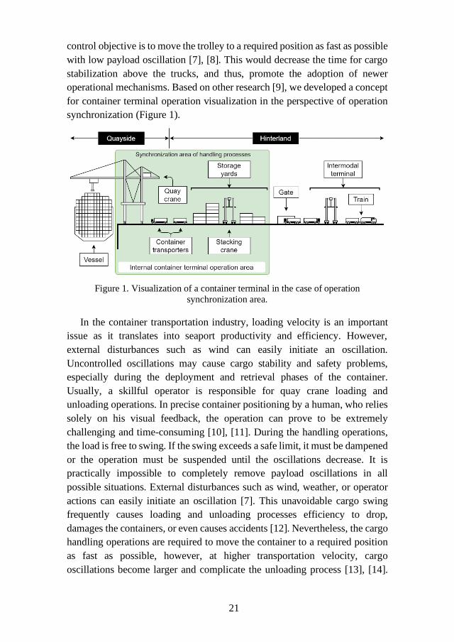
control objective is to move the trolley to a required position as fast as possible

with low payload oscillation [7], [8]. This would decrease the time for cargo

stabilization above the trucks, and thus, promote the adoption of newer

operational mechanisms. Based on other research [9], we developed a concept

for container terminal operation visualization in the perspective of operation

synchronization (Figure 1).

Figure 1. Visualization of a container terminal in the case of operation

synchronization area.

In the container transportation industry, loading velocity is an important

issue as it translates into seaport productivity and efficiency. However,

external disturbances such as wind can easily initiate an oscillation.

Uncontrolled oscillations may cause cargo stability and safety problems,

especially during the deployment and retrieval phases of the container.

Usually, a skillful operator is responsible for quay crane loading and

unloading operations. In precise container positioning by a human, who relies

solely on his visual feedback, the operation can prove to be extremely

challenging and time-consuming [10], [11]. During the handling operations,

the load is free to swing. If the swing exceeds a safe limit, it must be dampened

or the operation must be suspended until the oscillations decrease. It is

practically impossible to completely remove payload oscillations in all

possible situations. External disturbances such as wind, weather, or operator

actions can easily initiate an oscillation [7]. This unavoidable cargo swing

frequently causes loading and unloading processes efficiency to drop,

damages the containers, or even causes accidents [12]. Nevertheless, the cargo

handling operations are required to move the container to a required position

as fast as possible, however, at higher transportation velocity, cargo

oscillations become larger and complicate the unloading process [13], [14].

22

Also, this will cause the positioning inaccurate. To attain better positional

accuracy of the quay crane spreader, a control system that accounts for the

acceleration of the trolley and oscillation of the cargo is required. One of the

most efficient and easiest ways given practical implementation is to use

motion-profiling methods; however, fast motion commonly conflicts with the

smoothness of motion due to the residual oscillation [15]. Reaching a

compromise between the velocity of motion and the oscillation reduction is

one of the challenging tasks in the motion profiling area for automated control

systems [16]. To increase the motion velocity, it is necessary to control rapid

increments or decrements of acceleration, which would cause high jerks.

These jerks can be controlled. The jerk-limited profile is a common trajectory

pattern used by modern motion systems and it is a time-optimal solution of

jerk limited body control. The jerk limitation is used for the limitation of

deformations and vibrations induced by the reference trajectory, which can be

generated to cancel or reduce the oscillations [17]. The jerk-limited integration

into the trapezoidal velocity profile gives us the symmetric or asymmetric s-

shaped velocity profile. The smoothness of motion in these profiles depends

on jerk duration. Longer duration increases smoothness but decreases the time

efficiency.

Information regarding the control of the processes (decreasing the

inaccuracies of cargo fluctuations during handling operations) could

theoretically be synchronized with the central planning system, which

appropriately includes these factors in the Time Scales plan. In this way,

evaluating the crane operators and other technical characteristics of the system

can enable the synchronization of individual processes to achieve optimal

planning results.

1.1.2. The role of automated guided vehicles to improve the

performance of container terminals

The AGV system is widely used in the manufacturing industry, port, and

dock as a material conveying robot in the logistics system. AGV is flexible

and intellectualized. But many factors make an error during AGV

implementing a given route. With the development of port construction and

automated terminals, AGV positioning technology of current ports is single

and the perception and understanding of the external environment are

insufficient, which directly affects the operational efficiency of ports.

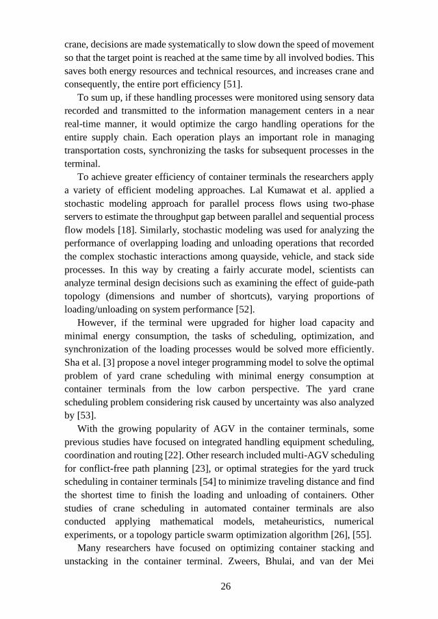
To achieve greater efficiency of container terminals the researchers apply

a variety of efficient modeling approaches. Lal Kumawat et al. applied a

stochastic modeling approach to parallel process flows using two-phase

23

servers to estimate the throughput gap between parallel and sequential process

flow models [18]. Similarly, stochastic modeling is used for analyzing the

performance of overlapping loading and unloading operations that recorded

the complex stochastic interactions among quayside, vehicle, and stack side

processes. In this way scientists, by creating a fairly accurate model, can

analyze terminal design decisions such as analyzing the effect of guide-path

topology (dimensions and number of shortcuts), varying proportions of

loading/unloading on system performance [19]. Other modeling techniques

are also developed for multidimensional performance evaluation of container

terminals according to logistics and operational, corporate social, financial,

and environmental dimensions [20] or looking for ways to design new

terminals with maximum efficiency [21].

With the growing popularity of AGV in container terminals, some previous

studies have focused on integrated scheduling for handling equipment

coordination and AGV routing [22], multi-AGV scheduling for conflict-free

path planning [23], or optimal strategies for the yard truck scheduling in

container terminal [24] to minimize the traveling distance and finding the

shortest time to finish the loading and unloading of containers. Other studies

of crane scheduling in automated container terminals are also conducted

applying mathematical models, metaheuristics, numerical experiments, or

random topology particle swarm optimization algorithms [25], [26].

In the research literature, some relevant information is still missing

concerning the place of AGV in the supply chain, by synchronizing various

contextual information (e.g., instant fuel consumption, battery reserve, and

energy consumption, etc.), the position in the terminal, the status of the

operation and other information related to planning activities. All this

information synchronized with the planning tools will allow us to plan the

cargo handling operations more accurately, but will also make changes to the

plan in near real-time, depending on the real situation in the container terminal

area.

1.1.3. The analysis of container lowering processes

Intermodal shipping containers are widely used in the global transport

chain to deliver various goods to end-users. Despite the obvious advantages,

there is still plenty of room for improvements, when it comes to increasing

time efficiency and quality. The global transport market is a network of

companies and end-users, who rely on well-managed standards and systems.

Recent trends and numbers suggest that about 90% of non-bulk global trade

is being managed by shipping containers worldwide [27], [28]. In 2016

24

Europe alone managed 0.8 billion tons of cargo [29]. Statistics show that

between 2007 and 2017, shipping volume increased by 66% (up to 148 million

TEUs), taking into account the global merchandise trade by marine traffic

[30]. Many engineers and managers worldwide foresaw such a rapid increase.

Yet, they could not manage it optimally. Thus, efficiency is a criterion, which

needs to be increased to adopt new challenges of the future. Cargo loading

operations rely on loading and unloading speeds, the safety of operation [31],

and energy consumption in the vicinity of the port [28]. These factors tend to

make final decisions when adopting new and untested technologies in

practice.

The modernization of container terminals through modern ICT

(Information and Communication Technology) solutions partly solves the

problems concerning the “green” terminal initiative [32]. The autonomy of

operations is adopted in many areas to control the stability of container

handling, transportation using terminal trucks, AGV [33], etc. Even now,

newly built cranes are using operators on-site to manage the loading

procedures [34]. Each new operator sees the loading standards as guidelines

but not strict rules. Therefore, crane autonomy [35] is necessary to increase

the efficiency of adopted standards and regulations, mechanical systems, and

associated port investments. An autonomous quay crane is not an innovation

on its own [25]. These complex systems already exist [36]. They are applied

in many areas of the industry including port operations [37]. On the other

hand, the modernization of existing infrastructure is a priority for most

companies, working with container handling. A more practical and real

solution is to modernize existing systems, rather than purchase all new

expensive infrastructure. Overall, there are crane stabilization systems that are

already in use [38], but they mostly lack quality feedback and operator

experience, which makes a huge impact on the efficiency of these expensive

systems [39].

In practice, the realization of complex control solutions is limited by the

fluctuations of the spreader with the load. Its movements are random, due to

external impacts, such as wind or physical contact with other objects [40]. It

is difficult to predict such random deviations in practice. In the most advanced

European ports, such as Rotterdam or Hanover, the handling procedures and

IT operations are mostly automated. However, the inclusion of the modern

automated quay cranes is still an innovation for smaller ports throughout the

world. In the light of the research and progress made in this area [1], [3], [12],

[41], [42], many ports in the world lack the application of these innovations.

Increasing the time efficiency of the cargo process is a topical issue

addressed in the scientific work, for which various solutions are proposed,

25

from management algorithms to cargo planning solutions [28], [33], [43]. The

quay cranes are analyzed in the way of increasing loading time [28], [44],

damping the load swinging during the loading-unloading process [44] using

additional feedbacks in control system with the PID or PI controllers or using

artificial intelligence analysis [13], [45]. One of the commonly used controller

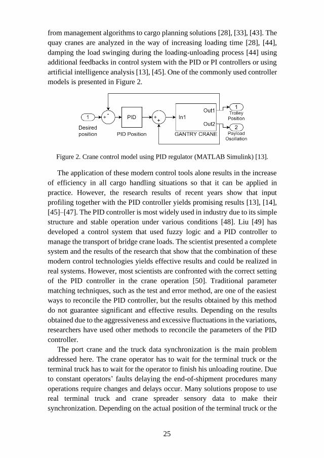
models is presented in Figure 2.

Figure 2. Crane control model using PID regulator (MATLAB Simulink) [13].

The application of these modern control tools alone results in the increase

of efficiency in all cargo handling situations so that it can be applied in

practice. However, the research results of recent years show that input

profiling together with the PID controller yields promising results [13], [14],

[45]–[47]. The PID controller is most widely used in industry due to its simple

structure and stable operation under various conditions [48]. Liu [49] has

developed a control system that used fuzzy logic and a PID controller to

manage the transport of bridge crane loads. The scientist presented a complete

system and the results of the research that show that the combination of these

modern control technologies yields effective results and could be realized in

real systems. However, most scientists are confronted with the correct setting

of the PID controller in the crane operation [50]. Traditional parameter

matching techniques, such as the test and error method, are one of the easiest

ways to reconcile the PID controller, but the results obtained by this method

do not guarantee significant and effective results. Depending on the results

obtained due to the aggressiveness and excessive fluctuations in the variations,

researchers have used other methods to reconcile the parameters of the PID

controller.

The port crane and the truck data synchronization is the main problem

addressed here. The crane operator has to wait for the terminal truck or the

terminal truck has to wait for the operator to finish his unloading routine. Due

to constant operators’ faults delaying the end-of-shipment procedures many

operations require changes and delays occur. Many solutions propose to use

real terminal truck and crane spreader sensory data to make their

synchronization. Depending on the actual position of the terminal truck or the

26

crane, decisions are made systematically to slow down the speed of movement

so that the target point is reached at the same time by all involved bodies. This

saves both energy resources and technical resources, and increases crane and

consequently, the entire port efficiency [51].

To sum up, if these handling processes were monitored using sensory data

recorded and transmitted to the information management centers in a near

real-time manner, it would optimize the cargo handling operations for the

entire supply chain. Each operation plays an important role in managing

transportation costs, synchronizing the tasks for subsequent processes in the

terminal.

To achieve greater efficiency of container terminals the researchers apply

a variety of efficient modeling approaches. Lal Kumawat et al. applied a

stochastic modeling approach for parallel process flows using two-phase

servers to estimate the throughput gap between parallel and sequential process

flow models [18]. Similarly, stochastic modeling was used for analyzing the

performance of overlapping loading and unloading operations that recorded

the complex stochastic interactions among quayside, vehicle, and stack side

processes. In this way by creating a fairly accurate model, scientists can

analyze terminal design decisions such as examining the effect of guide-path

topology (dimensions and number of shortcuts), varying proportions of

loading/unloading on system performance [52].

However, if the terminal were upgraded for higher load capacity and

minimal energy consumption, the tasks of scheduling, optimization, and

synchronization of the loading processes would be solved more efficiently.

Sha et al. [3] propose a novel integer programming model to solve the optimal

problem of yard crane scheduling with minimal energy consumption at

container terminals from the low carbon perspective. The yard crane

scheduling problem considering risk caused by uncertainty was also analyzed

by [53].

With the growing popularity of AGV in the container terminals, some

previous studies have focused on integrated handling equipment scheduling,

coordination and routing [22]. Other research included multi-AGV scheduling

for conflict-free path planning [23], or optimal strategies for the yard truck

scheduling in container terminals [54] to minimize traveling distance and find

the shortest time to finish the loading and unloading of containers. Other

studies of crane scheduling in automated container terminals are also

conducted applying mathematical models, metaheuristics, numerical

experiments, or a topology particle swarm optimization algorithm [26], [55].

Many researchers have focused on optimizing container stacking and

unstacking in the container terminal. Zweers, Bhulai, and van der Mei

27

proposed a new optimization model in the stochastic container relocation

problem in which the containers can be moved in two different phases: a pre-

processing and a relocation phase [56]. Xie and Song proposed optimal

planning for container pre-staging by applying a stochastic dynamic

programming model to minimize the total logistics cost [57]. Some previous

studies proposed an integrated optimization approach to determine optimal

crane and truck schedules and optimal pickup sequence of containers [25],

[58]–[60] leading to lower time and energy costs in the logistics process.

The optimal scheduling problem was also analyzed by Lu [61]. The author

examined the multi-automated stacking cranes and their scheduling methods

for automated container terminals based on graph theory. Other critical

factors, like energy consumption of quay cranes (QCs) were analyzed by Tang

et al. [32]. The author dealt with the performance of peak shaving policies for

quay cranes at container terminals with double cycling where some evaluation

indicators were selected for assessment including the observed peak power

demand, the productivity, and utilization of QCs and the average waiting time

of yard trucks (YTs).

The modeling of processes in container terminals is also not limited to the

application of classical methods. Advanced methods are used in recent studies.

Zhang et al. applied machine learning-driven algorithms for the container

relocation problem [62]. A combined data mining – optimization approach to

manage trucks operations in container terminals with the use of a truck

appointment system that reduce empty-truck trips was proposed by [63]. Some

previous studies have also shown that a multi-agent optimization approach can

be used for container terminals for the reactive and decentralized control of

container stacking in an uncertain and disturbed environment [64] or a system

dynamics simulation model to achieve the stable state of the main parameters

of intermodal terminals [60] [23].

The scheduling and optimization of technological processes is a key

problem while developing autonomous container terminals considering

energy consumptions and container loading process synchronization that has

not been fully investigated in the literature.

1.2. Methods for autonomous vehicles movement control and

navigation in port area

Taking into account the need for data exchange and process

synchronization, assessed in section 1.1, it is necessary not only to make a

correct choice choosing the right data exchange technology and

synchronization method, ensuring the integrity and sustainability of the port

28

operations. In this section, widely known truck and AGV navigation

technologies are presented that are currently used by many ports all around

the globe. The following technologies are used in modern AGV navigation

systems in port areas:

• Electromagnetic lines method.

• Electromagnetic reference point method.

• Laser navigation method.

• Optical navigation methods.

• GPS navigation method.

These technologies are briefly summarized and their key parameters are

discussed below in this section. This analysis was conducted to show the main

disadvantages of these systems and their low adaptability in the autonomous

terminal. However, most of these technologies can be combined and with new

emerging methods and systems, to increase response time, the accuracy of

navigation and agility for autonomy. Despite the technology being used for

tracking AGV in the port environment, cranes still miss the vital information

to adjust their handling processes efficiently. The crane operators and control

system lack in-time information to assess the container handling capacity in

the long term.

All these technologies allow us to identify the location of the AGV or other

transport vehicles in the port, increasing the level of autonomy for all

container handling processes, it is possible to achieve the higher objectives

that the European Union is pursuing today to achieve the Green Port

initiative [4].

1.2.1. Electromagnetic lines method

AGV navigation by electromagnetic lines (Figure 3) is an old and reliable

control method with an accuracy of ± 2 mm that is applicable to the control of

both open and closed AGV [65]. The main components of this method are:

guidewire, very a low-frequency generator, antenna, and autonomous vehicle.

The metal strip is laid out according to the required, pre-planned route on the

concrete pavement or in an incision of approximately 2.5 cm of concrete. An

electric current of appropriate frequency flows through this band, which

generates an electromagnetic field. The frequency required for the line is

generated by a very low-frequency generator e.g., HG G-57400 with standard

generated frequencies ranging from 5 kHz to 10 kHz.

29

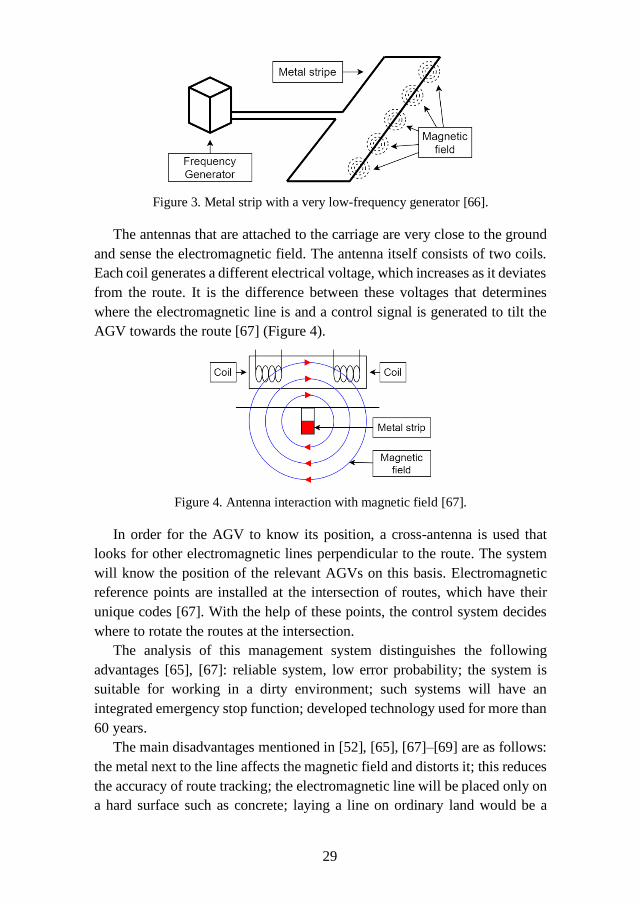
Figure 3. Metal strip with a very low-frequency generator [66].

The antennas that are attached to the carriage are very close to the ground

and sense the electromagnetic field. The antenna itself consists of two coils.

Each coil generates a different electrical voltage, which increases as it deviates

from the route. It is the difference between these voltages that determines

where the electromagnetic line is and a control signal is generated to tilt the

AGV towards the route [67] (Figure 4).

Figure 4. Antenna interaction with magnetic field [67].

In order for the AGV to know its position, a cross-antenna is used that

looks for other electromagnetic lines perpendicular to the route. The system

will know the position of the relevant AGVs on this basis. Electromagnetic

reference points are installed at the intersection of routes, which have their

unique codes [67]. With the help of these points, the control system decides

where to rotate the routes at the intersection.

The analysis of this management system distinguishes the following

advantages [65], [67]: reliable system, low error probability; the system is

suitable for working in a dirty environment; such systems will have an

integrated emergency stop function; developed technology used for more than

60 years.

The main disadvantages mentioned in [52], [65], [67]–[69] are as follows:

the metal next to the line affects the magnetic field and distorts it; this reduces

the accuracy of route tracking; the electromagnetic line will be placed only on

a hard surface such as concrete; laying a line on ordinary land would be a

30

challenge if the line is broken, without the assistance of additional systems,

the AGV will not move further and the whole system may become stuck; it

takes time to troubleshoot such system failures, as it is necessary to change

the line or part of it; lines are installed for the realization of a specific route. It

is necessary to change the whole line in order to change it, which is costly. It

is essential to choose the right route layout and to carry out detailed planning

to obtain maximum efficiency.

1.2.2. Electromagnetic reference point method

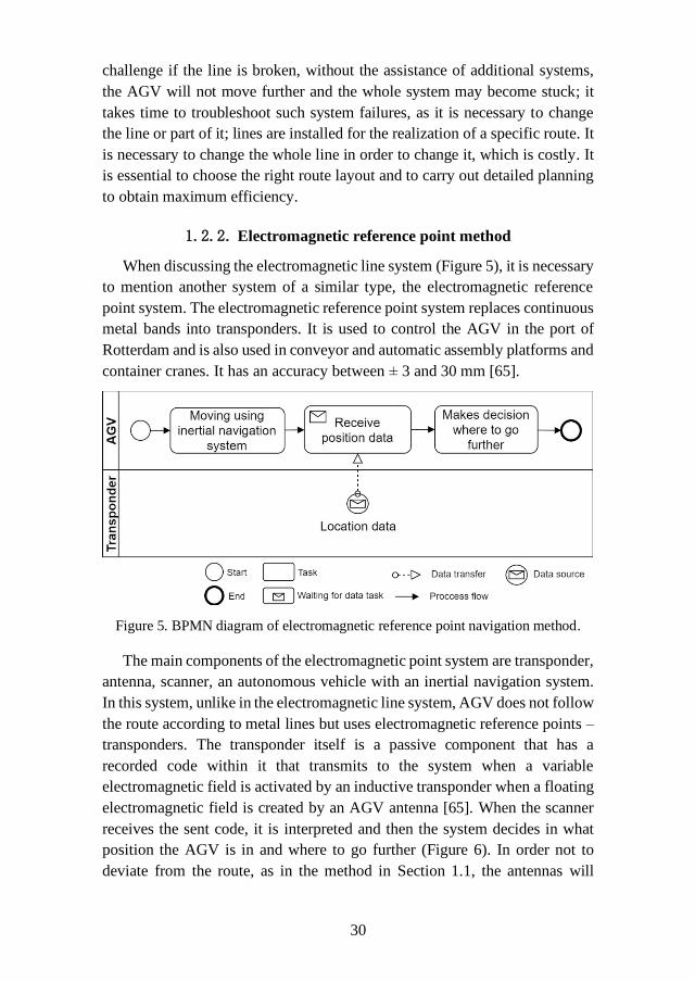
When discussing the electromagnetic line system (Figure 5), it is necessary

to mention another system of a similar type, the electromagnetic reference

point system. The electromagnetic reference point system replaces continuous

metal bands into transponders. It is used to control the AGV in the port of

Rotterdam and is also used in conveyor and automatic assembly platforms and

container cranes. It has an accuracy between ± 3 and 30 mm [65].

Figure 5. BPMN diagram of electromagnetic reference point navigation method.

The main components of the electromagnetic point system are transponder,

antenna, scanner, an autonomous vehicle with an inertial navigation system.

In this system, unlike in the electromagnetic line system, AGV does not follow

the route according to metal lines but uses electromagnetic reference points –

transponders. The transponder itself is a passive component that has a

recorded code within it that transmits to the system when a variable

electromagnetic field is activated by an inductive transponder when a floating

electromagnetic field is created by an AGV antenna [65]. When the scanner

receives the sent code, it is interpreted and then the system decides in what

position the AGV is in and where to go further (Figure 6). In order not to

deviate from the route, as in the method in Section 1.1, the antennas will

31

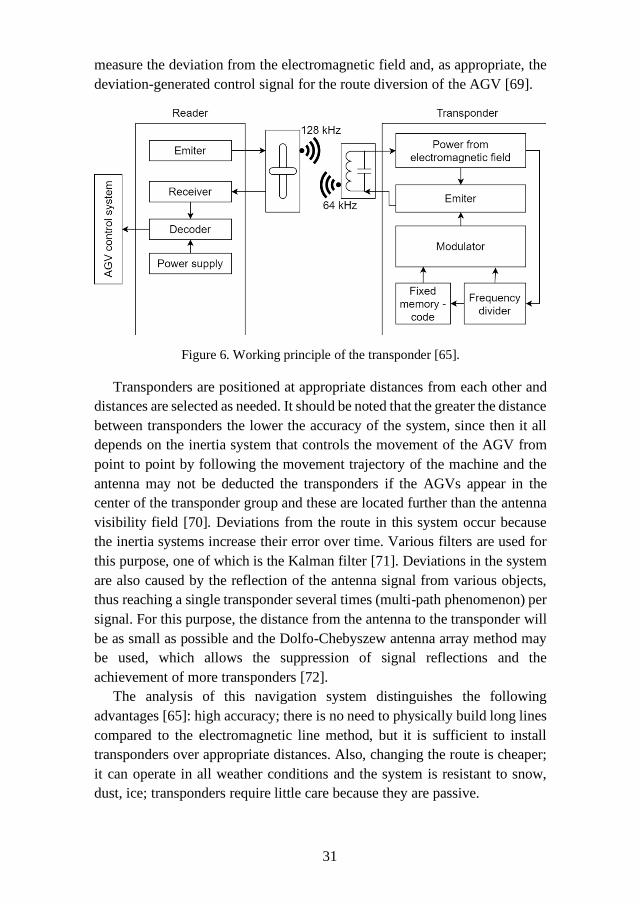
measure the deviation from the electromagnetic field and, as appropriate, the

deviation-generated control signal for the route diversion of the AGV [69].

Figure 6. Working principle of the transponder [65].

Transponders are positioned at appropriate distances from each other and

distances are selected as needed. It should be noted that the greater the distance

between transponders the lower the accuracy of the system, since then it all

depends on the inertia system that controls the movement of the AGV from

point to point by following the movement trajectory of the machine and the

antenna may not be deducted the transponders if the AGVs appear in the

center of the transponder group and these are located further than the antenna

visibility field [70]. Deviations from the route in this system occur because

the inertia systems increase their error over time. Various filters are used for

this purpose, one of which is the Kalman filter [71]. Deviations in the system

are also caused by the reflection of the antenna signal from various objects,

thus reaching a single transponder several times (multi-path phenomenon) per

signal. For this purpose, the distance from the antenna to the transponder will

be as small as possible and the Dolfo-Chebyszew antenna array method may

be used, which allows the suppression of signal reflections and the

achievement of more transponders [72].

The analysis of this navigation system distinguishes the following

advantages [65]: high accuracy; there is no need to physically build long lines

compared to the electromagnetic line method, but it is sufficient to install

transponders over appropriate distances. Also, changing the route is cheaper;

it can operate in all weather conditions and the system is resistant to snow,

dust, ice; transponders require little care because they are passive.

32

Disadvantages [25], [67], [71] are metal structures near the route affect

accuracy; signal reflections mislead the system and reduce accuracy; the AGV

inertia system increases its bias over time, so additional methods and

techniques need to be used to solve this; failure of any transponder causes

problems in the system that may damage traffic.

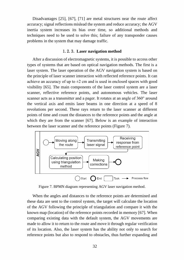
1.2.3. Laser navigation method

After a discussion of electromagnetic systems, it is possible to access other

types of systems that are based on optical navigation methods. The first is a

laser system. The laser operation of the AGV navigation system is based on

the principle of laser scanner interaction with reflected reference points. It can

achieve an accuracy of up to ±2 cm and is used in enclosed spaces with good

visibility [65]. The main components of the laser control system are a laser

scanner, reflective reference points, and autonomous vehicles. The laser

scanner acts as a transmitter and a pager. It rotates at an angle of 360° around

the vertical axis and emits laser beams in one direction at a speed of 8

revolutions per second. These rays return to the laser scanner at different

points of time and count the distances to the reference points and the angle at

which they are from the scanner [67]. Below is an example of interaction

between the laser scanner and the reference points (Figure 7).

Figure 7. BPMN diagram representing AGV laser navigation method.

When the angles and distances to the reference points are determined and

these data are sent to the control system, the target will calculate the location

of the AGV following the principle of triangulation and compare it with the

known map (location) of the reference points recorded in memory [67]. When

comparing existing data with the default system, the AGV movements are

made to allow it to return to the route and move it through regular verification

of its location. Also, the laser system has the ability not only to search for

reference points but also to respond to obstacles, thus further expanding and

33

exploiting the laser scanner. It can scan the outlines of obstacles, draw a two-

dimensional contour map [71] and decide how to overcome the obstacle with

the help of the control system. A two-level map with a module can be used to

increase the adaptability and flexibility of the navigation system. The first

level is a map showing the objects closest to the AGV, and the second level is

a map showing the location of the environmental zones. Such a system allows

for more complex autonomous transport, loading and unloading operations

[73]. The laser control system can be adjusted using the unscented Kalman

filter (UKF) and the fuzzy interference system (FIS). UKF is used for system

error measurement and processing, for guessing sensor values based on

available data, and FIS for dynamic noise reduction. With the help of these

improvements, AGVs can move at higher speeds [74].

The laser localization system can be extended using the IEEE 802.15.4a

wireless sensor network (WSN), which is used as a localization and

communication module. The Kalman filter is replaced by the Monte Carlo

particle (MCP) and anchor box methods to find passive reference points. In

such a system laser localization takes a secondary role and is used to adjust

the system. The most important advantage of such a system is the

determination of the AGV position without any preconception [75].

The analysis of this navigation system distinguishes the following

advantages [65], [71]: high precision system (±2 cm); no need to make any

changes to the running surfaces, which makes this system flexible and the cost

of changing routes is not high. The laser scanner can detect obstacles and their

dimensions.

Disadvantages include [65], [69]: extraneous reflective surfaces can cause

inaccuracies and errors in the system; snow, dirt, light may also have a

negative impact on the system’s activity. Reference points will be freely

visible and will not be obstructed by other objects so that the return beam

reaches the scanner. For this reason, considerable time is spent adjusting the

positions of the reference points.

1.2.4. Optical navigation method

In addition to the laser system, there are also several methods based on

optics: navigation by tracking colored bands, navigation by following

environmental features. The color tape method, presented in Figure 8, is

characterized by accuracy of ± 2 mm and an object identification system with

accuracy of less than ±5 cm. The optical methods in question are used in

enclosed, clean rooms with good visibility [65]. Main components of the AGV

34

navigation method based on color tape tracking: colored tape, IR sensor array

or other optical sensor arrays, autonomous vehicle.

This method is very similar to the electromagnetic line method considered

in Section 1.1, only here it is a passive band that does not generate

electromagnetic fields.

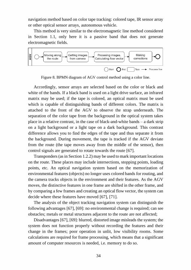
Figure 8. BPMN diagram of AGV control method using a color line.

Accordingly, sensor arrays are selected based on the color or black and

white of the bands. If a black band is used on a light drive surface, an infrared

matrix may be used; if the tape is colored, an optical matrix must be used

which is capable of distinguishing bands of different colors. The matrix is

attached to the front of the AGV to observe the strap underneath. The

separation of the color tape from the background in the optical system takes

place in a relative contrast, in the case of black-and-white bands – a dark strip

on a light background or a light tape on a dark background. This contrast

difference allows you to find the edges of the tape and thus separate it from

the background. During movement, the tape is tracked if the AGV deviate

from the route (the tape moves away from the middle of the sensor), then

control signals are generated to rotate towards the route [67].

Transponders (as in Section 1.2.2) may be used to mark important locations

on the route. These places may include intersections, stopping points, loading

points, etc. An optical navigation system based on the memorization of

environmental features (objects) no longer uses colored bands for routing, and

the camera tracks objects in the environment and their features. As the AGV

moves, the distinctive features in one frame are shifted in the other frame, and

by comparing a few frames and creating an optical flow vector, the system can

decide where these features have moved [67], [71].

The analysis of the object tracking navigation system can distinguish the

following advantages [67], [69]: no environmental change is required; can see

obstacles; metals or metal structures adjacent to the route are not affected;

Disadvantages [67], [69]: blurred, distorted image misleads the system; the

system does not function properly without recording the features and their

change in the frames; poor operation in unlit, low visibility rooms. Some

calculations are required for frame processing, which means that a significant

amount of computer resources is needed, i.e. memory to do so.

35

1.2.5. GPS navigation method

GPS is used for the management of AGV. A BPMN diagram of such a

system is presented in Figure 9. This system is used in open areas because the

satellite signal does not pass in closed areas. The system can reach an accuracy

of up to ±2-10 cm [65]. The main components of the satellite AGV navigation

system are a GPS module with an antenna, satellites, base station, and an

autonomous vehicle.

Satellites send information about their location and time at appropriate

time intervals, while the GPS module with an antenna captures the signals of

these satellites and calculates the time of arrival of the signals. The estimated

times are proportional to the distance from the satellite to the GPS module and

the GPS module learns its coordinates using the triangulation method [76].

Figure 9. BPMN diagram representing a GPS-based AGV control system.

To obtain greater positioning accuracy (up to some centimeters), a base

station (Figure 9) is used, which is located in a fixed location and also captures

satellite signals. When the GPS module is connected by radio to the station,

the position is adjusted to increase accuracy. It is also necessary to assess

where to attach the GPS antenna, as this position may alter the change in

positioning efficiency to 600%, thus creating additional errors [77].

The analysis of the satellite navigation system distinguishes the following

advantages [65]: a flexible system because routes can be programmed and

reprogrammed through management programs. The only additional

environmental change required is the mother station.

Disadvantages are: [65], [71], [76] adverse weather conditions or satellite

signals can render the GPS almost incapacitated; the system operates only in

36

open areas; to calculate the exact position of the AGVs, the GPS module must

contact at least 4 satellites. The accuracy of GPS is directly linked to the

number of satellites and the signal strength. The construction of the base

station on-site is a costly initiative.

1.2.6. Short sub-section discussions

The technologies mentioned in Section 1.2 could be used to track the

movement of AGV or other heavy port vehicles. They are used more

frequently nowadays to optimize the planning and scheduling of tasks. New

technologies are widely adopted by the industry to fill the technological gaps

and provide the port operators with all necessary information for decision

support. Technology combination provides more opportunities to implement

green port ideas and brings them closer to solving the challenge of synching

individual processes. Wireless technologies analyzed in the next section

(RFID, LoRaWAN, Wi-Fi, 4G, 5G, etc.) could improve the existing

infrastructure both at the technical and software levels. It is no secret that the

performance of the container terminal depends not only on the technical

equipment and other resources but also on the planning methods and systems.

A well-planned container handling process ensures optimized operations for

other technical means of the port.

However, in many cases, the systems in question do not evaluete the near

real-time triggers. Navigational and other systems for tracking the movement

of the vehicles on-site do not ensure operational handling. Therefore,

researchers analyze not only factual information received from the planning

systems but also the contextual information received from sensory

technologies. This allows making the right decisions during the container

handling process.

In Section 1.3, other technologies are presented which provide the

necessary additional information for knowledge extraction to make an

optimized decision for container handling.

1.3. Alternative wireless communication technologies and LoRaWAN

application for port operations

In many ports around the world, various IT technology infrastructures for

data transfer and reception at the terminal are increasingly being expanded.

Modern network technologies and positioning equipment are some of the most

necessary infrastructures in modern port operations to efficiently automate the

port loading process. Real-Time Locating System (RTLS) allows determining

the location of process operators on-site or heavy moving objects in near real-

37

time. This system uses tags that are attached to the objects needed to be

tracked. Base main stations can scan these tags remotely to determine their

location and get primary information about the object. Various technologies

are applied to increase the accuracy of the measurements, including GPS, Wi-

Fi, RFID, mobile communication (4G, 5G, etc.), LoRaWAN, and more. These

technologies have their advantages, but also restrict their technological

adaptability.

1.3.1. Analysis of RFID data transmission

RFID means the use of radio frequency waves for wireless data

transmission. RFID systems consist of three main parts – RFID scanner, RFID

antenna and RFID tags. RFID systems can be divided into active RFID and

passive RFID (Figure 10). The main difference between active and passive

RFID systems is the use of tags. RFID tags are divided into two categories:

active and passive tags. Active tags have a separate power source and operate

in a larger range. Passive tags do not require an additional power source but

operate in a smaller range. Passive RFID tags have two main components: an

antenna and an information storage chip connected to it. Meanwhile, active

RFID tags have three components: an antenna, an information storage chip

connected to it, and its own separate power source.

Communication between the RFID scanner and the tag is conducted in

several different ways, depending on the frequency band used for the tag. The

markings operating in low LF and high HF frequency bands are very close to

the scanner antenna in relation to the radio wavelength. In this nearest field

region, the tag is closely connected to the scanner transmitter. The tag can

change the electromagnetic field created by the scanner by changing the

electrical load in the mark. When switching between lower and higher relative

loads, the tag creates a change that the scanner can detect.

At UHF and higher frequencies, the tag is more than one radio wavelength

from the reader, so a different approach is needed. To retrieve information that

is stored in the passive RFID tag, the tag must be within the range of the

electromagnetic field emitted by the RFID scanner. The electromagnetic field

created by the scanner causes the movement of electrons through the tag

antenna, thereby acting as a microchip for storing tag information. The chip

in the bookmark then responds by sending stored information to the scanner

in the form of another radio signal. This is called retrospective dissemination.

The scanner detects and interprets electromagnetic radio wave feedback,

which then sends data to a computer or microcontroller [78].

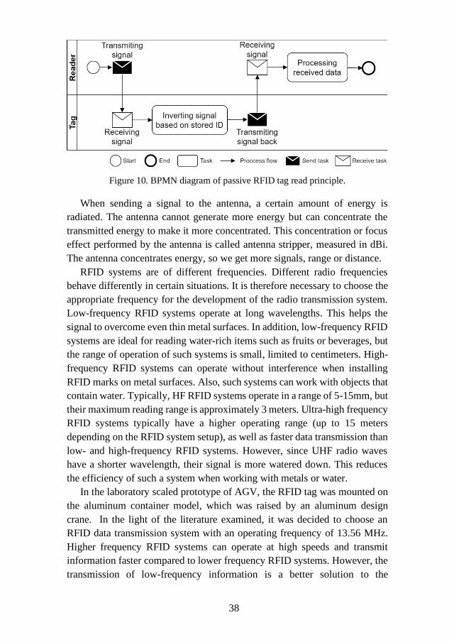
38

Figure 10. BPMN diagram of passive RFID tag read principle.

When sending a signal to the antenna, a certain amount of energy is

radiated. The antenna cannot generate more energy but can concentrate the

transmitted energy to make it more concentrated. This concentration or focus

effect performed by the antenna is called antenna stripper, measured in dBi.

The antenna concentrates energy, so we get more signals, range or distance.

RFID systems are of different frequencies. Different radio frequencies

behave differently in certain situations. It is therefore necessary to choose the

appropriate frequency for the development of the radio transmission system.

Low-frequency RFID systems operate at long wavelengths. This helps the

signal to overcome even thin metal surfaces. In addition, low-frequency RFID

systems are ideal for reading water-rich items such as fruits or beverages, but

the range of operation of such systems is small, limited to centimeters. High-

frequency RFID systems can operate without interference when installing

RFID marks on metal surfaces. Also, such systems can work with objects that

contain water. Typically, HF RFID systems operate in a range of 5-15mm, but

their maximum reading range is approximately 3 meters. Ultra-high frequency

RFID systems typically have a higher operating range (up to 15 meters

depending on the RFID system setup), as well as faster data transmission than

low- and high-frequency RFID systems. However, since UHF radio waves

have a shorter wavelength, their signal is more watered down. This reduces

the efficiency of such a system when working with metals or water.

In the laboratory scaled prototype of AGV, the RFID tag was mounted on

the aluminum container model, which was raised by an aluminum design

crane. In the light of the literature examined, it was decided to choose an

RFID data transmission system with an operating frequency of 13.56 MHz.

Higher frequency RFID systems can operate at high speeds and transmit

information faster compared to lower frequency RFID systems. However, the

transmission of low-frequency information is a better solution to the

39

development of the described container security system laboratory model, due

to the reduced response of communication signals to metal objects located

nearby.

1.3.2. GPS technologies in ports

The GPS positioning system is a Global Navigation Satellite System

(GNSS) via US satellites. There are also more existing GNSS systems:

Russian-owned GLONASS, China’s Beidou and Galileo in Europe. This

system works by receiving signals from the satellites flying around the planet.

The device on Earth's surface receives signals from at least 4 satellites. A

triangulation method is used to determine the position of the device at a certain

point in time [79]–[81].

There are many seaports around the world using GPS positioning

technology to determine the location of cranes or AGV. One example is that

the GPS positioning system was adapted to Busan Port terminal [82]–[86].

The system used low-cost GPS positioning devices that were connected to

AGV and ECH. This made it possible to monitor the location of the technique

in real-time.

The use of GPS is widespread in the freight transport market due to

reasonable price, system stability and sufficient accuracy. However, such a

system often results in poor GPS connectivity or the complete absence of GPS

signals in container terminals. For example, in a container terminal, under an

STS crane, where containers are placed in rows to heights. Interference occurs

when the GPS positioning device captures signals that are reflected from

nearby surfaces. This problem is even greater when signal interference is

caused by metal surfaces. In places where the satellite signal is poor, the

accuracy of the positioning system may decrease drastically [87], [88].

1.3.3. Advantages of the combination of RFID and GPS technologies

The alternative that scientists around the world point out is a positioning

method that combines two or more technologies and thus compensates for

each other's shortcomings. In other words, although the overall positioning is

performed by GPS, RFID technology activates and starts positioning

operations when the satellite signal is unstable, its quality is poor and there are

not enough visible satellites. In places such as tunnels where the satellite

signal is completely switched off, the satellite navigation system cannot

calculate positions. RFID technology could be used here to combine GPS and

RFID. Until the satellite signal is received, the RFID antennas are positioned

40

in that field to scan the RFID tags on moving objects, thus complementing the

accuracy of the positioning system [52].

1.3.4. Wi-Fi technologies in port

Ports are changing. The level of integration of different wireless devices,

software agents and activities, together with increasing connectivity between

different logistics chain actors has created a new ecosystem in which new risks

have appeared. Cybersecurity is one of the challenges of the industry and

policymakers, and an engineers and cybersecurity specialists should work

alongside to ensure that these critical infrastructures [89] are adequately

protected while facilitating the full development of new remote

communication technologies in a sector that has relatively lagged behind

others in transitioning to the new “4.0 world” [90].

Wi-Fi, called Wireless Fidelity technology, is a wireless network

communication industrial standard, proposed by IEEE and called the

IEEE802.11 standard. It is short-distance wireless communication

technology. In port operations, Wi-Fi and wireless subsequent communication

play an important role in data transmission between local network points [91]

to increase the data flow security and speed [89]. These communication links

work as a key technological solution for inner data flows within the

organization, supplying the transport chain with decision support

functionality, allowing operators to make predictions and control operations,

plan shipments, trucks and supporting logistics services.

Global location services are being developed by many companies all over

the world. Major players of the smart logistics domain, namely HERE

Technologies with Sigfox company, proposed new opportunities to apply

Internet of Things (IoT) solutions for containerization, particularly in supply

chain and logistics [92]. By integrating global coverage of Wi-Fi hotspots and

utilizing the worldwide network and geolocation engines, the industry is

presented with unique assets localization tools, for both indoors (including

inside factories warehouses and other buildings) and outdoors, without any

additional infrastructure, regardless of the size and quantity of assets [93].

On a global scale, the use of IoT asset tracking solutions for the supply

chain and logistics sectors could theoretically create huge economic value for

all participants, according to Cisco and DHL. Taking into consideration that

current RTLS technological and software solutions are not always viable due

to high costs and short battery life constraints, the adaptation of low-power

and high range technologies is a vital key for success in the coming years,

namely the adoption of LoRaWAN with local decision support.

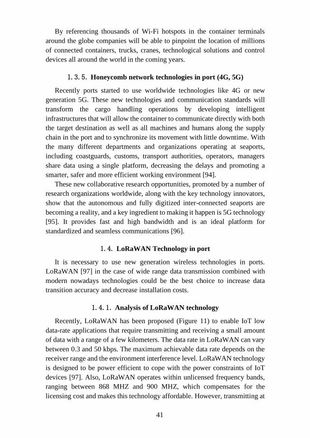
41

By referencing thousands of Wi-Fi hotspots in the container terminals

around the globe companies will be able to pinpoint the location of millions

of connected containers, trucks, cranes, technological solutions and control

devices all around the world in the coming years.

1.3.5. Honeycomb network technologies in port (4G, 5G)

Recently ports started to use worldwide technologies like 4G or new

generation 5G. These new technologies and communication standards will

transform the cargo handling operations by developing intelligent

infrastructures that will allow the container to communicate directly with both

the target destination as well as all machines and humans along the supply

chain in the port and to synchronize its movement with little downtime. With

the many different departments and organizations operating at seaports,

including coastguards, customs, transport authorities, operators, managers

share data using a single platform, decreasing the delays and promoting a

smarter, safer and more efficient working environment [94].

These new collaborative research opportunities, promoted by a number of

research organizations worldwide, along with the key technology innovators,

show that the autonomous and fully digitized inter-connected seaports are

becoming a reality, and a key ingredient to making it happen is 5G technology

[95]. It provides fast and high bandwidth and is an ideal platform for

standardized and seamless communications [96].

1.4. LoRaWAN Technology in port

It is necessary to use new generation wireless technologies in ports.

LoRaWAN [97] in the case of wide range data transmission combined with

modern nowadays technologies could be the best choice to increase data

transition accuracy and decrease installation costs.

1.4.1. Analysis of LoRaWAN technology

Recently, LoRaWAN has been proposed (Figure 11) to enable IoT low

data-rate applications that require transmitting and receiving a small amount

of data with a range of a few kilometers. The data rate in LoRaWAN can vary

between 0.3 and 50 kbps. The maximum achievable data rate depends on the

receiver range and the environment interference level. LoRaWAN technology

is designed to be power efficient to cope with the power constraints of IoT

devices [97]. Also, LoRaWAN operates within unlicensed frequency bands,

ranging between 868 MHZ and 900 MHZ, which compensates for the

licensing cost and makes this technology affordable. However, transmitting at

42

low frequencies and long range is restricted in some regions. Consequently,

the LoRa Alliance has defined different frequency plans that vary on a

regional basis. Furthermore, in the same region, there might be a difference in

the permitted transmission frequency bands based on countries’ regulations.

Figure 11. Rich picture of the LoRaWAN network for IoT applications in ports.

Generally, LoRaWAN uses a wide bandwidth which helps to resist both

interference and noise. On the other hand, LoRaWAN uses the star topology

as shown in Figure 11. IoT devices are connected to LoRa End-devices (EDs):

AGV, stacking crane, quay crane, which are connected directly to one or many

gateways (GWs). Each GW is connected to the network server (NS), which

can be connected to one or many application servers (ASs). The connection

between LoRaWAN EDs and GWs is a LoRaWAN wireless communication,

while the connection between the GW and the NS and AS is an IP connection

[98]. Additionally, an ED can be connected to a LoRa GW by using one of the

following activation techniques: Over-The-Air-Activation (OTAA), or

Activation by Personalization (ABP). After the activation phase, the EDs start

communicating their messages to the GW. However, these messages should

be authenticated and encrypted by using a network key and an application key

AppKey. The NS knows all NwKeys of all EDs, while the application server

knows all AppKeys of all EDs. However, the difference between the ABP and

the OTAA activation modes is that in the ABP activation mode, all the secret

keys and addresses are static and they are stored at the ED, and the EDs are

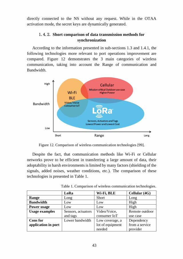
43

directly connected to the NS without any request. While in the OTAA

activation mode, the secret keys are dynamically generated.

1.4.2. Short comparison of data transmission methods for

synchronization

According to the information presented in sub-sections 1.3 and 1.4.1, the

following technologies more relevant to port operations improvement are

compared. Figure 12 demonstrates the 3 main categories of wireless

communication, taking into account the Range of communication and

Bandwidth.

Figure 12. Comparison of wireless communication technologies [99].

Despite the fact, that communication methods like Wi-Fi or Cellular

networks prove to be efficient in transferring a large amount of data, their

adoptability in harsh environments is limited by many factors (shielding of the

signals, added noises, weather conditions, etc.). The comparison of these

technologies is presented in Table 1.

Table 1. Comparison of wireless communication technologies.

LoRa Wi-Fi, BLE Cellular (4G)

Range Long Short Long

Bandwidth Low Low High

Power usage Low Low High

Usage examples Sensors, actuators

and tags

Video/Voice,

consumer IoT

Remote outdoor

use case

Cons for

application in port

Lower bandwidth Low coverage, a

lot of equipment

needed

Dependency

from a service

provider

44

Port operations require stable communication with enough bandwidth to

send basic sensory data to the planning systems. LoRaWAN technology

provides the best technical characteristics to be used in various scenarios for

improving port operations, including long-range communication in container

terminals, between base stations and moving objects, eliminating signal

shielding by metal obstacles. Many other advantages of this method were

described previously.

1.5. Section conclusions

1. Many researchers have focused on optimizing container stacking in the

container terminal. Zweers, Bhulai, and van der Mei proposed a new

optimization model in the stochastic container relocation problem in

which the containers can be moved in two different phases: a pre-

processing and a relocation phase [56]. Xie and Song proposed optimal

planning for container pre-staging by applying a stochastic dynamic

programming model to minimize the total logistics cost [57]. Some

previous studies proposed an integrated optimization approach to

determine optimal crane and truck schedules and optimal pickup

sequence of containers [58], [59], [100], [101] leading to lower time and

energy costs in the logistics process. These studies are relevant in dealing

with processes synchronization and improving the efficiency of current

systems.

2. Modeling of processes in container terminals is also not limited to the

application of classical methods, advanced methods must be applied to

ensure the efficiency of long-term operations for the entire transport

chain. Some previous studies have shown that a multi-agent optimization

approach can be used for container terminals for the reactive and

decentralized control of container stacking in an uncertain and disturbed

environment [64] or a system dynamics simulation model to achieve the

stable state of the main parameters of intermodal terminals [60].

3. The port transport tracking systems reviewed in the section show that

their individual use often does not produce the desired result, and their

application in planning systems has so far not been sufficiently discussed

in scientific work. However, it is often mentioned that the adjustment of

these tracking systems, by combining additional technologies, allows for

more precise positioning in the area of the terminal, as well as the

possibility of collecting not only movement data but also contextual

information. Applying the latter data to synchronization and real-time

planning of loading work can have a significant impact on optimized

45

performance. To synchronize the movement data between trucks and

quay cranes, LoRa technology was chosen due to its unique properties

dealing with long-range communication tasks in harsh environments,

optimal for port operations. LoRaWAN networks provide higher

interference immunity compared to other wireless communication

technologies (SIGFOX, LTE-Cat 1, LTE-M, NB-LTE) while

maintaining optimal battery usage using sleep mode and high link

threshold values. Therefore, it was concluded that in order to solve these

problems it is necessary to use LoRa technology for secure and reliable

connections for handling processes synchronization.

4. This whole overview allows evaluating individual operations and in the

context of synchronization to optimize the loading process and maximize

port autonomy. Also, it enables the selection of the correct technologies

for each handling operation. In the following section, we will discuss the

methodology developed for port process synchronization and the method

proposed for sensory data transfer.

46

2. DEVELOPMENT OF METHODOLOGY FOR PORT

OPERATION SYNCHRONIZATION – METHOD AND

ALGORITHM

2.1. Application of LoRaWAN technology for data synchronization in

the port area

2.1.1. LoRaWAN technology and its adoption for data synchronization

Among the various wireless technologies used to bridge the gap between

sensors and gateways to the Internet, there are solutions inspired by the

cellular communication approach. In these cases, the wireless end-devices are

linked with the base station, which defines a one-hop cell; the base stations

are connected with a backbone network (wired or wireless). However, despite

the current cellular network infrastructure, 4G technology could potentially

address many IoT scenarios. The complex architecture and the demanding

protocol stack result in the high computational capability of the end-nodes,

which in turn implies high-cost and high-power consumption, something not

compatible with most of the actual applications. Only the next generation

technology (5G) promises a mass deployment in the future. Therefore, other

technologies are used in this field today: Low Power Wide Area Networks

(LPWANs). Their main advantages are the wide-area coverage and the

reduced number of base stations, thanks to the innovative radios that trade off

the sensitivity with the throughput; the simplified communication protocol

stack that, in turn, reduces the infrastructure complexity. Consequently, both

the power consumption and the cost are diminished. Currently, the consumer

market, the industry, and the academic world are proposing/using several

LPWANs; the 3rd generation partnership project (3GPP) itself standardized

the so-called Narrowband-IoT or NB-IoT in LTE release 13, focusing on

machine-to-machine, delays tolerant communications. Nevertheless, the use

of licensed bands affects costs as well and makes device management

cumbersome (e.g., due to SIM cards). At this time, most of the adopter

consensus is achieved by LoRaWAN, which has been turned into a de-facto

standard. It is an open standard defined by the LoRa Alliance that now is

implemented in many commercially available devices from multiple

manufacturers. The LoRaWAN wide success is demonstrated [102] by both

the constantly increasing applications in various scenarios, and the huge

available scientific literature.

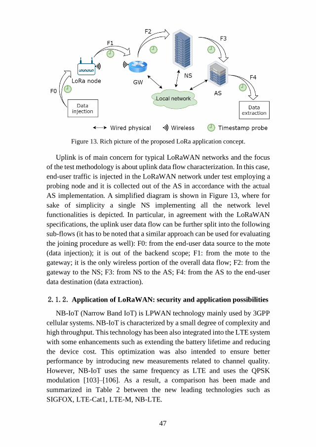
47

Figure 13. Rich picture of the proposed LoRa application concept.

Uplink is of main concern for typical LoRaWAN networks and the focus

of the test methodology is about uplink data flow characterization. In this case,

end-user traffic is injected in the LoRaWAN network under test employing a

probing node and it is collected out of the AS in accordance with the actual

AS implementation. A simplified diagram is shown in Figure 13, where for

sake of simplicity a single NS implementing all the network level

functionalities is depicted. In particular, in agreement with the LoRaWAN

specifications, the uplink user data flow can be further split into the following

sub-flows (it has to be noted that a similar approach can be used for evaluating

the joining procedure as well): F0: from the end-user data source to the mote

(data injection); it is out of the backend scope; F1: from the mote to the

gateway; it is the only wireless portion of the overall data flow; F2: from the

gateway to the NS; F3: from NS to the AS; F4: from the AS to the end-user

data destination (data extraction).

2.1.2. Application of LoRaWAN: security and application possibilities

NB-IoT (Narrow Band IoT) is LPWAN technology mainly used by 3GPP

cellular systems. NB-IoT is characterized by a small degree of complexity and

high throughput. This technology has been also integrated into the LTE system

with some enhancements such as extending the battery lifetime and reducing

the device cost. This optimization was also intended to ensure better

performance by introducing new measurements related to channel quality.

However, NB-IoT uses the same frequency as LTE and uses the QPSK

modulation [103]–[106]. As a result, a comparison has been made and

summarized in Table 2 between the new leading technologies such as

SIGFOX, LTE-Cat1, LTE-M, NB-LTE.

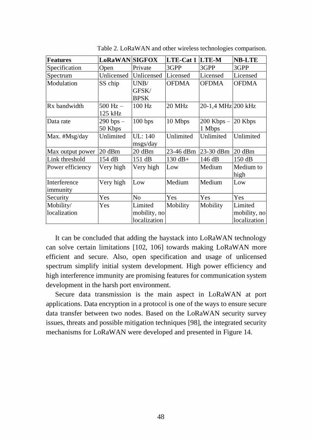
48

Table 2. LoRaWAN and other wireless technologies comparison.

Features LoRaWAN SIGFOX LTE-Cat 1 LTE-M NB-LTE

Specification Open Private 3GPP 3GPP 3GPP

Spectrum Unlicensed Unlicensed Licensed Licensed Licensed

Modulation SS chip UNB/

GFSK/

BPSK

OFDMA OFDMA OFDMA

Rx bandwidth 500 Hz –

125 kHz

100 Hz 20 MHz 20-1,4 MHz 200 kHz

Data rate 290 bps – 50 Kbps

100 bps 10 Mbps 200 Kbps – 1 Mbps

20 Kbps

Max. #Msg/day Unlimited UL: 140

msgs/day

Unlimited Unlimited Unlimited

Max output power 20 dBm 20 dBm 23-46 dBm 23-30 dBm 20 dBm

Link threshold 154 dB 151 dB 130 dB+ 146 dB 150 dB

Power efficiency Very high Very high Low Medium Medium to

high

Interference

immunity

Very high Low Medium Medium Low

Security Yes No Yes Yes Yes

Mobility/

localization

Yes Limited

mobility, no

localization

Mobility Mobility Limited

mobility, no

localization

It can be concluded that adding the haystack into LoRaWAN technology

can solve certain limitations [102, 106] towards making LoRaWAN more

efficient and secure. Also, open specification and usage of unlicensed

spectrum simplify initial system development. High power efficiency and

high interference immunity are promising features for communication system

development in the harsh port environment.

Secure data transmission is the main aspect in LoRaWAN at port

applications. Data encryption in a protocol is one of the ways to ensure secure

data transfer between two nodes. Based on the LoRaWAN security survey

issues, threats and possible mitigation techniques [98], the integrated security

mechanisms for LoRaWAN were developed and presented in Figure 14.

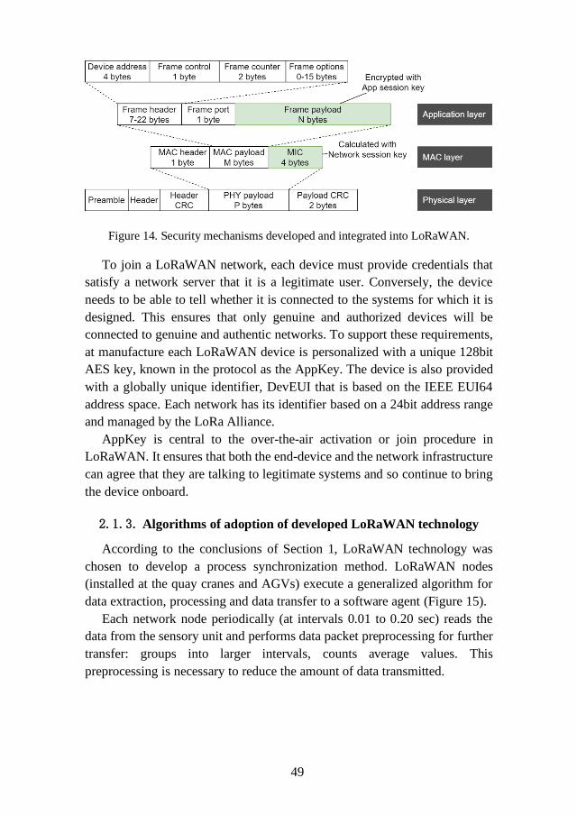
49

Figure 14. Security mechanisms developed and integrated into LoRaWAN.

To join a LoRaWAN network, each device must provide credentials that

satisfy a network server that it is a legitimate user. Conversely, the device

needs to be able to tell whether it is connected to the systems for which it is

designed. This ensures that only genuine and authorized devices will be

connected to genuine and authentic networks. To support these requirements,

at manufacture each LoRaWAN device is personalized with a unique 128bit

AES key, known in the protocol as the AppKey. The device is also provided

with a globally unique identifier, DevEUI that is based on the IEEE EUI64

address space. Each network has its identifier based on a 24bit address range

and managed by the LoRa Alliance.

AppKey is central to the over-the-air activation or join procedure in

LoRaWAN. It ensures that both the end-device and the network infrastructure

can agree that they are talking to legitimate systems and so continue to bring

the device onboard.

2.1.3. Algorithms of adoption of developed LoRaWAN technology

According to the conclusions of Section 1, LoRaWAN technology was

chosen to develop a process synchronization method. LoRaWAN nodes

(installed at the quay cranes and AGVs) execute a generalized algorithm for

data extraction, processing and data transfer to a software agent (Figure 15).

Each network node periodically (at intervals 0.01 to 0.20 sec) reads the

data from the sensory unit and performs data packet preprocessing for further

transfer: groups into larger intervals, counts average values. This

preprocessing is necessary to reduce the amount of data transmitted.

50

Figure 15. The data acquisition and transfer algorithm for each LoRaWAN node.

The data extraction interval could be pre-selected for a longer period, but

recent studies have shown that it decreases the resolution of the data, which is

relevant for the evaluation of the initial data. After the period and after

processing, the data is encrypted applying the AES-128 algorithm using

AppKey. The encrypted data is then added to the LoRaWAN data packet,

which uses Network Session Key to additionally count the MIC (Message

Integrity Code). MIC is similar to a checksum, except that it prevents

intentional tampering with a message. Network Session Key is used to validate

the integrity of each message by its MIC. Finally, the generated package is

sent to the server.

Figure 16. Data flow diagram for the total AGV assignment process.

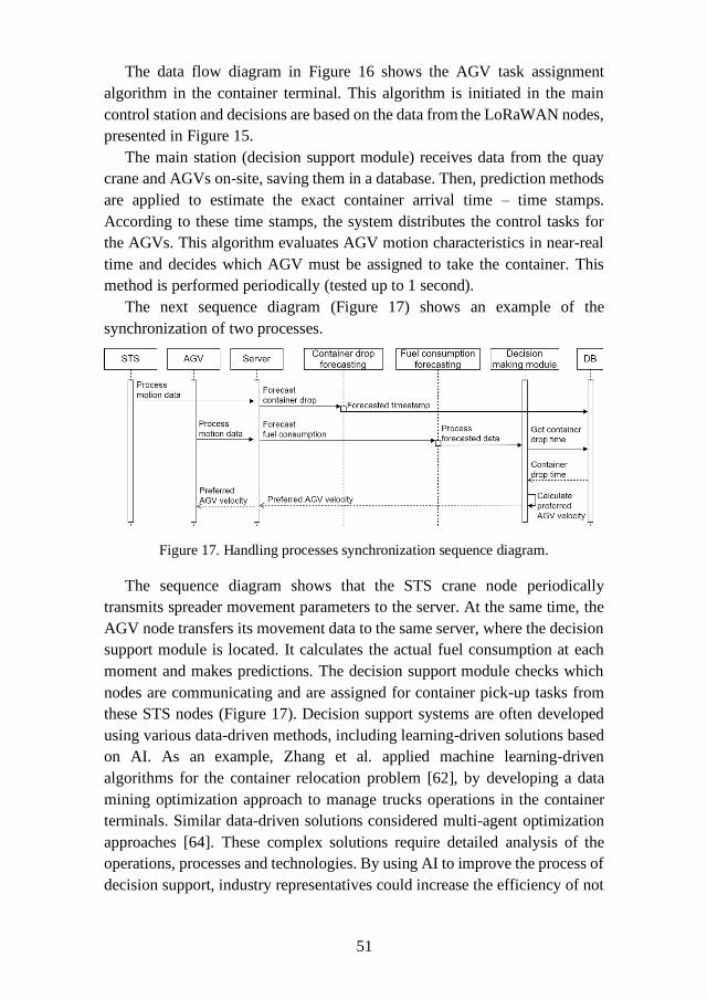
51

The data flow diagram in Figure 16 shows the AGV task assignment

algorithm in the container terminal. This algorithm is initiated in the main

control station and decisions are based on the data from the LoRaWAN nodes,

presented in Figure 15.

The main station (decision support module) receives data from the quay

crane and AGVs on-site, saving them in a database. Then, prediction methods

are applied to estimate the exact container arrival time – time stamps.

According to these time stamps, the system distributes the control tasks for

the AGVs. This algorithm evaluates AGV motion characteristics in near-real

time and decides which AGV must be assigned to take the container. This

method is performed periodically (tested up to 1 second).

The next sequence diagram (Figure 17) shows an example of the

synchronization of two processes.

Figure 17. Handling processes synchronization sequence diagram.

The sequence diagram shows that the STS crane node periodically

transmits spreader movement parameters to the server. At the same time, the

AGV node transfers its movement data to the same server, where the decision

support module is located. It calculates the actual fuel consumption at each

moment and makes predictions. The decision support module checks which

nodes are communicating and are assigned for container pick-up tasks from

these STS nodes (Figure 17). Decision support systems are often developed

using various data-driven methods, including learning-driven solutions based

on AI. As an example, Zhang et al. applied machine learning-driven

algorithms for the container relocation problem [62], by developing a data

mining optimization approach to manage trucks operations in the container

terminals. Similar data-driven solutions considered multi-agent optimization

approaches [64]. These complex solutions require detailed analysis of the

operations, processes and technologies. By using AI to improve the process of

decision support, industry representatives could increase the efficiency of not

52

only individual operations on-site, but also increase the turnarounds of the

containers on a global scale.

The concept of LoRaWAN network for container terminal presented in

Figure 18 was proposed by the author.

Figure 18. Concept of LoRaWAN network in a container terminal.

The equipment layout was based on the Google Maps picture of Klaipėda

city container terminal presented in Figure 19.

Figure 19. The satellite view of the container terminal in Klaipėda.

The LoRaWAN network consists of LoRa nodes (7 stacking cranes, AGV,

3 quay cranes) that periodically send movement data to the network gateways.

There are several gateways in the terminal area to ensure full coverage and

effective communication when the moving nodes are between obstacles. The

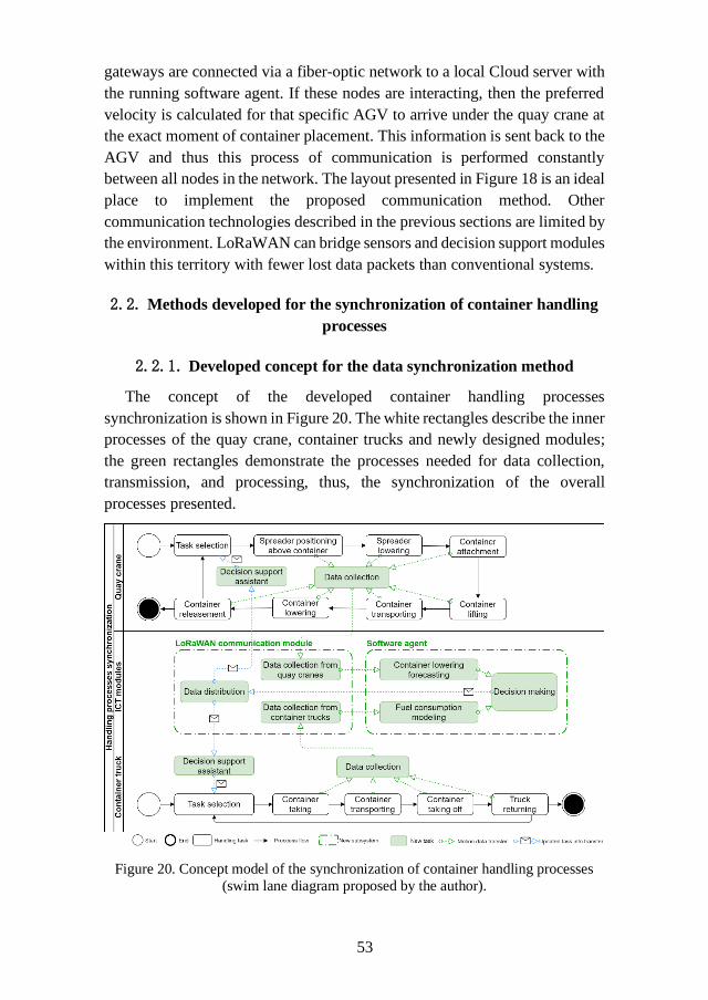
53

gateways are connected via a fiber-optic network to a local Cloud server with

the running software agent. If these nodes are interacting, then the preferred

velocity is calculated for that specific AGV to arrive under the quay crane at

the exact moment of container placement. This information is sent back to the

AGV and thus this process of communication is performed constantly

between all nodes in the network. The layout presented in Figure 18 is an ideal

place to implement the proposed communication method. Other

communication technologies described in the previous sections are limited by

the environment. LoRaWAN can bridge sensors and decision support modules

within this territory with fewer lost data packets than conventional systems.

2.2. Methods developed for the synchronization of container handling

processes

2.2.1. Developed concept for the data synchronization method

The concept of the developed container handling processes

synchronization is shown in Figure 20. The white rectangles describe the inner

processes of the quay crane, container trucks and newly designed modules;

the green rectangles demonstrate the processes needed for data collection,

transmission, and processing, thus, the synchronization of the overall

processes presented.

Figure 20. Concept model of the synchronization of container handling processes

(swim lane diagram proposed by the author).

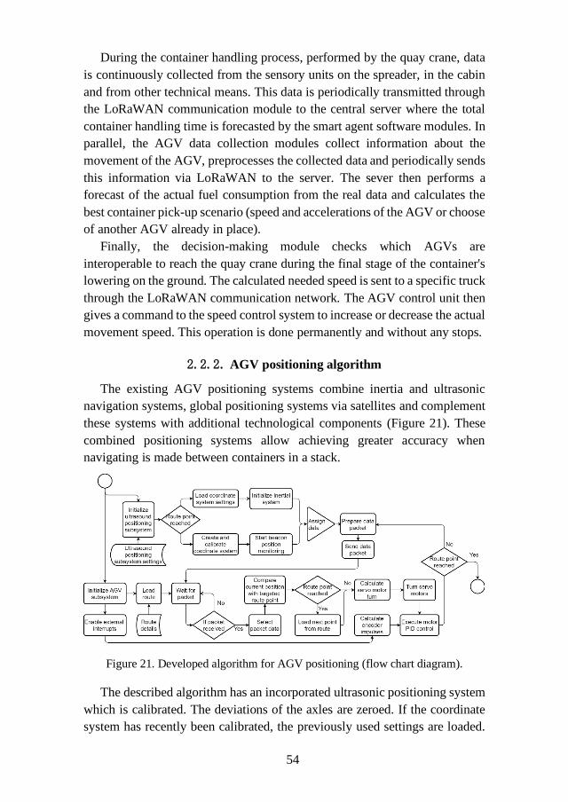
54

During the container handling process, performed by the quay crane, data

is continuously collected from the sensory units on the spreader, in the cabin

and from other technical means. This data is periodically transmitted through

the LoRaWAN communication module to the central server where the total

container handling time is forecasted by the smart agent software modules. In

parallel, the AGV data collection modules collect information about the

movement of the AGV, preprocesses the collected data and periodically sends

this information via LoRaWAN to the server. The sever then performs a

forecast of the actual fuel consumption from the real data and calculates the

best container pick-up scenario (speed and accelerations of the AGV or choose

of another AGV already in place).

Finally, the decision-making module checks which AGVs are

interoperable to reach the quay crane during the final stage of the container's

lowering on the ground. The calculated needed speed is sent to a specific truck

through the LoRaWAN communication network. The AGV control unit then

gives a command to the speed control system to increase or decrease the actual

movement speed. This operation is done permanently and without any stops.

2.2.2. AGV positioning algorithm

The existing AGV positioning systems combine inertia and ultrasonic

navigation systems, global positioning systems via satellites and complement

these systems with additional technological components (Figure 21). These

combined positioning systems allow achieving greater accuracy when

navigating is made between containers in a stack.

Figure 21. Developed algorithm for AGV positioning (flow chart diagram).

The described algorithm has an incorporated ultrasonic positioning system

which is calibrated. The deviations of the axles are zeroed. If the coordinate

system has recently been calibrated, the previously used settings are loaded.

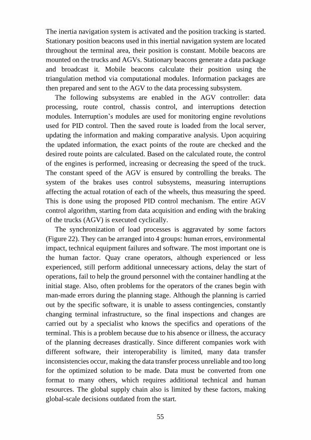
55

The inertia navigation system is activated and the position tracking is started.

Stationary position beacons used in this inertial navigation system are located

throughout the terminal area, their position is constant. Mobile beacons are

mounted on the trucks and AGVs. Stationary beacons generate a data package

and broadcast it. Mobile beacons calculate their position using the

triangulation method via computational modules. Information packages are

then prepared and sent to the AGV to the data processing subsystem.

The following subsystems are enabled in the AGV controller: data

processing, route control, chassis control, and interruptions detection

modules. Interruption’s modules are used for monitoring engine revolutions

used for PID control. Then the saved route is loaded from the local server,

updating the information and making comparative analysis. Upon acquiring

the updated information, the exact points of the route are checked and the

desired route points are calculated. Based on the calculated route, the control

of the engines is performed, increasing or decreasing the speed of the truck.

The constant speed of the AGV is ensured by controlling the breaks. The

system of the brakes uses control subsystems, measuring interruptions

affecting the actual rotation of each of the wheels, thus measuring the speed.

This is done using the proposed PID control mechanism. The entire AGV

control algorithm, starting from data acquisition and ending with the braking

of the trucks (AGV) is executed cyclically.

The synchronization of load processes is aggravated by some factors

(Figure 22). They can be arranged into 4 groups: human errors, environmental

impact, technical equipment failures and software. The most important one is

the human factor. Quay crane operators, although experienced or less

experienced, still perform additional unnecessary actions, delay the start of

operations, fail to help the ground personnel with the container handling at the

initial stage. Also, often problems for the operators of the cranes begin with

man-made errors during the planning stage. Although the planning is carried

out by the specific software, it is unable to assess contingencies, constantly

changing terminal infrastructure, so the final inspections and changes are

carried out by a specialist who knows the specifics and operations of the

terminal. This is a problem because due to his absence or illness, the accuracy

of the planning decreases drastically. Since different companies work with

different software, their interoperability is limited, many data transfer

inconsistencies occur, making the data transfer process unreliable and too long

for the optimized solution to be made. Data must be converted from one

format to many others, which requires additional technical and human

resources. The global supply chain also is limited by these factors, making

global-scale decisions outdated from the start.

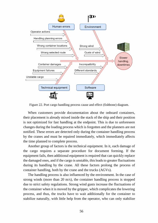
56

Figure 22. Port cargo handling process cause and effect (fishbone) diagram.

When customers provide documentation about the onboard containers,

their placement is already mixed inside the stack of the ship and their position

is not optimized for fast handling at the endpoint. This is due to unforeseen

changes during the loading process which is forgotten and the planners are not

notified. These errors are detected only during the container handling process

by the cranes and must be repaired immediately, which immediately affects

the time planned to complete process.

Another group of factors is the technical equipment. In it, each damage of

the cargo requires a separate procedure for document forming. If the

equipment fails, then additional equipment is required that can quickly replace

the damaged ones, and if the cargo is unstable, this leads to greater fluctuations

during its handling by the crane. All these factors prolong the process of

container handling, both by the crane and the trucks (AGVs).

The handling process is also influenced by the environment. In the case of

strong winds (more than 20 m/s), the container handling process is stopped

due to strict safety regulations. Strong wind gusts increase the fluctuations of

the container when it is moved by the gripper, which complicates the lowering

process, and thus, the trucks have to wait additionally for the container to

stabilize naturally, with little help from the operator, who can only stabilize

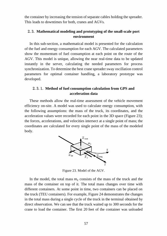
57

the container by increasing the tension of separate cables holding the spreader.

This leads to downtimes for both, cranes and AGVs.

2.3. Mathematical modeling and prototyping of the small-scale port

environment

In this sub-section, a mathematical model is presented for the calculation

of the fuel and energy consumption for each AGV. The calculated parameters

show the momentum of fuel consumption at each point on the route of the

AGV. This model is unique, allowing the near real-time data to be updated

instantly in the server, calculating the needed parameters for process

synchronization. To determine the best crane spreader sway oscillation control

parameters for optimal container handling, a laboratory prototype was

developed.

2.3.1. Method of fuel consumption calculation from GPS and

acceleration data

These methods allow the real-time assessment of the vehicle movement

efficiency on-site. A model was used to calculate energy consumption, with

the following assumptions: the mass of the truck, its coordinates, and the

acceleration values were recorded for each point in the 3D space (Figure 23);

the forces, accelerations, and velocities intersect at a single point of mass; the

coordinates are calculated for every single point of the mass of the modeled

body.

Figure 23. Model of the AGV.

In the model, the total mass 𝑚𝑡 consists of the mass of the truck and the

mass of the container on top of it. The total mass changes over time with

different containers. At some point in time, two containers can be placed on

the truck (TEU containers). For example, Figure 24 demonstrates the changes

in the total mass during a single cycle of the truck in the terminal obtained by

direct observation. We can see that the truck waited up to 300 seconds for the

crane to load the container. The first 20 feet of the container was unloaded

58

from the truck in the stack by the end of the 440th second. The second 20 feet

container was unloaded from the truck by the end of the 640th second and the

truck went back to the crane by the end of the 800th second, which concludes

the full cycle.

Figure 24. Example of the total mass change during a single cycle in the terminal.

Next, we present the energy consumption model necessary for the

estimation of the energy losses during these full cycles in the terminal. The

model uses the calculated rolling (0.0098) and air (1.69) resistance

coefficients. To calculate these coefficients, additional measurements were

made with the truck, and the measuring equipment during the experimental

phase. Detailed methodical explanation is presented in Section 3.2.4.

The following equation (1) presents the energy consumption of the truck

that is required for acceleration or maintain constant velocity:

Emov = ∫ Pmovdttets

, (1)

where ts – the starting time point t of the truck work cycle (ship-stack-

ship), te– the ending time point t of the truck work cycle (ship-stack-ship).

Truck movement power Pmov is calculated using the following equation:

Pmov = {FT(t) ⋅ |v(t)|, when ahorz > 0

0, otherwise, (2)

where v(t) – the velocity of the total mass body at the exact time, ahorz(t)

– the acceleration value of the body (explained below in (5)). The total

resistance force FT(t) of the movement of the body is calculated for each time

point t:

FT(t) = Fin(t) + Fair(t) + Froll(t). (3)

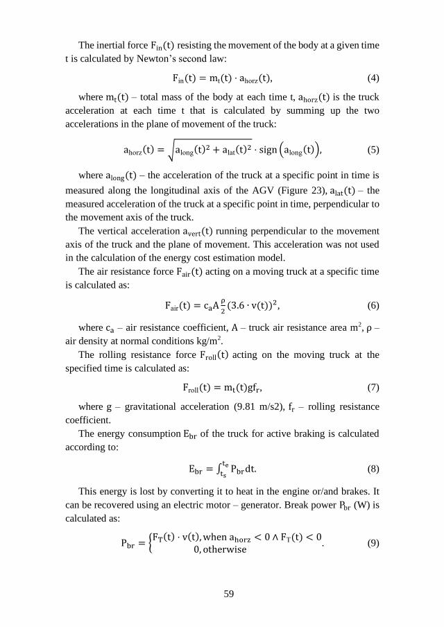
59

The inertial force Fin(t) resisting the movement of the body at a given time

t is calculated by Newton’s second law:

Fin(t) = mt(t) ⋅ ahorz(t), (4)

where mt(t) – total mass of the body at each time t, ahorz(t) is the truck

acceleration at each time t that is calculated by summing up the two

accelerations in the plane of movement of the truck:

ahorz(t) = √along(t)2 + alat(t)

2 ⋅ sign (along(t)), (5)

where along(t) – the acceleration of the truck at a specific point in time is

measured along the longitudinal axis of the AGV (Figure 23), alat(t) – the

measured acceleration of the truck at a specific point in time, perpendicular to

the movement axis of the truck.

The vertical acceleration avert(t) running perpendicular to the movement

axis of the truck and the plane of movement. This acceleration was not used

in the calculation of the energy cost estimation model.

The air resistance force Fair(t) acting on a moving truck at a specific time

is calculated as:

Fair(t) = caAρ

2(3.6 ∙ v(t))2, (6)

where ca – air resistance coefficient, A – truck air resistance area m2, ρ –

air density at normal conditions kg/m2.

The rolling resistance force Froll(t) acting on the moving truck at the

specified time is calculated as:

Froll(t) = mt(t)gfr, (7)

where g – gravitational acceleration (9.81 m/s2), fr – rolling resistance

coefficient.

The energy consumption Ebr of the truck for active braking is calculated

according to:

Ebr = ∫ Pbrdttets

. (8)

This energy is lost by converting it to heat in the engine or/and brakes. It

can be recovered using an electric motor – generator. Break power Pbr (W) is

calculated as:

Pbr = {FT(t) ⋅ v(t),when ahorz < 0 ∧ FT(t) < 0 0, otherwise

. (9)

60

The energy consumption model presented above was calculated by

numerical integration using the rectangular method. The integration step was

determined by the recording frequency of the recorded data, which was 10 ms.

Energy consumption was calculated only for those periods when the truck was

moving. The data which was recorded when the truck was not moving was

excluded from the calculations to reduce the errors caused by measurement

noise, in energy calculation.

The following assumptions have been made in the calculation of fuel

consumption. The fuel consumption of a truck consists of two parts: fixed to

maintain the efficiency of the truck, and variable (to overcome forces resisting

movement to increase or maintain a constant velocity); in the variable part,

the relationship between the power supplied to the truck wheels and the fuel

consumption of the engine at that time is linear.

Constant fuel consumption (l/s) component at a specific point in time is:

cp(t) = pfb(t), (10)

where pf is the constant component coefficient. The binary factor b(t)

determines whether the engine is running at a specific time:

b(t) = f(x) = {1, when the engine is ON0, otherwise

. (11)

A variable component l/s/W of fuel consumption at a particular point in

time:

cd(t) = dfPmov(t), (12)

where df ─ constant component coefficient and fuel consumption (l/s) at a

specific point in time is:

ct(t) = cp(t) + cd(t). (13)

The component factors are calculated from the truck's measurement data:

masses, accelerations, velocities, and total fuel consumption during the

measurement period Ct (l).

By integrating the elements of (13) during the measurement period (from

ts to te) we get the total fuel consumption:

∫ cp(t)dttets

+ ∫ cd(t)dttets

= ∫ ct(t)dttets

(14)

or

∫ pfb(t)dttets

+ ∫ dfPmov(t)dttets

= ∫ ct(t)dttets

. (15)

As a result, we get:

61

pf ∫ b(t)dttets

+ dfEmov = Ct, (16)

where pf and df, there are two unknowns. Other elements are derived from

the measurement results. A two-equation system was created to find

unknowns by using data from two separate measurements (indices 1 and 2):

{pf ∫ b1(t)dt

tets

+ dfEmov1 = Ct1

pf ∫ b2(t)dttets

+ dfEmov2 = Ct2

. (17)

System (17) in matrix form:

A = [∫ b1(t)dttets

Emov1

∫ b2(t)dttets

Emov2

], B = [Ct1

Ct2]. (18)

Now we can write:

A [pf

df] = B. (19)

The coefficients are calculated as:

[pf

df] = A−1B. (20)

To calculate fuel and energy consumptions, it is necessary to have the

components of the resistance to the movement of the truck. The calculation

methodology of these components is presented in Section 3.2.4. To find these

components, experimental field measurements were performed to determine

the necessary data for the calculations. To calculate the energy usage required

to transport the container, it is necessary to self-assess the coefficients of

aerodynamic and total resistance to the movement of the truck. The

methodology for determining these coefficients experimentally is given

below.

The coefficient of total rolling resistance f, is determined when the truck

rolls freely on a level road surface in still air. During the experiment, two runs

were performed: at a high initial velocity va1, and at low initial velocity va2.

In both cases, the duration of time t1, t2 were measured until the velocity of

movement of the truck decreases to the minimum: vb1(during the first ride),

vb2 (during the second run).

This methodology can be applied up to velocities va1 = 30 km/h. The

determination of aerodynamic drag coefficient cd had the same procedures as

for determining rolling resistance. This methodology also applies to velocities

up to va1 = 30 km/h.

62

The total rolling resistance coefficient is calculated according to:

fr =28.2∙(a2∙v1

2−a1∙v22)

1000∙(v12−v2

2), (21)

where v1 – average velocity is determined as:

v1 =va1+vb1

2, (22)

where va1 – initial set velocity, km/h, vb1– minimal set velocity, km/h, a1

– average acceleration is calculated as:

a1 =va2−vb1

t1, (23)

where t1 – time of the experimental drive test, v2 – average velocity km/h

is calculated as:

v2 =va2+vb2

2, (24)

where va2 – normal set velocity, km/h, vb1– minimum set velocity km/h,

a2 – average acceleration, and calculated as:

a1 =va2−vb2

t2, (25)

where t2 – time of the experimental drive test.

The aerodynamic drag coefficient is calculated according to the

expression:

ca =6∙m∙(a1−a2)

A∙(v12−v2

2), (26)

where A – the area of the truck with the container, m2, m – total mass of

the truck kg is calculated as:

m = mt +mkont +mkr, (27)

where mt – mass of the empty truck (ready for operation), mkr – mass of

the cargo kg, mkont – mass of the empty container kg.

Based on these methodologies the real field experiment was performed

(see in Sections 3.1.4 and 3.2.4 ) to determine the rolling resistance and air

drag coefficients, which were used in the energy (fuel) consumption model

and energy (fuel) consumption calculation.

2.3.2. Development of a crane control system prototype

New Quay crane control methods require the adoption of novel ICT

technological solutions and testing environments, attempting to solve the

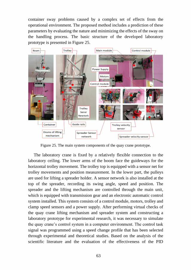
63

container sway problems caused by a complex set of effects from the

operational environment. The proposed method includes a prediction of these

parameters by evaluating the nature and minimizing the effects of the sway on

the handling process. The basic structure of the developed laboratory

prototype is presented in Figure 25.

Figure 25. The main system components of the quay crane prototype.

The laboratory crane is fixed by a relatively flexible connection to the

laboratory ceiling. The lower arms of the boom face the guideways for the

horizontal trolley movement. The trolley top is equipped with a sensor net for

trolley movements and position measurement. In the lower part, the pulleys

are used for lifting a spreader holder. A sensor network is also installed at the

top of the spreader, recording its swing angle, speed and position. The

spreader and the lifting mechanism are controlled through the main unit,

which is equipped with transmission gear and an electronic automatic control

system installed. This system consists of a control module, motors, trolley and

clamp speed sensors and a power supply. After performing virtual checks of

the quay crane lifting mechanism and spreader system and constructing a

laboratory prototype for experimental research, it was necessary to simulate

the quay crane’s control system in a computer environment. The control task

signal was programmed using a speed change profile that has been selected

through experimental and theoretical studies. Based on the analysis of the

scientific literature and the evaluation of the effectiveness of the PID

64

controller in this type of crane control systems, described in sub-section 1.1.3,

it was decided, to select the appropriate speed profile for the input, which was

combined with the PID controller for the control of the quay crane

transportation process.

2.3.3. Crane spreader control mathematical model

The following mathematical model described the laboratory cranes

spreader control sub-system, involving the PID and PI control methods

developing the container anti-sway algorithm. Firstly, the converter performs

conversion of the control signal to PWM signal which afterward generates the

motor phase voltages UA and UB:

{UA = f(u(t))

UB = f(u(t)) . (28)

Then, the generation of voltages UA and UB are implemented using PWM

signal modulation. The equivalent motor, which was used in the laboratory

prototype, is the stepper motor. Motor equations is:

{

diA

dt=

1

L(UA − RiA − eA)

diB

dt=

1

L(UB − RiB − eB)

Mv = −Km (iA −eA

Rm) sin(Nrθ) +

+Km (iB −eB

Rm) cos(Nrθ) −Mbtcos(4Nrθ)

dθ

dt= ωv

, (29)

where Km – torque constant of the stepper motor, iA and iB – stepper motor

coil current, eA and eB – the electromotive force of stepper motor, Rm –

magnetization resistor, Nr – stepper motor tooth per pole, θ – single step

rotation angle, Mbt – internal braking torque, R – winding resistance, L –

winding inductance, UA and UB – A and B phase winding voltages.

Therefore, the S-shaped profile, as part of a single control system, can be

used as a reference signal of the control system. A comprehensive

mathematical model was also developed:

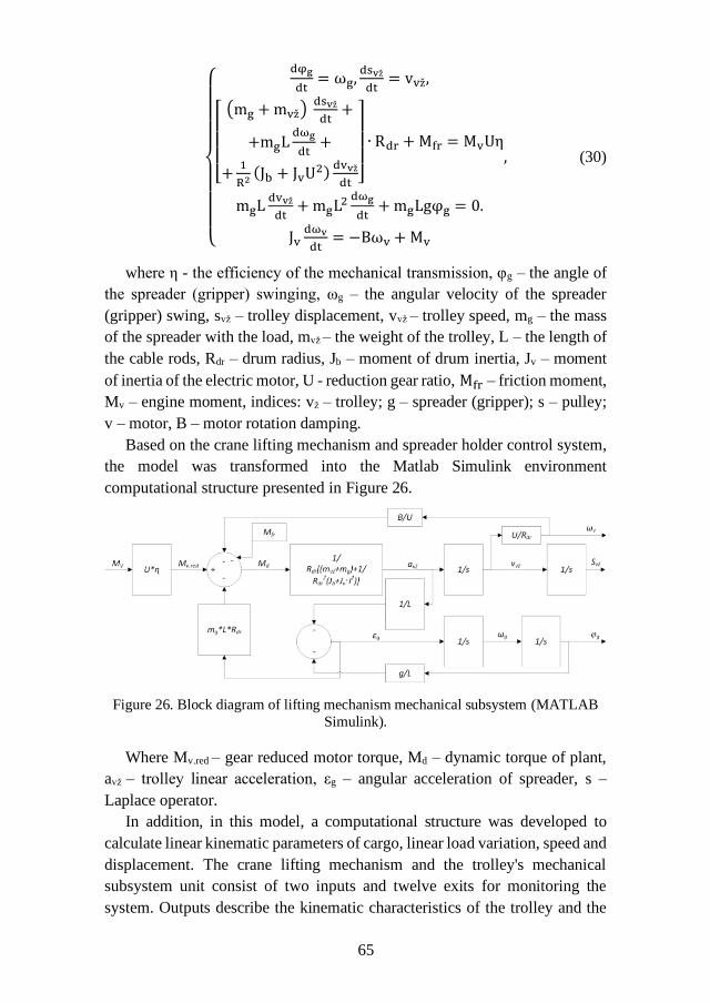
65

{

dφg

dt= ωg,

dsvž

dt= vvž,

[ (mg +mvž)

dsvž

dt+

+mgLdωg

dt+

+1

R2(Jb + JvU

2)dvvž

dt ]

∙ Rdr +Mfr = MvUη

mgLdvvž

dt+mgL

2 dωg

dt+mgLgφg = 0.

Jvdωv

dt= −Bωv +Mv

, (30)

where η - the efficiency of the mechanical transmission, φg – the angle of

the spreader (gripper) swinging, ωg – the angular velocity of the spreader

(gripper) swing, svž – trolley displacement, vvž – trolley speed, mg – the mass

of the spreader with the load, mvž – the weight of the trolley, L – the length of

the cable rods, Rdr – drum radius, Jb – moment of drum inertia, Jv – moment

of inertia of the electric motor, U - reduction gear ratio, Mfr – friction moment,

Mv – engine moment, indices: vž – trolley; g – spreader (gripper); s – pulley;

v – motor, B – motor rotation damping.

Based on the crane lifting mechanism and spreader holder control system,

the model was transformed into the Matlab Simulink environment

computational structure presented in Figure 26.

Figure 26. Block diagram of lifting mechanism mechanical subsystem (MATLAB

Simulink).

Where Mv.red – gear reduced motor torque, Md – dynamic torque of plant,

avž – trolley linear acceleration, εg – angular acceleration of spreader, s –

Laplace operator.

In addition, in this model, a computational structure was developed to

calculate linear kinematic parameters of cargo, linear load variation, speed and

displacement. The crane lifting mechanism and the trolley's mechanical

subsystem unit consist of two inputs and twelve exits for monitoring the

system. Outputs describe the kinematic characteristics of the trolley and the

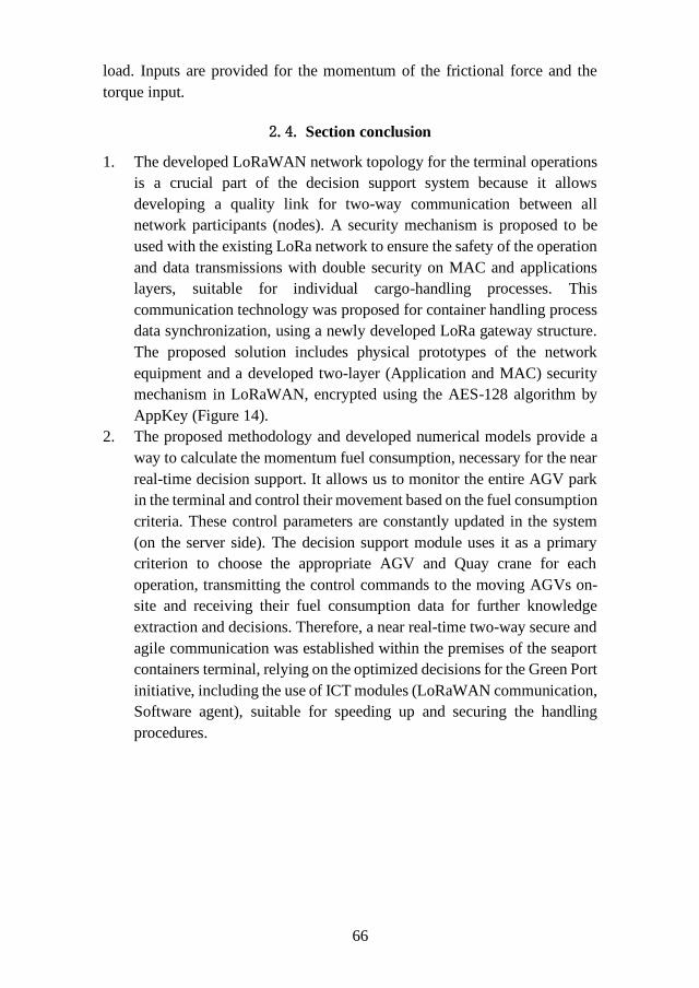
66

load. Inputs are provided for the momentum of the frictional force and the

torque input.

2.4. Section conclusion

1. The developed LoRaWAN network topology for the terminal operations

is a crucial part of the decision support system because it allows

developing a quality link for two-way communication between all

network participants (nodes). A security mechanism is proposed to be

used with the existing LoRa network to ensure the safety of the operation

and data transmissions with double security on MAC and applications

layers, suitable for individual cargo-handling processes. This

communication technology was proposed for container handling process

data synchronization, using a newly developed LoRa gateway structure.

The proposed solution includes physical prototypes of the network

equipment and a developed two-layer (Application and MAC) security

mechanism in LoRaWAN, encrypted using the AES-128 algorithm by

AppKey (Figure 14).

2. The proposed methodology and developed numerical models provide a

way to calculate the momentum fuel consumption, necessary for the near

real-time decision support. It allows us to monitor the entire AGV park

in the terminal and control their movement based on the fuel consumption

criteria. These control parameters are constantly updated in the system

(on the server side). The decision support module uses it as a primary

criterion to choose the appropriate AGV and Quay crane for each

operation, transmitting the control commands to the moving AGVs on-

site and receiving their fuel consumption data for further knowledge

extraction and decisions. Therefore, a near real-time two-way secure and

agile communication was established within the premises of the seaport

containers terminal, relying on the optimized decisions for the Green Port

initiative, including the use of ICT modules (LoRaWAN communication,

Software agent), suitable for speeding up and securing the handling

procedures.

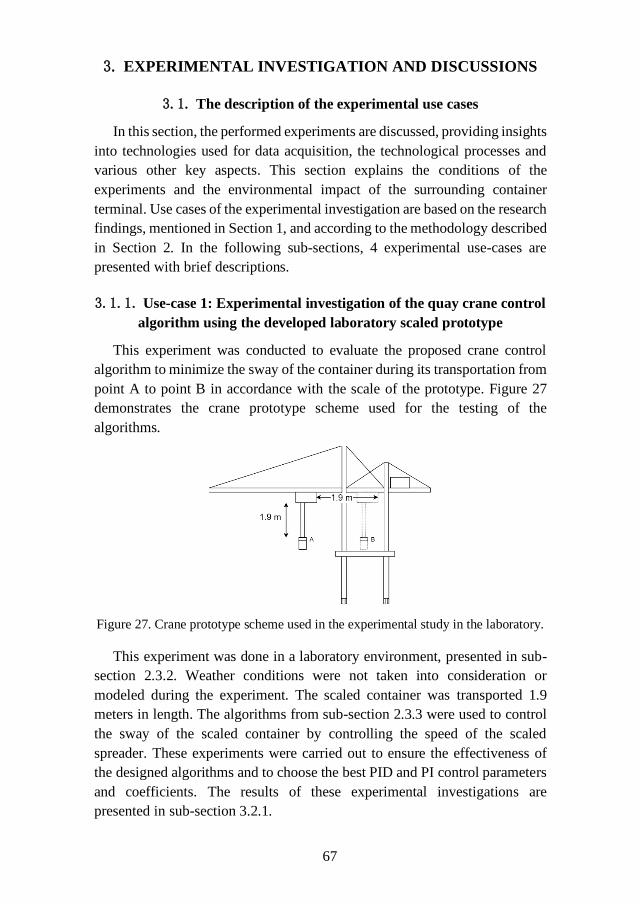
67

3. EXPERIMENTAL INVESTIGATION AND DISCUSSIONS

3.1. The description of the experimental use cases

In this section, the performed experiments are discussed, providing insights

into technologies used for data acquisition, the technological processes and

various other key aspects. This section explains the conditions of the

experiments and the environmental impact of the surrounding container

terminal. Use cases of the experimental investigation are based on the research

findings, mentioned in Section 1, and according to the methodology described

in Section 2. In the following sub-sections, 4 experimental use-cases are

presented with brief descriptions.

3.1.1. Use-case 1: Experimental investigation of the quay crane control

algorithm using the developed laboratory scaled prototype

This experiment was conducted to evaluate the proposed crane control

algorithm to minimize the sway of the container during its transportation from

point A to point B in accordance with the scale of the prototype. Figure 27

demonstrates the crane prototype scheme used for the testing of the

algorithms.

Figure 27. Crane prototype scheme used in the experimental study in the laboratory.

This experiment was done in a laboratory environment, presented in sub-

section 2.3.2. Weather conditions were not taken into consideration or

modeled during the experiment. The scaled container was transported 1.9

meters in length. The algorithms from sub-section 2.3.3 were used to control

the sway of the scaled container by controlling the speed of the scaled

spreader. These experiments were carried out to ensure the effectiveness of

the designed algorithms and to choose the best PID and PI control parameters

and coefficients. The results of these experimental investigations are

presented in sub-section 3.2.1.

68

3.1.2. Use-case 2: Experimental study of the data acquisition

equipment used on the quay cranes.

The aim of this experimental research was to test the real working

conditions of the quay cranes, the operators’ work and conditions, the

efficiency of the spreader and the unnecessary forces accumulated during the

container handling operations. In recent years, researchers have worked

closely with electrically powered terminal trucks and cranes [107], [108]. To

assess the need for synchronization, this experimental research was performed

at Klaipėda seaport. During the research, the quay crane carried out container

handling operations, during which the statistical data was collected. Data was

collected from 204 handling operations (full cycles). These full cycles include

container transportation from the ship to the truck and from the truck to the

ship. MK2 data logger hardware was used for these experimental

measurements (Figure 28).

Figure 28. The data acquisition equipment used for experimental measurements at

Klaipėda seaport.

When determining the dynamic parameters of the object under

investigation (in this case – the container), data about its acceleration, speed,

position in space, were measured and recorded. For this purpose, a DL1 - MK2

data logger (Race Technology, UK), a three-way accelerometer (guaranteed

2g minimum full scale on both axes; resolution of 0.005g; optional 6g sensor

available as a factory option) vibration measurements (vibration factory tested

69

at 25g, 50Hz sinusoid for 5 minutes), was used to record and store vehicle

motion dynamics parameters. For positioning, the meter is connected to a GPS

antenna (GPS – module outputs position, speed, position accuracy and speed

accuracy every 200ms with no interpolation; GPS tracking loops optimized

for applications up to about 4g; tracking of all satellites in view). Based on the

time course of the vehicle and the acceleration readings, the device measures

the speed of the test object with an accuracy of 0.16 km/h, with a measurement

error of up to 1%. Longitudinal and transverse accelerometers record

accelerations up to 20 m/s2 and measurement error up to 0.05 m/s2.

This research aimed to experimentally prove the inefficiency of the current

procedures and technological solutions. Collected data includes the duration

of the separate handling procedures and general statistical information. These

experimental results are discussed in sub-section 3.2.2.

3.1.3. Use-case 3: Experimental study of on-site quay cranes using

data acquisition equipment

In the experimental research DL1 - MK2 data logger/analyzer was used to

acquire and transfer statistical data (Figure 28). It uses a three-axis

accelerometer. Dynamical characteristics were examined, including

acceleration, speed and position. A GPS antenna was used to increase the

accuracy. Movement speed detection accuracy was set to 0.16 km/h due to

technological reasons and data logging accuracy was set to 1% due to

irregularities in the electronics. The mounting point was set on the spreader,

shown in Figure 29.

This position was chosen as more reliable and safer due to constant

movements and obstructions, unnecessary hits in all areas. Battery life was not

an essential part of the equipment. Its full capacity lifetime was enough to

function on a regular basis for the entire period of experimentation (8000

mAh). DL1 – MK2 data logger chosen because it allows all the data to be

referenced to not just time, but also a position during 3D movement. This

allows the data to be interpreted in a strict understandable way, referenced

clearly to the actual position and time stamp.

Braking points and gripper usage was analyzed with the built-in three-axis

accelerometer enhanced for high downforce applications. It is capable of

detecting minute changes with a 100Hz update rate on all attached sensors and

accelerometer channels. It also provides 8 analog channels (with 0-20 V

battery voltage) for sensor inputs ready for additional measurements and 2

CAN channels with up to 1 M baud rate with 14 CAN filters per channel (CAN

2.0 compatible).

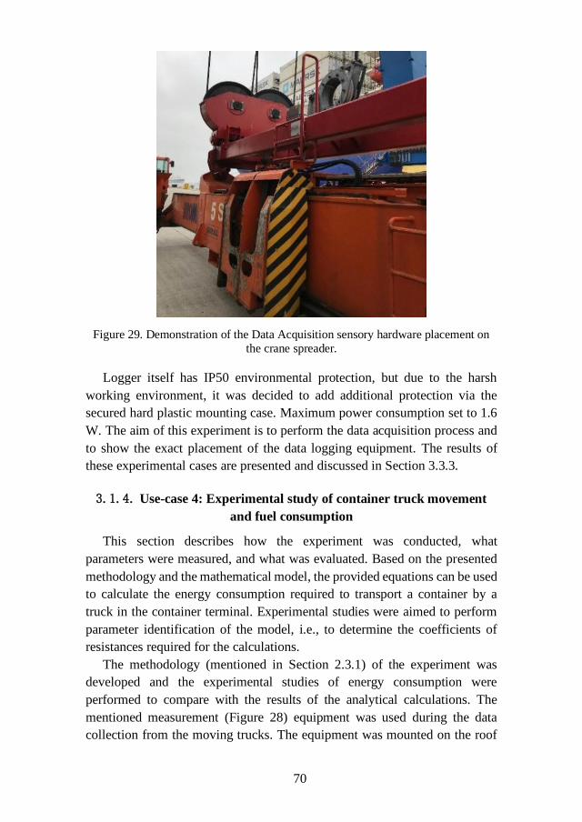
70

Figure 29. Demonstration of the Data Acquisition sensory hardware placement on

the crane spreader.

Logger itself has IP50 environmental protection, but due to the harsh

working environment, it was decided to add additional protection via the

secured hard plastic mounting case. Maximum power consumption set to 1.6

W. The aim of this experiment is to perform the data acquisition process and

to show the exact placement of the data logging equipment. The results of

these experimental cases are presented and discussed in Section 3.3.3.

3.1.4. Use-case 4: Experimental study of container truck movement

and fuel consumption

This section describes how the experiment was conducted, what

parameters were measured, and what was evaluated. Based on the presented

methodology and the mathematical model, the provided equations can be used

to calculate the energy consumption required to transport a container by a

truck in the container terminal. Experimental studies were aimed to perform

parameter identification of the model, i.e., to determine the coefficients of

resistances required for the calculations.

The methodology (mentioned in Section 2.3.1) of the experiment was

developed and the experimental studies of energy consumption were

performed to compare with the results of the analytical calculations. The

mentioned measurement (Figure 28) equipment was used during the data

collection from the moving trucks. The equipment was mounted on the roof

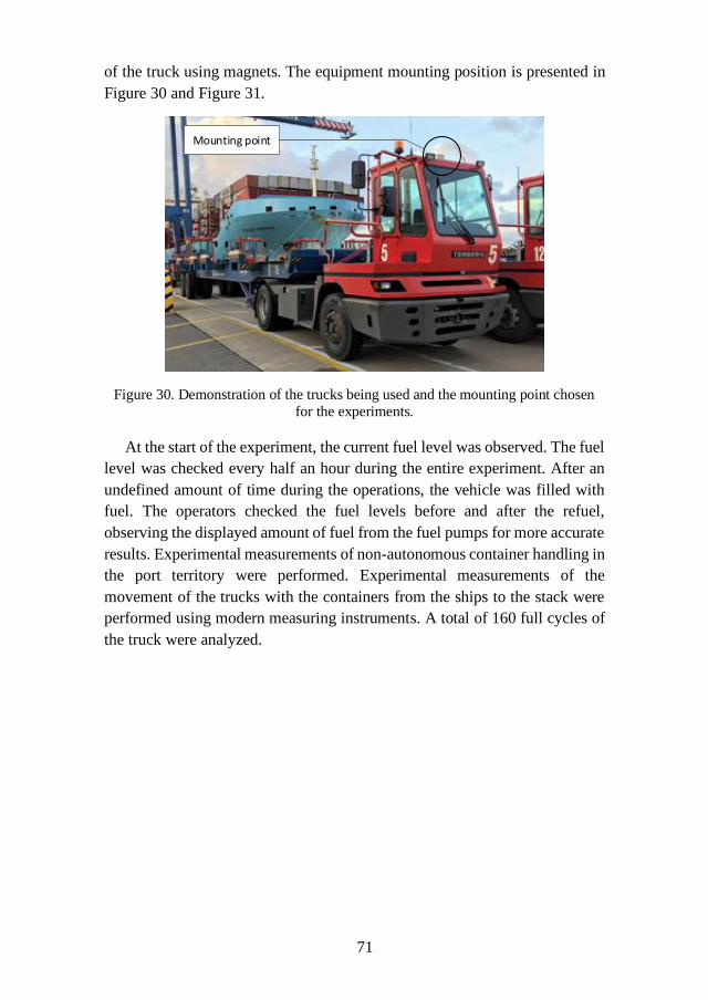
71

of the truck using magnets. The equipment mounting position is presented in

Figure 30 and Figure 31.

Mounting point

Figure 30. Demonstration of the trucks being used and the mounting point chosen

for the experiments.

At the start of the experiment, the current fuel level was observed. The fuel

level was checked every half an hour during the entire experiment. After an

undefined amount of time during the operations, the vehicle was filled with

fuel. The operators checked the fuel levels before and after the refuel,

observing the displayed amount of fuel from the fuel pumps for more accurate

results. Experimental measurements of non-autonomous container handling in

the port territory were performed. Experimental measurements of the

movement of the trucks with the containers from the ships to the stack were

performed using modern measuring instruments. A total of 160 full cycles of

the truck were analyzed.

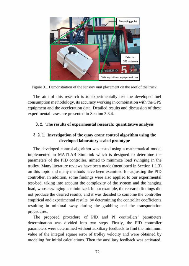
72

Figure 31. Demonstration of the sensory unit placement on the roof of the truck.

The aim of this research is to experimentally test the developed fuel

consumption methodology, its accuracy working in combination with the GPS

equipment and the acceleration data. Detailed results and discussion of these

experimental cases are presented in Section 3.3.4.

3.2. The results of experimental research: quantitative analysis

3.2.1. Investigation of the quay crane control algorithm using the

developed laboratory scaled prototype

The developed control algorithm was tested using a mathematical model

implemented in MATLAB Simulink which is designed to determine the

parameters of the PID controller, aimed to minimize load swinging in the

trolley. Many literature reviews have been made (mentioned in Section 1.1.3)

on this topic and many methods have been examined for adjusting the PID

controller. In addition, some findings were also applied to our experimental

test-bed, taking into account the complexity of the system and the hanging

load, whose swinging is minimized. In our example, the research findings did

not produce the desired results, and it was decided to combine the controller

empirical and experimental results, by determining the controller coefficients

resulting in minimal sway during the grabbing and the transportation

procedures.

The proposed procedure of PID and PI controllers’ parameters

determination was divided into two steps. Firstly, the PID controller

parameters were determined without auxiliary feedback to find the minimum

value of the integral square error of trolley velocity and were obtained by

modeling for initial calculations. Then the auxiliary feedback was activated.

Mounting point

Data aquisituon equipment box

External

GPS antenna

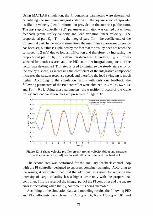
73

Using MATLAB simulation, the PI controller parameters were determined,

calculating the minimum integral criterion of the square error of spreader

oscillation velocity (detail information provided in the author’s publication).

The first step of controller (PID) parameter estimation was carried out without

feedback (crane trolley velocity and load variation linear velocity). The

proportional part Kp1, Ti1 – is the integral part, Td1 – the coefficients of the

differential part. In the second simulation, the minimum square error tolerance

has been set, but this is explained by the fact that the trolley does not reach the

set speed (0.2 m/s) due to low amplification and therefore, by increasing the

proportional part of Kp1, this deviation decreases. Therefore, Kp1 = 0.2 was

selected for another search and the PID controller integral component of the

factor was determined. This step is used to minimize the steady state error of

the trolley’s speed, as increasing the coefficient of the integrative component

increases the system response speed, and therefore the load swinging is much

higher. According to the simulation results with only one feedback, the

following parameters of the PID controller were obtained: Kp1 = 0.6, Ki1 = 13,

and Kd1 = 0.01. Using these parameters, the transition process of the crane

trolley and load variation rates are presented in Figure 32.

Figure 32. S-shape velocity profile (green), trolley velocity (blue) and spreader

oscillation velocity (red) graphs with PID controller and one feedback.

The second step was performed for the auxiliary feedback control loop

with the PI controller designed to suppress container swinging. According to

the results, it was determined that the additional PI system for reducing the

intensity of cargo volatility has a higher error only with the proportional

controller. This is a result of the integral part of the PI controller and the square

error is increasing when the Kp2 coefficient is being increased.

According to the simulation data and modeling results, the following PID

and PI coefficients were chosen: PID: Kp1 = 0.6, Ki1 = 13, Kd1 = 0.01, and

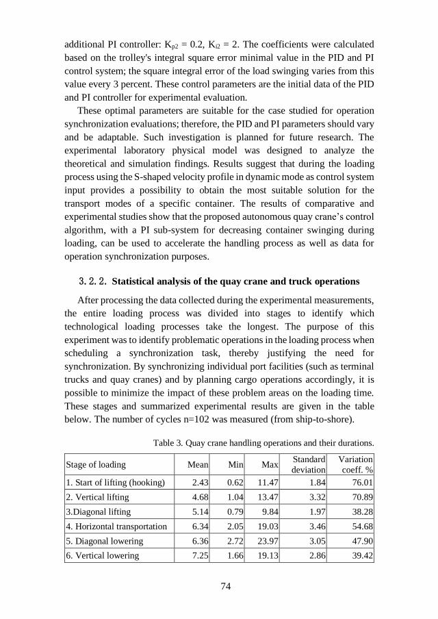
74

additional PI controller: Kp2 = 0.2, Ki2 = 2. The coefficients were calculated

based on the trolley's integral square error minimal value in the PID and PI

control system; the square integral error of the load swinging varies from this

value every 3 percent. These control parameters are the initial data of the PID

and PI controller for experimental evaluation.

These optimal parameters are suitable for the case studied for operation

synchronization evaluations; therefore, the PID and PI parameters should vary

and be adaptable. Such investigation is planned for future research. The

experimental laboratory physical model was designed to analyze the

theoretical and simulation findings. Results suggest that during the loading

process using the S-shaped velocity profile in dynamic mode as control system

input provides a possibility to obtain the most suitable solution for the

transport modes of a specific container. The results of comparative and

experimental studies show that the proposed autonomous quay crane’s control

algorithm, with a PI sub-system for decreasing container swinging during

loading, can be used to accelerate the handling process as well as data for

operation synchronization purposes.

3.2.2. Statistical analysis of the quay crane and truck operations

After processing the data collected during the experimental measurements,

the entire loading process was divided into stages to identify which

technological loading processes take the longest. The purpose of this

experiment was to identify problematic operations in the loading process when

scheduling a synchronization task, thereby justifying the need for

synchronization. By synchronizing individual port facilities (such as terminal

trucks and quay cranes) and by planning cargo operations accordingly, it is

possible to minimize the impact of these problem areas on the loading time.

These stages and summarized experimental results are given in the table

below. The number of cycles n=102 was measured (from ship-to-shore).

Table 3. Quay crane handling operations and their durations.

Stage of loading Mean Min Max Standard

deviation

Variation

coeff. %

1. Start of lifting (hooking) 2.43 0.62 11.47 1.84 76.01

2. Vertical lifting 4.68 1.04 13.47 3.32 70.89

3.Diagonal lifting 5.14 0.79 9.84 1.97 38.28

4. Horizontal transportation 6.34 2.05 19.03 3.46 54.68

5. Diagonal lowering 6.36 2.72 23.97 3.05 47.90

6. Vertical lowering 7.25 1.66 19.13 2.86 39.42

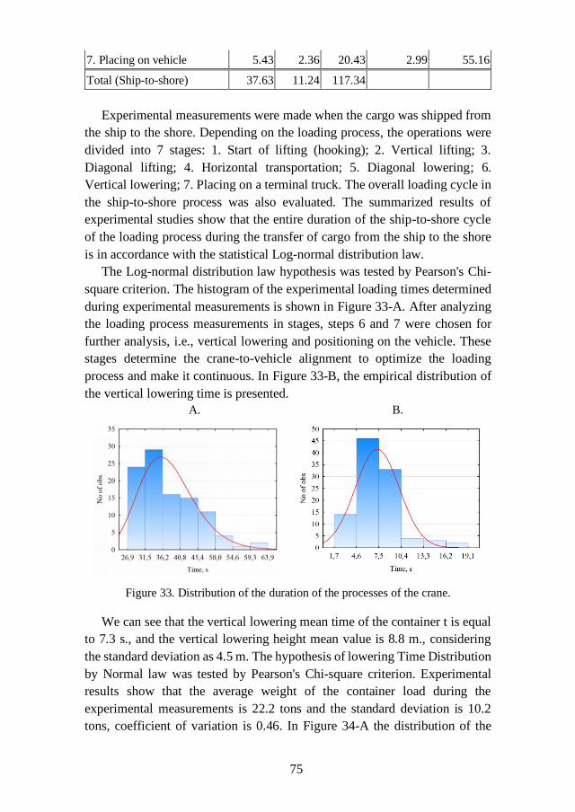
75

7. Placing on vehicle 5.43 2.36 20.43 2.99 55.16

Total (Ship-to-shore) 37.63 11.24 117.34

Experimental measurements were made when the cargo was shipped from

the ship to the shore. Depending on the loading process, the operations were

divided into 7 stages: 1. Start of lifting (hooking); 2. Vertical lifting; 3.

Diagonal lifting; 4. Horizontal transportation; 5. Diagonal lowering; 6.

Vertical lowering; 7. Placing on a terminal truck. The overall loading cycle in

the ship-to-shore process was also evaluated. The summarized results of

experimental studies show that the entire duration of the ship-to-shore cycle

of the loading process during the transfer of cargo from the ship to the shore

is in accordance with the statistical Log-normal distribution law.

The Log-normal distribution law hypothesis was tested by Pearson's Chi-

square criterion. The histogram of the experimental loading times determined

during experimental measurements is shown in Figure 33-A. After analyzing

the loading process measurements in stages, steps 6 and 7 were chosen for

further analysis, i.e., vertical lowering and positioning on the vehicle. These

stages determine the crane-to-vehicle alignment to optimize the loading

process and make it continuous. In Figure 33-B, the empirical distribution of

the vertical lowering time is presented.

A. B.

Figure 33. Distribution of the duration of the processes of the crane.

We can see that the vertical lowering mean time of the container t is equal

to 7.3 s., and the vertical lowering height mean value is 8.8 m., considering

the standard deviation as 4.5 m. The hypothesis of lowering Time Distribution

by Normal law was tested by Pearson's Chi-square criterion. Experimental

results show that the average weight of the container load during the

experimental measurements is 22.2 tons and the standard deviation is 10.2

tons, coefficient of variation is 0.46. In Figure 34-A the distribution of the

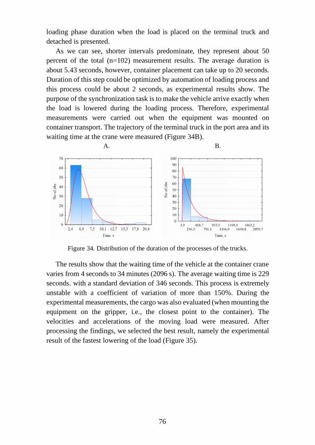
76

loading phase duration when the load is placed on the terminal truck and

detached is presented.

As we can see, shorter intervals predominate, they represent about 50

percent of the total (n=102) measurement results. The average duration is

about 5.43 seconds, however, container placement can take up to 20 seconds.

Duration of this step could be optimized by automation of loading process and

this process could be about 2 seconds, as experimental results show. The

purpose of the synchronization task is to make the vehicle arrive exactly when

the load is lowered during the loading process. Therefore, experimental

measurements were carried out when the equipment was mounted on

container transport. The trajectory of the terminal truck in the port area and its

waiting time at the crane were measured (Figure 34B).

A. B.

Figure 34. Distribution of the duration of the processes of the trucks.

The results show that the waiting time of the vehicle at the container crane

varies from 4 seconds to 34 minutes (2096 s). The average waiting time is 229

seconds. with a standard deviation of 346 seconds. This process is extremely

unstable with a coefficient of variation of more than 150%. During the

experimental measurements, the cargo was also evaluated (when mounting the

equipment on the gripper, i.e., the closest point to the container). The

velocities and accelerations of the moving load were measured. After

processing the findings, we selected the best result, namely the experimental

result of the fastest lowering of the load (Figure 35).

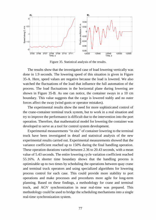
77

Figure 35. Statistical analysis of the results.

The results show that the investigated case of load lowering vertically was

done in 1.9 seconds. The lowering speed of this situation is given in Figure

35-A. Here, speed values are negative because the load is lowered. We also

watched the fluctuations of the load that influence the full automation of the

process. The load fluctuations in the horizontal plane during lowering are

shown in Figure 35-B. As one can notice, the container sways in a 10 cm

boundary. This value suggests that the cargo is lowered stably and no outer

forces affect the sway (wind gusts or operator mistakes).

The experimental results show the need for more sophisticated control of

the crane-container terminal truck system, but to work in a real situation and

try to improve the performance is difficult due to the intervention into the port

operation. Therefore, that mathematical model for lowering the container was

developed to serve as a tool for control system development.

Experimental measurements “in situ” of container lowering to the terminal

truck have been investigated in detail and statistical analysis of the new

experimental results carried out. Experimental measurements showed that the

variance coefficient reached up to 150% during the final handling operation.

These operation durations varied between 2.36 to 20.43 seconds, with a mean

value of 5.43 seconds. The entire lowering cycle variation coefficient reached

55.16%. A shorter time boundary shows that the handling process is

optimizable up to two times by scheduling the operations between quay crane

and terminal truck operators and using specialized algorithms for lowering

process control for each case. This could provide more stability to port

operations and make processes and procedures more agile for long-term

planning. Based on these findings, a methodology for crane and terminal

truck, and AGV synchronization in near real-time was prepared. This

methodology could be used to bridge the scheduling mechanisms into a single

real-time synchronization system.

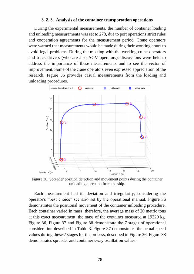
78

3.2.3. Analysis of the container transportation operations

During the experimental measurements, the number of container loading

and unloading measurements was set to 278, due to port operations strict rules

and cooperation agreements for the measurement period. Crane operators

were warned that measurements would be made during their working hours to

avoid legal problems. During the meeting with the working crane operators

and truck drivers (who are also AGV operators), discussions were held to

address the importance of these measurements and to see the vector of

improvement. Some of the crane operators even expressed appreciation of the

research. Figure 36 provides casual measurements from the loading and

unloading procedures.

Figure 36. Spreader position detection and movement points during the container

unloading operation from the ship.

Each measurement had its deviation and irregularity, considering the

operator's “best choice” scenario set by the operational manual. Figure 36

demonstrates the positional movement of the container unloading procedure.

Each container varied in mass, therefore, the average mass of 20 metric tons

at this exact measurement, the mass of the container measured at 19220 kg.

Figure 36, Figure 37 and Figure 38 demonstrate the 7 stages of operational

consideration described in Table 3. Figure 37 demonstrates the actual speed

values during these 7 stages for the process, described in Figure 36. Figure 38

demonstrates spreader and container sway oscillation values.

79

These values are of high importance, because higher values correlate with

the actual speed of the operation during the 7th stage by lowering the speed of

container positioning on the transport means or AGV. The overall

transportation process is then prolonged to compensate for the sway and keep

up with the work standard for the safety of cargo and security of operation.

These operations are mostly synchronized with the on-site AGV operators and

working standards to keep up with the ship unloading procedure. Yet, due to

technological reasons, delays occur on a daily basis.

Figure 37. Demonstration of spreader speed actual values during the 7 stages of

operation.

Initial results suggest that the operator did not maintain the same speed

during the horizontal transfer of the container. The operator made sudden

joystick control movements to stop the transportation process for a short

period. Figure 37 demonstrates the ladder shape of the speed values, which

correlates with the initial suggestion. This is due to the operator’s mistake,

lack of experience and unsynchronized actions between AGV or truck and the

crane. Each ladder produces additional oscillation, which is kept up to the final

7th stage.

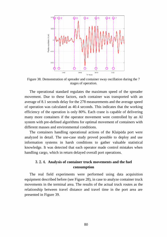
80

Figure 38. Demonstration of spreader and container sway oscillation during the 7

stages of operation.

The operational standard regulates the maximum speed of the spreader

movement. Due to these factors, each container was transported with an

average of 8.1 seconds delay for the 278 measurements and the average speed

of operation was calculated as 40.4 seconds. This indicates that the working

efficiency of the operation is only 80%. Each crane is capable of delivering

many more containers if the operator movement were controlled by an AI

system with pre-defined algorithms for optimal movement of containers with

different masses and environmental conditions.

The containers handling operational actions of the Klaipėda port were

analyzed in detail. The use-case study proved possible to deploy and use

information systems in harsh conditions to gather valuable statistical

knowledge. It was detected that each operator made control mistakes when

handling cargo, which in return delayed overall port operations.

3.2.4. Analysis of container truck movements and the fuel

consumption

The real field experiments were performed using data acquisition

equipment described before (see Figure 28), in case to analyze container truck

movements in the terminal area. The results of the actual truck routes as the

relationship between travel distance and travel time in the port area are

presented in Figure 39.

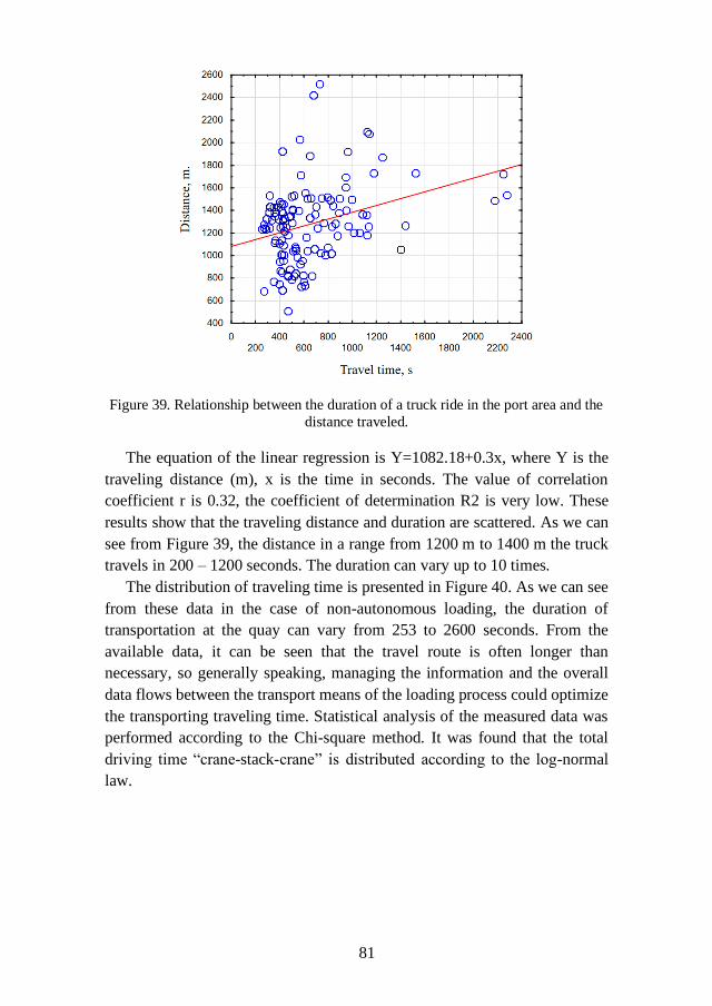
81

Figure 39. Relationship between the duration of a truck ride in the port area and the

distance traveled.

The equation of the linear regression is Y=1082.18+0.3x, where Y is the

traveling distance (m), x is the time in seconds. The value of correlation

coefficient r is 0.32, the coefficient of determination R2 is very low. These

results show that the traveling distance and duration are scattered. As we can

see from Figure 39, the distance in a range from 1200 m to 1400 m the truck

travels in 200 – 1200 seconds. The duration can vary up to 10 times.

The distribution of traveling time is presented in Figure 40. As we can see

from these data in the case of non-autonomous loading, the duration of

transportation at the quay can vary from 253 to 2600 seconds. From the

available data, it can be seen that the travel route is often longer than

necessary, so generally speaking, managing the information and the overall

data flows between the transport means of the loading process could optimize

the transporting traveling time. Statistical analysis of the measured data was

performed according to the Chi-square method. It was found that the total

driving time “crane-stack-crane” is distributed according to the log-normal

law.

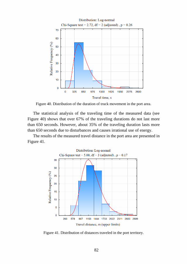
82

Figure 40. Distribution of the duration of truck movement in the port area.

The statistical analysis of the traveling time of the measured data (see

Figure 40) shows that over 67% of the traveling durations do not last more

than 650 seconds. However, about 35% of the traveling duration lasts more

than 650 seconds due to disturbances and causes irrational use of energy.

The results of the measured travel distance in the port area are presented in

Figure 41.

Figure 41. Distribution of distances traveled in the port territory.

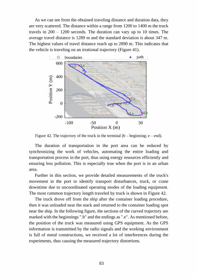
83

As we can see from the obtained traveling distance and duration data, they

are very scattered. The distance within a range from 1200 to 1400 m the truck

travels in 200 – 1200 seconds. The duration can vary up to 10 times. The

average travel distance is 1289 m and the standard deviation is about 347 m.

The highest values of travel distance reach up to 2890 m. This indicates that

the vehicle is traveling on an irrational trajectory (Figure 41).

Figure 42. The trajectory of the truck in the terminal (b – beginning; e – end).

The duration of transportation in the port area can be reduced by

synchronizing the work of vehicles, automating the entire loading and

transportation process in the port, thus using energy resources efficiently and

ensuring less pollution. This is especially true when the port is in an urban

area.

Further in this section, we provide detailed measurements of the truck's

movement in the port to identify transport disturbances, truck, or crane

downtime due to uncoordinated operating modes of the loading equipment.

The most common trajectory length traveled by truck is shown in Figure 42.

The truck drove off from the ship after the container loading procedure,

then it was unloaded near the stack and returned to the container loading spot

near the ship. In the following figure, the sections of the curved trajectory are

marked with the beginnings ".b" and the endings as ".e". As mentioned before,

the position of the truck was measured using GPS equipment. As the GPS

information is transmitted by the radio signals and the working environment

is full of metal constructions, we received a lot of interferences during the

experiments, thus causing the measured trajectory distortions.

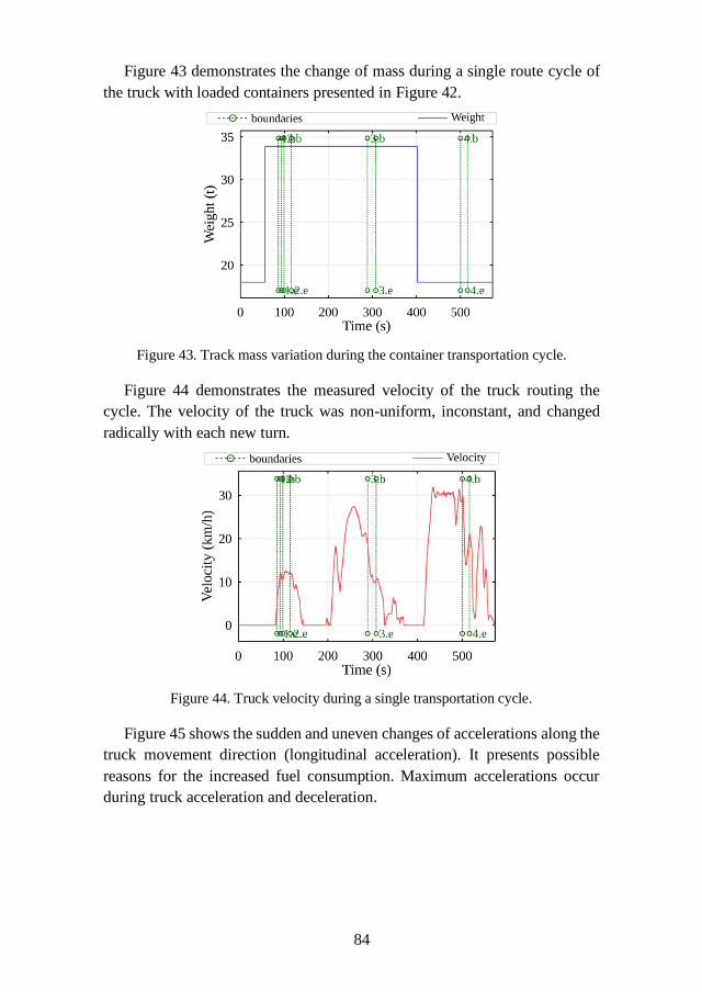
84

Figure 43 demonstrates the change of mass during a single route cycle of

the truck with loaded containers presented in Figure 42.

Figure 43. Track mass variation during the container transportation cycle.

Figure 44 demonstrates the measured velocity of the truck routing the

cycle. The velocity of the truck was non-uniform, inconstant, and changed

radically with each new turn.

Figure 44. Truck velocity during a single transportation cycle.

Figure 45 shows the sudden and uneven changes of accelerations along the

truck movement direction (longitudinal acceleration). It presents possible

reasons for the increased fuel consumption. Maximum accelerations occur

during truck acceleration and deceleration.

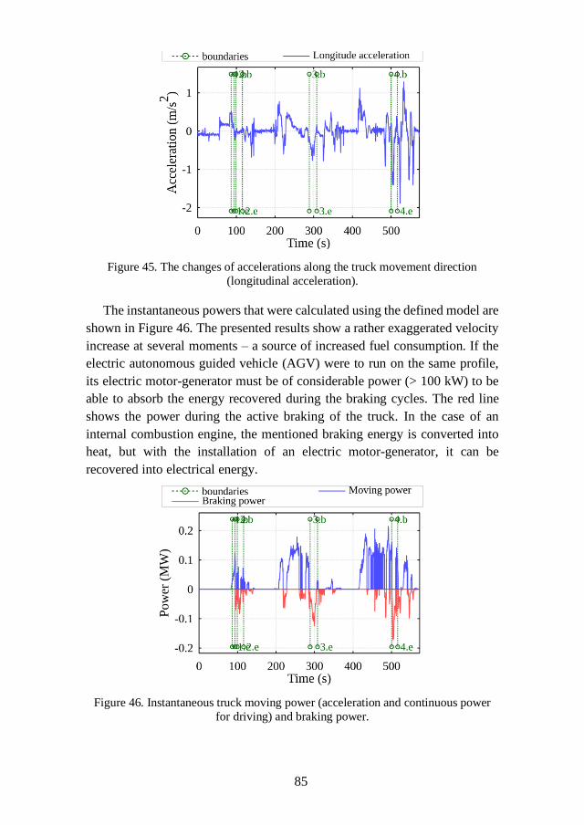
85

Figure 45. The changes of accelerations along the truck movement direction

(longitudinal acceleration).

The instantaneous powers that were calculated using the defined model are

shown in Figure 46. The presented results show a rather exaggerated velocity

increase at several moments – a source of increased fuel consumption. If the

electric autonomous guided vehicle (AGV) were to run on the same profile,

its electric motor-generator must be of considerable power (> 100 kW) to be

able to absorb the energy recovered during the braking cycles. The red line

shows the power during the active braking of the truck. In the case of an

internal combustion engine, the mentioned braking energy is converted into

heat, but with the installation of an electric motor-generator, it can be

recovered into electrical energy.

Figure 46. Instantaneous truck moving power (acceleration and continuous power

for driving) and braking power.

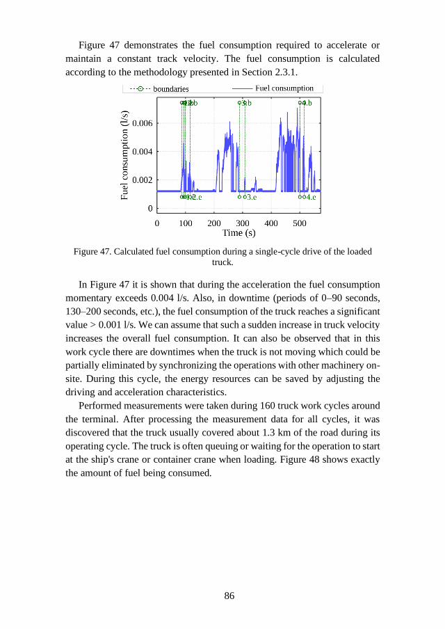
86

Figure 47 demonstrates the fuel consumption required to accelerate or

maintain a constant track velocity. The fuel consumption is calculated

according to the methodology presented in Section 2.3.1.

Figure 47. Calculated fuel consumption during a single-cycle drive of the loaded

truck.

In Figure 47 it is shown that during the acceleration the fuel consumption

momentary exceeds 0.004 l/s. Also, in downtime (periods of 0–90 seconds,

130–200 seconds, etc.), the fuel consumption of the truck reaches a significant

value > 0.001 l/s. We can assume that such a sudden increase in truck velocity

increases the overall fuel consumption. It can also be observed that in this

work cycle there are downtimes when the truck is not moving which could be

partially eliminated by synchronizing the operations with other machinery on-

site. During this cycle, the energy resources can be saved by adjusting the

driving and acceleration characteristics.

Performed measurements were taken during 160 truck work cycles around

the terminal. After processing the measurement data for all cycles, it was

discovered that the truck usually covered about 1.3 km of the road during its

operating cycle. The truck is often queuing or waiting for the operation to start

at the ship's crane or container crane when loading. Figure 48 shows exactly

the amount of fuel being consumed.

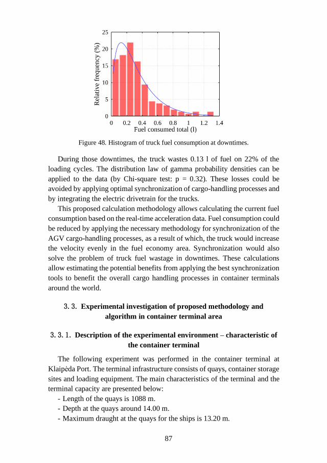
87

Figure 48. Histogram of truck fuel consumption at downtimes.

During those downtimes, the truck wastes 0.13 l of fuel on 22% of the

loading cycles. The distribution law of gamma probability densities can be

applied to the data (by Chi-square test: p = 0.32). These losses could be

avoided by applying optimal synchronization of cargo-handling processes and

by integrating the electric drivetrain for the trucks.

This proposed calculation methodology allows calculating the current fuel

consumption based on the real-time acceleration data. Fuel consumption could

be reduced by applying the necessary methodology for synchronization of the

AGV cargo-handling processes, as a result of which, the truck would increase

the velocity evenly in the fuel economy area. Synchronization would also

solve the problem of truck fuel wastage in downtimes. These calculations

allow estimating the potential benefits from applying the best synchronization

tools to benefit the overall cargo handling processes in container terminals

around the world.

3.3. Experimental investigation of proposed methodology and

algorithm in container terminal area

3.3.1. Description of the experimental environment – characteristic of

the container terminal

The following experiment was performed in the container terminal at

Klaipėda Port. The terminal infrastructure consists of quays, container storage

sites and loading equipment. The main characteristics of the terminal and the

terminal capacity are presented below:

- Length of the quays is 1088 m.

- Depth at the quays around 14.00 m.

- Maximum draught at the quays for the ships is 13.20 m.

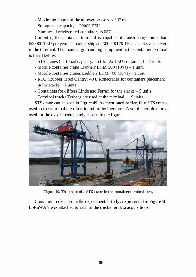
88

- Maximum length of the allowed vessels is 337 m.

- Storage site capacity – 20000 TEU.

- Number of refrigerated containers is 657.

Currently, the container terminal is capable of transloading more than

600000 TEU per year. Container ships of 3000–9178 TEU capacity are served

in the terminal. The main cargo handling equipment in the container terminal

is listed below:

- STS cranes (51 t load capacity, 65 t for 2x TEU containers) – 4 units.

- Mobile container crane Liebherr LHM 500 (104 t) – 1 unit.

- Mobile container cranes Liebherr LHM 400 (104 t) – 1 unit.

- RTG (Rubber Tired Gantry) 40 t, Konecranes for containers placement

in the stacks – 7 units.

- Containers fork lifters Linde and Ferrari for the stacks – 5 units.

- Terminal trucks Terberg are used at the terminal – 19 units.

STS crane can be seen in Figure 49. As mentioned earlier, four STS cranes

used in the terminal are often found in the literature. Also, the terminal area

used for the experimental study is seen in the figure.

Figure 49. The photo of a STS crane in the container terminal area.

Container trucks used in the experimental study are presented in Figure 50.

LoRaWAN was attached to each of the trucks for data acquisitions.

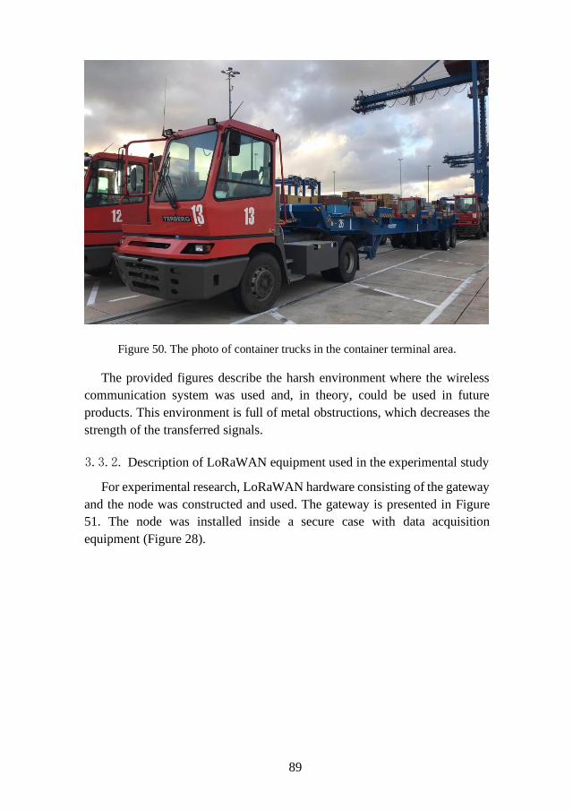
89

Figure 50. The photo of container trucks in the container terminal area.

The provided figures describe the harsh environment where the wireless

communication system was used and, in theory, could be used in future

products. This environment is full of metal obstructions, which decreases the

strength of the transferred signals.

3.3.2. Description of LoRaWAN equipment used in the experimental study

For experimental research, LoRaWAN hardware consisting of the gateway

and the node was constructed and used. The gateway is presented in Figure

51. The node was installed inside a secure case with data acquisition

equipment (Figure 28).

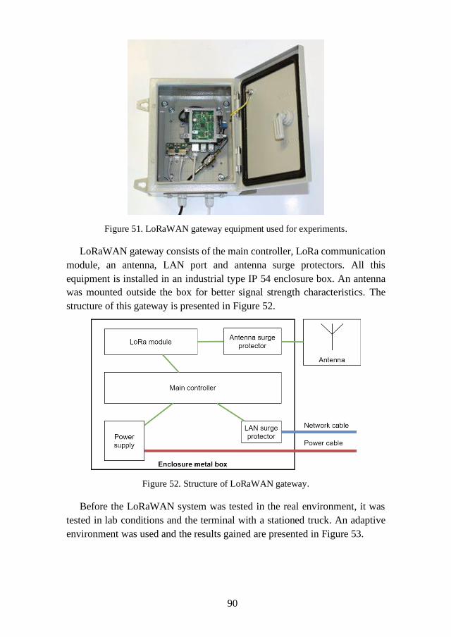
90

Figure 51. LoRaWAN gateway equipment used for experiments.

LoRaWAN gateway consists of the main controller, LoRa communication

module, an antenna, LAN port and antenna surge protectors. All this

equipment is installed in an industrial type IP 54 enclosure box. An antenna

was mounted outside the box for better signal strength characteristics. The

structure of this gateway is presented in Figure 52.

Figure 52. Structure of LoRaWAN gateway.

Before the LoRaWAN system was tested in the real environment, it was

tested in lab conditions and the terminal with a stationed truck. An adaptive

environment was used and the results gained are presented in Figure 53.

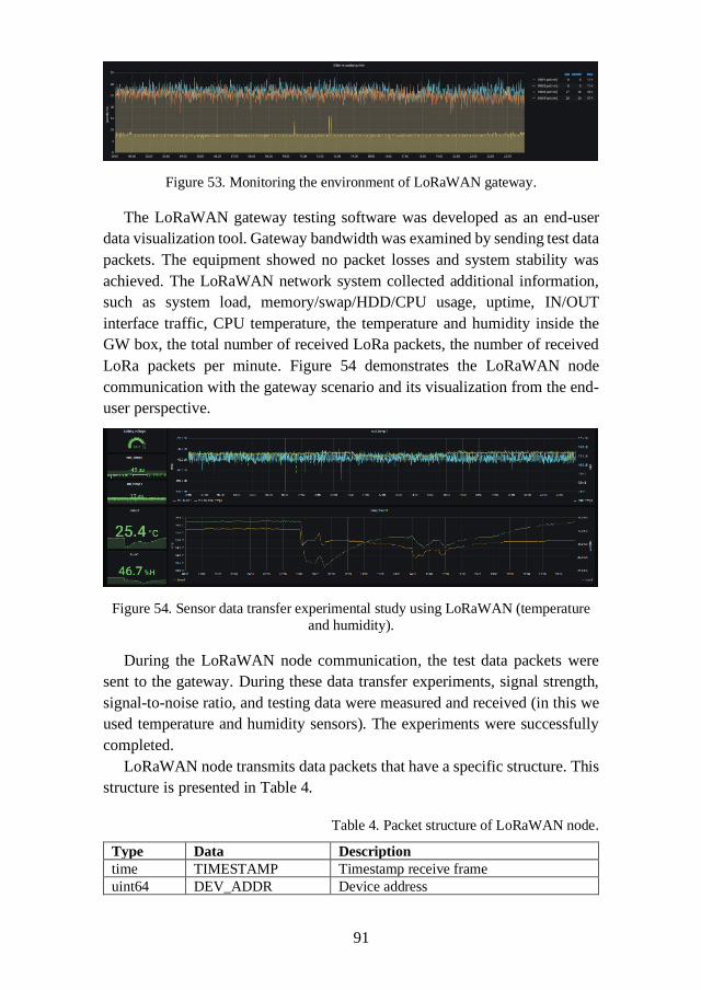
91

Figure 53. Monitoring the environment of LoRaWAN gateway.

The LoRaWAN gateway testing software was developed as an end-user

data visualization tool. Gateway bandwidth was examined by sending test data

packets. The equipment showed no packet losses and system stability was

achieved. The LoRaWAN network system collected additional information,

such as system load, memory/swap/HDD/CPU usage, uptime, IN/OUT

interface traffic, CPU temperature, the temperature and humidity inside the

GW box, the total number of received LoRa packets, the number of received

LoRa packets per minute. Figure 54 demonstrates the LoRaWAN node

communication with the gateway scenario and its visualization from the end-

user perspective.

Figure 54. Sensor data transfer experimental study using LoRaWAN (temperature

and humidity).

During the LoRaWAN node communication, the test data packets were

sent to the gateway. During these data transfer experiments, signal strength,

signal-to-noise ratio, and testing data were measured and received (in this we

used temperature and humidity sensors). The experiments were successfully

completed.

LoRaWAN node transmits data packets that have a specific structure. This

structure is presented in Table 4.

Table 4. Packet structure of LoRaWAN node.

Type Data Description

time TIMESTAMP Timestamp receive frame

uint64 DEV_ADDR Device address

92

double RSSI Received signal strength indication

string PHY_PAYLOAD Payload from message

Data packets sent by the LoRaWAN gateway to the nodes have their own

structure which is presented in Table 5.

Table 5. Packet structure of LoRaWAN gateway.

Type Data Description

time TIMESTAMP Timestamp receive frame

macaddr INCIDENT_DEV_ADDR Device address

uint32 ALERT_CODE Alert code

string PHY_PAYLOAD Payload message

double RSSI Received signal strength indication

double BASE_RSSI Base RSSI value is defined by the first

received message from device to

detector

double VARIANCE Define variance

The main structure of the data packets received by the gateway consists of

timestamp received frame, device address, alert code, payload message,

received signal strength indication. The base RSSI value is defined by the first

received message from device to detector, define variance. The payload

includes information dedicated to each node.

3.3.3. The description of the experimental study

During the experimental case study, the LoRaWAN system was mounted

on a moving AGV. The developed wireless data logging system was used to

collect the parameters in real-time described in 3.1.2. During the experiment,

several positions of system placement were discussed with the operators on-

site. Obvious positions were considered taking into account the security

measures, the harsh working conditions (possibility to damage the system

during cargo handling operations) and the possibility to have easy access to

mount or change the equipment. The best possible scenario was to mount the

system on the top of the cabin of the truck (Figure 30 and Figure 31).

Next, the system was initiated from the cabin using connected laptop

equipment. Similar equipment was used in a secure location near the quay

crane, simulating the access point of the network. This was done to ensure the

stability and work-ready conditions of the software and wireless connection.

Updates were performed for the sensory units of the node. The truck moved

in the usual manner across the terminal with the loaded cargo. The following

movement path describes the average movement pattern (Figure 55).

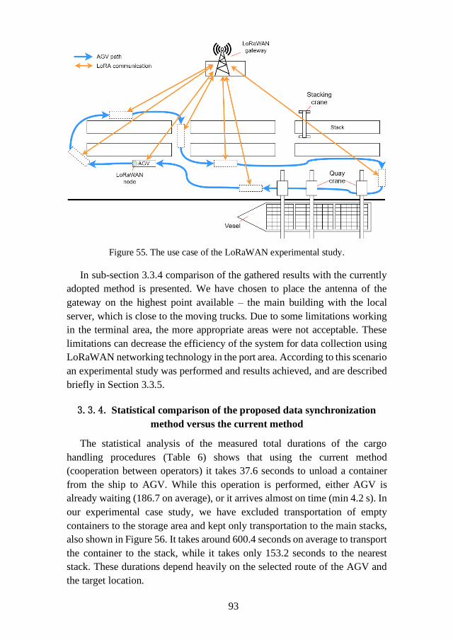
93

Figure 55. The use case of the LoRaWAN experimental study.

In sub-section 3.3.4 comparison of the gathered results with the currently

adopted method is presented. We have chosen to place the antenna of the

gateway on the highest point available – the main building with the local

server, which is close to the moving trucks. Due to some limitations working

in the terminal area, the more appropriate areas were not acceptable. These

limitations can decrease the efficiency of the system for data collection using

LoRaWAN networking technology in the port area. According to this scenario

an experimental study was performed and results achieved, and are described

briefly in Section 3.3.5.

3.3.4. Statistical comparison of the proposed data synchronization

method versus the current method

The statistical analysis of the measured total durations of the cargo

handling procedures (Table 6) shows that using the current method

(cooperation between operators) it takes 37.6 seconds to unload a container

from the ship to AGV. While this operation is performed, either AGV is

already waiting (186.7 on average), or it arrives almost on time (min 4.2 s). In

our experimental case study, we have excluded transportation of empty

containers to the storage area and kept only transportation to the main stacks,

also shown in Figure 56. It takes around 600.4 seconds on average to transport

the container to the stack, while it takes only 153.2 seconds to the nearest

stack. These durations depend heavily on the selected route of the AGV and

the target location.

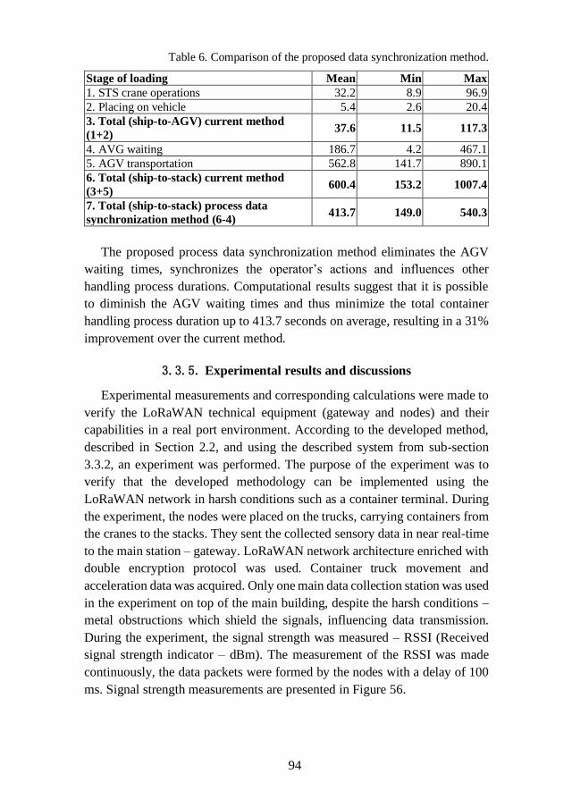
94

Table 6. Comparison of the proposed data synchronization method.

Stage of loading Mean Min Max

1. STS crane operations 32.2 8.9 96.9

2. Placing on vehicle 5.4 2.6 20.4

3. Total (ship-to-AGV) current method

(1+2) 37.6 11.5 117.3

4. AVG waiting 186.7 4.2 467.1

5. AGV transportation 562.8 141.7 890.1

6. Total (ship-to-stack) current method

(3+5) 600.4 153.2 1007.4

7. Total (ship-to-stack) process data

synchronization method (6-4) 413.7 149.0 540.3

The proposed process data synchronization method eliminates the AGV

waiting times, synchronizes the operator’s actions and influences other

handling process durations. Computational results suggest that it is possible

to diminish the AGV waiting times and thus minimize the total container

handling process duration up to 413.7 seconds on average, resulting in a 31%

improvement over the current method.

3.3.5. Experimental results and discussions

Experimental measurements and corresponding calculations were made to

verify the LoRaWAN technical equipment (gateway and nodes) and their

capabilities in a real port environment. According to the developed method,

described in Section 2.2, and using the described system from sub-section

3.3.2, an experiment was performed. The purpose of the experiment was to

verify that the developed methodology can be implemented using the

LoRaWAN network in harsh conditions such as a container terminal. During

the experiment, the nodes were placed on the trucks, carrying containers from

the cranes to the stacks. They sent the collected sensory data in near real-time

to the main station – gateway. LoRaWAN network architecture enriched with

double encryption protocol was used. Container truck movement and

acceleration data was acquired. Only one main data collection station was used

in the experiment on top of the main building, despite the harsh conditions –

metal obstructions which shield the signals, influencing data transmission.

During the experiment, the signal strength was measured – RSSI (Received

signal strength indicator – dBm). The measurement of the RSSI was made

continuously, the data packets were formed by the nodes with a delay of 100

ms. Signal strength measurements are presented in Figure 56.

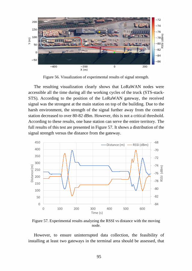
95

Figure 56. Visualization of experimental results of signal strength.

The resulting visualization clearly shows that LoRaWAN nodes were

accessible all the time during all the working cycles of the truck (STS-stack-

STS). According to the position of the LoRaWAN gateway, the received

signal was the strongest at the main station on top of the building. Due to the

harsh environment, the strength of the signal further away from the central

station decreased to over 80-82 dBm. However, this is not a critical threshold.

According to these results, one base station can serve the entire territory. The

full results of this test are presented in Figure 57. It shows a distribution of the

signal strength versus the distance from the gateway.

Figure 57. Experimental results analyzing the RSSI vs distance with the moving

node.

However, to ensure uninterrupted data collection, the feasibility of

installing at least two gateways in the terminal area should be assessed, that

-84

-82

-80

-78

-76

-74

-72

-70

-68

0

50

100

150

200

250

300

350

400

450

0 100 200 300 400 500 600

RSS

I (d

Bm

)

Dis

tan

ce (m

)

Time (s)

Distance (m) RSSI (dBm)

96

will overlap and fill possible signal loss gaps. Such infrastructure will not be

costly and not hard to install. Such a system will be much cheaper compared

to the other. In comparison, it would take more than 10 Wi-Fi gateways to fill

such territory, even using the latest 5G technologies. The proposed solution is

much more effective, as it requires small data packets to be sent from each

measurement point, and the transfer is not crucial as well. LoRaWAN

technology fits well for such use cases and is fully compatible with the

proposed methodology described in Section 2.1.

3.4. Section conclusion

1. In this section, the experimental study is provided, describing the

technical means used for data acquisition and transfer in the container

terminal of Klaipėda Port. LoRaWAN network architecture was used

with security mechanisms to ensure that the system would work in a real

environment using sensory data and safety protocols. A communication

efficiency experiment was performed using moving trucks with attached

LoRa nodes, collecting sensory information about the position of the

trucks, their speed and accelerations. The results show that the proposed

long-range LoRaWAN networking technology is adaptable in the harsh

environment of the container terminal and can be used for data

synchronization among moving nodes. These nodes were placed on the

moving trucks and no insignificant signal losses were observed during

the cargo handling procedures. Placement of other technical means to

acquire the same signals and same data from the trucks is possible, but

such infrastructure would cost more to deploy and maintain during a long

operational period. To cover the whole terminal, it is suggested that two

base stations (gateways) on opposite sides of the terminal should be used

for better signal coverage. The harsh environment of the terminal, taking

into account the shielding of the signals by the metal obstructions, e.g.,

containers in the stacks, can cause additional problems for the other

conventional system with higher bandwidth (4G, 5G, Wi-Fi). The

sensory data was received without any deviations and downtimes and for

such a system deployment it is more than enough to optimize the truck

movement and crane operations, synchronizing the processes using

limited sensory data at full.

2. Computational results suggest that it is possible to diminish the AGV

waiting times and thus minimize the total container handling process

duration up to 413.7 seconds on average, resulting in a 31% improvement

over the current method.

97

3. LoRaWAN technology is not new in the research community, but its

adoption in new areas to solve unconventional problems and its

optimization to suit the needs of the industry is a complex

interdisciplinary challenge to informatics and transport engineers as

demonstrated in the previous sections.

98

CONCLUSIONS

1. The performed literature review in the areas of container terminal

optimization, control of quay crane and cargo handling processes, AGV

navigation, route planning, wireless and smart technologies show that

current systems and algorithms are not enough to solve the synchronization

problems or to increase the efficiency of the container handling process.

The existing planning systems do not evaluate real-time data for processes

synchronization, which leads to lowered effectiveness of the procedures.

To synchronize the movement data between trucks and quay cranes LoRa

technology was chosen due to its unique properties dealing with long-range

communication tasks in harsh environments, optimal for port operations.

LoRaWAN networks provide higher interference immunity compared to

other wireless communication technologies (SIGFOX, LTE-Cat 1, LTE-

M, NB-LTE) while maintaining optimal battery usage using sleep mode

and high link threshold values. The used modulation and bandwidth are

optimal for sensory data transmission in port operations with an unlimited

number of messages while maintaining 290 bps–50 Kbps data rates. The

adoption of the new data synchronization system requires new

infrastructure deployment, yet, it is problematic to apply these new

technologies in the harsh environment of the container terminal. Therefore,

it was concluded that to solve these problems it is necessary to use LoRa

technology for secure and reliable connections for handling processes

synchronization.

2. A new method for processes data synchronization between port trucks and

quay cranes was developed, including assignment, positioning and data

exchange algorithms, decision support modules, and LoRaWAN network

topology with double security on MAC and applications layers that are

suitable for individual cargo-handling processes:

A. The concept of container handling process data synchronization

between two nodes (AGV and quay crane) was proposed, including

the use of ICT modules (LoRaWAN communication, Software agent).

Additionally, to speed up the data acquisition and process control, two

modules were proposed in both nodes (Data collection and Decision

support). This method is suitable for speeding up and securing the

handling procedures, reducing downtimes of the trucks, and ensuring

optimal vehicle energy consumption for the entire operational cycle,

according to the EU Directive 2018/410 for the “green” port guides.

B. Wireless communication technology was proposed for container

handling process data synchronization, using a newly developed LoRa

99

gateway structure. The proposed solution includes physical

prototypes of the network equipment and a developed two-layer

(Application and MAC) security mechanism in LoRaWAN protocol,

encrypted using the AES-128 algorithm by AppKey.

3. Comparative and experimental research results show:

A. Computational results suggest that it is possible to diminish the AGV

waiting times and thus minimize the total container handling process

duration up to 413.7 seconds on average, resulting in a 31%

improvement over the current method.

B. The proposed long-range LoRaWAN networking technology is

adaptable in the harsh environment of the containers terminal and can

be used for data synchronization among moving nodes. The average

signal strength in the port environment was -77.49 dBm, and the

maximum signal strength drop not exceed the threshold. If the

threshold of -120 dBm is not reached, then the signal loss is not

critical at the terminal. The results suggest that by using only a single

gateway it is possible to cover medium size container terminal for data

acquisition from all nodes. The number of LoRa nodes can be

increased to cover even the largest port areas like Rotterdam but to

make it happen simply more gateways must be used.

4. Future research will be aimed at the evaluation of complex decision

support methods to improve the operator actions, developing state of the

art in process control and prediction using novel AI algorithms (machine

learning, deep learning and neural networks). This will help improve the

crane operator’s work by providing real-time situation information, not

only predicting an action but also making process data synchronization

more accurate in long-term planning. The performed research and future

planned activities are based on the Lithuanian Smart Specialization

Strategy (RIS3) priority – transport, logistics and ICT.

100

BIBLIOGRAPHY AND REFERENCES

[1] L. A. Tuan, H. M. Cuong, P. Van Trieu, L. C. Nho, V. D. Thuan, and

L. V. Anh, “Adaptive neural network sliding mode control of

shipboard container cranes considering actuator backlash,” Mech. Syst. Signal Process., vol. 112, pp. 233–250, 2018, doi:

10.1016/j.ymssp.2018.04.030.

[2] I. Golovin and S. Palis, “Robust control for active damping of elastic gantry crane vibrations,” Mech. Syst. Signal Process., vol. 121, 2019,

doi: 10.1016/j.ymssp.2018.11.005.

[3] M. Sha et al., “Scheduling optimization of yard cranes with minimal energy consumption at container terminals,” Comput. Ind. Eng., vol.

113, pp. 704–713, 2017, doi: 10.1016/j.cie.2016.03.022.

[4] European Commission, “The European Green Deal: Communication

from the Commission to the European Parliament, the European Council, the Council, the European Economic and Social Committee

and the Committee of the Regions,” p. 24, 2019, doi:

10.2307/j.ctvd1c6zh.7. [5] N. Sun, Y. Wu, H. Chen, and Y. Fang, “An energy-optimal solution

for transportation control of cranes with double pendulum dynamics:

Design and experiments,” Mech. Syst. Signal Process., vol. 102, 2018, doi: 10.1016/j.ymssp.2017.09.027.

[6] M. Kermani, G. Parise, L. Martirano, L. Parise, and B. Chavdarian,

“Optimization of Peak Load Shaving in STS Group Cranes Based on

PSO Algorithm,” 2018, doi: 10.1109/EEEIC.2018.8494467. [7] A. A. Elbadawy and M. M. G. Shehata, “Anti-sway control of marine

cranes under the disturbance of a parallel manipulator,” Nonlinear

Dyn., vol. 82, no. 1–2, pp. 415–434, 2015, doi: 10.1007/s11071-015-2165-3.

[8] M. A. Majid, W. S. W. Ibrahim, S. Mohamad, and Z. A. Bakar, “A

comparison of PID and PD controller with input shaping technique for

3D gantry crane,” Proc. - 2013 IEEE Conf. Syst. Process Control. ICSPC 2013, no. December, pp. 144–148, 2013, doi:

10.1109/SPC.2013.6735121.

[9] M. E. Taner, O. Kulak, and M. U. Koyuncuoǧlu, “Layout analysis affecting strategic decisions in artificial container terminals,” Comput.

Ind. Eng., vol. 75, no. 1, 2014, doi: 10.1016/j.cie.2014.05.025.

[10] T. T. Wong, C. H. H. Tang, and M. Mailah, “Robust active heave compensated winch-driven overhead crane system for load transfer in

marine operation,” ICIAS 2012 - 2012 4th Int. Conf. Intell. Adv. Syst.

A Conf. World Eng. Sci. Technol. Congr. - Conf. Proc., vol. 1, pp. 111–

116, 2012, doi: 10.1109/ICIAS.2012.6306170. [11] T. T. Wong, C. H. H. Tang, and M. Mailah, “Winch driven active

heave compensation for load transfer in overhead crane system,”

ICIAS 2012 - 2012 4th Int. Conf. Intell. Adv. Syst. A Conf. World Eng.

101

Sci. Technol. Congr. - Conf. Proc., vol. 1, pp. 34–39, 2012, doi:

10.1109/ICIAS.2012.6306154. [12] M. Zhang, Y. Zhang, H. Chen, and X. Cheng, “Model-independent

PD-SMC method with payload swing suppression for 3D overhead

crane systems,” Mech. Syst. Signal Process., 2019, doi:

10.1016/j.ymssp.2019.04.046. [13] H. I. Jaafar, Z. Mohamed, A. F. Z. Abidin, and Z. A. Ghani, “PSO-

tuned PID controller for a nonlinear gantry crane system,” Proc. - 2012

IEEE Int. Conf. Control Syst. Comput. Eng. ICCSCE 2012, pp. 515–519, 2013, doi: 10.1109/ICCSCE.2012.6487200.

[14] H. I. Jaafar, M. F. Sulaima, Z. Mohamed, and J. J. Jamian, “Optimal

PID controller parameters for nonlinear gantry crane system via MOPSO technique,” Proc. - 2013 IEEE Conf. Sustain. Util. Dev. Eng.

Technol. IEEE CSUDET 2013, pp. 86–91, 2013, doi:

10.1109/CSUDET.2013.6670992.

[15] T. Eglynas, M. Bogdevičius, A. Andziulis, and M. Jusis, “Trolley Motion Control Based on S-shaped Velocity Profile for Quay Crane

Cargo Oscillation Comparison,” Moksl. - Liet. ateitis, vol. 9, no. 3,

2017, doi: 10.3846/mla.2017.1034. [16] K. H. Rew, C. W. Ha, and Y. S. Kim, “A practically efficient method

for motion control based on asymmetric velocity profile,” Int. J. Mach.

Tools Manuf., vol. 49, no. 7–8, pp. 678–682, 2009, doi: DOI 10.1016/j.ijmachtools.2009.01.008.

[17] R. Béarée, “New Damped-Jerk trajectory for vibration reduction,”

Control Eng. Pract., vol. 28, pp. 112–120, Jul. 2014, doi:

10.1016/j.conengprac.2014.03.010. [18] G. Lal Kumawat, D. Roy, R. De Koster, and I. Adan, “Stochastic

Modeling of Parallel Process Flows in Intra-logistics Systems:

Applications in Container Terminals and Compact Storage Systems,” Eur. J. Oper. Res., 2020, doi: 10.1016/j.ejor.2020.08.006.

[19] D. Roy and R. de Koster, “Stochastic modeling of unloading and

loading operations at a container terminal using automated lifting

vehicles,” Eur. J. Oper. Res., vol. 266, no. 3, pp. 895–910, 2018, doi: 10.1016/j.ejor.2017.10.031.

[20] S. Karakas, A. Z. Acar, and M. Kirmizi, “Development of a

multidimensional performance evaluation model for container terminals at Marmara Sea,” Res. Transp. Bus. Manag., no. May, p.

100498, 2020, doi: 10.1016/j.rtbm.2020.100498.

[21] M. J. Basallo-Triana, C. Vidal Holguín, and J. J. Bravo Bastidas, “Planning and design of a chassis container terminal,” IFAC-

PapersOnLine, vol. 52, no. 13, pp. 2578–2583, 2019, doi:

10.1016/j.ifacol.2019.11.595.

[22] Y. Yang, M. Zhong, Y. Dessouky, and O. Postolache, “An integrated scheduling method for AGV routing in automated container

terminals,” Comput. Ind. Eng., vol. 126, no. October, pp. 482–493,

102

2018, doi: 10.1016/j.cie.2018.10.007.

[23] M. Zhong, Y. Yang, Y. Dessouky, and O. Postolache, “Multi-AGV scheduling for conflict-free path planning in automated container

terminals,” Comput. Ind. Eng., vol. 142, no. June 2019, p. 106371,

2020, doi: 10.1016/j.cie.2020.106371.

[24] X. Hu, J. Guo, and Y. Zhang, “Optimal strategies for the yard truck scheduling in container terminal with the consideration of container

clusters,” Comput. Ind. Eng., vol. 137, no. September, p. 106083,

2019, doi: 10.1016/j.cie.2019.106083. [25] L. Zhen, H. Hu, W. Wang, X. Shi, and C. Ma, “Cranes scheduling in

frame bridges based automated container terminals,” Transp. Res. Part

C Emerg. Technol., 2018, doi: 10.1016/j.trc.2018.10.019. [26] A. Malekahmadi, M. Alinaghian, S. R. Hejazi, and M. A. Assl

Saidipour, “Integrated continuous berth allocation and quay crane

assignment and scheduling problem with time-dependent physical

constraints in container terminals,” Comput. Ind. Eng., vol. 147, no. July, p. 106672, 2020, doi: 10.1016/j.cie.2020.106672.

[27] U. Clausen, J. Kaffka, and F. Meier, “CONTSIM–Container Terminal

Management with Simulation,” Procedia - Soc. Behav. Sci., vol. 54, pp. 332–340, 2012, doi: 10.1016/j.sbspro.2012.09.752.

[28] S. Kavakeb, T. T. Nguyen, K. McGinley, Z. Yang, I. Jenkinson, and

R. Murray, “Green vehicle technology to enhance the performance of a European port: A simulation model with a cost-benefit approach,”

Transp. Res. Part C Emerg. Technol., vol. 60, pp. 169–188, 2015, doi:

10.1016/j.trc.2015.08.012.

[29] E. COMMISSION, “Annex to Motorways of the Sea Detailed Implementation Plan,” 2018.

[30] H. Benamara, “Role of International Shipping,” in UNCTAD

Multilayer Expert Meeting on transport, Trade Logistics and Trade Facilitation 21-23 November 2018, Geneva, 2018, no. November, p.

13p.

[31] C. Speier, J. M. Whipple, D. J. Closs, and M. D. Voss, “Global supply

chain design considerations: Mitigating product safety and security risks,” J. Oper. Manag., vol. 29, no. 7–8, pp. 721–736, Nov. 2011, doi:

10.1016/j.jom.2011.06.003.

[32] G. Tang, M. Qin, Z. Zhao, J. Yu, and C. Shen, “Performance of peak shaving policies for quay cranes at container terminals with double

cycling,” Simul. Model. Pract. Theory, vol. 104, no. April, p. 102129,

2020, doi: 10.1016/j.simpat.2020.102129. [33] J. Xin, R. R. Negenborn, and G. Lodewijks, Trajectory planning for

AGVs in automated container terminals using avoidance constraints:

A case study, vol. 19, no. 3. IFAC, 2014.

[34] K. S. Hong and Q. H. Ngo, “Dynamics of the container crane on a mobile harbor,” Ocean Eng., 2012, doi:

10.1016/j.oceaneng.2012.06.013.

103

[35] K. Zheng, Z. Lu, and X. Sun, “An Effective Heuristic for the Integrated

Scheduling Problem of Automated Container Handling System Using Twin 40’ Cranes,” 2010 Second Int. Conf. Comput. Model. Simul., no.

1990, pp. 406–410, Jan. 2010, doi: 10.1109/ICCMS.2010.290.

[36] F. Alasali, S. Haben, and W. Holderbaum, “Stochastic optimal energy

management system for RTG cranes network using genetic algorithm and ensemble forecasts,” J. Energy Storage, 2019, doi:

10.1016/j.est.2019.100759.

[37] V. Papaioannou, S. Pietrosanti, W. Holderbaum, V. M. Becerra, and R. Mayer, “Analysis of energy usage for RTG cranes,” Energy, 2017,

doi: 10.1016/j.energy.2017.02.122.

[38] D. Liu and Y. E. Ge, “Modeling assignment of quay cranes using queueing theory for minimizing CO2 emission at a container

terminal,” Transp. Res. Part D Transp. Environ., 2018, doi:

10.1016/j.trd.2017.06.006.

[39] K. Bichou, “An empirical study of the impacts of operating and market conditions on container-port efficiency and benchmarking,” Res.

Transp. Econ., 2013, doi: 10.1016/j.retrec.2012.11.009.

[40] A. Arena, W. Lacarbonara, and A. Casalotti, “Payload oscillations control in harbor cranes via semi-active vibration absorbers: Modeling,

simulations and experimental results,” 2017, doi:

10.1016/j.proeng.2017.09.136. [41] Š. Ileš, J. Matuško, and F. Kolonić, “Sequential distributed predictive

control of a 3D tower crane,” Control Eng. Pract., 2018, doi:

10.1016/j.conengprac.2018.07.001.

[42] R. I. Verdés Kairuz, L. T. Aguilar, A. F. de Loza, and J. E. Andrade García, “Robust Positioning Control Law for a 3D Underactuated

Crane System,” IFAC-PapersOnLine, 2018, doi:

10.1016/j.ifacol.2018.07.319. [43] B. Li, H. Liu, D. Xiao, G. Yu, and Y. Zhang, “Centralized and optimal

motion planning for large-scale AGV systems: A generic approach,”

Adv. Eng. Softw., vol. 106, pp. 33–46, 2017, doi:

10.1016/j.advengsoft.2017.01.002. [44] C. Güven and D. T. Eliiyi, “Trip allocation and stacking policies at a

container terminal,” Transp. Res. Procedia, vol. 3, no. July, pp. 565–

573, 2014, doi: 10.1016/j.trpro.2014.10.035. [45] Z. Sun, N. Wang, Y. Bi, and J. Zhao, “A DE based PID controller for

two dimensional overhead crane,” Proc. 34th Chinese Control Conf.,

no. 1, pp. 2546–2550, 2015. [46] F. Panuncio, W. Yu, and X. Li, “Stable neural PID anti-swing control

for an overhead crane,” IEEE Int. Symp. Intell. Control - Proc., pp. 53–

58, 2013, doi: 10.1109/ISIC.2013.6658616.

[47] M. J. Stojčić, “DESIGN AND IMPLEMENTATION OF A DIGITAL POSITIONING SYSTEM WITH CONTROLLED JERK,” Facta

Universitatis, Series: Automatic Control and Robotics, vol. 13, no. 3.

104

. 159–168, Dec. 2014.

[48] C. Yang, Z. Zhang, and Q. Zhao, “Study on Intelligent Control of Two-Dimensional Precision Positioning System,” in 2008 International

Conference on Computer Science and Software Engineering, 2008,

vol. 4, pp. 835–838, doi: 10.1109/CSSE.2008.1211.

[49] C. Liu, H. Zhao, and Y. Cui, “Research on Application of Fuzzy PID in Collective Pitch Control System,” 2011 Int. Conf. Control. Autom.

Syst. Eng., pp. 1–4, 2011, doi: 10.1109/ICCASE.2011.5997553.

[50] N. Lv, H. Li, M. Li, and M. Hou, “Based on PID Control Optimization Of Synchronous Motor Control,” Conf. Meas. Inf. Control, pp. 2111–

2114, 2012.

[51] T. Eglynas, M. Jusis, S. Jakovlev, A. Senulis, A. Andziulis, and S. Gudas, “Analysis of the efficiency of shipping containers

handling/loading control methods and procedures,” Adv. Mech. Eng.,

vol. 11, no. 1, 2019, doi: 10.1177/1687814018821229.

[52] T. Le-Anh and M. B. M. De Koster, “A review of design and control of automated guided vehicle systems,” Eur. J. Oper. Res., vol. 171, no.

1, pp. 1–23, 2006, doi: 10.1016/j.ejor.2005.01.036.

[53] J. He, C. Tan, and Y. Zhang, “Yard crane scheduling problem in a container terminal considering risk caused by uncertainty,” Adv. Eng.

Informatics, vol. 39, no. October 2018, pp. 14–24, 2019, doi:

10.1016/j.aei.2018.11.004. [54] J. Cao, Q. Shi, and D. H. Lee, “Integrated quay crane and yard truck

schedule problem in container terminals,” Tsinghua Sci. Technol., vol.

15, no. 4, pp. 467–474, 2010, doi: 10.1016/S1007-0214(10)70089-4.

[55] T. G. Crainic and K. H. Kim, “Intermodal Transportation,” vol. 14, no. 06, pp. 467–537, 2007, doi: 10.1016/S0927-0507(06)14008-6.

[56] B. G. Zweers, S. Bhulai, and R. D. van der Mei, “Optimizing pre-

processing and relocation moves in the Stochastic Container Relocation Problem,” Eur. J. Oper. Res., vol. 283, no. 3, pp. 954–971,

2020, doi: 10.1016/j.ejor.2019.11.067.

[57] Y. Xie and D. P. Song, “Optimal planning for container prestaging,

discharging, and loading processes at seaport rail terminals with uncertainty,” Transp. Res. Part E Logist. Transp. Rev., vol. 119, no.

October, pp. 88–109, 2018, doi: 10.1016/j.tre.2018.09.008.

[58] Q. Zeng, Y. Feng, and Z. Yang, “Integrated optimization of pickup sequence and container rehandling based on partial truck arrival

information,” Comput. Ind. Eng., vol. 127, no. October 2018, pp. 366–

382, 2019, doi: 10.1016/j.cie.2018.10.024. [59] C. Zhou, B. K. Lee, and H. Li, “Integrated optimization on yard crane

scheduling and vehicle positioning at container yards,” Transp. Res.

Part E Logist. Transp. Rev., vol. 138, no. June 2019, p. 101966, 2020,

doi: 10.1016/j.tre.2020.101966. [60] D. Muravev, H. Hu, A. Rakhmangulov, and P. Mishkurov, “Multi-

agent optimization of the intermodal terminal main parameters by

105

using AnyLogic simulation platform: Case study on the Ningbo-

Zhoushan Port,” Int. J. Inf. Manage., no. April, p. 102133, 2020, doi: 10.1016/j.ijinfomgt.2020.102133.

[61] H. Lu and S. Wang, “A study on multi-ASC scheduling method of

automated container terminals based on graph theory,” Comput. Ind.

Eng., vol. 129, no. January, pp. 404–416, 2019, doi: 10.1016/j.cie.2019.01.050.

[62] C. Zhang, H. Guan, Y. Yuan, W. Chen, and T. Wu, “Machine learning-

driven algorithms for the container relocation problem,” Transp. Res. Part B Methodol., vol. 139, pp. 102–131, 2020, doi:

10.1016/j.trb.2020.05.017.

[63] C. Caballini, M. D. Gracia, J. Mar-Ortiz, and S. Sacone, “A combined data mining – optimization approach to manage trucks operations in

container terminals with the use of a TAS: Application to an Italian

and a Mexican port,” Transp. Res. Part E Logist. Transp. Rev., vol.

142, no. June, p. 102054, 2020, doi: 10.1016/j.tre.2020.102054. [64] I. Rekik and S. Elkosantini, “A multi agent system for the online

container stacking in seaport terminals,” J. Comput. Sci., vol. 35, pp.

12–24, 2019, doi: 10.1016/j.jocs.2019.06.003. [65] H. H. Götting, “Automation and Steering of Vehicles in Ports,” Port

Technology International 10, pp. 101–111, 2000.

[66] R. Demuth, “Frequency Generator HG G-57400ZE,” Götting KG, 2017. .

[67] A. Vale, R. Ventura, P. Lopes, and I. Ribeiro, “Assessment of

navigation technologies for automated guided vehicle in nuclear fusion

facilities,” Rob. Auton. Syst., vol. 97, pp. 153–170, 2017, doi: 10.1016/j.robot.2017.08.006.

[68] I. F. A. Vis, “Survey of research in the design and control of automated

guided vehicle systems,” Eur. J. Oper. Res., vol. 170, no. 3, pp. 677–709, 2006, doi: 10.1016/j.ejor.2004.09.020.

[69] A. Dhanvijay and M. M. Raut, “Intelligent Autonomous Automated

Guided Vehicle,” Int. J. Innov. Res. Electr. Electron. Instrum. Control

Eng., vol. 4, no. 12, pp. 97–100, 2016, doi: 10.17148/IJIREEICE.2016.41219.

[70] S. Lu, C. Xu, R. Y. Zhong, and L. Wang, “A RFID-enabled positioning

system in automated guided vehicle for smart factories,” J. Manuf. Syst., vol. 44, pp. 179–190, 2017, doi: 10.1016/j.jmsy.2017.03.009.

[71] A. Y. . Nee, Y. Suzhu, M. Zarinejad, J. Wei, W. Zhou, and S. Subbiah,

Handbook of Manufacturing Engineering and Technology. 2015. [72] S. Lu, C. Xu, R. Y. Zhong, and L. Wang, “A passive RFID tag-based

locating and navigating approach for automated guided vehicle,”

Comput. Ind. Eng., no. xxxx, pp. 0–1, 2018, doi:

10.1016/j.cie.2017.12.026. [73] H. Martínez-Barberá and D. Herrero-Pérez, “Autonomous navigation

of an automated guided vehicle in industrial environments,” Robot.

106

Comput. Integr. Manuf., vol. 26, no. 4, pp. 296–311, 2010, doi:

10.1016/j.rcim.2009.10.003. [74] K. Jung, J. Kim, J. Kim, E. Jung, and S. Kim, “Positioning accuracy

improvement of laser navigation using UKF and FIS,” Rob. Auton.

Syst., vol. 62, no. 9, pp. 1241–1247, 2014, doi:

10.1016/j.robot.2014.03.016. [75] C. Kirsch and C. Röhrig, “Global localization and position tracking of

an Automated Guided Vehicle,” IFAC Proc. Vol., vol. 18, no. PART

1, pp. 14036–14041, 2011, doi: 10.3182/20110828-6-IT-1002.01245. [76] S. . Kalaimagal and R. . Sivaramakrishnan, “Navigation Of

Autonomous Ground Vehicle Using Gps System,” Int. J. Eng. Res.

Technol., vol. 1, no. 7, pp. 1–6, 2012. [77] M. Joerger, J. Christ, R. Duncan, and B. Pervan, “Integrated design of

an AGV for improved GPS-based path-following performance,” Int. J.

Veh. Des., vol. 42, pp. 263–286, 2006.

[78] M. Yeoman, “No Title,” RFID Tag Read Range and Antenna Optimization, 2014. https://www.comsol.com/blogs/rfid-tag-read-

range-antenna-optimization/ (accessed Jan. 15, 2021).

[79] J. F. Sekaran, H. Kaluvan, and L. Irudhayaraj, “Modeling and Analysis of GPS–GLONASS Navigation for Car Like Mobile Robot,” J. Electr.

Eng. Technol., vol. 15, no. 2, 2020, doi: 10.1007/s42835-020-00365-

1. [80] G. W. Roberts, X. Tang, and C. Brown, “A review of satellite

positioning systems for civil engineering,” Proc. Inst. Civ. Eng. Civ.

Eng., vol. 168, no. 4, 2015, doi: 10.1680/cien.15.00013.

[81] J. A. Arnold, “Navigating the future,” Public Roads, vol. 59, no. 2, 1995, doi: 10.22459/ntf.06.2017.

[82] S. Jung, “Self-Organizing Clusters for Routing Algorithm by Diffusing

an Interest in Wireless Sensor Networks,” 5th ACIS Int. Conf. Softw. Eng. Res. Manag. Appl. (SERA 2007), pp. 702–710, Aug. 2007, doi:

10.1109/SERA.2007.118.

[83] A. M. Martín-Soberón, A. Monfort, R. Sapiña, N. Monterde, and D.

Calduch, “Automation in Port Container Terminals,” Procedia - Soc. Behav. Sci., 2014, doi: 10.1016/j.sbspro.2014.12.131.

[84] H. Cho, “Design and Implementation of an Active RFID System

Platform,” 2005. [85] M. Yu and S. Wang, “Study on Scheduling System Based on Multi-

Agent of Container Terminal,” 2006 10th Int. Conf. Comput. Support.

Coop. Work Des., pp. 1–6, May 2006, doi: 10.1109/CSCWD.2006.253056.

[86] “A Study on the Advance Transportation System for Inter Terminal

Transshipment: Focused on the Busan New Port,” J. Korean Navig.

Port Reserch, vol. 44, no. 4, 2020, doi: 10.5394/KINPR.2020.44.4.298.

[87] R. Ramesh and K. Usha Kiran, “Design and analysis of dual band

107

MIMO antenna system for GPS and IoT wireless applications,” Int. J.

Innov. Technol. Explor. Eng., vol. 8, no. 5, 2019. [88] M. F. M. Yazair et al., “Suitability analysis for DGPS radio beacon

establishment at port klang Malaysia,” Int. J. Eng. Adv. Technol., vol.

8, no. 6 Special Issue 3, 2019, doi: 10.35940/ijeat.F1077.0986S319.

[89] B. Gunes, G. Kayisoglu, and P. Bolat, “Cyber security risk assessment for seaports: A case study of a container port,” Comput. Secur., vol.

103, p. 102196, Apr. 2021, doi: 10.1016/j.cose.2021.102196.

[90] I. de la Peña Zarzuelo, M. J. Freire Soeane, and B. López Bermúdez, “Industry 4.0 in the port and maritime industry: A literature review,”

J. Ind. Inf. Integr., vol. 20, p. 100173, Dec. 2020, doi:

10.1016/j.jii.2020.100173. [91] C. Chapman, “Locking down the infrastructure: Internet, Wi-Fi, wired,

VPN, WAN, and the core,” in Network Performance and Security,

Elsevier, 2016, pp. 39–83.

[92] M. Široka, S. Piličić, T. Milošević, I. Lacalle, and L. Traven, “A novel approach for assessing the ports’ environmental impacts in real time –

The IoT based port environmental index,” Ecol. Indic., vol. 120, p.

106949, Jan. 2021, doi: 10.1016/j.ecolind.2020.106949. [93] J. Muñuzuri, L. Onieva, P. Cortés, and J. Guadix, “Using IoT data and

applications to improve port-based intermodal supply chains,”

Comput. Ind. Eng., vol. 139, p. 105668, Jan. 2020, doi: 10.1016/j.cie.2019.01.042.

[94] J. Sun, Q. Yu, M. Niyazbek, and F. Chu, “5G network information

technology and military information communication data services,”

Microprocess. Microsyst., p. 103459, Nov. 2020, doi: 10.1016/j.micpro.2020.103459.

[95] A. Pant, M. Singh, and M. S. Parihar, “A frequency

reconfigurable/switchable MIMO antenna for LTE and early 5G applications,” AEU - Int. J. Electron. Commun., vol. 131, p. 153638,

Mar. 2021, doi: 10.1016/j.aeue.2021.153638.

[96] O. M. Dardeer, H. A. Elsadek, H. M. Elhennawy, and E. A. Abdallah,

“Ultra-wideband bandstop filter with multiple transmission zeros using in-line coupled lines for 4G/5G mobile applications,” AEU - Int.

J. Electron. Commun., vol. 131, p. 153635, Mar. 2021, doi:

10.1016/j.aeue.2021.153635. [97] Y. Chen and D. Han, “Water quality monitoring in smart city: A pilot

project,” Autom. Constr., vol. 89, pp. 307–316, May 2018, doi:

10.1016/j.autcon.2018.02.008. [98] H. Noura, T. Hatoum, O. Salman, J.-P. Yaacoub, and A. Chehab,

“LoRaWAN security survey: Issues, threats and possible mitigation

techniques,” Internet of Things, vol. 12, p. 100303, Dec. 2020, doi:

10.1016/j.iot.2020.100303. [99] Semtech Corporation, “Why LoRa?,” 2021.

https://www.semtech.com/lora/why-lora (accessed Jan. 15, 2021).

108

[100] O. Dinu, E. Rosca, V. Dragu, M. Rosca, and A. Ilie, “Optimization of

the transfer function through handling productivity control in port container terminals,” Procedia Manuf., vol. 22, pp. 856–863, 2018,

doi: 10.1016/j.promfg.2018.03.121.

[101] C. Zhou, W. Wang, and H. Li, “Container reshuffling considered space

allocation problem in container terminals,” Transp. Res. Part E Logist. Transp. Rev., vol. 136, no. December 2019, pp. 1–23, 2020, doi:

10.1016/j.tre.2020.101869.

[102] D. Fernandes Carvalho et al., “A test methodology for evaluating architectural delays of LoRaWAN implementations,” Pervasive Mob.

Comput., vol. 56, 2019, doi: 10.1016/j.pmcj.2019.03.002.

[103] R. S. Sinha, Y. Wei, and S. H. Hwang, “A survey on LPWA technology: LoRa and NB-IoT,” ICT Express. 2017, doi:

10.1016/j.icte.2017.03.004.

[104] Y. Li, X. Cheng, Y. Cao, D. Wang, and L. Yang, “Smart choice for the

smart grid: Narrowband internet of things (NB-IoT),” IEEE Internet Things J., 2018, doi: 10.1109/JIOT.2017.2781251.

[105] B. Vejlgaard, M. Lauridsen, H. Nguyen, I. Z. Kovacs, P. Mogensen,

and M. Sorensen, “Coverage and Capacity Analysis of Sigfox, LoRa, GPRS, and NB-IoT,” 2017, doi: 10.1109/VTCSpring.2017.8108666.

[106] K. Mekki, E. Bajic, F. Chaxel, and F. Meyer, “Overview of Cellular

LPWAN Technologies for IoT Deployment: Sigfox, LoRaWAN, and NB-IoT,” 2018, doi: 10.1109/PERCOMW.2018.8480255.

[107] K. P. Park, J. H. Cha, and K. Y. Lee, “Dynamic factor analysis

considering elastic boom effects in heavy lifting operations,” Ocean

Eng., 2011, doi: 10.1016/j.oceaneng.2011.04.007. [108] N. Bahnes, B. Kechar, and H. Haffaf, “Cooperation between Intelligent

Autonomous Vehicles to enhance container terminal operations,” J.

Innov. Digit. Ecosyst., vol. 3, no. 1, pp. 22–29, 2016, doi: 10.1016/j.jides.2016.05.002.

109

LIST OF PUBLICATIONS

CA WoS publications with IF:

1. T. Eglynas, S. Jakovlev., V. Jankunas, R. Diziokas, J. Janutėnienė,

D. Drungilas, M. Jusis, E. Pocevicius, M. Bogdevičius, A.Andziulis.

Evaluation of the energy consumption of container diesel trucks in a

container terminal: A case study at Klaipeda port. Science Progress. Vol.

104(3), 1-25 (2021) IF 2.774

Contribution: development of experimental methodology, executing

experiments and analysis of the results obtained, preparation of

conclusions.

2. T. Eglynas, A. Andziulis, M. Bogdevičius, J. Janutėnienė, S. Jakovlev,

V.Jankūnas, A. Senulis, M. Jusis, M. Bogdevičius, S. Gudas. 2019.

Modeling and experimental research of quay crane cargo lowering

processes. Advances in Mechanical Engineering. Vol. 11(12), pp. 1–9

IF 1.024

Contribution: raising an idea, development of experimental methodology,

executing experiments and analysis of the results obtained, preparation of

conclusions.

3. T. Eglynas, M. Jusis, S. Jakovlev, A. Senulis, A. Andziulis, S. Gudas.

2019. Analysis of the efficiency of shipping containers handling/loading

control methods and procedures. Advances in Mechanical Engineering.

Vol. 11(1) , pp. 1–12 IF 1.024

Contribution: raising an idea, participation in the mathematical modeling,

creation of a control algorithm, development of a quay crane control

system prototype, programming, executing experiments and analysis of the

results obtained, preparation of conclusions.

4. A. Andziulis, T. Eglynas, M. Bogdevičius, M. Jusis, A. Senulis. 2016.

Multibody dynamic simulation and transients analysis of quay crane

spreader and lifting mechanism. Advances in Mechanical Engineering.

Vol. 8(9), pp. 1–11 IF 0.67

Contribution: literature analysis, executing experiments, data analysis,

preparation of conclusions.

Conference proceedings:

1. S. Jakovlev, T. Eglynas, M. Jusis, S. Gudas, V. Jankunas. Use Case of

Quay Crane Container Handling Operations Monitoring Using ICT to

Detect Abnormalities in Operator Actions. 6th International Conference on

Vehicle Technology and Intelligent Transport Systems (2020), Čekija.

Contribution: preparation of presentation material.

110

2. S. Jakovlev, T. Eglynas, M. Jusis, S. Gudas, E. Pocevicius, V. Jankunas.

Analysis of the Efficiency of Quay Crane Control. The 7th IEEE

Workshop on Advances in Information, Electronic and Electrical

Engineering, Liepaja, Latvija 2019.

Contribution: presenter in remote conference.

3. T. Eglynas, M. Jusis, S. Jakovlev, A. Senulis, P. Partila, S. Gudas.

Research of Quay Crane Control Algorithm with Embedded Sway Control

Sub-routine. 27th Telecommunications Forum TELFOR 2019, Serbija.

Contribution: preparation of presentation material.

4. M. Jusis, T. Eglynas, A. Senulis, S. Gudas, S. Jakovlev, M. Bogdevičius.

Pietryčių Baltijos konteinerių terminalų apžvalga ir krovos tendencijos.

Jūros ir krantų tyrimai 2017. p. 86-90.

Contribution: preparation of poster presentation material.

111

1st publication / 1 publikacija

Evaluation of the energy consumption of container diesel trucks in a container terminal: A

case study at Klaipeda port

T. Eglynas, S. Jakovlev., V. Jankunas, R. Diziokas, J. Janutėnienė, D. Drungilas, M. Jusis, E. Pocevicius, M. Bogdevičius, A.Andziulis.

Science Progress Vol. 104(3), 1-25 (2021)

IF: 2.774

DOI: 10.1177/00368504211035596

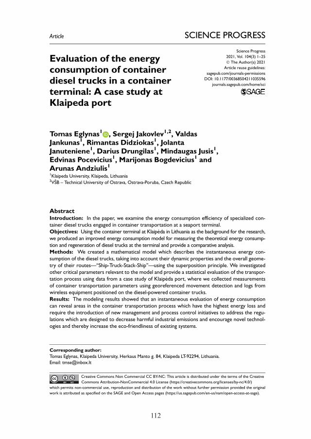
112

Article SCIENCE PROGRESS

Science Progress

2021, Vol. 104(3) 1–25

� The Author(s) 2021

Article reuse guidelines:

sagepub.com/journals-permissions

DOI: 10.1177/00368504211035596

journals.sagepub.com/home/sci

Evaluation of the energyconsumption of containerdiesel trucks in a containerterminal: A case study atKlaipeda port

Tomas Eglynas1 , Sergej Jakovlev1,2, ValdasJankunas1, Rimantas Didziokas1, JolantaJanuteniene1, Darius Drungilas1, Mindaugas Jusis1,Edvinas Pocevicius1, Marijonas Bogdevicius1 andArunas Andziulis11Klaipeda University, Klaipeda, Lithuania2VSB – Technical University of Ostrava, Ostrava-Poruba, Czech Republic

AbstractIntroduction: In the paper, we examine the energy consumption efficiency of specialized con-tainer diesel trucks engaged in container transportation at a seaport terminal.Objectives: Using the container terminal at Klaip_eda in Lithuania as the background for the research,we produced an improved energy consumption model for measuring the theoretical energy consump-tion and regeneration of diesel trucks at the terminal and provide a comparative analysis.Methods: We created a mathematical model which describes the instantaneous energy con-sumption of the diesel trucks, taking into account their dynamic properties and the overall geome-try of their routes—‘‘Ship-Truck-Stack-Ship’’—using the superposition principle. We investigatedother critical parameters relevant to the model and provide a statistical evaluation of the transpor-tation process using data from a case study of Klaip _eda port, where we collected measurementsof container transportation parameters using georeferenced movement detection and logs fromwireless equipment positioned on the diesel-powered container trucks.Results: The modeling results showed that an instantaneous evaluation of energy consumptioncan reveal areas in the container transportation process which have the highest energy loss andrequire the introduction of new management and process control initiatives to address the regu-lations which are designed to decrease harmful industrial emissions and encourage novel technol-ogies and thereby increase the eco-friendliness of existing systems.

Corresponding author:

Tomas Eglynas, Klaipeda University, Herkaus Manto g. 84, Klaipeda LT-92294, Lithuania.

Email: tmse@inbox.lt

Creative Commons Non Commercial CC BY-NC: This article is distributed under the terms of the Creative

Commons Attribution-NonCommercial 4.0 License (https://creativecommons.org/licenses/by-nc/4.0/)

which permits non-commercial use, reproduction and distribution of the work without further permission provided the original

work is attributed as specified on the SAGE and Open Access pages (https://us.sagepub.com/en-us/nam/open-access-at-sage).

112 113

Conclusion: Based on the research results, the article can provide a reference for the estimationof diesel truck efficiency in seaport terminal operations.

KeywordsContainer terminal, container truck, energy consumption, measurement, modeling,transportation

Introduction

The transport sector accounts for a quarter of the total greenhouse gas emissionsproduced by the European Union (EU), and this proportion is still growing asindustry intensifies. To reduce the effect on the climate, it is necessary to eliminateemissions due to transport by 90% by 2050,1 while also ensuring that on-site cargohandling services in the transport industry remain internationally competitive.2 Themost effective means of enhancing container handling operations at these terminalsis in determining the most critical operations where energy loss is encountered,3

improving the existing systems through the replacement or improvement of infra-structure,4 and proposing complex solutions to maintain the sustainability of thetransportation operations.5 However, multidimensional performance evaluationmetrics such as these require a significant investment of time, effort, sectoral exper-tise, and holistic knowledge which are not suitable for instantaneous evaluations ofseparate container handling processes. CO2 emission calculation methods have alsobeen used to assess the efficiency of container handling terminals.6 Researchers7

have designed models to simulate the quantification of carbon emissions in whichthe energy consumption8–12 of container trucks is based on diesel consumption.However, these models only examine the overall efficiency of the terminal over along period and do not provide an opportunity to examine the efficiency of individ-ual container handling operations and infrastructure units. The tasks of schedulingcontainer transportation routes, optimization, and synchronization of handlingprocesses have been solved by various researchers. For example, Sha et al.13 pro-posed a novel integer programming model for the optimization of yard crane sche-duling and their energy consumption at container terminals. This model consideredkey factors such as crane movement and turning distances and the practical opera-tional rules directly related to total energy consumption. With the growing popu-larity of automated guided vehicles (AGVs) at container terminals, some previousstudies have focused on integrated scheduling for the coordination of handlingequipment and AGV routing,14 multi-AGV scheduling for conflict-free path plan-ning,15 and optimization of strategies for yard truck scheduling at container term-inals16 to minimize energy costs. Other studies17–22 have analyzed quay cranes(QCs) and related seaport infrastructure to improve transportation operations.

Previous studies have introduced models for the estimation of energy consump-tion in electric vehicles (EVs),23 investigating energy recuperation capabilities andmotor overload conditions. Recent literature contains energy modeling techniquesfor EV energy consumption in large-scale transportation networks.24,25 Some mod-els provide simulations of the battery powered AGV systems used at automated

2 Science Progress

114

container terminals, evaluating their performance26 according to parameters suchas the number of AGVs, charging station configurations, recharging policies, etc.However, these models are not suitable for the estimation of energy consumptionby container transportation at the terminal. Furthermore, diesel-powered containertransportation currently prevails at seaport container terminals, and battery pow-ered AGVs are still the machines of the future. It is therefore important to identifythe energy needs to transport a container from ship to stack to minimize fuel con-sumption and CO2 emissions and determine the potential energy savings throughthe deployment of battery powered AGVs.

In summary, previous studies have focused on the assessment of the general per-formance of container terminals over a long period but did not consider individualcontainer transportation route analysis in terms of energy consumption; no specia-lized models for the estimation of instantaneous energy costs involved in transport-ing individual containers at a terminal are available. In the present article, weanalyzed the technical efficiency of container handling equipment (i.e. diesel-powered container trucks) in terms of energy consumption per route (cycle)—‘‘ship-truck-stack-ship’’—using a model which evaluates instantaneous energy con-sumption. The results allow the total efficiency of container handling during truckoperations to be increased through the use of the superposition principle. Themodel was verified with data collected from on-site measurements at the Klaip_edaport container terminal.

Methods

In this section, we present a mathematical method which describes fuel and energyconsumption based on the experimental data from on-site measurements. Thismethod not only allows the total fuel consumption for the entire operational periodto be evaluated but also the fuel consumption for each individually transportedcontainer. The model also allows a real-time estimation of the efficiency of thevehicle’s on-site movements.

Energy cost estimation model

The model calculates energy consumption according to the mass of the truck, itscoordinates, and its acceleration values. Specific parameters were recorded for eachpoint in 2D space (refer to Figure 1 for the model): traction force F(t,C), whichchanges over time and depends on fuel consumption, truck velocity v(t), total resis-tance force FT(t), and the tangent to the trajectory t(t) intersecting at a single pointof mass. The coordinates were calculated for each point of mass in the modeledbody.

The work of each truck is defined by a cycle: the truck moves from the ship tothe stack and back again. During the cycle, the mass of the modeled body changes.In the model, the total mass m1 comprises the mass of the truck plus the mass ofthe container it carries, and mass m2 is the mass of the truck alone. The total mass

Eglynas et al. 3

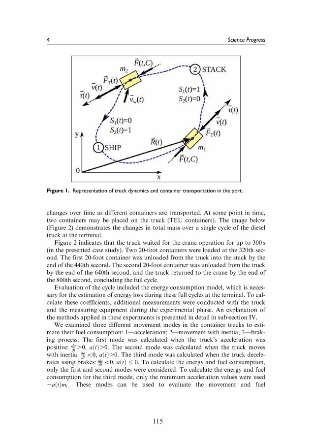
114 115

changes over time as different containers are transported. At some point in time,two containers may be placed on the truck (TEU containers). The image below(Figure 2) demonstrates the changes in total mass over a single cycle of the dieseltruck at the terminal.

Figure 2 indicates that the truck waited for the crane operation for up to 300 s(in the presented case study). Two 20-foot containers were loaded at the 320th sec-ond. The first 20-foot container was unloaded from the truck into the stack by theend of the 440th second. The second 20-foot container was unloaded from the truckby the end of the 640th second, and the truck returned to the crane by the end ofthe 800th second, concluding the full cycle.

Evaluation of the cycle included the energy consumption model, which is neces-sary for the estimation of energy loss during these full cycles at the terminal. To cal-culate these coefficients, additional measurements were conducted with the truckand the measuring equipment during the experimental phase. An explanation ofthe methods applied in these experiments is presented in detail in sub-section IV.

We examined three different movement modes in the container trucks to esti-mate their fuel consumption: 1—acceleration; 2—movement with inertia; 3—brak-ing process. The first mode was calculated when the truck’s acceleration waspositive: da

dt.0, a tð Þ.0. The second mode was calculated when the truck moves

with inertia: dadt\0, a tð Þ.0. The third mode was calculated when the truck decele-

rates using brakes: dadt\0, a tð Þ � 0. To calculate the energy and fuel consumption,

only the first and second modes were considered. To calculate the energy and fuelconsumption for the third mode, only the minimum acceleration values were used2a tð Þmi:. These modes can be used to evaluate the movement and fuel

Figure 1. Representation of truck dynamics and container transportation in the port.

4 Science Progress

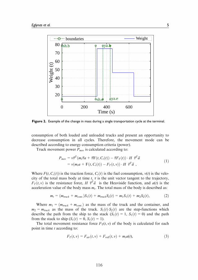
116

consumption of both loaded and unloaded trucks and present an opportunity todecrease consumption in all cycles. Therefore, the movement mode can bedescribed according to energy consumption criteria (power).

Truck movement power Pmov is calculated according to:

Pmov= v~tT mt~ta+~tF t,Ct tð Þð Þ �~tFT tð Þð Þ � H ~tT~a� �

= v mta+F t,Ct tð Þð Þ � FT t, vð Þð Þ � H ~tT~a� �

,ð1Þ

Where F(t,Ct tð Þ) is the traction force, Ct tð Þ is the fuel consumption, v(t) is the velo-city of the total mass body at time t, t is the unit vector tangent to the trajectory,FT t, vð Þ is the resistance force, H ~tT~a

� �is the Heaviside function, and a(t) is the

acceleration value of the body mass mt. The total mass of the body is described as:

mt = mtruck +mcont:ð ÞS1 tð Þ+mtruckS2 tð Þ=m1S1 tð Þ+m2S2 tð Þ, ð2Þ

Where m1 = mtruck +mcont:ð Þ as the mass of the truck and the container, andm2 =mtruck as the mass of the truck. S1 tð Þ�S2 tð Þ are the step-functions whichdescribe the path from the ship to the stack (S1 tð Þ= 1, S1 tð Þ= 0) and the pathfrom the stack to ship (S1 tð Þ= 0, S1 tð Þ= 1):

The total movement resistance force FT(t, v) of the body is calculated for eachpoint in time t according to:

FT t, vð Þ=Fair t, vð Þ+Froll t, vð Þ+mta(t), ð3Þ

Figure 2. Example of the change in mass during a single transportation cycle at the terminal.

Eglynas et al. 5

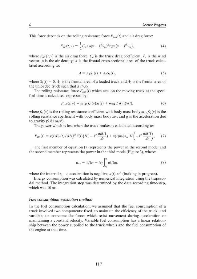
116 117

This force depends on the rolling resistance force Froll tð Þ and air drag force:

Fair t, vð Þ= 1

2CaAr(v�~tT~vw)

2sign v�~tTvw� �

, ð4Þ

where Fair t, vð Þ is the air drag force, Ca is the truck drag coefficient,~vw is the windvector, r is the air density; A is the frontal cross-sectional area of the truck calcu-lated according to:

A=A1S1 tð Þ+A2S2 tð Þ, ð5Þ

where S1 tð Þ= 0, A1 is the frontal area of a loaded truck and A2 is the frontal area ofthe unloaded truck such that A1.A2.

The rolling resistance force Froll tð Þ which acts on the moving truck at the speci-fied time is calculated expressed by:

Froll t, vð Þ=m1g fr1(v)S1 tð Þ+m2g fr2(v)S2 tð Þ, ð6Þ

where fr1 vð Þ is the rolling resistance coefficient with body mass body m1, fr2 vð Þ is therolling resistance coefficient with body mass body m2, and g is the acceleration dueto gravity (9.81m/s2).

The power which is lost when the truck brakes is calculated according to:

PBR tð Þ= v tð ÞFT t, vð ÞH ~tT~a tð Þ� �

H(�~tTd~a(t)

dt)+ v tð Þmt aavj jH �~tT d~a(t)

dt

� �, ð7Þ

The first member of equation (7) represents the power in the second mode, andthe second member represents the power in the third mode (Figure 3), where:

aav = 1=(t2 � t1)

ðt2t1

a tð Þdt, ð8Þ

where the interval tj � ti acceleration is negative, a tð Þ\0 (braking in progress).Energy consumption was calculated by numerical integration using the trapezoi-

dal method. The integration step was determined by the data recording time-step,which was 10ms.

Fuel consumption evaluation method

In the fuel consumption calculation, we assumed that the fuel consumption of atruck involved two components: fixed, to maintain the efficiency of the truck, andvariable, to overcome the forces which resist movement during acceleration ormaintaining a constant velocity. Variable fuel consumption has a linear relation-ship between the power supplied to the truck wheels and the fuel consumption ofthe engine at that time.

6 Science Progress

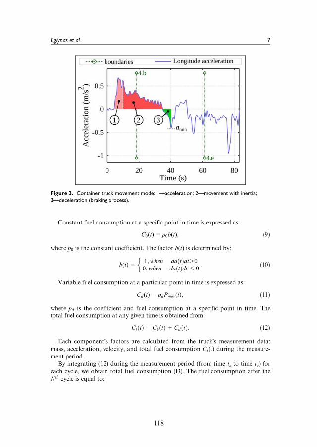
118

Constant fuel consumption at a specific point in time is expressed as:

C0(t)= p0b(t), ð9Þ

where p0 is the constant coefficient. The factor b(t) is determined by:

b(t)=1,when da tð Þdt.0

0,when da tð Þdt � 0

�: ð10Þ

Variable fuel consumption at a particular point in time is expressed as:

Cd(t)= pdPmov(t), ð11Þ

where pd is the coefficient and fuel consumption at a specific point in time. Thetotal fuel consumption at any given time is obtained from:

Ct tð Þ=C0 tð Þ+Cd tð Þ: ð12Þ

Each component’s factors are calculated from the truck’s measurement data:mass, acceleration, velocity, and total fuel consumption Ct(t) during the measure-ment period.

By integrating (12) during the measurement period (from time ts to time te) foreach cycle, we obtain total fuel consumption (l3). The fuel consumption after theNth cycle is equal to:

Figure 3. Container truck movement mode: 1—acceleration; 2—movement with inertia;3—deceleration (braking process).

Eglynas et al. 7

118 119

XNcycle

k= 1

ðtektsk

C0k(t)dt+XNcycle

k= 1

ðtektsk

Cdk(t)dt=XNcycle

k= 1

ðtektsk

Ctk(t)dt, ð13Þ

Equation (13) can be rewritten as:

ap0 + bpd = c, ð14Þ

where a, b, c are the coefficients:

a=XNcycle

k= 1

ðtektsk

C0k(t)dt

b=XNcycle

k= 1

ðtektsk

Cdk(t)dt

c=XNcycle

k= 1

ðtektsk

Ctk(t)dt

, ð15Þ

The fuel consumption coefficients are determined after the Nth cycle by minimiz-ing the objective function:

minF=(apo + bpd � c)2, ð16Þ

We introduce the variables vector ~xT = p0, pd½ �. Minimization of the objectivefunction is performed using the method of iterations, when each iteration k solvesthe following equation:

Ik½ �T Ik½ �D~xk = � Ik½ �TFk , ð17Þ

where the Jacobi matrix:

Ik½ �= dF(xk)

d~x

� �: ð18Þ

After solving (17), we obtain the improved variable vector:

~xk+ 1 =~xk +D~xk , ð19Þ

where k is the iteration number.To calculate fuel and energy consumption, it is necessary to know the compo-

nents which resist movement of the truck. The calculation method of these compo-nents is presented in sub-section III. To find these components, experimentalmeasurements were performed in the field to determine the necessary data for thecalculations.

8 Science Progress

120

Method of estimation of the air and rolling resistance coefficients

To calculate the energy expended in transporting the container, it is necessary toassess the aerodynamic coefficients and total resistance to the movement of thetruck. The method for determining these coefficients experimentally is given below.

The coefficient of the total rolling resistance is estimated for each period suchthat t= ti+ 1 � ti. This allows evaluation of the fuel consumption of a truck with acargo load during movement, where S1(t)=1, and without a load, whereS2(t)=1. This improvement in the rolling resistance coefficient is necessarybecause it allows us to estimate the vertical strain on each truck wheel. Thismethod can be applied up to velocities of val = 30km/h, which is suitable for thestudied case since truck speed in the terminal is restricted up to 30 km/h.

The total rolling resistance coefficient during the period t= ti+1�ti is calculatedfrom the equation:

frk, i, i+ 1 =28:2 � ai+ 1 � v2i � ai � v2i+ 1

� �

1000 � v2i � v2i+ 1

� � , ð20Þ

where k= 1 when Si tð Þ= 1, and k= 2 when Si tð Þ= 2; ai = a tið Þ andai+ 1 = a ti + tð Þ; vi = v(ti) and vi+ 1 = v(ti+ t) for the movement velocities of peri-ods ti and ti+ 1.

The movement velocity vi+ 1 is determined by using the acceleration values aiand ai+ 1 according to:

vi+ 1 = vi +t

2(ai + ai+ 1), ð21Þ

Determining the aerodynamic drag coefficient Ca applies the same proceduresas determining the rolling resistance. The drag coefficient Ca in the periodt= ti+ 1 � ti is calculated according to the expression:

ck, i, i+ 1 =6 � mt � ai � ai+ 1ð ÞA � v2i � v2i+ 1

� � , ð22Þ

such that v2i � v2i+ 1 6¼ 0; where A is the frontal area of the truck determined from(5), mt is the total mass of the truck calculated from (2) for k=1 whenS1 tð Þ= 1,S2 tð Þ= 0, and k=2 when S1 tð Þ= 0, S2 tð Þ= 1.

Using these methods, we conducted a field experiment to determine the rollingresistance and air drag coefficients, which were then applied in the momentaryenergy (fuel) consumption model and energy (fuel) consumption calculation.

Setup of experimental equipment

This section describes the experimental conditions, measured parameters, and eval-uated factors. Based on the presented methods, the equations can be applied to cal-culate the energy consumption required to transport a container at the container

Eglynas et al. 9

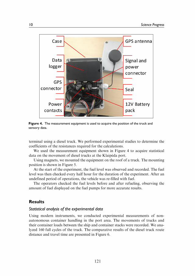
120 121

terminal using a diesel truck. We performed experimental studies to determine thecoefficients of the resistances required for the calculations.

We used the measurement equipment shown in Figure 4 to acquire statisticaldata on the movement of diesel trucks at the Klaip_eda port.

Using magnets, we mounted the equipment on the roof of a truck. The mountingposition is shown in Figure 5.

At the start of the experiment, the fuel level was observed and recorded. The fuellevel was then checked every half hour for the duration of the experiment. After anundefined period of operations, the vehicle was re-filled with fuel.

The operators checked the fuel levels before and after refueling, observing theamount of fuel displayed on the fuel pumps for more accurate results.

Results

Statistical analysis of the experimental data

Using modern instruments, we conducted experimental measurements of non-autonomous container handling in the port area. The movements of trucks andtheir container loads between the ship and container stacks were recorded. We ana-lyzed 160 full cycles of the truck. The comparative results of the diesel truck routedistance and travel time are presented in Figure 6.

Figure 4. The measurement equipment is used to acquire the position of the truck andsensory data.

10 Science Progress

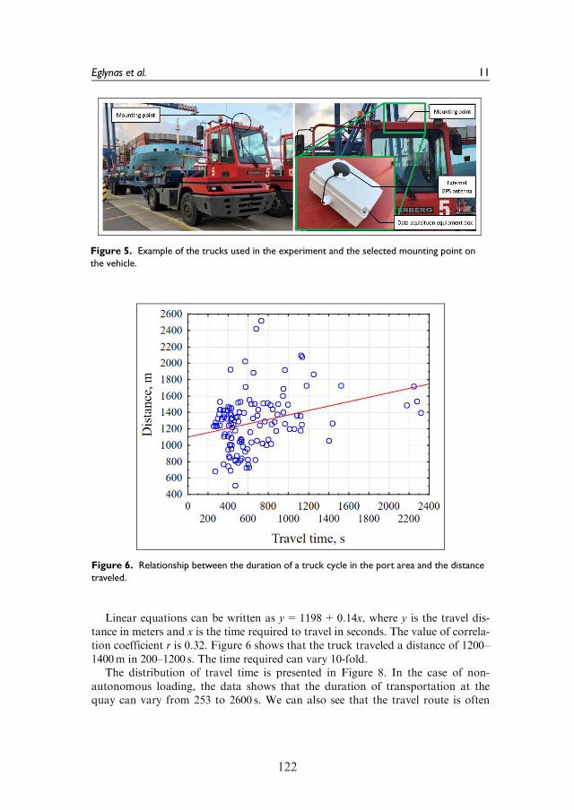
122

Linear equations can be written as y= 1198+ 0:14x, where y is the travel dis-tance in meters and x is the time required to travel in seconds. The value of correla-tion coefficient r is 0.32. Figure 6 shows that the truck traveled a distance of 1200–1400m in 200–1200 s. The time required can vary 10-fold.

The distribution of travel time is presented in Figure 8. In the case of non-autonomous loading, the data shows that the duration of transportation at thequay can vary from 253 to 2600 s. We can also see that the travel route is often

Figure 5. Example of the trucks used in the experiment and the selected mounting point onthe vehicle.

Figure 6. Relationship between the duration of a truck cycle in the port area and the distancetraveled.

Eglynas et al. 11

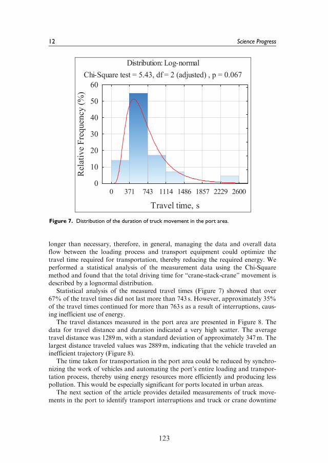
122 123

longer than necessary, therefore, in general, managing the data and overall dataflow between the loading process and transport equipment could optimize thetravel time required for transportation, thereby reducing the required energy. Weperformed a statistical analysis of the measurement data using the Chi-Squaremethod and found that the total driving time for ‘‘crane-stack-crane’’ movement isdescribed by a lognormal distribution.

Statistical analysis of the measured travel times (Figure 7) showed that over67% of the travel times did not last more than 743 s. However, approximately 35%of the travel times continued for more than 763 s as a result of interruptions, caus-ing inefficient use of energy.

The travel distances measured in the port area are presented in Figure 8. Thedata for travel distance and duration indicated a very high scatter. The averagetravel distance was 1289m, with a standard deviation of approximately 347m. Thelargest distance traveled values was 2889m, indicating that the vehicle traveled aninefficient trajectory (Figure 8).

The time taken for transportation in the port area could be reduced by synchro-nizing the work of vehicles and automating the port’s entire loading and transpor-tation process, thereby using energy resources more efficiently and producing lesspollution. This would be especially significant for ports located in urban areas.

The next section of the article provides detailed measurements of truck move-ments in the port to identify transport interruptions and truck or crane downtime

Figure 7. Distribution of the duration of truck movement in the port area.

12 Science Progress

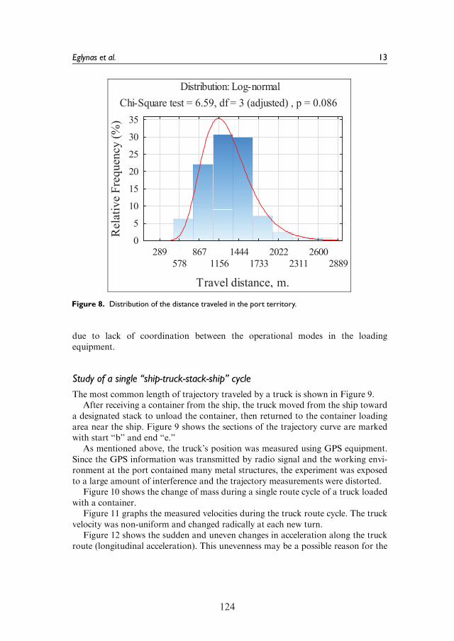
124

due to lack of coordination between the operational modes in the loadingequipment.

Study of a single ‘‘ship-truck-stack-ship’’ cycle

The most common length of trajectory traveled by a truck is shown in Figure 9.After receiving a container from the ship, the truck moved from the ship toward

a designated stack to unload the container, then returned to the container loadingarea near the ship. Figure 9 shows the sections of the trajectory curve are markedwith start ‘‘b’’ and end ‘‘e.’’

As mentioned above, the truck’s position was measured using GPS equipment.Since the GPS information was transmitted by radio signal and the working envi-ronment at the port contained many metal structures, the experiment was exposedto a large amount of interference and the trajectory measurements were distorted.

Figure 10 shows the change of mass during a single route cycle of a truck loadedwith a container.

Figure 11 graphs the measured velocities during the truck route cycle. The truckvelocity was non-uniform and changed radically at each new turn.

Figure 12 shows the sudden and uneven changes in acceleration along the truckroute (longitudinal acceleration). This unevenness may be a possible reason for the

Figure 8. Distribution of the distance traveled in the port territory.

Eglynas et al. 13

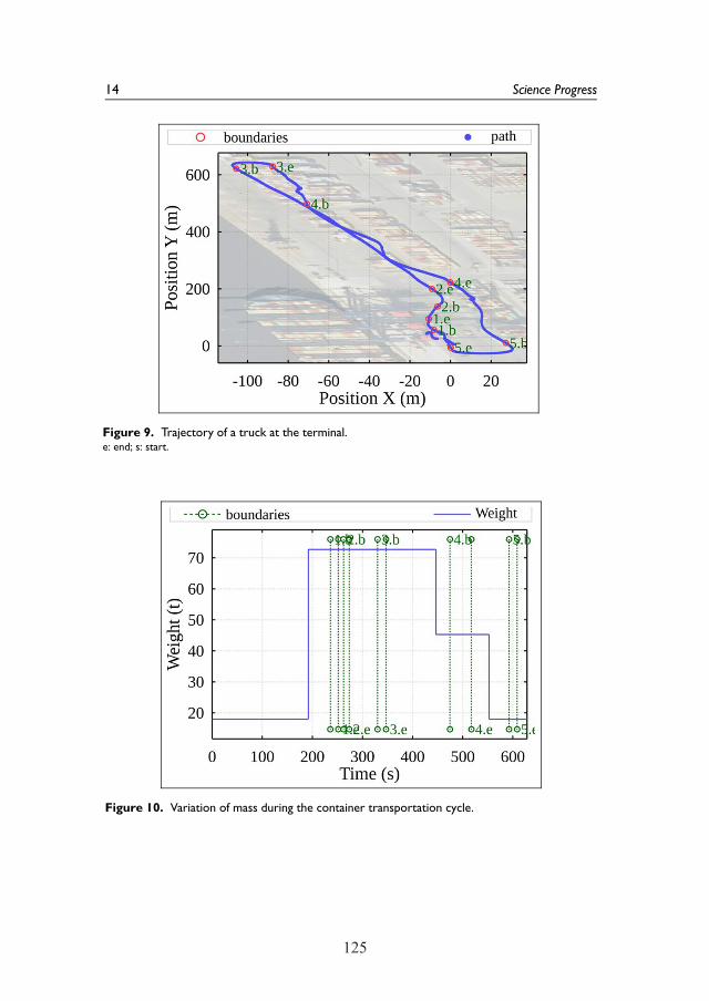
124 125

Figure 9. Trajectory of a truck at the terminal.e: end; s: start.

Figure 10. Variation of mass during the container transportation cycle.

14 Science Progress

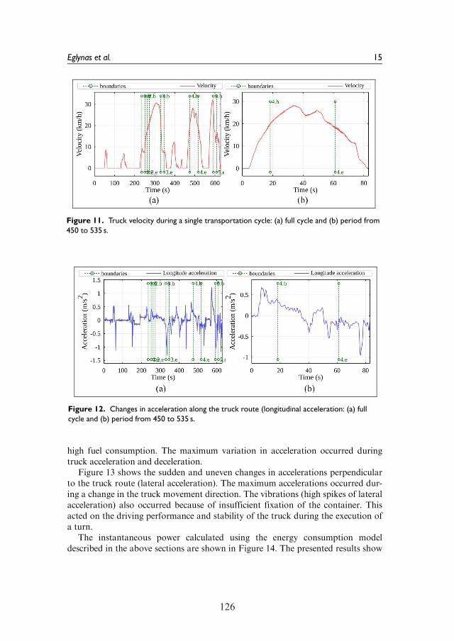
126

high fuel consumption. The maximum variation in acceleration occurred duringtruck acceleration and deceleration.

Figure 13 shows the sudden and uneven changes in accelerations perpendicularto the truck route (lateral acceleration). The maximum accelerations occurred dur-ing a change in the truck movement direction. The vibrations (high spikes of lateralacceleration) also occurred because of insufficient fixation of the container. Thisacted on the driving performance and stability of the truck during the execution ofa turn.

The instantaneous power calculated using the energy consumption modeldescribed in the above sections are shown in Figure 14. The presented results show

Figure 11. Truck velocity during a single transportation cycle: (a) full cycle and (b) period from450 to 535 s.

Figure 12. Changes in acceleration along the truck route (longitudinal acceleration: (a) fullcycle and (b) period from 450 to 535 s.

Eglynas et al. 15

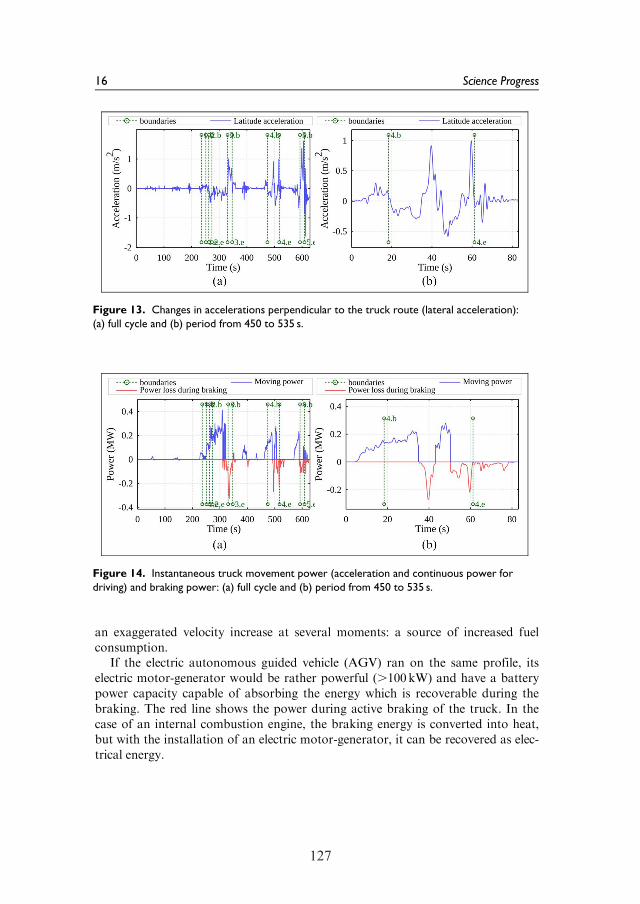
126 127

an exaggerated velocity increase at several moments: a source of increased fuelconsumption.

If the electric autonomous guided vehicle (AGV) ran on the same profile, itselectric motor-generator would be rather powerful (.100kW) and have a batterypower capacity capable of absorbing the energy which is recoverable during thebraking. The red line shows the power during active braking of the truck. In thecase of an internal combustion engine, the braking energy is converted into heat,but with the installation of an electric motor-generator, it can be recovered as elec-trical energy.

Figure 13. Changes in accelerations perpendicular to the truck route (lateral acceleration):(a) full cycle and (b) period from 450 to 535 s.

Figure 14. Instantaneous truck movement power (acceleration and continuous power fordriving) and braking power: (a) full cycle and (b) period from 450 to 535 s.

16 Science Progress

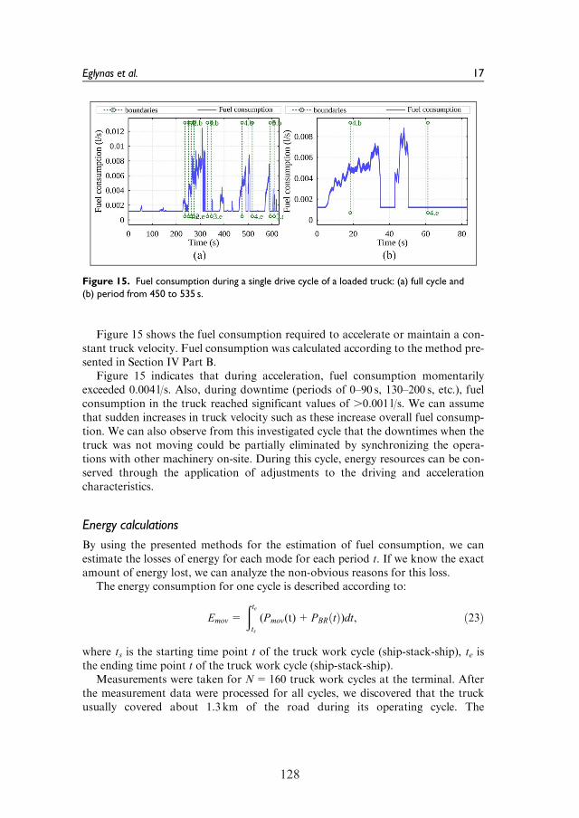
128

Figure 15 shows the fuel consumption required to accelerate or maintain a con-stant truck velocity. Fuel consumption was calculated according to the method pre-sented in Section IV Part B.

Figure 15 indicates that during acceleration, fuel consumption momentarilyexceeded 0.004 l/s. Also, during downtime (periods of 0–90 s, 130–200 s, etc.), fuelconsumption in the truck reached significant values of .0.001 l/s. We can assumethat sudden increases in truck velocity such as these increase overall fuel consump-tion. We can also observe from this investigated cycle that the downtimes when thetruck was not moving could be partially eliminated by synchronizing the opera-tions with other machinery on-site. During this cycle, energy resources can be con-served through the application of adjustments to the driving and accelerationcharacteristics.

Energy calculations

By using the presented methods for the estimation of fuel consumption, we canestimate the losses of energy for each mode for each period t. If we know the exactamount of energy lost, we can analyze the non-obvious reasons for this loss.

The energy consumption for one cycle is described according to:

Emov=

ðtets

(Pmov(t)+PBR tð Þ)dt, ð23Þ

where ts is the starting time point t of the truck work cycle (ship-stack-ship), te isthe ending time point t of the truck work cycle (ship-stack-ship).

Measurements were taken for N=160 truck work cycles at the terminal. Afterthe measurement data were processed for all cycles, we discovered that the truckusually covered about 1.3 km of the road during its operating cycle. The

Figure 15. Fuel consumption during a single drive cycle of a loaded truck: (a) full cycle and(b) period from 450 to 535 s.

Eglynas et al. 17

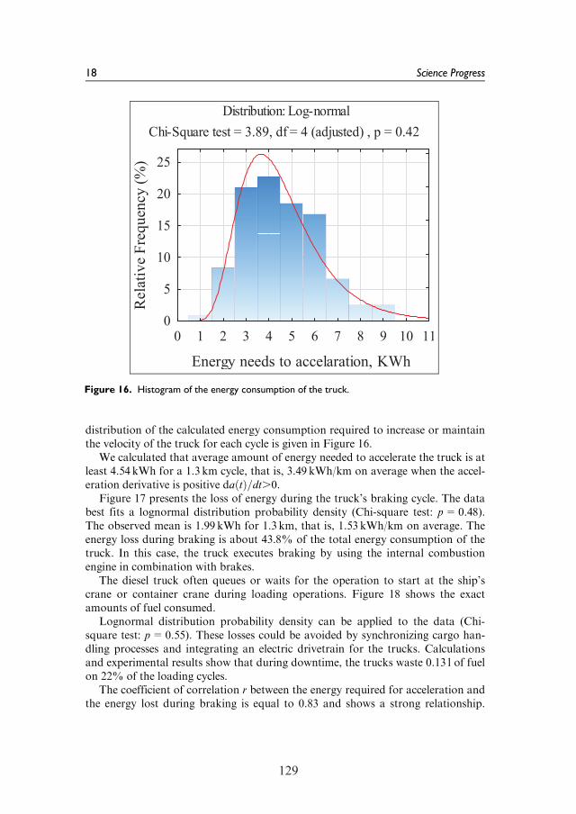
128 129

distribution of the calculated energy consumption required to increase or maintainthe velocity of the truck for each cycle is given in Figure 16.

We calculated that average amount of energy needed to accelerate the truck is atleast 4.54 kWh for a 1.3 km cycle, that is, 3.49 kWh/km on average when the accel-eration derivative is positive da tð Þ=dt.0.

Figure 17 presents the loss of energy during the truck’s braking cycle. The databest fits a lognormal distribution probability density (Chi-square test: p=0.48).The observed mean is 1.99 kWh for 1.3 km, that is, 1.53 kWh/km on average. Theenergy loss during braking is about 43.8% of the total energy consumption of thetruck. In this case, the truck executes braking by using the internal combustionengine in combination with brakes.

The diesel truck often queues or waits for the operation to start at the ship’scrane or container crane during loading operations. Figure 18 shows the exactamounts of fuel consumed.

Lognormal distribution probability density can be applied to the data (Chi-square test: p=0.55). These losses could be avoided by synchronizing cargo han-dling processes and integrating an electric drivetrain for the trucks. Calculationsand experimental results show that during downtime, the trucks waste 0.13 l of fuelon 22% of the loading cycles.

The coefficient of correlation r between the energy required for acceleration andthe energy lost during braking is equal to 0.83 and shows a strong relationship.

Figure 16. Histogram of the energy consumption of the truck.

18 Science Progress

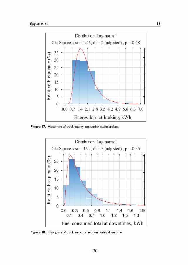
130

Figure 17. Histogram of truck energy loss during active braking.

Figure 18. Histogram of truck fuel consumption during downtime.

Eglynas et al. 19

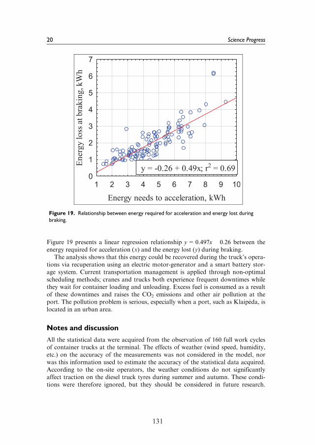
130 131

Figure 19 presents a linear regression relationship y= 0:497x� 0:26 between theenergy required for acceleration (x) and the energy lost (y) during braking.

The analysis shows that this energy could be recovered during the truck’s opera-tions via recuperation using an electric motor-generator and a smart battery stor-age system. Current transportation management is applied through non-optimalscheduling methods; cranes and trucks both experience frequent downtimes whilethey wait for container loading and unloading. Excess fuel is consumed as a resultof these downtimes and raises the CO2 emissions and other air pollution at theport. The pollution problem is serious, especially when a port, such as Klaip_eda, islocated in an urban area.

Notes and discussion

All the statistical data were acquired from the observation of 160 full work cyclesof container trucks at the terminal. The effects of weather (wind speed, humidity,etc.) on the accuracy of the measurements was not considered in the model, norwas this information used to estimate the accuracy of the statistical data acquired.According to the on-site operators, the weather conditions do not significantlyaffect traction on the diesel truck tyres during summer and autumn. These condi-tions were therefore ignored, but they should be considered in future research.

Figure 19. Relationship between energy required for acceleration and energy lost duringbraking.

20 Science Progress

132

According to the operators, visibility decreases during harsh weather conditions(heavy rain and wind) and they must be more cautious at these times. Crane opera-tors are also more cautious under these conditions since they affect the speed ofcontainer placement on diesel trucks or AGVs. During winter, ice-covered roadsmay affect overall tyre traction by increasing the distance required to brake whiletransporting heavy cargo.

Downtime occurs frequently, and sometimes, either because of error or otherscheduling reasons, the destination of the container changes several times per cycle.When the deck of the ship is fully unloaded, the lids which cover the ship’s hullmust be removed. This creates long waiting times (downtimes), the removal proce-dure taking up to 30min to complete.

Fuel consumption is currently measured by acquiring the readings from sensorsinstalled in the diesel truck’s fuel tank. The observed measurements varied greatlyin each work cycle. In future experiments, a different fuel consumption measure-ment method should be used. All these observations are critical and should be con-sidered in future research and for the development of new synchronization toolsand methods for port operations.

Conclusion

Each new solution and method must include concrete factors, that is, the travelspeed of the trucks (with all acceleration points for each driver), and the quay craneand stack crane operational capabilities (for each operator). Consideration of thesefactors will certainly not only aid in increasing the efficiency of overall operationsin the transport chain globally but will also help decrease harmful emissions.

The experimental measurements and the described methods show that the totalenergy losses reached 3.49 kWh/km during the transportation of a container, andthe energy loss for braking reached 1.53 kWh/km on average. For each new cycle,the energy loss during braking reached 43.8% on average of the truck’s total energyconsumption.

The proposed fuel consumption model proved to be 91% accurate (it is very sen-sitive to real fuel consumption measurements and the statistical data of previousmeasurements with slight approximations). The coefficients of the proposed modelwere calculated from the two measurements taken during the on-site experimentalstudy. The model was applied to calculate the theoretical fuel consumption for thethird measurement. The results were compared to real fuel consumption, and onlya 9% deviation was observed.

To ensure the model’s long-term accuracy and possible adaptation in port oper-ations, it is vital to measure the fuel consumption as accurately as possible. A slightchange or deviation from the real value (up to 0.1 l) can have a critical effect onthe final results (the accuracy of the proposed model). The methods, which we veri-fied with an experimental study, can determine the fuel consumption of any portcontainer truck (with or without a load), calculate the energy due to momentum,and determine the most rational control parameters for optimal fuel consumption

Eglynas et al. 21

132 133

at any given moment based on real-time acceleration data. The truck, if operatedeffectively, would move with an even velocity to maximize fuel economy and solvethe problem of fuel wasted as a result of downtime.

Acknowledgements

The authors would also like to thanks Klaipeda university project members: prof. dr. E.Guseinoviene, dr. M. Kurmis, Z. Lukosius, A. Senulis for deep insights and relevant contri-bution to the work.The authors would also grateful for the support from the Klaipeda city Containers handlingcompany LKAB ‘‘Smelt _e’’ for providing consultations, access to the technical means, andvaluable insights during the experimental phase of the project.

Declaration of conflicting interests

The author(s) declared no potential conflicts of interest with respect to the research, author-ship, and/or publication of this article.

Funding

The author(s) disclosed receipt of the following financial support for the research, author-ship, and/or publication of this article: This research is funded by the European RegionalDevelopment Fund according to the supported activity ‘‘Research Projects Implemented byWorld-class Researcher Groups’’ under Measure No. 01.2.2-LMT-K-718-01-0081, under agrant agreement with the Research Council of Lithuania (LMT).

ORCID iD

Tomas Eglynas https://orcid.org/0000-0002-9973-5896

References

1. European Commission. The European Green Deal: Communication from the

Commission to the European Parliament, the European Council, the Council, the

European Economic and Social Committee and the Committee of the Regions, 2019, p.

24.

2. Serra P and Fancello G. Towards the IMO’s GHG goals: a critical overview of the

perspectives and challenges of the main options for decarbonizing international

shipping. Sustain 2020; 12: 3220.

3. Nabavi-Pelesaraei A, Bayat R, Hosseinzadeh-Bandbafha H, et al. Modeling of energy

consumption and environmental life cycle assessment for incineration and landfill

systems of municipal solid waste management – a case study in Tehran Metropolis of

Iran. J Clean Prod 2017; 148: 427–440.

4. Karakas S, Acar AZ and Kirmizi M. Development of a multidimensional performance

evaluation model for container terminals at Marmara Sea. Res Transp Bus Manag

2020; 100498.

5. Harper P. Decomposition for decarbonisation: evaluation of decarbonisation

programmes. Sci Prog 2016; 99: 235–261.

22 Science Progress

134

6. Geerlings H and Van Duin R. A new method for assessing CO2-emissions from

container terminals: a promising approach applied in Rotterdam. J Clean Prod 2011;

19: 657–666.

7. Yun P, Xiangda L, Wenyuan W, et al. A simulation-based research on carbon emission

mitigation strategies for green container terminals. Ocean Eng 2018; 163: 288–298.

8. Sim J. A carbon emission evaluation model for a container terminal. J Clean Prod

2018; 186: 526–533.

9. Martınez-Moya J, Vazquez-Paja B and Gimenez Maldonado JA. Energy efficiency and

CO2 emissions of port container terminal equipment: evidence from the Port of

Valencia. Energy Policy 2019; 131: 312–319.

10. Yu H, Ge YE, Chen J, et al. CO2 emission evaluation of yard tractors during loading at

container terminals. Transp Res Part D Transp Environ 2017; 53: 17–36.

11. Khanali M, Akram A, Behzadi J, et al. Multi-objective optimization of energy use and

environmental emissions for walnut production using imperialist competitive algorithm.

Appl Energy 2021; 284: 116342.

12. Ghasemi-Mobtaker H, Mostashari-Rad F, Saber Z, et al. Application of photovoltaic

system to modify energy use, environmental damages and cumulative exergy demand of

two irrigation systems-a case study: barley production of Iran. Renew Energy 2020; 160:

1316–1334.

13. Sha M, Zhang T, Lan Y, et al. Scheduling optimization of yard cranes with minimal

energy consumption at container terminals. Comput Ind Eng 2017; 113: 704–173.

14. Yang Y, Zhong M, Dessouky Y, et al. An integrated scheduling method for AGV

routing in automated container terminals. Comput Ind Eng 2018; 126: 482–493.

15. Zhong M, Yang Y, Dessouky Y, et al. Multi-AGV scheduling for conflict-free path

planning in automated container terminals. Comput Ind Eng 2020; 142: 106371.

16. Hu X, Guo J and Zhang Y. Optimal strategies for the yard truck scheduling in container

terminal with the consideration of container clusters. Comput Ind Eng 2019; 137: 106083.

17. Zhen L, Hu H, Wang W, et al. Cranes scheduling in frame bridges based automated

container terminals. Transp Res Part C Emerg Technol 2018; 97: 369–384.

18. Malekahmadi A, Alinaghian M, Hejazi SR, et al. Integrated continuous berth allocation

and quay crane assignment and scheduling problem with time-dependent physical

constraints in container terminals. Comput Ind Eng 2020; 147: 106672.

19. Zeng Q, Feng Y and Yang Z. Integrated optimization of pickup sequence and container

rehandling based on partial truck arrival information. Comput Ind Eng 2019; 127:

366–382.

20. Zhou C, Lee BK and Li H. Integrated optimization on yard crane scheduling and

vehicle positioning at container yards. Transp Res Part E Logist Transp Rev 2020; 138:

101966.

21. Dinu O, Rosca E, Dragu V, et al. Optimization of the transfer function through

handling productivity control in port container terminals. Procedia Manuf 2018; 22:

856–863.

22. Zhou C, Wang W and Li H. Container reshuffling considered space allocation problem

in container terminals. Transp Res Part E Logist Transp Rev 2020; 136: 1–23.

23. Genikomsakis KN and Mitrentsis G. A computationally efficient simulation model for

estimating energy consumption of electric vehicles in the context of route planning

applications. Transp Res Part D Transp Environ 2017; 50: 98–118.

Eglynas et al. 23

134 135

24. Xu X, Aziz HMA and Guensler R. A modal-based approach for estimating electric

vehicle energy consumption in transportation networks. Transp Res Part D Transp

Environ 2019; 75: 249–264.

25. Xu X, Aziz HMA, Liu H, et al. A scalable energy modeling framework for electric

vehicles in regional transportation networks. Appl Energy 2020; 269: 115095.

26. Ma N, Zhou C and Stephen A. Simulation model and performance evaluation of

battery-powered AGV systems in automated container terminals. Simul Model Pract

Theory 2021; 106: 102146.

Author biographies

Tomas Eglynas received his PhD degree in Transport Engineering in 2017. He now works as a

researcher at the Marine Research Institute of Klaipeda University and as the CEO of

"Inotecha" (Research company) Ltd. Topics of his research interests are intelligent systems,

electronics, software development, and Industry 4.0.

Sergej Jakovlev received his PhD degree in Transport Engineering in 2016. He now works as a

researcher at the Marine Research Institute of Klaipeda University and as a senior researcher

at the Telecommunications Department of VSB-Technical University of Ostrava. Topics of

his research interests are intelligent systems, operations research and big data analytics.

Valdas Jankunas received his PhD degree in Electrical and Electronics Engineering from

Kaunas Technology University in 2013. His employment experience included Klaipeda

University. His special fields of interest included Power Electronics and Embedded Systems.

Rimantas Didziokas obtained the qualification of a Mechanical engineer in 1976. Candidate

of Technical Sciences (now Ph.D.). Highest professional achievements: 1995-1996 Member

of Klaipeda City Municipal Council; 1996-2000 Member of Seimas of Lithuania; 1999-2000

Minister of Transport and Communications (Lithuania). His research interests are

Mechanical engineering, control systems, and industrial applications.

Jolanta Januteniene received her Ph.D. in Mathematics in 2001. She is a member of editorial

boards of journal Transport (CA) and reviewers of highly ranked CA and SCOPUS journals.

Topics of her research interests are Mechanical engineering, mathematical modeling, compo-

site materials, and statistical data analytics.

Darius Drungilas received his Ph.D. Degree in 2014 in Informatics engineering. Now works as

a Researcher and Associate professor at Klaipeda University Marine Research Institute and

Informatics and Statistics Department of Klaipeda University. Topics of his research inter-

ests are machine learning algorithms, industry 4.0, and affective computing.

Mindaugas Jusis acquired Master’s Degree in Informatics engineering in 2014. Now work at

Klaipeda University as a lecturer and junior researcher. Has experience working with inter-

national projects and with industry. He has excellent skills in programming: JAVA, PHP,

Swift etc. His special fields of interest include data acquisition systems, Industry 4.0, Internet

of Things.

24 Science Progress

136

Edvinas Pocevicius received his Bachelors degree in Electrical and Electronics Engineering in

2021. Now works in Klaipeda University at the Department of Informatics engineering as a

junior researcher. Topics of his research interests are Electronics, Automation and Control

Systems, Sensor systems.

Marijonas Bogdevicius is a habilitated Doctor of Technology, full member of the Lithuanian

Academy of Sciences. Field of interest: dynamics of mechanical, hydraulic and pneumatic

systems, computational mechanics, dynamics of vehicles, dynamics of traffic flows. Works

at Vilnius Gediminas Technical University at the Departments of Mobile Machinery and

Railway Transport.

Arunas Andziulis now works in Klaipeda University at the Department of Informatics engi-

neering as a senior researcher, having more than 50 years’ experience of working in Industry,

developing electronics devices, semiconductors and smart systems. Topics of his research

interests are Electronics, Automation and Control Systems, Big Data analytics.

Eglynas et al. 25

136 112

2nd publication / 2 publikacija

Modeling and experimental research of quay crane cargo lowering processes

T. Eglynas, A. Andziulis, M. Bogdevičius, J. Janutėnienė,S. Jakovlev, V. Jankūnas, A. Senulis, M. Jusis, M. Bogdevičius,

S. Gudas.

Advances in Mechanical Engineering Vol. 11(12), 1-9 (2019)

IF: 1.024

DOI: 10.1177/1687814019896927

138

Research Article

Advances in Mechanical Engineering2019, Vol. 11(12) 1–9� The Author(s) 2019DOI: 10.1177/1687814019896927journals.sagepub.com/home/ade

Modeling and experimental research ofquay crane cargo lowering processes

Tomas Eglynas1 , Arunas Andziulis1, Marijonas Bogdevicius2, JolantaJanut _enien _e3, Sergej Jakovlev1,3, Valdas Jank�unas1, Audrius Senulis1,Mindaugas Jusis1,4, Paulius Bogdevicius2 and Saulius Gudas4

AbstractThis article studies an operational problem arising at a container terminal. Klaipeda city port operations were surveilledup close and relevant remarks were made. The time efficiency of the existing container-lowering procedures using thesimulation studies with a test-bed and with a real life crane operation was examined. Statistical analysis of the experi-mental results has showed that non-automated processes have higher time variance for the lowering process. The oper-ations of quay crane for container handling ‘‘ship-to-shore’’ were analyzed, and lowering procedures time variationswere determined. Each container is transported at operators own risk and with pre-defined time efficiency; therefore, itis hard to predict the optimal time for each container handling operation, thus, eventually, additional costs arise.Mathematical model was developed, which described dynamical characteristics of the container movement during lower-ing procedures. The lowering crane operation was modeled using known dynamic values for each separate case, and thecomplexity of the problem was proven. The results of modeling and experimental results show that it is possible toachieve optimal values with the existing processes.

KeywordsDynamics modeling, quay crane, simulation, experimental research, container-lowering process, statistical analysis

Date received: 24 September 2019; accepted: 27 November 2019

Handling Editor: James Baldwin

Introduction

Intermodal shipping containers are widely adopted inthe global transport chain to deliver various goods toend-users. Despite the obvious advantages, there is stillplenty of room for improvements when it comes totime efficiency and quality increase. Global transportmarket is a network of companies and end-users, whorely on well-managed standards and systems. Recenttrends and numbers suggest that about 90% of non-bulk global trade is being managed by shipping con-tainers worldwide.1,2 Europe alone in 2016 managed0.8 billion tons of cargo.3 Statistics shows that duringthe 10-year period between 2007 and 2017, shippingquantities increased by 66% (up to 148million TEUs),taking into account the global merchandise trade by

marine traffic.4 Many engineers and managers world-wide foresaw such rapid increase. Yet, they could notmanage it in an optimal manner. Thus, efficiency is acriterion which needs to be increased in order to adoptnew challenges of the future. Cargo loading operationsrely on loading and unloading speeds, safety of

1Klaipeda University, Klaipeda, Lithuania2Vilnius Gediminas Technical University, Vilnius, Lithuania3VSB-Technical University of Ostrava, Ostrava-Poruba, Czech Republic4Cyber-Social Systems Engineering Group, Vilnius University, Vilnius,

Lithuania

Corresponding author:

Tomas Eglynas, Klaipeda University, Herkaus Manto g. 84, LT-92294

Klaipeda, Lithuania.

Email: tmse@inbox.lt

Creative Commons CC BY: This article is distributed under the terms of the Creative Commons Attribution 4.0 License

(https://creativecommons.org/licenses/by/4.0/) which permits any use, reproduction and distribution of the work

without further permission provided the original work is attributed as specified on the SAGE and Open Access pages

(https://us.sagepub.com/en-us/nam/open-access-at-sage).

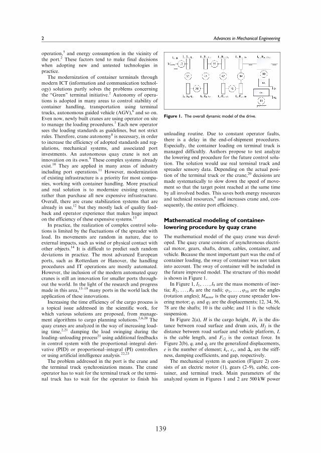
138 139

operation,5 and energy consumption in the vicinity ofthe port.2 These factors tend to make final decisionswhen adopting new and untested technologies inpractice.

The modernization of container terminals throughmodern ICT (information and communication technol-ogy) solutions partly solves the problems concerningthe ‘‘Green’’ terminal initiative.2 Autonomy of opera-tions is adopted in many areas to control stability ofcontainer handling, transportation using terminaltrucks, autonomous guided vehicle (AGV),6 and so on.Even now, newly built cranes are using operator on siteto manage the loading procedures.7 Each new operatorsees the loading standards as guidelines, but not strictrules. Therefore, crane autonomy8 is necessary, in orderto increase the efficiency of adopted standards and reg-ulations, mechanical systems, and associated portinvestments. An autonomous quay crane is not aninnovation on its own.9 These complex systems alreadyexist.10 They are applied in many areas of industryincluding port operations.11 However, modernizationof existing infrastructure is a priority for most compa-nies, working with container handling. More practicaland real solution is to modernize existing systems,rather than purchase all new expensive infrastructure.Overall, there are crane stabilization systems that arealready in use,12 but they mostly lack of quality feed-back and operator experience that makes huge impacton the efficiency of these expensive systems.13

In practice, the realization of complex control solu-tions is limited by the fluctuations of the spreader withload. Its movements are random in nature, due toexternal impacts, such as wind or physical contact withother objects.14 It is difficult to predict such randomdeviations in practice. The most advanced Europeanports, such as Rotterdam or Hanover, the handlingprocedures and IT operations are mostly automated.However, the inclusion of the modern automated quaycranes is still an innovation for smaller ports through-out the world. In the light of the research and progressmade in this area,15–19 many ports in the world lack theapplication of these innovations.

Increasing the time efficiency of the cargo process isa topical issue addressed in the scientific work, forwhich various solutions are proposed, from manage-ment algorithms to cargo planning solutions.2,6,20 Thequay cranes are analyzed in the way of increasing load-ing time,2,21 damping the load swinging during theloading–unloading process21 using additional feedbacksin control system with the proportional–integral–deri-vative (PID) or proportional–integral (PI) controllersor using artificial intelligence analysis.22,23

The problem addressed in the port is the crane andthe terminal truck synchronization means. The craneoperator has to wait for the terminal truck or the termi-nal truck has to wait for the operator to finish his

unloading routine. Due to constant operator faults,there is a delay in the end-of-shipment procedures.Especially, the container loading on terminal truck ismanaged difficultly. Authors propose to test analyzethe lowering end procedure for the future control solu-tion. The solution would use real terminal truck andspreader sensory data. Depending on the actual posi-tion of the terminal truck or the crane,20 decisions aremade systematically to slow down the speed of move-ment so that the target point reached at the same timeby all involved bodies. This saves both energy resourcesand technical resources,6 and increases crane and, con-sequently, the entire port efficiency.

Mathematical modeling of container-lowering procedure by quay crane

The mathematical model of the quay crane was devel-oped. The quay crane consists of asynchronous electri-cal motor, gears, shafts, drum, cables, container, andvehicle. Because the most important part was the end ofcontainer loading, the sway of container was not takeninto account. The sway of container will be included inthe future improved model. The structure of this modelis shown in Figure 1.

In Figure 1, I1, . . . , I9 are the mass moments of iner-tia; R2, . . . ,R9 are the radii; u1, . . . ,u10 are the angles(rotation angles); Mmotor is the quay crane spreader low-ering motor; q1 and q2 are the displacements; 12, 34, 56,78 are the shafts; 10 is the cable; and 11 is the vehiclesuspension.

In Figure 2(a), H is the cargo height, H1 is the dis-tance between road surface and drum axis, H2 is thedistance between road surface and vehicle platform, Lis the cable length, and F12 is the contact force. InFigure 2(b), qi and qj are the generalized displacements,e is the number of element; ke, ce, and De are the stiff-ness, damping coefficients, and gap, respectively.

The mechanical system in question (Figure 2) con-sists of an electric motor (1), gears (2–9), cable, con-tainer, and terminal truck. Main parameters of theanalyzed system in Figures 1 and 2 are 500 kW power

Figure 1. The overall dynamic model of the drive.

2 Advances in Mechanical Engineering

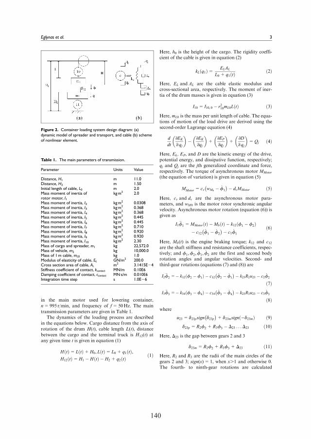
140

in the main motor used for lowering container,n=995 r/min, and frequency of f=50Hz. The maintransmission parameters are given in Table 1.

The dynamics of the loading process are describedin the equations below. Cargo distance from the axis ofrotation of the drum H(t), cable length L(t), distancebetween the cargo and the terminal truck is H12(t) atany given time t is given in equation (1)

H tð Þ= L tð Þ+H0, L tð Þ= L0+ q1 tð Þ,H12 tð Þ=H1 � H tð Þ � H2 + q2 tð Þ

ð1Þ

Here, h0 is the height of the cargo. The rigidity coeffi-cient of the cable is given in equation (2)

kL q1ð Þ= ELAL

L0 + q1 tð Þ ð2Þ

Here, EL and AL are the cable elastic modulus andcross-sectional area, respectively. The moment of iner-tia of the drum masses is given in equation (3)

I10 = I10, 0 � r210mL0L tð Þ ð3Þ

Here, mL0 is the mass per unit length of cable. The equa-tions of motion of the load drive are derived using thesecond-order Lagrange equation (4)

d

dt

∂EK

∂ qj

� �� ∂EK

∂qj

� �+

∂EP

∂qj

� �+

∂D

∂ qj

� �=Qj ð4Þ

Here, Ek, EP, and D are the kinetic energy of the drive,potential energy, and dissipative function, respectively;qj and Qj are the jth generalized coordinate and force,respectively. The torque of asynchronous motor MMotor

(the equation of variation) is given in equation (5)

M �Motor = cv wM0

� _f1

� �� dvMMotor ð5Þ

Here, cv and dv are the asynchronous motor para-meters, and wM0 is the motor rotor synchronic angularvelocity. Asynchronous motor rotation (equation (6)) isgiven as

I1€f1 =MMotor tð Þ �Mb tð Þ � k12 f1 � f2ð Þ� c12 _f1 � _f2

� �� c1 _f1

ð6Þ

Here, Mb(t) is the engine braking torque; k12 and c12are the shaft stiffness and resistance coefficients, respec-tively; and f1,f2, _f1, _f2 are the first and second bodyrotation angles and angular velocities. Second- andthird-gear rotations (equations (7) and (8)) are

I2€f2 =� k12 f2 � f1ð Þ � c12 _f2 � _f1

� �� k23R2u23 � c2 _f2

ð7Þ

I3€f3 =� k34 f3 � f4ð Þ � c34 _f3 � _f4

� �� k23R3u23 � c3 _f3

ð8Þ

where

u23 = d23psign d23p� �

+ d23msign �d23mð Þ ð9Þ

d23p =R2f2 +R3f3 � D23 . . .D23 ð10Þ

Here, D23 is the gap between gears 2 and 3

d23m =R2f2 +R3f3 +D23 ð11Þ

Here, R2 and R3 are the radii of the main circles of thegears 2 and 3; sign(x)= 1, when x.1 and otherwise 0.The fourth- to ninth-gear rotations are calculated

Figure 2. Container loading system design diagram: (a)dynamic model of spreader and transport, and cable (b) schemeof nonlinear element.

Table 1. The main parameters of transmission.

Parameter Units Value

Distance, H1 m 11.0Distance, H2 m 1.50Initial length of cable, L0 m 2.0Mass moment of inertia ofrotor motor, I1

kgm2 2.0

Mass moment of inertia, I2 kgm2 0.0308Mass moment of inertia, I3 kgm2 0.368Mass moment of inertia, I4 kgm2 0.368Mass moment of inertia, I5 kgm2 0.445Mass moment of inertia, I6 kgm2 0.445Mass moment of inertia, I7 kgm2 0.710Mass moment of inertia, I8 kgm2 0.920Mass moment of inertia, I9 kgm2 0.920Mass moment of inertia, I10 kgm2 2.30Mass of cargo and spreader, m1 kg 22,572.0Mass of vehicle, m2 kg 10,000.0Mass of 1m cable, mL0 kg 1.0Modulus of elasticity of cable, EL GN/m2 200.0Cross section area of cable, AL m2 3.1415E24Stiffness coefficient of contact, kcontact MN/m 0.10E6Damping coefficient of contact, ccontact MNs/m 0.010E6Integration time step s 1.0E26

Eglynas et al. 3

140 141

similarly as the second and third. Tenth gear rotationequation is as equation (12)

I10€f10 = _I10 _f10 +1

2

∂I10

∂f10

_f10

� �2

� k910 f10 � f9ð Þ � c910 _f10 � _f9

� �

� c10 _f10 � R10kL q1ð Þ R10f10 � q1ð Þ� R10c10 R10

_f10 � _q1� �

ð12Þ

Cargo and vehicle movement equations (13) and (14)are

m1€q1 =� _m1 _q1 � kL q1 � R10f10ð Þ� cL _q1 � R10

_f10

� �+m1g � F12sign d12ð Þ

+1

2R6f6 � q1ð Þ2 ELAL

L2

� �� caer0 _q1ð Þ2sign _q1ð Þ

ð13Þ

m�2q2 =F12sign d12ð Þ+m2g � k2q2 � c2 _q2 ð14Þ

Here, q1, q2 is the displacement of masses m1 and m2;m1 and _m1 are the cargo, spreader, and cable total massand its derivative of time, respectively; cL is the cablecoefficient of resistance; and caer0 is the aerodynamicforce coefficient of resistance (equation (15))

d12 = H2 � q2ð Þ � H1 � H q1ð Þð Þ ð15Þ

Here, m2 is the vehicle mass, and k2 and c2 is the coeffi-cients of vehicle suspension stiffness and resistance,respectively.

Thus, the mathematical model of quay crane wasconstructed and the results of container-lowering wereexamined for the comparison with the experimentaldata and giving implication of the possible loweringtime reduction.

Experimental investigation

The aim of research was to test the real working condi-tions of the quay crane, operators work, the spreaderefficiency, and unnecessary forces accumulated duringcontainer loading.24 A simulation model was developedand tested. In recent years, researchers work closelywith electrically powered terminal trucks and cranes.25

In order to assess the need for synchronization, authorsconducted experimental research in Klaipeda port.During the experimental research, the quay crane car-ried out loading operations, during which the data werecollected. The practical experiment collected data from204 real cycles of the loading process from ship to thequay and back again. MK2 data logger hardware wasused for these experimental measurements (seeFigure 3).

When determining the dynamic parameters of theobject under investigation (in this case, the container),data about its acceleration, speed, and position in spacewere measured and recorded. For this purpose, a DL1-MK2 data logger (Race Technology, UK), a three-wayaccelerometer (guaranteed 2 g minimum full scale onboth axes; resolution of 0.005 g; optional 6 g sensoravailable as a factory option) vibration measurements(vibration factory tested at 25 g, 50Hz sinusoid for5min), was used to record and store vehicle motiondynamics parameters. For positioning, the meter isconnected to a GPS antenna (GPS—outputs position,speed, position accuracy, and speed accuracy every200ms with no interpolation; GPS tracking loops opti-mized for applications up to about 4 g; tracking of allsatellites in view). Based on the time course of the vehi-cle and the acceleration readings, the device measuresthe speed of the test object with an accuracy of 0.16km/h,with a measurement error of up to 1%. Longitudinaland transverse accelerometers record accelerations upto 20m/s2 and measurement error up to 0.05m/s2.

After processing the data collected during the experi-mental measurements, the entire loading process wasdivided into stages to identify which technological load-ing process takes the longest. The purpose of thisexperiment was to identify problematic operations inthe loading process when scheduling a synchronizationtask, thereby justifying the need for synchronization.By synchronizing individual port facilities (such as ter-minal trucks and quay cranes) and by planning cargooperations accordingly, it is possible to minimize theimpact of these problem areas on the loading time.These stages and summarized experimental results aregiven in Table 2.

Experimental measurements were implementedwhen the cargo was shipped from the ship to the shore.Depending on the loading process, the operations are

Figure 3. DL1-MK2 data logger (Race Technology, UK).

4 Advances in Mechanical Engineering

142

divided into seven stages: (1) start of lifting (hooking),(2) vertical lifting, (3) diagonal lifting, (4) horizontaltransportation, (5) diagonal lowering, (6) vertical low-ering, and (7) placing on terminal truck. The overallloading cycle in the ship-to-shore process was also eval-uated. The summarized results of experimental studiesshow that the entire duration of the ship-to-shore cycleof the loading process during the transfer of cargo fromthe ship to the shore is in accordance with statisticallog-normal law.

The number of data n = 102 was measured (fromship to shore). The log-normal law hypothesis wastested by Pearson’s x2 criterion. The histogram of theexperimental loading times determined during experi-mental measurements is shown in Figure 4.

After analyzing the loading process measurements instages, steps 6 and 7 were chosen for further analysis,that is, vertical lowering and positioning on the vehicle.These stages determine the crane-to-vehicle alignmentto optimize the loading process and make it continu-ous. In Figure 5, the distribution of the vertical lower-ing time is presented.

We can see that the vertical lowering mean time ofthe container t is equal to 7.3 s, and the vertical loweringheight mean value is 8.8m, considering the standarddeviation as 4.5m. Hypothesis of lowering time distribu-tion by Normal law was tested by Pearson’s x2 criterion.Experimental results show that the average weight of thecontainer load during the experimental measurements is22.2 ton and the standard deviation is 10.2 ton, and coef-ficient of variation is 46%. In Figure 6, the distributionof the loading phase duration is presented, when theload is placed on the terminal truck and detached.

As we can see shorter intervals predominate, theyrepresent about 50% of the total (n=102) measure-ment result. Average is about 5.43 s; however, containerplacement can take up to 20 s. Duration of this stepcould be optimized by automation of loading process,and this process could be about 2 s, as show experimen-tal results. The purpose of the synchronization task isto make the vehicle arrive when the load lowered dur-ing the loading process. Therefore, experimental mea-surements carried out when the equipment mounted ona container transport. Experimental research measured

Table 2. Statistical data of container loading time.

Stage of loading Mean Min Max Standard deviation Variation coefficient (%)

1. Start of lifting (hooking) 2.43 0.62 11.47 1.84 76.012. Vertical lifting 4.68 1.04 13.47 3.32 70.893. Diagonal lifting 5.14 0.79 9.84 1.97 38.284. Horizontal transportation 6.34 2.05 19.03 3.46 54.685. Diagonal lowering 6.36 2.72 23.97 3.05 47.906. Vertical lowering 7.25 1.66 19.13 2.86 39.427. Placing on vehicle 5.43 2.36 20.43 2.99 55.16Total (Ship-to-shore) 37.63 26.91 63.87 7.68 20.42

Figure 4. Histogram of experimental load from ship-to-ship onthe quay.

Figure 5. Histogram of experimental measurements of verticallowering of container toward vehicle height.

Eglynas et al. 5

142 143

the trajectory of the terminal truck in the port area andits waiting time at the crane (see Figure 7).

The results show that the waiting time of the vehicleat the container crane varies from 4 s to 34min(2096 s). The average waiting time is 229 s and standarddeviation 346 s. The process is extremely unstable witha coefficient of variation of more than 150%. Duringthe experimental measurements, the cargo was alsoevaluated (when mounting the equipment on thegripper—the closest point to the container). Duringthese experimental measurements, the velocities andaccelerations of the moving load were measured. Afterprocessing the results, we selected the best result—theexperimental result of the fastest lowering of the load(see Figure 8).

The results show that investigated case of load low-ering vertically was done in 1.9 s. The lowering speed ofthis situation is given in Figure 8(a). As a result, speedvalues are negative because the load is lowered. Wealso watched the fluctuations of the load that influencethe full automation of the process. The load fluctua-tions in the horizontal plane during lowering are shownin Figure 8(b). As one can notice, container sways in a10 cm boundary. This value suggests that the cargolowered in a stable manner and no outer forces affectthe sway (wind gusts or operator mistakes).

The experimental results show the need of moresophisticated control of the crane–container terminaltruck system, but to work in real situation and toimprove the performance are difficult due to the inter-vention into the port operation. Therefore, the mathe-matical model for lowering the container was developedto make adequate modeling and producing the tool forcontrol system development.

Results and discussion

During the numerical simulation, the cargo loweringprocess was analyzed, which corresponds to the loadingstage 6 of the experimental investigations. Simulationof the lowering process was completed by evaluatingthe force during contact placing the load on the vehicle.The results of numerical simulation are presented inFigure 9.

During numerical simulation, the load was loweredvertically down (see in Figure 9(a)). Due to the highweight of the load and the elasticity of the cable, thedamping occurs. Figure 10 shows the situation whenthe load is placed on a vehicle with a dynamic forceF12 of ;180 kN (see Figure 9(b)).

Changes of torque moment of the gear wheels duringlowering presented in Figure 10.

During the modeling phase, the gap between thegear teeth was estimated. As we see during the loweringof the load, it has a negative effect; it excites the vibra-tions of the gears. This affects the lowering process; thevibrations pass to the cable and consequently worsenthe loading conditions. Figure 11 shows the accelera-tion during horizontal lowering, and in Figure 11(a),the numerical simulations show that the accelerationvalues increase significantly when cargo has a contactwith terminal truck. This is consistent with experimen-tal measurements (Figure 11(b) (point 7)), with a signif-icant increase in acceleration values and excitation ofthe terminal truck when the load is applied. On com-parison, the results with the best experimental data thatwas achieved during the lowering (b) – was 2.4 s, butmodeling results show that it is – in ideal conditions –possible to make the operation in 0.5 s (a). And, theresults are comparable in time and amplitude, thus

Figure 6. Histogram of experimental measurement containerplacement on terminal vehicle.

Figure 7. Histogram of experimental measurements of vehiclewaiting time.

6 Advances in Mechanical Engineering

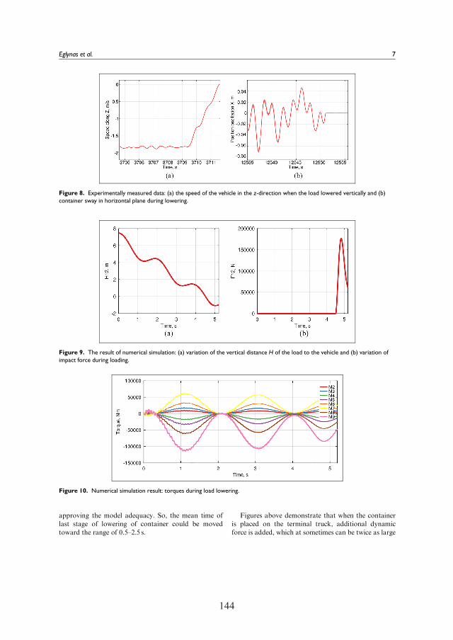
144

approving the model adequacy. So, the mean time oflast stage of lowering of container could be movedtoward the range of 0.5–2.5 s.

Figures above demonstrate that when the containeris placed on the terminal truck, additional dynamicforce is added, which at sometimes can be twice as large

Figure 8. Experimentally measured data: (a) the speed of the vehicle in the z-direction when the load lowered vertically and (b)container sway in horizontal plane during lowering.

Figure 9. The result of numerical simulation: (a) variation of the vertical distance H of the load to the vehicle and (b) variation ofimpact force during loading.

Figure 10. Numerical simulation result: torques during load lowering.

Eglynas et al. 7

144 145

as the levering container weight. This is a knowneffect in classical mechanics. Such regularity is con-firmed by the results of numerical simulation andexperimental acceleration measurements (see Figure11). Experimental measurements show a very similartendency during container loading procedures.

Conclusion

In this article, as a result, we demonstrate the generali-zation of the measurements with real quay crane andterminal vehicle and propose a mathematical modeldescribing the dynamic properties of both.Experimental measurements ‘‘in situ’’ of container-lowering to terminal truck have been investigated indetail and statistical analysis of the new experimentalresults carried out. Experimental measurements showedthat variance coefficient reached up to 150% on finalhandling operation. These operation durations variedbetween 2.36 and 20.43 s, with a mean value of 5.43 s.The entire lowering cycle variation coefficient reached55.16%. Shorter time boundary shows that the han-dling process is optimizable up to two times by schedul-ing the operations between quay crane and terminaltruck operators and using specialized algorithms forlowering process control for each individual case. Thisin fact could provide stability to port operations andmake processes and procedures more agile for long-term planning. According to these new experimentaldata and research findings, further plans will be pre-pared to develop a methodology for crane and terminaltruck, AGV synchronization in real time and will beused to bridge the scheduling mechanisms into a singlereal-time synchronization system.

Acknowledgements

The authors thank other project (No. 01.2.2-LMT-K-718-01-0081) members: Dr R Didziokas, Dr E Guseinoviene, Dr M

Kurmis, Dr D Drugnilas, and Z Lukosius for valuableinsights and collection of data on site.

Declaration of conflicting interests

The author(s) declared no potential conflicts of interest withrespect to the research, authorship, and/or publication of thisarticle.

Funding

The author(s) disclosed receipt of the following financial sup-port for the research, authorship, and/or publication of thisarticle: This research was funded by the European RegionalDevelopment Fund according to the supported activity‘‘Research Projects Implemented by World-class ResearcherGroups’’ under Measure No. 01.2.2-LMT-K-718-01-0081.

ORCID iD

Tomas Eglynas https://orcid.org/0000-0002-9973-5896

References

1. Clausen U, Kaffka J and Meier F. CONTSIM—con-

tainer terminal management with simulation. Procedia:

Soc Behav Sci 2012; 54: 332–340.2. Kavakeb S, Nguyen TT, McGinley K, et al. Green vehi-

cle technology to enhance the performance of a Eur-

opean port: a simulation model with a cost-benefit

approach. Transp Res Part C Emerg Technol 2015; 60:

169–188.3. European Commission. Annex to motorways of the sea

detailed implementation plan, 2018, https://vayla.fi/docu

ments/20473/465955/Final-II-MoS-study-2018-2+Annex.

pdf/9cbe31a9-afde-4c79-9370-394bc864ffa54. Benamara H. Role of international shipping. In:

UNCTAD multiyear expert meeting on transport, trade

logistics and trade facilitation, Geneva, 21–23 November

2018, p.13. Geneva: United Nations Conference on

Trade and Development.

Figure 11. Numerical modeling (a) and experiment (b) results comparison.

8 Advances in Mechanical Engineering

146

5. Speier C, Whipple JM, Closs DJ, et al. Global supplychain design considerations: mitigating product safetyand security risks. J Oper Manag 2011; 29: 721–736.

6. Xin J, Negenborn RR and Lodewijks G. Trajectoryplanning for AGVs in automated container terminalsusing avoidance constraints: a case study. IFAC Proc Vol

2014; 47: 9828–9833.7. Hong KS and Ngo QH. Dynamics of the container crane

on a mobile harbor. Ocean Eng 2012; 53: 16–24.8. Zheng K, Lu Z and Sun X. An effective heuristic for the

integrated scheduling problem of automated containerhandling system using twin 40’ cranes. In: Proceedings ofthe 2010 second international conference on computer

modeling and simulation, Sanya, China, 22–24 January2010, pp.406–410. New York: IEEE.

9. Zhen L, Hu H, Wang W, et al. Cranes scheduling inframe bridges based automated container terminals.

Transp Res Part C Emerg Technol 2018; 97: 369–384.10. Alasali F, Haben S and Holderbaum W. Stochastic opti-

mal energy management system for RTG cranes networkusing genetic algorithm and ensemble forecasts. J Energy

Storage 2019; 24: 100759.11. Papaioannou V, Pietrosanti S, Holderbaum W, et al.

Analysis of energy usage for RTG cranes. Energy 2017;125: 337–344.

12. Liu D and Ge YE. Modeling assignment of quay cranesusing queueing theory for minimizing CO2 emission at acontainer terminal. Transp Res Part D Transp Environ

2018; 61: 140–151.13. Bichou K. An empirical study of the impacts of operating

and market conditions on container-port efficiency andbenchmarking. Res Transp Econ 2013; 42: 28–37.

14. Arena A, Lacarbonara W and Casalotti A. Payload oscil-lations control in harbor cranes via semi-active vibrationabsorbers: modeling, simulations and experimentalresults. Procedia Engineer 2017; 199: 501–509.

15. Tuan LA, Cuong HM, Trieu P, et al. Adaptive neuralnetwork sliding mode control of shipboard container

cranes considering actuator backlash. Mech Syst Signal

Process 2018; 112: 233–250.16. Sha M, Zhang T, Lan Y, et al. Scheduling optimization

of yard cranes with minimal energy consumption at con-

tainer terminals. Comput Ind Eng 2017; 113: 704–713.17. Iles S, Matusko J and Kolonic F. Sequential distributed

predictive control of a 3D tower crane. Control Eng Pract

2018; 79: 22–35.18. Verdes Kairuz RI, Aguilar LT, de Loza AF, et al. Robust

positioning control law for a 3D underactuated crane sys-

tem. IFAC-PapersOnline 2018; 51: 450–455.19. Zhang M, Zhang Y, Chen H, et al. Model-independent

PD-SMC method with payload swing suppression for 3D

overhead crane systems. Mech Syst Signal Process 2019;

129: 381–393.20. Li B, Liu H, Xiao D, et al. Centralized and optimal

motion planning for large-scale AGV systems: a generic

approach. Adv Eng Softw 2017; 106: 33–46.21. Guven C and Eliiyi DT. Trip allocation and stacking pol-

icies at a container terminal. Transp Res Proc 2014; 3:

565–573.

22. Sun Z, Wang N, Bi Y, et al. A DE based PID controller

for two dimensional overhead crane. In: Proceedings of

the 34th Chinese control conference, Hangzhou, China,

28–30 July 2015, pp.2546–2550. New York: IEEE.23. Jaafar HI, Mohamed Z, Abidin AFZ, et al. PSO-tuned

PID controller for a nonlinear gantry crane system. In:

Proceedings of the 2012 IEEE international conference on

control system, computing and engineering (ICCSCE

2012), Batu Ferringhi, Malaysia, 23–25 November 2012,

pp.515–519. New York: IEEE.24. Park KP, Cha JH and Lee KY. Dynamic factor analysis

considering elastic boom effects in heavy lifting opera-

tions. Ocean Eng 2011; 38: 1100–1113.25. Bahnes N, Kechar B and Haffaf H. Cooperation between

intelligent autonomous vehicles to enhance container ter-

minal operations. J Innov Digit Ecosyst 2016; 3: 22–29.

Eglynas et al. 9

146 113

3rd publication / 3 publikacija

Analysis of the efficiency of shipping containers handling/loading control methods and

procedures

T. Eglynas, M. Jusis, S. Jakovlev, A. Senulis, A. Andziulis,S. Gudas.

Advances in Mechanical Engineering Vol. 11(1), 1-12 (2019)

IF: 1.024

DOI: 10.1177/1687814018821229

148

Research Article

Advances in Mechanical Engineering2019, Vol. 11(1) 1–12� The Author(s) 2019DOI: 10.1177/1687814018821229journals.sagepub.com/home/ade

Analysis of the efficiency of shippingcontainers handling/loading controlmethods and procedures

Tomas Eglynas1,2 , Mindaugas Jusis2,3, Sergej Jakovlev1,4,Audrius Senulis1,5, Arunas Andziulis2 and Saulius Gudas3

AbstractMost modern quay cranes operate under the operator’s control. Lifting, lowering, and transporting a container fromone platform to another are just some of the actions that a person is responsible for, but the negative consequences ofhandling can be caused not only by his actions. An error, loading transient instability, or an undervalued environmentalfactor in the control algorithm can cause a risk to human safety, container, and cargo security. In order to control cargo-handling risk, it is necessary to improve the cargo control systems not only by changing their software, but also by creat-ing additional control algorithms and systems. These systems with programmed control algorithms should be integratedinto existing systems to control cargo security and its transfer time. In this article, transient processes and dynamicproperty of the cargo-handling operation are described and multibody dynamics simulation performed using laboratoryprototype of a quay crane. The experimental research performed and integrated autonomous quay crane control algo-rithm developed with the proposed embedded container swinging control subroutine operated in optimal mode whenthe control system used PID controller with a feedback including additional PI controller and S-shaped input signal forthe analyzed case with the defined parameter set.

KeywordsMultibody dynamics, transients, simulation, mathematical modeling, control methods, motion control, profiling tech-niques, quay crane, container handling

Date received: 27 September 2018; accepted: 3 December 2018

Handling Editor: Xiangwei Bu

General introduction

Risk of cargo transportation process and impact ofhandling/loading procedures

Each year, millions of different types of containers aretransshipped in intermodal terminals. Large quaycranes are used as the main transport means for loadingcargo from ship to shore and back. Thus loading pro-cess is very important stage of intermodal transporta-tion, where necessary measures have to be ensured toachieve high level of physical and technological safety.Incorrect operation of the operator or inappropriatecrane control algorithms can not only damage the

1Marine Research Institute, Klaip _eda University, Klaip _eda, Lithuania2Department of Informatics and Statistics, Klaip _eda University, Klaip _eda,Lithuania3Institute of Data Science and Digital Technologies, Vilnius University,

Vilnius, Lithuania4VSB—Technical University of Ostrava, Ostrava, Czech Republic5Department of Engineering, Klaip _eda University, Klaip _eda, Lithuania

Corresponding author:

Tomas Eglynas, Marine Research Institute, Klaip _eda University,Universiteto ave. 17, LT-92294 Klaipeda, Lithuania.

Email: tmse@inbox.lt

Creative Commons CC BY: This article is distributed under the terms of the Creative Commons Attribution 4.0 License

(http://www.creativecommons.org/licenses/by/4.0/) which permits any use, reproduction and distribution of the work without

further permission provided the original work is attributed as specified on the SAGE and Open Access pages (https://us.sagepub.com/en-us/nam/

open-access-at-sage).

148 149

containers or cargo, but also damage terminal propertynear the quay crane. Failure to comply with the safetyrequirements may result in an accident or technicaldisaster, such as a crane crash or container crash. Eachquay crane is unique in its capabilities, so applyingcommon restrictions to all cranes is not appropriate.Each container terminal, based on the needs and possi-bilities, builds quay cranes whose specifications meetloading needs. The main limitations of the crane inmany cases are reflected in their technical characteris-tics, such as spreader lifting capacity, speed of the trol-ley, crane travel speed, carriage movement distance,stroke of the boom length and others. In order toensure cargo safety, it is necessary to monitor and eval-uate all parameters limiting the operation of the crane.Therefore, security is achieved through restrictions.1 Itis also necessary to assess critical situations. For exam-ple, what happens if one of the carrier ropes is broken,voltage variation hops in the high power supply net-work, and the impact of the opposite wind will affectthe maximal allowable weight lifting process. This isjust a small part of the situations that should be evalu-ated to ensure both the safety of the cargo and thesmooth operation of the quay crane. One of the maincauses of disasters has been identified as the swinging ofthe containers. The reasons for the aforementionedswinging are different. Starting from strong wind gusts,operator error, and ending with failure to stabilize theloaded cargo.2–5 This kind of swinging is easy excitedbecause the steel rods connecting load and the spreaderof the trolley. Such swinging results increase the time ofcontainer transport from point ‘‘A’’ to ‘‘B’’ and decreasecargo safety factor.

In recent years, scientists are increasingly examininghow to optimize existing quay cranes due to increasedtransport flows. One of the most commonly encoun-tered problems in ports is the optimization of containerlifting cranes and by means of specific control algo-rithms.6–10 To date, many different control algorithmshave been developed by many authors all around theworld, which, under laboratory conditions, solve indi-vidual problems of crane control with limited applic-ability in real life scenarios. However, the need forcomplex algorithms representing real life scenariosremains the same, focusing not only on individual load-ing procedures, but also on the entire cargo ship–shore–ship process. Generally, the development of newquay crane control algorithms11 is associated with thetask of solving the problem of container sway duringloading procedures. Causes of these sways may vary ineach separate case.2–4,12,13 Sometimes swinging iscaused by the crane mechanisms (vibrations, motortransients, or uneven surface of the track of the movingdevices), but there are cases, where the cause of swing-ing is unknown. They can be triggered by complex setof forces acting on the container and impact the cargo

inside the container. Other scientists2,3,14 are trying tosolve the problem of crane load swinging. The investi-gation is related to the crane-lifting mechanism wherethe container and crane connected by metal rods. Dueto different container weights, wind gusts, and liftingcontrol algorithms, containers often start swinging atthe very beginning of its lifting processes. This requiresmore time for the container to be transported frompoint ‘‘A’’ to point ‘‘B’’ in the port. Due to changingaccelerations, it is likely that the container gets dam-aged by collision with quay crane structures. As it isknown, in the case of strong winds, quay cranes do notusually handle loading operations, which eventuallyincrease loading costs. So, all of this should be avoidedby developing more agile technical and software solu-tions for modernized cranes.14,15

Analysis of crane control algorithms and technologies

In the maritime intermodal terminal, the main control-lable unit of the quay crane is a trolley, driven by elec-tric motors moving to the intended position as quicklyas possible, while maintaining the minimum load swing-ing.16,17 Uncontrolled swinging leads to cargo stabilityand safety problems, especially in container take-offand lowering procedures. The most experienced craneoperators are responsible for container handling opera-tions. The latter, relying precisely on the positioning ofthe container by the quay crane, rely on their visualfeedback (carrying out control operations, determinedby visual field of view). Such handling procedures canprove to be very complex and time-consuming, espe-cially in extreme situations, where precise positioningdepends entirely on operator experience.18 In any load-ing procedure, the load can easily swing. If such swing-ing exceeds the safety limits, swinging must be inhibitedor the operator must suspend loading operations untilthe swinging fall to a safe limit. Complete eliminationof such resulting swinging is practically impossible evenwith the use of modern control technologies, but in spe-cific situations, such swinging can be easily suppressed.This swinging can be influenced by various external fac-tors such as wind, weather changes, or operatoractions.16 This inevitable swinging of cargo often leadsto reduced cargo-handling efficiency, container dam-age, or accidents in the terminal.19 Moreover, the load-ing process requires a fast container transport to therequired position, but the transport speed is as high aspossible, thus the load varies more, thereby aggravatingthe operation of the operator and the entire transporta-tion process.20,21 Freight fluctuations also affect theoperation of an experienced operator and reduce thepositioning accuracy of the spreader. In order toachieve a higher positioning accuracy of the cranespreader, it is necessary to install a control system thatevaluates the trolley acceleration and the amplitude of

2 Advances in Mechanical Engineering

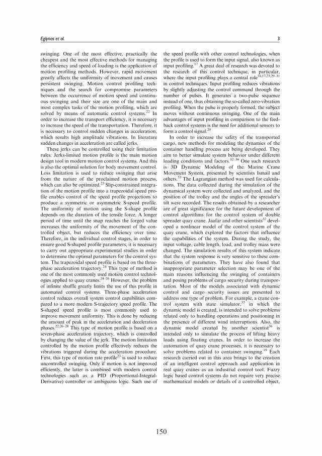
150

swinging. One of the most effective, practically thecheapest and the most effective methods for managingthe efficiency and speed of loading is the application ofmotion profiling methods. However, rapid movementgreatly affects the uniformity of movement and causespersistent swinging. Motion control profiling tech-niques and the search for compromise parametersbetween the occurrence of motion speed and continu-ous swinging and their size are one of the main andmost complex tasks of the motion profiling, which aresolved by means of automatic control systems.22 Inorder to increase the transport efficiency, it is necessaryto increase the speed of the transportation. Therefore, itis necessary to control sudden changes in acceleration,which results high amplitude vibrations. In literaturesudden changes in acceleration are called jerks.

These jerks can be controlled using their limitationrules. Jerks-limited motion profile is the main motiondesign tool in modern motion control systems. And thisis also the optimal solution for body movement control.Loss limitation is used to reduce swinging that arisefrom the nature of the proclaimed motion process,which can also be optimized.23 Slip-constrained integra-tion of the motion profile into a trapezoidal speed pro-file enables control of the speed profile projections toproduce a symmetric or asymmetric S-speed profile.The uniformity of motion using the S-shape profiledepends on the duration of the tensile force. A longerperiod of time until the snap reaches the forged valueincreases the uniformity of the movement of the con-trolled object, but reduces the efficiency over time.Therefore, in the individual control stages, in order toensure good S-shaped profile parameters, it is necessaryto carry out appropriate experimental studies in orderto determine the optimal parameters for the control sys-tem. The trapezoidal speed profile is based on the three-phase acceleration trajectory.24 This type of method isone of the most commonly used motion control technol-ogies applied to quay cranes.24–26 However, the problemof infinite shuffle greatly limits the use of this profile inautomated control systems. Three-phase accelerationcontrol reduces overall system control capabilities com-pared to a more modern S-trajectory speed profile. TheS-shaped speed profile is most commonly used toimprove movement uniformity. This is done by reducingthe amount of peak in the acceleration and decelerationphases.22,26–28 This type of motion profile is based on aseven-phase acceleration trajectory, which is controlledby changing the value of the jerk. The motion limitationcontrolled by the motion profile effectively reduces thevibrations triggered during the acceleration procedure.First, this type of motion rate profile23 is used to reduceuncontrolled swinging. Only if motion is not improvedefficiently, the latter is combined with modern controltechnologies such as a PID (Proportional-Integral-Derivative) controller or ambiguous logic. Such use of

the speed profile with other control technologies, whenthe profile is used to form the input signal, also known asinput profiling.17 A great deal of research was devoted tothe research of this control technique, in particular,where the input profiling plays a central role16,17,23,29–31

in control techniques. Input profiling reduces vibrationsby slightly adjusting the control command through thenumber of pulses. It generates a two-pulse sequenceinstead of one, thus obtaining the so-called zero-vibrationprofiling. When the pulse is properly formed, the subjectmoves without continuous swinging. One of the mainadvantages of input profiling in comparison to the feed-back control systems is the need for additional sensors toform a control signal.29

In order to increase the safety of the transportedcargo, new methods for modeling the dynamics of thecontainer handling process are being developed. Theyaim to better simulate system behavior under differentloading conditions and factors.32–36 One such researchis 3D Dynamic Modeling of the Marine CraneMovement System, presented by scientists Ismail andothers.33 The Lagrangian method was used for calcula-tions. The data collected during the simulation of thedynamical system were collected and analyzed, and theposition of the trolley and the angles of the spreader’stilt were recorded. The results obtained by a researcherare of great significance for the future development ofcontrol algorithms for the control system of doublespreader quay crane. Jaafar and other scientists32 devel-oped a nonlinear model of the control system of thequay crane, which explored the factors that influencethe capabilities of the system. During the study, theinput voltage, cable length, load, and trolley mass werechanged. The simulation results of this system indicatethat the system response is very sensitive to these com-binations of parameters. They have also found thatinappropriate parameter selection may be one of themain reasons influencing the swinging of containersand posing problems of cargo security during transpor-tation. Most of the models associated with dynamiccontrol and cargo security issues are presented toaddress one type of problem. For example, a crane con-trol system with state simulator,35 in which thedynamic model is created, is intended to solve problemsrelated only to handling operations and positioning inthe presence of different wind interruptions. Also, thedynamic model created by another scientist36 isintended only to simulate the process of lifting heavyloads using floating cranes. In order to increase theautomation of quay crane processes, it is necessary tosolve problems related to container swinging.19 Eachresearch carried out in this area brings to the creationof an intelligent control approach and application inreal quay cranes as an industrial control tool. Fuzzylogic based control systems do not require very precisemathematical models or details of a controlled object,

Eglynas et al. 3

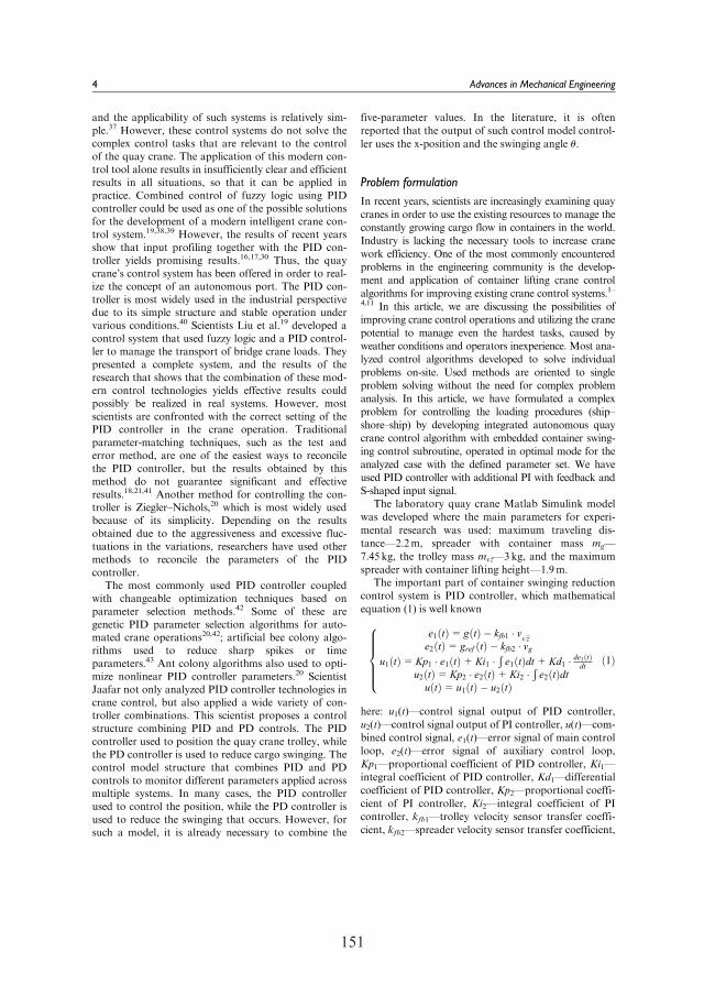
150 151

and the applicability of such systems is relatively sim-ple.37 However, these control systems do not solve thecomplex control tasks that are relevant to the controlof the quay crane. The application of this modern con-trol tool alone results in insufficiently clear and efficientresults in all situations, so that it can be applied inpractice. Combined control of fuzzy logic using PIDcontroller could be used as one of the possible solutionsfor the development of a modern intelligent crane con-trol system.19,38,39 However, the results of recent yearsshow that input profiling together with the PID con-troller yields promising results.16,17,30 Thus, the quaycrane’s control system has been offered in order to real-ize the concept of an autonomous port. The PID con-troller is most widely used in the industrial perspectivedue to its simple structure and stable operation undervarious conditions.40 Scientists Liu et al.19 developed acontrol system that used fuzzy logic and a PID control-ler to manage the transport of bridge crane loads. Theypresented a complete system, and the results of theresearch that shows that the combination of these mod-ern control technologies yields effective results couldpossibly be realized in real systems. However, mostscientists are confronted with the correct setting of thePID controller in the crane operation. Traditionalparameter-matching techniques, such as the test anderror method, are one of the easiest ways to reconcilethe PID controller, but the results obtained by thismethod do not guarantee significant and effectiveresults.18,21,41 Another method for controlling the con-troller is Ziegler–Nichols,20 which is most widely usedbecause of its simplicity. Depending on the resultsobtained due to the aggressiveness and excessive fluc-tuations in the variations, researchers have used othermethods to reconcile the parameters of the PIDcontroller.

The most commonly used PID controller coupledwith changeable optimization techniques based onparameter selection methods.42 Some of these aregenetic PID parameter selection algorithms for auto-mated crane operations20,42; artificial bee colony algo-rithms used to reduce sharp spikes or timeparameters.43 Ant colony algorithms also used to opti-mize nonlinear PID controller parameters.20 ScientistJaafar not only analyzed PID controller technologies incrane control, but also applied a wide variety of con-troller combinations. This scientist proposes a controlstructure combining PID and PD controls. The PIDcontroller used to position the quay crane trolley, whilethe PD controller is used to reduce cargo swinging. Thecontrol model structure that combines PID and PDcontrols to monitor different parameters applied acrossmultiple systems. In many cases, the PID controllerused to control the position, while the PD controller isused to reduce the swinging that occurs. However, forsuch a model, it is already necessary to combine the

five-parameter values. In the literature, it is oftenreported that the output of such control model control-ler uses the x-position and the swinging angle u.

Problem formulation

In recent years, scientists are increasingly examining quaycranes in order to use the existing resources to manage theconstantly growing cargo flow in containers in the world.Industry is lacking the necessary tools to increase cranework efficiency. One of the most commonly encounteredproblems in the engineering community is the develop-ment and application of container lifting crane controlalgorithms for improving existing crane control systems.1–4,11 In this article, we are discussing the possibilities ofimproving crane control operations and utilizing the cranepotential to manage even the hardest tasks, caused byweather conditions and operators inexperience. Most ana-lyzed control algorithms developed to solve individualproblems on-site. Used methods are oriented to singleproblem solving without the need for complex problemanalysis. In this article, we have formulated a complexproblem for controlling the loading procedures (ship–shore–ship) by developing integrated autonomous quaycrane control algorithm with embedded container swing-ing control subroutine, operated in optimal mode for theanalyzed case with the defined parameter set. We haveused PID controller with additional PI with feedback andS-shaped input signal.

The laboratory quay crane Matlab Simulink modelwas developed where the main parameters for experi-mental research was used: maximum traveling dis-tance—2.2m, spreader with container mass mg—7.45 kg, the trolley mass mvz—3kg, and the maximumspreader with container lifting height—1.9m.

The important part of container swinging reductioncontrol system is PID controller, which mathematicalequation (1) is well known

e1 tð Þ= g tð Þ � kfb1 � vv z^e2 tð Þ= gref tð Þ � kfb2 � vg

u1 tð Þ=Kp1 � e1 tð Þ+Ki1 �Ðe1 tð Þdt+Kd1 � de1 tð Þ

dt

u2 tð Þ=Kp2 � e2 tð Þ+Ki2 �Ðe2 tð Þdt

u tð Þ= u1 tð Þ � u2 tð Þ

8>>>><>>>>:

ð1Þ

here: u1(t)—control signal output of PID controller,u2(t)—control signal output of PI controller, u(t)—com-bined control signal, e1(t)—error signal of main controlloop, e2(t)—error signal of auxiliary control loop,Kp1—proportional coefficient of PID controller, Ki1—integral coefficient of PID controller, Kd1—differentialcoefficient of PID controller, Kp2—proportional coeffi-cient of PI controller, Ki2—integral coefficient of PIcontroller, kfb1—trolley velocity sensor transfer coeffi-cient, kfb2—spreader velocity sensor transfer coefficient,

4 Advances in Mechanical Engineering

152

and g(t)—input signal proportional to the referencetrolley vmax velocity.

The S-shaped velocity profile (see Figure 2) was usedas input signal for experimental and modeling andcould be described (equations (2)–(7)).

The trolley acceleration was calculated

aTR =vmax

taccð2Þ

The maximum possible acceleration of the S-shapespeed profile was calculated as

amax =aTR

1� j% � 0:005ð Þ ð3Þ

here j%—the initial tangency value was selected whichis equal to 50% of the original value. The breaking con-stant was calculated as

j=2 � amax � 100

tacc � j%ð4Þ

Jerk’s value depends on the phase of the S-profileand it can be 0, j, and –j. The quay crane control

system recalculated the acceleration a, speed v, andposition x within each time interval

a= a0 + j � Dt ð5Þ

v= v0 + a0 � Dt+j � Dt22

ð6Þ

x= x0 + v0 � Dt+a0 � Dt2

2+

j � Dt36

ð7Þ

here: Dt is the time interval related to converter samplerate, a0 is the acceleration value where initial value is 0because the trolley starts moving from 0 acceleration andeach calculation step after Dt the a0 value is recalculatedby equaling a0= a by previous calculation step (fromequation (5)), and v0 is the value of the previous speedwhere initial value is 0 because the trolley starts movingfrom 0 velocity and each calculation step after Dt the v0value is recalculated by equaling v0= v by previous calcu-lation step (from equation (6)). x0 is the value of the pre-vious position, where initial value is 0 because the trolleystarts moving from 0 position and each calculation stepafter Dt the x0 value is recalculated by equaling x0=x byprevious calculation step (from equation (7)), and vmaxwas determined using real crane parameters and reducedup to laboratory crane prototype resulting 0.2m/s.

The design variables of PID and PI controller that needto be determined are as follows: for PID controller in maincontrol loop—Kp1, Ki1, and Kd1, and for additional PIcontroller in auxiliary control loop—Kp2 and Ki2.

Development of crane’s control systemprototype

To date, many different control algorithms were devel-oped that solve individual problems,2,6–8 but there isstill a need for the development of complex algorithmsthat are oriented not only to individual loading

Figure 1. General block diagram of control system. ttr is thetrolley traveling time, and the reference block output gref(t) isequal to zero because the spreader oscillation velocity must bereduced to zero.

Figure 2. S-shape velocity profile: velocity (red dotted), acceleration (blue dashed), and jerk (black solid).

Eglynas et al. 5

152 153

procedures but also to a full ship–shore–ship stevedor-ing cycle. Frequently, the creation of new quay cranecontrol algorithms9,44 is associated with solving prob-lems, which attempt to solve the problem of containerswinging,45,46 the causes of which can occur in eachcase.10,11 Sometimes swinging caused by the mechan-isms of the crane itself, such as the engine, or uneventrack surfaces on which the devices move. However,there are cases in which the causes of swinging areunknown—they can be caused by a complex set ofeffects on the container area or even within the con-tainer itself. The basic structure of the developedlaboratory prototype is presented in Figure 3.

The laboratory crane fixed by a relatively flexibleconnection to the laboratory ceiling. The lower arms ofthe boom are facing the guideways for the horizontaltrolley movement. The trolley top is equipped with asensor net for trolley movements and position measure-ment. In the lower part, the pulleys used for lifting aspreader holder. A sensor network also installed at thetop of the spreader, recording its swing angle, speed,and position. The spreader and the lifting mechanismcontrolled through the main unit, which is equippedwith transmission gear and an electronic automatic con-trol system installed. This system consists of a controlmodule, motors, trolley, and clamp speed sensors and apower supply. After performing virtual checks of thequay crane–lifting mechanism and spreader system and

constructing a laboratory prototype for experimentalresearch, it was necessary to simulate the quay crane’scontrol system in a computer environment. The controltask signal programmed using a speed change profilewas selected through experimental and theoretical stud-ies. Based on the analysis of the scientific literature andthe evaluation of the effectiveness of the PID controllerin this type of crane control systems, it was decided,first, to select the appropriate speed profile for theinput, which was combined with the PID controllerfor the control of the quay crane transportation pro-cess. Experimental studies have been carried out toselect the input forecourt method, which comparedthe efficiency of two speed profiles to evaluate thecontainer’s continuous swinging. In order to comparethese profiles, mathematical calculations were carriedout with respect to crane speed, lifting power, andother characteristics and setting similar accelerationand deceleration parameters. As the input signal shap-ing is one of the important actions for the reductionof the initial sway of the container, the S-shaping ofthe input signal is analyzed. The initial accelerationand deceleration settings in both above-mentionedcases of the Y-axis are tacc=4 s, which corresponds tothe synchronous speed profile.

The calculations using above-mentioned equations(equations (2)–(7)) are implemented in the ArduinoControl Module and Simulink modeling. During the

Figure 3. The main system components of quay crane prototype.

6 Advances in Mechanical Engineering

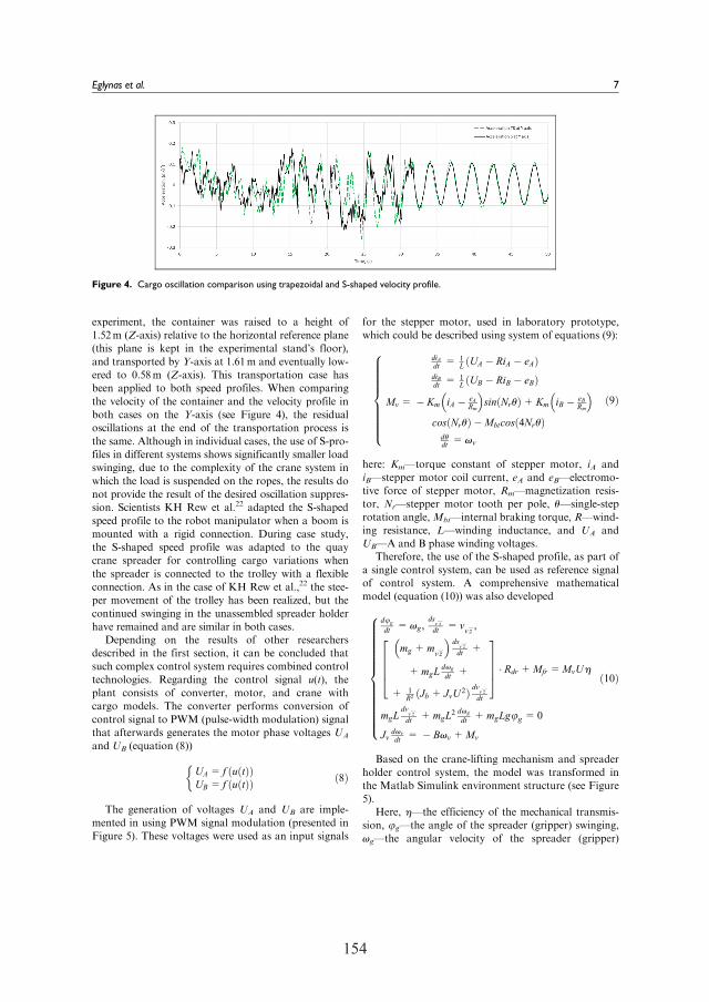
154

experiment, the container was raised to a height of1.52m (Z-axis) relative to the horizontal reference plane(this plane is kept in the experimental stand’s floor),and transported by Y-axis at 1.61m and eventually low-ered to 0.58m (Z-axis). This transportation case hasbeen applied to both speed profiles. When comparingthe velocity of the container and the velocity profile inboth cases on the Y-axis (see Figure 4), the residualoscillations at the end of the transportation process isthe same. Although in individual cases, the use of S-pro-files in different systems shows significantly smaller loadswinging, due to the complexity of the crane system inwhich the load is suspended on the ropes, the results donot provide the result of the desired oscillation suppres-sion. Scientists KH Rew et al.22 adapted the S-shapedspeed profile to the robot manipulator when a boom ismounted with a rigid connection. During case study,the S-shaped speed profile was adapted to the quaycrane spreader for controlling cargo variations whenthe spreader is connected to the trolley with a flexibleconnection. As in the case of KH Rew et al.,22 the stee-per movement of the trolley has been realized, but thecontinued swinging in the unassembled spreader holderhave remained and are similar in both cases.

Depending on the results of other researchersdescribed in the first section, it can be concluded thatsuch complex control system requires combined controltechnologies. Regarding the control signal u(t), theplant consists of converter, motor, and crane withcargo models. The converter performs conversion ofcontrol signal to PWM (pulse-width modulation) signalthat afterwards generates the motor phase voltages UA

and UB (equation (8))

UA = f u tð Þð ÞUB = f u tð Þð Þ

�ð8Þ

The generation of voltages UA and UB are imple-mented in using PWM signal modulation (presented inFigure 5). These voltages were used as an input signals

for the stepper motor, used in laboratory prototype,which could be described using system of equations (9):

diAdt

= 1LUA � RiA � eAð Þ

diBdt

= 1LUB � RiB � eBð Þ

Mv = � Km iA � eARm

� �sin Nruð Þ+Km iB � eB

Rm

� �

cos Nruð Þ �Mbtcos 4Nruð Þdudt=vv

8>>>>>>>><>>>>>>>>:

ð9Þ

here: Km—torque constant of stepper motor, iA andiB—stepper motor coil current, eA and eB—electromo-tive force of stepper motor, Rm—magnetization resis-tor, Nr—stepper motor tooth per pole, u—single-steprotation angle,Mbt—internal braking torque, R—wind-ing resistance, L—winding inductance, and UA andUB—A and B phase winding voltages.

Therefore, the use of the S-shaped profile, as part ofa single control system, can be used as reference signalof control system. A comprehensive mathematicalmodel (equation (10)) was also developed

dug

dt=vg,

dsv z^

dt= v

v z^,

mg +mvz^

� �ds

v z^

dt+

+mgLdvg

dt+

+ 1R2 Jb + JvU

2ð Þ dvv z^dt

26664

37775 � Rdr +Mfr =MvUh

mgLdv

v z^

dt+mgL

2 dvg

dt+mgLgug = 0

Jvdvv

dt= � Bvv +Mv

8>>>>>>>>>>>>><>>>>>>>>>>>>>:

ð10Þ

Based on the crane-lifting mechanism and spreaderholder control system, the model was transformed inthe Matlab Simulink environment structure (see Figure5).

Here, h—the efficiency of the mechanical transmis-sion, ug—the angle of the spreader (gripper) swinging,vg—the angular velocity of the spreader (gripper)

Figure 4. Cargo oscillation comparison using trapezoidal and S-shaped velocity profile.

Eglynas et al. 7

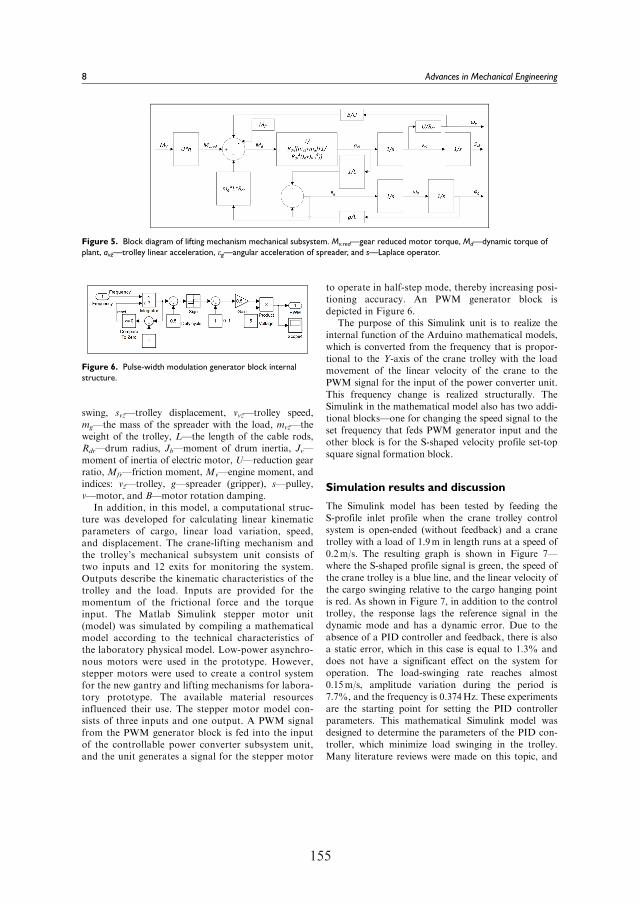
154 155

swing, svz—trolley displacement, vvz—trolley speed,mg—the mass of the spreader with the load, mvz—theweight of the trolley, L—the length of the cable rods,Rdr—drum radius, Jb—moment of drum inertia, Jv—moment of inertia of electric motor, U—reduction gearratio, Mfr—friction moment, Mv—engine moment, andindices: vz—trolley, g—spreader (gripper), s—pulley,v—motor, and B—motor rotation damping.

In addition, in this model, a computational struc-ture was developed for calculating linear kinematicparameters of cargo, linear load variation, speed,and displacement. The crane-lifting mechanism andthe trolley’s mechanical subsystem unit consists oftwo inputs and 12 exits for monitoring the system.Outputs describe the kinematic characteristics of thetrolley and the load. Inputs are provided for themomentum of the frictional force and the torqueinput. The Matlab Simulink stepper motor unit(model) was simulated by compiling a mathematicalmodel according to the technical characteristics ofthe laboratory physical model. Low-power asynchro-nous motors were used in the prototype. However,stepper motors were used to create a control systemfor the new gantry and lifting mechanisms for labora-tory prototype. The available material resourcesinfluenced their use. The stepper motor model con-sists of three inputs and one output. A PWM signalfrom the PWM generator block is fed into the inputof the controllable power converter subsystem unit,and the unit generates a signal for the stepper motor

to operate in half-step mode, thereby increasing posi-tioning accuracy. An PWM generator block isdepicted in Figure 6.

The purpose of this Simulink unit is to realize theinternal function of the Arduino mathematical models,which is converted from the frequency that is propor-tional to the Y-axis of the crane trolley with the loadmovement of the linear velocity of the crane to thePWM signal for the input of the power converter unit.This frequency change is realized structurally. TheSimulink in the mathematical model also has two addi-tional blocks—one for changing the speed signal to theset frequency that feds PWM generator input and theother block is for the S-shaped velocity profile set-topsquare signal formation block.

Simulation results and discussion

The Simulink model has been tested by feeding theS-profile inlet profile when the crane trolley controlsystem is open-ended (without feedback) and a cranetrolley with a load of 1.9m in length runs at a speed of0.2m/s. The resulting graph is shown in Figure 7—where the S-shaped profile signal is green, the speed ofthe crane trolley is a blue line, and the linear velocity ofthe cargo swinging relative to the cargo hanging pointis red. As shown in Figure 7, in addition to the controltrolley, the response lags the reference signal in thedynamic mode and has a dynamic error. Due to theabsence of a PID controller and feedback, there is alsoa static error, which in this case is equal to 1.3% anddoes not have a significant effect on the system foroperation. The load-swinging rate reaches almost0.15m/s, amplitude variation during the period is7.7%, and the frequency is 0.374Hz. These experimentsare the starting point for setting the PID controllerparameters. This mathematical Simulink model wasdesigned to determine the parameters of the PID con-troller, which minimize load swinging in the trolley.Many literature reviews were made on this topic, and

Figure 5. Block diagram of lifting mechanism mechanical subsystem. Mv.red—gear reduced motor torque, Md—dynamic torque ofplant, avz—trolley linear acceleration, eg—angular acceleration of spreader, and s—Laplace operator.

Figure 6. Pulse-width modulation generator block internalstructure.

8 Advances in Mechanical Engineering

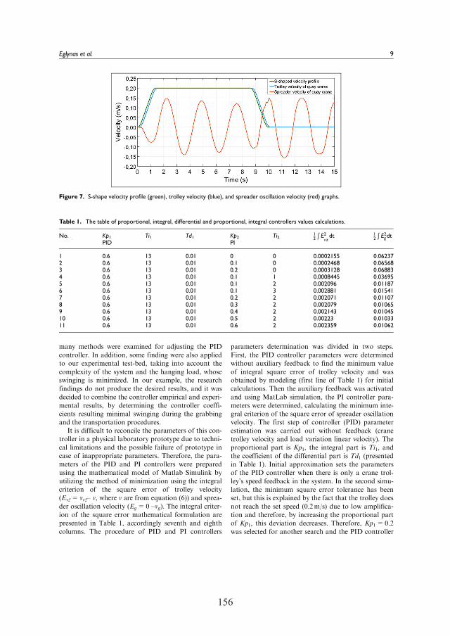
156

many methods were examined for adjusting the PIDcontroller. In addition, some finding were also appliedto our experimental test-bed, taking into account thecomplexity of the system and the hanging load, whoseswinging is minimized. In our example, the researchfindings do not produce the desired results, and it wasdecided to combine the controller empirical and experi-mental results, by determining the controller coeffi-cients resulting minimal swinging during the grabbingand the transportation procedures.

It is difficult to reconcile the parameters of this con-troller in a physical laboratory prototype due to techni-cal limitations and the possible failure of prototype incase of inappropriate parameters. Therefore, the para-meters of the PID and PI controllers were preparedusing the mathematical model of Matlab Simulink byutilizing the method of minimization using the integralcriterion of the square error of trolley velocity(Evz= vvz– v, where v are from equation (6)) and sprea-der oscillation velocity (Eg=0 –vg). The integral criter-ion of the square error mathematical formulation arepresented in Table 1, accordingly seventh and eighthcolumns. The procedure of PID and PI controllers

parameters determination was divided in two steps.First, the PID controller parameters were determinedwithout auxiliary feedback to find the minimum valueof integral square error of trolley velocity and wasobtained by modeling (first line of Table 1) for initialcalculations. Then the auxiliary feedback was activatedand using MatLab simulation, the PI controller para-meters were determined, calculating the minimum inte-gral criterion of the square error of spreader oscillationvelocity. The first step of controller (PID) parameterestimation was carried out without feedback (cranetrolley velocity and load variation linear velocity). Theproportional part is Kp1, the integral part is Ti1, andthe coefficient of the differential part is Td1 (presentedin Table 1). Initial approximation sets the parametersof the PID controller when there is only a crane trol-ley’s speed feedback in the system. In the second simu-lation, the minimum square error tolerance has beenset, but this is explained by the fact that the trolley doesnot reach the set speed (0.2m/s) due to low amplifica-tion and therefore, by increasing the proportional partof Kp1, this deviation decreases. Therefore, Kp1=0.2was selected for another search and the PID controller

Figure 7. S-shape velocity profile (green), trolley velocity (blue), and spreader oscillation velocity (red) graphs.

Table 1. The table of proportional, integral, differential and proportional, integral controllers values calculations.

No. Kp1 Ti1 Td1 Kp2 Ti212

ÐE2v z^dt

12

ÐE2gdt

PID PI

1 0.6 13 0.01 0 0 0.0002155 0.062372 0.6 13 0.01 0.1 0 0.0002468 0.065683 0.6 13 0.01 0.2 0 0.0003128 0.068834 0.6 13 0.01 0.1 1 0.0008445 0.036955 0.6 13 0.01 0.1 2 0.002096 0.011876 0.6 13 0.01 0.1 3 0.002881 0.015417 0.6 13 0.01 0.2 2 0.002071 0.011078 0.6 13 0.01 0.3 2 0.002079 0.010659 0.6 13 0.01 0.4 2 0.002143 0.0104510 0.6 13 0.01 0.5 2 0.00223 0.0103311 0.6 13 0.01 0.6 2 0.002359 0.01062

Eglynas et al. 9

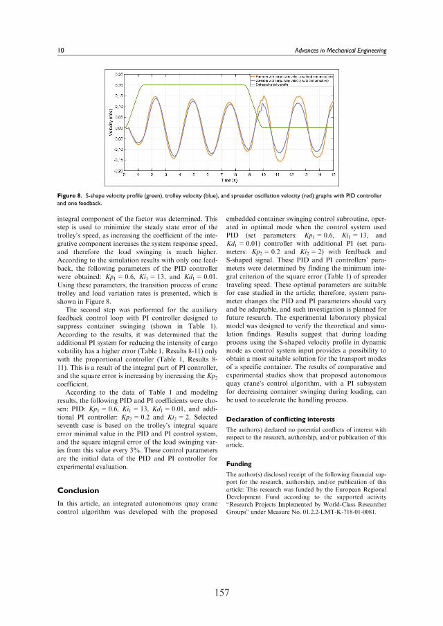
156 157

integral component of the factor was determined. Thisstep is used to minimize the steady state error of thetrolley’s speed, as increasing the coefficient of the inte-grative component increases the system response speed,and therefore the load swinging is much higher.According to the simulation results with only one feed-back, the following parameters of the PID controllerwere obtained: Kp1=0.6, Ki1=13, and Kd1=0.01.Using these parameters, the transition process of cranetrolley and load variation rates is presented, which isshown in Figure 8.

The second step was performed for the auxiliaryfeedback control loop with PI controller designed tosuppress container swinging (shown in Table 1).According to the results, it was determined that theadditional PI system for reducing the intensity of cargovolatility has a higher error (Table 1, Results 8-11) onlywith the proportional controller (Table 1, Results 8-11). This is a result of the integral part of PI controller,and the square error is increasing by increasing the Kp2coefficient.

According to the data of Table 1 and modelingresults, the following PID and PI coefficients were cho-sen: PID: Kp1=0.6, Ki1=13, Kd1=0.01, and addi-tional PI controller: Kp2=0.2 and Ki2=2. Selectedseventh case is based on the trolley’s integral squareerror minimal value in the PID and PI control system,and the square integral error of the load swinging var-ies from this value every 3%. These control parametersare the initial data of the PID and PI controller forexperimental evaluation.

Conclusion

In this article, an integrated autonomous quay cranecontrol algorithm was developed with the proposed

embedded container swinging control subroutine, oper-ated in optimal mode when the control system usedPID (set parameters: Kp1=0.6, Ki1=13, andKd1=0.01) controller with additional PI (set para-meters: Kp2=0.2 and Ki2=2) with feedback andS-shaped signal. These PID and PI controllers’ para-meters were determined by finding the minimum inte-gral criterion of the square error (Table 1) of spreadertraveling speed. These optimal parameters are suitablefor case studied in the article; therefore, system para-meter changes the PID and PI parameters should varyand be adaptable, and such investigation is planned forfuture research. The experimental laboratory physicalmodel was designed to verify the theoretical and simu-lation findings. Results suggest that during loadingprocess using the S-shaped velocity profile in dynamicmode as control system input provides a possibility toobtain a most suitable solution for the transport modesof a specific container. The results of comparative andexperimental studies show that proposed autonomousquay crane’s control algorithm, with a PI subsystemfor decreasing container swinging during loading, canbe used to accelerate the handling process.

Declaration of conflicting interests

The author(s) declared no potential conflicts of interest withrespect to the research, authorship, and/or publication of this

article.

Funding

The author(s) disclosed receipt of the following financial sup-port for the research, authorship, and/or publication of thisarticle: This research was funded by the European RegionalDevelopment Fund according to the supported activity‘‘Research Projects Implemented by World-Class ResearcherGroups’’ under Measure No. 01.2.2-LMT-K-718-01-0081.

Figure 8. S-shape velocity profile (green), trolley velocity (blue), and spreader oscillation velocity (red) graphs with PID controllerand one feedback.

10 Advances in Mechanical Engineering

158

ORCID iD

Tomas Eglynas https://orcid.org/0000-0002-9973-5896

References

1. Barysien_e J. A multi-criteria evaluation of container ter-

minal technologies applying the COPRAS-G method.

Transport 2012; 27: 364–372.2. Cao L and Liu L. Adaptive fuzzy sliding mode method-

based position and anti-swing control for overhead

cranes. In: Proceedings of the 2011 third international con-

ference on measuring technology and mechatronics auto-

mation, Shangshai, 6–7 January 2011, vol. 2, pp.335–338.

New York: IEEE.3. Yoshihara H, Fujioka N and Kasahara H. A new vision-

sensorless anti-sway control system for container cranes.

In: Proceedings of the 38th IAS annual meeting on confer-

ence record of the industry applications conference, Salt

Lake City, UT, 12–16 October 2003, pp.262–269. New

York: IEEE.4. Sano H, Ohishi K, Kaneko T, et al. Anti-sway crane

control based on dual state observer with sensor-delay

correction. In: Proceedings of the 11th IEEE international

workshop on advanced motion control (AMC), Nagaoka,

Niigata, 21–24 March 2010, pp.679–684. New York:

IEEE.5. Kawai H, Choi Y, Kim YB, et al. Position measurement

of container crane spreader using an image sensor system

for anti-sway controllers. In: Proceedings of the interna-

tional conference on control, automation and systems,

Seoul, South Korea, 14–17 October 2008, pp.683–686.

New York: IEEE.6. Chao SL and Lin YJ. Evaluating advanced quay cranes

in container terminals. Transport Res E: Log 2011; 47:

432–445.7. Schaub H. Rate-based ship-mounted crane payload pen-

dulation control system. Control Eng Pract 2008; 16:

132–145.8. Chang C, Chiang K and Description AS. The nonlinear

3-D crane control with an intelligent operating method.

In: Proceedings of the 2008 SICE annual conference,

Tokyo, Japan, 20–22 August 2008, pp.2917–2921, 2008.9. Zhi-Jun LI, Zhen LI, Hui-Jie LI, et al. Research of coor-

dinated control method of hybrid power crane system.

In: Proceedings of the international conference on model-

ling, identification and control, Wuhan, China, 24–26

June 2012, pp.1093–1097. New York: IEEE.10. Tanaka Y, Konishi Y, Araki N, et al. Development of

high speed controller of container crane by binary input

using mixed logical dynamical system. In: Proceedings of

the 2009 fourth international conference on innovative com-

puting, information and control (ICICIC), Kaohsiung,

Taiwan, 7–9 December 2009, pp.181–184. New York:

IEEE.

11. Chang D, Jiang Z, Yan W, et al. Integrating berth alloca-

tion and quay crane assignments. Transport Res E: Log

2010; 46: 975–990.12. Fang Y, Wang P and Zhang X. A motion planning-based

adaptive control method for an underactuated crane sys-

tem. IEEE T Control Syst Tech 2012; 20: 241–248.

13. Tanaka Y, Konishi Y, Araki N, et al. Control of con-tainer crane by binary input using mixed logical dynami-cal system. In: Proceedings of the international conferenceon control, automation and systems, Seoul, South Korea,14–17 October 2008, vol. 2, pp.13–17.

14. Nundrakwang S, Benjanarasuth T, Ngamwiwit J, et al.Multivariable control of overhead crane system by CRAmethod. In: Proceedings of the SICE annual conference,Tokyo, Japan, 20–22 August 2008, vol. 1, pp.3278–3282.New York: IEEE.

15. Roso V, Woxenius J and Lumsden K. The dry port con-cept: connecting container seaports with the hinterland.

J Transp Geogr 2009; 17: 338–345.16. Elbadawy AA and Shehata MMG. Anti-sway control of

marine cranes under the disturbance of a parallel manip-ulator. Nonlinear Dynam 2015; 82: 415–434.

17. Majid MA, IbrahimWSW, Mohamad S, et al. A compar-ison of PID and PD controller with input shaping tech-nique for 3D gantry crane. In: Proceedings of the IEEE

conference on systems, process & control (ICSPC), KualaLumpur, Malaysia, 13–15 December 2013, pp.144–148.New York: IEEE.

18. Wong TT, Tang CHH and Mailah M. Winch driven

active heave compensation for load transfer in overheadcrane system. In: Proceedings of the 4th international con-

ference on intelligent and advanced systems (ICIAS2012),Kuala Lumpur, Malaysia, 12–14 June 2012, pp.34–39.New York: IEEE.

19. Liu C, Zhao H and Cui Y. Research on application offuzzy adaptive PID controller in bridge crane control sys-tem. In: Proceedings of the 2011 international conference

on control, automation and systems engineering (CASE),Beijing, China, 27–29 June 2014, pp.1–4. New York:IEEE.

20. Jaafar HI, Mohamed Z, Abidin AFZ, et al. PSO-tunedPID controller for a nonlinear gantry crane system. In:

Proceedings of the IEEE international conference on con-

trol system, computing and engineering, Penang, Malaysia,23–25 November 2012, pp.515–519. New York: IEEE.

21. Jaafar HI, Sulaima MF, Mohamed Z, et al. Optimal PIDcontroller parameters for nonlinear gantry crane systemvia MOPSO technique. In: Proceedings of the IEEE con-

ference on sustainable utilization and development in engi-

neering and technology (CSUDET), Selangore, Malaysia,30 May–1 June 2013, pp.86–91. New York: IEEE.

22. Rew KH, Ha CW and Kim YS. A practically efficientmethod for motion control based on asymmetric velocityprofile. Int J Mach Tools Manuf 2009; 49: 678–682.

23. Bearee R. New damped-jerk trajectory for vibrationreduction. Control Eng Pract 2014; 28: 112–120.

24. Sun N, Zhang X, Fang Y, et al. Transportation task-oriented trajectory planning for underactuated overheadcranes using geometric analysis. IET Control Theory Appl

2012; 6: 1410–1423.25. Xuebo Z, Yongchun F, Ning SUN, et al. A pseudospec-

tral time-optimal motion planner for underactuated over-head crane systems. In: Proceedings of the 32nd Chinese

control conference, Xi’an, China, 26–28 July 2013, vol. 3,pp.4397–4402. New York: IEEE.

26. Sun N, Fang Y, Member S, et al. Phase plane analysis

based motion planning for underactuated overhead

Eglynas et al. 11

158 159

cranes. In: Proceedings of the IEEE international confer-

ence on robotics and automation, Shanghai, China, 9–13May 2011, pp.3483–3488. New York: IEEE.

27. Stoychitch M. An algorithm of linear speed control of astepper motor in real time. Ann Fac Eng 2013; 11: 51–56.

28. Wu Z and Xia X. Optimal motion planning for overheadcranes. IET Control Theory Appl 2014; 8: 1833–1842.

29. Vaughan J, Yoo J, Knight N, et al. Multi-input shapingcontrol for multi-hoist cranes. In: Proceedings of the

American control conference, Washington, DC, 17–19June 2013, pp.3455–3460. New York: IEEE.

30. Prof A, Brock S, Member I, et al. Analysis of input shap-ing and PID-controller interaction structures for two-mass systems. In: Proceedings of the 16th international

conference on mechatronics–mechatronika, Brno, 3–5December 2014. New York: IEEE.

31. Ngo OH, Nan Y and Hong K. Command shaping for

vibration reduction of container cranes. In: Proceedingsof the 12th international conference on control, automation

and systems, JeJu Island, South Korea, 17–21 October2012, pp.651–655. New York: IEEE.

32. Jaafar HI, Mohamed ZZ, Jamian JJ, et al. Dynamicbehaviour of a nonlinear gantry crane system. Proc Tech-nol 2013; 11: 419–425.

33. Ismail RMTR, Ahmad MA, Ramli MS, et al. Nonlineardynamic modelling and analysis of a 3-D overhead gantrycrane system with payload variation. In: Proceedings of

Third UKSim European symposium on computer modeling

and simulation, Athens, 25–27 November 2009, pp.350–354. New York: IEEE.

34. Bogdevicius M and Vika A. Investigation of the dynamicsof the overhead crane lifting process in the vertical plane.Transport 2005; 20: 176–180.

35. Tomczyk J, Cink J and Kosucki A. Dynamics of an over-head crane under a wind disturbance condition. AutomConstr 2014; 42: 100–111.

36. Cha JH, Roh MI and Lee KY. Dynamic response simu-lation of a heavy cargo suspended by a floating cranebased on multibody system dynamics. Ocean Eng 2010;37: 1273–1291.

37. Ranjbari L and Shirdel AH. Designing precision fuzzycontroller for load swing of an overhead crane. Neural

Comput Appl 2015; 26: 1555–1560.

38. Wang L, Zhang H and Kong Z. Anti-swing control ofoverhead crane based on double fuzzy controllers. In:Proceedings of the 27th Chinese control and decision con-

ference (2015 CCDC), Qingdao, 23–25 May 2015,pp.981–986. New York: IEEE.

39. Yang C, Zhang Z and Zhao Q. Study on intelligent con-trol of two-dimensional precision positioning system. In:Proceedings of the international conference on computer

science and software engineering, Hubei, China, 12–14December 2008, vol. 4, pp.835–838. New York: IEEE.

40. Sun Z, Wang N, Bi Y, et al. A DE based PID controllerfor two dimensional overhead crane. In: Proceedings of

the 34th Chinese control conference, Hangzhou, China,28–30 July 2015, pp.2546–2550. New York: IEEE.

41. Wong TT, Tang CHH and Mailah M. Robust activeheave compensated winch-driven overhead crane systemfor load transfer in marine operation. In: Proceedings of

the robust active heave compensated winch-driven overhead

crane system for load transfer in marine operation, KualaLumpur, Malaysia, 12–14 June 2012, vol. 1, pp.111–116.New York: IEEE.

42. Lv N, Li H, Li M, et al. Based on PID control optimiza-tion of synchronous motor control. In: Proceedings of theconference on measurement, information and control

(MIC), Harbin, China, 18–20 May 2012, pp.2111–2114.43. Li P, Li Z and Yang Y. The application research of ant

colony optimization algorithm for intelligent control onspecial crane. In: Proceedings of the 2012 second interna-

tional conference on instrumentation, measurement, com-

puter, communication and control, Harbin, China, 8–10December 2012, pp.999–1004. New York: IEEE.

44. Maghsoudi MJ, Mohamed Z, Tokhi MO, et al. Controlof a gantry crane using input-shaping schemes with dis-tributed delay. Trans Inst Meas Control 2017; 39: 361–370.

45. Schmidt R, Barry N and Vaughan J. Tracking of a targetpayload via a combination of input shaping and feedbackcontrol. IFAC—PapersOnLine 2015; 48: 141–146.

46. Ahmad MA, Ismail RR, Ramli MS, et al. Investigations

of NCTF with input shaping for sway control of adouble-pendulum-type overhead crane. In: Proceedings

of the 2nd international conference on advanced computer

control, Shenyang, China, 27–29 March 2010, vol. 3,pp.456–461. New York: IEEE.

12 Advances in Mechanical Engineering

114

4th publication / 4 publikacija

Multibody dynamic simulation and transient analysis of quay crane spreader and lifting

mechanism

A. Andziulis, T. Eglynas, M. Bogdevičius, M. Jusis, A. Senulis.

Advances in Mechanical Engineering Vol. 8(9), 1-11 (2016)

IF: 0.67

DOI: 10.1177/1687814016670803

161

Research Article

Advances in Mechanical Engineering2016, Vol. 8(9) 1–11� The Author(s) 2016DOI: 10.1177/1687814016670803aime.sagepub.com

Multibody dynamic simulation andtransient analysis of quay cranespreader and lifting mechanism

Arunas Andziulis1, Tomas Eglynas1,2, Marijonas Bogdevicius2, MindaugasJusis1 and Audrius Senulis1

AbstractNowadays, container shipment in the intermodal terminals is overloaded. The quay crane and its control system have tobe properly prepared for rapid cargo reloading. The advanced control system may increase container loading efficiencydue to the reduced transportation time. However, faster transportation demands higher safety. In this article, theauthors performed multibody dynamics simulation of the container spreader and lifting mechanism by analyzing moreadvanced mathematical model of the quay crane. Trolley motion and cargo swing angle transient responses of thedynamic system were acquired and analyzed during model simulation. The main target of this research is to determinethe system behavior during transients. The simulation results showed that the transients induced by startup of the verti-cal spreader travel affect the whole crane system in all the investigated cases. In addition, the influence of flexible cablecauses additional oscillations of cargo and reciprocating trolley displacement. The simulation of the container spreaderand lifting mechanism will help detect motion deviations of the quay crane in real time.

KeywordsMultibody dynamics, transients, simulation, mathematical modeling, quay crane

Date received: 1 July 2016; accepted: 30 August 2016

Academic Editor: Crinela Pislaru

General introduction

Risk of cargo transportation process and impact ofcrane restrictions

Every year, container shipment is increasing and thecontainer terminals get loaded more. Because of thissituation, the terminals must load more containersusing the same transportation equipment. One of themost important aspects of cargo loading is operationsafety which can decrease in overloaded terminals.1–3

In order to ensure safety of the container during trans-portation, an optimal operational strategy4,5 of a quaycrane control has to be ensured. In addition, the restric-tions and limitations of the intermodal quay crane haveto be appropriately assessed performing numericalsimulations of multibody dynamics and the transientprocesses.

One of the most researched cargo damage reasons inthe past years is container swinging.2,6,7 The main causeof the container and spreader swinging is the flexiblesteel cable connection between the spreader and trolleyof the quay crane.8 The container can produce swingingmotion because of different container weights, windgusts, and human actions. As a result, more time isrequired for the container shipment from point A to

1Marine Science and Technology Centre, Klaipeda University, Klaipeda,

Lithuania2Department of Transport Technological Equipment, Vilnius Gediminas

Technical University, Vilnius, Lithuania

Corresponding author:

Tomas Eglynas, Marine Science and Technology Centre, Klaipeda

University, Bijunu g. 17-206, LT-91225 Klaipeda, Lithuania.

Email: tmse@inbox.lt

Creative Commons CC-BY: This article is distributed under the terms of the Creative Commons Attribution 3.0 License

(http://www.creativecommons.org/licenses/by/3.0/) which permits any use, reproduction and distribution of the work without

further permission provided the original work is attributed as specified on the SAGE and Open Access pages (https://us.sagepub.com/en-us/nam/

open-access-at-sage).

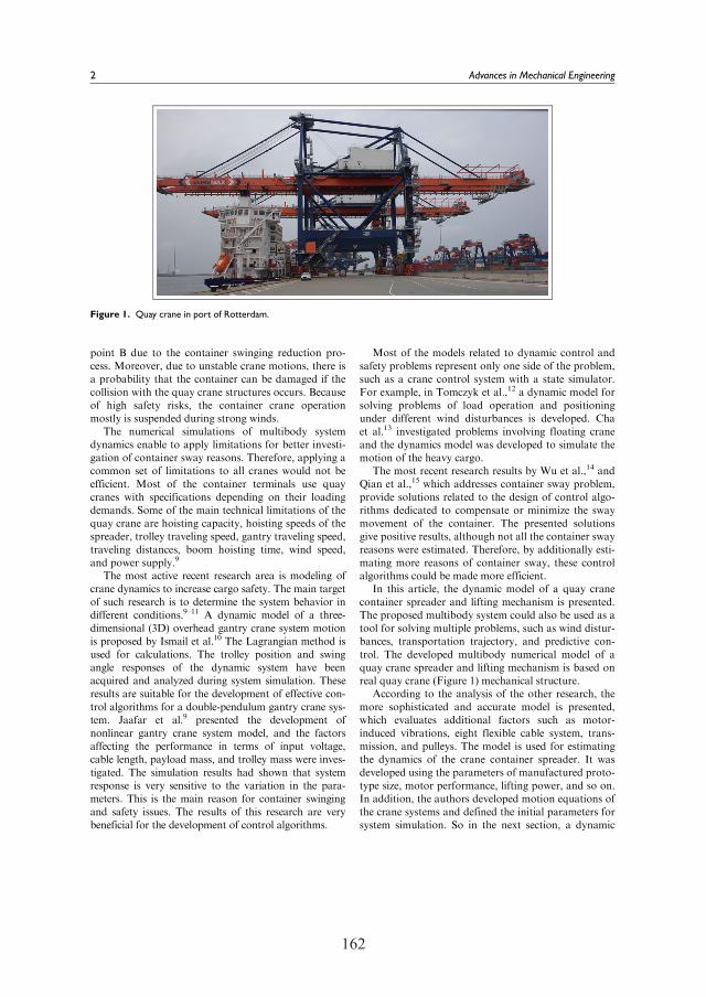
162

point B due to the container swinging reduction pro-cess. Moreover, due to unstable crane motions, there isa probability that the container can be damaged if thecollision with the quay crane structures occurs. Becauseof high safety risks, the container crane operationmostly is suspended during strong winds.

The numerical simulations of multibody systemdynamics enable to apply limitations for better investi-gation of container sway reasons. Therefore, applying acommon set of limitations to all cranes would not beefficient. Most of the container terminals use quaycranes with specifications depending on their loadingdemands. Some of the main technical limitations of thequay crane are hoisting capacity, hoisting speeds of thespreader, trolley traveling speed, gantry traveling speed,traveling distances, boom hoisting time, wind speed,and power supply.9

The most active recent research area is modeling ofcrane dynamics to increase cargo safety. The main targetof such research is to determine the system behavior indifferent conditions.9–11 A dynamic model of a three-dimensional (3D) overhead gantry crane system motionis proposed by Ismail et al.10 The Lagrangian method isused for calculations. The trolley position and swingangle responses of the dynamic system have beenacquired and analyzed during system simulation. Theseresults are suitable for the development of effective con-trol algorithms for a double-pendulum gantry crane sys-tem. Jaafar et al.9 presented the development ofnonlinear gantry crane system model, and the factorsaffecting the performance in terms of input voltage,cable length, payload mass, and trolley mass were inves-tigated. The simulation results had shown that systemresponse is very sensitive to the variation in the para-meters. This is the main reason for container swingingand safety issues. The results of this research are verybeneficial for the development of control algorithms.

Most of the models related to dynamic control andsafety problems represent only one side of the problem,such as a crane control system with a state simulator.For example, in Tomczyk et al.,12 a dynamic model forsolving problems of load operation and positioningunder different wind disturbances is developed. Chaet al.13 investigated problems involving floating craneand the dynamics model was developed to simulate themotion of the heavy cargo.

The most recent research results by Wu et al.,14 andQian et al.,15 which addresses container sway problem,provide solutions related to the design of control algo-rithms dedicated to compensate or minimize the swaymovement of the container. The presented solutionsgive positive results, although not all the container swayreasons were estimated. Therefore, by additionally esti-mating more reasons of container sway, these controlalgorithms could be made more efficient.

In this article, the dynamic model of a quay cranecontainer spreader and lifting mechanism is presented.The proposed multibody system could also be used as atool for solving multiple problems, such as wind distur-bances, transportation trajectory, and predictive con-trol. The developed multibody numerical model of aquay crane spreader and lifting mechanism is based onreal quay crane (Figure 1) mechanical structure.

According to the analysis of the other research, themore sophisticated and accurate model is presented,which evaluates additional factors such as motor-induced vibrations, eight flexible cable system, trans-mission, and pulleys. The model is used for estimatingthe dynamics of the crane container spreader. It wasdeveloped using the parameters of manufactured proto-type size, motor performance, lifting power, and so on.In addition, the authors developed motion equations ofthe crane systems and defined the initial parameters forsystem simulation. So in the next section, a dynamic

Figure 1. Quay crane in port of Rotterdam.

2 Advances in Mechanical Engineering

162 163

model of container spreader dynamics and liftingmechanism is proposed.

Mathematical model and dynamics ofcontainer spreader transients

Before the development of better algorithm, a newmathematical model of the crane spreader and realquay crane prototype was created (Figure 2). The

model will provide theoretical data about spreader sta-tus. The vibrations and their sources in the crane sprea-der and lifting mechanism were evaluated and providedadditional information for new mathematical model forthe crane (Figure 3). The mathematical model (Figure3) marked ‘‘Part C’’ (trolley with lifting mechanism)and ‘‘Part D’’ (container spreader) is the same like inprototype (Figure 2).

Most attention is paid to motor vibrations and cabletensions. Because of very long cables in cranes, addi-tional container swinging can appear. Mostly, it iscaused by the weather conditions and wrong algorithmsfor operating devices. The best solution for this prob-lem is adding additional sensors, such as, in our case,an accelerometer. The sensor’s data could be used forcontainers’ position estimation, detection, and reduc-tion in container swinging. This could increase trans-portation security. Combined algorithm generator andreal-time sensor data will provide the best algorithm fora particular kind of cargo that is stored in the con-tainer. In addition, it will allow adjusting algorithm in

Figure 2. Scaled prototype of intermodal quay crane: (a)virtual prototype and (b) physical prototype.

Figure 3. Dynamic model of quay crane spreader and lifting mechanism.

Andziulis et al. 3

164

real time, if the weather conditions change or someunexpected situation appears (uneven control, shift ofthe cargo in the container, crane swinging due to thewind, etc.).

The developed model of the quay crane spreaderand lifting mechanism is based on several assumptions.First, all bodies in the model are considered as solidbodies that cannot be deformed. The physical andmechanical properties of all the cables (such as stretch-ing of cables while carrying heavy cargo) were assumedand estimated and their mathematical models areincluded in equations. Additionally, the electro-mechanical transient processes of electric motors andimperfections of trolley path were estimated.

For better container transportation problem solu-tion, the new mathematical model was used for the con-tainer spreader and lifting mechanism, which will helpto evaluate the situation. Torque mathematical equa-tion of first electrical asynchronous motor with gear _Mei

is shown below

_Mei =UredeiCei(vei0 � Uredei _ui)� deiMei ð1Þ

Here, dei and Cei are the motor parameters, vei0 is theangular velocity, and Uredei is the gear ratio of the motorreduction. The analyzed system consists of two bodieswith mass centers in points Ci and Cj. They are con-nected to the cable at mounting points i and j. The cablestiffness and damping coefficients are kij and cij, respec-tively. The tension force in this cable is Fij, and the var-iation in mechanical work of this force is equal to

dWij =FijdLij ð2Þ

Here, Lij is the distance between i and j; dLij is the var-iation in distance between i and j. The distance of Lij isequal to

L2ij =(ri � rj)T (ri � rj) ð3Þ

Here, ri and rj are the vectors of i and j, respectively, incommon coordinate system OXYZ

ri = rci +A(ui)rci, irj = rcj +A(uj)rcj, j

ð4Þ

Here, rCi and rCj are the vectors of mass centers of bod-ies, A(ui) and A(uj) are the matrixes of angular rota-tion (about X-axis), rci, i is the distance between bodymass center Ci and body point i, and rcj, j is the distancebetween body mass center Cj and body point j. The var-iation in distance Lij is

dLij=drij

T

Lijrij ð5Þ

Here

drij= drci+ dui

dA(ui)

dui

� �rci, i � drcj � duj

dA(uj)

duj

" #rcj, j

ð6Þ

Using equations (5) and (6), the variations in mechani-cal work can be calculated as

dWcj= drciT � qrci + duiqri + drcj

Tqrcj + dujqrj ð7Þ

Here, qrci and qrcj are the vectors of the generalizedforces that apply to bodies i and j; qri and qrj are thegeneralized forces that apply to bodies i and j

qrci =Fij

Lijrij, qui =

Fij

Lijrci, i

T dA(ui)

dui

� �Trij ð8Þ

qRcj=

Fij

Lijrij, quj =

Fij

Lijrcj, j

TdA(uj)

duj

" #T

rij ð9Þ

The cable tension force is

Fij = �kij(Lij � Lij, 0)� Cij_Lij

� �H(Lij � Lij, 0) ð10Þ

Here, H(Lij � Lij, 0) is the Heaviside function and Lij, 0 isthe initial cable length between i and j. _Lij is the cablelinear speed

_Lij =1

Lij_rij

T � rij ð11Þ

Here, _rij is the time derivative of vector rij

_rij = _rci+ _ui

dA(ui)

dui

� �rci, i � _rcj � _uj

dA(uj)

duj

" #rcj, j ð12Þ

Equations of motionsSystem of motion equations for the first body (cranewithout load)

m1€q12 =� k31(q12 � R3u3)� c31( _q12 � R3 _u3)

� k41(q12 � R3u4)� c41( _q12 � R4 _u4)

+ e2T (F5q51 +F6q61 +F7q71 +F8q81)

� _m1 _q12 +F1R2

ð13Þ

m1€q13=� k10(q13+ a3u1 � Z11)

� k20(q13 � a4u1 � Z12)� c20( _q13 � a4 _u1 � _Z12)

� c10( _q13+ a3 _u1 � _Z11)� m1g � _m1 _q13

+ e3T (F5q51+F6q61+F7q71 +F8q81)+F1R3

ð14Þ

4 Advances in Mechanical Engineering

164 165

I1 €u1 =� k10a3(q13 + a3u1 � Z11)

� c10a3( _q13 + a3 _u1 � _Z11)

� k20a4(q13 � a4u1 � Z12)

+ c20a4( _q13 � a4 _u1 � _Z12)� _I1 _u1 +M51

+M61 +M71 +M81 +M1R

ð15Þ

Here, m1 is the mass of the first body, I1 is the inertialmoment of the first body about the X-axis, _m1 and _I1are the first time derivatives of mass and mass inertialmoment of the first body (assumption of cable windingon the pulley), respectively. a3 and a4 are the geometri-cal parameters. Z11 and Z12 are the kinematic excita-tions of the first body pulleys; _Z11 and _Z12 are thederivatives of kinematic excitations by time. e2 and e3are the unit vectors on Y- and Z-axis in common coor-dinate system OXYZ. k31, k41, c31, and c41 are stiffnessand damping coefficients of trolley positioning systembelts. k10, k20, c10, and c20 are the stiffness and dampingcoefficients of the pulleys of trolley positioning system.F5, F6, F7, and F8 are the cable tension forces. M51,M61, M71, M81, and M1R are the torques of the firstbody, transferred by cables 5, 6, 7, and 8. F1R2 and F1R3

are the air resistance forces (projection on Y- and Z-axis) and torques q51, q61, q71, and q81 are the vectorsof the generalized forces of cables 5, 6, 7, and 8, respec-tively, determined using equation (8).

System of motion equations for the second body(spreader with the container)

M2€rC2= q52 + q62 + q72 + q82 + f2W + f2R ð16Þ

I2 €u2 =M52 +M62 +M72 +M82 +MR2 ð17ÞI21 €u21 =R21(F5 � F6)�Mfr21sign( _u21) ð18Þ

I22 €u22 =R22(F7 � F8)�Mfr22sign( _u22) ð19Þ

Here, F2W is the vector of weight force (20); f2R andMR2

are the vector of air resistance force and torque of thesecond body, respectively. q52, q62, q72, and q82 are thevectors of the generalized forces of cables 5, 6, 7, and 8,respectively, calculated using equation (8). M52, M62,M72, and M82 are the torques of the first body, trans-ferred by cables 5, 6, 7, and 8, respectively. M2 is thematrix of masses of the second body calculated usingequation (19). Mfr21 and Mfr22 are the torques of frictionof polyspast

fF2WgT = ½0, 0, � m2g� ð20Þ½M2�= diag(m2,m2, I2) ð21Þ

System of motion equations for the third and fourthbodies and the third asynchronous motor torque(trolley motion equations)

_Me3 =Urede3Ce3(ve30 � Urede3 _u3)� de3Me3 ð22Þ

I3 €u3 =� k31R3(R3u3 � q12)� c31R3(R3 _u3 � _q12)

� k34R3(R3u3 � R4u4)� c34R3(R3 _u3 � R4 _u4)

+Me3 �Me3R ð23Þ

I4 €u4 =� R4k41(R4u4 � q12)� R4c41(R4 _u4 � _q12)

� R4k34(R4u4 � R3u3)

� R4c34(R4 _u4 � R3 _u3)�Me4R

ð24Þ

Here, k31, k34, c31, and c34 are the stiffness and dampingcoefficients of belts. u3, u4, _u3, and _u4 are the angularposition and speed of the third and fourth bodies. R3

and R4 are the radii of the pulleys, I3 is the massmoment of inertia of the third motor and pulley, and I4is the moment of inertia of the fourth pulley. Me3 is thetorque of the motor. Ce3 and de3 are the motor para-meters. Me3R is the torque of resistance of the thirdbody. ve30 is the motor angular velocity.

System of motion equations for lifting mechanism

_Me1 =Urede1Ce1(ve110 � Urede1 _u11)� de1Me1 ð25Þ

I11 €u11 =� R11 k1(R11u11 � R12u12)ð+ c1(R11 _u11 � R12 _u12)Þ(1� e�fbeltb24)

+Me1 �Mfr11sign( _u11)

ð26Þ

I12 €u12 =� R12 k1(R12u12 � R11u11)ð+ c1(R12 _u12 � R11 _u11)Þ(1� e�fbeltb13)

�M9, 5 �Mfr12sign( _u12)

ð27Þ

_Me2 =Urede2Ce2(ve130 � Urede2 _u13)� de2Me2 ð28Þ

I13 €u13 =� R13(k3(R13u13 � R14u14)

+ c3(R13 _u13 � R14 _u14))(1� e�fbeltb58)

+Me2 �Mfr13sign( _u13)

ð29Þ

I14 €u14 =� R14 k3(R14u14 � R13u13)ð+ c3(R14 _u14 � R13 _u13)Þ(1� e�fbeltb67)

�Mfr14sign( _u14)�M15, 8 �Mfr14sign( _u14)

ð30Þ

M9, 5 =F5R13,M15, 8 =F8R14 ð31Þ

where Me1 and Me2 are the torques of the first and sec-ond asynchronous motors, respectively; u11, u12, u13,and u14 are the angular positions of the first, second,third, and fourth pulleys, respectively. Ce1, de1, Ce2, andde2 are the first and second motor parameters. ve110 andve130 are the first and second motor angular velocities,respectively. I11, I12, I13, and I14 are the moments ofinertia of the first, second, third, and fourth pulleys,

Andziulis et al. 5

166

respectively. R11, R12, R13, and R14 are the radii of thefirst, second, third, and fourth pulleys, respectively. k1,k2, k3, k4, c1, c2, c3, and c4 are the stiffness and dampingcoefficients of the belts.M9, 5 andM15, 8 are the momentsof inertia of the second and fourth pulleys, caused bythe tension forces in cables 5 and 8, on points 9 and 15of the pulleys, respectively. Mfr11 , Mfr12 , Mfr13 , and Mfr14

are the torques of the friction force of the first, second,third, and fourth pulleys, respectively. fbelt is the frictioncoefficient; b24, b13, b58, and b67 are the angles of beltwarp.

System of equations for generalized forces of thefifth cable

q5 =F5

L9, 10(r9 � r10) ð32Þ

F5 =� k5(L9, 10 � L9, 10, 0)� c5 _L9, 10 ð32aÞ

r9 = rC1 +A1(u1)rC1, 9 ð32bÞ

rC1, 9 = rC1,O12 + rO12, 9 ð32cÞ

r10 = rC2 +A2(u2)(rC2,O21 + rO21, 10) ð32dÞ

r9, 10 = r9 � r10 ð32eÞ

L29, 10 = r9, 10T r9, 10 ð32fÞ

_L9, 10 =1

L9, 10� _r9, 10

T r9, 10 ð32gÞ

_r9, 10 = _r9 � _r10 ð32hÞ

_r9 = _rC1 + _u1

dA1

du1

� �rC1, 9 +A1(u1)_rC1, 9 ð32iÞ

_r10 = _rC2 + _u2

dA2

du2

� �rC2, 10 +A2(u2)_rC2, 10 ð32jÞ

_r10 = _rC2 + _u2

dA2

du2

� �rC2, 10 +A2(u2)_rC2, 10 ð32kÞ

rO12, 9 =R13 cos b9, 10

R13 sin b9, 10

� �ð32lÞ

b9, 10 =aO12,O21 � g9, 10 ð32mÞ

sinaO12,O21 =YO21 � YO12

LO12, O21

ð32nÞ

sin g9, 10 =R13 � R21

LO12,O21ð32oÞ

L2O12,O21=(rO12 � rO21)T (rO12 � rO21) ð32pÞ

rO21, 10 =R21 cos bO11,O21

R21 sin bO11,O21

� �ð32qÞ

rC2, 10 = rC2,O21 + rO21, 10 ð32rÞ

rO21, 10 =R21 cos b9, 10

R21 cos b9, 10

� �ð32sÞ

Here, k5 and c5 are the stiffness and damping coeffi-cients of the fifth cable, respectively (k5 depends on linelength L9, 10). R21 is the radius of the left pulley on thetrolley.

System of equations for generalized forces of thesixth, seventh, and eighth cables using system ofequations (32)

q6 =F6

L11, 12(r12 � r11) ð33Þ

q7 =F7

L12, 13(r12 � r13) ð34Þ

q8 =F8

L14, 15(r14 � r15) ð35Þ

Moments applied on the first and second bodies

M51 = exT ~rC1, 9 � A1(u1)

T � q5� �

M61 = exT ~rC1, 12 � A1(u1)

T � q6� �

M71 = exT ~rC1, 12 � A1(u1)

T � q7� �

M81 = exT ~rC1, 15 � A1(u1)

T � q8� �

M52 = exT ~rC2, 10 � A2(u2)

T � q5� �

M62 = exT ~rC2, 11 � A2(u2)

T � q6� �

M72 = exT ~rC2, 13 � A2(u2)

T � q7� �

M82 = exT ~rC2, 14 � A2(u2)

T � q8� �

M1R = exT ~rC1p � A1(u1)

T � f1R� �

M2R = exT ~rC2p � A2(u2)

T � f2R� �

ð36Þ

Here, fexg and fezg are the unit vectors;fexgT = ½1, 0, 0� and fezgT = ½0, 0, 1�. ½~rCl, k � is the asym-metric matrix

~rCl, k =o �rCl, kZ rCl, kY

rCl, kZ o �rCl, kX�rCl, kY rCl, kX o

24

35 ð37Þ

Here, k= 9, 10, 11, 12, 13, 14, 15 and l= 1, 2.

Equations of air resistances of the first and secondbodies

f1R =� 1

2rairA1RC1R _rC1

T _rC1

� �_rC2½_rC2�

+1

2rairA1RC1Rvwind

Tvwind

� � ð38Þ

6 Advances in Mechanical Engineering

166 167

f2R =� 1

2rairA2RC2R _rC2

T _rC2

� �_rC1½_rC1�

+1

2rairA2RC2Rvwind

Tvwind

� � ð39Þ

where A1R and A2R are the frontal areas of the first andsecond bodies, respectively, and C1R and C2R are theaerodynamic coefficients of bodies. rair is the air den-sity, and vwind is the vector of wind speed. General sys-tem of equations of the container spreader and liftingmechanism can be written as

_x(t)= f x(t), u(t), d(t)ð Þf g ð40Þ

Here, d(t) is the vector of the excitation and disturbanceforces (wind and other factors), and x(t) is the vector ofdynamic system state

x(t)=Me1,Me2,Me3,u11,u12,u13,u14,u3,u4, rC1u1, rC2,u2,u21,u22, _u11, _u12, _u13, _u14

_u3, _u4, _rC1,u1, _rC2, _u2, _u21, _u22

8<:

9=;ð41Þ

u(t) is the action vector

u(t)= fUrede1,Urede2,Urede3gT ð42Þ

In the next section, the results of multibody dynamicsimulation are presented.

Simulation results and discussions

The simulation of the container spreader and liftingmechanism will help detect motion deviations of the

quay crane in real time. The mathematical model wasdeveloped for scaled quay crane prototype as shown inthe previous section. Any crane’s control algorithmoptimization was not included in the simulation. In themathematical experiment, the vibrations were simulatedduring the transient processes. The main target of thesimulation was to calculate the influence of the transi-ent processes for quay crane model. The cargo liftingprocess was simulated for the first and second motors.

The initial values of the model parameters used forthe mathematical experiment are presented in Table 1.The duration of simulation was 10 s, but the transientmotions stabilize after about 2 s and most of the repre-sented results are in this time period.

The graphs of the angular velocity of the first andsecond motors with the pulleys are presented inFigure 4. This is a standard transient process of theasynchronous motor. The transient processes of boththe motors last for 0.2 s as shown in Figure 4. Themotor’s pulley’s transient lasts longer—about 1.0 s.These simulation results show that both the motors inthe crane system work similar.

The motors also have an impact on the cargo liftingspeed due to the transient processes. As shown inFigure 5, high-amplitude vibrations affect the verticalvelocities of cargo lifting. These vibrations last longerthan motor transient process, because the container issuspended and the cables are tensioned by cargoweight. As shown in Figure 5, the transient processlasts about 1.4 s.

The cargo displacements are shown in Figure 6.There are two components (coordinates by Y- and Z-axis) of vector rC2. The cargo horizontal displacement

Table 1. Initial values and model parameters used for the mathematical experiment.

System parameters Units of measurement Values System parameters Units of measurement Values

a1 m 0.062 R11 m 0.02a2 M 0.1 R12 m 0.04a3 m 0.2 R13 m 0.02a4 m 0.2 R14 m 0.02a5 m 0.1 R15 m 0.04a6 M 0.1 R16 m 0.02I1 kgm2 1023 R21 m 0.02I2 kgm2 1023 R22 m 0.02I11 kgm2 1024 b1 m 0.02I12 kgm2 1024 b2 m 0.02I13 kgm2 1024 b3 m 0.1I14 kgm2 1024 b4 m 0.1I3 kgm2 1023 b5 m 0.1I4 kgm2 1023 b6 m 0.1I21 kgm2 1024 b7 m 0.2I22 kgm2 1024 mC1 kg 1.872Cei Nm 379.12 mC2 kg 0.765de1 1=s 46.728 Ured1 – 20kx N/m 106 Ured2 – 20cx Ns/m 0.01 Dt s 1025

Andziulis et al. 7

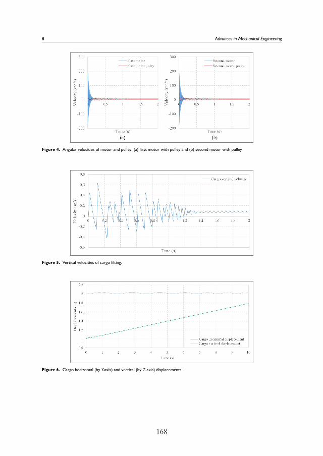
168

Figure 4. Angular velocities of motor and pulley: (a) first motor with pulley and (b) second motor with pulley.

Figure 5. Vertical velocities of cargo lifting.

Figure 6. Cargo horizontal (by Y-axis) and vertical (by Z-axis) displacements.

8 Advances in Mechanical Engineering

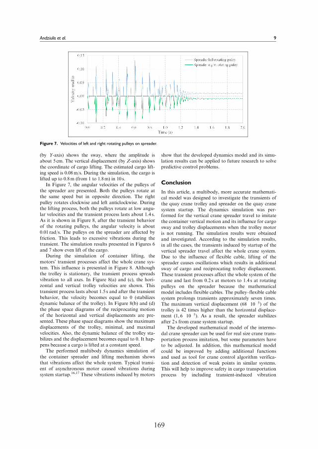
168 169

(by Y-axis) shows the sway, where the amplitude isabout 5 cm. The vertical displacement (by Z-axis) showsthe coordinate of cargo lifting. The estimated cargo lift-ing speed is 0.08m/s. During the simulation, the cargo islifted up to 0.8m (from 1 to 1.8m) in 10 s.

In Figure 7, the angular velocities of the pulleys ofthe spreader are presented. Both the pulleys rotate atthe same speed but in opposite direction. The rightpulley rotates clockwise and left anticlockwise. Duringthe lifting process, both the pulleys rotate at low angu-lar velocities and the transient process lasts about 1.4 s.As it is shown in Figure 8, after the transient behaviorof the rotating pulleys, the angular velocity is about0.01 rad/s. The pulleys on the spreader are affected byfriction. This leads to excessive vibrations during thetransient. The simulation results presented in Figures 6and 7 show even lift of the cargo.

During the simulation of container lifting, themotors’ transient processes affect the whole crane sys-tem. This influence is presented in Figure 8. Althoughthe trolley is stationary, the transient process spreadsvibration to all axes. In Figure 8(a) and (c), the hori-zontal and vertical trolley velocities are shown. Thistransient process lasts about 1.5 s and after the transientbehavior, the velocity becomes equal to 0 (stabilizesdynamic balance of the trolley). In Figure 8(b) and (d)the phase space diagrams of the reciprocating motionof the horizontal and vertical displacements are pre-sented. These phase space diagrams show the maximumdisplacements of the trolley, minimal, and maximalvelocities. Also, the dynamic balance of the trolley sta-bilizes and the displacement becomes equal to 0. It hap-pens because a cargo is lifted at a constant speed.

The performed multibody dynamics simulation ofthe container spreader and lifting mechanism showsthat vibrations affect the whole system. Typical transi-ent of asynchronous motor caused vibrations duringsystem startup.16,17 These vibrations induced by motors

show that the developed dynamics model and its simu-lation results can be applied to future research to solvepredictive control problems.

Conclusion

In this article, a multibody, more accurate mathemati-cal model was designed to investigate the transients ofthe quay crane trolley and spreader on the quay cranesystem startup. The dynamics simulation was per-formed for the vertical crane spreader travel to imitatethe container vertical motion and its influence for cargosway and trolley displacements when the trolley motoris not running. The simulation results were obtainedand investigated. According to the simulation results,in all the cases, the transients induced by startup of thevertical spreader travel affect the whole crane system.Due to the influence of flexible cable, lifting of thespreader causes oscillations which results in additionalsway of cargo and reciprocating trolley displacement.These transient processes affect the whole system of thecrane and last from 0.2 s at motors to 1.4 s at rotatingpulleys on the spreader because the mathematicalmodel includes flexible cables. The pulley–flexible cablesystem prolongs transients approximately seven times.The maximum vertical displacement (68 � 10�5) of thetrolley is 42 times higher than the horizontal displace-ment (1, 6 � 10�5). As a result, the spreader stabilizesafter 2 s from crane system startup.

The developed mathematical model of the intermo-dal crane spreader can be used for real size crane trans-portation process imitation, but some parameters haveto be adjusted. In addition, this mathematical modelcould be improved by adding additional functionsand used as tool for crane control algorithm verifica-tion and detection of weak points in similar systems.This will help to improve safety in cargo transportationprocess by including transient-induced vibration

Figure 7. Velocities of left and right rotating pulleys on spreader.

Andziulis et al. 9

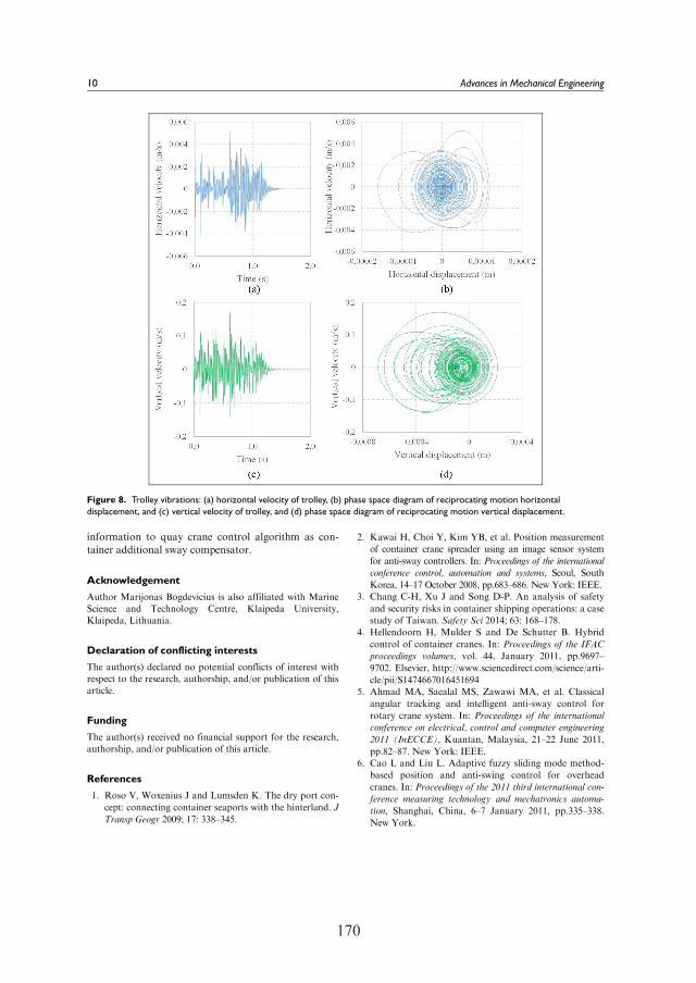
170

information to quay crane control algorithm as con-tainer additional sway compensator.

Acknowledgement

Author Marijonas Bogdevicius is also affiliated with MarineScience and Technology Centre, Klaipeda University,Klaipeda, Lithuania.

Declaration of conflicting interests

The author(s) declared no potential conflicts of interest withrespect to the research, authorship, and/or publication of thisarticle.

Funding

The author(s) received no financial support for the research,authorship, and/or publication of this article.

References

1. Roso V, Woxenius J and Lumsden K. The dry port con-

cept: connecting container seaports with the hinterland. J

Transp Geogr 2009; 17: 338–345.

2. Kawai H, Choi Y, Kim YB, et al. Position measurement

of container crane spreader using an image sensor system

for anti-sway controllers. In: Proceedings of the international

conference control, automation and systems, Seoul, South

Korea, 14–17 October 2008, pp.683–686. New York: IEEE.3. Chang C-H, Xu J and Song D-P. An analysis of safety

and security risks in container shipping operations: a case

study of Taiwan. Safety Sci 2014; 63: 168–178.4. Hellendoorn H, Mulder S and De Schutter B. Hybrid

control of container cranes. In: Proceedings of the IFAC

proceedings volumes, vol. 44, January 2011, pp.9697–

9702. Elsevier, http://www.sciencedirect.com/science/arti-

cle/pii/S14746670164516945. Ahmad MA, Saealal MS, Zawawi MA, et al. Classical

angular tracking and intelligent anti-sway control for

rotary crane system. In: Proceedings of the international

conference on electrical, control and computer engineering

2011 (InECCE), Kuantan, Malaysia, 21–22 June 2011,

pp.82–87. New York: IEEE.6. Cao L and Liu L. Adaptive fuzzy sliding mode method-

based position and anti-swing control for overhead

cranes. In: Proceedings of the 2011 third international con-

ference measuring technology and mechatronics automa-

tion, Shanghai, China, 6–7 January 2011, pp.335–338.

New York.

Figure 8. Trolley vibrations: (a) horizontal velocity of trolley, (b) phase space diagram of reciprocating motion horizontaldisplacement, and (c) vertical velocity of trolley, and (d) phase space diagram of reciprocating motion vertical displacement.

10 Advances in Mechanical Engineering

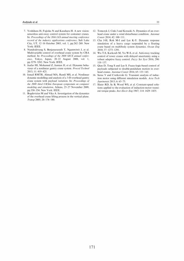
170 171

7. Yoshihara H, Fujioka N and Kasahara H. A new vision-sensorless anti-sway control system for container cranes.In: Proceedings of the 38th IAS annual meeting conference

record of the industry applications conference, Salt LakeCity, UT, 12–16 October 2003, vol. 1, pp.262–269. NewYork: IEEE.

8. Nundrakwang S, Benjanarasuth T, Ngamwiwit J, et al.Multivariable control of overhead crane system by CRAmethod. In: Proceedings of the 2008 SICE annual confer-

ence, Tokyo, Japan, 20–22 August 2008, vol. 1,pp.3278–3282. New York: IEEE.

9. Jaafar HI, Mohamed Z, Jamian JJ, et al. Dynamic beha-viour of a nonlinear gantry crane system. Proced Technol

2013; 11: 419–425.10. Ismail RMTR, Ahmad MA, Ramli MS, et al. Nonlinear

dynamic modelling and analysis of a 3-D overhead gantrycrane system with payload variation. In: Proceedings of

the 2009 third UKSim European symposium on computer

modeling and simulation, Athens, 25–27 November 2009,pp.350–354. New York: IEEE.

11. Bogdevicius M and Vika A. Investigation of the dynamicsof the overhead crane lifting process in the vertical plane.Transp 2005; 20: 176–180.

12. Tomczyk J, Cink J and Kosucki A. Dynamics of an over-

head crane under a wind disturbance condition. Automat

Constr 2014; 42: 100–111.13. Cha J-H, Roh M-I and Lee K-Y. Dynamic response

simulation of a heavy cargo suspended by a floating

crane based on multibody system dynamics. Ocean Eng

2010; 37: 1273–1291.14. Wu T-S, Karkoub M, Yu W-S, et al. Anti-sway tracking

control of tower cranes with delayed uncertainty using a

robust adaptive fuzzy control. Fuzzy Set Syst 2016; 290:

118–137.15. Qian D, Tong S and Lee S. Fuzzy-logic-based control of

payloads subjected to double-pendulum motion in over-

head cranes. Automat Constr 2016; 65: 133–143.16. Sarac V and Cvetkovski G. Transient analysis of induc-

tion motor using different simulation models. Acta Tech

Jaurinensis 2013; 6: 65–75.17. Slater RD, Sc B, Wood WS, et al. Constant-speed solu-

tions applied to the evaluation of induction-motor transi-

ent torque peaks. Inst Electr Eng 1967; 114: 1429–1435.

Andziulis et al. 11

115

5th publication / 5 publikacija

Use Case of Quay Crane Container Handling Operations Monitoring Using ICT to Detect

Abnormalities in Operator Actions

S. Jakovlev, T. Eglynas, M. Jusis, S. Gudas, V. Jankunas,M. Voznak.

Proceedings of the 6th International Conference on Vehicle Technology and Intelligent Transport Systems (VEHITS 2020), 63-67 (2020)

DOI: 10.5220/0008880700630067

Use Case of Quay Crane Container Handling Operations Monitoring using ICT to Detect Abnormalities in Operator Actions

Sergej Jakovlev1,2 a, Tomas Eglynas1 b, Mindaugas Jusis1,3 c, Saulius Gudas3, Valdas Jankunas1 d and Miroslav Voznak2 e

1Klaipeda University, Bijunu str. 17 – 206, Klaipeda, Lithuania 2VŠB-Technical University of Ostrava, 17, Listopadu 15, 708 33, Ostrava-Poruba, Czech Republic

3Vilnius University, Akademijos str. 4, LT-04812 Vilnius, Lithuania

Keywords: Data Acquisition, Communication Technology, Engineering, Systems Design.

Abstract: This paper presents the initial research findings from the Klaipeda port monitoring action related to Blue economy development initiative in the Baltic Sea. Use case study demonstrates the possibility to address the problem of information system deployment in harsh industrial environment to gather valuable statistical knowledge. Custom made monitoring and data transmission units were developed to utilize the best practice of engineering to solve real problems of Klaipeda Port. Several key operations and parameters were monitored during the research, including containers spreader movements, physical characteristics of the cables, metal constructions. Initial results suggested that crane operators’ involvement in the control of the cargo movement produced incorrect control patterns (joystick movements) that delayed port operations. Each control movement of the joystick needs to have a direct real-time feedback from the spreader (actual movement of the cargo). Feedback control functionality will allow adjusting the spreader movement according to the operator and will decrease the cargo transportation time during constant breaks.

1 INTRODUCTION

Klaipeda Sea Port has distinguished itself in the Baltic Region due to its rapid increase in cargo flows and adoption of Blue Economy regulations and strategies, that require decrease of CO2 and other harmful gasses in industry surrounding the Sea Port and related to Port activities (including shipbuilding, bulk cargo transit, fossil fuel transship, fishing and production).

Many practioners’ and action methodology developers in the transport chain did research in this area. Ranging from communication and control systems application with deep insights and relevant reviews, economical calculations and practical use cases (Tuan et al., 2018; Golovin and Palis, 2019; Henikl et al., 2012; Sha et al., 2017). Overall, possibility to adopt new technologies in such closed a https://orcid.org/0000-0002-1440-8221 b https://orcid.org/0000-0002-9973-5896 c https://orcid.org/0000-0001-8035-3938 d https://orcid.org/0000-0003-3077-3568 e https://orcid.org/0000-0001-5135-7980

environments is a rare opportunity. In practice, the realization of complex control solutions limited by the cost efficiency in comparison to standardized and commonly used solutions (Jakovlev et al., 2012; Andziulis et al., 2012).

Adoption of new ideas is difficult even to “modern minds” (Eglynas et al., 2013). In practice, it is difficult to come close to working equipment and to acquire agreement for their monitoring on-site. Initial visual analysis suggested developing new ideas how to lower fluctuations of the containers gripper. Its movements are random in nature, due to external impacts, such as wind or physical contact with other objects. It is difficult to predict such random deviations in practice (Golovin and Palis, 2019; Trabke, 2014).

In comparison, European ports such as Rotterdam or Hanover apply new systems for vibration decrease

Jakovlev, S., Eglynas, T., Jusis, M., Gudas, S., Jankunas, V. and Voznak, M.Use Case of Quay Crane Container Handling Operations Monitoring using ICT to Detect Abnormalities in Operator Actions.DOI: 10.5220/0008880700630067In Proceedings of the 6th International Conference on Vehicle Technology and Intelligent Transport Systems (VEHITS 2020), pages 63-67ISBN: 978-989-758-419-0Copyright c© 2020 by SCITEPRESS – Science and Technology Publications, Lda. All rights reserved

63

173

Use Case of Quay Crane Container Handling Operations Monitoring using ICT to Detect Abnormalities in Operator Actions

Sergej Jakovlev1,2 a, Tomas Eglynas1 b, Mindaugas Jusis1,3 c, Saulius Gudas3, Valdas Jankunas1 d and Miroslav Voznak2 e

1Klaipeda University, Bijunu str. 17 – 206, Klaipeda, Lithuania 2VŠB-Technical University of Ostrava, 17, Listopadu 15, 708 33, Ostrava-Poruba, Czech Republic

3Vilnius University, Akademijos str. 4, LT-04812 Vilnius, Lithuania

Keywords: Data Acquisition, Communication Technology, Engineering, Systems Design.

Abstract: This paper presents the initial research findings from the Klaipeda port monitoring action related to Blue economy development initiative in the Baltic Sea. Use case study demonstrates the possibility to address the problem of information system deployment in harsh industrial environment to gather valuable statistical knowledge. Custom made monitoring and data transmission units were developed to utilize the best practice of engineering to solve real problems of Klaipeda Port. Several key operations and parameters were monitored during the research, including containers spreader movements, physical characteristics of the cables, metal constructions. Initial results suggested that crane operators’ involvement in the control of the cargo movement produced incorrect control patterns (joystick movements) that delayed port operations. Each control movement of the joystick needs to have a direct real-time feedback from the spreader (actual movement of the cargo). Feedback control functionality will allow adjusting the spreader movement according to the operator and will decrease the cargo transportation time during constant breaks.

1 INTRODUCTION

Klaipeda Sea Port has distinguished itself in the Baltic Region due to its rapid increase in cargo flows and adoption of Blue Economy regulations and strategies, that require decrease of CO2 and other harmful gasses in industry surrounding the Sea Port and related to Port activities (including shipbuilding, bulk cargo transit, fossil fuel transship, fishing and production).

Many practioners’ and action methodology developers in the transport chain did research in this area. Ranging from communication and control systems application with deep insights and relevant reviews, economical calculations and practical use cases (Tuan et al., 2018; Golovin and Palis, 2019; Henikl et al., 2012; Sha et al., 2017). Overall, possibility to adopt new technologies in such closed a https://orcid.org/0000-0002-1440-8221 b https://orcid.org/0000-0002-9973-5896 c https://orcid.org/0000-0001-8035-3938 d https://orcid.org/0000-0003-3077-3568 e https://orcid.org/0000-0001-5135-7980

environments is a rare opportunity. In practice, the realization of complex control solutions limited by the cost efficiency in comparison to standardized and commonly used solutions (Jakovlev et al., 2012; Andziulis et al., 2012).

Adoption of new ideas is difficult even to “modern minds” (Eglynas et al., 2013). In practice, it is difficult to come close to working equipment and to acquire agreement for their monitoring on-site. Initial visual analysis suggested developing new ideas how to lower fluctuations of the containers gripper. Its movements are random in nature, due to external impacts, such as wind or physical contact with other objects. It is difficult to predict such random deviations in practice (Golovin and Palis, 2019; Trabke, 2014).

In comparison, European ports such as Rotterdam or Hanover apply new systems for vibration decrease

Jakovlev, S., Eglynas, T., Jusis, M., Gudas, S., Jankunas, V. and Voznak, M.Use Case of Quay Crane Container Handling Operations Monitoring using ICT to Detect Abnormalities in Operator Actions.DOI: 10.5220/0008880700630067In Proceedings of the 6th International Conference on Vehicle Technology and Intelligent Transport Systems (VEHITS 2020), pages 63-67ISBN: 978-989-758-419-0Copyright c© 2020 by SCITEPRESS – Science and Technology Publications, Lda. All rights reserved

63

economy development initiative in the Baltic Sea. Use case study demonstrates the possibility to address the problem of information system deployment in harsh industrial environment to gather valuable statistical knowledge. Custom made monitoring and data transmission units were developed to utilize the best practice of engineering to solve real problems of Klaipeda Port. Several key operations and parameters were monitored during the research, including containers spreader movements, physical characteristics of the cables, metal constructions. Initial results suggested that crane operators’ involvement in the control of the cargo movement produced incorrect control patterns (joystick movements) that delayed port operations. Each control movement of the joystick needs to have a direct real-time feedback from the spreader (actual movement of the cargo). Feedback control functionality will allow adjusting the spreader movement according to the operator and will decrease the cargo transportation time during constant breaks.

1 INTRODUCTION

Klaipeda Sea Port has distinguished itself in the Baltic Region due to its rapid increase in cargo flows and adoption of Blue Economy regulations and strategies, that require decrease of CO2 and other harmful gasses in industry surrounding the Sea Port and related to Port activities (including shipbuilding,

environments is a rare opportunity. In practice, the realization of complex control solutions limited by the cost efficiency in comparison to standardized and commonly used solutions (Jakovlev et al., 2012; Andziulis et al., 2012).

Adoption of new ideas is difficult even to “modern minds” (Eglynas et al., 2013). In practice, it is difficult to come close to working equipment and

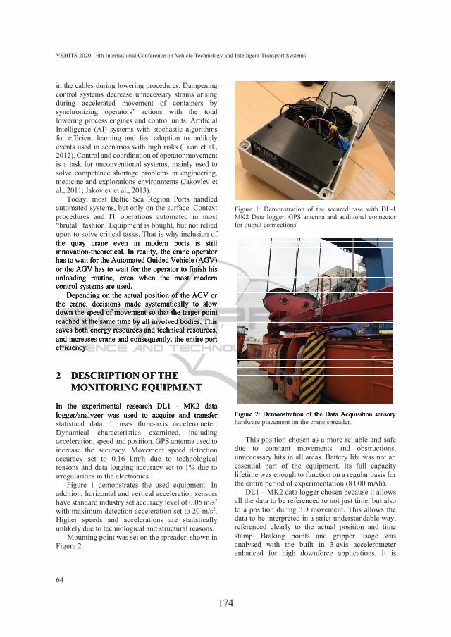
174

in the cables during lowering procedures. Dampening control systems decrease unnecessary strains arising during accelerated movement of containers by synchronizing operators’ actions with the total lowering process engines and control units. Artificial Intelligence (AI) systems with stochastic algorithms for efficient learning and fast adoption to unlikely events used in scenarios with high risks (Tuan et al., 2012). Control and coordination of operator movement is a task for unconventional systems, mainly used to solve competence shortage problems in engineering, medicine and explorations environments (Jakovlev et al., 2011; Jakovlev et al., 2013).

Today, most Baltic Sea Region Ports handled automated systems, but only on the surface. Context procedures and IT operations automated in most “brutal” fashion. Equipment is bought, but not relied upon to solve critical tasks. That is why inclusion of the quay crane even in modern ports is still innovation-theoretical. In reality, the crane operator has to wait for the Automated Guided Vehicle (AGV) or the AGV has to wait for the operator to finish his unloading routine, even when the most modern control systems are used.

Depending on the actual position of the AGV or the crane, decisions made systematically to slow down the speed of movement so that the target point reached at the same time by all involved bodies. This saves both energy resources and technical resources, and increases crane and consequently, the entire port efficiency.

2 DESCRIPTION OF THE MONITORING EQUIPMENT

In the experimental research DL1 - MK2 data logger/analyzer was used to acquire and transfer statistical data. It uses three-axis accelerometer. Dynamical characteristics examined, including acceleration, speed and position. GPS antenna used to increase the accuracy. Movement speed detection accuracy set to 0.16 km/h due to technological reasons and data logging accuracy set to 1% due to irregularities in the electronics.

Figure 1 demonstrates the used equipment. In addition, horizontal and vertical acceleration sensors have standard industry set accuracy level of 0.05 m/s2 with maximum detection acceleration set to 20 m/s2. Higher speeds and accelerations are statistically unlikely due to technological and structural reasons.

Mounting point was set on the spreader, shown in Figure 2.

Figure 1: Demonstration of the secured case with DL-1 MK2 Data logger, GPS antenna and additional connector for output connections.

Figure 2: Demonstration of the Data Acquisition sensory hardware placement on the crane spreader.

This position chosen as a more reliable and safe due to constant movements and obstructions, unnecessary hits in all areas. Battery life was not an essential part of the equipment. Its full capacity lifetime was enough to function on a regular basis for the entire period of experimentation (8 000 mAh).

DL1 – MK2 data logger chosen because it allows all the data to be referenced to not just time, but also to a position during 3D movement. This allows the data to be interpreted in a strict understandable way, referenced clearly to the actual position and time stamp. Braking points and gripper usage was analysed with the built in 3-axis accelerometer enhanced for high downforce applications. It is

VEHITS 2020 - 6th International Conference on Vehicle Technology and Intelligent Transport Systems

64

the quay crane even in modern ports is still innovation-theoretical. In reality, the crane operator has to wait for the Automated Guided Vehicle (AGV) or the AGV has to wait for the operator to finish his unloading routine, even when the most modern control systems are used.

Depending on the actual position of the AGV or the crane, decisions made systematically to slow down the speed of movement so that the target point reached at the same time by all involved bodies. This reached at the same time by all involved bodies. This reached at the same time bysaves both energy resources and technical resources, and increases crane and consequently, the entire port efficiency.

2 DESCRIPTION OF THE MONITORING EQUIPMENT

In the experimental research DL1 - MK2 data logger/analyzer was used to acquire and transfer Figure 2: Demonstration of the Data Acquisition sensory

capable of detecting minute changes with 100Hz update rate on all attached sensors and accelerometer channels. It also provides an 8 analogue channels (with 0-20 V battery voltage) for sensor inputs ready for additional measurements and 2 CAN channels with up to 1 M baud rate with 14 CAN filters per channel (CAN 2.0 compatible). Logger itself has an IP50 environmental protection, but due to the harsh working environment, it was decided to add additional protection via the secured hard plastic mounting case. Maximum power consumption set to 1.6 W.

3 EXPERIMENTAL MEASUREMENT RESULTS

Number of container loading and unloading measurements set to 278, due to port operations strict rules and cooperation agreements for the measurement period. Crane operators were warned that measurements took place during their working hours to avoid legal problems. During the meeting with the working crane operators and truck drivers (who are also AGV operators), discussions were made to address the importance of these measurements and to see the vector of improvement. Some of the crane operators even expressed appreciation for the research. The following Figures

provide casual measurements from the loading and unloading procedures.

Each measurement had its own deviation and irregularity, considering the operator “best choice” scenario set by the operational manual. Figure 3 demonstrates the positional movement of the container unloading procedure. Each container varied in mass, therefore, average mass of 20 metric tons considered for the mean calculations. At this exact measurement, the mass of the container measured at 19.220 kg.

Figure 3 and the following Figures 4-5 demonstrate 7 stages of operational consideration: 1. Container raising with hooking; 2. Vertical raising of container; 3. Bias raising of container; 4. Horizontal transportation of container; 5. Bias lowering of the container; 6. Vertical lowering of the container; 7. Container placement on the transport means

(truck or AGV). The following Figure 4 demonstrates the actual

speed values during these 7 stages for the process, described in Figure 3.

The following Figure 5 demonstrates spreader and container sway oscillation values. These values are of high importance, because higher values correlate with the actual speed of the operation during the 7th stage, by lowering the speed of container positioning on the transport means or AGV.

Figure 3: Spreader position detection and movement points during the container unloading operation from the ship.

Use Case of Quay Crane Container Handling Operations Monitoring using ICT to Detect Abnormalities in Operator Actions

65

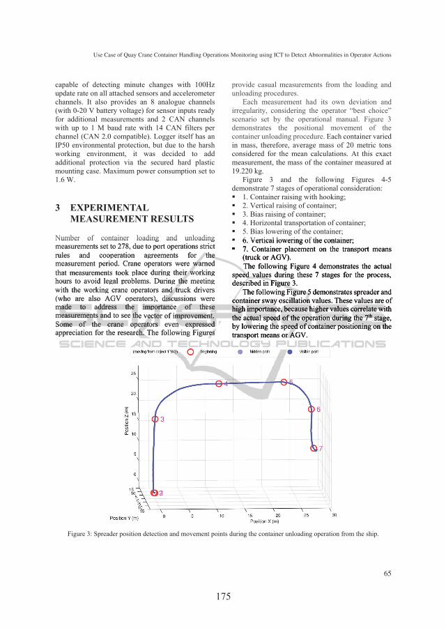
174 175

in the cables during lowering procedures. Dampening control systems decrease unnecessary strains arising during accelerated movement of containers by synchronizing operators’ actions with the total lowering process engines and control units. Artificial Intelligence (AI) systems with stochastic algorithms for efficient learning and fast adoption to unlikely events used in scenarios with high risks (Tuan et al., 2012). Control and coordination of operator movement is a task for unconventional systems, mainly used to solve competence shortage problems in engineering, medicine and explorations environments (Jakovlev et al., 2011; Jakovlev et al., 2013).

Today, most Baltic Sea Region Ports handled automated systems, but only on the surface. Context procedures and IT operations automated in most “brutal” fashion. Equipment is bought, but not relied upon to solve critical tasks. That is why inclusion of the quay crane even in modern ports is still innovation-theoretical. In reality, the crane operator has to wait for the Automated Guided Vehicle (AGV) or the AGV has to wait for the operator to finish his unloading routine, even when the most modern control systems are used.

Depending on the actual position of the AGV or the crane, decisions made systematically to slow down the speed of movement so that the target point reached at the same time by all involved bodies. This saves both energy resources and technical resources, and increases crane and consequently, the entire port efficiency.

2 DESCRIPTION OF THE MONITORING EQUIPMENT

In the experimental research DL1 - MK2 data logger/analyzer was used to acquire and transfer statistical data. It uses three-axis accelerometer. Dynamical characteristics examined, including acceleration, speed and position. GPS antenna used to increase the accuracy. Movement speed detection accuracy set to 0.16 km/h due to technological reasons and data logging accuracy set to 1% due to irregularities in the electronics.

Figure 1 demonstrates the used equipment. In addition, horizontal and vertical acceleration sensors have standard industry set accuracy level of 0.05 m/s2 with maximum detection acceleration set to 20 m/s2. Higher speeds and accelerations are statistically unlikely due to technological and structural reasons.

Mounting point was set on the spreader, shown in Figure 2.

Figure 1: Demonstration of the secured case with DL-1 MK2 Data logger, GPS antenna and additional connector for output connections.

Figure 2: Demonstration of the Data Acquisition sensory hardware placement on the crane spreader.

This position chosen as a more reliable and safe due to constant movements and obstructions, unnecessary hits in all areas. Battery life was not an essential part of the equipment. Its full capacity lifetime was enough to function on a regular basis for the entire period of experimentation (8 000 mAh).

DL1 – MK2 data logger chosen because it allows all the data to be referenced to not just time, but also to a position during 3D movement. This allows the data to be interpreted in a strict understandable way, referenced clearly to the actual position and time stamp. Braking points and gripper usage was analysed with the built in 3-axis accelerometer enhanced for high downforce applications. It is

VEHITS 2020 - 6th International Conference on Vehicle Technology and Intelligent Transport Systems

64

capable of detecting minute changes with 100Hz update rate on all attached sensors and accelerometer channels. It also provides an 8 analogue channels (with 0-20 V battery voltage) for sensor inputs ready for additional measurements and 2 CAN channels with up to 1 M baud rate with 14 CAN filters per channel (CAN 2.0 compatible). Logger itself has an IP50 environmental protection, but due to the harsh working environment, it was decided to add additional protection via the secured hard plastic mounting case. Maximum power consumption set to 1.6 W.

3 EXPERIMENTAL MEASUREMENT RESULTS

Number of container loading and unloading measurements set to 278, due to port operations strict rules and cooperation agreements for the measurement period. Crane operators were warned that measurements took place during their working hours to avoid legal problems. During the meeting with the working crane operators and truck drivers (who are also AGV operators), discussions were made to address the importance of these measurements and to see the vector of improvement. Some of the crane operators even expressed appreciation for the research. The following Figures

provide casual measurements from the loading and unloading procedures.

Each measurement had its own deviation and irregularity, considering the operator “best choice” scenario set by the operational manual. Figure 3 demonstrates the positional movement of the container unloading procedure. Each container varied in mass, therefore, average mass of 20 metric tons considered for the mean calculations. At this exact measurement, the mass of the container measured at 19.220 kg.

Figure 3 and the following Figures 4-5 demonstrate 7 stages of operational consideration: 1. Container raising with hooking; 2. Vertical raising of container; 3. Bias raising of container; 4. Horizontal transportation of container; 5. Bias lowering of the container; 6. Vertical lowering of the container; 7. Container placement on the transport means

(truck or AGV). The following Figure 4 demonstrates the actual

speed values during these 7 stages for the process, described in Figure 3.

The following Figure 5 demonstrates spreader and container sway oscillation values. These values are of high importance, because higher values correlate with the actual speed of the operation during the 7th stage, by lowering the speed of container positioning on the transport means or AGV.

Figure 3: Spreader position detection and movement points during the container unloading operation from the ship.

Use Case of Quay Crane Container Handling Operations Monitoring using ICT to Detect Abnormalities in Operator Actions

65

Number of container loading and unloading Number of container loading and unloading measurements set to 278, due to port operations strict e to port operations strict rules and cooperation agreements for the rules and cooperation agreements for the measurement period. Crane operators were warned measurement period. Crane operators were warned that measurements took place during their working hours to avoid legal problems. During the meeting hours to avoid legal problems. During the meeting with the working crane operators and truck drivers with the working crane operators and truck drivers (who are also AGV operators), discussions were made to address the importance of these made to address the importance of these measurements and to see the vector of improvement. e vector of improvement. Some of the crane operators even expressed Some of the crane operators even expressed appreciation for the research. The following Figures

6. Vertical lowering of the container; 7. Container placement on the transport means

(truck or AGV). The following Figure 4 demonstrates the actual

speed values during these 7 stages for the process, described in Figure 3.

The following Figure 5 demonstrates spreader and container sway oscillation values. These values are of high importance, because higher values correlate with the actual speed of the operation during the 7th stage, by lowering the speed of container positioning on the transport means or AGV.

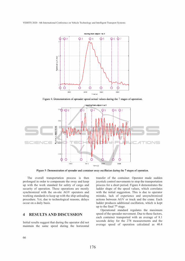
176

Figure 4: Demonstration of spreader speed actual values during the 7 stages of operation.

Figure 5: Demonstration of spreader and container sway oscillation during the 7 stages of operation.

The overall transportation process is then prolonged in order to compensate the sway and keep up with the work standard for safety of cargo and security of operation. These operations are mostly synchronized with the on-site AGV operators and working standards to keep up with the ship unloading procedure. Yet, due to technological reasons, delays occur on a daily basis.

4 RESULTS AND DISCUSSION

Initial results suggest that during the operator did not maintain the same speed during the horizontal

transfer of the container. Operator made sudden joystick control movements to stop the transportation process for a short period. Figure 4 demonstrates the ladder shape of the speed values, which correlates with the initial suggestion. This is due to operator mistake, lack of experience and unsynchronized actions between AGV or truck and the crane. Each ladder produces additional oscillation, which is kept up to the final 7th stage.

Operational standard regulates the maximum speed of the spreader movement. Due to these factors, each container transported with an average of 8.1 seconds delay for the 278 measurements and the average speed of operation calculated as 40.4

VEHITS 2020 - 6th International Conference on Vehicle Technology and Intelligent Transport Systems

66

Figure 4: Demonstration of spreader speed actual values during the 7 stages of operation.

Figure 5: Demonstration of spreader and container sway oscillation Figure 5: Demonstration of spreader and container sway oscillation Figure 5: Demonstration of spreader during the 7 stages of operation.

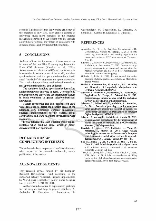
176 177

seconds. This indicates that the working efficiency of the operation is only 80%. Each crane is capable of delivering much more container if the operator movement controlled by AI system with pre-defined algorithms for optimal movement of containers with different masses and environmental conditions.

5 CONCLUSIONS

Authors indicate the importance of these researches in terms of the new Blue Economy regulations for Ports CO2 decrease (Kavakeb et al., 2013). Autonomous and electrical AGVs and trucks are now in operation in several ports of the world, and their synchronization with the operational standards is still a real “headache” for engineers and operators on-site. That is why these problems need to be addressed and real operational statistical data collected.

The containers handling operational actions of the Klaipeda port were analysed in detail. Use case study proved possible to deploy and use information system in harsh conditions to gather valuable statistical knowledge.

Custom monitoring and data transmission units were developed to detect the problem areas of the Klaipeda Port. Containers spreader movements, physical characteristics of the cables, metal constructions and crane operators’ involvement were monitored.

It was detected that each operator made control mistakes when handling cargo, which in return delayed overall port operations.

DECLARATION OF CONFLICTING INTERESTS

The authors declared no potential conflicts of interest with respect to the research, authorship, and/or publication of this article.

ACKNOWLEDGEMENTS

This research is/was funded by the European Regional Development Fund according to the supported activity ‘Research Projects Implemented by World-class Researcher Groups’ under Measure No. 01.2.2-LMT-K-718-01-0081.

Authors would also like to express deep gratitude for the insights and help to project members: A. Andziulis, R. Didziokas, J. Januteniene, E.

Guseinoviene, M. Bogdevicius, D. Cirtautas, A. Senulis, M. Kurmis, D. Drungilas, Z. Lukosius.

REFERENCES

Andziulis, A., Pltys, R., Jakovlev, S., Adomaitis, D., Gerasimov, K., Kurmis, M., Pareigis, V., 2012. Priority based tag authentication and routing algorithm for intermodal containers RFID sensor network. Transport. Vol. 27.

Eglynas, T., Jakovlev, S., Bogdevičius, M., Didžiokas, R., Andziulis, A., Lenkauskas, T., 2013. Concept of cargo security assurance in an intermodal transportation. In: Marine Navigation and Safety of Sea Transportation: Maritime Transport and Shipping.

Golovin, I., Palis, S., 2019. Robust control for active damping of elastic gantry crane vibrations. Mech. Syst. Signal Process.

Henikl, J., Kemmetmüller, W., Kugi, A., 2012. Modeling and Simulation of Large-Scale Manipulators with Hydraulic Actuation. IFAC Proc.

Jakovlev, S., Andziulis, A., Bulbenkiene, V., Didziokas, R., Bogdevicius, M., Plestys, R., Zakarevicius, R, 2012. Cargo container monitoring data reliability evaluation in WSN nodes. Elektron. ir Elektrotechnika.

Jakovlev, S., Bulbenkiene, V., Andziulis, A., Adomaitis, D., 2011. E-services providing complex containers cargo conditions monitoring information system. In: International Conference on Management of Emergent Digital EcoSystems, MEDES’11.

Jakovlev, S., Voznak, M., Andziulis, A., Kurmis, M., 2013. Communication technologies for the improvement of marine transportation operations. In: IFAC Proceedings Volumes (IFAC-PapersOnline).

Kavakeb, S., Nguyen, T.T., McGinley, K., Yang, Z., Jenkinson, I., Murray, R., 2015. Green vehicle technology to enhance the performance of a European port: A simulation model with a cost-benefit approach. Transp. Res. Part C Emerg. Technol. 60, 169–188.

Sha, M., Zhang, T., Lan, Y., Zhou, X., Qin, T., Yu, D., Chen, K., 2017. Scheduling optimization of yard cranes with minimal energy consumption at container terminals. Comput. Ind. Eng.

Tuan, L.A., Cuong, H.M., Trieu, P. Van, Nho, L.C., Thuan, V.D., Anh, L.V., 2018. Adaptive neural network sliding mode control of shipboard container cranes considering actuator backlash. Mech. Syst. Signal Process.

Use Case of Quay Crane Container Handling Operations Monitoring using ICT to Detect Abnormalities in Operator Actions

67

real operational statistical data collected. The containers handling operational actions of the

Klaipeda port were analysed in detail. Use case study proved possible to deploy and use information system in harsh conditions to gather valuable statistical knowledge.

Custom monitoring and data transmission units were developed to detect the problem areas of the Klaipeda Port. Containers spreader movements, physical characteristics of the cables, metal constructions and crane operators’ involvement were monitored.

It was detected that each operator made control mistakes when handling cargo, which in return delayed overall port operations.

DECLARATION OF CONFLICTING INTERESTS

Henikl, J., Kemmetmüller, W., Kugi, A., 2012. Modeling and Simulation of Large-Scale Manipulators with Hydraulic Actuation. IFAC Proc.

Jakovlev, S., Andziulis, A., Bulbenkiene, V., Didziokas, R., Bogdevicius, M., Plestys, R., Zakarevicius, R, 2012. Cargo container monitoring data reliability evaluation in WSN nodes. Elektron. ir Elektrotechnika.

Jakovlev, S., Bulbenkiene, V., Andziulis, A., Adomaitis, D., 2011. E-services providing complex containers cargo conditions monitoring information system. In: International Conference on Management of Emergent Digital EcoSystems, MEDES’11.

Jakovlev, S., Voznak, M., Andziulis, A., Kurmis, M., 2013. Communication technologies for the improvement of marine transportation operations. In: IFAC Proceedings Volumes (IFAC-PapersOnline).

Kavakeb, S., Nguyen, T.T., McGinley, K., Yang, Z., Jenkinson, I., Murray, R., 2015. Green vehicle technology to enhance the performance of a European port: A simulation model with a cost-benefit approach. Transp. Res. Part C Emerg. Technol. 60, 169–188.

Sha, M., Zhang, T., Lan, Y., Zhou, X., Qin, T., Yu, D., Chen, K., 2017. Scheduling optimization of yard cranes

116

6th publication / 6 publikacija

Analysis of the Efficiency of Quay Crane Control

S. Jakovlev, T. Eglynas, M. Jusis, S. Gudas, E. Pocevicius,V. Jankunas.

2019 IEEE 7th Workshop on Advances in Information, Electronic and Electrical Engineering (AIEEE), 1-3 (2019)

DOI: 10.1109/AIEEE48629.2019.8977009

179

978-1-7281-5709-2/19/$31.00 ©2019 IEEE

Analysis of the Efficiency of Quay Crane Control

Sergej Jakovlev Klaipeda University Klaipeda, Lithuania

https://orcid.org/0000-0002-1440-8221

Saulius Gudas Vilnius university Vilnius, Lithuania

saulius.gudas@khf.vu.lt

Tomas Eglynas Klaipeda University Klaipeda, Lithuania

https://orcid.org/0000-0002-9973-5896

Edvinas Pocevicius Klaipeda University Klaipeda, Lithuania edvinas@inotecha.lt

Mindaugas Jusis Klaipeda University Klaipeda, Lithuania

https://orcid.org/0000-0001-8035-3938

Valdas Jankunas Klaipeda University Klaipeda, Lithuania

https://orcid.org/0000-0003-3077-3568

Abstract—In this paper, we examine the engineering possibility to apply monitoring equipment to detect movement patterns and collect statistical information in harsh container handling environment, during loading and unloading procedures. We design a simple, yet highly efficient data capture tool and use it to solve a transportation problem to lower the security issues and costs associated with increased turn-over time. This is an ongoing EU Structural fund project, its aim is to present a way and a technological solution to synchronize the crane, and Automated guided vehicle (AGV) processes. We demonstrate the problem and provide the readers with a use case study.

Keywords— monitoring, stabilization, control system, sway control.

I. INTRODUCTION Transportation section is constantly looking for a way to

decrease the cost of port handling operations. Old heavy machinery usage is causing delays in transport operations in the whole transport chain. Maintenance costs are lowering the profitability and cause on-site operators’ faults and costs related to security and safety. Most cargo handling machinery operated by less optimal standardized procedures and control systems. Containers often sway in a chaotic manner during loading due to different container weights, wind gusts, operator experience and control routines. Its stabilization is hard due to large weights and size [1].

Engineering and industry communities dedicate much attention to the examination and improvement of mechanical crane stabilization systems and construction of new elements. However, less attention in paid towards the autonomy of crane control operations [2] and training of operators to work with new autonomy services. New research trends focus on the entire transport cycle (ship-crane-shore-crane-ship) and discuss the mechanical nature of the problem [3], [4] and [5].

Experienced operators on-site do container-handling procedures according to regulations and own experience, but due to lack of positive experience, many mistakes happen. However, due to lack of knowledge of some crucial elements of the control, these operators tend to learn on the false information, and their acquired skills tend to increase the inefficiency with time.

In literature, propositions are made to apply the most common limitation rules [6, 7]. Best practice methodologies apply motion profiles in motion control systems for heavy body movement control [8] to solve problems related to container fluctuations [9, 10, 11].

II. DEVELOPMENT AND APPLICATION OF CRANE’S CONTROL SYSTEM DATA ACQUISITION PROTOTYPE

We used DL1 - MK2 data logger/analyzer to acquire and transfer statistical data, which uses three-axis accelerometer. Dynamical characteristics examined, including acceleration, speed and position. GPS antenna used to increase the accuracy. Accuracy of movement speed detection set to 0.16 km/h due to technological reasons and data logging accuracy set to 1% due to irregularities in the electronics. Figure 1 demonstrates the used equipment.

Fig. 1. Secured case with DL-1 MK2 Data logger, GPS antenna and additional connector for output connections.

In addition, horizontal and vertical acceleration sensors have standard industry set accuracy level of 0.05 m/s2 with maximum detection acceleration set to 20 m/s2. Higher speeds and accelerations are statistically unlikely due to technological and structural reasons. Mounting point was set on the spreader, shown in Figures 2 and 3.

Spreader placement position was secured with handles. Mounting was done using simple but reliable solution to use plastic straps. They are agile and tough to break. No physical or electromagnetic interference detected in this area. Its position was good enough for the entire loading and unloading procedure. It had direct visibility contact with the other devices, including GPS.

Authorized licensed use limited to: Technical University of Ostrava. Downloaded on June 08,2021 at 12:25:10 UTC from IEEE Xplore. Restrictions apply.

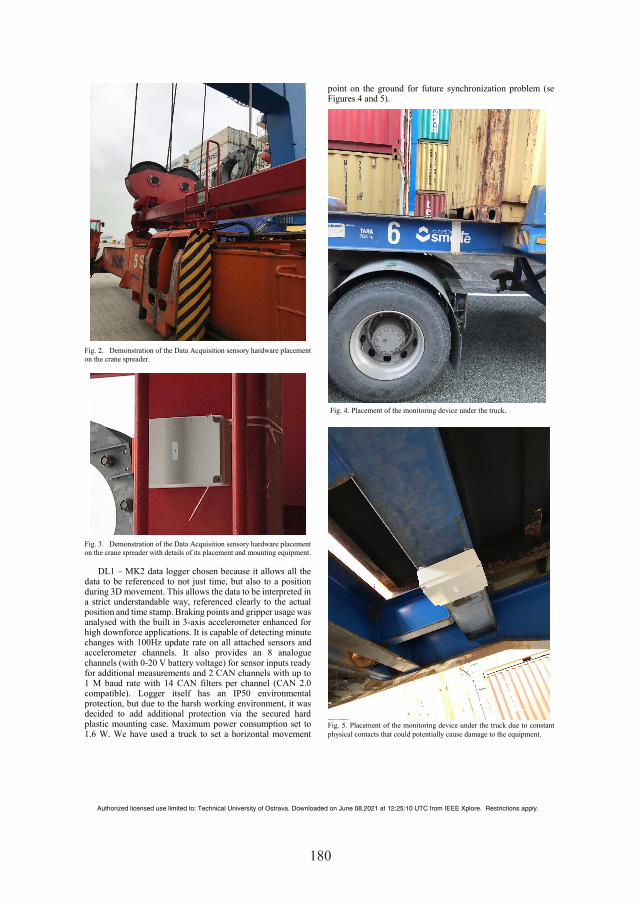
180

Fig. 2. Demonstration of the Data Acquisition sensory hardware placement on the crane spreader.

Fig. 3. Demonstration of the Data Acquisition sensory hardware placement on the crane spreader with details of its placement and mounting equipment.

DL1 – MK2 data logger chosen because it allows all the data to be referenced to not just time, but also to a position during 3D movement. This allows the data to be interpreted in a strict understandable way, referenced clearly to the actual position and time stamp. Braking points and gripper usage was analysed with the built in 3-axis accelerometer enhanced for high downforce applications. It is capable of detecting minute changes with 100Hz update rate on all attached sensors and accelerometer channels. It also provides an 8 analogue channels (with 0-20 V battery voltage) for sensor inputs ready for additional measurements and 2 CAN channels with up to 1 M baud rate with 14 CAN filters per channel (CAN 2.0 compatible). Logger itself has an IP50 environmental protection, but due to the harsh working environment, it was decided to add additional protection via the secured hard plastic mounting case. Maximum power consumption set to 1.6 W. We have used a truck to set a horizontal movement

point on the ground for future synchronization problem (se Figures 4 and 5).

Fig. 4. Placement of the monitoring device under the truck.

Fig. 5. Placement of the monitoring device under the truck due to constant physical contacts that could potentially cause damage to the equipment.

Authorized licensed use limited to: Technical University of Ostrava. Downloaded on June 08,2021 at 12:25:10 UTC from IEEE Xplore. Restrictions apply.

180 181

This position chosen as a more reliable and safe due to

constant movements and obstructions, unnecessary hits in all areas. Battery life was not an essential part of the equipment. Its full capacity lifetime was enough to function on a regular basis for the entire period of experimentation (8 000 mAh).

III. DATA ACQUISITION RESULTS AND FUTURE WORK Initial data collection results suggest that operational

stability depends heavily on the optimization of operation control through inner transport chain management and regulations. In other words, productivity and efficiency of the crane rely on the operator experience. Faults done by operators are not corrected in due manner, though new regulations and systems applied. This in turn, allows constant mistakes to happen and will provide other operators with false context data.

In the following Figures 6 and 7, we demonstrate the ship unloading results for a single procedure.

Fig. 6. Movement path detected via monitoring unit.

Fig. 7. Speed vs time dependency along X axis.

Initial suggestions based upon the visual inspection of the data from points: 3-4, 4-5, 5-6 and 6-7. As one may notice, sudden changes in the speed value correlate with the inappropriate movements of the crane control joystick due to operator faults. Operator was not considering the weather conditions and speed of transportation correctly, and thus, at

the end of operation, decreased the efficiency of operation by 15% from optimal value. Each movement was done without machine inner control and decreased safety and security as well. Keeping in mind that these operations were done in accordance with the operational standards and ISO.

These are the primary results gained after the initial testing of the equipment and visualization of data. Future work will continue the examination of the results and a network of monitoring units will be prepared to detect all movements for a single 12 hours shift. This will help accumulate all the relevant statistical data and provide future research with the knowledge base used to find a technological solution for the AGV(truck) and Crane(operator) synchronization problem.

ACKNOWLEDGMENT This research is/was funded by the European Regional

Development Fund according to the supported activity ‘Research Projects Implemented by World-class Researcher Groups’ under Measure No. 01.2.2-LMT-K-718 -01-0081, under grant agreement with the Research Council of Lithuania (LMT).

Authors would also like to thank Klaipeda university project members: prof. dr. A. Andziulis, prof. dr M. Bogdevicius, prof. dr. E. Guseinoviene, prof. dr. R. Didziokas, prof. dr. J. Januteniene, dr. M. Kurmis, dr. D. Drungilas, Z. Lukosius for deep insights and relevant contribution to the work.

REFERENCES [1] S.-L. Chao and Y.-J. Lin, “Evaluating advanced quay cranes in

container terminals,” Transp. Res. Part E Logist. Transp. Rev., vol. 47, no. 4, pp. 432–445, Jul. 2011.

[2] L. I. Zhi-jun, L. I. Zhen, L. I. Hui-jie, Z. Ye, S. Cheng, and S. U. N. Yan, “Research of Coordinated Control Method of Hybrid Power Crane System,” pp. 1093–1097, 2012

[3] Y. Fang, P. Wang, and X. Zhang, “A Motion Planning-Based Adaptive Control Method for an Underactuated Crane System,” vol. 20, no. 1, pp. 241–248, 2012.

[4] L. Cao and L. Liu, “Adaptive Fuzzy Sliding Mode Method-Based Position and Anti-swing Control for Overhead Cranes,” 2011 Third Int. Conf. Meas. Technol. Mechatronics Autom., no. 2, pp. 335–338, Jan. 2011.

[5] H. Sano, K. Ohishi, T. Kaneko, and H. Mine, “Anti-sway crane control based on dual state observer with sensor-delay correction,” 2010 11th IEEE Int. Work. Adv. Motion Control, pp. 679–684, Mar. 2010.

[6] R. Béarée, “New Damped-Jerk trajectory for vibration reduction,” Control Eng. Pract., vol. 28, pp. 112–120, Jul. 2014.

[7] M. A. Majid, W. S. W. Ibrahim, S. Mohamad, and Z. A. Bakar, “A comparison of PID and PD controller with input shaping technique for 3D gantry crane,” Proc. - 2013 IEEE Conf. Syst. Process Control. ICSPC 2013, no. December, pp. 144–148, 2013.

[8] J. Vaughan, J. Yoo, N. Knight, and W. Singhose, “Multi-Input Shaping Control for Multi-Hoist Cranes,” pp. 3455–3460, 2013.

[9] C. Liu, H. Zhao, and Y. Cui, “Research on Application of Fuzzy PID in Collective Pitch Control System,” 2011 Int. Conf. Control. Autom. Syst. Eng., pp. 1–4, 2011.

[10] L. Ranjbari and A. H. Shirdel, “Designing precision fuzzy controller for load swing of an overhead crane,” 2015.

[11] V. Roso, J. Woxenius, and K. Lumsden, “The dry port concept: connecting container seaports with the hinterland,” J. Transp. Geogr., vol. 17, no. 5, pp. 338–345, Sep. 2009.

Authorized licensed use limited to: Technical University of Ostrava. Downloaded on June 08,2021 at 12:25:10 UTC from IEEE Xplore. Restrictions apply.

117

7th publication / 7 publikacija

Research of Quay Crane Control Algorithm with Embedded Sway Control Sub-routine

T. Eglynas, M. Jusis, S. Jakovlev, A. Senulis, P. Partila, S. Gudas.

2019 27th Telecommunications Forum (TELFOR), 1-4 (2019)

DOI: 10.1109/TELFOR48224.2019.8971115

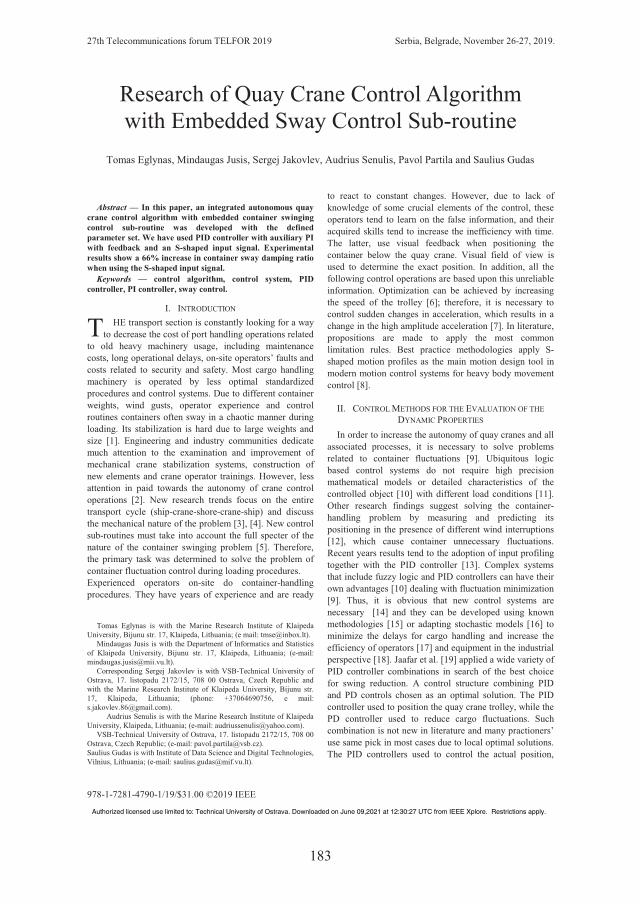
183

27th Telecommunications forum TELFOR 2019 Serbia, Belgrade, November 26-27, 2019.

978-1-7281-4790-1/19/$31.00 ©2019 IEEE

Abstract — In this paper, an integrated autonomous quay

crane control algorithm with embedded container swinging control sub-routine was developed with the defined parameter set. We have used PID controller with auxiliary PI with feedback and an S-shaped input signal. Experimental results show a 66% increase in container sway damping ratio when using the S-shaped input signal.

Keywords — control algorithm, control system, PID controller, PI controller, sway control.

I. INTRODUCTION HE transport section is constantly looking for a way

to decrease the cost of port handling operations related to old heavy machinery usage, including maintenance costs, long operational delays, on-site operators’ faults and costs related to security and safety. Most cargo handling machinery is operated by less optimal standardized procedures and control systems. Due to different container weights, wind gusts, operator experience and control routines containers often sway in a chaotic manner during loading. Its stabilization is hard due to large weights and size [1]. Engineering and industry communities dedicate much attention to the examination and improvement of mechanical crane stabilization systems, construction of new elements and crane operator trainings. However, less attention in paid towards the autonomy of crane control operations [2]. New research trends focus on the entire transport cycle (ship-crane-shore-crane-ship) and discuss the mechanical nature of the problem [3], [4]. New control sub-routines must take into account the full specter of the nature of the container swinging problem [5]. Therefore, the primary task was determined to solve the problem of container fluctuation control during loading procedures. Experienced operators on-site do container-handling procedures. They have years of experience and are ready

Tomas Eglynas is with the Marine Research Institute of Klaipeda University, Bijunu str. 17, Klaipeda, Lithuania; (e mail: tmse@inbox.lt).

Mindaugas Jusis is with the Department of Informatics and Statistics of Klaipeda University, Bijunu str. 17, Klaipeda, Lithuania; (e-mail: mindaugas.jusis@mii.vu.lt).

Corresponding Sergej Jakovlev is with VSB-Technical University of Ostrava, 17. listopadu 2172/15, 708 00 Ostrava, Czech Republic and with the Marine Research Institute of Klaipeda University, Bijunu str. 17, Klaipeda, Lithuania; (phone: +37064690756, e mail: s.jakovlev.86@gmail.com).

Audrius Senulis is with the Marine Research Institute of Klaipeda University, Klaipeda, Lithuania; (e-mail: audriussenulis@yahoo.com).

VSB-Technical University of Ostrava, 17. listopadu 2172/15, 708 00 Ostrava, Czech Republic; (e-mail: pavol.partila@vsb.cz). Saulius Gudas is with Institute of Data Science and Digital Technologies, Vilnius, Lithuania; (e-mail: saulius.gudas@mif.vu.lt).

to react to constant changes. However, due to lack of knowledge of some crucial elements of the control, these operators tend to learn on the false information, and their acquired skills tend to increase the inefficiency with time. The latter, use visual feedback when positioning the container below the quay crane. Visual field of view is used to determine the exact position. In addition, all the following control operations are based upon this unreliable information. Optimization can be achieved by increasing the speed of the trolley [6]; therefore, it is necessary to control sudden changes in acceleration, which results in a change in the high amplitude acceleration [7]. In literature, propositions are made to apply the most common limitation rules. Best practice methodologies apply S-shaped motion profiles as the main motion design tool in modern motion control systems for heavy body movement control [8].

II. CONTROL METHODS FOR THE EVALUATION OF THE DYNAMIC PROPERTIES

In order to increase the autonomy of quay cranes and all associated processes, it is necessary to solve problems related to container fluctuations [9]. Ubiquitous logic based control systems do not require high precision mathematical models or detailed characteristics of the controlled object [10] with different load conditions [11]. Other research findings suggest solving the container-handling problem by measuring and predicting its positioning in the presence of different wind interruptions [12], which cause container unnecessary fluctuations. Recent years results tend to the adoption of input profiling together with the PID controller [13]. Complex systems that include fuzzy logic and PID controllers can have their own advantages [10] dealing with fluctuation minimization [9]. Thus, it is obvious that new control systems are necessary [14] and they can be developed using known methodologies [15] or adapting stochastic models [16] to minimize the delays for cargo handling and increase the efficiency of operators [17] and equipment in the industrial perspective [18]. Jaafar et al. [19] applied a wide variety of PID controller combinations in search of the best choice for swing reduction. A control structure combining PID and PD controls chosen as an optimal solution. The PID controller used to position the quay crane trolley, while the PD controller used to reduce cargo fluctuations. Such combination is not new in literature and many practioners’ use same pick in most cases due to local optimal solutions. The PID controllers used to control the actual position,

Research of Quay Crane Control Algorithm with Embedded Sway Control Sub-routine

Tomas Eglynas, Mindaugas Jusis, Sergej Jakovlev, Audrius Senulis, Pavol Partila and Saulius Gudas

T

Authorized licensed use limited to: Technical University of Ostrava. Downloaded on June 09,2021 at 12:30:27 UTC from IEEE Xplore. Restrictions apply.

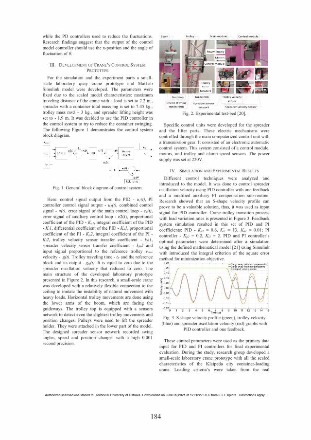
184

while the PD controllers used to reduce the fluctuations. Research findings suggest that the output of the control model controller should use the x-position and the angle of fluctuation of �.

III. DEVELOPMENT OF CRANE’S CONTROL SYSTEM PROTOTYPE

For the simulation and the experiment parts a small-scale laboratory quay crane prototype and MatLab Simulink model were developed. The parameters were fixed due to the scaled model characteristics: maximum traveling distance of the crane with a load is set to 2.2 m., spreader with a container total mass mg is set to 7.45 kg., trolley mass mvž – 3 kg., and spreader lifting height was set to - 1.9 m. It was decided to use the PID controller in the control system to try to reduce the container swinging. The following Figure 1 demonstrates the control system block diagram.

Fig. 1. General block diagram of control system.

Here: control signal output from the PID - u1(t), PI

controller control signal output - u2(t), combined control signal - u(t), error signal of the main control loop - e1(t), error signal of auxiliary control loop - e2(t), proportional coefficient of the PID - Kp1, integral coefficient of the PID - Ki1, differential coefficient of the PID - Kd1, proportional coefficient of the PI - Kp2, integral coefficient of the PI - Ki2, trolley velocity sensor transfer coefficient - kfb1, spreader velocity sensor transfer coefficient - kfb2 and input signal proportional to the reference trolley vmax velocity - g(t). Trolley traveling time - ttr and the reference block and its output - grf(t). It is equal to zero due to the spreader oscillation velocity that reduced to zero. The main structure of the developed laboratory prototype presented in Figure 2. In this research, a small-scale crane was developed with a relatively flexible connection to the ceiling to imitate the instability of natural movement with heavy loads. Horizontal trolley movements are done using the lower arms of the boom, which are facing the guideways. The trolley top is equipped with a sensors network to detect even the slightest trolley movements and position changes. Pulleys were used to lift the spreader holder. They were attached in the lower part of the model. The designed spreader sensor network recorded swing angles, speed and position changes with a high 0.001 second precision.

Fig. 2. Experimental test-bed [20].

Specific control units were developed for the spreader

and the lifter parts. These electric mechanisms were controlled through the main computerized control unit with a transmission gear. It consisted of an electronic automatic control system. This system consisted of a control module, motors, and trolley and clamp speed sensors. The power supply was set at 220V.

IV. SIMULATION AND EXPERIMENTAL RESULTS Different control techniques were analyzed and

introduced to the model. It was done to control spreader oscillation velocity using PID controller with one feedback and a modified auxiliary PI compensation sub-routine. Research showed that an S-shape velocity profile can prove to be a valuable solution, thus, it was used as input signal for PID controller. Crane trolley transition process with load variation rates is presented in Figure 3. Feedback system simulation resulted in this set of PID and PI coefficients: PID - Kp1 = 0.6, Ki1 = 13, Kd1 = 0.01; PI controller - Kp2 = 0.2, Ki2 = 2. PID and PI controller’s optimal parameters were determined after a simulation using the defined mathematical model [21] using Simulink with introduced the integral criterion of the square error method for minimization objective.

Fig. 3. S-shape velocity profile (green), trolley velocity

(blue) and spreader oscillation velocity (red) graphs with PID controller and one feedback.

These control parameters were used as the primary data

input for PID and PI controllers for final experimental evaluation. During the study, research group developed a small-scale laboratory crane prototype with all the scaled characteristics of the Klaipeda city container-loading crane. Loading criteria’s were taken from the real

Authorized licensed use limited to: Technical University of Ostrava. Downloaded on June 09,2021 at 12:30:27 UTC from IEEE Xplore. Restrictions apply.

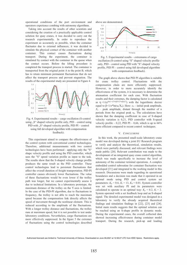
184 185

operational conditions of the port environment and operators experience combing with autonomy algorithms.

Taking into account the results of other scientists and considering the creation of a practically applicable control solution for quay cranes, it was decided to carry out the research experimentally. In order to reproduce the experiment as accurately as possible, when the container fluctuates due to external influences, it was decided to simulate the physical contact of the container with another container. This contact causes fluctuations during transport. During the experiment, the container is simulated by contact with the container in the queue when the contact occurs. Before the lifting procedure is completed the transport process is started. The container is transported from the original point A to the point B, which has to retain minimum permanent fluctuations that do not affect the transport process and prevent stagnation. The results of the experimental study are presented in Figure 4.

Fig. 4. Experimental results – cargo oscillation (S-control

using „S“ shaped velocity profile only, PID – control using PID with „S“-shaped velocity profile, PID PI – control

using full developed algorithm with compensation feedback).

This experiment aimed to compare the effectiveness of

the control system with conventional control technologies. Therefore, additional measurements with two control technologies have been performed - applying only the "S" shape velocity profile and using the PID controller, which uses the "S" speed variation profile as input to the task. The results show that the S-shaped velocity change profile produces the same result as the PID controller. These control technologies lead to persistent fluctuations that affect the overall duration of freight transportation. PID-PI controller causes obviously lower fluctuations. The value of these fluctuations would be even lower if the trolley path was longer, but we cannot experimentally assess it due to technical limitations. In a laboratory prototype, the maximum distance of the trolley on the Y-axis is limited. In the case of the PID-PI algorithm, due to fluctuations in frequency, the trolley is not able to reach the maximum speed because the compensation link directly affects the speed of movement through the nonlinear element. This is reduced according to the amplitude of the fluctuations. With a longer trolley distance and fluctuations, the trolley runs at maximum speed, but it is not possible to test under laboratory conditions. Nevertheless, cargo fluctuations are more effectively suppressed. In the figure 5 the extremes of fluctuations using the control technologies described

above are demonstrated.

Fig. 5. Experimental results – extremums of cargo

oscillation (S-control using “S” shaped velocity profile only, PID – control using PID with “S”-shaped velocity profile, PID PI – control using full developed algorithm

with compensation feedback). The graph above shows that PID PI algorithm is suitable

for crane trolley control. Fluctuations with the compensation chain are more efficiently suppressed. However, in order to more accurately identify the effectiveness of the system, it is necessary to determine the attenuation coefficient for each case. With fluctuation results and their extremes, the damping factor is calculated as � =1/(e(ln(1+(2*�/�)*(2*�/�)))/2) with the logarithmic decree equal to �=1/n*ln(x0/Xn). Here: x0 – initial peak amplitude, Xn – peak amplitude, distant through the number of n periods from the original peak x0. The calculations have shown that the damping coefficient in case of S-shaped velocity variation is 0,21, PID controller with S-speed velocity profile – 0,22, PID PI – 0,66, which is up to 66% more efficient compared to recent control techniques.

V. CONCLUSIONS In this work, the presented small-scale laboratory crane

model was developed during a joint EU Research program to verify and analyze the theoretical, simulation results, which were partially discussed, and relevant findings were made public [20]. Relevant contribution was made to the development of an integrated quay crane control algorithm, which was made specifically to increase the level of autonomy of the container terminal operations. A complex embedded control subroutine for container fluctuation was developed [21] and integrated to the working model in this research. Discussions were made regarding its operational boundaries and a decision was made that it operated in an optimal mode using PID and control system set parameters: Kp = 0.6, Ki = 13, Kd = 0.01. System controller was set with auxiliary PI and its parameters were calculated to operate in an optimal way: Kp = 0.2, Ki = 2. System operated with a set feedback loop and an S-shaped signal. The detailed experimental model was designed in a laboratory to verify the already acquired theoretical findings and simulation findings in [22], [23] and [24]. Initial main results suggests that the optimal solution can be reached using an S-shape profile in dynamic mode. During the experimental cases, the overall collected data showed increasing effectiveness during container model transport. During the research, pick-up and loading

Authorized licensed use limited to: Technical University of Ostrava. Downloaded on June 09,2021 at 12:30:27 UTC from IEEE Xplore. Restrictions apply.

186

operations were experimented. Overload cycle was introduced to the system concept. S-shaped proved to be efficient even in full cycle mode. A suggestion is made, that in real transportation cycle, full scale operations might be optimized, by introducing new concepts for container speed correction during lifting and loading procedures. Thus, transportation operation can be optimized for separate containers and transport modes.

The results of comparative and experimental studies show that using the proposed autonomous quay crane control algorithm with a sub-system for fluctuations minimization is possible in an experimental environment. Results suggest that during loading process using the S-shaped velocity profile in dynamic mode as control system input provides a possibility to obtain a most suitable solution for the transport modes of a specific container. The results of comparative and experimental studies show that proposed autonomous quay crane’s control algorithm, with a PI sub-system for decreasing container swinging during loading, can be used to accelerate the handling process. These determined parameters are suitable for this case study presented in the paper; therefore, each case study should consider changing the parameters of PID and PI while other parameters should be adaptable.

ACKNOWLEDGEMENT This project has received funding from European

Regional Development Fund project No. 01.2.2-LMT-K-718-01-0081 under grant agreement with the Research Council of Lithuania (LMT).

This work was also supported by the grant SGS reg. No. SP2019/41 conducted at VSB - Technical University of Ostrava, Czech Republic.

Authors would also like to thank project members: prof. dr. A. Andziulis, prof. dr M. Bogdevicius, prof. dr. E. Guseinoviene, prof. dr. R. Didziokas, prof. dr. J. Januteniene, V. Jankunas, D. Cirtautas, dr. M. Kurmis, dr. D. Drungilas, Z. Lukosius for contribution.

REFERENCES [1] S.-L. Chao and Y.-J. Lin, “Evaluating advanced quay cranes in

container terminals,” Transp. Res. Part E Logist. Transp. Rev., vol. 47(4), 2011, pp. 432–445.

[2] L. I. Zhi-jun, L. I. Zhen, L. I. Hui-jie, Z. Ye, S. Cheng, and S. U. N. Yan, “Research of Coordinated Control Method of Hybrid Power Crane System,” In Proceedings of International Conference on Modelling, Identification & Control (ICMIC), 2012, pp. 1093–1097.

[3] Y. Fang, P. Wang, and X. Zhang, “A Motion Planning-Based Adaptive Control Method for an Underactuated Crane System,” IEEE Transactions on Control Systems Technology, vol. 20(1), 2012, pp. 241–248.

[4] L. Cao and L. Liu, “Adaptive Fuzzy Sliding Mode Method-Based Position and Anti-swing Control for Overhead Cranes,” in Proc., Third Int. Conf. Meas. Technol. Mechatronics Autom., no. 2, 2011, pp. 335–338.

[5] H. Sano, K. Ohishi, T. Kaneko, and H. Mine, “Anti-sway crane control based on dual state observer with sensor-delay correction,”

in Proc., 11th IEEE Int. Work. Adv. Motion Control, 2010, pp. 679–684.

[6] R. Béarée, “New Damped-Jerk trajectory for vibration reduction,” Control Eng. Pract., vol. 28, 2014, pp. 112–120.

[7] M. A. Majid, W. S. W. Ibrahim, S. Mohamad, and Z. A. Bakar, “A comparison of PID and PD controller with input shaping technique for 3D gantry crane,” in Proc. - 2013 IEEE Conf. Syst. Process Control. ICSPC 2013, 2013, pp. 144–148.

[8] J. Vaughan, J. Yoo, N. Knight, and W. Singhose, “Multi-Input Shaping Control for Multi-Hoist Cranes,” in Proc., American Control Conference, 2013, pp. 3455–3460.

[9] C. Liu, H. Zhao, and Y. Cui, “Research on Application of Fuzzy PID in Collective Pitch Control System,” in Int. Conf. Control. Autom. Syst. Eng., 2011, pp. 1–4.

[10] L. Ranjbari and A. H. Shirdel, “Designing precision fuzzy controller for load swing of an overhead crane,” 2015.

[11] V. Roso, J. Woxenius, and K. Lumsden, “The dry port concept: connecting container seaports with the hinterland,” J. Transp. Geogr., vol. 17(5), 2009, pp. 338–345.

[12] H. Kawai, Y. Choi, Y. B. Kim, and Y. Kubota, “Position measurement of container crane spreader using an image sensor system for anti-sway controllers,” in Int. Conf. Control. Autom. Syst., 2018, pp. 683–686

[13] A. A. Elbadawy and M. M. G. Shehata, “Anti-sway control of marine cranes under the disturbance of a parallel manipulator,” Nonlinear Dyn., vol. 82(1–2), 2015, pp. 415–434.

[14] Z. Sun, N. Wang, Y. Bi, and J. Zhao, “A DE based PID controller for two dimensional overhead crane,” in Proc., of 34th Chinese Control Conference (CCC), no. 1, 2015, pp. 2546–2550.

[15] N. Lv, H. Li, M. Li, and M. Hou, “Based on PID Control Optimization Of Synchronous Motor Control,” Conf. Meas. Inf. Control, 2012, pp. 2111–2114.

[16] H. I. Jaafar, Z. Mohamed, A. F. Z. Abidin, and Z. A. Ghani, “PSO-tuned PID controller for a nonlinear gantry crane system,” in Proc. - 2012 IEEE Int. Conf. Control Syst. Comput. Eng. ICCSCE 2012, pp. 515–519.

[17] P. Li, Z. Li, and Y. Yang, “The Application Research of Ant Colony Optimization Algorithm for Intelligent Control on Special Crane,” in 2012 Second International Conference on Instrumentation, Measurement, Computer, Communication and Control, 2012, pp. 999–1004.

[18] H. I. Jaafar, Z. Mohamed, J. J. Jamian, A. F. Z. Abidin, A. M. Kassim, and Z. A. Ghani, “Dynamic Behaviour of a Nonlinear Gantry Crane System,” Procedia Technol., vol. 11, 2013, pp. 419–425.

[19] H. I. Jaafar, M. F. Sulaima, Z. Mohamed, and J. J. Jamian, “Optimal PID controller parameters for nonlinear gantry crane system via MOPSO technique,” in Proc. - 2013 IEEE Conf. Sustain. Util. Dev. Eng. Technol. IEEE CSUDET 2013, 2013, pp. 86–91.

[20] T. Eglynas, M. Jusis, S. Jakovlev, A. Senulis, A. Andziulis, and S. Gudas, “Analysis of the efficiency of shipping containers handling/loading control methods and procedures,” Res. Artic. Adv. Mech. Eng., vol. 11(1), 2019, pp. 1–12.

[21] A. Andziulis, T. Eglynas, M. Bogdevicius, M. Jusis, and A. Senulis, “Multibody dynamic simulation and transient analysis of quay crane spreader and lifting mechanism,” Adv. Mech. Eng., vol. 8(9), 2016, pp. 1-11.

[22] A. Santamaria, M. Tropea, P. Fazio, and F. De Rango, “Managing emergency situations in VANET through heterogeneous technologies cooperation,” Sensors, 18(5), 2018, E1461.

[23] F. De Rango, N. Palmieri, M. Tropea, and G. Potrino, “UAVS team and its application in agriculture,” A simulation environment. SIMULTECH, 2017, pp. 74-379.

[24] A Socievole, E Yoneki, F De Rango, J Crowcroft, "Opportunistic message routing using multi-layer social networks," in Proc. of the 2nd ACM workshop on High performance mobile opportunistic systems, 2013, pp.39-46.

Authorized licensed use limited to: Technical University of Ostrava. Downloaded on June 09,2021 at 12:30:27 UTC from IEEE Xplore. Restrictions apply.

186 118

8th publication / 8 publikacija

Pietryčių Baltijos konteinerių terminalų apžvalga ir krovos tendencijos

M. Jusis, T. Eglynas, A. Senulis, S. Gudas, S. Jakovlev,M. Bogdevičius.

Jūros ir krantų tyrimai 2017, 86-90 (2017)

ISSN: 2538-7243

188

Jūros ir krantų tyrimai 2017. Konferencijos medžiaga

86

PIETRYČIŲ BALTIJOS KONTEINERIŲ TERMINALŲ APŽVALGA IR KROVOS TENDENCIJOS

Mindaugas Jusis1, Tomas Eglynas1, Audrius Senulis4, Saulius Gudas2, Sergej Jakovlev3, Marijonas Bogdevičius3

1Klaipėdos universiteto Jūros technologijų ir gamtos mokslų fakulteto Informatikos ir statistikos katedra, Klaipėda, 2Vilniaus universiteto Programų

sistemų inžinerijos skyrius, Vilnius, 3Klaipėdos universiteto Jūros technologijų ir gamtos mokslų fakulteto Jūros mokslų ir technologijų centras,

Klaipėda, 4Klaipėdos universiteto Jūros technologijų ir gamtos mokslų fakulteto Inžinerijos katedra, Klaipėda

mindaugas.jusis@gmail.com

Įvadas. Didėjantys krovinių srautai, augančios uostų krovos apimtys bei didesni atplaukiantys laivai didina Klaipėdos uosto infrastruktūros plėtros poreikį. Per analizuojamą laikotarpį nuo 2009 metų konteinerių krova uoste didėjo beveik dvigubai (195000 TEU) ir šiuo metu siekia ~449 tūkst. TEU (VĮ „Klaipėdos valstybinio jūrų uosto direkcija“, 2016). Šiame darbe analizuojami pietryčių Baltijos šalių konteinerių terminalų krovos pajėgumai (KTKP), krovos apimtys bei pokyčiai per pastaruosius 5 metus, lyginamos konteinerių krovos apimtys. Darbe, įvertinus Klaipėdos uosto plėtros planus bei kitų uostų pokyčių patirtį, taikant linijinį metodą, prognozuojama Klaipėdos uosto artimiausių metų konteinerių preliminari krova ir aptariamos Klaipėdos KTKP plėtros galimybės. Taip pat pateikiamas išvestinis rodiklis uosto KTKP palyginimui – konteinerių krovos pajėgumas terminalo krantinės ilgiui (Paulauskas, 2011). Šis įvertis suteikia galimybę lengviau palyginti KTKP apimtis.

Konteinerių krovos terminalų rodikliai ir statistika. Klaipėdos uostas per pastaruosius metus padarė reikšmingą pažangą konteinerių krovos srityje. Klaipėdos Smeltės terminale buvo įdiegti nauji krantinės kranai, galintys aptarnauti „Postpanamax“ tipo konteinerinius laivus (UAB „Klaipėdos Smeltė“, 2016). Ši investicija leido pasiekti 44 % didesnę krovą lyginant su analizuojamo laikotarpio pradžia, 2009 metais (UAB „Klaipėdos Smeltė“, 2016). Klaipėdos uoste įsikūrę du konteinerių terminalai, kuriuose vykdoma konteinerių krova 2016 metais pasiekė ~449 tūkst. TEU, o jų krantinių bendras krantinės ilgis siekia 1888 metrus (VĮ „Klaipėdos valstybinio jūrų uosto direkcija“, 2016). Klaipėdos konteinerių krovos terminalas geriausią krovą buvo pasiekęs 2014 metais, kai konteinerių krova sudarė 5,61 mln. t arba ~450 tūkst. TEU per metus (VĮ „Klaipėdos valstybinio jūrų uosto direkcija“, 2016). Klaipėdos uoste didžiausias aptarnautas konteinerinis laivas (2015 metai)

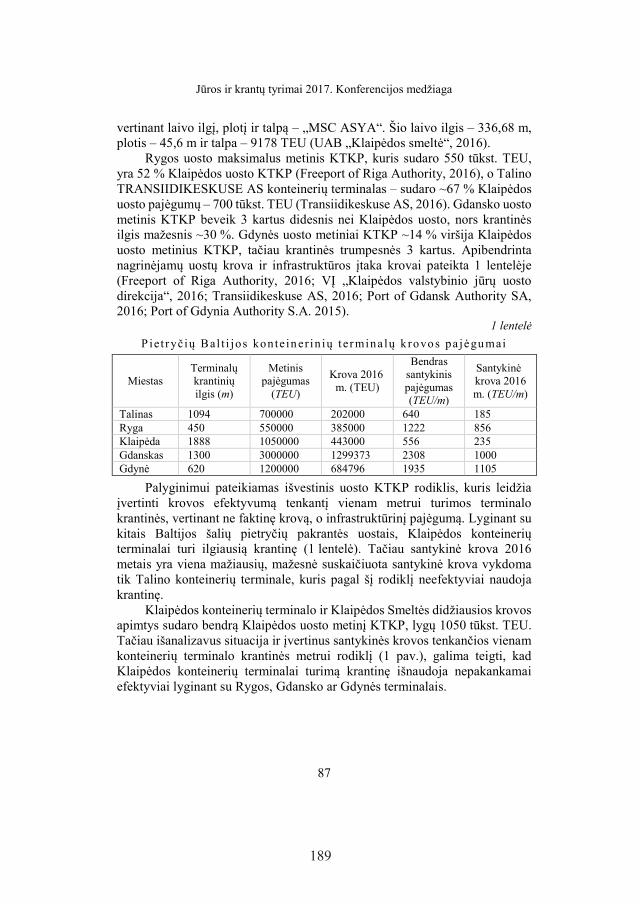
188 189

Jūros ir krantų tyrimai 2017. Konferencijos medžiaga

87

vertinant laivo ilgį, plotį ir talpą – „MSC ASYA“. Šio laivo ilgis – 336,68 m, plotis – 45,6 m ir talpa – 9178 TEU (UAB „Klaipėdos smeltė“, 2016).

Rygos uosto maksimalus metinis KTKP, kuris sudaro 550 tūkst. TEU, yra 52 % Klaipėdos uosto KTKP (Freeport of Riga Authority, 2016), o Talino TRANSIIDIKESKUSE AS konteinerių terminalas – sudaro ~67 % Klaipėdos uosto pajėgumų – 700 tūkst. TEU (Transiidikeskuse AS, 2016). Gdansko uosto metinis KTKP beveik 3 kartus didesnis nei Klaipėdos uosto, nors krantinės ilgis mažesnis ~30 %. Gdynės uosto metiniai KTKP ~14 % viršija Klaipėdos uosto metinius KTKP, tačiau krantinės trumpesnės 3 kartus. Apibendrinta nagrinėjamų uostų krova ir infrastruktūros įtaka krovai pateikta 1 lentelėje (Freeport of Riga Authority, 2016; VĮ „Klaipėdos valstybinio jūrų uosto direkcija“, 2016; Transiidikeskuse AS, 2016; Port of Gdansk Authority SA, 2016; Port of Gdynia Authority S.A. 2015).

1 lentelė

Piet ryčių Bal t i jos kontein er in ių t ermina lų krovo s pa jėgu mai

Miestas Terminalų krantinių ilgis (m)

Metinis pajėgumas

(TEU)

Krova 2016 m. (TEU)

Bendras santykinis pajėgumas (TEU/m)

Santykinė krova 2016 m. (TEU/m)

Talinas 1094 700000 202000 640 185 Ryga 450 550000 385000 1222 856 Klaipėda 1888 1050000 443000 556 235 Gdanskas 1300 3000000 1299373 2308 1000 Gdynė 620 1200000 684796 1935 1105

Palyginimui pateikiamas išvestinis uosto KTKP rodiklis, kuris leidžia įvertinti krovos efektyvumą tenkantį vienam metrui turimos terminalo krantinės, vertinant ne faktinę krovą, o infrastruktūrinį pajėgumą. Lyginant su kitais Baltijos šalių pietryčių pakrantės uostais, Klaipėdos konteinerių terminalai turi ilgiausią krantinę (1 lentelė). Tačiau santykinė krova 2016 metais yra viena mažiausių, mažesnė suskaičiuota santykinė krova vykdoma tik Talino konteinerių terminale, kuris pagal šį rodiklį neefektyviai naudoja krantinę.

Klaipėdos konteinerių terminalo ir Klaipėdos Smeltės didžiausios krovos apimtys sudaro bendrą Klaipėdos uosto metinį KTKP, lygų 1050 tūkst. TEU. Tačiau išanalizavus situacija ir įvertinus santykinės krovos tenkančios vienam konteinerių terminalo krantinės metrui rodiklį (1 pav.), galima teigti, kad Klaipėdos konteinerių terminalai turimą krantinę išnaudoja nepakankamai efektyviai lyginant su Rygos, Gdansko ar Gdynės terminalais.

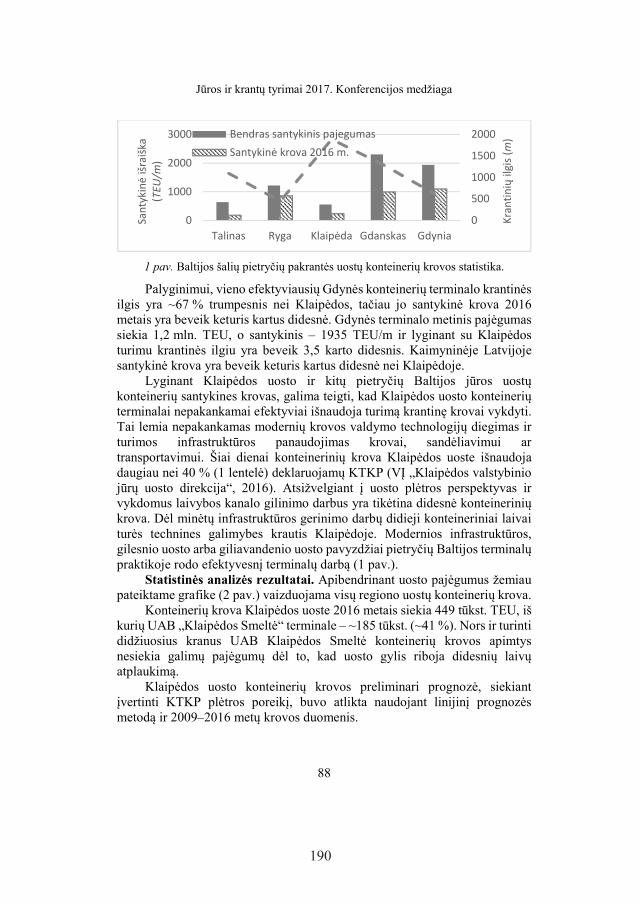
190

Jūros ir krantų tyrimai 2017. Konferencijos medžiaga

88

1 pav. Baltijos šalių pietryčių pakrantės uostų konteinerių krovos statistika.

Palyginimui, vieno efektyviausių Gdynės konteinerių terminalo krantinės ilgis yra ~67 % trumpesnis nei Klaipėdos, tačiau jo santykinė krova 2016 metais yra beveik keturis kartus didesnė. Gdynės terminalo metinis pajėgumas siekia 1,2 mln. TEU, o santykinis – 1935 TEU/m ir lyginant su Klaipėdos turimu krantinės ilgiu yra beveik 3,5 karto didesnis. Kaimyninėje Latvijoje santykinė krova yra beveik keturis kartus didesnė nei Klaipėdoje.

Lyginant Klaipėdos uosto ir kitų pietryčių Baltijos jūros uostų konteinerių santykines krovas, galima teigti, kad Klaipėdos uosto konteinerių terminalai nepakankamai efektyviai išnaudoja turimą krantinę krovai vykdyti. Tai lemia nepakankamas modernių krovos valdymo technologijų diegimas ir turimos infrastruktūros panaudojimas krovai, sandėliavimui ar transportavimui. Šiai dienai konteinerinių krova Klaipėdos uoste išnaudoja daugiau nei 40 % (1 lentelė) deklaruojamų KTKP (VĮ „Klaipėdos valstybinio jūrų uosto direkcija“, 2016). Atsižvelgiant į uosto plėtros perspektyvas ir vykdomus laivybos kanalo gilinimo darbus yra tikėtina didesnė konteinerinių krova. Dėl minėtų infrastruktūros gerinimo darbų didieji konteineriniai laivai turės technines galimybes krautis Klaipėdoje. Modernios infrastruktūros, gilesnio uosto arba giliavandenio uosto pavyzdžiai pietryčių Baltijos terminalų praktikoje rodo efektyvesnį terminalų darbą (1 pav.).

Statistinės analizės rezultatai. Apibendrinant uosto pajėgumus žemiau pateiktame grafike (2 pav.) vaizduojama visų regiono uostų konteinerių krova.

Konteinerių krova Klaipėdos uoste 2016 metais siekia 449 tūkst. TEU, iš kurių UAB „Klaipėdos Smeltė“ terminale – ~185 tūkst. (~41 %). Nors ir turinti didžiuosius kranus UAB Klaipėdos Smeltė konteinerių krovos apimtys nesiekia galimų pajėgumų dėl to, kad uosto gylis riboja didesnių laivų atplaukimą.

Klaipėdos uosto konteinerių krovos preliminari prognozė, siekiant įvertinti KTKP plėtros poreikį, buvo atlikta naudojant linijinį prognozės metodą ir 2009–2016 metų krovos duomenis.

0

500

1000

1500

2000

0

1000

2000

3000

Talinas Ryga Klaipėda Gdanskas Gdynia

Kra

nti

nių

 ilgi

s (m

)

San

tyki

nė 

išra

iška

  (TEU

/m)

Bendras santykinis pajegumas

Santykinė krova 2016 m.

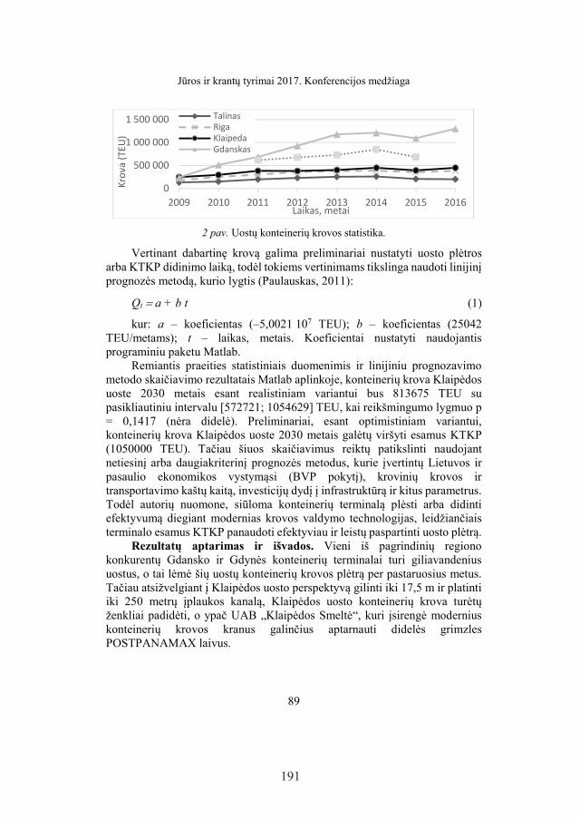
190 191

Jūros ir krantų tyrimai 2017. Konferencijos medžiaga

89

2 pav. Uostų konteinerių krovos statistika.

Vertinant dabartinę krovą galima preliminariai nustatyti uosto plėtros arba KTKP didinimo laiką, todėl tokiems vertinimams tikslinga naudoti linijinį prognozės metodą, kurio lygtis (Paulauskas, 2011):

Qt a + b t (1)

kur: a – koeficientas (–5,0021 107 TEU); b – koeficientas (25042 TEU/metams); t – laikas, metais. Koeficientai nustatyti naudojantis programiniu paketu Matlab.

Remiantis praeities statistiniais duomenimis ir linijiniu prognozavimo metodo skaičiavimo rezultatais Matlab aplinkoje, konteinerių krova Klaipėdos uoste 2030 metais esant realistiniam variantui bus 813675 TEU su pasikliautiniu intervalu [572721; 1054629] TEU, kai reikšmingumo lygmuo p = 0,1417 (nėra didelė). Preliminariai, esant optimistiniam variantui, konteinerių krova Klaipėdos uoste 2030 metais galėtų viršyti esamus KTKP (1050000 TEU). Tačiau šiuos skaičiavimus reiktų patikslinti naudojant netiesinį arba daugiakriterinį prognozės metodus, kurie įvertintų Lietuvos ir pasaulio ekonomikos vystymąsi (BVP pokytį), krovinių krovos ir transportavimo kaštų kaitą, investicijų dydį į infrastruktūrą ir kitus parametrus. Todėl autorių nuomone, siūloma konteinerių terminalą plėsti arba didinti efektyvumą diegiant modernias krovos valdymo technologijas, leidžiančiais terminalo esamus KTKP panaudoti efektyviau ir leistų paspartinti uosto plėtrą.

Rezultatų aptarimas ir išvados. Vieni iš pagrindinių regiono konkurentų Gdansko ir Gdynės konteinerių terminalai turi giliavandenius uostus, o tai lėmė šių uostų konteinerių krovos plėtrą per pastaruosius metus. Tačiau atsižvelgiant į Klaipėdos uosto perspektyvą gilinti iki 17,5 m ir platinti iki 250 metrų įplaukos kanalą, Klaipėdos uosto konteinerių krova turėtų ženkliai padidėti, o ypač UAB „Klaipėdos Smeltė“, kuri įsirengė modernius konteinerių krovos kranus galinčius aptarnauti didelės grimzles POSTPANAMAX laivus.

0

500 000

1 000 000

1 500 000

2009 2010 2011 2012 2013 2014 2015 2016

Kro

va (

TEU

)

Laikas, metai

TalinasRigaKlaipedaGdanskas

192

Jūros ir krantų tyrimai 2017. Konferencijos medžiaga

90

Gauti preliminarūs prognozės rezultatai, taikant linijinį prognozavimo metodą ir remiantis praeities statistine informacija, leidžia daryti prielaidą, kad esamos Klaipėdos uosto konteinerių krovos terminalų infrastruktūros turėtų pakakti. Konteinerių krovai augant optimistiniais tempais (2030 m. – 1054629 TEU) Klaipėdos uosto infrastruktūros konteinerių pajėgumų krovai pakaks artimiausiems 13 metų. Tačiau ilgalaikėje perspektyvoje (nuo 2030 metų) būtina planuoti uosto plėtrą arba didinti uosto krovos galimybes diegiant modernias krovos valdymo technologijas ar plėtotis veiklą statant giliavandenį uostą. Tai lemia pagrindinių konkurentų – Gdynės, Rygos ir Gdansko efektyvesnis krantinių išnaudojimas ir geresni konkurentų uostų santykiniai KTKP.

Literatūra Freeport of Riga Authority. 2016. Statistics. [žiūrėta 2017-02-06]. Prieiga per internetą

http://rop.lv/en/about-port/statistics.html. Paulauskas V. 2011. Optimalus uostas. Klaipėda: Klaipėdos universiteto leidykla. Port of Gdansk Authority SA. 2016. Cargo Statistics. [žiūrėta 2017-02-06]. Prieiga per internetą

https://www.portgdansk.pl/about-port/cargo-statistics. Port of Gdynia Authority S.A. 2015. Cargo Statistics. [žiūrėta 2017-02-06]. Prieiga per internetą

http://www.port.gdynia.pl/en/about-port/statistics. Transiidikeskuse AS. 2016. Container Terminal. [žiūrėta 2017-02-06]. Prieiga per internetą

http://www.tk.ee/en/terminals/container-terminal/. UAB „Klaipėdos smeltė“. 2016. Konteinerių terminalų paslaugos. [žiūrėta 2017-02-10]. Prieiga

per internetą http://www.smelte.lt/lt/paslaugos/konteineriuterminalo-paslaugos/. VĮ „Klaipėdos valstybinio jūrų uosto direkcija“. 2016. Uosto statistika. [žiūrėta 2017-02-06].

Prieiga per internetą http://www.portofklaipeda.lt/uosto-statistika.

192 193

NOTES

194

NOTES

194 195

NOTES

Redaktorė: Zuzana Šiušaitė

Vilniaus universiteto leidykla Saulėtekio al. 9, III rūmai, LT-10222 Vilnius El. p. info@leidykla.vu.lt, www.leidykla.vu.lt

Tiražas 20 egz.