Deep-Sea Research I 49 (2002) 735–749

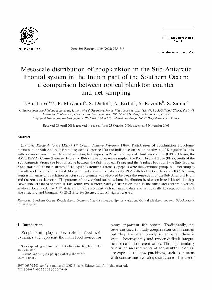
Mesoscale distribution of zooplankton in the Sub-AntarcticFrontal system in the Indian part of the Southern Ocean:

a comparison between optical plankton counterand net sampling

J.Ph. Labata,*, P. Mayzauda, S. Dallota, A. Errhifa, S. Razoulsb, S. Sabinia

aOc!eanographie Biochimique et Ecologie, Laboratoire d’Oc!eanographie de Villefranche sur mer (LOV), UPMC-INSU-CNRS, Paris VI,

Maitre de Conferences, Observatoire Oceanologique, BP. 28, 06234 Villefranche sur mer, FrancebEquipe d’Oc!eanographie biologique, UPMC-INSU-CNRS, Laboratoire Arago, 66650 Banyuls-sur-mer, France

Received 23 April 2001; received in revised form 23 October 2001; accepted 5 November 2001

Abstract

(Antartic Research (ANTARES) IV Cruise, January–February 1999). Distribution of zooplankton biovolume/

biomass in the Sub-Antarctic Frontal system is described for the Indian Ocean sector, northwest of Kerguelen Islands,

with a comparison of two types of sampling techniques: WP2 net and optical plankton counter (OPC). During the

ANTARES IV Cruise (January–February 1999), three zones were sampled: the Polar Frontal Zone (PFZ), south of the

Sub-Antarctic Front; the Frontal Zone between the Sub-Tropical Front; and the Agulhas Front and the Sub-Tropical

Zone, north of the main stream of the Agulhas Return Current. Copepods were the dominant group in all net samples

regardless of the area considered. Maximum values were recorded in the PFZ with both net catches and OPC. A strong

contrast in terms of population structure and biomass was observed between the zone south of the Sub-Antarctic Front

and the zones to the north. The patterns of the zooplankton biovolume distribution by size confirmed this relationship.

Biovolume 2D maps showed in this south area a more patchy distribution than in the other areas where a vertical

gradient dominated. The OPC data are in fair agreement with net sample data and are spatially heterogenous in both

size structure and biomass. r 2002 Elsevier Science Ltd. All rights reserved.

Keywords: Southern Ocean; Zooplankton; Biomass; Size distribution; Spatial variation; Optical plankton counter; Sub-Antarctic

Frontal system

1. Introduction

Zooplankton play a key role in food webdynamics and represent the main food source for

many important fish stocks. Traditionally, nettows are used to study zooplankton communities,but they are often poorly suited when there isspatial heterogeneity and render difficult integra-tion of data at different scales. This is particularlytrue when measurements of zooplankton biomassare expected to show patchiness, such as in areaswith contrasting hydrologic structures. The use of

*Corresponding author. Tel.: +33-04-9376-3845; fax: +33-

04-9376-3893.

E-mail address: jean-philippe.labat@obs-vlfr.fr

(J.Ph. Labat).

0967-0637/02/$ - see front matter r 2002 Elsevier Science Ltd. All rights reserved.

PII: S 0 9 6 7 - 0 6 3 7 ( 0 1 ) 0 0 0 7 6 - 0

optical plankton counter (OPC) introduced byHerman (1988, 1992) represents an alternative tocharacterize, at different scales, abundance andsize distribution of zooplankton. OPC is a power-ful tool permitting description of size distributionof zooplankton at both large and small scales(Herman et al., 1993; Huntley et al., 1995; Katoet al., 1997; Mullin and Cass-Calay, 1997; Osgoodand Checkley, 1997; Currie et al., 1998; Wielandet al., 1997; Grant et al., 2000; Huntley et al.,2000). Knowledge of changes in size structure ofplankton communities has long been recognized asessential to understanding of population dynamicsat the mesoscale (Sheldon et al., 1972; Vidal andWhitledge, 1982).

Here we present data from the AntarcticResearch (ANTARES) IV Cruise (January–Feb-ruary 1999). ANTARES is the French contributionto Southern Ocean-Joint Global Ocean Flux Study(SO-JGOFS).

Zooplankton distributions were considered in astudy area characterized by a strong horizontaltemperature and salinity gradient (Park andGamberoni, 1997) close to both Sub-Antarcticand Sub-Tropical Fronts (STFs) in the IndianOcean (Nagata et al., 1988). We compare thecontinuous record of the distribution of zooplank-ton biovolume/biomass in the different watermasses and describe the characteristics of thezooplankton population structure in these areasof very contrasting hydrological structures.

2. Material and methods

Zooplankton samples were collected in threemain hydrological domains, chosen after a pre-liminary mesoscale survey of the area:

* Station 3 area, was located in the Polar FrontalZone (PFZ), south of the Sub-Antarctic Front.

* Station 7 area was located in the Frontal Zonebetween the STF and the Agulhas Front (AF).

* Station 8 area was located in the Sub-TropicalZone (STZ), north of the main stream of the‘‘Agulhas Return Current’’ (sometimes called‘‘South Indian Ocean Current’’) (Park andGamberoni, 1997).

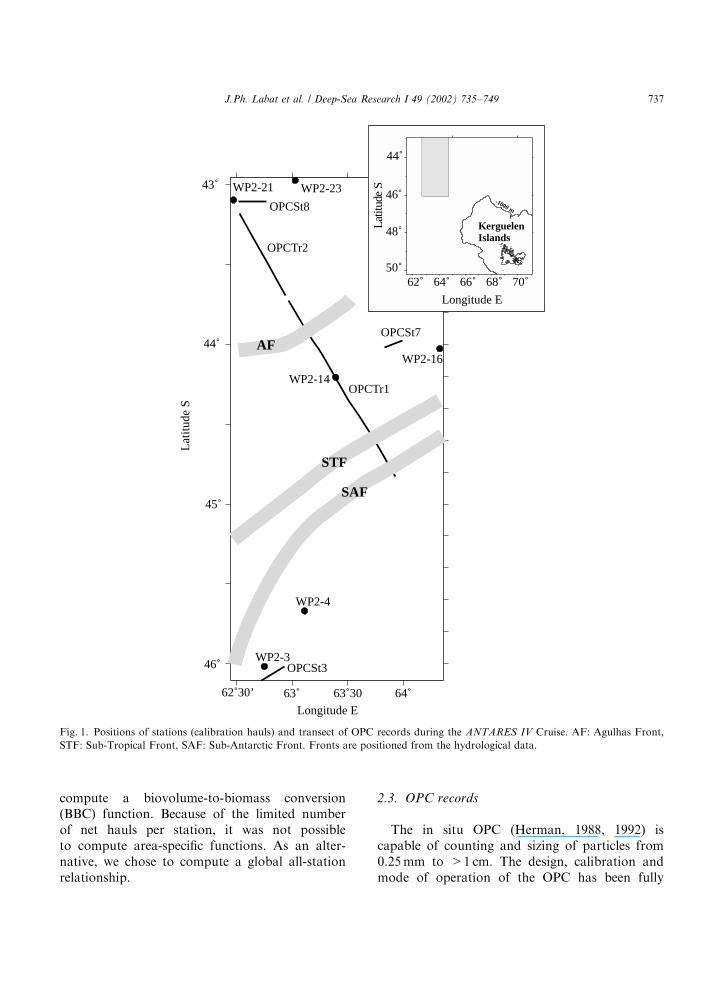
During net sampling, a Lagrangian approachwas used, with the ship following a drifting buoyfor the duration of the stations. Fig. 1 shows theposition of net hauls and OPC lines.

2.1. Net sampling

Zooplankton were collected at night with atriple WP2 net (0.25m2 surface aperture and200 mm mesh size). Vertical hauls were made from200 m to the surface. One net was used for biomassmeasurement and another one for taxonomicdescription and enumeration.

Biomass samples were filtered on 200 mm pre-weighed netting and rinsed with ammoniumformate. The material was immediately frozen at�201C on board. Within 3 months, all sampleswere oven dried (48 h at 601) at the laboratory andweighed. Total weight is expressed in milligram ofdry weight per cubic meter, DW mg m�3.

Taxonomic samples were preserved immediatelyafter the catch, with 5% buffered formaldehyde.

2.2. Net sample treatments

Species determinations, enumerations and bio-volume estimates were made with a binocularmicroscope coupled to an image analysis system.An equivalent spherical diameter (ESD) sizedistribution was constructed for each net sample.Sub-samples of 200–400 individuals (with aMotoda box splitter) were used to measure theESD of each individual with a Visiolab 1000system (Biocom). ESD of an organism was definedas the diameter of the sphere that has an identicalprojected surface.

Sample biovolume (SBV) of each sample wascomputed from the individual ESD measurement:

SBV ¼ kXn

i¼1

p6

ESDið Þ3" #

;

where k is the sub-sample ratio, n the number ofindividuals, and ESDi the ESD of the ithindividual.

For each sample, the value of SBV can beassociated with a value of total biomass derivedfrom the corresponding net. It was then possible to

J.Ph. Labat et al. / Deep-Sea Research I 49 (2002) 735–749736

compute a biovolume-to-biomass conversion(BBC) function. Because of the limited numberof net hauls per station, it was not possibleto compute area-specific functions. As an alter-native, we chose to compute a global all-stationrelationship.

2.3. OPC records

The in situ OPC (Herman, 1988, 1992) iscapable of counting and sizing of particles from0.25 mm to >1 cm. The design, calibration andmode of operation of the OPC has been fully

62˚30’ 63˚ 63˚30 64˚

46˚

45˚

44˚

43˚

WP2-3

WP2-4

WP2-14

WP2-16

WP2-21 WP2-23

OPCTr2

OPCSt8

OPCSt7

OPCTr1

OPCSt3

62˚ 64˚ 66˚ 68˚ 70˚

Longitude E

50˚

Latit

ude

S

KerguelenIslands

-1000 m

Longitude E

Lat

itude

S

AF

STF

SAF

44˚

46˚

48˚

Fig. 1. Positions of stations (calibration hauls) and transect of OPC records during the ANTARES IV Cruise. AF: Agulhas Front,

STF: Sub-Tropical Front, SAF: Sub-Antarctic Front. Fronts are positioned from the hydrological data.

J.Ph. Labat et al. / Deep-Sea Research I 49 (2002) 735–749 737

described by Herman (1988, 1992). Briefly, theOPC consists of a flow-through tunnel, andparticles passing through the tunnel cross arectangular light beam, the attenuation of whichis proportional to the size of the particle. OPCemploys a narrow light beam of 4mm width,20 mm height and 220 mm length. Each particlegoing through this beam is viewed as a projectedsurface. Thus the digital size recorded when aparticle passes through can be converted to adiameter, which is the diameter of a sphereblocking the same amount of light as the particle(ESD). Output from the OPC in an integer varyingfrom 0 to 4095. The OPC we used was the -1Tmodel. It was mounted on a Batfish vehicle with aCTD sensor (Seabird SB25) and towed at a speedbetween 7 and 9 knots in a saw-tooth undulatingpattern cycling between the surface and 70 or200 m depth. The position of the ship was recordedfrom a GPS system. The distance covered wascomputed from the position data. The volume ofwater passing the OPC was estimated from thisdistance and the tunnel dimensions.

In each sampling area, a short OPC transect(around 10 n.m.) was achieved in connection withtwo calibration hauls during the night period. Atwo part, long transect of 110 nautical miles(n.m.): OPC tr1 and OPC tr2, crossed the generalhydrologic structure from the PFZ to the STZ.Physical parameters were recorded during bothsections, but for technical reasons plankton sizedata were recorded only during OPC tr2. OPC tr2was also done during the night period.

At station 3, the depth range covered by theoscillation was between the surface and 70 m. Forthe two other stations (7 and 8) the Batfishoscillated between the surface and 200 m depth.For stations 3 and 8, the same transect wascovered twice back and forth.

OPC data acquisition software was used toconvert signals from the underwater unit intostandard OPC text files. These raw data weretransformed using software developed locally(TADO 4.2; Labat unpublished). Size count dataand physical measurements were pooled by spatialunit cells delimited by chosen intervals forhorizontal and vertical dimensions. For each unitcell the means of physical parameters were

computed and the corresponding size distributionrecorded. Size distribution can be expressed eitheras number per size class or as volume per size class.The volume was calculated as parts per billion ormm3 m�3. The estimated biovolume by size classrepresented a proxy of the biomass as a function ofsize. All these unit cells are spatially localized by adepth and a distance from starting point of thetransect. To analyze the global size distribution ofthe transect, a preliminary approach was donewith 255 size classes of 50 mm interval rangingfrom 0.250 to 13 mm. Then a second estimate wascomputed with size classes corresponding to thehomogeneous groupings observed in the prelimin-ary analysis.

The maps of biovolume were interpolated by atriangulation method with linear interpolation.This method was used because it is an exactinterpolator where data are honored very closelyand no grid nodes were computed outside of therange of data. A grid dimension of 40� 30 wasused. Computations were made using Surfer 7.0Software.

2.4. Correspondence between ESD view by the

OPC and ESD view by the Visiolab

To verify correspondence between the differentestimates of ESD by OPC and by image analysis,an intercalibration was performed. A movingaveraged smoothing was used to avoid theinfluence of local variations. We used correspon-dences between easily distinguishable points, e.g.maxima and minima of distribution up to an ESDof 2mm, beyond which data became too irregularto be meaningful. Small shifts between bothestimates were corrected with a linear function:ESDopc¼ ð0:8670:07ÞESDvisio � ð0:0470:11Þ; (n ¼12; r ¼ 0:97; po0:01).

3. Results

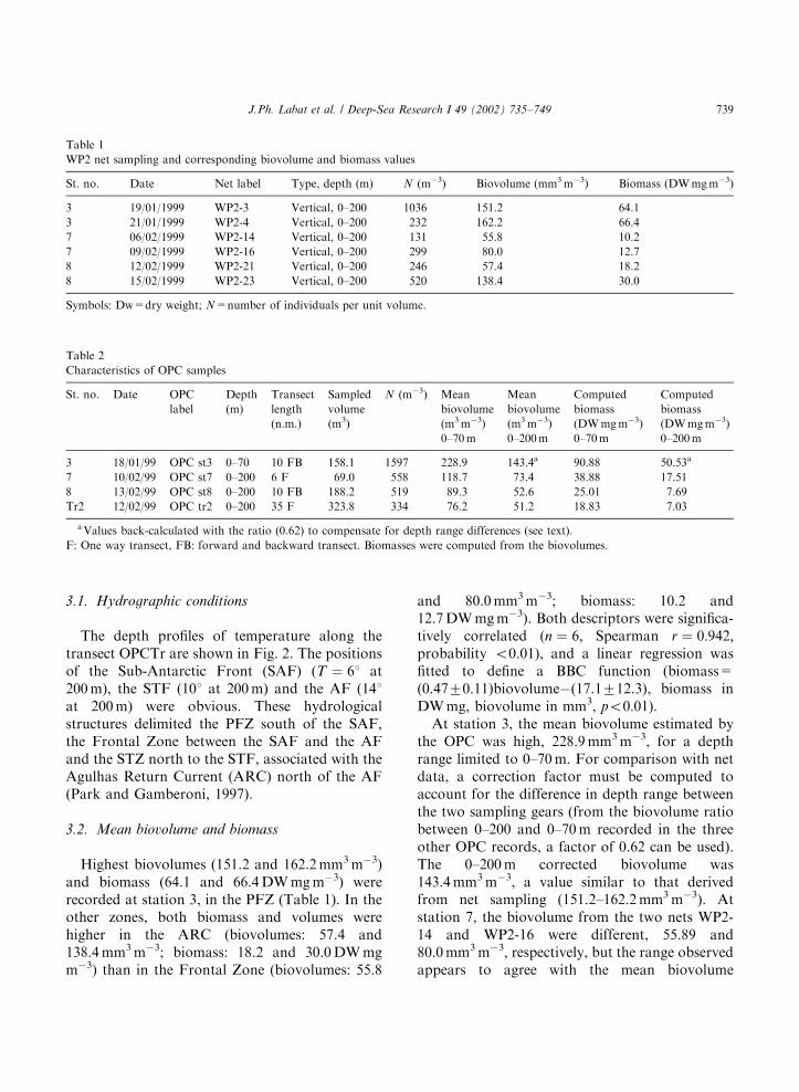
Table 1 gives the characteristics of the netsampling and the Table 2 the characteristics of theOPC transect.

J.Ph. Labat et al. / Deep-Sea Research I 49 (2002) 735–749738

3.1. Hydrographic conditions

The depth profiles of temperature along thetransect OPCTr are shown in Fig. 2. The positionsof the Sub-Antarctic Front (SAF) (T ¼ 61 at200 m), the STF (101 at 200 m) and the AF (141at 200 m) were obvious. These hydrologicalstructures delimited the PFZ south of the SAF,the Frontal Zone between the SAF and the AFand the STZ north to the STF, associated with theAgulhas Return Current (ARC) north of the AF(Park and Gamberoni, 1997).

3.2. Mean biovolume and biomass

Highest biovolumes (151.2 and 162.2 mm3 m�3)and biomass (64.1 and 66.4 DW mg m�3) wererecorded at station 3, in the PFZ (Table 1). In theother zones, both biomass and volumes werehigher in the ARC (biovolumes: 57.4 and138.4 mm3 m�3; biomass: 18.2 and 30.0 DW mgm�3) than in the Frontal Zone (biovolumes: 55.8

and 80.0 mm3 m�3; biomass: 10.2 and12.7 DW mg m�3). Both descriptors were significa-tively correlated (n ¼ 6; Spearman r ¼ 0:942;probability o0.01), and a linear regression wasfitted to define a BBC function (biomass=(0.4770.11)biovolume�(17.1712.3), biomass inDW mg, biovolume in mm3, po0:01).

At station 3, the mean biovolume estimated bythe OPC was high, 228.9 mm3 m�3, for a depthrange limited to 0–70 m. For comparison with netdata, a correction factor must be computed toaccount for the difference in depth range betweenthe two sampling gears (from the biovolume ratiobetween 0–200 and 0–70 m recorded in the threeother OPC records, a factor of 0.62 can be used).The 0–200 m corrected biovolume was143.4 mm3 m�3, a value similar to that derivedfrom net sampling (151.2–162.2mm3 m�3). Atstation 7, the biovolume from the two nets WP2-14 and WP2-16 were different, 55.89 and80.0 mm3 m�3, respectively, but the range observedappears to agree with the mean biovolume

Table 1

WP2 net sampling and corresponding biovolume and biomass values

St. no. Date Net label Type, depth (m) N (m�3) Biovolume (mm3 m�3) Biomass (DWmgm�3)

3 19/01/1999 WP2-3 Vertical, 0–200 1036 151.2 64.1

3 21/01/1999 WP2-4 Vertical, 0–200 232 162.2 66.4

7 06/02/1999 WP2-14 Vertical, 0–200 131 55.8 10.2

7 09/02/1999 WP2-16 Vertical, 0–200 299 80.0 12.7

8 12/02/1999 WP2-21 Vertical, 0–200 246 57.4 18.2

8 15/02/1999 WP2-23 Vertical, 0–200 520 138.4 30.0

Symbols: Dw=dry weight; N=number of individuals per unit volume.

Table 2

Characteristics of OPC samples

St. no. Date OPC

label

Depth

(m)

Transect

length

(n.m.)

Sampled

volume

(m3)

N (m�3) Mean

biovolume

(m3 m�3)

0–70m

Mean

biovolume

(m3 m�3)

0–200m

Computed

biomass

(DWmgm�3)

0–70m

Computed

biomass

(DWmgm�3)

0–200m

3 18/01/99 OPC st3 0–70 10 FB 158.1 1597 228.9 143.4a 90.88 50.53a

7 10/02/99 OPC st7 0–200 6 F 69.0 558 118.7 73.4 38.88 17.51

8 13/02/99 OPC st8 0–200 10 FB 188.2 519 89.3 52.6 25.01 7.69

Tr2 12/02/99 OPC tr2 0–200 35 F 323.8 334 76.2 51.2 18.83 7.03

aValues back-calculated with the ratio (0.62) to compensate for depth range differences (see text).

F: One way transect, FB: forward and backward transect. Biomasses were computed from the biovolumes.

J.Ph. Labat et al. / Deep-Sea Research I 49 (2002) 735–749 739

computed from the corresponding OPC transect,73.3 mm3 m�3. In the station 8/transect 2 area, thedifference in biovolume between the two net haulswas even greater (57.4 and 138.4 mm3 m�3), andboth were larger than the mean biovolumescomputed from the OPC data at OPC st8 andOPC tr2 (52.62 and 51.2 mm3 m�3, respectively).

3.3. Taxonomic composition

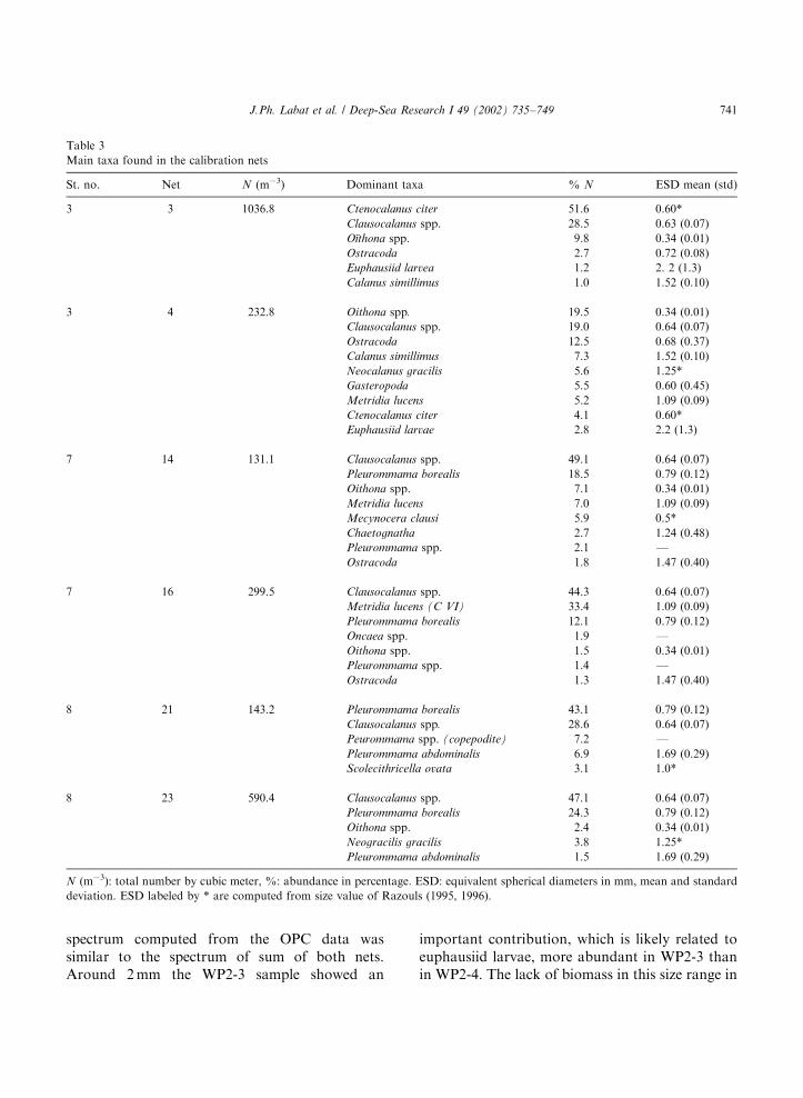
Zooplankton taxonomic composition and ESDof the main species is reported in Table 3.Copepods were the dominant group in all netsamples regardless of the area considered.

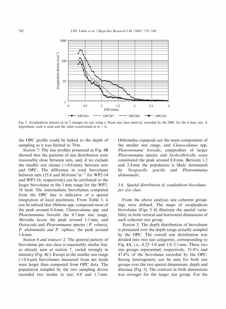
3.4. Number by size classes in the OPC data

The size distribution showed one peak with themaximum number of individuals in the size class0.35 mm (Fig. 3). OPC st3 illustrated the higherabundance in the Sub-Antarctic Zone compared tothe other survey lines with enhanced difference inthe 1–2 mm size range. OPC st8 and OPC tr2corresponded to similar geographical zones andshowed minimum values with almost identical sizeprofiles.

3.5. Distribution of biovolume by size class

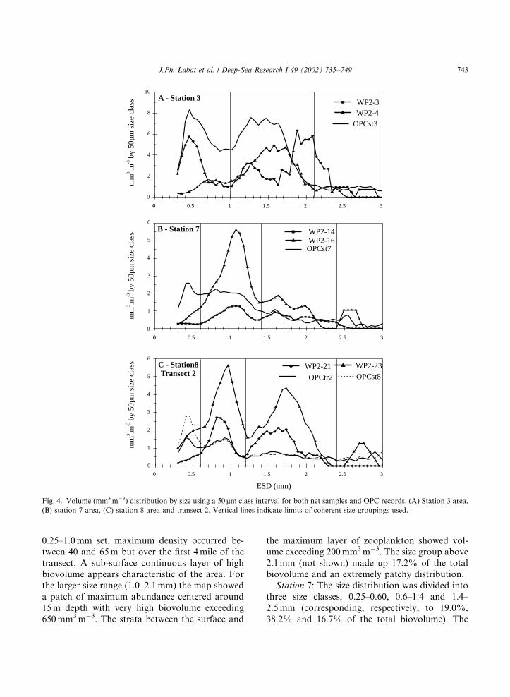
Station 3: Size distribution of biovolume showedimportant differences on the one hand between thetwo nets samples and on the other hand betweenthe net samples and the OPC (Fig. 4A). Netsample WP2-3 and OPC presented a size profilewith a mode around 0.5 mm not seen in the WP2-4net sample. A comparison with the size character-istics and abundance (Table 3), suggested a majorcontribution of the following species: Oithona spp.,Clausocalanus spp. and Ctenocalanus citer. Be-cause the densities observed in the larger sizecategories are relatively similar, the differencebetween WP2-3 and WP2-4 samples can be relatedto the presence of small individuals belonging tothis taxonomic group in WP2-3. The similarity intotal volume (151.2 and 162.2 mm3 m�3) confirmedthat animal concentrations decrease with increas-ing size (1036 n. m.�3 in WP2-3 and 232 n. m.�3 inWP2-4).

In the 1–2 mm range, WP2-3 showed a modearound 1.25 mm ESD, which is masked by abroader peak around 1.6 mm for WP2-4 (Fig. 4A).This size range corresponds to Calanus simillimus

and Neocalanus gracilis as major contributors.Interestingly, within this size range, the size

6 7 8 9

9

10

10

11

11

12

12

12

12

13

13

13

14

14

15.015

15 16.0

16

16

17.0

17

17

18

18

10 20 30 40 50 60 70 80 90 100 110

-150

-100

-50

0

Dep

th (

m)

SAF

STF

AF Agulhas Return Current

Sub AntarcticZone

Polar Frontal Zone

Frontal Zone

Subtropical Zone

44˚49' 44˚00' 43˚11'Distance (nm) Distance (nm) OPC Transect 1 OPC Transect 2

Fig. 2. Temperature profile along the OPC tr1 and OPC tr2 transects, contour levels are given at 0.51C intervals. SAF: Sub-Antarctic

Front (61C at �200m), STF: Sub-Tropical front (101C at �200m), AF: Agulhas Front (141C at �200m). Zone limits from Park and

Gamberoni (1997).

J.Ph. Labat et al. / Deep-Sea Research I 49 (2002) 735–749740

spectrum computed from the OPC data wassimilar to the spectrum of sum of both nets.Around 2mm the WP2-3 sample showed an

important contribution, which is likely related toeuphausiid larvae, more abundant in WP2-3 thanin WP2-4. The lack of biomass in this size range in

Table 3

Main taxa found in the calibration nets

St. no. Net N (m�3) Dominant taxa % N ESD mean (std)

3 3 1036.8 Ctenocalanus citer 51.6 0.60*

Clausocalanus spp. 28.5 0.63 (0.07)

O.ıthona spp. 9.8 0.34 (0.01)

Ostracoda 2.7 0.72 (0.08)

Euphausiid larvea 1.2 2. 2 (1.3)

Calanus simillimus 1.0 1.52 (0.10)

3 4 232.8 Oithona spp. 19.5 0.34 (0.01)

Clausocalanus spp. 19.0 0.64 (0.07)

Ostracoda 12.5 0.68 (0.37)

Calanus simillimus 7.3 1.52 (0.10)

Neocalanus gracilis 5.6 1.25*

Gasteropoda 5.5 0.60 (0.45)

Metridia lucens 5.2 1.09 (0.09)

Ctenocalanus citer 4.1 0.60*

Euphausiid larvae 2.8 2.2 (1.3)

7 14 131.1 Clausocalanus spp. 49.1 0.64 (0.07)

Pleurommama borealis 18.5 0.79 (0.12)

Oithona spp. 7.1 0.34 (0.01)

Metridia lucens 7.0 1.09 (0.09)

Mecynocera clausi 5.9 0.5*

Chaetognatha 2.7 1.24 (0.48)

Pleurommama spp. 2.1 FOstracoda 1.8 1.47 (0.40)

7 16 299.5 Clausocalanus spp. 44.3 0.64 (0.07)

Metridia lucens (C VI) 33.4 1.09 (0.09)

Pleurommama borealis 12.1 0.79 (0.12)

Oncaea spp. 1.9 FOithona spp. 1.5 0.34 (0.01)

Pleurommama spp. 1.4 FOstracoda 1.3 1.47 (0.40)

8 21 143.2 Pleurommama borealis 43.1 0.79 (0.12)

Clausocalanus spp. 28.6 0.64 (0.07)

Peurommama spp. (copepodite) 7.2 FPleurommama abdominalis 6.9 1.69 (0.29)

Scolecithricella ovata 3.1 1.0*

8 23 590.4 Clausocalanus spp. 47.1 0.64 (0.07)

Pleurommama borealis 24.3 0.79 (0.12)

Oithona spp. 2.4 0.34 (0.01)

Neogracilis gracilis 3.8 1.25*

Pleurommama abdominalis 1.5 1.69 (0.29)

N (m�3): total number by cubic meter, %: abundance in percentage. ESD: equivalent spherical diameters in mm, mean and standard

deviation. ESD labeled by * are computed from size value of Razouls (1995, 1996).

J.Ph. Labat et al. / Deep-Sea Research I 49 (2002) 735–749 741

the OPC profile could be linked to the depth ofsampling as it was limited to 70 m.

Station 7: The size profiles presented in Fig. 4Bshowed that the patterns of size distribution werereasonably close between nets, and, if we excludethe smaller size classes (o0.6 mm), between netsand OPC. The difference in total biovolumebetween nets (55.8 and 80.0 mm3 m�3 for WP2-14and WP2-16, respectively) can be attributed to thelarger biovolume in the 1 mm range for the WP2-16 haul. The intermediate biovolumes computedfrom the OPC line is indicative of a spatialintegration of local patchiness. From Table 3, itcan be infered that Oithona spp. composed most ofthe peak around 0.4 mm, Clausocalanus spp. andPleurommama borealis the 0.7 mm size range,Metridia lucens the peak around 1.1 mm, andOstracoda and Pleurommama species (P. robusta,P. abdominalis and P. xiphias) the peak around1.6 mm.

Station 8 and transect 2: The general pattern ofbiovolume per size class is reasonably similar but,as already seen at station 7, varied strongly inintensity (Fig. 4C). Except in the smaller size range(o0.6 mm) biovolumes measured from net haulswere larger than computed from OPC data. Thepopulation sampled by the two sampling devicerecorded two modes in size, 0.8 and 1.7 mm.

Oithonidae copepods are the main components ofthe smaller size range, and Clausocalanus spp,Pleurommama borealis, copepodites of largerPleurommama species and Scolecithricella ovata

constituted the peak around 0.8 mm. Between 1.2and 2.4 mm the population is likely dominatedby Neogracilis gracilis and Pleurommama

abdominalis.

3.6. Spatial distribution of zooplankton biovolume

per size class

From the above analyses size coherent group-ings were defined. The maps of zooplanktonbiovolume (Figs. 5–8) illustrate the spatial varia-bility in both vertical and horizontal dimensions ofeach coherent size group.

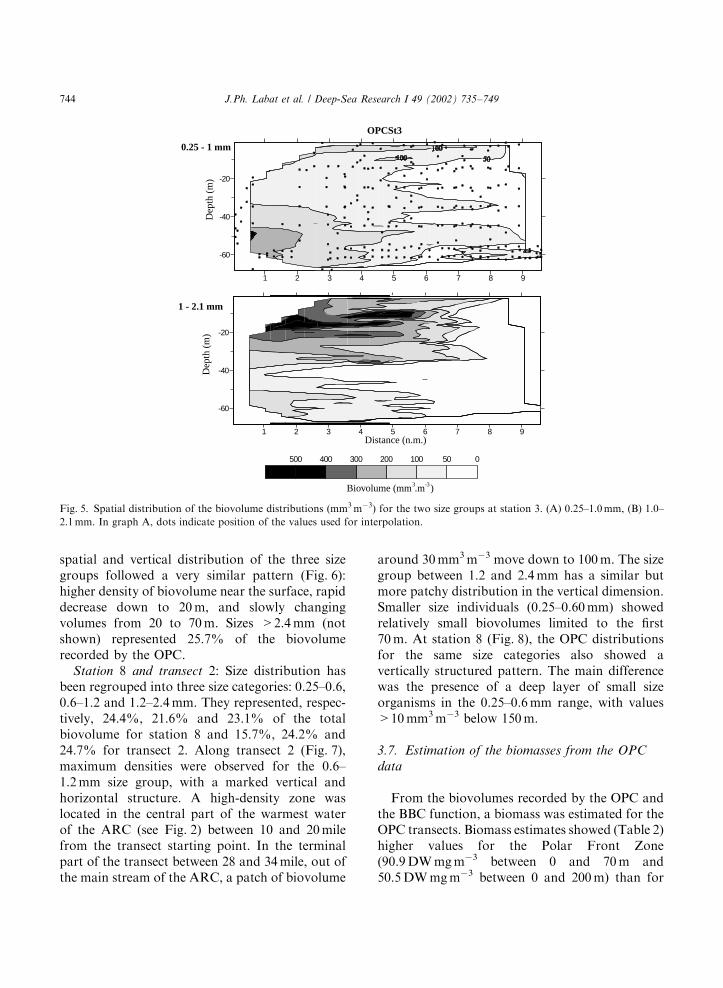
Station 3: The depth distribution of biovolumeis presented over the depth range actually sampledby the OPC. The overall size distribution wasdivided into two size categories, corresponding toFig. 4A, i.e., 0.25–1.0 and 1.0–2.1 mm. These twosize groups represented, respectively, 35.4% and47.4% of the biovolume recorded by the OPC.Strong heterogeneity can be seen for both sizegroups over the two spatial dimensions, depth anddistance (Fig. 5). The contrast in both dimensionswas stronger for the larger size group. For the

1

10

100

1000

Zoo

plan

kton

den

sity

(n.

m)

-3

0 0.5 1 1.5 2 2.5 3 ESD (mm)

OPCSt3 OPCSt7 OPCSt8 OPCTr2

Fig. 3. Zooplankton density (n. m.3) changes by size using a 50 mm size class interval, recorded by the OPC for the 4 data sets. A

logarithmic scale is used and the value transformed in (n þ 1).

J.Ph. Labat et al. / Deep-Sea Research I 49 (2002) 735–749742

0.25–1.0 mm set, maximum density occurred be-tween 40 and 65 m but over the first 4 mile of thetransect. A sub-surface continuous layer of highbiovolume appears characteristic of the area. Forthe larger size range (1.0–2.1 mm) the map showeda patch of maximum abundance centered around15 m depth with very high biovolume exceeding650 mm3 m�3. The strata between the surface and

the maximum layer of zooplankton showed vol-ume exceeding 200 mm3 m�3. The size group above2.1 mm (not shown) made up 17.2% of the totalbiovolume and an extremely patchy distribution.

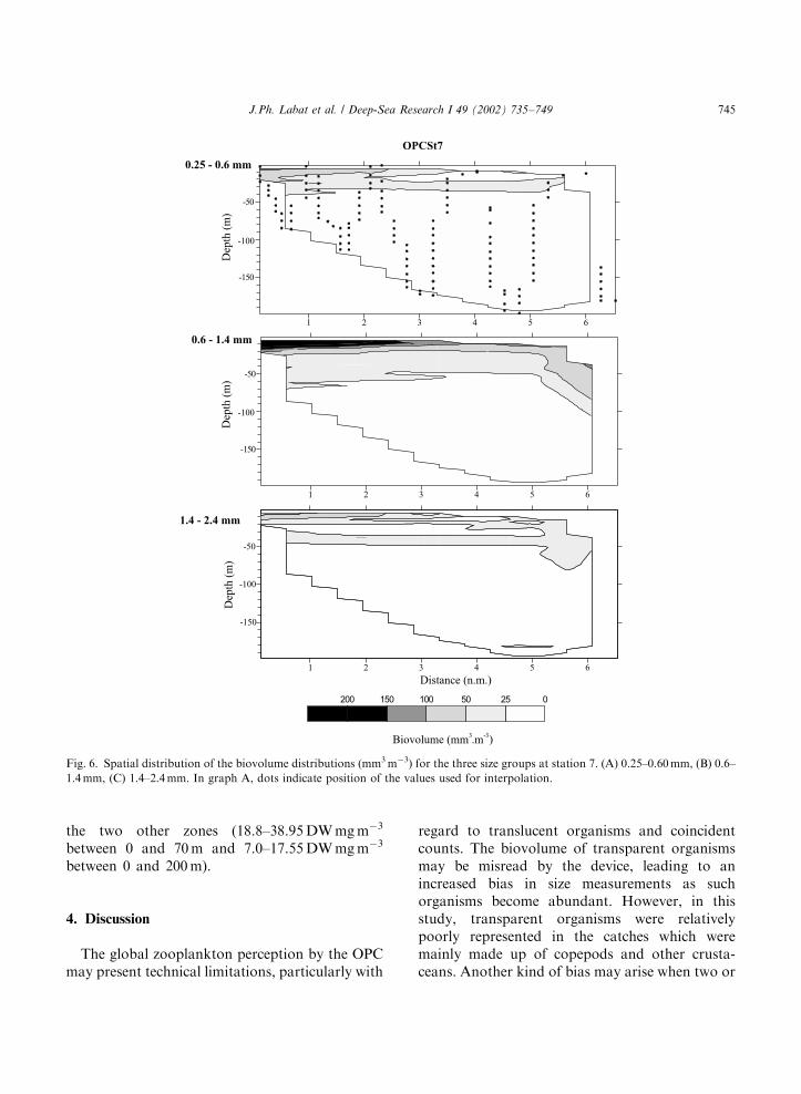
Station 7: The size distribution was divided intothree size classes, 0.25–0.60, 0.6–1.4 and 1.4–2.5 mm (corresponding, respectively, to 19.0%,38.2% and 16.7% of the total biovolume). The

0

2

4

6

8

10

0 0 0.5 1 1.5 2 2.5 3

A - Station 3

0 0 0.5 1 1.5 2 2.5 3

B - Station 7

0

1

2

3

4

5

6

0 0.5 1 1.5 2 2.5 3

C - Station8Transect 2

mm

.m b

y 50

µm s

ize

clas

s3

-3m

m.m

by

50µm

siz

e cl

ass

3-3

mm

.m b

y 50

µm s

ize

clas

s3

-3

ESD (mm)

WP2-3WP2-4

OPCst3

OPCst7

WP2-14WP2-16

WP2-21 WP2-23

OPCtr2 OPCst8

0

1

2

3

4

5

6

Fig. 4. Volume (mm3 m�3) distribution by size using a 50mm class interval for both net samples and OPC records. (A) Station 3 area,

(B) station 7 area, (C) station 8 area and transect 2. Vertical lines indicate limits of coherent size groupings used.

J.Ph. Labat et al. / Deep-Sea Research I 49 (2002) 735–749 743

spatial and vertical distribution of the three sizegroups followed a very similar pattern (Fig. 6):higher density of biovolume near the surface, rapiddecrease down to 20 m, and slowly changingvolumes from 20 to 70 m. Sizes >2.4 mm (notshown) represented 25.7% of the biovolumerecorded by the OPC.

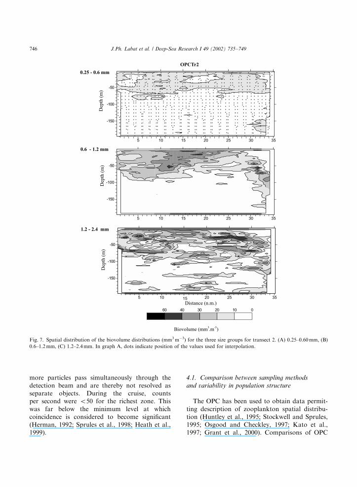
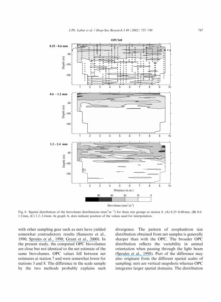
Station 8 and transect 2: Size distribution hasbeen regrouped into three size categories: 0.25–0.6,0.6–1.2 and 1.2–2.4mm. They represented, respec-tively, 24.4%, 21.6% and 23.1% of the totalbiovolume for station 8 and 15.7%, 24.2% and24.7% for transect 2. Along transect 2 (Fig. 7),maximum densities were observed for the 0.6–1.2 mm size group, with a marked vertical andhorizontal structure. A high-density zone waslocated in the central part of the warmest waterof the ARC (see Fig. 2) between 10 and 20 milefrom the transect starting point. In the terminalpart of the transect between 28 and 34 mile, out ofthe main stream of the ARC, a patch of biovolume

around 30mm3 m�3 move down to 100 m. The sizegroup between 1.2 and 2.4 mm has a similar butmore patchy distribution in the vertical dimension.Smaller size individuals (0.25–0.60mm) showedrelatively small biovolumes limited to the first70 m. At station 8 (Fig. 8), the OPC distributionsfor the same size categories also showed avertically structured pattern. The main differencewas the presence of a deep layer of small sizeorganisms in the 0.25–0.6 mm range, with values>10 mm3 m�3 below 150 m.

3.7. Estimation of the biomasses from the OPC

data

From the biovolumes recorded by the OPC andthe BBC function, a biomass was estimated for theOPC transects. Biomass estimates showed (Table 2)higher values for the Polar Front Zone(90.9DW mg m�3 between 0 and 70 m and50.5 DW mg m�3 between 0 and 200 m) than for

0.25 - 1 mm

1 - 2.1 mm

Biovolume (mm .m )3 -3

1 2 3 4 5 6 7 8 9

-60

-40

-20

1 2 3 4 5 6 7 8 9Distance (n.m.)

-60

-40

-20

050100200300400500

Dep

th (

m)

Dep

th (

m)

OPCSt3

Fig. 5. Spatial distribution of the biovolume distributions (mm3 m�3) for the two size groups at station 3. (A) 0.25–1.0mm, (B) 1.0–

2.1mm. In graph A, dots indicate position of the values used for interpolation.

J.Ph. Labat et al. / Deep-Sea Research I 49 (2002) 735–749744

the two other zones (18.8–38.95 DW mg m�3

between 0 and 70 m and 7.0–17.55 DW mg m�3

between 0 and 200 m).

4. Discussion

The global zooplankton perception by the OPCmay present technical limitations, particularly with

regard to translucent organisms and coincidentcounts. The biovolume of transparent organismsmay be misread by the device, leading to anincreased bias in size measurements as suchorganisms become abundant. However, in thisstudy, transparent organisms were relativelypoorly represented in the catches which weremainly made up of copepods and other crusta-ceans. Another kind of bias may arise when two or

1 2 3 4 5 6

Distance (n.m.)

-150

-100

-50

0.25 - 0.6 mm

0.6 - 1.4 mm

1.4 - 2.4 mm

1 2 3 4 5 6

-150

-50

1 2 3 4 5 6

-150

-50

Biovolume (mm .m )3 -3

02550100150200

Dep

th (

m)

Dep

th (

m)

Dep

th (

m)

OPCSt7

-100

-100

Fig. 6. Spatial distribution of the biovolume distributions (mm3 m�3) for the three size groups at station 7. (A) 0.25–0.60mm, (B) 0.6–

1.4mm, (C) 1.4–2.4mm. In graph A, dots indicate position of the values used for interpolation.

J.Ph. Labat et al. / Deep-Sea Research I 49 (2002) 735–749 745

more particles pass simultaneously through thedetection beam and are thereby not resolved asseparate objects. During the cruise, countsper second were o50 for the richest zone. Thiswas far below the minimum level at whichcoincidence is considered to become significant(Herman, 1992; Sprules et al., 1998; Heath et al.,1999).

4.1. Comparison between sampling methods

and variability in population structure

The OPC has been used to obtain data permit-ting description of zooplankton spatial distribu-tion (Huntley et al., 1995; Stockwell and Sprules,1995; Osgood and Checkley, 1997; Kato et al.,1997; Grant et al., 2000). Comparisons of OPC

5 10 15 20 25 30 35

-150

-100

-50

5 10 15 20 25 30 35

-150

-100

-50

5 10 15 20 25 30 35

Distance (n.m.)

-150

-100

-50

01020304060

Biovolume (mm .m )3 -3

0.25 - 0.6 mm

0.6 - 1.2 mm

1.2 - 2.4 mm

Dep

th (

m)

Dep

th (

m)

Dep

th (

m)

OPCTr2

Fig. 7. Spatial distribution of the biovolume distributions (mm3 m�3) for the three size groups for transect 2. (A) 0.25–0.60mm, (B)

0.6–1.2mm, (C) 1.2–2.4mm. In graph A, dots indicate position of the values used for interpolation.

J.Ph. Labat et al. / Deep-Sea Research I 49 (2002) 735–749746

with other sampling gear such as nets have yieldedsomewhat contradictory results (Sameoto et al.,1990; Sprules et al., 1998; Grant et al., 2000). Inthe present study, the computed OPC biovolumesare close but not identical to the net estimate of thesame biovolumes. OPC values fell between netestimates at station 7 and were somewhat lower forstations 3 and 8. The difference in the scale sampleby the two methods probably explains such

divergence. The pattern of zooplankton sizedistribution obtained from net samples is generallysharper than with the OPC. The broader OPCdistribution reflects the variability in animalorientation when passing through the light beam(Sprules et al., 1998). Part of the difference mayalso originate from the different spatial scales ofsampling: nets are vertical snapshots whereas OPCintegrates larger spatial domains. The distribution

1 2 3 4 5 6 7 8 9 10

-150

-50

1 2 3 4 5 6 7 8 9 10

-150

-100

-50

1 2 3 4 5 6 7 8 9 10

-150

-50

Biovolume (mm .m )3 -3

010204060

Dep

th (

m)

Dep

th (

m)

Dep

th (

m)

0.25 - 0.6 mm

0.6 - 1.2 mm

1.2 - 2.4 mm

Distance (n.m.)

-100

OPCSt8

-100

Fig. 8. Spatial distribution of the biovolume distributions (mm3 m�3) for three size groups at station 8. (A) 0.25–0.60mm, (B) 0.6–

1.2mm, (C) 1.2–2.4mm. In graph A, dots indicate position of the values used for interpolation.

J.Ph. Labat et al. / Deep-Sea Research I 49 (2002) 735–749 747

recorded at station 3 provides a good example witha strong divergence in the size distibution betweenthe two nets, which agree with the OPC distribu-tion when the mean of the two nets is considered.This phenomenon is particularly obvious at thisstation where the zooplankton distribution ispatchiest in both dimensions. Another key featureof the OPC records is the better representation ofthe smaller sizes of zooplankton with a constantmode below 0.5 mm, corresponding mainly to thegroup of small Oithonidae.

4.2. OPC biomass estimate

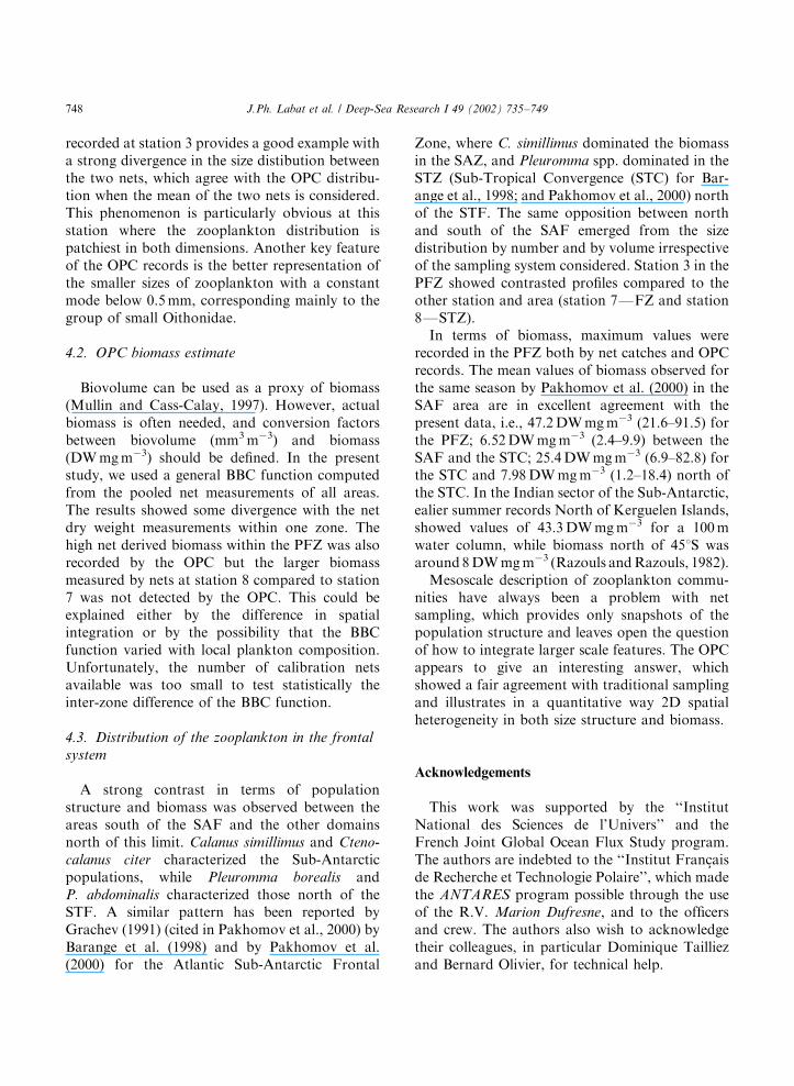
Biovolume can be used as a proxy of biomass(Mullin and Cass-Calay, 1997). However, actualbiomass is often needed, and conversion factorsbetween biovolume (mm3 m�3) and biomass(DW mg m�3) should be defined. In the presentstudy, we used a general BBC function computedfrom the pooled net measurements of all areas.The results showed some divergence with the netdry weight measurements within one zone. Thehigh net derived biomass within the PFZ was alsorecorded by the OPC but the larger biomassmeasured by nets at station 8 compared to station7 was not detected by the OPC. This could beexplained either by the difference in spatialintegration or by the possibility that the BBCfunction varied with local plankton composition.Unfortunately, the number of calibration netsavailable was too small to test statistically theinter-zone difference of the BBC function.

4.3. Distribution of the zooplankton in the frontal

system

A strong contrast in terms of populationstructure and biomass was observed between theareas south of the SAF and the other domainsnorth of this limit. Calanus simillimus and Cteno-

calanus citer characterized the Sub-Antarcticpopulations, while Pleuromma borealis andP. abdominalis characterized those north of theSTF. A similar pattern has been reported byGrachev (1991) (cited in Pakhomov et al., 2000) byBarange et al. (1998) and by Pakhomov et al.(2000) for the Atlantic Sub-Antarctic Frontal

Zone, where C. simillimus dominated the biomassin the SAZ, and Pleuromma spp. dominated in theSTZ (Sub-Tropical Convergence (STC) for Bar-ange et al., 1998; and Pakhomov et al., 2000) northof the STF. The same opposition between northand south of the SAF emerged from the sizedistribution by number and by volume irrespectiveof the sampling system considered. Station 3 in thePFZ showed contrasted profiles compared to theother station and area (station 7FFZ and station8FSTZ).

In terms of biomass, maximum values wererecorded in the PFZ both by net catches and OPCrecords. The mean values of biomass observed forthe same season by Pakhomov et al. (2000) in theSAF area are in excellent agreement with thepresent data, i.e., 47.2 DW mg m�3 (21.6–91.5) forthe PFZ; 6.52 DW mg m�3 (2.4–9.9) between theSAF and the STC; 25.4 DW mg m�3 (6.9–82.8) forthe STC and 7.98 DW mg m�3 (1.2–18.4) north ofthe STC. In the Indian sector of the Sub-Antarctic,ealier summer records North of Kerguelen Islands,showed values of 43.3 DW mg m�3 for a 100 mwater column, while biomass north of 451S wasaround 8DW mg m�3 (Razouls andRazouls, 1982).

Mesoscale description of zooplankton commu-nities have always been a problem with netsampling, which provides only snapshots of thepopulation structure and leaves open the questionof how to integrate larger scale features. The OPCappears to give an interesting answer, whichshowed a fair agreement with traditional samplingand illustrates in a quantitative way 2D spatialheterogeneity in both size structure and biomass.

Acknowledgements

This work was supported by the ‘‘InstitutNational des Sciences de l’Univers’’ and theFrench Joint Global Ocean Flux Study program.The authors are indebted to the ‘‘Institut Fran-caisde Recherche et Technologie Polaire’’, which madethe ANTARES program possible through the useof the R.V. Marion Dufresne, and to the officersand crew. The authors also wish to acknowledgetheir colleagues, in particular Dominique Tailliezand Bernard Olivier, for technical help.

J.Ph. Labat et al. / Deep-Sea Research I 49 (2002) 735–749748

References

Barange, M., Pakhomov, E.A., Perissinotto, R., Froneman,

P.W., Verheye, H.M., Taunton-Clark, J., Lucas, M.I., 1998.

Pelagic community structure of the subtropical convergence

region south of Africa and in the mid-Atlantic Ocean. Deep-

Sea Research I 45, 1663–1687.

Currie, W.J.S., Claereboudt, M.R., Roff, J.C., 1998. Gaps and

patches in the ocean: a one-dimensional analysis of

planktonic distributions. Marine Ecological Progress Series

171, 15–21.

Grachev, D.G., 1991. Frontal zone influences on the distribu-

tion of different zooplankton groups in the central part

Indian sector of the Southern Ocean. In: Samoila, M.S.,

Shumkova, S.O. (Eds.), Ecology of Commercial Marine

Hydrobionts. TINRO Press, Vladivostok, pp. 19–21.

(in Russian).

Grant, S., Ward, P., Murphy, E., Bone, D., Abott, S., 2000.

Field comparison of an LHPR net sampling system and an

optical plankton counter (OPC) in the Southern Ocean.

Journal of Plankton Research 22, 619–638.

Heath, M.R., Dunn, J., Fraser, J.G., Hay, S.J., Madden, H.,

1999. Field calibration of the optical plankton counter with

respect to Calanus finmarchicus. Fisheries and Oceanogra-

phy 8 (Suppl. 1), 13–24.

Herman, A.W., 1988. Simultaneaous measurement of zoo-

plankton and light attenuance with a new optical plankton

counter. Continental Shelf Research 8, 205–221.

Herman, A.W., 1992. Design and calibration of a new optical

plankton counter capable of sizing small zooplankton.

Deep-Sea Research I 39, 395–415.

Herman, A.W., Cochrane, N.A., Sameoto, D.D., 1993. Detec-

tion and abundance estimation of euphausiids using an

optical plankton counter. Marine Ecological Progress Series

94, 165–173.

Huntley, M.E., Zhou, M., Nordhausen, W., 1995. Mesoscale

distribution of zooplankton in the California current in late

spring, observed by optical plankton counter. Journal of

Marine Research 53, 647–674.

Huntley, M.E., Gonz!alez, A., Zhu, Y., Zhou, M., Irigoyen, X.,

2000. Zooplankton dynamics in a mesoscale eddy-jet system

off California. Marine Ecological Progress Series 201,

165–178.

Kato, S., Ito, N., Gunji, K., Aoki, I., Nishida, S., 1997. Small-

and Mesoscale zooplankton distributions in the Kuroshio

Area. JAMSTECR 36, 129–136.

Mullin, M.M., Cass-Calay, S.L., 1997. Vertical distributions of

zooplankton and larvae of the Pacific hake (whiting),

Merluccius productus, in the California current system.

CalcCOFI Report 38, 127–136.

Nagata, Y., Michida, Y., Umimura, Y., 1988. Variation of

positions and structures of the oceanics fronts in the Indian

Ocean sector of the Southern Ocean in the period from

1965–1987. In: Sahrhage, D. (Ed.), Antarctic Ocean and

Resources Variability. Springer, Berlin, pp. 92–98.

Osgood, K.E., Checkley Jr., D.M., 1997. Observations of deep

aggregations of Calanus pacificus in the Santa Barbara

Basin. Limnology and Oceanography 42, 997–1001.

Pakhomov, E.A., Perissinotto, R., McQuaid, C.D., Froneman,

P.W., 2000. Zooplankton structure and grazing in the

Atlantic sector of the Southern Ocean in late austral

summer 1993. Part 1. Ecological zonation. Deep-Sea

Research I 47, 1663–1686.

Park, Y-H., Gamberoni, L., 1997. Cross-frontal exchange of

Antartic intermediate water and Antartic bottom water in

the Crozet Basin. Deep-Sea Research II 44, 963–986.

Razouls, C., 1995. Diversit!e et r!epartition g!eographique chez

les cop!epodes p!elagiques. 1-Calanoida. Annales de l’Institut

oc!eanographique N.S 71, 81–404.

Razouls, C., 1996. Diversit!e et r!epartition g!eographique chez

les cop!epodes p!elagiques 2-Platycopioida, Misophrioida,

Mormonilloida, Cyclopoida, Poecilostomatoida, Siphonos-

tomatoida, Harpacticoida, Monstrilloida. Annales de l’In-

stitut oc!eanographique N. S. 72 (1), 1–14.

Razouls, C., Razouls, S., 1982. Element du bilan energ!etique du

mesozooplancton antarctique. CNFRA 53, 131–141.

Sameoto, D., Cochrane, N., Herman, A., 1990. Use of multiple

frequency acoustics and other methods in estimating

copepod and euphausiid abundances. ICES, CM 1990/

L:81, pp. 1–9.

Sheldon, R.W., Prakash, A., Sutcliffe Jr., W.H., 1972. The size

distribution of particles in the ocean. Limnology and

Oceanography 17, 327–340.

Sprules, W.G., Jin, E.H., Herman, A.W., Stockwell, J.D., 1998.

Calibration of an optical plankton counter for use in

freshwater. Limnology and Oceanography 43, 726–733.

Stockwell, J.D., Sprules, J.D., 1995. Spatial and temporal

patterns of zooplankton biomass in Lake Erie. ICES

Journal of Marine Science 52, 557–567.

Vidal, J., Whitledge, T.E., 1982. Rates of metabolism of

planktonic crustaceans as related to body weight and temp-

erature of habitat. Journal of Plankton Research 4, 77–84.

Wieland, K., Petersen, D., Schnack, D., 1997. Estimates of

zooplankton abundance and size distribution wih the

optical plankton counter (OPC). Archives of Fisheries and

Marine Research 45, 271–280.

J.Ph. Labat et al. / Deep-Sea Research I 49 (2002) 735–749 749