Habitat modeling in high-gradient streams: the mesoscale approach and application

Ecological Applications, 24(4), 2014, pp. 844–861� 2014 by the Ecological Society of America

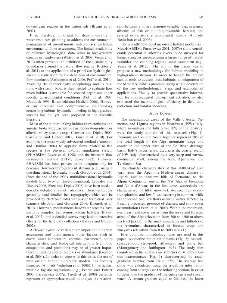
Habitat modeling in high-gradient streams: the mesoscale approachand application

PAOLO VEZZA,1,2,6 PIOTR PARASIEWICZ,3,4 MICHELE SPAIRANI,5 AND CLAUDIO COMOGLIO1

1Department of Environment, Land and Infrastructure Engineering, Politecnico di Torino, C.so Duca degli Abruzzi 24,10129 Torino, Italy

2Institut d’Investigacio per a la Gestio Integrada de Zones Costaneres Universitat Politecnica de Valencia, Valencia, Spain3Rushing Rivers Institute, Amherst, Massachusetts 01002 USA

4S. Sakowicz Inland Fisheries Institute, Zabieniec, Poland5FLUME s.r.l., Aosta, Italy

Abstract. This study aimed to set out a new methodology for habitat modeling in high-gradient streams. The methodology is based on the mesoscale approach of the MesoHABSIMsimulation system and can support the definition and assessment of environmental flow andhabitat restoration measures. Data from 40 study sites located within the mountainous areasof the Valle d’Aosta, Piemonte and Liguria regions (Northwest Italy) were used in theanalysis. To adapt MesoHABSIM to high-gradient streams, we first modified the datacollection strategy to address the challenging conditions of surveys by using GIS and mobilemapping techniques. Secondly, we built habitat suitability models at a regional scale to enabletheir transferability among different streams with different morphologies. Thirdly, due to theabsence of stream gauges in headwaters, we proposed a possible way to simulate flow timeseries and, therefore, generate habitat time series. The resulting method was evaluated in termsof time expenditure for field data collection and habitat-modeling potentials, and it representsa specific improvement of the MesoHABSIM system for habitat modeling in high-gradientstreams, where other commonly used methodologies can be unsuitable. Through itsapplication at several study sites, the proposed methodology adapted well to high-gradientstreams and allowed the: (1) definition of fish habitat requirements for many streamssimultaneously, (2) modeling of habitat variation over a range of discharges, and (3)determination of environmental standards for mountainous watercourses.

Key words: brown trout; environmental flows; GIS; high-gradient streams; hydropower; marble trout;mesohabitat; mesoscale; mountain streams; Salmo; small dams.

INTRODUCTION

Mountainous high-gradient streams are increasingly

being exploited by water abstractions, diversions, and

small hydroelectric dams (e.g., Horne et al. 2004,

Anderson et al. 2006a, b, Zimmerman and Lester 2006,

Marnezy 2008, CIPRA 2010, McLarney et al. 2010,

GIM-UNDP 2011). Several studies have shown that

many types of flow alteration (e.g., magnitude, frequen-

cy, and timing) modify the aquatic and riparian habitat

and induce a variety of ecological responses (Poff and

Zimmerman 2010).

High-gradient streams are generally low-order water-

courses or headwaters and are defined as having from

moderate to quick flow with some turbulent water (e.g.,

MNHESP 1999). The stream morphology is usually

characterized by scoured channels on moderate to steep

slopes with abrupt drops, and boulders, cobbles, gravel,

and sand substrates. In addition to pools, glides, and

riffles, which are common units in channels with low to

moderate gradients, cascades, rapids, and step-pools are

typical channel hydromorphologic units (HMUs) in

these particular watercourses (Halwas and Church

2002).

Since high-gradient streams generally have small

dimensions and are located in remote sites, they are

characterized by low or no human impact and have high

ecological value. Moreover, due to their limited dis-

charges, they can be more susceptible even to small

water withdrawals and management practices. However,

information about the impacts of water abstractions is

particularly scarce for these small streams, and more

research is needed to investigate the effects of flow

reduction on instream environments (Dewson 2007).

Many of these high-gradient streams can support

different fish species whose conservation status is of

community (e.g., the European Habitats Directive 1992/

42/EEC, for marble trout, Salmo marmoratus) and/or

local interest (e.g., brown trout, Salmo trutta fario;

Vezza et al. 2012a). Furthermore, mountainous high-

gradient streams and headwaters are also an important

source of inorganic and organic matter for the

Manuscript received 19 November 2011; revised 27 June2013; accepted 10 September 2013; final version received 2October 2013. Corresponding Editor: A. K. Ward.

6 E-mail: [email protected]

844

downstream reaches in the watersheds (Bryant et al.

2007).

It is, therefore, important for decision-making in

water resources planning to address the environmental

management of mountainous watercourses, including

environmental flows assessment. The limited availability

of reference hydrological data series in high-gradient

streams or headwaters (Watson et al. 2009, Vezza et al.

2010) often prevents the definition of the sustainability

boundaries around the natural flow regime (Richter et

al. 2011) or the application of a priori eco-hydrological

stream classification for the definition of environmental

flow standards (Arthington et al. 2006, Poff et al. 2010).

Modeling the channel hydro-morphology and its rela-

tions with stream biota is then needed to evaluate how

much habitat is available for selected organisms under

specific environmental conditions (Poff et al. 1997,

Maddock 1999, Rosenfield and Hatfield 2006). Howev-

er, an adequate and comprehensive methodology

concerning habitat–hydraulic modeling in high-gradient

streams has not yet been proposed in the scientific

literature.

Most of the studies linking habitat characteristics and

aquatic biota were carried out in moderate-gradient or

alluvial valley streams (e.g., Crowder and Diplas 2000,

Covington and Hubert 2003, Hauer et al. 2010). For

example, the most widely advocated method (Acreman

and Dunbar 2004) to appraise flows related to fish

species is the physical habitat simulation system

(PHABSIM; Bovee et al. 1998) and the instream flow

incremental method (IFIM; Bovee 1982). However,

PHABSIM has been proven to be adequate only for

perennial low/moderate-gradient streams (e.g., using a

one-dimensional hydraulic model; Gordon et al. 2004).

Since the end of the 1990s, multidimensional hydraulic

models (e.g., two- or three-dimensional; Crowder and

Displas 2006, Shen and Diplas 2008) have been used to

describe detailed channel hydraulics. These techniques

generally need detailed bed topography, which can be

provided by electronic total stations or terrestrial laser

scanners (de Jalon and Gortazar 2006, Kozarek et al.

2010). However, mountainous headwater streams have

spatially complex, hydro-morphologic habitats (Bryant

et al. 2007), and a detailed survey may lead to extensive

efforts for the field data collection (Halwas and Church

2002).

Although hydraulic variables are important in habitat

assessment and maintenance, other factors such as

cover, water temperature, chemical parameters, shore

characteristics, and biological interactions (e.g., food

competition and predation) may be of greater impor-

tance in limiting species biomass or abundance (Gordon

et al. 2004). In order to cope with this issue, the use of

multivariate habitat suitability models has recently

increased (Ahmadi-Nedushan et al. 2006). In particular,

multiple logistic regressions (e.g., Pearce and Ferrier

2000, Parasiewicz 2007a, Tirelli et al. 2009) currently

represent an appropriate model to analyze the relation-

ship between a binary response variable (e.g., presence/

absence of fish or suitable/unsuitable habitat) and

several explanatory environmental factors (Ahmadi-

Nedushan et al. 2006).

The recently developed mesoscale habitat models (i.e.,

MesoHABSIM; Parasiewicz 2001, 2007a) show consid-

erable potential in allowing rivers to be surveyed for

longer stretches encompassing a larger range of habitat

variables and enabling regional-scale assessment (e.g.,

Vezza et al. 2012a). The aim of this paper was to

propose a new methodology for habitat modeling in

high-gradient streams. In order to handle the present

lack of tools to address these habitats, an adaptation of

the MesoHABSIM is presented along with a description

of the key methodological steps and examples of

applications. Finally, to provide quantitative informa-

tion for environmental management activities, we also

evaluated the methodological efficiency in field data

collection and habitat modeling.

STUDY DOMAIN

The mountainous areas of the Valle d’Aosta, Pie-

monte, and Liguria regions in Northwest (NW) Italy,

where mountains and hills cover 60% of the territory,

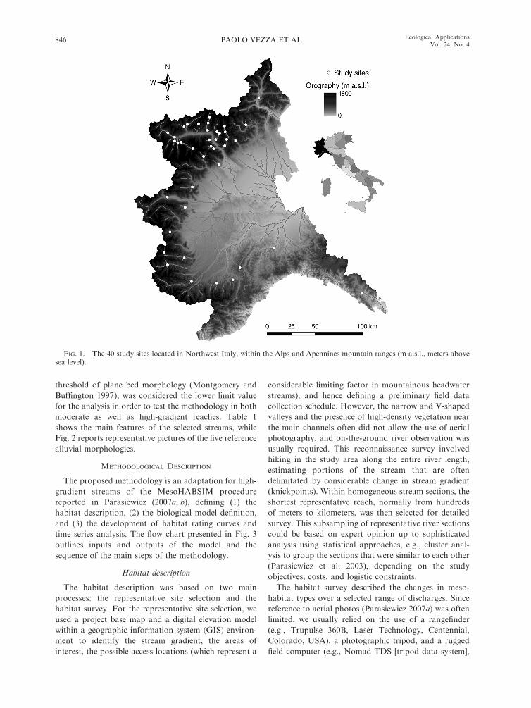
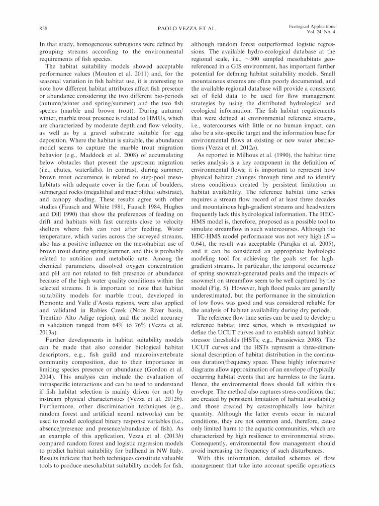
were the study domain of this research (Fig. 1).

Piemonte and Valle d’Aosta together represent 28% of

the total length of the Alps mountain range and

constitute the upper part of the Po River drainage

basin, Italy’s largest river. Liguria is the coastal region

of NW Italy, characterized by a very steep and narrow

continental shelf, among the Alps, Apennines, and

Tyrrhenian Sea.

The climatic characteristics of this 34 000-km2 area

vary from the Apennine–Mediterranean climate in

Liguria and southeastern hills of Piemonte, to the

Alpine–Continental one in the NW Alps of Piemonte

and Valle d’Aosta; in the first zone, watersheds are

characterized by little snowpack storage, high evapo-

transpiration, and low flows occurring in summer, while

in the second one, low flows occur in winter affected by

freezing processes, presence of glaciers, and snow cover

accumulation (Vezza et al. 2009). Within the mountain-

ous areas, land cover varies from the rocky and forested

areas of the Alps (elevation from 300 to 4800 m above

sea level [a.s.l.]), to the small mountains and hillsides of

the Apennines characterized by forests, crops and

vineyards (elevation from 0 to 2000 m a.s.l.).

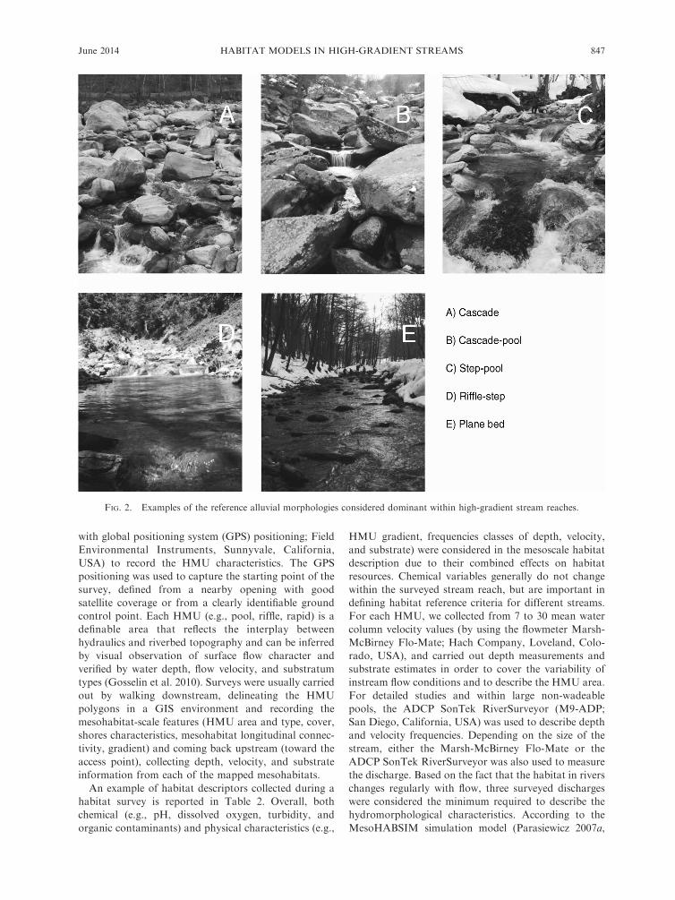
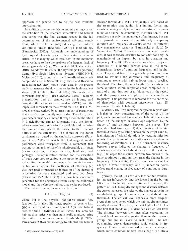
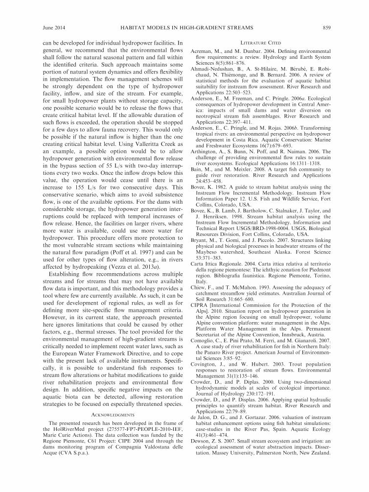
Five dominant morphology types are used in this

paper to describe mountain streams (Fig. 2): cascade,

cascade-pool, step-pool, riffle-step, and plane bed

(Montgomery and Buffington 1997). The study sites

considered in the analysis are stretches of 40 mountain-

ous watercourses (Fig. 1) characterized by reach

gradients varying from 2% to 22%. The average bed

slope was calculated using the available information

coming from surveys (see the following section) in order

to determine the gradient of the entire surveyed stream

reach. A stream gradient equal to 2%, i.e., the lower

June 2014 845HABITAT MODELS IN HIGH-GRADIENT STREAMS

threshold of plane bed morphology (Montgomery and

Buffington 1997), was considered the lower limit value

for the analysis in order to test the methodology in both

moderate as well as high-gradient reaches. Table 1

shows the main features of the selected streams, while

Fig. 2 reports representative pictures of the five reference

alluvial morphologies.

METHODOLOGICAL DESCRIPTION

The proposed methodology is an adaptation for high-

gradient streams of the MesoHABSIM procedure

reported in Parasiewicz (2007a, b), defining (1) the

habitat description, (2) the biological model definition,

and (3) the development of habitat rating curves and

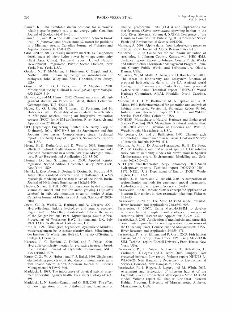
time series analysis. The flow chart presented in Fig. 3

outlines inputs and outputs of the model and the

sequence of the main steps of the methodology.

Habitat description

The habitat description was based on two main

processes: the representative site selection and the

habitat survey. For the representative site selection, we

used a project base map and a digital elevation model

within a geographic information system (GIS) environ-

ment to identify the stream gradient, the areas of

interest, the possible access locations (which represent a

considerable limiting factor in mountainous headwater

streams), and hence defining a preliminary field data

collection schedule. However, the narrow and V-shaped

valleys and the presence of high-density vegetation near

the main channels often did not allow the use of aerial

photography, and on-the-ground river observation was

usually required. This reconnaissance survey involved

hiking in the study area along the entire river length,

estimating portions of the stream that are often

delimitated by considerable change in stream gradient

(knickpoints). Within homogeneous stream sections, the

shortest representative reach, normally from hundreds

of meters to kilometers, was then selected for detailed

survey. This subsampling of representative river sections

could be based on expert opinion up to sophisticated

analysis using statistical approaches, e.g., cluster anal-

ysis to group the sections that were similar to each other

(Parasiewicz et al. 2003), depending on the study

objectives, costs, and logistic constraints.

The habitat survey described the changes in meso-

habitat types over a selected range of discharges. Since

reference to aerial photos (Parasiewicz 2007a) was often

limited, we usually relied on the use of a rangefinder

(e.g., Trupulse 360B, Laser Technology, Centennial,

Colorado, USA), a photographic tripod, and a rugged

field computer (e.g., Nomad TDS [tripod data system],

FIG. 1. The 40 study sites located in Northwest Italy, within the Alps and Apennines mountain ranges (m a.s.l., meters abovesea level).

PAOLO VEZZA ET AL.846 Ecological ApplicationsVol. 24, No. 4

with global positioning system (GPS) positioning; Field

Environmental Instruments, Sunnyvale, California,

USA) to record the HMU characteristics. The GPS

positioning was used to capture the starting point of the

survey, defined from a nearby opening with good

satellite coverage or from a clearly identifiable ground

control point. Each HMU (e.g., pool, riffle, rapid) is a

definable area that reflects the interplay between

hydraulics and riverbed topography and can be inferred

by visual observation of surface flow character and

verified by water depth, flow velocity, and substratum

types (Gosselin et al. 2010). Surveys were usually carried

out by walking downstream, delineating the HMU

polygons in a GIS environment and recording the

mesohabitat-scale features (HMU area and type, cover,

shores characteristics, mesohabitat longitudinal connec-

tivity, gradient) and coming back upstream (toward the

access point), collecting depth, velocity, and substrate

information from each of the mapped mesohabitats.

An example of habitat descriptors collected during a

habitat survey is reported in Table 2. Overall, both

chemical (e.g., pH, dissolved oxygen, turbidity, and

organic contaminants) and physical characteristics (e.g.,

HMU gradient, frequencies classes of depth, velocity,

and substrate) were considered in the mesoscale habitat

description due to their combined effects on habitat

resources. Chemical variables generally do not change

within the surveyed stream reach, but are important in

defining habitat reference criteria for different streams.

For each HMU, we collected from 7 to 30 mean water

column velocity values (by using the flowmeter Marsh-

McBirney Flo-Mate; Hach Company, Loveland, Colo-

rado, USA), and carried out depth measurements and

substrate estimates in order to cover the variability of

instream flow conditions and to describe the HMU area.

For detailed studies and within large non-wadeable

pools, the ADCP SonTek RiverSurveyor (M9-ADP;

San Diego, California, USA) was used to describe depth

and velocity frequencies. Depending on the size of the

stream, either the Marsh-McBirney Flo-Mate or the

ADCP SonTek RiverSurveyor was also used to measure

the discharge. Based on the fact that the habitat in rivers

changes regularly with flow, three surveyed discharges

were considered the minimum required to describe the

hydromorphological characteristics. According to the

MesoHABSIM simulation model (Parasiewicz 2007a,

FIG. 2. Examples of the reference alluvial morphologies considered dominant within high-gradient stream reaches.


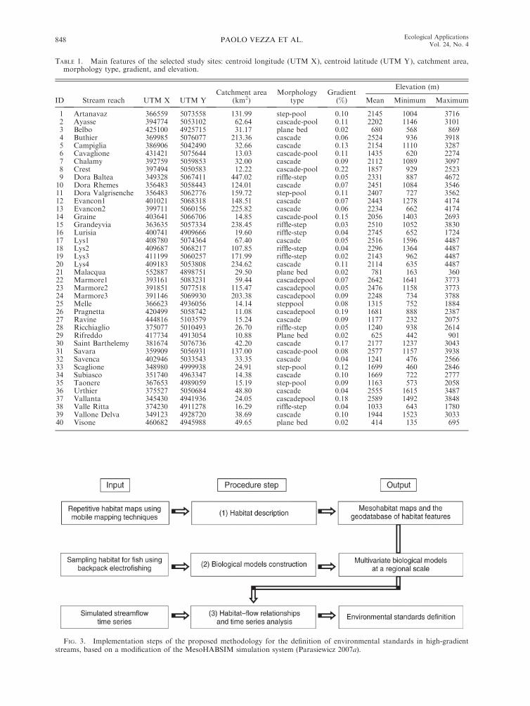
TABLE 1. Main features of the selected study sites: centroid longitude (UTM X), centroid latitude (UTM Y), catchment area,morphology type, gradient, and elevation.

ID Stream reach UTM X UTM YCatchment area

(km2)Morphology

typeGradient

(%)

Elevation (m)

Mean Minimum Maximum

1 Artanavaz 366559 5073558 131.99 step-pool 0.10 2145 1004 37162 Ayasse 394774 5053102 62.64 cascade-pool 0.11 2202 1146 31013 Belbo 425100 4925715 31.17 plane bed 0.02 680 568 8694 Buthier 369985 5076077 213.36 cascade 0.06 2524 936 39185 Campiglia 386906 5042490 32.66 cascade 0.13 2154 1110 32876 Cavaglione 431421 5075644 13.03 cascade-pool 0.11 1435 620 22747 Chalamy 392759 5059853 32.00 cascade 0.09 2112 1089 30978 Crest 397494 5050583 12.22 cascade-pool 0.22 1857 929 25239 Dora Baltea 349328 5067411 447.02 riffle-step 0.05 2331 887 467210 Dora Rhemes 356483 5058443 124.01 cascade 0.07 2451 1084 354611 Dora Valgrisenche 356483 5062776 159.72 step-pool 0.11 2407 727 356212 Evancon1 401021 5068318 148.51 cascade 0.07 2443 1278 417413 Evancon2 399711 5060156 225.82 cascade 0.06 2234 662 417414 Graine 403641 5066706 14.85 cascade-pool 0.15 2056 1403 269315 Grandeyvia 363635 5057334 238.45 riffle-step 0.03 2510 1052 383016 Lurisia 400741 4909666 19.60 riffle-step 0.04 2745 652 172417 Lys1 408780 5074364 67.40 cascade 0.05 2516 1596 448718 Lys2 409687 5068217 107.85 riffle-step 0.04 2296 1364 448719 Lys3 411199 5060257 171.99 riffle-step 0.02 2143 962 448720 Lys4 409183 5053808 234.62 cascade 0.11 2114 635 448721 Malacqua 552887 4898751 29.50 plane bed 0.02 781 163 36022 Marmore1 393161 5083231 59.44 cascadepool 0.07 2642 1641 377323 Marmore2 391851 5077518 115.47 cascadepool 0.05 2476 1158 377324 Marmore3 391146 5069930 203.38 cascadepool 0.09 2248 734 378825 Melle 366623 4936056 14.14 steppool 0.08 1315 752 188426 Pragnetta 420499 5058742 11.08 cascadepool 0.19 1681 888 238727 Ravine 444816 5103579 15.24 cascade 0.09 1177 232 207528 Ricchiaglio 375077 5010493 26.70 riffle-step 0.05 1240 938 261429 Rifreddo 417734 4913054 10.88 Plane bed 0.02 625 442 90130 Saint Barthelemy 381674 5076736 42.20 cascade 0.17 2177 1237 304331 Savara 359909 5056931 137.00 cascade-pool 0.08 2577 1157 393832 Savenca 402946 5033543 33.35 cascade 0.04 1241 476 256633 Scaglione 348980 4999938 24.91 step-pool 0.12 1699 460 284634 Subiasco 351740 4963347 14.38 cascade 0.10 1669 722 277735 Taonere 367653 4989059 15.19 step-pool 0.09 1163 573 205836 Urthier 375527 5050684 48.80 cascade 0.04 2555 1615 348737 Vallanta 345430 4941936 24.05 cascadepool 0.18 2589 1492 384838 Valle Ritta 374230 4911278 16.29 riffle-step 0.04 1033 643 178039 Vallone Delva 349123 4928720 38.69 cascade 0.10 1944 1523 303340 Visone 460682 4945988 49.65 plane bed 0.02 414 135 695

FIG. 3. Implementation steps of the proposed methodology for the definition of environmental standards in high-gradientstreams, based on a modification of the MesoHABSIM simulation system (Parasiewicz 2007a).


Vezza et al. 2012a), the HMU survey was normally

repeated from three to five times between the minimum

low flows (e.g., defined using low flows regionalization

formulas; Vezza et al. 2010) and the medium/high flows

expected on that river (e.g., derived from flow duration

curves; Piedmont Region 2007).

The lower flow threshold occurs during late autumn

and early winter in Alpine streams and during summer

in Apennine–Mediterranean ones (Vezza et al. 2010). In

contrast, the upper flow threshold is usually controlled

by the spring snowmelt processes in the Alps and by the

spring/autumn rainy events in the Apennines. As a

general rule, reference conditions for habitat surveying

are indicated as the flow range in the key bioperiods for

the considered fish community, e.g., rearing and growth

stage or migration and spawning period (sensu Para-

siewicz et al. 2008).

Biological models

The biological indicators proposed in the present

research for high-gradient streams are based on the

Target Fish Community approach (Bain and Meixler

2008), and can be particular species of fish, their life

stages, guilds, or the entire fish community.

The fish community composition varies within the

region of interest according to the catchment coordi-

nates and elevation, also including reach gradient and

morphology (Carta Ittica Regionale 2004, Comoglio et

al. 2007). To determine the fish community composition,

a list of the expected species was created considering

different fish bioperiods, especially in rivers with high

levels of seasonal migration (Parasiewicz et al. 2007).

The list can be extrapolated from existing institutional

databases (e.g., Carta Ittica Regionale 2004) and

subsequently integrated through direct fish samplings.

The fish samplings were carried out to get precise data

for the construction of biological models through the

observation of the mesohabitat use by a selected

organism during its diurnal routine. For model applica-

tion purposes, and even for setting habitat restoration

measures in regulated or channelized streams, biological

models were built in these natural reference conditions

in terms of natural flow regime and fish community

composition (age-structured populations, only autoch-

thonous species, absence of restocking and fisheries).

Within pristine high-gradient streams characterized by

little or no human impact, fish data were collected by

sampling every HMU with backpack electrofishing and

using the multiple-pass removal method (Kruse et al.

1998). Mesohabitats were separated using nets in order

to assure the direct association between sampled areas

and sampled fish species. Before being released within

the same sampled HMU, each fish was measured in

terms of mass and fork length, then classified into adult

and juvenile life stages by means of length–age

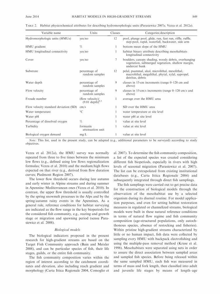
TABLE 2. Habitat physicochemical attributes for describing hydromorphologic units (Parasiewicz 2007a, Vezza et al. 2012a).

Variable name Units Classes Categories/description

Hydromorphologic units (HMUs) yes/no 12 pool, plunge pool, glide, run, fast run, riffle, ruffle,step-pool, rapid, waterfall, backwater, side arm

HMU gradient % 1 bottom mean slope of the HMU

HMU longitudinal connectivity yes/no 1 habitat binary attribute describing mesohabitatslongitudinal connectivity

Cover yes/no 7 boulders, canopy shading, woody debris, overhangingvegetation, submerged vegetation, shallow margin,undercut bank

Substrate percentage ofrandom samples

12 pelal, psammal, akal, microlithal, mesolithal,macrolithal, megalithal, phytal, xylal, sapropel,detritus, debris

Water depth percentage ofrandom samples

9 classes in 15-cm increments (range 0–120 cm andabove)

Flow velocity percentage ofrandom samples

9 classes in 15-cm/s increments (range 0–120 cm/s andabove)

Froude number (flow velocity)/(9.81 depth)0.5

1 average over the HMU area

Flow velocity standard deviation (SD) cm/s 1 SD over the HMU area

Water temperature 8C 1 water temperature at site level

Water pH 1 water pH at site level

Percentage of dissolved oxygen % 1 value at site level

Turbidity formazinattenuation unit

1 value at site level

Biological oxygen demand mg/L 1 value at site level

Note: This list, used in the present study, can be adapted (e.g., additional parameters to be surveyed) according to studyobjectives.


relationships and, in more detailed species studies, by

using scales analysis (Vezza et al. 2012a).

The biological data were the basis for the calculation

of probabilistic models aimed at establishing habitat

suitability criteria with information coming from one or

more rivers. As reported in Ahmadi-Nedushan et al.

(2006), logistic regressions currently represent an

appropriate method for the habitat evaluation process

to identify the habitat attributes affecting species

distribution. In the present work, the Akaike’s informa-

tion criteria (AIC; Sakamoto 1991), along with a

multiple logistic regression model, were performed to

select the habitat attributes influencing species presence

or abundance at different life stages. The algorithm uses

AIC and a stepwise forward procedure to determine

which parameters should be included in the following

regression formula:

R ¼ e�z ð1Þ

where e is natural-log base and z ¼ b1x1 þ b2x2 þ . . . þbnxn þ a, where xn are significant habitat attributes, bnare regression coefficients, and a is a constant. Habitat

suitability models were built using a fivefold cross-

validation procedure in which 20% of the randomly

selected data were separated and used for model

validation. These data have the same proportion of

suitable units as the whole data set. To increase model

certainty, this procedure was repeated 20 times and,

each time, a new set of randomly selected data was set

aside for validation purposes. After 20 runs, the model

generated a list of parameters selected in at least two

runs and conducted one additional run using only these

parameters as input attributes. The last step was the

review of standard errors calculated for each recorded

attribute and the removal of the attributes with errors

greater than the regression coefficient derived from using

standardized variables (Parasiewicz et al. 2012a).

Two binary habitat suitability models were created as

follows: a suitable habitat model indicating the potential

for fish presence (to distinguish between absence and

presence of the fish) and an optimal habitat model for

high abundance of fish (to distinguish between fish

presence and abundance). The cutoff value for low and

high abundance was determined as the inflection point

of the envelope curve of the fish density histograms

(Vezza et al. 2012a). The area under the receiver

operating characteristic (ROC) curves and the model

accuracy (in terms of correctly classified instances)

provided the measures of the model’s performance

(Hosmer and Lemeshow 2000). The area under the

ROC curve defines the discrimination capacity of the

model over a range of threshold levels (Pearce and

Ferrier 2000) by plotting the proportion of HMUs

correctly predicted (sensitivity or true positive rate) vs.

the units incorrectly predicted to be occupied (false

positive rate). In the area under the ROC curve, a value

of 0.7 indicates moderate discrimination power of the

model to distinguish between absence/presence (or

presence/abundance) of fish, while a value of 0.8 refers

to acceptable discrimination, and one of 0.9 refers to

outstanding discrimination (Hosmer and Lemeshow

2000).

The obtained habitat suitability criteria were applied

to all HMUs mapped in the study area to calculate the

probability ( p) of presence and high abundance by using

the following equation:

p ¼ 1=ð1 þ ezÞ ð2Þ

and it was used to classify habitat into suitability

categories (not suitable, suitable, or optimal). The

inflection point on the ROC curve was used to define

the probability threshold to determine the best separa-

tion of suitable and not suitable (or suitable and

optimal) units (Parasiewicz 2007a).

The reference habitat attributes considered in this

study are presented in Table 2. Unfortunately, the

literature-based information that could be used for the

development of habitat suitability criteria is currently

underdeveloped for the region of interest, and the

available studies have low applicability in high-gradient

streams, being mainly related to micro-scale suitability

models, low-gradient reaches, and carried out only for

water depth and flow velocity (Vismara et al. 2001).

Thus, we relied on field data rather than literature for

developing habitat suitability criteria for high-gradient

streams.

Habitat rating curves and time series analysis

The digital mesohabitat maps built during the habitat

surveys and the mesohabitat suitability criteria were the

basis for the development of habitat–flow rating curves

for each site. The area of HMUs with suitable (or

optimal) habitats was summarized for every site by

weighting suitable habitat area by 25% and the optimal

habitat area by 75%, and it was plotted against the

wetted area at the highest measured flow Parasiewicz

(2007a). The habitat values were interpolated using a

mathematical spline function for the target species and

life stages to represent the habitat rating curve.

Moreover, rating curves for generic fish were also

calculated. The generic fish was considered as a

hypothetical species that uses the same habitat as all

the investigated species in the community for which the

multiple-occupant areas are counted only one time.

Therefore, the generic-fish habitat can be seen as the

total physical habitat available for the considered fish

community. Obviously, the available physical habitat

area does not take into account any limitations caused

by biotic interactions (such as predation, competition,

and mutualism). Another option reported in (Para-

siewicz 2007a) is to compute community habitat by

weighting the habitat of each species by their expected

proportion in the target fish community. However, the

quantitative fish data, along with life history informa-

tion in the fish community, were often unavailable for

our study sites and, therefore, we considered the


approach for generic fish to be the best available

approximation.

In addition to reference fish community rating curves,

the definition of the reference streamflow and habitat

time series was the final element needed in the full

determination of the environmental reference condi-

tions, which could be analyzed using the uniform

continuous under threshold (UCUT) methodology

(Parasiewicz 2007b). Although the understanding of

hydrological characteristics in headwater streams is

critical for managing water resources in mountainous

areas, we have to face the problem of a frequent lack of

stream gauge data (e.g., Watson et al. 2009, Vezza et al.

2010). To address this issue, the Hydrologic Engineering

Center-Hydrologic Modeling System (HEC-HMS;

McEnroe 2010), along with the Snow-Band snowmelt

computation of the Streamflow Synthesis and Reservoir

Regulation (SSARR) model, were used in the present

study to generate the flow time series for high-gradient

streams (HEC 2001, Hu et al. 2006). The model with

snowmelt capability (HEC; available online)7 requires

precipitation and air temperature as inputs, and

estimates the snow water equivalent (SWE) and the

impacts of snowmelt on the streamflow. The HEC-HMS

model is characterized by a large number of parameters

that are often not directly measurable. Therefore, these

parameters must be estimated through model calibration

in a neighboring similar catchment (i.e., the donor)

where streamflow data series are available and by fitting

the simulated outputs of the model to the observed

outputs of the catchment. The choice of the donor

catchment was based on the similarity approach (Para-

jka et al. 2005) in which the hydrological model

parameters were transposed from a catchment that

was most similar in terms of its physiographic attributes

(mean elevation, drainage density, land use, and

geology). The optimization method and the execution

of trials were used to calibrate the model by finding the

values for the model parameters that minimize each

calibration criterion. The coefficient of efficiency (E)

was then used to provide an indication of the degree of

association between simulated and recorded flows

(Chiew and McMahon 1993). The flow time series were

generated for the ungauged stream using the calibrated

model and the reference habitat time series produced.

The habitat time series was calculated as:

HAðtÞ ¼ PHðQðtÞÞ ð3Þ

where PH is the physical habitat-vs.-stream flow

function for a given life stage, species, or generic fish,

Q(t) is the streamflow at time t, and HA(t) is the habitat

area for time t (Milhous et al. 1990). The obtained

habitat time series was then statistically analyzed using

the uniform continuous under thresholds (UCUTs;

Parasiewicz 2007b) methodology to establish the habitat

stressor thresholds (HST). This analysis was based on

the assumption that habitat is a limiting factor, and

events occurring rarely in nature create stress to aquatic

fauna and shape the community. Identification of HST

considers not only the magnitude of an impact, but can

also provide a means of quantitatively comparing

duration and frequency of events, as well as different

flow management scenarios (Parasiewicz et al. 2012b,

Vezza et al. 2013a). To evaluate environmental thresh-

olds, it was therefore essential to consider not only the

magnitude of an impact, but also its duration and

frequency. The UCUT-curves are considered projected

contours of a habitat surface area in the three-

dimensional space of duration, frequency, and habitat

area. They are defined for a given bioperiod and were

used to evaluate the durations and frequency of

continuous events with habitat lower than a specified

threshold. Therefore, the sum length of all events of the

same duration within bioperiods was computed as a

ratio of a total duration of all bioperiods in the record

and the proportions are plotted as a cumulative

frequency. This procedure is repeated for the entire set

of thresholds with constant increments (e.g., 2%increment of suitable habitat).

To identify HST, we analyzed the specific regions with

a higher or lower concentration of the curves on the

plot, and common and less common habitat events were

based on the changes in area slope expressed by the

shape of and distances between the curves. The

procedure had two steps: (1) determination of habitat

threshold levels by selecting curves on the graphs and (2)

identification of critical durations by locating inflection

points. Interpretation of these patterns was based on the

following observations: (1) The horizontal distance

between curves indicates the change in frequency of

events associated with a habitat increase to the next level

(e.g., the larger the distance between two curves at the

same continuous duration, the larger the change in the

frequency of the events), (2) steep curves represent low

change in event frequency, and (3) inflection points

reflect rapid change in frequency of continuous dura-

tions.

Typically, the UCUTs for very low habitat availabil-

ity happen infrequently and are located in the bottom

left corner. As habitat level continues to increase, this

pattern of UCUTs rapidly changes and distance between

the curves increases. We selected the highest curve in the

rare-habitat group of curves as a rare-habitat level

threshold. The critical level defines a more frequent

event than rare, below which the habitat circumstances

rapidly decrease. Therefore, the next higher UCUT line

(the first that stands out) is identified as a critical level.

The distance between the lines after exceeding the

critical level are usually greater than in the previous

group, but are still close to each other. The next

outstanding curve, demarcating rapid change in fre-

quency of events, was assumed to mark the stage at

which more common habitat levels begin (no stress;7 http://www.hec.usace.army.mil/


Parasiewicz 2007b). The inflection points on the UCUTs

demarcate change in frequency of habitat under-

threshold durations. This observation helps to identify

the longest periods that a habitat condition is allowed to

continue under a specified threshold. The events

exceeding these durations were subdivided into one of

two categories: allowable or catastrophic. An allowable

event is likely to occur every few years, but at the intra-

annual scale, these long events are unusual, i.e., do not

happen more than twice in a year. Catastrophic events

occur on a decadal-scale, and we chose as catastrophic

threshold the shortest of the longest durations.

The results of HST analysis were used to develop

habitat augmentation strategies, i.e., short-term flow

increases, aimed at reducing continuous duration of

habitat under HST. Once the allowable duration of

habitat under rare or critical habitat levels was exceeded,

the strategy called for release of water that will increase

the amount of habitat to critical or common level,

respectively. This strategy was then summarized in

operational rules that can be used for dam operations.

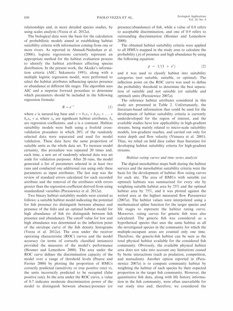
RESULTS

As a first step, the efficiency of the proposed

methodology was evaluated in terms of field data

collection, i.e., mesohabitat survey and description.

Fig. 4 shows the expenditure of time for data collection

in the selected streams, referring to an eight-hour

working day of a team of two people. It is interesting

to note how performance values decrease in line with

stream gradient and are stratified referring to stream

morphology and riverbed characteristics. A breakpoint

was located at 7% gradient, beyond which the perfor-

mance in terms of surveyed linear distance was around

0.4 km/day. For very high-gradient study sites, i.e.,

those with 22% gradient and rocky cascade-pool channel

morphology, performance decreased to 0.25 km/day.

A database of ;500 records of HMUs observation,

quantitatively sampled for fish, was collected since fall

2008 and is currently available for the study area. For

the purpose of demonstration in this paper, we focused

our attention on salmonids, i.e., marble trout (Salmo

marmoratus) and brown trout (Salmo trutta fario),

which are characteristic of the region of interest (see

Vezza et al. 2012a for further mesohabitat suitability

models). Table 3 shows the models for each fish species,

related to adult and juvenile life stages. The autumn/

winter model for marble trout is shown, which is related

to its migration and spawning season, while for brown

trout, the spring/summer model related to the rearing

and growth bio-period is reported. Due to the limited

number of observations of juvenile marble trout, the

abundance model is not shown here. Overall, for the

area under the ROC curve, values range from 0.81

(acceptable discrimination) to 0.90 (outstanding dis-

crimination), while the accuracy of the models, in terms

of correctly classified instances, varied from 61% to 72%.

In Fig. 5, several examples of habitat–flow rating

curves are presented that define the habitat variation at

the selected range of flows for different species, life

stages, and the generic fish for each of the considered

five morphological channel types separately. For catch-

ments characterized by only one fish species, i.e., brown

trout for Vallone d’Elva and Campiglia Streams and

Taonere and Subiasco Creeks, the habitat curve for

generic fish was not calculated.

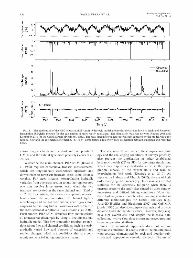
An example of hydrological model calibration is

shown in Fig. 6, using Grana Stream as the donor

catchment. The model inputs (temperature, precipita-

tion, streamflow time series) and outputs (simulated and

residual flow time series) for the period August 2001–

December 2010 are reported. The obtained residual

flow, i.e., the difference between the observed and

simulated time series, shows the inability of the model

to capture the peak streamflow magnitude, while the

coefficient of efficiency (E ¼ 0.64) demonstrates a

relatively good association between simulated and

recorded flows (Parajka et al. 2005).

The calibrated hydrologic model was then used to

generate the reference habitat time series for Valleritta

Creek (ID 38 in Table 1) and to calculate the uniform

continuous under threshold (UCUT) curves for the

winter low-flow period (simulated period 1970–2010;

Fig. 7). Each curve on the diagram represents the

cumulative duration of events (between 2% and 30% of

the channel area). The reduction in slope, as well as the

increase of spacing between two curves, indicate an

increase in the frequency of under-threshold events

(Parasiewicz 2007b). Rare-catastrophic (8% of channel

area), critical-persistent (10%), and common habitat

(28%) thresholds were then selected, and their inflection

points were used to demarcate associated persistent and

catastrophic durations of events (Fig. 7).

FIG. 4. Efficiency of mesoscale field data collection in high-gradient streams, expressed in terms of surveyed linear distance.Stream gradient has no unit and it is expressed as elevationchange/horizontal distance.


DISCUSSION

A recent European report (CIPRA 2010) has high-

lighted that, in addition to an already relevant number

of existing hydropower plants and other water abstrac-

tions, several hundred applications for new small

hydropower plants (SHP) are being presented across

the whole Alpine area. The key conclusion of the report

is that regional-based planning is considered necessary

in order to make decisions about new SHP facilities to

ensure that further development of hydropower is

compatible with both environmental protection require-

ments and the targets set for renewable energy

production. This European trend reflects the increasing

worldwide significance of small-hydro (NREL 2001,

Anderson et al. 2006a, McLarney et al. 2010, GIM-

UNDP 2011) as a ‘‘new’’ renewable energy source

(REN21 2010). Despite this increasing demand for

further exploitation of water resources in mountainous

high-gradient streams, an adequate methodology con-

cerning habitat–hydraulic modeling for these particular

watercourses is not yet available in the scientific

literature.

To cope with the issues noted in the previous

paragraph, we propose a new methodology for habi-

tat–hydraulic modeling in high-gradient streams based

on an adaptation of the MesoHABSIM simulation

model reported in (Parasiewicz 2007a), which we have

developed and tested in several streams of the Alps and

Apennines in NW Italy. To adapt MesoHABSIM to

high-gradient streams: (1) The data collection strategy

was modified to address the challenging conditions of

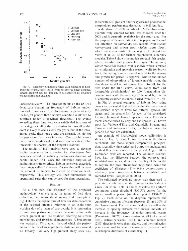
TABLE 3. Marble trout (Salmo marmoratus) biological modelsfor autumn/winter and brown trout (Salmo trutta fario)biological models for spring/summer.

Species, model, and parameter Value

Marble trout: adult

Presence model

Estimated success (%) 66Area under ROC curve 0.87Probability cutoff 0.40Constant �0.868HMU gradient (%) �0.094Depth 60–75 cm (%) 4.49Velocity 30–45 cm/s (%) 4.39Akal (gravel) (%) 14.11

Abundance model

Estimated success (%) 62Area under ROC curve 0.87Probability cutoff 0.74Constant �2.36No connectivity (yes/no) 20.49Pool (yes/no) 20.23Velocity 0–15 cm/s (%) �4.58

Marble trout: juvenile

Presence model

Estimated success (%) 72Area under ROC curve 0.77Probability cutoff 0.34Constant �2.56Ruffle (yes/no) �16.95Depth 15–30 cm (%) �2.62Velocity 0–15 cm/s (%) 1.94Macrolithal, 20–40 cm (%) 1.68

Brown trout: adult

Presence model

Estimated success (%) 72Area under ROC curve 0.84Probability cutoff 0.45Constant �2.38HMU gradient (%) �0.124Boulders (yes/no) 2.55Canopy shading (yes/no) 0.68Step-pool (yes/no) 1.91Depth 30–45 cm (%) �1.19Megalithal, .40 cm (%) 2.16Macrolithal, 20–40 cm (%) 3.59

Abundance model

Estimated success (%) 62Area under ROC curve 0.82Probability cutoff 0.51Constant �24.24Boulders (yes/no) 18.35Step-pool (yes/no) 1.96Depth 60–75 cm (%) 3.22Velocity 15–30 cm/s (%) �4.29Water temperature (8C) 3.85

TABLE 3. Continued.

Species, model, and parameter Value

Brown trout: juvenile

Presence model

Estimated success (%) 68Area under ROC curve 0.81Probability cutoff 0.35Constant �6.27HMU gradient (%) �0.089Boulders (yes/no) 2.23Run (yes/no) �1.21Depth 30–45 cm (%) 2.22Velocity 30–45 cm/s (%) �2.77Macrolithal, 20–40 cm (%) 5.27Akal (gravel) (%) 4.30Water temperature (8C) 1.35

Abundance model

Estimated success (%) 67Area under ROC curve 0.86Probability cutoff 0.60Constant �8.20HMU gradient (%) 0.29Canopy shading (yes/no) 2.22Plunge pool (yes/no) 7.83Depth 75–90 cm (%) �25.50Mesolithal, 6–20 cm (%) 4.42Water temperature (8C) 1.79

Notes: The habitat variable coefficients are multipliers of thesignificant habitat attribute values, and the model accuracy andthe area under the receiver operating characteristic (ROC)curve were used to estimate the predictive power of the model.The probability cutoff for both presence and abundance modelswas derived from the ROC curves in order to classify habitatsinto suitability categories (Parasiewicz 2007a). Habitat physico-chemical attributes for describing hydromorphologic units(HMU; Parasiewicz 2007a, Vezza et al. 2012a). This list, usedin the present study, can be adapted (e.g. additional parametersto be surveyed) according to the study objectives. Attributeswith many categories (e.g., HMUs) are broken down intomultiple variables in binary (yes/no or 1/0) format.


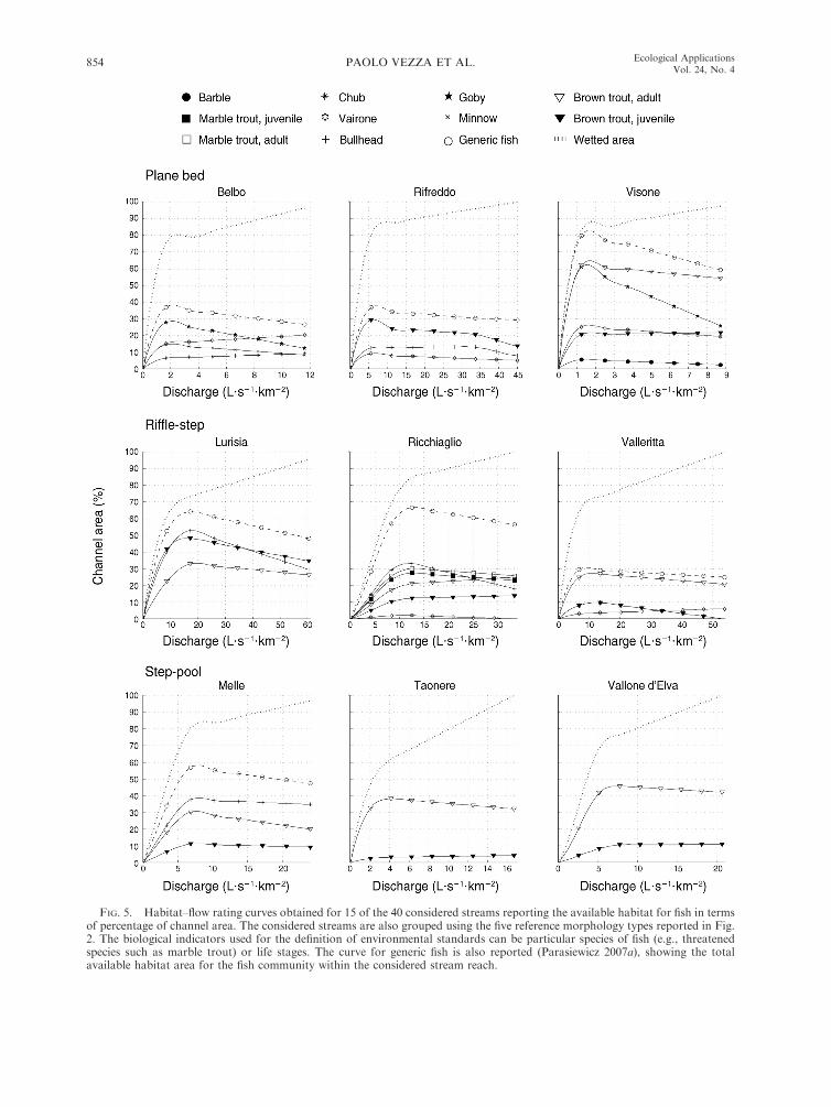
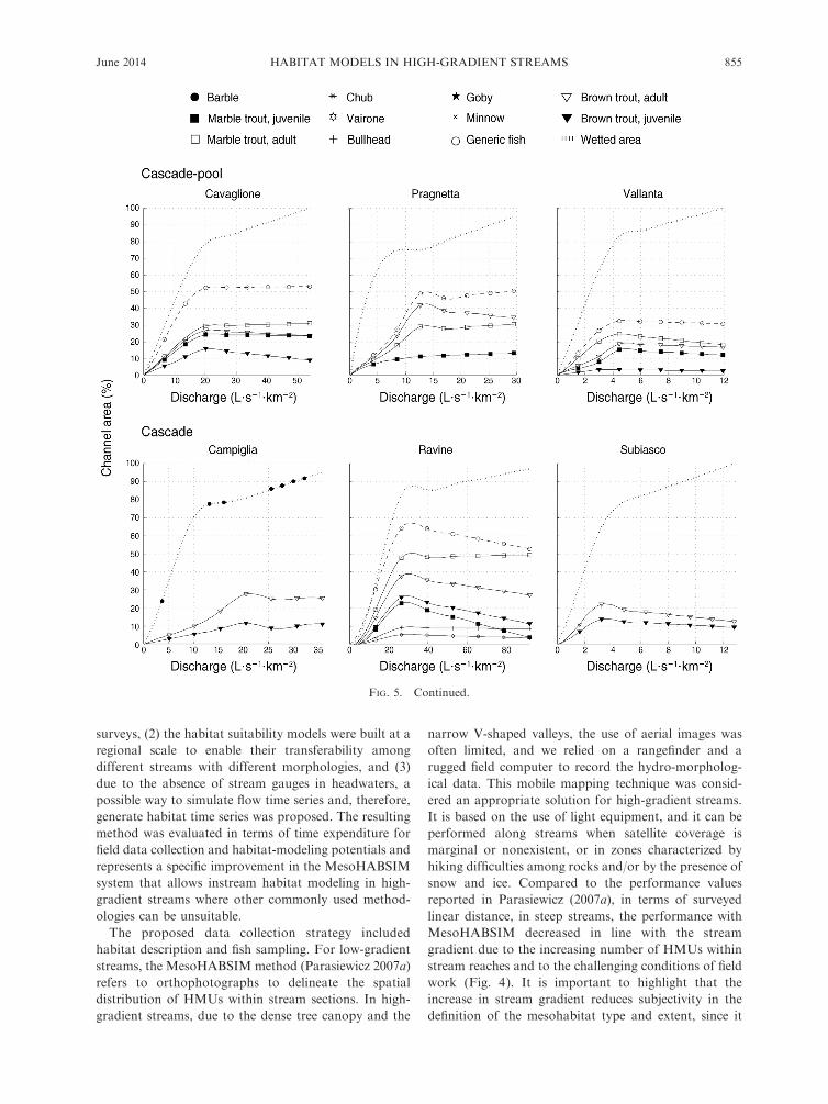
FIG. 5. Habitat–flow rating curves obtained for 15 of the 40 considered streams reporting the available habitat for fish in termsof percentage of channel area. The considered streams are also grouped using the five reference morphology types reported in Fig.2. The biological indicators used for the definition of environmental standards can be particular species of fish (e.g., threatenedspecies such as marble trout) or life stages. The curve for generic fish is also reported (Parasiewicz 2007a), showing the totalavailable habitat area for the fish community within the considered stream reach.


surveys, (2) the habitat suitability models were built at a

regional scale to enable their transferability among

different streams with different morphologies, and (3)

due to the absence of stream gauges in headwaters, a

possible way to simulate flow time series and, therefore,

generate habitat time series was proposed. The resulting

method was evaluated in terms of time expenditure for

field data collection and habitat-modeling potentials and

represents a specific improvement in the MesoHABSIM

system that allows instream habitat modeling in high-

gradient streams where other commonly used method-

ologies can be unsuitable.

The proposed data collection strategy included

habitat description and fish sampling. For low-gradient

streams, the MesoHABSIM method (Parasiewicz 2007a)

refers to orthophotographs to delineate the spatial

distribution of HMUs within stream sections. In high-

gradient streams, due to the dense tree canopy and the

narrow V-shaped valleys, the use of aerial images was

often limited, and we relied on a rangefinder and a

rugged field computer to record the hydro-morpholog-

ical data. This mobile mapping technique was consid-

ered an appropriate solution for high-gradient streams.

It is based on the use of light equipment, and it can be

performed along streams when satellite coverage is

marginal or nonexistent, or in zones characterized by

hiking difficulties among rocks and/or by the presence of

snow and ice. Compared to the performance values

reported in Parasiewicz (2007a), in terms of surveyed

linear distance, in steep streams, the performance with

MesoHABSIM decreased in line with the stream

gradient due to the increasing number of HMUs within

stream reaches and to the challenging conditions of field

work (Fig. 4). It is important to highlight that the

increase in stream gradient reduces subjectivity in the

definition of the mesohabitat type and extent, since it

FIG. 5. Continued.


allows mappers to define the start and end points of

HMUs and the habitat type more precisely (Vezza et al.

2012a).

To describe the main channel, PHABSIM (Bovee et

al. 1998) requires consecutive transect measurements,

which are longitudinally extrapolated upstream and

downstream to represent instream areas using distance

weights. For steep streams, extrapolating hydraulic

variables from one cross section to another unmeasured

one may involve large errors, even when the two

transects are located in the same channel unit (Reid et

al. 2010). In contrast, the mesoscale approach reported

here allows the representation of channel hydro-

morphology and habitat distribution, since it gives more

emphasis to the longitudinal variations rather than to

the cross-sectional variations (Rivas Casado et al. 2004).

Furthermore, PHABSIM simulates flow characteristics

at unmeasured discharges by using a one-dimensional

hydraulic model. This flow simulation requires assump-

tions about flow and channel conditions, such as steady,

gradually varied flow and absence of waterfalls and

sudden changes, which are conditions that are com-

monly not satisfied in high-gradient streams.

The steepness of the riverbed, the complex morphol-

ogy and the challenging conditions of surveys generally

also prevent the application of other establishedhydraulic models (2D or 3D) for discharge simulation,

which may require a considerable effort in the topo-graphic surveys of the stream units and lead to

overwhelming field work (Kozarek et al. 2010). As

reported in Halwas and Church (2002), the use of highorder surveying instruments (e.g., laser scanners or total

stations) can be extremely fatiguing when there is

onerous access to the study sites caused by thick canopyunderstory and difficult hiking conditions. Note that

these hydro-dynamic models, which are implemented indifferent methodologies for habitat analyses (e.g.,

River2D [Steffler and Blackburn 2002] and CaSiMiR

[Jorde 1997]) can describe complex channels and providedetailed hydraulic habitat metrics. However, they may

have high overall cost and, despite the intensive datacollection, involve slow data processing procedures and

large computational efforts.

Since the mesoscale approach does not requirehydraulic simulation, it adapts well to the mountainous

watercourses, characterized by rock and boulder sub-

strata and step-pool or cascade riverbeds. The use of

FIG. 6. The application of the HEC-HMS rainfall-runoff hydrologic model, along with the Streamflow Synthesis and ReservoirRegulation (SSARR) module for the calculation of snow water equivalent. The simulation was run between August 2001 andDecember 2010 for the Grana Stream (Piedmont, Italy). The peak streamflow magnitude was not captured by the model, while theresidual flow and the coefficients of efficiency (E¼ 0.64) demonstrate a relatively good association between simulated and recordedflows.


repetitive mapping of stream reaches demonstrates a

good performance in terms of surveyed linear distance

and allows modeling of habitat variations over the range

of measured discharges. The multiple mapping approach

is, therefore, suggested for high-gradient streams, since it

is based on a more effective data collection procedure.

Note that during medium/high flow, the hydrodynamic

conditions are characterized by tumbling and jet-and-

wake flows around rocks, and the possibility of wading

the stream channel can set the upper limit for surveys.

The habitat–flow rating curves show how habitat

availability generally decreases or remains constant after

reaching a maximum habitat value. A flow increase after

optimal conditions leads to an increase of turbulence

and flow velocity and, therefore, to a reduction of

shelters and suitability (e.g., Visone, Lurisia, Ravine

Streams). This characteristic is particularly valid for

plane bed, riffle-step, and cascade morphologies in

which the high gradient and the stream dimensions

often prevent the lateral expansion of wetted area at

higher discharges. In contrast, the shape of the curves

for step-pool and cascade-pool morphologies seems to

capture the persistence in habitat availability for fish

according to the increase of discharge (e.g., Vallone

d’Elva, Cavaglione, Vallanta Streams). As pool size

increases, habitat condition will also increase in stability

when flow increases.

Due to the steepness of the river bed, the use of

electrofishing grids or snorkeling surveys (mentioned in

Parasiewicz 2007a) was limited in high-gradient streams.

Collecting fish data in each HMU with backpack

electrofishing can be considered an appropriate tech-

nique to quantitatively collect fish data at the mesoscale

and to represent fish population densities in each

sampling site. From a biological perspective, the

mesoscale habitat models in high-gradient streams offer

several interesting opportunities and show flexibility in

modeling habitat for the fish community. This mesoscale

approach can reveal larger spatial and temporal

ecological patterns, since it involves a large range of

habitat variables (Jewitt et al. 2001), e.g., consideration

of river longitudinal connectivity and fish seasonal

response to habitat characteristics (Table 3). The list

of habitat characteristics, chosen for the biological

models construction, can be easily adapted according

to the study objectives (e.g., considering additional

parameters to be surveyed). The mesohabitats descrip-

tion across the region of interest can be considered the

appropriate scale resolution to capture the different

ways in which these animals interact with the spatial

arrangement of habitat characteristics. For model

extrapolation and application purposes, we recommend

construction of biological models using data from

different streams with different morphologies and

gradients. This regional-scale approach represents an

improvement in transferability of habitat models among

streams and has revealed potential for the definition of

fish habitat requirements for many streams simulta-

neously. Moreover, to define the environmental stan-

dards at a regional scale, one can refer to the bottom-up

approach proposed in Vezza et al. (2012a) to upscale the

MesoHABSIM results for the entire region of interest.

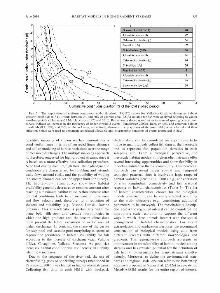
FIG. 7. The application of uniform continuous under threshold (UCUT) curves for Valleritta Creek to determine habitatstressor thresholds (HST). Events between 2% and 30% of channel area (%CA) suitable for fish were analyzed referring to winterlow-flow periods (1 January–21 March between 1970 and 2010). Reduction in slope, as well as an increase of spacing between twocurves, indicate an increase in the frequency of under-threshold events (Parasiewicz 2007b). Rare, critical, and common habitatthresholds (8%, 10%, and 28% of channel area, respectively, shown in the gray rows of the inset table) were selected and theirinflection points were used to demarcate associated allowable and catastrophic durations of events (expressed in days).


In that study, homogeneous subregions were defined by

grouping streams according to the environmental

requirements of fish species.

The habitat suitability models showed acceptable

performance values (Mouton et al. 2011) and, for the

seasonal variation in fish habitat use, it is interesting to

note how different habitat attributes affect fish presence

or abundance considering the two different bio-periods

(autumn/winter and spring/summer) and the two fish

species (marble and brown trout). During autumn/

winter, marble trout presence is related to HMUs, which

are characterized by moderate depth and flow velocity,

as well as by a gravel substrate suitable for egg

deposition. Where the habitat is suitable, the abundance

model seems to capture the marble trout migration

behavior (e.g., Maddock et al. 2008) of accumulating

below obstacles that prevent the upstream migration

(i.e., chutes, waterfalls). In contrast, during summer,

brown trout occurrence is related to step-pool meso-

habitats with adequate cover in the form of boulders,

submerged rocks (megalithal and macrolithal substrate),

and canopy shading. These results agree with other

studies (Fausch and White 1981, Fausch 1984, Hughes

and Dill 1990) that show the preferences of feeding on

drift and habitats with fast currents close to velocity

shelters where fish can rest after feeding. Water

temperature, which varies across the surveyed streams,

also has a positive influence on the mesohabitat use of

brown trout during spring/summer, and this is probably

related to nutrition and metabolic rate. Among the

chemical parameters, dissolved oxygen concentration

and pH are not related to fish presence or abundance

because of the high water quality conditions within the

selected streams. It is important to note that habitat

suitability models for marble trout, developed in

Piemonte and Valle d’Aosta regions, were also applied

and validated in Rabies Creek (Noce River basin,

Trentino Alto Adige region), and the model accuracy

in validation ranged from 64% to 76% (Vezza et al.

2013a).

Further developments in habitat suitability models

can be made that also consider biological habitat

descriptors, e.g., fish guild and macroinvertebrate

community composition, due to their importance in

limiting species presence or abundance (Gordon et al.

2004). This analysis can include the evaluation of

intraspecific interactions and can be used to understand

if fish habitat selection is mainly driven (or not) by

instream physical characteristics (Vezza et al. 2012b).

Furthermore, other discrimination techniques (e.g.,

random forest and artificial neural networks) can be

used to model ecological binary response variables (i.e.,

absence/presence and presence/abundance of fish). As

an example of this application, Vezza et al. (2013b)

compared random forest and logistic regression models

to predict habitat suitability for bullhead in NW Italy.

Results indicate that both techniques constitute valuable

tools to produce mesohabitat suitability models for fish,

although random forest outperformed logistic regres-

sions. The available hydro-ecological database at the

regional scale, i.e., ;500 sampled mesohabitats geo-

referenced in a GIS environment, has important further

potential for defining habitat suitability models. Small

mountainous streams are often poorly documented, and

the available regional database will provide a consistent

set of field data to be used for flow management

strategies by using the distributed hydrological and

ecological information. The fish habitat requirements

that were defined at environmental reference streams,

i.e., watercourses with little or no human impact, can

also be a site-specific target and the information base for

environmental flows at existing or new water abstrac-

tions (Vezza et al. 2012a).

As reported in Milhous et al. (1990), the habitat time

series analysis is a key component in the definition of

environmental flows; it is important to represent how

physical habitat changes through time and to identify

stress conditions created by persistent limitation in

habitat availability. The reference habitat time series

requires a stream flow record of at least three decades

and mountainous high-gradient streams and headwaters

frequently lack this hydrological information. The HEC-

HMS model is, therefore, proposed as a possible tool to

simulate streamflow in such watercourses. Although the

HEC-HMS model performance was not very high (E ¼0.64), the result was acceptable (Parajka et al. 2005),

and it can be considered an appropriate hydrologic

modeling tool for achieving the goals set for high-

gradient streams. In particular, the temporal occurrence

of spring snowmelt-generated peaks and the impacts of

snowmelt on streamflow seem to be well captured by the

model (Fig. 5). However, high flood peaks are generally

underestimated, but the performance in the simulation

of low flows was good and was considered reliable for

the analysis of habitat availability during dry periods.

The reference flow time series can be used to develop a

reference habitat time series, which is investigated to

define the UCUT curves and to establish natural habitat

stressor thresholds (HSTs; e.g., Parasiewicz 2008). The

UCUT curves and the HSTs represent a three-dimen-

sional description of habitat distribution in the continu-

ous duration/frequency space. These highly informative

diagrams allow approximation of an envelope of typically

occurring habitat events that are harmless to the fauna.

Hence, the environmental flows should fall within this

envelope. The method also captures stress conditions that

are created by persistent limitation of habitat availability

and those created by catastrophically low habitat

quantity. Although the latter events occur in natural

conditions, they are not common and, therefore, cause

only limited harm to the aquatic communities, which are

characterized by high resilience to environmental stress.

Consequently, environmental flow management should

avoid increasing the frequency of such disturbances.

With this information, detailed schemes of flow

management that take into account specific operations


can be developed for individual hydropower facilities. In

general, we recommend that the environmental flows

shall follow the natural seasonal pattern and fall within

the identified criteria. Such approach maintains some

portion of natural system dynamics and offers flexibility

in implementation. The flow management schemes will

be strongly dependent on the type of hydropower

facility, inflow, and size of the stream. For example,

for small hydropower plants without storage capacity,

one possible scenario would be to release the flows that

create critical habitat level. If the allowable duration of

such flows is exceeded, the operation should be stopped

for a few days to allow fauna recovery. This would only

be possible if the natural inflow is higher than the one

creating critical habitat level. Using Valleritta Creek as

an example, a possible option would be to allow

hydropower generation with environmental flow release

in the bypass section of 55 L/s with two-day interrup-

tions every two weeks. Once the inflow drops below this

value, the operation would cease until there is an

increase to 155 L/s for two consecutive days. This

conservative scenario, which aims to avoid subsistence

flow, is one of the available options. For the dams with

considerable storage, the hydropower generation inter-

ruptions could be replaced with temporal increases of

flow release. Hence, the facilities on larger rivers, where

more water is available, could use more water for

hydropower. This procedure offers more protection to

the most vulnerable stream sections while maintaining

the natural flow paradigm (Poff et al. 1997) and can be

used for other types of flow alteration, e.g., in rivers

affected by hydropeaking (Vezza et al. 2013a).

Establishing flow recommendations across multiple

streams and for streams that may not have available

flow data is important, and this methodology provides a

tool where few are currently available. As such, it can be

used for development of regional rules, as well as for

defining more site-specific flow management criteria.

However, in its current state, the approach presented

here ignores limitations that could be caused by other

factors, e.g., thermal stresses. The tool provided for the

environmental management of high-gradient streams is

critically needed to implement recent water laws, such as

the European Water Framework Directive, and to cope

with the present lack of available instruments. Specifi-

cally, it is possible to understand fish responses to

stream flow alterations or habitat modifications to guide

river rehabilitation projects and environmental flow

design. In addition, specific negative impacts on the

aquatic biota can be detected, allowing restoration

strategies to be focused on especially threatened species.

ACKNOWLEDGMENTS

The presented research has been developed in the frame ofthe HolRiverMed project (275577-FP7-PEOPLE-2010-IEF,Marie Curie Actions). The data collection was funded by theRegione Piemonte, C61 Project: CIPE 2004 and through thedams monitoring program of Compagnia Valdostana delleAcque (CVA S.p.a.).

LITERATURE CITED

Acreman, M., and M. Dunbar. 2004. Defining environmentalflow requirements: a review. Hydrology and Earth SystemSciences 8(5):861–876.

Ahmadi-Nedushan, B., A. St-Hilaire, M. Berube, E. Robi-chaud, N. Thiemonge, and B. Bernard. 2006. A review ofstatistical methods for the evaluation of aquatic habitatsuitability for instream flow assessment. River Research andApplications 22:503–523.

Anderson, E., M. Freeman, and C. Pringle. 2006a. Ecologicalconsequences of hydropower development in Central Amer-ica: impacts of small dams and water diversion onneotropical stream fish assemblages. River Research andApplications 22:397–411.

Anderson, E., C. Pringle, and M. Rojas. 2006b. Transformingtropical rivers: an environmental perspective on hydropowerdevelopment in Costa Rica. Aquatic Conservation: Marineand Freshwater Ecosystems 16(7):679–693.

Arthington, A., S. Bunn, N. Poff, and R. Naiman. 2006. Thechallenge of providing environmental flow rules to sustainriver ecosystems. Ecological Applications 16:1311–1318.

Bain, M., and M. Meixler. 2008. A target fish community toguide river restoration. River Research and Applications24:453–458.

Bovee, K. 1982. A guide to stream habitat analysis using theInstream Flow Incremental Methodology. Instream FlowInformation Paper 12. U.S. Fish and Wildlife Service, FortCollins, Colorado, USA.

Bovee, K., B. Lamb, J. Bartholow, C. Stalnaker, J. Taylor, andJ. Henriksen. 1998. Stream habitat analysis using theInstream Flow Incremental Methodology. Information andTechnical Report USGS/BRD-1998-0004. USGS, BiologicalResources Division, Fort Collins, Colorado, USA.

Bryant, M., T. Gomi, and J. Piccolo. 2007. Structures linkingphysical and biological processes in headwater streams of theMaybeso watershed, Southeast Alaska. Forest Science53:371–383.

Carta Ittica Regionale. 2004. Carta ittica relativa al territoriodella regione piemontese: The ichthyic zonation for Piedmontregion. Bibliografia faunistica. Regione Piemonte, Torino,Italy.

Chiew, F., and T. McMahon. 1993. Assessing the adequacy ofcatchment streamflow yield estimates. Australian Journal ofSoil Research 31:665–680.

CIPRA [International Commission for the Protection of theAlps]. 2010. Situation report on hydropower generation inthe Alpine region focusing on small hydropower, volumeAlpine convention platform: water management in the Alps.Platform Water Management in the Alps. PermanentSecretariat of the Alpine Convention, Innsbruck, Austria.

Comoglio, C., E. Pini Prato, M. Ferri, and M. Gianaroli. 2007.A case study of river rehabilitation for fish in Northern Italy:the Panaro River project. American Journal of Environmen-tal Sciences 3:85–92.

Covington, J., and W. Hubert. 2003. Trout populationresponses to restoration of stream flows. EnvironmentalManagement 31(1):135–146.

Crowder, D., and P. Diplas. 2000. Using two-dimensionalhydrodynamic models at scales of ecological importance.Journal of Hydrology 230:172–191.

Crowder, D., and P. Displas. 2006. Applying spatial hydraulicprinciples to quantify stream habitat. River Research andApplications 22:79–89.

de Jalon, D. G., and J. Gortazar. 2006. valuation of instreamhabitat enhancement options using fish habitat simulations:case-studies in the River Pas, Spain. Aquatic Ecology41(3):461–474.

Dewson, Z. S. 2007. Small stream ecosystem and irrigation: anecological assessment of water abstraction impacts. Disser-tation. Massey University, Palmerston North, New Zealand.


Fausch, K. 1984. Profitable stream positions for salmonids:relating specific growth rate to net energy gain. CanadianJournal of Zoology 62:441–451.

Fausch, K., and R. White. 1981. Competition between brooktrout (S. fontinalis) and brown trout (S. trutta) for positionsin a Michigan stream. Canadian Journal of Fisheries andAquatic Sciences 38:1220–1227.

GIM-UNDP. 2011. Growing inclusive markets. Self-supporteddevelopment of micro-hydro power by village community(East Asia: China). Technical report. United NationsDevelopment Programme, Private Sector Division, NewYork, New York, USA.

Gordon, N., T. McMahon, B. Finlayson, C. Gippel, and R.Nathan. 2004. Stream hydrology: an introduction forecologists. John Wiley and Sons, Hoboken, New Jersey,USA.

Gosselin, M. P., G. E. Petts, and I. P. Maddock. 2010.Mesohabitat use by bullhead (Cottus gobio) Hydrobiologia.652(1):299–310.

Halwas, K., and M. Church. 2002. Channel units in small, highgradient streams on Vancouver Island, British Columbia.Geomophology 43(3–4):243–256.

Hauer, C., G. Unfer, M. Tritthart, E. Formann, and H.Habersack. 2010. Variability of mesohabitat characteristicsin riffle-pool reaches: testing an integrative evaluationconcept (FGC) for MEM-application. River Research andApplications 27:403–430.

HEC [Hydrologic Engineering Center, U.S. Army Corp ofEngineers]. 2001. HEC-HMS for the Sacramento and SanJoaquin river basins. Comprehensive study. Technicalreport. U.S. Army Corp of Engineers, Sacramento, Califor-nia, USA.

Horne, B., E. Rutherford, and K. Wehrly. 2004. Simulatingeffects of hydro-dam alteration on thermal regime and wildsteelhead recruitment in a stable-flow lake Michigan tribu-tary. River Research and Applications 20:185–203.

Hosmer, D., and S. Lemeshow. 2000. Applied logisticregression. Second edition. Chichester, Wiley, New York,New York, USA.

Hu, H., L. Kreymborg, B. Doeing, B. Doeing, K. Baron, and S.Jutila. 2006. Gridded snowmelt and rainfall-runoff CWMShydrologic modeling of the Red River of the North Basin.Journal of Hydrologic Engineering 11(2):91–100.

Hughes, N., and L. Dill. 1990. Position choice by drift-feedingsalmonids: model and test for arctic grayling (Thymallusarcticus) in subarctic mountain streams, interior Alaska.Canadian Journal of Fisheries and Aquatic Sciences 47:2039–2048.

Jewitt, G., D. Weeks, G. Heritage, and A. Gorgens. 2001.Hydro-Ecology: linking hydrology and aquatic ecology.Pages 77–90 in Modelling abiotic-biotic links in the riversof the Kruger National Park, Mpumulanga, South Africa.Proceedings of Workshop HW2, Birmingham, UK, July1999. IAHS, Wallingford, Oxfordshire, UK.

Jorde, K. 1997. Okologisch begrundete, dynamische Mindest-wasserregelungen bei Ausleitungskraftwerken. Mitteilungendes Instituts fur Wasserbau. Heft 90. University of Stuttgart,Stuttgart, Germany.

Kozarek, J., C. Hession, C. Dollof, and P. Diplas. 2010.Hydraulic complexity metrics for evaluating in-stream brooktrout habitat. Journal of Hydraulic Engineering ASCE136(12):1067–1076.

Kruse, C. G., W. A. Hubert, and F. J. Rahel. 1998. Single-passelectrofishing predicts trout abundance in mountain streamswith sparse habitat. North American Journal of FisheriesManagement 18(4):940–946.

Maddock, I. 1999. The importance of physical habitat asses-ment for evaluating river health. Freshwater Biology 41:373–391.

Maddock, I., N. Smolar-Zvanut, and G. Hill. 2008. The effectof flow regulation on the distribution and dynamics of

channel geomorphic units (CGUs) and implications formarble trout. (Salmo marmoratus) spawning habitat in theSoca River, Slovenia. Volume 4, XXIVth Conference of theDanubian Countries IOP Publishing, IOP Conference Series:Earth and Environmental Science 4:012026.

Marnezy, A. 2008. Alpine dams: from hydroelectric power toartificial snow. Journal of Alpine Research 96:91–112.

McEnroe, B. 2010. Guidelines for continuous simulation ofstreamflow in Johnson County, Kansas, with HEC-HMS.Technical report. Report to Johnson County Public Worksand Infrastructure Stormwater Management Program. John-son County Public Works and Infrastructure, Olathe,Kansas, USA.

McLarney, W., M. Mafla, A. Arias, and D. Bouchonnet. 2010.The threat to biodiversity and ecosystem function ofproposed hydroelectric dams in the LA Amistad worldheritage site, Panama and Costa Rica, from proposedhydroelectric dams. Technical report. UNESCO WorldHeritage Committee. ANAI, Franklin, North Carolina,USA.

Milhous, R. T., J. M. Bartholow, M. A. Updike, and A. R.Moos. 1990. Reference manual for generation and analysis ofhabitat time series. Version II. Biological Report 90(16),Instream flow information paper 27. U.S. Fish and WildlifeService, Fort Collins, Colorado, USA.

MNHESP [Massachusetts Natural Heritage and EndangeredSpecies Program]. 1999. Massachusetts natural heritage atlas:2000–2001 edition. Division of Fisheries and Wildlife,Westborough, Massachusetts, USA.

Montgomery, D., and J. Buffington. 1997. Channel-reachmorphology in mountain drainage basins. Geological Societyof America Bulletin 109:591–611.

Mouton, A. M., J. D. Alcaraz-Hernandez, B., B. De Baets,P. L. M. Goethals, and F. Martınez-Capel. 2011. Data-drivenfuzzy habitat suitability models for brown trout in SpanishMediterranean rivers. Environmental Modelling and Soft-ware 26(5):615–622.

NREL [National Renewable Energy Laboratory]. 2001. Smallhydropower systems. Technical report DOE/GO-102001-1173. NREL, U.S. Department of Energy (DOE), Wash-ington, D.C., USA.

Parajka, J., R. Merz, and G. Bloschl. 2005. A comparison ofregionalisation methods for catchment model parameters.Hydrology and Earth System Science 9:157–171.

Parasiewicz, P. 2001. Mesohabsim: A concept for application ofinstream flow models in river restoration planning. Fisheries26:6–13.

Parasiewicz, P. 2007a. The MesoHABSIM model revisited.River Research and Applications 23(8):893–903.

Parasiewicz, P. 2007b. Using MesoHABSIM to developreference habitat template and ecological managementscenarios. River Research and Applications 23:924–932.

Parasiewicz, P. 2008. Application of mesohabsim and target fishcommunity approaches for selecting restoration measures ofthe Quinebaug River, Connecticut and Massachusetts, USA.River Research and Application 24:459–471.

Parasiewicz, P., S. B. Ehman, and P. Corp. 2003. Fish habitatassessment on Stony Clove Creek, NY, using MesoHAB-SIM. Technical report. Cornell University Press, Ithaca, NewYork, USA.

Parasiewicz, P., J. Rogers, A. Larson, T. Ballesterro, L.Carboneau, J. Legros, and J. Jacobs. 2008. Lamprey Riverprotected instream flow report. Volume report NHDES-R-WD-08-26. New Hampshire Department of EnvironmentalServices, Concord, New Hampshire, USA.

Parasiewicz, P., J. Rogers, J. Legros, and M. Wirth. 2007.Assessment and restoration of instream habitat of theEightmile River in Connecticut: developing a MesoHABSIMmodel. Volume report 62, chapter Northeast InstreamHabitat Program. University of Massachusetts, Amherst,Massachusetts, USA.


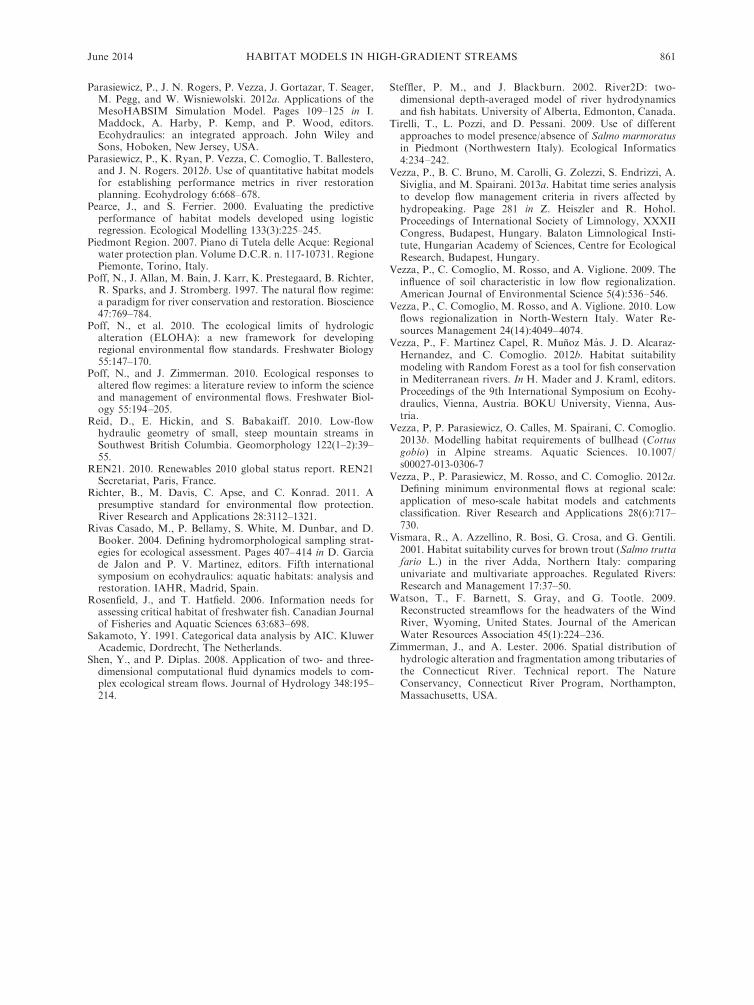
Parasiewicz, P., J. N. Rogers, P. Vezza, J. Gortazar, T. Seager,M. Pegg, and W. Wisniewolski. 2012a. Applications of theMesoHABSIM Simulation Model. Pages 109–125 in I.Maddock, A. Harby, P. Kemp, and P. Wood, editors.Ecohydraulics: an integrated approach. John Wiley andSons, Hoboken, New Jersey, USA.

Parasiewicz, P., K. Ryan, P. Vezza, C. Comoglio, T. Ballestero,and J. N. Rogers. 2012b. Use of quantitative habitat modelsfor establishing performance metrics in river restorationplanning. Ecohydrology 6:668–678.

Pearce, J., and S. Ferrier. 2000. Evaluating the predictiveperformance of habitat models developed using logisticregression. Ecological Modelling 133(3):225–245.

Piedmont Region. 2007. Piano di Tutela delle Acque: Regionalwater protection plan. Volume D.C.R. n. 117-10731. RegionePiemonte, Torino, Italy.

Poff, N., J. Allan, M. Bain, J. Karr, K. Prestegaard, B. Richter,R. Sparks, and J. Stromberg. 1997. The natural flow regime:a paradigm for river conservation and restoration. Bioscience47:769–784.

Poff, N., et al. 2010. The ecological limits of hydrologicalteration (ELOHA): a new framework for developingregional environmental flow standards. Freshwater Biology55:147–170.

Poff, N., and J. Zimmerman. 2010. Ecological responses toaltered flow regimes: a literature review to inform the scienceand management of environmental flows. Freshwater Biol-ogy 55:194–205.

Reid, D., E. Hickin, and S. Babakaiff. 2010. Low-flowhydraulic geometry of small, steep mountain streams inSouthwest British Columbia. Geomorphology 122(1–2):39–55.

REN21. 2010. Renewables 2010 global status report. REN21Secretariat, Paris, France.

Richter, B., M. Davis, C. Apse, and C. Konrad. 2011. Apresumptive standard for environmental flow protection.River Research and Applications 28:3112–1321.

Rivas Casado, M., P. Bellamy, S. White, M. Dunbar, and D.Booker. 2004. Defining hydromorphological sampling strat-egies for ecological assessment. Pages 407–414 in D. Garciade Jalon and P. V. Martinez, editors. Fifth internationalsymposium on ecohydraulics: aquatic habitats: analysis andrestoration. IAHR, Madrid, Spain.

Rosenfield, J., and T. Hatfield. 2006. Information needs forassessing critical habitat of freshwater fish. Canadian Journalof Fisheries and Aquatic Sciences 63:683–698.

Sakamoto, Y. 1991. Categorical data analysis by AIC. KluwerAcademic, Dordrecht, The Netherlands.

Shen, Y., and P. Diplas. 2008. Application of two- and three-dimensional computational fluid dynamics models to com-plex ecological stream flows. Journal of Hydrology 348:195–214.

Steffler, P. M., and J. Blackburn. 2002. River2D: two-dimensional depth-averaged model of river hydrodynamicsand fish habitats. University of Alberta, Edmonton, Canada.

Tirelli, T., L. Pozzi, and D. Pessani. 2009. Use of differentapproaches to model presence/absence of Salmo marmoratusin Piedmont (Northwestern Italy). Ecological Informatics4:234–242.

Vezza, P., B. C. Bruno, M. Carolli, G. Zolezzi, S. Endrizzi, A.Siviglia, and M. Spairani. 2013a. Habitat time series analysisto develop flow management criteria in rivers affected byhydropeaking. Page 281 in Z. Heiszler and R. Hohol.Proceedings of International Society of Limnology, XXXIICongress, Budapest, Hungary. Balaton Limnological Insti-tute, Hungarian Academy of Sciences, Centre for EcologicalResearch, Budapest, Hungary.

Vezza, P., C. Comoglio, M. Rosso, and A. Viglione. 2009. Theinfluence of soil characteristic in low flow regionalization.American Journal of Environmental Science 5(4):536–546.

Vezza, P., C. Comoglio, M. Rosso, and A. Viglione. 2010. Lowflows regionalization in North-Western Italy. Water Re-sources Management 24(14):4049–4074.

Vezza, P., F. Martinez Capel, R. Munoz Mas. J. D. Alcaraz-Hernandez, and C. Comoglio. 2012b. Habitat suitabilitymodeling with Random Forest as a tool for fish conservationin Mediterranean rivers. In H. Mader and J. Kraml, editors.Proceedings of the 9th International Symposium on Ecohy-draulics, Vienna, Austria. BOKU University, Vienna, Aus-tria.

Vezza, P, P. Parasiewicz, O. Calles, M. Spairani, C. Comoglio.2013b. Modelling habitat requirements of bullhead (Cottusgobio) in Alpine streams. Aquatic Sciences. 10.1007/s00027-013-0306-7

Vezza, P., P. Parasiewicz, M. Rosso, and C. Comoglio. 2012a.Defining minimum environmental flows at regional scale:application of meso-scale habitat models and catchmentsclassification. River Research and Applications 28(6):717–730.

Vismara, R., A. Azzellino, R. Bosi, G. Crosa, and G. Gentili.2001. Habitat suitability curves for brown trout (Salmo truttafario L.) in the river Adda, Northern Italy: comparingunivariate and multivariate approaches. Regulated Rivers:Research and Management 17:37–50.

Watson, T., F. Barnett, S. Gray, and G. Tootle. 2009.Reconstructed streamflows for the headwaters of the WindRiver, Wyoming, United States. Journal of the AmericanWater Resources Association 45(1):224–236.

Zimmerman, J., and A. Lester. 2006. Spatial distribution ofhydrologic alteration and fragmentation among tributaries ofthe Connecticut River. Technical report. The NatureConservancy, Connecticut River Program, Northampton,Massachusetts, USA.


Habitat modeling in high-gradient streams: the mesoscale approach and application

Documents

Transcript of Habitat modeling in high-gradient streams: the mesoscale approach and application