Chapter 13

Light Microscopy in Aquatic Ecology: Methods for PlanktonCommunities Studies

Maria Carolina S. Soares, Lúcia M. Lobão, Luciana O. Vidal,Natália P. Noyma, Nathan O. Barros, Simone J. Cardoso,and Fábio Roland

Abstract

Planktonic organisms dominate waters in ponds, lakes and oceans. Because of their short life cycles,plankters respond quickly to environmental changes and the variability in their density and compositionare more likely to indicate the quality of the water mass in which they are found. Planktonic communityis formed by numerous organisms from distinct taxonomic position, ranging from 0.2 μm up to 2 mm.Despite others, the light microscopy is the most used apparatus to enumerate these organisms and differ-ent techniques are necessary to cover differences in morphology and size. Here we present some of themain light microscopy methods used to quantify different components of planktonic communities, suchas virus, bacteria, algae and animals.

Key words: Bacterioplankton, phytoplankton, limnology, enumeration, virioplankton,zooplankton.

1. Introduction

The general understanding of the word plankton is referred toany drifting organism (virus, bacteria, plants or animals) thatinhabit the pelagic zone of oceans, seas or bodies of freshwater.Planktonic community comprises organisms that are taxonomi-cally diverse and more defined by their ecological niche ratherthan their genetic classification. It includes:

• Virioplankton: the most diverse and abundant component ofplankton, infecting a wide range of planktonic organisms.

H. Chiarini-Garcia, R.C.N. Melo (eds.), Light Microscopy, Methods in Molecular Biology 689,DOI 10.1007/978-1-60761-950-5_13, © Springer Science+Business Media, LLC 2011

215

216 Soares et al.

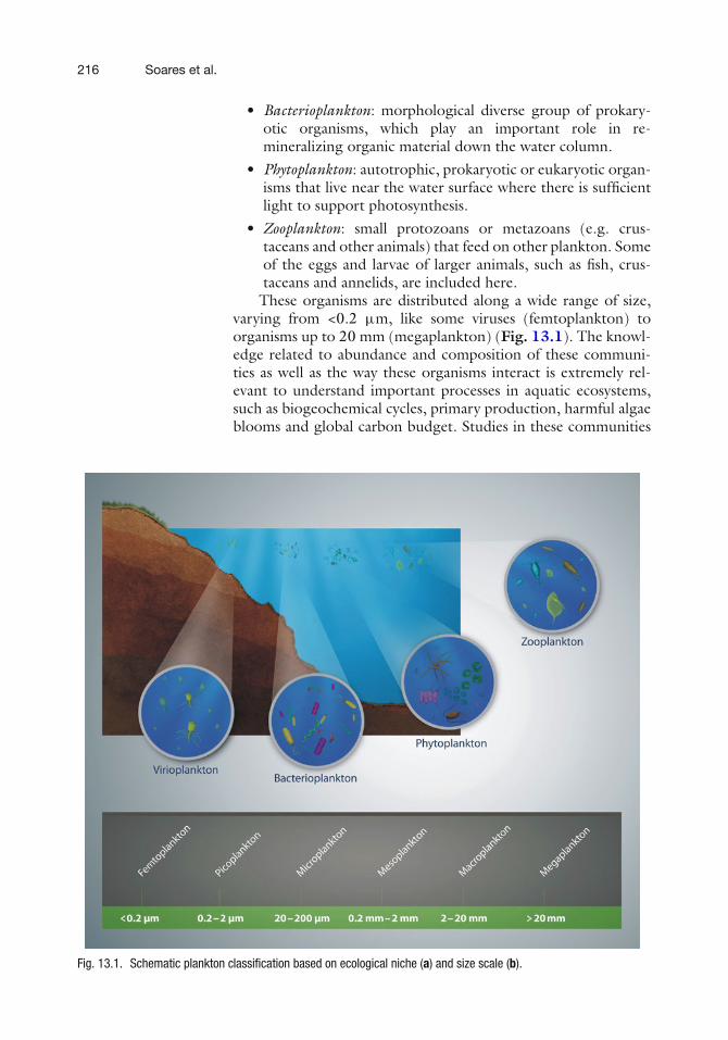
• Bacterioplankton: morphological diverse group of prokary-otic organisms, which play an important role in re-mineralizing organic material down the water column.

• Phytoplankton: autotrophic, prokaryotic or eukaryotic organ-isms that live near the water surface where there is sufficientlight to support photosynthesis.

• Zooplankton: small protozoans or metazoans (e.g. crus-taceans and other animals) that feed on other plankton. Someof the eggs and larvae of larger animals, such as fish, crus-taceans and annelids, are included here.

These organisms are distributed along a wide range of size,varying from <0.2 μm, like some viruses (femtoplankton) toorganisms up to 20 mm (megaplankton) (Fig. 13.1). The knowl-edge related to abundance and composition of these communi-ties as well as the way these organisms interact is extremely rel-evant to understand important processes in aquatic ecosystems,such as biogeochemical cycles, primary production, harmful algaeblooms and global carbon budget. Studies in these communities

Fig. 13.1. Schematic plankton classification based on ecological niche (a) and size scale (b).

Light Microscopy in Aquatic Ecology 217

evolved together with microscopic techniques. The vast majorityof planktonic bacteria started to be revealed only with the use offluorescence microscopy and more recently, the discovery of theabundance of viruses in natural waters reflects the development ofdirect counting methods for bacterial enumeration. Other smallercomponents of plankton such as nanoflagellates and picoplanktonare still overlooked in many studies. On the other hand, due to itssize, techniques for phytoplankton and zooplankton estimationsare widely known and used, and these are probably the most well-known components of planktonic community. Although manyother techniques including molecular biology and transmissionelectronic microscopy have been widely used nowadays, the lightmicroscopy is still the primary source for qualitative studies inplanktonic organisms. Thus, this paper aims to group and describethe most used and available light microscopy techniques to studythe broad range of organisms from virioplankon to zooplankton.

2. Materials

2.1. Virus 1. Anodisc filters, 0.02 μm pore size, 25 mm diameter(aluminum oxide).

2. AA Milipore mixed-ester membrane filters, 0.8 μm poresize, 25 mm diameter.

3. Glass 22 mm diameter filter holder with 15 mL funnel,Millipore-type.

4. Vacuum source, suitable for at least 25 cm Hg vacuum.5. Glass microscope slides, 25 × 75 mm, standard thickness,

frosted at one end.6. Glass coverslips (25 mm × 25 mm).7. SYBR Green I nucleic-acid gel stain 10,000× concentrate

in anhydrous DMSO.8. p-phenylenediamine dihydrochloride or 1,4-

phenylenediamine dihydrochloride (Sigma).9. Glycerol.

10. Phosphate buffer saline (PBS, 0.05 M Na2HPO4, 0.85%(w/v) NaCl, pH 7.5).

11. 0.02 μm filtered-autoclaved ultra pure water.12. 0.02 μm filtered formalin (37–39% (w/v) saturated

formaldehyde solution).13. 0.02 μm filtered samples, formalin preserved, 2% (v/v)

final concentration.

218 Soares et al.

14. 2.0 mL clean and sterilized micro-centrifuge tubes.15. Pipettes suitable for 2–10 mL volumes.16. 5 and 10 mL clean, sterilized tips.17. 50 mL conical centrifuge tube.18. Glass Erlenmeyer filter flasks or multiple filter holder.19. Polystyrene Petri dish.20. Low-temperature dry-heat block with anodized aluminum

heat block.21. Non-fluorescent immersion oil for microscopy (refractive

index (n.d.) 1/4 = 1.516; Olympus).22. Epifluorescence microscope with high-pressure mercury

burner (HBO 100 W), 100× objective, 10× 10 ocu-lar grid, light filters as blue excitation (450–490 nmwide-bandpass) and green excitation (480–550 nm wide-bandpass). A minimum total magnification of 1000× isrequired, although 1250 or higher is preferred.

2.2. Bacteria 1. Polycarbonate membrane, black or stained with IrgalanBlack (1), 0.2 μm pore size, 2.5 mm diameter.

2. Glass 22 mm diameter filter holder with 15 mL funnel,Millipore-type.

3. Vacuum source, suitable for at least 25 cm Hg vacuum.4. Glass microscope slides, 25 × 75 mm, standard thickness,

frosted at one end.5. Glass coverslips (25 mm × 25 mm).6. Formaldehyde 37%, <0.2 μm filtered to a final concentration

of 2% (0.5 mL 37% formaldehyde per 10 mL sample).7. Acridine Orange stock solution 1 mg/mL; 0.2 μm filtered.

Storage cold and dark.8. Non-fluorescent immersion oil for microscopy (refractive

index (n.d.) 1/4 = 1.516).9. Epifluorescence microscope with high-pressure mercury

burner (HBO 100 W), 100× objective, ocular grid, lightfilters as blue excitation (450–490 nm wide-bandpass) andgreen excitation (480–550 nm wide-bandpass). A minimumtotal magnification of 1000× is required, although 1250×or higher is preferred.

2.3. Phytoplankton 1. Amber bottles.2. Lugol’s fixative: Dissolve 10 g I2 (pure iodine; toxic) and

20 g KI in 200 mL distilled water and 20 mL concentratedglacial acetic acid. Store in darkened bottle.

3. Sedimentation chambers of various volumes.

Light Microscopy in Aquatic Ecology 219

4. Inverted microscope with 40× objective, equipped with anocular grid.

2.4. Zooplankton 1. Glass bottle.2. Neutralized formalin solution (40% formaldehyde) to pro-

duce a final concentration of about 4%.3. Automatic volumetric pipette or a Hansen–Stempel pipette.4. Sedgwick-Rafter Counting Chamber.5. Microscope with 10–40× objectives, equipped with an ocu-

lar grid.

3. Methods

3.1. VirusQuantification

About 30 years ago, fluorescence microscopy became the stan-dard method for counting planktonic prokaryotic cells collectedon blackened polycarbonate filters. SYBR Green I and SYBR Goldare notable stains to enumerate microorganisms (2). The first oneis an extremely sensitive cyanine-based fluorescent dye that bindsto double-stranded DNA (dsDNA) and RNA. It is commonlyused for nucleic-acid gel staining due to its high sensitivity super-bright fluorescence and low background, and is considered a less-mutagenic alternative to ethidium bromide (3). SYBR Green I hasbeen used in both fluorescence microscopy and flow-cytometrycounts of viruses (Fig. 13.2a).

1. Rinse each tube (50 mL centrifuge tube) three times withthe samples. Fix samples with filtered formalin immediatelyafter collecting to 2% (v/v) final concentration. Use briefinversion of the sampling container to mix in the fixativeand then place it on ice. Slides need to be prepared within4 h; if it is not possible, samples should be stored at −80◦C(see Note 1).

2. Filter 2 mL of each sample with replicates. If 2 mL is toomuch, dilute the sample with 0.02 μm filtered samples pre-served with 2% (v/v) formalin. Work through the completeslide-preparation procedure to ensure the volume of samplesbeing filtered is appropriate for enumeration. It is impor-tant to know the exact sample volume filtered. Place samplesimmediately in ice.

3. Clean the filter tower with filtered ultra pure water andethanol. Moisten the 0.8 μm pore size, 25 mm diameterwith filtered H2O and put it onto the center of the filterholder. Put a 0.02 μm pore size, 25 mm diameter Anodiscfilter on top of the first one. Using a pipette to transfer thedesired volume of sample to the filter funnel, turn the vac-uum pump to B20 kPa or 20 cm Hg VAC.

220 Soares et al.

Fig. 13.2. Main planktonic groups imaged by light microscopy after staining with SYBR Green I (a, Virioplankton) andacridine orange (b, Bacterioplankton) and fixing with lugol’s solution (c–g, phytoplankton) and formalin (h–l, zooplankton).In (a), virus-like-particles are encircled; other particles are indicated by arrows. In b, bacterial cells are encircled andpicoplanktonic cells indicated by arrows, c cyanobacteria, d and e diatoms, f cryptomonads, g desmid, h and i rotifers,j copepod, k and l cladocerans. Bars, 10 μm (a); 10 μm (b); 30 μm (c); 5 μm (d); 10 μm (e–g); 25 μm (h, k);50 μm (i, l); 0.5 mm (j).

Light Microscopy in Aquatic Ecology 221

4. After the water has filtered through, leave the vacuum pumpon and carefully remove the clamp and filter funnel. Thesame 0.8 μm filter can be used for multiple samples. The0.02 μm filter needs to be dried before the stain process.While filters are drying, use a pipette and tip to dispense10 μL droplet of the working concentration SYBR GreenI reagent onto the middle of each Petri dishes labeled withthe number of samples. Once filters are dry, place each filteronto the 10 μm SBYR reagent dropped backside down ineach labeled Petri dishes. Microorganisms on the topside ofthe filter will be stained by the reagent, which will easily passthrough the filter from the underside to the top. Stain eachfilter for 18 min, keeping the stained filters in the dark.

5. Put the dried Anodisc filter (0.02 μm) onto the labeled glassmicroscope slide. To mount the filter, use a pipette and tipto dispense 27–30 μL of 0.1% (v/v) p-phenylenediamineanti-fade mounting medium onto a 25× 25 mm glasscoverslip.

6. To enumerate the virus, use a 100× fluorescence oil-immersion objective with immersion oil. Put a drop of oilonto the center of a coverslip and move the objective downto the drop of oil. SYBR Green I is excited with maximumat 488 nm. Using a 10× 10 ocular grid, count between 30and 40 boxes for a total of 10 fields by randomly moving thestage to a new position around the entire filter. The total for10 fields should be >200 viruses counted.

7. Calculate the total density (number of virus per mL) fromconversion factor: (NV × 100)/(n × RSF)/V, where NVis the average number of viruses per field, n is the numberof boxes (of 100 total) counted on the microscope eyepiecegrid per field, RSF is the grid-reticle scaling factor (repre-senting the ratio of the filtered area to the 10 × 10 gridvisible in the eyepiece) and V is the volume of the filteredsample (mL).

3.2. BacteriaEnumeration

Bacteria enumeration is performed under fluorescencemicroscopy equipped with specific light filters in accordancewith the staining used. Bacteria are stained on membranes usingfluorochromes. Acridine Orange and DAPI (4′,6′-diamidino-2-phenylindole) have been the most used stains for bacteriaenumeration by aquatic microbiologists (see Note 2). Theepifluorescence microscopy method was introduced by Hobbieet al. (2), which led to a better understanding of bacterioplanktonrole to the aquatic microbial food web. Fluorescence microscopyhas been used to determine bacterial biomass and bacteriaphylogenetic identification (see Note 3) in addition to bacteriacounting (see Note 4) (Fig. 13.2b).

222 Soares et al.

1. Fix samples immediately following sampling with free-particle formaldehyde (see Section 2.2, Item 6). Fixed sam-ples should be kept in the dark and slides should be preparedsoon to avoid cell degradation.

2. Moisten the filter unit with particle-free water; place the1.2 μm supporting filter and subsequently the 0.2 μm blackmembrane. The supporting filter can be used several times.Rinse the filter unit funnel with ultra pure water and place iton top of the filters and fasten it with the clamp.

3. Pour known volume of sample on 2.5 mm unit membranefilter and add Acridine Orange at a final staining concentra-tion of 0.01%. Wait for 1 min (3) and then gently filter. Referto Note 5 for sample volume adjustment.

4. Filter samples at a maximum vacuum of 100 mmHg to avoidcell damage until whole samples pass through the filter. Letthe suction continue and air flow through the filters whileremoving the funnel and let the filter dry a little. The filtershould be moist but not wet.

5. Place the filter on a glass slide using a small drop of immer-sion oil. Put on the central top of black membrane a smalldrop of immersion oil and mount with a clean coverslip,pressing down firmly in a folded paper towel until the oilmoves out of the edges of the coverslip. Store frozen andprotected from light.

6. Thoroughly rinse funnels with particle-free water betweensamples.

7. Count at least 10 grids randomly spread over the filter. Aminimum of 200 cells should be counted. This reduces thestandard deviation and provides a trusty mean (4). WhenAcridine Orange is used, bacteria should be counted on blueexcitation (U-MSWB2 450–490 nm wide-bandpass). Cellsshine in orange and green colors. Heterotrophic cells andautotrophic cells may be differed by using green excitationfilter (U-MSWG2 480–550 nm wide-bandpass), at whichonly autotrophy cells shine (5).

8. Calculate bacterial cell number from the following conver-sion factor: (n × A)/(V × a) where,n is the mean number of bacterial cells, A is the filter area,a is the area of the counting grid, V is the volume of sam-ple collected × volume of sample filtered/(volume of thecollected sample + volume of the fixative).

3.3. PhytoplanktonEnumeration

For phytoplankton enumeration, a whole water sample must becollected (unfiltered and unstrained) (Fig. 13.2c–g). Sedimen-tation is the preferred method for phytoplankton concentration,because it is nonselective (unlike filtration) and nondestructive(unlike filtration or centrifugation). For enumeration, several

Light Microscopy in Aquatic Ecology 223

alternative counting chambers can be used (Sedwick–Rafter,Lund, Palmer-Maloney). The commonly used Sedgewick–Rafterchamber is the most suitable for counting large algae at low con-centration, once high magnification objectives cannot be used.Here we discuss sedimentation and counting techniques using theinverted microscope (6) which is the better suited equipment forquantitative analysis of multispecies present in natural samples.Whenever possible, phytoplankton species should be examinedalive, particularly delicate species of flagellated algae.

1. Fix the samples in Lugol’s solution, at a final concentrationof 1:100 (see Note 6). Samples must be stored in dark glass-ware protected from light.

2. After mixing with the Lugol’s solution, gently add the sam-ple into a sedimentation chamber. Refer to Note 7 for sedi-mentation chamber volumes and care.

3. Fill the chamber to the top edge with sufficient excess to per-mit the water to “bead” upward above the edge. Slide thechamber cover cap across the top of the cylinder to removeany excess of water and to enclose the sample of exact vol-ume without entrapping any air bubbles. The time to ensurecomplete sedimentation of all organisms in hours should beat least three times the height in cm of the sedimentationchamber (7). Keep the chamber on a vibration and light-freearea.

4. Remove the extra volume and mount the chamber with anadequate coverslip.

5. Enumerate organisms using an inverted microscope. Beforecounting, the entire chamber must be analyzed to ensurethe homogeneous sedimentations of cells. Individual (cells,colonies, coenobium, filaments) are enumerated in randomnon-overlapping fields, previously defined (8). At least 100individuals of the dominant taxa must be counted (error<20%, p < 0.05) (9). When organisms lie across the marginareas, those along the upper and right edges (or lower andleft) must not be counted. Empty diatoms, dinoflagellates orother damaged cells are not counted.

6. Calculate the total density from the following conversionfactor: [field surface (μm2) × chamber length (mm) × num-ber of fields]/109. Cell volume can be calculated for eachspecies by comparing cellular morphology with solid geo-metric shapes most closely related (10).

3.4. Zooplankton Zooplankton samples often need to be concentrated in the fieldusing plankton net or a pump. The sampling success will largelydepend on the selection of a suitable gear; mesh size of nettingmaterial, time of collection, water depth of the study area andsampling strategy. After sampling, fixation should be carried out

224 Soares et al.

as early as possible preferentially within 5 min after the collectionto avoid damage to animal tissue by bacterial action and autolysis.The methodology described here is applied to large zooplanktongroups, such as rotifers (Fig. 13.2 h–i), microcrustaceans – cope-pods (Fig. 13.2j) and cladocerans (Fig. 13.2 k, l).

1. Depending on the used concentration, dilute the concen-trated sample of zooplankton to exactly 50, 100 or 200 mLwith tap water. Use a graduated cylinder.

2. Mix organisms thoroughly within the graduated cylinder(vortex mixer or magnetic stirrer) and immediately obtaina subsample. Work rapidly to minimize the effect of organ-ism settling.

3. Obtain a subsample of 1 mL with an automatic volumetricpipette. Use a wide-mouth pipette so as not to restrict uptakeof large zooplankton or a Hansen–Stempel pipette.

4. Add this subsample to Sedgwick–Rafter chamber whichholds exactly 1 mL.

5. Count all organisms in number of subsamples definedaccording to the concentration of organisms in the subsam-ples (2–5).

6. Calculate the total density from the following conversionfactor: ind. L−1 = average count per cell ± standard devi-ation of the mean × volume of sample (mL)/volume of lakewater filtered (L). The biovolume is estimated by measur-ing cells’ dimension and by approximation of a geometricshape (11–13). In the case of microcrustaceans (cladoceraand copepoda) is commonly used the value of dry weight,which is measured in an analytical microbalance (14, 15).

3.5. Identificationof Damaged Cells

In natural populations, an important fraction of bacteria and phy-toplankton cells are compromised or dying whenever lysis ratesare important. Indeed, recent works have demonstrated that lysisis an important process not only in oceans (16) but also inlakes (17). The identification of damaged cells requires appro-priate methods to reliably discriminate living from dead or com-promised cells in natural phytoplankton. A rapid procedure toidentify damaged cells can be done using tests for viability suchas the LIVE/DEAD BacLight Bacterial Viability kit (MolecularProbes) to estimate total counts of viable/damage of both bacte-ria (18) and cyanobacteria (19, 20). This kit utilizes a mixtureof SYTO R© 9 green-fluorescent nucleic-acid stain and the red-fluorescent nucleic-acid stain, propidium iodide. These stains dif-fer in their ability to penetrate into healthy cells. When both dyesare used together, SYTO 9 labels viable bacteria, while propidiumiodide penetrates into bacteria with damaged membranes. Meth-ods for viability evaluation of other phytoplanktonic organismsare also available (21).

Light Microscopy in Aquatic Ecology 225

4. Notes

1. If samples were stored at −80◦C, certify that the samples’temperature reach the room temperature (25◦C) before thefiltration.

2. The specific fluorescent probe DAPI (4′6′-diamidino-2-phenylindole) can also be used by the aquatic ecologist (22).When DAPI is used, the bacteria quantification is done onUV filters (U-MNU2, BP 330–385 nm, Olympus).

3. One common way to estimate bacterial biomass is to usea computer-assisted image analysis system. It consists ofusing a microscope of epifluorescence with a video cam-era, a computer equipped with video acquisition capabilitiesand appropriate software for image processing. In our case,we use the software Image Pro-Plus 5.0. Samples are pre-pared like described for enumeration of total bacteria andbiomass is determined by measure geometric formula. Theimage must be passing a following application of filter inorder to improve it, according to the following sequence(23): Gauss filter (kernel 5 × 5) followed by Laplace filter(kernel 5 × 5) and a median filter (rank 3), the latter runthree times. After calculating a three-dimensional param-eter volume, using the formula V = π/4 × W 2(L − W /3)(V= volume, L = Length, W = Width), the result is appliedin the formula (24): m = CV α, where, C = 120 fg C, V =volume of cell and a = 0.76.

4. Fluorescence in situ hybridization (FISH) with rRNA-targetprobes is another staining technique that allows phyloge-netic identification of bacteria in mixed assemblages (25)through fluorescence microscope. Such procedure is rou-tinely used in the analysis of bacterioplankton, althoughmust be necessary that other excitation filters besides blueand green to this approach.

5. The volume of the bacteria samples for staining must beadjusted in accordance to the bacterial abundance andthis can be determined by trial and error. One or twomilliliter has been the most usual sample amount for naturalsamples.

6. Lugol is a recommended fixative for phytoplankton. It actsnot only on the cell preservation but also accelerating thesedimentation process within the chamber, since it increasescells’ weight.

7. Sedimentation chambers are available in volumes of 1, 5, 10,25, 50 and 100 mL. The concentrated volume is related tothe sample turbidity and varies inversely to the amount of

226 Soares et al.

organisms. The sedimentation chambers and their coverslipsmust be cleaned thoroughly to avoid contamination withorganisms from previous samples.

References

1. Hobbie, J. E., Daley, R. J., Jasper, S. (1977)Use of nucleopore filters for counting bacte-ria by flurescence microscopy. Appl EnvironMicrob 49, 1225–1228.

2. Noble, R. T., Fuhrman, J. A. (1998) Useof SYBR Green I for rapid epifluorescencecounts of marine viruses and bacteria. AquatMicrob Ecol 14, 113–118.

3. Patel, A., Noble, R. T., Steele, J. A., Schwal-bach, M. S., Hewson, I., Furhman, A.(2007) Virus and prokaryote enumerationfrom planktonic aquatic environments by epi-fluorescence microscopy with SYBR Green I.Nat Protoc 2, 269–276.

4. Kirchman, D. J. (1993) Statistical analysisof direct counts of microbial abundance, in(Kemp, P. F., Sherr, B. F., Sherr, E. B.,Cole, J. J. eds.), Handbook of Methods inAquatic Microbial Ecology. Lewis Publishers,Boca Raton, FL, pp. 117–119.

5. Daley, R. J, Hobbie, J. E. (1975) Directcounts of aquatic bacteria by a modified epi-fluorescence technique. Limnol Oceanogr 20,875–882.

6. Utermöhl, H. (1958) Zur Vervolkomnungder quantitativen phytoplankton–methodik.Mitt Int Ver Theor Angew Limnol 9,1–38.

7. Margalef, R. (1969) Counting, in (Vollen-weider, R. A., Talling, J. F., Westlake, D.F. eds.). A Manual on Methods for Measur-ing Primary Production in Aquatic Environ-ments (I.B.P. Handbook 12). Blackwell Sci-ent. Publ., Oxford and Edinburgh, pp. 7–14.

8. Uhelinger, V. (1964) Étude statistiquedes methods de dénobrement planctonique.Arch Sci 17, 121–223.

9. Lund, J. W. H., Kipling, C., Lecren, E. D.(1958) The inverted microscope method ofestimating algal number and statistical basisof estimating by counting. Hydrobiologia 11,143–170.

10. Hillebrand, H., Dürselen, C. D., Kirschtel,D., Pollingher, U., Zohary, T. (1999) Bio-volume calculation for pelagic and benthicmicroalgae. J Phycol 35, 408–424.

11. Gates, M. A., Rogerson, A., Berger, J. (1982)Dry to wet biomass conversion constant forTetrahymena Elliot (Ciliophora, Protozoa).Oecologia 55, 145–148.

12. Ruttner-Kolisko, A. (1977) Suggestions forbiomass calculation of planktonic rotifers.Arch Hydrobiol 8, 71–76.

13. Pauli, H. R. (1989) A new method toestimate individual dry weights of rotifers.Hydrobiologia 186/197, 355–361.

14. Dumont, H. J, Van De Velde, I., Dumont, S.(1975) The dry weight estimate of biomassin a selection of cladocera, copepoda androtifera from the plankton, periphyton andbenthos of continental waters. Oecologia 19,75–97.

15. Manca, M., Comoli, P. (1999) Studies onzooplankton of Lago Paione Superior. J Lim-nol 58, 131–135.

16. Agustí, S., Sánchez, C. (2002) Cell viabilityin natural phytoplankton communities quan-tified by a membrane permeability probe.Limnol Oceanogr 47, 818–828.

17. Agustí, S., Alou, E., Hoyer, MV., Frazer, T.K., Canfield, D. E. (2006) Cell death in lakephytoplankton communities. Freshwater Biol51, 1496–1506.

18. Freese, H. M., Karsten, H. M., Schumann, R.(2006) Bacterial abundance, activity, and via-bility in the eutrophic river Warnow, North-east Germany. Microb Ecol 51, 117–127.

19. Dagnino, D., de Abreu Meireles, D., deAquino Almeida, J. C. (2006) Growth ofnutrient–replete microcystis PCC 7806 cul-tures is inhibited by an extracellular sig-nal produced by chlorotic cultures. EnvironMicrobiol 8, 30–36.

20. Lengke, M. F., Ravel, B., Fleet, M. E.,Wanger, G., Gordon, R. A. S., Southam,G. (2006) Mechanisms of gold bioaccumula-tion by filamentous cyanobacteria from Gold(III)-Chloride complex. Environ Sci Technol40, 6304–6309.

21. Schumann, R., Schiewer, U., Karsten, U.,Rieling, T. (2003) Viability of bacteria fromdifferent aquatic habitats. II. Cellular fluo-rescent markers for membrane integrity andmetabolic activity. Aquat Microb Ecol 32,137–150.

22. Poter, K. G, Feig, Y. S. (1980) The use ofDAPI for identifying and counting aquaticmicroflora. Limnol Oceanogr 25, 943–948.

23. Massana, R., Gasol, M. J., Bjørnsen, P. K.,Black-Burn, N., Hagström, A., Hietanen, S.,Hygum, B. H., Kuparinen, J., Pedrós-Alió,C. (1997) Measurement of bacterial size viaimage analysis of epifluorescence prepara-tions: description of an inexpensive systemand solutions to some of the most commonproblems. Scientia Marina 61, 397–407.

Light Microscopy in Aquatic Ecology 227

24. Norland, S. (1993) The relation betweenbiomass and volume of bacteria, in (Kemp,P. F., Sherr, B. F., Sherr, E. B., Cole, J.J. eds.), Handbook of Methods in AquaticMicrobial Ecology. Lewis, Boca Raton, FL,pp. 303–308.

25. Cottrell, M. T., Kirchman, D. L. (2000)Community composition of marine bac-terioplankton determined by 16 s RRNAgene clone libraries and fluorescence in situhybridization. Appl Environ Microbiol 66,5116–5122.