Melting of Aromatic Compounds: Molecular Dynamics Simulations

Materials Theory, Simulations, and Parallel Algorithms

MATERIALS RESEARCH SOCIETY

SYMPOSIUM PROCEEDINGS VOLUME 408

Materials Theory, Simulations, and

Parallel Algorithms Symposium held November 27-December 1, 1995, Boston, Massachusetts, U.S.A.

EDITORS:

Efihimios Kaxiras Harvard University

Cambridge, Massachusetts, U.S.A.

John Joannopoulos Massachusetts institute of Technology

Cambridge, Massachusetts, U.S.A.

Priya Vashishta Louisiana State University

Baton Rouge, Louisiana, U.S.A.

Rajiv K. Kalia Louisiana State University

Baton Rouge, Louisiana, U.S.A.

9to r*ZlT?

MIR1SI MATERIALS RESEARCH SOCIETY

PITTSBURGH, PENNSYLVANIA

ÄBPiovod fax BU&Ü2 tstöc

This material is based upon work supported by the national Science Foundation under Grant no. DMR-9527893.

This work relates to Department of Navy Grant Number N00014-96-1-0296 issued by the Office of Naval Research. The United States Government has a royalty-free license throughout the world in all copyrightable material contained herein.

Single article reprints from this publication are available through University Microfilms Inc., 300 North Zeeb Road, Ann Arbor, Michigan 48106

CODEN: MRSPDH

Copyright 1996 by Materials Research Society. All rights reserved.

This book has been registered with Copyright Clearance Center, Inc. For further information, please contact the Copyright Clearance Center, Salem, Massachusetts.

Published by:

Materials Research Society 9800 McKnight Road Pittsburgh, Pennsylvania 15237 Telephone (412) 367-3003 Fax (412) 367-4373 Homepage http://www.mrs.org/

Library of Congress Cataloging in Publication Data

Materials theory, simulations, and parallel algorithms : symposium held November 27-December 1, 1995, Boston, Massachusetts, U.S.A. / editors, Efthimios Kaxiras, John Joannopoulos, Priya Vashishta, Rajiv K. Kalia.

p. cm.—(Materials Research Society symposium proceedings ; v. 408) Includes bibliographical references and index. ISBN: 1-55899-311-8 (alk. paper) 1. Materials science—Computer simulation—Congresses. 2. Parallel

programming (Computer science)—Congresses. 3. Computer algorithms— Congresses. I. Kaxiras, Efthimios II. Joannopoulos, John III. Vashishta, Priya IV. Kalia, Rajiv K. V. Series: Materials Research Society symposium proceedings ; v. 408.

TA404.23.M38 1996 96-3079 620.1'1'01 13—dc20 CIP

Manufactured in the United States of America

CONTENTS

Preface xiii

Materials Research Society Symposium Proceedings xvi

PARTI: ADVANCES IN COMPUTATIONAL METHODS

The SEISM* Project: A Software Engineering Initiative for the Study of Materials 3

G. Mula, C. Angius, F. Casula, G. Maxia, M. Porcu, and Jinlong Yang

Polarization, Dynamical Charge, and Bonding in Partly Covalent Polar Insulators 9

R. Resta, S. Massidda, M. Posternak, and A. Baldereschi

Linear-Response Calculations of Electron-Phonon Coupling Parameters and Free Energies of Defects 13

Andrew A. Quong and Amy Y. Liu

'Atomic and Electronic Structure of Germanium Clusters at Finite Temperature Using Finite Difference Methods 19

James R. Chelikowsky, Serdar Ögüt, X. Jing, K. Wu, A. Stathopoulos, and Y. Saad

•Equation of State for PdH by a New Tight Binding Approach 31 D.A. Papaconstantopoulos and M.J. Mehl

A Tight-Binding Model Beyond Two-Center Approximation 37 C.Z. Wang, M.S. Tang, Bicai Pan, C.T. Chan, and K.M. Ho

Tight-Binding Initialization for Generating High-Quality Initial Wave Functions: Application to Defects and Impurities in GaN 43

Jörg rieugebauer and Chris O. Van de Walle

Ab Initio Calculations for SiC-AI Interfaces by Conjugate-Gradient Techniques 49

Masanori Kohyama

O(N) Scaling Simulations of Silicon Bulk and Surface Properties Based on a Non-Orthogonal Tight-Binding Hamiltonian 55

rioam Bernstein and Efthimios Kaxiras

A Semi-Empirical Methodology to Study Bulk Silica System 61 Ai Chen and L. Rene Corrales

Monte-Carlo Studies of Bosonic van der Waals Clusters 67 M. Meierovich, A. Mushinski, and M.P. nightingale

Invited Paper

O(N) Multiple Scattering Method for Relativistic and Spin Polarized Systems 73

S.V. Beiden, Q.Y. Quo, W.M. Temmerman, Z. Szotek, O.A. Oehring, Yang Wang, Q.M. Stocks, D.M.C. Mcholson, W.A. Shelton, and H. Ebert

Derivation of Interatomic Potentials by Inversion of Ab Initio Cohesive Energy Curves 79

M.Z. Bazant and Efthimios Kaxiras

Mixed Approach to Incorporate Self-Consistency into Order-N LCAO Methods 85

Pablo Ordejon, E. Artacho, and J.N. Soler

PART II: PARALLEL ALGORITHMS AND APPLICATIONS

*Fast Algorithms for Composite Materials 93 L. Qreengard

Molecular Dynamics Simulations of a Siloxane-Based Liquid Crystal Using an Improved Fast Multipole Algorithm Implementation 99

Alan Mctienney, Ruth Pachter, Soumya Patnaik, and Wade Adams

A Parallel Implementation of Tight-Binding Molecular Dynamics Based on Reordering of Atoms and the Lanczos Eigen-Solver 107

Luciano Colombo, William Sawyer, and Djordje Marie

"Large Scale Molecular Dynamics Study of Amorphous Carbon and Graphite on Parallel Machines 113

J. Yu, Andrey Omeltchenko, Rajiv K. Kalia, Priya Vashishta, and Donald W. Brenner

Massively Parallel Molecular Dynamics and Simulations for Many-Body Potentials 125

L.T. Wille, C.F. Corn well, and W.C. Money

*Ab-lnitio Molecular Dynamics of Organic Compounds on a Massively Parallel Computer 131

Francois Qygi

ACRES: Adaptive Coordinate Real-Space Electronic Structure 139

N.A. Modine, Gil Zumbach, and Efthimios Kaxiras

'Electronic Structure Calculations on a Real-Space Mesh With Multigrid Acceleration 145

D.J. Sullivan, E.L. Briggs, C.J. Brabec, and J. Bernholc

'Invited Paper

VI

The Massively Parallel O(N) LSMS-Method: Alloy Energies and Non-Collinear Magnetism 157

G.M. Stocks, Yang Wang, D.M.C. Nicholson, W.A. Shelton, W.M. Temmerman, Z. Szotek, B.N. Harmon, and V.P. Antropov

Variational Monte Carlo on a Parallel Architecture: An Application to Graphite 169

M. Menchi, A. Bosin, and S. Fahy

Structure, Mechanical Properties, and Thermal Transport in Microporous Silicon Nitride Via Parallel Molecular Dynamics 175

Andrey Omeltchenko, Aiichiro Nakano, Rajiv K. Kalia, and Priya Vashishta

Early Stages of Sintering of Si3N4 Nanoclusters Via Parallel Molecular Dynamics 181

Ken/7 Tsuruta, Andrey Omeltchenko, Rajiv K. Kalia, and Priya Vashishta

PART III: FRACTURE. BRITTLE/DUCTILE BEHAVIOR AND LARGE SCALE DEFECTS

Parallel Simulations of Rapid Fracture 189 Farid F. Abraham

Dynamic Simulation of Crack Propagation with Dislocation Emission and Migration 199

ti. Zacharopoulos, DJ. Srolovitz, and R.A. LeSar

Dynamics and Morphology of Cracks in Silicon Nitride Films: A Molecular Dynamics Study on Parallel Computers 205

Aiichiro Nakano, Rajiv K. Kalia, and Priya Vashishta

Representation of Finite Cracks by Dislocation Pileups: An Application to Atomic Simulation of Fracture 217

Vijay Shastry and Diana Parkas

Mechanism of Thermally Assisted Creep Crack Growth 223 Leonardo Qolubovi'c and Dorel Moldovan

Embrittlement of Cracks at Interfaces 229 Robb Thomson and A.E. Carlsson

Effect of Crack Blunting on Subsequent Crack Propagation 237 J. Schiotz, A.E. Carlsson, L.M. Canel, and Robb Thomson

Critical Evaluation of Atomistic Simulations of 3D Dislocation Configurations 243

Vijay B. Shenoy and Rob Phillips

Invited Paper

VII

Simulation of Dislocations in Ordered Ni3AI by Atomic Stiffness Matrix Method 249

Y.E. Hsu and T.K. Chaki

First Principles Simulations of Nanoindentation and Atomic Force Microscopy on Silicon Surfaces 255

R. Perez, M.C. Payne, I. Stich, and K. Terakura

'Dislocation Kink Motion—Ab-lnitio Calculations and Atomic Resolution Movies 261

J.C.ti. Spence, tl.R. Kolar, Y. Huang, and H. Alexander

An Ab Initio Investigation of a Grain Boundary in a Transition Metal Oxide 271

/. Dawson, P.D. Bristowe, M.C. Payne, and M-H. Lee

Temperature and Strain Rate Effects in Grain Boundary Sliding 277

C. Molteni, G.P. Francis, M.C. Payne, and V. Heine

Ab Initio Investigation of Grain Boundary Sliding 283 M.C. Payne, G.P. Francis, C. Molteni, N. Marzari, V. Deyirmenjian, and V. Heine

Environment Sensitive Embedding Energies of Impurities, and Grain Boundary Stability in Tantalum 291

Genrich L. Krasko

PART IV: THERMODYNAMIC STABILITY OF MATERIALS

Gradient-Driven Diffusion Using Dual Control Volume Grand Canonical Molecular Dynamics (DCV-GCMD) 299

Frank van Swol and Grant S. Heffelfinger

"Lattice Instabilities, Anharmonicity and Phase Transitions in PbTi03 and PbZr03 305

K.M. Rabe and U.V. Waghmare

Configuration Dependence of the Vibrational Free Energy in Substitutional Alloys and Its Effects on Phase Stability 309

G.D. Garbulsky and G. Ceder

Molecular Dynamics Study of Structural Transitions and Melting in Two Dimensions 315

L.L. Boy er

Ab Initio and Model Calculations on Different Phases of Zirconia 321

Uwe Schönberger, Mark Wilson, and Michael W. Finnis

*lnvited Paper

VIII

Melting of Aromatic Compounds: Molecular Dynamics Simulations 327

P.W.-C. Rung, J.T. Books, CM. Freeman, S.M. Levine, B. Vessal, J.M. newsam, and M.L. Klein

Distribution of Rings and Intermediate Range Correlations in Silica Glass Under Pressure—A Molecular Dynamics Study 333

Jose Pedro Rino, Qonzalo Gutierrez, Ingvar Ebbsjö, Rajiv K. Kalia, and Priya Vashishta

First-Principles Calculations of Heusler Phase Precursors in the Atomic Short-Range Order of Disordered BCC Ternary Alloys 339

Jeffrey D. Althoff and Duane D. Johnson

Structural Phase Transition from Fluorite to Orthorhombic FeSi2 by Tight Binding Molecular Dynamics 345

Leo Miglio, Massimo Celino, Valeria Meregalli, and Francesca Tavazza

Prediction of a Very Hard Triclinic Form of Diamond 351 O. Benedeh, M. Facchinetti, L. Miglio, and S. Sena

Cu-Au Alloys Using Monte Carlo Simulations and the BFS Method for Alloys 357

Ouillermo Bozzolo, Brian Good, and John Ferrante

Clustering and Extended Range Order in Binary Network Glasses 363

Dmitry Tiekhayev and John Kieffer

Phase Stability of the Sigma Phase in Fe-Cr Based Alloys 369 Marcel ti.F. Sluiter, Keivan Esfarjani, and Yoshiyuki Kawazoe

Defect Structure of ß NiAl Using the BFS Method for Alloys 375 Guillermo Bozzolo, Carlos Amador, John Ferrante, and Ronald D. rioebe

First-Principles Calculation of the Structure of Mercury 383 Michael J. Mehl

PARTV: SURFACES AND INTERFACES OF MATERIALS

'Bonding and Vibrational Properties of CO-Adsorbed Copper 391

Steven P. Lewis and Andrew M. Rappe

Atomistic Monte Carlo Simulations of Surface Segregation in (FexMni_x)0 and (NixCoi.x)0 401

C. Battaile, R. riajafabadi, and D.J. Srolovitz

Invited Paper

Spatial Redistribution of Niobium Additives Near Nickel Surfaces 407

Leonid S. Muratov and Bernard R. Cooper

*Some Computer Simulations of Semiconductor Thin Film Growth and Strain Relaxation in a Unified Atomistic and Kinetic Model 413

A Madhukar, W. Yu, R. Viswanathan, and P. Chen

Theory of Initial Oxidation Stages on Si(100) Surfaces by Spin-Polarized Generalized Gradient Calculation 427

K. Kato, T. Yamasaki, T. Uda, and K. Terakura

Growth Mechanism of Si Dimer Rows on Si(001) 433 T. Yamasaki, T. Uda, and K. Terakura

Ab Initio Study of Expitaxial Growth on a Si(100) Surface in the Presence of Steps 439

V. Milman, S.J. Pennycook, and D.E. Jesson

Molecular-Dynamics Simulations of Hydrogenated Amorphous Silicon Thin-Film Growth 445

T. Ohira, O. Ukai, M. rioda, Y. Takeuchi, M. Murata, and H. Yoshida

Dissociative Adsorption and Desorption Processes of CI2/GaAs(001) Surfaces 451

Takahisa Ohno

Formation Energy, Stress, and Relaxations of Low-Index Rhodium Surfaces 457

Alessio Fiiippetti, Vincenzo Fiorentini, Kurt Stokbro, Riccardo Valente, and Stefano Baroni

Full-Potential LMTO Calculation of Ni/Ni3AI Interface Energies 463

D.h. Price and B.R. Cooper

Simulations of the Structure and Properties of the Polyethylene Crystal Surface 469

J.L. Wilhelmi and G.C. Rutledge

PART VI: COMPLEX MATERIALS SIMULATIONS

*Ab Initio Molecular Dynamics Simulations of Molecular Crystals 477

Mark E. Tuckerman, Tycho von Rosenvinge, and Michael L. Klein

'Invited Paper

Molecular Dynamics Simulations of SiSe2 Nanowires 489 Wei Li, Rajiv K. Kalia, and Priya Vashishta

Ab Initio Core-Level Shifts in Metallic Alloys 495 Vincenzo Fiorentini, Michael Methfessel, and Sabrina Oppo

Native Point Defect Densities and Dark Line Defects in ZnSe 503 M.A. Berding, A. Sher, and M. van Schilfgaarde

First-Principles Simulations of Interstitial Atoms in Ionic Solids 509

E.A. Kotomin, A. Svane, T. Brudevoll, W. Schulz, and N.E. Christensen

Hydrogen Diffusion in Quartz: A Molecular Dynamics Investigation 515

A. Bongiorno and L. Colombo

Investigation of Crystalline Quartz and Molecular Silicon-Oxygen Compounds With a Simplified LCAO-LDA Method 521

R. Kaschner, O. Seifert, Th, Frauenheim, and Th. Köhler

Calculation of Electromagnetic Constitutive Parameters of Insulating Magnetic Materials With Conducting Inclusions 527

Eric Küster, Rick Moore, Lisa Lust, and Paul Kemper

Hydrogenation Effects on Structures of Silicon Clusters 533 Takehide Miyazaki, Ivan Stich, Tsuyoshi Uda, and Kiyoyuki Terakura

Valence-Band Offset at the Zn-P Interface Between ZnSe and lll-V Wide Gap Semiconductor Alloys: A First- Principles Investigation 539

F. Bernardini and R.M. nieminen

Electronic Structure and Stability of Ordered Vacancy Phases of NbN 545

E.C. Ethridge, S.C. Erwin, and W.E. Pickett

Atomistic Study of Boron-Doped Silicon 551 M. Fearn, J.li. Jefferson, and D.G. Petti for

First-Principles Calculations of the Elastic Properties of the Nickel-Based LI 2 Intermetallics 557

D. lotova, N. Kioussis, S.P. Lim, S. Sun, and R. Wu

Ab-lnitio Calculations of the Electronic Structure and Properties of Titanium Carbosulfide 563

Bala Ramalingam, Michael E. Mctlenry, Warren M. Garrison, Jr., and James M. MacLaren

EELS Studies of B2-Type Transition Metal Aluminides: Experiment and Theory 567

O.A. Botton, Q.Y. Quo, W.M. Temmerman, Z. Szotek, C.J. Humphreys, Yang Wang, Q.M. Stocks, D.M.C. riicholson, and W.A. Shelton

Sintering of Amorphous Si3N4 Nanoclusters: A Molecular Dynamics Study of Stress Analysis 573

Jinghan Wang, Kenji Tsuruta, Andrey Omeltchenko, Rajiv K. lialia, and Priya Vashishta

DFT Study of the Monocyclic and Bicyclic Ring Geometries of C20 579

Zhiqiang Wang, Paul Day, and Ruth Pachter

The Magnetic Structure of Cuo.2Nio.8 Alloys 585 Yang Wang, Q.M. Stocks, D.M.C. riicholson, W.A. Shelton, Z. Szotek, and W.M. Temmerman

Computer Simulation of Cluster Ion Impacts on a Solid Surface 591

Z. Insepov and I. Yamada

Molecular Dynamics Simulations for Xe Absorbed in Zeolites 599

J.-H. Kantola, J. Vaara, T.T. Rantala, andj. Jokisaari

Author Index 605

Subject Index 609

XII

PREFACE

Significant advances have been made recently toward understanding the properties of materials through theoretical approaches. These approaches are based either on first-principles quantum mechanical formulations or semiempirical formulations, and have benefitted from increases in computational power. The advent of parallel computing has propelled the theoretical approaches to a new level of realism in modelling physical systems of interest. The theoretical methods and simulation techniques that are currently under development are bound to become powerful tools in understanding, exploring and predicting the properties of existing and novel materials.

The aim of this symposium was to bring together scientists from several subfields of materials theory and simulations. Its purpose was: to make contact with traditional continuum approaches to materials theory; to discuss critically current developments in computational and simulational approaches specifically aimed at addressing real materials problems, and with emphasis on parallel computing; and to present examples of the most successful applications of computational and simulational work to date.

The main topics of the symposium were:

(I) Advances in Computational Methods, covering new methodologies for calculating materials properties and new algorithms for efficient computations, such as CXrl) scaling.

(II) Parallel Algorithms and Applications, covering novel approaches to parallel computations and examples of large-scale simulations using parallel architectures.

(III) Fracture, Brittle/Ductile Behavior and Large Scale Defects, covering theoretical developments and simulations related to fracture phenomena and large scale defects such as dislocations and grain boundaries.

(IV) Thermodynamic Stability of Materials, covering new theoretical approaches and their applications to the stability of materials at finite temperature and pressure.

(V) Surfaces and Interfaces of Materials, covering problems related to surface properties, growth and the interfaces of materials.

(VI) Complex Materials Simulations, covering a range of topics on materials with complex atomic or molecular structure, clusters, alloys and point defects.

These six topics form distinct sections in the present volume. Topic (III) was covered in a joint session with Symposium Q, "fracture-Instability Dynamics, Scaling, and Brittle/Ductile Behavior."

XIII

The symposium was sponsored by the national Science Foundation and by the Office of Naval Research. We are thankful for their generous support. Finally, we would like to thank Susan Krumplitsch for her dedicated and efficient secretarial work, and Martina Bachlechner, Ingvar Ebbsjö, and Haiping Yang for editorial help.

Efthimios Kaxiras John Joannopoulos Priya Vashishta Rajiv K. Kalia

March 1996

XIV

MATERIALS RESEARCH SOCIETY SYMPOSIUM PROCEEDINGS

Volume 377— Amorphous Silicon Technology—1995, M. Hack, E.A. Schiff, M. Powell, A. Matsuda, A. Madan, 1995, ISBN: 1-55899-280-4

Volume 378— Defect- and Impurity-Engineered Semiconductors and Devices, S. Ashok, J. Chevallier, I. Akasaki, n.M. Johnson, B.L. Sopori, 1995, ISBM: 1-55899-281-2

Volume 379— Strained Layer Epitaxy—Materials, Processing, and Device Applications, J. Bean, E. Fitzgerald, J. Hoyt, K-Y. Cheng, 1995, ISBN: 1-55899-282-0

Volume 380— Materials—Fabrication and Patterning at the Nanoscale, C.R.K. Marrian, K. Kash, F. Cerrina, M.Q. Lagally, 1995, ISBM: 1-55899-283-9

Volume 381—Low-Dielectric Constant Materials—Synthesis and Applications in Microelectronics, T-M. Lu, S.P. Murarka, T.S. Kuan, C.H. Ting, 1995, ISBM: 1-55899-284-7

Volume 382— Structure and Properties of Multilayered Thin Films, T.D. Nguyen, B.M. Lairson, B.M. Clemens, K. Sato, S-C. Shin, 1995, ISBM: 1-55899-285-5

Volume 383— Mechanical Behavior of Diamond and Other Forms of Carbon, M.D. Drory, M.S. Donley, D. Bogy, J.E. Field, 1995, ISBM: 1-55899-286-3

Volume 384— Magnetic Ultrathin Films, Multilayers and Surfaces, A. Fert, H. Fujimori, Q. Guntherodt, B. Heinrich, W.F. Egelhoff, Jr., E.E. Marinero, R.L. White, 1995, ISBM: 1-55899-287-1

Volume 385— Polymer/Inorganic Interfaces II, L. Drzal, M.A. Peppas, R.L. Opila, C. Schutte, 1995, ISBM: 1-55899-288-X

Volume 386— Ultraclean Semiconductor Processing Technology and Surface Chemical Cleaning and Passivation, M. Liehr, M. Hirose, M. Heyns, H. Parks, 1995, ISBM: 1-55899-289-8

Volume 387— Rapid Thermal and Integrated Processing IV, J.C. Sturm, J.C. Qelpey, S.R.J. Brueck, A. Kermani, J.L. Regolini, 1995, ISBM: 1-55899-290-1

Volume 388— Film Synthesis and Growth Using Energetic Beams, H.A. Atwater, J.T. Dickinson, D.H. Lowndes, A. Polman, 1995, ISBM: 1-55899-291-X

Volume 389— Modeling and Simulation of Thin-Film Processing, CA. Volkert, R.J. Kee, D.J. Srolovitz, M.J. Fluss, 1995, ISBM: 1-55899-292-8

Volume 390— Electronic Packaging Materials Science VIII, R.C. Sundahl, K.A. Jackson, K-M. Tu, P. B0rgesen, 1995, ISBM: 1-55899-293-6

Volume 391— Materials Reliability in Microelectronics V, A.S. Oates, K. Qadepally, R. Rosenberg, W.F. Filter, L. Qreer, 1995, ISBM: 1-55899-294-4

Volume 392— Thin Films for Integrated Optics Applications, B.W. Wessels, S.R. Marder D.M. Walba, 1995, ISBM: 1-55899-295-2

Volume 393— Materials for Electrochemical Energy Storage and Conversion— Batteries, Capacitors and Fuel Cells, D.H. Doughty, B. Vyas, J.R. Huff, T. Takamura, 1995, ISBM: 1-55899-296-0

Volume 394— Polymers in Medicine and Pharmacy, A.C. Mikos, K.W. Leong, M.L. Radomsky, J.A. Tamada, M.J. Yaszemski, 1995, ISBM: 1-55899-297-9

Volume 395— Gallium nitride and Related Materials—The First International Symposium on Gallium Mitride and Related Materials, R.D. Dupuis, J.A. Edmond, F.A. Ponce, S.J. Makamura, 1996, ISBM: 1-55899-298-7

Volume 396— Ion-Solid Interactions for Materials Modification and Processing, D.B. Poker, D. Ila, Y-T. Cheng, L.R. Harriott, T.W. Sigmon, 1996, ISBM: 1-55899-299-5

Volume 397— Advanced Laser Processing of Materials—Fundamentals and Applications, D. norton, R. Singh, J. Marayan, J. Cheung, L.D. Laude, 1996, ISBM: 1-55899-300-2

Volume 398— Thermodynamics and Kinetics of Phase Transformations, J.S. Im, B. Park, A.L. Greer, G.B. Stephenson,1996, ISBM: 1-55899-301-0

MATERIALS RESEARCH SOCIETY SYMPOSIUM PROCEEDINGS

Volume 399— Evolution of Epitaxial Structure and Morphology, R. Clarke, A. Zangwill, D. Jesson, D. Chambliss, 1996, ISBN: 1-55899-302-9

Volume 400— Metastable Metal-Based Phases and Microstructures, R.D. Shull, Q. Mazzone, R.S. Averback, R. Bormann, R.F. Ziolo, 1996 ISBN: 1-55899-303-7

Volume 401— Epitaxial Oxide Thin Films II, J.S. Speck, D.K. Fork, R.M. Wolf, T. Shiosaki, 1996, ISBN: 1-55899-304-5

Volume 402— Silicide Thin Films—Fabrication, Properties, and Applications, R. Tung, K. Maex, P.W. Pellegrini, L.H. Allen, 1996 ISBN: 1-55899-305-3

Volume 403— Polycrystalline Thin Films II—Structure, Texture, Properties, and Applications, H.J. Frost, C.A. Ross, M.A. Parker, E.A. Holm, 1996 ISBN: 1-55899-306-1

Volume 404— In Situ Electron and Tunneling Microscopy of Dynamic Processes, R. Sharma, P.L. Qai, M. Qajdardziska-Josifovska, R. Sinclair, L.J. Whitman, 1996, ISBN: 1-55899-307-X

Volume 405— Surface/Interface and Stress Effects in Electronic Material Nanostructures, R.C. Cammarata, S.M. Prokes, K.L. Wang, A. Christou, 1996, ISBN: 1-55899-308-8

Volume 406— Diagnostic Techniques for Semiconductor Materials Processing, S.W. Pang, O.J. Qiembocki, F.H. Pollack, F. Celii, CM. Sotomayor Torres, 1996, ISBN 1-55899-309-6

Volume 407— Disordered Materials and Interfaces—Fractals, Structure, and Dynamics, H.E. Stanley, H.Z. Cummins, D.J. Durian, D.L. Johnson, 1996, ISBN: 1-55899-310-X

Volume 408— Materials Theory, Simulations, and Parallel Algorithms, E. Kaxiras, P. Vashishta, J. Joannopoulos, R.K. Kalia, 1996, ISBN: 1-55899-311-8

Volume 409— Fracture—Instability Dynamics, Scaling, and Ductile/Brittle Behavior, R. Blumberg Selinger, J. Mecholsky, A. Carlsson, E.R. Fuller, Jr., 1996, ISBN: 1-55899-312-6

Volume 410— Covalent Ceramics III—Science and Technology of Non-Oxides, A.F. Hepp, A.E. Kaloyeros, Q.S. Fischman, P.N. Kumta, J.J. Sullivan, 1996, ISBN: 1-55899-313-4

Volume 411— Electrically Based Microstructural Characterization, R.A. Gerhardt, S.R. Taylor, E.J. Qarboczi, 1996, ISBN: 155899-314-2

Volume 412— Scientific Basis for Nuclear Waste Management XIX, W.M. Murphy, D.A. Knecht, 1996, ISBN: 1-55899-315-0

Volume 413— Electrical, Optical, and Magnetic Properties of Organic Solid State Materials II, L.R. Dalton, A.K-Y. Jen, M.F. Rubner, C.C-Y. Lee, O.E. Wnek, L.Y. Chiang, 1996, ISBN: 1-55899-316-9

Volume 414— Thin Films and Surfaces for Bioactivity and Biomedical Applications C. Cotell, S.M. Qorbatkin, Q. Qrobe, A.E. Meyer, 1996, ISBN: 1-55899-317-7

Volume 415— Metal-Organic Chemical Vapor Deposition of Electronic Ceramics II, D.B. Beach, S.B. Desu, P.C. Van Buskirk, 1996, ISBN: 1-55899-318-5

Volume 416— Diamond for Electronic Applications, D. Dreifus, A. Collins, K. Das, T. Humphreys, P. Pehrsson, 1996, ISBN: 1-55899-319-3

Volume 417— Optoelectronic Materials - Ordering, Composition Modulation, and Self- Assembled Structures, E.D. Jones, A. Mascarenhas, P. Petroff, R. Bhat, 1996, ISBN: 1-55899-320-7

Volume 418— Decomposition, Combustion, and Detonation Chemistry of Energetic Materials, T.B. Brill, W.C. Tao, T.P..Russell, R.B. Wardle, 1996 ISBN: 1-55899-321-5

Volume 419— Spectroscopy of Heterojunctions, N. Tolk, Q. Margaritondo, E. Viturro,1996, ISBN: 1-55899-322-3

Prior Materials Research Society Symposium Proceedings available by contacting Materials Research Society

Part I

Advances in Computational Methods

THE SEISM* PROJECT: A SOFTWARE ENGINEERING INITIATIVE

FOR THE STUDY OF MATERIALS

G.MULA. C.ANGIUS, F.CASULA, G. MAXIA, M.PORCU AND JINLONG YANG INFM - Dipartimento di Scienze Fisiche, University of Cagliari Via Ospedale 72,1-09124 Cagliari, ITALY

ABSTRACT

Structured programming is no longer enough for dealing with the large software projects allowed by today's computer hardware. An object-oriented computational model has been developed in order to achieve reuse, rapid prototyping and easy maintenance in large scale materials science calculations. The exclusive use of an object-oriented language is not mandatory for implementing the model. On the contrary, embedding Fortran code in an object-oriented language can be a very efficient way of fulfilling these goals without sacrificing the huge installed base of Fortran programs. Reuse can begin from one's old Fortran programs. These claims are substantiated with practical examples from a professional code for the study of the electronic properties of atomic clusters. Out of the about 20,000 lines of the original Fortran program, more than 70% of them could be reused in the C++ objects of the new version. Facilities for dealing with periodic systems and for scaling linearly with the number of atoms have been added without any change in the computational model.

INTRODUCTION

The present state of computational materials science is quite healthy and its future may be even better, as could be guessed by its excellent achievements and by the ever increasing number of dedicated workshops. Yet there is a recurrent talk[l] that productivity and achievements would be immensely greater were the object-oriented (O-O) programming style adopted by the majority of computational scientists.

Has this talk some real justification? Why scientific programmers should be willing to change their programming style, albeit in a limited way, when structured programming still serves their needs quite well?

The stock answer to both questions is that in principle, for very large projects, 0-0 technology allows programmers far faster production rates and far higher levels of code reuse than possible with structured programming. Now, is this promise a sufficient reason for computational materials scientists to plunge into O-O technology? Or shouldn't it be a safer attitude to wait for 0-0 technology to achieve a higher level of standardization (and of delivery) than is now available?

Clear-cut answers are not well suited to these questions. The present trend in computational science is towards larger and ever more complex application programs, but always dedicated to essentially one goal. A typical materials science program blends together in one package, for one definite purpose, the code for a theoretical method with the code for a small group of closely related physical properties. Subprograms more complex than single numerical routines are hardly ever exchanged between different programs. Up to a certain program size this single-minded approach can be a reasonable choice and for small sizes even the best one. For really large programs, on the contrary, it has nothing to recommend itself and it is simply a legacy of old habits. This being said, however, it is not at all obvious how to build our applications in a different way, and to reduce this problem to a simple switching from Fortran to some 0-0 language doesn't help to understand the real issues involved in a change of the programming approach.

A clearer perspective can be opened by pilot projects with which to experiment, in some well-defined scientific area, the feasibility and the usefulness of O-O technology for heavy-duty computations. At the heart of such projects there should be some computational model, or, somewhat equivalently, some vision of what computing should become in an O-O environment. Computational materials science is a homogeneous enough scientific field to host a pilot project of this kind. Because of the collaborative nature of the scientific enterprise such a software

3

Mat. Res. Soc. Symp. Proc. Vol. 408 ° 1996 Materials Research Society

engineering initiative could trigger a significant productivity boost in new materials design. The time scale of the project could be dramatically shortened if it were possible to exploit the enormous base of existing materials science Fortran programs.

The SEISM* project builds upon this analysis. Its basic idea is that scientific programmers don't need to abandon Fortran for an 0-0 language just to enjoy the advantages of an 0-0 architecture. No need for everybody to start doing code translations, or even to stop writing Fortran codes in the future. What is advocated by SEISM is simply to learn to insert Fortran code inside an O-O environment. It is just a matter of exploiting modern software engineering techniques, not of changing language. In fact almost all modern operating systems allow the possibility of linking together modules written in different languages. The required procedures are straightforward and easy to apply to new code written on purpose. But even old programs may be reused: as is shown in this paper one just needs somewhat greater, but still quite reasonable, amounts of time and patience.

The heart of SEISM is its computational model, to be described in the next section. Then we outline the procedure used to convert to object-orientation a professional Fortran program for the computation of the electronic and structural properties of atomic clusters. Some sizable advantages of this conversion are reported in the following section, where we show how facilities can be added to the converted program to enable it to study periodic systems, or to scale linearly with the number of atoms, or both. The final section contains a brief discussion of further developments.

SEISM COMPUTATIONAL MODEL

An 0-0 analysis begins by defining the objects which belong to the problem. This step is never trivial, but has unusual features in the case of scientific problems. In fact, much as in a bank managing problem one would deal with accounts, tellers, customers and so on, in a scientific problem one would be expected to deal with equations, algorithms, solutions. Such an approach, however, though a natural one for a computational scientist used to deal separately with data and algorithms, is definitely not the best. Actually, in the limit of very large programs, it leads to unavoidable entanglements between code sections which should best be left separated and to severe difficulties in code reuse and maintenance.

A better approach is to start from samples and probes. Every physical investigation deals basically with these two concepts. Even to study the time evolution of a spontaneous process one needs some observational means, i.e. a probe, and an object to be studied, i.e. a sample. In experimental materials science samples would be just the ordinary materials samples, and probes the ordinary measuring instruments. Both concepts can be effectively extended to define the corresponding sofware objects in computational materials science. Thus a software Sample can be defined as the container of everything needed to specify the state of a physical sample, from size and shape to nuclear coordinates, atomic numbers, electron eigenfunctions and eigenvalues, occupation numbers and electron charge density distribution. Analogously a software Probe would contain the data needed to specify the type, strength and time dependence of the perturbing tool be it a particle or a field, together with the algorithms to compute the response of the sample.

Software samples would have of course to be built on purpose with proper software tools. Generally speaking these tools are the embodiment of some theoretical, not necessarily first- principle, method. Self-consistent methods get information from the sample and update it on the basis of some well-defined procedure. From this viewpoint there is no distinction between methods for self-consistent band structure calculations and methods for molecular dynamics simulations. A suitable common name for these objects seems therefore to be Method, the main difference between Method and Probe objects being, of course, that the former can modify the content of Sample while the latter cannot.

It is useful to complete this analysis with a fourth class of objects, defined as repositories of bodies of organized knowledge like atomic theory, point group theory, cristal structure theory and so on. The general name of this objects could be Library, the other objects being able to access their information but never to alter it.

Our computational model is thus essentially a collection of objects belonging to the above four classes, plus an additional one which can be called a Simulation Manager. It is basically a

container which can accomodate a Sample and a Method, plus any number of other objects of Library and Probe types. Its task is to handle the user interface and the information exchanges between objects, including all the relevant inizializations.

Nothing in principle can prevent the realization of these computational model completely in Fortran, or in any other structured program language for that matter. Structured languages, however, offer only very limited means to protect an object by unforeseen, and unwanted, interactions with other objects. This remark also applies to the facilities for building objects, for providing them with some hierarchical structure, or for using the same name for different procedures. All these features, which are called encapsulation, abstract data types, inheritance and polymorphism, respectively, in O-O jargon, greatly ease the programmer's task. To do without them would mean to put too strong a burden on the programmer. The conclusion is that in practice large programs cannot be written in 0-0 style using Fortran only. However, as is shown in the next section, it is still possible to produce object-oriented programs with an O-O language and with Fortran.

Simulation Manager

Method Method 1

Sample

Library list

Library 1 Library 2

Probe list

Sample 1 Probe 1 Probe 2

Fig. 1. 0-0 architecture of SEISM computational model

BASIC MODEL IMPLEMENTATION

We started from a widely used Fortran program[2] which has been developed for the calculation of the electronic properties of atomic clusters. The program is based on the Discrete Variational Method[3] (DVM) and is a remarkable piece of software chock full of finely tuned numerical routines. It is an all-electron local-density-functional approach in which the one electron eigenfunctions are expressed as combinations of atomic orbitals. The required numerical integrations are done as weighted sums of integrand values at points determined by any suitable discrete sampling rule. The rule used by our code is based on the Diophantine method[4,5]. Further, the one-electron density is expanded in terms of a set of suitable fit functions [5]. We surely did not want to rewrite any of the numerical routines in any other language.

We used a two-step procedure: In the first step the Fortran compiler (or whatever appropriate) is invoked to produce what are called object versions of the structured language routines one wants to reuse; in the second one the chosen O-O language is used to link together in an executable module those object versions plus the new object-oriented code. We chose C++ because of its wide availability and general reliability, but we would like to stress that the usefulness of our approach is by no means restricted to the use of this particular language.

The DVM Fortran code has been built around three large subprogram blocks, Dirac, Mol and Sym. Dirac produces the free-atom energies and orbitals needed for expanding the cluster eigenfunctions, building the initial charge distribution and computing the binding energy, while Sym contains all the information needed to deal with the symmetry properties of atomic clusters, such as point group operations and representations. Dirac and Sym codes, being self-contained sets of data and routines not to be changed or worked on by any reason, have been repackaged as a whole as Library objects called Atom and Structure.

On the contrary Mol, which contains the proper DVM code, had to generate a Sample object and a Method object which we called DvmCluster. In turn DvmCluster had to be given a suitable internal structure, so to allow inheriting from it when building other Methods. Therefore Mol could not be embedded as a whole in a C++ object, like Dirac and Sym, but had to be separated into a set of unconnected routines, each one to be embedded in a C++ function of some object.

The most difficult part of this task was to disentangle the web of links connecting together all Mol routines and data structures, so to be able to reuse as many as possible unchanged Fortran routines as C++ functions of DvmCluster. With a reasonable amount of time and patience we have been able to finish the task and to produce the O-O architecture displayed in Fig.l. One can see from the figure how the SEISM computational model has been implemented: The object list includes a Simulation Manager, a Sample, a Method (DvmCluster) and two Library objects (Structure and Atom).

On the whole we have been able to reuse a sizable part of the Fortran code: the ratio of reused Fortran lines to the original total number is about 70%. In the conversion all heavy-duty numerical routines have been preserved.

EXTENSION TO SOLIDS AND TO O(N) SCALING

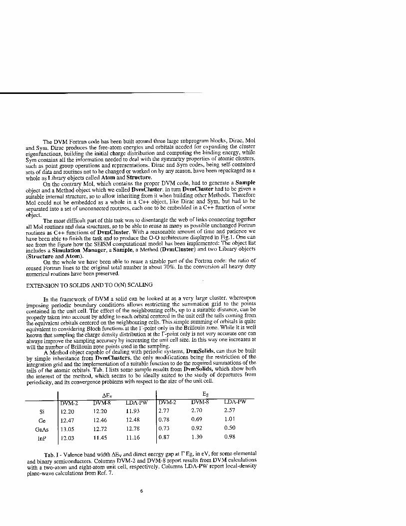
In the framework of DVM a solid can be looked at as a very large cluster, whereupon imposing periodic boundary conditions allows restricting the summation grid to the points contained in the unit cell. The effect of the neighbouring cells, up to a suitable distance, can be properly taken into account by adding to each orbital centered in the unit cell the tails coming from the equivalent orbitals centered on the neighbouring cells. This simple summing of orbitals is quite equivalent to considering Bloch functions at the T-point only in the Brillouin zone. While it is well known that sampling the charge density distribution at the T-point only is not very accurate one can always improve the sampling accuracy by increasing the unit cell size. In this way one increases at will the number of Brillouin zone points used in the sampling.

A Method object capable of dealing with periodic systems, DvmSolids, can thus be built by simple inheritance from DvmClusters, the only modifications being the restriction of the integration grid and the implementation of a suitable function to do the required summations of the tails of the atomic orbitals. Tab. I lists some sample results from DvmSolids, which show both the interest of the method, which seems to be ideally suited to the study of departures from periodicity, and its convergence problems with respect to the size of the unit cell.

Si

Ge

GaAs

InP

DVM-2

12.20

12.47

13.05

12.03

AEv Eg

DVM-8 LDA-PW DVM-2 DVM-8 LDA-PW

12.20 11.93 2.77 2.70 2.57

12.46 12.48 0.78 0.69 1.01

12.72 12.78 0.73 0.92 0.50

11.45 11.16 0.87 1.30 0.98

Tab. I - Valence band width AEV and direct energy gap at T Eg, in eV, for some elemental and binary semiconductors. Columns DVM-2 and DVM-8 report results from DVM calculations with a two-atom and eight-atom unit cell, respectively. Columns LDA-PW report local-density plane-wave calculations from Ref. 7.

Further, to implement a linearly scaling method, we chose to use W. Yang's approach [6]. It makes a smooth division of the system into a set of subsystems, the spatial extent of which is defined by a suitably normalized set of partition functions. At the end of each iteration the charge density, the total energy and the Fermi level of the system are reconstructed through a weighted sum over the subsystems, the weights being the partition functions. The only coupling between subsystems is through the total system potential and the value of the Fermi level. To implement LsDvmClusters, the linearly scaling version of DvmClusters, we had only to add to DvmClusters functions for enabling a loop of DVM calculations over each subsystem, for introducing the partition functions and for performing the weighted sums. Fig. 2 displays timings for sample calculations with DvmClusters and LsDvmClusters, which show the linearly scaling behavior of the latter and a rather small critical size.

time (s)

o -pEH-nffi-M-rlTT ii 11 i 11 11 11 111 i n 11 ii 11 11 11 | 0 5 10 15 20 25 30 35 40

Number of atoms

Fig.2. Execution times of LsDvmCluster (triangles) and DvmCluster (squares) for calculations on Si clusters of 5,17 and 29 atoms.

time (s) 12000 -r

T i r 1111111111111111111111111111 [ 11111 0 5 10 15 20 25 30 35 40

Number of atoms Fig.3. Execution times of LsDvmSolids (triangles) and DvmSolids (squares) for calculations on bulk Si with unit cells containing 2, 8 and 16 atoms.

Finally, LsDvmSolids has been generated from DvmSolids, just as LsDvmCIusters has been generated from DvmClusters, practically with no added labor. Fig. 3 displays timings of sample calculations with DvmSolids and LsDvmSolids which show a quite analogous behavior to the cluster calculations.

CONCLUDING REMARKS

We have demonstrated the practical feasibility of giving an 0-0 architecture to an installed base of professional Fortran programs. By adding new capabilities to the basic model we also demonstrated the potential of our computational model. Current developments include a set of Probes to compute optical spectra, phonon spectra and correlation functions; new Methods to compute molecular dynamics, classical and first-principle; a graphical user interface (GUI). The last item serves well to stress a particularly important feature of object-orientation, namely that in order to have a program running it is sufficient to have a minimally configured instance of the basic objects. Our user interface was just a command line. Now it is being converted into a GUI without any interference with the rest of the program. This possibility of incremental improvements is perhaps one the most interesting features of O-O programming, in that it combines the advantages of rapid prototyping with those of a top down approach.

However the most important reason for adopting an O-O architecture is the effectiveness it gives to intergroup collaborations. Exciting perspectives in new materials design can be opened by the research activity of many groups sharing the same computational model.

ACKNOWLEDGEMENTS

This work was supported in part by C.N.R. through Comitato per le Scienze dell'Informazione. In addition we acknowledge a grant of computer time from CRS4.

REFERENCES

* The SEISM project is being promoted by the Condensed Matter Theory Group of the Physical Sciences Department, University of Cagliari, Italy. Information about its development is available on the Web at http://sparclO.unica.it, or by email to [email protected] [1] See, e.g.,P.F. Dubois, Comput. Phys. 5, 568 (1991); K. J. M. Moriarty, S. Sanielevici, K.Sun, and T. Trappenberg, Comput. Phys. 7, 560 (1993) and references therein. [2] B. Delley, D. E. Ellis, A. J. Freeman, E.J. Baerends and D. Post, Phys. Rev. B27, 2887 (1989) [3] D. E. Ellis and G. S. Painter, Phys. Rev. B2, 2887 (1970) [4] C. B. Haselgrove, Math. Comp. 15, 323 (1961) [5] E. J. Baerends and P. Ros, Int. J. Quantum Chem. S12, 169 (1978) [6] W. Yang, Phys. Rev. Lett. 66, 1438 (1991) [7] Si and InP data from: S. Massidda, A. Continenza, A.J. Freeman, T.M. de Pascale, F. Meloni, M. Serra, Phys. Rev. B41, 12079 (1990); Ge data from: M.T. Yin, ML. Cohen, Phys. Rev. B26, 5668 (1982); GaAs data from: F. Manghi, G. Riegler, CM. Bertoni, C. Calandra, Phys. Rev. B28, 6157 (1983);

POLARIZATION, DYNAMICAL CHARGE, AND BONDING IN PARTLY COVALENT POLAR INSULATORS

T*** R. RESTA*, S. MASSIDDA", M. POSTERNAK***, A. BALDERESCHT *INFM~Dipartimento di Fisica Teorica, Universitä di Trieste, 1-34014 Trieste, Italy "INFM-Dipartimento di Scienze Fisiche, Universitä di Cagliari, 1-09124 Cagliari, Italy ""Institut Romand de Recherche Numerique en Physique des Materiaux (IRRMA), CH-1015 Lausanne, Switzerland

ABSTRACT

We have investigated the macroscopic polarization and dynamical charges of some crystalline dielectrics presenting a mixed ionic/covalent character. First principles investigations have been done within the Hartree-Fock, LDA, and model GW approaches. All calculations have been performed on the same footing, using the all-electron FLAPW scheme. Apparently similar oxides have strikingly different behaviors: some (like the ferroelectric perovskites) have giant dynamical charges, while others (like ZnO) are quite normal and display dynamical charges close to the nominal static ones. We find the rationale for such differences.

INTRODUCTION

The dynamical charges of a polar crystal (also called Born effective charges or trasverse charges) measure by definition the current flowing across the sample during a relative sublattice displacement. The dynamical charge of an ion is a tensor having its site symmetry, and is defined at zero electric field [1]. In the extreme ionic limit, and assuming a rigid-ion picture, the dynamical charge coincides with the nominal static charge of the ion. In a realistic picture, the static charge of a given ion is largely arbitrary and ill defined from first principles, whereas the dynamical charge is experimentally accessible (via phonon spectra) and microscopically well defined [2]. The modern theory of the macroscopic polarization [3] allows first-principle calculations of the dynamical charges as Berry phases.

The interesting case studies are those where the polar crystal has a mixed ionic/covalent character, and the displacement of a given ion induces a nonrigid displacement of the associated electronic charge. In some of these cases (like in ZnO) the dynamical charges turn out to be very close to their nominal value (i.e. ±2), while in others (like the ferroelectric perovskites) the dynamical charges may assume giant values (more than three times the nominal value). The aim of the present study is to get physical insight into the microscopic mechanisms governing the dynamical charges, and in particular to understand the reasons for such qualitative differences.

Besides the above physical motivation, the present study has also a technical motivation. So far, first-principle studies of the dynamical charges have been performed within density- functional theory in the local-density approximation (LDA). Since polarization phenomena are dominated by delicate hybridization mechanisms, we investigate how LDA performs in

9

Mat. Res. Soc. Symp. Proc. Vol. 408 c 1996 Materials Research Society

comparison with alternate schemes, where the band structure (and hence hybridization) are rather different from the LDA one. Before presenting our first-principle results, we use a highly simplified tight-binding method to show qualitatively how the covalence mechanism

strongly affects the dynamical charges.

A MODEL PICTURE

Let us take the simple model of a one-dimensional chain with two sites per cell, sketched in Fig. 1, and whose nearest-neighbor tight-binding Hamiltonian in the centrosymmetric

structure is: H = £[ (-l)'A c)cj - t0(c]cj+1 + H.c.) ]. (1)

3

The difference between the site energies of the two ions is 2A; for the materials of interest here—having mixed ionic/covalent character—the hopping t0 is of the order of 2A. Owing to the simplified model, the static ionic charges are well defined, and one would naively expect that when the chain is distorted (lower sketch in Fig. 1), the current flowing through the chain is proportional to the static charge. Indeed, this is true only if we keep the hopping t fixed (equal to t0) during the distortion, which is rather unphysical indeed. In a more realistic model the hopping t modulates with the bond length, and this is in fact the main mechanism accounting for nontrivial values of the dynamical charges. In this work we are going to verify to which extent such a simple picture, borrowed from Harrison's textbook [4], applies to real materials in a first-principle framework. We notice that what makes the value of the dynamical charge different—and possibly much different—from the static one is the fact that occupied and empty band states mix with the displacement (while they do

not mix if i = t0).

Figure 1: A one-dimensional chain in the centrosymmetric structure (upper sketch) and with a frozen-in zone-center optical phonon (lower sketch). Black and gray circles schematize anions and cations. The dynamical charge measures the current flowing through the chain

during the sublattice displacement.

CALCULATIONS

The calculations which the present study is based upon are reported in Refs. [5, 6] (for the ferroelectric perovskite KNb03), and in Refs. [7, 8] (for ZnO). Numerical results are tabulated therein in detail. Here we analyze the main message emerging from the computational data. All our calculations are performed using the first principles full-potential-linearized- augmented-plane-wave (FLAPW) method. Macroscopic polarization and dynamical charges

are evaluated as Berry phases [3]. In the most recent of the cited papers [8], the ZnO dynamical charge is investigated using three different approaches: LDA, Hartree-Fock (HF), and a model GW scheme. The three different physical approximations use the same numerical and

10

computational scheme: they differ amongst themselves only in the physical scheme used for reducing the many-electron problem to a mean-field selfconsistent one-electron problem.

In KNb03 we have found giant values of the dynamical charges. In order to check on a first-principles ground whether the covalence mechanism sketched above is basically correct, we have added a fake repulsive potential inside a sphere centered on the Nb ion, which only acts upon electrons of d symmetry. Technically, our FLAPW band-structure scheme makes such counterfeit quite simple. Assuming for our fake perovskite the same ferroelectric distortion as for the real material, the calculation provides a much smaller value of the spontaneous polarization. The numerical results given in Ref. [6] demonstrate therefore that the giant current detected during polarization reversal experiments is doubtless due to covalence effects. Upon suppressing artificially the latter, the material becomes a "trivial" oxide, where the relative displacements of crystal sublattices drag a total current slightly smaller than implied by their nominal charge, in a a rigid-ion picture.

From experimental evidence, the same covalence mechanism does not apply as it is in ZnO. Our first-principle calculations, performed according to three different physical approximations, agree among themselves and with the experimental data: this only fact is not yet very informative about the phenomenon. In order to investigate the underlying microscopic mechanism, we have performed a band-by-band decomposition, where we have investigated the partial currents of different electronic states (well separated in energy) induced by the sublattice displacements.

Let us focus for instance on the displacement of oxygen. In the extreme ionic limit, where the ions are assumed to be rigid, the total ionic charge would be —2, arising from the following individual contributions: +6 (core charge); -2 (completely filled 02s bands); -6 (completely filled 02p bands). In this same picture, the Zn3d states are attached rigidly to the Zn site, and cannot contribute anyhow to the oxygen dynamical charge. Our first- principle calculation provides instead (at the HF level) a total value of —2.1, with the following decomposition: +6 (core); -2.5 (02s bands); -6.5 (02p bands); +0.9 (Zn3d bands). The main message conveyed by these data is confirmed by a more complete analysis, reported elsewhere [8].

Therefore, our calculations point out that strong deviations from the nominal values are occurring, which compensate however each other when added up to the total dynamical charge. This demonstrates that all the electronic states behave in a strongly nonrigid fashion, and this is particularly surprising for the 02s ones. In fact, since the 02s bands are very low in energy (about 23 eV below the valence-band edge within the HF scheme), one would have guessed naively a rigid behavior of them under ionic displacement. A similar unexpected behavior of 02s states was found previously in a perovskite by other authors [9].

Finally, we find a simple reason for the compensation of the different contributions, resulting in a quite normal value of the total dynamical charge in ZnO. Explicit inspection shows that the lowest conduction states in the neighborhood of the fundamental gap have mainly s character (Zn4s and 03s). Therefore, they are coupled weakly with the highest valence states and the subspace of the occupied and unoccupied electronic states do not mix with ionic displacements, despite the fact that the subspaces of the occupied states mix strongly amongst themselves.

Roughly speaking, and using the pictorial language of our tight-binding model, we could conclude that the effective hopping t (related to the fundamental gap) depends strongly on the ionic displacements in perovskites, while it is essentially independent from them in ZnO.

ACKNOWLEDGMENTS

This work was supported by the Swiss National Science Foundation (Grant 20-39.528.93). Calculations have been performed on the computers of EPF-Lausanne, ETH-Zürich, and

ETH-CSCS (Centro Svizzero di Calcolo Scientifico).

REFERENCES

1. M. Born and K. Huang, Dynamical Theory of Crystal Lattices (Oxford University Press,

Oxford, 1954).

2. R. Pick, M.H. Cohen, and R.M. Martin, Phys. Rev. B 1, 910 (1970).

3. For a review see: R. Resta, Rev. Mod. Phys. 66, 899 (1994).

4. W.A. Harrison, Electronic Structure and the Properties of Solids (Freeman, San Fran-

cisco, 1980).

5. R. Resta, M. Posternak, and A. Baldereschi, Phys. Rev. Lett. 70, 1010 (1993).

6. M. Posternak, R. Resta, and A. Baldereschi, Phys. Rev. B 50, 8911 (1994).

7. A. Dal Corso, M. Posternak, R. Resta, and A. Baldereschi, Phys. Rev. B 50, 10715

(1994).

8. S. Massidda, R. Resta, M. Posternak, and A. Baldereschi, Phys. Rev. B, 15 December

1995.

9. Ph. Ghosez, X. Gonze, Ph. Lambin, and J.-P. Michenaud, Phys. Rev. B 51, 6765 (1995).

12

LINEAR-RESPONSE CALCULATIONS OF ELECTRON-PHONON COUPLING PARAMETERS AND FREE ENERGIES OF DEFECTS

Andrew A. Quong* and Amy Y. Liu** *Sandia National Laboratories, Livermore CA 94551-0969 "Department of Physics, Georgetown University, Washington, DC 20057

ABSTRACT

Linear-response theory provides an efficient approach for calculating the vibrational properties of solids. Moreover, because the use of supercells is eliminated, points with little or no symmetry in the Brillouin zone can be handled. This allows accurate determinations of quantities such as real-space force constants and electron-phonon coupling parameters. We present highly converged calculations of the spectral function a2F{u) and the average electron-phonon coupling for Al, Pb, and Li. We also present results for the free energy of vacancy formation in Al calculated within the harmonic approximation.

INTRODUCTION

The vibrational spectrum of a solid plays an important role in the determination of many physical properties. While standard density-functional-based electronic-structure methods allow for the accurate determination of ground-state energetics, these methods do not easily allow the calculation of phonons for large systems at arbitrary points in the Brillouin zone. However, with linear-response methods, phonons for large systems at all points in the Bril- louin zone can be obtained in a computationally efficient manner. In the present paper, we concentrate on two specific problems where an accurate determination of the phonons over the full Brillouin zone is essential for describing the physical phenomena of interest. First we present results for electron-phonon coupling parameters for some simple metals, and second we present results for the temperature-dependent free energy of vacancy formation in Al.

The frozen-phonon total-energy method has been widely used to study the phonon spectrum in many materials. The primary limitation of the method is that only phonon wavevectors that lie along high-symmetry directions, and that correspond to reasonably sized supercells, can be considered. This makes it difficult to determine accurately quantities that involve integrations over the wavevector throughout the Brillouin zone.

The advantage of the linear-response approach is that the vibrational modes of the system can be determined from the electronic wavefunctions and eigenvalues of the undistorted crystal. In contrast to the total-energy methods, the calculation of phonon properties using linear-response methods is done using the same unit cell that is used for the ground-state calculation. However, since the sums over k points in the Brillouin zone are dictated by the group of the phonon wavevector q, sums over the full zone rather than just the irreducible wedge are often required.

There are several different schemes for obtaining the dynamical matrices using linear- response theory [1]. All depend on solving the following set of coupled equations which relate the change in charge density nx to the change in potential Hi.

ni(r) = £ fjL^ItL < ,/\Hl\u >< „|r >< r(l/ >t (1)

13


and

ff1(r)=^1(r) + /dVni(r')V(r,r'). (2)

In the above equations, v labels the single-particle electronic states, / is the Fermi occupation number, Vx is the perturbation due to a rigid displacement of an ion, and V is the electron- electron interaction that contains both the Coulomb and exchange-correlation pieces. The coupled set of equations is solved self-consistently either via iteration or by minimizing the energy (which is variational). In the present calculations we solve for the induced charge density directly by solving the Bethe-Salpeter equation of the form:

ni(r) = n5(r) + /dVn1(r')^(r,r'), (3)

where the kernel K is related to the polarizability of the electronic system and n\ is the first-order change in charge density due to the unscreened perturbation Vj. The present method is described in detail elsewhere [2], and we refer the reader to these references for

further information.

ELECTRON-PHONON INTERACTION

The calculation of electron-phonon coupling parameters from first principles has long been a sought after goal. It requires knowledge of the the low-energy electronic excitation spectrum, the complete vibrational spectrum, and the self-consistent response of the electronic system to lattice vibrations. Linear-response theory provides one approach for studying the electron-phonon interaction within the density-functional framework. Phonon frequencies are calculated throughout the Brillouin zone as discussed above. Furthermore, the matrix elements for scattering of electrons by these phonons are computed from the first- order change in the self-consistent potential. For calculating electron-phonon parameters, the linear-response method is a powerful alternative to the more traditional frozen-phonon method since quantities such as the spectral function a2F{uj), the phonon density of states F{u), and the electron-phonon mass enhancement parameter A, all involve integrations over the phonon wavevector throughout the Brillouin zone.

We have extended the planewave-based linear-response method to the calculation of electron-phonon coupling parameters. We present here calculations of the electron-phonon spectral function for Al, Pb and Li. A similar method based on LMTO basis functions was recently presented in Ref. [3]. In the present work, the electronic wavefunctions are expanded in a planewave basis set, the electron-ion interaction is represented by pseudopotentials and the electron-electron interaction is treated within the local density approximation. The phonon frequencies and polarization vectors are calculated within linear response. The doubly-constrained Fermi-surface averages of the electron-phonon matrix elements needed to determine the coupling parameters [4] are performed using dense meshes of k points (1300 points and 728 points in the fee and bec irreducible Brillouin zones (IBZ), respectively) and by replacing the <5 functions in energy with Gaussians. Phonon wavevectors are sampled on coarser meshes of 89 and 140 points in the fee and bec IBZs, respectively.

The phonon dispersion curves calculated for Al are shown in Figure 1(a). The agreement with neutron diffraction data [5] is excellent throughout the Brillouin zone. The spectral function calculated for Al is shown in Fig. 1(b). Extraction of a2F from conventional

14

(a) 40.0

£- 30.0

S, ~3 20.0

/

10.0 If

Figure 1: (a) Comparison of calculated Al phonon dispersion curves (solid lines) with experimentally measured frequencies (circles), (b) Al spectral function. The results of the present calculation are represented by the solid line. Results from two proximity electron tunneling spectroscopy experiments are indicated by the dashed line and the squares.

tunneling data is not possible for a weak-coupling superconductor like Al. Instead spectral functions extracted from proximity electron tunneling experiments [6] are shown for comparison. Unfortunately, the analysis of this type of tunneling data involves the introduction of additional fitting parameters, which can lead to large uncertainties in the extracted spectral function. The value of the electron-phonon mass enhancement parameter determined from the first inverse-frequency moment of the calculated spectral function is A = 0.438, which is in good agreement with other calculations [3, 7] and with heat capacity data [8]. Using the calculated a2F as input into the Eliashberg equations, we find that a p* of 0.162 is required to fit the observed transition temperature of Tc = 1.18 K. The same value of fi* yields a gap equal to the experimental value of 0.180 meV. The consistency between independent fits to the gap and to Tc is one measure of the accuracy of our results.

Next we consider the strong-coupling superconductor Pb, for which high-quality conventional tunneling data are available. From the theoretical stand point, the importance of relativistic effects in Pb make it a more difficult system to treat than Al. The present calculations for Pb are performed in the scalar relativistic approximation. The phonon dispersion curves are shown in Figure 2(a). Overall, there is good agreement between calculated (solid lines) and measured (open circles) phonon frequencies [9], and the calculation is able to reproduce some subtle features in the dispersion curves such as the Kohn anomaly between T and K. (The jaggedness of the solid lines, which merely connect the calculated frequencies, is due to the discrete sampling of phonon wavevectors.) Note however that there are significant discrepancies between the calculated and measured frequencies for the low-energy transverse mode, particularly in the region near X and K. The minima in both the longitudinal and transverse modes at X are unusual in that they are not observed in other fee metals. Even an eighth neighbor Born-von Karman fit (dashed line) to the measured frequencies is unable to reproduce the dispersion near X, especially for the longitudinal mode [10]. Our preliminary results obtained using the frozen-phonon approach indicate that the differences between the calculated and measured frequencies can be significantly reduced if the spin-orbit interaction is taken into account.

15

4.0 8.0 (0 (meV)

12.0

Figure 2: (a) Pb phonon dispersion curves. The solid lines connect calculated frequencies at the sampled wavevectors, and circles indicate the experimentally measured frequencies. Also shown is a Born-von Karman fit to the measured frequencies (dashed line), (b) Spectral function of Pb. The results based on the calculated frequencies are shown as a solid line, those based on the frequencies obtained from the force constant fit are given by the dashed line, and the results from the inversion of tunneling data are plotted as circles.

The spectral function for Pb is plotted in Fig. 2(b). The calculations (solid line) reproduce the two peak structure seen in the data (open circles) [11], but there are differences in the peak locations and heights, especially for the lower-frequency peak. The mass enhancement parameter is calculated to be A = 1.20, which is significantly lower than the tunneling result of 1.55. The discrepancies are due in large part to the errors in the calculated transverse-mode phonon frequencies. To demonstrate this, we have computed the spectral function using the calculated phonon linewidths (which do not depend explicitly on the phonon frequencies), along with the phonon frequencies generated from the Born-von Karman fit to the data. The resulting a2F(ui) is plotted as a dashed line in Figure 2(b). Us- ing the empirical force constants, which accurately describe the dispersion of the transverse modes, we obtain good agreement with the experimental results in the low-frequency regime. On the other hand, since the Born-von Karman fit does not give accurate frequencies for the longitudinal mode, the resulting spectral function is less accurate than the first-principles results in the high-frequency regime.

Finally, we discuss the electron-phonon interaction in bcc Li. The lack of a superconducting transition in Li has been a long-standing puzzle. Frozen-phonon calculations [12] have suggested that the electron-phonon coupling strength in Li is similar to that in Al. Hence a transition temperature on the order of 1 K is expected if a value of p.* « 0.15 is assumed. Experimentally, however, no transition is observed, at least down to 6 mK. The present calculations yield a mass enhancement parameter of A = 0.45, which is similar to earlier results. Using the calculated spectral function as input to Eliashberg theory, we find that an unphysically large value of p* « 0.3 is required to suppress Tc below the experimental limit. The observed absence of superconductivity in Li therefore remains an open problem. The resolution of this puzzle may require consideration of the low-temperature crystal structure of Li, or the role of manybody interactions such as electronic correlations and spin fluctuations.

16

FREE ENERGY OF DEFECTS

Defects play an important role in many physical phenomena. Mechanical properties, diffusion, nucleation, and growth are just a few examples where the details of the defect energetics control the observed physical behavior of the system. Much progress has been made in determining the energetics of defects at zero temperature using electronic-structure methods [13]. However, the effects of temperature on the energetics have not been explored extensively with first-principles calculations. Because experiments are performed at finite temperatures and mechanical properties are temperature dependent, it is important to investigate finite-temperature effects. While the free energy can be obtained via ab initio molecular dynamics calculations, supercells are required to probe any vibrational modes other than those at q = 0. The computational challenge then lies in solving the electronic structure problem for very large cells, and limitations similar to those in the frozen-phonon method are encountered.

200.0 400.0 600.0 Temperature (K)

800.0 1000.0

Figure 3: Calculated free energy of the monovacancy in Al.

In the present work, the free energy for the formation of monovacancies in Al is calculated in the harmonic approximation. The calculations are performed in a planewave basis set, the defect is modeled with a 27 atom unit cell, and ten Monkhorst and Pack k-points are used to sample the Brillouin zone. In Figure 3, we plot the free energy of the monovacancy. At T = 0, we obtain a formation energy of 0.52 eV, in good agreement with other theoretical results [13] and in fair agreement with the experimental enthalpy of formation of 0.66 eV [14]. The most striking feature of the curve is the strong dependence of the free energy on temperature. At 500K, there is a 20% reduction in the free energy. This change in the defect energetics can have a dramatic effect on equilibrium properties and other physical phenomena.

CONCLUSIONS

Linear-response methods allow the calculation of the full vibrational spectrum of complex systems. This opens the door to using first-principles techniques to address problems that

17

require information about the phonons throughout the Brillouin zone. The electron-phonon interaction and the temperature dependence of the formation energy of defects are just two examples of problems where such detailed knowledge of the lattice dynamics is essential for understanding the physical properties of interest.

ACKNOWLEDGEMENTS

We thank J. K. Freericks and E. Nicol for useful discussions. This work was supported in part by the United States Department of Energy, Office of Basic Science, Materials Science Division, and by the MPCRL through grants of computer time at the Paragon at Sandia National Laboratories.

REFERENCES

1. S. Baroni, P. Giannozzi, A. Testa, Phys. Rev. Lett. 58, 1861 (1987); X. Gonze, D. C. Allan, and M. P. Teter, Phys. Rev. Lett. 68, 3603 (1992); S. Y. Savrasov, Phys. Rev. Lett. 69, 2819 (1992).

2. A. A. Quong and B. M. Klein, Phys. Rev. B. 46, 10734 (1992); A. A. Quong, A. Y. Liu and B. M. Klein, Proceedings of the Fall 1992 MRS Meeting (Mat. Res. Soc, Pittsburgh, 1992).

3. S. Y. Savrasov, D. Y. Savrasov and O. K. Andersen, Phys. Rev. Lett. 72, 372 (1994).

4. See, for example, G. Grimvall, The Electron-Phonon Interaction in Metals (North Hol- land, Amsterdam, 1981).

5. G. Gilat and R. M. Nicklow, Phys. Rev. 143, 487 (1966).

6. See, for example, E. L. Wolf, Principles of Electron Tunneling Spectroscopy (Oxford University, New York, 1985).

7. M. M. Dacorogna, M. L. Cohen and P. K. Lam, Phys. Rev. Lett. 55, 837 (1985).

8. N. E. Phillips, CRC Crit. Rev. Solid State Sei. 2, 467 (1971).

9. B. N. Brockhouse, T. Arase, C. Caglioti, K. R. Rao and A. D. B. Woods, Phys. Rev 128, 1099 (1962).

10. E. R. Cowley, Solid State Commun. 14, 587 (1974).

11. W. L. McMillan and J. M. Rowell, in Superconductivity, edited by R. Parks (Marcel Dekker, New York, 1969), Vol 1.

12. A. Y. Liu and M. L. Cohen, Phys. Rev. B 44, 9678 (1991).

13. See, for example, A. D. Vita and M. J. Gillan, J. Phys. Condens. Matter 3 6225 (1991) and references therein.

14. M. J. Fluss, L. C. Smedskjaer, M. K. Chason, D. G. Legnini, and R. W. Siegel, Phys. Rev. B 17 3444 (1978).

18

ATOMIC AND ELECTRONIC STRUCTURE OF GERMANIUM CLUSTERS

AT FINITE TEMPERATURE USING FINITE DIFFERENCE METHODS

JAMES R. CHELIKOWSKY", SERDAR ÖGÜT*, X. JING*, K. WU",

A. STATHOPOULOS", Y. SAAD"

•Department of Chemical Engineering and Materials Science, Minnesota Supercomputer

Institute, University of Minnesota, Minneapolis, Minnesota 55455, USA

"Department of Computer Science, Minnesota Supercomputer Institute,

University of Minnesota, Minneapolis, Minnesota 55455, USA

ABSTRACT

Determining the electronic and structural properties of semiconductor clusters is one

of the outstanding problems in materials science. The existence of numerous structures

with nearly identical energies makes it very difficult to determine a realistic ground state

structure. Moreover, even if an effective procedure can be devised to predict the ground state

structure, questions can arise about the relevancy of the structure at finite temperatures.

Kinetic effects and non-equilibrium structures may dominate the structural configurations

present in clusters created under laboratory conditions. We illustrate theoretical techniques

for predicting the structure and electronic properties of small germanium clusters. Spefically,

we illustate that the detailed agreement between theoretical and experimental features can

be exploited to identify the relevant isomers present under experimental conditions.

INTRODUCTION

It is generally asserted that semiconductor clusters undergo important reconstructions

relative to bulk crystalline fragments. This assertion is supported by the existence of "magic

number" effects in their physical and chemical properties [1]. The cluster structural param-

eters affect the chemical reactivity, photofragmentation, Raman and photoelectron spectra

[2-5], but a systematic approach to extract the geometrical structures from such data is still

lacking. For these nanostystems in their unsupported form, no direct experimental probe

of the atomic structure exists which is comparable to x-ray diffraction for bulk periodic

materials, or scanning tunneling microscopy for surfaces. On the theory side, methods for

structure prediction are confronted with major difficulties when applied to clusters. Many

of these difficulties arise from the existence of multiple local minima in the potential energy

surface of these systems.

While it is appealing to consider empirical force fields, or interatomic potentials to com-

pute the structural properties of clusters, these approaches require careful construction and

deep insight into the nature of the chemical bond [6,7]. Since clusters often contain atoms

in unusual configurations, it is difficult to transfer interatomic interactions from known crys-

19


talline environments [8-11]. For this reason, it is useful to concentrate on ab initio methods

which require no empirical input.

One promising procedure for calculating structural energies is based on ab initio pseu-

dopotentials constructed within the local density approximation [12-18]. If one is given the

spatial and energetic distributions of the valence electrons one can compute the electronic

energy for a given structure. The pseudopotential approximation effectively removes the

chemically inert core electrons from the problem. The resulting wave functions are smoothly

varying since the core states have been excluded. Such wave functions permit the efficient

application of simple basis sets.

Given a formalism to compute structural energies, there remains a serious issue in de-

termining which structures are energetically viable. For cluster sizes exceeding a few atoms,

one generally relies on simulated annealing procedures for global geometry optimization

[11,17,18]. In practice, once a cluster exceeds a dozen atoms or so, one can rarely perform

the simulation at a rate which insures the final structure is the ground state structure. Trap-

ping by local minima in the simulation is also a problem [11,18] The accuracy of theoretical

methods and dynamical effects is another issue as the cluster size and the number of compet-

ing structures increases. Even for some small clusters, such as Si6, these effects are already

of the same order of magnitude as the energy difference between the lowest energy isomers

[8]. For these reasons, comparison between theory and experiment is essential to identify the

relevant isomers.

THEORETICAL METHODS

Langevin Dynamics: Isothermal Simulations and Simulated Annealing

In Langevin dynamics, the ionic positions, Rj, evolve according to the Langevin equation:

Mj Rj = -VRj E({Rj}) - yMj Rj + Gj (1)

where E({Rj}) is the total electronic energy of the system and {Mj} are the ionic masses. The

last two terms on the right hand side of Eq. (1) are the dissipation and fluctuation forces,

respectively. The dissipative forces are defined by the friction coefficient, 7. The fluctuation

forces are defined by random Gaussian forces, {G?-}, with a white spectrum [19,20].

Langevin molecular dynamics coupled to the simulated annealing procedure can provide

a general tool for complex structural optimization [21,22]. The temperature can be controlled

without rescaling the velocities as is often done in Newtonian molecular dynamics. Energy

can exchange into and out of the system as required by the temperature of the heat bath.

Simulated annealing need not follow each time step of the "natural evolution" of the phys-

ical system. Annealing rates can be significantly faster if the dynamics lead to acceptable

shortcuts relative to the natural evolution.

Langevin dynamics can also be used for isothermal simulations. The heat bath can play

20

the role of a buffer gas in experimental situations, although the time frame is quite different.

The use of Langevin dynamics as a thermostat can be rigorously justified [23] in the same

sense as a Nose-Hoover thermostat [24]. Although Langevin dynamics is not appropriate for

following the physical dynamics of the system such as vibrational modes, it is an appropriate

isothermal simulation procedure for thermodynamic properties.

As opposed to Monte Carlo simulations, molecular dyanamics simulations sample the

configuration space by collectively moving the particles. Molecular dynamics simulations also

move faster to the minima in a potential energy surface by exploiting the interatomic forces.

On the other hand, the stochastic nature of the random forces present in Langevin molecular

dynamics helps the system to escape from metastable states in a manner reminiscent of

"uphill" moves in Monte Carlo simulations [25].

Quantum Interatomic Forces

Within the local density approximation (LDA) [26], the total ground state energy may

be expressed as follows:

E„,t = T[p] + E,.i{Ra, [/>]) + Ehart[p} + EIC[p] + Ei.i(Rc) (2)

where T[p] is the kinetic energy, Ee_; (Ra,[p)) is the ionic potential energy, Ehart[p] is the

Hartree potential energy, Exc[p] is the exchange-correlation energy [27], Ei-i(Ra) is the inter-

ionic core interaction energy, and p(r) is the ground state valence charge density.

In Eq. (2), the contributions from the electron-ion and ion-ion interactions are the only

two parts which have explicit dependence on the nuclear coordinates. Since the Hellmann-

Feynman theorem asserts that the first-order change in the wave functions does not con-

tribute to the forces, only the Ee-i and £,-_,- terms are relevant to the interatomic forces [28].

The total force, F%, on an atom located at R„ in the a direction for a finite system is,

dEtot dEe-j dEj-j dR« dR% dR« { '

The inter-ionic core interaction is simply the point-charge point-charge interaction under the

frozen core approximation. It is the direct pair summation of Coulomb interactions for an

isolated system, and an Ewald summation for a periodic system.

A complicating issue is that the ionic term is described by a non-local ionic pseudopoten-

tial. The potential can be generated by a variety of approaches [29]. Here we use the method

of Troullier and Martins [30]. The interactions between valence electrons and pseudo-ionic

cores may be separated into a local potential and a Kleinman and Bylander [31] form of a

non-local pseudopotential in real space [32].

K-o-WlMr) = £ V,oc(|ra|)y.„(r) + £ K'^u^rJAVfa,,) (4)

21

lm

and < AV,a > is the normalization factor, lm

where r„ = r - Ra, and the «;m are the atomic pseudopotential wave functions of angu-

lar momentum and azimuthal quantum numbers, (lm), from which the / dependent ionic

pseudopotential Vj(r) are generated. AVj(r) = Vt(r) - V\„c{r) is the difference between the /

component of the ionic pseudopotential and the local ionic potential.

The energy from the electron-ion interaction, £e_; can be obtained by using Eq. (4) as,

Ee„i = YJjp{r)VUra)d3r+ £ <A^>[rj! (5) ° a,n,lm

where the sum on n, is over the occupied states. Combining Eq. (3) and Eq. (5), one can

get an expression for the force,

F*= !p{r)9V'°^d\ + 2Y,<AV? >/<", ^-^ (6) a I r\ ) Q^a / , /m n,lm ßra dR

n,Bn

The force from the electronic contribution comprises two parts. The first term at the right

hand side of Eq. (6) is the contribution from the local ionic potential, and the second term

is from the non-local potential.

Real Space Methods for Quantum Forces

To obtain these forces, one needs to solve for the eigenvalues and vectors. A common

approach is to use a plane wave basis set [16]. The basis set is constructed by imposing a

supercell geometry. The cluster of interest is placed within a large unit cell which is then

artificially replicated to fill all space. The size of the cell sets the length scale of the plane

wave basis. This "forced" periodicity of supercells allows standard "band structure" codes

to be used for non-periodic systems.

The plane wave basis is required to replicate not only the electronic states of the localized

system of interest, but also "vacuum" regions imposed by the supercell geometry. One issue

which complicates supercell calculations concerns interactions from one cell into another. A

large supercell must be used to avoid such interactions. However, computational intensity of

the calculation increases significantly with the cell size. If one wishes to examine a charged

cluster, the problem becomes more acute as the total electronic energy summed over the

supercells diverges. A simple "fix" to this problem is to insert a uniform compensating

charge in each supercell, but determining the effect of this uniform background in terms of

a total energy, or binding energy, is non-trivial [11,33].

22

It is possible to examine clusters without the use of plane wave basis. A new approach

which does not utilize plane waves is based on the higher-order finite difference method [32].

In the finite difference method the unknown variables are the wave functions on a discrete

grid. Derivatives are approximated by summing over the value of the function at neighboring

grid points.

Let us consider a solution for the one-electron Schrödinger equation using a higher order

finite difference expression for the kinetic energy operator, i.e., expansions of the Laplacian.

We impose a simple uniform grid on our system where the points are described in a finite

domain by (xityj,zk). We approximate |^ at (xityj,zk) by

0= £ C„*(«, + nh,yj,zk) + 0(h™+>) (7) n = -N

where h is the grid spacing and N is a positive integer. This approximation is accurate to

0(h2JV+2) upon the assumption that i> can be approximated accurately by a power series in

h. Algorithms are available to compute the coefficients C„ for arbitrary order in h [33].

With the kinetic energy operator expanded as in Eq. (1), one can set up a one-electron

Schrödinger equation over a grid. While we assume a uniform grid over the three dimensions,

this is not a necessary assumption. We solve for i>(xityj,zk) on the grid by solving the secular

equation:

~2m ^2 Cni4>n{xi + nih,yj,Zk)

N N

+ ]C C^n(xi,yj + n2h,zk)+ J2 C„,il>n(xityj,zh + n3h)

+ [ Vion(xi,yj,zk)+ VH(xi,yj,zk) + Vxc(xi,yj,zk)]ipn(xi,yj,zk) = E„ i>„{xi,yhzk) (8)

where Vio„ is the nonlocal ionic pseudopotential, VH is the Hartree potential and Vrc is the

local density expression [26,27] for the exchange and correlation potential. Two parameh

used in setting up the matrix are the grid spacing h, and the order "r

Another complication concerns the nonlocality of the ionic pseudopotential, i.e., the an-

gular momentum component of the wavefunction. The integral involving KanM is performed

over the grid. One has

fu,m(x,y,z) AV,(x,y,z) i>„(x,y,z)dxdydz = ^2u,m(xi,yj,zk)AV,(xi,yj,zk)rl>n(xi,yj,zk)h3 (9)

J ijk

Eq. (8) is a matrix eigenvalue problem. If there are M grid points, the size of the

full matrix, A, resulting from the above eigenvalue problem is M x M. The matrix A for

these isolated systems is real, symmetric, and sparse. These attributes can be exploited in

expediting the diagonalization procedure. The sparsity of the matrix is a function of the

order JV to which the kinetic energy is expanded. To solve the above eigenvalue problem, we

23

can utilize one of several iterative procedures developed in the literature for sparse matrices,

see for example[34]. Two popular such procedures are the accelerated subspace iteration

and the Lanczos algorithm. These methods consist of projecting the original problem into

a small subspace in which standard techniques can be used. For example, in the simplest

version of the subspace iteration algorithm, an initial basis X0 = [XQ, xlt..., xm] is chosen and

the power Xk = AkX0 is formed for a certain power k. Then, a Ritz procedure is applied

to A with this matrix, i.e., Xk is orthonormalized into a matrix Yk and the eigenvalues A,-

and eigenvectors <j>i of the small my. m matrix YfAYk are computed by a standard method

such as the QR algorithm [34]. The eigenvalues A; are then used as approximations to the

eigenvalues of A and the vectors Yk<j>i are used as approximations to the eigenvectors of A.

The procedure is repeated with X replaced by the set of approximate eigenvectors until

convergence is reached. In realistic implementations of this procedure, it is common to use

a Chebyshev polynomial Ct(A) instead of the powers Ak to obtain the next basis Xk from

X. The Lanczos algorithm also utilizes a Ritz procedure, but the basis used consists of the

successive powers Akv0,k = 1,.. ,,m where v0 is an initial vector. In this case, the dimension

m increases at each step. Both procedures can and should be 'preconditioned' to improve

convergence rates [35]. Preconditioning consists of enhancing a given vector introduced in

the new basis by a process which amplifies the desired eigenvector components and dampens

the others.

One important observation is that these diagonalization algorithms use the coefficient

matrix A only to perform matrix-by-vector products. The sparse matrix A can be stored in

one of several sparse formats available [35] which avoid storing the zero elements. Performing

matrix-vector products with these formats is inexpensive. However, because of the special

structure of the matrix, an even more appealing alternative is to perform these matrix vector

products in 'stencil' or 'operator' form [36]. Indeed, there is no need to store the matrix in

any sparse form since the coefficients C„,,i = l,2,3;n = -N,N in Eq. (8) are constant. As a

result, the matrix-by-vector kinetic operations required by the diagonalization routine can

be performed by only accessing the desired components of the current vector * and forming

a small linear combination using these coefficients Cni. Similarly, the non-local operations

are accomplished by performing vector-by-vector operations. This strategy not only saves

storage, but also leads to an efficient implementation on most high-performance vector and

parallel computers.

Several issues must be addressed to solve Eq. (8). The first concerns the procedure

by which the self-consistent field is constructed. The exchange-correlation potential, Vxc,

is constructed trivially once the charge density has been constructed over the grid. The

Hartree potential can be determined by setting up a matrix equation and solving with

iterative methods. The self-consistent field is then established by iterating a solution to the

one-electron Schrödinger equation as per standard techniques [32].

24

SIMULATED ANNEALING SIMULATIONS FOR Ge CLUSTERS

Langevin simulated annealing has been used in previous work to determine the structure

of silicon clusters. Here we focus on germanium clusters.

With respect to the technical details, the initial temperature of the simulation was taken

to be 2800 K; the final temperature was taken to be 300 K. The annealing schedule lowered

the temperature 500 K each 50 time steps. The time step was taken to be 7fs. The friction

coefficient in the Langevin equation was taken to be 6 x 10-4 a.u. After the cluster reached

a temperature of 300 K, the clusters were quenched to 0 K. The ground state structure was

found through a direct minization by a steepest descent procedure.

Choosing an initial atomic configuration takes some care. If the atoms are too far apart,

they will exhibit Brownian motion and may not form a stable cluster as the simulation

proceeds. If the atoms are too close together, they may form a metastable cluster which

may be kinetically inaccessible from the ground state. Typically, the initial cluster is formed

by a random placement of the atoms with the constraint that any given atom is between

1.05 and 1.3 times the dimer bond length of at least one atom.

With respect to computing the quantum forces, the cluster in question is placed in a

spherical domain. Outside of this domain, the wave function is required to vanish. The

radius of the sphere is such that the outmost atom is at least 6 a.u. from the boundary.

Initially, the grid spacing was 0.8 a.u. For the final quench to a ground state structure,

the grid spacing was reduced to 0.5 a.u. The pseudopotential was defined using a 4s2V

configuration. The core radius was chosen to be 2.9 a.u. The local part of the potential was

taken to be the I = 0 component.

In Figure 1, we illustrate a simulated anneal for a seven atom germanium cluster. While

the initial cluster contains a number of bonds, the structure is somewhat removed from the

ground state. After ~200 time steps, the ground state structure is essentially formed. As

for the corresponding silicon cluster, the ground state of Ge7 is a bicapped pentagon. The

binding energy shown is relative to the isolated Ge atom. We have not included gradient

corrections, or spin polarization in our work. Therefore, the values indicated are likely to

overestimate the binding energies by ~ 20% or so.

In Figure 2, we present the ground state structures for Ge„ for n < 7. The structures for

Ge„ are very similar to Si„. The primary difference resides in the bond lengths. The Si bond

length in the crystal is 2.35 Ä, whereas in Ge the bond length is 2.44 Ä. This difference is

reflected in the bond lengths for the corresponding clusters. Ge„ bond lenghts are typically

a few percent larger than the corresponding Si„ clusters. For example, in Ge4 the two bond

lengths which characterize the structure are 2.35 Ä and 2.44 Ä. For Si4, the corresponding

bond lengths are 2.31 Ä and 2.40 Ä.

25

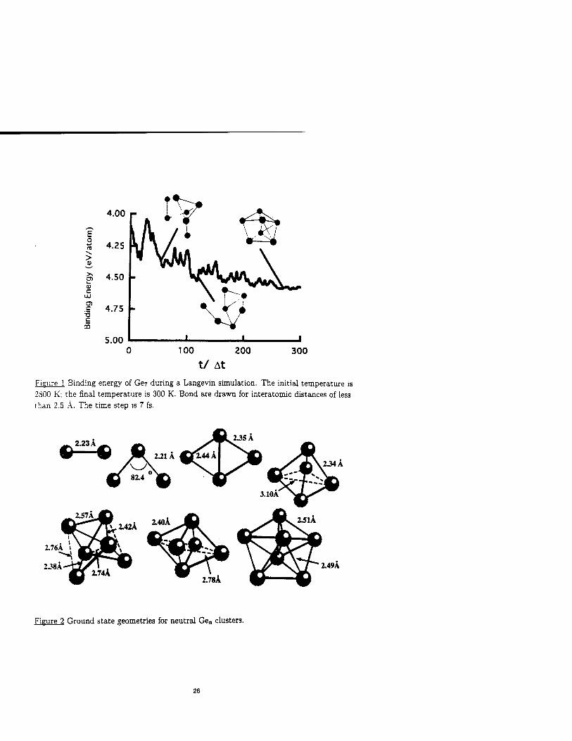
4.00

E 0 fcJ 4.25 ^ > D '^-' >* 4.50 b. u c

UJ rn c 4.75

■o c CO

5.00 100 200

t/ At 300

Figure 1 Binding energy of Ge7 during a Langevin simulation. The initial temperature is 2800 K; the final temperature is 300 K. Bond are drawn for interatomic distances of less than 2.5 A. The time step is 7 fs.

2.23 A

2.76A i

2J8A

2.34 A

Figure 2 Ground state geometries for neutral Ge„ clusters.

26

Another striking similarity between Ge and Si clusters concerns n = 6 clusters. For Si6, two quasi-degenerate structures are observed; a bicapped tetrahedron and a distorted octahedron. These structures are also observed for Ge6 and they are also quasi-degenerate, i.e., the energy difference between the two structures is ~1 meV/atom. The general similarity of small Ge and Si clusters is consistent with recent mobility measurements [37].

FINITE TEMPERATURES SIMULATIONS FOR THE PHOTELECTRON SPECTRA OF Ge CLUSTERS

There have been very few direct comparisons between cluster properties as determined from experiment and theory. This situation in large part is due to theoretical difficulties in replicating the experimental "environment." Often clusters are created by laser ablation. Assessing the temperature regime and dynamical effects under such conditions is highly nontrivial. However, advances in experimental techniques and preparation have ameliorated this situation. Clusters which have been mass selected and "annealed" by a buffer gas, or deposited on an inert substrate, offer the possibility of direct comparisons with theoretical

calculations.

Comparative studies of photofragmentation and electron affinity have been performed earlier to explain general trends in the stability of some small clusters as a function of their size [9,10], e.g., for Si„, n < 10. Very recently, a comparison of theoretical and experimental Raman spectra for size-selected Si4, Si6, and Si7 clusters embedded in a solid nitrogen matrix was successfully used to determine the relevant isomers [4,38]. Here we focus on photoemission, which has been the spectroscopic method of choice in the past 20 years to monitor the electronic structure of solids.

For clusters, there are a number of unresolved issues in the interpretation of the photoelectron spectra. Cheshnovsky et al. [36] performed ultraviolet photoelectron spectroscopy (UPS) measurements on the negatively charged silicon and germanium clusters (Si~,n < 12) using the 6.4 eV ArF excimer laser. UPS spectra, interpreted in terms of the neutral cluster properties, were used to gauge the gap between the highest occupied molecular orbital (HOMO) and the lowest unoccupied molecular orbital (LUMO). Large gaps were assigned to the magic number clusters, while other clusters appeared to have vanishing gaps [5]. The existing theoretical estimates [8] for these gaps showed, however, substantial disagreement with the measured values. It was proposed [5] that elaborate calculations including transition cross sections and final states effects were necessary to identify the clusters geometry from the photoemission data.

For Si~ clusters, we have demonstrated that atomic relaxation is important in analyzing such photoemission data [39]. In this work, we used a plane wave basis and a supercell geometry. This method required the use of a compensating uniform charge. With the higher order finite difference procedure outlined in this paper, no compensating charge is required.

27

We illustrate the "density of states" for Gef in Figure 3 and compare to the photoemis-

sion work. The calculated spectrum was generated in the constant matrix approximation,

and using an average of the density of states over a 3 ps isothermal simulation. One does

not expect transition cross sections to modify qualitatively the spectra, since the electronic

levels involed here mostly derive from the same type of germanium atomic 4p-states. As in

the case of silicon, the simulation accurately replicates the measured spectrum.

-5 -4 -3 -2 -1

Energy (eV)

Figure 3 Calculated density of states for Gef compared to photoemission measurements [5].

CONCLUSIONS

In this paper, we have illustrate theoretical techniques for predicting the structure and

electronic properties of small germanium clusters. Specifically, we have illustated that the

detailed agreement between theoretical and experimental features can be exploited to identify

the relevant isomers present under experimental conditions.

ACKNOWLEDGMENTS

We would like to acknowledge support for this work by the National Science Foundation

and by the Minnesota Supercomputer Institute.

REFERENCES

1. Physics and Chemistry of Small clusters, edited by P. Jena, B. K. Rao, and S. N. Khanna

(Plenum, New York, 1987).

2. M. F. Jarrold, Science 252, 1085 (1991); J. M. Alford R. T. Laaksonen, and R. E.

Smalley, J. Chem. Phys. 94, 2618 (1990).

3. L. A. Bloomfield, R. R. Freeman, and W. L. Brown, Phys. Rev. Lett. 54, 2246 (1985).

28

4. E. C. Honea, A. Ogura, C. A. Murray, K. Raghavachari, W. 0. Sprenger, M. F. Jarrold,

and W. L. Brown, Nature 366, 42 (1993).

5. 0. Cheshnovsky, S. H. Yang, C. L. Pettiette, M. J. Craycraft, Y. Liu, and R. E. Smalley,

Chem. Phys. Lett. 138, 119 (1987).

6. K. Glassford, and J.R. Chelikowsky, Phys. Rev. B43, 14557 (1991).

7. J.R. Chelikowsky, K. Glassford, and J.C. Phillips, Phys. Rev. B44, 1538 (1991).

8. K. Raghavachari, J. Chem. Phys. 84, 5672 (1986).

9. K. Raghavachari, Phase Transitions 24-26, 61 (1990)

10. K. Raghavachari and C. M. Rohlfing, J. Chem. Phys. 94, 3670 (1991).

11. N. Binggeli and J. R. Chelikowsky, Phys. Rev. B 50, 11764 (1994); N. Binggeli, J.L.

Martins, and J.R. Chelikowsky, Phys. Rev. Lett. 68, 2956 (1992).

12. D. Hohl, R. O. Jones, R. Car, and M. Parrinello, Phys. Rev. Lett. 55, 2471 (1985); D.

Hohl, R. O. Jones, R. Car, and M. Parrinello, J. Chem. Phys. 89, 6823 (1988).

13. R. Kawai and J. H. Weare, Phys. Rev. Lett. 65, 80 (1990).

14. J.-Y. Yi, D. J. Oh, J. Bernholc, Phys. Rev. Lett. 67, 1594 (1991).

15. V. Kumar and R. Car, Phys. Rev. B 44, 8243 (1991).

16. J.R. Chelikowsky, and M.L. Cohen: "Ab initio Pseudopotentials for Semiconductors,"

Handbook on Semiconductors, Editor: Peter Landsberg, (Elsevier, 1992), Vol. 1, p. 59.

17. P. Ballone and W. Andreoni, Phys. Rev. Lett. 60, 271 (1988); R. Car, M. Parrinello,

and W. Andreoni, in Microclusters, edited by S. Sugano, Y. Nishina, and S. Ohnishi,

Springer Series in Materials Science Vol. 4 (Springer-Verlag, Berlin, 1987), p. 134; P.

Ballone, W. Andreoni, R. Car, and M. Parrinello, Europhy. Lett. 8, 73 (1989).

18. U. Rötlisberg, W. Andreoni, and P. Giannozzi, J. Chem. Phys. 96, 1248 (1991).

19. R. Kubo, Rep. Prog. Theor. Phys. 29, 255 (1966).

20. H. Risken, The Fokker-Planck Equation, (Springer-Verlag, Berlin), 1984.

21. R. Biswas and D.R. Hamann, Phys. Rev. B 34, 895 (1986).

22. Examples of Langevin dynamics can be found in S.A. Adelman, and B.J. Garrison, J.

Chem. Phys. 65, 3751 (1976); J.D. Doll, and D.R. Dion, J. Chem. Phys. 65, 3762

29

(1976); J. C. Tully, George H. Gilmer, and Mary Shugard, J. Chem. Phys. 71, 1630

(1979), and references therein.

23. N. Binggeli, and J.R. Chelikowsky, Phys. Rev. B 50, 11764 (1994).

24. S. Nose, Mol. Phys. 52, 255 (1984); W.G. Hoover, Phys. Rev. A 31, 1695 (1985).

25. S. Kirkpatrick, CD. Gelatt, and M.P. Vecchi, Science 220, 671 (1983).

26. P. Hohenberg and W. Kohn, Phys. Rev. 136, B864 (1964); W. Kohn and L.J. Sham,

Phys. Rev. 140, A1133 (1965).

27. J. P. Perdew and A. Zunger, Phys. Rev. 23, 5048 (1981).

28. R. P. Feynman, Phys. Rev. 56, 340 (1939).

29. J.R. Chelikowsky, and M.L. Cohen: "Ab initio Pseudopotentials for Semiconductors,"

Handbook on Semiconductors, Editor: Peter Landsberg, (Elsevier, 1992), Vol. 1, p. 59.

30. N. Troullier and J. L. Martins, Phys. Rev. B 43, 8861 (1991).

31. L. Kleinman and D.M. Bylander, Phys. Rev. Lett. 48, 1425 (1982).

32. J.R. Chelikowsky, N. Troullier, and Y. Saad, Phys. Rev. Lett., 72, 1240 (1994), J.R.

Chelikowsky, N. Troullier, K. Wu, and Y. Saad, Phys. Rev. B 50, 11355 (1994), X.

Jing, N. Troullier, D. Dean, N. Binggeli, J.R. Chelikowsky, K. Wu, and Y. Saad, Phys.

Rev. B 50, 12234 (1994).

33. B. Fornberg and D. Sloan, "A review of pseudospectral methods for solving partial

differential equations", in Acta Numerica 1994 (A. Iserles, ed.), Cambridge Univ. Press,

pp. 203-267.

34. B.N. Parlett and Y. Saad, Linear Algebra and Its Applications 88/89, 575 (1987).

35. Y. Saad, Numerical Methods for Large Eigenvalue Problems, (Halstead Press,1992).

36. J.M. Ortega, Introduction to Parallel and Vector Solutions of Linear Systems (Manch-

ester University Press, 1992).

37. J. M. Hunter, J. L. Fye, M. F. Jarrold, and J. E. Bower, Phys. Rev. Lett. 73, 2063

(1994).

38. X. Jing, N. Troullier, J.R. Chelikowsky, K. Wu and Y. Saad, Solid State Comm. (in

press).

39. N. Binggeli, and J.R. Chelikowsky, Phys. Rev. Lett. 75, 493 (1995).

30

EQUATION OF STATE FOR PdH BY A NEW TIGHT BINDING APPROACH

D. A. PAPACONSTANTOPOULOS and M. J. MEHL Complex Systems Theory Branch, Naval Research Laboratory, Washington, DC 20375-5320

ABSTRACT

We present an extension of a newly proposed tight-binding method of calculating total energies and related quantities to the study of binary compounds. As an example, we discuss the equation of state of the palladium-hydrogen system.

INTRODUCTION

In the November '92 MRS proceedings' and subsequently in Ref. 2 we presented the idea of using a tight-binding (TB) Hamiltonian to fit simultaneously the first principles energy bands and total energy for a given material. Since then we have improved and refined our method and applied it to all transition metals.3,4 Details of the formalism we used and several applications have already been published elsewhere.3,4 In this paper we discuss the extension of our method to binary compounds with an application to PdH.

METHOD

To summarize, in our method we include s, p and d orbitals so that the size of the TB Hamiltonian is 9x9 per atom. We express the 10 (14 for the A-B interactions) TB two-center parameters Pj(r) in the form of a distance-dependent polynomial times an exponential term, i.e.,

,2

P,(r) = (ai+bir+cir2)e-xirf(r) (1)

where ai; bit c; and X; are parameters determined by fitting to first principles calculations and f(r) is a cutoff function designed to extend up to five shells of atoms. In our calculations for the monatomic materials we have set the Cj parameters to zero but we have included them in our calculations for binary compounds. On the other hand, in our monatomic materials studies we included the overlap matrix while in the present study of PdH we performed the fit using an orthogonal Hamiltonian.

We have also introduced a volume dependence on the on-site TB parameters h, assuming the following form,

h, = a, + ß,pm + 7(P4'3 (2)

j.2

where p = £ e"°r

neighbors

and at, ßt, yt and 5 are parameters determined by the fit. In our monatomic calculations we used ( = s, p and d. In our present calculation for PdH we split the d's into t2g and eg

symmetries, thus introducing a fourth h,.

31

Mat. Res. Soc. Symp. Proc. Vol. 408 @ 1996 Materials Research Society

Finally our formalism, unlike other works,5"7 does not rely on a pair potential for the fitting of the total energy. As described in Ref. 3, instead of using a pair potential, we have shifted the individual eigenvalues by a constant that makes the sum of the shifted eigenvalues exactly equal to the eigenvalue sum.

In our application for PdH we have a 10x10 Hamiltonian (9 orbitals for Pd plus the Is hydrogen orbital), which was chosen to be orthogonal and is determined by a total of 73 parameters found in Eqs. (1) and (2).

TOTAL ENERGY RESULTS

We have varied the above 73 parameters to simultaneously fit the energy bands and total energies for fee and bec Pd and for the NaCl, CsCl and fluorite structures of PdH. The equation of state for all these structures is shown in Fig. 1.

0.250

0.200

_ 0.150 >.

"55 O 0.100

fc 0.050 c

LU

0.000

-0.050 -

T" I —1 r 1—■ 1 / /

C1 PdH2"^ //

\ X\ L10PdH

\\ \\ /'''' / " ''••"■-. \\

,;:••"' B2PdH/' / \>\ \ bec Pd

Ö'V "SK &> o .<>■'' V-*.?& 6---""

■'' tec Pd ,,/' /

.—--"" ° ^/ B1 PdH O ^^

J>*^~^*^

1 I 1 1 1 1

80 100 120 140 o 160 180 Volume/Unit Cell (Bohr3)

Figure 1. Equation of state for the Pd-H system.

The quantity E that is plotted in Fig. 1 is the energy of formation defined as follows:

E(Pd„Hln) - nE(Pd) - i mE(H2) (3)

32

where E(Pd„Hnl) is the total energy of each compound, E(Pd) is the equilibrium energy of fee Pd and E(H2) is the total energy of the hydrogen molecule.8 It is clear that all these structures fit very well with an rms error of about 1 mRy.

The next question is whether this parametrization fits well with structures that we have not fitted. We have tested the Cu3Au structure by comparing APW calculations for Pd3H to the TB Pd3H. As is shown in Table I, the TB value of E for Pd3H is 95 mRy while the APW value is 156 mRy. Clearly we do not have quantitative agreement but the energy is well above the stable structure. Similarly, we find PdH3 and Pd7H well above the NaCl structure but we did not perform corresponding APW calculations for comparison. In Fig. 1 we also show the Energy volume graph of the Ll0 structure. This was fitted at only the point shown by the diamond symbol which was enough to give us a reasonable position for this structure. In Table I we also list a TB-APW comparison of the bulk moduli. The agreement here, as expected, is not as good as for the lattice constants.

Table I. Total Energy Data for the Palladium-Hydrogen System.

Compound Phase Lattice Constant Energy Bulk Modulus a.u. mRy GPa

TB APW Exp TB APW TB APW Exp

Pd fee 7.35 7.31 7.35" -1.67 0.0 252 201 195 Pd bec 5.85 5.82 8.73 9.81 237 194 PdH NaCl 7.81 7.71 7.73a -54.00 -55.68 172 206 183 PdH CsCl 4.88 4.92 -25.49 -25.39 186 180 PdH2 CaF2 8.86 8.81 151.21 149.57 89 134 Pd3H Cu3Au 6.75 7.15 94.62 156.12 140 171 PdH3 Cu3Au 5.95 - 493.98 - 72 - Pd7H fee supercell 7.22 - 245.97 - 174 - a Reference 9

We have also attempted to calculate the shear moduli Qj and while we obtained a value a factor of two smaller than experiment for C44, our Cn-C12 value was larger by a factor of four.

ADSORPTION OF HYDROGEN ON PALLADIUM

Because the tight-binding method produces a small size Hamiltonian, it is ideal for studying large scale systems, including surfaces. In particular, it can be used to study the adsorption of hydrogen onto the surface of a metal. In this section we will use the tight-binding method to calculate the adsorption energy for a monolayer of Hydrogen chemisorbed onto the Pd (001) surface.

We begin by testing the quality of our PdH parametrization to describe the Pd surface. Surface energies can be calculated by creating a slab of Pd, periodically repeated in the directions orthogonal to the surface, with the appropriate surface exposed. To maintain periodicity in the third direction we can periodically replicate the slab, keeping the surfaces far enough apart so that electrons from one slab do not interact with electrons from neighboring

33

slabs. The slabs themselves must be thick enough to eliminate interactions between the two surfaces. We find that a slab 25 atoms thick is more than sufficient to separate the surfaces. The energy of the slab is then calculated using the tight-binding model. The energy required to create a surface is then given by:

Esurf= ^[E(slab)-NE(bulk)] (4)

where Esurf is the energy required to create an area A of new surface, E(slab) is the energy of the slab, N is the number of atoms in one unit cell of the slab, and E(bulk) is the energy of one atom in the bulk material. The factor of two in the denominator of (4) is due to the presence of two surfaces in the calculation.

Our results for several simple Pd surfaces are shown in Table II, where we compare them to both first-principles10 and Modified Embedded Atom Method (MEAM)11 results. We have not included surface relaxation in these calculations, but the energy difference due to relaxation is small (-0.1 J/m2). Surface energies are difficult to calculate experimentally, but Tyson and Miller12 have determined that the surface energy of Pd, averaged over all surfaces, is 2.00 J/m2. From the table we see that our first-principles calculations give surface energies closer to experiment than the embedded-atom results. We are not in good agreement with the first- principles results,10 but these were done using only a three-layer slab, so some interaction between the surfaces may have been present. We do correctly predict that the close-packed (111) face has the lowest surface energy.

Table II. Energies of Simple Palladium Surfaces in J/m2.

Face TB MEAM" First-Principles10

(001) 1.80 1.66 (011) 2.08 1.67 2.70 (111) 1.54 1.38 1.04

Calculation of the adsorption energy of Hydrogen follows a similar method. For simplicity, we consider the geometry of a monolayer of Hydrogen atoms chemisorbed on the (001) surface of Pd, with the hydrogen atoms sitting in the hollow sites.10 The adsorption energy is given by

Ead = _L [E (total) - E(Pd Slab) - 2 E(H)] (5)

where E(total) is the total energy per unit cell of the Pd+H system, E(Pd Slab) is the energy of the Pd slab alone, and E(H) is the energy of an isolated Hydrogen atom. Again, we did not consider the relaxation of either the Hydrogen layer or the Pd substrate. We find an adsorption energy of -2.52 eV/atom. This should be compared to the experimental determination13 of -2.77 eV/atom, and the first-principles10 value of -2.92 eV/atom. We see that the tight-binding method has comparable accuracy to the first-principles result.

34

DISCUSSION

The extension of our TB methodology for PdH appears to give a good fit of the equation of state for six different phases and certainly predicts reasonable high energies for the non-stable phases that were not fitted. In addition, our calculations of the simple Pd surfaces as well as the adsorption energy of hydrogen in Pd are consistent with other calculations and experiment. However, unlike our studies for the monatomic materials, we were unable to obtain reliable values for the elastic constants. We believe that the reason our scheme does not work as well in PdH as in the monatomic transition elements is the fact that we have not been able to fit the energy bands well enough despite our satisfactory fitting of the total energy. The simultaneous fitting of energy bands and total energies has been the corner stone of our philosophy in this work. We believe that a sufficiently accurate fitting of the energy bands (with rms deviation not exceeding 10-20 mRy) is an essential ingredient for ensuring transferability of the TB parameters. The fact that despite the poor fitting of the energy bands we still obtain a satisfactory picture of the PdH energetics is reminiscent of the success of the various second moment approximation approaches.6 In these methods usually the energy bands are not accessible but total energy differences are successfully computed.

ACKNOWLEDGMENT

This work is partially supported by a grant from the U.S. Office of Naval Research.

REFERENCES

1. M.M. Sigalas and D.A. Papaconstantopoulos, Mat. Res. Soc. Symp. Proc. Vol. 291, 27 (1993).

2. M.M. Sigalas and D.A. Papaconstantopoulos, Phys. Rev. B49, 1574 (1994). 3. R.E. Cohen, M.J. Mehl and D.A. Papaconstantopoulos, Phys. Rev. B50, 14694 (1994). 4. M.J. Mehl and D.A. Papaconstantopoulos, Europhys. Lett. 31, 537 (1995). 5. L. Goodwin, AJ. Skinner and D.G. Pettifor, Europhys. Lett. 9, 701 (1989). 6. W. Zhong, Y.S. Li and D. Tomanek, Phys. Rev. B44, 13053 (1991). 7. C.H. Zu, C.Z. Wang, C.T. Chan and K.M. Ho, J. Phys. Condens. Matter 4, 6047

(1992). 8. We used E(H2) = -2.312 Ry. M.R. Pederson, private communication. 9. D.K. Hsu and R.G. Leisure, Phys. Rev. B20, 1339 (1979).

10. D. Tomanek, Z. Sun and S.G. Louis, Phys. Rev. B43, 4699 (1991). 11. M.I, Baskes, Phys. Rev. B46, 2727 (1992). 12. W.R. Tyson and W.A. Miller, Surf. Sei. 62, 267 (1977). 13. C. Nyberg and CG. Tengstal, Phys. Rev. Lett. 50, 1680 (1983).

35

A TIGHT-BINDING MODEL BEYOND TWO-CENTER APPROXIMATION

C. Z. WANG, M. S. TANG, BICAI PAN, C. T. CHAN, and K. M. HO

Ames Laboratory-USDOE, and Department of Physics, Iowa State University, Ames, IA 50011

ABSTRACT

We present a tight-binding model which goes beyond the traditional two-center approximation and allows the hopping parameters and the repulsive energy to be dependent on the bonding environment. We show that this model works well for metallic as well as covalent systems.

ESfTRODUCTION

Tight-binding molecular dynamics has been emerging as a useful scheme for atomistic simulation of structural, dynamical and electronic properties of realistic materials [1]. Nevertheless, previous works on tight-binding potentials almost invariably adopt the two-center approximation for hopping integrals [2-11]. While the two-center approximation greatly simplifies the tight-binding (TB) parametrization and works well for strongly covalent bonded structures, neglecting multicenter interactions is inadequate to describe systems where metallic effects are significant (e.g. simple-cubic, ß-tin, bcc, and fee structures of carbon and silicon).

In this paper, we present an approach which goes beyond the traditional two-center approximation and allows the tight-binding parameters and the repulsive potential to be dependent on the bonding environment. We tested this model for the cases of carbon and silicon and show that the approach describes properly the properties of carbon and silicon over a wide range of bonding environments.

THE MODEL

In this model, the environment dependence of the tight-binding parameters are considered through incorporating two functions into the traditional two-center integrals. The first one is a screening function which mimics the electronic screening effects in solid such that the interaction strength between two atoms in the solid becomes weaker if there are intervening atoms located between them. This approach allows us to distinguish between first and farther neighbor interactions within the same interaction potential without having to specify separate interactions for first and second neighbors. The second one is a scaling function which scales the distance between two atoms according to their effective coordination numbers. Longer effective bond lengths are assumed for higher coordinated atoms. The strength of the TB parameters between atoms (' andy are therefore dependent on the coordination number of the atoms: weaker interaction strength for larger-coordinated structures. This model preserves the two-center form of the tight- binding hopping integrals while the multicenter effects are taken into account.

We use a minimal basis set of one .$ and three p atomic orbitals to construct the tight-binding Hamiltonian for carbon and silicon with the hopping parameters and the pairwise repulsive potential expressed as

/!(ry)=aiÄy-ot2exp(-a3Äy«4)(i.5i;/.) (1)

In this expression, h(rjf) denotes the possible types of interatomic hopping integrals, VSS(J, Vspo, Vppc, Vppjt and pairwise repulsive potential ^fij) between atoms i and;'. r,y is the real distance and /?,y is the scaled distance between atoms i and 7 (see Eq. (4)). Sij is the screening function. The parameters a\, «2, 0:3, and (X4 and parameters for the scaling function Ry and the

37

Mat. Res. Soc. Symp. Proc. Vol. 408 ffl 1996 Materials Research Society

screening function Sa can be different for different hopping integrals and pairwise repulsive potential Note that expression Eq.(l) reduces to the traditional two-center form if we set Rtj - rtj

expressed in a hyperbolic tangent function,

Stj = tank %ij (2)

andS,;=0. The screening function is expressed in a hyperbolic tangent function,

with

§j = ft X, exp{-Ä[(r(/+r;7)/ry]ft} (3)

where ft, ft, and ft are screening parameters. The screening function varies smoothly from 0

to near 1 as £ is increased. The scaling between the real and the effective interatomic distance is defined by

Rij = njfl.ni.rij) (4)

where flm.nfi is a function of the effective coordination numbers of atoms i and; which are given by

»,•= Zj (1-Sy) (5)

where 5,-; is also in the form of the screening function defined above. Besides the hopping parameters, the diagonal TB matrix elements in this model are also

dependent on the bonding environments. The expression for the diagonal matrix elements is

ey = ex.o + Zj Aex(rü) (6)

where Aex(r;j) takes the same expression as Eq. (1), X denotes the two types of orbitals (soip). Finally, we express the repulsive energy term in a functional form as in the previous tight-

binding model for carbon developed by Xu et al. [8], that is,

Erep = I,-/(X; <Knj)) (?)

where #>y) is the pairwise potential between atoms i and; and/is a functional expressed as a

fourth-order polynomial with argument x= S/ 0(ry-), i.e.,flx) = E„ cnx», («=0,1,2,3,4).

FITTING PROCEDURE

The parameters and functions in the model are determined by fitting the electronic band structures and the energy-volume curves of different coordinated crystalline structures of carbon and silicon obtained by self-consistent first-principles density functional calculations.

The density functional calculations were performed for carbon using the norm-conserving pseudopotential [12] and the Ceperly-Alder local exchange-correlation energy as parametrized by Perdew and Zunger [13], gradient corrections for the exchange correlation energy were also included following the generalized gradient approximation proposed by Perdew and Wang [14]. The electronic wave functions were expanded in a mixed basis set containing plane waves up to an energy cutoff of 25 Ry and 4 localized orbitals per carbon atom. The sampling grid for Brillouin zone integration of the total energy and electronic charge calculations contains 60, 90, 50, 165, 165 and 146 k-points respectively for the diamond, graphite, linear-chain, simple-cubic, bcc, and fee structures. For silicon, we use a pseudopotential plane-wave code to generate the

38

band structures and energy-volume curves. The calculations were performed using an energy cutoff of 12.5 Ry. The sampling grid for Brillouin zone integration of the total energy and electronic charge calculations contains 60, 60, 56, 56, and 60 k-points respectively for the diamond, ß-tin, simple-cubic, bcc, and fee structures.

The fitting is performed with heavier weight on the lower-energy structures. Because the use of a minimal basis set is inadequate for describing the higher energy bands, we focus our fitting on the occupied energy bands and some states above but near the Fermi level. Additional checks have also been made to ensure that the model gives reasonable results for the elastic moduli and phonon frequencies in the diamond and graphite structures. Details of the fitting procedure and the resulting parameters will be published elsewhere [15,16].

RESULTS AND DISCUSSIONS

In Fig. 1, the band structures obtained from the present model for carbon are compared with the first-principles calculation results. The tight-binding model reproduces well the occupied bands for carbon crystalline structures with coordination numbers varying from 2 (linear chain) to 12 (fee). The lower part of the conduction bands in simple cubic, bcc, and fee structures and the band gap in the diamond structure are also fairly well described. Due to the absence of higher-energy orbitals in the basis set, our model docs not have good fit to the conduction bands of the three lower-coordinated covalcnt structures. However, a good description of the occupied energy bands should be adequate for studying the structural properties of condensed phases.

Ä 0

en © -10

(a) linear chain

10- M^X-^V^.

> S o- >. 5 -io- c

111 ■20-

(d) sc

10- T^T^, --^^ > 2, o-i

en fe -10-

UJ -20-

(b) graphite

10-

0-

10-

20-

(e) bcc

Fig. 1. The electronic energy bands of various crystalline structures of carbon calculated using the present TB model (solid curves) are compared with the first-principles LDA calculation results (dots). The Fermi levels are located around E= 0 eV.

39

The binding energies as a function of nearest neighbor distance for carbon in different crystalline structures are presented in Fig. 2. The present approach improves significantly the transferability of the tight-binding model to describe the energies of the higher-coordinated metallic structures in addition to the lower-coordinated linear chain, graphite, and diamond structures. The model also describe accurately the binding energy of the hexagonal diamond structure, which is about 0.2 eV/atom higher than that of cubic diamond.

fee

-10.0

diamond

graphite

1.2 1.4 1.6 1.8 2.0 2.2 2.4 Nearest-neighbour distance (A)

Fig. 2. The binding energies as a function of nearest neighbor distance for carbon in different crystalline structures calculated using the present TB model are compared with the results from the first-principles LDA (with gradient correction) calculations. The solid curves are the TB results and the dashed curves are the LDA results.

Table I. Elastic constants and phonon frequencies of diamond and graphite calculated from the present TB model are compared with the results of previous two-center TB model [8] and experimental data [17,18]. Elastic constants are in units of 1012dyn/cm2 and the phonon frequencies are in Terahertz.

Present model Two-center model [8] Experiment [17,18]

a (A) 3.585 3.555 3.567 B 4.19 4.56 4.42 C] I-C12 9.25 6.22 9.51 C44 5.55 4.75 5.76

V-LTO(r) 41.61 37.80 39.90

V-TA(X) 25.73 22.42 24.20

V-TO(X) 32.60 33.75 32.00

V-LOA(X) 36.16 34.75 35.50

C11-C12 (graphite) 8.94 8.40 8.80

V-E2g2 (graphite) 48.99 49.92 47.46

V-A2u (graphite) 26.07 29.19 26.04

40

We have also calculated some phonon frequencies and elastic constants for diamond and graphite structures. The results are listed in Table I in comparison with the results of previous TB model [8] and experimental values [17,18]. These results also show overall improvements over the previous model using two-center approximation. In particular, the elastic constants of diamond obtained from the present model are in much better agreement with the experimental data. The vibration frequencies calculated at zero temperature are slightly higher than the experiment values. Since the experimental values are obtained at room temperature, we believe that the vibration frequencies from the present tight-binding model should in even better agreement with experiments if one takes into account temperature effects.

Preliminary results of energy-volume curves of different crystalline structures of silicon obtained from the present tight-binding model are compared with the first-principles density functional calculation results in Fig. 3. The present model describes quite well not only the energy-volume curve of the diamond structure, but also that of the metallic ß-tin, simple-cubic, bcc, and fee structures. The vibration frequencies and the elastic constants obtained from the present TB model as shown in Table II are also in good agreement with experimental data.

-2.5- \ P- -tin Si F \* o

-3.0- Vs0 bcc

3- -3.5- ^v^fcC >■ u> -4.0 J ^^S^^^^^f^ (1) c

LU -4.5-

-5.0- 1

—"^- diamond i i i i

2.0 2.2 2.4 2.6 2.8 3.0 3.2

Nearest Neighbor Distance (A)

Fig. 3 The binding energies as a function of nearest neighbor distance of silicon crystalline structures calculated using the present TB model are compared with the results from the first- principles LDA calculations. The solid curves are the TB results and the dashed curves are the LDA results.

Table II. Elastic constants and phonon frequencies of silicon calculated from the present TB model are compared with the results of previous two-center TB model [5] and experimental data [17]. Elastic constants are in units of 1012dyn/cm2 and the phonon frequencies are in Terahertz.

Present model Two-center model [5] Experiment [17]

a (A) 5.41 5.45 5.43 B 0.981 1.042 0.978 C11-C12 0.846 0.699 1.012 C44 0.690 0.685 0.796 V-LTO(r) 17.00 18.31 15.53

V-TA(X) 4.33 4.50 4.49

V-TO(X) 14.52 16.38 13.90

V-LOA(X) 12.09 13.18 12.32

41

CONCLUSIONS

In this paper, we presented an empirical scheme to incorporate environment-dependence of interactions into the tight-binding model. We demonstrated that the inclusion of multicenter interactions into the tight-binding model improves substantially the transferability of the model to describe higher-coordinated metallic structures. While the parameters can still be further optimized, the approach has already been very successful for describing the band structures, banding energies, elastic constants, and vibrational properties of carbon and silicon systems with coordination numbers ranging from 2 to 12. We anticipate that this approach will be useful for generating transferable tight-binding models for other systems.

ACKNOWLEDGMENTS

Ames Laboratory is operated for the U.S. Department of Energy by Iowa State University under contract No. W-7405-Eng-82. This work was supported by the Director for Energy Research, Office of Basic Energy Sciences, and the High Performance Computing and Communications initiative, including a grant of computer time at the NERSC at Livermore.

REFERENCES

1. For review, see C. Z. Wang, K. M. Ho, and C. T. Chan, Comp. Mat. Sei, 2, 93 (1994); C. Z. Wang and K. M. Ho, Adv. Chem. Phys. in press.

2. J. C. Slater and G. F. Koster, Phys. Rev. 94, 1498 (1954). 3. W. A. Harrison, Electronic Structure and the Properties of Solids, (Freeman, San Francisco

1980). 4. D. J. Chadi, Phys. Rev. Lett. 41, 1062 (1978); Phys. Rev. B 29, 785 (1984). 5. L. Goodwin, A.J. Skinner, and D.G. Pettifor, Europhys. Lett. 9, 701 (1989). 6. S. Sawada, Vacuum 41, 612 (1990). 7. M. Kohyama, J. Phys: Condens. Matter 3, 2193 (1991). 8. C. H. Xu, C. Z. Wang, C. T. Chan, and K. M. Ho, J. Phys: Condensed Matter, 4, 6047

(1992). 9. I. Kwon, R. Biswas, C. Z. Wang, K. M. Ho, and C. M. Soukoulis, Phys. Rev. B 49, 7242

(1994). 10. J. L. Mercer, Jr. and M. Y. Chou, Phys. Rev. B 47, 9366 (1993); ibid 49, 8506 (1994). 11. R. E. Cohen, M. J. Mehl, and D. A. Papaconstantopoulos, Phys. Rev. B 50, 14694 (1994). 12. J. R. Chelikowsky, S. G. Louie, D. Vanderbilt and C. T. Chan, Int. J. of Quantum Chem.

Quantum Chem. Symp. 18, 105 (1984). 13. P. Perdew and A. Zunger, Phys. Rev. B 23, 5048 (1981). 14. P. Perdew and Y. Wang, Phys. Rev. B 33, 8800 (1986). 15. M. S. Tang, C. Z. Wang, C. T. Chan, and K. M. Ho, to be published. 16. B. C. Pan, C. Z. Wang, K. M. Ho, and M. S. Tang, to be published. 17. Semiconductors: Physics of Group IV Elements and I1I-V Compounds, Landolt-Bornstein

New Series III/17a, Eds. O. Madelung, M. Schulz, and H. Weiss, (Springer-Verlag, 1982); Semiconductors: Intrinsic Properties of Group IVElements and III-V, II-VI and I-VII Compounds, Landolt-Bornstein New Series III/22a, Eds. O. Madelung, M. Schulz, (Springer-Verlag, 1987).

18. M. S. Dresselhaus and G. Dresselhaus, in Light Scattering in Solids III, ed. M. Cardona and G. Guntherodt (Springer, Berlin, 1982) p.8.

42

Tight-binding initialization for generating high-quality initial wave functions: application to defects and impurities in GaN

JÖRG NEUGEBAUER AND CHRIS G. VAN DE WALLE Xerox Palo Alto Research Center, 3333 Coyote Hill Road, Palo Alto, California 94304

ABSTRACT

We describe a new method that allows an efficient construction of high-quality initial wavefunctions which are required as input for iterative total-energy methods. The key element of the method is the reduction of the parameter space (number of wavefunctions) by about two orders of magnitude by projecting the plane-wave basis onto an atomic basis. We show that the wave functions constructed within this basis set are very close to the exact plane-wave wavefunctions, resulting in a rapid total-energy convergence.

INTRODUCTION

Recent developments in first-principles total-energy methods combined with increasingly powerful computers now allow a realistic description of even very complex systems. Typically, all these methods rely on an iterative scheme to improve the wavefunctions and minimize the total energy. An iterative scheme (compared to a direct diagonalization method) has two advantages: (i) it reduces the number of operations to diagonalize the hamiltonian from 0{N3) to 0{N2) (where N is the number of basis functions) and (ii) instead of keeping the entire hamiltonian in the memory only matrix-by-vector operations have to be performed requiring memory which scales like O(N). These features have enabled the calculation of very large systems with up to 100,000 plane waves (PW) even on workstations. Previous improvements have mainly focused on reducing the number of time steps per iteration, or the time needed per iteration. The construction of the initial wavefunctions, which are necessary to start the iterative algorithm, has attracted little attention.

In this paper we describe a method which overcomes this problem by representing the hamiltonian in a tight-binding (TB) basis constructed from the atomic pseudo wavefunctions. We show that the resulting initial wave functions result in a very rapid total-energy convergence. A comparison between the TB results and the final PW results reveals interesting information about adequacy and limitations of a localized basis set. We will focus here exclusively on bulk GaN calculations as an example; for more complex applications to defects and impurities we refer to Refs. [1, 2].

METHOD

A standard approach in first-principles methods is the selfconsistent solution of the Kohn-Sham (KS) equation[3]:

Htf, = e,*i (1)

43

Mat. Res. Soc. Symp. Proc. Vol. 408 ® 1996 Materials Research Society

where e,- are the Kohn-Sham eigenvalues and *,• the corresponding eigenfunctions. The KS

equation is commonly expressed in a PW basis set:

*,(r) = Ec.(G + k)e,(G+k)r (2) G

where G are the plane waves and k are the special k-points in the first Brillouin zone. [4] Using this ansatz, the KS equation transforms into an eigenvalue problem:

£ < G + k | H | G' + k >< G' + k | *,- >= c-(k) < G + k | *,- > . (3) G'

This eigenvalue problem can be solved by diagonalizing the hamiltonian H (an N x N matrix with N the number of plane waves); this approach works well for small matrices. However, the computational effort scales like 0(N3), rendering this method increasingly prohibitive for large matrices, i.e., for large systems. In order to circumvent this problem, iterative schemes are applied to solve Eq. (3); these scale mainly like 0{N2). Starting from

an initial guess for the wave functions tff > tne deviation from the exact solution can be

calculated: A*, = (H - e,-)*i (4)

These deviations can be used to iteratively improve the wave functions *;. The simplest procedure to obtain new wave functions is a steepest descent (SD) approach, where only information from the last step is used [#<"> = /SD(tf f""1')]. More refined approaches (which require more memory and more computer time per step) such as conjugate gradient (CG) use also the information from the second-to-last last step [*<"> = /«!(*<»-»>, *<»-»>)]^

Regardless of the method used, a good initial guess for the starting wave functions is essential and can dramatically improve the convergence of the method. The simplest way to create a set of starting wave functions is the use of random numbers for the plane wave coefficients in Eq. (2). A more elaborate method is to use a subset of the PW basis and solve Eq. (3) directly. This method works well if the subset contains already all the relevant PW basis functions and adding more PW functions results only in small changes. This assumption works well for elements with rather delocalized valence orbitals (e.g., Si, Al, As). However, the approach becomes very inefficient for highly localized orbitals such as the 25 and 2p orbitals of second row elements or elements where d or higher-angular-

momentum orbitals are important. The major obstacle in solving Eq. (3) directly is the large number of PW functions

necessary to represent the wave functions. To give a specific example, for GaN a minimum energy cutoff of 40 Ry is needed.1 This energy cutoff translates to about 300 PW/atom which are used to describe only two wave functions *, per atom (if only valence orbitals are considered). The key element of our approach is therefore to reduce the number of basis functions. This is achieved by projecting the PW basis onto an atomic basis set (with 4 orbitals/atom), thus reducing the number of orbitals by almost two orders of magnitude. We use here the atomic pseudo wavefunctions {//} but any basis set with a comparable number of elements can be used if the basis set represents the system adequately.

First, for each fc-point we project the atomic orbitals onto the plane wave basis set:

<G + k |/i>=y /»(r) exp"'<G+k)rdr. (5)

i\Ve use soft Troullier-Martins pseudopotentials for Ga and N [5]. For the following discussion the Ga 3d electrons are described within the non-linear exchange-correlation correction (nice) [6].

Using these coefficients, the hamiltonian can be transformed for each fc-point from the PW basis into the atomic basis:

*V(k) = ££<HG + k><G + k|H|G' + kxG' + k|z/>. (6) G G'

It is interesting to note that this transformation becomes particularly efficient in a real- space approach [7] where the short-range character of the atomic orbitals can be used to significantly reduce the number of operations.

The atomic orbitals are non-orthogonal; the overlap matrix is given by:

SM1/(k)=</i | v>=J2<P I G + kxG + k| v> (7) G

The wavefunctions {$,} are expanded in the atomic basis

l*.>=£c.vl/<> (8)

where the coefficients c^ are given by the eigenvalue problem for the non-orthogonal TB basis:

£[H„„(k) - SM„(k)e,(k)]C,v(k) = 0 (9) V

or, in matrix representation: (H - Se)c = 0 (10)

This eigenvalue problem can readily be transformed [8] into the standard form by using the Cholesky decomposition

S-1 = LLT (11)

Multiplying Eq. (10) with L, we get

(LHLT-le)(LT)-1c = (H-le)c = 0 (12)

where H = LHLT is hermitic. Equation (12) is equivalent to Eq. (3) except for the size of the matrix: H is an M x M matrix (M being the number of atomic orbitals) and can be easily diagonalized by standard methods. The coefficients c are given by c = LTc. Using Eq. (5) and (8) we immediately obtain the PW representation [Eq. (2)] of the wave functions $:

<G + k|¥,->=£cv,<G + k|,,> (13)

This procedure is repeated selfconsistently until Eq. (3) is solved in the TB basis. The resulting wave functions ^lJB are then used to start the iterative algorithm.

APPLICATION OF THE METHOD

We have implemented the above described method in the FHI93 code as described by Stumpf and Scheffler [9]. The memory requirements are minimal: only the hamiltonian and some other small M x M matrices have to be kept in memory. For the plane-wave projectors of the atomic orbitals [Eq. (2)] we use the fact that a translation T in real space is simply a phase shift exp[t(G + k)r] in reciprocal space; only the plane-wave coefficients

45

-12M - 10 15 # Iterations

Figure 1: Total-energy convergence for several initial basis sets: atomic pseudo-orbitals only (solid line), +4 additional s-like gaussian-shaped orbitals (dashed line), and +16 additional fr- aud p-like gaussian shaped orbitals (dot-dashed line). The first four iterations are performed in the TB basis.

per orbital per species (not per atom) have to be kept in memory. This is a considerable advantage compared to a PW subspace diagonalization where the complete hamiltonian is required, which is a large Ng x Ns matrix (JV, being the number of PW orbitals in the subset).

Let us now discuss a specific example. Figure 1 shows the total energy versus the number of iterations for a two-atom fee GaN bulk cell. More realistic applications are described elsewhere [1, 2]. The first four iterations are performed within the TB basis set. As starting charge density p we use a superposition of atomic orbitals (p = £M f»Pw with pßß =| fi(r) |2) where the /„ are chosen to optimally represent the selfconsistent charge density of GaN bulk. Specifically, we set /„ = Pßß where />„„ are the diagonal elements of the statistical operator P = £< | #; > /°cc < *•' I- We note that the occupation numbers /„ used to construct the starting wave function are incomplete even with respect to the selfconsistent charge density in the TB basis set since non-diagonal elements Pßv

of the statistical operator are neglected. The fact that the total energy remains virtually constant in the TB part (solid line in Fig. 1) indicates that this procedure gives an excellent guess for the starting wave function. The same occupation numbers, although only derived from the bulk charge density, have also shown to be a very good guess for more complex systems such as native defects or surfaces.

Using this method with a TB-basis set consisting of the four atomic pseudo-orbitals (Figure 1; solid line) shows a very fast convergence {AElot < 1 mHartree after 20 iterations) even though we use only simple but very fast SD steps. An application of the method to larger systems (defect and surface calculations) showed that the number of iterations is almost independent of the system size. The projection of the PW orbitals on the atomic orbitals acts as a filter, effectively suppressing high-energy contributions and thus avoiding instabilities which typically slow convergence.

We can improve the convergence even further by adding additional orbitals for the N atom. Adding orbitals to the Ga atom has only a minor effect. We use here gaussian

46

K \S

V© ̂

w

Ö

*

Figure 2: Difference charge density between PW result and TB result for a) atomic Orbitals only, b) atomic orbitals + 4 s-like gaussian orbitals, and c) with atomic orbitals + 16 s and p-like gaussian orbitals. The contour spacing is 0.005 e/bohr3. Solid (dashed) lines mark regions with positive (negative) charge density.

shaped s-like (4 additional orbitals) and s- and p-like (16 additional orbitals) orbitals with a half width Agauss = 1,2,3,4 bohr. Figure 1 shows the improvement of the convergence.

COMPLETENESS OF THE TB-BASIS

Our approach, in which we get the selfconsistent charge density for both the TB and the PW basis, gives interesting insight into limitations and completeness of the TB basis set. On the one hand, improving the completeness improves the total-energy convergence in our method (see Fig. 1). On the other hand, many approximate or empirical methods rely solely on TB-like orbitals, making it interesting to study these deviations.

An important value, which gives a measure for the completeness, is the difference between the total energies in the PW and TB basis: AElot = E™ - £™. AEtot is always negative (the TB basis is a subset of the PW basis) and vanishes if the TB basis is complete. Using only atomic orbitals already gives a very small difference of A£tot « 0.04 H. To put this value into perspective, we have performed a similar calculation for bulk Si. We find a value which is nearly one order of magnitude larger (AElot w 0.3 H), indicating that GaN is much better described by a simple sp basis of atomic orbitals. The origin is the very different character of the chemical bond: a correct description of the strong covalent bonds in Si requires also orbitals with d character, while the ionic-like bonds in GaN can be well represented by a superposition of the atomic s and p orbitals.

We have also studied the differences in the charge densities between the TB and the PW basis set (see Fig. 2). Figure 2(a) shows that the deviations are strongly localized around the N atom, explaining why adding Ga related orbitals has little effect in improving the TB basis. An increase in the number of TB-orbitals by adding additional .s-like [Fig. 2(b)] and s- and p-like orbitals [Fig. 2(c)] decreases the difference in the charge density dramatically; the remaining difference has (Mike character [Fig. 2(c)].

CONCLUSIONS

We have proposed a method to efficiently construct a set of starting wave functions that can be used as input for iterative methods. The method can be easily implemented in standard first-principles codes. Application of this method to bulk GaN and defects and impurities in GaN revealed a number of remarkable properties of the constructed TB wavefunctions: (i) they are very close to the "complete" PW wavefunctions, (ii) using these wavefunctions in an iterative scheme results in very fast convergence, and (iii) the number of iterations is almost independent of the system size. The method becomes particularly efficient in a real-space approach, where the short-range character of the atomic orbitals can be used.

ACKNOWLEGMENTS

One of the authors (J.N.) acknowledges financial support by the DAAD (German Academic Exchange Service).

References

[1] J. Neugebauer and C. G. Van de Walle, Phys. Rev. B 50, 8067 (1994).

[2] J. Neugebauer and C. G. Van de Walle, Phys. Rev. Lett, (in press).

[3] W. Kohn and L. J. Sham, Phys. Rev. 140, A1133 (1965).

[4] J. Ihm, A. Zunger, and M. L. Cohen, J. Phys. C 12, 4409 (1979).

[5] N. Troullier and J. L. Martins, Phys. Rev. B 43, 1993 (1991).

[6] S. G. Louie, S. Froyen, and M. L. Cohen, Phys. Rev. B 26, 1738 (1982).

[7] J. R. Chelikowsky, N. Troullier, and Y. Saad, Phys. Rev. Lett. 72, 1240 (1994).

[8] W. H. Press, S. A. Teukolsky, W. T. Vetterling, and B. P. Flannery, Numerical Recipes (University Press, Cambridge, 1992).

[9] R. Stumpf and M. Schemer, Comp. Phys. Commun. 79, 447 (1994).

48

AB INITIO CALCULATIONS FOR SiC-Al INTERFACES BY CONJUGATE-GRADIENT TECHNIQUES

MASANORI KOHYAMA Department of Material Physics, Osaka National Research Institute, AIST, 1-8-31, Midorigaoka, Ikeda, Osaka 563, Japan, [email protected]

ABSTRACT

Conjugate-gradient (CG) techniques for ab initio calculations of large complex systems have been examined for SiC-Al interfaces. The CG method by Bylander, Kleinman and Lee is more efficient than the Teter-Payne-Allan (TPA) method, the modified TPA method and the block Davidson method, although the TPA method is efficient for SiC surfaces. From the relaxed configurations, we have found strong attractive interactions between C and Al atoms, which should play a favorable role for adhesion between SiC and Al.

INTRODUCTION

It is of much importance to investigate the microscopic nature of metal- ceramic interfaces for the practical use of ceramics [1]. Theoretical calculations of atomic and electronic structures of metal-ceramic interfaces should be fruitful in order to understand the bonding nature and the origin of adhesion [1,2]. Nowadays, there exist a possibility to perform ab initio calculations for such complex systems by virtue of the development of the first-principles molecular dynamics method. Since the Car-Parrinello method [3], various related or extended methods such as the steepest descent (SD) method and the conjugate-gradient (CG) method have been developed [4,5]. These iterative methods can efficiently obtain the electronic ground state in the plane-wave pseudopotential method, and thus can perform molecular dynamics or relaxations according to exact Hellmann-Feynman forces.

It is essential to develop or select the most efficient methods for respective systems. The CG method by Teter, Payne and Allan (TPA) [4,5] is known to be superior to the other methods in dealing with long supercells for surfaces or interfaces in semiconductors without the problem of time steps. However, the TPA method cannot easily deal with metallic large systems because of charge sloshing [6,7]. The charge-sloshing instability is caused by too large changes in the Hartree potential in steps in electronic minimization. The Fourier transform VH(G) is proportional to N(G)/G2, where N(G) is the transform of electron density. Thus the changes in N(G) generate amplified changes in VH(G) at small G in large systems. In metallic systems with no band gap, substantial changes in N(G) frequently occur.

The first purpose of this study is to examine the most efficient methods in obtaining the electronic ground state and exact Hellmann-Feynman forces for metal-ceramic interfaces such as SiC-Al interfaces. Such systems have special features such as long supercells, metallic nature and electronic states with quite different characters in one system, which should impose some difficulty or restriction on convergence behavior. We examine the CG method by TPA, the CG method by Bylander, Kleinman and Lee (BKL) [8], the all-band CG method [9,10], the modified TPA method [11], and the block Davidson method [12]. The second purpose is to investigate the microscopic nature of SiC-Al interfaces. We analyze the C-Al and Si-Al interactions.

THEORETICAL TECHNIQUES

In the TPA method, the preconditioned CG techniques are used so as to

49


minimize the total energy directly. In one iteration of one state, the gradient vector of the total-energy functional with respect to the present wave function is calculated. After the preconditioning, the conjugate- direction vector is constructed under the orthogonality constraints. A new wave function is given by the line minimization, where the mixing ratio of the present function and the conjugate-direction vector is determined so as to minimize the total energy. This iterative improvement is terminated by proper conditions, and is applied from one band to the next band. The electron density and potential are updated simultaneously with the update of one state in each iteration so as to ensure the direct energy minimization.

The all-band method is possible, although this requires additional memory. The CG algorithm is applied in the multidimensional space of all the states, and all the wave functions are updated simultaneously. The line minimization is performed with a quadratic form of the energy variation for a trial step.

In dealing with metallic systems, it is necessary to introduce fractional occupancies. We adopt the Gaussian broadening with sigma of 0.2eV [13] to determine the occupancies. After the update of all states, the subspace diagonalization is usually performed so as to obtain proper energy expectation values for new occupancies. This procedure often causes instability because the subspace diagonalization generates changes in electron density in metallic systems. On the other hand, electronic minimization in metallic systems can also be performed in the framework of the finite-temperature density-functional theory, where the free energy containing the entropy term of electrons are minimized and the occupancies are the Fermi functions [14,15]. In this framework, the subspace rotations by Gillan in stead of exact diagonalization and the iterative update of occupancies as independent variables seem to be effective so as to prevent instability [14,15]. We examine the effect of the subspace rotations [11].

In all the above methods, electron density and potential are generally maintained to be consistent with wave functions. Thus final wave functions are automatically self-consistent eigenstates of the Hamiltonian. On the other hand, there exist methods of another kind, where iterative techniques are used to obtain eigenstates of the Hamiltonian with fixed potential, and electron density and potential are updated by a proper mixing scheme in self- consistent cycles [16] as conventional band calculations.

The BKL method belongs to this kind. The band-by-band CG algorithm is used so as to minimize expectation values of the Hamiltonian with fixed electron density and potential. The gradient vector and the conjugate- direction vector are constructed similarly to the TPA method. A new wave function is constructed by the present function and the conjugate-direction vector so as to minimize the expectation value of the Hamiltonian. The iterative improvement for one state is terminated by proper conditions. After running all the states, the subspace diagonalization and the update of occupancies are performed for metallic systems. Then the electron density and potential are updated by the mixing scheme of Kerker [16] as

Ni^MG) = NlnM(G) + AG2/(G2+Go2)[Nou-c

M(G) - NlnM(G)], (1)

where A and Go are the parameters to be optimized for respective systems. The CG techniques can efficiently diagonalize Hamiltonian of large size.

And it is possible to save computations by controlling the termination conditions, because states need not be converged exactly in early stages to self-consistency. It is clear that the changes in N(G) at small G can be suppressed by Eq.(l). Thus it should be possible to suppress the charge- sloshing instability of metallic large systems by this method [17].

There exist other methods of this kind, where Hamiltonian is diagonalized iteratively [12,18-20]. Some of these methods aim to minimize the residual

50

vectors and thus there exist a possibility that some eigensolutions could be missed. In contrast, the block Davidson method [12,20] can give all requested lowest solutions similarly to the BKL method. Both aim to minimize energy expectation values. In a simple version of this method [12], the Hamiltonian is diagonalized in the subspace formed by approximate eigenvectors and their residual vectors corresponding to the preconditioned gradient vectors in the BKL method. Obtained lowest solutions and their residual vectors are again used in the next subspace diagonalization.

In this study, the SiC(110)-Al(110) interface with both [001] axes parallel is dealt with. The lattice misfit is settled by expanding Al layers along the (110) plane by 8.5%, and the lattice parameter of 0.436nm is used for SiC. In the initial configurations, Al layers are positioned so that the surface Al atom is located at the position with the same coordinates on the (110) plane as the missing neighbor of the surface atom of SiC. Two kinds of interfaces with different translations are dealt with. In Type A, the Al atom neighbors on the surface C atom, and in Type B neighbors on the surface Si atom. The initial distance between the Al and SiC layers is determined so that the distance between the Al and C or Si atoms is the same as the average of bond lengths in bulk Al and SiC. For the tests of various methods, we use the 5+5 supercell of Type A with repeated five SiC and five Al layers, where the distance between Al layers is adjusted so as to preserve the atomic volume of Al. The 7+7 supercells are used for the relaxations, where the initial distance between Al layers has been optimized by energy minimization.

The size of the 5+5 supercell is 0.436nmX0.308nmX1.52nm, and the length of the 7+7 supercell is 2.13nm. Four special k points and the norm-conserving pseudopotentials [21] are used. For the 5+5 supercell, we use 1723 plane waves with a cutoff energy of 17.5Ry, and 36 orbitals for 55 electrons. For the 7+7 supercell, we use 4209 plane waves with a cutoff energy of 25.5Ry, and 48 orbitals for 77 electrons. All the initial wave functions in the present tests are those given by diagonalization of the Hamiltonian using the empirical pseudopotential. In the TPA method, the iteration for one state is terminated when the decrease in the energy is smaller than either 10_!*Ry or 30% of the change in the first iteration. In the BKL method, the iteration is terminated when the decrease in the expectation value is smaller than either 10"BRy or 30% of the change in the first iteration.

RESULTS AND DISCUSSION

TPA Method

First, we have applied the TPA method to a SiC(llO) surface as a nonmetallic system. The slab is made from the 5+5 supercell by removing Al layers. Fig. 1 shows the results as well as those of the all-band CG method and the SD method. The TPA method is the most efficient. The all-band CG method is also efficient, although the convergence rate becomes worse at the middle stage. It can be said that the band-by-band method is more efficient for systems with long supercells, because updating the Hamiltonian self- consistently in each iteration of each state is important for such systems.

Results of the TPA method for the SiC-Al interface are shown in Fig. 2. In this case, the improvement of a state with an occupancy less than 10~3 is performed similarly to the BKL method. Through one cycle for all bands, the total energy is decreased, although this is suddenly changed after the subspace diagonalization at the end of the cycle because of a sudden change in charge density. Thus the oscillation occurs as shown in Fig. 2. We have also observed much stronger charge sloshing in the all-band CG method combined with the exact subspace diagonalization.

As mentioned In the preceding section, the convergence behavior in the CG

51

>- en

>- o er Ld Z ÜJ

>

LÜ cr

102

10°

10"2H

10"*

10"6

10"8

o MODIFIED (0.4) . • MODIFIED (0.5)

• oQ aB„Eia

EJ TPA *BKL

0*uo"oO

*** a*-

ITERATION

Fig.l. Comparison of the convergence behavior of the TPA method, the all- band CG method and the SD method for a SiC(llO) surface. The counts of iterations for the all-band CG method and the SD method are divided by four to account for iterations in the inner loop of the TPA method.

i r 0 10 20 30

ITERATION Fig.2. Comparison of the convergence behavior of the TPA method, the BKL method and the modified TPA method using the subspace rotations with the parameters of 0.4 and 0.5 [14] for the SiC-Al interface. In the modified TPA method, absolute values of relative energies are plotted because of oscillation. For the BKL method, the most efficient result is plotted.

ation with the occupancies as

ain diagonalized ons, which should ty, similarly to in Fig. 2, we have the convergence nally reveals an about 10"ERy and remaining in the

method may be improved by replacing the subspace diagonaliz subspace rotation or by introducing the iterative update of independent variables [11,14,15]. These schemes aim to obt eigenstates with true occupancies gradually through iterati prevent large changes in electron density causing instabili the effect of a mixing scheme in the BKL method. As shown found that the subspace rotations by Gillan indeed improve behavior as examined in [11]. However, the total energy fi oscillation around the true converged value with a width of with off-diagonal terms of the Hamiltonian between orbitals order of 10~"Ry, which seems to be difficult to be removed.

BKL Method

On the other hand, the BKL method can easily reach the electronic ground state as shown in Figs. 2 and 3. It is essential to determine proper parameter values in Eq.(l). In the most successful case, the averaged number of iterations for each state is about three, although it is one or two at the final stage. The computational cost is rather low as compared with the TPA method because electron density is not so frequently calculated.

We have examined the block Davidson method, where a 72X72 matrix is diagonalized by three times for each k point in each self-consistent cycle [12]. This procedure balances with the BKL method with respect to the number

52

Fig.3. Comparison of the convergence behavior in self-consistency of the BKL method and the block Davidson (BD) method for the SiC-Al interface. Averaged distances between input and output densities in units of electrons/a.u.3 are plotted against the self-consistent iterations. For the parameters of the Kerker scheme, several values of Go2 in units of Ry are examined with A=1.0.

10

Ü z < i— CO Q

10

I0

10

BKL a Go2=0.5 • «Go2 = 1.0 % oGo2 = 1.5

i\ ******* -2-

-4

**\ _ %s

•*s*ä®lÄsSU -6- BD \ ^^"S01

@ Go2 = 1.0 \ °o0 • o,

• Go2 = 1.5 • ' -B ••

I I

0 10 20 30

ITERATION

of times of calculating the product of Hamiltonian by a vector. As shown in Fig. 3, the convergence rate in self-consistency becomes much worse at the middle stage for the same parameters in the Kerker scheme. Similar behavior is observed for the total energy. We do not deny the possibility that better behavior could be attained by using other parameters in the mixing scheme. However, the block Davidson method does not seem to be suitable for the present system. We have found a tendency that whole states approach converged ones all together through iterative subspace diagonalization, and thus whole states suffer from influence of variable metallic states. This seems to cause the present slow convergence. In contrast, lower states of SiC rapidly reach converged ones and then metallic states converge by the band-by-band scheme in the BKL method, which results in the fine convergence.

Finally, it is concluded that the BKL method is the most suitable for the SiC-Al interface, and is perhaps suitable for other metal-ceramic interfaces.

Microscopic Nature of the SiC-Al Interface

Fig. 4 shows the relaxed configurations of the 7+7 supercells by the BKL method. The C-Al interactions at the interface have quite different features from the Si-Al interactions. In Type A, the valence electrons are pulled from the Al atom to the surface C atom similarly to the electrons of Si in bulk SiC, and the Al atom moves toward the surface C atom. In Type B, electron density is increased between the Si and Al atoms, although there exist repulsive forces in the initial configuration. Thus the Al atom moves rather toward the surface C atoms. Type A is more stable than Type B.

Of course, the present configurations contain large deformation of Al to suppress lattice misfit. However, we think that the present features should be applicable to microscopic regions of practical interfaces. The present attractive C-Al interactions should play a favorable role in the adhesion between SiC and Al surfaces in the recent bonding technology [22].

ACKNOWLEDGMENTS

The author is grateful to A. Sawamura for helpful discussions. The author thanks to Y. Zempo and K. Miwa for information on the all-band CG method.

53

Fig.4. Electron- density distributions in the relaxed configurations of the SiC-Al interface, (a) Type A and (b) Type B. Contours in the (110) plane perpendicular to the interface are plotted in spacing of 0.0175 electrons/a.u.3. Small circles indicate C and Si atoms, and large circles indicate Al atoms. The Al atom faces the C atom in Type A, and the Al atom faces the Si atom in Type B. As compared with initial configurations, the Al atom moves toward the C atom in Type A. In Type B, the Al atom moves away from the Si atom and toward the C atoms.

REFERENCES

[1]

[2 [3 [4 [5 [6 [7 [8 [9

[10 [11 [12 [13

[14 [15 [16 [17 [18 [19 [20 [21 [22

F.S. Ohuchi and M. Kohyama, J. Am. Ceram. Soc. 74, 1163 (1991); M. Kohyama et al., J. Phys. Chem. Sol. 53, 345 (1992). M.W. Finnis et al., Mater. Res. Soc. Proc. 357, 427 (1995). R. Car and M. Parrinello, Phys. Rev. Lett., 55, 2471 (1985). M.P. Teter, M.C. Payne and D.C. Allan, Phys. Rev. B 40, 12255 (1989). M.C. Payne et al., Rev. Mod. Phys. G4, 1045 (1992). M. Needels et al., Phys. Rev. B 46, 9768 (1992). C. Kruse et al., J. Am. Ceram. Soc. 77, 431 (1994). D.M. Bylander, L. Kleinman and S. Lee, Phys. Rev. B 42, 1394 (1990). Y. Zempo et al., J. Mol. Struc. 310, 17 (1994).

King-Smith and D. Vanderbilt, Phys. Rev. B 49, Atlas, Phys. Rev. B 50, 15248 B 40, 5428 (1989). Phys. Rev. B 28, 5480 (1983)

R.D. A.F. Wright and S.R. D. Singh, Phys. Rev. C.L. Fu and K.M. Ho, ibid. 33, 3778 (1986) M.J. Gillan, J. Phys. M.P. Grumbach et al., G. G. D.M. Wood and A. J.L. Martins and M.L. Cohen, C.H. Park et al., Phys. Rev.

5828 (1994). (1994).

R.J. Needs et al.,

Condens. Matter 1, 689 (1989). J. Phys. Condens. Matter G, 1999 (1994).

P. Kerker, Phys. Rev. B 23, 3082 (1981). Kresse and J. Hafner, Phys. Rev. B 49, 14251 (1994).

Zunger. J. Phys. A 18, 1343 (1985). Phys. Rev. B 37, 6134 (1988). B 47, 15996 (1993).

G.B. Bachelet et al., Phys. Rev. B 24, 4745 (1981); 2G, 4199 (1982). T. Suga and K. Miyazawa, in Metal-Ceramic Interfaces, edited by M. Ruhle et al. (Pergamon Press, Oxford, UK, 1990), pp.189-195.

54

O(N) SCALING SIMULATIONS OF SILICON BULK AND SURFACE PROPERTIES BASED ON A NON-ORTHOGONAL TIGHT-BINDING

HAMILTONIAN

NOAM BERNSTEIN*, EFTHIMIOS KAXIRAS** * Division of Applied Sciences (DAS), Harvard University, Cambridge, MA 02138,

[email protected] ** DAS and Physics Department, Harvard University, Cambridge, MA 02138

ABSTRACT

We have implemented a molecular-dynamics algorithm for silicon using a non-orthogonal tight-binding Hamiltonian with the functional form of Menon and Subbaswamy. Parame- ters for this Hamiltonian were determined by fitting to a database of first-principles total energy calculations of bulk phases and point defect formation energies. These geometries were chosen to reproduce the configurations seen in defective crystalline and amorphous silicon. We have also implemented the non-orthogonal density-matrix method, paying particular attention to data motion locality to facilitate efficient parallelization of the algorithm. The necessary sparse matrix operations (trace, transpose, matrix multiplication) have also been implemented on a single processor workstation with an algorithm which takes O(N) time. Tests of the method's accuracy involved calculations of surface energies and structural reconstructions and activation energies for bulk diffusion through concerted exchange. We present results of a simulation of the melting and rapid quenching of a silicon sample using molecular-dynamics, and examine the resulting structures.

INTRODUCTION

The basic problem in atomistic simulations is the calculation of the energies and forces for a given configuration of atoms. Non-orthogonal tight-binding is a promising technique for this calculation. It treats the electrons quantum mechanically, although probably less accurately than LDA. Because it uses a minimal basis and involves localized interactions, it can be used efficiently with an 0(N) solver. In this work we will describe a new set of parameters for a non-orthogonal tight binding Hamiltonian and a parallelizable implementation of an O(N) solver. We will discuss tests of this model on bulk structures, point defects, activation energies and surface reconstructions. We also report results of a simulation of liquid and amorphous silicon.

MODEL

Our Hamiltonian uses the functional form given by Menon and Subbaswamy1 (MS-TB in the following). We add a smooth cutoff at 4.25 A, which includes the second nearest neighbors in the low energy Si structures. The use of a non-orthogonal basis leads to a generalized eigenvalue problem with the Hamiltonian and overlap matrices (eqn. 1). They are assumed to be proportional to one another, according to the prescription of extended Hiickel theory (eqns. 3 and 4). Note that in our work we allow K, the Hiickel non-orthogonality coefficient to vary with distance with the coefficient C0 ^ a (eqn. 6). The potential matrix elements (and therefore the Hamiltonian and overlap matrix elements) are taken to vary with distance by a simple exponential relation multiplied by a cutoff function (eqns. 7 and 8).

55

Mat. Res. Soc. Symp. Proc. Vol. 408 e 1996 Materials Research Society

Table I: Model parameters for our non-orthgonal tight-binding scheme. Notation as of Menon et al.1, except C0, Rcut and Wcnt as noted in text

es = -13.098 eV €p = -5.849 eV

*sss = -2.143 eV * sps = 1.951 eV Vpps = 3.635 eV PPP = -0.680 eV a Xo

= 1.726 A-1

= 0.00822 eV d0 = 2.255 A K0 -- = 1.420 c0 -- = 1.965

Rent = 4.05 A wcut = 0.2 A

H*i = EiS% (1) E = Y,Ei + E Wry) (2) occ i <ij>

H, = (l + ±-Sy^ (3) 5^ = ^^ (4)

S2{r) = (Sssa{r) + 2V3Sspa(r)-3Spp,(r))/i (5) K(r) = K0 + C0(r - d0)2 (6)

VWO = Vx»ß exp(-a(r - d„))C(r) (7)

II r < Äcut - WCMt

(1 + cos((r - Rcut)/Wcut))/2 Rcvt-W^KrKR^t (8) 0 r > Ret

Vrep(r) = Xo exp(-4a(r - d0)) (9)

To obtain the parameters used in the calculations (Table I) we fitted the results of certain structures to an ab-initio total energy database because as we will show, the parameters of Menon et al.1 did not work well for the geometries we are interested in, as discussed in the following sections. This database includes energies of bulk structures (diamond and /J-Sn) at different volumes, the diamond structure band gap, point defect formation energies (vacancy, tetrahedral and hexagonal interstitials), and one activation energy (the concerted exchange saddle point).

In previous non-orthogonal tight-binding work the energies of the s and p Orbitals and the four symmetry allowed potential matrix elements are taken a priori from Harrison's work2. We find that allowing these parameters to vary improves the fit to the database greatly. One important point is that the classical repulsion term, Xo, is vei7 small in our scheme. Therefore any energy variations between different structures do indeed have a quantum mechanical origin in the electronic bonding, and do not arise from the classical pair repulsion term.

IMPLEMENTATION

The most time consuming part of the the simulation is the calculation of the band structure term in the energy and interatomic forces. Using dense matrices and diagonalizing the generalized eigensystem takes time that scales as O(N%t0ms). A more efficient approach3'4,8

consists of minimizing the energy, written as the trace of the Hamiltonian times the density matrix, with respect to the density matrix. In this approach, the most computationally demanding operation is the product of two matrices. If the Hamiltonian and density matrices have a finite range in real space, the approach can be implemented with sparse matrices, and its computational cost scales in 0(NatomB).

56

Binding Energy vs. Volume for Various Bulk Structures

DIA ß-Sn BCT5 SC -4.1 -4.3 -4.5 -4.7 -4.9 -5.1 -5.3

Band Structure for Various Schemes

\ <*/■ y ■ \^4 ■ V

17 20 23 fitted

LDA present work

MS-TB

12 15 18 14 17 20 13 16 19 fitted Volume/atom (Ä3)

Figure 1: Energy vs. volume for diamond, /3-Sn, BCT5 and simple cubic structures

Figure 2: Band structure along high symmetry directions for the diamond

structure lattice

In order to parallelize the computation efficiently we map a three dimensional mesh of processors to a grid of volumes, and distribute to each processor the rows of the H and S matrices that correspond to atoms in its volume. To make all the communication local we then transform the sum over k in the matrix product into a sum only over atoms in adjacent volumes:

4Nat Wneiskior» ca = Y, A'kBkj = Y, Aik<BWj

k=l k'=l

(10)

FITTING OF PARAMETERS AND TESTS

Bulk Phases: The energies of the four structures we considered show good agreement between this model and LDA calculations (Figure 1). The diamond and /3-Sn structures, which were in the fitting databse, show almost exact agreement, while the original set of parameters used by Menon et al. overestimate the binding energy difference between these two structures by 0.7 eV. The BCT5 and simple cubic (SC) structures were not part of the databse; although the binding energy of these structures is overestimated, they are still higher in energy than the diamond structure.

Band Structure: The band structure shows good agreement with LDA at the L and X points both for the present parametrization and in the MS-TB model (Figure 2). At the T point, however, the present work reproduces the band width much more accurately, and the direct gap is 0.62 eV. This is also the minimum gap in this model.

Point Defects: The formation energies of the vacancy, tetrahedral interstitial and hexagonal interstitial as given by LDA were part of the fitting database. The MS-TB model overestimates the formation energies of all three defects by large factors.

Activation Energy: The energy of the concerted exchange (CE) pathway shows good agreement between the present work and LDA calculations (Figure 3). Only the saddle point, at 90°, was in the fitting databse. The MS-TB model again overestimates the energy throughout the path, and has a metastable minimum at 60°, a feature also exhibited by the present work.

Using a conjugate gradient energy minimization algorithm with appropriate constraints,

57

Concerted Exchange Pathway

fitted

0 10 20 30 40 50 60 70 80 90

Angle (deg)

Figure 3: Energy for the concerted exchange pathway

Table II: Surface reconstruction energies. 7: surface energy in eV per (1 x 1) cell. A7: relaxation energy relative to ideal (1 x 1) 7.

LDA7 present work

(100) Ideal (1 x 1) 7 (100) Relaxed (1 x 1) A7 (100) Buckled dimer (2 x 1) A7

2.5 -0.03 -0.938

1.4 -0.02 -0.60

(111) Ideal (1 x 1) 7 (111) Relaxed (1 x 1) A7 (111) (2 x 2) T4 adatoms A7 (111) (2 x 2) H3 adatom A7

1.569

-0.1710

-0.4411

-0.3311

0.91 -0.016 -0.39 -0.36

the 64 atoms sample was relaxed to its optimal configuration at the saddle points of the CE pathway. This is a more refined test of the accuracy of the model. The agreement with LDA6

is qualitatively quite good, both in the bond length relaxation and in the energy reduction. Surface Energies and Reconstructions: Relaxing the Si(100) surface in several reconstruc-

tions provides a test of the model far from the regime where it was fit, and gives some measure of its transferability. The results for the ideal and relaxed (1 x 1) surfaces and relaxed (2 x 1) buckled dimer reconstruction are shown in Table II. The present work underestimates the energy of the ideal surface and the relaxation of the (2 x 1) buckled dimer reconstruction by approximately the same factor.

A more demanding test is the relaxation of the ideal Si(lll) surface, and the (2 x 2) T4 adatom and (2 x 2) H3 adatom reconstructions. The results (Table II) are qualitatively similar to those for the (100) surface.

SIMULATIONS

Liquid Silicon: We simulated a 64 atom liquid silicon sample using a constant NVT molecular dynamics method and a slightly older parameter set. A highly defective crystalline sample was allowed to evolve for 2.6 ps with an MD timestep of 1 fs at a temperature of

58

(a) Pair Correlation Function

(b) Pair Correlation Function

Angle Distribution Function

0.06

2- Q.

0.04

0.02

0 ( ) 40 80 120 160

e

An gle Distribution Function 0.12

0.09

Q. 0.06

0.03

0 ( ) 40 80 120 160

e

Figure 4: Structural properties of liquid Si (a) and amorphous Si (b)

3000 K, with the volume constrained to be 0.92 times the volume of the diamond structure phase, Vdia- The pair correlation function and angle distribution function (Figure 4) are both similar to those seen in LDA Car-Parrinello simulations12. The measured diffusivity was 3 x 10~4 cm2/s at 3000 K, compared with 2 x 10~4 cm2/s obtained by Stich et al. at 1800 K. The area under the first neighbor peak in the pair correlation function corresponds to approximately 7.5 neighbors, somewhat higher than the value of 6.5 measured in the LDA simulation.

Amorphous Silicon: The previously described liquid silicon sample was quenched at a rate of 2.5 x 1014 K/s to 525 K and then allowed to equilibrate for 5 ps at T = 525 K and V = 1.06V,ga. Finally, the sample was relaxed with a conjugate gradient energy minimization algorithm. The final pair correlation function and angle distribution functions are shown in Figure 4. The overall structure is quite similar to that seen in experiment and in LDA calculations. The equilibrium volume of the final sample is 1.03Vdia, larger than the crystal, as expected from expriment13. The excess enthalpy compared with the crystal is 0.20 eV/atom, lower than the value of 0.28 eV/atom obtained by Stich et al.12, but still higher than the experimentally measured value of 0.12 ev/atom14. This is not surprising, since the periodic boundary conditions and the small unit cell cause excess strain, and the fast quenching rate probably freezes in more defects despite the annealing.

CONCLUSIONS

We have presented a new non-orthogonal tight-binding Hamiltonian for silicon. We also describe an implementation of an O(N) solver based on the density matrix method, using sparse matrix math designed to be efficiently parallelized. Our model reproduces well the formation energies of point defects and activation barriers; it represents a substantial im-

59

provement over the previous set of parameters published for this functional form1. More complex tests including relaxation of the concerted exchange saddle point and the reconstructions of the (100) and (111) surface show good agreement with LDA results.

Finally, a simulation of melting and quenching a sample of silicon gives realistic results for the pair correlation and angle distributions seen in the liquid and amorphous states. We hope to apply this model to more complex systems of scientific and techonological interest in the future.

ACKNOWLEDGEMENTS

This research was supported by ONR and MRSEC (Harvard's Materials Research Science and Engineering Center).

REFERENCES

*M. Menon and K. R. Subbaswamy, Phys. Rev. B 50, 11577 (1994).

2W. A. Harrison, Electronic Stucture and the Properties of Solids (Freeman, San Francisco, 1980), Solid State Table of the Elements.

3X.-P. Li, R. W. Nunes, and D. Vanderbilt, Phys. Rev. B 47, 1993).

4M. S. Daw, Phys. Rev. B 47, 10895 (1993).

5R. W. Nunes and D. Vanderbilt, Phys. Rev. B 50, 17611 (1994).

6K. C. Pandey, Phys. Rev. Lett. 57, 2287 (1986)

7M. T. Yin and M. L. Cohen, Phys. Rev. B 24, 2303 (1981)

8Inder P. Batra, Phys. Rev. B 41, 5048 (1990)

9H. Balamane, T. Halicioglu, and W. A. Tiller, Phys. Rev. B 46, 2250 (1992)

10J. E. Northrup, Phys. Rev. Lett. 57, 154 (1986)

nR. D. Meade and D. Vanderbilt, Phys. Rev. B 40, 3905 (1989)

12I. Stich, R Car, and M. Parrinello, Phys. Rev. B 44, 11092 (1991)

13J. S. Custer, Michael O. Thompson, D. C. Jacobson, J. M. Poate, S. Roorda, W. C. Sinke, F. Spaepen, Appl. Phys. Lett. 64, 437 (1994)

14E. P. Donovan, F. Spaepen, D. Turnbull, J. M. Poate, D. C. Jacobson, J. Appl. Phys. 57, 1795 (1985)

60

A SEMI-EMPIRICAL METHODOLOGY TO STUDY BULK SILICA SYSTEM

Ai Chen and L. Rene Corrales Environmental Molecular Sciences Laboratory, Pacific Northwest National Laboratory*, Richland, WA 99352 *Pacific Northwest National Laboratory is a multiprogram national laboratory operated by Battelle Memorial Institute for the U.S. Department of Energy.

ABSTRACT

A semi-empirical methodology [1,2] developed to model and simulate covalently bonded networked systems is modified to study the heteroatomic mixtures of silica. This methodology is capable of grasping the essential qualitative and quantitative features of the coupling between the electronic coordinates and the geometric structure. The methodology is used to simulate and to probe the structural and thermodynamic properties of the bulk crystalline, amorphous solid and the melt states of silica.

INTRODUCTION

Heteroatomic networked materials that exhibit a modest electronegativity difference between the different types of atoms generally form covalent bonds that contain significant ionic character. The ionic character is a result of charge transference (i.e. a shift of electron density) from the less electronegative atom to the one with greater electronegativity and thus leads to a partial charge on each atom. In these systems, as the bonds stretch and vibrate the partial charge fluctuates around an equilibrium value. Moreover, as a bond breaks the dissociation pathway will be either homolytic (covalent) or heterolytic (ionic) depending upon which pathway is the most stable. In principle, such a description can be obtained using quantum chemical approaches as in simulations based on density functional theory [3,4]. However, this approach remains computationally intensive for use in large scale molecular dynamics (MD) simulations. Although empirical model potentials have proven to be successful and useful, they have not succeeded in capturing details of the electronic fluctuations. In this work, we present a simulation methodology that incorporates a semiempirical calculation into a classical simulation approach. This method is capable of grasping the essential qualities of ionic character in an otherwise covalent bond, and we show that it provides an excellent description of silica.

In the present work, a set of constant volume molecular dynamics simulations has been performed to examine the crystalline, liquid and amorphous states of silica. Extended Hückel theory [5] (EHT) is used to model the nearest neighbor bonding interactions in a pairwise localized molecular orbital environment. It provides a set of electronic coordinates given by the rotational and hybridization states of the valence orbitals. The modified Buckingham [6] (exp-6) potential is used to model the nonbonded neighbor interactions. This approach provides a quantitative measure of self diffusion in the melt as a function of temperature, and gives a melt structure whose pair distribution function is in good agreement with experimental and other simulation results.

POTENTIAL MODEL

The total potential energy of the system for a given configuration of N atoms is determined by

— ' W pEHT i pCore , pProm\ . V^ pmonbonding \ i pa (1)

where the first sum is over all atoms in the system, the second sum is over all bonded neighbors, and the third sum is over all nonbonded neighbors within a specified cutoff

61

Mat. Res. Soc. Symp. Proc. Vol. 408 °1996 Materials Research Society

radius. EfH1', E^ore and Ef/0"1 are the bonding terms corresponding to the binding energy calculated using EHT, a pairwise empirical core repulsion energy and a promotion energy term, respectively. The latter term is the energy required to promote electrons in either Si or 0 from the unbonded state into their corresponding bonded states. 2J™n on *"s

is the energy due to nonbonded neighbors. Ef accounts for "single" atom energies due to dangling bonds.

The bonding potential is simplified by using a spatially localized molecular orbital approximation which is described as follows. A necessary requirement is that the atoms must be sufficiently close to one another to have overlapping atomic orbitals. For a fixed configuration of the nuclear coordinates, the overlaps of all the hybrid orbital pairs between a pair of atoms are computed and only the dominant overlap is retained, the rest are set equal to zero. Thus, in general, a single hybrid orbital on a given atom overlaps with a single hybrid orbital on a neighbor atom. The net effect is to produce an effective pairwise additive potential with an environmentally sensitive interaction due to implicit contributions of the electronic coordinates to the bonding potential.

The energy Ef-HT is computed by analytic diagonalization of the resulting 2x2 secular equation H — ES = 0, which is an outcome of using the abridged set of overlaps that have been retained after optimization of the rotations and hybridizations. The minimum molecular orbital energy is

(2)

where (3)

(4)

(5)

where a and ß are the optimal hybrid orbital labels on atoms i and j, respectively. H- is the off-diagonal term of an effective one-electron Hamiltonian,

Hff = -FSf(EfEf)1'2 (6)

where F is a constant, and Sff is the hybrid orbital overlap between orbital a on atom i and orbital ß on atom j. Ef is the hybrid orbital energy of orbital a on atom i, determined using valence state ionization energies [7,8]. The binding energy per atom pair is given by the doubly occupied lowest molecular orbital energy,

EEHT = 2Eij (7)

The core energy term in Eq.(l) is represented by a simple exponential decay function,

Etp = ACOTeexp(-Bcorerij) (8)

where the parameters Acore and BCOTe are determined by an empirical fit to the gas phase Si2 dimer and 02 dimer. The parameters are averaged for the Si-0 bond core interaction using the standard mixing rules.

The promotion energy term in Eq.(l) has the following format,

E[/°m = Epsl°

m + E%°m + E%% TU > req (9)

62

E <j — B - ^B2 - AAC

2A

A = (1-Sf)

B = Ef + Ef - 2Hfsf

C = : EfEß3 - Eff

££•» = 11 - £M_J LAEsi (10)

EProm= h_£a_ UEO (11)

/ <?aM2

EM% = f 1 - |H Afe-o (12)

where 5,^ and S,., are the overlaps between orbital a on atom i and orbital /? on atom j at a distance r^- and at the equilibrium distance re,, respectively. The exponent n in Eq.(10) and Eq.(ll) is determined such that it minimizes the magnitude of the discontinuity in the forces at the bonding cutoff where the nonbonded potential is switched on. Here we have set n = 3.75. AEsi is the energy required to promote an electron from the s to p orbital for silicon [1]. We have chosen to have the four valence orbitals equally share the promotion energy, and hence the factor of one fourth. The promotion energy of Eq.(ll) is due to the following. The ground state electron configuration for 0 places two electrons in the s orbital and four electrons in the p orbitals. The hybridized sp configuration for 0 in which four electrons occupy the sp orbitals and two electrons occupy the p orbitals is energetically degenerate with the atomized ground state energy just described. However, the bonding configuration is such that the two sp orbitals form the overlaps with adjacent atoms, and the two lone pairs are then formed by the p orbitals. In our scheme, this requires that two electrons be promoted from the sp orbitals to the p orbitals, and hence we introduce AEo as the energy required to promote those two electrons.

We take into consideration the fact that EHT incorrectly describes the dissociation pathway for heteroatomic systems and introduce a correction via Eq.(12). AEsi-o is the energy difference between the final dissociation energy calculated using EHT (without any corrections) and the homolytic dissociation energy calculated by occupying the correct molecular orbitals of the unbonded atoms. As can been seen by Eq.(12), the function goes from zero to its full value as the overlap varies from its equilibrium value to zero, respectively. This leads to at least a qualitatively correct homolytic dissociation pathway for this system. The ionic pathway can be similarly calculated by considering the cost of removing an electron from one atom and placing it on the other. Hence, both pathways can be determined. In this work, we have strictly used the homolytic dissociation pathway. The exponent in Eq.(12) is determined by comparison with ab initio calculations of heterodiatomic molecules [9].

As a pair of atoms break their bond, the corresponding bonding energy terms of Eq. (1) go to zero. The promotion energy is consequently included in the dangling bond term of Eq.(l) and is given by,

E?b = E? - -AEA (13)

where AE& can be either AEsi or AEo as described above depending on whether the atom i is silicon or oxygen.

The nonbonded interaction is given by the modified Buckingham potential,

ETh°ndin9 = "nir-f + bnbexp(-rik./pnb) (14)

The parameters anj, bnb and pnb are initially estimated and then further refined.


The molecular dynamics (MD) simulation is implemented using the velocity Verlet algorithm with variable time steps in an NVT ensemble. The time steps are confined to

63

20.0 SO.O

40.0 -

20.0

1 - 8S00K 2 - 8000K 3 - 7500K 4 - 6500K 5 - 5000K 6 - 4250K

1 i"

2

n~s 3

*tf£&^ 4

0.0 r ~ ^^ "r^^""' ^T r- ~>^ T"-*"^ o.O 0.0 1.0 2.0 3.0 4.0 5.0 0.0 1.0 2.0 3.0 4.0

Time (ps) Time (ps)

(a) (b)

Figure 1: Mean-squared displacement vs time of (a) silicon atoms, and (b) oxygen atoms.

5.0

be less than 1 x 10_155, and the step lengths are also restricted to be less than 0.1Ä. The variable time steps are used here in order to reduce the fast vibration and instability when simulating high temperature system starting from a random configuration. At each MD step, the position and velocity of each atom are updated. Following each MD step, and while keeping the positions fixed, the electronic coordinates are optimized by varying the rotational parameters (Euler angles) and the hybridization parameter for each atom such that the magnitude of the binding energy is maximized for all bonded pairs.

In this work, two distinct initial configurations have been studied: (System 1) A low temperature starting configuration consisting of an a-quartz structure with 48 S1O2 molecules at a crystal density of 2.7686 g/cm3 was heated from OK to 6000K in increments of 250K. (System 2) A high temperature starting configuration consisting of a random structure with 24 Si02 molecules at a solid state density of 2.203 g/cm3 was equilibrated at 10,000K and then cooled down to 250K, also in increments of 250K. Each system was equilibrated for 15,000 MD time steps at each temperature, after which 200 samples were taken over 5,000 time steps and averaged.

Even at 6000K system 1 does not show any diffusion nor any bond breaking and reforming activity. A higher temperature is expected to melt the system as evidenced by the high temperature system. The diffusion of the atoms in system 2 can be seen clearly in Figure 1, which shows the mean-squared displacement of silicon atoms and oxygen atoms cooling from the random starting configuration. Comparison of Figures la and lb show that the oxygen atoms diffuse much faster than the silicon atoms. The self diffusions at 8500K are determined to be 1.427 x 10_4cm2/s and 6.42 x 10_5cm2/.s for oxygen and silicon respectively. At 5000K, the self diffusions slow down to 3.84 x 10~6cm2/.s and 2.98 x 10_6cm2/s for oxygen and silicon respectively. The diffusion of both atom types slowed down considerably at 4250K, at which time the bond forming and breaking events have ceased.

Figure 2(a) and 2(b) show the radial distribution and angle distribution between system 1 and system 2 at 1750K, respectively. The next-nearest neighbor coordination numbers, obtained by intergrating the RDF data shown in Figure 2(a), are Nsi-o = 4, No-o — 6, and Nsi-si = 4 for both systems, which suggest that the tetrahedra is the basic structural unit. At longer distance, system 1 retains some structure characteristics indicating that it is still in the crystalline phase, while system 2 has lost all the structure characteristics as in an amorphous phase. The nearest-neighbor bond distances are determined to be

64

24

16

— 2

T=1750K

I ft SI-SI

■

AJ^

. . ,

Si-0

A

0.08

0.06

2 0.04 D

0.00

1 T=1750K

' — 2 O-Si-0

I

V Si-p-Si \\/

/■

/ /l ,„

\\

24

16 I — 8000K — 4250K — 2500K

A O-O

I Si-O

60 90 120 150 180 Angle (deg)

0 1 2 3 4 5 Distance, r (Angstrom)

(c)

0 12 3 4 5 Distance, r (Angstrom)

(a) (b)

Figure 2: (a) Radial distribution function, and (b) angle distribution of all bonded atoms for system 1 (solid line) and system 2 (dashed line) at 1750K; (c) Radia! distribution function of system 2 at higher

temperatures.

1.625Ä(Si-0), 2.6Ä(0-0), and 3.03Ä(Si-Si) for system 1, and 1.625Ä(Si-0), 2.625Ä(0-0), and 2.975Ä(Si-Si) for system 2. In Figure 2(b), system 1 has two peaks centered at 109° and 141°, respectively, corresponding to intratetrahedral (O-Si-0) and intertetrahedral (Si-O- Si) angles, while system 2 only has one peak centered at 109°. It has been reported [10-17] that the average nearest-neighbor bond distances are in the range of 1.60-1.62A(Si-O), 2.62-2.65Ä(0-0), and 3.07-3.13Ä(Si-Si); also the average (O-Si-0) and (Si-O-Si) angles range from 109.7° - 110.4°, and 144.0° - 156.0°, respectively. Our results are in good agreement with those experimental results.

The cooling effect on the radial distribution function of system 2 is also shown in Figure 2(c). At 8000K, there is evidence of diffusion between the first and second nearest neighbor shells of Si-O. At 4250K, the first sharp peak of Si-0 is separated from the second shell by a gap in which the g(r) function is zero, indicating that the exchange between the two shells has vanished. The gap between the two peaks continues to increase at 2500K, indicating that we are annealing the system.

From the heating curve of the two systems, the constant volume heat capacity is determined. For the crystal state of system 1, C„ = 75.81 J/mol K at T=100-2000, which is in good agreement with Delia Valle and Andersen's simulation result of Cv = 74.83 J/mol K [18]. For system 2, the heat capacity, C„ = 76.05 J/mol K for T in the range of 1000- 4000K, and Cv = 100.14 J/mol K for T in the range of 4000-6000K. The heat capacity has a larger value at higher temperatures, which is due to the structural rearrangements and the vibrational anharmonicity. Our results agree well with the experimental measurement for liquid silica which is Cp = 77.75 ± 3.88 J/mol K for T=1500-2500K [19]. As discussed in Ref. 18, the difference between constant pressure and constant volume specific heat, Cp

and C„, is expected to be small, as the thermal expansion of silica is small.

CONCLUSION

Our semiempirical methodology has been applied to simulate bulk silica, where we

65

have shown that the structural and thermodynamic results are in excellent agreement with experimental measurements and other simulation results. This approach clearly provides an intermediate method between empirical and semiempirical models with the advantages of both approaches (i.e. pairwise additive for simple calculation as in empirical methods, and electronic coordinates as in semiempirical methods). In this work we have shown that including electronic coordinates does provide an excellent means to describe covalently bonded systems with partial ionic character. In future work, we will show the calculated partial charge distribution of the system as a function of temperature, along with other calculated properties. Further work is continuing in our laboratory to refine our model, and to apply the methodology to study the surfaces and interfaces of silica.

ACKNOWLEDGMENTS

This work was performed under the auspices of the Division of Chemical Sciences, Office of Basic Energy Sciences, U.S. Department of Energy under Contract DE-AC06-76RLO 1830 with Battelle Memorial Institute that operates the Pacific Northwest Laboratory and the Associated Western Universities, Inc., Northwest Division (AWU NW) under Grant No. DE-FG06-89ER-75522 with the U.S. Department of Energy.

REFERENCES

1. A. Chen and L.R. Corrales, J. Chem. Phys. submitted, (1995).

2. L.R. Corrales and P.J. Rossky, Chem, Phys. Lett. 194, p.363 (1992).

3. J. Samthein, A. Pasquarello, and R. Car, Phys. Rev. Lett. 74, p.4682 (1995).

4. D.C. Allan and M.P. Teter, Phys. Rev. Lett. 59, p.1136 (1987).

5. R. Hoffman, J. Chem. Phys. 39, p.1397 (1963).

6. I.G. Kaplan, Theory of Molecular Interactions, (Elsevier, Amsterdam, 1986).

7. I.N. Levine, Quantum Chemistry, 2nd Ed., (Allyn and Bacon, Boston, 1974); M.J.S. Dewar and M.L. McKee, J. Comput. Chem. 4, p.84 (1983).

8. C.J. Ballhausen and H.J. Gray, Molecular Orbital Theory, (Benjamin, New York, 1965).

9. K.A. Peterson, Pacific Northwest National Laboratory, Private communication.

10. R.L. Mozzi and B.E. Warren, J. Appl. Cryst. 2, p.164 (1969).

11. A.C. Wright and R.N. Sinclair in The Physics of SiQ2 and its Interfaces, edited by

S.T. Pantelides, (Pergamon Press, 1978).

12. P.A.B. Johnson, A.C. Wright, and R.N. Sinclair, J. Non-Cryst. Solids, 58, p.109 (1983).

13. D.I. Grimley, A.C. Wright, and R.N. Sinclair, J. Non-Cryst. Solids, 119, p.49 (1990).

14. M. Misawa, D.L. Price and K. Suzuki, J. Non-Crystalline Solids, 37, p.85 (1980).

15. Y. Waseda, The Structure of Non-Crystalline Materials, (McGraw-Hill, 1980).

16. R. Dupree and R.F. Pettifer, Nature (London), 308, p.523 (1991).

17. J.H. Konnert and J. Karle, Acta Cryst. A 29, p.702 (1973).

18. R.F. Delia Valle and H.C. Andersen, J. Chem. Phys. 97, p.2682 (1992).

19. N.D. Stout and A.J. Piwinskii, High Temp. Sei. 15, p.275 (1982).

66

Monte-Carlo studies of bosonic van der Waals clusters

M. Meierovich, A. Mushinski and M.P. Nightingale Department of Physics,

University of Rhode Island, Kingston, RI 02881.

Abstract

In a previous paper [1], we developed a form of variational trial wave function and applied it to van der Waals clusters: five or less atoms of Ar and Ne modeled by the Lennard-Jones potential. In addition, we tested the trial functions for a hypothetical, light atom resembling Ne but with only half its mass. We did not study atoms such as He4 with larger de Boer parameters, i.e., systems in which the zero point energy plays a more important role relative to the potential energy. This is the main purpose of the present paper. In fact, we study clusters to the very limit where the zero- point energy destroys the ground state as a bound state. A simple picture of this un-binding transition predicts the power law with which the energy vanishes as the de Boer parameter approaches its critical value and the power of the divergence of the the size of the clusters in this limit. Our numerical results are in agreement with these predictions.

1 Introduction We consider clusters of bosonic Lennard-Jones atoms for which we present two sets of results. Firstly, there are improved estimates of the ground state energies of systems studied previously with variational Monte Carlo [1]. The improvements were obtained with a modified diffusion Monte Carlo algorithm [2], similar to Ref. [3]. Secondly, we study the behavior of the clusters for small masses. That is, in reduced units such that the Lennard-Jones pair potential has the form r-12 — 2r"6, the only independent parameter in the Schrödinger equation is the reduced inverse mass m_1, a quantity proportional to the square of the de Boer parameter. As the de Boer parameter increases, the relative importance of the zero-point energy and the ground state energy of a cluster increase, as does its size. At a critical value of the de Boer parameter, the ground state energy E0 vanishes while the average cluster size (r), as defined below, diverges and the cluster ceases to exist in a bound state.

For the simple case of a dimer one can show that

lim E0 ~ (Am)2, m[mc

67


lim(r) ~ (Am)"1. (1) m\rnc

where Am = m-mc with mc the critical value of the reduced mass. Note that mc depends on N, the number of atoms in the cluster and is expected to be a monotonically decreasing function of N. The mathematical mechanism that yields Eqs. (1) is the following. Two

scattering states forming a complex conjugate pair merge at zero momentum to produce two states with "complex momentum": a physically acceptable bound state and a state with unacceptable behavior at infinity. This mechanism is probably not limited to the dimer and

it is quite plausible that Eqs. (1) apply in general to clusters of any finite size.

2 Results Table 1 shows the comparison between the ground state energy estimates obtained by using variational Monte Carlo [1] and our improved diffusion Monte Carlo algorithm. Results obtained by variational Monte Carlo suffer from a systematic bias, i.e., if we denote by Ej = {V"r|W|«/*r), the variational estimate obtained a given normalized trial state |«/>T), one has E0 <= Ef, where the equality holds only if the trial function is the exact ground state

wave function. If one defines

X2 = <V>T|(«-£O)2|^T} (2)

the following inequality holds (see Ref. [1] for details and references):

0 < ET - E0 < ._, X „ , (3)

where E1 is the energy of the first, totally symmetric excited state. To estimate the number of correct digits in the variational estimate of the ground state and to ascertain how good a

bound inequality (3) is we introduce the following quantity:

q,= -bg»(*-lpfr| (4)

The results are shown in Table 1. Quite remarkably, the bound given in Eq. (3) is very tight. Next we compare the behavior of the ground state energy on mass with the behavior

predicted by Eqs. (1). Fig. 1 shows the energy as a function of the de Boer parameter for clusters of sizes iV = 3,4 and 5. The energy has been normalized by dividing by the classical ground state energy and we note that the linear behavior for small de Boer parameter, i.e., large mass, follows from the harmonic approximation. Fig. 2 explicitly shows the data in a double-logarithmic plot of the ground state energy vs the deviations from the respective

critical points. The average size of the clusters was expressed in terms of r,j, the distance between

atoms i and j, using the following two definitions: (1) r = 52i<j2{rij)/N(N - 1) (2) R = E,-<j(2(r?.)/./V(iV-1))1/2. Double logarithmic plots of the average size vs the deviations from the respective critical points are shown in Figs. 3 and 4. It should be noted that in contrast to the diffusion Monte Carlo estimates of the energy, the estimates of the average size are biased

68

N ET E0 Q' Ar Ne

*-Ne

3 -2.553335364(1) -1.7195589(3) -1.308443(2)

-2.553335375(2) -1.7195586(5). -1.308444(1)

11.9 7.40 5.95

Ar Ne

}-Ne

4 -5.1182368(2) -3.464174(8) -2.64356(3)

-5.1182376(4) -3.464229(13) -2.64383(4)

7.53 4.67 3.74

Ar Ne

^-Ne

5 -7.78598(1) -5.29948(8) -4.0669(1)

-7.7862(5) -5.3037(3) -4.0748(5)

4.23 2.79 2.55

Table 1: Estimates of the ground state energies EQ for noble gases Ar and Ne and hypothetical lighter particle |-Ne obtained by using improved diffusion algorithm compared with estimates E? taken from Ref. [1]. Standard errors in the last digit are given in parentheses. Estimates of the relative errors, as described in text, are given by Q'.

0.0

0.2

-^E/Edas vs. ^ i I i i I i i

0.4 -

Ne

1-Ne" ^^ He

0.6

Ar AT = 3 N = 4 •■•■ N = 5 —

0.8 ~

i n i i i i i i 1 1

0 0.05 0.1 0.15 0.2 0.25 0.3 0.35 0.4 0.45

Figure 1: -\/EÖjEdZ vs. de Boer parameter, 1/y/m.

Energy 10°

10"

10"

lO"3

10

-1 .1 i @ i g. *

Äe® N = 3 f*-i ©

<® AT = 4 K3-H

© iV = 5 H—! Slope 2 ■ - - - -•

e ■■' ß

■ e ■©

/ e ■%

.•' G

.■'•

.■'S i i i i

10° 101 102 103 104

Figure 2: Log-log plot of the normalized ground state energy E0/Ec[liS vs. the deviation from the un-binding transition, m — rac.

in the sense that for any operator A that does not commute with the hamiltonian diffusion Monte Carlo yields the matrix element {ipj\A\ip0) rather than the ground state expectation value (i^0\A\ipo)- The values shown in the figures were obtained by linear extrapolation from (V'TI^IV'T) and (ipT\A\ip0). Irregularities in the quality of the trial functions are presumably responsible for the corresponding irregularities in the average cluster sizes for the smallest

masses in the N = 5 case.

3 Conclusions

We presented estimates of the ground state energies of van der Waals clusters in a wide range of masses. The results show that wave functions introduced in Ref. [1] provide good trial functions in the whole range from the classical limit to the ultra-quantum limit, where the clusters cease to form a bound state. Results for the behavior in the vicinity of the un- binding transition corroborates Eqs.( 1). The agreement for the case of the energy is very good; for the divergence in the size dependence the average cluster size of the clusters closest to the transition was not quite large enough to show the asymptotic "critical behavior."

4 Acknowledgments

It is a great pleasure to acknowledge numerous discussions with David Freeman, Alex Meyerovich, Cyrus Umrigar and Sergei Stepaniants. This work was supported by the Office of Naval Research and by NSF Grants Nos. DMR-9214669 and CHE-9203498.

70

Average Size

1 io-2

■•©

N = 3 i—i . TV = 4 I-«—I

Slope — 1 ■ • •

?«.s _^_ —i

10" 10" 10° 101 102 103

Figure 3: Log-log plot of the average cluster size r as defined in the text vs. the deviation from the un-binding transition, m — mc.

1 io-2

Gyration Radius

1. 1

'•■ I

i 1 1

JV = 5 te-i - Slope -1 •■■■

© -

*

G

-

1 1

••§ i * ,2

10- 10° io1 io2 io3 io4

Figure 4: Log-log plot of the gyration radius R vs. the deviation from the un-binding transition, i

71

References [11 A. Mushinski and M.P. Nightingale, J. Chem. Phys. 101, 8831 (1994).

[2] M. Meierovich, A. Mushinski and M.P. Nightingale, (unpublished).

[3] C.J. Umrigar, M.P. Nightingale and K.J. Runge, J. Chem. Phys. 99, 2865 (1993).

72

O(N) MULTIPLE SCATTERING METHOD FOR RELATIVISTIC AND SPIN POLARIZED SYSTEMS

S.V. BEIDEN*, G.Y. GUOt, W.M. TEMMERMANt, Z. SZOTEK*, G.A. GEHRING*, YANG WANG*, G.M. STOCKS*, D.M.C. NICHOLSON*, W.A. SHELTON*, AND H. EBERT§ * Department of Physics, University of Sheffield, Sheffield, U.K., ' Daresbury Laboratory, Daresbury, War-

rington, WA4 4AD, U.K., * Oak Ridge National Laboratory, Oak Ridge, TN 37831, § Institute for Physical Chemistry, University of München, Theresienstr. 37, D-80333 München, Germany

ABSTRACT

We have implemented the fully relativistic and spin-polarized extension of the O(N) real space locally self-consistent multiple scattering formalism [1]. Here we present preliminary results for the spin and orbital magnetic moments and magneto-crystalline anisotropy in iron metal. The spin and orbital moments are in good agreement with the results of conventional electronic structure methods. In addition we present preliminary results for the magneto- crystalline anisotropy obtained in the frozen potential approximation.

INTRODUCTION

The consideration of magnetic interactions in solids relativistically leads to magneto- crystalline anisotropy which is one of the important physical quantities that determine the technical magnetic properties of bulk metallic alloys [2] and thin films [3, 4, 5] and is also of importance to the physics of heavy fermion systems [6]. So far, first principles quantum mechanical calculations of the magneto-crystalline anisotropy have been carried out only by using k-space methods designed for periodic systems. This however considerably limits the range of applications. In this paper we advocate use of an order-N real space method that offers the hope of allowing us to perform spin polarized relativistic total energy calculations in complex systems such as disordered alloys, thin films, and magnetic multilayers where non-periodic effects, such as compositional inhomogeneities, lattice relaxations, and non- collinear magnetizations, are important. Moreover, in the case of periodic systems, a real space approach might provide a novel way of analyzing such properties as orbital magnetic moment and even such subtle relativistic effects as the magneto-crystalline anisotropy.

In this paper we present the relativistic and spin-polarized implementation of the real space order(N) locally self-consistent multiple scattering (LSMS) [7]. In the LSMS method it is assumed that the Green function for each site in the solid can be obtained by considering only multiple scattering effects from a finite cluster of atoms, referred to as the local interaction zone (LIZ), surrounding that site. In this method the LIZ size is the central convergence parameter. We perform calculations for bulk BCC Fe that illustrate the evolution of the spin and orbital moments and magneto-crystalline anisotropy energy as a function of the LIZ size.

The magneto-crystalline anisotropy energy of a transition metal is a notoriously difficult quantity to calculate in k-space [8, 9, 10, 11]. In some calculations in excess of 300,000 k- points were required to converge the necessary Brillouin zone integrations [11]. The hope here is that the use of a real space approach, which avoids the difficult Brillouin zone integration, will make the task of calculating the magneto-crystalline anisotropy easier.

73


In the past the LSMS method has been successfully applied in a variety of situations including: the study of the energy of short range order in Ni-rich ß'-NiAl [12], the study of magnetic short range order in CuNi alloys [13], and the study of non~collinear magnetism in NiFe alloys [14]. Here we extend its range of applicability by incorporating relativistic effects which allow us to treat magneto-crystalline anisotropy on equal footing with chemical

substitutions.

COMPUTATIONAL TECHNIQUE

The real space 0(N) multiple scattering method involves self-consistent calculations in which Poisson equation is solved for the whole system, while the electron density, the density of states, and thereby the total energy of a system, are obtained by solving multiple scattering problem for a LIZ centered on each of the atom sites. Thus the total electron density, used in solving the Poisson equation, is given by the set of individual site densities [1, 7]

w here <r,-(r) is the truncation function for the Voronoi polyhedron that confines atom i, and M corresponds to the size of the LIZ around site i.

To calculate pM we have used the real space relativistic spin polarized scattering theory approach. The multiple scattering formula for the relativistic Green's function G(r, r', E) has been discussed by Strange et. al [15, 16]. In the vicinity of site i it can be written as:

G(vi,T[,E)= £ Z[(r,E)[rM([(}t,E)}XyZiy(r',E)-j:Zl(v<,E)Ji(r>,E) (2)

A,A' A

where the scattering path matrix for the cluster M is:

TM(K}„E) = [Tü1-gM]- (3)

Here A stands for the pair of relativistic quantum numbers (/c,//), E is the one electron energy, and (,- denotes a configuration of the cluster near the site i. The real space structure constants matrix gM consists ofMxM matrix sub-blocks which are calculated with respect to site i. The cluster t-matrix TM has M non-zero blocks on the diagonal, each of which corresponds to a single-site relativistic scattering matrix t, [15]. The functions Zx and JA are respectively properly normalized regular and irregular scattering solutions of the single site Dirac equation corresponding to an incident wave in the A channel for the potential centered at the site i. For spin-dependent muffin-tin potentials the spinor wave function Z\ as well as single-site t-matrix have a complicated structure of the form ZA = EA'

2A,A<, where the

contributions Zx,y satisfy a set of coupled, single-site Dirac equations. However, in almost all cases it is sufficient to retain only two terms, i.e. ZKlß = ZKjtl]Klll + Z_K_i,WK,„ [15, 16].

Once we have found the Green function we can calculate such quantities as the density

of states: _. n(E) = —7m / TrG(r, r, E)d3r (4)

magnetic moment: i T r a fBF

-Ira jd\ j FTrßaG(v,r,E)dE (5)

74

and orbital moment:

L = —Im fd3rf F TrßLG(r, r, E)dE (6)

where the trace is over spin space, ß and a are standard 4x4 Dirac and Pauli matrices, and L is the orbital moment operator. The charge density, which is needed to perform self-consistent calculations, is defined as:

p(r) = —Im I FTrG(r,r,E)dE ■K J

(7)


In Fig.l we show the convergence of the spin moment, orbital moment and the ratio of the orbital to spin moments as a function of the LIZ size. We note that for the spin moment

2.5 [

a 2.0

fi 1.5

E o § 1.0 c a w 0.5

0.0

Spin

Orbital -

Ratio Orbital to Spin -

2 3 4 5 LIZ Size (Shells)

0.08 O "1 er

0.06 g © 3 a

0.04 3-

0.02 g,

w as

0.00 ©"

Figure 1: Convergence of the spin and orbital magnetic moments and the ratio of orbital to spin moments as a function of the LIZ size for BCC Fe (lattice spacing: 5.27 Bohr).

the value obtained with a LIZ of only one shell is within 7% of the value for six shells. Therefore, only slight improvement is obtained by including up to five additional shells. For the orbital moment, the one shell result differs from the six shells result by 20%, whilst the five shells result is within 2% of the result for six shells. Clearly, the spin and orbital moments have different convergence properties, the orbital moment being more sensitive to the environment. For the case of the ratio of the orbital to spin moments the one shell result differs from the six shells result by 12%. Furthermore, the five and six shells results are essentially identical implying that the ratio is well converged after six shells.

In table 1 we show our results for the spin and orbital moments together with literature values obtained using k-space methods and experiment. One can see that our values of 2.08/is and 0.041^B for spin and orbital moments respectively compare very well with the k-space results. Indeed, our results are in excellent agreement with the k-space equivalent of our method, namely the spin-polarized relativistic Korringa, Kohn and Rostoker (SPR- KKR) method, for which the corresponding values are 2.08/JB and 0.056/<B.

75

Table 1. Spin and Orbital moments of BCC Fe.

ms(//s) m0(/*s) method Reference |

2.16 0.048 LMTO [8] 2.21 0.053 SPR-LMTO [17]

2.19 2.19

0.059 0.091

LMTO LMTO+OPC

[18]

2.19 2.19

0.049 0.078

FP-LMTO FP-LMTO+OPC

[10]

2.16 0.050 FLAPW [19]

2.08 0.056 SPR-KKR [20]

2.08 0.041 SPR-LSMS This work

2.08 0.092 Experiment [21]

2.02 0.087 Experiment [22]

The magneto-crystalline anisotropy results from the total energy difference between the easy and hard magnetization axes. For bulk transition metal magnets Fe, Co, and Ni it is very small and, consequently, difficult to calculate using the k-space methods. As can be seen in Fig.2, it is possible to obtain widely different values for this quantity even within different implementations of the same band structure method, sometimes to the point of obtaining the wrong sign. Since, the anisotropy energy is only of the order of /xeVs, one might presume such a quantity to be beyond the scope of the accuracy of the real space methodology used in this paper, where, for six shells, the absolute convergence of the total energy is only ~ lmRy. However, if the truncation errors affect the easy and hard axis energies in the same way it may still be possible to obtain a reliable anisotropy energy. As we shall see later this appears to be the case, suggesting that origins of the magneto-crystalline anisotropy are relatively

local in real space. For BCC Fe the relevant quantity is the energy difference A001"111 = E001 - E111, where

Eom and Enl are the total energies corresponding to the spin moment pointing in the [001] and [111] crystallographic axes respectively. We have calculated A001-111 using the frozen potential approximation in which the energy difference E001 - Eln is approximated by the band structure energy difference, E%>£ - E$, where Ex

BVg = f^ tn(e, [xyz\)de. Here

n(e, [xyz]) is the density of states at the electron energy e, tB and eF are the bottom of the conduction band and the Fermi energy respectively, and [xyz] denotes the crystallographic orientation of the spin moment. We have calculated A001"111 for LIZ sizes from one to four shells. For each LIZ size we converge EB

yg to an accuracy of 10"9Ry. Our results are shown in Fig.2 together with the results of previous calculations using conventional k-space methods. We note that an attempt to calculate A001"111 by means of the k-space equivalent of our method, namely the SPR-KKR band structure method, with a non-self-consistent potential [23], yielded an unrealistic value of +45.0//eV [11]. Noteworthy is that, in our calculation, the sign, one of the major sources of contention between the various k-space calculations, is independent of the number of shells up to four shells. Whilst four values are not sufficient to make definitive convergence statements, we find the trend encouraging and more calculations

are in progress. In summary, we have presented a new real space approach for performing relativists spin

polarized electronic structure calculations. We have used the new method to calculate the

76

01 b

h C

a e

c

2.0,

i i i

>< SPR-LMTO [9] Fe : BCC

1.0 y LMTO [8] & FP-LMTO [10]

0.0 __ / jS

1.0 X. LSMS

Expt. [21] >w _^^°^^

2.0'

u V«-^ V^

-» n

^~~^-FP-LMTO+OPC [10] i i i

0 2 3 LIZ Size (Shells)

Figure 2: Convergence of the magneto-crystalline anisotropy energy as a function of the LIZ size for BCC Fe (lattice spacing: 5.27 Bohr). Results of previous calculations are marked on the left axis. Experiment is indicated by the dot-dash line.

spin and orbital magnetic moments of BCC Fe. These quantities appear to be sufficiently rapidly convergent to make their calculation in real space tractable. In addition we have calculated the magneto-crystalline anisotropy energy. Although our calculations are not yet converged in LIZ size, we are obtaining satisfactory agreement with experiment. Since the new methodology is by construction order-N it opens up the possibility of studying spin and orbital moments and magneto-crystalline anisotropy in complex inhomogeneous systems such as interfaces in magnetic multi-layers and disordered alloys.

ACKNOWLEDGMENTS

Work supported by Office of Basic Energy Sciences, Division of Materials Science (GMS) and Mathematical, Information, and Computational Sciences Division (GMS, YW, DMN and WAS), US-DOE, under subcontract DEAC05-84OR21400 with Lockheed-Martin Energy Systems, Inc.. Work of SVB was supported by EPSRC GR/K09793.

References

[1] D.M.C. Nicholson, G.M. Stocks, Y. Wang, W.A. Shelton, Z.Szotek and W.M. Temmer- man, Phys. Rev. B 50 14686 (1994).

[2] F.E. Luborsky, J.D. Livingston and G.Y. Chin, in Physical Metallurgy edited by R.W. Cahn and P. Haasen, (Amsterdam: North-Holland Physics Publishing, 1983).

[3] J.G. Gay and R. Richter, Phys. Rev. Lett. 56 2728 (1986).

[4] G.H.O. Daalderop, P.J. Kelly, and M.F.H. Schuurmans, Phys. Rev. B 44 12054 (1992).

[5] G.Y. Guo, W.M. Temmerman and H. Ebert, J. Phys.: Condensed Matter, 3 8205 (1991).

77

[6] M.B. Suvasini, G.Y. Guo, W.M. Temmerman and G.A. Gehring, Phys. Rev. Lett. 71

2883 (1993).

[7] Yang Wang, G.M. Stocks, W.A. Shelton, D.M.C. Nicholson, Z.Szotek and W.M. Tern-

merman, Phys. Rev. Lett. 75 2867 (1995).

[8] G.H.O. Daalderop, P.J. Kelly, and M.F.H. Schuurmans, Phys. Rev. B 41 11919 (1990).

[9] G.Y. Guo, W.M. Temmerman, and H. Ebert, Physica B 172 61 (1991).

[10] J. Trygg, B. Johansson, 0. Eriksson and J.M. Wills, Phys. Rev. Lett. 75 2871 (1995).

[11] G. Hoermandinger, and P. Weinberger, J. Phys.: Condensed Matter, 4 2185 (1992).

[12] Yang Wang, G.M. Stocks, D.M.C. Nicholson, W.A. Shelton, E.L. Hines, Z.Szotek and W.M. Temmerman, in High-Temperature Ordered Intermetallic Alloys VI, (Mater.

Res. Soc. Proc. 364 1995) p 381.

[13] Yang Wang, G.M. Stocks, D.M.C. Nicholson, W.A. Shelton, Z.Szotek and W.M. Tem-

merman, (this volume).

[14] G.M. Stocks, Yang Wang, D.M.C. Nicholson, W.A. Shelton, Z.Szotek, W.M. Temmer-

man, B.N. Harmon and V.P. Antropov, (this volume).

[15] P.Strange, H.Ebert, J.B.Staunton and B.L.Gyorffy J.Phys.: Condencs. Matter. 1 2959

(1991).

[16] P.Strange, J.B.Staunton and B.L.Gyorffy J.Phys.C: Solid State Phys. 17 3355 (1984).

[17] G.Y. Guo, H. Ebert, W.M. Temmerman and P.J. Durham, Phys. Rev. B 50 3861 (1994).

[18] P. Soderlind, 0. Eriksson, B. Johansson, R.C. Albers and A.M. Boring, Phys. Rev B

45 12911 (1992).

[19] R. Wu, D. Wang and A.J. Freeman, Phys. Rev. Lett. 71 3581 (1993).

[20] H. Ebert, P. Strange and B.L. Gyorffy, J. Phys. F 18 L135 (1988).

[21] K.-H. Hellewege and 0. Madelung, Magnetic Properties of 3d, 4d and 5d Elements, Alloys and Compounds, edited by Landolt-Bornstein, (Springer-Verlag, Berlin, New Se-

ries, Vol III/19a, 1986).

[22] C.T. Chen, Y.U. Idzerda, H.-J. Lin, N.V. Smith, G. Meigs, E. Chaban, G.H. Ho, E.

Pellegrin and F. Sette, Phys. Rev. Lett. 75, 152 (1995).

[23] V.L. Moruzzi, J.F. Janak and A.R. Williams, Calculated Electronic Properties of

Metals (Oxford: Pergamon, 1978).

78

DERIVATION OF INTERATOMIC POTENTIALS BY INVERSION OF AB INITIO COHESIVE ENERGY CURVES

M. Z. BAZANT', EFTHIMIOS KAXIRAS" Department of Physics, Harvard University, Cambridge, MA 02138 * [email protected], ** [email protected]

ABSTRACT

An analytic procedure for inverting ab initio cohesive energy vs. volume curves to obtain a parameter-free interatomic potential is presented. The procedure determines the radial functions in a cluster potential, assuming an angular dependence. The method is a nonlinear generalization of the ab initio pair potential formula of Carlsson, Gelatt and Ehrenreich to higher orders of cluster expansion [1]. We demonstrate our method by deriving an 06 initio cluster potential for silicon with the Stillinger-Weber angular dependence [2]. A novel property of the potential is that bond-bending forces are not monotonic in the bond length, as is the case with most empirical potentials, but rather are peaked at the first neighbor distance. The validity of the inverted potential is discussed along with its use in the development of new interatomic potentials.

INTRODUCTION

Classical interatomic potentials could play a crucial role in the study of complex materials phenomena through large-scale molecular dynamics simulations because they allow a much faster evaluation of energies and forces, compared to quantum mechanical methods. What is limiting the applicability of classical potentials is that typically, efficiency is attained at the cost of accuracy. For semiconductors like silicon, the prototypical covalent material for developing new potentials, the situation is particularly demanding because pair potentials, which work well for metals and ionic solids, are simply not adequate [3]. Theories that discuss the basic form of a cluster expansion for an empirical potential [3, 4] provide little guidance on the specific form of the potential: The form is usually an educated guess, motivated by physical intuition and containing a number of adjustable fitting parameters [5].

In this paper, we present a method for obtaining parameter-free classical potentials directly from first principles quantum mechanical energy calculations. A truncated cluster expansion for the cohesive energy of a crystal implies a functional relationship between the energy and various factors in the expansion. Inversion of this relationship leads to determination of the radial functions in the cluster expansion. For three-body and higher order terms, angular dependences must be assumed. Our method represents a generalization of the "ab initio pair potential" of Carlsson, Gelatt, and Ehrenreich (CGE in the following), originally applied to metals [1]. The inversion procedure provides theoretical insight to guide the development of new empirical potentials and may produce useful interatomic potentials for semiconductors without the arduous and uncontrolled process of fitting adjustable parameters.

THEORY

We begin with a brief description of the inversion method. Consider an isotropic crystal structure defined by a set of atomic positions {Ri} about a central atom located at the origin. Let r be the nearest neighbor distance, and group the atoms into shells of radius

79


spr containing np atoms each. Number the shells so that s-i < s2 < s3 < .... By construction Si = 1. Isotropie expansion and contraction of the crystal is described by varying r while keeping {sp} and {np} constant. Assume first that the cohesive energy is completely described by a pair potential interaction,

oo

Then separate the first shell term from the sum in Eq.(l), and solve for </>(r), oo

£(r)=n^(r) + £V(Spr) (2)

#r) = -fj5(r)-£v(v-)j. (3) "i \ p=2 J

Now view Eq.(3) as a recursion: by recursive substitution for (j>(r), we obtain

4,[E]{r) = ±E(r) - £ %E(spr) + £ ^E{spsqr) -..., (4) nl p=2nl p,g=2 nl

which is identical to the expression obtained by CGE. The original derivation of the inversion formula by CGE relies on the linearity of E[<j>], and thus cannot be generalized to higher orders of cluster expansion, in which products of radial functions appear [lj. All that is required for our derivation, however, is the ability to solve for </>(r) in terms of <t>{spr) for p > 2, which permits a straightforward generalization to higher order terms.

Our approach reveals the mathematical structure of the CGE formula in a simple manner: the pair potential at r is chosen so that the first neighbor contribution to the cohesive energy, ni<j>{r), provides exactly the energy left over from interactions with higher shells. A simple consequence of this observation is that, if <j>[r') is known for all r' > r, then Eq.(3) uniquely determines <f>(r). This suggests an analytic procedure that does not involve an explicit formula like Eq.(4). Suppose that the potential has a cutoff distance a such that (f>(r) = 0 for r > a. The pair potential can then be generated by solving for </>(r) using Eq.(3) in order of decreasing r starting at the cutoff. The sums in the CGE formula are implicitly contained in the procedure. In addition to providing a simpler way to compute the potential, our procedure is crucial for nonlinear energy functionals in which it would be cumbersome even to write down the explicit formulae.

Now let us generalize of the procedure to the next order in the cluster expansion. Define the many-body component of the cohesive energy by subtracting off the pair contribution,

oo

Fc{r) = Ec(r)-Y,np<j>{sI,r), (5) P=I

where C denotes the crystal structure. In the following derivation we must assume that Fc{r) is known, i.e. that <j>(r) can be determined, either directly or by inversion of Ec0(r) for some C0 ± C. The latter case is possible only if the angular dependence in C0 makes the many-body terms vanish (as for example, in the diamond lattice for silicon empirical potentials [5]).

Although more complicated cluster potentials and cluster functionals can be accommodated, we will only consider separable three-body potentials of the form [2, 6],

F{9, h](r) = Z329(Ri)9(Rj)Wij), (6) i j>i

80

where cos0„ = Ri ■ Rj. Assuming that we are given the angular dependence h(9), then we can invert F[g] to obtain the radial function g(r) as follows: With Aj, denoting the set of atoms in shell p, define,

s=EE M%), (?) i€Ap j€A,

where in the second sum, if p = q, then only j > i should be considered to avoid double counting a triplet of atoms. With these definitions, the many-body contribution to the cohesive energy becomes,

oo oo

fW = EE<w(v)j(¥)' (8) P=lq=p

Separate the terms involving only g(r),

F{r) = aug{r)2 + ]TaiPs(spr) p=2

5(0' EEaP?5(V-)5(v) p=2 q=T

= ang(r)2 + ß(r)g(r)+j(r), (9)

where ß(r) and "f(r) denote the corresponding terms in square brackets, giving

, . -ß(r) + y/ß(r)* + 4au(F(r)-y(r)) 9(r) = ^ . (10)

We have chosen the positive root in the quadratic formula, because the many-body energy should be positive [3]. As before, the idea is to view Eq.(10) as a recursion, since g(r') appears in the expressions ß(r) and y(r). An explicit formula could be obtained by recursive substitution, but it involves a complicated set of nested square roots. As in the pair potential case, it is much simpler to use the recursion directly in place of an explicit formula. The right hand side of Eq.(10) depends only on r' for r' > r, so we can solve for g(r) in order of decreasing radius starting at the cutoff distance.

APPLICATION TO SILICON

To illustrate the inversion procedure, we have performed density functional calculations in the local density approximation (LDA) to obtain the cohesive energy vs. volume curves for silicon in the cubic diamond and /3-tin structures. We use a plane wave basis with a 12 Ry cutoff and 512 points in the full Brillouin zone for reciprocal space integrations. The LDA data is shifted, by choosing the appropriate energy for an isolated atom, so that the equilibrium binding energy for the diamond structure is equal to the experimental value of -4.63 eV [5].

In order to invert the energy curves, an interpolant must be constructed so that the energy can be sampled at arbitrary volume (or, equivalently, at any first neighbor distance). Following CGE, we use rational interpolation in the region of calculated cohesive energy values and an exponential tail, aexp(-6r - cr2), for larger distances. The coefficients a, b and c are chosen so that the interpolant is continuous with two continuous derivatives. Curve (i) of Fig. 1(a) shows the LDA data points for the diamond lattice with the interpolant.

For reasons discussed below, it is also instructive to consider a shorter cutoff for the potential, which, of course, implies the same cutoff for the energy. As an example, we choose the Stillinger-Weber (SW) cutoff distance a = 3.77118Ä. Smooth cutoff of the energy at

81

E (eV)

1—1 ■ 1 1 1 1 1 1

1 / z' - \ (Ü) / /& -

\ & (a)

i i i i i i i

1.5 '1 2.5 3 3.5 4 4.5 5 5.5

>' (A)

4> (eV)

0.4

0.2

0

-0.2

-0.4

-0.6

-0.8

-1

-1.2

-1.4

■ 1 ' \ ' ' 1 1 1 1 -

" '\ \l 2 3 4

- '■. \ / /^^ -

V s\v.y -

^^i) (b) -

I i r ' 1 , r

- 1.5 2 2.5 3 3.5 4 4.5 5 5.5

r (A)

ff (v^v)

1.2

1

1

"■■. SW

1 1 1 1 1 1

(c) -

0.8 -

0.6 -

0.4 -

0.2 - 1

1

2 > i i i

^^ 4

2.4 2.6 2.8 3

(A) 3.4

Figure 1: An ab initio cluster potential for silicon: (a) the diamond LDA energy data vs. first neighbor distance (O), the interpolant without (i) and with (ii) the SW cutoff; (b) the inverted pair potentials that exactly reproduce (i) and (ii), the SW pair potential, numbers p = 1 — 4 marking equilibrium diamond shell radii; (c) the inverted radial function the reproduces the ß-tin LDA data with the SW cutoff (not shown) assuming the SW angular factor, the SW radial function; numbers marking equilibrium /?-tin shell radii.

82

r = a is accomplished by multiplying the interpolated curve by the following function,

II if x < 0 exp^exp^) if 0 < a: < 1 , (11) 0 if x > 1

where x = (r — (a — S))/5. This choice of cutoff function is continuous with all derivatives continuous, except at x = 0 where only one derivative is continuous. It also has exactly the asymptotic behavior of the SW radial functions at the cutoff distance with the choice a = 2aSw/6 = 3.49183Ä [2]. The smoothing range 8 = 1.2Ä is chosen to allow for flexibility in cutting off the original curve while maintaining the exact energy values near the minimum in order to preserve important equilibrium properties (e. g. binding energy, lattice constant, and bulk modulus). The inversion procedure is implemented by starting at the cutoff, and solving for <j>{r) at equally spaced mesh points (6r = 0.011Ä) using piecewise quadratic interpolation to evaluate (f>(r') for r' > r.

The pair potential is shown in Fig. 1(b) for energy curves (i) and (ii). The potential obtained from the energy curve before the cutoff is applied (i), the CGE potential, has long range. The equilibrium volume is set by a balance between a repulsive force among first neighbors and an attractive force among second and third neighbors. The situation is quite different, however, after the cutoff is applied (ii): In that case the potential is short-ranged with the equilibrium volume set by a zero force interaction with only the first neighbors.

The LDA data for /?-tin is interpolated and is cutoff in a similar way as diamond. The many-body energy F(r) is computed using the inverted pair potential (ii). To ensure that F(r) > 0 in the smoothing range, a larger value of a, 4.15, is required. As an important example, we assume the widely-used Stillinger-Weber angular dependence [2],

h{8) = (cos(ö) + |) , which vanishes at the tetrahedral angle, so that F(r) = 0 for the diamond lattice (the C0 lattice introduced earlier). In order to get reasonably fast decay of g(r) at the cutoff, F(r) is multiplied by the same cutoff function as E(r). This only affects energies in the original smoothing range and gives g(r) exactly the same asymptotic dependence as the SW radial function with the choice ap = 4jsw/S = 8.3804.

The inverted radial function g(r) for the ß-ün lattice is shown Fig. 1(c). Notice that rmin, the minimum radius for validity of the inversion, is around 2.2 A, where second neighbor contributions in the diamond lattice become important. The inverted curve starts out very close to SW near the cutoff radius; it peaks around the nearest neighbor distances (both shells 1 and 2 contribute to the coordination, rij + n2 = 2 + 4 = 6) and becomes smaller at decreasing radii. This behavior is in contrast to most empirical potentials which have monotonic radial functions like SW. We have observed similar behavior by inverting energies for other lattices as well as different angular dependences. Thus, we have theoretical evidence that the many-body radial function should be peaked at roughly the first neighbor distance, i.e. the strength of bond-bending forces is largest at the equilibrium distance and decreases when bonds are either stretched or compressed.

DISCUSSION AND CONCLUSION

Although the inversion procedure is exact, it does not necessarily produce a realistic potential. The reason is that it requires the cluster expansion to be valid over the entire range of atomic volumes from solid to gas, producing a potential of artificially long range, which can be understood as follows: Because the solution begins at the cutoff and proceeds to smaller distances, the tail of the inverted potential comes from the energy of a greatly

83

expanded crystal whose first neighbors are near the cutoff. This tail is then used to describe interactions with higher shells in determining the potential at the nearest neighbor distance in the equilibrium solid. The problem is that long-range interactions in a solid are screened compared to isolated atoms at the same separation.

For semiconductors like Si, which require higher orders of cluster expansion, the problem is even more serious. The angular dependence of cluster potentials is intended to describe bond-bending forces, primarily for sp3 hybrid orbitals, in condensed phases However, when the crystal is expanded so that the atoms are well isolated, covalent bonding between hybrids is presumably replaced by a more spherically symmetric, metallic type interaction. Thus, we would not expect the inversion procedure with a long range to produce a reasonable three- body radial function g(r). From these considerations, the introduction of a cutoff function in the manner described above is motivated by physical requirements.

We propose that this procedure of determining the effective interatomic potential is closer to first-principles than other approaches that rely on arbitrarily chosen functional forms with many adjustable parameters. Moreover, the procedure can be generalized to handle anisotropic structures (for 4>(r) at least) as well as other classes of cluster potentials and cluster functionals. By comparing the inverted pair potentials <j>(r) for multiple crystals, information on the environmental dependence of bond strengths can be extracted. A comparison of radial functions g(r) for multiple crystals is equally interesting. The degree of similarity of the inverted radial functions for a particular choice of h(0) is a parameter-free quantitative measure of how well the angular dependence can describe the energetics of volume expansions in different bulk phases.

In conclusion, we have described a procedure for inverting ab initio cohesive energy vs. volume curves to obtain the radial functions of a cluster potential that exactly reproduces the curves with a given angular function. The procedure generalizes a recursive proof of the CGE pair potential formula. We have inverted LDA curves for diamond and /3-tin silicon resulting in an ab initio cluster potential with the SW angular dependence, and have briefly discussed strengths and weaknesses of the procedure.

ACKNOWLEDGMENTS

MZB acknowledges a Computational Science Graduate Fellowship from the Office of Sci- entific Computing of the Department of Energy. This work was supported in part by ONR grant #N00014-93-I-0190.

REFERENCES

1. A. Carlsson, C. Gelatt, and H. Ehrenreich, Phil. Mag. A, 41 (1980).

2. F. H. Stillinger and T. A. Weber, Phys. Rev. B, 31, 5262 (1985).

3. A. E. Carlsson, in Solid State Physics: Advances in Research and Applications, edited by H. Ehrenreich and D. Turnbull (Academic, New York, 1990), Vol. 43, pp. 1-91, and references therein.

4. G. C. Abell, Phys. Rev. B, 31, 6184 (1985).

5. H. Balamane, T. Halicioglu, and W. A. Tiller, Phys. Rev. B, 46, 2250 (1992).

6. E. Kaxiras and K. C. Pandey, Phys. Rev. B, 38 736 (1988).

84

MIXED APPROACH TO INCORPORATE SELF-CONSISTENCY INTO ORDER-N LCAO METHODS

PABLO ORDEJON*, E. ARTACHO" and J. M. SOLER** *Departamento de Fi'sica, Universidad de Oviedo, 33007 Oviedo, Spain. **Departamento de Fi'sica de Materia Condensada, Universidad Autönoma de Madrid, 28049 Madrid, Spain.

ABSTRACT

We present a method for selfconsistent Density Functional Theory calculations in which the effort required is proportional to the size of the system, thus allowing the aplication to problems with a very large size. The method is based on the LCAO approximation, and uses a mixed approach to obtain the Hamiltonian integrals between atomic orbitals with Order-N effort. We show the performance and the convergence properties of the method in several silicon and carbon systems, and in a DNA periodic chain.

INTRODUCTION

In the last few years, the realization of the possibility of devising algorithms with Order-N scaling (which scale linearly with the system size) for the electronic structure problem has led to a flurry of activity [1]. These Order-N methods would allow the calculation of total energies and forces for systems with thousands of atoms, opening the possibility of performing ab initio molecular dynamics (MD) simulations in systems with unprecedented size. Several approaches [1] have been thoroughly tested in the context of parametrized tight-binding models or in simplified non-selfconsistent versions of the Local Density Approximation (LDA). The application to full selfconsistent Density Functional Theory (DFT) is far less well established, due to the fact that the cost of computing the selfconsistent Hamiltonian is so large that it seriously overrides the gains obtained by the use of an Order-N algorithm.

In this work, we present a selfconsistent LDA formulation with linear scaling and small computational demands, so that systems with many hundreds of atoms can be treated in modest workstations. The main ingredients of the method are: (i) Use of the linear combination of atomic orbitals (LCAO) approximation, as a basis of expansion of the electronic states, (ii) Mixed approach for the calculation of the matrix elements of the selfconsistent LDA Hamiltonian between atomic orbitals. Some of the terms are computed by numerical integration in a real-space grid, whereas others are stored in tables and interpolated, (iii) Computation of total energies and forces from the LDA Hamiltonian in Order-N operations by using truncated Wannier-like localizad wave functions (LWF) as electronic states, and a band-energy functional which is minimized with no orthogonality constraints [1].

CALCULATION APPROACH

The valence electrons are treated selfconsistently in the LDA to DFT. The core electrons are replaced by the non-local, norm-conserving pseudopotentials Vps in the Bachelet et al. form [2]. We use the parametrization of Perdew and Zunger [3] for the exchange-correlation (XC) potential.

In this work we use minimal basis sets of one s and three p orbitals per atom. These are extremely size-efficient, reducing the number of variables dramatically, compared to plane-wave or real-space grid approaches, so that larger systems can be studied. The errors implied by the choice of a basis can be reduced at the expense of increasing its size, with the corresponding increase of computational effort. However, the error magnitude should be carefully checked, and compared with other sources of error (like the linear scaling solution of the Hamiltonian) to ensure that an increase of the basis is really worthwhile. The extension

85

Mat. Res. Soc. Symp. Proc. Vol. 408 ®1996 Materials Research Society

to larger bases is perfectly possible within the present formulation, and is presently underway. The basis orbitals used in this work are the 5 and p pseudoatomic orbitals of Sankey and

Niklewski [4]. These are slightly excited pseudoatomic orbitals ^„(r), obtained by solving the valence electron problem in the isolated atom with the boundary condition that the atomic orbitals vanish outside a given radius rc (different for each orbital). The orbitals are therefore strictly localized, with the great advantage that they give rise to sparse overlap and Hamiltonian matrices (since matrix elements between distant orbitals vanish). The extent of the interactions and the sparseness of the matrices depend on the cutoff radius rc of each atom. These are not critical as long as it is well passed the maximum of the atomic wave function. For an analysis of the quality of pseudoatomic orbitals as a basis for solid state calculations we refer the reader to Ref. [5].

To avoid dealing with the long range of the electron-core attraction, we first rewrite the Kohn-Sham Hamiltonian by adding and substracting the Hartree potential V£ created by the neutral-atom charge no(r), defined as

«o(r) = l>»A(r - R.) (1)

where i runs over the atoms, and where nfA is the spherical atomic charge density of the atom i in its neutral, isolated state with p° electrons on each orbital p. If we define Sn(r) = n(r) — n0(r) where n(r) is the actual charge density, and VJf is the Hartree potential created by Sn(r), we can write the Kohn-Sham Hamiltonian as

HKS = g- + £ [yNL(r - R.) + VNA(r - R,)] + Vtf(r) + VXc(r (2)

VNL is the non-local part of the pseudopotential, and VNA is the "neutral atom" potential of a given atom at R;, which is the sum of the local part of the pseudopotential VL of that atom, and the Hartree potential created by its neutral charge nfA:

r„NA(r_ p \ FNA(r - R) = Vh(r - R) + e2 / "' ^_ J^'dr*. (3)

VNA is short ranged, since the core attraction cancels the electron repulsion beyond rc. The LDA Hamiltonian matrix elements for a given particle density are obtained us-

ing a combination of techniques, adopting the most convenient one for each term of the Hamiltonian. The kinetic energy term, neutral atom potential and non-local part of the pseudopotential, are all independent of the charge density ra(r), and their matrix elements between atomic orbitals can be expressed as sums of two center, {(pß\p2/2m\(j>1/), or three center, (<^|VNL(r - R,-)|<M and (^|yNA(r - R)I<M> integrals, which only depend on the relative positions of pairs or triplets of atoms. The same is true for the overlap matrix elements Sßl/ = {(f>ß\<f>v), which are two center integrals. We follow the method proposed by Sankey and Niklewski [4] to compute all these integrals: they are calculated beforehand and tabulated as a function of the relative position of the centers. These tables are used during the simulation, to calculate all the non-zero integrals by interpolation. The details of the procedure can be found in Ref. [4]. Since all these integrals are zero for distant enough atoms, their number scales linearly with the size of the system, as well as the computation time.

The remaining terms of the Hamiltonian to be computed are {<t>ß\V^\<l>u) and (^|Vxc|^), both of which depend on the selfconsistent charge n(r). We calculate these integrals using a real-space grid technique: we first compute the charge density n(r) and Sn(r) at the points of a regular grid in real space. This is straightforward since the basis orbitals are defined in real space. Poisson's equation for the Hartree potential is then solved by the standard fast Fourier transform (FFT) method [6], assuming a supercell geometry, or by the multigrid

86

method [6]. In spite of its Nlog N scaling, we presently use FFT's for simplicity, since this part represents a minor contribution to the total computational load for the systems studied. Note that only two FFT's are neccesary per SCF cycle (to compute the Hartree potential in real space) in contrast with plane-wave based calculations. The XC potential is trivially computed on each point of the grid, since it only depends on the value of the charge density n(r) at that point. Once the value of the Hartree potential Vjf(r) and the XC potential Vxc(r) are known at every point of the grid, the integrals {4>ß\Vy\(j)J) and (<^|Vxc|</v) are computed by direct summation over these points. Sparse matrix multiplication algorithms are used to compute only the non-zero integrals (those between orbitals on atoms closer than 2rc), using only the grid points in which both orbitals are non-zero. The same techniques are used to compute the charge density on the points of the grid for a given LCAO density matrix, also in Order-N operations.

Once the Kohn-Sham Hamiltonian has been obtained for a given charge density, we use a recently proposed Order-N method [1,7] to compute the band structure energy. This approach combines the use of LWF's as electronic states, with a modified band energy functional which is minimized with respect to those electronic orbitals by means of a conjugate gradients (CG) algorithm without the need of imposing orthonormality constraints, to yield the exact ground state band structure energy EBs- The elimination of the orthogonalization and the truncation of the LWF's beyond a given cutoff Rc from their center provide a linear scaling algorithm. The errors involved in this truncation, which can be reduced arbitrarily by increasing the value of Äc, are analyzed in detail in Ref. [1].

After the band energy is minimized, the new charge density and the corresponding Kohn- Sham Hamiltonian can be obtained, and a new band energy minimization is done. We will refer to this process (calculation of the Hamiltonian, minimization of the band energy functional, and calculation of the new charge density) as a SCF cycle. The procedure is repeated until selfconsistency in the charge density or the Hamiltonian is obtained. At this point, the system total energy can be computed as

E = EBS-jJ VH{r)n{r)dr + y j V$(r)n0{r)dr + j [eXc - Vkc] n{r)dr + Uü-ee (4)

where VH(I") is the Hartree potential of the selfconsistent charge n(r), and, following Sankey [4], we have defined

«--T£Ä -T /*<""•<"■ (5)

As in the case of the Kohn-Sham Hamiltonian, we have added and substracted the electrostatic energy of the neutral atom charge n0(r) to obtain Eq. (4). The advantage, again, is that f/y-ee can be expressed as a sum of short range contributions, which is easy to evaluate in Order-N operations [4], thus avoiding the problems related with the long range character of the ionic core interactions.

For molecular dynamics simulations, and for geometrical optimizations, the atomic forces are needed. We compute these using a variation of the Hellman-Feynman theorem, which includes Pulay-like corrections to account for the fact that the basis set is not complete, and it moves with the atoms. The force on atom i can be computed as:

dE ^ dH% dS,v dU^ce

<ffi,~ ^"" OR, ' % ""OR; 3R;

+ 2E^(^I^HI«-2E^(|^|VH5 + VXC|«, (6) ßl/ i^"i pv

where H° = p2/2m + V^L + VNA, and pßV and Eß„ are the density and energy density matrices [4], respectively. The first three terms are calculated interpolating the table data [4], whereas the last two terms are computed by numerical integration in the grid.

87

PERFORMANCE AND RESULTS

In order to demonstrate the linear scaling of the method, we have performed selfconsistent LDA calculations in a series of periodic cubic supercells of silicon in the diamond structure, with sizes from 64 to 1000 atoms. The T point was used for the Brillouin zone sampling. A cutoff of 5.0 a.u. was used for the atomic orbitals. The LWF's were truncated to 4.5 Ä, which includes up to third neighbors of the central atom on each LWF [1]. Figure 1-a shows that the memory scales linearly with the size of the system. Figure 1-b shows the CPU time per SCF cycle in a typical MD simulation, including the calculation of the charge density, Hamiltonian matrix elements, minimization of the band structure energy, and the calculation of the atomic forces. The calculations were performed in an IBM PowerPC of 17 Mfiops (Linpack 100x100). The band structure energy minimization within each SCF cycle required an average of 20 CG iterations. The number of SCF cycles depends on the simulation temperature, length of the time step, and mixing algorithm for selfconsistency. For this system and all the others studied so far, we have not seen any significant dependence of the number of minimization iterations and SCF cycles neccesary for the selfconsistency with the size of the system. Therefore, a linear scaling of the CPU time per SCF cycle indicates that the overall selfconsistent calculation scales as Order-N. Both the CPU and memory requirements are small enough to permit the calculation of a system of 1000 silicon atoms in a very modest workstation.

SIZE

(Mb)

CPU 100 TIME

(min)

0 250 500 750 1000 0 250 500 750 1000 NUMBER OF ATOMS

FIG. 1. Memory (a), and CPU time per SCF cycle (b), for a simulation of Si supercells with different number of atoms. Data obtained in an IBM PowerPC of 17 Mfiops.

We next discuss the convergence of the total energy as a function of the number of points in the real-space grid (or the spacing between grid points). We characterize the fineness of the grid by the value of the kinetic energy Ecut (in Ry) of the maximum reciprocal space vectors that the grid can represent. This allows comparison with the convergence of calculations based on plane-waves. In Figure 2 we show the results, for carbon, of the difference in energy with the coverged (£„,(=100 Ry) results. The full circles show the energy per primitive cell (i.e., per two C atoms) for a diamond supercell of 64 atoms, using the f point. The result is converged below 1 meV/atom for a cutoff of 30 Ry. In order to check that this fast convergence is not due to an error compensation in a system with many atoms, we also show (diamonds) the total energy (again, referred to the converged value) for a cluster of three carbon atoms. We see that the convergence is also excellent for 30 Ry. This is in sharp contrast with the results of plane-wave calculations, in which the cutoff neccesary to achieve convergence (with the same C pseudopotential used here) is much higher. The open circles in Figure 2 show the convergence of a plane-wave calculation (energy per primitive cell in diamond, taken from Ref. [8]), showing a much worse behavior. Note, moreover, that the energy cutoff in our case refers to the representation of the charge density, whereas in the plane-wave case it refers to the wave functions, which in principle implies an even higher (four times) cutoff in the charge density. The reason for the fast convergence of our approach is that most of the Hamiltonian terms are not computed in the grid, so they do not depend on its spacing. Since the kinetic energy is interpolated from tables (independent of the grid), and for the Hartree energy only the part from 8n is computed in the grid, the accuracy required in the grid calculation is much smaller than in plane-waves.

88

AE (eV)

50 75 Ecut (Ry)

FIG. 2. Energy convergence versus grid equivalent cutoff for carbon. Full cicles: diamond supercell with 64 atoms (energy per primitive cell). Diamonds: C3 cluster. Open circles: standard plane-wave calculation (energy per primitive cell, taken from Ref. [8])

To test the accuracy of the minimal basis sets used in this work, we have performed a molecular dynamics simulation of the C60 fullerene. We have found the equilibrium distance by means of a dynamical quenching. In the calculation, a cubic supercell of 15 Ä of side and a minimal basis with a cutoff rc = 4.1 u.a. were used. No attempt was made to optimize this cutoff to improve the quality of the results. The LWF's were truncated to Rc = 5 Ä, and a grid with a equivalent cutoff of 100 Ry for the description of the charge density was used. From our calculations, we obtain bond lengths for the double and single bonds of 1.415 A and 1.472 Ä, respectively, whereas the experimental values [9] for solid C6o are 1.40 ± 0.015 and 1.45 ± 0.015 Ä, respectively. Other LDA calculations [10] yield values between 1.38 and

1.40 Ä for the double bond and 1.43 and 1.45 Ä for the single bond. To show the typical performance of the method in dynamical simulations, we have per-

formed a dynamical quenching of a C240 fullerene, starting from coordinates obtained with a non-selfconsistent model [4]. We use the same parameters as in the C6o calculation, except for the size of the supercell, which in this case is 22 Ä. The time step used was 1.05 fs. Figure 3 shows the number of SCF cycles for each MD time step. We also show the instantaneous ionic temperature as a function of time.

50 TIME STEPS

FIG. 3. Number of SCF cycles and instantaneous temperature vs time step in a dynamical quenching of a C240 fullerene.

Finally, and in order to test the limits of the method, we have applied it to a DNA double helix. Lewis et al. [11] used a non-selfconsistent approach to study a 10 guanine-cytosine basepairs segment. Here, we try the first selfconsistent ab-initio calculation of this important biomolecule. We have used a supercell geometry which contains a whole twist of the helix, repeated periodically in the z direction. The number of atoms in the cell is 650, and its size is 30x30x33 A. It includes H, C, N, 0, and P atoms, of which 0 is the species which

89

requires a finer grid, due to the compactness of its valence orbitals. We have used LWF's truncated to 4.0 Ä. For fixed positions, two calculations were performed. In the first one, we use a grid with an equivalent cutoff of 100 Ry. In this case, the self consistency was started making a "chemical" initial guess of electrons being located in a and ■K bonds and lone pairs. The calculation required a memory of 560 Mb, and convergence was achieved after 56 SCF cycles, with an average of 9 CG iterations per SCF cycle (excluding the first one, which required 868 iterations). A second calculation was done with a cutoff of 200 Ry, starting with the former solution. In this case, the required memory was 900 Mb, and only three SCF steps were neccesary, with an average of three CG iterations per cycle. The energy difference between the 100 Ry and the 200 Ry calculations was smaller than 0.5 meV/atom, showing that 100 Ry provide a very accurate description of the system. These results show that the calculation of complex biomolecules in medium-size computers is possible. Work in this direction is in progress.

CONCLUSIONS

In conclusion, we have presented an approach to perform selfconsistent LDA calculations with Order-N scaling. The method allows the treatment of systems with many hundreds of atoms, requiring small computational resources. We have tested the performance in systems with silicon and carbon atoms, and made the first attempt of a selfconsistent ab- initio calculation of a DNA molecule.

ACKNOWLEDGMENTS

Work partially supported by DOE Grant No. DEFG 02-91ER45439 and DGICYT (Spain) Grant No. PB92-0169.

REFERENCES

1. P. Ordejon, D. A. Drabold, R. M. Martin and M. P. Grumbach, Phys. Rev. B 51, 1456 (1995), and references therein.

2. G. B. Bachelet, D. R. Hamman and M. Schlüter, Phys. Rev. B 26, 4199 (1982).

3. J. Perdew and A. Zunger, Phys. Rev. B 23 5048 (1981).

4. 0. F. Sankey and D. J. Niklewski, Phys. Rev. B 40, 3979 (1989).

5. D. Sanchez-Portal, E. Artacho and J. M. Soler, Solid State Commun. 95, 685 (1995), and to be published.

6. W. H. Press, B. P. Flannery, S. A. Teukolsky and W. T. Vettering, Numerical Recipes, Cambridge University, New York, 1989.

7. J. Kim, F. Mauri and G. Galli, Phys. Rev. B. 52, 1640 (1995).

8. N. Troullier and J. L. Martins, Phys. Rev. B 43, 1993 (1991).

9. C. S. Yannoni et al, J. Am. Chem. Soc. 113, 3190 (1991).

10. N. Troullier and J. L. Martins, Phys. Rev. B 46, 1754 (1992), and references therein.

11. J. P. Lewis, O. F. Sankey and P. Ordejon, submitted to Phys. Rev. Lett.

90

Part II

Parallel Algorithms and Applications

FAST ALGORITHMS FOR COMPOSITE MATERIALS

L. GREENGARD Courant Institute of Mathematical Sciences, New York University, New York, NY 10012

ABSTRACT

We briefly review recently developed fast algorithms for the evaluation of electrostatic fields in composite materials consisting of a collection of piecewise homogeneous inclusions embedded in a uniform background. These algorithms are based on combining a suitable boundary integral equation with the fast multipole method and a conjugate gradient-like iterative method. The CPU time required grows linearly with the number of points in the discretization of the interface between the inclusions and the background material, bringing large-scale calculations within practical reach.

INTRODUCTION

A classical problem in electrostatics involves the determination of effective transport properties in composite materials. Mathematically, the problem can be posed as the second order elliptic partial differential equation

(1) V((TVW) = 0

where a is piecewise constant, supplemented by suitable boundary conditions or by a radiation condition at infinity. Eq. (1) can be difficult to solve due to the dynamic range of a, which can vary enormously, and the geometry, which can be very complex. As a result, much effort has been devoted to the design of schemes which avoid direct solution of the differential equation, including effective medium theory, variational methods, and asymptotic calculations (see [10] for more detailed references).

Unfortunately, none of these schemes is suited to the quantitative evaluation of the field in complex geometries. For that purpose, one must solve the governing equation numerically. There are, of course, many options for doing this including finite difference, finite element, and integral equation methods. We will restrict our attention to the last category, since eq. (1) can be recast as an interface integral equation, reducing the dimensionality of the problem and obviating the need for a complex mesh generation procedure.

In the present paper, we will briefly review the integral equation approach [4,10,16,23], provide pointers to the literature on fast multipole methods, and demonstrate the performance of the method with an example.

THEORY

Potential representation

Consider first an infinite two-dimensional medium with uniform conductivity a0 in which are embedded a finite number M of disjoint inclusions Dk with conductivity CT^, for k =

93


1,..., M. Let us denote the boundary of Dk by Vk and the total interface by T = U^T*. A standard approach is then to seek the solution as a single layer potential

(2) u(P) = *(/>) + / G(P, Q)P(Q) dsQ,

where * denotes the applied potential, G(P,Q) = ^rlog \P - Q\ is the free-space Green's function for the Laplace equation, and p is an unknown surface charge density. Continuity of the potential is then automatically satisfied. Letting uk denote the restriction of u to the kth inclusion, and u0 the restriction of u to the exterior domain, the usual continuity of flux conditions can be written in the form

co &=**& onrfc, k = l,...,M. du — "" df

Imposition of these conditions on the integral representation (2) yields the Fredholm integral equation of the second kind

t f)C (3) 2Xk^(P) = p(P) - 2Xk jr ^-(P, Q)p(Q) dsQ, for P £ Tk,

where Xk = ^f1 and d/dvp denotes the derivative in the direction of the normal at P. (See [10,16,23]* for a full derivation.)

This integral equation has two notable features. First, it is invertible and well-conditioned [10,16]. Second, the kernel of the integral equation -§^(P, Q) is a smooth function of Q on smooth boundaries, with limiting value -§^{P, P) given by the curvature at the point P. Thus, a high-order quadrature rule applied to (3) can be shown to yield a high-order convergent numerical scheme. We choose the trapezoidal rule for quadrature, equispaced in arclength, since it is particularly simple and provides superalgebraic convergence on closed curves. For this, we discretize each boundary Tk using Nk points with stepsize hk = \Tk\/Nk, where |I\| denotes the length of the curve. Associated with each such point Pj1 is an unknown charge density />*. Eq. (3) is then replaced by

M N,

(4) Pi - 2AJ£ ht £ ^-G(Pi,Pl)p'k = 2A,-|£(JY). /=i *=i 1

This is a dense linear system of dimension N x N, where N = £tii Nk. Direct solution, based on Gaussian elimination, requires 0(NS) operations and is prohibitively expensive for large values of N. Therefore, we solve the system iteratively, using the generalized minimum residual method GMRES [20]. The reason for choosing a conjugate gradient-like method, such as GMRES, is that the eigenvalues of the system (4) cluster at one. Therefore, the number of iterations required can be shown to be independent of N, so that the amount of work required to solve the linear system scales like J ■ f{N) where J is the number of iterations and f(N) is the amount of work required to compute matrix-vector products. Since the linear system is dense, naive methods require 0( J ■ N2) work. The Fast Multipole Method, however, allows the cost to be reduced to O(N) per iteration, so that the cost of solving the linear system is 0(J • N).

The Fast Multipole Method

The Fast Multipole Method (FMM) is a multilevel scheme for the evaluation of Coulom- bic interactions in either two and three space dimensions [5,8,11,12,19]. For a system of

94

JV charges, the FMM requires 0(N) work to evaluate all pairwise interactions, with the constant depending on the desired precision. With minor modification, the FMM allows for the calculation of electrostatic interactions in periodic systems as well [11]. We refer to the reader to the papers listed above for a complete description of the method. Related fast algorithms are described in [1,2,3].

RESULTS

We illustrate the performance of the FMM-accelerated integral equation method with one example (Fig. 1). Eighty-one inclusions are situated in an infinite medium and subject to a uniform applied field. With 500 points in the discretization of each interface, the resulting linear system is dense and of dimension 40,500 x 40,500. Twenty-eight iterations and less than five minutes of CPU time are required to solve the system to six digits of accuracy using an IBM RS/6000 Model 580.

Figure 1: Eighty-one inclusions in an infinite medium, with conductivity contrast 108. The left-hand figure depicts the geometry, while the right-hand picture shows contours of the induced potential (u — \P).

CONCLUSIONS Fast multipole-accelerated integral equation methods allow for the accurate calculation of

electrostatic fields in composites with complex geometries. While the potential formulation above applies to infinite medium problems, one need only replace G{P, Q) in (2) by the doubly-periodic Green's function to simulate periodic structures [10]. Effective transport coefficients can then easily be extracted from the computed solution. Fast schemes have been extended to three dimensions [17], as well as to problems of plane elasticity [7,9]. Integral equation methods which could benefit from FMM-type acceleration occur in three- dimensional elasticity [18], piecewise isotropic elasticity [22], and fully anisotropic problems [13,14].

There are two difficulties encountered in the simulation of composite materials which should be mentioned, however. The first is that the method above does not address the presence of corners in the inclusion boundaries. For a discussion of the modifications needed to obtain an accurate integral representation in nonsmooth domains, we refer the reader to [15]. The second is that the surface charge distribution can be nearly singular when two inclusions are close to touching. This requires careful mesh refinement for resolution.

95

Moreover, the integral equation (3) becomes more and more ill-conditioned as the separation distance goes to zero, and the method outlined above is impractical. We have recently overcome this difficulty for random dispersions of disks by means of a modified method of images [6]. Accurate calculations can be achieved using only a few degrees of freedom for each disk. Extension of this idea to three dimensional dispersions of spheres is underway.

ACKNOWLEDGMENTS

This work was supported by the Applied Mathematical Sciences Program of the U.S. Department of Energy under Contract DEFGO288ER25053, by a NSF Presidential Young Investigator Award and by a Packard Foundation Fellowship.

REFERENCES

1. J. Barnes and P. Hut, Nature 324, 446 (1986).

2. G. Beylkin, R. Coifman and V. Rokhlin, Comm. Pure and Appl. Math. 44, 141

(1991).

3. A. Brandt and A. A. Lubrecht, J. Comput. Phys. 90, 348 (1990).

4. C. A. Brebbia, J. C. F. Teiles, and L. C. Wrobel, Boundary element techniques, Springer

Verlag, Berlin, 1983.

5. J. Carrier, L. Greengard, and V. Rokhlin, Siam J. Sei. Stat. Comput. 9, 669 (1988).

6. H. Cheng and L. Greengard, DOE/CMCL Report 95-005, New York University, 1995.

7. A. Greenbaum, L. Greengard, and A. Mayo, Physica D 60, 216 (1992).

8. L. Greengard, The Rapid Evaluation of Potential Fields in Particle Systems, MIT Press, Cambridge, 1988.

9. L. Greengard, M. C. Kropinski, and A. Mayo, J. Comput. Phys., to appear.

10. L. Greengard and M. Moura, Acta Numerica, 379 (1994).

11. L. Greengard and V. Rokhlin, J. Comput. Phys. 73, 325 (1987).

12. L. Greengard and V. Rokhlin, Chemica Scripta 29A, 139 (1989).

13. J. Helsing, J. Mech. Phys. Solids 43, 815 (1995).

14. J. Helsing, Report Number TRITA-NA-9406, Department of Numerical Analysis and Computing Science, Royal Institute of Technology, Stockholm, 1994.

15. J. Hetherington and M. F. Thorpe Proc. R. Soc. Lond. A 438, 591 (1992).

16. M. A. Jaswon and G. T. Symm, Integral Equation Methods in Potential Theory and

Elastostatics, Academic Press, New York, 1977.

17. K. Nabors and J. White IEEE Trans, on Circuits and Systems 39, 946 (1992).

96

18. N. Phan-Thien and S. Kirn, Microstructures in Elastic Media, Oxford University Press, New York, 1994.

19. V. Rokhlin, J. Comput. Phys. 60, 187 (1985).

20. Y. Saad and M. H. Schultz SIAM J. Sei. Stat. Comput. 7, 856 (1986).

21. D. I. Sherman, Nonhomogeneity in Elasticity and Plasticity, Pergamon Press, Oxford, 1959.

22. P. S. Theocaris and N. I. Ioakimidis, Q. Jl. Mech. Appl. Math. 30, 437 (1977).

23. J. Van Bladel, Electromagnetic Fields, McGraw-Hill, New York, 1964.

97

MOLECULAR DYNAMICS SIMULATIONS OF A SILOXANE-BASED LIQUID CRYSTAL USING AN IMPROVED FAST MULTIPOLE ALGORITHM

IMPLEMENTATION

ALAN McKENNEY , RUTH PACHTER , SOUMYA PATNAIK and WADE ADAMS Materials Directorate, Wright Laboratory, Wright-Patterson Air Force Base, OH

ABSTRACT

In our continuing efforts towards designing materials with controlled optical properties, large- scale molecular dynamics simulations of a molecular cluster of a liquid crystalline cyclic siloxane are still limited by the size of the molecular system. Such simulations enable evaluation of the orientation order parameter of the system, as well as modelling the behavior of the material in bulk. This study summarizes improvements in the implementation of the fast multipole algorithm for computing electrostatic interactions which is included in the molecular dynamics program PMD[7, 8], such as the elimination of computations for empty cells and the use of optimal interaction lists. Moreover, an improved implementation of a 3-D Fast Multipole Method (FMM3D) based on the algorithm previously proposedfl, 2] is described in detail. The structure of the module, details of the expansions, parallelization, and its integration with the molecular dynamics simulation code are explained in detail. Finally, the utility of this approach in the study of liquid crystalline materials is briefly illustrated.

INTRODUCTION

The high cost of computing long-range electrostatic forces for molecular dynamics simulations has led to the use of simplified models for such forces, or even to neglecting them entirely. To calculate all interactions between n atoms in the obvious way requires 0(n2) arithmetic operations, which is prohibitive for large molecules. If interactions between atoms separated by more than a certain cut-off radius rcutoff are ignored, the cost is 0(n) (for large n); such methods are called cutoff methods. However, this approximation is often inappropriate.[3]

One approach to include long-range forces is to compute longer-range forces less frequently than short-range forces, as in the distance-class method described in[4]. The distance-class method has an asymtotic cost of 0(nN) for N timesteps, as N gets large. A second approach (available as an option in CHARMm[5]) is to use a power series approximation for the long-range forces: the volume taken up by the molecule is divided into cubes, and a power series defined for each cube to describe the long-range forces. If the power series are computed directly from the charges, and the optimal number of cubes is chosen, the cost is 0{n3l2).

A refinement of the power-series approach is the fast multipole method[l, 6], which uses a hierarchy of partitions of the volume and a divide-and-conquer strategy to compute the power series in 0(n) operations. This makes it possible to recompute the electrostatic forces every timestep, even for very large systems. However, the cost of computing all electrostatic interactions remains high, even with the fast multipole method: with current implementations, one calculation of the electrostatic interactions requires several times as much computer time as the rest of the calculations for a timestep. For this reason, those codes which use the fast multipole method usually do not recompute all the interactions every timestep, which then negates the primary benefit of using that method..

This paper describes ongoing research into methods to reduce this cost, with the goal of making it practical to recompute all electrostatic interactions every timestep. We have experimented with changes to a molecular dynamics code PMD[7, 8], which contains an implementation of the fast multipole algorithm PFMA. We have also developed a new fast multipole implementation FMM3D, with

99


Greengard and Rokhlin's fast translation scheme[2], which we have incorporated into CHARMm[5].

BRIEF OVERVIEW OF THE FAST MULTIPOLE ALGORITHM

The fast multipole algorithm involves the following elements:

1. A cubic computational domain of width w, containing all the charges, is divided into 8 cubes of width w/2, or level-1 cells. Each cube is itself divided up the same way, to yield 64 level-2

cells, and so on down to level /.

2. The field in the cell due to the charges in all "sufficiently distant" cells is represented by a local expansion of the form £m,n Amj„Lm,n(r - r0), where the Lm,„ are 0{rn).

3. The field "sufficiently distant" from the cell due to all the charges in the cell is represented by a multipole expansion of the form EB,»^»,»^ - ro)> where tne Mm,n are 0(l/r"+1).

"Sufficiently distant" is some appropriate (level-independent) multiple of the cell's width. The error due to truncating the series at n = p can be bounded by ep+1, where « is an 0{\) error factor determined by the criterion for "sufficiently distant."

Multipole expansions are computed for all cells at all levels, whereby the expansion for a cell on level k < I is computed from the expansions for its 8 component level-(fc + 1) cells, or "children."

The local expansion for a cell is computed by starting with the local expansion for the cell's parent (next coarser level cell containing it), and adding in the contributions to the field from multipole expansions for all cells sufficiently far away, yet not so far away that their contribution is already included in the parent's local expansion. Thus, the field due to charges

• within a distance d is computed by the usual formula, called "direct calculation."

• between d and 2d is computed by translating level-/ multipole expansions and adding them to the level-/ local expansion.

• between 2d and Ad by translating parents' level (level-(Z - 1)) multipole expansions and adding them to the parent's local expansion.

and so on. The list of cells whose multipole expansions contribute directly to the given cell's local expansion is called its interaction list.

The cost of the method described in [1] is 0(np2), provided / is optimal. Since the error is also dependent on p, the choice of p is a trade-off between accuracy and speed, and cost comparisons must be for methods and/or choices of p which give similar accuracy.


Different Interaction Lists within PFMA

We investigated three possible improvements of the PFMA implementation, all related to efficiency: reducing indirection in array addressing, ignoring empty cells, and using interaction lists with better error bounds.1 The first two changes brought, at worst, no improvement. Reducing indirection reduced the execution time slightly in some cases. Ignoring empty cells substantially reduced the cost of handling expansions when many cells were empty, for example, when modelling a long, thin molecule. An assessment of hybrid versus optimal interaction lists is briefly summarized below.

Manuscript in preparation.

100

» ; H

. ! ■

M ; M

M ; M

M ; M

M ; M

M ; M

M ; W

Mi M

M ; M

! H

M • H

-]■- 1 • : M

i M W ; M

M ; M ! M M : M

* : " H ; M M ; M M ; M: M ; H

M ! W M • w

M : H

M : w ...,:-..■

M ! H

M ■ M

M * St

(* M M M M

M ■ f • M:;

:» x i - ** W

1 M ' ...].... .,.].... :H M

w ; M M ; M M ; u

M M u M H

: : ! M • M

M : w

U 1 H

M ' M M

11 j M

M ; M

: M M j H

H ; M I'M-

J4 : M

x : M | M

M : H

: M M

M : M

M ; M M ; M M ; M M ; M

:.»* M ; M

M • H ..*• M

Same-Level Hybrid Optimal

Figure 1: Types of Interaction Lists. (X = Target Local Exp., M = Source multipole exp.)

3 Levels 4 Levels

Figure 2: Error Versus p for Hybrid and Optimal Lists. (+ = Optimal, o = Hybrid.)

Tests and timings were performed on a Silicon Graphics workstation, with PFMA run "stand-alone," that is, not as part of a larger simulation code.

The three types of interaction lists discussed here are illustrated by two-dimensional slices shown in figure 1, where X identifies the target local expansion and M identifies multipole expansions directly contributing to X. The description in the previous section suggests a type of interaction list we shall call same-level interaction lists; it is illustrated by the leftmost slice. PFMA uses an interaction list which includes both cells on the target's level and cells on the target's parent's level (the next coarser level), which we call a hybrid interaction list. The error analysis of [1] suggests that the error factor e for same-level interaction lists should be 0.41, and for the scheme in PFMA, it should be 0.66. Although same-level lists involve more translations per local expansion, if p is chosen for each to obtain the same ep+1, the method with same-level lists should be roughly 4.5 times as fast.

A further refinement is to chose a parent-level cell only if it does not increase e above 0.41, otherwise the 8 child-level cells. We call these optimal interaction lists; this method should be 8.3 times as fast for the same error bound.

In fact, the errors do not scale according to these rules. In figure 2, we show the error in the forces as a function of p. The line marked with circles is the error with hybrid lists, the line marked with plusses is the error with optimal lists. The dashed lines are the theoretical error scalings. The errors for both lists scale better than predicted: the error for hybrid lists scales almost as well as predicted for optimal lists. The result is that optimal lists do not offer any advantage over hybrid

101

lists.

New Fast Multipole Implementation

To make it easier to incorporate new ideas, rather than take an existing fast multipole implementation, we wrote a new one, called FMM3D. It is written in Fortran-90, although a mixed C/Fortran-77 implementation is being developed for computers without a Fortran-90 compiler. It.uses the fast translation method of Greengard and Rokhlin[2]. It is written in an object-oriented style, with expansions being abstract objects: the details of the implementation of expansions and translations are restricted to one module, while the cell structure and other logic controlling the computation, translation, evaluation, and (for parallel computers) communication of expansions are confined to the rest of the code. The code has been parallelized for the IBM SP-2 parallel computer. Finally, it

has been incorporated into CHARMm.

Fast Translations

The conversion of coefficients for an expansion centered at a point r0 to those for an expansion centered at another point r0' is a linear transformation. This can be thought of as matrix-vector multiplication, where the vectors are of length 0(p2), and thus requires 0(p4) operations. If, however, the vectors are scaled by certain diagonal matrices (which do not depend on r0 or r0'), this operation has the form of a (non-periodic) two-dimensional convolution, which can be computed in 0(p )

operations in Fourier space.

Parallelization

The parallel version of FMM3D assigns each non-empty cell at each level to a processor. When translating between cells on different processors, a copy of the expansion is sent to the target processor: multipole expansions are sent prior to being translated, while local expansions are sent after being translated. Communication for multipole-to-multipole translations is done during the multipole-computation phase, and for the local-to-local translations during the local-expansion phase, but the results of multipole-to-local translations are saved up and communicated during the "inter- mission" between the multipole and local expansion computation phase. To avoid dependency loops, a strict ordering is imposed: a child cell's processor number is always greater than or equal to its

parent cell's. The scheme for assigning cells to processors is essentially as follows: the computational cube is

bisected, by a slice perpendicular to the z axis, into two partitions. Each partition is then split into two partitions by a slice perpendicular to the y axis. Then each such partition is split in two by a slice perpendicular to the x axis. This continues again with the z axis, and so on until there are exactly as many non-empty partitions as processors. This does not balance the load, but does insure that all processors have some work to do.

Inclusion in CHARMm

The fast multipole implementation has been added to CHARMm as yet another method for computing non-bonded terms. FMM3D was modified to compute van der Waals forces with a cutoff,

and to use the CHARMm exclusion lists.

102

p

PFMA FMM3D

||error||2/ |value||2 ||error||2 / |value||2 Herford / Hvalue^

Potential Force Potential Force Potential Force

3 1.705 1.618 0.940 0.547 1.597 0.144

4 0.667 0.729 0.281 0.207 0.635 0.062

5 0.263 0.339 0.105 0.085 0.208 0.018

6 0.108 0.156 0.040 0.035 0.074 0.007

7 0.049 0.074 0.015 0.015 0.032 0.003

8 0.023 0.037 0.006 0.007 0.014 0.002

9 0.011 0.020 0.002 0.003 0.006 0.001

10 0.006 0.011 0.001 0.002 0.002 0.000

Table I: Errors X1000 vs. p for PFMA and FMM3D. (/ = 3.)

Comparison of FMM3D with PFMA

Comparisons were performed between PFMA and FMM3D using 10,000 random charges randomly placed within a 10 x 10 x 10 cube. Both codes were run on a Silicon Graphics Irix 4D/420VGX workstation. PFMA was compiled with the native C compile. FMM3D was compiled with the Ed- inburgh Portable Compilers Fortran-90 compiler.

Accuracy

Table I compares the accuracy of FMM3D and PFMA. (Note that the errors have been multiplied by 1000 for increased readability.) The improved accuracy of FMM3D is explained by the fact that PFMA uses fewer terms in the multipole-to-local translations than are described in [1]. The translation has entries of order r~(-k+1'> for k = 0,..., 2p. PFMA discards the terms for k > p, thus using roughly half as many operations. In the fast translation scheme in FMM3D, treating these terms as zero saves no operations, so we include them.

Timings

Table II compares the CPU times of FMM3D and PFMA on the Silicon Graphics workstation, for I = 3 (8 x 8 x 8 finest-level cells.) The columns marked "M to L" show the times for the multipole- to-local translations. The table on the right shows the range of CPU times for the direct calculation for "near" interactions (the interactions not computed using expansions), and for a direct calculation of all interactions.

The values in columns marked "M to L" should scale as p4 and p2, respectively, but in fact, they scale more like p2 and p. We presume this is due to "overhead" costs in the calculation; we are in the process of writing a mixed Fortran-77 and C version of FMM3D to test out how much is due to the use of Fortran-90 compilers, which are not as mature as Fortran-77 and C compilers.

103

p

PFMA FMM3D M toL Total M toL Total

3 5.76 113.70 34.32 122.60

4 9.28 116.92 38.85 148.76

5 15.22 125.12 46.58 139.62

6 21.27 131.13 57.58 155.40

7 31.11 141.13 60.47 158.75

8 45.71 155.26 74.33 179.30

9 69.65 184.06 92.90 222.90

10 98.01 214.27 121.49 243.77

Direct Interactions PFMA FMM3D

Near 105.98 - 108.09 77.88 - 99.72

All 492.60-513.93 390.52-398.90

Table II: CPU Time vs. p for PFMA and FMM3D. (/ = 3.)

Mpole. Transf. Local Eval. Direct Results Total (CPU) (CPU) (Elapsed) (CPU) (CPU) (CPU) (Elapsed)

4.50 0.11 0.60 14.12 18.90 10.33 1.42 0.45 0.02 0.14 8.41 0.96

1.15 1.03 0.03 0.15 4.77 0.49 7.01 8.05

24.14 0.62 2.90 0.02 0.08 2.59 2.41

16 0.38 9.64 0.02 0.04 1.83 13.06

Table III: CPU Time vs. P for FMM3D on the IBM SP-2. (/ = 3, p = 6, P = no. of processors.)

Timings for Parallel FMM3D

FMM3D has recently been ported to the IBM SP-2 parallel computer. The numerical errors for the SP-2 calculations are identical to those for the Silicon Graphics workstation, independent of the

number of processors. Getting useful timing figures on the SP-2 is difficult: elapsed times are considered better for eval-

uating parallel programs, yet these vary wildly from run to run on the SP-2. (Since SP-2 processors may be shared among parallel and even interactive jobs, system loads differ among a program's processors.) Even CPU times for steps involving communication vary greatly and unpredictably, suggesting that time spent waiting for messages is included in CPU time figures.

Table III shows the times for different steps of the calculation as the number of processors P is

varied. The steps are:

Mpole Compute and translate multipole expansions. Transf. Transfer results of multipole-to-local translations. Local Finish computing local expansions. Eval. Evaluate local expansions. Direct Direct calculation of near interactions. Results Broadcast results among all processors.

Each time shown is the maximum over all processors for the step. Elapsed times were used for steps with significant communication, CPU times were used for the rest.

104

^cutoff (Ä) ^elec EydV/ ^pot

11-14 -5336. 2839. 1063.

22-28 -13767. 2794. -7412.

44-56 -7891. 2792. -1539.

> 100 -10372. 2792. -4020.

FMM3D -10373. 2837. -3976.

Table IV: Initial Energy Calculations using CHARMm with Cut-off or FMM.

Molecular Dynamics with FMM3D

Computer simulations are in progress using CHARMm plus FMM3D to model a molecular cluster of a liquid crystalline cyclic siloxane with attached biphenylyl 4-allyloxybenzoate mesogens. Table IV shows the initial values of electrostatic, van der Waals, and total potential energy as computed by CHARMm, in kcal./mol. The first four lines were computed using the basic cut-off method with different values of the cut-off radius, the last used FMM3D to compute the electrostatic and van der Waals potentials. (Note that the molecular cluster is approximately 100 Ä long.) This table graphically illustrates the need to include all electrostatic interactions.

ACKNOWLEDGEMENTS

James Lupo, of the Materials Directorate, Wright Laboratory, provided help in the use of computer systems and software. Leslie Greengard, of New York University, gave useful advice and discussions on the fast multipole algorithm and issues relevant to its use in molecular dynamics simulations.

REFERENCES

1. L. Greengard and V. Rokhlin, Rapid evaluation of potential fields in three dimensions, in Vortex Methods, edited by C. Anderson and C. Greengard, volume 1360 of Lecture Notes in Mathematics, pages 121-141, Berlin, 1988, Springer Verlag.

2. L. Greengard and V. Rokhlin, On the efficient implementation of the fast multipole algorithm, Technical Report YALEU/DCS/RR-602, Yale University Dept. of Computer Science, 1988.

3. J. Guenot and P. A. Kollman, Journal of Computational Chemistry 14, 295 (1993).

4. H. Grubmüller, H. Heller, A. Windemuth, and K. Schulten, Molecular Simulation 6, 121 (1991).

5. B. R. Brooks et al., Journal of Computational Chemistry 4, 187 (1983).

6. L. Greengard and V. Rokhlin, J. Comp. Physics 73, 325 (1987).

7. A. Windemuth and K. Schulten, Molecular Simulation 5, 353 (1991), (Reference not verified).

8. J. A. Board Jr., J. W. Causey, J. F. Leathrum Jr., A. Windemuth, and K. Schulten, Chem. Phys. Letters 198, 89 (1992).

105

A Parallel Implementation of Tight-binding Molecular Dynamics based on Reordering of Atoms and the Lanczos Eigen-solver

Luciano Colombof, William SawyerJ, Djordje MaricJ t INFM and Dipartimento di Fisica, Universitä di Milano, via Celoria 16, 20133 Milano, Italy

| CSCS-ETH, Swiss Scientific Computing Center, La Galleria, 6928 Manno, Switzerland

Abstract

We introduce an efficient and scalable parallel implementation of tight-binding molecular dynamics (TBMD) which employs reordering of the atoms in order to maximize data- locality of the distributed tight-binding (TB) Hamiltonian matrix. Reordering of the atom labels allows our new algorithm to scale well on parallel machines since most of the TB hopping integrals for a given atom are local to the processing element (PE) therefore minimizing communication. The sparse storage format and the distribution of the required eigenvectors reduces memory requirements per PE. The sparse storage format and a stabilized parallel Lanczos eigen-solver allow consideration of large problem sizes relevant to materials science. In addition, the implementation allows the calculation of the full spectrum of individual eigen-values/-vectors of the TB matrix at each time-step. This feature is a key issue when the dielectric and optical response must be computed during a TBMD simulation. We present a benchmark of our code and an analysis of the overall efficiency.

Introduction

In the standard implementation of tight-binding molecular dynamics1'2 the atomic trajectories are obtained from the following total energy functional,

Etat = E/- + £ <*»l#|*n> fFD(en,T) + Urep (1)

where H is the one-electron Hamiltonian, fFD{en,T) is the Fermi-Dirac distribution, and |\t„ > is the eigenfunction of H associated to the eigenvalue e„. Here \iSn> is cast in the form of a linear combination of Löwdin orbitals |v/,;>,

l*»>=I>}"W> (2)

where / is a quantum number index and i labels the atoms. The key computational part of TBMD is the diagonalization of the TB Hamiltonian

matrix < <pi'j\H\<pij > in each time-step of the simulation in order to determine the full spectrum of both eigenvalues en and eigenvectors |<^i,;>, which are needed to compute potential energy and interatomic forces, respectively. The intrinsic computational workload

107


of the diagonalization procedure is known to scale as N%t, where Nat is the number of atoms in the simulation box. In order to overcome this order of complexity we introduce an efficient parallel implementation of the TBMD scheme which employs reordering of the atoms in order to minimize the number of atomic interactions which are cut by PE boundaries. This implementation also exploits the sparse character of the TB Hamiltonian by only storing the non-zero entries resulting from first nearest-neighbor interactions.

Reordering allows our new algorithm to scale well on parallel machines since most of the TB hopping integrals for a given atom will be on the local PE. This data locality minimizes communication. During a typical TBMD simulation particle motion may make it necessary to periodically reorder atoms in the label space in order to maintain data locality. The sparse storage format, in turn, as well as the distribution of the required eigenvectors, reduces memory requirements per PE. The revised matrix is tridiagonalized by the parallel Lanczos algorithm, and finally diagonalized by a fully parallel implementation of a common LAPACK library routine.

Methods such as reordering to minimize the number of atomic interactions (or cut edges of the corresponding graph) have already been successfully employed3'4 in classical molecular dynamics codes. We are unaware, however, of the application of this idea to the TBMD model.

Large scale simulations (e.g., simulation boxes containing > 1000 atoms) can now be considered so that material science problems with unprecedented size result within the reach of a quantum mechanical calculation. We apply the present algorithm to investigate a 1000-atom sample of amorphous (a-Si) silicon.

Parallel Diagonalization Algorithm

Three fundamental problems need to be addressed in the diagonalization of very large problems on a parallel machine:

1. The sparsity of the TB Hamiltonian matrix H must be exploited such that only non- zero elements are stored and distributed over the PEs in a way that avoids excessive communication when it is referenced.

2. The norbNat x n°rbNat {norb is the number of Löwdin orbitals per atom) matrix of eigenvectors is dense and must be distributed over the PEs.

3. The diagonalization algorithm must be scalable, i.e., communication between PEs should be avoided as far as possible.

The Lanczos algorithm5 lends itself ideally to a parallel implementation. The first step in the eigen-solver is the Lanczos tridiagonalization in which the matrix H is decomposed into a tridiagonal matrix T and an orthogonal matrix Q of Lanczos vectors, such that H = QTQT. Each Lanczos vector (and subsequently each eigenvector) is distributed over all the processors. This is advantageous since the only operations involving entire vectors (thus requiring communication) are scalar products, which can be efficiently implemented. In particular, the reorthogonalization operation, when required, falls into this category.

The Lanczos algorithm requires only vector operations and the matrix-vector multiplication Hx, an operation which normally requires all P PEs to communicate. Fortunately

108

in this case atom interactions only occur between nearest neighbors (within a given cutoff R, i.e., the relative distance between atom i and j, r,-j < R) and the underlying graph is sparse. Hx can be calculated efficiently* and with minimal communication if the PE ownership of the elements of x corresponds well to that of the elements of H (i.e., data locality is present).

Assuming for the ease of implementation that all norbNat vectors in the implementation are distributed in a block-wise fashion with each PE owning approximately nb = n Nat/P elements, data locality can be achieved by reordering the atoms such that most atoms and their corresponding contributions to the TB Hamiltonian matrix are on the same PE. One way to do this is to reorder the atoms such that the bandwidth of the matrix is minimized. To this end the highly efficient Reverse Cuthill-McKee algorithm6 can be used.

On the other hand, since the material is fairly homogeneous (i.e., the atomic density is basically constant), the simulation box can be subdivided into P sub-boxes (assuming P = 2') and the atoms can be also reordered according to their Cartesian coordinates. This approach will also tend to minimize the number of atomic interactions (or cut edges of the corresponding graph) and has already been successfully employed.3,4 Note that reordering has no effect on the eigenvectors or eigenvalues.

In low temperature simulations there is little atomic movement in each time step and few new atom pair interactions occur. Thus the reordering need not be performed at each time step. With increasing temperature the atoms move about, and thus reordering is more often necessary.

For each pair (i, j) of interacting atoms, an m x m TB interaction matrix TBij can be defined, where m = n°rb + n°rb and n°rb = the number of Löwdin orbitals for atom i. In the case of silicon where a {s,px,py,pz} basis set is used (n°rb = ?i?r6 = norb = 4), we have:

TBu = A En

■s.- 0 0 0 S{Sj SipXj Sipyj Sipzj

0 Pxi 0 0 pxisj pxipxj pxipyj pxipzj

0 0 pyi 0 pviSj pyipxj pyipyj pyipzj

0 0 0 pzi pziSj pzipxj pzipy. pziPzj

SjSi Sjpxi Sjpyi Sjpzi SJ 0 0 0

PxjSi PxjPxi PXjPVi PxjPZ> 0 pxj 0 0

Pvjsi PyjPxi PyjPyi PyjPz, 0 0 pyj 0

PxjSi pzjPxi pzjpzi pzjpzi 0 0 0 pzj

where Vi, j\i ^ j Di and Dj are norb x norb diagonal matrices, due to the orthogonality of the TB basis set, and Eij is dense nfb x n°rb matrix, representing the interatomic Löwdin orbital interactions. TBij thus describes the complete contribution of the i,j atom pair to the TB Hamiltonian H.

It is apparent that the set (J TBij completely defines the TB Hamiltonian matrix H; thus only the TBij need to be created and stored. The matrix-vector multiplication Hx becomes Hx = J2i,j\i<j,n <Rlf,jTBijIi,jX, where Iij is a m x norbNat matrix which represents the gather operation of necessary x\ (and its transpose is the scatter operation of the result). The number memory accesses of vector elements [xtl,... ,Xim] which do not reside on the owner of (i,j) is directly linked to the number of edges of the underlying graph cut at PE boundaries, thus an efficient reordering of atoms implies less communication in Hx.

"In fact a Hx product becomes an 0(Nat) operation.

109

The Lanczos algorithms is augmented by Gramm-Schmidt reorthogonalization5 to insure that there is no lose of orthogonality in the Lanczos vectors. In order to reorthogonalize the vectors, a parallel dense matrix-vector multiplication has been implemented. This parallelized dgemv BLAS routine requires one n-vector to be summed over all PEs for every n2 operations performed and is therefore not a communication bottleneck.

We use a fully parallelized LAPACK routine dsteqr for the second phase of the algorithm, namely the diagonalization of the tridiagonal matrix T arising from the first phase, and the transformation of Q to the desired eigenvectors {c^}. Each PE has a complete copy of T, and the algorithm therefore requires no communication. Since almost all of its computation is required in performing Givens' rotations5 on the dense distributed matrix

of eigenvectors, it scales linearly in the number of PEs.

Performance

The method outlined above has been applied to investigate the structural and electronic properties of 1-Si and a-Si. The simulation box is a periodically repeated cube consisting of Ncei, cells in each dimension, each cell consisting of eight Si atoms. A NEC Cenju-3 sys- tem7 with 128 VR4400SC RISC processors in the machine, each having 32 Kbytes on-chip cache, 1 Mbyte of second-level cache, and 64 Mbytes of main memory, was used for simulations with Nceii = 2,3,4,5. The Cenju-3 CPUs are MlPS-compatible 64-bit processors clocked at 75 MHz. They communicate via a packet-switched multi-stage interconnection network composed of 4x4 crossbar switches. The machine is hosted by a VR4400SC-based

workstation. The observed performance in table 1 illustrates several features of the algorithm, in

particular its scalability to large numbers of PEs on the NEC Cenju-3 even for a relatively small NcM = 3 problem shown in figure 1. In addition, at certain problem sizes a super- linear speedup is observed, e.g., from 16 to 32 PEs on the Cenju-3 for the Nceu = 4 problems size. For 32 PEs, the blocks of eigenvectors fit into the secondary cache and effectively avoid main-memory access for the second phase of the diagonalization. On the other hand, the algorithm for a given number of PEs still scales as N%t, as is inherent to

full matrix diagonalization algorithms.

Table 1 : Performance of TBMD on the NEC Cenju-3

Problem size Processing elements

Nctll Nat 1 2 4 8 16 32 64 128

2 3 4 5

64 216 512 1000

10.80' 407.40'

8.568 425.6 6593

5.515 200.3 3250

4.067 98.46 1812 10442

3.315 50.90 883.4 5202

2.907 30.21 289.7 2643

2.897 20.81 155.8 1347

3.303 21.23 113.5 632.1

All execution times in seconds

Results

The method outlined above has been applied to investigate the structural and electronic properties of 1-Si and a-Si. The Goodwin et al.s TBMD parameterization was used to model

tOriginal sequential version run on 1 Cenju-3 PE. The times for the parallel version run on 1 PE are 16.15 s. and 835.7 s. (Ncen =2,3). Larger NceU values on 1 PE are not possible due to memory restrictions.

110

I Tridiagonalization Ccnju-3

( Diagonalization Cenju-3

1 2 4 8 16 32 64 128

Processing Elements (PEs)

Figure 1: The performance in seconds (logarithmic scale) for one time-step of the relatively small 216-atom problem on the NEC Cenju-3. The Lanczos tridiagonalization phase scales well until 32 PEs, at which point communication becomes a bottleneck on the Cenju-3. The diagonalization phase, which is communication-free, scales well to 64 PEs on both machines. Cache effects result in a super-linear speedup from 2 to 8 PEs on the Cenju-3. Large problems sizes allow scalability to higher numbers of PEs. The sequential version of the code runs roughly two times faster than the parallel version on 1 PE (shown here).

the Si-Si interactions. The liquid sample was obtained annealing at high temperature (1800 K) a simulation box containing 1000 atoms where the initial atomic positions have been randomly shifted with respect to a perfect diamond lattice. The amorphous material has been obtained by quenching a simulation box containing 1000 atoms of liquid silicon down to room temperature with a cooling rate as large as 1014 Ks_1. Throughout the simulation the time-step was 10-15 s. The obtained g(r) illustrated in figure 2 is in excellent agreement with first-principles calculation by Stich et al..9 The atomic coordination was found to be equal to 6.4 and slightly smaller than 4 for 1-Si and a-Si, respectively.

Conclusions

We have presented a parallel implementation of TBMD with complexity 0{N*JP), where Nat is the number of atoms and P is the number of PEs. The parallel performance scales well even for large P on distributed memory parallel machines. The algorithm relies on the reordering of atoms to ensure that data locality is preserved.

In addition, we have shown that our scalable parallel implementation of TBMD is able to melt a four-fold coordinated crystalline material described by a large simulation box (1000 atoms) into an highly-coordinated liquid and drive it back to a nearly four-fold coordinated amorphous semiconductor at room temperature.

Acknowledgments This work would not have been possible without the continual assistance from Andreas Müller during the programming of TBMD. The parallelization of this work has been performed as part the Joint CSCS-ETH/NEC Collaboration in Parallel

111

3.5 -

1 ..„,.,.....,-■.,„, ■ , in

3 " ►

-

2.5 "

2 ' ♦ -

1.5 "

4

► ( ♦A*'^

0.5 -

♦ /

"

1«. ..^Tl 1--. I . i I «

distance (Ä)

Figure 2: Particle-particle correlation function of a-Si at room temperature. Full line: TBMD results (lOOOatoms); dots: first-principle results of of Stich, et al.9 (64 atoms).

Processing.10 Finally we would like to thank Karsten Decker for his support and careful proofreading of this manuscript.

References

1L. Colombo, in Proceedings of Physics Computing '94, R- Gruber and M. Tomassini Eds. (Lugano, 1994)

2C.Z. Wang and K.M. Ho, Comp. Mat. Sei. 2 (1994) 93

3T. Clark, R. v. Hanxleden, K. Kennedy, C. Koelbel, L.R. Scott, in Proceedings of the Scalable High Performance Computing Conference (IEEE, 1992).

4R. Ponnusamy, J. Saltz, A. Choudhary, Y.S. Hwang and G. Fox, IEEE Transactions on Parallel and Distributed Systems 6, 8 (1995), pages 815-829.

5G.H. Golub and C.F.V. Loan, Matrix Computations (Johns Hopkins, 1989)

6E.H. Cuthill and J. McKee, in Proceedings of 24th Nat. Conf. Assoc. Comp. Mach. (ACM, 1969), page 157

7S. Doi, T. Washio, K. Muramatsu, and T. Nakata. In Preprints of Parallel CFD '94

(Kyoto Institute of Technology, Japan, May 1994), pages 31-36.

8L. Goodwin, A.J. Skinner, and D.G. Pettifor, Europhys. Lett. 9 (1989) 701

9I. Stich, R. Car, and M. Parrinello, Phys. Rev. B44 (1991) 11092

10C. Clemencon et al., in Proceedings of the First International Workshop on Parallel Pro-

cessing, V.K. Prasanna, V.P. Bhatkar, L.M. Patnaik, and S.K. Tripathi Eds. (McGraw- Hill Publishing, New Delhi, 1994), page 110

112

LARGE SCALE MOLECULAR DYNAMICS STUDY OF AMORPHOUS CARBON AND GRAPHITE ON PARALLEL MACHINES

J. YU, ANDREY OMELTCHENKO, RAJIV K. KALIA, PRIYA VASHISHTA Concurrent Computing Laboratory for Materials Simulations Department of Physics & Astronomy and Department of Computer Science Louisiana State University Baton Rouge, LA 70803-4001

DONALD W. BRENNER Department of Materials Science and Engineering North Carolina State University Raleigh, NC 27695

ABSTRACT

Using a reactive empirical bond-order potential (REBOP) model for hydrocarbons1, large scale molecular dynamics simulations of carbon systems are carried out on parallel machines. Structural and dynamical correlations of amorphous carbon at various densities are studied. The calculated structure factor agrees well with neutron scattering experiments and the results of tight- binding molecular dynamics simulations. The dynamic behavior of crack propagation through graphite sheet is also investigated with the molecular-dynamics method. Effects of external stress and initial notch shape on crack propagation in graphite are studied. It is found that graphite sheet fractures in a cleavage-like or branching manners depending on the orientations of the graphite sheet with respect to the external stress. The roughness of crack surfaces is analyzed. Two roughness exponents are observed in two different regions.

INTRODUCTION Carbon is unique among all the elements in that it can form strong covalent bonds with

various coordination numbers. Carbon can not only form many different kinds of chemical compounds, it also has a rich structure and complex phase diagrams. New structures of carbon, such as fullerenes and graphitic tubules, and various new compounds of carbon are continuously being discovered.

Despite intensive experimental and theoretical studies,2"1' there remain a lot questions and problems. The understanding of the connection between the microscopic structure and the physical properties of carbon systems is still far from complete. So far most ab initio approach and tight- binding7"10 simulation studies of carbon systems have focused on the structure and electronic properties. These approaches are highly accurate, but they are usually limited to relatively small systems. We focus our attention on structural and mechanical properties of carbon system in the nanometer regime. We choose a classical approach for practical. Although we may lose some detail information about the electronic structures, we try to keep the approximation as accurate as possible. The model we use in our simulations is called reactive empirical bond-order potential (REBOP) model developed recently by Brenner, et al.'

Using the REBOP model, we have recently carried out large-scale molecular-dynamics simulations to study various forms of carbon systems including amorphous carbon and graphite.

113


Structural and dynamical correlations of amorphous carbon at various densities are investigated. The dynamic behavior of crack propagation through graphite sheet is also investigated with the molecular-dynamics method.

In this paper we will give a brief description of the REBOP model, then report the results of the large-scale molecular dynamics simulations of amorphous carbon and graphite.

THE REACTIVE EMPIRICAL BOND-ORDER POTENTIAL (REBOP) MODEL

The reliability of atomistic simulations depends on the use of appropriate interatomic energies and forces. These have traditionally been derived from classical interaction potentials, from semiempirical electronic structure techniques or from ab initio calculations. Although first- principles methods (density functional theory with local density approximation) are available, their applications are still limited to small systems because the computational time scales as A0, where N the number of electrons. Recently O(N) algorithms12'13 have been developed for tight-binding approximation. However, for large system and long simulation times, classical molecular- dynamics is the only viable simulation technique.

In the simulation work reported here, we have used Brenner, el o/.'s Reactive Empirical Bond-Order Potential (REBOP) model' for hydrocarbon.

The general analytic form for the intramolecular potential energy was originally derived by Abell14 from chemical pseudopotential theory. Abell showed that chemical binding energy Eb can be simply written as a sum over nearest neighbors:

N N

Eb = ZZ [ Yj (ry) - b;j ^(ru); 1 j>I

The function VR(r) is a pair-additive interaction that represents all interatomic repulsions; VA(r) is an attractive pair-additive interactions that represents bonding from valence electrons; r is the distance between pairs of nearest-neighbor atoms; and b,j is the bond order derivable from Huckel or electronic structure theory.

Subsequently Tersoff15 introduced parameterized forms for the bond order that describe chemical bonding for solid silicon, carbon, and germanium. The value of the bond order was assumed to depend on local coordination and bond angles. In general, as coordination increases, the value of the bond-order function decreases. As the bonds become weaker with increasing coordination, equilibrium bond lengths increase and stretching force constants decrease. Using this approach, Tersoff was able to describe bonding in ambient and high-pressure phases of group IV elements as well as a number of surface and solid-state defect energies in these elements and their alloys.

Using Tersoffs empirical bond-order scheme by fitting to molecular mono-elemental systems of hydrogen and oxygen as well as a model reactive molecular solid, Brenner et. al{

developed a potential model for hydrocarbon molecules and solid carbon. In this model, the covalent bonding in molecular and solid-state structures is treated with a single classical expression. Moreover, it allows chemical processes including the formation and disassociation of covalent bonds. Therefore this model is called reactive empirical bond order potential (REBOP) model.lb

In the REBOP model, the pair potentials are written as:

114

vf(rü) = iS(rij)[l+Qij/rij]Aije^,

V£(ry) = ^(ry) 1 Bijne^. n= 1

The function f=(r) insures that the interactions include nearest neighbors only.

The bond order is written as:

by =(Pij +Pij )/2 + Pij.

The functions P?" and P* depend on local coordinations and bond angles for atom i and j,

respectively.

p?" = [ 1 + Z fkGKcosGj^Sijk^«-^ ^/NT-NT)]"1, k*ij

P* = < + <•

Fjj represents a bicubic spline. The value of 7Tyc depends on whether the bond between atoms i

and./ has radical character and is part of a conjugated system. The value of 7lyh depends on the

dihedral angle for carbon-carbon double bonds.

rryC = r^(4NJ,Nyonj),

rt? = Ty(NJ, Nj, Ny0nj) Z Z (1 - cos20>ljkl) ffk f=,. teij Mj

Here Fy and Ty are tricubic spline, and N{ is the coordination of atom i (excluding atom;'), and

N?onJ depends on local conjugation:

Nj=lffk(rik), k*i.j

Nr;nj=l + [i:frkF(Nk)]2+[ZfF(N{)]2,

and

C0S(CV = l4xrlkl Ir./xrj •

The REBOP model allows for covalent bond breaking and forming with associated changes in atomic hybridization within a classical potential, producing a powerful method for modeling complex chemistry in large many-body systems. Forces associated with rotation about dihedral angles for carbon-carbon double bonds as well as angular interactions associated with hydrogen centers have also been included. This new potential contains improved analytic functions and extended data base relative to an old version.13 Consequently the new potential gives a significantly better description of bond energies, bond length and force constants, interstitial defect and surface energies for diamond, and molecular vibrational energies. A detail description of the REBOP model is given in reference 1.

115

MOLECULAR DYNAMICS STUDY OF AMORPHOUS CARBON

Using the REBOP model for hydrocarbons, we have carried out large scale molecular dynamics study of various carbon systems. In this section we report the results of the MD study of amorphous carbon. In the next section we report the results of the MD simulation of fracture dynamics in graphite.

The molecular dynamics simulations of amorphous carbon were performed on 32,768- particle systems at various densities ranging from 2.0 to 3.2 (g/cm3). The equations of motion were integrated with the velocity-Verlet algorithm using a time step of 0.5 fs. Periodic boundary conditions were applied to the systems.

The amorphous carbon systems were prepared as follows: First liquid carbon at density of 3.2 g/cm3 was obtained by heating crystalline carbon system with diamond structure at the same density up to 9000 K where it was equilibrated for about 50,000 time steps. The liquid system was then cooled to 2000 K at a quenching rate of about 400 K/ps. The volume and shape of the MD cell was fixed during the quenching process. The stochastic temperature control method was used to control the temperature. The lower density amorphous systems were prepared by successively expanding the MD cell at 2000 K to 3.0, 2.8 2.0 g/cm3. At each density, the system was allowed to relax for about 10,000 time steps. Subsequently the amorphous systems at 2000 K with various density were further cooled to 300 K and 0 K at a quenching rate of about 100 K/ps. The structural properties of amorphous carbon were analyzed at 300 K and 0 K.

Figure 1 shows the simulation results for the pair-correlation function g(r) of the amorphous carbon at various densities at 300 K. For comparison, the result for the liquid carbon at density 2.0 g/cm3 and T = 5000 K is also shown in Fig. 1. The structure factor S(q) is shown in Fig. 2. The simulation result agrees well with the neutron scattering data measured by Li and Lannin3.

Figures 3 shows the bond angle and bond length distributions. The amorphous carbon is dominated by three-fold coordination. The 3-fold coordinated configuration has a peak at about 1.4 A in bond-length and a peak at about 117° in bond-angle which are characteristics of the graphite structure. The 4 - fold coordinated configuration has a peak at about 110° in bond - angle

u OJ)

I I I I I I I I I I I I I I I I I I Liquid D=2.0 g/cc T=5000K

i D = 3.2 g/cc

Lii<—t~~* i i i I i i i I i i i

0.0 2.0 4.0 6.0 8.0 10.0 r (A)

Fig. 1. The radius distribution functions of liquid carbon (density=2.0g/cm\ T=5000K) and amorphous carbon (300K) at various densities.

116

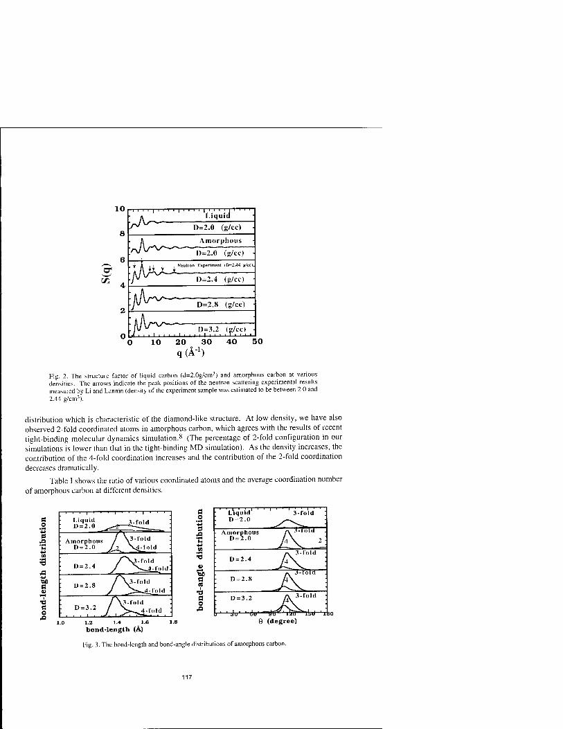
10

3 02

A Aniorpl

W^ isr7

-i i i i | i i i i | i i i i i i i ' i i iii '

:/A Liquid D=2.0 (g/cc)

Amorphous

/cc)

:^KXJ=Z Neutron Experiment <D=2.44 g/cc).

=2.4 (g/cc) ■

:j\j\r^- D=2.8 (g/cc)

I i i i i I i i D=3.2 (g/cc)

■In I I I 1.2 (g/cc)

1 i ■ T i i ■ ■

10 20 30 40 50 q (A"1)

Fig. 2. The structure factor of liquid carbon (d=2.0g/cm:1) and amorphous carbon at various densities. The arrows indicate the peak positions of the neutron scattering experimental results measured by Li and Lannin (density of the experiment sample was estimated to be between 2.0 and 2.44 g/cm-1).

distribution which is characteristic of the diamond-like structure. At low density, we have also observed 2-fold coordinated atoms in amorphous carbon, which agrees with the results of recent tight-binding molecular dynamics simulation.8 (The percentage of 2-fold configuration in our simulations is lower than that in the tight-binding MD simulation). As the density increases, the contribution of the 4-fold coordination increases and the contribution of the 2-fold coordination decreases dramatically.

Table I shows the ratio of various coordinated atoms and the average coordination number of amorphous carbon at different densities.

S 43

.a ■w ■on a V

■d a o .a

-I 1 1 1 1 1—I 1 r—I—r-

Liquid 3.fold D = 2.0 '

a o

MM

s 5 u +J «! •O

V "So a cd I

■a a o

1 1 1 1 1 ' ' I ' ' I ' ' I ' ■ Liquid 3-fold D = 2.0

Amorphous D = 2.0 Jsl U-Tola""'

D = 2.4 J£ D = 2.8

^

3-fold

CToTa-

D=3.2 A 3,ola :

ju' ' tju' "dir 'i!iir^tt>u '1 9 (degree)

Fig. 3. The bond-length and bond-angle distributions of amorphous carbon.

1.0 1.2 1.4 1.6 bond-length (Ä)

117

Table I. The ratio of various coordinations in amorphous carbon and the average coordination number Nc

Density 2-fold(%) 3-fold(%) 4-fold(%) Nc

(g/cm3) 2.0 9.1 84.4 6.5 2.97 2.4 1.6 87.4 11.0 3.09 2.8 0.6 84.1 15.3 3.14 3.2 0.5 78.0 21.5 3.21

Experimentally, most amorphous carbon are produced by evaporation or sputtering of graphite, or by mass-selected ion beam deposition techniques. The amorphous carbon samples produced by evaporation or sputtering of graphite are sp2 rich graphite-like; the amorphous carbon films obtained by mass-selected ion beam deposition techniques are found to be dominated by sp3

diamond-like bonding.

The simulation reported here mainly corresponds to the graphite-like amorphous carbon. The simulation results of amorphous carbon demonstrate the usefulness and effectiveness of the REBOP model. Currently we are using this model to study the mechanical properties of diamond- like amorphous carbon, especially, the investigation of the effect of hydrogen on the structure and transport properties of diamond-like amorphous carbon.

DYNAMICAL FRACTURE IN GRAPHITE SHEET Recently the dynamical behavior of cracks propagating through brittle, amorphous

materials and the morphology of the fracture surfaces has been the objects of much interest.16-22

To understand the dynamical behavior of cracks at atomic level, recently we have carried out a large scale molecular dynamics simulation of the crack propagation in graphite.

G(1,l)

Y

i

B(1,0)

-*- X Fig. 4. The graphite sheets: G( 1,1) and G( 1,0). (Arrows indicate the uniaxial tensile direction)

118

Crack propagation in a single graphite sheet has been investigated with large-scale molecular dynamics simulations on parallel computers. We have studied the effects of strain rate, shape of the notch, and the direction of the external strain with respect to the crystallographic axis.

Molecular dynamics simulations were performed on 100,800-particle systems. The size of the sheet was approximately 500 Ä x 600 Ä. The graphite sheet was initially laid out on the XY- plane, but the atoms were allowed to move in the Z-direction as well. No periodic boundary conditions were imposed and the boundaries were terminated with hydrogen atoms. The external strain was applied in the X-direction. We considered two different orientations of the graphite sheet in the XY plane (see Fig. 4). In one case, which we call G(l,l), there are bonds which are parallel to the X-axis. The other case we considered is G( 1,0), where the bonds make an angle of 30° with respect to the X-axis, and there are bonds parallel to the Y-axis.

Initially, the graphite sheets were uniformly expanded by 12%. Then, we inserted a notch and pulled the edges at a given strain rate. We used two different shapes of the notch: rectangular and triangular. The size of the notch was 20 Ä x 20 A. The simulations were performed either with a strain rate of 1% per 5,000 time steps (the time step was 1 femto second) or at a constant strain.

G(l,l) 10,000 At 700 r- Notch: Triangular

- Strain: 12.00% I Strain Rate: 0.0

600

500

400

3 300

200

100

IMMIHMI I I I I I I I I 100 200 300 400 500 600

Fig. 5. Snapshot of the crack propagation in graphite: G(l.l) under constant strain.

119

Figure 5 shows the snapshot of the graphite sheet with the orientation G(l,l) after 10,000 steps at constant strain of 12% and with the triangular notch. In this case, the crack propagates straight and the fracture is cleavage-like. Similar behavior was observed for a square notch under the same conditions.

700

600

500

400

3 300

200

100

G(1,0) 12,500 At Notch: Triangular

- Strain: 12.00% " Strain Rate: 0.0

' ■ ■ '■'■■■!■ JJ_L Jj 100 200 300

X(A) 400 S00 600

Fig. 6. Snapshot of the crack propagation in graphite G(1,0) under constant strain.

The situation is quite different for the G(1,0) orientation. Figure 6 shows the crack in the graphite sheet with the orientation G(1,0) and triangular notch after 12,500 steps at 12% strain. The crack branches and changes direction. Even more interesting is the behavior for the square notch. It turns out that for the G( 1,0) orientation and square notch the material does not break at 12% strain. In order to induce the fracture, we applied a strain rate of 1% per 5,000 steps. The crack started to propagate only after the strain exceeded 17%. For fracture at such a high strain and finite strain rate, the branching is dramatic, as shown in Fig. 7. Along with the obvious branches, we also see a number of periodically spaced attempted branches.

Figure 8 shows the crack tip position as a function of time for G(l,l) and G(1,0) orientation and constant strain of 12%. The crack speed is roughly constant for both orientations: 6.2 km/s for G( 1,1) and 5.7 km/s for G(1,0).

120

600

Constant Strain: 12% Initial: Triangular Notch

4 6 time (ps)

10

Constant Strain: 12% Initial :Triangular Notch

■ ■ 4' ' ' i,1 ' ' k' • time (ps)

Fig. 7. The crack propagation speed in graphite sheets: G(1,0) and G(l,l).

G(1,0) 12,750 At 700 p- Notch: Rectangular

I Strain: 19.55% I Sttaül Rate: 1% per 5,000 At

600

500

400

3 300

200

100

°h- _L1 I I III 0 100 200 300 400 500 600

X(A)

Fig. 8. Crack propagation in graphite: G(1,0) under constant strain rate.

121

To investigate the roughness of fracture surfaces we have calculated the roughness exponents from the height-height correlation function:

g(y) =<[h(y + y0)-h(y0)]2>5

of the crack surface using the height profile h(y). The bracket in the equation denotes the average over yn. For a self-affine surface, the height-height correlation is expected to obey the scaling relation g(y) ~ ya.

Figure 9(a) shows the height-height correlation function for the crack surface of the graphite G(1,0) under constant strain (12%). The log-log plot of the correlation function can be fitted with two straight lines with different slops (roughness exponents) characterizing two well- delineated regimes: For shorter length scales (< 30 Ä), we find a smaller roughness exponent of 0.51 +0.03 , whereas for larger length scales (> 30 A), we obtain a larger roughness exponent of 0.72 ± 0.03 .

-l—I—r—r r

a = 0.72 ± 0.03

Constant Strain: 12% Triangular Notch

3.0 4.0 ln(v)

- a = 0.56 ± 0.03

a = 0.81 ± 0.03

Strain: 17.5 %~ 19.5% atRate:0.2%/ps

Rectangular Notch 1.0U

2.0 3.0 4.0 ln(y)

Fig. 9. The height-height correlation function and roughness exponents of the graphite G(1,0): (a) under constant stress ( 12% ); (b) at constant stress rate ( 0.2% / ps ).

Figure 9(b) shows a log-log plot of the height-height correlation function for the crack surface of graphite G(1,0) when it was under finite strain rate (0.2%/ps, starting from 17%). Again, the height-height correlation function is characterized by two roughness exponents: 0.56 + 0.03 for shorter length scales, and 0.81 ± 0.03 for longer length scales.

SUMMARY

Using a reactive empirical bond-order potential (REBOP) model for hydrocarbons, large scale molecular dynamics simulations of carbon systems have been carried out on parallel machines. Structural and dynamical correlations of amorphous carbon at various densities have been investigated. The calculated structure factor agrees well with neutron scattering experiments and tight-binding molecular dynamics simulations. The fracture dynamics of graphite sheet has also been studied with the molecular dynamics method. Effects of external stress and initial notch shape on crack propagation in graphite have been studied. It is found that depending on the

122

orientations of the graphite sheet with respect to the external stress, graphite sheet fractures in a cleavage-like or branching manner. The roughness of crack surfaces has been analyzed. Two roughness exponents are observed in two different regions. For a shorter length scale (< 30 A), we obtained a smaller roughness exponent of 0.51 ±0.03 , while for a larger length scale (> 30 A),

we found a larger roughness exponent of 0.72 ± 0.03 . Under larger strain rate, the roughness

exponents of the fracture surface increases.

Currently, we are studying the fracture dynamics of high-density diamond-like amorphous carbon film and the effect of hydrogen concentration on the mechanical property of amorphous

carbon.

ACKNOWLEDGMENTS

We would like to thank Dr. A. Nakano for useful discussion. This work is supported by DOE, NSF, and AFOSR. The simulations were performed in the Concurrent Computing Laboratory for Materials Simulations (CCLMS) at Louisiana State University. The facilities in the CCLMS were acquired with equipment enhancement grants awarded by the Louisiana Board of Regents through Louisiana Education Quality Support Fund (LEQSF).

REFERENCES

1. (a) D. W. Brenner, Phys. Rev. B 42, 9458 (1990); (b) D. W. Brenner and S. B. Sinnott,

preprint. 2 J. Robertson, Adv. Phys. 35, 317 (1986); Prog. Solid State Chem. 21, 199 (1991); Phys. Rev.

Lett. 68, 220 (1992). 3 Fang Li and Jeffrey S. Lannin, Phys. Rev. Lett. 65, 1905 (1990). 4 D. R. McKenzie, D. Müller, and B. A. Paithorpe, Phys. Rev. Lett. 67, 773 (1991). 5 K. W. R. Gilkes, P. H. Gaskell, and J. Robertson, Phys. Rev. B 51, 12303 (1995). 6 S. Iarlori, G. Galli, and O. Martini, Phys. Rev. B 49, 7060 (1994). 7 G. Galli, R. M. Martin, R. Car, and M. Parrinello, Phys. Rev. Lett. 62, 555 (1989); Phys. Rev.

Lett. 63, 988 (1989). 8 C. Z. Wang and K. M. Ho, Phys. Rev. Lett. 71, 1184 (1993); C. Z. Wang, K. M. Ho, and C. T.

Chan, Phys. Rev. Lett. 70, 611 (1993); Phys. Rev. 8 47, 14835 (1993). 9 H.-P. Kaukonen and R. M. Nieminen, Phys. Rev. Lett. 68, 620 (1992). 10 Th. Frauenhein, P. Blaudeck, U. Stepan, and G. Jungnickel, Phys. Rev. B 48, 4823 (1993). 11 P. C. Kelires, Phys. Rev. Lett. 68, 1854 (1992); Phys. Rev. B 47, 1829 (1993) 12. X.-P. Li, R. W. Nunes, and D. Vanderbilt, Phys. Rev. B 47, 10891 (1993). 13. M. S. Daw, Phys. Rev. B 47, 10895 (1993). 14. G. C. Abell, Phys. Rev. B 31, 6184 (1985). 15 J. Tersoff, Phys. Rev. Lett. 61, 2879(1988); Phys. Rev. B 37, 6991 (1988); Phys. Rev. B 44,

12039 (1991). 16. E. Sharon, S. P. Gross, and J. Fineberg, Phys. Rev. Lett. 74, 5096 (1995). 17. E. Bouchaud, G. Lapasset, J. Planes, and S. Naveos, Phys. Rev. B 48, 2917 (1993); Phys. Rev.

Lett. 71, 2240 (1993). 18. K. J. Maloy, A. Hansen, E. L. Hinrichsen, S. Roux, Phys. Rev. Lett. 71, 205(1993). 19. J. S. Langer, Phys. Rev. Lett. 70, 3592 (1993). 20. M. Marder and X. Liu, Phys. Rev. Lett. 71, 2417 (1993). 21. F. F. Abraham, D. Brodbeck, R. A. Rafey, and W. E. Rudge, Phys. Rev. Lett. 73, 272 (1994). 22. A. Nakano, R. K. Kalia, and P. Vashishta, Phys. Rev. Lett. 75, 3138 (1995).

123

MASSIVELY PARALLEL MOLECULAR DYNAMICS SIMULATIONS FOR MANY-BODY POTENTIALS

L. T. WILLE, C. F. CORNWELL, AND W. C. MORREY Department of Physics, Florida Atlantic University, Boca Raton, FL 33431

ABSTRACT

We discuss the implementation of classical molecular dynamics simulations on Single- Instruction Multiple-Data computers with two-dimensional mesh connectivity. Specific timing results are given for the MasPar MP-1, complemented by a general time complexity analysis. Our main interest is in simulations with a number of particles N that is comparable to the number of processors P. In particular, we discuss results for large Si-clusters with up to 2000 particles, using a Stillinger-Weber potential. Particular attention is paid to the problem of handling in an efficient way the calculation of the three-body potential and force.

INTRODUCTION

One of the goals of computational materials science is the nanoscale study of kinetic processes in solids. The aim may be to allow a system to attain thermal equilibrium in order to extract information about, say, its phase diagram, or it may be to detect and analyze various metastable states in which the structure may get trapped. In other cases, one may be interested in a microscopic analysis of a dynamic process such as fracture or dislocation motion. Although a fully quantum mechanical study of the dynamics in solids and liquids is possible, for example by the Car-Parrinello technique, the size of systems and time scales that can be studied are relatively limited. As an alternative, classical molecular dynamics (MD) [1], based on empirical or quantum mechanically determined potentials, remains a viable option and has the advantage of permitting fairly large systems to be studied over much longer time periods. Major progress in understanding a variety of processes in a wide range of materials has come from such simulations in recent years. Nevertheless one has to realize that a direct simulation of truly macroscopic systems (= 1023

atoms) over laboratory time scales (minutes to hours) is still a long way off and may well never be feasible. The largest MD simulation to date [2] contains 600,000,000 atoms in a quasi-two- dimensional configuration, which is beginning to approach length scales of microelectronics features or grain sizes in metals. However, this number would need to be scaled up by a factor = 1014 to approach one mole of matter. An equally severe restriction is that MD simulations operate with time steps on the order of femtoseconds, so that a simulation of one second elapsed time would necessitate the execution of = 1015 time steps. Thus a microscopic simulation of fatigue in a turbine blade, to pick just one example, is out of the question with current hardware and algorithms. Of course, one may not need this amount of detail to be able to accurately model the phenomenon and predict its properties. Continuum models, treated analytically or, more commonly, by the finite element method and other numerical approximations, have been very valuable in this regard. Schemes linking the microscopic (quantum mechanical) models and the continuum limit, will become increasingly important in the future.

Simulations on the scale just described have only become possible through the advent of parallel computers. MD simulations are, at least in principle, well suited for parallel computation, since they involve the concurrent application of the same operation to different data elements, i.e. all particle force calculations and updates are performed simultaneously. Nevertheless the actual parallelization of an MD code for a given type of interaction potential and a given target machine is not a trivial task. Attention must be paid to such important issues as load balancing and avoiding the communication bottleneck. The appropriate strategy will be problem and machine dependent. For a given type of parallel computer, the optimal algorithm may even depend on the size of the system being studied. Several papers have discussed these topics in a variety of settings [2-5].

In the present work we analyze MD algorithms for Single-Instruction Multiple-Data (SIMD) computers with square mesh connectivity. We focus on short-ranged two- and three-body

125


potentials and numbers of particles (N) that are of the same order of magnitude as the number of processors (P). This covers a generic class of problems, including some biomolecules, polymers, and clusters. As a specific example, we study large Si-clusters in which the atoms are taken to interact through a Stillinger-Weber potential [6]. We have also employed the same programs in a study of fullerene tubes [7] in which the atoms are taken to interact through a Tersoff-Brenner potential [8]. Here we present timing results and algorithmic details, deferring a discussion of the physical findings to a future paper [9]. We are specifically excluding long-range potentials from the discussion. These pose their own problems since an exact calculation of all the forces scales as 0(N2) which is prohibitive for all but the smallest systems. Various approximate methods, with a gentler time complexity, have been proposed and have been shown to be parallelizable [4, 5]. We also note that the square mesh architecture is more restrictive than the widely adopted hypercube interconnection networks [10] since the former has a diameter of order *J¥, while the latter has a diameter of order log P [11] ensuring a shorter communication path between any two processors. In addition, any algorithm on the mesh can be embedded into the hypercube with dilation 1 and congestion 1, but the reverse is in general not possible [11]. Nevertheless, a number of parallel machines [10, 11] are based on a mesh connectivity and therefore efficient MD algorithms are of considerable interest.

METHOD

The MasPar MP-1 and MP-2 series of computers belong to the SIMD family, with up to 16,384 processor elements (PE's) arranged in a two-dimensional mesh with periodic boundary conditions. The PE's possess either 16 kBytes or 64 kBytes of local memory, as well as a number of registers. They communicate with nearest and next-nearest neighbors through a fast interconnection network called Xnet. Long-distance data interchange can be performed through a global router which is based on a multistage crossbar switch. Instructions are broadcast by the Array Control Unit (ACU) and are executed by all active processors on their local data elements. The status of a given PE (active/idle) is triggered by a binary flag. The ACU and the PE-array together form the data-parallel unit (DPU). The machine is front-ended by a DECStation 5000 which executes all serial constructs; communication between the front-end and the DPU is relatively slow and should be minimized in order to have an efficient code. More details on the architecture and the programming environment can be found elsewhere [10].

Generally speaking there are three main strategies for parallelizing MD simulations: atomic decomposition, spatial decomposition, and force decomposition [5]. In an atomic decomposition approach, each processor is assigned one or more atoms whose dynamic variables it needs to compute. The main advantages of this scheme are its simplicity and the fact that it is relatively straightforward to ensure load balancing. Its main drawback is that excessive interprocessor communication may occur, since in general atoms that are spatially close may not necessarily reside on adjacent processors. Spatial (or geometric) decomposition tries to overcome this problem by assigning to each processor a certain region of space in such a way that there is a contiguous mapping from simulation space to processor space. In this way long-range communication tends to be minimized at the expense of a potentially large load imbalance. If atoms reside on rigid lattice positions with relatively little atomic mobility a good division of the load over the processors can usually be attained, but if the system is spatially inhomogeneous this may not be possible. The latter would occur in simulations of spatially anisotropic macromolecules or in solids or liquids in which large fluctuations in density occur. The third possible parallelization method, force decomposition, is based on a block-decomposition of the force matrix. Effectively, each processor is assigned the task of calculating the force components for one or several atoms. To implement this scheme efficiently it is important to spread out the tasks equally over processors, which may be accomplished by a random ordering of atoms. This can lead to very efficient algorithms [5]. Unfortunately it is not known at present how to efficiently generalize this method for many-body potentials.

In the present work we wish to integrate Newton's equations of motion:

H2 N N

m; ^f1 = -V { X V2(ri,rj) + X V3(ri,rj,rk) } , i=l,...,N (1) at j*i j;k*i

126

where m; is the mass of atom i, V2 is a two-body (pair) potential, and V3 is a three-body potential. Our discussion will proceed completely generally, but all timing results are for the specific case of the Stillinger-Weber potential [6]. We note that the Tersoff-Brenner potential [8, 9] also fits in this methodology. Since a three-body potential is present force decomposition is not a viable parallelization method. Moreover, the present work was prompted by an investigation of Si- clusters and C-nanotubes with particle numbers of the order of a few thousand, roughly comparable to the size of the processor array. Since the spatial distribution of atoms is very irregular, geometric decomposition is also ruled out. (We note that geometric decomposition of three-dimensional space is possible on a two-dimensional processor grid, by treating the processor memory as the third dimension; however, for the reasons just described this is not an option for the problem under study.) Thus, atomic decomposition is the method of choice for the case where N ~ P and in the presence of short-range three-body interactions, even though this will necessarily entail some communication overhead.

In atomic decomposition, N/P atoms are assigned to each processor; we are interested here in cases in which this is a relatively small number (i.e., we take it to be 0(1)) and for ease of discussion we will assume that this ratio is an integer. Atoms in neighboring processors have no particular spatial relationship to one another. Consequently, the evaluation of the two- and three- body forces necessitates an 'all-to-all broadcast' [11] since each processor must communicate the coordinates of its atoms to all other processors. However, since we are dealing with a short-range potential many interactions will turn out to be zero since the interatomic distances involved are larger than the cut-off radius (Rc) of the potential. It is clearly advantageous to take into account this feature of the interactions. There are two main techniques for accomplishing this efficiently [1]: Verlet neighborhood lists and the link-cell method. Verlet's key idea is for each atom to maintain a list of its neighbors within a distance, Rv, somewhat larger than Rc; with a judicious choice of Rv this extended neighborhood needs to be updated only, say, every 10-20 time steps. In the link-cell method atoms are binned in (cubical) cells of size Rc (or somewhat larger); to test for neighbors only an atom's own bin and the 26 immediately surrounding it must be checked. In actual implementation it is customary to accomplish this by setting up a linked list of pointers chaining the atoms in a given cell. This feature speeds up search operations. Actually, the distinction between these two methods is somewhat artificial and, in fact, the fastest algorithms on sequential and vector computers use hybrid schemes that combine these two ideas.

RESULTS

We have implemented an atomic decomposition MD algorithm on the MP-1 with 4096 PE's and compare our results with a sequential version of the same algorithm running on a DECStation 5000. We use neighbor lists to speed up the calculations of the interactions. The remainder of the discussion focuses on the setting-up of these neighbor lists and the calculation of the force on each atom. The updating of the positions and velocities (performed in our calculations by means of Verlet's leap frog algorithm) is a trivially parallel operation and takes a negligible amount of time.

In time complexity analysis of parallel algorithms it is customary to distinguish three characteristic times for communication [11]: the start-up time (ts), the per-hop time (th), and the per-word transfer time (tw). The start-up time is the time it takes the sending processor to prepare the message, determine its routing path, and open a connection. This delay is incurred only once for each transfer. The per-hop time (or node latency) is the time it takes for a message to go from one processor to the next one in its path.The per-word transfer time is the inverse of the band width, i.e. the time it takes each word to traverse each link. We use m to denote the size of the message between any two processors; in the present case this would include the label and coordinates of each one of the N/P atoms residing on each processor.

The time taken for an all-to-all broadcast on the square mesh is [11]:

TaiUojlI = 2 ts (VP - 1) + tw m (P - 1). (2)

Since m is proportional to N/P we see that this time will scale as O(N). At the end of this step all processors have received the coordinates of all atoms. Next, the neighbor list is constructed in parallel for each one of the N/P atoms residing on each processor. Since there are N atoms to be

127

tested for inclusion in a given atom's neighborhood (and since N/P is 0(1)) this operation will take a time O(N). Thus, the overall time to construct the neighbor list is O(N), which is to be contrasted with a sequential machine on which the same set of operations takes time 0(N2). As will be seen, this 0(N) dependence dominates the asymptotic scaling of the algorithm. However, it must be kept in mind that all-to-all broadcasts are implemented in a highly efficient manner on most parallel computers and that neighbor lists need to be updated only every 10-20 time steps depending on the choice of Rv and the kinetic parameters of the simulation. Thus, the actual N-dependence of the computation time is relatively mild. Fig. 1 shows actual computation times for the sequential and parallel codes. As can be seen the O(N) dependence of the parallel code and the 0(N2) dependence of the sequential program are very well obeyed in practice. For the latter case, this step of the calculations quickly becomes a computational bottleneck.

80 CO

CD £ 60

40

20

^■«_i par riiimiinii Sgq

S

«**»•

mmttl „III»''»"

1 N(X1000) 2

Fig. 1: Time needed to construct the neighbor list for an N-atom system.

Next, the two- and three-body interactions need to be calculated for each atom. The computation of the two-body potential and force involves a loop over the neighbor list which can be executed in parallel. The execution time will be proportional to the size of the neighbor list which is an intensive variable, i.e. independent of N. Thus this step of the calculations can be performed in constant time, O(l), as opposed to the sequential program in which it takes time O(N). Without the use of neighbor lists this step would even take time 0(N2) on the sequential machine, which quickly becomes prohibitive. As can be seen in Fig. 2 these relations are very well obeyed. In particular the execution time on the MP-1 remains practically constant for N < 2000. Since we are running these programs on a 4,096 node machine, each PE contains at most one atom. We could, of course, have performed the simulations with N < 1024 on a 32x32 partition of the PE-array (an option that is available at compile time) in order to minimize the number of idle processors, and likewise for 1025 < N < 2048 on a 32x64 partition. However, our interest here was to illustrate the scaling of the execution times in the same environment. Our production runs [9] were executed in a DPU-partition that provided the best fit to the problem size at hand. On the 4,096 processor array the execution time for this part of the calculations would remain constant until N = 4,096 at which point a doubling of the execution time would occur. This would remain constant up to N = 8,192 at which another jump occurs, etc. The execution time for increasing N/P exhibits a typical plateau structure [12] with jumps at multiples of P.

The determination of the three-body potential and force poses somewhat more problems because there may be a non-zero interaction between atoms i, j, and k, with atom j in the neighbor list of atom i, and atom k within the neighbor list of atom j but outside that of atom i. In general the neighbor list of atom j does not reside on the processor devoted to atom i, so to make sure that this

128

effect is calculated correctly, we have constructed two neighbor lists for each atom: the first one containing atoms that are within a sphere of radius Rv of atom i, the second one containing atoms that are within a concentric shell consisting of the region between the spheres of radii 2RV and Rv. This second neighborhood tends to be somewhat larger than the first, but may be pruned considerably depending on the details of the potentials. For the three-body interactions a double loop needs to be executed over both neighbor lists. Clearly, the asymptotic execution time of this step of the calculations will still be 0(1) since the size of the neighbor lists is independent of N. On a sequential machine this time is 0(N) if neighbor lists are used. (It would be an unacceptable 0(N3) in a crude triple loop over atoms.) The actual execution times are shown in Fig. 3 and are seen to follow quite closely the anticipated behavior. Not surprisingly, they are considerably larger than the timings for the two-body interactions. The parallel execution times are constant in the range displayed, but will exhibit plateaus at multiples of P as a function of problem size N.

U.3-1 'ST

CD E

0.2-

^^^^ par IIIIIIIIIUIIIIIII SGQ

0.1-

nn-

.„•>iiin>

M , , , 1

1 N(x1000) 2

Fig. 2: Execution time for the calculation of two-body interactions.

^ 6i

^ 5

E ■■*= 4

3i

2

1

0

iiiiiiiiiiiiiiiiii SSQ

.».**

0 1 N(x1000) 2

Fig. 3: Execution time for the calculation of the three-body interactions.

129

CONCLUSIONS

Parallel computers have opened the way to materials simulations of unprecedented size and duration [2-5, 9]. Efficient parallel algorithms are strongly problem-size and architecture dependent. The present work focuses on short-range potentials with two- and three-body interactions and sizes of the same order as the number of processors (N/P = 0(1)). The overall time complexity of the algorithm is 0(N), due to the use of an atomic decomposition strategy which necessitates an all-to-all communication step to exchange atomic positions. Nevertheless, actual computation times are very acceptable. Other decomposition strategies [3-5] would become favorable at larger N/P ratios, but lead to load imbalance for the problems considered here. For example, Nakano et al. [2], using geometric decomposition and an ingenious multiple time-step method, quote results for a million particle simulation with three-body interactions in which communication times have become almost negligible. The algorithms presented here are scalable [ 11 ] if both N and P are increased, the ratio remaining fixed. If P is increased at fixed N, a number of idle processors will remain leading to inefficient use of the resources. If N is increased at fixed P, geometric decomposition will eventually become the method of choice. This cross-over point will occur asymptotically when N = 0(P2), the precise details depending on the parallel architecture and the nature of the potential.

REFERENCES

1. M. P. Allen and D. J. Tildesley, Computer Simulation of Liquids, Clarendon Press, Oxford, 1987.

2. N. Gr0nbech-Jensen, T. Germann, P. S. Lomdahl, and D. M. Beazly, IEEE Comp. Sei. Eng. 2 (2), 4 (1995); D. M. Beazly and P. S. Lomdahl, SIAM News 28 (2), 1 (1995); 28 (3), 1 (1995).

3. D. C. Rapaport, Comp. Phys. Comm. 76, 301 (1993).

4. A. Nakano, P. Vashishta, and R. K. Kalia, Comp. Phys. Comm. 77, 303 (1993); R. K. Kalia, and P. Vashishta, ibid. 83, 197 (1994); P. Vashishta, A. Nakano, R. K. Kalia, and I. Ebbsjö, J. Non-Cryst. Solids 182, 59 (1995).

5. S. Plimpton, J. Comp. Phys. 117, 1 (1995).

6. F. H. Stillinger and T. A. Weber, Phys. Rev. B 31, 5262 (1985).

7. S. Iijima, Nature 354, 56 (1991); T. W. Ebbesen and P. M. Ajayan, Nature 358, 220 (1992).

8. J. Tersoff, Phys. Rev. Lett. 56, 632 (1986); 61, 2879 (1988); Phys. Rev. B 37, 6991 (1988); D. W. Brenner, Phys. Rev. B 42, 9458 (1990).

9. C. F. Cornwell and L. T. Wille, presented at the 1995 MRS Fall Meeting, Boston, MA, 1995; to be published.

10. A. Trew and G. Wilson, Past. Present. Parallel - A Survey of Available Parallel Computing Systems. Springer Verlag, Berlin, 1991; K. Hwang, Advanced Computer Architecture - Parallelism. Scalability. Programmabilitv. McGraw-Hill, New York, 1993.

U.V. Kumar, A. Grama, A. Gupta, and G. Karypis, Introduction to Parallel Computing - Design and Analysis of Algorithms, Benjamin/Cummings, Redwood City, 1994.

12. L. T. Wille, J. L. Rogers, C. P. Burmester, and R. Gronsky, Future Generation Computer Systems 10,331 (1994).

130

AB-INITIO MOLECULAR DYNAMICS OF ORGANIC COMPOUNDS ON A MASSIVELY PARALLEL COMPUTER

FRANCOIS GYGI Institut Romand de Recherche Numerique en Physique des Materiaux (IRRMA) CH-1015 Lausanne, Switzerland

ABSTRACT

We present results of ab-initio electronic structure calculations and molecular dynamics simulations of organic molecules carried out using adaptive curvilinear coordinates, within the local density approximation of density functional theory. This approach allows for an accurate treatment of first-row elements, which makes it particularly suitable for investigations of organic compounds. A recent formulation of this method relies on a real-space approach which combines the advantages of finite-difference methods with the accuracy of adaptive coordinates, and is well suited for implementation on massively parallel computers. We used molecular dynamics simulations to obtain the fully relaxed structures of nitrosyl fluoride (FNO), and of the aromatic heterocycles furan and pyrrole. The equilibrium geometries obtained show excellent agreement with experimental data. The harmonic vibrational frequencies of furan and pyrrole were calculated by diagonalization of their dynamical matrix and are found to agree with experimental data within an rms error of 25 cm-1 and 28 cm-1

for furan and pyrrole respectively. This accuracy is comparable to that attained for smaller organic molecules using elaborate quantum chemistry methods.

INTRODUCTION

Ab-initio molecular dynamics simulations of organic compounds represent a challenge for most electronic structure methods currently in use. This difficulty is due to the presence in organic molecules of first-row elements whose wavefunctions are rapidly varying in space and therefore require a highly accurate numerical representation. Recent developments in ab- initio electronic structure have focused on the need to develop efficient molecular dynamics methods capable of treating all elements of the periodic table on an equal footing. Among them, the adaptive coordinate method [1] was recently proposed to improve the efficiency of the plane wave approach, and has been used in MD simulations including first-row elements [2]. The applicability of this method to the calculation of structural properties of solids and to the computation of band structures has also been demonstrated [3]. Recently, the adaptive coordinate method was reformulated using a real-space approach [4], which retains the simplicity of the recently introduced finite-difference formulation [5], while increasing is accuracy. The implementation of this method on a parallel computer is particularly straightforward since the real-space grid can be partitioned and distributed among processors. Most operations are then carried out locally on each processor, and interprocessor communications are kept to a minimum. In particular, no Fourier transforms are used in the calculation. The method is implemented on a Cray-T3D massively parallel computer. This approach is well suited to the calculation of the electronic structure of molecules containing first-row

131

Mat. Res. Soc. Svmp. Proc. Vol. 408 c 1996 Materials Research Society

elements, as was shown in Ref. [4] where it was used to calculate accurate bond lengths and vibrational frequencies of some first-row dimers, showing excellent agreement with both experiment and previous accurate local density functional calculations [6].

COMPUTATIONAL DETAILS

In this work, we applied the real-space adaptive-coordinate method to the calculation of the equilibrium geometries of nitrosyl fluoride, furan and pyrrole, within the local density approximation (LDA) of density functional theory [7]. Nitrosyl fluoride was chosen as an example of molecule containing the most rapidly varying potential of all first-row elements (fluorine), and in which the F-N bond length has a somewhat unusual value compared to typical F-N bonds found in other molecules. This characteristic has made FNO a challenging molecule for traditional quantum chemistry methods, requiring the use of large basis sets and of a refined treatment of correlations [8]. We also calculated the full vibrational spectrum of

furan and pyrrole by diagonalization of their dynamical matrix. In order to ensure a high accuracy of the calculations, we used the norm-conserving

pseudopotentials of Bachelet, Hamann and Schlüter [9], which reproduce accurately the atomic all-electron valence wavefunctions already at distances of 0.8, 0.7, 0.6 and 0.5 a.u. from the nuclei, for carbon, nitrogen, oxygen and fluorine respectively.

We used curvilinear coordinates, with deformation functions identical to those described in Ref. [4], which yield effective energy cutoffs of 360, 800, 900 and 990 Ry on the atomic sites for carbon, nitrogen, oxygen and fluorine, respectively. These values correspond to energy cutoffs of 90, 200, 225 and 247 Ry in conventional plane-wave calculations.

The molecules studied were placed in periodically repeated simulation cells of 8 x 8 x 8 A. Equilibrium geometries were obtained by first calculating the electronic ground state in a fixed trial atomic configuration. The ions were then allowed to move during a short molecular dynamics simulation, in which a small dissipation term was introduced in order to reach a

stable minimum energy configuration. The ability to perform molecular dynamics simulations has been commonly used to ex-

tract vibrational spectra from the ionic trajectories of a simulation. Various methods have been used, among which sophisticated signal processing techniques [10], as well as the maximum entropy method [11]. In this work, we chose instead to determine the vibrational frequencies of a molecule by explicit diagonalization of its dynamical matrix. This approach presents several advantages over the analysis of trajectories, among which the possibility of extracting the vibrational spectra of substituted isotopic species from the same calculation, without requiring additional molecular dynamics simulations. Furthermore, this approach also yields a full set of eigenmodes whose symmetry can be analyzed in order to label the eigenfrequencies. We determine the harmonic vibrational frequencies of a molecule contain-

ing N atoms by diagonalizing the 3N x 3N matrix

A,= 1 d2E (1) 13 Jmimj dxidxj

where a;,- denotes one of the 3N ionic degrees of freedom, (i.e. displacements along the directions x, y and z for each atom away from the equilibrium configuration) and m,- is the mass associated with the degree of freedom x*. The eigenvalues A of A are related to the

132

F-N N-0 F-N-0

Exp. (a) 1.512 1.136 110.1 Exp. (b) 1.517 1.131 109.9 Exp. (c) 1.520 1.130 110.2

LDA (this work) 1.515 1.134 111.1

LSD (c) 1.499 1.155 110.4 SCF (d) 1.395 1.113 110.5 QCISD(T) (d) 1.493 1.143 110.3

(a) Ref. [13], (b) Ref. [14], (c) Ref. [12], (d) Ref. [8]

Table 1: Structural parameters of nitrosyl fluoride (FNO) as obtained from experiment compared with our LDA results, and with other theoretical results. Distances are given in A and angles in degrees.

eigenfrequencies w by A = to2. The matrix A is calculated as

where Fi denotes the force acting on the degree of freedom Xi. The derivatives in Eq.(2) were evaluated by imposing small symmetric displacements away from the equilibrium configuration and computing the ionic forces in the 67V displaced configurations. The matrix elements of A were then computed using a symmetric 2-point finite difference formula, which eliminates the influence of any residual force at the reference equilibrium position.

RESULTS

The calculated equilibrium structural parameters of nitrosyl fluoride are given in Table 1 where they are compared with experimental data and with existing theoretical results. Our LDA results show a striking agreement with experimental data. They also compare well with the results of refined quantum chemistry calculations [8] performed with a high-quality basis set (6-311G(2d/)). The simpler SCF treatment was shown to yield poor structural parameters, related to the fact that the N-F bond in FNO is 0.13-0.15 Ä longer than typical N-F bonds [8]. Since the treatment of exchange and correlation used in Ref. [12] is identical to ours (LDA), we can attribute the difference between our results and those of Ref. [12] to a possible incompleteness of the basis set used in Ref. [12] and/or to the different treatment of core electrons in the two approaches (pseudopotential vs. all-electron calculation).

The structural parameters of furan were obtained using the same procedure. A comparison with experimental data and with the results of an MP2 quantum chemical calculation [15] is given in Table 2. Our LDA results are in excellent agreement with both experimental data and MP2 results.

133

Exp. LDA MP2

0-Ci 1.362 1.36 1.36 C1-C2 1.361 1.36 1.37 C2-C3 1.430 1.42 1.43 Ci-H, 1.075 1.09 1.08 C2-H2 1.077 1.09 1.08

04-0-Cx 106.6 106.6 106.9 0-C1-C2 110.7 110.5 110.5 C1-C2-C3 106.1 106.2 106.0 Hj-Ci-0 116.0 115.9 115.7 H2-C2-C3 127.8 127.5 127.9

Table 2: Structural parameters of furan as obtained from experiment (Ref. [16]), compared to the results of our LDA calculation and to those of a recent quantum chemical calculation including correlation at the MP2 level (Ref. [15]). Distances are given in Ä and angles in degrees.

In the case of pyrrole, we compare in Table 3 our results with experimental data of Ref. [17]. The agreement is of the same quality as for furan, with errors of the order of 0.01 Ä. The calculated vibrational frequencies of furan are given in Table 4 where they are compared with the recent experimental data of Klots et al. [18] The maximum error is 45 cm-1 and the rms error 24 cm-1. Some of the largest errors occur for the highest frequency modes which mostly involve in-plane stretching of C-H bonds. These errors can be attributed in part to the classical treatment of the protons adopted here, as well as to the neglect of anharmonic effects. C-H stretching frequencies are overestimated, whereas the frequencies of all other modes are generally underestimated. Other modes show very satisfactory agreement with experimental frequencies, with errors typically in the range of 10-35 cm-1. Molecular mechanics (MM3) parameters have recently been adjusted by Allinger and Yan [19] for furan, vinyl ethers and related compounds. While these authors obtained accurate fits of structures and energies, the spectroscopic data were less satisfactory. In the case of furan, the rms error of vibrational frequencies is 116 cm-1, and the maximum error 346 cm-1, illustrating the difficulty of representing accurately force fields of aromatic heterocycles by means of parametrized models.

The calculated vibrational spectrum of pyrrole is given in Table 5 and shows the same high accuracy as that of furan. The maximum error in this case is 53 cm-1 and the rms error 28 cm-1. The highest frequency corresponds to the N-H stretching mode and is overestimated, as are the frequencies of the C-H stretching modes. The frequencies of other modes are slightly underestimated as in the case of furan. The overall quality of these calculated vibrational spectra is comparable to that obtained on smaller molecules using quantum chemistry methods including a treatment of correlation equivalent or superior to MP2 perturbation theory.

134

Exp. LDA

N-Ci 1.370 1.37 C1-C2 1.382 1.38 C2-C3 1.417 1.42 C1-H2 1.076 1.09 C2-H3 1.077 1.09 N-Hj 0.996 1.02

C4-N-d 109.8 109.5 N-C1-C2 107.7 108.2 C1-C2-C3 107.4 107.1 Hrd-N 121.5 120.7 H2-C2-C3 127.1 127.5

Table 3: Structural parameters of pyrrole as obtained from experiment (Ref. [17]), compared to the results of our LDA calculation. Distances are given in A and angles in degrees.

species LDA Exp. Error species LDA Exp. Error Aj 3198 3169.4 29 Bi 3190 3160.6 30 At 3174 3139.7 35 Bi 3159 3129.7 30 A1 1463 1490.2 -27 Si 1543 1555.0 -12 A, 1373 1384.4 -12 Bi 1227 1266.7 -40 Ar 1131 1140.2 -9 Bi 1173 1180.6 -8 A, 1071 1067.0 4 Bi 1023 1042.5 -20 A, 984 995.0 -11 Bi 857 879.0 -22 Ai 863 870.8 -8 B2

B2

805 705

837.6 744.5

-33 A2 850 864.0 -14 -39 A2 680 724.5 -45 s2 607 602.7 4 A2 596 599.6 -4

Table 4: Harmonic vibrational frequencies (cm *) of furan calculated within the LDA and compared with the experimental data of Ref. [18].

135

species LDA Exp. Error species LDA Exp. Error

Ai 3583 3531 52 #i 3182 3143 39

Ai 3191 3150 41 Bx 3151 3118 32

Ai 3171 3128 43 B, 1519 1540 -21

Ai 1454 1476 -22 B, 1412 1424 -12

Ai 1383 1390 -7 Bx 1252 1288 -36

Ai 1158 1148 10 Bx 1116 1134 -18

Ai 1063 1075 -12 Bx 1025 1049 -24

Ai 1000 1017 -17 Bx 846 866 -20

Ai 873 882 -9 B2 792 827 -35

A2 840 864 -24 B2 681 722 -41

A2 646 692 -46 B2 627 624 3

A2 611 614 -3 B2 481 475 6

Table 5: Harmonie vibrational frequencies (cm compared to experimental results [18].

i of pyrrole calculated within the LDA and

CONCLUSIONS

We have used the real-space adaptive-coordinate method implemented on a massively parallel computer to calculate equilibrium and vibrational properties of organic compounds. A comparison with experimental data shows that the LDA yields very accurate structural properties for nitrosyl fluoride, as well as for the aromatic heterocycles furan and pyrrole. The calculated vibrational spectra of furan and pyrrole also show an excellent agreement with recent experimental data. These calculations of vibrational spectra show that the LDA provides a very accurate description of aromatic heterocycles. The unbiased nature of the numerical representation used guarantees an accurate description of molecular orbitals, and in particular of the delocalized ir electrons. The extension of this type of calculation to larger molecules or to solvated compounds is promising, especially in view of the forseeable increase in computing power brought by very large parallel computers.

ACKNOWLEDGEMENT

I would like to thank G. Galli for many useful discussions. This work is partially supported through the Parallel Application Technology Program (PATP) between the Ecole Polytechnique Federale de Lausanne (EPFL) and Cray Research, Inc.

REFERENCES

1. F. Gygi, Europhys. Lett. 19, 617 (1992); Phys. Rev. B 48, 11692 (1993).

2. F. Gygi, Phys. Rev. B 51, 11190 (1995).

3. D. R. Hamann, Phys. Rev. B 51, 7337 (1995); ibid. 51, 9508 (1995).

136

4. F. Gygi and G. Galli, Phys. Rev. B 52, 2229 (1995).

5. J. R. Chelikowsky, N. Troullier and Y. Saad, Phys. Rev. Lett. 72, 1240, (1994).

6. G. S. Painter and F. W. Averill, Phys. Rev. B 26, 1781 (1982).

7. D. M. Ceperley and B. J. Alder, Phys. Rev. Lett. 45, 566 (1980); Parametrization of J. P. Perdew and A. Zunger, Phys. Rev. B 23, 5048 (1981).

8. T .S. Dibble and J. S. Francisco, J. Chem. Phys 99, 397 (1993).

9. G. B. Bachelet, D. R. Hamann and M. Schlüter, Phys. Rev. B 26, 4199 (1982).

10. See e.g. J. Kohanoff, Comput. Mat. Sei. 2, 221, (1994).

11. See e.g. W. H. Press, B. P. Flannery, S. A. Teulkosky and W. T. Vetterling, Numerical Recipes, The Art of Scientific Computing (Cambridge University Press, 1986).

12. J. Andzelm and E. Wimmer, J. Chem. Phys 96, 1280 (1992).

13. K. S. Buckton et al. Trans. Faraday. Soc 65, 1975 (1969).

14. G. Cazzoli et al. Nuovo Cimento D 3, 627 (1984).

15. M. H. Palmer et al. Chem. Phys. 192, 111 (1995).

16. F. Mata et al, J. Mol. Struct. 48, 157 (1978).

17. L. Nygaard et al. J. Mol. Struct. 3, 491 (1969).

18. T. D. Klots et al, Spectrochim. Acta 50A, 765 (1994).

19. N. Allinger and L. Yan, J. Am. Chem. Soc. 115, 11918 (1993).

137

ACRES: ADAPTIVE COORDINATE REAL-SPACE ELECTRONIC STRUCTURE

N. A. MODINE, GIL ZUMBACH, EFTHIMIOS KAXIRAS Physics Department, Harvard University, Cambridge, MA 02138,

ABSTRACT

A real space approach to electronic structure calculations has several important advantages. A regular real-space mesh produces a sparse, local, and highly structured Hamiltonian, which enables effective use of iterative numerical methods and parallel computer architectures. However, a regular real space mesh has equal resolution everywhere, while actual physical systems are inhomogeneous. To remedy this inherent inefficiency without losing the advantages of a regular mesh, we carry out computations on a regular mesh in curvilinear space. There are several choices involved in the implementation of the method. These include the choice of the coordinate transform, the form of the discretized Laplacian, the regularization of the ionic potential for all-electron calculations, and the method of calculating the forces. Of particular interest is the use of error analysis to optimize the grid for a given physical system. The adaptive grid is versatile enough to describe accurately a very wide class of systems, including ones with highly inhomogeneous electronic distributions. We report all-electron calculations for atoms and molecules with Is and 2p valence electrons, and pseudopotential calculations for molecules and solids.

INTRODUCTION

Three desirable properties for any efficient electronic structure algorithm are sparsity, parallelizability, and adaptability. A sparse Hamiltonian allows effective use of iterative algorithms, which vastly reduce both memory and time requirements. A mapping onto a parallel machine that assigns identical tasks to each processor and produces a structured, local interprocessor communication pattern ensures good load balance and efficient communications. Adapting the grid resolution in different regions of space to the demands of the physical system allows efficient treatment of inhomogeneous systems such as the nuclear Coulomb potentials in all-electron calculations, pseudopotential calculations with Is, 2p, 3d, or 4f valence electrons, and systems with large regions of vacuum such as isolated atoms, molecules, clusters, or solid surfaces.

A number of groups1-5 have recently reported real space electronic structure computations using a regular grid. Electronic structure computations using regular real space grids result in sparse Hamiltonians and allow a natural mapping onto a parallel computer architecture. However, such approaches have uniform resolution in space and can not be adapted to inhomogeneous physical systems. A real space grid can be adapted to an inhomogeneous system by locally adding more basis elements. Recent work along these lines has used wavelets6,7, finite-elements8'9, and multi-grid methods10. Such local enhancement preserves the sparse Hamiltonian of a regular grid but interferes with the natural mapping onto a parallel machine and makes efficient parallelization more challenging.

In the following, we review our recently developed Adaptive Coordinate Real-Space Elec- tronic Structure (ACRES) method, which achieves all three of the desirable properties discussed above: sparsity, parallelizability, and adaptability.

139

Mat. Res. Soc. Symp. Proc. Vol. 408 s 1996 Materials Research Society

Figure 1: The two levels of the coordinate transformation as used for a pseudopotential calculation for 02 in a 12 x 12 x 24 a.u. box

METHOD

The central idea is to work on a regular grid in curvilinear space £ which is mapped by

a change of coordinates x(<f) to an adaptive mesh in real space x. The coordinate transformation differs from "classical" coordinate systems such as spherical coordinates in two important ways: (1) The grid is adapted to an arbitrary arrangement of atoms by taking a linear superposition of the adaptations associated with each atom. (2) The transformation is smooth and continuous everywhere and thus generates regular equations that are trivially parallelized. This type of transformation was pioneered in electronic structure calculations by F. Gygi11 for a plane wave basis. This adaptive plane wave approach has been fruit- fully pursued by several groups11-13, but it does not produce a sparse Hamiltonian. More recently, Gygi and Galli14 have reported pseudopotential real space calculations with an

adaptive mesh similar to the present method. The real space coordinates xi{(a;Pm) depend on the curvilinear coordinates E," and on

some set of parameters Pm that allow us to tune the change of coordinates to a particular problem. The Jacobian is given by J'a((; P) = dx'/d^ with \J\ = det J its determinant. Integrals are transformed according to fcPx = / d3£ \J\. The trivial metric g*1 = Stj in real

space corresponds to the metric gaß = J"1? J~^ in curvilinear coordinates (summation over repeated indices is implied). We express the Laplacian operator in curvilinear space as

A = ~da (\J\gaf3d0 (1)

because this form remains self-adjoint (with respect to the measure \J\) after discretization as long as the antisymmetric discretized operators da and dß are identical for each term.

IMPLEMENTATION

The equations are discretized using a finite difference scheme on a regular grid in curvilinear space. We find that we need to use at least a second order (four point) discretization for the

derivatives in order to obtain good results. We use a two level coordinate transformation x{£; P) with a global backdrop and further

local adaptation. This is illustrated in Fig. 1. The global backdrop is used only for systems with a large region of vacuum such as isolated atoms or molecules. It maintains the rectangular shape of the grid cells but requires regions of enhanced grid density that extend all the way to the boundaries of the simulation box. This enhancement of the grid in un- desired areas makes this type of transformation ineffective for increasing grid resolution in

140

fi-l

2Af « Figure 2: The evaluation of SIN/2 and 8IN.

several different areas. Therefore, we use a second level of grid transformation which creates a spherical deformation of the grid localized around each atomic position.

In order to generate a good coordinate transform x(£; P) for a given physical problem, we define a merit functional m(f; P) and choose the parameters P that minimize this quantity. To justify our choice of a merit functional, consider a one dimensional numerical integral evaluated using a regular grid in £ coordinates with mesh spacing A£

M/;n = £A£|J(6;P)|/(zte;P)) = £A£/i(P). (2)

We estimate the error in this integral by using IN as an approximant for / and comparing its value to IN/2- Fig. 2 shows SIN/2, the elementary contribution to the integral with N/2 points, and SIN, the contribution from the same region of space computed with N points. An estimate of the error contributed by this region is given by

6e(f) = 6IN-6Im = Aef?/2. (3)

To avoid cancellation of errors from different regions of space, we take our merit functional to be

(4)

The above idea is easily generalizable to three-dimensional integrals. The integrand / is chosen to be a physically important function such as the electronic charge, the total potential, or the exchange-correlation energy density.

The presence of the grid breaks translational invariance, and this effect can be quite large for all-electron calculations due to the Coulomb singularity. This effect is effectively eliminated by three techniques: (1) The dependence is reduced by adaptation, which makes the cell of the real space grid small near the atomic sites. This is sufficient to eliminate the problem for pseudopotential calculations. (2) The Coulomb potential is found by solving the discretized Poisson equation with the sum of electronic and nuclear charges as the source. This provides a natural regularization of the Coulomb divergence. (3) The nuclear charge is smoothly spread over a few grid points by means of a small Gaussian.

Since the grid changes as the atoms are moved, it is necessary to include Pulay corrections in the calculation of the forces. Fig. 3 shows our calculated forces. The Hellmann-Feynman force is accurately evaluated and would give the exact derivative of the energy if the grid did not change. With the Pulay corrections, we obtain forces which reproduce the derivative of the energy with excellent accuracy.

We use periodic boundary conditions with or without a phase shift. Adding a phase shift allows us to do band structure calculations for solids. Fig. 4 shows that our real-space calculations give very good agreement with plane wave calculations for the band structure of Si.

141

<

rr

o LL

•—• Derivative of the Energy o—oHellmann-Feynman Force Q—B Pulay Corrected Force

1.45 Distance (A.U.)

1.50

Figure 3: The forces from an all-electron computation for H2 with a 32 x 32 x 64 grid.

1.5 ■ ACRES with a 32X32X48 grid

--« Plane waves with 24 Ry. cutoff^

'L r Position in Brilloum Zone

Figure 4: The bands structure of diamond structure Si unfolded from the results for a 4 atom unit cell. 30 inequivalent k-points were used to sample the Brilloum zone.


Using the approach described in this paper, we have implemented DFT/LDA15 and DFT/GGA16 electronic structure calculations on the Naval Research Laboratory CM-5 massively parallel supercomputer. We have also implemented the norm-conserving nonlocal pseudopotentials of Bachelet et al.17, and the Kleinman-Bylander procedure18. Table I lists our results for a number of systems. For comparison, we include the results of other theory and experiment. Comparison reveals that our results are in good agreement with other theoretical work using similar methods and with experimental values. In conclusion, we have fully functional all-electron and pseudopotential ACRES codes that enable us to calculate accurate forces and accurate band structures on a parallel machine.

ACKNOWLEDGEMENTS

This work was supported by the Office of Naval Research grant N00014-93-1-0190.

142

Table I: Comparison of our results with other theory and experiment. References are " Ref. 19, S-VWN; ' Ref. 20; c Ref. 21, Perdew-Wang; d Ref. 19, B-LYP; e Ref. 21, PW GGA-II; } Ref. 22, Perdew-Zunger; > Ref. 23, 2p4 JD state; h Ref. 22, PW91; ' Ref. 24,

VWN; ' Ref. 24, Harmonic fitting to experiment. aQ is binding distance, u> is vibrational frequency, E0 is minimum energy, Eat is total energy, 6 is the bond angle, and k is the bulk

modulus. The Si calculations are for the diamond structure.

ACRES I Other Theory Experiment

All-electron |

H2 [LDA] do (a.u.) u> (cm-1) E0 (Ry)

1.448 4192

-2.276

1.446" 4207" -2.27c

1.401' 4401'

-2.349'

H2 [GGA] a0 (a.u.) to (cm-1) E0 (Ry)

1.416 4381

-2.340

1.413d

4373e

-2.34=

1.401' 4401'

-2.349'

0 [LDA] Eat (Ry) -148.870 -148.938' -150.027s

0 [GGA] Eat (Ry) -149.912 -149.994" -150.027°

02 [LDA] aa (a.u.) u> (cm-1)

2.32 1661

2.30" 1642"

2.28' 1580'

02 [GGA] o0 (a.u.) u (cm-1)

2.34 1557

2.34" 1518d

2.28' 1580'

Pseudopotential

H2 [LDA] a0 (a.u.) to (cm-1)

1.441 4212

1.446" 4207"

1.401' 4401'

N2 [LDA] a0 (a.u.) u> (cm-1)

2.067 2375

2.07' 2401"

2.07" 2377->

02 [LDA] aa (a.u.) u> (cm-1)

2.281 1588

2.30" 1642"

2.28' 1580'

H20 [LDA] a0 (a.u.) 9 (deg)

1.840 104.1

1.844" 103.6"

1.812" 103.9"

Si [LDA] a0 (a.u.) k (GPa)

10.04 98.08

10.16' 96.57'

10.26 98.80

REFERENCES

1. J. R. Chelikowsky, N. Troullier, and Y. Saad, Phys. Rev. Lett. 72, 1240 (1994); J. R. Chelikowsky, N. Troullier, K. Wu, and Y. Saad, Phys. Rev. B 50, 11355 (1994).

2. J. Bernholc, J.-Y. Yi, and D. J. Sullivan, Faraday Discuss. 92, 217 (1991); E. L. Briggs, D. J. Sullivan, and J. Bernholc, Phys. Rev. B 52, R5471 (1995).

3. S. Baroni and P. Giannozzi, Europhys. Lett. 17, 547 (1992).

4. K. A. Iyer, M. P. Merrick, and T. L. Beck, J. Chem. Phys. 103, 227 (1995).

5. T. Hoshi, M. Arai, and T. Fujiwara, Phys. Rev. B 52, R5459 (1995).

143

6. K. Cho, T. A. Arias, J. D. Joannopoulos, and P. K. Lam, Phys. Rev. Lett. 71, 1808 (1993).

7. S. Q. Wei and M. Y. Chou, preprint.

8. S. R. White, J. W. Wilkins, and M. P. Teter, Phys. Rev. B 39, 5819 (1989).

9. E. Tsuchida and M. Tsukada, Sol. St. Comm. 94, 5 (1995); Phys. Rev. B 52, 5573 (1995).

10. E. J. Bylaska et al., in Proc. 6th SIAM Conf. Parallel Processing for Sei. Corn-put. (San Francisco, 1995).

11. F. Gygi, Europhys. Lett. 19, 617 (1992); Phys. Rev. B 48, 11692 (1993); 51, 11190 (1995).

12. D. R. Hamann, Phys. Rev. B 51, 7337 (1995); 51, 9508 (1995).

13. A. Devenyi, K. Cho, T. A. Arias, and J. D. Joannopoulos, Phys. Rev. B 49, 13373 (1994).

14. F. Gygi and G. Galli, Phys. Rev. B 52, R2229 (1995).

15. We use the exchange-correlation local functional proposed by J. P. Perdew and A. Zunger, Phys. Rev. B 23, 5048 (1981).

16. J. P. Perdew, in Electronic Structure of Solids '91, edited by P. Ziesche and H. Eschrig (Akademie Verlag, Berlin, 1991).

17. G. B. Bachelet, D. R. Hamann, and M. Schlüter, Phys. Rev. B 26, 4199 (1982).

18. L. Kleinman and D. M. Bylander, Phys. Rev. Lett. 48, 1425 (1982).

19. B. G. Johnson, P. M. W. Gill, and J. A. Pople, J. Chem. Phys. 98, 5612 (1993).

20. K. P. Huber and G. Herzberg, Molecular Spectra and Molecular Structure (Van Nostrand Reinhold Company, New York, 1979), Vol. IV.

21. J. P. Perdew et al, Phys. Rev. B 46, 6671 (1992).

22. Y.-M. Juan and E. Kaxiras, Phys. Rev. B 48, 14944 (1993); Private communication.

23. C. E. Moore, Atomic Energy Levels (U. S. Government Printing Office, Washington,

1971), Vol. I.

24. F. W. Kutzler and G. S. Painter, Phys. Rev. B 37, 2850 (1988).

144

ELECTRONIC STRUCTURE CALCULATIONS ON A REAL-SPACE MESH WITH MULTIGRID ACCELERATION

D. J. SULLIVAN, E. L. BRIGGS, C. J. BRABEC, and J. BERNHOLC Department of Physics, North Carolina State University, Raleigh, NC 27695-8202

ABSTRACT

We have developed a set of techniques for performing large scale ab initio calculations using multigrid accelerations and a real-space grid as a basis. The multigrid methods permit efficient calculations on ill-conditioned systems with long length scales or high energy cutoffs. We discuss the design of pseudopotentials for real-space grids, and the computation of ionic forces. The technique has been applied to several systems, including an isolated C6o molecule, the wurtzite phase of GaN, a 64-atom cell of GaN with the Ga d-states in valence, and a 443-atom protein. The method has been implemented on both vector and parallel architectures. We also discuss ongoing work on O(N) implementations and solvated biomolecules.

INTRODUCTION

Over the course of the last several decades, plane-wave-based methods have been used to perform electronic structure calculations on a wide range of physical systems. The Car- Parrinello (CP) and other iterative methods [1, 2] have made such calculations possible for systems containing several hundred atoms [3]. While these methods have been very successful, several difficulties arise when they are extended to physical systems with large length scales or containing first-row or transition-metal atoms. Special techniques have been developed to handle some of these problems. Optimized pseudopotentials [4, 5], the augmented-wave method [6], plane waves in adaptive-coordinates [7-9] and preconditioning combined with conjugate-gradient techniques [10, 11] have had considerable success; however, these techniques are still constrained by the plane-wave basis, which requires periodic boundary conditions for every system and fast Fourier transforms (FFTs) to efficiently transform between real and reciprocal space. In particular, FFTs involve non-local operations that impose constraints on the adaptability of these algorithms to massively-parallel computer architectures, because they perform best on problems that can be divided into localized domains.

It has been appreciated for some time that there are potential advantages to performing electronic-structure calculations entirely in real space. Boundary conditions are not constrained to be periodic; this permits the use of non-periodic boundary conditions for clusters and a combination of periodic and non-periodic boundary conditions for surfaces. By employing nonuniform real-space grids, it is possible to add resolution locally, e.g., for a surface or cluster calculation. A basis that uses a high density of grid points in regions where the ions are located and a lower density of points in vacuum regions can lead to order of magnitude savings in the basis size and total computational effort [12]. More importantly, the use of a real-space basis opens up the possibility of using multigrid iterative techniques to obtain solutions of the Kohn-Sham equations. Multigrid methods [13], which provide automatic preconditioning on all length scales, can greatly reduce the

145


number of iterations needed to converge the electronic wavefunctions. Furthermore, the real-space multigrid formulation does not involve long-range operations and is particularly suitable for parallelization and O(N) algorithms [14-17], because every operation can be partitioned into hierarchical real-space domains.

There have been a number of previous real-space grid-based electronic-structure calculations. The finite-element method was applied by White et al. [18] to one-electron systems. They used both conjugate-gradient and multigrid acceleration to find the ground- state wavefunction. Two of the present authors [12] used nonuniform grids with locally enhanced regions in conjunction with multigrid acceleration to calculate the electronic properties of atomic and diatomic systems with nearly singular pseudopotentials. They verified that the preconditioning afforded by multigrid was effective in multi-length-scale systems. Chelikowsky et al. [19] have used high-order finite-difference methods and soft non-local pseudopotentials on uniform grids to calculate the electronic structure, geometry, and short-time dynamics of small Si clusters. The present authors have developed a real-space grid method with multigrid methods and tested it extensively against plane- wave results [20]. Other recent real-space work includes finite-differencing on warped grids [21, 22], wavelet bases [23, 24], hierarchical non-linear grids applied to diatomics [25], and multigrid calculations on first and second row atoms [26].

REAL-SPACE MESH DESIGN

Several issues that are absent from plane-wave or orbital-based methods arise when using a real-space grid approach. In the former case the wavefunctions, potentials, and the electronic density are representable in explicit basis functions, and thus are known everywhere. In a real-space grid implementation, these quantities are known only at a discrete set of grid points, which can introduce a spurious dependence of the Kohn-Sham eigenvalues, the total energy, and the ionic forces on the positions of the ions with respect to the real-space grid. We have developed a set of techniques that can overcome these difficulties and can be used to compute accurate, static and dynamical properties of large physical systems. In our formalism the wavefunctions, density, and potentials are directly represented on a three-dimensional real-space grid with linear spacing hgrid and number of mesh points -/Vsr,d- The ions are represented by soft-core norm-conserving pseudopotentials [27]. Exchange and correlation effects are treated using the local density approximation (LDA) of density functional theory.

Discretization and Pseudopotentials

For reasons of accuracy and computational efficiency, we discretize the Kohn-Sham equations in a generalized eigenvalue formulation:

A{Tpn] + B[Veffipn] = enB{4>n}. (1)

A and B are the components of the Mehrstellen discretization [28], which is based on Hermite's generalization of Taylor's theorem. It uses a weighted sum of the wavefunction and potential values to improve the accuracy of the discretization of the entire differential equation, not just the kinetic energy operator. The weights for the 0(h*rid) discretization

146

Table I: Mehrstellen discretization weights in 3D (h is the grid spacing).

Grid point 6/i2*A 6*B central

nearest neighbors second neighbors

24 -2 -1

6 1 0

are given in Table I. We have found that the fourth-order Mehrstellen discretization produces equivalent or better accuracy than the sixth-order central-finite-difference one. The higher accuracy of the Mehrstellen approach is achieved by using a non-separable discretization, and more local information (second nearest-neighbor points, for example).

We have found that pseudopotentials, especially the rather hard ones, must be smoothed before they are suitable for real space calculations. Smoothing is necessary to avoid high- frequency variation on the real-space mesh which reduces accuracy and slows convergence. This variation is absent from plane-wave calculations because the basis cuts off the large- G components of the potentials exactly [29]. To achieve this same cutoff effect in real space, we use the following filtering procedure: The radial pseudopotentials are Fourier- transformed to G space. They are multiplied by a cutoff function which decreases rapidly beyond 7r/(a/i), where a is typically in the range 1.5 - 2.0. The filtered potentials are then back-transformed to real space. We have found that the Fourier-filtered pseudopotentials retain the accuracy of those used in plane-wave calculations.

To test the smoothness of the pseudopotentials, an isolated atom or a bulk system is displaced relative to the grid. The magnitude of the variation in total energy is a measure of smoothness of the pseudopotentials. In Fig. 1 we show the change in the LDA energy of a carbon atom and a diamond supercell as a function of distance from a mesh point. In addition, the degeneracy pattern of the eigenvalues and the ionic forces are examined. If the pseudopotential is insufficiently smooth, the ionic forces in a symmetric lattice, for example, will be not be small (vanish).

To facilitate comparisons with plane-wave calculations, we define an energy cutoff for the real-space calculation, ir2/2h2 [Ry], to be equal to that of a plane-wave calculation that uses a FFT grid with the same spacing as the multigrid calculation [30].

To efficiently solve Eq. (1), we have used multigrid iteration techniques that accelerate convergence by employing a sequence of grids of varying resolutions. The final solution is obtained on a grid fine enough to accurately represent the pseudopotentials and the electronic wavefunctions. If the solution error is expanded in a Fourier series, it may be shown that iterations on any given grid level will quickly reduce the components of the error with wavelengths comparable to the grid spacing but are ineffective in reducing the components with wavelengths large relative to the grid spacing [13, 31]. The multigrid method reduces these latter error components by treating them on a sequence of auxiliary grids with progressively larger grid spacings, on which the errors appear as high-frequency components. This procedure provides excellent preconditioning for all length scales present in the system and leads to very rapid convergence rates.

To summarize, one self-consistent iteration consists of a multigrid step to solve Eq. (1), followed by the orthogonalization of the orbitals, and an update of the electronic density. The components of the effective potential that depend on the density (Hartree and

147

> >

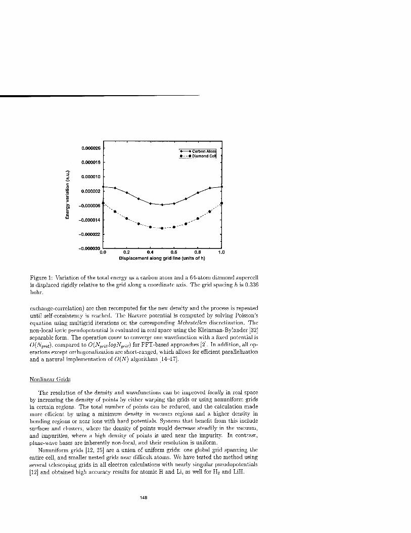
0.000026

0.000018

0.000010

0.000002

-0.000006

-0.000014

-0.000022

-0.000030 0.0

♦ ♦ Carbon Atom • - ~ • Diamond Cell

-•---.,-

0.2 0.4 0.6 0.8 1.0 Displacement along grid line (units of h)

Figure 1: Variation of the total energy as a carbon atom and a 64-atom diamond supercell is displaced rigidly relative to the grid along a coordinate axis. The grid spacing h is 0.336 bohr.

exchange-correlation) are then recomputed for the new density and the process is repeated until self-consistency is reached. The Hartree potential is computed by solving Poisson's equation using multigrid iterations on the corresponding Mehrstellen discretization. The non-local ionic pseudopotential is evaluated in real space using the Kleinman-Bylander [32] separable form. The operation count to converge one wavefunction with a fixed potential is 0(NgTid)) compared to 0(NgridlogNgrid) for FFT-based approaches [2]. In addition, all operations except orthogonalization are short-ranged, which allows for efficient parallelization and a natural implementation of 0(N) algorithms [14-17].

Nonlinear Grids

The resolution of the density and wavefunctions can be improved locally in real space by increasing the density of points by either warping the grids or using nonuniform grids in certain regions. The total number of points can be reduced, and the calculation made more efficient by using a minimum density in vacuum regions and a higher density in bonding regions or near ions with hard potentials. Systems that benefit from this include surfaces and clusters, where the density of points would decrease steadily in the vacuum, and impurities, where a high density of points is used near the impurity. In contrast, plane-wave bases are inherently non-local, and their resolution is uniform.

Nonuniform grids [12, 25] are a union of uniform grids: one global grid spanning the entire cell, and smaller nested grids near difficult atoms. We have tested the method using several telescoping grids in all electron calculations with nearly singular pseudopotentials [12] and obtained high accuracy results for atomic H and Li, as well for H2 and LiH.

148

Figure 2: An example of a separable non-linear coordinate transformation to increase the resolution near an impurity.

Scaled grids [7, 21, 22] are a warping of one uniform grid by means of a coordinate transformation. In general the transformation is non-separable; we prefer a separable coordinate transformation (see Fig. 2) in order to avoid mixed derivatives in the kinetic- energy operator. As a test of the utility and accuracy of scaled grids, we examined the the interstitial 0 impurity in Si [33] for two grid layouts: a dense uniform grid with a 76-Ry cutoff and a scaled grid with a cutoff that varied from 18 Ry to 76 Ry. The number of points needed for the scaled grid was smaller by a factor of four. In each case, a 64-atom supercell was used and all atoms were fully relaxed. The two calculations agree well: the maximum difference in Kohn-Sham eigenvalues was 40 meV and the maximum difference in ionic coordinates was 0.03 Ä.

Ionic Forces and Molecular Dynamics

Ab initio molecular dynamics (MD) simulations require accurate ionic forces so that higher-order integrators and large time-steps can be used to achieve long simulation times. If the grid layout, whether uniform or nonuniform, does not change when the ions move, the Hellmann-Feynman (HF) force theorem [34] applies with no Pulay corrections [35]. However, the calculation of the HF forces on a real-space grid requires careful consideration of numerical errors because the derivative of even a filtered pseudopotential can introduce high-frequency components. The accuracy of the forces was tested by comparing equilibrium structures with ones determined with plane waves or experiment, by checking whether symmetric structures have zero forces, and by monitoring the constancy of the MD total energy over long simulations.

The traditional implementation of the HF forces is often sufficiently accurate for structural optimization. Considering the various force components, the contribution of the local pseudopotential has a small numerical error because the electronic charge density is smooth, and thus its integral with the derivative of the local pseudopotential is well converged. However, the contribution to the ionic forces from the non-local projectors is often less accurate. This is because each derivative of the projector is integrated against every orbital, which are less smooth than the density, and because the numerical errors in these integrals do not cancel.

We have developed a more accurate implementation of HF forces for real-space grids

149

20.0

-20.0 0.0 2000.0 4000.0

Time (a.u.) 6000.0

Figure 3: A large-time-step molecular dynamics simulation of a 64-atom Si supercell at an approximate temperature of 1100 K. The total energy was conserved to within 10~5 a.u. with the kinetic energy on the order of 0.3 a.u. of the run was 0.15 ps.

The time-step was 80 a.u., and the length

called "virtual displacements." Instead of integrating the radial derivative of the pseudopotentials (interpolated onto the grid) against the density or wavefunctions, we finite- difference the interpolated pseudopotential and integrate this numerical approximation of the HF derivative against the density and wavefunctions. Differencing the pseudopotential cannot introduce high-frequency components that would contribute to the integration error. Typically, each ion's pseudopotential is virtually displaced four times to compute its numerical derivative. Note that the density and wavefunctions are fixed as required by the HF theorem. The computational work is thus limited to computing additional localized integrals.

The virtual displacements procedure was used to optimize all structures quoted in this report, and the structural parameters compared well to those computed by with a plane- waves basis. A sensitive test of the accuracy of the forces is a long-time MD simulation. We evolved a 64-atom Si supercell over 0.15 ps with a 80 a.u. time-step and found that the MD energy was conserved to within 4/ueV per atom; see Fig. 3.

PARALLELIZATION

There are two apparent parallelization schemes for a real-space grid method. First, the orbitals could be distributed over processors and stored there. Its major advantage is that our highly-optimized serial code would require few changes. However, the orthogonalization of the orbitals would perform inefficiently because entire orbitals must be exchanged between processors. Our preferred scheme is data decomposition, where real-space domains

150

Table II: Comparison of GaN results obtained with the Ga 3d electrons in valence. The multigrid calculation uses a 64-atom supercell, 250-Ry cutoff and T point sampling. See text [eV].

Band Gap Cohesive Energy Full potential LMTO [36] 240 Ry, Plane waves, 2-atom cell [37] Multigrid, 64-atom cell

2.00 1.89 1.88

10.89

10.64

are distributed over processors. Orthogonalization becomes tegrals can be computed in two parts: the intra-processor the inter-processor part sends only the intermediate sums important, the compact nature of the Mehrstellen operator small amounts of data between nearest-neighbor processors from the Cray YMP-C90 to the massively-parallel Cray T3D balancing ( 90%) on all systems tested. These tests used up

efficient because overlaps in- portion is fully parallel, and between processors. Just as requires the exchange of only

. In tests of the code, ported , we found nearly perfect load to 512 processors.

TESTS AND RESULTS

A significant advantage of the multigrid method is the speed of convergence to the electronic ground state for a given initial ionic configuration. For systems requiring a small energy cutoff or of small size, the speed advantage with respect to CP-based methods is not substantial. However, for systems requiring a large energy cutoff, or of large dimensions, this advantage—as measured in actual computational time—is typically an order of magnitude. This is because the maximum stable time-step in the Car-Parrinello method must be much smaller than in the multigrid approach. Our initial tests of the real-space multigrid method were discussed previously [12, 20] and included a full comparison with established plane-wave results.

To illustrate the ability of the multigrid method to handle ill-conditioned systems, test calculations were performed on a 64-atom GaN cell in the zinc-blende structure with the Ga 3d electrons in valence. A grid spacing of 0.14 bohr was used, which corresponds to an energy cutoff of 250 Ry in a plane-wave calculation. Only the T point was included in k-space sampling. Starting with random initial wavefunctions, only 75 self-consistent steps were required to converge the total energy. Recently, several calculations have been performed on GaN that explicitly included the d-electrons in valence; the multigrid results are in very good agreement with these calculations (see Table II).

In addition, the energy of formation of the Ga interstitial impurity in a 64-atom GaN supercell was calculated to be 7 eV. The ions were not relaxed at this 250-Ry cutoff in order to conserve computer resources. Instead, ionic coordinates from a fully-relaxed Ga interstitial calculation with the Ga 3d electrons in core were used. As a check, the interstitial was also fully relaxed with the Ga 3d electrons in valence, but at a 160-Ry cutoff with a slightly softer pseudopotential. The maximum difference in ionic coordinates between the two relaxed structures was 0.1 A.

The present results for the Ga interstitial confirm our previous values, obtained with

151

Table III: Multigrid convergence tests in an 8-atom supercell: grid spacing [bohr], equivalent plane-wave cutoff [Ry], total energy [a.u.], and the number of steps to converge the density.

Grid Spacing Cutoff Total Energy SCF steps 0.421 25. -44.87968 22 0.336 35. -45.03331 17 0.280 60. -45.06240 21 0.210 110. -45.06605 26

the Ga 3d electrons in core [38]; namely, the Ga interstitial is one of the low-energy native defects in GaN. Recent experimental results indeed find indirect evidence for its presence, since Ga precipitates are formed upon annealing [39],

We have also studied the wurtzite phase of GaN in a 32-atom supercell with the d electrons in core. The discretization in the hexagonal plane is straightforward because the grid lines can be mapped onto a Cartesian plane. The Kohn-Sham eigenvalues computed by the real-space and plane-wave methods are in excellent agreement.

An isolated Cßo molecule was selected as an example of a non-periodic system. The simulation cell was a cube of length 23 bohr and the grid spacing was 0.360 bohr. The initial ionic coordinates were generated using the classical Tersoff-Brenner potential [40], and the electronic wavefunctions were set to zero on the boundaries of the cell. After the convergence of the electronic system, the ions were relaxed using the same relaxation scheme as before. Two distinct bond lengths were found in the final structure, corresponding to the carbon-carbon single and double bonds. There were twice as many single bonds as double bonds, and the average double and single bond lengths were 1.39 and 1.44 Ä, compared to 1.41 and 1.45 Ä obtained in a previous CP calculation [41] for the C6o solid. The standard deviations of the bond-length distributions were on the order of 10~3 A in both calculations. The experimental values for the solid are 1.40 and 1.45 Ä, respectively.

Next, we examine the efficiency of multigrid acceleration. Table III illustrates the convergence properties as a function of grid resolution for an 8-atom diamond cell. The observed convergence rates are largely independent of the energy cutoff. The number of self-consistent steps required to converge the density is also nearly independent of the system size. At an equivalent cutoff of 35 Ry, the multigrid method required 17 steps to converge the total energy of the 8-atom diamond cell to a tolerance of 10~8. When the same calculation was performed for a 64-atom cell only 20 SCF steps were needed.

Finally, we compare the convergence rates for four iterative-diagonalization schemes: steepest descents, multigrid, steepest descents with periodic subspace rotation, and multigrid with periodic subspace rotation. Subspace rotation (subspace diagonalization) speeds up iterative diagonalization schemes because it efficiently resolves exact or near degeneracies between orbitals. In the tests, the initial wavefunctions were randomly chosen, a worse-case scenario, and the time step was the same for each scheme. Ordinary multigrid rapidly decreases the error, but the convergence stalls after 15 steps because the density is changing slowly. Periodic subspace rotation sorts out the small degeneracies between states, and when several unoccupied states are included in the calculation, it mixes in new information from the unoccupied sector. This greatly improves the convergence rate, even

152

5.0

1.0

-3.0

MG-SR SD-SR MG SD

'

0.0 20.0 40.0 60.0 80.0 SCF Steps

Figure 4: Comparison of the convergence rates for multigrid-accelerated steepest descents (MG), MG with periodic subspace rotation (MG-SR), steepest descents (SD), and steepest descents with with periodic subspace rotation (SD-SR). The jumps in the lower two curves are due to the subspace rotation. The system is a distorted 64-atom Si supercell with a 12-Ry cutoff, starting from randomly-generated wavefunctions.

for steepest descents.

ONGOING WORK

Order-N Implementations

For very large systems, the complexity of the calculations increases as 0(Na(oms) in computer time due to orthogonalization, and the memory increases as 0(N^oms). Several approaches that reduce both types of scaling behavior to 0(Natoms) have been proposed. These O(N) methods rely on the assumption that physical properties are local, and that the Orbitals and/or the density matrix—when localized in finite volumes about each atom—can describe the electronic charge density, kinetic-energy density, etc. to useful accuracy.

We have implemented a real-space version of both the wave-function [14,16] and density matrix approaches [15, 17]. Our calculations are not yet fully self-consistent in the density, possibly due to high-frequency components in the density. Nonetheless as a preliminary test, the LDA energy was evaluated within the O(N) approximation using the exact density. A 64-atom diamond supercell was converged for both the orbital [16] and density-matrix [17] methods, using four atom-centered orbitals/support functions per atom. The radius of the localization volume extended to third neighbors. The difference between the exact LDA total energy and the O(N) energy was 0.5 eV/atom for the orbital method, and 0.3 eV/atom for the density-matrix method. A possible reason for this slight difference is that the density-matrix functional requires a smaller localization volume for this system.

153

Figure 5: Three views of the electronic charge density of the amyloid /3-peptide associated with Alzheimer's disease. The top view shows the entire molecule; the lower two views are close-ups of the first quarter and second third of the molecule, respectively.

Solvated Biomolecules

In collaboration with L. Peterson (UNC-Chapel Hill), we are investigating the properties of a protein associated with Alzheimer's disease, the amyloid /3-peptide Ci46045N42H2io. The LDA calculations were performed on the Cray-T3D (128 or 256 processors), using a structure obtained from NMR data that was refined by a molecular-mechanics force field program (AMBER). See Fig. 5 for a plot of the electronic charge density. Presently, we are relaxing the system quantum mechanically in the presence of water, which is treated by a classical potential. We have also implemented the generalized gradient approximation to DFT (GGA) [42], which is known to improve the description of hydrogen bonding as well as the values of the binding energies. In tests on an amino acid (phenylalanine), the GGA disassociation energy was lower by 7% than the LDA value of 142.59 eV.

SUMMARY

We have developed a methodology for performing large-scale ab initio electronic-structure calculations entirely in real space. The use of highly-efficient multigrid techniques to accelerate convergence rates is particularly important for ill-conditioned systems requiring high energy cutoffs or with large length scales. In addition, the multigrid method is readily adaptable to parallel computer architectures. We have used this multigrid method in long- time ab initio MD simulations and in studies of the structural and electronic properties of clusters, surfaces and biomolecules. Additional applications are in progress.

154

REFERENCES

1. R. Car and M. Parrinello, Phys. Rev. Lett. 55, 2471 (1985).

2. For a recent review, see M. C. Payne, D. C. Allan, M. P. Teter, T. A. Arias, and J. D. Joannopoulos, Rev. Mod. Phys. 64, 1045 (1992).

3. See, for example, I. Stich, M. C. Payne, R. D. King-Smith, and J.-S. Lin, Phys. Rev. Lett. 68, 1351 (1992); K. D. Brommer, M. Needels, B. E. Larson, and J. D. Joannopou- los, ibid. 68, 1355 (1992); P. Boguslawski, Q.-M. Zhang, Z. Zhang, and J. Bernholc, ibid. 72, 3694 (1994).

4. D. Vanderbilt, Phys. Rev. B 41, 7892 (1990).

5. A. M. Rappe, K. M. Rabe, E. Kaxiras, and J. D. Joannopoulos, Phys. Rev. B 41, 1227 (1990); J.-S. Lin, A. Qteish, M. C. Payne, V. Heine, ibid. 47, 4174 (1993); G. Li and S. Rabii, unpublished (1992).

6. P. E. Blöchl, Phys. Rev. B 41, 5414 (1990).

7. F. Gygi, Europhys. Lett. 19, 6617 (1992); F. Gygi, Phys. Rev. B 48, 11692 (1993);

8. D. R. Hamann, Phys. Rev. B 51, 7337 (1995); 51, 9508 (1995);

9. A. Devenyi, K. Clio, T. A. Arias, and J. D. Joannopoulos, Phys. Rev. B 49, 13373 (1994).

10. M. P. Teter, M. C. Payne, and D. C. Allan, Phys. Rev. B 40, 12255 (1989).

11. T. A. Arias, M. C. Payne, and J. D. Joannopoulos, Phys. Rev. Lett. 69, 1077 (1992); Phys. Rev. B 45, 1538 (1992).

12. J. Bernholc, J.-Y. Yi, and D. J. Sullivan, Faraday Disc. Chem. Soc. 92, 217 (1991).

13. A. Brandt, Math. Comp. 31, 333 (1977); GMD Studien, 85, 1 (1984).

14. W. Yang, Phys. Rev. Lett. 66, 1438 (1991); G. Galli and M. Parrinello, ibid. 69, 3547 (1992); F. Mauri, G. Galli, and R. Car, Phys. Rev. B 47, 9973 (1993); P. Ordejön, D. A. Drabold, M. P. Grumbach, and R. M. Martin, ibid. 48, 14646 (1993).

15. S. Baroni and P. Giannozzi, Europhys. Lett. 17, 547 (1992); X.-P. Li, R. Nunes, and D. Vanderbilt, Phys. Rev. B 47, 10891 (1993); M. Daw, ibid. 47, 10895 (1993); W. Hierse and E. Stechel, ibid. 50, 17811 (1994); S. Goedecker and L. Colombo, Phys. Rev. Lett. 73, 122 (1994).

16. J. Kim, F. Mauri, and G. Galli, Phys. Rev. B 52, 1640 (1995).

17. E. Hernandez and M. J. Gillan, Phys. Rev. B 51, 10157 (1995); E. Hernandez, C. M. Goringe, and M. J. Gillan, preprint (1995).

18. S. R. White, J. W. Wilkins, and M. P. Teter, Phys. Rev. B 39, 5819 (1989).

19. J. R. Chelikowsky, N. Troullier, and Y. Saad, Phys. Rev. Lett. 72, 1240 (1994); J. R. Chelikowsky, N. Troullier, K. Wu, and Y. Saad, Phys. Rev. B 50, 11355 (1994); X. Jing, N. Troullier, D. Dean, N. Binggeli, J. R. Chelikowsky, K. Wu, and Y. Saad, ibid. 50, 12234 (1994).

20. E. L. Briggs, D. J. Sullivan, and J. Bernholc, Phys. Rev. B 52, R5471 (1995).

21. F. Gygi and G. Galli, Phys. Rev. B 52, R2229 (1995).

155

22. G. Zumbach, N. A. Modine, and E. Kaxiras, preprint (1995).

23. K. Cho, T. A. Arias, J. D. Joannopoulos, and P. K. Lam, Phys. Rev. Lett. 71, 1808 (1993).

24. S. Wei and M. Y. Chou, preprint (1995).

25. E. J. Bylaska, S. R. Kohn, S. B. Baden, A. Edelman, R. Kawai, M. Elizabeth, G. Ong, and J. H. Weare, presented at the Sixth SIAM Conference on Parallel Processing for Scientific Computing, San Fransisco (1995).

26. K. A. Iyer, M. P. Merrick, and T. L. Beck J. Chem. Phys. 103, 227 (1995); T. L. Beck, K. A. Iyer, and M. P. Merrick, Proc. Sixth International Conference on Density Functional Theory, Paris (1995).

27. D. R. Hamann, Phys. Rev. B 40, 2980 (1989).

28. L. Collatz, The Numerical Treatment of Differential Equations, (Springer-Verlag, Berlin, 1960), p. 164.

29. To be precise, the LDA exchange-correlation potential is not represented exactly in a plane-wave basis because it is a non-linear function of the density. However, its contribution to the high-frequency variation is small.

30. We assume that the electronic charge density is expanded with an energy cutoff twice as large as that of the wavefunctions.

31. W. L. Briggs, A Multigrid Tutorial, (SIAM Books, Philadelphia, 1987).

32. L. Kleinman and D. M. Bylander, Phys. Rev. Lett. 48, 1425 (1982).

33. M. Needels, J. D. Joannopoulos, Y. Bar-Yam, and S. T. Pantelides, Phys. Rev. B 43, 4208 (1991).

34. H. Hellmann, Einführung in die Quantenchemie, (Deuticke, Leipzig, 1937); R. P. Feyn- man, Phys. Rev. 56, 340 (1939).

35. P. Pulay, Mol. Phys. 17, 197 (1969).

36. V. Fiorentini, M. Methfessel, M. Scheffler, Phys. Rev. B 47, 13353 (1993).

37. A. F. Wright and J. S. Nelson, Phys. Rev. B 50, 2159 (1994).

38. P. Boguslawski, E. L. Briggs, and J. Bernholc, Phys. Rev. B 51, 17255 (1995).

39. Z. Lillenthal-Weber, presented at the 1995 MRS Fall Meeting, Boston, MA (1995).

40. J. Tersoff, Phys. Rev. Lett. 56, 632 (1986); Phys. Rev. Lett. 61, 2879 (1988); Phys. Rev. B 37, 6991 (1988); D. W. Brenner, Phys. Rev. B 42, 9458 (1990).

41. Q.-M. Zhang, J.-Y. Yi, and J. Bernholc, Phys. Rev. Lett. 66, 2633 (1991).

42. A. D. Becke, J. Chem. Phys. 96, 2155 (1992); J. P. Perdew, J. A. Chevary, S. H. Vosko, K. A. Jackson, M. R. Pederson, D. J. Singh, and C. Fiolhais, Phys. Rev. B 46, 6671 (1992).

156

THE MASSIVELY PARALLEL 0[N] LSMS-METHOD: ALLOY ENERGIES AND NON-COLLINEAR MAGNETISM

G.M. STOCKS*, YANG WANG*, D.M.C. NICHOLSON*, W.A. SHELTON*, W.M. TEMMERMANt, Z. SZOTEKt. B.N. HARMON* and V.P. ANTROPOV* 'Oak Ridge National Laboratory, Oak Ridge, TN 37831, tDaresbury Laboratory, Daresbury, Warringion, WA4 4AD, U.K. i Department of Physics & Astronomy, Ames Laboratory, Iowa State University, Ames, IA 50011

ABSTRACT

We present an overview of the locally self-consistent multiple scattering (LSMS) method. The method is based on real space multiple scattering theory, is naturally highly parallel, and has been implemented on Intel Paragon parallel platforms within the Center for Compu- tational Sciences at Oak Ridge National Laboratory. 0(JV)-scaling is demonstrated for unit cells as large as 1000-atoms. We discuss in detail how the real space' convergence properties of the method can be controlled by taking advantage of the stationary properties of a finite temperature Harris-Foulkes free energy functional. We show how the LSMS method can be combined with spin-dynamics to treat non-collinear magnetic states of materials. We show some preliminary results for the ground state magnetic structure of FCC Feo.65Nio.35 alloys that indicate the possible existence of non-collinear arranges of magnetic moments in this system.

INTRODUCTION Recently, there has been considerable interest in the development of a new class of order-

N [0[N]) methods for performing ab initio local density approximation (LDA) [1, 2] calculations on complex systems [3, 4, 5]. An 0[N] method is one for which the computational effort required to treat an JV-atom system grows linearly with N, rather than as N3 as in conventional LDA electronic structure methods. The impetus to develop such methods is provided by the considerable success that LDA methods have enjoyed in providing a detailed understanding of many of the physical properties of simple systems, coupled with the need to understand more complex systems where it is necessary to treat the interactions between lOO's-1000's of atoms. Such systems include disordered and amorphous alloys, grain boundaries, dislocation core structures, surface and interface structure, and non-collinear magnetic structures in metals and alloys, to cite a few.

Further impetus to the development of 0[iV]-methods is provided by advances in scalable massively parallel processing (MPP) computers. State of the art MPP machines can have lOO's-1000's of compute processors with high speed message passing between them. For example, the Intel Paragon model XP/S-150 has 1024-nodes, where each node has three processors, two shared memory compute processors plus a communication processor to allow efficient inter-node communication. Clearly, 0[Ar]-methods that efficiently decompose across the nodes of a MPP computer offer the possibility of truly scalable approaches to LDA calculations. On the contrary, the A^-scaling of conventional methods prohibits their use in the large N regime almost independent of any reasonable expectations regarding the future development of computational technology.

In this paper we review the locally self-consistent multiple scattering (LSMS) [5] method that we have developed. The LSMS method is an all-electron 0[N] LDA method that is specifically designed for implementation on MPP computers. In the LSMS method the problem of solving the LDA equations for a iV-atom system is made tractable by decomposing

157


it into N linked locally self-consistent sub-problems using multiple scattering theory (MST) implemented in real space. To ensure the efficient implementation and convergence of real space MST techniques, we exploit the analytic properties of the single particle Green function and the variational properties of a new Harris-Foulkes like LDA free energy functional [4].

The result is an method that significantly enlarges the domain of applicability of all electron methods such as the Korringa, Kohn, and Rostoker (KKR) band structure method [6, 7], to

which it is closely related. In subsequent sections we present details of the LSMS method, review its convergence

properties and show scaling data for system sizes up to 1024-atoms. In addition we show results of applying the method to studies of the energies of mixing of disordered and short range ordered (SRO) alloys. As prelude to implementing the recent formulation by Antropov et al. of spin dynamics [8], we show how the LSMS method can be extended to treat non-collinear arrangements of magnetic moments in metals and alloys and show results of calculations of the magnetic ground state structure of disordered FCC Feo.65Nio.35 alloys.

THE LSMS METHOD

In LDA the central quantity of interest is the electronic density p(r) for the system. Conventionally, p(r) is obtained from the self-consistent solution of a set of single particle

Euler-Lagrange equations of the form

[-V2 + V(r)]^(r) = ei*,-(r), (1)

CO

?(?)•= E/te-zOI*«!2- (2) 1=0

v« = "2? IF^i+ 2I^F^[+ ^w- (3) In these equations /(e; — fi) is the Fermi function, fi is the chemical potential which is determined from constraint, J\f = /00rf3rp(r), that the system contains Af-electrons, and Pxc(r) is the LDA exchange-correlation potential. The ground state total energy of the

system is then obtained from

E = £° en(e, v [p, r])/(e; - p)de - J drpv [p, r] + U [p] + Exc [p] (4)

where, n(e) is the electronic density of states (DOS) at electron energy e, U [p] and Exc [p] are the Coulomb and exchange-correlation energies respectively, and Rydberg units are used.

The N3 divergence associated with standard LDA method arises during the solution of the Schrödinger equation (Eq. 1) and results from the 0[N3] operations required to either diagonalize or invert (depending upon the electronic structure method used) a matrix whose size is proportional to N. The central simplification used in the LSMS method comes from noting that, because Eq. 4 is stationary with respect to variation in p(r) (6E/Sp = 0), it is possible to use an approximate solution of the Schrödinger equation and, therefore, an approximate />(r), without producing a large error in E. Thus, the way the problem of solving the LDA equations for a large, A^-atom, system is made tractable is to decompose the larger problem of solving the Schrödinger (Eq. 1) for the entire system into N linked sub-problems. To this end, we decompose total electron charge density into contributions, p'(r), from each site through p(r) = £)i /)'(r)o-1(r), where a'(r) is the truncation function [9] for the Voronoi polyhedron surrounding the i-th site, and then obtain an approximation,

158

p'M(r), to the exact ^'(r)- F°r this we u^e real space MST and only consider scattering from a finite, M-atom, spatial region surrounding each site. The cluster of M atoms included in the region is referred to as the local interaction zone (LIZ) of the atom. Every atom in the system is considered to be at the center of its own LIZ.

It is important to note that the above decomposition is used only to facilitate the solution of the Schrödinger equation, whilst for the potential reconstruction step, where it is necessary to accurately treat the Madelung potential associated with the long range Coulomb interactions that result from charge transfer, we evaluate Eq. 3 for the full TV-atom system using standard methods. We refer to this procedure as local self-consistency to distinguish it from the normal self-consistency procedure where a standard k-space band theory method is used to solve Eq. 1. The neglect of the direct long range quantum interactions means that certain physical effects, such as Fermi surface nesting, will not be included in our method. However, inclusion of a relatively small number of atoms within the LIZ, coupled with the accurate treatment of the electrostatics, yields reliable charge densities, total energies, and magnetic properties. Although the latter sometimes requires use of a somewhat larger LIZ.

Using MST, the electron density in the vicinity of the i'^-site can be written as [10]

pi,(r) = --Im ['' de (^ ^(r; e) [TM({£}.-; e)]L ^,(r; e) - £ Zi(r; e).TL(r; e)\ , (5) ff ■/-°° VLU L )

where the factor of 2 is for spin, £/ is the Fermi energy, and L represents a combination of angular and azimuthal quantum numbers, / and m. The functions Z'L(r;e) and J'L(r;e) are regular and irregular solutions of the single site Schrödinger equation. The quantity £M({£};;

e) 's tne scattering path matrix [11], which in real space is given by

TM({a-;0 = [T-Jitth^-G^e)}-1 (6)

where the symbol {£},• denotes the configuration of the atoms within the LIZ of atom i, and e is the one-electron energy parameter. The real space structure constant, G^f(i;e), is composed ofaMxM array of free-particle propagator sub-blocks g^k(e) that connect sites j and k. The i-matrix, TM({£}i;e), has M non zero sub-blocks on the diagonal, each of which corresponds to a single site scattering matrix t3(e), where j, k = 1,2,..., M.

Clearly, the LSMS algorithm is highly scalable on MPP's since each node can be assigned the calculation of the r-matrix elements, the electron density, and DOS for the atom(s) mapped onto it. Construction of the r-matrix at each site requires that each node inverts a matrix of dimension (/max + 1)2M, where /max is the angular momentum cut off (typically 'max < 3). Thus, the overall scaling is proportional to M3N, i.e., O(N) since the prefactor M3 is independent of system size. If M <C N this is clearly advantageous compared to corresponding reciprocal space KKR method since the latter requires inversion of a matrix of dimension (/max + 1)2-N, for which the scaling is 0(N3), at a sufficient number of k-points to converge necessary Brillouin zone integrations.

PARALLEL IMPLEMENTATION OF THE LSMS METHOD

A schematic representation of the mapping of the LSMS algorithm onto a MPP computer is displayed in Fig. 1 (left). Consider, the ith atom of an Af-atom system (only part of which is shown) where the LIZ of atom i is confined to its nearest neighbor shell (atoms j, k, I, m in the illustration). The LSMS algorithm proceeds as follows. An initial guess of the potential v'(r), and electron density P'M{T), for the ith site, and the positions of all atoms in the

159

200 400 600 800 1000 1200 Number of atoms(nodes)

Figure 1: Left: Mapping of the real space LSMS algorithm onto a massively MPP computer, assuming a one atom per node breakdown of the N-atom system. Right: Scaling behavior of the LSMS algorithm. Solid squares: measured total execution time per SCF iteration versus the system

size. Solid line: ideal O(N) scaling.

system, is loaded onto the zth-node. The node determines which other nodes are within its own LIZ. It then calculates the i-matrix, f(e), corresponding to its own potential and requests and receives the i-matrices of other atoms (nodes), i.e., P{e), tk(e), t'(e), and f"(e), within its own LIZ. In addition it sends its own t-matrix to the nodes for which it is one of the atoms (nodes) in the LIZ of the atom(s) on the remote node. At this point, the ith- node has sufficient information to calculate the real space r-matrix elements (Eq. 6), and hence the local electron density (Eq. 5) for the atom it is associated with. Since all nodes

execute this procedure, the total electron density is now known [p(v) = Ei/9M(r)<T'(r)]' and the potential for the next SCF iteration can be constructed. Calculation of fi and the Madelung potential apart, this is essentially a local process. Calculating the Madelung potential requires knowledge of the boundary conditions of the large cell, as well as the electric multipole moments on the remote sites which have to be exchanged among nodes. The complete process is then repeated until charge self-consistency is achieved.

In Fig. 1 (right), we show how the execution time scales with respect to system size up to 1024-atoms. The data were gathered on the 1024-node Intel MP Paragon XP/S-150 MPP supercomputer in the Center for Computational Sciences (CCS) at Oak Ridge National Laboratory (ORNL). The calculations were for large cell models of FCC Cu consisting of NxMxP repeats of the underlying FCC lattice. The data were gathered for a LIZ consisting of 13 atoms, sufficient for determining the SCF charge densities. The fact that measured execution time (squares) fall (with one exception) onto the solid line illustrates the O(N) scaling property of the LSMS algorithm. Importantly, the wall clock time per SCF iteration is essensially independent of system size provided the number of nodes deployed is scaled

along with the number of atoms (ideal scale up).

CONVERGENCE PROPERTIES OF THE LSMS METHOD

Having established the O(N) scaling behavior, it is now necessary to demonstrate that the convergence of the electronic density and total energy with respect to the size of the LIZ is sufficient to make the crossover between the k-space KKR method and LSMS method

160

acceptable. Clearly, the LSMS method is advantageous for system sizes N > Mmjn, where Mm\n is the minimum LIZ size that is required to obtain acceptable precision on the total energy. The convergence properties of the LSMS method can be best understood and maximized by taking advantage of the finite temperature, X, Harris-Foulkes like [12, 13] free energy functional, FH, namely [4] :

/CO

dtf{t-p)n[t,v{p,v)]} -CO

(7)

where the temperature dependent internal energy, E(T), is given by

E(T) = r deef(e - p)n [e, v(p, r)] - / drpv(p, r) + U [p] + Exc [p] (8) J — oo J

and the electron hole entropy, 5(T), is obtained from

/CO

dm [e,v(P, r)] {f(e-p) In /(£_^) + (l_/(e-^)) ln(l-f(e-p))}} (9) -co

In these equations v(p,r) is the so called output potential defined through

v(p,r) = S(U + EX,

Sp(r) (10)

and the electronic density of states n [e,v(p, r)] is evaluated for v(p, r). The free energy functional defined by Eqs. 7, 8, 9 and 10 has the property that it is stationary with respect to all of the parameters that specify it, namely, p(r), v(p,r), f(e — p), p, and T (at T = 0), and one can exploit this fact by using approximate values for these quantities while still retaining an accurate total energy. In particular, the locally self-consistent crystal electronic

charge density, PM{T) = J2i /9M(r)cr'(r); can be used in place of the exact electronic charge p(r). The magnitude of the error in the total energy that results from this approximation

0.5

-0.5

10

12 3 LIZ Size (Shells)

-10

197.9 mRy

2 3 4 5 6 LIZ Size (Shells)

Figure 2: Error in the energy of FCC Cu as a function of the LIZ size used to determine: Left:

PM(*) only; Right: pM(r) and the band structure energy.

alone is shown in Fig. 2 (left) as a function of the LIZ size. The results are for FCC Cu for which the exact total energy can be obtained using the k-space KKR-method. It is important to note that, in Fig. 2 (left), the LSMS algorithm has been used only in the

161

determination of PM{?) and that the total energy, in particular the band structure energy

(the first term on the left hand side of Eq. 8), has been evaluated exactly using k-space methods. Surprisingly, a LIZ consisting of only a single shell of neighbors (13-atoms) is sufficient to obtain a charge density which yields a total energy that is accurate to ~ 0.1 mRy. The error that results from using the LSMS algorithm both in the self-consistency step and in evaluating the band structure energy is shown in Fig. 2 (right). Whilst convergence of the band structure energy is slower than that of /JM(F),

an accuracy of ~ 1.0(~ 0.1) mRy can still be achieved using ~ 4(~ 7)-shells without recourse to any of the other stationary properties of FH- A more difficult test case is provided by BCC Mo for which the chemical potential falls in the middle of the rf-band complex. The dashed line in Fig. 3 shows the error in the total energy, Fn(T = 0), as a function of the LIZ size. Clearly the energy is slowly convergent, requiring ~ 8-shell LIZ to obtain ~ lmRy accuracy. However, here we can take advantage of two further stationary properties of FH namely stationarity with respect to f(e — n) and T. The former property allows us to use the approximate conduction band Fermi function of Nicholson et al. [4] to enable the efficient calculation of FH{T) at large fictitious electron temperatures, whilst the latter allows the FH(T) calculated at these large electron temperatures to be extrapolated back to T = OK, thereby allowing the ground state energy to be eveluated.

30 , , M!l MM n 100 ,MIIIMMIII,IIIMNIIIIII,IIIII

T=8000K

jr=0K /<* <T=4000K

=S^i

Molybdenum bcc

■*'■■■'■■■■'

e

© fa

50

0

-SO

-100

' M I I | I M l | I J I I | I I I

Mo : bcc E(T)-E(0) „ --

, — —»-"" " Err.or..(T=?L F(T)-F(0)

T[S(T)-S(0)] '■

. i .... i i .

2000 4000 6000 Temperature (Kelvin)

8000 -150 L.

12345678 0 Number of Neighbor Shells

Figure 3: Left: Error in the free energy of BCC Mo as a function of LIZ size for three electron temperatures. Right: Error in the free energy of BCC Mo as a function of electron temperature.

The behavior of the conduction band Fermi function fp(z — [i) = l/[((z — fi + a)/a)2P+l]

is compared with the standard Fermi function, /F(Z — fi) = l/[e'z~'I>/3 + 1] in Fig. 4 (left). It has the property that for energies e > /x — 2a it is essentially idendical to the standard Fermi function. However, it has only P poles in the upper half of the complex energy plane and their number (2P/cr = ß = 1/kßT) is inversely proportional to the electron temperature T. This is to be compared with the true Fermi function fp(z — //) which has an infinite string of poles emanating from fi. The pole structure of fp(z — //) is shown in Fig. 4 (right). Clearly it is expedient to choose a such that fp(z — fi) accurately tracks fp{z — ß) over the occupied conduction band and then falls to zero before the first core state is reached (core levels are assumed to be fully occupied). For most transition metals this means choosing a ~ lRy. Thus, an effective electron temperature of ~ 2500K yields only P ~ 16 poles. Consequently, using a large effective electron temperature, reduces the computational effort required to perform the calculations, since the energy integration implicit in Eq. 5 can be transformed to a sum over the residues at the poles of fp(z — ft). In addition use of a large

162

c a

e Figure 4:

of fP(z -

Left: Comparison of the conduction band and true Fermi functions. Right: Pole structure /i) in the complex energy plane for T = 2500A' and o = l.ORy.

effective electron temperature improves the real space convergence of the calculations, since at large complex energies the real space structure constants GM(i; e) that appear in Eq. 6 decay rapidly in real space.

The behavior of FH(T), together with the contributions from the internal energy, E(T)

Eq. 8, and electron hole entropy, —TS(T) Eq. 9, are shown in Fig. 4 (right) for BCC Mo. Again, to eliminate all error, excepting that involved in using fp(z — fi) in place of fp(z — y.), the free energy was calculated using k-space methods. The quadratic behavior of FH{T)

around T = OK is clearly evident. Given the values of E(T) and S(T) at some temperature T = Tj the free energy at some other temperature can be obtained from the expansion of FH{T) to quadratic order [4]

F(T) = E(Tf) - T + {T-Tif

2Tf S(Tf) (11)

In particular, if the T = OK energy is sought, it is convenient to use the fact that Eq. 11 implies F(0) = [E{TS) + F(T»]/2 [4, 14]. The resultant error in F(0) obtained from using Eq. 11 is shown, as a function of Tj, in Fig. 3 (right). Clearly, for Mo, quite accurate (AE < lmRy) ground state energies can be obtained by extrapolation back from very large electron temperatures (T ~ 6000K); even larger electron temperatures (T ~ 8000K) can be used for Cu. Given that we can use a large fictitious temperature and still obtain reliable energies we can now use this device to accelerate the convergence of the LSMS method in LIZ size. In Fig. 3 (left) we show the error in FH{T) as a function of the LIZ-size for a number of electron temperatures. Whilst it requires a LIZ of ~ 8-shells to obtain mRy accuracy at T = OK, < lmRy convergence can be obtained at T > 4000K for a LIZ of ~ 4-shells.

MIXING ENERGIES OF DISORDERED CucZn(1_c) ALLOYS

An important application of the LSMS method is the direct calculation of the total energy of very large super cell models of disordered alloys. Binary CucZn(!_c) alloys at low temperatures form FCC (a-phase) solid solutions for Zn concentrations less than 38% and ordered compound in B2 structure (ß' phase) for Zn concentrations around 50%. At high temperatures (T > 740K) the ordered £?2-CuZn compound undergoes an order-disorder phase transition into a BCC (ß phase) solid solution. For FCC(BCC) alloys we have modeled the disordered phase using a large super cell consisting of 4 x 4 x 4(4 x 4 x 8) repeats of the underlying FCC(BBC) cell. The lattice sites are occupied by Cu and Zn atoms in such a way

163

that the sample is either (nearly) random or has some specified SRO. An important advantage of the LSMS method is that, in addition to successfully modeling the disordered phase, states of arbitrary long and SRO can be modeled in a straightforward manner. Samples with 128 Cu and 128 Zn atoms on a BCC lattice and with 179 Cu atoms and 77 Zn atoms on a FCC lattice were employed to simulate Cuo.5Zn0.5 alloys and Cu0.7Zn0.3 alloys, respectively. The SRO samples were generated to have SRO parameters that agree with the experimentally

measured values [15, 16]. In the LSMS calculation, the LIZ of each atom was chosen to include up to 7 neighboring atom shells for BCC samples, and 4 neighboring atom shells for FCC samples. In Fig. 5(left) we show as a function of the Cu concentration, c, the heats of

mixing, Emix = Eaiioy - cEcu - (1 - c)£zn, where E^y is the energy per atom of the random alloy and ECa and EZn are the energies per atom of pure FCC Cu and Zn, respectively. The LDA one-electron potentials in the calculation are constructed using the atomic sphere

as I -4.«

1 • 1 • 1 ■ • Sample , ASA I-

- \ ■ Sample ,ASA / -

1 \ A Hultgren el ai J -

1 \ - Kowalski & Spencer /

: \ • / 7

\v

/ A / A /A

/ k

L CuZn alloys ■

/A A

: "

5.0 -" 1 1 1 1 1

4.0 r

CU0.5Zn0.5> bCC

i

3.0 \ C Expt-, Ahlers ) j

7..0

- i 1.0

( Expt., Spencer J

\ i i i i

i 0.2 0.4 0.6

Zinc Concentration 3 4 5 LIZ Size (Shells)

Figure 5: left: Energies of mixing of CucZn(j_ of CucZnn_c) alloys as a function of LIZ size.

alloys right: Convergence of the ordering energy

approximation (ASA) [17]. The calculated heats of mixing are in excellent agreement with

the semi-empirical results [18, 19] derived from experiment. To demonstrate the convergence properties of the LSMS method for a real alloy system

we have calculated, as a function of LIZ size, the ordering energy for BCC Cu0.5Zn0.5 alloys. The ordering energy, defined as the difference energy, EB2-BCC = Em - EBCC, between the energy of the ordered B2 compound, EB2, and that of the disordered BCC phase, EBCC, is shown in Fig. 5 (right). Due to a cancelation of errors between Em and EBCC, the ordering energy is essentially constant for LIZ sizes > 2 neighbor shells. The calculated ordering energy is within range of experimental results and is in excellent agreement with Ahlers'

experiment. It should be noted that the agreement between the results of our LSMS calculation and

experimental measurements of the energy of mixing shown in Fig. 5 (left) is better than obtained on the basis of the self-consistent field Korringa-Kohn-Rostoker coherent potential approximation (KKR-CPA) [20]. The major reason for this is that charge correlation is not fully included in the KKR-CPA method [21]. In contrast, the LSMS does not use the CPA but rather carries out the calculation on a representative random configuration and therefore, automatically includes the effects of charge correlation. Careful study of the LSMS results for the charge distribution in disordered alloys, has revealed a linear relation between the self-consistent charges associated with an atomic site and the long range electrostatic

164

potential [22]. This relation has interesting implications in the context of LDA and reveals a fundamental behavior of charges in alloys.

NON-COLLINEAR MAGNETISM

There is a growing realization of the importance of understanding the magnetic behavior of systems in which the magnetic order is non-collinear [23, 24]. By non-collinear we mean that the magnetic moments associated with individual sites in the crystal are not aligned along the same axis of spin quantization. This is in contra-distinction to the simple cases of ferromagnetic order, in which moments are parallel, and anti-ferromagnetic order, in which different site moments align anti-parallel. Non-collinear magnetism occurs even in ordered systems with no chemical disorder such as Cr [25] and MnAu2 [26] which exhibits helimagnetism. In disordered systems such as substitutionally disordered and amorphous alloys non-collinear magnetism is more common [24, 27, 28, 29]. In addition, non-collinear magnetism is a feature of any magnetic system away from T = OK.

Recently, Antropov et dl. [8] have formulated a general ab initio theory of the dynamics of the orientational degrees of freedom in magnetic systems. The spin dynamics (SD) formulation allows for the study of both general non-collinear ground state structures and finite temperature effects. An important key in the future development of this theory is its implementation within an ab initio method that is able to handle large non-periodic systems. In the remainder of this section we map out the important features of the implementation of SD within the LSMS method and show some preliminary results of calculations of the magnetic structure of a substitutionally disordered FCC Fe65Ni35 Invar alloy that indicate the existence of a non-collinear ground state.

The ansatz that underlies the ab initio formulation of non-collinear magnetic states and of spin dynamics is the separation of the fast electronic degrees of freedom, responsible for moment formation, from the slow orientational degrees of freedom, responsible for the state of magnetic order. The oreintational degrees of freedom could correspond to reorientation of the magnetic moments due to thermal fluctuations at finite temperature or to reorientation due to the effects of exchange fields during a ground state search. For local magnetic moments that are well localized about an atomic site, the orientational degrees of freedom correspond to rotations of these local moments. Assuming the moment direction is sufficiently constant over some volume surrounding each site, say a muffin-tin sphere, a local moment orientation can be defined through

^= I drm\v)l\j drm\v)\. (12)

where m'(r) is the magnetization density about the i'^-site. Thus we can visualize a non- collinear system as a set of scatterers for which the orientations of the local moments vary from site to site.

Fortunately, MST provides a natural language for describing the electronic states of such spin canted systems. Thus extending the LSMS method to non-collinear magnetic states is relatively straight-forward. The central complication arising in non-collinear systems is that it is not possible to define a global frame of reference in which the electron-ion potential is diagonal i.e the electron-ion potential is, of necessity, a matrix in spin space. However, for a system of disjoint scatterers it is possible to define a local, site dependent, frame of reference in which the site electron-ion potential is diagonal:

165

where the matrix Üi tranforms operators from the global to the local frame. In the local frame, standard methods for calculating the single scatterer t-matrix and wave functions can be applied. The inverse transformation can then be applied at each site in order to construct the i-matrix and scattering path matrix in the global frame.

Figure 6: Magnetic moment orientations in a 256-atom super-cell model of a substitutional FCC Fe65Ni35 Invar alloy. The small(large) spheres are Fe(Ni)-sites. The magnitude and direction of the magnetic moments are indicated by the length and direction of the arrows. Left: Initial random orientational configuration. Right: Final self-consistent orientational configuration.

In the vicinity of site i, the Green function is given by

<?«({*, e},-; r; e) = £ Zi(v; e) [rM({(, e},-; «OlL %v& 0 ~ E %& ')%& e)' ^ LU L

where the quantities appearing on the left hand side carry the same meaning as in Eq. 5 excepting they are now 2x2 matrices in spin-space (denoted by') and {£,e},- represents a chemical and magnetic configuration of the atoms in the LIZ. Note, in Eq. 14, both the scattering path matrix and the wave function matrices are in the same reference frame. Given the Green function in either the local or the global frame, the electron density and the magnetic moment density can be obtained using

^{r) = --lmTr\ f+°° dz f(z - ß)gM(U,e}i;r;z) (15)

anc^ r +oo 1 m' (r) = —ImTr / dz f(z - /»)&*({& e}i;r;z) a . (16)

It is a matter of convenience to evaluate the Green function matrix £/M({£,e};;r;z) in the local frame of site i, since the only transformation operation that is required is to transform f M({£, e}j; e) from the global frame to the local frame.

FecNi(i_c) alloys in the composition range around 65 atomic percent are classic Invar alloys. In addition to exhibiting negligible coefficient of thermal expansion over a wide temperature range, the property for which these systems are named (Invar-iable), they also

166

exhibit complex magnetic behavior. In fact it is likely that the Invar behavior is strongly coupled to the magnetic state. Indeed, it has been speculated that the magnetic state of FecNi(i_c) alloys in the Invar region may involve non-collinear arrangements of moments. Support is given to this speculation by the results of applications of the SD formalism to FCC Fe which have revealed complex magnetic ground states [8].

We have used our non-collinear LSMS code to perform large cell (256-atom) studies of the ground state magnetic structure of FCC Feo.65Nio.35 alloys. We begin by occupying the sites of a (4 x 4 x 4) repeat of the underlying FCC cell (lattice parameter of 6.6 Bohr) with Fe and Ni atoms in a 65/35 ratio in a manner which is consistent with the measured SRO parameters (which show a slight tendency for ordering). Self-consistent field potentials from a previous collinear spin polarized calculation were used as inputs. The calculation was then initialized by associating a set of moment orientations that were generated using a random number generator. This initial configuration of moments is shown in Fig. 6(right). The calculation was then iterated to self-consistency, not only in terms of the charge and moment densities, but also in terms of the orientational configuration. The final moment configuration is shown in Fig. 6 (right)

Interestingly, most magnetic moments align ferro-magnetically (both Ni and Fe sites). However, a few sites remain in which the magnetic moment is not parallel to the overall magnetization direction, one site is anti-parallel and several sites have their magnetization canted with respect to the sample magnetization. Investigation of these sites reveals them to be Fe-sites that have either zero or one Ni atom in the first neighbor shell. In particular the only site in the sample that has all Fe nearest-neighbors has its magnetic moment pointing anti-ferromagnetically, indicative of the anti-ferromagnetic coupling that exists in pure FCC Fe at the same lattice parameter. Clearly, the magnetic SRO is intimately connected with the chemical SRO and, therefore, should be observable in neutron scattering experiments. However, a number of caviats remain. Firstly, the LIZ used in these calculation consisted of only a single neighbor shell. Secondly, by analogy to FCC Fe, we expect the ground state magnetic structure that we obtain to be volume sensitive. Thirdly, we expect the reults to be sensitive to the atomic SRO and therefore the specific atomic arrangement for which the calculations are performed. Calculations to investigate all of these possibilities are underway.

ACKNOWLEDGMENTS

Work supported by Office of Basic Energy Sciences, Division of Materials Science (GMS) and Mathematical, Information, and Computational Sciences Division (GMS, YW, DMN and WAS), US-DOE, under subcontract DEAC05-84OR21400 with Lockheed-Martin Energy Systems, Inc.. The calculations were performed on the Intel Paragon XP/S-150 in the CCS at ORNL. The authors wish to thank Ross Toedte (CCS) for producing the magnetic moment visualizations. Color versions can be seen on the World Wide Web at the following URL: http://oldpc.7ns.ornl.gov/~gms/Accomplishments-96/BB96-pl.html

References [1] P. Hohenberg and W. Kohn, Phys. Rev. B136, 864 (1964).

[2] W. Kohn and L.J. Sham, Phys. Rev. A140, 1133 (1965).

[3] W. Yang, Phys. Rev. Lett. 66, 1438 (1991); S. Baroni and P. Giannozzi, Europhys. Lett. 17, 547 (1992); G. Galli and M. Parrinello, Phys. Rev. Lett. 69, 3547 (1992); F. Mauri, G. Galli, and R. Car, Phys. Rev. B 47, 9973 (1993); X.-P. Li, R.W. Nunes, and D. Vanderbilt, Phys. Rev. B 47, 10891 (1993); M.S. Dow, Phys. Rev. B 47, 10895

167

(1993); W. Kohn, Chem. Phys. Lett. 208, 167 (1993); P. Ordejon, D.A. Drabold, M.P. Grumbach, and R.M. Martin, Phys. Rev. B 48, 14646 (1993); J.R. Chelikowsky, N. Troullier, and Y. Saad, Phys. Rev. Lett. 72, 1240 (1994); S. Goedecker and L. Colombo, Phys. Rev. Lett. 73, 122 (1994); E.B. Stechel, A.R. Williams, and P.J. Feibelman, Phys. Rev. B 49, 10088 (1994); F. Mauri and G. Galli, Phys. Rev. B 50, 4316 (1994); S.-Y. Qiu, C.Z. Wang, K.M. Ho and C.T. Chan, J. Phys.: Condens. Matter 6, 9153 (1994); E.

Hernandez and M.J. Gillan, Phys. Rev. B 51, 10157 (1995); M. Aoki, in Hume Rothery

Award Symposium for Professor David Pettifor: Structure and Phase Stability, edited by G. M. Stocks, C.T. Liu, and P.E.A. Turchi (TMS, Warrendale, Pennsylvania), to be

published. [4] D.M.C. Nicholson, G.M. Stocks, Y. Wang, W.A. Shelton, Z. Szotek, and W.M. Tern-

merman, Phys. Rev. B 50, 14686, (1994) [5] Y. Wang, G.M. Stocks, W.A. Shelton, D.M.C. Nicholson, Z. Szotek, and W.M. Tern-

merman, Phys. Rev. Letters 75, 2867, (1995)

[6] J. Korringa, Physica 13, 392 (1947). [7] W. Kohn and N. Rostoker, Phys. Rev. 94, 111 (1954). [8] V.P. Antropov, M.I. Katsnelson, M. van Schilfgaarde, and B.N. Harmon Phys. Rev.

Letters 75, 729, (1995) [9] Yang Wang, G. M. Stocks, and J. S. Faulkner, Phys. Rev. B49, 5028 (1994).

[10] J. S. Faulkner and G. M. Stocks, Phys. Rev. B21, 3222 (1980). [11] B. L. Györffy and M. J. Stott, in Band Structure Spectroscopy of Metals and Alloys,

edited by D. J. Fabian and L. M. Watson (Academic, New York, 1973), p. 385.

[12] J. Harris, Phys. Rev. B 31, 1770 (1985). [13] W.M.C. Foulkes and R. Haydock, Phys. Rev. B 39, 12520 (1985).

[14] M.J. Gillan, J. Phys. (Condens. Matter) 1, 689 (1989).

[15] C.B. Walker and D.T. Keating, Phys. Rev. 130, 1726 (1963). [16] L. Reinhard, B. Schönfeld, G. Kostorz, and W. Bührer, Phys. Rev. B41, 1727 (1990).

[17] O.K. Andersen, Solid State Communications 13, 133 (1973). [18] R. Hultgren, P.D. Desai, D.T. Hawkins, M. Gleiser, and K. K. Kelley, Selected Values

of Thermodynamics Properties of Binary Alloys, (American Society of Metals, Metals

Park, Ohio, 1973), p. 816. [19] M. Kowalski and P.J. Spencer, J. Phase Equilibria 14, 432 (1993).

[20] G.M. Stocks, W.M. Temmerman, and B.L. Györfy, Phys. Rev. Letters 41, 339 (1978).

[21] D.D. Johnson and F.J. Pinski, Phys. Rev. B48, 11553 (1993). [22] J.S. Faulkner, Yang Wang, and G.M. Stocks, Phys. Rev. B, 52, 17106 (1995).

[23] J. Kubler, L.M. Snadratskii, and M. Uhl, J. Appl. Phys. 76, 6694 (1994).

[24] R. Lorenz and J. Hafner, J. Mag. Mag. Mat. 139, 209 (1995).

[25] N.I. Kulikov and V.V. Tugushev, Sov. Phys. Usp. 27, 954 (1984).

[26] A. Herpin, P. Meriel, and J. Villain, C. R. Acad. Sei. 249, 1334 (1959); J.M.D. Coey,

Can. J. Phys. 65, 1210 (1987). [27] R.A. Cowley, N. Cowlam, and L.D. Cussens, J. de Phy. (Colloque c8), 49, 1285 (1988)

[28] R.A. Cowley, N. Cowlam, P.K. Ivison, and J. Martinez, J. Mag. Mag. Mat. 104-107,

159 (1992). [291 T.J. Hicks and 0. Moze, Phil. Mag. B 65, 1191 (1992).

168

VARIATIONAL MONTE CARLO ON A PARALLEL ARCHITECTURE: AN APPLICATION TO GRAPHITE

M. Menchi*. A. Bosin*, and S. Fahy** *INFM and Dipartimento di Scienze Fisiche, Universita di Cagliari, Italy **Physics Department, University College Cork, Ireland

ABSTRACT

We present the parallelization strategy adopted to perform Variational Quantum Monte Carlo calculations on solids on distributed-memory architectures and the issues involved in the development of the parallel programs. Results obtained by the calculation of total electronic energy of graphite using nonlocal pseudopotentials in conjunction with the Vari- ational Monte Carlo approach will be shown.

INTRODUCTION

The interest in Quantum Monte Carlo (QMC) methods[l] for the investigation of the electronic structure of real materials[2, 3, 4, 5] is due to the potentially exact description they provide for the electron-electron interaction. This is a great improvement over single- particle approximate schemes such as the local density approximation^] (LDA) to density functional theory(DFT), especially for systems in which electron correlation plays a fundamental role. At present time, a major obstacle to the advancement of our conceptual understanding and our ability to predict the electronic structure of real materials is the difficulty of treating electron correlation effects in a fully adequate fashion.

An example of material for which electron correlation effects are very important is graphite; it is an important example of van der Waals interactions, and we are interested in studying its properties which are the consequence of two different kind of interaction that bind the structure. In graphite the spacing between layers is large compared with the bond length in the layers: the bonding within a single layer is very strong while the layers are held together by comparatively weak interactions attributed to a van der Waals type of dynamic interaction between the electrons of adjacent sheets of carbon. QMC calculations allow the simultaneous incorporation of short-range covalent bonding as well as longer-range correlations responsible for the van der Waals interaction at high level of accuracy. Since the computational effort involved in these QMC solid-state simulations is very demanding, even using pseudopotentials[18] to describe the ionic fields, the first step in our project has been the parallelization of the Variational Monte Carlo codes. Due to the almost independent nature of many of the steps that make up QMC algorithms, the latter turn out to be intrinsically parallel and, if suitably programmed, they can greatly exploit distributed-computing resources. We have resorted to a widespread and easy-to-use software for the management of our distributed computing facilities: the Parallel Virtual Machine (PVM) package[13] in its revision 3.3 . From the viewpoint of the user program it consists of an external library which provides access to all the services of the message- passing programming model[7]. In the present work we have modified the existing sequential algorithm[3], implementing parallelization in the FORTRAN programs by calls to the PVM library [7].

169

Mat. Res. Soc. Symp. Proc. Vol. 408 • 1996 Materials Research Society

VARIATIONAL MONTE CARLO

The aim of Variational Monte Carlo simulations is the calculation of mean values of the kind ($T|fi"|$r), of an hermitian operator H - here we consider the hamiltonian operator of a system of iV electrons in an external field - over a trial many-body wavefunction $j-(R). The wavefunction is explicitly parametrized and it is chosen to be the best approximation we know of the ground state of the exact hamiltonian H; in the usual scheme the parameters are varied to minimize the expectation value (H) > E0, where E0 is the unknown ground state energy. This problem of multidimensional integration can be solved by means of stochastic or Monte Carlo techniques: the mean value of the hamiltonian (H) can be written in the form[8]

. = (mm Jn(R)EL(B.)dR { }~ (*l*> J&T(R)dR

where EL(R) = (H^T(R)) /*T(R) is usually called the "local energy". If we are able

to sample *y(R) with a random walk in the configuration space of the system, then our Monte Carlo solution is

W^EW.) (2) where M is the number of steps in the walk, and {R;} is the collection of M points in the configuration space visited by the random walk. The equality is exact only within the statistical uncertainty due to the finite size of the walk. The sampling of *r(R) is

achieved using the Metropolis algorithm [9]: the random walk is developed starting from an initial guess of the electronic configuration Ri and each point of the walk is reached by the previous through the move R —* R' = R + A77, where A is a positive number and 77 is a vector whose components have uniform distribution in the interval ( —1,1). Let P(R -> R') be the transition probability between R and R' in the random walk. If we impose the dynamics of the walk satisfy the condition

P(R -> R') = min *r(R') *T(R)

(3)

that is the walk satisfies detailed balance condition, once the equilibrium has been reached the M points reached by the walk sample *j-(R), and we are able to evaluate the energy by Eq. 1. To overcome the problem due to the sequential correlation[10] between two subsequent configurations, one developed from the other, in Eq. (2) we evaluate the so- called local energy EL(Ri) every Nm steps in such a way that the M averages, taken every Nm steps would be independent one of another, and their standard deviation can be used to calculate the statistical error affecting Monte Carlo results. The trial many-body wave function we use is of the form Slater-Jastrow *T(R) = $j(R)Z)T(R)Dl(R) where D* is tne

determinant, for electrons with spin s, of the matrix whose elements are Da = <l>j(r') and the {fa} are a set of single-particle wave functions[3],[ll],[12]. The Jastrow factor Wj(R) is of the form

*j(R) = exp ' (I,N) a,N)

.(>,0=(T,i) (T,1)<(»,0<(»'J)

(4)

170

and consists of two different contributions: a two-body term that has the role to keep into account correlation between electrons and is chosen to be of the form [3],[15] u(r) =

A(l — e~r'F)/r where A and F are variational parameters, and a one-body term which allows a variational adjustment of the electron charge density in the presence of the two- body term w(r,j). In the Umrigar algorithm [14], instead of working directly on {H}, the parameters in \PT are found that minimize the variance of the local energy. This can be seen as a procedure of fitting instead of integral evaluation and is one of the reasons why it is more convenient than the minimization of the energy itself [14], together with the fact that the quantity being minimized has a known lower bound (viz. zero). The minimization of the variance algorithm is usually used to optimize trial wave functions for use in quantum Monte Carlo calculations.

METHOD

As we have seen in the previous Section, our problem is to develop a random walk for R to reach the steady-state distribution and to calculate the average in Eq. 2 over the M configurations, once equilibrium has been reached. Let P be the number of processors (or nodes) available. Due to the fact that we have just one electronic configuration R evolving in the configuration space, our problem is naturally partitioned in a purely sequential part, that is the equilibration phase, and in a purely parallel one that is the average phase. Once equilibrium has been reached, a copy of the configuration is placed on each of the P nodes and they independently evolve until the sum of all the steps performed by each of the P copies is equal to M. The program is organized according to the master/slave model[7]; one copy of the master program - manually started by the user - performs all the start-up operations, the warm-up phase, generates and coordinates the slave programs, and finally computes the average (Monte Carlo result) and the standard deviation (statistical error). The slave program, automatically started by the master on each of the P processors, is responsible for the random walk of the electronic configuration once equilibrium has been reached, and, every Nm steps, evaluates EL(R{) and sends it to the master. We should point out that, in solid-state systems, the evaluation of the energy is by far the most computationally demanding part of the calculation, while moving to a new configuration takes relatively little computation. At the same time the slave saves the electronic configuration and quantities required for the minimization of the variance[14] in an external file. This method easily lends itself to load-balancing and fault-tolerance capabilities. In fact, since every slave sends to the master program its average every Nm steps (say, every block of steps), the master keeps count of the blocks currently terminated by all the slaves, and immediately sends back the authorization to go on with the next block if the target number M has not been reached yet. Hence every slave goes on computing until it is stopped by the master: all the slaves are stopped at approximately the same time, with the fastest having performed the highest number of blocks. As we have seen, the block averages are stored by the master and they do not get lost if one or more slaves fail; in addition, in this case, the program automatically continues with those slaves still operating. If all the slaves should fail for some reason, the master tries to restart at least one of them before giving up. In the previous discussion we have assumed that the master program is not subject to failures, otherwise we have to begin all over again as we would do with the sequential program. In addition to the sequential correlation considered in the previous Section, we must pay some attention to the fact that during the average calculation we are starting from the same

configuration on each processor. This means that the first part of the different walks on each node are correlated to one another, up to a length of the order of the autocorrelation time of the system. Hence the independence between walks is reached only after the autocorrelation time has passed. Since the autocorrelation time after equilibration is much shorter than the equilibration time, it is more efficient to equilibrate on the master for all slaves than to have each slave equilibrate for itself (in this way the slave machines can do

other useful work while the master is equilibrating). Another fundamental point closely related to the one just discussed is the generation of the (pseudo) random numbers[16]. If

the random number sequences on the different processors happen to be correlated to one another, we are in trouble since the hypothesis of independence between the corresponding walks breaks down. To overcome this problem we have used a random-number generator[17] with a very long period (much longer than all the random numbers needed by all the slaves) for slave programs, and the initial seed needed by each slave is randomly generated by the master using its own generator. In this way the probability of having correlated sequences

is negligible.

RESULTS AND COMMENTS

Our computer experiments have been done using different clusters of workstations, homogeneous, as the IBM 9076-SP2 Scalable Power Parallel, or heterogeneous single- or multi- processor workstation clusters. Heterogeneous clusters have been used as platforms to develop and improve our parallel PVM application, while most of the results we are going to show were obtained on IBM-SP2. Variational Monte Carlo has been applied to calculate the total energy of rhombohedral graphite using a simulation cell with periodic boundary conditions[3]. Results were obtained using a simulation cell with 16 atoms. Ionic fields are described by nonlocal pseudopotentials generated by the scheme of Hamann, Schlüter and Chiang[18] for use in local-density-functional calculations. The evaluation of the nonlocal energy involves the unbiased estimation of a spherical integral for each atom within a cutoff radius of each electron, as described in detail in Ref. [3]. By the comparison of total energies calculated by VMC using two different trial wave functions, i.e. a Jastrow factor with just the two-body term and the full Jastrow factor shown in Eq. (4), quoted in the two first lines of Table I, we observe that the introduction of the one-body term in the Jastrow factor produces a substantial lowering of the total energy (here we have obtained

5.4 eV/atom). Total Energy (eV/atom)

*rK- + x) variance minimization

-148.86(4)

-154.26(3)

-154.42(2)

Table I: Comparison between graphite total energies obtained using a Jastrow factor with just the two- body term (first row), a full Jastrow factor (second row), and by minimization of the variance (third row).

Statistical errors in the last digits are in parentheses.

The one-body term used here has Fourier coefficients x(G) = p{G)u(G), where p{G) is the Fourier coefficient of the LDA particle density and u(G) is the transform of the 2- body term u(r). Our finding is in agreement with the result quoted by Fahy, Wang and Louie in 1990[3]. The result quoted in the last row of the Table is obtained applying the minimization of the variance technique[14], with the Fourier coefficients x(G) as variational

172

parameters[19], starting from the configurations sampled during the walk guided by the full trial wave function and from which we have obtained the total energy quoted in the second line. We observe a further lowering of the total energy of about 0.16 eV/atom.

Our principal purpose in the present work has been to develop a competitive parallel computational tool for the VMC simulation of solid-state systems. To understand the dependence of the computational efficiency on the number P of processors, in Fig. 1 we show the reciprocal of the execution time T(P) spent by the parallel program during the calculation of the averages (dots), and of the total execution time (diamonds), that includes also the purely sequential part, versus the number of processors. We observe

Figure 1: Reciprocal of the execution time T(P) spent on P processors normalized to T(l), the time spent on a single processor. The theoretical limit is represented by the solid line of equation T(l) = PT(P). Dots refer to the measured execution times for the parallel part of the code. Diamonds refer to the measured total execution times, viz. including also the sequential part.

that the influence of the sequential part on the parallelization efficiency is sizeable. On P = 15 processors, for the average phase (dots), the gain in speed is 14.82, only 1% less than the maximum achievable; including the influence of the sequential part, we found that the gain in speed is only 11.1, about 25% less than the maximum achievable, but this improves for longer averaging phases. The speedup test has been performed on a IBM-SP2: the processors and the communication network are dedicated, then this case represents the best-case performance of the code.

CONCLUSIONS

We have developed a PVM application for the calculation of total energies of solids described by nonlocal pseudopotentials by quantum Variational Monte Carlo techniques. The convenience of parallel computing for quantum Monte Carlo methods is clear and the computational efficiency turns out to be remarkably high: on a homogeneous dedicated system it is very near to the theoretical limit. On a non dedicated system which is running other jobs, the performance is less favorable but, in either case, the calculation of the

173

averages, which is by far the most CPU-demanding part of the program, exploits the available resources in the best way due to a simple but optimal load-balancing approach. The choice of the PVM package has been successful: it has proved to be a powerful, reliable,

easy-to-use tool and perfectly suited to our needs.

ACKNOWLEDGMENTS

This work has been supported by the Human Capital and Mobility Programme through contract No. CHRX-CT94-0462. IBM-SP2 computer time was provided by the Centre for Advanced Studies, Research, and Development in Sardinia (CRS4, Cagliari, Italy).

REFERENCES

1. D. Ceperley, G. V. Chester, and M. H. Kalos, Phys. Rev. B 16, 3081 (1977). D. Ceperley and B. J. Alder, Phys. Rev. Lett. 45, 566 (1980).

2. D. Ceperley and B. J. Alder, Phys. Rev. B 36, 2092 (1987).

3. S. Fahy, X. W. Wang, and S. G. Louie, Phys. Rev. B 42, 3503 (1990).

4. T. Pang and S. G. Louie, Phys. Rev. Lett. 65, 1635 (1990).

5. X. P. Li, D. M. Ceperley, and R. M. Martin, Phys. Rev. B 44, 10929 (1991).

6. for a review, see Theory of the Inhomogeneous Electron Gas, ed. by S. Lundqvist and N. H. March (Plenum, New York, 1983).

7. A. Geist, A. Beguelin, J. Dongarra, W. Jiang, R. Manchek, V. Sunderam, PVM 3 user's guide and reference manual, Oak Ridge National Laboratory (Tennesse, USA, 1994).

8. C. J. Umrigar, M. P. Nightingale, and K. J. Runge, J. Chem. Phys. 99, 2865 (1993).

9 N. Metropolis, A. W. Rosenbluth, M. N. Rosenbluth, A. H. Teller, and E. Teller, J. Chem. Phys. 21, 1087 (1953).

10. C. J. Umrigar, Phys. Rev. Lett. 71, 408 (1993).

11. J. R. Chelikowski and S. G. Louie, Phys. Rev. B 29, 3470 (1984); C. T. Chan, D. Vanderbilt, and S. G. Louie, ibid. 33, 2455 (1986).

12. J. Ihm, A. Zunger, and M. Cohen, J. Phys. C 12, 4409 (1979).

13. Jack Dongarra, G. A. Geist, Robert Manchek, and V. S. Sunderam, Computers in Physics 7, 166 (1993).

14. C. J. Umrigar, K. G. Wilson and J.W. Wilkins, Phys. Rev. Lett. 60, 1719 (1988).

15. D. Ceperley Phys. Rev. B 18, 3126 (1978).

16. S. K. Park and K. W. Miller, Communications of the ACM 31, 1192 (1988).

17. P. L'Ecuyer, Communications of the ACM 31,-742 (1988).

18. D. R. Hamann, M. Schlüter, and C. Chiang, Phys. Rev. Lett. 43, 1494 (1979).

19 G. Rajagopal, R. J. Needs, S. Kenny, W. M. C. Foulkes, A. James, Y. Wang, and M. Y. Chou, Bull. Am. Phys. Soc. 39, 619 (1994).

174

STRUCTURE, MECHANICAL PROPERTIES, AND THERMAL TRANSPORT IN MICROPOROUS SILICON NITRIDE VIA PARALLEL

MOLECULAR DYNAMICS

ANDREY OMELTCHENKO, AHCHIRO NAKANO, RAJIV K. KALIA, PRIYA VASHISHTA Concurrent Computing Laboratory for Materials Simulations Department of Computer Science Department of Physics and Astronomy Louisiana State University, Baton Rouge, LA 70803 [email protected] [email protected] [email protected] priyav @bit.csc.lsu.edu http://www.cclms.lsu.edu/cclms/

ABSTRACT

Molecular dynamics simulations are performed to investigate structure, mechanical properties, and thermal transport in amorphous silicon nitride under uniform dilation. As the density is lowered, we observe the formation of pores below p = 2.6 g/cc and at 2.0 g/cc the largest pore percolates through the entire system. Effects of porosity on elastic constants, phonons and thermal conductivity are investigated. Thermal conductivity and Young's modulus are found

to scale as p1-5 and p3-6, respectively.

INTRODUCTION

Silicon nitride is an excellent material for high-temperature applications.1 Due to its resistance to wear and corrosion, it has found numerous applications in automotive, aerospace, and cutting-tool industries. Silicon nitride is also used as a dielectric layer in electronics industry. Silicon nitride is synthesized by chemical vapor deposition (CVD), reactive sintering or sintering of nanosized clusters. Often the samples contain microvoids which have a strong effect on physical properties.2 Depending on growth conditions, the density of CVD-grown samples can range from 2.6 to 3.0 g/cc.3 In reaction-bonded Si3N4, the density can be as low as 60% of the theoretical

value (3.2 g/cc) for the a-crystalline phase. We have performed molecular-dynamics (MD) simulations to investigate the effect of

porosity on structure, elastic properties, and thermal conductivity of a-SisN/j. In our simulations, pores start to form when the density is decreased to 2.6 g/cc. As the density is lowered below 2.6 g/cc, the number of pores and their sizes increase dramatically and around 2.0 g/cc the largest pore percolates through the entire system. Thermal conductivity and Young's modulus were calculated for densities between 2.0 and 3.2 g/cc. We find that the thermal conductivity scales with density as p' with t =1.5. Similar values of the scaling exponent t were observed in experiments on silica and carbon aerogels.4-5 The MD results for the Young's modulus follow the relation E ~ p^

with x = 3.6, which is close to the experimental result for silica aerogels6 and the percolation model with vector force constants.7

175


PARALLEL MOLECULAR DYNAMICS

In our MD simulations, we have used effective interatomic potentials8 which include screened Coulomb potential to account for charge-transfer effects, charge-dipole interaction due to large polarizability of nitrogen atoms, and steric repulsion. Additionally, covalent effects are included through three-body terms. The results of MD simulations for ot-crystalline Si3N4 using these interatomic potentials are in good agreement with experiments for elastic constants, phonon density-of-states (DOS), and specific heat ß For amorphous silicon nitride, the calculated static structure factor agrees well with the neutron scattering results of Ref. 3.

MD simulations were performed for 36,288-particle systems at various densities ranging from p = 2.0 to 3.2 g/cc and at several temperatures between 300 and 1500K. Periodic boundary conditions were imposed, and the equations of motion were integrated with the velocity-Verlet algorithm9 using a time step of 2 femto seconds. The calculations were performed on 16 nodes of the IBM SP parallel machine at Argonne National Laboratory. The parallel MD implementation, based on domain decomposition, is scalable and has a small communication overhead (< 8%). For a 36,288 particle system on 16 SP-1 nodes the performance is 5000 time steps an hour.

Amorphous Si3N4 was prepared as follows. The cc-crystalline Si3N4 system at the theoretical density of 3.2 g/cc was heated to 6000K and equilibrated for 60,000 time steps. This high-temperature system was "slowly" cooled to 1500K; at several intermediate temperatures the system was thermalized for at least 30,000 time steps before lowering its temperature. Lower density amorphous configurations were prepared by successively expanding the system at 1500 K to 3.0, 2.8,...,2.0 g/cc. At each density, the system was allowed to relax for 30,000 steps. Subsequently the glasses at 1500K were successively cooled and well-thermalized at 1200, 700, 500, and 300K.

We calculated the thermal conductivity of a-Si3N4 using a non-equilibrium molecular dynamics (NEMD) approach.10 In this scheme, a small external perturbation is introduced and the response is calculated from the difference in the heat currents between the non-equilibrium MD run and the equilibrium MD simulation with identical initial conditions. This subtraction technique substantially reduces the noise due to fluctuations of the heat current.9»10 We also calculated the thermal conductivity from equilibrium heat current autocorrelation function, and the results agree with the NEMD values. The statistical error is, however, smaller in the NEMD approach.

RESULTS

Fig. 1 (a) shows the effect of uniform dilation on the structure of a-Si3N4. As the density is lowered, isolated pores start to form below 2.6 g/cc. With further decrease in the density, pores grow dramatically and coalesce into larger entities, see Figs. 1 (b) and (c). The formation of pores is accompanied by a significant increase in the population of under-coordinated atoms. At a critical density around 2.0 g/cc, the largest pore percolates through the entire system. This is shown in the snapshot in Fig. 1 (d). At the critical density 40% of silicon atoms are three-fold coordinated.

We find that the morphology of pores near the percolation threshold is consistent with the percolation theory. As shown in figure 2, the density dependence of the average pore volume Qav (the second moment of the pore volume distribution flav = Xv2n(v)/Zvn(v)) near the percolation

threshold diverges as (p - pc)"T, where pc = 2.0+0.05 g/cc and y = 1.95+0.17. This value of the critical exponent y is consistent with the percolation theory.11

176

\ '■■•

(a) (b) (c)

*.

2.6 g/cc 2.4 g/cc 2.0 g/cc Figure 1: Snapshots of pores in a-Si3N4 at (a) 2.6 g/cc, (b) 2.4 g/cc, (c) 2.0 g/cc and (d) the percolating pore at 2.0 g/cc.

6000

°< 4000

i 2000 -

0 0.2

P (g/cc) Figure 2. Average pore volume as a function of the density of the system.

These structural changes have considerable effect on the vibrational density-of-states (DOS) and thermal transport in Si3N4 glasses. The phonon DOS was calculated from the fast Fourier transform of the velocity autocorrelation function. Figure 3 (a) shows the total DOS as well as the contributions due to Si and N atoms in a-Si3N4 at room temperature and p = 2.8 g/cc. There are broad peaks around 50 and 130 meV. The former has significant contributions from both Si and N atoms, whereas the latter is largely due to vibrations of N atoms. As the glass density is decreased to 2.0 g/cc, the network of tetrahedra becomes less rigid and the low-energy part of the DOS is enhanced, see Fig. 3 (b). The high-frequency part displays quite different behavior. When the density is reduced from 3.2 to 2.6 g/cc, the high-energy part shifts to higher energies because of an increase in internal stresses. With further decrease in the density, the formation of pores releases these stresses and the high-energy edge shifts back to lower energies.

177

F(E)

jj 1 ---Si N

j \ Total

1 rJ" \ Iff *

-/; 't >■ i

0 50 100 E (meV)

150 0 150 50 100 E (meV)

Figure 3: (a) Total (solid curve) and partial (dashed curve - Si, dotted curve - N) phonon DOS of a-Si3N4 at 2.8 g/cc; (b) comparison of phonon DOS at 2.8 g/cc (solid curve) and 2.0 g/cc (dashed curve).

The thermal conductivity, X, of a-Si3N4 has been calculated at various densities between

300K and 1500K. Figure 4 shows the density dependence of X at two temperatures. We fit these

results to a power law X ~ p< and we find the exponent t = 1.58±0.09 and 1.45+0.06 at 300 and 1500K, respectively. At other temperatures between 300 and 1500K, the MD results are also well- described by the same power-law relation with t = 1.5.15 We are not aware of any published experimental results for the high-temperature thermal conductivity of amorphous silicon nitride. However, experimental measurements on silica5 and carbon6 aerogels indicate that X ~ p1-5 over a wide range of densities.

2.0

Sl.5

c< 1.0

—1 1'" 1 o

_ SO A - T=1500 * A/

" ^^ ^^ J* er ^ -4^T=300K

i 2.0 2.5 3.0

p (g/cc) Figure 4. Density dependence of thermal conductivity at 300K (triangles) and 1500K (circles).

We have also examined the effect of porosity on elastic properties of a-Si3N4. To calculate elastic constants, the systems were brought to their minimum energy configurations by the conjugate gradient (CG) method13 and then subjected to a strain by deforming the MD box. For 21 different types of deformation, the changes in the energy were calculated by the CG method and

178

fitted to quadratic forms. Subsequently we constructed the 6 x 6 symmetric elastic modulus

tensor, Caß (a, ß = 1, 2, 3, 4, 5, 6 = xx, yy, zz, yz, zx, xy), from which the compliance tensor (Saß = C-'aß) and the Young's modulus, E, were computed. For a-crystalline Si3N4 at 3.2 g/cc,

we calculated E for several different directions, 6, with respect to the c axis. The calculated values

of the Young's modulus, E(9 = 5°) = 419 GPa, E(6 = 64.2") = 375 GPa, and E(9 = 83.1°) = 386 GPa, are in good agreement with experimental results.14

Figure 5 shows the density dependence of the Young's modulus. The calculated values

can be fitted to E ~ pT, where x = 3.6±0.2. There are no experimental results available for the elastic exponent in a-Si3N4. However, the calculated value is close to the experimental elastic exponent (T = 3.2 - 3.8) for SiÜ2 aerogels6 and also the exponent in the 3-dimensional percolation

model with vector force constants (3.625 <%< 3.795).7

400

2.5 3 p (g/cc)

Figure 5: Density dependence of the Young's modulus of a-Si3N4.

CONCLUSIONS

Micropore formation is observed in MD simulation of a-Si3N4 as the density is reduced below 2.6 g/cc. Around 2.0 g/cc the largest pore percolates through the system. The morphology of pores near the critical density follows the percolation theory. The porosity has a significant effect on thermal and elastic properties of a-Si3N4. Thermal conductivity and Young's modulus scale with the density as p1-5 and p3-6, respectively.

ACKNOWLEDGMENTS

This work was supported by DOE (Grant No. DE-FG05-92ER45477), NSF (Grant No. DMR-9412965), and AFOSR (Grant No. F 49620-94-1-0444). Simulations were performed on the 128-node IBM SP computer at Argonne National Laboratory and the parallel machines in the

179

Concurrent Computing Laboratory for Materials Simulations (CCLMS) at Louisiana State University. The facilities in the CCLMS were acquired with equipment enhancement grants awarded by the Louisiana Education Quality Support Fund.

REFERENCES

1. Silicon Nitride by P. T. B. Shaffer and A. Goel (Advanced Refractory Technologies Inc, Buffalo, NY, 1993); S. V. Ghaisas and A. Madhukar, Phys. Rev. Lett. 56, 1066 (1986); S. V. Ghaisas and A. Madhukar, App. Phys. Lett. 53, 1599 (1988). 2. Preparation and Properties of Solid State Materials, ed. W. R. Wilcox, (Marcel Dekker Inc, New York and Basel); C. S. Marians and L. W. Hobbs, J. Non-Cryst. Solids 106, 309 (1988); C. S. Marians and L. W. Hobbs, J. Non-Cryst. Solids 106, 317 (1988). 3. M. Misawa et al., J. Non-Cryst Solids 34, 313 (1979); T. Aiyama et al., J. Non-Cryst Solids 33, 131 (1979). 4. O. Nilsson, Ä. Fransson, and O. Sandberg, Aerogels, Springer Proceedings of Physics 6, ed. J. Fricke (Springer, Heidelberg, 1986), p. 121; J. Fricke et al., Int. J. of Heat and Mass Transfer 35, 2305 (1992). 5. X. Lu et al., J. Appl. Phys. 73, 581 (1993). 6. J. Gross and J. Fricke, J. Non-Cryst. Solids 145, 217 (1992); J. Gross et al., Phys. Rev. B 45, 12776 (1992). 7. S. Havlin and A. Bunde, in Fractals and Disordered Systems, eds. A. Bunde and S. Havlin (Springer-Verlag, Berlin, 1991), p. 97. 8. P. Vashishta, R. K. Kalia, and I. Ebbsjö, Phys. Rev. Lett. 75, 858 (1995); C.-K. Loong, P. Vashishta, R. K. Kalia, and I. Ebbsjö, Europhys. Lett. 31, 201 (1995); details of the interatomic potentials are given in a forthcoming paper by P. Vashishta, R. K. Kalia, and I. Ebbsjö. 9. M. P. Allen and D. J. Tildesley, Computer Simulation of Liquids, (Oxford University Press, Oxford, 1990). 10 D. J. Evans, Phys Lett 91A, 457 (1982); M. J. Gillan and M. Dixon, J. Phys. C16, 869 (1983). 11. Introduction to Percolation Theory by D. Stauffer (Taylor & Francis, London, 1985); F. Family and R. Pandey, J. Phys. A 25, L745 (1992); M. Plischke and Z. Räcz, Phys. Rev. Lett. 53, 415 (1984). 12. In the effective medium theory for bond percolation, the generalized conductivity is essentially described by the same power law, see S. Kirkpatrick, Rev. Mod. Phys. 45, 574 (1973). 13. Numerical Recipes, W. H. Press, B. P. Flannery, S. A. Teukolsky, W. T. Vetterling, (Cambridge University Press, 1989). 14. A. A. Mukaseev et al., Poroshk. Metall. 12, 97 (1972); L. Cartz and J. D. Jorgensen, J. Appl. Phys. 52, 236 (1981).

180

EARLY STAGES OF SINTERING OF Si3N4 NANOCLUSTERS VIA

PARALLEL MOLECULAR DYNAMICS

Kenji Tsuruta, Andrey Omeltchenko, Rajiv K. Kalia, and Priya Vashishta Concurrent Computing Laboratory for Material Simulations Department of Physics & Astronomy, Department of Computer Science Louisiana State University, Baton Rouge, LA 70803-4001

E-mail: [email protected]

World Wide Web: http://www.cclms.lsu.edu

ABSTRACT We investigate early stages of sintering of silicon nitride (Si3N4) nanoclusters by

molecular-dynamics (MD) simulations on parallel computers. Within 100 pico seconds, an asymmetric neck is formed between nanocrystals at 2,000K. In the neck region, there are more four-fold than three-fold coordinated Si atoms. In contrast, amorphous nanoclusters develop a symmetric neck, which has nearly the same number of three-fold and four-fold coordinated Si atoms. In the case of sintering among three nanoclusters, a chain-like structure forms in 200 pico seconds. The present study shows that sintering is driven by rapid diffusion of surface atoms and cluster rearrangement.

INTRODUCTION Sintering1 of fine grains is of great importance in the formation of high-density ceramics.

In recent years, a great deal of effort has been made to synthesize less brittle ceramics by consolidation of nanometer size clusters.2-3 Many different experimental probes4 have been used to determine the properties of so-called nanophase materials. The sintering behavior of nanosize particles4-5 is found to be different from that of macroscopic particles.6

In this paper, we present a large-scale molecular-dynamics study of sintering of Si3N4 nanoclusters. An atomistic picture of neck formation and underlying dynamical processes during the initial stages of sintering1 are obtained through the simulation. Crystalline nanoclusters at 2,000K initially undergo considerable relative rotation and then a few Si and N atoms join the two nanocrystals. After 100 ps, the relative motion subsides and an asymmetric neck1-5 is formed between the two nanocrystals. We have also investigated sintering of a pair of amorphous silicon nitride nanoclusters at 2.000K. The neck between amorphous nanoclusters is much more symmetric than the neck between thermally rough nanocrystals. In the neck region between amorphous nanoclusters, the populations of three-fold and four-fold coordinated Si atoms are almost equal; in the neck between nanocrystals, there are more four-fold than three-fold coordinated Si atoms.7 For both crystalline and amorphous nanoclusters, three nanoclusters form chain-like structures.1-5 In all cases, we find that sintering is driven by diffusion of surface atoms.6-8 The atomic diffusion in the neck region of amorphous nanoclusters is four times faster than in the neck between nanocrystals.

PARALLEL MOLECULAR DYNAMICS OF Si3N4 We carried out molecular-dynamics calculations for Si3N4 with effective interatomic

potentials that combine two-body and three-body terms.9 The two-body potentials include: charge-transfer effects through screened Coulomb potentials; charge-dipole interaction to take into

181


account the large electronic polarizability of nitrogen; and steric repulsion between atoms. Three- body bond-bending and bond-stretching terms include covalent effects.

The effective interatomic potential for Si3N4 has been validated by comparing MD results11 with various experimental measurements:11-12 The calculated bond lengths and bond angle distributions of the cc-crystal and the amorphous phase are in excellent agreement with x-ray and neutron scattering measurements. The MD results11 for intermediate range order in amorphous Si3N4 also agree well with neutron scattering measurements.11-12 The MD calculations of elastic constants, phonon density-of-states, and specific heat of crystalline oc- Si3N4 are in good agreement with experiments.12-13 The results for thermal conductivity and crack propagation in Si3N4 further support the validity of the potential.13

The equations of motion were integrated with the velocity- Verlet algorithm10 using a time step of 2 femto seconds. The MD simulations were performed on the IBM SP computer at Argonne National Laboratory and on Digital's 40-node Alpha system on two Gigaswitches in our Concurrent Computing Laboratory for Materials Simulations.

SINTERING OF NANOCRYSTALS

Silicon nitride nanocrystals were prepared with Wulffs construction.14 First we obtained faceted a-Si3N4 nanocrystals of grain sizes 80Ä (20,335 atoms per cluster) and 110Ä (51,233 atoms per cluster) at T=0. The clusters were heated to 2,500K over a time period of 150 ps; at several intermediate temperatures the systems were thermalized for a duration of 20 to 50 ps. From 2,500K we reduced the temperature to 2,000K in 10 ps and again thermalized the nanoclusters for 50 ps each. At both T=0 and 2,000K, surfaces of nanocrystals are found to be terminated with N atoms. The surfaces are rough at 2,000K, while those are smooth at T=0.

(a) 80 Ä ( b) ( S «fJÄpilwIllISk

«5 Ä§If&4C-axi

; I

JIM 1

e\~'V%*b&&%&£r*&.~ • ,;*■££ .*(;""..- -•vis'-&?:1S'i?.',:j

(^^^^1 ^^^H

Fig. 1 Snapshots of nanocrystals at 2,000K: (a) at time t = 0; (b) after 40 ps; (c) after 100 ps. Small spheres represent Si atoms, and large spheres denote N atoms.

Figure 1 shows snapshots of the two nanocrystals with 20,335 atoms each at 2,000K. Before starting the MD simulation, we aligned the nanocrystals so that their c-axes were coincident and the (0001) facets were parallel to each other [Fig. 1(a)]. We initially set the minimum separation between the nanocrystals at 3.5Ä and their total angular momentum to zero. The MD simulation of these nanocrystals evolved at 2.000K for 220 ps. During the first 30 ps, the two nanocrystals underwent considerable rotational motion. Figure 1 (b) shows that by 40 ps a couple of Si atoms on one of the nanocrystals had formed bonds with N atoms on the other

182

nanocrystal. These Si-N bonds remained intact while the nanocrystals continued to rotate relative to each other. Between 60 and 100 ps, a neck between highly rough small facets of the two nanocrystals began to form. Figure 1 (c) shows that the neck is highly asymmetric. Between 100 and 220 ps, the neck size stabilized and the relative motion between the clusters subsided. The analysis of the neck region reveals that 55% of Si atoms are four-fold coordinated and the remaining Si atoms have three-fold coordinations.

Figure 2 exhibits the sintering process for larger nanocrystals with grain sizes ~ 110A (51,233 atoms per cluster). The c-axes of these two nanocrystals were initially aligned parallel to each other and the minimum separation between the nanocrystals was set equal to 3A [Fig. 2 (a)]. Both nanocrystals had zero initial angular momentum. Within 30 ps, a few Si and N atoms on the surfaces connected the two nanocrystals [Fig. 2 (b)]. Between 30 and 100 ps, the number of these intercluster bonds remained nearly the same while the nanocrystals underwent significant rotational motion relative to each other. After 100 ps we observed a steady growth of an asymmetric neck between the two nanocrystals [Fig. 2 (c)]. The neck joined highly rough small facets of the two nanocrystals.

Figure 3 shows the time variation of the mean-square displacements of Si and N atoms in the neck region and inside the two nanocrystals (Fig. 1) after 200 ps of the MD simulation at 2,000K. The atoms in the neck region diffuse much more rapidly than those inside the nanocrystals. From the mean-square displacements, we estimate the self-diffusion coefficients of Si and N in the neck region to be approximately 10"6 cm2/s.

(a) no Ä c-axis;

■ f!M ■ ' MSI 1

,;\

^ J|Pf$> ill :€}

-Si in neck — | -Si in bulk —i

N in neck N in bulk

Fig. 2 Snapshots of nanocrystals containing 51,233 atoms each: (a) at t = 0; (b) after 100 ps; (c) after 200 ps.

Fig. 3 Time variation of the mean-square displacements of Si and N atoms in the neck region (upper curves) and inside the two nanocrystals (lower curves).

SINTERING OF AMORPHOUS NANOCLUSTERS The MD simulation was also performed to investigate sintering of amorphous

nanoclusters. The simulation involved a pair containing 20,643 and 20,706 atoms. These clusters were obtained from well-thermalized bulk amorphous Si3N4 at room temperature.13 The clusters were relaxed with the conjugate-gradient methods, and then heated to 2,000K over a time

183

period of 20 ps and thermalized for 100 ps each. Initially, the minimum separation between the two nanoclusters was 4Ä and the angular momentum of each cluster was set equal to zero. The MD simulation for the amorphous nanoclusters evolved for 700 ps.

-Si in neck — •■ -N in neck -Si in bulk — 4* -N in bulk

Fig. 4 Snapshot of sintered amorphous nanoclusters after 700 ps. The top cluster contains 20,643 atoms and the bottom cluster has 20,706 atoms.

Fig. 5 Mean-square displacements in the neck region and inside the amorphous nanoclusters at 2,000K.

Within 10 ps, a few Si and N atoms joined the two amorphous nanoclusters. In the next 160 ps, the clusters underwent relative motion but the number of intercluster Si-N bonds remained nearly the same. After 170 ps, the neck between the two amorphous nanoclusters started to form and the relative motion of the clusters was considerably reduced. The snapshot in Fig. 4 shows that the neck remains almost symmetric. The neck contains approximately the same number of four-fold and three-fold coordinated Si atoms. From Fig. 5, we found the self- diffusion coefficients to be approximately 5xl0~6 cm2/sec. These values are significantly larger than those inside the amorphous nanoclusters.

SINTERING OF THREE NANOCLUSTERS We have also investigated the sintering of three nanoclusters. Figure 6 shows snapshots

of sintering of three nanocrystals at 2,000K. Each nanocrystal contains 20,335 atoms. Initially the clusters were placed on the vertices of an equilateral triangle with the minimum separation of 3A [Fig. 6 (a)]. The angular momentum of each cluster was again set equal to zero. Within 100 ps, a significant rearrangement of the nanocrystals occurs followed by the onset of neck formation [Fig. 6 (b)]. Subsequently the relative motion of the clusters subsides.

Figure 7 exhibits sintering of three amorphous nanoclusters at 2,000K. (Each cluster has 20,643 atoms.) In this case we started the MD simulation with a configuration of nanoclusters aligned along a straight line [Fig. 7 (a)]. In the first 100 ps, we observed rearrangement of the clusters. In the next 100 ps, a symmetric neck forms between each pair of clusters [Fig. 7 (b)]

184

and the relative motion subsides. Figures 6 and 7 indicate that three nanoclusters of Si3N4 form chain-like structures. Such structures have been observed experimentally for ceramic nanoclusters.1'5

Fig. 6 Snapshots of sintering of three nanocrystals at 2,000K: (a) at time t=0; (b) at t=250ps.

Fig. 7 Sintering of three amorphous nanoclusters: (a) at time t=0; (b) after 400ps.

185

CONCLUSION In conclusion, we have shown that Si3N4 nanocrystals with grain sizes ~ 100Ä form

asymmetric necks, while amorphous nanoclusters develop a symmetric neck at 2,000K. In both cases, the neck formation is preceded by considerable rearrangement of nanoclusters. In all cases, rapid diffusion of surface atoms triggers sintering.

ACKNOWLEDGMENT This work was supported by DOE (Grant No. DE-FG05-92ER45477), NSF (Grant No.

DMR-9412965), AFOSR (Grant No. F 49620-94-1-0444), and USC-LSU Multidisciplinary University Research Initiative (Grant No. F 49620-95-1-0452). Simulations were performed on the 128-node IBM SP computer at Argonne National Laboratory and the parallel machines in the Concurrent Computing Laboratory for Materials Simulations (CCLMS) at Louisiana State University. The facilities in the CCLMS were acquired with equipment enhancement grants awarded by the Louisiana Board of Regents through Louisiana Education Quality Support Fund. Discussions with Drs. A. Nakano and J. Wang are gratefully acknowledged.

REFERENCES 1. Sintering Key Papers, eds. S. Somiya and Y. Moriyoshi (Elsevier Applied Science, London,

1990); Sintering Processes, ed. G. C. Kuczynski (Plenum Press, New York, 1980), vol. 13.

2. Silicon Nitride Ceramics: Scientific and Technological Advances, eds. I.-W. Chen, P. F. Becher, M. Mitomo, G. Petzow, and T.-S. Yen, Mater. Res. Soc. Symp. Proc. vol. 287, 1993.

3. A. Pechenik, G. J. Piermarini, and S C. Danforth, J. Am. Ceram. Soc. 75, 3283 (1992). 4. J. Karch, R. Birringer, and H. Gleiter, Nature (London) 330, 556 (1987); R. W. Siegel, in

Materials Interfaces: Atomic-Level Structure and Properties, eds. D. Wolf and S. Yip (Chapman and Hall, London, 1992), p. 431.

5. J. E. Bonevich and L. D. Marks, in Nanophase and Nanocomposite Materials, eds. S. Komarneni, J. C. Parker, and G. J. Thomas, Mater. Res. Soc. Symp. Proc. vol. 286, 1993; H. Hahn and R. S. Averback, Nanostruct. Mater. 1, 95 (1992).

6. C. Herring, J. Appl. Phys. 21, 301 (1950); R. Sempere, D. Bourret, T. Woignier, J. Phalippou, and R. Jullien, Phys. Rev. Lett. 71, 3307 (1993).

7. L. W. Hobbs, J. Non-Crystalline Solids 182, 27 (1995). 8. A. Madhukar, Thin Solid Films 231, 8 (1993). 9. P. Vashishta, R. K. Kalia, J. P. Rino, and I. Ebbsjö, Phys. Rev. B 41, 12197 (1990). 10. M. P. Allen and D. J. Tildesley, Computer Simulation of Liquids, (Oxford University Press,

Oxford, 1990). 11. P. Vashishta, R. K. Kalia, and I. Ebbsjö, Phys. Rev. Lett. 75, 858 (1995); C.-K. Loong,

P. Vashishta, R. K. Kalia, and I. Ebbsjö, Europhys. Lett. 31, 201 (1995). 12. M. Misawa, T. Fukunaga, K. Niihara, T. Hirai, and K. Suzuki, J. Non-Crystalline Solids

34, 313 (1979); S. C. Moss and D. L. Price, in Physics of Disordered Materials, eds. D. Adler, H. Fritzsche, and S. R. Ovshinski (Plenum, New York, 1985), p. 77.

13. A. Omeltchenko, A. Nakano, R. K. Kalia, and P. Vashishta, to appear in Europhys. Lett.; A. Nakano, R. K. Kalia, and P. Vashishta, Phys. Rev. Lett. 75, 3138 (1995).

14. L. D. Landau and E. M. Lifshitz, Statistical Physics (Pergamon, Oxford, 1993); the Wulffs construction requires the computation of surface energies along different directions. For a given orientation, periodic boundary conditions were removed and the surface energy of crystalline a-Si3N4 was calculated after relaxing the system with the conjugate gradient method.

186

Part III

Fracture, Brittle/Ductile Behavior and Large Scale Defects

PARALLEL SIMULATIONS OF RAPID FRACTURE

Farid F. Abraham

IBM Research Division, Almaden Research Center, K18/D2, 650 Harry Road, San Jose,

CA 95120-6099

ABSTRACT

Implementing molecular dynamics on the IBM SP2 parallel computer, we have studied the fracture of two-dimensional notched solids under tension using million atom systems. Brittle materials are modelled through the choice of interatomic potential function and the speed of the failure process, and our interest is to learn about the dynamics of crack propagation in ideal materials. Recent laboratory findings occur in our simulation experiments, one of the most intriguing is the dynamic instability of the crack tip as it approaches a fraction of the sound speed. A detailed comparison between laboratory and computer experiments is presented, and microscopic processes

are identified. In particular, an explanation for the limiting velocity of the crack being significantly less than the theoretical limit is provided.

INTRODUCTION: A Computational Approach to Materials Failure

Continuum fracture theory typically assumes that cracks are smooth and predicts that they accelerate to a limiting velocity equal to the Rayleigh speed of the material.1,2

In contrast, experiment tells us that, in a common fracture sequence, an initially smooth and mirrorlike fracture surface begins to appear misty and then evolves into a rough, hackled region with a limiting velocity of about six-tenths the Rayleigh speed. In some brittle materials, the crack pattern can also exhibit a wiggle of a characteristic wavelength. Recent experiments have clearly shown that violent crack velocity oscillations occur beyond a speed of about one-third the Rayleigh speed and are correlated with the roughness of the crack surface.3 The authors concluded that the fracture dynamics may be universal, or structure independent, and that a dynamical instability of the crack tip governs the crack velocity behavior and the morphology sequence of 'mirror, mist and hackle.' All of these features are unexplained using continuum theory, though recent theoretical advances (e.g., by Langer4 and Marder,5) are providing very important insights into this difficult problem. This suggests that a fundamental understanding may require a microscopic picture of the fracturing process. Pioneering atomistic simulations of crack propagation by Ashurst and Hoover6 and the brittle to ductile transition by Cheung and Yip7 were too small in size to study the dynamical crack stability issue.

With the advent of scalable parallel computers, computational molecular dynamics can be a very powerful tool for providing immediate insights into the nature of fracture dynamics. We have studied the rapid fracture of two dimensional triangular solids with up to 1500 atoms on a side, or about one half of a micron in length.8 If we were to do three dimensions for an equivalent number of atoms, a cube would be only 130 atoms on a side! But like experiment,3 our interest was to study two-dimensional 'mode one' loading. We were able to follow the crack propagation over sufficient time and distance intervals so that a comparison with experiment became feasible.

189


The molecular dynamics simulation technique is based on the motion of a given number of atoms governed by their mutual interatomic interactions described by continuous interatomic potentials and requires the numerical integration of Hamilton's equations of motion.9 The interatomic forces are treated as central forces, modeled as a combination of a Lennard-Jones (LJ) 12:6 with a spline cutoff.10 We express quantities in terms of reduced units. Lengths are scaled by the parameter a, the value of the interatomic separation for which the LJ potential is zero, and energies are scaled by the parameter e, the depth of the minimum of the LJ potential. Reduced temperature is therefore kT/e. Our choice of these simple interatomic force laws is dictated by our de- sire to investigate the qualitative features of a particular many-body problem common to a large class of real physical systems and not governed by the particular complexities of a unique molecular interaction. Richard Feynman summarizes this viewpoint well: "If, in some cataclysm, all scientific knowledge were to be destroyed, and only one sentence passed on to the next generation of creatures, what statement would contain the most information in the fewest words? I believe it is the atomic hypothesis that all things are made of atoms - little particles that move around in perpetual motion, attracting each other when they are a little distance apart, but repelling upon being squeezed into one another. In that one sentence, you will see, there is an enormous amount of information about the world, if just a little imagination and thinking are applied."

For an nice description of fast parallel algorithms for short-range molecular dynamics, we refer the reader to Plimpton's JCP article.11 Our parallel molecular dynamics program is implemented on the IBM SP2 using 64 nodes. For 2,027,776 atoms, the update time per time step is 0.4 seconds with 96 percent efficiency.

METHOD AND RESULTS: THE FRACTURE MODEL AND COMPUTER EXPER- IMENTS

Our system is a 2D rectangular slab of atoms with L atoms on a side, where L = 712 for the half million atom system and 1424 for the two million atom system. The slab is initialized at a reduced temperature of 0.00001. In our preHrninary simulations, triangular notches of 10 lattice spacings are cut midway along the lower horizontal slab boundary, and an outward strain rate ix is imposed on the outer most columns of atoms defining the opposing vertical faces of the slab. A linear velocity gradient is established across the slab, and an increasing lateral strain occurs in the solid slab. We found that a strain rate of ex = 0.0001 is sufficiently small for our size systems to prevent multiple fracture accompanying fracture at the notch. With this choice, the solid fails at the notch tip when the solid has been stretched by ~ 3 percent. We have also used an order of magnitude less strain rate of ex = 0.00001. At the onset of crack motion, the imposed strain rate remains constant (experiment 1) or is set to zero (experiment 2), and the simulation is continued until the growing crack has traversed the total length of the slab.

Figures 1 and 2 graphically summarize our nonzero strain rate simulation (experiment 1) for L = 712. Figure 1 shows (a) the crack tip position (in units of reduced length) and (b) the crack tip speed (in units of the Rayleigh sound speed), both as a function of reduced time. Figure 1(c) is an expanded view of the crack tip speed for early time. From Figure la, we find that the crack tip achieves a limiting speed equal to 0.57 of the Rayleigh speed CR. However, the "instantaneous" tip velocity is very erratic (Figure lb) after reaching a speed of 0.32CR. Before a time of about 70

190

and a speed less than 0.32cR, the acceleration of the crack tip is quite smooth (Figure lc); but with the onset of the erratic fluctuations of the tip speed, there is significant deceleration of the propagating crack. Each of these features in Figs, la, b and c are obtained for experiment 2 and for the larger system (L = 1424), and they are in agreement with Fineberg's et al. experiments.3 Like in the laboratory experiment, the influence of physical boundaries are a concern when sound and dynamical defects

800

0.5

0.4

0.3

0.2

0.1

0.0

3 50 100 150 200 250 30 1 I

~ c) early tip speed.

1

1

1

1

-

50 55 70 75 60 65

time Fig. 1. (a) The crack tip position (in units of reduced length) as a function of reduced time. The slope is the limiting speed in reduced units which corresponds to 0.57 of the Rayleigh speed CR\ (b) The crack tip speed (in units of the Rayleigh sound speed) as a function of reduced time; (c) An expanded view of the crack tip speed for early time.

reflect from them. It should be noted that the onset of the instability relative to tip motion ( St = 15 ) occurs significantly earlier than it takes sound to travel from the tip to a lateral boundary and return ( 8t = 80 ). Hence, the transition seems to be an intrinsic instability.

Figure 2 shows the time evolution of the propagating crack using a gray-scale

rendering of the instantaneous local transverse velocity vx, or transverse strain rate. The scale goes from dark grey for the most negative vx to light grey for the most positive vz. Initially, the brittle crack propagates in a straight line and leaves "mirror" cleaved surfaces. Periodic stress waves immediately appear with motion. Corresponding to the onset of the erratic oscillations of the tip speed, at a tip speed of ~ 0.32C.R, the crack first begins to roughen and then to oscillate back and forth at approximate angles of < 30 degrees from the vertical (the original direction of crack motion) and along symmetry lines of the crystal. Accompanying the oscillating 'zigzag' excursions of the growing crack is significant relaxation in the regions immediately next to the newly created surfaces. Prominent 'zigs' or 'zags' in the crack direction were accompanied by

191

a propagating atomic displacement along two adjacent rows of atoms ( a slip plane) that are ± 30 degrees to the vertical; it is initiated at the vertex of the change of direction and travels at about the longitudinal sound speed ci. These 'dislocations' appear as slanted, inverted V being emitted from the moving crack tip, first to the right and then to the left. They may be traced back to their origin by constructing an imaginary line 30 degrees from the vertical and passing through the V. The vertical separation between neighboring dislocations equals the wavelength of the oscillating crack and is ~ 115. The V is simply an acoustical wake created by the moving dislocation. When

Fig. 2. The time evolution of the propagating L-J crack at constant strain rate of 0.0001 using a gray-scale rendering of the instantaneous local transverse velocity vz, or strain rate, which goes from dark grey for the most negative vx to light grey for the most positive vx. The time sequence goes from left to right and top to bottom. The frames are for reduced times 100, 150, 175, 200, 225, 250, 275, 300 and 325.

the dislocation hits the top free boundary, an atomic step is formed. In experiment 1, the solid is being stretched at a nonzero strain rate, and it is "keeping up" with the lateral boundary expansion beyond its elastic limit through the creation and growth of a single crack seeded by the notch, as well as by necking through the slippage of adjacent atomic rows of atoms. For experiment 2, where the initially imposed strain rate is an order of magnitude smaller and set zero after the onset of crack propagation, we observe less dislocation emission accompanying the zigzag motion of the crack tip except at the final failure of the slab. This is in contrast to experiment 1 where increasing the strain

192

during tip propagation forces the slab to relieve the additional strain by the sliding of atomic rows at each turning point of the crack direction at 30 degrees for forward. These off-angle slips provide an excellent signature for crack oscillation.

Another class of dislocations exists which are not apparent in the gray-scale pic-

tures of the transverse velocity fields as presented in Figure 2. In Figure 3, the dislocation trajectories are shown for experiment 1 at various times during fracture tip motion. The off-angle slips are quite evident as lines emitted from the crack tip at plus and minus 30 degrees from the direction of motion. What is surprising is the appearance of an abundance of dislocations being emitted near the crack tip at right angles

yj y V Fig. 3. Snapshot pictures of the dislocation trajectories for the L-J fracture simulation in Figure 8. The time sequence goes from left to right and for reduced times 130, 235

and 360.

with respect to the forward motion! By examination, we observe that the transverse dislocations go out some distance, then return to the fracture surface where they disappear. The spacing between these dislocations is quite regular. We can understand their origin as a transverse slippage between two neighboring rows of atoms arising from a growing shear stress at the crack tip as the ever-increasing cascade of broken bonds in the forward direction allows equalling increasing parted rows of atoms to want to relax laterally. This buildup of severed atomic rows wanting to relax will eventually be sufficiently large enough to overcome the barrier to slippage. The front to slippage will manifest itself as a dislocation. Of course, this is a repeating process, hence a continual creating of transverse dislocations. Also, the return of dislocations to the crack surface and the healing of the surface is a consequence neighboring bands of matter bounded by slip planes relaxing to equilibrium.

Fig. 4. a) The onset of crack instability, in reduced time intervals of 7 and beginning at reduced time 85. b) Late zigzag crack propagation, in reduced time intervals of 7 and beginning at reduced time 220.

193

To highlight the microscopic features of the failure dynamics, we present Figure 4 which is a short-time interval sequence of close-up views of the crack tip at an early time and at a late time. We see the onset of the crack instability beginning as a roughening of the created surfaces which eventually results in the pronounced zigzag tip motion; i.e., "smooth —> rough —+ zigzag" corresponds to "mirror —♦ mist —» hackle." The times of onset for these various regions is shown in Figure 5. Note that roughening occurs before transverse slippage.

200

150

c

I 100 o Q.

crack tip versus time (reduced units)

limiting speed=0.51cR

j i i 1—

40 60

time

100

Fig. 5. The crack tip position (in units of reduced length) as a function of reduced time for experiment 2. The onset of the crack instability beginning as a roughening of the created surfaces is denoted by R; the first transverse dislocation by D; and the onset of the pronounced zigzag tip motion by Z.

Also, the onset of roughening corresponds to a point in the crack tip dynamics where the time it takes the tip to traverse one lattice constant approximately equals the period for one atomic vibration. Hence, the bond-breaking process no longer sees a symmetric environment due to thermal averaging, but begins to see local atom configurations "instantaneously" distorted from perfect lattice symmetry. This gives rise to small-scale (atomic) fluctuations in the bond-breaking path and, hence, atomic roughening. This roughening could trigger larger scale deviations. In the hackle region, the growth of the fracture is not simply a sharp one-dimensional cleavage progressing in a zigzag manner at 30 degrees from the vertical, or mean crack direction. Instead, we see a stair-step growth of connected "ideal 30 degree segments," resulting in a net forward angle of less than 30 degrees from the horizontal before changing the local direction by ~ 60 degrees. The "ideal 30 degree crack segments" open at a velocity approximately equal to the Rayleigh speed CR ! The origin of the erratic velocity oscillations is associated with the stair-step branching and connecting of regions of failure at and preceding the crack tip. The oscillating zigzag motion of the crack tip and the seg- mented stair-step growth contribute to the effective "forward" crack speed being less

194

than theoretical prediction. The local fracturing is "brittle."

-29.0 0.0 7.0

14.0 29.0 50.0

Fig. 6. Contour plot of the dynamic crack-tip stress agg in a region spanning a length 60 a and as a function of reduced time (see Figure 5). The stress contours have been multiplied by a factor of 100, the outer most contour being 50 followed by 100, 200,

300, etc.

Figure 6 shows a contour plot of the dynamic crack-tip stress ogg in a region spanning a length 60 a and as a function of reduced time. The white line at the bottom of the figure gives the silhouette of the of the crack profile. We note that as the crack tip accelerates, the stress field flattens in the forward direction and expands laterally. Crack roughening occurs at approximately time 24 (Figure 5). In this time region, the stress distribution around the forward direction is flat, albeit noisy. With the disappearance of the prominent forward peak in the stress field, the crack can fluctuate off center, and the perfect forward motion is destroyed. By the time the crack tip has achieved its prominent zig-zag wandering (time equal to 50) the stress field is very broad and distorted, consistent with the erratic motion.

This microscopic branching has associated with it a larger-scale characteristic wavelength and a growing coarse-grain roughness The wavelength of our rough surface is about two orders of magnitude smaller than the millimeter wavelength measured by experiment. From the profiles, the roughness, or width, as a function of this distance are calculated.12 We find that the width w scales with length L, according to the relation w ~ L^, where £ = 0.81. This result is in agreement with recent conjectures of a "universal" roughness exponent for the crack surface of real brittle materials.12 In a continuum simulation of brittle fracture for PMMA, Xu and Needleman argue that the cohesive force between fracturing surfaces is approximately one-half micron.13 This may be a proper "effective" force law for this complex material where surfaces do not separated by breaking short-range atomic bonds on the scale of angstroms. Hence,

195

a new size scale of microns enters the macroscopic picture of fracture where the surface roughness, or wavelength, is millimeters. Simply scaling our results from atomic dimensions to microns transforms our observed wavelengths to millimeters.

We are presently performing a series of fixed strain experiments with a slit geom-

etry for the crack and different initial crack lengths of 10, 20, 40 and 60.14 The critical tension for crack propagation is given by ^/W^ ~ constant. We have learn several scaling rules. For example, the dynamics of crack position L versus tune t is found to be homogeneous first-order; i.e., XL = Xfunction{t) = function(M) and collapses to a

single curve if L and * are scaled by I«,-3'* or T*/2. For all experiments with different

initial crack lengths, we find that the crack tip begins to roughen at a speed around 0.33 of the Rayleigh speed cR. Also, the crack length at the onset of roughening scales

as yir0„sfcTc ~ constant. We received a real surprise when we did our same fracture simulations on the

two-dimensional triangular L-J crystal notched at the bottom horizontal boundary, but now the crystal was rotated by 90 degrees from our original orientation! That is to say, in the previous experiments, the notch is pointed perpendicular to horizontal atomic rows spaced by v/3/2a intervals, a being the lattice constant. Now, the notch is pointed perpendicular to horizontal atomic rows separated by l/2a interval spacings, this being termed the cleavage direction since the created surface by fracture has the lowest energy. Much to our surprise, the crack did not proceeded upward, but turned toward the horizontal, then branched. See Figure 7. This result led us to investigate the elastic behavior of our simple crystal under large strains. We found a profound anisotropy in the dependence of Young's modulus and Poisson ratio on Mode I strain for the 2D L-J crystal for the original lattice orientation and the 90 degree rotation of the original lattice orientation. Such an anisotropy in the elasticity for large strains leads us to suspect that this was the origin for the different fracture behavior for the

different notch orientations and loadings.

SUMMARY

A detailed comparison between laboratory and computer experiments has been presented. Many of the recent laboratory findings occur in our simulation experiments, one of the most intriguing being the dynamic instability of the crack tip and its associated properties. Microscopic processes have been identified, and explanations of certain features have been suggested; in particular, the reason for the limiting velocity being significantly less than the theoretical limit. Like Gross et al., we conclude that the fracture behavior appears to be universal, or independent of materials structure, simply because we observe the laboratory phenomena for our two-dimensional simple atomic system. Of course, as is often the case, the time and length scales in an atomistic simulation are significantly different from typical laboratory experiment. In contrast to millimeters and microseconds, we observed the phenomena to occur on scales of tens of nanometers and pico- to nano- seconds. However, our "simulation microscope" is validated by comparison and agreement with experiment. As mentioned earlier, the influence of physical boundaries is a concern when sound and dynamical defects reflect from them; e.g., the appearance of Wallner lines on fractured surfaces may occur in brittle materials and are known to be caused by stress waves reflected from nearby surfaces. Comparison with the larger system suggests that the immediate effects concerning the overall features of the slab fracture were minor. The "real bottleneck" is

time; we need to simulate to microsecond time-scales!

196

Fig. 7. The time evolution of the propagating L-J crack at constant strain rate of 0.0001. The time sequence goes from left to right. The top row is for the original lattice orientation and the bottom row is for a 90 degree rotation of the original lattice orientation.

ACKNOWLEDGEMENTS

This research was conducted in part, using the resources of the Cornell Theory Center, which receives major funding from the National Science Foundation and New York State with additional support from the Advanced Research Projects Agency, the National Center for Research Resources at the National Institutes of Health, IBM Corporation and members of the Corporate Research Institute.

REFERENCES

1. L. B. Freund, Dynamical Fracture Mechanics (Cambridge Univ. Press, New York,

1990).

2. H. J. Herrmann and S. Roux, editors, Statistical Models for the Fracture of Dis- ordered Media (North-Holland, Amsterdam, 1990).

3. J. Fineberg, S. P. Gross, M. Marder and H. L. Swinney, Phys.Rev.Lett., 67, 457 (1991); J. Fineberg, S. P. Gross, M. Marder and H. L. Swinney, Phys.Rev., B45, 5146 (1992). S. P. Gross, J. Fineberg, M. Marder, W. D. McCormick and H. L. Swinney, Phys.Rev.Lett., 71, 3162 (1993).

4. J. S. Langer, Phys.Rev.Lett., 70, 3592 (1993); J. S. Langer and H. Nakanishi, Phys.Rev.E, 48, 439 (1993).

197

5. M. Marder and X. Liu, Phys.Rev.Lett., 71, 2417 (1993).

6. W. T. Ashurst and W. G. Hoover, Phys.Rev., B14, 1465 (1976).

7. K. S. Cheung and S. Yip, Phys.Rev.Lett., 65, 1804 (1990).

8. F. F. Abraham, D. Brodbeck, R. Rafey and W. E. Rudge, Phys.Rev.Lett.,, (1994).

9. F. F. Abraham, Advances In Physics, 35, 1 (1986).

10. B. L. Holian, A. F. Voter, N. J. Wagner, R. J. Ravelo, S. P. Chen, Wm. G. Hoover, C. G. Hoover, J. E. Hammerberg and T. D. Dontjie, Physical Review A, 43, 2655

(1991).

11. S. Plimpton, J.Comp.Phys., 117, 1 (1995).

12. K. J. Mal0y, A. Hansen, E. L. Hinrichsen and S. Roux, Phys.Rev.Lett., 68, 213

(1992).

13. X.-P. Xu and A. Needleman, J.Mech.Phys.Solids, 42, 1397 (1994).

14. F. F. Abraham, unpublished.

198

DYNAMIC SIMULATION OF CRACK PROPAGATION WITH DISLOCATION EMISSION AND MIGRATION

N. ZACHAROPOULOS", D.J. SROLOVITZ*, R.A. LeSAR** 'Department of Materials Science and Engineering, University of Michigan, Ann Arbor, MI 48109-2136, [email protected], [email protected] **Los Alamos National Laboratory, Los Alamos, NM 87545, [email protected]

ABSTRACT

We present a simulation procedure for fracture that self-consistently accounts for dislocation emission, dislocation migration and crack growth. We find that the dislocation microstructure in front of the crack tip is highly organized and shows a complex temporal-spatial evolution. The final dislocation microstructure and the number of emitted dislocations immediately proceeding fracture varies rapidly with the loading rate. For high loading rates, fracture occurs at smaller loads with increasing loading rate. However, the load at fracture shows a maximum with respect to loading rates.

INTRODUCTION

As is well known, crack propagation and dislocation plasticity are intimately linked in metallic alloys. Despite years of study, however, our understanding of crack growth with dislocation generation and propagation is still in its infancy. Rice and Thomson [1] proposed that dislocation emission from the crack tip determines how ductile (or brittle) fracture will be. Other studies [2-8] have shown that the dislocations shield the crack from the applied stress. These theoretical studies have either considered the direct elastic interaction between a crack and dislocations [2-7] or have addressed crack tip shielding through more continuum plasticity based approaches [8]. Simulations of crack growth with dislocation emission have been used to describe ductile-to-brittle transitions in multilayers [9]. Nonetheless, the synergism between dislocation emission and crack tip shielding has not self-consistently accounted for the true dislocation microstructure.

Dislocation emission from the crack tip has been observed using in situ deformation in a transmission electron microscope [10-12], Unfortunately, since such studies were, by necessity, performed on extremely thin samples, it is unclear how these observations relate to fracture in bulk materials. Although post crack propagation observations of materials have provided hints as to the nature of the dislocation microstructure associated with fracture, it is difficult to extrapolate back to the actual dislocation microstructure development and crack shielding that actually took place immediately before and following fracture. TTierefore, both models and experiments that examine the emission of dislocations from the crack tip and their subsequent migration will be central.

Recently, simulations have been performed which account for the motion of large numbers of dislocations and the formation of dislocation microstructures [13-17]. In the present study, we apply such a simulation method to the situation of a crack subject to mode III loading to account for dislocation emission from the crack tip, dislocation microstructure formation and evolution and crack propagation in an attempt to bridge the gap between discrete crack tip shielding models, dislocation emission models and continuum plasticity models.

SIMULATION METHOD

In this study, we employ the fast multipole method (FMM) developed by Greengard and Rokhlin [18] in order to describe dislocation interactions in two dimensions (we consider only parallel, straight dislocations). The basic concept of the multipole method is that the pairwise interactions between dislocations in two different, well-separated regions of the material can be replaced by the multipole expansion of the field from all dislocations in one region evaluated at the center of the other region. Regions, or sets, of dislocations are considered well-separated when

199


the centers of the sets are separated by a distance greater than 3R, where R is the radius of each, individual region. , ... ,

This approach is based upon a tree hierarchy. The highest level of the tree (level 0) is the simulation cell. This is divided into quadrants, thus creating level 1 cells. Each of the level 1 cells is again divided into quadrants which represent level 2 cells. This procedure is earned out to a level in which the cells (leaves) contain an optimal number of dislocations (see [16] for details). A level i cell is the parent of the level i+1 cells that it is divided into; the latter are the former's children. , . , . ,

Starting at the lowest level, we calculate the multipole expansion at the center of each leal. We then shift the multipole of each cell to the center of its parent, summing the contributions from all four children to yield the multipole moment of the parent. By repeating the procedure, the multipoles for all of the cells at each level are attained. Thus, if we are interested in the stress on a dislocation we only need to consider the direct interactions with the dislocations within the same leaf and the first nearest neighbor leaves. The well-separated dislocations are accounted for via the multipole moments. The advantage of this algorithm is that the computational operations are O(N), where N is the number of dislocation in the entire simulation cell.

MODE III CRACK

In this study, we consider the relatively simple case of a semi-infinite crack under anti- plane shear loading. We describe the simulation cell in terms of complex coordinates z=x+\y and make use of a simple coordinate transformation. The negative x semi-axis of the simulation cell is mapped into the (>0 half-space in the complex C, = \ + it) = Vz transform plane. Hence, the condition of traction-free crack faces is satisfied by introducing image dislocations. The tractions on the free surface created by the stress field of a dislocation located at £,- = %t + iri; are negated by the stress field of an image dislocation of opposite Burgers vector situated at £, = -^,- + IT), . The dislocation-dislocation interactions are calculated in the transform plane by way of the FMM using the multipole expansion of the screw dislocation potential, ß

ß(C) = Wn(0 , (1)

where b is the Burgers vector. We write the dislocation stress field in the z plane as a combination of the real and imaginary parts of the derivative of ß(Q

°'«=sß'«>^ (2)

where ad{z) = adyz + iadxZ and n is the shear modulus. The total stress field is then the linear

superposition of (^(z) and the stress field of the loaded crack, a^z)

V2Jtz , (3)

where Km is the applied mode in stress intensity factor. The force on a dislocation is given by the Peach-Köhler relation

F = (bö)xi (4)

where ö is the total stress tensor and £ the dislocation line direction. The presence of dislocations modifies the stress intensity factor at the crack tip from the applied value Km to

200

K -K \JhS l + J A

(5)

where £>,-, z,- refer to the burgers vector and position of the i* dislocation, respectively, and the bar denotes the complex conjugate. The second terra in Eq. (5) is the shielding term.

The criterion for crack growth is the satisfaction of the classical Griffith condition

K,ip>2^ ; (6)

where 7 is the surface energy. In these simulations, the crack is always brought/kept at equilibrium before any emission or motion of dislocations occurs, since we assume that crack propagation is much faster than dislocation motion. Screw dislocations of positive Burgers vector are emitted in pairs at slip planes inclined at ±30° to the crack plane (similar to the approach used in [9]) at a distance of Ab away from the tip. Emission takes place when the force on the incipient dislocation pair exceeds the Peierls force (lattice friction) and there are no dislocations present in a radius of 2b from the point of emission. Once emitted, the dislocations move with a velocity, v = MF, where F is the Peierls force, and the dislocation motion is not confined to any particular plane. The time step in these simulations is determined dynamically and is controlled by the slowest process (crack growth or emission). Dislocations whose trajectory crosses the crack faces are annihilated.


The evolution of the dislocation microstructure and the fracture behavior were investigated for different values of the applied loading rate, Km, presented here in units of MPa Vm • M, where the dislocation mobility is in units of MPa_1-s_1. Figure 1 shows the evolution of the dislocation microstructure for Km =0.5. The physical parameters (b, n, 7) are chosen to match those of copper. The first micrograph is shown for time t=to (to - -72 MPa'-M1), where the dislocation microstructure is restricted to a small region in front of the crack tip. As time progresses, the size of the dislocated region grows and the microstructure undergoes a transition from a relatively scattered configuration of dislocations (3.0to) to one with well-defined branches radiating from the crack tip (3.5to). Farther from the crack tip, the branches bifurcate into a less well defined structure (5.0to). These branches become less well defined as the dislocation density increases (5.5to), although they persist to just before Kti„ reaches the critical value for crack growth (8.5to).

The final microstructures, just before the crack propagates catastrophically are presented in Fig. 2 for different loading rates. For large Km, the dislocation microstructures are limited to the immediate neighborhood of the crack tip and are significantly less developed than the dense, extended ellipse-shaped microstructures that are observed at low loading rates. These microstructures are nearly identical with those seen during the microstructural evolution of a low KJU simulation, where time increases clockwise starting from the micrograph in the lower right. In all cases, we note the existence of a dislocation free zone directly ahead of the crack. This zone is a result of the fact that any dislocation ahead of the crack at y**0, experiences a force that drives it further away from the y=0 line.

Figure 3 shows the number of emitted dislocations as a function of the normalized, applied stress intensity KmlKc, where Knj>Kc is the condition for crack growth in the absence of any dislocations. The four curves in this figure correspond to different values of Km and terminate at the value of the applied loading at which cleavage occurs. We observe that the increase in the number of emitted dislocations per increase in loading is greater for small values of Km than it is for large values. This is because the same change in the applied stress intensity factor occurs over a longer time period at low loading rates, hence the emitted dislocations have more time to move away from the crack tip such that more dislocations can be nucleated. At large loading rates, the value of KmlKc at which the crack propagates through the system increases as the loading rate is decreased because more dislocations are emitted, increasing the crack tip shielding. However, the high density of dislocations produced at low loading rates eventually limits the nucleation of additional dislocations. This occurs because the back stress these dislocations create at the

201

Figure 1. Evolution of the dislocation microstructure in front of the crack tip loaded at K„,=0.5. The double-arrowed bars represent the relative scales.

\KW = 0.1

K in 5.0

M.**..

"VÄ -V

-/// 0.5

K!n = lo.o

<

Figure 2. Final micrographs for four different values of K,,,. The double-arrowed bars represent the relative scales.

202

2000

W

I

150C-

100C-

500-

12.0

Figure 3. Number of emitted dislocations as a function of the applied stress intensity factor normalized by 2-^fty for four different loading rates.

/ \

/

/ /

.1 V '%''*'X'*■■

/ /

Figure 4. Two micrographs that show the fracture behavior for Ku,=0.1. The region in the vicinity of the crack tip is magnified for clarity.

emission sites near the crack tip sufficiently balances the stress field due to the crack at those sites. As a result, a crack loaded at a low rate will produce a high density of dislocations but the dislocation generation is eventually shut-off. Therefore, the material loaded at the lowest rate fractures at relatively low KmlKc.

203

At the lowest loading rates, the crack can extend in a stable manner since it moves into a region of increased dislocation density, which is absent at higher rates (see Fig. 2). This may be seen more clearly in Fig. 4, where we show the dislocation microstructure immediately after the crack begins to propagate and when it has grown well into the high dislocation density region ahead of the initial crack tip position. As the load is further increased no new dislocations are emitted from the crack tip owing to the high density of dislocations already present in that region. However the dislocation microstructure does evolve such that those dislocations ahead of the crack move slightly above or below the crack plane, essentially opening up a dislocation free channel for the crack to propagate through.

CONCLUSIONS

We have developed a simulation procedure for fracture that self-consistently accounts for dislocation emission, dislocation migration and crack growth. We find that the dislocation microstructure in front of the crack tip is highly organized and shows a complex temporal-spatial evolution The final dislocation microstructure and the number of emitted dislocations immediately proceeding fracture varies rapidly with the loading rate. For high loading rates, fracture occurs at smaller loads with increasing loading rate. However, the load at fracture shows a maximum with respect to loading rates. At low loading rates, the smaller fracture load is associated with stable crack growth and dislocation microstructure evolution that decreases the dislocation emission rate and forms an easy crack path.

ACKNOWLEDGMENTS

We would like to thank Professor P. M. Anderson for several enlightening discussions. The authors gratefully acknowledge the support of the U.S. Dept. of Energy, Basic Energy Sciences, Division of Materials Science.

REFERENCES

1. J.R. Rice and R. Thomson, Phil. Mag. 29, 73 (1974). 2. R. Thomson and J. Sinclair, Acta Metall. 30, 1325 (1982). 3 J Weertman, Acta Metall. 26, 1731 (1978); 7. Mater. Sei. 15, 1306 (1980). 4 B. Majumdar and S. Burns, Acta Metall. 29, 579 (1981); Int. J. Fract. Mach. 21, 229

(1983). 5 S. Chang and S.M. Ohr, J. Appl. Phys. 52, 7174 (1981). 6. S.M. Ohr and S. Chang, J. Appl. Phys. 53, 5645 (1982). 7 J Weertman, I.-H. Lin, R. Thomson, Acta Metall. 31, 473 (1983). 8. E.W. Hart, Int. J. Solids Struct. 16, 807 (1980). 9 P M Anderson and C. Li in Thin Films: Stresses and Mechanical Properties IV, edited by

P H Townsend, T.P. Weihs, J.E. Sanchez, Jr., P. B0rgesen (Mater. Res. Soc. Proc. 308, Pittsburgh, PA 1993), p. 731-736.

10. S.M. Ohr and J. Narayan, P/./7. Mag. A 41, 81(1980). „..,,,,.„., 11 S Kobayashi and S.M. Ohr, Phil. Mag. A 42, 763 (1980); Scnpta Metall. 15, 343 (1981);

J. Mater. Sei. 19, 2273 (1984). „.,„„, ,„ „n„^ 12 J A Horton and S.M. Ohr, Scripta Metall. 16, 621 (1982); J. Mater. Set. 17, 3140 (1982). 13. J. Lepinoux and L.P. Kubin, Scripta Metall. 21, 833 (1987). 14 AN Gulluoglou, D.J. Srolovitz, R. LeSar, and P.S. Lomdahl, Scripta Metall. 23, 1347

(1989); in Simulation and Theory of F.volving Microstructures. edited by M.P. Anderson and A D Rollet (The Minerals, Metals & Materials Society 1990), p. 239-247.

15 R J Amodeo and N.M. Ghoniem, Phys. Rev. B 41, 6958 (1990); in Modeling the Deformation of Crystalline Solids, edited by T.C. Lowe, A.D. Rollet, P.S. Follansbee and G S. Daehn (The Minerals, Metals & Materials Society 1991), p. 125-143.

16 H.Y. Wang and R. LeSar, Phil. Mag. A 71, 149 (1995). 17 D B Barts and A.E. Carlsson, Phys. Rev. B 52, 2195 (1995). 18. L. Greengard and V. Rokhlin, J. Comp. Phys. 73, 325 (1987).

204

DYNAMICS AND MORPHOLOGY OF CRACKS IN SILICON NITRIDE FILMS: A MOLECULAR DYNAMICS STUDY ON PARALLEL COMPUTERS

AnCHIRO NAKANO, RAJIV K. KALIA, PRIYA VASHISHTA Concurrent Computing Laboratory for Materials Simulations Department of Computer Science Department of Physics and Astronomy Louisiana State University, Baton Rouge, LA 70803

[email protected] [email protected] [email protected] http://www.cclms.lsu.edu/cclms/

ABSTRACT

Multiresolution molecular dynamics approach on parallel computers has been used to investigate fracture in ceramic materials. In microporous silica, critical behavior at fracture is analyzed in terms of pore percolation and kinetic roughening of fracture surfaces. Crack propagation in amorphous silicon nitride films is investigated, and a correlation between the speed of crack propagation and the morphology of fracture surfaces is observed. In crystalline silicon nitride films, temperature-assisted void formation in front of a crack tip slows down crack propagation.

INTRODUCTION

Porous silica has been the focus of many investigations [1]. This environmentally safe material has numerous technological applications: It is used in thermal insulation of commercial and household refrigerators; in passive solar energy collection devices; in particle detectors; and in catalysis and chemical separation. There is an exciting possibility of utilizing it as an embedding framework in optical switches made of quantum-confined microclusters. Since these applications are due to the remarkable porous structure of the system, it is important to understand the size and spatial distributions of pores and the morphology of pore interfaces.

Silicon nitride has been at the forefront of research for high-temperature, high-strength materials owing to its outstanding properties [2]. The combination of low thermal expansion and high strength makes silicon nitride one of the most thermal-shock-resistant materials currently available. The strong covalent bonding between the atoms results in a superb resistance of mechanical deformation and chemical corrosion. Additionally, silicon nitride based films have found a number of applications in microelectronics technology. For these applications, the mechanism of fracture is one of the most important issues.

The morphology of fracture surfaces has drawn a great deal of attention in recent years [3-7]. It is now well-established that a fracture surface, z(x,y), is a self-affine object in that it remains invariant under the transformation, (x, y, z) -> (ax, ay, a? z), where £ is known as the roughness exponent. A decade ago, Mandelbrot and coworkers reported the first measurements of the roughness exponent for metallic surfaces [3]. Since then there has been a great deal of controversy regarding the value of £. Bouchaud, Lapasset, and Planes carried out measurements

205


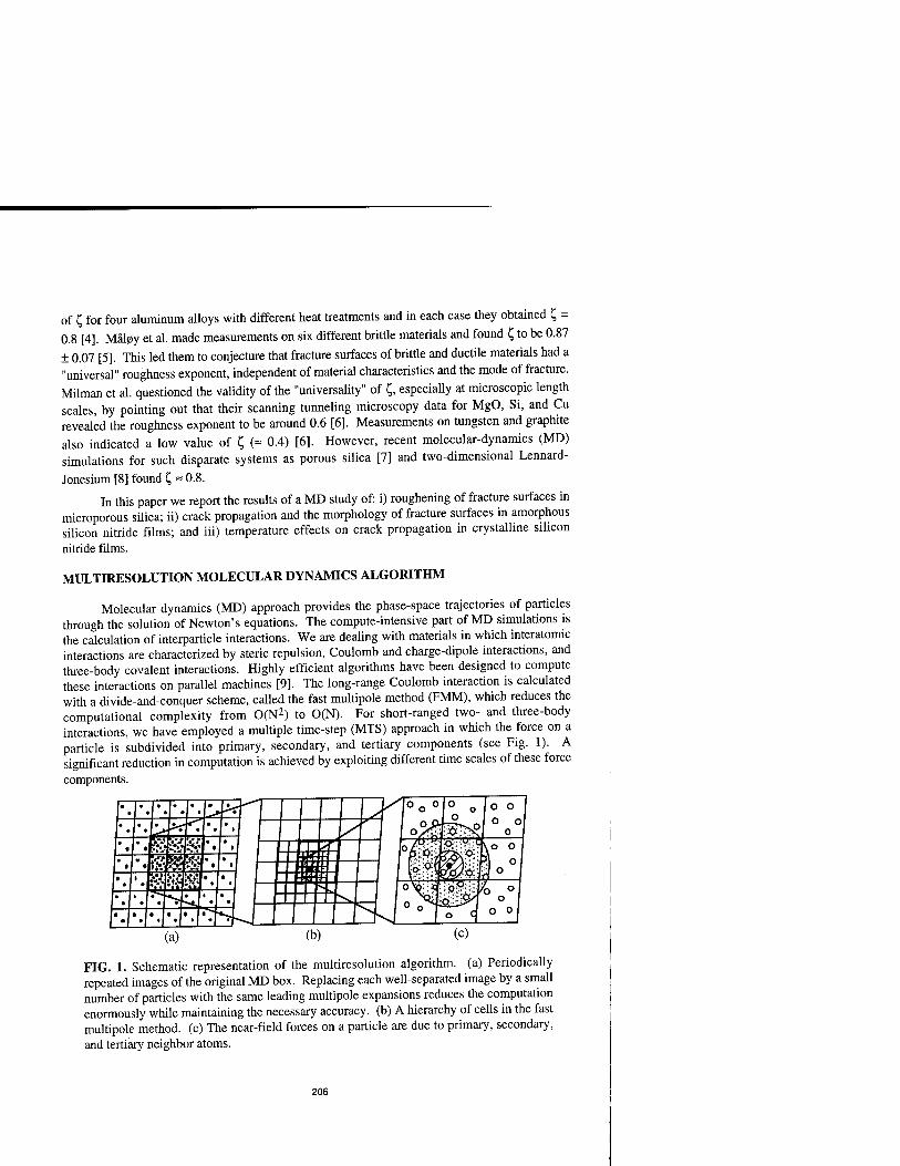
of C, for four aluminum alloys with different heat treatments and in each case they obtained £ =

0.8 [4]. Mäl0y et al. made measurements on six different brittle materials and found £ to be 0.87

± 0.07 [5]. This led them to conjecture that fracture surfaces of brittle and ductile materials had a "universal" roughness exponent, independent of material characteristics and the mode of fracture. Milman et al. questioned the validity of the "universality" of £, especially at microscopic length scales, by pointing out that their scanning tunneling microscopy data for MgO, Si, and Cu revealed the roughness exponent to be around 0.6 [6]. Measurements on tungsten and graphite also indicated a low value of £ (= 0.4) [6]. However, recent molecular-dynamics (MD) simulations for such disparate systems as porous silica [7] and two-dimensional Lennard-

Jonesium [8] found t, ~ 0.8.

In this paper we report the results of a MD study of: i) roughening of fracture surfaces in microporous silica; ii) crack propagation and the morphology of fracture surfaces in amorphous silicon nitride films; and iii) temperature effects on crack propagation in crystalline silicon

nitride films.

MULTIRESOLUTION MOLECULAR DYNAMICS ALGORITHM

Molecular dynamics (MD) approach provides the phase-space trajectories of particles through the solution of Newton's equations. The compute-intensive part of MD simulations is the calculation of interparticle interactions. We are dealing with materials in which interatomic interactions are characterized by steric repulsion, Coulomb and charge-dipole interactions, and three-body covalent interactions. Highly efficient algorithms have been designed to compute these interactions on parallel machines [9]. The long-range Coulomb interaction is calculated with a divide-and-conquer scheme, called the fast multipole method (FMM), which reduces the computational complexity from 0(N2) to O(N). For short-ranged two- and three-body interactions, we have employed a multiple time-step (MTS) approach in which the force on a particle is subdivided into primary, secondary, and tertiary components (see Fig. 1). A significant reduction in computation is achieved by exploiting different time scales of these force components.

•*** • I» 1

N*.E@eSB$ • 1 • 1 * I • 1

1* 1 * 1*1 * fölgp:! * 1 * 1

•1 'I Iff 11 1*1 * spstör.N I • •

1 • ••M-.M-^f- (a)

FIG. 1. Schematic representation of the multiresolution algorithm, (a) Periodically repeated images of the original MD box. Replacing each well-separated image by a small number of particles with the same leading multipole expansions reduces the computation enormously while maintaining the necessary accuracy, (b) A hierarchy of cells in the fast multipole method, (c) The near-field forces on a particle are due to primary, secondary, and tertiary neighbor atoms.

206

Figure 2 shows the performance of this approach on the Touchstone Delta and the IBM SP1 machine at Argonne National Laboratory. For a 4.2 million particle silica glass, the execution time for a single MD time step is only 4.84 seconds on the 512-node Delta machine. The execution time scales linearly with the size of the system and the computation dominates the communication time.

5

4

a. 2 3

o 2

04-

/ □ Delta total o SP1

communication

103

FIG. 2. Execution time per step for multiresolution MD simulations of amorphous SiÜ2 (solid curves) with 8,232p particles where p is the number of processors. Open squares and open circles are the results on the Delta and SP1, respectively. Dashed curves denote the communication overhead.

FRACTURE OF SILICA GLASS

Structural properties and mechanical failure in porous silica have been investigated with million-particle MD simulations [7]. The results for pore size distribution, internal surface area and surface-to-volume ratio of pores, and fractal dimension are in accordance with structural measurements. We have performed MD calculations on 1.12-million particle amorphous silica systems, investigating the growth of pores with a decrease in the density of the system. As the normal-density glass is uniformly expanded, the pores begin to form when the density of the system is reduced to 1.8 g/cm3. Further decrease in the density of the system causes an increase in the number of pores and also the pores coalesce to form larger entities (see Fig. 3). There is a dramatic increase in the size of pores when the mass density is reduced to the critical value, pc = 1.4 g/cm3. At the critical density, some pores percolate through the entire system causing fracture. In Fig. 4 we show one of the surfaces of the percolating pore.

The roughness of a fracture surface is calculated from the height-height correlation function, G(o), where o is the horizontal distance. The MD results for G(o) are well-described by the relation, G(o) ~ c£ with C, = 0.87 ± 0.02 for a < 10 nm (see Fig. 5). The MD results for the roughness exponent agree with experimental measurements, thus lending further support to experimental claims that the roughness exponent of fracture surfaces is a material-independent quantity. Moreover, the MD results indicate that the universality of the roughness exponent may prevail even at length scales < 10 nm.

207

FIG. 3. Snapshots of two-dimensional slices of MD configurations of silica (1.12 million particles) at densities 1.8 g/cm3 and 1.4 g/cm3. Bright and dark pixels represent pores and silica, respectively.

FIG. 4. Snapshot of a fracture surface resulting from a percolating pore in silica glass at; mass density of 1.4 g/cm3.

208

S 1.2

FIG. 5. Height-height correlation function (open circles) versus the in-plane distance, o",

for the fracture surface shown in Fig. 4. The solid line is the best fit, G(ü) - 0^ with C, =

0.87+ 0.02 for CT< 10 nm.

CRACK PROPAGATION IN AMORPHOUS SILICON NITRIDE FILMS

Molecular-dynamics study of fracture in amorphous SJ3N4 films [10] involved systems with 100,352 atoms (typical dimensions of a film were 220Ä x 220Ä x 20Ä), interacting via a combination of two- and three-body potentials. The two-body potential includes steric repulsion, the effect of charge-transfer via Coulomb interaction, and the large electronic polarizability of anions through the charge-dipole interaction [11]. Three-body interactions with bond-bending and bond-stretching terms were introduced to include covalent effects [11].

To evaluate the quality of the interaction scheme, various structural and dynamical correlations and elastic constants in the bulk Si3N4 were computed and the results were compared with available experimental measurements [10, 11]. In the crystalline state, the MD results for interparticle separations (Si-Si, Si-N, and N-N) and bond angle distributions (N-Si-N and Si-N-Si) are in excellent agreement with experiments. Not only that, the MD static structure factor for the glass agrees well with neutron-scattering measurements over the entire range of wave vectors. The specific heat of crystalline cc-Si3N4, obtained from the phonon density-of- states, is also in excellent agreement with experimental measurements over a wide range of temperatures. The MD results for various elastic modulii are also in reasonable agreement with experimental values [12, 13], see Table I.

We first prepared well-thermalized bulk system by quenching the molten state and then periodic boundary conditions were removed and the systems were relaxed with MD and conjugate-gradient methods. These well-thermalized crystalline and amorphous Si3N4 films were subjected to uniaxial tensile loads by displacing atoms uniformly in the leftmost and rightmost layers (thickness ~ 5.5Ä each) along the x direction. The strain was applied at a constant rate while maintaining the temperature at 300 K.

To investigate crack propagation, we insert a crack in an uniaxially stretched film (strain ~ 4 %) by removing particles within a region whose projection onto the xy plane is 4 Ä x 50 Ä,

209

and we use a strain rate of 0.01 ps'1. The crack plane is parallel to the yz plane, and the crack propagates along the y direction.

MD (GPa) Experiment (GPa)

ßv-l 287 282*

ßa-l 824 847a

ßc-l 943 870a

E (5°) 419 456b

E (64.2°) 375 378b

E(83.1°) 386 488b

TABLE I. Elastic modulii of a-Si3N4. The MD results for the hydrostatic bulk

modulus, ßv"1, the inverse linear compressibilities parallel to the a and c axes, ßa"' and

ßc"1, the elastic modulii along the directions with angles 5°, 64.2°, and 83.1° from the c axis, are compared with experiments: aRef. 12; bRef. 13.

Figure 6 shows snapshots of the amorphous Si3N4 film projected onto the xy plane. Initially the crack propagates straight along the y direction, as shown in Fig. 6 (a), for the first 4.5 ps. At 7.9 ps, we observe the formation of voids in front of the crack tip, see Fig. 6 (b). These voids grow and form a secondary crack at t = 10.8 ps, see Fig. 6 (c). Eventually the secondary crack and the initial crack coalesce and the resulting crack surface is very rough, as evident from the snapshot in Fig. 6 (d) at t = 16.4 ps.

We have calculated the height-height correlation function [10],

g(y) = ([h(y+y0)-h(y0)]2)1/2,

of the crack surface using the height profile, h(y). In the equation, the bracket denotes the average over yo- For a self-affine surface, the height-height correlation function is expected to obey the scaling relation, g(y) ~ y? [3-7].

Figure 7 shows a log-log plot of the height-height correlation function for the crack surface in the amorphous film. There are two well-delineated regimes in this figure. For smaller length scales, we observe a rather smooth crack surface with a smaller roughness exponent. By linear fitting, we obtain a roughness exponent of 0.44 ± 0.02 for y < % = 25 Ä. Beyond this

crossover length, \, the surface is rougher with a larger exponent, ^ = 0.82 ± 0.02.

210

1(a)

Wfyi' W?-m

■;*Vt' 1 *.<*.'-:' ".:• *-';

(c)

' £t' :->••• 1 (b)!i

'-'»' ■'/!*r^'i' »"■■V'*' ■;' *

£ft

1 '<*■■ I

-"''■-* s*/;C v«..?"';

ÜB *>''-■ ■;.;.■ 1 .,■„';:., W";

:i *■" ̂ fjf^Sff^^i^H

200 A

FIG. 6. Snapshots of crack propagation in an amorphous Si3N4 film at time (a) 4.5 ps, (b) 7.9 ps, (c) 10.8 ps, and (d) 16.4 ps.

4

3.5

3

S 2-5

£ 2

1.5 -

1 -

0.5

~1 ' ' a = 0.82 i 0.02 f

-1 0 1

FIG. 7. Log-log plot of the height-height correlation function, g(y) (open circles). The solid curves represent the best fit, g(y) ~ y£, with C, = 0.44 ± 0.02 for y < \ = 25 Ä, and t,

= 0.82+ 0.02 for y>t

211

To relate the morphology of the crack surface to the crack dynamics [14], we show in Fig. 8 the crack tip position as a function of time. Initially the crack propagates slowly and continuously. At 12 ps the crack tip jumps suddenly as the initial and secondary cracks coalesce. The distances between this and each of the subsequent jumps are between 20 and 40 Ä, which are close to the crossover length of the height-height correlation function. We thus conclude that the smaller roughness exponent (£ = 0.44) corresponds to slow crack propagation inside

microcracks, and the larger exponent (£ = 0.82) corresponds to the inter-microcrack propagation associated with the coalescence of microcracks. The average propagation speed in the second regime (1630 m/s) is much larger than in the first regime (640 m/s).

The crossover from quasi-static to rapid fracture was also observed in recent experiments by Bouchaud and Naveos [15]. For titanium aluminum alloys, they observed a crossover of the roughness exponent from 0.45 to 0.84. They also found that the crossover length scale decreases when the local stress intensity factor, or correlatively, the crack velocity increases.

This crossover phenomenon is consistent with a model in which a fracture surface is considered the trace of a line propagating in a random medium [15,16]. The model predicts the roughness exponent to be 0.75 for high-velocity and 0.5 for low-velocity fracture surfaces [17].

200

s £ 150 • PN

o o. .& Siooh a I« u

50

">—r

640 m/sec

1630 m/sec

i*j*TT 10 12

t(ps) 14 J i_

16

FIG. 8. Crack tip position as a function of time (solid curves) in an amorphous Si3N4 film. Linear fits (dashed lines) before and after 12 ps give the average crack tip velocities of 640 m/s and 1630 m/s, respectively.

CRACK PROPAGATION IN CRYSTALLINE SILICON NITRIDE FILMS

Understanding why some materials are intrinsically brittle, and others are intrinsically ductile is one of the central problems in materials science [18,19]. It is also important to understand the effect of temperature on the brittleness of materials. The brittle-to-ductile transition is exhibited by almost all materials. The change in the fracture behavior from brittle cleavage to ductile failure occurs usually in a narrow range of temperature accompanied by a dramatic increase in the fracture toughness [20].

212

Nucleation and growth of tensile cracks at finite temperatures have been studied in the framework of statistical mechanics [21-23]. Solid under stress is treated as a metastable state, and fracture at a failure threshold corresponds to a metastability limit, or spinodal [22]. Crack near spinodal is a fractal object describable as a percolation cluster; a Griffith-like classical crack [24] is surrounded by a fractal halo of micro voids [21]. Such a nonclassical crack extends through the growth and absorption of voids in front of the crack tip. Recently, the Griffith criterion [24] has been extended to account for the propagation of a self-affine crack [25].

Molecular-dynamics study of fracture in a-crystal Si3N4 films involved systems with

100,352 atoms (typical dimensions of a film were 220Ä x 220Ä x 20Ä) at temperatures 300 K and 1,500 K. The film surface is (001) and uniaxial strain is applied in the [210] direction. Cracks propagate in the [010] direction. We insert a crack in an uniaxially stretched film (strain - 4 %) by removing particles within a region whose projection onto the xy plane is 4 Ä x 50 Ä. With this strain condition, the crack starts to propagate without further stretching.

Figure 9 shows snapshots of the a-Si3N4 films at temperatures 300 K and 1,500 K, projected onto the (001) plane. At 300 K, the crack propagates straight in a cleavage manner as shown in Fig. 9 (a). At 1,500 K, the crack initially propagates slowly but eventually it stops, see Fig. 9 (b).

200 A

3« yc vS^vf ;p<i

*?S#i

FIG. 9. Snapshots of crack propagation in a-Si3N4 film at temperatures (a) 300 K and (b) 1,500 K.

Figure 10 shows the crack tip position as a function of time at the two different temperatures. At 300 K, the crack accelerates continuously to 3,110 m/sec. The Rayleigh wave velocity [24] of a-Si3N4 is estimated to be 6,400 m/sec. At 1,500 K, the crack propagates at 940 m/sec before 6 ps, but then the propagation stops.

This difference in crack propagation is a direct consequence of the different atomic structures in front of the crack tip. Figure 11 shows atomic structures at crack tips at the two different temperatures. At 300 K, the crack tip is atomically sharp as shown in Fig. 11 (a). This structure supports the fast, cleavage-like propagation. At 1,500 K, we observe a sequence of

213

microvoids in front of the crack tip. The periodicity of these microvoids is that of the hexagonal symmetry of the (001) surface. At high temperatures, crack propagates through formation and absorption of microvoids. The resulting propagation is slow, and sometimes it cannot be sustained.

200

150- o

g, 100-

% 5°l- !- U

i—i—i—i—i—r

T = 300 K 3110 m/sec

i _L

T = 1,500 K 940 m/sec - I L_

3 4 5 t (ps)

8

FIG. 10. Crack tip position as a function of time (solid curves) in cc-Si3N4 film at temperatures 300 K and 1,500 K. Linear fits (solid lines) give the average crack tip velocities of 3,110 m/s and 940 m/s, respectively.

FIG. 11. Atomic structures at crack tips in oc-Si3N4 films at temperatures (a) 300 K and (b) 1,500 K.

214

CONCLUSIONS

We have simulated fracture in ceramic materials using multiresolution molecular dynamics approach on parallel computers. In microporous silica, critical behavior at fracture is analyzed in terms of pore percolation and kinetic roughening of fracture surfaces. In amorphous Si3N4 films, correlation between the speed of crack propagation and the morphology of fracture surfaces has been observed. In crystalline Si3N4 films, temperature-assisted void formation in front of a crack tip has been shown to slow down crack propagation.

ACKNOWLEDGMENTS

This work was supported by the U.S. Department of Energy, Grant No. DE-FG05-92ER45477, National Science Foundation, Grant No. DMR-9412965, Air Force Office of Scientific Research, Grant No. F 49620-94-1-0444, and USC-LSU Multidisciplinary University Research Initiative, Grant No. F 49620-95-1-0452. A part of these simulations were performed on the 128-node IBM SP computer at Argonne National Laboratory. The computations were also performed on parallel machines in the Concurrent Computing Laboratory for Materials Simulations (CCLMS) at Louisiana State University. The facilities in the CCLMS were acquired with the Equipment Enhancement Grants awarded by the Louisiana Board of Regents through Louisiana Education Quality Support Fund (LEQSF).

REFERENCES

1. J. Fricke, J. Non-Cryst. Solids 121,188 (1990). 2. J. Mukerji, in Chemistry of Advanced Materials, ed. C. N. R. Rao, Blackwell (Oxford,

1993). 3. B. B. Mandelbrot, D. E. Passoja, and A. J. Paullay, Nature 308,721 (1984). 4. E. Bouchaud, G. Lapasset, and J. Planes, Europhys. Lett. 13,73 (1990).

5. K. J. Mal0y, A. Hansen, E. L. Hinrichsen, and S. Roux, Phys. Rev. Lett. 68, 213 (1992); ibid. 71,205 (1993).

6. V. Y. Milman, R. Blumenfeld, N. A. Stelmashenko, and R. C. Ball, Phys. Rev. Lett. 71, 204 (1993).

7. A. Nakano, R. K. Kalia, and P. Vashishta, Phys. Rev. Lett 73, 2336 (1994). 8. F. F. Abraham, D. Brodbeck, R. A. Rafey, and W. E. Rudge, Phys. Rev. Lett. 73, 272

(1994). 9. R. K. Kalia, S. W. de Leeuw, A. Nakano, D. L. Greenwell, and P. Vashishta, Comput.

Phys. Commun. 74, 316 (1993); A. Nakano, P. Vashishta, and R. K. Kalia, ibid. 77, 302 (1993); A. Nakano, R. K. Kalia, and P. Vashishta, ibid. 83,197 (1994).

10. A. Nakano, R. K. Kalia, and P. Vashishta, Phys. Rev. Lett 75, 3138 (1995).

11. P. Vashishta, R. K. Kalia, and I. Ebbsjö, Phys. Rev. Lett. 75, 858 (1995); C.-K. Loong, P. Vashishta, R. K. Kalia, and I. Ebbsjö, Europhys. Lett 31, 201 (1995).

12. L. Cartz and J. D. Jorgensen, J. Appl. Phys. 52,236 (1981). 13. A. A. Mukaseev, V. N. Gribkov, B. V. Shchetanov, A. S. Isaikin, and V. A. Silaev,

Poroshk. Metall. 12,97 (1972).

215

14. J. Fineberg, S. P. Gross, M. Marder, and H. L. Swinney, Phys. Rev. Lett. 67, 457 (1991).

15. E. Bouchaud and S. Navels, J. Phys. I (France) 5, 547 (1995). 16. J.-P. Bouchard, E. Bouchard, G. Lapasset, and J. Planes, Phys. Rev. Lett. 71, 2240 (1993)

17. D. Etras and M. Karder, Phys. Rev. Lett. 69, 889 (1992).

18. J. R. Rice and R. Thomson, Philos. Mag. 29,73 (1974).

19. S. J. Zhou, A. E. Carlsson, and R. Thomson, Phys. Rev. Lett. 72, 852 (1994).

20. M. Khantha, D. P. Pope, and V. Vitek, Phys. Rev. Lett. 73, 684 (1994).

21. J. B. Rundle and W. Klein, Phys. Rev. Lett. 63, 171 (1989). 22. R. L. B. Selinger, Z.-G. Wang, W. M. Gelbart, and A. Ben-Shaul, Phys. Rev. A 43, 4396

(1991). 23. L. Golubovic and S. Feng, Phys. Rev. A 43, 5223 (1991). 24. B. Lawn, Fracture of Brittle Solids (Cambridge University Press, Cambridge, 1993).

25. E. Bouchaud and J.-P. Bouchaud, Phys. Rev. B 50, 17752 (1994).

216

REPRESENTATION OF FINITE CRACKS BY DISLOCATION PILEUPS : AN APPLICATION TO ATOMIC SIMULATION OF FRACTURE

Vijay Shastry and Diana Farkas Department of Materials Science and Engineering, Virginia Tech., Blacksburg VA 24061.

ABSTRACT

The elastic displacement field solution of a semi-infinite crack in an anisotropic body, calculated using a complex variable approach due to Sih and Liebowitz, is usually used by atomistic simulations of fracture. The corresponding expression for the displacement field of a finite crack is numerically cumbersome since it involves multiple square roots of complex numbers. In this study, displacement field of the crack is calculated by superposing the displacements of dislocations in an equivalent double pileup, equilibrated under mode I conditions. An advantage of this method is its extensibility to atomistic studies of more complex systems containing multiple cracks or interfaces. The pileup representation of the finite crack is demonstrated as being equivalent to its corresponding continuum description using the example of a double ended crack in a-Fe, loaded in mode I. In these examples, the interatomic interaction in a-Fe is described by an empirical embedded atom (EAM) potential.

Introduction

Molecular statics, atomistic simulations of fracture require the initial displacements of atoms in the simulation cell before relaxing the atomic configuration in accordance with interatomic force laws. This elastic field is also used to obtain atomic positions in the outer boundary region, far from the crack tip. Traditionally, these simulations [1, 2, 3] have used a specific crack geometry in which a single ended crack is embedded in an anisotropic material. The initial displacements of atoms are approximated by that prescribed by the elastic displacement field of a semi-infinite crack in the anisotropic body. Equivalently, one can also use a finite double ended crack geometry to study the fracture processes at the two tips provided the appropriate elastic solution for the displacement field is used. The displacement field of a mode I double ended crack can be obtained using a complex variable approach by Sih and Liebowitz [4]. The numerical implementation of this solution is cumbersome, because of the multiplicity of roots involved in the expressions for displacements.

The elastic displacement field is obtained more conveniently, in certain special cases, by determining the displacement field due to a double pileup of opening Volterra dislocations equilibrated by external loading. The pileup displacement field is obtained by the simple superposition of displacements of these dislocations. The algebraic expressions for the displacements of dislocations located in cubic materials are simple, if the fine and Burgers vectors lie along directions of even- fold symmetry [5]. This method can also be used to construct the displacement field of cracks with bonds linking the faces. Further, the method can be extended to study systems containing multiple cracks and cracks in inhomogeneous materials.

The next section discusses how the dislocation distribution in the equivalent pileup, loaded under mode I and pinned at two ends, is obtained. A simple comparison between the displacement fields predicted by the Sih formalism and the pileup method is shown. Next, the effect of bonding

217


between the crack faces on the dislocation distribution in the pileup is discussed for cases where the external loading is at least as high as the Griffith value for a crack with traction free faces. This study of bonding effects is useful in verifying the accuracy of traction free boundary conditions when the crack is found to be stable above the Griffith loading. The atomic arrangement, which uses the pileup displacement field, is shown for a crack in a-Fe modeled using the Simonelli EAM potential [6].

The elastic displacement field of the double pileup

The complex variable formulae suggested by Sih and Liebowitz [4] can be used to calculate the displacement field of the double ended crack and they are

-ext

U

S2

^- \s2Pl{jzi - (e/2y - Zl) - sm{\j4 - (m? - *2)}

-^- {«a?i(^?-(</2)» - zr) - sM\l4 - W2)2 - *2)}

(1)

(2)

Here zx = x + siy and z2 = x + s2y. Here, «i, s2 pi, p2, 9i, and q2 are constants which depend upon the elastic compliances and are not reproduced here for brevity, i/2 is the half length of the double ended crack and aext is the externally applied stress.

In this work, the 2D displacement field of a finite mode I crack is calculated by linearly superposing the displacement fields of model opening Volterra dislocations in an equivalent double pileup pinned at the two tips. The displacement fields of individual Volterra dislocations are obtained from the sextic theory of Stroh described by Hirth and Lothe [5]. The crack plane is located midway between two adjacent atomic planes which are then displaced symmetrically in opposite directions, by amounts prescribed by the opening profile of pileup. This method of constructing the crack preserves the bonds that link atoms located on either side of the crack plane. Therefore, bonding tractions are present on the crack faces along the entire length of the crack.

The crack is represented as a region stretching from -lj2 < x < £/2, which obeys a non-linear constitutive law, and is bounded on both sides by elastic half spaces. The discrete dislocation representation of the loaded crack implies that the continuity of normal tractions is evaluated at selected points along the crack. The condition for continuity of normal tensile tractions is

*) = ^r^Tr^*-*•<■>• (3) 2ir(l - u) J-e/2 (x - t)

= 0 {-(.12 <x< £/2). (4)

The shear components of tractions are zero along the plane of a mode I crack. <j>(x) = d[Auy(x)]/dx is the dislocation distribution function, where Aiij(i) is the crack opening at location x. ii"1! is the effective shear modulus for the cleavage plane. When the coordinate axes fixed on a crack embedded in a cubic material, lie parallel to directions with even-fold symmetry, p"ff is phrased in terms of elastic constants (C;J),

„«" = Cn — Ci:

(C22/Cn)1/4Cn C22 + C\\

Cu

1/2- C\\Csi

Cu - C\2 + 2C?66(Cii - C12)

1/2

(5)

Here, C;J are transformed to the coordinate system fixed on the crack. The coordinate system has basis vector y oriented along the normal to the crack plane, whereas z contains the crack front and

218

x = y x i. Cii = [C11C12]1'2. In the example considered here, the untransformed elastic constants corresponding to the Simonelli potential [6] for a-Fe aie Cu = 1.51et>/A3, C12 = Q.91ev/Ä3 and C44 = 0.7ev/A3.

a*(x), the resistive stress due to bonding, depends upon the total opening at x. One functional form of u*(x), suggested by Beltz and Rice [7] is

ff«*(a) = 22!^)e-A«.M/*, (6) Li LI

where 7, is the surface energy of the cleavage plane, L, the Fermi-Rose decohesion length. For the Simonelli potential based on a-Fe, the {011} plane has constitutive properties 7S = 0.09ev/A2

and L = 0.33A.

Eqn. (4) is solved using a method developed by Erdogan and Gupta [8] at discrete points, Xi = 1/2 cos(iri/N), for <j>(x). Here, (j>(x) is assumed to be singular at the pinning points x = ±1/2. The total number of discrete points, JV = 160, here. The Burgers vectors of dislocations located at Xi, are obtained by integrating <j>(x) over a length interval assigned to a>;.

Figure 1 compares the displacements due to a traction free crack, predicted by the Sih and Liebowitz and the pileup methods, for atoms located on the atomic plane y = 2.Q72A which forms the upper crack face. The crack lies on the (Oil) plane at y = 1.014A and the crack front is parallel to [100]. The two approaches predict identical values of displacement due to the crack tip for each of the atoms shown. The crack has half length 1/2 = 22.3A and is embedded in an iron crystal, which is described by the Simonelli potential. The external loading on the crack is aext = 0.07eu/A3. The Griffith value of external stress for this case is 0.058ei>/A3. When the atomic ensemble was allowed to relax using molecular statics scheme [9], the critical loading for cleavage was observed to lie between 0.06 — 0.07eu/A3.

Effect of bonding on the dislocation distribution

Figure 2 shows the relative opening between crack faces for different values of acxt for two types of cracks in iron. In one case, bonding exists between crack faces whereas the other crack is traction free. The crack front lies along [100] and the crack plane is (OlT).^(t) for a "traction free" crack is obtained by setting a* to zero in Eqn. (4). Here, /xe// = 0.65ev/A3 and 1/1 = 22.3A. The opening profiles are drawn only for one half of the crack and are symmetric about its center. When aext > 0.07et)/A3, the opening profiles for the cracks with and without bonding are very similar. At high levels of remote loading, the region immediately behind the tip, where bonding tractions are largest, is small. Here, bonding tractions are large since the opening is comparable to L (decohesion length). The opening increases with further distance away from the tip and the effect of bonding tractions diminishes rapidly. However, when aext is lowered, the opening increases less rapidly with distance from away the tip and the effect of bonds on the opening profile is more pronounced. The effect of bonding on the opening between crack faces and therefore, the dislocation distribution in the pileup is found to be small.

Figure 3 illustrates the variation of bonding tractions with distance from the pinning point, x = +i/2. The maximum in bonding tractions occurs when Auy = L and its location is taken to be the position of the real crack tip. As <jtxt is lowered, the crack tip retreats under the influence of bonding. When this retreat is large, i.e. greater than 0.6A here, the singularities at the pinning points are lost. Then, solutions for <f>(x), singular at the two pinning points, cannot be found.

Finally, Fig. 4 shows the initial atomic arrangement around a crack in a-Fe at a€xt = 0.07ev/A3.

219

c 0) E CD O

JÖ Q. CO Q

-0.4 0 40 80 120 160

Distance from the crack center (°A)

(a) Ux in Ä along the plane y = 2.072

CD CJ « a. en

160

Distance from the crack center (°A)

(b) uy in Ä along the plane y = 2.072

Figure 1: Displacements ux and uy along the atomic plane y = 2.072Ä. The solid lines are the displacement values predicted by the Sih and Liebowitz formula whereas the D symbols denote the displacements of individual atoms predicted by the pileup method. The crack is located along the atomic plane y = 1.014Ä.

220

Bonds o - 0.063 No bonds o = 0.063

Bonds a = 0.07 No bonds a = 0.07

Bonds a - 0.08 onds o = 0.08

5 10 15 20

Distance from the crack center, x (A°)

Figure 2: Symbols +, x and * represent relative opening between crack faces when bonding tractions are present, for three values of <jext = 0.063, 0.07, 0.08eu/A3. The dashed lines represent the corresponding profiles for the traction free crack.

0.24

20 21 22 23 24

Distance from crack center, x (Ac)

Figure 3: Variation of constitutive stress, a*, with distance from the positive crack tip when bonding is present between the crack faces. For brevity, the variation is shown only for the region immediately behind the tip. Stress u in ev/A3.

221

r——i 10 v T—

O, 5 D) C o CO

0 o < *-—" 0) Ü -b

-10

o o '

o o

oooooooo

*y.

X

GGooGOO°°

000000°

Gooooooo°

o o

, o °

-30 -20 -10 0 10 20 30

Distance (A0) along [0,-1,-1]

Figure 4: Initial (unrelaxed) Atomic arrangement around a [100](0lT) crack in a-Fe.

Acknowledgments

The authors gratefully acknowledge support for this work by the Office of Naval Research (ONR). We are grateful to Prof. Peter Anderson for his helpful input on the displacement fields of finite cracks.

REFERENCES

1. K. S. Cheung and S. Yip, Modelling Simul. Mater. Sei. Eng. 2, 865 (1994). 2. R. G. Hoagland, M. S. Daw, S. M. Foiles, and M. I. Baskes, J. Mater. Res. 5, 313 (1990). 3. C. S. Becquart, P. C. Clapp, and J. A. Rifkin, Molecular dynamics simulations of fracture in

RuAl, in Mat. Res. Soc. Symp. Proc, volume 288, pages 519-524, Materials Research Society,

1993. 4. G. C. Sih and H. Liebowitz, Mathematical theories of brittle fracture, in Fracture - An Advanced

Treatise, edited by H. Liebowitz, volume II, pages 69-189, Academic Press, New York, 1968. 5. J. P. Hirth and J. Lothe, Theory of Dislocations, John Wiley and Sons, 1982. 6. G. Simonelli, R. Pasianot, and E. J. Savino, Embedded-atom-method interatomic potentials

for bec-iron, in Mat. Res. Soc. Symp. Proc, volume 291, pages 567-572, Materials Research Society, 1993.

7. G. E. Beltz and J. R. Rice, Dislocation nucleation versus cleavage decohesion at crack tips, in Modeling the deformation of Crystalline Solids, edited by T. C. Lowe, A. D. Rollet, P. S. Follansbee, and G. S. Daehn, pages 457-480, Warrendale, PA, 1991.

8. F. Erdogan and G. D. Gupta, Q. Appl. Math. 29, 525 (1972). 9. V. Shastry and D. Farkas, Manuscript in preparation .

222

MECHANISM OF THERMALLY ASSISTED CREEP CRACK GROWTH

LEONARDO GOLUBOVIC and DOREL MOLDOVAN Department of Physics, West Virginia University, Morgantown, WV 26506

ABSTRACT

We use atomistic Monte-Carlo simulations to investigate the dynamics of cracks which sizes are smaller than the Griffith length. We demonstrate that such cracks can irreversibly grow proviso their size is larger than a certain critical length which is smaller than the Griffith length, as recently suggested [ L. Golubovic and A. Peredera, Phys. Rev. E51, 2799 (1995)]. We show here that this thermally assisted creep crack growth is dominated by irreversible changes in the region of the crack tip, primarily in the form of dislocation emissions and nucleation of microcavities and voids. These processes act together during the crack growth: the crack tip region acts as a source for emissions of dislocations which subsequently serve as seeds for creation of vacancy clusters in a region away but still close to the crack tip. Eventually, passages between these vacancy clusters and the mother crack are formed and the crack thus increases in size. As this process repeats, the crack grows.

INTRODUCTION

Stressed solids can be treated as a metastable state of matter analogous to, say, supercooled liquids [l]-[6]. The failure treshold corresponds to a metastability limit, or spinodal point, at which the external stress a as a function of the strain reaches its maximum, <7mal [2]-[4]. If the external tensile stress is smaller than crmal, a stressed sample will still break, however, with a time-delayed fracture. The sample lifetime depends on the temperature and the applied stress [7]. This phenomenon is believed to be directly related to the processes of microcrack nucleation and growth [2]-[6]. Microcrack nucleation is phenomenologically similar to that of the stable phase droplets in a metastable state [8]. The seminal work of Griffith on fracture mechanics [9], already contains all the elements to construct a phenomenological theory of microcrack nucleation. The critical, Griffith crack behaves like a critical droplet: Cracks larger than the Griffith crack grow irreversibly in a rapid fashion [10]. On the other hand, the growth of cracks which are smaller than the Griffth crack size is energetically disfavored. It is believed, however, that their size can still change in time, however, in a slow fashion via an activational dynamics [4]-[6]. Nature of this thermally assisted creep crack growth remains unclear, in spite of its practical significance [7].

Here we use atomistic Monte-Carlo simulations to investigate the dynamics of cracks which sizes are smaller than the Griffith length. We demonstrate that such cracks can irreversibly grow proviso their size is larger than a certain critical length which is smaller than the Griffith length, as recently suggested [5] [6]. We show here that this thermally assisted creep crack growth is dominated by irreversible changes in the region of the crack tip, primarily in the form of dislocation emissions and nucleation of microcavities. These two tipes of processes act together to produce the crack growth: the crack tip region acts as a source for emissions of dislocations which subsequently serve as seeds for

223


creation of vacancy clusters ( microcavities) in a region away but still close to the crack tip. Eventually, passages between these mirocavities and the mother crack are formed and the crack thus increases in size. As this process repeats, the crack grows.

THEORIES OF FRACTURE NUCLEATION

We begin by reviewing first the conventional theory of fracture nucleation inspired by the pioneering work of Griffith. [9] In this picture microcracks play a role analogous to that of the stable phase droplets in a metastable state. Griffith established a criterion for crack growth by estimating the energy cost of creating a brittle crack of length L in a solid under a uniaxial stress c perpendicular to the crack. Creation of the crack, for example, in a two-dimensional solid, costs an energy of the order

E(L) = gL - fgl. (1)

The first term in (1) is the energy cost of creating crack's edges by breaking atomic bonds. Thus ga, with a the atomic size, is of the order of a bond energy. After crack creation, its edges will separate, with maximal opening displacement of the order d = uL/Y, where Y is the Young modulus. The crack opening relaxes the stress in a domain of size L2 and lowers the elastic energy of the stressed solid by an amount of the order L2o/2Y. This yields the second term in (1), which, in contrast to the first one, energetically favors crack growth. Crack energy (1) reaches its maximum at L equal to the critical Griffith length Lg = gY/a2, corresponding to the energy (1) of the order Eg = E(Lg) = g2Y/a2. The crack state with L = Lg is unstable: For L > Lg, the crack growth decreases E(L). This leads to the well-known irreversible, very rapid crack growth [10]. For L < Lg, an increase of L costs a positive amount of energy (1). This hinders the crack growth for L < Lg. This picture resembles that of standard nucleation phenomena [8], with Eg playing the role of the nucleation energy barrier Et,. The nucleation rate Rm - or the time t/v needed for the fracture to be nucleated by thermal fluctuations - can be, in general, estimated by the Arrhenius law RN = 1/tx ~ exp(—Eb/kBT).[8} Within the conventional fracture nucleation picture Ei is identified with Eg. Thus Eb = Eg = g2Yja2.

This conventional theory was criticized by Golubovic and Feng (GF) [5]. They consider surface processes such as surface diffusion [11], which restructure crack edges and may inhibit healing of microcracks shorter than the Griffith length L = Lg. These processes become active as soon as the crack opening displacement d becomes larger than the atomic size a. This happens for L > £m;n with Lmi„ = aY/a, or, as g » aY, Lmin = g/c- By considering surface processes inhibiting crack healing, GF argued that the effective energy barrier for the fracture nucleation is of the order E(Lmi„). Thus, Ei = E(Lmi„) = gLmin = g2/a, in the phenomenological theory of fracture nucleation proposed in GF. As Eg/E(Lmin) fa Lg/Lmin » Y/c « cmax/a, the nucleation rate predicted by GF is, for weak stresses, a << amax, enormously larger than that of the conventional theory.

More recent Monte-Carlo dynamics simulations of Golubovic and Peredera provided, however, a different prospect on the same problem [6]. They indicate that microcavities ( i.e., clusters of vacant sites) rather than microcracks ( i.e., lines or surfaces of

224

"broken bonds") are major nucleated defects in the delayed fracture regime. Thus, the major kinetic process in the time-delayed fracture is the nucleation of vacancy clusters or microcavities ( possibly having a non-zero Burgers vector), not of critical Griffith-type microcracks. Energetics of a vacancy cluster nucleation is rather different from that of the Griffith crack: Consider, for example, a vacancy cluster in a 2d solid. If R is its linear size, the cluster involves« (R/a)2 vacant sites. Its size-dependent energy is of the form

EVUR) = gR - aR2- (2)

The first term in (2) is, as in Eq. (1), the surface energy contribution(~perimeter~ R in 2d). The second term in (2) is a stress-induced volume contribution(~area~ R2 in 2d) [6][12]. This volume term can be rationalized as follows: Consider a solid under a tensile stress a with no vacancy cluster initially present. As the number of atoms is conserved, the creation of the cluster induces an increase of the sample's linear size preferentially along the direction of the applied stress [6] [12]. This lowers the energy by SE =stressxcluster volume~ crR2 yielding the second term of the equation (2). By Eq. (2), the size of the critical vacancy cluster, maximizing Evac(R), is of the order Rc = g/ir, whereas the energy barrier for the vacancy cluster nucleation is of the order Et = Evac = g2 ja. Interestingly, this energy-barrier scale for fracture nucleation coincides with that proposed by Golubovic and Feng [5], however, from seemingly different arguments. Thus, the microcavity nucleation yields fracture nucleation barriers and corresponding rates identical to those proposed before, in a different manner, by Golubovic and Feng [5]. This agreement is probably not accidental. These authors invoke in their discussion processes which start to restructure microcrack edges as soon as the microcrack size reaches the lengthscale Lmin. This lengthscale coincides with the size of the critical vacancy cluster, Rc. As Rc = Lm;„, one may argue that the processes restructuring microcrack edges would transform a microcrack of the size Lmi„ into a microcavity of the size Rc which then continues to grow irreversibly. In this way one can rationalize the suggestion of GF that a crack with L = Lmin never heals and continues to grow irreversibly. Thus, Lmi„ is the true critical size of defects in solids under weak tensile stresses.

GROWTH OF CRACKS SHORTER THAN THE GRIFFITH SIZE

Whereas the previous works indicate that a crack of the length L in the range Lg > L > Lmin is likely to slowly grow irreversibly due to thermal fluctuations ( seemingly violating Griffith's original ideas), these works say little about the actual nature of this growth. To clarify the nature of this thermally activated ( creep) crack growth we performed atomistic ( off lattice) Monte-Carlo simulations of a 2d Lennard-Jones solid under a tensile stress, similar to recent simulations in Refs. [4] and [6]. Here we simulate behavior of cracks shorter than the Griffith length, L < Lg. In Figures 1 and 2 we give the time evolution of the solid initially containing such a crack. The sample is under an external tensile force along the vertical direction. The time unit used in these figures is one Monte-Carlo Cycle (MCC) [ 1MCC involves updates of all particles' positions via the standard Metropolis algorithm].

Figure 1 is an example from our simulations illustrating creation of microcavities ( vacancy clusters) nucleated from dislocations emitted by the crack tip. These emissions

225

quickly blunt initially sharp crack tips. More importantly, these emissions frequently produce defects having character of dislocation-vacancy pairs - see the first atomic configuration in Fig. 1. This pair dissociates and the free dislocation continues to glide [ see t = 1333]. Eventually, this same dislocation acts as a seed for creation of another vacancy [ see t = 5333], which evolves into a microcavity [ see the left bottom corner at t = 10000]. Meanwhile, the crack tip gets further blunted by the emission of another dislocation [ see t = 10000] which temporarily gets trapped by the nearby vacancy forming a dislocation-vacancy pair close to the crack tip [ see t between 10000 and 12000].

t=1333

W.VAV.V."«

•«••••••■•••••••4 »•••••••••••••••a • ••••• ••••• ••••••••••••••••

••••••• •••••••■ •••••;

•••••••*•••• •*AV ••♦••••*•

t=5333

Sä^«2«*waaw.Taaaa:!

ZR*. •-•.•.••••• ••••••••• •••••ÄMSÄÄf !

t=-10000

t=10500

AVAVAVAVAV..»*""««».»««; A» • • • • • * • * • • •A? • ••

iBr_ ••••••••••••••••••••••••••••• ' WiftÄÄÄ* •.££••••••• •••••• ••••••••

t=12000

t=15000 t=17000

Figure 1: Creation of cavities nucleated from dislocations emitted by the crack tip.

226

Eventually this pair dissociates, and the free dislocation approaches the left bottom corner where the microcavity is waiting for it. Once they had come close to each other, a new microcavity was formed sitting next to the old one [ see t = 15000 and t = 170001 *figure _ depicts the further evolution of this sample [ between 27000 and 34500] We see that the two microcavities from t = 17000 joined into a single one [ see t = 270001. Finally a passage between this cavity and the mother microcrack is nucleated [ see t = 34500] '

t=27000 t=34500

Figure 2 : Nucleation of a passage between two microcavities.

These simulations show that the thermally assisted creep crack growth is a complex combination of three types of processes going on in the region of the crack tip: (i) emissions of dislocations from the crack tip, (ii) these dislocations subsequently serve as seeds for creation of vacancy clusters ( microcavities) in a region close to the crack tip, and (iii) nucleation of passages between these mirocavities and the mother crack. These subsequent processes form a cycle by which the crack grows. This picture suggests a simple kinetic model for he thermally assisted creep growth of the crack length L as a sequence of steps like to that in Figures 1 and 2: During each step the crack tip produces one or few cavities

Ürtür ?T ff/<7u'°C T1 tHe Cnergy E{R) * 9R- Here' "« is local stress » ^e vicinity of the blunt tip with radius« R. Thus, aloc » *(L/Ry", where c is the remote (external) stress. By combining these relations, one finds R(L) * #JL and *,oe/ff * L/Rc, where

V MV Cnt CaVUy Size ( in the absence of the crack) discussed in the previous

section. ^Note a strong dependence of the cavity size R(L) on the crack length L: For

rZr~ p mi" v mm:mal P°ssible size of a crack [5] [6]): R * Rc and aloc » a. For t~v "*?/Y*;a and °t°c « Y « <Tmax- Thus, as the crack size L grows, the size

of the cavities it nucleates decreases, and becomes the atomic size a when L reaches the Griffith length L This growth is step-like. During each step L increases by AI * R(L)

S™vam nUtl'Tu?e interVal At ~ ^9RlkBT). Thus, the average speed of the crack ,(I) = AI/A* behaves as v(L) ~ eXp(-gR{L)/kBT) = exp{-gR}JkBTL).

Gr-ZnS K\ tme SC3le ne6ded fOT a Crack with ^' **W «I I reaA the Gnmth size behaves as

t(L0) exp[ V °

-*m AJminyP

*)• (3)

For J; ~ J f ^ eakmg temPerature- ^ £mm(<0 = R< = g/<r * (<7m«/«r)a. For the smallest possible cracks with L0 = Imjn, the time scale (3) behaves as the microcavity nucleation time [6], whereas for L0 = Lg * (,m.,/,)zJ, the time scale (3) becomes microscopic, t(Lg) ~ exp(Tm/T) -thermal bond breaking time.

227

For a « u-max-, the growth of L is a sequence of many steps (as the one in Figures 1 and 2) with decreasing sizes Ln+i - Ln = R(Ln) = R2

c/Ln, for the n-th step. Thus L\ -L\ = nR2

c. This implies that during the growth of L from the inital L0 to the Griffith size Lg there is a large number of about N = (L2 — L2

0)IR2

C = (<Tmal/<r)2[l — (L„/Lg) ] steps. The time scale (3) is actually dominated by the time it takes to grow from Ln=0

to L„=i, i.e., by the time it takes for the first nucleation event to occur. All subsequent cavity nucleations involve smaller energy barriers gR{Ln) and thus time scales smaller than that in Eq. (1).

To summarize, here we used numerical simulations to reveal a complex nature of the thermally assisted growth of cracks shorter than the Griffith size and suggest a simple kinetic model for this growth.

ACKNOWLEDGMENTS

This work is suported by the NSF/WV EPSCoR program.

REFERENCES

1. K. Nishioka and J. K. Lee, Philos. Mag. A 44, 779 (1981). 2. R. L. B. Selinger, Z.-G. Wang, W. M. Gelbart, and A. Ben-Shaul, Phys. Rev. A 43,

4396 (1991) 3. Z.-G. Wang, U. Landman, R. L. Blumberg Selinger, and W. M. Gelbart, Phys. Rev.

B 44, 378 (1991). 4. R. L. B. Selinger, Z.-G. Wang, and W. M. Gelbart, J. Chem. Phys. 95, 9128 (1991). 5. L. Golubovic and S. Feng, Phys. Rev. A 43, 5223 (1991). 6. L. Golubovic and A. Peredera, Phys. Rev. E 51, 2799 (1995). 7. S. S. Brenner, in Fiber Composite Materials ( American Society for Metals, Metals

Park, OH, 1965), p. 11. 8. E. M. Lifshits and L. P. Pitaevski, Physical Kinetics ( Pergamon, Oxford, 1981), p.

427-431. 9. A. A. Griffith, Philos. Trans. R. Soc. London Ser. A 227, 163 (1920); see also, L. D.

Landau and E. M. Lifshits, Theory of Elasticity, 2nd ed. (Pergamon, Oxford, 1970), pp. 144-149.

10. N. F. Mott, Engineering 165, 16 (1948). 11. C. Herring, J. Appl. Phys. 21, 301 (1950). 12. C. Herring, J. Appl. Phys. 21, 437 (1950); F. R. N. Nabarro, Report of a Conference

on the Strength of Solids ( Phys. Soc, London, 1948), p. 75.

228

Embrittlement of Cracks at Interfaces

Robb Thomson, Emeritus Materials Science and Engineering Laboratory

National Institute of Standards and Technology Gaithersburg, MD, USA 20899

and

A. E. Carlsson Department of Physics Washington University St. Louis, MO 63130

Abstract

This paper presents a synopsis of already published work for cracks on interfaces and new results on the effect of changing the chemistry of the atoms at the interface. Once the appropriate cut-off for the oscillatory singularity in the interface analysis is determined, the physics of the crack is determined in terms of an appropriate driving force for a particular event of interest, and a lattice resistance to the event. Analytic approximations are available for the driving forces, and the lattice resistance is determined on the basis of a block construction for the lattice. We show that for the case where the chemical bonding at the interface is different from that in the matrix, the same ideas are applicable, provided the different chemistry is incorporated correctly in the lattice resistance construction.

1. Introduction

The proposition on which this paper is based is that the crack, whether on an interface or not, is governed by a balance between the elastic driving forces determined by the far field continuum elastic fields, and the lattice resistance exerted in the core of the crack by the nonlinear bonds of the lattice. The template for this idea is the classic Griffith relation which says that the crack is in equilibrium with respect to cleavage when the elastic crack extension force is balanced by the surface tension of the cleavage surface being created at the crack tip by the nonlinear bond breaking. Our thesis is that this idea can be generalized to the case of lattice breakdown by shear at the crack tip when a dislocation is formed. Rice[l] was the first to demonstrate that such a balance was realized in Mode II dislocation emission in which the crack is loaded in pure Mode II, and the dislocation is emitted on the crack plane ahead of the crack. But the principle can also be applied to the case when the dislocation is emitted in a blunting configuration, at an angle to the original crack plane, and the crack is loaded in mixed Modes I and II, and also when the crack is on an interface. Rice and coworkers have discussed the blunting case from the point of view

229


of the "tension shear coupling" which is expected to operate when the crack is loaded in Mode I[2], but Zhou, etal[3] showed that the important effect in blunting emission is the ledge formation at the tip of the blunted crack.

2. Elastic Driving Forces. In three recently published papers[4,5,6], we have shown that the principal difficulty associated with the phase singularity which mixes the modes at the tip of the crack in a logarithmically divergent fashion, can be alleviated by expressing the elastic driving forces for both cleavage and emission in terms of stress intensity factors evaluated at the crack core. That is, an atomic cut-off is introduced for the phase singularity factor in the analysis. We found that the appropriate cut-off distance was simply the range parameter of the force law binding the atoms together. Thus, the core elastic driving force, Q appropriate to either cleavage or emission is given, respectively, by

kj + k),

2V (1)

KII

V where lower case k refers to the core stress intensity factor described earlier, and are related to the load stress intensity factors, K by the relation

k = AV, (2)

where both k and K are complex stress intensity factors, k = ki + ikn, etc. The phase factor, T] is given by

2a r

(3)

2ir '" «2/ii + V2 2TT'" U + 5(fii/fi2), 1 «i^ + Z'i _ J_ln ll(/ii/^) + 5

where r is the radial distance from the crack tip along the cracking plane (which might be a branching plane) for cleavage, or the radial distance along the slip plane for dislocation emission, a is the half length of the parent crack. The elastic constant, fi' is given by

= 2{l-v)w2 (4)

/il + /<2

Subscripts on elastic coefficients refer to a particular sublattice, and (i, K, and v are the standard elastic coefficients for isotropic elasticity. We note that the cleavage driving force is an invariant in the sense that it does not depend on the phase angle, but the emission driving force most certainly does depend on the core phase angle.

The relations for transforming from the parent load stress intensity factors, K to the effective stress intensity factors,k' for an inclined plane are given by the proceedure first

230

proposed by Cotterell and Rice[7], and given for the interface by Rice, Suo and Wang[8], which we repeat below.

k'j = uoe\2nr = AC/E98 4- /C//EM

K = Ki + iKn = |X|e,^-")

rr -

y' -

yll _

COsh7T«

1

cosh ire

1

cosh ixe

1

cosh 7re

og 9 9' sinh((7r - 0)e)cos — + e~

{"~e)( cos -(cos2 - - esinö)

cosh((;r - 0)e)sin — + e-'""9'' sin -(sin2 - + esin0)

29 9, 9 sinh((7r-0)e)sin— + e.-^~e)e sm -(cos2 - -esin0)

og 9 9 cosh((;r - 6)e)cos — + e~("'e)l cos -(sin2 - + esinfl)

(5)

With the equations (5), the elastic driving force can be determined for any of the events, 1) cleavage on the parent plane, 2) nonblunting emission on the parent plane (called Mode II emission above), 3) cleavage on a plane inclined to the parent crack plane, or 4) blunting emission of a dislocation on an inclined plane. The crack may lie on an interface separating two dissimilar elastic media, or it may be in homogeneous material.

3. Lattice Resistance.

The lattice resistance half of the problem is simply

Tic lls (6)

for cleavage (including branching cleavage), according to the Griffith relation. Rice(l) proposed that for emission, the lattice resistance is similarly given by the "unstable stacking fault", which is simply the theoretical shear strength of the lattice expressed as an energy,

/ve — 7u3- (7)

As noted, this shear energy must be augmented when the (blunting) dislocation slip plane is inclined to the parent crack plane.

The construction for this augmented lattice resistance is shown in Fig. 1. In the figure, the bonds are cut on the cleavage plane to the crack tip, and a block of atoms is defined by the cleavage plane and the inclined slip plane. The lattice resistance is computed by shearing the block along the slip plane. For atoms far from the crack tip, the energy changes during shearing are just those computed for the -yus by Rice[l]. However, at the crack tip, as the block is sheared, one atom bond is broken as the crack becomes blunted[3]. In the case of the actual crack, as shear takes place on the slip plane, a continuum distribution

231

of dislocations,/?, moves out of the tip. The lattice resistance is the misfit stress exerted on these dislocations. Thus,

Tlc= oß(x)dx Jo

(8)

= £/■*■' o

where in the second equation, a lattice sum is taken over the bonds crossing the slip plane multiplied by the local dislocation density, 6;. The force, /,, is the bond force component parallel to the slip plane. If the dislocation density is highly localized near the crack tip, then nothing else can be done. However, if the dislocation density is rather evenly spread over a large number of atoms at the tip, then the sum can be broken into a series of terms corresponding to the uniform shear displacement, and an end correction,

R«*/m.I(0)+ / cß(x)dx Ji (9)

= /moi(O) + 7UJ-

/mai(O) is the maximum bond force exerted in the first bond at the crack tip. This form of the lattice resistance must be taken instead of the simple fu, whenever

the dislocation emsision blunts the crack. If the bonds on the cleavage plane are different from those in the matrix, then /mal(0) corresponds to the segregated chemical bond, while the fu, refers to the bonds in the matrix. This construction is made for nearest neighbor pair forces, and when the force law is more general, then Eqn. (8) or (9) must be extended in an obvious manner. It is also obvious how to extend the construction for more physical crystal lattices than the simple hexagonal lattice shown. But the simple generic case illustrated will be used to test the ideas with actual simulations in the 2D hexagonal

lattice.

3. Lattice Simulations.

Our simulations were accomplished with a lattice Green's function technique described in an earlier paper[9], and were made for a homogeneous lattice, for simplicity. That is, the spring constants of the lattice are everywhere equal. Fig. 2 shows the results of a series of simulations in which the matrix bonding was held fixed, and the bonding on the interface was varied. In the figure, the total Q in the parent crack system is plotted on the Ordinate, and fmaz on the absissa. The dashed line represents the critical values for emission. The second line is a plot of twice the bond strength of the cleavage plane bonds as a function of the same fmaz, and is proportional to the Griffith Qc. The emission line lies lower than the Griffith line to the right (emission is stable relative to cleavage), and the two curves lie on top of one another to the left of their intersection. The points to the right correspond to loading the crack in pure Mode I. When the two lines intersect, the crack can still be made to emit rather than cleave by adding Mode II loading, up to that value of Mode II where the lattice is unstable in shear on the cleavage plane, and a dislocation is emitted on the cleavage plane instead of the inclined slip plane. The emission induced by Mode II

232

0 1 Figure 1. Block diagram for computation of lattice resistance. The bonds across the

cleavage plane are cut up to the crack tip, and the block is rigidly sheared in the direction of the arrow along the slip plane. As the shear progresses, the energy changes in the bonds between the numbered atoms is given by Eqn. (8). After some manipulation, this energy can be written approximately as Eqn. (9). The energy changes in the bonds labelled A,B,C correspond to the standard -yu,.

0.03 0.035 0.04 0.045 0.05 0.055 0.06 0.065 0.07 Maximum Force

Figure 2. Simulation results for the hexagonal 2D lattice for fixed force laws in the matrix, and variable force law on the cleavage plane. The absissa is the slip plane component of the maximum force, fmaz, developed in the bond between atoms 1 and 2, and the ordinate is the driving force, Q as measured in the "lab" or parent crack coordinates. The full line corresponds to emission results, and the dashed line is a plot of twice the bond strength of the 12 bond plotted as a function of f,nax-

233

is shown by the portion of the emission line to the left of the intersection with the cleavage

line. Figure 2 shows a remarkable correspondence between the emission condition predicted

by the block construction, and the simulation results. That is, the emission criterion is accurately linear in /max- From the slope of the emission curve, the value of 60 can

determined to be about 0.25 in atomic units. The point where the cleavage and emission lines meet is the crossover of the material

from brittle to ductile behavior. In our simulations, this point is a function of the relative slopes of the two lines, and of their intercepts in the plots. The emission line is found to to have zero intercept, as if the fus contribution in Eqn. (9) were negligible. The cleavage line, however, does have a nonzero intercept, because fmaz is only approximately linear in the bond strength, and for small values of fmaz departs strongly from linearity, going into the origin with zero slope. Thus, the cross over can be derived from the force law, and the

computed value of 60 •

4. Conclusion.

This simple model throws a strong light on the physical mechanisms underlying chemical embrittlement. Although its specific predictions must be followed up further before general criteria for chemical embrittlement can be made; nevertheless, it is clear that the simple intuitive idea that embrittlement is caused by a weakening of the crack plane by chemical segregation is far too simple. A crack plane can certainly be forced by lowering the bonding at the plane, but whether a crack on that plane will cleave or emit a dislocation will be determined by much subtler considerations associated with the details of the (altered) bonding. The results described here for the special case of a homogeneous lattice have also been shown by us to apply to the interface, if the appropriate driving force expressions and core stress intensity factors are factored into the analysis. Finally, it appears that simple ideas associated with the elastic driving force, and a rigid block lattice resistance construction may be useful in determining the ductility in real materials, without actual calculation of the crack structure.

5. Acknowledgement.

A.E.C. gratefully acknowledges support from the Office of Naval Research under Grants

Number N00014-92-J-4049.

234

References 1. J. R. Rice, J. Mech. Phys. Solids 40, 239 (1992). 2. J. R. Rice, G. E. Beltz, and Y. Sun, Topics in Fracture and Fatigue, ed. A. S. Argon, Springer (New York) (1993). 3. S. J. Zhou, A. Carlssou and R. Thomson, Phys. Rev. Lett., 72, 852 (1994). 4. S. J. Zhou and R. Thomson, Phys. RevB, 49B 44 (1994). 5. R. Thomson, Phys. RevB., 52 7124 (1995). 6. R. Thomson, Phys. RevB., 52 in press. 7. B. Cotterell and J. R. Rice, Int. J. Fract., 16 155 (1980). 8. J. R. Rice, Z. Suo and J. -S Wang in Metal-Ceramics Interfaces, edited by M. Ruhle, A. G. Evans, M. F. Ashby, and J. Hirth, Acat Scripta Met. Proc. Series 4 (Pergamon, New Yourk, 1990), p. 269. 9. R. Thomson, S. J. Zhou, A. E. Carlsson, and V. K. Tewary, Phys. Rev. B, 46B, 10613 (1992).

235

EFFECT OF CRACK BLUNTING ON SUBSEQUENT CRACK PROPAGATION

J. SCHI0TZ*, A. E. CARLSSON*, L. M. CANEL*, and ROBB THOMSON" *Department of Physics, Washington University, St. Louis, MO 63130-4899 **National Institute of Standards and Technology, Gaithersburg, MD 20899

ABSTRACT

Theories of toughness of materials depend on an understanding of the characteristic instabilities of the crack tip, and their possible interactions. In this paper we examine the effect of dislocation emission on subsequent cleavage of a crack and on further dislocation emission. The work is an extension of the previously published Lattice Greens Function methodology[l, 2, 3]. We have developed a Cavity Greens Function describing a blunt crack and used it to study the effect of crack blunting under a range of different force laws. As the crack is blunted, we find a small but noticeable increase in the crack loading needed to propagate the crack. This effect may be of importance in materials where a dislocation source near the crack tip in a brittle material causes the crack to absorb anti-shielding dislocations, and thus cause a blunting of the crack. It is obviously also relevant to cracks in more ductile materials where the crack itself may emit dislocations.

INTRODUCTION

When a sharp crack in a material is loaded until it deforms plastically at the crack tip, two fundamentally different modes of deformation can occur. The crack may propagate (possibly leading to cleavage of the specimen), or it may emit a dislocation. In the first case the material is said to be intrinsically brittle, in the second it is intrinsically ductile. Even for single crystals, many other aspects of the microstructure of the material influence the behavior of the material, such as dislocation activity in the material surrounding the crack and shielding of the stress fields by the dislocations present in the vicinity of the crack. In this paper we will however concentrate on the intrinsic behavior of the crack.

The intrinsic behavior of the crack can be predicted by comparing the critical stress intensity factors necessary for cleavage and for dislocation emission. The cleavage is well described by the Griffith criterion[4], but several criteria have been proposed for the dislocation emission. Rice[5] has proposed an emission criterion given by a well- defined solid-state parameter, the unstable stacking fault energy (7„s), characterizing the barrier to displacement along the slip plane. In this model the emission criterion becomes a "balance" between two energies: The surface energy (j3) and the unstable

237


stacking energy. Zhou et al.[2, 6] extended this model to include the energy of the small ledge at the end of the crack, and showed that for most physically realistic force laws this term dominates the energetics, leading to an emission criterion containing both 7s and -fU3 and a ductility criterion that is independent of j3.

These ductility criteria all assume that the crack is sharp at the atomic level. However, emission of a dislocation will change the local geometry of the crack, possibly changing both the emission and cleavage criteria. Furthermore, a crack may absorb a dislocation, coming from sources in the neighborhood of the crack tip. This may also lead to blunting of the crack. In the following we will discuss the effects such blunting may have on the dislocation emission and cleavage of the crack.

METHODOLOGY

Ordinary molecular dynamics (MD) simulations of cracks are very difficult, due to the extremely slow decay of the stress fields (a oc r~lf2). This makes it necessary to use very large systems to minimize the effects of boundary conditions; millions of atoms may be required even for two-dimensional simulations. On the other hand all of the interesting phenomena will be concentrated near the crack tip, and most of the atoms are just propagating the elastic field. This leads to a very inefficient use of computer resources.

Our solution is to model the elastic response of the surrounding media by a Green's function. The atoms are divided in two classes. The atoms near the crack tip interact with each other through a non-linear force law (the non-linear zone), whereas the atoms far from the crack tip interact only through linear forces. This linear zone can then be fully described by a lattice Green's function Gy(r,r'), describing the response of the atom at r to a force acting on the atom at r'. One needs only the Green's function elements involving the nonlinear zone and a defect zone. The Green's function can be calculated in a computationally efficient way. The procedure for calculating the Green's function, and for introducing a defect (a crack in this case) has been discussed by Zhou et al.[l]. The total energy of the system can then be described as the sum of the energy in the elastic far field (calculated from the Green's function) and in the non-linear interactions. In this way the total energy of the system is described as a function of a much reduced number of degrees of freedom (the positions of the 102-103 atoms in the non-linear zone, compared to the 106-107

atoms in the full problem). The problem can then be treated with conventional minimization techniques [3].

We use this method to study the deformation modes of blunt cracks with up to seven atomic layers of blunting, for a range of force laws. Figure la show a typical initial configuration. We have a region in front of the crack where the atoms are allowed to

238

oi%® äV Ä? &» J»% JK*&

&$8$®m$f ätäßks&m •V

»V5JV»V»Vä* a» jg$w J$» &SS2&3& &£///&& /<&¥&¥•<

**£Ä!T» AfXsA ^IXäf Jz

Figure 1: The two deformation modes, (a) shows the configuration before plastic deformation. The crack, three atomic layers thick, extends out of the left of the picture. Only atoms in the non-linear zone are shown, see text, (b) shows the crack propagating by cleavage, (c) shows the crack emitting a dislocation. The dislocation has traveled along the black line. Since it cannot leave the non-linear zone, it has been pinned at the bottom (indicated by the arrow). To make the path of the dislocation visible, the atoms were given two different colors. Prior to emission the atoms were lined up in rows of the same color. Where the dislocation has traveled lines of atoms of different color meet.

move freely, and two spurs are added, alog which dislocations generated at the crack tip can move away from the crack. Since bonds cannot be broken and reformed in the linear zones, dislocations will be unable to leave the non-linear zone.

The inter-atomic interactions in the non-linear zone are described by the ÜBER pair

potential:

F(r) = _fc(r_ro)expfl^-^) (1)

where r is the inter-atomic separation, r0 is the separation in equilibrium, and ß is a range parameter. We cut off the interactions so that only nearest-neighbor interactions are included, and shift the potential slightly to avoid a step in the force law. Further, a small scaling of the force law is used to preserve the elastic constants, thus enabling us to use the same Green's function for all the force laws. The force law thus becomes

F(r) = C -k(r - r-o) exp ( ] - F0 (2)

where F0 = -fc(rcutoff - r0) exp ((rcutoff - r0)/ß) assures that the force is zero at the cutoff distance rcutoff (in this work 1.7r0). This is only a slight perturbation of the force law as the scaling factor C only differs from unity by a few percent. Since this work does not study specific materials, no attempt is made to use realistic many-body potentials.

239

Open symbols: Disl. emission. Filled symbols: Cleavage.

8&BBUR

i Full calculation > Reduced non-linear zone

3.8

3.6

3.4

-n o —i a a>

"or —I cr c 3

3.2 Ä

3.0

Blunting (layers) Blunting (layers)

Figure 2: Left: The force required for cleavage or dislocation emission as a function of the blunting, for seven different force laws. Right: The effect of reducing the non-linear zone at the crack tip. When the atoms shown in black are removed from the non-linear zone (i.e. they are restricted to interact through linear forces), the effect of the blunting is reduced. The range parameter in the force law is ß = 0.25.

RESULTS

When we load the cracks until plastic deformation occur, two different deformation modes are observed: cleavage and dislocation emission, see figure 1. The dislocation emission always occurs in the downwards direction, as shown in the figure, except for the case of a single layer of blunting, where the crack geometry is symmetric. Furthermore, the emission occurs in such a way that the asymmetric crack geometry is preserved. This means that further dislocations can be expected to be emitted in the same direction, provided that the dislocation can move so far away that its effect on the local stress field at the crack tip is small. When a sufficient number of dislocations have been emitted, their combined screening may prevent further emission, and cause the crack to propagate by cleavage or begin emitting in the opposite direction. This may have been observed experimentally[7, 8].

Figure 2 (left) shows the force required for cleavage or dislocation emission as a function of the blunting, for seven different force laws. All force laws result in cleavage in the case of a sharp crack, but for a range of force law parameters dislocation emission becomes favored as soon as the crack is blunted. In all cases the required force for cleavage increases slightly with increasing blunting. When dislocation emission occur the force also increases slightly with the blunting as soon as any blunting occurs, but for these force laws the force required to emit a dislocation from the

240

sharp crack is larger that for the blunt crack. The tendency for the sharp crack to propagate is so large that it is difficult to measure the dislocation emission criterion

accurately.

Using a conformal mapping technique, we have been able to calculate the stress field around a blunt crack (to be published elsewhere), but only in anti-plane strain (mode III loading). The result is as could be expected: far from the crack the stress field is unperturbed by the blunting, and decays as for the sharp crack (a <x r~ll2), but near the crack tip the stress singularity is similar to what is found near a wedge-shaped

crack [9]:

a oc ra, a = - 1 (3) ZTV — u

i.e. a = -2/5 for the given configuration, a 60° wedge, as opposed to -1/2 for a sharp crack (9 = 0). This leads to a reduction of the stresses near the crack tip, and thus to an increase in the crack loading needed to break the bonds. However, this leads us to expect an increase in the load of approximately 25-50% over the range of blunting investigated here, versus the observed increase of only ~ 10%. This is caused by the difference between the mode I and mode III configurations. Williams[10] has solved the mode I wedge configuration and the stress singularity is significantly different. He finds a = -0.478 for this geometry, leading to a stress singularity that is indistinguishable from the sharp crack. This would lead us to expect that there should be no effect from the blunting. So we have to seek the explanation of the observed effect elsewhere than in linear elasticity.

Figure 2 (right) shows the result of reducing the number of atoms interacting through non-linear forces. This strongly suppresses the effect of the blunting, indicating that it is mostly a non-linear effect. When the crack is loaded the bonds at the blunt end of the crack are stretched into their non-linear regime. They are thus stretched more than they would have been if the bonds had been purely linear, and the bonds at the corner where the crack appear do not have to stretch as much, and therefore do not break as early. As the blunting increases, more non-linear bonds become available for relieving the stress concentration at the corner.

CONCLUSIONS

We have shown that blunt cracks have a stronger tendency to emit dislocations than do sharp cracks. This may be important in intrinsically brittle materials, where the natural tendency for a sharp crack is to propagate by cleavage rather than to emit dislocations. In these materials a dislocation may be blunted by absorbing a dislocation from a nearby source, and thereby be turned into an emitting crack, preventing further cleavage.

241

We also observe, that dislocation emission from an asymmetric blunt crack preferentially occurs to one side, and that the emission preserves the shape of the crack. This leads to emission of multiple dislocations to the same side, even in situations where emission on two symmetrical slip planes should be equally favorable, and where a simple shielding argument would result in emission of every second dislocation on

alternate planes.

ACKNOWLEDGMENTS

The authors would like to thank Rob Phillips for many useful discussions. This work was in part supported by the National Institute of Standards and Technology under award 60NANB4D1587, and by the Office of Naval Research under Grant Nos. N00014-92-J-4049 and N00014-92-F-0098.

REFERENCES

[1] R. Thomson, S. J. Zhou, A. E. Carlsson, and V. K. Tewary, Phys. Rev. B 46, 10613 (1992).

[2] S. J. Zhou, A. E. Carlsson, and R. Thomson, Phys. Rev. Lett. 72, 852 (1994).

[3] L. M. Canel, A. E. Carlsson, and R. Thomson, Phys. Rev. B 52, 158 (1995).

[4] A. A. Griffith, Philos. Trans. R. Soc. London Ser. A 221, 163 (1920).

[5] J. R. Rice, J. Mech. Phys. Solids 40, 239 (1992).

[6] S. J. Zhou, A. E. Carlsson, and R. Thomson, Phys. Rev. B 47, 7710 (1993).

[7] H. Vehoff and P. Neumann, Acta Metall. 28, 265 (1980).

[8] S. M. Ohr, Mater. Sei. Eng. 72, 1 (1985).

[9] R. Thomson, Solid State Physics 39, 2 (1986).

[10] M. L. Williams, J. Appl. Mechanics 19, 526 (1952).

242

Critical Evaluation of Atomistic Simulations of 3D Dislocation Configurations

Vijay B. Shenoy, Rob Phillips Division of Engineering, Brown University, Providence, RI 02912

Abstract Though atomistic simulation of 3D dislocation configurations is an important objective for the analysis of problems ranging from point defect condensation to the operation of Frank-Read sources, such calculations pose new challenges. In particular, use of finite sized simulation cells produce additional stresses due to the presence of fixed boundaries in the far field which can contaminate the interpretation of these simulations. This paper discusses an approximate scheme for accounting for such boundary stresses, and is illustrated via consideration of the lattice resistance encountered by straight dislocations and simulations of 3D bow out of pinned dislocation segments. These results allow for a reevaluation of the concepts of the Peierls stress and the line tension from the atomistic perspective.

Introduction Three dimensional dislocation configurations such as dislocation loops and Frank-Read sources play an important role in determining the plastic behavior of crystalline solids. Atomistic simulations of such defect configurations are essential for a) validation of the continuum theories that are widely used to model these defects and b) computation of fundamental parameters (e.g. line tension) that are required in the continuum analysis. Unfortunately, atomistic simulations are restricted by the size of the simulation cell, ne- cessitating approximate treatments of the boundary conditions. One approach used with much success is to adopt the linear elastic solution for the defect of interest as the initial trial solution for the atomistic energy minimisation with the atoms on the boundary of the simulation cell fixed at the positions dictated by the elastic solution. This may not be a serious drawback if the goal of the simulation is the determination of the static dislocation core structure. However, in response to an external stress the defects move within the simulation cell, and this motion is strongly influenced by the boundary. Thus if the boundary forces are not explicitly accounted for, the results of the simulation will not be simulation cell-size independent leading to difficulty in assigning meaning to quantities such as the Peierls stress or the line tension.

In this paper, we develop a method that explicitly accounts for the boundary stress, and is illustrated through the example of a screw dislocation. It is found that the boundary force scales as the inverse square of the simulation cell size. This formulation is applied to the calculation of the lattice resistance curve for a screw dislocation in aluminum. In addition, a simple 3D configuration of bowing out of a pinned screw dislocation under an applied stress is also considered where it is found that continuum theory provides a quantitative description of the mechanics of such bow out.

Boundary Stress In this section we describe the methodology for explicitly accounting for the boundary force. We restrict attention to the case of a straight screw dislocation for the sake of clarity. The simulation cell is chosen to be a cylinder with axis along the ^-direction as shown in fig. 1. The atoms are displaced using the linear elastic solution which is taken as the trial solution for the atomistic energy minimisation. During the minimisation step the atoms in a region F (as shown in fig. 1) are held at the positions dictated by the linear elastic solution that has been imposed; only the atoms in the region M of radius R {dynamic region) enclosed by F (cf. fig. 1) are allowed to move. The relaxed atomistic core of the dislocation is thus

243


Figure 1: Side view of geometry of simulation cell. Shaded area denotes region where atoms are fixed according to linear elastic solution

obtained. To simulate the interaction of the dislocation with a homogeneous applied shear stress, we apply a homogeneous strain corresponding to the given stress oil the relaxed configuration of the dislocation, by displacing the atoms both m F and M in the relaxed configuration by the displacements corresponding to the homogeneous strain. Thus, far away from the core the displacements are in agreement with linear elasticity in that they are the sum of the displacements due to the dislocation and those due to the applied homogeneous stress. Again, during the energy minimisation process, the atoms in F are held fixed and the atoms in M are allowed to move. The dislocation moves through the crystal to a new position P (cf. fig. 1), which is determined by the equilibrium condition

rapp + TL(d) + Tb(d) = 0. (1)

In eq. (1), d = OP as shown in fig. 1, rapp is the resolved shear stress which causes a Peach-Koehler force rappb in the Zi-direction (b is the Burgers vector), TL is the lattice resistance function (cf. [1]) and rb is the boundary stress. The last two terms are functions of the position d of the dislocation. While the lattice resistance is periodic, the boundary term is monotonically increasing.

What is the origin and significance of the boundary stress term? On the application of a homogeneous strain, the net displacement of the atoms before relaxation in region F is equal to the sum of elastic displacements due to the dislocation at O (uo) and the displacements due to the homogeneous strain. After relaxation the dislocation moves to the point P, therefore if the dislocation were present in an infinite crystal, the displacements of the atoms in F would have been the sum of the elastic displacements due to the dislocation at P (up) and the displacement due to the homogeneous strain. Thus the boundary conditions (displacements in region F), after relaxation, are not consistent with the fields induced by the presence of the dislocation at P. The net effect of this inconsistency is to spuriously increase the total energy stored in the system. This additional energy cost gives rise to an additional energetic stress on the dislocation which we denote the boundary stress and which tends to repel the dislocation from the boundary. This stress is important in the simulation of dislocations in crystals with low lattice resistance (FCC, HCP). The significance of the

244

boundary stress is that it is size dependent and decreases with increasing R , leading to size dependence of quantities deduced from the simulation such as the Peierls stress or the line tension. Indeed, Basinski et al. [2] observed such effects in their calculation of the Peierls stress in a model sodium lattice. Thus it is crucial that this stress is accounted for explicitly in cases with low lattice resistance. In the case of dislocations in materials with high lattice resistance (e.g. BCC metals) this term may be neglected since it is dominated by the lattice resistance term which is a few orders of magnitude larger.

An outline of the method used in the computation of the boundary stress 1% is given below. Details may be found in [3]. Let dMe denote the external boundary of the moving region M while dMs denotes the slip surface AO and <9MS< denotes the slip surface corresponding to the dislocation at P (AP) (cf. fig. 1). Let ()o represent the fields associated with the dislocation at O and ()p those associated with the unconstrained (as though in an infinite crystal) dislocation at P. We now move the dislocation from O to P while keeping the displacements on dMe fixed at uo, i.e., a constrained movement of the dislocation. If AW(d) is the elastic energy cost associated with this operation, then the boundary force /i, (force due to the boundary being fixed) is given approximately by

, dAW fb = -~iW

(2) n = fb/b.

To obtain AW(d), we consider two configurations of the dislocation. First, the energy is computed when the dislocation is at 0. The total elastic energy (W\) of this configuration is given by

Wi = l- f to- [u0]dS +\ f to- uodS, (3) 2 J8M, 2 JBMC

where to is the traction vector on the boundary due to the stress field of the dislocation at 0 and [ ] represents the jump in the displacement across the slip surface (i.e. the Burgers vector). Secondly, we consider the energy when the dislocation is at P, with the displacements on dMe fixed at uo- This configuration may be taken as the superposition of the two fields up and Au(= \io — up) and yields an elastic energy W2,

- / tp • \vLp\dS + I f tp • uPdS + f tp • AudS + I f At • AudS (4) 2 JdM,, 2 JdM, JdMe 2 JdMe

Here tp is the traction on the boundary due to the stress field of the dislocation at P and At corresponds to the traction of the stresses associated with the fields Au. The additional energy stored in the system due to the inconsistent boundary is now given by AW = W2 — Wi and the boundary stress is obtained using eq. (2). A plot of the normalised boundary stress (magnitude) as a function of d/R for the case of aluminum is given in fig. 2, where it is seen that for small values of d/R the force is linear and diverges as d/R approaches unity. In most applications the exact result may be approximated by a linear function of the form

where [L is the shear modulus and A is the boundary force coefficient which is equal to 6.3 for screw dislocations in isotropic solids. It is clear from eq. (5) that for a given d, r;, depends on the inverse square of the size of the simulation region M. Applications Our preliminary applications of these results to atomistic simulations are performed using the embedded atom potentials for aluminum developed by Ercolessi and Adams [5]; the

245

W2

. ' ' ' ' I i i i i i i 1 i i i i 1 ' i i 1 ' ' ' ' I '

0.025

• *> b = 2.851 A

R = 30.0 A /:

0.020 - -

0.015 :

0.010 '- :

0.005 '- ^ d/R

, , i ,

-

0.1 0.4 0.6 U.U U.I w-t. u.u U--T v.v --- -■■ „

Figure 2: Boundary stress for screw dislocation in Al. (R = 30.0 A)

dislocation considered is of screw type with Burgers vector ^(110). Two applications are discussed, the first being the calculation of the lattice resistance function for screw dislocations and the second the bow out of a pinned dislocation. In all of the calculations below the position d of the dislocation is obtained by computing the value of x1 at which the slip ([ui]) equals 6/2. For the dislocations considered here, this measure accurately reflects the dislocation position.

0.0000 o

-0.0005

TL/U

-'—'—i—

R D 70.0 A A 50.0 Ä

61k 0.6 0.8

Peierls Stress = 0.00068 \i

Figure 3: Lattice Resistance Function for screw dislocation in Al. The dashed line is a guide to the eye.

Lattice Resistance Function and Peierls Stress

The lattice resistance function is computed using the equilibrium condition of eq. (1). The initial point O (cf. fig 1.) is chosen to be in a Peierls valley (point of equilibrium under

246

absence of external stress). The screw dislocation undergoes a splitting reaction into two Shockley partials. Thus the lattice resistance curves presented here are for the extended dislocation. Fig. 3. shows the lattice resistance curves computed with various cell-sizes. It is seen that the lattice resistance curve is size-independent. The Peierls stress associated with these curves is 0.00068/«. The resistance curve is multi-welled unlike that supposed by the Peierls-Nabarro model.

Bow out of a pinned dislocation segment under applied stress

The atomistic simulation of a pinned dislocation is an important step towards the simulation of a Frank-Read source. Previous work in this direction has been restricted to continuum formulations. For example, Foreman [6] used Brown's self stress[7] approach in his simulation of dislocation bow out. A simpler continuum theory adopts a line tension model (Nabarro [8]), where it is supposed that a dislocation behaves like a flexible string characterized by a line tension T. Our goals in these simulations are a) to examine the validity of the concept of line tension and to compute its value and b) to compare the shape of the bow out predicted by the continuum theory with that obtained from atomistics.

The simulation of bow out of a pinned segment under an applied stress is achieved as follows. A straight screw dislocation is placed along the axis of a cylindrical cell of atoms of length L (the axis of the cylinder is the a^-axis in fig. 1 and goes into the plane of the paper), with the radius of the dynamic region M set to R. A strain corresponding to the applied stress Tapp is now applied to this configuration and the atomistic energy is minimised. In the energy minimisation step, in addition to the atoms in the region F, the atoms along the planes x2 = 0 and x2 = L are held fixed emulating a pinning effect on the dislocation.

The equilibrium shape of the bow out as predicted by continuum theory may be obtained as follows. We consider a dislocation that is on the x2-axis pinned at the points x2 = 0 and x2 = L. The homogeneous applied stress exerts a Peach-Koehler force rappb on the dislocation in the xx direction. Let the equilibrium shape of the segment be given by xj = f(x2). Assuming a constant line tension T, the line shape is given by that function that minimises the functional

/(/) = £ (iyi + f'2 - rappbf + ^ dx2, (6)

where /' is the derivative of / with respect to x2 and A = A/j.b2/(4:Tr2R2), where A is the boundary force coefficient. The quadratic term in / accounts for the additional energy due to the rigid boundary. The solution / is given by the catenary (for details see ref. [3])

tt ^ _ W> (, sinh J±(L - x2) + sinh yßx2\ f{X2) - ^y1 simvp J ()

It is evident that the maximum bow out d occurs at x2 = L/2. We adopt the following strategy in computing line tension from atomistic simulations.

We "measure" the maximum bow out d from the results of the simulation. On knowing d the line tension may be calculated as

T = - ^ ^ (8)

K^fc-a)" using eq. (7) (see ref. [3]). If the effect of the boundary is not explicitly accounted for (A = 0) one may obtain an uncorrected estimate of the line tension as Tu = TappbL2/Sd.

Table I shows the computed values of line tension for various lengths of the dislocation. It is seen that the value of T computed using eq. (8) are size independent, while those computed using the uncorrected estimate are strongly size dependent. Further, fig. 4 shows a comparison of the catenary solution which is derived from continuum arguments with the atomistic solution where it is evident that the agreement is excellent.

247

1 1 ' , , 1 , : 1 1 | 1 > 1 1 1 ' i i 1 i

: x, (ä) Solid - Atomistics Dashed - Elasticity

■ sT ^ = 0.005^ - ■ // ■ // ■

- // - \

// \ - '- ff

fj \

1 ^^^ 1^ = 0.0025 V

ii y^ ^^ \\ //

\ V- v V \\ V\

V V

1

^(A) , i , ,

\& 0 50 100 150 200

Figure 4: Comparison of Atomistic and Catenary bow outs.

Table I: Line Tension for Screw Dislocation in Al (Ä=40.0 Ä)

i(Ä) Tu//j.b2 (without boundary effects) T/fib2 (with boundary effects)

53.94 108.52 211.20

0.43 0.55 0.95

0.42 0.43 0.46

Conclusion The significance of additional stresses that act on a dislocation due to fixed boundaries is discussed. These boundary stresses can be estimated on the basis of a linear elastic treatment of the interaction of the fields due to the perturbed dislocation and the frozen boundaries. This scheme has been applied to computing the lattice resistance curve of a screw dislocation in Al. The bow out of a pinned screw dislocation in Al is studied using atomistics and it is found that the concept of line tension is meaningful. Even in the simplest of 3D configurations such as the bow out of a dislocation, it is seen that the boundary force cannot be neglected. Thus the explicit accounting of the boundary stresses is important for obtaining meaningful results from atomistic simulations of 3D dislocation configurations.

Acknowledgements The authors thank V. Bulatov, A. Carlsson and M. Khantha for their valuable comments. Support for this work by NSF under Grant No. CMS-9414648 is gratefully acknowledged.

References U. F. Kocks, A. S. Argon, M. F. Ashby, Progress in Material Science, 19, (1975). Z. S. Basinski, M. S. Duesbery, R. Taylor, Can. J. Phys., 49, p. 2160, (1971). V. B. Shenoy, R. Phillips, Manuscript under preparation. M. S. Daw, M. I. Baskes, Phys. Rev. Lett, 50, p. 1285, (1983). F. Ercolessi, J. Adams, Europhys. Lett., 26, p. 583, (1993). A. J. E. Foreman, Phil. Mag., 15, p. 1011, (1967). L. M. Brown, Phil Mag., 10, p. 441, (1964). F. R. N. Nabarro, Theory of Crystal Dislocations, Oxford University Press, (1967).

248

SIMULATION OF DISLOCATIONS IN ORDERED Ni3Al BY ATOMIC STIFFNESS MATRIX METHOD

Y. E. HSU, T.K. CHAKI State University of New York, Department of Mechanical and Aerospace Engineering, Buffalo, NY 14260

ABSTRACT

A simulation of structure and motion of edge dislocations in ordered Ni3Al was performed by atomic stiffness matrix method. In this method the equilibrium positions of the atoms were obtained by solving a set of linear equations formed by a stiffness matrix, whose terms consisted of derivatives of the interaction potential of EAM (embedded atom method) type. The superpartial dislocations, separated by an antiphase boundary (APB) on (111), dissociated into Shockley partials with complex stacking faults (CSF) on (111) plane. The core structure, represented by the Burgers vector density distribution and iso-strain contours, changed under applied stresses as well as upon addition of boron. The separation between the superpartials changed with the addition of B and antisite Ni. As one Shockley partial moved out to the surface, a Shockley partial in the interior moved a large distance to join the lone one near the surface, leaving behind a long CSF strip. The decrease in the width of the APB upon addition of B and antisite Ni has been explained by a reduction of the strength of directional bonding between Ni and Al as well as by the dragging of B atmosphere by the superpartials.

INTRODUCTION

Nickel aluminide. Ni3Al, is an intermetallic compound with Ll2-type ordered crystal structure. The single crystal of Ni3Al is ductile at room temperature and its yield strength increases with temperature, reaching peak values at temperature in the range 700-1000 K. The generally accepted mechanism [1-4] for this flow stress anomaly involves immobilization of screw superpartial dislocations by cross- slip from {111} to {010} planes, forming Kear-Wilsdorf [5] locks. In order to verify the theoretical models [1-4] and study the dislocation core structure, a few atomistic computer simulations of screw superdislocations have been performed [6-9]. The simulations (except those by Yoo et al. [8]) showed non-planar core structures of screw superpartials.

It has recently been recognized that the plastic strain in Ni3Al at relatively low temperatures is controlled by free movement of edge dislocations on {111} planes [4.10.11]. The transmission electron microscopic studies [10.11] of Ni3Al specimens deformed at room temperature have shown the presence of numerous edge dipoles. However, no atomistic simulation of edge dislocations in Ni3Al has been reported. Furthermore, even though the beneficial effect of B doping on the ductility in polycrystalline Ni3Al (slightly Ni rich) at room temperature has been documented [12.13] quite a few years ago. no report of the effects of B and excess Ni on the dislocation core structure is known to us. Here we present the results of a computer simulation (performed by a new algorithm) of the core structure and mobility of edge dislocations in Ni3Al. The simulations are also performed in Ni3Al containing B and antisite Ni.

249

Mat. Res. Soc. Symp. Proc.Vol. 408 e1996 Materials Research Society

COMPUTATIONAL METHOD

First, we constructed a parallelopiped block of Ni3Al crystal. The coordinate axes were chosen parallel to the sides of the block with the x-axis along [10T], y-axis along [111] and z-axis along [121]. The dimensions of the block along x, y and z axes were 18.048 nm (143 layers), 3.507 nm (18 layers) and 0.657 nm (8 layers), respectively. A periodic boundary condition was applied along the z-axis while the other two surfaces were free. An edge superdislocation was introduced along the z-direction by removal of two (10T) half-planes of atoms near the middle of the block. The block with the superdislocation contained 5112 atoms. Then, one empty half-plane was displaced with respect to the other along [lOT] so that two superpartials with a (111) x\PB in between them was created. To study the effect of B doping on the dislocations, we constructed a B-doped Xi3Al block by introducing a B atom in the octahedral interstitial site of every 27th lattice cell. We preferentially put B atoms on the cells containing the glide plane. We also constructed a Xi-rich. B-doped Ni3Al block by introducing B and antisite Ni atoms [14] in every 64th cell in such a way that the antisite Ni and intersititial B did not occupy adjacent cells. The concentrations of B and antisite Ni are close to the optimum numbers [15] which provide the maximum ductility.

The model block was relaxed by the atomic stiffness matrix method. In this method the positions of the atoms are determined by modified Newton's method [16]. Let X interacting atoms be in equilibrium under an external force f. which has 3X components corresponding to X atoms. The potential energy (U) of the system is a function of the position coordinates (denoted by vector x in 3X dimensional space). Xow, let f be changed to f+Af. Due to this increment in force, let the displacements of the atoms be u, which is a vector with 3X components, u is determined iteratively by the following equation [16]:

u5+1 = -Qi[Ks]-1(Ars-f-Af) (1)

where the superscript s denotes the iteration number, a is a scalar multiplier and [K] is named as the atomic stiffness matrix, in analogy with the finite element method [17] of the continuum mechanics. [K] is given by

dxr,dx„ A'p, = A',p = Q_ a_ , p,q = 1.3A'

The interaction potential used here is an embedded atom method (EAM) potential developed by Voter and Chen [18]. The iterations are continued until the force components on all unconstrained atoms are less than 2.7 x 10-3 eV nm-1. In order to reduce the number of iterations, a is chosen at every iteration (starting with 1.0) so that U at a particular iteration becomes the smallest. Instead of taking the inverse of [K] directly, we solved for u in eqn. (1) by the Cholesky factorization method [19]. With the availability of large memory in the present- day computers, the storing of elements of [K] matrix does not pose any problem, and consequently the present technique offers an alternative (and also efficient) method for static simulations.

For visualization of the dislocation, the positions of the atoms of certain layers were plotted by projecting them onto to the slip plane. The location of the dislocation was quantitatively determined by the Burgers vector density distribution

250

p, which is the spatial derivative of the disregistry in the positions of the atoms above and below the slip plane [20]:

/»»(*) = 2öf[*«.(*)] (3)

where <Sur is the disregistry in the x-component of the displacement. The core structure of the dislocation was represented by iso-strain contours. The strain components at an atomic location were calculated from the distortion of a cell formed by 12 nearest neighbor atoms around a reference atom. The strain was calculated by taking the finite difference of the following strain-displacement relation:

1 / dui du, \ ^ = 2te + Ö (4)


During relaxation the superpartials glided on (111) plane, changing the width of APB. They also split into Shockley partials with complex stacking fault (CSF) on (111) in between a pair. Fig. 1(a), (b) and (c) show the atomic configurations around the glide plane in pure Xi3Al, B-doped Ni3Al and B-doped Xi76Al24 blocks, respectively, with arrows indicating the locations of the Shockley partials. Fig. 2(a). (b) and (c) show the iso-strain (ei2) contours on the glide plane around the superpartials in pure Ni3Al. B-doped Ni3Al and B-doped Xi^AI^ blocks, respectively. In all three cases the dislocation cores were essentially planar, spreading on the slip plane and extending towards the slip direction. Fig. 3 shows the iso-strain contour plots representing the core structures of the superpartials in pure Xi3Al under an external shear stress of 507 MPa. It is seen that under external stresses the cores remained planar, but changed somewhat in shape.

Fig. 1 shows that the equlibrium positions of the Shockley partials are different in three blocks and they are not symmetric in B-doped blocks. The equilibrium separations between the superpartials. measured (from Burgers vector density distribution) as the distance between the centers of the two CSF regions, were 7.92. 5.42 and 5.90 nm in pure Xi3Al, B-doped Ni3Al and B-doped Xi76Al24. respectively. The initial separation between the superpartials, created by removal of half-planes, was 4.03 nm. It should be noted that the equlibrium separations between the superpartials in B-doped materials were smaller than that in pure Ni3Al. In earlier papers [15] we explained B-enhanced ductility in Ni3Al by proposing that strong Ni-B bonding causes weakening in Xi-Al directional bonding. In fact, the weakening of Xi-Al bonding by B decreased the shear modulus (G) which controls the equilibrium separation between the partials. The values of G in dislocation-free blocks of pure Xi3Al. B-doped Xi3Al and B-doped Xi76Al^ were simulated to be 75, 68 and 70 GPa, respectively.

Another important effect of strong Xi-B interactions is that the core structure of the superpartials became distorted in the presence of B. as seen in the iso- strain contour plots of Fig. 2. Away from the dislocations, local distortion of the lattice around B atoms is also seen (Fig. 2). Strong Xi-B interactions can produce Cottrell atmosphere [21] around the superpartial core. The difficulty in dragging such atmospheres will cause a reduction in the equilibrium separation between

251

OOOÖÖOOOÖO0 OTTCTO-OTITJO ö ooooooo o o ooooo

Fig. 1. Projections of two (111) planes on the glide plane. Open and closed symbols denote atoms above and below the glide plane, respectively, (a) X13AI: (b) B-doped Xi3Al: (c) B-doped Ni76Al24. Circle: Xi: Triangle: Al: Square: B.

-8.45 [ 1 0 1 ] in nm Fig. 2. Iso-strain (e,2) contours. (a)Xi3Al:(b)B-doped NiiAl:(c)B-doped Ni7liAl24.

252

the superpartials in B-doped Ni3 Al. The asymmetry in the positions of the Shock- ley partials in the unstressed blocks of B-doped materials can be traced to arbitrary locations of B atoms on the glide plane (fig. 1).

Under increasing external stresses, four Shockley partials initially glided together, maintaining constant inter-separations. However, as the outermost right Shockley partial was about to move out to the free surface, there was a dramatic rearrangement of the remaining partials. The movement of the Shockley partials was illustrated in a plot (fig. 4) of the positions of the partials in pure Nig Al against the applied shear strain. As the outermost right partial came close (within about 2 nm) to the free surface, it felt attractive image force and moved rapidly to the free surface (curve a in fig. 4). At this stage the inner right partial kept on moving in a usual way, but the inner left partial moved rapidly (curve c in fig. 4) to reduce the APB width. The inner right partial eventually went out to the free surface (curve b in fig. 4). At this stage the outermost left partial moved rapidly (curve d in fig. 4) and caught up the inner left partial. This pair of the Shockely partials then moved together until they moved out of the block.

-8.45 8.08

[ 1 0 1 ] in nm

Fig. 3. Iso-strain (e!2) contour plots representing cores of stressed (507 MPa) superpartials in pure Ni3Al.

10

£ s

s o

o 0.

15 30 45

Shear strain (10"3)

Fig. 4. Positions of Shockley partials against the applied shear strain. Curves a and b correspond to the right superpartial. and c and d to the left superpartial.

253

CONCLUSIONS

The core structure, dissociation into partials and glide of an edge superdislocation in Ni3Al have been simulated by the atomic stiffness matrix method. The core structure of the superpartials changed in shape under external stresses as well as due to the presence of B atoms, but remained planar on (111). Under external stresses large movement and rearrangement of the Shockley partials took place.

REFERENCES

1. P. H. Thornton, R. G. Davies, and T. L. Johnston, Metall. Trans. 1A, 207

(1970). 2. S. Takeuchi and E. Kuramoto. Acta Metall. 21, 415 (1973). 3. V. Paidar, D. P. Pope, and V. Vitek, Acta Metall. 32, 435, 1984. 4. P. B. Hirsch. Phil. Mag. A 65. 569 (1992). 5. B. H. Kear and H. G. F. Wilsdorf, Trans. Metall. Soc. 224, 382 (1962). 6. M. Yamaguchi, V. Paidar. D. P. Pope, and V. Vitek, Phil. Mag. A 45, 867 (1982). 7. D. Farkas and E. J. Savino, Scripta Metall. 22. 557 (1988). 8. M. H. Yoo, M. S. Daw, and M. I. Baskes in Atomistic Simulation of Materials - Bevond Pair Potentials, edited by V. Vitek and D. J. Slorovitz (Plenum Press, New York. NY 1989). p. 401-410. 9. T. A. Parthasarathy, D. M. Dimiduk, C. Woodward, and D. Diller in High Temperature Ordered Intermetallic Alloys, edited by L. Johnson, D. P. Pope, and J. O. Stiegler (Mat. Res. Soc. Proc. 213. Pittsburgh, PA 1991), p. 337-342. 10. A. Korner. Phil. Mag. A 58. 507 (1988). 11. X. Shi. G. Saada. and P. Veyssiere in High Temperature Ordered Intermetallic Allovs VI. edited by J. A. Horton. I. Baker. S. Hanada. R. D. Noebe. and D. S. Schwartz (Mat. Res. Soc. Proc. 364. Pittsburgh. PA 1995). p. 701-706. 12. K. Aoki and O. Izumi. J. Japan Inst. Metals 43. 1190 (1979). 13. C.T. Liu. C.L. White, and J.A. Horton, Acta Metall. 33. 213 (1985). 14. A. Dasgupta. L.C. Smedskjaer. D.G. Legnini. and R.W. Siegel. Mater. Lett. 3, 457 (1985). 15. T.K. Chaki. Philos. Mag. Lett. 61, 5 (1990): Mater. Sei. Eng. A. 190. 109 (1995). 16. M. Hestenes. Conjugate Direction Methods in Optimization, Springer-Verlag, New York. 1980. pp. 17-18. 17. K.-J. Bathe. Finite Element Procedures in Engineering Analysis. Prentice Hall. New Jersey, 1982. 18. A. F. Voter and S. P. Chen in Characterization of Defects in Materials, edited by R. W. Siegel. J. R. Weertman. and R. Sinclair (Mat. Res. Soc. Proc. 82. Pittsburgh. PA 1987). p. 175-180. 19. R. D. Cook in Concepts and Applications of Finite Element Analysis. 2nd edition. John Wiley. New York 1981. pp. 41-45. 20. V. Vitek. L. Lejcek. and D. K. Bowen in Interatomic Potential and Simulation of Lattice Defects, edited by P. C. Gehlen. J. R. Beeler. Jr.. and R. I. Jaffe (Plenum Press: New York 1972). p. 493. 21. J. P. Hirth and J. Lothe. Theory of Dislocations. 2nd ed.. Wiley. New York.

254

FIRST PRINCIPLES SIMULATIONS OF NANOINDENTATION AND ATOMIC FORCE MICROSCOPY ON SILICON SURFACES

R. PEREZ*, M.C. PAYNE*, I. STICH** and K. TERAKURA*** * Theory of Condensed Matter, Cavendish Laboratory, University of Cambridge, Madmgley Road, Cambridge CB3 OHE, United Kingdom ** JRCAT, Angstrom Technology Partnership 1-1-4 Higashi, Tsukuba, Ibaraki 305, Japan *** JRCAT, NAIR, 1-1-4 Higashi, Tsukuba, Ibaraki 305, Japan

ABSTRACT

Total-Energy pseudopotential calculations are used to study both the onset and development of plasticity in nanoindentation experiments and the contrast mechanism in non-contact AFM images on Si(lll) surfaces. As regards nanoindentation, plastic flow of atoms towards interstitial positions and extrusion of material towards the tip walls, stabilized by the adhesive interactions with the tip, are the dominant mechanisms. These plastic deformations are triggered by the delocalization of the charge induced by the stress in the elastically compressed structure. Atomic resolution contrast in AFM is shown to be clearly enhanced by the partial covalent chemical interaction between the dangling bonds of the adatoms in the surface and the apex atom in the tip. The contrast mechanism can be understood in terms of the coupling between the tip and the charge transfer modes among the different dangling bonds in the surface.

INTRODUCTION

The fabrication of structures where several of the characteristic dimensions approach the atomic limit has pervaded solid state physics for the last two decades. Characteriza- tion techniques have evolved in the same direction, probing the properties of matter on progressively shorter scales. This is the case of indentation experiments, where the use of an atomic force microscope with a sharp indenter has made it possible to reduce the depth of the indentation to just one nanometer[l]. At the same time, new techniques like the Scanning Tunneling Microscope (STM) and the Atomic Force Microscope (AFM) have been specifically devised to operate in the atomic scale. The development of these techniques and, especially, the interpretation of the images obtained with the tip-based microscopes requires a detailed knowledge of the interaction between the tip and the surface. The purpose of this paper is to show what we can learn about two extreme regimes of that interaction by quantum mechanical simulation of the problem using Total-Energy pseudopotential methods[2].

Atomic scale simulations using simplified interatomic potentials have already been applied to the problem of tip-surface interaction[3, 4, 5]. These studies have provided significant information about the process, but we consider that the explicit consideration of the electronic degrees of freedom provided by ab initio methods is crucial to describe the breaking and remaking of bonds involved in the plastic response, and the weak interaction between the dangling bonds of the adatoms and the apex atom in the tip which provides the contrast mechanism in non-contact AFM experiments.

NANOINDENTATION

The typical output of an indentation experiment is a relation between the load applied and the indentation depth. While the elastic contribution to these load-indentation depth curves can be handled in an exact way, using the classical solutions of Hertz, very little is known about the plastic deformation, and empirical relations for the yield strength of the material are used in their modelling. Due to the higher loads per atom reached in these nanoindentations, plasticity effects are expected to become particularly important. Our simulations will describe the mechanical response of the system for nanometer-size

255


indentations and explore the microscopic mechanisms involved in the onset and development of plasticity and the active role of the bonding sites of the tip in this process. These results are relevant to the description of this particular regime, as well as to the modelling of the indentation tests used in materials characterization.

The system that we have considered is a supercell containing a hard metallic indenter, a Si (111) slab and a vacuum region. The indenter is a sharp tetrahedral tip built up of twenty Al atoms stacked in four (lll)-FCC planes. The relative positions of the atoms in the indenter are held fixed during the whole indentation process. This model retains the most important characteristics of a hard metallic tip, providing an accurate description of the bonding between the atoms in the surface and those of the tip. The Si slab contains 240 atoms and is built up of eight (111) planes in an almost square two-dimensional 5X3A/3 unit cell each layer containing thirty atoms. The upper surface of the slab in contact with the tip has a 2x1 Pandey reconstruction. The bottom surface is kept unreconstructed by saturating each dangling bond with an H atom. The total dimensions of the supercell are 19.2 x 19.9 x 28.15 Ä. Initially the indenter is placed on top of the uppermost buckled atom in one of the n-bonded chains. The orientation of the tip is symmetric with respect to the (110) planes of the slab.

The indentation process was simulated in a stepwise, quasi-static manner by making small movements of the tip normal to the slab. At each step the atoms in the slab were allowed to relax to their equilibrium positions (forces less than 0.03 eV/A) for that particular position of the tip. Optimized non-local pseudopotentials[6] including only s and p components were used to describe the Al and Si ion cores. The electronic states were expanded at the V point of the Brillouin zone. A cutoff for the plane wave basis set of 7 Ry was used.

TOTAL ENERGY vs TIP HEIGHT

Figure 1: Total-energy of the system as a function of the the tip height. The continuous line corresponds to the indentation process while the different dashed lines refer to the retraction of the tip from different stages of the indentation process. The tip height is referred to the position of the last Si layer in an ideal Si (111) surface.

The total energy of the system for the different positions of the tip during the indentation process (black continuous line) and the retraction of the tip from different stages of the indentation (dashed lines) is shown in Fig. 1. .We consider first the indentation process. The results show a pattern of elastic deformations followed by plastic deformations seen as discontinuous jumps in the energy. These plastic deformations are associated with the breaking of a few bonds where the stress has acumulated during the elastic regime. A few atoms in the structure undergo large displacements (of the order of 1 Ä) to form a new stable bonding configuration in which the stress has been released. This new structure is elastically deformed upon further loading. The other remarkable feature in the total-energy

256

curve is that it shows work hardening of the material: the stress necessary to produce those plastic deformations increases with the deformation.

In the case of the simulations pulling the tip back from different stages of the indentation process, the total-energy (dashed lines in Fig. 1) shows hysteresis, with several different stable structures for a given value of the tip height, and the system follows different paths in the different backward trajectories. This hysteretic behaviour is related to the breaking of the bonds already formed between the tip and the sample during the loading process. More importantly, the plot shows a transition from perfect recovery of the original structure of the Si slab for small indentations to permanent damage when we unload from a point beyond the step where plastic flow in the second double layer has taken place.

A detailed account of the atomistic processes involved in plastic flow for the different stages of the indentation will be published elsewhere[7]. Let us just mention that two different regimes can be identified. The first one (A-C, in Fig. 1) is characterized by an increasing coordination of the atoms in the first Si surface double layer with atoms in the walls of the tip, and by elastic deformations induced in the Si second double layer. The competition between the bonds formed with the atoms in the tip and the elastic deformation induced in the Si tetrahedral network determines that, upon further indentation, those atoms undergo a stick-slip motion along the walls of the tip, recovering positions in the direction of indentation which are very close to the ones in the original undeformed structure. This stick-slip motion is responsible for the friction, and hence the dissipation observed in earlier simulations[5].

After step C the system can no longer resist the induced stress with a pure elastic deformation, and plastic flow in the second double layer takes place. The transition to this new regime is mediated by the spontaneous breaking of the symmetry of the displacement pattern in the [110] direction. The mechanisms which dominate the plastic response are the plastic flow to the interstitials, inside the slab, and the shear flow around the indenter in the surface. As indentation proceeds (E-F), the plastically deformed areas in the surface and below the indenter make contact and we reach the full plastic flow regime (G), with plastic deformation inside the slab becoming easier because of the upward displacements of atoms in the planes above[7]. The evolution of plastic flow observed in the simulation supports the model used in some continuum elastic theories of the indentation contact which include plasticity effects [8]. .

Finite temperature and strain rate effects, not considered in our quasi-static, T= 0 simulations are known to influence the indentation process. An estimate of their effect can be obtained by calculating the energy barriers at the crossing points between the different stable structures found in the total-energy diagram. These barriers have been determined for four different crossings (labelled kl-k4 in Fig. 1). In the first three cases (kl-k3), the barriers are quite low: 0.10, 0.12 and 0.30 eV. These processes, which involve mainly changes in the reconstruction of the surface, can be easily thermally activated and the system would adopt the lowest energy structure available, avoiding states of high stress such as A. On the contrary, the last transformation (k4) has a high barrier of 1.20 eV, and it is unlikely that the combined effect of temperature and strain rate could dramatically reduce the high stress necessary to produce the crossing.

ATOMIC RESOLUTION IN NON-CONTACT AFM

Recently Giessibl[9] has shown that atomic resolution is feasible in non-contact UHV conditions using a Si tip scanning a reactive surface, the reconstructed Si(lll) 7x7 surface, and a novel force detection scheme that senses the force gradient, instead of the force itself, through frequency modulation. The lower part of Giessibl's experimental image shows a multitip image of the surface, then the quality deteriorates, and suddenly, for the width of a unit cell, the characteristic protrusions associated with the 12 adatoms on the top layer of the reconstruction according to the Takayanagi DAS model can be clearly seen. After this, the resolution deteriorates again, and no image is obtained for the rest of the scan. It should be noticed that the motion of the tip during imaging is very complicated, with

257

the tip mean position much further away from the surface than the expected range of the interaction. According to ref. [9] the distance between the tip and the surface at the closest point is 5 A and the estimated attractive force, at that point, is -0.14 nN.

The work presented here involves the understanding of the mechanisms of image formation in non-contact AFM. In particular, the feasibility of achieving atomic resolution with just the Van der Waals interactions, which are not dominated by the interaction between the two closest atoms, and the changes in the tip structure which are related to the true atomic resolution observed in a small area of the experimental image.

We have addressed these questions in the Si(lll)—5x5 reconstruction, which contain esentially the same features that are present in the 7x7. The system that we have considered is a supercell, with inversion symmetry, containing a Si(lll) slab, two tips (one on each side of the Si slab) and a vacuum region. The Si slab is built up of eight (111) planes, with a total of 200 atoms, in which the central two layers are kept fixed to simulate the bulk crystal termination of the surface. The length of the unit cell normal to the surface is 12 times the double layer spacing in the [111] direction of the bulk crystal. The tips used in the experiment are etched out of single-crystalline Si. As the natural cleavage planes of Si are (111) planes, it is reasonable to consider that the very end of the tip is bounded by those planes. According to this model, we have considered sharp tetrahedral tips with 4 and 10 Si atoms stacked in two (three) Si(lll) planes. We have saturated the dangling bonds of the atoms in the base of these tips with hydrogen atoms, except in one case for reasons to be discussed below. The Si atoms in the base of the tip and the H atoms attached to them are held fixed during the scanning process.

The operation of the microscope was simulated in a stepwise, quasi-static manner by making small movements of the rigid part of the tip parallel to the slab at a constant height above the surface. At each step the atoms in both the slab and the tip were allowed to relax to their equilibrium positions (forces less than 0.01 eV/A) for that particular position of the tip. In the electronic structure part of the calculation we used the Generalized Gradient Approximation (GGA) of density functional theory, following the prescription of White and Bird[10].

Our aim is to explore other contrast mechanisms apart from the Van der Waals interaction. One of the likely candidates to provide a "bonding" attraction is the interaction between the dangling bonds in the adatoms and a dangling bond pointing out of the apex atom of the tip. In order to analyze this effect, scans for the 5x5 reconstruction have been performed using three different tips. Two of them have four Si atoms arranged in the same tetrahedral structure, the only difference being the presence or absence of H atoms saturating the dangling bonds of the atoms in the base. This saturation changes the hybridization of the Si atoms in the base of the tip to a state close to the sp3 of the bulk, and charge flows from the centre of the tetrahedra to the bonds with the hydrogen atoms and the Si-Si bonds, and the apex atom is left with three strong bonds with the other Si atoms and a dangling bond pointing out in the [111] direction. The third tip, with 10 Si atoms and H saturating the base, has a charge distribution similar to the saturated four Si atoms tip.

The total energy of the system and the normal force for the different positions of the three tips scanning along the main diagonal of the 5x5 reconstruction at a constant height of 5 A above the adatoms are shown in Fig. 2. All the tips show minima in the total energy at the position of the adatoms, the minimum in the stacking-faulted half being deeper, but there is a clear enhancement of the contrast between the adatoms and other positions on the surface when the scan is performed with one of the tips with a dangling bond pointing out from the apex atom towards the surface. Similar results are obtained in the case of the normal force, where the tips with the dangling bond show an increase in the value of the force and larger differences between the position of the adatoms and those in between them or in the corner hole.

It is interesting to compare these results with a estimate of the Van der Waals interaction for these tips with a Si surfacefll]. Considering just the attractive part of the potential, a typical value for the interaction constant, and a normal distance of 5 Ä we obtain -0.03 eV

258

TOTAL ENERGY (eV) Si(lll)-5x5 NORMAL FORCE (nN) Si(lll)-5x5

5 10 15 20 25 30 Tip Position along tho Main Diagonal (Angstroms)

5 10 15 20 25 30 Tip Position along the Main Diagonal (Angstroms)

Figure 2: Total energy (in eV) and normal force (in nN) for the scan along the main diagonal of the 5x5 reconstruction at a constant height of 5 Ä above the adatoms. Squares (triangles, rhombuses) correspond to the tip without (with) a dangling bond. All the tips show minima at the position of the two adatoms in the main diagonal. The corner hole is located at 17.83 Ä, the unfaulted (faulted) half of the cell to the left (right).

and -0.025 nN for the binding energy and the normal force in the case of a tip with four Si atoms. These values are of the same order of the ones obtained in the first-principles calculation for the tip without a dangling bond, but they are clearly smaller than the energies and forces for the tips with a dangling bond (these being comparable to the Van der Waals interaction of a macroscopic tip with the experimental curvature radius of 40 Ä). These results suggest that there is another important contribution, apart from the Van der Waals interaction, to the binding energy of the system. In fact, the results show the onset of bonding between the dangling bonds in the adatoms and the dangling bond on the apex atom in the tip. Clear evidence of this process comes from the comparison of the charge densities for the two positions in which the tip is on top of one of the adatoms: Charge accumulates in the region between the adatom and the apex of the tip, and depletes from the backbond and from the rest of the dangling bonds in the surface. The normal displacements of the adatoms during the tip scan are also consistent with this picture. The adatom closer to the tip is moving upwards, by up to 0.06 Ä and taking charge, while the other adatom in the main diagonal moves downwards, and charge is removed from its dangling bond.

These results suggest an explanation for the sudden switch of the tip to atomic resolution observed in the experiments of Giessibl[9] in terms of changes in the structure of the apex of the tip which affect the charge density distribution. If the tip picks up a Si atom from the surface, or it loses a contaminant previously attached to it, a dangling bond may appear directed towards the surface, in which case the contrast is dramatically enhanced until that dangling bond is saturated again. The presence of localized pz states in the apex of the tip has already been proposed to explain the enhancement of atomic resolution observed with the STM on silicon surfaces[12].

CONCLUSIONS

We have presented the first quantum mechanical simulations of a nanoindentation process and the operation of the AFM. The atomic mechanisms for plastic deformation in nanoindentations have been determined: these are plastic flow of atoms towards interstitial positions inside the slab, and extrusion of material towards the tip at the surface. The shear flow around the indenter is induced by the non-uniform volume strain and stabilized

259

by the adhesive interactions with the tip. These adhesive interactions, disregarded in many continuum approaches to the problem, are also shown to be responsible for friction through the induced stick-slip motion of Si atoms along the walls of the tip, the hysteretic behaviour observed in the simulations pulling the tip out from different stages of the indentation process, and the recovery of plastic strains during unloading. The plastic deformations are triggered by the delocalization of the charge density induced by the stress in the elastically compressed structure. Finally, the onset of plastic irreversible deformation of the sample is related to the plastic deformation of the second double layer of the slab.

In the case of AFM, our simulations provide a clear understanding of the imaging process, showing that the range of operation, the values of the force, and the images determined experimentally, can be understood as a result of the interaction of the tip with the adatoms in the surface. Atomic resolution contrast is clearly enhanced by the partially covalent chemical interaction between the dangling bonds of the adatoms and the apex atom in the tip. The atomic resolution of the tip should be adscribed to the presence of localized pz

states in the apex of the tip due to structural changes which occur during the scanning process. The contrast mechanism is related to the coupling between the tip and the charge transfer modes among the different dangling bonds in the surface.

ACKNOWLEDGEMENTS

The calculations on nanoindentation were performed as a part of the "Grand Challenge" collaborative project, coordinated by Prof. M. J. Gillan, on the Cray T3D at the Edinburgh Parallel Computing Centre. Computer time for the AFM simulations was provided on the Connection Machine CM5E at JRCAT in Tsukuba. R. P. acknowledges the financial support of the Human Capital and Mobility Programme of the European Union under contracts ERBCHBICT930779 and ERBCHRXCT930369.

REFERENCES

[1] B. Bhushan and V. N. Koinkar, Appl. Phys. Lett. 64, 1653 (1994).

[2] M. C. Payne et al. , Rev. Mod. Phys. 64, 1045 (1992).

[3] J. B. Pethica and A. P. Sutton, J. Vac. Sei. Technol. A 6, 2494 (1988); A. P. Sutton et al, in Electron Theory in Alloy Design, edited by D. G. Pettifor and A. H. Cottrell (The Institute of Materials, London, 1992), p. 191-233.

[4] U. Landman, W. D. Luedtke, N. A. Burnham and R. J. Colton, Science 248, 454 (1990); U. Landman et al, in Scanning Tunneling Microscopy HI, edited by R. Wiesen- danger and H.-J. Güntherodt (Springer, Berlin, 1993), p. 207-259.

[5] J. S. Kallman et al. , Phys. Rev. B 47, 7705 (1993).

[6] A. Rappe, et al. , Phys. Rev. B 41, 1227 (1990); J. S. Lin, et al. , Phys. Rev. B 47, 4174 (1993).

[7] R. Perez, M. C. Payne and A. D. Simpson, Phys. Rev. Lett. 75, 4748 (1995).

[8] J. S. Field and M. V. Swain, J. Mater. Res. 8, 297 (1993).

[9] F. J. Giessibl, Science, 267, 68, (1995).

[10] J. A. White and D. M. Bird, Phys. Rev. B (RC), 50, 4954 (1994).

[11] J. Tsraelachvili. Intermolecular k Surface Forces, (Academic, London, 1992), p. 176.

[12] J. E. Demuth, U. Koehler and R. J. Hamers, J. Microscopy, 151, 299 (1988); C. J. Chen, Phys. Rev. Lett. 65, 448 (1990).

260

DISLOCATION KINK MOTION - AB-INITIO CALCULATIONS AND ATOMIC RESOLUTION MOVIES

J.C.H.SPENCE, H.R. KOLAR, Y.HUANG AND H. ALEXANDER* Dept. of Physics, Arizona State University, Tempe, Az. 85287. [email protected] *n Physics Institute, Universität zu Köln, D5, 41 Germany.

ABSTRACT

The results of recent ab-initio, relaxed, computations for the energy barrier to the motion of a kink on a 30° partial dislocation in silicon are summarised. The electronic structure and charge density are given. We suggest that the shearing motions involved with ductility and kink motion are controlled by the band structure energy involving valence electrons, whereas the tensile forces involved in fracture depend on both ion-ion and valence forces. Experimental atomic resolution TEM images of dissociated dislocation lines in silicon are discussed. These are formed using "forbidden reflections" with the dislocation lines lying on (111), normal to the electron beam. For images of samples at 600 C recorded at video rates, differences between successive frames reveal the motion of individual kinks, from which the kink velocity and migration energy can be estimated.

INTRODUCTION

The development of ab-initio computational schemes based on the local density approximation together with new atomic resolution transmission electron microscope (TEM) imaging methods provide an entirely new opportunity to understand the motion of dislocation kinks. At the atomic level, the ductility of materials is based on the dislocation and its kinks, which are the sites within a crystal where plastic deformation may be identified with the motion of a single atom, according to widely accepted theory [1]. Thus the right hand dislocation line shown dashed in figure 1 for silicon may move forward to the right (in direction [11-2]) under an external stress if the kink (labeled A) moves down the page to B (in direction [-110]), or vice versa, depending on the direction of the external stress. (Figure 4 shows a more schematic picture). The problem is akin to stress-induced diffusion without mass transport. The energy barriers to the thermal nucleation of these kinks and to their motion control the temperature-dependent strength of ductile materials, and exert a controlling influence on the formation and motion of misfit dislocations during crystal growth. Very little is know experimentally about kink pinning, which may control materials properties. The atomic and electronic structure of kinks is also fundamental to our understanding of many other phenomena. The temperature and orientation dependence of the critical resolved shear stress (failure of Schmid's law), and the phenomenon of lattice friction (which establishes a terminal velocity for dislocations) can only be explained in terms of the atomic structure of kinks. In metals, double kink nucleation energies Edk exert a controlling influence, the energy barrier to kink migration is small, and studies based on atomic potentials have given a good understanding of general trends. For semiconductors, new effects such as photoplasticity and a dependence of dislocation mobility on doping appear [2]. Experiments suggest that kinks provide one of the electrically active sites on dislocations [3]. Several excellent reviews have recently been given [4,5,6]. Current unresolved issues include the charge on kinks, anti-phase defects (APD) [7,8], the shuffle-glide question [9], correlated kink motion [10], and the nature of impurity pinning centers [11]. For silicon at low temperatures the Peierls potential is probably rate-controlling, and a consensus has emerged that the bulk band-gap is cleared of deep dislocation states by a Peierls-type reconstruction of both the common 30° and 90° partial dislocations cores [12,13]. Reconstruction implies a high migration energy Em, since it requires the breaking and reforming of bonds for kink motion. Experiments [14] give Em > 1.2 eV for 60° and edge dislocations.

261


ABAB-

Fig. 1. Projection down (111) of atomic structure of reconstructed 30° partial dislocation with kinks at A. Dotted lines trace dislocation cores. Unit cell used for calculations and stacking sequences indicated. N-membered rings in middle layer (bold lines) numbered.

In recent years we have used both atomic resolution TEM imaging and ab-initio computations to estimate these critical energy barriers for kink nucleation and motion on the two dominant partial dislocations in silicon, and to try to determine the obstacles to kink motion at the atomic scale. The following is a review of our most recent work, which includes the first direct experimental observations of kink motion, and our calculations of the migration energy for reconstructed kinks on the 30° Shockley partial dislocation lying on (111) in silicon.

AB-INITIO CALCULATIONS FOR KINK ENERGIES

Dislocations in silicon are dissociated into partial dislocations, separated by ribbons of stacking fault SF, as shown in Fig. 1 and in the experimental images discussed later. Dislocation motion results if thermal fluctuations throw a segment of line forward, generating kink pairs (one of which is shown at A in Fig. 1), which are driven apart along the line by the application of an external stress. Measurements of dislocation velocity by TEM, intermittent loading and internal friction [5] give 1.8 < Q < 2.5 eV for the sum of the mobility and nucleation energies.

For our calculation of the mobility energy, we have used a centrosymmetric supercell containing 186 Si atoms and two 30° partial dislocations forming a dipole, as shown in Fig. 1. The driving force for kink motion is the tendency for the dipole to annihilate, which provides a stress on each dislocation of about 198 MPa (We take the stacking fault energy y = 76 ergs/cm2

262

[16]). Each partial contains a kink (of opposite signs), and the monoclinic supercell used is periodically continued without severe bond distortion. The lateral alignment of kinks minimizes kink-kink forces. The structure corresponds to a line of geometric kinks running 10.82° away from [1-10]. The atomic model used for our dislocation core calculations was partly derived from high resolution electron micrographs [17]. Since a reconstructed structure is favored for the dislocation core [18,19,20] we have adopted Hirsch's reconstructed model [6] for the kink, and do not consider anti-phase defects, which may be rare [5]. We denote the initial state of the kink by A and the final state, in which it has moved one period along the dislocation line, by B (Fig. 1). The first step is to compute the total internal energy of the supercell as a function of some configuration coordinate representing the motion of the kink from A to B.

An approximate first-principles electronic structure method [21] was used which closely matches more rigorous calculations, but greatly reduces computational effort. Previous applications include surface reconstructions, clathrate structures and Fullerines [22]. The total internal energy Etot is obtained from a sum of single-electron eigenvalues ( EBS, band structure ), an electron- electron interaction energy and an ion-ion interaction energy ( ESR, short range), and an exchange- correlation energy correction Exc based on the local density approximation [21]. The pseudopotential is of the nonlocal norm-conserving Hamann-Schluter-Chiang type [23]. The electron wave function is approximated as a linear combination of pseudo-atomic orbitals, obtained from self-consistent LDA pseudopotential computations for the isolated atom with a cutoff radius rc =5 Bohr. A fast algorithm has been developed using several approximations, the most important being the use of neutral-atom charge densities in the evaluation of the electron exchange-correlation energy (Harris functional [24]). Our quantum molecular dynamics (QMD) algorithm obtains the force on the ith-atom from the derivative of total energy with respect to nuclear coordinates. Atoms are allowed to move in two femtosecond time steps according to the classical equations of motion, and the minimum internal energy state is sought using the dynamical quenching algorithm. To reduce computing time, several empirical potentials were evaluated [25,26,27,28]. Four fully relaxed reconstructed kink structures were first obtained using these potentials in combination with molecular dynamics (MD). Each relaxed structure was calculated and compared with the above ab- initio method. Our results [29] show that the lowest energy structure for the 30° partial with kinks is obtained using the Tersoff Si(c) potential, which gives a lower bond bending stiffness than others [30]. Bigger et al [12] have shown that the Tersoff potential is also able to reproduce the ab- initio structure reasonably well for a reconstructed 90° partial dislocation. We therefore adopted this Tersoff fully relaxed structure as the initial structure and continued to relax it using the ab-initio QMD technique. Two special k points along the direction of the geometric kink are used. After relaxation, a stable configuration with an RMS force on atoms close to zero (0.25 eV/A per kink) was obtained (kink A), confirming that a metastable state has been found. A second similar computation (kink B) was completed for the same structure in the final state, with the kink position moved (from A to B) by one atomic unit. To investigate the pathway and energy barrier between states A and B, we assume initially that all atoms move on straight line paths between these configurations. The ab-initio algorithm is used to obtain the total energy per kink as a function of configuration coordinate along this line. Since the use of a straight line path overestimates the saddle-point energy (the RMS force obtained for the straight line saddle-point is twice as large as that of kink A ), we subsequently applied a constrained MD relaxation, in which kink core atoms with large motions (> 0.4 A) were fixed initially at the saddle-point configuration given by the straight path algorithm. Relaxation was terminated when the forces at the saddle point configuration were equal to those of the relaxed kinks. The results are shown in Fig. 2. The energy of kink B is higher than that of kink A because of the additional stacking fault area created. Kinks therefore tend to move from B to A. Thus, we identify the height of the barrier (moving from B to A ) as the kink migration energy Wm (30°) = 2.1 ± 0.3 eV {rounding error only). This value is close to the experimental value of 1.58 + 0.22 eV in n-type silicon [31], and to theoretical values between 1.4 and 1.9 eV [32], depending on the kink variant considered. The preceeding method has also been applied to the nucleation of a single kink. We obtain 1.3± 0.3 eV for the nucleation energy.

263

c '2. \— Q. >

CD

CO XI

CD c

LU

-2

I i i I | i i I I 1 I I i I | ! I i . | ;:' i | i i l

Straight line path

o

i i } i i i t-

1 ' I ; ' ' ' I Kink A

-H- i i [ i i i i

Kink B

Figure 2. Total internal energy change per kink as a function of configuration parameter.

The calculations also provide the kink electronic structure and charge density as a function of kink position. From this the deep states corresponding to dangling bonds at kinks may be used to form a charge-density map of the kink states. The saddle-point band structure is particularly important, and we find that this contains metallic defect states, unlike the equilibrium kink states A and B, which are semiconducting with a small gap. From a study of the band structure and the position of the Fermi level for various doping conditions, the effect of doping on dislocation mobility may be understood [29, 33,34]. These calculations explain [29] the result [34] that doping enhances dislocation mobility in silicon, n doping more so than p. This occurs because defect states above the intrinsic Fermi level move down at the saddle point. Figure 3 shows the filled valence charge density on the midplane of the supercell for kink A viewed along [111].

In our previous work [35] on the atomic energy barrier to crack propagation in silicon, a delicate balance between the Coulomb energy ESR and band structure energy EBS was found to be controlling, with the Coulomb interaction providing the retarding force to crack propagation. Experimentally [36], doping has little effect on the fracture toughness of silicon, consistent with its small effect on EBS- Coulomb interactions come into play for the large tensile bond-stretches involved in fracture, whereas shearing motions are involved in kink movement. The Si (111) (2X1) shuffle surface reconstruction (which is generated by cleavage) may thus be governed by the Coulomb force, whereas these computations show that the glide movement for dislocations is controlled by the band structure force.

264

Fig. 3. Charge density map on (111) for kinks with k=7t/c. Contours of constant charge density are given in units of 744 e/Vc, with Vc the unit cell volume. Dashed line is dislocation core.

EXPERIMENTAL OBSERVATIONS OF KTNK MOTION.

Controlled and reproducible experimental work on kink motion is extremely difficult, since the stress and temperature at the kink site must be accurately known. Then, in principle, measurements of kink velocity against temperature would yield activation energies. Direct observation of kinks has so far not proven possible, and there are many other experimental difficulties. A number of indirect techniques have been developed, such as pulse deformation, internal friction, weak-beam electron microscopy and various spectrocopies - all this experimental work on kink nucleation and growth in semiconductors has recently been summarised [5,37].

Our approach to the measurement of kink nucleation and migration energies has been: 1. To use widely dissociated non-equilibrium dislocations whose partial separation gives directly the stress on the kinks [38]. The two-stage deformation preserves the high temperature, high stress separation, which is retained when samples are cooled under stress. 2. To observe the dislocation cores and kink motion at elevated temperature in a TEM using images formed from Bragg reflections generated only by the stacking fault separating the partials [15]. The electron beam runs along (111), normal to the dislocation line, and the image is formed from the inner (4-2-2)/3 type reflections, which are forbidden in bulk silicon, but which occur in a thin slab of crystal containing a stacking fault. Figure 4 shows the geometry. The extra SF plane generates six <42-2>/3 Bragg beams within the SF ribbon and not elswhere, and are used to form our lattice images. The d- spacing for the (4-22)/3 planes is d422 = h = 0.33 ran., or one Peierls valley wide. These valleys run along the (Oil) tunnels in the diamond structure, orthogonal to (42-2)/3. Electron microdiffraction patterns, using a 2nm diameter electron probe situated on the SF, have been published showing these strong "forbidden" beams [15]. Unlike small surface islands, the extended translational symmetry of the fault plane generates sharp reflections. As a monatomic surface island grows, diffuse elastic scattering concentrates into peaks around the forbidden

265

a)

[42-2]

Figure 4.(a). Experimental geometry. Stacking fault SF on (111) separating 30° and 90° partial dislocation lines, with kink pair K, K' shown and low-energy Peierls valleys along [110]. By running together these kinks advance the dislocation line in direction V. 4 (b) shows side view, indicating forbidden (42-2)/3 Bragg reflections and bulk (220) beams.

reflection positions, which are absent for a thin slab of 3n double layers not containing a SF. Computed dynamical diffraction patterns from SFs have been published for varying degrees of surface roughness, together with simulated TEM images of kinks [17]. Our aim is not to determine the atomic structure of kinks from these images, but to identify them, measure their velocity, and observe pinning phenomena in order to identify obstacles to kink motion. The image resolution is 0.33 nm. The most important difficulties with this work are : 1. Radiation damage from the beam. A series of experiments have shown that beam-induced pinning centers are not seen in lattice images at voltages below about 130 kV, but rapidly become severe above that voltage. Radiation- enhanced dislocation glide (REDG), due to electron-hole recombination at kink sites must however be taken account of. 2. Surface roughness makes kink site identification difficult. We therefore take differences between video-rate images recorded during kink motion. Surface roughness is therefore subtracted out, allowing a measurement of the distance the kink has moved in a known time and temperature. 3. The effects of REDG can be minimized by taking images under low dose conditions before and after kink motion, and by keeping the beam switched off during the motion. Figure 5 shows such a typical "forbidden reflection" TEM image. This was recorded on video at room temperature following annealing at 130°C. It shows a 30/90° dislocation, recorded under low dose conditions to avoid the introduction of pinning centers, with video frame integration used to reduce noise and exposure. The 30° partial was leading before cooling under load from 420°C. Image calculations [15] show that the bright diagonal band of regularly spaced dots is essentially the lattice image of the double layer of atoms (spaced 0.33 nm apart) which has been removed to form the intrinsic stacking fault. We note the following: 1. The partial dislocation separation is 2.805 nm corresponding to a stress of 275 MPa. The equilibrium separation is 5.8 nm - the SF was expanding toward equilibrium during the 130°C anneal. 2. The density of kinks is clearly higher on the 90° partial, which is consistent with the finding that the mobility of this partial is generally found to be higher than that of the 30°

266

Figure 5. Filtered composite high-resolution forbidden reflection lattice image of an unrelaxed dissociated 60° dislocation (30°/90°). See text for details.

267

partial [5]. (If the image contrast were dominated only by surface roughness, the density of apparent kinks would be equal on both partials). 3. Over dislocation lengths of several hundred nanometers, no evidence of obstacles was seen on a scale greater than about 0.3 nm. Any pining centers must be smaller than this. 4. Regular patches of dots, corresponding to surface islands, are not seen outside the stacking fault. (A full analysis of these images, including simulations, is given in [15]).

An intensity analysis of these and similar images is underway. From this we expect to be able to deduce the density of kinks along the line, and hence the kink formation energy Fk- For the image shown in figure 5, the stress is large, so that an analysis based on one-dimensional nucleation and growth theory must be used to extract Fk from the kink concentration in these samples quenched from high temperature [1]. An expression must be assumed for the kink-kink interaction energy. In the simpler case of very low stress, with the partials close to their equilibrium separation of 5.8 nm, the concentration c of kinks is close to its equilibrium value

c =—exp(-Ft/kT) 1 a

which gives the formation energy directly. We note, however, that the two kinks of a pair are not exactly identical [39]. Most recently we have obtained images using a new Image Plate detector system, which provides greater dynamic range and more pixels. Using these low stress images from well annealed samples, we expect that values of the kink formation energy will be obtainable.

Measurements of the kink migration energy Wm (90) have also be obtained. By subtracting two successive video frames recorded during motion of a 90/30° dislocation at 600 °C we were able to measure kink velocity directly. In this case the partials were moving together. Cross- correlation between stationary portions of the image was used to align the images. The bright region remaining in a difference image is the thin strip of SF on the 90° partial eliminated by the passage of kinks as the SF collapses. We found the width of these strips, measured normal to the dislocation line, to be one, two or three Peierls valleys ( d422 )■ Contrast due to the time- independent surface roughness is eliminated in these difference images. The known frame time (33 ms) sets a lower limit on kink velocities. It is not possible to determine where the kinks nucleated - single kink nucleation at pins or homogeneous nucleation of kink pairs on the line are both possible. From study of many such images, we find the following:

1. Consistent with previous work which compares dislocation velocities in irradiated and unirradiated samples [40,41,42], under the high electron beam intensity needed for fast imaging at atomic resolution, pinning centers are probably introduced by the beam (possibly at existing defects). The density of pins must quickly saturate within the first milliseconds - none were observed during our observations. It appears that the REDG effect on kink velocity more than compensates for pinning delays. Our measurements of dislocation (not kink) velocity with the beam on are in agreement with previous work using TEM observations [40].

2. While the transit time for kinks between pins separated by 9 nm is comparable with the frame time, delays t of the order of seconds occur between nucleation events. Using t = VD~ ' exp (En/kT), we obtain 2.4 eV for a typical unpinning energy. Candidate pining sites include dopants, O, C impurities, vacancies and self interstitials. Although the concentration of each of these is too low in the bulk to account for the observed pinning, higher concentrations must be expected at dilated regions near the dislocation core. The anti-phase defect (APD) - a dangling bond in an otherwise dimer-reconstructed core - may also be responsible.

3. Consistent with the finding that 90° partials are more mobile that 30° partials, negligible motion (on the atomic scale) was observed for the 30° partial at 600°C and 100 kV beam energy. (Mobility has also been found to depend on which partial is leading or trailing).

4. Correlated kink nucleation on both partials was not observed.

268

A series of frames were obtained showing the collapse of a single Peierls valley between pinning points 8.7nm apart. Difference images showed that three frames differed; the transit time for a single kink was therefore between 33 and 66 millisecs, giving an average kink velocity at 600°C of vk = 220 nm s~l at a stress of a = 68 MPa. Now the kink velocity for a dislocation with Burgers vector b is

abhvna2 , TI_ ,,_. abh ^

v = £_exp(-W / kT) = £> 2 * kT m 2kT '

where VD is the Debye frequency and Dp the double kink diffusion coefficient. Using b=0.22nm,

a = 0.384 nm, VD =1.3 x 1013 ,we then have Wm <1.7 eV +.0.16. Experiments on the photoplastic effect in silicon which measure dislocation mobility as a function of optical illumination can be understood as a reduction of activation enthalpy for the 30/90 configuration by 0.68 eV due to optically induced recombination [43]. Applying this correction, we have Wm (90) = 1.02 + 0.16 eV for the migration energy of a kink on the 90° partial dislocation in silicon.

CONCLUSIONS

Our main findings are the kink migration energy, pinning energies, the observation that kink motion is intermittent and jerky under the beam, and the suggestion that valence electrons are involved mainly in shear and ductility whereas ion-ion forces play a more important role in fracture. Our calculation for the motion of a Hirsch kink allowed it to move half the periodicity of a reconstructed core (or the full period of an unreconstructed core) - a much larger computation will be needed for the full period, or for other kink structures [39]. Information on core reconstruction should be obtainable from a quantitative analysis of these forbidden reflection images. Experimental imaging below the kink nucleation temperature (about 300 C) would greatly simplify the analysis, however we were unable to observe any. The introduction of dislocations in-situ, perhaps by indentation, after surface cleaning in a UHV electron microscope would eliminate the problem of surface roughness and allow much more accurate measurements of kink density and hence formation energy. Low-dose imaging using image plate detectors, with the beam off during kink motion, minimizes radiation effects. It seems clear that by combining larger computations (which will allow more candidate kink structures to be considered) with experiments on these type of samples (which allow the kink stress to be determined) using UHV energy-filtering electron microscopes, a full understanding of the atomic basis of ductility might be obtained.

ACKNOWLEDGMENTS

Thanks to J. Hirth and O.Sankey for discussions. Supported by N.S.F. award DMR9526100.

REFERENCES

1 J. P. Hirth and J. Lothe, Theory of Dislocations (McGraw-Hill, New York, 1982). 2 J. R. Patel and A. R. Chaudhuri, Phys. Rev. 143, 601 (1966). 3 L. C. Kimerling, J. R. Patel, J. L. Benton and P. E. Freeland, Proc. Int. Conf. Defects and Radiation Effects in Semicon., Osio, Japan No. 59, 11 (1980). 4 M. Duesbery, G. Richardson, Solid State and Materials Sciences, 17, 1(1991). 5 H. Alexander and H. Teichler. in: Materials Science and Technology, vol 4, (eds. R. W. Cahn, P. Hassen, E. J. Kramer, VCH Weinheim) pp 251. 1993 6 P. B. Hirsch, Materials Science and Technology, 1, 666 (1985). 7 M. Heggie and R. Jones, Inst, Phys. Conf. Ser. No. 67, 1 (1983). 8 P. B. Hirsch, J. Micros. 118, 3 (1980).

269

9 F. Louchet and J. Thibault-Desseaux, Rev. Phys. Appl. 22, 207 (1987). 10 H.-J. Möller, Acta Metallurgien 26, 963 (1978). 11 M. Heggie, R. Jones and A. Umerski Phys. Stat. Sol. (a)138, 383 (1993). 12 J. Bigger, D. Mclnnes, A. Sutton, M. Payne, I. Stich, R. King-Smith, D. Bird and L. Clark, Phys. Rev. Lett. 69, 2224 (1992). 13 J. R. Chelikowsky, Phys. Rev. Lett. 49, 1569 (1982). 14 B. Ya. Farber, Yu. L. Iunin, V. I. Nikitenko, H Alexander and P Specht, Phys. Stat. Sol (a) 138, 557 (1993) and earlier papers. 15 H. Alexander, J. Spence, D.Shindo, H.Gottschalk, N.Long, Phil. Mag. A 53, 627 (1986). 16 J. C. H. Spence and H. Kolar, Philo. Mag. A, 39, 59 (1979). 17 J.C.H. Spence, 39th Ann. Proc. Electr Micros. Soc., ed. G. Bailey 120 (1981). 18 R. Jones, J Phys. (Orsay), 40, C6, Suppl. 6, 33 (1979). 19 S. Marklund, J Phys. (Orsay), 44, C4, Suppl. 9, 25 (1983). 20 J. E. Northrup, M. L. Cohen, J. R. Chelikowsky, J. C. H. Spence, and A. Olsen, Phys. Rev. B 24, 4623 (1981). 21 O. F. Sankey and D. J. Niklewski, Phys. Rev. B. 40, 3979 (1989). 22 Y. Huang, J. Spence, O. Sankey, G. Adams, Surf. Sei. 256, 344 (1991); G. Adams and O. Sankey, Phys. Rev. Lett. 67, 867 (1991); D. Drabold, P. Fedders, S. Klemm and O. Sankey, Phys. Rev. Lett. 67, 2179 (1991). 23 D. R. Hamann, M. Schlüter and C. Chiang, Phys. Rev. Lett. 43, 1494 (1979). 24 J. Harris, Phys. Rev. B 31, 1770 (1985). 25 J. Tersoff, Phys. Rev. B 38, 9902 (1988). 26 B. W. Dodson, Phys. Rev. B 35, 2795 (1987). 27 E. Kaxiras and K. C. Pandey, Phys. Rev. B 38, 12736 (1988). 28 H. Koizumi and T. Ninomiya, J. Phys. soc. Jpn. 44, 898 (1978). 29 Y. Huang, J. Spence and O. Sankey, Phys. Rev. Letts. 74, p. 3392 (1995). 30 U. Trinczek and H. Teichler, Phys. Stat Sol. (a) 137, 577 (1993). 31 V. Nikitenko, B. Färber and Yu. Iunin, Sov. Phys. JETP 66 (4), 738 (1987). 32 R. Jones, in: "Dislocations in Solids" - Proc. Yamada Conf. IX, (eds. H. Suzuki et. al.), Univ. of Tokyo Press, 343 (1985). 33 R. Jones, Philos. Mag. B, 42, 213 (1980). 34 J. R. Patel and A. R. Chaudhuri, Phys. Rev. 143, 601 (1966). 35 J. C. H. Spence, Y. M. Huang and O.F. Sankey, Acta Metall. 41, 2815 (1993). 36 G. C. Rybicki and P. Pirouz, NASA Technical Paper 2863 (1988). T. Michalski, Y. M. Huang and J. Spence, unpublished work (1991). 37 H.Gottschalk, N. Hiller, S. Sauerland, P. Specht, H. Alexander. Phys. Stat. Sol. (a) 138, p.547 (1993) 38 K. Wessel and H. Alexander. Phil Mag. 45, p.1523 (1977). 39 V. Bulatoff and A. Argon. These proceedings. 40 P.Hirsch, A. Ourmazd, P. Pirouz. Inst. Phys. Conf. Ser. Vol 60, p.29 (1981) 41 A. Louchet. Phil. Mag. 43, p.1289 (1981). 42 H. Gottschalk, H. Alexander, V. Dietz. Inst. Phys. Conf. Ser. Vol 87, p.339 (1987) 43 K. Küsters and H. Alexander. Physica 116B. p.594 (1983).

270

AN AB INITIO INVESTIGATION OF A GRAIN BOUNDARY IN A TRANSITION METAL OXIDE

I. DAWSON and P.D. BRISTOWE.

Department of Materials Science and Metallurgy, University of Cambridge, Pembroke Street, Cambridge, CB2 3QZ, U.K.

M.C. PAYNE and M-H. LEE.

TCM Group, Cavendish Laboratory, Madingley Road, Cam- bridge, CB3 OHE, U.K.

ABSTRACT

We have used ab initio total energy plane wave pseudopotential methods to per-

form the first completely ab initio investigation of the atomic and electronic structure

of a grain boundary in a transition metal oxide. The X) = 15 (210)[001] tilt boundary in rutile Ti02 is studied using the conjugate gradients iterative minimisation technique for performing total energy calculations within the LDA and pseudopotential approximations. The stability of the experimentally observed translation state of the boundary

is confirmed, and some insight is gained into its electronic structure.

INTRODUCTION

The rutile phase of Ti02 exhibits some unique dielectric and optical properties which can be utilised in various technological applications such as thin film coatings, sensor devices, and electrochemistry. It has also been used in catalysis, and as a paint pigment. The material is frequently used in the form of thin polycrystalline films, which contain grain boundaries and other structural and chemical imperfections. The presence of these defects has a direct efFect on the physical properties of the material and consequently on the performance of the electronic device concerned. It is clear that as a prerequisite to understanding how such imperfections affect the properties of the material, it is necessary to obtain microscopic information concerning the defects at both the atomic and electronic level. In this paper, we describe a microscopic investigation of a specific planar interface in Ti02 which has been studied previously using

high resolution electron microscopy [1,2], and also computationally using a classical shell model potential [1]. This interface is the £ = 15 36.9° (210)[001] tilt boundary. Previous work has focussed on determining the atomic structure of the boundary which is characterised both experimentally and theoretically by an in-plane translation of ap-

proximately j [120]. Experiment suggests a small volume contraction at the boundary which may be due to a loss of oxygen or an excess of titanium ions. The classical

271


calculations, which were performed under stoichiometric conditions, suggested a small

volume expansion at the boundary.

The advantage of the present work, which uses a first principles methodology, is that it provides important information concerning the distribution of charge density at the boundary, the density of electronic states, the atomic structure and grain boundary

energy. The only input data are the atomic number and mass of the elements concerned, i.e., titanium and oxygen. Hence there is no concern about free fitting of potentials to

experimental data, as in the tight binding method. We assume that the boundary is

perfectly stoichiometric.

METHODOLOGY

We have used ab initio total energy calculations to determine the electronic structure, ionic geometries and grain boundary energy. These calculations are carried out in

the framework of density functional theory using the local density approximation as parameterised by Perdew and Zunger. The nuclei and core electrons of titanium and oxygen are represented using non-local norm-conserving pseudopotentials, generated by an ab initio method [3]. The strongly-localised oxygen p-orbitals and titanium d- orbitals can cause serious convergence problems with plane wave basis sets, and hence we have used the improved optimised pseudopotentials developed by Lee et al [3].

Periodic boundary conditions were used to represent the material, and the periodic supercell used is shown in Fig 1(a). This starting configuration for the boundary structure is based on the one obtained from classical calculations [1], and illustrates the relative translation of | [120]. To a first approximation it agrees well with the experimental HREM observations of the boundary. The supercell extends periodically in all directions, and consists of two identical but separate tilt boundaries related to one another by inversion symmetry. In total it contains 60 atoms and is held at constant volume. A layer of atoms between each boundary is held crystallographically fixed in order to simulate the bulk boundary condition. There are 160 occupied valence bands in the system. The cell dimensions are 10 x 21 x 3 Angstroms. The valence electron pseudowavefunctions were expanded in terms of plane waves up to a cutoff of

500eV, which corresponds to ~ 25600 plane waves. This cutoff was deemed suitable by monitoring the convergence of the lattice parameter of the perfect crystal with respect to the number of plane waves. Two Monkhorst-Pack k-points [4], (|,0,|) and (5,0,-4) are used for Brillouin zone sampling. The total error in energy differences due to plane

wave cutoff and sampling is estimated to be less than O.OleV.

The Kohn-Sham energy functional was minimised by a band-by-band conjugate

gradients scheme [5]. Note that the use of a plane wave formalism allows straightforward, accurate determination of the Hellmann-Feynman forces, which can be used for ab initio relaxation of ionic positions to the lowest energy configuration. This was also

carried out by a conjugate gradients algorithm, iterated until the residual forces on each

atom were less than 0.1eV/Ä. The calculations were carried out using the CETEP code on the Cray T3D parallel computer at Edinburgh Parallel Computing Centre, U.K.

272

Before proceeding to the grain boundary production run, the pseudopotentials were tested for accuracy in bulk rutile using 4 k-points at 500eV cutoff. The results for the lattice parameters and bond lengths of the bulk material are shown in Table

1. The lattice parameters agree with experimental values to within approximately 2%. The band gap is typically underestimated in the LDA, at 1.6eV compared to the experimental value of 3eV [6]. The ab initio bandwidths also agree well with

photoemission spectra, the error being only 5-10% [6].

Parameter Theory Experiment

a (A) 4.603 4.594

c(A) 2.976 2.956

U 0.3039 0.3048

c a 0.6465 0.6434

(Ti-0)x (A) 1.961 1.949

(Ti-0)2 (A) 1.978 1.980

Table 1 - Ab initio lattice parameters

and bond lengths for bulk rutile.

RESULTS

The relaxed supercell shown in Fig 1(b) clearly indicates that relaxations away from the starting ionic configuration are small. The stability of the observed translation state of the ]T) = 15 (210)[001] tilt boundary is therefore confirmed by the CETEP calculations. The figure shows the oxygen structural units at the grain boundary and illustrates the mirror symmetry of the oxygen sublattice. The relaxed boundary configuration removes the mirror symmetry of the titanium sublattice and conserves the mirror symmetry of the oxygen sublattice, ensuring that oxygen bond distortion at the boundary is

minimised.

Fig 2(b) shows the (Ti-O) bonds in the relaxed supercell. In bulk rutile, there are two sets of (Ti-O) bonds - those of length 1.961 A and 1.978 A. In the grain boundary region, the bond lengths vary between 1.81 A and 2.03 A (-6% to +2%). The oxygen

octahedra in the boundary core are correspondingly distorted.

Fig 3 displays a shaded contour plot of the calculated pseudocharge density on a (001) plane passing through Ti and 0 sites, for the relaxed tilt grain boundary and the surrounding bulk. The units are arbitrary. Such plots are useful in understanding

exactly how the bonding at grain boundaries differs from bonding in the bulk. The identification of regions of increased electron density may be useful in understanding

273

(GB)

(GB)

(a) (b)

» ® « @ &$>& @ ® ®. ®<®®i

■ ®@® * —i

^ : at ft «ft * :.-«► ^a J «s JP )—( s»

® ® ®£ •;# ® ®5 % ®

p» 3^

®

© ®~ '"■■*'■' :

jL 8» @ ® ?• ® ® ® ®f ®

:®®® '• : ®„ •« © & f® l ....

Figure 1 - Atomic structure of the J^ = 15 [001] tilt grain boundary showing (a) the unrelaxed

and (b) the relaxed configurations. Both structures are viewed along [001] with Ti atoms light and O

atoms dark. The initial configuration shown incorporates the observed boundary in-plane translation

of i [120].

Total converged DOS for Interface and bulk.

(a)

40.0

35.0

interface BulkrutNe

(I)

30.0 . A -

I 25° « 20.0 D

I

y 15.0

10.0 (B) k 5.0 AL I f\AA \k\

(GB)

(GB)

-12.0 -7.0 Energy (ev)

Figure 2 - (a) Total density of states (DOS) at (j,0,i) for bulk rutile and the relaxed 60-atom

supercell. Note the increased bandwidth in the boundary system. This is consistent with the overall

trend towards bond length reduction in the boundary core. A decrease in bond length means that

the atoms are pushed closer together, i.e., there is greater orbital overlap than in the bulk, hence a

larger bandwidth. The band gap is from -2.9 to -0.3eV, and (b) Ti-O bonds in the relaxed J] = 15

structure, showing the distortion of the oxygen octahedra in the boundary core.

274

M(GB)'L

< I

(GB)

X-Axis

Figure 3 - Charge density distribution through a (001) section across the tilt boundary, with the x-axis along [120] and y-axis along [210]. The electron density varies from approximately zero in the light areas to about 4.5 electrons per cubic Ä in the dark areas. Most of the electron density is

concentrated on the oxygen sites and is spherically symmetric. Observe the mirror symmetry of the

oxygen sublattice across the grain boundary plane.

phenomena such as segregation to grain boundaries, and diffusion along grain boundaries. Notice that in the bulk region, the charge density is highly localised on the oxygen ions and is nearly spherically symmetric. Since this is a pseudopotential calculation, only the valence electron density is shown. The highly ionic nature of the material means that the valence electron density is concentrated almost entirely on oxygen sites, and titanium ions are invisible. However there is certainly non-negligible covalent bonding present in the bulk, and there seems to be an even greater degree of

covalency in the boundary core. This is illustrated by the small flares of charge density located along the [110] (Ti-O) bond directions. Thus, as expected, the structural properties of Ti02 in the bulk or near a defect cannot be completely described by a fully ionic model. The covalent nature of the (Ti-O) bond has been noted in previous experimental and theoretical studies [6]. We find the grain boundary energy to be 1.91 Jm-2, as compared to 1.70 Jm-2 from the classical shell model calculation [1].

GRAIN BOUNDARY STATES IN THE BAND GAP

Since some of the bonds are distorted in the relaxed tilt boundary structure, electronic states should be present in the band gap. We therefore expect the boundary to have some intrinsic electrical activity, and this has important technological consequences. To determine the presence of grain boundary interface states, the electronic Kohn- Sham eigenvalues of the relaxed ionic configuration have been calculated at the (j,0,j) k-point. Fig 2(a) shows the total density of states for bulk rutile (6 atoms) and the 60-atom grain boundary (GB) cell. The calculated total DOS for the GB model has

275

similar characteristics to that of the bulk - the peak positions remain at roughly the same energies, suggesting no major change in the bonding. The peak heights differ because of the different model sizes. The only major difference is that several filled states (6) extend into the band gap from the valence band edge, and at the top edge of the 0-2s band. There are no deep levels introduced into the fundamental band gap, consistent with this boundary being of low energy and having a reasonably well-

coordinated structure. This result is consistent with the findings of Mo et al [7] on

alumina, Tarnow et al [8] on Ge, and Kohyama et al [9] on Si, all of whom found that their tilt GB system introduced localised shallow states mainly associated with the

upper edge of the valence band and no deep states in the band gap. Further work, involving a larger model and analysis of the band-by-band charge density, is being

carried out to determine the precise nature and origin of the gap states in terms of the

local bond distortion and distribution of charge density.

ACKNOWLEDGEMENTS

ID acknowledges an EPSRC research studentship. The calculations were performed partly on local workstation facilities provided by EPSRC grant GR/K03975 and partly using an allocation of time on the Cray T3D parallel computer at Edinburgh Parallel Computing Centre, U.K., under grant GR/K41649. The use of Cerius2 (Molecular Simulations) is also acknowledged and thanks are due to J.A. White and R. Perez for

helpful discussions.

REFERENCES

1. W.Y. Lee, P.D.Bristowe, I.G. Solorzano, and J.B. Vandersande, MRS. Proc. 319,

239 (1994).

•2. U. Dahmen, S. Paciornik, I.G. Solorzano, and J.B. Vandersande, Int. Sei 2, 125

(1994)

3. M-H. Lee, J.S. Lin, M.C. Payne, V. Heine, V. Milman, and S. Crampin, "Optimi sed Pseudopotentials with kinetic energy filter tuning", submitted to Phys. Rev. B.

4. H.J. Monkhorst and J.D. Pack, Phys. Rev. B 13, 5188 (1976).

5. M.C. Payne, M.P. Teter, D.C. Allan, T.A. Arias, and J.D. Joannopoulos, Rev. Mod.

Phys. 64 1045, (1992).

6. K.M. Glassford and J.R. Chelikowsky, Phys. Rev. B 46, 1284 (1992).

7. S-D. Mo, W.Y. Ching and R.H. French, J.Amer.Ceram Soc, to be published (1995).

8. E. Tarnow, T. Arias, P.D. Bristowe, P. Dallot, G.P. Francis, J.D. Joannopoulos, and

M.C. Payne, MRS. Proc. 193, 235 (1990)

9. M. Kohyama et al, J. Phys. C 21, 3205 (1988).

276

TEMPERATURE AND STRAIN RATE EFFECTS IN GRAIN BOUNDARY SLIDING

C. MOLTENI, G.P. FRANCIS, M.C. PAYNE AND V. HEINE Cavendish Laboratory - University of Cambridge, Madingley Road, CAMBRIDGE CB3 OHE (UK)

ABSTRACT

We have performed total energy density functional theory calculations to investigate the sliding process at the S = 5 (001) twist grain boundary in germanium. The accurate quantum mechanical description of the interatomic bonding provides valuable insights into the mechanisms of bond breaking and remaking that occur during the sliding.

In this paper we show how total energy calculations can be used to describe finite temperature and strain rate effects in this grain boundary.

INTRODUCTION

Grain boundary sliding, that is the sliding of one grain over another parallel to the boundary interface that occurs when a polycrystalline sample is subject to external forces, is an important process in the deformation and fracture of polycrystals, especially at fairly high temperature (typically T > 0.4Tme/<) [1].

In order to get an accurate quantum mechanical description of the interatomic bonding in the bond breaking and remaking mechanisms that occur during the sliding, we have performed total energy pseudopotential calculations of the sliding process at the E = 5 (001) twist grain boundary in germanium, which has been chosen as a typical covalently bonded material.

In Fig.l, we show the evolution of the total energy of the boundary, as a function of the relative displacement u between the two grains, during a quasi-static simulation sliding along a whole Coincidence Site Lattice (CSL) face diagonal (which, for this boundary, lies in the [120] direction). The energy profile shows a typical stick-slip behaviour. At first the energy increases in a quasi-elastic way and suddenly it drops: the process is then repeated. By analyzing the atomic configurations before and after each energy jump, we have found that these energy jumps correspond to breaking and remaking of bonds that occur when a threshold internal stress has been reached. These rebonding processes affect, in turn, local groups of a few atoms localized at the boundary interface and are associated with the clearance of gap states. Further details about the results of this study and of a similar simulation on the S = 5 (001) twist grain boundary in aluminium are given elsewhere [2].

Since the sliding simulation has been carried out quasi-statically, the boundary is effectively at zero temperature and rebonding occurs when the energy barriers between configurations have reduced to zero. In this paper we address how the results of the ab initio simulations can be extended in a semi-quantitative way to describe finite temperature and strain rate effects. This is achieved by calculating the energy barriers for the rebonding processes that occur during the sliding as a function of the applied deformation.

277


0 20 40 60 80 100 Grain displacement (u/CSL diagonal in %)

Figure 1: The energy of the S = 5 (001) twist grain boundary in germanium during the sliding process.

COMPUTATIONAL FRAMEWORK

The ab initio simulation consists of total energy pseudopotential calculations within the local density approximation of density functional theory. The germanium ion cores have been described with a local pseudopotential. A plane wave basis set with energy cutoff of 125 eV and the conjugate gradient minimization technique have been used [3].

The £ = 5 (001) twist grain boundary, whose structure and properties have been previously studied with ab initio techniques [4], has been modelled by means of two slab-like grains of 6 and 8 (004) layers so that the simulation cell contains two equivalent grain boundaries. One grain is rotated with respect to the other by 36.9 degrees about the [001] axis: in this way the lattices of the two grains share 1 out of 5 atoms (hence the value of the index £). The coincident lattice sites define a superperiodic lattice called the Coincidence Site Lattice (CSL). We choose a simulation cell that has, in the (001) plane, the periodicity of the Coincidence Site Lattice. Therefore, the simulation cell contains 5 atoms per (001) layer, giving a total of 70 atoms. After fixing the rotation, the boundary has an additional structural degree of freedom, consisting of a rigid translation of one grain with respect to the other within the irreducible part of the Displacement Shift Complete Lattice unit cell. The starting configuration for the sliding simulation corresponds to a translational state equal to (-1/20,1/20,0) in term of the CSL cell unit vectors: amongst the translational states studied previously [4], this showed both low energy and the best bonding, with most of the atoms 4-fold coordinated. Two k points have been used for the Brillouin zone integration. The 4 layers of atoms enclosing each boundary are let free to relax, while the other atoms have been kept fixed in order to reproduce bulk bonding conditions.

The sliding has been simulated quasi-statically by applying constant relative grain displacements along the CSL face diagonal: one grain is shifted with respect to the other in steps equal to 1/100 of the CSL face diagonal and after each step the structure is fully

278

relaxed. In the following section we develop a model, starting from the total energy calculations

described above, that provides information about finite temperature and strain rate effects in the boundary.


Starting from the three points immediately after the first three rebonding events, and running the simulation backward by applying reverse grain displacements, we have completed the quasi-elastic energy curves associated with the first three configurations of the boundary. The results are shown in Fig.2. Along each elastic curve the topology of the

"0.0 10.0 20.0 30.0 Grain displacement (u/CSL diagonal in %)

Figure 2: The grain boundary energy during the forward (circles) and backward (squares) sliding. The filled symbols highlight the high temperature energy path.

bonding in the grain boundary is the same, although distortions in the bond lengths and angles, due to the different degree of strain, are present. We call the intersections between the completed curves cross-overs and we label them with the Roman numbers I, II and III. It can be seen that for each value of the relative displacement u between the two grains, there are now several possible energy states.

At zero temperature, as previously calculated, the system can undergo the structural transformation that brings it from one curve to the other only at the spontaneous jump points, when the boundary has become unstable because of the high internal stress and there is no energy barrier to be overcome. On the contrary, at finite temperature, the system can undergo the rebonding process at lower values of the relative grain displacement, when the boundary is still in a metastable state, provided it has enough energy to overcome the barrier associated with the structural transformation at that particular u, so that there is no need to reach the high stress configurations at the spontaneous jump point: however this process has to be thermally activated. At fairly high temperatures, the system should have enough energy to overcome the barriers near the cross-overs and so follow the lower energy

279

path highlighted by the filled symbols in Fig.2. We have calculated the energy barriers at the three cross-overs, obtaining the following values: 0.10 eV (I), 0.52 (II) and 0.67 (III). These values are much lower than the activation energy for bulk self-diffusion in germanium

[5]. We have analyzed the structural transformation associated with the second cross-over in

great detail. It consists of a rotation of a single bond connecting two atoms on the opposite sides of the boundary, roughly in the plane containing the initial and final positions of the bond. This resembles the first half of the concerted exchange mechanism proposed for self-diffusion in silicon [6]. A single transformation coordinate can be defined in this case: the angle of rotation 9 between the initial and final direction of the bond.

For a fixed value of the relative displacement u between the two grains, we calculate the height of the energy barrier as the difference between the maximum energy along the transformation path and the initial one (0 = 0). The energy barriers and the corresponding heights are shown in Fig.3. As expected, the height of the barrier decreases monotonically

>

CO n >»

0) c tu

1.0

0.5 -

0.0

-0.5

-1.0

/> / ^ 4,-a \ -

© \ S // # S) \

A-°-~ ^ ■ edw?. v b '™ V*

"A ' fi \ *\ . \ \ B \ s c

x s ' \ v ■

1 1

A 1 1

0 20 40 60 80 9 (deg)

10 14 18 u/CSL diagonal in %

Figure 3: The energy barriers (left panel) for the structural transformation associated with

cross-over II at different values of the relative grain displacement u: u equal to 8% (diamonds); 10% (circles); 14% (squares); 16% (triangles down); 18% (triangles up). The right

panel shows the corresponding barrier heights.

towards zero with u and reaches zero value at the spontaneous jump point uj = 19%, where the system no longer needs to be thermally activated to undergo the structural

transformation. To provide a qualitative description of the mechanism of jumping from one structure to

the other, we assume that only the two elastic curves that cross at II (which we label a and ß) are involved in the process in the range of grain displacement we are going to consider (from 6% to 19%). In practice, more than two curves might be involved, but this involves only minor changes in the model and is unlikely to modify the results substantially.

Let us consider initially the system at a relative grain displacement u0 before II (e.g. «o = 6%) on the lower energy curve a. Since the energy barrier is quite high, it is very

280

unlikely that at this point the system has already jumped onto curve ß. The two grains are supposed as a first approximation to slide across each other with constant velocity v, which represents the strain rate, and so u = u0 + vt.

The barrier heights previously calculated concern jumps from a to ß (E" (u)). The barrier heights for jumps from ß to a (E^a(u)) are evaluated by adding to E" (u) the energy difference between ß and a as a function of«. The rates of jumping between a and ß and ß and a are respectively «"*» = vexp[-Ef{u)/KBT} and it*" = uexp[~E^{u)/KBT]. These rates depend on both temperature T and sliding velocity v, since u = u0 + vt. As a first approximation, we assume u, which represents the attempt rate to cross between configurations, to be equal to the optical phonon frequency at Y. We write the equations for the time evolution of the probabilities to be on one curve or the other (Pa{t) and Pp(t)), allowing jumps both from a to ß and from ß to a, and solve these equations with the initial conditions Pa(0) = 1; Pß{0) = 0. Pß{t), the probability of having made the jump to ß, is equal to zero when the system is still on a and is equal to 1 after the structural transformation. We characterize the rebonding process by the time tR when Pß{tR) = 1/2 and by the corresponding relative grain displacement uR = u0 + vtR where rebonding has occurred. The values of uR are shown in Fig.4 (left panel) as a function of temperature for a range of sliding velocities.

From Fig.4 it can be seen that at zero temperature the rebonding events occur at the spontaneous jump points irrespective of the sliding velocity, as previously calculated, while at high temperature and for slow velocities the rebonding occurs near the cross-over, since the system has enough energy and/or time to overcome the energy barrier between the initial and final configurations. Intermediate values are found for conditions between these extremes. In Fig.4 (right panel) we show, as a function of temperature and sliding velocity, the

difference between the average stress in the range («0, uj) when the rebonding event occur at uR and the average stress the system would have following the lower energy path: it

— v=1 m/s v=10"* m/s v^O"4 m/s v=10~*m/s

1.2

« 0.8 o in in

55 °-4

400 800 1200 Temperature (K)

o.o

Ov=1 m/s av=10"!m/s Ov=10"*m/s Av=10"*m/s

Q

\\ la

X \

X.

iSflSOB 0 400 800 1200

Temperature (K)

Figure 4: The rebonding relative grain displacement (left panel) and the excess average stress (with respect to the average stress along the lower energy path) (right panel) as a function of temperature for different sliding velocities.

281

can be seen that high temperatures and low sliding velocities considerably reduce the stress required to produce the grain boundary sliding.

CONCLUSIONS

The results described in the previous section support the following qualitative picture: At very low temperature the rebonding events occur only at the spontaneous jump points so that the system follows the energy path calculated in the original quasi-static simulation. At high temperature the rebonding events occur near the cross-overs: the system follows the lower energy path, avoiding high stress structures. At intermediate temperatures the structural transformations do not occur at the cross-overs, but they still occur well before the spontaneous jump points, with a significant reduction of the stress required to drive the sliding. The same picture applies also to high, low and intermediate sliding velocities, if the system is maintained at fixed temperature.

ACKNOWLEDGEMENTS

We thank Dr.A.P.Sutton (Department of Materials, Oxford University) for helpful discussions. CM. acknowledges the support of the EC Human Capital and Mobility programme (contract no.ERBCHBICT941123). The work was assisted by the HCM Network "Ab initio (from electronic structure) calculation of complex processes in materials" (contract no.ERBCHRXCT930369).

REFERENCES

1. A.P.Sutton and R.W.Ballufn, "Interfaces in crystalline materials", Oxford University Press (1995)

2. M.C.Payne, G.P.Francis, C.Molteni, N.Marzari, V.Deyirmenjian and V.Heine, these proceedings

3. M.C.Payne, M.P.Teter, D.C.Allan, T.A.Arias and J.Joannopoulos, Rev.Mod.Phys. 64, 1045 (1992)

4. E.Tarnow, P.Dallot, P.D.Bristowe, J.D.Joannopoulos, G.P.Francis and M.C.Payne, Phys.Rev.B 42, 3644 (1990)

5. G. Vogel, G. Hettich and H. Mehrer, J. Phys. C: Solid State Phys. 16, 6197 (1983)

6. K.C.Pandey, Phys.Rev.Lett. 57, 2287 (1986)

282

AB INITIO INVESTIGATION OF GRAIN BOUNDARY SLIDING

M.C. PAYNE, G.P. FRANCIS, C. MOLTENI, N. MARZARI, V. DEYIRMENJIAN AND V. HEINE Cavendish Laboratory - University of Cambridge, Madingley Road, CAMBRIDGE CB3 OHE (UK)

ABSTRACT

We are using total energy pseudopotential calculations to carry out an extensive investigation into grain boundary sliding in a number of different systems, in order to understand, at microscopic level, the fundamental mechanisms responsible for this process.

In this paper we present results for the sliding process at the S = 5(001) twist grain boundary in germanium, chosen as a typical covalently bonded material, and contrast them with preliminary results obtained for the S = 5 (001) twist grain boundary in aluminium, a typical metal.

INTRODUCTION

In polycrystalline materials, significant contributions to high temperature deformation and fracture are due to grain boundary sliding, defined as any shear displacement of one grain with respect to the other, parallel to the boundary interface and localized near to the interface, that occurs in response to applied forces [1]. Grain boundary sliding is a complex phenomenon that depends on deformation variables, temperature and interface characteristics. At present, there is no detailed understanding of the microscopic mechanisms responsible for the sliding. For this reason, we believe that a state of the art ab initio investigation, providing an accurate quantum-mechanical description of the interatomic bonding, can give valuable insights into the fundamental mechanisms of bond breaking and remaking that occur during the sliding process. These mechanisms are present not only in grain boundary sliding, but, more generally, in materials subject to mechanical deformation and in thermally activated processes. Our goal is to analyze the sliding mechanisms in different materials, characterized by qualitatively different mechanical response. Therefore, we have chosen to study grain boundaries in germanium, a typical covalent semiconductor with brittle behaviour, and in aluminium, a typical ductile metal. A ductile to brittle transition is expected when aluminium grain boundaries are embrittled with gallium: we plan to study this system in the future, this being the connecting link between the two prototype grain boundaries we are presently investigating.

Simple periodic grain boundaries, with ideally planar interfaces, have been considered in this study, which, therefore, do not include effects due to steps and interface imperfections. We have studied the S = 5 (001) twist grain boundary in both germanium and aluminium. This particular grain boundary, which, in the case of germanium, has been previously studied with pseudopotential density functional theory techniques [2,3,4], is formed by bringing together the (001) faces of two semicrystals, one of which has been rotated with respect to the other by 36.9 degrees. After such a rotation, the lattices of the two grains share 1 out of 5 lattice sites, thus defining a new superperiodic lattice: the Coincidence Site Lattice (CSL). The index E, which is equal to the reciprocal of the coincident site density, is a measure of this superperiodicity. Once the rotation has been fixed, additional degrees of

283


freedom for the boundary consist of a rigid translation in the (001) plane of one grain with respect to the other within the displacement shift complete lattice (DSCL) unit cell [5] and an expansion, with respect to the bulk, in the [001] direction which usually accompanies the presence of the grain boundary: this expansion defines the grain boundary volume. The grain boundary energy is defined as the excess energy due to the presence of the grain boundary with respect to the bulk, per unit area of the interface.

In the following two sections we will present details of the computational method and results of the sliding simulations. Since the sliding processes have been simulated quasi statically, the systems are effectively at zero temperature. A method for including temperature and strain rate effects, starting from the results collected in the ab initio calculations, is presented elsewhere [6].


We have performed total energy pseudopotential calculations within the local density approximation of density functional theory. Plane wave basis sets for the electronic wave functions with energy cutoffs of 125 eV and 200 eV for Ge and Al respectively and the conjugate gradient minimization technique have been used [7]. The germanium ion cores are described with a local pseudopotential and a non-local pseudopotential has been used for the Al ions.

The simulation of the aluminium grain boundary has been performed with a modified algorithm that deals with the problems that arise in density functional calculations of metals. The scheme that we have used employs a Fermi surface smoothing with large smearing widths, that gives Brillouin zone sampling convergence and numerical stability similar to those observed in semiconductors at least for simple metals [8]. The functional to be minimized is a free energy with an entropic contribution determined by the smearing function. The spurious temperature effects introduced by the smearing are eliminated by an analytic correction that reproduces up to the second order in the smearing the energy of the zero temperature ground state [9].

In our simulations, two slab-like grains of 6 and 8 (004) layers for Ge and 6 and 6 (002) layers for Al, which produce two equivalent grain boundaries, are modelled in a orthorhombic cell, periodically repeated. In the (001) plane the simulation cell has the symmetry of the CSL unit cell and each layer contains 5 atoms. Therefore, there are 70 atoms in the Ge simulation cell and 60 in the Al one. Two k points, (1/4,1/4,0) and (—1/4,1/4,0), have been used to sample the Brillouin zones of both systems. The four layers that enclose each boundary are allowed to relax, while the other atoms are kept fixed to reproduce the bulk boundary conditions. The sliding has been simulated in a quasi- static way: one grain is shifted with respect to the other along the CSL cell face diagonal, in steps equal to 1/100 and 1/50 of the CSL cell face diagonal for Ge and Al respectively, then the structure is allowed to relax. The step lengths are a compromise between the computational workload and the necessity to maintain the system close to equilibrium.


Before starting the sliding simulation, the equilibrium structures of the grain boundaries have to be found. The procedure consists of fixing the relative rotation and translational state between the two grains, relaxing the ionic positions and then relaxing the cell along the

284

[001] direction. For the E = 5 (001) twist grain boundary in germanium, several different translational states have been studied in a previous work [4]: it has been found that there is not a well defined absolute minimum energy geometry, as for the tilt grain boundary [10], but that a series of almost equally probable structures exists, all with energies in the range 1.18 - 1.44 Jm~2. This is due to the inherent frustration in the system caused by the competition between the imposed twist geometry and the tendency to form bonds in specific directions. We take, as the starting configuration for the sliding, the structure corresponding to a translation of (-1/20,1/20,0) with respect to the CSL unit cell vectors. This structure shows both low energy and the best bonding, with most of the atoms four- fold coordinated. The interface is characterized by the presence of in-plane bonds, which we call dimers in analogy with the (001) surface, on both sides of the boundary interface. The starting structure for the germanium simulation is shown in Fig.l.

Figure 1: The initial structure of the Ge E = 5(001) twist grain boundary. Two layers above (light atoms) and two layers below (dark atoms) the boundary plane are shown. The CSL cell is represented.

In the case of aluminium, since the computational workload is higher than for germanium, we have investigated fewer translational states than in germanium, to determine if the energies for translational states at opposite sides of the irreducible zone of the DSCL unit cell are very different. We find that this is not the case and so we take as starting configuration for the sliding a translational state of (0,0,0) and an expansion in the [001] direction of 0.2Ä per boundary, for which the forces on the bulk-like layers are significantly reduced. The initial configuration for the aluminium boundary is shown in Fig.2.

In Fig.3, we show the evolution of the energy for the germanium grain boundary during the sliding of an entire CSL cell face diagonal. The energy shows a typical stick-slip profile.

285

Figure 2: The initial structure of the Al E = 5(001) twist grain boundary. Two layers above (light atoms) and two layers below (dark atoms) the boundary plane are shown. The CSL cell is represented.

0 20 40 60 80 100 Grain displacement (u/CSL diagonal in %)

Figure 3: The Ge grain boundary energy during the sliding process. The arrow shows where disorder starts to migrate away from the boundary interface

At first the energy increases in a quasi-elastic way, then it suddenly drops: this type of process is repeated several times. The energy jumps correspond to breaking and remaking

286

of bonds that lead to the rearrangement of the structure of the boundary when a threshold internal stress has been reached.

By looking at the atomic configurations before and after each energy jump, we observe that these rebonding events are localized at the boundary interface and affect, in turn, local groups of a few atoms. For example, the atomic rearrangement that occurs in the first energy jump is shown in Fig.4: a single bond across the boundary plane is initially broken and new bonds are created, producing two new dimers, one on each side of the boundary. The second energy jump corresponds to a very simple structural transformation, consisting of the rotation of a single bond between atoms on opposite sides of the boundary. This structural transformation, that closely resembles the first half of the concerted-exchange mechanism proposed for self-diffusion in silicon [11], has been studied in detail in order to investigate temperature effects and is described elsewhere [6].

Figure 4: The structure of the group of atoms that modify their positions significantly before (left) and after (right) the first energy jump in Ge. The two shadings refer to the atoms on opposite sides of the boundary.

We have also calculated the electronic density of states for the structures found in the ab initio calculations before and after each energy jump, using a tight-binding model with an sp3s* basis set which gives a good band structure for germanium [12]. In Fig.5 we show, as an example, the electronic density of states before and after the third energy jump: the effect of the rebonding event is to greatly reduce the number of states in the gap created during the deformation.

In the first half of the sliding simulation for Ge, the rebonding processes produce low energy configurations, with internal shear stresses similar to the previous configuration of the boundary just before the bond breaking: after each abrupt transition, the new boundary is immediately strong and resists further shear deformation. Eventually this behaviour changes and the new configurations of the boundary have high energies and small or even negative internal shear stresses, which implies that the boundary is no longer capable of opposing the external stress. Even when the stress becomes positive again, the new boundary configurations do not have low energies. In particular, the structure of the boundary after a sliding of a whole CSL cell is different from the initial structure: this is due to plastic deformation, introduced during the sliding, that prevents the system from recovering its original superperiodicity. The arrow in Fig.3 identifies the point where the disorder is no longer confined within the two layers adjacent to the grain boundary and instead migrates away from the boundary interface: this occurs at a relative grain displacement of 47% of the CSL diagonal when, for the first time, a bond is broken between the second and the third layers away from the boundary interface. These plastic deformations, which produce

287

7.0

c

I** CO

CO o a

o.o

1 ' \

i ■

-2.0 0.0 Energy (eV)

2.0 -4.0 -2.0 0.0 Energy (eV)

Figure 5: The electronic density of states of the Ge grain boundary near the band gap before (left) and after (right) the third energy jump. The dashed lines indicate the Fermi levels.

high energy structures, induce a loss of strength in the material and would be expected to lead to fracture.

The simulation for the sliding at the Al grain boundary is presently in progress and results are still preliminary. We are carrying out simulations using both pseudopotential density functional theory calculations and a glue model scheme, employing a modified Sutton-Chen potential [13]. The ab initio calculations show that the Al grain boundary has a much lower energy than the Ge grain boundary. Furthermore the quasi-elastic energy curves generated during the sliding are much less steep than in Ge: as is expected, in a ductile metal, without strong directional bonding, the sliding occurs much more easily than in a brittle semiconductor. During the sliding, the glue model calculation shows a periodic energy profile, the periodicity being the DSCL unit cell. This would suggest that the atoms on each side of the boundary are not strongly perturbed from their crystallographic positions during the sliding process. This result is not affected by the length of the sliding step. In contrast, the ab initio calculations do not seem to show the same periodicity, but instead show features similar to the germanium grain boundary. Previous work [13] has revealed errors in the glue model description of aluminium when the bonding begins to show covalent character. It is possible that the origin of the difference between the sliding simulations for aluminium using the glue model and the fully ab initio calculation is similar. The ab initio calculation could be revealing some covalent bonding, particularly in the regions in which the bonding is strongly perturbed, which in turn induces a stick-slip character to the sliding process, but is absent in the glue model simulations.

288

CONCLUSIONS

We have presented the results of ab initio simulations of grain boundary sliding. For the S = 5 (001) twist grain boundary in germanium, the sliding occurs through a stick- slip mechanism mediated by rebonding events. These affect groups of a few atoms at the boundary interface and are associated with the clearance of the gap states. At high applied deformation, migration of disorder from the boundary interface produces a loss of strength in the material. A second simulation of the E = 5 (001) twist grain boundary in aluminium is presently in progress. From our preliminary results we can conclude that the sliding process occurs more easily in the Al grain boundary, a ductile material, than in germanium, that is a brittle semiconductor.

ACKNOWLEDGEMENTS

We are grateful to Dr.A.P.Sutton (Department of Materials, Oxford University) for useful discussions. CM. acknowledges the support of the EC Human Capital and Mobility programme (contract no.ERBCHBICT941123). The work was assisted by the HCM Net- work "Ab initio (from electronic structure) calculation of complex processes in materials" (contract no.ERBCHRXCT930369).

REFERENCES

1. A.P.Sutton and R.W.Balluffi, "Interfaces in crystalline materials", Oxford University Press (1995)

2. M.C.Payne, P.D.Bristowe and J.D.Joannopoulos, Phys.Rev.Lett. 58, 1348 (1987)

3. E.Tarnow, P.D.Bristowe, J.D.Joannopoulos and M.C.Payne, J. Phys.: Condens. Mat- ter 1, 327 (1989)

4. E.Tarnow, P.Dallot, P.D.Bristowe, J.D.Joannopoulos, G.P.Francis and M.C.Payne, Phys. Rev. B 42, 3644 (1990)

5. W.Bollmann, Crystal Defects and Crystalline Interfaces (Springer, Berlin, 1970)

6. C.Molteni, G.P.Francis, M.C.Payne and V.Heine, these proceedings

7. M.C.Payne, M.P.Teter, D.C.Allan, T.A.Arias and J.Joannopoulos, Rev.Mod.Phys. 64, 1045 (1992)

8. M.J.Gillan, J.Phys.: Condens.Matter 1, 689 (1989)

9. A.De Vita, N.Marzari, M.C.Payne and M.J.Gillan, to be published

10. T.A.Arias and J.D.Joannopoulos, Phys.Rev. B 49, 4525 (1994)

11. K.C.Pandey, Phys.Rev.Lett. 57, 2287 (1986)

12. P.Vogl, H.P.Hjalmarson and J.D. Dow, J.Phys.Chem.Solids 44, 365 (1983)

13. V.Deyirmenjian, V.Heine, M.C.Payne, V.Milman, R.M.Lynden-Bell and M.W.Finnis, submitted to Phys.Rev.B (1995)

289

ENVIRONMENT SENSITIVE EMBEDDING ENERGIES OF IMPURITIES, AND GRAIN BOUNDARY STABILITY IN TANTALUM

GENRICH L. KRASKO Materials Directorate, U. S. Army Research Laboratory, AMSRL-MA-CC, Aberdeen Proving Ground, MD 21005-5069

ABSTRACT

Metalloid impurities have a very low solubility in Tantalum, and therefore prefer to segregate at the grain boundaries (GBs). In order to analyze the energetics of the impurities on the Tantalum GB, the LMTO calculations were performed on a simple 8-atom supercell emulating a typical (capped trigonal prism) GB environment. The so-called "environment-sensitive embedding energies" were calculated for Hydrogen, Boron, Carbon, Nitrogen, Oxygen, Phosphorus, and Sulphur, as a function of the electron charge density due to the host atoms at the impurity site. The calculations showed that, at the electron density typical of a GB, Carbon has the lowest energy (followed by Nitrogen and Boron) and thus would compete with the other impurities for the site on the GB, tending to displace them from the GB. The above energies were then used in a modified Finnis-Sinclair embedded atom approach for calculating the cohesive energies and the equilibrium interplanar distances in the vicinity of a (111)X3 tilt GB plane, both for the clean GB and that with an impurity. These distances were found to oscillate, returning to the value corresponding to the equilibrium spacing between (111) planes in bulk BCC Tantalum by the 10th-12th plane off the GB. Carbon, Nitrogen and Boron somewhat dampen the deformation wave (making the oscillations less than in the clean GB), while Oxygen, Phosphorus and Sulphur result in an increase of the oscillations. The cohesive energies follow the same trend, the GB with Carbon being the most stable. Thus, Carbon, Nitrogen and Boron may be thought of as being cohesion enhancers, while Oxygen, Phosphorus and Sulphur result in decohesion effects.

INTRODUCTION

The reduced cohesion of grain boundaries (GBs) is known to be often the controlling factor limiting ductility, and, actually the performance and reliability of high-strength metallic alloys [1]. Intergranular embrittlement in metals is usually caused by impurities segregating towards the GBs[2-6], Impurities present in bulk concentrations of 10~3-10~4 atomic percent can result in a dramatic decrease of plasticity, drastically degrading mechanical properties of metallic alloys, and thus posing significant technological problems. This detrimental effect of just ppm of impurities may be readily understood: a simple estimate shows that a ppm amount of impurity is sufficient for saturating all the grain boundaries in a typical grain-size polycrystal.

Recent progress in developing efficient methods of first-principles calculations and computational algorithms made possible systematic studies of the role of impurities in intergranular cohesion on the electron-ion level. Calculations on the supercell models of GBs with impurities in Iron [7-9] and Tungsten [10] have provided an in-depth insight into mechanisms of GB cohesion/decohesion processes.

Since the first-principles electronic calculations on low-symmetry systems (such as lattice defects or GBs) are still extremely complicated and costly, semi-empirical methods based on solid first-principles foundations have been developed. Among them, the most popular is the Embedded Atom Method (EAM) [11-13]. This method has been successfully used in a wide variety of calculations.

The purpose of this paper is to elucidate energetics of impurities on a Tantalum GB and analyze the effect of impurities on the intergranular cohesion in Tantalum.

Rather than doing sophisticated first-principles calculations on multi-atom models of a GB, we have chosen to calculate the quantity that may be called "environment-sensitive embedding energy"(EE), the energy of an impurity atom in an atomic environment typical for a GB (capped trigonal prism). Knowledge of these energies for different impurities enables one to compare the relative stability of a particular impurity in the Tantalum GB. Our approach is obviously an extension of the so-called "Effective Medium "(EM) theory[14-19]. Earlier, the EEs

291


of impurities in Iron[8,9] and Tungsten [10] were calculated and used in analysis of GB stability in those metals. . .

Having calculated the EEs for a number of impurity atoms, one can use this intormation on the impurity energetics in a modified EAM approach for calculating the GB relaxation. The latter calculation enables one to draw important conclusions regarding the intergranular cohesion in Tantalum in the presence of a definite impurity in the GB.


Environment Sensitive Embedding Energies

The basic idea of the EM approach was to replace the low symmetry system consisting of an atom plus a host matrix by a high symmetry effective system of the atom and the homogeneous electron gas of a density equal to that seen by the atom. The energy of interest was called"the embedding energy and was equal to the energy difference between the atom embedded in the electron gas and separately the isolated atom and the electron gas.

The EM theory, as a first and very crude approximation, completely neglected any covalent effects, though one could expect that a metalloid impurity in a transition metal would develop strong sp-d hybridization resulting in covalent bonds. The introduction of covalent effects via perturbation theory [18], resulted in significant corrections in the embedding function for hydrogen. Further attempts to improve upon the EM method were undertaken in recent years [20,21]. , _ t

Rather than introducing corrections to the EM concept, we have chosen to perform tirst- principles calculations on a simplified model of a GB environment, varying hydrostatically all the characteristic volumes, thus generating a series of "environment sensitive" embedding energies (EEs) as a function of the electron charge density due to the host (Tantalum) atom at the impunty site. In our case an impurity is actually "embedded" into a crystal lattice environment, rather than into an electron jellium, as in the original EM theory.

The model chosen for the GB environment is an 8-atom hexagonal supercell (la6X, where X is an impurity atom). The supercell is shown in Fig. 1, together with the capped trigonal prism coordination of the surrounding Tantalum atoms.

Fig. 1 The TagX hexagonal supercell emulating a typical trigonal prism environment of Tantalum atoms in the (111)23 GB: a) the supercell; b) the trigonal prism coordination; © Ta, • Impurity

A trigonal prism GB configuration follows from the theory of hard-sphere packing[22]. Atomistic relaxation studies have also shown[23] that an impurity atom, such as Phosphorus or Boron, is likely to occupy an interstitial position in the center of the trigonal prism formed by

292

Iron atoms in the GB core. The hexagonal supercell has been chosen both because of its relatively high symmetry and its emulation of a (111)23 GB environment.

We performed the spin-polarized scalar-relativistic Linear Muffin Tin Orbitals (LMTO) [24] calculations; the von Barth-Hedin [25] exchange-correlation and the frozen core approximations were also used. First, a series of calculations (for six different volumes) was performed with an impurity absent from the supercell, i.e., an empty sphere of the same radius as that of the radius of the impurity's Wigner-Seitz sphere was substituted for the latter. Similar calculations were then performed for each of the impurities: Hydrogen, Boron, Carbon, Nitrogen, Oxygen, Phosphorus, and Sulphur. The EEs were defined as follows:

EE = ETTae«) - EOTagO) - E(») (1)

where E(Ta6#) and E(Ta60) are respectively the energies of the supercell with and without the impurity (O stands for an empty sphere substituted for the impurity atom), and E(9) is the energy of the free impurity atom. In order to make the calculations more consistent, we have chosen to use, as E(«)s, the values of E(Tag«) - BTagO) extrapolated to the zero charge density (n=0), which would correspond to the energies of impurities in the GB environment with the host crystal lattice infinitely expanded The EE energies, Eq.(l), as a function of n, the electron charge density due to Tantalum atoms at the impurity site, are presented in Fig. 2.

Plots in Fig. 2 explain an experimentally observed in many metals the phenomenon known as "site competition." As one can see, in the range of electron charge density typical of a GB (0.015-0.025 a.u.), Carbon has the lowest energy and thus would push the other impurities off the GB. To the best of our knowledge, any experimental information on the site-competition effect of impurities in Tantalum is absent.

0.00 0.01 0.02 n(a.u.)

0.03

Fig. 2. The Environment Sensitive Embedding Energies (EEs) vs electron charge density (in atomic units, a.u.)

The plots in Fig. 2 also reveal an important aspect of GB impurity behavior. All the plots (except for that for Hydrogen) have well-pronounced minima. The positions of the minima correspond to electron density at the impurity site due to the surrounding Tantalum atoms that would occur if the GB were allowed to relax in such a way as to minimize the impurity's energy. The minima positions systematically shift towards lower densities with the impurity loosing its competitive power. Lower charge density means a more "loose" GB, less strong and more prone to decohesion. From this point of view, only, Sulphur and Phosphorus are the obvious candidates for being "decohesive," Boron and Oxygen, are marginal, while Carbon and Nitrogen may be called "cohesion enhancers." Calculations of GB relaxation shed more light on intergranular cohesion/decohesion due to impurities.

293

Grain Boundary Relaxation

First-principles calculations are still too time consuming and costly to be used for the investigation of GB relaxation. A semi-empirical EAM is obviously more appropriate. In order to find both the embedding functions and the pair potentials, the EAM uses expenmental data, such as cohesive energies and elastic moduli, for the system of interest. This approach, easily applicable to pure metals and compounds may become, in fact, inappropriate if the effect oi an isolated impurity atom or an impurity atom on a GB is to be studied. For example, one can, in principle, in a metal-hydrogen system, use the embedding function and the pair potentials found from experimental information on that metal's hydrides. This information, however, can be misleading, since the effect of isolated hydrogen atoms on electronic structure and cohesive properties of the metal may be completely different from that of periodic arrays of hydrogen atoms typical of hydrides. In Ref.[9] we have found that hydrogen in the Iron GB does not at all contribute its electron to the Iron d-valence band, contrary to a general belief that in transition metals the hydrogen's electron will inevitably go to a d-band.

In order to resolve this difficulty we have chosen to calculate the energy contributions due to impurity atoms in the GB by using the EEs discussed above. Since the EAM functions are also fundamentally dependent on the electron charge density at an atom site, the EEs may simply be added to the EAM energy of the host atoms:

E =2R Eemb(n(R)) +l/22RiR. V(R.R') +EE(n(Rimp)) (2)

where Eemb (n) and V(R,R') are the EAM embedding energy and the pair potential as found for the bulk BCC Ta (we used the Finnis-Sinclair functions and parameters for Tantalum [12]). The third term is the energy of the impurity atom. R and R' are the positions of the host atoms, Rimp

is that of the impurity, and n(R) and n(Rimp), are the electron charge densities at the cite of a host atom and the impurity respectively. The electron charge density at a given site can be taken to be a superposition of the free atom charge densities or found from more sophisticated procedures.

As mentioned above, the GB environment we were dealing with was that of the (111) Z3 tilt GB. The GB structure can be represented as a succession of (111) hexagonal planes:

....CBACBACBACBACBÄBCABCABCABCABC...

(the GB plane is marked by A). The CBABC atomic structure of the core of the GB (clean or with an impurity) was also emulated by the supercell and shown in Fig. 1. In order to find the GB structure corresponding to a minimum of energy, Eq.(2), the interplanar distances were varied, while the interatomic spacings and the structure within the (111) planes were unchanged.

The GB relaxation calculations show that, like in the case of the Iron and Tungsten GBs[8-10], the interplanar separations oscillate, as a function of distance from the GB, the deformation waves decaying by the 10th-12th plane away from the GB. An interesting feature of the clean GB relaxation is that the distance between the 2nd and 3rd planes is less than half of the (111) interplanar distance in bulk BCC Tantalum (0.430Ä vs 0.954Ä). This "»-phase" effect (collapsing of two (111) planes) has been also found in Fe[8,9] and W[10]. The simple physical explanation of it is that (as one can see from Fig. 1) the Ta3 atoms across the GB move towards each other simply to decrease the volume of the void between them. When an impurity atom sits in the void, the («-phase effect disappears.

The impurity atoms, Carbon and Hydrogen cause some "damping of the relaxation deformation waves, i. e. decreasing the oscillation amplitudes (with respect to those in a clean GB). The amplitude increases with Oxygen, Phosphorus and Sulphur. Damping the deformation wave may be interpreted as "cohesion enhancement," while increasing the deformation wave oscillations may be thought of as resulting in "decohesion."

Carbon and Nitrogen are known to be GB cohesion enhancers in steels, while Oxygen, Phosphorus and Sulphur, strong embrittlers, are believed to weaken the GB cohesion. There is evidence that ppm concentrations of Oxygen result in intergranular embrittlement of Tantalum [26]. At the same time, addition of Carbon seem to somewhat neutralize the adverse effect of Oxygen [27]. The latter may be the result of the site-competition effect ("a site-competition cleansing") Unfortunately, reliable experimental information on effect of impurities on Tantalum mechanical properties is still lacking.

294

Hydrogen is one of the worst embrittlers in many metals. The EAM calculation [13] has shown that a Hydrogen atom on a Nickel GB does weaken the metallic bond across the GB, lowering the fracture stress by some 15%. Our first-principles calculations in Iron [9] suggest that one of the decohesive factors is a weak Fe-H-Fe bond across the GB. Experimental information on effect of Hydrogen on Tantalum mechanical properties is also lacking.

From a thermodynamic point of view [28], the impurity's embrittling potency depends on the difference between the enthalpies of the impurity's segregation on the initial GB and on the two free surfaces emerging upon fracture. The higher the difference, the stronger the embrittling potency of the impurity. As a less rigorous but simpler criterion, in Ref.[29] the sublimation energy differences between the host and impurity were calculated in an ideal solution model for over 60 elements. According to that criterion, in Tantalum, only Nitrogen, Boron and Carbon are cohesion enhancers, carbon being the strongest. The effects of impurities on GB stability can be also analyzed by simply comparing the GB energy differences between the GB with impurities and the clean GB.

The corresponding values for the impurities discussed are plotted in Fig. 3. One can see that the AE values are more negative again for Boron, Carbon and Nitrogen that can be thought of as "cohesion enhancers," and less negative for the potential "embrittlers," Hydrogen, Oxygen, Phosphorus and Sulphur. Hydrogen should be the worst embrittler: its AE is only slightly negative (a positive AE would mean instability of the GB with impurity at absolute zero temperature).

Fig. 3. AE=EGg(X)-EGB(cln), the energy difference between the GB with impurity X and clean GB, vs the Periodic Chart group number

CONCLUSIONS

The Environment Sensitive Embedding Energies (EEs)--the energies of an impurity atom in an environment typical of a GB in Tantalum as a function of electron charge density at the impurity site-were calculated for a number of impurities. The knowledge of these energies enabled us to predict the site competition effect in Tantalum, and draw conclusions about the relative stability of GBs with different impurities. The calculation of GB relaxation also revealed some interesting features of the GB. Since the EEs can be easily calculated for various host environments, a modified EAM can be used to analyze the impurity's energetics in a variety of situations.

ACKNOWLEDGEMENTS

Helpful discussions with Dr. W. T. Ebihara of U. S. Army ARDEC as well as with Dr. C. A. Michaluk of Cabot Corp. are gratefully acknowledged. The author is also grateful to Dr. R. P. I. Adler of ARL for his interest and invaluable support. The LMTO code used in calculations was developed by Prof. N. Christensen.

295

REFERENCES

1. C. L. Briant and S.K. Banerji in Embrittlement of Engineering Alloys (ed. C. L. Briant and S.K. Banerji) , Acad. Press, New York, 1983, p. 21; M. Guttmann and D. McLean in Interfacial Segregations (ed. W.C. Johnson and J. M. Blakely), ASM, 1979, p. 261 2. A. R. Troiano, Trans. Am. Soc. Met., 52, 54 (1960) 3. J. P. Stark and H. L. Marcus, Metall. Trans. A , 8A, 1423 (1977) 4. D. Y. Lee, E. V. Barrera, P. Stark and H. L. Marcus, Metall. Trans. A, ISA, 1415 (1984) 5. C. L. Meyers, Jr., G. Y. Onoda, A. V. Levy, and R. J. Kotfila, Trans. Metall. Society of AIME, 233, 720(1965) 6. M. P. Seah, J. Phys. F 10, 1043 (1980) 7 R Wu A. J. Freeman, and G. B. Olson, J. Mater. Res. 7, 2403 (1992); Phys. Rev. B47, 6855 (1993): R. Wu and A. J. Freeman, Phys. Rev. B47, 3904 (1993); R. Wu, A. J. Freeman, and G. B. Olson, Phys. Rev. B50, 75 (1994); A. J. Freeman and R. Wu, Science, 265, 376 (1994) 8. G. L. Krasko and G. B. Olson, Solid State Commun., 76, 247 (1990); G. L. Krasko, in Structure and Properties of Interfaces in Materials (ed. W. A. T. Ctark, U. Dahmen, and C. L. Briant), Mat. Res. Soc. Symp. Proc. 238, Pittsburgh, PA (1992), p. 481; G. L. Krasko, in Defect-Interface Interactions (eds. J. Broughton, P. Bristow, and J. Newman), Mat. Res. Soc. Symp. Proc. 291, Pittsburgh, PA (1993), p. 109 9. G. L. Krasko and G. B. Olson, Solid State Commun., 79, 113 (1991) 10. G. L. Krasko, Scripta Metall et Mater. 28, 1543 (1993); G. L. Krasko, Int. J. Refractory Metals & Hard materials, 12, 251 (1994) 11. M. S. Daw , Phys. Rev., B39, 7441 (1989); M. S. Daw and M. I. Baskes, ibid, B29, 6443(1984) 12 M. W. Finnis and J. E. Sinclair, Phil. Mag., A50, 45 (1984); A53, 161 (1986) 13. M. S. Daw and M. I. Baskes, Phys. Rev. Lett., 50, 1285 (1983); M. S. Daw and M. I. Baskes, in Chemistry and Physics of Fracture (ed. R. H. Jones and R. M. Latanision), Martinus Nijhoff, 1987, p. 196 14. J. K. N0rskov and N. D. Lang, Phys. Rev., B21, 2136 (1980) 15. M. J. Stott and D. M. Zaremba, Phys. Rev., B22, 1564 (1980) 16. M. J. Puska, R. M. Nieminen, and M. Manninen, Phys. Rev., B24, 3037 (1981) 17. M. J. Stott and E. Zaremba, Can. J. Phys, 60, 1145 (1982) 18. J. K. N0rskov, Phys. Rev., B26, 2875 (1982) 19. K. W. Jacobsen, J. K. N0rskov and M. J. Puska, Phys. Rev., B35, 7423 (1987) 20. T. J. Raeker and A. E. DePristo, Surface Sei., 235, 84 (1990) and references therein 21 N. Chetty, K. W. Jacobsen, and J. K. N0rskov, Lett. J. Phys., Condens. Matter, 3, 5437 (1991); N. Chetty, K. Stokboro, K. W. Jacobsen, and J. K. N0rskov, Phys. Rev. B46, 3798 (1992) 22. M. F. Ashby, F. Spaepen, and S. Williams, Acta Metall. 26, 1647 (1978); M. F. Ashby and F. Spaepen, Scripta Met., 12, 193 (1978); H. F. Frost, M. F. Ashby, and F. Spaepen, Scripta Met., 14, 1051 (1980) 23. M. Hashimoto, Y. Ishida, R. Yamamoto, M. Doyama, and T. Fujiwara, Scripta Met.,16, 267 (1982); M. Hashimoto, Y. Ishida, R. Yamamoto, and M. Doyama , Acta Metall., 32, 1 (1984); Y. Ishida and M. Mori, Journal de Physique, Colloque C4, 46, C4-465 (1985) 24. O. K. Andersen, O. Jepsen, and D. Glötzel, in Highlights of Condensed Matter Theory (ed. F. Bassani, F. Fumi and M. P. Tosi) North Holland, New York, 1985; O. K. Andersen, in Electronic Structure of Complex Systems (ed. P. Phariseau and W. M. Timmerman), Plenum, New York, 1984, p. 11; H. L. Skriver. The LMTO Method . Springer, Berlin, 1984 25. U. von Barth and L. Hedin, J. Phys., C 5, 1629 (1972) 26. A. E. Diaz and R. E. Reed-Hill, Scripta Met., 13, 491 (1979) 27. R. Kumar, C. E. Mosheim, and C. A. Mechaluk, in High Tmperature Silicides and Refractory Alloys (ed. by C. L. Briant, J. J. Petrovic, B. P. Bewlay, A. K. Vasudevan, and H. A. Lipsitt), Mat. Res. Soc. Symp. Proc. 322, Pittsburgh, PA (1994), p. 413 28. J. R. Rice and J.-S. Wang, Mat. Sei. and Eng. A, 107, 23 (1989); P. M. Anderson, J-S. Wang, and J. R. Rice, in Innovations in Ultrahigh-Strength Steel Technology (ed. by G. B. Olson, M. Azrin, and E. S. Write). 34th Sagamore Army Resesarch Conference Proceedings, 1990, p. 619 29. M. P. Seah, Acta Metall., 28, 955 (1980)

296

Fart IV

Thermodynamic Stability of Materials

GRADIENT-DRIVEN DIFFUSION USING DUAL CONTROL VOLUME GRAND CANONICAL MOLECULAR DYNAMICS (DCV-GCMD)

FRANK VAN SWOL and GRANT S. HEFFELFINGER Parallel Computational Sciences Department, Sandia National Laboratories, Albuquerque, New Mexico 87185-1111

ABSTRACT

Recently we developed a new nonequilibrium molecular simulation method [1] that allows the direct study of interdiffusion in multicomponent mixtures. The method combines stochastic insertion and deletion moves characteristic of grand canonical (GC) simulations with molecular dynamics (MD) to control the chemical potential |i(- of a species i. Restricting the insertions and deletions to two separate control volumes (CV's) one can apply different (X; 's in distinct locations, and thus create chemical potential gradients. DCV-GCMD can be used to study transient phenomena such as the filling of micropores or used in steady-state mode to determine the diffusion coefficients in multicomponent fluid mixtures. We report on the effects of molecular interactions and demonstrate how in a sufficiently nonideal ternary mixture this can lead to up-hill or reverse diffusion. In addition we introduce a novel extension of DCV-GCMD that is specifically designed for the study of gradient-driven diffusion of molecules that are simply too large to be inserted and deleted.

INTRODUCTION

Molecular diffusion is an essential part of many technologically important processes including crystal growth, membrane separations, and reaction kinetics. Theoretical approaches aimed at predicting diffusion behavior in a multicomponent system generally require detailed knowledge of both the thermodynamic behavior of the mixture and the diffusion coefficient matrix, ml , of mutual diffusion coefficients. Whereas simulations and molecular theory have both been very successful at providing the equilibrium thermodynamic properties, determining transport properties has presented more serious difficulties. Recently we introduced a general and direct method for studying diffusion in mixtures [1]. The method combines grand canonical Monte Carlo (GCMC) techniques with molecular dynamics (MD) yielding a simulation that employs two control volumes. The control volumes are the only regions in space where we use GCMC moves (i.e. atom insertions and deletions). The atoms are moved through space by using MD exclusively, irrespective of the region. In both control volumes we have the freedom to select the chemical potential for each species. By setting different chemical potentials in distinct control volumes we can force the system to exhibit chemical potential gradients that will result in a nonequilibrium simulation of steady state diffusion. By measuring the atom fluxes and the steady-state density profile, we can use Fick's Law to determine the diffusion coefficients.

To apply DCV-GCMD one must ensure that a sufficient number of successful atom insertions/deletions are performed in order that the requested chemical potentials are indeed reached inside each control volume. In practice, this implies a large number of attempted atom insertions/deletions per MD timestep. For the simulations below, this number ranges from 160 to 1536 (in each control volume) and is a function not only of the system size but also the density and rate of diffusion. A consistency check can be conveniently performed by application of the potential distribution theorem. The large number of GC moves, coupled with the need to measure the flux requires long simulations with large cross-sectional areas. These requirements can all be met simultaneously with a parallel implementation [2] that employs spatial decomposition MD [3] as well as spatial decomposition GCMC [4].

299


An obvious limitation of DCV-GCMD that is shared with all other GC simulations is the restriction to small molecules. Inserting/deleting large molecules is accompanied by such a large change in energy that the probability of accepting such a move becomes prohibitively small. To overcome this we need to implement either a type of stepwise insertion/deletion as has been developed for polymeric systems, or we can resort to circumventing the problem of insertion/ deletion altogether. In this paper we have elected for the latter approach.

Rather than enforcing n chemical potentials {|i;,/= 1,«} in an «-component mixture through insertion and deletion moves for all n components, we shall fix the total pressure p in conjunction with n-1 chemical potentials {(i;, i = 1, n - 1}. The H-th species could then be the large component. Trading one field variable (i.e. |i„) for another (i.e. p) still leaves the system and hence the gradients well defined. The price we pay for this trick is that we now have to simulate with a fixed number of atoms, Nn of the large species n. In turn fixing Nn will limit the total duration of the steady-state gradient. Once a certain number of atoms of species n has diffused across the simulation box, the steady-state will be replaced by a transient state. Nn will be the only extensive variable of the simulation. It replaces the total volume V used in a traditional DCV-GCMD, and will act to bound the total volume during the simulation. Thus, although V will be a function of time, t, V(t) will not diverge due to the finite value of Nn.

Since the DCV-GCMD simulation already implies a inhomogeneous system, the pressure control is best implemented with the help of two actual pistons. This type of pressure control was introduced a few years ago by Lupkowski and Van Swol [5], and it can be straightforwardly

incorporated into a DCV-GCMD simulation. The remainder of this paper consists of three parts: we report on the results for diffusion in a

nonideal ternary mixture performed with a so-called Loschmidt tube. Our nonideal mixture displays uphill diffusion for one of the three components during the early parts of the approach to the final uniform equilibrium state. In the second part we describe a DCV-GCMD simulation that focuses directly on creating steady-state uphill diffusion. Finally, we present the results of DCV-GCMD simulation using pressure control.

THE MODEL

We have employed two different models in this work (I and II). The Model I fluid consists of a ternary mixture of WCA atoms. That is. we employ Lennard-Jones pair-potentials that are cut at the potential minimum, i.e. at r = 2 /6o^, and shifted to provide a continuous short- ranged potential that is zero at the cutoff and has zero force at that point. Nonideality is most easily introduced by modifying the familiar Lorentz-Berthelot mixing rules as follows:

o-.= (\ -a)Gi + aöj-,i< j = A,B, C

a Ü = °ij (1)

£ij = J£i£j

All Model I simulations were performed with a = 0; the size ratios for components B and C were: aB/aA = 1.35, and oc/aA = 1.2 , the mass ratios were mB/mA = 2 and mc/mA = 1.4, energy ratios were eB/eA = 1.0 and £c/eA = 1.0. The state point chosen for the Model I ternary is defined by a temperature, kT/eA = 1.0, and a pressure,

pa\/zA = 0.61058. The Model II fluid is also a cut and shifted Lennard-Jones fluid, except the cut-off potential

was taken to be 2.5oi;- and mB/mA = 1. The temperature for the Model II simulations was kT/zA = 1.35. In addition, for this binary mixture, the mixing rules in equation 1 were used

300

with a = 0.5, the standard Lorentz-Berthelot mixing rules.

BULK SIMULATIONS

In order to perform the continuum analysis, and to obtain chemical potential values for the subsequent DCV-GCMD simulations we first performed MD simulations for the three possible binary mixtures: AB, BC, and AC. All of these were run in the NPT ensemble, using a Nose- Hoover algorithm. The state point chosen is defined by(paA)/eA = 0.61058, and kT/eA = 1.0. The first task was to confirm that we have a set of nonideal mixtures. To this end we determined the chemical potentials of each component as a function of mole fraction. The degree of nonideality, the deviation from an ideal solution, is expressed by the excess Gibbs free energy, G /(RT), as a function of mole fraction. Thus for the three possible binary mixtures, we experimented with the fluid model. We eventually found three binaries which exhibited both positive (BC) and negative (AB and AC) excess free energies, but no sign of immiscibility at our desired T and p, a complication we wanted to avoid. We also employed predictions based on conformal solution theory and found excellent agreement, indicating that for this fluid model we could in the future eliminate most of the bulk simulations. The bulk Nit

N:, p, T simulations for each of the three ij mixtures also provided us with the tracer diffusion coefficients. These coefficients were then extrapolated to infinite dilution to give D°tj that will enter the continuum analysis.

LOSCHMIDT TUBE SIMULATION

One way that diffusion data can be obtained in the laboratory is by using the Loschmidt tube. This simple apparatus consists of two compartments, left and right, that are filled with two different mixtures separated by a removable divider. At time t=0 one removes the divider and allows diffusion to take place. By reinserting the divider at a later time, t, one can monitor the composition in each half of the tube as the diffusion process continues to bring the system closer to the final equilibrium state which is one of uniform composition.

In order to extract diffusion data, one needs to describe the experiment by a theory, that is, we need to solve the diffusion equation [6]. In the simplest type of analysis, and one that will suffice for the illustration we present here, the diffusion equation is linearized and solved by separation of variables. As input for the continuum approach we need binary diffusion coefficients as a function of composition. In practice, these are estimated from diffusion data at infinite dilution. In addition, we need equilibrium thermodynamic data, the behavior of the activity coefficients with composition in the different binary mixtures.

Simulation is a perfect method for testing the various assumptions made in going from experimental data for the compositions as a function of time to mutual diffusion coefficients. In a simulation we can smoothly control the degree of nonideality and mass ratios.

Our Loschmidt tube simulations are performed with a rectangular box of square cross- section. We insert a short range 9-3 repulsive wall at either end of the simulation box and apply periodic boundary conditions in the other two dimensions. The simulations start from a step profile configuration. On the left we place a binary mixture of A and B, whereas on the right we start with B and C. Both sides are close to a composition of 50-50 and are filled using DCV- GCMD with chemical potentials that correspond to a reduced pressure of 0.61058. Since both compartments have the same volume, the final composition of the ABC ternary will be approximately 25-50-25.

In Figure 1 we present the simulation results for the composition of the left and right hand side compartments as a function of time. The molefractions shown are defined as the number of molecules of species i in a compartment divided by the total number of molecules in that

301

compartment. Species A and C display the expected behavior of monotonic decay/increase to their final uniform values. In contrast, species B initially approaches the final composition from both sides but then continues the diffusion in the same direction driving the compositions further apart! Thus we must conclude that species B undergoes uphill diffusion for a good fraction of the diffusion simulation. This phenomenon was apparently first observed in experiments with simple gases performed by Arnold and Toor in the 1960's [7]. After a million timesteps all mole fractions are within 2% of their final values.

Following Taylor and Krishna [6], we have solved the one-dimensional linearized diffusion equation that applies to both the experiment and simulation. The necessary thermodynamic information was obtained by fitting Wilson parameters to the activity data generated by the constant pressure simulations on binary mixtures. Alternatively, given its impressive accuracy one could use conformal solution theory. The infinite dilution binary diffusion data is combined with the thermodynamic data to determine the Fickian diffusion matrix for the ternary at the final composition of the ternary in the Loschmidt tube. The solution of the diffusion equation exhibits the same crossover and uphill diffusion for species B as the simulation. The continuum prediction is not quantitative, possibly because it assumes a constant density, whereas our model displays a strong difference in density for the AB and the BC mixture.

Figure 1. Mole fractions as a function of time from molecular dynamics in a Loschmidt tube. For each species we show compositions of the left and right-hand compartments as a function of time. Note that species B displays uphill diffusion starting around t = 400. The system dimensions (in x, y, and z) are 256aA,and SaA, &oA, respectively.

o s-"~ \

•"X3

t(eA/m/5/aA

CHEMICAL POTENTIAL CONTROL: SMALL MOLECULES

For small molecules we implement the original DCV-GCMD method. We study the same ternary mixture as in the Loschmidt tube simulation with the ii,- 's chosen such that we could focus on the early stages of the tube simulation where we observed uphill diffusion. Again, the chemical potentials for the control volumes were obtained from the previous bulk Nt, Nj, p, T runs, and hence the system exhibits a zero pressure gradient. In Figure 2 we plot the mole fraction profiles for the three components. The measured fluxes show that species A and C move down hill, as expected but component B moves uphill just as in the Loschmidt simulation.

CHEMICAL POTENTIAL CONTROL: LARGE MOLECULES

To test the new method employing pressure control, we used DCV-GCMD to set up two

302

regions of different composition for the Model II binary discussed above. We then implemented two changes. First, we replaced the periodic boundary conditions in the direction of diffusion by two pistons. The same force per unit area, (paA)/eA = 1.2 was applied to each. Second, we switched off the insertions and deletions for species B. The initial position of each piston was located well outside the control volumes. The latter must remain fixed in space during the course of the simulation. As the simulation proceeds, species B diffuses from the high to the low mole fraction side. In order to satisfy the simultaneous constraint of the set pressure and the set chemical potential of species A, the diffusion of B is accompanied by a reduction of volume on the high xB side, and a volume increase on the low xB side. The volume change is not conserved due to the differences in volume changes of mixing for the two different compositions in the system. An intermediate mole fraction profile for this system is shown in Figure 3.

We note that both conventional DCV-GCMD and the new method can immediately be used to study diffusion through membranes and porous materials simply by putting a model porous phase between the two control volumes. If the porous material can support a pressure difference one can also choose to have the compartments be subject to different pressures. Applications of this strategy include the study of gas separations and reverse osmosis.

Figure 2. Steady-state mole fractions as a function of position from the DCV- GCMD simulation. The two control volumes extend from -88 to -40 and 40 to 88 (in units of O^ ). The system size for this DCV-GCMD simulation was 256(74 ' 16o/i <<N» = 15051

16aA and

-96.0 -64.0 -32.0 0.0 32.0 64.0 96.0 X/G

A

PARALLEL ALGORITHM

The parallel algorithm developed for DCV-GCMD takes advantage of the fact that DCV- GCMD is carried out in alternating phases, an MD phase followed by a GCMC phase. Thus during the MD phase, which lasts one timestep, spatial decomposition MD [3] is employed: each processor determines the forces and new positions for all molecules in its domain (or subvolume). These same domains are then employed during the GCMC phase with each processor either carrying out insertions/deletions within its domain if it lies within one of the two control volumes or Widom test insertions for determination of the chemical potential profiles, U.;(JC), if its domain lies outside both control volumes. The necessary energy calculation, whether for insertions/deletions, or Widom test insertions, is carried out in parallel as described by Heffelfinger and Lewitt [4]. A full description of this parallel implementation of DCV-GCMD will appear shortly [2].

In this work, we employed 1536 insertions/deletions per control volume during each GCMC

303

phase for the 15,000 atom Model I simulation (Figure 2). The data was averaged over 100,000 GCMD timesteps (one MD phase followed by one GCMC phase) requiring 3.86 hours of CPU time on 1024 nodes of Sandia's Intel Paragon. The Model II system (Figure 3) was smaller. For this system, we employed 160 insertions/deletions per control volume during each GCMC phase.

CONCLUSIONS

DCV-GCMD is a powerful technique for studying gradient-driven diffusion in mixtures. It can also be used to study transport through membranes and porous materials such as zeolites. It is an ideal tool for simulations of gas separations, adsorption, or emptying of pores. In this paper we have presented an extension of the method that will allow the study of gradient-driven diffusion of large molecules in a mixture. This advance was made possible by using pistons to control the total pressure, eliminating insertions and deletions for the large molecules.

Figure 3. Mole fractions for a DCV-GCMD system with pistons. The cross sectional area is 144oA and <(N» = 9155. The control volumes extend from -24 to -12 and from 12 to 24 (in units of aA). The piston's initial reduced positions were -24 and 48 but have now moved to -32.2 and 44.9. Note that the composition of the left control volume persists into the volume yielded by the withdrawing piston on the left.

ACKNOWLEDGMENTS

c o t5 CO

a> o

-48.0 -36.0 -24.0 12.0 0.0 x/a

12.0 24.0 36.0 48.0

This work was carried out at Sandia National Laboratories which is operated for the Department of Energy under Contract No. DE-AC04-94AL 85000.

REFERENCES

1. G. S. Heffelfinger and F. van Swol, J. Chem. Phys. 100, p. 7548 (1993).

2. G.S. Heffelfinger, in preparation.

3. S. J. Plimpton, J. Comp. Phys., 117, p. 1 (1995) and references therein.

4. G. S. Heffelfinger and M. E. Lewitt, J. Comp. Chem., to appear (1995).

5. M. Lupkowski and F. van Swol, J. Chem. Phys., 93, p. 737 (1990).

6. R. Taylor and R. Krishna, Multicomponent Mass Transfer. John Wiley, New York, 1993.

7. K. R. Arnold and H. L. Toor, AIChE J., 13, p. 909 (1967).

304

LATTICE INSTABILITIES, ANHARMONICITY AND PHASE TRANSITIONS IN PbTi03 AND PbZr03

K. M. RABE and U. V. WAGHMARE Department of Applied Physics, Yale University, New Haven, CT 06520

Most perovskite structure oxides exhibit structural phase transitions from a high- temperature cubic phase to a distorted low-temperature phase which can be described by the freezing-in of one or more phonon modes of the cubic structure [1]. The first-order cubic-tetragonal ferroelectric transition in PbTi03 at Tc = 763 K involves the freezing-in of a single Ti5 polar mode. In PbZr03, the structure of the antiferroelectric low-temperature orthorhombic phase is far more complicated, with forty atoms per unit cell and the freezing-in of R2& and S3 modes, perhaps accompanied by other modes as well [2] [3].

In recent work, it has been shown that the lattice instabilities and resulting structural distortions in PbTi03, PbZr03 and other perovskite structure oxides can be accurately calculated using first-principles density-functional methods [4]-[12]. For PbTi03 and PbZr03, we use the density-functional conjugate- gradients total-energy method (CASTEP 2.1) with optimized pseudopotentials and a plane-wave basis set. In addition, we use the variational density-functional linear-response method [13]. This is especially important for the study of structural transitions in the perovskites, since it allows us to calculate force constant matrices at arbitrary values of k, thus probing lattice instabilities, as well as directly to calculate the Born effective charges and dielectric constants which play a role in the energetics of these polar compounds.

Accurate density-functional calculations for perovskite oxides are highly demanding computationally, precluding the possibility of directly studying the phase transitions through ab initio molecular dynamics or Monte Carlo. Instead, we construct effective Hamiltonians for these systems using the recently developed lattice Wannier function method for application to general phonon-related structural transitions [14]. For PbTi03, this approach yields a model system consisting of 3-component vectors on a simple cubic lattice [15]. For the complex antiferroelectric transition in PbZr03, the model consists of 2-component vectors on the faces of the unit cells of a simple cubic lattice, describing oxygen octahedra rotations and inhomogenous strain, coupled to a lattice of three-component vectors which describe the competing ferroelectric instability [16].

For PbTi03, the parameters appearing in the effective Hamiltonian, including coupling to strain, have been obtained from first-principles linear-response calculations of phonon frequencies, Z* and e«,, and total energy calculations of uniform distortions. Using mean field theory and Monte Carlo simulation, we have studied the finite-temperature behavior of the PbTi03 model, obtaining a Tc of 660 K and a latent heat of 3400 J/mol (the experimental value is 4800 J/mol). In

305


addition, we have established that strain coupling is crucial in producing the observed first-order cubic-tetragonal transition. If the parameters coupling the local polar distortion to strain are set to zero in the model, Monte Carlo calculations show a change in character to a second-order cubic-rhomobohedral transition at a significantly lower temperature of 400 K [15].

For PbZrOz, calculations of the phonon dispersion relation show that there are several unstable branches. Thus, even to obtain correct qualitative features of the low-energy surface, the form of the anharmonic terms is crucial. We include onsite and short-range intersite anharmonic interactions as well as coupling to strain, with parameters determined from first-principles calculations of uniform distortions and doubled supercells. Comparisons, where possible, with energies calculated using the LAPW method in Ref. 12 show good agreement. Exploration of low-energy distortions shows a local minimum corresponding to the observed ground state structure, with other local minima extremely close in energy. This puts stringent demands on the accuracy of the model, which can be achieved by selected additional first-principles calculations for overdetermination of the effective Hamiltonian parameters.

Ongoing and future work using these effective Hamiltonians includes studies of the dynamical behavior of PbTiO^, made possible by the simple form of the kinetic energy obtained in the lattice Wannier function method, and Monte Carlo simulations to investigate the antiferroelectric transition and intermediate phase in PbZr03.

ACKNOWLED GEMENTS

We thank M. C. Payne and V. Milman for the use of CASTEP 2.1. This work was supported by ONR Grant N00014-91-J-1247 and the Cornell Theory Center. In addition, K. M. R. acknowledges the support of the Clare Boothe Luce Fund and the Alfred P. Sloan Foundation.

REFERENCES

1. M. E. Lines and A. M. Glass, Principles and Applications of Ferroelectrics and Related Materials (Oxford, 1977), Chap. 8. 2. F. Jona, G. Shirane, F. Mazzi and R. Pepinsky, Phys. Rev. 105, 349 (1957). 3. W. Cochran and A. Zia, phys. stat. sol 25, 273 (1968). 4. R. E. Cohen and H. Krakauer, Ferroelectrics 136, 65 (1992); R. E. Cohen, Nature 358, 136 (1992). 5. D. J. Singh and L. L. Boyer, Ferroelectrics 136, 95 (1992). 6. R. D. King-Smith and D. Vanderbilt, Phys. Rev. B49, 5828 (1994); W. Zhong, R. D. King-Smith and D. Vanderbilt, Phys. Rev. Lett. 72, 3618 (1994). 7. K. M. Rabe and U. V. Waghmare, Ferroelectrics 151, 59 (1994).

306

8. M. Posternak, R. Resta and A. Baldereschi, Phys. Rev. B50, 8911 (1994). 9. Ph. Ghosez, X. Gonze and J.-P. Michenaud, Ferroelectrics 153, 19 (1994). 10. A. V. Postnikov, T. Neumann and G. Borstel, Phys. Rev. B50, 758 (1994); A. V. Postnikov and G. Borstel, Phys. Rev. B50, 16403 (1994). 11. H. Krakauer and R Yu, Phys. Rev. Lett. 74, 4067 (1995). 12. D. J. Singh, Phys. Rev. 52, 12559 (1995). 13. X. Gonze, D. C. Allan and M. P. Teter, Phys. Rev. Lett. 68, 3603 (1992). 14. K. M. Rabe and U. V. Waghmare, Phys. Rev. B52, 13236 (1995). 15. K. M. Rabe and U. V. Waghmare, to be published in J. Phys. Chem. Solids 16. U. V. Waghmare and K. M. Rabe, unpublished.

307

CONFIGURATION DEPENDENCE OF THE VIBRATIONAL FREE ENERGY IN SUBSTITUTIONAL ALLOYS AND ITS EFFECTS ON

PHASE STABILITY

G. D. GARBULSKY AND G CEDER Department of Materials Science and Engineering, Massachusetts Institute of Technology, Cambridge, MA 02139

ABSTRACT

The lattice vibrations influence the ordering tendencies in substitutional alloys through the configurational dependence of the vibrational free energy. In this paper we study the size of this effect and the trends with chemical affinity and size mismatch. By analyzing available experimental information and by studying simple model systems for which the phonon frequencies can be easily computed, we find that a) changes in transition temperatures of order-disorder transformations of 30% due to the lattice vibrations may not be uncommon; b) the transition temperatures are usually lowered when the vibrations are included in the modeling of the system, except for certain combinations of size mismatch and chemical affinity; and c) that the largest contribution to the configurational dependence of the vibrational free energy is due to the intermediate and high frequencies of the spectrum.

INTRODUCTION

Recent advances in theoretical models and computer power have made the first-principles calculations of alloy phase diagrams a powerful tool in materials science [1,2]. Precise control of external variables, attainability of extreme experimental conditions, and low cost make the computational models an attractive alternative to traditional laboratory experi- mentation for the design of new materials. In order to compete with "real" experiments, the computational models have to be reliable and capable of producing quantitative predictions. To achieve this goal, theoretical models have to include all the important contributions to the alloy free energy.

In particular, methods to deal with substitutional disorder are well developed [2]. Quan- tum mechanics can be used to parametrize an Ising-like Hamiltonian for an alloy with any required accuracy. This lattice Hamiltonian allows to compute the configurational entropy of a material and to evaluate its phase diagram. Although first-principles calculations based on this procedure have been successful in reproducing the topology of many real- alloy phase diagrams, the effect of neglecting other contributions to the free energy is unclear. Recently, Wolverton and Zunger [3] showed how the character of the short range order in Ni-V and Pd-V is modified by the electronic entropy. The effects of lattice vibrations may be even more dramatic. It has been shown experimentally that for the Ni-Al, Fe-Al, Fe-Cr, and Cu-Au systems [4, 5, 6, 7] the change of vibrational entropy in order disorder and segregating phase transformations can be comparable in magnitude to the change in the configurational entropy. Some theoretical calculations [8, 9, 10, 11], based on simplified models for the vibrational free energy, support these conclusions, by showing that the inclusion of the vibrations in the theoretical models can significantly alter the predicted phase stability, bringing the predictions in closer agreement with experiment.

Despite this realization, very little has been done to study the magnitude of the effect 309


of the lattice vibrations and the trends with size mismatch and chemical affinity. In this paper, we study model systems for which the vibrational free energy can be computed exactly within the harmonic approximation. This allows us to derive conclusions about the size and origin of the vibrational effect on alloy phase stability.

THE VIBRATIONAL FREE ENERGY

The effect of the lattice vibrations on the phase stability of substitutional alloys can be studied with an Ising-like lattice model [8, 12]. The only requirement for this transformation is that every microstate of the alloy be uniquely mapped to a configuration of the atoms on a fixed lattice. The difference in time scales between lattice vibrations and substitutions implies that for every substitutional arrangement, there is a well defined vibrational free energy. As our focus is on the vibrational free energy, we ignore the electronic excitations. The lattice Hamiltonian contains the "chemical" energy of the relaxed ground state structure and its vibrational free energy. Therefore, the partition function of the system defined by this lattice Hamiltonian includes both configurational and vibrational degrees of freedom. In the harmonic approximation and for temperatures larger than the characteristic Debye temperatures of the system, the lattice Hamiltonian is [10]:

mT> = *w + (W.»»(^.T+M - |Mp +..., <„ where a labels the configuration of the A and B atoms on the lattice, {} symbolizes averages (per atom) over the Brillouin zone, EQ is the fully relaxed ground state energy, u> is the vibrational frequency of a phonon mode, and kg and Ti are the Boltzmann and Planck constants respectively. The terms that are not dependent on a have been left out of the lattice Hamiltonian, as they do not contribute to the configurational thermodynamics.

The leading term, (log(oj)) kßT, in this high temperature expansion is enough to accurately represent the vibrational free energy for temperatures of the order of, or higher than the Debye temperatures of the system [10], Since most phase transformations occur in this temperature range, in the rest of the paper we will concentrate on this term.

For systems described with classical potentials, the dynamical matrix is easily obtained from the second derivates of the total energy [13]. By diagonalizing this matrix, the values of the frequencies of the normal modes of the system can be obtained and the averages in Eq. (1) are easily computed for a given configuration a of A and B atoms.

To study the thermodynamic properties of the alloy system, the actual dependence of H on the configuration a is parametrized using a cluster expansion technique [14]. The occupancy of site i is labeled by a spinlike variable Oi [at = +1(—1) when a B (A) atom is on site i]. The substitutional state (or configuration) of an JV-site alloy, a, is then an N-dimensional vector of l's and — l's. The alloy Hamiltonian is written as

H(a,T) = J2Va(T)aa(S), (2) a

where the sum is over aH clusters a of lattice points. The cluster functions aa are defined as the product of the spin variables on cluster a, and Va are the effective cluster interactions (ECI). Once the ECI are known, the thermodynamic properties of the alloy can be computed using any of the standard statistical mechanics techniques.

In most systems, the ECI can be obtained from the values of H(a, T) for a few (~ 10)

310

ordered structures of the A and B atoms on the sites of the lattice [15, 16, 17]. With the above approximations, we would only need E0 and (log(w)) for these configurations.

Because phase stability depends on differences in thermodynamic potentials, only the formation values of E0, (log(w)), etc. are needed. For a structure with composition c, the formation value of a quantity Q is defined as: AQ = Q - [cQA + (1 - C)QB}-

The model system we studied is an fee Lennard-Jones (LJ) alloy, described by three LJ functions corresponding to the A-A, A-B, and &-B interactions, with the functional form:

V(r) = e((R/r)12 - 2(R/r)6). The values of the LJ parameters used in the calculations are summarized in Table 1. The geometry (unit cell shape and size, and the internal coordinates of the atoms) of all the ordered structures was optimized to minimize the energy. To perform the

Table 1: Sets of Lennard-Jones parameters integrals over the Brillouin zone to (eAA = 1 and RAA = 1). Set number 1 corre- get (logM), we used the equivalent

sponds to a model of the Ar-Kr system [18]. of 408 sPecial ^ P0intS-

Set# eAB RAB CJ3B RBB

1 1.437 1.003 1.371 1.062 2 1.185 1.031 1.371 1.062

3 0.813 1.031 1.371 1.062

4 0.813 1.000 1.000 1.000

5 1.000 0.974 1.000 1.000

WHAT ARE THE "IMPORTANT" FREQUENCIES?

An interesting question to address is what part of the frequency spectrum is responsible for the values of A (log(w)). To answer this question, we define the function:

s(w) = log(w)Aff(w) , (3)

where Ag(w) is the formation value of the vibrational density of states (VDOS). Then the value of A (log(w)) can be obtained as the area under the curve s(ui), i.e.,

(4) TOO

A (log(w)) = / s(u)dw

The results for 6 ordered structures of the system described with the first set of LJ parameters in Table 1 are shown in Fig. 1. The contribution of s(w) to A (log(w)) is, in most cases, larger in the high frequency region of the spectrum than in the low frequency modes. This is in agreement with recent experimental findings in Fe-Al [6]. This observation has important consequences for the applicability of approximate methods based on the elastic constants of the ordered structures, like the Debye approximation [19].

MAGNITUDE OF THE EFFECT

A rough estimate of the effect of the lattice vibrations on the phase diagram of a substitutional binary alloy can be obtained by assuming that only the nearest neighbor (NN) pair ECI is non-zero in the Hamiltonian of the alloy:

H{a, T) = {Vchem + VvibkBT)m2 (a2), (5)

where Vchem and Vvib are the chemical and vibrational ECI obtained by cluster expanding E0 and (log(w)) respectively, (<r2) is the lattice average of the cluster functions on the NN

311

0.5 1 1.5 Frequency (THz)



0.5 1 1.5 Frequency (THz;



Figure 1: Contribution to the formation value of the logarithmic average of the frequencies for some structures with the first set of LJ parameters in Table 1. The plots correspond to the following structures in the Strukturbericht notation: a) Ll0, b) Lli, c) A-rich Ll2, d) B-rich Ll2, e) A-rich D022, and f) B-rich D022- The frequency scale corresponds to eAA = 9.832meV and RAA = 3.87Ä.

pairs of the lattice, and m2 is the number of NN pairs per lattice site (e.g., m2 = 6 for fee and m2 = 4 for bee). The transition temperatures at composition 1/2 for systems with only NN ECI are given by Tc = a \V\ /kB, where a is a numerical constant that only depends on the underlying lattice and on whether the system is ordering or segregating. For the fee lattice, a = 1.7 for ordering systems and a = 9.8 for segregating systems, while for bec, a = 6.5 regardless of the ordering tendency. The ratio between the transition temperatures computed with and without considering the vibrations is then:

(6) rpche\ 1 =F aVvi

where the "—" and "+" correspond to ordering and segregating systems respectively. The predicted values of the relative change in transition temperatures, ^hem+mb-T^hem)/T^hem, according to Eq. (6) are shown in Fig. 2 as a function of Vvn, for fee and bee alloys.

We used Eq. (6) to estimate the effect of the lattice vibrations on the phase stability of the LJ systems described in Table 1. The predicted relative change in the transition temperatures is shown in Fig. 2 (labels "set#l" through "set#5"). For this rough estimate, the NN vibrational ECI were obtained by fitting a cluster expansion with only this ECI (and an empty and point terms) to the values of A (log(w)) of 16 ordered structures.

Estimates of the effect of vibrations on the phase stability of real materials can be made using the experimental results of Fultz and collaborators [4, 5, 6, 7]. They measured differences in vibrational entropy between different configurations of several alloys. These differences allow us to obtain an estimate for the value of the NN vibrational ECI, assuming a short range cluster expansion, and recalling that AS„,(, = -iBA (log(u)) in the high temperature limit. The resulting estimates for the change in transition temperature at composition 1/2 are shown in Fig. 2. For the alloy systems studied, all transition temper-

312

-0.5

Figure 2 tions on systems.

Nearest neighbor vibrational ECI

Rough estimate of the effect of lattice vibra- the predicted phase stability for some alloys See text for explanation.

atures are reduced by the lattice vibrations. It is clear from Fig. 2 that the effect of the lattice vibrations on the transition temperatures can be significant. Although using only NN interactions makes this a rough estimate, the truncation of the cluster expansion is not expected to bias the estimate towards larger effects. Therefore, lowering transition temperatures by 30% might not be uncommon. In the next section we analyze whether the trend of lowering Tc in Fig. 2 can be explained.

TRENDS

CO <

_, A <log(w)> > 0

AE<O /;:AE<oi*;-:;p' h */ /:.::;.... c {}:jf

-^iAE>°§/ /^. A <log(w)> > 0 ;]

A <log(w)> < 0

AE>O

-1

AR Figure 3: Trends in the effect of lattice vibrations on phase stability. The shaded region corresponds to the LJ parameters that define systems in which the vibrations tend to increase Tc.

Our simple model system allows us to analyze how the effect of the lattice vibrations on phase stability changes, when changing the size mismatch and chemical affinity of the alloy species. In principle, this is achieved by systematically varying the parameters that define the Lennard-Jones potentials (i.e., CAA, RAA, £AB, RAB>

eBB, and RBB) and computing the vibrational effective interactions for different sets of parameters. For simplicity, we computed A (log(w)) for just one ordered structure (Ll0). The results obtained may not be valid for more complex systems, but provide a guideline for analyzing simple cases.

Power expansions of AS and A (log(w)) for Ll0 can be constructed numerically around eAA = iAB = CBB = 1 and RAA = RAB = RBB = 1- The linear terms of the expansions result: A (log(w))Llo « 0.84Ae - 2.86AE and AELlo « -4.70Ae + 4.05AÄ, where Ae = tAB - {CAA + £SB)/2 and Aß = RAB - (RAA + ABB)/

2-

These equations divide the parameter space (Ae.Afi) in four areas (see Fig. 3). In the unshaded areas, A£Li0 and A (log(w))Llo have opposite signs and the effect of the lattice vibrations is to reduce the (ordering or segregating) transition temperature. The behavior

313

in these areas is consistent with the intuitive understanding of the vibrational effect: In ordering systems, A-B bonds have lower energy than the average of the A-A and B-B bonds. Usually lower energy means stiffer bonds and therefore lower vibrational entropy. This lower entropy will make the ordered structure less stable and hence its transition temperature will be lower. A similar argument can be applied to segregating systems with the same conclusion. In a small area of parameter space (shaded areas in Fig. 3) vibrations increase the transition temperature indicating that the simple picture described above breaks down.

CONCLUSIONS

The configurational dependence of the vibrational free energy can be expanded with a short-range Ising-like Hamiltonian. This makes it possible to compute the total free energy for the alloy system. Fits of this Hamiltonian to experimental data indicate that the effect of vibrations on transition temperatures may be significant.

In our model system, we find that the major contribution to the formation value of the vibrational free energy comes from the intermediate and high frequencies of the phonon spectrum. This prohibits the use of simplified models for the vibrational free energy which are based solely on information of the elastic constants. Although we confirmed the general trend of the lattice vibrations lowering the transition temperature, we identified cases where the opposite effect is expected.

This work was supported in part by the MRSEC Program of the National Science Foundation under Award Number DMR-9400334 and by the Charles Reed Fund at MIT.

References

[1] F. Ducastelle, Order and Phase Stability in Alloys (North-Holland, Amsterdam, 1991). [2] D. de Fontaine, Solid State Phys. 47, 33 (1994). [3] C. Wolverton and A. Zunger, Phys. Rev. B 52, 8813 (1995). [4] L. Anthony, J. K. Okamoto, and B. Fultz, Phys. Rev. Lett. 70, 1128 (1993). [5] B. Fultz et al., Phys. Rev. B 52, 3315 (1995). [6] L. Anthony et at, Phys. Rev. Lett. 73, 3034 (1994). [7] B. Fultz et al., Phys. Rev. B 52, 3280 (1995). [8] J. M. Sanchez, J. P. Stark, and V. L. Moruzzi, Phys. Rev. B 44, 5411 (1991). [9] M. Asta, R. McCormack, and D. de Fontaine, Phys. Rev. B 48, 748 (1993).

[10] G. D. Garbulsky and G. Ceder, Phys. Rev. B 49, 6327 (1994). [11] A. Silverman, A. Zunger, A. Kalish, and J. Adler, Phys. Rev. B 51, 10795 (1995). [12] G. Ceder, Comput. Mater. Sei. 1, 144 (1993). [13] A. A. Maradudin, E. W. Montroll, and G. H. Weiss, Theory of lattice dynamics in the

harmonic approximation (Academic Press, New York, 1963). [14] J. M. Sanchez, F. Ducastelle, and D. Gratias, Physica 128A, 334 (1984). [15] J. W. D. Connolly and A. R Williams, Phys. Rev. B 27, 5169 (198°). [16] D. B. Laks, L. G. Ferreira, S. Froyen, and A. Zunger, Phys. Rev. B 46, 12587 (1992). [17] G. D. Garbulsky and G. Ceder, Phys. Rev. B 51, 67 (1995). [18] M. L. Klein and J. A. Venables, Rare gas solids (Academic Press, London, 1976). [19] V. L. Moruzzi, J. F. Janak, and K. Schwarz, Phys. Rev. B 37, 790 (1988).

314

MOLECULAR DYNAMICS STUDY OF STRUCTURAL TRANSITIONS AND MELTING IN TWO DIMENSIONS

L. L. BOYER Complex Systems Theory Branch, Naval Research Laboratory, Washington, DC 20375-5345

ABSTRACT: Simple pair potentials are constructed which give hexagonal- or square- lattice ground states in two dimensions, depending on the value of a single parameter controlling the width of the potential well. Molecular dynamics calculations for free clusters of a few hundred particles are used to examine a structural transition from the square lattice, at low temperatures, to the hexagonal lattice at high temperatures. Another structural transition (melting) is identified by the onset of diffusion. The melting temperature is found to be a minimum near the point where the barrier between the two structures, as a function of lattice strain, is also a minimum.

INTRODUCTION

Contrary to a widely held belief, atoms interacting with simple pair potentials in two dimensions can have a square-lattice ground state[l]. A potential that is just wide enough to lower the energy substantially from the second-nearest-neighbor interactions of a square lattice, but not so wide as to achieve the same for a hexagonal lattice, can be expected to produce a square-lattice ground state. A pair potential with an adjustable width (w) is given by the sum of two gaussians and a 1/r12 term for repulsion at short range:

V(r) = C {l/2r12 - e^1'2 - ^e"8^1-425'2} . (1)

We choose the value of C so that the minimum of V(r) is -1. Varying w from 0 to 1 gradually increases the minimum energy of the hexagonal lattice relative to that of the square lattice. The minimum energies of the hexagonal and square lattices are nearly degenerate for w = 0.7. The energy of the hexagonal and square lattices are plotted as a function of unit-cell area in Figure 1 for two values of w, 0.7 and 0.75. We will see, from results of molecular dynamics (MD) simulations, that for the w = 0.7 potential, the square lattice (ground state) transforms to the hexagonal lattice at a temperature of about half the melting temperature. Increasing w to 0.75 removes the square to hexagonal transition and lowers the melting temperature.

METHOD

Molecular dynamics (MD) simulations are employed to study the structure of a monatomic 2-dimensional system as a function of temperature. We consider only free clusters of atoms because solids without free surfaces can be superheated above Tm, either in MD simulations using periodic boundary conditions, or in coated clusters, both experimentally [2], and in MD simulation[3]. For convenience, the mass and Boltzmann's constant are taken to be unity. In these units the temperature is just half the average velocity squared. Clusters with approximately circular shape are prepared from the bulk minimum energy lattices. Small random displacements of the atoms are included at the beginning of a simulation to aid in

315


»1 . 1

4 4 w=0.7

4 ■i \

w=0.75

w square \ \ \ \ \ \ \ \ \ \

yy // // ss\^C hex.

1.1 1.2 Area

Figure 1: Energy (per atom) of the hexagonal and square lattices as a function of the unit cell area for potentials with w = 0.7 and w = 0.75.

thermalization. In a typical run we increase the energy by a small amount (~ 0.01/atom) every ~ 10000 time steps (step size of 0.02), by appropriately scaling the velocities, until the cluster is clearly melted. Melting is identified by the onset of diffusion; which is monitored by computing the average square of the displacement of atoms per unit time from their positions at some earlier time:

D2 = 1

N(t-t0)i £kW-r.-(*o) (2)

Separate averages are taken over atoms which, at to, are within selected radii, Rj, with Rj-i < r,(<o) < Rj, to monitor diffusion in different parts of the cluster. Since each cluster was prepared without linear or angular momentum, and scaling the velocities does not change these quantities, any change in atomic positions over a long period of time either represents diffusion within the cluster or evaporation, which was independently monitored. Melting was found to occur before the onset of evaporation in typical simulations for clusters with w >~ 0.3. The value of Tm is defined by the onset of diffusion in the central region (^(^o) <~ 3) of the cluster.

RESULTS

Molecular dynamics simulations have been carried out for several cluster sizes, ranging from TV = 89 to N = 621 atoms, for various potentials with 0.3 < w < 1.0 (specifically, 0.3, 0.4, 0.5, 0.6, 0.65, 0.7, 0.75, 0.8, 0.9 and 1.0) and for both increasing and decreasing energy. Melting (freezing) was found to be reversible in the sense that T(E) and D(E) were essentially the same upon heating or cooling. This is illustrated in Figure 2 and Figure 3 where T(E) and D(T) are plotted for a cluster of 385 atoms interacting with the w = 0.75 potential. This was the potential that produced the lowest value for Tm\ in this case, ~ 0.06. Plots of T(E) for the other clusters generally had small nonlinear features

316

0.30 0.35 0.40 Energy/atom

Figure 2: Temperature vs Energy (relative to the infinite lattice ground state value) for the indicated cluster with heating (cooling) at the rate of 0.01 (-0.01) energy units per atom every 8192 time steps.

at the melting point similar to that shown in Figure 2. A better analysis of these features could be achieved by running for longer times on a finer energy mesh. However, our purpose is simply to identify an approximate value of Tm, and this is accomplished most easily by plotting D(T). The melting temperature for clusters with TV ~ 200, determined in this fashion, is found to be a minimum near the point where the barrier between the hexagonal and square lattice structures, as a function of lattice strain, is also a minimum[l]. As a function of w this occurs at w ~ 0.7.

For all the potentials considered, except for the w = 0.7 and w = 0.75 potentials, the structure after melting and freezing had the same lattice type (hexagonal or square) that it had originally. The precise after-freezing structures only differed from the before-melted structures in lattice orientation and minor shape changes. Clusters obtained using the w = 0.75 potentials generally contained regions of both lattice types after freezing; and similarly for the smaller w = 0.7 clusters. However, the larger w = 0.7 clusters were found to be predominantly hexagonal after freezing. This is discussed further below.

The diffusion parameter D(T) for central-region atoms in w = 0.75 clusters of various sizes (N =89, 213, 385, and 621) is plotted in Figure 4. Notice that the diffusion changes from zero rather abruptly, in each case, giving a fairly precise value for Tm. We see that the diffusion onset temperatures, defining Tm, increase by ~ 35% as N increases from 89 to 621. A fit of the these temperatures to 1/^ indicates a further increase of ~ 25%, to Tm = 0.085, in the large N limit.[4] The values of Tm for other values of w would also increase with increasing N, although, possibly, more slowly than for w = 0.75. In any case, Tm(w) would have a minimum near w = 0.75, since the Tm values for the N ~ 200 systems already considered[l] are greater than 0.085 for w < 0.65 and w > 0.85.

For comparison we show a similar plot of diffusion for clusters of atoms interacting with the w = 0.7 potential in Figure 5. In this case, the diffusion is remarkably different for the smaller clusters. Diffusion begins for the 89 atom cluster at about T = 0.02 and

317

N=385, w= 0.75

0.025

'MI

kv 0.020 V

0.015 cooling ,

0.010 1

1

A!

I heating

0.005

0.000 ,"^7

Figure 3: Diffusion D(T) of central-region atoms averaged over 8192 time steps, corresponding to Figure 2.

increases at a relatively slow rate to T ~ 0.09, followed by a more rapid rate of increase for T > 0.09. Similar results are seen for the N = 213 atom cluster except that the initial onset of diffusion occurs at a higher temperature (T ~ 0.03), followed by a slower rate of increase, compared to the N = 89 atom results, in the intermediate temperature range. The larger clusters (N = 385 and N = 621) show small peaks in D at T ~ 0.035 and T ~ 0.045 respectively, followed by an intermediate temperature range in which there is very little diffusion. Analysis of the structure below and above these peaks reveals that a transformation from the square lattice (ground state) to the hexagonal lattice takes place at these temperatures. For the larger clusters, the hexagonal structure persists with little further diffusion until the crystals melt at T ~ 0.1. Simulations carried out using a two times slower heating rate produced, qualitatively, the same result. Upon cooling, the larger clusters formed hexagonal structures below Tm which persisted to T = 0. Evidently, longer simulations are required to observe the transition from the hexagonal to the square lattice ground state. On the other hand, the small clusters were more likely to show signs of the square lattice after cooling from the liquid. Figure 6 shows a structure containing both hexagonal- and square- lattice coordination obtained by freezing the 89-atom cluster. In this case, the final structure is probably governed more by relaxations which lower the "surface" energy than from a nearby phase transition.

DISCUSSION

Two dimensional systems have received a great deal of attention, with much of the effort dealing with properties associated with melting. For a recent review see Glaser and Clark[5]. The differences between properties of two- and three- dimensional systems are often emphasized. Here, by judiciously choosing the interatomic potential, we make the two dimensional world more nearly like that in three dimensions. Specifically, systems that undergo structural transformations from one lattice type to another before melting, studied

318

w=0.75

0.025

0.020 -

0.015

0.010

Figure 4: Diffusion D(T) for central-region atoms for the indicated clusters averaged over 8192 time steps with heating rate as in Figure 2.

w =0.7

N=89 ' ;|/ 0.025 N=213

--■ N=385 ,' If -

0.020 - - N=621 .' :

0.015 - iw,'

0.010 -

T\

r ,'i

0.005 // \\ 11

0.000 r_- \ _\, i^—.-- A .-■ j

0.00 0.05 0.10

Figure 5: Diffusion D(T) for central-region atoms for the indicated clusters averaged over 8192 time steps with heating rate as in Figure 2.

319

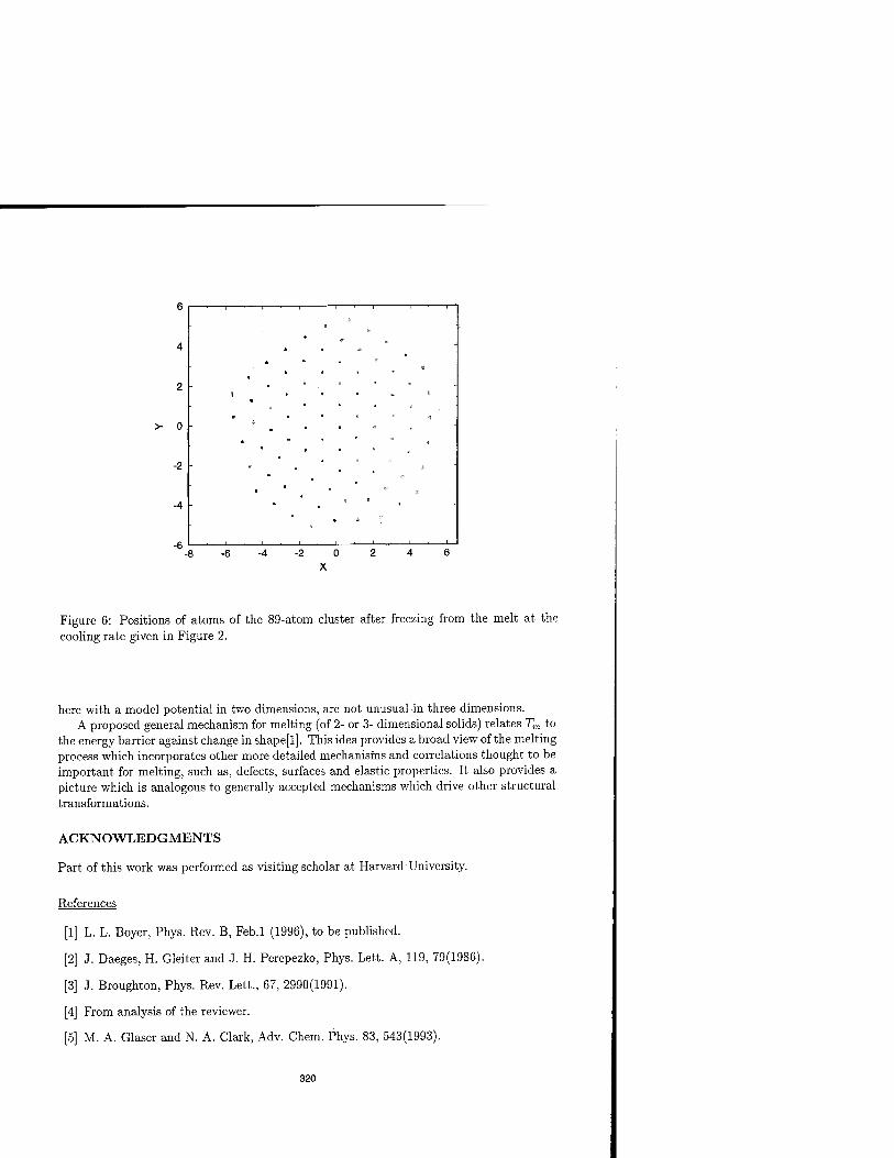
> 0

Figure 6: Positions of atoms of the 89-atom cluster after freezing from the melt at the cooling rate given in Figure 2.

here with a model potential in two dimensions, are not unusual in three dimensions. A proposed general mechanism for melting (of 2- or 3- dimensional solids) relates Tm to

the energy barrier against change in shape[l]. This idea provides a broad view of the melting process which incorporates other more detailed mechanisms and correlations thought to be important for melting, such as, defects, surfaces and elastic properties. It also provides a picture which is analogous to generally accepted mechanisms which drive other structural transformations.

ACKNOWLEDGMENTS

Part of this work was performed as visiting scholar at Harvard University.

References

[1] L. L. Boyer, Phys. Rev. B, Feb.l (1996), to be published.

[2] J. Daeges, H. Gleiter and J. H. Perepezko, Phys. Lett. A, 119, 79(1986).

[3] J. Broughton, Phys. Rev. Lett., 67, 2990(1991).

[4] From analysis of the reviewer.

[5] M. A. Glaser and N. A. Clark, Adv. Chem. Phys. 83, 543(1993).

320

Ab initio and Model Calculations on Different Phases of Zirconia

UWE SCHÖNBERGER, MARK WILSON and MICHAEL W. FINNIS* Max-Planck Institut für Metallforschung, Institut für Werkstoffwissenschaft, Seestr. 92, 70174 Stuttgart, Germany. *Present Adress: Atomistic Simulation Group, School of Mathematics and Physics, The Queen's University of Belfast, Belfast BT7 INN, Northern Ireland.

ABSTRACT

In order to get a better understanding of the energetics of Z1O2 (zirconia) ab initio calculations with the full potential linear muffin tin orbital method ( fp LMTO) have been performed on the tetragonal structure over a range of c/a and sublattice displacement. A new semi-empirical shell model is developed which makes use of Hartree-Fock calculations and includes compressible anions and quadrupolar distortions. The empirical model predicts energies for tetragonal distortion in agreement with the fp LMTO calculations. Furthermore, it enables us to understand why the seven-fold coordinated monoclinic phase is the low temperature equilibrium structure.

INTRODUCTION

Zirconia is an important ceramic material with many applications particularly at high temperatures. Pure Z1O2 shows two temperature driven phase transitions which have been investigated experimentally [1-3 ]. The high temperature phase of zirconia has the cubic fluorite structure. With decreasing temperature there is a martensitic phase transition at 2300°C to a tetragonal phase (c-t) followed by a second martensitic transition to a monoclinic phase (t-m) at about 1000°C. Doping with MgO stabilizes the cubic phase down to 800°C and it shows a (c-t) transformation with decreasing Mg concentration. Yttria (Y2O3) also stabilizes the cubic'and tetragonal phases to lower temperatures. One purpose of our study is to understand the stability of the phases by performing electronic structure calculations within density functional theory. These calculations extend the previous work of Jansen [4] which used the linear augmented plane wave (LAPW) method and use the fp LMTO method [8]. A second purpose of our study is to develop a potential model for accurately describing the high temperature behaviour. With the help of Hartree-Fock results a transferable model based on the ionic picture has been derived and successfully applied to the different phases of zirconia [5]. The biggest challenge for the potential model was to reproduce the seven coordinate monoclinic structure as groundstate. In terms of cation radii zirconia can be regarded as intermediate between the six- coordinate rutile structure taken by intermediate sized cations, and the eight- coordinate fluorite structure taken by large cation systems (i.e actinides). Previous empirical models [6,7] have failed to predict the monoclinic phase as groundstate,

instead favouring the orthorhombic a-Pb02 structure [5] . In this paper the ab

321


initio results for the tetragonal phase, the empirical model calculations and the experimental result are discussed.

COMPUTATIONAL METHODS

The ab initio total energy calculations have been performed with the fp LMTO method [8] within the local density approximation (LDA) with the exchange correlation potential of Hedin and Lundquist [9]. The fp LMTO method has been successfully applied to systems as diverse as transition metals, transition metal surfaces, phonon frequencies of Si, YBa2Cu3Ü7, MgO and metal-ceramic interfaces. An overview of the density functional theory can be found in [10]. To derive the potential model we use ab initio Hartree-Fock calculations due to Harding [11]. The potential model has two important aspects. Firstly, the anion- cation short-range contribution is handled via a compressible ion model (CIM) [12]. This allows for the spherical relaxation of the oxide anions ("breathing") in a manner equivalent to the older breathing-shell models. The critical difference is that the CIM is parameterized from well-chosen ab initio calculations rather than empirically fitting to crystal properties such as phonon modes. Secondly, polarization (induction) effects are included at both the dipolar and quadrupolar level via a polarizable-ion model (PIM) [13]. Both the CFM and PIM introduce many-body aspects into the potential model.

RESULTS

Calculations with the fp LMTO method have been performed for all three experimental structures of zirconia mentioned above. The cubic structure with three atoms per unit cell has been used to find an adequate set of basis functions. It has turned out that the low lying Zr 4p state has to be treated as a valence state and the Zr 4s state as a semi-core state within our method. This is surprising in view of the fact that the Zr 4p is about 1.5 Ry and the Zr 4s 2.3 Ry away from the valence band edge. Treating both states as semi-core states in a second energy panel leads to a calculated lattice constant which is at least 8% smaller than the value calculated by Jansen [4] (a=5.03Ä) while putting the Zr 4p state as valence state and the Zr 4s as core state leads to a lattice constant of 4.91A. Treating the Zr 4p as valence state and the Zr 4s either as valence state (A), equivalent to Jansen, or semi-core state (B) in a second energy panel leads to lattice constants of 5.04Ä (A) and 5.02Ä (B). Only these treatments lead to reasonable results in comparison with the experimental lattice constant extrapolated to OK (5.09 from Ref. [4]). For all further calculations we have chosen treatment (B) as it is variationally more flexible because it includes a Zr 5s basis function which is missing in treatment (A). More systematic investigations of the influence of semi-core states could be done with a modified fp LMTO method which allows muliple orbitals per L channel. These modifications have already been implemented in a LMTO ASA method [14]. In order to find the tetragonal structure of minimum energy calculations have been performed for different volumes, c/a ratios and oxygen displacements dz. The resulting total energies are shown in figure 1.

322

-0.03 -0.01 dz/c 0.01 0.03 0.03 -0.01 "yc 0.01 0.03 0.05

Figure 1. Total energy (mRy) versus oxigen displacement dz (units in c) for different c/a ratios and volumes.

From the results in figure 1. the minimum values can be found: (V/Vo)min=0.95 (V0=444 a.u.3), (c/aW = 1.43 and (dz)min=0.03. Our result for dz is half of the high temperature experimental result (dz=0.06). Preliminary calculations predict the monoclinic structure to be of lower energy than both the cubic and tetragonal phases. However, due to the poor representation of the huge interstitial region we do not regard the energy differences as reliable. Supercell calculations for the Mg doped ideal fluorite structure have also been performed on the system Zr7MgOi5. There are two distinct O vacancy positions within that model; one next nearest neighbour and one second nearest neighbour to the Mg ion. Without taking relaxation into account total energy calculations are found to favour the next nearest neighbour position by O.llRy. The most important result obtained by the new semi-empirical model calculations is the stabilization of the seven-coordinate monoclinic structure over the other structural possibilities. Figure 2 shows the energy/volume curves obtained using the CIM with full anion dipolar and quadrupolar induction effects. The experimentally observed monoclinic structure has the lowest energy with a molar volume in good agreement with experiment.

323

-8700.0

-8800.0

O E

-8900.0

-9000.0 25.0 30.0 35.0

V/A3 40.0 45.0

Figure 2. Energy/volume curves with the potential model.

Having successfully reproduced the experimental groundstate the potential model has been applied, without further modification, to study the tetragonal cubic transition. This allows contact to be made with the fp LMTO calculations. Figure 3 shows the total crystal energy against tetragonal distortion for a range of cell volumes at a fixed c/a ratio of 1.42. The dz minimum shifts from around 0.03 at the smallest volume considered to around 0.06 at the largest. This is consistent with the ab initio calculations (corresponding to OK) and the experimental observations (which correspond to high temperature and hence lower density).

324

20.0

0.10

Figure 3. Energy/tetragonal distortion curves for four V/Vo ratios with the potential model.

DISCUSSION AND CONCLUSIONS

A new empirical potential model for successfully reproduces for the first time the experimental monoclinic groundstate. Both the spherical relaxation of the anions ("breathing" - the CIM) and anion quadrupoles are found to be necessary. The role of the CIM is to destabilise lower coordinate structures, in particular the spurious PbQ2 structure which was stable with the simple shell model. Conversely, however, by including breathing shells in the CIM alone the higher coordinate fluorite structure is favoured. The lower symmetry, monoclinic structure correctly becomes stable with respect to the fluorite structure only when the anion quadrupole distortions are included.

An extensive set of density functional (fp LMTO) total energy calculations has been performed as a basis for understanding the (c-t) phase transition. The new potential model compares well with the fp LMTO calculations and explains the tetragonal distortion. It again requires both the CIM and the quadrupolar distortions to explain the tetragonality. The prediction of tetragonality by a pair potential or simple shell model is possible, but such a model is not transferable.

325

ACKNOWLEDGEMENTS

U. S. would like to thank the Deutsche Forschungsgemeinschaft (grant number Fi478/l-2) and Volker Heine and the TCM group in Cambridge for there hospitality where parts of this work has been carried out. M. W. would like to thank the Alexander von Humboldt Stiftung for financial support. We thank John Harding and Nick Pyper for providing details of their ab initio calculations and both them and Paul Madden for valuable discussions. This work has benefited from collaborations within, and has been partially funded by, the network on „Ab-initio calculation of complex processes in materials" (Contract ERBCHRXCT930369)

REFERENCES

1. H. S. Maita, E. C. Subbarao and K. K. Srivastava, Physica status solidi (a) 21, p. 9 (1974)

2. A. H. Heuer and M. Rühle, Acta Metall. 33, p. 2101 (1985)

3. M. Rühle, L. T. Ma, W. Wunderlich and A. G. Evans, Physica B 150, p.86 (1988)

4. H. J. F. Jansen, Phys. Rev. B 43, p.7267 (1991)

5. M. Wilson, U. Schönberger and M. W. Finnis, Phys. Rev. B, submitted.

6. E. V. Stefanovich, A.L.Shluger and C.R.A. Catlow, Phys. Rev. B 49, p.11560 (1994)

7. A. Dwivedi and A. N. Cormack, Phil. Mag. A 61, p.l (1990)

8. M. Methfessel, Phys. Rev B 38, p. 1537 (1988) and M. Methfessel, C. O. Rodriguez,0. K. Andersen , Phys. Rev B 40, p.2009 (1989)

9. L. Hedin and B. I. Lundquist, J. Phys. 4, p.2064 (1971)

10. R. O. Jones, O. Gunnarsson, Rev. Mod. Phys 61, p.689 (1989)

11. J. H. Harding, unpublished work.

12. M. Wilson, N. C. Pyper, J. H. Harding and P. A. Madden, J. Chem. Phys., to be published.

13. M. Wilson and P. A. Madden, J. Phys.: Condens. Matter 5, p.2687 (1993) and M. Wilson, P. A. Madden and B. J. C. Cabral, J. Phys. Chem, to be published.

14. F. Aryasetiawan and O. Gunnarsson, Phys. Rev. B 49, p.7219 (1994)

326

Melting of Aromatic Compounds: Molecular Dynamics Simulations

P. W.-C. Kling', J. T. Books1, C. M. Freeman2, S. M. Levine2, B. Vessal2, J. M. Newsam2, and M. L. Klein3

'Albemarle Corp., 8000 G.S.R.I. Ave., Baton Rouge, LA70820 2Biosym / MSI, 9685 Scranton Road, San Diego, CA 92121 ^Department of Chemistry, University of Pennsylvania, Philadelphia, PA 19104

ABSTRACT

We have used constant pressure molecular dynamics calculations to explore the behavior at various temperatures of two molecular crystals: benzene and a brominated phenyl compound. We observed a melting transition by heating the crystals from a low temperature. In the case of benzene, we performed one heating run of about 1 ns and obtained agreement with the experimental melting point to within some 8%. We have also simulated the melting of a more complex molecular crystal that contains bromine and phenyl groups. We performed four heating runs, with different rates of heating. For total simulation times of about 100, 220, 770, and 1150ps, the heating runs predicted melting temperatures that differed from the experimental melting temperature by 53%, 33%, 25%, and 9% respectively.

INTRODUCTION

The general theory of melting and glass formation is under active development [1-8]. To better understand the atomistic basis and mechanisms of melting and glass formation, many computer simulations had been carried out. Some of the systems studied include: benzene [31], methanol [9, 10], polyethylene [11 and refs. therein], fullerenes [12], nitrate salts [13], magnesium oxide [14], silicon dioxide [15, 16], silicon [17-19]; silicon with surfaces and defects [20], copper [21], copper with defects [21], and copper-titanium alloys [22].

One system that we studied was benzene. Over the years much work had been done to develop forcefields, analyze crystal packing, and simulate the solid and the liquid states. We have listed some of the references in [23-42]. In particular, Ciaessens et al. [28] pointed out the importance of including the quadrupole moment in simulations. Gupta et al. [35] have simulated liquid benzene over the temperature range of 280 to 460K. Anderson et al. [33] have simulated liquid benzene at 305K and solid benzene at 10K. Yashonath et al. [36] have simulated the orthorhombic phase at 218K, 1 bar and the monoclinic phase at 294K, 25kbar, and the liquid phase at 300K, 1 bar. Linse [31] had simulated benzene at 120, 258, 308, and 348K and showed that rotation around the C6 axis softened the peaks in the radial distribution functions as the temperature increased. In this paper we present some further studies of the melting of benzene.

Most of the earlier simulations employed the technique of molecular dynamics (MD) to obtain the raw data. It is well-known that the ideal way to estimate a phase transition point is by calculating

327

Mat. Res. Soc. Symp. Proc. Vol. 408 @ 1996 Materials Research Society

the free energy of both of the coexisting phases as a function of the relevant field variable. Assuming a robust free energy scheme and simulation (MD) protocol, the accuracy is then limited primarily by the quality of the forcefield. Broughton and Li [17] showed that this method could give impressive results. Using the forcefield of Stillinger and Weber [43], they calculated a melting point for silicon that agreed with the experimental value to within 0.5%. Furthermore, the MD results of Levesque et al. [44] and free energy calculations of Frenkel [45] on 4He showed the importance of calculating the free energy to determine the thermodynamic stability of the different phases involved in the transitions studied by MD. However, this method has not frequently been used because it is relatively expensive in terms of computer time.

Phillpot et al. [20] and Lutsko et al. [21] considered slabs of finite crystals and used the idea that even though the crystalline solid will melt at any temperature above the melting temperature, the speed by which the solid-melt front propagates through the system is a function of the temperature of the system. By extrapolating these data back to the temperature of zero propagation speed, they obtained an estimate of the melting transition accurate to about 10% for Si and Cu.

A common method for determining the melting and glass transition points is by calculating either some thermodynamic property such as the density, internal energy, or the mean-square displacement (MSD) of a certain subset of atoms in the system as a function of the simulation time [9, 10, 16]. In our work, we used these indicators to estimate the melting transition of both benzene and the brominated phenyl crystal.

In such MD simulations, we locate the melting and glass transition points by subjecting the system to heating (melting) and cooling (freezing) cycles. Due to computer hardware and CPU time constraints, the system size for "real" materials has typically been several hundred to several thousand atoms. Typically, the system has been equilibrated for about 1 to 100 ps at each temperature step. Thus the effective rate of temperature ramp or quench is much faster than conventional experiments resulting in substantial superheating in the heating / melting cycle and supercooling in the cooling / freezing cycle. In the heating cycle, superheating results in overprediction of the melting point. In the cooling cycle, typically the rapid quench results in glass formation instead of crystallization [8],

Furthermore, MD simulation assumes the crystal to be perfect, which is not the case in the crystals used for experiments on melting. The use of periodic boundary conditions attempts to simulate an infinite bulk system without any surfaces; it is known that crystal surfaces play an important role in the melting process [4 and references therein]. Phillpot et al. [20] showed that for Si, at temperatures above Tmd„ grain boundaries or free surfaces can initiate melting by nucleating the liquid phase. Lutsko et al. [21] reported the same results for Cu; they also studied the effect of two different sized voids on melting. In this work we assume the crystal is perfect which tends to cause the crystal to superheat.

SIMULATIONS

For both benzene and the brominated phenyl compound (BPC), we first minimized a computational cell containing N molecules. For benzene, N=32, while for the BPC, N=27. The

328

parameter set used to describe the interatomic potentials were from Biosym's PCFF forcefield [46- 49], This forcefield is based on the CFF91 forcefield [50-52],

In our MD simulations we mimicked an infinite crystal by applying periodic boundary conditions. All our MD simulations were performed using the Discover 3.1 package [52]. For benzene, dynamics was performed using Ewald summation. For BPC, the nonbond cut-off distance was 9.5A. In both cases, the integration time step was 1 fs but slightly different protocols were used; the two orders of magnitude difference in melting temperature between benzene and BPC reflects a significant difference in the nonbond energies. Thus, for the BPC it was sufficient to carry out NPT with velocity scaling followed by NVE for data collection; however, for benzene we used NVT/NPT/NVE wherein the Anderson method was used to control temperature for the first two stages. For BPC, four heating runs were made. At each temperature we used NPT to equilibrate the system for a time interval of xl and followed this with NVE for z1. In run #1, t, ranged from 2 to 12 ps while x2 ranged from 9 to 12 ps. This gave rise to a total run time of about 100 ps from room temperature to melting temperature. For runs #2, 3, and 4, the total times were about 220, 770, and 1150 ps respectively. For benzene, we ran 100 ps at each temperature step and the total simulation time was about 1 ns.

RESULTS

We present our results for benzene in Figure 1. Starting from the left hand side, the first graph is the mean-square displacement (MSD) of the carbon atoms at different temperatures, the second graph is the average density in g/cc, and the third graph is the average potential energy of the system. All the data reported here were collected during the NVE portions of the simulations. The MSD plots only show the data from the first 40% of the NVE runs.

The MSD curves are for T=293, 297, 303, and 308K. For T>303K, the MSD curves appear linear indicating unconstrained motion is available to the carbon atoms. For both density and potential energy curves, there is a sharp break around 300K. All of these indicate a melting transition around 300K, which differs from the experimental value of 278.5K by less than 8%.

For the BPC, the MSD, density, and potential energy curves were similar to our results for benzene. For this crystal we had also explored the dependence of the calculated melting temperature as a function of the length of the simulation or the effective heating rate. In Figure 2 we plot the difference between the experimental and the predicted melting temperature as a function of the total simulation times. We see that for the range of simulation times from about 100 to about 1150 ps, the difference decreased from 53 to 9%.

CONCLUSIONS

As computers become more powerful, MD simulation will become a viable way of estimating the melting temperature of complex crystals as long as careful thought is given to the crafting of a simulation protocol that is appropriate to the system.

329

Figure 1 Results from MD simulation of benzene.

0.93 29.aa

Ti ne <ps; Tsrapers+urs

250 310

Temperatur'£>. K

Figure 2 Results from MD simulation of a brominated phenyl compound

£ so O

.2 40 >

d30 s #20 u B

i10

s 200 400 6O0 800

Total Run Time, picosec

1.2O0

330

ACKNOWLEDGMENTS

PWCK would like to express his appreciation to F. Case, R. L. Davis, B. E. Eichinger, X. P. Li, and H. Sun for helpful discussions; and thank D. E. Goins, W. E. Moehle, and S. G. Thomas for their guidance and encouragement. The authors would like to thank Albemarle Corp. for permission to publish this work.

REFERENCES

1. H. J. Fecht, Nature, 356, 133 (1992). 2. R. W. Cahn, Nature, 356, 109 (1992). 3. D.W. Oxtoby, Nature, 347, 725 (1990). 4. R. W. Cahn, Nature, 323, 668 (1986). 5. Wright, J. D., Molecular Crystals Cambridge University Press, Cambridge, U.K., 1995. 6. Ubbelohde, A. R., The Molten State of Matter. John Wiley & Sons, Chicester, 1978. 7. J.-L. Barrat and M. L. Klein, Annu. Rev. Phys. Chem., 42, 23 (1991). 8. G. H. Fredickson, Ann. Rev. Phys. Chem., 39, 149 (1988). 9. M. Marchi and M. L. Klein, Z. Naturforsch, 44, 585 (1989). 10. P. Sindzingre and M. L. Klein, J. Chem. Phys., 96, 4681 (1992). 11. R.-J. Roe, J. Chem. Phys., 100, 1610 (1994). 12. S. G. Kim and D. Tomanek, Phys. Rev. Lett., 72, 2418 (1994). 13. G. F. Signorini, J.-L. Barrat, and M. L. Klein, J. Chem. Phys., 92, 1294 (1990). 14. R. Ferneyhough, D. Fincham, G. D. Price, and M. J. Gillan, Modelling Simul. Mater. Sei.

Eng., 2, 1101 (1994). 15. A. Nakano, L. Bi, R. K. Kalia, and P. Vashista, Phys. Rev. Lett., 71, 85 (1993). 16. B. M. Vessal, Amini, D. Fincham, and C. R. A. Catlow, Phil. Mag. B, 60, 753 (1989). 17. J. Q. Broughton and X. P. Li, Phys. Rev. B, 35, 9120 (1987). 18. A. P. Horsfield, and P. Clancy, Modelling Simul. Mater. Sei. Eng., 2, 277 (1994). 19. O. Sugino, and R. Car, Phys. Rev. Lett., 74, 1823 (1995). 20. S. R. Phillpot, S. Yip, and D. Wolf, Computers in Physics, 3, 20 (1989). 21. J. F. Lutsko, D. Wolf, S. R. Phillpot, and S. Yip, Phys. Rev. B, 40, 2841 (1989). 22. T. D. Kulp, G J. Ackland, M. Sob, V. Vitek, and T. Egami, Modelling Simul. Mater. Sei.

Eng., 1,315(1993). 23. D. E. Williams, J. Chem. Phys., 45, 3770 (1966). 24. D. J. Evans and R. O. Watts, Mol. Phys., 31, 83 (1976). 25. D. E. Williams and T. L. Starr, Comput. Chem., 1, 173 (1977). 26. D. Hall, T. H. Starr, D. E. Williams, and M. K. Wood, Acta Cryst, A36, 494 (1980). 27. O. Steinhauser, Chem. Phys., 73, 155 (1982). 28. M. Claessens, M. Ferrario, and J.-P. Ryckaert, Mol. Phys., 50, 217 (1983). 29. S. L. Price and A. J. Stone, Mol. Phys., 51, 569 (1984). 30. F. Serrano Adan, A. Banon, and J. Santamaria, Chem. Phys., 86, 433 (1984). 31. P. Linse, J. Am. Chem. Soc, 106, 5425 (1984). 32. P. Linse, S. Engstrom, and B. Jonsson, Chem. Phys. Lett., 115, 95 (1985).

331

33. J. Anderson, J. J. Ullo, and S. Yip, J. Chem. Phys., 86, 4078 (1987). 34. I. Pettersson and T. Liljefors, J. Comput. Chem., 8, 1139 (1987). 35. S. Gupta, W. B. Sediawan, and E. McLaughlin, Mol. Phys., 65, 961 (1988). 36. S. Yashonath, S. L. Price, and I. R. McDonald, Mol. Phys., 64, 361 (1988). 37. A. V. Dzyabchenko, Sov. Phys. Crystallogr., 34, 131 (1989). 38. M. Ostheimer and H. Bertagnoli, Z. Phys. Chem., 162, 171 (1989). 39. P. Pavlides, D. Pugh, and K. J. Roberts, Acta Cryst., A47, 846 (1991). 40. M. M. Thiery, J. M. Besson, and J. L. Bribes, J. Chem. Phys., 96, 2633 (1992). 41. J. Nagy, V. H. Smith, Jr., and D. F. Weaver, J. Phys. Chem., 99, 13868 (1995). 42. K. D. Gibson and H. A. Scheraga, J. Phys. Chem., 99, 3765 (1995). 43. F. H. Stillinger and T. A. Weber, Phys. Rev. B, 31, 5262 (1985). 44. D. Levesque, J.-J. Weis, and M. L. Klein, Phys. Rev. Lett., 51, 670 (1983). 45. D. Frenkel, Phys. Rev. Lett., 56, 858 (1986). 46. H. Sun, S. J. Mumby, J. R. Maple, and A. T. Hagler, J. Am. Chem. Soc, 116, 2978 (1994). 47. H. Sun, J. Comp. Chem., 15, 752 (1994). 48. H. Sun, S. J. Mumby, J. R. Maple, and A. T. Hagler, J. Phy. Chem., 99, 5873 (1995). 49. H. Sun, Macromolecules, 28, 701 (1995). 50. J. Maple, U. Dinur, A. T. Hagler, Proc. Nat. Acad. Sei. USA 85, 5350 (1988). 51. J. R. Maple, T. S. Thacher, U. Dinur, A. T. Hagler, Chemical Design Automation News, 5,

5(1990). 52. Discover User Guide, version 2.9/3.1, San Diego: Biosym Technologies, 1993.

332

DISTRIBUTION OF RINGS AND INTERMEDIATE RANGE CORRELATIONS IN

SILICA GLASS UNDER PRESSURE - A MOLECULAR DYNAMICS STUDY

Jose Pedro Rino Universidade Federal de Säo Carlos, Via Washington Luiz Km 235-13565-905,

Säo Carlos, S.P. Brazil

Gonzalo Gutierrez Facultad de Ffsica, P. Universidad Catölica de Chile,

Casilla 306, Santiago 22, Chile

Ingvar Ebbsjö The Studsvik Neutron Research Laboratory, S-611 82 Nyköping, Sweden

Rajiv K. Kalia and Priya Vashishta Concurrent Computer Laboratory for Materials Simulations

Department of Physics & Astronomy and Department of Computer Science Louisiana State University, LA 70803-4001

E-Mail: [email protected] Web: http://www.cclms.lsu.edu/

ABSTRACT

Using the molecular dynamics (MD) method, we have studied the effect of pressure on the distribution of rings and their relationship to intermediate range correlations manifested as the first sharp diffraction peak (FSDP) for SiC>2 glass. A systematic analysis of the modifications observed in the FSDP for densities ranging from 2.0 to 3.2 g/cm3 and temperatures from 0 to 1500 K is reported. The decrease in the height of the FSDP with increasing density is found to be proportional to the decrease in the number of 6-fold rings. For the density and temperature ranges studied in SiC>2 glass, the full width at half maximum (FWHM) of the FSDP remains unchanged.

INTRODUCTION

Structural order in silica glass can be divided into short-range order (SRO) and intermediate range order (IRO) [1-5]. X-ray [2], neutron [3] and nuclear magnetic resonance (NMR) [4] experiments reveal the presence of corner-sharing Si(Oi/2)4 tetrahedra in silica glass at normal density (2.2 g/cm3). The IRO is manifested as the first sharp diffraction peak (FSDP) in the static structure factor, S(q) in neutron and x-ray diffraction experiments [1-3].

One of the anomalous features of the FSDP in many network glasses, especially chalcogenide glasses such as GeSe2 and SiSe2, is that the height of the FSDP increases with increasing temperature [1,5,6]. This is contrary to the normal behavior where the height peaks in S(q) decrease with increasing temperature. The FSDP in GeSe2 and SiSe2 have been shown to arise mainly from Ge-Ge and Ge-Se (Si-Si and Si-Se) correlations between 4 and 10 Ä. The temperature dependence of the FSDP is found to be a balance between two competing effects: the disorder due to thermal vibrations and thermal expansion [5]. Thermal vibrations broaden the peaks in the pair distribution functions and hence reduce the amplitude of peaks in its Fourier transform, i.e., the static structure factor. On the other hand, the thermal expansion decreases the frustration associated with the disordered arrangement of GeSe2 tetrahedral units, thereby increasing the height of the FSDP. Neutron diffraction study by Susman et al. [7] has revealed that in Si02 glass the height of the FSDP decreases with increased temperature contrary to other glasses. Normal behavior of the FSDP in Si02 glass is a consequence of an essentially zero thermal-expansion coefficient so that the effect due to thermal vibration dominates. Using neutron diffraction, Susman et al. [8] have studied the changes in the intermediate range order up to 20%

333


densification in Si02 glass. Recently, Meade, Hemley and Mao [9] have carried out in situ x-ray measurements of the static structure factor S(q) of Si02 glass subjected to pressures of 8-42 GPa. With increasing pressure, they observed that the height of the FSDP decreases and its position shifts to higher q values, almost disappearing around 42 GPa.

In this paper we report the results of a large-scale molecular dynamics (MD) study of the influence of pressure and temperature on structural correlations in Si02 glass, especially the behavior of the FSDP and its relationship with the distribution of n -fold rings.

MOLECULAR DYNAMICS SIMULATIONS

The MD simulations were carried out for 52,728-particle (17,576 Si and 35,152 O) systems in cubic boxes of sides 92.7333 Ä corresponding to normal density p0= 2.2 g/cmJ. The size of the system was chosen so that there is no size dependence in the height and the position of the FSDP, which is strongly dependent on the number of particles (up to 5,000 particles) [10]. Periodic boundary conditions are employed and a time step of At = 1.5 fs is used.

Molecular-dynamics simulations were performed with a combination of two body and three-body effective interatomic potentials. The two-body interaction combine stenc repulsion, long-range Coulomb interaction due to charge-transfer effects, and charge-dipole interaction due to large electronic polarizability of O2" ions. The three-body covalent interactions include the effects of bond bending and stretching. The interaction potential gives an excellent description of structural correlations and bulk modulus of Si02 at normal density (37.6 GPa at 2.2 g/cmJ) [11].

The Si02 glasses were generated by slow cooling (40,000 At) and thermalization (40,000 At) of well equilibrated (100,000 At) liquids at high temperatures (~ 3,200 K) [11]. High density (2 4 2.6, 2.8, 3.0, and 3.2 g/cm3) Si02 glasses were also prepared in a similar fashion except that the length of'the MD cell and atomic positions were first appropriately scaled in high-temperature liquid states. A low density system (2.0 g/cm3 ) was also prepared in this way.


a) Pair distribution functions and bond angle distributions Partial pair distribution functions (PDF) for Si02 glass at three densities are shown in Fig_

1 It is remarkable that even after a 45% increase in the density, from 2.2 to 3.2 g/cm3, the Si-0 bond length remains unchanged at 1.61+ 0.02 A. At all densities there is a gap in the Si-0 PDF from 1.8 A to 2.3 Ä defining a shell of nearest neighbor tetrahedral coordination. The next-nearest neighbor distances decrease slightly as the density increases (see inset).

The O-O partial PDF upon densification has its first peak shifted from 2.654 Ä at normal density (2.2 g/cm3), to 2.644 A at 2.4 g/cm3, to 2.616 A at 2.8 g/cm3, to 2.578 Ä at 3.0 g/cm3

and to 2 570 A at 3.2 g/cm3. The second peak also decreases in height and shifts to the left. The shoulder observed around 3.5 Ä at 2.2 and 2.4 g/cm3 is completely destroyed at higher densities, even though the 0-0 coordination is practically the same (= 6) until 2.85 A.

The Si-Si nearest neighbor distance decreases by 0.128 A from 3.088 Ä at 2.2 g/cm3 to 2.960 Ä at 3.2 g/cm3. The nearest-neighbor coordination number remains the same for all densities. A dramatic modification occurs in the range of 3.5 A to 8 A where the second and third Si-Si next nearest neighbor distances are located, and as we will see next, this is reflected in the changes observed in the FSDP.

To obtain more information about the local structure and connectivity in the glass, we examine the bond angle distributions. In Fig. 2 we show the peak position and full width at half maximum (FWHM) of the bond angle distributions for all six bond angles at seven densities. The angles were calculated with Si-O, 0-0 and Si-Si cut-off distances of 2.0, 2.9 and 3.2 A, respectively. The bond angles in an ideal tetrahedron are O-Si-O=109.47°, O-O-O =60°, and Si-O- 0=35.26°. We see that even at the highest density studied, the basic local order is formed by very

334

well defined tetrahedra, and the increase in the density induces only small distortions in these basic units.

60 . . i i . . . p j . 11 . .

50 si Si-O

40 - 30 IN 2 .*4 20 ■T'' i - ,j rL^ 10 --** . J '*vr -

0

8 ■

1**'

o-o V 6 ■V ' ■

':'.' l- BJ3 4 "

2 . . . . >r*>\-*'

0 6 ?! Si-Si 5 - p (g/cm3) 4 - *V i1 2.2 3 £

— 2.8 ■ 3.2 2

1 - 0 L*-" L-f-J

ttr-r . . -1""' '

20

16

12

8

4

0

16 I 12 |

O

8

4

0

16

12

8

4

0

115

110

105

i i i i ■ i -T-l -TT-T-I T | 1

100 - 95 '. O-Si-O

90

^ 65 o-o-o

J 60 S < 55 •o e n so

iff ► - f.t —t y* ) "

40 Si-O-O ■

35 :iff y —< ** i

30 -

25 . . . > . ■ . ■ . i * i ■ i .

150

■^i -i-i

140 ■ "■■"->. 1 1 iv -

.[ i "'S--» 130 L. : _

. Si-O-Si L L

140

120 .

100 ( ■-■< >- 1 .

80 !>-,„, --<)

60 . Si-Si-Si l

40

25 ' Si-Si-O

20

15 .-j r—

r * ■••< )

10 i . i. i . i . i . i . i .

8 10 12 O N t« 00 O N (S M ri ri ri fi to

r(A) p (g/cm3)

Figure 1. Partial pair distribution functions Figure 2. Bond angle distributions, and coordination numbers at three densities.

The connectivity of tetrahedra is primarily described through Si-O-Si bond angle. Here we observe a significant change under densification. At normal density, Si-O-Si has its peak at 144.5° with FWHM of 17° which agrees very well with magic-angle-spinning NMR experiments [4]. As the density increases, the Si-O-Si bond angle shifts to 136° (FWHM=20°) at 3.2 g/cm3. The densification causes the tetrahedra to be closer to each other by decreasing the connectivity angle, which is consistent with the decreasing Si-Si nearest and next nearest neighbor distances as shown in Fig. 1. b) Distribution of n-fold Rings at Different Densities

The structure and network topology of a glass can be further characterized through the distribution of« -fold rings. An n -fold ring is defined as the shortest closed path of alternating Si- O bonds. Therefore, an n -fold ring consists of In alternating Si-O bonds. For a system with N 4-fold coordinated Si atoms there are 6N rings in the glass. For example, a- and ß-cristobalite have only six 6-fold rings, whereas a- and ß-quartz have four 6-fold and two 8-fold rings [12]. We have calculated the distribution of rings from n =2 to 12. The distribution of distances and angles for each n -fold ring are also calculated.

Figure 3 shows the dependence of n -fold ring for n = 3-10 with density ranging from 2.0 to 3.2 g/cm3; the number of two-fold rings is found to be zero. For all densities the largest number of rings correspond to n = 5, 6, and 7. It is interesting that 5- and 6-fold rings show a maximum at the normal density. The sum of five- and seven-fold rings is nearly constant at all the densities

335

we have studied. Rings with n = 3, 4, 7, 8, 9, and 10 increase monotonically in number as the density increases from 2.0 to 3.2 g/cm3.

2.0

= O

-4-*

« 1.5 55 s-,

a

d

s-

X! s

1.0 ■

0.5

0.0

1 1 1 ■ ■III

-». .-e*. 6 fold e "n --» -- 5 fold V -

-A~ —t *^ -a—-D--0-: :?> :-8==-D .

□'" 1*-^ --□-- 7 fold ~~A.

-- »-- 8 fold .-♦--• .•" .■•

•-- o— .-*>- -o-~° . --O-. 4 fold

--» - 9 fold _„_ .-■*• --—' ■-- :£::*i:S: :S= ::#:"B --H-

1 1 1

- 3 fold -- i.i.i

■-- i

10 fold .i.i.

2.0 2.2 2.4 2.6 2.8 3.0 3.2

Density (g/cm3)

Figure 3. Distribution of n -fold rings as a function of the density.

c) Static Structure Factor and the First Sharp Diffraction Peak

In Fig. 4 (a) we show the neutron static structure factor at 2.2, 2.8, and 3.2 g/cm3. The height and position of the FSDP are affected by the increase in the density. Note that in Fig. 4 (b) the simple elastic compression can not account for the observed shift in the position of the FSDP. The densification induces a large change in the height of the second peak, but has small effect on peaks at large values of q. The dominant contribution to the FSDP at q~1.5 A"1 is related in r -space to density-density correlations in the region of 4-8 Ä [5,6,11]. Thus, the FSDP provides information about the intermediate range order in glasses, although the nature and how the structural entities give rise to the FSDP is still controversial. The FWHM of the FSDP at different densities is shown in the Fig. 4 (c). The FWHM is small and remains nearly constant with the density. From this width we can infer the correlation length of the intermediate range order, ~2JT/(FWHM/2), which is in the range 15-25 Ä.

d) Correlation Between the Number of 6-fold Rings and the Height of the FSDP

We now explore the relationship between the height of the FSDP and the number of 6-fold rings per Si atom in SiC>2 glass. In Figs. 5 (a) and (b) we plot the density dependence of the number of 6-fold rings and the height of the FSDP. The ratio of the height of the FSDP and the number of 6-fold rings is shown in Fig. 5(c). It is quite remarkable that even though the number of six-fold rings and the height of the FSDP vary substantially with density, their ratio is almost constant for the entire range of density, from 2.0 g/cm3 to 3.2 g/cm3.

Correlations in SiC>2 glass span two domains: (i) the short range order which extends to 4 Ä, and (ii) intermediate range order between 8 Ä and 25 Ä, where dominant contribution to the FSDP comes from 4-8 A region which is related to the diameter of six-fold rings. It has been shown by MD simulations that beyond this length (L/2 > 25 A, L being the length of the MD box) there is no contribution to the FSDP [10].

336

2.0

1.5

1.0

0.5

0.0

2.1

2.0

1.9

1.8

1.7

1.6

1.5

0.8

0.6

0.4

0.2

0.0

-,..... . , . ■ \ • ■ i ■ ■ ■

A(a)

t) 1* / \\ XL

/ y/ 2.2^- r 2.8

T^M — ■ 3.2

0 12 3 4 5 6 7 q(AJ)

- --.-- S„(q)

■-*- fll S„(q) y'

y.-'"~ (b)

I l I i I ' I ' I ' I ' I

(c)

density P (g/cm3) ■ < i i i—i—i—

2.0 2.2 2.4 2.6 2.8 3.0 3.2

5

CL, Q

2.0

1.8

1.6

1.4

1.2

1.6

1.4

1.2

1.0

1.2

1.0

0.8

0.6

0.4

Figure 4. (a) MD total neutron static structure factor at three densities, (b) Position, where -pCp/po), (c) width of FSDP as a function of the density.

-i—|—i—|—i—i—i—i—i—|—i i i |—

/""*""•>. (a) •' *>

'. a-SiO, 1

i I i I ' I i I ■ I ' I ' I '

(b)

s„(q)

i i i i i i i i i i i i i i

(c)

.--.--•-

density p (g/cm3) ' ■ ■ I I I 1—I 1 1 1 L.

2.0 2.2 2.4 2.6 2.8 3.0 3.2

Figure 5. (a) Number of 6-fold rings, (b) height of the FSDP, and (c) ratio of height of the FSDP and the number of 6-fold rings as a function of the density.

e) Temperature Dependence of the FSDP at Normal Density To investigate the temperature dependence of the height and width of the FSDP, S(q) at

normal density at six different temperatures (0 K, 300 K, 600 K, 900 K, 1200 K and 1500 K) is calculated. Because the linear thermal expansion coefficient of silica is very small (0.5x10'6 per °C), the change in the volume is negligible over the whole range of temperature. The decrease in the height of the FSDP with temperature is in good agreement with the experiments of Susman et al. [7]. The position and FWHM remain unchanged with temperature, also in good agreement with the neutron experiments [7].

CONCLUSION

Large scale MD simulations are used to investigate the structure in Si02 glasses at several densities and temperatures. The decrease in the height of the FSDP with increasing density is found to be proportional to the decrease in the number of 6-fold rings. At all densities and temperatures, the full width at half maximum (FWHM) of the FSDP remains unchanged.

ACKNOWLEDGMENTS

J.P.R. would like to acknowledge financial support form FAPESP (Fundagäo de Amparo a Pesquisa do Estado de Säo Paulo) and CNPq (Conselho Nacional de Desenvolvimento Cientifico e Tecnologico). G.G. was supported by FONDECYT (Fondo Nacional de Investigaciones

337

Cienti'ficas y Tecnolögicas-Chile) Grant #2940022. This work was supported in part by DOE (Grant No. DE-FG05-92ER45477), NSF (Grant No. DMR-9412965) and AFOSR (Grant No. F 49620-94-1-0444). Simulations were performed on machines in the Concurrent Computing Laboratory for Materials Simulations (CCLMS) at Louisiana State University. The facilities in the CCLMS were acquired with equipment enhancement grants awarded by the Louisiana Board of Regents through Louisiana Education Quality Support Fund.

REFERENCES

1. S. C. Moss and D. L. Price, in Physics of Disordered Materials, ed. by D. Adler, H. Fritzsche, and S. R. Ovshinsky (Plenum, New York, 1985), p. 77; S. R. Elliot, Nature 354, 445(1991)

2. R. L. Mozzi and B. E. Warren, J. Appl. Cryst. 2, 164 (1969); A. C. Wright, J. Non-Cryst. Sol. 106, 1 (1988)

3. R. N. Sinclair and A. C. Wright, J. Non-Cryst. Sol. 57, 447 (1983); P. A. V. Johnson, A. C. Wright, and R. N. Sinclair, ibid 58, 109 (1983); D. I. Grimley, A. C. Wright, and R. N. Sinclair, ibid 109, 49 (1990)

4. R. Dupree and R. F. Pettifer, Nature 308, 523 (1984); R. F. Pettifer, R. Dupree, I. Farnan, and U. Steinberg, J. Non-Cryst. Sol. 106, 408 (1988)

5 P. Vashishta, R. K. Kalia, G. A. Antonio, and I. Ebbsjö, Phys. Rev. Lett. 62, 1651 (1989)

6 G. A. Antonio, R. K. Kalia, A. Nakano, and P. Vashishta, Phys. Rev. B 45, 7455 (1992)

7. S. Susman, K. J. Volin, D. G. Montague, and D. L. Price, Phys. Rev. B 43, 11076 (1991)

8. S. Susman, K. J. Volin, D. L. Price, M. Grimsditch, J. P. Rino, R. K. Kalia, P. Vashishta, G. Gwanmesia, Y. Wang, and R. C. Liebermann, Phys. Rev. B 43, 1194 (1991)

9. C. Meade, R. J. Hemley, and H. K. Mao, Phys. Rev. Lett. 69, 1387 (1992)

10. A. Nakano, R. K. Kalia, and P. Vashishta, J. of Non-Cryst. Sol. 171, 157-163 (1994)

11. P. Vashishta, R. K. Kalia, J. P. Rino, and I. Ebbsjö, Phys. Rev. B 41, 12197 (1990); W. Jin, P. Vashishta, R. K Kalia, and J. P. Rino, ibid 48, 9359 (1993); the same potential has been used successfully in MD simulation of densified silica glasses: W. Jin, R. K. Kalia, P. Vashishta, and J. P. Rino, Phys. Rev. Lett. 71, 3146 (1993); J. P. Rino, G. Gutierrez, I. Ebbsjö, R. K. Kalia, and P. Vashishta, to be published.

12. A. C. Wright and J. A. E. Desa, Phys. Chem. Glasses 19, 140 (1978); J. P. Rino, I. Ebbsjö, R. K. Kalia, A. Nakano, and P. Vashishta, Phys. Rev. B 47, 3053 (1993)

338

FIRST-PRINCIPLES CALCULATIONS OF HEUSLER PHASE PRECURSORS IN THE ATOMIC SHORT-RANGE ORDER OF

DISORDERED BCC TERNARY ALLOYS

JEFFREY D. ALTHOFF, DUANE D. JOHNSON Computational Materials Science Department Sandia National Laboratories Livermore, CA 94551-0969

ABSTRACT

We apply our recently developed first-principles theory of atomic short-range order in disordered multicomponent alloys to CuAuZn2 and AgAuZn2, two alloys which display partially-ordered B2 phases as well as fully-ordered Heusler structures. The calculated Warren-Cowley pair correlation functions for both alloys peak at the special points (|||) and (100), with the peak at (100) dominant. This is indicative of a tendency to B2 order at high temperatures, and a subsequent tendency to Heusler-type order at lower temperatures. An analysis in terms of effective interactions shows that the Au-Zn interaction drives the (100) ordering tendency, while the Ag-Au and Cu-Au interactions contribute more to the (222) ordering tendency - this effect is larger in CuAuZn2 and should lead to a slightly higher transition temperature for the B2 to Heusler transition in CuAuZn2 as compared to AgAuZn2.

INTRODUCTION

Many alloy systems display a disordered solid solution phase at high temperature. This phase is characterized by an absence of chemical long-range order (LRO) but a presence of atomic short-range order (ASRO). This ASRO is directly measurable by diffuse scattering experiments and provides valuable information on both the atomic interactions in the disordered phase and the ordering tendencies toward possible ordered phases. Even if a particular alloy does not experimentally possess a solid solution phase, the properties of a hypothetical solid solution phase can still be calculated and provide similar information.

The ASRO found in the solid solution is often a precursor to the transition from the disordered state to a lower temperature ordered state. In such cases, the ASRO provides a direct indication of the ordering tendencies which will be realized. In the present work we discuss two ternary alloys, AgAuZn2 and CuAuZn2, for which the ASRO is a precursor to two ordering transitions. We calculate and discuss the ASRO.

Multicomponent alloys often exhibit a series of ordering transitions, with one or more partially-ordered phases appearing as the temperature is lowered, ultimately reaching a fully-ordered state. The site occupations of the partially-ordered state may be obtained, at least approximately, from information on the interatomic interactions in the disordered state. Thus, the interactions determine not only the ordering wave vector and spinodal temperature, as in the binary case, but the occupations in the partially-ordered states as well.

The present work utilizes our recently-developed first-principles theory of ASRO in alloys

339


of an arbitrary number of components. Because the present calculations are based on the homogeneously disordered phase, there is no bias to any particular ASRO: the system is "free" to find its own ASRO due to the underlying electronic interactions.

ATOMIC SHORT-RANGE ORDER IN ALLOYS

The ASRO in a multicomponent alloy is described by the pair correlation function

(1)

where the angular brackets indicate a thermodynamic average at temperature T of the occupation variables ff, defined such that <ff is equal to 1(0) if there is (is not) a /(-species atom at site i. Note that the occupation variables at a site satisfy a single-occupancy constraint: at any site, the sum over species of the occupation variables must be equal to one. In order to work with independent variables, we implement the constraint by explicitly designating one species (the Nth. one) to be the "host" species - the occupation variables associated with the host are dependent variables. There are then (N — l) occupational degrees of freedom per site in an iV-component alloy. The correlation function can be thought of as an (N — l) dimensional matrix in the species indices whose inverse exists almost everywhere, with the possible exception of temperatures where the system is unstable. (Note that the "full" A^-dimensional correlation function matrix is singular because of the dependence of the host occupation variables on the independent occupation variables). The elements of the full correlation matrix can be obtained from those of the (N - 1) dimensional matrix from the constraint and from the definition, Eq. 1. The existence of the inverse is important for both physical and formal reasons - physically, the inverse of the correlation function is proportional to the Hessian of the free energy; formally, our first-principles theory of ASRO in multicomponent alloys [1] yields a non-singular portion of the inverse of qßU in reciprocal

space for the disordered alloy, i.e.,

I«"1 (*»]„ = A 1 4- l ß (2)

Here ß is the inverse temperature and Sjty(k) can be thought of as an effective chemical

interaction determined from the electronic structure of the system [1]. 5(2) embodies all electronic effects on the pair correlation function, including electron-hole effects, and is calculated within the Korringa-Kohn-Rostoker, Coherent Potential Approximation (KKR- CPA) electronic-structure scheme. Full details are given in Refs. [1, 2, 3]. In this work, we calculate Sjty within the "band-energy only" approximation, as in Refs. [1,4].

The Warren-Cowley SRO parameter is related to the direct correlation function qßv via

o>W = q^{k)

Ah ■c„l (3)

Note that Sty is calculated under approximations which insure that the sum rule for the

integrated intensity is satisfied, i.e. that q?" ■ASß or, in terms of the Warren-

Cowley SRO parameter in real space, aßl,(R = (0,0,0)) = 1. It is useful to think of the

ASRO in real space as being composed of nascent concentration waves of wave vector k.

340

Figure 1: The Heusler phase, showing the 3 inequivalent types of lattice sites.

The pair correlation function (or Warren-Cowley SRO parameter) can then be thought of as the spectral decomposition of the concentration waves. As long as the Warren-Cowley SRO parameter is finite at all k there is no compositional LRO in the system - a divergence in the correlation function at wave vector k signals the onset of LRO with a periodicity described by k. At very high temperature, the correlation function q(k) is independent of k

- there is no ASRO. As the temperature is lowered, ASRO develops and q(k) begins to show

it-dependent features. Often, there are very prominent peaks in q(k) which grow in height as the temperature is lowered. One or more of these peak heights diverges at the spinodal temperature for the ordering transition, and, in cases where the ASRO is a precursor to LRO, become the superlattice peaks in the Bragg scattering for the ordered alloy.

In multicomponent alloys, it is necessary to specify a "polarization vector" in composition space in order to fully determine the atomic distribution corresponding to a given concentration wave, particularly for partially ordered states. While the wave vector of the concentration wave specifies the arrangement of sublattices in the superstructure, the polarization vector specifies which species of atom(s) occupy the sublattices. It is possible to have, for example in an ABC2 alloy, a concentration wave in which species C occupies one sublattice preferentially while species A and B equally occupy another sublattice. The polarizations are taken to be the eigenvectors of g(_1), which are also the eigenvectors of the Hessian of the free energy, i.e. the principle directions of the free energy. Details will be

given in a forthcoming publication. The Heusler phase for ABC2 alloys (shown in Fig. 1) can be thought of as two static

concentration waves of wave vectors kx = (100) and k2 = (555) on an underlying bcc lattice. The (100) wave leads to a partially-ordered B2 structure whose site occupancies are determined by the polarization vector of the concentration wave. The B2 structure has two sublattices - one comprised of the cube corners of the bcc lattice, the other of the body centers. The {§§§) wave completes the ordering by making adjacent body centers

inequivalent, as shown in Fig. 1.

THE ALLOYS AgAuZn2 and CuAuZn2

Experimentally, AgAuZn2 orders (at approximately 1000 K) directly from the melt into a partially ordered B2 phase in which the Zn atoms are ordered on the cube corners while the Ag and Au atoms are disordered on the body centers. At approximately 600 K the Ag and

341

Au atoms order, yielding a Heusler phase (L2i structure). CuAuZn2 has a bcc disordered solid solution phase at high temperature, transforms to a partially ordered B2 phase at approximately 850 K, again with the Zn atoms ordered on the cube corners, and finally transforms to the Heusler phase at approximately 650 K. Binary AuZn displays a B2 ordered phase directly from the melt (at approximately 1030 K). AgZn has a bcc solid solution phase at high temperature and forms a metastable B2 structure if quenched; slow cooling yields a stable hexagonal structure at approximately 570 K [5]. Addition of 1% Au to AgZn stabilizes the B2 phase [5]. AgAu forms a disordered fee solid solution at high temperatures. CuAu forms an fee solid solution at high temperatures, orders into an orthorhombic (long-period) phase at approximately 680 K and transforms to an Ll0 structure at about 650 K. CuZn has a bcc solid solution phase at high temperature and transforms to a B2 structure at

approximately 730 K. The behavior of these two ternaries is thus intimately connected to the behavior of the

binaries. For the case of AgAuZn2, we expect a strong (100) ordering interaction from the Au-Zn pair, a weaker (100) ordering interaction from the Ag-Zn pair. Since Ag and Au form a solid solution phase, we expect a partially-ordered phase in which the Zn atoms order against the Ag and Au atoms, while the Ag and Au atoms remain disordered with respect to each other. Similarly, for CuAuZn2, the strongest ordering interaction is the Au- Zn interaction, which favors (100) ordering. The Cu-Zn interaction likewise favors (100) ordering. Although CuAu is an fee binary, calculations on bcc CuAu at the same lattice constant as CuAuZn2 show k = (|||) ordering with a spinodal temperature of approximately 5iOK. For CuAuZn2 we therefore expect a similar situation to AgAuZn2, with Zn ordering against Au and Cu, but we might expect subtle differences in the way that the Cu and Au

atoms occupy the partially-ordered phase. In Fig. (2) we show the elements of the pair correlation function matrix for AgAuZn2

and CuAuZn2 along two symmetry directions in the bcc Brillouin zone. For this figure, we display the off-diagonal elements of the Warren-Cowley pair correlation matrix, as would be done experimentally. It is clear that the Au-Zn correlation is the strongest, and peaks at k = (100) for both alloys. The ASRO is therefore indicative of B2-type ordering, and we would expect that the dominant ordering tendency will be for Au and Zn to occupy different sublattices in the B2-like short-range order. In addition, the Ag-Zn correlation (for AgAuZn2) and the Cu-Zn correlation (for CuAuZn2) also display k = (100) ASRO, though in both cases it is weaker than the Au-Zn correlation. The expectation, therefore, is that Ag and Zn (in AgAuZn2) and Cu and Zn (in CuAuZn2) will occupy different sublattices in the B2 ASRO. This expectation (i.e. Zn ordering against both Au and Cu/Ag) is borne out upon examining the polarization of the concentration wave: indeed, Zn occupies the cube corners preferentially, with Au and Ag (in AgAuZn2) or Au and Cu (in CuAuZn2) preferentially occupying the body centers equally. The Zn atoms will tend to have equal numbers of Au and Ag/Cu nearest neighbors.

The Ag-Au and Cu-Au correlations do not display (100) ASRO - in fact, the correlations are negative at (100) (this is permissible in a multicomponent alloy; see, for example [6]). This indicates that the Ag-Au pairs in AgAuZn2 and the Cu-Au pairs in CuAuZn2 should not tend to occupy different sublattices in a B2-type structure. Rather, these correlations peak at (i||) - this indicates that the Ag-Au pairs and Cu-Au pairs will tend to be found as second neighbors in the alloy. Because the (|||) ASRO is much weaker than the (100)

ASRO, it is to be expected that a transition to a (k = (100)) B2-partially ordered state will occur at higher temperature, with a subsequent transition establishing (||i)-type order at

342

30

20

10

-10

msm t-o-B-ö-B-< P«i-B-p..

— Ag-Au

— Ag-Zn

— Au-Zn

hQ-E

/

I

■

to

r F 3 t <J ] i H

30

20

10

-10

„a-jEff-i aaatai

— Cu-Au

— Cu-Zn

— Au-Zn

Figure 2: Components of the Warren-Cowley short-range order parameter in the off- diagonal representation (see text) for AgAuZn2 (left) and CuAuZn2 (right) for high-

symmetry directions in the Brillouin zone.

a lower temperature. This results in the formation of the Heusler phase. Further, because the tendency for (i||) ASRO is stronger in CuAuZn2 than in AgAuZn2, we expect that the B2 to Heusler transition temperature will be higher in CuAuZn2 than in AgAuZn2. This

expectation is borne out by experiment. Finally, in Fig 3 we show the elements of Sj^(k) for both alloys. As mentioned, S$(k)

can be thought of as an effective pairwise interaction - for purposes of discussion, we have transformed the results into a representation in which the diagonal interactions vanish (see,

e.g., Ref. [7]). In this representation, a negative value of Sff(k) indicates that ASRO at a

given k is energetically favorable. The tendencies discussed above are more clearly evident

in the S${k) plots.

CONCLUSION

We have shown, based on first-principles calculations, that the ASRO in AgAuZn2 and CuAuZn2 is a precursor to the ordering transitions in those alloys. The ASRO indicates a tendency to a partially-ordered B2 phase in which the Zn atoms preferentially occupy the cube corners, and the Au and Ag/Cu atoms preferentially occupy the body centers. The correlations also indicate a (weaker) tendency to (|||) ASRO. Taken together, these two features in the ASRO constitute precursors to the higher-temperature B2 ordering and subsequent Heusler phase ordering in these systems. In ref. [1], we shall explore the fundamental electronic origins for this ordering behavior.

343

u >. DC

CO

.<i

— Cu-Au

\ — Cu-Zn

— Au-Zn

.1

0

1^ \

\ \ i.. \ y -\ to ^

f P

X "1

y*8*

.1

Figure 3: Components of Sffl(k) in the off-diagonal representation (see text) for AgAuZn2

(left) and CuAuZn2 (right) for high-symmetry directions in the Brillouin zone.

ACKNOWLEDGEMENTS

Work supported by U.S. Department of Energy, Office of Basic Energy Science, Division of Materials Science under a New-Initiative, contract #DE-AC04-94AL85000.

REFERENCES

1. J.D. Althoff and D.D. Johnson, to be published.

2. J.B. Staunton, D.D. Johnson, and F.J. Pinski, Phys. Rev. B 50, 1450 (1994).

3. D.D. Johnson, J.B. Staunton, and F.J. Pinski, Phys. Rev. B 50, 1473 (1994).

4. J.D. Althoff, D.D. Johnson, and F.J. Pinski, Phys. Rev. Lett. 74, 138 (1995).

5. Ternary Alloys, edited by G. Petzow and G. Effenberg (VCH Publishers, New York, Vol. 1.

6. S. Hashimoto et al, J. Phys. Soc. Jap. 54, 3796 (1985).

7. D. de Fontaine, Solid State Physics 34, 73 (1979).

344

STRUCTURAL PHASE TRANSITION FROM FLUORITE TO ORTHORHOMBIC FeSi2 BY TIGHT BINDING MOLECULAR DYNAMICS

Leo MIGLIO, Massimo CELINO*, Valeria MEREGALLI and Francesca TAVAZZA Istituto Nazionale di Fisica della Materia and Dipartimento di Fisica dell' Universitä di Milano, via Celoria 16, 20133 MILANO, Italy. ♦ Ente per le Nuove Tecnologie, ENEA, C.R.E. della Casaccia, P.O. 2400, 00100 Roma, Italy.

ABSTRACT

In this paper we report a molecular dynamics simulation at constant pressure and constant temperature of the structural phase transition occurring in epitaxial FeSi2from the fluorite phase (metallic and pseudomorphic) to orthorhombic one (semiconductor and bulk stable). The evolution of the electronic density of states is carefully monitored during the transformation and we can show that the Jahn-Teller coupling between the density of states at the Fermi level and the lattice deformation drives the metal-semiconductor transition.

INTRODUCTION

The stable form of FeSi2 at room temperature, i.e. the ß-phase, unexpectedly displays a semiconductive gap of 0.85 eV and for this reason it has attracted a lot of interest in view of optoelectronic applications in silicon-integrated devices. In fact, at variance with respect to the related compounds NiSi2 and CoSi2, the metallic fluorite phase (y) is not bulk-stable, and muffin tin (LMTO) calculations by Christensen [1] have predicted a high desity of states at the Fermi level. Hence, it is postulated that a Jahn-Teller distortion drives the structure into the orthorhombic ß form, which displays 48 atoms in the unit cell (a=9.86 A, b=7.79 A, c=7.83 A) However, recent Molecular Beam Epitaxy experiments [2] have shown that the y phase is stable at very low coverages ontop Si(l 11), as due to the bad matching of the ß phase to the substrate and to the superior interface bonding provided by the fluorite arrangement. As the thickness of the film exceeds 15-20 A, the phase transition to the stable form occurs at annealing temperatures below 500 °C.

In a previous paper [3] we have predicted this activation barrier to be interface-originated, since total energy calculations for the bulk situation display a smooth decrease in energy from y to ß, along an assumed configurational path representing the structural distortion. Here we report a molecular dynamics simulation, based on the same tight binding (TB) potential adopted for the total energy calculations, where temperature and pressure are kept constant by a Nose thermostat and a Rahman-Parrinello piston. Therefore we are able to follow the natural change in size and shape of the unit cell from y to ß, to monitor the evolution of the electronic density of states along the actual configurational path, and to point out which atomic displacements are mostly responsible for the gap opening.

Our result is very remarkable in assessing the predictive power of tight binding molecular dynamics (TBMD), since the stable structure is very precisely obtained even if it did not enter the parameters fitting of our potential. Moreover, we have preliminar results for a corresponding simulation in CoSi2, where it is found that the fluorite structure is (correctly) stable, as due to the lower density of states at the Fermi level: a performance well beyond the common capabilities of the other semiempirical methods.

345


CALCULATION PROCEDURE

Tight Binding Potential

We use a semiempirical potential which we have succesfully used for the interpretation of the stability hierarchy in FeSi2 [4], FeSi and CoSi [5] epitaxial phases. It is grounded on the partition of the total energy into an attractive part Ebs, originated by a summation over occupied TB states 8n,k (n is the band index and k is the wavevector), and a repulsive contribution Erep, which is generated by the summation of one short-range, two-body potential <j>(i"ij) on the relevant shell of neighbours (j)

E = E+E = Z.e. + Z.,.<|>(r..) bs rep nK nk I<J Tv IJ

7

Ebs is negative and takes into account the electronic features, as provided by a Slater-Koster (SK) parametrization of the TB matrix [6] involving s, p orbitals for silicon and for s, p and d ones for iron. In the case of TBMD the diagonal (onsite) elements are kept frozen but the hopping elements between neighbouring atoms change according to the cosine directors and the modulus of i-jj. In particular, radial part of the SK parameters, Hy,m , scales with the interatomic distance r^ following the Harrison rules [7]

H,,r,m(rij) = Hu>(r0,j>(r°ij/rij)ni,r,

where 1, 1' = s, p, d; m = a, 7t, 8 and nu- = 2, 3.5 or 5 if none, one or both orbitals are d-like, respectively. In case of molecular dynamics simulations it is necessary to cutoff the slow decay of Harrison scalings within the cutoff radius imposed by the cell size, therefore we multiplied both the TB elements and the repulsive interactions <j>(rij) by

-sin[ V2 w

where rc = 3.3 A and w = 0.3: below 3 A the cutoff function is set to 1 and above 3.6 A it is 0. We have seen that in this complex structural transformation it is crucially important to keep within the cutoff range the attractive interactions between Si-Si and Fe-Fe third neighbours pairs.

The repulsive term phenomenologically represents the quantum-mechanical interaction between occupied orbitals and the summation of <]>(rij) is extended up to 3.6 A, as for the TB elements. We have chosen a simple two-body form

<Krij) = 4>Kp (rij J-moß

which, however, discriminates the metallic pairs from the silicon ones, whereas a suitable average is taken in the Si-Fe case. The forces entering the molecular dynamics simulation have been calculated by a straightforward derivative of the repulsive potential and an Hellman-Feynman estimation of the attractive part, retaining only k=0 terms [8].

Hy,m (r°ij) have been fitted to the augmented plane wave (FLAPW) calculations [9] of the fluorite structure, but for the Fe-Fe hopping terms, which are adjusted on the FLAPW bands of (CsCl) FeSi, where these pairs get much closer (second neighbour position), as it is the case for few of them in ß-FeSi2. Accordingly, the four repulsive parameters §§[ §; <t>pe pe m<;j Si mFe Fe

346

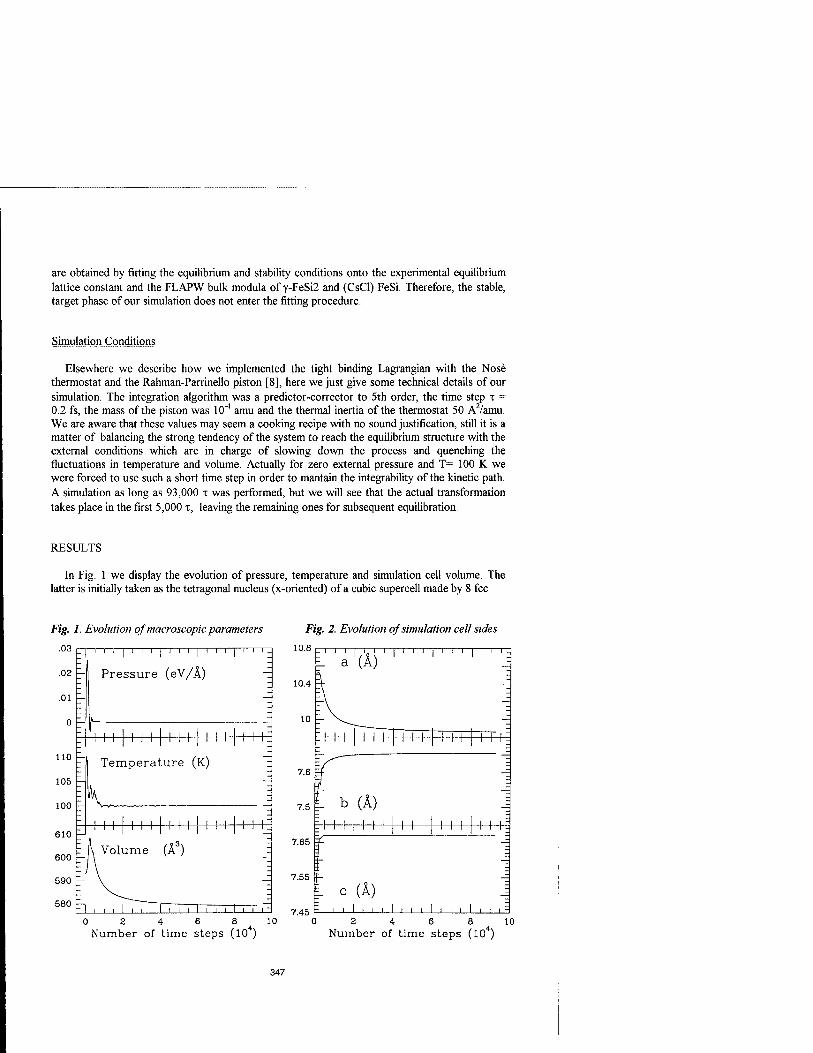
are obtained by fitting the equilibrium and stability conditions onto the experimental equilibrium lattice constant and the FLAPW bulk modula of y-FeSi2 and (CsCl) FeSi. Therefore, the stable, target phase of our simulation does not enter the fitting procedure.

Simulation Conditions

Elsewhere we describe how we implemented the tight binding Lagrangian with the Nose thermostat and the Rahman-Parrinello piston [8], here we just give some technical details of our simulation. The integration algorithm was a predictor-corrector to 5th order, the time step x = 0.2 fs, the mass of the piston was 10"4 amu and the thermal inertia of the thermostat 50 A2/amu. We are aware that these values may seem a cooking recipe with no sound justification, still it is a matter of balancing the strong tendency of the system to reach the equilibrium structure with the external conditions which are in charge of slowing down the process and quenching the fluctuations in temperature and volume. Actually for zero external pressure and T= 100 K we were forced to use such a short time step in order to mantain the integrability of the kinetic path. A simulation as long as 93,000 x was performed, but we will see that the actual transformation takes place in the first 5,000 x, leaving the remaining ones for subsequent equilibration.

RESULTS

In Fig. 1 we display the evolution of pressure, temperature and simulation cell volume. The latter is initially taken as the tetragonal nucleus (x-oriented) of a cubic supercell made by 8 fee

Fig. 1. Evolution of macroscopic parameters Fig. 2. Evolution of simulation cell sides

.03

.02

.01

0

110

105

100

610

600

590

580

I I I I I I I i I I | I I i | i i

Pressure (eV/Ä)

I 1 ] I I I | I 1 I 1 I 1 I | I I I

1 Temperature (K)

I I I I I I 1 | I 1 I | I I I ] I I I

Volume (Ä )

-1 i i i 1 i i i I i i i i i i i I i r i 0 2 4 6 8 1

Number of time steps (10 )

10.8

10.4

10

7.6

7.5

7.65

7.55

H ' ' I 'o' ' I ' ' ' I ' ' E- a (A)

I 1 I I 1 I I I I I I I \-+++

b (Ä)

l l I I I I I I I I I I i [ i:

(A) 7.45

0 0 2 4 I ! ! , I , I I I , 1 I I

6 8 10 Number of time steps (10 )

347

units, where a is two times the fee edge and b,c are the diagonals of the fee square faces. Fig. 2 reproduces their modification which correctly ends up very near the orthorhombic values. Also the atomic positions inside the simulation cell (taken as the average for the last 500 x) agree very well to the experimental structure and in Fig. 3 we report a comparison of the radial distribution functions for the initial (fluorite) configuration, the final one and the experimental structure. In Fig.4 we follow the evolution of the electronic density of states (DOS), which confirms that a metal-semiconductor transition is taking place.

Fig. 3. Comparison of the pair distribution functions for intial, final and target structures.

0

vS4

0

6

CaF2

1111111111111

M-M

M-Si

Si-Si

i i i I i i i i i i i

1.5

: M-M

1 h-

.5

0

1.5

.5

0

1.8

1.2

— .6

jß(sim.)

M I I M I | I I I | l_

jS(exp.)

— l

.5

M-Si :

Si-Si -

I ■ I I IM'll I I I I 1

1.5 iiiIi i i I I i i |i

- M-M

0

1.5

1

1.2

0

M-Si

Si-Si

' ' ' i i i i i

2 2.4 2.8 3.2 2 2.4 2.8 3.2 2 2.4 2.8 3.2

(A)

348

Fig. 4. Evolution of the electronic density of states (DOS), dashed line is the Fermi level.

2 CO

en o Q

-10 0 -10 0

ENERGY (eV) ENERGY (eV)

It is interesting to note that after the early lowering of the high density peak at the Fermi energy, the actual gap opening occurs only inbetween 4000 and 5000 t, as a consequence of the sudden displacement of a reduced set of atoms (two Fel, two Sil and two Sill units) [8]. Everything is concluded within the first 5000 x and the remaining time is used for a slow equilibration of the cell volume, especially along x, y.

In order to check that the peculiar position of the Fermi level is responsible for the driving force in the structural transition we have performed the same simulation for CoSi2, which is

349

stable in the fluorite structure, with a tight binding potential suitably fitted for cobalt suicides. Actually the shape of the density of states is very similar to fluorite FeSi2, but for the Fermi level position which lies at higher energies, as due to the extra electron per cobalt atom, in a low density region. The sample remained essentially in the initial configuration.

ACKNOWLEDGMENTS

We thank Vittorio Rosato and Fabrizio Cleri (ENEA, La Casaccia) for contributions on the isothermal-isobaric code. One of us (M.C.) was supported by the ENEA grant # 1896/INN/ 21.06.95. We also thank Stefano Lanzavecchia and Stefano Sanguinetti (University of Milano) for preparing the 3D figures. Work partially supported by the European HC&M Program, contract # CHRX-CT930318.

REFERENCES

1. N.E. Christensen, Phys. Rev. B 42, 7148 (1990).

2. H. von Kaenel, R.Stalder, H.Sirringhaus, N.Onda , J.Henz, Appl. Surf. Sei. 53, 196 (1991); AL.Vazquez de Parga, J.De la Figuera, C.Ocal R Miranda, Europhys. Lett. 18, 595 (1992); Le Thanh Vinh, J.Chevrier J.Derrien, Phys. Rev. B 46, 15946 (1992); H.Ch.Schaefer, B.Roesen, H.Moritz, A.Rizzi, BLengeler, HLuth, D.Gerthsen, Appl. Phys. Lett. 62, 2271 (1993).

3. Leo Miglio and Giovanna Malegori, Phys. Rev. B 52, 1448 (1995).

4. Leo Mglio, Francesca Tavazza and Giovanna Malegori, Appl. Phys. Lett. 67, (1995).

5. H. von Kaenel, C. Schwarz, S. Goncalves-Conto, E. Mueller, L. Miglio, F. Tavazza and G. Malegori, Phys. Rew. Lett. 74, 1163 (1995).

6. J.C. Slater and GF. Koster, Phys. Rev. B 94, 1498 (1954).

7. W.A. Harrison. Electronic Structure and the Properties of Solids (W.H. Freeman Company, San Francisco 1980).

8. Leo Miglio, Massimo Celino, Valeria Meregalli and Francesca Tavazza, unpublished.

9. K. A. Maeder, H. von Kaenel and A. Baldereschi, Phys. Rev B 48, 4364 (1993).

350

PREDICTION OF A VERY HARD TRICLINIC FORM OF DIAMOND

G. BENEDEK, M. FACCHINETTI, L. MIGLIO, S. SERRA. Istituto Nazionale di Fisica della Materia, Dipartimento di Fisica, Universita' di Milano, via Celoria 16,1-20133 Milano (Italy)

ABSTRACT

In a theoretical search for new hypotetical sp3-bonded carbon structure containing five-fold rings as a possible result of fullerene transformation under pressure, we have found a triclinic form of diamond with 16 atoms per unit cell which we called tcl-16. We have calculated the ground state structure, the cohesive energy, the bulk modulus and the electronic density of states by means of tight binding molecular dynamics (TBMD). Finally we have compared the phonon spectra at T to existing Raman data for a non-cubiaphasa of diamond.

INTRODUCTION

The progress made in growing diamond films and diamond-like films has brought new interest in the identification of new possible allotropes of carbon in order to improve our knowledge of its phase diagram and, in turn, favours the identification of new phases and allotropes which can appear in the synthesis of diamond-like films. Since the calculation of Fahy and Louie [1], it became clear that these allotropes should be found only as three-fold or four-fold coordinated structures, any higher coordination having too low stability. As a consequence these studies have been concentrated only onto these two cases.

The present study has been stimulated by the conjecture that the presence of five-fold rings in an sp3 network may increase the stiffness of diamond-like materials. Moreover it may give an alternative and more favorable way of reconverting the fullerite structure under moderate pressure. We have predicted a possible sp3 triclinic form of diamond with 16 atoms per unit cell, which we have called tcl-16. This new phase is characterized by periodic arrays of five-fold, seven-fold and six-fold rings Fig. 1 right panel. We have calculated the structural and electronic properties of this new phase by means of tight binding molecular dynamics (TBMD), based on very flexible potential that we have previously developed [2]. We have found that tcl-16 has a high stability and a large bulk modulus, comparable to body-centerd (BC8) and simple tetragonal (ST 12) phases [1], which makes it an interesting and competitive new hypothetical material.

RESULTS

The tcl-16 phase

The tcl-16 phase can be generated through the rebonding of the bct-4 phase. The bct-4 phase is an all sp2 phase proposed by Hoffman et at. [3] and calculated by Liu and Cohen [4], who found it relatively stable (0.3 eV above diamond). The bct-4 crystal consists of buckled layers of carbon chains joined by bonds parallel to the c axis (see Fig.l left panel) and displays a body centered tetragonal unit cell with 4 atoms per unit cell. It has been predicted to be mechanically stable with

351


respect to the transformation into diamond. A similar phase of hexagonal symmetry, called H-6 [5], was instead found to be mechanically unstable with respect to the same transformation.The basal planes of H-6 and bct-4 are very similar to the (111) and the (100) diamond surface, respectively . As a consequence it was suggested that it would be possible to grow a bct-4 carbon crystal as a pseudomorphic phase on the diamond (100) surface. As can be seen from Fig.l, bct-4 is constitued by large rings of 10 atoms. This large rings are unstable towards rebonding which leads to smaller rings.

bct-4

c-axi

a-axis

Fig.l Left panel: bct-4 crystal structure with the additional bonds (in black) considered in the rebonding procedure. Right panel: resulting crystal structure of tcl-16

In Fig.l (left panel) we show a possible rebonding process which generates tcl-16 from bct-4. A compression along a and b axes directly leads to the closure of the large 10-membered rings, giving pentagons and heptagons along two crystallographic directions and hexagons along the third one. This transformation involves continous deformations without any bond breaking, so that this transformation path should have a comparatively low barrier and might occur even at low temperature. The resulting sp3 structure has a triclinic symmetry and has 16 atoms per unit cell. (Fig.l right panel).

In Fig.2 we show a two-dimensonal projection of tcl-16 unit cell along two different crystallographic directions, which shows the characteristic periodic array of five-fold and seven- fold rings along a and b and six-fold rings along the c axis. From the topological point of view bct- 4 is a Platonic 3-connected net (103)4 [6], while tcl-16 is a 4-connected net (63527)16. This means that two of the six shortest rings is 5-fold against only one 7-fold ring. The conjecture about a large stiffness of tcl-16 relies on this topological argument.

Both the equilibrium distribution of atoms within the unit cell and the unit cell which minimize the total energy have been determined by using TBMD based on the Serra, Molteni, Miglio (SMM) carbon potential [2]. This potential, which includes many body terms also in the repulsive part, is able to reproduce very well the phase diagram of carbon including the amorphous and

352

liquid phases. The computational scheme that we have adopted is the following: we fix the parameters a and da of the cell and let the atoms freely relax to their ground state by a simulated annealing (SA) technique. Then, starting from these atomic positions, we slightly adjust the values of a or da and iterate the SA run. We have repeated these procedure for several unit cells until the global minimum was found. In Fig.3 we show the resulting bond length and bond angle distributions. The labels here indicated correspond to those of Fig.2, so that angles and bonds can be easily identified. Owing to the low symmetry, the number of unequivalent bonds is quite large, resulting in a sensible spread of the bond length and bond angles.

a axis a axis Fig. 2. Two-dimensional representation of tcl-16 structure along a, c axes and a, b axes

1.5 2 2.5 r (Ä)

100 110 120 0 ( degrees )

Fig. 3 Bond lenght distribution of tcl-16 (left panel"), and bond angle distribution (right panel)

We have found the most stable configuration with the basis vectors of the crystal lattice ab c equal to (d,0,0), (0,d,0), (d/4,d/4,f), respectively, with d=4.558 A and f=4.507 A. Actually a doubling of the third basis vector to (d/2,d/2,2f) yields a bet unit cell with 32 atoms.

353

The bulk modulus was calculated by fitting the total energy curve by the Murnaghan equation of state [7]. The total energy curve was obtained by accurately calculating the total energy of the crystal for different volumes, within the same tight binding (TB) scheme. Taking full advantages of the relatively low computational cost of the semiempirical TB, we used a very high number of k- points in the Brillouin Zone of the crystal. We have found that our tcl-16 is more stable than bct-4, conferming the plausibility of the rebonding procedure. The cohesive energy turns out to be only 0.23 eV above that of diamond against 0.3 eV for the bct-4 structure. Moreover, it turns out to be the hardest phase (to our knowledge) after the hexagonal (lonsdaleite) and cubic diamonds forms, with a bulk modulus of 413 GPa.

In Table I we summarized the results found for tcl-16 in comparison with diamond and other known phases.

PHASE Cohesive energy (eV)

per atom

Equilibrium Volume (A3/atom)

Bulk modulus (GPa)

ref Diamond 0.0 5.64 442 [1]

Lonsdaleite 0.02 5.66 440 ni tcl-16 0.23 5.85 413 BC-8 0.69 5.6 411 m

bct-4 (sp2 ) 0.3 6.65 362 [41

Table I. Equilibrium cohesive energy referred to the value of diamond, equilibrium volume and bulk moduli of some carbon phases.

M I I I I I I j I j I I I I j I I I I I I I I I | I

diamond

sp hybrid

-20 -15 -10 -5 0 5

energy ( eV ) -20 -15 -10 -5 0 5 10

energy ( eV )

Fig. 4. Electronic density of states of diamond (left panel) and tcl- 16 (right panel) in comparison

Also the high density of this new phase is remarkable. This is only slightly smaller than that of diamond and is consistent with the high stability and bulk modulus. The smaller value of the bulk modulus with respect to diamond is due to the elongation of the bonds on the principal diagonal of the cell, which produces an increase in the mean bond length and a decrease in the density. Concerning this point, we remind that the bulk modulus B, as it has been shown by Cohen [8], is

354

inversely proportional to the bond length. Unfortunately this effect overcompensates the stiffening of the bonds induced by pentagons and yelds an overall softening of the bulk modulus.

In Fig.4 we show the electronic density of states (EDOS) of tcl-16 and diamond, with the s or p characters of the electronic states indicated. It can be seen that the gap is only slightly increased (5.55 eV instead of 5.5 eV). The s band at lower energy is wider with respect to diamond while the p band becomes more localized, resulting in a lacking of the sp ibrid peak, which is characteristic for diamond.

c IB

e a

a (8

V) o a c a c

ii to*

500 1000 1500

wave number [cm ]

Fig. 5. Comparison between experimental Raman data [9] and vibrational spectrum obtained by the simulation.

Finally we remark that, the relatively high stability of tcl-16, which is comparable to BC8 and ST 12 phases, makes it a serious candidate for an alternative transformation path from sp2 to sp3

networks of and can be competitive with the other well known sp3 crystals. We have shown the plausibility of this arguments in a particular case ( from bct-4 to tcl-16). In this case a conversion into tcl-16 seems to be easier than back to diamond. But also in the polimerization of COO fiillerites under pressure [9] tcl-16 could be involved. The presence of pentagons in COO could favour the

355

transformation into our phase rather than diamond, lonsdaleite or BC8 sp3 networks, which are constituted only by hexagons. These phases should have a higher energy barrier for their transformation, needing a higher atomic rearrangements which is more difficult at least at the relatively low temperature (700-900 K) at which these experiments are carried out. As a matter of fact Kozlov et al. [10] have found the presence of a non-cubic (nor hexagonal) phase of diamond in diamond films produced by laser ablation of fullerites compressed at 2.6 GPa at the temperature of 700 K. In Fig. 5 we compare the phonon spectra in T obtained with TBMD and the Raman spectra obtained by Kozlov et al. [10].

Unfortunately the samples are not yet so good to make a realistic comparison between these different sets of data. In particular the high frequency part of the Raman spectra (around 1500 cm- 1) is completely absent in our data. It is probably due to graphitic regions behind them. Moreover, the structures at low frequencies not present in our spectrum, should be due to impurities in the samples. Anyway some general feature are similar, in particular in the medium range of frequencies the peaks show a certain correspondence. At the present level of study we cannot say whether this could be an experimental evidence for the tcl-16 phase.

Under suitable conditions the hardness is proportional to the Young modulus Y which, in turn is proportional to the bulk modulus B and the Poisson ratio V, Y=3(l-2v)B. In this work we take B as a measure of hardness neglecting the dependence of V on the structural difference between diamond and tcl-16. In a forthcoming paper we will present a complete calculation of the hardness depending on the crystal orientation.

ACKNOWLEDGMENTS

We thank dr. M. Kozlov for useful comments and for sending their experimental data prior to publication.

REFERENCES [1] S. Fahy and S.G.Louie, Phys. Rev. B 36, 3373, (1987) [2] S.Serra, C.Molteni and L.Miglio, J.Phys.: Condens. Matter 7, 4019, (1995) [3] R. Hoffman, T. Hughbanks, M. Kertesz, and P.H. Bird, J. Am. Chem. Soc. 105, 4831, (1983) [4] A.Y. Liu and M. L. Cohen, Phys. Rev. B 45, 5479, (1992) [5] A.Y. Liu and M. L. Cohen, and K.C. Hass, M.A. Tamor, Phys. Rev. B 43, 6742, (1991) [6] A.F. Wells, Three-Dimensional Nets and Polyhedra, John Wiley & Sons, New York 1976 [7] F.D. Murnaghan, Proc. Natl. Acad. Sei. U.S.A. 3, 244, (1944) [8] Marvin L. Cohen, Phys. Rev. B 32, 7988, (1985) [9] M.E. Kozlov, M.Hirabayashi, K.Nozaki, M.Tokumoto and H.Ihara, Appl. Phys. Lett. 66, 1199,(1995) [10] M.E. Kozlov, K.Yase, N. Minami, P.Fons, H.A. Durand, M.Hirabayashi, K.Nozaki, M. Tokumoto and H. Ihara, Proc ECS Meeting, (to be published)

356

Cu-Au ALLOYS USING MONTE CARLO SIMULATIONS AND THE BFS METHOD FOR ALLOYS

GUILLERMO BOZZOLO*, BRIAN GOOD" AND JOHN FERRANTE** * Analex Corporation, 3001 Aerospace Parkway, Brook Park, OH, 44142-1003 "National Aeronautics and Space Administration, Lewis Research Center, Cleveland, OH 44135.

ABSTRACT

Semi empirical methods have shown considerable promise in aiding in the calculation of many properties of materials [1,2]. Materials used in engineering applications have defects that occur for various reasons including processing [3]. In this work we present the first application of the BFS (Bozzolo, Ferrante and Smith) method for alloys [1] to describe some aspects of microstructure due to processing for the Cu-Au system (Cu-Au, CuAu3, and Cu3Au). We use finite temperature Monte Carlo calculations, in order to show the influence of 'heat treatment' in the low-temperature phase of the alloy. Although relatively simple, it has enough features that could be used as a first test of the reliability of the technique. The main questions to be answered in this work relate to the existence of low temperature ordered structures for specific concentrations, for example, the ability to distinguish between rather similar phases for equiatomic alloys (CuAu I and CuAu II, the latter characterized by an antiphase boundary separating two identical phases).

Engineering materials have defects that result from annealing and processing procedures. Ideal thermodynamic equilibrium is rarely achieved in the laboratory processing of the actual alloy, particularly for large scale structures. It is of interest, therefore, to simulate these procedures. In this paper we use Monte Carlo methods [4] to simulate processing and the BFS method [1] for system energetics. We start from a random distribution at high temperature, examine the structure by freezing the solid at various temperatures, and examine the micro-structure. The organization of the paper is as follows: first we discuss the Monte Carlo procedure, then give a brief description of the BFS method and finally examine defects appearing as a result of "quenching" the solid.

The Monte Carlo procedure employed is a variant ofthat used to simulate the Ising system. The computational cell used consists of 1008 atoms arranged on a face-centered cubic lattice. Boundary effects are minimized by the use of periodic boundary conditions. Each lattice site is characterized by the species of atom (i.e. Cu or Au) occupying the site. The initial state of the computational cell is a random alloy having a specified composition. The cell's lattice constant is assumed to depend only on composition and its variation with temperature is ignored. The lattice constant is determined from static zero-temperature BFS calculations (to be discussed below).

A sequence of temperatures (the "cascade") is chosen, and the system is allowed to equilibrate sequentially at each temperature (simulating the "slow cooling" of the alloy starting from a disordered solid solution) via a procedure where pairs of atoms of opposite species are chosen randomly for reversal. The reversal is accepted or rejected using the Metropolis criterion. Because of the above imposed restrictions, the temperature enters into the simulation only through the Met- ropolis criterion [4]. After equilibrium (based on the total energy), the simulation is allowed to proceed further in order to compute and average various properties such as the energy of the cell, the specific heat, and bond correlations.

While these simulations do not attempt to mimic the detailed dynamics of equilibration, they do offer a qualitative view of the effects of rapid versus slow cooling. The temperature treatment

357


(that is, the sizes of the steps between temperatures in the cascade) is of critical importance in determining the final state of the system. Slow cooling results in a highly-ordered low-temperature state, while rapid cooling results in an alloy with grain structure, in which each grain has essentially the ordering of the thermodynamic ground state.

The current simulation procedure does not allow for relaxation of neighbors of atoms whose species have been reversed. In cases where the lattice constants of the two species are substantially different (which is the case in the Cu-Au system), neglecting such relaxation may result in a significant error in the phase transition temperatures. In order to eliminate this limitation, we have begun follow-up work on the Cu-Au system in which the lattice is relaxed via a molecular dynamics process, while the system is ordered concurrently using the described Monte Carlo procedure. We are developing our computer code for a 16-processor SP2 parallel processing computer using the PVM environment.

The phase diagram of Cu-Au [5] indicates that a solid solution exists for the whole range of concentration, with well defined order-disorder transitions, that lead to simple Ll2 (for CuAu3 and Cu3Au) and Ll0 (for CuAu) fee ordered structures. Of special interest is the ordering for equiatomic alloys. For a narrow range of temperatures, there is a long-period superlattice (CuAu II) with an antiphase boundary (APB). While antiphase boundaries introduced by plastic deformation belong to the microstructure of the alloy, the former belongs to the phase. On either side of the APB, the alloy has the Ll0 structure, which for lower temperatures is the only phase found for the Cu-Au alloy (CuAu I). The purpose of this work is to determine the ordered structures of Cu-Au as a function of composition by means of Monte Carlo simulations and to examine the influence of the temperature (heat) treatment in the simulation in relation to the type of ordering found. The energetics of the system are calculated with the BFS method for alloys, which has been successfully applied to the study of other properties of the Cu-Au system. In what follows we provide a brief description of the BFS method and some comments on the Monte Carlo calculations, followed by a discussion of the main features of the Cu-Au phase diagram obtained in this work.

The BFS method is based on the idea that the energy of formation of an alloy is the superposition of individual contributions £; of non-equivalent atoms in the alloy [1]:

s,=e? + gd£?-£?°)- t1)

Si has two components: a strain energy £S, computed with equivalent crystal theory (ECT) [6], that accounts for the actual geometrical distribution of the atoms surrounding atom i, computed as if all its neighbors were of the same atomic species, and a chemical energy ec - ec°, which takes into account the fact that some of the neighbors of atom i may be of a different chemical species. For ef we interpret the chemical composition as a defect of an otherwise pure crystal. We represent this defect by 'perturbing' the electronic density in the overlap region between dissimilar atoms and locating them at equilibrium lattice sites of atom i. The ideas of ECT [6] are used to develop a procedure for the evaluation of the energy associated with this 'defect'. To free the chemical energy of structural defect energy which should only be included in the strain energy, we reference ef to a similar contribution where no such perturbation is included (ef°). The coupling function gt, which ensures the correct asymptotic behavior of the chemical energy, is defined as ff, = e~a- , where a; is

a solution of sf = -E'c [l - (1 + af)exp(-af)} (see ref. [7]), and where E'c is the cohesive energy for atom i. In the context of BFS, the terms 'strain' and 'chemical' represent quite different effects than the usually assigned meanings. For a clear understanding of this paper, we direct the reader to Ref. 1 where a detailed description of the calculation of the strain and chemical energy contributions is provided. Except for two parameters determined by fitting to experimental or theoretical alloy properties, the method relies on pure element properties. The parameters used in this work have been previously used, with a great degree of success, in BFS applications to the Cu-Au system, including surface segregation as well as multilayer surface relaxation studies [1,6].

358

There are some general observations regarding the results of the current study. Most simulations were performed following a 'cascade' process: starting with a random configuration at very high temperature, the cell was stabilized for successive temperature steps, which could be loosely related to a slow cooling of the actual alloy starting from a disordered solid solution where temperature treatment of the sample is essential in determining the final state. Slow cascade always resulted in highly ordered compounds at low temperatures, with very few antisite defects, whereas sudden cooling results in an alloy with grain structure, where each grain has basically the ordering pattern expected for the thermodynamic ground state. This process can be understood as if the quenching of the sample 'freezes' ordered domains within the cell, whose seed is already present in the initial disordered state.

We examined the final states of 'cascades' for three concentrations: 25, 50 and 75 at. % Au. At low temperatures these structures follow the LI2 (Cu3Au and CuAuß), and the Llo (CuAu I) ordering. The coordination parameter a, which indicates the probability that a Cu atom has a Au atom as a nearest-neighbor, should attain the values 0.3333 (CU3AU), 0.6667 (CuAu I) and 1.0000 (CuAu3) if perfect order was achieved. In our calculations these values are 0.3327,0.6630 and 0.9940, respectively. The final temperature for each one of these three alloys is T=100K.Slow cooling of certain disordered alloys to temperatures in the 400 K range result in the CuAu II structure, with a clearly defined APB, as seen in Fig. 1. The size of the computational cell limits the periodicity determined for this structure, which is found to be somewhat smaller than the experimental value. Still, it is significant that the high temperature phase is obtained with the current approach. Finally, sudden cooling of a disordered alloy results in partially ordered alloys, as shown in Fig. 2. Close examination of the final cells shows the possibility of identifying domains within the computational cell which essentially follow Llo ABAB stacking for the equiatomic case (Fig.2(b)) and LI2 ordering for alloys with 25 and 75 at. % Cu. To guide the eye, Fig. 2 shows a deformed computational cell for each concentration, where different (Fig.2(a),(c)) regions showing LI2 ordering can be seen. The Llo ordering can be seen in more than one direction. In order to highlight this, Fig. 3 shows a front view of quenched CuAu, where some domains are indicated as well as their orientation relative to each other.

In spite of the microstructure of the alloys shown in Fig. 2 there is a high degree of ordering as measured by the probability of an atom A having a nearest-neighbor of species B. If A denotes a Cu atom, this quantity should have the values 1.0, 0.6667 and 0.3333 for CuAu3, CuAu, and Cu3Au, respectively. As mentioned, slow cooling yields 0.9940, 0.6630 and 0.3327. The corresponding probabilities for Fig. 2 are 0.9735, 0.6524 and 0.3208, respectively, thus indicating that the domains of Llo and LI2 ordering locate themselves to optimize the expected coordination. The degree of order, size and abundance of domains is clearly a manifestation of the short range ordered that exists in the high temperature alloy.

None of the restrictions imposed if lifted, are expected to lead to a qualitatively different outcome. In all cases, the initial state for the Monte Carlo simulation was random at a very high temperature (5000 K), obviously well beyond the melting temperature. However, the atoms were constrained to equilibrium lattice sites. Moreover, no local relaxations were allowed, thus eliminating the possibility of tetragonal distortion. The computational cell was restricted to retain a constant volume, the main effect of which could be the degree of ordering achieved at each temperature. It might be safe to assume that this limitation will not alter the essential nature of the final state, i.e. the type of ordering found.

In conclusion, we have proposed the use of Monte Carlo techniques with the BFS method for energetics in order to simulate certain aspects of alloy processing for Cu-Au, namely, slow cooling and rapid quenching. This approach appears to reproduce some features of processing. Slow cooling to 100 K produces a single crystal for each alloy examined. Slow cooling to 400 K produces the CuAu II structure with antiphase boundaries as observed experimentally. Rapid cooling gives a granular micro-structure with grains having the equilibrium ground state structure of each alloy

359

studied. This Monte Carlo procedure could then be a possible non-dynamic method for studying the effects of alloy processing.

REFERENCES

1.. G. Bozzolo, J. Ferrante and J. R. Smith, Phys. Rev. B 45, 493 (1992); G. Bozzolo and J. Ferrante, Scr. Met. Mater. 26, 1275 (1992); Phys. Rev. B 45, 12191 (1992); Phys. Rev. B 46, 8600 (1992); Ultramicroscopy 42-44, 55 (1992); G. Bozzolo, B. Good and J. Ferrante, Surf. Sei. 289, 169 (1993); B. Good, G. Bozzolo and J. Ferrante, Phys. Rev. B 48, 18284 (1993); R. Kobistek, G. Bozzolo, J. Ferrante and H. Schlosser, Surf. Sei. 307-309, 390 (1994).

2. M.S. Daw, S.M. Foiles and M.I. Baskes, Mat. Sei. Reports 9, 251(1993). 3. P. Haasen, Physical Metallurgy, (Cambridge University Press, Cambridge, New York,

Melbourne, 1978). 4. N. Metropolis, A.W. Rosenbluth, M.N. Rosenbluth, A.H. Teller and E. Teller, J. Chem.

Phys. 6, 1087 (1953). 5. M. Hansen and K. Anderko, Constitution of Binary Alloys, p.198, (McGraw Hill Book

Co. Inc. 2nd ed., New Yourk, Toronto, London 1958). 6. J. R. Smith, T. Perry, A. Banerjea, J. Ferrante and G. Bozzolo, Phys. Rev. B 44, 6444

(1991) 7. J. H. Rose, J. R. Smith and J. Ferrante, Phys. Rev. B 28, 1835 (1983); J. H. Rose, J. R.

Smith, F. Guinea and J. Ferrante, Phys. Rev. B 29, 2963 (1984).

Fig. 1: Final geometry for slow cooling to 400 K (CuAu II).

360

Fig. 2 Expanded cells for quench cooling to 400K: (a) CuAu.3, (b) CuAu, and (c) CU3A11 showing resulting grain structure. Solid spheres denote Cu atoms.

361

Fig. 3 End view of Fig. 2 (b) showing domains with ABAB structures in each direction following quench cooling to 400K. Solid spheres denote Cu atoms.

362

CLUSTERING AND EXTENDED RANGE ORDER IN BINARY NETWORK GLASSES

Dmitry NEKHAYEV and John KEFFER Department of Materials Science & Engineering, University of Illinois, Urbana IL 61801

ABSTRACT

The clustering in alkali silica glasses (M20)x(SiO2)i-x, where M is either Na or Rb, and x ranges between 0 and 0.4, was studied using molecular dynamics simulations. Computations were performed using a semi-empirical potential, including two- and three-body terms as well as dynamic partial charge transfer. Characterization of the structures was based on pair correlation functions, neutron static structure factor and ring statistics. Results have shown a much stronger tendency to cluster in case of Na than of Rb. The irregular arrangement of Na is evidenced by a decay pattern in the Na-Na pair correlation function, which can be associated with a fractal dimension. The clustering tendency can be attributed to the differences in the way the network structure is able to accommodate the introduction of modifying cations. As opposed to Rb, the smaller Na cation can fit on sites only slightly larger than is required for Si. This would distort the structure but hardly alter its topology. Rb on the other hand, requires larger interstices, which results in a reconstruction of the network and a significantly different intermediate range order. Na can achieve a similar influence on the network structure if they group in pairs.

INTRODUCTION

Structure of alkali silica glasses has been extensively studied using different experimental techniques^1'5) Based on these investigations the description of the structure of this class of materials is commonly given in terms of a modified random network model (MRN)/6) in which the sites of alkali cations delimit regions of a more intact network. This model implies a tendency of modifier cations to cluster, a tendency which should be indicative of that to undergo phase separation. Analysis of this effect at atomic scale demands the knowledge of structural correlations beyond the short-range order. Current experimental methods, however, do not provide access unambiguously to this length scale. Molecular dynamics simulations are routinely used to assist in the interpretation of experimental signals, such as neutron scattering spectra^7"8)

With the advent of massively parallel computing environments, there is much incentive to revisit the issue of clustering and phase separation, since the extended-range order in simulated structure becomes more readily accessible. Along with a larger amount of data, often times comes an increased difficulty of processing the information. In the present paper we will concentrate on methodologies of structural analysis which we developed for the study of large systems, and which permits relevant insights already with much smaller systems.

COMPUTATIONAL PROCEDURE

The interaction potential used in these simulations included a repulsive Born-Mayer term, a Coulomb term, whose long-range effects were handled by an Ewald summation, and three-body terms to represent the directional covalent bonding/9) The potential parameters were optimized such as to reproduce experimental data for crystalline silica at room temperature and zero pressure, including density, Si-0 bond distance, as well as infrared and Raman spectra. The potential function so obtained allows for the simulation of the a- to /J-cristobalite phase transformation, in both directions and requiring no adjustments in either state. All optimization was done on systems containing 648 particles.

One important detail of the potential, which we introduced specifically for the study of binary silicates, is the dynamic charge transfer between atoms, which is invoked whenever a covalent bond is formed or broken. This feature has been designed to account for non-bridging oxygens in a more realistic way, since these have a different effective charge than the bridging oxygens of the silica network. Since the identities of non-bridging oxygens cannot be predicted when starting

363


simulations fiom random configurations, the amount of charge localized at the position of each atom is updated every time step, based on the number of neighbors within a cut-off distance and an empirical charge transfer function of the following form:

5ij = CijC-(riJlaiJ)\

where au is a constant chosen such that the function vanishes within the cut-off radius, and Q represents the amount of charge transferred between two bonding atoms. The parameter Q was adjusted so that the same partial charges on silicon and oxygen are generated as were used in previous work (approximately +2.3 for Si and -1.15 for O)/9) The new form of potential was tested for silica glass and crystalline structures for experimental data mentioned aboveA1"-1^


In the following we present data obtained for simulated binary alkali-silicate structures, including a total of 648 atoms, and having the general composition (M20)x(Si02)l-x, where x ranges between 0 and 0.4. The behaviors of two alkali cations, which differ from each other significantly in terms of size and electrostatic field strength, were studied, i.e., sodium and rubidium. For each composition, both systems were started from the same random configuration. The reason for this was to ascertain the reality of any differences in the final equilibrated structures. The systems were thermalized at 8000 K for 10 ps and cooled to 300 K over 100 ps (50,000 time steps at 2 fs). Structural analysis was performed on the final room temperature configurations.

Direct observation of the structures

Direct observation of the structures provides a first qualitative impression and is very useful for guiding the choice or design of the statistical analysis to be performed. The use of stereoscopic visualization improves the clarity of this initial examination. Representative snapshots of a sodium silicate and a rubidium silicate are shown in fig. 1. Careful inspection reveals that in (Na20)x(Si02)i-x , even at small x (between 0.05 and 0.1), Na ions tend to group in pairs. The positive charge of such pairs is neutralized by that of two negative non-bridging oxygens, which is consistent to MRN model. Rb ions, on the other hand, have a much lower tendency to cluster. They appear to occupy random positions throughout the network structure, and their charge is neutralized by bridging and non-bridging oxygens, arranged within a wider spread of distances from the cation.

In the range of x larger than 0.10 clustering in sodium silicates intensifies. The cations torm groups of more than two and seemingly align in channels surrounded by non-bridging oxygens. As will be confirmed below by ring statistics, the network apart from these clusters is relatively undisturbed. But as x increases, the effective volume of bulk silica network decreases, and for x>0.30 extended network segments with a structure similar to that of pure silica glass are no longer obvious. For the same range of x in rubidium silicates, proximity between alkali cations is inevitable due to their large concentrations. Cations are still positioned randomly up to the largest mole-fractions. This situation is the result of significant changes in the intermediate range structural order of the silica network, as will be shown below.

Silica network neutron static structure factor

The total static structure factor, as measured by neutron scattering, contains contributions from all constituents of the structure. Numerical simulations, however, allow one to trace how a change in composition affects the static structure factor of silica network by itself. This can be achieved by simply assigning a zero scattering cross section to the alkali cations. These 'network structure factors' are shown for all simulated systems in figs. 2 a and b. A significantly different behavior can be observed for the two systems. The structure factor for pure silica exhibits maxima near 80, 53, and 30 nm , corresponding to short-range structural correlations/11) and a first sharp diffraction peak (FSDP) at 16 nm , which has been explained as due to neutral Si(04)i/2 tetrahedra.(12) In sodium silicates the position, intensity and widths of the short range order peaks does not change significantly with increasing alkali content, whereas in rubidium silicates the

364

r=o^^f •ÖZ~Q/**"-i t3*(P ]»ir T^SLO ' J*^ ivTT*^» L2&P £S£ä&*7

lipyß1

Xk$tPi ^fy*m*/^

-f f^kijC hcJ^%

o? &*9-bßrk LT\^

" °T\

Fig 1. View of the simulation box for (M20)x(Si02)i-x, M=Na (left) and Rb (right), x=0.05. light circles represent oxygen atoms, gray - silicon atoms and large dark - alkali ions.

3

c C/3

3

c

0 20 40 60 80 100

q (nm'1) 0 20 40 60 80 100

q (nm"1) Fig 2. Transformation of Si-0 network neutron static structure factor for (M20)x(Si02)l-x binary glasses,

x=0.00-0.40, M=Na (a) and Rb (b). Lowest graphs correspond to x=0.00, highest - x=0.40.

365

amplitudes and widths of these peaks decrease by up to a factor of 2. The behavior of FSDP differs even more between the two systems. In case of Na the position

of the FSDP remains virtually the same throughout the entire composition range. Its intensity decreases very slightly with increasing alkali content, and for mole fractions of 0.15 and 0.2, splitting of the peak is indicated. A weak shoulder around 8 nnr1 is also visible for most compositions. In case of Rb a splitting of the FSDP into three peaks is quite obvious. The strongest of these peaks shifts towards lower wavenumbers with increasing alkali concentration. At very high x the low wavenumber features reduce to a single peak around 12 nnr1, whose intensity is significantly higher than that of the FSDP in sodium silicates. The main conclusion that can be drawn from this comparison is that large alkali cations greatly affect the short-range order of glass forming network, and that their presence gives rise to extended-range structural correlations.

Ring statistics

Ring statistics is a widely accepted measure of characterization of glass structure in terms of the network topology. Application of this method to simulated structures of pure silica have demonstrated its usefulness in determining the intermediate range order of this structure.^13) Here we employ this tool to elucidate the structural changes that take place in the network as a result of introducing modifying cations. In our analysis we used recently developed shortest-path-ring algorithm to obtain the ring statistics of silica network for all structures.^4) The results are presented on the fig 3. As we expected, the response of the network to presence of Na and Rb ions has similar features and at the same time significant differences.

At low alkali content (x<0.2) a maximum probability exist for encountering 5- to 7-membered rings. As x increases, the probability distribution becomes bimodal, with one maximum occurring around n = 13, and the other one between 3 and 5. This behavior is however much more pronounced in case of Rb. We can observe splitting for Rb at x=0.15, but in case of Na it does not occur before x=0.20. The peak corresponding to larger n has a maximum at 13 for Rb and at 10 for Na, with smaller amplitude. The frequency of small ring sizes, for the same x, peaks at smaller n for Rb than for Na (e.g., for x=0.35, nmax(Na)=4 and nmax(Rb)=3). As we can see, at x>0.30, in case of Rb, a significant amount of two-fold rings appears in the network, which is not the case for Na.

From the above observations we conclude that two types of rings exist in alkali glasses. A first type is characteristic for the bulk silica network. With decreasing network volume fraction, the need for connectivity gives rise to small ring sizes, and introduces strong deformation into the network structure. The fact that for x>0.20, the most probable ring size in rubidium silicate is smaller than that in sodium silicate, and that both are smaller than in pure silica glass, shows that the short-range order of the network is disturbed in both systems, but more so for Rb as the modifier. The second type of ring is the one embracing alkali clusters. Since Na clusters are more closely coordinated by non-bridging oxygens, the characteristic size of these rings lies between 9 and 12. Rb ions, because of their size and coordination requirements, they are surrounded by rings of even larger size.

Study of alkali ion pair correlation function

So far we discussed structural features of silica network as alkali oxide added gradually to the glass. Now we proceed to describe the structural correlations between alkali ions themselves. For all sodium compositions the maximum in the Na-Na pair correlation function corresponding to the first coordination shell occurs at 0.25 nm and has a width of 0.05 nm. In the Rb-Rb pair correlation function this peak occurs at 0.35 nm, and has a width of 0.12 nm (see Fig 4). The difference in the radius of the first coordination shell is straightforwardly related to the difference in cation size. The variation in coordination radius, relative to the magnitude of this radius, is however much larger in case of Rb. This indicates that the positions of Na cations relative to each other are more defined than those of Rb in their respective binary silicate structures.

The spatial cation-cation correlations of Na and Rb also differ over at larger distances, as long as the modifier concentration is less than 0.2. The slope of the cumulative radial distribution function (which is equivalent to the coordination number as a function of the distance), on a log-

366

.a (0

JQ O

Xi (0

o

I ' I 2 6 10 14 18 2 6 10 14 18

Ring size Ring size Fig. 3. Ring statistics of silica network in binary glasses (M20)x(Si02)i-x for different x:

(a) M = Na; (b) M = Rb.

1_

■ £

1 Na-Na

Ijl Rb-Nb

-r-l-T-

|fUtej^ 0 0.2 0.4 0.6 0.8 1

r (nm) Fig. 4. Partial pair correlation functions

for Na-Na and Rb-Rb , x=0.20.

Rb-Rb -fr-«6~v

0.05 0.15 0.25 0.35

X Fig. 5. Fractal dimension df versus x.

Circles are for Na, and triangles for Rb.

367

log scale, gives the Hausdorff fractal dimension that can be attributed to the geometry according to which these cations occupy space. These dimensions are shown in Fig 5. For all rubidium silicate compositions the fractal dimension is close to 3.0, which is in agreement with assumption of a random distribution of alkali ions. The same is true for systems with large sodium concentrations. Below a mole-fraction of 0.2, however, the fractal dimension for the sodium sub-structure decreases, and reaches 2.2 at x = 0.05. This behavior reflects the clustering tendency of sodium, because it means that the probability of finding an cation at a given distance r from another cation, decreases with increasing r. The energetic advantages of such non-uniform spatial distributions of sodium have to be established through the interactions with the silica network, in particular through the arrangements of non-bridging oxygens.

CONCLUSION

Molecular dynamics simulations were performed for a range of compositions of alkali silicate systems, (M20)x(Si02)i-x, where 0 < x < 0.4, and M was either Na or Rb. A refined semiempirical potential function was developed in order to better account for the different nature of bridging and non-bridging oxygens. The simulations showed that the development of the network topology is significantly different for the two alkali silicates. In sodium silicates, the static structure factors that can be attributed to network constituents only, are hardly affected by the increase of sodium concentration, while in rubidium silicates these structure factors reflect the formation of a new short- and intermediate range order. The ring size distribution is evidently bimodal in rubidium silicates, reflecting the new type of interstices which form to accommodate the large alkali cations. In sodium silicates the ring size distribution remains overall more uniform, and deviates less from that of pure silica. The tendency towards clustering of alkali cations was found to be much stronger in sodium than in rubidium silicates, based on the fractal geometry which can be associated with the spatial arrangement of sodium cations.

Acknowledgments: This research was supported by the National Science Foundation (DMR 93- 15779), as well as the US Dept. of Energy by providing computational resources at the Argonne National Laboratory. We also would like to thank Dr. L. Duffrene and F. Li for the stimulating discussions.

References:

1. J. Zarzycki, Rivista della Staz. Sper. Vetro, 5(1990) 13. 2. CM. Shramm, B.H.W.S. De Long V.E.J. Parziale, J. Amer. Chetn. Soc., 106(1984) 4396. 3.1. Farnan, J.F.Stebbins, J. Amer. Chem. Soc., 112(1990) 32. 4. G.S. Henderson, J. Non-Cryst. Solids, 183(1995) 43-50. 5. A.C.Hannon, B.Vessal, J.M.Parker, J. Non-Cryst. Solids, 150(1992) 97. 6. B.E.Warren, J.Biscoe, J. Am. Cer. Soc., 21(1938) 259. 7. B. Vessal, G.Greaves, P.T.Marten, A.V. Chadwick, R.Mole, S.Houde-Walter, Letters to Nature, 356(1992) 504. 8. J. Kieffer, C.A.AngeU, J. Chem.Phys., 90(1989) 4982. 9. D.C.Anderson, J.Kieffer, S. Klarsfeld, J. Chem. Phys. 98(1993) 8978. 10. M.T.Dove, Introduction to Lattice Dynamics, Cambridge Univ. Press 1993 154-159. 11 R.N.Sinclair, A.C.Wright, J. Non-Cryst. Solids 57(1983) 109. 12. H.Iyetomi, P.Vashishta, Phys. Rev. B, 47(1993) 3063. 13. J.P.RÜ10, LEbbsjo, R.K.Kalia, A.Nakano, P.Vashishta, Phys. Rev. B, 47(1993) 47. 14. D.S.Franzblau, Phys. Rev. B, 44(1991) 4925.

368

Phase Stability of the Sigma Phase in Fe-Cr based alloys

Marcel 11.1''. Sluiter. Keivan Esfarjani. and Yosliiyuki Kawazni' Institute lor Materials Research.Tolioku Fniversity. Sendai 980-77, Japan

ABSTRACT

The FeCr sigma phase is a good example of a complex structure: it. has 30 atoms in the unit cell and 5 inequivalem lattice sites, and it. belongs to the class of tetrahedrally close packed structures, also known as Frank-Kaspar structures. So far, such structures have not. been treated within a first-principles statistical thermodynamics framework. It. will be shown that due to advances in algorithms and hardware important features of the phase stability of complex phases can be computed. The factors which affect the stability of the sigma phase have been studied using carefully selected supercells for electronic total energy calculations. Cluster variation calculations in the tetrahedron approximation were performed to evaluate the effect of partial disorder and of finite temperature. The preferred occupancy of the 5 lattice sites has been investigated and is compared with experimental determinations.

INTRODUCTION

In recent years much progress has been made in the first-principles theory of alloy phase stability [1, 2, 3]. So far, these studies have been limited to superstructures of simple crystal structures, i.e. superstructures based on fee, bcc. or hep. The study of complex phases, where several inequivalent sites exist, is of interest both in its own right and for practical reasons. In many commercial alloys, the mechanical properties can be very aversely affected by the formation of complex intermetallics. Outside the area of metallurgy there are widespread uses for materials whose properties critically depend on the low symmetry of its crystal structure, such as for transducers. One of our theoretical motivations is to test the power of first principle methods combined with statistical mechanical treatment of an ising hamiltonian (lattice gas model) in predicting the site occupations in complex phases such as the a phase. Here, we report a new phenomenon of site occupation reversal found in the FeCr a phase[4]: see figure 1.

Figure 1: Orthographic projection of the a unit cell, (a) topview, (b) sideview. Sites A through E have been marked with spheres of decreasing size.

369


Pin' I'VC'r et phase was selected because it is ;m example of a topolouically clo.se parked (lep) plia.se of which there are many representatives|r>j. and also because, in contrast to many other tep phases, much experimental work lias been done on this material [6. 7, 8. 9|. Its unit cell contains 30 atoms which pertain to 5 crystallographically inequivalent sites A, B, C, D, and E, with the occupation numbers 2. 4, 8, 8. and 8, respectively [-1. 5]: its space group is Pii/mimi and the coresponding Pearson symbol is /P30. Three types of coordination occur: the A and D sites are icosahedrally coordinated, the B site has 15 nearest neighbors, and the C and E sites are 14-fold coordinated. The A and D sites are preferentially occupied by Fe atoms, and Cr is found mainly on the B.C, and E sites as has been determined from X-ray, synchrotron radiation anomalous scattering, neutron powder diffraction [6], and Mössbauer spectroscopy [8] experiments. These results were obtained in the region where the a phase is actually stable ie. around the Feo.sCVo.ö concentrations.

The 5 inequivalent sites make for 2° = 32 possible distributions of Fe and Cr atoms. It should be noted that these configurations are not superstructures of the a phase because they all have the same spacegroup. The total energies of these configurations were computed within the local density approximation with the Linear Muffin Tin Orbital (LMTO) method in the Atomic Sphere Approximation (ASA) [10]. The atomic sphere sizes were selected according to the average nearest neighbor distances, given that the a phase is a tcp phase, the smallest and largest sphere radii differed by less than 8%. We found however, that this size difference could not be ignored. Spin polarization was ignored because actual a FeCr is paramagnetic at. ambient temperatures [9]. Integrations in reciprocal space were carried out with the tetrahedron method using 52 k-points in the irreducible wedge. The a and c parameters of the tetragonal a phase, and the cell internal coordinates were held fixed at the experimental values for all configurations [4]. These data can be found in table (I)

Table I: Lattice constants and coordinates of the 5 inequivalent sites in units of a,b and c respectively, along with the degeneracy of each site in the last column.

Site x y z deg eneracy

A 0 0 0 2 B 0.3986 0.3986 0 4 C 0.1312 0.4635 0 8 D 0.2607 0.9339 0 8 E 0.6827 0.3173 0.248 8

=b=16.624 a.u c=8.6134 a.u

Formation energies Eform were computed from the total energies by subtracting the concentration weighted total energies of pure Fe and Cr with the a structure. Effective interatomic interactions V', were extracted from the formation energies with the Connolly-Williams method (CWM) [11]. In this method the effective interactions are determined by solving a linear system given by: EJorm = X!;sf K; where a represents a particular ordered atomic configuration (supercell), & refers to correlation function pertaining to cluster i. A singular value decomposition (SVD) algorithm was used to extract the values for 24 effective interactions. The sets of equations corresponding to thermodynamically stable structures were given more weight than the equations pertaining to unstable structures in the SVD procedure. Here, the word ''interactions'' shall refer both to multi-site terms and single-site terms. From the interactions calculated by CWM. one can calculate the total energies of different configurations. The reproduced formation energies have an rms error of 0.1 mRyd/atom. This error is well within the precision of the LDA calculations, and is much smaller than the smallest difference between the formation energies of any of the 32

370

configurations used in the CWM (see Figure 21.

Figure 2: Energy of Formation (in mRyd/atom) of atomic configurations with the a structure: configurations used with the CWM, as computed with the LMTO-ASA (circles); as computed from the effective interactions (plus'es); configurations not used for the determination of the effective interactions, as computed with the LMTO-ASA (squares); as computed from the effective interactions (crosses). The most stable configurations have been connected with a solid line and the occupancies of the A,B,C,D, and E sites have been indicated.

Fe concentration

Further proof that these interactions accurately represent the LDA formation energies is provided by an additional set of 10 structures [12], which were not used in the CWM type fitting. Figure 2 shows that their formation energies too, are accurately predicted within a fraction of a mRyd/atom.

The interactions were used to compute the site occupancy, entropy, and Helmholtz free energy of the <7 phase as a function of temperature and composition within the tetrahedron approximation of the cluster variation method (CVM) [13]. From the formation energies, one can also deduce the site preference at zero temperature. An analysis is summarized in table (II), the data being taken from figure(2).

Table II: Relative energies of different configurations. The higher energies appear at the higher lines. From the following energy ordering, one can deduce that for example when the site E is occupied by Fe (0) the formation energy is highest, and when occupied by Cr (1) it is lowest (occupation of A and B being the same); therefore Cr prefers to occupy the site E, and likewise one can deduce that it also prefers the site B, while Fe wants to occupy the sites A and D.

l=Cr : 0=Fe ; sites are in the order ABCDE

00110 10110 oiiio 11110 - - 00010 10010 01010 11010

00011 10011 •01011 11011 - - 00100 10100 01100 11100

00101 10101 01101 11101 - - 00001 10001 01001 11001

10110 10101 10011 10100 10010 10001 oiiio oiioi oioii oiioo 01010 01001

From the figure (2), one can see that as the Fe concentration goes down from 1. for example, the sites E and then C and B get respectively occupied by Cr, but toward lower Fe concentrations after the A site gets also populated by Cr, there is an occupation reversal: A gets occupied by

371

Fe again while the D site gets the Cr! This furious composition-dependent behavior persists in a weakened form at finite temperatures, as is shown in figure 3. Furthermore, since there is this net preference for Cr to occupy the sites B, C and E. and lor Fe to occupy the sites A and D (due probably to their size difference), there are two separate regions of concentrations above and below c =~ 0.33. For c < 0.33 the sites B,C,E are almost fully occupied by Cr, and for c. > 0.33 A and D are fully occupied by Fe.

Figure 3: Computed occupancy of the inequivalent sites in the a phase at 500 K as a function of composition; A site (solid), B site (dashed), C site (chain-dotted), D site (chain-dashed), and E site (dotted).

1.00 ' ?!

D/ /

>—' __l j

B / /''

1 j-.

0.75 / /

/ / / /

C .' • / /

0.50 A

/ /

/ / / / / /

^/ / i

/ / ,' /

,* / > i

• / ! /

! /

E /

0.25 / / / / *' /

0

/ / / /* f / : / '

0.2 0.4 0.6 Fe concentration

0.8 1.0

In the context of the Ising-type Hamiltonian it results from competing single-site and multi- site interactions. The single site interactions pertaining to the A and D sites make for a stronger Fe preference of the D site. However, the pair interactions can balance this preference because a D site has a D nearest neighbor, whereas an A site has no A nearest neighbors. If we start with the Cr on each site, and gradually exchange Fe for Cr, it follows that in case the Fe atoms are placed on the A sites only favorable Fe-Cr pairs are formed, whereas if those Fe atoms were placed on the D sites also unfavorable Fe-Fe pairs would result, hence the smaller slope in fig(3) for the D site.

Once all the A sites are filled up the D sites must be filled. At that point, the pairwise disadvantage for the D sites disappears because the A site has 4 D nearest neighbors whereas the D site has only one A and one D nearest neighbor. Clearly Fe occupation of the D sites leads to fewer Fe-Fe type pairs and thus becomes energetically more favorable than the A site occupation. While the D sites get filled with Fe, the A sites are reclaimed by Cr. Only when all the D sites have been filled can be Fe occupancy of the A sites increase again.

This description has been verified by computing the site occupation as a function of composition with all the multi-site interactions set to zero. In that case, the simple site occupation sequence D, A, B, C, and E is found with increasing Fe composition. For the B, C, and E sites our computations do not show such a frustrated site occupation behavior. In principle a structure having 2 or more inequivalent sites can exhibit this feature of site preference reversal.

In actual Fe-Cr alloys it is not possible to verify the site occupation over such a wide span of composition because the a phase has a narrow range of existence. However, around equi-atomic composition extensive studies have been performed [6, 7, 8, 9] and the dominant Fe occupation of the A and D sites is well established, as is the strong Cr preference of the E site. Regarding the B and C sites, our calculations are not in complete agreement with experiment. In actual alloys the B sites are found to have higher Cr occupancy than the C sites, in contrast to our results. One possible cause for the discrepancy is inaccuracy in our calculations due to the simplifying assumptions we have made, among which we can mention: 1) In the total energy calculations, we

372

haw not. included any relaxation of the atoms depending on their site occupancy, in other words, for all the ;S2 considered structures, the coordinates of the 30 sites and the lattice constant were the same. 2) the ASA sphere sizes are select«! according to the average nearest neighbor distances around each site, but selecting different sphere sizes will affect the calculated site preferences somewhat. On the experimental side too, there are complicating factors. For example, impurities can play a crucial role in the formation of the a phase [9]. These issues may not play a role in some of the other a phases. In Fe-V alloys, for example, the a phase occurs over a very wide range of compositions, so that it may actually be possible to observe a compositional site occupation

reversal. We have found that the reversal of site occupancy occurs not only as a function of composition,

but also as a function of temperature. In figure 4 the site occupation of a Fe0.6Cr0A alloy is shown. At high temperature the site occupation very slowly approaches the value corresponding to the random configuration. However, this limit is not reached at any finite temperature and, as no symmetry elements are removed in going from the chemically randomized configuration to a configuration with pure Fe and Cr occupancies, no order-disorder transformation takes place

[14].

Figure 4: Computed occupancy of the inequivalent sites in the a phase with composition Feo.6Cr0.4 as a function of temperature (K); line types as in the previous figure.

1.001

§

u ä

0.75

0.50

0.25

1000 4000 5000 6000 2000 3000 Temperature

The limit occupancy is determined purely by the composition. Figure 3 shows that in a a phase with 60 % Fe the C site has the most mixed occupancy, the other sites approaching almost pure Fe and Cr occupancy. In this alloy there are on average 12 Cr atoms per unit cell, 8 of which are accommodated on the E sites. The remaining 4 are placed on the C sites which makes for a Cr (Fe) occupancy of 50 % (50 %) at zero temperature. At the reversal temperature of about 1000 K the Fe occupancy is as low as 42 %, whereas at very high temperatures it approaches the average Fe concentration, 60 %. This apparent reversal of the site occupation is unique to complex phases. Again, it arises from the competition between single-site interactions and multi- site interactions. When the calculations are performed with single-site interactions only, the site occupancy is monotonic with temperature, and no reversal occurs. The site occupation reversal is a rather robust feature. CVM computations show that it occurs over a wide range of composition and effective interaction parameter space. Hence, it is likely to occur in actual alloys.

The occupancy reversal phenomenon has not yet been reported in the literature in spite of a large body of experimental work. However, it may in fact already have been observed. In table 4 of reference [6] it appears that the B, C, D, and E sites all exhibit non-monotonous site occupation as a function of temperature.

373

CONCLUSION

In conclusion, we have shown that the site occupation in a complex phase can be computed from first-principles. A reversal in the site preference as a function of compostion and/or temperature was observed. There is an indication that this phenomenon already was measured but went unnoticed.

ACKNOWLEDGMENTS

The authors wish to thank Drs. Mark van Schilfgaarde and Prabhakar P. Singh for making their LMTO-ASA programs available to us. One of the authors (M.S.) gratefully acknowledges the visiting professorship funded by Hitachi Corporation and the hospitality of The Institute for Materials Research at Tohoku University.

REFERENCES

1. CM. Stocks, D.M. Nicholson, W.A. Shelton. B.L. Gyorffy, F.J. Pinski, D.D. Johnson, J.B. Staunton. B. Ginatempo, P.E.A. Turchi. and M. Sluiter, "First-Principles Theory of Disor- dered Alloys and Alloy Phase Stability", in "Statics and Dynamics of Alloy Phase Trans- formations", eds. P.E.A. Turchi and A. Gonis, NATO ASI Series B: Physics - Vol. 319 , (Plenum, NY, 1994) p. 305.

2. M. Sluiter, D. de Fontaine, X. Q. Guo, R. Podloucky, and A. J. Freeman, Phys. Rev B42, 10460 (1990).

3. Z. W. Lu, S.-H. Wei, Alex Zunger, S. Frota-Pessoa, and L. G. Ferreira, Phys. Rev. B44, 512 (1991).

4. J.L.C. Daams, P. Villars. and J.H.N. van Vucht, "Atlas of Crystal Structures for Intermetallic Phases", (ASM International, Materials Park OH, 1991), p. 3804.

5. C.B. Shoemaker and D.P. Shoemaker, in Developments in the Structural Chemistry of Alloy Phases ed. B.C. Giessen (Plenum, New York, 1969) p. 107.

6. H.L. Yakel, Acta Cryst. B39, 20 (1983), and references therein.

7. H.L. Yakel, Acta Cryst. B39, 28 (1983).

8. A. Gupta, G. Principi, CM. Paolucci, Hyperfine Interactions 54, 805 (1990).

9. S.M. Dubiel and B.F.O. Costa, Phys. Rev. B47, 12257 (1993).

10. H.L. Skriver, "The LMTO Method", (Springer, Berlin, 1984).

11. J.W.D. Connolly and A.R. Williams, Phys. Rev. B27, 5169 (1983).

12. The 10 additional structures, in contrast to the earlier set of 32 structures, have lower symmetry than the sigma phase and hence are superstructures.

13. R. Kikuchi, Phys. Rev. 81, 988 (1951); J.M. Sanchez, F. Ducastelle and D. Gratias, Physica A128, 334 (1984).

14. An order-disorder transformation from sigma to some lower symmetry structure is possible. The 10 superstructures considered in this study did not break the convex hull of the ground states. However, there might be other superstructures that do break the convex hull.

374

DEFECT STRUCTURE OF ß NiAl USING THE BFS METHOD FOR ALLOYS

GUILLERMO BOZZOLO*, CARLOS AMADOR", JOHN FERRANTE*" AND RONALD D.

NOEBE*" * Analex Corporation, 3001 Aerospace Parkway, Brook Park, OH, 44142-1003 ** Facultad de Qui'mica, Universidad Nacional Autönoma de Mexico, Ciudad Universitaria, 04510

Distrito Federal, Mexico. "'National Aeronautics and Space Administration, Lewis Research Center, Cleveland, OH 44135.

ABSTRACT

The semiempirical BFS method for alloys is generalized by replacing experimental input with first- principles results thus allowing for the study of complex systems. In order to examine trends and behavior of a system in the vicinity of a given point of the phase diagram a search procedure based on a sampling of selected configurations is employed. This new approach is applied to the study of the ß phase of the Ni-Al system, which exists over a range of composition from 45-60 at. % Ni. This methodology results in a straightforward and economical way of reproducing and understanding the basic features of this system. At the stoichiometric composition, NiAl should exist in a perfectly ordered B2 structure. Ni-rich alloys are characterized by antisite point defects (with Ni atoms in the Al sites) with a decrease in lattice parameters. On the Al-rich side of stoichiometry there is a steep decrease in lattice parameter and density with increasing Al content. The presence of vacancies in Ni sites would explain such behavior. Recent X-ray diffraction experiments suggest a richer structure: the evidence, while strongly favoring the presence of vacancies in Ni sites, also suggests the possibility of some vacancies in Al sites in a 3:1 ratio. Moreover, local ordering of vacant sites may be preferred over a random distribution of individual point defects.

During the last decade, there has been tremendous progress in the development and implementation of several theoretical tools for the analysis and description of metals and their alloys. Each one of these techniques, mainly first-principles approaches (i. e. those which require only the identity of the constituent elements as input [1]) and semiempirical methods (i. e. those which require various degrees of experimental information as input [2]), are somehow limited in their range of applications in that they either involve prohibitive computational effort for realistic cases (first-principles) or suffer a lack of physical accuracy and detail in their predictions (semiempirical calculations). These limitations are clearly apparent when applying these techniques to alloys, therefore restricting their usefulness for theoretical alloy design. Current needs in materials development require theoretical support able to provide, with computational simplicity and physical consistency, information on new materials ranging from basic knowledge of their defect structure to a complete description of their mechanical properties and processing.

Among the semiempirical methods currently available, the BFS method for alloys [3] distin- guishes itself in that it does not have any a priori limitation on the number and type of elements and their alloys to which it can be applied. However, this necessary flexibility, which allows its application to a wide variety of systems, is based on the somewhat restrictive assumption that each alloy constituent exists in the alloy phase under study. For example, the /3-NiAl alloy is taken as an alloy of bcc-nickel and aluminum, although Ni and A! are fee elements and therefore no experimental data is available for the bec phases of these elements. There is a relatively small number of situations where the alloy and its constituents exist in the same phase (for example, the fee based

375


CuAu ordered alloy). In order to free the BFS method from this restriction, which would obviously limit its usefulness to those cases where experimental information is available, we have replaced the experimental input to the method by pure element parameters determined by first-principles Linear Muffin-Tin Orbitals (LMTO) method calculations. Moreover, greater consistency is achieved by also using the corresponding LMTO results for the alloy under study: the BFS parameters (AAB,

ABA) [3] for the AB alloy are analytically determined so as to reproduce the corresponding LMTO- determined heat of formation and lattice parameter. By doing so we also avoid the potential problem of inconsistency and ambiguity in data obtained from different experimental techniques.

While these BFS parameters might not necessarily be transferable to other portions of the phase diagram (i. e. to a different phase, even if it is based on the same structure), they should necessarily be a suitable choice for analyzing the vicinity of the phase under consideration, making this approach particularly useful for studying the defect structure of such alloys for the range of compositions for which that phase exists. Moreover, following this generalized version of the BFS method, it is particularly easy to include the effect of additions of any number of impurity elements on the basic properties of the alloy. A more detailed presentation of the theoretical procedure and applications to ternary systems will be the subject of a forthcoming publication. In this work, we concentrate on the implementation of this scheme to an alternative way of performing atomistic simulations, as will be described below, and apply this procedure to the relevant example of the defect structure of B2 NiAl. The computational efficiency of the BFS method and its simple formulation based on the concepts of BFS strain and chemical energies [3], allow for an alternative way of performing atomistic simulations based on surveying a large number of candidate configurations. This is particularly convenient if the goal is to gain understanding not only of the ground state properties of the system but knowledge on metastable states, thus giving us insight on the trends found experimentally. Instead of searching for an absolute energy minimum for a given concentration, we construct a large number of candidate configurations to obtain information on the energetics of the system close to the equilibrium state. These configurations are, to a certain extent, arbitrary, and do not necessarily correspond to the equilibrium state for a given composition. While most are experimentally unaccessible, they serve the purpose of determining trends in the bulk properties of the actual alloys. If the set of configurations sampled is sufficiently large and the structures are chosen respecting the symmetries underlying the studied phase, one would expect to find the equilibrium state or states sufficiently close to it for each composition. This approach is not meant to substitute for large scale Monte-Carlo simulations which would provide the full description of the composition and temperature dependence of the ground state. On the contrary, it could be taken as a supplementary set of calculations which could enhance the somewhat limited information provided by Monte-Carlo simulations. This sampling algorithm follows in spirit the comprehensive searches of ground states method [4]. The ideal thermodynamical equilibrium state theoretically determined is rarely achievable in the laboratory in the process of making the actual alloy. Knowledge of other low-lying states (i. e. states close in energy to the equilibrium state), combined with the results of Monte-Carlo simulations can only enhance our understanding of the basic features and behavior of the actual alloy.

The parameters for the BFS method are obtained from results of first-principles, all-electron, density-functional based calculations of the elemental constituents and ordered binary compounds of these elements. The particular implementation used in this work is the Linear Muffin-Tin Orbitals method [1] in the Atomic Sphere Approximation. As mentioned above, in order to provide parameters to the BFS method, we need to calculate the equilibrium properties of the elemental solid for the same symmetry of the compound to be studied. Thus, for this case we have calculated bcc Al and bcc Ni, as well as B2 ordered NiAl. Calculations were done for different values of the lattice constant, and total energies were then fitted to the universal equation of state of Rose et al. [5]. The LMTO method uses a minimal basis set, accordingly we have used only a, p and d Orbitals in the calculation. All calculations were done with equivalent sampling of the Brillouin zone using, for the

376

ao(A) Ec (ev/atom) Bo (GPa) E„ (eV/atom) Al(bcc) Ni(bcc)

3.192 2.752

3.945 5.869

77.3 249.2

1.8 3.0

Table 1: LMTO parameters for pure bcc Al and Ni

bcc lattice, 120 i-points in the irreducible wedge. Apart for the parameters describing the equation of state of the element, the parameterization of the BFS approach requires the formation energy of a vacancy. We have also calculated this quantity with the LMTO method using a supercell approach. Studies of the convergence of this property as a function of the supercell size showed that, for the required precision in the calculation (±0.1 eV/atom) and within practical computational limits, a supercell of 8 atoms is necessary.

As mentioned above, the consistent parameterization of the BFS method requires also the calculation of the formation energy and lattice constant of an ordered binary compound. We have chosen the bcc based B2 structure. This calculation for the compound is equivalent in the basis set and sampling of the Brillouin zone used for the elements.

The results from the LMTO calculation used in the parameterization of the BFS method for the present work are shown in Table 1. The equilibrium lattice parameter determined for /3-NiAl is aLMTO = 2.85 A, and the formation energy of the ground state B2 structure is Ah = -0.6092 eV/atom. The BFS parameters thus obtained are AAiNi = 0.0840Ä-1 and ANiAl = -0.0581 A-1.

The BFS method is based on the idea that the energy of formation of an alloy is the superposition of individual contributions £; of non-equivalent atoms in the alloy [3]:

£i=ef + 9i(e?-e?°)- (1)

£,- has two components: a strain energy es, computed with equivalent crystal theory (ECT) [6], that accounts for the actual geometrical distribution of the atoms surrounding atom i, computed as if all its neighbors were of the same atomic species, and a chemical energy ec - eCo, which takes into account the fact that some of the neighbors of atom »' may be of a different chemical species. For ef we interpret the chemical composition as a defect of an otherwise pure crystal. We represent this defect by 'perturbing' the electronic density in the overlap region between dissimilar atoms and locating them at equilibrium lattice sites of atom i. The ideas of ECT [6] are used to develop a procedure for the evaluation of the energy associated with this 'defect'. To free the chemical energy of structural defect energy which should only be included in the strain energy, we reference ef to a similar contribution where no such perturbation is included (ef°). The coupling function s„ which ensures the correct asymptotic behavior of the chemical energy, is denned as gi = e~a<, where af is

a solution of ef = -Efc [l - (1 + af)exp(-afj\ (see ref. [5]), and where E'c is the cohesive energy for atom »'. In the context of BFS, the terms 'strain' and 'chemical' represent quite different effects than the usually assigned meanings. For a clear understanding of this paper, we direct the reader to ref. 3 where a detailed description of the calculation of the strain and chemical energy contributions is provided. Except for two parameters determined by fitting to experimental or theoretical alloy properties, the method relies on pure element properties. The BFS parameters used in this work, as well as the ECT parameters are listed in refs. 3 and 6, respectively. These parameters have been previously used, with a great degree of success, in previous BFS applications to the Cu-Au system, including surface segregation as well as multilayer surface relaxation studies.

The BFS calculation was done on a 72 atom cell, allowing for isotropic lattice relaxation induced by the presence of vacancies and substitutional atoms. A comparison of the modeled results with experimental data is displayed in Fig. 1. The theoretical results, shown as a continuous line, consist of the calculated lattice parameter and density for the lowest energy configuration (within

377

zzt y%

yt Jz: B2 NiAl Al ontisites Ni ontisites

/ ^ 1 y

• o

/ / , /

y y 1 y V O

1 y . /

y\

iz=F Ni and Al ontisites Ni vacancies Al voconcies

y v—

1Z. yZ

TZ.

y\

yz Ni ond Al voconcies Ni antisite + Ni voconcies Al ontisite + Al voconcies

Fig. 1

378

2.90 -

2.85

E o o 2.80

<u u

2.75

* 0-NiAI

O Al-antisite

D (or ■) Ni-ontisite

X Ni ond Al ontisite

A (or ^) Ni-voconcies

o Al-voconcies

o Ni ond Al voconcies

* Ni-ontisite ond Ni-voconcies

+ 1

Al-antisite ond Al-voconcies ' ■ 1—-J 1 1 1—1

2.70 -

44 48 52 56 60 at. % Ni

Fig. 2

Lottice porameter (in A) as o function of Ni concentration for several NiAl structural forms. Different symbols denote olloys with Ni and/or Al ontisite defects os well os Ni ond/or Al voconcies. The shoded triangles ond squares indicate the lowest energy configurations ot each composition. Similar symbols for the same composition correspond to

different distributions of the some defect within

the computational cell.

379

1.10

.90»—i 1 1 1 i i i— 48 52 56 60

at. -% Ni

50 52 54

at. % Ni

Fig. 3

(o) Density ond (b) lattice porameter of non- stoichiometric NIAI alloys os o (unction of Ni concentration, normalized to their stoichiometric values. The solid squares denote experimental results from different investigators (see ref. 7). The lines denote BFS predictions, corresponding to the lowest energy states (solid squares and triangles) in Fig. 2.

380

the configuration set used in this simulation) for each composition. There is good agreement with experiment, particularly for Ni-rich alloys. The lowest energy states correspond to antisite point defects (Ni atoms occupy sites in the Al sublattice) for Ni-rich alloys and vacant Ni sites for Al- rich alloys. The departure from the experimental behavior, more noticeable in the Al-rich side of stoichiometry, could be partially due to the absence of computed local relaxations due to the presence of vacancies.

The availability of information regarding configurations close to the lowest energy state for each composition indicates that the defect structure could be richer than what was described above: very close in energy to the minimum energy states, one finds configurations that include vacancies both in the Ni and Al sublattice. For example, within the family of configurations composed of Al-vacancies plus Ni-vacancies, the values (hexagons in Fig. 2) with lattice parameters closest to those of the lowest energy states (solid triangles) consisted of locally ordered arrangements of vacancies (i.e. an Al vacancy shared by two Ni-vacancies at the nearest-neighbor distance) while those points further away consisted of more random distributions. This feature is independent of composition. Energetically, marked differences exist between different types of point defects, regardless of their relative location: Al antisite atoms, for example, not only increase the lattice parameter with increasing Al content but also introduce a noticeable energy difference with respect to alternative states characterized by combinations of Ni and Al vacancies. A more detailed discussion of the simulation can be found in Ref. 8.

The present paper shows the feasibility of this combined first-principles plus semi-empirical approach for the study of the role of complex defects in the stability of metallic alloys. Results for the system studied showed very good agreement with experimental information, essentially confirming the previously suggested explanation for the contraction of the equilibrium lattice constant of B2 NiAl off-stoichiometry alloys, but indicating also a more complex arrangement of defects. This method allows the study of complex systems which are unaccesible to first-principles calculations such as defects in ternary systems and defects in binary and ternary surfaces.

REFERENCES

1. O. K. Andersen, A. V. Postnikov and S. Y. Savrasov; Mat. Res. Soc. Symp. Proc. 253,

37 (1992). 2. J. K. Norskov, Phys. Rev. B 20 446, (1979); S. M. Foiles, M. I. Baskes and M. S. Daw,

Phys. Rev. B 26, 3259 (1986), and references therein. 3. G. Bozzolo, J. Ferrante and J. R. Smith, Phys. Rev. B 46, 493 (1992); G. Bozzolo and J.

Ferrante, Scr. Met. Mater. 26, 1275 (1992); Phys. Rev. B 45, 12191 (1992); Phys. Rev. B 46, 8600 (1992);

4. C. Wolverton, G. Ceder, D. de Fontaine and H. Dreysse, Phys. Rev. B 45 (1992) 13105. 5. J. H. Rose, J. R. Smith and J. Ferrante, Phys. Rev. B 28, 1835 (1983); J. H. Rose, J. R.

Smith, F. Guinea and J. Ferrante, Phys. Rev. B 29, 2963 (1984). 6. J. R. Smith, T. Perry, A. Banerjea, J. Ferrante and G. Bozzolo, Phys. Rev. B 44, 6444

(1991). 7. R. D. Noebe, R. R. Bowman and M. V. Nathal, Int. Maters. Rev. 38, 193 (1993). 8. G. Bozzolo, C. Amador, J. Ferrante and R. D. Noebe, Scripta Met.Mat. 33, 1907 (1995).

381

FIRST-PRINCIPLES CALCULATION OF THE STRUCTURE OF MERCURY

MICHAEL J. MEHL Complex Systems Theory Branch, Naval Research Laboratory, Washington, DC 20375-5345

ABSTRACT: Mercury has perhaps the strangest behavior of any of the metals. Although the other metals in column IIB have an hep ground state, mercury's ground state is the body centered tetragonal /5Hg phase. The most common phase of mercury is the rhombohedral aHg phase, which is stable from 79K to the melting point and meta-stable below 79K. Another rhombohedral phase, 7Hg, is believed to exist at low temperatures. First-principles calculations are used to study the energetics of the various phases of mercury. Even when partial spin-orbit effects are included, the calculations indicate that the hexagonal close packed structure is the ground state. It is suggested that a better treatment of the spin- orbit interaction might alter this result.

INTRODUCTION

Of all the metals in the periodic table, mercury has the most interesting behavior. A liquid at room temperature, the metal only solidifies below 234K. This phase, denoted aHg, (Pearson symbol hRl, space group R6m, Strukturbericht designation AlO), is a rhombohedral structure with one atom per unit cell and the primitive vectors at an angle of 70°44.6'[1]. Although aHg has been seen experimentally down to 5K, below 79K the ground state is the phase /?Hg (prototype aPa, Pearson symbol tI2, space group I4/mmm, Strukturbericht designation A„), a body-centered tetragonal (bet) phase with a c/a ratio of 0.7071[2]. Nearer to room temperature, aHg can be transformed to /3Hg by applying pressure. A third, meta-stable form, 7Hg, has also been observed[2]. Like aHg it is rhombohedral with one atom per unit cell, but the primitive vectors are at an angle of about 50°.

Since these phases of mercury all involve only one atom per unit cell, first-principles ab initio methods are relatively easy to use. An extensive literature search, however, found very few studies of mercury[5, 6, 7], with only one [7] including relativistic effects, which are important for all of the late fifth-row elements, and that only for metallic clusters. It is useful, therefore, to perform a series of first-principles calculations for the various phases of mercury. This paper presents results using the full potential, Linearized Augmented Plane Wave (LAPW) method[8, 9, 10] using the Hedin-Lundqvist[ll] parametrization of the Local Density Approximation (LDA)[12] to Density Functional Theory (DFT)[12, 13]. The calculations were initially performed in the scalar-relativistic approximation[14], which essentially ignores the spin-orbit interaction while maintaining the remaining relativistic contributions. Spin-orbit corrections were then included using the "second-variational" method[15].

THE STRUCTURES OF MERCURY

The primary structures of mercury are the rhombohedral aHg phase and the body- centered tetragonal /?Hg phase. Each phase can be described by two parameters: the volume and a parameter describing the orientation of the primitive vectors. In aHg this parameter is the angle a between the primitive vectors. In /?Hg the parameter is the c/a

383

Mat. Res. Soc. Symp. Proc. Vol. 408 "1996 Materials Research Society

ratio of the tetragonal unit cell. Special values of these parameters lead to higher symmetry unit cells. The primitive vectors of the rhombohedral aHg phase can be written in the form

ai = a ( l + x X X

a2 = a ( X l + x X

a3 = a ( X X l+x ) , x = i(v/(l + 2cosa)/(l-cosa)-l) (1)

)

where a is the angle between the primitive vectors. There are several special values of this angle. At a = 0 the vectors (1) are collinear, while at a = 2ir/3 they are coplanar. These unphysical situations bound the range of a. Several high symmetry lattices can also be obtained from (1). At a = 7r/3 we find the fee lattice, at a = TT/2 the simple cubic (sc) lattice, and at cos a = -1/3 the bec lattice. Because of these symmetries, a plot of the energy E(V, a) at fixed volume V would show the energy diverging as a approached both zero and 2ir/3, with extremal points at a = TT/3, TT/2, and cos_1(-l/3). Since the aHg phase has a w 70° degrees, this phase will appear between the fee and sc phases. The 7Hg phase, with a w 50°, has a smaller angle than the fee phase.

The primitive vectors of the bet /?Hg phase can be written in the form

) ) (2)

ai = ( a o 0 a2 = ( 0 a o a3 = ( i- 2° ¥

This lattice is identical to the fee lattice when c/a = y/2, and to the bec lattice when c/a = 1. It is interesting to note that, within experimental error, the ßRg lattice has c/a = I/A/2- At this value of c/a each mercury atom has two nearest neighbors, located directly above and below the atom along the z axis, at ±(2a3 — ax — a2), and eight next- nearest neighbors. The mercury atoms thus form chains running along the z direction.

FIRST-PRINCIPLES CALCULATIONS

The first set of calculations were performed using the LAPW method in the "scalar- relativistic" approximation outlined above. This method essentially ignores the spin-orbit interaction, keeping the remainder of the relativistic corrections. In all of the calculations the muffin-tin radius was set at RMT = 2.2 atomic units, a size chosen to allow large strains of the form (1) or (2) while keeping the muffin tins from touching. The momentum cutoff Kmax was chosen so that RMTKmax = 10.5, yielding typical secular-equation dimensions of about 300 x 300. Increasing the cutoff to 11.5 decreases the energy by about 0.3m Ry for all structures and volumes. The K-point meshes were chosen using a regular mesh evenly spaced along the primitive vectors. Meshes of 150-200 K-points in the irreducible Brillouin zone, depending on the structure, yield total energies accurate to about 0.3 mRy compared to larger K-point meshes. The energies computed here are thus accurate to about 0.5 mRy.

Comparing the scalar-relativistic and spin-orbit energies obtained from a Liberman- based atomic code[16] show that the spin-orbit interaction contributes 29.5 mRy to the total energy. This is a relatively large contribution, so the spin-orbit interaction is included by a variational method[15]. The spin-orbit energy is essentially converged if the second- variational basis uses 30 LAPW eigenstates in the variational calculation.

Energy-volume curves were calculated for mercury in the fee, bee and sc cubic lattices, the hexagonal close packed (hep) lattice, and the lattices described by (1) and (2) above.

384

For convenience the latter structures will be referred to as aHg and /?Hg, even when they are outside the range of parameters which properly describe these structures. While the cubic structures require only knowledge of the volume to determine the structural energy, the hep, aHg, and ßRg structures, require a knowledge of the energy as a function of the other lattice parameter. For the hep and /3Hg phases this parameter is c/a, while for aHg it is the angle a described in (1). Calculations were performed in both the scalar-relativistic approximation and with the variational spin-orbit energy included.

The computations for aHg are shown in Figure 1. At most volumes there are two

-0.875

-0.880

-0.885 | >. (£

° -0.890 m + -0.895

-0.900

-0.905

0.0 0.2 cos(a)

Figure 1: LAPW calculation of the total energy of aHg in the rhombohedral structure (systeml). Both scalar-relativistic and spin-orbit results are shown. The error bars represent the estimated uncertainties in the energies. The lines between the points are drawn as an aid to the eye.

minima in this plot, the global minimum between the sc and fee structures, corresponding to the observed aHg phase, and a secondary minimum between the bee and sc structures, which will be denoted a'Hg. These minima coalesce to the sc structure at large volumes. There are no minima in the region of the 7Hg phase[2]. Since this phase was obtained by shearing aHg, it is possible that the phase is stabilized by a non-hydrostatic shear.

Similar calculations for /?Hg are presented in Figure 2. Again, there are two minima. The first, corresponding to the observed /3Hg structure, is near c/a « 0.7. The second, denoted /3'Hg, has a rather large shear of c/a «1.7. This is analogous to the large c/a ratio found in the hep structures of Zn and Cd, and to the c/a ratio found in the calculations for hep Hg. Note that without the spin-orbit interaction the /?'Hg phase is lower in energy than the /3Hg phase, but the energy difference is not significant. The spin-orbit interaction lowers the energy of the /?Hg phase so that it is favored over the /3'Hg phase.

The energy-volume curves for the low energy structures of mercury are calculated by finding the minimum energy as a function of the strain lattice parameter at each volume for the aHg, /?Hg, and hep Hg structures. The equilibrium energies for each of these phases is shown in Table I, and the full energy volume curves are shown in Figure 3. From the calculations we must conclude that the hep structure is the ground state of mercury,

385

-0.905

Figure 2: LAPW calculation of the total energy of /?Hg in the bet structure (system2). Both scalar-relativistic and spin-orbit results are shown. The error bars represent the estimated uncertainties in the energies. The lines between the points are drawn as an aid to the eye.

contrary to experiment. The spin-orbit interaction does not change the relative ordering of the phases, and differences in the value of the spin-orbit interaction (the A column in Table I) are numerically insignificant. In addition, we see that the total energy calculations cannot distinguish between the aHg and the o/Hg phases, nor between the /?Hg and the ß'Hg phases.

If we nevertheless restrict ourselves to looking at the experimentally observed phases, we find the structural properties are in good agreement with experiment (Table II). The calculated volume of the aHg phase is about 13% smaller than the experimental volume, while the /?Hg phase is only 1% smaller than the experimental volume. These results are consistent with LDA calculations for similar structures. The calculations do overestimate the angle (a) for the aHg phase, but get the c/a ratio correctly in the /?Hg phase.

Table I: The equilibrium energies for several structures of mercury, shifted so that the energy of the scalar-relativistic hep phase is set to zero. The second column shows the scalar-relativistic energy, the third the energy including the spin-orbit interaction, and the fourth the difference between the two. The "primed" phases are defined in the text. The energy of atomic Hg is also shown.

Phase Scalar Spin-Orbit A Phase Scalar Spin-Orbit fee .00244 bee .00219 sc .00139 hep .00000 atom .02947

-.01013 .01257 a .00092 -.01230 .01322

-.01010 .01229 a' .00131 -.01237 .01368

-.01200 .01339 ß .00196 -.01160 .01356

-.01309 .01309 ß' .00193 -.01096 .01289

-.00466 .02947

386

-0.885 - YXA ..>-""■

'S ir E o

>. E> a c

UJ

-0.890

-0.895

<;.. \ Scatar-relativistic ^--""'

a

-0.900 \x \hcp ß

\\ Spin-Orbit ..•*" , ̂ i""" -0.905

•

'":h^i *"Of^" 1

■ ■■I

120 130 140 150 160 170 Volume/Atom (a.u.)

180 190

Figure 3: LAPW calculation of the total energy Hg as a function of volume for the aHg, /?Hg, and hep phases. Both scalar-relativistic and spin-orbit results are shown. The error bars represent the estimated uncertainties in the energies. The lines between the points represent a Birch fit to the points shown.

DISCUSSION

Given the many successes of the DFT, and LDA in particular, in determining the structural properties of crystals, it is somewhat disturbing that we cannot correctly predict the ordering of the low-lying energy states of mercury. There are, of course, possible improvements to the LDA[17], and these may provide part of the answer. A more obvious problem with the present calculation is the form of the spin-orbit calculation. The present method[10, 15] uses scalar-relativistic orbitals as a basis for the second diagonalization of the Hamiltonian including the spin-orbit interaction. This is a good basis set for most states, but it has serious difficulties in dealing with the p states, since the relativistic p\fi state is non-zero at the origin, while the scalar-relativistic p state vanishes there. This leads to an underestimation of the spin-orbit interaction of about 50% in this case, as can be seen in Table I. In the atomic calculation, where the it is calculated exactly, the spin-orbit interaction contributes 29.5 mRy to the total energy. For the bulk structures, however, where the spin-orbit interaction is only approximated, it contributes about 13 mRy/atom to the total energy. It seems likely that a better treatment of the spin-orbit interaction will increase this contribution. It has been suggested[10] that inclusion of px/2-like local

Table II: Structural properties of the aHg and /?Hg phases obtained from the LAPW calculations described in the text, compared to experiment.

aHg £Hg V (a.u.3) a (a.u.) a (deg) V (a.u.3) a (a.u.) c (a.u.) c/a

Experiment 179.7 Scalar-relativistic 158.2 Spin-Orbit 155.0

5.643 70.743 5.408 75.6 5.372 80.2

152.1 150.8 150.6

7.549 7.52 7.52

5.338 5.34 5.33

0.7071 0.71 0.71

387

Orbitals in the LAPW basis would improve the spin-orbit energy, but this suggestion has yet to be implemented.

ACKNOWLEDGMENTS

Partial support for this work was provided by the US Office of Naval Research. I also wish to thank David Singh for useful discussions concerning the spin-orbit corrections, and Larry Boyer for discussions concerning the "magic strains".

References

[1] R. W. G. Wycoff, Crystal Structures Vol. 1, 2nd edition, (John Wiley and Sons, New York, 1963), pp. 17-18.

[2] J. Donohue, The Structures of the Elements. (John Wiley k Sons, New York, 1974), pp. 191-199.

[3] L. L. Boyer, Acta Crystallogr. A45, FC29 (1989*).

[4] E. C. Bain, Trans. AIME, 70, 25 (1924).

[5] P. Ballone and G. Galli, Phys. Rev. B 40, 8563 (1989).

[6] P. Neisler and K. S. Pitzer, J. Phys. Chem. 91, 1084 (1987).

[7] P. P. Singh, Phys. Rev. B 49, 4954 (1994).

[8] O.K. Andersen, Phys. Rev. B 12 3060 (1975)

[9] S.H. Wei and H. Krakauer, Phys. Rev. Lett. 55 1200 (1985).

[10] D. J. Singh, Planewaves, Pseudopotentials, and the LAPW Method, (Kluwer Aca- demic Publishers, Boston, 1994).

[11] L. Hedin and B. I. Lundqvist, J. Phys. C 4, 2064 (1971).

[12] W. Kohn and L.J. Sham, Phys. Rev. 140 A1133 (1965).

[13] P. Hohenberg and W. Kohn, Phys. Rev. 136, B864 (1964).

[14] D. D. Koelling and B. N. Harmon, J. Phys. C 10, 2041 (1975).

[15] A. H. MacDonald, W. E. Pickett, and D. D. Koelling, J. Phys. C 13, 2675 (1980).

[16] D. A. Liberman, D. T. Cromer, and J. J. Waber, Comput. Phys. Commun. 2, 107 (1971).

[17] J. P. Perdew, J. A. Chevary, S. H. Vosko, K. A. Jackson, M. R. Pederson, D. J. Singh, and C. Fiolhais, Phys. Rev. B 46, 6671 (1992) and references therein.

388

Part V

Surfaces and Interfaces of Materials

Bonding and Vibrational Properties of CO-adsorbed Copper

Steven P. Lewis and Andrew M. Rappe Department of Chemistry and Laboratory for Research on the Structure of Matter,

University of Pennsylvania, Philadelphia, PA 19104-

Accurate density functional calculations are performed to investigate the structure and vibrational dynamics of carbon monoxide adsorbed to the (100) surface of copper. The adsorbate and substrate are considered as a unified system, with atoms of each treated on an equal footing. Coupling between the two components is found to have a significant effect. In particular, frustrated translational motion mixes strongly with transverse phonons of the substrate to form a broad resonance. Direct computation of anharmonic coupling between the internal CO bond stretching mode and other adsorbate-weighted modes confirms the experimental conclusion that the transient CO-stretch response seen in recent pump-probe studies is an indirect probe of the transient dynamics of frustrated translations. In this light, the computed resonance between this mode and substrate phonons suggests a dephasing mechanism to account for the observed relaxation dynamics.

Keywords: theory, density functional theory, pseudopotentials, molecule/surface interactions, carbon monoxide, copper, vibrational modes, dephasing, laser spectroscopy.

I. INTRODUCTION

Because of widespread applications, such as catalysis, epitaxial growth, corrosion protection, and chemical etching, the interaction of molecules with solid surfaces has been a problem of considerable interest to materials and surface scientists [1-3]. These systems are challenging to study because the union of a molecule and a surface produces a richer variety of properties than either component separately. One important consequence of molecular adsorption is the emergence of new, low-frequency vibrations associated with fluctuations of the adsorption bond. For the simplest case of a diatomic adsorbate, for example, the new vibrations are classified as bond stretching motion perpendicular to the surface, frustrated translational (or wagging) motion parallel to the surface, and frustrated rotational (or rocking) motion. These modes are of interest because of their instrumental role in many important processes on surfaces [4], including chemical reactivity of adsorbates, energy transport, surface diffusion, and desorption.

A prototypical system in the study of adsorbed metal surfaces is carbon monoxide on copper. Two recent pump-probe laser experiments [5,6] investigate the role that the low-frequency vibrations play in energy transfer between a copper substrate and an overlayer of CO. Qualitatively, the experiments differ mainly in the choice of surface: one studies the (100) surface [5] and the other the (111) surface [6]. These studies measure the time-resolved vibrational response of the CO molecules to (sub)picosecond heating of the copper substrate. In particular, they monitor the transient response of the high-frequency, internal CO bond-stretching mode, and, by arguing that the substrate heating is not high enough in energy to directly probe this mode, they infer that the data actually are caused by anharmonic coupling of the CO stretch to the low-frequency modes, especially frustrated translational motion. Thus the transient response of the internal CO vibration is viewed as an indirect probe of the frustrated translation dynamics. Both experiments observe a time dependence exhibiting a rapid rise to a peak near zero pump-probe delay time followed by a slower decay with characteristic time of about 2.5 ps for CO on the (100) surface and about 3.2 ps for CO on the (111) surface.

This system has also been addressed theoretically. A recent quantum chemistry analysis [7] has examined relaxation of the adsorbate vibrational motions through coupling to conduction electrons of the substrate. In this study, the copper substrate is modeled as a cluster with the atoms fixed in their experimental positions. The computed position of the CO molecule and the vibrational frequencies are in moderately good agreement with experiment [8-10]. The coupling rates to the copper conduction electrons are determined using the Fermi golden rule, and only the frustrated rotation and internal CO vibration are found to have decay times comparable to the experimental values. The frustrated translation and CO-metal stretch vibrations decay on a much slower time scale. The same authors have also performed a classical molecular-dynamics simulation of this system to include temperature dependence and both vibrational and electronic damping mechanisms

391


[11]. They find that the frustrated rotational mode is the fastest to decay at all temperatures, but that as temperature increases, the decay times of all modes come into the few picosecond range.

The vibrational properties of molecules interacting with surfaces have generally been described in terms of localized vibrational modes involving only motion of the molecule relative to the surface. The coupling of these localized vibrations to phonon modes of the substrate has typically been considered a higher-order effect In this work, we explore the nature of the coupling between molecular and substrate vibrations from first principles by determining the normal modes of the entire adsorbate-substrate system. This approach makes no assumptions regarding the nature of the normal modes, and therefore, the presence or absence of particular modes is an a posteriori conclusion of the calculation. We find that for the low-frequency modes of CO on the copper (100) surface, the character of the modes is strongly affected by this coupling. Our unified description of the vibrational eigenstates is then used to make contact with experiment.

The remainder of this report is devoted to describing the computational methods, exhibiting in detail the results of the calculations, and discussing the results as an interpretation of the experiments.

II. COMPUTATIONAL METHOD

A. The Electronic Problem

The quantum-mechanical framework for our calculations is density functional theory [12,13] within the local density approximation (LDA) [14,15]. Self-consistent solutions are found by direct minimization of the energy functional via the conjugate gradient method [16]. Forces on the atoms are computed from the ground-state electron density by implementing the Hellmann-Feynman theorem [17,18].

We use pseudopotentials [19] to describe the interaction of valence electrons with the frozen ion cores. As a result of the weaker potential, we are able to expand the single-particle wavefunctions in a plane-wave basis [20,21]. Norm-conserving [22], fully-separable [23] pseudopotentials have been constructed for carbon and oxygen, treating the 2s and 2p states as valence, and for copper, treating the 3d and 4s states as valence. These pseudopotentials have been optimized [24] to require as few plane waves as possible, thus ensuring maximal efficiency without loss of accuracy. In particular, we find that a plane-wave basis with a 50 Ry cutoff energy results in a plane-wave convergence error of less than 20 meV/electron for the absolute total energy. The convergence error for energy differences can be as much as three orders of magnitude smaller. Sixteen special k-points [25] are used to sample the surface Brillouin zone, which achieves a level of convergence comparable to the plane-wave convergence.

To model the adsorbed copper (100) surface, we impose periodic boundary conditions. This eliminates the edge effects which inevitably occur when an infinite surface is modeled by a finite cluster. Furthermore, it allows the use of many powerful concepts from crystal physics, including Bloch's Theorem and the Fermi surface. The latter is especially important for describing metallic systems. Since the true, semi-infinite surface is only periodic in two dimensions, we will describe the system as a periodic array of supercells in a finite slab geometry, with a layer of vacuum separating neighboring slabs. As long as the slab and vacuum layer are each thick enough, neighboring slabs will not interact with each other, and each surface will behave like a true surface on bulk metal. For copper, slabs can be kept fairly thin because of the excellent screening efficiency of its valence electrons. We find, in particular, that seven layers of copper and 13 A of vacuum are sufficient to achieve excellent convergence. This has been confirmed by testing as many as nine copper layers and 15 Ä of vacuum.

We have chosen to impose full monolayer coverage (0 = 1) of the copper surfaces in order to minimize the in-plane periodicity, and thus keep the system size tractable. This is in contrast to the experimentally realized system, which has half-monolayer coverage in a (\/2x V2)i?45° orientation. We plan to investigate this lower coverage in the future, but we expect that this will only serve to improve our quantitative accuracy and not change the qualitative results. An adsorbate layer is placed on both the top and bottom surfaces of the slab in this calculation in order to maintain inversion symmetry.

The supercell for CO on copper (100) in its slab geometry is a long tetragonal cell 30.6 x 2.54 x 2.54 A . Its long dimension, perpendicular to the surface, is chosen to accommodate the seven-layer copper slab, two layers of CO molecules (top and bottom surface), and the vacuum spacing. The lateral dimension of the cell is acu/%/2, where aou is the lattice constant of bulk copper. In order to maintain consistency in the calculation and to ensure that the study is totally ab initio, we have done a separate calculation to predict the lattice constant of bulk copper, and have used this result in defining the slab unit cell. The calculated value of aCu is 3.59 A, in excellent.agreement with the 3.61 A experimental lattice constant [26].

392

B. Vibrational Modes

The vibrational states of the combined CO/Cu(100) system are determined using a harmonic force-constant model, with no a priori assumptions regarding the nature of the modes. This model exploits the fact that, near an equilibrium structure in a multidimensional configuration space of atoms, the motions of the atoms obey Hooke's Law:

F1-F2 = M-(x1-x2) = -K-(xi-x2), (1)

where the vectors Xi and x2 give the UN coordinates for N atoms in two near-equilibrium configurations, Fi and F2 give the forces on the atoms in the two configurations, M is a diagonal matrix whose ith diagonal element is the mass of the ith atom, and K is a 3N x 3iV matrix of harmonic force constants. By computing the forces on all the atoms for many different configurations, it is possible to determine the matrix K by fitting the data to Eq. 1. Once K is known, we then treat Eq. 1 as a generalized eigenvalue equation whose eigenvectors describe the normal modes of vibration. The normal-mode frequencies are given by the square root of the corresponding eigenvalue.

In this study, phonon dispersion parallel to the surface is not considered. Thus, atoms in a given layer oscillate in phase with each other, and the computed normal modes correspond to the f-point of the surface Brillouin zone. Within the harmonic approximation, the tetragonal symmetry of the system decouples atomic motion perpendicular to the surface from motion parallel to the surface, and makes the two parallel directions degenerate. Thus, the 3iV x 3N force-constant matrix is block diagonal, and can be reduced to two unique NxN matrices, one for perpendicular oscillations and one for parallel oscillations.

We seek to describe all vibrational modes of the adsorbed surface, including the low-frequency acoustic modes of the substrate. It is important to describe these modes accurately, because the frustrated translational motion of the CO adsorbate is found to oscillate at a frequency in the same range [10]. Thus coupling of the adsorbate to bulk acoustic phonons may occur. Since a seven-layer slab cannot accommodate long- wavelength disturbances, it would seem that our method is not appropriate for these modes. However, we are able to surmount this difficulty by recognizing that layers near the middle of the slab are indistinguishable from bulk copper layers (hence the choice of a seven-layer slab). Therefore, by computing the force constants for bulk copper in a separate calculation, we are able to set up coupled-oscillator equations for a much thicker effective slab, in which an arbitrary number of bulk-like layers are inserted in the middle of the seven-layer slab.

In this type of calculation, there are two convergence issues: (a) the thickness of the effective slab, and (b) the number of layers treated explicitly as surface layers for the purposes of computing force constants. In the present study, 500 bulk layers were inserted to form the effective slab, which produces highly converged vibrational modes. In addition, we have computed force constants for the oxygen, carbon, and outermost copper layers explicitly. The remaining copper layers of the original seven-layer slab are assumed to couple to the layers below them according to the bulk force constants. This is reasonable, since the deviation of copper force constants from their bulk values dies off quite rapidly with distance into the surface due to screening effects. Test calculations which treat the second copper layer as part of the surface show that our approximation is valid.

III. RESULTS AND DISCUSSION

A. Structure

An analysis of the vibrational states of CO on copper requires first determining the equilibrium atomic positions. Experiment indicates that CO adsorbs atop a copper atom with the carbon end facing the surface and the molecule oriented normal to the surface [27-29]. We have confirmed this picture by computing the relative energy for binding at other sites or with other orientations. Equilibrium interlayer separations are summarized in Table I. The symbol A{A, B) denotes the distance between layers of atoms A and B. Copper atoms are numbered consecutively from the outermost layer. Note that the adsorbed-CO molecular bond length and the length of the adsorption bond are in excellent agreement with experiment [28,29]. Reconstructions parallel to the surface have not been considered, but are not expected to be present.

In order to assess the effect of adsorption on the individual components, we have also computed the relaxations of a bare copper (100) surface and the equilibrium bond length of a free CO molecule. These

393

TABLE I. Computed equilibrium layer separations for (a) CO adsorbed to the copper (100) surface, (b) the bare copper (100) surface, and (c) a free CO molecule. The comparison to bulk copper refers to the computed separation between (100) layers in bulk copper: 1.796 A.

Layer Separation % difference from Experiment Pairs (A) bulk Cu spacing __

(a) CO on copper (100)

A(0,C) 1.136 1.15±0.10Ä« A(C,Cu) 1.882 1.90±0.10A-,

*• ' ; 1.92±0.05 Ab

A(Cu!,Cu2) 1-815 +1-10 A(Cu2,Cu3) 1-815 +1-1° A(Cu3,Cu4) 1-796 0.00

A(Cui,Cu2) A(Cu2,Cu3) A(Cu3,Cu4)

(b) Bare copper (100)

1771 -1-38 -(1-2-2-4)% c

1.807 +0-60 +(0.0-1.0)% c

1.795 -0.02

(c) Free CO molecule

1.128 Ad A(Q,C) 1-123

aRef. [28], for 0 = 0.5 CO coverage bRef. [29], for 9 = 0.5 CO coverage. cSee Table 4 of Ref. [31]. dSee, for example, Ref. [33].

calculations are also summarized in Table I. For the bare copper surface, the separation between the two outermost layers contracts relative to bulk copper, whereas the separation between the next two layers expands. This is in excellent quantitative agreement with both experiment [30] and a prior calculation [31]. For the adsorbed surface, however, the separation between the outer two copper layers is now larger than the bulk separation. Similarly, the bond length of the adsorbed CO molecule expands by 1.2% relative to

the free molecule. The structural results in Table I also indicate the level of convergence with respect to slab thickness. In

particular, near the middle of the slab, the interlayer separation is essentially indistinguishable from the bulk

copper value.

B. Vibrational Modes

The vibrational modes and frequencies of CO on copper (100) are computed using the force-constant model described in Section IIB. We emphasize again that no a priori information regarding the nature of the modes or their frequencies was included in the calculation. Table II lists the perpendicular and parallel interlayer force constants obtained by displacements of the oxygen, carbon, and outermost copper atoms. The force constants represent the second derivative of the energy with respect to atomic coordinates. Therefore, the order of differentiation should not matter, so that, for example, the force constant on carbon due to a displacement of oxygen should equal the force constant on oxygen due to a displacement of carbon. The degree to which these and similar pairs of computed force constants disagree suggests an error of about 1% in the calculations. Before solving for the normal modes, the force-constant matrix is explicitly symmetrized. The calculated interlayer force constants of bulk copper are tabulated, as well. These data are used to construct the force-constant matrix for the effective slab.

Figure 1 illustrates the calculation of the vibrational modes. The density of perpendicular modes at the f-point is shown in Fig. 1(a). This spectrum is characterized by a broad band of modes below 262 cm-1 and two isolated modes, labeled A and B, at frequencies of 2140 and 398 cm-1, respectively. Relative atomic

394

TABLE II. Computed perpendicular and parallel force constants (a) for a CO/Cu(100) slab and (b) for bulk copper. Units are eV/A2. The entry in row i, column j, refers to the force on atom i due to a displacement of atom j.

Perpendicular Parallel

(a) CO/Cu(100) slab

0 C Cm O C Cm

0 -113.6 111.4 1.1 -2.13 2.77 -0.61 c 112.5 -121.7 9.7 2.81 -3.95 0.97

Cm 1.1 9.7 -14.9 -0.60 0.97 -2.02 CU2 0.0 0.6 4.0 -0.08 0.20 1.66 CU3 0.0 0.0 0.1 0.01 -0.01 0.03 Cu4 0.0 0.0

Cuo

-0.1

(b) Bulk copper

0.00 0.00

Cuo

0.00

Cuo -8.4 -4.06 Cm 4.1 2.02 Cm 0.2 0.01 Cu3 -0.1 0.00

displacements associated with modes A and B are represented in Fig. 1(b). The horizontal axis labels atomic layers, and the vertical axis shows the relative displacement perpendicular to the surface of a given layer from its equilibrium position. These modes are strongly localized at the adsorbate, and correspond to stretching of the internal molecular bond and of the adsorption bond, respectively. Atomic motions for these modes are quite close to the idealizations, except that the outermost copper layer participates significantly in the adsorption-bond stretching mode. The computed frequencies are in reasonably good agreement with the experimental values [8,9] for the half-covered surface, 2086 and 345 cm-1, respectively, although they are both too high by about 55 cm-1. The broad band of modes at lower frequencies corresponds to the T-J-X longitudinal branch of bulk copper phonons, as has been confirmed both by examination of the normal mode vectors and by a separate calculation for bulk copper.

Figure 1(c) exhibits the spectrum for parallel modes, and it is characterized by a broad band below 185 cm-1, an isolated mode, labeled C, at 353 cm-1, and a feature, labeled D, centered at 45 cm-1 in the low-frequency band. Mode C corresponds to frustrated rotational, or rocking, motion of the CO molecule, as revealed by the normal coordinate represented in Fig. 1(d). The computed frequency is again somewhat higher than the 6 = 0.5 experimental value [9] of 285 cm-1. The broad band below 185 cm-1 primarily consists of transverse bulk copper phonon modes.

Atomic motions for three modes in feature D are also shown in Fig. 1(d). These modes all exhibit large-amplitude, in-phase motion of the carbon and oxygen atoms, which is characteristic of frustrated translational motion. However an appreciable amplitude persists throughout the substrate, with the copper atoms oscillating in a phonon-like manner. Thus we find that there is no single mode which corresponds to frustrated translation, but rather a resonance of modes which mix frustrated translational and bulk phonon motion. This resonance has a spectral width of about 13 cm-1 and a central frequency of 45 cm-1, as compared to the B = 0.5 experimental value [10] of 32 cm-1.

C. Interpreting Experiments

Recent pump-probe experiments [5,6] of CO on copper have probed the transient shift of the internal CO stretch frequency due to rapid heating of the substrate. They have argued that the observed shift is caused indirectly by the hot substrate through population of a lower-frequency mode to which the CO stretch anharmonically couples. They have identified the frustrated translation as the relevant mode, and thus interpret their data as revealing the relaxation dynamics of frustrated translational motion. By fitting

395

Xfl o Q u CO I—H

O • 1—1

X! Ö 0) a, S-, CO a,

CO o Q

CO u CO a,

4 -

i ;

- (a)

1 ' 1 1 1 w Q

—^

E 3 A-

Per

pen

dic

ula

r Dd

>

I I I 1 I i i 1 1 0 200 400 215 D

Frequen cy (cm !)

1 1 M 1 1 III

- (c) /

i i i i i 1 i i i i

Dis

pl.

- D / ( -f 1D- CO

£ Da - - K D3

i i i i 1 i i i i lllllll i ,

100 200 300 400

Frequency (cm-1)

(b) X

X

x x

1 1

X

1 1 1

Cue Cu5 Cu2 C 0

»OWOWMWOOWWOOWXKHWXKIWWW»;

(d) x*

><^^t^w»<*w%«^wSw^

w^w^w^V

CU40 CU30 CU20 CU10 C0

FIG. 1. Normal modes of vibration for a monolayer of carbon monoxide adsorbed on the copper (100) surface. The modes correspond to the f-point in the surface Brillouin zone, (a) Spectrum of modes with atomic motions perpendicular to the surface, (b) Relative atomic displacements for the two isolated modes, A and B, in (a), (c) Spectrum of modes with atomic motions parallel to the surface, (d) Relative atomic displacements for the isolated mode, C, and for three modes in the feature D in (c). Mode D\ is at the low-frequency end of the peak; D2 is at the center; and D3 is at the high-frequency end.

396

their data to a two heat-bath model, they have described the relaxation as being caused by coupling to the electrons and phonons of the substrate.

Our theoretical analysis of the vibrational modes permits us to make contact with the experiments. First, we study the anharmonic coupling between the CO stretch mode and the parallel modes with weight on the adsorbate. This will provide quantitative understanding of the relationship between the CO stretch frequency and the population of these other modes. We then propose a simple mechanism to account for the observed transient signal, which captures the essential physics without having to consider higher-order effects such as electron-phonon or anharmonic phonon-phonon coupling to the substrate.

The procedure for computing the anharmonic coupling between CO stretch and the other modes is as follows. We first freeze in a small-amplitude distortion of one of the parallel modes. Then within this distorted configuration, we make a series of CO-stretch distortions along the CO bond and compute the energy. Fitting total energy as a function of CO-stretch amplitude gives the CO-stretch frequency at the fixed amplitude of the lower-frequency mode. This is repeated for several amplitudes of this mode, and an anharmonic coupling constant is deduced from the dependence of CO-stretch frequency on the average population of the mode, which is related to its amplitude. This procedure is reminiscent of the Born- Oppenheimer approximation, and may be considered valid because of the large separation in frequencies between the CO-stretch mode and all other modes of the system.

The anharmonic CO-stretch frequency shift due to population of the frustrated rotational and translational modes1 is computed to be 1.6 and 1.0 cm-1 per quantum, respectively. The measured value, inferred as being caused by frustrated translation, is 1.4 cm-1 per quantum [5]. Thus we find that both frustrated rotation and translation are roughly equal in their ability to cause the CO-stretch frequency to shift. However, because frustrated rotation is so much higher frequency than frustrated translation, it requires a much greater amount of energy in the former mode to produce the same CO-stretch frequency shift as the latter. Therefore, we agree with the experimental authors that frustrated translational motion is responsible for the observed signal, and that the experiments indirectly probe its relaxation dynamics.

Our result showing strong mixing between frustrated translational motion and transverse copper phonons suggests a dephasing mechanism to account for the observed transient dynamics. In this model, the initial heating of the substrate excites a vibrational wave packet that is localized near the surface. The normal mode components of this wave packet evolve in time according to different frequencies, and therefore lose phase coherence over time. In this way, vibrational energy initially deposited near the surface spreads throughout the substrate. The experiments would be sensitive to this process only to the extent that it affects the frustrated translational motion of the adsorbate. Therefore, the measured transient response caused by this proposed mechanism would reflect the time-dependence associated with dephasing of frustrated translations.

We estimate the dephasing lifetime from a spectral analysis of an idealized frustrated translation (i.e., with amplitude only on the CO molecule) and find a value of about 0.5 ps. The experimental lifetime for a half-covered copper (100) surface is about 2 ps. Considering that the present calculation was for a fully covered surface, this level of agreement is quite good. In fact, we expect that, for the half-covered surface, the frustrated translation would not couple as strongly to the copper phonons, because a lower density of molecules on the surface would be less efficient at driving the substrate. Weaker coupling would result in a longer dephasing lifetime. We are currently testing this hypothesis by computing the properties of the half-covered surface.

IV. CONCLUSIONS

In this theoretical study, we have computed the properties of a monolayer of CO adsorbed to the (100) surface of copper using local density functional theory. By modeling the copper substrate in a slab geometry, and by treating the substrate and adsorbate on an equal footing, we have been able to determine the equilibrium atomic geometry and the normal modes of vibration of the combined system from first principles. The structural calculations reveal that the interaction between the CO molecule and the copper substrate affects the structure of both components. In particular, the adsorption causes the outer layer of copper atoms

As we showed in Section III B, frustrated translation is not a normal mode of the system. However, for the purposes of the anharmonic analysis, we treat frustrated translation as the parallel mode with weight only on the adsorbate that is orthogonal to the frustrated rotational mode.

397

to relax outward relative to the bulk interlayer separation. This is to be contrasted with the bare copper surface, for which the outer copper layer relaxes inward relative to bulk. Furthermore, the equilibrium CO bond length is found to lengthen by about 1.2% on adsorption.

In the vibrational calculations, it has been found that three of the normal modes correspond directly to the internal CO bond stretching mode, the adsorption-bond stretching mode, and the frustrated rotational mode. However, the idealized frustrated translational mode mixes with the phonons of the substrate and broadens into a resonance, which is clearly seen as a peak in the density of modes. The computed frequencies of the three isolated modes and the central frequency of the frustrated translation resonance are in good agreement with the experimental values for the half-covered surface, although are all systematically somewhat high.

The computed normal modes have been used to make contact with pump-probe measurements of the transient shift of the internal CO stretch frequency [5,6]. These experimental studies propose that this mode couples anharmonically to the frustrated translational mode, and that the measurements are, therefore, indirectly probing the transient dynamics of this latter mode. We address these results first by studying the anharmonic coupling of the CO stretch to frustrated rotations and translations. Both modes are found to couple with about the same strength to the CO stretch, however frustrated translation has a greater effect on the frequency because its population is much greater under the conditions of the experiments. We propose a dephasing mechanism to account for the inferred frustrated translational relaxation dynamics based on the computed mixing of this mode with bulk copper phonons to form a resonance. The width of the resonance suggests a dephasing lifetime of 0.5 ps, in reasonably good agreement with the ~2 ps lifetime measured for the half-covered system. This proposed mechanism, based solely on a harmonic analysis of the vibrations of the combined system, is able to account for much of the observed signal without having to consider higher-order effects such as electron-phonon coupling or anharmonic phonon-phonon coupling.

ACKNOWLEDGMENTS

The authors would like to acknowledge useful discussions with H.-L. Dai, R. M. Hochstrasser, J. P. Culver, and E. J. Mele. Computational support for this project was provided by the N. S. F. through the San Diego

Supercomputer Center.

[1] G. A. Somorjai, Introduction to Surface Chemistry and Catalysis, (Wiley, New York, 1994). [2] X.-L. Zhou, X.-Y. Zhu, and J. M. White, Surf. Sei. Rep. 13, 73 (1991). [3] R. Vanselow, et al., ed. Chemistry and Physics of Solid Surfaces, Vol. I-III, (CRC, Boca Raton, 1977-82); and

R. Vanselow and R. Howe, eds. Chemistry and Physics of Solid Surfaces, Vol. IV-VIII, (Springer-Verlag, Berlin,

1982-90). [4] P. Hänggi, P. Talkner, and M. Borkovek, Rev. Mod. Phys. 62, 251 (1990). [5] T. A. Germer, J. C. Stephenson, E. J. Heilweil, and R. R. Cavanagh, Phys. Rev. Lett. 71, 3327 (1993); and J.

Chem. Phys. 101, 1704 (1994). [6] J. P. Culver, M. Li, L. G. Jahn, R. M. Hochstrasser, and A. G. Yodh, Chem. Phys. Lett. 214, 431 (1993). [7] M. Head-Gordon and J. C. Tally, J. Chem. Phys. 96, 3939 (1992), and Phys. Rev. B 46, 1853 (1992). [8] R. Ryberg, Surf. Sei. 114, 627 (1982). [9] C. J. Hirschmugl, G. P. Williams, F. M. Hoffmann, and Y. J. Chabal, Phys. Rev. Lett. 65, 480 (1990); J. Electron

Spectrosc. 54/55, 109 (1990); and C. J. Hirschmugl, Y. J. Chabal, F. M. Hoffman, and G. P. Williams, J. Vac. Sei. Techno! A 12, 2229 (1994).

[10] J. Ellis, J. P. Toennies, and G. Witte, J. Chem. Phys. 102, 5059 (1995). [11] J. C. Tully, M. Gomez, and M. Head-Gordon, J. Vac. Sei. Techno! A 11, 1914 (1993). [12] P. Hohenberg and W. Kohn, Phys. Rev. 136, 864B (1964). [13] W. Kohn and L. J. Sham, Phys. Rev. 140, 1133A (1965). [14] D. M. Ceperley and B. J. Alder, Phys. Rev. Lett. 45, 566 (1980). [15] J. Perdew and A. Zunger, Phys. Rev. B 23, 5048 (1981). [16] M. C. Payne, M. P. Teter, D. C. Allan, T. A. Arias, and J. D. Joannopoulos, Rev. Mod. Phys. 64, 1045 (1992). [17] H. Hellmann, Einfuhrung in die Quantumchemie, (Deuticke, Leipzig, 1937). [18] R. P. Feynman, Phys. Rev. 56, 340 (1939). [19] J. C. Phillips and L. Kleinman, Phys. Rev. 116, 287 (1959).

398

[20] J. Ihm, A. Zunger, and M. L. Cohen, J. Phys. C 12, 4409 (1979); and 13, 3095 (1980). [21] W. E. Pickett, Comp. Phys. Rep. 9, 115 (1989). [22] D. R. Hamann, M. Schlüter, and C. Chiang, Phys. Rev. Lett. 43, 1494 (1979). [23] L. Kleinman and D. M. Bylander, Phys. Rev. Lett. 48, 1425 (1982). [24] A. M. Rappe, K. Rabe, E. Kaxiras, and J. D. Joannopoulos, Phys. Rev. B 41, 1227 (1990). [25] D. J. Chadi and M. L. Cohen, Phys. Rev. B 8, 5747 (1973). [26] C. Kittel, Introduction to Solid State Physics, 6th Ed., (Wiley, New York, 1986), p. 23. [27] J. C. Tracy, J. Chem. Phys. 56, 2748 (1972). [28] S. Andersson and J. B. Pendry, Phys. Rev. Lett. 43, 363 (1979). [29] C. F. McConville, D. P. Woodruff, K. C. Prince, G. Paolucci, V. Chab, M. Surman, and A. M. Bradshaw, Surf.

Sei. 166, 221 (1986). [30] Q. T. Jiang, P. Fenter, and T. Gustafsson, Phys. Rev. B 44, 5773 (1991). [31] Th. Rodach, K.-P. Bohnen, and K. M. Ho, Surf. Sei. 286, 66 (1993). [32] G. te Velde and E. J. Baerends, Chem. Phys. 177, 399 (1993). [33] H. B. Gray, Chemical Bonds: An Introduction to Atomic and Molecular Structure, (Benjamin, Menlo Park,

1973), p. 98.

399

Atomistic Monte Carlo Simulations of Surface Segregation in (FexMni.*)0 and (Ni^Co/.JO

C. BATTAILE*, R. NAJAFABADI", DJ. SROLOVITZ' 'Department of Materials Science and Engineering, University of Michigan, Ann Arbor, MI

48109, [email protected] "Knolls Atomic Power Laboratory, Schenectady, NY 12309

ABSTRACT

An atomistic Monte Carlo (MC) method has been used to predict equilibrium segregation of isovalent cations to (001) surfaces in (FexMm-x)0 and (NixCo;^)0. The surface is found to be enriched with solvent in both systems. Long-range electrostatic interactions and atomic motions that occur on small time scales make the MC approach very computationally demanding. The Free Energy Minimization (FEM) method is a more efficient alternative for performing such segregation simulations, but involves several approximations. Comparison of the surface segregation profiles determined using the MC and FEM simulation methods show that the two are essentially indistinguishable. The FEM results can be obtained about 1,000 times faster than the MC predictions. Therefore, the FEM method is a practical and accurate alternative to the more cumbersome MC approach.

INTRODUCTION

The interfacial properties of multicomponent solids can depend sensitively on the interfacial composition and, hence, on the degree of interfacial segregation. Computer simulation methods have proven [1-2] to be a valuable tool for studying interfacial segregation on an atomic scale. Perhaps the most powerful of these atomic-scale techniques is Monte Carlo (MC). Limited only by the approximations inherent in the interatomic interactions that it employs, the MC method is an accurate technique for predicting equilibrium segregation. However, MC methods are generally time-consuming and, hence, there is an impetus to replace them with faster approximate methods, provided that such methods do not severely degrade the accuracy of the segregation calculations.

One such method is that of Free Energy Minimization (FEM). In this method, the free energy of a system of atoms is expressed using an interatomic potential, and then minimized with respect to atomic coordinates and composition to yield the equilibrium configuration. Whereas the MC method includes the effects of temperature by way of Boltzmann statistics, most interatomic potentials are sufficiently complex that the free energy of a system of atoms can only be formulated in a tractable form if thermal and entropic effects are approximated.

The FEM method was shown [3-4] to be in good agreement with Monte Carlo segregation results in metal alloys which were modeled using Embedded-Atom Method (EAM) [5] potentials. To date, no such comparisons have been made for segregation in ionic solids. This is partly because of the difficulties introduced by long-range electrostatic interactions which make complete atomistic MC simulations of segregation in ionic solids very difficult. In this paper, we report the first MC simulation results on the segregation of isovalent substitutional cations in cubic metal- oxides. We compare the results of these MC simulations to FEM predictions to determine if the faster method can provide sufficient accuracy to avoid the more lengthy MC calculations in the future. The FEM method employs a Local Harmonic [6-7] approximation of atomic vibrations and a mean-field Effective Atom [3] representation of a solid solution. Previous results [8] have shown that a mean-field treatment of cation substitution in oxides can lead to accurate segregation results. Therefore, the present comparison between the MC and FEM results provides a vehicle by which the accuracy of the Local Harmonic assumption, when applied to studying the segregation of isovalent substitutional cations in cubic metal-oxides, can be established.

401


METHOD

Both of the simulation techniques, MC and FEM, used in this study employ conventional ionic pair potentials to describe the potential energy of a system of atoms. These potentials have been shown [9-11] to accurately predict bulk and defect properties of ionic solids. The potential energy, V, is described in the Born-Mayer form, i.e., a pair-wise sum over all bonds,

N

XX 1=1 j>\ L r>j~

B &M.b..ri]).£iL+m r.;0 ' 17

(1)

where N is the total number of atoms, the summation over ions j includes the neighbors of ion i within some predetermined interaction range (for the first two terms in Eq. 1); By, by, and Cy are parameters describing the short-range interaction between ions i and); r-y is the separation between ions i and,/; and qt is the charge on ion /'. The electrostatic energy (the last term in Eq. 1) is determined using Ewald's method [12] and ionic polarization is included via the Shell Model [13].

The interaction constants [15] that are used to parameterize the interatomic potential in Eq. 1 were derived from quantum-mechanical calculations and then adjusted to improve the agreement with experimental data. All atoms are allowed to polarize via the shell model. The cation species are assumed to interact only electrostatically (i.e., By, by, and Cy are zero when i and j are both cations) and the van der Waals interaction acts only between oxygen atoms (i.e., Cy is non-zero only when i andy are both oxygen). Therefore, an oxide alloy, AO-BO, can be simulated using only the interaction constants for AO and BO. Substitution of isovalent cations onto the cation sublattice in cubic metal-oxides is considered, and substitution of these isovalent cations onto the anion (oxygen) sublattice is prohibited.

The MC method uses a conventional Metropolis algorithm [16] to equilibrate the atomic coordinates and cation solute distribution in a Reduced Grand Canonical ensemble [3] at finite temperature. The 3N atomic positions and the N/2 species on the cation sublattice are sampled at random, and new configurations are accepted in accordance with the Boltzmann distribution. This distribution is parameterized by the change in energy that results from an attempted configurational modification, and the energy is computed using the potential energy in Eq. 1 plus a term resulting from the chemical potential [1,8]. This chemical potential term is simply AßNs, where A/i is the difference between the chemical potentials of the solute and solvent cation species and Ns is the number of solute cations in the system. The average occupation at each cation site is calculated every 3N MC steps in order to determine the equilibrium distribution of cations in the crystal. The desired bulk concentration is maintained by appropriately choosing and then fixing the chemical potential difference, Aß.

The FEM method predicts corresponding equilibrium configurations by minimizing the free energy of the system with respect to the 3N atomic coordinates and N/2 local cation site occupancies. The free energy is based on the potential energy in Eq. 1. The effects of atomic vibrations (i.e., kinetic energy and entropy) are included through a Local Harmonic [6-7] approximation. In general, the vibrational contribution to the free energy can be calculated from the discrete phonon density of states (i.e., the normal-mode vibrational frequencies of the system), which can be determined from the matrix of force constants (i.e., the dynamical matrix) in the harmonic approximation. The Local Harmonic assumption treats the solid as a system of harmonic oscillators in which the vibrations of an atom are not coupled to the vibrations of the other atoms. Thus the 3N normal-mode vibrational frequencies are determined from TV 3x3 dynamical matrices.

The system is considered to be a Reduced Grand Canonical ensemble. In both methods (MC and FEM) the system is assumed to be in contact with a reservoir of cations, with which the system can exchange atoms. However, substitution is allowed only onto the cation sublattice. Thus the total number of cations remains constant, but the relative number of solute and solvent cations may change. In the FEM, the free energy is evaluated using a mean field approximation to the cation site occupation [3,8]. In this approximation, each cation site in the crystal is assigned an effective solute concentration which represents the time-average occupancy of the site. Thus, the free energy of a solid solution is expressed in terms of the atomic positions and effective cation site concentrations [3] and a point approximation to the configurational entropy.

402

The MC and FEM calculations are performed on a rectangular supercell of atoms. Each atom is initially located at its perfect crystal location. Periodic boundary conditions are imposed in all three directions and the repeat length in the direction parallel to the longest edge of the simulation cell (i.e., the z-direction) is increased by twenty times the nearest-neighbor separation to generate a pair of free (001) surfaces. Thus each simulation is performed on an infinite array of semi-infinite slabs, each slab being separated by a vacuum. For a more detailed discussion of the MC and FEM methods used in this study, see Refs. 3 and 17.

RESULTS

The cation distributions near the (001) surface of (Fe^Mn;-*)«} at T=1000K are shown in Fig. 1. Each Monte Carlo data point corresponds to the time-average Fe2+ concentration in each crystal plane parallel to the surface. The data in Fig. la was obtained over 405,000 MC steps per atom, and the data in Fig. lb over 417,000 MC steps per atom. The data was binned into five subsets (ignoring the first 100 MC steps per atom), which were then used to calculate the time- averages and the standard deviations (i.e., the error bars) in Fig. 1.

The Fe2+ distribution shown in Fig. la was computed using Shell Model potentials [14] for FeO and MnO. The data in Fig. lb was obtained using the same potentials, but none of the ions were allowed to polarize. The concentration profile obtained by prohibiting ionic polarization (Fig. lb) is much more precise (i.e., the error bars are smaller) than the profile determined by allowing all of the ions to polarize (Fig. la). (The bulk concentrations in Figs, la and lb are different because, while both simulations were performed using the same value for the chemical potential difference, Aß, the different ionic polarization schemes result in different kinetic energies.) A comparison of the MC and FEM results in both cases show that these two methods yield essentially indistinguishable solute segregation profile data not only at the surface, but also deeper into the bulk.

The average solute cation concentration at the (001) surfaces of (Fe^Mn^JO and (NijCo^O at T=1000K are summarized in Table I. Predictions from both the MC and FEM methods are shown. The uncertainties in the MC values are lowest in the case where the cations

0.16

0.12 -

£0.08 -

0.04

0.00

0.06

12 3 4 z ((002) planes)

(a)

12 3 4 5 z ((002) planes)

(b)

Fig. 1. Fe2+ atomic fraction, Xf>, in the vicinity of the (001) surface of (Fe^Mni-^O at T=1000K, computed using (a) Shell Model potentials [14] and (b) the same potentials with all ions held rigid. The open circles and solid lines (—e—) represent the MC data and the filled circles and dashed lines (--•--) represent FEM data.

403

Table I. Solute concentrations at (001) surfaces of (Fe,Mn7-*)0 and (Ni.tCo,..r)0 at 7"=1000K

X(001)"Xbulk System Xfeuii; MC EEM Difference (%)

(Fe,Mn;-*)0 0.1103 -0.099810.0040 -0.0993 0.50 ± 4.01 (Fe,Mn;-;c)0* 0.0803 -0.069410.0022 -0.0723 -4.1813.17 (Fe^Mni-x)Ot 0.0497 -0.044610.0004 -0.0445 0.2210.90 (Ni^CoyJO 0.3814 -0.260510.0171 -0.2824 -8.4116.56

"These data correspond to the plot in Fig. la. tThese values were calculated using Shell Model potentials, but no ions were allowed to polarize.

They correspond to the plot in Fig. lb.

were not allowed to polarize. In all cases, the (001) surface is enriched with solvent, and not solute. This behavior would not be expected based solely on solute misfit arguments, and demonstrates the importance of surface energy effects in determining segregation [17].

DISCUSSION

The MC technique provides an accurate tool for predicting equilibrium surface structures and surface segregation profiles. However, the time required to perform MC calculations is often prohibitively large. Each MC simulation shown in Fig. 1 and Table I required approximately six months of CPU time on a Hewlett-Packard 9000/735 workstation. This problem particularly affects atomistic MC simulations of ionic solids. Each time the atomic configuration changes in the course of these MC simulations, the long-range electrostatic interactions must be re-evaluated. In Ewald's method, these electrostatic interactions range over several images of the simulation cell, and the displacement of a single ion requires a calculation over many simulation cells. (By comparison, when using potentials that involve only short-range interactions, the displacement of an atom usually involves a calculation over some small portion of the simulation cell, usually to second or third nearest-neighbors.)

The Shell Model [13] represents each ion as consisting of two distinct parts: a core, representing the nucleus and the tightly-bound inner-shell electrons; and a shell, representing the valence electrons. The core and shell are connected by a harmonic spring which is generally stiff compared to the other contributions to the potential energy. Thus, a comparatively small time scale is required in MC simulations of Shell Model ionic solids (as compared, for example, to that in metals). An MC simulation with a small time scale requires more MC steps per unit of simulation time. The uncertainty in MC results generally decreases as the simulation time increases. Therefore, the uncertainty in MC results will decrease as the time scale increases (given the same number of MC steps and the same acceptance percentage for atomic displacements). This is demonstrated in Fig. 1, where the two simulations were run for nearly the same number of MC steps (about 400,000 per atom) and the same acceptance percentage for atomic displacements (about 60%). The simulation performed using rigid ions (Fig. lb) yields MC results that are considerably more precise (i.e., have smaller standard deviations) than the simulation using polarizable cations (Fig. la). Thus, in order to improve the uncertainty associated with the simulation results in Fig. la, a large number of MC steps would be required.

Because MC simulations of surface segregation in ionic systems demand substantial computational resources, more efficient approaches, such as the FEM method, introduce a significant advantage in computation time over the MC method. For example, each FEM simulation in Fig. 1 and Table I required only five hours on a Hewlett-Packard 9000/735 workstation. However, the approximations that allow this substantial gain in efficiency must be validated. The mean-field representation of the cation solute distribution in cubic metal-oxides has proven very accurate when compared to MC calculations [8]. (This is not very surprising, since the cations interact only electrostatically, and this interaction is long-range [18].) Thus, the comparisons

404

presented here serve to evaluate the accuracy of the Local Harmonic approximation when applied to segregation in these oxide systems.

The comparisons between the MC and FEM methods presented in Fig. 1 and Table I indicate that the two agree well. The FEM method is able to predict the average Ni2+ and Fe2+

concentrations at the (001) surfaces of (Ni^Coy.x)0 and (Fe^Mn^O to within a few percent of the MC values. These data show that while in principle the MC data is more accurate than the FEM data, the limited statistical accuracy of the MC data (dictated by the MC simulation's substantial computational requirements) makes the FEM approach effectively more accurate in most practical situations.

The FEM results presented here were obtained about 1,000 times faster than the corresponding MC data. Because of this enormous savings in computation time, and since the FEM calculations of surface solute concentration and solute distributions agree very well with MC predictions, the FEM is a practical and accurate alternative to the more costly MC approach for predicting interfacial segregation behavior in ionic solids. The FEM approach can be used to efficiently predict all of the segregation thermodynamics. Such calculations are effectively impossible today using MC methods due to the unrealistically large computational resources required.

CONCLUSIONS

The equilibrium cation solute segregation profile around (001) surfaces in (FexMn;-.r)0 and (NijCo/.JO were predicted using both atomistic Monte Carlo (MC) and Free Energy Minimization (FEM) simulations. The MC method is limited in accuracy only by the interatomic potentials, but is very computationally demanding. The FEM uses a Local Harmonic approximation for atomic vibrations and a mean-field effective atom representation of a solid solution. However, the FEM simulations can be performed approximately 1,000 times faster than the MC results and the two methods yield essentially identical results. Therefore, the FEM method provides an efficient and accurate technique for predicting equilibrium surface segregation in cubic metal-oxides.

ACKNOWLEDGMENTS

This research is supported by the Advanced Research Projects Agency (ARPA) and the Naval Research Laboratory (NRL) under Contract N0O014-96-1-G0OO.

REFERENCES

1. S.M. Foiles, Phys. Rev. B, 32, 7685-93 (1985). 2. W.C. Mackrodt and P.W. Tasker, J. Amer. Ceram Soc, 72, 1576-83 (1989). 3. R. Najafabadi, H.Y. Wang, D.J. Srolovitz, and R. LeSar, Ada metali, 39, 3071-82 (1991). 4 L. Zhao, R. Najafabadi, and D.J. Srolovitz, Modelling Simul. Mater. Sei., 1, 539-51 (1993). 5. S.M. Foiles, M.I. Baskes, and M.S. Daw, Phys. Rev. B 33, 7983-91 (1986). 6. R. LeSar, R. Najafabadi, and D.J. Srolovitz, Phys. Rev. Lett., 63, 624-7 (1989). 7. A.P. Sutton, Phil. Mag. A, 60, 147-59 (1989). 8. C. Battaile, R. Najafabadi, and D.J. Srolovitz in Structure and Properties of Interfaces in

Ceramics, edited by D. Bonnell, M. Riihle, and U. Chowdhry (Mater. Res. Soc. Proc. 357, Pittsburgh, 1995) pp. 435-40.

9. M.J. Norgett, J. Phys. C, 4, 298-306 (1971). 10 T.S. Chen, F.W. de Wette, and G.P. Alldredge, Phys. Rev. B, 15, 1167-86 (1977). 11. W.C. Mackrodt and P.W. Tasker, J. Amer. Ceram. Soc, 72, 1576-83 (1989). 12. P.P. Ewald, Annalen der Physik, 64, 253-87 (1921). 13. B.G. Dick and A.W. Overhauser, Phys. Rev., 112, 90-103 (1958). 14. M.J.L. Songster and A.M. Stoneham, Phil. Mag. B, 43, 597-608 (1981). 15. R.W. Grimes and S. Vyas (private communication). 16 N. Metropolis, A.W. Rosenbluth, M.N. Rosenbluth. A.H. Teller, and E. Teller, 7. Chem.

Phys. 21, 1087-92 (1953). 17. C. Battaile, R. Najafabadi, and D.J. Srolovitz, J. Amer. Ceram. Soc. (1995) in press. 18. V.G. Vaks, A.I. Larkin, and S.A. Pikin, Sov. Phys. JETP 24, 240-9 (1967).

405

SPATIAL REDISTRIBUTION OF NIOBIUM ADDITIVES NEAR NICKEL SURFACES

Leonid S. Muratov and Bernard R. Cooper West Virginia University, Department of Physics, Morgantown, WV 26506

ABSTRACT

The spatial redistribution of niobium atoms near the surface of pure nickel has been considered in the low niobium concentration limit. The calculation of free energy includes lattice relaxation around niobium atoms by using molecular dynamics (MD) incorporating atomistic potentials based on ab-initio quantum mechanical calculations and includes vibrational entropy phenomenologically within the local harmonic approximation.

INTRODUCTION

Segregation of bulk solute species to surfaces and interfaces plays a crucial role in many important properties and applications of metallic systems. For example, because of the strong affinity of niobium for oxygen and the brittleness of the consequent niobium oxides, the recently observed [1] niobium grain boundary enrichment is believed to play a major role in the susceptibil- ity to fracture of certain nickel-rich alloys. One of the interesting features of this enrichment is its strong temperature and environmental dependence. To understand the nature of these phenomena we have performed a theoretical study of the spatial distribution of niobium atoms near the surface of pure nickel.

Equilibrium distribution of impurities is determined by the minimum of free energy with respect to atomic coordinates. The Helmholtz free energy includes internal energy as well as entropy terms. Entropy, unlike internal energy, cannot be written as an ensemble average and therefore cannot be found directly from molecular dynamics (MD) or Monte Carlo (MC) simulation. Instead one can consider differences in substitutional free energy between two ensembles (with and without solute atom) in MC simulations [2]. Because such an approach appears to be computationally intensive in the case of strong lattice relaxation around impurities, we consider the alternative of calculating entropy in some approximation. Specifically we have treated configurational entropy in the Bragg-Williams approximation (see for example [3]) and vibrational entropy in the local harmonic approximation (LHA)[4].

METHODOLOGIES

In the dilute limit, atoms of additives cannot significantly change the initial lattice structure of a host material — in the sense that atomic sites cannot appear (disappear) and all relaxation occurs in the vicinity of initial atomic sites. In this case, there are two distinct contributions to the total entropy - configurational entropy, which originates from the number of ways atoms can be arranged in a static lattice, and vibrational entropy. We have considered the configurational entropy, in the Bragg-Williams approximation and then phenomenologically included the vibrational entropy in the resulting concentration distribution. In the very dilute limit, when correlation between atoms of additives can be neglected, substitutional energy and entropy depends only on the distance from the surface, and the additive concentration C is given by:

c'=Qexpl Tj )• (1)

where subscripts / and b indicate the /-th layer or the bulk of material for corresponding quantities^ is the substitutional energy, i.e., the energy difference arising from a substitution of one

407


atom of the host material by an additive atom; Sv is the vibrational entropy; T is the temperature and kB is Boltzman's constant.

a) Interatomic potentials

We used molecular dynamics to account for lattice relaxation and the possible effects of higher temperature on the substitutional internal energy. In the quasi-classical limit, the internal energy of a system with N classical particles is described by the following functional form:

£ = 5V({A}^)+Z ^(W,^)+Z V3({p3},rltrnrt)+.... (2)

where the first term describes the energy contribution of the z'-th atom as a function of atomic volume; this term represents the embedded-atom-method-like (EAM-like) contribution; the second term represents pair potentials, the third — three-body contribution, etc. Notations {p,} indicate adjustable parameters in the corresponding terms.

The accuracy of MD or MC simulations depends on the physical quality and number of terms kept in (2). Commonly this series is truncated after the second (pair) term. Although the first two terms can be derived from first principles, for practical purposes it is customary to use empirical or semi-empirical potentials fitted to reproduce certain physical properties of materials, such as bulk modulus and energy of defect formation. Often, these properties are not very well known or information is not readily available. Especially difficult is choosing pair potentials between two different types of atoms, and geometric or weighted averaging between two pure atomic potentials is used instead.

To overcome these problems we have employed a recently developed [5] method where interatomic potentials are fitted to a large total-energy-change database generated by quantum mechanical calculations. For these calculations we considered a two-atom tetragonal unit cell with square base a and height c. The second atom was initially placed in the center of the unit cell to form a body-centered-tetragonal structure. Energies for selected deformations of crystal lattices of pure metals and intermetallic compounds were calculated using a full-potential linear combination of "muffin-tin-orbitals" (LMTO) method. The usual limitations of LMTO are eliminated by including interstitial potentials and multiple energy windows. The details of this full-potential LMTO method are described in [6].

The particular forms of EAM-like and pair potentials used here, can be found in [5]. The results of the fitting of their parameters to the LMTO total-energy-differences calculations are shown in Figures 1 -3. Three types of deformations of the initial unit cell were considered. The first (Figs. 1-3 a) is uniform expansion/contraction. The second and the third are constant volume deformations. For the second (Figs. 1-3 b), we considered a displacement of the central atom parallel to the edge c. For the third type of deformation (Figs. l-3c), the ratio of c/a has been

gradually changed. We note that if c I a = V2 the structure is FCC; and when c/a = 1; it is BCC. Since the properties of FCC metals can be accurately reproduced in the framework of the

EAM and pair potentials, a successful fitting for nickel (Fig. 1) in the whole range of deformations was expected. The corresponding results for niobium are shown in Figure 2. Although niobium has an open (BCC) structure, we considered deformations around an FCC structure to model a potential better adapted to its submergence into the FCC structure of the host material — nickel. The fitting for niobium is far from perfect. This result also could be expected, since it is commonly believed that angular-dependent potentials are required for the accurate description of open structures in covalent materials. Our initial effort to include such terms (three-body poten

408

Figures 1-3. Total energies for selected lattice deformations: a) - uniform expansion/contraction; b)- displacement ofeach second layer of material; c) - squeezing/dilation in z direction, while volume of the cell is maintained as constant by adjusting a (dimension of the base in x-y plane). Results of LMTO calcu-

lations are shown by solid lines, fitted interatomic potentials - by dashed line. Figure 1: pure nickel; Figure 2: pure niobium; Figure 3: 50% nickel- niobium compound.

3.5 4.0 4.5 5.0 Lattice constant A

3.0 3.5 4.0 Lattice constant (Z), A

tials) is discussed below. Finally, to find the cross-atom Ni-Nb potentials we considered a 50% Ni-Nb compound. While fitting these potentials, we assumed that Ni-Ni and Nb-Nb potentials remain the same as for the pure materials. The results of the fitting are shown in the Figure 3. The precision of this fitting is somewhat better than for the pure niobium.

b) Lattice relaxation and internal energy calculations.

An MD simulation cell initially was constructed of 6x6x10 FCC cells - 1440 atoms (10 cells in (100) direction) with periodic boundary conditions. A free surface was created by adding a region of vacuum much wider (10 cells) than the range of interatomic potentials on top of the (100) surface of the simulation cell (MD cell A). Periodic boundary conditions provide a corresponding region of vacuum to the bottom and make the slab infinite in the x and y directions. Simulations were performed at constant temperature and pressure with the variable tetragonal simulation cell. Initially about 20,000 MD steps were performed to allow surface relaxation on pure nickel while temperature was gradually reduced to zero. After that, a single atom of nickel at the surface layer of the MD cell was substituted by an atom of niobium and an additional 6,000 steps were performed to allow for annealing as the temperature was decreased from 10K almost to OK. The same procedure was repeated for a niobium atom substituted in each of the first 10 layers.

409

For the geometry described above, relaxation at high temperature takes a long time because of low energy deformations of the slab as a whole. Therefore, we used such geometry (MD cell A) only for low temperature energy calculations. For high temperature simulations we introduced another geometry (MD cell B) where a free surface was simulated by an internal void. This void was created by removing 128 atoms (4x4x2 FCC cells) inside a tetragonal closed volume. Peri- odic boundary conditions were applied in all directions for the whole cell. Although such a geometry does not allow complete surface relaxation, substitutional energies obtained for MD cell B at low temperature are very similar to those found for MD cell A (see Figure 4). High temperature simulations with such a MD cell can be easily performed due to its rigidity.

c) Vibrational entropy.

Vibrational entropy can be found by calculating eigenfrequencies of lattice vibrations. This requires diagonalization of a 3Nx3N matrix with many degenerate and almost degenerate eigenvalues. To avoid this we used a local harmonic approximation (LHA) [4] which is closely related to the Einstein model for vibrations of solids. The LHA has been shown to be accurate for a wide range of temperature and very effective from a computational point of view [4]. In this approximation, the vibrational entropy can be simplified to

S'=-3*B£ In (( ■ V .1/3 ^

(3) k„T

where vc„,- are eigenvalues of the local dynamical matrix for each atom ;' in the simulation cell.

SIMULATIONS AND DISCUSSION.

The results of our computer simulations at zero temperature for both MD cells are presented in Fig. 4. The major feature is a high energy barrier adjacent to the surface. This result seems to contradict simple size arguments - niobium atoms (2.85 A) are bigger than nickel (2.49 A), and the need for extra space should make it energetically preferable for niobium to stay near the surface. However, electron density is depleted near the surface and that makes it energetically unfavorable for the more covalent niobium to stay there. This effect is more pronounced in the second layer from the surface where size relaxation is restricted. The most energetically favorable position for Nb was found to be the fourth layer. Here electron density is restored to its bulk value, and the extra flexibility of having the first three surface layers assists in the size relaxation. This energy effect is relatively small (about 50 meV below the bulk limit) and requires a large surface. Therefore it can be seen only for slab geometry (MD cell A).

Experimental data on the surface concentration of niobium was available only for a commercial alloy Inconel-718 [1] which has a complex composition. For this alloy, in normal operating conditions, the surface concentration of Nb can be 8 times as high as its bulk concentration. However, it was found [1] that at the low temperature and in a high vacuum when special measures were taken to remove the oxygen from the system, the concentration of Nb in the surface area was actually lower than bulk concentration. When the temperature was raised above 800K, the Nb concentration became much higher at the surface.

We modeled the effects of higher temperature using MD cell B (with the void). Energy differences of substitution of a Nb atom in each of the first two layers rather than in the bulk are shown in Figure 5 as functions of temperature. It can be seen that these differences remain almost un-

410

- <> MDcellA

—X MD cell B

o ^> 4 5 6 7

Layer's Number

~*| » Bulk

Figure 4. Substitutional internal energy for atom of Nb in different positions with respect to surface.

.75

1.50 -

1.25

.00 J

0.75

-Q— Internal energy

-+— Free energy

Second layer

0 400 800 Temperature, K

Figure 5. Difference in substitutional energy between the surface and next-to-surface layers material as a function of temperature.

200

changed for the whole range of temperatures. The height of the computed barrier (~1 eV) prevents niobium from locating in the first two layers (see equation (4)), and including vibrational entropy did not change this. The contribution from vibrational entropy is negligible for the surface layer and much smaller than the height of the barrier for the second-from-surface layer.

What else can be responsible for niobium surface enrichment at high temperature? The obvious thought is that the presence of residual oxygen and possibly carbon near the surface of In- conel-718 (as found in [1]) could change the situation. Lack of experiments for pure materials prevent direct validation of our approximations, and the possibility of a deficiency of our model for covalent materials also remains.

4. THREE-BODY POTENTIALS

We tried to improve the accuracy of fittings of the ab-intio total-energy-differences by including three-body potentials. The major problem associated with three-body potentials is the absence of physical reasoning behind one or another functional form for them. In addition, a variety of possible three-atom configurations for compound materials makes it very difficult to choose parameters. We tried a simple analytical form for angular dependence with the hope that it will be sufficient to stabilize the BCC structure of niobium:

/!(cos(B)) = 1 + a, cos(6)+a 2 cos2 (6) (4) where a, and cc2 are adjustable parameters. The angular dependent contribution to the internal energy can be written as:

i jk

where

411

fS> ^exP —~Z7\ r»<r< (6)

0 r„*rc

are radial dependent functions providing smooth cutoff and variable amplitudes for different types of atoms. Only the parameters gtJ and y ,y are type dependent. To minimize computational

cost, the cutoff distance rc was initially chosen short enough to include only nearest neighbors. These three-body potentials significantly improved the agreement between fitted MD poten-

tials and LMTO calculations. Preliminary simulations showed reduction in the height of the energy barrier. However, it was observed that the values of parameters are unstable with respect to variation of cutoff distance. Even a small change of rc resulted in a completely different fitting. On top of this, short range potentials produce large gradients which cause unphysical forces. Ap- parently, the cutoff distance for three-body potentials should be extended at least to the second neighbor.

CONCLUSION

Our analysis of the spatial distribution of niobium in nickel shows a strong depletion in concentration of niobium at the free surface. While this agrees with experiment at low temperature in an atmosphere reduced in oxygen, apparent disagreement with experiment at high temperature in an uncontrolled atmosphere, in our opinion is due to the effects of oxygen and possibly carbon [1]. Therefore, the most interesting development for further simulations will be to include oxygen atoms.

The accuracy of simulations can and will be improved by incorporating three-body potentials. Expanding the cutoff distance of three-body potentials in doing this should not result in a significant decrease of the computational efficiency because it will affect only a few atoms surrounding the impurity atom.

Another way to increase the accuracy of simulations is to fit Ni-Nb potentials to the results of quantum mechanical calculations performed for a bigger unit cell (at least 8-16 atoms). In this case the relative effect of inaccurate Nb-Nb potentials can be significantly reduced, and the potentials generated will be more adequate to treating the low concentration of niobium.

In conclusion we want to emphasize that our approach is completely ab-initio (no preliminary experimental measurements are needed) and can be used as a convenient tool for the modeling of physical properties of new alloys .

This research was sponsored by the National Science Foundation/West Virginia EPSCoR program. We have benefited greatly from discussions with B.S.Kang.

1. D.J.Dwyer, XJ.Pang, M.Gao, and R.P.Wei Appl. Surf. Sei. 81, 229 (1994). 2. J.D.Rittner, S.M.Foiles, and D.N.Seidman, Phys. Rev. B, 50, 12004 (1994) and references therein. 3. D. de Fontaine, Solid State Physics, 34 p.73 (1979). 4. R.LeSar, R.Najafabadi, and D.J.Srolovitz, Phys. Rev. Lett. 63, 624 (1989). 5. J.Mei, B.R.Cooper, Y.G.Hao, and F.L.Van Scoy, pp 165-174 in Alloy Modeling and Design (ed. G.M.Stocks and P.E.A. Turchi, TMS Publishing, Warrendale, PA, 1994). and references therein. 6. D.L.Price and B.R.Cooper, Phys. Rev. B 39, p. 4945 (1989); D.L.Price, J.M.Wills, and

B.R.Cooper, Phys. Rev. B. 46 p.l 1368 (1992).

412

SOME COMPUTER SIMULATIONS OF SEMICONDUCTOR THIN FILM GROWTH AND STRAIN RELAXATION IN A UNIFIED ATOMISTIC AND KINETIC MODEL

A. Madhukar, W. Yu, R. Viswanathan and P. Chen Photonic Materials and Devices Laboratory, Departments of Materials Science and Physics, University of Southern California, Los Angeles, CA 90089-0241, USA.

ABSTRACT

An overview is provided of an evolving atomistic and kinetic model of semiconductor growth that unifies the main features of strain relaxation in low and high lattice misfit heteroepitaxy. The model reveals a kinetic pathway for dislocation formation during growth with little or no energy cost at low misfits, thus providing a way out of the longstanding dilemma of too high dislocation nucleation energies predicted by classical theories of the equilibrium behaviour of a fixed number of particles at low misfits. The essential kinetic processes underlying the model are identified on the basis of comparison of the predictions of kinetic Monte-Carlo simulations of growth with real-time or in-situ data obtained in such experiments as reflection high-energy electron diffraction (RHEED) and scanning probe microscopy (SPM). Relative significance of these atomistic kinetic processes is shown to naturally lead to strain relaxation via defect initiation at low misfits while maintaining smooth surface morphology or at high misfits change to 3-dimensional morphology while initially maintaining coherence. The potential role of steps in providing sources for defect formation is examined through molecular dynamics simulations of Ge overlayers on Si (001) stepped surfaces.

I. INTRODUCTION

In this paper a brief overview is provided of an atomistic and kinetic framework that attempts to unify the two well known modes of strain relaxation in strained heteroepitaxy: formation of misfit dislocations at low (<2%) lattice misfits while the growth front remains essentially 2-dimensional (2D) and onset of 3-dimensional (3D) growth front morphology leading to formation of 3D islands while the system remains coherent. These two modes have been examined as distinct modes for several decades[l], largely based upon macroscopic (continuum) and thermodynamic descriptions which have provided considerable understanding of and insights into the phenomena of strain accommodation[2,3]. Nevertheless, most issues pertaining to the atomistic mechanisms and kinetics underlying the macroscopic observations remain open. At low misfits the unrealistically high theoretical values of the activation energy for the surface half-loop nucleation mechanism of misfit dislocation generation when it is assumed, as in all theories to date, that the film morphology is atomically flat is an outstanding issue, apart from the lack of atomistic models for half-loop formation [3]. Likewise, surface morphology stability analyses (carried out excluding defect formation) provide little information on the underlying atomic processes[4]. The situation is a consequence of the fact that analyses in either category have largely been carried out in a framework that examines the ground state thermodynamic behaviour of a fixed number of particles. Growth, however, is the evolution of a changing number of particles under mutual and thermodynamic forces. As such, it is the surface atomic processes and their associated evolving kinetics that, under the chosen growth conditions, should be expected to control the evolution of the system with no prior prejudice for which strain relaxation mechanism may manifest first. The complexity of mathematical formulations of such phenomena has prevented realistic analytical formulations and solutions. In the past decade, however, the advances in computing power have made it possible for such phenomena to be realistically simulated to gain considerable atomic level understanding provided (1) realistic models of growth are formulated and (2) sufficient and reliable information on some of the more important kinetic rates is available from appropriate experiments. On this latter front, the

413


parallel development in atomic level techniques such as scanning tunnelling microscopy offer considerable potential for generating useful information. Together, the two offer to this classic field, of considerable significance to the synthesis and fabrication of advanced semiconductor device structures and devices (particularly ultra small nanostructures involving a few million particles), the opportunity for the first time to examine previous macroscopic notions and uncover new aspects via examination of the time dependent evolution of the system.

The main objective of this paper is thus to summarize and expose the real nature of the simplest growth process of significance to the larger class of compound semiconductor heteroepitaxy, namely, molecular beam epitaxy of GaAs on GaAs(OOl) and of the strained InGaAs on GaAs(OOl). To this end, I must necessarily rely on the references cited for the details of any particular experimental observation or theoretical/simulation study of relevance to our objective. Sec. II contains a very brief summary of a model for MBE growth of compounds involving at least one vapor phase species in the molecular form. In sec. Ill are cited some of the more important kinetic Monte-Carlo simulation results obtained from the model and their comparison with the available experiments (in both low and high misfit regimes) that provide a check on the essential correctness or lack thereof of the model. In sec. IV are presented some recent results of a molecular dynamics study of Ge overlayers on Si (001) using the Stillinger- Weber potentials. The emphasis is on examining the potential role of steps in providing a source of high local stress and thus defects. Finally, sec. V concludes with a few comments on the likely future directions of experiments, theory, and simulation which, when judiciously integrated, offer a real possibility of understanding, and thus controlling, growth of strained systems.

II. AN ATOMISTIC MODEL FOR COMPOUND SEMICONDUCTOR MBE

The earliest atomistic model [5] for compound semiconductor MBE was introduced in 1984 based upon the pioneering experimental work of Arthur[6] and Foxon and Joyce[7] on the nature of the adsorption and dissociative reaction and incorporation of the arsenic molecules in homoepitaxy of GaAs (001). This model, called the configuration-dependent reactive- incorporation (CDRI) model [5], accounts for the following surface kinetic processes[8]: (i) Sticking coefficients of the group III atoms, (ii) Adsorption coefficients for the group V molecular species, (iii) Intraplanar migration of group III atoms in which the jump probabilities depend upon the

binding energies of both, the initial and final bonding configurations, (iv) Interplanar (i.e. up or down a step) migration of the group III atoms with the jump

probabilities dependent upon, once again, initial and final configuration binding energies, (v) The group III local configuration (including steps) dependent reaction rates for the

dissociative molecular reaction of physisorbed group V diatomic molecules (e.g. As2"). (vi) The associative reaction of chemisorbed As atoms (As(c)) to form As2* and its subsequent

desorption. The model thus assumes that if As4 species is employed, then the conversion rate of As4

to physisorbed As2* species is not the rate limiting step during growth. An important experimental finding is that atomic arsenic has not been detected to come off the GaAs growth front. This implies that both the arsenic atoms of the As2* molecule are incorporated in the growth process. Arthur proposed that two adjacent Ga atoms may provide the dominant kinetic pathway for As2* dissociative reaction and incorporation. In the kinetic Monte-Carlo simulations we allow the As2* to react with single, two, three, etc. Ga atom configurations with different rates and examine the consequences for the growth front morphology and stoichiometry.

Based upon the CDRI model, kinetic Monte-Carlo computer simulations of GaAs (001) homoepitaxy, GaAs (001)/AlGaAs heteroepitaxy, and GaAs(001)/InGaAs strained heteroepitaxy have been carried out. The As (2x4) surface reconstruction of the As-stabilized GaAs (001) surface most commonly employed in MBE growth is accounted for. In the kinetic Monte-Carlo methodology, the above noted kinetic processes are represented as rates having the Arrhenius form, R=Roexp(-Ei7kBT). Note that compared to kinetic Monte-Carlo simulations within the simplified elemental models [8] that do not account for the presence of the molecular species in compound growth, the CDRI model introduces only two additional rate parameters

414

corresponding to As2* reaction at single Ga atoms and As2* desorption. The reaction rates at two or more Ga configurations are scaled with respect to the reaction rate at single Ga atoms in the same spirit as the local bonding dependent scaling for Ga surface migration rates utilized in the elemental models and in our CDRI model. The methodology of KMC implementation is given in ref. 8.

For strained systems such as InGaAs on GaAs(OOl), the simulations incorporate a postulated influence of the local configuration dependent strain energy as well as the decaying nature of the strain fields as a function of the distance from the interface on, (a) the intraplanarjump rates of the group III atoms [9], (b) interplanar jump rates of the group III atoms with a postulated local strain dependent

reduction (enhancement) in the downwards (upwards) jump rates[9] (i.e. enhanced asymmetry in the so-called Schwobel barriers),

(c) a local strain, and hence cluster size, dependent activated incorporation behaviour for group III atom incorporation at cluster (2D or 3D) edges and at cluster coalescence boundaries [9],

(d) an asymmetry in the reaction rates of As2' at steps and cluster edges versus flat terraces or central regions of evolving clusters [10].

As is readily seen, the CDRI model accounts for most, if not all, of the surface kinetic processes competing to control the nature of the evolving thin film. In particular, for strained epitaxy it treats surface morphology evolution and defect initiation on equal footing. To gain this realism in the starting model of the growth process, the price it pays is, 1. inability to formulate solvable analytical descriptions while still retaining the essence of the

compound semiconductor growth process, and 2. the need to specify unknown input rate parameters to carry out kinetic Monte-Carlo

simulations, thus limiting the usefulness to examining the growth outcomes as a function of the relative magnitudes of the various kinetic rates. No absolute scale for the rates can yet be specified. Consequently, the temperature appearing in the rate parameters cannot be unambiguously related to the real lattice temperature during growth. The value of KMC is thus limited to identifying the relative behaviour of the kinetic processes that would give outcomes qualitatively in conformity with experimental findings as a function of the growth conditions.

In the next section we cite a few examples of the experimental results on homoepitaxy and strained epitaxy which, when compared with the outcomes of the CDRI model based kinetic Monte-Carlo simulations, place rigorous constraints on the nature of the kinetic processes consistent with the observations. It is in this sense that these simulations have been both helpful in gaining a better understanding of epitaxy and strain relaxation and identifying (i.e. defining) more clearly the nature and significance of the issues that may now be examined with yet more powerful and fundamental computational approaches. This, at least, has narrowed the issues relevant to a realistic description of the epitaxy of compound semiconductors and identified what needs to be done further.

m. KNOWN EXPERIMENTAL RESULTS AND COMPARISON WITH CDRI MODEL BASED SIMULATIONS

The vast majority of information during MBE growth has been generated via reflection high-energy electron diffraction (RHEED) pattern and intensity dynamics and is thus related to the structural nature of the evolving growth front in response to the chosen growth conditions[5,8,10]. As. the computer simulations provide the location of each atom during growth, a comparison of the growth front morphology is enabled provided the knowledge of atom positions could be reliably converted to the resulting RHEED behaviour. Even then, a certain degree of non-uniqueness is inherent and may be minimized by invoking supplementary experimental information obtained by independent means, such as on stoichiometry. In the following the known behaviours of RHEED intensity from static GaAs (001), and its dynamics for GaAs(OOl) homoepitaxy and strained GaAs(001)/InxGai_xAs heteroepitaxy are compared with the consequences of the CDRI model for different postulated behaviours of the kinetic rate parameters. Further results on GaAs homoepitaxy and GaAs(001)/AlGaAs lattice matched (essentially) heteroepitaxy are given in ref. 8.

415

HI.A. RHEED Specular Beam Intensity for Static GaAs (001) Prior to growth initiation via opening of the group III flux(es) in conventional MBE, the

GaAs substrate is held at a certain temperature and arsenic flux. In fig. 1(a) is shown the measured behaviour of the RHEED specular beam intensity as a function of the substrate temperature for a given As4 pressure. Note the cap-like behaviour in the As (2x4) reconstruction regime usually employed in MBE growth. The variation in the intensity is a manifestation of a changing steady-state (with respect to arsenic adsorption / desorption) surface step density distribution and surface stoichiometry while still maintaining the As(2x4) reconstruction. Figure 1(b) shows the behaviour of a surface smoothness parameter (that has been shown [5] to mimic RHEED specular beam intensity ), obtained [11] from the kinetic Monte-Carlo simulations based on the CDRI model. Note that in the simulations the Ga migration, physisorbed As2* dissociative

120

GaAs (100) 1001 Static State Intensity

PAs4-1.2x10-<

550 600 TEMPERATURE ("C)

630 640 650 660 670 TEMPERATURE fC)

Fig. 1. Panel (a) shows the experimentally determined behaviour of the RHEED specular beam intensity from GaAs (001) static surface as a function of the substrate temperature (Ts) at a fixed As4 pressure. Panel (b) shows the behaviour obtained from kinetic Monte-Carlo simulations based on the CDRI model. (Taken from ref. 11)

molecular reaction, associative reaction between chemisorbed As, and desorption of As2 are accounted for. In particular, detailed balance is satisfied as it should be under no growth conditions. As stated previously, the unknown nature of the precise activation energies and prefactors in the kinetic rates makes the temperature scale in fig. 1(b) not conform to that in the experiments. The qualitative nature of the experimentally observed cap-like behaviour is nevertheless well reproduced. In the process, the kinetic rates used get fixed and are not allowed to change upon initiation of growth. Only a time scale, inversely related to the chosen flux of the group HI atoms, gets introduced during growth and provides a characteristic time scale for the operation of a particular set of rates during the interval between successive arrival of group III atoms. This is a very severe constraint on the relative values of the input rate parameters which minimizes the arbitrariness that the rate parameters may otherwise have. It is also worth appreciating that models that do not explicitly account for the group V species related kinetics can neither reproduce the experimentally observed (fig. 1(a)) behaviour of the starting substrate in compound semiconductor MBE nor is there a demonstration that the chosen rate parameters in such models satisfy detailed balancing for the static substrate. Thus while ignoring the presence of group V species and its related kinetics reduces the number of independent input rate parameters by two (the rest of the parameters are the same in the CDRI model), the price paid is so severe as to make such over simplified models loose the essence of compound semiconductor growth via MBE. Further examples of the critical significance of the anion kinetics in MBE of compound semiconductor are provided in the following.

m.B. GaAs(OOl) As(2x4) Homoepitaxy Besides showing the existence of the RHEED specular spot intensity oscillation during

growth [5] and the intensity recovery behaviour upon growth termination as a function of the growth temperature and group III delivery rate at fixed arsenic overpressure[ll], a very important early prediction of the CDRI model based simulations was the significance of the arsenic overpressure in impacting the surface morphology during growth[12]. This is shown in fig. 2,

416

KINETIC MONTE-CARLO SIMULATIONS MEASUREMENTS

= mr.

TJtlb=£7S°C

Tlub = 550°C

. Ity/WWi^,^^^^

T„b«=57S»C

T,„b = «K«C *P, A«2

JL 20 40 60 80

TIME (SEC) Rg. 2.

along with the subsequent experimental determination of the RHEED behaviour. This represents a fundamental and key feature of compound semiconductor MBE, i.e. the role of anion surface molecular reaction and incorporation kinetics. Its profound significance for heteroepitaxy, particularly strained heteroepitaxy, has also been experimentally demonstrated by adjustments of the group V to group III flux ratios to achieve highest quality growth fronts and interfaces, as well as by the CDRI based computer simulations[8]. We discuss strained epitaxy next.

m.C. Strained Hetero- epitaxy : Low Misfit and Defect Introduction

In fig.3(a) is shown the . measured RHEED behaviour during InxGai_xAs growth on GaAs(OOl) under die usual As-stabilized as well as under metal-stabilized growth front conditions [13]. Note the "double-peak" structure of the RHEED intensity in the latter case. As the CDRI model is the only

Shows the CDRI predicted dependence of the RHEED specular beam intensity dynamics as a function of arsenic pressure (left panel) and the measured behaviour (right panel) for GaAs(OOl) homoepitaxy. (Taken from ref. 12)

model that accounts for the presence of the anions, it is in a position to examine the effect of the arsenic pressure. Figure 3(b) shows the calculated behaviour[10] of the surface smoothness parameter. The simulations reveal that the double-peak nature under metal-stabilized conditions is obtained only when the reaction, and hence incorporation, rates of the ASj* at the cluster edges (steps) are allowed to be higher than those in the central regions of the clusters and at terracesflO]. It is a consequence of the evolving relative distribution of double (i.e. As-to-As and metal-to-metal) and single (i.e. As-to-metal or vice-versa) steps and the interference effects during diffraction at the chosen diffraction conditions[10]. At high arsenic pressure this asymmetry becomes minimal and the normal single peak structure is found (fig.3(c)).

Three important features in the atomistic kinetics influenced by the strain are accounted for in the preceding simulations. The first is a reduction in the downwards inter-planar migration rates and an enhancement in the intraplanar migration rate of In. As we shall see later in this section, with increasing compressive strain, sufficient asymmetry in these rates will give rise to the observed change from 2D to 3D morphology with increasing In content. The second feature is a higher As2" dissociative reaction rate at the cluster edges than at the flat terraces in the clusters. The third important lattice misfit induced feature accounted for in the above described simulations is that the atoms at the 2D cluster periphery are displaced from their lattice sites to achieve lowering of the 2D cluster strain energy [9]. The energy of the cluster as a function of its size was calculated within the framework of the Frank-van der Merwe model using the elastic

417

OFF BRAGG tlQggGOaSgAS

t: o> z Ul g

*1/V- V As-STABIUSED

i \ METAL V STABIL! SEO

(a)

TIME

ff. 50

O O

GROWTH TIME (t^)

-#G110 HIGy As PRESSURE

= 0.75 sec

12 3 4

GROWTH TIME (tML)

Rg.3. Panel (a) shows the measured RHEED specular beam intensity dynamics for InGaAs growth under arsenic and metal stabilized growth conditions. Panel (b) shows the behaviours obtained from the CDRI model based Monte-Carlo simulations when it is assumed that the compressive strain (i) enhances upwards interplanar migration (ii) causes higher dissociative reaction of As2* at cluster edges than at terraces or cluster central regions, and (iii) introduces a cluster size dependent cation incorporation barrier at the cluster edges. (Taken from ref. 10)

constants of bulk InAs and GaAs. With continued growth the formation of a continuous atomic plane by the merger of the 2D clusters thus demands a cooperative rearrangement of the cluster edge atoms that introduces a cost in lattice strain energy for atom incorporation at the 2D cluster edges and coalescence boundaries. A kinetic mechanism for point and extended defect initiation is thus introduced[9]. This is accounted for in these simulations via activated incorporation rates at the island edges and at coalescence boundaries that depend upon the island size-dependent local strain energy[9]. Indeed, since even for high lattice mismatch, such as 7% for InAs on GaAs, the first monolayer is essentially flat and forms via merger of 2D clusters, the behaviour of the first monolayer formation of this system is also sufficient to illustrate this point. Shown in fig. 4 are [110] cross-sections of InAs 2D clusters at 0.1ML and 0.3ML coverage. The arrow indicates a position where a vacancy defect got formed due to a high local strain dependent high activation energy for atom incorporation. The significance of this kinetics when the surface acquires a rough or 3D island morphology is discussed later in this section. Independent experimental evidence for activated atom incorporation is found in the studies of Evans et al [14] and Grandjean et al[15]. This makes the growth rate of a given cluster dependent upon its size, slowing the cluster growth rate when it becomes large. It also provides a mechanism for extended defect formation via the subsequent correlated migration (under mutual strain fields) of the vacancies introduced at no energy cost at the essentially flat, though containing monolayer steps, growing front, thethermal and configurational entropy effects being automatically accounted for [9]. The activation energy for formation of a surface half- loop within this description is thus likely to be closer to the correlated migration activation energy and of order a few eV at most, consistent with the experiments. This mechanism, based upon the dynamics and kinetics of evolving growth front (rather than the atomically flat surface with no vacancies and/or steps taken as the reference state in classical continuum theories) thus provides a mechanism of dislocation introduction with low activation energies at low lattice mismatches.

: High Misfit and 3D Island Formation At high misfits, such as for InAs on GaAs, the downward interplanar and intraplanar

migrations are proportionately decreased and enhanced, respectively, in the simulations. The net

418

(a) COVERAGE fl = 0.1 o OCCUPIED SITES

100

50

glOO

to

50

o o

o o

oo

O o

' ' ■

(b) COVERAGE 8=0.3 DEFECT

rtO O O 0 o o oo oo

■ ' I ■ * » ■ J-. 30

Fig. 4.

consequence within the same framework is a strong tendency towards formation of 3D islands as shown in fig. 5(a). Shown is the coverage in different cation atomic planes for a delivery of 0.9ML beyond the first ML that acts as a wetting layer (total delivery 1.9ML). For 7% misfit, upto the 6* cation layer (labelled layer 11 as there are intervening As atomic planes) has acquired measurable coverage indicating 3D island formation. However most of the islands, though partially strain relaxed, are nevertheless coherent. This was experimentally confirmed first in the studies on Inn.5 Gao^As 3D islands formed on GaAs (001) by Guha et al [16]. Remarkably, strain accommodation in the GaAs substrate to depths of ~100Ä (fig. 5(a)) was observed, a feature not accounted for in the simulations. Islands below a certain size, though partially strain relaxed, were nevertheless found to be coherent (i.e. without defects) whereas the larger islands showed defects entering symmetrically through the island edges [16]. This is a consequence of the macroscopic shear and normal stresses being the highest at the island edges as first argued by Guha [16] but also consistent with the atomistic picture in terms of an activated incorporation of atoms at island

15 20" ATOMIC POSITIONS

Shows kinetic Monte-Carlo simulation results for defect (vacancy) formation during deposition of InAs on GaAs (001) due to 2D cluster coalescence. (Taken from ref. 9)

edges provided by our unified framework. This early observation of Guha et al [16] has been confirmed in the recent in-situ TEM studies of Ge islands on Si(100) by LeGoues et al [17]. The latter studies follow the growing islands and observe slowing down of the island growth rate as it gets bigger until a defect appears at the edge, whence the island growth rate picks up again due to the release of the strain energy. The process repeats itself. These experimental results provide further support for the postulated behaviour[9] of an activated atom incorporation kinetics at island edges used in the MC results of fig. 5. For completeness we note that Guha also showed [16] that under growth conditions where the surface morphology becomes rough but without any obvious formation of distinct 3D islands, dislocation loops appear predominantly at the troughs

8s£

GROWTH TIME (T^>

Fig.5. Shows CDRI model based Monte-Carlo computer simulation results for highly compressively strained (4% and 7%) growth on GaAs(OOl). Panel (a) shows the cation layer coverages and panel (b) the behaviour of the RHEED Specular beam intensity. The strain dependence of the kinetic parameters is the same as for fig.3. (Taken from ref. 9)

(a)

- rui_ * 'sec

<\ (1) bCOMPRESSlVE#IG02 (2) a COMPRESS[VE#JGOI \ \ \

a **c;""

~ """a---..

a.4 .1 VlMC *IG02 (b)

0.3

0.2 t\ 0.1 Ka^^^a.

0.4

0.3 \ V=|SJC

#IG01

0.2

O.I ^S

( 3 LO 2.0 3.0 4.0 50 6.0

419

where, he showed, the stress is once again the highest, analogous to the stress concentration at the 3D island edges. Most recently, our in-situ ultra high vacuum STM/AFM studies of 2D to 3D morphology change regime for InAs on GaAs (001) as a function of increasing InAs coverage while keeping all other conditions identical have provided the behaviour of the 3D island evolution[18].

In fig. 6 are shown AFM images of InAs on GaAs (001) at 1.61ML and 1.74ML InAs deposition [18]. The former is in the transition stage where 3D islands (bright spots) are present

a) M^'T^. - ' b) g^r^^v-■-■:r:-^--

iKSmhi

200 nm

PSSR Fig 6 Shows in-situ UHV AFM images of InAs islands forming at 1.61ML (panel a) and 1.74ML (panel

b) deposition of InAs on GaAs (001) at 500°C.

along with 2D clusters and some quasi 3D clusters (heights between 2 - 4ML) whereas the latter is in the regime where 3D islands dominate, but prior to their coalescence. While the observed features are qualitatively similar to the behaviour obtained from kinetic Monte-Carlo simulations based upon the above identified nature of strain effects on the atomistic kinetics in the CDRI model, the availability of such experimental measurements provides incentive to further investigate the 2D to 3D morphology change regime through improved calculation of local strains and more sophisticated simulations. Such efforts are underway in our group, as further elaborated in the next section.

It is thus seen that the CDRI model, by virtue of explicitly accounting for the presence ot the anion molecular species and its surface kinetics, is capable of dealing with the true nature of compound semiconductor MBE. Models which do not account for this are inherently incapable of providing a clear understanding of the mechanisms and kinetics of compound semiconductor MBE, homo- or hetero-epitaxy. Furthermore, the comparison of the directions in which the kinetic rates need to be changed in the presence of strain (they can only go up or down with respect to homoepitaxy) with the observed RHEED intensity dynamics as a function of the growth conditions and increasing strain fixes these directions. Once fixed, the same strain dependent kinetics explains independent data on island density (obtained from in-situ STM/AFM studies) and defect initiation (obtained from high resolution TEM) as a function of the growth conditions. The CDRI model with the postulated behaviour of the kinetic rates under strain thus is currently the only atomistic model that consistently explains the vast available experimental information while at the same time unifying the behaviour of growth front morphology evolution and defect initiation within the same physical framework.

IV. MOLECULAR DYNAMICS SIMULATIONS OF Ge OVERLAYERS ON Si (001)

In sec. Ill we discussed strain relaxation at low and high misfits from the perspective of the time evolution of a system with changing number of particles i.e. growth. To be able to cover the time scales of growth in a real system, we employed kinetic Monte-Carlo simulations and employed the atomistic CDRI model for growth. In the process, two ingredients had to be dealt with. One is the specification of the rate parameters. Second, relating to strained epitaxy, concerns the physical model for elastic effects needed to calculate the local configuration dependent strains, strain energies, and eventually their impact upon the local conftguration-

420

dependent rate parameters themselves. In the simulations presented here, the local strains and strain energies are calculated[9] within the simplest linear elasticity model as used in the original work of Frank and van der Merwe while discussing misfit dislocation formation. One other kinetic Monte-Carlo simulation employed molecular mechanics approach to calculating the local strain energies[19]. Other simple models, such as the Keating model for tetrahedral semiconductors could be used for this purpose. Regardless of which of these simple models, practicable from a computational viewpoint in the context of large scale simulations, may be used (or any other more sophisticated model), the basic fact remains that calculating local energies still leaves open the question of how to use such information to modify the kinetic rates, i.e. activation energies and pre-factors, needed in a kinetic Monte-Carlo simulation. Needed are these rates as a function of the changing environment during growth.

Another important consideration pertains to the equilibration of the initial kinetic energy of the particles impinging of the surface and, in MBE etc., even more importantly, the heat of formation of the chemical bonds. This local energy equilibration, thought to occur on a few picosecond time scale, can for a very short duration impart considerable energy locally that in turn can shake the atoms locally sufficiently to cause initial changes in configurations on a time scale much shorter than assumed in representing the kinetics in terms of Arrhenius rates. Recognizing this physical effect, in our kinetic Monte-Carlo simulations the impinging atom is allowed to sample all configurations in a pre-specified local area about the point of impingement and reach the most stable configuration before the kinetic rates for different process take over. A more reliable way of dealing with these very short time scale behaviour is, of course, via molecular dynamics. In the context of growth this does require doing MD for a few picoseconds each time a particle is accommodated from the vapour to the solid but since it may be reasonable to consider the impact to involve only a small number of atoms locally, it is practicable to do so for a reasonable total number of arriving particles in growth. Thus a combination of molecular dynamics for initial energy equilibration followed by kinetic Monte-Carlo for the time scales of real growth would allow accounting for the true nature of growth provided the kinetic rate parameters could be established. In principle, molecular dynamics simulations can provide the relative order of the rate parameters as a function of local configurations and this could be done ahead of time for the variety of the most important local configurations anticipated to occur during growth and stored, to be called during growth simulations. To be quantitatively reliable, however, such simulations, if done from first principles, would at this time still be too computationally intensive requiring enormous computational time even on the most massively parallel computing platforms - a truly Grand challenge problem. Realistically therefore, at this time, what can be attempted is molecular dynamics for the above stated purpose using semiempirical inter-atomic potentials, while fully recognizing their limitations. For lattice misfitting systems, the inter-atomic potentials also account for the elastic effects.

Guided by the above considerations, we at USC have initiated a program to combine molecular dynamics and kinetic Monte-Carlo methodologies to examine the behaviour of Ge on Si (001) system. The choice of the material system is based upon consideration of the fact that the inter-atomic potentials for this system are the most well examined compared to any other semiconductor combination so that their weaknesses are generally fairly well documented. In the following we report on some initial findings of the behaviour of Ge overlayers on Si (001) (2x1) surfaces with and without steps. The aim is to further examine the proposition discussed in section III that local stresses such as at step edges which occur on flat surfaces as well as at the surface and edges of 3D islands, can cause defect initiation via formation of local point defect complexes. The simulations reported below are not yet for the true growth evolution but rather an examination for a fixed number of particles. They are, however, close to experimental examination of deposited defect-free films and their subsequent annealing to examine evolution of defects. Following this approach, Perovic and co-workers[20] have in the past few years reported remarkable observations on the GeSi on Si(001) system. In particular, formation of misfit dislocations with low activation energies at overall low misfits is explained via a mechanism of high local stresses associated with local Ge concentration fluctuation along the step edges. We hope to report on the true growth problem involving simulations combining molecular dynamics and kinetic Monte-Carlo in a future publication.

Figure 7 shows a schematic representation of the problem examined. Figure 7(a) shows a Si (001) (2x1) surface having a monoatomic step running perpendicular to the dimer direction on

421

(c) DA step (d) DB step

Fig.7. Schematic representation of monoatomic and bi- atomic steps on Si (001) (2x1) surface.

the upper terrace, the so-called SA step. For such a clean Si surface, as a reference, and for such a surface covered by one to 3ML of Ge having (2 x 1) or (2 x 5) reconstruction [21], we have examined (a) atomic level stress distribution as a function of spatial position, and (b) the tendency for defect formation. The same has been examined for monoatomic step running parallel to the dimers on the upper terrace (fig. 7b) (the so-called SB step) and the double atomic height steps, DA (fig. 7c) and DB (fig. 7d). The Stillinger-Weber potentials for Si-Si, Ge-Ge, and Si-Ge interactions are used as done in a recent paper[21] that examined equilibrium ground state (i.e. 0 K) energies of Ge overlayers on flat Si (001) (2x1)

surface, and the migration activation energy for Ge on Si. We parenthetically note that, in conformity with our faster intraplanar migration rate (i.e. lower activation energy) for compressive stress inferred from the comparison of the kinetic Monte-Carlo simulations of InAs on GaAs RHEED behaviour and 3D island formation, the activation energy for Ge migration on Si is found in these simulations to be about 30% lower than for Si (0.43 eV compared to 0.67 eV). In our simulations, the simulation cell size has varied from (16 x 16 x 101) to as large as (96 x 32 x 101) in the x and y (perpendicular and parallel, respectively, to the length of the step)

and z (perpendicular to the surface) directions, the units being ax v = 3.84Ä and az = 1.36 A. Periodic boundary conditions are applied in the x and y directions in such a fashion as to give a surface containing up / down steps (not vicinal surface) with a separation half the x dimensions of the simulation cell. Standard molecular dynamics methodology is used along with the conjugate gradient energy minimization to obtain atomic configurations, energies, and atomic level stresses at different temperatures. The molecular dynamics time step is lfs and upto 5000 steps (i.e. 5ps) are executed at a given temperature.

In fig.8 is shown the spatial dependence of atomic stress along x, y, and z for 3ML Ge on a Si(001) (2x1) substrate with SB step at 0 K. The atomic plane numbering convention followed is as follows; Nz=0 represents the uppermost Si substrate atomic layer and Nz=-1 represents the next Si atomic plane below. Thus the left half of the Nz=-1 plane is below the Nz=0 atomic plane and the other half is exposed, constituting the substrate surface region on the lower terrace. Note that the topmost Ge plane labelled Nz=3 is such that the dimers are oriented along the x axis i.e. perpendicular to the step edge defined by the Ge layer. If referred to by itself, one may think of it as a SA step on the Ge overlayer, even though it came about due to a starting SB step on the Si substrate. Note that ojx i.e. the stress along the Ge dimers on Nz=3 is tensile (as is the case for a Ge (2x1) surface without steps). The behaviour of 0"yy, which is perpendicular to the Ge dimers for Nz=3, shows compressive stress, (once again as found for a Ge(2xl) surface without steps). As we go to the next layer, Nz=2, oix is seen to be compressive throughout whereas Gyy is seen to be tensile for the lower terrace and compressive for the upper terrace, exhibiting thus a strong stress discontinuity across the step. For Nz=l, both o~„ and ayy show compressive strain in the plane with oscillating behaviour for the upper terrace and a discontinuity across the step in the values averaged over the spatial position. Finally, for atomic plane Nz=0, on the side of the Si substrate atomic plane Nz=-1 defining the starting Si lower terrace, both ajx and oyy are non- oscillatory and compressive at a value lower than the respective average values on the oscillatory side. We have also calculated the off-diagonal components (i.e. shear) of the atomic level stress

422

I

1.2

0.8 Nz = 3 even row

odd row .

Ge

0.0

-0.4 - ■

-0.8 - - 1.2

o.e Nz-2

0.4

0.0 Ge Ge

-_^^^ y

-0.8 - 1.2

0.8 Nzd

0.4

0.0 Ge Ge

MW i, ■- -0.8 VT 1.2

0.8 Nz-0

0.4 SI Ge

-0.4

-0.8 ,

CTyy

1.2

0.8 even raw odd row

0.4

0.0

-0.4

' ■

■

■0.8 ■

1.2 1 1 1

o.e -

0.0 1 •0.4 L / ■

-o.e 1.2 - 0.8 ■

0.4 ■

-0.4 VVVVVVVvV -0.8 • 1.2

0.8 ■

0.4 •

... mm

1.?

0.6 even row odd row .

0.4 ■

0.0

-0.4 . -0.8 • 1.2 I

0.8 ■

0.4 • 0.0

-0.4 . -0.8 ■

1.2 1

0.8 * 0.4 "II1111111 0.0

-0.4 .imimi -0.8 - 1.2 i

0.6 ■

0.4 WHUUI; "* iMAUMAi-- <u VVVmvvvi / ■0.8

80 120 150 30 60 90 120 150 90 120 150

at OK

3MLGe

« (A) * (A) x (A) Fig. 8. Spatial dependence of atomic stress along x, y, and z for 3ML Ge (2x1) on Si (001) substrate

with a SB step.

tensor. A complete analysis will be presented elsewhere. Clearly, the atomic level stress behaviour, to our knowledge examined for the first time in the present study, shows considerable richness and interesting features which potentially can have significant consequences for defect

initiation. In fig.9 we show the spatial

arrangement of the 3ML Ge overlayer on the starting SB step on the Si (001) surface at 0 K and an enlarged view at 900 K. The atoms significantly displaced from their low temperature positions clearly signify the initiation of defect formation near the step region. The defect first appearing at 900 K is consistent with the observed non- defected nature of 3 ML Ge on Si in experiments as they correspond to depositions at -773 K. In such experimental systems the 3ML Ge layer remains coherent with 2D morphology. Our simulations suggest that even 3ML Ge if heated to higher temperatures, is not likely to be stable and near the steps and significant atomic displacements will set in leading to a tendency for

at 900K

3MLGe

Fig. 9. Spatial arrangement of the 3ML Ge overlayer on Si(OOl) with SB step at 0 K and an enlarged view of the defected region near the step at 900K.

423

formation of either defects near steps first or rearrangement of atoms from a 2D morphology to a roughened, perhaps even 3D island, morphology. The molecular dynamics simulations can not unambiguously distinguish between these two possibilities as this is related to the time for which the simulations can practically be run. It is possible that the displacement of the atoms seen in fig.9 at the end of 5 ps of simulation time may continue to evolve if one waited long enough (i.e. the simulation continued to run). All we can ascertain is that the configuration seen in fig.9 is a local minimum in the energy. Nevertheless, we take the view that these simulations clearly indicate that step edges are indeed likely sources of defect initiation. Limitations of space do not permit discussion here of the behaviour found for other types of steps (SA, DA, and DB) examined for their influence on the Ge overlayers with (2x1) or (2x5) surface reconstruction. Briefly, defects are eventually found to occur though in some cases the temperature is as high as 1200 K. A more complete report on these studies will be published elsewhere.

V. SUMMARY

In this paper, a unified atomistic and kinetic framework that treats surface morphology and defect initiation mechanisms of strain relaxation on equal footing has been presented. Experimental data are cited that, when compared to the outcomes of the configuration-dependent reactive-incorporation model based Monte-Carlo simulations, reveal the nature of the strain- dependent kinetic processes responsible for the evolution of the surface morphology and defect initiation. In particular, it is shown that the RHEED intensity dynamics of InGaAs on GaAs, InAs island formation and density dependence on the growth conditions, and a mechanism for defect initiation via formation of surface vacancies at the growth front, can all be consistently described within the CDRI model when account is taken of (1) a local strain dependent reduced (enhanced) downwards (upwards) interplanar migration, (2) enhanced intraplanar migration with increasing compressive strain, including arsenic coverage induced surface strain, (3) enhanced molecular arsenic dissociative reaction kinetics at cluster edges compared to flat terraces, and (4) a local strain dependent activation barrier for atom incorporation at partially strained 2D or 3D cluster edges. This unified picture also circumvents the classic dilemma of too high an activation energy for surface half-loop formation as the vacancies are formed at no cost in energy.

In the 3D island morphology growth regime, the presence of the island induced strain fields in the substrate is shown to provide a long range mechanism for introducing a tendency for equalizing the island sizes but, given the random spatial initiation of islands, is unlikely to provide sufficiently strong forces to later cause regular spatial arrangement. Thus a true self- organized growth of islands is highly unlikely. By contrast, the strain fields induced in the protective cap layers by a set of islands below are experimentally and theoretically demonstrated to give rise to a vertically self-organized behaviour for multiple sets of islands.

The atomistic nature of local stresses has been examined, for the first time, via molecular dynamics simulations for clean Si(001) (2x1) surface and Ge overlayers on Si (001) (2x1) surfaces without and with SA, SB, DA, and DB steps, at 0 K and at finite temperatures. The atomic displacements and the stress discontinuity at the step edge elucidate the role of steps and further corroborate our proposition that local stresses at the step edges can cause defect initiation and point complexes. The MD framework presented in this paper will be integrated with kinetic Monte-Carlo to handle real growth simulations.

ACKNOWLEDGEMENTS

The work reported is, in part, based on the work of former and current students, Dr. S. Guha, Mr. Q. Xie, Mr. T.R. Ramachandran, and Mr. N. Kobayashi. The support of the Air Force Office of Scientific Research (Lt. Col. G. Pomrenke), Army Research Office (Dr. J. Zavada), and Office of Naval Research (Dr. G.B. Wright and Dr. L. Cooper) for different aspects of the work is gratefully acknowledged.

424

REFERENCES

1. See, for example, A. Madhukar, Thin Solid Films 231, p. 8 (1993).

2. See, for example, Strained Layer Superlattices, edited by T. Pearsall, Academic Press, New York, Vols. 1 and 2 (1990).

3. See, for example, Epitaxical Growth, edited by J.W. Matthews, Academic Press, New York, Vols. A and B (1975).

4. DJ. Srolovitz, Acta Metall. 37, p. 621 (1989).

5. S.V. Ghaisas and A. Madhukar, J. Vac. Sc. Technol. B3, p. 540 (1985); A. Madhukar and S.V. Ghaisas, Phys. Rev. Lett. 56, p. 1066 (1986).

6. J.R. Arthur, Surf. Sc. 43, p. 449 (1974); J. Appl. Phys. 37, p. 3057 (1966); ibid 39, p. 4032 (1968).

7. C.T. Foxon and B.A. Joyce, Surf. Sc. 50, p. 434 (1975); ibid 64, p. 293 (1977).

8. For a review of the CDRI model based results until 1987, see A. Madhukar and S.V. Ghaisas, CRC Critical Review in Solid State and Materials Sciences 14, p. 1 (1988).

9. S.V. Ghaisas and A. Madhukar, Proc. Soc. Photo-Opt. Instrument. Engr. (SPIE) 944, p.16 (1988); S.V. Ghaisas and A. Madhukar, J. Vac. Sc. Technol. B7, p. 264 (1989).

10. S.V. Ghaisas and A. Madhukar, J. Appl. Phys. 65, p. 1888 (1989).

11. S.B. Ogale and A. Madhukar, App. Phys. Lett. 52, p. 723 (1988).

12. A. Madhukar and S.V. Ghaisas, Appl. Phys. Lett. 47, p. 247 (1985).

13. B.F. Lewis, T.C. Lee, F.J. Grunthaner, A. Madhukar, R. Fernandez and J. Maserjian, J. Vac. Sc. Technol. B2, p. 419 (1984).

14. K.R. Evans, C.E. Stutz, D.K. Lorance, and R.L. Jones, J. Vac. Sc. Technol. B7, p. 259 (1989).

15. N. Grandjean, J. Massies, and V.H. Etgens, Phys. Rev. Lett. 69, p. 796 (1992).

16. S. Guha, A. Madhukar, and K.C. Rajkumar, Appl. Phys. Lett. 57, p. 2110 (1990); S. Guha, Ph.D. Dissertation, University of Southern California, 1991.

17. F. LeGoues, M.C. Reuter, J. Tersoff, M. Hammar, and R.M. Tromp, Phys. Rev. Lett. 73, p.3447 (1994).

18. N. Kobayashi et al., To be published.

19. Djafari-Rouhani et al., Pre-Print (1990).

20. D.D. Perovic and D.C. Houghton, MRS Proc, 263, p. 391 (1992).

21. C. Roland and G. Gilmer, Phys. Rev.B 47, p. 16286 (1993).

425

THEORY OF INITIAL OXIDATION STAGES ON Si(100) SURFACES BY SPIN-POLARIZED GENERALIZED GRADIENT CALCULATION

K. KATO, T. YAMASAKI, T. UDA, AND K. TERAKURA Joint Research Center for Atom Technology, c/o National Institute for Advanced Interdisciplinary Research, Tsukuba-shi, Ibaraki, JAPAN.

ABSTRACT

The chemical reaction of an O2 molecule on the Si(OOl) surfaces is studied by the ab initio molecular dynamics with the spin-polarized generalized gradient approximation. The dissociative adsorption of an O2 molecule has been found to occur over two adjacent Si(OOl) dimers with a spin flip-flop transition. The spin-state transition could cause a substantial retardation for dissociative adsorption of an O2 molecule. The C-type defect after chemisorption of a dissociated O2 molecule, however, shows a spin-triplet state, indicating a barrier-less dissociative chemisorption. These results explain well the overall aspects including preferential oxidation of C-type defects found by recent experimental reports.

INTRODUCTION

The well studied oxidation of Si(100) surfaces is of great interests for production of highly integrated Si devices. The prevention of Si surface oxidation is, on the other hand, a critical subject for production processes in Si device technology because Si surfaces are easily oxidized at room temperatures in the atmosphere.

There have been still some arguments on the early stages in Si(100) surface oxidation. Molec- ular beam studies report that an O2 molecule adsorption occurs through physisorption-mediated chemisorption at low temperatures and through inelastic dissociation at high temperatures[l]. Those are conjectured from the decrease in sticking probabilities with temperature by low- incident-energy O2 molecules and the increase in sticking probabilities with temperature by high-incident-energy O2 molecules. Recent STM studies reported that C-type defects on Si(100) surfaces show a strong preference for oxidation rather than clean Si(100) surfaces[2]. This result also supports the idea that there is some sort of energy barrier for O2 molecule chemisorption on the clean Si(100) surfaces. The existence of a small protrusion has been observed on Si(100) surfaces by a STM study when the surface is exposed to O2 molecules. This experimental result is not, however, clear enough to identify the consequence of oxygens adsorbed on Si surfaces. Those ambiguities for understanding the Si surface oxidation have stimulated us to study the Si(100) surface oxidation based on first principles calculations.

The present study is focused on the physisorption-mediated chemisorption of an O2 molecule corresponding to early oxidation stages, where the reaction is ruled by a delicate energy balance between the two states. This investigation requires rigorous treatments by theoretical calculations. We must carefully calculate molecular binding energies and cohesive energies of solids. The ground states of an O atom and an O2 molecule are paramagnetic spin-triplet states. The local density approximation (LDA) does not provide accurate binding and cohesive energies for materials consisting of the first-row elements because of rapid spatial variation in wave functions. The present study, therefore, introduces the spin-polarization and generalized gradient approximation (GGA) for exchange-correlation energies. By applying this method, the study has investigated

427


Figure 1: Initial configurations of the (a), (b), (c), and (d) cases for 02 molecule adsorption on the Si(100)-c(4x2) surface. Open circles are O atoms, and shaded and filled circles are Si atoms,

respectively.

the O2 molecular dissociation on Si(100) surfaces and has been extended to the chemisorption

on C-type defects.

CALCULATIONS

The present calculations are implemented with Perdew formalism for the spin-polarized GGA calculations[3]. The exchange-correlation potentials are discretized on the minimum number of fast-Fourier transforming grids within the plane-wave basis set by following the White-Bird formalization[4]. The calculations are performed using ultrasoft pseudopotentials for oxygens[5]. GGA calculations have described well binding energies for molecules and cohesive energies for solids consisting of the first-row elements. In the present study, O2 molecule binding energies are calculated by different calculation methods. The LDA calculation gives the binding energy of 8.91 eV, which is 74 % larger than the experimental result of 5.11 eV[6]. This binding energy is reduced to be 8.02 eV by using the GGA calculation and is further reduced to 7.19 eV by employing the spin-polarized local-density approximation (LSDA), taking account of spin-polarization in O atoms and molecules. The spin-polarized GGA reduces the binding energy to 5.89 eV. This value is still high compared with the experimental result, but may be satisfactory enough to apply to the dissociative chemisorption of an O2 molecule. The Si(100) surface is modeled as a repeated slab, consisting of 10 layers of Si atoms and a vacuum spacing of the same thickness. The calculations have been performed by 2 k points with cut-off energies of 25 Ry for the wave functions and 144 Ry for the augmented electron densities, respectively.


Phvsisorption on SiflOO)

Adsorption of O2 molecules is started on the Si(100)-c(4x2) surface, where dangling bonds of Si dimers are close enough for O2 molecules to make bonds. Figure 1 shows candidate sites for

428

Figure 2: Final configurations of the (a), (b), (c), and (d) corresponding to Fig. 1 after atoms are fully relaxed while the initial spin-triplet state is conserved.

O2 molecules to adsorb. Each molecule is first placed parallel to and far from the Si(100) surface. Then, they are moved toward the Si surface according to forces acting on each atom.

Since the ground states of an O2 molecule and the Si surface are a spin-triplet and a spin- singlet states, respectively, the total system is in a spin-triplet state. Symmetries of spin states can be changed through spin-orbit interactions. In the case of O2 molecules, however, the energy of spin-orbit interaction is 4.92 x 10~4 eV, being too small to change the spin state in a short period of collision time. For investigating physisorbed states, O2 molecules are first moved while conserving the ground spin sates. Figures 2(a) to (d) show the final configurations of optimized geometries corresponding to the initial configurations denoted by Figs. 1(a) to (d). The valence charge densities of O and Si are slightly overlapped but do not show any mixing with each other. The O2 molecular bond length does not show any elongation in any of these cases. The surface Si atoms also show almost no relaxation. The adsorption energies of cases (a) to (d) are close to 0 eV. Those results imply that the final configurations of O2 molecule adsorption are in physisorbed states.

Chemisorption on SiflOOl

Our next interest is whether the final configurations could remain unchanged when the spin- state is treated as one of the degrees of freedom. As a consequence, the final configurations of case (a) and (b) remained unchanged even if the spin-state is allowed to change. This means that there is no energy relaxation pathway for these cases to accommodate the spin gap energy of about 1 eV in O2 molecules. Those treatments for cases (c) and (d), however, give substantial differences in the final configurations.

429

• *■

MM (c)

Figure 3: Final configurations of the (c) and (d) corresponding to Fig. 2 when the spin-triplet state is allowed to change. The final spin-state results in a spin-singlet state.

In the case of (c), an O2 molecule results in a weakly chemisorbed state. The electronic states in the O2 molecule are mixed with the occupied states in the dangling bonds. The detailed analyses on the valence densities on the adsorbed O2 molecule indicate that the antibonding 2p7r* orbitals of the O2 molecule are occupied by electrons from the lower Si atoms. The spin state is changed from a triplet- to a singlet-state by this electron reoccupation. This gives a substantial O2 bond elongation of 0.30 A. The antisymmetric dimer below the O2 molecule is redeformed to be a symmetric form. The energy gain by this chemisorption is as much as 2.77 eV.

In the case of (d), an O2 molecule expands its bond length and is finally dissociated over the two adjacent Si dimers. This reaction occurs where the two anti-bonding 2p7rJ and 2p<r* states of an O2 molecule are interacting with TT bonds in Si dimers. The dissociated O atoms finally settle between TT bonds of Si dimers. The valence charge densities of the final configurations indicate that electrons in the dimer it bonds are almost absorbed in atomic states in the O atoms because of the difference in electronegativity. The spin state, therefore, results in a spin-singlet state. The antisymmetric dimers are redeformed to be a symmetric form. The energy gain is as much as 5.99 eV because of the strong four Si-0 bond formation rather than the O2 molecular bond.

Since the energy of spin-orbit interaction in an O2 molecule is too small for an incident O2 molecule to change its spin state, dissociation pathways and energy-barriers for the (d) case are closely analyzed by paying attention to the spin-conservation law. Possible initial configurations for spin-states are a triplet, a quintet, and a singlet states when an O2 molecule is far above the Si(100) surface. In the spin-quintet state, both the O2 molecule and the Si surface are in a spin-triplet state. When the Si(100) surface is in a spin-triplet state, one dimer should be symmetric because two electrons in the same spin state occupy the different dangling bonds on both sides of a dimer. This configuration gives 0.38 eV higher energy than the ground state in the present calculation because of a spin gap energy of Si surface and a formation energy from an antisymmetric to a symmetric dimer. In the spin-singlet state, both the O2 molecule and the Si surface are in a spin-singlet state. When the O2 molecule is in a spin-singlet state, it costs 0.97 eV higher energy than the ground state, being much too high compared to the spin-quintet states. In this study, therefore, the O2 molecule dissociation is started from the triplet- and the

quintet-states. The total energy of the system is calculated as a function of O atom height from the Si surface

as shown in Fig. 4. In the case of the triplet-state, the system begins to show a higher energy at the O2 molecule dissociation stage. The sharp increase in energy prevents the breaking of

430

-5153

.A-.---A ---A

-5154 /

•5155 ' / ■

> I >, -5156 t 1 ♦ T O t-

-5157 ■ i -•-Singlet

-■A--Triplet

-5158 7 -«••Quintet

-5159

■/

1.5 2 2.5 O Height from Si Surface (A)

Figure 4: Total energy as a function of O height from the Si surface when an O2 molecule is dissociated for the case (d) in Fig. 1. Circles, triangles, and rectangles represent spin-singlet, triplet, and quintet configurations.

the molecular bond. In the case of the quintet-state, the system is directly transformed into a singlet state when the total spins in the O2 molecule and the Si surface are coupled together in the anti-parallel direction. Since the anti-bonding 2p?r* and 2p<7* states in the O2 molecule begin to interact with anti-parallel occupied states in the dangling bonds on Si atoms, the system does not face any apparent barrier during the O2 molecule dissociation. The initial energy gap of the quintet-state from the triplet-state, therefore, corresponds to the energy barrier for the dissociation in this case.

Chemisorption on C-tvpe defects

The model for a C-type defect proposed by one of the authors has reproduced well STM images obtained form the experiments. The chemisorption of an O2 molecule on the C-type defect is examined on this structure. The results indicate that the O2 molecule is dissociated over the C-type defect without any apparent energy barrier. The final configurations are shown in Fig. 5. Figures (a) and (b) correspond to the up- and down-spin charge densities of occupied states from the Fermi level to leV lower sates. The conspicuous difference from the clean surface oxidation is that the system remains in the initial triplet-state even after the chemisorption, as seen in the occupied charge densities from the figures. The conservation of spin states in chemisorption reveals that it has a strong correlation with the preferential oxidation of C-type defects on Si(100)

surfaces.

CONCLUSION

We have performed spin-polarized GGA calculations for physisorption-mediated chemisorption of an O2 molecule on clean Si(100) surfaces and on C-type defects of Si(100) surfaces. The

431

Figure 5: Final configurations of chemisorption on a C-type defect, (a) and (b) show up- and down-spin charge densities of occupied states from the Fermi level to leV lower states.

calculated results reveal that the dissociative adsorption of an O2 molecule occurs over two adjacent Si(100) dimers with a spin flip-flop transition. The final configuration of this reaction results in a spin-singlet state, while most of the physisorbed O2 molecules on the Si(100) surfaces remain in a spin-triplet state. This transition gives a substantial retardation because of small energy of the spin-orbit interaction or the spin singlet to triplet excitation on Si surfaces. In the case of C-type defects, the final spin state is found to remain in the triplet state as the same with the initial configuration, implying that it occurs as a barrier-less transition. Those findings explain well the recent experimental reports.

ACKNOWLEDGEMENT

The work was supported by New Energy and Industrial Technology Development Organiza- tion(NEDO).

REFERENCES

1. T. Miyake, S. Soeki, H. Kato, T. Nakamura, and A. Namiki, Phys. Rev. B 42, 11801(1990).

2. P. Avouris and D. Cahill, Ultramicroscopy 42-44, 838(1992).

3. J. P. Perdew and Y. Wang, Phys. Rev. B 45, 13244(1992).

4. J. A. White and D. M. Bird, Phys. Rev. B 50, 4954(1994).

5. D. Vanderbilt, Phys. Rev. B 41, 7892(1990).

6. K. P. Huber and G. Herzberg, in Molecular Spectra and Molecular Structure (Van Nostrand Reinhold Company, New york, 1979).

432

GROWTH MECHANISM OF Si DIMER ROWS ON Si(OOl)

T. YAMASAKI, T. UDA AND K. TERAKURA Joint Research Center for Atom Technology, c/o National Institute for Advanced Interdisciplinary Research, Tsukuba-shi, Ibaraki, JAPAN

ABSTRACT

Initial processes of Si dimer row growth on Si(OOl) surface is studied by the first principles molecular dynamics method. We optimize several different ad-Si clusters composed of one to four atoms on the surface and estimate activation energies for some important growth processes. At lower temperatures, a metastable ad-Si dimer in the trough between substrate dimer rows attracts monomers and tends to grow into a short diluted-dimer row in the perpendicular direction to the substrate dimer rows. In high temperatures as ad-Si dimers can diffuse, a direct dimer condensation process is possible to elongate the dense-dimer rows also in the perpendicular

direction.

INTRODUCTION

The Si(OOl) surface is of fundamental importance in today's device technologies and has been investigated very extensively. Observations by the scanning tunneling microscopy (STM) have revealed atomically various kinds of phenomena, for example, surface reconstructions, adsorption of other elements, defects, and step kinetics, etc. As for homo-epitaxial growth, experiments revealed following features: One-dimensional dimer rows perpendicular to the substrate dimer rows grow around 500 K [1, 2]; At lower temperatures, diluted-dimer rows are formed [3, 4], but they disappear when the temperature is elevated above 350°C; At lower temperatures and ad-Si atoms are dilute, orthogonal ad-dimers on top of the substrate dimer rows are dominant [4, 5]; etc. So far, one of the most popular description of the growth is as follows. Some nucleus attracts diffusing monomers one after another to form dense-dimer rows. However, the experimental observation of such detailed atomic processes is rather limited. Even the stable ad-dimer configuration is still in controversy.

In the present work, we study the mechanism how Si atoms grow into one dimensional dimer rows by using the first principles molecular dynamics (FPMD) method. We optimized several different clusters composed of one to four ad-Si atoms and estimated activation energies of important growth processes of dimer formation, dimer diffusion and dimer condensation.

CALCULATIONS

We used the FPMD method based on the density functional theory and on the pseudopotentials. The surface unit cell size is 4x4 with an exception of 4x6 for diluted-dimer row configurations. A unit cell contains a slab of ten Si(001) layers and a vacuum region of the same thickness. The clean surface has the c(4x2) symmetry. Additional Si atoms are placed on both sides of the slab to keep the inversion symmetry for convenience. The criterion for the force convergence is 0.5 X 10~3 Hartree/a.u. Two sampling k points are taken in the two dimensional irreducible Brillouin zone. The cut-off energy for the expansion of wave functions is 9.0 Ry. In

433

Mat. Res. Soc. Symp. Proc. Vol. 408 # 1996 Materials Research Society

Figure 1: Optimized configurations and their energies (in eV) defined by Eq.(l) in the text. Black (gray) circles represent ad-silicon (the substrate 1st layer silicon) atoms.

most cases we applied the local density approximation (LDA). The generalized gradient approximation (GGA) [6] is also applied to confirm reliability of the LDA results for some important cases. In order to estimate the energy barrier, we performed the following two-step optimization process: first, we optimize the structure and calculate the total energy under the constraint that the center of mass of specified atoms is confined in a given plane perpendicular to the direction in which the specified atoms are supposed to move; second, the center of mass is shifted in the assumed direction by a small distance (0.1~0.2 a.u.).


Figure 1 shows our optimized configurations with LDA and their energies defined as

En,i = (^[surface + (n ad-Si's)j] — £[clean surface])/«, (1)

with E[A] the total energy for the system A and (n,i) specifying the configuration i among clusters with n Si adatoms.

The most stable position for the ad-Si atom is the M-site in the trough between the substrate dimer rows (Fig.l-la), being consistent with the result by Brocks et al. [7].

434

Table I: Relative energies of ad-dimers to the 2a configuration with LDA and GGA . Unit is eV/dimer.

2a 2b 2c 2e LDA 0.000 0.073 0.187 0.759 GGA 0.000 0.115 0.318 0.854

+0.46 eV -1.33eV

Figure 2: Configuration change in a dimer formation process. A black circle with an arrow is the controlled atom

The most stable dimer configuration is shown in Fig.l as 2a and this dimer buckles to form semiconducting electronic structure like the buckled dimers on the clean surface. A parallel dimer configuration on top of the substrate dimer row (Fig.l-2b) is the second most stable configuration. The energy difference between these two configurations is 0.073 eV/ad-dimer. This value is very close to an experimental value of 0.06±0.01 estimated by Zhang et al. [5]. We again optimized dimer configurations of 2a,2b,2c, and 2e with GGA, and confirmed the order of stability obtained by LDA, although the configuration of 2a becomes more stable (Table I).

We calculated the energy barrier in the process of forming the most stable dimer (Fig.l-2a) from two monomers and found they require no additional activation energy to the diffusion barrier of a monomer. Figure 2 shows the intermediate configurations in this process. The monomers can diffuse easily and whenever two of them meet together, they form the stable dimer. The energy barrier to dissociate the dimer is estimated to be 1.33 eV.

Among the clusters composed of four ad-Si atoms, the most stable one can be regarded as a shortest dense-dimer row configuration (Fig.l-4a). With the results mentioned so far, one may speculate that the dimer (Fig.l-2a) will work as a nucleus of a dense-dimer row and attracts monomers. However, the most stable dimer does not attract the monomers and dimers. The energies for the configurations of 3b, c and d are essentially nothing but the weighted average of the energies of configurations of la and 2a. The fact that all the configurations of 4d, e and f and that of 2a have almost the same energy implies that there is no energy gain by bringing a dimer at the neighboring positions of the most stable dimer.

On the other hand, we found a quasi-stable dimer in the trough (Fig.l-2c) attracts monomers

435

+1.45eV -1.45eV

Figure 3: Configuration change in the process of dimer diffusion along the substrate dimer row.

strongly to the neighboring M-sites to form a trimer like in Fig.l-3a, because the dimer 2c creates four active dangling bonds at the substrate dimers to which this dimer is bonded. The configuration 2d is another one which also attracts monomers to the neighboring M-sites to eliminate dangling bonds. Note that the trimer 3a has definitely a lower energy than any combination of a monomer and the dimer 2a. The process of the diluted-dimer row growth is exactly the same as what was proposed for Al adsorption on Si(OOl) surface by Brocks et al. [8]. The existence of this diluted-dimer row is actually supported by STM [1, 4].

For the infinite length rows the energy difference between the dense-dimer row (Fig.l-8a) and the diluted-dimer row (Fig.l-4c) is 0.15 eV/ad-atom. Once the dimer row becomes long, the energy difference between the diluted-dimer row and the dense one will become large. Therefore, a long diluted-dimer row has to transform into possibly some pieces of dense-dimer row by some thermal processes. Disappearance of the diluted-dimer rows is observed at higher temperatures (> 350°C) [1].

We then studied the dimer diffusion processes. By using the two step optimization, we estimated the energy barriers of two diffusion processes, along and across the substrate dimer rows. Figure 3 shows the intermediate configuration change of the dimer diffusion process along the substrate dimer row. The energy barrier in this case is 1.45 eV [9], being slightly larger than the dissociation barrier mentioned above. On the other hand, the diffusion barrier across the dimer rows is 1.8 eV. These results suggest that dimers can diffuse along the dimer row at certain high temperatures. Dijkkamp et al. [10] observed diffusion of clusters though the character of clusters was not identified. Their tentative estimation of the diffusion barrier was about 1 eV which may depend on the assumed frequency factor. Based on our simulation, we believe that the diffusing cluster observed by Dijkkamp et al. [10] may be the ad-dimer of 2a because it is so easily formed and very stable.

Let us consider again the transformation process of the diluted-dimer rows. At the temperatures (> 350°C) where the diluted dimer rows disappear, the ad Si-dimers can diffuse easily. Therefore the probability for dimers to strike the strings of diluted-dimer row will be high. Be- cause a long diluted-dimer is unstable as already mentioned, such collisions may change locally the diluted-dimer configurations into dense ones. However, elaborate calculations are required to check the efficiency of such a process. Monomer collisions may also play important roles for the

436

y \ y \ +1.3eV -1.6eV +1.6eV -1.7eV / X / X

Figure 4: Formation process of the shortest dense dimer row configuration of 4a from the two

stable dimers configuration of 4d.

transformation. We then studied a dimer condensation process. Two dimers may come close to each other

as shown in the configuration 4d and transform into the stable configuration 4a. Figure 4 shows the configuration change in the process of formation of the 4a from the 4d configuration. As an intermediate state between the configurations of 4d and 4a, we have found a fairly stable configuration 4b which is obtained by rebonding in the substrate. This rebonding process requires an activation energy of 1.3 eV. From the configuration 4b to that of 4a, we pulled substrate Si atoms up. By this control the ad-Si dimer exchanged the position with the substrate atoms with an activation energy of 1.6 eV. This value is slightly larger than the diffusion barrier of the ad-Si dimer along the substrate dimer row. However, the energy barrier for the configuration 4b to transform back to that of 4d is almost the same value with that from 4b to 4a. In this sense, once the configuration 4d changes to that of 4b, it eventually ends up with the configuration 4a in most cases. Therefore, the critical process for the formation of dense-dimer rows from the stable ad-dimers is the one from the 4d to 4b configurations with an energy barrier of 1.3 eV. We point out here the possible existing experimental support for the configuration 4b. For a low coverage regime at 475 K, islands formed by two ad-dimers across the neighboring substrate dimer rows are clearly observed [1]. This type of islands will probably correspond to the configuration 4b. Another related example can also be seen at the edge of the dense-dimer rows (see the upper- right panel of Fig.2 of ref.[ll]). These considerations suggest that the process of forming the dense-dimer rows from the stable dimers may play some important roles particularly at high temperatures where the stable ad-dimers can diffuse easily.

437

CONCLUSION

We have studied the detailed atomic processes in the initial crystal growth of Si on Si (001) surface. We have found that the most stable dimer can be easily formed and that it can be a diffusing unit along the substrate dimer row at certain high temperatures. We have estimated the energy barrier for the stable dimers to form the dense-dimer rows and concluded that such a process will be important at high temperatures. However, as this dimer attracts neither monomers nor dimers and the energy barrier for diffusion of the dimer is high (1.45 eV), it cannot be a nucleus for the growth of a dense-dimer row at lower temperatures. On the other hand, a metastable dimer in the trough can be a nucleus for a diluted-dimer row at low temperatures, which, however, cannot grow into a very long string and may eventually transform into some pieces of dense-dimer row. We have suggested a possibility that collision of the diffusing dimer onto the diluted-dimer row may induce local transformation from the diluted-dimer row to the dense-dimer row.

ACKNOWLED GEMENT

We thank Dr. M. Ichikawa for valuable discussions and comments. Thanks are also given to Dr. Y. Morikawa and Dr. K. Kato for their kind assistance in the numerical calculations and for useful discussions. The present calculations were performed with the JRCAT Supercom- puter System. The financial support from New Energy and Industrial Technology Development Organization (NEDO) is gratefully acknowledged.

REFERENCES

1. Y. W. Mo et al., J. Vac. Sei. Technol. A 8, 201 (1990).

2. Y. W. Mo and M. G. Lagally, Surf. Sei. 248, 313 (1991).

3. Y. W. Mo et al., Phys. Rev. Lett. 63, 2393 (1989).

4. P. J. Bedrossian, Phys. Rev. Lett. 74, 3648 (1995).

5. Z. Zhang et al., Phys. Rev. Lett. 74, 3644 (1995).

6. J. P. Perdew, Physica B 172, 1 (1991).

7. G. Brocks, P. J. Kelly, and R. Car, Phys. Rev. Lett. 66, 1729 (1991).

8. G. Brocks, P. J. Kelly, and R. Car, Phys. Rev. Lett. 70, 2786 (1993).

9. We confirmed non-existence of spin polarization even at the transition state. The inclusion of the GGA reduces the energy barrier only by 0.03 eV. We may be able to find a smaller energy barrier by investigating other paths of dimer diffusion like via exchange with the substrate dimer.

10. D. Dijkkamp, E. J. van Loenen, and H. B. Elswijk, in Proceedings of the 3rd NEC Symposium on Fundamental Approach to New Material Phases, Vol. 17 of Springer Series

of Material Science (Springer-Verlag, Berlin, 1992), p. 85.

11. Y. W. Mo et al, Surf. Sei. 268, 275 (1992).

438

AB INITIO STUDY OF EPITAXIAL GROWTH ON A Si(100) SURFACE IN THE PRESENCE OF STEPS

V. MILMAN *, SJ. PENNYCOOK **, D.E. JESSON ** * BIOSYM/MSI, The Quorum, Barnwell Road, Cambridge, UK, [email protected] ** Solid State Division, ORNL, Oak Ridge TN 37831

ABSTRACT

The motion of a Si adatom over the reconstructed Si(lOO) surface with single-height rebonded (SB) step is studied using the pseudopotential total energy method. The step is shown to act as a good sink for adatoms descending onto the lower ledge. This is due to the presence of deep traps at the rebonded dimer row on the lower terrace and to the negative Ehrlich-Schwoebel barrier (the activation barrier for descent from the edge is 0.23 eV lower than for the motion on a flat surface). The diffusion characteristics of the adatom on both terraces are virtually unaffected by the presence of the step. The dimer buckling sequence on a lower terrace depends strongly on the position of the adatom along the diffusion path.

INTRODUCTION

The interest in atomistic mechanisms of epitaxial growth of semiconductors is constantly increasing due to the technological importance of semiconductor surfaces and to the large number of fundamental problems related to interatomic interactions on surfaces. The most reliable theoretical approach that provides predictive power and physical insight into growth mechanisms is based on ab initio simulations.

This article reports the results of a large scale study of adatom diffusion over the reconstructed non ideal Si(100) surface, the most important surface for semiconductor device applications. The role of steps in semiconductor thin film growth has been long recognised [1]. The efficiency of the step edge growth is determined by kinetic factors, i.e., by the rate at which adatoms approach the edge from both upper and lower terrace. Phenomenological theories of the step-affected growth [2-4] mainly rely on certain numerical values deduced from experimental data and would benefit greatly from direct determination of such parameters as the binding energy differences at various sites and the energy barriers for adatom diffusion. The aim of the present paper is to calculate these values for the most important type of steps on the Si(100) surface, the so-called SB

steps [5].

THEORY

The calculations presented in the following sections were performed within the DFT formalism using the computer code CASTEP/CETEP [6]. A plane wave basis set is used to represent the wave functions of valence electrons, and the size of the basis set is determined by the energy cutoff for plane waves. The total energy is minimized using the preconditioned conjugate gradient search in the space of the expansion coefficients. The biggest supercells studied here contain up to 282 atoms in the slab geometry and require up to 50000 basis functions for convergence. Such problem can only be solved using massively parallel computers, so the results below were obtained using the Paragon XP/S 35 supercomputer. Technical details of the parallel implementation are given in ref. [7].

Electron-ion interactions are described via norm-conserving s-only nonlocal pseudopotential of the Kerker type [8] in the separable Kleinman-Bylander representation [9]. The action of the pseudopotential on wave functions is calculated in real space [10]. No optimisation of the soft Si pseudopotential was necessary as the surface geometry converged at 10 Ry cut-off energy.

Electron-electron interactions are represented using the local density approximation (LDA). Exchange-correlation interactions are calculated using Perdew and Zunger's parametrization [11]. The structural properties of silicon calculated within LDA are rather accurate and they are very close to the results obtained using the gradient corrected functional (GGA). For example, the

439

Mat. Res. Soc. Symp. Proc. Vol. 408 * 1996 Materials Research Society

calculated equilibrium lattice constant is 5.386 Ä and 5.393 Ä when using LDA and GGA, respectively; the bulk modulus is 96 and 94 GPa, and the pressure derivative of the bulk modulus is 3.91 and 3.93 [12].

Structural optimization is carried out using calculated Hellmann-Feinman forces and the conjugate gradient minimisation scheme with line search in the combined space of atomic coordinates and electronic wave functions. The gradient in the electronic subspace is calculated as a product of the Hamiltonian and a wave function.

The Brillouin zone integration is performed using the special points scheme which allows one to substitute three dimensional integration by summation over few specially selected points. A single r-point is found to be sufficient for all but the smallest supercells presented below, where a set of four k-points was used.

RESULTS

Diffusion on the Ideal SiflOO) Surface

We performed a number of calculations for the clean Si(100) surface as a validation stage in the study of diffusion on the stepped surface. The most pronounced feature of the Si(100) surface is the reconstruction that involves the formation of Si dimers. The creation of symmetric dimers reduces the number of dangling bonds on the surface and lowers the energy by about 2 eV/dimer. Low temperature STM experiments demonstrated unambiguously that the dimers at equilibrium are asymmetric (buckled) [13], and at room temperature the dimers appear to be symmetric because of the rapid flicking between the two possible buckled orientations [14].

We found that the p(2xl) reconstruction, which is characterized by all dimers being tilted in the same direction, lowers the energy by 0.05 eV/dimer. The alternating ordering of dimers within a row creates an extra energy gain of 0.04 eV/dimer which adds up to the 0.09 eV/dimer energy difference between the p(2x2) and the (2x1) symmetric structure. The consequent ordering of the buckling sequences between neighbouring rows further reduces the energy by 0.03 eV/dimer and stabilises the c(4x2) structure. Thus we obtain the energy difference between symmetric and asymmetric configurations as 0.12 eV/dimer.

The buckling amplitude defined as the height difference between two atoms of a dimer is 0.66 Ä for both p(2x2) and c(4x2) structures. The buckling angle is 17.2° and the dimer bond length is 2.27 Ä for these two configurations. The energetics and the structural characteristics are in good agreement with the results of other ab initio studies of the Si (100) surface [15-17].

Further tests involved calculations of the surface diffusion properties of the Si adatom on the Si(100) surface. The diffusion process is known to be highly anisotropic [18]. We performed the calculations for the Si adatom using a bigger supercell (194 atoms) and a higher energy cut-off (10 Ry) than in the previous first principles studies [19,20]. It is important to note that we took full account of dimer buckling and of its change along the diffusion path, so that the results should be compared to that of the recent study by Zhang et al. [20] rather than to the results of Brocks et al. [19] who studied symmetric reconstruction only.

Our results for binding geometry agree with the earlier conclusions. The global minimum is located at point M on top of the second layer atom, while the symmetric pedestal site H on top of the dimer row is only 0.09 eV higher in energy (0.1 eV in [20]) and represents a metastable adsorption site. No deep binding site exists in the channel between the dimer rows.

The diffusion path in the direction along the dimer rows is a zig-zag between the adsorption site M and the dimer bridge site which is the saddle point of the trajectory. The path consists of a jump from M to H with the barrier of 0.65 eV (0.6 eV [19]; 0.70 eV [20]) and further hop over the bridge site with the barrier of 0.59 eV (0.55 eV in [20]). The overall barrier is 0.65 eV and its height is in excellent agreement with the experimental measurement of 0.67 eV [18]. The barrier for the hopping across the channel is 0.96 eV (1.0 eV [19]; 0.95 eV [20]). The calculated diffusion anisotropy of 1000:1 at 500 K agrees well with the STM results [18].

An interesting issue that can be addressed using the present approach is the influence of an adatom on the dimer buckling. It was shown recently that the proximity of a Ge adatom at its adsorption site M to the next dimer row causes strong in-phase buckling of the two dimers in the next row [21]. There is no direct bonding between these dimers and the adatom, and the driving

440

Mi is on top of rebonded atoms where the barrier is 0.44 eV. Thus this route and the Mi to M2 route represent two plausible trajectories for the diffusion of an adatom after crossing the step edge.

(a)

(b)

Figure 1. Diffusion trajectory for Si adatom across the SB rebonded step: (a) top view; (b) side view. The image includes snapshots of the adatom along the path. The substrate structure is represented for clarity by a single atomic configuration that approximately corresponds to the position of adatom at site A.

The motion of an adatom has a strong effect on the dimer buckling in its vicinity. The structure of the free dimer row on the lower terrace which originally consisted of alternatingly buckled dimers changes when the adatom moves beyond the metastable site A. One can notice that the buckling defect in that row is similar to the structure predicted for the adatom on a flat surface. The normal buckling sequence in the free dimer row is restored when the adatom escapes through

force for this configuration comes from the second-layer atom displacements. The present study shows that the same buckling defect is caused also by the Si adatom. Recent STM observations confirmed unambiguously the presence of such defects in the vicinity of adatoms [22].

To summarize, results on the structure, energetics and diffusion characteristics for the flat Si(100) surface are in consistently good agreement with the results of similar first principles studies and with the available experimental data.

Surface Diffusion in the Presence of Steps

The geometry of adatom migration on a flat surface and the associated energy barriers described in the previous section provide the most basic information required for phenomenological modeling of crystal growth. However, realistic growth models should take into account an interaction between a diffusing adatom and surface steps. As early as the 1960s, the concept of the step barrier, the so-called Ehrlich-Schwoebel barrier, was introduced [1]. The value of this barrier represents the difference between the energy barrier for descending diffusion across a step edge and the barrier for diffusion on a flat terrace. The positive step barrier implies islanding as a plausible growth mechanism since the adatoms on an upper terrace are more likely to stay on it rather than to cross the step edge. The negative step barrier should correspond to a layer by layer growth since it is easy for adatoms to descend to the lower terrace during growth. A number of sophisticated modeling approaches have been developed that rely on numerical estimates of the Ehrlich-Schwoebel barrier [2-4]. Accurate determination of the barrier is thus required for successful modeling of epitaxial growth.

The present study is restricted to the Si adatom diffusion across the SB rebonded step [5] which plays an important role in kinetics of epitaxial growth. The SB step is the single-height step with the dimer rows on the upper terrace oriented perpendicular to the step edge. The dimer rows on the lower terrace are parallel to the edge since the structure of the bulk Si requires the rows on the terraces separated by single-height steps to be orthogonal. The term "rebonded" means that there are bonds at the step edge between the upper and the lower terrace dimers.

The supercell for this calculation contained 282 atoms arranged as six dimers on the upper terrace (two rows three dimers long), and four free dimers (one row) and eight rebonded dimers (two rows of four) on the lower terrace. We start with placing an adatom at the site M on the upper terrace and allowing for complete relaxation. The adatom is further forced towards the step with all coordinates except for the diffusion coordinate allowed to relax. The diffusion trajectory is illustrated in Fig. 1 which shows a zig-zag path from the site M through the dimer bridge site at the upper terrace and further to the binding site M2 on top of the rebonded dimer row. This trajectory has a metastable site A at the step edge which is approximately 0.2 eV higher in energy than the binding site on the upper terrace. This site is encountered after the adatom passes through the dimer bridge site, and its existence reflects the difficulty of breaking a bond at the step edge dimer.

The overall barrier for this trajectory is 0.42 eV which is lower than the diffusion barrier on a flat surface. Thus we obtain a negative Ehrlich-Schwoebel barrier of -0.23 eV. Its magnitude is higher than obtained by Zhang et al. [20], and the most likely explanation is related to dimer buckling. The adiabatic trajectory method [20] might be in error if a major rearrangement of buckled dimers is taking place. Indeed, if a dimer were to switch from its buckling orientation to the opposite one, this would involve a change of the z-coordinate of its atoms by about 1.2 Ä while the diffusing adatom advances by a mere 0.1-0.2 Ä. Zhang et al. did not report any modification of the buckling pattern along the diffusion trajectory [20] while we observed flipping of the dimers on both upper and lower terraces.

The binding sites next to the step edge are energetically favourable compared to adsorption on either upper or lower terrace. The site Mi (Fig. 1) is 0.32 eV lower in energy than the site M which means that the uphill diffusion from M] to M has a barrier of 0.74 eV. Effectively the step edge allows adatom flow only in the downhill direction. Further diffusion away from the step follows the path to the deepest adsoiption site M2 (Fig. 1). The activation barrier for the Mi to M2 hopping is 0.49 eV and the site M2 is 0.8 eV lower in energy than the site M. Evidently the rebonded dimers can serve as efficient sink for adatoms descending from the upper terrace since they provide easily accessible deep traps at sites M2. Another possible diffusion path from the site

442

(b)

(c)

Figure 2. Charge density distribution in the (100) plane that approximately contains the upper terrace dimers (they are vertical in the figures). The images refer to an adatom located at the trap site M2 (a); adsorption site on the lower terrace (b); saddle point for diffusion on the lower terrace (c).

the activation barrier of 1.5 eV from the trap at M2 to the regular adsorption site on the lower terrace. The buckling defect can now be seen in the row of rebonded dimers, where the pair of dimers closest to the adatom adopts symmetric configuration.

These effects are illustrated by the changes in the electron density distribution as shown in Fig. 2. The slices through the top layer of atoms on the upper ledge conveniently illustrate buckling of the dimers on the lower terrace, since only charge density from a higher atom in a dimer can be seen in the slice plane. We see that the buckling defect is present in the free dimer row on the lower terrace when adatom is at the trap site M2 (Fig. 2a). A similar defect is created in the rebonded row when adatom crosses the trough to become bonded at a regular site on the lower terrace (Fig. 2b). Note that the further advance of an adatom along its diffusion trajectory which takes it another 2-3 Ä away from the step is sufficient for the defect in the rebonded row to disappear (Fig. 2c).

The binding energy for the configuration that corresponds to Fig. 2b agrees with that for the site M on the upper terrace and with the binding energy on a flat surface within 0.03 eV. This implies that the system size is sufficiently big to eliminate finite size effects. Further, the pedestal site on top of the lower terrace row is 0.09 eV higher in energy than the ground state (exactly as for a flat surface). The barrier for diffusion on top of the lower terrace dimer row is 0.63 eV as compared to 0.65 eV for a flat surface. These results indicate that the atoms beyond the row of rebonded dimers do not feel the presence of the step. Also, adatoms located further from the step than the bonding site shown in Fig. 2b do not affect the structure of the step.

443

CONCLUSIONS

We have used first principles technique to simulate adatom diffusion over the flat reconstructed Si(100) surface as well as over the rebonded SB step. The main role of the SB step in epitaxial growth is to provide an efficient sink for adatoms from both the upper and lower terrace. The barrier for the downhill motion is lower than for the diffusion on a flat surface which should result in preferential atom flow towards the lower ledge. The rebonded dimers then provide a sequence of deep traps and the pathways for easy diffusion along the step edge which might be faster than on a flat surface.

ACKNOWLEDGEMENTS

The authors acknowledge the use of the Intel Paragon XP/S 35 computer located in the Oak Ridge National Laboratory Center for Computational Sciences (CCS), funded by the Department of Energy's Mathematical, Information, and Computational Sciences (MICS) Division of the Office of Computational and Technology Research. Part of this research was sponsored by the Division of Materials Sciences, U.S. Department of Energy, under contract No. DE-AC05- 84OR21400 with Lockheed Martin Energy Systems.

REFERENCES

1. G.Ehrlich, J. Chem Phys. 44, 1039 (1966); R.L.Schwoebel, J. Appl. Phys. 40, 614 (1969). 2. M.D.Johnson et al, Phys. Rev. Lett. 72, 116 (1994). 3. P.Smilauer, M.R.Wilby and D.D.Vvedensky, Phys. Rev. B47, 4119 (1993). 4. J.E.Vannostrand, S.J.Chey, M.A.Hasan, D.G.Cahill and J.E.Green, Phys. Rev. Lett. 74,

1127(1995). 5. D.J.Chadi, Phys. Rev. Lett. 59, 1691 (1987). 6. M.C.Payne, M.P.Teter, D.C.Allan, T.A.Arias and J.D.Joannopoulos, Rev. Mod. Phys. 64

1045 (1992). 7. L.J.Clarke, I.Stich and M.C.Payne, Comp. Phys. Commun. 72, 14 (1992). 8. G.P.Kerker, J. Phys. C13, L189 (1980). 9. LKleinman and D.M.Bylander, Phys. Rev. Lett. 48, 1425 (1982). 10. R.D.King-Smith, M.C.Payne and J.S.Lin, Phys. Rev. B44, 13063 (1991). 11. J.P.Perdew and A.Zunger, Phys. Rev. B23, 5048 (1981). 12. Experimental values are 5.429 A for lattice constant, 100 GPa for bulk modulus and 4.23 for

its pressure derivative. 13. R.A.Wolkow, Phys. Rev. Lett. 68, 2636 (1992). 14. J.Knall and J.B.Pethica, Surf. Sei. 265, 156 (1992). 15. N.Roberts and R.J.Needs, Surf. Sei. 236, 112 (1991). 16. J.Dabrowski and M.Scheffler, Appl. Surf. Sei. 56-58, 15 (1992). 17. J.E.Northrup, Phys. Rev. B47, 10032 (1993). 18. Y.W.Mo, J.Kleiner, M.B.Webb and M.G.Lagally, Phys. Rev. Lett. 66, 1998 (1991). 19. G.Brocks, PJ.Kelly and R.Car, Phys. Rev. Lett. 66, 1729 (1991). 20. Q.M.Zhang, C.Roland, P.Boguslawski and J.Bernholc, Phys. Rev. Lett. 75, 101 (1995). 21. V.Milman, D.E.Jesson, S.J.Pennycook, M.C.Payne, M.H.Lee and I.Stich, Phys. Rev.

B50, 2663 (1994). 22. RA.Wolkow, Phys. Rev. Lett. 74, 4448 (1995).

444

MOLECULAR-DYNAMICS SIMULATIONS OF HYDROGENATED AMORPHOUS SILICON THIN-FILM GROWTH

T. OHIRA*, O. UKAI*, M. NODA*,Y. TAKEUCHI**, M. MURATA**, and H. YOSHIDA** »Advanced Technology Research Center, Mitsubishi Heavy Industries, Ltd., Yokohama, 236, Japan, [email protected] **Nagasaki Research & Development Center, Mitsubishi Heavy Industries, Ltd., Nagasaki 851- 03, Japan

ABSTRACT

We have performed molecular-dynamics (MD) simulations of hydrogenated amorphous silicon (a-Si:H) thin-film growth using realistic many-body semiclassical potentials developed to describe Si-H interactions. In our MD model, it was assumed that SiH3, SiH2 and the H radicals are main precursors for the thin-film growth. In MD simulations of a-Si:H thin-film growth by many significant precursor SiH3 radicals, we have evaluated average radical migration distances, defect ratios, hydrogen contents, and film growth rates as a function of different incident radical energies to know the effect of the radical energization on the properties. As a result of the comparison between the numerical and experimental results, it was observed that the agreement is fairly good, and that an increase of radical migration distance due to the radical energization is effective on a- Si:H thin-film growth with a low defect.

INTRODUCTION

Thin films of hydrogenated amorphous silicon (a-Si:H) fabricated by plasma-enhanced chemical vapor deposition (PECVD) [1] are valuable for functional materials used in electronic devices such as solar cells [2]. The structural, electrical and optical properties of a-Si:H greatly depend on some manufacturing conditions in PECVD. Thus it is very important to understand the surface processes of film growth microscopically to control the structure of a-Si:H films. Current experimental measurements, however, are insufficient to understand these processes. Thus process simulations with computers have been used in recent years.

Some Monte Carlo simulations [3] [4] of hydrogenated amorphous silicon thin-film growth have been carried out to comprehend those processes. But Monte Carlo method needs much assumption and a lot of parameters, and often loses physical meanings [5]. On the other hand, the molecular-dynamics (MD) method is an important tool for understanding atomic-scale chemical processes. Central to the success of this type of study is the incorporation of an interatomic potential energy expression which can accurately describe chemical bonding. Tersoff has introduced a relatively simple many-body expression which accurately describes the bonding in various silicon polymorphs [6]. In addition, it is reported that the Tersoff-type potentials would be especially useful for applications in materials science, where many processes fall at the interface of gas-phase and solid-phase chemistry [7].

In a previous study, we have confirmed that the Tersoff potentials for Si are suitable for a-Si formation [8], and have developed Tersoff-type potentials [9] suitable for a-Si:H formation by rapid quenching. In addition, we have been recently applying a MD method with the Tersoff-type potentials to analyses of thin-film growth processes. From previous experimental results by others [10], it has been found that SiH3, SiH2, and the H radical can have an influence on these processes and that, in particular, the SiH3 radical is a significant precursor [11]. In addition, an experimental method has been recently reported in which the defect density in a-Si:H deposited at low substrate temperatures decreased with addition of thermally energized growth precursors by a heated mesh in a plasma-enhanced chemical vapor deposition apparatus [12].

In this work, we have performed molecular dynamics simulations of a-Si:H thin-film growth by many significant precursor SiH3 radicals on a substrate with the initial position randomly chosen and the initial energy constant. Thus we have studied average radical migration distances,

445

Mat. Res. Soc. Symp. Proc. Vol. 408 "1996 Materials Research Society

defect ratios, hydrogen contents, and film growth rates as a function of different incident radical energies to understand the effect of the radical energization on the properties. The following matters are discussed in this paper; (i) new Tersoff-type interatomic potential expression, (ii) a- Si:H thin-film growth model, (iii) a relation between SiH3 radical migrations and defect ratios (iv) an evaluation of hydrogen content and film growth rate.

THEORETICAL METHODS

Interatomic Potential

In this work, a many-body Tersoff-type interatomic potential expression [6], two-body term implicitly including three-body term, has been improved to describe Si-H interactions. A total energy U as a function of atomic coordinates is given as the following.

U='22[aijVr(rij)-bijVa(rij)] (1) i 1 >i ' w

Vr (rij ) = Aij exp (- Ay nj ) ; Va (rij ) = By exp ( - ntj ry) (2)

ay = Sij (1 + /J,- zy ) > kj = Xj (1 + A- hj) (3)

T<7 = , ? . fc <Tik ) ö ik 8 (ß ijk ) (4)

Sij = 2 ^(rs) «a g ^i) exPloa (ny -/a) (5)

2

g(^i ) = 1 + f2 " , 2 (6) rf,- [ dt + (A,- - cos 6ijk ) ]

A^-)='

1, rij<Rij

, , jr(r,;- - Rt:) -A + -^ COS f ' ' 1, Ry<ry<Sy (7)

0, r,y > Sij

where r,y is the distance between atom i and;', and 8^ is the angle between vectors ry and /•,•£. All parameters are shown in Table I. The parameters were defined referring to structural data

on SiHn (n=l,3) radicals from ab inittio calculation and experimental measurement [9]. In particular, the parameters on the i-j-k, H-H-Si, H-H-H, H-Si-Si, and H-Si-H, were derived from another empirical interatomic potential for Si-H interactions in other group [13].

Film Growth Model

Figure 1 shows a schematic of molecular dynamics simulation cell presenting a-Si:H film growth model. This model consists of a-Si:H substrate, 16.1Axl6.1ÄxlO.OÄ, and incident radicals as shown in Fig. 1. The a-Si:H substrate was made by quenching a liquid Si with H rapidly [9] and equilibrating its bulk with a surface. The atoms in a bottom 1.0Ä layer are held rigid in their equilibrium position while the remaining layer is allowed to move with full dynamics. Theosubstrate temperature is maintained by immersing the silicon and hydrogen atoms in a mid 8.0A layer in a thermostat employing the velocity scaling method of Berendsen et al. [13]. Periodic boundary conditions were employed in the two directions parallel to the surface.

Radicals with incident translational, rotational, and vibrational energy are allowed to deposit on a substrate. The initial position of the center of mass of the incident radical is chosen from the random sets of coordinates in the plane of the surface and then moved away about 5A from the

446

surface such that the radical experiences no initial interaction with the substrate. The ratio of SiHySiH^/H are derived from incident radical flux densities calculated in plasma and gas analysis in PECVD. In this study, only SiH3 radicals are treated as incident ones because they are significant precursors in the case of a source gas of 100% SiH4. An interval of incident radicals is set 2 to 3ps since we find a radical migration time is about 2 to 3 ps. The trajectories of all the particles are determined by integrating the equation of motion according to the velocity form of the Verlet algorithm [14]. The typical time step employed in the simulation is O.lfs.

Table I All parameters for silicon, hydrogen to be used in a new Tersoff-type potential developed in this study.

i-j Si-Si H-H Si-H H-Si

A(eV) 1.8308 x 103 8.007 x 10 4.8733 x 102 4.8733 x 10 2

B(eV) 4.7118 x 102 3.138 x 10 1.8470 x 10 1.8470 x 10 2

A (A1) 2.4799 4.2075 2.9117 2.9117

^(AJ) 1.7322 1.7956 1.9898 1.9898 Ä(Ä) 2.70 1.10 1.85 1.85 S(Ä) 3.00 1.70 2.05 2.05

X 1.0 1.0 1.0485 1.0485

E 1.0 1.0 1.1027 1.1027

i-j-k Si-Si-Si H-H-Si Si-H-Si H-Si-Si <T(A ) 0.0 3.0 0.0 0.0

ß 1.1000 xlO-6 1.0 1.1000x10 0.5 n 7.8734 x 10-1 1.0 7.8734 xlO"' 1.0 c 1.0039 x 10 5 0.0 1.0039 x 10 4.7762 x 10 d 1.6217 x 10 1.0 1.6217 x 10 6.3214 x 10 h -5.9825 xlO-1 -1.0 -5.9825 xlO"' -1.0 m 1.0 1.6094 1.0 1.6094

w 1.0 4.0 0.0 0.6999

6 0.0 0.0 0.0 0.0

i-j-k Si-Si-H H-H-H Si-H-H H-Si-H <x(A) 0.0 3.0 0.0 3.0

ß 1.1000x10 1.0 1.1000 x 10 ~6 1.0 n 7.8734 x 10"1 1.0 7.8734 x 10 _1 1.0 c 1.0039 x 10 5 0.0 1.0039 x 10 5 0.0 d 1.6217 x 10 1.0 1.6217x10 1.0 h -5.9825 x 10"1 -1.0 -5.9825 x 10 "' -1.0 m 1.0 1.6094 1.0 1.6094 at 1.5 4.0 0.4 4.0 6 0.0 0.0 0.8512 0.0


We have performed molecular dynamics simulations of a-Si:H thin-film growth by many significant precursor SiH3 radicals on a substrate of 450 K, and have evaluated average radical migration distances, defect ratios (dangling bond ratios), hydrogen contents, and film growth rates as a function of different incident radical energies to know the effect of the radical energization on the properties. The incident translational, rotational, and vibrational energies are assumed to be equal in our study. In this section, the relation between radical migration distances and defect ratios, and numerical results on film growth rates and hydrogen contents are discussed compared

447

with experimental results. Finally, a pair correlation function on a-Si:H thin-film with experimental results is presented in order to know if thin-film generated in our MD simulation has a real amorphous structure.

Radical Radical SiH2 SiH3

Radical H

Z

&&^

Migration

Incident Radicals

Substrate Movable No Temperature Control

Substrate Movable Temperature Control

Substrate Rigid

Basic cell

Fig. 1 A schematic of molecular dynamics simulation cell presenting a- Si:H film growth model.

300 600 900 1200 Incident radical energy (eV)

10;

*102

' 10'

10l

;■■ i ■ ' i '

: Tsub. = 450 K ' 1 ' ' 1 : • Expt. [12] : ■ Expt. 0 Cal. i

o • :

- \ • O

• : ■ •

1 1 ■. ■ i

300 600 900 1200 Incident radical energy (eV)

Fig. 2 The average SiH3 radical migration distances on a substrate for various incident radical energies. The migration distance is obtained by calculating the migration of the Si atom of SiH3. The error bars show deviation of the data.

Fig. 3 Relative defect ratios for various incident radical energies. White circles denote the simulated results in this study. Solid circles and squares show other's [12] and our experimental results by constant photocurrent measurement.

448

Radical Migration Distance and Defect Ratio

Figure 2 and 3 show the simulated and experimental results on an average radical migration distances on a substrate [15] and relative defect ratios in a thin-film for various incident radical energies. From Fig. 2, it is seen that, when radicals having an incident energy of about 600 to 700K adsorb on aosubstrate, the simulated average radical migration distance is largest and the value is about 32A. On the other hand, from Fig. 3, it is found that a relative defect ratio is smallest in the case of incident radicals having an energy of about 600 to 700K, which is shown in our experimental data and other's [16]. We find that the radical energization is effective on the radical migration on a substrate, and that the probability would increase that SiH3 can connect with a dangling bond on a substrate. This could lead to a low defect ratio or a low dangling bond ratio.

4 j3.0 [■

" 2.0 ? o

1.0

0.0

1 Tsub.

1 1 = 450 K

1 1

oCal. - 40

I I I I I I Tsub = 450 K sub o Cal.

■ • Expt. c

0)

I 30 • Expt. [16]

- u c 20 o ° o o o 0 °

" o •

° • • • ' '

O) 2 10

■o > I 0

••••••• •

200 300 400 500 600 700 800 900 Incident radical energy (K)

200 300 400 500 600 700 800 900 Incident radical energy (K)

Fig. 4 A-Si:H film growth rates for various incident radical energies. White and solid circles show the numerical and our experimental results.

Film Growth Rate and Hydrogen Content

Figure 4 denotes the simulated results on film growth rates. This values are derived from a deposited thin-film thickness divided by the number of incident radicals times a real interval estimated by incident flux densities of about lO^cirfV1 [17]. It is seen that the numerical results are in good agreement with experimental ones, and that they increase as increasing incident radical energies. The validity of an evaluation of film growth rates was obtained from these results.

Hydrogen contents in a-Si:H thin-film are shown in Fig. 5. You can see that the simulated results are about 18% and have no relation of incident radical energies, and that the agreement between our simulated and experimental results is fairly good. It is said that, in general, hydrogen atoms on a substrate surface are abstracted from the surface by incident SiH3 radicals. That's why hydrogen contents in a-Si:H thin-film decrease to about 10 to 20 %. In visualization of the MD

Fig. 5 Hydrogen contents in a-Si:H thin- film for various incident radical energies. White and solid circles shows the numerical and other's experimental results [16].

MA) Fig. 6 Pair correlation function in a-Si:H thin-film. Solid and dotted lines show our simulated results and neutron diffraction experiment [18].

449

simulation, we could confirm the hydrogen abstraction occurs on a substrate surface.

a-Si:H Structure

We report in Fig. 6 pair correlation function g(r) of our simulated a-Si:H thin-film, compared with experimental data [18]. Solid and dotted lines denote numerical and experimental results, respectively. You can see that in both Si-Si and Si-H the distance at which the first peak falls in our numerical results is almost equal to that in experimental data. Although the small discrepancy of a second peak distance between our numerical results and experimental data in Si-H can be seen, a profile that has two peaks within 5 A is obtained in this simulation. This profile is characteristic of amorphous structure. From this results, it is found that a thin-film generated in our MD simulation has an amorphous structure.

SUMMARY

We have performed molecular dynamics simulations of a-Si:H thin-film growth by many significant precursor SiH3 radicals on a substrate using a new Tersoff-type interatomic potential to describe Si-H interactions, developed in this study . Thus we have investigated average radical migration distances, defect ratios, hydrogen contents, and film growth rates as a function of different incident radical energies to understand the effect of the radical energization on the properties. As a result of the comparison between the numerical and experimental results, it was found that the agreement on defect ratios, hydrogen contents, and film growth rates is fairly good, and that an increase of a radical migration distance due to the radical energization is effective on a- Si:H thin-film growth with a low defect.

REFERENCES

1. W. E. Spear and P.G. LeComber, Solid State Commun. 17, 1193(1975). 2. K. Tanaka and A. Matsuda, Mater. Sei. Rep. 2, 139(1987). 3. K. K. Gleason, K. S. Wang, M. K. Chen, and J. A. Reimer, J. Appl. Phys. 61, 2866(1987). 4. M. J. McCaughey and M. J. Kushner, J. Appl. Phys. 65, 186(1989). 5. D.W. Brenner, D.H. Robertson, R.J. Carty, D. Srivastava and B.J. Garrison, Mat. Res. Soc.

Symp. Proc. 278, 255(1992). 6. J. Tersoff, Phys. Rev. Lett. 56, 632(1986); Phys. Rev. B 37, 6991(1988); ibid. 39,

5566(1989). 7. D. W. Brenner, Mat. Res. Soc. Symp. Proc. 141, 59(1989); Phys. Rev. B 42, 9458(1990). 8. T. Ohira, T. Inamuro and T. Adachi, Sol. Energy Mater. Sol. Cells 34, 565(1994). 9. T. Ohira, T. Inamuro and T. Adachi, MRS Symp. Proc. 336, 177(1994). 10. F.R. Jeffery, H.R. Shanks, and G.C. Danielson, J. Appl. Phys. 50, 7034(1979). 11. N. Itabashi, N. Nishiwaki, M. Magane, S. Naito, T. Goto, A. Matsuda, C. Yamada and E.

Hirota, Jpn. J. Appl. Phys. 29, L505(1990). 12. H. Nishio, G. Ganguly and A. Matsuda, MRS Symp. Proc. 297, 91(1993). 13. H.J.C. Berendsen, J.P.M. Postma, W.F. van Gunsteren, A. DiNola and J.R. Haak, J.

Chem. Phys. 81, 3684(1984). 14. L. Verier, Phys. Rev. 159, 98(1967). 15. T. Ohira, O. Ukai, T. Adachi, Y. Takeuchi, and M. Murata, Phys. Rev. B 52, 8283(1995). 16. G. Ganguly, H.Nishio and A. Matsuda, Appl. Phys. Lett. 64, 3581(1994). 17. T. Shirafuji, W. Chen, M. Yamamuka and K. Tachibana, Jpn. J. Appl. Phys. 32, 4946

(1993). 18. A. Menelle, Ph.D. thesis, Universite Pierre Marie Curie (Paris VI), 1987.

450

DISSOCIATIVE ADSORPTION AND DESORPTION PROCESSES OF Cl2/GaAs(001) SURFACES

TAKAfflSA OHNO National Research Institute for Metals, Tsukuba-shi, Ibaraki 305, Japan

ABSTRACT

The energetics of both dissociative adsorption of CI2 molecules on reconstructed GaAs(OOl) surfaces and desorption of chlorides from the chlorinated GaAs(OOl) surfaces is theoretically investigated, employing the first-principles pseudopotential density-functional approach within the generalized gradient approximation. On the Ga-rich GaAs(001)-(4x2) surface a CI2 molecule is found to dissociate with no potential barrier over a Ga dimer and the Ga dimer is also simultaneously broken upon chlorination, resulting in formation of GaCl with two backbonds to the As layer below. The desorption energy of a GaCl molecule is smaller than that of a Cl atom, although the former involves breaking two Ga-As backbonds and the latter involves the breakup of one Ga-Cl bond. On the As-rich (2x4) surface, the dissociation of a CI2 molecule over an As dimer is an activated process and the As dimer is not broken by the Cl adsorption. The desorption energy of a AsCl molecule is larger than that of a Cl atom. The obtained results are consistent with recent experiments such as temperature-programmed desorption measurements.

INTRODUCTION

Understanding of the interaction of gas molecules with solid surfaces has been one of the major goals in modern surface science. Dissociative adsorption and desorption of molecules, which represent the initial and final steps of catalytic gas-surface reactions respectively, are important processes from both a scientific and technological point of view. In recent years, a great deal of effort has been devoted to understanding the dissociative adsorption of hydrogen molecules on metal surfaces.

The interaction of halogen molecules with semiconductor surfaces plays an essential role in dry etching processes used in fabrication of integrated circuits and optoelectronic devices. Chlorine is the most important halogen molecule employed in GaAs etching partly because of the volatility of the resulting products. Despite its technological importance only a few studies have been reported for the fundamental surface reactions of chlorine molecules [1]. In this paper we theoretically investigate the energetics of both dissociative adsorption of Cb_ molecules on reconstructed GaAs(OOl) surfaces and desorption of chlorides from the chlorinated GaAs(OOl) surfaces, employing the first-principles pseudopotential density-functional approach within the generalized gradient approximation. It is shown that the processes of CI2 dissociative adsorption and chloride desorption on the Ga-rich and the As-rich GaAs(OOl) surfaces are much different.

CALCULATION METHODS

We perform first-principles total-energy calculations based on density functional theory. The total energy functional is minimized with respect to both the plane-wave coefficients of the occupied orbitals and the ionic degrees of freedom by using the conjugate gradient technique [2]. Beyond the local density approximation, we include the nonlocal exchange and correlation effects within the generalized gradient approximation of Perdew and Wang [3]. The generalized gradient approximation has been found to improve the description of the adsorption and desorption processes of molecules on solid surfaces [4]. We employ ab initio norm-conserving pseudopotentials of the Kleinman-Bylander type [5]. The pseudo wavefunctions are expanded in terms of a plane-wave basis set corresponding to a kinetic-energy cutoff of 7.29 Ry. Four special k points are employed to sample the primitive surface Brillouin zone.

451


The GaAs(OOl) surface exhibits various reconstructions depending on processing conditions [6,7]. We consider the Ga-rich (4x2) and the As-rich (2x4) surfaces in this paper, both of which have three dimers and one dimer vacancy within the surface unit cell. These two GaAs(OOl) surfaces obey the electron counting rule; all Ga dangling bonds are empty and all As dangling bonds are fully filled. The GaAs(OOl) surface is modeled using supercell geometry with a (4x2) or (2x4) surface unit cell containing a six layer GaAs slab. The dangling bonds on the bottom surface of the slab are terminated with hypothetical hydrogen atoms [8]. The (4x2) and (2x4) surface unit cells correspond to a CI2-CI2 separation of 8.0 A, which implies a weak interaction between Ch molecules in adjacent supercells. The substrate atoms in the topmost four GaAs layers are fully relaxed for every fixed position of the molecule which is adsorbed or desorbed. This is because the substrate atoms have time to move appreciably during dissociation and desorption events, due to the small mass ratio between Ga, As, and Cl atoms, in contrast to the case of the H2 dissociation [4]. It is found that a supercell containing a six layer GaAs slab and an energy cutoff of 7.29 Ry are sufficient to achieve the convergence of energy differences within 0.1 eV.


First, we consider the dissociative adsorption of a CI2 molecule on the Ga-rich GaAs(OOl)- (4x2) surface with three Ga dimers on the top layer. Figure 1 presents the potential energy curves for the Cl2 dissociation as a function of the Cl-Cl bond length, for various values of the height of the CI2 molecule above the surface. The CI2 molecule is approaching over the center Ga dimer with its axis kept parallel to the surface as shown in Fig. 1. It is found that the potential energy of the CI2 molecule with its original bond length reduces as the CI2 height decreases, which indicates that the CI2 molecule is attracted to the surface. This is because the Ga dangling-bond orbitals sticking out into vacuum are empty as the electron counting rule indicates. The CI2 molecule

©-©

AX

1.5 2 2.5 3 3.5 4 4.5 O

Cl-Cl bond length (A)

Figure 1: Potential energy for the dissociative adsorption of a CI2 molecule over the center Ga dimer on the Ga-rich GaAs(001)-(4x2) surface, as a function of the Cl-Cl bond length for various values of the height of the CI2 molecule above the surface. The CI2 height is measured from the adsorption site of a Cl atom. Schematic geometry for the CI2 dissociative adsorption is also illustrated. The CI2 molecule is kept parallel to the surface and within the plane spanned by the Ga dimer bond and the (001) surface normal. Filled, open, and dotted circles denote Ga, As, and Cl atoms, respectively.

452

located far from the surface has a large energy barrier for dissociation. As the molecule approachescloser to the surface, the dissociation barrier becomes lower and finally vanishes. Consequently, the CI2 dissociative adsorption on the center Ga dimer is a barrierless and exothermic reaction. The Ga dimer is also simultaneously broken upon the CI2 dissociative adsorption, which leads to the formation of GaCl with two backbonds to the As layer below as shown in Fig. 1. This resultant surface obeys the electron counting rule, namely, the Ga dangling bonds remaining on the two side Ga dimers are still empty after the chlorination of the center Ga dimer. The CI2 dissociation over the side Ga dimer has almost the same potential energy as that over the center Ga dimer.

The CI2 adsorption over one Ga dimer does not significantly affect the energetics of additional CI2 adsorption over other Ga dimers, since the CI2 adsorption does not violate the electron counting rule. Thus, CI2 molecules always adsorb dissociatively over Ga dimers with no potential barrier. This barrierless CI2 dissociation over Ga dimers leads to a thermodynamically stable structure covered with GaCl, where each surface Ga atom has one Cl bond and two backbonds to As in the second layer as shown in Fig. 2(a). This monochloride surface may be the most stable final geometry since more CI2 molecules hardly dissociate on this surface. Actually, the CI2 dissociation over the dimer vacancy is thermodynamically unstable and it seems also difficult for CI2 molecules to dissociate over the GaCl region because of the closed-shell feature of the GaCl unit. In terms of thermodynamics, a mixed-bonding geometry consisting of both monochloride Ga atoms and dichloride Ga atoms, which is shown in Fig. 2(b), is more stable than the monochloride surface at higher Cl coverage. Such geometry will be produced by annealing the monochloride surface after CI2 exposure [1].

Figure 2: Schematic geometries of the highly chlorinated Ga-rich GaAs(OOl)- (4x2) surfaces, (a) the monochloride geometry covered with GaCl and (b) the mixed-bonding geometry consisting of monochloride Ga atoms and dichloride Ga atoms. Although both geometries are thermodynamically stable, it is difficult to produce the mixed-bonding geometry by the CI2 adsorption without annealing. Filled, open, and dotted circles denote Ga, As, and Cl atoms, respectively.

Next we investigate the CI2 dissociative adsorption on the As-rich GaAs(001)-(2x4) surface. The clean As-rich (2x4) surface is characterized by three As dimers and one As-dimer vacancy on the top layer, and the dangling-bond orbitals of the As-dimer atoms are completely filled [7]. Figure 3 presents the potential energy curves of a CI2 molecule dissociating over the center As dimer. The dissociation geometry is also illustrated in Fig. 3. The potential energy of the CI2 molecule with its original bond length increases as the molecule approaches the surface, in contrast to the CI2 over the Ga dimer of the Ga-rich (4x2) surface. This arises from the repulsion between the closed shell CI2 molecule and the filled As dangling-bond orbitals. Consequently, the CI2 dissociation over the As dimer is an activated process with an energy barrier of 0.9 eV. The dissociated atomic chlorines are chemisorbed on the As-dimer atoms without breaking the As dimer as shown in Fig. 3. This chlorinate As-rich surface is, however, not the most stable geometry. The Cl atoms are bonded more strongly to the second-layer Ga atoms exposed by the As-dimer vacancy than to the As-dimer atoms. It is found that the CI2 molecule dissociates over the As-dimer vacancy with no potential barrier, similar to the CI2 over the Ga dimer on the Ga-rich surface.

453

1.5 2.5 3.5 o

Cl-CI bond length (A)

4.5

Figure 3: Potential energy for the dissociative adsorption of a Ch molecule over the center As dimer on the As-rich GaAs(001)-(2x4) surface, as a function of the Cl-CI bond length for various values of the height of the CI2 molecule above the surface. The CI2 height is measured from the adsorption site of a Cl atom. Schematic geometry for the CI2 dissociative adsorption is also illustrated. The CI2 molecule is kept parallel to the surface and within the plane spanned by the As dimer bond and the (001) surface normal. Filled, open, and dotted circles denote Ga, As, and Cl atoms, respectively.

The As dangling bonds are completely filled on the As-rich (2x4) surface, as the electron counting rule indicates. When a CI2 molecule adsorb dissociatively at the As-dimer vacancy with no energy barrier, the As dangling bonds become partially filled because there is a large amount of charge transfer from the As dangling bonds to the Ga-Cl bonds at the dimer vacancy. As the result of the partial filling of the As dangling bonds, the energy barrier for CI2 dissociation over the As dimer is significantly reduced after the Cl adsorption at the As-dimer vacancy. Consequently, on the As-rich (2x4) surface, the barrier for CI2 dissociative adsorption strongly depends on the point of impact in the unit cell of the incoming CI2 molecule and on the coverage of Cl on the surface. The adsorption energy of the CI2 molecule is also strongly dependent on these factors. The CI2 dissociative adsorption on the As-rich surface results in a thermodynamically stable structure where Cl atoms are adsorbed at the As dimer in onefold-coordinated sites and at the As-dimer vacancy, as shown in Fig. 4.

Figure 4: Schematic geometry of the stable As-rich GaAs(001)-(2x4) surface which is highly chlorinated by the CI2 dissociative adsorption. Filled, open, and dotted circles denote Ga, As, and Cl atoms, respectively.

Finally, we consider the processes of chloride desorption from the GaAs(OOl) surface chlorinated by CI2 molecules. Temperature-programmed desorption (TPD) measurements show that GaCl is the only desorption product from the chlorination of the Ga-rich (4x2) surface by CI2 adsorption whereas desorption of AsCb, GaCh, and GaCl, as well as desorption of As2 and AS4, is given from the chlorination of the As-rich (2x4) surface [1]. Figure 5 presents the potential

454

energy curves for the description of a GaCl molecule and a Cl atom from the chlorinated Ga-rich (4x2) surface as a function of the desorption height. The desorption energy of a GaCl molecule is smaller than that of a Cl atom, although the former involves breaking two Ga-As backbonds and the latter involves the breakup of only one Ga-Cl bond. This implies the strong bonding of the Ga-Cl bond and the weakening of the Ga-As backbond. When a Cl atom bonded to a Ga atom is moved upwards and all other atoms are relaxed, the relaxed Ga atom follows the Cl movement and the Ga-Cl bond is not broken. The relaxed Ga atom has only one stable position, that is, the Ga- Cl bonding geometry. Until the Cl atom is moved upwards by about 1.5 A, the Ga atom does not have two stable positions; one is bonded to the substrate As atoms and the other is bonded to the Cl atom. In this way, once the Cl atom is bonded to the Ga atom, it is difficult to break the Ga-Cl bond. The calculated desorption energy of a GaCl molecule is 2.4 eV, which is in good agreement with the experimentally estimated value of 1.7 eV [1]. On the chlorinated As-rich (2x4) surface the desorption energy of a Cl atom is remarkably dependent on the adsorption site and the Cl coverage of the surface. When a As-Cl unit on the surface is considered, however, the desorption energy of the Cl atom is always smaller than that of the AsCl molecule. Thus, when the sample is heated the Cl atoms from the AsCl units will react with other AsCl or GaCl units to form volatile products such as AsCb and GaCb. These present results are consistent with the TPD measurements.

0 0.5 1 1.5 2 2.5 3 3.5 4 Height (A)

Figure 5: Potential energy for the desorption process of a GaCl molecule and a Cl atom from the chlorinated Ga-rich GaAs(001)-(4x2) surface as a function of the desorption height. The desorption height is measured from the original geometry. Schematic geometries for these desorption processes are also illustrated. The GaCl molecule is moved on the [-110] plane with the bond direction fixed. Filled, open, and dotted circles denote Ga, As, and Cl atoms, respectively.

CONCLUSION

We have theoretically investigated the energetics of both dissociative adsorption of CI2 molecules on the reconstructed GaAs(OOl) surfaces and desorption of chlorides from the chlorinated GaAs(OOl) surfaces by using the first-principles pseudopotential density-functional approach within the generalized gradient approximation. It is shown that the processes of Ch dissociative adsorption and chloride desorption on the Ga-rich and the As-rich GaAs(001) surfaces are much different. On the Ga-rich GaAs(001)-(4x2) surface a Cl2 molecule is found to adsorb dissociatively with no potential barrier over a Ga dimer and the Ga dimer is also simultaneously broken upon the CI2 adsorption, resulting in formation of GaCl with two backbonds to the As layer below. The breaking of the Ga dimer is certainly a prerequisite for etching. The desorption

455

energy of a GaCl molecule is smaller than that of a Cl atom, although the former involves breaking two Ga-As backbonds and the latter involves the breakup of one Ga-Cl bond. On the As-rich (2x4) surface the process of the Cl2 dissociative adsorption strongly depends on the impact point and on the surface Cl coverage. The dissociative adsorption of a Cl2 molecule over an As dimer is an activated process and the As dimer is not broken by the Cl adsorption, whereas the U2 dissociation over the As-dimer vacancy is a barrierless and exothermic reaction. The desorption energy of a AsCl molecule is larger than that of a Cl atom. The obtained results are consistent with recent experiments such as temperature-programmed desorption measurements.

REFERENCES

[11 A Ludviksson, M. Xu, and R. M. Martin, Surf. Sei. 277, 282 (1992). [2] M.P. Teter, M.C. Payne, and D.C. Allan, Phys. Rev. B40, 12255 (1989). [3] J P Perdew J A. Chevary, S.H. Vosko, K.A. Jackson, M.R. Pederson, D.J. Singh, and C.

Fiolhais, Phys. Rev. B46, 6671 (1992). ,„ ,ml ,.„.,, [4] B Hammer K.W. Jacobsen, and J.K. Norskov, Phys. Rev. Lett. 70, 3971 (1993). [5] L. Kleinman and D.M. Bylander, Phys. Rev. Lett. 48, 1425(1982) [6] M.D. Pashley, K.W. Haberern, W. Friday, J.M. Woodall, and P.D. Kirchner, Phys. Rev.

Lett. 60, 2176'(1988). [7] T. Ohno, Phys. Rev. Lett. 70, 631 (1993). [8] T Ohno and K. Shiraishi, Phys. Rev. B42, 11194 (1990); K. Shiraishi, J. Phys. Soc. Jpn.

59, 3455 (1990).

456

FORMATION ENERGY, STRESS, AND RELAXATIONS OF LOW-INDEX RHODIUM SURFACES

Alessio Filippetti and Vincenzo Fiorentini INFM - Dipartimento di Scienze Fisiche, Universitä di Cagliari, 1-09124 Cagliari, Italy

Kurt Stokbro*, Riccardo Valente, and Stefano Baroni INFM and Scuola Internazionale Superiore di Studi Avanzati, IS4OI4 Trieste, Italy

* (also at Mikroelektronik Centret, Danmarks Tekniske Universitet, Lyngby, Denmark)

ABSTRACT

Ab initio local-density-functional-theory calculations of formation energies, surface stress, and multilayer relaxations are reported for the (111), (100), and (110) surfaces of Rh. The study is performed using ultrasoft pseudopotentials and plane waves in a parallel implementation.

INTRODUCTION

In this paper we report ab initio calculations of surface energies, stress and relaxations of low-index Rh surfaces. Our results provide, among others, original information on surface stress and surface stress anisotropy, confirming the recent findings by Feibelman for Pd and Pt [1]. This is a positive test of the feasibility and accuracy of such calculations within the pseudopotential method.

A proper understanding of the basic properties of clean metal surfaces is an essential step forward in the study of adatom diffusion and of catalysis of basic chemical reactions on metal surfaces, both topics of obvious fundamental and technological interest [2]. Ab initio calculations on transition metal surfaces can provide adsorption geometries, dissociation barriers, and diffusion paths for use within empirical methods (e.g. kinetic Montecarlo), and deeper insight into the basic governing mechanisms, and are therefore of the utmost importance.

With a view at studying diffusion barriers [3] and molecular dissociation [4] on low-index surfaces of transition metals, we have undertaken a series of ab initio calculations on the surfaces of Rh. Besides its interest as a catalyst, good experimental data exist for seldiffusion on Rh, in particular for its (100) face [5]. Here we present surface formation energies, surface stress, and multilayer relaxations of the clean Rh low-index surfaces; work in progress on surface vacancy formation, homoadsorption and self-diffusion on Rh surfaces will be pre-

sented elsewhere. Our calculations were performed within local-density-functional-theory [6], using ultrasoft pseudopotentials [7] to describe ion-electron interaction, a plane-waves basis, and iterative diagonalization algorithms in an efficient parallel implementation [8]. A newly developed variant of the Vanderbilt scheme [7] has been used, whereby norm conservation is only released for those angular-momentum channels which would otherwise generate very hard potentials (the d-channel in the present case) [9].

For bulk Rh, the following computational parameters were found to give converged total energy differences and structural properties: plane-wave cutoff of 30 Ryd, 10 special-point mesh for the fee lattice, Fermi-surface smearing of 0.05 Ryd, first-order approximation of Methfessel and Paxton [10] for the occupation numbers distribution function (an up-to- date, lucid discussion of this treatment of the metallic state in ab initio calculations has been given recently by de Gironcoli [11]). For all calculations, we used downfolded meshes

457


equivalent to the one used for the bulk. The resulting bulk parameters are a0 = 7.215 bohr and B = 3.079 Mbar. The theoretical lattice constant was used in all calculations. The surface areas per atom are 26.03 bohr2, 22.54 bohr2 and 36.81 bohr2 for the (100), (111) and (110) surfaces, respectively. Our results, given below in eV/atom, should be divided

by the above values to switch to eV/bohr2.

RELAXED SURFACE GEOMETRIES

The topmost layers of most clean transition-metal surfaces are known to relax inward [12]. The intralayer spacing between the first two top layers, in particular, is appreciably reduced with respect to its bulk value. Such a relaxation is accompanied by smaller relaxations of the second and third layers, that may be directed both inward or outward.

The magnitude of the relaxations depends markedly on surface orientation. It is common knowledge that larger inward relaxations occur for rougher surfaces (i.e. with lower atomic density). Our results, reported for the three low-index clean surfaces of Rh in Table I, confirm this tendency: the (110) surface shows the largest relaxations, the closest-packed (111) the smallest. Also, even the second and third layer in (110) relax noticeably, while for (100) and (111) only the top-layers show an appreciable shift.

This work Ref. [13] (100) (110) (111) (100) (110) (111)

Ad12 -3.4 -10.5 -1.6 -3.5 -7.5 -2.5

Ad23 0.5 4.4 -0.4

Ad34 -0.3 -1.6 0.3

Table I: Intra-layer relaxations (percentage variation with respect to ideal layer spacing) for the three low-index surfaces of Rh. Results from Ref. [13] are included for comparison.

The results in Table I were obtained with 7-layers slabs, whereby all layers have been relaxed to their equilibrium position. The relaxation pattern is insensitive to a further increase of the number of layer for the (100) and (111) surfaces. For the (110), changes are non-zero but marginal: using a 9-layers slab, Adu is almost unchanged (-10.7 %), and Ad23

and A<?34 are only slightly reduced (3.5 % and -1.0 % respectively). We emphasize that results in Table I are variations in interlayer spacing, which include relaxation contributions from the layers above and below the one considered. For the top layer these values are equal to the deviation from the ideal position only when the underlying layers are kept fixed.

In Table I, our results are also compared with those of Methfessel et al. [13], who used the FP-LMTO method to calculate the top layer relaxations while keeping all other layers fixed. While the relaxation trend as function of roughness is the same in both calculations, a sizable quantitative difference appears for the (110) surface. To clarify this, we repeated our calculations relaxing only the first surface layer, obtaining a relaxation of -7.5 %. The deviation from our full results is thus due to the neglect of multilayer relaxation in Ref. [13]. Indeed, this relaxation mode is expected to play a role on the (110) face, where first- layer and third-layer atoms are nearest-neighbors. Our results show that the assumption (suggested in Ref. [14] for bcc (100) surfaces) that the top interlayer spacing remains unchanged irrespective of the movements of the layers below, is inappropriate for the fee

(110) surface. We now briefly recall Pettifor's [15] model for the trend systematization of the basic

properties of transition-metal surfaces. In transition metals, according to this model, the

458

bulk equilibrium lattice constant results from the competition of a negative (attractive) pressure due to bonding, localized, and directional d states, and of the repulsive pressure of the delocalized sp ones (which tend to decrease their kinetic energy). At the surface, sp electrons can spill out into vacuum, and the top layer is further driven inward by the d electron attraction. Within this model, one expects the top-layer relaxation to follow a roughly parabolic trend as a function of d occupation. (This feature was basically confirmed by the DFT-LDA calculations of Methfessel et al. [13], where further detailed discussions can be found.) At the end of a transition series, the s-d balance is reversed, with the s electrons providing cohesion and the d states functioning more and more as a closed shell as one approaches the noble metals. The fee structure is typical of this section of the transition series. Rh is peculiar in that it is the first metal in the id transition series found to be stable in the fee structure, while still exhibiting typical transition metal-like features such as sizable inward relaxations, high Fermi level density of states (mostly d in nature), and the ensuing efficient and short-ranged screening.

SURFACE FORMATION ENERGIES AND WORK FUNCTIONS

Surface roughness plays a key role in determining the general trends of formation energy, work function, and relaxations. One could pick any of these quantities as a quantitative measure of the roughness, since each of them exhibits well defined trends as a function of roughness. Within the Smoluchowsky model [16], a rough surface presents a smaller inward- oriented electric dipole moment compared to a smoother surface of the same material. One thus expects the (110) surface to have the largest formation energy (having the highest number of removed nearest neighbors) and the smallest work function; on the other hand, the close-packed (111) surface should have the smallest surface energy and the largest work function. Our results for the surface energies a and work functions W of the three surfaces, listed in Table II, are in line with these expectations.

This work Ref. [13] (100) (110) (111) (100) (110) (111)

au 1.34 1.96 0.98 ar 1.32 1.89 0.97 1.27 1.84 0.99 Aa 0.02 0.07 0.01 Wu 5.45 5.07 5.59 W 5.46 5.07 5.56 5.25 4.94 5.44

Table II: Surface energy a, relaxation energy A<r (the surface energy change upon relaxation) and work function for the three clean surfaces, 'u' and V indicate unrelaxed and relaxed surfaces respectively. All results are in eV/atom. Results of Ref. [13] are included for comparison.

Results are given for both relaxed and unrelaxed surfaces. Surface energies and work functions are only marginally affected by relaxations, even for the rough (110) surface. The discussion of this feature given in a previous work on W [14] applies to Rh as well. Our results are seen to compare well with those of Ref. [13]. Numerical deviations are quite minor, considering the difference between the two methods employed.

A technical point concerning the calculation of surface energies is in order here. It is generally assumed that surface energies can be extracted straightforwardly as differences of the energy of a slab mimicking the surface, and of an appropriate bulk energy. For the

459

present case

a = lim hElh-NEhnlkl (1) jv —>co Z

with N the number of layers and £bulk the bulk energy per atom. It has been recently proven by Boettger [17] that the surface energy diverges as a function of slab thickness if the incremental energy of the slab upon addition of an atom differs (however little) from the bulk energy Ehvik. While this results has not yet been widely appreciated, in a recent work it has been shown [18] that the problem is indeed relevant in practice even for technically state-of-the-art calculations. A simple solution to the problem was suggested [18] : the bulk energy to be used in Eq. 1 is the linear part of the slab total energy as a function of N. This choice of £buik, besides being the natural one, leads to fast convergence of a (see Ref. [18] for further details). In our calculations we indeed encountered essentially the same situation mentioned in Ref. [18] for Pt (100), and computed a by the method

suggested there.

SURFACE STRESS

Surface stress is an important quantity providing insight into surface structure, and useful trend information on a number of processes, such as surface recontructions. For example, relief of tensile in-plane stress is believed to cause the quasi-hex reconstruction

of the (100) surface of 5d fee transition metals [19]; a contractive reconstruction observed recently on Cu (100) [20] has been attributed to the same cause [23]. The surface stress is defined as the strain derivative of surface energy per surface cell [1, 21]. If all bulk

contributions to the stress are zero, the surface stress is thus

.urf = I da_ _ n_ (2) Taß ~ A deaß ~ 2ATaß' { '

where Taß is the volume-averaged stress tensor [22] of the supercell. As usual the factor of 2 accounts for the two surfaces of the slab. A positive r^rf is a tensile stress favoring in-plane contraction of the surface, while a negative (compressive) stress favors surface expansion.

For the stress calculations, we used an energy cutoff of 45 Ryd, at which the bulk stress is essentially zero (T^ ~ 5 x 10~6 eV/bohr3), and dispensed therewith with bulk corrections to the surface stress [21]. If the bulk stress were non zero, it should be subtracted out much in the same way as in the calculation of the surface energy. In passing we verified that the surface energies calculated at 45 Ry deviate from those calculated at 30 Ry by less than

0.01 eV/atom. In Table III we report the surface stress for the (111), (100) and (110) surfaces of Rh.

For the unrelaxed surface the planar components of the stress are sizably larger than the vertical component. The latter is however non-zero, and in fact quite large for the very open (110) surface. Relaxation reduces appreciably the in-plane components (up to about 50 %) and renders the z component of the supercell stress negligible in comparison to the

planar components, as it should be. As expected, the stress is anisotropic for the (110) surface. The ratio of the stress

components along the [lTO] and [001] directions is 1.59 (1.09) for the relaxed (unrelaxed) surface. These appear consistent with the anisotropy values of 1.47 (1.05) for relaxed (unrelaxed) Pd (110), and 2.08 (1.47) for relaxed (unrelaxed) Pt (110) recently reported by Feibelman [1]. Both anisotropy and absolute values of the (110) stress components

460

_suri Tsurf XX w

(HI) u 1.46 (100) u 2.03 (110) u 2.65 2.87

(Hl) r 1.17 (100) r 1.43 (110) r 1.25 2.01

Table III: Surface stress (eV/atom) for unrelaxed ('u') and relaxed (V) Rh surfaces. For the (110) surface, the xx component is the [001] one, and the yy is the [HO]. See the text for the effects of relaxation.

are comparable to those of Pd, but much smaller than for Pt. This seems consistent with the absence of missing-row reconstructions of clean Rh (110) and Pd (110), and its presence for Pt (110). Note also that anisotropy is strongly enhanced by relaxation due to a larger decrease of the stress along [001] (i.e. transversally to the surface channels), again in agreement with Feibelman's results for Pt and Pd. Also, the stress values are quite insensitive to the number of layers used in its calculation, which is consistent with Feibelman's finding that close to 99 % of the stress on a Pt (111) surface originates from the top surface layer.

To our knowledge these are the first calculations of stress for Rh surfaces. The only other stress calculation for Rh we are aware of is that of Ref. [19], in which a stress of 1.94 eV/atom was obtained for unrelaxed Rh (100). This compares well with the value of 2.03 eV/atom obtained here, expecially in view of the very different computational methods used in the two cases.

SUMMARY

The present ab initio calculations of surface formation energies, work functions, relaxations, and stress for the clean low-index surfaces of Rh provide an encouraging test of the accuracy of the (ultrasoft)-pseudopotential method for transition metal surface studies. It is anticipated that it will soon be possible to study e.g. the surface stress of reconstructed surfaces, which should clarify the role of stress and stress anisotropy in surface reconstructions. The study of adsorption and of simple surface defects (vacancies, adatom-vacancy pairs), and diffusion processes, also seems within reach.

ACKNOWLEDGEMENTS

We thank Sabrina Oppo for useful discussions and help with the k-point folding code. The Computing Center of CRS4 (Centro Ricerche e Studi Superiori in Sardegna), Cagliari, provided access to, and computing time on an IBM SP2 within a collaborative framework between CRS4 and the University of Cagliari.

REFERENCES

1. P. J. Feibelman, Phys. Rev. B 51, 17867 (1995).

2. A. Zangwill, Physics at surfaces (Cambridge University Press, 1988).

461

3 Several accurate ab initio LDA calculations of diffusion barriers and paths on Al surfaces exist: see P. J. Feibelman, Phys. Rev. Lett. 65 729 (1990), and R. Stumpf and M. Schemer,

ibid. 72, 254 (1994).

4. K. Stokbro and S. Baroni, to be published.

5. G. Kellog, Phys. Rev. Lett. 72, 1662 (1994).

6 R Dreizler and E. K. U. Gross Density functional theory, (Springer, Berlin, 1990). The ' exchange-correlation energy by D. M. Ceperley and B. J. Alder, Phys. Rev. Lett. 45, 566

(1980) is used in the parametrization of J. P. Perdew and A. Zunger, Phys. Rev. B 23, 5048

(1981).

7. D. Vanderbilt, Phys. Rev. 41, 7892 (1990).

8. R. Valente and S. Baroni, to be published.

9. K. Stokbro, to appear in Phys. Rev. B.

10. M. Methfessel and A. P. Paxton, Phys. Rev. B 40, 3616 (1989).

11. S. de Gironcoli, Phys. Rev. B 51, 6773 (1995).

12. Recent unpublished work (R. Stumpf, private communication) indicates however that surface relaxation may Mow the opposite trend on hep transition metals (Ti, Zr), similarly to

"simple" hep metals such as Be.

13. M. Methfessel, D. Hennig, and M. Schemer, Phys. Rev. B 46, 4816 (1992).

14. C. L. Fu, S. Ohnishi, E. Wimmer and A. J. Freeman, Phys. Rev. Lett. 53, 675 (1984).

15 D G Pettifor, J. Phys. F 8, 219 (1978). A simpler model, proposed by M. W. Finnis and V Heine, J. Phys. F 4, L37 (1974), appUes the Smoluchowski [16] smoothening argument to sp metals: cleavage of the cristal causes the charge density to spill-out into vacuum, which reduces the electronic kinetic energy. As a consequence, a dipole moment arises at the surface, causing an inward electrostatic force acting on top-layer atoms.

16. R. Smoluchowski, Phys. Rev. 60, 661 (1941).

17. J. C. Boettger, Phys. Rev. B 49, 16798 (1994).

18. V. Fiorentini and M. Methfessel, to be published.

19. V. Fiorentini, M. Methfessel, and M. Schemer, Phys. Rev. Lett. 71, 1051 (1993).

20. S. Müller, A. Kinne, M. Kottcke, R. Metzler, P. Bayer, L. Hammer, and K. Heinz, Phys. Rev.

Lett. 75 2859 (1995).

21. R. J. Needs, Phys. Rev. Lett. 58 53 (1986); D. H. Vanderbilt, ibid. 59, 1456 (1987).

22. 0. H. Nielsen and R. M. Martin, Phys. Rev. B 32, 3792 (1985).

23. V. Fiorentini, to be published.

462

FULL-POTENTIAL LMTO CALCULATION OF Ni / Ni3Al

INTERFACE ENERGIES

D.L. Price*, B.R. Cooper** *Department of Physics, University of Memphis, Memphis, TN 38152

**Department of Physics, West Virginia University, Morgantown, WV 26506

ABSTRACT

Solid solution precipitates, including Ni3Al in Ni, play an important role in modifying

and improving properties of structural and high temperature alloys. The nature of the

interface between the host alloy and the precipitate has a large influence on the nature

of the precipitate properties, and upon the energetics of their formation. We present

here a brief summary of initial ab-initio electronic structure calculations of the Ni/Ni3Al

interface, and present results for the interfacial energy. Our results indicate that that the

spin-moment transition from high moment Ni to low moment Ni3Al accounts for much of

the (zero temperature) interface energy. Corresponding paramagnetic calculations give a

significantly lower interfacial energy, and one that is more consistent with high temperature

(above the Curie temperature) experimental results.

INTRODUCTION

The Ni/NisAl Interface

The Ni based superalloys are typically manufactured with small Al impurity concen-

trations. During cooling, the aluminum atoms precipitate into Ni3Al droplets, and grow

by the process of Ostwald ripening.1'2 Final droplet radii may vary greatly, depending on

growth conditions, but typical radii are on the order of lO^/im- In these alloys, the Ni host

maintains the bulk Ni fee structure, with a lattice constant a0 = 6.65 a.u. Bulk Ni3Al has

the Ll2 structure (Al on a simple cubic lattice, with Ni at the face centers) with a lattice

constant of a0 = 6.74 a.u. Thus there is about 1% lattice mismatch between host matrix

and precipitate, and the Ni3Al droplets form in a manner which is commensurate with the

host lattice. Both Ni and Ni3Al are ferromagnetic; bulk Ni has a magnetic moment of

0.6/iB per atom, and a Curie temperature of 360°C; Ni3Al has a much lower moment of

0.1/iß, and a much lower Curie temperature of 40K. The presence of the precipitate significantly affects the alloy strength and structural

characteristics, and the Ni/Ni3Al system has been one of the most thoroughly studied, by

both experimental and theoretical means. Matrix/precipitate interface characteristics, and

interfacial energy, play an important role in the theoretical description of properties such as

droplet size, shape, and growth rate (and in turn in determining material characteristics).

With this in mind, we have undertaken an ab-initio investigation of the interface charac-

teristics, including the interface energy, using an accurate, density functional, calculation

of the interface electronic structure.

Calculational Method

Our method of calculating the electronic structure of the interface uses a full-potential

LMTO implementation3 of the (local) density functional method. This LMTO method

463


is fully self consistent, with a completely general form for the one-electron potential and

electron density (with space divided into non-overlapping muffin-tin spheres and a true

interstitial). The one-electron basis functions consist of muffin-tin orbitals centered on the

muffin-tin spheres (with nominal values of the /, m, and s quantum numbers). In this

study, we have included s, p, d, and / basis functions, on both Ni and Al sites. The method

also has the ability to include additional spdf basis functions with differing K'S (energies),

which provides a basis set with enhanced flexibility. Only one K value was used in the

work reported here, due to the large unit cells involved. To compensate for this, the value

of K was optimized by first obtaining the optimum value for bulk Ni (by minimizing the

total energy), and the optimum value for bulk Ni3Al. The two K'S were nearly equal, and

the average was used for all of the results presented here. Good numerical accuracy is

required to extract the interface energies and so a large number of terms were kept in the

various expansions (such as fourier expansions in the interstitial, and spherical harmonic

expansions in the muffin-tin spheres). This LMTO method has been employed in a large

number of applications, and has proven reliable for bulk, surface, and interface geometries.

Unit Cell Geometries

The calculation of the interface was accomplished using the repeated slab method, where

we have chosen to examine an (001) interface. The Ni/Ni3Al (001) interface is shown in

Fig. 1. It can be seen that this interface is a rather gentle one: in particular there is

transition layer of Ni which can be considered to be either the last plane of the Ni region,

or the first plane of the Ni3Al region. The unit cells (supercells) for the calculation were

constructed by stacking four-atom blocks, each of either Ni4 or Ni3Al. Each block consists

of two distinct (A, B) (001) planes. The Ni4 blocks contain two Ni atoms in each plane,

while the Ni3Al blocks contain one layer with two Ni atoms, and one with one Ni and one

Al atom. Supercells for a (001) interface study can be formed by stacking a number n of

Ni4 blocks, followed by a number of Ni3Al blocks. The work reported here includes the

minimal lxl stacking of blocks (with 8 atoms per unit cell), as well as results for the 3x3

stacking (with 24 atoms per unit cell).

ooo IXXXDIOIO:

Fig. 1. The Ni/Ni3Al (001) interface, depicted in a) (110) and b) (100) cross-sections. The larger

circles represent Ni, the smaller, Al.

464

The repeated unit cells are fairly large (to provide independent interfaces), and so

the interface energy is a small fraction of total energy, and extraction of the interfacial

energy from the calculated total energies presents a difficult numerical task. A number of

different methods of achieving this suggest themselves. The straight-forward method is to

simply take the supercell total energy and subtract the appropriate number of bulk unit

cell energies; calculated using the minimum number of atoms in the bulk unit cells (and

divide by the supercell cross-sectional area A):

7 = {E„x„ - n(4EK, + EmA])}/A

where £nx„ is the energy of the nxn supercell. A numerically superior method, however, is

to use bulk energies calculated using supercells similar to those used for the interface, and

so an improvement is to at least use

7 = {£nxn " "(£Ni4 + EmM)}/A,

which obtains the bulk energies for similar four-atom cells of Ni and Ni3Al. (Bulk energies

used below were obtained in this way. Larger bulk supercells may provide more reliable

results.) Alternatively, one can avoid calculating bulk energies, and obtain the interface energy

by calculating the supercell energy of larger and larger n x n stackings, and extrapolating

linearly back to zero layers. Accurate values of the bulk energies should agree with the

asymptotic slope of a graph of energy versus ??., and so either method should provide the

same value for the interface energy. In practice, however, the slopes are large, the intercepts

small, and relatively small numerical changes in the bulk energies can result in relatively

large changes in the extrapolated interface energy.

RESULTS

Bulk Properties

We calculated energy versus lattice constant for bulk Ni and for bulk Ni3Al, for both

polarized and unpolarized states. The bulk Ni calculation gives an equilibrium lattice

constant of a0 = 6.45 a.u., about 3% smaller than the 6.65 a.u. experimental value. The

calculated magnetic moment is 0.57^B, compared to the experimental value of 0.61/ZB, and

the difference in energy between the spin-polarized and unpolarized calculations is 0.0036

Ry/atom. The bulk Ni3Al calculation gives a lattice constant a0 = 6.53 a.u., (3% smaller

than the experimental 6.74 a.u.), for a calculated lattice mismatch of 1%. We obtain a

Ni3Al moment of 0.14/JB, and an essentially zero polarization energy.

As a result of the lattice mismatch, the interface energy will include both strain energy

as well as simple interfacial energy. (It is competition between the two which determines

the droplet size at which non-spherical shapes are energetically favored.4) It is the latter

energy we wish to obtain, and we do this by choosing a compromise lattice constant (6.6

a.u.), with which we construct the supercells; and then also use the same lattice constant

for calculation of the bulk energies.

465

Figure 2. a) The total electron density for the lxl unit cell, with cross-sections in (110) and

(100) planes. The Ni are the atoms which appear to be larger, b) The spin density in the (110)

plane.

Spin-polarized calculations

Figure 2 gives the total electron density for the lxl unit cell. Subtraction of the bulk

energies from the calculated supercell energy results in a surface energy, 7, of 88 ergs/cm2.

(Experimental values5 tend to be somewhat smaller than this: see below.) The small size

of this unit cell makes it difficult to analyze the effect of the interface upon the bonding,

which suggests that the lxl cell may be too small to provide independent surfaces. An

examination of the spin density confirms that this is so.

The spin density in a (110) plane is also given in Fig. 2, and, as this figure suggests,

the spin moments of the Ni sites have intermediate values throughout the unit cell, ranging

from 0.30 pB in the Ni/Ni3Al region to 0A7fiB in the Ni region. The lxl unit cell is too

small to contain an apparently broad spin transition from high moment Ni to low moment

N13AI.

The electron density for the larger, 3x3 unit cell is given in Fig 3. Again subtracting

the bulk energies, we calculate a surface energy of 7= 63 ergs/cm2, which is reasonably

consistent with the lxl interface energy.

The 3x3 spin density is given in Fig. 4, along with the Ni spin-moments of each atomic

layer. The figure shows a change in moments across the interface which is remarkably

smooth. The total change from high to low moments is spread over three to four layers,

with altered moments extending into both the Ni and Ni3Al regions. (The 3x3 cell appears

to be large enough to contain this transition.) The suppression of spin moment in Ni regions

must come at the expense of some polarization energy, and an estimate of the portion of

the surface energy due to moment suppression in Ni can be obtained from the polarization

energy of bulk Ni. Combining the bulk polarization energy of 0.0036 Ry/atom with a

rough estimate of the number of suppressed moments per unit cell (obtained from Fig. 4),

indicates that much of the calculated interface energy may be accounted for in this way.

466

Fig. 3. The electron density of the 3x3 unit cell, shown in (110) and (001) cross-sections.

Experimental values have been reported5 in a wide range, but are are roughly from 8 to

20 ergs/cm2 (obtained, for example, from precipitate growth rates), and are clearly lower

than calculated here. These experiments, however, are performed at elevated temperatures

(around 600 to 700 °C), well above the bulk Curie temperatures. Since we estimated that a

substantial portion of the calculated (spin-polarized) interface energy arises from moment

suppression at interface, it is reasonable to expect that the loss of moment above the Curie

temperature may result in a substantial decrease in surface energy. An alternative to the

rough estimate of the polarization contribution to 7, discussed above, is to repeat the

calculation, without allowing spin-polarization; that is, a paramagnetic calculation.

Non-spin-polarized calculation

The results of repeating the same calculations without spin polarization are as follows:

By subtraction of unpolarized bulk energies from the lxl and 3x3 unpolarized supercell

energies, we obtained surface energies of -23 ergs/cm2 for the lxl cell and -118 ergs/cm2

for the 3x3 unit cell. As expected, the energies have indeed been lowered by the removal

of spin-polarization, but lowered to the point of being negative. Such negative surface

energies imply dissolution of the precipitate rather than growth, and are not consistent

with the (650°C) experiments. In addition, however, they are substantially lower than one

would have estimated using the spin-polarized energies as discussed above, and moreover

are not at all consistent with each other. These points strongly suggest that the fault likely

lies in the values for the unpolarized bulk energies, providing an incorrect value for the

slope of energy versus number of layers. In fact, a linear extrapolation of energy from the

3x3 through lxl to 0x0 gives a positive surface energy, with 7 = 25 ergs/cm2. This value

is consistent with expectations and we believe this to be the more reliable result.

CONCLUSIONS

We have calculated and examined the electronic structure of the (110) Ni/Ni3Al in-

terface, and obtained values for the interfacial energy. The interface energy, with spin

467

ID O

C * 0) O E c^

d o o

o H n n n n n H Fig. 4. a) Spin density and spin moments of the 3x3 unit cell.

polarization included, was calculated to be 63 ergs/cm2 (using a 24 atom unit cell and

subtraction of bulk energies), a value some what larger than most experimental results.

The spin moment transition across the interface was found to be quite smooth, extending

over at least three atomic layers, and we identified this slow spin density transition across

the interface as providing a major contribution to the interface energy. We also investigated

a non-polarized calculation and found a lowered interface energy. Subtraction of the bulk

unpolarized energies gave unreasonable results, but linear extrapolation of the supercell

energies (to zero material) provided a interface energy of 25 ergs/cm2. This treatment of

the paramagnetic states of Ni and Ni3Al may well ignore significant effects due to local

spin-correlations as well as other thermal contributions to the surface energy, however, the

value is in rough accord with experimental values.

ACKNOWLEDGMENTS

This work was supported by the NSF/West Virginia EPSCOR progra-m.

REFERENCES

1. The Superalloys, edited by C.T. Sims and W.C. Hagel, (Academic, New York, 1971).

2. A.J. Ardell, in Phase Transformations, 1997, edited by G.W. Lorimer (The Institute

of Metals, London, 1988), p. 485.

3. D.L. Price, B.R. Cooper, and J.M. Wills, Phys. Rev. B.48, 15301 (1993); D.L. Price

and B.R. Cooper, Phys. Rev. B39, 4945 (1989).

4. W.C. Johnson and P.W. Voorhees, Solid State Phenomena, 23, 87 (1992).

5. A.J. Ardell, Interface Science, (1994); H.A. Calderon, P.W. Voorhees, J.L. Jurray, and

G. Kostorz, Acta. Metall. Mater. 42, 991 (1994).

468

SIMULATIONS OF THE STRUCTURE AND PROPERTIES OF THE POLYETHYLENE CRYSTAL SURFACE

J.L. Wilhelmi, G.C. Rutledge

Department of Chemical Engineering, Massachusetts Institute of Technology, Cambridge, MA 02139

ABSTRACT

The structures and thermodynamic properties of the (100), (010), and (110) lateral surfaces of extended-chain polyethylene crystals between 0 K and 300 K were determined by free energy minimization using consistent quasi-harmonic lattice dynamics. Slight rotations of the outermost chains from their corresponding orientations in the bulk were observed. These deviations from bulk structure were confined to the first three molecular layers (approximately 10 A) at the surface. Surface free energy calculations found the (110) surface to be the most stable over the entire temperature range modeled, with free energies ranging from 95.4 erg/cm2

to 103.5 erg/cm2, at temperatures of 0 K and 300 K, respectively. Surface free energies of the (100) and (010) surfaces were found to be at least 15% higher than the (110) surface, with the (100) surface slightly more stable than the (010) surface, over all temperatures considered. Surface free energy increases as the density of chains at the surface decreases. The surface free energy at low temperatures was determined predominantly by intermolecular potential energy; at higher temperatures, excess entropy accounted for nearly half the surface free energy. Surface entropy was almost entirely due to lattice mode motions.

INTRODUCTION

It has been well established that linear, flexible chain polymers crystallized from dilute solution form lamellar crystals. Such crystals, as shown in Figure 1, have two distinct surfaces,

rs r\ rs rs

Lateral , Surface

rs rs rs rs

O O

rs rs rs "Fold" Surface

Figure 1: Schematic of a tightly-folded lamellar crystal.

known as lateral and fold surfaces. Since the prevalent kinetic theories of polymer crystallization postulate that crystal growth occurs through the addition of chain segments to the lateral surface, it is expected that the structure and properties of the lateral surface will have a strong influence on polymer crystal growth behavior.[l] The properties of the lateral crystal surface

469

Mat. Res. Soc. Symp. Proc.Vol. 408® 1996 Materials Research Society

are also of interest in understanding surface properties of crystals grown under pressure, epitax- ially grown crystals, crystals of rigid polymers, or any other system in which the lateral surface may be macroscopically observed. However, to this date, few studies have been conducted to quantify the structure and properties of the lateral surface in crystalline polymers. [2-4]

The present study offers the first rigorous calculation of the temperature dependence of the structure and properties of the polyethylene lateral crystal surface, determined from first principles. This study uses consistent quasi-harmonic lattice dynamics simulations to find the free energy minimum structures of the (100), (010), and (110) lateral surfaces of extended chain polyethylene crystals, up to temperatures of 300 K.

MODEL

The present modeling approach is similar to that used in a previous study of bulk crystalline polyethylene.[5] In this work, the method is adapted to simulate two-dimensional crystal slabs. The surfaces were modelled by considering the thermal motions in thin crystalline slabs of extended chain polyethylene, such as that for the simulation cell used to represent the (100) surface shown in Figure 2. In this case, the crystalline slab with (100) surfaces was generated with a simulation cell (shaded in the diagram) containing 14 chains. In the diagram, diagonal

/X/X/X/X/X/X/N

(ioo) x , \ / \ ' \ y\ ' \ , \ /\] (ioo) SURFACE ;\ ; \ , \ , \ , \-,-\,\'s' ***"*

Y A /x >x /x >x >x /x /x

Figure 2: Representation of thin molecular slab used to model the (100) surface: diagonal lines are projections of chain backbones as viewed down the chain axis; the shaded region

indicates the simulation cell; bold chains are those which lie on the (100) surface.

lines are the projections of the chain backbones as viewed down the c-axis. Bold-faced chains are those which lie on the (100) surface, and all chains outside of the shaded region are generated by periodic boundary conditions in the direction parallel to the surface. The (010) and (110) surfaces were similarly represented with appropriate changes in the simulation cell and the directions of periodicity considered. Slab thicknesses of 50 Ä were found to be sufficient to ensure non-interacting surfaces and attainment of bulk structure in the center of the slab. Simulations of thicker slabs did not change surface properties significantly. In all analyses, the unit cell was constrained to be orthorhombic, with lattice periodicities parallel to the surface fixed at values characteristic of the bulk. All chains were assumed to be conformationally equivalent.

470

The following free energy expression was minimized to determine the equilibrium surface structures:

G(T, P) = U(a) + Avib(T, a) - PV(a) (1)

where G is the Gibbs free energy, U is the minimum potential (electronic) energy for a slab of thickness a, Avib is the vibrational Heimholte free energy, P is the pressure, and V is the volume.

Electronic energies were evaluated using a Hessian-biased force field developed by Kara- sawa, Dasgupta, and Goddard (KDG).[2] The KDG force field parameters were found to fit quantum mechanical calculations for butane, experimental vibrational frequencies for butane, and experimental vibrational frequencies and structural parameters for polyethylene. The force field has also been used to model phonon dispersion curves, specific heats, and thermal expansion parameters of bulk crystalline polyethylene to a high degree of accuracy. [2,5] Even though the force field was not specifically parameterized to surface properties, it should provide a good first approximation. Unit cell-based cutoffs of 25 A were used to evaluate long range interactions in the surface simulations. Simulations of both bulk and surface properties were also carried out with longer cutoff distances, with no significant changes.

Vibrational Heimholte free energies were calculated using consistent quasi-harmonic lattice dynamics.[5,6] This approach treats the thermal motion of the atoms in a crystal as harmonic about the equilibrium position of the constituent atoms. Quasi-harmonic analyses allow for the lattice parameters, and therefore the potential energy surface and vibrational frequencies, to vary with temperature, leading to a first order prediction of the temperature dependence of structures and properties. Diagonalization of the dynamical matrix as a function of wave vector yields the frequencies of the 3N normal modes from which vibrational free energies are determined using statistical mechanics. We computed vibrational frequencies on a mesh of 20 points spanning the first Brillioun zone; calculations with finer integration meshes generated similar results. The accuracy of these calculations is limited by the extent to which thermal motions may be considered harmonic. Such limitations are likely to be important at higher temperatures. Previous studies on the application of the harmonic approximation to bulk crystals suggest that the assumption is reasonably accurate up to 2/3 to 3/4 of the melting temperature. [7,8] Unlike the atoms embedded in the bulk crystal, atoms near the surface have fewer constraints on their motions; studies of surfaces of noble gas crystals suggest that anharmonic motions may become prevalent at temperatures as low as one sixth of the melting point. [9] Due to the constraints imposed by the polymer connectivity, we anticipate reasonable validity of the harmonic approximation in this study to a temperature intermediate between 1/3 and 2/3 of the melting temperature.

The structure comprising the minimum in Gibbs free energy was determined as follows. For a given slab thickness a, the structure of minimum potential energy was determined with respect to atomic positions, using analytical derivatives. In order to hold the slab thickness fixed, one degree of freedom specifying the translational distance between chains at opposite surfaces of the slab was held constant. At this minimum in potential energy, the normal mode frequencies and corresponding vibrational free energy were determined quantum mechanically. The slab thickness was then varied systematically, with repeated refinement of U and Avib, to minimize G. The pressure was set to zero in all cases. Using this approach, all results were calculated consistently from the force field, without the need of other experimental data as parameters in the simulations.

471

RESULTS

The free energy minimum structures of the surface unit cells were found to have a large region in the center of the crystalline slab in which the structures of the chains were virtually identical to the structures obtained in analyses of the bulk crystal, and a much smaller region near the lateral surfaces in which the structure of the chains were observed to deviate slightly from the corresponding bulk structure.

The structural feature most sensitive to the presence of a surface was a deviation in the setting angles in the chains in the outermost layers of the crystalline slab. In all cases, we observed a rotation of the outermost chains towards an orientation in which the plane of the chain backbone approaches an orientation closer to normal to the plane of the surface. Alternating counterrotations were observed in subsequent layers, limited to the 2-3 outermost layers, 0-10 A, of the (100), (010), and (110) surfaces over the entire temperature range modeled. Studies of the surfaces of n-alkane crystals have also concluded that deviations in molecular structure are limited to the outermost two to three molecular layers. [3] In Figure 3, the deviation in chain setting angles from their bulk values is plotted against the chain layer (layer 1 being the surface), for the 0 K simulation of the (100), (010), and (110) faces. Although no constraints

Mr-v

■*•* u

„a

o<

Layer (l=Surface)

Figure 3: Deviations in 0 K chain setting angle from corresponding bulk structure as a function of crystal habit and depth from surface (layer l=surface).

were placed on layer-to-layer spacing between chains in the direction normal to the surface, no significant departure from the spacing characteristic of the bulk was observed in any of the calculations, even for planes of chains close to the surface.

472

The following equation was used to compute surface properties:

V = ■tjur/ *bulk (2)

where V is the surface property, Psurl is the property of interest calculated for the surface simulation cell, PMk is the property calculated for a bulk unit cell having the same number of chains, and A is the surface area exposed. The 0 K surface free energies for the (100), (010), and (110) surfaces were found to be 109.7, 111.8, and 93.4 erg/cm2, respectively. The values for (100) and (010) surfaces are consistent with the work of Karasawa et al.[2] Those authors did not investigate the (110) surface, which is the predominant growth face observed in polyethylene crystals. The temperature dependence of the surface free energies is shown in Figure 4. As can be seen in the plot, the (110) surface is predicted to be the most stable lateral surface over the entire temperature range modeled, in agreement with the observation that

1 1

140- • ■

(100) (010) •

u 130- • (110)

V e-^ WN », B «-S 120-

ta °f ■

i ■ 1 110-, •

s to

100- ♦

•

9 0-

♦ ♦

1 1

SO 100 ISO 200

Temperature (K)

2S0 300

Figure 4: Surface free energies as a function of temperature and crystal habit.

strictly (110) crystal growth of polyethylene from solution is observed over the temperature range 0-300 K. The (100) and (010) surfaces have significantly higher surface free energies, but the (100) surface is slightly more stable than the (010) surface over all temperatures modeled. Thomas and Staveley have reported a surface free energy of 33.1 erg/cm2 for the polyethylene crystal-vacuum interface based on a contact angle study of low density polyethylene samples; however, it is expected that the exposed surface in their study contained significant regions of amorphous polymer. [10] The results of the current study are expected to better characterize the lateral crystal surface, as the simulations do not suffer from the difficulties associated with isolating the surface from amorphous regions.

473

More detailed information on the thermodynamics of the surfaces can be obtained by considering the different contributions to the surface free energy, namely intramolecular potential energy, intermolecular potential energy, vibrational energy, and the entropy. For all surfaces and temperatures, the intramolecular energy contribution to the surface free energy was found to be less than 2%. Surface vibrational energy accounted for 5% to 20% of the surface free energy. At low temperatures, the intermolecular potential energy contributes over 80% of the surface free energy, and the entropic contribution is negligible. As the temperature increases, the entropy makes a significantly greater portion of the surface free energy, accounting for nearly half the surface free energy at 300 K. The entropy arises entirely from vibrations of the lattice normal modes. It is found that the stability of the (110) face appears to be due to lower excess vibrational energies and entropies over the entire temperature range considered, which ultimately suggests that the vibrational frequency spectrum of the (110) surface is most similar to that of bulk crystalline polyethylene.

CONCLUSIONS

The structure and properties of the (100), (010), and (110) lateral crystal surfaces of polyethylene crystals were determined from first principles at temperatures of 0 K to 300 K. The main assumptions were the use of an empirically derived force field to quantify the interactions of the atoms and the modeling of the thermal motions of the system as quasi-harmonic. These approximations are expected to be less accurate above about 200 K. Nevertheless, the results suggest a very consistent picture for the structure and relative stability of the low index faces of the lateral crystallographic surfaces over the entire temperature range considered. In particular, only a modest rotation of chains is found near the surface, which is confined to the 2-3 outermost layers. There is no indication of lattice expansion in the vicinity of the surface. The (110) surface is found to be at least 15% lower in energy than either the (100) or (010) surfaces, primarily due to lower vibrational energy and entropy associated with the denser packing of chains at this surface.

ACKNOWLEDGMENTS

We are grateful to the 3M Corporation for financial support of this work.

REFERENCES

1. J. Lauritzen and J. Hoffman, J. Research NBS, 1960, 64A, 73. 2. N. Karasawa, S. Dasgupta and W. Goddard, J. Phys. Chem., 1991,95,2260. 3. T. Yamamoto, M. Hikosaka and N. Takahashi, Macromolecules, 1994, 27, 1466. 4. G. Liang, D. Noid, B. Sumpter and B. Wunderlich, Makromol. Chem., Theory Simul.,

1993,2, 245. 5. D. Lacks and G.C. Rutledge, J. Phys. Chem., 1994, 98, 1231. 6. B. Willis and A. Pryor, Thermal Vibrations in Crystallography, Cambridge University

Press, London, 1975, pp. 1-77. 7. J. Lutsko, D. Wolf and S. Tip, J. Chem. Phys., 1988, 88, 6525. 8. D. Lacks and G.C. Rutledge, J. Chem. Phys., 1994, 101, 9961. 9. F.W. de Wette, in Interatomic Potentials and Simulation of Lattice Defects, Plenum,

New York, 1972, pp. 653-671. 10. D. Thomas and L. Staveley,/. of Chem. Soc.,1952,4569.

474

Part VI

Complex Materials Simulations

Ab initio molecular dynamics simulations of molecular crystals

Mark E. Tuckerman, Tycho von Rosenvinge. and Michael L. Klein

Department of Chemistry, University of Pennsylvania. Philadelphia, PA 1910.(

Molecular crystals are studied using the Car-Parrinello ab initio molecular dynamics simulation technique. In particular, the motion of protons in a variety of systems is considered. Results are presented on the rotation of the methyl group in solid nitromethane and proton transfer through a hydrogen bond in hydrogen chloride dihydrate crystal.

I. INTRODUCTION

Ab initio molecular dynamics (MD) has been established as an important tool in the investigation of chemically complex environments. Rather than requiring an empirical interaction potential as input, the interatomic forces are computed directly from the electronic structure. In the Car-Parrinello (CP) approach [1,2]. the electronic structure is described using the Kohn-Sham formulation [3] of the density functional theory [4], and the Kohn-Sham orbitals are expanded in a plane wave basis. The expansion coefficients are treated as a set of fictitious dynamical variables that are propagated adiabatically with respect to the nuclei, so that, at each time step, they describe the instantaneous ground state Born-Oppenheimer surface. In this way. the need to solve the Kohn-Sham equations explicitly is avoided. The CP approach has proved useful in a wide variety of physical and chemical applications.

The work presented here is aimed at applying the CP approach in the study oi molecular crystals. Specifically, the motion of protons in molecular solids will be considered. Among the most common phenomena involving proton motion in such systems are the rotational motion of methyl groups and the displacement of protons through hydrogen bonds [5]. The study of such processes allows investigation into the role of structural relaxation involving other nuclei and the assessment of the role of tunneling. In order to incorporate quantum effects into the CP scheme, it is necessary to go beyond the approximation of classical nuclei that is almost always made. As yet, there is no satisfactory method for obtaining true quantum dynamics at finite temperature. However, it is possible to obtain quantum mechanical averages of equilibrium properties using the path integral approach [6-10].

In the path integral formulation, the quantum canonical partition function, Tr(e_ew). is expressed as a sum over paths in imaginary time that are periodic with a period equal to ß = 1/kgT. In practice, the path integral is represented as a multi-dimensional integral over discretized paths, a formulation that is isomorphic to a closed, classical polymer chain with nearest neighbor harmonic coupling [11]. Such an integral can be evaluated using MD techniques, and can, therefore, be incorporated easily into the CP scheme. However, because of the stiffness of the harmonic coupling, a straightforward MD approach will suffer from the fact that the trajectories will not be ergodic and hence not sample the entire configuration space [12]. Recently, Tuckerman, et al [7] have introduced a MD algorithm for path integrals that is almost as efficient as more traditional Monte Carlo schemes. The algorithm involves a change of variables that diagonalizes the harmonic interaction and the coupling of each degree of freedom to a Nose-Hoover chain thermostat [13] to insure ergodic motion of the new variables.

The paper is organized as follows: In Sec. II A, the CP Lagrangian and equations of motion are reviewed. The discussion is generalized to include the incorporation of ultrasoft pseudopotentials [14] for treatment of core electrons and involves the use of the constraint nonorthogonal orbital (CNO) method recently introduced by Hutter. et al [15]. In Sec. IIB, the path integral CP method is discussed, and the algorithm of Tuckerman, et al is described

477


and compared to more straightforward approaches. In Sec. Ill, the results of a simulation of solid nitromethane are presented. This system is intended as an illustrative example of the rotational motion of methyl groups. In Sec. IV, proton displacement through the hydrogen water-water hydrogen bond in hydrogen chloride dihydrate is discussed, and the results of classical and quantum (path integral) simulations are compared. Conclusions are presented in Sec. V.

II. METHODS

A. Ab initio molecular dynamics

The equations of motion for Car-Parrinello molecular dynamics are derived from an extended Lagrangian in which electronic orbitals {<f>i} execute fictitious dynamics that allows them to follow the motion of nuclei having positions {R/} while remaining on the instantaneous ground state Born-Oppenheimer surface. This is accomplished by keeping the fictitious kinetic energy of the orbitals small compared to that of the nuclei and assigning to them a small fictitious mass parameter \i. The interatomic forces are computed via the Hellman-Feynman theorem from the instantaneous electronic structure at each nuclear configuration.

The extended Lagrangian takes the form

C = ßE(m) + xEM/R? - £[{<*,}, {R,}] + £ A« {(^\S({RiWi) - %) (1) /

where {Mi} are the masses of the nuclei, and E[{<f>;}, {R/}] is the Kohn-Sham energy density functional given by

E[m, {R,}] = -i X>.|V2|^,> + I Jdrdr'^^1 + Exc[n]

+ JdrVUr)n(r) + J2(<f>i\VNh\4>t) + U({RI}) (2)

In Eq. (2), the external potential is expressed in terms of an atomic pseudopotential that contains a local component VJoc(r) and a nonlocal operator VNL- The use of pseudopotentials eliminates [16,14] the need to treat core electrons explicitly. The term "ion" is used to refer to the unit consisting of the nucleus with core electrons attached. n(r) is the electronic density, i?xc[ra] is the exchange and correlation functional, and £/({R/}) is the ion-ion interaction energy.

The last term in Eq. (1) contains a set of Lagrange multipliers A,j that insure the fulfillment of the constraint conditions

MS({R,})to) = Sij (3.)

Note that Eq. (3) takes the form of a generalized orthonormality condition [14]. The hermitian overlap operator S is given by S'({R/}) = I + P({R/}). The imposition of this constraint condition allows incorporation of ultrasoft pseudopotentials into the Lagrangian, Eq. (1), together with the augmentation of the electronic charge density n(r) [14]. For norm-conserving pseudopotentials, P is zero, and S reduces to an identity operator, giving

478

the usual orthonormality constraint. For ultrasoft pseudopotentials, P is composed of projectors onto functions that characterize the pseudopotential. Details of the implementation of ultrasoft pseudopotentials in CPMD are given elsewhere [17].

Because the constraint condition couples both electronic and ionic degrees of freedom, the usual SHAKE and RATTLE [18,19] procedures used to enforce the constraint must be iterated through the ionic positions. This complication can be avoided by introducing a transformation of the electronic orbitals from the set {&} to a new set {0,-} given by \<t>i) = Ej \^j)Tji- The transformation matrix T = 0"1/2 , where 0,, = (i/>i\S{{Ri})\ipj) is the matrix element of the operator S with respect to the new orbitals [20,21,15]. Both 0 and therefore T are hermitian. Thus, given the definition of the orbital transformation, the constraint condition, Eq. (3), can be shown to be satisfied automatically. The orbitals {ipi} are used instead of {<&} to formulate the CP Lagrangian. Since Eq. (3) is satisfied implicitly, no explicit constraint on the new orbitals is required. However, for use in a MD scheme, an arbitrary set of constraint conditions, <ra[{0;}] = 0, is imposed on the orbitals {ipi} in order to prevent them from becoming linearly dependent. A CP Lagrangian incorporating the new orbitals and arbitrary constraint conditions is then proposed that takes the form

2 /

where H is the Kohn-Sham Hamiltonian and M = O-1.. An alternative formulation of the energy density functional in terms of nonorthogonal orbitals has been presented by Maun and Galli [22]. In their scheme, while no explicit matrix inversion is required, departures from the exact energy density functional can occur when the orbitals are not at the precise minimum, making their approach less suitable for MD.

The equations of motion derived from Eq. (4) are

/#;) = IV.')+EA«; ""

MIRI = FI + Tx(HA[) (5)

where (Aj),-j = (&|VjS|^j). F/ is the force that would be derived from Eq. (1) and H^ is the matrix element of the Kohn-Sham Hamiltonian with respect to the orthogonal orbitals Hij = (^;|.ff|^j). The transformed electronic force \(pi) is given by

\<pi) = -E (J%> -Es&XfcWi>J T* (6)

This is just the usual electronic force rotated by the matrix Ty;, and with A,., replaced by

{h\H\h)- While the constrained nonorthogonal orbital (CNO) method requires that some condition

be imposed, a simpler condition than Eq. (3) can be chosen. In particular, the simple orthonormality constraint, (ipi\ipj) = &ij, and the norm constraint, {4>i\4>i) = 1, conditions have been investigated and shown to be satisfactory choices [15]. For norm constraints, it is necessary to monitor the off-diagonal elements of the overlap matrix (V>;|^j)- If they are observed to grow -beyond a specified tolerance, the orbitals must be rotated using the unitary transformation that diagonalizes this matrix. This operation will set the off-diagonal elements once again to zero but will not effect the dynamics, since the CP Lagrangian is invariant under unitary transformation in the space of occupied states. A tolerance of 10-3

has been found to be sufficiently small to maintain a stable scheme [15]. The norm constraint has the advantage that it constitutes only N conditions as opposed to the N2 conditions required by the full orthonormality constraint.

479

B. Ab initio path integral molecular dynamics

Quantum corrections to equilibrium properties of the ionic subsystem can be computed by applying the CP method to path integral (PI) molecular dynamics [8-10]. The validity of this approach can be seen by writing down the imaginary time path integral expression for the quantum canonical partition function in the Born-Oppenheimer limit [23]. With the approximation that the temperature k^T = 1/ß is small compared to the gap in the electronic spectrum, the path integral expression for the partition function takes the form

Z = / £>[Ri] ■ • • V[RN] exp j - / dr £±A/,R?(r) + £i({R,(T)}) 1.7=1 -

where E0({J{.i}) is the ground state energy surface (see Ref. [9] for details). Eq. (7) can be written as the limit of a discretized "classical phase space"' integral [6]:

lim t[JVjdR^--dRlPjdPtp--dPT)

x exp l -ß J2 + -AVp(Rj M R(.+i))S + -^o({R/},s)I (S)

where {R/}'s* denotes the set of all nuclear positions at imaginary time slice s, and the path

periodicity condition Rj = R/ is assumed, top is the chain frequency vP/3. Note that the Gaussian integral over the fictitious momenta yields simply a temperature-dependent prefactor. {Mj} is a set of fictitious bead masses and .V' is an overall normalization constant. From Eq. (8), it can be seen that the ground state energy surface must be evaluated at each imaginary time slice, a fact requiring the introduction of a set of Kohn-Sham orbitals for each time slice [8].

Eq. (8) can be evaluated for finite (but large) P using molecular dynamics techniques. An extended Lagrangian corresponding to Eq. (8) can be written down [8-10] that leads to the following set of equations of motion:

n\W) = \tf)) + ZW dcra

0(0 (*)i

MW W (>) -Mwf, 2R'/' - R' >(»+!) R' (s-m 1 d£(s>

P3RY

where E is the energy density functional expressed in terms of the nonorthogonal orbitals:

£(*'=E,jMJ?)(^',|ÄW|^')). Eqs. (9) can, in principle, generate the quantum canonical distribution. However, clue to

the presence of stiff harmonic forces arising from the quantum kinetic energy, the sampling efficiency will be very poor, as was pointed out by Hall and Berne [12]. An efficient PIMD algorithm was proposed recently by Tuckerman, et al [7] that employs a change of variables to the staging modes used in path integral Monte Carlo calculations [24-27]. The use of staging coordinates has the effect of diagonalizing the quantum kinetic energy. In addition, each degree of freedom is coupled to a Nose-Hoover chain thermostat [13] to ensure that the motion of each mode is ergodic. This method has recently been incorporated into the CP scheme [10]. The staging transformation is defined by

480

u(1) - R(1) U[ — r\.[ , .(») _T>(») R\

S> - R <>)* (s = 2,...,P) (10)

where R^s)' = [ as a recursion:

>M -

■ 1)R^+1' + Rj-x']/s. The inverse staging transformation can be expressed

R^1J ,(!) »W » Rr = UY> + ■ LR(»+i) 5

(a = 2, ...,/>) (11)

The s = P term is used to start the recursion using the path periodicity condition R7 = A more general form of the staging transformation, useful for very large P is give in (i) R'

Ref. [7]. The staging transformation is substituted into Eq. (8) as a change of variables, giving

the following expression for the partition function:

Z = lim P —CO 1=1 J J

exp -/?£ £- + ±MJ*W,)° p£o({R/(u ,uP)]») (12)

where the masses M\ replacing the physical masses Mi, referred to as the "staging masses"', are given by Aff = M/, M\

S) = sMi/{s - 1) for s = 2,...,P. The fictitious masses M'}

3)

■•(>) As) are assumed to a constant multiple of the staging masses, i.e., Af/ = cMt . The notation {R/(u;1,,...,u(

/P))}(s) is intended to indicate that at each time slice s, the elements of the

set {R/}(s) of cartesian bead positions for the different atoms are functions of all the staging variables U;X), ...,u\P\ In order to produce the distribution in Eq. (12), the following set of equations of motion is employed:

H#>> = l<^s)> •£A<*> daa

Wi

r'M,",W MI ul,l - MI uPul,l p 1 dE

■ntfW)

——-Mi {/,!«/,, 9uV

J.l'+l

4RZl,M — W,Af ~~ VflC/.M-iS/.M

/) fj(s) _ ' W _ /) «MiiM V*7K — 7« V«! VK+1

'"I ..(s) (s) /^v ■ (s) .(s) 3MW = 1M ~ QMVM-IVM

t/ = l,...,Mio„-l

l,...,Meiec-l

(13)

In Eqs. (13), the index I = x,y,z runs over the cartesian components of vectors u\s'. Both the electronic and the ionic subsystems have been coupled to independent sets of chain thermostats of lengths Me/cc and Mion, respectively. For the ions, each cartesian component of each mode variable is coupled to its own Nose-Hoover chain thermostat with the thermostat mass parameter QR = l/(ßuip). For the electrons, a single thermostat chain is used with masses Qi = 2Ee/u>l, QK = 2Ee/(Ncul), where Ee is the desired electron kinetic energy, toe is a characteristic frequency of the fictitious electron dynamics, and Ne is the number of

481

fictitious dynamical degrees of freedom in the electronic subsystem. The thermostat forces are given by

~W _ j/M (A')\2 l G/>=M/

M"1 W.M-l ~ 1R \iiM-2)

ß

~ ß 2 i_

~~ß

+ QR{(1 2 1

G{ti = QR(ftU) j/ = 2,...,Mion-2,M,-

(') _ 7M-1 —

v<>)

JM-2 W4-T ?M('7M) -0-

K = 2, ...,A/e)cc -2,Meuc (14)

Using the recursive inverse transformation, Eq. (11), the forces on the staging modes can be computed straightforwardly in terms of the primitive forces —dE^/dR/J

1 dE^

Pdufl

1 dffM _ J_

P du1/} ~ P

(j-2) g£W 8E<-s)

(15)

Although Eqs. (13) and (15) have been written for the staging modes, they could have equally well been written in terms of the normal modes of the chain [28]. A comparison between staging and normal modes was carried out in Ref. [10], and the two approaches were found to exhibit equal sampling efficiency. These methods were also compared to the primitive scheme given in Eqs. (9) and to the method proposed by Marx and Parrinello in Ref. [9]. The results of this comparison are shown in Fig. 1, where the convergence of the primitive energy estimator

3NP

W

P N

jM/ü£(RW-R)/<'+1>)a- 4i>[M-} W {R/} w (16)

for the four methods is plotted. The system studied consisted of a single water molecule in a box of length 5.3 A with periodic boundary conditions at a temperature of 100K with P = 32. Details of this comparison can be found in Ref. [10]. In Fig. 1 the cumulative average of the estimator in Eq. (16) over a runs of length 10000 steps is shown. It can be seen from the figure that the method described above with either staging or normal modes converged significantly faster than the other two approaches. (See Ref. [10] for a more in depth comparison). Since PICP calculations are extremely demanding computationally due to the requirement of P sets of Kohn-Sham orbitals, the increased sampling efficiency afforded by the method described above can result in a substantial savings in CPU time.

482

Figure 1: Cumulative average of the primitive energy estimator (Hartrees), Eq. (16), for a path integral simulation of a single HjO molecule using Eqs. (9) (Method I), using the method in Ref.(9] (Method II), and the methods presented here (Method III).

III. DYNAMICS OF THE NITROMETHANE CRYSTAL

The nitromethane crystal (CH3N02) was studied as an example of a system in which rotational motion of a methyl group plays an important role. In the gas phase, the barrier to rotation of the unit about the C-N axis is very small (about 6 cal/mole) [29]. This raises the possibility that in the solid state (melting point 301.7K) the barrier might remain small enough that rotational reorientation could be observed. Furthermore, in earlier neutron scattering experiments with an energy resolution of 0.053 meV, no definite resolution of the tunnel splitting of rotational states was possible [30], suggesting that tunneling phenomena have a negligible effect on the rotational motion at temperatures near the melting point. Hence, the approximation of classical nuclei is sufficient to study the dynamics of the nitromethane crystal, and the techniques described in Sec. IIA can be applied.

Ab initio MD simulations were performed using two unit cells (eight molecules) of the crystal (orthorhombic, space group P212121 [31]). The lattice parameters were taken to be a=5.404 A, 5=6.513 A, c=8.996 A, which allows for a small thermal expansion from the T = 0 values. Core electrons were treated using Vanderbilt's ultrasoft pseudopotential scheme [14], and a plane wave cutoff of 35 Ry was used. Exchange was treated using the gradient corrected functional of Becke [32], while correlation was treated within the LDA. The electron mass parameter \i = 600 a.u., and the time step St = 5 a.u. A trajectory of total length 4 ps was generated. The temperature was set at T = 285Ä', just below the melting point, to allow sufficient rotational reorientation to occur over the course of the simulation.

In Fig. 2 the frequency spectrum is shown, which is computed from the velocity autocorrelation function using

/H f Jo dte" ,E/(v/(0)-v/(0)

E/(v/(0)-v7(0)> (17)

Since the pure modes measured by IR spectroscopy in the crystal (T = 78A') [33] and liquid (T = 354Ä') [34] are not substantially different, some comparison with the results presented here is possible. The spectrum shown in Fig. 2 exhibits the same qualitative features of the IR spectra [33,34]. As is expected when ultrasoft pseudopotentials are used, a consistent 2% - 6% red shift away from the IR frequencies is observed.

483

U?)

40.0

30-0

20.0

I, 10.0 1

IULJ i ;\ 2000.0

Freq (1/cm)

Figure 2: Frequency spectrum for solid nitromethane at T = 285K computed from Eq.. f!7).

It is interesting to attempt to resolve the spectrum into contributions arising from the motions of the methyl and nitrate groups separately. This is accomplished by computing the Fourier transforms of the velocity autocorrelation functions of the hydrogens and of the oxygens. When this is done, one finds that the hydrogen spectrum retains all of the qualitative features of the full spectrum, indicating that at the temperature considered, the rotation of the methyl group is not decoupled from other modes of the molecule. Similarly, the oxygen spectrum exhibits many of the features of the full spectrum, except for the high frequency CH stretching modes. From these results it can be concluded that a one- dimensional model, based only on the rotation angle 9, would be insufficient to describe properly the rotational motion of the methyl group at this temperature.

IV. PROTON TRANSFER IN HYDROGEN CHLORIDE DIHYDRATE

Hydrogen chloride dihydrate is a monoclinic crystal with space group P2i/c. The lattice parameters are a = 3.991 Ä, b = 12.055 Ä, c = 6.698 Ä, ß = 100.58 degrees [35]. The structure contains puckered layers of Cl~ ions connected by hydrogen bonds from water molecules. The water molecules are held together in pairs by a short hydrogen bond (2.4,1 A), forming H502

ions. Such a crystal presents an interesting opportunity to study quantum contributions to the motion of the proton in the hydrogen bond joining the two water molecules in each H5OJCI- unit. Since the H5OJ ions appear in an ordered, crystalline environment, it is expected that quantum effects will be important. Thus, the methods presented in Sec. IIB were applied and the results compared to classical CP calculations.

The system simulated consisted of a single unit cell of the crystal (containing four H.sOjCl- units) at a temperature of 200K. As in the previous example, Vanderbilt pseudopotentials were used to treat core electrons. The same plane wave cutoff and exchange and correlation functional of the previous example were used here. Since only equilibrium properties are sought, all hydrogen atoms were given the mass of deuterium, and the scaled mass scheme of Ref. [36] was employed in order to allow use of a large time step. Thus, an electron mass parameter of fj, = 900 a.u. and a time step of 12 a.u. were possible. The combination of scaled masses and the CNO formulation of the Vanderbilt scheme,with norm constraints saves roughly a factor of 3 in CPU time over standard velocity Verlet integration

484

(see Sec. II of Ref. [15]). Path integral CP calculations were carried out using the staging MD approach with P = 8. While this value of P is probably too small for the chosen temperature, it is sufficiently large to make a qualitative comparison between the quantum and classical simulation results. The fictitious masses of the ions were chosen to be twice their physical values (i.e., M\ = 2Mj, Mj = 2M\ ). Nose-Hoover chain thermostat lengths of Meiec = 4 and M,-on = 4 and mass parameters determined by Auip and OJP were coupled to the electrons and ions, respectively. The thermostatted equations of motion, Eqs. (13), were integrated using the techniques described in Ref. [10] with a 7th order Suzuki/Yoshida integrator for the thermostats. 6000 total steps were generated. The convergence of the simulation is checked by plotting out the cumulative average of both the primitive (cf. Eq. (16)) and virial [37] energy estimators. Both of these estimators show convergence within the first 1000 steps.

The focus of these calculations is to study properties of the proton in the 0-0 hydrogen bond. To this end it is useful to study the two dimensional distribution of the 0-0 distance vs. the assymmetric stretch coordinate rf12 = dl — d2, where dx and d2 are the distances between the proton and each of the two oxygen atoms. Such plots have been used by Benoit, et al in studies of high pressure phases of ice [38]. The contours of this distribution are shown in Fig. 3. Figs. 3(a) and 3(b) show the classical and quantum distributions, respectively. Each distribution is obtained by averaging over the four H5OjCl~ units in the cell. From these plots, it is clear that there is a significant qualitative difference between the classical and quantum cases. Except at small 0-0 distances (2.3 A - 2.4 A), the classical distribution has a strong tendency to be bimodal, indicating that the proton is most likely to be found residing on one oxygen site or another. The quantum distribution shows the proton to be more delocalized in the hydrogen bond than in the classical case. Even at relatively large 0-0 separations (up to 2.6 A), the quantum distribution shows very little bimodal character. Rather the proton is more uniformly distributed in the range -0.6 A < d12 < 0.6A. This observation suggests that there is a significant contribution to the quantum distribution coming from tunneling configurations of the proton.

These observations are consistent with the notion that in an ordered environment, the free energy surface experienced by the proton has a symmetric double well character at large 0-0 separations and is a single minimum function at small 0-0 distances (see, for example, recent quantum chemical calculations of protonated water clusters by Komatsuzaki and Ohmine [39]). The minimum energy configuration of the isolated H50t has an 0-0 distance of about 2.4 A with the proton residing midway between the two oxygens. In the crystal, the presence of the environment causes significant distortion of this complex, inducing the barrier at larger 0-0 separations. The fraction of configurations with 2.3 A < Roo < 2.4 Ä is 9%, with 2.4 Ä < R00 < 2.5 Ä is 57%, with 2.5 Ä < R00 < 2.6 Ä is 31%, with 2.6 Ä < Roo < 2.7 Ä is 3% based on the classical simulation results. The corresponding fractions for the quantum calculation are 10%. 66%, 20%, and 4%:

V. CONCLUSION

Ab initio molecular dynamics and path integral molecular dynamics simulations based on the CP approach have been used to investigate two representative examples of molecular crystals in which proton motion plays an important role. In the first example, the nitromethane crystal near the melting point, the rotational dynamics of the methyl group is found to be coupled strongly to the other modes of the system, suggesting that a one- dimensional model based only on the rotation angle is not sufficient to describe this motion. The calculated frequency spectrum is found to be in good agreement with IR spectra but exhibiting a small red shift due to the use of ultrasoft pseudopotentials. In the second example, the hydrogen chloride dihydrate crystal, it is found that the probability distribution

485

of the proton in the water-water hydrogen bond is effected qualitatively by quantum effects. This observation is consistent with the notion that in an ordered environment, the potential surface experienced by the proton can be either a symmetric double well potential at large 0-0 separations or a single minimum function when the 0-0 distance is closer to the canonical value of 2.4 A.

Classical

Figure 3: Contours of the 2-dimensional distribution function of the 0-0 distance and assy- metric stretch (^12 = d^-d?) coordinate averaged over the four H5O.TCI- units in the hydrogen chloride dihydrate crystal at T = 200A'. All distances are in A. (a) Classical, (bl Quantum

VI. ACKNOWLEDGMENTS

One of us (M.E.T.) would like to acknowledge an NSF Postdoctoral Research Associate- ship in Computational Science and Engineering # ASC95-04076.

486

[1] R. Car and M. Parrinello, Phys. Rev. Lett. 55, 2471 (1985)

[2] G. Galli and M. Parrinello, in Computer Simulations in Materials Science, edited by M. Meyer

and V. Pontikis (Kluwer, Dordrecht, 1991)

[3] W. Kohn and L.J. Sham, Phys. Rev. 140, A1133 (1965)

[4] P.Hohenberg and W. Kohn, Phys. Rev. 136, B86 (1964)

[5] H.P. TrommsdorfF, in Disorder in Materials, 10 No. 2, edited by B.M. Powell (1995)

[6] M. Parrinello and A. Rahman, J. Chem. Phys 80, 860 (1984)

[7] M.E. Tuckerman, B.J. Berne, G.J. Martyna and M.L. Klein, J. Chem. Phys. 97, 2635 (1992)

[8] D. Marx and M. Parrinello, Z. Phys. B 95, 143 (1994)

[9] D. Marx and M. Parrinello, J. Chem. Phys. (submitted)

[10] M.E. Tuckerman, D. Marx, M.L. Klein, and M. Parrinello, J. Chem. Phys. (submitted)

[11] D. Chandler and P.G. Wolynes, J. Chem. Phys. 74, 4078 (1981)

[12] R.W. Hall and B.J. Berne, J. Chem. Phys. 81, 3641 (1984)

[13] G.J. Martyna M.L. Klein and M. Tuckerman, J. Chem. Phys. 97, 2635 (1992)

[14] D. Vanderbilt, Phys. Rev. B 41, 7892 (1990)

[15] J. Hutter, M. Tuckerman and M. Parrinello, J. Chem. Phys. 102, 859 (1995)

[16] Bachelet, G. B., Hamann, D. R. and Schlüter, M., Phys. Rev. B 26, 4199 (1982)

[17] K. Laasonen, A. Pasquarello, R. Car, C. Lee and D. Vanderbilt, Phys. Rev. B 47, 10142 (1993)

[18] J.P. Ryckaert, G. Ciccotti, and H.J.C. Berendsen, J. Comput. Phys. 23, 327 (1977)

[19] H.C. Andersen, J. Comput. Phys. 52, 24 (1983)

[20] I. Stich, R. Car, M. Parrinello and S. Baroni, Phys. Rev. B 39, 4997 (1989)

487

[21] G. Galli and M. Parrinello, Phys. Rev. Lett. 24, 3547 (1992)

[22] F. Mauri and G. Galli, Phys. Rev. B 50, 4316 (1994)

[23] J. Cao and B.J. Berne, J. Chem. Phys. 99, 2902 (1993)

[24] E.L. Pollock and D.M. Ceperley, Phys. Rev. B 30 2555 (1984)

[25] M. Sprik, M. Klein and D. Chandler, J. Chem. Phys. 83, 3942 (1985)

[26] M. Sprik, M. Klein and D. Chandler, Phys. Rev. B 31, 4234 (1985)

[27] D.F. Coker, D. Thirumali and B.J. Berne, J. Chem. Phys. 86, 5689 (1987)

[28] G.J. Martyna and J. Cao, J. Chem. Phys. (submitted)

[29] E. Tannenbaum, R.J. Myers, and W.D. Gwinn, J. Chem. Phys. 25, 42 (1956)

[30] S.F. Trevino and W.H. Rymes, J. Chem. Phys. 73, 3001 (1980)

[31] S.F. Trevino, E. Prince, and C.R. Hubbard, J. Chem. Phys. 73 2996 (1980)

[32] A.D. Becke, Phys. Rev. A 38, 3098 (1988)

[33] D.C. McKean and R.A. Watt, J. Mol. Spect. 61, 184 (1976)

[34] J.R. Hill, D.S. Moore, S.C. Schmidt, and C.B. Storm, J. Phys. Chem. 95, 3037 (1991)

[35] J.-O. Lundgren and I. Olovsson, Acta. Cryst. 23, 966 (1967)

[36] M.E. Tuckerman and M. Parrinello, J. Chem. Phys. 101, 1316 (1994)

[37] M.F. Herman, E.J. Bruskin, and B.J. Berne, J. Chem. Phys. 76, 5150 (1982)

[38] M. Benoit, M. Bernasconi, D. Marx, and M. Parrinello, Nature (submitted)

[39] T. Komatsuzaki and I. Ohmine, Chem. Phys. 180, 239 (1994)

488

MOLECULAR DYNAMICS SIMULATIONS OF SiSe2 NANOWIRES

Wei Li, Rajiv K. Kalia, and Priya Vashishta

Concurrent Computing Laboratory for Material Simulations Department of Physics & Astronomy, Department of Computer Science Louisiana State University, Baton Rouge, LA 70803-4001 [email protected] http://www.cclms.lsu.edu

ABSTRACT

Structural and mechanical behavior of SiSe2 nanowires is investigated with the molecular- dynamics (MD) method. Nanowires contain finite number of non-intersecting chains of edge- sharing Si(Sei/2)4 tetrahedra. The simulations are based on an effective interatomic potential containing both 2- and 3-body interactions. It is found that the nanowires remain highly crystalline and stay in the elastic deformation regime up to a critical strain. Under large uniaxial strain, fracture of the nanowires is initiated by broken bonds in one of the chains at the outermost layer. This induces cross-linking among the neighboring chains, which leads to the presence of corner- sharing tetrahedra and local amorphization. Local amorphization propagates across nanowires while multiple cracks start at the boundaries of the amorphous region. The dynamics of amorphization and fracture are discussed.

INTRODUCTION

In recent years, the nanostructured materials have been the objects of much interest for their distinctive properties and applications. Various fabrication techniques such as special filling mechanism, nuclear track etching, electrochemical deposition and electron beam lithography, have been used to obtain nanocomposite materials [1-3]. In this paper, we report the results of molecular-dynamics (MD) simulations on silicon diselenide (SiSe2) nanowires.

Crystalline SiSe2 consists of edge-sharing Si(Sej/2)4 tetrahedra. This leads to a network with macroscopic extension in one dimension. The structure and vibrational spectra of bulk crystalline and amorphous SiSe2 have been investigated both theoretically and experimentally [4- 9]. Tenhover et al. [10] have determined that in amorphous SiSe2, 26% Si atoms are participated only in corner-sharing tetrahedra, 22% Si atoms are involved exclusively in edge-sharing tetrahedra, and 52% Si atoms occur in tetrahedra that share only one edge. Recently, MD simulations have been performed to investigate the nature of tetrahedral molecular fragments in SiSe2 glass [11]. It is reported that edge-sharing tetrahedra are the building blocks of chain-like- molecular fragments. Elastic and thermodynamic properties of SiSe2 have also been experimentally investigated [12-14].

PREPARATION OF NANOWIRES

Our MD simulations are based on an effective interatomic potential containing both 2-body and 3-body interactions [15]. The 2-body potential consists of steric repulsion due to atomic sizes, screened Coulomb interaction caused by the charge-transfer effect, and charge-dipole interaction resulting from the large electronic polarizability of Se2". The 3-body covalent contribution takes into account the bond-bending effect. This form of the potential has been used in the MD simulations to study many covalent materials at various conditions of densities and temperatures [11,15-18], To evaluate the quality of this potential in SiSe2, we have calculated the melting temperature for bulk SiSe2 at experimental glass density 3.25g/cm3 [19]. The MD result for the melting temperature, Tm= 1250K+ 20K, compares very well with the experimental value of 1233K i 5K [19]. We have also calculated the static structure factor, Sn(q), and compared it with neutron scattering experiment [5], see Fig.l. Clearly the MD results are in good agreement with the experimental data on amorphous SiSe2-

489

Mat. Res. Soc. Symp. Proc. Vol. 408 * 1996 Materials Research Society

Fig.l. Neutron static structure factor for SiSe2 glass at 200K The open circles are the MD suits for a 13,824 particle sys tern in 3D with periodic boun ary conditions. The solid lint represent the neutron diffract: measurements (Ref.5).

In c-SiSe2, the non-intersecting chains of edge sharing tetrahedra are along the c-axis [20]. To prepare nanowires, we first obtain adjacent chains from the 3-D crystalline structure. Number of chains in a nanowire varies from 1 to 64s while number of particles varies from 3,600 to 230,400. Length of the nanowires is 3,510.6A. Diameters of the nanowires are in the range of 10-60Ä. Periodic boundary conditions are applied only along the c-axis, while the nanowires are allowed to move freely along the other two directions. During the MD simulations, a time step of At = 1.45xl0"15 seconds is used to integrate the equations of motion. This conserves the energy to one part in 106. Starting from the crystalline setup, each nanowire is heated gradually to a temperature of 100K and thermalized over a period of 50,000At. Uniaxial strain, ezz, is then applied to the nanowires along the c-axis. Each nanowire is thermalized for 3,000At after stretching it for 1%. Mechanically stable configurations of the nanowires are determined by Steepest Descent Quench (SDQ) scheme [20],

PROPERTIES UNDER SMALL UNIAXIAL STRAIN

Structural information of the nanowires is obtained from the partial pair-distribution functions gaß(r), coordinations, bond-angle distributions, and the ring statistics. It is found that non-intersecting-chain-like structures remain intact in the nanowires under small uniaxial strain. There is no cross-linking between chains. Figure 2 shows the change in nearest-neighbor distances and bond angles of an 8-chain nanowire during the stretching process .

1 1—1—1—1—1—1—

5

°2 4 -

3

2 pooopopop o,o o^ 0 0.04 0.08 0.12

strain

1 1U —i—|—i—i—r (b)

100 - • .

0 90

80

70

1—1 1 1—L.

888g-

0 0.04 0.08 0.12 strain

Fig.2. Response of structural correlations to uniaxial strain in an 8-chain nanowire. (a) Open circles denote the bond length rsi-se, solid dots represent the position of the 1st peak in gsi-si(r). and triangles are the 2nd peak in gsi-siW- (b) Open circles denote the bond angle Si-Se-Si, solid dots represent the bond angle Se-Si-Se.

490

When a nanowire is stretched, Si-Se bond length and the Si-Si distance along a single chain (the first peak in gsi-SiC1")) increase in response to the global elongation of nanowire in the c-direction. The Si-Si distance between different chains (the second peak in gsi-siM) decreases as the chains get closer to each other. The bond angle Si-Se-Si increases from the ideal crystalline value of 80° to 91°, whereas the intra-tetrahedra Se-Si-Se angle decreases from 100° to 88°. This result reveals that the tetrahedral units are squeezed in the direction perpendicular to c-axis when the nanowire is stretched. The above statements for an 8-chain nanowire hold for all of the nanowires that we have simulated.

An analysis of the changes in the internal energy due to the applied strain is essential to the understanding of the mechanical properties of SiSe2 nanowires. We find that the internal potential energy of nanowires depend quadratically on the net displacement along the c-axis, see Fig.3(a).

o

©

"" • 1 ■ I~' 1 ■ 1 ■ 1 ■

-6? " (a)

® ®

-6^ ® ~®

®® -64 -.®®®®® i.i.i.

0 20 40 dL(nm)

—1—1— 1 1 1 IE 3 - (b) S

z-^ ' m.

S 7. *

^ z y :* i -

0 X , ■ i i i

0 5 10 15 20 25 30 35

chain

Fig.3. (a) Internal potential energy per particle vs. net displacement along the c-axis for the 8-chain nanowire during stretching (solid dots) and after releasing (open circles) the load, (b) Force constants scale linearly with number of chains, Nchain.

The nanowires display no hysteresis and the state of the nanowire may be specified only by the value of strain. In other words, the nanowires remain in the elastic deformation regime up to the critical strain and there is no noticeable plastic deformation. The force constants k of the nanowires scales linearly with the number of chains in a nanowire, see Fig.3(b). This suggests that the intra- chain interactions of the nanowires are strong and responsible for the macroscopic mechanical behaviors, while the inter-chain interactions are weak but play roles of holding the chains together in the nanowires.

AMORPHIZATION AND FRACTURE UNDER LARGE UNIAXIAL STRAIN

Our MD simulations reveal that the critical strain, ezz = 15%, is independent of number of chains in a nanowire. Figure 4(a) shows a series of snapshots for a 64-chain nanowire projected onto the a-b plane at the critical value of strain (this nanowire has 230,400 particles). At 6.5 ps, we observe the first non-crystalline structure from one of chains at the outermost layer. As time evolves, the non-crystalline region grows and propagates transversely. At 10.9 ps, it propagates completely across the nanowire. Figure 4(b) shows the same series of snapshots projected onto the b-c plane. These snapshots present only a segment of the nanowire near the fracture region. We observe that the non-crystalline structure propagates not only transversely but also longitudinally. It forms a sandwich-like structure with a non-crystalline region in the middle. At 29.0 ps, the nanowire fractures at one of the two boundaries of the non-crystalline region.

To understand the mechanism of fracture in SiSe2 nanowires, we have analyzed othe temperature and density profiles. We first divide the nanowires into cells of dimensions 10Ä x

491

800A

Fig.4. Fracture of a 64-chain nanowire (3510.6Ä with 230,400 atoms). Only Si atoms are plotted, (a) Projection onto a-b plane, (b) Projection onto b-c plane (only a segment near the fracture site is presented).

492

10A x 13.5A as shown in the top figure in Fig.4(a). The a-b projection has 4x7 cells, and we label the cells by their positions on the a-b plane as (i, j) (i=l,..., 4, j=l,..., 7). The cell with indices (1,2) is the place where we observe the first non-crystalline structure. Along the c-axis there are 300 cells. For each cell, local temperature is obtained to determine the kinetic behavior. Local bond angle distribution is analyzed to determine the change of atomic structure. Local density is calculated to determine where and when a crack starts and how it propagates. From the temperature profiles at 6.5ps, we observe a thermal spike arising at the site where we can locate the non-crystalline structure. Local bond angle analysis is performed for a segment near the thermal spike. This segment is divided into three parts, namely A, B and C. Part B includes the cell where thermal spike appears, while parts A and C include several neighboring cells. It can be seen that some large Si-Se-Si angles appear in part B. This is caused by broken bonds at the outermost layer of chains, which form corner-sharing tetrahedra with neighboring chains. This local cross- linking structure can therefore be recognized as local amorphization. Particles in the rest of the nanowire remain highly crystalline, which can be verified by the well-defined peaks in bond angle distributions in parts A and C.

From the time evolution of temperature profiles, we have observed that the fracture of nanowires is initiated by thermal spikes from one of the chains at the outermost layer. The thermal spikes propagate across the nanowires while the high-temperature amorphous region expands along the c-direction. In our simulations, a crack is defined when the density in a cell becomes zero. From the time evolution of density profiles, we find that multiple cracks start from the boundaries of amorphous region. These cracks propagate from the surface layer into the inner layers until the nanowire fractures.

From the moment when a crack appears, it releases energy to nearby material. Therefore the material close to the crack site may have higher temperature with its structure still remaining crystalline. We define an envelope of thermal spike to include the cells where local temperature are higher than Tm. We also define an envelope of amorphous region to include the cells where corner-sharing tetrahedra appear. Figure 5 shows the time evolution of the two envelopes. It can be seen that before cracks start at about lOps, the two envelopes agree with each other. After cracks start, the two envelopes separate.

14

^ 12

1 s H

6

4

■ 1 ■—1—'—1—1—1—» ^ Amorphous w. ■

*«:"—'#"rT"TT"T"!"T"!"T"T>S:""""" ■i»

>'.--'*-!-+-l-'l--l--M--M--W---:**" ■

"«X>.i'.l.i.. L.jL.i.JL.i.JjU*" _ S»-<:-4-4-,:-4-i-fct'

X+444-fj* *tf-H* -

: \*v*/ ■

Thermal Spikes —i—1—i—1—i—1 i 1 i

■

Fig.5. Envelopes of thermal spike and amorphouse region. Cracks start at about 10 ps when the two envelopes separate.

500A"

Similar time sequences of fracture are observed for nanowires with 16, 32 and 64 chains. Large scale MD simulations on parallel architectures for nanowires containing millions of particles with diameter up to 1,000Ä are under progress. To determine the driving force of the local amorphization and fracture in nanowires, we are performing internal stress analysis for nanowires subject to different strains. Further results will be presented later.

CONCLUSION

We have investigated the structural and mechanical properties of SiSe2 nanowires under uniaxial strain. Our results reveal that the non-intersecting-chain-like structures remain intact in the

493

nanowires under small uniaxial strain. The macroscopic mechanical behaviors of these SiSe2 nanowires are predicted to obey Hooke's law. The intra-chain interactions of the nanowires are strong and responsible for the macroscopic mechanical behaviors, while the inter-chain interactions are weak and play roles in holding chains together. We have reported the observation of amorphization and fracture in nanowires under large uniaxial strain. We find that the fracture of nanowires are initiated by a thermal spike from the chains at the outermost layer. Bonds are broken at the site where thermal spike arises. These broken bonds form corner sharing tetrahedra with neighboring chains. The cross-linking of chains lead to local amorphization, which propagates across the nanowire to form a sandwich-like structure with an amorphous region in the middle. Multiple cracks start from the boundaries of amorphous region and propagate from the outermost layer into the inner layers.

ACKNOWLEDGMENT

This work was supported by U.S. Department of Energy (Grant No. DE-FG05- 92ER45477) National Science Foundation (Grant No. DMR-9412965), and Air Force Office of Scientific Research (Grant No. F49620-94-1-0444). One of the authors (W. Li) would like to acknowledge NSF Graduate Research Traineeship (Grant No. GER9355007). The simulations are performed on the 40 node Digital Alpha system based on two Gigaswitches in the Concurrent Computing Laboratory for Materials Simulations (CCLMS) at Louisiana State University. The computational facilities in the CCLMS are supported by the Louisiana Education Quality Support Fund (LEQSF).

REFERENCES

1. C. Guerret-Piecourt, YL. Bouar, A. Loiseau, H. Pascard, Nature, 372, 761, (1994). 2. T.M. Whitney, J.S. Jiang, P.C. Searson, CL. Chien, Science, 261, 1316, (1993). 3. CM. Knoedler, J. Appl. Phys. , 68, 1129, (1990). 4. L. F. Gladden, S. R. Elliott, J. Non-Crystalline Solids, 109, 211-222 (1989). 5. R. W. Johnson, et al., J. Non-Crystalline Solids, 83, 251-271 (1986). 6. S. Sugai, Phys. Rev., B35, 1345-1361 (1987). 7. S. Susman, DL. Price, K.J. Volin, R.J. Dejus, D.G. Montague, J. Non-Crystalline Solids,

106, 26, (1988). 8. M. Tenhover, M.A. Hazle, R.K. Grasselli, Phys. Rev. Lett., 51, 404, (1983). 9. J.E. Griffiths, M. Malyj, G.P. Espinosa, J.P. Remeika, Phys. Rev., B30, 6978, (1984). 10 M Tenhover, R.D. Boyer, R.S. Henderson, T.E. Hammond, G.A. Shreve, Solid State

Communications, 65, 1517-1521 (1988). 11. G.A. Antonio, R.K. Kalia, A. Nakano, P. Vashishta, Phys. Rev., B45, 7455, (1992). 12. R. Bhadra, S. Susman, K.J. Volin, M. Grimsditch, Phys. Rev., B39, 1378, (1989). 13. M.S. Chandrasekharaiah, J.L. Margrave, J. Phys. Chem. Ref. Data, 23, 499, (1994). 14. I. Tomaszkiewicz, S. Susman, K.J. Volin, P.A.G. O'Hare, J. Chem. Thermodynamics,

26, 1081, (1994). 15 P Vashishta, R. K. Kalia, J. P. Rino, I. Ebbsjo, Phys. Rev., B41, 12197-12209 (1990). 16 W Jin, R. K. Kalia, P. Vashishta, J. P. Rino, Phys. Rev. Lett., 71, 3146 (1993). 17. A. Nakano, L. Bi, R. K. Kalia, P. Vashishta, Phys. Rev., B49, 9441-9452 (1994). 18. C.K. Loong, P. Vashishta, R.K. Kalia, I. Ebbsjö, Europhys. Lett., 31(4), 201 (1995) 19. R.W. Johnson, S. Susman, J. McMillan, K.J. Volin, Mat. Res. Bull., 21, 41, (1986). 20. J. Peters, B. Krebs, Acta Cryst., B38, 1270, (1982). 21 FH Stillinger, T.A. Weber, Phys. Rev., A28, 2408-2416 (1983).

494

AB INITIO CORE-LEVEL SHIFTS IN METALLIC ALLOYS

Vincenzo Fiorentini,1 Michael Methfessel,2 and Sabrina Oppo1

(1) INFM - Dipartimento di Scienze Fisiche, Universitä di Cagliari, Italy

(2) Institut für Halbleiterphysik, P.O. Box 409, D-15204 Frankfurt/Oder, .Germany

ABSTRACT Core-level shifts and core-hole screening effects in alloy formation are studied ab initio by

constrained-density-functional total-energy calculations. For our case study, the ordered intermetallic alloy MgAu, final-state effects are essential to account for the experimental Mg Is shift, while they are negligible for Au 4/. We explain the differences in the screening by analyzing the calculated charge density response to the core hole perturbation.

INTRODUCTION: AB-INITIO CALCULATIONS OF CORE-LEVEL SHIFTS

Core levels are in a way the fingerprints of atoms. Since core levels are affected by the environment surrounding the atom, the observation of their relative position, i.e. of core- level shifts [1], allows to analyze the charge transfer and structural changes undergone by the atoms when a crystal is formed [2], when an atom is at the surface [3] rather than in the bulk of a solid, or when an alloy is formed out of two elemental solids [4, 5].

In the case of alloy formation (the subject of this paper), a major objective has been to determine the charge transfer between the constituents. Clearly, charge moving from one atom to another causes potential shifts at the atomic sites, which modify the core level binding energies. However, the relation between these shifts and some measure of the charge transfer is not unambiguous. In the simplest form of the "potential model", the change in the average potential felt by a core electron in a binary compound with a valence charge

transfer Aq is taken as AV = Aq(k-M) (1)

where k and M describe the intra- and inter-atom responses, respectively [5]. Thus, k is similar to a Hubbard U parameter and M is a Madelung contribution. These parameters can be estimated from other known quantities, but this involves guesswork and is made difficult by the cancellation between k and M. More importantly, the potential model of Eq. (1) is only valid for the "initial state" picture, i.e. to describe the the positions of the core levels in the alloy and the pure metal before a core electron is removed. To compare to the measured binding energies, a final-state screening contribution must be taken into account. This can be included in the formalism only by adding yet another parameter to

the model. It seems thus desirable to make a detailed analysis of a typical system using a method

which can quantify the various contributions unambiguously. In the present work, we use ab-initio density-functional total-energy calculations to study the MgAu alloy, for which accurate core level shifts have been measured. By studying an effectively isolated excited atom, the screening of the core hole by the valence electrons is described correctly. The core-level shift is cleanly separated into initial-state and final-state relaxation contributions, which can then be checked against the appropriate models. In addition, direct inspection of densities of states (DOS), on-site charges, and screening charge distributions gives an understanding of the effects of alloying, and the different screening responses to a core hole.

Ultimately, we find that the final-state contribution is very important, as it changes both the sign and the magnitude of the core-level shift on the Mg atom. The screening of the Mg

495


Is core hole is substantially less effective in the alloy than in the pure Mg metal. In turn, the change in screening can be attributed to the reduced Mg valence charge in the alloy. This secondary consequence of the Mg-to-Au charge transfer is at least as important as the direct effect on the initial-state core levels. The initial-state core-level shifts turn out to be compatible with an simple rigid-band model.

Calculation of core-level shifts - In the measurement of core-level binding energies, an

electron is emitted from the core state into the vacuum. In a metal, another electron moves in to screen the positive charge of the core hole. The reservoir providing the screening electron is that of the valence electrons of the surrounding infinite crystal. Effectively then, the core electron has been lifted to the Fermi level Ep. Therefore the initial-state estimate of the core binding energy is the position of the core eigenvalue relative to Ep (not relative to the vacuum potential). The energy relevant to spectroscopic observation (the measured binding energy of the core state including final-state [6] screening effects) can be expressed as the difference in total energy before and after emission of the core electron. The electronic system is neutral and in equilibrium subject to each prescribed core occupation, with the screening electron added to the valence band in the case of a core hole.

The ab initio theoretical analysis of the final-state core binding energies is difficult: the presence of a core hole breaks the translational symmetry of the lattice, requiring the use of appropriate supercells where the core hole is decoupled from its periodic images, or of equivalent treatments. Also, it is imperative to allow for self-consistency of the charge rearrangement around the core hole. The alloy core-level shift, including final-state relaxation effects, is calculated as

A = [iO? = 1) " <T(<? = 0)] - [£TOT(? = 1) - £TOT(? = 0)], (2)

where the total energies of supercells of the alloy and the pure constituent elements are evaluated for one electron and no electron (q = 1 and q = 0, respectively) promoted out of the relevant core level to the valence band. For an accurate DFT calculation, the resulting shift should be close to the experimental value. The initial-state estimate is obtained by comparing the core eigenvalues relative to Ep for the two systems. The difference of the full and initial-state results is, by definition, the final-state screening contribution. In this context, it is advantageous to use an all-electron method, which gives direct information on core electron levels. Note that surface properties (specifically, the work function) do not enter either description. This must be the case for an acceptable model: the exact core binding energy, expressed as the difference of two total energies, is a bulk property.

Our self-consistent electronic-structure and total-energy calculations were done with the all-electron full-potential LMTO method [7], within the local approximation (LDA) to density-functional theory (DFT) [8]. Minimization of the energy under a constrained core occupation is rigorously justified [9] in the DFT framework: a self-consistent calculation under the chosen constraint provides a variational total energy in the parameter subspace identified by the constraint, and the rigorous definition of core level shifts as differences of total energies can be applied. To calculate the final-state core-level shifts, we perform total-energy calculations at various occupations of the relevant core state in appropriate supercells (see below).

Connection between initial-state and exact core-level shifts -Within DFT, one can adopt an approach similar to Slater's transition-state concept [10], which adds to our understanding of final-state effects. This is based on Janak's formula [11], which for the present purposes

496

can be restated as dET

dq = EF - Ec(q) = ec{q), (3)

where EF is the Fermi energy, Ec is the core-level eigenvalue, and q is the promoted charge. If we assume that the core level energy varies linearly with the occupation of the level (a good approximation), the total-energy difference of Eq.2 can be expressed via trapezoidal-rule integration of Eq.3 between zero and unit promoted charge, as

A « |{Klloy(l) + efoy(0)]-[erst(l) + erst(0)]}

» Ai + f{KUoy(l) - <Uoy(0)] - [erst(l) - <°nst(0)]}

(4)

where the second line rephrases the alloy core-level shift as a correction to the initial-state estimate Ai = efloy(0) - e^ons'(0). This identifies the correction due to final-state screening effects as the difference of core eigenvalue drop upon depopulation of the level in the two environments. The above description helps to make contact to differences in the screening response of the two environments in question. In general terms, the eigenvalue of the depopulated core state drops by a larger amount when the valence electrons screen the core

hole less efficiently. Formally, the occupation of a state can be varied continuously in DFT, which allows

self-consistent calculations at arbitrary occupation. Therewith one can verify that the total energy derivative (Eq.3) is very nearly linear in the occupation number of the state. The second derivative of the total energy vs. promoted charge is positive, which of course indicates that at non-zero promoted charge the system is unstable towards reoccupation of the state [12]. This, however, does not affect the variational character of the total energy

under each occupation constraint [9].

A CASE STUDY: MgAu

We applied the technique outlined above to the core shifts of the Mg Is and Au 4/ levels upon formation of the binary, CsCl-structure MgAu alloy (assumed to be ordered) out of bulk Au and Mg. Accurate experimental data [4, 5] exist for the core level shifts upon formation of this alloy. The calculated structural parameters for MgAu, Au and Mg are given in Table I. The results for these bulk systems are of standard DFT-LDA quality.

For Mg, the fee structure was adopted.

a0 (bohr) B0 (Mbar) Ecoh (eV/atom) MgAu th. MgAu exp.

6.09 6.15

1.05 3.70

Au th. Au exp.

7.68 7.70

1.85 1.73

4.33 3.81

Mg th. Mg exp.

8.38 8.46

0.40 1.69

Table I: Structural properties of MgAu (CsCl structure), Au (fee) and Mg (fee). Cohesive energy do not include spin-polarization. The Mg experimental lattice constant corresponds to the experimental volume per atom in the hep structure.

To study the core-hole-excited solids, we used 16-atom supercells for both CsGl-structure MgAu, and fee Mg and Au. The distance of the core hole from its periodic images exceeds

497

12 bohr in all cases, and tests show that our values for the core level shifts are converged with respect to cell dimension. The localization of the calculated density response provides an a posteriori justification for the supercell approach. The Brillouin-zone integration was done using more than 50 irreducible special points. Muffin-tin radii for Mg (Au) are 2.94 (2.60) bohr in the pure metal and 2.50 (2.70) in the compound at the experimental lattice constants, and are scaled with the lattice constant. All the calculations are scalar-relativistic.

As already mentioned, the core eigenvalues extracted from bulk calculations provide the initial-state estimate of the core shifts (see text after Eq. 4). An electron is then removed from each core state of interest in each of the bulk supercells, and the full "final-state" core level shifts are obtained as total energy differences. Using fractional occupation, we verified the linear behaviour of ec, and the validity of the Slater transition state rule.

The results of the calculations in the different approximations are summarized in Table II, and compared with the experimental values of Ref. [5]. The full results are in very good agreement with experiment for both cases. The initial-state estimate is accurate for the Au 4/ shift, but it is incorrect in sign and magnitude for Mg Is. The screening contributions to the shifts are thus completely different in the two cases: negligible for Au, very substantial for Mg. This is a valuable piece of information provided by the ab initio calculation. While

shift exp full initial screening Au 4/ Mg Is

0.74 0.34

0.73 0.25

0.74 -0.44

0.01 0.69

Table II: Mg Is and Au 4/ core-level shifts in MgAu with respect to Au and Mg bulk. All values are in eV. Column "full" is the full calculation, column "initial" is the initial-state shift (difference of core eigenvalues at zero promoted charge), column "screening" is the difference of the previous two, and is the contribution due to screening effects. Experimental data from Ref.[5].

appropriate for Au, the initial-state approximation gives a qualitatively incorrect picture of the Mg Is shift. This is due to the differences in the screening response at the Mg site in the alloy as compared to the elemental bulk. The positive shift (obtained from both full final-state calculation and experiment) means that the core eigenvalue drops more strongly when depopulated in the alloy than in elemental Mg. So the screening response to the core-hole perturbation at the Mg site is less effective in the alloy than in Mg bulk: clearly, this could not be inferred from an initial-state or model estimate. Note that even the

case exp calc Au 4/ in Au bulk Au 4/ in MgAu

85.88 S6.62

85.78 86.51

Mg Is in Mg bulk Mg Is in MgAu

1303.20 1303.54

1306.78 1307.03

Table III: Calculated vs. measured core-level binding energies, in eV, referred to the Fermi level. Experiment: Ref.[5]

absolute core binding energies (referred to EF, and obtained as total-energy differences) are in remarkable agreement with experiment. Errors are well below 1%, as can be seen in Table III. This may be not too surprising, since the core levels are obtained as differences of two exact (within DFT-LDA) total energies.

Also, we mention that the solid with a core hole is the initial-state configuration for the primary-hole recombination with ensuing emission of the Auger electron [13]. The init.ia.l-

498

Figure 1: Screening charge density for a 4/ core hole at the Au site in MgAu (left) and in Au bulk (right). All pictures drawn on the same scale. Solid (dashed) line: positive (negative) values.

state estimate of the Mg—»MgAu shift of the KLL Auger transition extracted from our calculated eigenvalues in the core-hole-excited solid is 1.3 eV, which compares reasonably with the experimental value of 1.0 eV [5]. (Of course, this agreement may result from the cancellation of multiple-core-hole [1, f3] relaxations.)

Initial-state shifts - Initial-state-based models used to infer charge transfer from core- level shifts, rely implicitly on a rigid-band picture: a shift of the DOS of the constituents is related to charge transfer from one species to another. Assuming that core levels move rigidly along with the valence DOS, an estimate of the charge transfer from species 2 to 1 is

Aq (1): Z^'Ae«1» 42) A42' = -Aq (2)

where DF is the DOS at the Fermi level, and Aec is the core level shift. The core shift measures, via the Fermi-level DOS, the amount of depletion or filling of the valence DOS, i.e. the charge transfer. Our initial-state results agree with this simple picture. Using calculated initial-state shifts and Fermi-level DOS, we get opposite sign and about equal moduli of the Aq's: -0.195 electrons for Mg, and 0.199 for Au, which are reasonable estimates of the charge transfer. Of course, this picture is insufficient to account for the full results,

which contain a large screening contribution. Final-state screening contribution - To understand the environment dependence of the

screening, we examine differences of total charge densities of the perturbed and the unperturbed supercells of the three materials around an excited Mg or Au atoms: these differences are the response or screening density. The response density of Au bulk to the Au 4/ core excitation is very localized, and due mostly to the transition-metal-like screening of the bd electrons (right panel in Fig. 1). The Au rf-shell contains 10 electrons both before and after the core hole is created. Our picture for the Au screening is that the d shell moves closer to the nucleus, leaving behind a charge-depleted ring; the screening electron from valence sp

states fills up this ring. In the MgAu alloy, the screening is almost identical to that in Au bulk, very short-ranged and dominated by the d shell (left panel of Fig. 1); accordingly, the core shift has practically no screening-related contribution, and the initial-state estimate is accurate. This is in full agreement with both calculation and experiment.

As was to be expected, in bulk Mg the response density to a Mg Is hole is a roughly spherical screening lump of sp nature (Fig. 2, right panel); its extension is normal on

499

Figure 2: Screening density for a Is at the Mg site in MgAu (left) and in Mg bulk (right).

the scale of the Mg-Mg interatomic distance in the bulk, but appreciably larger than that of the response density around Au in its own bulk. Since the interatomic distances are ^Au-Au = 5.43 bohr in Au, <4ig-Mg = 5.92 bohr in Mg, and dAu-Mg = 5.27 bohr in MgAu, we expect sensitivity of the spatially-extended screening response of Mg to the surrounding environment in MgAu. Indeed this is the case, as seen in Fig.2. Now, there are two basically different ways of interpreting the final-state effects for Mg. First: alloying changes the properties of the unexcited Mg atom (essentially, by charge transfer); only this modified screening ability of the Mg atom matters. For Mg, there is less screening charge spread out over the atomic volume than in the bulk constituent, which reduces the screening efficiency. The site-projected density of states at the Fermi level has also decreased (by a factor of 2), and this again reduces the available "mobile" charge. Second: concurrently to the first mechanism, the Mg screening charge extends far enough as to be sensitive to the its neighborhood. Charge is subtracted by the neighbors to the screening lump, making the response less efficient.

The second explanation is tempting in view of the screening response shape in Fig.2 (left). While in Mg bulk (right panel) only Mg atoms relatively far from the excitation site are present, in MgAu eight polarizable Au neigbors surround the excited Mg site at an appreciably (~10 %) shorter distance. Contour counting in Fig.2 already suggests that the screening charge at the core-hole is partially depleted. This also results from the integrated screening charges Qscr within spheres surrounding the core-hole site. Assuming sphere radii of 2.48 bohr for Au and 2.68 a.u for Mg, one gets Qscr = 0.840 and 0.680 electrons for Mg in Mg bulk and MgAu, respectively. The depletion in the alloy results in a large positive contribution to the shift, as calculated and observed. For Au, Qscr = 0.845 and 0.821 electrons in Au bulk and MgAu respectively. (Of course, integrated charges within spheres are to some extent arbitrary, and should only be taken as qualitative indicators.)

On the other hand, while the density response is undoubtedly modified by the neighbors, most of the difference in screening response comes from within the Mg atom. Most of the spherically-averaged Mg-to-MgAu difference of screening potential around the Mg site (whose integral gives the value of the potential shift at the nucleus) is bounded within half interatomic distance, although it remains non zero outside as well. We suggest that it is a combination of the two mechanisms just outlined that causes the screening deterioration at the Mg site in MgAu, the bulk of it being due to pure charge transfer, with comparatively

500

minor effects caused by shape and extension of the screening response density. Antiscreening around Mg in MgAu - While possibly not central to the understanding of

the screening contribution to the Mg Is shift, the "antiscreening" feature on Au neighbors visible in the Mg Is density response in Fig. 2, right panel, is quite interesting. We suggest that it may be interpreted as follows. The Friedel oscillation wavelength for an electron gas having the average density of Mg (p = 0.024 bohr'3), is A = 3.7 bohr, while it is A = 2.2 bohr at the higher density of Au (p = 0.098 bohr"3). We may then roughly picture the response charge around Mg as a blob of Mg-density (low) electron gas surronded at close distance by blobs of Au-density (high) electron gas. The screening wavelength around Mg gets shorter (more akin to a high-density gas), approaching the efficiently-screening Au sites: we name this a variable-wavelength Friedel oscillation of the core-hole screening density.

SUMMARY

Results of realistic, fully ab initio density-functional theory calculations of core level shifts have been presented for the Mg Is and Au 4/ bulk-to-alloy shifts upon formation of the MgAu intermetallic alloy. A large screening contribution was found for the Mg Is shift, whereas the same contribution is negligible for Au if. We observed unusual features in the screening around an excited Mg atom in MgAu, and suggested a physical picture in terms of variable-wavelength Friedel oscillation around the Mg core hole, caused by the neighboring

Au atom in the alloy. The ab initio treatment provides useful information about alloy core-level shifts, which

could not be obtained from experiment or models: calculated core-level shift accurately reproduce experiment; theory can quantify initial-state and screening contributions separately; initial-state shifts are found to be compatible with a rigid-band model; screening densities at excited Au and Mg atoms enable to understand final-state contributions; charge

transfer is the central control parameter for the shifts.

REFERENCES

1. W. F. Egelhoff, Surf. Sei. Rep. 6, 253 (1987). 2. A. R. Williams and N. D. Lang, Phys. Rev. Lett. 40, 954 (1978). 3. B. Johansson and A. Rosengren, Phys. Rev. B 21, 4427 (1980); A. Rosengren and B. Johansson,

ibid. 22, 3706 (1980). M. Methfessel, D. Hennig, and M. Scheffler, Surf. Sei 287/288, 785 (1993); M. Alden, H. L. Skriver, and B. Johansson, Phys. Rev. Lett. 71, 2449 (1993).

4. G. K. Wertheim et al, Phys. Rev. B 20, 860 (1979). 5. T. D. Thomas and P. Weightman, Phys. Rev. B 33, 5406 (1986). 6. G. D. Mahan, Many-particle physics (Plenum, New York 199). 7. M. Methfessel, Phys. Rev. B 38, 1537 (1988); M. Methfessel, C. O. Rodriguez, and 0. K.

Andersen, ibid. 40, 2009 (1989); 0. K. Andersen, 0. Jepsen, and D. Glötzel, in Highlights of Condensed Matter Theory, F. Bassani, F. Fumi, and M. P. Tosi eds., (North-Holland 1985).

8. 0. Gunnarsson and R. O. Jones, Rev. Mod. Phys. 61, 689 (1989). We use the LDA exchange- correlation functional by D. M. Ceperley and B. J. Alder, Phys. Rev. Lett. 45, 566 (1980), as parametrized by S. H. Wosko, L. Wilk, and M. Nusair, Can. J. Phys. 58, 1200 (1980).

9. P. H. Dederichs, S. Blügel, R. Zeller, and H. Akai, Phys. Rev. Lett. 53, 2512 (1984); 0. Gunnarsson and B. I. Lundqvist, Phys. Rev. B 13, 4274 (1976).

10. J. C. Slater, Quantum theory of molecules and solids-IV (McGraw-Hill, New York 1974). 11. J. Janak, Phys. Rev. B 18, 7165 (1978). 12. See 0. A. Pankratov and P. P. Povarov, Phys. Lett. A 134, 339 (1989). 13. P. Weightman, Rep. Prog. Phys. 45, 753 (1982).

501

NATIVE POINT DEFECT DENSITIES AND DARK LINE DEFECTS IN ZnSe

M. A. BERDING, A. SHER, M. VAN SCHILFGAARDE SRI International, Menlo Park, California 94025, [email protected]

ABSTRACT

Native point defect densities (including vacancies, antisites and interstitials) in ZnSe are calculated using a quasichemical formalism, including both vibrational and electronic contributions to the defect free energy. The electronic contribution to the defect formation free energy is calculated using the self-consistent first-principles full-potential linearized muffin-tin orbital (FP-LMTO) method and the local-density approximation (LDA). Gradi- ent corrections are included so that absolute reference to zinc atoms in the vapor phase can be made. We find that the Frenkel defect formation energy is ~0.3 eV lower at a stacking fault than in the bulk lattice. Nonradiative-recombination-induced Frenkel defect generation at stacking faults is proposed as a mechanism responsible for the limited device lifetimes.

INTRODUCTION

An important issue remaining in the development of a device technology of ZnSe-based light emitting diodes (LEDs) and lasers is the device degradation resulting in short operational lifetimes. The degraded devices exhibit large dark areas in the active region, where electron-hole recombination is dominated by nonradiative mechanisms [1-3]. So-called dark patches have been associated with the operational generation of networks of dislocations nucleated at threading dislocations and penetrating into the active region [1,3]; dark spots have been associated with the original threading defects; and dark line defects (DLDs) along (100) directions that lie in the active region remain unidentified but are not directly related

to dislocations[2]. While portions of the degradation mechanism are understood, there has only been spec-

ulation concerning the underlying source of nonradiative sites and the origin of the DLDs. In this paper we propose an originating mechanism based on the excess generation of zinc- Frenkel defect pairs at stacking faults, where the formation energy is reduced to less than the recombination energy (E9) of an electron-hole pair. Mid-gap levels of the zinc-interstitial associated with the Frenkel defect pair serve as additional nonradiative recombination sites. The energy released during nonradiative recombination events both generates additional Frenkel pairs and feeds into the dislocation system, resulting in dislocation motion and mul-

tiplication.

THEORY

Total energies and band structures were calculated using a full-potential version of the linearized muffin-tin orbital (FP-LMTO) method, in the local density functional approximation (LDA). Careful attention was paid to making the basis set complete for both the wave functions and the representation of the charge density. The core was allowed to relax during the self-consistency cycle, and the semi-core d electrons in the selenium were treated explicitly as valence states in a second panel. The energy of the ionized defects is calculated within the atomic spheres version of the LMTO.

Unlike pseudopotential methods, the LMTO is an all-electron method and the LDA

503


Schrödinger equation is solved for the full potential inside spheres surrounding each nucleus and centered at the tetrahedral interstitial sites. Muffin-tin radii were chosen positioned at each atomic site and at each tetrahedral interstitial site. In the usual manner, supercells involving repeated arrays of defects were used so as to maintain periodic boundary conditions. Supercells containing both 16 and 32 lattice sites were used. For both supercell sizes, the overall lattice constant was allowed to relax. For the 16-site cell, first-neighbor relaxation was included; for the 32-site cell, first and second neighbors were permitted to relax.

We have examined eight defects: cation and anion vacancies, cation and anion antisites, and the cation and anion interstitial at both the cation and anion tetrahedral interstitial sites. Unless otherwise noted, we have used the zinc atom in the vapor phase as our reference state for reporting energies; the defect reactions considered and the notation used for the defects are given in Table I.

With few exceptions, gradient corrections (GC) to the LDA have been found to systematically improve the prediction of the cohesive energy in a wide range of materials [4]. The improvement in the cohesive energy is largely due to improvement in the calculation of the total energy of the free atoms, rather than the solid. Here, we are interested in calculating total energies for reactions in which a constituent is exchanged between the solid and the vapor, and thus the errors inherent in the local-density calculation of the cohesive energy will be present in these energies also. Because the relaxations do not change significantly when gradient corrections are added, we have completed the majority of the calculation, including the relaxation, within the FP-LMTO. The gradient correction energy, calculated at the LDA-determined relaxed positions, is then added to the LDA energy.

TABLE I. Defect reactions considered for compound ZnSe. Notation is as follows: The primary symbol refers to the species, the subscript refers to the site that the species occupies, with no subscript indicating that the species is occupying its usual lattice site. V corresponds to a vacancy and / an interstitial; free is the free atom reference state. Two types of interstitials are considered, both occupying tetrahedral sites, the first surrounded by four zinc nearest neighbors, 7z„, and the second surrounded by four selenium nearest neighbors, ise. All species are neutral. Formation energies reported here have been calculated using 16-atom supercells. Energies for the 32-atom cells are from 0.03 to 0.2 eV larger.

Defect Reaction Energy (eV)

LDA GC Total

Vs<!

Znz„ Sez„ Zn/Zo

Se'z„ Se's.

ZnSe —> yz„Se-f Zn;,.ec

Zn/r„ —> ZnVse 2Zii/,.ce —. ZnZiisc 2ZnSe —• Sez„Se 4- 2Zii/,.ec

Zn/ree —> Zii/Zn

Zn/r„ —> Zn,St

ZnSe —> Se/Zn + Zn/r„ ZnSe —> Se/si + Zn/ree

5.09 0.72

-1.37 9.57 1.10 1.36 7.55 9.10

-0.46 0.32 1.00

-1.16 0.32 0.26

-0.75 -0.85

4.63 1.04

-0.37 8.42 1.42 1.62 6.80 8.24

504

We have included in our calculation of the defect formation free energy a term that comes from modifications of the vibrational spectrum when a defect is introduced into the lattice. This change is especially important for reactions in which atoms are exchanged with the free zinc atom reservoir. We have used Keating's valence force-field model for the short-range elastic interactions [5], with a point-charge model to account for the coulombic interactions [6] with a charge chosen to yield agreement with experiments for the zone center splitting of the transverse and longitudinal optical phonons. A Green's function approach is used to evaluate the lattice-defect-induced modifications to the phonon spectrum; from the perturbed phonon density of states, the change in the vibrational free energy can be calculated. Further details can be found in Ref. [7].

Defect concentrations are calculated using the quasichemical analysis. Both neutral and ionized defects are included in the analysis, with the one electron donor and acceptor energies extracted from the LDA calculations. Full Fermi-Dirac statistics are used, and appropriate degeneracies of the neutral and ionized states are included. Zinc free atoms are used as the reservoir, and thus the zinc chemical potential is fixed by the zinc partial pressure. The free energy of this reservoir is included in the calculations. The chemical potential of the selenium, /xSe, is determined by the existence of the ZnSe in equilibrium with the zinc vapor phase via the relationship /iS. + ^z,i = Mz..se- Further details of the methodology can be found

in Ref. [7].

RESULTS

Calculated defect formation energies for ZnSe are listed in Table I. These energies, along with the energies for their ionized states were incorporated into the quasichemical analysis, and total defect concentrations as a function of zinc partial pressures over the existence region for undoped material were calculated. Results for 600 °C are given in Figure 1 for material doped with an acceptor density of 1019 cm"3. The dominant defect is the selenium antisite for low zinc partial pressures and the zinc intersitial for high zinc partial pressures. We find that isolated native point defects do not result in a substantial auto-compensation of the acceptor density, in agreement with previous theoretical work based on stoichiometric

crystals [8].

If we consider the (111) direction in the cubic zincblende crystal, the stacking sequence of the anion-cation bilayers is •■ ABCABC-- where A, B, and C indicate unique spatial positions of the bilayers in the (lll)-plane. The hexagonal wurtzite crystal can be interpreted as a simple alteration in the stacking to an ■ ■ • AB AB AB ■ ■ ■ sequence that maintains the four-fold tetrahedral coordination of each atom, but alters the crystal group properties. Both intrinsic and extrinsic stacking faults can be viewed as a local region of wurtzite in an

otherwise zincblende crystal.

To approximate the Frenkel defect formation energy at a stacking fault we consider the Frenkel defect in the wurtzite crystal structure. In the wurtzite crystal and at a stacking fault there are two inequivalent high-symmetry interstitial positions in which the nearest neighbor atoms are furthest away. We have only considered one class of interstitial, that which has the largest volume (defined as the volume of a sphere centered at the high symmetry interstitial site and with a radius defined by the distance to the first nearest neighbor). The interstitial volume at the stacking fault is 20% larger than the largest interstitial site in the zincblende lattice and thus we expect a lower interstitial formation energy at a stacking fault.

505

1019

1018 CO

F 1017 o r 11)1« o ffi 1015

a> 1014 o o 11)13 o

101* 05 m 11)11 Q

101°

—

*^ ^N [Zn,] - \ _ = -S v1^ ,->X ^ ^ ~ \ ~^r S -

_ /\/ N\ /^[Znse] _

/\ /\ - r- / V \ tSeZn] " / . . ./\ .\ .

10-1° 10-9 10-8 10-7 10-6 10-5 10-4 10-3

Zinc partial pressure (atm)

FIGURE 1. Native point defect concentrations at 600 °C as a function of zinc partial pressure within the existence region of ZnSe, and with an acceptor density of 1019 cm-3.

The formation energy for the zinc Frenkel defect, pair, in botli the zincblende and the wurtzite crystals, is given in Table II. Note that for the neutral defect reactions, the zinc Frenkel defect formation energy is lowered 0.3 eV and 0.5 eV with respect to the zinc- and selenium- tetrahedral interstitial sites, respectively. Although the energy lowering is substantial, the Frenkel defect formation energy is still of the order of 6 eV and thus will be a relatively slow process for thermally generating zinc interstitials and zinc vacancies in ZnSe, and will not be a likely event as a consequence of a nonradiative recombination event.

Because there are localized levels associated with the zinc interstitial and vacancy, we must include the ionized levels in the analysis, as was done above. We have found that the zinc vacancy is a double acceptor with both ionization levels at the valence band edge. The zinc interstitial (at a Se interstitial site) is a double donor with energy levels at 1.7 and 1.4 eV above the valence band edge. For Fermi energies below mid-gap - that is, in p-type regions - the electrons from the zinc interstitial donor levels will drop into the acceptor levels associated with the zinc vacancy. This self-compensation mechanism lowers the Frenkel defect pair formation to 3.1 eV for Zn;Si and to 2.8 eV for the zinc interstitial in the wurtzite structure. Although the Frenkel defect formation energy in the zincblende is still larger than the band gap, in the wurtzite crystal, and therefore at a stacking fault, the energy is less than the band gap and therefore a Frenkel defect can be generated at a stacking fault by a nonradiative e-h recombination event. Because the magnitude of the binding energy of the zinc interstitial is higher at a stacking fault, interstitials will be trapped there. The mid-gap levels associated with the zinc interstitial will most likely serve as additional nonradiative recombination centers.

506

TABLE II. Frenkel defect reaction energies in various hosts.

Host Reaction Energy (eV)

zincblende zincblende wurtzite

zincblende wurtzite

Znz„ — V+ Zn/z„ Znz„ — V+ Zn/5, ZnZll — V+ Zn/. Znz„ — V- + Zn+t Znz„ — V— + Zn++

6.1 6.3 5.8

3.1 2.8

CONCLUSIONS

Based on our findings, we propose a degradation mechanism in which excessive Frenkel defect pairs are generated at stacking faults present in quantum well structure via the energy available through nonradiative recombination events. The zinc interstitials generated in these events serve as additional nonradiative recombination centers, thus amplifying the Frenkel defect generation rate. The thermal energy made available from nonradiative recombination events at the Frenkel-defect-dressed stacking faults produces temperature gradients that could also contribute to dislocation motion and multiplication.

This model may also provide the basis of an explanation for the so-called dark line defects. Some of the zinc interstitials formed at the stacking fault should be trapped there in potential wells, but others may diffuse away. In the presence of all the dislocation motion and multiplication, one may have an ordering of the interstitials along the (100) directions. Although we have not completed this portion of our modeling, certainly our model of Frenkel defect generation at the stacking fault provides an explanation of a source of very mobile point defects that may be correlated with these dark line defects.

ACKNOWLEDGMENTS

This work has been supported by ARPA Contract MDA972-92-C-0053 and ONR contract

N00014-89-K-132.

REFERENCES

1 S. Guha, .1. M. DePuydt, M. A. Haase, .1. Qiu, H. Cheng, Appl. Phys. Lett. 63, 3107

(1993). 2 S. Guha, H. Cheng, M. A. Haase, J. M. DePuydt, .]. Qiu, B. J. Wu, G. E. Hofler Appl.

Phys. Lett. 65, 801 (1994). 3 G.C. Hua, N. Otsuka, D. C. Grillo, Y. Fan, J. Han, M. D. Ringle, R. L. Gunshor,

M. Hovinen, A. V. Nurmikko, Appl. Phys. Lett. 65, 1331 (1994). 4 M. van Schilfgaarde, M. A. Berding, A.T. Paxton (submitted to Phys. Rev. B). 5 P. N. Keating, Phys. Rev. 145, 637 (1966). 6 A. A. Maradudin, E. W. Montroll, G. H. Weiss, I. P. Ipatova, in Solid State Physics

Supp. 3, edited by H. Ehrenreich, F. Seitz, D. Turnbull, Academic Press, New York

1971, p. 1. 7 M. A. Berding, M. van Schilfgaarde, A. Sher, Phys. Rev. B 50, 1519 (1994). 8 C. G. Van de Walle, D. B. Laks, G.F. Neumark, S. T. Pantelides, Phys. Rev. B 47,

9425 (1993).

507

First-Principles Simulations of Interstitial Atoms in Ionic Solids

E.A. KOTOMIN,"'1''* A. SVANE ", T. BRUDEVOLL ", W.SCHULZ ", and N.E. CHRISTENSEN "

° Institute of Physics and Astronomy, Aarhus University, DK-8000 Aarhus C, Denmark b Institute of Solid State Physics, University of Latvia, 8 Kengaraga Str., Riga LV-1063, Latvia

The atomic and electronic structure of the radiation-induced interstitial atoms in MgO and KC1 crystals representing two broad classes of ionic solids are calculated and compared. The first-principles full potential LMTO method is applied to a 16-atom supercell. For both crystals the energetically most favourable configuration is a dumbbell centered at a regular anion site. Its (110) and (111) orientations are very close in energy which permits the dumbbell to rotate easily on a lattice site. The mechanism and the relevant activation energy for thermally activated diffusion hops from the dumbbell equilibrium position to the cube face and cube center are discussed in the light of the available experimental data for MgO. In order to interpret recent experimental data on Raman spectroscopy, the local vibrational frequences are calculated for the dumbbell in KC1 (the so-called H center). A strong coupling is found between its stretching molecular mode and the breathing mode of the nearest cations whose frequency is predicted.

I. INTRODUCTION

Ceramics based on the Mg0-Al203 system are known as prospective materials for fu- sion reactors, for which purpose they have to maintain structural and electrical integrity under irradiation with fast neutrons, 7-rays, and high energy particles [1]. Such irradi- ations produce a number of Frenkel defects, i.e. interstitial atoms and vacancies. Sec- ondary diffusion-controlled reactions between these primary radiation defects can result in the appearance of defect clusters, dislocation loops, and voids affecting considerably the mechanical properties of the ceramics. This has been a main motivation for the intensive study in recent years of the mechanisms and kinetics of radiation damage in oxide materials, in particular MgO and A1203 [2,3]. Several kinds of radiation-induced point defects have been investigated, the simplest ones are called F+ and F centers (0 vacancy with one and two trapped electrons, respectively) [4]. However, surprisingly little is known so far about their counterparts, interstitial oxygen atoms, Oi, whereas similar radiation-induced defects in alkali halides with the same crystal structure and high ionicity, e.g. KC1 and KBr, are relatively well studied experimentally and theoretically [5,6]. These interstitials are unstable with respect to the formation of chemical bonds with regular halogen ions, X-, which leads to the X2 quasi-molecules (called H centers) centered on halogen lattice sites. Their diffusion occurs via X^ bond breaking, and the resulting X° atom moves along the (110) axis through the cube face center, the saddle point of the diffusion path

In contrast, practically nothing is known about corresponding properties of 0; atoms in MgO [4,7], including the mechanism and activation energy of their thermal diffusion, which are important for predicting the efficiency of defect aggregation. In order to shed more light on this problem, we study in this paper the atomic and electronic structure as well as the mechanism and the activation energy for diffusion of the radiation-induced 0°

509


atoms in MgO. In addition, we study the H centers in KC1 crystals. Here our purpose is twofold: (i) to check our method on a well-known system, and (ii) to suggest a theoretical interpretation of recent Raman experiments on these defects [8].

II. METHOD OF CALCULATION

A full potential linear muffin tin orbital (FP LMTO) method has been used [9]. It is combined with the local density approximation (LDA) [10] for treatment of exchange and correlation effects. The basic setup of our FP LMTO calculations is similar to that used in Ref. [11] for the study of Fe impurity in MgO; 0 2s states were included in the valence band panel and no empty spheres were used. The optimized lattice constant for pure MgO was 2.8% smaller than the experimental value of a=4.21 A whereas the relevant bulk modulus of 5=15.8 GPa was very close to the experimental data. The calculated electronic density maps demonstrate that pure MgO is a highly ionic material, which agrees well with both, the pseudopotential calculation of Ref. [12] and the Hartree-Fock (HF) study of Ref. [13]. This allows us to treat MgO as consisting of double-charged ions Mg2+ and 02~. In KC1 the optimized lattice parameter and the bulk modulus are 6.133 Ä and 26.9 GPa, which differ from the experimental data by —1.8% and 29.3%, respectively.

For defect calculations a 16-atom supercell (a primitive fee unit cell extended twice along all three translation vectors) was used adding a neutral atom. The size of the supercell is limited by the computational time required for larger-scale calculations. This supercell allows us to optimize displacements of nearest neighbour (NN) atoms surrounding the defect. The supercell was divided into non-overlapping muffin-tin spheres. For an accurate comparison of total energies of any two different interstitial configurations, consistent sphere radii were used. These radii were chosen as large as possible for that particular configuration pair without making further compromises with respect to other configurations.

III. RESULTS

A. Defect geometry and energetics: MgO crystals

We have studied four different atomic configurations (geometries) of the interstitial oxygen atom, 0;, shown in Fig. la (A to C): cube center (cc), face center (fc) and two dumbbells (the (111) and (110) split interstitials). After allowing the atoms to relax to the equilibrium positions, we found that the cc configuration is the energetically least favourable of all four cases. The unrelaxed fc configuration lies 0.31 eV above the one of unrelaxed cc. However, after relaxation of the NN, the fc and cc configurations gain 5.21 eV and 3.14 eV, respectively. This demonstrates the importance of relaxations for such defects. The relative displacements of the NN 0 and Mg ions are (in units of a/2): 11.4 % and 3.12 % for cc and 12.2 % and 11.2 % for fc, respectively. In the cc case ionic relaxation is caused mainly by Coulomb interactions of ions whereas in the fc case ions are compressed so densely that short-range forces start to dominate. This gives an explanation to the great asymmetry in 0 and Mg displacements observed in these two

510

V9 oi Me, (b)

«L£

ZC

M

«

FIG. 1. (a) Schematic sketch of possible configurations of the interstitial atoms in fee ionic crystals: cube center (A), face center (B), and the (HO)-oriented dumbbell (C). The two local vibrational modes of high-frequency are the stretching one of the quasi-molecule (shaded) and the breathing mode of its nearest cations, (b) Proposed mechanism of interstitial Oi atom

motion in MgO crystals.

When an interstitial atom forms a dumbbell (Fig. la), it fits the crystalline lattice much better. Relevant relaxation energies for (111) and (110) dumbbells are 0.46 eV and 1.10 eV, respectively. The optimized equilibrium distances between the two 0 atoms constituting (111) and (110) dumbbells were R= 1.36 Ä and 1.38 Ä, respectively. Both dumbbell configurations lie much lower in energy than cc and fc configurations. The (111) configuration is 0.15 eV lower in energy than the (110) one. In the case of the (110) dumbbell, two kinds of NN Me2+ cations (Me=K,Mg), marked as Mei and Me2 in Fig. la, have opposite directions of displacements whereas they are equivalent for the (111) dumbbell and relax outwards by 0.9 % a relative to the dumbbell.

B. H centers in KC1 crystals: local vibration problem

From the electron spin resonance measurements it is known that the orientation of the H center molecular axis varies from one alkali halide crystal to another [5]; in KC1 it lies along the (110) axis whereas but along the (111) axis in NaCl. In this work we examined both orientations. For the (110) case the total energy has been calculated and minimized as a function of five basic ionic displacements: the distance between the two Cl atoms constituting the H center, and three kinds of cation displacements: x,y displacements of four NN Kj" cations lying in the same plane as the Clj molecule, displacements along the z axis perpendicular to this plane of the two NN Kj cations, and similar z displacements of six NNN Kj cations in the corners of the cube (Fig. la). Note that the two NN Cl" anions lying along the (110) axis cannot be relaxed due to the symmetry of the supercell and that in the (111) case all six NN K+ cations are equivalent.

We found that the optimized H center geometry is in good agreement with cluster HF calculations [14]). The C72~ bond lengths are R = 2.55 Ä and 2.50 Ä for the (110)

511

and (111) orientations, respectively, both shorter than the equilibrium distance in the free CI2 molecule (2.76 Ä). Our total energy is lower for the (111) orientation which agrees with the above-mentioned HF calculations but it contradicts the experimentally observed preference for the (110) orientation which is estimated to be about 0.03 eV. There are two possible reasons for this discrepancy: the small supercell does not allow for a relaxation of NNN anions, and the calculated lattice parameter is smaller than the experimental one. Both factors disfavour the (110) dumbbell orientation.

With the geometry optimized for both orientations, we calculated H center vibrational frequences as shown in Table I. We simulated theoretically the effect of different mode decouplings, one mode at a time. Our calculations support the idea [8] of a strong coupling of the stretching Cl^ molecular mode and the breathing mode of its NN K+ cations. Due to the presence of an anisotropic (110) H center the two Kj cations lying along the z axis are no longer equivalent to four other NN K+ cations lying in the same plane as CZj (Fig. la). In the (110) case the decoupled stretching and breathing modes have very close frequencies, 268 cm-1 and 270 cm"1. At the next stage we allow them to be coupled via motion of the four NN in-plane K]1" cations which results in a 81 cm-1 gap between these two basic modes. Further incorporation of the motion of the two NN Kj cations lying along the z axis changes the breathing mode only by 10 cm-1. The motion of the six NNN Kj ions does not affect any of the two vibrational modes. Lastly, in the brackets of Table I we give also the vibrational frequencies calculated for the experimental lattice constant. They are significantly lower than those calculated for the theoretical lattice

constant. As a result of a strong coupling of the stretching and breathing modes in the (110)

case we expect two Raman frequencies to exist in KC1. The highest calculated vibrational frequency of 307 cm-1 is close to the only experimentally observed Raman value of 329 cm-1. The other frequency is calculated to lie around 235 cm-1, i.e., we predict a gap of 72 cm-1 between these two modes. However, assuming a fixed size of the gap the latter frequency could in fact lie higher at around 257 cm-1. Note that paired Raman spectra

TABLE I. Calculated vibrational frequencies (in cm-1) of the H center in KC1 for two possible orientations of its axis and the effect of coupling of different vibrational modes for the (110) case. Figures in brackets correspond to calculations using the experimental

lattice constant.

Case Coupling type Cl2 molecule K+ Cation stretching breathing

(110) experiment [8] 329 ?

(110) no coupling coupling via motion of 4NN in-plane K+

plus motion of 2NN K+ ions along z axis plus motion of 6NNN K+ ions HF cluster calculation [15]

268 (250) 270 (241) 306 (276) 225 (211) 306 235 307 235 314

(111) complete coupling 273 224

512

have indeed been observed in KBr and NaBr [8]. For the (111) orientation the stretching- breathing coupling is much weaker, the calculated splitting is smaller (40 cm-1) and the stretching mode of the H center falls down to 273 cm-1, i.e., closer to the continuum phonon spectrum. This suggests that a comparison of vibrational frequencies from theory and experiment could be better suited to determine the orientation of quasi-molecular

defects than comparisons based only on the total energy.

C. Diffusion mechanism for interstitials in MgO

As follows from the energies of four configurations discussed above, the most favourable ground state interstitial defect configuration in MgO crystals corresponds to the (111)- oriented dumbbell. For this configuration the lattice distortion caused by Oj Frenkel defects is very small, in agreement with experimental data for irradiated MgO [7]. One can imagine a 3D diffusion of oxygen interstitial atoms as a result of dumbbell breaking and subsequent 0" ion hops along the (110) axis (see Fig. lb, positions 1-2-3).

The activation energy for the (110) hop (its saddle-point A is shown in Fig. lb) is 1.45 eV. It is interesting to note that a very similar magnitude for the activation energy (1.6 eV) was reported for diffusion-controlled recombination of O-related defects during

their annealing in irradiated MgO samples [7]. A dumbbell rotates easily on a lattice site, which permits it to change the lowest energy (111) orientation for the (110) one which is necessary for a hop, as well as to reorient between equivalent (110) orientations (see B in Fig. lb). This rotation via the (111) saddle-point requires only an activation energy of 0.15 eV and does not affect the final activation energy of the diffusion controlled by the (110) hops. The hop to the cube center position (Fig. la,A) is energetically very costly

and is avoided by the O; atom. It should be stressed here that the proposed mechanism differs qualitatively from

that for the double-charged 0?" ion diffusion [16]. In that case the energetically most favourable equilibrium position is the cube center, from where the ion can hop either directly along the (100) axis with an activation energy of 1.17 eV (the fc saddle point) or via the so-called collinear interstitial mechanism characterized by a much smaller activation energy of 0.54 eV (the (111) dumbbell is the saddle point). Such a discrepancy in the behaviour of interstitial oxygen atoms depending on their effective charges arises entirely due to quite different Coulomb interactions with surrounding ions. This point will be

discussed in detail elsewhere.

IV. CONCLUSION

The main conclusion of our study is that the interstitial halide atoms in alkali halides and the interstitial oxygen atoms in MgO reveal remarkable similarity in their structure and diffusion mechanism. In both cases they turn out to be chemically very active and transform into the dumbbell centered on a lattice site. In both cases the interstitial 3D migration is achieved due to a combination of the dumbbell hops along the (110) axis with its periodic rotations on the lattice site which needs much less energy. In the present MgO study we calculated these energies to be 1.45 eV and 0.15 eV, respectively; in KC1 they are known experimentally to be 0.07 eV and 0.03 eV, respectively.

513

We predicted also an additional Raman vibrational mode of the H center in KC1 and demonstrated that the vibrational frequencies are more sensitive to the orientation of intrinsic diatomic molecules than the total energy. This could be exploited to identify the correct orientation by comparing calculated and measured Raman frequencies.

V. ACKNOWLEDGMENTS

This study was supported by a HCM grant contract No. ERB4001GT931527 (TB),

by the Danish Research Council project No. 11-0530-1 (EK) and the EC HCM network on Solid State Atomic Scale Simulations, contract No. CHRX-CT93-0134 (EK, NEC).

* email: [email protected]; FAX: (+371) 711-2583. [1] S. J. Zinkle, Nucl. Instr. Meth., B91, 234 (1994). [2] J. Valbis and N. Itoh, Rad. Eff. Def. Solids, 116, 171 (1991). F. W. Clinard and L. W.

Hobbs, in: Physics of Radiation Effects in Crystals, edited by R. S. Johnson and A. N. Orlov (North Holland, Amsterdam, 1986), p.387; J. H. Crawford Jr., Nucl. Instr. Meth.

Bl, 159 (1984). [3] C. Kinoshita, Y. Isobe, H. Abe, Y. Denda, and T. Sonoda, J. Nucl. Mater., 206, 341 (1993);

C. Kinoshita, K. Hayashi, and T.E. Mitchell, Advances in Ceramics 10, 490 (1989). [4] 0. Kanert and J.-M. Spaeth (Eds.), Defects in Insulating Crystals (World Scientific, Singa-

pore, 1993). [5] K. S. Song and R. T. Williams, Self-Trapped Excitons (Springer Series in Solid State Sci-

ences, 105, 1993); J.-M. Spaeth, J. R. Niklas, and R. H. Bartram, Structural Analysis of Point Defects in Solids (Springer Series in Solid State Sciences, 43, 1992).

[6] E. A. Kotomin, V. E. Puchin, and P. W. M. Jacobs, Phil.Mag. 68, 1359 (1993). [7] C. Scholz and P. Ehrhart, Proc. Mater. Res. Soc. Symp., 279, 427 (1993). [8] T. Suzuki, K. Tanimura, and N. Itoh, Phys. Rev. B48, 9298 (1993). [9] M. Methfessel, Phys. Rev. B38, 1537 (1988); M. Methfessel, C. 0. Rodriguez, and 0. K.

Andersen, Phys. Rev. B40, 2009 (1989). [10] R. Jones and 0. Gunnarsson, Rev. Mod. Phys. 61, 689 (1989). [11] M. A. Korotin, A. V. Postnikov, T. Neumann, G. Borstel, V. I. Anisimov, and M. M.

Methfessel, Phys. Rev. B49, 6548 (1994). [12] A. De Vita, M. J. Gillan, J. S. Lin, M. C. Payne, I. Stich, and I. J. Clarke, Phys. Rev. B46,

12964 (1992). [13] M. Causa, R. Dovesi, C. Pisani, and C. Roetti, Phys. Rev. B33, 1308 (1990). [14] A. L. Shluger, V. E. Puchin, T. Suzuki, K. Tanimura, and N. Itoh, Phys. Rev. B51, (1995). [15] V. E. Puchin, A. L. Shluger, K. Tanimura, and N. Itoh, Phys. Rev. B47, 6226 (1993). [16] P. W. M. Jacobs and E. A. Kotomin, Abst. Int. Conf. Radiation Effects in Insulators,

Catania, 1995, p.20.

514

HYDROGEN DIFFUSION IN QUARTZ: A MOLECULAR DYNAMICS INVESTIGATION

A.BONGIORNO and L.COLOMBO INFM and Dipartimento di Fisica, Universita. di Milano, via Celoria 16, 20133 Milano (Italy)

ABSTRACT

We present a molecular dynamics investigation on hydrogen diffusivity in crystalline quartz by computing the diffusion coefficient over a wide range of temperatures (700K < T < 1500K) and by characterizing the diffusion path and mechanism. Our main findings are: (i) hydrogen diffusion is anisotropically confined along the c-axis in a- and /3-quartz; {it) hydrogen diffuses through a jump-like mechanism; (in) the temperature-dependent diffusivity follows an Arrhenius law with activation energy of 0.56 eV and 0.27 eV for Q-

and ^-quartz, respectively.

INTRODUCTION

Silicon dioxide (Si02) is an important material for the manifacturing industry, as well as for basic science. Its most natural contaminant, for both the crystalline (quartz) and amorphous (silica) phase, is hydrogen (H). Despite this, there is very little knowledge about the diffusion process of H in Si02- As for the experimental results, the determination of the activation energy E„ for the diffusion process is vague. Values for E„ are scattered in the large 0.07 eV - 0.92 eV interval. [1-6] Furthermore, no experimental determination of the diffusion path and mechanism is present. On the theoretical side, the picture is even less established. Most of the theoretical investigations on impurity diffusion in quartz and silica have been addressed to model the charge transport by interstitial alkali halides. Evidence of anisotropic diffusion along the optical axis (c-axis) is reported.[7,8]

The goal of the present work is to derive a complete atomistic description of H diffusion in a- and /?-quartz. To this aim we have performed large-scale simulations based on classical molecular dynamics (MD). MD is an ideal tool for modelling impurity diffusionh since the complete dynamics of the defect as well as the host matrix is in fact described. The issues that are addressed in this work are: (i) the determinantion of the diffusion coefficient of atomic H versus temperature; (ii) the determination of the diffusion path and diffusion mechanism.

In the next Section we briefly describe our computational framework and present the model potential here adopted. Finally, we present and discuss our results .

THE COMPUTATIONAL MODEL

As for Si02, we adopted the interatomic model by Vashista ei al.,[9] consisting in both short range and Coulomb interactions. In particular, the short range contribution is represented as a sum of a two-body steric repulsion, a three-body angular interaction, and a charge-dipole contribution taking into account the electron polarizability effects. This model potential has been widely and successfully applied to a number of Si02-based materials, like: quartz,[9] fused silica,[10] and pressure-arnorphized Si02.[ll] Although a full description of the model potential can be found elsewhere, [9] we like to remark that the Vashista et al. potential gives a fairly good reproduction of the phonon spectrum of quartz. This, in turn, provides a realistic thermal bath for the diffusing H defect.

515


The Si-H and 0-H interactions have been modeled with a two-body short range potential. We adopted the anharmonic Morse functional to fit a selected set of properties of the Si-H and 0-H bonds. In the case of the Si-H pair, we simply fitted the universal binding curve as derived by Rose et a/..[12] This procedure has been previously and successfully followed to model Si-H in crystalline silicon. [13] In the case of the 0-H pair, we exactly solved the Schrödinger equation for the Morse oscillator and fitted the first and second energy level to, respectively, the harmonic and second-harmonic vibrational stretching frequencies. The interatomic equilibrium distance d0-tf=0.96Ä measured by Katz in Si02 [14] was used as a third fitting parameter. A more detailed description of the fitting step is reported elsewhere. [15]

Our MD simulations have been performed at various temperatures within the constant volume ensemble. The equations of motion have been integrated by using the velocity- Verlet algorithm with a time-step as short as 0.5 10-15 s. Such a short time-step warrants good total energy conservation at any temperature during microcanonical runs.

The simulation box was periodically repeated and contained 8 Si02 unit cells, corresponding to 72 atoms. The cell size has been chosen so small, so to allow for very long simulations. As a matter of fact, we found that simulation times as long as several hundreds picoseconds are needed in order to give a reliable quantitative evaluation for the diffusion coefficient D. This is shown in Fig.l where we report, in the case of /3-quartz at T=950K, the value of D as function of simulation time. Fully convergence is finally reached after 500 ps (corresponding to 106 time-steps).

1 1 | ! . 1 | 1 t i .

**** H 20 • —

U _ 0) - (fl —

11 15 — ^ B z ü z

> 10 — o \ 2 *-< _ — w 5 — ~- Q

I i 1 i i P 1 i ' ' 0 200 400 6C

time (ps)

FIG.l - Diffusion coefficient for /^-quartz at T=950K as function of the simulation time

We have carefully checked whether any size effect could be present in our simulations. We have computed the lattice relaxations at T=0K of the Si02 lattice against insertion of interstitial H. We used a large box containing as many as 81 Si02 unit cells (corresponding to 243 atoms) and placed H at different interstitial positions either along the c-axis and in other regions. In all of the calculations, we did not observed any relaxation of those Si and O atoms lying at distances larger than 4 Ä from the impurity. As expected, the largest relaxation occurred when H was placed into a tetrahedral unit, with a formation energy for such a defect as high as ~ 9 eV. This result indicates that most likely the intra-

516

tetrahedral regions will not be interested by the diffusion phenomena. Such a conclusion is validated by our finite-temperature results discussed in the next Section.

Finally, we put special care in order to prevent any bias in our results, as due to the selection of arbitrary starting conditions. To this aim, the simulations were repeated three times for any structure (a- and /?-quartz) using different starting configurations. The final results were, finally, averaged over the three simulations.


In Fig.2 we collect our results for the H diffusivity coefficient. Diffusion in trydimite quartz is shown for comparison, but not discussed here. It is apparent that a nearly perfect Arrhenius behaviour is found for any structure. The resulting activation energies for the a- and ^-quartz are, respectively, 0.56 eV and 0.27 eV. It is worth noting that the most referenced experimental value for E„ in /3-quaxtz given in Ref.[5] is 0.3 eV, in quite good agreement with our findings. The diffusion coefficient has been computed from the mean square displacement

S2H(t,T) = \RH(t,T) - RH(0,T)\

2 (1)

(where Rn(t,T) is the hydrogen position at time t and temperature T), according to the Einstein relation:

DH(T)= lim S2H(t,T)/6t

t—>+oo (2)

o

Q

10

10 '

10^

10

10^

temperature ( K )

1500 1250 1000 900 800 750 700

Tridymite i ß-Quartz i a-Quartz

9 10 11 12 13 14 15

10*/T ( K )

FIG.2 - Diffusion coefficient as function of temperature

In Fig.3 we show how Sjj(t, T) looks like for a- and /?-quartz at different temperatures. The most relevant feature of Fig.3 is that 5#(t,T) does not grow smoothly and linearly with time. Rather, it is a discontinuos function displaying plateaus (corresponding to time intervals during which the H atom does not move, but simply vibrates around

517

a fixed position) and steps (corresponding to sudden and sizeable changes in the H position). Incidentally, such a behaviour was also observed for H diffusing into crystalline Si.[13] The obvious conclusion is that the diffusion of H takes place through a jump-like mechanism.

«Nl 300

- 800 K i *~v 200

N E 100

; p 25 5.0 75 25 6.0 75

1500

1000 K

yiA^A/1

2.5 6.0 7.5

.

- 950 K

—f /Vw^" 2.5 5.0 75 2.5 5.0 7.5 25 5.0 75

TIME ( 10 time-step)

FIG.3 - Mean square displacement S2H{t,T) of H in a- (top) and /3-quartz (bottom)

In order to verify this conclusion, we have collected the H trajectory in real space and plotted it in Fig.4. Here the SiC>2 lattice is represented at rest for sake of clarity. The figure shows a side view of the c-axis and the H position is represented by a dots plotted every few hundreds time-steps. It is apparent that the trajectory is indeed a sequence of jumps occurring between metastable equilibrium positions (represented by the clouds where the dots are dense). We have computed the potential energy surface experienced by the H atom either along the c-axis and in the planes normal to it. The metastable equilibrium position do correspond to local minima of such a surface.

Fig.4 is representative of all of our simulations. In other words, we have always observed H moving along the c-axis. The static total energy calculations discussed in the previous Section have already demonstrated that the intra-tetrahedral regions are forbidden. But, what about the larger channels parallel to the c-axis present in both the a- and ß-quartz structures ? Why are they not interested by the diffusion ? We have tried to address this question by carefully looking at the very first steps of our simulations. In particular, we have selected several different random starting positions for the impurity atom and followed the H trajectory. The result is shown in Fig.5, where a top view along the c-axis is shown. We can clearly observe a capture mechanism, according to which the H atom is very soon (i.e. after few hundreds of time-steps) trapped in the small channels parallel to the c-axis. After than, H has been never observed to escape from that region (at least for the time interval explored in the present work). Our conclusion is, therefore, that the diffusion path is anisotropic and spatially confined.

518

FIG.4 - H trajectory along the c-axis in ft- (top) andQf-quartz (bottom)

FIG.5 - Trapping mechanism of H in the /?-quartz structure

519

We believe that this is a very interesting result which deserve a more extensive investigation. In particular, we propose here two possible experiments aimed to address the question whether the H diffusion is really anisotropically confined along the c-axis. In the first one, the implantation profile of H in quartz could be measured for ion implantation experiments performed in similar conditions along or perpendicularly to the c-axis. Ac- cording to our results, a deeper depth profile for the H atoms in the Si02 structure should be observed when the implantation direction is parallel to the c-axis. In the second experiment, H thermal desorption spectra from crystalline Si02 surfaces could be recorded. In this case, the present findings suggest that the desorption rate should be larger for the surface oriented normally to the c-axis.

ACKNOWLEDGEMENTS

We are gratefully to G. Spinolo and A. Vedda (Milano) for useful discussions. We acknowledge computational support by Consorzio Interuniversitario Lombardo Elaborazione Automatica (CILEA, Milano, Italy).

REFERENCES

1. C.R. Helmes, and E.H. Poindexter, Rep. Prog. Phys. 57, 791 (1994) 2. R.W. Lee, R.C. Frank, and D.E. Swets, J. Chem. Phys. 36, 1062 (1962) 3. J.E. Shelby, J. Appl. Phys. 54, 1683 (1971) 4. W.G. Perkins, and D.R. Begal, J. Chem. Phys. 54, 1683 (1971) 5. A.G. Revesz, J. Elettrochem. Soc. 126, 122 (1993) 6. L. Verdi, and A. Miotello, Phys. Rev.B47, 14187 (1993) 7. H. Jain, and A.S. Nowick, J. Appl. Phys. 53, 477 (1982); ibid. 53, 485 (1982) 8. J. Plata, J. Breton, and C. Girardet, Phys. Rev. B38, 3482 (1988) 9. P. Vashista, R.K. Kalia, J.P. Rino, and I. Ebbsjö, Phys. Rev. B41, 12197 (1990)

10. P. Vashista, R.K. Kalia, and J.P. Rino, Phys. Rev. B48, 9359 (1993) 11. W. Jin, R.K. Kalia, P. Vashista, and J.P. Rino, Phys. Rev. Lett. 71, 3146 (1993) 12. J.H. Rose, J. Ferrante, and J.R. Smith, Phys. Rev. Lett. 47, 675 (1981) 13. G. Panzarini, and L. Colombo, Phys. Rev. Lett. 73, 1636 (1994) 14. A. Katz, Philips Res. Repts. 17, 133 (1962) 15. A. Bongiorno, and L. Colombo, submitted for publication (1995)

520

INVESTIGATION OF CRYSTALLINE QUARTZ AND MOLECULAR SILICON-OXYGEN COMPOUNDS WITH A SIMPLIFIED LCAO-LDA METHOD

R. KASCHNER*, G. SEIFERT*, Th. FRAUENHEIM**, Th. KÖHLER** 'Institut für Theoretische Physik, Technische Universität Dresden, D-01062 Dresden, Germany "Theoretische Physik III, Technische Universität Chemnitz-Zwickau, D-09107 Chemnitz, Germany

ABSTRACT

Crystalline and molecular silicon-oxygen compounds are investigated using a simplified LCAO-LDA scheme for the construction of a nonorthogonal tight-binding (TB) Hamilto- nian within a two-center approximation. The applicability of this method to the important class of silicon oxides and related molecules is demonstrated. In particular, the properties of the equilibrium structure of a-quartz and several Siloxane molecules are calculated and found to agree well with experiments and self-consistent calculations. To obtain such a good agreement it is necessary to include also the 3d states of Si into the LCAO basis of the wavefunctions.

INTRODUCTION

Silicon-oxygen compounds are a widely investigated class of materials having considerable technological importance. Theoretical investigations of structural properties in such systems are in many cases based on empirical potentials - see references in Ref. [1]. While these potentials describe the equilibrium structures fairly well, they fail if one considers electronic defects (as e.g. substitutional atoms) or configurations which are far away from equilibrium. Such effects can be properly described by high-level ab-initio methods. Re- cently, ab-initio calculations have been performed for the structure of silicon oxides - e.g., a-quartz - using pseudopotentials [1, 2], the FLAPW method [3] or variational density- functional perturbation theory [4]. However, all these methods are computationally very time-consuming and allow the consideration of small systems only. Therefore, methods which can combine the advantages of the efficient and simple empirical potentials with the accuracy of ab-initio schemes are highly desirable.

We have developed a density-functional (DF) based nonorthogonal tight-binding (TB) method having these advantages. The method is almost parameter-free, computationally fast and allows the consideration (including molecular dynamics) of systems with hundreds of atoms at comparable accuracy as for smaller systems. For details in describing the method we refer to Refs. [5, 6] and for successful applications, see Refs. [7, 8, 9].

Here we want to show the applicability of this simplified DF-method to Si-O(-H) compounds: We present tests for crystalline (a-) quartz and for selected molecules containing Si and 0 (and H) atoms. The method for the construction of the TB Hamiltonian is briefly outlined in the next section. After this we describe the technique for the construction of the repulsive potential for Si-O, which introduces some new ideas, different to the systems studied previously [1]. We present the results for (i) a-quartz and (ii) some Siloxane molecules: The obtained equilibrium structures and physical properties are compared with

521


other calculations and with experiments. We will show that the quality of the results can be improved for solid as well as molecular systems if the 3d valence states of Si are

considered. Finally a summary is given.

METHOD AND PRACTICAL REALIZATION

The method is based on an LCAO ansatz of the Kohn-Sham wave functions. Atomic-

like wave functions - centered at the atomic sites - as linear combinations of Slater-type orbitals are used as basis functions. They are obtained by self-consistent atomic calculations within the local density approximation (LDA). The effective Kohn-Sham potential in a next step is approximated as a simple superposition of the potentials of the neutral atoms. Consistent with this approximation - see [10] - , only two-centre Hamiltonian matrix elements are considered. All these two-centre terms h^ and the overlap matrix elements £„„ are calculated using potentials and wave functions from LDA-density functional theory (DFT) rather than fitted as in parametrized empirical schemes. This consideration of only two-center terms leads to a Hamiltonian matrix similar to empirically parametrized

non-orthogonal TB. To impove the quality of the results, we use instead of free atoms slightly "compressed"

atoms, which are achieved by using an additional confinement potential of the form {r/r0)n

in the atomic scf calculations. Such potential originally was introduced by Eschrig [11] in favor of an optimization of LCAO-LDA band structure calculations in metals. The confinement radius r0 is related to the covalent radius of the particular atom type. The corresponding contracted valence electron orbitals are then used as a basis set to represent

the wavefunctions for the extended systems. After solving the general eigenvalue problem for the determination of the single par-

ticle energies and eigenstates of the system, the total energy is written as the sum of a "bandstructure energy" (sum of occupied Kohn-Sham energies) and a repulsive two-particle

interaction [6, 12]. Following Ref. [5], the repulsive energies for the different atom-type combinations are

derived as universal short range pair potentials from fitting the differences between the bandstructure energies of proper molecular and crystalline reference systems and the cor-

responding scf-LDA cohesive energy curves. The presented scheme can be viewed as a "hybrid" between an ab initio method - based

on density functional theory - and the usage of purely empirical schemes. The results for Si-Si, H-H and Si-H have been presented recently [13]. For the construc-

tion of the 0-0 and 0-H repulsive potentials, again as reference structures the dimers 02

and OH were chosen. For Si-0, instead of the dimer a tetrahedral SiO^- cluster - with the Si atom in the center

- has been used. This cluster anion is a "closed-shell" system and appears as structural unit in the Si02 crystals as quartz and stishovite and in Silicates as well. The SiO^- cluster was embedded in the potential of four neutralizing positive point charges surrounding the system, which simulates the surrounding of this cluster in condensed systems. The scf cohesive energy curve as a function of the Si-0 distance was calculated using the LCAO

computer code "adf" [14].

522

Table I: Bulk properties of a-quartz compared with experiment and pseudopotential (PP) calculations [2]

Exp. PP calc. This work without d

This work with d

Equilibrium volume (Ä3) Lattice parameters (A):

a c

37.9

4.92 5.42

35.8

4.89 5.49

32.7

4.70 5.12

37.0

4.90 5.33

rsi-o (A) 1.605 1.614

1.596 1.599

1.593 1.595

Qo-si-o Qsi-O-Si

109...111° 143°

107...112° 144°

107.. .111° 132.7°

107...111° 144.2°

Binding energy (eV) Bulk modulus (GPa)

19.2 34-37

22.2 38.1

19.6 60.9

19.1 26.1

RESULTS

a-quartz

For the calculation we used an orthorhombic supercell containing 16 primitive unit cells, i.e. 48 Si and 96 O atoms - with the basic lenghts 2a, 2\/3a and 2c. The consideration of such a large supercell verifies the use of the T point approximation (instead of a k- space summation over the Brillouin zone), which is suitable for applications to amorphous structures.

For the determination of the equilibrium structure, the cohesive energy and the bulk modulus, the volume of the supercell has to be changed. At each considered volume the input geometry was relaxed at various unit cell parameters a and c corresponding to this volume.

In Table I we summarize the results for a-quartz and compare with experimental data and results from pseudopotential calculations [2]. If we use - as usual - the occupied (s and p) valence states as basis for the atomic wavefunctions the results in the third column are obtained:

We find the same equilibrium structure - built by the well-known SiO^ polyhedra (cf. above) - as reported from experiments, with almost matching the experimentally determi-

523

ned binding energy [2]. In agreement with Chelikowsky et al. [2] the Si-0 bond lengths change only very little with pressure (< 1%) and even expand slightly for small pressures. Note, that the Si04~ tetrahedra in a-quartz rotate against each other under pressure, while the Si-0 bond length remains practically unchanged.

The O-Si-0 angle agrees well with the experimental value; the "soft" Si-O-Si angle is obtained to be by 10° too small. The equilibrium volume V was found to be slightly too small; the bulk modulus obtained is in the right order of magnitude but somewhat too

large. In order to describe correctly all quantities one has to consider in the atomic wave-

function basis also the 3d states of silicon, which play a noticeable role in the Si-0 bond due to the large electronegativity of oxygen. If one includes the 3d states of Si with the same confinement radius (r0=3.8 a.u.) as for the 5 and p states, one gets already an improvement of the results, in particular, the Si-O-Si angle takes for the equilibrium volume the value 151°. However, in this case the effect of the rather diffuse 3d states of Si on the Si-0 bond is slightly overestimated. An optimization of r$ - see below - gives the Si-O-Si bond angle in a-quartz in nice agreement with experiment; also the cell parameters for the equilibrium structure of a-quartz, the binding energy and the bulk modulus are improved considerably; see the fourth column in Table I.

Furthermore, we have calculated the phonon density of states of a-quartz; for computational details see Ref. [15]. As most prominent features in the density of states we find two bands.in the regions 1000-1200 cm"1 and 550-700 cm"1 clearly separated by a gap between 750 and 1000 cm"1. For more details see Ref. [16]. The vibrational properties nicely agree with scf calculations and with experiments [4, 17].

Siloxane molecules

The following molecules have been studied (see Fig. 1): I) Si2OH6 (Disiloxane); II) Si2OH4; III) Si202H4 (Cyclo-Disiloxane); IV) Si202H2; V) Si04H4; VI) Si303H6 (Cyclosiloxane).

For each molecule the equilibrium geometry was determined by using a conjugate gradient energy.minimization technique. We find reasonable agreement of the bond angles (within 4°) and bond lengths (within 1...3%) in all cases with other data [18-22]. The details are given in Ref. [16].

Only in the Disiloxane molecule, similar to the bulk case (see above), the calculated Si-O-Si angle is too small by about 10°, if one does not consider the d states of Si. Con- sidering the 3d states with r^=3.8 a.u., i.e. with the same r0 as for the s and p states, an improved value (148°) is obtained for this angle - similar to the angle (151°) in a-quartz for this case. We now optimized rd

0 to get the correct angle (142.5°) [18] and obtained 3.0 a.u.. Using this value also for a-quartz this angle and the other quantities agree very well with the experimental data; see above. Hence, an optimized confinement radius rd

0 obeys transferability between molecules and solids.

524

H3S> SiH3 H2Sil_2siH2

I II

H""-Si \-">H H\ /H

III IV

H H OH .:/

I H, /°-Si\ HO^si\ H^"S\ /°

V VI

Figure 1: (a-f) Equilibrium structures of the considered Siloxane molecules I-VI.

SUMMARY

We have demonstrated the applicability of a recently developed non-SCF LCAO-LDA scheme to silicon-oxygen compounds. We have calculated the energetic, electronic and vibrational properties of bulk a-quartz. Additionally, we have tested the method to describe correctly the structure and properties of several Siloxane molecules containing Si, 0 and H atoms.

Our results nicely agree with other calculations and experiments. An excellent agreement is obtained if also the unoccupied 3d states of silicon are considered. It could be shown that a transferable optimal confinement radius ro for the d states can be used for molecular as well as for solid state calculations.

Hence, our method has been shown to work well for systems where unoccupied d valence states contribute to the bonding. Therefore, this method should be applicable to the treatment of other Si-0 systems - in particular, amorphous Si-0 structures [23]. Moreover, applications of this method to other systems with polar bonds and significant contributions of d states in the bonding are encouraged.

ACKNOWLEDGEMENTS

We gratefully acknowledge support from the Deutsche Forschungsgemeinschaft.

REFERENCES

1. J. Sarnthein, A. Pasquarello, and R. Car, Phys. Rev. Letters 74, 4682 (1995).

525

2 J R Chelikowsky, N. Troullier, J.L. Martins, and H.E. King Jr., Phys. Rev. B 44, 489 (1991); see also N. Binggeli and J.R. Chelikowsky, Phys. Rev. Lett. 69, 2220 (1992).

3. A. Di Pomponio and A. Continenza, Phys. Rev. B 48, 12558 (1993).

4. C. Lee and X. Gonze, Phys. Rev. B 51, 8610 (1995).

5. D. Porezag, Th. Frauenheim, Th. Köhler, G. Seifert, and R. Kaschner, Phys. Rev. B

51, 12947°(1995).

6. G. Seifert, D. Porezag, and Th. Frauenheim, Int. J. Quantum Chem., in press.

7. R. Schmidt, J. Schulte, 0. Knospe, and G. Seifert, Phys. Lett. A 194, 101 (1994).

8. Th. Frauenheim, U. Stephan, P. Blaudeck, and D. Porezag, Phys. Rev. B 48, 18189

(1993).

9. Th. Frauenheim, G. Jungnickel, Th. Köhler, and U. Stephan, Journ. Non-Cryst. Solids

182, 186 (1995).

10. G. Seifert and H. Eschrig, phys. stat. sol. (b) 127, 573 (1985).

11 H. Eschrig and I. Bergert, Phys. Stat. Sol. (b) 90, 621 (1978); H. Eschrig: Optimized LCAO method and the electronic structure of extended systems, Akademie-Verlag,

Berlin 1988.

12. G. Seifert and R.O. Jones: Z. Phys. D 20, 77 (1991).

13. Th. Frauenheim, F. Weich, Th. Köhler, S. Uhlmann, D. Porezag, and G. Seifert, Phys.

Rev. B 52, 11492 (1995).

14 E J. Baerends and P. Ros, Int. J. Quantum Chem. Symp. 12, 169 (1978); G. te Velde

and E.J. Baerends, J. Comp. Phys. 99, 84 (1992).

15. Th. Köhler, Th. Frauenheim, and G. Jungnickel, Phys. Rev. B (15-th Nov. 1995).

16. R. Kaschner, Th. Frauenheim, Th. Köhler, and G. Seifert, submitted to J. Comp.-

Aided Materials Design.

17. J.S. Tse and D.D. Klug, J. Chem. Phys. 95, 9176 (1991).

18. M.J. Barrow, E.A. Ebsworth, and M.M. Harding, Acta Crystallogr. B 35, 2093 (1979).

19. M.W. Schmidt, K.A. Nguyen, M.S. Gordon, and J.A. Montgomery Jr., J. Am. Chem.

Soc. 113, 5998 (1991).

20. A. Samogyi, J. Tamas, and A. Csaszar, J. Mol. Structure (Theochem) 232, 123 (1991).

21. W.B. De Almeida and P.J. O'Malley, Chem. Phys. Lett. 178, 483 (1991).

22. J.A. Tossell, J.H. Moore, K. McMillan, and M.A. Coplan, J. Am. Chem. Soc. 113,

1031 (1991).

23. P. Deak, Z. Hajnal, Th. Frauenheim, and R. Kaschner, to be published.

526

CALCULATION OF ELECTROMAGNETIC CONSTITUTIVE PARAMETERS OF INSULATING MAGNETIC MATERIALS WITH CONDUCTING INCLUSIONS

Drs. Eric Küster, Rick Moore , Lisa Lust and Paul Kemper

Signature Technology Laboratory, Georgia Tech Research Institute, Georgia Institute of Tech- nology, Atlanta, GA 30332 ([email protected])

ABSTRACT

A Method of Moments (MoM) electromagnetic model of percolating conducting films was applied to calculate the effective parameters of the composite formed by conducting inclusions placed within a dispersive magnetic but nondispersive dielectric matrix. The MoM calculations demonstrate a coupling between the magnetic properties of the matrix and the effective composite permittivity and frequency dispersion of the composite. The coupling of permittivity and permeability is observed near the percolation threshold of the composite and for high conductivity inclusions. The prediction agrees with physical expectations since near percolation the conduction correlation length dominates the effective permittivity of the composite and this correlation length is determined by both the permittivity and permeability of the composite.

INTRODUCTION AND PROBLEM DEFINITION

Effective medium theories (EMT) have been applied to predict the AC permittivity of conducting inclusions in nondispersive dielectrics1'2'3. The same methodology has been applied to predict the complex dielectric and complex magnetic properties of non-conducting inclusions placed in non-conductive magnetic media . Composite properties were predicted by using isolated AC EMT calculations where the permittivity and permeability of the composite are determined separately and from the volumetric loading and constitutive parameters of the composite inclusions. The various EMT assume that conducting inclusions remain electrically small. The models can not account for effects of enhanced electromagnetic scattering among electrically correlated groups of inclusions or coupling of electromagnetic constitutive parameters which may occur when the conducting inclusions approach the percolation threshold. The physical correlation length, i; ,and electrical correlation lengths, iU are respectively t, = a(p-pc) and ^ = a (p-pc) v£|I where p and pc are inclusion concentration and percolation threshold respectively, a is the characteristic inclusion size, X is electromagnetic wavelength with 8 and u, the effective constitutive parameters of the composite at that wavelength. As the percolation threshold of the conducting inclusions is approached the AC conducting correlation length may become a significant fraction of the electromagnetic wavelength within the composite and the electrically long conducting path(s) is found to dominate the value of the effective constitutive parameters. The interdependence of correlation and effective parameters leads to a non linear dependence. Since the electromagnetic wavelength in the composite is scaled by the relative index and the index is a function of the medium permeability, it is expected that an interplay of effective permittivity and matrix permeability will be observed.

The MoM approach is not limited by correlation length, conductivity of inclusions nor the matrix which surrounds the inclusions. Therefore it was applied in this paper to study the impact of the matrix permeability on effective permittivity. The following sections first outline the

527


method of moments electromagnetic model of the composite which predicts the anisotropic scattering (reflection and transmission coefficient) of planar percolating composites. The predicted reflection and transmission are then used to calculate effective constitutive parameters. Measured electromagnetic complex transmission data are then presented to demonstrate the experimental validity the MoM model for percolating film, dielectric laminate geometries. The paper concludes with predicted results of MoM simulations for percolating inclusions and films within magnetic media and these calculations demonstrate the coupling of electric and magnetic properties.

SUMMARY OF METHOD OF MOMENTS MODEL OF PERCOLATING SYSTEMS

The term percolating system is applied to the finite dimension films formed from the lattice of the conducting elements. Our MoM simulations of percolating systems utilize predetermined geometries of electrically small, square platelet conducting inclusions which are placed randomly on a square lattice to represent a percolating network of specified inclusion fraction. Three dimensional composites are modeled as laminates of inclusion surfaces where inclusions on different surfaces may or may not be electrically connected. The composite is thus parallel planar surfaces of matrix layers in which percolating films of arbitrary conductivity patches are embedded. The matrix material which surrounds the inclusions may possess frequency dispersive permittivity and permeability which are different from free space, and the embedded metallic surfaces/particles may be perfect or imperfect conductors. The MoM problem is to compute the plane wave transmission and reflection coefficients for the slab of artificial dielectric/conductor thus created and use the reflection and transmission to calculate effective constitutive parameters.

The general problem of finding the transmission and reflection through a laminate composite with an arbitrary inhomogeneous percolating structure is made tractable in the MoM codes only through simplifying assumptions. For example, when a laminate is composed of a structure which can be assumed periodic in two dimensions, considerable simplification ensues because only one unit cell of the structure needs to be investigated in detail. It is found that to correctly simulate electromagnetic properties of an "infinite size" percolating system, the unit cell must be larger than one electrical wavelength, and the unit cell must be a reasonably typical sample of the overall structure. If the unit cell is not larger than one wavelength the periodicity of the unit cell impacts the calculated electromagnetic properties, especially at the frequencies approaching the DC limit. Even if one percolating panel of the laminate does not have intrinsic periodicity, periodic boundary conditions may be applied to a large finite sample of the panel to simulate the effect of the infinite panel in a reasonable way. The alternative approach to periodic boundary conditions would be an iterative solution to the numerical effective field problem.

In the MoM simulations a two dimensional periodicity in the panels to be studied was assumed. The side length of a unit cell of the lattice, L, was taken as a measure of the size of the region to be studied in detail. The percolating unit cells were characterized by their correlation length, which depends on the fill factor of the metallic patch inclusions in the matrix medium. Since the cells are constructed randomly on a square lattice, periodicity assumptions were carefully made. Multiple runs on a variety of realizations of a particular system were required to find the average system response and typical fluctuations. Previous investigations of percolating systems have shown that near the percolation threshold the system tends to be approximately periodic with a cell size on the order of the correlation length. Thus a reasonable choice for the cell size for a computation will satisfy L > %. Near the critical threshold the correlation length diverged, so there was little chance of doing a direct computation exactly at this state of the sys-

528

tem. MoM code calculations are frequency domain simulations which find solutions to the wave

equation by calculating surface currents over the complete percolating surface(s). MoM models the plane wave transmission by finding a solution to Maxwell's equations in integral form. The formulation assumes that all the fields have an exponential +ja>t time dependence where the angular frequency is that of the incident plane wave. All fields are expanded in a set of basis functions known as Floquet modes. The Floquet modes are a special set of plane waves which are in one-to-one correspondence with the points on a reciprocal lattice. They are characterized by two integers which describe the number of times the mode oscillates in crossing a unit cell in each of the two transverse directions. The 00 Floquet mode is just the incident plane wave.

The incident field induces surface currents on the metallic surfaces of the structure. Conduc- tivity, position, size and shape of the elements are used in the method of moments to obtain the scattered fields, and a core portion of the method of moments code is designed to produce an approximate solution for induced surface currents at a particular frequency. This situation is to be contrasted with methods which solve the partial differential equations for the scattered fields themselves. The final form of the moment method approach is the linear algebra problem

ZI = V (1) where Z is a matrix which couples the individual current density basis functions, / is a vec-

tor with the unknown amplitudes of the current density basis functions, and V is the source vector due to the incident field on the panel. The unknown amplitudes are found by inverting the matrix, Z, and multiplying by the source vector.

Figure 2 shows a single surface of one percolating geometry. Average properties of composites (using many percolating film representations) can be determined by repeated calculation. The modeling approach is particularly attractive since RF sputtering and photoetching techniques allow an experimenter to measure the properties of laminates which are made using masks derived from the MoM representations.

y£r*&. $&**/£ *4 r ■-:,

•>'sX' <■%„ //r &J "/,'??. Aj?*s>

lu^^iiw- „&$*>"•*"* mf' vftii 4ffi.

Figure 1. MoM simulation of the geometry for a percolating film. Conducting particulates are electrically small squares which are DC connected along their broad sides. Corner connections are not allowed in model and test panels.

EXPERIMENTAL TECHNIQUE AND MODEL VALIDATION

Transmission data of 2'x2' composite samples over a 12:1 bandwidth in frequency were obtained using a free space focussed beam system 5 and these data were used to validate MoM

529

predictions for laminated percolating films with conductor fractions from 20 to 50%. The system is designed to produce a homogeneous planar wave front over a variable spot size and such a free space measurement technique must be used when dealing with percolating composites to assure that the measurement volume is larger than electrical the correlation length. A typical example of the comparison between experimental results and a MoM theoretical prediction for complex transmission of a laminate formed from percolating films is shown in Figure 3.

£ -1 -=?

e <

1 10 Scaled frequency relative to dielectric spacer, ad/e0

Scaled Frequency relative to dielectic spacer, aö/tQ

Figure 2. MoM predictions compared to measured data for a 4 layer laminate of percolating films, p - pc =0.03. Data were not predicted nor taken for frequencies between 2 and 4 and the two measured data sets are for measurements for two incident field polarizations.

MoM SIMULATIONS OF CONDUCTING INCLUSIONS IN MAGNETIC MATRICES

MoM simulations were performed for laminate percolating films for conducting film inclusion fractions of 0.001 >pc -p > 0.4. The choice of inclusion dimension and unit cell size set the percolation threshold near 0.4 for these calculations. Effective e and u. were determined by inversion of the MoM predicted complex transmission and reflection data. Simulations included percolating composites which contained up to 8 layers of percolating conducting films and for these calculations conducting inclusions on differing films were not DC connected but were separated by a thin (0.1 mm) nondispersive dielectric layers with properties typical of ferrites (i.e. e~ 10). The frequency dependence and magnitude of the separating layer permeability was the variable. Computation times were significant. Simulations with films with inclusions 4% below percolation for 10 frequencies and 8 conductivities required approximately 36 hours of CPU time on a Sparc2 workstation.

Figure 3 and Figure 4 illustrate typical effects of placing conducting inclusions (fractional content 8% below percolation) in a magnetic matrix. These figures show the ratios of the real,er, and imaginary parts, £■, of the permittivity as placed in a purely dielectric matrix (e = 10) to that for the same inclusions placed in nondispersive magnetic matrix (e = 10 and u. the indicated value). Simulations demonstrated that the addition of magnetic surroundings reduced er and e.. for inclusion fractions below pc. Changes were predicted to be largest for more conductive inclusions whose larger current densities should be most affected by the presents of magnetic material.

Figure 5 shows calculated ratios for a dispersive relative permeability and conducting inclu-

530

sion fractions near the percolation threshold. Note that the trend observed in the initial calculations, 8%, below percolation was not always maintained. At relative frequencies where the permeability is large, the addition of magnetic surroundings tend to increase e^ and e;. As permeability approaches unity (large relative frequency) the permittivity increases to remain above its value for purely dielectric surroundings. More extensive simulations are ongoing using different realizations of percolating systems close to pc and establish better average behavior and statistical variance.

CD 1= £ o UJ z

Element a = c ra,pc-p = 0.08

-•- n = 50 - —»- u=10

2 - ; —A— u = 5

■

~N/^ 1 -

n u i

Element q = 0.2 q„ , p„ - p = 0.08

1 10 Scaled Frequency(ad/en)

5|1 It 1 £ o I UJZ

caled Frequency(o\j/£0) .10

Figure 3. Calculated effective real permittivity ratios for conducting inclusions (of two conductivities, aa and 0.2aa) placed in a nondispersive magnetic matrices with indicated relative permeabilities.

S c A -

—•— n = 50 -«-- u = 10

o si ,o

Effe

ctiv

e Im

agin

a N

on-m

agne

tic/m

a

o -

^

ro c

o I

i

-i

i

_ • \

^ >- i

ca <S - -1 O) 3 CO '«=

El

1 10 Scaled frequency (crd/e0)

A Element a = 0.2 aa, pc - p = 0.08

1 -

3 - -

2 -1

1 - — ^^^n

n "I I, I I I I I I I I u I

1 10 Scaled frequency (cVe«)

Figure 4. Calculated effective imaginary permittivity ratios for conducting inclusions (of two conductivities, aa

and 0.203) placed in a nondispersive magnetic matrices with indicated relative permeabilities.

531

1 I

Element oa ,(|i = 40f 6 + 65f-8)

1 -j

-*-pc-p = .02 _*-pc-p = .01 -A-pc-p = .002

* V

o.t-= 1 10 Scaled Frequency (oj/eg)

Element a,, u = 40f""6 + 65f -.8

Scaled Frequency (f =

Figure 5. The figure shows the MoM predicted effective permittivity ratios for percolating conducting inclusions placed within a dispersive magnetic material with permeability as indicated. The matrix permittivity is dispersionless and set equal to 10. Predictions are shown for three conducting concentrations.

CONCLUSIONS

In summary MoM simulations of laminates formed from conductive percolating inclusions placed in magnetic matrixes will have effective permittivities which will differ from those predicted from effective medium theories where magnetic and dielectric properties are treated as independent variables. The differences will be most apparent when the inclusions have high conductivities or when conducting inclusions are near their critical fraction. Additional results of these simulations show are as follows.

Magnetic properties of the mixed media obey a simple volumetric weighting. These simulations assume continuous magnetic films and not particulates surrounding the conducting inclusions. Secondly, frequency dispersion of the effective permittivity for conducting inclusions surrounded by dispersive magnetic material will differ from that expected for dielectric/conducting percolating systems. Since magnetic and dielectric properties are coupled, magnetic dispersion will contribute to frequency dispersion of the permittivity.

REFERENCES

1. J. P. Clerc, G. Giraud, J. M. Laugier, and J. M. Luck, Advances in Physics 39 (3), 191-309 (1990).

2. R. S. Koss, and D. Stroud, Phys. Rev. B 35 (17), 9004-9013 (1987); X.Zhang and D. Stroud, Phys. Rev. B 52 (3), 2131-2137 (1995)

3.1. Webman, J. Jortner, and M. Cohen, Phys. Rev. B 15 (12), 5712-5722 (1977). 4. R.Geyer, J. Mantese and J. Baker-Jarvis, NIST Technical Note 1371, US Dept. of Com-

merce, October 1994. 5.P.Kemper and R. Moore, MRS Symposium Proceedings 1994, 372, 187-192.

532

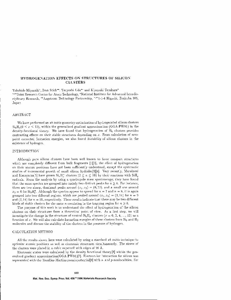
HYDROGENATION EFFECTS ON STRUCTURES OF SILICON CLUSTERS

Takehide Miyazaki*, Ivan Stich**, Tsuyoshi Uda** and Kiyoyuki Terakura* *'** Joint Research Center for Atom Technology, "National Institute for Advanced Interdis- ciplinary Research, "Angstrom Technology Partnership, *'**l-l-4 Higashi, Tsukuba 305,

Japan

ABSTRACT

We have performed an ab initio geometry optimization of hydrogenated silicon clusters Si6H,.(0 < x < 12), within the generalized gradient approximation (GGA-PW91) in the density-functional theory. We have found that hydrogenation of Si6 clusters provides contrasting effects on their stable structures depending on x. From calculation of zero- point corrected formation energies, we also found bistability of silicon clusters in the

existence of hydrogen.

INTRODUCTION

Although pure silicon clusters have been well known to favor compact structures which are completely different from bulk fragments [l][2], the effect of hydrogenation on their atomic positions have not been sufficiently understood, except the systematic studies of incremental growth of small silicon hydrides[3][4]. Very recently, Murakami and Kanayama[5] have grown Si„H+ clusters (2 < n < 10) by their reactions with SiH,, radicals. From the analysis by using a quadrupole mass spectroscopy, they have found that the mass spectra are grouped into mainly two distinct peaks for n > 6. For instance, there are two sharp, dominant peaks around (xilx2) = (0,12), and a small one around 2:3 = 6 for Si6H+. Although the spectra appear to spread for n = 7 and n = 8, it is again grouped into two different regions, which are peaked around (x-i,x2) = (3,14) for n = 9 and (2,14) for n = 10, respectively. These results indicate that there may be two different kinds of stable clusters for the same n coexisting in the trapping region for n > 6.

The purpose of this work is to understand the effect of hydrogenation of the silicon clusters on their structures from a theoretical point of view. As a first step, we will investigate the change in the structure of neutral SieHx clusters (x = 0, 2, 4, ..., 12) as a function of x. We will also calculate formation energies of these clusters from Siß and H2

molecules and discuss the stability of the clusters in the presence of hydrogen.

CALCULATION METHOD

All the results shown here were calculated by using a standard ab initio technique to optimize atomic positions as well as electronic structures simultaneously. The atoms of the clusters were placed in a cubic supercell with edges of 16 A.

Electronic states were calculated by the density-functional theory[8] within the generalized gradient approximation(GGA-PW91)[7]. Electron-ion interaction for silicon was represented with the Troullier-Martins pseudopotential[9] with s- and p-nonlocalities. For

533


(a) (b) (c)

Figure 1: Optimized structure of Si6. The "bonds" between atoms are guides to the eye. Three characteristic unoccupied orbitals are also chosen and shown. The calculated energy eigenvalues relative to HOMO are (a) 2.18 eV(LUMO), (b) 2.376 eV and (c) 4.389

eV , respectively.

hydrogen, the Vanderbilt's ultrasoft pseudopotential[10] with the core radius of 1.0 a.u. was used. Wavefunctions were expanded in plane-wave basis set up to 12.25Ry on the T-point in the Brillouin zone. The deficit charge in the ultrasoft pseudopotential was expanded in plane waves up to 81 Ry. Correspondingly, the same cut-off energy was used for plane-wave expansion of the total valence charge density. Hereafter, we use the notation (12.25,81 )Ry for the cut-off energies of the wavefunction and charge density, respectively. Iterations with respect to wavefunctions were continued until the change in the total energy per iteration step became less than 1.36xlO_4eV / cluster. Optimization of atomic coordinates was performed until the maximum absolute forces on all atoms became less

than 0.0257 eV / Ä. We tested the quality of our method by calculating the bond lengths of a hydrogen

and a silane molecules in a cubic supercell with the edge of 8 Ä, respectively. For H2, we obtained the H-H bond length rf(H-H) of 0.773 Ä and the cohesive energy Ecoh of 4.293eV with cut-off energy of (12.25,81)Ry, compared with experimental values, rf(H-H) = 0.741 Ä and Ecoh = 4.478 eV, respectively. When we used (25,169)Ry, <f(H-H) = 0.755 Ä and Ecoh = 4.381 eV were obtained. For SiH4, d(Si-H) was calculated to be 1.492 Ä with (12.25,81)Ry, very close to experimental value, rf(Si-H) = 1.48 Ä. Therefore we decided

to use the cut-off energy (12.25,81 )Ry throughout this work. In order to seek for the cluster geometries with lowest possible energies, we further

performed Car-Parrinello-like dynamical simulated annealing(DSA) optimizations of candidate configurations at each x within the local-density approximation. For this purpose, we used the norm-conserving pseudopotential and a bare Coulomb potential for Si and H, respectively, with cut-off energy of (10,40)Ry. The DSA-obtained structures were used as the input of the above-mentioned high quality calculation procedures and total-energy

minimizations were repeated.


In Fig.l, we illustrate the optimized structure of a Si6 cluster with three chosen unoccupied orbitals that show dangling-bond characters. The structure agrees well with

534

<•> (b)

Figure 2: Optimized structures of (a) Si6H2 and (b) SieH,i. hydrogen atoms.

Small, yellow spheres represent

W. M

Figure 3: Optimized structures of Si6H6. Hexasilaprismane in panel (a) is the most stable. Panels (b) and (c) illustrate quasistable state with 0.14 eV and 0.69 eV higher in energy relative to (a), respective!}'.

that calculated by Raghavachari and Rohlfing[2]. When hydrogenating this cluster, it is highly expected that hydrogen atoms are attached on apexes to terminate these dangling bonds. In fact, we have obtained the structures of Si6H2 and Si6H4 as illustrated in Fig.2. It should be noted that the configuration of silicon atoms in both Si6H2 and Si6H4 are essentially the same as that in pure Si6. This means that hydrogenation of the Si6 cluster with low coverage does not have significant effect on its geometry. When the number of H atoms becomes six, the structure shown in Fig.3(a) (hexasilaprismane) is favored by 0.14 eV in energy than that with Si6-derived connectivity(Fig.3(b)). It is important to notice that, in hexasilaprismane, all silicon atoms are fourfold coordinated with one hydrogen atom. There is another local-minimum structure, hexasilabenzene with D^i symmetry(Fig.3(c)), whose energy is 0.69 eV relative to hexasilaprismane . Nagase et a/.[11] have calculated the energies of hexasilabenzene with both D3J and Deh symmetries and found that the former is 0.0057 eV lower than the latter, at the level of HF/6-31G**. As for the hexasilaprismane, Sax and Janoschek have found it to be the most stable isomer of Si6H6 [13]. Nagase et al. also performed energetics of hexasilaprismane and D3rf-hexasilabenzene and found that the former is preferred to the latter by 0.412 eV at the level of HF/6-31G*[12], in good agreement with our result from density-functional calculation. Figure 4 illustrates optimized Si6H8 clusters. Again, all silicon atoms are

535

Figure 4: Optimized structures of Si6H8. (a) Stable structure, (b) Quasistable structure

with energy 0.18 eV relative to (a).

Figure 5: Optimized structures of Si6H10. The cluster in the panel (a) is called bicy-

clo[2.2.0]hexasilane.

fourfold coordinated and terminated with one or two H atoms in the stable structure. The structure with the character of Si6 is less stable by 0.18 eV than the former. To- gether with the result of Si6H6, the favored structure of a hydrogenated Si6 cluster changes discontinuously depending on the number of hydrogen atoms on the clusters. This means that there are two distinct geometrical categories to which the Si6:H clusters belong. For x = 10, we found two structures illustrated in Fig.5. Bicyclo[2.2.0]hexasilane (Fig.5(a))

has also been calculated by Nagase and Kudo[14]. The geometry in Fig.5(b) has a six- membered ring where two SiH units, where the Si-H bonds are parallel to the molecular plane, are paired on adjacent silicon sites. They form puckered threefold coordinations, suggesting the mixing of the sp2 character around the silicon atoms. In order to check the stability of this structure in Fig.5(b), we have performed DSA starting from an initial configuration with SiH units placed not on nearest neighbor sites. We found that such a structure is unstable against pairng of the SiH units, or otherwise converged into those with higher energies. It was also found that the energy of the cluster was very high if the two SiH units form a pair on adjacent silicon atoms with at least one of the two Si-H

bonds being normal to the molecular plane. Finally, we show in Fig.6 the stable structure of Si6H12 with a 6-membered ring (cyclo-

hexasilane), together with quasistable clusters which have 5- and 4-membered rings. The total energies of the latter two clusters are 0.16 eV and 0.51 eV relative to cyclohexasi-

536

Figure 6: Optimized structures of Si6H12 with (a) 6-, (b) 5- and (c) 4-membered rings, respectively.

lane, respectively. Although the five-membered ring is little deformed from a equilateral pentagon in our calculation, Onida and Andreoni[6] found substantial distortion of the five-membered ring to lower its energy further by about 0.06 eV.

It is now obvious that hydrogenated Si6 clusters belong to either of two distinct geometrical categories depending on the coverage of hydrogen. In the high coverage case, there exist a simple rule that governs the topological evolution of the clusters with respect to the connectivity among atoms. Let us start from SieHö (hexasilaprismane, Fig.3(a)). If one cuts any bond which connects two triangles and terminates each broken bond with an additional hydrogen atom, then the prismane structure opens up and becomes a Si6H8(Fig.4(a)). On the other hand, if a neighboring pair of the edges are disconnected at the same time and the dangling bonds are terminated with additional four hydrogen atoms, then a Si6H10 (Fig.5(a)) is created. This simple "cut and terminate" rule also applies to the transformation of Si6H10 into Si6H12 as well as Si6H8 into Si6H12. However, this rule cannot be used for construction of both Si6H2 and Si6H4 from Si6. In the low coverage cases, the connectivity among silicon atoms is completely different from the high coverage regime and a shell-like model should be considered.

Table 1: Zero-point corrected formation energies (in eV) of Si6Hx clusters from a Si6

cluster and hydrogen molecules, as a function of x.

X ^formy^j ZPE total 2 -0.42 0.16 -0.26 4 -1.78 0.32 -1.46 6 -1.80 0.48 -1.32 8 -2.99 0.64 -2.35

10 -4.80 0.80 -4.00 12 -5.98 0.96 -5.02

We have calculated the formation energies of Si6H,,. clusters from a Si6 cluster and hydrogen molecule. For this purpose, we have included the zero-point energy (ZPE)

537

corrections of hydrogen atoms to the total energy (see Table I). The formation energy is defined as E}orm{x) = Etot (SieH*) - Etot (Si6) - (x/2) Etot (H2). Here we used the total energy of a hydrogen molecule calculated with cut-off energy of (12.25,81 )Ry. We chose 0.13 eV / H as the ZPE of a H2 molecule from ref.[15]. As for H atoms on the clusters, we

assumed the ZPE to be 0.21 eV / H, also based on the values in ref.[15], which suggests that the ZPE of a hydrogen atom bound to silicon atoms is almost independent of its

environment (molecule or bulk). Interestingly, the calculated formation energy has two minima, -1.46 eV at x=A and

-5.02 eV at z=12, respectively. This implies the bistability of Si6 clusters in the presence of hydrogen. It is also worthy to note that the energy gain caused by hydrogenation is much smaller for x < 8 than for x > 10. This means that this bistability partly originates from the balance between two competing factors, strong binding in a hydrogen molecule and a large energy gain due to hydrogenation. Extension of our calculation to positively

ionized clusters as well as larger ones is already in progress. This work has been partly supported by the New Energy and Industrial Technology

Development Organization (NEDO).

References [I] K. Raghavachari and V. Logovinsky, Phys. Rev. Lett. 55 (1985) 2853.

[2] K. Raghavachari and CM. Rohlflng, Chemical Physics Lett. 143 (1988) 428.

[3] M.L. Mandich and W.D. Reents, Jr., J. Chem. Phys. 95 (1991) 7360. and references therein.

[4] K. Raghavachari, J. Chem. Phys. 95 (1991) 7373, and references therein.

[5] H. Murakami and T. Kanayama, Appl. Phys. Lett. 67 (1995) 2341.

[6] G. Onida and W. Andreoni, Chem. Phys. Lett. 243 (1995) 183.

[7] J.P. Perdew, in "Electronic Structure of Solids '91", edited by P. Ziesche and E. Eschrig (Akademie Verlag, Berlin, 1991).

[8] P. Hohenberg and W. Kohn, Phys. Rev. 136 (1964) B864; W. Kohn and L.J. Sham, Phys. Rev. 140 (1965) A1133.

[9] N. Troullier and J.L. Martins, Phys. Rev. B43 (1991) 1993.

[10] D. Vanderbilt, Phys. Rev. B41 (1990) 7892.

[II] S. Nagase, T. Kudo and M. Aoki, J. Chem. Soc, Chem. Comm. (1985) 1121.

[12] S. Nagase, M. Nakano and T. Kudo, J. Chem. Soc. Chem. Commun. (1987) 60.

[13] A. Sax and R. Janoschek, Angew Chem., Int. Ed. Engl. 25 (1986) 651.

[14] S. Nagase and T. Kudo, J. Chem. Soc, Chem. Comm. (1988) 54.

[15] CG. Van de Walle, Phys. Rev. B49 (1994) 4579.

538

VALENCE-BAND OFFSET AT THE ZN-P INTERFACE BETWEEN ZnSe AND III-V WIDE GAP SEMICONDUCTOR ALLOYS:

A FIRST-PRINCIPLES INVESTIGATION

F. BERNARDINI, R. M. NIEMINEN Laboratory of Physics, Helsinki University of Technology, FIN-02150 Espoo, Finland

ABSTRACT

We present a first-principles calculation of the valence-band offset at the (001) interface between ZnSe and III-V lattice-matched alloys based on Al, Ga, In, P elements, namely Alo.5Ino.5P and Gao.5Ino.5P- Among the different possible interface geometries we have focused on the P- terminated alloy in contact with the Zn-terminated ZnSe crystal. The results of this study show the existence of a very low band offset at the abrupt interface, both for the ideal geometry and for the relaxed atomic positions. The investigation of the electronic interface band structure reveals the presence of a low-lying half-filled interface band related to the Zn-P bond.

INTRODUCTION

Successful p-doping of ZnSe by nitrogen plasma sources [1] has made possible the fabrication of blue-green diode lasers [2] based on II-VI semiconductors. In spite of the great effort expended over this novel wide band gap semiconductor technology, two problems still affect the devices, keeping them far from commercial applications: (i) the laser lifetime is short, presumably due to dislocation growth and motion during the lasing, (ii) high operational voltages are needed to overtake the Schottky barrier [3] formed at the interface between metal contacts and p-doped ZnSe. Unfortunately traditional methods to overcome this problem, like high-density doping on the semiconductor side, to allow tunneling transmission, and metal contact alloying, have been unsuccessful. An improvement has been obtained using semimetallic HgSe contact [4] or ZnSe-ZnTe pseudoternary superlattices as buffer layers [3].

A radical solution to the metal contact problem is the use of an alternative configuration [5], in respect to the customary p-oa-n, where the device is grown on p-doped substrate instead of an n-doped one. The advantage of this configuration, called n-on-p, is the possibility to make low-resistance metallic contacts by highly doped ra-ZnSe. In this configuration the hole injection must be achieved via a p-ZnSe/p-GaAs heterointerface. Using an abrupt interface, however, the valence-band discontinuity AEV — 1.2 eV hinders the hole injection [6]. It has been found that a substantial reduction in the valence-band offset is achieved in ZnSe-GaAs(OOl) heterojunctions through the insertion of thin pseudomorphic Ge layer at the interface [7], or using an unbiased beam pressure ratio during the ZnSe grow on GaAs by molecular beam epitaxy [8j.

Recently, Pessa et al [5] have considered the possibility to reduce the band offset by applying a thick barrier reduction layer (BRL) made of p-doped wide-gap III-V semiconductor ternary alloys. These materials are especially appealing for several reasons. They are based on the well established III-V semiconductor technology, and varying the alloy concentration it is possible to obtain perfect lattice matching conditions with GaAs and ZnSe, with the benefit to avoid interface stress so hazardous for this system very sensitive to dislocation nucleation and creep. The composition of the barrier reduction layer alloy has to be designed to minimize the valence- band discontinuity at the ZnSe interface. On the GaAs side low resistivity can be obtained by high p-doping density for both materials. A preliminary investigation [5] has pointed out Al^Ini-^P and Ga^Ini-^P alloys as possible candidates.


The calculations performed are based on density-functional theory in its local density approximation for the exchange and correlation functional, using Ceperly and Alder's form [9] as parametrized by Perdew and Zunger [10]. Two different computational approaches are used, the Car-Parrinello method as implemented by R. Stumpf et al. [11] and the Full Potential Linear

539

Mat. Res. Soc. Symp. Proc.Vol. 408® 1996 Materials Research Society

Muffin Tin Orbital (FP-LMTO) [12]. The second one is used only for selected configurations to check the results obtained with the first. Norm-conserving pseudopotentials for Ga, In, As, P, Zn and Se have been generated by the standard Hamann method [13] and compared with the outcomes of the FP-LMTO calculations for the binary compounds, a cutoff of 12 Ry, used for the supercell calculation, is sufficient to obtain converged values for bulk properties. Zn 3d levels are included in the core and accounted using the nonlinear core correction (NLCC) [14]. Reciprocal space summation is performed using special k points [15]. The valence-band offset AEV is calculated from

AEV = [EV(L) - EV(R)\ + [Vd(L) - Vel(R)} + i[A„(L) - A0(Ä)]

where letters R and L , refer to the left and right side of the interface and Ev, Vei and A0

are, respectively, the energy of the valence-band edge, the averaged electrostatic potential, and the spin-orbit splitting in the bulk. The second term Vd is extracted from a self-consistent calculation for supercell containing thick slabs of the two materials. The potential is averaged using the running slab technique of Baidereschi et al. [16]. The last term takes in account the effect of the spin-orbit splitting at the valence-band edge. As our self-consistent calculations are non-relativistic, the spin-orbit splitting is evaluated using experimental data for the binary and ternary compounds reported in Ref. [17] and [18].

Since the Zn 3d levels are not treated explicitly in the pseudopoiential, FP-LMTO calculations are carried out for reference. The LMTO basis consists of 18 orbitals atom, i. e. s, p, and d partial waves with kinetic energies of -K2

= -0.2 and -1.0 Ry. Following a previous experience [19] , Zn 3d orbitals are considered as proper band states, while In id, Ga 3<2 and Se 3d states are included in a second energy panel as semicore states. The radii of the atomic spheres are chosen to fulfill the touching-spheres conditions, an equal number of empty spheres of the same size is added to improve the sphere packing. No basis functions are centered on the empty spheres. Reciprocal space integration is performed using 8 k points obtained folding the (333) Monkhorst- Pack mesh [21] for the specific supercell geometry. Only one k point is sufficient for the semicore panel. The remaining core states are self-consistently relaxed in a spherical approximation. After a self-consistency run, the core levels from the slabs centermost layers atoms have been used to calculate the VBO according to the method outlined in Ref. [20]. The VBO is obtained as the sum of four terms:

AEV = lElulk(L)-E^lk{R)} + [E^lk(L)-E^,k(R)}

- [Esclab(L) - Es

c,ab(R)} + |[Ao(£) - Ao(Ä)]

where E^lk are the valence-band edge in the two bulk materials, Ebulk the cation Is core levels binding energy, Ef.Iab the same cation binding energy for the centermost layers atoms, A0 the spin-orbit splitting at the valence-band edge.

INTERFACE STRUCTURES

Two different interfaces have been investigated, the (lxl) and the c(2x2) by means of the repeated slab method. The supercell used for the first interface contains 40 atoms divided in two slabs, 10 Selenium and 11 Zinc atoms placed according to the zincblende structure, 10 Phospho- rus and 9 cations, Indium, Aluminum or Gallium atoms. Inside the slab representing the alloy, the atomic structure is no more zincblende but a more complex one, having ai (1/2,1/2,0), a2(l/2, -1/2,0), a3(0,0,1) as translation vectors and four basis atoms located in 7i(0,0,0), r2(l/4,l/4,l/4), r3(0,l/2,l/2), r4(l/4,3/4,3/4). This superstructure can be also considered as a lxl superlattice, namely (AlP)i(InP)1(001) and (GaP)1(InP)1(001), for AllnP and GalnP, respectively. Stoichiometric fractions for GaAs lattice-matched AlJni-xP and GayIni-yP are x = y = 0.51, and our superlattice model closely represents these concentrations. While we focus on the Zn-P interface, the composition of the first and second cation layers are still undetermined, two sequences are possible (the interface atoms are marked in boldface):

540

• • ■ -X-P-In-P-Zn-Se-Zn-Se-Zn-P-In-P-X- • • ■ (a) or

■ • • -In-P-X-P-Zn-Se-Zn-Se-Zn-P-X-P-In- ■ ■ • (b)

were X stands for Al or Ga. Each structure has been first considered in the zincblende ideal geometry with equal anion-cation bond lengths. Then the atomic positions have been relaxed in two steps, (i) only Phosphorus layers have been shifted to the equilibrium positions, (ii) full relaxation of all layers has been allowed. The supercell length is kept equal to 10 times the ZnSe equilibrium lattice parameter (10.6 a.u.) obtained for the bulk.

The second supercell, used for the c(2x2) interface, is shorter than the previous (84.8 a.u.). It contains 64 atoms arranged in 32 layers, each having two inequivalent cations (anions). This geometry offers the possibility to have a better description of the alloy we have investigated. The specific arrangement of the atoms chosen in this case is: (0,0,0) and (-\/2/4,\/2/4,l/2) for Al (Ga), (0,^2/2,0) and (x/2/4,^/4,1/2) for In, (0,^/4,1/4), (0,-^2/4,1/4), (v^/4,x/2/2,3/4), (-v/2/4,^/2,3/4), for P, being ai(i/2,\/2,0), a2(-\/2,V5,0), a3(0,0,l), the translation vectors. According to this arrangement each anion is surrounded by a shell of first neighbors composed by the same number of Al (Ga) and In atoms. In this case no distinction exists between the sequences (a) and (b) referred to above. The atomic sequence is then:

• • ■ -X-P-In-P-Zn-Se-Zn-Se-Zn-P-In-P-X- • • •

• ■ ■ -In-P-X-P-Zn-Se-Zn-Se-Zn-P-X-P-In- ■ • •

with both In and Al (Ga) cations in the same layer.

RESULTS

Pseudopotential calculations

We will first examine the results for the (lxl) interface in detail. The calculated valence-band offsets for the interface structures are reported in Table 1. We want to point out the following features: (i) all of the four band offsets lie in a narrow range between -0.22 and +0.07 eV, (ii) in the absence of atomic relaxation the VBO is independent of the atomic arrangement on the second layer, (iii) atomic relaxation affects the VBO but does not change it dramatically, (iv) the averages reported in the last row are nearly equal to the values found for the ideal geometry.

Table 1: Valence-band offset at AllnP-ZnSe(OOl) and GalnP-ZnSe(OOl) acceptor interfaces (in eV). Values reported in each row refer to: (i) (lxl) unrelaxed geometry, (ii) only Phosphorus layers relaxed, (iii) full relaxation of all layers, (iv) average over the atomic sequences (a) and (b) for the full-relaxed geometry, (v) c(2x2) unrelaxed geometry, (vi) relaxation only for interface atoms.

(lxl) AllnP-ZnSe(a) AllnP-ZnSe(b) GalnP-ZnSe(a) GalnP-ZnSe(b) ideal P-relax. full-relax, average

-0.11 -0.12 -0.13 -0.09 -0.22 -0.09

-0.15

+0.02 +0.02 -0.14 -0.14 -0.11 +0.07

-0.02 c(2x2) AllnP-ZnSe GalnP-ZnSe ideal relaxed

-0.08 -0.04

+0.02 +0.03

The anion relaxation to the equilibrium position inside the alloy gives a very small contribution to the band offset in the AllnP alloy while it seems more important for the GalnP alloy. The composition of the first and second cation layers influence the VBO when the effect of the interface strain is taken in account. Indeed in both the AllnP-ZnSe and GalnP-ZnSe interfaces the Zn-P bond length is found to be 1% shorter in sequence (a) than in sequence (b). This suggests the importance to use a more realistic model for the interface in which both Al (Ga) and In are mixed in the same layer if the relaxation at the interface is considered.

541

We have examined the charge distribution, the potential profile and the interface band dispersion for one of the four systems studied. A comparison with the others shows little differences that do not affect our conclusions. Figures 1 and 2 refer to the AlInP-ZnSe(001)(lxl) interface related to the atomic sequence labeled with (a). As can be seen in Fig. 1, the perturbation due to the acceptor bond is localized in a very thin layer around the interface. This charge distribution induces long-range fields which require the use of very long supercell in order that the electrostatic potential should be converged in the centermost region of each slab. In Fig. 2, we have plotted the local component of the effective potential ( Vjj + VIC + V^c ) along the longitudinal axis (z axis) of our supercell. The macroscopic average potential profile confirms the convergence of the potential to the asymptotic value inside the slabs. It is evident that the formation at the interface of a huge electrostatic dipole sum of an electronic and ionic contributions. In absence of this dipole the band offset would be equal to 1.13 eV for the AllnP-ZnSe interface and 1.17 eV for the GalnP-ZnSe, values very similar to what reported for the GaAs-ZnSe(OOl) interface [6]. Depending on the system considered the dipole contribution varies from 1.1 eV to 1.35 eV. This is an exceptionally high value and is the key feature of this abrupt interface and the reason for the very low band offset found.

8 a A /"'. "\ A

ZnSe ; / AllnP I

.' ZnSe

j ; 1 j

'

Figure 1: AlInP-ZnSe(001)(lxl)(a) interface. Charge distribution along the supercell axis averaged by Baldereschi's running slab technique. Two different running slab lengths have been used (i) 5.3 a.u. (dashed line) related to the ZnSe bulk structure, (ii) 10.6 a.u. (solid line) suitable for the alloy enlarged cell.

Figure 2: AlInP-ZnSe(001)(lxl)(a) interface. Two lines are drawn: the solid one represents the so-called potential planar average [16] obtained from the integration of the effective potential over the xy plane parallel to the interface. The dashed line is the macroscopic aver-

The interface band structure has been investigated to understand the origin of the charge perturbation shown in Fig 1. The band dispersion along the high symmetry directions of the interface two-dimensional reciprocal cell is shown in Fig. 3. Above the bulk valence-bands we can see two additional bands that have been marked with circles. They belong to the Zn-P acceptor bonds at the two sides of the slabs used for the calculations. As expected they are placed just above the valence-band edge, and they are only partially filled, since the Fermi energy cuts them in two parts. This acceptor state makes the interface metallic and allows a charge transfer between the two semiconductors to an unusual extent.

A less detailed investigation has also been carried out for the c(2x2) interface. It is considered first in its ideal position geometry described above, then only the Zn and P atoms at the interface have been relaxed to their equilibrium positions. The experience gained with the (lxl) interface suggests that a further relaxation involving the whole slab structure should not affect the band offset significantly. The values of the VBO are listed in Table 1. All of these are inside the range covered by the values found for the (lxl) interface. The analysis of the relaxation pattern offers the possibility to look for possible effects of reconstruction if they appear at this length scale. We have found for the c(2x2) interface a behavior consistent with a pure relaxation. Zn atoms relax outward with respect to their slab by 0.08 a.u. while P atoms shift parallel to the interface plane toward the Al (Ga) sites. No distortion related to the interface formation happens inside our unit cell. It is possible that reconstruction happens for larger cells, but it is more likely that the equilibrium geometry for the interface involves a degree of intermixing, leading to a compensated interface. Only a more extended study over several possible structures will confirm if this interface can be stable at least for specific values of the element chemical potentials. This

542

possibility is not excluded a priori since a previous investigation [22] has found that an abrupt interface can be thermodynamically stable under specific stoichiometric conditions.

All-electron calculations

The VBO and the interface band structure for both the alloys have been calculated also with the FP-LMTO method. The results reported here are for the (lxl) interface in its unrelaxed (a) sequence. The VBO obtained is +0.05 (+0.26) eV for the AllnP-ZnSe (GalnP-ZnSe) interface. These values are slightly higher respect to what found with the pseudopotential method. The trend from AllnP to GalnP toward a higher VBO is anyway fulfilled. In order to understand if the difference is due to the description of the interface electronic structure, the band dispersion has been examined for the AllnP-ZnSe interface (Fig. 4) and compared with the results of the pseudopotential calculations (Fig. 3). The two bandstructures are in excellent agreement. The band energies and dispersion are extremely well reproduced, confirming the validity of the results obtained. The small discrepancy is perhaps caused by the effect of the Zn 3d - P 3p hybridization on the charge transfer at the interface, accounted for only in the all-electron calculation.

Figure 3: Interface band structure the high symmetry directions of the AllnP- ZnSe(OOl) two dimensional reciprocal cell obtained with pseudopotential based method. Two bands related to the acceptor bond states are marked with circles.

Figure 4: Interface band structure along the high symmetry directions of the AllnP- ZnSe(OOl) two dimensional reciprocal cell. This band structure is obtained with FP-LMTO method. The resemblance with the band structure shown in Fig. 3, confirms the reliability of the pseudopotential calculations.

CONCLUSIONS

In this work we have investigated the valence-band offset at the Zn-P bonded abrupt interfaces between AEnP and GalnP alloy in contact with ZnSe. The calculations performed with pseudopotentials find a low value for the valence-band offset for both materials. These values seems to be weakly dependent on the cation atomic arrangement inside the alloy. The lattice equilibrium geometry at the interface has been investigated for the (lxl) and c(2x2) systems. The atomic displacement from the ideal positions are consistent with a pure relaxation pattern. Band offset values obtained for the relaxed geometries are slightly different and show uniform trends, and sequence (b) has an higher value than (a). The band structure at the (lxl) interface has been investigated by means of pseudopotential and FP-LMTO methods. An acceptor-like state related to the Zn-P bond is found to lie above the valence-band giving a metallic character to the interface. This state is also responsible of the large charge perturbation shown in Fig 1 . The values for the band offset obtained with the all-electron approach are systematically higher by =i 0.1 eV respect to what found with the pseudopotentials, and this difference is ascribed to the Zn 3d - P 3p level hybridization. The system studied represents one of the possible interface geometries between ZnSe and AllnP or GalnP alloys. The authors can not exclude nor confirm the thermodynamical stability of this interface. A more extended work is in progress to explore the band offset at the other possible interfaces.

543

ACKNOWLEDGMENTS

This research has been supported by the EC-HCM grant (contract ERBCHBGCT930505) and by the Academy of Finland. The authors gratefully acknowledge R. Stumpf and M. Schemer for supplying the Car-Parrinello code and D. R. Hamann for the pseudopotential generation package.

REFERENCES

[1] R. M. Park, M. B. Troffer, C. M. Rouleau, J. M. DePuydt, M. A. Haase, Appl. Phys. Lett. 57, 2127 (1990).

[2] M. A. Haase, J. Qiu, J. M. DePuydt, H. Cheng, Appl. Phys. Lett. 59, 1272 (1991) [3] Y. Fan, J. Han, L. He, J. Saraie, R. L. Gunshor, M. Hagerrot, H. Jeon, A. V. Nurmikko,

G. C. Hua, N. Otsuka, Appl. Phys. Lett. 61, 3160 (1992). [4] Y. Lansari, J. Ren, B. Sneed, K. A. Bowers, J. W. Cook Jr. , J. F. Schetzina, Appl. Phys.

Lett. 61, 2554 (1992) [5] M. Pessa, K. Rakennus, P. Uusimaa, P. Savolainen, A. Salokatve, Phys. Stat. Sol. (b), 187,

337 (1995). [6] N. Kobayashi, Appl. Phys. Lett. 55, 1235 (1989). [7] G. Bratina, L. Vanzetti, L. Sorba, G. Biasiol, A. Franciosi, M. Peressi, S. Baroni, Phys.

Rev. B, 50, 11723 (1994). [8] R. Nicolini, L. Vanzetti, Guido Mula, G. Bratina, L. Sorba, A. Franciosi, M. Peressi, S. Ba-

roni, R. Resta, A. Baldereschi, J. E. Angelo, W. W. Gerberich, Phys. Rev. Lett. 72, 294 (1994).

[9] D. M. Ceperley, B. J. Alder, Phys. Rev. Lett. 45, 556 (1980). [10] J. Perdew, A. Zunger, Phys. Rev. B, 23, 5048 (1981). [11] R. Stumpf, M. Schemer, Comp. Phys. Comm. 79, 447 (1994)

[12] M. Methfessel, Phys. Rev. B 38, 1537 (1988). [13] G. B. Bachelet, D. R. Hamann, and M. Schlüter, Phys. Rev. B 26, 4199 (1982); [14] S. G. Louie, S. Froyen, M. L. Cohen, Phys. Rev. B, 26 , 1738 (1982). [15] D. J. Chadi, M. L. Cohen, Phys. Rev. B 8, 5747 (1973). Six k points are used for the (lxl)

interface, 4 for the c(2x2). [16] A. Baldereschi, S. Baroni, R. Resta, Phys. Rev. Lett. 61, 734 (1988).

[17] C. G. Van de Walle, Phys. Rev. B, 39, 1871 (1989). [18] M. P. C. M. Krijn, Sem. Sei. Tech. 6, 27 (1991). [19] M. Methfessel, M. Schemer, Physica B, 172, 175 (1990) [20] A. Continenza, S. Massidda, Phys. Rev. B, 50, 11949 (1994) [21] H. J. Monkhorst, J. P. Pack, Phys. Rev. B, 13, 5188 (1976) [22] A. Kley, J. Neugebauer, Phys. Rev. B, 50, 8616 (1994).

544

Electronic Structure and Stability of Ordered Vacancy Phases of NbN

E.C. Ethridge, S.C. Erwin, W.E. Pickett Complex Systems Theory Branch, Naval Research Laboratory, Washington DC 20375

ABSTRACT

A recently reported metastable phase of NbN with a superconducting Tc=16.4 K is characterized using full potential electronic structure methods. This new phase, which has Pm3m (cubic) symmetry, can be described as the Bl (rocksalt) structure with 25% ordered vacancies on each sublattice. We compare the equation of state and electronic spectrum of this Pm3m phase with its rocksalt counterpart [1] and with Nb4N3 in the I4/mmm (tetragonal) phase, which allows the characterization of N vacancies without accompanying Nb vacancies. For Pm3m NbN, the calculated lattice constant is 5% smaller than reported and the energy is 1.00 eV/molecule higher than Bl NbN, suggesting that the newly reported phase is something other than a stoichiometric Pm3m phase of NbN. We report on the energy surface for tetragonal distortions of this phase, from which we evaluate its structural stability and obtain Poisson's ratio.

INTRODUCTION

A notable feature of niobium nitrides is their propensity to stabilize in structures with varying degrees of stoichiometry and vacancy concentrations, which results in a broad spectrum of physico-chemical properties. Depending upon stoichiometry, NbN phases range from insulating to superconducting with an upper limit Tc of 17.3 K [2,3,4]. It was the recent report of a new metastable superconducting phase that motivated us to investigate the electronic properties and structural stability of ordered vacancy NbN structures. In this work we address three superconducting phases of NbN using first principles density functional techniques: (1) the rocksalt structure (space group Fm3m), (2) the tetragonally distorted rocksalt structure obtained when one-quarter of the N is removed, denoted by Nb4N3 and (3) Nb3N3, the rocksalt structure obtained when one-quarter of the Nb and N are removed. These phases will be referred to as Nb4N4, Nb4N3, and Nb3N3, respectively.

The new phase of NbN, which prompted this work, was reported as thin films synthesized on MgO (100) substrates using pulsed laser deposition [3]. According to x-ray diffraction studies, its structure may be regarded as the rocksalt structure with 25% ordered vacancies on both the metal and metalloid sublattices. Thus, each atomic site is four-fold planar coordinated with atoms of the opposite type and the vacancy sites are six-fold coordinated with atoms of one type. The structure may be envisaged as nonpenetrating Nb octahedra and nonpenetrating N octahedra, both centered at vacancy sites. The space group is Pm3m. Nb3N3 reportedly has a superconducting Tc of 16.4 K and a lattice parameter of 4.442 A, which are both comparable to the experimental values of 16 K and 4.378 A for Nb4N4.

Also considered in this study is a tetragonal distortion of the rocksalt structure with 25% ordered vacancies on the metalloid sites. This allows for the characterization of N vacancies without accompanying Nb vacancies. Thin films of Nb4N3 vapor-deposited on MgO (100) substrates have a superconducting Tc near 11.5 K [2]. The space group is I4/mmm. The

545


experimental lattice parameters are a=4.382 Ä, c=2*4.316 Ä, the internal parameter is zjv&= 0.2521 c, and the primitive cell has four Nb and three N [5].

In this phase, there are two distinct Nb and N atom types. Nb(l) is four-fold coordinated with N, while Nb(2) is five-fold coordinated with N. The N atoms, which are all six-fold coordinated with Nb, differ depending on which type of Nb it maintains the highest coordination with. Hence, N(l) will refer to the N which is four-fold coordinated with Nb(2) and two-fold coordinated with Nb(l). N(2) is four-fold coordinated with Nb(l) and two-fold coordinated

with Nb(2).

THEORETICAL RESULTS

The bulk of this work is based on density functional theory using the method of linear combination of atomic orbitals (LCAO). The details of this approach, which are described elsewhere [6], invoke the Perdew-Zunger-exchange-correlation potential [7] within a local- density approximation (LDA). Depending upon the phase, between 15 and 20 special k points in the irreducible Brillouin zone are used to obtain the self-consistent band structure of the three phases. For the density of states (DOS) calculations, the Hamiltonian was diagonalized at a minimum of 104 k points in the irreducible zone, interpolated to a denser grid using a Fourier spline method [8], and integrated with the linear tetrahedron method [9]. The basis functions were expanded in a set of 17 Gaussian exponents contracted into seven s-type, five p-type, and four d-type functions for Nb, and 12 exponents contracted into

four s-type and three p-type functions for N. The other method adopted in this work is the full potential linearized augmented plane

wave method (LAPW) [10,11]. The Vosko-Wilk-Nusair [12] parametrization of the exchange- correlation energy and potential was used within the local density approximation. For these calculations sphere radii for the Nb and Nb vacancies are Rjv&=2.30 a.u. and for the N and N vacancies, Rjv=1.55 a.u. The basis set cutoff was defined by RjvKm(l:c=7.0, which translates to R;viKm(Il:=10.4. The basis set size ranged from 760 LAPWs for the smallest volume to 1080 LAPWs for the largest volumes. The Nb 3p semicore states were treated in the same window for additional accuracy that might be necessary at the smaller volumes considered, and additional local functions were used for the Nb 3p and 4d states and for the N 2s states. Twenty special k points were used in all calculations.

The self-consistent band structure, DOS, and Mulliken populations [13] for all phases were computed with the LCAO method. For the total energy calculations, LAPW was used for Nb4N4, Nb3N3, and tetragonal strains of Nb3N3, while LCAO was used for Nb4N3.

Band Structure and DOS

In Fig. 1, the band structure and DOS are shown for the three phases. We observe the following behavior in the band structure and DOS: for the Nb4N4 structure in Figs.1(a) and (b), Mulliken population analysis indicates minimal mixing of orbital types in the valence and conduction states in the band structure. The N p states comprise the manifold of bands 6 eV below EF (the energy zero). The bands with Nb d character, which first appear near -5 eV, dominate the energies near EF and above. The onset of the Nb p manifold lies above the Nb d near 6 eV. The DOS reflects this behavior with two distinct peaks. The first peak centered near -6 eV is comprised mostly of N p states with some admixture of Nb d

546

(a) (b) (c)

2.0

0.0

> <D

-2.0

o iS -4-0

-6.0

-8.0

(d) (e) fm J£ä m» iöPM1

r x M r 0.1

9?" #■ W, t

- -

. 1

r X M R r 0.1 r x M r 0.1

Figure 1: Self-consistent electronic band structure and density of states (DOS) for (a,b) Nb4N4, (c,d) Nb4N3, and (e,f) Nb3N3. The character of each band, using the method described in the text, is indicated. Filled squares denote N p character, filled circles denote Nb p character, and open circles denote Nb d character. DOS is in states/eV-Ä. The Fermi level is the energy zero. Calculations were performed in the primitive cell of the Nb3N3 structure.

states. The second peak is slightly above EF and has Nb d character. In Nb4N3, shown in Figs. 1(c) and (d), the bands derived from the 2p states of the N atoms that remain lie in the same energy region as they do in Nb4N4. Correspondingly a low-energy peak similar to that observed in the DOS for Nb4N4 is present. But removing one-fourth of the N atoms has a pronounced effect on the Nb states. The spectral weight of the Nb d states is redistributed and results in a more diffuse DOS at higher energies. In addition, one of the bands near 0.75 eV below EF has Nb p character between the simple cubic high symmetry points M and R. Mulliken population analysis shows this to originate from Nb(l), and that this is the only region for which Nb p states are present within the Nb d complex. The Nb3N3

band structure, shown in Fig. 1(f), differs from the others most notably in (1) comparing to Nb4N4, the Nb3N3 band width reduces by 40%, (2) the band slightly below EF with Nb p character in Nb4N3 is not present. Instead a highly dispersive band similar to that observed in the isostructural NbO vacancy phase [14,15] appears. This band has Nb d character below EF and changes to primarily Nb p character as it crosses the Fermi energy and peaks at the R point. (3) A dramatic redistribution of the spectral weight of the Nb d bands results in a sharply peaked structure in the DOS, shown in Fig. 1(e), at EF.

Charge Analysis

For each of the structures, Mulliken charges were computed and decomposed according to orbital and symmetry type. For Nb4N4, the total charge transferred from Nb to N is 0.81 electrons. Nb4N3 is more ionic: N(l) has an excess charge of 0.98 while N(2) has an excess charge of 1.07. Nb3N3 is the least ionic with a charge transfer of 0.60. By comparing the three phases, we observe the ionicity is a direct consequence of the N vacancy concentration.

547

£j @>tW

(a)

Figure 2: (a) Contour plot of the difference between the self-consistent charge density of Nb3N3 and the superposition of the atomic constituents in a Nb-rich plane. Centered in the figure is a vacancy site. (b)Contour plot of the difference between the self-consistent charge density of Nb4N4 and that of Nb4N3. The lattice parameters of Nb4N3 are used in both calculations. Centered in the figure is a Nb atom. Above and below are the N atoms in Nb4N4 which are not present in Nb4N3. Solid lines are positive contours. Dashed lines are

negative contours.

This is manifest in the Nb p and d orbitals. Those orbitals directed toward nearest neighbor N vacancies retain more charge than those directed toward nearest neighbor N. For example, charge on the various Nb p orbitals is comparable in Nb4N3, but p orbitals on Nb(l) that are directed toward vacancy sites retain more charge. They give rise to the occupied band with Nb p character which occurs near -0.75 eV between the high symmetry points M and R, previously discussed. To illustrate this point further, a contour plot of the difference between the self-consistent charge density and the superposition of atomic charge densities in Nb3N3

is shown in Fig. 2(a). The Nb-rich plane, which is shown, is the plane with Nb atoms two- fold planar coordinated with N atoms. Charge transfer is greatest between the Nb p and d orbitals that are directed toward N atoms. Fig. 2(b) shows the charge density difference between the self-consistent charge density of Nb4N4 and that of Nb4N3, both computed with

the lattice parameters of the Nb4N3 phase.

Equations of State

In Table I, the results of the total energy calculations are summarized. The numbers in

548

Table I: Equation of state results for the Nb4N4, Nb4N3, and Nb3N3 phases. Lattice parameters are in A and bulk modulii are in Mbars. Numbers in parentheses are from experiment.

Parameter Nb4N4 Nb4N3 Nb3N3

a c B

4.365 (4.378)"

3.57

4.316 (4.382)" 4.358 (4.316)"

3.29

4.214 (4.442)6

2.97 a. Ref. 4 b. Ref. 2

parentheses are experimental values. For Nb4N4, the calculated lattice constant is 4.365 Ä, which is within 0.3% of the experimental value. For Nb4N3, we obtain a lattice parameter in the a-direction of 4.316 A, which is 1.5% smaller than experiment. In the c-direction, the lattice parameter is 4.358 A, which is 1% larger than experiment. Consequently the theoretical c/a ratio is 1.010, somewhat larger than the experimental value of 0.985. To arrive at these calculated values, the cell volume, V, and c/a ratio were varied independently over a range of values within ±8% of experiment (the single internal parameter was not optimized). At each volume, the optimal c/a and corresponding E(V) were determined by fitting the total energy to a third-order polynomial in c/a; the resulting values of E(V) were then fit to a Birch equation of state. The most sizeable disparity between the theoretical and experimental lattice constants (4.214 A and 4.442 A respectively) is found in Nb3N3. We also find that the energy of Nb3N3 is 1.0 eV per NbN unit higher than in the Nb4N4 phase. These equation of state results are not compatible with the identification of the reported Nb3N3 structure.

Although the calculated lattice parameter for Nb3N3 is a good lattice match with the MgO substrate (4.21 to 4.24 A), the equation of state calculations [1,16] do not establish the stability of the solid against symmetry lowering strains. We investigate a possible tetragonal instability of the Pm3m structure. For twenty-one distinct tetragonal structures, with 7.76 <a<8.21 a.u. (b=a) and 7.60<c<8.40 a.u., the energies were computed and fit to a fourth order polynomial in a and c. The maximum deviation of the fit was 0.093 mRy per NbN unit. The minimum occurred for a cubic structure with ao=c„=4.203 A, consistent with the cubic equation of state described above. The quadratic terms in the fit give the tetragonal shear modulus C11-C12=2.48 MBar and bulk modulus JB=(Cn+2C12)/3=2.97 MBar. Our fit to the energy surface gives a Poisson ratio P=0.32, very close to the ideal value of 1/3 for an isotropic solid. We find no secondary minimum in the energy surface. Hence the tetragonal strains only serve to increase the energy.

CONCLUSION

In summary, while we were able to methodically study the effects of ordered vacancies on the metalloid and on the metal/metalloid sublattices in the Nb-N system, our local density calculations do not support the existence of the Nb3N3 phase. We find that (1) Nb3N3 is 1.0 eV/NbN higher than Nb4N4 and (2) the lattice parameter is 5% larger than reported. Independent first principles calculations confirm these findings [16]. A tetragonal distortion of the Pm3m phase, which may complicate interpretation of the x-ray diffraction data, does

549

not rectify the discrepancies between the reported calculations and experiment.

ACKNOWLEDGMENTS

E.C.E gratefully acknowledges the Institute for Computational Sciences and Informatics at George Mason University for support in the early stages of this work and the continued support from the National Research Council as an NRL Postdoctoral Fellow. W.E.P gratefully acknowledges computational support from the Alaska Region Supercomputing Center.

REFERENCES

1. E.C. Ethridge, S.C. Erwin, W.E. Pickett, Phys. Rev. B 52, R8589 (1995).

2. G. Oya and Y. Onodera, J. Appl. Phys. 45, 1389 (1974).

3. R.E. Treece, J.S. Horwitz, and D.B. Chrisey, Mater. Res. Soc. Proc. 343, 747 (1994); R.E. Treece et al, Appl. Phys. Lett. 65, 2860 (1994); R.E. Treece, J.S. Horwitz, D.B. Chrisey, and E.P. Donovan, Chem. Mater. 6, 2205 (1994); R.E. Treece et al, Phys. Rev. B 51, 9356 (1995).

4. K.S Keskar, T. Yamashita, and Y. Onodera, Japan J. Appl. Phys. 10, 370 (1971).

5. P. Villars and L.D. Calvert, Pearson's Handbook of Crystallographic Data for Intermetal- lic Phases (American Society of Metals, Metals Park, OH, 1991).

6. S.C. Erwin, M.R. Pederson, and W.E. Pickett, Phys. Rev. B 41, 10437 (1990).

7. J.P. Perdew and A. Zunger, Phys. Rev. B 23, 5048 (1981).

8. W.E. Pickett, H. Krakauer, and P.B. Allen, Phys. Rev. B 38, 2721 (1988).

9. G. Lehmann and M. Taut, Phys . Status Solidi B 54, 469 (1972).

10. D. Singh, Planewaves, Pseudo-potentials, and the LAPWMethod (Kluwer, Boston, 1994); D.J. Singh, Phys. Rev. B 43, 6388 (1991).

11. S.H. Wei and H. Krakauer, Phys. Rev. Lett. 55, 1200 (1985).

12. S. Vosko, L. Wilk, and M. Nusair, Can. J. Phys. 58, 1200 (1980).

13. R.S. Mulliken, J. Chem. Phys. 23, 1833 (1955).

14. E. Wimmer et al., J. Phys. Chem. Sol. 43, 439 (1982).

15. W.W. Schulz and R.M. Wentzcovitch, Phys. Rev. B 48, 16986 (1993).

16. S.Ögüt and K.M. Rabe, Phys. Rev. B 52, R8585 (1995).

550

ATOMISTIC STUDY OF BORON-DOPED SILICON

M. FEARN *, J.H. JEFFERSON " AND D.G. PETTIFOR * 'Oxford University, Department of Materials, Parks Road, Oxford 0X1 3PH, UK. **DRA (Electronics Sector), St. Andrews Road, Great Malvern Worcs WR14 3PS.

ABSTRACT

Atomistic simulations using both tight-binding and density-functional approaches have been performed to investigate boron-related defects in silicon. In agreement with experiment, the boron interstitial is shown to be a negative- U center in the sense that its neutral charge state, with an associated Jahn-Teller distortion off the ideal tetrahedral site, is never the ground state for any value of the chemical potential in the gap. The possible consequences for an electron-assisted migration of the interstitial are discussed. We also find the boron substitutional defect to be a next-nearest neighbor of a silicon vacancy in agreement with EPR spectra.

A semi-empirical tight-binding model of the boron-silicon system is validated by direct comparison with the accurate density-functional results and is then used to perform molecular dynamics simulations of boron diffusion at high temperatures. The mobility of the interstitial is found to be strongly charge-state dependent. Termination of the boron interstitial migration path by recombination with a silicon vacancy is shown to be a very likely process with a number of configurations having no barrier to capture when the boron is a near-neighbor of the vacancy.

INTRODUCTION

Boron is the most commonly used p-type dopant in silicon based semiconducting devices. Efficient operation of these devices relies upon attaining a sharply defined dopant profile [1]. This can usually be achieved during low temperature growth of the device during which the boron is incorporated substitutionally on the lattice. However, subsequent processing can degrade the dopant profile substantially. Theoretical attempts to understand this degradation have been largely based on continuum models, which require input data such as diffusion energy barrier heights usually obtained by fitting experimental results [2]. However, these models give no insight into the detailed atomistic processes occuring within the material and, with device dimensions shrinking rapidly, single atomic step diffusion events can begin to become important in perturbing the dopant profile. An understanding of boron in silicon at the atomic level is therefore highly desirable to gain deeper insight into dopant migration in general and what factors may affect it.

The purpose of the computer simulations reported here is threefold. (1) To obtain, using an accurate ab-initio technique, relaxed geometries and ground-state energies of defects thought to be relevant to atomistic processes associated with boron diffusion in silicon. (2) To perform similar calculations using the more approximate, but less computationally demanding, tight-binding (TB) method to verify its applicability to this problem. (3) To use the TB method to perform molecular dynamics calculations of boron diffusion at high temperatures to investigate the diffusion mechanisms dynamically.

METHODS

The ab-initio calculations reported here have been performed using density-functional theory within the local density approximation (LDA) [3]. The one-electron wave functions are expanded in a basis of plane waves with the electron-ion interaction described by norm- conserving, non-local pseudopotentials. For Si we have used a standard pseudopotential of the Kerker type [4], whereas for boron a new optimised pseudopotential was generated

551


according to the scheme of Ref. [5]. This pseudopotential, following Denteneer et. al. [6], was tested by evaluating the predicted lattice constant of boron phosphide in the zinc-blende structure. For a plane wave cut-off of 300 eV the predicted lattice constant was within 2% of the experimental value. We have used a plane-wave cut-off of 300 eV throughout the calculations reported here. The silicon pseudopotential predicts an equilibrium lattice constant within 1% of the experimental value. Thirty-two atom b.c.c. supercells were used and full unconstrained relaxation of all^atoms was performed until the maximum force on any one atom was less than 0.05eV/A. Four special k-points [7] were employed to sample the Brillouin zone. For charged defect calculations, the supercell was implicitly neutralized, following standard practice, with a uniform background charge to avoid divergence of the long-ranged Coulomb terms [8].

In the tight-binding calculations the one-electron wave fuctions are expanded in a minimal (sp3) basis of localized orbitals. Effective atomic energies and hybridisation matrix elements of the Hamiltonian are treated as parameters and are fitted to experimental data and/or accurate ab-initio calculations. The resulting Hamiltonian is diagonalised to give the one-electron energy spectrum and the levels filled to the Fermi energy to yield the ground-state band energy. To this is added an effective pairwise repulsive energy (which accounts for the repulsion of the ionic cores at short range), resulting in the total energy of the system. The Si-Si interactions were parameterised here according to the well-established model of Goodwin et. al. [9]. The Si-B interactions were parameterised using a scheme analagous to that described by Rasband et. al. [10]. Supercells of 64 atoms, with gamma point sampling, were used. In the molecular dynamics simulations, and when performing lattice relaxations, the forces on the atoms were evaluated using the Hellmann-Feynman theorem.

RESULTS

As mentioned in the introduction, boron is incorporated substitutionally on the lattice during low temperature growth but the associated doping profile becomes degraded with subsequent processing. At the atomistic level, this degradation is believed to occur through the introduction of Si interstitials which diffuse to the boron doped region (such as the narrow base region of a heterojunction bipolar transistor) where they 'kick out' substitutional B~ dopant ions into interstitial channels in which they readily diffuse [11, 12]. We therefore consider in detail the interstitial boron defect in its various charge states, by performing accurate density-functional calculations.

When located at the tetrahedral interstitial site the boron interstitial defect introduces a three-fold level deep in the band gap. In the neutral case this level is occupied by one electron. A symmetry-breaking Jahn-Teller (JT) distortion, which occurs when an orbitally degenerate level is partially occupied, is therefore expected for the neutral and negative charge states considered here. In the positive charge state, no JT distortion is expected since the deep level will be unoccupied. This is indeed what is found. For the positive charge state the boron remains at the ideal tetrahedral site. In the neutral case the boron moves along a [100] direction forming a split interstitial type defect. Finally, in the negative charge state the boron moves to a site very close to the hexagonal interstitial site. These ground-state geometries are displayed in Figure 1.

The formation energy of the boron interstitial defect, in charge state Q (where Q=-1,0 or 1) is defined by,

Ef{Bt) = Ef(Bj) - [E°(BS) + E°bulk/N] + Qße (1)

where EQ(B[) is the total energy of a supercell containing a boron interstitial, E°(Bs) is the total energy of a neutral supercell containing a substituional boron defect and Ebuik is the total energy of a perfect bulk supercell containing N atoms and \ie is the

552

Figure 1: Ground state geometries for boron interstitial in various charge states.

electron chemical potential. We have expressed the formation energy relative to a non- defected system with a substitutional boron, the term E°ulh/N ensuring that it contains the correct number of atoms. Ef{Bi) for three different charge states is shown in Figure 2, as a function of the electron chemical potential pe, measured with respect to the top of the valence band in pure bulk Si. This clearly shows the 'negative- IP behaviour of this defect in that the neutral charge state is not stable for any value of the chemical potential in the band gap. The stable charge state switches directly from positive to negative as the chemical potential is raised.

The magnitude of the effective electronic correlation energy U may be obtained via,

U = E+ + E.- 2£0 (2)

where E+, E0 and £_ are the relaxed total energies of the positive, neutral and negatively charged systems respectively. U is evaluated to be —0.19 eV here in good agreement with the experimental value of —0.24± 0.09 eV [14]. The predicted ionization levels from Figure 2 though are in rather poorer agreement with experiment. This may be due to the large underestimation of the band gap by the LDA scheme. However, an a posteriori shift of the defect level and conduction bands, following [13], to reproduce the experimental band gap, leads to good agree-

0.2 0.4 0.6 0.8 1.0 Chemical Potential (eV)

1.2

Figure 2: Formation energy of a boron interstitial in Si, for positive, neutral and negative charge states as a function of the electron chemical potential. Negative- U behaviour is observed.

ment of the ionization levels with the experimental values [14]. The charge-state dependent geometries of the boron interstitial suggest that an

electron-assisted migration process may occur in which the boron continually changes its charge state during its migration through the lattice. The mechanism, similar to that proposed by Bourgoin and Corbett [15], occurs as follows. A B+ ion absorbs a conduction band electron to create neutral 5°. This is unstable because of the negative- U and a second electron is absorbed and accompanied by a motion of the resulting B~ ion to a new position of lowest potential energy near the hexagonal interstitial site. In this new position, the B~ ion will eventually lose its two electrons to the valence band and the resulting B+ ion will again be in an energetically unfavourable location, and the whole process repeats. For diffusion to occur through the lattice, the B~ configuration must

553

be a saddle point for the B+ migration. Further total energy calculations are underway to determine whether or not the various charge states are indeed saddle points at the positions where they absorb or emit electrons. Experimental data suggests this may not be the case or that a small additional barrier may exist [16].

The vacancy in silicon is highly mobile and may well come into the vicinity of a substitutional boron. EPR experiments have been performed [17, 18] to study the resulting neutral defect complex formed between the boron substitutional defect and a vacancy. The boron atom was shown to sit at a next nearest neighbor site to the vacancy. Our calculations support this conclusion. We find, after relaxation, that the next nearest neighbor configuration is 0.15eV lower in energy compared to when the boron is a nearest neighbor of the vacancy.

While the ab initio method yields accurate results for defect energetics it is computationally demanding and, for performing large scale molecular dynamics simulations on modern-day workstations, it is desirable to be able to use a more approximate method such as tight-binding. We have computed defect formation energies using the tight-binding method and compared the results to similar calculations using the density-functional method. The results are shown in Table 1.

Method System Size k-points E%Bj) E"f(Bs - Siv) LDA 32 4 2.39 3.12 TB 32 4 2.95 3.62 TB 64 4 3.18 3.48 TB 216 1 3.29 3.51

Table 1: Comparison of defect formation energies, in eV, evaluated using the tight-binding (TB) and local-density-approximation (LDA) methods. Bs — Siv denotes a substitutional boron-vacancy pair at nearest neighbor separation.

The boron interstitial formation energy shown in Table 1 was defined previously in equation (1). In a similar fashion, we define the formation energy of a substitutional boron- vacancy pair as,

EJ(BS, Siv) = EQ(BS, Siv) - [E°(BS) - E°bulk/N} + Q^ (3)

where E®(Bs, Siv) is the energy of a supercell containing a substitutional boron-vacancy pair. E°(Bs) and E°ulk are as defined previously. The first two rows of Table 1 show that for identical system sizes and k-point sampling the tight-binding and local-density results are in reasonable agreement, in particular the relative ordering of the defect energies. Table 1 also shows tight-binding results for larger system sizes and indicates that these defect energies are already reasonably well converged for the 32 atom, 4 k-point cells considered in the LDA calculations. We also find that the present tight-binding model predicts correctly the Jahn-Teller distortion of the boron interstitial and the next-nearest configuration of the boron-substitutional vacancy complex discussed above.

With the computational efficiency of the tight-binding scheme we were able to perform a molecular dynamics (MD) simulation of boron diffusion on a modern workstation. We placed a single boron interstitial within a silicon supercell of 64 atoms (65 atoms in total). After careful equilibration we performed 30,000 MD timesteps corresponding to 15ps of real time. The simulations were carried out at a temperature of 60% of the model melting temperature, comparable to experimental processing temperatures. Figure 3 shows the trajectory of the boron atom during the run for two different charge states. The positive

554

Ü&JL ^ ■ i/i

Figure 3: Figure showing the trajectory of a boron interstitial in silicon performed using tight-binding molecular dynamics at a temperature 60% of the melting temperature. 30,000 timesteps over 15ps are shown for the two different charge states.

charge state case displays a small diffusion of the boron atom. However, in the negative charge state case the diffusion is greatly enhanced. Diffusion generally occurs along (110) 'tunnels' within the lattice. This is in marked contrast to the case of hydrogen in silicon [19] for which the hydrogen jumps periodically between bond-centre locations in the silicon lattice avoiding the (110) 'tunnels' entirely.

An additional issue is how the diffusion path of the interstitial shown above may be terminated. One possible mechanism is that the interstitial may recombine with a vacancy. Our tight-binding calculations suggest this is a very likely mechanism. We have performed a number of relaxations for configurations where the boron interstitial is a nearest neighbor or next-nearest neighbor to the vacancy. In all cases the boron is captured by the vacancy. In the next nearest neighbor configuration the interstitial pushes onto a Si atom which itself falls into the vacancy. The boron then follows in behind onto a substitutional site. We are presently repeating these calculations using the ab-initio method.

CONCLUSIONS

Using both tight-binding and density-functional methods, we have performed atomistic simulations of boron-related defects in silicon. The boron interstitial is shown to behave as a negative- U centre for which the neutral charge state is never the ground state for any value of the electron chemical potential in the gap. This negative- U behaviour of the interstitial is driven by symmetry-lowering Jahn-Teller distortions of the tetrahedral site for the neutral and negative charge states. The simulations also support experimental evidence that the boron substitutional defect adopts a next-nearest-neighbor configuration with a silicon vacancy.

A computationally efficient tight-binding model was validated for the boron-silicon system and then used to perform molecular dynamics simulations of the diffusion of a boron interstitial at high temperatures. The mobility of the interstitial was seen to be strongly charge-state dependent. Termination of the interstitial migration path by recombination with a vacancy was found to be a very likely process.

555

ACKNOWLEDGMENTS

The authors would like to acknowledge Andrew Horsfield, Alex Bratkovsky and David Robbins for useful discussions. The majority of the calculations reported here used the computational facilities of the Materials Modelling Laboratory (MML) in the Department of Materials at Oxford University. The MML was partially funded by SERC Grant No. GR/H58278. We would also like to thank Ming-Hsien Lee for kindly providing the boron pseudopotential used in this work and Mike Payne for use of the ab-initio code : CASTEP.

REFERENCES

1. D.J. Eaglesham, in Physics World (Institute of Physics), Nov. (1995).

2. P.M. Fahey, P.B. Griffin and J.D. Plummer, Rev. Mod. Phys. 61, 289 (1989).

3. M.C.Payne, M.P.Teter, D.C.Allan, A.T.Arias and J.D.Joannopoulos, Rev. Mod. Phys. 64, 1045 (1992).

4. G.P. Kerker, J. Phys. C 13, L189 (1980).

5. J.S. Lin, A. Qteish, M.C. Payne and V. Heine, Phys. Rev. B 47 4174 (1993).

6. P.J.H. Denteneer, CG. Van de Walle and S.T. Pantelides, Phys. Rev. B 39 10809 (1989).

7. H.J. Monkhorst and J.D. Pack, Phys. Rev. B 13, 5188 (1976).

8. R. Shah, A.De Vita and M.C. Payne, J. Phys. C 7, 6981 (1995).

9. L. Goodwin, A.J. Skinner and D.G. Pettifor, Europhys. Lett. 9, 701 (1989).

10. P.B. Rasband, A.P. Horsfield and P. Clancy (to be published in Phil. Mag.) (1996).

11. G.D. Watkins, Phys. Rev. B 12, 5824 (1975).

12. C.S. Nichols, CG. Van de Walle and S.T. Pantelides, Phys. Rev. B 40, 5484 (1989).

13. CG. Van de Walle, P.J.H. Denteneer, Y. Bar-Yam and S.T. Pantelides, Phys. Rev. B 39, 10791 (1989).

14. R.D. Harris, J.L. Newton and G.D. Watkins, Phys. Rev. B 36, 1094 (1987).

15. J.C. Bourgoin and J.W. Corbett, Phys. Lett. 38A, 135 (1972).

16. R.D. Harris, G.D. Watkins and L.C. Kimerling, Mater. Sei. Forum, 10-12, 163 (1986).

17. M. Sprenger, R. van Kemp, E.G. Sieverts and C.A.J. Ammerlaan, Phys. Rev. B 35, 1582 (1987).

18. G.D. Watkins, Phys. Rev. B 13, 2511 (1976).

19. G. Panzarini and L. Colombo, Phys. Rev. Lett. 73, 1636 (1994).

556

FIRST-PRINCIPLES CALCULATIONS OF THE ELASTIC PROPERTIES OF THE NICKEL-BASED Ll2 INTERMETALLICS

D. IOTOVA, N. KIOUSSIS, S. P. LIM, S. SUN, AND R. WU

Department of Physics and Astronomy, California State University Northridge, CA 91330-

8268

ABSTRACT

The elastic constants of the Ll2-type ordered nickel-based intermetallics Ni3X (X = Mn, Al, Ga, Si, Ge), have been calculated by means of ab initio total-energy electronic structure calculations based on the full-potential linear-muffin-tin-orbital (FLMTO) method. The origins in the electronic structure of the variation of the elastic constants, bulk and shear moduli are investigated across the series, and the effects of the anisotropy of bonding charge density on the shear anisotropy factor and the degree of ductility is discussed.

INTRODUCTION

The Ll2-type ordered nickel-based intermetallic series, Ni3X (X = Mn, Al, Ga, Si, Ge), provide a class of systems exhibiting unique mechanical properties that make them attractive for structural applications at elevated temperatures. [1] One of the outstanding features of plastic deformation in this class of systems is the anomalous increase in flow stress with increasing temperature in contrast to conventional compounds.[2] Their resistance to oxidation, the low density and the high melting temperatures are also of central interest. To interpret the anomalous yield behavior of Ll2 alloys, Yoo [3] proposed that the effect of elastic anisotropy on the temperature dependence of yield stress is as important as the anisotropy of antiphase boundary energy [4] in describing dynamic breakway of superpartial screw dislocations from cross-slipped segments.[5] Recent measurements [6] of single crystal elastic constants for this series of Ni-based type compounds indicate a large elastic anisotropy factor, A, ranging from 2.5 to 3.3, except for Ni3Ge (A = 1.72). An inherent drawback to using this class of intermetallics as useful structural materials is the tendency of polycrystalline ordered stoichiometric alloys (except for polycrystalline Ni3Mn) to undergo brittle intergranular fracture, even though single crystals of Ni3X are highly ductile. [1] The available experimental data indicate a strong effect of chemistry on the tendency for brittle intergranular fracture, with the resistance to fracture increasing in the order X = Ge < Si < Ga ~ Al < Mn. [7] The trend of intergranular fracture behavior in polycrys-

talline Ni3X (grain-boundary cohesive strength) has been found to correlate well with the difference in atomic electronegativity, [7] the difference in valency,[8] and the relative s-orbital electronegativities [9] of the atomic constituents of the compound.

In this paper we report first principles total energy electronic structure calculations of the elastic constants of the Ll2-type ordered nickel-based intermetallic series, Ni3X, X = Mn, Al, Ga, Si, Ge. The elastic constants contain some of the most important information that can be obtained from ground-state total-energy calculations. The elastic constants determine the response of the crystal to external forces, as characterized by the bulk modulus, shear modulus, Young's modulus, and Poisson's ratio, and so play an important part in determining the strength of a material. There is also a tendency toward correlation between the elastic constants and the melting temperature of a solid. [10] In addition to being the most

557


fundamental mechanical properties, the elastic constants provide basic information about the nature of interatomic interactions in solids. The purpose of this work is to investigate the origins in the electronic structure of the variation of the elastic constants with chemical environment across the series, to examine whether the ratio of bulk modulus to shear modulus S (a parameter associated with the deformation ability of a compound [11]) correlates with the difference in electronegativity, [7] and to understand the nature of the chemical bonds responsible for the unusual mechanical behavior of this class of systems. From an electronic structural point of view, the difference on going from Ni3Al to Ni3Si and from Ni3Ga to Ni3Ge is the addition of an extra p-electron on the X atom.

In crystals with the LI2 structure (the fcc-based ordered structure), there exist three independent elastic constants-in the contracted notation, Cn, C12 and C44.[12] A set of three independent ab initio total-energy calculations (i.e. total energy as a function of strain) is required to determine these elastic constants. We have determined the bulk modulus, On, and C44 from distortion energies associated with uniform hydrostatic pressure, uniaxial strain and pure shear strain, respectively. The shear moduli for the {001} plane along the [100] direction and for the {110} plane along the [110] direction, are Gjpoi] = C44 and G{U0} = |(Cn — C12), respectively. The shear anisotropy factor, A = (C^_g ); provides a measure of the degree of anisotropy of the electronic charge distribution.

The total energy has been calculated by means of self-consistent first-principles electronic structure calculations based on the full-potential linear-muffm-tin-orbital (FLMTO) method. [13] Because the atomic bonding in intermetallics has both metallic and directional characteristics, a full potential approach is essential. The calculation for the determination of elastic constants is far more sophisticated than the calculation of bulk properties (i.e., lattice constants, heat of formations, etc.). The elastic constants are evaluated at the theoretical equilibrium volume. The application of strain on the lattice implies a lowering of symmetry from that of the bulk crystal and the strain energy involved is small, typically of the order 0.01 eV/atom or less for a 1% strain. Therefore, very accurate total energy calculations are required. The fc-point sampling was done using the "special-point" method. [14] The number of k points was increased until the total energy was converged to less than ~ 0.1 mRy. The bulk modulus was calculated using 84 k-points in the irreducible wedge of the cubic Brillouin zone; the calculations of Cn and C44, which involve a lowering of the symmetry, were carried out with 126 and 125 k-points, respectively. Two sets of tail parameters re (the kinetic energy of the bases in the interstitial) were used, one floating at the average interstitial kinetic energy and the other, kept fixed at an optimized value for the energy of a paricular state (for example of the semi-core 3d state of gallium).

NUMERICAL RESULTS AND DISCUSSION

The calculated and experimental[6] values of the equilibrium lattice constant, bulk modulus and elastic stiffness constants across the Ni3X series are listed in Table I. With the exception of Ni3Ga, the calculated values of the elastic constants agree with the experimental values to within 30 %. The calculated elastic constants of Ni3Ga show a large discrepancy with the experimental values. Our calculated value of 2.49 xlO11-^- for the bulk modulus for Ni3Ga, which agrees well with the FLAPW result of 2.24 xl0n|j, [15] differs substantially from experiment. The error in C44 of Ni3Ge is also large; using the experimental values of the lattice constant instead, we find that C44 = 1-49 x lO11^ and Cn = 3.32 x lO11^, in better agreement with experiment. Also listed in Table I are values of the shear moduli

558

Table I. Experimental and calculated lattice constants a (in A), elastic constants, bulk and shear moduli (in units of lO11^) for the Ni3X (X = Mn, Al, Ga, Ge, Si) intermetallic series. Also listed are values of the anisotropy factor A and Poisson's ratio v. The exper- imantal data for a are from Ref. [16]. The experimental data for B, the elastic constants, A and v are taken from Ref. [6]. The theoretical values for Ni3Si are from Ref. [17]. Also listed in the table are values of the polycrystalline elastic quantities- shear moduli G, Young moduli (in units of -T-) and the ratio ^. The experimental data for these quantities are from

Ref. [6]

Comp. a B Cn C12 C44 G{no} A v G ^ E

G{ooi\ Ni3Mn 3.42 2.80 3.18 2.61 1.64 0.29 5.75 0.451 0.83 3.37 2.27

exp. 3.59 1.92 2.45 1.65 1.45 0.40 2.90 0.403 0.75 2.26 2.55

N13AI 3.48 2.34 2.78 2.12 1.86 0.33 5.64 0.433 0.95 2.46 2.50 exp. 3.56 1.71 2.21 1.46 1.24 0.38 3.31 0.398 0.77 2.22 2.00

Ni3Ga 3.47 2.49 2.96 2.26 2.02 0.35 5.73 0.432 1.03 2.42 2.70 exp. 3.58 1.46 1.91 1.23 1.08 0.34 3.17 0.392 0.68 2.16 1.76

Ni3Ge 3.49 2.42 3.26 2.00 1.90 0.63 3.02 0.380 1.22 1.98 3.14 exp. 3.56 1.83 2.63 1.43 1.03 0.60 1.72 0.352 0.83 2.20 2.17

Ni3Si 3.43 2.57 3.47 2.12 2.43 0.68 3.60 0.379 1.46 1.76 3.68 th. 3.50 2.60 3.63 2.05 1.72 0.79 2.18 0.361 1.25 2.05 3.24

G{ooi} = C44 and G{n0} = \{CU - C12), the anisotropy factor A, and the Poisson's ratio v, respectively. The larger values for G{ooi} compared to those for G{uo], suggest that these compounds shear easier on the {110} rather than on the {001} planes. Furthermore, the shear moduli increase on going from Ni3Mn to Ni3Si, whereas the anisotropy factor decreases across the series. It has been suggested [18] that large values of A can give rise to the driving force (i.e, tangential forces) acting on screw dislocations to promote the cross-slip pinning

processes. Many of the intermetallic alloys are not available as single crystals, but the isotropic

bulk and shear modulii can be measured from polycrystalline samples. Using our calculated elastic constants for single crystals, we have calculated the shear modulus G, and the Young's modulus E for polycrystalline systems using the Hill's method.[19]Table I presents these results, including the experimental measurements[6] when they are available. The ratio, ^, has been suggested to provide an indication of the deformation ability. [11] The resistance to plastic deformation is proportional to G and the burgers vector, b, while the fracture strength is proportional to the bulk modulus, B, and the lattice constant. The higher the value of |T, the more ductile the material would be. Although the attribution of the extent of fracture range solely to the || ratio is highly simplistic, it nevertheless indicates the tendency of brittleness for the Ni3X intermetallics. Interestingly, the § ratio is found to decrease on going from Ni3Mn to Ni3Si, suggesting a corresponding decrease of ductility. This trend of

559

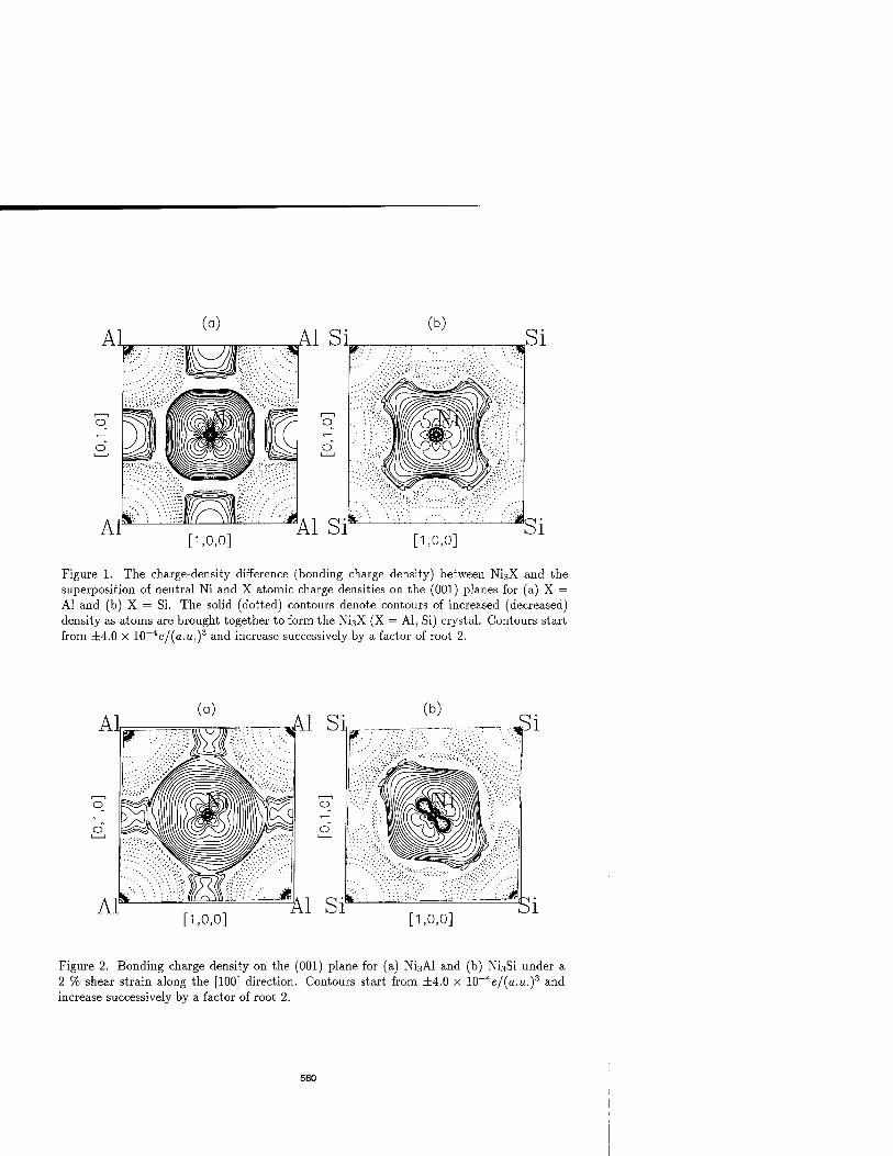
[1,0,0] [1,0,0]

Figure 1. The charge-density difference (bonding charge density) between Ni3X and the superposition of neutral Ni and X atomic charge densities on the (001) planes for (a) X = Al and (b) X = Si. The solid (dotted) contours denote contours of increased (decreased) density as atoms are brought together to form the Ni3X (X = Al, Si) crystal. Contours start from ±4.0 X 10_4e/(a.u.)3 and increase successively by a factor of root 2.

[1,0,0] [1,0,0]

Figure 2. Bonding charge density on the (001) plane for (a) Ni3Al and (b) Ni3Si under a 2 % shear strain along the [100] direction. Contours start from ±4.0 x 10~4e/(a.«.)3 and increase successively by a factor of root 2.

560

the S ratio is similar to the trend of the tendency for brittle intergranular fracture, with the grain-boundary cohesive strength changing in the order Ni3Mn > Ni3Al > Ni3Ga > Ni3Si.[7] We find that the § ratio decreases linealrly with the difference in atomic electronegativity between Ni and X as suggested by Taub et al.[7]

The mechanical strength of materials is due ultimately to the atomic bonding strength. The shearing in a certain direction involves the stretching of bonds and termination of the elastic regime involves the breaking of bonds. To gain an understanding of the changes of bonding charactersitics on going from Ni3Al to Ni3Si, we present in Fig. 1(a) the bonding- charge-density contour plots on the (001) plane (i.e. a mixed Ni-X, X = Al, Si plane). The bonding charge density, is defined as the difference of the total charge density in the solid and the superpositions of neutral atomic charge densities placed at atomic sites, i.e.,

Ap(r) = p30nd(r) - EQj°c<(r - rn). The bonding charge density represents the net charge redistribution as atoms are brought together to form the crystal. The solid and dotted curves represent accumulation (depletion) of electronic charge. For all compounds, we observe a depletion of charge from the X sites and a build-up of directional d-bonding charge at the Ni sites. In both compounds we find that the depletion of electron density at the X(A1 or Si) sites is accompanied by significant anisotropic buildup of the directional d-bonding charge at the nickel sites along the nearest neighbor Ni-X direction. The bonding directionality is caused mainly by the polarization of the p electrons at the X sites as a result of the p-d hybridization. On the other hand, while in Ni3Al there is a significant buildup of interstitial bonding charge at the octahedral sites (sites between the next-nearest-neighbor (NNN) Ni and X sites), in Ni3Si there is a depletion of bonding charge at the corresponding sites. The more pronounced directional bonding between the Ni and Si atoms, compared to that between the Ni and Al atoms, is responsible for the stronger resistance to shear in Ni3Si, as indicated by the larger values of shear moduli of Ni3Si. The bonding charge densities of Ni3Ga and Ni3Ge resemble those of Ni3Al and Ni3Si, respectively. Comparing the /- and site- projected density of states, we find that the addition of the p electron on going from Al to Si results in the lowering of the p-band with respect to the fermi energy and the filling of the Ni-d hole. This results to a reduction of the density of states at the Fermi energy in Ni3Si. In order to gain insight at the microscopic level into the redistribution of bonding charge as the systems undergo deformation, we present in Fig. , 2 the bonding charge density contour plots on the (001) plane under a 2% pure shear strain along the [100] direction, for (a) Ni3Al and for (b) Ni3Si. One can see that the response of bonding charge to deformation is quite different for the two systems. The bonding charge density is preserved and only slightly deformed in Ni3Al, while it changes substantially in Ni3Si, indicating a greater resistance to

shear (larger value for C44) in Ni3Si. To summarize, we have presented total-energy FLMTO electronic structure calculations

of the elastic constants of the Ll2-type ordered nickel-based intermetallics Ni3X (X= Mn, Al, Ga, Si, Ge). The agreement between theory and experiment for the elastic constants is relatively good (with a maximum error of about 30%) except for Ni3Ga. The larger error in Ni3Ga might be due to the sensitivity of the semi-core 3d state to the choice of the tail parameter. The large values of the anisotropic factor across the series is due to the anisotropic distribution of bonding charge. The calculated & ratio for the polycrystalline systems is found to correlate well with the difference in atomic electronegativity between Ni and X, as has been suggested experimentally.

561

ACKNOWLEDGMENTS

The research was supported through the U.S. Army Research Office under Grant No. DAAH04- 93-G-0427 and the Office of Research at California State University Northridge.

References

[I] C. L. Briant, in Intermetallic Compounds - Principles and Practices, edited by J. H. Westbrook and R.L. Fleischer, (John Wiley k Sons, 1995), Vol. 1, p 895.

[2] D.M. Wee, 0. Noguchi, Y. Oya, and T. Suzuki, Trans. Jap. Inst. Metals, 21, 237 (1980).

[3] M.H.Yoo, Scripta Metall. 20, 915 (1986).

[4] V.Paidar, D.P.Pope, and V.Vitek, Acta Metall. 32, 435 (1984).

[5] S.Takeuchi and E.Kuramoto, Acta Metall. 21, 415 (1973).

[6] H.Yasuda, T.Takasugi and M.Koiwa, Acta Metall. 40-2, 381 (1992).

[7] A. I. Taub and C. L. Briant, Acta Metall. 35, 1597 (1987).

[8] T. Takasugi and 0. Izumi, Acta Metall. 33, 1247 (1985).

[9] M. E. Eberhart and D. D. Vvedensky, Phys. Rev. Lett. 58, 61 (1987).

[10] M. E. Fine, L. D. Brown, and H. L. Marcus, Scripta Metall. 18, 951 (1984).

[II] S.F.Pugh Phil. Mag. 45, 823 (1954).

[12] H. B. Huntington, The Elastic Constants of Crystals, (Academic Press, 1958).

[13] D.L.Price and B.R.Cooper Phys. Rev. B 39, 4945 (1989).

[14] D. J. Chadi and M. L. Cohen, Phys. Rev. B 8, 5747 (1973).

[15] R. Wu, private communication (1995).

[16] Smithell's Metals Reference Book. 6th ed., edited by E. Brandes (Butterworths, Lon- don, 1983).

[17] M.H.Yoo, C.L.Fu and J.A.Horton Materials Science and Engineering, A176, 431 (1994).

[18] C. L. Fu and M.H. Yoo, Mat. Chem. and Phys. 32, 32 (1992).

[19] R.Hill Proc. Phys. Soc. A65, 349 (1952).

562

AB-INITIO CALCULATIONS OF THE ELECTRONIC STRUCTURE AND PROPERTIES OF TITANIUM CARBOSULFIDE

Bala Ramalingam*, Michael E. McHenry*, Warren M. Garrison, Jr.*, James M. MacLaren** *MSE Department, Carnegie Mellon University, Pittsburgh, PA 15213 **Physics Department, Tulane University, New Orleans, LA 70118

ABSTRACT

Titanium carbosulfide (TiaCS) is frequently found as an inclusion phase in Ti - containing steels. It is of considerable interest because, whenever present in preference to the more common manganese sulfide (MnS), it significantly improves the toughness (a very desirable property) of the steel. Currently, to the best of our knowledge, there is no data, either computational or experimental, regarding the structural properties of T12CS. This data is needed to understand the influence of the Ti2CS inclusions on the toughness of the host material.

In this paper, our results from the ab-initio calculations, using the LKKR-ASA (Layer Korringa Kohn Rostoker method in the Atomic Spheres Approximation) on the equilibrium ground state properties of bulk Ti2CS are presented and discussed. In particular, attention is focused upon (a) the Energy - Atomic Volume curve generated to calculate the equilibrium lattice constant and the bulk modulus, and (b) the density of states calculations. The application of these results to the subsequent study of an interface involving the carbosulfide and the host matrix is also illustrated.

INTRODUCTION

Fracture in many ductile materials proceeds by the growth and coalescence of voids nucleated at second phase particles. In ultra-high strength steels, it has been found [1] that T12CS particles are more resistant to void nucleation than the more common manganese sulfide MnS particles, resulting in an improvement of the fracture toughness by more than a factor of two when the sulfur is gettered as Ti2CS instead of as MnS. Currently, no explanation exists as to why this is the case - the bonding at the particle-matrix interface is thought to be of crucial importance in void nucleation by decohesion of the interface and hence our computational efforts are directed at a thorough investigation of the electronic structure & properties of the interfaces of MnS and T12CS particles in an iron matrix. Before an attempt is made to study interfaces involving Ti2CS, it is essential to obtain the properties (such as the elastic modulii and the electronic structure) of the bulk phase.

There is no literature, either computational or experimental, on the properties of T12CS. There are no reports to indicate that the phase has been artificially synthesized in any form. Ti2CS has a hexagonal crystal structure (Figure 1) with c = 11.2 Ä and a = 3.21Ä (c/a = 3.5) [2]. Besides the crystal structure and the lattice dimensions, very little is known about the phase. The bonding in the material is, in particular, very poorly understood. We believe that this is the first work to report on the electronic structure and properties of Ti2CS.

[ 1 1 0 j View

Figure 1 : Ti2CS Unit Cell

563


METHODOLOGY

The LKKR method, developed by MacLaren et. al. [3], is a modification of the original KKR technique [4]. Both methods use the muffin-tin approximation to the true crystal potential and use the 'spherical harmonic bases' within the muffin tin and 'plane wave bases' in the interstitial region. In the atomic spheres approximation, one considers overlapping spheres centered at every atom site and there is no interstitial volume in the system. The original KKR method is suitable for bulk systems (systems that possess full three-dimensional periodicity) only. The LKKR method partitions 3-D space into layers and requires Bloch periodicity only within each layer (i.e. the requirement of periodicity is relaxed in the direction perpendicular to the layers) - thus it is well adapted to handle systems that exhibit only 2-D periodicity. This allows for planar defects like surfaces and interfaces to be treated within the same framework as the bulk material.

The calculation employs a Green's function technique adapted to multiple scattering theory-it solves for the one electron Green's function within the semi-relativistic, local spin density and self-consistent field approximations. All desired electronic properties can be obtained once the local energy resolved density of states, p (r,E), for each atom is obtained. The charge density is related to the one electron Green's function as follows:

p(r, E) = - - Im f dk. G(r, k, E) (1)

where the integration is over the 2-D Brillouin zone.

RESULTS & DISCUSSION

Variation of Total Energy with Lattice Constant:

For the purpose of this calculation, the experimentally reported c/a ratio of 3.5 was held constant and 'a' was allowed to vary between 5.90 Bohr (1 Bohr = 0.529Ä) and 6.50 Bohr. The variation of the total energy as a function of the lattice constant is depicted in Figure 2. A smooth curve joining the points was obtained by fitting the standard Birch-Murnaghan equation of state to the discrete points. The equilibrium lattice constant (corresponding to the minimum total energy) and the bulk modulus were then obtained from this fit.

Initially, the calculation was done sampling 6 k-points in a Brillouin zone wedge and using 37 interstitial plane waves - this predicted an equilibrium lattice constant of 6.25 Bohr (which is about 3% higher than the experimentally reported value) and a bulk modulus of 2.5

Table 1: Predicted Lattice Constant and Bulk Modulus as a function of k-points1 and number of plane waves2

Nuilibr.1 l'l k-fVIllls 6 IK 6 Numlvi Mt pLine \\a\e-i 37 37 55 Lattice Constant, a (Bohr) 6.25 6.25 6.26 Bulk Modulus, B (Mbar) 2.51 2.51 2.47 1 - number of k-points sampled in one Brillouin zone wedge 2 - number of interstitial plane waves used in the calculation

564

-0.56

-0.58

-0.60

-0.62

-0.64

-0.66

5.90 6.00 6.40 6.10 6.20 6.30 Lattice Constant (Bohrs)

Figure 2 : Total Energy - Lattice Constant Curve

6.50

Mbar. As mentioned earlier, no prior experimental or computational data regarding the bulk modulus is available to compare our results with; as a measure of internal consistency, we varied both the number of k-points sampled and the number of interstitial plane waves used in the calculation - that the results are quite well converged can be seen from Table 1. In general, the LKKR calculations predict the lattice constant to within 2% and the bulk modulus to within 20%. The fact that the LKKR code does slightly worse in the case of TJ2CS may be due to the complexity of the structure involved - we intend to redo our calculations using a full-potential method in the near future as a further means of checking our current results. Nevertheless, the current results seem to be quite reasonable and the fact that the material has a fairly high bulk modulus, higher than many ionic materials and yet much less than the covalently bonded 'hard' materials (for instance, diamond has a bulk modulus of about 5.45 Mbar) is indicative of the mixture of ionic and covalent bonding present in the material.

Density of States:

The energy resolved density of states (DOS) for each of the atom sites is shown in Figure 3. The DOS for Ti is largely 'd' in character with the highest peak lying 2 eV above the Fermi level (thus there are a large number of unoccupied d-states in the system). The sulfur DOS exhibits predominantly s-like character at 12-16 eV below the Fermi level and p-like character from near the Fermi level to about 8 eV below it ; in comparison, both the s- and the p- characters in carbon are confined to relatively narrow energy ranges. Again, this is indicative of the mixed ionic and covalent character in the bonding within the solid. We are presently engaged in (a) calculating the band structure of Ti2CS and (b) generating charge density contours in various planes in the crystal structure. The results from these calculations, in addition to the density of states distribution, should provide us with a good understanding of the exact nature of bonding within the crystal.

565

100

90

80 w .t c 70

-P <r 60 w

15 50 w "6 40 ^

30 0) Q

20

10

0 -18 -16 -14 -12 -10 -8 -6 -4 -2 0

Energy (relative to Fermi Energy), eV Figure 3: Density of States at the different sites in Ti2CS

CONCLUSIONS

In summary, we have used the LKKR technique within the ASA approximation to investigate the ground state electronic structure of Ti2CS. We find that the predicted lattice constant of 6.26 Bohr is in reasonable agreement with the experimentally reported value. We also find the material to have a bulk modulus of about 2.5 Mbar, a value that falls between that of ionically- and covalently- bonded materials. We conclude that this is due to the presence of largely covalent Ti-C bonds and reasonably ionic Ti-S bonds.

ACKNOWLEDGMENTS

The financial support of this project by the Army Research Office for proposal 30912-MS is gratefully acknowledged.

REFERENCES

1. K.J. Handerhan, W.M. Garrison, Jr. and N.R. Moody, Met. Trans. A, 20A, p. 105 (1989) ; J.L. Maloney and W.M. Garrison, Jr., Scripta Met., 23, p. 2097 (1989).

2. W.B. Pearson, A Handbook of Crystal Structure Data, Pergamon Press, p. 2004.

3. J.M. MacLaren, S. Crampin, D.D. Vvedensky and J.B. Pendry, Phys. Rev. B40, p. 12164 (1989).

4. J. Korringa, Physica, 1947, p. 13; W. Kohn and N. Rostoker, Phys. Rev., 1954, p. 94.

566

EELS STUDIES OF B2-TYPE TRANSITION METAL ALUMINIDES: EXPERIMENT AND THEORY.

G.A. BOTTON*, G.Y. GUOt, W.M. TEMMERMANt, Z. SZOTEK*, C.J. HUMPHREYS*, YANG WANG*, G.M. STOCKS*, D.M.C. NICHOLSON*, and W.A. SHELTON* * Department of Materials Science, Univ. Cambridge, Cambridge, CB2 3QZ, U.K., ' Daresbury Laboratory, Warringion, WAJ, J,AD, U.K., $ Oak Ridge National Laboratory, Oak Ridge, TN 37831-6114, USA.

ABSTRACT

The electronic structure and bonding character of intermetallic alloys are investigated by a combination of electron energy loss spectroscopy (EELS) experiments and ab initio electronic structure calculations. A detailed comparison is made between experimental spectra and calculations. The changes in electronic structure within a transition metal aluminide series and also due to alloying are studied using EELS spectra. The Korringa-Kohn-Rostoker coherent-potential-approximation method and large supercell models are used to investigate changes in composition and the effect of dopants on the electronic structure.

INTRODUCTION

Intermetallic alloys are a class of materials of potential interest for high performance structural applications. A serious difficulty limiting their current use, however, is their intrinsic brittle behavior at room temperature. Electron energy loss spectroscopy (EELS) is a potentially powerful local probe of the electronic structure of alloys. This locality is twofold. Firstly, EELS white lines result from the excitation of p-core electrons into unoccupied s- and J-conduction band states and, as such, probe the local (atom specific) densities of states. Secondly, because the EELS experiment is performed in a high resolution electron microscope, the spectra result from small regions of the sample. This microprobe capability then opens up the exciting possibility of simultaneously probing the chemistry and electronic structure of such important determinants of mechanical properties as grain boundaries. However, before EELS can be used in this way, the key question as to whether EELS spectra can be understood in terms of a single particle framework must be answered in the affirmative. Here, we show results of EELS experiments on bulk transition metal aluminides and corresponding electronic structure calculations based on the local density approximation (LDA) that suggest this is the case.

MATERIALS AND METHODS

Alloys were prepared by arc melting high purity starting materials (Al 99.999% pure and 99.98% pure transition metal (TM)). Transmission electron microscopy specimens were prepared by electropolishing 3mm diameter disks. Energy loss spectroscopy was carried out on a Philips CM30 electron microscope equipped with a Gatan model 666 spectrometer. At the operating voltage of lOOkV an energy resolution, measured at the full width at half maximum of the no loss peak, of better than leV is typically obtained. Theoretical calculations using the linear muffin-tin orbital (LMTO) method [4], the Korringa-Kohn- Rostoker coherent-potential-approximation (KKR-CPA) method [3] and the large system multiple scattering (LSMS) method [5] are used to calculate the density of states (DOS). The DOS are either compared directly to experiment or are combined with the transition

567


matrix elements to calculate the EELS spectrum. According to Fermi's golden rule [1] the energy loss transition probability 0, for excitation from an occupied core level of angular momentum / to unoccupied conduction band final states of angular momenta I + 1 and I — 1 is given schematically by [2]

0, oc {|M,+1|Vn + IM,-!!2™,-!} (1)

where M,±i are matrix elements and n,-ti are the / decomposed unoccupied local DOS measured relative to the Fermi energy tp.

RESULTS

Electronic structure in transition metal alloys Considerable differences are observed in the experimental EELS spectra of the transition

metal L edges in FeAl, CoAl and NiAl (Fig.l, left) with respect to the edges of the same metals in pure standards (see [6]). The edges from the intermetallics show a decrease in white-line intensity with respect to the continuum background after the edge and a secondary peak (or shoulder in the case of FeAl) on the high energy side of the white line. The calculated white-line spectra (Fig.l, right) obtained using LMTO densities of states and Eq. 1 show excellent agreement with the experimental spectra, reproducing the fine structure and intensity variations of the white-lines across the TM series. The calculations show that the observed reduction of the white-line intensity is due to filling of the rf-bands associated with the transition metal sites. The agreement with experiment allows one to be confident about the validity of the combined approach and the implications that follow in terms of bonding.

1.5 10"3

i | i i i i | , , , , , , , l .

--FeAlFeL i , , , ,

-NiAINiL; \ /"-

/• '■-■"■.

'c D xi <

_

c B c

-

..i..._*-r -

-20 -10 0 10 20 30 Energy Loss (eV) above the threshold

40 -10 0 10 20 30 Energy Loss (eV)

relative to the threshold

Figure 1: Left: Transition metal L edges in FeAl, CoAl and NiAl. Right: Calculated Co and Ni L white lines in CoAl and NiAl. The intensity scale is constant for the two spectra.

In Fig. 2 (left), we show the results of EELS experiments on a series of B2 (/?)-phase NijAli-a, alloys. Again, a considerable band filling effect is clearly seen in the data. The white-line intensity varies continuously on the Ni rich side, whereas, it is constant in the Ni deficient alloy. Interestingly, the change in the filling trend occurring at the stoichiometric

568

composition correlates with the variation of the macroscopic properties (magnetic suscepti- bility, resistivity and electronic specific heat) and the defect structure of this alloy described by Koch and Koenig [7], Butler et al. [8] and Lipson and Taylor [9]. As spectra in stoichiometric NiAl and the Ni deficient alloy are similar (Fig.2, left, lower curve), our experiments indicate that there is no significant change in bonding when constitutional vacancies are introduced in the Ni sublattice. This agrees with recent conclusions of Cottrell [10]. In Ni rich alloys, the compositional variations are accommodated by antisite defects (TM atoms on the Al sublattice) which are more stable than Al vacancies. Because the Ni d bands are hybridized with Al s-p bands, the spectra show a "dilution" effect of the Al s-p electrons from the Al atoms by their replacement with Ni atoms in the "wrong" sites.

<

1 1 1 1 1 1 1 1 1 1 1 1 1 1 1 1 1 1 1 1 1 , , . 1 ,

x=.63

- 1 ^~\ / x=.55 r =

- J\ \v J x=.50

-

- 1 \ .'/' "-■-

J> V .'• x=.45 .-■„-

i

. .J-.". . . 1 . . , . 1 , , , , 1

840 850 860 870 880 Energy Loss (eV)

890 900 12 3 4 5 e-eP (eV)

Figure 2: Left: Experimental Ni Z-spectra of /?-phase Ni^Alj-^ alloys. Right: Calculated Ni-site densities of states of /3-phase NixAli_x alloys obtained using the KKR-CPA method.

We have calculated the densities of states of /?-phase Ni^Ali-r alloys using the Korringa- Kohn-Rostoker coherent-potential approximation (KKR-CPA) method. In this method the effects of disorder (vacancies on the Ni sub-lattice, in the case of Al-rich alloys, and Ni antisite defects on the Al sub-lattice, in the case of Ni-rich alloys) are treated using the CPA. The unoccupied Ni-site DOS for the experimentally relevant energy range (summed over the Ni-sublattice and, where appropriate, Ni-anti-site defects) are shown in Fig. 2 (right). The corresponding total DOS for both occupied and unoccupied states are shown in Fig. 3 (left).

Because there is substantial charge transfer in this alloy system, we have also used the newly developed order-N Locally Self-consistent Multiple Scattering (LSMS) method to obtain compositionally averaged potentials for use in the KKR-CPA, rather than use the standard KKR-CPA self-consistency procedure. The reason for doing this results from the KKR- CPA's neglect of certain charge transfer contributions to the effective electron-ion potential, effects that are treated accurately by the LSMS method [12]. Ideally, one should also use the LSMS method for calculating the DOS, however, for the unoccupied, free electron like, part of the DOS that is relevant to the EELS the real space techniques used in the LSMS method converge quite slowly. Thus, for the present purposes we use the KKR-CPA to calculate DOS and will defer direct use of the LSMS DOS to a later publication. The DOS based on the LSMS potentials are shown in Fig. 3 (right). In the LSMS part of the calculation the disorder is simulated using a large (250-site) super cell comprising a 5x5x5 repeat of

569

e-eF (eV) -5 0 5 e-e, (eV)

Figure 3: Densities of states Ni-sites of Ni^Ali-*. Left: KKR-CPA. Right: LSMS

the underlying B2 (CsCl) lattice, with vacancies (anti-site defects) randomly distributed on the Ni(Al) sub-lattices as appropriate. Once self-consistency has been obtained, suitable configurationally averaged single site potentials are constructed for use in the KKR-CPA. From Fig. 3 it can be seen that the two approaches give similar results for the cases where we have performed both calculations for the same concentration. Given this, we confine our discussion of the EELS experiment to a comparison with the KKR-CPA DOS. It should be noted that in Fig. 2 (right) there is a small contribution from Ni p-states, however it is sufficiently small that the DOS can be safely used to compare [neglecting matrix element effects (see Eq. 1)] with the experimental EELS spectra. We postpone to a later publication full KKR-CPA and LSMS based EELS calculations.

In agreement with experiments, the calculations for Ni-rich alloys show an increase of the DOS at ep and a lowering of ep within the band. This is consistent with the increased energy interval between ep and the first peak above ep and also with the increased intensity of the peak at the edge threshold seen in the EELS data. In the Ni deficient alloy, changes are not observed in the EELS spectra. This is again consistent with the DOS in that both the position of the first peak above ep changes little relative to tp and the relative heights of the DOS at tp and the first peak do not change in going from the sub-stoichiometric to

stoichiometric composition.

Effects of dopants on bonding Considerable modifications of the macroscopic properties can be introduced by alloying

and doping with ternary elements. Given our success in modeling the electronic structure in NiAl, a suitable ternary system to study is the well characterized [11] Ni-Al-Cu system. In Fig. 4 we show Ni and Cu L-edge spectra obtained from a Alo.s(Cu0.iNio.4) alloy. When Cu is in solid solution the intensity of the first peak at the Ni threshold (Fig. 4, left) decreases significantly with respect to its form in Alo.55Nio.45 or Alo.5Nio.5- Looking at the L edge of the Cu dopant (Fig. 4, right) a white line appears, relative to the pure Cu metal [13]. This is suggestive that J-holes are introduced at the dopant sites. Charge transfer from the Cu to Ni d bands, via hybridization, seems thus to occur upon alloying NiAl with Cu. We note also that the Cu and Ni L edges are very similar, and this is indicative of a region of a common

570

, 1 , , , 1 | 1 1 1 1 | , 1 I ,_

^^ - " '"-■ *s-'~'~~

c -) ■-.,,„«•>

•O

< _

>*, ■-*,---> " a

js a) : , -U-f': , , 1 , , , , 1 , , , i , , , , i , , , ,"

840 850 860 870 880 890 Energy Loss (eV)

90 920 930 940 950 960 Energy Loss (eV)

970

Figure 4: Left: Ni L-edge in Al5o(Ni40Cuio). Right: Cu L-edge in Al5C)(Ni4oCuio).

band behavior. In Fig. 5 we show the DOS obtained using the LMTO method for Ni8(Al7Ni) (left),

Ni8Al8 (center), and (Ni7Cu)Al8 (right), super-cell models of Ni-rich, stoichiometric, and Cu-doped /?-phase NiAl. For the Cu doped alloys the EELS data indicate a shift of tp to

I111!"1

.-—\

'8 - "

■e < C/5 \ O " 1 1 A

Q

M.LMIM

'1 , , i | , i i | i i i | i i i

(Average)

Cu s+d

o \ (w Q 'M ^

/ I,

0„ 2 4,, 6 Energy (eV)

-202468 Energy (eV) relative to Ef -2 0^ 2 4,, 6

Energy (ev)

Figure 5: LMTO DOS for 16-atom super-cell models of NiCuAl alloys (s+d, Ni+Cu). Left: Ni8(Al7Ni). Center: Ni8Al8. Right: (Ni7Cu)Al8.

higher energies with Cu doping. This effect is consistent with the supercell calculations, where for (Ni7Cu)Al8 (Fig. 5, right) the energy interval between tp and the first peak above tp is decreased with respect to the pure Ni8Al8 supercell. (Fig. 5, center). The DOS just above ep, relative to the intensity of the first peak above e/r, is also reduced in agreement with the near edge structure of the Ni edge. This is evidenced by the fact that the first peak in the experimental spectrum is greatly reduced and appears as a shoulder. In this energy region a common band effect is also observed in that the DOS corresponding to Ni and Cu sites are very similar. It is also interesting that the DOS at ep relative to the first peak above ep is lower at the Cu sites than Ni. Again this is consistent with the EELS data for

571

which the shoulder present in the Ni edge is only just visible at the Cu edge.

CONCLUSIONS

We have demonstrated that EELS is a very efficient tool to retrieve information about the electronic structure of alloys. Variations in bonding across a series of aluminides have been demonstrated and excellent agreement with calculations shown. Our spectra indicate that significant changes in the near edge structure occur upon changes in alloy composition.

These changes have been associated with the variation in the Fermi level within the energy bands and correlate with both the bonding behavior and the macroscopic properties. Upon

alloying with ternary elements, significant changes both on the host lattice atoms and on the dopant atoms are observed with respect to their pure or "host" lattice state.

ACKNOWLEDGMENTS

The work of GAB was supported financially by EPSRC and was initiated during a NSERC (Canada) fellowship. The work of GMS, YW, DMN and WAS was supported by Office of Basic Energy Sciences, Division of Materials Science (GMS) and Mathematical, Informa- tion, and Computational Sciences Division (GMS, YW, DMN and WAS), US-DOE, under subcontract DEAC05-84OR21400 with Lockheed-Martin Energy Systems, Inc.. We thank Sir A. Cottrell for pointing out Lipson and Taylor's paper and for making his work available prior to publication. We are grateful to Mrs Y. Zheng for some of the NixAli-j, samples and Dr W. M. Stobbs for continued interest in this work.

References

[1] D.D. Vvedensky , in Unoccupied Electronic States, Eds. J.C. Fuggle and J.E. Inglesfield

(Springer Verlag, Berlin), 139 (1993). [2] G.A. Botton, G.-Y. Guo , W.M.Temmerman and C.J. Humphreys, to be submitted

(1995). [3] G.M. Stocks, D.M.C. Nicholson, W.A. Shelton, B.L. Gyorffy, F.J. Pinski, D.D. John-

son, J.B. Staunton, B. Ginatempo, P.E.A. Turchi, and M. Sluiter, in Statics and Dynamics of Phase Transformations edited by P.E.A. Turchi and A. Gonis, (Plenum Press, New York, NATO-ASI Series B:Physics, 1993), pp305-360.

[4] H.L. Skriver, The LMTO Method: Muffin-Tin Orbitals and the Electronic Structure (Springer, Berlin, 1984)

[5] Yang Wang, G.M. Stocks, W.A. Shelton, D.M.C. Nicholson, Z.Szotek and W.M. Tern- merman, Phys. Rev. Lett. 75 2867 (1995).

[6] R.D. Leapman, L.A. Grünes and P.L. Fejes Phys. Rev. B26, 614 (1982). [7] J.M. Koch and C. Koenig Phil. Mag. B54, 177 (1986). [8] S R. Butler, J.E. Hanlon and R.J. Wasilewski, J. Phys. Chem. Solids, 30, 1929 (1969). [9] H. Lipson and A. Taylor, Proc. Royal Soc. London, A173, 232 (1939).

[10] A.H. Cottrell, Intermetallics, 3, 341 (1995). [11] A.J. Bradley and H. Lipson, Proc. Royal Soc. London, A167, 421 (1938). [12] J.S. Faulkner, Y. Wang and G.M. Stocks, Phys. Rev. (1995) (in press). [13] G.A. Botton, C.B. Boothroyd , A. Ul-Hamid, S.B. Newcomb, W.M. Stobbs, Electron

Microscopy and Analysis 1993, Edited by A.G. Craven, (The Institute of Physics, Lon-

don), p.43 (1993).

572

SINTERING OF AMORPHOUS Si3N4 NANOCLUSTERS: A MOLECULAR DYNAMICS STUDY OF STRESS ANALYSIS

Jinghan Wang, Kenji Tsuruta, Andrey Omeltchenko, Rajiv K. Kalia, and Priya Vashishta

Concurrent Computing Laboratory for Materials Simulations Department of Physics & Astronomy and Department of Computer Science Louisiana State University, Baton Rouge, LA 70803-4001 [email protected] http://www.cclms.lsu.edu

ABSTRACT

We investigate the onset and growth of the neck between amorphous Si^^ nanoclusters at zero and finite pressures. Local stress fluctuations and atomic self-diffusion in the interface region are found to be responsible for neck formation. External pressure has a dramatic influence on the rate of sintering.

INTRODUCTION

Silicon nitride, due to strong covalent bonding and low thermal expansion coefficient, is one of the best thermal shock and chemical corrosion resistant ceramic materials. It also displays excellent mechanical properties at high temperatures.[l] Like all ceramics, the one undesirable characteristic of silicon nitride is its brittle behavior. Recent experiments reveal that nanostructured ceramics are less brittle than coarse-grained ceramics.[3-5]

One of the important issues concerning the synthesis of nanophase ceramics is their sintering behavior. Many theoretical models have been proposed [6] to account for different mechanisms operating at various stages of sintering. Many of the models consider only large spherical particles with an isotropic surface energy and the capillarity to be the driving force. Recent experimental results [7] indicate that these assumptions may break down in the case of sintering of nanosize particles. Theoretical models have not yet addressed issues concerning the structure and mechanical behavior of nanoparticle sintering at the atomistic level. Microscopies of the neck formation during the early stages of sintering is also difficult to investigate experimentally.

In this paper we report a molecular-dynamics (MD) simulation study of initial stage of smtering of a pair of amorphous Si3N4 nanoclusters at T = 2000K. The size of nanoclusters is 80 A. At zero pressure, the clusters form a symmetric neck of size ~ 20 A within the first 700 ps of the MD simulation. The neck formation is preceded by an incubation period which lasts for approximately 160 ps. During incubation the clusters are joined by a few Si-N intercluster bonds, and the local stresses in the neck region are small. After the incubation period, non-uniform stresses on the order of a few GPa develop in the neck region. Concomitantly there is a significant increase in the number of Si-N bonds joining the two nanoclusters. The neck region has nearly the same number of four-fold and three-fold coordinated Si atoms. The atomic self-diffusion in the neck region is five times larger than in the interior of the clusters. External pressure has a dramatic effect on the rate of sintering.

RESULTS

Molecular-dynamics simulations were performed with effective interatomic potentials consisting of two-body and three-body terms. [8] The two-body terms include screened Coulomb potential, charge-dipole interaction, and steric repulsion between atoms. The first two terms take into account charge-transfer and electronic polarizibility effects in the system. Three-body bond bending and bond stretching terms take into account covalent effects in silicon nitride.

573


The above interatomic potential has been tested extensively by comparing MD results with experimental measurements. The calculated bond lengths and bond angle distributions for a- Si3N4 are in excellent agreement with experiments. [9] The MD results for vibrational density of states (DOS) are also in good agreement with recent neutron scattering data. [10] The specific heat [10] of a-Si3N4 agrees very well with experiments over a wide range of temperatures. [11] The

MD result for the bulk modulus (287 GPa) of <x-Si3N4 is within a few percent of the experimental result (281 GPa) [12], and the calculated values of Young's modulii along different orientations with respect to the c-axis are within 15% of experimental measurements. [13] The MD results for the static structure factor (including the first sharp diffraction peak, the fingerprint of intermediate- range order) and DOS of amorphous SJ3N4 are also in good agreement with neutron scattering measurements^ 14,10]

Molecular-dynamics simulations were performed for two amorphous Si3N4 clusters of diameter D ~ 80Ä and density 2.8 g/cm3. (The clusters contained 20,643 and 20,706 atoms.) The clusters were obtained from bulk amorphous Si3N4 which was prepared by heating a-Si3N4 crystal to 6000K over 190 ps and then quenching the system systematically to 300K over a time period of 270 ps. The two amorphous clusters were relaxed with the MD and conjugate gradient methods. Subsequently they were heated to 2,000K over a time period of 20 ps and thermalized for 100 ps. The forces and potential energy were calculated with a multiple time-scale approach, and the equations of motion were integrated with the velocity-Verlet algorithm [15] using a time step size of 2 femto seconds.

Figures la and lb show initial and final atomic configurations of clusters at zero pressure and T = 2000K. Before sintering the surfaces of the two clusters are found to be terminated by nitrogen atoms. At time t = 0, the angular momentum of each cluster is set equal to zero and the minimum separation between the two clusters is 3.5Ä. Starting with this initial configuration (figure la), MD simulation were carried out for 700 ps. As figure lb shows, the two clusters form a nearly symmetric neck. The size of the neck is estimated to be approximately one-fourth (~ 20A) of the size of each cluster. From partial pair-distribution functions we find that the neck has nearly the same number of 4-fold and 3-fold coordinated Si atoms.

Figure 2 shows the neck growth during sintering at P = 0. The neck size is estimated by counting the number of intercluster Si-N bonds, 3\&j_N> in the neck region (%_N is the number of nearest Si-N neighbors within a cutoff distance of 2.3 Ä, i.e., the distance at which the minimum after the first peak in Si-N partial pair-distribution function occurs at 2000K). Figure 2 shows

Fig. 1 Snapshots of the two amorphous Si3N4 nanoclusters at T = 2000K: (a) at time t = 0; (b) after 700 ps.

574

100 TT I I iI I I 1 I I IT I ] I r I 1 ] I 1 I

1

/ ' (b)

eck formation

600 800 400

t[ps] Fig. 2 Formation of intercluster Si-N bonds in the neck region as a function of time.

distinct evolutionary stages of sintering. Within the first 10 ps a few Si-N bonds join the two clusters. In the next 150 ps the clusters undergo substantial relative motion without a significant increase in ^VSJ-N- This motion results in spontaneous formation and breaking of intercluster Si-N bonds. After 170 ps the relative motion of the two clusters subsides and there is a steady increase in IA&i-N- During this stage the number of new Si-N bonds is significantly larger than the number of spontaneously broken Si-N bonds.

To understand the mechanism behind sintering, we have analyzed the local stress distribution in the neck region. The stress is calculated from the well-known virial expression and the mechanical approach [16]. (We divide the system into slices of thickness 5.5A along the z axis and the local stresses are calculated for each slice.) At zero pressure, we find the local stresses during the incubation period are nearly zero throughout the two clusters (see figure 3a for t = 80 - 120 ps). When the neck growth starts (see figure 3b), non-uniform local stresses on the order of a

z[A] 40

180 HO 100 z[A]

=1 ^K

(a) (b) Fig. 3 Local stress distribution azz in the clusters as a function of time for pressureless sintering, (a) During the incubation stage (t = 80 - 120 ps); (b) during the neck growth (t = 200 - 240 ps). The arrows indicate the location of the neck region.

575

few GPa develop in the neck region. Concomitantly, the number of Si-N bonds 7YSJ_N begins to increase (cf. figure 2). We find that the position of the maximum stress varies with time during neck formation. After 700 ps, the neck size is ~ 20Ä and it contains 90 Si-N bonds.

In both virial and mechanical approaches, the stress includes the momentum and force contributions. Variations in the local stress reflect thermal and density fluctuations. We observe a large local density fluctuation in the neck region during the neck growth. These fluctuations have a significant effect on intercluster Si-N bond formation. Comparing figures 2 and 3 we arrive at the conclusion that local stress fluctuations give rise to atomic self-diffusion in the interface region and thus the neck formation.

We have determined the self-diffusion of surface atoms from their mean-square displacement (MSD). Figure 4 shows the MSD after the neck growth starts (t = 170 ps). For comparison, we also show the MSD in the interior of clusters. Clearly the surface atoms in the neck region are much more diffusive than those inside the clusters. From figure 4 we estimate that the self-diffusion coefficients of Si and N atoms are approximately 2 x 10"6 cm2/sec in the neck region. This is almost five times as large as the self-diffusion of atoms in the interior of clusters.

0 12 3 4 t[ps]

Fig. 4 Mean-square displacement of atoms in the neck region and in the interior of clusters after the neck growth starts.

To investigate the effect of pressure on sintering, we imposed on the top and bottom of the two clusters an external pressure of 0.4 GPa along the z axis. The starting configuration of clusters was taken from the previous case of pressureless sintering. This initial configuration had been run for 80 ps at P = 0 and it only contained six intercluster Si-N bonds.

Figure 5a shows the internal stress distribution czz as a function of time. We find that in response to the external pressure an internal stress of 3.8 GPa develops in the neck region within the first 20 ps. Subsequently, the peak value of the stress in the neck region relaxes. However, the local stress distribution throughout the clusters is still non-uniform. As shown in figure 5b, the external pressure has a very significant influence on the sintering rate. At 0.4 GPa, the intercluster Si-N bond-formation rate becomes considerably larger than the rate at P = 0. It takes only 40 ps to form a neck of size 20 A; at P = 0 a neck of this size forms in 700 ps.

We also carried out the MD simulations and stress analysis performed above on two nanocrystalline cluster system. We find that the sintering of the nanocrystals shows very similar behavior as that of the amorphous nanoclusters.

576

EA mn "B

3 S

2$ O 80

l a fc 60 0 Ä

«2 20

0 40 u

[ps] 01

-a e

20

1 0

Pressure o ~0.4GPa

!"l"rf1-?-,-ri-»f«

50 100 150

(a)

t[ps]

(b) Fig. 5 The effect of pressure on sintering: (a) local stress distribution azz as a function of time; (b) Intercluster bond-formation at zero and finite pressures.

CONCLUSION

We have presented results of MD simulations for sintering of amorphous Si3N4

nanoclusters at zero and finite pressures. We find that non-uniform internal stresses are the major cause of self-diffusion of atoms in the interface region, and this leads to neck formation. At zero pressure, a symmetric neck of size 20 A is formed within 700 ps. The neck contains nearly equal number of 4-fold and 3-fold coordinated Si atoms. Under an external pressure of 0.4 GPa the rate of neck formation is an order-of-magnitude faster than that at zero pressure.

ACKNOWLEDGMENT

We acknowledge useful discussions with Drs. A. Nakano and E. Ma. This work was supported by DOE (Grant No. DE-FG05-92ER45477), NSF (Grant No. DMR-9412965) and AFOSR (Grant No. F 49620-94-1-0444). Simulations were performed on the 128-node IBM SP computer at Argonne National Laboratory and the parallel machines in the Concurrent Computing Laboratory for Materials Simulations (CCLMS) at Louisiana State University. The facilities in the CCLMS were acquired with equipment enhancement grants awarded by the Louisiana Board of Regents through Louisiana Educational Quality Support Fund.

REFERENCES

1. Silicon Nitride Ceramics. Scientific and Technological Advances, edited by I.-W. Chen, P. F. Becher, M. Mitomo, G. Petzow, and T.-S. Yen (Mater. Res. Soc. Symp. Proc. 287, 1993); Silicon Nitride 93. edited by M. J. Hoffmann, P. F. Becher, and Petzow (Trans. Tech. Publications, Switzerland, 1994).

2. J. Karch, R. Birringer, and H. Gleiter, Nature 330, 556 (1987).

3. T. Rouxel and F. Wakai, Acta Metall. Mater. 41, 3203 (1993).

4. R. W. Siegel and G. E. Fougere, in Nanophase Materials: Synthesis-Properties-Application, edited by G. J. Hadjipanayis and R. W. Siegel (Kluwer, Dordrecht, 1994) p. 223.

5. A. Pechenik, G. J. Piermarini, and S. C. Danforth, J. Am. Ceram. Soc. 75, 3283 (1992).

6. H. E. Exner, in Sintering Key Papers, edited by S. Somiya and Y. Moriyoshi (Elsevier Applied Science, London, 1990) p. 87; D. L. Johnson, in Sintering Processes, edited by G. C. Kuczynski (Plenun Press, New York, 1980) vol. 13, p. 97; W. D. Kingery, H. K. Bowen, and

577

D R Uhlmann, in Introduction to Ceramics. (John Wiley & Sons, New York, 1976); D. L. Johnson, J. Appl. Phys. 40, 192 (1969).

7. J. E. Bonevich and L. D. Marks, Mat. Res. Soc. Symp. Proc. 286, 3 (1993).

8. P. Vashishta, R. K. Kalia, J. P. Rino, and I. Ebbsjö, Phys. Rev. B41, 12197 (1990).

9. P. Vashishta, R. K. Kalia, and I. Ebbsjö, Phys. Rev. Lett. 31, 858 (1995).

10. C.-K. Loong, P. Vashishta, R. K. Kalia, and I. Ebbsjö, Europhys. Lett. 31, 201 (1995).

11. Silicon Nitride, ed. by T. B. Shaffer and A. Goel (Advanced Refractory Technologies Inc., Buffalo, New York, 1993). 12. A. Nakano, R. K. Kalia, and P. Vashishta, Phys. Rev. Lett. 23, 3138 (1995).

13 L. Cratz and J. D. Jorgensen, J. Appl. Phys. 52, 236 (1981); A. A. Mukaseev, V. N. Gribkov, B. V. Shchetanov, A. S. Isaikin, and V. A. Silaev, Poroshk. Metall. 12, 97 (1972).

14. M. Misawa et al., J. Non-cryst. Solids 34, 313 (1979); T. Aiyama et al., ibid. 33, 131 (1979). 15. M. P. Allen and D. J. Tildesley, in Computer Simulation of Liquids, (Oxford University Press, Oxford, 1990). 16 J F Lutsko, J. Appl. Phys. 65, 2991 (1989); K. S. Cheung and S. Yip, J. Appl. Phys. 70, 5688 (1991); D. H. Tisa, J. Chem. Phys. 70, 1375 (1979).

578

DFT Study of the Monocyclic and Bicyclic Ring Geometries of C20

Zhiqiang Wang, Paul Day, and Ruth Pachter Materials Directorate, Wright Laboratory, WL/MLPJ,

Wright-Patterson Air Force Base, Ohio 45433-7702

Abstract

The monocyclic and bicyclic ring geometries of C20 are optimized using both the local density functional approximation (LDA) and gradient-corrected density functional theory (BLYP). The energy of the bicyclic ring is found to be higher than that of the monocyclic ring in both LDA and BLYP calculations. The BLYP results confirm the previous single point calculation based on Hartree-Fock geometries[l], which is in favor of the monocyclic ring geometry, while the LDA results still favor the cage geometry. LDA frequencies of both ring geometries are also presented.

Introduction

As C6o and its derivatives exhibit increasingly interesting materials properties, such as superconductivity[2] and non-linear optical response [3], attention has also focused on the smallest carbon cluster to form the closed fullerene structure, C20 The appeal of C20 is due not only to its relevance in gaining a further understanding of COO, but also to the possibility of its being an intermediate in the formation of COO and larger fullerenes. Experimental evidence shows the dominant structures of C20 as monocyclic and bicyclic rings [4], although kinetic and entropic effects should be considered when compared with energetic calculations. Previous theoretical studies have focused on three forms of C20: a monocyclic ring, a corannulene-like bowl, and the fullerene-like cage [1, 5, 6, 7, 8]. In this note we report the results of our full geometry optimizations of the four isomers of C20: monocyclic and bicyclic rings, bowl, and cage (as shown in Fig. 1), using both the LDA and the gradient-corrected LDA (BLYP) approaches. We also report the vibrational spectra of the two ring geometries from our LDA calculations.

Method DFT calculations were carried out with DMol version 2.3.6 [9]. Two functionals of the exchange-correlation energy were used: one is a LDA which combines Slater exchange with the Vosko-Wilk-Nusair parametrization of Ceperley and Alder's correlation energy of a uniform electron gas by Monte Carlo studies (VWN) [10], and the other is the

579


gradient-corrected functional of the exchange term by Becke[ll] and the correlation term by Lee, Yang, and Parr[12] (BLYP). The input structures for the DFT optimizations were taken from the optimized geometry of HF or other DFT calculations. The basis set consists of double numerical DFT atomic orbitals augmented by polarization functions (DNP), comparable to the Gaussian 6-3lG(d,p) basis sets. Iteration of ten to twenty

steps are typically needed for a full geometry optimization. Tolerances were taken as 0 001 for the gradient, 0.001 for the displacement or 0.00001 for the energy (all m atomic units). HF calculations were carried out with parallel GAMESS [13] using 32 or

64 processors on an Intel Paragon.

Fig. 1 The structures of four C2o isomers: fullerene, bicyclic ring, bowl, and mono-

cyclic ring.

Results and Discussion Table I lists our calculated energies of the four geometry forms of C2o clusters using the LDA and BLYP approaches with the fully optimized geometries. The BLYP calculation prefers the monocyclic ring structure over the cage by an energy difference of 3.3 eV, while LDA (VWN) favors the cage over the monocyclic ring by 3.9 eV. The bicyclic ring geometry is found not to be the lowest energy geometry, with its energy higher than that of the monocyclic by 0.8 and 2.3 eV, respectively, in the LDA and BLYP calculations. Our BLYP results after full geometry optimization confirm what has been predicted

580

Table 1: Calculated energies (units of Hartree) of the mono- and bicyclic rings, bowl, and cage isomers of C20 using DFT geometry optimizations. Values in parentheses are relative energies (units of eV).

geometry rings bowl cage monocyclic bicyclic

LDA -754.8975(0) -754.8677(0.81) -754.9850(-2.39) -755.0389(-3.85) BLYP -761.5997(0) -761.5141(2.33) -761.5444(1.50) -761.4777(3.32)

from the previous single point BLYP calculation using the HF geometry[1]. Although the full optimization does not change the order of energy of each geometry, the LDA optimization reduced the energy by 1.4 eV after optimizing the HF monocyclic ring, which is now comparable to the energy difference between the monocyclic ring and the cage, namely, 3.8 eV. This does indicate the importance of a full geometry optimization when comparing energy differences.

The geometries (bond lengths and angles) of the two ring forms of C20, optimized with LDA and BLYP, are listed in Table II. Our LDA optimization from the HF monocyclic ring geometry with Cioh has a C2h symmetry imposed (DMol can only handle Abelian symmetry group), and in the resulting geometry the two bond angles are much closer to being identical (162° ± 1.0°), indicating that the ring is closer to assuming a Dioh symmetry. However, a DFT optimization starting with and preserving the D\0h symmetry has an energy about 0.05 eV higher, thus excluding an exact D\oh symmetry as being the lowest energy geometry. Several independent runs result in some isoenergetic geometries with bond angles within the range of 162±1.0°, indicating the energy surface near the minimum to be rather flat. Alternating bond angles are dominant in all of these geometries. Although we did not obtain an exact Cioh symmetry, we believe it is in one of these isoenergetic geometries. We note that previously the LDA C20 monocyclic ring optimized geometry was claimed to assume a Cioh symmetry[5]. Our LDA optimized bicyclic ring geometry has a D2h symmetry, although only C, symmetry is imposed. The BLYP geometry is shown to be very close to the LDA geometry. The geometries for the other isomers (bowl and cage) of C20 are reported in ref. [8], which also shows that LDA geometries are much closer to BLYP than to HF. The symmetries of some of these geometries are also different using the different approaches. For example, the cage has C2 symmetry in HF, but C; symmetry after the DFT optimization.

Fig. 2 shows our calculated harmonic vibrational frequencies of the C2o monocyclic and bicyclic rings using LDA, in comparison with the HF/631G(d) results for monocyclic ring [1]. Although LDA overestimates the bond energy, its vibrational frequencies are usually close to those of BLYP, as we noted previously [14]. The similarity of the LDA geometry to that of BLYP, rather than the HF result, also indicates that LDA vibrational spectra could be used as an alternative to those of BLYP, which are expensive to calculate. Because of the lack of an exact Cioh symmetry of our LDA geometry of monocyclic ring, it does not show the exact degeneracy of some frequencies as HF does, but the two LDA values of each of these HF degenerate frequencies are also close enough except for the pair of 440 and 471 cm-1. LDA results are in agreement with HF in the

581

Table 2: Bond lengths (A) and angles (°) of the monocyclic and bicyclic rings of C2o after DFT(LDA, BLYP) geometry optimizations. The numerical labels of the carbon

atoms are taken to be the same as those listed in Fig. 1.

Monocyclic C1-C2 C2-C3 Cl-2-3 C2-3-4

VWN 1.245 1.329 162.3±0.4 161.7±0.4

BLYP 1.243 1.333 162.3-162.9 160.9-161.8

Bicyclic C1-C2 C2-C3 C2-C4 C4-C5 C5-C6 C6-C7 C7-C8

VWN 1.47 1.48 1.34 1.27 1.30 1.28 1.30

BLYP 1.49 1.49 1.34 1.27 1.30 1.28 1.30

Cl-2-3 Cl-2-4 C2-4-5 C4-5-6 C5-6-7 C6-7-8

VWN 90.0 130.0 150.7 159.1 141.9 138.3

BLYP 90.0 130.6 149.6 159.7 140.8 139.2

low frequency region after the latter are rescaled by a factor of 0.89. However, there are significant differences in the two gaps between the LDA spectra of 561, 858 cm and 1589, 1994 cm-1. These gap widths are 297 and 405 cm-1 for LDA, but 108 and 829 cm-1 for HF. These differences also cause the inconsistency of spectra near these two gaps for the LDA and HF approaches. The understanding of such differences may enable to identify the geometry experimentally and to verify the validity of these two approaches on such systems. Previous work has shown that DFT might be superior to HF and even to MP2 method in frequency calculations[15]. Interestingly, the LDA calculated bicyclic ring spectra does not show the second big band gap present in that of monocyclic ring. The first gap is also much smaller. The zero point energy of the monocyclic and bicyclic rings are 2.66 and 2.69 eV, respectively, still in favor of the

monocyclic ring geometry.

Conclusion We have added two new results to the database of controversial theoretical results for the C20 cluster: the BLYP full geometry optimization and LDA vibrational spectra of the ring geometries. Our full geometry optimization using BLYP is in favor of the monocyclic ring geometry, which does not change the qualitative relation between the ring, bowl, and cage geometries of C20 predicted previously by a single point calculation. The bicyclic ring is not the lowest energy geometry in both LDA and BLYP calculations. The LDA vibrational spectra of the monocyclic ring show significant differences with those of HF/631G(d) on the widths of two band gaps. These gaps are not significant in

the LDA spectra of the bicyclic ring.

582

o

•i—I o c

2700

2025

1350-

675

0 Monocyclic Monocyclic Bicyclic

LDA Hartree-Fock LDA

Fig. 2 Calculated harmonic vibrational frequencies (cm ') for the C20 monocyclic and bicyclic rings using LDA(VWN), as compaxed to those using HF/631G(d,p).

583

References [1] K. Raghavachari, D. L. Strout, G. K. Odom, G. E. Scuseria, J.A. Pople, B.G.

Johnson and P.M.W. Gill, Chem. Phys. Lett. 214 (1993) 357.

[2] Y. Achiba, T. Nakagawa, Y. Matusui, S. Suzuki, H. Shiromaru, K. Yamauchi, K. Nishiyama, M. Kainosho, H. Hoshi, Y. Maruyama, and T. Mitani, Chem. Letters, 7 (1991) 98.

[3] W. Blau, H. Byrne, D. Cardin, T. Dennis, J. Hare, H. Kroto, and R. Taylor, Phys. Rev. Letters 67 (1991) 1423; F. Henari, J. Callaghan, H. Stiel, W. Blau, and D. Cardin, Chem. Phys. Letters, 199 (1992) 144.

[4] G. von Helden, M. T. Hsu, N.G. Gotts, P.K. Kemper, and M.T. Bowers, Chem. Phys. Lett., 204 (1993) 15; H. Handschuh, G. Gantefor, B. Kessler, P. S. Bechthold, and W. Ebhardt, Phys. Rev. Lett., 74 (1995) 1095.

[5] P. R. Taylor, E. Bylaska, J.H.Weare, and R. Kawai, Chem. Phys. Lett., 235 (1995) 558.

[6] V. Parasuk and J. Almlof, Chem. Phys. Lett., 184 (1991) 187.

[7] J. Grossman, L. Mitas, and K. Raghavachari, Phys. Rev. Lett., 75 (1995) 3870.

[8] Z. Wang, P. Day, and R. Pachter, Chem. Phys. Lett., (in press).

[9] B. Delley, J. Chem. Phys. 92 (1990) 508. DMol is distributed by Biosym Technolo- gies, Inc. at San Diego, CA.

[10] S. J. Vosko, L. Wilk, and M. Nusair, Can. J. Phys., 58 (1980) 1200.

[11] A. D. Becke, J. Chem. Phys., 88 (1988) 2547.

[12] C. Lee, W. Yang, R. G. Parr, Phys. Rev. B 37 (1988) 786.

[13] M.W. Schmidt, K.K. Baldridge, J.A. Boatz, S.T. Elbert, M.S. Gordon, J.J.Jensen, S. Koseki, N. Matsunaga, K.A. Nguyen, S. Su, T.L. Windus, M.Dupuis, J.A. Mont- gomery, J. Comp. Chem., 14 (1993) 1347.

[14] Z. Wang, P. Day, and R. Pachter, Chem. Phys. Lett., 237 (1995) 45.

[15] B. G. Johnson, P. M. W. Gill, and J. A. Pople, J. Chem. Phys. 98 (1993) 5612.

584

THE MAGNETIC STRUCTURE OF Cu0.2Ni0.8 ALLOYS

YANG WANG*, G. M. STOCKS*, D. M. C. NICHOLSONt, W. A. SHELTON*, Z. SZOTEKH, AND W. M. TEMMERMANI 'Metals and Ceramics Division, Oak Ridge National Laboratory, Oak Ridge, TN 37831 I Computational Physics and Engineering Division, Oak Ridge National Laboratory, Oak Ridge, TN 37831 ^Engineering Physics and Mathematics Division, Oak Ridge National Laboratory, Oak Ridge, TN 37831 'SERC, Daresbury Laboratory, Daresbury, Warrington, WA4 4AD, U.K.

ABSTRACT

The locally self-consistent multiple scattering method is applied to ab initio spin-polarized local density approximation calculations for ferromagnetic CuNi alloys. The samples used to model the alloys are constructed with experimentally measured short range order parameters. These large cell calculations are performed using the Intel Paragon XP/S massively parallel processing supercomputer. The neutron magnetic diffuse scattering cross sections are calculated and compared with experiment. The dependence of magnetic moment formation on the local environment is discussed.

INTRODUCTION

The Ni-rich CuNi alloys are ferromagnetic at low temperatures. Their average bulk magnetic moment decreases approximately at the rate of lpB for every replacement of a Ni atom by a Cu atom[l, 2, 3], which is essentially non-magnetic in the alloys. The reduction of the average bulk magnetic moment is caused not only by simple dilution of the Ni concentration but also by reduction of the Ni moment with increase of the Cu concentration^]. However, as the Cu concentration approaches 60%, the reduction of the bulk moment departs from the linear relationship. This phenomenon is not predicted by our KKR-CPA calculation[4] and is believed to be associated with the local environments influence on Ni moments.

Since the earlier work of Jaccarino and Walker[5], much effort has been put into understanding the local environment affects on Ni moment behavior in CuNi alloys. In spite of some success of phenomenological approaches [6] to the problem, little progress has been made regarding the first principles calculation of the local effects. This is largely due to the lack of sufficient computing power to carry out the calculations. Using the locally self-consistent multiple scattering (LSMS) method[7], together with the currently available massively parallel processing supercomputing technology, we were able to perform first principles electronic structure calculations for large unit cells, which were employed to simulate disordered ferromagnetic CuNi alloys, and to observe directly the magnetic moment distribution among the constituent atoms. The moment-moment correlation functions can thus be obtained from the results of the calculation, and can be used to determine such physical quantities as the neutron magnetic diffuse scattering cross-section.

COMPUTATIONAL APPROACH

The LSMS method is an order-N real space approach to electronic structure calculations within the framework of the local density approximation (LDA)[8, 9] for large cells consisting of hundreds or thousands of atoms. The LSMS method is based on the observation that a good approximation to the electron density in the vicinity of an atom site in the system can be obtained by considering only the electronic multiple scattering processes in a finite

585


spatial region centered at the site. This region is referred to as the local interaction zone (LIZ). Every atom in the system is considered to be at the center of its own LIZ, and one can use this fact to obtain an approximation to the electron density on every atom site in the system. Because of the stationary nature of the thermodynamic free energy[10], we are allowed to use the approximate electron density for the fully self-consistent field (SCF) calculation without making a significant error in the energy. Given this algorithm, the electronic structure problem is reduced to that of calculating the electron density on the central atom of N finite clusters of sites, where N is the number of atoms in the system. According to multiple scattering theory[ll, 12], the spin-dependent electron density in the vicinity of atom i is given by

pjj(r) = —Im f ' de fc #(r; e)^]^(«}.■; «(r; e) - £ Z?{r; e) J*(r; e) *■ J-°° ILL' L

, (1)

where the expression inside the square brackets is the one-electron Green's function[13]. The symbol s stands for spin, M is the number of atoms in the LIZ of atom i, {£},• denotes an atomic configuration of the LIZ, ts is the Fermi energy, and TJ^({£},; e) is the scattering path matrix for the cluster of atoms in the LIZ. The functions Z£''(r;e) and J'L'\r;e) are regular and irregular solutions of the single site Schrödinger equation. The spin-polarized LDA one-electron potential to be used for the next SCF iteration is then reconstructed, which involves solving Poisson's equation, with an appropriate boundary condition on the large cell boundary, for a total electron density made up of a sum of the single site densities. The LSMS method can be made highly scalable on a parallel computer if one assigns each atom in the cell to a compute node. The amount of work to be done by each node for calculating />JJ(r) is essentially unchanged with respect to the system size JV.

Given the electron density for each spin channel, the magnetic spin moment, /*,-, can be calculated using

W=/.^r{,Jfr)-/#(r)}, (2)

where ü{ is the atomic cell volume of site i. Once the individual moments are obtained, we are able to determine the Stoner-Hubbard parameter, which is the intra-atomic interaction energy between spin up and spin down d-electrons, for the magnetic constituents of the alloy. According to Stoner's itinerant electron model[14, 15] for ferromagnetism, the moment at each site is proportional to the exchange splitting of the atom on the site. The proportionality constant is the inverse of the Stoner-Hubbard parameter / for the atom. In addition to the calculation of the Stoner-Hubbard parameter, we are also able to examine the magnetic moment-moment correlations and calculate the neutron magnetic diffuse scattering cross section, which, in the units of milibarn, is given by[16]

% = lx72M276x^^^^{(fi(Q)9^-(f(Q)9ß})(fMsiN-(nQ)^))), (3) Oll O JV {j Wttij

where the magnetic Bragg scattering has been excluded. The symbol g represents the g- factor of the spin moment, /,(Q) is magnetic form factor for atom i, Ri, is the spatial distance between site i and site j, and Q is the magnitude of the scattering vector, which is the difference between the incoming and outgoing neutron wave vectors. The symbol (...) represents the average over a grand canonical ensemble. In practice, we rely on self-averaging over the large cell instead of using the ensemble average.

586


A preliminary study of the local moment behavior in ferromagnetic CuNi alloys has been done for Cuo.2Nio.8- To simulate the alloy, we constructed a large unit cell sample which contains 51 Cu and 205 Ni atoms occupying the underlying fee lattice and is assumed to repeat itself to fill the space. The distribution of the atoms in the large cell is not completely random. Rather, it is slightly short range clustering and has the same short range order parameters as the experimental sample[17]. A SCF spin-polarized LSMS calculation for the large cell was performed on the Intel PARAGON XP/S-150 massively parallel processing supercomputer systems at ORNL. In the calculation, the LIZ of each atom was chosen to include 6 neighboring atom shells, which corresponds to 87-atom clusters. The muffin-tin approximation was applied to the one-electron potential and the electron density.

The calculated spin moment of each site is plotted against the total spin moment on the first neighboring shell of the site in figure 1. It agrees with the experiment [17] in that the

0.8

0.0

-0.2

CU0.2Ni0.8

■Cu site moment

■Ni site moment

n " i*&grg&^te»6aflargtofr-7j>-

Cu

0.0 1.0 2.0 3.0 4.0 5.0 6.0 7.0

total spin moment on nn shell (u, )

8.0

Figure 1: The magnetic spin moment distribution in a f.c.c. Cuo.jNics disordered alloy. The spin moment of each atom is plotted against the total spin moment on the first neighboring shell. The moments were calculated using the spin-polarized LSMS method with muffin-tin approximation.

Ni moments are finite and aligned along the same direction, while the Cu spin moments are near zero and pointing in the opposite direction to the Ni spin moments. Evidently, there is a strong correlation between individual spin moments and their neighboring total moments, which suggests that the spin moments on the neighboring shells play a major role in the local environmental effects on a single site moment. As a matter of fact, the spin moment of individual Ni atoms can differ by as much as 0.3fiß for various local environments.

It is well known that the itinerant electron model by Stoner is a transparent scheme for correlating the magnetic properties of ferromagnetic metals and alloys. Its assumption that the carriers of the magnetism are the unpaired electrons in the d band is consistent with local spin density theory[18, 19]. The central parameter in this model is the Stoner-Hubbard parameter /, the exchange energy between the Bloch d-band electrons. To check Stoner

587

theory against the result of our LSMS calculation, in figure 2, we plot for each Ni atom the

0.05

u

0.04

0.03

0.02

0.01

0.00

i ' ' ' ' i

Ni Sites in Cun ,Nin U.Z U.o

o.o 0.2 0.3 0.4

magnetic moment ( |L)

Figure 2: The exchange splitting versus the spin moment on each Ni site. The slope of the fitting line gives the Stoner-Hubbard parameter.

exchange splitting versus the spin moment. The exchange splitting is assumed to be the energy difference between the spin-up and spin-down <f-resonances. As predicted by Stoner theory, the data points fall on a straight line. The slope of the line gives the Stoner-Hubbard parameter for Ni atoms in Cu0.2Ni0.g alloys and is found to be 0.071 Ry (or 0.97 eV), which can be compared with 0.074 Ry (or 1.01 eV) and 0.072 Ry (or 0.99 eV) obtained by other methods for Ni atoms in fee Ni[20, 21]. Knowing the moment on each site and using Eq. 3, we are able to calculate the.-neutron magnetic diffuse scattering cross section. In figure 3,

we present the calculated cross section for Cu0.2Ni0.8 together with the experimental results of Cable et o/.[17]. In the calculation, fm(Q) was obtained from fitting the experimentally measured magnetic form factors, and /cu(Q) was set to be 1.0. The ^-factor was chosen to be 2.27 for Ni and 2.0 for Cu. Calculated and experimental results agree very well with each other for large Q's. In particular, the calculated cross section reproduces the small oscillation around 1.8/Ä in the measured data which is mainly due to magnetic short range ordering. As Q decreases, the calculated cross section begins to rise, essentially following the same trend as the experiment. However we note that the calculations cannot describe the divergence at small Q. For a system of 256 atoms the neutron scattering cross section for Q values smaller than 0.5/Ä cannot anymore be evaluated. An accurate evaluation of the cross section for smaller Q requires a summation of Rij over a greater distance. This result therefore gives the smallest scattering vector which describes a given system size, obviously the smaller the scattering vector the larger the system is required.

SUMMARY

In conclusion, we have employed a 256-atom supercell to model the disordered phase of ferromagnetic Cuo.2Nio.s alloys and used the LSMS method to calculate the spin moment

588

10

E

I 8

6 -

1 1 1 I 1 1 ' "' 1 1—

■ ■ Experiment

0 OB O O O

° Calculation

CU0.2Ni0.2

-

°o- 0 % ■

-

°c V, ff^^^V*^ 1 1

s o is 2 s

0 12 3 scattering vector (1/A)

Figure 3: The neutron magnetic diffuse scattering cross section versus the magnitude of the neutron scattering vector. The solid squares are the calculated result, whereas the open circles represent the experimental value.

of individual sites. Local environmental effects were investigated based on the result of the LSMS calculation. The magnetic environments are found to have substantial short range affects on the magnetic moment of individual atoms. The linear relationship, predicted by Stoner theory, between the exchange splitting and spin moment on Ni atoms is graphically demonstrated by our calculations (Fig. 2) The overall agreement between experiment and the LSMS calculation for the neutron magnetic diffuse scattering cross section provides evidence for the magnetic short range order.

ACKNOWLEDGMENTS

This work is sponsored by the Division of Materials Sciences and the Applied Mathemat- ical Sciences Program, Office of Basic Energy Sciences, USDOE, under contract DEAC05- 84OR21400 with Lockheed Martin Energy Systems. We also acknowledge support from the Center for Computational Sciences at ORNL. One of the authors (YW) would like to acknowledge support from the ORNL Postdoctoral Research Associate Program administrated jointly by ORNL and ORISE.

References [1] S. A. Ahem and W. Sucksmith, Proc. Phys. Soc. B 69, 1050 (1956).

[2] S. A. Ahem, M. J. C. Martin, and W. Sucksmith, Proc. Roy. Soc. (London) A 248, 145 (1958).

[3] A. T. Aldred, B. D. Rainford, T. J. Hicks, and J. S. Kouvel, Phys. Rev. B 7, 218 (1973).

589

[4] Yang Wang, G. M. Stocks, D. M. C. Nicholson, W. A. Shelton, Proceedings of the TMS symposium 1993, Alloy Modeling and Design edited by G. M. Stocks and P. E. A. Turchi, pp. 137 (The Minerals, Metals and Materials Society, Warrendale, 1994).

[5] V. Jaccarino and L. R. Walker, Phys. Rev. Lett. 15, 258 (1965).

[6] R. A. Medina and J. W. Cable, Phys. Rev. B 15, 1539 (1977).

[7] Yang Wang, G. M. Stocks, D. M. C. Nicholson, W. A. Shelton, Z. Szotek, and W. M. Temmerman, Phys. Rev. Lett. 75, 2867 (1995).

[8] P. Hohenberg and W. Kohn, Phys. Rev. B 136, 864 (1964).

[9] W. Kohn and L. J. Sham, Phys. Rev. A 140, 1133 (1965).

[10] D. M. C. Nicholson, G. M. Stocks, Y. Wang, and W. A. Shelton, Z. Szotek, and W. M. Temmerman, Phys. Rev. B 50, 14686 (1994).

[11] Lord Rayleigh, Philos. Mag. 34, 481 (1892).

[12] J. Korringa, Physica 13, 392 (1947).

[13] J. S. Faulkner and G. M. Stocks, Phys. Rev. B 21, 3222 (1980).

[14] E. C. Stoner, Proc. Roy. Soc. A 154, 656 (1936).

[15] E. C. Stoner, Proc. Roy. Soc. A 165, 372 (1938).

[16] W. Marshall, J. Phys. C 1, 88 (1968).

[17] J. W. Cable, E. 0. Wollan, and H. R Child, Phys. Rev. Letts. 22, 1256(1969).

[18] U. von Barth and L. Hedin, J. Phys. C 5, 1629 (1972).

[19] 0. Gunnarsson and B. I. Lundqvist, Phys. Rev. B 13, 4274 (1976).

[20] 0. Gunnarsson, J. Phy. F 6, 587 (1976).

[21] 0. K. Andersen, J. Madsen, U. K. Poulsen, 0. Jepsen and J. Kollar, Physica B 86-88, 249 (1977).

590

COMPUTER SIMULATION OF CLUSTER ION IMPACTS ON A SOLID SURFACE

Z. INSEPOV, I. YAMADA Ion Beam Engineering Experimental Lab., Kyoto University,Sakyo, Kyoto 606-01 Japan, [email protected]

ABSTRACT

The sputtering probabilities for normal and oblique cluster ion impacts were calculated by the use of two-dimensional molecular dynamics (MD) calculations. These simulations have revealed the angular dependence of ejecting surface atoms on the cluster incidence angle. The ejecting flux has a symmetrical form with an essential lateral component in the case of normal cluster incidence. For an oblique cluster indidence we found a sharp asymmetry of sputtering orientation. We obtained that the ejecting flux consists of three components: a) fast flying atoms with the velocities higher than the cluster velocity v ~ 2.3v0, b) approximately self-similar component with v <=> v0, and, finally, c) slowly moving tail with v ~ 0.2v0, where v0 is the cluster velocity. According to our MD results we developed a new model of surface modification phenomena which consists of the Langevin Dynamics based on the Kardar-Parisi-Zhang equation, combined with a Monte-Carlo procedure for crater formation at normal and oblique cluster impacts. We obtained that for a symmetrical crater shape with a size in the order of 20 A, a significant smoothing occurs after irradiation by ~ 103 cluster impacts which has been supported by experiment at dose of ~ 1014 ion/cm2. The rate of the smoothing process can be significantly accelerated if the lateral sputtering phenemenon is taken into account. Simulation of oblique cluster impact on a surface at a grazing angle of 30° by constructing of asymmetric crater shape gives an opposite result: the surface roughness increases. The latter obtaining qualitatively agrees with the experiment.

INTRODUCTION

Cluster ion irradiation of solid surfaces has become a unique method for surface modification, distinguished from other techniques because of its ability to deliver high total energy, determined by cluster size and acceleration voltage, together with soft impact on a surface. The most interesting effect of cluster ion irradiation on a solid substrate appeares to be the surface smoothing effect. As it was established experimentally in Ref. [1], the surface roughness of various substrate materials measured by atomic force microscope have been considerably reduced after irradiation with C02 cluster ions accelerated to 10 kV. A rough surface containing valleys and hills of average heights in the order of 100 Ä becomes almost flat with residual roughness reduced by a factor of 10. The result of irradiation is drastically changed when the cluster hits a surface with an oblique direction. The surface roughness increases in this case. These results have been obtained for Pt, Cu, poly-Si, Si02, Si3N4 films and glass substrates.

In recent experiments [2] fast heavy ions were irradiated on glassy surfaces at normal and oblique directions. The authors have shown that a critical angle exists between an incident cluster velocity and surface normal above which the smoothing process is changed to opposite, and the surface roughning process occurs. The authors gave the value between 15° - 20° for this critical angle.

The Molecular Dynamics (MD) calculations of cluster impact with normal incidence on a solid surface have shown that a hot and highly compressed region with a transient temperature of up to 105 K and pressure up to 1 Mbar arises in a short time interval which probably leads to generation

591


of shock waves on the atomic scale [3-6]. The MD calculations revealed the lateral sputtering effect, in which the most of ejected surface atoms acquire momentums with a lateral orientation.

MD simulations of cluster-surface impacts account for many properties of new phenomena except for the surface smoothing effect. This is because the smoothing effect requires such a long time interval when compared to the typical MD calculation time for single cluster impacts. MD technique provides data for many cluster impacts too, however it is limited to the study of small surface pieces with typical sizes in the order of 100 x 100 A2 [7,8]. The computational cell size for this new surface smoothing phenomenon should be at least in the order of 1000 x 1000 Ä2, and the impacts of around 103 clusters on this surface area should be modeled, which imposes extreme requirements for hardware.

In Ref. [9], the authors have considered that the smoothing and corrugation of a surface profile is induced by tensile or compressive stresses which act along the surface plane. Based on equilibrium MD simulations the authors have shown that surface step free energies are essential for surface morphologies. The surface transformations produced by cluster irradiation differ from the subject in work [9] because of their non-equilibrium origin.

An oblique impact of 78.2 MeV single 127I ions on crystal I-vanine surfaces was studied in Ref. [10]. The authors obtained that the craters are asymmetrical, with much longer size along the ion azimuth of incidence than in the case of normal single heavy ion impact.

The emission of a target material at a hyper-velocity dust particle collision with a solid target was studied in frame of two-dimensional hydrodynamics code in Ref. [11].

Of course, all these results are of great interest to better understand the phenomena of crater formation and emission of a target material at cluster-surface impacts. Two-dimensional MD models of cluster - surface collision [7] are very useful to study the initial stage of the impact events. The advantage of these models is its simplicity, but not in expense of the physics, because, as it is noted elsewhere [11,12], the asymptotic behavior of emitted target particles appears to be similar for 2D and 3D cases.

The velocity region we restricted in this work is within so-called high-velocity impact region with the velocities v/c, ~ 1-10, where c„ is the sound velocity in target, which has been poorly studied by MD so far.

MOLECULAR DYNAMICS

A two-dimensional MD model of high-velocity Ar349 cluster impacts with energy of 20 - 100 eV/atom on a solid surface of about 100000 atoms was used in order to study the geometry of sputtering flux at normal and oblique cluster directions. The atoms were interacted via Buckingham potential [5]. The MD model includes a constant pressure procedure and a linked list procedure combined with the Verlet-list method [17]. The cluster and surface temperatures and surface virial pressure were calculated from transverse components of atomic velocities, as in Ref. [3-5],

The emitted flux was treated in terms of mass or atomic number distribution over radial velocities, dNIdv, for different time instants. Fig. 1 represents the distribution of emitted target atoms over the atomic velocities, and was obtained for the oblique cluster impact at 60° between the cluster incidence and surface normal, for dv=Q. 15v0, where v0 = (2E/m0)

m is the initial cluster velocity, m0 is the atomic mass. This figure reveales three characteristic time intervals: a) the fast target atoms flying with the velocities v <= 2.3 v0, b) the power-law dependent self-similar part with the velocities v ~ v0, and c) the slowest part with the velocities v ~ 0.2v0. The fast flying "leader" was not revealed in the case of normal cluster impact. The explanation of this finding seems to be as follows. As it is seen from the geometry of the surface pressure, the side-

592

■S 500 -i X VO = 28.4 km /s c o ^—1 \ ^ 10° " a" 50

o H < 10 - / \ V 1 5- u 3 i -

^

\f

rarefaction waves at an oblique impact are asymmetric and stronger than in the case of normal impact because the impact is directed closer to the open target surface. The second reason is that the rarefaction shock waves act on a very thin subsurface layer, and the shock stress value can

easily exceed the critical breaking stress. Two other slower parts of emitted flux exist at normal impact case too. The presence of the fast moving particles persuasively indicates that shock waves are really generated during the cluster impact on a solid target. From the shock wave theory [11,12] it is known that the function vIR is stationary in the coordinates rlR, zIR in axisymmetric geometry, where R(t) is the the shock wave front coordinate. Assuming R ~ ta, where t is the time elapsed from the instant of impact, v ~ dR/dt, and #(0 ~ pR 2, where N(t) is the number of target atoms flowed into the shock wave front and p is the target number density, we can get the power-law distribution:

dN/dv-v-t, where ßs = 3 for the energy conservation

and ßi = 2 for the momentum conservation, independently on space dimension. These two dependences are plotted in Fig. 1 as straight lines with appropriate slopes.

The geometry of emitted target particles is represented in Fig. 2. This figure shows a distinct asymmetrical distribution of particles 315 fs after the oblique impact. The lateral distribution of ejected atoms was not found in this case. We used this result for the modeling of surface modification, together with the symmetrical lateral sputtering probabilities obtained in our previous paper [3] for the case of normal cluster impact on a solid surface.

We obtained in this MD simulation that an oblique impact gives a larger disordered area of a target material, in comparison with normal cluster impact. We found this area assuming that a negative pressure exceeding some limit value will disorder the material. We did not model the latter particularity in this work.

SURFACE MODIFICATION

0.2 0.3 0.5 0.8 1.5 3.14.6 Radial velocity / vQ

Fig. 1 The velocity distribution function of emitted target atoms at Ar349 impact with E = 84 eV/atom and incidence angle of 60° from surface normal on a surface modeled by 92400 two-dimensional Si atoms, äFvp=0.15v0, v0 is the cluster velocity. Step lines correspond to time instants of 941 fs (thin line) and 2.5 ps (thick line) after the impact. Two straight lines relied on self-similar dependences with constant momentum (solid line) and constant energy (dashed line).

Fig. 2 The distribution of emitted target atoms at an oblique cluster impact for the instant / = 315 fs. vz, vy and v0 are the atomic velocity components and cluster velocity, respectively.

The aim of this work is to develop a simple numerical model of solid surface modification by cluster irradiation based on a

593

phenemenological Langevin Dynamics equation of motion in form, of the Kardar-Parisi-Zhang (KPZ) equation [13]:

^-w^l^^M, (i) This equation was used quite successfully to

describe a wide variety of growth models including ballistic aggregation, vapor deposition, and the morphology of growing surfaces or interfaces [14- 16]. It represents the nonlinear dynamics of growing surface profiles in terms of the coarse- grained interface heights h(r,t) in a ^/-dimensional space where r is the radius-vector in a (d-X)- dimension plane at time t, and accurately describes behavior in later-stages or scaling properties of a growing interface. The first term describes the surface relaxation driven by diffusion processes, the coefficient v is the surface tension. The nonlinear second term corrects the growing height's velocity, and the last term represents a Gaussian white noise with time average:

(t|(r4-0, (n (r,/)i| (r',/')) -2Y& (r-r')6 (/-/'),

where y is the amplitude of the noise which can be identified with the equilibrium evaporation rate multiplied by a surface temperature [16].

A single Gaussian hill having a typical area of single central Gaussian hill, L = 51. The order 104 - 107 A2 and a height of order 102 Ä was dose of 1 cluster impact on a hill placed in the center of the computational cell, corresponds to 1.5 x 10n ion/cm2. Average cluster sizes are in the order of 103 atoms,

and total cluster energies are ~ 20 - 200 keV. The typical irradiation parameters used for surface smoothing are as follows: doses are in the range of 1011 - 1014 ion/cm2, or 101 - 103 cluster/hill. We assumed also that clusters hit the surface with normal and oblique directions at a random position. Displacements of surface particles after the cluster impact were modeled in accordance with the probability obtained in our MD simulation of single cluster ion impact on a flat surface. To model the result of many cluster impacts, we assumed that a given amount of surface material is sputtered independently for each cluster impact.

We added the pinning forces in order to favour integer values of heights, in units of the layer space parameter c:

*A xis

Fig. 3 The results of bombarding with 10 normal (a) and oblique (b) cluster impacts on an area L x L which initially contained a

■ V„ sin /2JI h(r,t)\

The stochastic term in the KPZ equation was modified according to a crater formation procedure which reflects the cluster impact of a given energy and cluster size. We have defined the surface roughness from the variance:

594

!-(£?(*-Of. where A, is the height of i-th column, Z, is the length of computational cell, and hm is the mean

surface height:

A-=' /u ■ The crater geometry was introduced by the use of a Monte-Carlo procedure [17]: (i) select a random position for cluster impact; (ii) form a crater with a volume that

corresponds to the given cluster size and energy; (iii) select a position on the surface for redeposition; (iv) calculate the change in potential energy dU; (v) if dU is negative, accept new position; (vi) otherwise, select a uniformly distributed random number crE[0,l]; (vii) if exp(dUlkBT) < cu do not accept new position; (viii) simulate another jump of redepositing particle, i.e. start from (iii). Here, we have chosen Udepending on z coordinate only. Therefore, dU~ dz, where dz is the height difference between destination and initial positions. The items (iii) - (vii) were repeated for each ejected atom individually.

To understand better the geometry effect of ejected surface atoms due to the cluster impact, we modeled various occurences for the redeposition event. Particles can be reflected from the first position and redeposited at another position, or be sputtered from the surface. Thus, we have taken into consideration a lateral sputtering effect. The shape of a rim around the crater in case of normal impact was chosen depending on the local hill slope. In the case of an oblique impact we have constructed a very asymmetrical rim according to the experimental result of single heavy ion impact [10], and did not take the lateral spreading movement into account.

Periodical boundary conditions were used in two directions along the x and y axis. The equation (1) contains the model parameter

v which can be considered as surface diffusion coefficient [18]. This choice allows us to model different substrate materials.

CO w ID z X o Z) O a: LU Ü < li-

w

0.24

0.22

0.20

0 200 400 600 800 1000

ION DOSE, in 1.5x1011 ion/cm2

Fig. 4 Dose dependence of surface roughness for L = 51 (160 Ä) for 103 cluster impacts. Circles correspond to normal orientation of cluster velocity, squares - to oblique at 60° cluster impact. Triangles show the result when the probability of sputtering was chosen to be equal to 0.5 for an oblique impact.

on a Si surface [3].

THE RESULTS AND DISCUSSIONS

The nonlinear differential equation (1) have been transformed to the difference equation and computed numerically. We use dimensionless units for the length and time variables, the parameters in equation (1) were: v = 10"4 cm2/s [18], To = 300 K. We supposed in this work that sputtered surface atoms diffuse with the maximal diffusion coefficient. The calculation were performed for the cell sizes L2 = 625, 2601, 10000 and 40000 atomic positions.

Fig. 3 depicts the result of 103 cluster impacts on a 2D - surface containing 2601 atomic positions at normal (a) and oblique (b) cluster incidences. The area size correspond to 160x160 A2. The diameter of a crater was chosen to be 20 A which corresponds to 3000 Ar atoms impact

One cluster impact corresponds to the cluster ion dose of 1.5 x 1011 ion/cm2.

595

It should be noted that if one uses a typical surface diffusion coefficient on the order of 10" cm2/s [18] for Si adatoms on a Si surface at room temperature, no modification could be achieved. Therefore, we supposed that modification of Si surface with cluster irradiation could be possible if laterally sputtered substrate atoms are overheated due to their significant momentums along the surface, and, hence, they are highly nonequilibrated with the surface. Obviously, this is a new, non-equilibrium mechanism of surface modification which does not need much energy compared with the conventional surface diffusion or melting.

Fig. 4 represents the results of surface roughness calculations in the case when no pinning forces were included into the equation (1), for the cell size L = 51 for two cases of normal (circles) and oblique (squares) cluster impacts on a surface. To get these results we supposed that all ejected at the impact target atoms were redeposited on the surface. There was almost no change of results if the probability of sputtering was chosen to be equal to 0.5 (triangles), in the case of an oblique impact. Similar results were obtained for all cell sizes and for cluster energies higher than 50 eV/atom when surface sputtering is noticeable.

SUMMARY

1) MD revealed an existence of three parts of emitted target atoms after an oblique cluster impact with energy of £ ~ 100 eV/atom and velocity of v0 - 30 km/s. The fastest part flying with the velocity of v ~ 2.3v0 was not found in case of normal cluster impact with the same total cluster energy. The main part of emitted atoms has velocities on the order, or much less than v0. The yield of ejected target atoms contains no lateral component, at an oblique impact.

2) A new simple numerical model based on the Kardar-Parisi-Zhang equation for surface modification by accelerated cluster impacts at normal and oblique incidences was developed. The craters formed after cluster impact on a substrate surface have been modeled by the use of the Monte-Carlo technique. The probabilities of sputtering were extracted from the MD calculations of cluster-surface impacts.

3) The calculations were performed for the cell sizes L2 = 625, 2601, 10000 and 40000 atomic positions. If no lateral diffusion was included in the equation of motion, surface roughness increases after irradiation with normal cluster impacts. Significant smoothing effect was obtained for all cell sizes due to the enchancement of surface diffusion coefficient after normal cluster bombardment. The shape of the symmetrical rim around a crater effects the surface roughness very little.

4) Constructing of a sharply asymmetrical crater shape together with excluding of lateral spreading effect can, in principle, explain the roughning phenomenon at an oblique cluster impact, but the rate of roughning was not so high in this model. The phenomenon of surface roughning at an oblique impact seems to be more complicated, and it needs more detailed investigation.

REFERENCES

1 I. Yamada, J. Matsuo, Z. Insepov and M. Akizuki, Proc. Intern. Conf. IBMM, Canberra, Australia, 1995,(to be published).

2 A. Gutzmann, S. Klaumunzer, and P. Meier, Phys.Rev.Lett. 74, p.2256, (1995). 3 Z. Insepov, M. Sosnowski and I. Yamada, Trans. Mat. Res. Soc. Jpn. 17, p.lll (1994). 4 Z. Insepov, M. Sosnowski, G. Takaoka and I. Yamada, Mat.Res.Soc.Proc, 316, p.999 (1994). 5 Z. Insepov and I. Yamada, MM B 99, p.248 (1995). 6 C.L. Cleveland and U. Landman, Science 257, p.335 (1992). 7 K.-H. Müller, J.Appl.Phys. 61, p.2516 (1987).

596

8 H. Haberland, Z. Insepov and M. Moseler, Phys.Rev.B 51, p. 11061 (1995). 9 Y.H. Xie, G. Gilmer, C. Roland et al., Phys. Rev. Lett. 73, p.3006 (1994). 10 J. Kopniczky, CT. Reimann, A. Hallen, B.U.R. Sandqvist, P. Tengvall and R. Erlangsson,

Phys.Rev.B 49, p.625 (1994). 11 N.A. Inogamov, A.B. Konstantinov, S.I. Anisimov and S.B. Zhitenev, Sov. Phys.JETP 72,

p.948 (1991). 12 Ya.B. Zel'dovich, Yu.P. Raiser, Physics of Shock Waves and High-Temperature

Hydrodynamic Phenomena. Academic, New York (1967). 13 M. Kardar, G. Parisi and Y. Zhang, Phys.Rev.Lett. 56, p.889 (1986). 14 F. Family, J.Phys. A: Math.Gen. 19, p.L441 (1986). 15 L.M. Sander in Solids far from equilibrium, edited by C. Godreche, Cambridge Univ.Press,

1992, p.450-511. 16 H.-N. Yang, G.-C. Wang, and T.-M. Lu, Phys.Rev.B 51, p.17932 (1995). 17 F. Abraham, Adv.Phys. 35, p.l (1986). 18 D. Srivastava and B.J. Garrison, Phys. Rev.B 47, p.4464 (1993).

597

MOLECULAR DYNAMICS SIMULATIONS FOR Xe ABSORBED IN ZEOLITES

J.-H. KANTOLA, J. VAARA, T. T. RANTALA* and J. JOKISAARI Dept. of Physical Sciences, University of Oulu, Oulu, Finland, *[email protected]

ABSTRACT

We have carried out molecular dynamics simulations for Xe atoms absorbed in two different zeolites, NaA and A1PO-11. The main emphasis is in the distribution of Xe in the zeolites, Xe-Xe„ interactions in NaA, and structural data on Xe-zeolite cage interactions. We report single-particle and pair correlation data, along with diffusion constants of Xe at 300 K. NMR chemical shifts of Xe were estimated using ab initio parametrization.

INTRODUCTION

Noble gas atoms probe the local properties of their environment by showing a response in their NMR parameters [1,2]. 129Xe (spin-±) has become the most popular nucleus, mainly due to the sensitivity of its chemical shift, <5Xe, to the surroundings. 5Xe is a sum of contributions from dynamical collisions and interactions with local electromagnetic fields, which cause deformations in the outer electronic shells.

Molecular dynamics (MD) simulations based on atomic level interactions can give a detailed picture of the mechanisms behind spectroscopic observables. The experimental temperature and loading dependencies of <5Xe [3] were reproduced quantitatively in recent grand canonical Monte Carlo (MC) simulations of Xe in NaA [4], although the zeolite lattice was kept rigid. We have chosen that as a reference to our present MD work where, in addition to reproducing some of the MC and experimental data, we are able to see the effects of zeolite lattice dynamics and to directly evaluate quantities such as the Xe diffusion constant £>xe- MD also provides statistical information on the Xe adsorption sites for ab initio work [5]. After testing our method against known data, we are able to study new zeolites like A1PO-11 and SAPO-11, which are also examined experimentally in our laboratory.

SIMULATIONS

The crystal structure of dehydrated zeolite A has been measured from a single crystal by x-ray diffraction [6]. The unit cell is cubic with the lattice constant of 24.56 A and formula (Nai2Al12Sii2048)8- It consists of eight larger roughly spherical a-cages of a size about 12 A with connecting necks. One of these is shown in Fig. 1 (a).

The 12 Na in an a-cage occupy three different sites. Eight Na(l) are near the center of 6-rings, three Na(2) in the plane of 8-rings and one Na(3) on a 4-ring. Experimentally only ca. 90 of the ideal 96 Na ions are contained in the unit cell of the dehydrated lattice.

We also consider A1P04-11, which forms 1-dimensional elliptical channels of stacked 10-rings of-Al-O-P-O- chains with the ideal formula (AlP04)2o [7]. Fig. 1 (b) shows the body centered orthorhombic unit cell with the sides axbxc— 13.53 x 18.48 x 8.37 A .

Models and potentials

The simulations were performed in the canonical (constant NVT) ensemble using the Nose-Hoover MD algorithm [8] in conjunction with the Verlet stepping routine at T = 300 K.

599


k ::'^r^ Fig. 1. (a) One a-cage of dehydrated zeolite NaA. (b) Unit cell of zeolite AIPO4-H.

We chose the commercial simulation software Cerius2 [9], which was run on SGI Indy and Power Onyx platforms for model building, simulations and analysis.

The systems considered were (I) a Xe atom and (II) eight Xe atoms distributed in the unit cell of NaA, and (III) a Xe atom in the unit cell of A1PO-11. The simulations (I) and (III) were aimed at investigating Xe distribution, adsorption sites and diffusion at low Xe-loading conditions. A lengthy enough MD simulation of type (II) should allow the cage occupancy statistics to reach the equilibrium distribution. This might require excessively long trajectories and in (II), we chose to distribute the number of Xe-atoms at different cages as 0, 0, 0, 1, 1, 1, 2 and 3 roughly according to the distribution obtained in ref. 4.

In all simulations the potentials were chosen to be very close to those in ref. 4 to preserve comparability. The software limits the functional forms of the interaction potentials, and fitting to the available forms was done. For the Xe-Xe potential, the exp-6 form

Vk-XeW = Do '(l-ls)-JL (?)e (1) .7-6 7

was fitted to the Maitland-Smith Xe-Xe potential [4] by weighting with the Boltzmann distribution at 300 K. The fit was very good around the potential minimum, r0, and deviates most (1.4 x 10-22 J) at about 6± 1 A. The effective Xe-zeolite interaction [4] was described with Lennard-Jones (LJ) potentials

12

Vxe-Na/oM = D0 (?)-'(?) (2)

The potentials and corresponding parameters for Xe-Xe and Xe-cage interactions are listed in Table I. The potential functions for interactions between the atoms in zeolite lattice were found from built-in libraries of Cerius2, where we adopted the burchartl.01 [10] and UNIVERSAL1.01 [11] force fields. The former was used among the elements O, Al, Si and P of the cage, and the latter one was applied to interactions involving Na.

The charges of the exchange cations Na were assigned according to Kiselev [12], where the number of close oxygen atoms is the key factor. As the Na(2) at the 8-rings connecting adjacent a-cages are off-center, the coordination numbers for Na(l), Na(2) and Na(3) are six, three and four, respectively. The charges +1 and +\ were given for six- and three- coordinated cations, and +§ was interpolated for the four-coordinated ones. Neutrality of the unit cell was balanced by a slight collective adjustment of the charges -0.2 of all oxygen atoms. During the simulations some cations escape from their initial sites leading to a somewhat obscure situation with the coexistence of differently charged free Na ions.

Periodic boundary conditions were applied and both electrostatic and dispersion forces were calculated with the Ewald lattice summation method [13]. Neighbor lists for nonbonded interactions were used to reduce the simulation effort; the time interval between their updates was 100 fs in calculations (I) and (III), but was reduced to 25 fs in (II).

600

Table I. Interaction potentials and parameters for Xe used in the simulations.

pair Xe-Xe

potential type exp-6

parameter Do ro

value 3.893 x 10~21

4.3563

UI

J Ä

7 14.7304 -

Xe-0 LJ Do ro

2.996 x lO-21

3.7826 J Ä

Xe-Na LJ D0

ro

5.396 x lO-22

4.1262 J Ä

The chosen intrazeolite potentials were tested by performing energy minimizations of the two zeolites at different unit cell dimensions. Minimum energy configurations were reached with distortions smaller than 0.3% and 5% from the experimental unit cells (which were used during the actual simulations) in the cases of NaA and A1PO-11, respectively.

The time step At was calibrated by monitoring the total energy conservation of microcanonical test simulations. At = 1 fs was short enough to prevent any drift in Etot over 2 ps for both zeolites. The coupling time vr between the studied system and the thermal bath of the actual canonical simulation was found by requiring the fluctuation pattern of the kinetic energy to match qualitatively with that observed in the microcanonical ensemble. This resulted in TT = 100 and 30 fs for NaA and A1PO-11, respectively.

Analysis

Single-particle (SDF) and pair distribution (PDF) functions were calculated from the trajectories, the former for both Xe and Na, and the latter for the pairs Xe-0 and Xe-Na. Diffusion constants were computed based on the RMS distances traversed by the atoms.

Following ref. 4, the NMR chemical shifts of Xen, i.e., n Xe atoms in an a-cage, were assumed to be pairwise additive with contributions from interactions with Na ions, Xe and O. As with the potentials, the last one can be taken as an effective shielding from the lattice. The chemical shift was calculated from the binary shielding curves axe (rxe-o) as foe = Ei^ref - cxe (rxe-aj) where cTref corresponds to a free Xe atom, and i runs over all atoms of element a. The Xe-0 shielding curve was obtained from ab initio calculations on the Xe-OH2 system [14], the Xe-Na curve is from ref. 15, and Xe-Xe data from ref. 5.

RESULTS

MD requires more computer time than MC to sufficiently probe the available phase space. The present trajectories (I), (II) and (III) are 105, 80 and 149 ps, respectively, of which the first 40, 20 and 40 ps were used for thermalization and the remaining part for analysis. Quantitative conclusions will have to await for a forthcoming article [16], but some general properties and trends can already be seen from these trajectories.

Zeolite NaA

Xe atoms reside near the inner wall of the a-cage, as expected due to attractive Xe-wall ^ interactions. The Xe SDF maxima, depicted in Fig. 2 (a), are on the average located about L, 4 A from the centers of the O atoms that define the effective potential. The SDF of Na ions | in Fig. 2 (b) shows that Na(l) sites remain mostly occupied, while the cations originally at §■ Na(2) are more mobile. ^

601

,• • ■ «< ■•»• •••■

. >■-...• *.< . N

■•/ X*

• • *

"»., . . ..« •

i ■ j ' " if'

V- ■'•""'-■/ • i ••• V--*--. • • • < • » .*" "-»• •' • ■ ji ■ f

Fig. 2. Single-paxticle distribution (plane projection) of (a) Xe atoms and (b) Na ions in the Q-cage of zeolite NaA. The relative size of the spheres here and in Fig. 4 encode the

popularity of a given intracage 1 Ä3 volume element in the trajectory.

It can be seen from the Xe SDFs calculated for clusters Xe2 and particularly Xe3 (not shown in the figures) that the adsorbant atoms are forced to sample the interior of the a-cage more evenly as the cage becomes crowded with more Xe atoms. This effect would obviously become more pronounced if clusters with n > 3 would be considered.

The calculated diffusion constants are shown in Table II. Intercage transport was not observed in the present simulations. Xe must approach at precisely right angles to the plane of the 8-ring to pass through. In addition, the Na ions may be blocking the path at some occasions. Comparison of DXe with (e.g., NMR) experiments is difficult because the experimental results contain also an interparticle contribution. However, the entries in Table II describe well the intracage mobility trend of Xe in NaA: the site-to-site diffusion is slower (ca. 40% for Xe3) at higher loadings than for Xe that occupies its a-cage alone. The difference between Xe simulation (I) and the cluster Xei of (II) may be in part due to the higher frequency of updates of the neighbor list in the latter.

Table II. Diffusion constants Dxe (m2/s) in the zeolites NaA and A1PO-11. Separate entries are given for NaA at different Xe loadings per a-cage. £>Xe,|| denotes diffusion along

the channel in A1PO-11.

simulation cluster isotropic I (I) 1 XeONaA Xei 8.7 x 10~9

(n) 8Xe@NaA Xei 6.5 x 1(T9

Xe2 5.9 x irr9

Xe3 4.3 x 10-9

(III) 1 Xe@AlPO-l 1 6.2 x irr9

D Xe,||

1.8 x 10-8

Fig. 3 displays the Xe-0 and Xe-Na PDFs for Xei in simulation (II). The insets of the figure show how the PDFs change in the Xe2 and Xe3 clusters. There is depletion of the onset region to the left of the first peak of the Xe-0 PDF, and accumulation at slightly higher interatomic distances. For the Xe-Na PDF the dominant feature is the increase of the first peak at the expense of depletion further out. The attractive Xe-Xe interaction increases the Xe-wall distance slightly from Xei to Xe2, but the situation would reverse if still larger n were considered.

Jameson et al. found a very good agreement between their MC Xei chemical shift, 77.2 ppm [4], and the experimental 74.8 ppm [3]. Our present result is 136 ppm, where

602

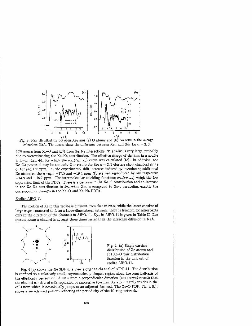
1.2- (a).

0.9- ■

I °*1 1

0.6- I 0.0— \m Jl ■

0.3- li 'i I .Ol- 1 " -2

0.0- 1 n -3

■

4 6 8 10 12

(b) 1.2 '

0.8 !| l n-2

0.4 ■

0.4- I JH ,

n-3 0.2

0.0- I i A 0.0

-0.2

0.4- " z + 3 S 10 12

6 8

rlk r/^ Fig. 3. Pair distribution between Xei and (a) O atoms and (b) Na ions in the a-cage

of zeolite NaA. The insets show the difference between Xen and Xei for n = 2,3.

60% comes from Xe-0 and 40% from Xe-Na interactions. The value is very large, probably due to overestimating the Xe-Na contribution. The effective charge of the ions in a zeolite is lower than +1, for which the uxe^Xe-Na) curve was calculated [15]. In addition, the Xe-Na potential may be too soft. Our results for the n = 2,3 clusters show chemical shifts of 151 and 168 ppm, i.e., the experimental shift increases induced by introducing additional Xe atoms to the a-cage, +17.5 and +19.4 ppm [3], are well reproduced by our respective +14.8 and +16.7 ppm. The intermolecular shielding functions ffxe(rxe-a) weigh the low separation limit of the PDFs. There is a decrease in the Xe-0 contribution and an increase in the Xe-Na contribution to <5xe when Xe3 is compared to Xei, paralleling exactly the corresponding changes in the Xe-0 and Xe-Na PDFs.

Zeolite A1PO-11

The motion of Xe in this zeolite is different from that in NaA; while the latter consists of large cages connected to form a three-dimensional network, there is freedom for adsorbants only in the direction of the channels in A1PO-11. Dxe in A1PO-11 is given in Table II. The motion along a channel is at least three times faster than the intracage diffusion in NaA.

"-■*. ..*"

Fig. 4. (a) Single-particle distribution of Xe atoms and (b) Xe-0 pair distribution function in the unit cell of zeolite A1PO-11.

Fig. 4 (a) shows the Xe SDF in a view along the channel of A1PO-11. The distribution is confined to a relatively small, asymmetrically shaped region along the long half-axis of the elliptical cross section. A view from a perpendicular direction (not shown) reveals that the channel consists of cells separated by successive 10-rings. Xe atom mainly resides in the cells from which it occasionally jumps to an adjacent free cell. The Xe-0 PDF, Fig. 4 (b), shows a well-defined pattern reflecting the periodicity of the 10-ring network.

603

The calculated chemical shift in A1P0-11 is 150 ppm, which consists solely from Xe-0 interactions. This value is in fair agreement with the experimental values [17] that range roughly from 120 to 140 ppm in the low loading limit.

Finally, to examine the validity of the effective Xe-0 potential, local density (LDA) calculations were performed for the Xe atom in the plane of an A1PO-11 cluster consisting of a 10-ring with terminating hydrogens. It was found that the effective potential is a good approximation. Both the ab initio results and Eq. (2) predict a 2 Ä wide, flat potential in the direction of the longer half-axis of the elliptical channel.

CONCLUSIONS

For NaA our results agree qualitatively with those of ref. 4: Xe atoms prefer contact with the cage walls and their mobility from one cage to another is low at 300 K. It is difficult to directly compare our parametrization of the chemical shift with that of the earlier work [4]. However, the loading trend of <$xe is well reproduced here and even the changes in the contributions of the cage walls are seen to be reflected in the structural data. In A1PO-11 the Xe atoms are mainly located in the cells between 10-rings, but move rapidly from one cell to another. The experimental foe is reproduced semi-quantitatively. The parametrization of the intrazeolite Xe chemical shift surface in terms of pair interaction contributions will be investigated later in a fuller account of the present simulations [16].

ACKNOWLEDGMENTS

We thank the Academy of Finland for financial support, Mr. M. Ylihautala for discussions, Dr. C.I. Ratcliffe for supplying the unit cell of A1PO-11 and Dr. L. Laaksonen for assistance with software. J.V. thanks also the Jenny and Antti Wihuri and Vilho, Yrjö and Kalle Väisälä Funds for grants. Computational resources were supplied by CSC, Espoo, Finland.

REFERENCES

1. P.J. Barrie and J.K. Klinowski, Progr. NMR Spectr. 24, 91 (1992). 2. J. Jokisaari, Progr. NMR Spectr. 26, 1 (1994). 3. C.J. Jameson et al, J. Chem. Phys. 96, 1676 (1992). 4. C.J. Jameson et al, J. Chem. Phys. 100, 5965 (1994); 100, 5977 (1994). 5. J. Vaara, T. T. Rantala, J.-H. Kantola and J. Jokisaari, to be published. 6. J.J. Pluth and J.V. Smith, J. Am. Chem. Soc. 102, 4704 (1980). 7. J.M. Bennet, J.W. Richardson, Jr, J.J. Pluth and J.V. Smith, Zeolites 7, 160 (1987). 8. S. Nose, J. Chem. Phys. 81, 511 (1984); W.H. Hoover, Phys. Rev. A 31, 1695 (1985). 9. Cerius2, Molecular Simulations Inc., Burlington, MA, (1994). 10. E. de Vos Burchart, Ph.D. Thesis, Technische Universiteit Delft (1992). 11. A.K. Rappe et al, J. Am. Chem. Soc. 114, 10024 (1992). 12. A.V. Kiselev and P.Q. Du, J. Chem. Soc. Faraday Trans. 2 77, 1 (1981); A.G. Bezus,

A.V. Kiselev, A.A. Lopatkin and P.Q. Du, ibid. 74, 367 (1978). 13. N. Karasawa and W.A. Goddard III, J. Phys. Chem. 93, 7320 (1989). 14. J. Lounila, J. Vaara, R. Seydoux, J. Jokisaari and P. Diehl, to be published. 15. A. Freitag, Ch. van Wüllen and V. Staemmler, Chem. Phys. 192, 267 (1995). 16. J.-H. Kantola, J. Vaara, T.T. Rantala and J. Jokisaari, to be published. 17. J.A. Ripmeester and C.I. Ratcliffe, J. Phys. Chem. 99, 619 (1995).

604

AUTHOR INDEX

Abraham, Farid F., 189 Adams, Wade, 99 Alexander, H., 261 Althoff, Jeffrey D., 339 Amador, Carlos, 375 Angius, C, 3 Antropov, V.P., 157 Artacho, E., 85

Baldereschi, A., 9 Baroni, Stefano, 457 Battaile, C, 401 Bazant, M.Z., 79 Beiden, S.V., 73 Benedek, Q., 351 Berding, M.A., 503 Bernardini, F., 539 Bemholc, J., 145 Bernstein, Noam, 55 Bongiomo, A., 515 Books, J.T., 327 Bosin, A., 169 Botton, Q.A., 567 Boyer, L.L., 315 Bozzolo, Guillermo, 357, 375 Brabec, C.J., 145 Brenner, Donald W., 113 Briggs, E.L., 145 Bristowe, P.D., 271 Brudevoll, T., 509

Canel, L.M., 237 Carlsson, A.E., 229, 237 Casula, F., 3 Ceder, Q., 309 Celino, Massimo, 345 Chaki, T.K., 249 Chan, CT., 37 Chelikowsky, James R., 19 Chen, Ai, 61 Chen, P., 413 Christensen, N.E., 509 Colombo, Luciano, 107, 515 Cooper, Bernard R., 407, 463 Comwell, C.F., 125 Corrales, L. Rene, 61

Dawson, I., 271 Day, Paul, 579 Deyirmenjian, V., 283

Ebbsjö, Ingvar, 333 Ebert, H., 73 Erwin, S.C., 545 Esfarjani, Keivan, 369 Ethridge, E.C., 545

Facchinetti, M., 351 Fahy, S., 169 Farkas, Diana, 217 Fearn, M., 551 Ferrante, John, 357, 375 Filippetti, Alessio, 457 Finnis, Michael W., 321 Fiorentini, Vincenzo, 457, 495 Francis, Q.P., 277, 283 Frauenheim, Th., 521 Freeman, CM., 327

Qarbulsky, Q.D., 309 Qarrison, Jr., Warren M., 563 Qehring, O.A., 73 Oolubovic, Leonardo, 223 Qood, Brian, 357 Qreengard, L., 93 Quo, Q.Y., 73, 567 Qutierrez, Qonzalo, 333 Qygi, Francois, 131

Harmon, B.N., 157 Heffelfinger, Grant S., 299 Heine, V., 277, 283 Ho, K.M., 37 Hsu, Y.E., 249 Huang, Y., 261 Humphreys, C.J., 567

Insepov, Z., 591 lotova, D., 557

Jefferson, J.H., 551 Jesson, D.E., 439 Jing, X., 19 Johnson, Duane D., 339 Jokisaari, J., 599

Kalia, Rajiv K., 113, 175, 181, 205, 333, 489, 573

Kantola, J.-H., 599 Kaschner, R., 521 Kato, K., 427 Kawazoe, Yoshiyuki, 369 Kaxiras, Efthimios, 55, 79, 139 Kemper, Paul, 527 Kieffer, John, 363 Kioussis, H., 557 Klein, Michael L., 327, 477 Köhler, Th., 521 Kohyama, Masanori, 49 Kolar, H.R., 261 Kotomin, E.A., 509 Krasko, Qenrich L., 291 Kung, P.W.-C, 327 Küster, Eric, 527

605

Lee, M-H., 271 LeSar, R.A., 199 Levine, S.M., 327 Lewis, Steven P., 391 Li, Wei, 489 Lim, S.F., 557 Liu, Amy Y., 13 Lust, Lisa, 527

MacLaren, James M., 563 Madhukar, A., 413 Marie, Djordje, 107 Marzari, li., 283 Massidda, S., 9 Maxia, Q., 3 McHenry, Michael E., 563 McKenney, Alan, 99 Mehl, Michael J., 31, 383 Meierovich, M., 67 Menchi, M., 169 Meregalli, Valeria, 345 Methfessel, Michael, 495 Miglio, Leo, 345, 351 Milman, V., 439 Miyazaki, Takehide, 533 Modine, N.A., 139 Moldovan, Dorel, 223 Molteni, C, 277, 283 Moore, Rick, 527 Morrey, W.C., 125 Mula, Q., 3 Murata, M., 445 Muratov, Leonid S., 407 Mushinski, A., 67

riajafabadi, R., 401 riakano, Aiichiro, 175, 205 Mekhayev, Dmitry, 363 Meugebauer, Jörg, 43 newsam, J.M., 327 Dicholson, D.M.C., 73, 157, 567, 585 Nieminen, R.M., 539 Nightingale, M.P., 67 Noda, M., 445 Noebe, Ronald D., 375

Ögüt, Serdar, 19 Ohira, T., 445 Ohno, Takahisa, 451 Omeltchenko, Andrey, 113, 175, 181, 573 Oppo, Sabrina, 495 Ordejon, Pablo, 85

Pachter, Ruth, 99, 579 Pan, Bicai, 37 Papaconstantopoulos, D.A., 31 Patnaik, Soumya, 99 Payne, M.C., 255, 271, 277, 283 Pennycook, S.J., 439 Perez, R., 255 Pettifor, D.O., 551 Phillips, Rob, 243

Pickett, W.E., 545 Porcu, M., 3 Posternak, M., 9 Price, D.L., 463

Quong, Andrew A., 13

Rabe, K.M., 305 Ramalingam, Bala, 563 Rantala, T.T., 599 Rappe, Andrew M., 391 Resta, R., 9 Rino, Jose Pedro, 333 Rutledge, Q.C., 469

Saad, Y., 19 Sawyer, William, 107 Schi0tz, J., 237 Schönberger, Uwe, 321 Schulz, W., 509 Seifert, Q., 521 Serra, S., 351 Shastry, Vijay, 217 Shelton, W.A., 73, 157, 567, 585 Shenoy, Vijay B., 243 Sher, A., 503 Sluiter, Marcel H.F., 369 Soler, J.M., 85 Spence, J.C.H., 261 Srolovitz, D.J., 199, 401 Stathopoulos, A., 19 Stich, Ivan, 255, 533 Stocks, Q.M., 73, 157, 567, 585 Stokbro, Kurt, 457 Sullivan, D.J., 145 Sun, S., 557 Svane, A., 509 Szotek, Z., 73, 157, 567, 585

Takeuchi, Y., 445 Tang, M.S., 37 Tavazza, Francesca, 345 Temmerman, W.M., 73, 157, 567, 585 Terakura, Kiyoyuki, 255, 427, 433, 533 Thomson, Robb, 229, 237 Tsuruta, Kenji, 181, 573 Tuckerman, Mark E., 477

Uda, Tsuyoshi, 427, 433, 533 Ukai, O., 445

Vaara, J., 599 Valente, Riccardo, 457 Van de Walle, Chris Q., 43 van Schilfgaarde, M., 503 van Swol, Frank, 299 Vashishta, Priya, 113, 175, 181, 205, 333,

489, 573 Vessal, B., 327 Viswanathan, R., 413 von Rosenvinge, Tycho, 477

606

Waghmare, U.V., 305 Yamada, I., 591 Wang, C.Z., 37 Yamasaki, T., 427, 433 Wang, Jinghan, 573 Yang, Jinlong, 3 Wang, Yang, 73, 157, 567, 585 Yoshida, H., 445 Wang, Zhiqiang, 579 Yu, J., 113 Wilhelmi, J.L., 469 Yu, W., 413 Wille, L.T., 125 Wilson, Mark, 321 Zacharopoulos, M., 199 Wu, K., 19 Zumbach, Oil, 139 Wu, R., 557

607

SUBJECT INDEX

ab initio, 49, 85, 145, 271, 383 activation

barrier, 439 energy, 515

adaptive grid, 139 adatom diffusion, 439, 457 adsorption, surface, 427, 451 affinity, chemical, 309, 407 algorithm, fast multipole, 93, 99 amorphization, 489 anisotropic diffusion, 515 anisotropy, 557 antiphase boundary, 357 approximation

generalized gradient, 451, 533 local-density, 85, 169, 503, 567, 585 quasi-harmonic, 13 scalar-relativistic, 383 two-center, 37, 521

band structure, 539 binary compound, 31 bistability, 533 brittle materials, 189 bulk

diffusion, 55 lattice, 503 modulus, 351, 563 moment, 585 structure, 469

charge density, 261 dynamical, 9 transfer, 61

chemical reaction, 427 shifts, 599

cluster(s) semiconductor, 19 vacancy, 223 van der Waals, 67 velocity, 591

cohesion, intergranular, 291 composition, of alloys, 567 core(-)hole

perturbation, 495 screening effects 495

core-level shifts, 495 correlation

functions, 339 length, 527

crack, 189, 199, 205, 223, 229, 237 elastic, 229 finite, 217 growth, 199, 223 propagation, 113, 189, 199, 205, 237

crystal liquid, 99 packing, 327 polar, 9

curvilinear coordinates, 131

defect, 43 densities, 503 formation, 413 ratio, 445 structure, 375

deformations elastic, 489 plastic, 255

degrees of ductility, 557 of freedom, 321

delocalization, 255 density of states, 345, 351, 563 desorption, surface, 451 dielectric(s)

crystalline, 9 matrix, 527

diffraction peak, 333 diffusion

barriers, 457 constants, 599 gradient-driven, 299

diffusivity, 515 dislocation(s), 199, 223, 237, 243, 249, 261

formation, 413 disorder, 369 dopant, 551 ductility, 261, 291

effects correlation, 169 entropic, 579 kinetic, 579 spin-orbit, 383

elastic constants, 175, 557 electronic

configuration, 521 coordinates, 61 entropy, 309 structure, 73, 271, 463, 477, 509, 545, 567

electron-phonon coupling, 13 electrostatics, 93 energy

cohesive, 79, 351 repulsive, 37 total, 31

entropy, 407 epitaxial growth, 433 equation

boundary integral, 93 of state, 31

equilibrium spacing, 291

609

error analysis, 139

finite temperature, 19, 357, 477 fracture, 189, 199, 205, 277, 283, 489 fullerene transformation, 351

geometry optimization, 407 glass formation, 327 grain boundary, 271, 277, 283 Greens function, 237

host matrix, 463, 563 hydrogen contents, 445 hydrogenation, 533

impurities, 43, 291 instability, 189, 305 integral, hopping, 37, 43, 107 interaction

adhesive, 255 attractive, 49 chemical, 255 interatomic, 217, 401, 439 magnetic, 73 spin-orbit, 383

interatomic bonding, 283 forces, 477

interface, 49, 229 metallic-ceramic, 49 pore, 205 stress, 539

interfacial energy, 463 interstitial atoms, 509 ionic

force, 145 solids, 509

irradiation, 591

lattice, 315, 503, 539 constant, 539, 545 dynamics, 469, 599 parameter, 375 relaxation, 407 resistance, 229, 243 vibrations, 309

length bond, 79, 169 Griffith, 223

Lennard-Jones potential, 67 line tension, 243

magnetic moments, 73, 157, 585 materials science, 3 mechanism

diffusion, 515 growth, 433, 439

melting transition, 327 methods

conjugate gradient, 49, 93, 271 density-matrix, 55 fast multipole, 93, 99, 199

finite difference, 19, 131 free energy minimization, 401 multigrid, 139, 145 stiffness matrix, 249 tight-binding, 31, 43, 55, 345, 351

microstructure, 357 molecular

crystals, 477 dynamics simulation, 55, 99, 125, 131, 189,

205, 299, 315, 327, 333, 345, 351, 427, 433, 445, 477, 489, 515, 573, 591, 599

monoclinic phase, 321 structure, 321

Monte Carlo method, 67, 169, 243, 299, 357, 401

morphology stability, 413 multiple scattering, 73, 157, 585

nanoclusters, 181 neck

formation, 181 region, 181

notch shape, 113

573

ordering tendency, 339

pair distribution function, 333 parallel

architecture, 169 computation, 125, 157, 189 computers, 125, 131

Feierls stress, 243 percolation threshold, 527 periodic chain, 85 permeability, 527 phase

stability, 309, 369 transitions, 305, 309, 345

plastic deformations, 255 polarization, 9 porosity, 175 potential

chemical, 299, 551 cluster, 79 interatomic, 79, 489 many-body, 125 well, 315

precipitate, 463 properties

structural, 19, 521, 563 vibrational, 13

radical energization, 445 Raman spectroscopy, 509 real space, 85, 131, 139, 145 relaxation dynamics, 391 response

dielectric, 107 linear, 13, 305 optical, 107

610

roughness, 591 exponents, 113

self-diffusion, 61, 573 short-range order, 339, 363 simulation, 509

atomistic, 217, 551 molecular dynamics, 55, 99, 125, 131,

189, 205, 299, 315, 327, 333, 345, 351, 427, 433, 445, 477, 489, 515, 573,591,599

Monte Carlo, 67, 169, 243, 299, 357, 401 non equilibrium, 299

sintering, 181, 573 sliding, 277, 283 spatial redistribution, 407 spin dynamics, 157 stability, 545 stacking fault, 503 static structure, 363 strain relaxation, 413 stress, 249

anisotropy, 457 fluctuations, 573

structural correlations, 363 order, 333 transition, 315

super partials, 249 superstructures, 369 surface, 433, 451

entropy, 469

free energy, 469 interactions, 391 stress, 457

theory density functional, 85, 139, 277, 305, 391,

439,457,495,521,579 linear-response, 13, 305

thermal conductivity, 175 expansion, 333 transport, 175

tight-binding potential, 31, 43, 55, 345, 351 topology, 363 transformation, 321, 345 transition, 427 translational motion, 391

vacancy phases, 545 valence

band offset, 539 orbitals, 61

van der Waals clusters, 67

wave functions, 43, 521 wavelets, 139

x-ray diffraction, 375

zero point energy, 67

611

Melting of Aromatic Compounds: Molecular Dynamics Simulations

Documents

Transcript of Melting of Aromatic Compounds: Molecular Dynamics Simulations