![Музыкальная диалогика [Musical "Dialogy"]](https://static.fdokumen.com/doc/165x107/6323fa395f71497ea904967f/muzikalnaya-dialogika-musical-dialogy.jpg)
Melodies in Space: Neural processing of musical features
105
Melodies in space: Neural processing of musical features A DISSERTATION SUBMITTED TO THE FACULTY OF THE GRADUATE SCHOOL OF THE UNIVERSITY OF MINNESOTA BY Roger Edward Dumas IN PARTIAL FULFILLMENT OF THE REQUIREMENTS FOR THE DEGREE OF DOCTOR OF PHILOSOPHY Dr. Apostolos P. Georgopoulos, Adviser Dr. Scott D. Lipscomb, Co-adviser March 2013
Transcript of Melodies in Space: Neural processing of musical features
Melodies in space: Neural processing of musical features
A DISSERTATION
SUBMITTED TO THE FACULTY OF THE GRADUATE SCHOOL
OF THE UNIVERSITY OF MINNESOTA
BY
Roger Edward Dumas
IN PARTIAL FULFILLMENT OF THE REQUIREMENTS
FOR THE DEGREE OF
DOCTOR OF PHILOSOPHY
Dr. Apostolos P. Georgopoulos, Adviser
Dr. Scott D. Lipscomb, Co-adviser
March 2013

© Roger Edward Dumas 2013
i
Table of Contents Table of Contents .......................................................................................................... i
Abbreviations ........................................................................................................... xiv
List of Tables ................................................................................................................. v
List of Figures ............................................................................................................. vi
List of Equations ...................................................................................................... xiii
Chapter 1. Introduction ............................................................................................ 1
Melody & neuro-‐imaging .................................................................................................. 1
The MEG signal ................................................................................................................................. 3
Background ........................................................................................................................... 6
Melodic pitch ..................................................................................................................................... 6
Melodic contour ............................................................................................................................... 7
Melodic perplexity .......................................................................................................................... 9
Models of music cognition ............................................................................................. 11
Stable and unstable tones ......................................................................................................... 11
Gravity, magnetism & inertia ................................................................................................... 13
Tonal space ...................................................................................................................................... 14
The Circle of Fifths ....................................................................................................................... 14
The diatonic scale ......................................................................................................................... 16
Diletski’s circle of fifths’ (1679) ............................................................................................. 17
Euler’s tonnetz (1739) ............................................................................................................... 19
ii
Riemann’s tonnetz (1880) ........................................................................................................ 19
Traditional tonnetz ...................................................................................................................... 20
Longuet-‐Higgins Harmonic space (1962) .......................................................................... 21
Lubin’s toroidal tonal space ..................................................................................................... 22
The probe tone profile, key-‐finding torus and self-‐organizing map ...................... 23
Helical tonal surfaces ...................................................................................................... 28
Chew spiral array model (2000) ................................................................................. 29
Dumas perfect 4th helix (P4h) ...................................................................................... 30
Chapter 2. Materials and Methods ...................................................................... 37
Subjects ................................................................................................................................ 37
Experiment A: Neural processing of pitch ......................................................................... 37
Experiment B: Neural processing of auto-‐correlation ................................................. 37
Experiment C: Neural processing of interval distance ................................................. 37
Experiment D: Neural processing of next-‐note probability ....................................... 37
Stimuli .................................................................................................................................. 38
Experiment A .................................................................................................................................. 38
Experiments B, C, and D ............................................................................................................. 40
Task ...................................................................................................................................... 42
All Experiments ............................................................................................................................. 42
Data acquisition ................................................................................................................ 42
All Experiments ............................................................................................................................. 42
Chapter 3. Data Analyses ....................................................................................... 43
Experiment A .................................................................................................................................. 43
iii
Experiment B .................................................................................................................................. 44
Experiment C .................................................................................................................................. 46
Euclidean distance (Ed) ............................................................................................................. 48
Ed -‐ Tonal Space #1: Frequency ratio (F, D1) ................................................................... 48
Ed -‐ Tonal Space #2: Longuet-‐Higgins (LH) harmonic space (1962a) .................. 49
Ed -‐ Tonal Space #3 Krumhansl and Kessler (KK) major key probe tone profile
(1982). .......................................................................................................................................... 50
Ed -‐ Tonal Space 4: Parncutt (P88) major key chroma salience profile (2011).51
Ed -‐ Tonal space #5: Chew (CH) Spiral array model (2000). ..................................... 52
Ed -‐ Tonal Space #6: Dumas perfect fourth helix (P4h) (2012). .............................. 53
Experiment D .................................................................................................................................. 55
Chapter 4. Results .................................................................................................... 57
Experiment A .................................................................................................................................. 57
Experiment B .................................................................................................................................. 59
Experiment C .................................................................................................................................. 60
Experiment D .................................................................................................................................. 60
Chapter 5. Discussion .............................................................................................. 62
Chapter 6. Concluding remarks and future directions ................................ 66
Bibliography .............................................................................................................. 67
Appendix A – Experiment B plots ....................................................................... 74
Appendix B: Experiment C MEG sensor plots ................................................. 84
Tonal space #1: -‐log Frequency ................................................................................... 84
iv
Tonal space #2: Longuet-‐Higgins harmonic space ................................................ 85
Tonal space #3: Dumas perfect 4th helix .................................................................. 86
Tonal space #4: Krumhansl & Kessler probe tone profile ................................. 87
Tonal space #5: Parncutt chroma salience profile ............................................... 88
Tonal space #6: Chew spiral array model ................................................................ 89
v
List of Tables Table 1-‐1. P4h parameter descriptions and values. ................................................................................................... 34
Table 1-‐2. P4h dimensions and formulae. ....................................................................................................................... 34
Table 1-‐3. P4h, key of C. Pitches, P4 steps, angles, coordinates and consonance units for pitches
within the octave centered on the origin (middle C). Columns: a) P4 pitch class; b) P4 step
relative to origin C (0); P4 step angle (∠xy) in degrees; P4 step angle (∠xy) in radians; .............. 35
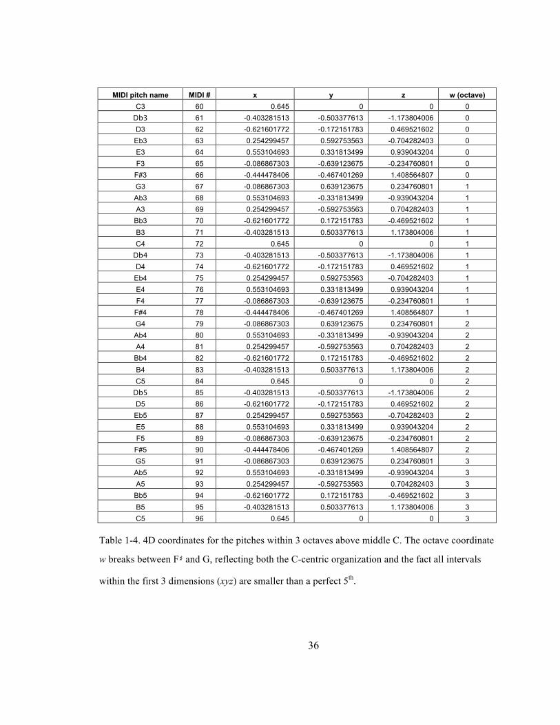
Table 1-‐4. 4D coordinates for the pitches within 3 octaves above middle C. The octave coordinate w
breaks between F♯ and G, reflecting both the C-‐centric organization and the fact all intervals
within the first 3 dimensions (xyz) are smaller than a perfect 5th. ........................................................... 36
Table 2-‐1. Set of 24 pitches used to produce the quasi-‐random pure-‐tone stimuli. ..................................... 40
Table 3-‐1. 14-‐note stimulus set with coordinate values for 6 tonal mappings (D1-‐6). D1: Frequency, D2:
Longuet-‐Higgins’ harmonic space, D3: Dumas’ P4h, D4: Krumhansl & Kessler’s probe tone
profile, D5: Parncutt’s chroma salience profile, D6: Chew’s spiral array model. ................................. 47
Table 3-‐2. Melodic interval probabilities (MIP) for stimulus intervals within the octave C3-‐C4.
Ordinal: interval first note. Abscissa: interval second note. ........................................................................ 55

vi
List of Figures Figure 1-‐1. MEG sensor plot, flat-‐brain layout. Arrows indicate anterior (A), posterior (P), left (L) and
right (R). ................................................................................................................................................................................ 4
Figure 1-‐2. Right-‐hand rule and brain biomagnetics. a) The “right-‐hand rule” mnemonic illustrates
the relative direction of current flow (thumb), magnetic force (index finger) and magnetic field
(curled fingers) in an electric conductor. b) Biomagnetics of a cortical fold. The signal from the
radial projection of a gyral source (i.e. a source parallel to the cortical surface) is prone to
cancellation from its neighbors. The tangential projection of magnetic force from a sulcus is
more readily detected by the SQUID. ........................................................................................................................ 5
Figure 1-‐3. Examples of disjunct motion (above) and conjunct motion (below) (Deutsch, 1987). .......... 7
Figure 1-‐4. Notated sample stimuli with serial auto-‐correlations increasing from pseudo-‐random (AC
0.0) to highly auto-‐correlated (AC 0.9). ................................................................................................................... 8
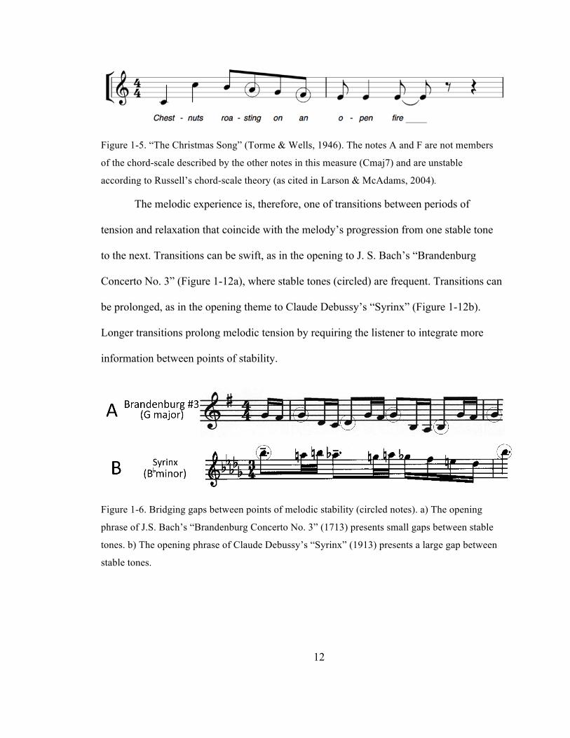
Figure 1-‐5. “The Christmas Song” (Torme & Wells, 1946). The notes A and F are not members of the
chord-‐scale described by the other notes in this measure (Cmaj7) and are unstable according to
Russell’s chord-‐scale theory (as cited in Larson & McAdams, 2004). ..................................................... 12
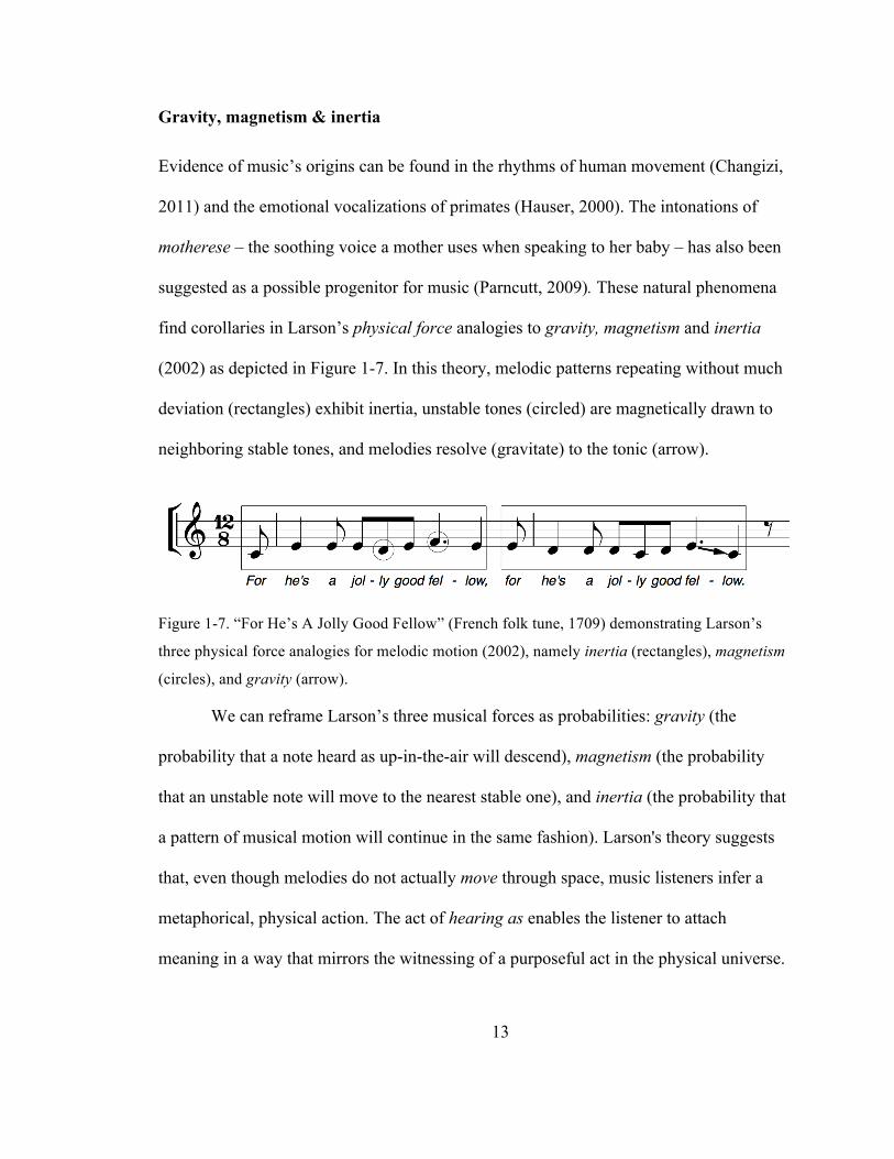
Figure 1-‐6. Bridging gaps between points of melodic stability (circled notes). a) The opening phrase
of J.S. Bach’s “Brandenburg Concerto No. 3” (1713) presents small gaps between stable tones.
b) The opening phrase of Claude Debussy’s “Syrinx” (1913) presents a large gap between stable
tones. .................................................................................................................................................................................... 12
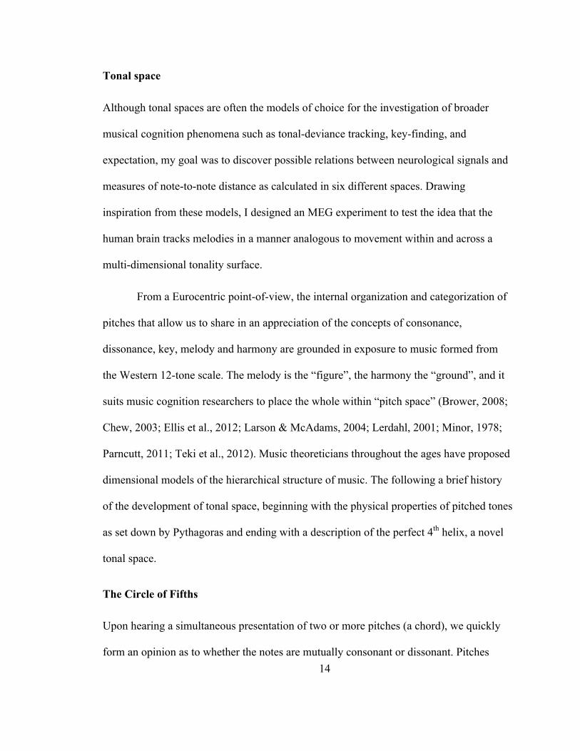
Figure 1-‐7. “For He’s A Jolly Good Fellow” (French folk tune, 1709) demonstrating Larson’s three
physical force analogies for melodic motion (2002), namely inertia (rectangles), magnetism
(circles), and gravity (arrow). ................................................................................................................................... 13
Figure 1-‐8. Pythagoras’ chromatic scale (Gibson & Johnston, 2002). ................................................................. 16
Figure 1-‐9. Pitches of the D Dorian mode: D, E, F, G, A, B, C, D’ .............................................................................. 17
Figure 1-‐10. Diletski’s musical notation of the Circle of Fifths. Pitch names added by the author
(Jensen, 1992). ................................................................................................................................................................. 18
vii
Figure 1-‐11. Euler’s tonnetz was based on orthogonal axes of fifths and thirds (1739). ........................... 19
Figure 1-‐12. Riemann’s Just Intonation tonnetz (Hyer, 1995). .............................................................................. 20
Figure 1-‐13. Traditional tonnetz for the extended key of C major (as cited in Gollin, 2011). The 12
pitch classes of the chromatic scale are arranged along 3 axes of perfect 5ths, major 3rds, and
minor 3rds. ........................................................................................................................................................................ 21
Figure 1-‐14. Longuet-‐Higgins’ model of consonance/dissonance in two and three dimensions. a) 2-‐
dimensional “harmonic space” encompassing the “extended” keys of C major and C minor, plus
F♯ and D♭. c. The 3-‐dimensional lattice features the addition of an octave dimension along a
vertical axis (Longuet-‐Higgins, 1962a). ................................................................................................................ 22
Figure 1-‐15. Steps in the transformation of the traditional tonnetz into a two-‐dimensional closed
surface (Lubin, 1974). .................................................................................................................................................. 23
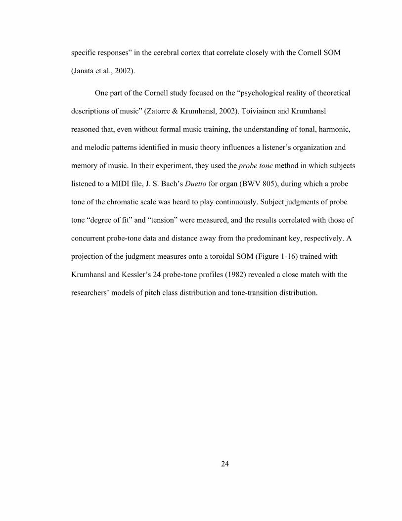
Figure 1-‐16. Krumhansl and Kessler’s self-‐organizing map (SOM) depicts “inter-‐key distance” results
from behavioral experiments in which subjects were asked to judge degree-‐of-‐fit for probe
tones heard at the end of major and minor scales (1982). a) Unfolded SOM (Toiviainen &
Krumhansl, 2003). Lines indicate circle of fifths for major keys (red) and minor keys (blue). b)
Top/bottom and left/right edges of the SOM are joined to form a torus. ............................................. 25
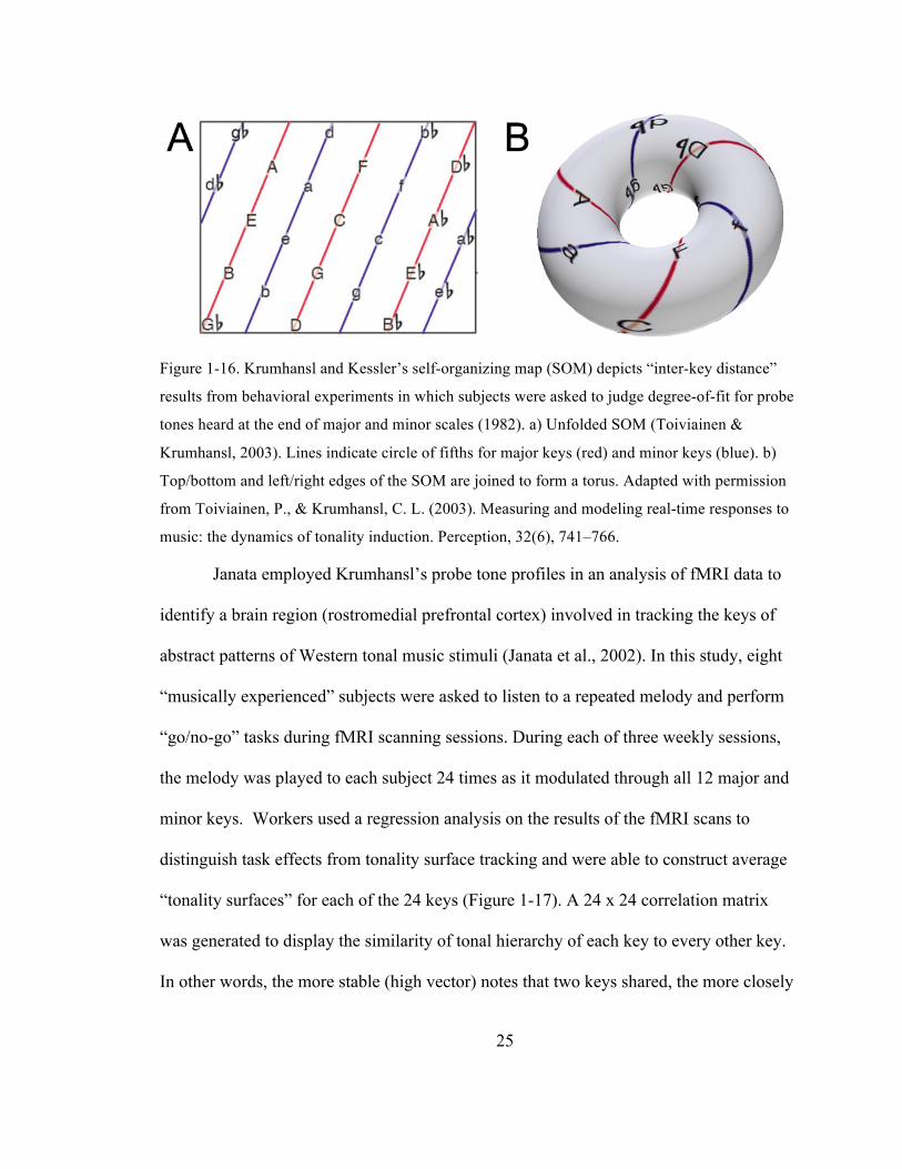
Figure 1-‐17. A toroid model of tonal space. a) An unfolded, two-‐dimensional map of key correlations
(Janata et al., 2002). Opposite edges connect to each other to form a continuous, wrapping
surface. Major scales and their relative minors share the same 7-‐note scale and are positively
correlated (dark red). b) Toroidal representation the key correlation map. ...................................... 26
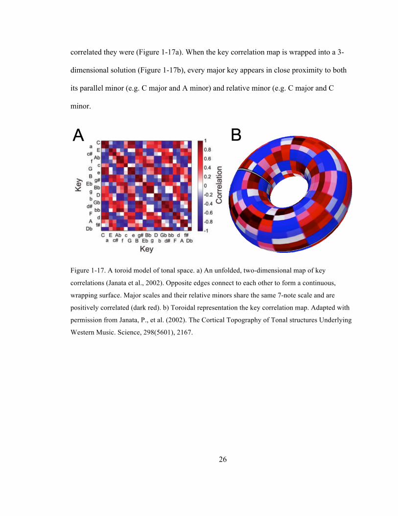
Figure 1-‐18. Properties of the tonality surface. a. Panels show the average tonality surface for
tonality-‐tracking voxels for each of the 24 keys in the original melody. The surface represents
an unfolded torus: the top and bottom edges of each rectangle wrap around to each other, as do
the left and right edges. The activation peak in each panel (red = strongest) reflects the
melody’s progression through all of the keys. b. Distributed mappings of tonality on the self-‐
organizing map (SOM). Each set of 9 panels depicts the areas of highest activation (key focus)
viii
after every chord played in a 9-‐chord key-‐changing sequence that consisted of the chords D
minor diminished, G, C minor, A♭, F, D♭, B♭ minor, E♭, A♭, and modulated from C minor to A♭
major. The top set shows the subjective probe tone judgments, while the bottom set shows the
mapping of the key-‐finding algorithm (Janata et al., 2002). ........................................................................ 27
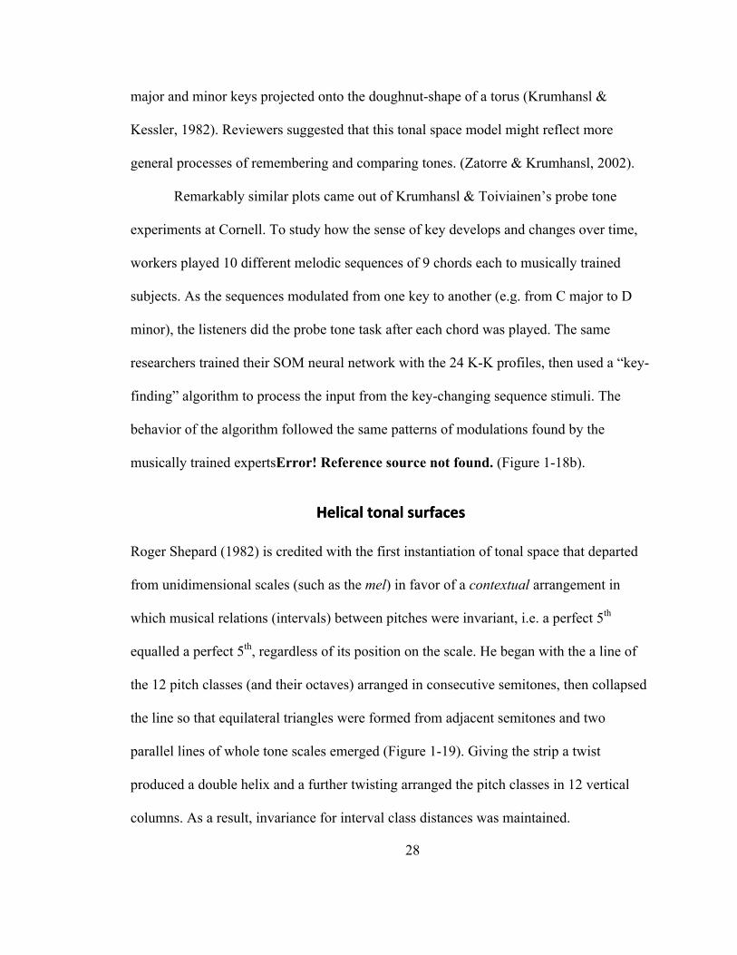
Figure 1-‐19. Stages in the construction of a double helix of musical pitch: (a) the flat strip of
equilateral triangles, b) the strip of triangles given one complete twist per octave, and (c) the
resulting double helix shown as wound around a cylinder (Shepard, 1982). ..................................... 29
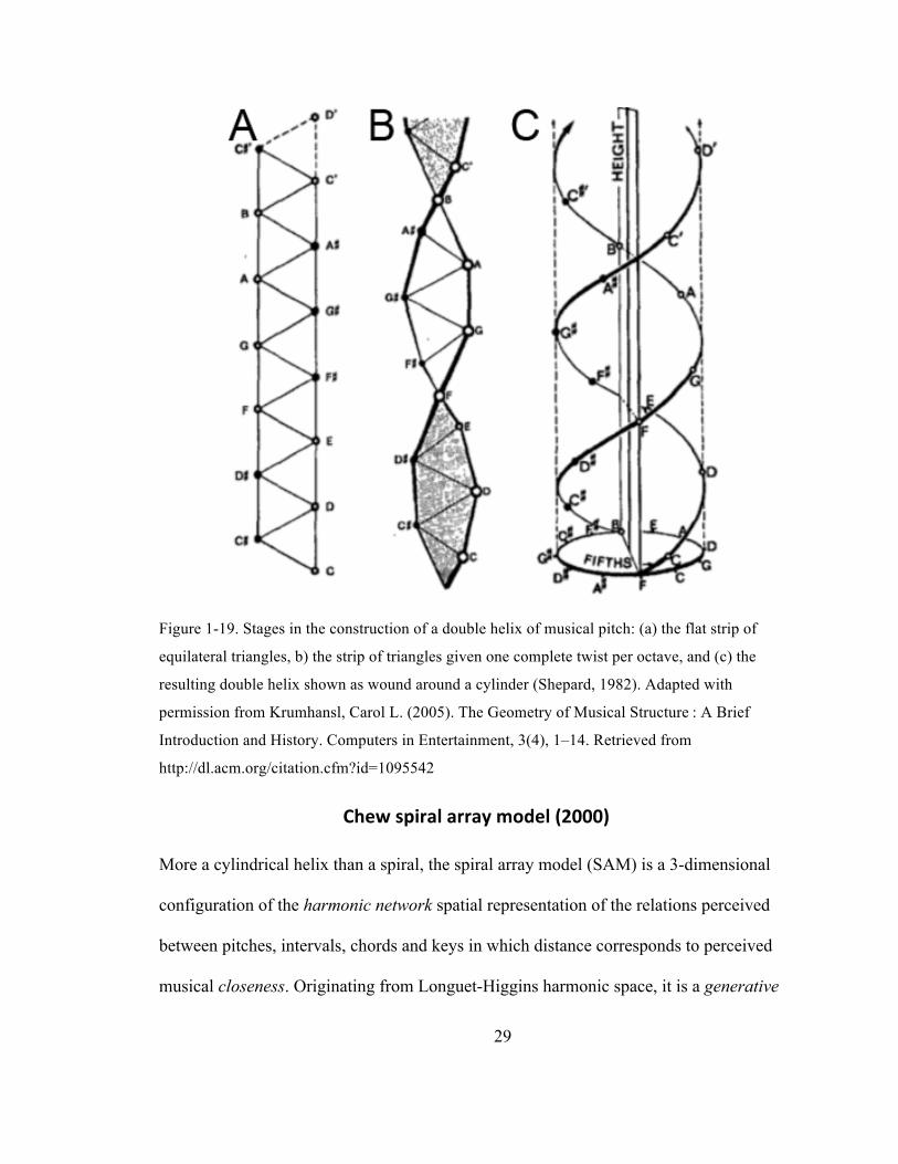
Figure 1-‐20. Wrapping harmonic space to form the SAM. A) Longuet-‐Higgins harmonic space
centered on C (range: B♭to B) is curved in upon itself until the pitches A and F meet, forming b)
a cylindrical helix wherein the Euclidean distance for all interval classes is invariant (Chew &
Chen, 2005). The vertical orientation of the four major 3rd axes is maintained. ................................ 30
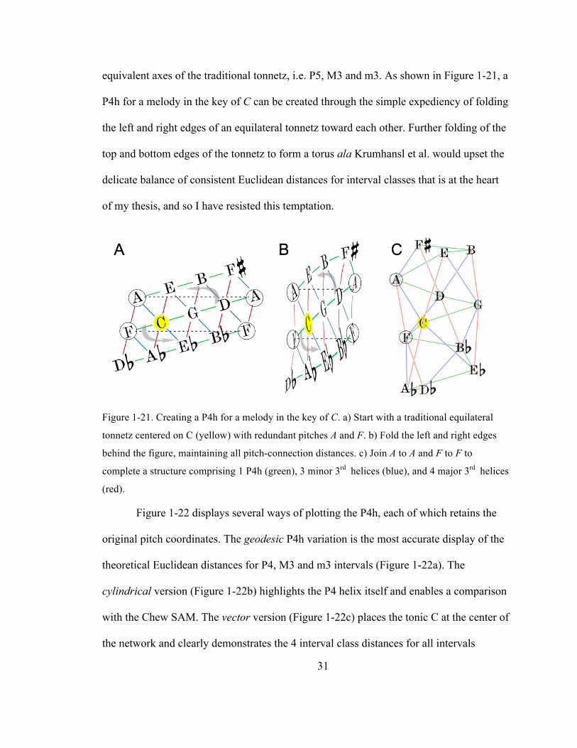
Figure 1-‐21. Creating a P4h for a melody in the key of C. a) Start with a traditional equilateral tonnetz
centered on C (yellow) with redundant pitches A and F. b) Fold the left and right edges behind
the figure, maintaining all pitch-‐connection distances. c) Join A to A and F to F to complete a
structure comprising 1 P4h (green), 3 minor 3rd helices (blue), and 4 major 3rd helices (red). 31
Figure 1-‐22. P4h variations, key of C. a) geodesic, b) cylindrical, c) vector, showing relative distances
from the tonic C. .............................................................................................................................................................. 32
Figure 1-‐23. Comparing the P4h with Pauling and Corey’s α-‐helix. a) With a step-‐height of 0.23
consonance units (cu, the vector distance for every P4, M3 and m3 interval in the model), the
P4h has a step-‐rotation of 97.74° and step-‐height/radius ratio (h/r) of 0.356. b) The α-‐helix
protein structure (Stryer, 1995) has a similar step-‐rotation (100°), but an elongated h/r of 0.60.
................................................................................................................................................................................................ 33
Figure 2-‐1. Block diagram of Random notes stimulus showing 24 contiguous 24-‐note segments. ...... 39
Figure 2-‐2. Example 24-‐note quasi-‐random stimulus segment. ........................................................................... 39
Figure 2-‐3. Example of the 20ms amplitude fade-‐in and fade-‐out at each tone junction. Amplitudes
were ramped between 0db and the adjusted peak amplitude. .................................................................. 39
ix
Figure 2-‐4. Piano-‐roll representation of stimulus model. a) Sequence with a serial auto-‐correlation of
0.0. b) Sequence with a serial auto-‐correlation of 0.9. ................................................................................... 41
Figure 2-‐5. Notated sample stimuli with serial auto-‐correlations increasing from pseudo-‐random (AC
0.0) to highly auto-‐correlated (AC 0.9). ................................................................................................................ 41
Figure 3-‐1. Example of an MEG sensor pitch-‐processing vector (PPV) showing the mean neural
activity across subjects (ordinal: femtoTesla) for each of the 24 stimulus pitch-‐classes (abscissa:
piano keyboard range C3-‐B4) for sensor #154. ............................................................................................... 43
Figure 3-‐2. Flat-‐brain MEG sensor map showing location of Sensors #14 and #15 (circled). ................ 44
Figure 3-‐3. Example comparison of auto-‐correlation-‐processing vector (ACPV) for two sensors: S14
(blue) & S15 (red). Ordinal axis: Mean MEG signal intensity (MMSI) per pitch across subjects. 45
Figure 3-‐4. Plot of log frequency (Hz) for stimulus pitches. .................................................................................... 48
Figure 3-‐5. Longuet-‐Higgins’ (1962a) harmonic space for the key of C major. abscissa: perfect 5th,
ordinal: major 3rd, z-‐axis: octave. ............................................................................................................................ 49
Figure 3-‐6. Krumhansl & Kessler’s (1982) major key probe tone profile for the key of C major. .......... 50
Figure 3-‐7. Parncutt’s (2001) chroma salience profile adds weighted root supports to Krumhansl’s
probe tone profile. ......................................................................................................................................................... 51
Figure 3-‐8 Chew (2000) Spiral array model, key of C major. ................................................................................. 52
Figure 3-‐9. Dumas’ perfect fourths helix (P4h) for the key of C major. ............................................................. 53
Figure 3-‐10. Excerpt from sample stimulus AC 0.7. a) The tritone F4-‐B4 has a high PI. b) The perfect
4th G3-‐D3 has a low PI. Both intervals have the same scalar distance (4 steps). ................................ 56
Figure 4-‐1. MEG sensor plots of correlations between sensor PPVs. Sensors with positively correlated
PPVs. These occurred ~4x more frequently than negative correlations and were clustered in
the frontal (bilateral) and left temporo-‐occipital regions. ........................................................................... 57
Figure 4-‐2. MEG sensor plots of correlations between sensor PPVs. Sensors with negatively
correlated PPVs were found in opposite hemispheres, mostly in frontal and less so in posterior
regions. ............................................................................................................................................................................... 58

x
Figure 4-‐3. (a-‐b) Plots of all positively correlated MEG sensors/AC (across subjects) a) AC 0.0, b) AC
0.9. (c-‐d) Plots of ACPV for all sensors (across subjects) c) AC 0.0, d) AC 0.9. Relations for
pseudo-‐random stimuli were stronger and more numerous than for more-‐highly auto-‐
correlated stimuli, especially in frontal regions. (See Appendix A for all plots.) ............................... 59
Figure 5-‐1. Comparison of results from two MEG music studies. a) Clusters of brain activation related
to processing of interval distance as measured in Tonal space #6 (Dumas perfect 4th helix).
Green = positive relations, red = negative. b) Power and spatial distribution of the aSSR in each
of the four conditions (grand average across subjects) (Patel & Balaban, 2001). ............................. 63
Figure 5-‐2. MEG sensor plots of relations between brain activity and stimulus melodic interval
distance in two models of diatonic tonal space. a) Dumas P4h. b) Chew SAM. The strength and
number of both positively-‐ and negatively-‐correlated brain signals are larger for the P4h plot.
................................................................................................................................................................................................ 64
Figure 6-‐1. Plots for melody autocorrelation of 0.0. a) Positively correlated MEG sensors/AC across
subjects. b) Piano-‐roll representation of sample stimulus. c) Average ACPVs across subjects for
all sensors. ......................................................................................................................................................................... 74
Figure 6-‐2. Plots for melody autocorrelation of 0.1. a) Positively correlated MEG sensors/AC across
subjects. b) Piano-‐roll representation of sample stimulus. c) Average ACPVs across subjects for
all sensors. ......................................................................................................................................................................... 75
Figure 6-‐3. Plots for melody autocorrelation of 0.2. a) Positively correlated MEG sensors/AC across
subjects. b) Piano-‐roll representation of sample stimulus. c) Average ACPVs across subjects for
all sensors. ......................................................................................................................................................................... 76
Figure 6-‐4. Plots for melody autocorrelation of 0.3. a) Positively correlated MEG sensors/AC across
subjects. b) Piano-‐roll representation of sample stimulus. c) Average ACPVs across subjects for
all sensors. ......................................................................................................................................................................... 77
xi
Figure 6-‐5. Plots for melody autocorrelation of 0.4. a) Positively correlated MEG sensors/AC across
subjects. b) Piano-‐roll representation of sample stimulus. c) Average ACPVs across subjects for
all sensors. ......................................................................................................................................................................... 78
Figure 6-‐6. Plots for melody autocorrelation of 0.5. a) Positively correlated MEG sensors/AC across
subjects. b) Piano-‐roll representation of sample stimulus. c) Average ACPVs across subjects for
all sensors. ......................................................................................................................................................................... 79
Figure 6-‐7. Plots for melody autocorrelation of 0.6. a) Positively correlated MEG sensors/AC across
subjects. b) Piano-‐roll representation of sample stimulus. c) Average ACPVs across subjects for
all sensors. ......................................................................................................................................................................... 80
Figure 6-‐8. Plots for melody autocorrelation of 0.7. a) Positively correlated MEG sensors/AC across
subjects. b) Piano-‐roll representation of sample stimulus. c) Average ACPVs across subjects for
all sensors. ......................................................................................................................................................................... 81
Figure 6-‐9. Plots for melody autocorrelation of 0.8. a) Positively correlated MEG sensors/AC across
subjects. b) Piano-‐roll representation of sample stimulus. c) Average ACPVs across subjects for
all sensors. ......................................................................................................................................................................... 82
Figure 6-‐10. Plots for melody autocorrelation of 0.9. a) Positively correlated MEG sensors/AC across
subjects. b) Piano-‐roll representation of sample stimulus. c) Average ACPVs across subjects for
all sensors. ......................................................................................................................................................................... 83
Figure 6-‐11. Neural-‐tonal map: -‐log frequency. Regression coefficient (b) significance [-‐ln(p), p <
0.05] per sensor across all stimuli and subjects. Green = positive relations, red = negative.
Bright colors indicate higher significance. .......................................................................................................... 84
Figure 6-‐12. Neural-‐tonal map: Longuet-‐Higgins harmonic space. Regression coefficient (b)
significance [-‐ln(p), p < 0.05] per sensor across all stimuli and subjects. Green = positive
relations, red = negative. Bright colors indicate higher significance. ...................................................... 85
xii
Figure 6-‐13. Neural-‐tonal map: Dumas perfect 4th helix. Regression coefficient (b) significance [-‐ln(p),
p < 0.05] per sensor across all stimuli and subjects. Green = positive relations, red = negative.
Bright colors indicate higher significance. .......................................................................................................... 86
Figure 6-‐14. Neural-‐tonal map: Krumhansl & Kessler probe tone profile. Regression coefficient (b)
significance [-‐ln(p), p < 0.05] per sensor across all stimuli and subjects. Green = positive
relations, red = negative. Bright colors indicate higher significance. ...................................................... 87
Figure 6-‐15. Neural-‐tonal map: Parncutt chroma salience profile. Regression coefficient (b)
significance [-‐ln(p), p < 0.05] per sensor across all stimuli and subjects. Green = positive
relations, red = negative. Bright colors indicate higher significance. ...................................................... 88
Figure 6-‐16. Neural-‐tonal map: Chew spiral array model. Regression coefficient (b) significance [-‐
ln(p), p < 0.05] per sensor across all stimuli and subjects. Green = positive relations, red =
negative. Bright colors indicate higher significance. ...................................................................................... 89
xiii
List of Equations Equation 1 ............................................................................................................................................................................... 48
Equation 2 ............................................................................................................................................................................... 49
Equation 3 ............................................................................................................................................................................... 50
Equation 4 ............................................................................................................................................................................... 51
Equation 5 ............................................................................................................................................................................... 52
Equation 6 ............................................................................................................................................................................... 53
xiv
Abbreviations ACPV auto-correlation processing vector
BA Brodmann area
BCE Before the Common Era
BOLD blood-oxygen level dependency signal
ERAN early right anterior negativity
DMEG successive absolute differences in the MEG signal
D1, 2, 3, 4, 5, 6 distance vectors in six tonal spaces
Ed, Euclidean distance
EEG electroencephalograph, -y
fMRI functional magnetic resonance imaging
LH harmonic space (Longuet-Higgins, 1979)
HZ Hertz, -log frequency tonal space
KK probe tone profile tonal space (Krumhansl et al., 1982)
MEG magnetoencephalograph, -y
MIDI musical instrument digital interface
MIP musical interval perplexity
MMN mismatch negativity
ms milliseconds
P4h perfect 4th helix tonal space (Dumas, 2011)
P88 chroma salience profile (Parncutt, 2011)
PI perplexity index
PPV pitch-processing vector
SAM spiral array model (Chew, 2000)
SMA supplementary motor area in the brain
SOM self-organizing map
SQUID super-conducting quantum interference device
1
Chapter 1. Introduction
Melody & neuro-‐imaging
With modern digital technology, it is now possible to capture, store, and describe
brain data in relation to musical stimuli with some degree of confidence. Increasing
financial and material resources are being made available to music-brain researchers and,
as a result, the number of music perception and cognition publications is expanding
exponentially (Levitin & Tirovolas, 2011). Two paradigmatic threads run through the
majority of brain-music studies. First, published brain-imaging studies involving musical
stimuli overwhelmingly emphasize brain regions-of-interest (ROI). Studies have shown,
for example, that the brain response is strong for pitch in the right hemisphere and for
rhythm in the left (Kanno et al., 1996; Limb, Kemeny, Ortigoza, Rouhani, & Braun,
2006; Ono et al., 2011). Second, many investigators favor psycho-acoustical phenomena
over higher-level processing. Their attentions rest primarily on the brain’s response to
isolated events such as unexpected chord progression completions (S.-G. Kim, Kim, &
Chung, 2011), out-of-key endnotes (Hashimoto, Hirata, & Kuriki, 2000), fundamental
and spectral pitch preference, (Schneider et al., 2005), Huggins pitch (Chait, Poeppel, &
Simon, 2006) and melody errors (Yasui, Kaga, & Sakai, 2009).
Among neuro-musicological publications, studies of the brain’s response to
melodic phrases are comparatively rare. One explanation for the scarcity of such
publications is that the predominant brain-scanning method is functional magnetic
resonance imaging (fMRI). Users of fMRI have uncovered information about task-related
flow of oxygenated blood (blood-oxygen level dependency, or BOLD signal) to specific
2
brain areas. A strong BOLD signal in a brain region-of-interest indicates increased
oxygen usage and concomitant neural activity. As it is an indirect measure of brain
activity, i.e. the measure of a signal indirectly related to synaptic events, fMRI is
subsequently challenged by the “…significant temporal and spatial differences between
electro-physiological responses and the complex cascade of the hemodynamic responses”
(Pouratian, et al. 2003). When compared to the speed of synaptic events (~1k Hz), the
development of the blood-oxygen signal captured by fMRI is slow (2 to 5 seconds). As a
consequence, fMRI experiments relating brain activity to changes in melodic parameters
focus on signals that are acquired at a latency of several seconds, i.e. well after the
subject has been exposed to the stimulus. These studies have involved the contrasting of
melodies with fixed-pitch sound (Patterson, Uppenkamp, Johnsrude, & Griffiths, 2002),
melodic contour discrimination (Lee, Janata, Frost, Hanke, & Granger, 2011),
identification of scrambled music (Matsui, Tanaka, Kazai, Tsuzaki, & Katayose, 2013),
temporal reversal of a melody (Zatorre, Halpern, & Bouffard, 2009), recognizing heard
and imagined melodies (Herholz, Halpern, & Zatorre, 2012) and free improvisation (De
Manzano & Ullén, 2012).
In contrast, neuroscientists have used the high temporal resolution of MEG (ms)
to relate brain response to specific musical events, e.g. consonant vs. dissonant melodic
tones (Kuriki, Isahai, & Ohtsuka, 2005), lyrics and melody deviants (Yasui et al., 2009),
omission of one tone out of a musical scale (Nemoto, 2012), melodic contour deviation
perception (Fujioka, Trainor, Ross, Kakigi, & Pantev, 2004), different pitch extraction
from same tone complexes (Patel & Balaban, 2001) and probability of chord progression
(S.-G. Kim et al., 2011).
3
The MEG signal
MEG features high temporal resolution (~1 ms), reasonable spatial precision (~5mm) and
high fidelity, i.e. the clean, direct measurement of undistorted electro-magnetic
fluctuations in neural populations (Lounasmaa, Hamalainen, Hari, & Salmelin, 1996). It
is the ideal technology for matching synchronous neural interactions (Georgopoulos AP
et al, 2007) to the processing of melodies played at normal tempos. It takes
approximately 100,000 synaptic events to produce a sufficiently large signal (~50 to 1000
femtoTeslas, or 10-15 T) for detection by an MEG sensor, aka super-conducting quantum
interference device (SQUID). (By comparison, the earth’s magnetic field registers at
5x10¹⁰ fT, or roughly 1 billion times stronger.) Each one of the 248 SQUIDS (Figure
1-1) in the whole-head Magnes 3600WH system (4-D Neuroimaging, San Diego, CA)
used in these experiments captures the biomagnetic signal of these dense clusters of
tightly-interconnected pyramidal cells in the cerebral cortex to a depth of approximately 4
mm and at a rate of 1017.25 samples-per-second.
4
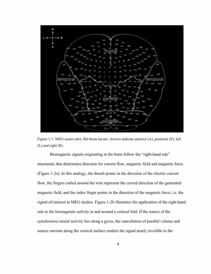
Figure 1-1. MEG sensor plot, flat-brain layout. Arrows indicate anterior (A), posterior (P), left
(L) and right (R).
Biomagnetic signals originating in the brain follow the “right-hand rule”
mnemonic that determines direction for current flow, magnetic field and magnetic force
(Figure 1-2a). In this analogy, the thumb points in the direction of the electric current
flow, the fingers curled around the wire represent the curved direction of the generated
magnetic field, and the index finger points in the direction of the magnetic force, i.e. the
signal-of-interest in MEG studies. Figure 1-2b illustrates the application of the right-hand
rule to the biomagnetic activity in and around a cortical fold. If the source of the
synchronous neural activity lies along a gyrus, the cancellation of parallel volume and
source currents along the cortical surface renders the signal nearly invisible to the
5
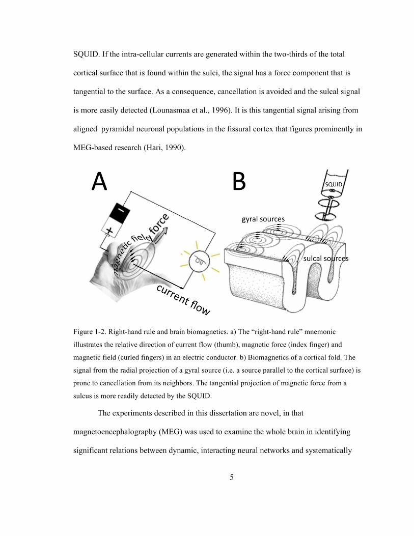
SQUID. If the intra-cellular currents are generated within the two-thirds of the total
cortical surface that is found within the sulci, the signal has a force component that is
tangential to the surface. As a consequence, cancellation is avoided and the sulcal signal
is more easily detected (Lounasmaa et al., 1996). It is this tangential signal arising from
aligned pyramidal neuronal populations in the fissural cortex that figures prominently in
MEG-based research (Hari, 1990).
Figure 1-2. Right-hand rule and brain biomagnetics. a) The “right-hand rule” mnemonic
illustrates the relative direction of current flow (thumb), magnetic force (index finger) and
magnetic field (curled fingers) in an electric conductor. b) Biomagnetics of a cortical fold. The
signal from the radial projection of a gyral source (i.e. a source parallel to the cortical surface) is
prone to cancellation from its neighbors. The tangential projection of magnetic force from a
sulcus is more readily detected by the SQUID.
The experiments described in this dissertation are novel, in that
magnetoencephalography (MEG) was used to examine the whole brain in identifying
significant relations between dynamic, interacting neural networks and systematically

6
varied musical features of entire melodies. The following chapter serves as an
introduction to theories of music cognition related to the melodic features of my stimuli.
Background
Neurophysiological studies of brain lesions and related behavioral deficits have shown
that the human brain is a complex functional network comprising specialized neural
populations. Although pitch perception has been studied extensively by musicologists,
philosophers, psychologists, audiologists, and, lately, neuroscientists (Levitin &
Tirovolas, 2011; Purwins & Hardoon, 2009), little is written about cortical sub-networks
involved in the processing of melodies. Our approach to this problem is novel, in that we
employ magnetoencephalography (MEG) to study four melodic features: pitch, contour,
interval and perplexity.
Melodic pitch
Our study of neural processing of pitch is novel in that it examines the brain’s response to
melodies in their entirety. Researchers mainly focus on brain response to stimuli other
than entire melodic passages, e.g. mismatched negativities elicited by final, oddball notes
or chords (e.g. Maess et al., 2001; Herholz et al., 2009; Kim et al., 2011). Such
explanations fall short of describing the complex neural interactions involved in melody
processing. In our study entitled “Experiment A: Neural processing of pitch”, we used
MEG to discover synchronous neural networks involved in processing melodic stimuli.
7
Melodic contour
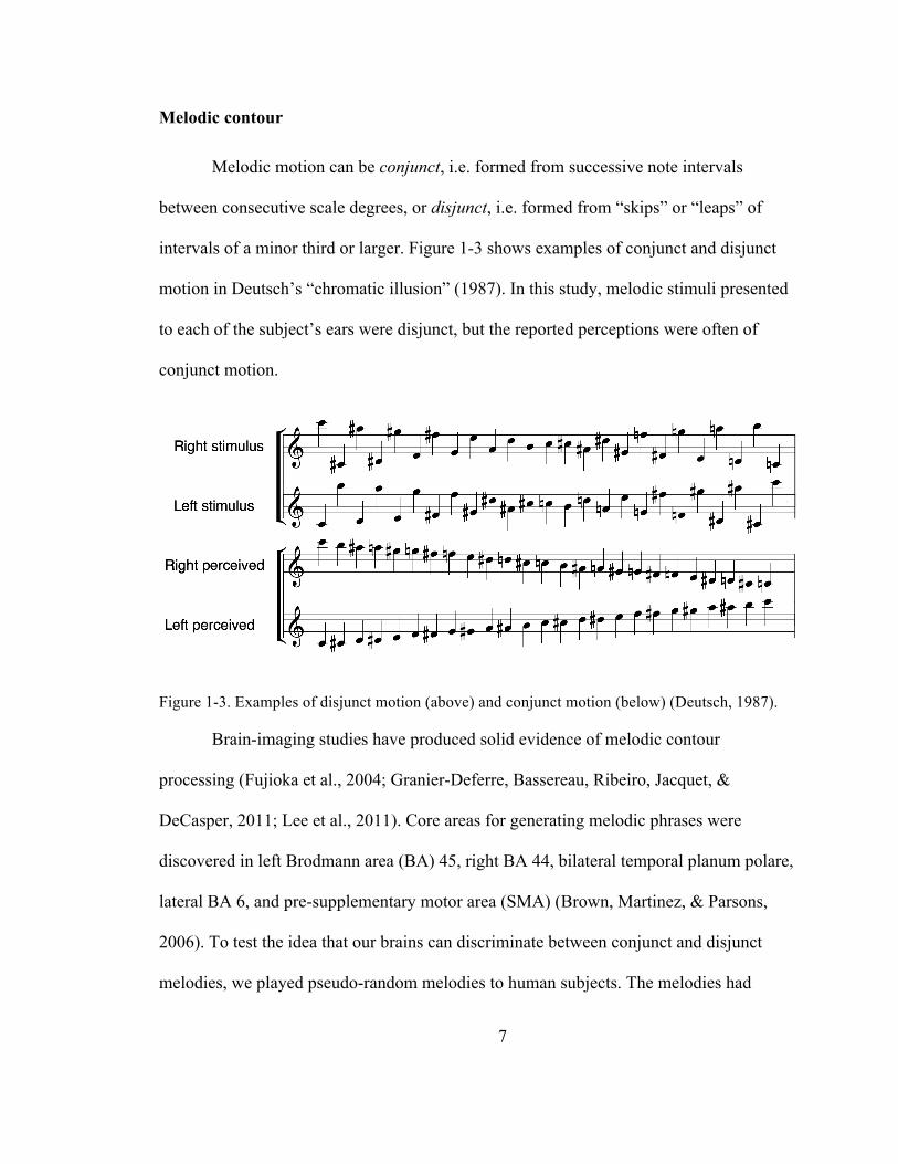
Melodic motion can be conjunct, i.e. formed from successive note intervals
between consecutive scale degrees, or disjunct, i.e. formed from “skips” or “leaps” of
intervals of a minor third or larger. Figure 1-3 shows examples of conjunct and disjunct
motion in Deutsch’s “chromatic illusion” (1987). In this study, melodic stimuli presented
to each of the subject’s ears were disjunct, but the reported perceptions were often of
conjunct motion.
Figure 1-3. Examples of disjunct motion (above) and conjunct motion (below) (Deutsch, 1987).
Brain-imaging studies have produced solid evidence of melodic contour
processing (Fujioka et al., 2004; Granier-Deferre, Bassereau, Ribeiro, Jacquet, &
DeCasper, 2011; Lee et al., 2011). Core areas for generating melodic phrases were
discovered in left Brodmann area (BA) 45, right BA 44, bilateral temporal planum polare,
lateral BA 6, and pre-supplementary motor area (SMA) (Brown, Martinez, & Parsons,
2006). To test the idea that our brains can discriminate between conjunct and disjunct
melodies, we played pseudo-random melodies to human subjects. The melodies had
8
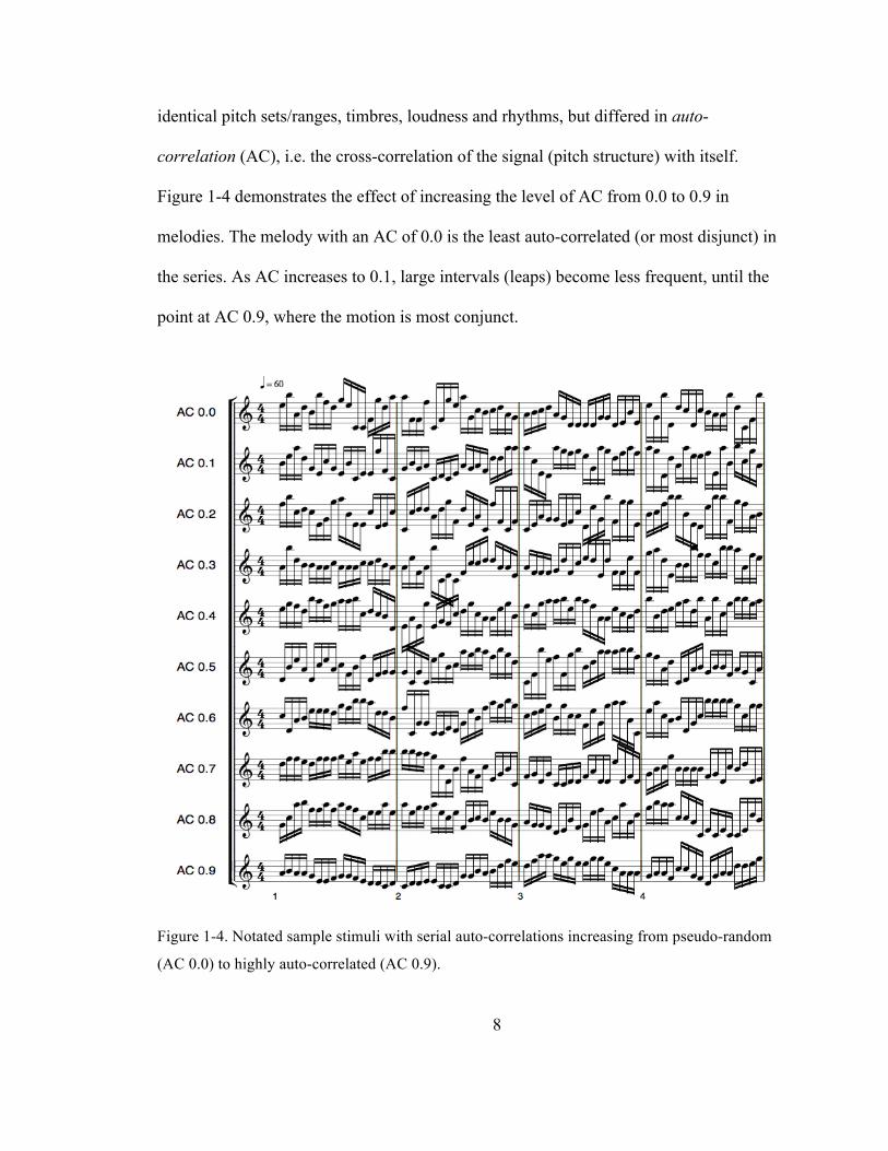
identical pitch sets/ranges, timbres, loudness and rhythms, but differed in auto-
correlation (AC), i.e. the cross-correlation of the signal (pitch structure) with itself.
Figure 1-4 demonstrates the effect of increasing the level of AC from 0.0 to 0.9 in
melodies. The melody with an AC of 0.0 is the least auto-correlated (or most disjunct) in
the series. As AC increases to 0.1, large intervals (leaps) become less frequent, until the
point at AC 0.9, where the motion is most conjunct.
Figure 1-4. Notated sample stimuli with serial auto-correlations increasing from pseudo-random
(AC 0.0) to highly auto-correlated (AC 0.9).
9
Melodic perplexity
Humans have evolved to anticipate future events, an ability that gives us a distinct
advantage in our environment. Although the psychological and physiological
consequences are not vital, musical expectations are critical to the aesthetic experience
(Narmour, 1990). The generation, confirmation, even the violation of our expectations
are essential to understanding the communication of emotion and meaning in music.
When we listen to a tune, we expect melodies to follow certain rules, and we identify
note groupings, or phrases, by identifying local discontinuities in temporal proximity,
pitch, duration and dynamics. For example, we expect that a melody in a major key is
composed from a set of seven pitch-classes (i.e. do-re-mi-fa-sol-la-ti/si)1.
According to Meyer (1956), violations of our expectations occur in three forms:
a) an event expected within a given context is delayed; b) the context fails to generate
strong expectations for any particular continuation; and c) the continuation is unexpected
or surprising. Neuroscientists working with MEG have discovered an event-related
mismatch negativity (MMN) that occurs in the brain when a wholly-unexpected note or
chord is heard at the end of a sequence (Koelsch, et al. 2001; Leino et al., 2007; Maess et
al., 2001; Maess, et al., 2007). Drawing from a Western music corpus, MEG researchers
recently reported negative correlations between probabilities for inappropriate chord
progressions and elicited brain responses (Kim, Kim, & Chung, 2011). Researchers have
also found evidence that expectations in melodic pitch structure can be accurately
1 These are the syllables in the Tonic sol-fa pedagogical technique invented by Sarah Ann Glover (1785-1867). The system is based on movable do solfège, whereby every tone is given a name according to its relationship with other tones in the key. Glover changed the seventh syllable si to ti so that no two syllables would begin with the same letter. Si is still used in languages other than English.
10
modeled as “a process of prediction based on the statistical induction of regularities in
various dimensions of the melodic surface” (Pearce & Wiggins, 2006). Their results point
to two characteristic brain responses: the early (right) anterior negativity (ERAN) with a
latency of 150–280 ms, and a later bilateral or right-lateralized negativity with a latency
of 500 ms (Koelsch et al., 2001). The former is considered as a response to the violation
of harmonic expectation, while the latter reflects higher processing for integrating
unexpected harmonies into the ongoing context (Steinbeis, Koelsch, & Sloboda, 2006).
If one could quantify the level of predictability for melodic intervals, then a
perplexity index might be created for the purpose of determining note-by-note
expectancy. To that end, and with incalculable assistance from my colleagues, I have
converted each of 10,000 melodies from A Dictionary of Musical Themes (Barlow &
Morgenstern, 1948)) to Musical Instrument Digital Interface (MIDI) note number format
and generated the melodic interval perplexity (MIP) index, i.e. the probability of
occurrence throughout the corpus for each unique note-pair. Armed with the MIP index
table, I was able to correlate the constantly changing perplexity levels of the stimulus
with averaged note-for-note MEG data, linking MIP with the dynamic brain signal
underlying the inferred probability of notes following each other throughout a
monophonic musical stimulus.

11
Models of music cognition
Stable and unstable tones
Composers of Western classical music follow conventions for the horizontal (temporal)
and vertical (tonal) placement of notes (Jackendoff & Lerdahl, 1983). These conventions
lead to music-listener expectations (Larson & McAdams, 2004; Narmour, 1990). Upon
hearing a familiar tune, a listener expects the melody to follow a path guided by previous
experience and, if the listener is musically-trained, by conventions set down in the
genre’s canon, e.g. melodies in the Western classical tradition generally comprise a set of
7 pitch-classes (a key) and are written in a either a major or minor mode. The subjective
experience of melody has been described as periods of “implication” and “realization”
(Narmour, 1990), and “stability conditions” (Lerdahl, 1988, p. 316). Krumhansl explains
tonal stability as a “hierarchy” of “structural significance” imposed upon a set of tones by
“…a context defining a major or minor key” (1990). Russell’s “chord-scale” theory
defines a stable tone as a member of a chord-scale, i.e. a set of pitches that best project
the sound of a chord. Conversely, an unstable tone is one that is not high in the tonal
hierarchy. Unstable tones generate melodic tension (Narmour, 1990) that can ultimately
be resolved (relaxed) through melodic movement to a stable tone. In Figure 1-5, the
uncircled notes (C, E, G, and B) in the opening measure of “The Christmas Song” (Figure
1-5) are members of a chord-scale (C-major-seventh). As such, they are more stable, (i.e.
higher in the tonal hierarchy) than the non-member (unstable) fourth and sixth notes (A
and F, circled).
12
Figure 1-5. “The Christmas Song” (Torme & Wells, 1946). The notes A and F are not members
of the chord-scale described by the other notes in this measure (Cmaj7) and are unstable
according to Russell’s chord-scale theory (as cited in Larson & McAdams, 2004).
The melodic experience is, therefore, one of transitions between periods of
tension and relaxation that coincide with the melody’s progression from one stable tone
to the next. Transitions can be swift, as in the opening to J. S. Bach’s “Brandenburg
Concerto No. 3” (Figure 1-12a), where stable tones (circled) are frequent. Transitions can
be prolonged, as in the opening theme to Claude Debussy’s “Syrinx” (Figure 1-12b).
Longer transitions prolong melodic tension by requiring the listener to integrate more
information between points of stability.
Figure 1-6. Bridging gaps between points of melodic stability (circled notes). a) The opening
phrase of J.S. Bach’s “Brandenburg Concerto No. 3” (1713) presents small gaps between stable
tones. b) The opening phrase of Claude Debussy’s “Syrinx” (1913) presents a large gap between
stable tones.
13
Gravity, magnetism & inertia
Evidence of music’s origins can be found in the rhythms of human movement (Changizi,
2011) and the emotional vocalizations of primates (Hauser, 2000). The intonations of
motherese – the soothing voice a mother uses when speaking to her baby – has also been
suggested as a possible progenitor for music (Parncutt, 2009). These natural phenomena
find corollaries in Larson’s physical force analogies to gravity, magnetism and inertia
(2002) as depicted in Figure 1-7. In this theory, melodic patterns repeating without much
deviation (rectangles) exhibit inertia, unstable tones (circled) are magnetically drawn to
neighboring stable tones, and melodies resolve (gravitate) to the tonic (arrow).
Figure 1-7. “For He’s A Jolly Good Fellow” (French folk tune, 1709) demonstrating Larson’s
three physical force analogies for melodic motion (2002), namely inertia (rectangles), magnetism
(circles), and gravity (arrow).
We can reframe Larson’s three musical forces as probabilities: gravity (the
probability that a note heard as up-in-the-air will descend), magnetism (the probability
that an unstable note will move to the nearest stable one), and inertia (the probability that
a pattern of musical motion will continue in the same fashion). Larson's theory suggests
that, even though melodies do not actually move through space, music listeners infer a
metaphorical, physical action. The act of hearing as enables the listener to attach
meaning in a way that mirrors the witnessing of a purposeful act in the physical universe.
14
Tonal space
Although tonal spaces are often the models of choice for the investigation of broader
musical cognition phenomena such as tonal-deviance tracking, key-finding, and
expectation, my goal was to discover possible relations between neurological signals and
measures of note-to-note distance as calculated in six different spaces. Drawing
inspiration from these models, I designed an MEG experiment to test the idea that the
human brain tracks melodies in a manner analogous to movement within and across a
multi-dimensional tonality surface.
From a Eurocentric point-of-view, the internal organization and categorization of
pitches that allow us to share in an appreciation of the concepts of consonance,
dissonance, key, melody and harmony are grounded in exposure to music formed from
the Western 12-tone scale. The melody is the “figure”, the harmony the “ground”, and it
suits music cognition researchers to place the whole within “pitch space” (Brower, 2008;
Chew, 2003; Ellis et al., 2012; Larson & McAdams, 2004; Lerdahl, 2001; Minor, 1978;
Parncutt, 2011; Teki et al., 2012). Music theoreticians throughout the ages have proposed
dimensional models of the hierarchical structure of music. The following a brief history
of the development of tonal space, beginning with the physical properties of pitched tones
as set down by Pythagoras and ending with a description of the perfect 4th helix, a novel
tonal space.
The Circle of Fifths
Upon hearing a simultaneous presentation of two or more pitches (a chord), we quickly
form an opinion as to whether the notes are mutually consonant or dissonant. Pitches
15
presented sequentially are also judged on their relative melodic merits, or how well they
fit together to build a musical phrase. The twin concepts of interval and scale can be
traced to the school of Pythagoras around 500 BCE (Gibson & Johnston, 2002).
Pythagoras built a 12-tone (chromatic) scale around frequency ratios of 2:1 (the octave)
and 3:2 (the perfect 5th)2, reducing each number by half (octaves) until it was less than an
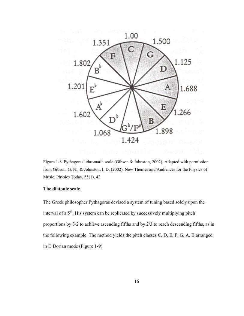
octave above the fundamental. The resulting scale-tone ratios can be seen in Figure 1-8.
The circle of fifths moves clockwise from C. The shaded notes outline the 7-note diatonic
C major scale, and are represented by the white keys of a piano. The un-shaded notes
complete the 12-tone scale and denote the black keys. The numbers indicate the ratio of
the frequency of each note with that of the fundamental (Gibson & Johnston, 2002).
2 The term perfect fifth refers to the fifth note (e.g. “G”) from the tonic (“C”) in an ascending diatonic scale. It exhibits “perfect consonance”, as opposed to the medieval “imperfect consonance” of the interval of a third or a sixth. With the modern exception of the perfect fourth, all other intervals within a octave from the tonic are considered to be dissonant. (Rushton, 2004)
16
Figure 1-8. Pythagoras’ chromatic scale (Gibson & Johnston, 2002). Adapted with permission
from Gibson, G. N., & Johnston, I. D. (2002). New Themes and Audiences for the Physics of
Music. Physics Today, 55(1), 42
The diatonic scale
The Greek philosopher Pythagoras devised a system of tuning based solely upon the
interval of a 5th. His system can be replicated by successively multiplying pitch
proportions by 3/2 to achieve ascending fifths and by 2/3 to reach descending fifths, as in
the following example. The method yields the pitch classes C, D, E, F, G, A, B arranged
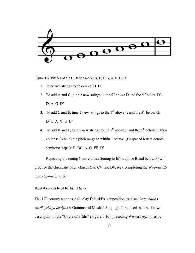
in D Dorian mode (Figure 1-9).
17
Figure 1-9. Pitches of the D Dorian mode: D, E, F, G, A, B, C, D’
1. Tune two strings to an octave: D D’
2. To add A and G, tune 2 new strings to the 5th above D and the 5th below D’.
D A G D’
3. To add C and E, tune 2 new strings to the 5th above A and the 5th below G:
D C A G E D’
4. To add B and F, tune 2 new strings to the 5th above E and the 5th below C, then
collapse (retune) the pitch range to within 1 octave. (Unspaced letters denote
semitone steps.): D BC A G EF D’
Repeating the tuning 5 more times (tuning to fifths above B and below F) will
produce the chromatic pitch classes (F#, C#, G#, D#, A#), completing the Western 12-
tone chromatic scale.
Diletski’s circle of fifths’ (1679)
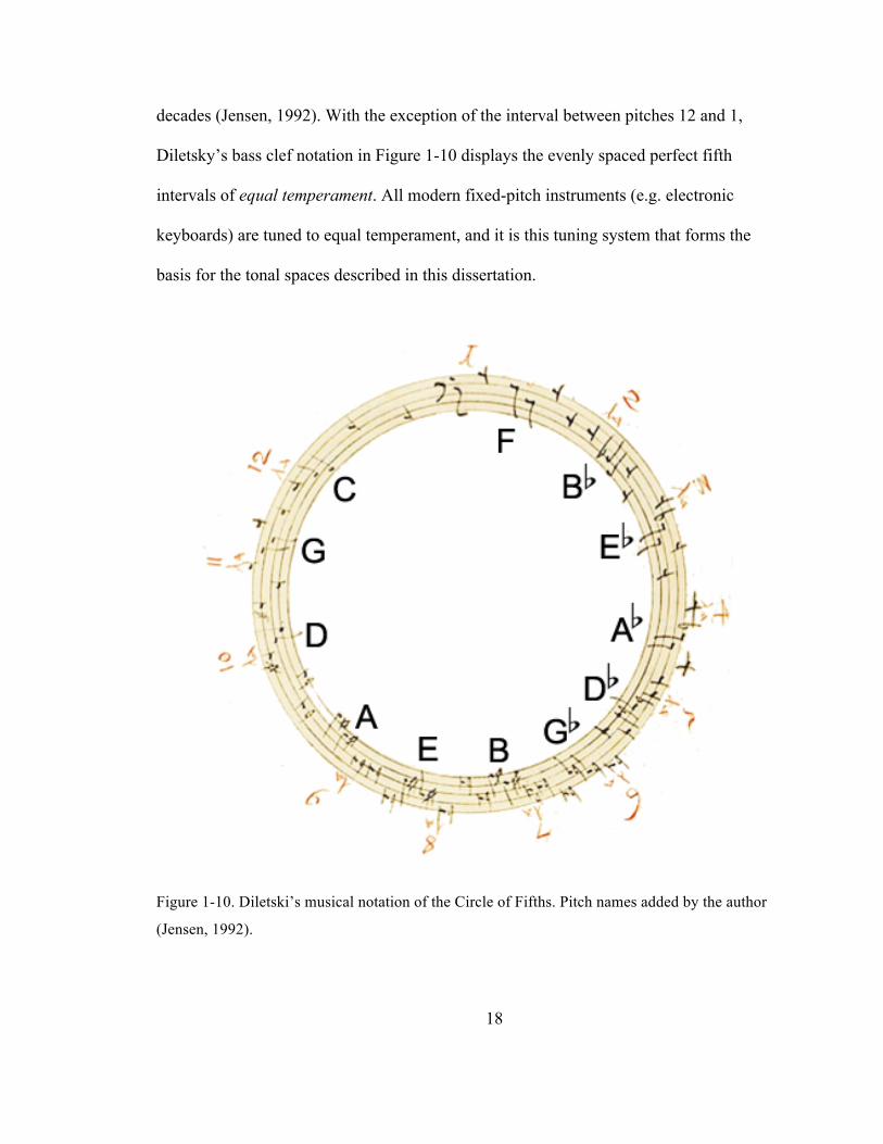
The 17th-century composer Nicolay Diletski’s composition treatise, Grammatika
musikiyskago peniya (A Grammar of Musical Singing), introduced the first-known
description of the “Circle of Fifths” (Figure 1-10), preceding Western examples by
18
decades (Jensen, 1992). With the exception of the interval between pitches 12 and 1,
Diletsky’s bass clef notation in Figure 1-10 displays the evenly spaced perfect fifth
intervals of equal temperament. All modern fixed-pitch instruments (e.g. electronic
keyboards) are tuned to equal temperament, and it is this tuning system that forms the
basis for the tonal spaces described in this dissertation.
Figure 1-10. Diletski’s musical notation of the Circle of Fifths. Pitch names added by the author
(Jensen, 1992).
19
Euler’s tonnetz (1739)
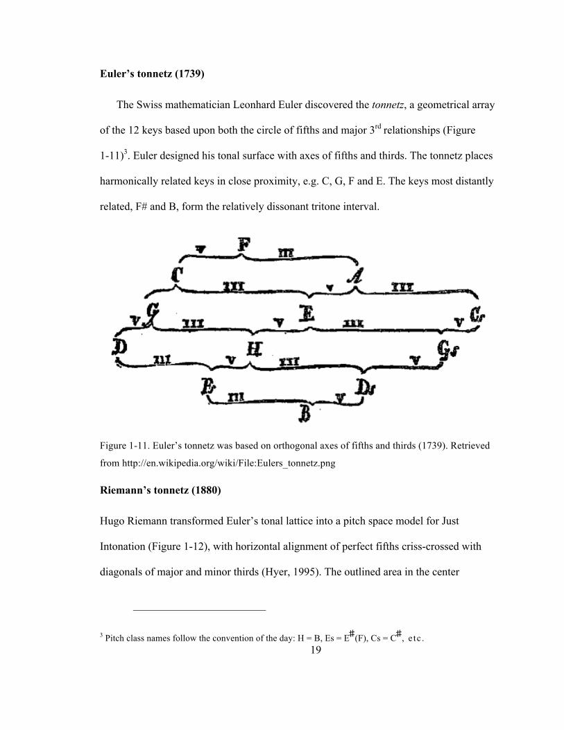
The Swiss mathematician Leonhard Euler discovered the tonnetz, a geometrical array
of the 12 keys based upon both the circle of fifths and major 3rd relationships (Figure
1-11)3. Euler designed his tonal surface with axes of fifths and thirds. The tonnetz places
harmonically related keys in close proximity, e.g. C, G, F and E. The keys most distantly
related, F# and B, form the relatively dissonant tritone interval.
Figure 1-11. Euler’s tonnetz was based on orthogonal axes of fifths and thirds (1739). Retrieved
from http://en.wikipedia.org/wiki/File:Eulers_tonnetz.png
Riemann’s tonnetz (1880)
Hugo Riemann transformed Euler’s tonal lattice into a pitch space model for Just
Intonation (Figure 1-12), with horizontal alignment of perfect fifths criss-crossed with
diagonals of major and minor thirds (Hyer, 1995). The outlined area in the center
3 Pitch class names follow the convention of the day: H = B, Es = E♯(F), Cs = C♯, e tc .
20
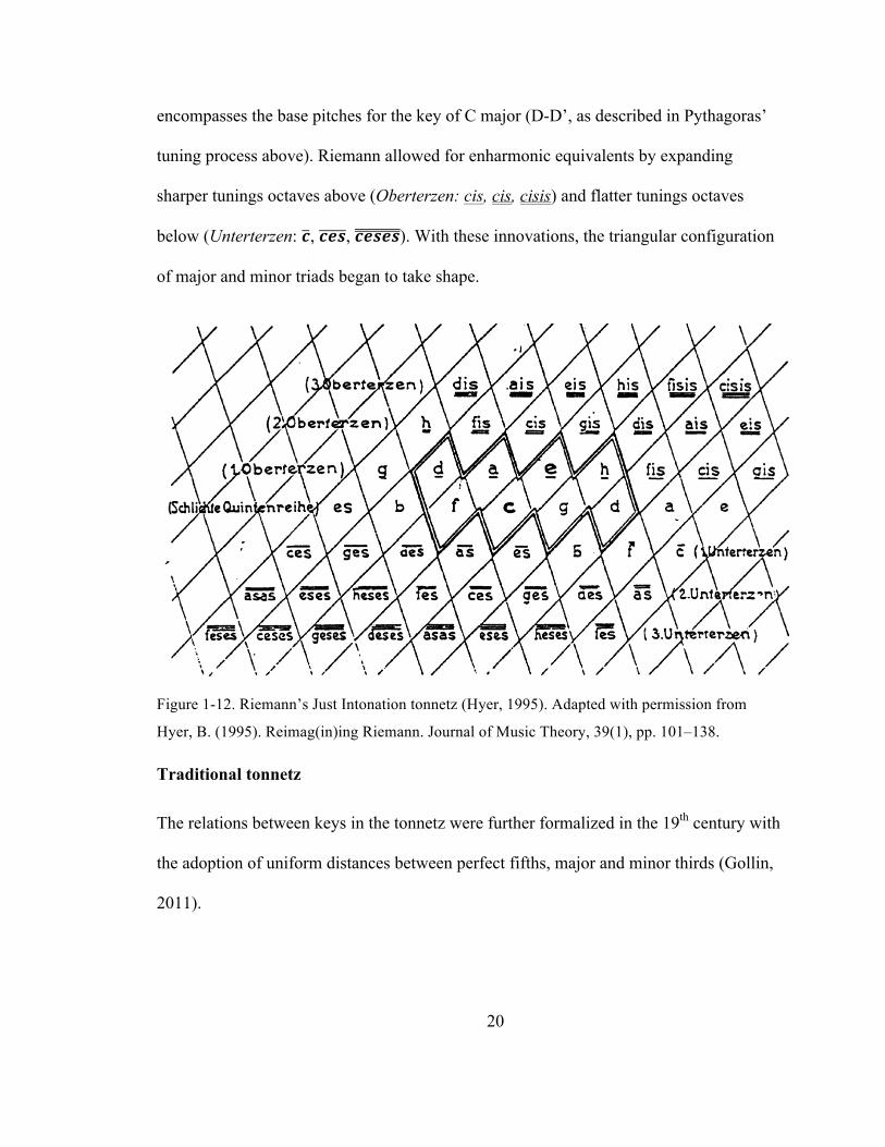
encompasses the base pitches for the key of C major (D-D’, as described in Pythagoras’
tuning process above). Riemann allowed for enharmonic equivalents by expanding
sharper tunings octaves above (Oberterzen: cis, cis, cisis) and flatter tunings octaves
below (Unterterzen: 𝒄, 𝒄𝒆𝒔, 𝒄𝒆𝒔𝒆𝒔). With these innovations, the triangular configuration
of major and minor triads began to take shape.
Figure 1-12. Riemann’s Just Intonation tonnetz (Hyer, 1995). Adapted with permission from
Hyer, B. (1995). Reimag(in)ing Riemann. Journal of Music Theory, 39(1), pp. 101–138.
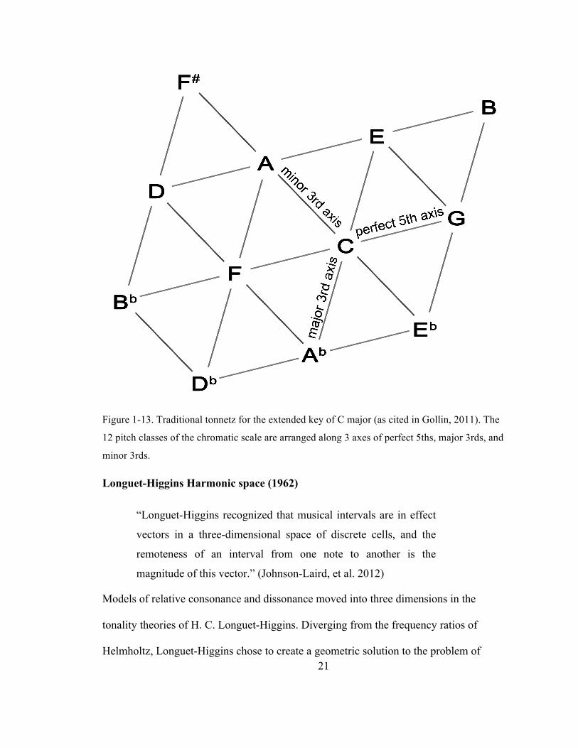
Traditional tonnetz
The relations between keys in the tonnetz were further formalized in the 19th century with
the adoption of uniform distances between perfect fifths, major and minor thirds (Gollin,
2011).
21
Figure 1-13. Traditional tonnetz for the extended key of C major (as cited in Gollin, 2011). The
12 pitch classes of the chromatic scale are arranged along 3 axes of perfect 5ths, major 3rds, and
minor 3rds.
Longuet-Higgins Harmonic space (1962)
“Longuet-Higgins recognized that musical intervals are in effect
vectors in a three-dimensional space of discrete cells, and the
remoteness of an interval from one note to another is the
magnitude of this vector.” (Johnson-Laird, et al. 2012)
Models of relative consonance and dissonance moved into three dimensions in the
tonality theories of H. C. Longuet-Higgins. Diverging from the frequency ratios of
Helmholtz, Longuet-Higgins chose to create a geometric solution to the problem of
22
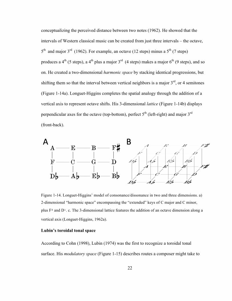
conceptualizing the perceived distance between two notes (1962). He showed that the
intervals of Western classical music can be created from just three intervals – the octave,
5th and major 3rd (1962). For example, an octave (12 steps) minus a 5th (7 steps)
produces a 4th (5 steps), a 4th plus a major 3rd (4 steps) makes a major 6th (9 steps), and so
on. He created a two-dimensional harmonic space by stacking identical progressions, but
shifting them so that the interval between vertical neighbors is a major 3rd, or 4 semitones
(Figure 1-14a). Longuet-Higgins completes the spatial analogy through the addition of a
vertical axis to represent octave shifts. His 3-dimensional lattice (Figure 1-14b) displays
perpendicular axes for the octave (top-bottom), perfect 5th (left-right) and major 3rd
(front-back).
Figure 1-14. Longuet-Higgins’ model of consonance/dissonance in two and three dimensions. a)
2-dimensional “harmonic space” encompassing the “extended” keys of C major and C minor,
plus F♯ and D♭. c. The 3-dimensional lattice features the addition of an octave dimension along a
vertical axis (Longuet-Higgins, 1962a).
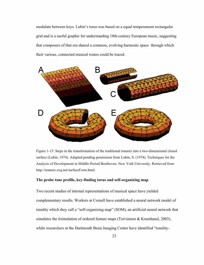
Lubin’s toroidal tonal space
According to Cohn (1998), Lubin (1974) was the first to recognize a toroidal tonal
surface. His modulatory space (Figure 1-15) describes routes a composer might take to
23
modulate between keys. Lubin’s torus was based on a equal temperament rectangular
grid and is a useful graphic for understanding 18th-century European music, suggesting
that composers of that era shared a common, evolving harmonic space through which
their various, connected musical routes could be traced.
Figure 1-15. Steps in the transformation of the traditional tonnetz into a two-dimensional closed
surface (Lubin, 1974). Adapted pending permission from Lubin, S. (1974). Techniques for the
Analysis of Development in Middle-Period Beethoven. New York University. Retrieved from
http://tonnetz.zxq.net/surfaceForm.html.
The probe tone profile, key-finding torus and self-organizing map
Two recent studies of internal representations of musical space have yielded
complementary results. Workers at Cornell have established a neural network model of
tonality which they call a “self-organizing map” (SOM), an artificial neural network that
simulates the formulation of ordered feature maps (Toiviainen & Krumhansl, 2003),
while researchers at the Dartmouth Brain Imaging Center have identified “tonality-
24
specific responses” in the cerebral cortex that correlate closely with the Cornell SOM
(Janata et al., 2002).
One part of the Cornell study focused on the “psychological reality of theoretical
descriptions of music” (Zatorre & Krumhansl, 2002). Toiviainen and Krumhansl
reasoned that, even without formal music training, the understanding of tonal, harmonic,
and melodic patterns identified in music theory influences a listener’s organization and
memory of music. In their experiment, they used the probe tone method in which subjects
listened to a MIDI file, J. S. Bach’s Duetto for organ (BWV 805), during which a probe
tone of the chromatic scale was heard to play continuously. Subject judgments of probe
tone “degree of fit” and “tension” were measured, and the results correlated with those of
concurrent probe-tone data and distance away from the predominant key, respectively. A
projection of the judgment measures onto a toroidal SOM (Figure 1-16) trained with
Krumhansl and Kessler’s 24 probe-tone profiles (1982) revealed a close match with the
researchers’ models of pitch class distribution and tone-transition distribution.
25
Figure 1-16. Krumhansl and Kessler’s self-organizing map (SOM) depicts “inter-key distance”
results from behavioral experiments in which subjects were asked to judge degree-of-fit for probe
tones heard at the end of major and minor scales (1982). a) Unfolded SOM (Toiviainen &
Krumhansl, 2003). Lines indicate circle of fifths for major keys (red) and minor keys (blue). b)
Top/bottom and left/right edges of the SOM are joined to form a torus. Adapted with permission
from Toiviainen, P., & Krumhansl, C. L. (2003). Measuring and modeling real-time responses to
music: the dynamics of tonality induction. Perception, 32(6), 741–766.
Janata employed Krumhansl’s probe tone profiles in an analysis of fMRI data to
identify a brain region (rostromedial prefrontal cortex) involved in tracking the keys of
abstract patterns of Western tonal music stimuli (Janata et al., 2002). In this study, eight
“musically experienced” subjects were asked to listen to a repeated melody and perform
“go/no-go” tasks during fMRI scanning sessions. During each of three weekly sessions,
the melody was played to each subject 24 times as it modulated through all 12 major and
minor keys. Workers used a regression analysis on the results of the fMRI scans to
distinguish task effects from tonality surface tracking and were able to construct average
“tonality surfaces” for each of the 24 keys (Figure 1-17). A 24 x 24 correlation matrix
was generated to display the similarity of tonal hierarchy of each key to every other key.
In other words, the more stable (high vector) notes that two keys shared, the more closely
26
correlated they were (Figure 1-17a). When the key correlation map is wrapped into a 3-
dimensional solution (Figure 1-17b), every major key appears in close proximity to both
its parallel minor (e.g. C major and A minor) and relative minor (e.g. C major and C
minor.
Figure 1-17. A toroid model of tonal space. a) An unfolded, two-dimensional map of key
correlations (Janata et al., 2002). Opposite edges connect to each other to form a continuous,
wrapping surface. Major scales and their relative minors share the same 7-note scale and are
positively correlated (dark red). b) Toroidal representation the key correlation map. Adapted with
permission from Janata, P., et al. (2002). The Cortical Topography of Tonal structures Underlying
Western Music. Science, 298(5601), 2167.
27
Figure 1-18. Properties of the tonality surface. a. Panels show the average tonality surface for
tonality-tracking voxels for each of the 24 keys in the original melody. The surface represents an
unfolded torus: the top and bottom edges of each rectangle wrap around to each other, as do the
left and right edges. The activation peak in each panel (red = strongest) reflects the melody’s
progression through all of the keys. b. Distributed mappings of tonality on the self-organizing
map (SOM). Each set of 9 panels depicts the areas of highest activation (key focus) after every
chord played in a 9-chord key-changing sequence that consisted of the chords D minor
diminished, G, C minor, A♭, F, D♭, B♭ minor, E♭, A♭, and modulated from C minor to A♭ major.
The top set shows the subjective probe tone judgments, while the bottom set shows the mapping
of the key-finding algorithm. Adapted with permission from Janata et al., (2002). The Cortical
Topography of Tonal structures Underlying Western Music. Science, 298(5601), 2167.
The team identified cortical sites that were consistently and systematically
sensitive to key changes (Figure 1-18a), i.e. their regression analysis revealed correlations
between the moment-to-moment activity of neural populations and the calculated
harmonic motion across a theoretical tonality surface, a 3D map of the distances among
28
major and minor keys projected onto the doughnut-shape of a torus (Krumhansl &
Kessler, 1982). Reviewers suggested that this tonal space model might reflect more
general processes of remembering and comparing tones. (Zatorre & Krumhansl, 2002).
Remarkably similar plots came out of Krumhansl & Toiviainen’s probe tone
experiments at Cornell. To study how the sense of key develops and changes over time,
workers played 10 different melodic sequences of 9 chords each to musically trained
subjects. As the sequences modulated from one key to another (e.g. from C major to D
minor), the listeners did the probe tone task after each chord was played. The same
researchers trained their SOM neural network with the 24 K-K profiles, then used a “key-
finding” algorithm to process the input from the key-changing sequence stimuli. The
behavior of the algorithm followed the same patterns of modulations found by the
musically trained expertsError! Reference source not found. (Figure 1-18b).
Helical tonal surfaces Helical tonal surfaces
Roger Shepard (1982) is credited with the first instantiation of tonal space that departed
from unidimensional scales (such as the mel) in favor of a contextual arrangement in
which musical relations (intervals) between pitches were invariant, i.e. a perfect 5th
equalled a perfect 5th, regardless of its position on the scale. He began with the a line of
the 12 pitch classes (and their octaves) arranged in consecutive semitones, then collapsed
the line so that equilateral triangles were formed from adjacent semitones and two
parallel lines of whole tone scales emerged (Figure 1-19). Giving the strip a twist
produced a double helix and a further twisting arranged the pitch classes in 12 vertical
columns. As a result, invariance for interval class distances was maintained.
29
Figure 1-19. Stages in the construction of a double helix of musical pitch: (a) the flat strip of
equilateral triangles, b) the strip of triangles given one complete twist per octave, and (c) the
resulting double helix shown as wound around a cylinder (Shepard, 1982). Adapted with
permission from Krumhansl, Carol L. (2005). The Geometry of Musical Structure : A Brief
Introduction and History. Computers in Entertainment, 3(4), 1–14. Retrieved from
http://dl.acm.org/citation.cfm?id=1095542
Chew spiral array model (2000)
More a cylindrical helix than a spiral, the spiral array model (SAM) is a 3-dimensional
configuration of the harmonic network spatial representation of the relations perceived
between pitches, intervals, chords and keys in which distance corresponds to perceived
musical closeness. Originating from Longuet-Higgins harmonic space, it is a generative
30
model, in that larger structures (keys, scales, chords) spring from the proximity of their
component pitches. As are all tonal spaces in this thesis, the SAM is based on the notion
of the circle of fifths, where each pitch on the spiral sits between two pitches at the
interval of a perfect 5th (Figure 1-20). Pitches spaced at a 3rd are closer than are pitches at
a second interval. Major intervals are closer than minors, i.e. a major 3rd is shorter than a
minor 3rd .
Figure 1-20. Wrapping harmonic space to form the SAM. A) Longuet-Higgins harmonic space
centered on C (range: B♭to B) is curved in upon itself until the pitches A and F meet, forming b)
a cylindrical helix wherein the Euclidean distance for all interval classes is invariant (Chew &
Chen, 2005). The vertical orientation of the four major 3rd axes is maintained. Adapted with
permission from Chew, E. (2003). Thinking Out of the Grid and Inside the Spiral – Geometric
Interpretations of and Comparisons with the Spiral Array Model. Network. Retrieved from
http://lit.gfax.ch/Interpretations of and Comparisons with the Spiral Array Model.pdf.
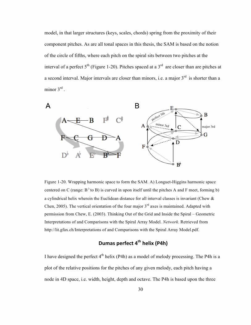
Dumas perfect 4th helix (P4h)
I have designed the perfect 4th helix (P4h) as a model of melody processing. The P4h is a
plot of the relative positions for the pitches of any given melody, each pitch having a
node in 4D space, i.e. width, height, depth and octave. The P4h is based upon the three
31
equivalent axes of the traditional tonnetz, i.e. P5, M3 and m3. As shown in Figure 1-21, a
P4h for a melody in the key of C can be created through the simple expediency of folding
the left and right edges of an equilateral tonnetz toward each other. Further folding of the
top and bottom edges of the tonnetz to form a torus ala Krumhansl et al. would upset the
delicate balance of consistent Euclidean distances for interval classes that is at the heart
of my thesis, and so I have resisted this temptation.
Figure 1-21. Creating a P4h for a melody in the key of C. a) Start with a traditional equilateral
tonnetz centered on C (yellow) with redundant pitches A and F. b) Fold the left and right edges
behind the figure, maintaining all pitch-connection distances. c) Join A to A and F to F to
complete a structure comprising 1 P4h (green), 3 minor 3rd helices (blue), and 4 major 3rd helices
(red).
Figure 1-22 displays several ways of plotting the P4h, each of which retains the
original pitch coordinates. The geodesic P4h variation is the most accurate display of the
theoretical Euclidean distances for P4, M3 and m3 intervals (Figure 1-22a). The
cylindrical version (Figure 1-22b) highlights the P4 helix itself and enables a comparison
with the Chew SAM. The vector version (Figure 1-22c) places the tonic C at the center of
the network and clearly demonstrates the 4 interval class distances for all intervals
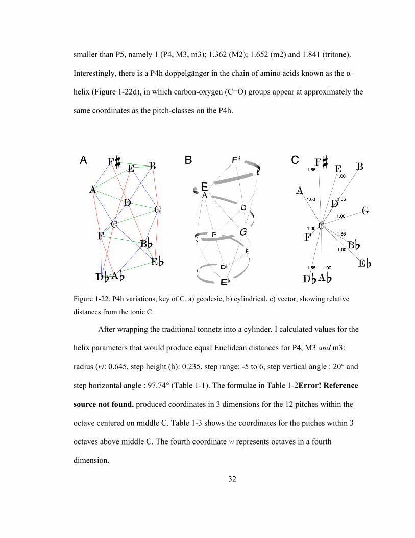
32
smaller than P5, namely 1 (P4, M3, m3); 1.362 (M2); 1.652 (m2) and 1.841 (tritone).
Interestingly, there is a P4h doppelgänger in the chain of amino acids known as the α-
helix (Figure 1-22d), in which carbon-oxygen (C=O) groups appear at approximately the
same coordinates as the pitch-classes on the P4h.
Figure 1-22. P4h variations, key of C. a) geodesic, b) cylindrical, c) vector, showing relative
distances from the tonic C.
After wrapping the traditional tonnetz into a cylinder, I calculated values for the
helix parameters that would produce equal Euclidean distances for P4, M3 and m3:
radius (r): 0.645, step height (h): 0.235, step range: -5 to 6, step vertical angle : 20° and
step horizontal angle : 97.74° (Table 1-1). The formulae in Table 1-2Error! Reference
source not found. produced coordinates in 3 dimensions for the 12 pitches within the
octave centered on middle C. Table 1-3 shows the coordinates for the pitches within 3
octaves above middle C. The fourth coordinate w represents octaves in a fourth
dimension.
33
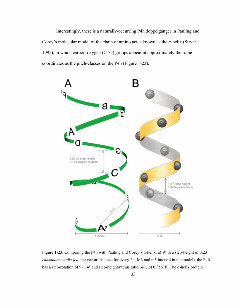
Interestingly, there is a naturally-occurring P4h doppelgänger in Pauling and
Corey’s molecular model of the chain of amino acids known as the α-helix (Stryer,
1995), in which carbon-oxygen (C=O) groups appear at approximately the same
coordinates as the pitch-classes on the P4h (Figure 1-23).
Figure 1-23. Comparing the P4h with Pauling and Corey’s α-helix. a) With a step-height of 0.23
consonance units (cu, the vector distance for every P4, M3 and m3 interval in the model), the P4h
has a step-rotation of 97.74° and step-height/radius ratio (h/r) of 0.356. b) The α-helix protein
34
structure has a similar step-rotation (100°), but an elongated h/r of 0.60. Adapted with
permission from Stryer, L. (1995). Biochemistry (4th ed., pp. 27–30). New York: W. H. Freeman
& Company.
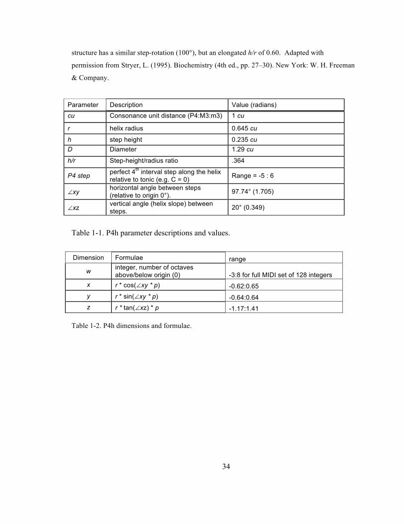
Table 1-1. P4h parameter descriptions and values.
Table 1-2. P4h dimensions and formulae.
Parameter Description Value (radians) cu Consonance unit distance (P4:M3:m3) 1 cu
r helix radius 0.645 cu
h step height 0.235 cu D Diameter 1.29 cu
h/r Step-height/radius ratio .364
P4 step perfect 4th interval step along the helix relative to tonic (e.g. C = 0) Range = -5 : 6
∠xy horizontal angle between steps (relative to origin 0°). 97.74° (1.705)
∠xz vertical angle (helix slope) between steps. 20° (0.349)
Dimension Formulae range
w integer, number of octaves above/below origin (0) -3:8 for full MIDI set of 128 integers
x r * cos(∠xy * p) -0.62:0.65 y r * sin(∠xy * p) -0.64:0.64 z r * tan(∠xz) * p -1.17:1.41

35
Table 1-3. P4h, key of C. Pitches, P4 steps, angles, coordinates and consonance units for pitches
within the octave centered on the origin (middle C). Columns: a) P4 pitch class; b) P4 step
relative to origin C (0); P4 step angle (∠xy) in degrees; P4 step angle (∠xy) in radians;
Pitch P4 step ∠xy (°) ∠xy radians w x y z cu (rel. to C)
F# 6 586.44 10.24 0 -0.44 -0.47 1.41 1.84
B 5 488.7 8.53 0 -0.4 0.5 1.17 1.65
E 4 390.96 6.82 0 0.55 0.33 0.94 1.00
A 3 293.22 5.12 0 0.25 -0.59 0.7 1.00 D 2 195.48 3.41 0 -0.62 -0.17 0.47 1.36
G 1 97.74 1.71 0 -0.09 0.64 0.23 1.00
C 0 0 0 0 0.65 0 0 0.00
F -1 -97.74 -1.71 0 -0.09 -0.64 -0.23 1.00 Bb -2 -195.48 -3.41 0 -0.62 0.17 -0.47 1.36
Eb -3 -293.22 -5.12 0 0.25 0.59 -0.7 1.00
Ab -4 -390.96 -6.82 0 0.55 -0.33 -0.94 1.00
Db -5 -488.7 -8.53 0 -0.4 -0.5 -1.17 1.65
36
MIDI pitch name MIDI # x y z w (octave) C3 60 0.645 0 0 0
Db3 61 -0.403281513 -0.503377613 -1.173804006 0 D3 62 -0.621601772 -0.172151783 0.469521602 0 Eb3 63 0.254299457 0.592753563 -0.704282403 0 E3 64 0.553104693 0.331813499 0.939043204 0 F3 65 -0.086867303 -0.639123675 -0.234760801 0
F#3 66 -0.444478406 -0.467401269 1.408564807 0 G3 67 -0.086867303 0.639123675 0.234760801 1 Ab3 68 0.553104693 -0.331813499 -0.939043204 1 A3 69 0.254299457 -0.592753563 0.704282403 1
Bb3 70 -0.621601772 0.172151783 -0.469521602 1 B3 71 -0.403281513 0.503377613 1.173804006 1 C4 72 0.645 0 0 1
Db4 73 -0.403281513 -0.503377613 -1.173804006 1 D4 74 -0.621601772 -0.172151783 0.469521602 1 Eb4 75 0.254299457 0.592753563 -0.704282403 1 E4 76 0.553104693 0.331813499 0.939043204 1 F4 77 -0.086867303 -0.639123675 -0.234760801 1
F#4 78 -0.444478406 -0.467401269 1.408564807 1 G4 79 -0.086867303 0.639123675 0.234760801 2 Ab4 80 0.553104693 -0.331813499 -0.939043204 2 A4 81 0.254299457 -0.592753563 0.704282403 2
Bb4 82 -0.621601772 0.172151783 -0.469521602 2 B4 83 -0.403281513 0.503377613 1.173804006 2 C5 84 0.645 0 0 2
Db5 85 -0.403281513 -0.503377613 -1.173804006 2 D5 86 -0.621601772 -0.172151783 0.469521602 2 Eb5 87 0.254299457 0.592753563 -0.704282403 2 E5 88 0.553104693 0.331813499 0.939043204 2 F5 89 -0.086867303 -0.639123675 -0.234760801 2
F#5 90 -0.444478406 -0.467401269 1.408564807 2 G5 91 -0.086867303 0.639123675 0.234760801 3 Ab5 92 0.553104693 -0.331813499 -0.939043204 3 A5 93 0.254299457 -0.592753563 0.704282403 3
Bb5 94 -0.621601772 0.172151783 -0.469521602 3 B5 95 -0.403281513 0.503377613 1.173804006 3 C5 96 0.645 0 0 3
Table 1-4. 4D coordinates for the pitches within 3 octaves above middle C. The octave coordinate
w breaks between F♯ and G, reflecting both the C-centric organization and the fact all intervals
within the first 3 dimensions (xyz) are smaller than a perfect 5th.
37
Chapter 2. Materials and Methods
Subjects
Experiment A: Neural processing of pitch
10 healthy, right-handed subjects, ages 25-37 y, (5M:5F, non-musicians).
Experiment B: Neural processing of auto-correlation, Experiment C: Neural
processing of interval distance, Experiment D: Neural processing of next-note
probability
10 healthy, right-handed subjects, ages 27-47 y, (7M:3F, non-musicians).
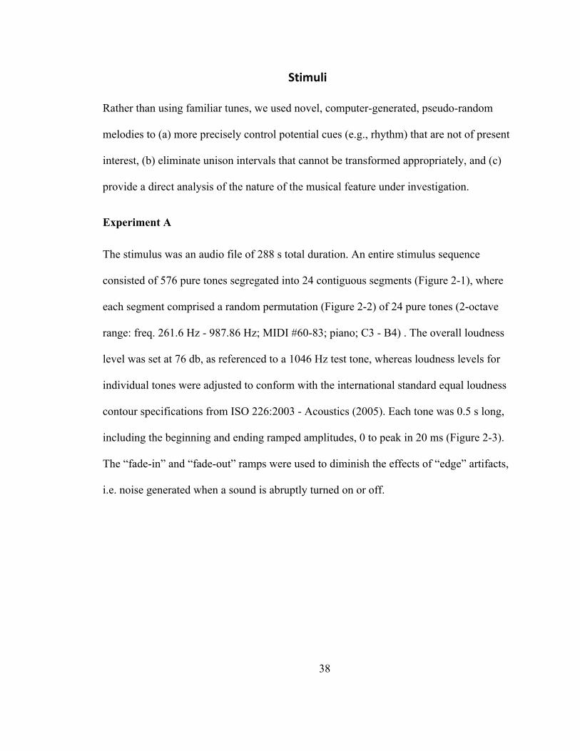
38
Stimuli
Rather than using familiar tunes, we used novel, computer-generated, pseudo-random
melodies to (a) more precisely control potential cues (e.g., rhythm) that are not of present
interest, (b) eliminate unison intervals that cannot be transformed appropriately, and (c)
provide a direct analysis of the nature of the musical feature under investigation.
Experiment A
The stimulus was an audio file of 288 s total duration. An entire stimulus sequence
consisted of 576 pure tones segregated into 24 contiguous segments (Figure 2-1), where
each segment comprised a random permutation (Figure 2-2) of 24 pure tones (2-octave
range: freq. 261.6 Hz - 987.86 Hz; MIDI #60-83; piano; C3 - B4) . The overall loudness
level was set at 76 db, as referenced to a 1046 Hz test tone, whereas loudness levels for
individual tones were adjusted to conform with the international standard equal loudness
contour specifications from ISO 226:2003 - Acoustics (2005). Each tone was 0.5 s long,
including the beginning and ending ramped amplitudes, 0 to peak in 20 ms (Figure 2-3).
The “fade-in” and “fade-out” ramps were used to diminish the effects of “edge” artifacts,
i.e. noise generated when a sound is abruptly turned on or off.
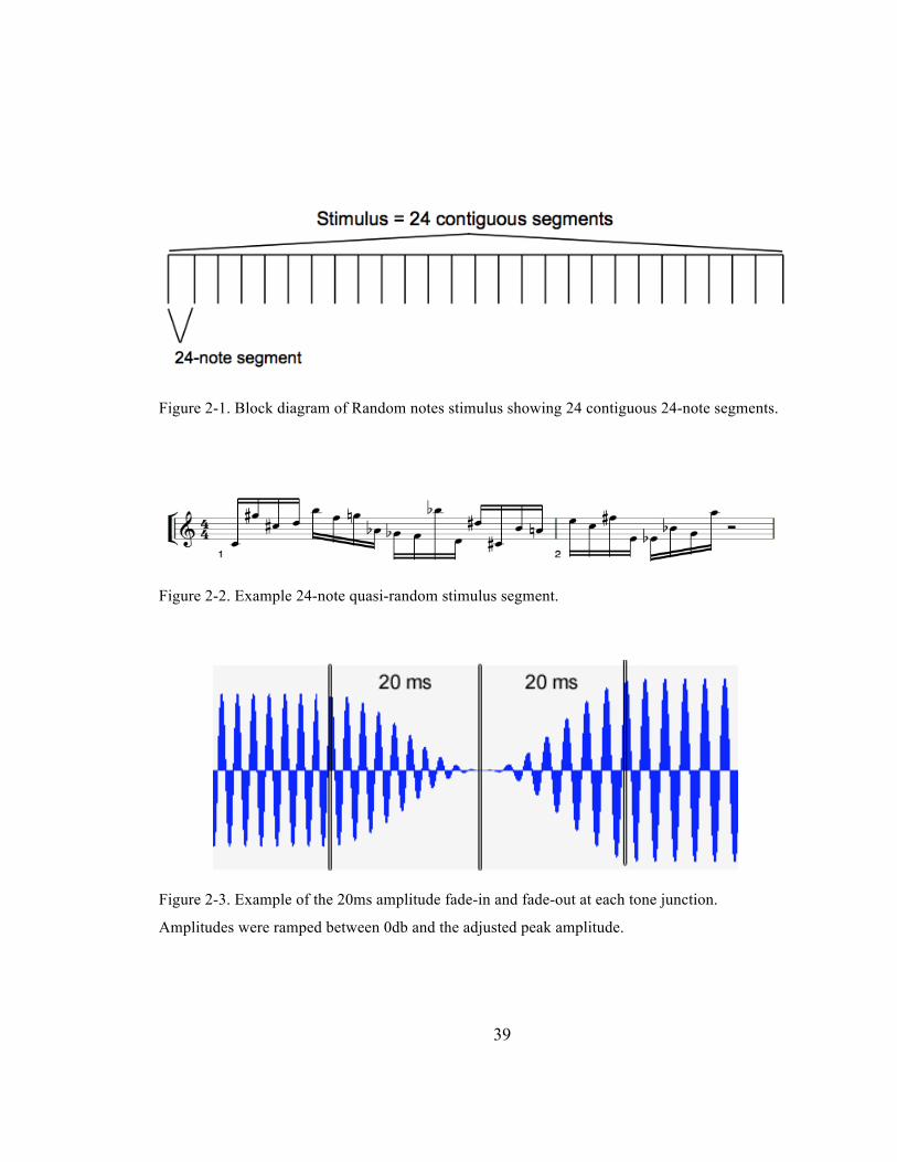
39
Figure 2-1. Block diagram of Random notes stimulus showing 24 contiguous 24-note segments.
Figure 2-2. Example 24-note quasi-random stimulus segment.
Figure 2-3. Example of the 20ms amplitude fade-in and fade-out at each tone junction.
Amplitudes were ramped between 0db and the adjusted peak amplitude.
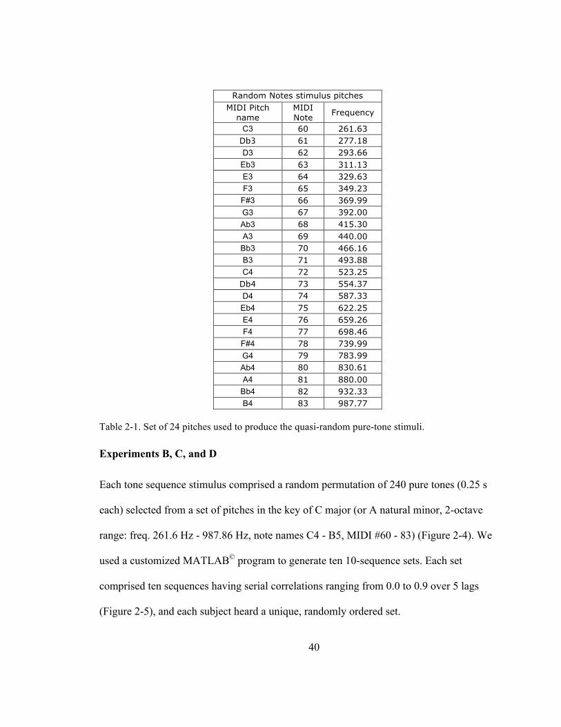
40
Random Notes stimulus pitches MIDI Pitch
name MIDI Note Frequency
C3 60 261.63 Db3 61 277.18 D3 62 293.66 Eb3 63 311.13 E3 64 329.63 F3 65 349.23
F#3 66 369.99 G3 67 392.00 Ab3 68 415.30 A3 69 440.00
Bb3 70 466.16 B3 71 493.88 C4 72 523.25
Db4 73 554.37 D4 74 587.33 Eb4 75 622.25 E4 76 659.26 F4 77 698.46
F#4 78 739.99 G4 79 783.99 Ab4 80 830.61 A4 81 880.00
Bb4 82 932.33 B4 83 987.77
Table 2-1. Set of 24 pitches used to produce the quasi-random pure-tone stimuli.
Experiments B, C, and D
Each tone sequence stimulus comprised a random permutation of 240 pure tones (0.25 s
each) selected from a set of pitches in the key of C major (or A natural minor, 2-octave
range: freq. 261.6 Hz - 987.86 Hz, note names C4 - B5, MIDI #60 - 83) (Figure 2-4). We
used a customized MATLAB© program to generate ten 10-sequence sets. Each set
comprised ten sequences having serial correlations ranging from 0.0 to 0.9 over 5 lags
(Figure 2-5), and each subject heard a unique, randomly ordered set.
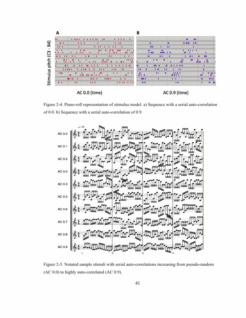
41
Figure 2-4. Piano-roll representation of stimulus model. a) Sequence with a serial auto-correlation
of 0.0. b) Sequence with a serial auto-correlation of 0.9.
Figure 2-5. Notated sample stimuli with serial auto-correlations increasing from pseudo-random
(AC 0.0) to highly auto-correlated (AC 0.9).

42
Task
All Experiments
Subjects lay supine on a bed wearing pneumatic earphones with protective foam ends.
Subjects were asked to stay still with their eyes closed while listening to a sequence of
tones lasting approximately 5 minutes (Experiment A) or 11 minutes (Experiments B, C,
and D).
Data acquisition
All Experiments
Neural recordings. Magnetic field activity of the brain was recorded using 248 axial
gradiometers (Magnes 3600WH, 4-D Neuroimaging, San Diego, CA) at a sampling rate
of 1017 Hz (bandpass: 0.1- 400 Hz). Given a stimulus of 666 s, and the sampling rate
above, the data generated for each subject consisted of 248 matrices (one per sensor),
each containing approximately 288,000 measurements (Experiment A) or 677,000
measurements (Experiments B, C, and D).
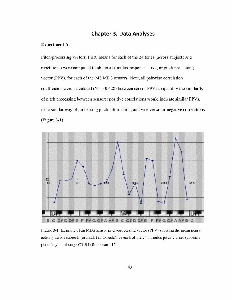
43
Chapter 3. Data Analyses Experiment A
Pitch-processing vectors. First, means for each of the 24 tones (across subjects and
repetitions) were computed to obtain a stimulus-response curve, or pitch-processing
vector (PPV), for each of the 248 MEG sensors. Next, all pairwise correlation
coefficients were calculated (N = 30,628) between sensor PPVs to quantify the similarity
of pitch processing between sensors: positive correlations would indicate similar PPVs,
i.e. a similar way of processing pitch information, and vice versa for negative correlations
(Figure 3-1).
Figure 3-1. Example of an MEG sensor pitch-processing vector (PPV) showing the mean neural
activity across subjects (ordinal: femtoTesla) for each of the 24 stimulus pitch-classes (abscissa:
piano keyboard range C3-B4) for sensor #154.
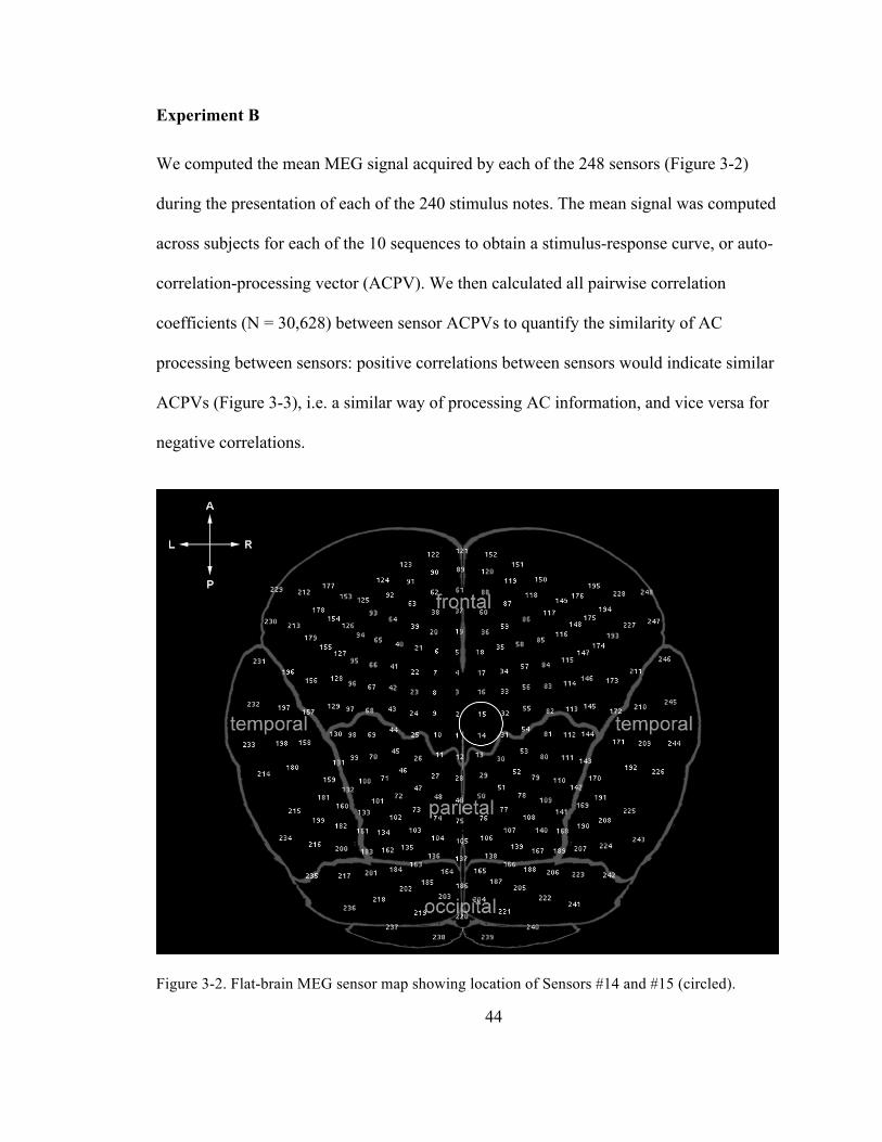
44
Experiment B
We computed the mean MEG signal acquired by each of the 248 sensors (Figure 3-2)
during the presentation of each of the 240 stimulus notes. The mean signal was computed
across subjects for each of the 10 sequences to obtain a stimulus-response curve, or auto-
correlation-processing vector (ACPV). We then calculated all pairwise correlation
coefficients (N = 30,628) between sensor ACPVs to quantify the similarity of AC
processing between sensors: positive correlations between sensors would indicate similar
ACPVs (Figure 3-3), i.e. a similar way of processing AC information, and vice versa for
negative correlations.
Figure 3-2. Flat-brain MEG sensor map showing location of Sensors #14 and #15 (circled).
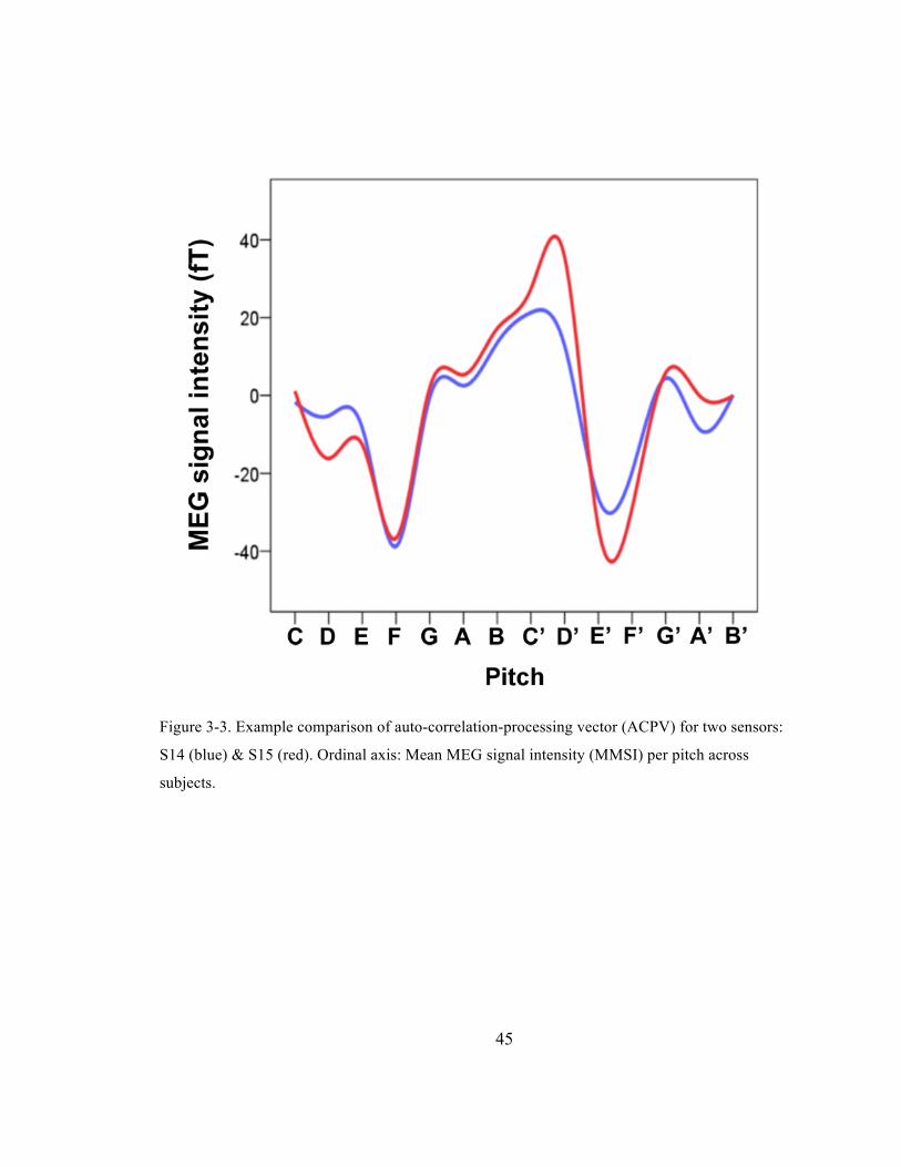
45
Figure 3-3. Example comparison of auto-correlation-processing vector (ACPV) for two sensors:
S14 (blue) & S15 (red). Ordinal axis: Mean MEG signal intensity (MMSI) per pitch across
subjects.
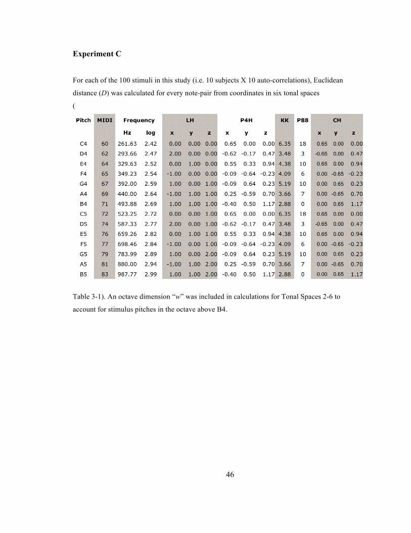
46
Experiment C
For each of the 100 stimuli in this study (i.e. 10 subjects X 10 auto-correlations), Euclidean
distance (D) was calculated for every note-pair from coordinates in six tonal spaces
(
Table 3-1). An octave dimension “w” was included in calculations for Tonal Spaces 2-6 to
account for stimulus pitches in the octave above B4.
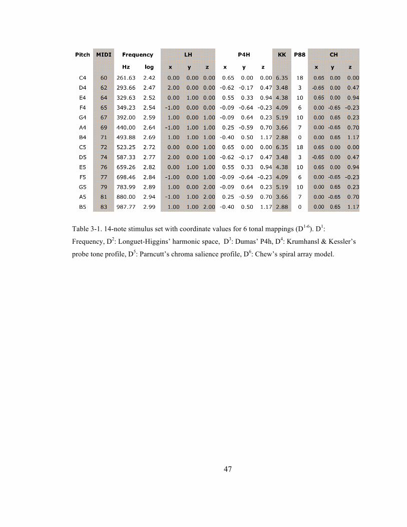
47
Table 3-1. 14-note stimulus set with coordinate values for 6 tonal mappings (D1-6). D1:
Frequency, D2: Longuet-Higgins’ harmonic space, D3: Dumas’ P4h, D4: Krumhansl & Kessler’s
probe tone profile, D5: Parncutt’s chroma salience profile, D6: Chew’s spiral array model.
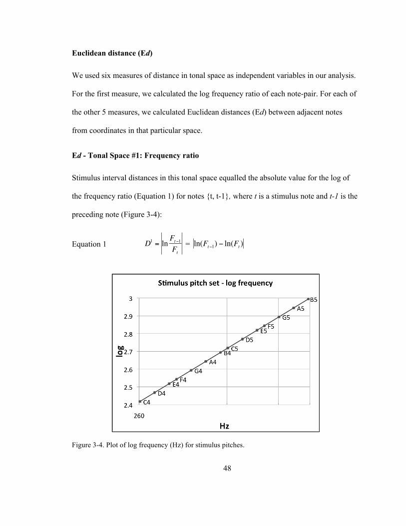
48
Euclidean distance (Ed)
We used six measures of distance in tonal space as independent variables in our analysis.
For the first measure, we calculated the log frequency ratio of each note-pair. For each of
the other 5 measures, we calculated Euclidean distances (Ed) between adjacent notes
from coordinates in that particular space.
Ed - Tonal Space #1: Frequency ratio
Stimulus interval distances in this tonal space equalled the absolute value for the log of
the frequency ratio (Equation 1) for notes {t, t-1}, where t is a stimulus note and t-1 is the
preceding note (Figure 3-4):
Equation 1 =
Figure 3-4. Plot of log frequency (Hz) for stimulus pitches.
€
D1 = ln Ft−1Ft
€
ln(Ft−1) − ln(Ft )

49
Ed - Tonal Space #2: Longuet-Higgins (LH) harmonic space (1962a)
Interval distances in LH space (Figure 3-5) were calculated using Equation 2 and pitch
coordinate values from 3 axes: P5, M3 and octave.
Equation 2
Figure 3-5. Longuet-Higgins’ (1962a) harmonic space for the key of C major. abscissa: perfect
5th, ordinal: major 3rd, z-axis: octave.
€
D2 = a + b + ca = (P5t − P5t−1)
2, b = (M3t −M3t−1)2, c = (P8t − P8t−1)
2
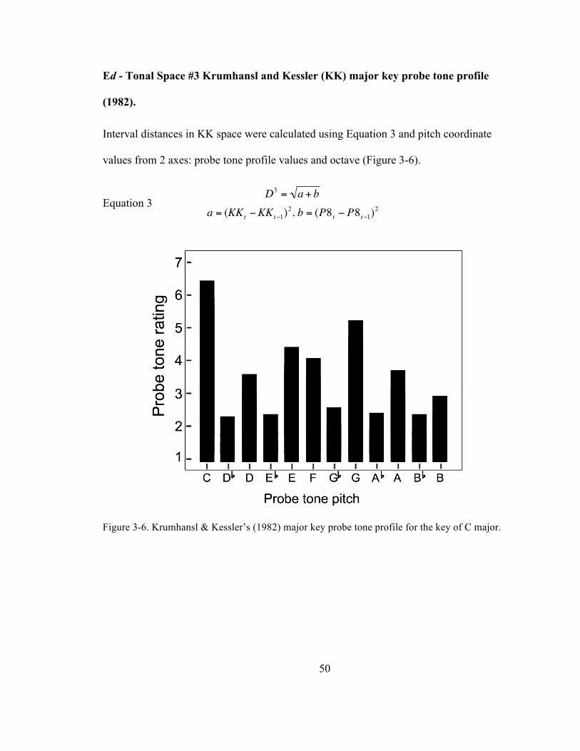
50
Ed - Tonal Space #3 Krumhansl and Kessler (KK) major key probe tone profile
(1982).
Interval distances in KK space were calculated using Equation 3 and pitch coordinate
values from 2 axes: probe tone profile values and octave (Figure 3-6).
Equation 3
Figure 3-6. Krumhansl & Kessler’s (1982) major key probe tone profile for the key of C major.
€
D3 = a + ba = (KKt −KKt−1)
2, b = (P8t − P8t−1)2
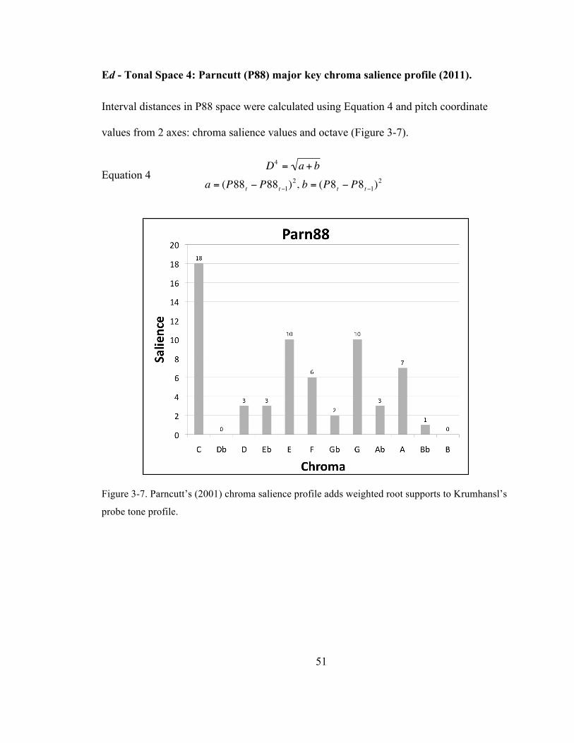
51
Ed - Tonal Space 4: Parncutt (P88) major key chroma salience profile (2011).
Interval distances in P88 space were calculated using Equation 4 and pitch coordinate
values from 2 axes: chroma salience values and octave (Figure 3-7).
Equation 4
Figure 3-7. Parncutt’s (2001) chroma salience profile adds weighted root supports to Krumhansl’s
probe tone profile.
€
D4 = a + ba = (P88t − P88t−1)
2, b = (P8t − P8t−1)2
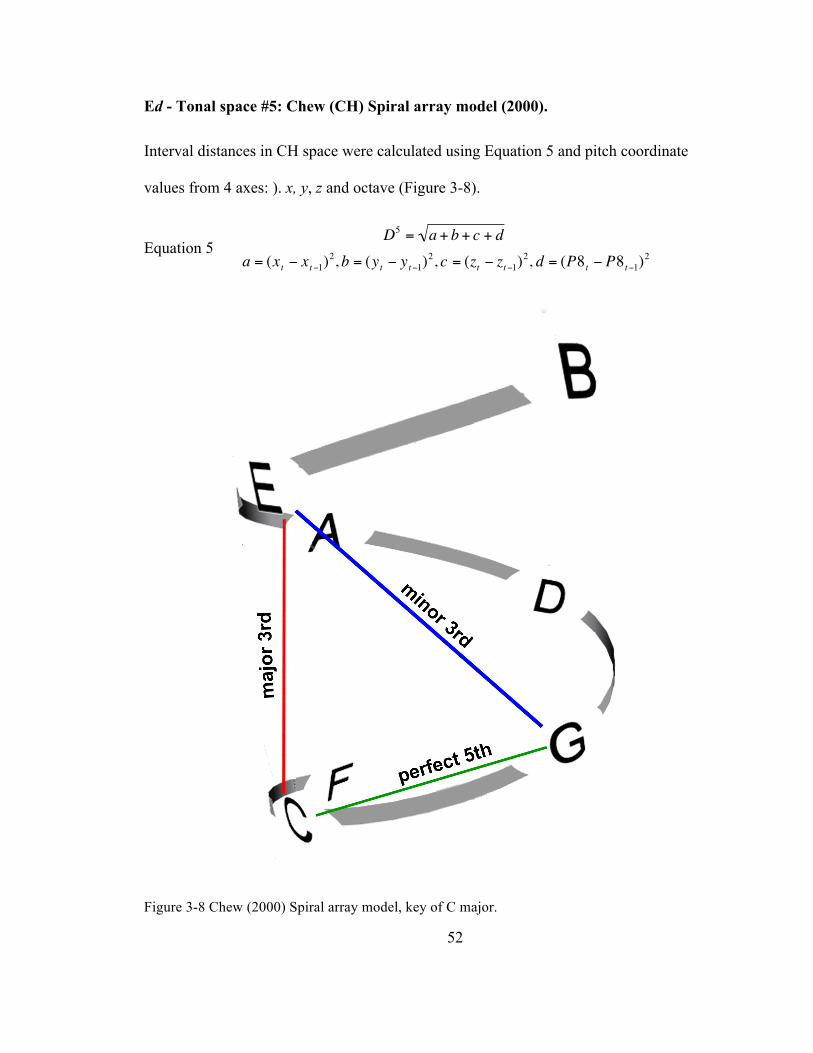
52
Ed - Tonal space #5: Chew (CH) Spiral array model (2000).
Interval distances in CH space were calculated using Equation 5 and pitch coordinate
values from 4 axes: ). x, y, z and octave (Figure 3-8).
Equation 5
Figure 3-8 Chew (2000) Spiral array model, key of C major.
€
D5 = a + b + c + d
a = (xt − xt−1)2, b = (yt − yt−1)
2, c = (zt − zt−1)2, d = (P8t − P8t−1)
2
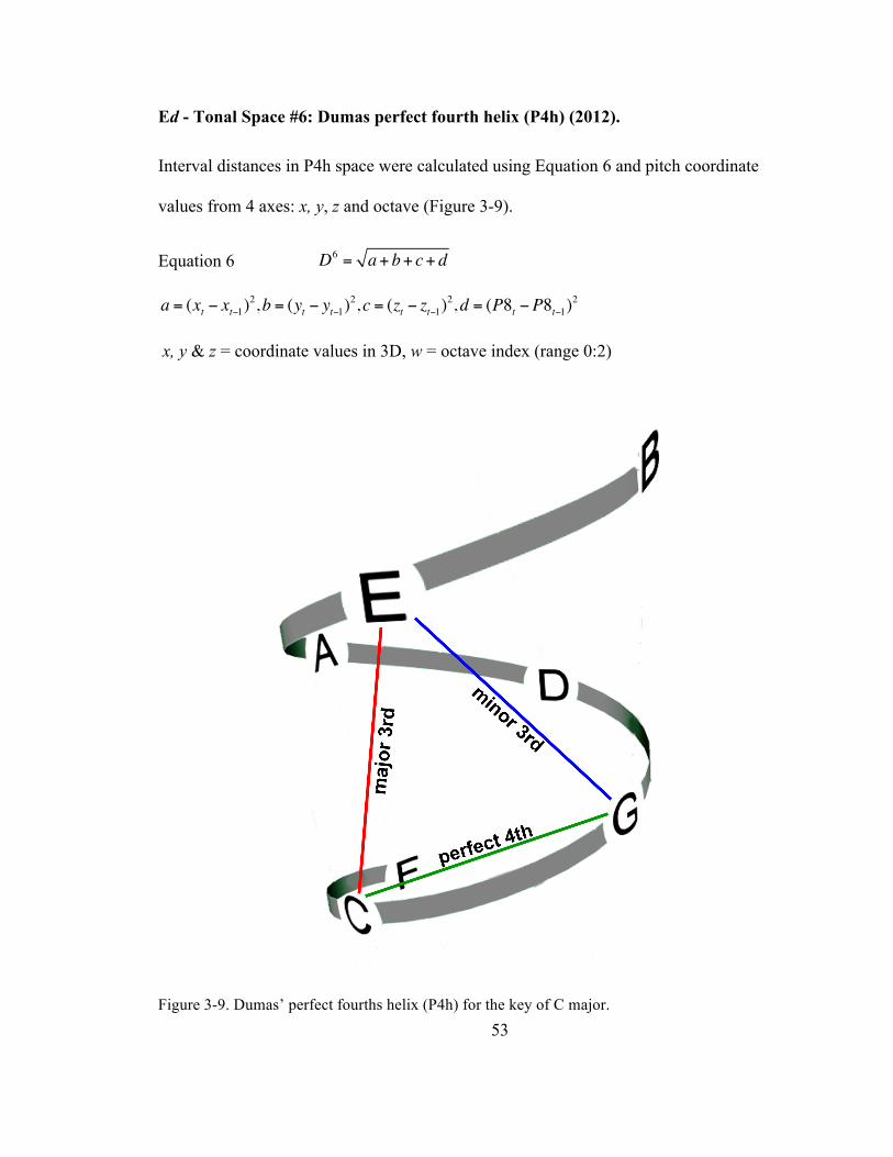
53
Ed - Tonal Space #6: Dumas perfect fourth helix (P4h) (2012).
Interval distances in P4h space were calculated using Equation 6 and pitch coordinate
values from 4 axes: x, y, z and octave (Figure 3-9).
Equation 6
x, y & z = coordinate values in 3D, w = octave index (range 0:2)
Figure 3-9. Dumas’ perfect fourths helix (P4h) for the key of C major.
D6 = a+ b+ c+ d
a = (xt − xt−1)2,b = (yt − yt−1)
2,c = (zt − zt−1)2,d = (P8t −P8t−1)
2
54
Auto-regression analysis. With respect to the neural signal, successive absolute
differences in the MEG signal (DMEG) were calculated between successive note means for
each of 248 sensors. With respect to the notes, Ed D1, 2, 3, 4, 5, 6 were calculated between
successive note coordinates. we wanted to assess the relations between changes in neural
activity to tone changes in each one of the six different tonal spaces. For that purpose, we
carried out an autoregression analysis (to account for possibly correlated errors), where
the dependent variable was DMEG and the independent variables were D1, 2, 3, 4, 5, 6 in six
separate regressions.
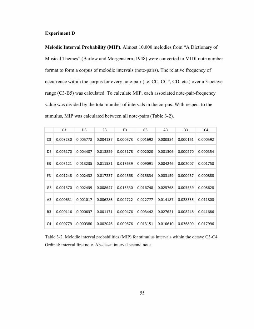
55
Experiment D
Melodic Interval Probability (MIP). Almost 10,000 melodies from “A Dictionary of
Musical Themes” (Barlow and Morgenstern, 1948) were converted to MIDI note number
format to form a corpus of melodic intervals (note-pairs). The relative frequency of
occurrence within the corpus for every note-pair (i.e. CC, CC#, CD, etc.) over a 3-octave
range (C3-B5) was calculated. To calculate MIP, each associated note-pair-frequency
value was divided by the total number of intervals in the corpus. With respect to the
stimulus, MIP was calculated between all note-pairs (Table 3-2).
C3 D3 E3 F3 G3 A3 B3 C4
C3 0.003230 0.005778 0.004137 0.000573 0.001692 0.000354 0.000161 0.000592
D3 0.006170 0.004407 0.013859 0.003178 0.002020 0.001306 0.000270 0.000354
E3 0.003121 0.013235 0.011581 0.018639 0.009091 0.004246 0.002007 0.001750
F3 0.001248 0.002432 0.017237 0.004568 0.015834 0.003159 0.000457 0.000888
G3 0.001570 0.002439 0.008647 0.013550 0.016748 0.025768 0.005559 0.008628
A3 0.000631 0.001017 0.006286 0.002722 0.022777 0.014187 0.028355 0.011800
B3 0.000116 0.000637 0.001171 0.000476 0.003442 0.027621 0.008248 0.041686
C4 0.000779 0.000380 0.002046 0.000676 0.013151 0.010610 0.036809 0.017996
Table 3-2. Melodic interval probabilities (MIP) for stimulus intervals within the octave C3-C4.
Ordinal: interval first note. Abscissa: interval second note.
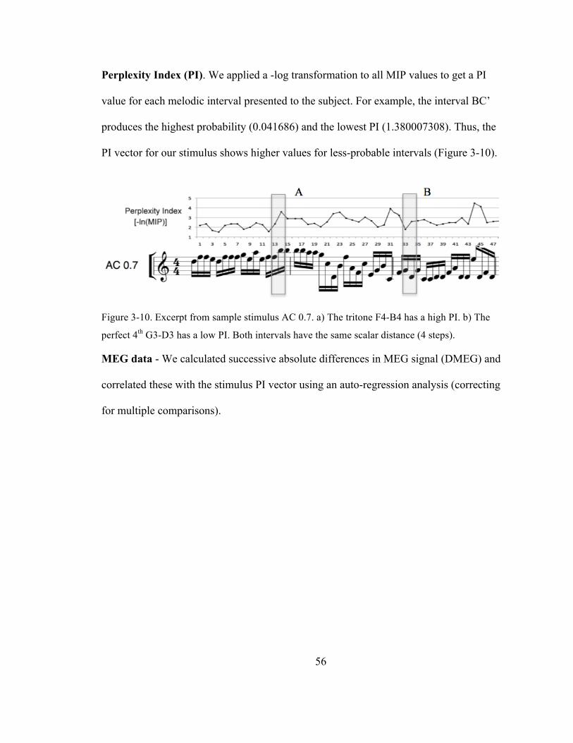
56
Perplexity Index (PI). We applied a -log transformation to all MIP values to get a PI
value for each melodic interval presented to the subject. For example, the interval BC’
produces the highest probability (0.041686) and the lowest PI (1.380007308). Thus, the
PI vector for our stimulus shows higher values for less-probable intervals (Figure 3-10).
Figure 3-10. Excerpt from sample stimulus AC 0.7. a) The tritone F4-B4 has a high PI. b) The
perfect 4th G3-D3 has a low PI. Both intervals have the same scalar distance (4 steps).
MEG data - We calculated successive absolute differences in MEG signal (DMEG) and
correlated these with the stimulus PI vector using an auto-regression analysis (correcting
for multiple comparisons).
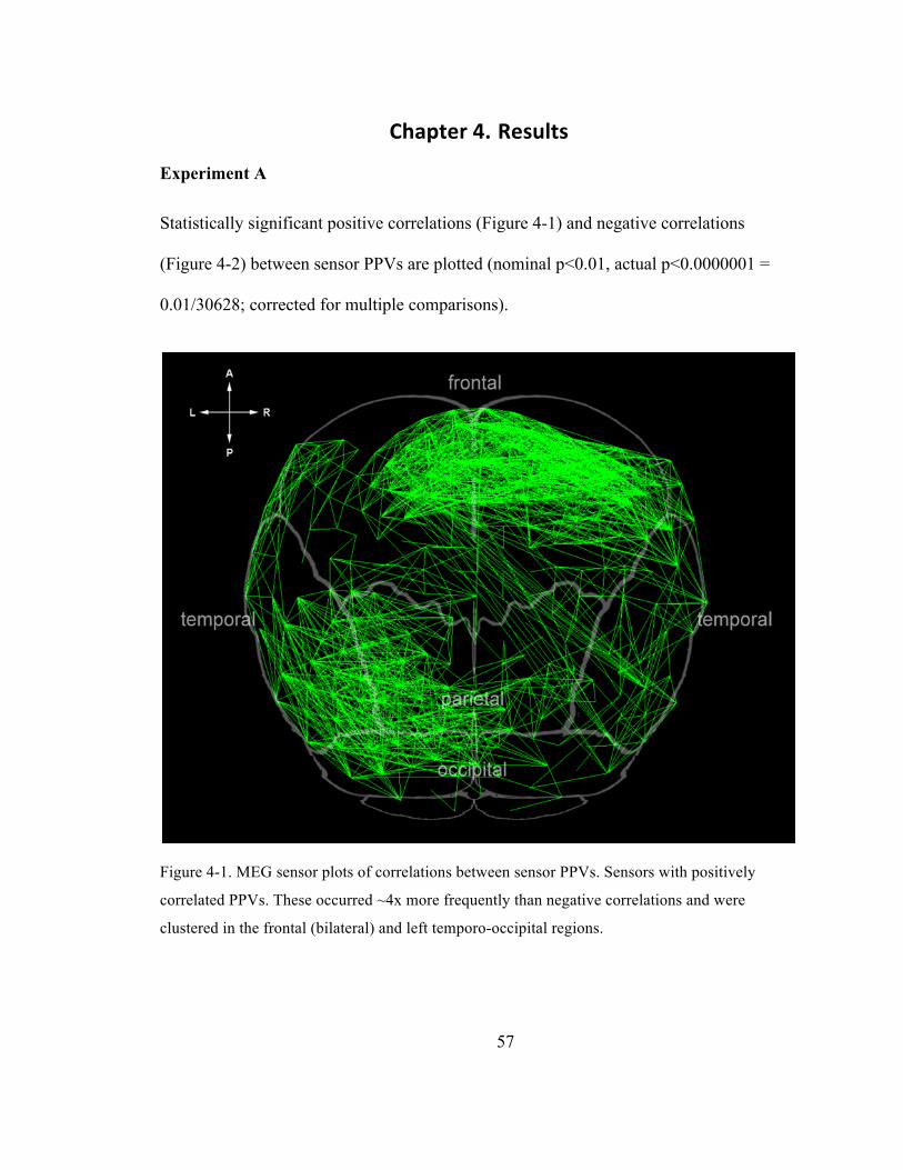
57
Chapter 4. Results Experiment A
Statistically significant positive correlations (Figure 4-1) and negative correlations
(Figure 4-2) between sensor PPVs are plotted (nominal p<0.01, actual p<0.0000001 =
0.01/30628; corrected for multiple comparisons).
Figure 4-1. MEG sensor plots of correlations between sensor PPVs. Sensors with positively
correlated PPVs. These occurred ~4x more frequently than negative correlations and were
clustered in the frontal (bilateral) and left temporo-occipital regions.
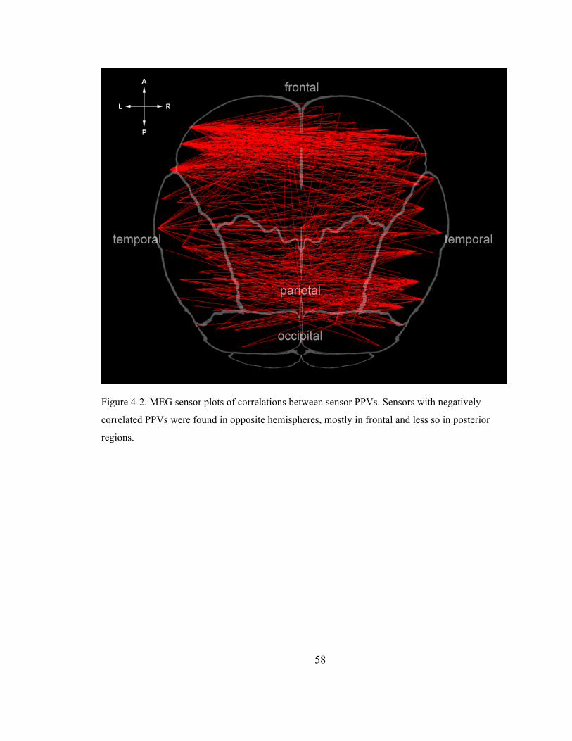
58
Figure 4-2. MEG sensor plots of correlations between sensor PPVs. Sensors with negatively
correlated PPVs were found in opposite hemispheres, mostly in frontal and less so in posterior
regions.
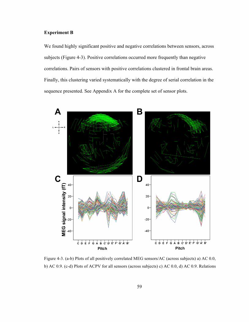
59
Experiment B
We found highly significant positive and negative correlations between sensors, across
subjects (Figure 4-3). Positive correlations occurred more frequently than negative
correlations. Pairs of sensors with positive correlations clustered in frontal brain areas.
Finally, this clustering varied systematically with the degree of serial correlation in the
sequence presented. See Appendix A for the complete set of sensor plots.
Figure 4-3. (a-b) Plots of all positively correlated MEG sensors/AC (across subjects) a) AC 0.0,
b) AC 0.9. (c-d) Plots of ACPV for all sensors (across subjects) c) AC 0.0, d) AC 0.9. Relations
60
for pseudo-random stimuli were stronger and more numerous than for more-highly auto-
correlated stimuli, especially in frontal regions. (See Appendix A for all plots.)
Experiment C
The analyses yielded six neural-tonal maps corresponding to the independent variables.
We found dense clusters of systematic (positive and negative coefficients) and
statistically significant (p < 0.05) relations between MEG data and each one of the 6 tonal
maps. Brain patterns included nodes in bilateral superior temporal (positive), bilateral
temporo-parietal (positive) and right parieto-occipital (negative) areas. (See Appendix B
for individual plots.). These patterns varied systematically with tonal space. Temporal
nodes were more prominent with the Hz, LH and P4H spaces and least prominent with
P88 space. Right parieto-occipital (negative) nodes were most prominent with Hz and
P4H. Four positive clusters in plots HZ, LH and P4H were similar to each other in
significance and location. Plots KK, P88 and SAM showed positive clusters with lower
significance.
Experiment D
We found highly significant, positive relations (p < .0001) between the neural activity for
each melodic interval and the -log of the probability of that interval's occurrence in the
corpus. Signs of melodic perplexity processing cropped up in bilateral prefrontal,
midline, superior parietal and occipital cortex, sparing posterior lateral cortical areas
(including primary auditory cortex). Previous studies also implicate prefrontal cortex in
melody discrimination (Brown & Martinez, 2007), pitch identification (Bermudez &
61
Zatorre, 2005), representations of auditory Gestalten (Koelsch, 2011), and passive music
listening (Ohnishi et al., 2001).
These results suggest that music appreciation involves prediction. When an
unexpected note arrives, the brain taps a “perplexity sub-network” to deal with it.
Different analyses (MIP and SAC) of the same data show strong relations in the bilateral
frontal and prefrontal areas. Although their measures of melodic complexity were
different, namely level of melody serial auto-correlation and melodic interval probability,
both analyses produce quite similar sub-networks. The absence of anterior temporal
activity is most notable, especially in light of the role played by this region in processing
movement through tonal space.
62
Chapter 5. Discussion Experiment A revealed the existence of brain sub-networks processing pitch information
in a similar fashion. Sensors with positively correlated PPVs occurred ~4x more
frequently than negative correlations and were clustered in the frontal (bilateral) and left
temporo-occipital regions. Sensors with negatively correlated PPVs were found in
opposite hemispheres, mostly in frontal and less so in posterior regions.
Experiment B provided strong evidence of brain sub-networks processing serial
correlation information in a similar fashion. Positive correlations occurred more
frequently than negative correlations. Pairs of sensors with positive correlations clustered
in various brain areas. The systematic modulation of these networks seems to depend on
the degree of serial correlation in the tone sequence presented.
Experiment C yielded significant and systematic relations (positive and negative)
between MEG data and each one of the six tonal maps, demonstrating that brain
activation data to a series of tones can be differentially interpreted when referred to
distinct tonal mappings encoding the stimulus tones. The neural sub-networks discovered
are similar to those found in Patel and Balaban’s 2001 MEG study of brain response to
interval direction (Figure 5-1). In the plots from both studies, significant relations are
shown in bilateral frontal and temporo-parietal areas, including a strong relations in right
parietal.
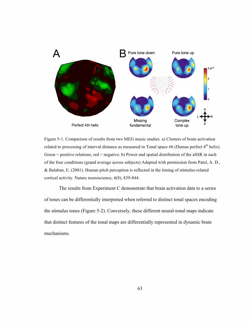
63
Figure 5-1. Comparison of results from two MEG music studies. a) Clusters of brain activation
related to processing of interval distance as measured in Tonal space #6 (Dumas perfect 4th helix).
Green = positive relations, red = negative. b) Power and spatial distribution of the aSSR in each
of the four conditions (grand average across subjects) Adapted with permission from Patel, A. D.,
& Balaban, E. (2001). Human pitch perception is reflected in the timing of stimulus-related
cortical activity. Nature neuroscience, 4(8), 839-844.
The results from Experiment C demonstrate that brain activation data to a series
of tones can be differentially interpreted when referred to distinct tonal spaces encoding
the stimulus tones (Figure 5-2). Conversely, these different neural-tonal maps indicate
that distinct features of the tonal maps are differentially represented in dynamic brain
mechanisms.
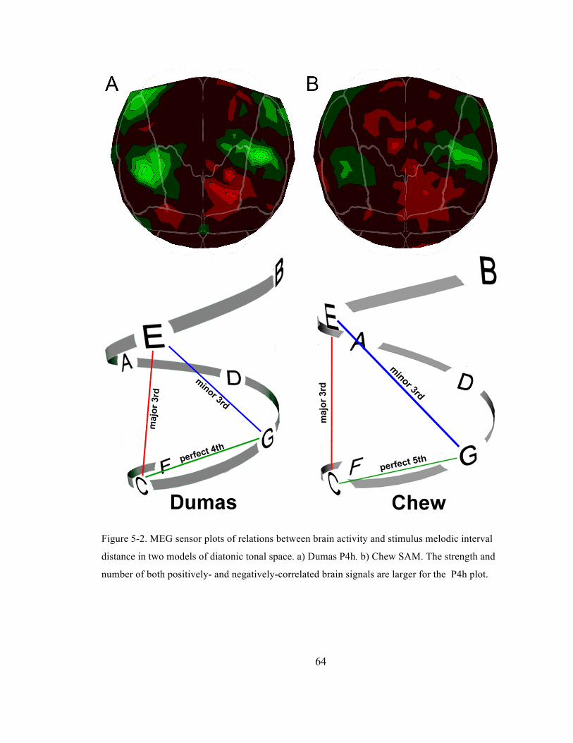
64
Figure 5-2. MEG sensor plots of relations between brain activity and stimulus melodic interval
distance in two models of diatonic tonal space. a) Dumas P4h. b) Chew SAM. The strength and
number of both positively- and negatively-correlated brain signals are larger for the P4h plot.

65
Experiment D produced highly significant, positive relations (p < .0001) between the
neural activity for each melodic interval and the -log of the probability of that interval's
occurrence in the corpus. Signs of melodic perplexity processing appeared in bilateral
prefrontal, midline, superior parietal and occipital cortex, sparing posterior lateral cortical
areas (including primary auditory cortex). Previous studies also implicate prefrontal
cortex in melody discrimination (Brown & Martinez, 2007), pitch identification
(Bermudez & Zatorre, 2005), representations of auditory Gestalten (Koelsch, 2011), and
passive music listening (Ohnishi et al., 2001).
These results suggest that music appreciation involves prediction. When an
unexpected note arrives, the brain taps a “perplexity sub-network” to deal with it.
Different analyses (MIP and SAC) of the same data show strong relations in the bilateral
frontal and prefrontal areas. Although their measures of melodic complexity were
different, namely auto-correlation and melodic interval probability, both analyses
produced similar sub-networks. The absence of anterior temporal activity is most notable,
especially in light of the role played by this region in processing movement through tonal
space.
66
Chapter 6. Concluding remarks and future directions
The ability relate cortical activity to distinct features of a musical stimulus may prove
fruitful in understanding the human brain in health as well as illness. Through extensive
cross-correlation analysis, we have demonstrated that the music listener’s brain responds
to systematic, quantifiable variation in melodic pitch, contour, interval distance and
perplexity. We have also demonstrated that neural sub-networks involved in processing
these features are found in both hemispheres, but primarily in frontal regions for pitch,
contour and perplexity.
Further analysis of the MEG data from the auto-correlation stimulus trials should
provide more information about how the brain responds to different melodic contours. In
addition, data from trials in which composed melodies were played to subjects has yet to
be examined. Our analysis of this data could lead to better understanding of musical
expectation, if not to an innovative new field of music cognition. Melody prediction
research could be the path leading to the development of a real-time, brain-to-music
interface. As well as increasing our knowledge of the human mind, it is my hope that this
methodology will prove useful as both an aid in the diagnosis and treatment of mental
illness, and as a facilitator of non-verbal communication and self-expression.
67
Bibliography
Bach, J. S. (1713). Brandenburg Concerto No. 3 in G.
Barlow, H., & Morgenstern, S. (1948). A Dictionary of Musical Themes. (H. Barlow & S. Morgenstern,
Eds.) (Sixth., p. 642). New York: Crown.
Bermudez, P., & Zatorre, R. J. (2005). Conditional associative memory for musical stimuli in
nonmusicians: implications for absolute pitch. The Journal of neuroscience : the official journal of
the Society for Neuroscience, 25(34), 7718–7723.
Brower, C. (2008). Paradoxes of Pitch Space. Music Analysis, 27(1), 51–106. doi:10.1111/j.1468-
2249.2008.00268.x
Brown, S., & Martinez, M. J. (2007). Activation of premotor vocal areas during musical discrimination.
Brain and cognition, 63(1), 59–69.
Brown, S., Martinez, M. J., & Parsons, L. M. (2006). Music and language side by side in the brain: a PET
study of the generation of melodies and sentences. The European journal of neuroscience, 23(10),
2791–803. doi:10.1111/j.1460-9568.2006.04785.x
Chait, M., Poeppel, D., & Simon, J. Z. (2006). Neural response correlates of detection of monaurally and
binaurally created pitches in humans. Cerebral cortex (New York, N.Y. : 1991), 16(6), 835–848.
doi:10.1093/cercor/bhj027
Changizi, M. (2011). Harnessed: How Language and Music Mimicked Nature and Transformed Ape to
Man (p. 242). BenBella Books, Inc. Retrieved from http://changizi.wordpress.com/book-harnessed/
Chew, E. (2000). Towards a Mathematical Model of Tonality.
Chew, E. (2003). Thinking Out of the Grid and Inside the Spiral – Geometric Interpretations of and
Comparisons with the Spiral Array Model. Network. Retrieved from http://lit.gfax.ch/Interpretations
of and Comparisons with the Spiral Array Model.pdf
Cohn, R. (1998). Neo-Riemannian Tonal Theory: A Survey and a Historical Perspective. Journal of Music
Theory, 42(2), 167–180. Retrieved from http://www.jstor.org/stable/10.2307/843871
68
De Manzano, O., & Ullén, F. (2012). Activation and connectivity patterns of the presupplementary and
dorsal premotor areas during free improvisation of melodies and rhythms. NeuroImage, 63(1), 272–
280. Retrieved from http://www.ncbi.nlm.nih.gov/pubmed/22732560
Debussy, C. (1913). Syrinx.
Deutsch, D. (1987). Illusions For Stereo Headphones. Audio, (March), 36–48.
Ellis, R. J., Norton, A. C., Overy, K., Winner, E., Alsop, D. C., & Schlaug, G. (2012). Differentiating
maturational and training influences on fMRI activation during music processing. NeuroImage, 1–11.
doi:10.1016/j.neuroimage.2012.01.138
Fujioka, T., Trainor, L. J., Ross, B., Kakigi, R., & Pantev, C. (2004). Musical training enhances automatic
encoding of melodic contour and interval structure. Journal of cognitive neuroscience, 16(6), 1010–
1021. doi:10.1162/0898929041502706
Georgopoulos, A. P., Karageorgiou, E., Leuthold, A. C., Lewis, S. M., Lynch, J. K., Alonso, A., Aslam, Z.,
et al. (2007). Synchronous neural interactions assessed by magnetoencephalography: a functional
biomarker for brain disorders. J.Neural Eng., 4(4), 349. doi:doi:10.1088/1741-2560/4/4/001
Gibson, G. N., & Johnston, I. D. (2002). New Themes and Audiences for the Physics of Music. Physics
Today, 55(1), 42. doi:10.1063/1.1457264
Gollin, E. (2011). Three-Dimensional Tonnetze. Journal of Music Theory, 42(2), 195–206. Retrieved from
http://www.jstor.org/stable/10.2307/843873
Granier-Deferre, C., Bassereau, S., Ribeiro, A., Jacquet, A.-Y., & DeCasper, A. J. (2011). A Melodic
Contour Repeatedly Experienced by Human Near-Term Fetuses Elicits a Profound Cardiac Reaction
One Month after Birth. (G. Chapouthier, Ed.)PLoS ONE, 6(2), 10. Retrieved from
http://www.pubmedcentral.nih.gov/articlerender.fcgi?artid=3044162&tool=pmcentrez&rendertype=a
bstract
Hari, R. (1990). The Neuromagnetic method in the study of the human auditory cortex. In F. Grandori, M.
Hoke, & G. L. Romani (Eds.), Auditory evoked magnetic fields and electric potentials (vol 6., pp.
222–282). Basel: Advanced Audiology.
69
Hashimoto, T., Hirata, Y., & Kuriki, S. (2000). Auditory cortex responds in 100 ms to incongruity of
melody. Neuroreport, 11(12), 2799–2801. Retrieved from
http://www.ncbi.nlm.nih.gov/pubmed/10976966
Hauser, M. D. (2000). The sound and the fury: Primate vocalizations as reflections of emotion and thought.
In N. L. Wallin & B. Merker (Eds.), The origins of music (pp. 77–102). MIT Press.
Herholz, S. C., Halpern, A. R., & Zatorre, R. J. (2012). Neuronal correlates of perception, imagery, and
memory for familiar tunes. Journal of cognitive neuroscience, 24(6), 1382–97. Retrieved from
http://www.ncbi.nlm.nih.gov/pubmed/22360595
Hyer, B. (1995). Reimag(in)ing Riemann. Journal of Music Theory, 39(1), pp. 101–138. Retrieved from
http://www.jstor.org/stable/843900
Janata, P., Birk, J. L., Horn, J. D. Van, Léman, M., Tillmann, B., Bharucha, J. J., Van Horn, J. D., et al.
(2002). The Cortical Topography of Tonal structures Underlying Western Music. Science, 298(5601),
2167. doi:10.1126/science.1076262
Jensen, C. R. (1992). A Theoretical Work Of Late Seventeenth-Century Muscovy: Nikolai Diletskii’s
“Grammatika” And The Earliest Circle Of Fifths. Journal of the American Musicological Society,
45(2), 305. Retrieved from http://en.wikipedia.org/wiki/Nikolay_Diletsky
Johnson-Laird, P., Kang, O., & Chang Leong, Y. (2012). On Musical Dissonance. Music Perception, 30(1),
19–35. Retrieved from http://www.jstor.org.ezp1.lib.umn.edu/stable/10.1525/mp.2012.30.1.19
Kanno, A., Nakasato, N., Fujita, S., Seki, K., Kawamura, T., Ohtomo, S., Fujiwara, S., et al. (1996). Right
hemispheric dominance in the auditory evoked magnetic fields for pure-tone stimuli.
Electroencephalography and clinical neurophysiology. Supplement, 47, 129–132.
Kim, S. G., Kim, J. S., & Chung, C. K. (2011). The Effect of Conditional Probability of Chord Progression
on Brain Response: An MEG Study. PloS one, 6(2), e17337.
Kim, S.-G., Kim, J. S., & Chung, C. K. (2011). The effect of conditional probability of chord progression
on brain response: an MEG study. PloS one, 6(2), e17337. Retrieved from
http://www.pubmedcentral.nih.gov/articlerender.fcgi?artid=3045443&tool=pmcentrez&rendertype=a
bstract
70
Koelsch, S. (2011). Toward a neural basis of music perception - a review and updated model. Frontiers in
psychology, 2(June), 110. doi:10.3389/fpsyg.2011.00110
Koelsch, S., Maess, B., Gunter, T. C., & Friederici, A. D. (2001). Neapolitan chords activate the area of
Broca. A magnetoencephalographic study. Annals of the New York Academy of Sciences, 930, 420–
421.
Krumhansl, C. L. (1990). Cognitive Foundations of Musical Pitch (p. 307). New York: Oxford University
Press.
Krumhansl, C. L., & Kessler, E. J. (1982). Tracing the dynamic changes in perceived tonal organization in
a spatial representation of musical keys. Psychological review, 89(4), 334–368.
Kuriki, S., Isahai, N., & Ohtsuka, A. (2005). Spatiotemporal characteristics of the neural activities
processing consonant/dissonant tones in melody. Experimental brain research Experimentelle
Hirnforschung Expérimentation cérébrale, 162(1), 46–55. doi:10.1007/s00221-004-2114-8
Larson, S., & McAdams, S. (2004). Musical Forces and Melodic Expectations: Comparing Computer
Models and Experimental Results. Music Perception: An Interdisciplinary Journal, 21(4), pp. 457–
498. Retrieved from http://www.jstor.org/stable/10.1525/mp.2004.21.4.457
Lee, Y.-S. S., Janata, P., Frost, C., Hanke, M., & Granger, R. (2011). Investigation of melodic contour
processing in the brain using multivariate pattern-based fMRI. NeuroImage, 57(1), 293–300.
doi:10.1016/j.neuroimage.2011.02.006
Lerdahl, F. (1988). Tonal Pitch Space. Music Perception, 5(3), 315–349.
Lerdahl, F. (2001). Tonal pitch space (p. 411). New York: Oxford University Press.
Levitin, D. J., & Tirovolas, A. K. (2011). Twenty-six years of Music Perception: Trends in the field.
Society for Music Perception & Cognition meeting.
Limb, C. J., Kemeny, S., Ortigoza, E. B., Rouhani, S., & Braun, A. R. (2006). Left hemispheric
lateralization of brain activity during passive rhythm perception in musicians. The anatomical
record.Part A, Discoveries in molecular, cellular, and evolutionary biology, 288(4), 382–389.
Longuet-Higgins, H C. (1962). Quantum mechanics and biology. Biophysical journal, 2(2 Pt 2), 207–215.
71
Longuet-Higgins, H. C. (1962). Letter to a musical friend. Music Review, 23, 244–248.
Lounasmaa, O. V, Hamalainen, M., Hari, R., & Salmelin, R. (1996). Information processing in the human
brain: magnetoencephalographic approach. Proceedings of the National Academy of Sciences of the
United States of America, 93(17), 8809–8815.
Lubin, S. (New Y. U. (1974). Techniques for the Analysis of Development in Middle-Period Beethoven.
Retrieved from http://tonnetz.zxq.net/surfaceForm.html
Maess, B., Jacobsen, T., Schroger, E., & Friederici, A. D. (2007). Localizing pre-attentive auditory
memory-based comparison: magnetic mismatch negativity to pitch change. NeuroImage, 37(2), 561–
571.
Maess, B., Koelsch, S., Gunter, T. C., & Friederici, A. D. (2001). Musical syntax is processed in Broca’s
area: an MEG study. Nature neuroscience, 4(5), 540–545.
Matsui, T., Tanaka, S., Kazai, K., Tsuzaki, M., & Katayose, H. (2013). Activation of the left superior
temporal gyrus of musicians by music-derived sounds. Neuroreport, 24(1), 41–5.
doi:10.1097/WNR.0b013e32835c1e02
Meyer, L. (1956). Emotion and meaning in music. Chicago: University of Chicago Press.
Minor, N. (1978). Harmony , Structure & Expectancy : Music Theory pitch ( space ) — > time — >. Music
Perception, 1–5.
Narmour, E. (1990). The analysis and cognition of basic melodic structures : the implication-realization
model (p. 485). Chicago: University of Chicago Press.
Nemoto, I. (2012). Evoked magnetoencephalographic responses to omission of a tone in a musical scale.
The Journal of the Acoustical Society of America, 131(6), 4770–84. Retrieved from
http://www.ncbi.nlm.nih.gov/pubmed/22712949
Normal equal-loudness-level contours - ISO 226 : 2003 Acoustics International Organization for
Standardization ( ISO ) 2nd edition. (2005).International Organization, 2005–2005.
Ohnishi, T., Matsuda, H., Asada, T., Aruga, M., Hirakata, M., Nishikawa, M., Katoh, A., et al. (2001).
Functional anatomy of musical perception in musicians. Cerebral cortex (New York, N.Y. : 1991),
11(8), 754–60. Retrieved from http://www.ncbi.nlm.nih.gov/pubmed/11459765
72
Ono, K., Nakamura, A., Yoshiyama, K., Kinkori, T., Bundo, M., Kato, T., & Ito, K. (2011). The effect of
musical experience on hemispheric lateralization in musical feature processing. Neuroscience letters,
496(2), 141–5. Retrieved from http://www.ncbi.nlm.nih.gov/pubmed/21513771
Parncutt, R. (2009). Prenatal and infant conditioning, the mother schema, and the origins of music and
religion. Musicae Scientiae, 13(2 Suppl), 119–150. doi:10.1177/1029864909013002071
Parncutt, R. (2011). The Tonic as Triad: Key Profiles as Pitch Salience Profiles of Tonic Triads. Music
Perception: An Interdisciplinary Journal, 28(4), pp. 333–366. doi:10.1525/mp.2011.28.4.333
Patel, A. D., & Balaban, E. (2001). Human pitch perception is reflected in the timing of stimulus-related
cortical activity. Nature neuroscience, 4(8), 839–844. doi:10.1038/90557
Patterson, R. D., Uppenkamp, S., Johnsrude, I. S., & Griffiths, T. D. (2002). The processing of temporal
pitch and melody information in auditory cortex. Neuron, 36(4), 767–776. Retrieved from
http://www.ncbi.nlm.nih.gov/pubmed/12441063
Pearce, M. T., & Wiggins, G. A. (2006). Expectation in Melody: The Influence of Context and Learning.
Music Perception, 23(5), 377–405. Retrieved from http://www.jstor.org/stable/40285982
Purwins, H., & Hardoon, D. R. (2009). Trends and perspectives in music cognition research and
technology. Connection Science, 21(2-3), 85–88. doi:10.1080/09540090902734549
Rushton, J. (2004). Perfect Consonance. Retrieved April 30, 2004, from <http://www.grovemusic.com>
Schneider, P., Sluming, V., Roberts, N., Scherg, M., Goebel, R., Specht, H. J., Dosch, H. G., et al. (2005).
Structural and functional asymmetry of lateral Heschl’s gyrus reflects pitch perception preference.
Nature neuroscience, 8(9), 1241–1247. doi:10.1038/nn1530
Shepard, R. N. (1982). Geometrical approximations to the structure of musical pitch. (D. Deutsch,
Ed.)Psychological Review, 89(4), 335–353. Retrieved from
http://psycnet.apa.orgjournals/rev/89/4/305
Steinbeis, N., Koelsch, S., & Sloboda, J. A. (2006). The role of harmonic expectancy violations in musical
emotions: evidence from subjective, physiological, and neural responses. Journal of cognitive
neuroscience, 18(8), 1380–1393.
Stryer, L. (1995). Biochemistry (4th ed., pp. 27–30). New York: W. H. Freeman & Company.
73
Teki, S., Kumar, S., Kriegstein, K. Von, Stewart, L., Lyness, C. R., Moore, B. C. J., Capleton, B., et al.
(2012). Navigating the Auditory Scene : An Expert Role for the Hippocampus, 32(35), 12251–12257.
doi:10.1523/JNEUROSCI.0082
Toiviainen, P., & Krumhansl, C. L. (2003). Measuring and modeling real-time responses to music: the
dynamics of tonality induction. Perception, 32(6), 741–766. doi:10.1068/p3312
Yasui, T., Kaga, K., & Sakai, K. L. (2009). Language and music: differential hemispheric dominance in
detecting unexpected errors in the lyrics and melody of memorized songs. Human Brain Mapping,
30(2), 588–601. doi:10.1002/hbm.20529
Zatorre, R. J., Halpern, A. R., & Bouffard, M. (2009). Mental Reversal of Imagined Melodies: A Role for
the Posterior Parietal Cortex. Journal of cognitive neuroscience, 22(4), 775–89.
doi:10.1162/jocn.2009.21239
Zatorre, R. J., & Krumhansl, C. L. (2002). Mental Models and Musical Minds. Science, 298(5601), 2138.
Retrieved from http://search.epnet.com/login.aspx?direct=true&db=aph&an=8908926
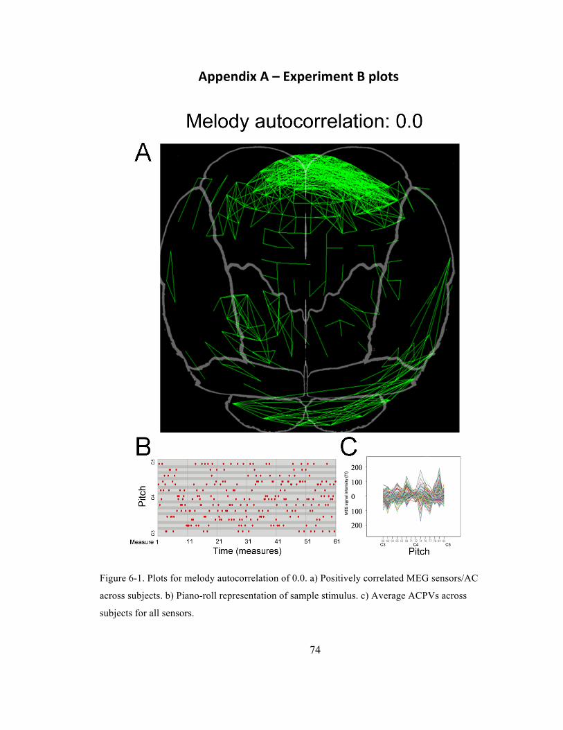
74
Appendix A – Experiment B plots
Figure 6-1. Plots for melody autocorrelation of 0.0. a) Positively correlated MEG sensors/AC
across subjects. b) Piano-roll representation of sample stimulus. c) Average ACPVs across
subjects for all sensors.
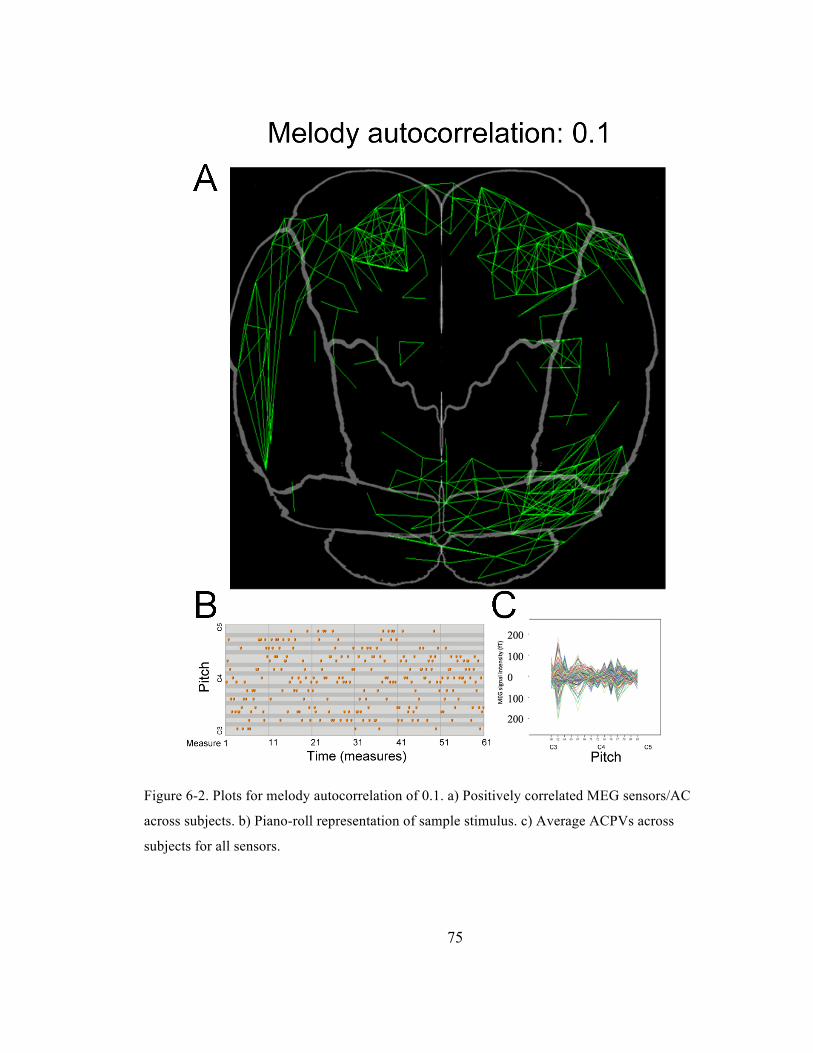
75
Figure 6-2. Plots for melody autocorrelation of 0.1. a) Positively correlated MEG sensors/AC
across subjects. b) Piano-roll representation of sample stimulus. c) Average ACPVs across
subjects for all sensors.
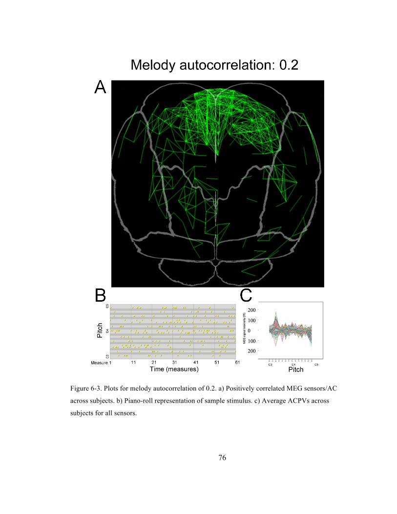
76
Figure 6-3. Plots for melody autocorrelation of 0.2. a) Positively correlated MEG sensors/AC
across subjects. b) Piano-roll representation of sample stimulus. c) Average ACPVs across
subjects for all sensors.
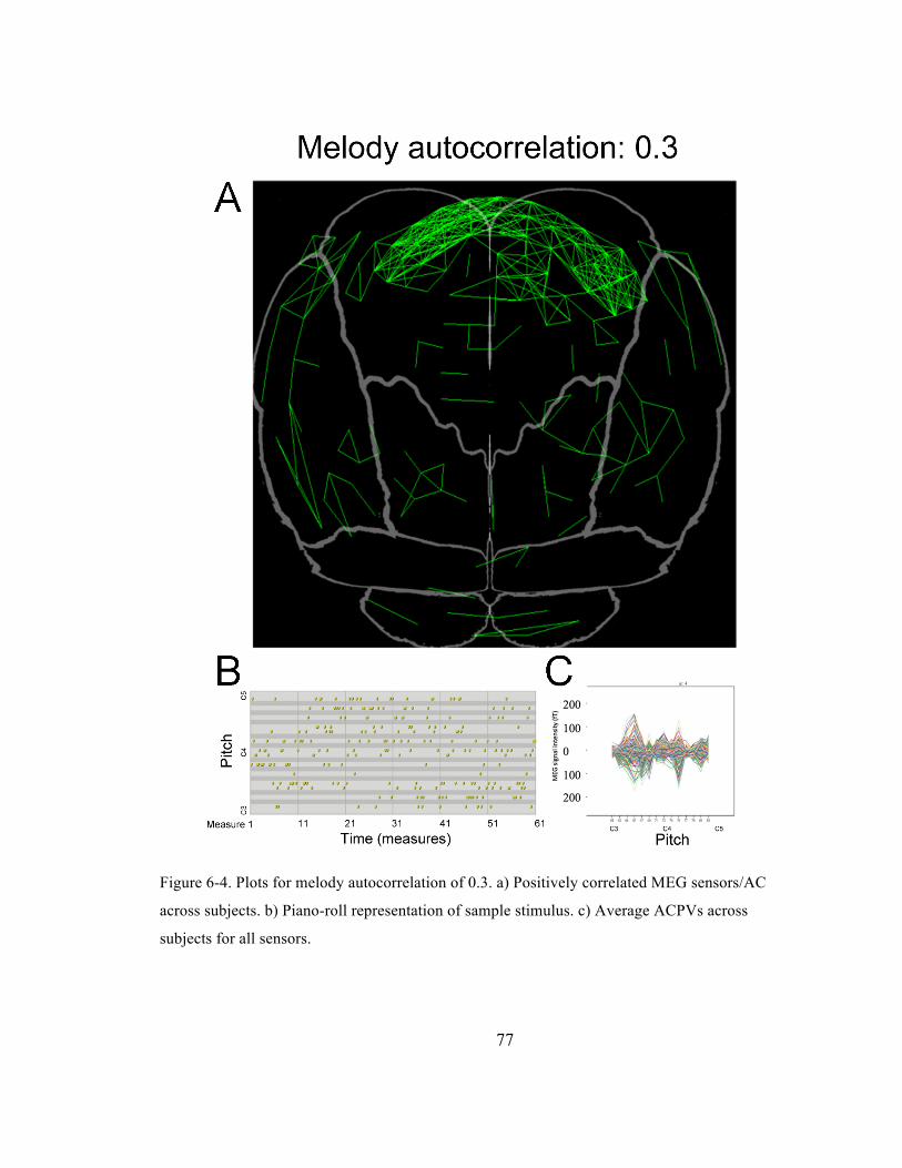
77
Figure 6-4. Plots for melody autocorrelation of 0.3. a) Positively correlated MEG sensors/AC
across subjects. b) Piano-roll representation of sample stimulus. c) Average ACPVs across
subjects for all sensors.
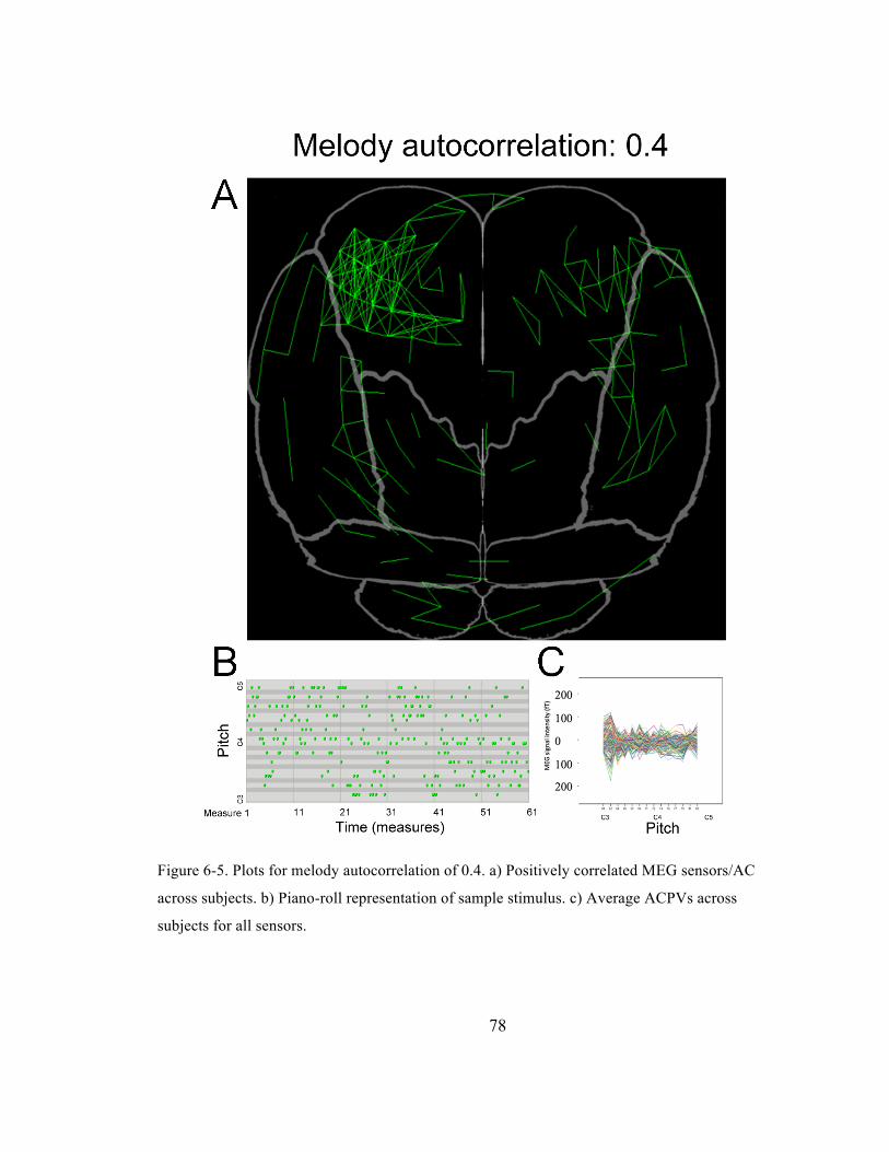
78
Figure 6-5. Plots for melody autocorrelation of 0.4. a) Positively correlated MEG sensors/AC
across subjects. b) Piano-roll representation of sample stimulus. c) Average ACPVs across
subjects for all sensors.
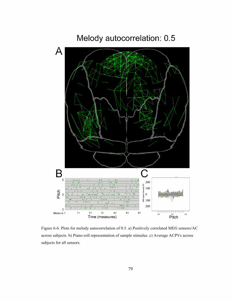
79
Figure 6-6. Plots for melody autocorrelation of 0.5. a) Positively correlated MEG sensors/AC
across subjects. b) Piano-roll representation of sample stimulus. c) Average ACPVs across
subjects for all sensors.
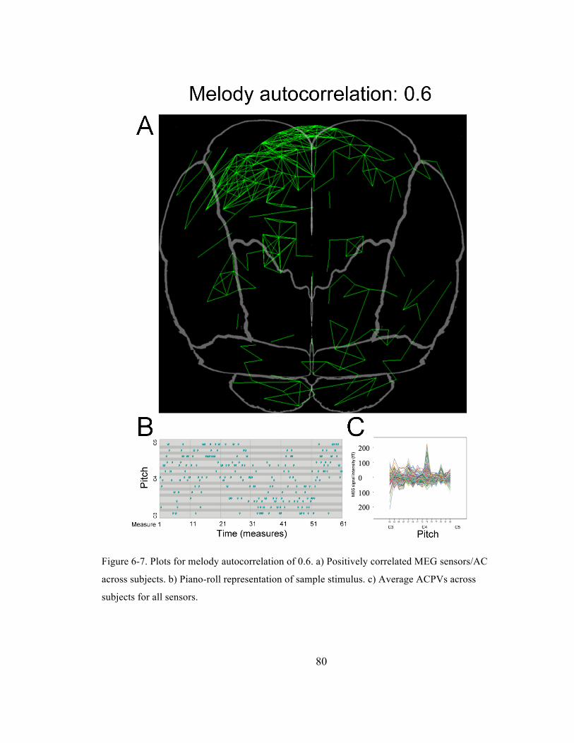
80
Figure 6-7. Plots for melody autocorrelation of 0.6. a) Positively correlated MEG sensors/AC
across subjects. b) Piano-roll representation of sample stimulus. c) Average ACPVs across
subjects for all sensors.
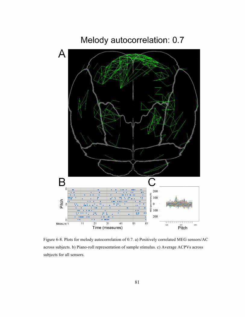
81
Figure 6-8. Plots for melody autocorrelation of 0.7. a) Positively correlated MEG sensors/AC
across subjects. b) Piano-roll representation of sample stimulus. c) Average ACPVs across
subjects for all sensors.
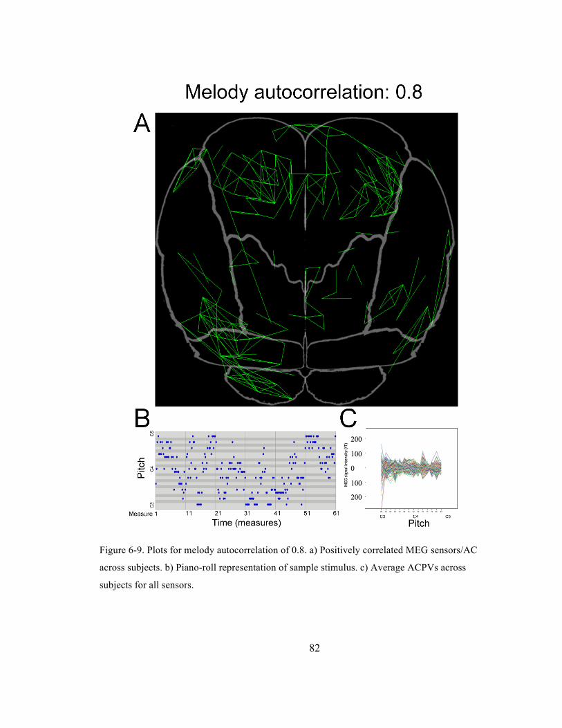
82
Figure 6-9. Plots for melody autocorrelation of 0.8. a) Positively correlated MEG sensors/AC
across subjects. b) Piano-roll representation of sample stimulus. c) Average ACPVs across
subjects for all sensors.
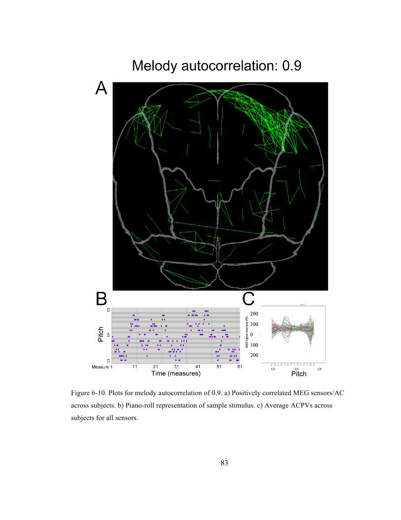
83
Figure 6-10. Plots for melody autocorrelation of 0.9. a) Positively correlated MEG sensors/AC
across subjects. b) Piano-roll representation of sample stimulus. c) Average ACPVs across
subjects for all sensors.
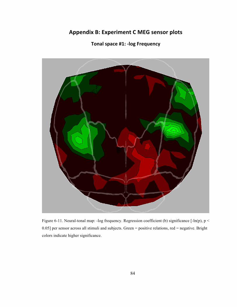
84
Appendix B: Experiment C MEG sensor plots
Tonal space #1: -‐log Frequency
Figure 6-11. Neural-tonal map: -log frequency. Regression coefficient (b) significance [-ln(p), p <
0.05] per sensor across all stimuli and subjects. Green = positive relations, red = negative. Bright
colors indicate higher significance.
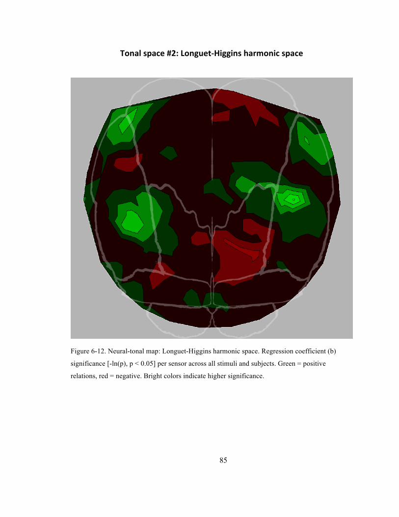
85
Tonal space #2: Longuet-‐Higgins harmonic space
Figure 6-12. Neural-tonal map: Longuet-Higgins harmonic space. Regression coefficient (b)
significance [-ln(p), p < 0.05] per sensor across all stimuli and subjects. Green = positive
relations, red = negative. Bright colors indicate higher significance.
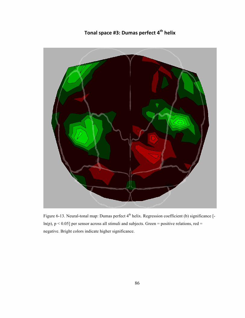
86
Tonal space #3: Dumas perfect 4th helix
Figure 6-13. Neural-tonal map: Dumas perfect 4th helix. Regression coefficient (b) significance [-
ln(p), p < 0.05] per sensor across all stimuli and subjects. Green = positive relations, red =
negative. Bright colors indicate higher significance.
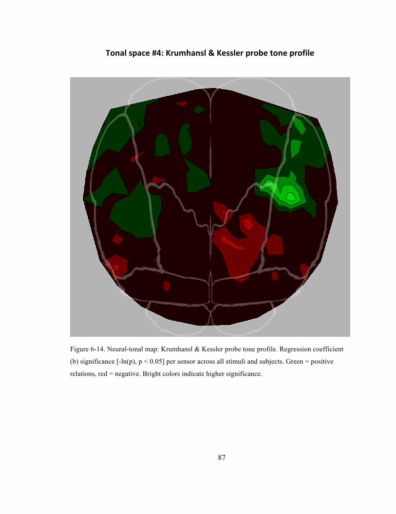
87
Tonal space #4: Krumhansl & Kessler probe tone profile
Figure 6-14. Neural-tonal map: Krumhansl & Kessler probe tone profile. Regression coefficient
(b) significance [-ln(p), p < 0.05] per sensor across all stimuli and subjects. Green = positive
relations, red = negative. Bright colors indicate higher significance.
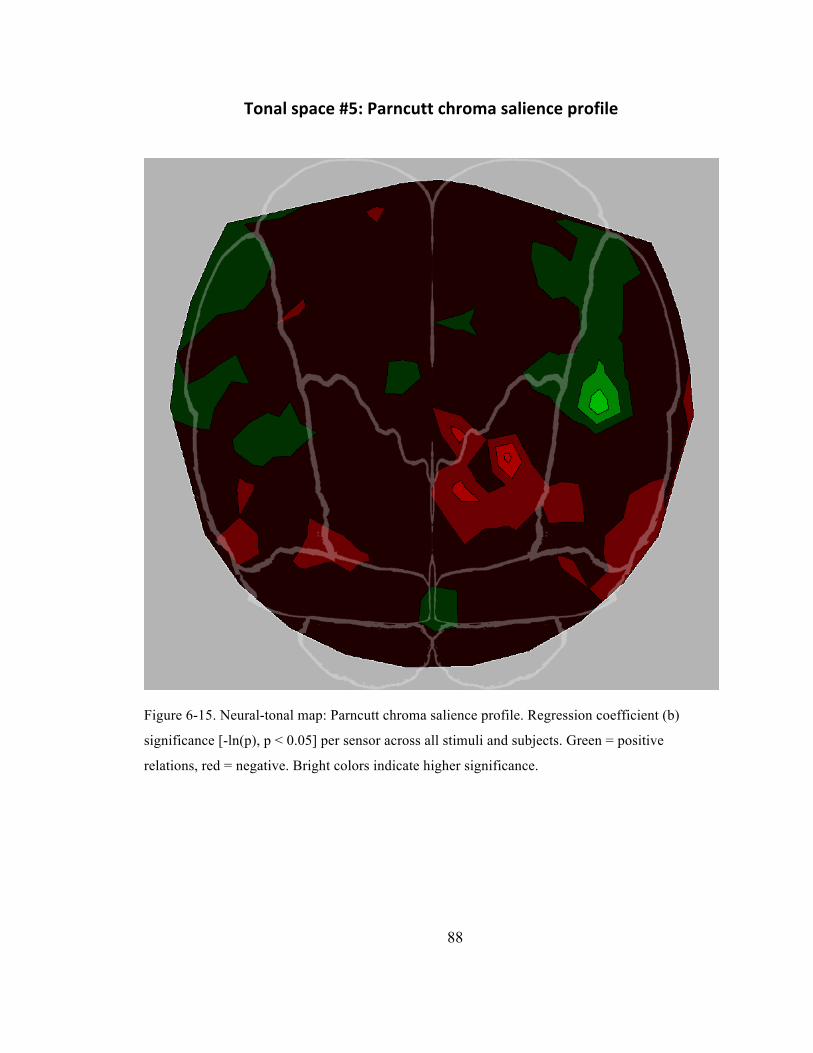
88
Tonal space #5: Parncutt chroma salience profile
Figure 6-15. Neural-tonal map: Parncutt chroma salience profile. Regression coefficient (b)
significance [-ln(p), p < 0.05] per sensor across all stimuli and subjects. Green = positive
relations, red = negative. Bright colors indicate higher significance.

89
Tonal space #6: Chew spiral array model
Figure 6-16. Neural-tonal map: Chew spiral array model. Regression coefficient (b) significance
[-ln(p), p < 0.05] per sensor across all stimuli and subjects. Green = positive relations, red =
negative. Bright colors indicate higher significance.