Measurements of landscape-scale fluxes of carbon dioxide in the Peruvian Amazon by vertical...

JOURNAL OF GEOPHYSICAL RESEARCH, VOL. 105, NO. D17, PAGES 22,137-22,146, SEPTEMBER 16, 2000

Measurements of landscape-scale fluxes of carbon dioxide in the Peruvian Amazon by vertical profiling through the atmospheric boundary layer

Laura R. Kuck, • Tyrell Smith Jr., • Ben B. Balsley, • Detlev Helmig, • Thomas J. Conway, 2 Pieter P. Tans, 2 Kenneth Davis, 3 Michael L. Jensen, • John A. Bognar, • Rosaura Vazquez Arrieta, 4 Rodolfo Rodriquez, 4 and John W. Birks •

Abstract. Vertical profiles of carbon dioxide were measured within and above the atmospheric boundary layer at a tropical forest site in the Peruvian Amazon during July 1996 using a tethered balloon sampling platform. Flask samples were collected within and above the mixed layer and analyzed off-site for carbon dioxide by nondispersive infrared spectrophotometry. Ozone and temperature vertical profiles were used to determine the boundary layer heights and growth rates. The mean values for methane, carbon monoxide, hydrogen, carbon-13, and oxygen-18 ratios were determined within and above the mixed layer. Daytime carbon dioxide flux values were calculated using the budget method. Nocturnal fluxes were estimated by integrating the carbon dioxide mixing ratios as a function of height from the ground to the inversion layer and dividing the total accumulated carbon dioxide by the time since sunset. The daytime carbon dioxide flux of-13 + 2 •tmol C m '2 s '• and the nocturnal flux of +5.0 + 1.0 •tmol C m '2 s '• are in good agreement with previous studies in the Brazilian Amazon.

1. Introduction

The Amazon rain forest occupies a surface area of approximately 5 x 1012 m 2, making up about 40% of the terrestrial phy- tomass [Food and Agriculture Organization (FAO), 1993]. The influx or effiux of carbon to or from mature forests was often ig- nored in carbon cycling models based on the assumption that these fbrests had reached a steady state with the atmosphere; that is, photosynthetic carbon intake was balanced by respiratory emissions. However, forests may be undergoing fertilization due to the increasing concentration of carbon dioxide in the atmosphere and the higher deposition rate of nitrogen and other miner- als [Gifford, 1994; Eamus and Jarvis, 1989; McMurtrie et al., 1992; McGuire et al., 1995]. On the other hand, their continued destruction through deforestation and biomass burning is a significant short-term carbon dioxide source that ultimately de- creases the forest's potential as a carbon sink [Auclair and Bed- ford, 1993; Vloedbeld and Leeroans, 1993; Brown et al., 1993].

Work by Tans et al. [1990] questioned previous estimates of ecosystem sinks and their associated fluxes. They used a general circulation model and the north-south atmospheric carbon dioxide concentration gradient to determine that "the total carbon dioxide uptake by oceans is considerably less than the uptake by terrestrial systems" and that "there must be a terrestrial sink at temperate latitudes to balance the carbon budget and to match the

•Cooperative Institute for Research in Environmental Sciences (CIRES), University of Colorado, Boulder.

2Climate Monitoring and Diagnostics Laboratory, NOAA, Boulder, Colorado.

3Department of Soil, Water, and Climate, University of Minnesota, St. Paul.

4Facultad de Ingenieria, Universidad de Piura, Piura, Peru.

Copyright 2000 by the American Geophysical Union.

Paper number 2000JD900105. 0148-0227/00/2000JD900105 $09.00

north-south gradient of atmospheric carbon dioxide." Taylor and Lloyd [ 1992] also suggested that the missing sink is concentrated in forests by calculating probable rates of carbon sequestration for major ecosystems and using a global three-dimensional (3-D) tracer transport model. It is clear that improved measurements of carbon dioxide fluxes in the tropical and temperate forests are necessary in order to obtain a better understanding of the global carbon budget.

Four major field measurement campaigns in which CO2 fluxes were measured have taken place in the Amazon rain forest [ Wo•y et al., 1988; Fan et al., 1990; Grace et al., 1995; Malhi et al., 1998]. WoJby et al. conducted CO2 flux measurements near Manaus as part of the Amazon Boundary Layer Experiment (ABLE 2A) during the 1985 dry season and the 1986 wet season. The focus of the ABLE 2A field experiment was to determine the sources/sinks, distributions, and fates of trace gases in the troposphere over the Amazon basin. Wotgy et al. measured carbon dioxide fluxes from three different platforms using three methods of gas collection and analysis. Soil fluxes were evaluated by the chamber method. Samples were withdrawn from the enclosure with a syringe and analyzed in the field by gas chromatography (GC). Discrete flask samples were collected within the forest canopy from a tower platform and evaluated off-site by GC. Continuous sampling within the boundary layer was accom- plished with the use of a nondispersive infrared (NDIR) analyzer located onboard a NASA Electra aircraft. This aircraft was used

to make measurements along the entire length of the Brazilian Amazon.

The aircraft sampled the mixed layer as it developed during the day. Flights lasted approximately 6 hours, starting at sunrise as solar heating began to affect the buoyancy and depth of the boundary layer. Nocturnal respiration generated a morning surface layer that contained high concentrations of carbon dioxide and could be used to delineate the growing mixed layer. The convective boundary layer (CBL) increased at a rate of about 5- 10 cm/s, eroding the low concentration relic layer from the previ-

22,137

22,138 KUCK ET AL.: MEASUREMENTS OF LANDSCAPE-SCALE FLUXES OF CARBON DIOXIDE

ous day. By midday, photosynthetic uptake in the forest resulted in an inverted CO2 profile with the lowest concentrations at the lowest flight level. Sampling within the canopy demonstrated nearly uniform CO2 concentrations, which is consistent with significant turbulent mixing [WoJby et al., 1988].

The daytime rate of carbon dioxide flux into the forest was estimated by monitoring the decline in the carbon dioxide column content. This method assumes that the CBL is well mixed and

that the carbon dioxide concentration is constant from t.he ground to the lowest flight altitude. The nocturnal and early morning boundary layer profiles had to be excluded due to this assumption. The CBL height was established based on carbon dioxide and ozone data. WoJby et al. [ 1988] estimated a maximum midday uptake of carbon by forest vegetation at -21 _+ 9 gmol C m '2 s 'l. This value is comparable to the carbon dioxide flux determined by Desjardins et al. [1985] (-16 __ 7 gmol C m '2 s 'l) over a Canadian forest at similar solar irradiance (-600 W/m2). This midday uptake rate also is reasonable when compared to the average daily uptake rate during sunlit hours of-6.5 + 2.8 gmol C m '2 s 4, which is derived from the 12-hour mean solar irradiance at the top of the canopy (-190 W/m2). This model is based on the assumption that the solar flux is linear with photosynthetic rates [Desjardins et al., 1985]. The mean net emission rate from forest soils was determined to be 4.2 __ 0.5 gmol C m '2 s 4.

Flux measurements at this site were continued by Fan et al. [ 1990] during the 1987 wet season as part of the ABLE 2B cam- paign. Eddy correlation data were acquired using a sonic anemometer and a nondispersive infrared analyzer at an altitude of 39 m, about 9 m above the canopy top. Carbon dioxide storage was evaluated through vertical profiles obtained by sequentially collecting samples at eight altitudes ranging from 39 m to the soil surface. Soil emissions of carbon dioxide were measured using the chamber method. The rates of carbon dioxide increase within

the aluminum chambers were measured using a NDIR analyzer. Data were collected for a total of 12 days.

Fan et al. [ 1990] found the daytime mean carbon dioxide concentration above the canopy ranged from a minimum of 340 ppmv (midday) to a maximum of more than 370 ppmv (accumulated before sunrise). Storage concentrations were a significant pan of their flux calculations since the CO2 respired at night can be used for photosynthetic uptake as well as emitted to the developing morning mixed layer. Daytime carbon dioxide uptake averaged -10 gmol C m '2 s 'l, with a maximum uptake of-21 I. tmol C m '2 s '• occurring at noon. The mean nocturnal respiration rate was 5.9 gmol C m '2 s 'l, exhibiting little variation with the time of night. The net daily uptake of carbon dioxide corresponds to a flux of-l.1 Gt C yr -1 when integrated over 5 x 1012 m 2, the estimated area of the Amazon basin [FAO, 1993].

The field experiment by Grace et al. [ 1995] was performed at Reserva Jaru in Rondonia, Brazil, during the 1992 dry season and 1993 wet season. The research team measured CO2 flux using an eddy correlation system with a fast closed-path infrared analyzer and a sonic anemometer. The platform consisted of a 45-m tower that extended 15 m above the forest canopy. The longest continuous data collection sequence lasted 44 days with occasional short calibration and maintenance periods. Carbon dioxide flux into the forest was at a maximum during the morning hours of "normal" weather days, followed by an afternoon decline and a very low nocturnal efflux. Days that were characterized by low solar radiation and high wind speeds exhibited more symmetry between daytime influx and nocturnal effiux. Overall, 33 days out

of the 44 showed a downward net (24-hour) CO2 flux from the atmosphere into the forest [Grace et al., 1995]. There was a net uptake during daylight hours ranging from -5 to -20 gmol C m '2 s 'l and a mean noctumal effiux of 6.5 p, mol C m '2 s 'l. An analysis of both the wet and dry seasons showed that in general, carbon dioxide influx from photosynthetic gains exceeded carbon dioxide effiux from respiratory and decay losses. These losses could not be attributed to measurement error or to the loss of carbon

dioxide by drainage of cold air at night [Grace et al., 1996]. Grace et al. 11995] developed an annual model using clima-

tological data collected from the top of their platform. The model estimated a 24-hour-based net carbon accumulation of-8.5 + 2

mol C m -2 yr 'l for this particular region of the rain forest. As with the Fan et al. [1990] study, this flux can be extrapolated to the entire rain forest of the Amazon basin if it is assumed that the ba-

sin behaves in the same way as the experimental site, yielding an estimated Amazon carbon accumulation of-0.51 + 0.12 Gt C yr '• [Grace et al., 1995].

Malhi et al. [1998] conducted a year-long eddy correlation study at the same site as the Grace et al. [ 1995] field experiment, with the goal of addressing the possible seasonal and interannual variations in the ecosystem carbon balance. A sonic anemometer and a fast response infrared gas analyzer were used to make eddy correlation measurements from a 41.5-m tower. Micrometeoro-

logical data were collected continuously for a year, and carbon flux data were collected for 54% of the year.

The experiment revealed that the net daytime carbon uptake showed significant seasonal variation, peaking at -21 gmol C m '2 s 'l in the wet season and decreasing to -17 gmol C m '2 s 'l in the dry season. There was very little seasonal variation in the average nocturnal flux of 6.5 + 0.5 gmol C m '2 s -l, for which Mahli et al. [1998] attribute little dependence on soil temperature or soil moisture.

Over the year, the Mahli et al. [1998] flux estimates corre- spond to a total Amazon net sink of-2.9 Gt C yr 'l, a value considerably larger than the Fan et al. [ 1990] estimate (- 1.1 Gt C yr' •) and the Grace et al. [1995] estimate (-0.51 Gt C yr4). Mahli et al. [1998, p. 31,604] state that "although the basic diumal cycle of CO2 fluxes is very similar for all three sites, only a small difference in bulk photosynthetic and respiratory fluxes can lead to large differences in net carbon balance."

These field experiments can be compared to a flask experiment led by the Commonwealth Scientific and Industrial Re- search Organization (CSIRO) of Australia. This experiment found that in 1986 and 1987 South America may have accumulated as much as 2 Gt C yr 'l [Enting et al., 1995]. Theoretical models predict enhanced carbon storage as a response to increasing atmospheric concentrations of carbon dioxide with a net influx of about I Gt C/yr for all of the tropics [Houghton, 1991 ].

These experimental and theoretical accumulation rates demon- strate the strong possibility that the Amazon basin is not in a steady state with the atmosphere but instead is acting as a net carbon sink. The flux measurements are hindered, however, by the limited area of coverage of the direct flux measurements. In this experiment, fluxes averaged over large footprint areas are inferred from vertical profiles obtained via flask measurements. This is, however, an indirect method for inferring fluxes and re- quires that atmospheric transport be simulated accurately. The CO2 profiles extending above the boundary layer are valuable in- dependent of the flux calculations in that they are direct observations of free-tropospheric CO2 mixing ratios.

KUCK ET AL.: MEASUREMENTS OF LANDSCAPE-SCALE FLUXES OF CARBON DIOXIDE 22,139

2. Experiment

2.1. Site Description and Balloon Platform This field experiment was carried out in July of 1996 as a joint

effort between our research group at the University of Colorado at Boulder and the University of Piura in Peru. One goal of the experiment was to measure the flux of CO2 between the atmosphere and a remote area of the Amazon rain forest. Vertical profiling through the CBL by means of a balloon platform provides a means of obtaining CO2 fluxes in this region that can be compared to other experimental results. The site description and balloon platform have been described previously [Helmig et al., 1998]. Briefly, this experiment was performed in the Peruvian Amazon approximately 500 km west of Iquitos and approximately 50-200 km from the eastern Andes mountain ranges (4 o

o

35'15" S, 77 28'00" W). This site is close to Saramiriza, a small village on the Marafion River. Access to this region is restricted to boats and helicopters. The canopy height of this mainly primary tropical forest is 20-30 m. The anthropogenic disturbance to this site is less than an estimated 5% of the total land cover, mainly due to small clearings within a 10 km radius of the site. The area used for the balloon launch site was a clearing of approximately 100 x 300 m which had been clear cut an estimated 1-2 years prior to the experiment. Biomass burning was not observed during the experimental period of July 10-15, 1996.

Vertical profiling through the CBL was achieved by attaching evacuated flasks and temperature, pressure, and ozone instru- mentation to the tether of a 43-m 3 helium balloon (The Blimp Works, Statesville, North Carolina). For a winch we applied the same technique that our group developed for flying kites [Balsley et al., 1994a, b]. The main winch was a modified capstan attached to the rear axle of a truck which was supported by jack stands. A small 12-V electric takeup reel was used for spooling the tether. This technique has the advantage of allowing deploy- ment of tethered balloons with a high lift capacity without having to provide a high-powered electrical winch.

2.2. Flask Sampling and Analysis

Glass 2.5-L flasks were used to collect the air samples for off- site analysis. The flasks were evacuated in the field to <0.5 torr using an Edwards E2-M2 vacuum pump. The basic payload consisted of a styrofoam container capable of holding five of these flasks (7.5 kg). Each flask was fitted with a battery-operated, remote-controlled solenoid valve and an 8 inch length of PTFE tubing which protruded from the styrofoam package.

An additional package attached to the tether contained a radio- sonde (Vaisala Model RS-80), an En-Sci electrochemical ozonesonde, and a UV ozonesonde developed by our research group [Bognar and Birks, 1996]. This package (3.5 kg) was used to measure the temperature, pressure, wind speed, wind direction, solar intensity, relative humidity, and ozone mixing ratio of the atmosphere during the balloon's ascent and descent. The ozone and temperature profiles were evaluated in real time in order to determine the CBL height and its rate of change. The flasks were opened sequentially during the balloon's descent at approximately 1.2, 0.8, 0.4, 0.2, and 0.1 times the CBL height. Multiple samples improve our spatial and temporal sampling of altitude- averaged mixed layer mean mixing ratios.

The flasks were shipped back to Boulder, Colorado, for analysis by The National Oceanic and Atmospheric Administration Climate Monitoring and Diagnostics Laboratory (NOAA/CMDL). These samples were quantitatively transferred

from the 2.5-L collection flasks to 0.5-L analysis flasks. The transfer was performed using a noncontaminating diaphragm pump system that is part of the NOAA/CMDL flask program [Thoning et al., 1995]. Carbon dioxide was analyzed using a Siemens Ultramat III NDIR instrument using standards traceable to primary standards. The precision of the flask transfer and analysis system was determined to be +0.2 ppmv. All samples were dried before analysis, yielding mol fractions based on dry air. In addition, the flasks were analyzed for methane, carbon monoxide, and hydrogen, as well as carbon and oxygen isotope ratios.

2.3. Flux Calculations

This experiment focused on obtaining profiles of CO2 within and above the tropical boundary layer. The profiles alone provide an interesting point observation of the vertical distribution of CO2 in a region that is critically important to the atmospheric CO2 budget. Vertical profiles of CO2 within and above the CBL can also be used to derive surface fluxes of CO2 using a boundary layer budget method. These flux estimates are representative of a large area of forest (order 100 km2). The upwind extent of the flux footprint (20-40 km) is approximately the product of the time between profiles (typically 1-2 hours) and the mean wind speed in the boundary layer (order 5 m s-l). Note that the 300 m x 100 m clearing at the tether site can be safely neglected, espe- cially in daytime, given the size of the flux footprint. While these budget-based flux estimates are not as direct as eddy covariance measurements and only a limited number of days can be sampled in this way, the flux footprint is at least 100 times greater than that of a typical tower-based eddy covariance measurement. Flux footprints from surface-layer towers are typically less than I km 2 during convective conditions [e.g., Horst and Well, 1992]. Given the sparsity of CO2 flux data in the Amazon region, these measurements add significantly to the flux database in this vast area of intense biological activity.

The mixed-layer budget method, as discussed by Raupach et al. [1992] and Denmead et al. [ 1996], can be used to determine a flux from scalar concentrations obtained through flask sampling within a vertical profile in the CBL. The flux is determined by monitoring the changing concentration in the mixed layer, the changing inversion height, and the carbon dioxide concentration that is being entrained. Two conditions must be satisfied to derive accurate surface fluxes using this method. First, the CBL must be well mixed so that the carbon dioxide mixing ratio Cavg is uniform. This means that C is a function of time but not a

function of measurement height z. The flux profile varies linearly with height for a well-mixed layer. Second, there must be negligible horizontal advection. Horizontal advection, if it occurs, cannot be distinguished from a surface flux via the mixed-layer budget method. If these assumptions are valid, the scalar conser- vation equation, averaged over the depth of the mixed layer, be- comes

--- + -w h h J/t

where

h

rc Ce

air); W

depth of the mixed layer, the CBL height; flux density at the surface; free atmosphere concentration just above h (entrained

mean vertical velocity at the top of the CBL.

22,140 1.8 - -

1.6

1.4

1.2

0.6

0.4

0.2

0

10

2OOO

1031 LT

** ß ß ß ,$ •11• 1346 LT

...

, , ,

15 20 25 30

Ozone mixing ratio, ppbv

Figure 1. Ozone vertical profiles for July 13, 1996.

35

1800

(.• 1600

E 14oo

(D 1200

•', 1000

03 800

0 600

400

200 10

ß 12 July 1996

0 13July1996 ß 14 July 1996 -- Linear Regression Lines

12 14 16 18

Time of day, LST, hours Figure 2. Boundary layer height versus. time for July 12, 13, and 14, 1996.


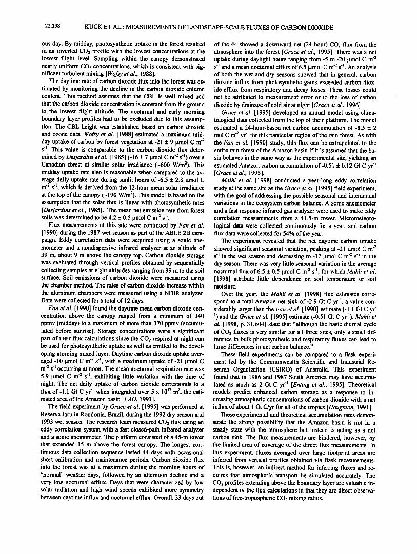
Table 1. Carbon Dioxide Mixing Ratios Table 1. (continued)

July 10, 1996 1123 750 4 365.29 July 13, 1996 1045 1230 14 360.48

July I0, 1996 1134 390 4 366.97 July 13, 1996 1102 515 14 365.00

July 10, 1996 1139 180 4 366.59 July 13, 1996 1108 220 14 365.90

July 10, 1996 1142 81 4 365.66 July 13, 1996 1115 30 14 364.39

July 10, 1996 1244 2 4 365.60 July 13, 1996 1243 1540 17 360.76

July 10, 1996 1235 1470 5 367.71 July 13, 1996 1303 800 17 360.45

July 10, 1996 1244 750 5 366.76 July 13, 1996 1312 400 17 360.29

July 10, 1996 1251 370 5 366.59 July 13, 1996 1318 210 17 359.98

July 10, 1996 1256 108 5 368.82 July 13, 1996 1322 108 17 359.64

July 10, 1996 1300 87 5 366.53 July 13, 1996 1436 1610 19 360.06

July 10, 1996 1357 1470 6 367.07 July 13, 1996 1456 848 19 358.71

July 10, 1996 1406 730 6 369.61 July 13, 1996 1503 400 19 358.34

July 10, 1996 1412 380 6 356.62 July 13, 1996 1508 200 19 357.55

July 10, 1996 1416 210 6 369.25 July 13, 1996 1511 108 19 358.24

July 10, 1996 1420 93 6 369.52 July 13, 1996 1625 1600 20 359.75

July 10, 1996 1500 1530 7 365.38 July 13, 1996 1641 840 20 359.14

July 10, 1996 1508 760 7 368.71 July 13, 1996 1649 406 20 358.28

July 10, 1996 1514 380 7 367.85 July 13, 1996 1656 200 20 357.63 July 10, 1996 1518 190 7 367.17 July 13, 1996 1700 105 20 358.09 July 10, 1996 1522 85 7 366.91 July 13, 1996 2157 400 21 356.69 July 10, 1996 1607 1730 8 363.31 July 13, 1996 2204 196 21 358.27 July 10, 1996 1618 1110 8 363.39 July 13, 1996 2210 113 21 359.37 July 10, 1996 1626 580 8 363.51 July 13, 1996 2215 53 21 363.72 July 10, 1996 1632 290 8 364.00 July 13, 1996 2219 30 21 370.26 July 10, 1996 1636 120 8 363.86 July 14, 1996 1135 800 22 362.02 July 12, 1996 1530 1570 9 362.85 July 14, 1996 1143 405 22 362.76 July 12, 1996 1612 800 9 359.54 July 14, 1996 1149 193 22 362.42 July 12, 1996 1620 400 9 359.87 July 14, 1996 1153 95 22 361.82 July 12, 1996 1622 300 9 359.68 July 14, 1996 1547 1600 24 359.55 July 12, 1996 1627 138 9 359.34 July 14, 1996 1606 829 24 358.59 July 12, 1996 1752 1550 11 359.50 July 14, 1996 1615 398 24 358.37 July 12, 1996 1813 740 11 357.33 July 14, 1996 1620 200 24 358.46 July 12, 1996 1827 390 11 357.53 July 14, 1996 1626 99 24 358.63 July 12, 1996 1831 190 11 362.71 July 14, 1996 2210 384 25 357.54 July 12, 1996 1834 94 11 357.45 July 14, 1996 2217 185 25 357.34 July 12, 1996 2136 340 13 356.31 July 14, 1996 2223 102 25 359.36 July 12, 1996 2144 162 13 358.42 July 14, 1996 2229 47 25 362.27 July 12, 1996 2150 74 13 358.92 July 14, 1996 2234 23 25 367.26 July 12, 1996 2154 34 13 361 ø86 July 15, 1996 1142 915 27 360.08 July 12, 1996 2158 19 13 377.49 July 15, 1996 1206 252 27 366.51

July 15, 1996 1211 130 27 372.61

Date Time, LT Altitude, m agl Flight CO2, ppmv Date Time, LT Altitude, m agl Flight CO2, ppmv

22,142 KUCK ET AL.' MEASUREMENTS OF LANDSCAPE-SCALE FLUXES OF CARBON DIOXIDE

1800 1600

1400

1200

1000 800

600 400

200

0

356 358 360 362 364 366

CO2, ppmv

Figure 3. Carbon dioxide vertical profiles for July 12, 1996.

Note that we have rewritten the vertical flux divergence as the difference between surface and entrainment fluxes and have re-

written the entrainment flux using a mixed-layer jump model [e.g., Stull, 1988].

The first term on the right-hand side describes how the changing carbon dioxide concentration is affected by the surface flux, and the second term is the effect from entrainment. We cannot evaluate /4/using this data and must assume that it is small compared to the CBL growth rate. This is a reasonable assumption during vigorous CBL growth, but does add a degree of uncertainty to these results. Rearranging the equation and assuming W << Oh/r3t yields

1800

1600

1400

1200

1000

800

600

400

2OO

0

356

1459 approximate CBL height

1105 LT

1311 LT

358 360 362 364 366

CO2, ppmv

Figure 4. Carbon dioxide vertical profiles for July 13, 1996

1600

1400

1200

000

800

6OO

400

2OO

1611 LT

apprO•iemi.;• • CBL

1146 LT

0

356 358 360 362 364 366

CO2, ppmv

Figure 5. Carbon dioxide vertical profiles for July 14, 1996.

Fc = h( OCavg..)- (Ce - Cavg) Oh (2) c•t c•t

Thus the surface flux can be derived from a minimum of two

measurements of the carbon dioxide concentration in the mixed

layer at two different times, the concentration of CO2 in the entrained air, and the change in the inversion layer height with time. Daytime fair weather and steady, low-wind conditions are opti- mal for application of this method.

Nighttime CO2 emissions were estimated by assuming that the entrainment flux was negligible so that only the first term on the right-hand side of equation (2) was used. Since vertical mixing is weak on a calm night, it is reasonable to treat the nighttime boundary layer to a first approximation as unaffected by exchange with the rest of the troposphere.

2.4. Error Analysis

Fluxes estimated using the boundary layer budget method are subject to uncertainties arising from the precision of the data used in equation (2) and from the assumptions needed to arrive at equation (2). The dominant source of uncertainty in this method is the assumption that horizontal and vertical mean advection are both negligible. This assumption is regularly violated by synoptic and mesoscale flow patterns, as well as convective storms. While data from stormy periods are readily excluded, horizontal advection is more difficult to identify. Since this term scales linearly with the mean wind, low-wind situations minimize the potential for advection. Beyond this, our ability to quantify this potential error is very limited without either direct observations of the horizontal mixing ratio gradient or direct observations of the vertical flux divergence within the mixed layer. Neither observation is available from this experiment.

One indicator of horizontal advection is the rate of change of CO2 mixing ratio above the influence of the Earth's surface. In the absence of deep convection the time rate of change of the


Table 2. Results of Daytime Surface Flux Calculations

Date

ProfileCollection Solar Flux,

Times, LT Surface T, K W m '2

h tiCave (C e - Cave) dh dt dt

mppm S '1 mppm S -1 Fc, mppm S '1 Fc, gmol C m '2 s -•

July 12 1616 and 1820 303.9+1.0 350+50 July 13 1105 and 1311 303.5+1.0 950+50 July 13 1311 and 1459 304.6+1.0 875+50 Ju. ly 14 1146 and 1611 305.9+1.0 750+50

-0.427+0.065 0.079+0.077 -0.506+0.101 - 17.9+ 3.6

-0.617+0.094 0.042+0.013 -0.575+ 0.095 - 20.3+ 3.4

-0.279+0.055 0.018+0.011 -0.297+0.056 - 10.5+ 2.0

-0.260+0.032 0.012+0.082 -0.271+0.088 - 9.6+ 3.1

CO2 mixing ratio above the boundary layer will be dominated by horizontal advection. Profiles obtained on July 13, for instance, show a very steady CO2 mixing ratio above the CBL. In contrast, mixing ratios measured above the boundary layer on July 12 change significantly. One could argue that the drop in CO2 mixing ratio within the CBL on that day was caused by horizontal advection as well. One cannot assume, however, that boundary layer advection is the same as that above the boundary layer. We do not therefore attempt to adjust our surface flux estimates for horizontal advection. However, July 10 data exhibit large and contradictory evolution of CO2 mixing ratios within and above the CBL in addition to high winds, followed by storms on July 11. Since it is likely that the evolution of CO2 mixing ratios on this day is dominated by advection within as well as above the boundary layer, we do not attempt to derive surface fluxes from those data.

Uncertainties in each of the observed quantities in equation (2) can be propagated to find the resulting uncertainty in the flux estimate. That uncertainty is included in the tables presented below. It is important to note therefore that the uncertainties in these tables do not include the potential for systematic errors due to neglecting horizontal advection. Finally, we assume that the jump model of entrainment is valid and that the boundary layer growth rate and the jump in CO2 mixing ratio across the boundary layer top are both changing in a nearly linear fashion with re-

5OO

45O

400 1,• • 35O

300

250 200 150

IO0

2150 uI

355 360 365 370 375

CO2, ppmv

Figure 6. Nocturnal carbon dioxide vertical profiles.

spect to time over the time interval of the CO2 profile pairs used to estimate surface fluxes. This assumption is weakest if conditions are evolving rapidly and the time interval between profiles is large (a possible problem during the rapid midmorning growth of the CBL), or late in the afternoon when the rate of growth of the CBL can approach zero or even become negative. Our profiles all show significant positive CBL growth rates, and we compute entrainment on as short a time interval as possible. At night we integrate the CO2 profile up to a level where entrainment should be negligible (i.e., approximately 50 m above the top of the noctural boundary layer).

3. Results and Discussion

3.1. Boundary Layer Height

Ozone and potential temperature profiles were used to delineate the growth of the mixed layer. Figure 1 demonstrates the abrupt change that occurs in two ozone profiles at the top of the mixed layer. The boundary layer height increases from -950 m mean sea level (msl) at 1031 LT to-1200 m msl at 1346 LT. These data and additional inversion heights collected from both ascent and descent ozone profiles were plotted against time to obtain the rate of growth of the mixed layer for each day. Figure 2 demonstrates the increase in boundary layer height for each day. The slope of each line yields the daily mixed layer growth rate. There was a significant variation in the growth rate of the CBL for the 3 days in which it was evaluated (1.8, 3.0, and 4.5 cm/s), but all of the rates were within daily variations observed in past studies [Stull, 1988; Hipps et al., 1994; Lhomme et al., 1997; Martin et al., 1988].

3.2. Daytime Carbon Dioxide Profiles and Fluxes

Samples were collected on July 10, 12, 13, and 14. The measured CO2 concentrations are given in Table 1. Samples were not collected during flights 1-3. The data from July 10 appear to be dominated by horizontal advection, and hence were not used for flux calculations since equation (1) assumes that horizontal advection is negligible. High winds (>9 m s -]) and contradictory evolution of CO2 mixing ratios above and within the CBL (see Table 1) indicate advection and/or convective storm activity in the region. On the remaining days where surface fluxes were computed, wind speeds were less than 3 m s -], and the CO2 mix-

Table 3. Nocturnal Carbon Dioxide Surface Flux Values

Date ProfileCollection Time, LT F•., gmol C m -2 s 'l

July 12 2150 +5.2 ñ 1.8 July 13 2210 +6.3 ñ 1.8 July 14 2223 +3.9 ñ 1.3


1800 1800 1800

1600

1400

1200

1000

800

6OO

400

200

, I . I

, I :

, ,

i0 1750 1800 1850

Methane, ppb

1600

1400

1200

1000

800

600

400

200

I

0 ,

120 140 160 180

Carbon Monoxide, ppb

1600

1400

1200

1000 800

600

400

2OO

, I '

I = '

,

350 550 750

Hydrogen, ppb

1800

1600

1400

...i 12oo

E lOOO

-a 800

,,• 600

400

2O0

, I :

, I

i .=. :

1800

1600

1400

...i 12oo

E lOOO

'a 800

• 600

400

200

' I :

-8.4 -8.2 -8 -7.8 -7.6 -4 -2 0 2

delta 13Carbon, ø1oo delta 180xygen, ø1oo

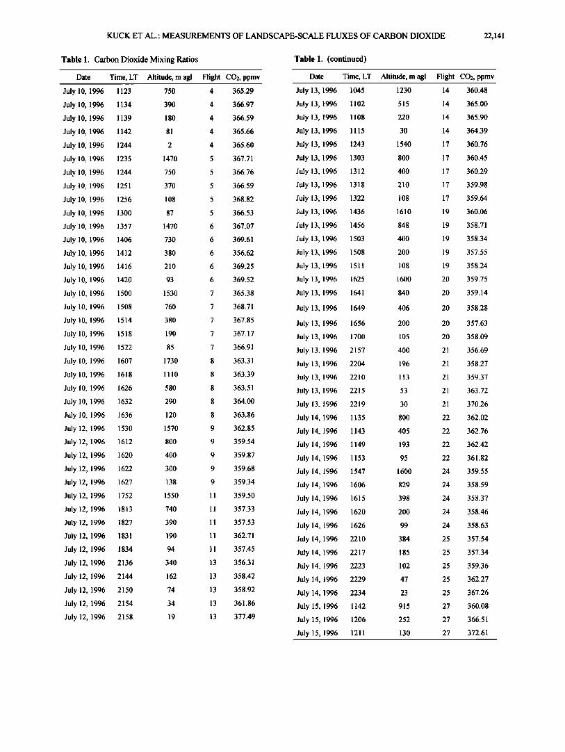
Figure 7. Average mixing ratios of CH4, CO, and H 2 and average values of (513C and (5•80 in CO 2 above and within the mixed layer. Error bars are one standard deviation.

Table 4. Average Mixing Ratios Within and Above the Mixed Layer

Average Mixing Ratio Within Average Mixing Ratio Above Species the Mixed Layer (200-400 m agl) the Mixed Layer (-1570 m agl)

CH4 1792 + 41 ppbv 1764 + 45 ppbv CO 154 + 14 ppbv 138 + 14 ppbv H2 518 + 95 ppbv 506 + 19 ppbv 03 16.6 + 5.8 ppbv* 20.3 + 6.0 ppbv

CO2 362.0 + 4.2 ppmv* 362.9 + 3.2 ppmv ]3C - 7.9 + 0.20/00 - 8.0 + 0.20/00 ]80 - 0.2 + 1.7ø/oo - 0.2 + 1.7ø/oo

*Highly dependent on time of day.

KUCK ET AL.' MEASUREMENTS OF LANDSCAPE-SCALE FLUXES OF CARBON DIOXIDE 22,145

ing ratios above the influence of the CBL were relatively steady flux is also comparable to nocturnal fluxes found in various other over time. forest types (7.8 [lmol C m -2 s -1, aspen forest [Black et al., 1996];

The carbon dioxide vertical profiles for the 3 remaining days 4.6 [lmol C m '2 s -1, deciduous forest [Woj•y et al., 1993]; 3.5 are shown in Figures 3, 4, and 5. On July 13 the average midday •mol C m -2 s -1, oak-hickory-pine forest [Baldocchi and Vogel, carbon dioxide mixed layer concentration was 360.1 + 0.4 ppmv, 1996]; 4.6 [lmol C m '2 s 'l, aspen forest [Schlenter and Van Cleve in good agreement with the July 13, 1996, marine boundary sur- 1985]). face layer mixing ratio of 361.7 ppmv for 6øS measured by NOAA/CMDL. This difference is smaller than might be antici- 3.4. Vertical Profiles and Average Concentrations pated from modification of the boundary layer by surface fluxes of Other Chemical Species over the region. If this pattern were found to persist over time, it The average vertical profiles of CH4, CO, H2, and the 13C and would suggest that net surface-atmosphere exchange of CO2 in •80 isotopes of CO2 are shown in Figure 7, and the average the Amazon is close to zero when averaged over the entire conti- measured concentrations within and above the mixed layer are nent. Our single point is suggestive, but not sufficient to draw summarized in Table 4. The small changes in mixing ratios of such a conclusion. Data from flight 20 were not used for flux cal- these species during the day prevented accurate estimates of culations since there was little change in the CO2 concentration fluxes of these species. }towever, the vertical profiles and aver- from the previous flight, suggesting a net flux of approximately zero in the late afternoon (1625-1700 LT).

Flux values were calculated using equation (2) and are listed in Table 2. The two data points collected closest to the ground were not used in the budget calculations since, due to local surface flux heterogeneity, the surface layer mixing ratios may not

age mixing ratios are reported for comparison with future measurements in this region.

4. Conclusions

Our estimates of daytime and nocturnal CO2 fluxes in the be representative of the mixed layer mean values. The average nearly undisturbed Peruvian Amazon are in good agreement with daytime flux, determined by weighting the daily values according previous studies in Brazil, all of which determined the Amazon to the reciprocal of their uncertainty, is -0.37 + 0.06 m ppmv CO2 forest to be a net carbon sink. Tropical forests are far more di- s -l. This daytime flux is equivalent to -13 + 2 •mol C m -2 s 'l, in verse than temperate forests, requiring measurements with large comparison with the midday carbon dioxide uptake estimated by footprint areas in order to obtain representative data. Our sam- Woj•y et al. [ 1988] (-6.5 + 2.8 gmol C m -2 s-•), Fan et al. [1990] pling approach of vertical profiling from a balloon platform has a (-10 gmol C m -2 s-l), Grace et al. [1995] (-5 to -20 gmol C m -2 s- major advantage of a very large footprint area (order of 100 km 2) 1), and Malhi et al. [1998] (-17 gmol C m -2 s -• wet season' -21 in comparison with surface-layer tower eddy-covariance meas- gmol C m '2 s -• dry season). urements (<1 km 2 under convective conditions). Owing to time

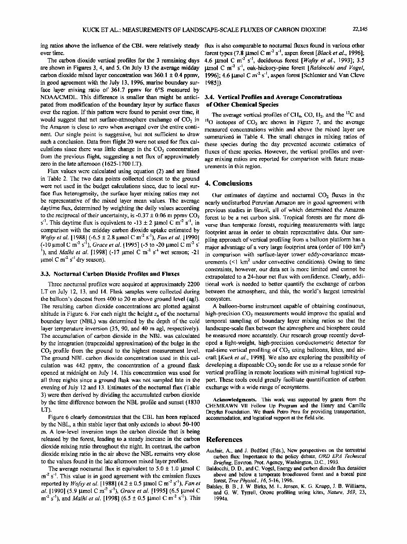
constraints, however, our data set is more limited and cannot be 3.3. Nocturnal Carbon Dioxide Profiles and Fluxes extrapolated to a 24-hour net flux with confidence. Clearly, addi-

Three nocturnal profiles were acquired at approximately 2200 tional work is needed to better quantify the exchange of carbon LT on July 12, 13, and 14. Flask samples were collected during between the atmosphere, and this, the world's largest terrestrial the balloon's descent from 400 to 20 m above ground level (agl). ecosystem. The resulting carbon dioxide concentrations are plotted against A balloon-borne instrument capable of obtaining continuous, altitude in Figure 6. For each night the height z,, of the nocturnal high-precision CO2 measurements would improve the spatial and boundary layer (NBL) was determined by the depth of the cold temporal sampling of boundary layer mixing ratios so that the layer temperature inversion (35, 90, and 40 m agl, respectively). landscape-scale flux between the atmosphere and biosphere could The accumulation of carbon dioxide in the NBL was calculated be measured more accurately. Our research group recently devel- by the integration (trapezoidal approximation) of the bulge in the oped a light-weight, high-precision conductometric detector CO2 profile from the ground to the highest measurement level. real-time vertical profiling of CO2 using balloons, kites, and air- The ground NBL carbon dioxide concentration used in this cal- craft [Kuck et al., 1998]. We also are exploring the possibility of culation was 442 ppmv, the concentration of a ground flask developing a disposable CO2 sonde for use as a release sonde for opened at midnight on July 14. This concentration was used for vertical profiling in remote locations with minimal logistical sup- all three nights since a ground flask was not sampled late in the port. These tools could greatly facilitate quantification of carbon evening of July 12 and 13. Estimates of the nocturnal flux (Table exchange with a wide range of ecosystems. 3) were then derived by dividing the accumulated carbon dioxide by the time difference between the NBL profile and sunset (1830 Acknowledgments. This work was supported by grants from the CHEMRAVV2q VII Follow Up Program and the Henry and Camille LT). Dreyfus Foundation. We thank Petro Peru for providing transportation,

Figure 6 clearly demonstrates that the CBL has been replaced accommodation, and logistical support at the field site. by the NBL, a thin stable layer that only extends to about 50-100 m. A low-level inversion traps the carbon dioxide that is being released by the forest, leading to a steady increase in the carbon References dioxide mixing ratio throughout the night. In contrast, the carbon

Auclair, A., and J. Bedford (Eds.), New perspectives on the terrestrial dioxide mixing ratio in the air above the NBL remains very close carbon flux: Importance to the policy debate, ORD EPA Technical to the values found in the late afternoon mixed layer profiles. Briefing, Environ. Prot. Agency, Washington, D.C., 1993.

The average nocturnal flux is equivalent to 5.0 5 1.0 [lmol C Baldocchi, D. D., and C. Vogel, Energy and carbon dioxide flux densities m -2 s -•. This value is in good agreement with the emission fluxes above and below a temperate broadleaved forest and a boreal pine

forest, Tree Physiol., 16, 5-16, 1996. reported by Woj•y et al. [ 1988] (4.2 5 0.5 •tmol C m -2 s-•), Fan et Balsley, B. B., J. W. Birks, M. L. Jensen, K. G. Knapp, J. B. Williams, al. [1990] (5.9 gmol C m -2 s-•), Grace et al. [1995] (6.5 •mol C and G. W. Tyrrell, Ozone profiling using kites, Nature, 369, 23, m -2 s-l), and Malhi et al. [1998] (6.5 5 0.5 [lmol C m '2 s-l). This 1994a.


Balsley, B. B., J. W. Birks, M. L. Jensen, K. G. Knapp, J. B. Williams, and G. W. Tyrrell, Vertical profiling of the atmosphere using high- tech kites, Environ. Sci. Technol., 28, 422A-427A, 1994b.

Black, T. A., G. Den Hartog, H. H. Neumann, P. D. Blanken, P. C. Yang, C. Russell, Z. Nesic, X. Lee, S. G. Chen, R. Staebler, and D. Novak, Annual cycles of water vapor and carbon dioxide fluxes in and above a boreal aspen forest, Global Change Biol., 2(3), 219-229, 1996.

Bognar, J. A., and J. W. Birks, Minaturized ultraviolet ozonesonde for atmospheric measurements, Anal. Chem., 68, 3059-3062, 1996.

Brown, S., C. A. S. Hall, W. Knabe, J. Raich, M. C. Trexler, and P. Woomet, Tropical forests: Their past, present, and potential future role in the terrestrial carbon budget, Water Air Soil Pollut., 70, 71-94, 1993.

Denmead, O. T., M. R. Raupach, F. X. Dunin, H. A. Cleugh, and R. Leuning, Boundary layer budgets for regional estimates of scalar fluxes, Global Change Biol., 2(3), 255-264, 1996.

Desjardins, R.L., J. L. MacPherson, P. Alvo, and P. H. Schuepp, Measurements of turbulent heat and carbon dioxide exchange over forests from aircraft, in The Forest-Atmosphere Interaction, edited by B.A. Hutchinson and B.B. Hicks, pp. 645-658, D. Reidel, Norwell, Mass., 1985.

Eamus, D., and P. F. Jarvis, The direct effects of increase in the global atmospheric carbon dioxide concentration on natural and commercial temperature trees and forests, Adv. Ecol. Res., 19, 1-55, 1989.

Enting, I. G., C. M. Trudinger, and N. B. A. Trivett, A synthesis inversion of the concentration and •5•3C of atmospheric carbon dioxide, Tellus, Ser. B, 47, 35-52, 1995.

Fan, S. M., S.C. Wofsy, P.S. Bakwin, D. J. Jacob, and D. R. Fitzjarrald, Atmosphere-biosphere exchange of carbon dioxide and ozone in the central Amazon forest, J. Geophys. Res., 95, 16,851-16,864, 1990.

Food and Agriculture Organization (FAO), Third interim report on the state of tropical forests, Rome, 1993.

Gifford, R. M., The global carbon cycle - A viewpoint on the missing sink, Aust. J. Plant Physiol., 21 (1), 1 - 15, 1994.

Grace, J., et al., Carbon dioxide uptake by an undisturbed tropical rain forest in southwest Amazonia, 1992 to 1993, Science, 270, 778-780, 1995.

Grace, J., Y. Malhi, J. Lloyd, J. Mclntyre, A. C. Miranda, P. Meir, and H. S. Miranda, The use of eddy covariance to infer the net carbon dioxide uptake of Brazilian rain forest, Global Change Biol., 2(3), 209-217, 1996.

Helmig, D., B. Balsley, K. Davis, L. R. Kuck, M. Jensen, J. Bognar, T. Smith Jr., R. V. Arrieta, R. Rodriguez, and J. W. Birks, Vertical profiling and determination of landscape fluxes of biogenic nonmethane hydrocarbons within the planetary boundary layer in the Peruvian Amazon, J. Geophys. Res., 103(19), 25,519-25,532, 1998.

Hipps, L.E, E. Swiatek, and W. P. Kustas, Interactions between regional surface fluxes and the atmospheric boundary layer over a heterogeneous watershed, Water Resour. Res., 30, 1387-1392, 1994.

Horst, T.W., and J.C. Weil, Footprint estimation for scalar flux measurements in the atmospheric surface layer, Boundary Layer Meteorol., 59, 279-296, 1992.

Houghton, R.A., Tropical deforestation and atmospheric carbon dioxide, Clim. Change, 19, 99-118, 1991.

Kuck, L. R., R. D. Godec, P. P. Kosenka, and J. W. Birks, High precision conductometric detector for the measurement of atmospheric carbon dioxide, Anal. Chem., 70, 4678-4682, 1998.

Lhomme, J.-P., B. Monteny, and P. Bessemouiin, Inferring regional surface fluxes from convective boundary layer characteristics in a Sahelian environment, Water Resour. Res., 33, 2563-2569, 1997.

Malhi, Y., A.D. Nobre, J. Grace, B. Kruijt, M.G.P. Peteira, A. Culf, and S. Scott, Carbon dioxide transfer over a central Amazonian rain forest, J. Geophys. Res., 103, 31,593-31,612, 1998.

Martin, C. L., D. Fitzjarrald, M. Garstang, A. P. Oliveira, S. Greco, and E. Browell, Structure and growth of the mixing layer over the Amazonian rain forest, J. Geophys. Res., 93, 1361-1375, 1988.

McGuire, A.D., J. M. Melillo, and L. A. Joyce, The role of nitrogen in the response of forest net primary production to elevated atmospheric carbon dioxide, Annu. Rev. Ecol. Syst., 26, 473-503, 1995.

McMurtrie, R. E., H. N. Cornins, M. U. F. Kirschbaum, and Y.-P. Wang, Modifying existing forest growth models to take account of effects of elevated carbon dioxide, Aust. J. Bot., 40, 657-677, 1992.

Raupach, M. R., O. T. Denmead, and F. X. Dunin, Challenges in linking atmospheric carbon dioxide concentrations to fluxes at local and regional scales, Aust. J. Bot., 40, 697-716, 1992.

Schlentner, R. E., and K. Van Cleve, Relationships between carbon dioxide evolution from soil, substrate temperature and substrate moisture in four mature forest types in interior Alaska, Can. d. For. Res., 15, 97-106, 1985.

Stull, R.B., An Introduction to Boundary Layer Meteorology, 666 pp., Kluwer Acad., Norwell, Mass., 1988.

Tans, P. P., I. Y. Fung, and T. Takahashi, Observational constraints on the global atmospheric carbon dioxide budget, Science, 247, 1431- 1438, 1990.

Taylor, J. A., and J. Lloyd, Sources and sinks of atmospheric carbon dioxide, Aust. J. Bot., 40, 407-418, 1992.

Thoning, K. W., T. J. Conway, N. Zhang, and D. Kitzis, Analysis system for measurement of carbon dioxide mixing ratios in flask air samples, J. Atmos. Oceanic Technol., 12, 1349-1356, 1995.

Vloedbled, M., and R. Leemans, Quantifying feedback processes in the response of the terrestrial carbon cycle to global change: The modeling approach of IMAGE-2, Water Air Soil Pollut., 70, 615-628, 1993.

Wofsy, S.C., R. C. Harriss, and W. A. Kaplan, Carbon dioxide in the atmosphere over the Amazon Basin, J. Geophys. Res., 93, 1377-1387, 1988.

Wofsy, S.C., M. l,. Goulden, J. W. Munger, S.-M. Fan, P.S. Bakwin, B. C. Daube, S. L. Bassow, and F. A. Bazzaz, Net exchange of carbon dioxide in a mid-latitude forest, Science, 260, 1314, 1993.

R.V. Arrieta and R. Rodriquez, Facultad de Ingenieria, Universidad de Piura, Piura, Peru.

B.B. Balsley, J.W. Birks, J.A. Bognar, D. Helmig, M.L. Jensen, L. R. Kuck, and T. Smith Jr., Cooperative Institute for Research in Environmental Sciences (CIRES), University of Colorado, Boulder, CO 80309-0215.

T.J. Conway, and P.P. Tans, Climate Monitoring and Diagnostics Laboratory, NOAA, 325 Broadway, Boulder, Colorado 80303.

K. Davis, Department of Soil, Water, and Climate, University of Minnesota, St. Paul, MN 55108-6028.

(Received July 20, 1999; revised February 3, 2000; accepted February 8, 2000.)

Measurements of landscape-scale fluxes of carbon dioxide in the Peruvian Amazon by vertical...

Documents

Transcript of Measurements of landscape-scale fluxes of carbon dioxide in the Peruvian Amazon by vertical...