�����������������

Citation: Rossi, G.B.; Cannata, A.;

Iengo, A.; Migliaccio, M.; Nardone,

G.; Piscopo, V.; Zambianchi, E.

Measurement of Sea Waves. Sensors

2022, 22, 78. https://doi.org/

10.3390/s22010078

Academic Editor: Ali Khenchaf

Received: 30 October 2021

Accepted: 17 December 2021

Published: 23 December 2021

Publisher’s Note: MDPI stays neutral

with regard to jurisdictional claims in

published maps and institutional affil-

iations.

Copyright: © 2021 by the authors.

Licensee MDPI, Basel, Switzerland.

This article is an open access article

distributed under the terms and

conditions of the Creative Commons

Attribution (CC BY) license (https://

creativecommons.org/licenses/by/

4.0/).

sensors

Article

Measurement of Sea Waves

Giovanni Battista Rossi 1,* , Andrea Cannata 2,3 , Antonio Iengo 4 , Maurizio Migliaccio 5,6,Gabriele Nardone 7 , Vincenzo Piscopo 5 and Enrico Zambianchi 5,8

1 Dipartimento di Ingegneria Meccanica, Energetica, Gestionale e dei Trasporti, University of Genova,Via Opera Pia 15A, 16145 Genova, Italy

2 Dipartimento di Scienze Biologiche, Geologiche e Ambientali, Università degli Studi di Catania,Corso Italia 57, 95129 Catania, Italy; andrea.cannata@unict.it

3 Istituto Nazionale di Geofisica e Vulcanologia, Sezione di Catania, Osservatorio Etneo, Piazza Roma 2,95125 Catania, Italy

4 ARPAL-Hydrological and Weather Centre, Viale Brigate Partigiane 2, 16129 Genova, Italy;antonio.iengo@arpal.liguria.it

5 Department of Engineering and Department of Science and Technology, Università degli Studi di Napoli“Parthenope”, Centro Direzionale Isola C4, 80143 Naples, Italy; maurizio.migliaccio@uniparthenope.it (M.M.);vincenzo.piscopo@uniparthenope.it (V.P.); enrico.zambianchi@uniparthenope.it (E.Z.)

6 Istituto Nazionale di Geofisica e Vulcanologia, Sezione ONT, Via di Vigna Murata 605, 00143 Roma, Italy7 ISPRA—Istituto Superiore per la Protezione e la Ricerca Ambientale, Via Vitaliano Brancati 48,

00144 Rome, Italy; gabriele.nardone@isprambiente.it8 Consorzio Nazionale Interuniversitario per le Scienze del Mare (CoNISMa), Piazzale Flaminio 9,

00196 Rome, Italy* Correspondence: g.b.rossi@unige.it; Tel.: +39-010-335-2966

Abstract: Sea waves constitute a natural phenomenon with a great impact on human activities,and their monitoring is essential for meteorology, coastal safety, navigation, and renewable energyfrom the sea. Therefore, the main measurement techniques for their monitoring are here reviewed,including buoys, satellite observation, coastal radars, shipboard observation, and microseism analysis.For each technique, the measurement principle is briefly recalled, the degree of development isoutlined, and trends are prospected. The complementarity of such techniques is also highlighted,and the need for further integration in local and global networks is stressed.

Keywords: dynamic measurement; sea state measurement; wave buoys; satellite remote sens-ing; coastal radars; shipboard sea state observation; microseism observation; networks for seawaves monitoring

1. Introduction

Sea waves are produced as a response to wind energy transfer at the air–sea interface.Short surface waves form at the sea surface, increasing the surface roughness and, thus,the wind stress and the wave height. This process continues until the waves have reachedequilibrium with the wind forcing. In a vertical plane, sea waves are formed in twoextremes: wave crests and troughs. The vertical distance between crest and trough isdefined as the wave height, whereas the wave period can be defined as the time it takes fortwo consecutive crests to pass through a fixed point. Wave sizes vary from centimeters inlength (ripples or capillary waves) to kilometers (storm surges and tides), but historically,the measurement of waves in the open sea has aimed at recording information on windwaves, with a wavelength from meters to hundreds of meters.

An apparently random sea surface can be thought of as the sum of many simplewave trains, whose parameters can be defined via a time domain approach (zero-crossing).However, introducing the wave spectrum in the frequency domain is a more efficientway to formalize this concept. Using harmonic analysis, each wave recording is brokendown into a large number of sine waves of different frequencies, directions, amplitudes,and phases. This approach, defined as Fourier analysis, provides an approximation of

Sensors 2022, 22, 78. https://doi.org/10.3390/s22010078 https://www.mdpi.com/journal/sensors

Sensors 2022, 22, 78 2 of 36

the irregular shape of the real sea wave, recorded as the sum of trigonometric functions(sine curves); each frequency and direction describes a component of the wave that has anassociated amplitude and phase.

The wave height is usually expressed as significant wave height Hs, defined as themean value of the highest one-third of wave heights [1], or it can be estimated from thespectrum obtained from a time series of sea surface elevation. The vertical displacement ofthe sea surface over time in a fixed position, measured with a non-directional instrument,can be represented as a sum of sinusoidal signals in frequency f. Assuming random phasesand adding the square of all the amplitudes in a small frequency range, we obtain a non-directional wave frequency spectrum S(f ) of the wave signal (with dimensions m2/Hz).

Wave spectra can be estimated using spectral estimation methods—either non paramet-rical, such as the fast Fourier transform (FFT) following a proper estimation procedure [2],or parametrical, based, for example, on autoregressive moving average (ARMA) modelingof the time history [3].

Directional instruments can also measure horizontal displacements. The goal ofdirectional wave measurement is to obtain accurate estimates of the two-dimensionalenergy distribution in frequency f and direction θ, without any preliminary assumptionsabout the shape of the distribution. The sea surface can be described by the two-dimensionalspectrum of waves in frequency and direction S(f,θ), expressed as the product of the non-directional wave frequency spectrum S(f ) and the directional distribution, as follows:

S( f , θ) = S( f )[

a1 cos θ + b1 sin θ + a2 cos(2θ) + b2 sin(2θ) + ∑∞n=3(an cos(nθ) + bn sin(nθ))

], (1)

where n is the summation index. It is currently highly recommended that all directionalwave measurement devices reliably estimate the energy of the wave S(f ), which is relatedto the wave height, and the first four coefficients of the Fourier series a1, b1, a2, and b2in Equation (1), which defines the directional distribution of this energy [4]. The com-bination of S(f ), a1, b1, a2, and b2, or any other equivalent parameters [5], forms the setof “first-5” spectral wave parameters. They provide basic information (significant waveheight, peak wave period, and average wave direction in the peak wave period), as wellas a further set of sea state information to be used for a wide range of applications. Fur-thermore, the first four moments of the directional distribution are the mean direction ofthe wave (the first moment), the directional spread (the second moment), the skewness(the third moment, defines how the directional distribution is concentrated), and thekurtosis (the fourth moment, defines the peakedness of the distribution).

Significant advances have been made in the measurement of waves over the pastdecades, and numerous measurement devices are now available that operate on differentprinciples, some of which are well-established while others are still under development.Here, several measurement techniques are reviewed, including buoys, satellite observa-tion, coastal radars, shipboard observation, and microseism analysis. For each technique,the measurement principle is recalled, the degree of development is outlined, and trendsare prospected. In any case, standardized measures are essential to ensure consistencybetween the different stations, so much so that it is necessary to define reliable measurementnetworks and integrate information at the regional level. This last aspect is thus highlightedat the end of the paper

2. Wave Buoys2.1. Drifting Buoys

Buoys, whether moored or drifting, have the ability to communicate, in a programmedway, in real time via satellite telecommunication systems, transmitting acquired observa-tions to collection centers. The collected data are used in different applications, includingresearch, environmental monitoring, weather forecasts, validation of oceanographic andmeteorological models, as well as safety at sea and coastal defense works planning [6].

There are many different types of drifting buoys and moored buoys, depending onthe application and measurements required in different seas and oceans. Drifting buoys

Sensors 2022, 22, 78 3 of 36

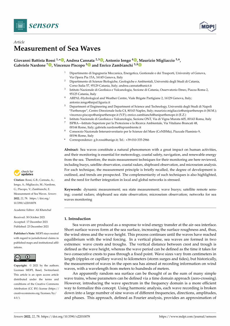
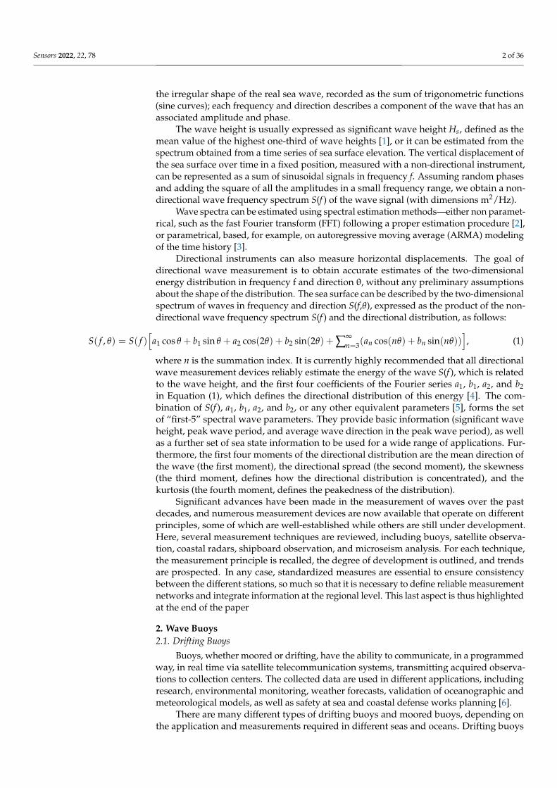
are floating platforms without any type of anchor, and can be divided into three differentcategories: surface drifter, subsurface floats, and ice buoys. Surface drifters (see Figure 1)provide a unique representation of surface current dynamics, and can supplement satelliteobservations to study climate-scale problems. Generally, drifters are characterized by asurface buoy and a drogue moving below the sea surface and attached by a long, thin tether.Batteries, sensors, and other electronics are contained in the buoy, whereas the drogue isan underwater anchor, a cylinder of four to seven sections, with a large hole through themiddle of each section, giving the drogue the appearance of a holey sock [7]. The holes areimportant because they create lots of small areas of turbulence to slow its larger slipstreamspeed and improve its stability when moving. In this way, its speed and direction canbe made to better match those of the actual currents. Drifters also measure temperatures,salinity, air pressure, and surface wind speed and direction. A drifter that is not tetheredto its drogue is a good wave following device, and is a potential tool for global wavemeasurements. A drifter can also be used to yield high-quality directional wave spectraby installing on it a downward-looking acoustic Doppler current profiler (ADCP), used toderive two-dimensional spectra from wave orbital velocities, or a global positioning system(GPS), to measure the motion of the drifter at frequencies greater than 0.01 Hz. WhereasADCPs are expensive, GPS sensors are relatively cost-effective and easy to install. Thus,wave drifters are generally developed based on GPS receivers and deployed in the opensea. Directional wave spectra (DWS) drifters are a new generation of GPS-based trackingdevices, able to compute the “first-5” directional Fourier coefficients (a0, a1, b1, a2, b2) usedto derive wave parameters such as significant wave height, swell direction, and directionalspread, among others [8].

Figure 1. A drifter neatly compressed for deployment (left) and with the nylon drogue fullyextended (right), as it will be in the water once the cardboard wraps dissolve. Photos cour-tesy of National Oceanic and Atmospheric Administration (NOAA)—Atlantic Oceanographic andMeteorological Laboratory.

Autonomous systems used to profile the deeper waters of oceans are called floats, simi-lar to drifters, because they are unmoored and measure currents, temperature,and salinity. Floats are programmed to drift below the sea surface at different depths,forced by both horizontal currents and surface waves. Measuring waves accurately usingfloats is possible, and relatively inexpensive. One of the main applications involves anInertial Motion Unit (IMU)-type device consisting of tri-axial accelerometers, rate gyros,

Sensors 2022, 22, 78 4 of 36

and magnetometers. IMUs provide an accurate measurement of accelerations and tilts.Further upward-looking ADCP is also applicable. To change their buoyancy, floats areequipped with simple mechanical pumps, bladders, and other devices, allowing them tofluctuate between different depths. Data sending takes place after the floats rise to the seasurface periodically to send data via their satellite antenna [9].

The main application of both surface drifters and subsurface floats is to measureocean trajectories, which are useful for both visualizing ocean motion and determiningthe time-evolving velocity fields. Lagrangian analysis of ocean velocity data reveals thatvery different kinds of circulation patterns occur in different regions, and shows theinteractions between currents, topography, and coastlines. A recent experiment has shownthe possibility of obtaining wave measurements from floats via measurement of the pressuredifference between the top and the bottom of the float [10].

Ice buoys are mainly used to track the dynamic and thermodynamic evolution ofdrifting Arctic and Antarctic sea ice, and to acquire meteorological and upper oceanographicdata [11,12]. They can sit on sea ice in the open Artic or Antarctic Ocean to evaluate theseasonal evolution of the thermohaline structure of the ocean during ice formation/freezeup. Depending on how the platform sits on the sea ice, snow depth and ice thicknessvariations may be derived from either ultrasonic range finders, such as those on automaticweather stations (AWS) or ice mass-balance thermistor strings, or solid-state sensors [13,14].Generally, ice buoys measure the ice motion using an inertial motion unit (IMU), performingmeasurements at 10 Hz and transmitting the full wave spectrum, geographical location,and battery power status at predefined intervals [15]. In most cases, these buoys are part ofa wider buoy network, which includes moored wave buoys, automatic weather stations,GPS buoys, and data loggers that transmit the data via satellites in real-time. In researchapplications, ice buoys used for wave spectral data detection via onboard accelerometershave been deployed in marginal ice zones during the period of ice formation (pancakeice) [16].

2.2. Moored Buoys

The last type of buoys focused on in this paper is moored buoys (see Figure 2),a category that encompasses a large number of platforms (either small and cheap or rela-tively large and expensive) anchored in fixed positions to derive long-term observationsunder many various atmospheric conditions and with different oceanographic sensors.

Several platforms have been developed for moored buoys; they can vary from afew centimeters in height and width to over ten meters, but all different sorts of mooredbuoys had been developed to capture and model information about ocean dynamics on thesurface, determining the directional spectrum of waves in the open sea. Data are usuallytransmitted in real time and disseminated via the global telecommunication system (GTS)of WMO for use by national meteorological centers.

These data can be used to greatly improve forecasting and warnings for severestorms, since wave patterns have been verified to exhibit negative bias at maximum windspeeds [17–19].

A buoy wave-measurement system has some typical components, such as the plat-form (comprising the hull and the mast), the power system (e.g., sealed lead acid gelbatteries charged by solar panels), the electronics payload (i.e., data acquisition systems,nautical light, GPS receivers, and one or more data transmitters), the sensors (wave andmeteo-oceanographic sensors), and the mooring. Wave buoys can be spherical, cylindrical,discus-shaped, or boat-shaped [20]. Plastic and foam construction has spread in recentyears for hulls, but the current trend is to use aluminum or marine alloy steel as a construc-tion material to prevent the release of microplastics into the sea. Mooring methods dependon the depth of deployed waters and cost factors; essentially, there are three typical systems:all chain mooring (used in shallow water), semi-taut mooring, and inverse-catenary moor-ing [21,22]. The buoys must be moored carefully; tensions are to be avoided so that theirmovements are not affected by the mooring and they can adequately define the free surface.

Sensors 2022, 22, 78 5 of 36

Moorings that allow the buoy to float freely and actively rotate within a well-defined guardcircle can be made of steel-linked chain and wire rope, synthetic fiber rope, or bungee cord.Synthetic ropes (nylon, polyester, polypropylene, or advanced fibers) do not noticeablycorrode or deteriorate in seawater, and their strength to immersed weight ratio is excellent,so they are often used for buoy moorings.

Figure 2. The Capo Mele moored buoy is a Fugro Oceanor SEAWATCH Midi 185 (radius of 1.85 m).It is located at about 3NM from Andora port (Liguria, Italy). Thanks to a weather station 2 m abovesea level, the buoy measures wind (direction, intensity, gust), atmospheric pressure, humidity, and airtemperature. The observed marine parameters are wave significant height and maximum peak, waveperiod and direction, current intensity and direction from 3.5 to 70 m, and sea surface temperature.Photo courtesy of Regional Agency for Environmental Protection of Liguria Region (ARPAL).

Several methods have been described to determine the directional spectrum of wavesin the open sea using moored buoys; a full account of the physical principles on whichthey are based has been given in [23–26], while an in-depth study of the evolution of thesedevices was given in [27–29]. The spectrum of the sea surface is not exactly reproducibleanalytically, but under certain wind conditions the spectrum acquires a characteristic shape.With experimental tests, parametric spectrum models have been obtained consisting ofapproximate expressions that can adapt to the spectrum of sea surface elevation. Amongthe many proposed similar models are the Pierson–Moskowitz model and JONSWAP [30].These spectra were experimentally derived under fully developed wind conditions in thegeneration area in deep water, and can be used to relate the shape of the spectrum of thewind waves. To measure the directional spectrum of wind waves using moored buoys,an FFT is generally performed on the buoy displacement data. Considering only the “first-5” Fourier coefficients, this produces a smoothed version of the directional spectrum, as thecoefficients are averaged to decrease the variance of the estimate. After that, the directional

Sensors 2022, 22, 78 6 of 36

wave spectrum is calculated from the average coefficients using an appropriate weightingfunction [31,32].

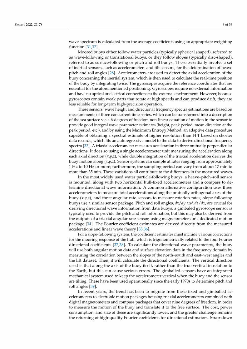
Moored buoys either follow water particles (typically spherical shaped), referred toas wave-following or translational buoys, or they follow slopes (typically disc-shaped),referred to as surface-following or pitch and roll buoys. These essentially involve a setof inertial sensors, such as accelerometers and tilt sensors, for the determination of heavepitch and roll angles [28]. Accelerometers are used to detect the axial acceleration of thebuoy concerning the inertial system, which is then used to calculate the real-time positionof the buoy by integrating twice. The gyroscopes acquire the reference coordinates that areessential for the aforementioned positioning. Gyroscopes require no external informationand have no optical or electrical connections to the external environment. However, becausegyroscopes contain weak parts that rotate at high speeds and can produce drift, they areless reliable for long-term high-precision operation.

These sensors’ wave height and directional frequency spectra estimations are based onmeasurements of three concurrent time series, which can be transformed into a descriptionof the sea surface via a 6-degrees of freedom non-linear equation of motion in the sensor toprovide good integral wave parameter estimates (height, peak period, mean direction at thepeak period, etc.), and by using the Maximum Entropy Method, an adaptive data procedurecapable of obtaining a spectral estimate of higher resolution than FFT based on shorterdata records, which fits an autoregressive model to the data to derive directional frequencyspectra [33]. A triaxial accelerometer measures acceleration in three mutually perpendiculardirections. It does so using a single accelerometer unit measuring the acceleration alongeach axial direction (x,y,z), while double integration of the triaxial acceleration derives thebuoy motion along (x,y,z). Sensor systems can sample at rates ranging from approximately1 Hz to 10 Hz or more; furthermore, the sampling period can vary from about 17 min tomore than 35 min. These variations all contribute to the differences in the measured waves.

In the most widely used water particle-following buoys, a heave–pitch–roll sensoris mounted, along with two horizontal hull-fixed accelerometers and a compass to de-termine directional wave information. A common alternative configuration uses threeaccelerometers to measure total accelerations along the mutually orthogonal axes of thebuoy (x,y,z), and three angular rate sensors to measure rotation rates; slope-followingbuoys use a similar sensor package. Pitch and roll angles, dz/dy and dz/dx, are crucial forderiving directional wave information from data buoys; a gimbaled gyroscope sensor istypically used to provide the pitch and roll information, but this may also be derived fromthe outputs of a triaxial angular rate sensor, using magnetometers or a dedicated motionpackage [34]. The Fourier coefficient estimates are derived directly from the measuredaccelerations and linear wave theory [35,36].

For a slope-following system, the coefficient estimates must include various correctionsfor the mooring response of the hull, which is trigonometrically related to the four Fourierdirectional coefficients [37,38]. To calculate the directional wave parameters, the buoywill use both angular motion data and surface elevation data in the frequency domain bymeasuring the correlation between the slopes of the north–south and east–west angles andthe lift dataset. Then, it will calculate the directional coefficients. The vertical directionused is that along the axis of the buoy itself, rather than the true vertical in relation tothe Earth, but this can cause serious errors. The gimballed sensors have an integratedmechanical system used to keep the accelerometer vertical when the buoy and the sensorare tilting. These have been used operationally since the early 1970s to determine pitch androll angles [39].

In recent years, the trend has been to migrate from these fixed and gimballed ac-celerometers to electronic motion packages housing triaxial accelerometers combined withdigital magnetometers and compass packages that cover nine degrees of freedom, in orderto measure the motion of the buoy and translate it to the free surface. The cost, powerconsumption, and size of these are significantly lower, and the greater challenge remainsthe returning of high-quality Fourier coefficients for directional estimators. Strap-down

Sensors 2022, 22, 78 7 of 36

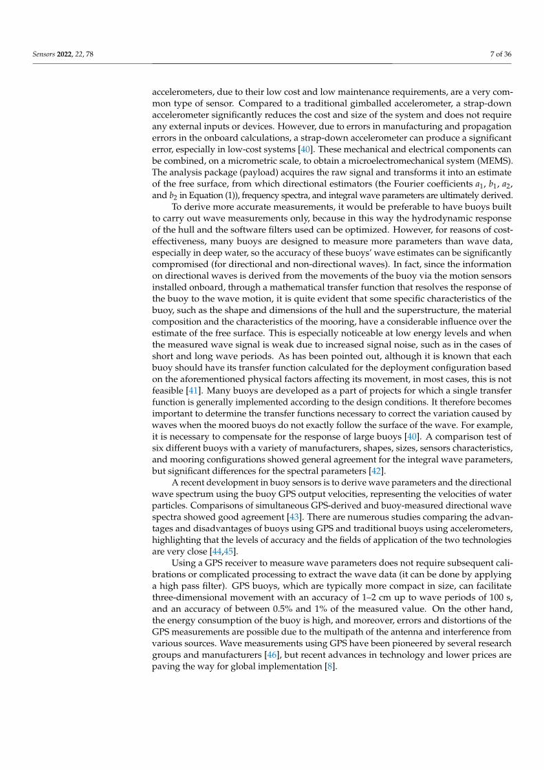
accelerometers, due to their low cost and low maintenance requirements, are a very com-mon type of sensor. Compared to a traditional gimballed accelerometer, a strap-downaccelerometer significantly reduces the cost and size of the system and does not requireany external inputs or devices. However, due to errors in manufacturing and propagationerrors in the onboard calculations, a strap-down accelerometer can produce a significanterror, especially in low-cost systems [40]. These mechanical and electrical components canbe combined, on a micrometric scale, to obtain a microelectromechanical system (MEMS).The analysis package (payload) acquires the raw signal and transforms it into an estimateof the free surface, from which directional estimators (the Fourier coefficients a1, b1, a2,and b2 in Equation (1)), frequency spectra, and integral wave parameters are ultimately derived.

To derive more accurate measurements, it would be preferable to have buoys builtto carry out wave measurements only, because in this way the hydrodynamic responseof the hull and the software filters used can be optimized. However, for reasons of cost-effectiveness, many buoys are designed to measure more parameters than wave data,especially in deep water, so the accuracy of these buoys’ wave estimates can be significantlycompromised (for directional and non-directional waves). In fact, since the informationon directional waves is derived from the movements of the buoy via the motion sensorsinstalled onboard, through a mathematical transfer function that resolves the response ofthe buoy to the wave motion, it is quite evident that some specific characteristics of thebuoy, such as the shape and dimensions of the hull and the superstructure, the materialcomposition and the characteristics of the mooring, have a considerable influence over theestimate of the free surface. This is especially noticeable at low energy levels and whenthe measured wave signal is weak due to increased signal noise, such as in the cases ofshort and long wave periods. As has been pointed out, although it is known that eachbuoy should have its transfer function calculated for the deployment configuration basedon the aforementioned physical factors affecting its movement, in most cases, this is notfeasible [41]. Many buoys are developed as a part of projects for which a single transferfunction is generally implemented according to the design conditions. It therefore becomesimportant to determine the transfer functions necessary to correct the variation caused bywaves when the moored buoys do not exactly follow the surface of the wave. For example,it is necessary to compensate for the response of large buoys [40]. A comparison test ofsix different buoys with a variety of manufacturers, shapes, sizes, sensors characteristics,and mooring configurations showed general agreement for the integral wave parameters,but significant differences for the spectral parameters [42].

A recent development in buoy sensors is to derive wave parameters and the directionalwave spectrum using the buoy GPS output velocities, representing the velocities of waterparticles. Comparisons of simultaneous GPS-derived and buoy-measured directional wavespectra showed good agreement [43]. There are numerous studies comparing the advan-tages and disadvantages of buoys using GPS and traditional buoys using accelerometers,highlighting that the levels of accuracy and the fields of application of the two technologiesare very close [44,45].

Using a GPS receiver to measure wave parameters does not require subsequent cali-brations or complicated processing to extract the wave data (it can be done by applyinga high pass filter). GPS buoys, which are typically more compact in size, can facilitatethree-dimensional movement with an accuracy of 1–2 cm up to wave periods of 100 s,and an accuracy of between 0.5% and 1% of the measured value. On the other hand,the energy consumption of the buoy is high, and moreover, errors and distortions of theGPS measurements are possible due to the multipath of the antenna and interference fromvarious sources. Wave measurements using GPS have been pioneered by several researchgroups and manufacturers [46], but recent advances in technology and lower prices arepaving the way for global implementation [8].

Sensors 2022, 22, 78 8 of 36

3. Satellite Remote Sensing

In this section, the physical basis and logic components of satellite microwave remotesensing are reviewed first. The goal is to provide a unitary and solid framework of thefundamentals. In Section 3.2, a brief summary of the main value-added products, out of theones focused on the sea wave, is given. Special reference to operational services is made.Finally, in Section 3.3, the use of microwave remotely sensed measurements in sea wavesmonitoring is reviewed.

3.1. Background

Satellite microwave (MW) remote sensing represents a special observational toolespecially for regions that are not easily accessible for in-situ measurements. Further,due to the MW’s propagation and interaction peculiarities, satellite measurements areindependent of solar illumination providing a denser revisit time [47]. This is of particularrelevance to the ocean environment, since it is the main locus of dynamical processes,and in some areas only a few in situ measurements can be made, for instance in theSouthern Ocean. Furthermore, MWs are much less dependent on cloud cover [47].

MW remote sensing also involves some critical features that must be considered.Satellite MW remote sensors are narrowband systems that estimate the complex reflectivityof the ocean surface in an “imperfect” manner. The main objective criteria for defining suchimperfections are the resolutions—the radiometric resolution, the spatial resolution andthe spectral resolution. The additional temporal resolution or revisit time depends on thesensor swath and scanning configuration, as well as the platform height.

MW satellite sensors can be passive or active: in the passive case, when there is nosource of illumination onboard the satellite, the electromagnetic data received at the sensorantenna are those naturally emitted by the marine scene; in the active case, an electromag-netic pulse is transmitted by the sensor antenna into the ocean, and the correspondingelectromagnetic signal reflected by the environment is received by the sensor [47]. In bothcases, random measurements occur because of the random nature of the scene.

Another important point is the observational scale. Some satellite sensors are meantto observe geophysical phenomena at large scales, and therefore they are called large-scalesensors, while some others operate at small scales, and are called small-scale sensors.In general terms, the spatial coverage is paid for by a coarser spatial resolution [47].

MW remote sensing calls for the solution of three subproblems: measurements, for-ward modeling and inverse modeling. The first subproblem is relevant to the accomplish-ing of not only high-quality measurements, but also to the proper design of the sensor.The second subproblem is sometimes neglected in modern blind approaches; once a propergeophysical quantity of interest is defined, it is important to investigate whether the ob-served measurements are related to said geophysical quantity. In a formal sense the forwardmodel calls for the development of a theoretical relationship between the observable quan-tity at the sensor and the geophysical quantity. Further refinement leads to a semi-empiricalgeophysical model function (GMF) that is appropriately tailored with reference to thegeophysical quantity and the sensor of interest. The third subproblem is known as theinverse problem, and calls for the quantitative estimation of the geophysical quantity of in-terest via a proper set of measurements. This latter problem is usually non-linear, ill-posed,and affected by noise. Despite these challenges, MW remote sensing is able to generatehigh-quality geophysical products that greatly contribute to the advancement of marinescience and operational services.

Passive MW sensors are known as MW radiometers, and collect the electromagneticfield data naturally emitted by the environment at their receiving antenna. MW radiometersare large-scale sensors, and their spatial resolution is not fine [47].

Radar altimeters are large-scale nadir-facing active sensors. This peculiar nadir-facingconfiguration and its spatial resolution makes the measurements sensitive to large-scalesea surface slopes. Therefore, the radar altimeter is the best MW sensor for sea stateestimation [34,48–51].

Sensors 2022, 22, 78 9 of 36

Scatterometers are large-scale off-nadir active sensors. The primary application ofscatterometers is the indirect measurement of near-surface (local) winds over the ocean.Such scatterometer winds are routinely assimilated into Numerical Weather Models [52–55].

Synthetic Aperture Radar (SAR) is a narrowband-coherent, i.e., phase-preserving,off-nadir-active MW imaging sensor. The design of SAR is meant to enhance the spatialresolution, and it is used for applications that are not time-variable within the coherencetime or integration time of such sensors. The SAR is a small-scale sensor that, although it ismainly optimized for defense and geophysical applications, has gained more and moreinterest in marine applications as well [47].

3.2. Review of the Main Marine Value-Added Products

Let us briefly review the main marine value-added products associated with the MWsatellite sensors but the ones related to sea waves that are reported in much more detail inSection 3.3.

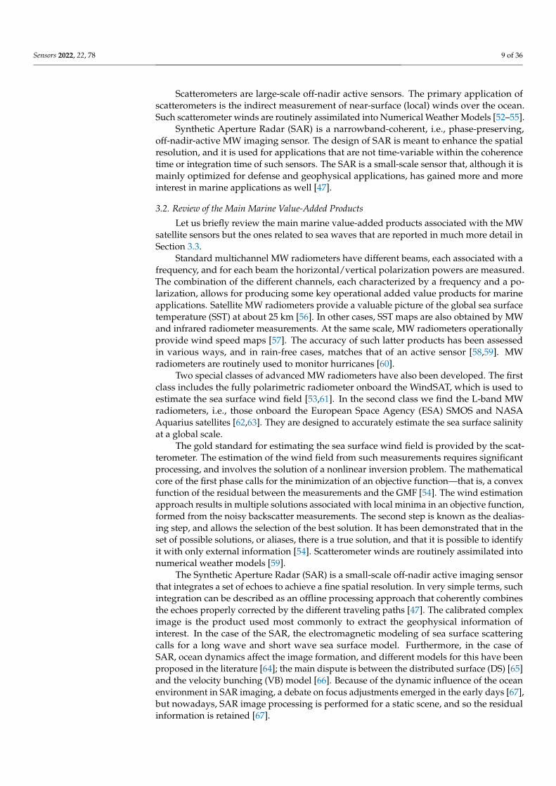
Standard multichannel MW radiometers have different beams, each associated with afrequency, and for each beam the horizontal/vertical polarization powers are measured.The combination of the different channels, each characterized by a frequency and a po-larization, allows for producing some key operational added value products for marineapplications. Satellite MW radiometers provide a valuable picture of the global sea surfacetemperature (SST) at about 25 km [56]. In other cases, SST maps are also obtained by MWand infrared radiometer measurements. At the same scale, MW radiometers operationallyprovide wind speed maps [57]. The accuracy of such latter products has been assessedin various ways, and in rain-free cases, matches that of an active sensor [58,59]. MWradiometers are routinely used to monitor hurricanes [60].

Two special classes of advanced MW radiometers have also been developed. The firstclass includes the fully polarimetric radiometer onboard the WindSAT, which is used toestimate the sea surface wind field [53,61]. In the second class we find the L-band MWradiometers, i.e., those onboard the European Space Agency (ESA) SMOS and NASAAquarius satellites [62,63]. They are designed to accurately estimate the sea surface salinityat a global scale.

The gold standard for estimating the sea surface wind field is provided by the scat-terometer. The estimation of the wind field from such measurements requires significantprocessing, and involves the solution of a nonlinear inversion problem. The mathematicalcore of the first phase calls for the minimization of an objective function—that is, a convexfunction of the residual between the measurements and the GMF [54]. The wind estimationapproach results in multiple solutions associated with local minima in an objective function,formed from the noisy backscatter measurements. The second step is known as the dealias-ing step, and allows the selection of the best solution. It has been demonstrated that in theset of possible solutions, or aliases, there is a true solution, and that it is possible to identifyit with only external information [54]. Scatterometer winds are routinely assimilated intonumerical weather models [59].

The Synthetic Aperture Radar (SAR) is a small-scale off-nadir active imaging sensorthat integrates a set of echoes to achieve a fine spatial resolution. In very simple terms, suchintegration can be described as an offline processing approach that coherently combinesthe echoes properly corrected by the different traveling paths [47]. The calibrated compleximage is the product used most commonly to extract the geophysical information ofinterest. In the case of the SAR, the electromagnetic modeling of sea surface scatteringcalls for a long wave and short wave sea surface model. Furthermore, in the case ofSAR, ocean dynamics affect the image formation, and different models for this have beenproposed in the literature [64]; the main dispute is between the distributed surface (DS) [65]and the velocity bunching (VB) model [66]. Because of the dynamic influence of the oceanenvironment in SAR imaging, a debate on focus adjustments emerged in the early days [67],but nowadays, SAR image processing is performed for a static scene, and so the residualinformation is retained [67].

Sensors 2022, 22, 78 10 of 36

The marine applications of SAR measurements are diverse, but the only one thathas been considered to support operational services is related to marine oil pollutionand vessel monitoring. Such applications are particularly benefitted by polarimetric SARmeasurements [68,69].

3.3. Sea Waves Monitoring

In this subsection, the focus is on ocean wave products as generated by MW satelliteremote sensing measurements.

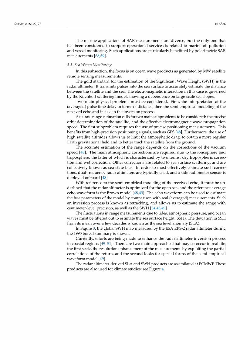
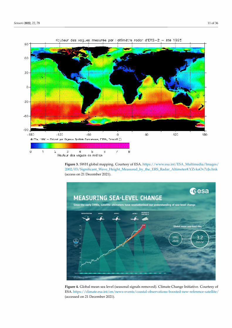
The gold standard for the estimation of the Significant Wave Height (SWH) is theradar altimeter. It transmits pulses into the sea surface to accurately estimate the distancebetween the satellite and the sea. The electromagnetic interaction in this case is governedby the Kirchhoff scattering model, showing a dependence on large-scale sea slopes.

Two main physical problems must be considered. First, the interpretation of the(averaged) pulse time delay in terms of distance, then the semi-empirical modeling of thereceived echo and its use in the inversion process.

Accurate range estimation calls for two main subproblems to be considered: the preciseorbit determination of the satellite, and the effective electromagnetic wave propagationspeed. The first subproblem requires the use of precise positioning measurements. Thisbenefits from high-precision positioning signals, such as GPS [48]. Furthermore, the use ofhigh satellite altitudes allows us to limit the atmospheric drag, to obtain a more regularEarth gravitational field and to better track the satellite from the ground.

The accurate estimation of the range depends on the corrections of the vacuumspeed [48]. The main atmospheric corrections are required due to the ionosphere andtroposphere, the latter of which is characterized by two terms: dry tropospheric correc-tion and wet correction. Other corrections are related to sea surface scattering, and arecollectively known as sea state bias. In order to most effectively estimate such correc-tions, dual-frequency radar altimeters are typically used, and a side radiometer sensor isdeployed onboard [48].

With reference to the semi-empirical modeling of the received echo, it must be un-derlined that the radar altimeter is optimized for the open sea, and the reference averageecho waveform is the Brown model [48,49]. The echo waveform can be used to estimatethe free parameters of the model by comparison with real (averaged) measurements. Suchan inversion process is known as retracking, and allows us to estimate the range withcentimeter-level precision, as well as the SWH [34,48,49].

The fluctuations in range measurements due to tides, atmospheric pressure, and oceanwaves must be filtered out to estimate the sea surface height (SSH). The deviation in SSHfrom its mean over a few decades is known as the sea level anomaly (SLA).

In Figure 3, the global SWH map measured by the ESA ERS-2 radar altimeter duringthe 1995 boreal summary is shown.

Currently, efforts are being made to enhance the radar altimeter inversion processin coastal regions [49–51]. There are two main approaches that may co-occur in real life;the first seeks the resolution enhancement of the measurements by exploiting the partialcorrelations of the return, and the second looks for special forms of the semi-empiricalwaveform model [49].

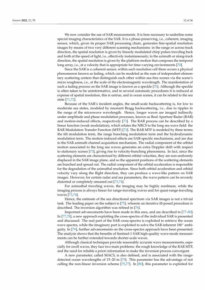
The radar altimeter-derived SLA and SWH products are assimilated at ECMWF. Theseproducts are also used for climate studies; see Figure 4.

Sensors 2022, 22, 78 11 of 36

Figure 3. SWH global mapping. Courtesy of ESA. https://www.esa.int/ESA_Multimedia/Images/2002/03/Significant_Wave_Height_Measured_by_the_ERS_Radar_Altimeter#.YZvksOv7zJs.link(access on 21 December 2021).

Figure 4. Global mean sea level (seasonal signals removed). Climate Change Initiative. Courtesy ofESA. https://climate.esa.int/en/news-events/coastal-observations-boosted-new-reference-satellite/(accessed on 21 December 2021).

Sensors 2022, 22, 78 12 of 36

We now consider the use of SAR measurements. It is here necessary to underline somespecial imaging characteristics of the SAR. It is a phase-preserving, i.e., coherent, imagingsensor, which, given its proper SAR processing chain, generates fine-spatial resolutionimages by means of two very different scanning mechanisms: in the range or across-trackdirection, the spatial resolution is given by linearly modulated chirp pulses traveling backand forth at the speed of light, i.e., effectively instantaneously; in the azimuth or along-trackdirection, the spatial resolution is given by the platform motion that composes the temporallong array, i.e., at a velocity that is appropriate for time-varying environments [70].

Since the SAR is a coherent sensor, within each resolution cell there occurs a physicalphenomenon known as fading, which can be modeled as the sum of independent elemen-tary scattering centers that distinguish each other within sea-free scenes via the scene’smicro roughness, i.e., at the scale of the electromagnetic wavelength. The manifestation ofsuch a fading process on the SAR image is known as a speckle [70]. Although the speckleis often taken to be uninformative, and in several automatic procedures it is reduced atexpense of spatial resolution, this is untrue, and in ocean scenes, it can be related to the seastate [71,72].

Because of the SAR’s incident angles, the small-scale backscattering is, for low tomoderate sea states, modeled by resonant Bragg backscattering, i.e., due to ripples inthe range of the microwave wavelength. Hence, longer waves are imaged indirectlyunder amplitude and phase modulation processes, known as Real Aperture Radar (RAR)and motion-induced effects, respectively [73]. The RAR process can be described by alinear function (weak modulation), which relates the NRCS to the long sea wave field: theRAR Modulation Transfer Function (MTF) [73]. The RAR MTF is modeled by three terms:the tilt modulation term, the range bunching modulation term and the hydrodynamicmodulation term. The motion-induced effects are SAR-specific mechanisms, and are dueto the SAR azimuth channel acquisition mechanism. The radial component of the orbitalmotion associated to the long sea waves generates an extra Doppler shift with respectto stationary scenes [73], giving rise to velocity-bunching phenomena. In fact, since thescattering elements are characterized by different orbital velocities, they are non-uniformlydisplaced in the SAR image plane, and so the apparent positions of the scattering elementsare bunched and spread out. The radial component of the orbital acceleration is responsiblefor the degradation of the azimuthal resolution. Since both orbital acceleration and orbitalvelocity vary along the flight direction, they can produce a wave-like pattern on SARimages. However, for certain radar and sea parameters, the wave pattern can be severelydistorted or completely smeared out [73,74].

For azimuthal traveling waves, the imaging may be highly nonlinear, while theimaging process is always linear for range-traveling waves and for quasi-range-travelingwaves [73,74].

Hence, the estimate of the sea directional spectrum via SAR images is not a trivialtask. The leading paper on the subject is [75], wherein an iterative ill-posed procedure isdescribed. The inversion algorithm was refined in [76].

Important advancements have been made in this area, and are described in [77–80].In [77,78], a new approach exploiting the cross-spectra of the individual SAR is presentedand discussed. The real part of the SAR cross-spectra is exploited to retrieve the oceanwave spectra, while the imaginary part is exploited to solve the SAR-inherent 180◦ ambi-guity. In [79], further advancements on the cross-spectra approach have been presented.The analysis shows that the benefits of Sentinel-1 SAR high-quality wave-mode measure-ments can be further extended towards shorter-scale waves.

Although classical techniques provide reasonably accurate wave measurements, espe-cially for swell waves, they face two main problems: the rough knowledge of the RAR MTF,and the need for reliable a priori information to make the inversion process convergent.

A new parameter, called MACS, is also defined, and is associated with the range-detected ocean wavelengths of 15–20 m [79]. This parameter has the advantage of notcalling the non-linear inversion scheme [75,77]. In [80], this parameter is exploited for

Sensors 2022, 22, 78 13 of 36

global analysis. Along the same conceptual idea has been designed one the sensor onboardof the China France Oceanography Satellite (CFOSAT): the SWIM. It is a Real ApertureRadar (RAR) that observe range travelling waves at high spatial resolution while filter outthe azimuth travelling waves [81].

In [82], a study based on deep-learning and co-located radar altimeter and ESASentinel-1 SAR data offers remarkable results. The deep learning approach has beenimplemented for low-level SAR cross-spectra, used to estimate the SWH.

In [83–85], fully polarimetric SAR measurements are exploited. Physically, the ap-proach benefits from the dependence of the polarimetric Cloude–Pottier decomposition,i.e., the eigenvector dependence, on the orientation angles. Such an approach is feasible forhigh-quality fully polarimetric SAR sensors, such as Radarsat-2. The main advantage of thisapproach is that the complex hydrodynamic MTF [74] does not need to be estimated [83,84].In [85], a validation of the polarimetric approach with Radarsat-2 measurements is per-formed. The analysis shows good agreement with buoy data [85].

Because of the non-linear relationship between the SAR image spectra and the oceanspectra [73–75], several empirical approaches have been explored to estimate the SWHusing SAR images, e.g., in [86,87], two polarimetric approaches are presented.

A popular and effective approach is the so-called azimuth cut-off approach [88–93].It was first proposed in [88]. It uses physical phenomena directly associated with the SARazimuth channel’s image formation [73–75]. In very simple terms, the azimuth SAR channelis unable to image ocean wavelengths smaller than the azimuth cut-off. Such a cut-off isempirically related to the sea state, and in some cases it can also be interpreted in termsof wind speed [89,90]. The actual implementation is rather complex, and affects the finalquality of the estimate [90], but the enhanced quality of the new SAR sensors, such as thatonboard the ESA Sentinel-1 missions, makes the azimuth cut-off approach very promising.

Let us finally consider another method for observing sea waves: along-track SARinterferometry [94–97]. The along-track SAR interferometer measures complex imagecorrelation using two SAR acquisitions that are in all respects similar except for the (small)time difference. The phase difference, i.e., the along-track polarimetric phase, can be relatedto the ocean wave spectra, allowing its estimation. In fact, the sea surface radial velocitycan be determined by the interferometric phase of each resolution unit, and then the wavespectrum is obtained from the radial velocity. However, this method is still affected byvelocity bunching.

An alternative approach, based on across-track airborne SAR interferometry, has beenalso proposed [98]. It employs a well assessed procedure meant to estimate the DigitalElevation Model over stable scenarios to the marine case. Of course it must be operatedwith the two SAR antennas of the interferometer acquiring at the same time (single-passmode) and this is not feasible by satellites at present time [98].

The fundamental advantage of these methodologies is related to the fact that whilethe amplitude spectra depend strongly on the NRCS modulation of ocean long waves,which is roughly known, the phase difference is related to the ocean wave spectrum in aknown manner.

Since SAR has the unique ability to indirectly measure the sea’s directional spectra,it is important to assess the quality of such SAR-derived wave spectra [99]. In [99], a qualityanalysis of the key characteristics is performed based on a physical/statistical approach.

4. Coastal HF Radars

Coastal HF (High-frequency) radars are land-based remote sensing instruments thathave attained great popularity in the last few decades, even though they are still consideredan “emerging” observation technique by the Global Ocean Observing System. The reasonfor their wide distribution [100] lies in the fact that they are able to provide synoptic data(i.e., simultaneous over a relatively large area), repeated in time at unprecedentedly highspatial and temporal resolutions.

Sensors 2022, 22, 78 14 of 36

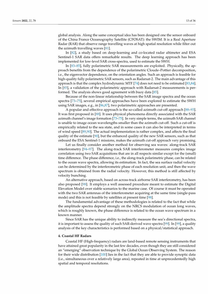
Their essential principle is based on the backscattering of an electromagnetic signalby the sea surface. This phenomenon gives rise to a spectrum of backscattered signals(see Figure 5). The main peaks correspond to the first-order scatter from the so-calledBragg waves. They are the result of a coherent resonance, analogous to the Bragg effectthat emerges in atomic lattice detection by X-rays. These Bragg peaks occur when thewavelength of surface ocean waves is approximately half as long as the wavelength ofthe transmitted signal, as first observed in [101] and later clarified in [102–106]. Thesefirst-order peaks provide information about surface currents, whose velocity (radial ve-locity with respect to the antennas) can be inferred in relatively simple terms from theDoppler shift associated with the presence of a current underlying the surface wave trains,as reviewed in [107].

The continuum surrounding the first-order (dominant) peak represents the higher-order scattering, partly due to the nonlinear interactions between surface ocean waves.This portion of the spectrum is the source of information regarding surface gravity waves.Its inversion is based on the relationship, established in [108–110] and further developedin [111,112], between the backscattered signal and the ocean wave directional spectrum.The inversion of an integral equation allows us to retrieve wave parameters such as waveheight and mean direction, as well as dominant wave period. Several approaches havebeen applied to carry out such a reconstruction, as reviewed in [113].

Figure 5. Main characteristics of a typical HF radar spectrum [114].

The inversion process is far more complex than that of the first-order spectrum, and issubject to a number of theoretical limitations, as thoroughly discussed in [115].

At the lower end of the measurable wave height range, i.e., at low sea states, the mainlimitation is related to the low signal-to-noise ratio, which is frequency-dependent (HFradars operating at higher frequencies can detect lower sea states), and this prevents theaccurate detection of very low wave heights [115]. At the higher end of the measurable waveheight range (high sea states), as well as in the case of very intense surface currents, first-and second-order peak regions may not be well separated, meaning the wave spectrumis not well defined. This effect is also frequency-dependent, and as a rule of thumb,the upper threshold for accurate wave height detection can be estimated by Equation (2):

hthr =2k0

, (2)

Sensors 2022, 22, 78 15 of 36

where k0 is the radar wavenumber [116,117]. Wave heights above hthr will be under-or overestimated.

HF radars can be divided into two different categories, Direction Finding and BeamForming systems [118]. Direction Finding instruments are characterized by a compactstructure, with closely spaced or even co-located transceiving antennas; these systemsprovide information on the wave field that is not resolved in azimuth. This means thatthe outcome of the inversion in this case will represent an azimuthal average aroundthe transceiving system, thus necessitating the use of circular statistics [119]. Parametersare thus derived over a circumference centered on the transceiving antenna’s location(the so-called range cell). Its radius should not be too long, to ensure a sufficiently strongsignal, but not too short, to avoid breakers and the influence of local bathymetry [120,121].On the other hand, Beam Forming, also known as Phase Array, radars utilize arrays ofantennas, which introduces additional logistical issues in the installation and maintenanceprocesses, and they are unable to reconstruct wave directional spectra on a grid.

As with any measurement instrument, and in particular remote sensing ones (evenland-based, such as HF radars), validation is a non-negotiable prerequisite for scientificutilization. Validation proceeds through the intercomparison of measurements providedby different instruments. As discussed in [122], this is a very delicate issue, as metrics haveto be devised to compare the outputs of different instruments that typically provide veryvaried results. A preliminary assessment of differences in the measurement principles,of their inherent constraints, and of biases due to different sampling rates and similar issueshas to be preliminarily carried out. After considering the above, and comparable outputshave been produced, proper validation can be undertaken.

The typical touchstone of HF radar-derived wave parameters is represented by dataobtained with different kinds of wave buoys [120,123–127]. However, other systems havebeen used for validation, including a bottom-installed current meter equipped with apressure transducer [128] and satellite altimeter data [129]. More recently, the output ofa sensor for directional wave measurements installed on an ADCP mounted on a MEDAelastic beacon was used [130]. Finally, impressive intercomparison experiments, utilizingseveral moored buoys along with a number of coastal weather stations and model outcomes,have recently been described [131].

The most common first validation step involves the superposition and qualitativecomparison of data in time: this has been done in the past for relatively limited shortperiods, starting from the 1980s and early 1990s [132,133] up to very recently [134–137],with only a few exceptions, such as [138]. In recent years, such simple validations havebeen carried out in the framework of investigations over longer time periods, such as inthe yearly analysis by [120], and in multi-annual ones [127,139,140].

The next (quantitative) step is building scatterplots and estimating statistical param-eters, such as correlation coefficients [141]. This is also a very straightforward type ofanalysis for any data validation, and is extremely common, even though some caveats haveto be taken into account [142]. Examples of simple correlation statistics of HF radar-derivedwave parameters vs. in situ and/or remotely sensed data can be found throughout therelevant literature. A number of additional statistical descriptors used to validate HF radardata vs. buoy data (and vs. model outputs, see below) have recently been introduced [127].

A further step in the data validation process would be the comparison of frequency anddirectional spectra [115,143,144], which is not straightforward. As to the former, Krogstadet al. [122] underlined how the simple superposition of spectra measured by differentinstruments (e.g., buoy and HF radar) may not yield consistent results because of samplingdifferences, possibly solved by looking at the mean spectral ratio for specific frequencyranges and building some kind of spectral calibration on this basis. The direct comparisonof directional spectra is also unlikely to provide robust results, but may nonetheless provideinteresting information.

Once validated, HF radar data may, in turn, be used for the validation of numericalwave models, becoming the benchmark themselves, and thus inverting the perspective.

Sensors 2022, 22, 78 16 of 36

This is the case reported in [145], which represents probably the first example of this,and such an approach was recently employed in the Gulf of Naples [130]. The latter papercompares HF radar-derived wave parameters with two different wave models, a coarse-and a high-resolution one. The authors find quite a good agreement between the two datasets, even though caution needs to be applied in this, as the above-mentioned theoreticallimitations of the inversion procedures for radar data might affect the two extremes ofobserved sea states. By following this path and strengthening the sea-truth function,as was already done for surface currents [146], HF-derived wave parameters can also beassimilated into models [147–149].

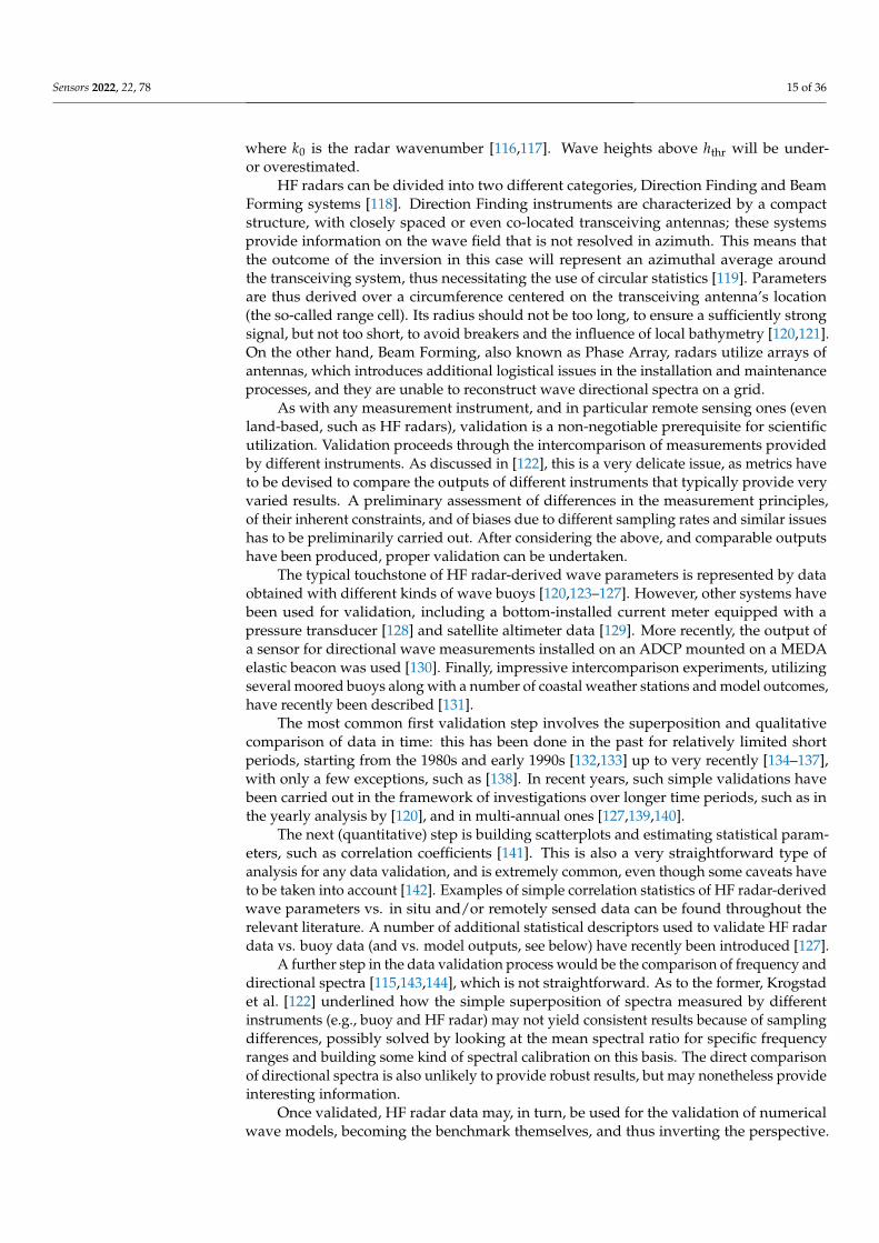
To give a few examples of some recent results and applications, Figure 6 showsthe results of a multiyear analysis carried out in the Gulf of Naples [127], where waveparameters were drawn from a network of three HF radar systems located in Portici,Castellammare and Sorrento (PORT, CAST and SORR in the map), utilizing data collectedbetween May 2008 and December 2012 from a 5 km-radius range cell (red arcs in the map).Validation data for the seasonal variability, spanning from November 2015 through toDecember 2018, were derived from a sensor for directional wave measurements installedon an Acoustic Doppler Current Profiler, itself mounted on a MEDA elastic beacon justoff the urban littoral of the city of Naples. The figure shows the modulation, in termsof direction and wave height, of the wave climate in the locations sampled, which showsite-specific differences due to the bathymetry and morphology of the Gulf. A strongseasonal variability in the parameters shows up quite clearly, with higher wave heights inautumn and winter, as can be expected on the basis of the local and regional meteorologicalconditions (as detailed and discussed in the paper).

Figure 6. Seasonal rose diagrams for the waves measured between May 2008 and December 2012by three HF radar stations installed in the Gulf of Naples, and between November 2015 and De-cember 2018 by an ADCP mounted on a MEDA elastic beacon: (a) winter; (b) spring; (c) summer;and (d) autumn (the maps show the locations of the different instruments and the extension of therange cell utilized around the radar antennas). Adapted from [127].

Sensors 2022, 22, 78 17 of 36

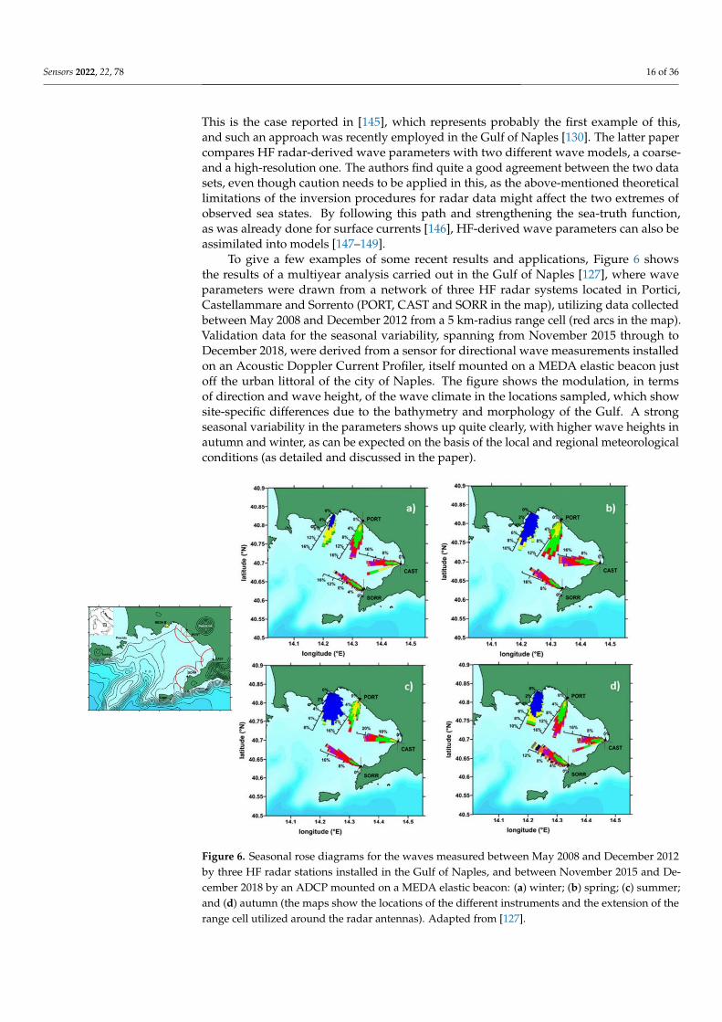
Figure 7 is an example of the use of HF radars during extreme events on the Spanishcoast [121]: it shows very good qualitative agreement between buoy and HF radar-derivedwave heights (SWH in the figure) in the course of two storms that occurred in 2017 and 2020(Figure 7). The grey shaded columns and the black line are the hourly sea surface height(SSH) and the meteorological tide recorded by a tide-gauge located in Tarragona (TG1),respectively; the blue line represents wave buoy measurements provided by a Seawatchinstrument deployed off Tarragona (B1); the red and green lines are the radar data derivedwith different versions of the proprietary manufacturer’s software used for the inversion(green line not present in the 2017 data). The pink dashed lines are the lower and upperlimits of wave height detection derived from the theoretical constraints discussed above.

Figure 7. Comparison of measurements collected by different instruments during two storms thatoccurred in 2017 and 2020 (adapted from [121]). The abbreviations in the plots are explained in themain text of this paper.

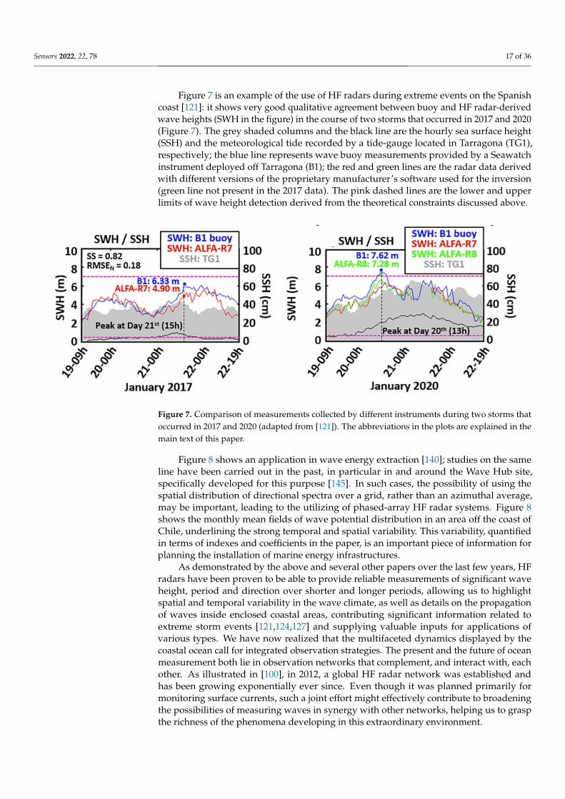
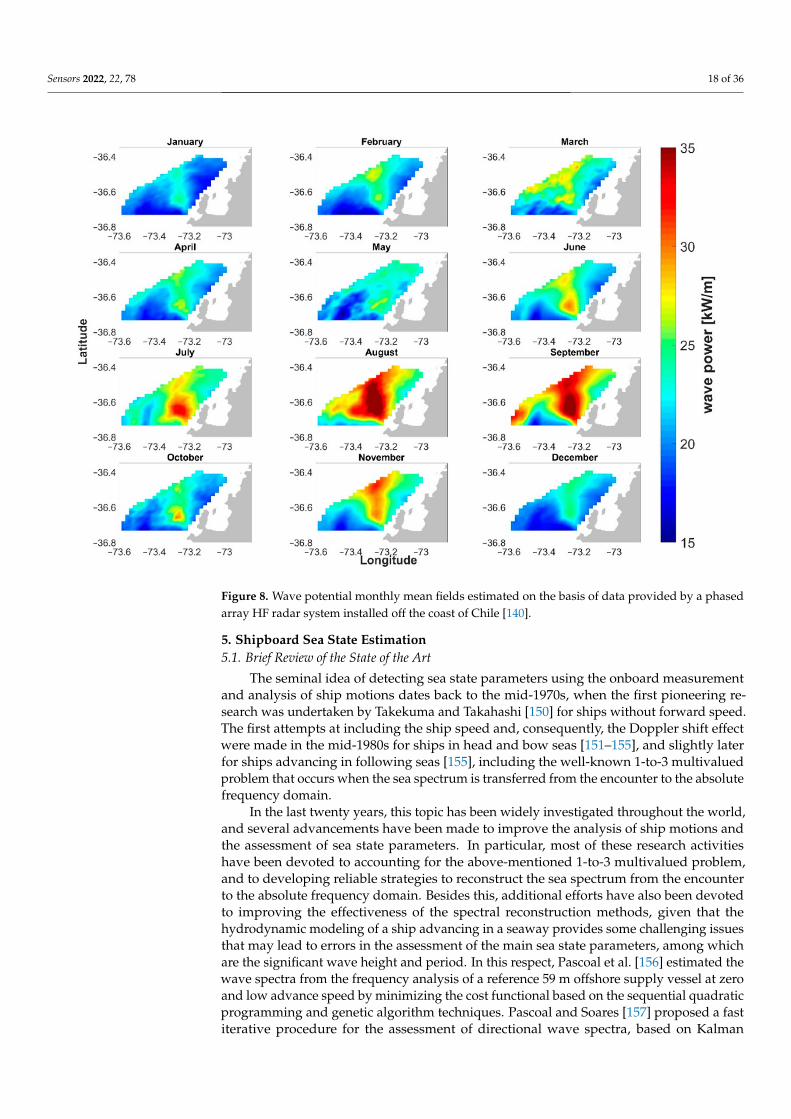
Figure 8 shows an application in wave energy extraction [140]; studies on the sameline have been carried out in the past, in particular in and around the Wave Hub site,specifically developed for this purpose [145]. In such cases, the possibility of using thespatial distribution of directional spectra over a grid, rather than an azimuthal average,may be important, leading to the utilizing of phased-array HF radar systems. Figure 8shows the monthly mean fields of wave potential distribution in an area off the coast ofChile, underlining the strong temporal and spatial variability. This variability, quantifiedin terms of indexes and coefficients in the paper, is an important piece of information forplanning the installation of marine energy infrastructures.

As demonstrated by the above and several other papers over the last few years, HFradars have been proven to be able to provide reliable measurements of significant waveheight, period and direction over shorter and longer periods, allowing us to highlightspatial and temporal variability in the wave climate, as well as details on the propagationof waves inside enclosed coastal areas, contributing significant information related toextreme storm events [121,124,127] and supplying valuable inputs for applications ofvarious types. We have now realized that the multifaceted dynamics displayed by thecoastal ocean call for integrated observation strategies. The present and the future of oceanmeasurement both lie in observation networks that complement, and interact with, eachother. As illustrated in [100], in 2012, a global HF radar network was established andhas been growing exponentially ever since. Even though it was planned primarily formonitoring surface currents, such a joint effort might effectively contribute to broadeningthe possibilities of measuring waves in synergy with other networks, helping us to graspthe richness of the phenomena developing in this extraordinary environment.

Sensors 2022, 22, 78 18 of 36

Figure 8. Wave potential monthly mean fields estimated on the basis of data provided by a phasedarray HF radar system installed off the coast of Chile [140].

5. Shipboard Sea State Estimation5.1. Brief Review of the State of the Art

The seminal idea of detecting sea state parameters using the onboard measurementand analysis of ship motions dates back to the mid-1970s, when the first pioneering re-search was undertaken by Takekuma and Takahashi [150] for ships without forward speed.The first attempts at including the ship speed and, consequently, the Doppler shift effectwere made in the mid-1980s for ships in head and bow seas [151–155], and slightly laterfor ships advancing in following seas [155], including the well-known 1-to-3 multivaluedproblem that occurs when the sea spectrum is transferred from the encounter to the absolutefrequency domain.

In the last twenty years, this topic has been widely investigated throughout the world,and several advancements have been made to improve the analysis of ship motions andthe assessment of sea state parameters. In particular, most of these research activitieshave been devoted to accounting for the above-mentioned 1-to-3 multivalued problem,and to developing reliable strategies to reconstruct the sea spectrum from the encounterto the absolute frequency domain. Besides this, additional efforts have also been devotedto improving the effectiveness of the spectral reconstruction methods, given that thehydrodynamic modeling of a ship advancing in a seaway provides some challenging issuesthat may lead to errors in the assessment of the main sea state parameters, among whichare the significant wave height and period. In this respect, Pascoal et al. [156] estimated thewave spectra from the frequency analysis of a reference 59 m offshore supply vessel at zeroand low advance speed by minimizing the cost functional based on the sequential quadraticprogramming and genetic algorithm techniques. Pascoal and Soares [157] proposed a fastiterative procedure for the assessment of directional wave spectra, based on Kalman

Sensors 2022, 22, 78 19 of 36

filtering, and applied it to a typical 70 m long vessel. Nielsen and Stredulinsky [158]analyzed a set of full-scale motion measurements, obtained during the sea trials conductedon the research vessel CFAV Quest, and compared the estimated sea state conditions againstthe relevant ones gathered by the wave radar processor Wave Monitoring System (WaMoS-II), installed on the considered vessel. Montazeri et al. [159] developed and applied asimplified parametric approach to estimate the wave parameters, based on the spectralmoments of resembled sea spectra and a partitioning method to separately estimate thewind and swell components. Nielsen [160] developed an improved method to transformthe wave spectrum from the encounter to the absolute frequency domain, consisting of twopseudo-algorithms, the former based on the spectral moments of the resembled spectra,the latter consisting of an optimization method, applied to a class of parametric spectra.Brodtkorb et al. [161] developed an online sea state assessment algorithm, based on theanalysis of heave, roll and pitch motions, with no a priori assumptions related to the wavespectrum shape. The algorithm was implemented in a dynamic positioning model andtested through real simulations under different sea state conditions. Piscopo et al. [162]developed a new wave spectrum reconstruction procedure, based on the combined analysisof heave and pitch motions, and tested it against a set of numerical simulations carried outon the reference S175 containership, with different sea state conditions, speeds and headingangles. Nielsen and Diez [163] compared the estimated sea state conditions, gatheredfrom an in-service containership, with the relevant values obtained from a hindcast study,and discussed some aspects concerning the effect of the vessel speed on the reliabilityof the measured data. Finally, Pennino et al. [164] applied a parametric wave spectrumresembling procedure to a set of real motion measurements, taken onboard the researchvessel “Laura Bassi” during an oceanographic campaign in the Antarctic Ocean carried outduring January and February 2020, and compared them against a set of weather forecastdata provided by the global-WAM model.

5.2. Methodology

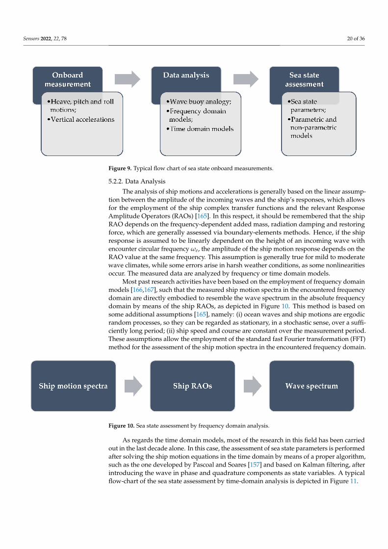
The employment of a vessel as a complex system capable of measuring sea stateconditions is encouraged by the variety of sensors and recording instruments, commonlyinstalled onboard modern ships, and capable of measuring the motion and accelerationsat specific points. In this respect, any vessel can be regarded as a “wave buoy” that,by means of a proper hydrodynamic model, can be employed to detect the main sea stateparameters, namely, the significant wave height, the wave peak period and the spectralshape, according to the flow-chart depicted in Figure 9, which is mainly based on threesubsequent steps: (i) onboard measurement of ship motions and accelerations; (ii) dataanalysis according to the wave buoy analogy by frequency or time-domain methods,and (iii) assessment of main sea state parameters by parametric or non-parametric models.Nevertheless, the wave buoy analogy still provides some challenging issues, mainly relatedto the complex hull forms that make the hydrodynamic modeling of a ship advancing in aseaway difficult, particularly when compared to a wave buoy, whose geometry is markedlysimpler. Furthermore, the ship advances in a seaway at a certain speed, which implies thatthe Doppler shift effect needs to considered. These topics will be outlined in the following.

5.2.1. Onboard Measurement

Ship motions and accelerations can be assessed by a variety of sensors, installedonboard the ship, or even by low-cost measurement systems, such as common smart-phones [164], which are generally equipped with several built-in sensors that provide rawdata at high sampling rates (i.e., motion sensors, accelerometers and gyroscopes). Thesedatasets can be analyzed separately or jointly in order to provide the time series of heave,pitch and roll motions to be further analyzed by means of the wave buoy analogy.

Sensors 2022, 22, 78 20 of 36

Figure 9. Typical flow chart of sea state onboard measurements.

5.2.2. Data Analysis

The analysis of ship motions and accelerations is generally based on the linear assump-tion between the amplitude of the incoming waves and the ship’s responses, which allowsfor the employment of the ship complex transfer functions and the relevant ResponseAmplitude Operators (RAOs) [165]. In this respect, it should be remembered that the shipRAO depends on the frequency-dependent added mass, radiation damping and restoringforce, which are generally assessed via boundary-elements methods. Hence, if the shipresponse is assumed to be linearly dependent on the height of an incoming wave withencounter circular frequency ωe, the amplitude of the ship motion response depends on theRAO value at the same frequency. This assumption is generally true for mild to moderatewave climates, while some errors arise in harsh weather conditions, as some nonlinearitiesoccur. The measured data are analyzed by frequency or time domain models.

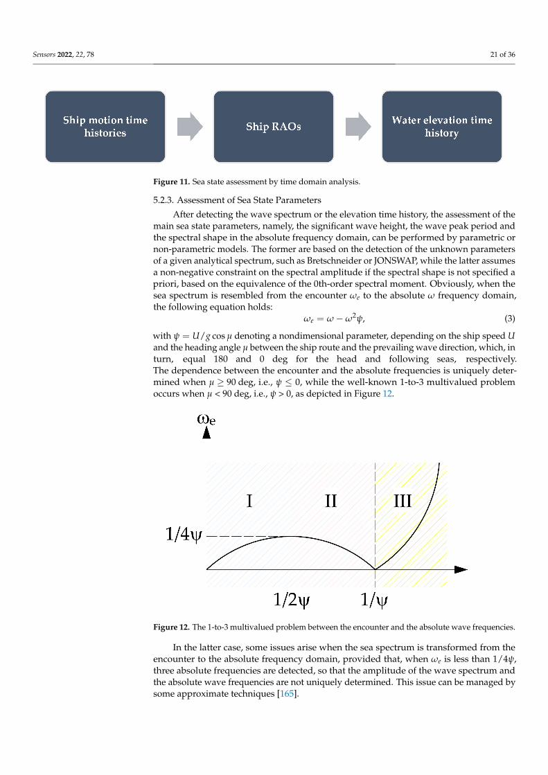
Most past research activities have been based on the employment of frequency domainmodels [166,167], such that the measured ship motion spectra in the encountered frequencydomain are directly embodied to resemble the wave spectrum in the absolute frequencydomain by means of the ship RAOs, as depicted in Figure 10. This method is based onsome additional assumptions [165], namely: (i) ocean waves and ship motions are ergodicrandom processes, so they can be regarded as stationary, in a stochastic sense, over a suffi-ciently long period; (ii) ship speed and course are constant over the measurement period.These assumptions allow the employment of the standard fast Fourier transformation (FFT)method for the assessment of the ship motion spectra in the encountered frequency domain.

Figure 10. Sea state assessment by frequency domain analysis.

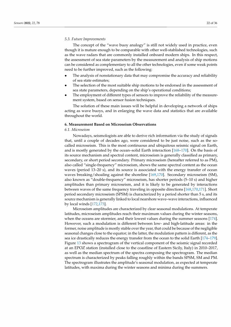
As regards the time domain models, most of the research in this field has been carriedout in the last decade alone. In this case, the assessment of sea state parameters is performedafter solving the ship motion equations in the time domain by means of a proper algorithm,such as the one developed by Pascoal and Soares [157] and based on Kalman filtering, afterintroducing the wave in phase and quadrature components as state variables. A typicalflow-chart of the sea state assessment by time-domain analysis is depicted in Figure 11.

Sensors 2022, 22, 78 21 of 36

Figure 11. Sea state assessment by time domain analysis.

5.2.3. Assessment of Sea State Parameters

After detecting the wave spectrum or the elevation time history, the assessment of themain sea state parameters, namely, the significant wave height, the wave peak period andthe spectral shape in the absolute frequency domain, can be performed by parametric ornon-parametric models. The former are based on the detection of the unknown parametersof a given analytical spectrum, such as Bretschneider or JONSWAP, while the latter assumesa non-negative constraint on the spectral amplitude if the spectral shape is not specified apriori, based on the equivalence of the 0th-order spectral moment. Obviously, when thesea spectrum is resembled from the encounter ωe to the absolute ω frequency domain,the following equation holds:

ωe = ω − ω2ψ, (3)

with ψ = U/g cos µ denoting a nondimensional parameter, depending on the ship speed Uand the heading angle µ between the ship route and the prevailing wave direction, which, inturn, equal 180 and 0 deg for the head and following seas, respectively.The dependence between the encounter and the absolute frequencies is uniquely deter-mined when µ ≥ 90 deg, i.e., ψ ≤ 0, while the well-known 1-to-3 multivalued problemoccurs when µ < 90 deg, i.e., ψ > 0, as depicted in Figure 12.

Figure 12. The 1-to-3 multivalued problem between the encounter and the absolute wave frequencies.

In the latter case, some issues arise when the sea spectrum is transformed from theencounter to the absolute frequency domain, provided that, when ωe is less than 1/4ψ,three absolute frequencies are detected, so that the amplitude of the wave spectrum andthe absolute wave frequencies are not uniquely determined. This issue can be managed bysome approximate techniques [165].

Sensors 2022, 22, 78 22 of 36

5.3. Future Improvements

The concept of the “wave buoy analogy” is still not widely used in practice, eventhough it is mature enough to be comparable with other well-stablished technologies, suchas the wave radars that are commonly installed onboard modern ships. In this respect,the assessment of sea state parameters by the measurement and analysis of ship motionscan be considered as complementary to all the other technologies, even if some weak pointsneed to be further improved, such as the following:

• The analysis of nonstationary data that may compromise the accuracy and reliabilityof sea state estimates;

• The selection of the most suitable ship motions to be endorsed in the assessment ofsea state parameters, depending on the ship’s operational conditions;

• The employment of different types of sensors to improve the reliability of the measure-ment system, based on sensor fusion techniques.

The solution of these main issues will be helpful in developing a network of shipsacting as wave buoys, and in enlarging the wave data and statistics that are availablethroughout the world.

6. Measurement Based on Microseism Observations6.1. Microseism

Nowadays, seismologists are able to derive rich information via the study of signalsthat, until a couple of decades ago, were considered to be just noise, such as the so-called microseism. This is the most continuous and ubiquitous seismic signal on Earth,and is mostly generated by the ocean–solid Earth interaction [168–170]. On the basis ofits source mechanism and spectral content, microseism is generally classified as primary,secondary, or short period secondary. Primary microseism (hereafter referred to as PM),also called “single-frequency” microseism, shows the same spectral content as the oceanwaves (period 13–20 s), and its source is associated with the energy transfer of oceanwaves breaking/shoaling against the shoreline [169,170]. Secondary microseism (SM),also known as “double-frequency” microseism, has shorter periods (5–10 s) and higheramplitudes than primary microseism, and it is likely to be generated by interactionsbetween waves of the same frequency traveling in opposite directions [168,170,171]. Shortperiod secondary microseism (SPSM) is characterized by a period shorter than 5 s, and itssource mechanism is generally linked to local nearshore wave–wave interactions, influencedby local winds [172,173].

Microseism amplitudes are characterized by clear seasonal modulations. At temperatelatitudes, microseism amplitudes reach their maximum values during the winter seasons,when the oceans are stormier, and their lowest values during the summer seasons [174].However, such a modulation is different between low- and high-latitude areas: in theformer, noise amplitude is mostly stable over the year, that could be because of the negligibleseasonal changes close to the equator; in the latter, the modulation pattern is different, as thesea ice drastically reduces the energy transfer from the ocean to the solid Earth [174–179].Figure 13 shows a spectrogram of the vertical component of the seismic signal recordedat an EPOZ station (installed close to the coastline of Eastern Sicily, Italy) in 2010–2017,as well as the median spectrum of the spectra composing the spectrogram. The medianspectrum is characterized by peaks falling roughly within the bands SPSM, SM and PM.The spectrogram illustrates the amplitude’s seasonal modulation, as expected at temperatelatitudes, with maxima during the winter seasons and minima during the summers.

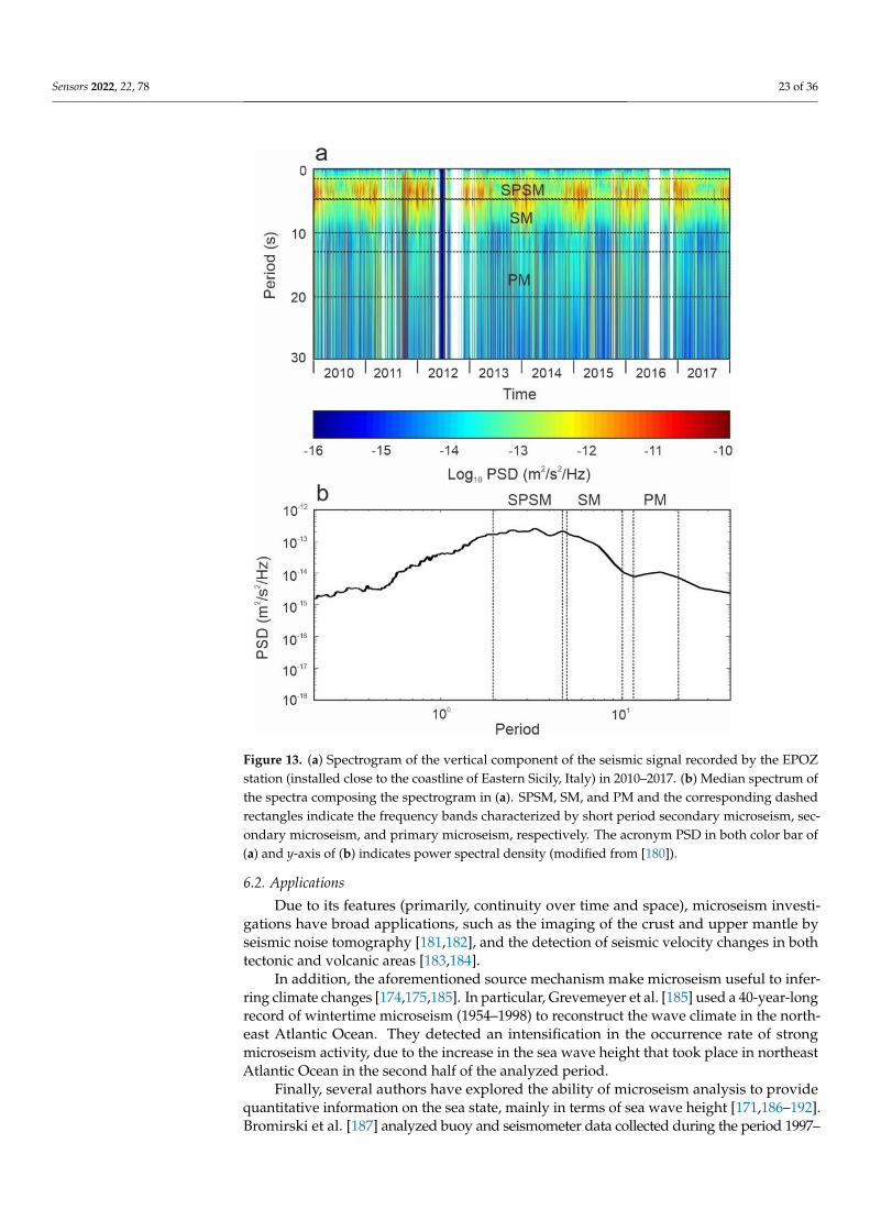
Sensors 2022, 22, 78 23 of 36

Figure 13. (a) Spectrogram of the vertical component of the seismic signal recorded by the EPOZstation (installed close to the coastline of Eastern Sicily, Italy) in 2010–2017. (b) Median spectrum ofthe spectra composing the spectrogram in (a). SPSM, SM, and PM and the corresponding dashedrectangles indicate the frequency bands characterized by short period secondary microseism, sec-ondary microseism, and primary microseism, respectively. The acronym PSD in both color bar of(a) and y-axis of (b) indicates power spectral density (modified from [180]).

6.2. Applications

Due to its features (primarily, continuity over time and space), microseism investi-gations have broad applications, such as the imaging of the crust and upper mantle byseismic noise tomography [181,182], and the detection of seismic velocity changes in bothtectonic and volcanic areas [183,184].

In addition, the aforementioned source mechanism make microseism useful to infer-ring climate changes [174,175,185]. In particular, Grevemeyer et al. [185] used a 40-year-longrecord of wintertime microseism (1954–1998) to reconstruct the wave climate in the north-east Atlantic Ocean. They detected an intensification in the occurrence rate of strongmicroseism activity, due to the increase in the sea wave height that took place in northeastAtlantic Ocean in the second half of the analyzed period.

Finally, several authors have explored the ability of microseism analysis to providequantitative information on the sea state, mainly in terms of sea wave height [171,186–192].Bromirski et al. [187] analyzed buoy and seismometer data collected during the period 1997–

Sensors 2022, 22, 78 24 of 36

1998 in California and derived site-specific seismic-to-wave transfer functions. Ferretti et al. [191]defined an automatic procedure, based mainly on a set of empirical relations [189,190],for estimating significant sea wave heights in near real-time from the spectral energycontent of the microseism, and presented an application in the Ligurian Sea (Italy). Otherauthors have applied a more physics-based approach to quantitatively link microseism andsea wave height [170,171,193,194]. Cannata et al. [180] analyzed the microseism recorded bysix seismic stations located close to the Eastern Sicilian coastline, and proposed a machinelearning-based approach to calculate a regression model for reconstructing the temporaland spatial variation in sea wave height using the microseism recorded at multiple seismicstations in different frequency bands.

Despite the good correlation found in these papers between microseism amplitudeand sea wave height, there are limitations [34,195]. First, the relation between thesephenomena can be time-varying. Indeed, in the case of secondary microseism, if theopposing waves are generated by coastal reflection, a particular relation is valid. How-ever, when the opposing waves are due to two uncorrelated wave systems, that relationis not valid anymore [34]. In addition, the locations of the microseism sources can bedifficult to determine, and so the wave parameters in a given location in the sea can bedifficult to define. This second issue can be solved using multiple sparse stations [192,196]or station arrays (that is, a certain number of seismic stations placed at discrete points in awell-defined configuration [197,198]).

6.3. Advantages of Microseism Monitoring

Microseism can be a valid complementary tool for monitoring sea wave activity.Indeed, although the microseism does not contain direct information on the sea state,and there could be limitations in deriving sea wave data from the microseism (see Section 6.2),there are several advantages. First of all, seismic stations have lower costs of both in-stallation and maintenance compared to other instruments routinely used for sea wavemonitoring. In addition, microseism is recorded continuously with a sampling frequencyfrom tens to hundreds of Hz and is acquired at a very high temporal resolution. The spatialresolution depends on the number of stations installed close to the coastline [180]. Further-more, in most areas, it is not necessary to install a seismic network specifically to recordthe microseism and then for sea wave height monitoring, but it is possible to use the seis-mic stations installed to monitor seismic and volcanic activities. In particular, broadbandseismometers (that is, seismometers able to detect very weak ground motions over a widefrequency band, which extends from tens of seconds to tens of Hz) installed worldwide arevery useful for microseism studies, as they record the whole microseism band [175,176].Finally, as seismometers were among the first geophysical instruments to be installed onEarth, one of the greatest areas of interest regards the possibility of deriving very long timeseries of microseism amplitude, which could highlight the long term variability in sea waveactivity [34,184].

7. Networks for Sea Wave Monitoring7.1. The Added Value of Networking for Marine Weather Forecasting

The variability in sea wave conditions can greatly affect marine operations, off-shoreand coastal infrastructures, and environmental aspects. This may be relevant to climaticpatterns associated with large-scale currents, and to the parameterization of air–sea flows.For all these reasons, the required spatial and temporal resolutions necessitate extendednetworks of homogeneous sensors. Long time series of systematic and simultaneousobservations (at the surface, in the water column, or at stations onshore), carried out withthe goal of collecting wave data at sufficient spatial and temporal densities, are crucial toocean exploitation.

For hundreds of years, collections of visual estimates of sea waves have been used toderive wave statistics, based on the appearance of the surface of the sea with reference tothe Beaufort scale. These have been suitable for use by marine officers and for producing

Sensors 2022, 22, 78 25 of 36

climate summaries on a global scale, such as the U.S. Navy Marine Climatic Atlas of theWorld or the UK Marine Data Bank. These atlases of ocean weather observations havelong been the only global source of observed data, and are also used for design purposes.Starting from this information, it was also possible to organize continuing and readilyaccessible archives of global climate information, such as the International Comprehen-sive Ocean Atmosphere Data Set (ICOADS) [199,200]. Nowadays, numerical modelingand satellite missions—the main sources of wave information at the global scale [201]—are combined with in situ data for calibration and validation [202–204]. To meet theseneeds, the design and maintenance of real-time sea wave monitoring networks is an es-sential activity in any monitoring program. The observations derived from moored buoysare considered to be better quality than ship observations with regard to the accuracyand reliability of measurements [205,206]. Other techniques are presented in this paper.It is clear that, in order to effectively describe the state of the sea, a system is needed thatintegrates in situ and remote observations with numerical modeling in order to achievethe spatial and temporal resolution that the description of such a complex phenomenonrequires. In fact, if the numerical models can meet the need for continuous data over timeand with a high spatial resolution, a fundamental aspect in the development of a model isthe verification of the reliability of the predictions of the model itself, because this outlinesthe behavior of the model in different meteorological situations, highlighting its systematiccharacteristics and assessing its reliability, under both average and extreme conditions,long periods and in the current situation. A good verification system allows one to not onlyunderstand where to intervene to make improvements, but above all, it allows for the bestuse to be made of the fields provided by the model according to the forecast objective.

7.2. Standards for Design and Management of a Sea-Waves Monitoring Network

There are specific criteria for the design of a network, depending on the purpose of themonitoring, related to specialized operators who conduct monitoring activities and possessspecific training and experience. Generally, most sea wave networks are managed bydifferent governmental entities in charge of national weather programs or environmentalmonitoring and protection programs; research centers mainly contribute to sampling anddata analysis. Observation systems are also used to provide commercial services, whichare sometimes dedicated to very restricted groups of users and are generally not composedof an observational network. The shared and integrated management of existing observingsystems would be preferable, in order to obtain a more efficient monitoring system.

The basic guidelines for designing meteorological observation networks, includingmarine wave monitoring networks, are provided by the WMO, the United Nations spe-cialized agency for international cooperation and coordination in the observation of theEarth’s atmosphere and its interactions with the land, oceans, weather, and climate itproduces [207]. The objective of the WMO is to support the meteorological activities of theMember States through the definition of good practices in the field of meteorological obser-vations, to promote an adequate level of uniformity and standardization in the practicesand procedures used for the measurements, and to facilitate cooperation in observations.The WMO Integrated Global Observing System (WIGOS) addresses the observation needsof the WMO, including the main areas of the standardization of observation tools andmethods, related metadata, and file formats. It provides an overview of all operatingsystems for the matrixes associated with the Earth’s atmosphere; moreover, it contributesto the co-sponsored observation systems supporting the activities of the WMO [208,209].The observations collected are subjected to quality controls according to the technicalstandards defined by the WMO Instruments and Methods of Observation Program (IMOP)and subsequently made public through the WMO Information System (WIS).

The Intergovernmental Oceanographic Commission of UNESCO (IOC) is the organiza-tion responsible for marine science within the United Nations. The IOC allows the MemberStates to coordinate ocean research and services, as well as related activities regardingoceanographic measurements focused on sustained ocean observing and data manage-

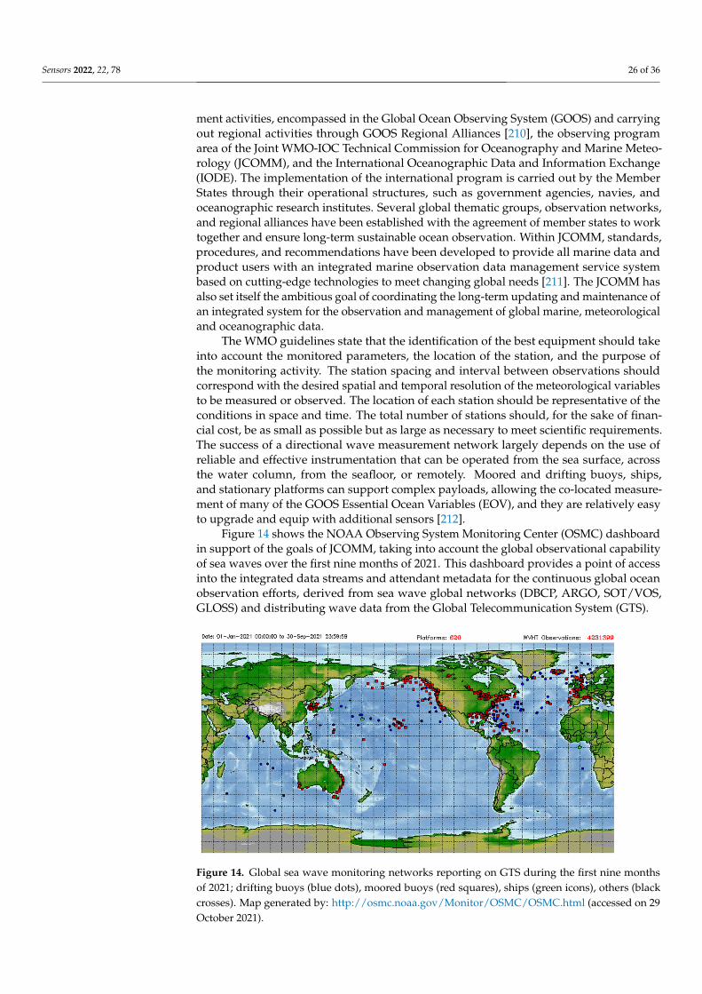
Sensors 2022, 22, 78 26 of 36

ment activities, encompassed in the Global Ocean Observing System (GOOS) and carryingout regional activities through GOOS Regional Alliances [210], the observing programarea of the Joint WMO-IOC Technical Commission for Oceanography and Marine Meteo-rology (JCOMM), and the International Oceanographic Data and Information Exchange(IODE). The implementation of the international program is carried out by the MemberStates through their operational structures, such as government agencies, navies, andoceanographic research institutes. Several global thematic groups, observation networks,and regional alliances have been established with the agreement of member states to worktogether and ensure long-term sustainable ocean observation. Within JCOMM, standards,procedures, and recommendations have been developed to provide all marine data andproduct users with an integrated marine observation data management service systembased on cutting-edge technologies to meet changing global needs [211]. The JCOMM hasalso set itself the ambitious goal of coordinating the long-term updating and maintenance ofan integrated system for the observation and management of global marine, meteorologicaland oceanographic data.

The WMO guidelines state that the identification of the best equipment should takeinto account the monitored parameters, the location of the station, and the purpose ofthe monitoring activity. The station spacing and interval between observations shouldcorrespond with the desired spatial and temporal resolution of the meteorological variablesto be measured or observed. The location of each station should be representative of theconditions in space and time. The total number of stations should, for the sake of finan-cial cost, be as small as possible but as large as necessary to meet scientific requirements.The success of a directional wave measurement network largely depends on the use ofreliable and effective instrumentation that can be operated from the sea surface, acrossthe water column, from the seafloor, or remotely. Moored and drifting buoys, ships,and stationary platforms can support complex payloads, allowing the co-located measure-ment of many of the GOOS Essential Ocean Variables (EOV), and they are relatively easyto upgrade and equip with additional sensors [212].

Figure 14 shows the NOAA Observing System Monitoring Center (OSMC) dashboardin support of the goals of JCOMM, taking into account the global observational capabilityof sea waves over the first nine months of 2021. This dashboard provides a point of accessinto the integrated data streams and attendant metadata for the continuous global oceanobservation efforts, derived from sea wave global networks (DBCP, ARGO, SOT/VOS,GLOSS) and distributing wave data from the Global Telecommunication System (GTS).

Figure 14. Global sea wave monitoring networks reporting on GTS during the first nine monthsof 2021; drifting buoys (blue dots), moored buoys (red squares), ships (green icons), others (blackcrosses). Map generated by: http://osmc.noaa.gov/Monitor/OSMC/OSMC.html (accessed on 29October 2021).

Sensors 2022, 22, 78 27 of 36

7.3. Globally Integrated Sea-Waves Monitoring Networks

Observing sea waves from drifting and moored buoys has a long history. Buoy projectsare now mature, and these technologies benefit from decades of field experience and in-ternational collaboration. The Data Buoy Cooperation Panel (DBCP) maintains a hugecatalog of wave buoy programs that supply data for operational and research purposes.The DBCP operates through the following action groups (and buoy programs): GlobalDrifter Program (GDP), Tropical Moored Buoy Implementation Panel (TAO/TRITON,PIRATA, RAMA), European EUCOS Surface Marine Programme (E-SURFMAR), Inter-national Arctic Buoy Programme (IABP), International South Atlantic Buoy Programme(ISABP), North Pacific Data Buoy Advisory Panel (NPDBAP), International Buoy Programfor the Indian Ocean (IBPIO), and International Programme for Antarctic Buoys (IPAB).The USA, Canada, Australia, Japan, and European countries are the major participants,but other countries with great potential to make contributions, such as India and China,are now joining in the cooperation.

The Lagrangian drifters deployed by GDP have been observing essential climatevariables (ECV) since 1979. The objective of GDP is to maintain a global array of sur-face drifting buoys (satellite-tracked) to meet the need for an accurate and dense setof in situ observations on a global scale. These EOV and ECV are essentially the near-surface currents, sea surface temperature, sea-level atmospheric pressure, winds, salinity,and waves [6]. The first generation of the GDP, the Surface Velocity Program (SVP), playedan important role in the TOGA program. The SVP drifters were the simplest version ofdrifters, and can only measure two parameters: ocean currents and sea surface temperature.With additional sensors, such as barometers, sonic anemometers, conductometers, and GPS,the performance of the drifters can be enhanced further to adapt to different applications.

The global tropical moored buoy arrays (TAO/TRITON, PIRATA, RAMA) are usedto monitor large-scale phenomena, such as El Niño and the Southern Oscillation (ENSO),showing the importance of the annual variability in the global climate. They are deployedat depths of up to 6000 m. Measurements taken by the mooring include surface variables,as well as subsurface temperatures down to a depth of 500 m [213]. The Tropical At-mosphere Ocean (TAO) and the Triangle Trans-Ocean Buoy Network the Pacific Ocean(TRITON) mooring array were successfully fielded to span the Pacific Ocean, with theimmediate ability to forecast El Nino phenomena up to a year ahead of their peak [214].TAO/TRITON was built over the ten-year period 1985–1994, and is presently supported bythe NOAA National Data Buoy Center and the Japan Agency for Marine Earth Science andTechnology. The Prediction and Research Moored Array in the Tropical Atlantic (PIRATA)was designed to study ocean–atmosphere interactions in the tropical Atlantic that affectregional weather and climate variability on seasonal, interannual, and longer time scales,and is motivated by the goal of understanding and better predicting certain phenom-ena, such as tropical Atlantic interannual to decadal variability and climate change [215].It was first established in the mid-1990s, and is supported by France (Meteo-France, CNRS,IFREMER), Brazil (INPE, DHN), and the USA (NOAA). The Research Moored Array forAfrican–Asian–Australian Monsoon Analysis and Prediction (RAMA) was designed tostudy the Indian Ocean’s role in monsoons. The array was initiated in 2004 and has sincegrown through the formation of new partnerships that currently include Indonesia, China,the USA, and the Bay of Bengal Large Marine Ecosystem (BOBLME) program.

The European EUCOS Surface Marine Programme (E-SURFMAR) is an optional pro-gram involving seventeen European meteorological services (Belgium, Croatia, Cyprus,Denmark, Finland, France, Germany, Greece, Iceland, Ireland, Italy, The Netherlands,Norway, Portugal, Spain, Sweden, and the United Kingdom) that coordinates, optimizesand progressively integrates the European meteorological services’ activities in surfaceobservations over the sea, including drifting and moored buoys, and voluntary observa-tional ships. The program is responsible for the coordination of buoy activities carriedout by the European meteorological services, and supports a Data Buoy Manager (DBM)to manage these activities [216,217]. In recent years, sea wave data from European research

Sensors 2022, 22, 78 28 of 36

and operational centers have also been made available through the Copernicus Marine(CMEMS) and EMODnet data portals, with increasing adherence to the emerging FAIRPrinciples for data publication.

The International Programme for Antarctic Buoys (IPAB) maintains collaborationamong national groups and international programs deploying buoys on the sea ice and anetwork of drifting buoys in the Southern Ocean.

The implementation of new assets must take into account the limits and potentialof each sea wave collection methodology in relation to the different purposes to whicha systematic monitoring activity can be oriented, as well as the essential activities of themaintenance, continuous testing, and evaluation of wave measurement systems. Most im-portantly, for a globally integrated ocean observation system, the necessary consensus hasnow been reached in the community of ocean observers to establish, grow and coordinateinternationally [218]. For regional (or national) observation systems in the coastal sector,the network requirements are considerably more demanding, because, while the range ofmeasurement technologies is the same, the density of the stations and their emphasis willbe greater [219,220].

The development of such integrated systems, which is crucial for the proper manage-ment and safety of both coastal areas and the open sea, must take into account a seriesof technological and scientific advances that have broadened the spectrum of platformsavailable to the scientific community and institutional stakeholders. The different method-ologies available must not be considered as in competition, but instead be thought of asconnected in a complementary way so as to be able to take full advantage of the strengthsof each. The goal is therefore the integration of all observations in order to monitor theessential parameters needed for a deeper understanding of the marine environment in theshort and long term.

8. Conclusions

Since sea waves have a great impact on human activities, accurate measurement andmonitoring at different geographical scales is a major goal at the international, nationaland local levels. There are several measurement techniques available, with differentdegrees of development and with, typically, complementary features. An ample selectionof such techniques, whose application is essential to meteorology, coastal safety, navigation,and renewable energy derived from the sea, has been here reviewed and includes buoys,satellite observation, coastal radars, shipboard observation, and microseism analysis. Aftera brief presentation of the measurement principle, the degree of development has beenoutlined, and future needs and trends have been prospected. Furthermore, it has beenstressed that the present and the future of ocean measurement lie in observation networksthat complement, and interact with, each other. In order to effectively describe the state ofthe sea, a system is needed that integrates in situ and remote observations with numericalmodeling in order to achieve the spatial and temporal resolution that the description ofsuch a complex phenomenon requires.

Author Contributions: Conceptualization, A.C., A.I., M.M., G.N., V.P., G.B.R., and E.Z.; supervision,G.B.R.; sections have been written as follows: Section 2, A.I. and G.N.; Section 3, M.M.; Section 4, EZ;Section 5, V.P., Section 6, A.C.; Section 7, G.N. and A.I.; writing, A.C., A.I., M.M., G.N., V.P., G.B.R.,and E.Z. All authors have read and agreed to the published version of the manuscript.

Funding: A.C. and G.N. thank the i-waveNET project, funded by the Interreg Italia-Malta Programme(notice 2/2019 Axis 3; project code C2-3.2-106).

Acknowledgments: The authors want to thank two anonymous reviewers, whose comments wereuseful to improve the paper.

Conflicts of Interest: The authors declare no conflict of interest.

Sensors 2022, 22, 78 29 of 36

References1. Longuet-Higgins, M.S. On the distribution of the heights of sea waves: Some effects of nonlinearity and finite band width.

J. Geophys. Res. 1980, 85, 1519–1523. [CrossRef]2. Rossi, G.B.; Crenna, F.; Berardengo, M.; Piscopo, V.; Scamardella, A. Investigation on Spectrum Estimation Methods for Bimodal

Sea State Conditions. Sensors 2021, 21, 2995. [CrossRef]3. Berardengo, M.; Rossi, G.B.; Crenna, F. Sea Spectral Estimation Using ARMA Models. Sensors 2021, 21, 4280. [CrossRef]4. Swail, V.; Jensen, R.; Lee, B.; Turton, J.; Thomas, J.; Gulev, S.; Yelland, M. Wave measurements, needs and developments the next

decade. In Proceedings of the OceanObs’09: Sustained Ocean Observations and Information for Society, European Space Agency,Venice, Italy, 21–25 September 2009.

5. Kuik, A.J.; Ph van Vledder, G.; Holthuijsen, L.H. A Method for the Routine Analysis of Pitch-and-Roll Buoy Wave Data.J. Phys. Oceanogr. 1988, 18, 1020–1034. [CrossRef]

6. Centurioni, L.; Horányi, A.; Cardinali, C.; Charpentier, E.; Lumpkin, R. A global ocean observing system for measuring sea levelatmospheric pressure: Effects and impacts on numerical weather prediction. Bull. Am. Meteorol. Soc. (BAMS) 2017, 98, 231–238.[CrossRef]

7. Lumpkin, R.; Pazos, M. Measuring surface currents with Surface Velocity Program drifters: The instrument, its data, and somerecent results. In Lagrangian Analysis and Prediction of Coastal and Ocean Dynamics (LAPCOD); Griffa, A., Kirwan, A.D., Mariano,A.J., Özgökmen, T., Rossby, H.T., Eds.; Cambridge University Press: Cambridge, UK, 2007; Chapter 2; pp. 39–67.

8. Centurioni, L.; Braasch, L.; Di Lauro, E.; Contestabile, P.; De Leo, F.; Casotti, R.; Franco, L.; Vicinanza, D. A New Strategic WaveMeasurement Station off Naples Port Main Breakwater. In Proceedings of the 35th Conference on Coastal Engineering, Antalya,Turkey, 17–20 November 2016.

9. Nilsson, J.A.U.; Dobricic, S.; Pinardi, N.; Taillandier, V.; Poulain, P.M. On the assessment of Argo float trajectory assimilation inthe Mediterranean Forecasting System. Ocean. Dyn. 2011, 61, 1475–1490. [CrossRef] [PubMed]

10. D’Asaro, E. Surface Wave Measurements from Subsurface Floats. J. Atmos. Ocean. Technol. 2015, 32, 816–827. [CrossRef]11. Wadhams, P.; Comiso, J.C.; Prussen, E.; Wells, S.; Brandon, M.; Aldworth, E.; Viehoff, T.; Allegrino, R.; Crane, D.R.

The development of the Odden ice tongue in the Greenland Sea during winter 1993 from remote sensing and field observations.J. Geophys. Res. Ocean. 1996, 101, 18213–18235. [CrossRef]

12. Liao, Z.; Cheng, B.; Zhao, J.; Vihma, T.; Jackson, K.; Yang, Q.; Yang, Y.; Zhang, L.; Li, Z.; Qiu, Y.; et al. Snow depth and ice thicknessderived from SIMBA ice mass balance buoy data using an automated algorithm. Int. J. Digit. Earth 2019, 12, 962–979.

13. Jackson, K.; Wilkinson, J. A novel and low-cost sea ice mass balance buoy. J. Atmos. Ocean. Technol. 2013, 30, 2676–2688. [CrossRef]14. Nicolaus, M.; Hoppmann, M.; Arndt, S.; Hendricks, S.; Katlein, C.; Nicolaus, A.; Rossmann, L.; Schiller, M.; Schwegmann, S.

Snow depth and air temperature seasonality on sea ice derived from snow buoy measurements. Front. Mar. Sci. 2021, 8, 655446.[CrossRef]

15. Voermans, J.; Rabault, J.; Filchuk, K.; Ryzhov, I.; Heil, P.; Marchenko, A.; Collins, C.; Dabboor, M.; Sutherland, G.; Babanin, A.Experimental evidence for a universal threshold characterizing wave-induced sea ice break-up. Cryosphere 2020, 14, 4265–4278.[CrossRef]

16. Meldrum, D.T. Recent developments at Dunstaffnage: The GPS-Argos drifter, the smart buoy and the mini drifter. In Proceedingsof the IEEE Sixth Working Conference on Current Measurement, San Diego, CA, USA, 13 March 1999; pp. 75–81.

17. O’Reilly, W.C.; Herbers, T.H.C.; Seymour, R.J.; Guza, R.T. A comparison of directional buoy and fixed platform measurements ofPacific swell. J. Atmos. Ocean. Technol. 1996, 13, 231–238. [CrossRef]

18. Bidlot, J.R.; Holmes, D.J.; Wittmann, P.A.; Lalbeharry, R.; Chen, H.S. Intercomparison of the performance of operational oceanwave forecasting systems with buoy data. Weather Forecast. 2002, 17, 287–310. [CrossRef]

19. Cavaleri, L. Wave modelling: Missing the peaks. J. Phys. Oceanogr. 2009, 39, 2757–2778. [CrossRef]20. World Meteorological Organization. Guide to Wave Analysis and Forecasting, 2nd ed.; (WMO No. 702); WMO: Geneva, Switzerland,

1998; 159p.21. Brown, D.T. Mooring Systems. In Handbook of Offshore Engineering; Chakrabarti, S.K., Ed.; Elsevier: Amsterdam, The Netherlands,

2005; Chapter 8; pp. 663–708.22. Taft, B.; Teng, C.; Rutledge, T. Low load compliant mooring history and status update. In Proceedings of the OCEANS ’09

“Marine Technology for our Future: Global and Local Challenges”, New Orleans, LA, USA, 26–29 October 2009; pp. 1–9.23. Longuet-Higgins, M.S.; Cartwright, D.E.; Smith, N.D. Observations of the directional spectrum of sea waves using the motions of

a floating buoy. In Ocean Wave Spectra; Prentice-Hall: Englewood Cliffs, NJ, USA, 1963; pp. 111–136.24. Cartwright, D.H.; Smith, N.D. Buoy Techniques for Obtaining Directional Wave Spectra, Buoy Technology; Marine Technology Society:

Washington, DC, USA, 1964; pp. 112–121.25. Bowden, K.F.; White, R.A. Measurements of the orbital velocities of sea waves and their use in determining the directional

spectrum. Geophys. J. Int. 1966, 12, 33–54. [CrossRef]26. Barstow, S.F.; Bidlot, J.R.; Caires, S.; Donelan, M.A.; Drennan, W.M.; Dupuis, H.; Graber, H.; Green, J.; Grønlie, Ø.; Guérin, C.; et al.

Measuring and analysing the directional spectrum of ocean waves. COST Action 2005, 714, 465.27. Mitsuyasu, H.; Tasai, F.; Suhara, T.; Mizuno, S.; Ohkusu, M.; Honda, T.; Rikiishi, K. Observations of the directional spectrum of

ocean waves using a cloverleaf buoy. J. Phys. Oceanogr. 1975, 5, 750–760. [CrossRef]

Sensors 2022, 22, 78 30 of 36

28. Daidola, J.C.; Basar, N.S.; Reyling, C.J.; Johnson, F.M.; Walker, R.T. Worldwide buoy technology survey. In Coast Guard; Office ofResearch and Development: Washington, DC, USA, 1991; Volume 1.

29. Meindl, A. Guide to moored buoys and other ocean data acquisition systems. In IOC-WMO, Data buoy Cooperation Panel—TechnicalDocument No. 8; DBCP: Geneva, Switzerland, 1996.

30. Hasselmann, K.; Barnett, T.P.; Bouws, E.; Carlson, H.; Cartwright, D.E.; Enke, K.; Ewing, J.A.; Gienapp, H.; Hasselmann, D.E.;Kruseman, P.; et al. Measurements of wind-wave growth and swell decay during the Joint North Sea Wave Project (JONSWAP).Deutshe Hydrogr. Zeitchrift 1973, 8, 1–95.

31. Beniot, M. Practical Comparative Performance Survey of Methods Used for Estimating Directional Wave Spectra From Heave-Pitch-Roll Data. In Proceedings of the 23rd Conference on Coastal Engineering, Venice, Italy, 4–9 October 1992; pp. 62–75.

32. Earle, M. Nondirectional and Directional Wave Data Analysis Procedures (Report No. NDBC Technical Document 96-01); NationalOceanic and Atmospheric Administration (NOAA): Slidell, LU, USA, 1996.

33. Lygre, A.; Krogstad, H.E. Maximum Entropy Estimation of the Directional Distribution in Ocean Wave Spectra. J. Phys. Oceanogr.1986, 16, 2052–2060. [CrossRef]

34. Ardhuin, F.; Stopa, J.E.; Chapron, B.; Collard, F.; Husson, R.; Jensen, R.E.; Johannessen, J.; Mouche, A.; Passaro, M.;Quartly, G.D.; et al. Observing Sea States. Front. Mar. Sci. 2019, 6, 124. [CrossRef]

35. Collins, C.O., III; Lund, B.; Waseda, T.; Graber, H.C. On recording sea surface elevation with accelerometer buoys: Lessons fromITOP (2010). Ocean Dyn. 2014, 64, 895–904. [CrossRef]

36. O’Reilly, W.C. An Introduction to Directional Wave Observations. In Wave Sensor Technologies Workshop; Alliance for CoastalTechnologies: St Petersburg, FL, USA, 7–9 March 2007.

37. Long, R.B. The statistical evaluation of directional spectrum estimates derived from pitch/roll buoy data. J. Phys. Oceanogr. 1980,10, 944–952. [CrossRef]

38. Herber, T.H.C.; Elgar, S.; Guza, R.T. Directional spreading of waves in the nearshore. J. Geophys. Res. 1999, 104, 7683–7693.[CrossRef]

39. Steele, K.E.; Teng, C.-C.; Wang, D.W. Wave direction wave measurements using pitch-roll buoys. Ocean Eng. 1992, 19, 349–375.[CrossRef]

40. Bender, L.C.; Guinasso, N.L.; Walpert, J.N.; Howden, S.D. A comparison of two methods for determining wave heights from adiscus buoy with a strapped-down accelerometer. In Proceedings of the 11th International Workshop on Wave Hindcasting andForecasting, Halifax, NS, Canada, 18–23 October 2009.

41. Cavaleri, L.; Abdalla, S.; Benetazzo, A.; Bertotti, L.; Bidlot, J.R.; Breivik, O.; Carniel, S.; Jensen, R.E.; Portills-Yandun, J.; Rogers,W.E.; et al. Wave modelling in coastal and inner seas. Prog. Oceanogr. 2018, 167, 164–233. [CrossRef]

42. Jensen, R.E.; Swail, V.; Bouchard, R.H. Quantifying wave measurement differences in historical and present wave buoy systems.Ocean Dyn. 2021, 71, 731–755. [CrossRef]

43. Doong, D.J.; Lee, B.C.; Kao, C.C. Wave measurements using GPS velocity signals. Sensors 2011, 11, 1043–1058. [CrossRef][PubMed]

44. Joodaki, G.; Nahavandchi, H.; Cheng, K. Ocean wave measurement using GPS buoys. J. Geod. Sci. 2013, 3, 163–172. [CrossRef]45. Andrews, E.; Peach, L. Wave Monitoring Equipment Comparison: An Evaluation of Current and Emerging In-Situ Ocean Wave Monitoring

Technology; Department of Environment and Science: Brisbane, QLD, Australia, 2019.46. Herbers, T.H.C.; Jessen, P.F.; Janssen, T.T.; Colbert, D.B.; Mac Mahan, J.H. Observing Ocean Surface Waves with GPS-Tracked

Buoys. J. Atmos. Ocean. Technol. 2012, 29, 944–959. [CrossRef]47. Ulaby, F.T.; Moore, R.K.; Fung, A.K. Microwave Remote Sensing, Active and Passive; Artech House: Norwood, MA, USA, 1981.48. Fu, L.L.; Cazenave, A. (Eds.) Satellite Altimetry and Earth Sciences: A Handbook of Techniques and Applications; Academic Press:

Cambridge, MA, USA; Elsevier: Amsterdam, The Netherlands, 2001.49. Vignudelli, S.; Kostianoy, A.G.; Cipollini, P.; Benveniste, J. (Eds.) Coastal Altimetry; Springer: Berlin/Heidelberg, Germany, 2011.50. Cazenave, A.; Hamlinton, B.; Horwath, M.; Barletta, V.R.; Benveniste, J.; Chambers, D.; Döll, P.; Hogg, A.E.; Legeais, J.F.;

Merrifield, M.; et al. Observational Requirements for Long-term Monitoring of the Global Mean Sea Level and Its ComponentsOver the Altimetry Era. Front. Mar. Sci. 2019, 6, 582. [CrossRef]

51. International Altimetry Team. Altimetry for the future: Building on 25 years of progress. Adv. Space Res. 2021, 68, 319–363.[CrossRef]

52. Kerkmann, J. Review on Scatterometer Winds; Technical Memorandum, No. 3; EUMETSAT: Darmstadt, Germany, 1998.53. Migliaccio, M.; Reppucci, A. A Review of Sea Wind Vector Retrieval By Means of Microwave Remote Sensing. Proc. Eur.

Microw. Assoc. 2006, 2, 136–140.54. Long, D.G.; Mendel, J.M. Identifiability in Wind Estimation From Scatterometer Measurements. IEEE Trans. Geosci. Remote Sens.

1991, 29, 268–276. [CrossRef]55. Soffelen, A.; Portabella, M. On Bayesian Scatterometer Wind Inversion. IEEE Trans. Geosci. Remote Sens. 2006, 44, 1523–1533.

[CrossRef]56. Nielsen-Englyst, P.; Høyer, J.L.; Pedersen, L.T.; Gentemann, C.L.; Alerskans, E.; Block, T.; Donlon, C. Optimal Estimation of Sea

Surface Temperature from AMSR-E. Remote Sens. 2018, 10, 229. [CrossRef]57. Goodberlet, M.A.; Swift, C.T.; Wilkerson, J.C. Remote Sensing of Ocean Surface Winds with the Special Sensor Microwave/Imager.

J. Geophys. Res. 1989, 94, 14547–14555. [CrossRef]

Sensors 2022, 22, 78 31 of 36

58. Wentz, F.; Ricciardulli, L.; Rodriguez, E.; Stiles, B.; Bourassa, M.; Long, D.G.; Hoffman, R.N.; Stoffelen, A.; Verhoef, A.;O’Neill, L.W.; et al. Evaluating and Extending the Ocean Winds Data Climate Record. IEEE J. Sel. Top. Appl. Earth Obs. RemoteSens. 2017, 10, 2165–2185. [CrossRef] [PubMed]

59. Bourassa, M.A.; Meissner, T.; Cerovecki, I.; Chang, P.S.; Dong, X.; De Chiara, G.; Donlon, C.; Dukhovskoy, D.S.; Elya, J.;Fore, A.; et al. Remotely Sensed Winds and Wind Stresses for Marine Forecasting and Ocean Modeling. Front. Mar. Sci. 2019,6, 443. [CrossRef]

60. Moradi, I.; Franklin Evans, K.; McCarty, W.; Cordero-Fuentes, M.; Gelaro, R.; Black, R.A. Assimilation of Satellite MicrowaveObservations over the Rainbands of Tropical Cyclones. Mon. Weather Rev. 2020, 148, 4729–4745. [CrossRef]

61. Yueh, S.H.; Wilson, W.J.; Dinardo, S.J.; Li, F.K. Polarimetric Microwave Brightness Signatures of Ocean Wind Directions.IEEE Trans. Geosci. Remote Sens. 1999, 37, 949–959. [CrossRef]

62. Le Vine, D.M.; Dinnat, E.P.; Meissner, T.; Wentz, F.J.; Kao, H.-Y.; Lagerloef, G.; Lee, T. Status of Aquarius and Salinity Continuity.Remote Sens. 2018, 10, 1585. [CrossRef]

63. Font, J.; Camps, A.; Borges, A.; Martìn-Neira, M.; Boutin, J.; Reul, N.; Kerr, Y.H.; Hahne, A.; Mecklenburg, S. SMOS:The Challenging Sea Surface Salinity Measurement From Space. Proc. IEEE 2010, 98, 649–665. [CrossRef]

64. Kasilingam, D.P.; Shemdin, O.H. Models for Synthetic Aperture Radar Imaging of the Ocean: A Comparison. J. Geophys. Res.1990, 95, 16263–16276. [CrossRef]

65. Harger, R.O. The Synthetic Aperture Radar Image of Time-variant Scenes. Radio Sci. 1980, 15, 749–756. [CrossRef]66. Hasselmann, K.; Raney, R.K.; Plant, W.J.; Alpers, W.; Shuchman, R.A.; Lyzenga, D.R.; Rufenach, C.L.; Tucker, M.J. Theory of

Synthetic Aperture Radar Ocean Imaging: A MARSEN view. J. Geophys. Res. 1985, 90, 4659–4686. [CrossRef]67. Vachon, P.W.; Raney, R.K. Ocean waves and optimal SAR processing: Don’t adjust the focus! IEEE Trans. Geosci. Remote Sens.

1992, 30, 627–630. [CrossRef]68. Migliaccio, M.; Nunziata, F.; Buono, A. SAR Polarimetry for Sea Oil Slick Observation. Int. J. Remote Sens. 2015, 36, 3243–3273.

[CrossRef]69. Nunziata, F.; Migliaccio, M.; Brown, C.E. Reflection Symmetry for Polarimetric Observation of Man-made Metallic Targets at Sea.

IEEE J. Ocean Eng. 2012, 37, 384–394. [CrossRef]70. Raney, R.K. Theory and Measure of Certain Image Norms in SAR. IEEE Trans. Geosci. Remote Sens. 1985, 23, 343–348. [CrossRef]71. Delignon, Y.; Garello, R.; Hillion, A. A Statistical Characterization of Sea-State SAR Images. In Proceedings of the Conference

Proceedings on Engineering in the Ocean Environment, Washington, DC, USA, 24–26 September 1990.72. Migliaccio, M.; Huang, L.; Buono, A. SAR Speckle Dependence on Ocean Surface Wind Field. IEEE Trans. Geosci. Remote Sens.

2019, 57, 5447–5455. [CrossRef]73. Nunziata, F.; Gambardella, A.; Migliaccio, M. An Educational SAR Sea Surface Waves Simulator. Int. J. Remote Sens. 2008, 29,

3051–3066. [CrossRef]74. Hasselmann, K.; Alpers, W. The Response of Synthetic Aperture Radar To Ocean Surface Waves. In Wave Dynamics and Radio

Probing of The Ocean Surface; Phillips, O.M., Hasselmann, K., Eds.; Plenum Press: New York, NY, USA, 1986; pp. 393–402.75. Hasselmann, K.; Hasselmann, S. On the nonlinear mapping of an ocean wave spectrum into a SAR image spectrum and its

inversion. J. Geophys. Res. 1991, 96, 10713–10729. [CrossRef]76. Hasselmann, S.; Brüning Hasselmann, K.; Heimbach, P. An Improved Algorithm for the Retrieval of Ocean Wave Spectra from

Synthetic Aperture Radar Image Spectra. J. Geophys. Res. 1996, 101, 16615–16629. [CrossRef]77. Engen, G.; Johnsen, H. SAR-Ocean Wave Inversion Using Image Cross Spectra. IEEE Trans. Geosci. Remote Sens. 1995, 33,

1047–1056. [CrossRef]78. Bao, M.; Alpers, W. On the Cross Spectrum Between Individual-Look Synthetic Aperture Radar Images of Ocean Waves.

IEEE Trans. Geosci. Remote Sens. 1998, 36, 922–932.79. Li, H.; Chapron, B.; Mouche, A.; Stopa, J.E. A New Ocean SAR Cross-Spectral Parameter: Definition and Directional Property

Using the Global Sentinel-1 Measurements. J. Geophys. Res. 2019, 124, 1566–1577. [CrossRef]80. Li, H.; Stopa, J.E.; Mouche, A.; Zhang, B.; He, Y.; Chapron, B. Assessment of Ocean Wave Spectrum using Global Envisat/ASAR

Data and Hindcast Simulation. Remote Sens. Environ. 2021, 264, 1–13. [CrossRef]81. Hauser, D.; Tourain, C.; Hermozo, L.; Alraddawi, D.; Aouf, L.; Chapron, B.; Dalphinet, A.; Delaye, L.; Dalila, M.; Dormy, E.; et al.

New Observations From the SWIM Radar On-Board CFOSAT: Instrument Validation and Ocean Wave Measurement Assessment.IEEE Trans. Geosci. Remote Sens. 2021, 59, 5–26. [CrossRef]

82. Quach, B.; Glaser, Y.; Stopa, J.E.; Mouche, A.; Sadowski, P. Deep Learning for Predicting Significant Wave Height From SyntheticAperture Radar. IEEE Trans. Geosci. Remote Sens. 2021, 59, 1859–1867. [CrossRef]

83. Schuler, D.L.; Lee, J.S.; Kasilingam, D.; Pottier, E. Measurement of Ocean Surface Slopes and Wave Spectra using PolarimetricSAR Image Data. Remote Sens. Environ. 2004, 91, 198–211. [CrossRef]

84. He, Y.; Shen, H.; Perrie, W. Remote Sensing of Ocean Waves by Polarimetric SAR. J. Atmos. Ocean Technol. 2006, 23, 1768–1773.[CrossRef]

85. Zhang, B.; Perrie, W.; He, Y. Validation of RADARSAT-2 Fully Polarimetric SAR Measurements of Ocean Surface Waves.J. Geophys. Res. 2010, 115, 1–11. [CrossRef]

86. Shao, W.; Wang, J.; Li, X.; Sun, J. An Empirical Algorithm for Wave Retrieval from Co-Polarization X-Band SAR Imagery.Remote Sens. 2017, 9, 711. [CrossRef]

Sensors 2022, 22, 78 32 of 36

87. Pramudya, F.S.; Pan, J.; Devlin, A.T.; Lin, H. Enhanced Estimation of Significant Wave Height with Dual-Polarization Sentinel-1SAR Imagery. Remote Sens. 2021, 13, 124. [CrossRef]

88. Kerbaol, V.; Chapron, B.; Vachon, P.W. Analysis of ERS-1/2 Synthetic Aperture Radar Wave Mode Imagettes. J. Geophys. Res.1998, 103, 7833–7846. [CrossRef]

89. Grieco, G.; Lin, W.; Migliaccio, M.; Nirchio, F.; Portabella, M. Dependency of the Sentinel-1 azimuth wavelength cut-off onsignificant wave height and wind speed. Int. J. Remote Sens. 2016, 37, 5086–5104. [CrossRef]

90. Corcione, V.; Grieco, G.; Portabella, M.; Nunziata, F.; Migliaccio, M. A Novel Azimuth Cut-off Implementation to Retrieve SeaSurface Wind Speed from SAR Imagery. IEEE Trans. Geosci. Remote Sens. 2019, 57, 3331–3340. [CrossRef]

91. Stopa, J.E.; Ardhuin, F.; Chapron, B.; Collard, F. Estimating Wave Orbital Velocity through the Azimuth Cutoff from Space-BorneSatellites. J. Geophys. Res. 2015, 120, 7616–7634. [CrossRef]

92. Stopa, J.E.; Mouche, A. Significant Wave Heights from Sentinel-1 SAR: Validation and Applications. J. Geophys. Res. 2017, 122,1827–1848. [CrossRef]

93. Pleskachevsky, A.; Jacobsen, S.; Tings, B.; Schwarz, E. Estimation of Sea State from Sentinel-1 Synthetic Aperture Radar Imageryfor Maritime Situation Awareness. Int. J. Remote Sens. 2019, 40, 4104–4142. [CrossRef]

94. Vachon, P.W.; Campbell, J.W.M.; Gray, A.L.; Dobson, F.W. Validation of along-Track Interferometric SAR Measurements of OceanSurface Waves. IEEE Trans. Geosci. Remote Sens. 1999, 37, 150–162. [CrossRef]

95. Bao, M.; Alpers, W.; Brüning, C. A New Nonlinear Integral Transform Relating Ocean Wave Spectra to Phase Image Spectra of anAlong-Track Interferometric Synthetic Aperture Radar. IEEE Trans. Geosci. Remote Sens. 1999, 37, 461–466.

96. He, Y.; Alpers, W. On the Nonlinear Integral Transform of an Ocean Wave Spectrum into an Along-track Interferometric SyntheticAperture Radar Image Spectrum. J. Geophys. Res. 2003, 108, 1–9. [CrossRef]

97. Zhang, B.; Perrie, W.; He, Y. Remote Sensing of Ocean Waves by Along-track Interferometric Synthetic Aperture Radar.J. Geophys. Res. 2009, 114. [CrossRef]

98. Schulz-Stellenfleth, J.; Lehner, S. Ocean Wave Imaging Using an Airborne Single Pass Across-Track Interferometric SAR.IEEE Trans. Geosci. Remote Sens. 2001, 39, 38–45. [CrossRef]

99. Portilla-Yandún, J.; Valladares, C.; Violante-Carvalho, N. A Hybrid Physical-Statistical Algorithm for SAR Wave Spectra QualityAssessment. IEEE J. Sel. Top. Appl. Earth Obs. Remote Sens. 2019, 12, 3943–3948. [CrossRef]

100. Ferla, M.; Nardone, G.; Orasi, A.; Picone, M.; Zambianchi, E.; Falco, P. Sea-Monitoring Networks. In Measurement for the Sea,Supporting the Marine Environment and the Blue Economy; Daponte, P., Rossi, G.B., Piscopo, V., Eds.; Springer: Berlin/Heidelberg,Germany, 2021.

101. Crombie, D.D. Doppler spectrum of sea echo at 13.56 Mc./s. Nature 1955, 175, 681–682. [CrossRef]102. Barrick, D.E. Theory of HF and VHF propagation across the rough sea, 1, The effective surface impedance for a slightly rough

highly conducting medium at grazing incidence. Radio Sci. 1971, 6, 517–526. [CrossRef]103. Barrick, D.E. Theory of HF and VHF propagation across the rough sea, 2, Application to HF and VHF propagation above the sea.

Radio Sci. 1971, 6, 527–533. [CrossRef]104. Barrick, D.E. First-order theory and analysis of MF/HF/VHF scatter from the sea. IEEE Trans. Antennas Propag. 1972, 20, 2–10.

[CrossRef]105. Barrick, D.E. HF radio oceanography—A review. Bound. Layer Meteorol. 1978, 13, 23–43. [CrossRef]106. Barrick, D.E.; Evans, M.W.; Weber, B.L. Ocean surface currents mapped by radar. Science 1977, 198, 138–144. [CrossRef]107. Paduan, J.D.; Washburn, L. High-frequency radar observations of ocean surface currents. Annu. Rev. Mar. Sci. 2013, 5, 115–136.

[CrossRef]108. Barrick, D.E. Remote sensing of sea state by radar. In Proceedings of the Ocean 72-IEEE International Conference on Engineering

in the Ocean Environment, Newport, RI, USA, 13–15 September 1972; pp. 186–192.109. Barrick, D.E. Extraction of wave parameters from measured HF radar sea-echo Doppler spectra. Radio Sci. 1977, 12, 415–424.

[CrossRef]110. Barrick, D.E. The ocean waveheight nondirectional spectrum from inversion of the HF sea-echo Doppler spectrum.

Remote Sens. Environ. 1977, 6, 201–227. [CrossRef]111. Lipa, B. Derivation of directional ocean-wave spectra by integral inversion of second-order radar echoes. Radio Sci. 1977, 12,

425–434. [CrossRef]112. Lipa, B. Inversion of second-order radar echoes from the sea. J. Geophys. Res. Ocean. 1978, 83, 959–962. [CrossRef]113. Wyatt, L. The measurement of the ocean wave directional spectrum from HF radar Doppler spectra. Radio Sci. 1986, 21, 473–485.

[CrossRef]114. Toro, V.G.; Ocampo-Torres, F.J.; Osuna, P.; García-Nava, H.; Flores-Vidal, X.; Durazo, R. Analysis of fetch-limited wave growth

using high-frequency radars in the Gulf of Tehuantepec. Cienc. Mar. 2014, 40, 113–132. [CrossRef]115. Wyatt, L.R.; Green, J.J.; Middleditch, A. HF radar data quality requirements for wave measurement. Coast. Eng. 2011, 58, 327–336.

[CrossRef]116. Wyatt, L.R. An evaluation of wave parameters measured using a single HF radar system. Can. J. Remote Sens. 2002, 28, 205–218.

[CrossRef]

Sensors 2022, 22, 78 33 of 36

117. Piscopo, V.; Rossi, G.B.; Crenna, S.; Gaglione, S.; Scamardella, A.; Uttieri, M.; Zambianchi, E. Measurement of sea waves.In Measurement for the Sea, Supporting the Marine Environment and the Blue Economy; Daponte, P., Rossi, G.B., Piscopo, V., Eds.;Springer: Berlin/Heidelberg, Germany, 2021.

118. Rubio, A.; Mader, J.; Corgnati, L.; Mantovani, C.; Griffa, A.; Novellino, A.; Quentin, C.; Wyatt, L.; Schulz-Stellenfleth, J.;Horstmann, J.; et al. HF radar activity in European coastal seas: Next steps toward a pan-European HF radar network.Front. Mar. Sci. 2017, 4, 8. [CrossRef]

119. Ranalli, M.; Lagona, F.; Picone, M.; Zambianchi, E. Segmentation of sea current fields by cylindrical hidden Markov models:A composite likelihood approach. J. R. Stat. Soc. Ser. C (Appl. Stat.) 2018, 67, 575–598. [CrossRef]

120. Saviano, S.; Kalampokis, A.; Zambianchi, E.; Uttieri, M. A year-long assessment of wave measurements retrieved from an HFradar network in the Gulf of Naples (Tyrrhenian Sea, Western Mediterranean Sea). J. Oper. Oceanogr. 2019, 12, 1–15. [CrossRef]

121. Lorente, P.; Lin-Ye, J.; García-León, M.; Reyes, E.; Fernandes, M.; Sotillo, M.G.; Espino, M.; Ruiz, M.I.; Gracia, V.; Perez, S.; et al.On the Performance of High Frequency Radar in the Western Mediterranean During the Record-Breaking Storm Gloria.Front. Mar. Sci. 2021, 8, 645762. [CrossRef]

122. Krogstad, H.E.; Wolf, J.; Thompson, S.P.; Wyatt, L.R. Methods for intercomparison of wave measurements. Coast. Eng. 1999, 37,235–257. [CrossRef]

123. Atan, R.; Goggins, J.; Harnett, M.; Agostinho, P.; Nash, S. Assessment of wave characteristics and resource variability at a1/4-scale wave energy test site in Galway Bay using waverider and high frequency radar (CODAR) data. Ocean Eng. 2016, 117,272–291. [CrossRef]

124. Fernandes, M.; Fernandes, C.; Barroqueiro, T.; Agostinho, P.; Martins, N.; Alonso-Martirena, A. Extreme wave height events inAlgarve (Portugal): Comparison between HF radar systems and wave buoys. In Proceedings of the 5th Jornadas de EngenhariaHidrográfica, Lisboa, Portugal, 19–21 June 2018; pp. 1–5.

125. Cai, L.; Shang, S.; Wei, G.; He, Z.; Xie, Y.; Liu, K.; Zhou, T.; Chen, J.; Zhang, F.; Li, Y. Assessment of significant wave height in theTaiwan Strait measured by a single HF radar system. J. Atmos. Ocean Technol. 2019, 36, 1419–1432. [CrossRef]

126. Bué, I.; Semedo, Á.; Catalão, J. Evaluation of HF Radar Wave Measurements in Iberian Peninsula by Comparison with SatelliteAltimetry and in Situ Wave Buoy Observations. Remote Sens. 2020, 12, 3623. [CrossRef]

127. Saviano, S.; Cianelli, D.; Zambianchi, E.; Conversano, F.; Uttieri, M. An integrated reconstruction of the multiannual wave patternin the Gulf of Naples (South-Eastern Tyrrhenian Sea, Western Mediterranean Sea). J. Mar. Sci. Eng. 2020, 8, 372. [CrossRef]

128. Lipa, B.; Nyden, B. Directional wave information from the SeaSonde. IEEE J. Ocean. Eng. 2005, 30, 221–231. [CrossRef]129. Orasi, A.; Picone, M.; Drago, A.; Capodici, F.; Gauci, A.; Nardone, G.; Inghilesi, R.; Azzopardi, J.; Galea, A.; Ciraolo, G.; et al. HF

radar for wind waves measurements in the Malta-Sicily Channel. Measurement 2018, 128, 446–454. [CrossRef]130. Saviano, S.; De Leo, F.; Besio, G.; Zambianchi, E.; Uttieri, M. HF radar measurements of surface waves in the Gulf of Naples

(Southeastern Tyrrhenian Sea): Comparison with hindcast results at different scales. Front. Mar. Sci. 2020, 7, 492. [CrossRef]131. Sotillo, M.G.; Mourre, B.; Mestres, M.; Lorente, P.; Aznar, R.; García-León, M.; Liste, M.; Santana, A.; Espino, M.; Álvarez, E.

Evaluation of the operational CMEMS and coastal downstream ocean forecasting services during the storm Gloria (January 2020).Front. Mar. Sci. 2021, 8, 644525. [CrossRef]

132. Wyatt, L.; Venn, J.; Burrows, G.; Ponsford, A.; Moorhead, M.; van Heteren, J. HF radar measurements of ocean wave parametersduring NURWEC. IEEE J. Ocean Eng. 1986, 11, 219–234. [CrossRef]

133. Lipa, B.J.; Barrick, D.E.; Isaacson, J.; Lilleboe, P.M. CODAR wave measurements from a North Sea semisubmersible. IEEE J.Ocean. Eng. 1990, 15, 119–125. [CrossRef]

134. Falco, P.; Buonocore, B.; Cianelli, D.; De Luca, L.; Giordano, A.; Iermano, I.; Zambardino, G.; Zambianchi, E. Dynamics and seastate in the Gulf of Naples: Potential use of high-frequency radar data in an operational oceanographic context. J. Oper. Oceanogr.2016, 9 (Suppl. 1), s33–s45. [CrossRef]

135. Lopez, G.; Conley, D.C.; Greaves, D. Calibration, validation, and analysis of an empirical algorithm for the retrieval of wavespectra from HF radar sea echo. J. Atmos. Ocean Technol. 2016, 33, 245–261. [CrossRef]

136. Lopez, G.; Conley, D.C. Comparison of HF radar fields of directional wave spectra against in situ measurements at multiplelocations. J. Mar. Sci. Eng. 2019, 7, 271. [CrossRef]

137. Basañez, A.; Lorente, P.; Montero, P.; Álvarez-Fanjul, E.; Pérez-Muñuzuri, V. Quality Assessment and practical interpretation ofthe wave parameters estimated by HF Radars in NW Spain. Remote Sens. 2020, 12, 598. [CrossRef]

138. Long, R.M.; Barrick, D.E.; Largier, J.L.; Garfield, N. Wave observations from central California: SeaSonde systems and in situwave buoys. J. Sens. 2011, 2011, 728936. [CrossRef]

139. Lorente, P.; Basañez Mercader, A.; Piedracoba, S.; Pérez-Muñuzuri, V.; Montero, P.; Sotillo, M.G.; Álvarez-Fanjul, E. Long-termskill assessment of SeaSonde radar-derived wave parameters in the Galician coast (NW Spain). Int. J. Remote Sens. 2019, 40,9208–9236. [CrossRef]

140. Mundaca-Moraga, V.; Abarca-del-Rio, R.; Figueroa, D.; Morales, J. A Preliminary Study of Wave Energy Resource Using an HFMarine Radar, Application to an Eastern Southern Pacific Location: Advantages and Opportunities. Remote Sens. 2021, 13, 203.[CrossRef]

141. Thomson, R.E.; Emery, W.J. Data analysis methods in physical oceanography, 2nd ed.; Elsevier: Amsterdam, The Netherlands, 2014;p. 638.

Sensors 2022, 22, 78 34 of 36

142. Legates, D.R.; McCabe, G.J., Jr. Evaluating the use of “goodness-of-fit” measures in hydrologic and hydroclimatic modelvalidation. Water Resour. Res. 1999, 35, 233–241. [CrossRef]

143. Wyatt, L.R. Chapter 9—The IMOS Ocean Radar Facility, ACORN. In Coastal Ocean Observing Systems; Academic Press: London,UK, 2015.

144. Wyatt, L.R. High frequency radar applications in coastal monitoring, planning and engineering. Aust. J. Civ. Eng. 2014, 12, 1–15.[CrossRef]

145. Wyatt, L.R. Wave and tidal power measurement using HF radar. Int. Mar. Energy J. 2018, 1, 123–127. [CrossRef]146. Iermano, I.; Moore, A.M.; Zambianchi, E. Impacts of a 4-dimensional variational data assimilation in a coastal ocean model of

southern Tyrrhenian Sea. J. Mar. Syst. 2016, 154, 157–171. [CrossRef]147. Siddons, L.A. Data Assimilation of HF Radar Data into Coastal Wave Models. Ph.D. Thesis, University of Sheffield, Sheffield,

UK, 2007.148. Siddons, L.A.; Wyatt, L.R.; Wolf, J. Assimilation of HF radar data into the SWAN wave model. J. Mar. Syst. 2009, 77, 312–324.

[CrossRef]149. Waters, J.; Wyatt, L.R.; Wolf, J.; Hines, A. Data assimilation of partitioned HF radar wave data into WaveWatch III. Ocean Model.

2013, 72, 17–31. [CrossRef]150. Takekuma, K.; Takahashi, T. On the Evaluation of Sea Spectra Based on the Measured Ship Motions. Trans. West Jpn. Soc.

Nav. Archit. 1973, 45, 51–57.151. Isobe, M.; Kondo, K.; Horikawa, K. Extension of MLM for estimating directional wave spectrum. In Proceedings of the Symposium

on Description and Modeling of Directional Seas, Copenhagen, Denmark, 18–20 June 1984.152. Kobune, K.; Hashimoto, N. Estimation of directional spectra from the maximum entropy principle. In Proceedings of the 5th

International Offshore Mechanics and Arctic Engineering (OMAE) Symposium, Tokyo, Japan, 13–18 April 1986.153. Hirayama, T. Real-time estimation of sea spectra based on motions of a running ship. J. Kansai Soc. Nav. Archit. 1988, 204, 21–27.154. Iseki, T.; Ohtsu, K.; Fujino, M. A study on estimation of directional spectra based on ship motions. J. Jpn. Inst. Navig. 1982, 86,

179–188. [CrossRef]155. Iseki, T.; Ohtsu, K. Bayesian estimation of directional wave spectra based on ship motions. Control Eng. Pract. 2000, 8, 215–219.

[CrossRef]156. Pascoal, R.; Guedes Soares, C.; Sørensen, J. Ocean wave spectral estimation using vessel wave frequency motions. J. Offshore Mech.

Arct. Eng. 2007, 129, 90–96. [CrossRef]157. Pascoal, R.; Guedes Soares, C. Kalman filtering of vessel motions for ocean wave directional spectrum estimation. Ocean Eng.

2009, 36, 477–488. [CrossRef]158. Nielsen, U.D.; Stredulinksy, D.C. Sea state estimation from an advancing ship—A comparative study using sea trial data.

Appl. Ocean Res. 2012, 34, 33–44. [CrossRef]159. Montazeri, N.; Nielsen, U.D.; Jensen, J.J. Estimation of wind sea and swell using shipboard measurements—A refined parametric

modelling approach. Appl. Ocean Res. 2016, 54, 73–86. [CrossRef]160. Nielsen, U.D. Transformation of a wave energy spectrum from encounter to absolute domain when observing from an advancing

ship. Appl. Ocean Res. 2017, 69, 160–172. [CrossRef]161. Brodtkorb, A.H.; Nielsen, U.D.; Sørensen, A. Online wave estimation using vessel motion measurements. In Proceedings of the

11th IFAC Conference on Control Applications in Marine Systems, Robotics and Vehicles CAMS 2018, Opatija, Croatia, 10–12September 2018.

162. Piscopo, V.; Scamardella, A.; Gaglione, S. A new wave spectrum resembling procedure based on ship motion analysis. Ocean Eng.2020, 201, 107137. [CrossRef]

163. Nielsen, U.D.; Dietz, J. Ocean wave spectrum estimation using measured vessel motions from an in-service container ship.Mar. Struct. 2020, 69, 102682. [CrossRef]

164. Pennino, S.; Angrisano, A.; Della Corte, V.; Ferraioli, G.; Gaglione, S.; Innac, A.; Martellato, E.; Palumbo, P.; Piscopo, V.;Rotundi, A.; et al. Sea State Monitoring by Ship Motion Measurements Onboard a Research Ship in the Antarctic Waters. J. Mar.Sci. Eng. 2021, 9, 64. [CrossRef]

165. Nielsen, U.D. A concise account of techniques available for shipboard sea state estimation. Ocean Eng. 2017, 129, 352–362.[CrossRef]

166. Tannuri, E.A.; Sparano, J.V.; Simos, A.N.; Da Cruz, J.J. Estimating directional wave spectrum based on stationary ship motionmeasurements. Appl. Ocean Res. 2003, 25, 243–261. [CrossRef]

167. Nielsen, U.D. Estimations of on-site directional wave spectra from measured ship responses. Mar. Struct. 2006, 19, 33–69.[CrossRef]

168. Longuet-Higgins, M.S. A theory of the origin of microseisms: Philosophical Transactions of the Royal Society of London. Ser. AMath. Phys. Sci. 1950, 243, 1–35.

169. Hasselmann, K. A statistical analysis of the generation of microseisms. Rev. Geophys. 1963, 1, 177–210. [CrossRef]170. Ardhuin, F.; Gualtieri, L.; Stutzmann, E. How ocean waves rock the Earth: Two mechanisms explain microseisms with periods 3

to 300 s. Geophys. Res. Lett. 2015, 42, 765–772. [CrossRef]171. Ardhuin, F.; Balanche, A.; Stutzmann, E.; Obrebski, M. From seismic noise to ocean wave parameters: General methods and

validation. J. Geophys. Res. Ocean 2012, 117, C05002. [CrossRef]

Sensors 2022, 22, 78 35 of 36

172. Bromirski, P.D.; Duennebier, F.K.; Stephen, R.A. Mid-Ocean microseisms. Geochem. Geophys. Geosyst. 2005, 6, 1–19. [CrossRef]173. Chen, Y.N.; Gung, Y.; You, S.H.; Hung, S.H.; Chiao, L.Y.; Huang, T.Y.; Chen, Y.L.; Jan, S. Characteristics of short period secondary

microseisms (SPSM) in Taiwan: The influence of shallow ocean strait on SPSM. Geophys. Res. Lett. 2011, 38, L04305. [CrossRef]174. Aster, R.C.; McNamara, D.E.; Bromirski, P.D. Multidecadal climate-induced variability in microseisms. Seismol. Res. Lett. 2008, 79,

194–202. [CrossRef]175. Stutzmann, E.; Schimmel, M.; Patau, G.; Maggi, A. Global climate imprint on seismic noise. Geochem. Geophys. Geosyst. 2009,

10, Q11004. [CrossRef]176. Tsai, V.C.; McNamara, D.E. Quantifying the influence of sea ice on ocean microseism using observations from the Bering Sea,

Alaska. Geophys. Res. Lett. 2011, 38, L22502. [CrossRef]177. Anthony, R.E.; Aster, R.C.; Wiens, D.; Nyblade, A.; Anandakrishnan, S.; Huerta, A.; Winberry, J.P.; Rowe, C. The seismic noise

environment of Antarctica. Seismol. Res. Lett. 2015, 86, 89–100. [CrossRef]178. Anthony, R.E.; Aster, R.C.; McGrath, D. Links between atmosphere, ocean, and cryosphere from two decades of microseism

observations on the Antarctic Peninsula. J. Geophys. Res. Earth Surf. 2017, 122, 153–166. [CrossRef]179. Cannata, A.; Cannavò, F.; Moschella, S.; Gresta, S.; Spina, L. Exploring the link between microseism and sea ice in Antarctica by

using machine learning. Sci. Rep. 2019, 9, 1–15. [CrossRef] [PubMed]180. Cannata, A.; Cannavò, F.; Moschella, S.; Di Grazia, G.; Nardone, G.; Orasi, A.; Gresta, S. Unravelling the Relationship Between

Microseisms and Spatial Distribution of Sea Wave Height by Statistical and Machine Learning Approaches. Remote Sens. 2020,12, 761. [CrossRef]

181. Porritt, R.W.; Miller, M.S.; O’Driscoll, L.J.; Harris, C.W.; Roosmawati, N.; da Costa, L.T. Continent–arc collision in the Banda Arcimaged by ambient noise tomography. Earth Planet. Sci. Lett. 2016, 449, 246–258. [CrossRef]

182. Tamura, J.; Okada, T. Ambient noise tomography in the Naruko/Onikobe volcanic area, NE Japan: Implications for geofluids andseismic activity. Earth Planet Space 2016, 68, 5. [CrossRef]

183. Brenguier, F.; Campillo, M.; Takeda, T.; Aoki, Y.; Shapiro, N.M.; Briand, X.; Emoto, K.; Miyake, H. Mapping pressurized volcanicfluids from induced crustal seismic velocity drops. Science 2014, 345, 80–82. [CrossRef]

184. Cannata, A.; Cannavò, F.; Montalto, P.; Ercoli, M.; Mancinelli, P.; Pauselli, C.; Leto, G. Monitoring crustal changes at volcanoes byseismic noise interferometry: Mt. Etna case of study. J. Volcanol. Geotherm. Res. 2017, 337, 165–174. [CrossRef]

185. Grevemeyer, I.; Herber, R.; Essen, H.H. Microseismological evidence for a changing wave climate in the northeast Atlantic Ocean.Nature 2000, 408, 349–352. [CrossRef] [PubMed]

186. Zopf, D.O.; Creech, H.C.; Quinn, W.H. The wavemeter: A land-based system for measuring nearshore ocean waves. Mar. Technol.Soc. J. 1976, 10, 19–25.

187. Bromirski, P.D.; Flick, R.E.; Graham, N. Ocean wave height determined from inland seismometer data: Implications forinvestigating wave climate changes in the NE Pacific. J. Geophys. Res. Ocean. 1999, 104, 20753–20766. [CrossRef]

188. Bromirski, P.D.; Duennebier, F.K. The near-coastal microseism spectrum: Spatial and temporal wave climate relationships.J. Geophys. Res. Solid Earth 2002, 107, ESE 5-1–ESE 5-20. [CrossRef]

189. Ferretti, G.; Zunino, A.; Scafidi, D.; Barani, S.; Spallarossa, D. On microseisms recorded near the Ligurian coast (Italy) and theirrelationship with sea wave height. Geophys. J. Int. 2013, 194, 524–533. [CrossRef]

190. Ferretti, G.; Scafidi, D.; Cutroneo, L.; Gallino, S.; Capello, M. Applicability of an empirical law to predict significant sea-waveheights from microseisms along the Western Ligurian Coast (Italy). Cont. Shelf Res. 2016, 122, 36–42. [CrossRef]

191. Ferretti, G.; Barani, S.; Scafidi, D.; Capello, M.; Cutroneo, L.; Vagge, G.; Besio, G. Near real-time monitoring of significant seawave height through microseism recordings: An application in the Ligurian Sea (Italy). Ocean Coast. Manag. 2018, 165, 185–194.[CrossRef]

192. Moschella, S.; Cannata, A.; Cannavò, F.; Di Grazia, G.; Nardone, G.; Orasi, A.; Picone, M.; Ferla, M.; Gresta, S. Insights intomicroseism sources by array and machine learning techniques: Ionian and Tyrrhenian Sea case of study. Front. Earth Sci. 2020,8, 114. [CrossRef]

193. Gualtieri, L.; Stutzmann, E.; Capdeville, Y.; Ardhuin, F.; Schimmel, M.; Mangeney, A.; Morelli, A. Modelling secondarymicroseismic noise by normal mode summation. Geophys. J. Int. 2013, 193, 1732–1745. [CrossRef]

194. Gualtieri, L.; Stutzmann, E.; Juretzek, C.; Hadziioannou, C.; Ardhuin, F. Global scale analysis and modelling of primarymicroseisms. Geophys. J. Int. 2019, 218, 560–572. [CrossRef]

195. Daponte, P.; Rossi, G.B.; Piscopo, V. (Eds.) Measurement for the Sea; Springer: Berlin/Heidelberg, Germany, 2021; in press.196. Möllhoff, M.; Bean, C.J. Seismic noise characterization in proximity to strong microseism sources in the Northeast Atlantic.

Bull. Seismol. Soc. Am. 2016, 106, 464–477. [CrossRef]197. Gerstoft, P.; Fehler, M.C.; Sabra, K.G. When Katrina hit California. Geophys. Res. Lett. 2006, 33, L17308. [CrossRef]198. Pratt, M.J.; Wiens, D.A.; Winberry, J.P.; Anandakrishnan, S.; Euler, G.G. Implications of sea ice on Southern Ocean microseisms

detected by a seismic array in West Antarctica. Geophys. J. Int. 2017, 209, 492–507. [CrossRef]199. Woodruff, S.D.; Slutz, R.J.; Jenne, R.L.; Steurer, P.M. A Comprehensive Ocean-Atmosphere Data Set. Bull. Am. Meteorol. Soc. 1987,

68, 1239–1250. [CrossRef]200. Freeman, E.; Woodruff, S.D.; Worley, S.J.; Lubker, S.J.; Kent, E.C.; Angel, W.E.; Berry, D.I.; Brohan, P.; Eastman, R.; Gates, L.; et al.

ICOADS release 3.0: A major update to the historical marine climate record. Int. J. Climatol. 2017, 37, 2211–2232. [CrossRef]

Sensors 2022, 22, 78 36 of 36

201. Komen, G.J.; Cavaleri, L.; Donelan, M.; Hasselmann, K.; Hasselmann, S.; Janssen, P.A.E.M. Dynamics and Modelling of Ocean Waves;Cambridge University Press: Cambridge, UK, 1996.

202. Caires, S.; Sterl, A.; Bidlot, J.R.; Graham, N.; Swail, V. Intercomparison of Different Wind–Wave Reanalyses. J. Clim. 2004, 17,1893–1913. [CrossRef]

203. Ardhuin, F.; Magne, R.; Filipot, J.F.; van der Westhyusen, A.; Roland, A.; Quefeulou, P.; Lefèvre, J.M.; Aouf, L.; Babanin, A.;Collard, F. Semi-empirical dissipation source functions for wind-wave models: Part I, definition and calibration and validation atglobal scales. J. Phys. Oceanogr. 2010, 40, 1917–1941. [CrossRef]

204. Ribal, A.; Young, I.R. 33 years of globally calibrated wave height and wind speed data based on altimeter observations. Sci. Data2019, 6, 77. [CrossRef] [PubMed]

205. Wilkerson, J.C.; Earle, M.D. A study of differences between environmental reports by ships in the voluntary observing programmeand measurements from NOAA buoys. J. Geophys. Res. 1990, 95, 3373–3385. [CrossRef]

206. Ingleby, B. Factors affecting ship and buoy data quality: A data assimilation perspective. J. Atmos. Ocean Technol. 2010, 27,1476–1489. [CrossRef]

207. WMO-No. 8. WMO Guide to Meteorological Instruments and Methods of Observation—Vol. III—Observing Systems; WMO: Geneva,Switzerland, 2018.

208. WMO-No. 1160. Manual on the WMO Integrated Global Observing System; WMO: Geneva, Switzerland, 2019.209. WMO-No. 1165. Guide to the WMO Integrated Global Observing System; WMO: Geneva, Switzerland, 2019.210. Moltmann, T.; Turton, J.; Zhang, H.M.; Nolan, G.; Gouldman, C.; Griesbauer, L.; Willis, Z.; Piniella, Á.M.; Barrell, S.;

Andersson, E.; et al. A Global Ocean Observing System (GOOS), delivered through enhanced collaboration across regions,communities, and new technologies. Front. Mar. Sci. 2019, 6, 291. [CrossRef]

211. WMO-No. 1093. Executive Summary of the Abridged Final Report with Resolutions and Recommendations of the Fourth Session of theJoint WMO/IOC Technical Commission for Oceanography and Marine Meteorology; WMO: Geneva, Switzerland, 2012.

212. Centurioni, L.R.; Turton, J.; Lumpkin, R.; Braasch, L.; Brassington, G.; Chao, Y.; Charpentier, E.; Chen, Z.; Corlett, G.;Dohan, K.; et al. Global in situ Observations of Essential Climate and Ocean Variables at the Air–Sea Interface. Front. Mar. Sci.2019, 6, 419. [CrossRef]

213. McPhaden, M.J.; Ando, K.; Bourlès, B.; Freitag, H.P.; Lumpkin, R.; Masumoto, Y.; Murty, V.S.N.; Nobre, P.; Ravichandran, M.;Vialard, J.; et al. The global tropical moored buoy array. In Proceedings of the OceanObs’09: Sustained Ocean Observations andInformation for Society Conference, Venice, Italy, 21–25 September 2009; Hall, J., Harrison, D.E., Stammer, D., Eds.; EuropeanSpace Agency: Paris, France, 2009; Volume 2.

214. Lin, M.; Yang, C. Ocean Observation Technologies: A Review. Chin. J. Mech. Eng. 2020, 33, 32. [CrossRef]215. Foltz, G.R.; Brandt, P.; Richter, I.; Rodríguez-Fonseca, B.; Hernandez, F.; Dengler, M.; Rodrigues, R.R.; Schmidt, J.O.; Yu, L.;

Lefevre, N.; et al. The Tropical Atlantic Observing System. Front. Mar. Sci. 2019, 6, 206. [CrossRef]216. Poli, P.; Emzivat, G.; Blouch, P.; Férézou, R.; Cariou, A. Météo France/E-SURFMAR HRSST (re)calibration. In Proceedings of the

Scientific and Technical Workshop on Traceability of Drifter SST Measurements, La Jolla, CA, USA, 13–14 October 2016.217. Bencivenga, M.; Nardone, G.; Ruggiero, F.; Calore, D. The Italian Data Buoy Network (RON). Adv. Fluid Mech. IX 2012, 74,

321–332.218. Birkemeier, W.A.; Jensen, R.E.; Bernard, L.J.; Bouchard, R. IOOS wave observations, a national perspective. In Proceedings of the

OCEANS ‘12 MTS/IEEE: Harnessing the Power of the Ocean, Hampton Roads, VA, USA, 14–19 October 2012.219. O’Reilly, W.C.; McGehee, D.D. Design of Regional Wave Monitoring Networks: A Case Study for the Southern California Bight,

Miscellaneous Paper CERC; U.S. Army Corps of Engineers—Coastal Engineering Research Center: Washington, WA, USA, 1994.220. Bailey, K.; Steinberg, C.; Davies, C.; Galibert, G.; Hidas, M.; McManus, M.A.; Murphy, T.; Newton, J.; Roughan, M.; Schaeffer, A.

Coastal mooring observing networks and their data products: Recommendations for the next decade. Front. Mar. Sci. 2019, 6, 180.[CrossRef]