Modeling freak waves from the North Sea

A. Slunyaev a, E. Pelinovsky a, C. Guedes Soares b,*

a Institute of Applied Physics, Nizhny Novgorod, Russiab Unit of Marine Technology and Engineering, Technical University of Lisbon, Instituto Superior Tecnico, 1049-001 Lisboa, Portugal

Received 9 February 2005; revised 21 February 2005; accepted 3 April 2005

Available online 25 October 2005

Abstract

Four freak events registered in the North Sea during a storm are presented and studied. The spatial evolution of the freak waves backward and

forward wave propagation is simulated within the framework of the Dysthe equation. The lifetimes and travel distances of the freak waves are

determined based on the results of the simulations. The wave evolution predicted by the Dysthe model is compared with the simulations of the

nonlinear Schrodinger and kinematical equations. The contributions of the effects of the nonlinear self-focusing (Benjamin–Feir instability) and

quasi-linear wave grouping are discovered with the help of the nonlinear Schrodinger approximation and the linear theory. It is found that though

the Benjamin–Feir instability is important for the description of freak wave evolution, the significant wave enhancement by itself may be achieved

even in the linear approximation.

q 2005 Elsevier Ltd. All rights reserved.

Keywords: Benjamin–Feir instability; Dysthe equation; Schrodinger equation; Freak waves; Rogue waves; Abnormal waves

1. Introduction

The occurrence of freak waves in the sea is an exciting

problem of modern oceanography and naval architecture. This

phenomenon has become evident in recent years mainly due to

the increasing number of instrumental measurements of

abnormally high waves appearing at the background of a typical

wave motion. Determination of the extreme values of wave-

induced loads and the design of safe ships and offshore structures

are being considered as knowledge of possible extreme and freak

waves increases, as described in [14,19,31]. The increasing

attention to freak waves led to the development of different

approaches for understanding and describing the phenomenon;

they take into consideration strong currents, variable bathyme-

try, atmospheric fronts, dispersive and nonlinear properties of

water waves as described, for instance, in the review [24].

Since the information about freak waves is usually rather

poor and incomplete, the analysis of real ocean measurements

of freak events is needed. Various recent papers have presented

the analysis of extreme and abnormal waves recorded in

the North Sea [17,21,35], Japan Sea [27], and Black Sea [9],

0141-1187/$ - see front matter q 2005 Elsevier Ltd. All rights reserved.

doi:10.1016/j.apor.2005.04.002

* Corresponding author. Tel.: C351 218417607l; fax: C351 218474015.

E-mail addresses: slunyaev@hydro.appl.sci-nnov.ru (A. Slunyaev),

guedess@mar.ist.utl.pt (C. Guedes Soares).

the Gulf of Mexico [18] and off the coast of Taiwan [4].

Together with probabilistic analysis of the waves, their

kinematic and dynamic characteristics were investigated by

collecting them from full-scale wave measurements [4,17,27].

The expected structure of extreme waves was discussed in

Ref. [34]. Hypothetical freak waves were simulated numeri-

cally within the frameworks of various evolution equations: the

cubic nonlinear Schrodinger equation [29,30,36]; more

accurate second-order theory for weakly modulated surface

waves [28] based on the Dysthe equation [11,38]. The

Zakharov equation was used in Refs. [1,23] and fully nonlinear

models were adopted in Refs. [2,5,16,41].

Real measured time-series containing extremely high waves

were simulated in Ref. [38] within the frameworks of the

Dysthe equations and in Refs. [9,33] within the first-order

nonlinear Schrodinger theory. Freak events were also modeled

in laboratory tanks (see, for instance, papers [3,7,16,25]). The

linear theory was used in Ref. [3] to explain the experiment.

The description of modern models applied for the simulation of

freak waves may be found in the review [24].

The North Sea attracts great interest due to its large offshore

developments and intense ship traffic. The New Year Wave,

which was reported for the first time in Ref. [21], has become a

famous freak wave because it has been analyzed by a number of

authors. It was registered at the jacket platform Draupner in the

North Sea on January 1st, 1995 in a storm of significant wave

height around 12 m. This and other freak wave records made in

the North Sea at the North Alwyn platform in 1997 were studied

Applied Ocean Research 27 (2005) 12–22

www.elsevier.com/locate/apor

A. Slunyaev et al. / Applied Ocean Research 27 (2005) 12–22 13

in the recent paper [17]. The parameters of individual waves

were investigated and compared with the sea state character-

istics. It was shown that steepness might be very important for

the impact on the engineering structures [13,15,20] thus

demonstrating that the features of wave shapes are very relevant.

Determination of the main physical mechanisms that

generate real ocean freak waves is an extremely burning

problem. Four of the events from the North Alwyn are studied

in the present paper with the help of various numerical

simulation approaches, which allow the identification of the

effects of nonlinear wave instability and dispersive grouping.

Section 2 of the paper describes the measuring conditions and

the basic analysis of the main wave properties. Section 3 is

devoted to the numerical simulations of the spatial wave

dynamics within the frameworks of the Dysthe equation, the

nonlinear Schrodinger equation (NLS) and the kinematic

theory, which allow the determination of the lifetimes of the

freak waves. Aiming to see the role of effects of the nonlinear

wave self-focusing instability the records are analyzed by

applying the nonlinear Schrodinger equation approximation in

Fig. 1. (a)–(d) 20-minute

Section 4. The simulation of the spatial wave evolution within

the NLS equation is compared to the results given by the

Dysthe equation. The method of the inverse scattering problem

is applied to the measured time series; this technique helps to

find out the manifestation of the Benjamin–Feir instability-the

envelope solitary waves and to estimate the role on nonlinear

instability. In Section 5 the action of dispersive effects is

demonstrated using quasi-linear approach to the time series

analysis and direct numerical simulation within the framework

of the linear model. Results are collected in the conclusion.

2. Data analysis

The freak waves were registered in the North Alwyn fixed

steel jacket platform in the northern North Sea (1844 0 E 60845 0

N, depth 126 m) during the storm from the 16th to 22nd of

November 1997. During this storm several abnormal waves

were identified as reported in Ref. [17]. From these records

four were chosen for the present study and they are displayed

on Fig. 1 and will be used for further analysis. Each of them has

wave records 1–4.

Table 1

Record 1 2 3 4

Code of the record NA9711180110 NA9711200131 NA9711200151 NA9711200311

Date and time of the record 18, 01:10 20, 01:31 20, 01:51 20, 03:11

Hmax Maximum wave height (m) 16.4 17.6 18.2 17.8

Hs Significant wave height (m) 6.9 8.1 7.9 7.8

Hmax/Hs Amplification 2.38 2.18 2.31 2.29

Amax Maximum wave amplitude (m) 11.3 12.0 13.2 11.3

A0 Averaged wave amplitude (m) 1.4 1.7 1.6 1.5

A20 Averaged square wave amplitude (m) 1.8 2.1 2.0 2.0

u0 Cyclic frequency of the carrier wave (rad/s) 0.64 0.59 0.61 0.63

hT0 Wave period (s) 9.8 10.6 10.3 9.9

k0 Carrier wavenumber (rad/m) 0.042 0.036 0.038 0.041

L0 Wave length (m) 151 175 166 154

Tevent Time moment of the freak event occurrence (s) 731 369 375 789

A. Slunyaev et al. / Applied Ocean Research 27 (2005) 12–2214

20 min duration with the sampling interval equal to 5 Hz. The

freak events can be always well distinguished in the records

given in Fig. 1 and all are represented by a very large single

wave.

The frequencies of the carrier waves u0 found for the

records are given in Table 1. The dispersion relation for surface

water waves is

u Zffiffiffiffiffiffiffiffiffiffiffiffiffiffiffiffiffiffiffiffikg tanh kh

p; (1)

where g is the gravity acceleration, k is the wave number and h

is the depth. The typical depth parameter k0h is found equal to

3.6 and higher, therefore (1) may be taken in its deep-water

limit

u Zffiffiffiffiffikg

p: (2)

Other main characteristics of the whole 20-minute records

are given in Table 1.

The condition on the height amplification

Hmax=HsO2; (3)

will be used as a simple definition of a freak wave. All the

waves show the amplification greater than 2.1 (see Table 1).

The records have similar carrier wave lengths (151–175 m) and

wave heights. The freak wave periods correspond to typical

ones in the records. The group and phase velocities of the

carrier waves vary in intervals CgrZ7.5–8.4 m/s and CphZ14.9–16.5 m/s.

The mean wave steepness does not exceed 0.07 while the

maximum one (corresponding to the freak waves, k0Amax)

reaches up to 0.4 and higher what conforms to the condition of

breaking waves.

3. Numerical simulations

The instrumental records are made at one point and cannot

give information of the surface dynamics. Simulation of the

spatial wave evolution may be performed to complete the

information. This can only be done in the assumption of

unidirectional wave propagation. Although it is known that

transversal wave dynamics may lead to the huge wave

appearance [30,36], this assumption is natural for the one-point

wave measurements and cannot be escaped. The transversal

shape of the freak waves cannot be estimated on the basis of one-

point field measurements.

The wave field backward and forward wave propagation

may be found by using evolution models. The main

characteristic that may be found with such simulation is the

lifetime of the freak wave. The chance to see the forming freak

wave long before the freak event may be also estimated, as was

done in Ref. [38] for the New Year Wave.

The main model used for the wave simulations is the Dysthe

equation in space-domain formulation [11,38], which looks

like

Bx CiBtt CiBjBj2K8jBj2Bt K2B2B�t K4iB4t Z 0

4z ZKv

vtjBj2

at z Z 0;

8>>><>>>:

(4)

44tt C4zz Z 0; K�h!z!0;

4z Z 0; z ZK�h;

where the field B(x, t) and dimensionless variables x and t are

connected with physical surface displacement h(X, T) by the

formulae

k0hZB0 C1

2ðBeiðk0XKu0TÞCB2e2iðk0XKu0TÞCB3e3iðk0XKu0TÞCkcÞ;

B0 ZK4t;B2 Z1

2B2 CiBBt;B3 Z

3

8B3;

tZu0TK2k0X;xZk0X; zZk0Z; �hZk0�h:

ð5Þ

The Dysthe Eq. (4) contains the exact linear dispersion (2),

second order nonlinearity (corresponding to four wave

interactions) and terms of nonlinear dispersion. This equation

has become popular for water wave simulations due to its

relative simplicity compared with the primary equations

of water waves. The dynamics of bichromatic waves

described by the Dysthe equation was compared with the

experiment in Ref. [39] and it was estimated that the wave

A. Slunyaev et al. / Applied Ocean Research 27 (2005) 12–22 15

evolution of typical oceanic conditions can be well-described

by the Dysthe equation for distances up to about 50

wavelengths.

The simulation within the frameworks of the Dysthe model

is made in this paper following, in general, the work [38]. The

split-step Fourier code written is similar to the one of [26]. Due

to periodical boundary conditions the waves from the starting

and the ending parts of the records mix what does not happen in

reality. This means that the obtained evolution of the waves

Fig. 2. (a)–(d) Wave evolution computed within the fra

near the boundaries is wrong. The domain of this mixing is

specified by the difference of the wave speeds from the group

velocity of the carrier wave. Typically the local frequency

(defined by several individual waves) in the records varies over

a range with a factor of two between extremes, therefore the

boundary mixing domain may be estimated as TboundZX/

Cgrz500/8Z62.5 s, where XZ500 m is the computation

domain, and Cgrz8 m/s is the typical group velocity of the

waves in the records. This problem should not influence

meworks of the Dysthe equation (for records 1–4).

Fig. 2 (continued)

A. Slunyaev et al. / Applied Ocean Research 27 (2005) 12–2216

the simulation of the freak waves, since they are away from the

boundaries of the time series (see Table 1).

The measured wave field is recalculated 500 m upstream

and downstream with the help of the Dysthe Eq. (4) in a way

similar to [38]. The invariant transformation of the Dysthe

equation x/Kx, t/Kt, B/B* is used to inverse the time

and to find the evolution upstream. This distance (1000 m)

corresponds to 6–7 wavelengths; the carrier wave runs it for

about 2 min. Such distance lies well in the interval of

applicability of the Dysthe equation mentioned above. The

computed evolution is given in Fig. 2. The point XZ0

corresponds to the experimental record, X!0—upstream, XO0—downstream. The images are qualitatively similar for all the

cases. It is seen that the trains corresponding the freak wave are

wider before and after the event and a little bit slower than the

carrier wave.

Since the amplitude criterion (3) is usually used for the

definition of a freak wave, the evolution of the maximum

wave height in space is considered more precisely. Such

dependence is given in Fig. 3 for record 1 (thick solid line).

The curves for other records look qualitatively similar and are

not given.

Fig. 3. Maximum wave height versus distance computed in numerical simulations for three approaches (linear (dashed line), NLS (thin solid line) and Dysthe (thick

solid line)) for record 1.

A. Slunyaev et al. / Applied Ocean Research 27 (2005) 12–22 17

The peak value of Hmax at XZ0 for the Dysthe model on

Fig. 3 is lower than the measured value because of the spectral

cutting (using the bandpass) when initializing the compu-

tations. The input field for the Dysthe model is B(x, t) which

should be found from h(X, T) (see (5)). This is done with the

help of an iterative procedure, when the domain of the spectral

coincidence of the original (measured) and reconstructed

(found from the obtained function B(x, t) by formulae (5))

fields is defined. The bandpass was chosen to be [0, 3u0],

where u0 is the cyclic frequency of the carrier wave. So, the

spectra of the measured and the simulated waves coincide in

this interval. The way of the spectral cutting is not unique and

may lead to the change of the wave dynamics. This problem

was discussed in Ref. [37]. The spectral cutting causes the

diminishing of the amplitudes of the steepest waves and

contradicts the desire to describe steep wave heights. The

simulation made for record 1 was compared with one when the

bandpass was chosen [0, 2u0]. It was found that the dynamics

of maximum wave heights agrees rather well (except for the

times of the peak freak heights).

The travel distance (Ltr) and lifetime (TlifeZLtr/Cgr) of the

freak waves are determined by the results of the simulations.

As the criterion determining when the wave is freak the

condition (3) is used. The results are given in Table 2.

It is seen from Table 2 that the lifetime varies from several

seconds up to almost a minute (the freak wave may be localized

Table 2

Record 1 2 3 4

Ltr Travel distance (m) 325 119 137 66

TlifeZLtr/Cgr Lifetime (s) 42.2 14.2 16.9 8.5

within up to about five wave lengths). This means that the

abnormal wave may make many oscillations during the freak

event (wave oscillates in height as the difference between the

group and phase velocities causes either a peak or a trough to

be successively at the center of the wave group). It is observed

from Fig. 2 that the freak wave remains an intensive wave

packet even far from the point of occurrence and the growing

wave may be marked rather long before the freak event. This

was pointed out for the case of the New Year Wave in Ref.

[38]. On the other hand, long before the collapse the freak wave

group may look similar to other groups that do not grow

significantly during the evolution. It is difficult to predict its

future amplification.

In the next sections the contribution of the self-focusing and

the linear dispersive effects are considered separately for better

understanding of the processes.

4. Effects of nonlinear wave self-focusing

The Benjamin–Feir instability has been suggested as the

explanation of the freak wave generation in Refs. [12,22,30];

and the exact ‘breathing’ solutions to the nonlinear Schro-

dinger equation (NLS) were suggested in the mentioned

papers as prototypes of freak waves. The NLS equation is

more robust when compared with the Dysthe equation, but it is

useful due to its known exact solutions and the methods

developed for its analysis. In this section the NLS

approximation will be used to estimate the contribution of

the effects of the nonlinear self-focusing. The Inverse

Scattering Technique will be applied to determine the

parameters of the ‘breathing’ waves.

A. Slunyaev et al. / Applied Ocean Research 27 (2005) 12–2218

The NLS equation is the leading order of the Dysthe system

(4):

KiBx CBtt CBjBj2 Z 0 (6)

where

k0h Z1

2ðBeiðk0XKu0TÞ CkcÞ: (7)

This equation belongs to the class of integrable equations

and contains solutions in the form of stable undying nonlinear

wave packets-envelope solitons

Bðx; tÞ Zffiffiffi2

pr

exp Kit2v

C ix 14v2 Kr2� �� �

cosh rvðxKvtÞ

; (8)

where r and v are dimensionless soliton amplitude and speed

correspondingly. In the framework of the integrable NLS

equation solutions conserve energy and shape after collisions

with other waves including other solitons [10]. Actually, the

‘breather’ of the NLS equation is a combination of envelope

soliton with quasi-linear background waves. The peak amplitude

of such coalescence is just a linear superposition of the

amplitudes of the envelope soliton and background waves [36].

Envelope solitary waves are generated from a plane wave

by the Benjamin–Feir (modulational) instability known for

deep-water surface waves, if the necessary condition is

satisfied (see [8]):

jDkj!kBF; kBF Z 2ffiffiffi2

pk2

0�A: (9)

Condition (9) is written for weak perturbations with the

wave number equal to Dk of a plane wave with amplitude �A.

Fig. 4. (a)–(b) Time-frequency spectrum (extractsZ100 s and extracts

The shift of the spectral satellites in the time spectrum due to

the modulational instability may be estimated from (9) as

uBFZCgrkBFz0.06 rad/s (assuming �AZA0). This corresponds

to the duration of modulation TBFz112 s.

To build the time-frequency spectrum the record was cut to

overlapping shorter samples and then the spectral density was

found for each of them. The set of the spectral densities gives

the ‘current’ spectrum of the record, see Fig. 4. The time-

frequency spectrum computed with a short sampling window

does not resolve the spectral fragmentation due to the

Benjamin–Feir instability, and the spectrum always has one

main spectral peak (see Fig. 4a for extracts of 100 s length). For

longer samples the spectrum may show several peaks (see

Fig. 4b for extracts of 180 s length). This agrees with the

estimation of the typical duration of unstable wave modulation

TBF. It was found that for the cases of the New Year Wave

[1,33] and the Black Sea Wave [9] the time-frequency

spectrum split into two peaks at the times of the freak wave

occurrence. This could tell about the important role of the

effects of the Benjamin–Feir instability.

The maximum increment smax of the instability is defined by

smax Z1

2u0k0

�A2: (10)

The local parameter smax was computed for the four

records, assuming �AZA0. It follows that the minimum local

growth time TgrowthZsmaxK1 is about 50 s. This corresponds to

the space scale XgrowthZTgrowth$Cgrz400 m. They are the

typical scales of modulations connected with nonlinear

dynamics of wave groups. The obtained lifetimes of the freak

waves Tlife are comparable with time Tgrowth, what may speak

Z180 s) of record 1. Shades of gray indicate the spectral density.

A. Slunyaev et al. / Applied Ocean Research 27 (2005) 12–22 19

about the importance of the effects of nonlinear modulations

for the wave dynamics.

The spatial evolution of the time series is found now within

the framework of the NLS equation. The dependence of

maximum height versus distance is given in Fig. 3 for record 1

(thin solid line). The figure represents rather similar curves

for the Dysthe and NLS models nearby the freak event. The

NLS simulation usually overestimates (comparing with the

Dysthe predictions) the maximum wave heights (especially-far

from the freak event) and diminishes the enhancement. For

other records the results are qualitatively similar.

To obtain a better estimation of the contribution of the

nonlinear self-focusing the scattering problem was solved for

the records. The Inverse Scattering Technique (IST) helps to

find the characteristics r and v of solitons (8), that manifest the

Benjamin–Feir instability, via solution of the eigenvalue

problem

ffiffiffi2

pJt Z

l B�

KB Kl

!J; J Z

j1

j2

!; (11)

where rZ2Rel and vK1Z2ffiffiffi2

pIml [10].

In the first time the dimensionless measured record was cut

into short samples (each of length 80 s) and the inverse

problem was numerically solved for each extract. The results

(the amplitudes of solitons contained in the freak waves) are

given in Table 3 (two first lines). The IST-analysis of a time

record is sensitive to the choice of the carrier wave, which is

used for normalizing (5). That is why the search for solitons

was repeated, but now the dimensional record was cut and each

sample was normalized according to its own mean frequency.

These results are given in the two last lines of Table 3. It is

supposed the latter values take into account the frequency

variation within the 20-minutes record. They differ slightly

from the previous results, but not very much.

If one assumes that Hz2A, where H is the wave height and

A is its amplitude, then the parameter 2Asol/Hm characterizes

how well the soliton describes the freak wave. It follows from

Table 3 that envelope solitons may make up 40% and more of

the freak waves amplitude. The intensive solitons conserve

their amplitudes in the integrable NLS model, but are destroyed

in the framework of the Dysthe model. This explains why the

NLS model reports about weaker wave amplification, and large

waves often occur.

The nonlinear equations applied in the present paper, are

weakly nonlinear and they require small values of wave

steepness. The measured time-series have rather weak

nonlinearity (except the peak freak waves). Two types of

nonlinear equations are used to see the sensitivity of the results

with respect to different accuracy of the description of

Table 3

Record

Asol Amplitude of soliton contained in freak wave

2Asol/Hm The part of the soliton in the freak wave

Asol Amplitude of soliton contained in freak wave

2Asol/Hm The part of the soliton in the freak wave

nonlinear effects. Following the conclusion of [39] the NLS

and Dysthe models should give similar results at the computed

distances (several wavelengths). This discrepancy is evidently

due to the extreme nature of the freak waves: they, in fact, do

not satisfy the conditions discussed in Ref. [39]. Firstly, the

considered freak waves are steep and even breaking, therefore

the weakly-nonlinear models cannot describe the wave

dynamics very accurately. Secondly, the effects of the self-

focusing should bring more difference between the results of

the Dysthe and NLS approximations, as shown in Ref. [5],

while in Ref. [39] this effect was not strong.

Thus, it is found that the effects of the Benjamin–Feir

instability play an important role in the wave evolution.

Nonlinear solitary groups may explain 40–90% of the peak

waves amplitudes. The curves of the evolution of the maximum

wave heights (Fig. 3) may differ significantly for the NLS and

Dysthe models, what proves the importance of accurate

description of nonlinear effects.

5. Wave focusing

The contribution of the effects of quasi-linear focusing due

to dispersion will be estimated in this section. The dispersive

focusing was suggested as a possible mechanism of freak wave

generation by several authors [3,6,32]. This mechanism

supports strong rapid wave enhancement.

The model equations used above require the spectrum to be

narrow. The kinematic theory does not need this assumption

and it is used in the investigation to see the importance of wide

spectrum for the process. The linear limit of water wave

dynamics may be computed via Fourier decomposition:

h0ðuÞ Z1

2p

ðCN

KN

hðX Z 0; TÞexpðKiuTÞdT ;

hðX;TÞ Z

ðCN

KN

h0ðuÞexpðiðuT KkðuÞXÞdu;

(12)

where k(u) is defined by the dispersive relation (2).

The forward and backward wave propagation in space is

solved in the linear limit (12). The evolution of maximum wave

height is plotted in Fig. 3 for record 1 (dashed line). The curve

corresponding to the linear limit happens to be closer to the

Dysthe case than to the NLS one. The relative coincidence of

linear and nonlinear predictions gives the idea about the

sufficiency of linear effects for the explanation of significant

wave enhancement.

To reveal the regions of dispersive focusing in the time

series the following approach may be applied. A simple

1 2 3 4

5.2 6.4 6.9 4.5

0.64 0.72 0.76 0.50

6.1 8.0 6.3 3.4

0.74 0.91 0.69 0.38

A. Slunyaev et al. / Applied Ocean Research 27 (2005) 12–2220

equation was suggested in Ref. [32] for the description of linear

wave grouping

vCgr

vTCCgr

vCgr

vXZ 0: (13)

Eq. (13) has evident physical sense: each spectral wave

component propagates with its own group velocity. The

solution of (13) corresponds to the Riemann (kinematic) wave

CgrðX;TÞ Z C0ðxÞ Z C0ðT KX=CgrÞ; (14)

where C0(x) describes initial distribution of the wave groups

with different frequencies (group velocities). The shape of such

kinematic wave continuously varies with distance, and its slope

is calculated from (14) as

vCgr

vTZ

dC0=dx

1K XC2

0

dC0

dx

: (15)

The case dC0/dxO0 corresponds to the process of wave

focusing. Then the wave enhancement (unlimited in theory)

may be achieved due to the merging of many waves.

The amplitude behavior may be found from the energy balance

Eq. [40]

vA2

vTC

v

vXðCgrA

2Þ Z 0; (16)

which together with (13) may be written as

dA2

dXZ f ; f Z

A2

C2gr

vCgr

vT: (17)

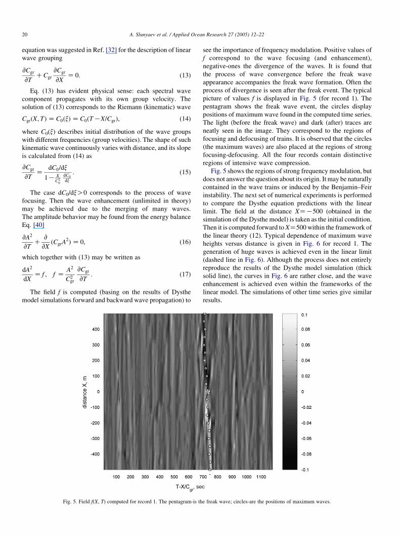
The field f is computed (basing on the results of Dysthe

model simulations forward and backward wave propagation) to

Fig. 5. Field f(X, T) computed for record 1. The pentagram-is th

see the importance of frequency modulation. Positive values of

f correspond to the wave focusing (and enhancement),

negative-ones the divergence of the waves. It is found that

the process of wave convergence before the freak wave

appearance accompanies the freak wave formation. Often the

process of divergence is seen after the freak event. The typical

picture of values f is displayed in Fig. 5 (for record 1). The

pentagram shows the freak wave event, the circles display

positions of maximum wave found in the computed time series.

The light (before the freak wave) and dark (after) traces are

neatly seen in the image. They correspond to the regions of

focusing and defocusing of trains. It is observed that the circles

(the maximum waves) are also placed at the regions of strong

focusing-defocusing. All the four records contain distinctive

regions of intensive wave compression.

Fig. 5 shows the regions of strong frequency modulation, but

does not answer the question about its origin. It may be naturally

contained in the wave trains or induced by the Benjamin–Feir

instability. The next set of numerical experiments is performed

to compare the Dysthe equation predictions with the linear

limit. The field at the distance XZK500 (obtained in the

simulation of the Dysthe model) is taken as the initial condition.

Then it is computed forward to XZ500 within the framework of

the linear theory (12). Typical dependence of maximum wave

heights versus distance is given in Fig. 6 for record 1. The

generation of huge waves is achieved even in the linear limit

(dashed line in Fig. 6). Although the process does not entirely

reproduce the results of the Dysthe model simulation (thick

solid line), the curves in Fig. 6 are rather close, and the wave

enhancement is achieved even within the frameworks of the

linear model. The simulations of other time series give similar

results.

e freak wave; circles-are the positions of maximum waves.

Fig. 6. Maximum wave height versus distance for record 1: comparison of the simulations in the Dysthe model (thick solid line) with the linear limit (dashed line).

The initial conditions: field at position XZK500, computed within the frameworks of the Dysthe equation.

A. Slunyaev et al. / Applied Ocean Research 27 (2005) 12–22 21

Dispersive focusing is a classical mechanism of wave

enhancement in the linear theory, but it turns out effective in

nonlinear media too. The processes of dispersive compression

in nonlinear Korteweg-de Vries and NLS equations were

considered in Refs. [32,36]. The latter simulations result that

although the effects of nonlinear instability play an important

role in the dynamics of generated freak waves, the significant

wave enhancement is achieved due to quasi-linear wave

grouping because of the difference in the group velocities. The

linear limit cannot describe carefully the wave evolution, but

shows the wave growth by itself.

6. Conclusion

Four freak waves recorded in the North Sea at the North

Alwyn in 1997 are presented in the paper. The time series do

not give the full information about the freak events; for

instance, the lifetimes of the freak waves were not determined.

The events are reconstructed with the help of numerical

simulations performed within the Dysthe, NLS and kinematic

equations in the assumption of unidirectional waves. The

spatial evolution forward and backward the wave propagation

is found, the dependences of maximum wave height are

analyzed to determine the lifetimes and travel distances of the

freak waves. The lifetimes vary from several seconds up to

42 s, the freak waves travel up to 325 m; the huge wave may

make one or many oscillations during the freak wave

occurrence.

The results of evolution within the frameworks of the

Dysthe equations are compared with predictions given by the

NLS equation and linear theory. The NLS approximation

and the Inverse Scattering Technique are applied to analyze the

strength of the nonlinear self-focusing. It seems that in an

appreciable part a freak wave is a soliton. The envelope

solitons may explain 40% and more of the extreme wave

amplitude. This proves the importance of the processes of the

Benjamin–Feir instability in the huge wave dynamics.

The linear theory is used to estimate the contribution of

dispersive effects. The calculation of the first derivative of the

local group velocity in the time series shows the presence of

regions of strong convergence/divergence nearby the freak

events. Simulation of the evolution upstream and downstream

displays the decisive role of the wave grouping due to the

difference in the group speeds. The wave enhancement by itself

may be easily achieved in the linear limit when the effects of

nonlinear instability are cancelled.

The predictions of evolution of maximum wave height

upstream and downstream are compared for all three models

(Dysthe, NLS, linear), considering the Dysthe model as the

main. While the NLS model predictions of wave amplification

seem to be difficult in use due to undying intensive envelope

solitons, the linear limit describes the evolution of maximum

wave heights unexpectedly well. This may be explained by the

leading role of linear effects for the wave enhancement.

Acknowledgements

The work was supported by freak wave generation in the

ocean (grant INTAS 01-2156) for all authors, grant INTAS 04-

83-3032 for A.S., and grants INTAS 03-51-4286 and RFBR 05-

05-64265 for E.P.

A. Slunyaev et al. / Applied Ocean Research 27 (2005) 12–2222

The wave data used here was collected and initially

analyzed in the research project ‘Rogue Waves-Forecast and

Impact on Marine Structures (MAXWAVE)’, which was

partially funded by the European Commission, under the

programme Energy, Environment and Sustainable Develop-

ment (Contract no. EVK3:2000-00544).

References

[1] Annenkov SYu, Badulin SI. Multi-wave resonances and formation of

high-amplitude waves in the ocean. In: Olagnon M, Athanassoulis GA,

editors. Proceedings of the workshop ‘Rogue Waves 2000’, Brest, France;

2000. p. 205–14.

[2] Brandini C, Grilli S. Evolution of three-dimensional unsteady wave

modulations. In: Olagnon M, Athanassoulis GA, editors. Proceedings

of the workshop ‘Rogue Waves 2000’, Brest, France; 2000. p. 275–82.

[3] Brown MG, Jensen A. Experiments on focusing undirectional water

waves. J Geophys Res 2001;106(16):917–28.

[4] Chien H, Kao C-C, Chuang LZH. On the characteristics of observed

coastal freak waves. Coast Eng J 2002;44:301–19.

[5] Clammond D, Grue J. Interation between envelope solitars as a model for

freak wave formations. Pt. 1: Long time interation. C R Mecanique 2002;

330:575–580.

[6] Clauss GF. Application of Gaussian wave packets for seakeeping test of

offshore structures. In: Torum O, Gudmestad OT, editors. Water wave

kinematics. Kluwer Academic Publications; 1990. p. 331–44.

[7] Clauss G. Dramas of the sea: episodic waves and their impact on offshore

structures. Appl Ocean Res 2002;24:147–61.

[8] Dias F, Kharif C. Nonlinear gravity and capillary-gravity waves. Annu

Rev Fluid Mech 1999;31:301–46.

[9] Divinsky BV, Levin BV, Lopatukhin LI, Pelinovsky EN, Slyunyaev AV.

A freak wave in the Black sea: observations and simulation. Dokl Earth

Sci 2004;395A:438–43.

[10] Drazin PG, Johnson RS. Solitons: an introduction. Cambridge University

Press; 1996.

[11] Dysthe KB. Note on a modification to the nonlinear Schrodinger equation

for application to deep water waves. Proc R Soc London A 1979;369:

105–14.

[12] Dysthe KB, Trulsen K. Note on breather type solutions of the NLS as a

model for freak-waves. Phys Scripta 1999;T82:48–52.

[13] Fonseca N, Guedes Soares C. Experimental investigation of the shipping

of water on the bow of a containership. Proceedings of the 22nd

international conference of offshore mechanics and artic engineering

(OMAE’03). New York: ASME. Paper OMAE2003-37456; 2003.

[14] Fonseca N, Guedes Soares C, Pascoal R. Prediction of ship dynamic loads

in heavy weather. Proceedings of the conference on design and operation

for abnormal conditions II, RINA, London, UK, November 6–7; 2001. p.

169–89.

[15] Fonseca N, Guedes Soares C, Pascoal R. Ship responses and structural

loads induced by abnormal wave conditions Proceedings of the

conference on design and operation for abnormal conditions III, RINA,

London, UK, January 26–27; 2005.

[16] Grue J, Clamond D, Huseby M, Jensen A. Kinematics of extreme water

waves. Appl Ocean Res 2003;25:355–66.

[17] Guedes Soares C, Cherneva Z, Antao EM. Characteristics of abnormal

waves in north sea storm states. Appl Ocean Res 2003;25:337–44.

[18] Guedes Soares C, Cherneva Z, Antao EM. Abnormal waves during

hurricane camille. J Geophys Res 2004;109:C08008.

[19] Guedes Soares C, Fonseca N, Pascoal R, Clauss GF, Schmittner CE,

Hennig J. Analysis of design wave loads on a FPSO accounting for

abnormal waves. Proceedings of the OMAE specialty conference on

integrity of floating production, storage & offloading (FPSO) systems.

New York: ASME. Paper OMAE-FPSO’04-0073; 2004.

[20] Guedes Soares C, Pascoal R, Antao EM, Voogt A, Buchner B. An

approach to calculate the probability of wave impact on an FPSO bows.

Proceedings of 23rd offshore mechanics and artic engineering

(OMAE’04). New York: ASME. Paper OMAE2004-51575; 2004.

[21] Haver S, Karunakaran D. Probabilistic description of crest heights of

ocean waves Proceedings of the fifth international workshop on wave

hindcasting and forecasting, Melbourne, FL; 1998.

[22] Henderson KL, Peregrine DH, Dold JW. Unsteady water wave

modulations: fully nonlinear solutions and comparison with the nonlinear

Schrodinger equation. Wave Motion 1999;29:341–61.

[23] Janssen PAEM. Nonlinear four-wave interactions and freak waves. J Phys

Oceanogr 2003;33:863–84.

[24] Kharif C, Pelinovsky E. Physical mechanisms of the rogue wave

phenomenon. Eur J Mech B Fluids 2003;22:603–34.

[25] Kuhnlein W, Clauss G, Hennig J. Tailor made freak waves within

irregular seas. Proceedings 21st international conference on Offshore

Mechanics and Arctic Engineering (OMAE’02). New York: ASME.

Paper OMAE2002-28524; 2002.

[26] Lo EY, Mei CC. Slow evolution of nonlinear deep water waves in two

horizontal directions: a numerical study. Wave Motion 1987;9:245–59.

[27] Mori N, Liu PC, Yasuda N. Analysis of freak wave measurements in the

sea of Japan. Ocean Eng 2002;29:1399–414.

[28] Onorato M, Osborne AR, Serio M. Extreme wave events in directional,

random oceanic sea states. Phys Fluids 2002;14:L25–L8.

[29] Onorato M, Osborne AR, Serio M, Bertone S. Freak waves in random

oceanic sea states. Phys Rev Lett 2001;86:5831–4.

[30] Osborne AR, Onorato M, Serio M. The nonlinear dynamics of rogue

waves and holes in deep water gravity wave trains. Phys Lett A 2000;275:

386–93.

[31] Pastoor W, Helmers JB, Bitner-Gregersen E. Time simulation of ocean-

going structures in extreme waves. Proceedings of the 22nd international

conference on offshore mechanics and arctic engineering (OMAE’03).

New York, USA: ASME. Paper OMAE2003-37490; 2003.

[32] Pelinovsky E, Talipova T, Kharif C. Nonlinear dispersive mechanism

of the freak wave formation in shallow water. Physica D 2000;147:

83–94.

[33] Pelinovsky EN, Slunyaev AV, Talipova TG, Kharif C. Nonlinear

parabolic equation and extreme waves on the sea surface. Radiophys

Quantum Electron 2003;46:451–63.

[34] Phillips OM, Gu D, Donelan M. Expected structure of extreme waves in a

Gaussian sea. Part I. Theory and SWADE buoy measurements. J Phys

Oceanogr 1993;23:992–1000.

[35] Sand SE, Hansen NE, Klinting P, Gudmestad OT, Sterndorff MJ. Freak

wave kinematics. In: Torum O, Gudmestad OT, editors. Water wave

kinematics. Kluwer Academic Publication; 1990. p. 450–535.

[36] Slunyaev A, Kharif C, Pelinovsky E, Talipova T. Nonlinear wave

focusing on water of finite depth. Physica D 2002;173:77–96.

[37] Trulsen K, Gudmestad OT, Velarde MG. The nonlinear Scrodinger

method for water wave kinematics on finite depth. Wave Motion 2001;33:

379–95.

[38] Trulsen K. Simulating the spatial evolution of a measured time series of

a freak wave. In: Olagnon’ M, Athanassoulis GA, editors. Proceedings

of the workshop ‘Rogue Waves 2000’, Brest, France; 2000. p. 265–74.

[39] Trulsen K, Stansberg CT. Spatial evolution of water waves: numerical

simulation and experiment of bichromatic waves. Proceedings of

Conference of the ISOPE 2001; 2001. p. 71–7.

[40] Whitham GB. Linear and nonlinear waves. Wiley; 1974.

[41] Zakharov VE, Dyachenko AI, Vasilyev O. New method for numerical

simulation of nonstationary potential flow of incompressible fluid with a

free surface. Eur J Mech B Fluids 2002;21:283–91.