Microbiological effects of high pressure processing on food.
Upload
khangminh22Category
view
1download
0

MEASUREMENTand CONTROL
in FOODPROCESSING

7244_C000.fm Page ii Thursday, July 6, 2006 11:15 PM

CRC is an imprint of the Taylor & Francis Group,an informa business
MEASUREMENTand CONTROL
in FOODPROCESSING
Manabendra Bhuyan, Ph.D.
Boca Raton London New York

Published in 2007 byCRC PressTaylor & Francis Group 6000 Broken Sound Parkway NW, Suite 300Boca Raton, FL 33487-2742
© 2007 by Taylor & Francis Group, LLCCRC Press is an imprint of Taylor & Francis Group
No claim to original U.S. Government worksPrinted in the United States of America on acid-free paper10 9 8 7 6 5 4 3 2 1
International Standard Book Number-10: 0-8493-7244-5 (Hardcover) International Standard Book Number-13: 978-0-8493-7244-5 (Hardcover) Library of Congress Card Number 2006001546
This book contains information obtained from authentic and highly regarded sources. Reprinted material isquoted with permission, and sources are indicated. A wide variety of references are listed. Reasonable effortshave been made to publish reliable data and information, but the author and the publisher cannot assumeresponsibility for the validity of all materials or for the consequences of their use.
No part of this book may be reprinted, reproduced, transmitted, or utilized in any form by any electronic,mechanical, or other means, now known or hereafter invented, including photocopying, microfilming, andrecording, or in any information storage or retrieval system, without written permission from the publishers.
For permission to photocopy or use material electronically from this work, please access www.copyright.com(http://www.copyright.com/) or contact the Copyright Clearance Center, Inc. (CCC) 222 Rosewood Drive,Danvers, MA 01923, 978-750-8400. CCC is a not-for-profit organization that provides licenses and registrationfor a variety of users. For organizations that have been granted a photocopy license by the CCC, a separatesystem of payment has been arranged.
Trademark Notice: Product or corporate names may be trademarks or registered trademarks, and are used onlyfor identification and explanation without intent to infringe.
Library of Congress Cataloging-in-Publication Data
Bhuyan, Manabendra.Measurement and control in food processing / Manabendra Bhuyan.
p. cm.Includes bibliographical references and index.ISBN-13: 978-0-8493-7244-5 (alk. paper)ISBN-10: 0-8493-7244-5 (alk. paper)1. Food industry and trade. I. Title.
TP370.B49 2006664’.02--dc22 2006001546
Visit the Taylor & Francis Web site at http://www.taylorandfrancis.com
and the CRC Press Web site at http://www.crcpress.com
Taylor & Francis Group is the Academic Division of Informa plc.
7244_Discl.fm Page 1 Tuesday, March 21, 2006 1:34 PM

Foreword
Maintenance of the quality of processed food is a matter of concern for bothfood manufacturers and customers. If a product does not meet the estab-lished specifications, then it has to be sold at a loss, destroyed, or reworked.Therefore, quality control in food processing has become an integral part ofthe food processing industry. By the end of the 20th century, the food pro-cessing industry gradually adopted automated process control technologiesand left behind traditional inspection methods for ensuring food quality andsafety. Food quality and safety activities shifted from human inspection ofindividual pieces to automated, statistically driven monitoring systems forimproved quality control. The new approach monitors key control points inthe process to make sure that the finished products will meet the specifica-tions. These changes were possible due to the advantages of computers,microchips, and sensor technology.
From the smallest baker to the largest snack manufacturer, food processinghas many operations elements in common. From receiving raw materials tothe finished product involving blending, the entire period of processing,removing defects, value addition, checking weight, and packaging, measure-ment and control devices have important roles to play. Therefore, it is essen-tial that the detecting systems are properly calibrated and users understandthe limitations of the systems.
Although different instruments or devices were used for several decadesfor measurement and control parameters during food processing, there havebeen tremendous changes in these instruments due to advancement inrelated areas. The measurement devices have become more accurate andefficient, less power consuming, smaller in size, easier to operate, and alsocheaper in many instances. Detection systems and control mechanisms willcontinue to be developed and improved. During the last 10 years sophisti-cation of scanning technology has improved many times over. Currently,biosensors are attracting a great deal of interest.
There exists much literature in the area, but it has not been compiled in oneplace. The author has made an attempt to compile all the available informationand present it in a comprehensive manner. This book is divided into five majorchapters covering various aspects of measurement and control in food process-ing. Apart from describing the principles and their applications, suitable exam-ples, problems, and their solutions are also provided wherever applicable.
This book will be useful for food scientists, instrumentation engineers, trans-ducer manufacturers, and food processing engineers. This is basically a refer-ence book, but can also be a textbook for food science and technology coursesbeing offered in different colleges and universities at the graduate level.
7244_C000.fm Page v Thursday, July 6, 2006 11:15 PM

I feel honored to have been asked to write the foreword for such animportant book. I would like to congratulate Dr. M. Bhuyan, the author, forhis dedication and wholehearted effort to present the book in this form. Hehas made a valuable contribution to food science and technology.
Professor P. C. Deka
Vice-ChancellorTezpur University, India
7244_C000.fm Page vi Thursday, July 6, 2006 11:15 PM

Preface
The beginning of my research in instrumentation and control in the teaindustry dates back to the early 1990s, when I first recognized the need forappropriate literature on the subject. I still remember when I had to jostlethrough dozens of tables of contents and indexes looking for discussions ofa suitable converter for measuring process parameters in the tea industry. Ialso remember how much of my valuable time was devoted to designing acircuit for lack of proper literature. The feeling of need at that time translatedinto the idea for this book now.
During the last few decades, many innovations came to the world of instru-mentation and control in food processing, and in spite of a significant amountof literature distributed in various places, common texts are still far less thanexpected.
Measurement and Control in Food Processing
is an attempt to makefood scientists aware of various means of food-related measurements andcontrols, help instrumentation engineers and transducer manufacturersdesign instruments and control schemes suitable for food-processing envi-ronments, make food engineers attentive to the applicability of instrumenta-tion and control to enhance quality and productivity, and more importantly,educate students of food science or food technology courses on methods andtechniques of measurements and control in food processing.
The advent of super-specializations in food processing has caused confu-sion about who actually handles measurement and control in food processing.A food-processing engineer may not know how to design a controller circuit,but at the same time an instrumentation engineer may not know what com-plex flavor components emanate from a cup of tea. It is not difficult to estab-lish coordination between these two areas of knowledge. During my longexperience in food-related instrumentation and control, I have encounteredsuch problems and realized that there should not be a sharp line betweenthese two forms of expertise. This motivated me to address the problemsfaced by food-processing engineers in quantifying food-related parametersand their control from the angles both of food processing and instrumentation.
The book is divided into five major chapters, beginning with an illustratedintroduction to food processing measurement and control in chapter 1. Chap-ter 2, a cornerstone for the book, is devoted to background materials aboutbasic principles of transducers and controllers. Numerical problems are dis-cussed in several sections so that readers can understand the applicabilityof food-processing devices. Readers who have already completed a coursein instrumentation and control can skip this chapter or can read it to refreshtheir knowledge. Chapter 3 deals exclusively with measurement techniquesfor food processing, covering a significant amount of food-related process
7244_C000.fm Page vii Thursday, July 6, 2006 11:15 PM

parameters. The chapter features the relevance and importance of processparameters in food-processing industries and discussion of measuring tech-niques, and specific applications in most recent developments have beenenumerated. A number of texts from research publications have beenincluded and several intelligent instrumentation techniques that haveemerged in recent years have been presented. In chapter 4, topics on con-trollers and indicators for food-processing industries with a good deal ofpractical application have been presented. Recent nontraditional controlschemes, such as fuzzy control, are also discussed in this chapter. Microcom-puter-based process monitoring and control is a major issue today. Thedevices, standards, and procedures and suitable examples for process–com-puter interaction are presented in chapter 5.
The book is intended to respond well to the need of food engineers,instrumentation engineers, transducer manufacturers, researchers, teachers,and students of food science or food technology. Although the book lookslike a reference work, it can also be a good textbook for a course in foodscience, food technology, or biosystems.
While the book is the result of my untiring efforts, there are many otherswho contributed to its development. I must thank Prof. P.C. Deka, Vice-chancellor, Tezpur University, India, for writing the foreword, where he haspresented a valuable comment on the aim and scope of the book; and myM Tech students, A.G. Venkatesh, Mahanada Saharaia, Pawan Kumar Bhar-gav, and Riku Chutia, for helping me with the artwork and text. A specialthanks to A.G. Venkatesh, who went to a lot of trouble with a major part ofthe artwork, sending it via email from the University of Manchester, andasking me to let him know “if there is anything more I can do.” Thanks alsoto my research scholars, Kishana Ram Kashwan and Surajit Borah, whohelped me to include some of the topics from their theses; to my colleagues,J.C. Dutta and P.P. Sahu, for their kind support during preparation of themanuscript; and to our office assistants, Dwipendra Ch. Das and DibakarNath, for their help.
I am grateful to the staff of Taylor & Francis Group for their professionalguidance and advice during the preparation of the project proposal and themanuscript, particularly to Susan B. Lee, Amber Donley, Marsha Pronin, andthe production team. I am also grateful to the reviewers (unknown) of myoriginal book proposal.
I must thank my wife, Arihana (Nanti), who helped me indirectly inwriting the book, particularly during the last few weeks before sending themanuscript to the publisher. I thank my daughter and son, Abhishruti (Pahi)and Abhinab (Pol), for their patience during the writing of this book.
7244_C000.fm Page viii Thursday, July 6, 2006 11:15 PM

Contents
Foreword ........................................................................................................ v
Preface........................................................................................................... vii
Chapter 1 Introduction ......................................................................... 1
1.1 Food Processing Industries .......................................................................... 11.1.1 Canned and Bottled Fruits and Vegetables .................................. 21.1.2 Beer ...................................................................................................... 41.1.3 Ciders .................................................................................................. 51.1.4 Soft Drinks.......................................................................................... 61.1.5 Sugar.................................................................................................... 71.1.6 Jams and Jellies.................................................................................. 81.1.7 Black Tea ............................................................................................. 9
1.2 Introduction to Process Instrumentation and Control .......................... 101.2.1 An Industrial Process ..................................................................... 111.2.2 Process Parameters ......................................................................... 131.2.3 Batch and Continuous Processes.................................................. 141.2.4 Process Instrumentation and Control .......................................... 141.2.5 Selection of Controller.................................................................... 22
1.3 Conclusion .................................................................................................... 24
Chapter 2 Measuring and Controlling Devices .............................. 27
2.1 Role of Transducers in Food Processing.................................................. 282.2 Classification of Transducers ..................................................................... 30
2.2.1 Self-Generating Type ...................................................................... 302.2.2 Variable Parameter Type................................................................ 302.2.3 Pulse or Frequency Generating Types......................................... 322.2.4 Digital Transducers ......................................................................... 32
2.3 Self-Generating Transducers ...................................................................... 332.3.1 Piezoelectric Transducers............................................................... 332.3.2 Thermocouples ................................................................................ 362.3.3 Photoelectric Transducers .............................................................. 412.3.4 Magneto-Electric Transducer......................................................... 442.3.5 Radioactive Transducer.................................................................. 47
2.4 Variable Parameter Type ............................................................................ 512.4.1 Resistive Transducer ....................................................................... 512.4.2 Inductive Transducers .................................................................... 722.4.3 Capacitive Transducer .................................................................... 77
7244_C000.fm Page ix Thursday, July 6, 2006 11:15 PM

2.5 Digital Transducers ..................................................................................... 802.5.1 Direct Digital Encoder.................................................................... 802.5.2 Frequency, Pulse Encoder .............................................................. 802.5.3 Analog-to-Digital Encoder............................................................. 812.5.4 Analog-to-Digital Converter ......................................................... 812.5.5 Digital Encoders .............................................................................. 82
2.6 Selection of Transducers ............................................................................. 832.7 Actuating and Controlling Devices .......................................................... 84
2.7.1 Actuators .......................................................................................... 852.7.2 Actuating Motors ............................................................................ 882.7.3 Final Control Elements................................................................... 962.7.4 Pneumatic Control Devices ........................................................... 98
2.8 Conclusion .................................................................................................. 103
Chapter 3 Measurements in Food Processing ............................... 105
3.1 Introduction ................................................................................................ 1083.2 Moisture Content Measurement ............................................................. 109
3.2.1 Role of Moisture Content in Quality of Food .......................... 1093.2.2 Microwave Absorption Method ..................................................1113.2.3 Radio Frequency (RF) Impedance Technique .......................... 1133.2.4 DC Resistance Technique............................................................. 1163.2.5 Infrared Technique ........................................................................ 122
3.3 Moisture Release During Drying of Food............................................. 1243.3.1 Mathematical Representation...................................................... 1243.3.2 Mechanical Loading Arrangement............................................. 1253.3.3 Measuring Circuit ......................................................................... 127
3.4 Humidity in the Food Processing Environment .................................. 1293.4.1 Definition of Humidity ................................................................ 1303.4.2 Conventional Types ...................................................................... 1313.4.3 Electrical Type of Humidity Meters........................................... 1343.4.4 Electronic Wet- and Dry-Bulb Hygrometer .............................. 135
3.5 Turbidity and Color of Food ................................................................... 1393.5.1 Turbidity Measurement................................................................ 1393.5.2 Food Color Measurement ............................................................ 143
3.6 Food and Process Temperature Measurement ..................................... 1523.6.1 Temperature Measurement in Food Processing....................... 1523.6.2 Thermocouples .............................................................................. 1533.6.3 Temperature of Food on a Conveyor ........................................ 1553.6.4 Food Tempering Monitoring....................................................... 1553.6.5 Precision Temperature Measurement ........................................ 156
3.7 Food Flow Metering.................................................................................. 1573.7.1 Magnetic Flow Meters.................................................................. 1583.7.2 Mass Flow Metering ..................................................................... 1593.7.3 Turbine Flow Meter ...................................................................... 1623.7.4 Positive Displacement Flow Meter ............................................ 162
7244_C000.fm Page x Thursday, July 6, 2006 11:15 PM

3.7.5 Solid Flow Metering ..................................................................... 1623.7.6 Gravimetric Feeder Meters.......................................................... 163
3.8 Viscosity of Liquid Foods......................................................................... 1653.8.1 Definition and Units ..................................................................... 1653.8.2 Newtonian and Non-Newtonian Food Flow ........................... 1663.8.3 Laboratory Type Saybolt Viscometer......................................... 1693.8.4 Capillary Tube Viscometer .......................................................... 1703.8.5 On-line Variable Area or Rotameter Type Viscometer............ 1723.8.6 Rotating Cylinder Viscometer..................................................... 174
3.9 Brix of Food ................................................................................................ 1773.9.1 Brix Standards................................................................................ 1793.9.2 Refractometers ............................................................................... 179
3.10 pH Values of Food..................................................................................... 1833.10.1 pH Scale.......................................................................................... 1833.10.2 pH Electrodes and Potential ....................................................... 1843.10.3 pH Signal Processing.................................................................... 1873.10.4 Ion-Sensitive Field Effect Transistor pH Sensors..................... 187
3.11 Food Enzymes............................................................................................ 1933.11.1 Importance of Food Enzyme Detection .................................... 1933.11.2 Enzyme Sensors............................................................................. 1933.11.3 Measuring Circuit ......................................................................... 1963.11.4 Semiconductor Enzyme Sensor .................................................. 1983.11.5 Applications in Food Processing ................................................ 199
3.12 Flavor Measurement ................................................................................. 2003.12.1 Sources of Flavor in Food............................................................ 2003.12.2 Physiology of Human Olfaction................................................. 2013.12.3 Organoleptic Panel........................................................................ 2023.12.4 Electronic Nose.............................................................................. 2033.12.5 Sensor Types .................................................................................. 2043.12.6 The Signal Processing and Pattern Recognition ...................... 2073.12.7 Applications of the Electronic Nose in Food Processing ....... 209
3.13 Food Texture and Particle Size................................................................ 2193.13.1 Electromechanical Measuring Techniques ................................ 2203.13.2 Fluorescence Technique for Beef Toughness Detection .......... 2243.13.3 Machine Vision Technique........................................................... 2263.13.4 Particle Size Detection.................................................................. 230
3.14 Food Constituents Analysis ..................................................................... 2313.14.1 Carbonates, Bicarbonates, and Organic Matters
in Bottled Water............................................................................. 2323.14.2 Volatile Compounds in Tropical Fruits ..................................... 2343.14.3 Moisture, Protein, Fat, and Ash Content of Milk Powder..... 2353.14.4 Components in Alcoholic Beverages ......................................... 2353.14.5 Quality Parameters in Cereals and Cereal Products............... 2363.14.6 Meat Content ................................................................................. 2373.14.7 Bacteria and Foreign Body Detection ........................................ 238
3.15 Conclusion .................................................................................................. 240
7244_C000.fm Page xi Thursday, July 6, 2006 11:15 PM

Chapter 4 Controllers and Indicators ............................................. 243
4.1 Introduction ................................................................................................ 2444.2 Temperature Control in Food Dehydration and Drying .................... 245
4.2.1 Control Parameters for Heat and Mass Transferin Drying ........................................................................................ 246
4.2.2 Feedback and Feedforward Control in Dryers ........................ 2494.2.3 A Single-Input, Single-Output (SISO) Dryer Model ............... 2514.2.4 A Multiple-Input, Multiple-Output (MIMO)
Dryer Model................................................................................... 2524.2.5 Feedforward Control in the Food Dryer................................... 255
4.3 Electronic Controllers................................................................................ 2584.3.1 On–Off Controller ......................................................................... 2604.3.2 Controller Modes .......................................................................... 2614.3.3 Fan Direction Control in Food Withering................................. 2654.3.4 Cooling Surface Area Control in Chocolate Tempering......... 271
4.4 Flow Ratio Control in Food Pickling Process ....................................... 2714.4.1 Ratio Controller ............................................................................. 2724.4.2 Control Valves................................................................................ 273
4.5 Atmosphere Control in Food Preservation ........................................... 2774.5.1 Control Scheme.............................................................................. 277
4.6 Timers and Indicators in Food Processing............................................ 2784.6.1 Rolling Program in Tea Manufacturing .................................... 2794.6.2 Temperature Indicator for Tea Dryer......................................... 284
4.7 Food Sorting and Grading Control ........................................................ 2874.7.1 Objective of Sorting ...................................................................... 2874.7.2 Various Sorting Techniques ......................................................... 2884.7.3 Automated Packaging and Bottling........................................... 289
4.8 Discrete Controllers................................................................................... 2904.8.1 Ladder Diagram ............................................................................ 2914.8.2 Programmable Logic Controllers ............................................... 292
4.9 Adaptive and Intelligent Controllers ..................................................... 2934.9.1 Self-Tuning Controllers ................................................................ 2944.9.2 Model Reference Adaptive Controllers ..................................... 2954.9.3 Intelligent Controllers................................................................... 296
4.10 Conclusion .................................................................................................. 300
Chapter 5 Computer-Based Monitoring and Control ................... 303
5.1 Introduction ................................................................................................ 3045.2 Importance of Monitoring and Control with Computers .................. 3045.3 Hardware Features of a Data Acquisition and Control Computer... 3055.4 Remote Data Acquisition with PCs........................................................ 306
5.4.1 Analog Signal Interfacing Card .................................................. 3085.4.2 Connector Arrangements............................................................. 308
5.5 Signal Interfacing....................................................................................... 3105.5.1 Input Signal Processing................................................................ 3105.5.2 Output Signal Processing ............................................................ 312
7244_C000.fm Page xii Thursday, July 6, 2006 11:15 PM

5.5.3 Interface Standards ....................................................................... 3125.5.4 Analog and Digital Signal Conversion ..................................... 3145.5.5 Interface Components .................................................................. 318
5.6 Examples of Computer-Based Measurement and Controlin Food Processing .................................................................................... 3205.6.1 Computer-Based Monitoring and Control of the
Withering Process in the Tea Industry ...................................... 3205.6.2 Computer-Based Sequential Timer for Tea Rollers ................. 324
5.7 Conclusion .................................................................................................. 328
Appendixes........................................................................................... 331
Appendix A: SI Units.................................................................................331
Appendix B: English System of Units......................................................332
Appendix C: CGS Systems of Units.........................................................332
Appendix D: Standard Prefixes ................................................................332
Appendix E: Piping and Instrumentation DrawingSensor Designations ..........................................................................333
Appendix F: Standard Psychrometric Chart ...........................................334
Index
............................................................................................................335
7244_C000.fm Page xiii Thursday, July 6, 2006 11:15 PM

7244_C000.fm Page xiv Thursday, July 6, 2006 11:15 PM

This book is dedicated
to the fond memory of my mother Rupoprabha Bhuyan
and my father Ratnadhar Bhuyan
and to all those who die every day
from diseases related to inadequate diets
and lack of nutrients in foods
7244_C000.fm Page xv Thursday, July 6, 2006 11:15 PM

7244_C000.fm Page xvi Thursday, July 6, 2006 11:15 PM

1
1
Introduction
CONTENTS
1.1 Food Processing Industries .......................................................................... 11.1.1 Canned and Bottled Fruits and Vegetables .................................. 2
1.1.1.1 Quality Control of Ingredients ......................................... 41.1.2 Beer ...................................................................................................... 41.1.3 Ciders .................................................................................................. 51.1.4 Soft Drinks.......................................................................................... 6
1.1.4.1 Syrup Dosing and Filling .................................................. 61.1.5 Sugar.................................................................................................... 71.1.6 Jams and Jellies.................................................................................. 81.1.7 Black Tea ............................................................................................. 9
1.2 Introduction to Process Instrumentation and Control .......................... 101.2.1 An Industrial Process ..................................................................... 111.2.2 Process Parameters ......................................................................... 131.2.3 Batch and Continuous Processes.................................................. 141.2.4 Process Instrumentation and Control .......................................... 14
1.2.4.1 On–Off Control Action .................................................... 161.2.4.2 Proportional Control Action ........................................... 171.2.4.3 Proportional Plus Integral Control Action ................... 211.2.4.4 Derivative Control Action ............................................... 211.2.4.5 PID Controller ................................................................... 22
1.2.5 Selection of Controller.................................................................... 221.3 Conclusion .................................................................................................... 24References ............................................................................................... 25Further Reading ..................................................................................... 25
1.1 Food Processing Industries
Food processing is a vast sector of the industrial world. A major percentageof cereals, vegetables, and fruits are processed for human consumption andpreservation for future use. In the United States, the combined activities ofthe agricultural, food processing, marketing functions, and supporting
7244.book Page 1 Wednesday, June 21, 2006 11:14 AM
2
Measurement and Control in Food Processing
industries generate about 20% of the gross national product and one fourthof the total workforce. According to a survey on current business, approxi-mately 1.7 million people in the United States were directly employed in foodmanufacturing alone in 1991, not counting related businesses [1]. Food tech-nology is the application of concepts generated by food science in processing,preservation, packaging, and distribution of safe and nutritious food.
At one time food manufacturers did not pay much attention to productionof food by scientific methods as is done today. Due to the traditional patternof the food industries, many food manufacturers still try to produce qualityproducts with the old-fashioned approaches of measurement and controlmethods: touching, smelling, and visual inspection. However, considerablequality, efficiency, and energy are sacrificed in adopting these traditionaltechniques.
The desirable characteristics of a food product are mainly determined byits demand and usage. The quality control of processed food products hasbecome a concern both for manufacturers and consumers. Therefore, qualitycontrol methods in food processing are required for the survival of theindustry because of user consciousness about safe and healthy products.Apart from the important chemical and physical changes that can take placeduring different stages of manufacturing, the quality of raw materials is alsoan important factor. A good-quality food product cannot be processed frompoor-quality raw materials. Apart from composition, uniformity of size,shape, color, and flavor have also become important in food processing.
The chemical aspect of food products is such an expansive field that it isnot possible to cover in detail and it is outside the scope of this book. Hencea brief overview of a series of food processing industries is given in thischapter, with an emphasis on the use of instrumentation and control.
When food processing was in its early stages, not much attention was paidto relating quality to physical and chemical characteristics. However, as thedemand for quality products gradually increased, analysis of the relationbetween chemical and physical characteristics started among food manufac-turers. The following sections give an overview of some food manufacturingprocesses with the potential of measurement and control strategies.
1.1.1 Canned and Bottled Fruits and Vegetables
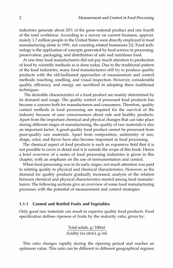
Only good raw materials can result in superior quality food products. Foodspecification defines ripeness of fruits by the maturity ratio, given by:
This ratio changes rapidly during the ripening period and reaches anoptimum value. This ratio can be different in different geographical regions;
Total solids, g/100mlAcidity (as citric), g/ml
7244.book Page 2 Wednesday, June 21, 2006 11:14 AM

Introduction
3
for example, in the case of orange juice, this ratio is 8 in California and Israel,whereas South Africa requires a minimum value of 5.
Many similar terms have also been formulated to define the maturity ofvegetables. A criterion for canning and freezing peas, for example, has beenformulated on the basis of content of alcohol in insoluble solids, which is thatpercentage of the fresh weight insoluble in 80% of ethyl alcohol after boiling for30 min. A tenderometer is a common instrument for determining this criterion.
In an unprocessed state, fruits and vegetables consist of an agglomerationof biochemical systems and their products, microorganisms such as yeast,molds, and bacteria. After processing and canning, the food should be in astabilized condition and the dish should have the same taste as that of thefresh material. Application of heat during processing causes undesirablechanges during storage due to enzyme loss and microorganism quality. Toavoid this and to improve the quality, the canned products are treated in ablanching process. In this process, the free and intercellular gases from thetissues are removed, causing a greater vacuum in the can and shrinking thetissues for ease of handling and filling. However, in this process there is aconsiderable loss of soluble nutrients such as sugars, amino acids, andvitamins. An electronic blanching process might reduce this loss to a con-siderable extent.
Once the cans are filled with fruit, heat treatment is performed, removinggases from the fruit tissues. Thermal heating stabilizes the product by killingmicroorganisms. The pH value of the food is responsible for the microfloracontent in the can and the resistance to heat. Canned and bottled fruits andvegetables are generally divided into the following four basic groups basedon their pH values:
1. Low-acid groups (pH of 5.3 and above); most vegetables2. Medium low-acid groups (pH of 5.3–4.5); carrots3. Medium-acid groups (pH of 4.5–3.7); tomatoes, pears, cherries, pine-
apples, and peaches4. High-acid groups (pH of 3.7 and below); apples, plums, and berries
The process of thermal heating is performed with varying degrees of timeand temperature levels. In the last two groups, heating is done at 212
°
F for ashorter period; but in low-acid and medium low-acid groups, high tempera-ture is used for heating the product. The
temperature coefficient
is a number inbacteriology that dictates the increase or decrease of temperature in
°
F thatcauses an increase or decrease in number of bacterial spores by a factor of 10.Thus, for example, if heating sterilizes the product when the food item isheated at 258
°
F and kills 10 times more bacterial spores than heating at 240
°
F,the factor is 18. This factor generally varies from 15 to 22. There must be anoptimum time and degree of heating for getting the best processing throughsterilization. Thus, in production of canned fruits and vegetables, a correctcorrelation among the pH value, heating temperature, and heating durationwill result in an optimum solution for quality control of the product.
7244.book Page 3 Wednesday, June 21, 2006 11:14 AM

4
Measurement and Control in Food Processing
1.1.1.1 Quality Control of Ingredients
The specifications of ingredient materials for best results are termed stan-dards. The standards used by a manufacturer depend on the product inwhich the material is to be used and on the manufacturing process. Thereis no universally set standard for each material. Setting a standard for ingre-dient material requires vast experience in handling, and the manufacturermight set its own specifications. Nevertheless, some broad outlines can begiven for dictating the specifications in the following categories:
• Identity:
This is a precise definition of originality of the material.Only microscopic tests can determine these attributes.
• Purity and composition: The aspects of this standard can have thefollowing factors:1. Chemical: This gives assay requirements such as percentage of
moisture, fat, protein, antioxidants, additives, and so on.2. Physical: This specifies the requirements such as size, color,
weight, viscosity, density, and so on.• Microbiological:
This refers to microbiological organisms responsiblefor health, safety significance, and sanitary conditions. Tests con-ducted to measure sanitary conditions are called filth tests.
• Packaging: This refers to the net weight and quantity of the packag-ing material.
• Storage: This standard depicts the conditions for cold storage outsidethe factory. Warehouse conditions such as temperature and relativehumidity are major concerns of this category.
During the processes of cooking, canning, and sterilization and filling offruits and vegetables, several process parameters must be measured andcontrolled, including the following:
1. pH, temperature, and timing during thermal heating of canned fruitsand vegetables
2. Moisture content, fat, protein, antioxidants, pH, color, brix, and fla-vor of the product
3. Filling weight and filling temperature for canning4. Temperature and humidity control during storage trials
1.1.2 Beer
Beer is an alcoholic beverage used worldwide. Considerable advances havebeen made during the last decades in the brewing industry in quality andmaintaining uniformity.
The beer brewing process uses four principal ingredients: malts, hops, water,and yeast. Barley is converted into malt and combined with water to form a
7244.book Page 4 Wednesday, June 21, 2006 11:14 AM

Introduction
5
mash. Fermentable sugar, maltose, is formed due to the presence of enzymesin the malt. Malt is prepared from barley corns in a process called malting.Chemical analysis, appearance, flavor, texture, and moisture content determinepurity of malts. The sugar maltose is boiled in a kettle with the addition ofhops. It is then strained, cooled, and sent to a fermenting vessel, where yeastis added. After a few days, alcohol is developed from the sugar and the resultingbeer is filtered and drained to a storage reservoir and then pasteurized. Pas-teurization is the heating process required to destroy pathogenic microorgan-isms. Controlled boiling of sugar maltose in the brew kettle is essential inbrewing to prevent insipid color, excessive bitterness, cloudy appearance, andinconsistent taste of the final product. Moreover the efficiency of the processcan be improved by maximizing heat transfer and evaporation [2].
The major parameters of beer that need measurement and control are thefollowing:
1. Temperature during pasteurization and evaporation
2. Flow rate of product in various stages
3. Color matching against standard colors set by brewing conventionsof various countries
4. Measurement of yeast cell counts and minerals5. Turbidity of the solution6. pH measurement of infected pitching yeast for its purification7. Estimation of oxygen, nitrogen, and hydrogen in the head space of
bottled beer
1.1.3 Ciders
Ciders are manufactured by fermentation of apple juice, which is a populardrink in many countries. Juice is extracted from disintegrated apple byapplying hydraulic pressure on the pulp. Colloidal separation of juice fromthe pressed pulp is achieved by adding a pectin-degrading enzyme followedby a gelatin solution. Centrifugation and filtration of the gelatin solutionremoves the precipitate. Evaporation reduces the volume of juice for inter-mediate storage (see [3] for further details). Addition of sulfur dioxide orascorbic acid to the juice causes fermentation and reduces the tendency ofthe product to become brown. Considerable attention should be given to thefollowing quality factors for the unfermented and fermented products:
The unfermented juice
1. Specific gravity of the fruit juice2. Total sugar content of the fruit juice
3. Total acidity (pH)
4. Tannin content5. Pectin content
7244.book Page 5 Wednesday, June 21, 2006 11:14 AM

6
Measurement and Control in Food Processing
The fermented product
1. Specific gravity and viscosity
2. Alcohol content
3. Sugar content
4. Total acidity
5. Tannin content
6. Sulfur dioxide content
1.1.4 Soft Drinks
Soft drinks are refreshing, nonalcoholic beverages. Soft drinks can be cate-gorized into the following groups:
1. Fruit drink or fruit juice
2. Soda water or any artificially carbonated water, either flavored ornonflavored
3. Ginger beer or any herbal or plant-based beverages
The ingredients of bottling syrup are: sugar, fruit juices, essences, citric orother permitted acids, artificial sweeteners, preservatives, colors, and emul-sions for cloudy products. Bottling syrup is prepared by careful addition ofall the ingredients in correct proportion and sequence. To control the qualityof the syrup, chemical and physical tests must be carried out. The followingparameters are responsible for the flavor of the syrup:
1. Percentage of soluble solids
2. Acidity (pH)
3. Sulfur dioxide and sodium benzonate content determination
1.1.4.1 Syrup Dosing and Filling
For high-speed bottling, a premix system is more popular in bottling plants.Here the syrup is mixed in correct proportion in a carbon dioxide pressurizedmixing chamber. An exact proportion of water is combined, cooled, carbon-ated, and filled into the bottle. The flavored syrup content or capacity priorto filling can be measured by an online refractometer, and a control signalcan be generated for adjusting the proportions of the ingredients.
1.1.4.1.1 On-Line Monitoring of the Qualities of Syrup
Brix, carbonation, and capacity of syrup must be graphically monitored formanagerial and quality-control purposes. Graphical records of the essentialquantities of syrup before bottling are powerful tools for statistical quality
7244.book Page 6 Wednesday, June 21, 2006 11:14 AM
Introduction
7
control. Apart from quality control of syrup, the soft drink industry focusesmuch attention on the hygiene of processing and bottling to keep bacterio-logical infection to a permitted limit.
1.1.5 Sugar
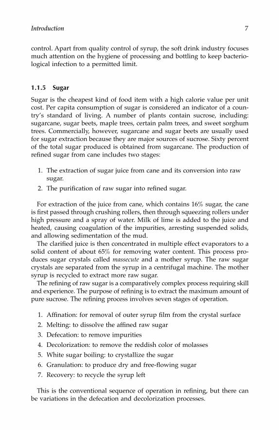
Sugar is the cheapest kind of food item with a high calorie value per unitcost. Per capita consumption of sugar is considered an indicator of a coun-try’s standard of living. A number of plants contain sucrose, including:sugarcane, sugar beets, maple trees, certain palm trees, and sweet sorghumtrees. Commercially, however, sugarcane and sugar beets are usually usedfor sugar extraction because they are major sources of sucrose. Sixty percentof the total sugar produced is obtained from sugarcane. The production ofrefined sugar from cane includes two stages:
1. The extraction of sugar juice from cane and its conversion into rawsugar.
2. The purification of raw sugar into refined sugar.
For extraction of the juice from cane, which contains 16% sugar, the caneis first passed through crushing rollers, then through squeezing rollers underhigh pressure and a spray of water. Milk of lime is added to the juice andheated, causing coagulation of the impurities, arresting suspended solids,and allowing sedimentation of the mud.
The clarified juice is then concentrated in multiple effect evaporators to asolid content of about 65% for removing water content. This process pro-duces sugar crystals called
massecute
and a mother syrup. The raw sugarcrystals are separated from the syrup in a centrifugal machine. The mothersyrup is recycled to extract more raw sugar.
The refining of raw sugar is a comparatively complex process requiring skilland experience. The purpose of refining is to extract the maximum amount ofpure sucrose. The refining process involves seven stages of operation.
1. Affination: for removal of outer syrup film from the crystal surface
2. Melting: to dissolve the affined raw sugar
3. Defecation: to remove impurities
4. Decolorization: to remove the reddish color of molasses
5. White sugar boiling: to crystallize the sugar
6. Granulation: to produce dry and free-flowing sugar
7. Recovery: to recycle the syrup left
This is the conventional sequence of operation in refining, but there canbe variations in the defecation and decolorization processes.
7244.book Page 7 Wednesday, June 21, 2006 11:14 AM

8
Measurement and Control in Food Processing
Process parameter monitoring and control in the sugar industry is essen-tial for manufacturing a product of uniform quality from raw materials ofvariable quantities. Two other important aspects of process control are min-imizing fuel consumption and sugar loss. During processing, sucrose solu-tions are hydrolyzed, forming invert sugar and causing chemical loss. Atlow pH (e.g., 8), the inversion is slow but it is higher at high temperature.To estimate the chemical loss, therefore, measurement of pH and tempera-ture are prime criteria.
Dry crystalline sucrose is noninverting but when it contains acids or someenzymes, the sucrose gets hydrolyzed. The invert sugar is hygroscopic; hencethe moisture content of the crystalline sugar also contributes to furtherenhancing the process of formation of invert sugar. The ideal ratio of sugarto water content is 100:1. As the moisture content is very minimal, sources oferror can contribute to the water content estimation. Therefore, sensitive andaccurate methods of moisture content measurement have to be employed inthis situation.
The appearance (hue) of the sugar is also a mark of its quality, influencedby the color and grain size. Therefore, detection of the color and grain sizecertainly helps in quality-control schemes in the sugar industry.
The sucrose content of the juice is also important. The most accuratemethod of sucrose content measurement is the polarization of raw sugar.Ash is a kind of impurity that can be present in the refined sugar. Althoughthis impurity does not account for any hazard, estimation of ash is mostfrequently carried out both during processing and on the final refined sugarbecause it is a general indication of the degree of refining. The conductometrymethod is generally used for ash content determination in sugar.
1.1.6 Jams and Jellies
Jams are sugar pectin gels obtained from fruit juice. Jellies are different fromjams in composition and texture. Strawberries, raspberries, black currants,red currants, guava, and pineapple are some of the fruits with high sugarcontent suitable for jam and jelly.
Generally fruit pulps are preserved for production in the off-season. Themost common method of preservation is adding sulfur dioxide with the fruitpulp. The sulfur dioxide is added as a gas, 6% aqueous solution, or a solutionof sodium meta bisulfate or calcium sulfate.
For jam preparation, fruit pulp and liquid pectin syrup are transported toboiling pans through pipes. They are mixed to get a pH value of 3.0 and themixture is then boiled at about 105
°
C. During boiling, agents like yeast,molds, and other destroying enzymes are removed.
In jelly manufacturing, a mixture of sucrose and glucose syrup is boileduntil solid content reaches 90%. The cooking is performed in open panevaporators or vacuum pans. After cooking, it is cooled to between 98
°
C and
7244.book Page 8 Wednesday, June 21, 2006 11:14 AM
Introduction
9
99
°
C, added with soaked gelatin. Finally, color and flavor are also added.The final product is stored in large slabs or molds.
Because pectin is the sole component of fruit juice, it cannot be destroyedduring cooking. In many cases, fruit pulp contains a considerable amount ofpectin-destroying enzymes. Therefore the pulp should be sufficiently cookedto release all of the enzymes. Even a small trace of enzyme left after cookingwill hydrolyze the pectin, forming gelatinous masses. In view of this, detectionof such natural enzymes in the fruit pulp and the cooked pulp is necessary.
Fruit pulps should contain uniform food content; it is therefore necessaryto perform tests to detect the fruit concentration. Fruit concentration can beascertained by measuring the percentage content of soluble solids by refrac-tometer. Acidity and percentage of insoluble solids are also important param-eters. For manufacturing jellies, the fruit pulp should contain high gelatinwith an ideal Bloom strength of 250, a reading obtained from a Bloomgelometer. Measurement of pH must also be performed because gel contentis dependent on it.
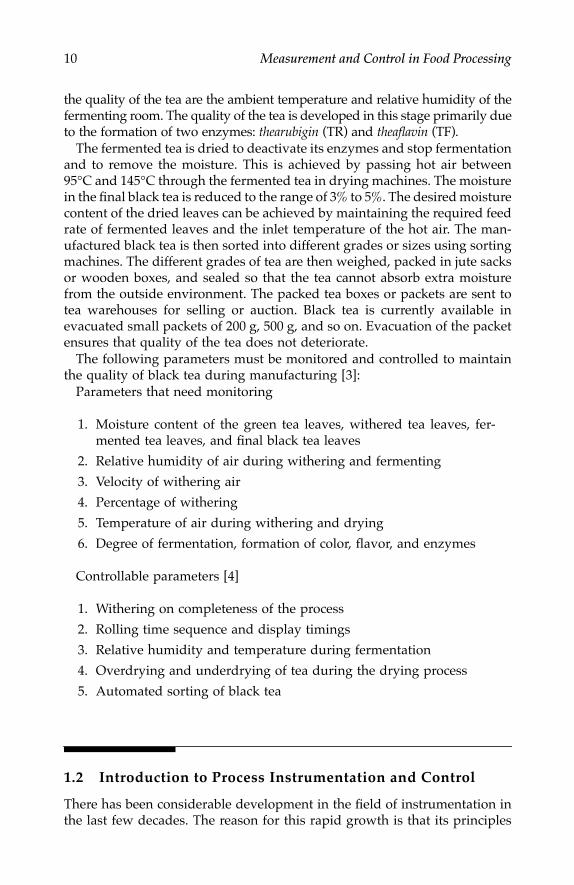
1.1.7 Black Tea
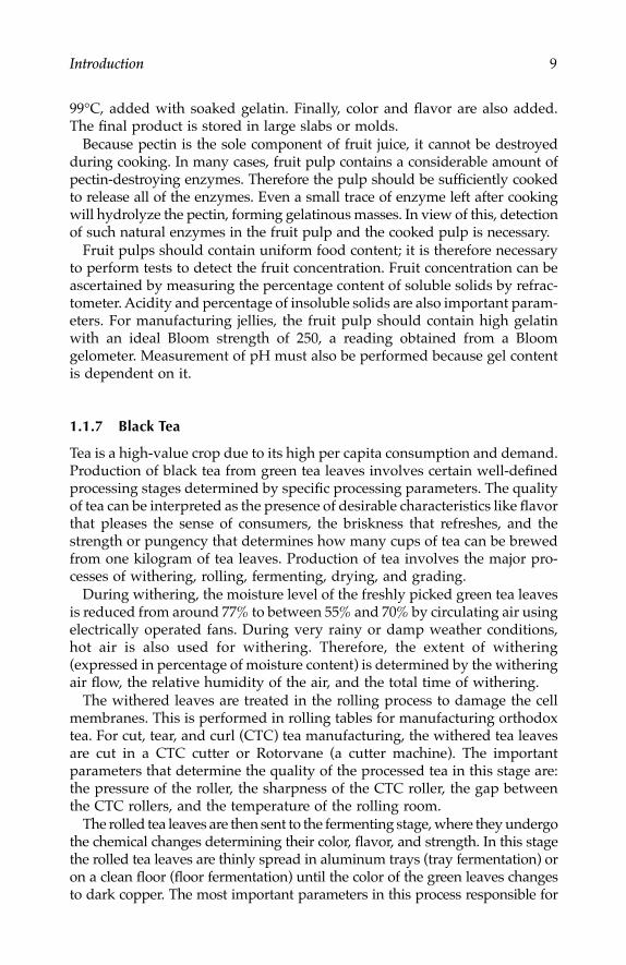
Tea is a high-value crop due to its high per capita consumption and demand.Production of black tea from green tea leaves involves certain well-definedprocessing stages determined by specific processing parameters. The qualityof tea can be interpreted as the presence of desirable characteristics like flavorthat pleases the sense of consumers, the briskness that refreshes, and thestrength or pungency that determines how many cups of tea can be brewedfrom one kilogram of tea leaves. Production of tea involves the major pro-cesses of withering, rolling, fermenting, drying, and grading.
During withering, the moisture level of the freshly picked green tea leavesis reduced from around 77% to between 55% and 70% by circulating air usingelectrically operated fans. During very rainy or damp weather conditions,hot air is also used for withering. Therefore, the extent of withering(expressed in percentage of moisture content) is determined by the witheringair flow, the relative humidity of the air, and the total time of withering.
The withered leaves are treated in the rolling process to damage the cellmembranes. This is performed in rolling tables for manufacturing orthodoxtea. For cut, tear, and curl (CTC) tea manufacturing, the withered tea leavesare cut in a CTC cutter or Rotorvane (a cutter machine). The importantparameters that determine the quality of the processed tea in this stage are:the pressure of the roller, the sharpness of the CTC roller, the gap betweenthe CTC rollers, and the temperature of the rolling room.
The rolled tea leaves are then sent to the fermenting stage, where they undergothe chemical changes determining their color, flavor, and strength. In this stagethe rolled tea leaves are thinly spread in aluminum trays (tray fermentation) oron a clean floor (floor fermentation) until the color of the green leaves changesto dark copper. The most important parameters in this process responsible for
7244.book Page 9 Wednesday, June 21, 2006 11:14 AM
10
Measurement and Control in Food Processing
the quality of the tea are the ambient temperature and relative humidity of thefermenting room. The quality of the tea is developed in this stage primarily dueto the formation of two enzymes:
thearubigin
(TR) and
theaflavin
(TF).The fermented tea is dried to deactivate its enzymes and stop fermentation
and to remove the moisture. This is achieved by passing hot air between95
°
C and 145
°
C through the fermented tea in drying machines. The moisturein the final black tea is reduced to the range of 3% to 5%. The desired moisturecontent of the dried leaves can be achieved by maintaining the required feedrate of fermented leaves and the inlet temperature of the hot air. The man-ufactured black tea is then sorted into different grades or sizes using sortingmachines. The different grades of tea are then weighed, packed in jute sacksor wooden boxes, and sealed so that the tea cannot absorb extra moisturefrom the outside environment. The packed tea boxes or packets are sent totea warehouses for selling or auction. Black tea is currently available inevacuated small packets of 200 g, 500 g, and so on. Evacuation of the packetensures that quality of the tea does not deteriorate.
The following parameters must be monitored and controlled to maintainthe quality of black tea during manufacturing [3]:
Parameters that need monitoring
1. Moisture content of the green tea leaves, withered tea leaves, fer-mented tea leaves, and final black tea leaves
2. Relative humidity of air during withering and fermenting
3. Velocity of withering air
4. Percentage of withering
5. Temperature of air during withering and drying
6. Degree of fermentation, formation of color, flavor, and enzymes
Controllable parameters [4]
1. Withering on completeness of the process
2. Rolling time sequence and display timings
3. Relative humidity and temperature during fermentation
4. Overdrying and underdrying of tea during the drying process
5. Automated sorting of black tea
1.2 Introduction to Process Instrumentation and Control
There has been considerable development in the field of instrumentation inthe last few decades. The reason for this rapid growth is that its principles
7244.book Page 10 Wednesday, June 21, 2006 11:14 AM
Introduction
11
are based on multidisciplinary facts and the applications are also multidis-ciplinary in nature. As technology advances in different fields, instrumenta-tion also advances technologically. There is always an increasing need forprecise, efficient measurement schemes in industrial environments. Indus-trial control and automation are meaningless without a proper instrumen-tation scheme. Therefore, technological advancement requires advancementin both instrumentation and control. A judicious amalgamation of instru-mentation and control can only contribute to the industrial needs for improv-ing quality, increasing productivity, increasing efficiency, reducingmanufacturing costs and material waste, saving energy, and so on.
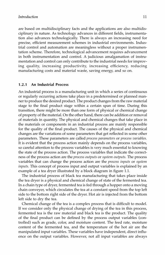
1.2.1 An Industrial Process
An industrial process is a manufacturing unit in which a series of continuousor regularly occurring actions take place in a predetermined or planned man-ner to produce the desired product. The product changes from the raw materialstage to the final product stage within a certain span of time. During thistransition, there might be more than one form of physical or chemical changeof property of the material. On the other hand, there can be addition or removalof materials in quantity. The physical and chemical changes that take place inthe materials or components in an industrial process are mainly responsiblefor the quality of the final product. The causes of the physical and chemicalchanges are the variations of some parameters that get reflected in some otherparameters. These parameters are called
process parameters
or
process variables.
It is evident that the process action mainly depends on the process variables,so careful attention to the process variables is very much essential to knowingthe state of the process action. The process variables that indicate the correct-ness of the process action are the
process outputs
or
system outputs.
The processvariables that can change the process action are the
process inputs
or
systeminputs.
This concept of process input and output variables is explained by anexample of a tea dryer illustrated by a block diagram in figure 1.1.
The industrial process of black tea manufacturing that takes place insidethe tea dryer is a physical and chemical change of state of the fermented tea.In a chain type of dryer, fermented tea is fed through a hopper onto a movingchain conveyer, which circulates the tea at a constant speed from the top leftside to the bottom right side of the dryer. Hot air is injected from the bottomleft side to dry the tea.
Chemical change of the tea is a complex process that is difficult to model.If we consider only the physical change of drying of the tea in this process,fermented tea is the raw material and black tea is the product. The qualityof the final product can be defined by the process output variables (con-trolled) such as grade, color, and moisture content. The feed rate, moisturecontent of the fermented tea, and the temperature of the hot air are themanipulated input variables. These variables have independent, direct influ-ence on the output variables. However, not all input variables are always
7244.book Page 11 Wednesday, June 21, 2006 11:14 AM

12
Measurement and Control in Food Processing
highly responsible for the quality of the product. For example, in a tea dryer,the density of the fermented tea does not have a direct influence or mighthave a low gain influence on the product quality.
At this point we can identify the flow rate of the black tea as productivityof the final product rather than defining it as quality. Not all process inputor output variables affect the quality of the product. Some process outputvariables might not indicate the quality of the product in a process. The flowrate of the black tea is a similar kind of output variable. Therefore, sufficientprocess knowledge is required to identify the actual process outputs thatrepresent the quality of the final product. Similarly, some input variablesmight not affect the quality of the product in a process. The block diagramin figure 1.2 represents the tea drying process, taking into account the cross-correlations between the input and output parameters.
FIGURE 1.1
Block diagram of a tea dryer.
FIGURE 1.2
Illustration of cross-relations in dryer input–output variables. (Notations as per figure 1.1.)
Moisture content offermented tea (MCF)
SpreadWear
and tearUneven
heat transfer
Feed rate of tea(FRT)
Temperature ofhot air (TH)
Flow rate ofhot air (FRH)
Moisture contentof made tea (MCM)
Color and flavorof made tea (CF)
Tea dryer
Disturbances
MCF
FRT
CF
MCM
TH
FRH
G1
G2
Gn
7244.book Page 12 Wednesday, June 21, 2006 11:14 AM
Introduction
13
A process can thus be represented by a system with manipulated inputvariables and controlled output process variables. The manipulated input vari-ables control the quality of the final product and the controlled output variablescarry the signature of the quality of the product.
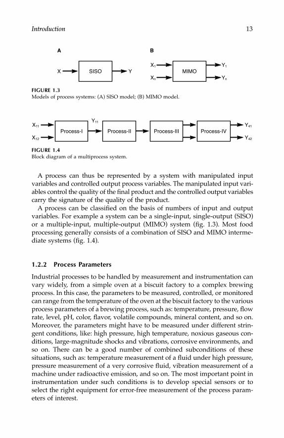
A process can be classified on the basis of numbers of input and outputvariables. For example a system can be a single-input, single-output (SISO)or a multiple-input, multiple-output (MIMO) system (fig. 1.3). Most foodprocessing generally consists of a combination of SISO and MIMO interme-diate systems (fig. 1.4).
1.2.2 Process Parameters
Industrial processes to be handled by measurement and instrumentation canvary widely, from a simple oven at a biscuit factory to a complex brewingprocess. In this case, the parameters to be measured, controlled, or monitoredcan range from the temperature of the oven at the biscuit factory to the variousprocess parameters of a brewing process, such as: temperature, pressure, flowrate, level, pH, color, flavor, volatile compounds, mineral content, and so on.Moreover, the parameters might have to be measured under different strin-gent conditions, like: high pressure, high temperature, noxious gaseous con-ditions, large-magnitude shocks and vibrations, corrosive environments, andso on. There can be a good number of combined subconditions of thesesituations, such as: temperature measurement of a fluid under high pressure,pressure measurement of a very corrosive fluid, vibration measurement of amachine under radioactive emission, and so on. The most important point ininstrumentation under such conditions is to develop special sensors or toselect the right equipment for error-free measurement of the process param-eters of interest.
FIGURE 1.3
Models of process systems: (A) SISO model; (B) MIMO model.
FIGURE 1.4
Block diagram of a multiprocess system.
X YSISO
A B
Xn Yn
X1 Y1
MIMO
X12
X11
Y11
Process-I Process-II Process-IIIY42
Y41
Process-IV
7244.book Page 13 Wednesday, June 21, 2006 11:14 AM

14
Measurement and Control in Food Processing
1.2.3 Batch and Continuous Processes
Production of a particular commodity involves well-defined multiple processoperations in a predetermined sequence, procedure, and time. If the rawmaterials are treated in the stages of operations continuously with a singlestream of product flow, the process is called a
continuous process.
If theproduct flow is discontinuous, meaning the raw materials or ingredients aretreated with a time lag between stages, the process is called a
batch process.
However, it is difficult to have a purely batch process or a purely continuousone. Some batch processes demand continuous control of some variables andsome continuous processes require some batch processing stages at the endof the schedule like batch sorting, batch packaging, and so forth.
In the past, most of the chemical and petroleum-based products weremanufactured in batch mode. Later it was felt that if there is a large demandfor single product and a system is inherently suited (physically or chemi-cally), a continuous process is more efficient than a batch process. If theseconditions are not fulfilled or the product does not become cost-effective toproduce using continuous process machinery, batch mode continues to bequite popular. Apart from this inherent advantage, batch mode processeshave other beneficial qualities, such as: processing flexibility, multiple usesof equipment, and higher safety in handling hazardous ingredients or prod-ucts because of short processing duration. One added advantage of batchmode processing is easy controllability. A continuous mode process willhave much more complex cross-correlation between process parametersthan a batch mode process.
1.2.4 Process Instrumentation and Control
As defined earlier, a process carries out a single or a series of operations ina sequential manner leading toward a particular goal or object. The processis governed by the controlled variables, which is the desired output. Amanipulated variable is a parameter that is varied by the controller to adjustthe output to the desired quality or quantity. In a process, control is thetechnique of setting the outputs if there is deviation from the desired level;the manipulated input variables are adjusted to minimize the deviation. Ina process, the causes of deviation of the output variables from a streamlinedbehavior can be either internal or external to the process. Irrespective of thereasons for the deviations, they are always categorized as disturbances. Somedisturbances are regular in nature (deterministic) and can be predicted andcompensated for within the system, but some cannot be predicted (stochas-tic). The effects of unpredictable disturbances can only be compensated forby a feedback control system.
In a closed-loop feedback control system, the difference between the outputof the system and the set point or desirable input is used as a measure forthe repair to be performed. The difference is called the error, which is usedto adjust the controllable input variable. To understand a manual control
7244.book Page 14 Wednesday, June 21, 2006 11:14 AM

Introduction 15
system, imagine the control of an electric heater by a human operator. Theoperator controls the temperature under a specific condition, for example,the maximum and minimum limits. The operator looks at the thermometer,and if the temperature is above the specified limit, he or she switches thepower off and thereby decreases the temperature. When the temperaturedecreases below the minimum limit, the operator switches the power on andthe temperature rises again. This is a manual control approach in which thehuman operator works as a controller.
In another situation, consider an electric oven temperature that is con-trolled within a certain limit using a simple thermal switch. When the tem-perature of the oven crosses the limit, the thermal switch disconnects electricpower to the oven, working as a controlled switch. If the temperature dropsbelow the limit, the thermal switch operates to continue the power supplyto the oven, thereby increasing the temperature. The set point of the tem-perature limit is imposed on the thermal switch; that is, the thermal switchis adjusted as per the temperature limit. In this example the thermal switchworks both as a sensor and feedback controller. This feedback controller isbasically an on–off controller that simply switches the input to the systemto on or off state when the output goes below or above the set point, respec-tively. Figure 1.5 shows the block diagram of a feedback control system andfigure 1.6 shows the temperature controller. There are few other types oftraditional controllers, such as proportional, derivative, and integral control-lers that vary the input according to some function of the error signal. The
FIGURE 1.5A feedback control system.
FIGURE 1.6Schematic diagram of a temperature-controlled electric oven.
Error
Output+
–
Actuator
Transducer
Set-point Process
Mainpowersupply
Electric oven
Heater coil
Thermal switch
7244.book Page 15 Wednesday, June 21, 2006 11:14 AM

16 Measurement and Control in Food Processing
advantage of a feedback control system is that a deviation of the output fromthe set point can be minimized by proper controller design. The output of aprocess generally fluctuates or deviates from the quality limit due to distur-bances or variations in the process parameters. If feedback control is adopted,such deviations can be eliminated or minimized easily.
In contrast to manual control, in automatic control, measurement andadjustment are made automatically and continuously. Manual control canbe used in simple and linear processes in which disturbances are fewer, theprocess is not fast, and minimal monitoring is required. In situations in whichprocess variables change too rapidly for the operator to take action, auto-matic control is compulsory. Thus in an alternative arrangement for theheater control example, the temperature can be measured by a suitablesensor, then the signal is processed and fed to a controller for adjusting theprocess input. A simple electronic circuit to follow simple control laws canbe realized by the controller. For complex control schemes the controller isrealized using a microprocessor or a personal computer.
In industry, controllers are generally used to perform a particular kind ofcontrol action or a combination of two or more actions. The type of controlaction produced is called the control mode. The selection of a particular kindof control action depends on the complexity of the control parameters forwhich it is required, behavior of the process variables, and cost effectiveness.The different modes of traditional control actions are as follows:
1. On–off or two-position control
2. Proportional control (P)
3. Proportional plus integral control (PI)
4. Proportional plus derivative (rate) control (PD)
5. Proportional plus integral plus derivative control (PID)
Traditional control schemes are not always successful in nonlinear, com-plex systems where advanced and intelligent control laws are found to bemore convenient. Such controllers are discussed in chapter 5.
1.2.4.1 On–Off Control Action
An on–off controller is the simplest and most inexpensive of controllers. Anon–off controller results in an output action, in only two states, dependingon the level of the manipulated variable. Describing the control action withreference to a valve on a flow pipe, the control actions are: “the valve is fullyopen” and “the valve is fully closed.” One state of the output is used whenthe manipulated variable is above the desired level (set point) and the otherstate is used when the manipulated variable is below the set point level.
Consider an on–off control action for a temperature-controlled batch retortused for closing and heat sterilization operation of cans to achieve microbi-ological stability in canning. As soon as the temperature crosses the set level,
7244.book Page 16 Wednesday, June 21, 2006 11:14 AM

Introduction 17
the steam entry valve is turned off. This causes the temperature to comedown to the set level because the valve is still in the off position. Cycling oftemperature and switching of the valve, on and off, continues simulta-neously, as shown in figure 1.7.
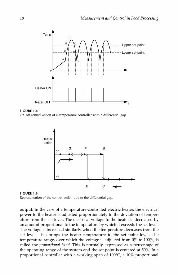
The range of temperature variation and the rate of switching are two veryimportant features of an on–off controller. They are dependent on the processresponse and characteristics. The range of temperature variation determinesthe precision of the controller, and a high rate of switching causes mechanicaldisturbances to the final control elements like actuators, valves, relays, and soon. Therefore, a simple on–off controller causes output to cycle rapidly astemperature crosses the set point. To eliminate this disadvantage, an on–offdifferential gap is introduced to the control action. This function causes theheater to turn off when the temperature exceeds the set point by a certainamount, which is generally half the gap. The gap prevents the controller fromcycling rapidly. Figure 1.8 shows the characteristics of an on–off temperaturecontroller with a differential gap. The representation of the differential gap foran on–off controller is shown in figure 1.9. As the temperature graduallyincreases from level A and reaches B through F, the heater turns off, droppingto point C. The temperature continues up to D, and then decreases to point E,where the heater once again turns on. The temperature might slightly dropup to point G, then again reaches B through F, repeating the cycle. Incorpora-tion of the differential gap in an on–off controller considerably reduces oscil-lations of the controlled output.
1.2.4.2 Proportional Control Action
In a proportional controller, the manipulated variable is proportionatelyadjusted according to the variation of the actual output from the desired
FIGURE 1.7On–off control action of temperature controller.
Set-point
Temp
t
ValveON–OFF
action
ON
OFF
7244.book Page 17 Wednesday, June 21, 2006 11:14 AM
18 Measurement and Control in Food Processing
output. In the case of a temperature-controlled electric heater, the electricalpower to the heater is adjusted proportionately to the deviation of temper-ature from the set level. The electrical voltage to the heater is decreased byan amount proportional to the temperature by which it exceeds the set level.The voltage is increased similarly when the temperature decreases from theset level. This brings the heater temperature to the set point level. Thetemperature range, over which the voltage is adjusted from 0% to 100%, iscalled the proportional band. This is normally expressed as a percentage ofthe operating range of the system and the set point is centered at 50%. In aproportional controller with a working span of 100°C, a 10% proportional
FIGURE 1.8On–off control action of a temperature controller with a differential gap.
FIGURE 1.9Representation of the control action due to the differential gap.
Lower set-point
Temp
AG
D
B C
EF
0
t
Heater ON
Heater OFF
Upper set-point
Heateraction
A
E C
G Fon
off
B
7244.book Page 18 Wednesday, June 21, 2006 11:14 AM

Introduction 19
band would be 10°C and the highest and lowest ranges of the band are 5°Caway from the set point level. The transfer characteristic of a proportionalcontroller is shown in figure 1.10. The figure illustrates that below 100°C,which is the lowest range of the proportional band, the heater power shouldbe 100%. On the other hand, above the highest range of the proportionalband (i.e., 110°C), the heater voltage should be zero. The voltage to be appliedto the heater therefore can be determined from the characteristic graphically.The heater voltage is fixed at 50% at the set point level. There is everypossibility that the proportional band might need to be adjusted as per therequirement of the process response and characteristics. Hence the propor-tional controller can have a wide band or narrow band of control. The transfercharacteristics of wide band and narrow band proportional controllers areshown in figure 1.11.
In a narrow band proportional controller, a small change in temperaturecauses a large manipulated output. The performance of a proportional con-troller can be expressed in terms of the controller gain as
Gain = 100%/proportional band (percent).
Hence, the gain of a narrow band proportional controller is higher thanthat of a wide band controller. A proportional controller is suitable for asystem where deviation of output is not large and is not sudden. A propor-tional controller can be incorporated in a closed-loop feedback control systemillustrated in figure 1.12. The output signal is sensed by a sensor and ampli-fied before comparison with the set point level. The error signal is positivewhen the output is below the set point level, negative when the output isabove the set point, and zero when the output is adjusted to make it equalto the set point. The proportional output is 50% when the error signal is zero.
In practical situations, the heat input for attaining set point temperaturenever equals 50% of the maximum available. Therefore, the output temperature
FIGURE 1.10Transfer characteristic of a proportional controller.
Hea
ter
volta
ge (
%)
Temperature (°C)
105
100
50
100
7244.book Page 19 Wednesday, June 21, 2006 11:14 AM

20 Measurement and Control in Food Processing
oscillates before coming to an equilibrium condition. The temperature differ-ence between the stabilized and set point level is called the offset. The offsettemperature value becomes less in a narrow band proportional controller.
For fine-tuning of a controller the offset must be removed. This can be donemanually or automatically. Manual reset is a traditional method in which apotentiometer is used to nullify the offset electrically. The amount of proportional
FIGURE 1.11Transfer characteristic of (A) a narrow band and (B) a wide band proportional controller.
FIGURE 1.12Block diagram of a proportional controller.
Hea
ter
volta
ge (
%)
Wide band
100
0
50
B
Hea
ter
volta
ge (
%)
Narrow band
100
0
50
A
Error
Amplifier
OutputProportionalcontroller
Transducer
Set-point
+
–Plant
7244.book Page 20 Wednesday, June 21, 2006 11:14 AM

Introduction 21
band shifting is manually done, step by step, until the manipulated input tocontroller (process heat demand) conforms with the set point level of temper-ature. The manual reset proportional controller is shown in figure 1.13.
1.2.4.3 Proportional Plus Integral Control Action
An automatic reset proportional controller performs a reset operation withthe help of an electronic integrator. The error is integrated and added withthe error signal. Due to the integral term in the control law, a sudden changein deviation is tracked continuously, at a certain rate, determined by the resetrate (inverse of the integral time). Performance of a proportional controlleris expressed by two terms: proportional gain and integral time constant.During integral time, equal parts of the output signal due to integral actionadvance as that of the output signal due to proportional action.
The block diagram and timing diagram of a proportional plus integralcontroller are shown in figure 1.14 and figure 1.15, respectively.
1.2.4.4 Derivative Control Action
Derivative control incorporates a term in the control law, which is first deriv-ative of the error signal. It facilitates the shift of the proportional band eitherup or down to compensate for rapidly changing outputs. The controller tracksthe set point level at a rate proportional to the rate of change of the error signal.If the output makes a sudden jump, the derivative action immediately brings
FIGURE 1.13Block diagram of a proportional controller with manual reset.
FIGURE 1.14Block diagram of a proportional plus integral controller.
Manual reset
Amplifier
OutputProportionalcontroller
Transducer
+
–PlantSet-point
+
–
Amplifier
OutputProportionalcontroller
Transducer
+Plant
Set-point +
–
Integration
7244.book Page 21 Wednesday, June 21, 2006 11:14 AM

22 Measurement and Control in Food Processing
the output toward the set point level. If the output changes gradually at aconstant rate, the output tracks the set point at a similar rate to the proportionalaction. In this control action, a derivative time constant can also be defined ina similar manner. The derivative action does not have any limit of occurrence,unlike integral action. The derivative action can occur even outside the pro-portional band. The speed of correction is proportional to the amount ofdeviation, but this incorporates oscillations in the system output. The timingdiagram of a proportional plus derivative control action is shown in figure 1.16.
1.2.4.5 PID ControllerCombination of these three modes of control action is advantageous forcontrolling complex processes. This mode of control is best suited for caseswhere the output fluctuations are large and sudden and the system has alag. The block diagram of a proportional-integral-derivative controller (PID)controller is shown in figure 1.17.
1.2.5 Selection of Controller
Selection of a controller for a particular application requires attention toseveral factors. It has been found that the simplest controller that meets therequirement of the process is the best and least expensive. Although a bettercontroller might be employed in a process that needs precise tuning of theoutput, a simple controller can be adequate in a process that permits acomparatively wide range of outputs.
Selection of a controller depends on the following factors:
1. Process response curve2. Physical system analysis3. Past experience4. Experimental testing
FIGURE 1.15Typical characteristics of a PI controller.
Output
Time
Adjustmentdue to I action
Adjustmentdue to P action
Integralaction time
7244.book Page 22 Wednesday, June 21, 2006 11:14 AM

Introduction 23
A process response curve is a plot between the process outputs with timewhen a steady input is applied. The process response curve for a first-orderthermal system is shown in figure 1.18. The essential characteristics of athermal process response curve are the time constant and the rate of temper-ature increase. The controllability of a process depends on these two factors.If the curve becomes steeper, the controllability of the process becomes diffi-cult. If the output temperature (Tp) starts increasing as soon as the input isapplied, there is no propagation delay or dead time. This relates to the timeconstant (τ). Such a system is easy to control. In a more complicated situation,
FIGURE 1.16Typical characteristics of proportional plus derivative controller.
FIGURE 1.17Block diagram of a PID controller.
Output
Time
Error
Time
Adjustment due to P action
Adjustment due to D action
Proportionalaction time
Amplifier
Output
Proportionalcontroller
Sensor
+
+
+
+
Plant
Set-point +
–
Derivative Integrator
7244.book Page 23 Wednesday, June 21, 2006 11:14 AM

24 Measurement and Control in Food Processing
when a heater is modified with thick metal plates, it introduces more timelag in the thermal system. This will introduce a second time constant, whichresults in a second-order system that is more difficult to control than a first-order system. The size of the process compared to the output requirementis also a major factor in selecting the controller. An oversized process doesnot give stable output, whereas an undersized one gives slow response.Analyzing controllability and process output stability requirements will helpin selecting the controller. Thorough knowledge about the process responsein the past is also an important clue. Experimental verification of the processresponse by computer simulation of the process is also a faithful method ofselection of a controller. However there are obviously some guidelines forcontroller selection, as follows:
1. A proportional controller is used where:a. load analysis is insignificant.b. offset can be permitted.c. a narrow proportional band is permitted.
2. Integral control is used where:a. offset cannot be permitted.b. process has a lag.
3. Derivative control is used where:a. sudden and large deviation of output takes place.b. there are severe plant lags.
1.3 Conclusion
In the food industry, numerous approaches are involved in every step, fromresearch to trade, where engineering techniques are mandatory. Our objective
FIGURE 1.18Response of a first-order thermal system.
τ
Final steady valueTemp
t
Tp = Tf (1- e–t/λ)63.2%
7244.book Page 24 Wednesday, June 21, 2006 11:14 AM
Introduction 25
is to help those practically involved with those engineering approaches tomake food processing more scientific and engineered. There is confusionabout who designs the food processing measurements and controls: a foodscientist or an instrumentation engineer? What should a food science coursecover? The definitions are misleading in the present day because behind themeasurement and control of most food processing systems is the skill of boththe food scientists and the engineers. In the broad perspective of food pro-cessing measurement and control, a food scientist is also an instrumentationengineer and vice versa.
The objective of this chapter is to inform food scientists as well as instru-mentation engineers about the basics of engineering concepts of measure-ment and control and food processes, respectively.
This chapter presented a short description of the various food processingindustries and the process parameters, as well as their importance in qualitycontrol. The basic structures of process input–output variables and basicprinciples of feedback control systems were also presented.
These basic concepts will be especially useful in understanding the variousmeasurement and control techniques discussed in later chapters.
References
1. Potter, N. N., and Hotchkiss, J. H. 1995. Food science (5th ed). Gaithersburg,MD: Coultate TP.
2. Lewis, M. J. 1995. Brewing. New York: Chapman & Hall.3. Ranken, M. D., and Kill, R. C. 1993. Food industries manual (23rd ed.). London:
Blackie Academic & Professional.4. Bhuyan, M. 1997. An integrated PC based tea process monitoring and control system,
PhD thesis, Department of Electronics, Gauhati University, India.
Further Reading
1. Beckett, S. T. (Ed.). 1994. Industrial chocolate manufacture and use (2nd ed.).London: Blackie Academic & Professional.
2. Multon, J. L. (Ed.). 1996. Quality control for foods and agricultural products. NewYork: VCH Publishers.
3. Ogata, K. 1982. Modern control engineering. New Delhi: Prentice Hall.4. Kuo, B. C. 1982. Automatic control systems (3rd ed.). New Delhi: Prentice Hall.5. Johnson, C. D. 2000. Process control instrumentation technology (6th ed.). Upper
Saddle River, NJ: Prentice Hall International.
7244.book Page 25 Wednesday, June 21, 2006 11:14 AM

7244.book Page 26 Wednesday, June 21, 2006 11:14 AM
27
2Measuring and Controlling Devices
CONTENTS2.1 Role of Transducers in Food Processing.................................................. 282.2 Classification of Transducers ..................................................................... 30
2.2.1 Self-Generating Type ...................................................................... 302.2.2 Variable Parameter Type................................................................ 30
2.2.2.1 Change in Resistance or Conductance.......................... 312.2.2.2 Change in Capacitance .................................................... 312.2.2.3 Change in Magnetic Properties ...................................... 31
2.2.3 Pulse or Frequency Generating Types......................................... 322.2.4 Digital Transducers ......................................................................... 32
2.3 Self-Generating Transducers ...................................................................... 332.3.1 Piezoelectric Transducers............................................................... 332.3.2 Thermocouples ................................................................................ 36
2.3.2.1 Thermocouple Materials.................................................. 382.3.2.2 Reference Junction Compensation................................. 392.3.2.3 Thermocouple Installations............................................. 392.3.2.4 Thermocouple Wire Insulators ....................................... 40
2.3.3 Photoelectric Transducers .............................................................. 412.3.3.1 Photo-Emissive Transducer............................................. 412.3.3.2 Photoconductive Cell ....................................................... 422.3.3.3 Photovoltaic Cell............................................................... 432.3.3.4 Photodiode and Phototransistor .................................... 44
2.3.4 Magneto-Electric Transducer......................................................... 442.3.4.1 Electrodynamic Transducer............................................. 452.3.4.2 Electromagnetic Transducer............................................ 462.3.4.3 Pulse Generator Type....................................................... 46
2.3.5 Radioactive Transducer.................................................................. 472.3.5.1 Penetrating Power ............................................................ 472.3.5.2 Half Life ............................................................................. 492.3.5.3 Half Distance ..................................................................... 49
2.4 Variable Parameter Type ............................................................................ 512.4.1 Resistive Transducer ....................................................................... 51
2.4.1.1 Potentiometer .................................................................... 522.4.1.2 Resistance Strain Gauge .................................................. 54
7244.book Page 27 Wednesday, June 21, 2006 11:14 AM

28 Measurement and Control in Food Processing
2.4.1.3 Diaphragm Pressure Sensor............................................ 602.4.1.4 Load Cell ............................................................................ 632.4.1.5 Resistance Temperature Detectors ................................. 632.4.1.6 Thermistors ........................................................................ 662.4.1.7 Semiconductor Temperature Sensors ............................ 692.4.1.8 Hot Wire Anemometer..................................................... 712.4.1.9 Resistive Humidity Sensors ............................................ 72
2.4.2 Inductive Transducers .................................................................... 722.4.2.1 Variable Inductance Type ................................................ 732.4.2.2 Variable Reluctance Type Sensors.................................. 74
2.4.3 Capacitive Transducer .................................................................... 772.5 Digital Transducers ..................................................................................... 80
2.5.1 Direct Digital Encoder.................................................................... 802.5.2 Frequency, Pulse Encoder .............................................................. 802.5.3 Analog-to-Digital Encoder............................................................. 812.5.4 Analog-to-Digital Converter ......................................................... 812.5.5 Digital Encoders .............................................................................. 82
2.5.5.1 Digital Shaft Encoder ....................................................... 822.6 Selection of Transducers ............................................................................. 832.7 Actuating and Controlling Devices .......................................................... 84
2.7.1 Actuators .......................................................................................... 852.7.1.1 Electrical Solenoids........................................................... 862.7.1.2 Electrical Motors ............................................................... 862.7.1.3 Fluid Control Valves ........................................................ 86
2.7.2 Actuating Motors ............................................................................ 882.7.2.1 DC Motors.......................................................................... 882.7.2.2 Control Motors .................................................................. 892.7.2.3 Stepper Motors.................................................................. 92
2.7.3 Final Control Elements................................................................... 962.7.3.1 Mechanical Types.............................................................. 972.7.3.2 Electrical Types.................................................................. 98
2.7.4 Pneumatic Control Devices ........................................................... 982.7.4.1 Baffle-Nozzle Detector ..................................................... 992.7.4.2 Pneumatic Amplifiers .................................................... 100
2.8 Conclusion .................................................................................................. 103Further Reading ................................................................................... 103
2.1 Role of Transducers in Food Processing
Transducers and sensors are the basic input devices for industrial processmeasurement and control. In some industries automatic control devices arenot adopted, either due to lack of necessity or lack of cost-effectiveness. Insuch situations, transducers might be used only for routine checks of various
7244.book Page 28 Wednesday, June 21, 2006 11:14 AM

Measuring and Controlling Devices 29
process parameters such as oven temperature in a small-scale biscuit factory.In this case, obviously, a microprocessor or a computer-based automaticcontroller is not cost effective. Hence, observing the temperature of the ovenby a thermocouple-based temperature indicator is sufficient. This impliesthat the measurement is taken manually so that the dough does not getoverbaked or underbaked.
Strictly speaking, transducers are not very commonly used devices inelectrical or electronic systems in industry. Transducers are used in systemsonly when some parameters of the system are to be quantified, measured,and observed. Some transducers are not of an electrical or electronic natureat all, like a mercury bulb thermometer used for measuring oven tempera-ture. This instrument is not capable of generating an electrical signal to beapplied to an electronic circuit. Such transducers are often used, but they areof no use in applications where automatic control is required. Therefore, bytransducer, we mean here an electrical type of transducer, unless specificallymentioned otherwise.
Generally, a transducer is a device that converts a physical signal to a signalof convenient form for measurement. The convenient form of signal is mostcommonly an electrical voltage, current, or pulse frequency. The electrical volt-age or current might need amplification, filtration, or linearization, which areperformed by circuits known as signal processing circuits. Sometimes pulse orfrequency signals need processing like wave shaping, modulation, and so on.
A wide range of physical parameters must be measured in industrial,laboratory, medical, space, and household equipment. The most commonphysical parameters that require transducers are temperature, pressure, andflow. Almost 90% of all the process parameters fall into these three categories.Other less common parameters that require transducers for measurementare position, displacement, velocity, acceleration, weight, force, density, andviscosity. Some other less common parameters are humidity, moisture con-tent, pH, sound level, mixing ratio, turbidity, color, and flavor.
We have imagined that all the transducers used for measurement of theseprocess parameters comprise a single unit that transduces the physical param-eters straight to an electrical signal. However, this is not always true becausemany transducers need help from a primary sensing device to convert aphysical signal to another convenient physical signal. In the second stage, thesecond physical signal is again converted to a proper electrical signal formeasurement. In this type of transducer, the first stage is called a primarytransducer and the second stage is called a secondary transducer. Mechanicaldevices like bourdon tube, bellows, diaphragms, springs, rings, and leversare some examples of primary sensors. These sensors are mostly elastic mem-bers that undergo some mechanical deformations or displacements whenforce, pressure, or load is applied to them. Some of the primary sensors alonerepresent a transducer where the parameter, in whatever form it is sensed, isused for the final application. Examples of such transducers are spindles,contacting members, pins, and fingers. This chapter covers the principles andareas of application of different transducers and controlling devices.
7244.book Page 29 Wednesday, June 21, 2006 11:14 AM

30 Measurement and Control in Food Processing
2.2 Classification of Transducers
The need for measurement of newer types of physical parameters is also areason for the increasingly large number of transducers. Based on designprinciples and application, transducers are grouped into the following fourdifferent classes:
1. Self-generating type
2. Variable parameter type
3. Pulse or frequency generating type
4. Digital type
2.2.1 Self-Generating Type
Self-generating transducers are designed to generate an electrical signal inproportion to the input physical signal. In most cases self-generating natureof the transducer is an inherent property of the material used for the trans-ducer. When the physical signal stimulates the material, a voltage is devel-oped. Examples are piezoelectric crystals, thermocouples, pH electrodes,radioactive sensors, photocells, electrodynamics, electromagnetics, andeddy-current type. The voltage developed by almost all the self-generatingtransducers is of very low strength and cannot be directly used for displayingor actuating a control device. Voltage or current amplification is necessarybefore applying it to an indicator, recorder, or control device. Apart fromvoltage amplification, filtering of the signal to remove noise picked up alsobecomes necessary. Corruption of the signal by noise is a very commonproblem in the case of transducers generating weak signals. The advantageof a self-generating transducer is that it does not require an extra source ofpower for the transducer.
2.2.2 Variable Parameter Type
A majority of the transducers fall into this category. Unlike self-generatingtransducers, a variable parameter type transducer cannot develop a voltageof its own. Instead, an electrical parameter of the device changes in propor-tion to the physical variable applied. The change in electrical parameter canbe categorized as one of the following:
1. Change in resistance or conductance
2. Change in capacitance
3. Change in magnetic properties
7244.book Page 30 Wednesday, June 21, 2006 11:14 AM

Measuring and Controlling Devices 31
2.2.2.1 Change in Resistance or Conductance
The resistive property of a material is exploited in designing these transduc-ers. When a physical variable is applied, the geometrical or molecular con-figuration of the material is changed, causing its resistance to changeproportionately. The variation of resistance is converted to a variation ofvoltage, commonly using a resistive circuit. The circuit uses a separate volt-age source for generation of the signal. Examples of resistive transducersand the physical variables that can be measured are as follows:
• Potentiometer: displacement, load, force
• Strain gauge: strain, pressure, load, torque
• Resistive thermometer: temperature, flow
• Thermistor: temperature
• Hygroscopic sensor: moisture content
• E-nose sensor: flavor, humidity
2.2.2.2 Change in Capacitance
In capacitive transducers, the capacitance of a capacitor is made to vary withthe input physical variable. The change in capacitance can be obtained eitherby changing the dimensions of the capacitor or by changing the dielectricproperty of the material of the capacitor. In this way, capacitive transducerscan measure various kinds of physical parameters. The variation of thecapacitance is utilized in a capacitive measuring circuit, such as a capacitanceAC bridge, an oscillator, an integrator circuit, and so on. Examples of capac-itive transducers are as follows:
• Variable area capacitor: angular displacement
• Charging/discharging capacitor: rotational speed
• Variable dielectric capacitor: moisture content, humidity, density,liquid level
2.2.2.3 Change in Magnetic Properties
A magnetic transducer works on the principle that one or more of thefollowing magnetic properties changes in accordance with the input physicalvariable: self-inductance, mutual inductance, reluctance, and so on. In mostof the magnetic transducers, the inductance of a magnetic coil is alteredeither by varying the magnetic properties of the core material or by varyingthe air gap in the magnetic core. In both cases the permeability of the mag-netic path changes, which in turn varies the inductance of the transducer.
Variable inductance transducers are mainly used for dynamic measure-ments such as pressure, displacement, acceleration, force, angular position,
7244.book Page 31 Wednesday, June 21, 2006 11:14 AM

32 Measurement and Control in Food Processing
and so on. Variation of the reluctance or inductance is converted to a repre-sentable voltage signal with the help of an excitation voltage applied to acircuit, which comprises the transducer. Examples of magnetic transducersare: single-core reluctance pressure sensors, linear variable differential trans-formers, rotational variable displacement transformers, electrodynamicrotary motion transducers, synchro-angle transmitters, noncontact proximitysensors, and magnetostrictive force transducers.
2.2.3 Pulse or Frequency Generating Types
A self-generating or variable parameter type of transducer generally outputsa signal that changes in magnitude proportionately to the physical variable.Some of the self-generating types of transducers produce a train of pulses,the frequency of which is proportional to the input physical variable. There-fore, the measuring circuit of this type of transducer is a pulse or frequencycounter that determines the number of pulses during a specific time period.The frequency is finally calibrated in terms of the input physical signal.Examples of pulse or frequency generating transducers are: an optical disctype of rotational transducer, turbine flow meter, radioactive flow meter,shaft speed meter, pressure sensing oscillator, shaft position transducer, andcapacitive controlled humidity sensing oscillator.
2.2.4 Digital Transducers
Digital transducers are more convenient for interfacing to microprocessor orcomputers. Digital transducers are designed to generate a digital signal pro-portional to the physical variable. Digital transducers have four distinct forms:
1. Direct digital encoding
2. Pulse, frequency, and time encoding
3. Analog-to-digital encoding
4. Analog-to-digital conversion
Except for direct digital encoding, any other analog and frequency generatingtransducer can be transformed into a digital transducer using an additionaldigital processing circuit.
With the increase in the importance and role of transducers, modern trans-ducers are designed to perform special tasks apart from sensing. Such trans-ducers generally measure some indirect parameters using intelligenttechniques. The additional functions that have to be carried out by thesetransducers include: linearization, averaging, biasing to a particular operat-ing range, relating to an indirect variable, and so on. Such transducers arecalled intelligent transducers. Examples of intelligent transducer functions are:relative humidity determination using thermal sensors, moisture release
7244.book Page 32 Wednesday, June 21, 2006 11:14 AM

Measuring and Controlling Devices 33
measurement by a load cell weighing system, brix measurement by refrac-tometer, and calorimetric estimation of enzymes. Intelligent transducers havegained importance recently in critical instrumentation environments. By thisconcept, transducers are classified as intelligent transducers and nonintelli-gent or dumb transducers.
2.3 Self-Generating Transducers
Some of these transducers are based on a certain quality or property of amaterial, stimulation of which by a physical variable makes the materialelectrically active. Another band of transducers adopts some other voltagegenerating principles like a turbine flow meter. Some types of self-generatingtransducers are discussed here.
2.3.1 Piezoelectric Transducers
There are certain materials in crystal form that generate voltage when amechanical force or pressure is applied along the planes (mechanical axis)or surfaces of the crystal. The voltage generated can be collected with thehelp of two precision electrodes placed across two other surfaces (electricalaxis). Piezoelectric crystals available in nature are quartz and tourmaline.Rochelle salt, barium titrates, and ammonium dihydrogen phosphate (ADP)are synthetic crystals, but they cannot withstand high mechanical stress.
The piezoelectric transducers are cut from a larger crystal in the directionof any of the electrical or mechanical axes that are perpendicular to the crystalor optical axis. The principle behind the development of a voltage across theelectrical planes of a piezoelectric crystal is that, when a mechanical force Fcauses a deformation to the crystal (fig. 2.1), a charge Q is produced. Thecharge produced is given by:
(2.1)
where d is the charge sensitivity of the crystal. The crystal material is adielectric, hence it behaves as a capacitor across the electrical planes. Thecapacitance is given by
(2.2)
that is,
(2.3)
Q dF=
C wl/t= ε
wl/t C= /ε
7244.book Page 33 Wednesday, June 21, 2006 11:14 AM

34 Measurement and Control in Food Processing
wherel = length of the crystal
w = width of the crystalt = thickness of the crystalε = permittivity of the material C = capacitance of the crystal
The charge developed in the crystal is also given by
(2.4)
where e0 is the voltage developed, that is, e0 = Q/C. Making Q = dF fromequation 2.1
(2.5)
Another definition of the transducer is the voltage sensitivity, given by
(2.6)
Using equation 2.3 and equation 2.5 the voltage sensitivity can beexpressed as
(2.7)
FIGURE 2.1Mechanical stress applied to a piezo-electric crystal.
w
e0
F
t
l
xi
Q e C= 0
e dF/C0 =
g
e tF/w
=
= /0
l
Voltage gradient/Mechanical pressure
ge CF
= 0
ε
7244.book Page 34 Wednesday, June 21, 2006 11:14 AM

Measuring and Controlling Devices 35
Problem 2.1A quartz crystal has a dimension of 2 mm × 2 mm × 1 mm. The crystal hasthe following properties: charge density, 2PC/N; Young modulus of elastic-ity, 8.6 × 10¹⁰ N/m; permittivity of the material, 40.6 × 10⁻¹² F/m. The crystalis subjected to a strain of 10 µ strain. Calculate
(a) force applied(b) charge developed(c) voltage developed
SOLUTIONGiven: Width = w = 2mm = 2 × 10⁻³ m
Length = l = 2mm = 2 × 10⁻³ mThickness = 1mm = 1 × 10⁻³ m
Charge density = d = 2 × 10–12 C/NPermittivity = ε = 40.6 × 10⁻¹² F/m
We know that stress developed (σ) = Young modulus (E) × strain (ε )Hence σ = 8.6 × 1010 × 10 × 10– 6
= 8.6 × 10⁵ N/m2
The stress, σ = F/A = F/wl (a) The force applied:
F = σ ωl= 8.6 × 105 × 2 × 2 × 10– 6
= 3.44 N(b) The charge developed:
Q = F/d= 3.44 × 2 × 10–12
= 6.88 pC(c) Voltage developed: e0 = Fg t/ωl
Voltage sensitivity: g = d/ε = (2 × 10–12)/(40.6 × 10–12)= 1/20.3
Hence voltage developed (eo)= (3.44 × 1 × 10–3 )/(20.3 × 2 × 10–3 × 2 × 10–3)= 42.36 V
The equivalent circuit of a piezoelectric crystal is shown in figure 2.2. Whenthe crystal is subjected to a sudden increase in force (a step input), a chargeis stored in the capacitor. The capacitor eventually discharges exponentiallyand the charge leaks off through the finite leakage resistance R. The initialleakage rate is determined by the discharging time constant RC. The leakageresistance R can be as high as 108 MΩ in quartz crystal.
Due to the automatic discharging phenomenon, the quartz crystal canmeasure only relative pressure, sometimes denoted as pounds per squareinch relative (Psir). It measures pressure relative to the initial transient level.
7244.book Page 35 Wednesday, June 21, 2006 11:14 AM

36 Measurement and Control in Food Processing
To limit the charge to leak off quickly, special amplifiers are used betweenthe crystal and the recorder. These are voltage amplifiers with a charge con-verting capacitor at the input, or a charge amplifier with a capacitor in thefeedback path. These special amplifiers are isolation amplifiers or vibrationamplifiers. Modern piezoelectric transducers are equipped with built-in junc-tion field effect transistors (JFET) or metal-oxide semiconductor field-effecttransistors (MOSFET)-based isolation amplifier and signal conditioners. Thesetransducers are called integrated circuit piezoelectric (ICP) transducers.
The outputs of piezoelectric crystals are normally corrupted by spuriousnoise signals caused by environmental effects such as temperature, moisture,and so on. To eliminate these effects, the transducers are designed withspecial compensating devices. In one type a built-in accelerometer cancelsout the effect of motion from the output signals of the piezoelectric crystal.
Piezoelectric pressure sensors have several merits for dynamic pressuremeasurement. They are compact in size, lightweight, and robust. The oper-ating frequency range covered is from almost DC to hundreds of kilohertz.Due to rugged construction, piezoelectric sensors are widely used in drasticenvironmental situations.
2.3.2 Thermocouples
It is the most common type of sensor used for temperature measurement,but in recent years thermocouples have been replaced by other temperaturesensors like resistance temperature detectors (RTD), thermistors, semicon-ductors, and so on.
In 1821, Seebeck discovered that when two dissimilar metallic wires arejoined together to form a junction and form a closed circuit (fig. 2.3) it causeselectric current to flow in the circuit when the two end junctions are at twodifferent temperatures. The current causes a small voltage developed acrossthe circuit. The thermodeveloped electromagnetic frequency (EMF) is given by
(2.8)
where K is the sensitivity of the thermocouple in V/°K and Ta and Tb aretemperatures of the two junctions. A basic thermocouple device consists oftwo dissimilar metals A and B to form junction J1, which is the measuring
FIGURE 2.2Equivalent circuit of piezoelectric crystal.
CF R e0
e K T Ta b= −( )
7244.book Page 36 Wednesday, June 21, 2006 11:14 AM

Measuring and Controlling Devices 37
junction. Two wires of material C are connected to the two metals A and Bto form another two junctions J2 and J3 (fig. 2.4). The wires of metal C areused to transfer the EMF developed by the thermocouple to the measuringinstrument, where it forms another two junctions J4 and J5. Junctions J2 andJ3 are called reference junctions, and they must be kept at a known constanttemperature. The additional junctions J4 and J5 should also be kept at constanttemperature. Isothermal strips are used to connect junctions J2, J3, J4, and J5
to ensure constant temperature. When the measuring junction J1 is at tem-perature Tm and the reference junctions (J2 and J3) are at temperature Tr, theEMF developed is given by this equation:
(2.9)
The output voltage e0 will be proportional to the measuring junction tem-perature Tm only when the reference junction temperature Tr is at 0°C, so that
(2.10)
Earlier, to realize equation 2.10 in temperature indicators or controllers,the reference junction was kept inside an ice bath. However, in recent timesreference junction compensation techniques are adopted where a correctionEMF value with proper polarity is added to the observed EMF. The effect issame as keeping the reference junction at 0°C.
FIGURE 2.3Seebeck thermo-EMF circuit.
FIGURE 2.4A practical thermocouple circuit.
Ta Tb
Alloy A
Alloy B
∆T
Metal A Metal C
Metal B Metal CJ3
J1
Measuringinstrument
Isothermal connectors
J5
J2 J4
e K T Tm r0 = −( )
e KTm0 =
7244.book Page 37 Wednesday, June 21, 2006 11:14 AM

38 Measurement and Control in Food Processing
2.3.2.1 Thermocouple Materials
National and international standards committees have recommended a vari-ety of thermocouple materials. Based on the materials used, thermocouplescan be classified as:
1. Base material thermocouple
2. Rare material thermocouple
Base material thermocouples use pure metals and alloys of iron, copper,and nickel. These thermocouples are more sensitive, less expensive, and givea nearly linear output. The drawbacks of this type of thermocouples are theirlow melting point and deterioration due to oxidation. Rare material thermo-couples are made of a combination of pure metals and alloys of platinum,tungsten, rhodium, and molybdenum. The main advantage of this type ofthermocouple is its higher operating range. Table 2.1 shows some commonlyused thermocouple materials and their important operating characteristics.
Problem 2.2A Chromel/Alumel thermocouple is assumed to have a nearly linear oper-ating range up to 1100°C with an EMF of 45.15 mV at this temperature. Thethermocouple is exposed to a temperature of 840°C. The cold junction tem-perature is estimated to be 25°C. Calculate the voltage measured withoutreference junction compensation.
SOLUTIONGiven these data:
Output voltage = 45.15 mV at temperature 1100°CThe measuring junction temperature = Tm = 840°CThe cold junction temperature = Tr = 25°C
TABLE 2.1
Standard Thermocouples
Type Materialsa
TemperatureRange(°C)
Accuracy(± °C)
Sensitivity(mV/°C)
E Chromel/Constantan –200–850 1.5 0.08J Iron/Constantan –200–850 3.0 0.05K Chromel/Alumel –200–1100 3.0 0.04R Platinum/rhodium (13%) 0–1400 2.0 0.012S Platinum/rhodium (10%) 0–1400 2.0 0.01T Copper/Constantan –250–400 2.0 0.05
a First material is more positive when the hot junction temperature is morethan the reference junction temperature.
Note: Constantan, Chromel, and Alumel are registered trade names of alloys.
7244.book Page 38 Wednesday, June 21, 2006 11:14 AM

Measuring and Controlling Devices 39
The sensitivity of the thermocouple:K = 45.15 mV/(1100 – 25)°C
= 0.042 mV/°C= 42µV/°C
The EMF indicated by the measuring instrument e0 = K (Tm – Tr )
= 0.042 × (840 – 25) = 34.23 mV
2.3.2.1.1 AmplificationThe output voltage of thermocouple is very small, typically 10 mV to 50 mVor even lees. A direct temperature readout device with a thermocouple needsamplification of the voltage by a factor of 100 or so. In most cases an instru-mentation amplifier is more suitable for thermocouple signal amplification.Apart from amplification, noise reduction measures might be required. Com-monly used methods for noise reduction are:
1. Use of twisted thermocouple wire from measuring junction to ref-erence junction
2. Grounding the measuring junction through the cable sheath3. Use of an amplifier with a high common mode rejection ratio
(CMRR)
2.3.2.2 Reference Junction Compensation
Practical realization of equation 2.10 needs a compensation component ofvoltage equivalent to KTr , which is added to the thermocouple output volt-age. With the advent of semiconductor thermal sensors, compensation cir-cuits can be easily incorporated in the readout device. The semiconductorsensor senses the reference temperature Tr and produces an equivalent volt-age depending on the type of thermocouple used and added with the outputvoltage using an op-amp summing amplifier. The addition operation of thecompensation component can be done by software in case of computer-basedmeasurement systems.
2.3.2.3 Thermocouple Installations
A bare thermocouple is not recommended because the junction and wirescould get damaged due to mechanical shock, pressure, chemical reaction,and other factors. Therefore thermocouple wires are always installed withsheaths or placed inside thermo-wells (fig. 2.5). However sheaths or thermo-wells impose a temperature gradient along the length of the sheath. Thiserror can be minimized by using long and small diameter wires, by usingsheath material of higher thermal conductivity, and by ensuring a highdegree of heat transfer between the medium and thermocouple. A high valueof heat transfer improves the response of the sensor by reducing the lag.
7244.book Page 39 Wednesday, June 21, 2006 11:14 AM

40 Measurement and Control in Food Processing
The following thermocouple sheath materials are commonly used:
1. Metals: Inconel 600 (maximum air temperature of 1150°C); stainlesssteel (maximum air temperature of 1150°C)
2. Ceramic: Silicon carbide, Frystan, alumina, and various types ofporcelains
3. Molybdenum: Maximum operating temperature of 2205°C
4. Tantalum: Maximum operating temperature of 2482°C
2.3.2.4 Thermocouple Wire Insulators
To protect the two thermocouple wires from contacting each other and fromdirect heating, ceramic insulator sleeves are used. They are available in varioussizes and shapes. Figure 2.6 shows some thermocouple wire insulators.
FIGURE 2.5A sheathed thermocouple.
FIGURE 2.6Thermocouple wires and insulators: (A) cross-sectional view of insulators; (B) single holeinsulator; (C) double hole insulator.
A
B
C
7244.book Page 40 Wednesday, June 21, 2006 11:14 AM
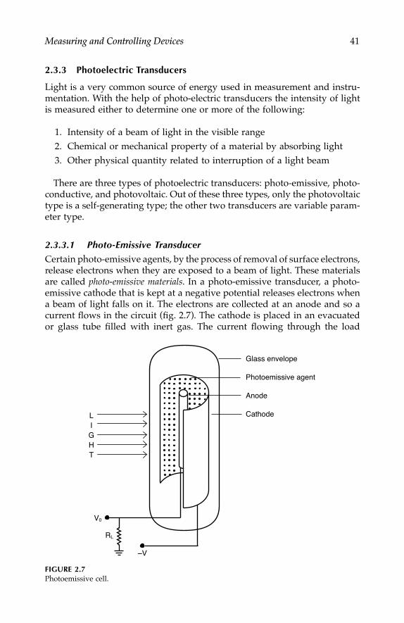
Measuring and Controlling Devices 41
2.3.3 Photoelectric Transducers
Light is a very common source of energy used in measurement and instru-mentation. With the help of photo-electric transducers the intensity of lightis measured either to determine one or more of the following:
1. Intensity of a beam of light in the visible range
2. Chemical or mechanical property of a material by absorbing light
3. Other physical quantity related to interruption of a light beam
There are three types of photoelectric transducers: photo-emissive, photo-conductive, and photovoltaic. Out of these three types, only the photovoltaictype is a self-generating type; the other two transducers are variable param-eter type.
2.3.3.1 Photo-Emissive Transducer
Certain photo-emissive agents, by the process of removal of surface electrons,release electrons when they are exposed to a beam of light. These materialsare called photo-emissive materials. In a photo-emissive transducer, a photo-emissive cathode that is kept at a negative potential releases electrons whena beam of light falls on it. The electrons are collected at an anode and so acurrent flows in the circuit (fig. 2.7). The cathode is placed in an evacuatedor glass tube filled with inert gas. The current flowing through the load
FIGURE 2.7Photoemissive cell.
V0
–V
RL
Glass envelope
Photoemissive agent
Anode
CathodeLIGHT
7244.book Page 41 Wednesday, June 21, 2006 11:14 AM

42 Measurement and Control in Food Processing
resistance is found to be proportional to the intensity of the light incidenton the cathode. The most commonly used cathode material is silver. Silveris oxidized and a thin layer of cesium is applied to it. To increase the sensi-tivity of these devices, photo multiplier tubes are used. In these tubes, dueto secondary emission and electron multiplication, an overall increase inelectron flow is obtained. Luminous sensitivities of such devices range from1A/lumen to more than 2,000A/lumen. Anode current ranges typically from100 µA to a maximum of 1A.
2.3.3.2 Photoconductive Cell
Photoconductive transducers are made up of semiconductor materials likecadmium sulphide, cadmium selenide deposited in a zigzag pattern, a thinlayer of germanium, lead sulfide, and so on; deposited over an insulatingbase like ceramic. The assembly is enclosed in a metal case with a glasswindow for the ray to pass through. The electrical conductivity of the layeris measured between two electrodes placed on two ends of the layer. Whena beam of light falls on the layer, its resistance decreases considerably. Thevariation of the resistance due to change in light intensity is measured bya simple voltage dividing circuit or the commonly used Wheatstone bridgecircuit. These transducers are very compact, rugged in construction, andhighly sensitive. Photocells of this type are commercially available in dif-ferent sizes (1⁄8 in. to 1 in. in diameter). Figure 2.8 shows the layout of sucha photocell.
Different photoconductive materials possess different time constants andspectral bands. For example, CdS has a time constant of 100 ms and worksin the spectral band of 0.47 to 0.71 µm. For practical use, a cell is rated indark resistance and power dissipation. Most devices have a typical darkresistance value varying from hundreds of ohms to several megaohms andpower dissipation of 50 mW to 500mW.
Problem 2.3A photoconductive cell is used to display completeness of fermentation ina tea fermentation process as shown in figure 2.9. A relay should be operated
FIGURE 2.8A photoconductive cell.
R
Base
Metal
Photoconductive strip
7244.book Page 42 Wednesday, June 21, 2006 11:14 AM
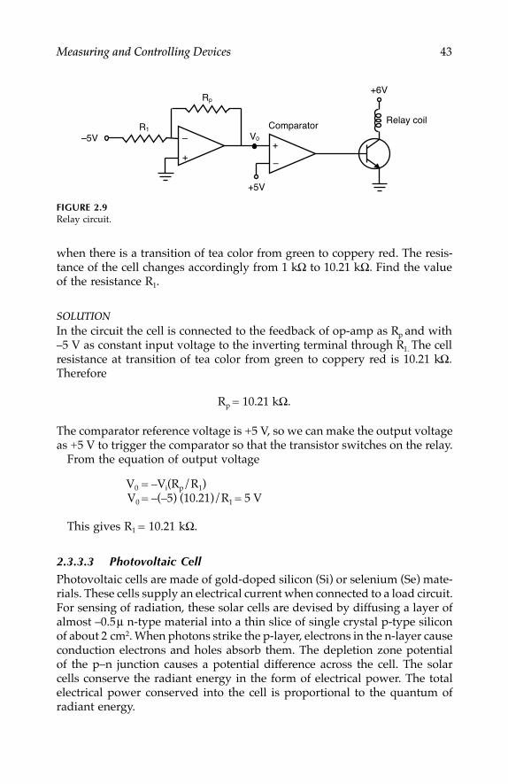
Measuring and Controlling Devices 43
when there is a transition of tea color from green to coppery red. The resis-tance of the cell changes accordingly from 1 kΩ to 10.21 kΩ. Find the valueof the resistance R1.
SOLUTIONIn the circuit the cell is connected to the feedback of op-amp as Rp and with–5 V as constant input voltage to the inverting terminal through R1. The cellresistance at transition of tea color from green to coppery red is 10.21 kΩ.Therefore
Rp = 10.21 kΩ.
The comparator reference voltage is +5 V, so we can make the output voltageas +5 V to trigger the comparator so that the transistor switches on the relay.
From the equation of output voltage
V0 = –Vi(Rp/R1)V0 = –(–5) (10.21)/R1 = 5 V
This gives R1 = 10.21 kΩ.
2.3.3.3 Photovoltaic Cell
Photovoltaic cells are made of gold-doped silicon (Si) or selenium (Se) mate-rials. These cells supply an electrical current when connected to a load circuit.For sensing of radiation, these solar cells are devised by diffusing a layer ofalmost –0.5 µ n-type material into a thin slice of single crystal p-type siliconof about 2 cm2. When photons strike the p-layer, electrons in the n-layer causeconduction electrons and holes absorb them. The depletion zone potentialof the p–n junction causes a potential difference across the cell. The solarcells conserve the radiant energy in the form of electrical power. The totalelectrical power conserved into the cell is proportional to the quantum ofradiant energy.
FIGURE 2.9Relay circuit.
+
–
–
+–5V V0
Rp
R1
+5V
Comparator
+6V
Relay coil
7244.book Page 43 Wednesday, June 21, 2006 11:14 AM

44 Measurement and Control in Food Processing
In addition to the use of photovoltaic cells as radiant energy sensors, theyare also used as solar cells for conserving sunlight as potential energy in anonconventional form of energy. An op-amp amplifier can be used to inter-face the cell to a readout device. The spectral bands on Si- and Se-based cellsare 0.44 µm to 0.62 µm, respectively. One disadvantage of photovoltaic cellsis that their resistance changes with radiant light frequency.
2.3.3.4 Photodiode and Phototransistor
A photodiode (fig. 2.10) is a semiconductor diode used in reverse biasedcondition. When the reverse biased diode is subjected to direct illumination,a direct current flows almost in direct proportion to the light intensity. Themain advantage of the photodiode is its fast response. Due to its goodfrequency response, it can be used faithfully for sensing light fluctuating athigh frequency.
The phototransistor is more sensitive than a photodiode (by as much as100 times) but its response is slow. In an NPN device, light falling on thecentral region produces electron hole pairs, reducing the barrier potentialacross the junctions. This results in more flow of current compared to thephotodiode. Hence it is much more sensitive than a photodiode. Figure 2.11shows the layout of a phototransistor.
2.3.4 Magneto-Electric Transducer
Magneto-electric transducers are also called induction-generator type trans-ducers. These transducers work on the principle of generation of a voltage
FIGURE 2.10A photodiode circuit.
FIGURE 2.11NPN junction phototransistor.
+
–V V0
+Vs
V0
Light
EB
C
7244.book Page 44 Wednesday, June 21, 2006 11:14 AM

Measuring and Controlling Devices 45
by electromagnetic induction. From the basic principle of the law, theinduced EMF is given by
(2.11)
where L is the self-inductance of the coil and dφ/dt is the rate of change offlux linkage with the coil. When a conductor moves in a magnetic field, thevoltage induced is given by
(2.12)
where B is the flux density (wb/cm2), l is the length of the conductor (cm),and v is the velocity (cm/sec) of the conductor. The voltage developed in acoil is proportional to the strength of the magnetic field, total number ofconductors, and velocity of the coil. Based on these design principles, thefollowing magneto-electric transducers are available:
1. Angular velocity electrodynamic transducer2. Linear velocity electromagnetic transducer3. Pulse generator type transducer
2.3.4.1 Electrodynamic Transducer
In this transducer, conductors are wound on a ferromagnetic material to forma coil, which is allowed to rotate in the annular space between a permanentmagnet and soft iron core (fig. 2.12). The voltage induced in the coil is tappedusing carbon brushes or slip rings. This type of transducer is used for angulardisplacement and velocity measurements.
FIGURE 2.12Electrodynamic transducer.
E Lddt
= − φ
e Bl v Volt= × −10 8
Brush
Coil
Soft iron
V0
N S
7244.book Page 45 Wednesday, June 21, 2006 11:14 AM

46 Measurement and Control in Food Processing
2.3.4.2 Electromagnetic Transducer
In an electromagnetic transducer a translation motion is used as the inputto the transducer for generating the electric voltage. In one form (fig. 2.13A)of the transducer, a coil is wound on a nonmagnetic former that is allowedto move to and fro in the annular space of a permanent magnet. The rate ofchange of magnetic flux, cut by the conductors of the coil, is proportional tothe transnational speed and the voltage induced in the coil. It is also pro-portional to the motion.
In another form (fig. 2.13B), a coil is wound on a permanent magnet andan object made of a ferromagnetic material is allowed to move at a certainvelocity. The motion causes the object to change the air gap; the magneticflux linked with the coil also changes at the same rate as that of the velocityof the object. Hence, the voltage induced indicates the transnational motionof the object.
Magnetoelectric transducers are mainly used to measure rotational speedof machines like motors, turbines and so on. When used as a rotational speedsensor, it is called a tacho-generator. Tacho-generators are especially useful asfeedback elements of a positional control system.
Apart from direct use of revolutions per minute (RPM) measurement, thesetransducers are also used for liquid flow and vibration measurement.
2.3.4.3 Pulse Generator Type
In a pulse generating type of transducer, a rotor is driven by a mechanicalforce produced either by flow or by any other motion (fig. 2.14). The outer
FIGURE 2.13Electromagnetic transducers: (A) moving coil type; (B) moving object type.
N
S
Coil
Non-magnetic former
Motion
N
S
Motion
Ferromagnetic object
B
A
7244.book Page 46 Wednesday, June 21, 2006 11:14 AM

Measuring and Controlling Devices 47
periphery of the rotor is a strong permanent magnet and at the outside ofthe housing near the rotor, a coil wound on a soft iron is placed. The coilshould be wound with a large number of turns (i.e., high inductance) so thatsufficient EMF can be developed in it. When the rotor rotates, flux from thepermanent magnet links with the coil only when the permanent magnetapproaches the coil. The voltage induced in the coil is a train of pulses withfrequency that is proportional to the speed of revolution of the rotor. Mea-surement of the pulse frequency gives a measure of the RPM of the rotor;figure 2.15 shows the type of pulse generated in this kind of transducer.
Figure 2.15A shows that four pulses are generated within a specific time,whereas figure 2.15B shows that eight pulses are generated during the sametime span when the rotor speed is increased by two times in the second case.
2.3.5 Radioactive Transducer
Radioactive transducers are based on the absorption pattern or depth ofpenetration of radioactive rays in a medium. Radioactive rays are liberatedby radio-isotopes like 60Co, 137Cs, 192Ir, and so on. The radioactive raysliberated by a radio-isotope are α, β, γ, and neutron radiations. The basiccharacteristics of radioactive rays for use as a source in instrumentation arethe following:
1. Penetrating power
2. Half life
3. Half distance
2.3.5.1 Penetrating Power
The penetrating power of α radiation is the lowest of all types of radioactiveradiations, which is about 11 cm in air and 0.1 mm in fabric. It is easilyabsorbed by a sheet of writing paper and an aluminum foil of 0.006 cmthickness. Penetration of β radiation is higher than α radiation due to its
FIGURE 2.14Pulse generating type of transducer.
FlowFlow
V
Rotor
Permanent magnet
Coil on soft iron
7244.book Page 47 Wednesday, June 21, 2006 11:14 AM
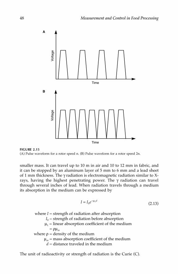
48 Measurement and Control in Food Processing
smaller mass. It can travel up to 10 m in air and 10 to 12 mm in fabric, andit can be stopped by an aluminum layer of 5 mm to 6 mm and a lead sheetof 1 mm thickness. The γ radiation is electromagnetic radiation similar to X-rays, having the highest penetrating power. The γ radiation can travelthrough several inches of lead. When radiation travels through a mediumits absorption in the medium can be expressed by
(2.13)
where I = strength of radiation after absorptionI0 = strength of radiation before absorption
µL = linear absorption coefficient of the medium= ρµm
where ρ = density of the mediumµm = mass absorption coefficient of the medium
d = distance traveled in the medium
The unit of radioactivity or strength of radiation is the Curie (C).
FIGURE 2.15(A) Pulse waveform for a rotor speed n. (B) Pulse waveform for a rotor speed 2n.
Vol
tage
Time
Vol
tage
Time
A
B
I I e Ld= −0
µ
7244.book Page 48 Wednesday, June 21, 2006 11:14 AM
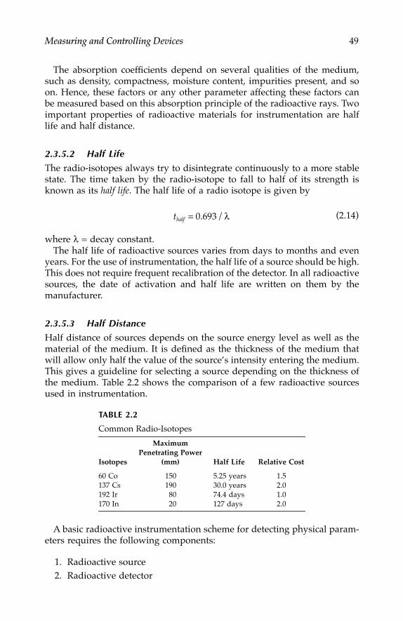
Measuring and Controlling Devices 49
The absorption coefficients depend on several qualities of the medium,such as density, compactness, moisture content, impurities present, and soon. Hence, these factors or any other parameter affecting these factors canbe measured based on this absorption principle of the radioactive rays. Twoimportant properties of radioactive materials for instrumentation are halflife and half distance.
2.3.5.2 Half Life
The radio-isotopes always try to disintegrate continuously to a more stablestate. The time taken by the radio-isotope to fall to half of its strength isknown as its half life. The half life of a radio isotope is given by
(2.14)
where λ = decay constant.The half life of radioactive sources varies from days to months and even
years. For the use of instrumentation, the half life of a source should be high.This does not require frequent recalibration of the detector. In all radioactivesources, the date of activation and half life are written on them by themanufacturer.
2.3.5.3 Half Distance
Half distance of sources depends on the source energy level as well as thematerial of the medium. It is defined as the thickness of the medium thatwill allow only half the value of the source’s intensity entering the medium.This gives a guideline for selecting a source depending on the thickness ofthe medium. Table 2.2 shows the comparison of a few radioactive sourcesused in instrumentation.
A basic radioactive instrumentation scheme for detecting physical param-eters requires the following components:
1. Radioactive source2. Radioactive detector
TABLE 2.2
Common Radio-Isotopes
Isotopes
MaximumPenetrating Power
(mm) Half Life Relative Cost
60 Co 150 5.25 years 1.5137 Cs 190 30.0 years 2.0192 Ir 80 74.4 days 1.0170 In 20 127 days 2.0
thalf = 0 693. /λ
7244.book Page 49 Wednesday, June 21, 2006 11:14 AM

50 Measurement and Control in Food Processing
3. Electronic processing unit
4. Indicator or recorder
A diagram of such a basic radioactive instrumentation scheme is shownin figure 2.16. The radioactive rays are allowed to pass through the testmedium, which moderates some of the radiation and so decreases thestrength of the radiation. The resulting radiation at the output is detectedby a radiation detector. A radiation detector is a device that converts theincident radiation to a proportional electrical signal, detecting the intensitydegradation due to absorption. The following various kinds of suitable radi-ation detectors are available for use with specific applications:
1. Geiger Muller counter
2. Scintillation counter
3. Ionization chamber
4. Proportional counter
5. Semiconductor counter
The electrical signal obtained from a radiation detector is conditioned byan electronic processing unit and the processed signal is displayed by anindicator or recorder.
Two different methods are adopted for testing a medium using radioactiveradiation: the direct transmission method and the back-scattering method.The direct transmission method is used when there is enough room to placethe detector at the other side of the test medium (fig. 2.17). Hence, the sourceand the detector are placed on the two sides of the test medium. When theother side of the test medium is inaccessible or not enough room is availableto place the detector, the back-scattering method is preferable. In this method,a very thin metallic foil placed at the back of the test medium is used as areflecting surface (fig. 2.18). After passing through the medium, the radiationgets reflected back through the medium to the detector. Radioactive trans-ducers are widely used for industrial applications due to their high accuracy,
FIGURE 2.16A basic radioactive instrumentation scheme.
FIGURE 2.17Direct transmission method ofmeasurement.
α,β,γ
Radioactivesource
Testmedium
Radioactivedetector
Electronprocessing
unitI = I0e–µLd
Detector
I = I0e–µLd
Input radiations Medium Output radiations
I0 d
7244.book Page 50 Wednesday, June 21, 2006 11:14 AM
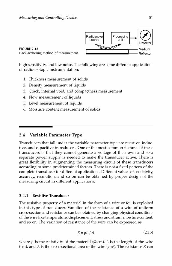
Measuring and Controlling Devices 51
high sensitivity, and low noise. The following are some different applicationsof radio-isotopic instrumentation:
1. Thickness measurement of solids2. Density measurement of liquids3. Crack, internal void, and compactness measurement4. Flow measurement of liquids5. Level measurement of liquids6. Moisture content measurement of solids
2.4 Variable Parameter Type
Transducers that fall under the variable parameter type are resistive, induc-tive, and capacitive transducers. One of the most common features of thesetransducers is that they cannot generate a voltage of their own and so aseparate power supply is needed to make the transducer active. There isgreat flexibility in augmenting the measuring circuit of these transducersaccording to some predetermined factors. There is not a fixed pattern of thecomplete transducer for different applications. Different values of sensitivity,accuracy, resolution, and so on can be obtained by proper design of themeasuring circuit in different applications.
2.4.1 Resistive Transducer
The resistive property of a material in the form of a wire or foil is exploitedin this type of transducer. Variation of the resistance of a wire of uniformcross-section and resistance can be obtained by changing physical conditionsof the wire like temperature, displacement, stress and strain, moisture content,and so on. The variation of resistance of the wire can be expressed as
(2.15)
where ρ is the resistivity of the material (Ω.cm), L is the length of the wire(cm), and A is the cross-sectional area of the wire (cm2). The resistance R can
FIGURE 2.18Back-scattering method of measurement. Reflector
Medium
Processingunit
Radioactivesource
Detector
R L A= ρ /
7244.book Page 51 Wednesday, June 21, 2006 11:14 AM

52 Measurement and Control in Food Processing
be changed by changing any one of ρ, L, or A. In most resistive transducers,the variation in resistance takes place due to only one of these parameters ata time. All three quantities are very rarely varied in the same transducer. Someof the commonly used transducers are explained in the following sections.
2.4.1.1 Potentiometer
The potentiometer is one of the simplest resistive transducers used for mea-surement of translational or rotational displacement. In its simplest form, itconsists of a potentiometer wire or a conducting strip with a movable contactattached to a clamp, called a slider or wiper. The contact motion can betranslational, rotational, or helical. The translational resistive elements arestraight devices, the full stroke length of which can range from 2 mm to 0.5m. The rotational devices are circular in shape with a maximum angulardisplacement of 310° to 360°. Helical potentiometers (helipot) are multiturnrotational devices used for measurement of helical motion. Figure 2.19 showsdifferent forms of potentiometers. For a translational potentiometer the out-put voltage e0 can be calculated as
(2.16)
where ei = input DC excitation voltageRp = total resistance of the potentiometer
FIGURE 2.19Potentiometers: (A) translational; (B) rotational; (C) helical.
V0Vi
V0
Vi
V0
Vi
A
C
B
e input voltageresistance at the output
total r0 = ×eesistance of the P M
e eR X X
Re
XXi
p i t
pi
i
. .
( / )0 = × = ×
tt
7244.book Page 52 Wednesday, June 21, 2006 11:14 AM

Measuring and Controlling Devices 53
Xi = input displacement, cmXt = total potentiometer length, cm
The sensitivity of the device is given by
S = e0/Xi = ei/Xt (V/cm) (2.17)
Hence, the sensitivity of a potentiometer can be increased by using a higherexcitation voltage. The power dissipation capacity of a potentiometer is animportant factor in designing it for a particular input voltage. Due to currentflowing through the potentiometer, heat is developed that is proportional tothe power dissipated, given by
(2.18)
The input voltage is, therefore
(2.19)
For durability of the potentiometer, the power dissipation should be aslow as possible. From equation 2.18, to minimize power dissipation of theinput voltage should be small and resistance should be high. However, it isobserved from equation 2.16 that reduction of input voltage will result alower sensitivity. Therefore, a compromise between these two factors has tobe made.
2.4.1.1.1 Materials
The following are the different types of potentiometer materials generally inuse:
1. Wire wound. These potentiometers are made of some resistive wireswound over a nonmagnetic former. The materials used are alloys ofnickel (i.e., chromium, nickel-copper) or some other precision resis-tive elements. These materials can carry comparatively large currentsat high temperatures. Their resistance temperature coefficient is usu-ally small, on the order of 20 × 10–6 Ω/Ω/°C.
2. Cermets potentiometer. It uses precious metal particles fused into aceramic base. The fused metal particles act as a resistive element.The main advantages of such materials are their high power ratingsand moderate temperature coefficient (from 100 × 10–6 to 200 × 10–6
Ω/Ω/°C).
3. Hot-molded carbon potentiometer. The resistive element of thispotentiometer is fabricated by molding together a mixture of carbonand thermosetting plastic binder.
P e Ri p= 2 /
e PRi p=
7244.book Page 53 Wednesday, June 21, 2006 11:14 AM

54 Measurement and Control in Food Processing
4. Carbon film potentiometer. In this potentiometer, the resistive ele-ment is a thin film of carbon deposited on a nonconducting base. Itsmain advantage is low cost but its temperature coefficient is high(1,000 × 10–6 Ω/Ω/°C).
2.4.1.1.2 Advantages
1. The transducer is inexpensive, very simple to operate, and requiressimple circuits.
2. The potentiometer is useful to measure large displacements.
3. The sensitivity is sufficiently high and therefore does not require anamplifier before driving control equipments.
4. The frequency response is good.
2.4.1.1.3 Disadvantages
1. The potentiometer requires a large torque or force to move the wiper.
2. Because the sliding contact is a moving part, it frequently gets mis-aligned, develops contact resistance, wears out, and produces noise.
2.4.1.2 Resistance Strain Gauge
Strain gauge is a resistive transducer that works on the principle of variationof resistance of a resistive element due to application of mechanical force orload. When a resistive element is subjected to a mechanical force, a mechan-ical stress (force/area) is developed along the element. If the element is elasticin nature, it undergoes mechanical strain (elongation or compression perunit length). Due to the deformation or dimensional change, the resistanceof the element changes directly proportional to the cause of the strain (i.e.,the applied mechanical force, pressure, motion, etc.). When the resistiveelement of a strain gauge is subjected to a mechanical stress, dimensionalchanges take place; that is, length increases and cross-sectional areadecreases. A compressive stress causes a reverse dimensional change. Thisproperty of the material is called the piezo-resistive effect. The effect thatchanges resistance can be described by the following equations.
The resistance of a wire conductor is given by
R = ρL/A
where ρ = the specific resistance of the material (Ω.m)L = length of the conductor (m)A = the cross-sectional area of the conductor (m2)
= CD2, C is a constant and D is the diameter (m)
7244.book Page 54 Wednesday, June 21, 2006 11:14 AM

Measuring and Controlling Devices 55
Hence, we can write that
R = ρL/CD2
If the conductor is stretched or compressed, its resistance will change dueto change in length and cross-sectional area and due to the piezo-resistanceeffect. Differentiation on R gives
Dividing the equation by (dL/L) gives
(2.20)
where v is the Poisson’s ratio of the material of the wire. The term
(2.21)
is called the gauge factor of the strain gauge. The gauge factor of a straingauge is a measure of its sensitivity. For most of the strain gauges the gaugefactor is about 2.0 and for nickel its value can vary from –12 to +6.
Resistance strain gauges are classified into two basic forms: unbonded andbonded.
2.4.1.2.1 Unbonded Strain GaugesAn unbonded resistance strain gauge is made of a set of resistive wires ofabout 25µ in diameter stretched between two supports. The wires arestretched between two structures, one fixed and the other movable. Figure2.20 shows such an unbonded strain gauge. The wires are stretched prior toapplication of strain to avoid sag and vibration. When the movable plate isdisplaced, the wires will be under tensile strain, causing a change in resis-tance. A displacement on the order of 50µ can cause a considerable strain inthe wires. The four wires are connected to a Wheatstone bridge circuit thatresults in unbalanced output voltage. Unbonded strain gauges are suitablefor measurement of very small displacements.
dRCD Ld dL L C D dD
CD
dR RCD L
= + +
=
2
2 2
2
2
1
( )( )
/( / ) (
ρ ρ ρ
dd dL L dD D
L CD
dR RdLL
dDD
d
ρ ρ ρρ
ρρ
+ +
= + +
) /
/
/
2
2
2
( / )( / )
( / )( / )
dR RdL L
vddL L
= + +1 2ρ ρ
( / )( / )dR RdL L
= λ
7244.book Page 55 Wednesday, June 21, 2006 11:14 AM

56 Measurement and Control in Food Processing
2.4.1.2.2 Bonded Strain Gauges
Bonded strain gauges are very fine resistive wire elements (about 25µ indiameter) or very thin metallic foils printed or etched on a backing plate(usually paper) in a zigzag or looped pattern as shown in figure 2.21. Thewire or the foil is covered by a protective material like a thin sheet of paper,bakelite, or Teflon. The backing plate is bonded to the surface of the testmaterial using an appropriate bonding or cementing material. Once thegauge is bonded to the surface, it becomes a part of the surface and strainis uniformly transferred to the gauge.
When a material is under stress, strain is developed in two directions: theprincipal strain (εx) in the longitudinal axis and the transverse strain (εy) inthe transverse axis. The transverse strain is given by
(2.22)
FIGURE 2.20Unbonded strain gauge.
FIGURE 2.21Bonded strain gauges: (A) wire gauge; (B) foil gauge.
Fixed plate
Movable plate
Stretched unbonded wire
Backing plateA
B
Fine wire
Leads
Metallic foil
ε εy xv= −
7244.book Page 56 Wednesday, June 21, 2006 11:14 AM

Measuring and Controlling Devices 57
where ν is the Poisson’s ratio. A strain gauge is always mounted on a surfacewith the longitudinal wire elements in the direction of the principal strain.Hence, a strain gauge picks up the principal strain with highest sensitivity inthis direction. Because the end loops of the grid are in the direction of thetransverse strain, the gauge picks up the transverse strain that results an errorin the measurement. To make the gauge insensitive to this transverse strain,two methods are adopted. In one method the end loops are made of materialsinsensitive to strain like copper or gold (fig. 2.21A). In the other method thecross-sectional area of the end loops is made considerably larger than that ofthe longitudinal wire elements (fig. 2.21B). This reduces the transverse straindeveloped in the end loops of the strain gauge. Strain gauges are manufac-tured in various configurations based on different applications such as these:
1. Grid type
2. Rossette type
3. Torque type
4. Helical type
Looping down the strain wire in the insulated base in a back and forthmanner (fig. 2.21A and fig. 2.21B) results in a grid type strain gauge. Whenthe axis of the strain in a plane is not exactly known, it is difficult to bondthe gauge in proper orientation for sensing the maximum strain developed.In such situations several grid gauges are placed as shown in figure 2.22. Itshows a three-element rosette gauge in which the angle between any twolongitudinal gauge axes is 45°.
Torque and helical gauges are used in special applications. Torque typegauges (fig. 2.23) have resistive element laid at an angle of 45° to the gauge
FIGURE 2.22Rossette type strain gauge.
7244.book Page 57 Wednesday, June 21, 2006 11:14 AM

58 Measurement and Control in Food Processing
axis. This gauge is used to measure torque in a rotating shaft where amaximum strain is developed along the direction of 45° to the shaft axis.Helical gauges are used to pick up radial as well as circumferential straindeveloped in a diaphragm used for pressure measurement (fig. 2.24).
2.4.1.2.3 Ratings of Metallic Strain GaugesThe gauge factor of most of the metallic gauges falls in the range of 2.0 to2.1. Foil and wire gauges are made from nichrome, Constantan (Ni and Cu),Isoelastic (Ni, Cr, and Mo), nickel, and platinum.
The resistance of strain gauges should be as high as possible to minimizeother interfering factors. Typical values of wire gauge resistances are 120 Ω,350 Ω, and 1,000 Ω; and 50 Ω and 1,000 Ω for foil gauges. The diameter ofthe wires used in the strain gauges is typically 25µ. This restricts its maximumcurrent carrying capacity to the order of 30 mA.
2.4.1.2.4 Semiconductor Strain GaugesSemiconductor strain gauges are used when a higher sensitivity is needed.Therefore, these strain gauges possess a higher gauge factor. Unlike metallicgauges, in semiconductor strain gauges the variation of resistance on appli-cation of strain is mainly due to variation of resistively. Germanium andsilicon are two commonly used semiconductor materials. The sensitivity ofsuch gauges depends on the degree of doping.
FIGURE 2.23Torque gauge.
FIGURE 2.24Helical gauge.
Base
Lead
7244.book Page 58 Wednesday, June 21, 2006 11:14 AM

Measuring and Controlling Devices 59
Semiconductor strain gauges are manufactured in wafer or filament forms,with a thickness of 0.05 mm, bonded to suitable insulating substrate materialsuch as Teflon. The gauge factor of semiconductor strain gauges is 130 ± 10%for a gauge of 350 Ω, 1 in. long, 1/2 in. wide, and 0.005 in. thick. The operatingrange is ± 3,000 microstrain and the power consumption is only 0.1 W. Theresolution is about 0.01 microstrain. The main advantages of semiconductorstrain gauges are higher sensitivity, higher resolution, low hysteresis, higherfrequency response, and small size.
2.4.1.2.5 Measuring Circuit
Signal conditioning circuits for strain gauges should eliminate two effects:First, the small change in resistance should be effectively converted to achange in voltage. Second, because the strain gauge is a resistive element,any deviation of gauge resistance due to change in temperature should beproperly compensated. A full Wheatstone bridge configuration takes care ofthe first effect where four strain gauges of similar ratings are connected tothe four branches of the bridge with proper strain polarity as shown in figure2.25. The direction of the arrow of the resistors in the bridge circuit indicatesthe polarity of the strain developed. Let the unstrained normal resistancesof the gauges be
R1 = R2 = R3 = R4
and the strained resistances of the gauge be
where ∆R = small change in resistance due to application of strain ε.
FIGURE 2.25A Wheatstone bridge measuring circuit.
R RR
Rε = ±
1∆
V0
R1 R2
R4 R3
V
7244.book Page 59 Wednesday, June 21, 2006 11:14 AM

60 Measurement and Control in Food Processing
The unbalanced output voltage can be determined as
(2.23)
However if different resistance variations are considered for each gauge,the output voltage equation take the form
(2.24)
where the individual strains picked up by the gauges are
In most of the cases, four identical gauges are employed to get an outputvoltage by equation 2.23.
2.4.1.3 Diaphragm Pressure Sensor
Diaphragm pressure sensors are made up of two elements:
• A thin metallic diaphragm to sense and convert pressure to deflection
• Strain gauges bonded to the diaphragm to pick up strain developedin radial and tangential directions
It uses a metal diaphragm with good spring characteristics. The diaphragmis clamped to the periphery of the connecting pipe with screws and nuts asshown in figure 2.26. When the diaphragm is subjected to a pressure P, itundergoes a deflection given by the equation
(2.25)
V VR R
R R R RR R
R R R R0 = ++ + −
− −+ + −
∆∆ ∆
∆∆ ∆( ) ( ) ( ) ( )
= + − −
= + − +
VR R
RR R
R
VR R R R
R
∆ ∆
∆ ∆
2 2
2
==
=
VR
R
V V
∆
From eq. 2.21 0 λ ε
VV
0 2 4 1 34= + − −λ ε ε ε ε[ ]
λε λε λε λε11
12
2
23
3
34
4
4
= = = =∆ ∆ ∆ ∆RR
RR
RR
andR
R, ,
PEt
r vy t y t=
−+
163 1
0 4884
4 23
( )( / ) . ( / )
7244.book Page 60 Wednesday, June 21, 2006 11:14 AM

Measuring and Controlling Devices 61
where P = pressure difference across diaphragmE = modulus of elasticity of the materialt = thickness of the diaphragmy = deflection of the diaphragmv = Poisson’s ratior = radius of diaphragm to clamped edge
For a small deflection, this equation is fairly linear, but sensitivity of thediaphragm becomes very small. Strain developed in two directions of thediaphragm, as follows:
1. A radial and tensile strain with maximum value at the outer periph-ery of the diaphragm
2. A tangential and compressive strain that is maximum at the center
These strains are picked up by two pairs of strain gauges as shown infigure 2.25. Strain gauges 1 and 3 sense the radial strain (tensile) and gauges2 and 4 sense the tangential strain (compressive). The radial and tangentialstresses are given by the equation
(2.26)
(2.27)
where rr and rt are the radii at which the corresponding radial and tangentialgauges are bonded. A strain gauge experiences both radial and transversestrain, so the actual strain developed is
(2.28)
FIGURE 2.26A diaphragm pressure sensor bonded withfour strain gauges.
t
Top view
End view
31
2
4
1,3 - Radial strain; 2,4- Tangential strain
R
sprt
r rr r= +
− +
38
11
31
2
22ν
ν ν( / )
sprt
r rt t= +
− +
38
11
33
2
22ν
ν ν( / )
εr r ts v s E= −( )/
7244.book Page 61 Wednesday, June 21, 2006 11:14 AM
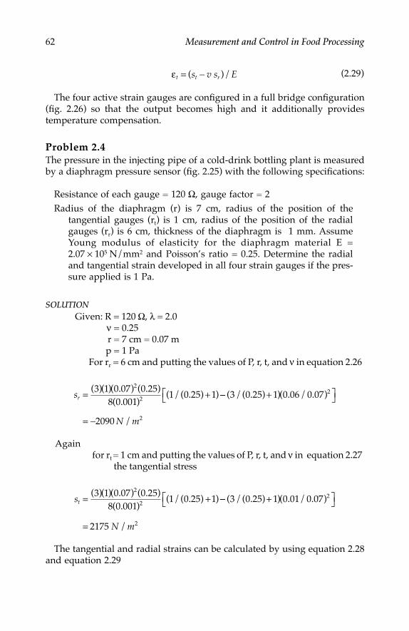
62 Measurement and Control in Food Processing
(2.29)
The four active strain gauges are configured in a full bridge configuration(fig. 2.26) so that the output becomes high and it additionally providestemperature compensation.
Problem 2.4The pressure in the injecting pipe of a cold-drink bottling plant is measuredby a diaphragm pressure sensor (fig. 2.25) with the following specifications:
Resistance of each gauge = 120 Ω, gauge factor = 2Radius of the diaphragm (r) is 7 cm, radius of the position of the
tangential gauges (rt) is 1 cm, radius of the position of the radialgauges (rr) is 6 cm, thickness of the diaphragm is 1 mm. AssumeYoung modulus of elasticity for the diaphragm material E =2.07 × 10⁵ N/mm2 and Poisson’s ratio = 0.25. Determine the radialand tangential strain developed in all four strain gauges if the pres-sure applied is 1 Pa.
SOLUTIONGiven: R = 120 Ω, λ = 2.0
ν = 0.25r = 7 cm = 0.07 mp = 1 Pa
For rr = 6 cm and putting the values of P, r, t, and ν in equation 2.26
Againfor rt = 1 cm and putting the values of P, r, t, and ν in equation 2.27
the tangential stress
The tangential and radial strains can be calculated by using equation 2.28and equation 2.29
εt t rs v s E= −( )/
sr = +( )( )( . ) ( . )( . )
( /( . ) )3 1 0 07 0 25
8 0 0011 0 25 1
2
2 −− +
= −
( /( . ) )( . / . )
/
3 0 25 1 0 06 0 07
2090
2
2N m
st = +( )( )( . ) ( . )( . )
( /( . ) )3 1 0 07 0 25
8 0 0011 0 25 1
2
2 −− +
=
( /( . ) )( . / . )
/
3 0 25 1 0 01 0 07
2175
2
2N m
7244.book Page 62 Wednesday, June 21, 2006 11:14 AM

Measuring and Controlling Devices 63
and
2.4.1.4 Load Cell
Load is an important parameter describing the mechanical force applied ona body. Measurement of load using a load cell gives an indication of somequality attribute of materials in the hopper or conveyor in a manufacturingunit. Force (F) and load (W) can be related by an equation as
(2.30)
where g is acceleration due to gravity.
2.4.1.4.1 Strain Gauge Based Load Cells
The principle of elastic deformation of a transmitting member due to appli-cation of load or force and the measurement of the deformation is utilizedin this type of sensor. Various types of mechanical devices used for sensingload through development of strain are shown in figure 2.27. Every sectionof the mechanical load sensor undergoes relative linear displacement, whichcauses a strain. This strain is a measure of the load transmitted by theresistive strain gauges. The strain is measured by using four strain gaugesconfigured in a bridge circuit arrangement. The strain gauges are bonded tothe surface of the mechanical sensor, which senses tensile and compressivestrain developed. The output voltage developed is amplified and calibratedto directly indicate the load or force. Forces as high as 10 tons or more canbe measured by properly designing the mechanical sensor.
2.4.1.5 Resistance Temperature Detectors
It is a well-known fact that resistance of a metal element changes withtemperature. This principle is used in resistance temperature detectors(RTDs). The change in resistance due to temperature variation is given by
(2.31)
ε νr r ts s E= −
= − − × ×
=
( )/
( . )/( . )2090 2175 0 25 2 07 105
−− × = =1272 1051 3ε ε
ε νt t rs s E= −
= + × ×
=
( )/
( . )/( . )2175 2090 0 25 2 07 10
1
5
303 1052 4× = =ε ε
F Wg=
R R Tt = +0 1( )α∆
7244.book Page 63 Wednesday, June 21, 2006 11:14 AM

64 Measurement and Control in Food Processing
where α is a positive resistance temperature coefficient. The metals used formaking resistance thermometers are generally platinum (–190°C to 660°C),copper (–150°C to 250°C), and nickel (0°C to 325°C). The operating temper-ature ranges of these metals are observed to be not very high, so theseelements are suitable for low temperature measurements only. The value ofα for platinum is on the order of 0.004/°C and that of nickel is 0.005/°C. Therequisite characteristics of these materials are as follows:
1. High temperature coefficients for higher sensitivity
2. High sensitivity for compactness
3. Good linearity for ease of calibration
4. Resistance to contamination for reliability
For a low temperature range, two other materials are found to be suitable:a gold–silver alloy for temperatures below 127°K and phosphor–bronze alloyfor temperatures below 7°K. These alloys possess sensitivity about 55 timesthat of the ordinary metals.
2.4.1.5.1 Construction
A resistance wire with a diameter ranging from 0.002 cm to 0.06 cm is gen-erally used, but a 0.01 cm diameter is most common. The wire is bifilarlywound on a nonconducting former or framework of mica-cross, ceramic flat,or round arbors. For surface temperature measurement a grid etched on aninsulated surface is used. Figure 2.28 shows different constructions of RTDs.The resistance thermometers have a resistance of between 0.1 ohm and a fewhundred ohms.
FIGURE 2.27Load sensors.
1 3
2 4
W W
1 2 4 3
1 2 4 3
W
Cantilever
Proving ring Cylinder
7244.book Page 64 Wednesday, June 21, 2006 11:14 AM
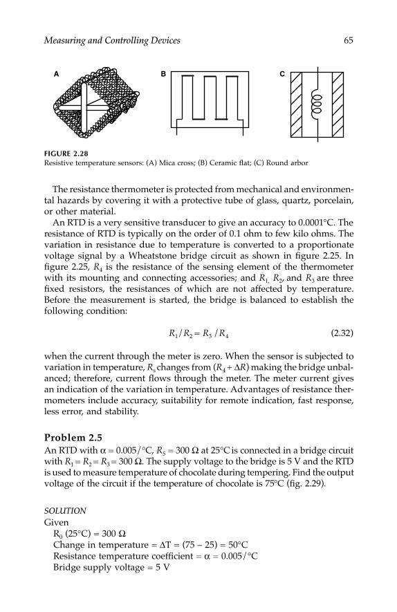
Measuring and Controlling Devices 65
The resistance thermometer is protected from mechanical and environmen-tal hazards by covering it with a protective tube of glass, quartz, porcelain,or other material.
An RTD is a very sensitive transducer to give an accuracy to 0.0001°C. Theresistance of RTD is typically on the order of 0.1 ohm to few kilo ohms. Thevariation in resistance due to temperature is converted to a proportionatevoltage signal by a Wheatstone bridge circuit as shown in figure 2.25. Infigure 2.25, R4 is the resistance of the sensing element of the thermometerwith its mounting and connecting accessories; and R1, R2, and R3 are threefixed resistors, the resistances of which are not affected by temperature.Before the measurement is started, the bridge is balanced to establish thefollowing condition:
R1/R2 = R3 /R4 (2.32)
when the current through the meter is zero. When the sensor is subjected tovariation in temperature, Rs changes from (R4 + ∆R) making the bridge unbal-anced; therefore, current flows through the meter. The meter current givesan indication of the variation in temperature. Advantages of resistance ther-mometers include accuracy, suitability for remote indication, fast response,less error, and stability.
Problem 2.5An RTD with α = 0.005/°C, RS = 300 Ω at 25°C is connected in a bridge circuitwith R1 = R2 = R3 = 300 Ω. The supply voltage to the bridge is 5 V and the RTDis used to measure temperature of chocolate during tempering. Find the outputvoltage of the circuit if the temperature of chocolate is 75°C (fig. 2.29).
SOLUTIONGiven
R0 (25°C) = 300 ΩChange in temperature = ∆T = (75 – 25) = 50°CResistance temperature coefficient = α = 0.005/°CBridge supply voltage = 5 V
FIGURE 2.28Resistive temperature sensors: (A) Mica cross; (B) Ceramic flat; (C) Round arbor
A B C
7244.book Page 65 Wednesday, June 21, 2006 11:14 AM

66 Measurement and Control in Food Processing
The resistance of the RTD at 75°C (from equation 2.31)
Rs (75°C) = 300[1 + 0.005(50)]= 375 Ω
The output voltage from the bridge circuit
2.4.1.6 Thermistors
Thermistors are semiconductor materials with negative temperature resis-tance coefficients; that is, their resistance decreases as temperature increases.The resistance of thermistors at room temperature usually ranges from 100ohms to 10 mega ohms. They are so sensitive to temperature that a 1°Cincrease can decrease resistance at room temperature by 6%. The workingranges of thermistors are typically 100°C to 300°C. The resistance tempera-ture characteristic of a thermistor is shown in figure 2.30. The equationrelating the resistance and absolute temperature of a thermistor is given by
(2.33)
where Rt = resistance at T°KR0 = resistance at T0°Kβ = thermistor constant; its common value lies around 4000°K
FIGURE 2.29RTD measuring circuit.
R1
R3
R2
RS
V0
VRTD
V Volt0 5300
300 300300
300 375
278
=+
−+
= mV
R R etT T=
−
0
1 1
0( )β
7244.book Page 66 Wednesday, June 21, 2006 11:14 AM
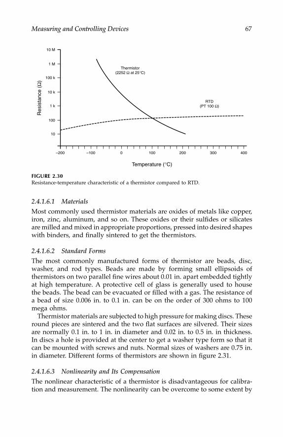
Measuring and Controlling Devices 67
2.4.1.6.1 Materials
Most commonly used thermistor materials are oxides of metals like copper,iron, zinc, aluminum, and so on. These oxides or their sulfides or silicatesare milled and mixed in appropriate proportions, pressed into desired shapeswith binders, and finally sintered to get the thermistors.
2.4.1.6.2 Standard Forms
The most commonly manufactured forms of thermistor are beads, disc,washer, and rod types. Beads are made by forming small ellipsoids ofthermistors on two parallel fine wires about 0.01 in. apart embedded tightlyat high temperature. A protective cell of glass is generally used to housethe beads. The bead can be evacuated or filled with a gas. The resistance ofa bead of size 0.006 in. to 0.1 in. can be on the order of 300 ohms to 100mega ohms.
Thermistor materials are subjected to high pressure for making discs. Theseround pieces are sintered and the two flat surfaces are silvered. Their sizesare normally 0.1 in. to 1 in. in diameter and 0.02 in. to 0.5 in. in thickness.In discs a hole is provided at the center to get a washer type form so that itcan be mounted with screws and nuts. Normal sizes of washers are 0.75 in.in diameter. Different forms of thermistors are shown in figure 2.31.
2.4.1.6.3 Nonlinearity and Its Compensation
The nonlinear characteristic of a thermistor is disadvantageous for calibra-tion and measurement. The nonlinearity can be overcome to some extent by
FIGURE 2.30Resistance-temperature characteristic of a thermistor compared to RTD.
–200 4003002001000–100
Temperature (°C)
Thermistor(2252 Ω at 25°C)
RTD(PT 100 Ω)
Res
ista
nce
(Ω)
10
100
1 k
10 k
100 k
1 M
10 M
7244.book Page 67 Wednesday, June 21, 2006 11:14 AM

68 Measurement and Control in Food Processing
connecting a low resistance (Rc) parallel to the thermistor resistance (Rt).Figure 2.32 shows the circuit and the graph for nonlinearity compensation.The equivalent resistance of the compensated thermistor is given by
(2.34)
Rate of variation of compensated resistance with respect to temperature is
FIGURE 2.31Forms of thermisters: (A) rod; (B) disc; (C) bead; (D) washer; (E) commercial ultra precisionthermistors. (E: Reprinted with permission from U.S. Sensor Corporation, USA)
FIGURE 2.32(A) Circuit for nonlinearity compensation. (B) Characteristics for compensated and uncompen-sated thermistor.
30 AWG (0.010")Tinned copper alloy wire
Epoxy coating
A
E
B C D
0.095"max
1.5" min
Rt alone
Rt and Rc in parallel
Tempetature
Res
ista
nce
Rt Rc
BA
R R R R Req t c t c= +( )/( )
7244.book Page 68 Wednesday, June 21, 2006 11:14 AM

Measuring and Controlling Devices 69
From this equation it is evident that
(2.35)
It shows that although linearity of a thermistor is compensated by theadditional resistor, the sensitivity is reduced. Thermistors with linearity ashigh as 0.2% over the temperature range of 0°C to 100°C are also available.Typical sensitivity values of thermistors are on the order of 3mV/°C at 200°C.
Thermistors are more popular as a device in limiter and regulator circuits,time delays, and temperature compensations than for absolute temperaturemeasurement. The power dissipation constant of thermistors is typically1mW/°C in free air. This parameter is important to estimate error produceddue to self-heating.
Advantages of thermistors are as follows:
1. Compactness and low cost
2. Good response and good sensitivity
3. Negligible contact and lead resistance error due to higher resistancevalue of the thermistor
Disadvantages include the following:
1. Nonlinear characteristics
2. Low operating range
3. Error due to self-heating
2.4.1.7 Semiconductor Temperature Sensors
Thermal semiconductor sensors are suitable for sensing ambient temperaturein the range of –55 to 155°C. A typical IC sensor develops a voltage or currentsignal proportional to absolute temperature. Accordingly, two types of ICsensors are commercially available: the voltage proportional to absolutetemperature (VPTAT) and current proportional to absolute temperature(IPTAT). The connection diagram of a popular VPTAT, IC LM335, is shownin figure 2.33.
When properly calibrated the IC gives an output voltage of 2.98 V at 25°Cand a variation of 10 mV/°C. A similar arrangement of an IC AD590, whichis an IPTAT, is shown in figure 2.34. AD590 gives a sensitivity of 1 mV/°C,which is 10 times smaller than that of LM335. The main advantages of IC
dRdT
dRdT
RR R
eq t c
c t
= ⋅+
2
2( )
dRdT
dRdT
eq t⟨
7244.book Page 69 Wednesday, June 21, 2006 11:14 AM
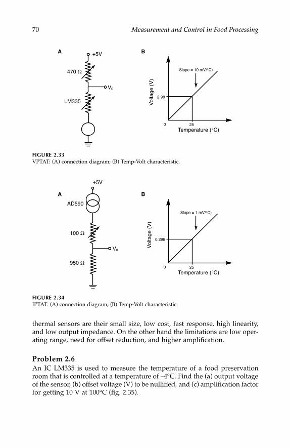
70 Measurement and Control in Food Processing
thermal sensors are their small size, low cost, fast response, high linearity,and low output impedance. On the other hand the limitations are low oper-ating range, need for offset reduction, and higher amplification.
Problem 2.6An IC LM335 is used to measure the temperature of a food preservationroom that is controlled at a temperature of –4°C. Find the (a) output voltageof the sensor, (b) offset voltage (V) to be nullified, and (c) amplification factorfor getting 10 V at 100°C (fig. 2.35).
FIGURE 2.33VPTAT: (A) connection diagram; (B) Temp-Volt characteristic.
FIGURE 2.34IPTAT: (A) connection diagram; (B) Temp-Volt characteristic.
+5V
470 Ω
LM335
V0
Temperature (°C)
Slope = 10 mV/°C)
Vol
tage
(V
)
0 25
2.98
A B
Temperature (°C)
Slope = 1 mV/°C)
Vol
tage
(V
)
0 25
0.298
A B
+5V
AD590
100 Ω
950 Ω
V0
7244.book Page 70 Wednesday, June 21, 2006 11:14 AM

Measuring and Controlling Devices 71
SOLUTIONGiven values
We know that the sensitivity of LM335 sensor = 10mV/°CCalibrated output voltage at 25°C = 2.98 VDifference of output voltage between 25°C and –4°C
= (25 – (–4)) × sensitivity= (25 + 4) × 10 mV/°C= 290 mV
(a) The sensor output voltage at –4°C = (2.98 – 0.290) V = 2.69 V(b) The sensor output voltage at 0°C = 2.98 – (25 × 10) = 2.98 – 0.25
= 2.73 V
Hence, the offset voltage to be nullified is 2.73V(c) The sensor output voltage at 100°C
= 2.73 + (100 × 10) mV= 2.73 + 1.0 V= 3.73 V
After nullifying the offset voltage, the differential input voltage to the ampli-fier at 100°C
= (3.73 – 2.73) V= 1.00 V
The required amplified voltage at 100°C = 10 VHence, the amplification factor = 10 V/1.00 V
= 10
2.4.1.8 Hot Wire Anemometer
The hot wire anemometer is a resistive transducer used for measurement offlow of gas or liquid through a pipe. The basic principle and setup of thehot wire anemometer is that a resistive wire is placed across the flow streamand a constant current is allowed to flow through it (fig. 2.36). The heat
FIGURE 2.35LM335 with the amplifier circuit.
LM335
+V
Output (0–10 V)
Offset
AMP
7244.book Page 71 Wednesday, June 21, 2006 11:14 AM

72 Measurement and Control in Food Processing
developed in the wire is dissipated into its surrounding when the velocityof the fluid changes; the amount of heat dissipated will also change. Thisheat loss changes the resistance of the wire. If the current supplied to thewire is kept constant, the change in resistance can be taken as a measure ofthe change in flow. This gives a constant current hot wire anemometer.
The resistive element is made of a platinum wire with a diameter of 0.0005to 0.03 cm and a length of 0.1 to 1 cm. The diameter of the wire should be keptsmall to experience less fluid pressure. The length of the wire should be halfof the pipe diameter and is placed at the center of the pipe with supports.
The variation in resistance of the wire due to change in fluid velocity isdetected by a Wheatstone bridge circuit. Contamination is a major problemof the hot wire anemometer. Another drawback is that when the current iskept at large value and fluid velocity drops by a large amount suddenly, thewire might burn out.
2.4.1.9 Resistive Humidity Sensors
Humidity has been measured using various mechanical devices for a longtime, but electrical resistance type humidity sensors are more popular thanmechanical types because in electrical types the signal can be transmittedand recorded by electronic devices. This type of humidity sensor is basedon variation of resistance of resistive wires on a nonconductive backingmaterial, as shown in figure 2.37A.
The space between the two wire electrodes is filled with a hygroscopiccompound like lithium chloride, phosphoric acid, calcium chloride, zincchloride, or tin-tetrachloride. When the sensor is exposed to air containingwater particles, the hygroscopic material absorbs water and the overall resis-tance between the two wire electrodes decreases. The change in resistanceis on the order of 10 MΩ to 10 KΩ. This variation in resistance can beconverted to a voltage by inserting the sensor in a resistive network or aWheatstone bridge circuit as shown in figure 2.37B and figure 2.37C.
2.4.2 Inductive Transducers
Inductive transducers constitute a major part of the transducer family, mostlyfor displacement and proximity measurement. Inductive transducers can bebroadly classified into two main types: self-generation and variable inductance.
In the self-generating type, a relative motion between a conductor and amagnetic field is converted to an induced voltage.
In a variable inductance transducer, the physical displacement is utilizedto vary the self-inductance or mutual inductance of a coil. The inductance
FIGURE 2.36Setup of a hot wire anemometer in a pipe flow.
Flow Wire
7244.book Page 72 Wednesday, June 21, 2006 11:14 AM

Measuring and Controlling Devices 73
of a coil can be changed by changing the following parameters by the dis-placement to be measured:
1. Number of turns of the coil
2. Length of the coil
3. Permeability of the core of the coil
2.4.2.1 Variable Inductance Type
The inductance of a coil of two different forms (as shown in fig. 2.38) can bechanged by changing the number of turns.
2.4.2.1.1 Change in Permeability
A coil is wound over a ferromagnetic former into which an iron core can beinserted using a nonmagnetic handle (fig. 2.39). When the iron core is dis-placed inside the former, the total permeability of the magnetic circuit
FIGURE 2.37(A) Resistive humidity sensor. (B) Potentiometric circuit. (C) Bridge circuit.
FIGURE 2.38(A) Translational transducer. (B) Rotational transducer.
Insulating backing
Coating
R
R
B C
A
R R
RRV0
Air core
Output
Displacement
Core
Output
BA
7244.book Page 73 Wednesday, June 21, 2006 11:14 AM

74 Measurement and Control in Food Processing
increases and when the core is taken out the permeability decreases propor-tionately. Hence, the self-inductance of the coil changes with the displace-ment of the core.
2.4.2.2 Variable Reluctance Type Sensors
The reluctance of a magnetic circuit can be varied with displacement of atarget with respect to a ferromagnetic core, as shown in figure 2.40.
The self-inductance of the coil is given by
(2.36)
where N = number of turnsRi = reluctance of iron path of the coilRg = reluctance of air gap
Practically the reluctance of the iron path can be neglected compared tothe air gap; therefore
(2.37)
FIGURE 2.39Variable permeability type sensor.
FIGURE 2.40Variable reluctance type sensor.
Handle
Iron core
Ferromagneticformer
Output
Target (iron) displacementAir gap
Ferromagnetic
motion
L N R Ri g= +2 /( )
L N Rg= 2 /
7244.book Page 74 Wednesday, June 21, 2006 11:14 AM

Measuring and Controlling Devices 75
The reluctance of the air gap is given by
(2.38)
where lg = length of the air gapµ0 = absolute permeability
and Ag = area of flux path through air
Because permeability and area of flux path are constants, Rg is proportionalto length of the air gap (lg) and self-inductance (L) is inversely proportionalto the length of the air gap. Therefore, as the target approaches the ferro-magnetic coil, the air gap decreases and the self-inductance increases pro-portionately.
2.4.2.2.1 Voltage Generating TypeThese are electromagnetic transducers designed to develop alternating volt-age proportional to velocity or displacement of some moving object. Onearrangement of this transducer is shown in figure 2.41.
2.4.2.2.2 Differential Voltage Transducer A differential transducer works on the principle of a variable reluctancetransducer. It consists of a coil having three windings—one primary and twoidentical secondary windings—as shown in figure 2.42. The two secondarywindings are spaced symmetrically with respect to the primary coil. Thecoils are wound over a nonmagnetic former. A ferromagnetic core made ofcast iron is inserted into the coil former with the help of a nonmagnetichandle. When the core is placed at the central location of the coil, the mutualinductances M1 and M2 between the primary and secondary windings (Sy1
and Sy2) become equal. M1 and M2 vary linearly as the core moves insidethe coil; that is, M1 decreases and M2 increases when the core moves towardthe right and similarly M2 decreases and M1 increases when the core movestoward the left.
FIGURE 2.41Electrodynamic transducer.
l Ag g= / µ0Rg
Brush
Coil
Soft iron
V0
N S
7244.book Page 75 Wednesday, June 21, 2006 11:14 AM

76 Measurement and Control in Food Processing
When the primary is supplied with an AC voltage (50 Hz–20 KHz), ACvoltages are induced in the two secondary windings given by the equation
(2.39)
where i is the current in the primary winding.When the core moves toward the right, e2 > e1
and when the core moves toward the left, e1 > e2.
Because the two secondary windings are connected in phase opposition,the output voltage e0 is given by
(2.40)
Hence, the output voltage is a modulated AC voltage with the same fre-quency as that of the supply voltage, which has a magnitude proportionalto the displacement of the core. By measuring the magnitude of the outputAC voltage, the displacement can be measured.
The advantages of differential transducer are the following:
1. High sensitivity and accuracy2. Output is not effected by temperature variation3. Effect of variation in supply voltage and frequency is less4. Resolution is high5. Due to absence of sliding contact, less force is required for operation6. Low hysteresis and good repeatability7. Low power consumption on the order of 1 W
FIGURE 2.42Transformer circuit of LVDT.
M1 M2
e1 e2
AC supply
Output
e Mdidt
e Mdidt1 1 2 2= =and
e e e0 1 2= −
7244.book Page 76 Wednesday, June 21, 2006 11:14 AM

Measuring and Controlling Devices 77
Disadvantages are as follows:
1. Not suitable for very small displacement2. Highly immune to stray magnetic fields3. Demodulator is required to get DC output
2.4.3 Capacitive Transducer
The capacitance of a capacitor in many cases can be a factor of measurementof some physical parameters like displacement, pressure, angular position,moisture content, and so on. A capacitive transducer works on the principleof variation of its capacitance by the physical variable. The capacitance Cbetween two parallel plates of a capacitor is given by
(2.41)
where K = dielectric constant of the mediumA = area of the platesd = distance between the platesε0 = permittivity = 8.85 pF/m
Capacitance C between the two plates can be varied by varying the distancebetween the two plates or the area of the medium.
In figure 2.43A, plate B moves toward or away from the fixed plate A,thereby varying the gap between the two plates, whereas in the arrangementshown in figure 2.43B, the gap remains fixed, but the effective area betweenthe two plates changes as plate B moves in an upward or downward directionas shown. In both cases, the capacitance changes proportionately to themotion. Hence, to the object whose displacement is to be measured, plate Bcan be attached to get the variation of the gap distance. Figure 2.43C showsan arrangement where the capacitance between fixed plate A and movableplate B varies due to the relative angular movement between them.
FIGURE 2.43Capacitive transducer.
CK A
d= ε0
B
B CA
AA'BB' AB
B'
A
x
7244.book Page 77 Wednesday, June 21, 2006 11:14 AM

78 Measurement and Control in Food Processing
Capacitive transducers can also be used for measurement of pressure usinga diaphragm as shown in figure 2.44. A metal diaphragm is allowed to deflectdue to application of pressure from one side. Maximum deflection is obtainedat a central zone against which a circular fixed electrode is placed. The dis-tance between the two electrodes changes due to the deflection caused by thepressure. The change in capacitance is a measure of the pressure applied.
Another important application of capacitive transducers is as a capacitivehumidity sensor. In this type of transducer the gap between the two platesand their cross-sectional area is fixed, but the dielectric constant of the mate-rial kept inside the plates varies when it absorbs moisture from the air. Theprinciple behind the function of this transducer is that when water particlesare added to a material the dielectric constant of a material changes.
The principle of a cylindrical capacitance is used for measurement of levelof liquids in a tank. Figure 2.45A shows the arrangement used for this leveldetection application.
A cylindrical capacitance cell is placed inside the tank filled with a liquid,the level of which has to be determined. A central electrode and the outercylindrical cell form the capacitance. The liquid filling the space between thetwo electrodes serves as the dielectric medium. The capacitance of the cellis given by
FIGURE 2.44Capacitive pressure sensor.
FIGURE 2.45(A) Capacitive cell for level measurement. (B) Equivalent circuit.
Fixed plate
Deflected diaphragm
Pressure
Cv
Cl
Ci
R
D
d
OutputInsulator
Tank
Central electrodeLiquid
Cylindrical electrode (cell)
H
A B
7244.book Page 78 Wednesday, June 21, 2006 11:14 AM

Measuring and Controlling Devices 79
(2.42)
where εl = relative permittivity of the liquidh = level of the liquid
d and D = radii of the two electrodes as shown in figure 2.45A.
Equation 2.42 shows that capacitance Cl is a linear function of liquid levelh. In a practical case, the total capacitance is a parallel combination of capac-itance of the liquid (Cl), capacitance of the liquid vapor (Cv), and capacitanceof the insulator (Ci). However, Cv and Ci are very small compared to Cl , sothese two values can be neglected. In addition to the capacitances, a leakageresistance R of several mega ohms is present between the two electrodes.The equivalent circuit is shown in figure 2.45B. The leakage resistance R canbe minimized by using a very high frequency source in the measuring circuit.An AC bridge is generally used for measurement of the level of the liquid.The main drawbacks of this type of transducer are as follows:
1. The capacitance cell does not work if the liquid is conductive, suchas citrus juice.
2. An error in capacitance persists due to the fact that the liquid sticksto the electrodes even if it falls down.
Problem 2.7A capacitive cell is used in a food processing industry to detect the level ofsquash in a reservoir of height 5 m. The diameter of the central electrode is1 cm and internal diameter of the cell is 10 cm. The permittivity of squashis 66.8 at a frequency of 200 MHz. Determine the sensitivity of the transducerin capacitance per unit level.
SOLUTIONGiven
The diameter of the central electrode = d = 1 cm = 0.01 mThe diameter of the cell = D = 10 cm = 0.1 mThe permittivity of squash = 66.8 × 8.85 × 10–12
The capacitance per unit meter of length (i.e., for h = 1 m) from equation 2.42
Hence, the sensitivity is 128 pF/m level.
Ch
D dll= ε
2 ln /
C = × × ××
= ×
−
−
66 8 8 85 10 12 0 1 0 01
128 10
12
12
. .ln( . / . )
FF
7244.book Page 79 Wednesday, June 21, 2006 11:14 AM

80 Measurement and Control in Food Processing
2.5 Digital Transducers
With the advent of microprocessor and microcomputer applications in pro-cess instrumentation and control, digital transducers have become morepopular than analog transducers. Digital transducers are more compatiblewith the microprocessor interface than the analog transducers. In a digitaltransducer, the output is obtained in discrete frequency or in a digitally codedform. The main advantages of digital transducers are as follows:
1. The output can be easily interfaced with a microprocessor or a digitaltransducer.
2. It becomes easier to display the physical parameter measured by adigital display module.
3. Because the signal obtained in pulse or frequency or digitally codedform does not depend on the amplitude of the signal, there is lessnoise or distortion during transmission.
Digital transducers have the following different forms:
1. Direct digital encoder2. Pulse, frequency, or time encoder3. Analog-to-digital encoder4. Analog-to-digital conversion
2.5.1 Direct Digital Encoder
A direct digital encoding type is the only real digital transducer that producesa parallel binary coded output without any signal processing or data manip-ulation operation. Such a type of real digital transducer is rarely developedin practice. A digital shaft encoder is an example of this type of transducer.It basically measures angular position or displacement of a shaft and pro-duces a binary number. This binary number can be comfortably interfacedwith a computer without further processing. Figure 2.46A shows this typeof transducer.
2.5.2 Frequency, Pulse Encoder
Many transducers produce a train of pulses with a frequency that is directlyproportional to the amplitude of the physical parameter. This decoder com-prises a transducer producing frequency or pulse signals and a counter toconvert the pulse to a parallel digital output. An optical revolution counter,
7244.book Page 80 Wednesday, June 21, 2006 11:14 AM

Measuring and Controlling Devices 81
a magnetic flow meter, and a radioactive flow meter are examples of thiskind of transducer. Because the frequency-dependent signal generated bythis transducer cannot be directly fed to a computer, a direct digital signalin parallel binary format is indirectly formed from the pulse signal. Thistransducer is shown in figure 2.46B.
2.5.3 Analog-to-Digital Encoder
In this type (fig. 2.46C), a digital output is derived in proportion to a physicalparameter by connecting an analog transducer, a voltage-to-frequency con-verter, and a digital counter in tandem. The amplitude-dependent electricalsignal obtained from the analog transducer is converted to a frequency-modulated signal (a train of pulses) by the voltage-to-frequency converter.A counter is used to convert the frequency-modulated signal to a parallelbinary number.
2.5.4 Analog-to-Digital Converter
In this technique, the output of an analog transducer is converted to a digitalcode by analog signal processing and analog-to-digital conversion as shownin figure 2.46D. The analog signal processing circuit either amplifies thesignal, filters the noise from the signal, or does both. The processed signalof the right amplitude is fed to the analog-to-digital converter to get a digitalsignal of binary format.
FIGURE 2.46Block diagrams of digital transducers: (A) Direct digital encoder; (B) Frequency/pulse encoder;(C) Analog-to-digital encoder; (D) Analog-to-digital converter.
Physical
signalDigital
transducer Digital output
A
Physical
signalAnalog
transducer
PulseCounter Digital output
B
Physical
signalAnalog
transducer
Voltage PulseVoltage to frequencyconverter
Counter Digital output
C
Physical
signal
Analog transducer
and amplifier
Pulse Analogto digitalconverter
Digital output
D
7244.book Page 81 Wednesday, June 21, 2006 11:14 AM

82 Measurement and Control in Food Processing
2.5.5 Digital Encoders
The digital encoder is the only digital transducer in the real sense of itsstructure. The other types of transducers discussed earlier are in some waymanipulated digital transducers. A digital encoder directly converts thephysical variable to a parallel digital output. The simplest example of adigital encoder is a digital shaft encoder for angular position measurement.
2.5.5.1 Digital Shaft EncoderA digital shaft encoder (fig. 2.47) is a circular coded disk driven by a rotatingshaft. The circular disk is divided into a certain number of sectors (Ns) andeach sector is partitioned into a number of tracks (Nt). There is a relationbetween the number of sectors and tracks, as Ns = 2Nt. For generating a 4-bit binary number from the encoder, the number of tracks should be 4, sothe total number of sectors is 16. Because the total angular revolution of 360°is divided into 16 sectors, the encoder can encode a minimum of 22.5° angulardisplacement. Hence, the sensitivity and resolution of measurement can beincreased by increasing the number of sectors, which is possible only byincreasing the number of tracks. If the number of tracks is doubled (i.e., 8),the resolution becomes 1.4°, which is 16 times higher than using four tracks.
There are three methods of coding the tracks and thereby three encodingor reading methods:
1. Contact encoder2. Magnetic encoder3. Optical encoder
2.5.5.1.1 Contact EncoderIn a contact encoder disc, the tracks are inscribed by a conducting and anonconducting layer. A conducting layer in a track results a binary 1, whereas
FIGURE 2.47A digital shaft encoder.
1
2
3
4
5
678
9
10
11
12
13
1415 0
Shaft
Disk
23
22
21
20
7244.book Page 82 Wednesday, June 21, 2006 11:14 AM

Measuring and Controlling Devices 83
a nonconducting layer gives a 0 as the output of the reading head. Brushesare used as the reading heads that collect the electrical voltage or currents.Figure 2.48A shows the arrangement of the contact encoder.
2.5.5.1.2 Magnetic EncoderIn a magnetic encoder the tracks are coated with a magnetic material overwhich the pattern of digital codes is inscribed. The magnetic spots are eithermagnetized or nonmagnetized to represent a binary 1 or 0. A tiny pickupcoil reads the magnetic spots. Life of the magnetic encoders is longer thanthat of the contact encoders. A magnetic encoder is shown in figure 2.48B.
2.5.5.1.3 Optical EncoderAn optical encoder (fig. 2.48C) uses a light source in front of an opticallycoded pattern, through which the light is allowed or restricted to passthrough. The pattern is made transparent to code a binary 1 or opaque tocode a 0. The light transmitted is picked up by an optical sensor and theelectrical signal represents the binary equivalent of the position of the shaft.
2.6 Selection of Transducers
Numerous types of transducers are commercially available for commonmeasurements such as temperature, pressure, flow, displacement, and so on.However, for very rare types of measurements such as compactness of apowdered sample, cracks and voids inside a structure, and others, available
FIGURE 2.48Digital encoders: (A) Contact encoder; (B) Magnetic encoder; (C) Optical encoder.
V
Electrical read heads
Magnetic spots
Magnetic read heads
Light source
Light detectors
A B C
7244.book Page 83 Wednesday, June 21, 2006 11:14 AM

84 Measurement and Control in Food Processing
transducers might be limited. For example, one has little choice of electrodesfor pH but can choose the appropriate one from a wide variety of transducersfor temperature measurement. The selection of the right transducer out ofthe available types depends on certain factors. The factors on which theselection of a transducer depends are as follows:
• Based on the performance of the transducer:
1. Accuracy, sensitivity, resolution, linearity, hysteresis, time con-stant, repeatability, and so on
2. Type of the output signal needed: analog or digital
3. Simplicity of the signal processing circuit needed
4. Mode of indication: local or remote
5. Type of application: indication, recording, or controlling
6. Signal-to-noise characteristics of the transducer
7. Operating range or scale of operation
• Based on handling:
1. Ruggedness of the transducer required for the application
2. Ease of operation, like calibration, balancing, zero setting, and so on
3. Suitability to environmental conditions
4. Ease of fault detection and maintenance
5. Safety for the application
6. Suitability in shape, size, and weight
• Based on cost effectiveness:
1. Initial cost including procurement and installation
2. Running cost
3. Expected working life
The number of transducers for common applications is large, so beforeselecting a transducer for measurement of a particular variable, these factorsshould be studied and the merits and demerits should be judiciously ana-lyzed. A good judgment will lead to an optimal selection of the transducer.In selecting a transducer with equal merits for a given application, thesimplest one with the fewest moving parts would normally be chosen.
2.7 Actuating and Controlling Devices
The function of an automatic controller is to compare the process outputwith the ideal or desired value and to generate a control signal that minimizes
7244.book Page 84 Wednesday, June 21, 2006 11:14 AM

Measuring and Controlling Devices 85
the deviation or error to zero to the smallest possible value with the help of acontrol action. The process output variable is measured by a transducer orsensor and the measured signal is fed to the controller. The controller consistsof an error detector to generate an error signal that is used to vary the input tothe plant as per a control law. The controller converts the error signal to a controlaction (e.g., on–off action, proportional action, derivative action, integral action,etc.). The low-energy control signal is converted to the actual system input likepressure, flow, and so on. This is done by the final control element.
The function of the final control action is to convert the low-energy controlsignal to an appropriate level to operate the actual process input variableslike angular velocity of the drive motor of a food extrusion process, feed rateof fermented tea in a tea dryer, and so on. The signal transmitter is practicallya control room device that converts the control signal to an appropriateelectrical, mechanical, or pneumatic signal. This conversion depends on thetype of actuator used in the next stage to conversion. For example if asolenoid operating at 10 A (full open) is to be actuated to open a valve, thesignal conversion to be performed is a voltage-to-current conversion; if a DCmotor is to run at 110 V (full speed) to drive a conveyor, the signal conversionwould be a power amplification. However, solid state devices like siliconcontrolled rectifiers (SCRs) and triacs for motor and heater control can beoperated with a low energy level signal. The sequence of operation of a finalcontrol element is shown in figure 2.49. The actuator is an integral part of afinal control action. The actuator finally manipulates the input to the plantand stimulates the final control element. For example, in a conveyor feedersystem the conveyor is the final control element and the motor that drivesthe conveyor is the actuator. Similarly, in a temperature on–off control sys-tem, the heater is the final control element and the relay is the actuator.Although the final control element is a part of the plant or process, it isspecially designed to fit into the control loop when used for an automaticcontrol system.
2.7.1 Actuators
An actuator is a kind of transducer, in a sense, that converts an electricalcontrol signal to a mechanical form to give a physical effect or action toactuate the final control element. In some cases, an actuator converts aphysical signal to give a pneumatic or hydraulic effect, as in pneumatic andhydraulic actuators. Actuators are designed and manufactured with a varietyof ratings. Hence, it is important to select the right type of actuator for a
FIGURE 2.49Block diagram of final control action.
TransmitterControl
signalActuator Final control
elementProcess
7244.book Page 85 Wednesday, June 21, 2006 11:14 AM

86 Measurement and Control in Food Processing
specific application. The following points should be kept in mind to makethe actuator selection simpler:
1. Type of power source (electrical, pneumatic, or hydraulic)
2. Reliability required
3. Mechanical power (torque or thrust) required
4. Control functions (on–off, PID, etc.)
5. Cost
The following types of actuators are considered for discussion here:
1. Electrical solenoids
2. Electrical motors
3. Fluid control valves
2.7.1.1 Electrical Solenoids
These work on the simple principle of magnetodynamics. Electrical solenoidsconsist of a coil and a plunger, where the plunger can be freestanding orspring loaded. The electrical voltage or current signal applied to the coilgenerates a mechanical motion (usually rectilinear) to make a valve open orclose. Solenoids are generally specified by voltage or current ratings andforce required to move the plunger. In some applications the duty cycle ofthe plunger motion (percentage of motion time to total time) is also specified.This rating is important for considering plunger thermal constraints.
2.7.1.2 Electrical Motors
In process industries the control inputs of various categories like conveyorfeed rate of raw materials, dosing of ingredients, hot air feeding using blow-ers, stirring, and mixing are performed by mechanical devices run by electricmotors. Sizes and types of such motors depend on the speed and torquerequired by the process operation. Moreover all motors cannot be controlledwith the same precision; therefore the motor employed depends on thecontrol precision.
2.7.1.3 Fluid Control Valves
A schematic cross-sectional view of a control valve is shown in figure 2.50.The fluid control valve accepts a signal from the controller, through theactuator, and adjusts the process fluid to maintain process parameters suchas pressure, flow, temperature, level, and composition at a desired level.Control valves are specially designed to meet the needs and characteristicsof the process fluid. Control valves are mainly of two types: sliding stemvalves with globe or angle configuration and rotary valves with ball andbutterfly configuration.
7244.book Page 86 Wednesday, June 21, 2006 11:14 AM

Measuring and Controlling Devices 87
The basic mechanism of a control valve is the change in fluid aperture tochange flow rate.
This is given by the equation
(2.43)
where Q = flow rate of the fluid (m3/sec)A = cross-sectional area of the fluid aperture (m2)v = velocity of the fluid flow (m/sec)
When the valve opening is varied in a control valve the flow rate is changeddue to the restriction imposed by the valve on the pipe. This restriction causesa pressure drop across the valve given by the equation
(2.44)
where K = valve constant (m3/sec/Pa1⁄2)∆P = pressure drop across the valve (Pa)
2.7.1.3.1 Sliding Stem Valves
The most common of the control valves are the sliding stem type. Slidingstem valves are designed with different materials, sizes of end connections,and control characteristics. Their guiding designs are cage guided, postguided, and stem guided, and connections are flanged, screwed, or weldedends. Materials used to make these valves include cast iron, carbon steel,stainless steel, and other high-performance materials. Sliding stem valvescan be used in rugged field conditions such as under high fluid pressure,vibration, and high temperature variations. Theses valves are manufacturedin pipe sizes ranging from 15 to 500 mm.
2.7.1.3.2 Butterfly Valve
The subclasses of butterfly valves are swing-through, lined, and high per-formance. The swing-through design is the most common and versatile. A
FIGURE 2.50Cross-section of a control valve.
Fluid
Flow
Stem
Plug
Valve casing
Seat
Q Av=
Q K P= ∆
7244.book Page 87 Wednesday, June 21, 2006 11:14 AM

88 Measurement and Control in Food Processing
butterfly valve is used for throttling applications requiring shutoff tighterthan 1% of full flow. They are manufactured in sizes of 50 mm to 2,500 mm.End connections of butterfly valves are flangeless, lugged, or welded.
Lined or high-performance butterfly valves are used to reduce leakage. Ina lined butterfly valve, an elastomer or polytetrafluoroethylene (PTFF) lininggives a contact to the disk, ensuring tight shutoff. High-performance butter-fly valves are provided with heavy shafts and disks, full pressure ratingbodies, and good quality seals. These valves are manufactured in sizes from50 mm to –1,800 mm.
2.7.1.3.3 Valve Selection
Although various valve manufacturers claim that their products are suitablefor particular applications, selection depends on various factors. The follow-ing factors are guidelines for selecting an appropriate valve:
1. Pressure rating and limits2. Pipe size and flow capacity3. Flow characteristics and range4. Temperature limit5. Shutoff leakage6. Pressure drop7. End connection type8. Material of body9. Life cycle cost
10. Actuation type
2.7.2 Actuating Motors
Three basic types of motors generally used as actuators—DC motors, controlmotors, and stepper motors—are discussed in this section.
2.7.2.1 DC Motors
There are many control applications for which DC motors offer many distincttechnical and economic advantages due to their versatility in wide ratings.DC motors are more useful where large and precisely controlled torque isrequired. Speed of DC motors can be exercised with a high degree of preci-sion. Small DC motors can be designed with high-energy permanent mag-nets, encapsulated epoxy resin windings, and electronic commutation tomake it more reliable than AC motors.
The working principle of DC motors is conversion of electrical energy to arotational mechanical energy with the help of cylindrical armature or rotorbetween a pair of magnetic poles. The magnetic poles produce the magneticflux that links with the armature coil for electromechanical energy conversion.
7244.book Page 88 Wednesday, June 21, 2006 11:14 AM
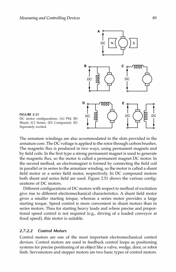
Measuring and Controlling Devices 89
The armature windings are also accommodated in the slots provided in thearmature core. The DC voltage is applied to the rotor through carbon brushes.The magnetic flux is produced in two ways, using permanent magnets andby field coils. In the first type a strong permanent magnet is used to generatethe magnetic flux, so the motor is called a permanent magnet DC motor. Inthe second method, an electromagnet is formed by connecting the field coilin parallel or in series to the armature winding, so the motor is called a shuntfield motor or a series field motor, respectively. In DC compound motorsboth shunt and series field are used. Figure 2.51 shows the various config-urations of DC motors.
Different configurations of DC motors with respect to method of excitationgive rise to different electromechanical characteristics. A shunt field motorgives a smaller starting torque, whereas a series motor provides a largestarting torque. Speed control is more convenient in shunt motors than inseries motors. Thus for starting heavy loads and where precise and propor-tional speed control is not required (e.g., driving of a loaded conveyor atfixed speed), this motor is suitable.
2.7.2.2 Control Motors
Control motors are one of the most important electromechanical controldevices. Control motors are used in feedback control loops as positioningsystems for precise positioning of an object like a valve, wedge, door, or robotlimb. Servomotors and stepper motors are two basic types of control motors.
FIGURE 2.51DC motor configurations. (A) PM; (B)Shunt; (C) Series; (D) Compound; (E)Separately excited.
N SDC
DC DC
DC DC DC
A
B C
D E
7244.book Page 89 Wednesday, June 21, 2006 11:14 AM

90 Measurement and Control in Food Processing
2.7.2.2.1 DC Servomotors
Although DC servomotors are basically same as DC motors in principle,servomotors are specially designed to work with servomechanism systems.DC servomotors differ from general DC motors as follows:
1. They are designed for low rotor inertia, so the torque-to-inertia ratiois very high.
2. They should have an extremely low time constant.
3. They have a relatively low power rating.
Servomotors are manufactured with medium and high power ratings,which are used in robotics, numerically controlled machines, and so on. Insome applications DC servomotors are driven by an electrical controllercalled a servo-driver. The servo-driver adjusts the speed of the servomotor,such as in motion control drives where pulse width modulation is used forcontrolling speed. The DC servomotors are operated and controlled in twomodes: armature-controlled mode and field-controlled mode.
2.7.2.2.2 Armature-Controlled Mode
The speed or angular displacement of the motor is controlled by varyingthe armature voltage while the field is separately excited and is heldconstant. However, in the field-controlled method, the motor is controlledby the separately excited field current and the armature voltage is heldconstant. Because armature-controlled mode is more popular, only thismethod is discussed here. Figure 2.52 illustrates an armature-controlledDC servomotor.
FIGURE 2.52(A) Circuit diagram of the armature-controlled DC motor. (B) Block diagram of the controlsystem.
if
iaEa
Ea Km
La
Ra
J
b
τmS+1θ
A
B
7244.book Page 90 Wednesday, June 21, 2006 11:14 AM

Measuring and Controlling Devices 91
The transfer function relating the output angular velocity and outputcontrol voltage Ea(s) is given by
(2.45)
where Km = K/(Rab + KKb) = motor gain constantτm = LaJ/(Rab + KKb) = motor time constant
In this systemRa = armature resistance (ohm)La = armature inductance (H)Ea = applied armature voltage (V)θ = angular displacement of motor shaft (rad)J = equivalent moment of inertia of the motor (Kg-m2)b = equivalent viscous friction coefficient of the motor
(N-m/rad/sec)K = motor torque constant (Kg-m/A)
Kb = back EMF constant (V/rad/sec)
The transfer function indicates that the DC servomotor is a first-ordersystem. The time constant can be made small by using low values of J andRa. The gain can be increased by using a high torque constant and a smallerback EMF constant, lower values of Ra and b. Typical ratings of commerciallyavailable servomotors are as follows:
• Full scale input voltage: 1.5 V to 24 V
• Impedance: 2.8 ohms to 700 ohms
• Time constant: 0.01 sec
• Full scale speed: 1000 RPM to 2000 RPM
• Starting voltage: 4.2 mV to 79 mV
• Load capacity: 1.8 to 12.4 gm-cm at full voltage
2.7.2.2.3 Two-Phase Servomotor
A two-phase servomotor is similar to a two-phase induction motor, with thedifference that a servomotor is designed with small diameter-to-length ratioto minimize the moment of inertia. This gives a good accelerating character-istic. Moreover, the power rating of a two-phase servomotor ranges from afraction of a watt to a few hundred watts. A schematic diagram of a two-phase servomotor is shown in figure 2.53. The fixed phase of the motor issupplied with a constant AC voltage and the control phase is supplied withthe control voltage of the same frequency. The frequency of the voltages usedis generally 50, 400, or 1,000 Hz. The control voltage (Ec) should be 90° phase
θ( )s•
θτ
( )( ) ( )s
E sK
s sa
m
m
•
=+1
7244.book Page 91 Wednesday, June 21, 2006 11:14 AM

92 Measurement and Control in Food Processing
shifted in time from the reference voltage to develop torque in the shaft ofthe rotor. The transfer function of the servomotor is given by
(2.46)
where Km = motor gain constantτm = motor time constant
Parameters such as position, velocity, speed, and acceleration are allmotion-related variables and their control is important in transportation ofmaterials by conveyer systems in food industries. In high-speed bottlingplants, servomotors can perform orientation of the empty bottles, positioningthem on the rails, and feeding them to the fill station. In these motion controlapplications, servomotors serve as the control components.
2.7.2.3 Stepper Motors
In many robotic and semirobotic industrial automation applications, steppermotors are used due to their special advantages. The main advantage of thestepper motors is that they can be interfaced easily with digital devices.Other advantages include low cost, robustness, simple construction, lowmaintenance, wide applications, high reliability, and robustness to adverseenvironmental conditions. Moreover, they provide excellent torque at lowspeed, which is not obtained in other DC motors. Three main types of steppermotors are permanent magnet type, variable reluctance type, and hybridtype. The hybrid type is the most popular type.
2.7.2.3.1 Permanent Magnet MotorsThese stepper motors are used in nonindustrial applications like computerprinters, disk drives, and so on. The cost of permanent magnet stepper motorsis low but they operate at low speed and low torque. These motors are operatedat relatively large step angles for which precise positioning becomes difficult.
FIGURE 2.53Schematic diagram of a two-phaseservomotor.
J
Ea
Ec
θFixed phase
Control phase
b
θτ
( )( ) ( )s
E sK
s sc
m
m
•
=+1
7244.book Page 92 Wednesday, June 21, 2006 11:14 AM

Measuring and Controlling Devices 93
2.7.2.3.2 Variable Reluctance MotorsIn this type of stepper motor the torque output is small, so it is used forsmall torque applications like micropositioning tables. Due to their lowtorque output for a given size, they are not used for industrial applications.Because these motors are not sensitive to current polarity as are permanentmagnet stepper motors, they require a different driver circuit compared toother types.
2.7.2.3.3 Hybrid Stepper MotorsA hybrid stepper motor consists of a slotted stator with two or more indi-vidual coils. The input digital signals are applied to these stator coils. Therotor does not carry any winding and a magnet is attached to the rotor asshown in figure 2.54. Figure 2.54 shows a four-pole stator and a five-polerotor structure. The rotor pole pitch is defined as
Rotor pole pitch = 360°/number of rotor poles
The rotor pole pitch of the motor shown is 72°. Each rotor pole is magne-tized at one end with N polarity and the poles at the other end are magne-tized by S polarity. Moreover, the N-pole set of rotor poles is arranged to bedisplaced from the S-pole set by half of the pole pitch. When coil AA′ isassumed to be energized to make pole at A an N and pole at A′ an S, thenrotor poles S1, S2, and S5 correspond to N; S3, and S4 to S. Similarly N1, N2,and N5 correspond to S; N3 and N4 to N.
FIGURE 2.54Cross-sectional view of a hybrid type of stepper motor.
S1
S2
S3 S4
S5
N
S
A
A'
B B'
N1
N2
N3N4
N5
N
S
A
A'
B B'
Stator
Permanent magnet (rotor)
Shaft
Rotor of S polarity Rotor of N polarityA, A', B, B' are stator coils
7244.book Page 93 Wednesday, June 21, 2006 11:14 AM

94 Measurement and Control in Food Processing
2.7.2.3.4 Method of Operation
As shown in figure 2.55, let the starting position be with coil AA′ energizedto carry a positive DC current so that the upper stator pole becomes N andthe lower stator pole becomes S. In this state, coil BB′ is assumed to be notenergized. The rotor remains in this orientation as long as the stator coilcurrent remains unchanged. In this state S1 is in alignment with the N polesof the stator. Therefore, the torque produced is zero (as sin θ = 0 at θ = 0°).The torque developed
between S5 and N (force of attraction in counterclockwise):
Torque ∝ (–sin 72°)
between S2 and N (force of attraction in clockwise):
Torque ∝ (sin 72°)
A similar result is obtained for stator S pole and rotor N poles. The rotoris pulled by equal torques in opposite directions for which the rotor remainsin standstill position. On the other hand, torque values between stator S poleand rotor S poles S3 and S4 are
between S4 and S (force of repulsion in clockwise):
Torque ∝ (cos 36°)
between S5 and S (force of repulsion in counterclockwise):
Torque ∝ (–cos 36°)
Position 2: Let Coil AA′ be de-energized and coil BB′ be energized by apositive current. This will cause pole at B to be N and pole at B′ to be S. The
FIGURE 2.55Rotor positions: (A) initial position; (B) position after one step movement.
N
S
S1
S2
S3 S4
S5
18°
A
A'
N
S
S1
S2
S3
S4
S5
A
A B
A'
7244.book Page 94 Wednesday, June 21, 2006 11:14 AM

Measuring and Controlling Devices 95
net rotor displacement for this change in coil excitation is 18°. The orientationof the rotor poles becomes such that it is identical to the starting orientationand so the rotor is again in equilibrium and standstill position. The torquedeveloped when there is a change of stator coil energization from AA′ to BB′ is
T = Tm (sin(S2 – N) + sin(S1 – N) – sin(S3 – N) + cos(S5 – S) – cos(S4 – S))= Tm (sin 18° + sin 90° – sin 54° + cos 18° – cos 54°)= 0.863 Tm
Because this is a positive torque, the shaft rotates in counterclockwisedirection and reaches the equilibrium position.
Position 3: Let us consider that coil BB′ is de-energized and coil AA′ isenergized by a negative DC current. In a similar way the torque developedcan be obtained by
T = Tm (sin 18° + sin 90° – sin 54° – cos 54° + cos 18°) = 0.00
Because the torque is zero it brings the rotor to equilibrium position. Thecomplete sequence for operating the stepper motor in counterclockwisedirection by steps of 18° is shown in table 2.3. In this example the anglecompleted in one sequence is 72°, which is known as pole pitch. A two-coilstator with two states needs four switching operations to complete a switch-ing cycle. The angle 18° is known as full step size, which is given by
Full step size = Rotor pole pitch/N
where N is the number of stator poles.The direction of rotation can be reversed by reversing the switching
sequence.
2.7.2.3.5 Half Stepping Operation
The previous analysis was based on the assumption that only one stator coilwas energized at a time. This operation is called half stepping. The resultwill be different if both the stator coils are energized at a certain periods in
TABLE 2.3
Stator Coil Current Sequence for Full Step Size Rotation
Sequence Coil AA′ Coil BB′Cumulative Rotor
Displacement
1 ON (+) OFF 0°2 OFF ON (+) 18°3 ON (–) OFF 36°4 OFF ON (–) 54°5 ON (+) OFF 72°
7244.book Page 95 Wednesday, June 21, 2006 11:14 AM

96 Measurement and Control in Food Processing
a cycle. Table 2.4 shows the complete sequence for half stepping operation.Half stepping operation provides more precise control of rotation of thestepper motor. High-resolution stepper motors provide microstepping up to500 microsteps, giving 100,000 steps per revolution. In a standard 200 stepshybrid motor, the rotor has two sections with 50 teeth on each section.
2.7.2.3.6 Stepper Motor DriverA digital signal cannot drive the stepper motor directly. Stepper motors aredesigned with a specified current rating so that the required torque can bedeveloped. Generation of pulses of appropriate current rating is done withthe help of a driver circuit. The driver circuit for a four-phase stepper motoris shown in figure 2.56.
2.7.3 Final Control Elements
It has already been mentioned that the final control element is part and parcelof a process plant. A complex process can be composed of many subsystemsof control loops where output variables are locally controlled by varying thecontrol inputs. In such cases the individual subsystems also contain a finalcontrol element. A control element can be developed in the form of mechan-ical, electrical, or pneumatic/hydraulic. Some application examples of thesetypes are discussed here and are further discussed in chapter 4.
TABLE 2.4
Stator Coil Current Sequence for Half Step Size Rotation
Sequence Coil AA′ Coil BB′Cumulative Rotor
Displacement
1 ON (+) OFF 9°2 ON (+) ON (+) 18°3 OFF ON (+) 27°4 ON (–) ON (+) 36°5 ON (–) OFF 45°6 ON (–) ON (–) 54°7 OFF ON (–) 63°8 ON (+) ON (–) 72°
FIGURE 2.56A basic driver circuit for a four-phasestepper motor.
A B A' B'
D1 D2 D3 D4
+V
7244.book Page 96 Wednesday, June 21, 2006 11:14 AM

Measuring and Controlling Devices 97
2.7.3.1 Mechanical Types
When a process needs a mechanical system to be operated by a controlelement, it becomes a mechanical final control element. Examples from foodprocessing include tea withering fans, dust blowers, grain hopper valves,dozing pumps, and so on.
To understand the function of a mechanical final control element, let usconsider a fan reversal control operation in a tea withering system, as shownin figure 2.57. In tea withering, green tea leaves are spread over a wire-nettedplatform and trough. A fan driven by induction motor pushes air from belowthe platform to dry the tea leaves. The moisture released from the tea leavesaccumulates over the withering troughs, saturating the air with moisture. Thisdisrupts the process of moisture release from the green tea leaves. To avoidthis problem, a reversing controller reverses the fan at a regular interval tosuck the saturated air surrounding the troughs out and let fresh air move there.If we consider this problem as a closed-loop control system, we can define themoisture releasing operation as the process, air flow rate (both directions) asthe input, and moisture content of the air (humidity) as the output. On theother hand, the motor reversing system is the controller, the motor is theactuator, and the withering trough or tunnel is the final control element.
A similar control operation in tea withering is the withering percentagecontroller (fig. 2.58). Withering percentage is defined as the reduction ofmoisture level of the green tea leaves as a percentage of the initial moisturecontent. There is a target set to this value and as soon as this value is achievedthe withering fan is stopped. If we consider this as a closed-loop controloperation we can define, similar to the fan reversal problem, the parameters,with air flow rate as the input and the withering percentage as the output;and the control components, the fan as the actuator and the withering troughas the final control element. These two control problems are discussed inchapter 4 with more emphasis on control aspects.
FIGURE 2.57Schematic diagram of fan direction control in tea withering.
Roof
Moisture
Tea leavesMesh
Fan
RH sensor
Controller
Relay
Set levels
7244.book Page 97 Wednesday, June 21, 2006 11:14 AM

98 Measurement and Control in Food Processing
2.7.3.2 Electrical Types
Electrical heating systems are good examples of electrical final control ele-ments in an industrial environment. In an electrical heater or oven the heatis generated electrically and the supply voltage is responsible for the amountof heat developed. Any temperature variation in the heater or oven can becontrolled by manipulating the supply voltage by on–off controller or con-tinuous adjustment by PID controller. In a microwave oven, the heating canbe controlled by controlling the output power of the magnetron. In foodprocessing applications, there are many examples in which such electricalheating and control is used. Such examples include microwave temperingof frozen foods, vacuum drying of citrus juice and grains, pasteurization offood, bread baking, and roasting of nuts and coffee beans.
Another important example of electrical control is the motor speed control.Many food process parameters depend on the speed of the drive motor usedfor various functions such as conveyor feeding, metered feeding by pumps,food mixing and stirring, blowing hot air in dryers, food extrusion, and so on.
2.7.4 Pneumatic Control Devices
Pneumatic devices for sensing and controlling in industrial processes havebeen successfully used for almost a half-century. With the advent of elec-trical and electronic components, pneumatic devices were replaced byelectrical and analog controllers. In recent times, in most industrial sys-tems, pneumatic controllers have been replaced by electronic analog anddigital controllers due to their advantages, such as miniaturization andcomputerization. In spite of this, pneumatic controllers are still functioningin many industries due to their most significant advantages: safety andreliability. Working principles of a few basic pneumatic devices are dis-cussed here.
FIGURE 2.58Schematic diagram of withering percentage control in tea industry.
Fan
Relay
Load cellLoadingplatform
Processingcircuit
Controller
Set level
7244.book Page 98 Wednesday, June 21, 2006 11:14 AM

Measuring and Controlling Devices 99
2.7.4.1 Baffle-Nozzle Detector
This is a basic type of pneumatic detector that generates a pneumatic signalcorresponding to a mechanical motion. Most pneumatic controllers use thisdetector as a primary sensing element. Figure 2.59 shows a nozzle actuatedby a mechanical motion applied through a pivoted baffle. A constant airsupply is applied to a fixed orifice that is connected to the nozzle thatexhausts directly to atmospheric pressure. In a fixed condition of the baffle,the air from the supply line flows through the orifice and exhausts out fromthe nozzle through the gap between the nozzle and baffle (x). When the bafflemoves closer to the nozzle the pressure in the line between orifice and nozzlepressure Pn rises and again falls when x increases. This back pressure Pn isthe transmitted output signal proportional to motion. The highest value ofPn, when x is zero, is determined by air supply pressure Ps. The lower limitis determined by the ratio of resistance to air flow between orifice and nozzlewhen x is very large. Between these two extremes, various nozzle pressuresare established. The linear operating range of 3 to 15 Psi is taken as thestandard input and output limits. In most of the pneumatic instruments,supply air of 1.4 kg/cm2 pressure is used. In the linear range, the ratio ofoutput pressure and input motion is called nozzle sensitivity or gain, whichis very high in this type of detector because a motion of 0.001 in. in the bafflecauses a change in nozzle pressure greater than 8 Psi. The detector showstwo other features:
1. It develops only a small reaction force equal to the product of nozzlepressure and nozzle throat area.
2. It uses only a small amount of air.
The force required to move the baffle is directly proportional to the linepressure and the cross-sectional area of the nozzle. For example, when the
FIGURE 2.59A baffle-nozzle detector.
Pn
Ps Nozzle
Baffle
Input motion
Gauge
OrificeSupply pressure
X
7244.book Page 99 Wednesday, June 21, 2006 11:14 AM
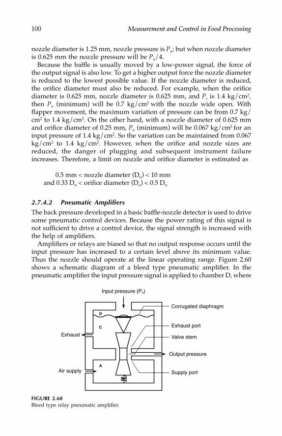
100 Measurement and Control in Food Processing
nozzle diameter is 1.25 mm, nozzle pressure is Pn; but when nozzle diameteris 0.625 mm the nozzle pressure will be Pn/4.
Because the baffle is usually moved by a low-power signal, the force ofthe output signal is also low. To get a higher output force the nozzle diameteris reduced to the lowest possible value. If the nozzle diameter is reduced,the orifice diameter must also be reduced. For example, when the orificediameter is 0.625 mm, nozzle diameter is 0.625 mm, and Ps is 1.4 kg/cm2,then Pn (minimum) will be 0.7 kg/cm2 with the nozzle wide open. Withflapper movement, the maximum variation of pressure can be from 0.7 kg/cm2 to 1.4 kg/cm2. On the other hand, with a nozzle diameter of 0.625 mmand orifice diameter of 0.25 mm, Pn (minimum) will be 0.067 kg/cm2 for aninput pressure of 1.4 kg/cm2. So the variation can be maintained from 0.067kg/cm2 to 1.4 kg/cm2. However, when the orifice and nozzle sizes arereduced, the danger of plugging and subsequent instrument failureincreases. Therefore, a limit on nozzle and orifice diameter is estimated as
0.5 mm < nozzle diameter (Dn) < 10 mm and 0.33 Dn < orifice diameter (Do) < 0.5 Dn
2.7.4.2 Pneumatic Amplifiers
The back pressure developed in a basic baffle-nozzle detector is used to drivesome pneumatic control devices. Because the power rating of this signal isnot sufficient to drive a control device, the signal strength is increased withthe help of amplifiers.
Amplifiers or relays are biased so that no output response occurs until theinput pressure has increased to a certain level above its minimum value.Thus the nozzle should operate at the linear operating range. Figure 2.60shows a schematic diagram of a bleed type pneumatic amplifier. In thepneumatic amplifier the input pressure signal is applied to chamber D, where
FIGURE 2.60Bleed type relay pneumatic amplifier.
Input pressure (Pn)
Exhaust
D
C
AAir supply
Corrugated diaphragm
Exhaust port
Valve stem
Output pressure
Supply port
7244.book Page 100 Wednesday, June 21, 2006 11:14 AM

Measuring and Controlling Devices 101
it exerts a downward force on a corrugated metal diaphragm so that it isflexed downward reducing the exhaust port gap and enlarging the supplyport gap. This causes more air to flow from chamber A to output and thento chamber C. The diaphragm is adjusted so that when the supply port isfully closed and the exhaust port is fully opened the input pressure rises toa given value, typically 5 Psi. When no signal is acting or a signal below 5Psi acts, air supply completely closes the supply port. When the input signalis 1.4 kg/cm2 the exhaust port is completely closed and the whole air supplymoves to output. Therefore, the amplified signal is of the same pressure asthat of the control signal, but volume is amplified. This is a forward-actingamplifier because an increase in signal pressure increases the air volume. Ina reverse-acting amplifier an increase in signal pressure decreases the airvolume. In some designs the output pressure is also increased in additionto the increase in air volume.
2.7.4.2.1 Force Balance Transmitter
To translate a force, a position, or a motion into a corresponding air pressurea force balance transmitter is used. Figure 2.61 shows the schematic diagramof the force balance transmitter. The T beam is free to pivot at P1. A force F1
generated by the variable to be measured is applied at one end of the beam.The leg on the T beam carries a flapper in front of which a nozzle is placed.Air supply of 1.4 kg/cm2 is applied to the nozzle line. An increase in F1 willcreate an counterclockwise turning movement on the T beam and so theflapper moves closer to the nozzle. This will increase the back pressure Pn andthe output signal is amplified by a pneumatic amplifier. The output pressureis then fed to the feedback bellow. An increase in output pressure will causethe bellow to expand and, thereby pushing one end of the L beam upward
FIGURE 2.61Force balance transmitter.
L-beam
Nozzle
Orifice
Flapper
T-beam
Feeble signal (Pn)
Amplified signal
Bleedrelay
To
atmospheric pressure
output
Airsupply
d
C
F3
b
a
P3
P1F1
P2 F2 Bellow
From
7244.book Page 101 Wednesday, June 21, 2006 11:14 AM
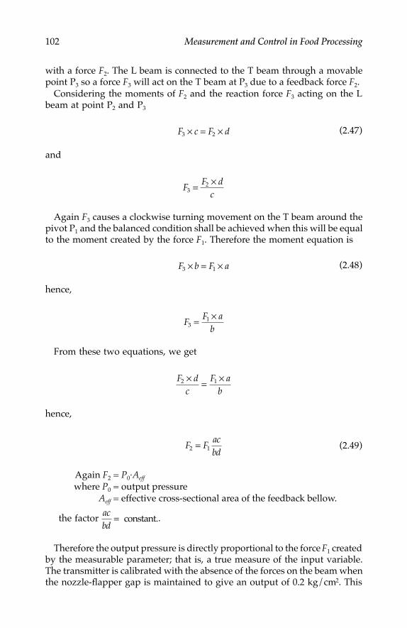
102 Measurement and Control in Food Processing
with a force F2. The L beam is connected to the T beam through a movablepoint P3 so a force F3 will act on the T beam at P3 due to a feedback force F2.
Considering the moments of F2 and the reaction force F3 acting on the Lbeam at point P2 and P3
(2.47)
and
Again F3 causes a clockwise turning movement on the T beam around thepivot P1 and the balanced condition shall be achieved when this will be equalto the moment created by the force F1. Therefore the moment equation is
(2.48)
hence,
From these two equations, we get
hence,
(2.49)
Again F2 = P0·Aeff
where P0 = output pressureAeff = effective cross-sectional area of the feedback bellow.
the factor .
Therefore the output pressure is directly proportional to the force F1 createdby the measurable parameter; that is, a true measure of the input variable.The transmitter is calibrated with the absence of the forces on the beam whenthe nozzle-flapper gap is maintained to give an output of 0.2 kg/cm2. This
F c F d3 2× = ×
FF d
c32= ×
F b F a3 1× = ×
FF a
b31= ×
F dc
F ab
2 1× = ×
F Facbd2 1=
acbd
= constant.
7244.book Page 102 Wednesday, June 21, 2006 11:14 AM

Measuring and Controlling Devices 103
can be done by adjusting the tension of a spring mounted in the flapper-nozzle assembly. The areas of the diaphragm and bellow and the length ofthe beams are related to each other in such a manner that the highest forceof measurable range will develop an output of 1.0 kg/cm2. Range of theinstrument can be changed by varying the position of the movable pivot P3.
2.8 Conclusion
Understanding the techniques of measurement and control in food process-ing mandates knowledge of basic principles of transducers, sensors, andcontrol components. Most of the transducers were developed first to fit themto specific applications; however their working principles propagated rap-idly to many other similar applications.
This chapter is intended to provide the reader with sufficient informationon principles and easy-to-understand applications of various types of trans-ducers. Actuating and control components were also discussed, but it wasnot possible to go into depth about control system engineering due to spacelimitations. With the information provided in this chapter one can hope tounderstand, design, and apply the concepts of transducers and controllersin food processing.
Further Reading
1. Doeblin, E. O. 1986. Measurement systems, application and design. New York:McGraw-Hill.
2. Patranabis, D. 1990. Industrial instrumentation. New York: McGraw-Hill.3. Jones, E. B. 1976. Instrument technology (Vol. II). Butterworth & Co..4. Johnson, C. D. 2000. Process control instrumentation technology (6th ed.). Upper
Saddle River, NJ: Prentice-Hall International.5. Toro, D. 1985. Electric machines and power systems. New Delhi: Prentice-Hall of
India.6. Anderson, N. A. 1998. Instrumentation for process measurement and control. Boca
Raton, FL: CRC Press.7. Barney, G. C. 1988. Intelligent instrumentation: Microprocessor applications in mea-
surement and control. New Delhi: Prentice-Hall of India.8. Liptak, B. G. (ed.). 1995. Instrument engineers handbook: Process measurement and
analysis. London: Butterworth & Heinemann.9. Ogata, K. 1982. Modern control engineering. New Delhi: Prentice-Hall of India.
10. Kuo, B. C. 1982. Automatic control systems (3rd ed.). New Delhi: Prentice-Hallof India.
11. Langton, M. A., and Say, M. G. (eds). 1985. Electrical engineering reference book(14th ed.). London: Butterworth & Co.
12. Van Valkenburg, M. E. 1988. Linear circuits. New Delhi: Prentice-Hall of India.
7244.book Page 103 Wednesday, June 21, 2006 11:14 AM

7244.book Page 104 Wednesday, June 21, 2006 11:14 AM

105
3Measurements in Food Processing
CONTENTS3.1 Introduction ................................................................................................ 1083.2 Moisture Content Measurement ............................................................. 109
3.2.1 Role of Moisture Content in Quality of Food .......................... 1093.2.1.1 Definition of Moisture Content .................................... 110
3.2.2 Microwave Absorption Method ..................................................1113.2.2.1 Loss Factor Measurement.............................................. 112
3.2.3 Radio Frequency (RF) Impedance Technique .......................... 1133.2.4 DC Resistance Technique............................................................. 116
3.2.4.1 Average Moisture Content Model of Plant Leaf ....... 1173.2.4.2 Measuring Circuit ........................................................... 120
3.2.5 Infrared Technique ........................................................................ 1223.3 Moisture Release During Drying of Food............................................. 124
3.3.1 Mathematical Representation...................................................... 1243.3.2 Mechanical Loading Arrangement............................................. 1253.3.3 Measuring Circuit ......................................................................... 127
3.4 Humidity in the Food Processing Environment .................................. 1293.4.1 Definition of Humidity ................................................................ 1303.4.2 Conventional Types ...................................................................... 131
3.4.2.1 Hair Hygrometer ............................................................ 1313.4.2.2 Wet- and Dry-Bulb Psychrometer................................ 1313.4.2.3 Fluidic Dry- and Wet-Bulb Hygrometer ..................... 133
3.4.3 Electrical Type of Humidity Meters........................................... 1343.4.3.1 Resistive Hygrometer..................................................... 1343.4.3.2 Electrolytic Hygrometer................................................. 1343.4.3.3 Capacitive Hygrometer.................................................. 134
3.4.4 Electronic Wet- and Dry-Bulb Hygrometer .............................. 1353.4.4.1 Microprocessor-Based Wet- and Dry-Bulb
Hygrometer...................................................................... 1353.4.4.2 Hygrometer Based on Linearized Model
of Psychrometric Chart .................................................. 1373.5 Turbidity and Color of Food ................................................................... 139
3.5.1 Turbidity Measurement................................................................ 1393.5.1.1 A Basic Turbidity Meter................................................. 140
7244.book Page 105 Wednesday, June 21, 2006 11:14 AM

106 Measurement and Control in Food Processing
3.5.1.2 Standards and Units of Turbidity ................................ 1403.5.1.3 Light Scattering Type Turbidity Meter........................ 1413.5.1.4 Optical Absorption Type Turbidity Meter.................. 1423.5.1.5 Turbidity Measurement in the Sugar Refining
Process .............................................................................. 1433.5.2 Food Color Measurement ............................................................ 143
3.5.2.1 Optical Reflectance Method.......................................... 1443.5.2.2 Color Reflectance and Digital Color Image
Processing in Food Grains ............................................ 1463.5.2.3 Color Matching in Fermented Tea............................... 148
3.6 Food and Process Temperature Measurement ..................................... 1523.6.1 Temperature Measurement in Food Processing....................... 1523.6.2 Thermocouples .............................................................................. 153
3.6.2.1 Thermocouple Installations........................................... 1543.6.3 Temperature of Food on a Conveyor ........................................ 1553.6.4 Food Tempering Monitoring....................................................... 1553.6.5 Precision Temperature Measurement ........................................ 156
3.7 Food Flow Metering.................................................................................. 1573.7.1 Magnetic Flow Meters.................................................................. 1583.7.2 Mass Flow Metering ..................................................................... 1593.7.3 Turbine Flow Meter ...................................................................... 1623.7.4 Positive Displacement Flow Meter ............................................ 1623.7.5 Solid Flow Metering ..................................................................... 1623.7.6 Gravimetric Feeder Meters.......................................................... 163
3.7.6.1 Rotary Vane Feeder ........................................................ 1633.7.6.2 Screw Feeder.................................................................... 1633.7.6.3 Belt Feeder ....................................................................... 164
3.8 Viscosity of Liquid Foods......................................................................... 1653.8.1 Definition and Units ..................................................................... 1653.8.2 Newtonian and Non-Newtonian Food Flow ........................... 1663.8.3 Laboratory Type Saybolt Viscometer......................................... 1693.8.4 Capillary Tube Viscometer .......................................................... 1703.8.5 On-line Variable Area or Rotameter Type Viscometer............ 1723.8.6 Rotating Cylinder Viscometer..................................................... 174
3.9 Brix of Food ................................................................................................ 1773.9.1 Brix Standards................................................................................ 1793.9.2 Refractometers ............................................................................... 179
3.9.2.1 Refraction Angle Refractometer ................................... 1803.9.2.2 Critical Angle Refractometer ........................................ 1803.9.2.3 U-Rod Refractometer ..................................................... 182
3.10 pH Values of Food..................................................................................... 1833.10.1 pH Scale.......................................................................................... 1833.10.2 pH Electrodes and Potential ....................................................... 184
3.10.2.1 Glass Electrode................................................................ 1843.10.2.2 Calomel Electrode........................................................... 185
7244.book Page 106 Wednesday, June 21, 2006 11:14 AM

Measurements in Food Processing 107
3.10.3 pH Signal Processing.................................................................... 1873.10.4 Ion-Sensitive Field Effect Transistor pH Sensors..................... 187
3.11 Food Enzymes............................................................................................ 1933.11.1 Importance of Food Enzyme Detection .................................... 1933.11.2 Enzyme Sensors............................................................................. 193
3.11.2.1 Principle of Operation ................................................... 1943.11.2.2 Calibration ....................................................................... 1953.11.2.3 Sensor Materials.............................................................. 195
3.11.3 Measuring Circuit ......................................................................... 1963.11.4 Semiconductor Enzyme Sensor .................................................. 1983.11.5 Applications in Food Processing ................................................ 199
3.12 Flavor Measurement ................................................................................. 2003.12.1 Sources of Flavor in Food............................................................ 2003.12.2 Physiology of Human Olfaction................................................. 2013.12.3 Organoleptic Panel........................................................................ 2023.12.4 Electronic Nose.............................................................................. 203
3.12.4.1 A Basic Electronic Nose ................................................. 2033.12.5 Sensor Types .................................................................................. 204
3.12.5.1 Chemoresistive Sensors ................................................. 2043.12.5.2 Conducting Polymer Sensors ....................................... 2053.12.5.3 Acoustic Sensors ............................................................. 2063.12.5.4 MOSFET Sensors............................................................. 207
3.12.6 The Signal Processing and Pattern Recognition ...................... 2073.12.6.1 Preprocessing................................................................... 2083.12.6.2 Feature Extraction........................................................... 2083.12.6.3 Classification.................................................................... 209
3.12.7 Applications of the Electronic Nose in Food Processing ....... 2093.12.7.1 E-Nose Systems Manufactured by Alpha
M.O.S. Inc. (France) ........................................................ 2093.12.7.2 Monitoring of Flavor of Beers ...................................... 2103.12.7.3 Fruit Ripeness Determination....................................... 2143.12.7.4 Tea Flavor Detection....................................................... 2143.12.7.5 Spice Flavor Detection ................................................... 218
3.13 Food Texture and Particle Size................................................................ 2193.13.1 Electromechanical Measuring Techniques ................................ 2203.13.2 Fluorescence Technique for Beef Toughness Detection .......... 2243.13.3 Machine Vision Technique........................................................... 226
3.13.3.1 Beef Tenderness Detection ............................................ 2263.13.3.2 Tea Texture Measurement in Grading......................... 228
3.13.4 Particle Size Detection.................................................................. 2303.13.4.1 Off-line Methods............................................................. 2303.13.4.2 On-line Techniques ......................................................... 230
3.14 Food Constituents Analysis ..................................................................... 2313.14.1 Carbonates, Bicarbonates, and Organic Matters
in Bottled Water............................................................................. 232
7244.book Page 107 Wednesday, June 21, 2006 11:14 AM

108 Measurement and Control in Food Processing
3.14.2 Volatile Compounds in Tropical Fruits ..................................... 2343.14.3 Moisture, Protein, Fat, and Ash Content of Milk Powder..... 2353.14.4 Components in Alcoholic Beverages ......................................... 235
3.14.4.1 Minerals in Wines........................................................... 2363.14.5 Quality Parameters in Cereals and Cereal Products............... 2363.14.6 Meat Content ................................................................................. 2373.14.7 Bacteria and Foreign Body Detection ........................................ 238
3.14.7.1 Bacteria Detection ........................................................... 2383.14.7.2 Foreign Body Detection ................................................. 2383.14.7.3 Removal of Stalks from Tea .......................................... 239
3.15 Conclusion .................................................................................................. 240References ............................................................................................. 240
3.1 Introduction
Most food processing techniques are extensions of traditional kitchen prep-aration methods that employ scientific techniques, making enough surplusproducts to be sold outside the household. Current food processing technol-ogies are gradual improvements of old techniques and equipment designsto improve quality and efficiency. As technology advanced, food processingtechnology also geared up to meet productivity, quality, safety, and economicrequirements. To keep pace with quality requirements and government reg-ulations, most food processing industries have a quality control or qualityassurance department that monitors raw materials, manufacturing pro-cesses, and the finished products. Food quality testing personnel performmany standardized physical and chemical tests on food products, checkingphysical properties (sizes, weight, density, etc.), chemical properties (pH,vitamin content, fat content, etc.), sensory attributes (appearance, taste, fla-vor, texture, etc.), and legal requirements or public health considerations(presence of certain microorganisms, insecticides, metal particles, etc.). Inobjective testing (physical and chemical properties), instrumental methodsare preferred, but objective testing of quality attributes like odor, taste, andso on are difficult to carry out by subjective methods. Present-day technologycontinues to develop and use various modern tools for both monitoring andcontrol of the various food quality parameters. Electronics have longappeared among the tools of measurement and control of food processing,but computer technology became an important part of measurement andcontrol only a few decades ago. The concept of computer-integrated manu-facturing (CIM) evolved in the 1970s and has revolutionized this field ofengineering. In this chapter, quality factors involved in food processing andtheir measuring techniques, monitoring systems, and control strategies formthe basis of discussion.
7244.book Page 108 Wednesday, June 21, 2006 11:14 AM
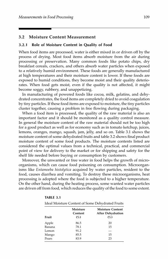
Measurements in Food Processing 109
3.2 Moisture Content Measurement
3.2.1 Role of Moisture Content in Quality of Food
When food items are processed, water is either mixed in or driven off by theprocess of drying. Most food items absorb moisture from the air duringprocessing or preservation. Many common foods like potato chips, drybreakfast cereals, crackers, and others absorb water particles when exposedto a relatively humid environment. These foods are generally manufacturedat high temperatures and their moisture content is lower. If these foods areexposed to humid conditions, they become moist and their quality deterio-rates. When food gets moist, even if the quality is not affected, it mightbecome soggy, rubbery, and unappetizing.
In manufacturing of powered foods like cocoa, milk, gelatins, and dehy-drated concentrates, the food items are completely dried to avoid coagulationby tiny particles. If these food items are exposed to moisture, the tiny particlescluster together, causing a problem in free flowing during packaging.
When a food item is processed, the quality of the raw material is also animportant factor and it should be monitored as a quality control measure.In general the moisture content of the raw material should not be too highfor a good product as well as for economy such as in tomato ketchup, juices,lemons, oranges, mango, squash, jam, jelly, and so on. Table 3.1 shows themoisture content of some dehydrated fruits and table 3.2 shows final productmoisture content of some food products. The moisture contents listed areconsidered the optimal values from a technical, practical, and commercialpoint of view for delivery to the market or for shipping and safety for theshelf life needed before buying or consumption by customers.
Moreover, the unwanted or free water in food helps the growth of micro-organisms, which can cause food poisoning on consumption. Microorgan-isms like Entamoeba histolytica acquired by water particles, resident to thefood, causes diarrhea and vomiting. To destroy these microorganisms, heatprocessing is adopted where the food is subjected to a higher temperature.On the other hand, during the heating process, some wanted water particlesare driven off from food, which reduces the quality of the food to some extent.
TABLE 3.1
Ideal Moisture Content of Some Dehydrated Fruits
Fruit
MoistureContent
(%)
Moisture ContentAfter Dehydration
(%)
Apple 86.5 20Banana 78.1 15Lemon 91.2 —Mango 85.5 15Pears 83.9 23
7244.book Page 109 Wednesday, June 21, 2006 11:14 AM

110 Measurement and Control in Food Processing
An estimation of the moisture content of the food items during and afterprocessing becomes an essential part of food quality monitoring and control.Estimation of moisture content of the raw materials of the food products isalso a routine quality procedure in many industries. Different food productsare treated differently for estimation of moisture content. This depends onfactors like size, shape, texture, amount of moisture, on-line or off-linerequirement, requirement of precision, and so on.
3.2.1.1 Definition of Moisture Content
Moisture content is defined in several ways that are specific to a certainmaterial and application. Moisture content is expressed either on a wet ordry basis. These two definitions of moisture content are
Moisture content (wet basis)
(3.1)
Moisture content (dry basis)
(3.2)
where Ww = weight of wet material (g)Wd = weight of dry material (g)
Moisture content of unprocessed foods are generally expressed on a wetbasis, but many food products after drying have their moisture contentexpressed on a dry basis only.
One of the most commonly used classical methods of moisture contentmeasurement in food products is the dry and weigh technique. In this tech-nique a representative sample of the food item is dried using a standarddrying oven and weighed by a precise weighing balance. The difference inmeasure of weight gives the moisture contained in the material. In thismethod there is a standard and predetermined time of drying for a particular
TABLE 3.2
Final Product Moisture Content of Some Food Products
Food Moisture Content (%)
Butter 16Cocoa bean 4Coffee bean 12Made tea 3–4Fats and oil 0.5–1Caramels and toffee 6–8
MW W
Wg gw
w d
w
= −( / )
MW W
Wg gd
w d
d
= −( / )
7244.book Page 110 Wednesday, June 21, 2006 11:14 AM

Measurements in Food Processing 111
material, during which all moisture particles are driven off. Such a moisturemeter (Model IR-30) manufactured by Denver Instruments (USA) is shownin figure 3.1. This instrument utilizes infrared heating and precision weighingfor quick and accurate moisture determination. It measures moisture orsolids content in a range of samples from powders to liquids.
Radio frequency (RF) impedance measurement and microwave permittiv-ity techniques are most suitable for fruits and grains due to their nondestruc-tive sensing behavior. Many food industries adopt these measuringtechniques due to the nondestructive or noncontact procedure and higheraccuracy achieved.
3.2.2 Microwave Absorption Method
In microwave absorption techniques, moisture content of fruits and vegeta-bles can be measured in the microwave frequency band of 20.3 GHz to 22.3GHz. The frequencies 2.45 GHz, 8.9 to 10.68 GHz, and 20.3 to 22.3 GHz arethe three regions in which the technique can be utilized. When an electro-magnetic wave of these frequencies passes through a material, water mole-cules greatly moderate the signal of the frequency range 20.3 to 22.3 GHzand water molecules produce molecular resonance. Hence, this frequency ismost suitable for moisture content, particularly for free water determination.Figure 3.2 shows the schematic arrangement of the microwave absorptiontype moisture meter.
FIGURE 3.1Infrared moisture meter, model IR-30. (Reprinted with permission from Denver Instruments,USA)
7244.book Page 111 Wednesday, June 21, 2006 11:14 AM

112 Measurement and Control in Food Processing
In this technique the complex relative permittivity of the material is uti-lized for measurement of moisture content. The complex relative permittivityof a food material can be represented as
(3.3)
where the real part ε′ is the dielectric constant and the imaginary part ε″ isthe dielectric loss factor. This loss factor of a material depends on the mois-ture present in the material.
3.2.2.1 Loss Factor Measurement
Figure 3.3 shows a loss factor measuring scheme using the microwave tech-nique. The permittivity measurement can be made by measurement on afree-ended semirigid Teflon insulated small coaxial copper conductor as thewave guide of the microwave energy. A wave guide 10 cm long consists ofa 7-mm diameter air line that is connected directly to the reflection andtransmission set. A 90° bend at 10 cm from the free end of the coaxial copperconductor is provided to facilitate contact with the surface of the sample.
FIGURE 3.2Block diagram of microwave moisture meter.
FIGURE 3.3Setup for loss factor determination of a food sample.
modulatorand oscillator attenuator detector
sample amplifierindicator
ε ε ε= ′ − ′′j
coaxial copperconductor guide
Microwavetransmitter and
receiver
pair line
10 cm
sample
10 cm
7244.book Page 112 Wednesday, June 21, 2006 11:14 AM

Measurements in Food Processing 113
The free end of the cable is cut and polished smoothly to avoid distortionperpendicular to the axis of the line.
The reflection coefficient of the wave guide at the dielectric interface at thetip of the probe is determined by the permittivity of the material in contactwith the probe. This technique can be adopted for moisture content deter-mination of fruits and vegetables. The technique provides a nondestructivemoisture evaluation of fruits and vegetables that is desired in many foodindustries.
3.2.3 Radio Frequency (RF) Impedance Technique
The basic principle of the RF impedance technique is that when a radiosignal of frequency below 10 MHz is passed through a food item containingwater particles, the water molecules absorbs some of the RF energy, causingmolecular motion. Figure 3.4 shows a block diagram of the RF absorptiontechnique. This technique is suitable for comparatively dry materials likegrains, cereals, corn, and so on. The RF technique of moisture measurementis based on the principle of measurement of the RF impedance of the sampleunder test. Best results are obtained when the measurement is performedwith an individual sample like soybean, pea, gram, or corn. The equivalentcircuit and phasor diagram of the measurement is shown in figure 3.5. Theimpedance model of the sample consists of a capacitance (C) and a parallelequivalent resistance (R). The susceptance of the sample is given by
(3.4)
when the sample is excited by an alternating voltage of angular frequencyω. The admittance of the sample is
(3.5)
where G is the conductance. The phase angle θ and the loss factor angle δare given by
(3.6)
and
(3.7)
B C= ω
Y G jB= +
θ ω= =− −tan [ ] tan [ / ]1 1CR B G
δ ω ω= = =−tan [ / ] / /1 1 C R G C G B
7244.book Page 113 Wednesday, June 21, 2006 11:14 AM

114 Measurement and Control in Food Processing
The current through the sample has two components, a capacitive and aresistive component. The currents through the capacitor and the resistor aregiven by
(3.8)
and
(3.9)
so the total current through the resistor is
(3.10)
where V is the voltage applied and Z is the impedance of the sample.
FIGURE 3.4RF impedance technique.
FIGURE 3.5Equivalent circuit for RF moisture measurement.
R.F.oscillator
sample amplifierand detector
indicator
V C R
V
δ
θ
Ic
I Vj Cc = ω
I V RR = /
I V Z
V G j C
=
= +
/
( )ω
7244.book Page 114 Wednesday, June 21, 2006 11:14 AM

Measurements in Food Processing 115
Figure 3.6 shows the electrode setup for the RF impedance technique ofmoisture content measurement. Two parallel plate brass electrodes arearranged for placing the sample between them. The upper electrode is con-nected to a spring pressure dial indicator and the lower electrode is fixed toa base. The upper electrode can be moved by a lever connected to the upperside of the dial gauge. The gauge indicates the desired pressure applied tothe sample to get proper contact, compactness, and uniformity betweenmeasurements.
The capacitance C can be calculated from the following mathematical steps:
(3.11)
and
(3.12)
where f is the frequency of the operating voltage.
FIGURE 3.6Fixed pressure application device.
Food
Handle
Gauge
Spring
Plate
ω θCR = tan
= + j j( t
( )= +
V I R j C
j CR j C
C
VI
/ ( / )
/
an )/
= +
=
1
1
1
ω
ω ω
θ ω
11 2+
=
tan θωC
CIV f
+12
2tan θπ
7244.book Page 115 Wednesday, June 21, 2006 11:14 AM
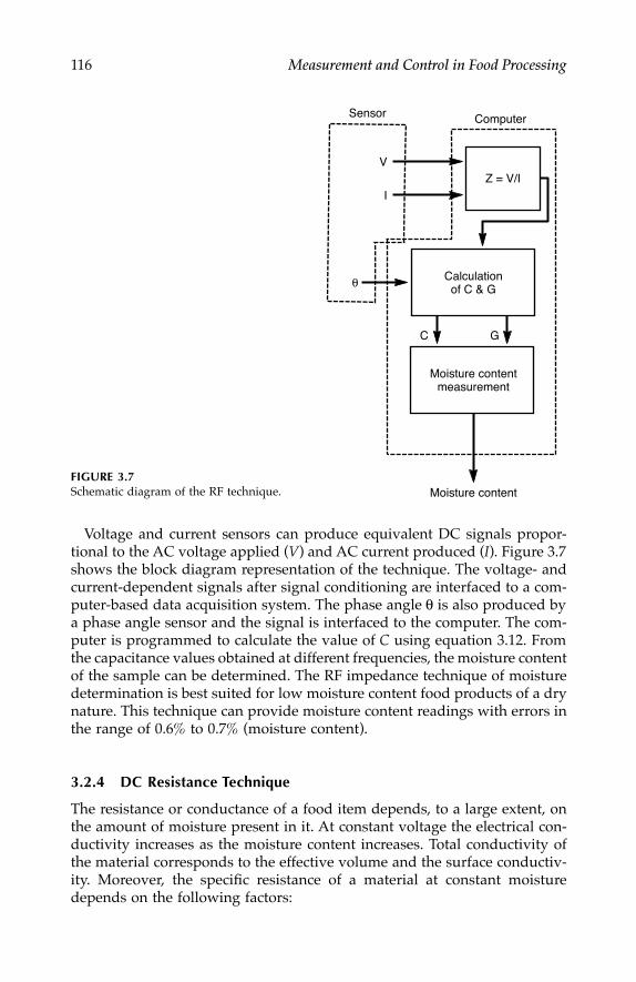
116 Measurement and Control in Food Processing
Voltage and current sensors can produce equivalent DC signals propor-tional to the AC voltage applied (V) and AC current produced (I). Figure 3.7shows the block diagram representation of the technique. The voltage- andcurrent-dependent signals after signal conditioning are interfaced to a com-puter-based data acquisition system. The phase angle θ is also produced bya phase angle sensor and the signal is interfaced to the computer. The com-puter is programmed to calculate the value of C using equation 3.12. Fromthe capacitance values obtained at different frequencies, the moisture contentof the sample can be determined. The RF impedance technique of moisturedetermination is best suited for low moisture content food products of a drynature. This technique can provide moisture content readings with errors inthe range of 0.6% to 0.7% (moisture content).
3.2.4 DC Resistance Technique
The resistance or conductance of a food item depends, to a large extent, onthe amount of moisture present in it. At constant voltage the electrical con-ductivity increases as the moisture content increases. Total conductivity ofthe material corresponds to the effective volume and the surface conductiv-ity. Moreover, the specific resistance of a material at constant moisturedepends on the following factors:
FIGURE 3.7Schematic diagram of the RF technique.
V
I
θ
Sensor Computer
Moisture content
Moisture contentmeasurement
Z = V/I
Calculationof C & G
C G
7244.book Page 116 Wednesday, June 21, 2006 11:14 AM

Measurements in Food Processing 117
1. Size and shape of electrodes
2. Distance or gap between electrodes
3. Electric field intensity, temperature, salt pressure, and so on
The electrical resistance of a material with moisture content Mc is given by
(3.13)
where K and b are two constants that depend on the size and shape ofelectrodes and other structure of the material under test. Although there arevarious arrangements available in DC conductance techniques, the model-based technique developed by Bhuyan et al. [1] for green tea leaf moisturemeasurement is discussed here.
In this method pairs of nonopposing penetrable needle electrodes suitablefor plant leaves were used. Figure 3.8 shows the basic measuring circuit forleaf moisture dependent resistance. In a basic resistive network, the outputvoltage V0 is given by the relation
(3.14)
where V is the DC supply voltage, Rt is the leaf resistance, and Rf is a fixedresistance connected to the circuit.
3.2.4.1 Average Moisture Content Model of Plant Leaf
Water particles in a plant leaf reside in structural microcapillaries of the leaf.In most of the plant leaves, the moisture particles do not homogeneouslyreside over the entire leaf but are distributed in different quantities in dif-ferent zones. The moisture content is higher near the petiole and midrib thanat the apex and edge, respectively. Therefore percentage moisture contentmeasurement in one zone of a plant leaf does not give a true representativevalue. In a leaf where water particles are distributed nonhomogeneously,moisture content measurement is possible by the dry and weigh method,but this is not an on-line method. To understand an average moisture contentmeasurement principle, the technique based on the model of leaf moisturecontent developed by Bhuyan et al. [1] is explained next.
The percentage of moisture content (wet basis) of a leaf section as shownin figure 3.9A can be represented by
(3.15)
RK
Mcb=
( )
VVR
R Rt
f t0 =
+( )
M W W W
W W
p w d w
m w
= − ×
= ×
( )/ %
( / ) %
100
100
7244.book Page 117 Wednesday, June 21, 2006 11:14 AM

118 Measurement and Control in Food Processing
where Ww = weight of wet leafWd = weight of dry leafWm = weight of moisture content
The total weight of wet leaf, dry leaf, and moisture of the leaf section canbe expressed as a sum of individual zonal weights (for zones 1, 2, …, n)
(3.16A)
(3.16B)
(3.16C)
The moisture content can be expressed using equation 3.15 and equation3.16C as
(3.17)
FIGURE 3.8Equivalent circuit for the leaf moisture measurement.
FIGURE 3.9Model of tea leaf for moisture content measurement: (A) Six moisture zones; (B) electrodes.
VRf
Rt V0
+
–
A B 1 cm
electrodes
leaf
insulating base
1
5
2 3
4 6
W W W Ww w w wn= + + +1 2 ……
W W W Wd d d dn= + + +1 2 ……
W W W Wm m m mn= + + +1 2 ……
MWW
WW
WWp
m
w
m
w
mn
w
= + + ×1 2 100 %
7244.book Page 118 Wednesday, June 21, 2006 11:14 AM

Measurements in Food Processing 119
The zonal moisture content ratio can be written as
(3.18)
From equation 3.18, the average moisture content Mp can be expressed as
(3.19)
where gi = zonal weightage factor.= Wwi/Ww
Taking Pi as a candidate for measurement of moisture content (Mpi) acrossith sensor electrode pair, the average moisture content can be expressed as
(3.20)
where K= Pi/Mri = sensor sensitivity.In this model equation it is assumed that the weightage factor gi is constant
within the boundary of a zone i. This factor is different for different plantleaves and for a particular type of leaf the factor is nearly constant. Figure3.9A shows the tea leaf topology divided into six zones. The relational valuesof the zonal weightage factors of the leaf can be described as
g1 > (g2, g3) > g4 > (g5, g6)
The zonal weightage factors g1, g2, g3, g4, g5, and g6 should be estimated fora particular plant leaf and then the sensor outputs P1, P2,…P6 can be used tocalculate the average moisture content Mp using equation 3.20. table 3.3shows the zonal weightage factors for healthy tea leaves. These values werecalculated by the dry and weigh method using a KAYBEE™ infrared mois-ture analyzer.
TABLE 3.3
Mean Values of Zonal Weights and Weightage Factors
Zones Zonal Weights (mg) Weightage Factor
1 59 0.232 48 0.183 47 0.184 38 0.155 33 0.136 32 0.13
MWW
irimi
w
= =, zone number
M g M i np i ri= × = …∑ 100 1%,
MK
g P i np i i= × =∑1100 1% for to
7244.book Page 119 Wednesday, June 21, 2006 11:14 AM

120 Measurement and Control in Food Processing
3.2.4.2 Measuring Circuit
Equation 3.20 is the basis of measurement of the moisture content of a plantleaf. This equation establishes the condition of the output voltage to varyfrom +V to 0 when the electrodes are open or short-circuited when the leafis totally dry (moisture content of 0%) and fully saturated (moisture contentof 100%), respectively. A linear variation is established between these twoextremes. For average moisture content of the six selected zones of the tealeaf, six electrode pairs are used, as shown in figure 3.10. The seventh elec-trode pair can be used for calibration of the instrument.
The circuit shown in figure 3.11A is used for generating a calibrated outputvoltage signal for final display of moisture content. It consists of an averag-ing, an inverting, and a calibrating amplifier connected in tandem. Theaveraging circuit gives the average output as per the following equation:
FIGURE 3.10Electrode system: (A) End and bottom view of the electrode system; (B) six-electrode connectioncircuit.
Fixed resistor
+V
(end view) insulator
bottom view
A
BV01 V02 V03 V04 V05 V06 V07
Electrode pairs
7244.book Page 120 Wednesday, June 21, 2006 11:14 AM

Measurements in Food Processing 121
(3.21)
where V01, V02, ……V06 are the electrode output voltages and Rf is the feed-back resistance of the op-amp amplifier. The estimated weightage factorsshown in table 3.3 are simulated by selecting proper values of input resistorsso that the following ratios are maintained:
The inverting output obtained from the first summing amplifier is ampli-fied by the second inverting amplifier to get the noninverting output. Thethird stage is a calibrating amplifier that calibrates the signal linearly from0 V to 12 V over the variation of moisture content from 0% to 100% in fullscale. The characteristic curves for different stages of the measuring circuitare shown in figure 3.11B. The calibrated output Vy is adjusted by the variable
FIGURE 3.11Amplifier system: (A) Circuit diagram; (B) Characteristics.
V RVR
VR
VRx f= − + ... +
01
1
02
2
06
6
gRR
gRR
gRR
f f f1
12
26
6
= = =, ,
RR
+12 V
A
B
V01
R1 R7 Rf
–Vx Vx
Vy
V0
RR
RR –
+–
+
–
+
V07
+12
Moisture content, % (MC)
C
A′
A′B MC Vs (–Vx) AD Reference to the calibrator AB MC Vs Vx
CD MC Vs Vy
A D
B
100
–12
LCDdisplay
7244.book Page 121 Wednesday, June 21, 2006 11:14 AM

122 Measurement and Control in Food Processing
output resistor R to the appropriate level for final display of the percentagemoisture content in a display module. The reference input to the LCD panelmeter is adjusted to display the percentage moisture content in digital formin the range from 0% to 100%.
The instrument was calibrated against known values of moisture contentof a tea leaf before using it for measurement. The zero setting calibratingresistance is adjusted to display zero (0%) and maximum (100%) readings,respectively. A moisture content of 0% can be simulated by keeping theelectrodes open circuited and adjusting the reference input potentiometer ofthe calibrating amplifier. Similarly, moisture content of 100% can be simu-lated by dipping the electrodes in impure water and adjusting the calibratingpot until a display of 100% is achieved. This DC conductance method ofmoisture content measurement gives a maximum error of ±0.5%.
3.2.5 Infrared Technique
The infrared (IR) technique is used for determination of the constituents ofmany food items, like oil, sugar, starch, grains, oilseeds, animal feeds, for-ages, and so on. This technique is based on the principle that water moleculesabsorb IR radiation selectively. For example, considerable absorption takesplace at wavelengths 1.45 µm and 1.94 µm [2], which is generally used formoisture measurement in food materials.
Figure 3.12 shows the schematic diagram of a basic IR moisture meter. TheIR source produces wavelengths of the absorption band that are focused and
FIGURE 3.12Schematic diagram of an IR moisture meter.
Detector
IR light source
Sample
Pre-amplifier
Synchronousdetector
Microcomputer
Display
MUX
AGC
ADC
7244.book Page 122 Wednesday, June 21, 2006 11:14 AM

Measurements in Food Processing 123
passed through a filter. The filter isolates two discrete light rays of wave-lengths, measuring wavelength and a reference wavelength, which areallowed to fall on the sample. The light reflected back after being absorbedby the water particles is detected by a detector like a lead sulfide detectorand converted to a modulated electrical signal. The output signal is amplifiedby a preamplifier to increase its level and sometimes an automatic gaincontroller (AGC) is used to feed back the preamplifier. A synchronous detec-tor demodulates the signal to give two DC signals proportional to the reflec-tance of the sample at the two wavelengths. The ratio between these twosignals is a representation of the moisture content of the sample. These twosignals are interfaced to a microcomputer after converting them to a digitalformat. The microcomputer calculates the reflectance ratio and gives a cali-brated display of the moisture content. The output signal of the moisturemeter has to be calibrated for each material. The actual moisture content ofthe material should be determined from a set of data for different moisturelevels. A quadratic regression equation can be formulated and the regressioncoefficients can be used for determining the moisture content.
The main advantages of this moisture meter are faster response, on-lineuse, noncontact and nondestructive, and it is especially suitable for fooditems. One limitation of this technique is that the instrument gives onlyrepresentative moisture content because IR does not penetrate very far belowthe surface of the sample. A commercial IR-based moisture meter (Model-SMART-II) manufactured by Moisture Register Products, a division ofAQUA Measure Instruments Co. (California), is shown in figure 3.13.
FIGURE 3.13Online IR moisture meter (Model SMART-II). (Reprinted with permission from Moisture RegisterProducts, A Division of AQUA Measure Instrument Co., California)
7244.book Page 123 Wednesday, June 21, 2006 11:14 AM

124 Measurement and Control in Food Processing
3.3 Moisture Release During Drying of Food
When a particular food material is dehydrated, cooked, dried, or withered,water particles are released, resulting in some variation in quality of thefood. Some foods require slight reduction of moisture, whereas some mustbe completely dried. The degree of drying might be different for differenttypes of raw materials and food products. In some cases the moisture isreleased initially or during an intermediate stage, whereas in others the foodproduct is dried at the final stage of processing. In many situations the rawmaterials require preheating or drying to reduce their moisture content. Theamount of water to be reduced depends on the initial moisture content ofthe raw materials. In such situations it might be necessary to know themoisture content of the raw material, how much moisture is being released,or to what extent the food item has been dried. Controlled release of waterparticles from a food item is an important criterion in many food processingapplications. To achieve the required quality, this factor needs to be measuredand monitored. This section describes a technique of measurement of mois-ture release during withering of tea developed by Bhuyan [3].
3.3.1 Mathematical Representation
The degree of moisture released from a food item can be expressed by apercentage term. Different food processing industries use different terms torepresent the same operation. For example, in the tea industry, the initialmoisture reduction process of the green tea leaves (the process of withering)is defined by the term percentage of withering, which can be expressed by amathematical expression. If the moisture content of green tea is known, theextent of withering (in percentage) to achieve the final moisture content ofthe processed food can be calculated as [4, 5]
(3.22)
where Pw = percentage of withering (%)Mg = moisture content of green leaf in wet basis (%)Mw = moisture content of withered leaf in wet basis (%)
Equation 3.22 is based on the assumption that about 4% dry substance islost during withering or drying of most of the food materials. The weightof tea leaf before or after withering is given by
(3.23)
PMMw
g
w
=−−
96100100( )( )
W W Wg mg d= +
7244.book Page 124 Wednesday, June 21, 2006 11:14 AM

Measurements in Food Processing 125
where Wg = weight of green tea leafWmg = weight of moisture in green leafWd = weight of dry tea leaf
The instantaneous value of weight of tea leaves during withering is given by
(3.24)
where Ww(t) = instantaneous weight of tea during witheringWmw(t) = instantaneous weight of moisture during withering
The moisture content of tea leaves before and during withering isexpressed in wet basis, respectively, as
(3.25)
and
(3.26)
From equation 3.22, equation 3.25, and equation 3.26, the instantaneousvalue of percentage of withering can be written by the equation
(3.27)
(3.28)
(3.29)
Hence, for estimation of withering percentage using equation 3.29, theinitial weight of green tea leaves (Wg) and the instantaneous weight of teaduring withering (Ww(t)) should be measured.
3.3.2 Mechanical Loading Arrangement
For continuous monitoring of withering percentage, the withering troughshould be equipped with a representative section of platform placed over
W t W t Ww mw d( ) ( )= +
MW
W Wgmg
mg d
=+( )
M tW t
W t Wwmw
mw d
( )( )
( ( ) )=
+
P tW W W
W t Wwmg mg d
mw mw
( )( /( ))
( ( )/( (=
− + −
96 1
1 tt Wd) ))%
+
=+
+96 W W t W
W W Wd ms d
d mg d
( ( ) )( )
%
P tW tWw
w
g
( )( )= 96
7244.book Page 125 Wednesday, June 21, 2006 11:14 AM

126 Measurement and Control in Food Processing
load sensors as shown in figure 3.14. Generally the representative section ispositioned at the middle of the withering trough to get a faithful represen-tation of moisture release for the entire trough. To minimize initial cost, theloading system can be constructed with a minimum number of load sensors.Two arrangements are possible: one with four load cells and one with asingle load cell (fig. 3.15).
The approximate weight of the tea leaves over the surface area of therepresentative section should be known to determine the capacity of the loadcells. If the total weight of the material is W, the approximate load distribu-tion at each of the load sensors will be W/4 in the arrangement shown infigure 3.15A. Hence, each load cell should have a maximum load-bearingcapacity of W/4. The loading platform should be such that it causes aconsiderable effective transmission of weight of the food material to the loadsensors. The arrangement shown in figure 3.15A requires an electronic sum-ming device in the subsequent stages of signal processing.
To reduce this additional cost of four load cells with an electronic summingdevice, the second arrangement of a single load sensor platform can be used(fig. 3.15B), which does not require a summing device. The load of foodmaterials placed on the representative section is directly sensed by the trans-mitting rod that is connected to the center of the platform and the load sensor
FIGURE 3.14A loading platform in tea withering trough.
FIGURE 3.15Loading modes in loading platform: (A) Four load cells; (B) Single load cell.
Loading platform Load cell
7244.book Page 126 Wednesday, June 21, 2006 11:14 AM

Measurements in Food Processing 127
placed on the floor. This structure ensures that maximum load is transmittedto the load sensor (about 98%).
3.3.3 Measuring Circuit
Load cells are designed either for compressive load, tensile load, or both. Inthe platform type of loading system, a compressive load cell is required.When a DC voltage of about 5 V is applied to the bridge circuit of a typicalload cell, a maximum output voltage of about 50 mV is developed with asensitivity of 1 mV/V. Hence, for determination of instantaneous load of therepresentative section, amplification of the signal is necessary because mostof the interfacing devices used for displaying and recording operate at volt-ages in the range from 0 V to 5 V. Figure 3.16 shows an instrumentationamplifier generally used for amplification of signal obtained from a bridgeconfiguration. The major characteristics of the instrumentation amplifierinclude high common mode rejection ratio (CMRR), high input impedance,low noise, negligible drift, and moderate bandwidth.
Problem 3.1The amplified output voltage of an instrumentation amplifier (fig. 3.16) isgiven by
FIGURE 3.16Circuit diagram of an instrumentation amplifier.
E e eRR
RR0 1 2
4
3
2
1
12= − +
( ) ( )
Gain control
Output frombridge
R2
R2
R2
R1
R4
R4
R3
–
+
–
+
+
–
Output
7244.book Page 127 Wednesday, June 21, 2006 11:14 AM

128 Measurement and Control in Food Processing
The amplification factor can be obtained by selecting proper values of R2,R3, and R4 and fine adjustment can be done with the variable resistor R1. Forexample, let the output voltage of the bridge be 5 mV for a load of 50 kgand the desired amplified output be 5 V. Find proper values of the resistancesof the amplifier. What is the sensitivity of the measurement system?
SOLUTIONGiven
Output voltage from the bridge = 5 mVAmplifier output voltage = 5 V
Therefore, the gain of the amplifier isA = 5.0/5mV = 1,000
Hence, from the given equation
(R4/R3)(1 + 2R2/R1) = 1,000
Assuming
R4/R3 = 100 kΩ/2 kΩ = 50
hence,(1 + 2R2/R1) = 20 and
2R2/R1 = 19 R2/R1= 9.5
If the value of R2 is chosen as 100 kΩthen
R1 = 100/9.5 = 10.52 kΩ,
so a 15 kΩ potentiometer can be used for R1.The sensitivity = output voltage/input weight
= 5 V/50 kg= 0.1 V/kg
For continuous monitoring of percentage of withering (Pw) a real-timemonitoring or data acquisition system is essential. The data manipulation isillustrated by a general block diagram, as shown in figure 3.17.
This topic is discussed in chapter 5 with more details about hardwareinterfacing components used for implementation of computer-based moni-toring and control of the tea withering process.
7244.book Page 128 Wednesday, June 21, 2006 11:14 AM

Measurements in Food Processing 129
3.4 Humidity in the Food Processing Environment
As mentioned earlier, during processing, manufacturing, and preservation,some food items like potato chips, dry breakfast cereals, and crackers absorbwater particles when exposed to relatively humid environments. As a result,
FIGURE 3.17Block diagram of data manipulation and display operation.
Data(volt)
Filtering
ScalingK=volt / Kg
Wd(t)Initial hold
Subtractor
Divider × 100
Divider × 96
Initial weight
Weight ofmoisture loss
% of moisture loss
% of drying
DisplaysWg
Operators
Fromdryer
Load celland circuit (1)
Load celland circuit (n)
MUX
S & H12 bit
ADC
7244.book Page 129 Wednesday, June 21, 2006 11:14 AM

130 Measurement and Control in Food Processing
the quality deteriorates due to physical, chemical, or biological changes thattake place in the food. Physically, food can become soggy, rubbery, andunappetizing. In the case of powdered foods, due to absorption of water, thefood becomes coagulated. Packed flour loses weight or dough forms a skinon the surface on releasing moisture under dry air conditions. Similarlygranulated sugar cakes when it absorbs moisture under humid conditions.The taste, flavor, and other qualities of some food items deteriorate due tochanges in the enzyme formation from excess amounts of water particlesabsorbed from the air. Apart from physical and chemical deterioration, bio-logical degradation can also take place in the food due to absorption ofmoisture. Many microorganisms like bacteria and viruses can thrive, makingthe food hazardous for consumption. Hence, the moisture level of the sur-rounding air plays a vital role during food processing and preservation. Inmany food processing and preservation industries, the humidity of the airis regulated to circumvent these problems. Table 3.4 shows different foodprocessing industries with typical humidity values where humidity mea-surement is essential. In such situations, measurement of humidity is essen-tial so that regulatory actions can be taken. This section describes the differenttechniques of humidity measurement.
3.4.1 Definition of Humidity
The term humidity means a quantitative indication of the amount of watervapor retained by a gas or air. More precisely, however, there are threedefinitions: absolute humidity, specific humidity, and relative humidity.
TABLE 3.4
Typical Air Humidity in Food Processing Industries
Food Process Stage Humidity (%)
Brewing and distillation Hops storage 60Fermentation 45Filter room 45Grain storage 40
Baking Sugar storage 35Icing and glazing 35Cookie drying 20Potato chips 20
Candy Caramel cooling 40Bar cooling 40–50Chocolate 13Hard candy making 30Hard candy packing 30Sugar storage 35
Concentrates Molasses grinding 25Honey grinding 25Citrus crystal packing 15
7244.book Page 130 Wednesday, June 21, 2006 11:14 AM

Measurements in Food Processing 131
Absolute humidity is the ratio of mass of water vapor contained in a gasmixture to the total mass of the gas mixture. Specific humidity gives the ratioof mass of water vapor present in a gas mixture to the mass of the dry gasmixture. Relative humidity is the ratio of mass of water vapor in a gas mixtureto the mass of moisture in a saturated mixture at equal volume, temperature,and pressure. In other words this is the ratio of moisture contained in a gasmixture to the maximum moisture the gas mixture can hold at equal volume,temperature, and pressure.
Two more definitions are also used to define the moisture-carrying prop-erty of a gas: dew point and saturation pressure. Dew point is the saturationtemperature of a gas–water vapor mixture. Dew point is an important param-eter to determine the minimum safe temperature of a food product in acooling machine. Saturation pressure is the pressure of a fluid required forcondensation to take place at a given temperature. This temperature is calledthe saturation vapor pressure temperature (SVPT) of the gas.
In most practical applications, humidity measurement aims at measure-ment of relative humidity, which is expressed as percentage of the ratiomentioned in the definition.
3.4.2 Conventional Types
The most common and conventional humidity meters are the hair hygrom-eter and wet- and dry-bulb psychrometers.
3.4.2.1 Hair HygrometerThis traditional method utilizes the change of mechanical and dimensionalproperties of organic material due to absorption of water particles (fig.3.18A). In this method a bunch of animal hair is fixed in a frame so that itsexpansion with an increase in relative humidity actuates an indicating instru-ment. The amount of moisture the hair can absorb is dependent on thetemperature and partial vapor pressure of the atmosphere and thus theexpansion of the hair is a function of the relative humidity of the air. In thismethod the accuracy over a large range is very poor.
3.4.2.2 Wet- and Dry-Bulb PsychrometerClassically relative humidity is found from the psychrometric chart basedon the temperature readings of two mercury thermometers, the dry bulb thatreads the air temperature (Td) and the wet bulb that reads the temperatureof adiabatic saturation (Tw). At this wet-bulb temperature the thermodynamicequilibrium is reached between cooling by evaporation and heating by con-vection. The mercury bulb of the wet thermometer is covered by a cottonwick that gets moistened from a small water pot. For a better response, thewet-bulb thermometer should be subjected to a large draft of air. When thewater of the cotton wick of the wet bulb evaporates, it becomes cooled. Theamount of evaporation is determined by the amount of water already present
7244.book Page 131 Wednesday, June 21, 2006 11:14 AM

132 Measurement and Control in Food Processing
in the surrounding air. In moist air, evaporation will be less, whereas dry airwill cause more evaporation. The difference between Td and Tw is known asdepression temperature or hygrometric difference (∆T). It determines the mag-nitude of relative humidity for a particular value of Td and ∆T. The equationrelating relative humidity and the two temperature readings can be expressed as
(3.30)
and
(3.31)
where Psat = saturation partial vapor pressurePt = total pressure K = a constant
The temperatures are expressed in °F.The constant K is given by
(3.32)
where A and B are two constants.
FIGURE 3.18Humidity sensors: (A) Hair hygrometer; (B) Resistive type; (C) Electrolytic type.
Hairs
Spring
Scale
A B
Pt wires
Insulator
P2O5
Air
Hygroscopic material
Insulator
C
RHPP
v
sat
(%) %= × 100
P P KP T Tv sat t d w= − −( )
K A B Tw= + − 1 32( )
7244.book Page 132 Wednesday, June 21, 2006 11:14 AM
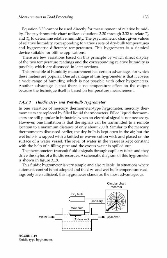
Measurements in Food Processing 133
Equation 3.30 cannot be used directly for measurement of relative humid-ity. The psychrometric chart utilizes equations 3.30 through 3.32 to relate Td
and Tw to determine relative humidity. The psychrometric chart gives valuesof relative humidity corresponding to various sets of dry-bulb temperaturesand hygrometric difference temperatures. This hygrometer is a classicaldevice suitable for offline applications.
There are few variations based on this principle by which direct displayof the two temperature readings and the corresponding relative humidity ispossible, which are discussed in later sections.
This principle of humidity measurement has certain advantages for whichthese meters are popular. One advantage of this hygrometer is that it coversa wide range of humidity, which is not possible with other hygrometers.Another advantage is that there is no temperature effect on the outputbecause the technique itself is based on temperature measurement.
3.4.2.3 Fluidic Dry- and Wet-Bulb Hygrometer
In one variation of mercury thermometer-type hygrometer, mercury ther-mometers are replaced by filled liquid thermometers. Filled liquid thermom-eters are still popular in industries when an electrical signal is not necessary.However, one limitation is that the signals can be transmitted to a remotelocation to a maximum distance of only about 200 ft. Similar to the mercurythermometers discussed earlier, the dry bulb is kept open in the air, but thewet bulb is wrapped with a knitted or woven cotton wick and placed on thesurface of a water vessel. The level of water in the vessel is kept constantwith the help of a filling pipe and the excess water is spilled out.
The thermometers transmit fluidic signals through capillary tubes and theydrive the stylus of a fluidic recorder. A schematic diagram of this hygrometeris shown in figure 3.19.
This fluidic hygrometer is very simple and also reliable. In situations whereautomatic control is not adopted and the dry- and wet-bulb temperature read-ings only are sufficient, this hygrometer stands as the most advantageous.
FIGURE 3.19Fluidic type hygrometer.
Cotton wick
Wet bulb
Dry bulb
Water spill over
Capillary
Circular chartrecorder
7244.book Page 133 Wednesday, June 21, 2006 11:14 AM

134 Measurement and Control in Food Processing
3.4.3 Electrical Type of Humidity Meters
Electrical humidity meters are based on sensors that undergo a variation ofsome electrical parameters such as resistance, conductance, and capacitance.These sensors are discussed next.
3.4.3.1 Resistive Hygrometer
A resistance element type of relative humidity sensor consists of two wireswound over an insulating former and a coating of hygroscopic materials likelithium chloride, phosphoric acid, calcium chloride, zinc chloride, or tintetrachloride (fig. 3.18B). When the hygroscopic material absorbs moisturefrom the air, dissociation takes place so the resistance between the two wireschanges. The variation of resistance due to humidity is between 10 MΩ and10 KΩ. The main disadvantage of this sensor is that error due to temperatureis high. Moreover, the sensor does not cover the full operating range ofrelative humidity. Hence, a number of such sensors are necessary to coverthe full range. Another disadvantage is that the wires are prone to contam-ination, so they should be made of noble metals only. An AC circuit performsthe measurement to avoid polarization. The accuracy of this transducer isabout ±1.5% (relative humidity).
3.4.3.2 Electrolytic Hygrometer
The electrolytic humidity sensor (fig. 3.18C) consists of two platinum wireswound over an insulating tube made of Teflon or Neopherene in duplexhelix winding form. The space between the windings is filled up with ahygroscopic compound like phosphorous pentoxide. The test air is thenpassed through the tube at a rate of about 100 cm3/min. When the cell isenergized by a DC voltage, a current flows through the winding under aconstant air flow condition. The system reaches equilibrium when the mois-ture absorption rate of the hygroscopic material equals the rate of electrolyticdecomposition. Therefore the current becomes proportional to the relativehumidity of air. The response of this device is slower than other two devicespreviously mentioned. In addition, a change in temperature tends to changethe calibration of the device.
3.4.3.3 Capacitive Hygrometer
In this type of sensor the relative permittivity of a material is allowed tochange with the absorption of moisture. Therefore a change in capacitancecan be obtained due to a change in relative humidity. These sensors are veryprecise in design and construction, making them extremely sensitive. Theelectrodes are made of gold or gold-plated metals, which makes them costlierthan other types.
All four types of humidity meters are available in battery-operated, por-table forms that are very popular for field measurements.
7244.book Page 134 Wednesday, June 21, 2006 11:14 AM
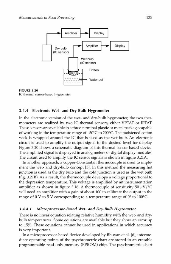
Measurements in Food Processing 135
3.4.4 Electronic Wet- and Dry-Bulb Hygrometer
In the electronic version of the wet- and dry-bulb hygrometer, the two ther-mometers are realized by two IC thermal sensors, either VPTAT or IPTAT.These sensors are available in a three-terminal plastic or metal package capableof working in the temperature range of –50°C to 200°C. The moistened cottonwick is wrapped around the IC that is used as the wet bulb. An electroniccircuit is used to amplify the output signal to the desired level for display.Figure 3.20 shows a schematic diagram of this thermal sensor-based device.The amplified signal is displayed in analog meters or digital display modules.The circuit used to amplify the IC sensor signals is shown in figure 3.21A.
In another approach, a copper-Constantan thermocouple is used to imple-ment the wet- and dry-bulb concept [3]. In this method the measuring hotjunction is used as the dry bulb and the cold junction is used as the wet bulb(fig. 3.21B). As a result, the thermocouple develops a voltage proportional tothe depression temperature. This voltage is amplified by an instrumentationamplifier as shown in figure 3.16. A thermocouple of sensitivity 50 µV/°Cwill need an amplifier with a gain of about 100 to calibrate the output in therange of 0 V to 5 V corresponding to a temperature range of 0° to 100°C.
3.4.4.1 Microprocessor-Based Wet- and Dry-Bulb Hygrometer
There is no linear equation relating relative humidity with the wet- and dry-bulb temperatures. Some equations are available but they show an error upto ±5%. These equations cannot be used in applications in which accuracyis very important.
In a microprocessor-based device developed by Bhuyan et al. [6], interme-diate operating points of the psychrometric chart are stored in an erasableprogrammable read-only memory (EPROM) chip. The psychrometric chart
FIGURE 3.20IC thermal sensor-based hygrometer.
Display
Wet bulb(IC sensor)
Dry bulb(IC sensor)
Display
Cotton
Water pot
Amplifier
Amplifier
7244.book Page 135 Wednesday, June 21, 2006 11:14 AM
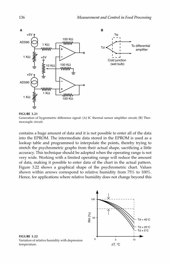
136 Measurement and Control in Food Processing
contains a huge amount of data and it is not possible to enter all of the datainto the EPROM. The intermediate data stored in the EPROM is used as alookup table and programmed to interpolate the points, thereby trying tostretch the psychrometric graphs from their actual shape, sacrificing a littleaccuracy. This technique should be adopted when the operating range is notvery wide. Working with a limited operating range will reduce the amountof data, making it possible to enter data of the chart in the actual pattern.Figure 3.22 shows a graphical shape of the psychrometric chart. Valuesshown within arrows correspond to relative humidity from 75% to 100%.Hence, for applications where relative humidity does not change beyond this
FIGURE 3.21Generation of hygrometric difference signal: (A) IC thermal sensor amplifier circuit; (B) Ther-mocouple circuit.
FIGURE 3.22Variation of relative humidity with depressiontemperature.
AD590
1 KΩ
AD590
1 KΩ
100 KΩ
1 KΩ
10 KΩ
1 KΩ
100 KΩ
100 KΩ
+5V
+5V
+5V
Td
Tw
Cold junction (wet bulb)
To differential amplifier
A B
0 5 10
50
100
Td = 45°C
Td = 25°CTd = 5°C
RH
(%
)
∆T, °C
7244.book Page 136 Wednesday, June 21, 2006 11:14 AM

Measurements in Food Processing 137
range, the corresponding data on the chart can be used. This simplifies thetechnique to a great extent. Figure 3.23 shows the schematic arrangementfor the microprocessor application.
3.4.4.2 Hygrometer Based on Linearized Model of Psychrometric Chart
A linearized model of the psychrometric chart was developed by Bhuyanand Bhuyan [7] for implementing the system by a computer. In this techniquefour piecewise linearized model equations are developed. In the piecewiselinearized technique, the data of the chart are divided into four zones thatare considered linear within individual boundaries. Figure 3.24 shows thefour operating zones AD, AC, BC, and BD in the relative humidity charac-teristics of the psychrometric chart.
The temperature limits for the zones are as follows:
Zone AC: 5°C ≤ Td ≤ 25°C
and 0°C ≤ ∆T ≤ 5°C
FIGURE 3.23Block diagram of microprocessor-based hygrometer.
FIGURE 3.24Four operating zones of the psychrometricchart. (Redrawn from Proc. Int. Conf. on Indus-trial Automation and Control, 1995 with permis-sion from IEEE.)
Dry sensor
Wet sensor
A
ADC
Microprocessor
Display
E PROM
A
Interface
0 5 10
50
100
Td= 45°C
Td= 25°C
Td= 5°C
RH
(%
)
∆T, °C
AC AD
BC BD
7244.book Page 137 Wednesday, June 21, 2006 11:14 AM

138 Measurement and Control in Food Processing
Zone AD: 25°C < Td ≤ 45°C
and 0°C ≤ ∆T ≤ 5°C
Zone BC: 5°C ≤ Td ≤ 25°C
and 5°C < ∆T ≤ 10°C
Zone BD: 25°C < Td ≤ 45°C
and 5°C < ∆T ≤ 10°C
After linearization the resulting equations for relative humidity (%) for thefour operating ranges are
RHAC = (0.204∆T + 0.072)Td – 12.76∆T + 97.88 (3.33a)
RHAD = (0.198∆T + 0.034)Td – 12.44∆T + 98.67 (3.33b)
RHBC = (0.251∆T + 0.122)Td – 12.31∆T + 94.55 (3.33c)
RHBD = (0.174∆T + 0.111)Td – 12.28∆T + 101.19 (3.33d)
Relative humidity can be calculated from any one of the above equationsusing the dry-bulb temperature (Td) and the depression or difference tem-perature (∆T =Td – Tw). Calculation of relative humidity using equations 3.33athrough 33.3d is performed online with a computer-based data acquisitiondevice. A schematic block diagram of this type of humidity measurement isshown in figure 3.25.
This computer-based wet- and dry-bulb hygrometer has the followingadvantages:
1. Free from temperature effect
2. Easy to calibrate
3. Covers the entire range (0%–100%)
Calibration in this technique is easy because the relative humidity is calcu-lated from the values of wet- and dry-bulb temperatures. If the temperaturereadings are properly calibrated the instrument will be automatically cali-brated for relative humidity.
FIGURE 3.25Block diagram of a computer-based hygrometer.
Dry sensor
Wet sensor
VDU
A
A
ADC ProgramPC
7244.book Page 138 Wednesday, June 21, 2006 11:14 AM

Measurements in Food Processing 139
3.5 Turbidity and Color of Food
Measurements of color and turbidity are important quality control methodsin many food processing industries. Table 3.5 shows some natural colors offoods and artificial colors used in foodstuffs. In many food items the chem-ical and the food values are reflected in their color. Apart from the processedfood, the color of the raw materials also plays an important role in qualitymonitoring in certain food processing industries. Color matching againststandard color of brewing conventions is a regular quality check in thealcoholic beverage industry. Similarly, syrup color testing is also conductedin the soft drink industry. Color and turbidity measurement is employed inthe sugar industry to monitor the clarity of the juice for further processing.In the tea industry the quality of the tea originates mainly from the processof fermentation. The color of the fermented tea gives an indication of itsquality. To improve appearance and to make food attractive, artificial coloris added; for example, in margarine, yellow color additive; in sauces andburgers, red color additive, and so on. There are numerous applications ofcolor and turbidity measurement in the food processing industries. Thissection explains some commonly used techniques.
3.5.1 Turbidity Measurement
Measurement of turbidity has been performed by brewers since the Middle Agesin very crude manners. In those days, a glass of wine was observed by holdingup to light; any small reflectance of light from particles present in the liquid wasvisible. This basic concept of observing the glass of liquid in light is the basis ofmost present turbidity measurements in the food processing industries.
TABLE 3.5
Natural and Artificiala Colors of Some Food Products
Food Color Cause
Bread crust Foxy Amount of sugar remainingin dough
Cocoa powder Orange/ginger-dark AlkalizationOil Green/orange Presence of chlorophyllFlour Creaminess BleachingMade tea Black Degradation of chlorophyllFermented tea Coppery red ThearubiginColored staff:
Cocktail cherriesSauces and burgersSmoked and cured fish
External coating of confectionaries:
E127erythrosineE128 red 2GE154 brown FK
E174 SilverE175 Gold
a As per permitted colors in the United States.
7244.book Page 139 Wednesday, June 21, 2006 11:14 AM
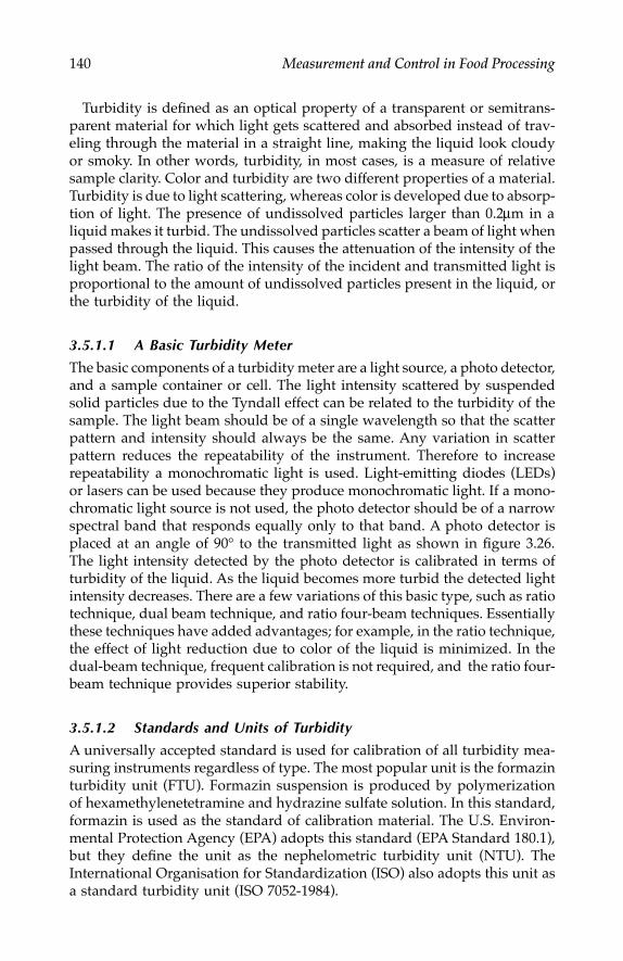
140 Measurement and Control in Food Processing
Turbidity is defined as an optical property of a transparent or semitrans-parent material for which light gets scattered and absorbed instead of trav-eling through the material in a straight line, making the liquid look cloudyor smoky. In other words, turbidity, in most cases, is a measure of relativesample clarity. Color and turbidity are two different properties of a material.Turbidity is due to light scattering, whereas color is developed due to absorp-tion of light. The presence of undissolved particles larger than 0.2µm in aliquid makes it turbid. The undissolved particles scatter a beam of light whenpassed through the liquid. This causes the attenuation of the intensity of thelight beam. The ratio of the intensity of the incident and transmitted light isproportional to the amount of undissolved particles present in the liquid, orthe turbidity of the liquid.
3.5.1.1 A Basic Turbidity Meter
The basic components of a turbidity meter are a light source, a photo detector,and a sample container or cell. The light intensity scattered by suspendedsolid particles due to the Tyndall effect can be related to the turbidity of thesample. The light beam should be of a single wavelength so that the scatterpattern and intensity should always be the same. Any variation in scatterpattern reduces the repeatability of the instrument. Therefore to increaserepeatability a monochromatic light is used. Light-emitting diodes (LEDs)or lasers can be used because they produce monochromatic light. If a mono-chromatic light source is not used, the photo detector should be of a narrowspectral band that responds equally only to that band. A photo detector isplaced at an angle of 90° to the transmitted light as shown in figure 3.26.The light intensity detected by the photo detector is calibrated in terms ofturbidity of the liquid. As the liquid becomes more turbid the detected lightintensity decreases. There are a few variations of this basic type, such as ratiotechnique, dual beam technique, and ratio four-beam techniques. Essentiallythese techniques have added advantages; for example, in the ratio technique,the effect of light reduction due to color of the liquid is minimized. In thedual-beam technique, frequent calibration is not required, and the ratio four-beam technique provides superior stability.
3.5.1.2 Standards and Units of Turbidity
A universally accepted standard is used for calibration of all turbidity mea-suring instruments regardless of type. The most popular unit is the formazinturbidity unit (FTU). Formazin suspension is produced by polymerizationof hexamethylenetetramine and hydrazine sulfate solution. In this standard,formazin is used as the standard of calibration material. The U.S. Environ-mental Protection Agency (EPA) adopts this standard (EPA Standard 180.1),but they define the unit as the nephelometric turbidity unit (NTU). TheInternational Organisation for Standardization (ISO) also adopts this unit asa standard turbidity unit (ISO 7052-1984).
7244.book Page 140 Wednesday, June 21, 2006 11:14 AM

Measurements in Food Processing 141
The Jackson turbidity unit (JTU) is an optical-based unit, whereas the Keisel-gur turbidity unit (KTU) is purely a parts per million (ppm) unit. The turbiditydeveloped when 1 mg of silica is mixed in 1 L of distilled water is called aKTU. This unit is equivalent to the JTU, which equals 6.9 times an FTU unit.Similarly the Mastic turbidity unit (MTU) relates to turbidity resulting when0.02 ml of mastic solution is added to 50 ml of distilled water. An MTU isequivalent to 0.125 times KTU, 0.0125 times FTU, and 0.125 times JTU.
3.5.1.3 Light Scattering Type Turbidity Meter
The basic setup of a turbidity meter based on the light scattering principleis shown in figure 3.26. One variation of this basic principle is the ratiotechnique shown in figure 3.27A. It is equipped with two photo cells to detectlight scattered in two opposite directions. In some devices a separate controlunit is used to enable constant intensity of the light source.
FIGURE 3.26Schematic diagram of a basic turbiditymeter.
FIGURE 3.27Basic turbidity meters: (A) Ratio turbidity detector; (B) Back-scattering detector.
Detector
Refracted ray
Transmittedray
SampleLightsource
Lens
Detector
Light source
Lens
Photo cell
Lens
Condensing lens Sample
Pipe
Sample
Spill over
Light source
Photo cell
A B
7244.book Page 141 Wednesday, June 21, 2006 11:14 AM

142 Measurement and Control in Food Processing
The scattering technique is utilized in a different manner in the back-scattering turbidity meter shown in figure 3.27B. In this unit the samplesurface is left open to circumvent the problem of window deposit in othermeters. The light incident on the sample is scattered from the particlespresent on the surface and received by a set of photo cells installed at theproper angle and position.
3.5.1.4 Optical Absorption Type Turbidity Meter
Turbidity measurement based on the principle of optical absorption methodemploys both off-line and on-line techniques. The principle behind this tech-nique is when a visible light ray is allowed to pass through the sample, acertain amount of light energy gets absorbed by the coloring matters andthe turbid suspension particles. Dispersion takes place in the incident lightray, causing a spectrum in the range of about 380 nm to 760 nm. The samelight ray is also transmitted through a turbid-free reference solution. Thefrequency of alteration is about 600 cycles per second.
In this technique (fig. 3.28) a visible light is paralleled by using a lens (A)and is passed through a cell of rectangular cross-section containing thesample liquid. The light transmitted through the sample is allowed to fallon a transmission grating kept at normal incidence position with respect tolenses B and C. The dispersion of light takes place in wavelengths between380 nm and 760 nm and the measurement is performed in this range only.This dispersed spectrum is sensed by an array of photodiodes positioned atcorrect angles. Each photodiode has a spectral wavelength equal to the totalspectral band divided by the number of photodiodes. The photodiodes cap-ture the spectrum and generate electrical signals corresponding to the spec-tral range from 380 nm to 760 nm at the spectral interval. The electricalsignals generated by the photodiodes are multiplexed, amplified, and fil-tered. The signal is then fed to an analog-to-digital converter and then pro-cessed by a computer.
FIGURE 3.28Setup of an optical turbidity meter.
Lightsource
Lens A
Sample inlet
Outlet
Lens B Lens CGrating
Photodetectors
7244.book Page 142 Wednesday, June 21, 2006 11:14 AM

Measurements in Food Processing 143
3.5.1.5 Turbidity Measurement in the Sugar Refining Process Turbidity measurement is very important in the sugar refining process. Theraw sugar juice is acidic and turbid, with a pH value that is maintained ata level of 7.0 by addition of lime, sulfur dioxide, and then by heat treatment.In sugar refining, pH measurement is conducted where lime is added andthis factor plays a vital role in determining the color of the refined sugar.The juice is heated after the addition of lime. After this process heavy pre-cipitation is formed containing insoluble lime salts, coagulated albumin,waxes, and gums. These precipitated compounds are clarified in the clarifier.The turbidity of the clarified juice is measured. A sampling line is used tomake the juice move from the clarifier continuously to the turbidity meter.
An optical absorption technique was used for relating color and turbiditywith the pH value of sugar juice by Govindraj and Sankaranaryanan [8]. Inthe sugar refining process the color obtained in the refined sugar is amber-brown due to the clarity of the sugar juice. The International Commissionfor Uniform Methods of Sugar Analysis (ICUMSA) has recommended theoptical range of 380 nm to 760 nm in the optical absorption method.
In their investigation the absorption pattern of the sugar juice wasobserved at 420 nm, 560 nm, and 720 nm. Absorption at these first twowavelengths accounts for color and the last (i.e., 720 nm) accounts for tur-bidity of the sugar juice. When the turbidity of sugar is minimal, the absorp-tion value at 720 nm is also a minimum. When there is minimum absorptionat 720 nm, the absorption value at 420 nm is the effective color value of thejuice at 420 nm; the effective color value was also obtained at 560 nm.
In their investigation the pH value of sugar was measured and controlledand the optimum pH corresponding to the best color was detected. The lightsource used was a halogen lamp and the detector consisted of an array ofphotodiodes based on an integrated circuit (40-pin DIP Hamamatsu S2312-38Q) with a quartz window. Pure water was used as the reference material.
3.5.2 Food Color Measurement
The color of an object should be determined by studying its spectral char-acteristics over the entire visible spectrum. When a ray of light interacts withan object, its color is obtained. When a beam of light incidents on an objecta part of the light is transmitted, some is reflected back, and some is absorbedby the material. As per this principle, the light that is reflected back iscollected and dispersed into its various component wavelengths. The degreeof reflectance in these wavelength regions represents the color. Food colormeasurement concerns only the visible range of the spectrum (i.e., approx-imately from 400 to 700 µm). Table 3.6 shows the color and visible spectrumwavelength relations and table 3.7 shows some conventioanl color measuringtechniques. The fundamental properties of an object responsible for its colorare spectral transmittance for transparent materials and spectral reflectancefor opaque materials. Because most of the food items can be consideredopaque, the reflectance technique is very important.
7244.book Page 143 Wednesday, June 21, 2006 11:14 AM

144 Measurement and Control in Food Processing
3.5.2.1 Optical Reflectance Method
This method uses a technique of measurement of light reflected from thesurface of the sample either in one dimension or in three dimensions. Thethree stimuli (tristimulus) correspond to amber, green, and blue as per theCommissions International de’Eclairage (CIE) standard. A continuous or on-line color spectrophotometer based on this approach is shown in figure3.29A. This method uses a sequential comparison and flicker photometermeasurement of the sample and a reference. A single filter develops the threestimuli outputs X, Y, and Z. The CIE standard response values of the tris-timulus are shown in figure 3.29B.
Another technique using the optical reflectance principle is shown in figure3.30. It uses the International Commission for Illumination (ICI) recom-mended viewing and illuminating integrating sphere to illuminate the sampleby a light beam sent through paralleling lenses. The color of the sample ismeasured per unit of percentage reflectance at closer wavelength intervals ofthe visible spectrum compared to a standard or reference color. The intensityof the light reflected from the sample is collected by the receiving lenses,making the light incident on a plane reflect grating. The spectrum of lightis forwarded to a silicon photodiode through a slit. The spectrum resolvedby the grating ranges from 400 nm to 700 nm, which is in the visible range.A stepper motor rotates in steps corresponding to the resolved wavelengthto control the grating, which is coupled to the stepper motor through areduction gear. The grating is brought to its normal incidence position withthe help of an optical encoder fixed to the sensor and a photo-reflector. The
TABLE 3.6
Color and Wavelength Correspondence
Color Wavelength (µm)
Violet 400–450Blue 450–500Green 500–570Yellow 570–590Orange 590–610Red 610–700
TABLE 3.7
Conventional Color Measuring Techniques for Some Food Items
Food Color Measuring Technique (Conventional)
Refined oil Pale, bright Color, Colored glass matchingFlour Creamy, bright Optical reflectanceWheat grain Hard red, soft white, amber Optical reflectanceFermented tea Coppery red Chemical test, colorimeterMade tea Black ColorimeterWine Black, red, purple, pink, white Colorimeter
7244.book Page 144 Wednesday, June 21, 2006 11:14 AM

Measurements in Food Processing 145
current produced by the photo detector, proportional to the intensity of light,is first converted into a voltage signal, which is then amplified and fed to acomputer.
FIGURE 3.29Fluorescence technique: (A) Schematic diagram of Tristimulus flicker method; (B) TristimulusCIE color standard. (Redrawn with permission from Encyclopedia of Chemical Technology, Vol.6, 4e, 849. © John Wiley & Sons, Inc.)
FIGURE 3.30Schematic diagram of the optical setup of a refractometer.
Source Flicker
Sample Standard
Z
Y
X
Photomultiplier
A
Abs
orba
nce
Wavelength (nm)
400 500 600 700
0.5
1.0
1.5
2.0
0
z
y
x
B
Source
Paralleling lens
Integratingsphere
Receivinglens
Split Grating
Photo diodestepper motor
7244.book Page 145 Wednesday, June 21, 2006 11:14 AM

146 Measurement and Control in Food Processing
If the difference of reflectance values for two samples at two equal wave-lengths is equal, it can be ascertained that the shades of the two samples arethe same but the concentration of color might be different. If the differenceof reflectance values is not equal, it can be ascertained that both the colorand the concentration are not the same. If the data are exactly the same, thenboth shade and concentration are the same in the two samples. Appropriateprograms can be written to include these conditions in the software. Thereflectance values for the sample and the standard color at different wave-lengths are determined a priori and stored in memory. From these values theparameters are calculated and the variations for the sample and the standardcolor are compared.
3.5.2.2 Color Reflectance and Digital Color Image Processingin Food Grains
Color is a useful factor in determining quality in grains and an importantvisual attribute of cereal grains used for grading. Color measure is used todenote class and degree of soundness of grains. For example, wheat is gradedon the basis of color as hard red, soft white, or amber durum. Further wheatclassification as hard red wheat is made on the basis of hue and concentra-tion. Similarly certain inferior qualities such as stained, pink immature, grassgreen, or bleached kernels are marks of discoloration of wheat grains.
Reflectance spectrophotometer is one of the methods by which color anal-ysis of grains can be performed. A Spectro-reflectometer is an example ofsuch instruments that measure the reflectance values for grains at differentwavelength regions (420 nm–700 nm). These devices measure the spatiallyaveraged color of the entire field. Selective color measurement of specificobjects or geometric zones enables better grading and classification of grains.This is possible by integrating the tristimulus value determination withdigital image processing capabilities. The schematic setup of this techniqueis shown in figure 3.31. The color data acquisition system consists of threemain components:
1. The sample illumination and viewing device
2. Optical setup and image generation and signal processing
3. Digital image acquisition and processing
The sample illumination is produced by incandescent tungsten filamentlamps powered by a highly regulated power supply to minimize the variationof spectra of illumination. The lamps should be hoisted on an annular plat-form, the height of which can be adjusted from the surface. The platform ofthe lamps can be centered on the viewing zone of the camera. The sampleplatform consists of a white, diffusely reflected foamboard for the backgroundagainst which the samples are compared. Due to this background, necessarycontrast is formed to distinguish the grains to be tested and a reference color.The camera is white balanced for this background.
7244.book Page 146 Wednesday, June 21, 2006 11:14 AM
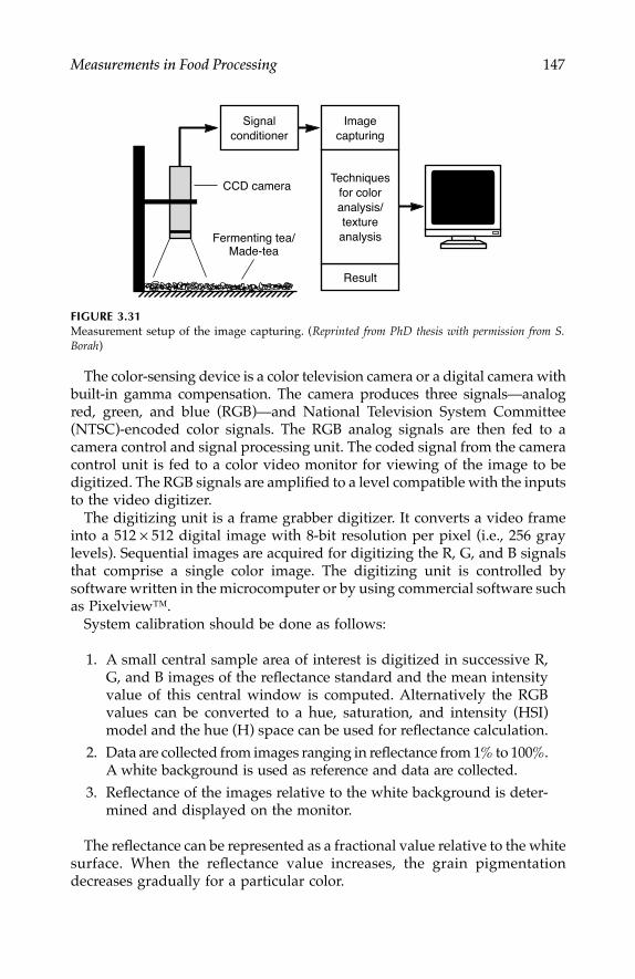
Measurements in Food Processing 147
The color-sensing device is a color television camera or a digital camera withbuilt-in gamma compensation. The camera produces three signals—analogred, green, and blue (RGB)—and National Television System Committee(NTSC)-encoded color signals. The RGB analog signals are then fed to acamera control and signal processing unit. The coded signal from the cameracontrol unit is fed to a color video monitor for viewing of the image to bedigitized. The RGB signals are amplified to a level compatible with the inputsto the video digitizer.
The digitizing unit is a frame grabber digitizer. It converts a video frameinto a 512 × 512 digital image with 8-bit resolution per pixel (i.e., 256 graylevels). Sequential images are acquired for digitizing the R, G, and B signalsthat comprise a single color image. The digitizing unit is controlled bysoftware written in the microcomputer or by using commercial software suchas Pixelview™.
System calibration should be done as follows:
1. A small central sample area of interest is digitized in successive R,G, and B images of the reflectance standard and the mean intensityvalue of this central window is computed. Alternatively the RGBvalues can be converted to a hue, saturation, and intensity (HSI)model and the hue (H) space can be used for reflectance calculation.
2. Data are collected from images ranging in reflectance from 1% to 100%.A white background is used as reference and data are collected.
3. Reflectance of the images relative to the white background is deter-mined and displayed on the monitor.
The reflectance can be represented as a fractional value relative to the whitesurface. When the reflectance value increases, the grain pigmentationdecreases gradually for a particular color.
FIGURE 3.31Measurement setup of the image capturing. (Reprinted from PhD thesis with permission from S.Borah)
CCD camera
Fermenting tea/Made-tea
Signalconditioner
Imagecapturing
Result
Techniquesfor coloranalysis/textureanalysis
7244.book Page 147 Wednesday, June 21, 2006 11:14 AM

148 Measurement and Control in Food Processing
3.5.2.3 Color Matching in Fermented Tea
A digital image processing and machine vision technique for color matchingin tea fermentation was developed by Borah and Bhuyan [9, 10]. Figure 3.32shows a photograph of the experimental setup in a tea factory.
In the black tea manufacturing process, green tea shoots are first withered,and then cut into smaller fragments to speed up enzymatic oxidation of thecatechins. The cut tea is fermented in a controlled environment to form twogroups of color compounds in the tea, theaflavins (TF) and thearubigin (TR).The analysis of the pigmenting compounds formed during fermentation oftea has been suggested by Mahanta [11]. In this method a black tea samplewas collected from the dryer mouth and the sample was extracted with 40 mlof aqueous acetone. The filtrate (0.3 ml) containing about 20 mg extract isseparated over a Sephadex LH-20 column into six fractions (I–VI) containingTFs and TRs along with chlorophylls and their derivatives. Table 3.8 showsthe characteristics of pigment products formed during the fermentation pro-cess. The Tocklai Tea Experimental Station under the Tea Research Associa-tion, India has developed two methods of color content analysis of tea [12].The first is based on polyphenol content of tea leaf and the second is basedon the measurement of the concentration of TF formed during fermentation.
In a method developed by Borah and Bhuyan [13] color images of ferment-ing tea are recorded by a digital camera and fed to a signal conditioner,which in turn converts the images to a digital signal. A computer retrievesthe images from the digital camera through an image capturing card. Thedigital camera is mounted over the fermentation table to continuously record
FIGURE 3.32Photograph during capturing of fermented tea images in a tea factory.
Electronic processor
Camera
Computer interface
Tea under fermentation
7244.book Page 148 Wednesday, June 21, 2006 11:14 AM

Measurements in Food Processing 149
the images of fermenting tea. The images used by the signal conditioner areconverted into a digital signal in the S-band frequency, which is then fed tothe computer. The computer receives the image from the input signal witha Pixelview™ card interfaced to the computer. A schematic diagram of thesetup is shown in figure 3.33.
In this technique a histogram comparison algorithm is used in matchingcolor of fermented tea with a standard color image. By definition a colorhistogram is a vector where each entry stores the number of pixels of a givencolor of the image in RGB color space. Histogram axes are partitioned uni-formly with fixed intervals by a heuristic approach to determine the bin size.The number of bins is kept small for computational efficiency but this reducesrecognition accuracy. The histogram bin size fixed in the method was 32. Afterreceiving an image, histograms were developed and plotted for each colorspace (fig. 3.34) and the corresponding histogram comparison for each colorspace was performed with the standard image using Euclidean and L1 (Man-hattan) norms to quantify a similarity between two colors. Given a pair of
TABLE 3.8
Characteristics of Pigment Products During Fermentation of Tea
Fractions of TF and TR Color Contribution Liquor Color
Thearubigin Reddish brownI TR-1 8.73
II TR-2 8.73III TR-3 14.3
Ethyleacetate 28.4 BlackChlorophylls and their derivatives 30.0 Golden yellow
IV TheaflavinsV Theflavnimongollate
VI Theaflavin digallate
Source: Proc. 30th Tocklai Conference, 1988. Reprinted with permission fromTocklai Tea Experimental Station, Assam, India, Tea Research Association (India).
FIGURE 3.33Schematic of the image capturing setup. (Reprinted with permission from Int. J. Food Sci. & Tech.,Vol. 40(6), Blackwell Publishing Co.)
CCD camera andconstant illuminationarrangement
Tea underfermentation
Signalconditioner
Imagecapturing card
Result
PC
7244.book Page 149 Wednesday, June 21, 2006 11:14 AM

150 Measurement and Control in Food Processing
histograms H(I) and H(Q) of input image I and the standard image Q, respec-tively, each containing n bins, the defined histograms intersection is as follows
(3.34)
where hj(I) = number of pixels of color j in images I and QNQ × MQ = size of the standard image
This measure can be represented by difference form (dissimilarity) as Man-hattan norm (L1) as
(3.35)
where NI × MI = image size
FIGURE 3.34Color histograms of a fermented tea image: (A) Space R; (B) Space G; (C) Space B. (Reprintedwith permission from Int. J. Food Sci. & Tech., Vol. 40(6), Blackwell Publishing Co.)
8000
40 80 120 160 200140 18010060
7000
6000
5000
4000
3000
2000
1000
0
Num
ber
of p
ixel
s
Bins
A
9000
20 80 120 160 200140 18010060
7000
6000
5000
4000
3000
2000
1000
0
8000
Num
ber
of p
ixel
s
40
Bins
C
8000
20 80 120 160 200140 18010060
7000
6000
5000
4000
3000
2000
1000
0
Num
ber
of p
ixel
s
40
Bins
B
S H I H Q
h I h Q
N M
j j
j
n
Q Q
( ), ( )
min ( ), ( )
=
×=∑
1
D H I H Qh I
N Mh Q
N M
N
j
I I
j
Q Qj
N
I
( ), ( )( ) ( ) =
×−
×
=
=∑
1
1××
−=∑M
h I h QI
j j
j
N
( ) ( )1
7244.book Page 150 Wednesday, June 21, 2006 11:14 AM

Measurements in Food Processing 151
For a given distance T, two histograms are said to be similar if S ≥ T orD ≤ T and the images are of the same color.
Images of well-fermented (WF) tea (almost deep-coppery red) are storedas a standard image. Tea images were captured sequentially from the startof fermentation to completion to generate a database of images of tea duringthe fermentation process. This database consists of images under the cate-gories not fermented (NF), underfermented (UF), well fermented (WF), andoverfermented (OF). A dissimilarity pixel value (DPV) for all the colorspaces—R, G, and B—are determined by comparing each of the sampleimages with the standard images. The histogram comparison method isadopted for finding the DPV of each image using the standard color images.DPV for all three spaces for the typical fermenting stages are shown in table3.9. A dissimilarity threshold pixel level was found from a large number ofimages that was taken as a faithful threshold level for discriminating between
TABLE 3.9
Dissimilarity Measures for R, G, and B Color Spaces
Sample NumberState of
FermentationDPV for
R Color SpaceDPV for
G Color SpaceDPV for
B Color Space
123456789
10111213141516171819202122232425262728
NFNFNFNFNFNFNFUFUFUFUFUFUFUFUFUFWFWFWFWFWFWFOFOFOFOFOFOF
0.770.390.380.450.670.540.670.360.420.420.370.350.420.350.410.310.570.220.210.130.130.260.600.300.320.280.590.36
0.560.450.700.410.510.560.620.400.300.460.320.430.530.370.360.350.180.100.210.240.180.150.500.480.440.350.560.33
0.610.410.510.620.480.430.730.390.310.370.550.520.410.360.400.410.240.090.230.250.240.200.540.490.340.420.680.51
Source: Int. J. Food Sci. & Tech., Vol. 40(6), 2005. Reprinted with permission from BlackwellPublishing Ltd., Oxford, UK.
7244.book Page 151 Wednesday, June 21, 2006 11:14 AM

152 Measurement and Control in Food Processing
the images. DPV calculation for the red (R) color space was done on eachtest sample and a decision was made as
NF for DPV value ≥ Thresholdand WF for DPV value < Threshold
A prominent variation of DPV was observed for the three spaces thatrevealed a good correlation between sensory panel judgment and the com-puter-aided approach.
In a variation of this technique they used only the hue (H) space of theHSI model of the images in a similar manner. The HSI color model is betterthan the RGB model for its illumination intensity invariant property.
This technique shows a potentiality for adopting machine vision tech-niques to eliminate human error in color matching in the tea industry.
3.6 Food and Process Temperature Measurement
Different types of transducers available for the measurement of processtemperature were discussed in chapter 2. However, based on the type offood material, type of control technique, precision requirements, and so on,temperature transducers can take different forms and variations in the foodindustry. In this section, temperature measurement in food processing situ-ations, with a special emphasis on application conditions, is discussed.
3.6.1 Temperature Measurement in Food Processing
The primary considerations required for food temperature measurement aretype of the food item (solid, liquid, viscous, etc.), accuracy needed, dynamicbehaviors (stationary or moving), atmospheric conditions, thermal coupling,and so on. The simplest situation of temperature measurement is in a sta-tionary phase of a food (i.e., while storing). For example, in cocoa buttermanufacturing, liquid cocoa butter is stored where the temperature shouldnot exceed 45°C. However, dry cocoa beans stored inside jute sacks with anincrease in temperature over 20°C can develop mold within a few days. Onthe other hand, bulk storage of chocolate is generally done at 40°C to 60°C.
Apart from storage heating or drying in stationary mode, treatment of fooditems with mixing and stirring also requires simple temperature measuringdevices. Such a situation might arise in production of milk compounds bymixing condensed milk or reconstituted milk, sugar, and water and heatingto 74°C. In the butter manufacturing process, after pasteurization, the creamis crystallized down to 3°C to 5°C in insulated tanks for a period not lessthan 4 hr. This cream is again heated to a churning temperature of 7°C to13°C before butter making.
7244.book Page 152 Wednesday, June 21, 2006 11:14 AM

Measurements in Food Processing 153
A fundamental difficulty of temperature sensors is thermal coupling. Incase of liquid foods like fruit juice, soft drink, and wines, the temperaturemeasurement needs an equilibrium condition between the sensor tempera-tures. The temperature during heating or drying of moving food productsalso undergoes rapid variation within a local region, causing unstable sensoroutput. This necessitates a sufficiently strong thermal coupling and fastresponse. The thermal difference developed in a temperature sensor can beshown by this equation:
(3.36)
where T = temperatureh = heat transfer coefficient at surface of sensorA = surface area of sensorW = weight of sensorCp = specific heat of sensor materialθ = time after sensor is in contact with the food
A large surface area (A) to mass ratio enables a shortened response time.Moreover, increasing heat transfer coefficient by forced convection or rapidflow of the liquid will also make the response fast. The following sectionsaddress some of these considerations in temperature transducers.
3.6.2 Thermocouples
Although thermocouples were primarily used for high temperature measure-ment, now they are used for a wide temperature range, from high to low. Mostfood processing industries use thermocouples because they are supplied withcalibration standards. Food industries generally incorporate temperature mea-surement in the lower range, below 300°C. In most cases storage and heatingare to be conducted below 100°C. Materials like lactose, polydextrose, sorbitel,xylitol, and so on melt comparatively at a lower temperature (below 300°C).The following thermocouples are generally used in process measurements:
1. Copper-Constantan2. Iron-Constantan3. Chromel-alumel4. Platinum-platinum/rhodium
However due to lower operating temperatures of measurement in foodprocessing, copper-Constantan is more widely used. The most suitable con-necting lead wire for a copper-Constantan thermocouple is copper-Constantanitself. Use of the same material as lead wire reduces the error due to devel-opment of spurious thermo EMF.
T TT T
e h A WCp1
1 0
−−
= ( / )θ
7244.book Page 153 Wednesday, June 21, 2006 11:14 AM

154 Measurement and Control in Food Processing
3.6.2.1 Thermocouple Installations
Thermocouples must be protected from adverse environmental conditionssuch as corrosion and oxidation using thermal wells. Cast or milled materialssuch as nichrome, chromel, and iron with thick walls are reactive and giveslower responses. From this point of view, ceramic materials such as vycor,sillimanite, and porcelain are more suitable as protecting materials.
To measure temperature of liquids flowing through pipes, thermocouplesare employed to ensure true food temperature. A radiation shield is neces-sary near the hot junction of the thermocouple. To get the maximum heattransfer effect, the thermocouple inserted through the pipe should conductheat radially and axially at the tip. For this the well should be thin andshould protrude slightly beyond the center of the pipe. The well of the pipeat the point of measurement should be properly insulated. If the diameterof the pipe is very small an expander is used or the well is mounted at thebend of the pipe (fig. 3.35 and fig. 3.36).
FIGURE 3.35Thermocouple installation in a pipe.
FIGURE 3.36Thermocouple installation in small pipes.
Flow
Thermowell
Stub
Insulator
Pipe
Expander
Stub
7244.book Page 154 Wednesday, June 21, 2006 11:14 AM

Measurements in Food Processing 155
3.6.3 Temperature of Food on a Conveyor
Special arrangements are necessary for sensing temperature measurementof food under moving conditions such as drying and pasteurization, pack-aging, and bottling. In such situations the sensors are either noncontactingor of traversing brush-skid design (fig. 3.37).
3.6.4 Food Tempering Monitoring
Food tempering is a process where plasticized fat of food is allowed to coolat a controlled temperature until its properties are stabilized. In chocolatemanufacturing, chocolate is tempered in a tempering machine. Proper tem-pering requires measurement of the cooling process, which is generally donein a temper meter. A temper meter basically monitors the relation betweentemperature and time with the help of a thermocouple and a miniaturetemperature recorder. It consists of the following elements (fig. 3.38):
1. A vacuum flask2. Ice powder to cause cooling3. A sample tube made of good conductive material4. A probe stud and insulator5. A thermocouple or thermistor6. A miniature recorder
The correctness of tempering can be determined by looking at the temper-ature–time graph plotted by the recorder. When the tempered chocolate (at30°C) is poured and immersed in the flask, it starts cooling and the thermo-couple senses the cooling temperature continuously.
FIGURE 3.37Temperature measurement under product in moving condition: (a) Packaging and canning; (b)Bottling.
Probe
Probe
Product
BA
Product
7244.book Page 155 Wednesday, June 21, 2006 11:14 AM

156 Measurement and Control in Food Processing
3.6.5 Precision Temperature Measurement
For temperature measurement in food processing, accuracy is needed on theorder of 0.1°C. A responsible food manufacturer does not disregard a digitafter the decimal point. RTDs are among the most widely used precisiontemperature sensors in the food industry due to their higher accuracy, sim-plicity, and flexibility of design. Another added advantage is their highresolution on the order of 0.01°C.
RTDs are generally made up of metallic (platinum, copper, or nickel) ornonmetallic (semiconductors) materials, the resistance of which increases astemperature increases. The resistance–temperature coefficient and meltingpoint of platinum are higher compared to nickel and copper, for which it isfound to be suitable.
In precision thermometry, platinum is used as a resistive element. A plat-inum resistance thermometer usually has a resistance between 10 and 35ohms at 0°C. The element is wound over or etched on in various forms (fig.3.39). The resistance element of the RTD is connected to the measuring circuit,which is most commonly a Wheatstone bridge circuit. The output voltageproduced by the circuit is amplified and recorded or displayed by a suitablemeter. Similar to thermocouples, RTD probes are also shielded by a protectivesheath or well made of porcelain, brass, or stainless steel. The platinum probeis placed at the end of the well, properly insulated from the body of the well.
A probable application of precise temperature measurement using RTD infood processing is a three-stage chocolate tempering machine. Such machinesare used to temper and crystallize cocoa butter to get tempered chocolate. At
FIGURE 3.38Apparatus for monitoring cooling curve infood tempering.
Plotter
InsulatorThermistor
Thermo flask
Crushed ice
Sample tube
7244.book Page 156 Wednesday, June 21, 2006 11:14 AM

Measurements in Food Processing 157
every stage of tempering, RTDs can be installed to measure the temperatureof both chocolate and coolant fluid. Platinum RTD probes are recommendedin tempering machines to achieve accuracy to within a tenth of a degree.
3.7 Food Flow Metering
Flow measurement of liquid food materials is primarily conducted to deter-mine the quantity or proportion of input material introduced into a process-ing stage. The important aspect of flow metering in the food industry is thequantity control; hence, special attention should be paid to designing a flowmeter for a special applications. For example, dealing with products thatsolidify at high temperature like hydrogenized oil, the flow meter might befitted with a heater. A wide variety of flow meters are available that workon different physical or electrical principles and have different advantagesand disadvantages.
Turbine, variable area gap meters, and vortex shedding meters are widelyused flow meters in many industrial applications, but these are not suitablefor high-viscosity food fluids. Venturi tubes and ultrasonic sensors are com-paratively less obstructive but are practically ineffective for liquids sus-pended with solid particles.
Pressure difference or the pressure drop principle is used in venture, orifice,and pitot tube flow meters. A positive displacement flow meter uses a rotarypiston, oval gear, sliding vane, or reciprocating piston. In all of these tech-niques, a velocity head is converted to a pressure drop and the flow meter ora part of it has to be inserted into the flow pipe. Due to this obstruction of the
FIGURE 3.39Platinum resistance thermometers.
Mica
Mica
Platinum Coil
Platinum
7244.book Page 157 Wednesday, June 21, 2006 11:14 AM

158 Measurement and Control in Food Processing
fluid flow, these flow meters are not suitable for food processing applicationsbecause they create problems of frequent cleaning and maintenance.
Electromagnetic, ultrasonic, and Coriolis mass flow meters are advanta-geous for liquids and pasty or viscous food materials.
3.7.1 Magnetic Flow Meters
There are many liquid foods that are suitable for metering by the principleof magnetic flow meter. As per Faraday’s law of electromagnetic induction,when a conductor is moved through a magnetic field, an EMF is generatedin the conductor that is proportional to the relative velocity between theconductor and the magnetic fluid.
The conductive principle can be applied to food items like fruit juices,yogurt, beer, citrus juice, and so on. Table 3.10 gives the conductance valuesof some liquid food materials. For liquids with conductivity as low as 0.1mS/cm, special design considerations have to be made for electromagneticflow metering. Most of the materials show higher conductivity at highertemperatures, so a liquid with marginal conductivity at a particular temper-ature can be metered satisfactorily at a higher temperature. Wines generallyhave smaller conductivity, but flow metering at higher temperature whileboiling (i.e., wort) might be possible.
The schematic representation of a magnetic flow meter is shown in figure3.40. The magnetic field (H) should be perpendicular to the flow directionand voltage induced (E) will be mutually perpendicular to both H and flowvelocity (v). The mathematical relation of the induced EMF with other param-eters is given by
(3.37)
where B = magnetic field strength (Tesla)v = flow velocity (m/s)
D = diameter of the flow pipe (m)
TABLE 3.10
Electrical Conductivity of Some Food Materials
Liquid Food MaterialConductivity
(mS/cm)
Molasses (at 50°C) 5,000Corn syrup 16Vodka (100 proof) 4Water (potable) 70
e BD v=
7244.book Page 158 Wednesday, June 21, 2006 11:14 AM

Measurements in Food Processing 159
The volumetric flow rate Q can be calculated from
(3.38)
where A = cross-sectional area of the pipe
The magnetic coils are energized either by AC or DC voltages. In the caseof DC, a pulsed DC excitation can be applied. There are variations of mag-netic floweters, including a pitot type. Figure 3.41 shows a pitot type ofmagnetic flow meter used in irregularly shaped pipes or conduits.
Magnetic flow meters are not affected by viscosity of the material as in the caseof molasses or sugar syrup. The capacity of magnetic flow meters ranges fromas low as 40 ml/m to 378 kl/m and can be accommodated in pipe sizes rangingfrom 2.5 mm to 2.4 m in diameter. The power consumption is about 20 W withDC excitation, 30 W for a 50-mm AC unit, and 0.3 kW for a 760-mm AC unit.
3.7.2 Mass Flow Metering
In food processing, in many situations, metered quantity of a food item isfed to the process to get the desired quantity of the product. For example,
FIGURE 3.40Schematic diagram of a magnetic flow meter.
FIGURE 3.41Schematic diagram of a pitot-type magneticflow meter.
V
E
Pipe
MagneticField
Q vA=
Flange mounting
Support
ConnecterMeter
7244.book Page 159 Wednesday, June 21, 2006 11:14 AM

160 Measurement and Control in Food Processing
liquid chocolate is a viscous material. When it is applied to a temperingmachine in metered quantity, mass flow metering can be selected. Similarly,feeding sugar juice to a yeast fermenter, glucose solution into isomerization,and plant, liquid milk to spray dryer of spray milk production are exampleswhere mass flow metering is essential.
All mass flow meters work on the principle that when a fluid rotates, aforce is produced that is proportional to the mass of the fluid. A Coriolis massflow meter employs a tangential acceleration produced by a fluid flowingthrough tube that is rotated about a fixed axis perpendicular to the tube axis.Figure 3.42 shows a fluid element of mass m flowing at constant velocity voutward away from the rotational axis of the tube rotating at a constantangular velocity ω. This rotation imparts a Coriolis acceleration given by ac =2vω. A Coriolis force of value Fc = 2mvω is exerted on the fluid, which triesto push the fluid element to the left. This force is balanced by the inertial force(Fi) of the fluid pushing the fluid to the left. Due to elasticity of the tube, theinertial force deflects the tube slightly to the right. Similarly, if the fluid massm moves inward at a constant velocity v in line with the tube axis that rotatesat a constant angular velocity of ω, a Coriolis force Fc acts in the oppositedirection and it is opposed by the inertial force Fi, causing the tube to deflectslightly to the right. In practice the tube is not rotated but vibrated, and thesame effect is observed. A mechanical exciter is placed at the middle of thetube while the ends are fixed. The two halves of the tube act like two differenttubes. Two reaction forces due to Coriolis effect are developed with opposingaction and create a small displacement in the flow tube. This displacement isproportional to the mass flow rate m given by
(3.39)
and so
FIGURE 3.42Fluid element in Coriolis flow meter: (A) Outward motion; (B) Inward motion.
ω
ν
Fc m
ων
Fcm
A B
F mlc = 2 ω
7244.book Page 160 Wednesday, June 21, 2006 11:14 AM

Measurements in Food Processing 161
(3.40)
where l is the fluid element length.Direct measurement of the displacement or force is not possible, but the
phase difference between the forces in the two halves can be measured. Inpractice, the tube is vibrated in sine wave pattern and the motion of the inlettube lags behind the motion of the outlet tube. This phase difference isdetected by placing a detector such as an electromagnetic pickup (measuresvelocity) or optical pickup (measures displacement). In the case of electro-magnetic sensors, a magnet is placed in one of the tubes and a wire is placedon the other, thereby generating an EMF in the coil proportional to therelative positions of the coil and magnet. If the tube is vibrated by a sinewave, both of the detectors produce sinusoidal signals with a phase differ-ence proportional to mass flow rate. When there is no flow, the phase dif-ference is also zero.
An electronic circuit, a microprocessor, or a computer can be used to receivethe two signals, determine the phase difference, and calibrate in terms ofmass flow rate. In some cases a frequency-dependent signal might also begenerated instead of a voltage or current signal. A Coriolis flow meter canbe calibrated to measure volumetric flow rate, density, or temperature inaddition to mass flow rate. Geometry of a Coriolis flow meter is shown infigure 3.43. Coriolis flow meters are recommended for mass flow measure-ments of liquids and slurries. The flow meter works well in the flow rangeup to 11,340 kg/min. The pipe size ranges from 1.5 mm to 150 mm. Althoughtemperature variation might affect the accuracy of this flow meter, viscosityhas no effect on its performance.
Mass flow rate of food items like beer, chocolate, fruit juice, honey, icecream, margarine, milk, molasses, peanut butter, tomato paste, and vegetableoil can be measured by Coriolis flow meter; however, the meters are proneto clogging. The flow meter is not suitable for products in which hardening,freezing, or crystallization is observed because the flow is obstructed. In suchcases a single-tube design is preferable to the dual-tube design to make
FIGURE 3.43A Coriolis flow meter geometry.
m F lc= /2ω
7244.book Page 161 Wednesday, June 21, 2006 11:14 AM

162 Measurement and Control in Food Processing
unplugging easier. Another drawback of the Coriolis flow meter is that it isprone to vibration. This flow meter should not be installed near large pumps,vibrating sorters or sieves, vibrating conveyors, and other such equipment.
3.7.3 Turbine Flow Meter
Turbine flow meters are also in use in some food processing industries, likedairy and beverages, but they have limitations on high viscosity of the foodor possible damage due to overspeeding during liquid and gas phases. Ifthese problems can be minimized, turbine flow meters are very accurate andsuitable for high-temperature fluids. The output signal of the turbine flowmeter is a pulsed waveform and therefore easy to interface with a computer.
3.7.4 Positive Displacement Flow Meter
In the positive displacement flow meter, the fluid is successively dividedinto segments by directing and discharging it through a chamber of knownvolume. Oscillating pistons, lobed impellers, sliding vanes, rotating discs,and so on are used to produce the successive revolutions. The liquid shouldform a seal in the meter; therefore highly viscous liquid foods such as honeyare suitable. Because this meter creates narrow tracks to direct and dischargethe liquid, the liquid should be free from suspensions or solid particles.Because this flow meter can be operated without a power supply, it is verypopular in applications like storage tank loading and process control metersfor liquids like edible oil and sugar syrup.
3.7.5 Solid Flow Metering
Flow measurement of liquids and gaseous products is carried out by install-ing the flow meters in the pipeline or chute through which the product flows.On the other hand, transportation mechanisms like hoppers and feeders areinvolved in solid flow metering. In most cases of solid flow of food products,flow measurement is performed for metered dosing. The transportationmechanism is automatically controlled to transport or feed a measured quan-tity of the solid food. For example, in a cocoa butter press, the cocoa kernelsare transported from the cocoa kernel container to the hydraulic pressthrough a metered dosing mechanism. In such situations either manual orcontrolled dosing or an automated set-level dosing method is used. Thereforein designing a solid flow meter, the design aspects of the supply bin andfeeder should also be taken into consideration. A good design of the surgehopper is also important to provide an accurate flow metering.
Throttling and metering the flow of solid material to the feeders are per-formed in various ways. Most of these devices work on the weighing prin-ciple, in which they determine the weight of material passing a given point.
7244.book Page 162 Wednesday, June 21, 2006 11:14 AM

Measurements in Food Processing 163
3.7.6 Gravimetric Feeder Meters
These meters comprise a weight-rate measuring device with a volumetriccontrol mechanism. The vertical gate gravimetric feeder is not advantageousfor throttling flows of large particle size, fibrous materials, and grains ofirregular shape. These feeders are generally designed to produce typicalmaterial ribbon of widths of 50 mm to 457 mm and to regulate depth ofmaterial up to 152 mm on the weight belt. The opening and closing of thegate can be actuated by electromechanical solenoids, pneumatic actuators,or servomotor-controlled actuators.
3.7.6.1 Rotary Vane Feeder
The assembly of a belt type gravimetric meter with a rotary control is shownin figure 3.44. The rotary vane feeder is suitable in a volumetric feed sectionwhere the material is aerated and has a low bulk density. Similar to thevertical feeder, a rotary feeder is also not suitable for handling materials thathave large particles and in some cases are not desirable for fibrous or stringymaterials. The rotor speed determines volumetric capacity. If a very highflow rate is desired the rotor speed must be high; however, in such situationsthe rotor pockets might not be completely filled with the materials. Undersuch circumstances, the use of rotary vane feeders is limited to free-flowingmaterials, such as salt, sugar, and tea grain.
3.7.6.2 Screw Feeder
In a screw feeder, the rotary motion of a screw element controls the deliveryof the material. A hopper delivers the material at the start of the screw feederor at the middle. The hopper is mounted so that the screw feeder is alwaysfilled with the material. Screws grooved in one direction deliver material toone end only and screws grooved in the opposite direction from the center
FIGURE 3.44Schematic diagram of a belt-type gravimetry meter.
Food materialBeltMotor
Hopper
Pneumaticrelay
Flapper nozzle
To recorder
7244.book Page 163 Wednesday, June 21, 2006 11:14 AM

164 Measurement and Control in Food Processing
deliver material to both ends. A long screw section prevents flooding ofmaterial through the screw feeder. Screw feeders can be custom built tofacilitate feeding of fibrous and coarse lumps. Materials prone to cloggingcan be accommodated using a double-ended screw feeder with lateral oscil-latory motion imparting a cleaning action. In such designs the material isfed alternately from both ends and the direction of screw rotation is alteredaccordingly. Figure 3.45 shows a cross-sectional view of a screw feeder.
3.7.6.3 Belt Feeder
In belt feeder a belt driven by electric motor and revolving around a specificdistance is used as the conveyor device. Because the quantity of material isnot controlled, the measurement can be performed by metering the beltspeed and a weight-sensing transducer installed below the belt. The feederis added with a volumetric flow regulator that can be a simple gate or arotary gate, a screw, or other volumetric control devices. Figure 3.46 showsa simple belt feeder added with a flow regulator. The gate is adjusted such
FIGURE 3.45Sectional view of a screw feeder.
FIGURE 3.46A belt feeder flow rate sensing and controlling.
Hopper Screw path
Outlet
Shaft
Spreader
F
Settingpoise weight
Pivot Belt
7244.book Page 164 Wednesday, June 21, 2006 11:14 AM

Measurements in Food Processing 165
that the belt load is balanced by an adjustable poise weight. Although thisfeeder is very popular in industries, its performance is affected by a numberof disadvantages.
3.8 Viscosity of Liquid Foods
3.8.1 Definition and Units
Viscosity is the property of a liquid that describes the amount of resistanceoffered by the liquid due to shear forces developed within it. Let us considertwo parallel layers of a fluid separated by a distance ∆y as shown in figure3.47. The upper layer is subjected to a constant force F and moving in thedirection of the force. The upper layer moves at a constant velocity ∆u whilethe lower layer is stationary. It is found that the force F is directly propor-tional to velocity ∆u and surface area A of the layers and inversely propor-tional to the separation distance ∆y. This can be expressed mathematically as
(3.41)
or
(3.42)
The shear stress is given by
(3.43)
where µ is a proportionality constant and is called the coefficient of viscosityor dynamic viscosity. The negative sign indicates that the momentum gradually
FIGURE 3.47Fluid layers to illustrate viscosity.
F Auy
∝ ∆∆
F Auy
= −µ ∆∆
σ = F A/
∆y
Area = A F, ν
ν = 0
7244.book Page 165 Wednesday, June 21, 2006 11:14 AM

166 Measurement and Control in Food Processing
decreases fromtop layer to bottom layer from high- to low-viscosity region.In equation 3.42, if ∆y tends to zero the shear stress becomes
(3.44)
and so
(3.45)
where the term γ is called the rate of shear or shear rate. From equation 3.44
(3.46)
The unit of dynamic viscosity in MKS (meter, kilogram, second) system is
The unit of viscosity in a CGS (centimeter, gram, second) system is
[1 Pa.s = 10 poise]
Poise is the practical unit of viscosity and it is often expressed in centipoise(0.01 poise). There is one more way of expressing viscosity, the kinematicviscosity, which is the ratio of viscosity and density of the liquid, expressed as
Stokes = υ = m2/sec
3.8.2 Newtonian and Non-Newtonian Food Flow
Newton’s law of fluid friction gives the relation between shear stress in fluidand the velocity gradient as
(3.47)
In food industries, food viscosity plays an important role in various situa-tions. For example, during spreading of food, a low viscosity is desirable,whereas for chewing or swallowing, the food should possess a higher viscosity.
σ µ µγ= = − =F Adudy
/ ( )
F Auy
= µ ∆∆
µ σ=du dy/
N ms
Pas
Pa s// /
.2
1 1= =
dyne cms
dyne scm
poise//
.2
21= =
σ µ µγ= =∆∆
uy
7244.book Page 166 Wednesday, June 21, 2006 11:14 AM

Measurements in Food Processing 167
Shear thinning behavior is exhibited in some fluid foods where viscositydecreases with increasing shear rate. Fruit purees, chocolates, and meatpastes are examples of such food materials.
Equation 3.44 describes the flow dynamics of a Newtonian fluid. Somefood materials like honey, fluid milk, fruit juice, and cold drinks exhibitNewtonian characteristics, whereas molten chocolate is a non-Newtonianfluid. Molten chocolate is a suspension mixture of sugar particles, cocoa, andmilk solids. It behaves as a non-Newtonian fluid due to the presence of solidparticles. In food industries various fluid food materials, including milkproducts, glucose syrups, gums, chocolate, praline pastes, caramels, toffee,dough, flour batter, chewing gums, and fats, show non-Newtonian behaviorin viscosity. Table 3.11 shows some food items with their viscosity valuesand table 3.12 gives shear rate for some food items with their importance ofprocessing.
There are basically two types of non-Newtonian liquids: time independentand time dependent. The first type flows immediately when a shear stressis applied. In the second type, there are two classes: shear thinning and shearthickening liquids. In the case of shear thinning liquids, the apparent viscos-ity decreases as the shear rate is increased; therefore, apparent viscosity isexpressed along with the shear rate to define its flow property. Condensedmilk, fruit purees, mayonnaise, mustard oil, and vegetable soups are exam-ples of shear thinning liquid foods. When the apparent viscosity increaseswith shear rate the liquid is called a shear thickening liquid. Examples of
TABLE 3.11
Viscosity Values of Some Food Materials
Food MaterialViscosity
(Pa.s)
Coffee cream 0.01Vegetable oil 0.10Honey 10.00Mayonnaise 4.2Apple sauce 7.32Banana puree 107.3Water 0.001
TABLE 3.12
Shear Ratios with Process Importance of Few Food Materials
Food Material Shear Ratio Process Operation
Salad dressing 10–6–10–4 Setting of fine suspensionsVegetable oil 10–1–101 Gravity drainingSnack food, cereals 100–102 ExtrusionChocolate, sauces 100–103 Pipe flowMost foodstuffs 101–102 Chewing and swallowingFruit squashes 101–103 Mixing and stirringMargarine, butter 102–104 Spreading
7244.book Page 167 Wednesday, June 21, 2006 11:14 AM

168 Measurement and Control in Food Processing
shear thickening foods are homogenized peanut butter and a 60% suspensionof corn syrup in water.
Time-dependent, non-Newtonian liquids behave as stable fluids only aftera finite time of application of a shear stress. Starch paste and fruit juice areexamples of time-dependent, non-Newtonian liquid foods. These are alsocalled Bingham liquids. If the response is similar to a shear thinning liquideven after application of yield stress, the liquid is called plastic. Chewinggum is a good example of a plastic food.
Viscosity of food requires measurement and control not only for achievingthe required quality of mouthful for bottling and canning, but also to estimatethe mechanics of flow, spreading, extrusion, and so on. A pump manufactureralways must know the viscosity and shearing ratio range of the food materialbefore designing a pump for that particular food. Power rating and geometryof mixing and stirring machines depends on the viscosity of the food.
One important factor on which viscosity depends is the temperature. Vis-cosity decreases rapidly with an increase in temperature. For example, tem-perature sensitivity of viscosity for water is 3%/°C at room temperature,whereas this temperature sensitivity at 100°C is 1%/°C.
Problem 3.2Water is mixed with corn syrup and the force needed to mix two layers ofthe product can be calculated by finding the relative force developed betweenthem. Assume that the layers are 0.15 cm apart. The velocities at which theingredients are injected into the mixing chamber are 10 cm/sec for waterand 8 cm/sec for corn syrup. The temperatures and coefficients of viscosityof water and corn syrup are 15°C and 0.011 poise and 37°C and 280 poise,respectively. Take unit layer areas for both. How can the force on corn syrupbe reduced to half? Assume that the temperature–viscosity sensitivity of cornsyrup is 5%/°C.
SOLUTIONGiven data
Unit area of the layers = A = 1 cm2
Distance between the layers = y = 0.15 cmViscosity of water at 15°C = µ25 = 0.011 poiseViscosity of corn syrup at 37°C = µ37 = 280 poiseVelocity of water = 10 cm/secVelocity of corn syrup = 8 cm/sec
The relative velocity between water and corn syrup
(10 – 8) cm/sec = 2 cm/sec
7244.book Page 168 Wednesday, June 21, 2006 11:14 AM

Measurements in Food Processing 169
The force required on the water layer from equation 3.45
FW = (0.011)(1)(2)/0.15= 0.146 dyne
Similarly the force required on the corn syrup layer
FCS = (280)(1)(2)/0.15= 3733.33 dyne
The force required to move the corn syrup layer can be reduced by increas-ing the temperature of corn syrup because viscosity decreases if temperatureis increased. If the temperature is reduced, the viscosity of corn syrup canbe calculated as follows:
The viscosity of corn syrup at 37°C = 280 poise.To decrease the viscosity by half (i.e., 140 poise), the reduction percentage
is 50%.The required decrease in temperature
=
3.8.3 Laboratory Type Saybolt Viscometer
A Saybolt viscometer is a laboratory type viscometer used to measure kine-matic viscosity. The principle of operation of the Saybolt viscometer is basedon measurement of the time required to drain a constant quantity of the liquidthrough a capillary tube. A schematic diagram of the Saybolt viscometer isshown in figure 3.48. In this arrangement a capillary is connected at the bottom
FIGURE 3.48Schematic diagram of a Saybolt viscometer.(All measurements in cm.)
505
10[%]
[%/ °= °
C]C
2.9758.8
2.46
1.22
0.1765
Constant temperaturebath
Liquid
Capillary
Corkstopper
7244.book Page 169 Wednesday, June 21, 2006 11:14 AM

170 Measurement and Control in Food Processing
of a graduated cylinder. The cylinder is placed inside a constant temperaturebath. The time (t) required to drain 60 ml of the liquid is used to calculate theviscosity. An empirical equation used for the calculation of viscosity is
(3.48)
where t = time to drain the liquid (in sec or degrees for Engler viscometer)A and B are two constants
Two variations of the Saybolt viscometer based on the amount of liquidto be drained are: the Redwood viscometer, where the amount of collectingliquid is 50 ml, and the Engler viscometer, where it is 200 ml. The constantsA, B and the quantity of collecting liquid for these three viscometers are asfollows:
The unit of kinematic viscosity expressed by these viscometers is m2/sec.This type of viscometer is also called an efflux cup viscometer.
On-line viscometers commonly used in food industries are capillary tube,rotameter, and rotating cylinder.
3.8.4 Capillary Tube Viscometer
This type of viscometer works on the principle of Hagen Poissulle’s laminarflow equation:
(3.49)
where Q = volumetric flow rate of the liquid through the capillaryL = length of the capillaryR = radius of the capillary tubeµ = dynamic viscosity
∆P = pressure drop across the capillary
A schematic arrangement of this viscometer is shown in figure 3.49. Theliquid is forced to move through the capillary at a constant flow rate by aconstant flow pump. A pressure differential transmitter converts the pressuredifference between the entry and exit of the capillary to an electrical signal.
Viscometer A B Q
Saybolt 0.22 180 60 mlRedwood 0.26 172 50 mlEngler 1.47 374 200 ml
υ = −AtBt
QR P
L= π
µ
4
8∆
7244.book Page 170 Wednesday, June 21, 2006 11:14 AM

Measurements in Food Processing 171
A commercial model of a capillary flow viscometer is equipped with theseother accessories:
• Y strainer: It is externally connected to filter the liquid with anaperture of about 150 microns.
• Filter: It protects the capillary from coke particles smaller than 250microns.
• Relief valve: It protects the flow system against excessive pressurethat might develop due to blockage of capillaries.
• Heat exchanger: It provides constant temperature by an oil bath withdeviation less than ±0.005°C.
• Oil bath stirrer: It uses two hollow blades for oil to flow radially.• Temperature controller: It detects bath temperature by a resistance
thermometer and implements a PI controller. • Heater: It uses an immersion electric heater.• Temperature set: It is a 10-turn potentiometer resistor.
The measurement range of the viscometer is 0 to 250 poise with an accuracyof ±1%. For implementing the viscometer for on-line application, a samplingsystem with a bypass line is used to draw a metered quantity of the liquidfrom the main flow line.
Problem 3.3A capillary tube viscometer is used to measure the viscosity of vegetable oilat 30°C. The capillary tube measures 2 cm in diameter and 20 cm in length.The differential pressure transmitter transmits a pressure signal of 4.8 Pa ata constant flow rate of 1.55 cm3/sec. Determine the viscosity of the oil.
FIGURE 3.49Schematic diagram of a capillary tube type viscometer.
CapillaryConstantpressure
pump
Air supply
Differentialpressure
Output
7244.book Page 171 Wednesday, June 21, 2006 11:14 AM

172 Measurement and Control in Food Processing
SOLUTIONGiven data
∆P = 4.8 PaR = 2 cm = 0.02 mL = 20 cm = 0.2 mQ = 1.55 cm3/sec = 1.55 × 10⁻⁶ m3/sec
From equation 3.49µ = π (4.8)(0.02)4/(8)(0.2)( 1.55 × 10⁻⁶)
= 0.97 Pa.s
3.8.5 On-line Variable Area or Rotameter Type Viscometer
A variable area or rotameter type viscometer is shown in figure 3.50. Thisviscometer works on the principle that under a constant flow rate the positionof a viscosity-sensitive float bob in a tapered tube is a function of the liquidviscosity. A constant flow of the liquid is maintained in a bypass line of theflow using a constant flow pump. A flow rate float bob, immune to viscosity,is set to the index mark by adjusting the flow rate. The other bob is viscositysensitive and its position on the tapered area of the meter indicates theviscosity of the liquid. The core of a double solenoid inductive sensor or alinear variable displacement transducer (LVDT) is attached to the viscosity-sensitive bob so that the inductive sensor can sense its position.
FIGURE 3.50Schematic diagram of a variable area viscometer.
Double solenoid
Connecting rod
Viscosity float
Flow rate float
Recovery pipe
Main flow
Bypass
C.F.P.
Valve
7244.book Page 172 Wednesday, June 21, 2006 11:14 AM

Measurements in Food Processing 173
The force balance conditions of the viscosity-sensitive float bob can beexpressed as follows:
Force due to the weight of the bob acting downward is
Fw = Vf (ρ2 – ρ1)
where Vf = velocity of the fluidρ2 = density of the float materialρ1 = density of the liquid
If the fluid pressures downward and upward are Fd and Fu, respectively, andthe viscosity drag force acting upward is Fv, then under equilibrium condition
Fv + Fu = Fw + Fd (3.50)
The effect of upward and downward pressures due to flow can be madeequal to zero by proper design of the rotameter. Therefore,
so the viscosity
(3.51)
Because the float is free it moves upward in a direction of flow andincreases the gap d between the tapered wall and float. The new float positionis a measure of the viscosity. The relation between the gap distances d withthe linear displacement x is shown in the geometric diagram of figure 3.51.The change in gap distance per unit displacement can be expressed as
(3.52)
FIGURE 3.51Geometry of float position, gap distance, anddisplacement.
F F
V AVd
w v
ff
=
− =( )ρ ρ µ2 1
µ ρ ρ= −( )2 1 dA
d x= tanθ2
dx
d
x θ/2
7244.book Page 173 Wednesday, June 21, 2006 11:14 AM

174 Measurement and Control in Food Processing
Hence the displacement x can be used to calibrate viscosity.This viscometer is suitable for recording and control applications and can
be used in closed or open systems under pressure or vacuum. The measure-ment range of this viscometer is 0 to 300 centipoise.
In food processing, lower range viscosity of liquids like vegetable oil, coffeecream, fruit juice, and soft drinks can be measured by rotameter type vis-cometers.
3.8.6 Rotating Cylinder Viscometer
A rotating cylinder viscometer is illustrated in figure 3.52. The inner cylinderis rotated at an angular velocity ω where the outer cylinder is fixed. The gapbetween the two cylinders is filled with the liquid. The relation betweentorque T and shear stress σ can be shown by
(3.53)
where L is the length of the cylinders and b is the gap between the twocylinders. The shear rate γ for the rotating cylinder as a function of theangular velocity ϖ is given by
(3.54)
Using equation 3.45, equation 3.52, equation 3.53, and equation 3.54 we get
(3.55)
FIGURE 3.52Rotating cylinder viscometer.
T b L= 2 2π σ
γ ϖ= −bddb
( )
TLb
bddb2 2π
µ ϖ= − ( )
a
b
Fluid
r
r2
1
ω
7244.book Page 174 Wednesday, June 21, 2006 11:14 AM

Measurements in Food Processing 175
Integrating dϖ and db terms from the outer layer to the inner layer of theliquid we get
(3.56)
The outer layer is stationary and the inner layer is moving, and puttingthese limits in the preceding equation we get
(3.57)
then
(3.58)
because ϖ i = 2πN.Using equation 3.58 viscosity of the liquid can be determined by measuring
the torque T required to rotate the inner cylinder at an RPM level of N.The rotating cylinder viscometer can also be implemented by a single inner
cylinder on the assumption that the wall of the outer cylinder has no influ-ence on the shear stress on the liquid. This assumption makes r2 approachinfinity and equation 3.58 can be written as
(3.59)
Equation 3.59 works well for Newtonian fluids but a careful evaluation isnecessary for each liquid.
Problem 3.4Viscosity of tomato sauce is measured by a rotating cylinder viscometer. Thetorque and speed of rotation at two different measurements are
The inner cylinder has a radius of 2.5 cm and the radius of the outer cylinderis 2.6 cm. The length of the cylinder is 4 cm. Determine the viscosity of thematerial.
N(RPM): 60 120 300T( N-m): 1.97 2.64 4.09
∫ ∫dT
Lb
r
r
dbi
ωπµ
ω= −
20
3
2
1
ωπ µiT
L r r= −
4
1 1
12
22
µπ
= −
TN L r r8
1 1
122
22
µπ
=
TNL r8
1
12
7244.book Page 175 Wednesday, June 21, 2006 11:14 AM
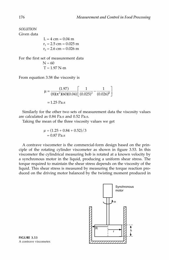
176 Measurement and Control in Food Processing
SOLUTIONGiven data
L = 4 cm = 0.04 mr1 = 2.5 cm = 0.025 mr2 = 2.6 cm = 0.026 m
For the first set of measurement dataN = 60T = 1.97 N-m
From equation 3.58 the viscosity is
Similarly for the other two sets of measurement data the viscosity valuesare calculated as 0.84 Pa.s and 0.52 Pa.s.
Taking the mean of the three viscosity values we get
µ = (1.25 + 0.84 + 0.52)/3 = 0.87 Pa.s
A contrave viscometer is the commercial-form design based on the prin-ciple of the rotating cylinder viscometer as shown in figure 3.53. In thisviscometer the cylindrical measuring bob is rotated at a known velocity bya synchronous motor in the liquid, producing a uniform shear stress. Thetorque required to maintain the shear stress depends on the viscosity of theliquid. This shear stress is measured by measuring the torque reaction pro-duced on the driving motor balanced by the twisting moment produced in
FIGURE 3.53A contrave viscometer.
=
.1 25= Pa.s
µπ
−( . )( )( )( )( . ) ( . ) ( . )
1 978 60 0 04
10 025
10 0262 222
ω
Rr h
Synchronous motor
7244.book Page 176 Wednesday, June 21, 2006 11:14 AM

Measurements in Food Processing 177
a suspension system. The suspended system turns to establish equilibriumand the angle of turn is proportional to shear stress developed on the mea-suring bob. The torque measuring system is isolated from the process systemby a magnetic coupling. By using a linear potentiometer the torque deflectionis converted to an electrical signal. In a manual indication system a torquedeflection pointer over a calibrated scale is used.
3.9 Brix of Food
Brix is primarily the measure of sugar (sucrose) concentration of a food, butmany other quality attributes of food can be ascertained from this parameter.On-line measurement of brix in food processing is important from both thequality and preservation point of view, to prevent the development of bacteriaand retain the taste, aroma, and shelf life of packed products like jam, syrup,fruit pulps, juices, and so on. Table 3.13 shows brix degrees of various foodproducts. This parameter is commonly measured by a brix hydrometer cali-brated directly to read in percentage w/w of sugar. However, there is a cor-relation of brix with the refractive index (RI) of sugar-containing liquid foodssuch as soft drinks or concentrated syrups at 20°C. This measurement is cali-brated to the International Sugar Scale that expresses the result in degree brix.
Manufacturing process of chocolate confectionary uses sugar in dry pow-dered form or in liquid form. Cannery pure sugar, for canning in liquid form,is delivered by tankers and stored in tankers. This sugar is mostly cane orbeet sugar dissolved in water to about 65% sugar syrup. The canners gen-erally code and defines fruit juice (10–30), light syrup (15–30), syrup (15–30),heavy syrup (20–40), extra heavy syrup (40–50) and fruit jam (60–68) in termsof degree brix. The best range of syrup strength for dessert meal is 35 to 40degree brix. Brix of food is related to specific gravity in terms of rheologicalproperty. Table 3.14 shows brix and specific gravity relationship of sugarsyrups for some specific values.
TABLE 3.13
Brix (%) Values for Some Food Products
Food Product Brix (%)
Tomato juice 0–25Light syrup 10–15Fruit juices 10–30Syrup 15–30Heavy syrup 20–40Exra heavy syrup 40–50Fruit jams 60–68Chocolate syrup 12–72Strawberry jam 36–82
7244.book Page 177 Wednesday, June 21, 2006 11:14 AM

178 Measurement and Control in Food Processing
Problem 3.5An on-line brix meter is required to measure degree brix of a sugar syrupand transmit the signal to a controller to control the brix to a value 50° brix.The total weight of sugar used is 500 kg. Find the required volume of thesugar syrup obtained by adding water.
SOLUTION
Weight of sugar = 500 kgTarget brix = 50°From table 3.15, the specific gravity of sugar syrup at the required brix is 1.232Hence water to be added = 500/1.232
= 405.84 liters
TABLE 3.14
Specific Gravity Corresponding to Brix of Sugar Syrup
Degree Brix (%) Specific Gravity
10 1.04015 1.06120 1.08325 1.10630 1.12935 1.15840 1.17945 1.20550 1.23255 1.26060 1.28865 1.31970 1.350
TABLE 3.15
Refractive Indexes for Some Brix Valuesof Sucrose Solutions at 20°C
Degree Brix Refractive Index
4.821 1.3417.679 1.3629.376 1.3840.091 1.4049.979 1.4259.170 1.4467.771 1.4675.862 1.4883.500 1.50
Source: TIMA-96, India, 1996. Adapted withpermission from R. Sridhar.
7244.book Page 178 Wednesday, June 21, 2006 11:14 AM

Measurements in Food Processing 179
3.9.1 Brix Standards
Although degree brix is a standard unit in the sugar industry for indicatingthe sucrose content, some sugar industries use the Twaddel degree for sugarsyrups. The Twaddel degree is defined as
°Tw = 200(SG–1.0) (3.60)
Here Twaddel divides the specific gravity (SG) range between SG = 1.0 and2.0 into 200 equal parts each of 0.005 SG values.
The dairy industry uses the Quevene degree for measuring the fat contentof milk where each degree corresponds to 0.001 SG (based on water with SG= 1.0) in excess of SG = 1.0, therefore
40°Q = 1.04 SG
that is,
°Q = (SG–1.0)(1000) (3.61)
The brewery industries use Sikes, Richter, or Teller scales on their alcoholmeters. This is volumetric percentage of ethyl alcohol in water given as
°S, °R, or °T = volume % of ethyl alcohol°S, °R, or °T multiplied by 2 (3.62)
i.e., Proof = 2(°S, °R, or °T) (3.63)
3.9.2 Refractometers
Refractometers are very popular as brix measuring meters that give moni-toring in both off-line and on-line environments. Brix has a well-definedcorrelation with the RI of a liquid. A stick dipped in pure water looks straight,whereas if sugar is added to the water, the stick will appear bent or broken.The reason is that the RI of the sugar syrup is higher than pure water. TheRI of air is 1.0003 and for most gases, solids, and liquids it varies between1 and 2. A basic refractometer measures the RI of a liquid sample, which isgiven by the following equation:
(3.64)
v0 = velocity of light in vacuumvm = velocity light in the material
Snell’s law gives the relation between the angle of incidence and angle ofrefraction of light. When a ray of light passes through a medium of lower
µ = vvm
0
7244.book Page 179 Wednesday, June 21, 2006 11:14 AM

180 Measurement and Control in Food Processing
RI to a medium of higher RI (fig. 3.54), the ratio of the sine of the angle ofincidence (α) and the sine of the angle of refraction (β) is defined as the RIof the second medium with respect to the first medium. This can be shown as
(3.65)
The RI of a material is generally expressed with air as the reference. There-fore, addition of sugar to a liquid changes the RI of the liquid that implies therelation between degree of brix and RI. The RI of sucrose at 20°C related tobrix degree is shown in table 3.15 [14]. Because the RI of a solution also changeswith temperature, corrective measures or compensation has to be made in brixmeasurement, of process products, at higher temperatures accordingly.
Refractometers are based on two principles, the refraction angle principleand critical angle change principle, which are discussed next.
3.9.2.1 Refraction Angle Refractometer
The basic concept of this refractometer is measurement of change in refractionangle as a function of RI of the test material. Figure 3.55A shows a schematicdiagram of a differential refractometer. It consists of a tungsten filament lampsource, the light from which passes through the combined cell windowthrough a mask. Refraction of light takes place at the window surface. Therefracted light is collected by a pair of opposed phototubes ratioed by a beamsplitter. The phototube produces the output signal proportional to the refrac-tion through the sample and a reference liquid. The beam splitter is positionedby servo controller so that the light beam falls on the photodetectors equally.
3.9.2.2 Critical Angle Refractometer
A critical angle refractometer is a kind of back-scattering refractometer (fig.3.55B) where the incident light is reflected back from the surface of a sample
FIGURE 3.54Illustration of refraction of light.
Medium A
Medium B
α Angle of incidence β Angle of refraction Va Velocity at medium A Vb Velocity at medium B µ RI of material from B to A
Va
Vb
α
β
µ αβ
= sinsin
7244.book Page 180 Wednesday, June 21, 2006 11:14 AM

Measurements in Food Processing 181
FIGURE 3.55ARefraction angle refractometer.
FIGURE 3.55BCritical angle refractometer.
Source
Mask
W2W1
ReferenceSampleCell
Photo detector Photo detector
Detector
Servo motor
Ratioamplifier
Photo cell(measuring)
Photo cell(reference)
Prism
SourceLens Sample
Half mirrorbeam splitter
Server driven nullrestorer glass
Amplifier
M
Detector
Cell
7244.book Page 181 Wednesday, June 21, 2006 11:14 AM

182 Measurement and Control in Food Processing
window. A prism is used to reflect back the light from a source incident at varyingincident angles. The reflected light is split using a half-mirror beam splitter. Thepoint of change from refraction is detected by a pair of photocells. An amplifieramplifies the signal proportional to the imbalance and repositions a restorer glassusing a servo balance system. A helipot positioned in tandem to the null glasssenses the position of the null glass, which is proportional to the critical angle.This refractometer design is utilized in probe type on-line refractometers usingfiber optic light transmitters and microprocessor technology.
3.9.2.3 U-Rod Refractometer
Another variation of the critical angle refractometer developed by Sridhar etal. is the U-rod refractometer [14]. The optical geometry of the principle of thisrefractometer is shown in figure 3.56. A collimated beam of extra bright redlight obtained from an LED is allowed to incident through the U-rod and strikethe critical surface. The light is reflected back and propagates through the tubeby repeated and total internal reflection and escapes at the end of the U-rod.A silicon photodiode is used as a detector to measure the light that escapes atthe output end. The LED used was AlGaAs capable of emitting 3,000 mod ofred light at 15 mA current. The U-rod size is 10 mm × 10 mm and made ofglass with an RI of 1.52. The radius of curvature of the U-rod is 50 mm. Asilicon photodiode of active detection area of 10 mm2 with a peak wavelengthdetection of 720 nm is used.
The principle behind the measurement is this: A portion of the light getsreflected and absorbed in the medium and the rest gets totally reflected backto the rod depending on the RI and critical angle of the liquid. In this U-rodrefractometer, a light–dark boundary (xc) is related to the RI of the liquidand the radius of curvature (R) as
xc = R(1 – µ) (3.66)
In this experiment, the electrical signal from the silicon photodiode is mea-sured at various sugar solution concentrations of known brix values. Table 3.16shows some results of this U-rod refractometer with collimated incident lights.
FIGURE 3.56A U-rod refractometer. (Redrawn from Proc. TIMA-96, India, with permission from R. Sridhar)
U-rod glass
7244.book Page 182 Wednesday, June 21, 2006 11:14 AM

Measurements in Food Processing 183
3.10 pH Values of Food
pH is a parameter that determines the quality of a food or any other qualitydependent on pH, particularly in packaging, preservation, or canning. Table3.17 shows pH of some food items and the dependence of pH on qualityduring processing.
3.10.1 pH Scale
pH is defined as the negative logarithm of the hydrogen ion (i.e., proton)concentration in a solution, which can be expressed as
pH = –log(H+) (3.67)
TABLE 3.16
Refractive Indexes and Output Voltagesfor Few Samples
Sample Refractive Index Output Voltage (V)
1 1.3520 0.6292 1.3665 0.59373 1.3835 0.55484 1.4040 0.49105 1.4245 0.43486 1.4440 0.3595
Source: TIMA-96, India, 1996. Adapted with per-mission from R. Sridhar.
TABLE 3.17
pH Values of Food Products with Process Factors
Food pH Range Process Factor
Cocoa beans 4.75–5.80 Fermentation during chocolate manufacturingCocoa powder 5.5 FlavorPectin gel 3.0–3.4 Gel formation in jam manufacturingBeet root 4.0 CanningFruit juice 2.5–4.0 PreservationVegetables 5.0–6.5 PreservationTomato juice 4.5 Heat stability of spoilage organismFresh fish 7.05–7.35 PreservationStale fish 6.0–6.6 PreservationGlucose syrup 4.8–5.2 Sugar manufacturingJellies 5.0 Preventing hydrolysis of pectin
7244.book Page 183 Wednesday, June 21, 2006 11:14 AM

184 Measurement and Control in Food Processing
Taking the antilogarithm of this equation, the hydrogen ion concentrationis equal to 10 raised to the power of pH; that is
(H+) = 10–pH (3.68)
For a dilute aqueous solution (water), the hydrogen ion concentration isapproximately equal to unity and so the pH is 7. A change in pH of one unitrepresents a change in concentration by a ratio of 10. For example, a solutionof pH 8 is 10 times more alkaline than a solution with pH of 7. The practicalrange of pH is from 1 to 14. An acid solution of unit strength has a pH of 0,whereas a base solution of unit strength has a pH of 14. The relation betweenhydrogen ion (H+) and hydroxyl ion (OH–) concentration with pH value ofa solution is illustrated by figure 3.57. The figure indicates that pH measure-ment can detect 14 decades of hydrogen ion concentration and changes assmall as 10–14 at pH of 14.
3.10.2 pH Electrodes and Potential
In pH measuring schemes, a pH glass electrode collects hydrogen ions anddevelops a potential at the glass surface with respect to the solution. TheNernst relationship describes the potential developed due to hydrogen ionconcentration as
(3.69)
where Eg = sum of reference potentials and liquid junction potentials that are constants (in mV)
Eg0 = potential when H+ = 1.0 H+ = hydrogen ion activity
T = absolute temperature (in °K)R = 1.986 cal/mol degreeF = Faradays (C/mol)
All aqueous solutions are associated with a water molecule combined withthe hydrogen ion. This combination is called hydronium (H3O+). When ahydronium ion gets closer to the glass electrode surface the hydrogen ionjumps and becomes associated with hydronium ions in an outer layer of theglass surface.
3.10.2.1 Glass Electrode
The working principle of potential development in a glass electrode (fig. 3.58)is that when two solutions of different hydrogen ion concentrations are sepa-rated by a thin glass wall an EMF is developed between the two solutions that
E ERT
FHg g= + +
0 102 303.
log ( )
7244.book Page 184 Wednesday, June 21, 2006 11:14 AM

Measurements in Food Processing 185
is a function of concentration of both. In practice a buffer solution of knownconcentration is used in a sealed glass electrode surrounded by the measur-ing solution. Soda lime glass gel (SiO2, 72.2%; CaO, 6.4%; Na2O, 21.4% mol)is suitable for development of potential between the separating solutions.This gel is suitable due to its low melting point, reduced hygroscopic, andlow electrical resistance. The potential difference between the external glasssurface exposed to the measuring solution (E1) and the internal glass surfaceat a constant pH of 7.0 (E2) is given by
E0 = E2 – E1 = 0.1984(T + 273.16)(7 – pH) (3.70)
This equation accounts for deviation of the constant pH of the internalsolution from 7.0 at 25°C due to change in temperature.
3.10.2.2 Calomel Electrode
In this electrode (fig. 3.59) an inner glass tube contains calomel (Hg + HgCl)and is accommodated with a platinum wire. A saturated solution of KCl
FIGURE 3.57Illustration of pH scale.
FIGURE 3.58A pH glass electrode.
0 1 2 3 4 5 6 7 8 9 10 11 12 13 14
10–7 10–1110–3 10–141
110–310–710–1110–14OH ion
H ion
Strongacid Neutral
Strongbase
pH
Glass envelope
Electrode lead
Platinum wireBuffer solution
7244.book Page 185 Wednesday, June 21, 2006 11:14 AM
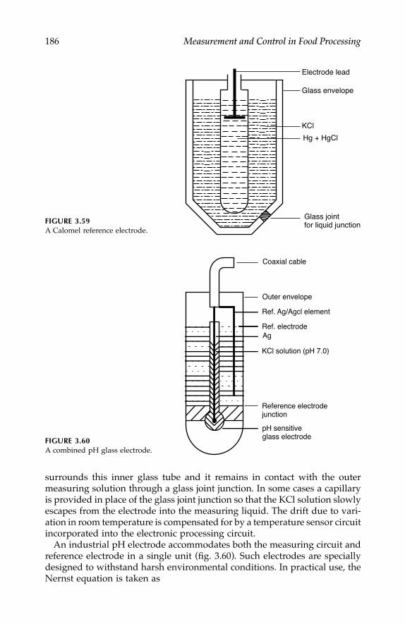
186 Measurement and Control in Food Processing
surrounds this inner glass tube and it remains in contact with the outermeasuring solution through a glass joint junction. In some cases a capillaryis provided in place of the glass joint junction so that the KCl solution slowlyescapes from the electrode into the measuring liquid. The drift due to vari-ation in room temperature is compensated for by a temperature sensor circuitincorporated into the electronic processing circuit.
An industrial pH electrode accommodates both the measuring circuit andreference electrode in a single unit (fig. 3.60). Such electrodes are speciallydesigned to withstand harsh environmental conditions. In practical use, theNernst equation is taken as
FIGURE 3.59A Calomel reference electrode.
FIGURE 3.60A combined pH glass electrode.
KCl
Glass envelope
Hg + HgCl
Glass jointfor liquid junction
Electrode lead
Coaxial cable
Outer envelope
Ref. Ag/Agcl element
Ref. electrode
KCl solution (pH 7.0)
Ag
Reference electrodejunction
pH sensitiveglass electrode
7244.book Page 186 Wednesday, June 21, 2006 11:14 AM

Measurements in Food Processing 187
E′0 = Er – 0.1984(T + 273.16)pH (3.71)
where Er is the fixed part of the total potential that depends on the electrodesystem. The term 0.1984(T + 273.16) gives a value of 59.2 mV at 25°C.Although this fixed part of the output voltage also changes with temperature,for practical purposes it can be assumed to be constant.
3.10.3 pH Signal Processing
The measuring circuit for pH signal processing should possess an inputimpedance fairly larger than the electrode impedance so that the loadingeffect is minimized. The output impedance of the glass electrode is on theorder of 109 ohms, so the voltage drop in the electrodes becomes largecompared to the EMF developed. Therefore an impedance-matching ampli-fier is used in the measuring circuit.
Operational amplifiers provide good impedance matching with the high-output impedance glass electrode and high amplification. Standardizationis also possible by varying the feedback current of the closed-loop amplifier.For calibration or standardization, the electrode should be cleaned withdistilled water between buffer immersions. Calibration with two buffers of7 pH and 4 pH are generally used. Calibrated buffers can also show deviationin pH due to absorption of CO2. Electrodes should be stored in the said buffersolutions. Cleaning of the electrodes is very important for storing and reuseafter a measurement. Automatic cleaning mechanisms are also available insome pH meters using ultrasonic, brush, water jet, and chemical cleaningdevices.
3.10.4 Ion-Sensitive Field Effect Transistor pH Sensors
Glass electrode pH meters are used primarily in laboratories and are difficultto use for on-line applications and in situ measurements. A few glass electrodepH meters have been converted for on-line applications, but problems ariseelsewhere, like short circuits in reference electrode to earth, high referenceelectrode impedance, and so on. With the advent of ion-sensitive membranesensors (ISMs) and ion-sensitive field effect transistors (ISFETs), on-line detec-tion of pH and other related food quality measures have become possible.Apart from on-line applicability, ISFETs have the following advantages:
1. ISFETs are robust and durable, and cleaning and reusing them issimple.
2. Mass production by IC technology keeps the cost low and size small.3. ISFETs can be used over an extremely wide temperature range.4. ISFETs can be made multifunctional by a combination of membranes.5. On-chip circuit integration is possible in ISFETs.
7244.book Page 187 Wednesday, June 21, 2006 11:14 AM

188 Measurement and Control in Food Processing
The structure of an ISFET is shown in figure 3.61. An ISFET is mainly a metaloxide semiconductor field effect transistor (MOSFET), where the metal gateis replaced by a complex structure that is sensitive to hydrogen ions. In placeof the metal gate of a MOSFET a reference electrode and a chemically sen-sitive insulator are placed and the measuring electrolyte is placed in contactbetween them. The gate voltage is applied to the reference electrode and theelectrolyte completes the electric gate-source circuit.
The ISFET sensing is based on a site binding theory [15–17]. According tothis theory the insulating surface contains hydroxyl groups that can getpositively or negatively charged depending on the concentration of hydro-gen ions of the electrolyte. In the case of SiO2 insulator, the binding sitesavailable are SiOH, SiO–, and SIOH+ and the ionization reactions are
(3.72)
Thus the surface potential is changed when the surface hydroxyl groupsbind with H+ ions.
The relation between concentration of [H+]b of protons in the electrolyteand concentration [H+]s of protons in the insulator follows the Boltzmannlaw:
(3.73)
where q = Charge (C) φ = potential drop in the electrolyte–insulator interface
K = Boltzmann constantT = Temperature (absolute)
FIGURE 3.61Schematic diagram of an ISFET sensor.
S D
1
2
3 3
4
B
V
Vgs
ds
1—Reference electrode2—Gate oxide3—Insulating region4—ChannelS—SourceD—DrainB—Bulk
SiOH SiO H
SiOH H SiOH
– +
+2+
↔ +
+ ↔
[ ] [ ] /H H eb sq KT+ + −= φ
7244.book Page 188 Wednesday, June 21, 2006 11:14 AM

Measurements in Food Processing 189
Writing equation 3.71 in pH terms
(3.74)
where pHs = pH of electrolytepHb = pH at the surface of the sensor area
Different materials are available as ISFET insulators, but Si3N4 has beenfound to be a very sensitive material [18], with a sensitivity of 56 mV/pH.A drift of 600 µV/h and a temperature dependence of 1.5 mV/°K at constantpH is found on an Si3N4 insulator. Figure 3.62 shows such an ISFET package.
Maritonia et al. [19] developed an ISFET pH sensor array in a surface-mounted device package on a printed circuit board (PCB) that is placed ina flow injection microchamber. The sensor chip measures 1.75 cm × 1.85 cmof die housed with an array of 12 ISFETs. Such chips are incorporated with
FIGURE 3.62An ISFET microsystem for pH detection. (A) ISFET array-based sensor chip. The laserscanmicroscope photograph shows in detail the ISFET sensitive area; (B) The microsystem packagephotograph and a sketch of the system prototype. (Reprinted with permission from Biosensors andBioelectronics, Vol. 18(5–6), Elsevier)
ϕ = −2 3. ( / )( )KT q pH pHs b
ISFETs
Conductivity sensor
Ag/AgClreference electrode
Electrodecompartment
Microchamberhead
Flow outlet
Electronic front end
A
B
Flow inlet
SMD packagedsensor chip
Metal shieldedprinted circuit board
Cell culturecluster
7244.book Page 189 Wednesday, June 21, 2006 11:14 AM

190 Measurement and Control in Food Processing
multifunctional blocks like temperature sensors and conducting sensors. Avery large scale integration (VLSI) electronic circuit package can accommo-date the sensor chip to be housed to reduce bias current. The sensors areoperated at a constant drain source current and high output impedance. Thereference currents for the sensor bias is obtained from a stable referencevoltage made independent of temperature from a band gap circuit. Thecircuit can be powered by a 4-V power supply for battery-supplied operation.
A pH-sensitive ISFET has been developed by Artigas et al. [20] for onlinestabilization of wine by ion exchange resins. They fabricated pH-sensitiveSi3N4 n-channel MOS (NMOS) gates that were fixed on a PCB and encapsu-lated with a photopolymer by photolithographic technique. The stabilizationof the wine was performed in a cationic exchange resin and samples werealternately collected every 3 min from the inlet and outlet of the resin columnusing a flow system operated by peristaltic pump. The sample flow rate wasmaintained at 48 to 50 liters per hour and a filter was used to prevent blockingof the pipes by resin particles. Figure 3.63 illustrates the schematic of theISFET-based wine stabilization system.
The pH ISFETs were calibrated by two standard solutions: one of aqueoussolution and another of ethanol solution. The responses of the ISFETs to thewine solutions and the buffer solutions are shown in figure 3.64. The sensi-tivity of the ISFETs was 49 mV per decade.
A pH-sensitive sensor with lithium lanthanum titanate materials has beendeveloped by Bohnke et al. [21]. The sensor can also be used for on-line pHcontrol during cleaning of a fermenter that uses hot acidic and alkalinemedia, control of pH of milk during fermentation, neutralization of acidicfoods, and so on. In their method, a polished titanium wire of 1.5 mmdiameter was fixed with a silver conducting glue on one face of a pellet of
FIGURE 3.63Schematic of ISFET-based wine stabilization system. (Reprinted with permission from Sensors andActuators (B-Chemical), Vol. B 89, Elsevier)
RC
SV
Sample
Carrier solution
pHGNG
PC
WRefCa2+ K+
Wine
1
2
PP
7244.book Page 190 Wednesday, June 21, 2006 11:14 AM

Measurements in Food Processing 191
FIGURE 3.64Responses of ISFET in wine flow system. (Reprinted with permission from Sensors and Actuators(B-Chemical), Vol. B 89, Elsevier)
FIGURE 3.65Measurement setup with the measuring and reference electrode. (Reprinted with permission fromSensors and Actuators (B- Chemical), Vol. B 89, Elsevier)
0
950
1000
1050
1100
1150
pH 7.02
pH 4.00
30 60
Time (min)
Pot
entia
l (m
V)
90 120
Acquisition unit
mV meterMINISIS 8000
Thermeg reference electrode
LLTO
Conductive Ag glue
Titanium wire
7244.book Page 191 Wednesday, June 21, 2006 11:14 AM
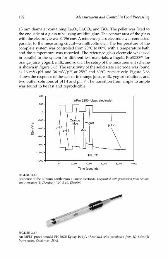
192 Measurement and Control in Food Processing
13 mm diameter containing La2O3, Li2CO3, and TiO2. The pellet was fixed tothe end side of a glass tube using araldite glue. The contact area of the glasswith the electrolyte was 0.196 cm2. A reference glass electrode was connectedparallel to the measuring circuit—a millivoltmeter. The temperature of thecomplete system was controlled from 20°C to 80°C with a temperature bathand the temperature was recorded. The reference glass electrode was usedin parallel to the system for different test materials, a Ingold Pro3200TM fororange juice, yogurt, milk, and so on. The setup of the measurement schemeis shown in figure 3.65. The sensitivity of the solid state electrode was foundas 16 mV/pH and 36 mV/pH at 25°C and 60°C, respectively. Figure 3.66shows the response of the sensor in orange juice, milk, yogurt solutions, andtwo buffer solutions of pH 4 and pH 7. The transition from ample to amplewas found to be fast and reproducible.
FIGURE 3.66Response of the Lithium Lanthanum Titanate electrode. (Reprinted with permission from Sensorsand Actuators (B-Chemical), Vol. B 89, Elsevier)
FIGURE 3.67An ISFET probe (model-PH-30GS-Epoxy body). (Reprinted with permission from IQ ScientificInstruments, California, USA)
400
200
0
–200
–400
–600
–800
–1,000
–1,2000 2,000 4,000
Time (seconds)
pH 4pH 7
pH 7Yogurt
Milk
E(m
V)/
ref
6,000 8,000 10,000
InPro 3200 (glass electrode)
Ti/LLTO
Orangejuice
7244.book Page 192 Wednesday, June 21, 2006 11:14 AM

Measurements in Food Processing 193
Commercial ISFET pH sensors are available in various probe configura-tions like stainless steel, micro round tip, piercing tip, epoxy body, heavyduty, graphite body, water-resistant rubber armored body, and so on. Figure3.67 shows a commercial pH ISFET probe (model pH30-GS) manufacturedby IQ Scientific Instruments, Inc. (USA).
3.11 Food Enzymes
Because enzyme activities are one of the most important facets of foodprocessing, researchers are currently trying to detect and quantify enzymesusing various solid state sensors developed so far. A few of them have beendiscussed in this section, and many of them are similar to the pH-sensitiveISFET sensors discussed in the last section.
3.11.1 Importance of Food Enzyme Detection
Enzymes are proteins with catalytic and specificity properties important foruse in food processing. Enzymes function well within a limited pH andtemperature range but their activity varies as pH and temperature vary. Someof the enzymes are naturally present in food materials, whereas others areused to enhance food processing actions or food quality. Table 3.18 gives theproperties and uses of some important enzymes found in food materials thatwill be certainly helpful for sensor researchers in understanding the impor-tance of the enzymes.
3.11.2 Enzyme Sensors
An enzyme sensor is a combination of a bioreceptor and a transducer. Thebioreceptor is the primary sensor that responds first to the biological worldand converts the biological event to an electrical signal with a secondarydevice, the transducer. In enzyme sensors the bioreceptor takes the help ofan immobilized enzyme as biocatalyst to transform the analyte to a productthat can be detected by the transducer. A large number of enzymes arecommercially available, but some need to be extracted in specific measure-ments. Updike and Hicks [22] developed the first enzyme sensor in 1967 bytrapping glucose oxidase in a layer of polyacrylamide gel attached to theplastic membrane of an oxygen electrode. Currently, physical entrapment isno longer used due to the short life of enzymatic activities achieved. There-fore, chemical immobilization techniques are more frequently used in enzymesensors such as cross-linking, immersion method, direct binding method,use of aerosols, use of membranes, electromagnetic multienzymatic tech-niques, and so on.
7244.book Page 193 Wednesday, June 21, 2006 11:14 AM

194 Measurement and Control in Food Processing
3.11.2.1 Principle of Operation
The enzyme sensor is basically composed of three parts: a thin enzymaticlayer, the substrate, and the transducer. These layers are shown in figure 3.68.The transducer surface is in contact with an enzymatic layer and the enzy-matic layer is immersed in a substrate composed of the solution under test.The substrate has a tendency to migrate toward the enzymatic layer and takespart in reaction with it. Thereby the substrate is transformed into a reactionproduct. This reaction product migrates toward the sensitive transducer andresults in an electrical signal. The cause of the electrical potential is the con-version of the product concentration at the interface. The response time of anenzyme sensor depends on diffusion of the substrate and the thickness of the
TABLE 3.18
Food Enzymes with Their Functions in Food Processing
Enzymes Food Item Functions
Pectinases, hemicellulases, cellulases
Apples, pears, berries, and citrus fruits
Added during maceration to enhance extraction of juice and to reduce fermentation time; reduces the viscosity of juices in pectinase treatment
Methoxy-pectin Jam, jelly, yogurt, and mayonnaise
Gelation formation; film formation
Amylases and cellulases
Immature fruit Degrade residual starch to impart haze and facilitate maceration and color extraction
β-1, 3/ β-1,6 glucanase
Wine Clarification and filtration of grapes infected with noble mold; preventing suspension of contaminant microorganisms
Glucanase Meat To determine freshnessImmobilized proteases
Wine Deacidification of wine
Naringinase, limonase
Grapefruit Hydrolyzing the bitter component without loss of natural yellow color
α- and β-amylase Wheat Splitting off maltose from damaged starch, controlling the extract of starch breakdown
Proteases Biscuit Breaking down protein, making it more extensible during sheeting and cutting
Milk Imparting bitter tasteCoconut Breaking down fat, producing rancid flavor
Lipases Milk Imparting bitter tasteGut enzymes Fish Autolysis of fish after harvestingOxidase Fish DegradingLecithinases Pasteurized milk Imparting sweet curding and bitty creamPectinestirases Pickles Pasteurization to prevent darkening and
softening of vegetables, flavor formationHypoxanthine,inosine, inosine-5‘-monophosphates
Fish Freshness
Lactate Wine Quality controlGlucose Wine FermentationLysine Wine Control of proteinsSucrose Jam Syrup formation
7244.book Page 194 Wednesday, June 21, 2006 11:14 AM

Measurements in Food Processing 195
layer. The response time can be reduced by using an extremely permeablemembrane and a very thin layer. However the response time of the sensorshould be greater or equal to the response of the transducer.
The response of enzyme sensors is mostly asymptotic and it takes a fewminutes to be steady depending on the type. Typically the time taken toreach 98% of the final steady value is taken as the time constant. The responsewith a urease membrane fixed onto a glass diffusion electrode is slower thanthe response of a membrane fixed to a monovalent cationic electrode [23].
3.11.2.2 Calibration
To calibrate the output voltage to a product concentration first the sensorresponse is allowed to be stable and then the slope of the linear region iscalculated. A urea sensor of such a type gives a calibration factor of approx-imately 100 mV/10–2 M. At low concentrations the response is slow and athigher concentrations the response is fast, giving a nonlinear response.Therefore the nonlinear part of the response is not used for calibration. Figure3.69 shows such a response of the sensor. An enzyme sensor can also becalibrated in terms of inhibitor substance. When a substrate concentration isfixed, an inhibitor that reduces enzymatic reactions can be detected withvarying concentration. Percentage inhibition (%I) is determined, represent-ing the potentials with and without inhibition as
(3.75)
where EI and E0 are the potential differences of the sensor with and withoutinhibitor for a fixed substrate concentration.
3.11.2.3 Sensor Materials
For determination of various compounds, enzymes are identified either bytheoretical modeling or by experimentation methods. For example, two typesof alcohols—ethanol and methanol—can be detected by using two enzymes[23]: alcohol dehydrogenases and alcohol oxidases. Alcohol oxidases haveregenerating capability in the presence of oxygen, but at low oxygen partialpressure the sensitivity is low at low alcohol concentrations. The other enzymes,alcohol dehydrogenases (ADH), need another coenzyme, nicotinamide adenine
FIGURE 3.68Schematic of components of an enzyme sensor.
Transducer—T
Enzyme Layer—P
Substrate—S
IE E
EI% = − ×0
0
100
7244.book Page 195 Wednesday, June 21, 2006 11:14 AM

196 Measurement and Control in Food Processing
dinucleotide (NAD), which should be regenerated only by a mediator. Avariety of mediators are identified and phenazine metho-sulfate is one ofthem. The direct electron transfer from the coenzyme to the electrode can befacilitated using organic conducting salts.
In breweries, milk production, and dairy industries, lactate is an importantenzyme [23] to be detected. In lactate sensors, enzymes like lactate monoox-ygenase, lactate dehydrogenase, and lactate oxidase are coupled with amper-ometric transducers like a pO2 electrode to detect oxygen concentration.Similarly the amino acid oxidase enzyme can be used to detect amino acids[23]. One electrode suitable for this application is a pO2 electrode or an H2O2
sensitive platinum electrode. When a pO2 electrode is used, catalase is rec-ommended to be immobilized simultaneously with glucose oxidase so thathalf of the oxygen can be reused.
3.11.3 Measuring Circuit
The basic requirement of an enzyme sensor is the electrode. It is constructedby coupling an electrochemical sensor, an electrode, and a thin layer ofimmobilized enzyme [23]. The enzyme produces the electrical signal that ismonitored by a potentiometric or amperometric circuit. In a potentiometriccircuit the differential voltage between a measuring electrode and a referenceelectrode is measured and can be calibrated in terms of concentration. Anexample of a potentiometric electrode is the pH electrode or gas electrode,such as pCO2 or pNH3 electrodes. In a glucose electrode, the potentiometricelectrode is made by immobilizing glucose oxidase on the sensitive compo-nent of the pH electrode. The enzyme catalyzes the oxidation of glucose intoglucose acid or glucono lactone as
(3.76)
The pH electrode detects the gluconic acid and the output voltage isproportional to glucose concentration.
FIGURE 3.69Calibration curve of a biosensor forurea. (Redrawn from Fig. 4.8, p. 63,Biosensors, English Edition, 1993,with kind permission from SpringerScience and Business Media)
mV
10–50
50
100
10–4 10–210–3
Concentration
Curea
Glucose + O H O gluconic a2 2glucose oxidase+ → ccid + H O2 2
7244.book Page 196 Wednesday, June 21, 2006 11:14 AM

Measurements in Food Processing 197
Enzyme sensor housing can be of two types: measurement conducteddirectly on the sample medium (batch method; see fig. 3.70) and the sampleplaced in a measuring cell, ensuring normal temperature and pH conditions[23]. In both of the techniques an enzyme electrode is placed next to areference electrode such as the standard calomel electrode. In another vari-ation both the electrodes can be combined in a single electrode, as is donein the pH glass electrode.
The differential output is applied to a millivoltmeter in case of the potenti-ometric measurement or to a potentiostat for amperometric measurements.The output is further connected to a recorder for continuous monitoring. In amore sophisticated situation the output can be connected to a data acquisitionsystem for additional works like data logging, signal processing, and so on.
In the case of an analyte flowing through a pipeline, a flow injection system(fig. 3.71) is more appropriate. A small quantity of the sample volume is
FIGURE 3.70Use of enzyme sensor in a batch system. (Redrawn from Fig. 8.2, p. 168, Biosensors, English Edition,1993, with kind permission from Springer Science and Business Media)
FIGURE 3.71Use of enzyme sensor by flow injection system. (Redrawn from Fig. 4.8, p. 63, Biosensors, EnglishEdition, 1993, with kind permission from Springer Science and Business Media)
MilliVoltmeter orPotentiostat
DAQ
Reference electrode
Enzymeelectrode
Sample
Measuringcell
Carrier gas
Sample
Biosensor
To electronics
Waste
Pump
Pump Injectionvalve
Waste
7244.book Page 197 Wednesday, June 21, 2006 11:14 AM

198 Measurement and Control in Food Processing
injected into a flow of carrier liquid. An accurately controlled volume of theliquid sample is injected into the carrier line using flow control systems. Thecarrier or reference liquid and the sample are injected into the sensor througha valve using pumps. The pumps are controlled by a computer to alternatelyinject the carrier and sample liquid to the cell and the sensor. In a flowinjection system the response is slower than the batch system as illustratedin figure 3.72.
3.11.4 Semiconductor Enzyme Sensor
Field effect transistors have been modified recently with the developmentof enzyme field effect transistors (ENFETs) [23]. They are made by a p-typesilicon substrate over which two n-type semiconductor zones are placed asa central channel. These two zones form the source (S) and drain (D) of thetransistor. A metallic gate (G) is isolated from the n-type channels by a thininsulating film of SiO2. To get a MOSFET structure, the substrate and sourceare grouped (fig. 3.73). When the transistor is not in a saturation state, thedrain current is given by the equation
(3.77)
where µ = mobility of electrons in the channelCox = capacity of the insulating oxide
W/L = width to length ratio of the channelVD, VG = drain-source and gate-source voltages, respectively
VT = threshold voltage
FIGURE 3.72Typical response of biosensors. (Redrawn from Fig. 8.3, p. 169, Biosensors, English Edition,1993,with kind permission from Springer Science and Business Media)
mV
Time
Fast response (batch system)
Slow response (batch system)
Slow response (flow injection system)Fast response (flow injection system)
I CWL
V V V VD ox G T D D= − −
µ ( )12
2
7244.book Page 198 Wednesday, June 21, 2006 11:14 AM

Measurements in Food Processing 199
To get a response from this transistor, the metallic gate is separated andthe enzyme sensitive to the analyte is used to cover the SiO2 layer.
A variation of the MOSFET is the ISFET (ion sensitive) where an enzymaticmembrane is placed instead of the metallic gate with a reference electrode.A pH-sensitive ISFET can also be used for glucose detection. Glucose oxidaseaccelerates the transformation of glucose into gluconolactone, which in turnhydrolyzes into gluconic acid that can be detected by the ENFET. Similarly,xanthine oxidase is immobilized on a polyvinylbutyral membrane to get thetransformation of hypoxanthine to uric acid, which can be detected by theISFET. This ISFET can be used for fish freshness detection because hypox-anthine is a fish freshness indicator.
3.11.5 Applications in Food Processing
In view of the information in table 3.18, it seems that enzyme sensors havepotential applications in the food industry. The specific applications mightbe monitoring ingredients, food additives, contaminations, and toxins [23].For example, a glucose electrode can be used to detect meat contaminationby microbes because microbes consume glucose on the meat surface. Simi-larly fish freshness can be detected by hypoxanthine- or inosine-sensitivesensors. Other examples are detection of lactate in the wine and yogurtindustry, amino acids (e.g., lysine) for monitoring proteins, sucrose for syrupsand jams, and ethanol for alcohol.
In some cases, enzyme sensors pose a problem of inadequacy of recyclingin the fermentation process. The enzymatic reactions produce some wasteproducts and contaminate the fermenter. To avoid this problem a represen-tative portion of the product is tested by the sensors and not recycled. Useof an autoclave also eliminates this problem. Here the sensor is placed in anautoclave and the enzyme is injected separately into the microchamber.When the activity of enzyme is insufficient it is renewed.
FIGURE 3.73Schematic of a Metal-Oxide-SemiconductorFET. (Redrawn from Fig. 4.30, p. 116, Biosensors,English Edition, 1993, with kind permission fromSpringer Science and Business Media)
n n
p-type Si
SiO2 SiO2
SG
D
VD
VGID
7244.book Page 199 Wednesday, June 21, 2006 11:14 AM

200 Measurement and Control in Food Processing
3.12 Flavor Measurement
Food items are mostly natural vegetative products that have a certain charac-teristic flavor. When food items are processed, the flavor pattern might changeand new flavor components might be produced. In some cases food flavoringadditives are also used to improve its value. In many cases a particular foodproduct is manufactured with different flavors to satisfy different consumerswith different tastes. For this, flavor additives, either synthetic or natural,like spices, essences, and oils are used. Flavors and fragrances are the resultsof substances that stimulate the sense of smell and taste of foods. Besidesthe four primary taste sensations—sweet, bitter, salty, and sour—flavor char-acteristics are produced due to our perception of odor.
3.12.1 Sources of Flavor in Food
Most natural flavor compounds are derived from plant substances, eitherfrom the aromatic, volatile vegetable oils or from the nonvolatile plant oilsknown as resins. Some fragrant substances are easily synthesizable like van-illin, the aromatic compound of vanilla. Most of the flavor compounds con-tain many contributing components, sometimes as many as hundreds. Someof them are organic acids, alcohols, aldehydes, amides, amines, aromatics,hydrocarbons, nitrites, and phenols.
A particular type of food product can have with different flavors due toeither raw material of different qualities or different processing methodsadopted. Table 3.19 shows various flavor compounds and causes of off-flavorsof some food products. Flavors can be technically categorized as follows:
1. Naturally obtained from plants and animal products by physicalmeans only
2. Synthetically produced but known to occur naturally3. Artificial flavoring compounds produced synthetically only
In most cases the value of the food is determined by its flavor to a greatextent. It is customary to say “the smell tells the taste.” In most food industries,one of the section of food quality determination is the flavor testing. Hence,estimation or identification of flavor becomes a major function in food indus-tries. Until recently, in most of the food industries this job has been done byorganoleptic means: smelling by experienced persons. For example, in thetea industry, tea tasting is a highly specialized profession. However, thereare problems associated with human tasters, like individual variability, adap-tation (becoming less sensitive if exposed for a long period), fatigue, infec-tions, state of mind, and so on.
7244.book Page 200 Wednesday, June 21, 2006 11:14 AM

Measurements in Food Processing 201
Because the odor particles are complex chemical compounds, they areequally sensitive to gas-liquid chromatography and mass spectrometry(GLC-MS). Detection of complex odors by these analytical techniques isexpensive, off-line, and time consuming. In many cases odors are not at allpossible to detect by GLC-MS techniques. These might be the reasons forthe prolonged survival of the old organoleptic methods of odor testing inthe food industries. However, E-nose sensor technology has been developedin the last decade that can be used for speedy and sensitive measurementof flavors, which will certainly make quality control in food industries reli-able and efficient.
3.12.2 Physiology of Human Olfaction
Odors are sensations caused when volatile organic compounds (VOCs) stim-ulate our olfactory receptors located in the olfactory epithelium at the roof ofthe nasal cavity (fig. 3.74). Odor receptors of the human nasal cavity can detectand discriminate up to 10,000 different chemical traces. The olfactory regionof each of the two nasal passages in humans is an area of about 2.5 cm2 holdingabout 50 million primary sensory receptor cells. The region consists of ciliain the olfactory epithelium projecting down into a layer of mucus about 60microns thick. The mucus lipids help the transportation of the odorant mol-ecules to the olfactory receptors and produce the signals that our brainreceives to interpret the odor. Each olfactory receptor neuron contains 8 to 20cilia where the molecular reception with the odorant occurs. Informationabout the stimulus causes a distinctive neuron activity pattern and suchpatterns allow us to discriminate between vast numbers of different smells.
Odorant particles are volatile tiny molecules of molecular weight of 20 to300 Daltons. Moreover they are polar and can be detected by humans atconcentrations below 1 ppb. The threshold levels of some odorant moleculesin water that can be detected by a healthy person are: green leaves, 0.32 ppm;
TABLE 3.19
Compounds Responsible for Flavor and Flavor Defects of Some Food
Food Item Process Compounds Causes of Flavor Defect
Bread Yeast fermentation,baking
Organic acids, alcohols,carbonyl compounds
—
Cocoa Fermentation, drying,bean roasting
— Mold, excess lactic and acetic acid in bean
Milk Source and processing Lactose, minerals Bacteria, enzyme, feed taints, weed taints
Oil Refining, deodorization Fat-soluble flavorcompounds
Defective storage
Meat(cured)
Curing Nitrites Defective fermentation and storage
Tea Fermentation Theaflavin Defective fermentation drying and storage
7244.book Page 201 Wednesday, June 21, 2006 11:14 AM

202 Measurement and Control in Food Processing
rose, 0.29 ppm; thyme, 86 ppb; lemon, 10 ppb; off-flavor in white fish, 0.01ppb; green pepper, 0.001 ppb; and grapefruit, 0.00002 ppb.
The human olfactory system has the limitation of discriminating mixturesof more than three to four components. The current E-nose technologyinvolves a device that mimics the human olfactory system with analogy toan array of olfactory receptors, signal excitation by neurons, and patternclassification in the brain that is discussed next.
3.12.3 Organoleptic Panel
Flavor-related food quality determination requires a reliable organolepticpanel; however human flavor or odor panels show wide variability andnonuniformity. This is due to state of mind, biases, fatigue, and other humanfactors. Therefore, instead of a single individual, a panel of individualsstatistically eliminates the problems to a greater extent. However, a panelcannot circumvent some of the requirements like extreme sensitivity, fast-ness, short time variability, and so on. In spite of using machine olfactionthe training data must be validated by an organoleptic panel only.
In forming a panel of between 5 and 10 people, the panel should passcertain tests: a triangle test, an intensity-rating test, and a multicomponentidentification test. In the triangle test, three samples are given to the personat the same time, two of which are identical and third that is of a differentintensity or quality. The person has to identify the third one.
In the intensity-rating test, a series of about 20 variations of concentrationsof a basic sample is placed in an odorless medium. One sample is removed
FIGURE 3.74Human olfactory system.
Olfactory bulb
Olfactoryepithelium
Nostril
Tooth
7244.book Page 202 Wednesday, June 21, 2006 11:14 AM

Measurements in Food Processing 203
and the person is asked to identify its position or order in the series accordingto its flavor.
In the multicomponent test, there are three mixtures containing two, three,and four components of flavor. The person is asked to identify each of them.
An individual who passes these three tests is considered to have the abilityto classify, distinguish, and compare with predetermined standards. An indi-vidual can act as a member of an odor panel only after a great amount ofexperience.
3.12.4 Electronic Nose
The electronic technology of mimicking the human olfactory system byelectronic nose is speedy and reliable. It can also make possible continuousreal-time monitoring of odor at specific sites and in the field, which was notpossible by gas chromatography and mass spectroscopy methods.
3.12.4.1 A Basic Electronic Nose
The electronic nose is made up of three functional components that operatein tandem: an array of gas sensors, a signal processing system, and anintelligent pattern analysis and recognition system. Each sensor in the arrayhas a unique sensitivity profile to the spectrum of odorants and differentsensitivity for different odorants. This distinguishability makes the systemsensitive to unknown odors.
In a basic electronic nose, the sensor array is housed in an odor-handlingand delivery system consisting of a small chamber connected to a tube anda diaphragm pump to pull the sample or a reference gas into the chamber.Figure 3.75 shows a typical headspace sampling setup used with an E-nose.The headspace is the space above the sample inside the container holding
FIGURE 3.75Setup of a typical headspace sampling system for E-nose.
Carrier gas To sensors
Head space
Valve Valve
Valve
7244.book Page 203 Wednesday, June 21, 2006 11:14 AM

204 Measurement and Control in Food Processing
the sample. A carrier gas such as dry air is supplied so that either the samplevapor carried by carrier gas or the carrier gas alone is supplied to the sensors.Switching the valves with a specific timing program manages this alteration.The sensor behaves steadily to the VOC stimulus after a few seconds, duringwhich the physical variation of the sensor due to the odorant is convertedto an electrical signal that is sent to a signal processing circuit.
After getting a response from the sample, a washing gas such as alcoholvapor is passed over the sensor surface for a specific duration to remove theodorant mixture from the surface and the sensor active material. A referencegas is again applied to the sensor array for starting a new measurement. Theperiod during which the sensor is exposed to the odorant is called the responsetime and the period for which the washing and reference gas is applied iscalled the recovery time. In many cases a single gas can facilitate both washingand referencing.
3.12.5 Sensor Types
Table 3.20 lists various sensor types and their measuring principles used inelectronic noses. Out of the listed types of sensors, metal oxide semiconduc-tor (MOS), conducting polymers, and bulk acoustic devices are most com-monly used.
3.12.5.1 Chemoresistive Sensors
Chemoresistive sensors are of two types: metal oxide and polymer. Thesesensors are based on change of resistance when exposed to volatile organic
TABLE 3.20
Common E-Nose Sensor Types, Measuring Principle, and Materials
Measuring Principle Sensor Types Materials
Chemoresistive Metal oxide Tin dioxide, zinc oxide, tungsten trioxide
Conducting polymer Polypyrorole, polyaniline, polythiophene, theophene, indoles
Conducting oligomers Short chain length conducting polymers
Mass sensitive Surface and bulk acoustic device Poly(siloxanes), charged polyelectrolytes, fluoropolymers
Field effect devices Metal insulator semiconductor or metal oxide semiconductor (MOSFET)
Catalytic metals such as palladium, platinum, iridium, and so on
Fiber optic devices Polymer bids on fiber optic bundles
Fluorescent, solvochromic dyes to detect solvation of vapors in the polymers
7244.book Page 204 Wednesday, June 21, 2006 11:14 AM

Measurements in Food Processing 205
compounds. Of these two types, MOS sensors are more popular in E-noseapplications. The typical materials used in MOS sensors are oxides of zinc,tin, titanium, tungsten, and iridium doped with a noble metal catalyst suchas platinum or palladium. The doped metal oxide material is then depositedover a glass or plastic substrate between two metal contacts over a resistiveheating filament. Two electrodes made of platinum, aluminum, or gold areused to connect the sensor to the output circuit. A heater made of platinummetal trace or wire is used to elevate the temperature of the sensor materialfrom, say 200°C to 400°C. The resistance between the two metal contactschanges in proportion to the concentration of the odorant when the dopedoxide material is exposed to the odorant. Different active sensor materialsrespond differently to an odorant, so for a particular gas, a particular activematerial is best suited. The sensitivity obtained from these sensors is on theorder of 5 ppm to 500 ppm, but a general-purpose sensor array can discrim-inate a wide variety of odorants.
The most common interfering errors for these sensors are change of con-ductivity of the sensor material with variation in humidity, susceptibilityto poisoning effect of sulfur compounds, and an inherent drift problem overperiods of hours to days. Figure 3.76 shows the constructional feature ofthe sensor.
3.12.5.2 Conducting Polymer Sensors
In this type of sensor the active material is a conducting polymer of thefamily like polypyrolles, thiophenes, indoles, or furans. The polymer mate-rial is electropolymerized between two electrodes with a gap of about 10 µm
FIGURE 3.76A chemoresistive sensor.
Substrate
Resistive heating
Metal electrodes
Odorant
Activematerial
7244.book Page 205 Wednesday, June 21, 2006 11:14 AM

206 Measurement and Control in Food Processing
to 20 µm. When these polymers are exposed to the odorants, the bonding ofthe molecules changes and affects the transfer of electrons along the polymerchain, causing a change in the conductivity. Conducting polymer sensorscan work at ambient temperature and they do not need heaters. The sensi-tivity obtained from this sensor is 10 ppm to 100 ppm.
The major drawbacks of conducting polymer sensors are that electropoly-merization is difficult, time consuming, and prone to be affected by humidity;and some odorants are not retained by the polymer and penetrate through,so it takes more time to recover the odorant particles from the sensor by therefreshing gas.
3.12.5.3 Acoustic Sensors
There are two types of acoustic devices: quartz crystal microbalance (QCM;see fig. 3.77) and surface acoustic wave (SAW) devices (fig. 3.78). These sen-sors are devised to give a mass changing effect.
The QCM is made up of a resonating disc a few millimeters in diameterand coated with a polymer. Two metal electrodes are connected to each sideof the disc. The resonance frequency obtained from the disc is about 10 MHzto 30 MHz when excited with an oscillating signal.
When these sensors are exposed to the odorant, the surface of the sensorsabsorbs the gas molecules and thereby the mass of the disc increases andreduces the resonance frequency. As an example, say a quartz crystal 166 µmthick cut along a certain axis will have a resonance frequency of 10 MHz. Ifthis sensor gains a mass of 1% from an odorant, a decrease of 1 KHz inresonance frequency results. When the sensor is exposed to a reference gasthe resonance frequency comes back to its original value. The selectivity andsensitivity of the QCM sensor depends on the coating of the polymer mate-rial. Minimizing the size and mass of the quartz crystal can reduce theresponse and recovery time of the sensor.
The input–output relationship of these sensors is fairly linear over a widedynamic range. The effect of temperature can also be made negligible in thistype of sensor. The SAW sensor operates at much higher frequency than theQCM sensor, hence the change in resonance frequency is also much higherin this sensor. The resonance frequency of a typical SAW sensor is on theorder of several hundred megahertz. Due to higher operating frequency, the
FIGURE 3.77A quartz crystal microbalance sensor.
Odorant
Polymer coating
Quartz disc
Electrodes
7244.book Page 206 Wednesday, June 21, 2006 11:14 AM

Measurements in Food Processing 207
signal-to-noise ratio is less in SAW sensors. The only disadvantage with QCMand SAW devices is that they require more complex electronic processingcircuits compared to conductivity sensors.
3.12.5.4 MOSFET Sensors
The principle behind the working of an MOS field effect transistor is thatwhen the odorants come in contact with the sensor, a reaction in the metaltakes place. The compounds formed due to the reactions can diffuse throughthe gate of the MOSFET to change the electrical properties. A typical MOS-FET structure of the sensor has a p-type substrate and n-doped regions withmetal contacts that work as source and drain. The selectivity and sensitivityof the sensor depend on the material and thickness of the metal catalystoperating at different temperatures.
The main advantage of this type of sensor is that they can be manufacturedwith an IC fabrication process and batch-to-batch variations can be minimized.
3.12.6 The Signal Processing and Pattern Recognition
The four important stages of E-nose signal processing and pattern recogni-tion are as follows:
1. Preprocessing2. Feature extraction3. Classification4. Decision making
Figure 3.79 shows the different stages of the E-nose signal processingoperation.
FIGURE 3.78A surface acoustic wave (SAW) sensor.
Membrane
Input sensor
Piezoelectric substrate
Wave directionOdorant
Wave traveldistance
Output sensor
Acousticwave
Wave length
7244.book Page 207 Wednesday, June 21, 2006 11:14 AM

208 Measurement and Control in Food Processing
3.12.6.1 Preprocessing
The sensor response in terms of variation of resistance in the case of chemore-sistive type and polymer sensors, or variation of mass and resonance fre-quency in the case of piezoelectric sensors is processed to obtain a variationin voltage or current. In the case of a chemoresistive sensor, a Wheatstonebridge circuit or a current to voltage converter circuit can be used to get avoltage signal, whereas an oscillator circuit or an integrating circuit can beused in QCM and SAW sensors. Sensor drift is one of the factors that has tobe compensated for in this stage. The most important function of this stageis the sensor output normalization. Because the sensors in the array will havedifferent sensitivities, the voltage levels of the output signals from the sensorswill be different. Hence the signal levels need a standardization or normal-ization. The voltage signals are then applied to a computer-based data acqui-sition system and the data are stored in the memory for pattern recognition.
3.12.6.2 Feature Extraction
This process uses mathematical techniques to find relevant but hidden infor-mation from the data. The techniques adopted for feature extraction aregenerally supervised linear transformations such as the classical principalcomponents analysis (PCA).
In PCA, the responses are expressed in terms of a linear combination oforthogonal vectors accounting for a certain amount of variance in the data.Data variance in each principal component is contributed by each eigenvaluewith varying importance. This technique removes any redundancy in theresponse and reduces the dimensionality of the problem. The mathematicaland statistical background of PCA is outside the scope of this book.
Nonlinear transforms such as Sammon nonlinear maps and Kohonen self-organizing maps are also used in some feature extraction software.
FIGURE 3.79Block diagram of various stages of E-nose system.
Feature 2
Time
Output
Feature 1
Feature 2
Feature 1
Class 1 Class 3
Class 2
Display ?
Decision making
ProcessingSensor array
Odorant Raw signals Calibrated signal Feature vector
ClassificationFeature extraction
Odo
r cl
ass
7244.book Page 208 Wednesday, June 21, 2006 11:14 AM

Measurements in Food Processing 209
3.12.6.3 Classification
In the classification stage, an estimation of the class for an unknown sampleis placed on the class assignment. When the E-nose response data are pro-jected on an appropriate low-dimensional space, the classification stage isused to identify the patterns that are representative of each odor. The clas-sification stage is able to assign to the data a class label to identify the odorantby comparing its patterns with those compiled during training. The differenttools used for performing classification work are K-nearest neighbors(KNNs), Bayesian classifiers, and artificial neural networks (ANNs).
The decision-making stage makes modifications if necessary to the classi-fication and even determines that “the unknown sample does not belong toany one of the odorants in the database” or “it belongs” or “it nearly belongsto,” and so on. Figure 3.80 shows a functional block diagram of the templatelearning and matching procedure and figure 3.81 shows the various patternrecognition techniques used for E-nose data processing.
3.12.7 Applications of the Electronic Nose in Food Processing
3.12.7.1 E-Nose Systems Manufactured by Alpha M.O.S. Inc. (France)
In their electronic nose systems, an array of 12 to 32 MOS/CP sensors andpattern recognition software is used. The systems can distinguish betweena variety of flavors of beverages like Brazilian and Colombian coffees; twoground coffee varieties (Coffea arabica and Coffea robusta); freeze-dried andspray-dried commercial instant coffees, and so on. Another electronic nosesystem has been developed to discriminate among eight different coffee
FIGURE 3.80Block diagram of template learning and matching procedure.
Rundata file
Run data file
Class 1 Class n Class K
Statistical classifier Match data per class
Classifiedsensor response
Class unknown Template matching processMatch with class-condition database
Class-condition database
Moving average
Assignclass
Templatefile
Statistical featureextractionFilter
7244.book Page 209 Wednesday, June 21, 2006 11:14 AM
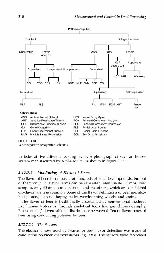
210 Measurement and Control in Food Processing
varieties at five different roasting levels. A photograph of such an E-nosesystem manufactured by Alpha M.O.S. is shown in figure 3.82.
3.12.7.2 Monitoring of Flavor of Beers
The flavor of beer is composed of hundreds of volatile compounds, but outof them only 122 flavor terms can be separately identifiable. In most beersamples, only 40 or so are detectable and the others, which are consideredoff–flavor, are less common. Some of the flavor definitions of beer are: alco-holic, estery, diacetyl, hoppy, malty, worthy, spicy, woody, and grainy.
The flavor of beer is traditionally ascertained by conventional methodslike human tasters or through analytical tools like gas chromatography.Pearce et al. [24] were able to discriminate between different flavor notes ofbeer using conducting polymer E-noses.
3.12.7.2.1 The Sensors
The electronic nose used by Pearce for beer flavor detection was made ofconducting polymer chemoresistors (fig. 3.83). The sensors were fabricated
FIGURE 3.81Various pattern recognition schemes.
Statistical
Pattern recognition
ANN Artificial Neural NetworkART Adaptive Resonance TheoryDFA Discriminate Function AnalysisGA Genetic AlgorithmLDA Linear Discriminant AnalysisMLR Multiple Linear Regression
Abbreviations
NFS Neuro Fuzzy SystemPCA Principal Component AnalysisPCR Principal Component RegressionPLS Partial Least SquareRBF Radial Basis FunctionSOM Self Organizing Map
Quantitative
Supervised
Supervised
DFA PCR
SupervisedUnsupervised Unsupervised
Patternanalysis
ANN Fuzzy
Supervised
SupervisedSelfsupervised
FIS FCMFNN
Self supervised
Others
Biological inspired
PCA CA MLP LVQPNN RBFSOM
GA
ART FuzzyART
NFS Wavelets
MLR PLS
7244.book Page 210 Wednesday, June 21, 2006 11:14 AM
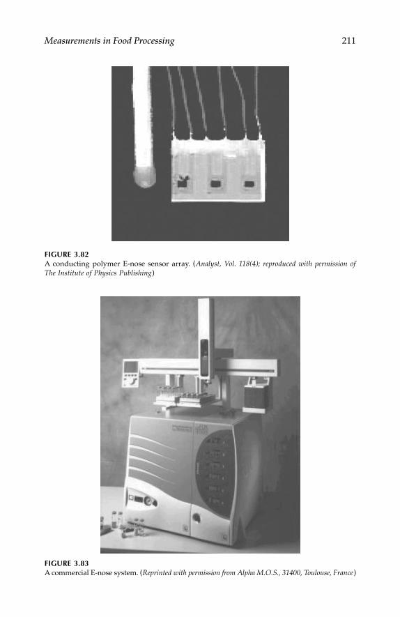
Measurements in Food Processing 211
FIGURE 3.82A conducting polymer E-nose sensor array. (Analyst, Vol. 118(4); reproduced with permission ofThe Institute of Physics Publishing)
FIGURE 3.83A commercial E-nose system. (Reprinted with permission from Alpha M.O.S., 31400, Toulouse, France)
7244.book Page 211 Wednesday, June 21, 2006 11:14 AM

212 Measurement and Control in Food Processing
by the method of microtechnology of pure gold on alumina tiles on whichan electrode pattern is etched by ultraviolet (UV) lithography and a gap isprovided to grow the polymer material.
3.12.7.2.2 Beer Headspace SamplingThe sampling device basically consists of three different units. The chemicalunit is made up of a glass vessel (volume = 0.2 m3) that holds the analyteimmersed in a temperature-controlled water bath set at 30°C. At 30°C, thebeer sample produces the characteristic odor. The sensor unit is housedwith four separate tiles, each carrying three different polymer sensors, fora total of 12 polymer sensors. The devices are wire bonded on one end andsoldered onto metal posts. A perplex lid is connected to the post where thesensor head is fastened. The lid is used to close the vessel when the mea-surement is performed. The mixing unit is formed with a motorized fanconnected to the perplex lid. When the device is under operation, the lidcloses the vessel and the fan is positioned inside the vessel. A schematicdiagram of the beer headspace sampling setup is shown in figure 3.84. Thesequence of operation of the measurement is as follows: First, the samplevessel is placed on the water bath and 100 cm3 of beer sample is placed inthe vessel. The vessel is sealed and allowed to remain undisturbed for 20min so that the liquid and vapor phases come into an equilibrium state.Then, the lid of the vessel is removed and the sensor head is positionedover the sample by lowering it. The circuit is switched on to monitor thechange in resistance of the sensors for a period of 10 min.The sensor headis then taken away from the vessel and the sensor head is cleaned withwater and dried by clean air for 2 min, which removes any contaminantsthat might be available. The sensor head is left to recover for 30 min beforetaking the next measurement.
FIGURE 3.84Beer headspace sampling system. (Analyst, Vol. 118(4); reproduced with permission of The Instituteof Physics Publishing)
Electrical connectionto interface electronics
Perspex lid
Sensor headTeflon/brass
Beer sample(100 cm2)
Temperature-controlled
waterbath
Samplevessel
Polymericsensors
Fan
7244.book Page 212 Wednesday, June 21, 2006 11:14 AM

Measurements in Food Processing 213
3.12.7.2.3 The Interface SystemThe variation of resistance corresponding to the beer flavor generated by thepolymer chemoresistor sensor array was converted to a 0 V to 5 V analogvoltage level for interfacing with the computer through an interfacing card. Thecircuit for generation of the equivalent analog signal is shown in figure 3.85.
The first stage of the circuit works as a constant current source to thepolymer sensor. The sensor is connected across the input port RA andground. The constant current source is made up of the precision voltagereference diode D2 connected across the output pin and inverting input ofthe first OPAMP (U2A). The constant voltage offset causes the currentthrough the precision scaling resistors (R3–R10); that is, through the polymersensor that is only related to the precision resistors selected through the DIPswitches (S3). In the second stage, offset voltage nullification is done withthe help of the variable resistor (CE2). Scaling of the output voltage is donewith the help of a gain adjust resistor (CE1).
Calibration is done by shorting the sensor connection (across RA andground) and adjusting the null offset potentiometer (CE2) to get zeroindication. The standard precision resistors are then selected through theswitch S3 so that the output voltage VA reaches the full-scale range of theA/D input device. This gives maximum resolution of the data acquisitionsystem.
FIGURE 3.85Measuring circuit for the polymer sensors (Analyst, Vol. 118(4); reproduced with permission of TheInstitute of Physics Publishing)
Sensor connection
0.1% Precision
S3SW DIP-4L Angle mount
RA R2
10k
+ VCC
– VCC
– VCC
– VCC
+ VCC
1R3150
1R9150k
1R715k
1R51k5
21R4100
21R10100k
21R810k
21R61k
2
211
1
1
12
1314 channel output
U2D
OP-400GP 2
VA
Gain adjust5kCE1
47kR13
910R14
2
2
Null offset3
50k
CE2 21 R12
R11100
200k 2
2
1
1
1
1
1
2
2
2
115kR15
C20.1 uF
D2LM336
11
34
OP-400GP
2V5
U2A
2
8 7 6 5
1 2 3 4
222
+
–+
–
7244.book Page 213 Wednesday, June 21, 2006 11:14 AM

214 Measurement and Control in Food Processing
3.12.7.3 Fruit Ripeness Determination
Llobet et al. [25] developed an E-nose system employing an array of low-cost tin oxide sensors to analyze the rate of ripeness of bananas. The exper-iment was conducted in a period of 8 to 14 days from the headspace of threesets of bananas during ripening. The multiproduct sensors used in the arraywere TGS 822 (Figaro, Japan, Inc.), SP-11 (P1) (FIS, Japan), MGS 1100 (Motor-ola, USA), and AAS14 (Capteur, Ltd. UK). A thin plastic tube was used tocollect the banana flavor from a sample vessel and carry it to the sensor headby a diaphragm pump. Data acquisition and storage was done by LabVIEW®
software (National Instruments, Inc). A sample measurement took 10 minand recovery to baseline was allowed in 50 min. A long recovery time wasallowed to nullify any residual smell.
PCA was used to justify the discriminating power and three supervisedclassifiers (namely fuzzy ARTMAP, LVQ, and MLP) were used to classifythe samples into seven distinct states of ripeness.
In classification of banana ripeness, banana skin color was used as a classreference because skin color is known to correlate well to sugar content. Thecategories of ripeness of three sets of bananas and their correspondence withskin color are shown in table 3.21.
The response data after normalization were stored for analysis by MLP,LVQ, and fuzzy ARTMAP. Altogether 175 response vectors from the threebanana sets were divided into four folds. The results of the classification interms of number of patterns correctly classified (number of patterns tested)and overall performance is shown in table 3.22.
3.12.7.4 Tea Flavor Detection
More than 500 chemical constituents are found in the organic compounds oftea, both volatile and nonvolatile. The best tea is the most aromatic and fullof good flavor. Conventionally, a few chemical tests supplemented by experthuman panel decisions ascertain the standard of the tea flavor. These tech-niques are subjective, influenced by adaptation, and have inherent faults thatmight even vary with time and the psychology of the panel experts at times.
In the tea industry, from inception of this trade, tea tasters have been usingspecific terminology; at present there are about 32 classes. Tea industries allover the world presently use these standard terminologies for tea flavor, butthere is no mention about quantitative description or score on these flavorterms [26, 27].
It was experimentally established that the application of the E-nose in teaquality and standard flavor determination is highly efficient and accurate.The experiments were conducted on five different overlapping tea samplesusing four MOS-based E-nose sensors (TGS-2611, TGS-842, TGS-822, andTGS-813-J01) [26–28].
A different experiment was conducted by Kashwan [29] on 10 tea flavorsfrom standard tea terminology and, more important, with nonoverlappingcomponents.
7244.book Page 214 Wednesday, June 21, 2006 11:14 AM
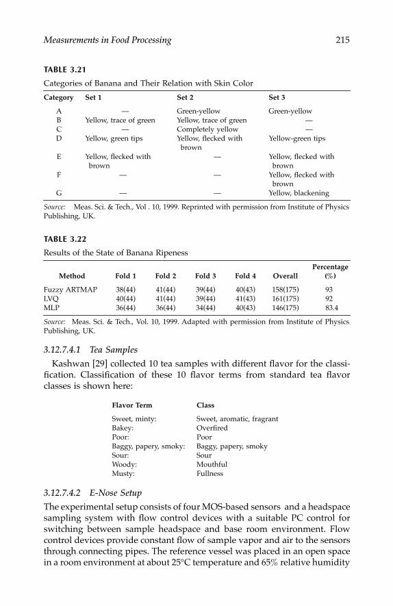
Measurements in Food Processing 215
3.12.7.4.1 Tea Samples
Kashwan [29] collected 10 tea samples with different flavor for the classi-fication. Classification of these 10 flavor terms from standard tea flavorclasses is shown here:
3.12.7.4.2 E-Nose Setup
The experimental setup consists of four MOS-based sensors and a headspacesampling system with flow control devices with a suitable PC control forswitching between sample headspace and base room environment. Flowcontrol devices provide constant flow of sample vapor and air to the sensorsthrough connecting pipes. The reference vessel was placed in an open spacein a room environment at about 25°C temperature and 65% relative humidity
TABLE 3.21
Categories of Banana and Their Relation with Skin Color
Category Set 1 Set 2 Set 3
A — Green-yellow Green-yellowB Yellow, trace of green Yellow, trace of green —C — Completely yellow —D Yellow, green tips Yellow, flecked with
brownYellow-green tips
E Yellow, flecked with brown
— Yellow, flecked with brown
F — — Yellow, flecked with brown
G — — Yellow, blackening
Source: Meas. Sci. & Tech., Vol . 10, 1999. Reprinted with permission from Institute of PhysicsPublishing, UK.
TABLE 3.22
Results of the State of Banana Ripeness
Method Fold 1 Fold 2 Fold 3 Fold 4 OverallPercentage
(%)
Fuzzy ARTMAP 38(44) 41(44) 39(44) 40(43) 158(175) 93LVQ 40(44) 41(44) 39(44) 41(43) 161(175) 92MLP 36(44) 36(44) 34(44) 40(43) 146(175) 83.4
Source: Meas. Sci. & Tech., Vol. 10, 1999. Adapted with permission from Institute of PhysicsPublishing, UK.
Flavor Term Class
Sweet, minty: Sweet, aromatic, fragrant Bakey: OverfiredPoor: PoorBaggy, papery, smoky: Baggy, papery, smokySour: SourWoody: MouthfulMusty: Fullness
7244.book Page 215 Wednesday, June 21, 2006 11:14 AM

216 Measurement and Control in Food Processing
with deviation less than ±2% and the sample vessel inside an oven at constantelevated temperature of 60°C. At elevated temperatures, dry tea was foundto emit a higher amount of VOCs. The photograph of the E-nose setupdeveloped for tea flavor classification is shown in figure 3.86.
3.12.7.4.3 Interface ElectronicsA computer-controlled relay switching circuit was developed for samplingfrom the headspace and reference room air. Data acquisition and onlinelogging of the response signals from E-nose sensors was performed by aPCL-708 high-performance data acquisition card from Dynalog (India).
3.12.7.4.4 Data AcquisitionOn-line logging and displaying of results were performed by GENIE dataacquisition software. They have performed data acquisition for a long dura-tion to generate a database for cluster analysis and ANN classification. Thedatabase consisted of 20 data sets for each of the 10 tea flavor samples andeach data set consists of 400 data vectors. Room environment was maintainedat a temperature of about 25°C and 65% relative humidity with deviationless than ±2%. Each data set was acquired for 200 sec and 300 sec was allowedfor refreshing to air. Figure 3.87 shows the display of the sensor responsesin a GENIE-based graphic window.
FIGURE 3.86Photograph of the E-nose setup for tea flavor classification. (Reprinted with permission from K.R.Kashwan)
Sample vessel
Online display
Reference vessel Flow control device Electronic control and switching
Metal chamberhousing 4 sensors
Artificial NeuralNetwork based
Electronic – NoseSet up
Data acquisition, processing, and signal conditioning
7244.book Page 216 Wednesday, June 21, 2006 11:14 AM
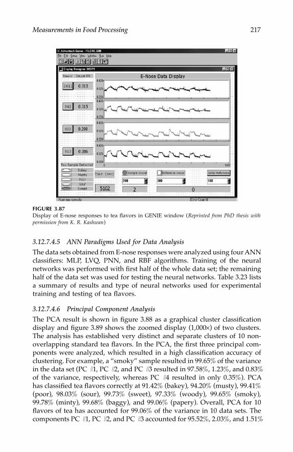
Measurements in Food Processing 217
3.12.7.4.5 ANN Paradigms Used for Data Analysis
The data sets obtained from E-nose responses were analyzed using four ANNclassifiers: MLP, LVQ, PNN, and RBF algorithms. Training of the neuralnetworks was performed with first half of the whole data set; the remaininghalf of the data set was used for testing the neural networks. Table 3.23 listsa summary of results and type of neural networks used for experimentaltraining and testing of tea flavors.
3.12.7.4.6 Principal Component Analysis
The PCA result is shown in figure 3.88 as a graphical cluster classificationdisplay and figure 3.89 shows the zoomed display (1,000×) of two clusters.The analysis has established very distinct and separate clusters of 10 non-overlapping standard tea flavors. In the PCA, the first three principal com-ponents were analyzed, which resulted in a high classification accuracy ofclustering. For example, a “smoky” sample resulted in 99.65% of the variancein the data set (PC #1, PC #2, and PC #3 resulted in 97.58%, 1.23%, and 0.83%of the variance, respectively, whereas PC #4 resulted in only 0.35%). PCAhas classified tea flavors correctly at 91.42% (bakey), 94.20% (musty), 99.41%(poor), 98.03% (sour), 99.73% (sweet), 97.33% (woody), 99.65% (smoky),99.78% (minty), 99.68% (baggy), and 99.06% (papery). Overall, PCA for 10flavors of tea has accounted for 99.06% of the variance in 10 data sets. Thecomponents PC #1, PC #2, and PC #3 accounted for 95.52%, 2.03%, and 1.51%
FIGURE 3.87Display of E-nose responses to tea flavors in GENIE window (Reprinted from PhD thesis withpermission from K. R. Kashwan)
7244.book Page 217 Wednesday, June 21, 2006 11:14 AM

218 Measurement and Control in Food Processing
of variance, respectively, whereas PC #4 accounted for only 0.94%. Figure3.90 shows a block diagram of the experimental arrangement to verify clas-sification power of the E-nose for tea flavors.
3.12.7.5 Spice Flavor Detection
Spices are popular food additives well known all over the world. Properripening of the spices is of utmost importance for obtaining good aromafrom them. Agricultural conditions such as type of soil, hybridized seeds,
TABLE 3.23
Architecture of Different Neural Networks and Correct Classification
NeuralNetworks Architecture
Classification(%)
MLP 6 hidden neuron, 4 input neurons, 10 output neurons, 0.35 learning rate, with momentum 0.42
87
LVQ 4 input neurons, 10 output neurons, learning rate 0.011, and conscious factor 1
92
PNN 4 input neurons, 10 neurons in output layer, spread constant 0.8 93RBF 4 input neurons, 10 neurons in output layer, spread constant 0.8 96
Source: An Artificial Neural Network-Based Electronic-Nose System: Tea and Spice Flavour Dis-crimination and Drift Parameter Determination, PhD thesis, Department of Electronics, TezpurUniversity, India, 2005. Reprinted with permission from K. R. Kashwan.
FIGURE 3.88PCA plot of tea flavorflavor clusters. (Reprinted from PhD thesis with permission from K. R.Kashwan)
1. Bakey 2. Musty 3. Poor 4. Sour 5. Sweet 6. Woody 7. Smokey 8. Minty 9. Baggy 10. Papery
1
–1.0 –1.0
–0.5 –0.5
0 0
PC #1PC #2
PC
#3
0.5 0.5
1.0
2
3
4
5
6
7
8
9
10
0.4
0.2
0
–0.2
–0.4
–0.6
7244.book Page 218 Wednesday, June 21, 2006 11:14 AM

Measurements in Food Processing 219
irrigation, and ecological conditions such as climatic changes and tropicalor nontropical weather can have strong correlations with the quality andaroma of the spice. Kashwan [29] used four MOS-based sensors along withan ANN classifier to classify the flavors of five common Indian varieties ofspice samples: onion, garlic, turmeric, chili, and ginger. The ANN was trainedwith a total of 400 sensor response vectors and tested with 200 data. It wasfound that the classifiers could correctly classify the spice flavors with accu-racy of 86%, 93%, 90%, and 95% by MLP, LVQ, PNN, and RBF respectively.The PCA plot for the five spice vectors is shown in figure 3.91.
3.13 Food Texture and Particle Size
Texture plays an important role in many food products to make it moreappealing. Analysis of the texture-related qualities of food products is anarea for development of new products or improvement of existing ones. Thetenderness of peas and poultry, crispness of potato chips, crunchiness ofapples, chewiness of chocolate bars, and so on are related to the textureproperties of those food items. Although texture features of an object arerelated to its surface appearance or feel, molecular or crystalline structure ofthe matter is also greatly related to the surface texture. In nonfood productswhere surface finishing is an important quality factor (e.g., floor tiles), the
FIGURE 3.89Zoomed PCA display for two flavorflavor clusters. (Reprinted from PhD thesis with permissionfrom K. R. Kashwan)
5
3
3—Poor5—Sweet
7244.book Page 219 Wednesday, June 21, 2006 11:14 AM

220 Measurement and Control in Food Processing
smoothness or roughness is only related to its surface texture, but with fooditems there are many factors in the internal structure and constituents fortexture. Table 3.24 shows textures of some food items and effects of constit-uents and treatments on texture formation.
3.13.1 Electromechanical Measuring Techniques
Buyers want a chewing gum to be chewy, crackers and potato chips to becrisp, steak to be compressible and shearable between the teeth, and breadto be soft in their mouth. It is a common practice among buyers to squeezea bread to test its freshness. It highlights a primary concept of testing thestiffness of some foods, like bread, by measuring the compressibility. Whenwe squeeze bread we apply a force, and the amount being applied indicates
FIGURE 3.90Block diagram of the tea and spice flavor measurement setup. (Reprinted from PhD thesis withpermission from K. R. Kashwan)
Powersupply unit
Sampleenvironment
Temperaturecontrol(oven)
Humiditycontrol
(AC room)
Pressurecontrol
(Pressurecooker)
Electroniccontrol
&power
switchingdevice
Flow controldevice A
Flow controldevice B
Baseenvironment
Flow pathjunction
Sensor 1
Sensor 2
Sensor 3
Sensor 4
Sample Room Air
Sample Detected
Process indicator
TeaRoom AirAlcohol
BenzeneKerosene
Dataacquisition
card&
ADC
7244.book Page 220 Wednesday, June 21, 2006 11:14 AM

Measurements in Food Processing 221
the stiffness of the bread. In terms of simple principles of mechanics, this ismeasurement of resistance or reaction to force applied. When we chew onchewing gum, shear force is applied to slide one layer of the gum pastanother layer. This shear force is a measure of the chewiness. When we pullapart or tear a muffin by applying outward force, the tensile force appliedis a measure of the looseness of the muffin.
Many specialized test instruments are available commercially to measuresome attribute of texture with different mechanisms and names. Figure 3.92shows the mechanical diagram of two types of squeezing testers. Theseinstruments measure the mechanical force applied or a calibrated attributelike a distance moved when the food is tested. For example, a succulometeradopts a force measurement technique where a compressive force is appliedto the food to squeeze juice from it. The tenderness of peas can be tested bymeasuring the compression and shear force applied by a tenderometer. Manysuch tenderometers are equipped with a recording chart to trace thetime–force curve to understand the rheological properties of the food item.
FIGURE 3.91PCA plot of spice aroma clusters (Reprinted from PhD thesis with permission from K. R.Kashwan)
TABLE 3.24
Texture Factors of Some Food Products
Food Texture Effecting Factors Process
Toffee Dextrose equivalent (DE) value of glucose syrup used EmulsificationFish Freezing below 0°C StorageMeat Toughness of connecting tissues TenderizingFats Ratio of solid fat to liquid oil TemperingMeat extracts Isolated proteins ExtrusionCheddar Consolidation and stretching of curd Cheddaring
1. Chilli 2. Garlic 3. Ginger 4. Onion 5. Turmeric
PCA #1PCA #2
1
1
00.5
0–0.5
–0.1
–0.2
–0.3
–0.4
0
1
2
3
4
5
0.1
0.2
0.3PCA #3
7244.book Page 221 Wednesday, June 21, 2006 11:14 AM

222 Measurement and Control in Food Processing
A penetrometer tests the toughness of food by measuring the force requiredto move a plunger a fixed distance through the food material. In this instrument(fig. 3.93A) a transient force is applied for a short duration that makes a plungertraverse through a food a certain distance to touch a contact. The contact inturn sends a signal (mechanical or electrical) to the pressure gauge to registerthe force applied. In a variation of this technique (fig. 3.93B), in a Bloom gelom-eter, lead shots are automatically dropped into a cup attached to the plungerthat is positioned above the liquid surface. The plunger moves a fixed distancethrough the liquid to make contact with a mechanical switch to cut off the flowof lead shot. The weight of lead shots or number of lead shots is a measure ofthe firmness of the liquid and is defined as degree Bloom.
Mechanical gauges that measure force or pressure have recently beenreplaced by electrical pressure or force transducers like load cells, and capacitiveor resistive diaphragms (discussed in chapter 2) to generate an electrical voltageor current proportional to some texture attribute. Such systems give digitalreadouts with calibration and recording facilities. In addition to having sensingcapability, these devices, as in the case of figure 3.93A and figure 3.93B usemechanical contacts to generate an electrical signal to register the force or load
FIGURE 3.92Food squeezing tester: (A) Single loaded plate; (B) Double loaded beam.
F
Scale
Foo
A
B
Scale
W W
Food
7244.book Page 222 Wednesday, June 21, 2006 11:14 AM

Measurements in Food Processing 223
used to penetrate the plunger through the food material. An author’s imagi-nation (this might be exaggerated) of an electronic succulumeter is shown infigure 3.93C. A press connected to an electric motor through a gear box appliesa constant force to the fruit to squeeze out juice and collect in a beaker. A
FIGURE 3.93Schematic diagrams of penetrometers: (A) Force measuring type; (B) Bloom gelometer; (C)Electronic succulometer.
F
Plunger
Food
Contact
Register signal
Door
Cup
Food
Plunger
Contact switchDoor close signal
Lead shotA
C
B
Motor
Gear box
Press
Steel vessel
Level sensorFruit
Electronics
Read out
7244.book Page 223 Wednesday, June 21, 2006 11:14 AM

224 Measurement and Control in Food Processing
miniature level detector generates an electrical signal proportional to theamount of the juice run out and it is calibrated in terms of succulence of the fruit.
3.13.2 Fluorescence Technique for Beef Toughness Detection
The tenderometers discussed earlier in the chapter mostly employ invasivetechniques, altering the food sample being tested so the food cannot bereused. Researchers try to predict whether or not the food is tough or tenderfrom a single, rapid, and noninvasive or nondestructive testing.
In the case of beef toughness detection, connective tissue is found to bethe prime cause of toughness and fluorescence is a way of detecting it [30].The reason for using fluorescence is that fibrous materials absorb light energyand re-emit it at a higher wavelength. When a UV (black) light excitesfluorescence of the connective tissues, they re-emit the UV light at a longerwavelength (i.e., blue-white). The emitted light can be collected by an opticalfiber for measurement, but it is difficult to standardize fluorescence mea-surements and there could be considerable error due to various florescenceproperties of the apparatus.
However, Swatland et al. [30] proved that it is possible to obtain similarfluorometry spectra using a fiber-optic probe. This fiber-optic probe methodis based on measurement of fluorescence emission spectra of meat througha large stationary window using the shape of the spectrum to measure thebiochemical type of collagen in the field. Types I and III collagen havedifferent fluorescence emission spectra. The maximum excitation in mosttypes of collagen in meat is found at 370 nm to 375 nm. An emissionspectrum for types I and II collagen is found at 440 nm to 510 nm. A mercurylamp with a 365-nm peak was used to get a prequenching peak (440 nm)due to collagen I and postquenching peak (510 nm) for collagen III. Peak at440 nm is regarded as the indicator for connective tissue that might causemeat toughness. The postquenching peak at 510 nm is the indicator of lowconnective tissue in meat.
The Fiber-Optic Probe
It uses the idea of fat-depth probe where a series of measurements areconducted through a small probe window. A single optical fiber probe ispenetrated through the muscles through a single window to detect connec-tive tissues. Figure 3.94A shows a block diagram of the setup used forfluorescence of beef. An optical fiber probe (fig. 3.94B) was inserted throughthe shaft of the probe to form a window behind the cutting head with anoptical surface of contact with meat of 1 mm2. An optical bench was used tolink the fiber to the handheld probe. Light from a 100 W short arc mercurylamp was directed through a heat-absorbing filter, a red attenuator filter, anda dichroic mirror. Light at a peak of 365 nm was directed into the proximalend of the optical fiber with a microscope objective. The fluorescence fromconnective tissue from the end of the optical fiber was measured by a side
7244.book Page 224 Wednesday, June 21, 2006 11:14 AM

Measurements in Food Processing 225
window photomultiplier. The dichroic mirror was used to separate out inputand output light through the single fiber.
The probe was controlled from a multiprogrammed workstation to controlthe insertion depth and measurement simultaneously. A precision potenti-ometer connected to a plate housed on the meat surface was used to measurethe depth coordinate of the fluorescence signal. All measurements wereperformed under computer control using a Hewlett-Packward 360 CMABASIC workstation operating through an IEEE 488 bus to a Zeiss-MPCcontroller and an HP Multiprogrammer 6942A.
FIGURE 3.94Fluorescence apparatus: (A) Block diagram of the optical apparatus; (B)Apparatus for measur-ing back-scattered polarized light. (1) xenon arc; (2) shutter; (3) illuminating branch of lightguide; (4) receiving branch of light guide; (5) grating monochromator; (6) stray-light filter; (7)photomultiplier; (8) crossed polarizers on the common trunk of the light guide normally incontact with the samples; (9) pressed plate of barium sulfate powder; and (10) depolarizer,used for standardization shaft had entered the meat. Switches on the MQM probe were usedto accept or reject data and to control labeling of the data on disk. A precision potentiometergeared to a plate remaining on the meat surface was used to measure the depth of theoptical window in the meat, thus providing depth coordinates (x-axis) for fluorescencesignals (y-axis). (Reprinted from J. Sci. of Food and Agri., Vol. 75, 45–49, with permission from JohnWiley and Sons, Inc.)
Source
A
B
Coupler
9
1 52 76
Fluorescencedetector
Optical fiber
Windowsample
10
8
43 λ
7244.book Page 225 Wednesday, June 21, 2006 11:14 AM

226 Measurement and Control in Food Processing
The relation between fluorescence and connective tissue and error causedby differences in myoglobin content of beef was investigated in this work.
3.13.3 Machine Vision Technique
In image processing, the term texture means a structural surface feature ofregular or repetitive patterns in certain objects. The repetitive patterns ofbasic texture elements are called texels. A texel is formed by a group of pixelswith periodic, quasi-periodic, or random placement. A texture can be coarse,fine, smooth, granulated, rippled, fibrous, and so on. In machine-vision-based food texture measurement techniques, texture features of images areused as the basis of measurement. Image processing techniques adopted infood texture measurement for a few examples are discussed here.
3.13.3.1 Beef Tenderness Detection
Tenderness of certain food items can be predicted by using textural featuresextracted from gray scale or color images of the food. Such a machine-vision-based technique was developed by Jeyamkondan et al. [31] for predictingcooked beef tenderness. Prior to that, Wulf et al. [32] investigated the corre-lation between colorimetric readings (L*, a*, b*) and beef tenderness andreported that b* value showed the highest correlation with shear force (R2 =0.4). This concept resulted in the BeefCamTM system to predict beef tender-ness developed by Colorado State University and Hunter Associate Labora-tory, Inc. However, according to Jeyamkondan et al. [31], there are certainlimitations of acceptance of this device due to the system tendency to cate-gorize too many tender caracasses as tough. Later Li et al. [33] developedan image processing technique using textural features from a gray levelcooccurrence matrix of pixel values of RGB color space.
Jeyamkondan et al. [31] developed an adaptive thresholding method usingthe fuzzy c-means (FCM) algorithm to discriminate fat from lean meat.Further they extended the method to predict shear force tenderness usingimage textural features extracted from CIElab color space. The close-upimages of the sample steak, central portion of the ribeye, were captured andused for analysis.
Their computer vision system consisted of a color video camera (A209,MicroImage Video Systems), an image digitizer (FlashPoint 128, IntegralTechnologies), a 550 MHz PC, and monitor to perform image processingoperations. A dedicated lighting chamber was designed for diffuse anduniform distribution of light. The white interior of the arched cover directedbase lighting to a 20 cm × 30 cm imaging area. Light was supplied by six50-W halogen lamps powered by a feedback controller to stabilize illumi-nation level. The camera was mounted above the lighting chamber, viewingthe imaging area through an observation port. A removable pan with amatte black surface was used to position the steak in the camera’s field of
7244.book Page 226 Wednesday, June 21, 2006 11:14 AM

Measurements in Food Processing 227
view. Camera resolution was 640 pixels × 480 pixels. Output was in RGB for-mat. A calibration grid was employed to quantify pixel size. An 8-mm lenswas mounted on the camera to capture a full image of the sample steak. Close-up images of the central portion of the ribeye were obtained with a 50-mmlens. The close-up images obviously provided more textural details. Figure3.95 shows a photograph of the image-capturing setup. The captured imageswere preprocessed by segmenting the ribeye from the background, intermus-cular fat, and extraneous tissues. Background was removed from the object byan adaptive thresholding method of FCM clustering. Fat and extraneous tis-sues were also removed by morphological operations.
Color, size, and orientation of the patterns influence the perception oftexture. The same texture at two different scales can be perceived as twodifferent textures. Color-textured features were extracted from ribeye seg-mented from full steak images and from the central region of ribeye.
Spatial gray level cooccurrence matrix (GLCM) analysis was used forextracting 14 textural features from grayscale images. Similarly a gray leveldifference histogram (GLDH) was also used to calculate seven second-ordertextural features. The features were used in FCM to discriminate fat from leanmeat. The tenderness classification was tested by an Inston Universal Testingmachine fitted with a Warner-Bratzler shear head attachment. Percentage
FIGURE 3.95Photograph of the beef imaging setup. (Reprinted from ASAE Annual International Meeting Pre-sentation, 2001, Paper No. 01-3063, with permission from American Society of Agriculture and Biolog-ical Engineers, 2001)
7244.book Page 227 Wednesday, June 21, 2006 11:14 AM

228 Measurement and Control in Food Processing
tenderness classified by shear force machine and machine vision techniquewere compared and a correct classification of tender and tough was foundat 92%. This computer vision approach shows the potential for nondestruc-tive and on-line applications in the meat industry.
3.13.3.2 Tea Texture Measurement in Grading
Texture analysis techniques where fractal dimensions have been used toextract texture information have proven to be the simplest method. Borah[10] developed a method for black tea texture measurement based on featureextraction from different subbands of the pyramidal decomposed images.As per this technique the lower subband images of the size 16 × 16 or 32 × 32also contain useful information about the tea grade texture variability. Vari-ance, entropy, and energy features were calculated for all subband imagesof black tea. This method facilitates categorizing a test image belonging toany one of eight different tea grades of different sizes of granules using k-means and SOM algorithms.
Feature Vectors
The following steps are adopted for feature vector extraction from the gray-scale images of tea:
1. The textured images are decomposed using fast wavelet transformon the subband images with a special set of Daubechie’s wavelet foreach gray value.
2. Subband images of different levels are stored for feature vector cal-culation. Mean, variance, entropy, and energy vectors were calcu-lated for all subband images.
Threshold Measurement
The extracted features of all groups were classified using Mahalanabis dis-tance. The Mahalanabis distance was measured in terms of standard distancefrom mean of samples. The method finds the two most significant imageswith highest distance that was considered the threshold value. Table 3.25shows, as an example, all possible combinations of the distances betweenfive test images I1 through I5. In the next step the highest distance was pickedup as the threshold (Mdxy) and the two corresponding images Ix and Iy wereconsidered to be located at the highest distance. When a test image is to beclassified under any one of the five groups, the distances are considered thefeature vector of the test images.
Tea Grades
Eight varieties of cut-tear-curl (CTC) tea grades were used as the classifica-tion groups. Table 3.26 shows these grades of tea with granule sizes andfigure 3.96 shows texture images of the tea grades.
7244.book Page 228 Wednesday, June 21, 2006 11:14 AM

Measurements in Food Processing 229
TABLE 3.25
Distances Among Five Images
Images I1 I2 I3 I4 I5
I1 Md12 Md13 Md14 Md15
I2 Md23 Md24 Md25
I3 Md34 Md35
I4 Md45
I5
Source: Machine Vision for Tea Quality Monitoring with SpecialEmphasis on Fermentation and Grading, PhD thesis, Departmentof Electronics, Tezpur University, India, 2005. Adapted withpermission from S. Borah.
TABLE 3.26
Tea Grades with Granule Sizes
Grade Name Full Name Granule Size (mm)
BOPL Broken orange pekoe large 2.0BOP Broken orange pekoe 1.7BOPSM Broken orange pekoe small 1.3BP Broken pekoe 1.0PF Pekoe fanning 0.5PD Pekoe dust 0.355Dust Dust —OF Orange fanning —
Source: Machine Vision for Tea Quality Monitoring with Special Em-phasis on Fermentation and Grading, PhD thesis, Department of Elec-tronics, Tezpur University, India, 2005. Reprinted with permissionfrom S. Borah.
FIGURE 3.96Texture images of eight tea grades. (Reprinted from PhD thesis with permission from S. Borah)
7244.book Page 229 Wednesday, June 21, 2006 11:14 AM

230 Measurement and Control in Food Processing
K Means and SOM Clustering
The K-means clustering algorithm adopts a method of estimating the numberof heterogeneous clusters present in a given data set by iteratively addingand adjusting cluster center. The algorithm calculates the sum-squared dis-tance of each data point to its cluster center. Eleven images from each ofseven different categories (a total of 77 images) were tested. This techniqueshows how the current manual method of tea grading can be made moreefficient by adopting a computer vision technique.
3.13.4 Particle Size Detection
Particle size of powdered foods like cocoa powder is an important factor forproducing drinks. In the case of cocoa powder particle size should be veryfine (maximum of 75 µm) to avoid sedimentation at the bottom of the drinks.In some other applications like the sugar industry, sugar should be free flowingand should have uniform particle size. The particle size of coarse sugar canbe 1.0 mm to 2.5 mm, whereas fine icing sugar should be 0.005 mm to 0.1 mm.Particle size has another important role to play in food grinders, where finenessrequirements restrict minimization of probable metal contamination from thegrinder discs. The grinder disc pressure can be adjusted and an increase inpressure increases metal contamination in food. Thus particle size detectioncan optimize the grinder disc pressure and gap to avoid metal contamination.
The conventional method of particle size measurement is dry sieving, bestsuited for material coarser than 75 µm. The food is shaken through a series ofsieve bases that have regularly spaced uniform size openings. The measure ofthe mass of material retained in the sieve gives the particle size. Particles smallerthan 75 µm should be measured using a special type of sieving mechanism.
3.13.4.1 Off-line Methods
Optical microscopy is a standard method of particle size detection for smallsamples in off-line mode. This technique is also used for calibration of otherparticle size detectors. The resolution is dependent on the wavelength oflight used. The size resolution depends on the electron beam energy andtypical resolution values are 0.006 µm to 0.01 µm.
In the optical scattering technique, light rays are allowed to scatter ordiffract into various directions and the amount of scattered light is measured.The scattered light from individual particles produces pulses that registercounts in counting bins according to size. Resolution of such devices rangesfrom 1 µm for water-suspended particles.
3.13.4.2 On-line Techniques
On-line particle size measurement can be conducted on flowing or movingfood using turbidimetry and the back-scattering principle, but due to variation
7244.book Page 230 Wednesday, June 21, 2006 11:14 AM

Measurements in Food Processing 231
of optical properties for change in composition this method is best suitedfor monitoring a change rather than absolute value measurement.
An electrical sensor based on the Coulter principle offers resolution around0.5 µm. In this technique a particle distribution is suspended in an electrolyteand a small orifice immersed between two electrodes draws the particles topass through it. When a particle traverses the orifice, it displaces its ownvolume in the electrolyte and causes a momentary change in resistanceproportional to the volume of electrolyte displaced. A voltage pulse propor-tional to the volume of the particle is obtained. The pulse corresponding toa particle is amplified, scaled, and registered into counting bins as per size.The particles drawn through the aperture are precisely controlled to allowthe system to count and size particles for an exact reproducible volume.Several thousands of particles per second are counted as per size with greataccuracy. The measurement is independent of size, shape, and color of theparticles. A fully automated online particle size analyzer (fig. 3.97) for processcontrol can be designed with these accessories: a sampling system to extracta sample from the flow line; a dilution water conditioner and agitator to mixthe powder sample with water for circulating through the measuring cell;sampling programmer, timer, and level controller; signal processing electron-ics with computer-based signal acquisition, logging, and displaying; and acomputer-based alarm and process controller to take appropriate measures.
3.14 Food Constituents Analysis
Food is closely related to aesthetic, nutritional value, and safety factors. Tomaintain these three factors at a standard level food manufacturers need to
FIGURE 3.97Block diagram of an online particle size analyzer.
Cell
Electrode
Delivery tube
Analog pulse processor
Digital pulseprocessor
Computer
Pumpcontrol
7244.book Page 231 Wednesday, June 21, 2006 11:14 AM

232 Measurement and Control in Food Processing
analyze constituents of the food they produce. A food process might be com-pletely tuned to a high productivity level, low cost, and high energy savings,but the product might have at low food value, low safety level, and lowhygiene level. The tea with the best flavor and best price might carry moreinsecticide than the permitted level, which is not noticed by the human nose.The food safety regulatory bodies deal with the risks inherent in production,processing, transportation, and preservation of food items. There must be ahealthy interface between the technology and law. Food regulatory bodiesspecify standard chemical and biochemical analyses to be conducted on food.Within the framework of this book it is not possible to provide full guidelineslaid by the food-related international or national legislations. In the UnitedKingdom it is covered by the Food Safety Act (1990), whereas in the UnitedStates the Federal Food, Drug, and Cosmetic Act covers similar issues.
Food content measurement and analysis, off-flavor detection, and foreignsubstance detection are some important issues in food processing. Food con-tent measurement is mostly dealt with in the off-line environment becausecontinuous measurement or analysis is a complex procedure that is difficultto design. Although it is envisioned that in the future food processing will beequipped with fully on-line and automatic analyzing methods, in most of thefood industries, routine food sample analysis is done at the laboratory off-lineonly. This section covers certain off-line or semi-off-line food analysis experi-ments conducted by researchers. The topics are discussed briefly; however,readers are advised to consult the texts from the references quoted for details.
3.14.1 Carbonates, Bicarbonates, and Organic Matters in Bottled Water
Bottled waters are carbonated beverages developed from the carbonation ofmineral waters. Naturally available water is also bottled after adding carbondioxide, which is called soda water. Some water beverages included addedacidified sugar syrup or other sweetener or essence. In some countries, fortreatment of malaria, a quinine salt is added to bottled water, known as tonicwater. Irrespective of the additional sweetener, essence, or tonic added tobottled water, the carbonates and bicarbonates are important anions foundin up to 85% of the inorganic salts.
Mee et al. [34] adopted the autotitralizer technique for rapid determinationof CO3 and HCO3 in bottled water. Figure 3.98 shows a schematic diagramof such a potentiometric autotitralizer. Such an autotitralizer performs titra-tion in the exact sequence of manual titration by automated opening andclosing of valves by an electronic or mechanical (multicam) programmer.The program sequence is as follows: The reagent valve (RV) is opened to fillthe burette with reagent from a storage jar to a prefixed mark. At this stagethe conducting follower probe is prefixed to maximum height. After this theprogrammer opens the sample valve (SV) and the flush valve (FV) opens toflush the cell with the sample. After flushing and filling SV and FV, both areclosed. The magnetic stirrer is started and the reagent is allowed to mix by
7244.book Page 232 Wednesday, June 21, 2006 11:14 AM
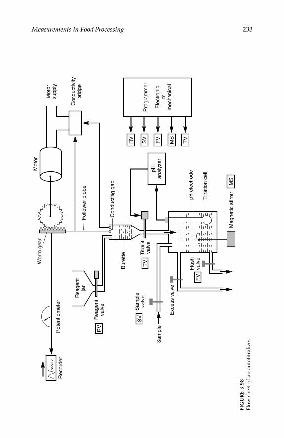
Measurements in Food Processing 233
FIG
UR
E 3.
98Fl
ow s
heet
of
an a
utot
itra
lizer
.
Mot
or
Mot
orsu
pply
Con
duct
ivity
brid
ge
pH e
lect
rode
Mag
netic
stir
rer
Titr
atio
n ce
ll
Sam
ple
Exc
ess
valv
e
Flu
shva
lve
Sam
ple
valv
e
Rea
gent
valv
e
FV
RV
Rec
orde
rP
oten
tiom
eter
Rea
gent
jar
Wor
m g
ear
Bur
ette Ti
tran
tva
lve
Con
duct
ing
gap
Fol
low
er p
robe
SV
FV
MS
MS
TV
TV
SV
RV
Pro
gram
mer
Ele
ctro
nic
orm
echa
nica
l
pHan
alyz
er
7244.book Page 233 Wednesday, June 21, 2006 11:14 AM

234 Measurement and Control in Food Processing
opening the titrant valve (TV). As soon as the reagent is added, the pHanalyzer is started to measure the pH of the solution of the titration cell. Inthe burette, the reagent level drops, the conducting gap breaks, and theconducting bridge powers a DC motor to advance the follower probe untilthe gap is covered. The movement of the follower probe is recovered by apotentiometer attached to the worm gear arrangement. When the end pointof the titration is reached, the pH analyzer closes the TV. The potentiometeras well as the recorder record the volume of the reagent and can be calibratedin terms of concentration or ppm.
Mee et al. [34] found that the autotitralizer needs at least 75 ml of the testsample for immersion of the electrode and stirrer, and 100 ml is the recom-mended volume. The recovery rate of HCO3 was found to be 98% to 119% byadding from 5 ppm to 100 ppm. Below 10 ppm of CO3, the standard deviationwas 28% and percentage error was 85%. These values for HCO3 were 10%and 9%, respectively, for less than 5 ppm. The CO3 ion was not correctlydetectable if the pH value of the water sample was neutral or acidic. Therefore,pH values were also continuously monitored using the autotitralizer.
Organic matters in drinking water or beverages change the taste. Mee etal. [35] further analyzed organic maters in bottled water by infrared spec-troscopy. They developed a rapid screening test for the detection of organicmatters based on CHCl3 extraction by IR spectrometer through 200 to4,000 cm–1 wave number. IR spectra of distilled water samples were takenfrom CHCl3 extracts of water both at ambient temperature and at an elevatedtemperature of 110°C (for 1 hr prior to extraction). IR bands were observedat 1,350 cm–1 at ambient temperature and two IR bands at 1,600 and 3,680 cm–1
were significantly observed at 110°C/1 hr heating due to thermal activationof organics present. They further studied the volatility of organics in water(by PS-SP-080 IR Data System) such as hydrocarbons and chlorinated hydro-carbons, decanol, and benzonitrile.
3.14.2 Volatile Compounds in Tropical Fruits
Tropical fruits are very popular in food processing for their unique flavorsand bright colors. Soft drinks and jam and jelly production depend most ontropical fruits: mango, papaya, passionfruit, avocado, and so on. The flavorof these fruits depends on a number of volatile compounds, so the estimationof these compounds is an important tool for food processing. Yamaguchi etal. [36] conducted an investigation on analysis of volatile compounds onthose four tropical fruits using GLC and combination of gas chromatogra-phy-mass spectroscopy (GS-MS), near magnetic resonance (NMR), IR, andUV spectroscopy.
The peel and seeds were removed from the fruits and edible parts werehomogenized with deionized water using a homogenizer. The homogenizedfruits were water distilled under reduced pressure in a nitrogen stream at awater bath. The distillate samples were extracted with dichloromethane
7244.book Page 234 Wednesday, June 21, 2006 11:14 AM
Measurements in Food Processing 235
using a liquid–liquid continuous extractor. The extract was dried and thesolvent was removed under vacuo. A Hewlett-Packard Model 5710-A GCwith a flame ionization detector was used for volatile profile analysis. Fusedsilica capillary columns were developed and used in the GC.
Another GC, Hitachi Model M-80 combination MS-GC (HP-5710A) wasused with the same GC column and oven temperatures. The following arethe results obtained from the GC-MS analysis:
Mango: 21 constituents; highest constituent, monoterpenes with 42.32%of total GC area.
Papaya: 20 components; highest, butyric acid with 37.34% of the totalGC area.
Passionfruit: 21 constituents; highest constituent, n-hexyl n-butyratewith 14.34% of total GC area.
Avocado: 52 constituents; highest constituent, trans-2-hexanol with58.95% of total GC area.
3.14.3 Moisture, Protein, Fat, and Ash Content of Milk Powder
A near infrared reflectance spectroscopy (NIRS) analyzer has been estab-lished by Ereifej et al. [37] as an efficient technique for detecting moisture,protein, fat, and ash content in dried milk powder. NIRS was initially usedfor moisture analysis in food products, but researchers later extended its useto protein and oil content. Several manufacturers have developed sophisti-cated instruments based on NIRS techniques for compositional analysis ofgrain and oilseeds. NIRS has also been successfully used for monitoringsugar and carbon dioxide in carbonated beverages by Frant et al. [38]. Intheir study, Ereifej et al. [37] used a Neotec NIRS model GOA-41 to detectmoisture, protein, fat, ash, and lactose content in four different milk samples:milk powder prepared by spray drying mixtures of skim and whole milk,milk powder prepared by mixing predried skim and whole milk, commercialsamples, and commercial cheese powders.
The instrument used spectra in the 1800 nm to 2320 nm region for theanalysis with four selected wavelengths. These wavelengths were used tocalibrate the readings with known composition. The results were justifiedby conventional oven, dry ashing, and the Microkjeldahl method for mois-ture, ash, and nitrogen content determination. Fat content results were cor-related with the Mojorrier procedure.
3.14.4 Components in Alcoholic Beverages
The finished products of alcoholic beverages range from pure aqueous alcoholto complex mixtures such as vermouths. Most of the volatiles of interestobtained in alcoholic beverages are present at a level of less than 50g/l. Liddle
7244.book Page 235 Wednesday, June 21, 2006 11:14 AM

236 Measurement and Control in Food Processing
et al. [39] adopted a very simple and fast analysis technique with a simplesample preparation method. They used a capillary GC using glass or fusedsilica columns. This facilitates faster analysis, allowing simple sample prep-arations. They were able to detect contaminants such as residual monomer,plasticizer, and antioxidants contributing to off-flavors. Total number of vol-atile compounds detected was about 21. Similarly, about 14 compounds weredetected in dry white wine. The diminishing of many volatile compoundswas noticed in 8-year-old rum, where only six components were found.
Apostolos et al. [40] detected mineral constituents such as aluminum, cal-cium, magnesium, and vanadium in Greek wines. For analysis of trace ele-ments of wines, flameless atomic absorption (FLAA) and neutron activationanalysis (NAA) were found to be the most sensitive and accurate methods.
3.14.4.1 Minerals in Wines
Analysis of the minerals in wine, particularly aluminum, calcium, magne-sium, and vanadium, is very important for quality control and handlingwines. Aluminum in wine is found in concentrations of 0.5 to 10 mg/l dueto possible contamination from storage in aluminum containers. Aluminumis undesirable in wine because it makes the wine cloudy. Calcium and mag-nesium present in wine combines with tartarates and precipitates as calciumand magnesium tartarates, even months after bottling. Calcium and magne-sium contents in wine can be due to soil conditions of grapes, treatment withfining agents, storage in concrete tanks, use of ion-exchange resins, and soon. Vanadium content in wine gives an off-flavor either by poisoning theyeast or by changing the morphology or physiology of the yeast.
A coaxial germanium-lithium drifted Ge(Li) detector (ORTEC Model WIN15 Series) can be used for this analysis. In this detector the output signalsare fed to a preamplifier (ORTEC Model 119) and a spectroscopy amplifier(ORTEC Model 571). The pulse height of the spectrum detected by the Ge(Li)detector is analyzed by a pulse height analyzer. The radiation detector isconsidered an ideal method for simultaneous determination of a large num-ber of trace elements due to its sensitivity, rapidity, precision, and accuracy.The precision of measurements reported are 0.72 mg/l for Al, 26 mg/l forCa, 64 mg/l for Mg, and 1.0 mg/l for vanadium.
3.14.5 Quality Parameters in Cereals and Cereal Products
Protein quantity and quality are of basic interest to cereal and food technolo-gists in assessment of the overall quality and the most important correlationto the final product. Starch is another constituent responsible for CO2 produc-tion during the baking process. Additions in flours (e.g., dry gluten, oxidizingagents, malt flour, enzymes, organic acids, emulsifier, etc.) are also importantdetectable matters. Pattakou et al. [41] assessed wheat flour to detect its waterabsorption capacity by Farinograph and mechanical properties of dough by
7244.book Page 236 Wednesday, June 21, 2006 11:14 AM

Measurements in Food Processing 237
Extensograph. The Extensograph properties of dough indicate suitability formaking bread and puff pastry goods. In addition, Extensograph propertiesindicate the action of oxidative agents and ingredients and percentage ofgluten to be added to improve rheological behaviors to wheat flour.
They also conducted Amylograph tests on wheat flour, and b-amylaseactivity, gassing power, and falling number tests to assess starch behavior;and Fermentograph tests on wheat flour to assess CO2 production duringyeast formation.
3.14.6 Meat Content
Protein and moisture content in pure meat is almost constant, but the nitro-gen content is different in different meat. As specified by the Society forAnalytical Chemistry, the Royal Society of Chemistry, the highest nitrogencontent (percentage nitrogen on fat-free basis) is 3.9 in chicken breast andthe lowest is 3.0 in tongue of animals in the United Kingdom. In othercountries, composition of meat products is represented by nitrogen or proteincontent of water/protein (e.g., in muscle meat 77% water/23% protein =3.35), indicating the fat-free meat content.
In Germany, the Feder number, the ratio of water to organic nonfat content,is used. This ratio is
Feder number = water%/( 100 – (fat% + water% + ash% )) (3.78)
In France the moisture of the defatted meat is used as the meat contentindicator. In the United States, the term protein on fat free is used:
PRf = (100 × protein%)/(100 – fat %) (3.79)
Rapid analytical methods have been developed for determination of meatcontent components, such as fat, protein, nitrogen, and water. The methodsare utilized in the following commercial analyzers:
1. The Infralyzer and the Foss SuperScan analyzer™ are convenient asfar as their operational techniques are concerned. In both the ana-lyzers, infrared light rays are passed through the sample and theenergy absorbed by the sample is measured. The system is com-prised of an IR source, electronic balance for accurate sample weightplacement, a reactor for sample preparation, and a detecting unit forfat, protein, carbohydrate, and water. The system is controlled by adesktop computer.
2. The AnylRay™ machine works on X-ray diffraction technique anddetects the fat content of meat. The sample requirement is compar-atively high (1–15 kg), but the sample can be reused.
7244.book Page 237 Wednesday, June 21, 2006 11:14 AM

238 Measurement and Control in Food Processing
3. The CEM Meat Analyser™ dries the sample in a microwave dryerand treats it in an automatic fat extraction unit with an automaticsolvent extraction and recovery system. The analyzer can give resultsin under 10 min.
4. The Dickei-John ground meat tester is an electrical device with whichan EMF in a piece of meat is developed by electromagnetic inductionprinciple. The EMF is calibrated in terms of lean meat content togive an instant readout.
3.14.7 Bacteria and Foreign Body Detection
3.14.7.1 Bacteria Detection
Microbiological infection and food poisoning is a matter of concern for foodmanufacturers and food testers. Poisoning by foodborne bacteria is mostlyassociated with large-scale food service operators rather than food manufac-turers; however, food packaging sectors should take every possible measureto prevent bacterial infection. The most common foodborne bacterias areListeria monocytogens, Salmonella, Campylobacter, Clostridium botulinum, Aero-moas hydrophila, and Bacillus subtilis. Bacteria growth in food is encouragedby moisture and osmotic pressure in food.
The conventional method of bacteria assessment is the plate-count method,which is very slow and can take several days. Therefore food manufacturersuse rapid methods like the Lumac method based on bioluminescence. Awidely used method was developed by Bactomatic, in which a sample ismixed with a medium and placed in an impedance-sensing cell under con-trolled temperature conditions. The impedance detection time (IDT) to reacha number of organisms with a specified concentration is used to quantifythe quality of many foods.
Rapid detection of pathogenic bacteria has been successfully tested by Tsenet al. [42] using a DNA hybridization technique. They used the probe fordetection of Salmonella spp in soy flour, macaroni, meat, and fish. The detec-tion takes 70 hr and counts as low as 1.6 per gram are possible.
3.14.7.2 Foreign Body Detection
Foreign bodies in food primarily include metal particles. In an on-linemethod the technique is similar to that of a general metal detector, but witha small aperture. The food is carried over a nonmetallic conveyor andallowed to pass through a small aperture around which three coils at asymmetrical electrical axis are placed. A central coil is excited by a high-frequency voltage inducing identical voltages in the other two coils con-nected in phase opposition. A voltage is induced due to imbalance in thecoil induction when a metal particle passes through the aperture. The equalinduced voltages are cancelled out when there is no metal particle.
7244.book Page 238 Wednesday, June 21, 2006 11:14 AM

Measurements in Food Processing 239
Another method of metal detection is the X-ray inspection in gross itemsin bulk materials. In materials in sheet form, optical detection methods offergood resolution at high speed. In an optical inspection system, images orscan data are acquired by video camera or a photodiode array. The outputfrom the array in successive scans can be analyzed on-line to detect thepresence of any foreign body.
3.14.7.3 Removal of Stalks from Tea
Due to improper withering, cutting, or drying, colored stalks are sometimesdeveloped in CTC tea. Stalk particles are amber to brown in color, whereasclean tea granules are black. The presence of stalk is detected by an array ofphotocells that receive filtered light reflected back from a single layer of tea.The filter selects the band of light nearest to the stalk color when the corre-sponding photocell sees a stalk color to develop an electrical voltage. Thevoltage in turn activates a small air jet to blow off the selected stalk instantly.An electromagnetic high-frequency vibrating conveyor is used to spread thetea with stalk across the width of the machine. The vibrator spreads the teainto a single layer, minimizing ejection of black tea particles. The filters arecleaned periodically by compressed air. A commercial and automated tea stalksorter machine manufactured by Senvec, Inc. (Japan) is shown in figure 3.99.
FIGURE 3.99Photograph of a tea color stalk sorter (Model-BTR-C Series). (Reprinted with permission fromHattori Seisakusho Ltd., Japan)
7244.book Page 239 Wednesday, June 21, 2006 11:14 AM

240 Measurement and Control in Food Processing
3.15 Conclusion
There is a large gap between the food industries and food scientists. In spiteof tremendous developments in the fields of electronics, instrumentation,and computer technology, the food industries have been facing many diffi-culties in measurement of food-related parameters. One reason for this gapis the development toward generalized applications of electronic sensors,leaving food-specific sensors far behind. For example, the new sensors likeISFET, ENFET, and E-nose sensors can detect food pH, enzymes, and flavors,but these new sensors must be adapted properly to make them effective forfood-related applications. Similarly. image processing has shown powerfulfeature extraction and classification capabilities, but food-related issues arevery limited.
This chapter provides sufficient information on the available methods infood-related measurement techniques with respect to various process param-eters. Some examples of applications are provided to guide one to implementthese techniques in one’s own applications. For a particular measurement,there is no common or single transducer for each type of food material.Therefore, in every section of this chapter, in discussing a particular mea-surement technique, the relevance of the technique for a particular foodmaterial has been explained. This should help the reader in identifying anappropriate technique for a specific application.
References
1. Bhuyan, M., Gogoi, S., and Choudhury, A. 1996. A novel technique of moisturemeasurement in green tea leaves. Proc. of Int. Conf. Trends in Industrial Measure-ments and Automation, 78–84.
2. Subramanyam, K., Venkataraman, V., and Sankaranarayanan, P. E. 1994. On-line moisture analyzer for tea industry. J. Instr. Soc. of India 24(3&4):124–130.
3. Bhuyan, M. 1997. An integrated PC-based tea process monitoring and controlsystem. PhD Thesis, Department of Electronics, Gauhati University, India.
4. TRA. 1991. Calculation of percentage of wither and corresponding moisturecontent of green and withered leaf. Res. Bulletin, Sr. No 184. Jorhat, India:Tocklai Tea Experimental Station.
5. TRA. Moisture 1962. content of green leaf and its relation to yield of made tea.Res. Bulletin, Sr. No 18. Jorhat, India: Tocklai Tea Experimental Station.
6. Bhuyan, M., Dutta, V., Sharma, P. K., and Choudhury, A. 1996. A microprocessorbased relative humidity measuring technique using piece-wise linearised mod-el of psychrometric chart. Proc of Int. Conf. Trends in Industrial Measurements andAutomation, 78–84.
7. Bhuyan, M., and Bhuyan, R. 1995. An on-line method for monitoring of relativehumidity using thermal sensors. Proc. of IEEE Int. Conf. on Industrial Automationand Control, 7–11.
7244.book Page 240 Wednesday, June 21, 2006 11:14 AM

Measurements in Food Processing 241
8. Govindraj, R., and Sankaranaryanan, P. E. 1996. Estimation of color and tur-bidity and pH values of sugar juice during sugar refining process. Proc. of Int.Conf. Trends in Industrial Measurements and Automation, 94–98.
9. Borah, S., and Bhuyan, M. 2002. Non destructive testing of tea fermentationusing image processing. Int. Conf. of Non Destructive Testing, Southport, UK.
10. Borah, S. 2005. Machine vision for tea quality monitoring with special emphasison fermentation and grading. PhD Thesis, Department of Electronics, TezpurUniversity, India.
11. Mahanta, P. K. 1988. Biochemical basis of color and flavor of black tea. Proc. of30th Tocklai Conf., 124–134.
12. TRA. 1988. Polyphenol content and theaflavin concentration analysis. Res. Bul-letin. Jorhat, India: Tocklai Tea Experimental Station.
13. Borah, S., and Bhuyan, M. 2005. A computer based system for matching ofcolor during the monitoring of tea fermentation. Int. J. Food Sci. Tech. 40:675–682.
14. Sridhar, R., Anil, P. K., Sankaranarayyan, P. E., and Rakowski, R. 1986. Newrefractometer for on-line brix measurement in the food processing industry.Proc. TIMA-96, 85–90.
15. Yates, D. E., Levine, S., and Healy, T. W. 1974. Site binding model of electricaldouble layer at the xide/water interface. J. Chem Soc. Faradays Trans. 70:1807–1819.
16. Fung, C. D., Cheung, P. W., and Ko, W. H. 1986. A generalized theory of anelectrolyte-insulator semiconductor field effect transistor. IEEE ED 33(1):8–18.
17. Ogrodzki, J., and Opalski, L. 2000. Modeling of semiconductor pH sensor forCAD. Proc. 7th Int. Conf. on Mixed Design of IC and Systems, MIXDES 2000,259–264.
18. Leandro, L., Lorenzelli, L., Margesin, B., Martinoia, S., Tedesco, M. T., and Valle,M. 2003. Bio-electrochemical signal monitoring of in-vitro cultured cells bymeans of an automated microsystems based on solid state sensor array. Biosens.Bioelectr. 18(5–6):621–626.
19. Martinoia, S., Rosso, N., Grattarola, G., Lorenzelli, L., Margesin, B., and Zen,M. 2001. Development of ISFET array-based microsystem. Biosens. Bioelectr.16:1043–1050.
20. Artigas J., Jimenez, C., Dominguez, C., Minguez, S., Gonzalo, A., and Alonso, J.2003. Development of a multi-parametric analyzer based on ISFET sensors ap-plied to process control in the wine industry. Sensors and Actuators B89:199–204.
21. Bohnke, C., Duroy, H., and Fourquet, J. K. 2003. pH sensors with lithiumlanthanum titanate sensitive materials: Application in food industries. Sensorsand Actuators B89:240–247.
22. Updike, S. J., and Hicks, G. P. 1967. The enzyme electrode. Nature 214:986–988. 23. Canh, T. M. 1993. Biosensors (English ed.). New York: Springer Science.24. Pearce, T. C., Gardner, G. W., and Friel, S. 1993. Electronic nose for monitoring
of the flavors of beer. Analyst 118:371–377.25. Llobet, L., Hines, E. L., Gardner, J. W., and Franco, S. 1999. Non-destructive
banana ripeness determination using a neural network based electronic nose.Meas. Sci. Tech 10:538–548.
26. Dutta, R., Hines, E. L., Gardner, J. W., Kashwan, K. R., and Bhuyan, M. 2003.Tea quality prediction using a tin oxide based electronic nose. Sensors andActuators 94:228–237.
27. Dutta, R., Kashwan, K. R., Bhuyan, M., Hines, E. L., and Gardner, J. W. 2003.Electronic nose based tea quality standardization. Neural Networks 16:847–853.
7244.book Page 241 Wednesday, June 21, 2006 11:14 AM

242 Measurement and Control in Food Processing
28. Dutta, R., Hines, E. L., Gardner, J. W., Kashwan, K. R., and Bhuyan, M. 2003.Determination of tea quality by using a neural network based electronic nose.Proc. International Joint Conference on Neural Network 1:404–409.
29. Kashwan, K. R. 2005. An artificial neural network based electronic-nose system:Tea and spice flavor discrimination and drift parameter determination. PhDThesis, Department of Electronics, Tezpur University, India.
30. Swatland, H. J. 1997. Relationship between the back-scatter of polarised lightand the optical detection of connective tissue fluorescence in beef. J. Sci. Foodand Ag. 75:45–49.
31. Jeyamkondan, S., Kanzler, G. A., and Lakshmikanth, A. 2001. Predicting beeftenderness with computer vision (Paper No.01-3603). ASABE Annual MeetingPresentation. St. Joseph, MI: American Society for Agricultural and BiologicalEngineers (ASABE).
32. Wulf, D. M., O’Connor, S. F., Tatum, J. D., and Smith, G. C. 1997. Using objectivemeasures of muscle color to predict beef longissimus tenderness. J. Anim. Sci.75:684–692.
33. Li, J., Tan, J., Martz, F. A., and Heymann, H. 1999. Image textural features asindicators of beef tenderness. Meat Sci. 53:17–22.
34. Mee, J. M., Jahangir, M., Faruq, I. M., and Al-Salem, S. 1983. Analysis of car-bonates in bottled waters by autotitraliser. In Instrumental analysis of foods:Recent progress, ed. Charalambous, G. and Inglett, G. (Vol. 2), 21–32. London:Academic Press.
35. Mee, J. M., Khan, P., and Ahmed, S. 1983. Application of direct mass spectros-copy for rapid analysis of organics in water beverages. In Instrumental analysisof foods: Recent progress, ed. Charalambous, G. and Inglett, G. (Vol. 2), 33–40.London: Academic Press.
36. Yamaguchi, K., Nishimura, O., Toda, H., and Mihara, S. 1983. Chemical studieson tfopical Fruits. In Instrumental analysis of foods: Recent progress, ed. Charalam-bous, G. and Inglett, G. (Vol. 2), 93–117. London: Academic Press.
37. Ereifej, K. I., and Markakis, P. 1983. Analysis of dried milk and cheese powdersby near infrared reflectance spectroscopy. In Instrumental analysis of foods:Recentprogress, ed. Charalambous, G. and Inglett, G. (Vol. 2), 237–242. London: Aca-demic Press.
38. Frant, M. S., and Labutti, G. 1980. Process infrared measurements. Anal. Chem.52:1331A–1344A.
39. Liddle, P., and Bossard, A. 1983. Glass capillary GC in wine and spirit industry.In Instrumental analysis of foods: Recent progress, ed. Charalambous, G. andInglett, G. (Vol. 2), 307–321. London: Academic Press.
40. Apostolos, P. G., Vassilaki-Grimani, M., and Kanias, G. D. 1983. Instrumentalneutron activation analysis of aluminum, calcium, magnesium and vanadiumin Greek wines. In Instrumental analysis of foods: Recent progress, eds. Charalam-bous, G. and Inglett, G. (Vol. 2), 323–334. London: Academic Press.
41. Vassiliki Pattakau, V., and Voudouris, E. 1983. Analytical instrumentation andassessment of quality parameters in cereals and their products. In Instrumentalanalysis of foods: Recent progress, eds. Charalambous, G. and Inglett, G. (Vol. 2),479–492. London: Academic Press.
42. Tsen, H., Wang, S., and Green, S. S. 1991. Salmonella detection in meat and fishby membrane hybridization with chromogenic/phosphatase/biotin DNAprobe. J. Food Sci. 56:1519–1523.
7244.book Page 242 Wednesday, June 21, 2006 11:14 AM

243
4Controllers and Indicators
CONTENTS4.1 Introduction ................................................................................................ 2444.2 Temperature Control in Food Dehydration and Drying .................... 245
4.2.1 Control Parameters for Heat and Mass Transferin Drying ........................................................................................ 246
4.2.2 Feedback and Feedforward Control in Dryers ........................ 2494.2.2.1 Mass and Energy Balance in Dryers ........................... 249
4.2.3 A Single-Input, Single-Output (SISO) Dryer Model ............... 2514.2.4 A Multiple-Input, Multiple-Output (MIMO)
Dryer Model................................................................................... 2524.2.5 Feedforward Control in the Food Dryer................................... 255
4.2.5.1 The Control Functions ................................................... 2574.3 Electronic Controllers................................................................................ 258
4.3.1 On–Off Controller ......................................................................... 2604.3.1.1 Bimetallic Thermal On–Off Controller........................ 260
4.3.2 Controller Modes .......................................................................... 2614.3.2.1 Proportional Controller.................................................. 2614.3.2.2 Integral Controller .......................................................... 2634.3.2.3 Derivative Controller ..................................................... 264
4.3.3 Fan Direction Control in Food Withering................................. 2654.3.3.1 The Relay Circuit ............................................................ 2684.3.3.2 Logic Control Circuit ..................................................... 2684.3.3.3 The Comparator Circuit ................................................ 269
4.3.4 Cooling Surface Area Control in Chocolate Tempering......... 2714.4 Flow Ratio Control in Food Pickling Process ....................................... 271
4.4.1 Ratio Controller ............................................................................. 2724.4.2 Control Valves................................................................................ 273
4.4.2.1 Types of Control Valves................................................. 2744.4.2.2 Valve Sizing ..................................................................... 275
4.5 Atmosphere Control in Food Preservation ........................................... 2774.5.1 Control Scheme.............................................................................. 277
4.6 Timers and Indicators in Food Processing............................................ 2784.6.1 Rolling Program in Tea Manufacturing .................................... 279
4.6.1.1 Roller Timing Sequence ................................................. 281
7244.book Page 243 Wednesday, June 21, 2006 11:14 AM

244 Measurement and Control in Food Processing
4.6.1.2 Programmable Timer Circuit ........................................ 2824.6.2 Temperature Indicator for Tea Dryer......................................... 284
4.7 Food Sorting and Grading Control ........................................................ 2874.7.1 Objective of Sorting ...................................................................... 2874.7.2 Various Sorting Techniques ......................................................... 2884.7.3 Automated Packaging and Bottling........................................... 289
4.8 Discrete Controllers................................................................................... 2904.8.1 Ladder Diagram ............................................................................ 2914.8.2 Programmable Logic Controllers ............................................... 292
4.8.2.1 Input and Output Modules........................................... 2924.8.2.2 Programming................................................................... 293
4.9 Adaptive and Intelligent Controllers ..................................................... 2934.9.1 Self-Tuning Controllers ................................................................ 2944.9.2 Model Reference Adaptive Controllers ..................................... 295
4.9.2.1 Some Design Criteria of Adaptive Controllers.......... 2954.9.3 Intelligent Controllers................................................................... 296
4.9.3.1 Fuzzy Logic Controller .................................................. 2974.10 Conclusion .................................................................................................. 300References ............................................................................................................ 301Further Reading ................................................................................... 302
4.1 Introduction
Due to the advent of modern electronic techniques and automatic controldevices supported by instrumentation, power electronics, and digital sys-tems, the control of machines in industries has been revolutionized. Eventoday, however, many food processing industries are run by either outdatedmechanical means or manual methods. As a result maximum quality, pro-ductivity, and efficiency are not ensured. Therefore, there are obvious rea-sons for incorporating scientific and electronic control devices in foodindustries. For example, most of the tea factories in India use single-phaseor three-phase induction motors ranging from 0.5 hp to 25 hp, totalingaround 50 to 60 in a tea factory of normal size for 10 to 12 different processoperations. However, these machines are still manually operated today. Fora production of 5 × 10⁵ kg/year of processed tea, the average power con-sumption of a tea factory is about 600 MWh and the total energy requirementof the entire tea sector in India is about 7 × 10⁵MWh [1]. This implies thatthere is ample opportunity to save a substantial amount of electrical energyin the tea industry alone. Automatic control for food processing not onlycontributes toward saving energy, but substantially improves quality andefficiency as well.
The usage of controllers in food processing is improving with greaterapplication of engineering capabilities. Applications of computer control,
7244.book Page 244 Wednesday, June 21, 2006 11:14 AM

Controllers and Indicators 245
instrumentation, neural networks, and artificial intelligence techniques aregaining importance in the food processing industries. A responsible foodmanufacturer is very much concerned about manufacturing a product to acertain standard and selling the food for profit. Control of food quality beginswith the raw materials and it continues through various manufacturingprocesses to storage and packaging. Good Manufacturing Practice (GMP)aims at well-designed manufacturing operations, quality control systems,and quality assurance systems. It is the duty of food manufacturers to adoptprocess instrumentation and process control devices to achieve reliable andeffective control at a reasonable cost.
During my research in development of computer control techniques forthe tea industry, it became apparent that there are many innovations yet tobe made to make tea processing automotive. Even today, in most tea factories,the quality of the tea during various processes is assessed by smelling,touching, and visual inspection, and machines are controlled by manualoperators. There are many similar examples in other food processing indus-tries in which control strategies are known and well defined, but design anddevelopment of control techniques has yet to be done.
Examples of industrial controllers and annunciation applications in foodprocessing include temperature and moisture content control in dryers andovens, flow control in rotary dryers in the sugar industry, withering controlin the tea industry, cooling surface area control in chocolate tempering,automated sorting and bottling, and atmospheric control in food storage.This chapter describes a series of examples of food processing systems high-lighting the process parameters, control actions adopted or recommendedby food scientists, and timers and annunciators associated with the controlstrategies. The chapter also presents a general overview of classical andmodern control schemes used for food processing control.
4.2 Temperature Control in Food Dehydration and Drying
The principle purpose of food dehydration and drying is removal of waterbefore preservation; however, food can be dehydrated to decrease its weight.In such applications, the size and shape of the food is retained, only the weightis reduced. The shipping cost based on weight is reduced, but when shippingcost is based on volume, not on weight, dehydration might not be useful.Another aim of dehydration is production of instant food items. In suchproduction, the cooking and other processing is conducted before the food isdried. Before consumption, the consumer has to make only a simple prepa-ration effort (e.g., mixing with hot water, adding spices or sauces, etc.).
Although sun drying is still popular for many agricultural products, dueto its inherent disadvantages, sun drying is not considered an efficientmethod for many reasons: it is slow and not suitable for many high-value
7244.book Page 245 Wednesday, June 21, 2006 11:14 AM

246 Measurement and Control in Food Processing
products, the space required for drying is greater, moisture content below15% is not achievable, and the food being exposed is subject to contaminationand losses due to various reasons.
The term food dehydration technically refers to drying artificially under con-trolled conditions. Although many other food processes like cooking, frying,and broiling involve removal of water from the food, these processes are notconsidered dehydration. Strictly speaking food dehydration means removalof water without any change in the food; that is, the food should be able tobe reconstituted with its original taste, flavor, and other properties by theaddition of water or other liquid. Therefore drying with maximum productstability and low moisture level is difficult to achieve. A precise and accuratecontrol of the drying phenomenon is necessary to achieve these criteria.
4.2.1 Control Parameters for Heat and Mass Transfer in Drying
In any type of food drying process, dehydration involves heat transfer fromthe drying air of the surrounding medium to the food and release of moisturefrom the food to the air. These two stages of heat and mass transfer shouldbe easily facilitated without any obstruction to achieve fast and efficientdrying. Factors affecting the drying process include surface area of the foodbeing exposed, temperature difference between the heating medium and thefood item, velocity of the heating air, humidity of the air collecting themoisture from the food, and atmospheric pressure of the heating air.
To speed up heat and mass transfer during drying, the food is generallyspread widely to an optimal thickness. However, there must be a compromisebetween spread thickness and the size of the conveyor floor, volume of thedryer, and the feed rate of the food. The drying air drives off moisture fromthe food and the hotter the air, the more moisture it can drive off, makingthe drying process faster. Therefore, a higher temperature difference betweenthe heating medium and the food speeds up drying. Air in motion can sweepup more moisture than stationary air. Therefore a high draft of air, if themedium is air, will facilitate a high uptake of moisture from the food.
The capacity of the air surrounding the food to hold moisture depends onits humidity. Less humid air permits release of more moisture, facilitatingfaster drying. This is the reason why an air hygrometric difference (differencebetween dry-bulb and wet-bulb thermometer) not less than 3°C is necessaryduring tea withering. Again, on a very rainy day with a relative humidity(RH) at more than 90% and temperature at 20°C, hot air is used to achievea proper withering.
Another important factor determining the minimum moisture contentlevel to which a food can be dried is the equilibrium RH of the food item.At this equilibrium RH, the food neither loses nor gains moisture. Below thislevel, food can be further dried; above this level it cannot be dried becauseit absorbs moisture from the surrounding air. However, this humidity level
7244.book Page 246 Wednesday, June 21, 2006 11:14 AM

Controllers and Indicators 247
is different at different temperatures. Graphs of moisture level with RH atdifferent temperatures are called water sorption isotherms of the food. Figure4.1 shows an example of the water sorption isotherm of two food products, Aand B. It is clear from the graph that, say at 100°C and 40% humidity, productB can be dried down to 2%, whereas product A can be dried only to 4%. At80°C product B can be dried to 6% and product A only to 10%. Again, if it issufficient to dry product A at 80°C down to 8%, and product B down to 4%,then the RH of the air should be 20%. It is not difficult to experimentallydetermine the water sorption isotherm of a food product. This can be done bydrying the food at different temperatures and RH levels and determining themoisture content by drying and weighing or any other method. Such plots arevery important in designing the control strategy for a drying system.
Drying food at higher temperature and for a longer duration could dam-age the constituents of the food. The drying rate can be made faster at lowertemperature by exposing the food at a lower atmospheric pressure. Dryingfood in a vacuum chamber releases moisture at a faster rate at lower tem-perature than drying at normal atmospheric pressure. Moisture in food isgenerally distributed from its surface to its core. Surface moisture, whendrying, is released faster, and it takes longer to draw off the inner-levelmoisture.
FIGURE 4.1Example of water sorption isotherm of two food items, A and B.
0 20 40 60 80 100
4
8
12
16
20
80
100
Temperature
MC
%(d
ry)
RH%
80
100
A
B
7244.book Page 247 Wednesday, June 21, 2006 11:14 AM

248 Measurement and Control in Food Processing
TAB
LE 4
.1
Salie
nt F
eatu
res
of C
omm
on F
ood
Dry
ers
Typ
eFe
ed F
orm
Han
dli
ng
Sty
leM
ain
Fea
ture
sH
eati
ng
Met
hod
Tem
per
atu
reO
ther
Var
iab
les
Dru
m o
r ro
ller
Liq
uid
, pas
tes,
pu
rees
, mas
hes
Mat
eria
l mov
es,
equi
pmen
t m
oves
Hea
ted
dru
m o
r ro
ller
mov
ing
in o
ppos
ite
dir
ecti
ons
Ste
am10
0°C
–150
°CSp
eed
of
dru
ms,
gap
be
twee
n d
rum
s
Spra
y d
ryer
Liq
uid
, pas
te,
pure
esL
iqui
d s
pray
ed in
d
ropl
ets
Spra
y d
ryer
, tow
ers
Furn
ace,
el
ectr
ical
200 °
CA
ir v
eloc
ity
Vac
uum
sh
elf
Liq
uid
, thi
n so
lidM
ater
ial s
tati
c,
equi
pmen
t st
atic
Con
den
ser
to c
olle
ct
rele
ased
wat
erH
ot a
ir, s
team
, el
ectr
ical
30°C
–40°
CV
acuu
m p
ress
ure
Vac
uum
be
ltL
iqui
d, t
hin
solid
Mat
eria
l mov
es,
equi
pmen
t m
oves
—St
eam
—V
acuu
m p
ress
ure
Tunn
el
dry
erSo
lid p
iece
sM
ater
ial m
oves
, eq
uipm
ent
mov
es H
ot a
ir d
irec
tion
Furn
ace
90°C
–110
°CV
eloc
ity
of a
ir, s
peed
of
truc
kTr
ough
d
ryer
Solid
pie
ces
Mat
eria
l sta
tic,
eq
uipm
ent
stat
icH
ot a
ir b
low
n by
fan
Furn
ace
90°C
–110
°CV
eloc
ity,
hum
idit
y, a
nd
tem
pera
ture
of a
ir; s
prea
d
thic
knes
s of
fo
odB
elt
trou
ghSo
lid p
iece
sM
ater
ial m
oves
, eq
uipm
ent
mov
esH
ot a
ir b
low
n by
fan
Furn
ace
90°C
–110
°CV
eloc
ity,
hum
idit
y an
d
tem
pera
ture
of a
ir; s
prea
d
thic
knes
s of
foo
d
Flui
diz
ed
bed
dry
erPa
rtic
ulat
es,
gran
ules
Mat
eria
l mov
es,
equi
pmen
t st
atic
Hot
air
blo
wn
susp
end
s pa
rtic
les
in
gent
le b
oilin
g
Furn
ace
100 °
C–1
20°C
Tem
pera
ture
and
vel
ocit
y of
hot
air
, fee
d r
ate
7244.book Page 248 Wednesday, June 21, 2006 11:14 AM

Controllers and Indicators 249
4.2.2 Feedback and Feedforward Control in Dryers
In this section we discuss control strategies necessary to control the dryingaction in dryers.
Table 4.1 outlines classifications and features of some common types ofdryers. The table reveals that controlling parameters of the drying processcan be different in different types of dryers. For example, in a drum or rollerdryer, the drying depends not only on the temperature of the steam, but alsoon the gap between the rollers and their speed; whereas in tunnel, trough,or belt trough dryers the controlling parameters are the speed of the belt,the velocity and temperature of the drying air, and the RH of the surroundingair. In view of different feed forms, handling styles, and other parametersresponsible for drying, the control problems of dryers can be broadly dividedinto two categories as discussed in the next sections.
4.2.2.1 Mass and Energy Balance in Dryers
Figure 4.2 shows a block diagram of a drying system with mass and energybalance variables. For energy balance, the dryer must fulfill the followingcondition:
heat in = heat absorbed by the product
This can be expressed by the energy balance equation
(4.1)
where Ma = air flow rate (kg dry air/hr)Mp = product flow rate (kg dry solid product/hr)Ha = heat content of air (kJ/ kg of dry air)Hp = heat content of product (kJ/kg of dry solid product)
The heat content of air is given by
(4.2)
where Cs = humid heat (kJ/dry air) = 1.005 + 1.88WTa = air temperature (°C )
FIGURE 4.2Representation of heat and mass transfer in a dryer.
ma, Ta2, W2Air
mρ, Tρ1, w1
Ta1, W1
Tρ2, w2
Product
Dryer
M H M H M H M Ha a P P a a P P2 1 1 2+ = +
H C T T WHa s a L= − +( )0
7244.book Page 249 Wednesday, June 21, 2006 11:14 AM

250 Measurement and Control in Food Processing
T0 = reference temperature (°C )W = absolute humidity (kg water/kg dry air)HL = latent heat of vaporization of water (kJ/kg water)
The heat content of product is given by
(4.3)
where w = moisture content of product (kg water/ kg of dry solid product)
CPw = specific heat of water (kJ/kg.K)CPP = specific heat of product (kJ/kg.K)TP = product temperature (°C )T0 = reference temperature (°C )
The overall moisture balance equation of the dryer is given by
(4.4)
Combining equations 4.1 through 4.4 we get the following expression forair flow
(4.5)
where Cs1 = 1.005 + 1.88W1
and Cs2 = 1.005 + 1.88W2
Problem 4.1A conveyor belt dryer is used to dry fermented tea from 60% moisturecontent (wet basis) at 25°C to 5% (wet basis). Dry hot air from the furnaceenters the dryer at 110°C and 1% (wet basis) RH. The drying air leaves thedryer at 30°C and 70% RH. The temperature of tea throughout drying processis 25°C. Compute the drying air requirement per kg of solid tea.
SOLUTION:The given data:
Initial fermented tea moisture content = w1 = 0.6/0.4 = 1.5 kg water/kgsolid tea
Final fermented tea moisture content = w2 = 0.05/0.95 = 0.052 kg water/kg solid tea
H wC C T TP Pw PP P= −( )0
M W M w M W M wa P a P2 1 1 2+ = +
MM C T T C w T w T
C Tap pp p p pw p p
s a
=− + − ( ) ( )1 2 1 1 2 2
1 22 2 1 2 1− + −C T H W Ws a L( )
7244.book Page 250 Wednesday, June 21, 2006 11:14 AM
Controllers and Indicators 251
Initial air temperature = 110°C and 1% RH
Exhaust air temperature = 30°C and 70% RH
Using equation 4.4
a) Using Microsoft Excel software for psychometric calculation from KWEngineering, 360 17th Street, Suite 100, Oakland, CA 94612 (see Appendix F):
W1 = 0.0186 kg water/kg dry air (at 30°C and 70% RH)
W2 = 0.009 kg water/kg dry air (at 110°C and 1% RH)
Using the preceding equation
The drying air requirement is 150.83 kg dry air/kg solid tea.
4.2.3 A Single-Input, Single-Output (SISO) Dryer Model
This is the simplest type of structure for a dryer when the control input isthe heating air temperature (manipulated variable) and the controlled outputis the moisture content of the food product. Because the moisture content ofthe product depends on a few other parameters, such as velocity and humid-ity of the drying air, pressure and humidity of the surrounding air, and theresidence time, these parameters are kept constant or manually controlledto a desired or predetermined value. Because residence time of the fooddetermines the bulk of heat transferred, which is responsible for overdryingand underdrying, this parameter can be considered as fixed for a batch typeof drying process. The air flow rate is kept at a constant level to compromisebetween dryer capacity and energy consumption. With these conditions inmind, a SISO dryer control scheme is shown in figure 4.3.
In such a control system the only manipulated variable is the drying airtemperature. A resistance temperature detector (RTD) or thermocouple tem-perature sensor probe properly sheathed and sufficiently long to reach the hotair passage through the dryer wall can be installed to measure the average
2 1+ =MM
W wMM
W wa
p1
a
p2+
MM
MM
MM
a
p
a
p
a
p
( . ) . ( . ) .
( .
0 009 1 5 0 0186 0 052
0 00
+ = +
996 1 448
150 83
) .
.
=
=MM
a
p
kg dry air/kg solid tea
7244.book Page 251 Wednesday, June 21, 2006 11:14 AM

252 Measurement and Control in Food Processing
temperature of drying air. A 4–20 mA temperature-to-current converter is themost common module to condition the sensor output voltage. For measuringthe moisture content of the food placed on trays, online moisture sensors likean infrared moisture sensor can be installed. Such on-line sensors convert thevoltage signals to a 4–20 mA current signal. Another possible moisture sensorin this application is a radio frequency (RF) absorption type.
The most common disturbances to the system include nonuniform mois-ture level and nonuniform drying characteristics of the product. These noisescause fluctuations in the output. Another noise source to the system mightarise from fluctuations of flow rate of drying air due to various designparameters of the dryer in spite of constant speed of the drive motor.
4.2.4 A Multiple-Input, Multiple-Output (MIMO) Dryer Model
In some dryers more than one practical input controls the drying process;for example, in a belt conveyor dryer, drying depends on the speed of theconveyor in addition to the temperature of the drying air. The input variablesthat affect the final moisture content of the food in a dryer are as follows:
1. The drying air temperature and humidity
2. The drying air flow rate
3. The residence time (i.e., speed of the conveyor)
FIGURE 4.3A dryer control system in SISO model.
Interface Electronics
Furnace
Fuel valve
Fuel Hot air Fan
Trays Exhaust
MC TT MT
Computer
7244.book Page 252 Wednesday, June 21, 2006 11:14 AM
Controllers and Indicators 253
Although the output or controlled variable in most of the drying applica-tions is considered to be moisture content, in some applications some specialquality parameters like color, flavor, texture, tenderness, and others mightalso be considered output variables. However, in view of the complex bio-chemical phenomena taking place in a food product, apart from release ofmoisture during drying, it is difficult to model a correlation between inputvariables and such output variables of special interest. In many food-dryingsituations, such cross-correlations are not yet theoretically established, sodryers are controlled manually or from experience considering such addi-tional output variables. This situation leads to the concept of a MIMO controlstrategy in a drying process.
Let us consider the tea dryer to understand a MIMO controller. The fer-mented tea is dried to reduce the moisture content from 65% to 70% to 2%to 5% during a residence time of 20 to 30 min. Two types of dryers are verycommon in the tea industry: a conventional conveyor belt dryer and a flu-idized bed dryer. In a conveyor belt dryer operating at atmospheric pressure,the fermented tea is carried by a perforated steel belt. There are three to fourparallel and vertical arrays of conveyors moving at different speeds. Thedried tea drops from the end of one belt to the next belt and traverses to thefinishing end. The hot air from the furnace is blown over the belts and theheat is evenly distributed. The tea is spread uniformly with the help ofspreaders. The first conveyor moves at a slower speed so that the fresh teahas a higher residence time to release more moisture initially. The speed ofthe subsequent conveyor belts is higher to allow the tea to pass quickly sothat the remaining small amount of moisture gets released.
Overdrying and underdrying are two serious problems in tea drying. Thisoccurs if the fermented tea is not fed at a proper rate or the temperature ofthe drying air is not maintained at a proper level. In many tea factories thefeeding mechanism is manual, which results overdrying or underdrying.Aside from the flavor components, tea color can be considered an outputparameter because improper drying causes tea color to deviate from thetargeted black color. Therefore tea color can be attributed to a kind of qualityparameter during drying. Keeping this view in mind, we are now in aposition to make a structure of a MIMO model of the tea dryer as shownin figure 4.4A. The output variables of the dryer are the moisture contentand color of the processed black tea. In the SISO model of figure 4.3, thesensors suitable for moisture content and temperature measurement werealready mentioned. In a MIMO structure the additional output vari-able—the color of the tea—can either be detected by optical methods ormachine vision techniques as discussed in chapter 3. The detected signalsare interfaced to a computer to determine the manipulated input variablesby a control law program.
In a MIMO model, when each input has effect on only one kind of outputit is called a noninteractive model, and it is easier to keep each output valueat its desired level when there are no disturbances. Dryer models are mostlyinteractive, a MIMO model of which is shown in figure 4.4B.
7244.book Page 253 Wednesday, June 21, 2006 11:14 AM

254 Measurement and Control in Food Processing
FIGURE 4.4AA tea dryer control system in MIMO model.
FIGURE 4.4BInteractive MIMO model of a tea dryer control system.
Collectingbin
Fermented tea Exhaustair
Fuel
Hot air
Controlmotor
Maindrive motor
Fan
Interface
Controlsignals
Computer Interfacing
Tea leaves
CT MT
Hopper
Furnace
Gc11
Gc12
Gc21
Gc22
u1
u2
G1
P
Q
G2
r1
r2
y1
y2
Plant
r1—reference temperature input; u1—actual temperature inputr2—reference conveyor speed input; u2—actual conveyor speed inputy1—moisture content of black tea; y2—color of black teaGc11, Gc12, Gc21, Gc22—controller interactive transfer functions
Controller
7244.book Page 254 Wednesday, June 21, 2006 11:14 AM
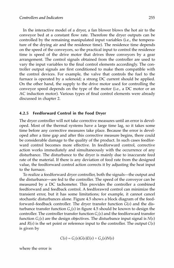
Controllers and Indicators 255
In the interactive model of a dryer, a fan blower blows the hot air to theconveyor bed at a constant flow rate. Therefore the dryer outputs can becontrolled by the remaining manipulated input variables (i.e., the tempera-ture of the drying air and the residence time). The residence time dependson the speed of the conveyors, so the practical input to control the residencetime is speed of the drive motor that drives three conveyors by a geararrangement. The control signals obtained from the controller are used tovary the input variables to the final control elements accordingly. The con-troller output signals are first conditioned to make them compatible withthe control devices. For example, the valve that controls the fuel to thefurnace is operated by a solenoid; a strong DC current should be applied.On the other hand, the supply to the drive motor used for controlling theconveyor speed depends on the type of the motor (i.e., a DC motor or anAC induction motor). Various types of final control elements were alreadydiscussed in chapter 2.
4.2.5 Feedforward Control in the Food Dryer
The dryer controller will not take corrective measures until an error is devel-oped. Most of the thermal systems have a large time lag, so it takes sometime before any corrective measures take place. Because the error is devel-oped after a time gap and after this corrective measure begins, there couldbe considerable damage to the quality of the product. In such cases feedfor-ward control becomes more effective. In feedforward control, correctiveaction works immediately and simultaneously with the occurrence of anydisturbance. The disturbance to the dryer is mainly due to inaccurate feedrate of the material. If there is any deviation of feed rate from the designedvalue, the feedforward control action corrects it by adjusting the heat inputto the furnace.
To realize a feedforward dryer controller, both the signals—the output andthe disturbance—are fed to the controller. The speed of the conveyor can bemeasured by a DC tachometer. This provides the controller a combinedfeedforward and feedback control. A feedforawrd control can minimize thetransient error, but it has some limitations; for example, it cannot cancelstochastic disturbances alone. Figure 4.5 shows a block diagram of the feed-forward–feedback controller. The dryer transfer function G(s) and the dis-turbance transfer function Gn(s) in figure 4.5 should be known to design thecontroller. The controller transfer function Gc(s) and the feedforward transferfunction G1(s) are the design objectives. The disturbance input signal is N(s)and R(s) is the set point or reference input to the controller. The output C(s)is given by
C(s) = Gc(s)G(s)E(s) + Gn(s)N(s)
where the error is
7244.book Page 255 Wednesday, June 21, 2006 11:14 AM

256 Measurement and Control in Food Processing
E(s) = R(s) – C(s) + G1(s)N(s)
so we get
C(s) = Gc(s)G(s)[R(s) – C(s)] + [Gc(s)G(s)G1(s) + Gn(s)]N(s)
The effects of N(s) can be eliminated by choosing Gc(s) so that
Gc(s)G(s)G1(s) + Gn(s) = 0
This gives the feedforward transfer function as
(4.6)
By proper design of the controller transfer function Gc(s), the feedforwardtransfer function G1(s) can be determined from equation 4.6.
Figure 4.6 shows the feedforward control scheme of a conveyor belt teadryer. In the feedforward control of the dryer, the air flow rate can becalculated from equation 4.5, which is used as set value of drying air flowrate. As per equation 4.5, the input and output variables that need to bemeasured are as follows:
• Temperatures of tea at inlet and outlet: Tp1 and Tp2
• Moisture content of tea at inlet and outlet: w1 and w2
• Humidity of drying air at inlet and exhaust: W1 and W2
• Temperature of drying air at inlet and exhaust: Ta1 and Ta2
• Feed rate of tea: Mp
FIGURE 4.5Block diagram of feedforward control of tea dryer.
G sG s
G s G sn
c1( )
( )( ) ( )
= −
Set point
TachometerG1(S)
Actuator
MoistureTransducer
DryerG(S)
Moisturecontent
Disturbance(change in conveyor speed)
R(S)
E(S)
C(S)
N(S)
ControllerGc(S)
Gn(S)
7244.book Page 256 Wednesday, June 21, 2006 11:14 AM

Controllers and Indicators 257
The temperature signals can be measured by sheathed thermocouples suit-able for the operating temperature range of the dryer (ambient to 150°C). Athermocouple will give a fairly linear response in this range of temperature.The most suitable moisture content sensor that can be used for measurementof tea moisture is an infrared sensor that can be used online and in a noninvasivemanner. Among various online humidity measuring techniques, the suitablemethod in this application will be an electronic dry- and wet-bulb psychrom-eter. The feed rate of tea in the conveyor can be detected by a tachometerconnected to the drive motor directly or through a gear arrangement.
4.2.5.1 The Control Functions
For calculation of the manipulated variable Ma using equation 4.5, the fol-lowing steps are involved:
A device calculates (Tp1 – Tp2) and then multiplies with Cpp to getCpp(Tp1 – Tp2).
FIGURE 4.6A schematic diagram of a feed-forward dryer control system.
Interface
MicrocomputerDisplay Plot
Operator Console
M
RH ma ω2 Tρ2Ta2
RH1Ta1Tρ1
mρ
ω1
2
Furnace
Collect
Input product
Exhaust air
hot air
7244.book Page 257 Wednesday, June 21, 2006 11:14 AM

258 Measurement and Control in Food Processing
The signals Tp1 and Tp2 are scaled properly to get (w1Tp1) and (w2Tp2) and asumming device adds them with the second term as negative input. Thesummed output is scaled by Cpw giving
Cpw(w1Tp1 – w2Tp2)
Cs1 and Cs2 values are calculated from the factor (1.005 + 1.88W). This canbe implemented by two scaled summers with a bias of 1.005. These valuesare used to calculate
(Cs1Ta2 – Cs2Ta1)
Finally, the manipulated variable Ma is calculated by two summers: onemultiplier and one divider. These operations can be done either by an elec-tronic controller or a computer. Various types of electronic controllers areavailable that are discussed briefly next.
4.3 Electronic Controllers
Implementation of a specific controller can be achieved in various waysdepending on the complexity, reliability, and cost factors. Mechanical or pneu-matic controllers are still in use in many applications despite their disadvan-tages. Electronic and computer control techniques are becoming more popular.Electronic analog controllers are widely used for the following reasons:
1. Electrical signals are easy to transmit over a long distance.2. Digital computers are compatible with electrical signals only.3. Electrical and electronic devices are almost maintenance free and
free from leakage, wear and tear, and so on.4. Intelligent and adaptive controllers can be designed with electrical
systems.5. Electrical systems are less expensive, require less space, and are easy
to install and operate.
Operational amplifiers are versatile in designing electronic controllers dueto their various analog computational facilities like summation, subtraction,multiplication, integration, differentiation, squaring, relational operations,and so on.
A common operation in a controller is error detection. A differential ampli-fier can be used in inverting mode with the signal voltage applied to theinverting terminal and the set-point voltage to the noninverting terminal(fig. 4.7A). The feedback resistor value can be adjusted to get an amplification
7244.book Page 258 Wednesday, June 21, 2006 11:14 AM

Controllers and Indicators 259
factor based on the sensitivity of the transducer, but if the transducer outputhas already been amplified by the transmitter, further amplification mightnot be required.
Analog controllers need to compute the control signal by using a controllaw. The complexity of the control law determines the complexity of thecircuit. For example, a proportional controller amplifies the error signal bya proportional gain whereas a PID controller must cascade with the propor-tional amplifier, an integrator, and a differentiator with proper gain con-stants. Analog computations like summation, subtraction, integration, anddifferentiation can be performed by operational amplifiers of various types.The basic forms of the circuits are shown in figure 4.7B–E.
Performing control operations often requires generating a signal based ona relation between an input signal and a reference signal. The relationalsignals are an equality signal, a greater than signal, and a less than signal.
Such signals are used to trigger a control component like a relay, motor,or solenoid. For relational operation an op-amp comparator circuit is usedwhere the inputs are applied to the two input terminals and the op-amp isoperated in open-loop mode (fig. 4.7F). The output changes from –Vcc to +Vcc
when the signal applied to the noninverting terminal becomes equal and
FIGURE 4.7Operational amplifier circuits for controller design. (A) Error detection; (B) Summer; (C) Sub-stractor; (D) Integrator; (E) Differentiator; (F) Comparator
R
Vi
Vi
V1
V2Ve
Vset
R
RR
R R
R
R
R
R
R
R
R
ViVo
Vi
Vref
+V
–V
C
C
A B
V1
V2
C D
E F
(V1 + V2)
(V1 – V2) Vo = 1 VidtC ∫
Vo = RCdVi
dt
7244.book Page 259 Wednesday, June 21, 2006 11:14 AM

260 Measurement and Control in Food Processing
greater than the signal applied to the inverting terminal. Thus dependingon relational signal needed (i.e., greater than or less than), the input signaland the reference signal should be properly connected. A signal based ononly the relational operator “equal” can be generated by applying the out-puts obtained from “greater than” and “less than” relational circuits to adigital logic circuit.
4.3.1 On–Off Controller
A two-position or on–off controller generates a control signal based on arelational condition of the input signal with a reference signal (i.e., greaterthan or less than). Due to oscillations of the output of the process for con-tinuous on–off action generated by the single reference on–off controller, anon–off controller with a differential gap is more suitable. In this type, twoset point or reference levels are imposed on the controller: an upper referencelevel and a lower reference level. An operational amplifier circuit implement-ing this operation is shown in figure 4.8. The upper comparator generates asignal transition from low to high (e.g., from 0 V–5 V) when Vin crosses thelevel of lower set point VL and the lower does the reverse; that is, the outputtraverses from high to low (e.g., 5 V–0 V) when the input crosses the upperset-point level VH. A logical operation of the outputs from the two compar-ators gives the on–off controller output with a differential gap. The controllercan be made to act in reverse by reversing the comparators.
4.3.1.1 Bimetallic Thermal On–Off Controller
Another convenient form of on–off controller used in thermal devices is thebimetallic strip controller. The temperature sensors discussed in chapters 2and 3 fall under electrical types that generate an electrical signal proportionalto temperature. In many applications in which a physical contact or defor-mation signal proportional to temperature is essential, bimetallic strip sen-sors are useful. Liquid expansion type temperature sensors also work by asimilar principle of thermal expansion, but bimetallic sensors are more pop-ular due to their inherent advantages. The most important advantage is thatdue to its conductivity to electricity the strip can be used as a thermal switch.
FIGURE 4.8Block diagram of an on–off controller.
Input signal
Lower setlevel
Higher setlevel Comp 1
Comp 2
Logic circuit(Controller)
Control output
ON/OFF
7244.book Page 260 Wednesday, June 21, 2006 11:14 AM

Controllers and Indicators 261
The sensor serves two purposes at the same time: a temperature sensor andalso an electrical switch. Although this sensor performs temperature sensingwith lower accuracy, higher hysteresis, and slow response, the sensor is usedin numerous applications of on–off temperature controls.
When two metal strips made of two materials and with two differentthermal expansion coefficients are bonded together, it forms a bimetallicthermal strip sensor. As shown in figure 4.9, when one end of the strip isfixed and the other end is free and the strip is heated, it bends downwardif the thermal expansion coefficient of the lower strip is smaller than that ofthe upper strip. The strip thickness and the deflection are exaggerated in thefigure; in practice the deflection is very small.
Many household and industrial thermal systems like ovens, air condition-ers, refrigerators, and so on employ a bimetallic strip switch to implementan on–off controller. From figure 4.9 it is understood that when the bimetalstrip bends downward it closes an electrical switch. The switch remains inthis closed position until the bimetal strip is cooled and returns to its originalset-point level position. Hence a temperature signal is sensed and made toactuate a control component like a solenoid valve, control motor, and so on.The switch can be used to actuate two different devices above and belowthe set-point level.
4.3.2 Controller Modes
The basic concept of conventional and linear controllers was discussed inchapter 1. In this section their mathematical representation and implemen-tation by analog circuits are presented.
4.3.2.1 Proportional Controller
The theory behind a proportional control action was discussed in chapter 1.The response equation of the controller is given by
P = Kpe + p0 (4.7)
FIGURE 4.9Schematic diagram of a bimetallic strip on–off switch.
Normal High temperature Low temperature
Bimetallic strip
ONOFF
ONOFF
Common
7244.book Page 261 Wednesday, June 21, 2006 11:14 AM

262 Measurement and Control in Food Processing
where P = proportional control output (0%–100%)Kp = proportional gain
e = error as a percentage of range of variablese0 = control output with no error
To implement equation 4.7 the op-amp circuit involved is a summingamplifier with a gain to each part selected by resistors, as shown in figure4.10. Therefore an equivalent voltage equation of the circuit in the line ofequation 4.7 can be written as
V = AVe + V0 (4.8)
where V = controller output voltageA = amplifier gain to input error = R2/R1
The correspondence between the output range, input range, and the pro-portional band of the controller should be determined prior. For example,for varying a servo-controlled valve operating in the range of 0 V–5 V (fullyclosed to fully open), a swing to 75% refers to (0.75)(5.0) = 3.75 V. Similarly,for a dryer, the moisture content of the product is measured and controlledin the range of 3% to 6%, which is converted by a moisture sensor to a voltageof 1 V to 4 V. The span or range of the signal is (4 – 1) = 3 V. Thus the physicalvariable versus electrical voltage correspondence is
On the other hand, proportional gain Kp determines the relation betweenthe error and the controller output. Let us assume that Kp = 5% per 1% errorwith the voltage ranges mentioned earlier. As per the value of Kp, the con-troller adjustment should be 5% for a 1% change in the error. This means fora change of (0.01)(3.0) = 30 mV in input voltage the controller output should
FIGURE 4.10Proportional controller circuit.
=−
=
36 3
1
Volt
Volt moisture
( )%
/ %.
Ve
Vo
R2
R1
R
R
R2
V
7244.book Page 262 Wednesday, June 21, 2006 11:14 AM

Controllers and Indicators 263
be changed by (0.05)(5.0) = 250 mV. Therefore the gain of the amplifier (A)should be equal to (250/30) = 8.33. This can be obtained by tuning the ratioof the feedback resistor and the input resistor of the op-amp amplifier circuitto 8.33.
4.3.2.2 Integral Controller
The output equation of an integral controller is given by
(4.9)
where p(t) = controller output , % of full scaleKI = integral gain ( s–1)
ep(t) = error in percentage from full scale valuepI(0) = controller output at t = 0
When realizing equation 4.9 in an op-amp circuit (fig. 4.11), the correspond-ing voltage equation is given by
(4.10)
where V0 = output voltageA = integral gain = 1/RCVe = error voltage
V0(0) = initial output voltage
The rate of the integral controller is determined by the integration timeconstant. If the integral gain KI is too large, the output increases very fast,producing oscillations before settling. The gain implies that a 1% change inthe error causes an output that changes KI% per second. Let the controller
FIGURE 4.11Integral controller circuit.
p t K e t dt pI p I
t
( ) ( ) ( )= +∫ 00
0 0V A V dt Ve
t
0
0= +∫ ( )
Ve
R2
R1
R1
Vout
C
7244.book Page 263 Wednesday, June 21, 2006 11:14 AM
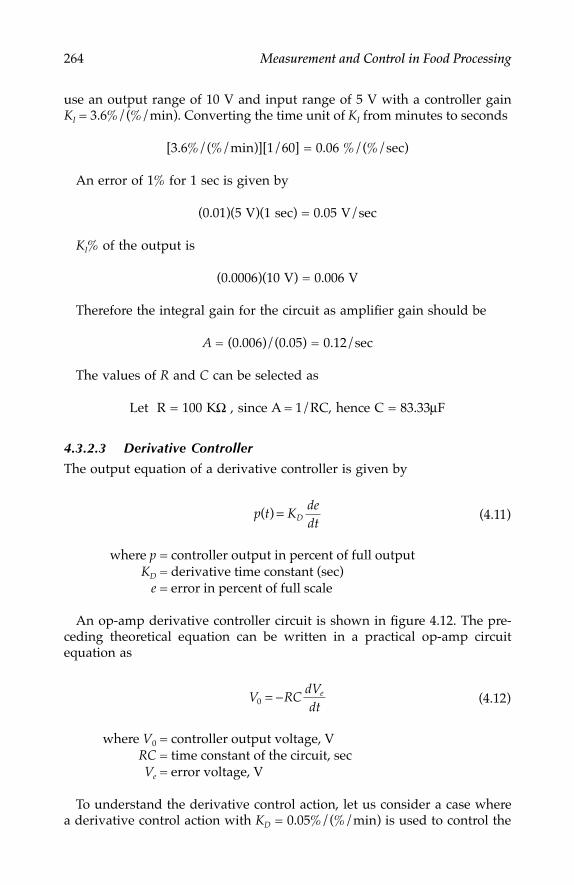
264 Measurement and Control in Food Processing
use an output range of 10 V and input range of 5 V with a controller gainKI = 3.6%/(%/min). Converting the time unit of KI from minutes to seconds
[3.6%/(%/min)][1/60] = 0.06 %/(%/sec)
An error of 1% for 1 sec is given by
(0.01)(5 V)(1 sec) = 0.05 V/sec
KI% of the output is
(0.0006)(10 V) = 0.006 V
Therefore the integral gain for the circuit as amplifier gain should be
A = (0.006)/(0.05) = 0.12/sec
The values of R and C can be selected as
Let R = 100 KΩ , since A = 1/RC, hence C = 83.33µF
4.3.2.3 Derivative Controller
The output equation of a derivative controller is given by
(4.11)
where p = controller output in percent of full outputKD = derivative time constant (sec)
e = error in percent of full scale
An op-amp derivative controller circuit is shown in figure 4.12. The pre-ceding theoretical equation can be written in a practical op-amp circuitequation as
(4.12)
where V0 = controller output voltage, VRC = time constant of the circuit, secVe = error voltage, V
To understand the derivative control action, let us consider a case wherea derivative control action with KD = 0.05%/(%/min) is used to control the
p t KdedtD( ) =
V RCdVdt
e0 = −
7244.book Page 264 Wednesday, June 21, 2006 11:14 AM

Controllers and Indicators 265
viscosity of chocolate by controlling the flow of lecithin (derived from oil-seed) for a maximum period of 2.0 sec. The viscometer output range is 0.4V to 2.0 V and the controller output range is 0 V to 5.0 V. The derivative gainexpressed in units of seconds is
[0.05 %/( %/min)](60) = 3.0 %/( %/sec)
This means that a 1% change in viscosity should change controller outputby 3.0% per sec. The 1% of the input is
0.01(2.0 – 0.4) = 0.016 V/sec
and therefore 3.0% of the output means
0.03(5) = 0.15 V
The derivative time constant is
RC = 0.15/0.016 = 9.37 sec in the op-amp circuit.
Taking the value of C = 20 µF, the value of
R = 468.5 KΩ
It was mentioned in chapter 1 that each control mode has its advantagesand disadvantages and using a single control mode is not recommended.The best way is to combine the control modes like proportional plus integral(PI), proportional plus derivative (PD), or proportional plus derivative plusintegral (PID) mode. These combined control modes can be implemented bycascading the op-amp circuits in tandem.
4.3.3 Fan Direction Control in Food Withering
It has already been mentioned that food dehydration is a controlled processfor removing moisture from food. Although the principal aim of food dehy-dration is to reduce weight or volume for preservation and transportation,
FIGURE 4.12Derivative controller circuit.
R2
R1
Ve
Vout
C
7244.book Page 265 Wednesday, June 21, 2006 11:14 AM

266 Measurement and Control in Food Processing
there can be other specific reasons in some foods. For example, in tea pro-cessing, withering is a process of dehydration in which the freshly pickedtea leaves are withered in withering troughs by blowing air for about 10 to12 hr. The principal aim of withering is to expedite the chemical changestaking place in the leaf cells, which is called chemical wither. If the tea leavesare not withered, it takes 15 to 20 hr to complete chemical withering. More-over, tea processed from long chemical wither is less valuable than teaobtained from controlled chemical withering for 10 to 12 hr.
The withering time varies depending on the relative humidity of the sur-rounding air, temperature, and flow velocity of the withering air. The mois-ture released from the tea accumulates over the trough during withering andgradually the air becomes more saturated with moisture. Over the course oftime, say 2 to 3 hr, less moisture can be released from the tea and the processslows. Therefore the saturated air is required to be sucked out so that freshair can replace it. To do so, normally the withering fan direction is reversedseveral times during withering [2]. This process is shown in figure 4.13.Traditionally fan direction reversal is performed manually at assumed reg-ular intervals. In this manual method, three-phase supply to the inductionmotor is connected to the starter through a phase change switch. The direc-tion of the motor is reversed when any two phases of the supply are inter-changed. With the help of a phase changeover switch, the connection of oneof the three phases is kept fixed as the other two phases are interchanged.The manual method of fan speed reversal is not recommended because ifwithering is continued beyond the time of air saturation, rate of release ofmoisture becomes slow. To avoid loss of time, energy, and quality, fan direc-tion control operation should be done at the correct time for a correct dura-tion. To circumvent this problem an automated withering fan speed reversaltechnique for the tea industry was developed by Bhuyan [1].
The device works on the principle of a simple closed-loop control systemin on–off controller mode. The RH of the air above the withering trough isthe key factor for the control device. An electrical transducer continuouslymeasures this RH and the signal is used for generating a command signalusing a comparator. The comparator compares the RH signal with two set-point levels, one high and the other low. When the RH signal is above the
FIGURE 4.13Schematic diagram of air flow in tea withering: (A) air blowing; (B) air sucking.
GTLMoisture
Roof
Mesh
Trough
Fan Fan
A B
7244.book Page 266 Wednesday, June 21, 2006 11:14 AM

Controllers and Indicators 267
high level, the comparator sends a signal, REVERSE, to a logic control circuit.However, before reversing, the braking of the motor has to be performed forat least 20 sec and then the motor has to be stopped. If the RH value is lessthan the low level, the motor has to be run in forward direction, sending asignal, FORWARD, to the logic control circuit. Therefore the following logicwas used to develop the command signal:
1. When RH > high, Command = REVERSE2. When RH < low, Command = FORWARD
Here REVERSE and FORWARD states can be any conventional digital logiclevels, which are most commonly 0 V and 5 V for transistor–transistor logic(TTL) technology. This command signal is used to generate the final logicstate signals for the power control circuits. The power control circuit consistsof controlled switches (commonly relays) triggered by the logic state signalsto reverse the connection of any two phases of the power supply to the motor.The connection of the induction motor to the three-phase supply throughthe controlled switch array is shown in figure 4.14.
Switches SW1 and SW2 are complementary for a particular direction ofthe motor, so that when SW1 is closed, SW2 should be open and vice versa.SW3 must be closed for running the motor in both directions. Table 4.2 is a
FIGURE 4.14Switch array for motor reversing: (A) conventional device; (B) relay circuit.
R
Y
B
SW1
SW2
SW3
SW2
SW1
R(Y)
B
Y(R)
Ph1
Ph2 Ph3
Induction motor
R
Y
B
B
R(Y) Y(R)
3 Φ supply
Electromagnetic relay
Insulator
Induction motor
Phase change switch
A
B
7244.book Page 267 Wednesday, June 21, 2006 11:14 AM

268 Measurement and Control in Food Processing
state table of the switches and phases. Hence, properly closing and openingthe switches supplies the motor with supply phases either in the sequenceRBY or RYB for forward and reverse directions, respectively. This phasereversal is mediated by a power control circuit. A block diagram of thecontroller is shown in figure 4.15A.
4.3.3.1 The Relay Circuit
The function of the relay circuit is to interchange the supply of any two ofthe three phases and keeping the third phase fixed. The circuit consists offive electromechanical relays. The logic table for the relay coil signals (S1–S3),relay states (RL1–RL5), and directions are shown in table 4.3.
4.3.3.2 Logic Control Circuit
The requirement of the logic control circuit is that when the command signalfrom the comparator undergoes a transition from low to high or from highto low, the logic circuit generates signals for triggering the right set of relays.
TABLE 4.2
State Table for Switches and Phases
Switches Supply PhasesDirection SW1 SW2 SW3 Ph1 Ph2 Ph3
Forward 1 0 1 R B YStop 0 0 0 0 0 0Reverse 0 1 0 Y B R
FIGURE 4.15Withering fan reversal controller: (A) block diagram representation; (B) basic control block; (C)logic control circuit.
Forward
Reverse
RhUpper set point
Lower set point
3-Φpower control Fan
Witheringthrough
Rh measurementComparatorLogiccontrol
Command Logiccontrolcircuit
Powercontrolcircuit
R Y B
R(Y)BY(R)
A
B
7244.book Page 268 Wednesday, June 21, 2006 11:14 AM

Controllers and Indicators 269
The circuit that performs this function is shown in figure 4.17. The circuitconsists of two parts, a delay circuit and a gate control circuit.
The delay circuit is clocked by a timer. The switching transistors generatehigh spikes that are applied to the trigger terminal of the timer. When thecommand signal changes state from 0 V to 5 V, transistor T1 gives a positivespike to the input trigger and the timer produces a delay of 20 sec. This delayis set by the time constant of an RC circuit externally connected to the timer.Similarly, when the command signal changes from 5 V to 0 V, transistor T2
generates the spike, producing a delay of 20 sec.When the command signal changes value from 0 V to 5 V, the output of
the timer remains low for 20 sec, resulting in the relay trigger signal beinglow for 20 sec, after which the motor is stopped. After 20 sec the output ofthe timer becomes high. Because the command is already high, the triggersignals RL1 and RL2 are high but RL3 is low. On the other transition of thecommand signal, RL2 and RL3 become high but RL1 remains low (table 4.3).
4.3.3.3 The Comparator Circuit
The comparator circuit is designed to generate the command signal corre-sponding to the value of the RH values. The command signal is generatedwith the following logic in mind:
1. When the RH exceeds the upper set level (SPH), the command signalchanges from 0 V to 5 V.
2. When the RH decreases below the lower set level (SPL) the commandsignal changes from 5 V to 0 V.
The timing diagram of the logic states with RH values is shown in figure4.16. Two comparators generate outputs C1 and C2 based on the level of RHwith respect to the set levels. The comparator outputs are applied to an RSflip-flop to trigger it as per the state table. The operation of the RS flip-flopas command signal generator is shown in table 4.4.
It is evident that a positive transition of C1 triggers the command signalgenerator for positive transition and negative transition of C2 triggers fornegative transition of the command signal. The flip-flop is set when RHexceeds SPH because at this transition the comparator output becomes high.It resets when RH decreases below SPL.
TABLE 4.3
State Table for the Relay Circuit
Relay Coil Signals Relays Supply PhasesS1 S2 S3 RL1 RL2 RL3 RL4 RL5 Ph1 Ph2 Ph3
0100
0101
0001
0100
0001
0101
0100
0001
0R0Y
0Y0B
0B0R
7244.book Page 269 Wednesday, June 21, 2006 11:14 AM
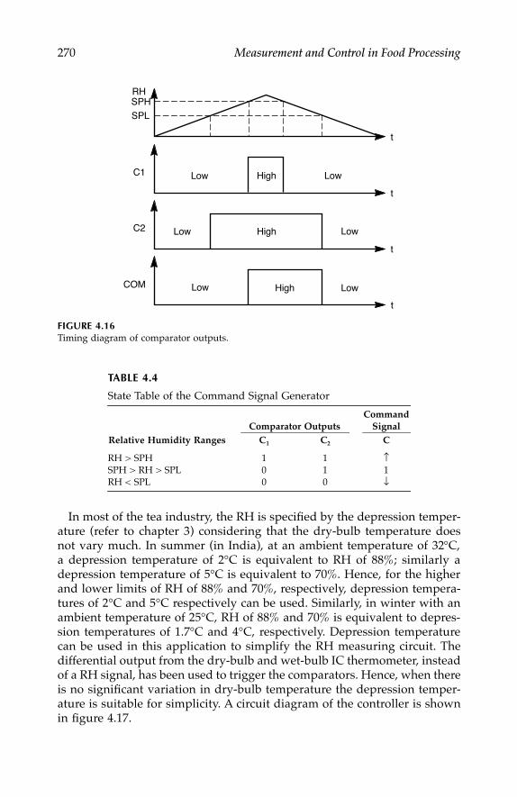
270 Measurement and Control in Food Processing
In most of the tea industry, the RH is specified by the depression temper-ature (refer to chapter 3) considering that the dry-bulb temperature doesnot vary much. In summer (in India), at an ambient temperature of 32°C,a depression temperature of 2°C is equivalent to RH of 88%; similarly adepression temperature of 5°C is equivalent to 70%. Hence, for the higherand lower limits of RH of 88% and 70%, respectively, depression tempera-tures of 2°C and 5°C respectively can be used. Similarly, in winter with anambient temperature of 25°C, RH of 88% and 70% is equivalent to depres-sion temperatures of 1.7°C and 4°C, respectively. Depression temperaturecan be used in this application to simplify the RH measuring circuit. Thedifferential output from the dry-bulb and wet-bulb IC thermometer, insteadof a RH signal, has been used to trigger the comparators. Hence, when thereis no significant variation in dry-bulb temperature the depression temper-ature is suitable for simplicity. A circuit diagram of the controller is shownin figure 4.17.
FIGURE 4.16Timing diagram of comparator outputs.
TABLE 4.4
State Table of the Command Signal Generator
Comparator OutputsCommand
SignalRelative Humidity Ranges C1 C2 C
RH > SPH 1 1 ↑SPH > RH > SPL 0 1 1RH < SPL 0 0 ↓
Low High
RHSPH
SPL
t
t
t
t
C1
C2
COM
High
High
Low
LowLow
Low Low
7244.book Page 270 Wednesday, June 21, 2006 11:14 AM

Controllers and Indicators 271
4.3.4 Cooling Surface Area Control in Chocolate Tempering
In chocolate manufacturing, tempering of chocolate is an important issue.Although chocolate tempering is theoretically very simple, it requires a greatdeal of experience, skill, and technique so that the chocolate is suitable forthe molding plant or enrober. Chocolate tempering requires sufficient coolingto form crystals; hence, temperature control during tempering is very essen-tial. Various chocolate tempering machines are available with electronic con-trollers. For example, the MSV Turbo model incorporates a new automaticcapacity control system. This control adjusts the cooling surface area basedon deviation of flow rate and temperature of chocolate. This ensures a uni-form degree of temper throughout the process. Additionally, the machineprovides a continuous cooling curve sampling unit. The machine is auto-mated by a programmable logic controller (PLC) with automatic startup.
4.4 Flow Ratio Control in Food Pickling Process
In preservation of foods, acetic acid is the main acid constituent found invinegars. The commercial name of this preservative is glacial with 99% to100% acid. Acetic acid is used in pickle and sauce manufacturing alone orwith vinegar. Lactic acid is also an important edible acid used in brining
FIGURE 4.17Withering fan reversal controller circuit.
+5V
+5V
+5V
+5V
1KΩ
1KΩ
1KΩ
1KΩ
1000µ
1000µ
1000µ
1.0µ
20KΩ
1
2
4
5
6
3
7
8 G1
G2
G3
ON/OFF
Command signal
T1
T2
555
AND gates
7244.book Page 271 Wednesday, June 21, 2006 11:14 AM

272 Measurement and Control in Food Processing
preservation of vegetables. The process of adding vinegar or acetic acid toa permitted ratio with water in a tank is called pickling. Controlling a properratio of fruit, pectin, acid, and sugar is also an important task in jam andjelly making. In such situations a fixed ratio between the flow rates of thetwo (or three) liquids is to be controlled. During food pickling, acid to waterratio, acid to pectin ratio, or water to brine ratio has to be controlled at aprespecified value. A strict adherence to the accurate proportion minimizesthe use of preservatives.
4.4.1 Ratio Controller
A schematic diagram of the flow ratio control in a pickling tank is shown infigure 4.18. For example, in this application the flow of acid is to be controlledat a preset ratio to flow of water. The flow of water is measured by a flowtransmitter and is applied to a ratio relay multiplier, which multiplies theflow of water by a preset factor. The output of the ratio relay is applied tothe flow controller along with the acid flow signal in a ratio. The voltagesignal and ratio factor of the control action can be expressed by the equations
(4.13)
and
(4.14)
where Vro = voltage signal from ratio relayK = preset factor of ratio relayR = ratio factor
Qa = flow of acid (to be controlled)Qw = flow of water
FIGURE 4.18Schematic diagram of a pickling ratio controller.
V KQro w=
RQQ
a
w
=
FT
FC
FT
WaterPectin, sugar etc.
Acid
Food picklingtank
Flowvalve
---------------------
7244.book Page 272 Wednesday, June 21, 2006 11:14 AM

Controllers and Indicators 273
To maintain the ratio, the flow of water is calculated at a set point by apreset factor. When the flow of water deviates from a set-point level, it foulswith the ratio relay deviating its output also as per equation 4.13. In turnthis deviated output signal calculates the controller output according toequation 4.14. Therefore the flow rate of acid is automatically compensatedor adjusted to the predetermined ratio. To understand the operation we canassume some numerical values. Let the maximum flow rate of water be 100liters per minute (lpm) and that of acid be 50 lpm. The ratio relay is adjustedto a ratio of 1:1, which means that a measured signal of 1 lpm flow of watermakes the controller allow an 0.5 lpm flow of acid; that is, if 60 lpm of waterflows then 30 lpm of acid will also be allowed to flow. Again if the ratiofactor changes to 1:2, then for 60 lpm of water flow, 120 lpm of acid willflow. Now, if the maximum flow rate of acid decreases to 25 lpm (the ratiofactor already set to 1:1) then a new ratio factor of 1:2 will be established inthe controller that changes the flow rate of acid from 25 lpm to 12.5 lpm.Hence, the ratio factor is established based on the range of the flow trans-mitters and the multiplying factor set into the ratio relay. Generally a flowrange is chosen so that the ratio factor is set at the middle.
The flow meters recommended for this application are differential pressuretransmitter type, turbine flow meter, or magnetic flow meters. Magnetic flowmeters will be more suitable for the acid line than the water line. In the caseof a differential pressure transmitter using an orifice type restriction, theoutput signal will be proportional to the square root of the flow rather thangiving a linear relationship. If the ratio relay factor is to be set to 0.5:1 to 5:1,then in case of orifice flow metering, the actual flow ratios will be
[(0.5/1)1/2] to [(5/1)1/2] = [0.70:1] to [2.23:1]
Use of two output modes of flow meters (i.e., square root and linearlyproportional) is not recommended unless one is converted to the other mode.Controlling the ratio between more than two flow signals will require a morecomplicated ratio control system.
4.4.2 Control Valves
A food process control operation involves, in most cases, control of manip-ulated variables like flow of raw materials and intermediate products fromone point to another. In many applications the flow control requires controlof variables like density, viscosity, and composition. The control signalsgenerated, based on some quality parameters of the product, are applied tothe control valve to regulate the manipulated inputs. A control valve regu-lates materials to a process by opening or closing a variable orifice in apipeline. The word material in food processing denotes either gases or liquids,but in most cases the material handled is in liquid, pasty, or semisolid phase.
Flow rate in food processing is generally expressed in volume per unit oftime and mass flow rate is very seldom used. Mass flow rate is related
7244.book Page 273 Wednesday, June 21, 2006 11:14 AM

274 Measurement and Control in Food Processing
primarily to the density of the food material. The volume flow rate of amaterial through a pipe is expressed as
Q = Av (4.15)
where Q = Flow rate (m3/sec)A = Area of pipe (m2)v = Flow velocity (m/sec)
Obviously equation 4.15 indicates that the flow rate can be varied byvarying the cross-sectional area of the flow line. If we can provide a systemby which the cross-sectional area can be varied using a variable-sized restric-tion, as shown in figure 4.19, the flow rate can be controlled. Figure 4.19shows that when the stem and plug moves up and down, the area of therestriction increases and decreases, respectively. Bournoulli’s theorem estab-lishes the pressure drop developed in the valve opening by the equation
(4.16)
where K = proportionality constant (m3/sec/Pa 1/2)∆p = p2 – p1 = pressure drop (Pa)
The proportionality constant is determined mainly by the size and geom-etry of the valve opening; however, the flowing material also influences thisconstant to some extent.
4.4.2.1 Types of Control Valves
The performance of a valve is normally specified by many factors and fea-tures but the primary factor of the classification of valves is the relationbetween valve stem position (stroke) and the flow rate. Valves are classifiedinto three different types based on this relation between the stem position(as percentage of full stroke) and flow rate (as percentage of full range). Thefollowing are three different types of control valves:
FIGURE 4.19Cross-sectional view of a control valve.
FluidFlow
Stem
Plug
Valve casing
Seat
Q K p= ∆
7244.book Page 274 Wednesday, June 21, 2006 11:14 AM

Controllers and Indicators 275
1. Quick opening: In this type of valve a small opening results inmaximum possible flow rate. As soon as the valve stem is movedby a small amount, say 30%, the flow rate jumps to 90% in this typeof valve.
2. Linear valve: This type of valve presents a linear variation of flowrate with stem travel.
3. Equal percentage: In many situations it is required that at a givenpercentage change in stem travel the flow rate also should changeby the same percentage. Here the flow rate does not become zero atmaximum stem travel to close the valve and this can be specified asQmin. When the valve is fully open it gives the maximum flow rate(Qmax). The range can be defined as
(4.17)
The characteristic of this valve is exponential and the flow rate can beexpressed as
(4.18)
where S = the stem travel
For example, in an equal percentage valve, maximum flow rate is 100 cm3/sec and minimum is 2 cm3/sec. The full stem travel of the valve is 3 cm. Therange is
R = (100cm3/sec)/(2 cm3/sec) = 50
The flow rate at any valve travel, say at 2 cm, can be determined as
Q = Qmin RS/Smax = (2 cm3/sec)(50)2cm/3cm = 27.14 cm3/sec
Figure 4.20 shows an electronically controlled valve manufactured byOmega Engineering, Inc. (USA).
4.4.2.2 Valve Sizing
The performance of a control valve depends on its design to the requiredspecifications. An oversized valve will fail to block the fluid even at thehigher side of the closing due to less effective resistance. Thus, it becomesdifficult to control the fluid. Moreover, it is not economical to use an over-sized valve for the same flow of liquid. Again, if the valve is undersized itwill not pass the necessary flow and a problem of plugging occurs. From a
RQQ
= max
min
Q Q RS S= min/ max
7244.book Page 275 Wednesday, June 21, 2006 11:14 AM

276 Measurement and Control in Food Processing
design point of view, the liquid volumetric flow rate can be defined by anequation as
(4.19)
where Cv = Valve flow coefficient∆p = Pressure across the valveSG = Specific gravity of the liquid
Values of Cv for different sizes of valves are shown in table 4.5.
FIGURE 4.20Photograph of an electronically controlled valve (Model PV14). © Omega Engineering, Inc, Allrights reserved. (Reproduced with the permission of Omega Engineering, Inc., Stamford, CT06907; www.omega.com).
TABLE 4.5
Valve Flow Coefficients
Valve Sizes (in.) Cv
0.25 0.30.50 31.00 141.50 352.00 553.00 1084.00 1746.00 4008.00 725
Q Cp
SvG
= ∆
7244.book Page 276 Wednesday, June 21, 2006 11:14 AM

Controllers and Indicators 277
4.5 Atmosphere Control in Food Preservation
Food preservation is mainly aimed at controlling growth of microorganismslike bacteria, yeasts, and molds. In addition to use of preservatives, anacceptable atmospheric condition also contributes a lot to food preservation.For example, fruits and vegetables can be preserved well if their respirationrate is reduced by reducing the oxygen content of the storage atmosphereand increasing the carbon dioxide content. However the required levels ofoxygen and carbon dioxide content can vary for different fruits and vegeta-bles. Oxygen content not only reduces respiration, but it also limits oxidationspoilage in oxidation-sensitive products like coffee, nuts, and others. Carbondioxide levels can be increased by adding the gas in liquid or gas form, butreduction requires scrubbing the air. Scrubbing can be done by passing theair through bags of solid calcium hydroxide or through a spray of causticsoda. Ripening of fruits like bananas or tomatoes can be controlled by reduc-ing ethylene levels in the storage atmosphere.
Moisture in the storage environment inhibits growth of microorganismsin food.Therefore humidity of the air plays an important role in food storagepreservation. Equilibrium RH of a substance indicates how hygroscopic thesubstance is. The equilibrium RH of a substance is the humidity value of theair at which the substance neither absorbs nor releases moisture.
Temperature of the surrounding air also matters for food spoilage. At lowertemperatures the biochemical degradation of food is low. However, this isnot true for all types of food. There are numerous examples of how foodstorage at low temperature spoils foods; for example, low temperatures inmeat freezing damages the muscle cells, and tissue cell breakdown takesplace in apples. Therefore temperature measurement and control is an impor-tant strategy in food preservation.
4.5.1 Control Scheme
Control of atmospheric storage air parameters as mentioned earlier shouldbe performed, keeping economic considerations in mind. From a controlpoint of view, the atmospheric storage control problem is well defined anddistinct and can be addressed by a noninteractive MIMO structure as shownin figure 4.21. Here the control scheme consist of four individual controlloops that are noninteractive.
Measurement and control of temperature and humidity have already beendiscussed. Two new parameters, oxygen and carbon dioxide, are included inthis application. On-line detection of oxygen can be performed by high zirco-nium oxide (voltage or current mode) fuel cells. These detectors do not requirea sampling system and the probes can be inserted directly into the process.Probes are available in lengths from 1.5 ft to 12 ft and should be inserted intothe process at the most representative region. Measurement ranges of these
7244.book Page 277 Wednesday, June 21, 2006 11:14 AM

278 Measurement and Control in Food Processing
detectors are 0% to 100%. Another suitable and more sensitive oxygen detectorfor this application is the galvanic detector, but this type of detector requirestemperature and gas flow rate compensation. Carbon dioxide gas detectioncan be performed using nondispersive infrared analyzers or mid-IR filter ana-lyzers, which are available in cell or probe structure. MOS-based gas sensorsare also available in a variety of forms and ratings. These sensors are mostlygeneral gas sensors in terms of selectivity and sensitivity and so calibrationfor a particular gas has to be performed by trial.
The controllers to drive the actuators and control valves shown in figure4.21 can be implemented by electronic controllers, but microprocessor- ormicrocomputer-based controllers can also be used. Simple proportional con-trollers suffice for the control problem because the signals are mostly theslow-varying type without many jumps.
4.6 Timers and Indicators in Food Processing
Earlier it was mentioned that a food processing industry can adopt either acontinuous or batch processing system. Most chemical- and petroleum-basedindustries adopted batch processing earlier but gradually realized that a con-tinuous process is more efficient and cost effective. Most food processing indus-tries prefer batch processing to continuous processing due to the many inherentbiochemical factors of food. In batch processing, a particular intermediate
FIGURE 4.21Schematic diagram of a storage atmosphere control system.
HT
OT
HC
OC
CO2C
CO2T
M TC
TT
Set
Set
Dehumidifier
Oxygen
Carbon dioxide
Storage trays
Storage air
Set
Set
7244.book Page 278 Wednesday, June 21, 2006 11:14 AM
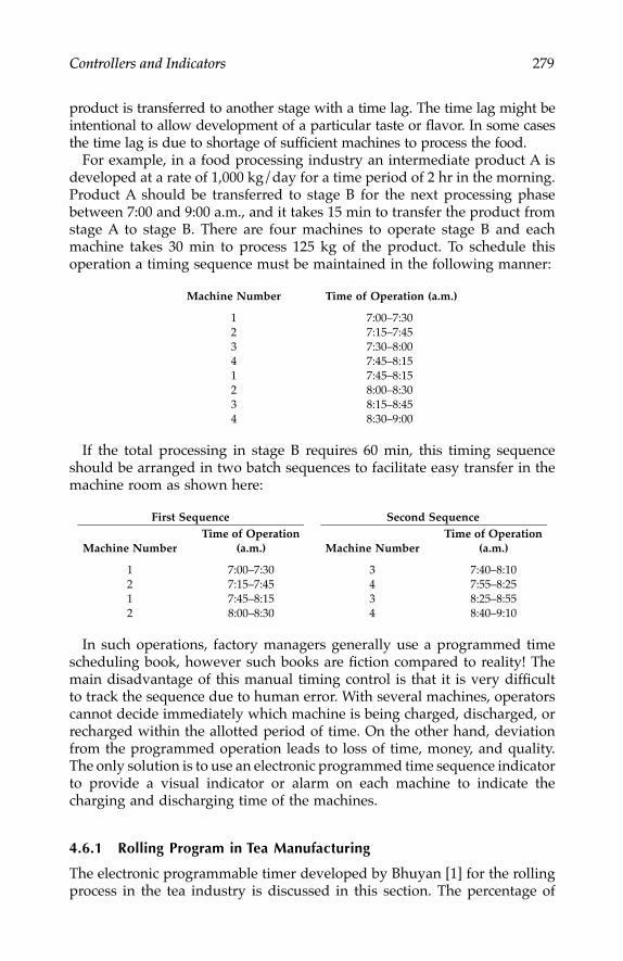
Controllers and Indicators 279
product is transferred to another stage with a time lag. The time lag might beintentional to allow development of a particular taste or flavor. In some casesthe time lag is due to shortage of sufficient machines to process the food.
For example, in a food processing industry an intermediate product A isdeveloped at a rate of 1,000 kg/day for a time period of 2 hr in the morning.Product A should be transferred to stage B for the next processing phasebetween 7:00 and 9:00 a.m., and it takes 15 min to transfer the product fromstage A to stage B. There are four machines to operate stage B and eachmachine takes 30 min to process 125 kg of the product. To schedule thisoperation a timing sequence must be maintained in the following manner:
If the total processing in stage B requires 60 min, this timing sequenceshould be arranged in two batch sequences to facilitate easy transfer in themachine room as shown here:
In such operations, factory managers generally use a programmed timescheduling book, however such books are fiction compared to reality! Themain disadvantage of this manual timing control is that it is very difficultto track the sequence due to human error. With several machines, operatorscannot decide immediately which machine is being charged, discharged, orrecharged within the allotted period of time. On the other hand, deviationfrom the programmed operation leads to loss of time, money, and quality.The only solution is to use an electronic programmed time sequence indicatorto provide a visual indicator or alarm on each machine to indicate thecharging and discharging time of the machines.
4.6.1 Rolling Program in Tea Manufacturing
The electronic programmable timer developed by Bhuyan [1] for the rollingprocess in the tea industry is discussed in this section. The percentage of
Machine Number Time of Operation (a.m.)
1 7:00–7:302 7:15–7:453 7:30–8:004 7:45–8:151 7:45–8:152 8:00–8:303 8:15–8:454 8:30–9:00
First Sequence Second Sequence
Machine NumberTime of Operation
(a.m.) Machine NumberTime of Operation
(a.m.)
1 7:00–7:30 3 7:40–8:102 7:15–7:45 4 7:55–8:251 7:45–8:15 3 8:25–8:552 8:00–8:30 4 8:40–9:10
7244.book Page 279 Wednesday, June 21, 2006 11:14 AM

280 Measurement and Control in Food Processing
total tea leaf handled daily out of the total annual crop varies from factoryto factory within a range from 0.35% to 1.25%. Factories are equipped withmachinery according to their handling capacity. For a 5 × 10⁵ kg annualproduction with a provision for intake of 0.85% of the annual crop in 10 hr/day will be able to handle 18,800 kg of fresh leaf [3]. The rolling machineryrequirement can be determined based on the capacity of the rolling sequenceor program used. The aim of such a rolling program is to produce as muchfermented leaf per hour as will keep the dryers full.
The total amount of handled fresh leaf of 18,800 kg/day with a moisturecontent of 66% will wither down to 12,200 kg of leaf with 65% wither. Tohandle the amount of withered leaf in the rolling section daily, the per-hourhandling capacity becomes 1,220 kg. This throughput can be obtained byproper programming of the rolling sequence, which depends on the numberof rollers, desired number of rolls, and the period of rolling. For a two-rollsystem with 30 min rolling time the rolling program will be different for 646-in. rollers (6 × 46 in.) and 14 36-in. rollers (14 × 36 in.). The rolling pro-grams [3] are as shown here:
For simplicity, the corresponding timing diagram for the roller charging anddischarging for Program I is shown in figure 4.22. Generally a 46-in. roller hasa capacity of rolling 260 kg to 325 kg of withered leaf and the capacity for a
Program I3 × 46-in. rollers 3 × 46-in. rollers
A B C D E FFirst Roll Second Roll
Roller Time (a.m.) Roller Time (a.m.)
A 7:00–7:30 D 7:40–8:10B 7:15–7:45 E 7:55–8:25C 7:30–8:00 F 8:10–8:40A 7:45–8:15 D 8:25–8:55B 8:00–8:30 E 8:40–9:10
Program II7 × 36-in. rollers 7 × 36-in. rollersA B C D E F G H I J K L M N
First Roll Second RollRoller Time (a.m.) Roller Time (a.m.)
A 7:00–7:30 H 7:40–8:10B 7:06–7:36 I 7:46–8:16C 7:12–7:42 J 7:52–8:22D 7:18–7:48 K 7:58–8:28E 7:24–7:54 L 8:04–8:34F 7:30–8:00 M 8:10–8:40G 7:36–8:06 N 8:16–8:46A 7:42–8:12 H 8:22–8:52B 7:48–8:18 I 8:28–8:58C 7:54–8:24 J 8:34–9:04D 8:00–8:30 K 8:40–9:10
7244.book Page 280 Wednesday, June 21, 2006 11:14 AM

Controllers and Indicators 281
36-in. roller is 120 kg to 145 kg. With these capacities, if the rollers are chargedas per Programs I and II, the throughput of rolled leaf per hour with 6 46-in.rollers will be between 1,120 kg and 1,300 kg and throughput for 12 36-in.rollers will be between 1,040 kg and 1,160 kg. Including 1.5 hr for shifting, theentire rolling operation will be completed within 11 to 12.5 hr with 6 46-in.rollers and within 12 to 13 hr with 12 36-in. rollers [3].
4.6.1.1 Roller Timing Sequence
Figure 4.22A shows a basic on–off timing, and figure 4.22B shows a dualon–off timing sequence. As seen from the timing diagram of figure 4.22C,each of the rollers A to F is charged and discharged for a specific period ofON time and OFF time, respectively. These ON and OFF time sequences arenot the same for all the rollers. For example, roller A starts charging from7:00 a.m. with the following ON and OFF times as per Program I:
FIGURE 4.22Timing diagrams for rollers: (A) basic timing; (B) double mode timing; (C) timing for Program I.
7:00 :15 :30 :45 8:00 :15 :30 :45 9:00 :15
A
B
C
D
E
F
TON1
TON TOFF
TOFF1
TON2
TOFF2
T
ON1 ON1OFF2OFF1 ON2
T
ON ONOFFOFF ON
C
B
A
7244.book Page 281 Wednesday, June 21, 2006 11:14 AM

282 Measurement and Control in Food Processing
The ON and OFF times for roller A are:
ON1 = 7:00–7:30 (a.m.) = 30 minOFF1 = 7:30–7:45 (a.m.) = 15 minON2 = 7:45–8:15 (a.m.) = 30 minOFF2 = 8:15–9:10 (a.m.) = 55 min
The ON and OFF times for roller B are:
OFF1 = 7:00–7:15 (a.m.) = 15 minON1 = 7:15–7:45 (a.m.) = 30 minOFF2 = 7:45–8:00 (a.m.) = 15 minON2 = 8:00–8:30 (a.m.) = 30 min
Hence, the rollers are required to be charged and discharged with two ONtimes and two OFF times. This timing sequence can be generated by aprogrammable timer circuit, as discussed in the next section.
4.6.1.2 Programmable Timer Circuit
A basic timer circuit is capable of producing ON and OFF pulses cycling ata specific frequency and ON/OFF time duration (duty cycle) as shown infigure 4.22B. The programmable timer circuit (fig. 4.23) consists of two majorparts: Circuit 1 (CK1) generates the required time delays for the ON/OFFpulses, and circuit 2 (CK2) is used to select different modes of duration. Thecircuit is made up of the following major components:
1. A timer2. Decade counters3. 4 to 16 decoder
The IC timer works as the main clock generator with a minimum of 1-minclock pulses. The CKT1 selects ON/OFF modes sequentially by changingthe outputs A, B, C, and D. The correspondence of the modes with outputsis as follows:
When A = 0, mode 1 = ON1B = 0, mode 2 = OFF1C = 0, mode 3 = ON2D = 0, mode 4 = OFF2E = 0, mode 1 = reset and restart
Reset is initiated by applying the inverted output of E to pin 2 and 3 ofthe decade counter of CK1. When a particular mode is in action, dependingon any one of the values of A through D, the duration of the mode is set bythe action of the 4 to 16 decoder of CK1; selector switchesthrough S1(P, Q)
7244.book Page 282 Wednesday, June 21, 2006 11:14 AM

Controllers and Indicators 283
to S4(P, Q); and the OR-NOR-OR gate combination. The time duration of anymode can be adjusted from one basic pulse duration to 99 times that basicpulse duration. For example, when a basic pulse duration is 1 min, the timeduration can be set from 1 (1 × 1) min to 99 (1 × 99) min.
In each mode there are two sets of switches P and Q. The outputs of IC4are 10 times the duration of outputs of IC2. For mode 1, let the requiredmode duration be 25 min. To set this duration, switch P1 of P and Q4 of Qare closed; that is, P1 gates output 2' to X and Q4 gates output 5 to Y fromIC4 and IC2, respectively. Therefore, the total duration selected is
P1 = 2 × 10 = 20 minQ4 = 5 × 1 = 5 min
Total time = 25 min
When output 2' of IC4 and output 5 of IC2 are both low, then the outputof OR gate O1 will be low, causing the output of the NOR gate N1 to becomehigh because at the same time A is also low at mode 1'. The COM signalbecomes high, resetting IC1 and IC3. This makes both outputs 1 and 1' low,which are applied to the clock input of IC5 after OR operation. When IC5undergoes low to high clock transition, it starts counting to the next state;
FIGURE 4.23Circuit diagram of a programmable timer.
IC-1 IC-25
14
2 3 6 710
1
12
11
9
8 20
21
22
23
17 18 19
24 1
2
4
10
15
2
3
4
R
15
3
IC-3 IC-45
14
2 3 6 710
1
12
11
9
8 20
21
22
23
17 18 19
24 1
2
4
15
2'
3'
4'
15'
3
3 4555ON/OFF
+5V
IC-5 IC-65
14
2 3 6 7 10
1
12
11
9
8 20
21
22
23
17 18 19
24 1
2
4
B
CD
3
5
A
E
Y
X1
Y1
X2
Y2
X3
Y3
X4
Y4
A
B
C
D
O
O
O
O
NO
NO
NO
NO
1
2
3
4
1
2
3
4
CK 1
CK 2
1
2
3
10
O
O
O
O
Y
0
1
2
9
1'
2'
3'
10'
P
P
P
P
X
0
1
2
9
7244.book Page 283 Wednesday, June 21, 2006 11:14 AM

284 Measurement and Control in Food Processing
that is, B becomes low, making mode 2 active. The duration of mode 2 canbe set by switch S2 like mode 1. After completing mode 2, the counteradvances to mode 3 and then mode 4 sequentially, the time durations ofwhich are set by mode duration selector switches S3 and S4. All the modeduration selector switches are separate and each switch comprises two linesof switches P and Q. When the maximum time duration of all the modeslies within a range of 10 times the basic clock pulse duration, the P lineswitches are not required and the X inputs to the OR gates O1 through O4
were connected to high. For example, if the clock pulse duration is 1 minand the maximum duration of the modes is 5 min, by closing switches Q0
through Q4, all the durations—1 min, 2 min, 3 min, 4 min, and 5 min—canbe programmed without using switch line P. This reduces the numbers ofswitches to be used.
The output signal for indicating the state of the timer in the four differentpositions (i.e., ON1, OFF1, ON2, and OFF2) is obtained by NAND operationof the outputs A and C of IC6. The truth table of the IC output and finaloutput is shown in table 4.6. The output Y can be used for indication of thefour different ON/OFF times. A relay can be driven through a transistor-switching circuit for indication with the help of colored lamps.
The circuit just described refers to a single roller timing sequence. For Nnumbers of rollers, N numbers of timer circuits should be used. The pulsegenerator can be common, triggering all the timer circuits simultaneously.A schematic diagram of the sequential timer for N numbers of rollers isshown in figure 4.24. Outputs Y and R are applied to the switching circuitfrom which the RED and AMBER lights are turned on. The RED lights areused to indicate the state of the rollers and AMBER lights can be used tocheck the function of the pulse generator. The programming of the timer asper Program I is shown in table 4.7.
4.6.2 Temperature Indicator for Tea Dryer
Tea drying is carried out on the fermented tea leaf (FTL) in drying machines.In traditional dryers, FTL is transported onto perforated moving trays and hotair is blown through it. Fluidized bed dryers are also very popular comparedto traditional dryers due to more homogenous and uniform mass and heat
TABLE 4.6
Truth Table for IC6 and Final Output
Outputs of IC6Clock A B C D Y Mode
1 0 1 1 1 1 ON12 1 0 1 1 0 OFF13 1 1 0 1 1 ON24 1 1 1 0 0 OFF2
7244.book Page 284 Wednesday, June 21, 2006 11:14 AM

Controllers and Indicators 285
transfer. The quality of the final processed tea during drying depends on thefollowing parameters:
1. Inlet and outlet temperature of the drying air2. Run-through time or feed rate of the FTL3. Volume of air
Conventionally, the inlet temperature is kept constant by regulating thetemperature and velocity of the drying air obtained from the furnace. On theother hand, even if the inlet temperature is maintained at a constant level,
FIGURE 4.24(A) Schematic diagram of sequential timer/indicator. (B) The relay control circuit.
TABLE 4.7
Timer Sequences
Duration of Rollers (min)Mode A B C D E F
ON1 30 0 0 0 0 0OFF1 15 15 30 40 55 70ON2 30 30 30 30 30 30OFF2 15 15 15 15 15 15
Programmabletimer
R
Y
R
Y
R
Y
11
1
1Red
1Amb
2Red
2Amb
nRed
nAmb
nn
n
22
2
1 minute pulse generator
Start/Stop
Reset On/Off
+5V
Switchingcircuit
Indicator
y
12VRLY
+12V
4.7 kW
B
A
7244.book Page 285 Wednesday, June 21, 2006 11:14 AM

286 Measurement and Control in Food Processing
the exhaust temperature cannot be maintained if the feed rate is not constant.This is because at a specific inlet temperature the total heat content of a fixedvolume of air is also fixed. Therefore the feed rate of FTL should be main-tained at a desired value to maintain good quality of the processed tea.
In the dryer the temperature of the exhaust air is a faithful representationof the feed rate of FTL. Therefore its measurement and monitoring becomesessential. The outlet temperature goes down with the feed rate of FTL, hence,FTL temperature increases and the tea is burnt, whereas at a higher feed rateFTL is underexposed to heat, which results underdried tea. If this phenom-enon is not remedied for a long time, the whole lot of tea in the dryer getsspoiled. Pressure spring thermometers are normally used to measure thedrying air temperatures, but these units fail to give any intelligent informa-tion about overdrying or underdrying of tea. To monitor drying conditionsof tea, many researchers have suggested continuous measurement of dryerinlet and outlet temperature [4–6].
A three-level dryer temperature indicator system has been developed byBhuyan [1] to quickly respond to overdrying and underdrying of tea. Thedevice is based on measurement of dryer exhaust temperature and develop-ment of a logical decision. The logic table of the three-level indicator systemis shown in table 4.8.
A block diagram of the indicator system is shown in figure 4.25. An ICthermal sensor is used to measure the dryer exhaust temperature and an
TABLE 4.8
Logic States for the Three Level Indicators
Ranges of ExhaustTemperature
IndicationDrying Status Feeding Status Red Blue Green
Th < T0 < Ti Over Under Off Off OnTl < T0 < Th Normal Normal Off On OffTa < T0 < Tl Under Over On Off Off
Note: Th = high set-level temperature; T0 = exhaust temperature; Ti = dryer inlettemperature; Ta = ambient temperature; Tl = low set-level temperature.
FIGURE 4.25Block diagram of the three-level temperature indicator.
Sensorand circuitTemperature
Voltage
Reference Vref low
Reference Vref high
Logic andRelay circuit
Comparator 1
Comparator 2
B
G
R
7244.book Page 286 Wednesday, June 21, 2006 11:14 AM

Controllers and Indicators 287
amplifier is used to amplify the signal. The amplified signal is applied simul-taneously to two op-amp comparators that compare the signal with the low-level and high-level temperature set points. The comparator individuallycompares the temperature-dependent voltage signal and produces two sig-nals, Vc1 and Vc2. These outputs are applied to a logic and then to a relaytriggering circuit as shown in figure 4.26. By properly selecting the referenceinputs to the comparators using selector switches, different levels of high andlow temperature can be set for varying conditions of the initial moisturecontent of the FTL. This fulfills different climatic conditions during drying.
4.7 Food Sorting and Grading Control
4.7.1 Objective of Sorting
Maintaining quality of products manufactured in a food processing industryis a continuous process of assessment in the various processing stages. Sort-ing and grading is one such stage where cleaning, inspection, or measure-ment of certain quality parameters is performed. The main objectives ofsorting and grading are contaminant detection; elimination of undesiredsubstances; assessment of dimensions, shape, and density; chemical compo-sition determination; detection of dry soluble matters, detection of off-colorand off-flavor product; detection of pesticide residue; and so on. The sortingoperation is performed on both the raw materials and the final product. Forexample, in the wheat milling process, the wheat grain is put through asorting process to remove impurities larger or smaller than the grains, similarto other cereals such as barley and oats. Other substances such as light grains,seeds, stones, and so on, are also removed during the sorting process.
FIGURE 4.26Relay connection diagram for indicators.
G
R
B
N/O
N/C
N/O
N/C
Ph
NRLY 1
RLY 2
7244.book Page 287 Wednesday, June 21, 2006 11:14 AM

288 Measurement and Control in Food Processing
In coffee manufacturing, uniform green coffee bean sizes are preferredbefore roasting and grinding. Defective beans are also sorted out andremoved before processing. Defects such as broken eggs in food processingare called wholeness, or the degree of whole and broken pieces. Appearanceof food also determines good or bad quality, like defects in moldy bread.Fruits and vegetables can be sorted before processing based on shape, size,and ripeness. Tea is graded as per grain size (as discussed in chapter 3) beforepackaging. If the lowest grade, “dust.” is mixed with the higher grades,“BOPL” or “BOP,” it does not command a good price.
Food color also can indicate quality or defects in food. Fruit color canindicate both ripeness and spoilage. Deep or dark color of fried foods indi-cates overfrying. Shapes can also become an important quality attribute, likethe degree of curvature of pickles. Some machines are designed to disposeof the odd-shaped pieces automatically.
4.7.2 Various Sorting Techniques
Conventional sorting and grading based on sizes and shapes is done usingmechanized openings called sieves or screens. The food items are allowedto pass through sieves of various sizes to sort out the food as per differentgrades. Examples of sieving operations include removing other cereals fromwheat, sorting and grading of tea by grain sizes, and separating defectivebeans in coffee manufacturing.
During tea manufacturing, tea ball sizes ranging from 0.5 cm to 1.0 cmformed with rolled or cut tea are removed using a special kind of machinecalled a ball-breaking machine. Here the rolled tea mixed with balls isallowed to fall inside a rotating cylinder. Due to centrifugal force, the ballsfind a different outlet and get separated from the smaller grains. All suchsorting machines are mechanically vibrated or rotated at a certain frequencyusing electrical motors with cam arrangements. The sorting machines aredesigned based on the mass of the food items, providing a relative motionon the platform to an outlet.
Many other sorting machines have been developed based on air-liftingmechanisms, where the lighter objects such as rice husks, get separated fromthe heavier grains due to velocity of aspirating air. Wheat flour of especiallyhigh quality can be manufactured based on particle size and protein contentby the air classification method. Here sieving cannot be used because parti-cles below 80µ cannot be separated. In this technique the centrifugal forceis balanced by air drag produced on individual particles. Manipulating theair volume can control the particle classification size. Adaptive controllershave also been developed to change the velocity of the air based on variationsin mass of the grains.
Sorting based on color attributes of the defective items has become popularrecently. Traditionally color sorting is done manually in many food process-ing industries, but manual methods are monotonous and prone to human
7244.book Page 288 Wednesday, June 21, 2006 11:14 AM
Controllers and Indicators 289
error. In coffee manufacturing, a single black-colored coffee bean can spoila whole lot of coffee. Therefore black coffee beans are sorted out by opticalsorting machines. A similar colored stalk separating technique for tea wasdiscussed in chapter 3.
Separating unripe fruits from ripe fruits can also be done using colorsorting and automated techniques of door closing and opening in a conveyorsystem. Belt sorter conveyors are typically 48 in. wide, traveling at a speedof 600 ft/min, and carrying a total of about 40,000 pounds of the productper hour. Cameras with lights are installed over the conveyor and imagesof the products are continuously monitored. When a defective item appearsin front of the camera, a computer detects the defect by image processingtechniques. The computer also determines the x-y coordinates of the locationof the item on the conveyor and then sends a signal to one or more fast-acting air jets installed over the conveyor to eject the defective item to a rejectconveyor. The time taken from detection to ejection can be only few micro-seconds. Most of the devices use a single SISO model in on–off control mode.The color or optical signal triggers a threshold circuit to generate the controlsignal to perform some action to reject the defective item.
Similar sorting and grading devices based on many other quality attributesare in the process of development.
4.7.3 Automated Packaging and Bottling
Packaging of food is aimed at protecting the food from physical, chemical,and microbiological spoilage. There are many types of food packaging meth-ods, but cans and bottles are the most popular for liquid foods. Bottlingtechniques are different for different materials; for example, soft drink bot-tling needs only a simple method, whereas fruit juice bottling involves hotfilling, bottle pasteurization, or aseptic filling. Bottling includes three mainstages: bottle washing, scanning, and filling. Automated bottle-washingmachines that maintain correct detergent strength and temperature are avail-able. Scanning detects the presence of any foreign object, any residual liquid,or cracks in a refilled bottle. Manual scanning requires a very high concen-tration level and good eyesight. Many automatic scanners have been devel-oped, in which a light beam is illuminated through the bottle. Any defectinterrupts the light beam, which can be detected. Automated bottle scannerscan supplement human scanners, but total replacement is not recommended.
Filling of bottles with beverages is performed by different techniques suchas vacuum filler, piston filler, cup-type filler, time-cycle filler, and so on, butvacuum filling is the most popular method. Speed of filling is a matter ofconcern to achieve production targets. High-speed bottling can be achievedby automated bottling techniques, where sensors and pneumatic actuatorsplay an important role. Pneumatic operations include orientation of theempty bottles, positioning them on the rail, and sending them to the filling
7244.book Page 289 Wednesday, June 21, 2006 11:14 AM

290 Measurement and Control in Food Processing
station. Sensors detect the presence of and defects in the bottle. A computercontrols the sequence of operations.
4.8 Discrete Controllers
Industrial food processing machineries are run mostly by motors, heaters,coolers, blowers, extruders, stirrers and other equipment that needs electricalpower. For example, when a tea withering system is started, the witheringfan motors of several withering troughs start simultaneously. The controllercontinuously determines the withering percentage of tea; when the targetvalue in a particular trough is reached, the motor automatically stops. Thestopping operation for a high-current AC machine can be handled by acontrol relay with a contact rating of high current. A control relay (fig. 4.27A)is an important component of discrete controllers. A control relay is basicallyan electromagnet that, when energized by a control signal of relatively lowpower, develops a magnetic force to make a physical contact between twoterminals. The relay contact includes three terminals: a common (C) terminal,a normally open (NO) terminal, and a normally closed (NC) terminal. Byaltering the connection from NO to NC terminal and vice versa, the polarityof the controller action can be reversed. For example, if a control signal needsto start a machine, the connection should be made to terminal C and NO;however, if the control signal needs to stop the machine, the connectionsshould be made to the C and NC terminals. The symbols used for designatinga control relay in an electrical diagram are shown in figure 4.27B.
When an industrial control requires operation of several machines in asequence with definite time intervals, the array of such control relays is usedin appropriate places and a sequential control signal triggers the relays toturn the machines on or off. Such control operations are called relay controls.In discrete state control, all inputs and outputs have only two states—true
FIGURE 4.27Control relay: (A) relay contacts; (B) symbols.
CR1
NO
NCC
Control Signal
NO NC
A
B
7244.book Page 290 Wednesday, June 21, 2006 11:14 AM

Controllers and Indicators 291
or false—such as temperature high or low, heater on or off, witheringachieved or not, or fan forward or reversed.
4.8.1 Ladder Diagram
A relay control operation for driving certain machines sequentially in anindustry based on certain input parameters can be expressed by a ladderdiagram. The ladder diagram follows some symbolic representations of thecontrol elements. In this diagram, all the circuit hardware is connected inparallel across the power supply line. Each branch of the ladder involves asingle input or combinations of inputs and a single command output. Theinputs and outputs are of the true–false nature.
A ladder diagram can be developed from the description of the controlproblem. If the control problem is very simple it can be directly transformedto the ladder diagram, whereas a complex operation needs several attemptsto complete the ladder diagram. The ladder diagram of the following exam-ple shows the development procedure.
In figure 4.28 a relay is used to activate the green light on a machine whenthe normally open (NO) switch SW1 is not depressed and the relay is notlatched. The relay is latched to activate the red light when the switch SW1is depressed. Hence, the relay is latched, and to unlatch the relay the normallyclosed (NC) switch SW2 is depressed, which opens the circuit and thereleases the relay. The ladder diagram for this problem is shown in figure4.29. The diagram has three parallel branches. In the first branch the controlrelay CR1 latch is shown. In the next two branches the two lights—greenand red—are connected to the main branch through the control relay con-tacts. The green and red lights are connected to the power supply throughthe NC and NO contacts of the relay, respectively.
The ladder diagram also shows how physical connections should be madefor the hardware components. This type of relay-based controllers is populardue to their simple and straightforward logic. In many industries, relaycontrollers are not replaced by computer control techniques. The program-ming of the relay controller is done by hard-wired connections of the com-ponents to the AC power line. Once the components are connected, as per
FIGURE 4.28Connection diagram of a relay used in anindicator latch control.
AC line
Contacts
Relay coil
RED GREEN
SW1
SW2
7244.book Page 291 Wednesday, June 21, 2006 11:14 AM

292 Measurement and Control in Food Processing
the ladder diagram, each component will follow the logic, making the systema relay sequencer.
4.8.2 Programmable Logic Controllers
Another alternative and modern technique of discrete control is the program-mable logic controller (PLC). The relay control is fully hardware based andthe only peripheral to the system is the machines, but in the case of PLCs,many other electronic devices such as comparators, integrators, summers,delays, and so on can be added. Because a PLC uses memory and a processor,many of the relaying actions can be implemented in software.
A PLC can be represented by the diagram shown in figure 4.30, where theprocessor accepts the input signals and performs logic calculations based onthe inputs, and then generates an output command signal.
4.8.2.1 Input and Output Modules
The input signals represent all discrete states of physical operations likeswitch position, motor condition, and so on. These inputs are received byan input module that converts the signals to an acceptable level for thecomputer. For example, a power line switch will send a 230 V AC when it isclosed and 0 V when it is open. These power line voltage levels are converted
FIGURE 4.29Ladder diagram of the indicator control.
FIGURE 4.30A basic PLC structure.
SW1 SW2
CR1
R
G
branch 1
branch 2
branch 3
OUTPUTS
module module
Controller
NPUTS
I
Software
7244.book Page 292 Wednesday, June 21, 2006 11:14 AM

Controllers and Indicators 293
to TTL or CMOS levels of digital states, say +5 V and 0 V, respectively. Aninput module can accommodate a certain number of channels.
The output modules receive digital signals from the processor to drivecontrol devices like motors, solenoids, and so on. Intermediate devices suchas relays, silicon controlled rectifiers (SCRs), and triacs are used to operatethe control components. Some of the output modules provide sequentialsignals like pulses to drive stepper motors. PLCs mostly discard the electro-magnetic relays, as in the case of relay controllers, and replace them withsolid state relays and software operations.
4.8.2.2 Programming
For programming a sequential control action based on some logical condi-tions of the inputs, the processor must detect the input and output signals.This detection is possible by addressing the locations or channels as in thecase of addressing the locations of peripherals like printers and plotters incomputers. Each input and output channel is specified by an address inhexadecimal format as shown here:
Input channels (8 numbers): 00 to 07
Output channels (8 numbers): 08 to 0F
Internal relays (8 numbers): 10 to 17
Timers (8 numbers): 18 to 1F
Apart from addressing physical devices, the programming needs toaddress software-based devices for relay, delay, counters, and so on. A timeris activated based on some condition of a device and when the condition isfulfilled the appropriate device is activated after the time indicated by thetimer. Similarly, counters count some events and after the specified numberof events is reached the controller makes some contacts.
Modern PLCs not only handle discrete controls, but can implement manyother continuous control actions like proportional, derivative, and integralcontrols as well. Intelligent controllers like fuzzy controllers have also beenmade possible in PLCs.
4.9 Adaptive and Intelligent Controllers
Adaptive controllers are control systems that can automatically adjust oradapt to variations in the process or environment by adjusting the controllersettings. The variations can take place in the process variables or in theprocess parameters. Based on the adaptation strategy, adaptive controllerscan be classified into two major types: self-tuning controllers (STCs) and
7244.book Page 293 Wednesday, June 21, 2006 11:14 AM

294 Measurement and Control in Food Processing
model reference adaptive controllers (MRACs). The salient features of theadaptive controllers, for which they are so popular, are the following:
1. They can accommodate uncertainty in constant or slow-movingparameter changes in the process.
2. They require very little a priori knowledge about the plant parame-ters.
In designing an adaptive controller, the major task involves developmentof a control law with adjustable controller parameters and design of anadaptation law for adjusting the controller parameters. After designing thecontroller, the convergence of the error (the difference between the idealcontroller parameters and the adjusted controller parameters) must be ana-lyzed to avoid delay and oscillations. However, the convergence problemcan be avoided to a great extent with a priori knowledge about the plantparameter variations [7].
4.9.1 Self-Tuning Controllers
STCs are based on the continuous identification of the closed-loop model ofthe plant. Figure 4.31 shows the structure of an STC. The main control loopconsists of the plant and the controller and the outer loop performs the self-tuning of the controller parameters. A parameter estimator takes the processinputs and outputs to estimate the process parameters on-line. Any variationin the process parameter is fed to a block that determines the controllerparameters based on the variations. These controller parameters are used toadjust the main controller parameters. A recursive identification method isused to estimate the plant parameters. The identification algorithm shouldnot take much time so that the adjustment can be made immediately beforethe next variation of plant parameters takes place. Various parameter esti-mations techniques include least square, stochastic approximation, maxi-mum likelihood, instrumental variables, extended Kalman filtering, and so
FIGURE 4.31Structure of a self-tuning adaptive controller.
Controllerparametercalculation
Parameterestimation
ProcessController
Process parameter
e yω−
7244.book Page 294 Wednesday, June 21, 2006 11:14 AM

Controllers and Indicators 295
on. The estimation algorithms for these techniques are available elsewhereand readers are advised to consult other references for details.
4.9.2 Model Reference Adaptive Controllers
Figure 4.32 shows a basic structure of an MRAC. Based on the ideal condi-tions a model of the process is used to generate the ideal or model outputs(Ym). An error detector generates the error as the difference between Ym andthe actual plant outputs Y. A calculation unit takes the error, the inputs, andthe outputs to calculate the controller parameters, which are then used toadjust the controller parameters. The detailed techniques of MRACs can beobtained in works by Landau [8, 9] and Parks [10].
4.9.2.1 Some Design Criteria of Adaptive Controllers
STCs can be designed based on the following criteria:
• Process model
• Process identification model
• Knowledge about the process
• Control design criteria
• Control algorithm
The techniques for the design criteria of these models are available inIsermann [11, 12], Wittenmark [13], and Goodwin et al. [14]. The differentcontrol algorithms of adaptive controllers are minimum variance controller[15], pole placement controller [16], linear quadratic Gaussian controller [17],and generalized predictive controller [18, 19].
Table 4.9 and table 4.10 describe the salient features of some practically imple-mented and commercial adaptive controllers for food processing, respectively.
FIGURE 4.32Structure of an MRAC.
Controllerparametercalculation
Referencemodel
ProcessControllere
yω−
y
+
u
my
+
7244.book Page 295 Wednesday, June 21, 2006 11:14 AM

296 Measurement and Control in Food Processing
4.9.3 Intelligent Controllers
Intelligent control methods are becoming popular in the control world, whichsupports the traditional controls to a great extent. Intelligent controllers canendow a control system with flexibility and tunability that conventionalmethods could never exhibit.
Intelligent controllers are designed for processes with complex dynamicsto meet some of the following requirements:
1. Heuristic approaches to tune the controller parameters
2. Knowledge about the process from the past
3. Fault detection techniques
A properly designed intelligent controller can reduce the monotonous andtraditional behaviors of a controller. Intelligent controllers can substantiallyreduce development time and cost. Further, intelligent controllers use farless computational time compared to traditional controllers due to the heu-ristic approaches used. The most popular intelligent control approaches arefuzzy logic and neural networks. Neither of them can replace the traditionalcontrollers, but they can provide support as an additional tool for the tradi-tional systems. Because fuzzy controllers are more applicable in a controlsystem, this type of controller is discussed here.
TABLE 4.9Salient Features of Some Practical Adaptive Controllers
Function Type ModelControlledVariable
DisturbanceParameters Convergence
Cross-flowgrain dryer
STC Poleplacement
Exhaust airtemperature
Grain moisturecontent
Fast
Airconditioning
STC Supervisory Temperature Air flow rate,heat transfer
Fast
Food extruder STC GPC/SISO Productpressure
Moisture content(square wave)
After learning
TABLE 4.10Salient Features of Some Commercial Adaptive Controllers
Manufacturer Model Name TypeControlled
VariableTarget or Tested
Industry
ASEA, Stockholm,Sweden
Novatune MVC — Various
Predicted Control,Norwich, UK
Connoisseur MPC Temperature, product flow rate
Dairy, coffee, sugar
Universal DynamicsTech, Canada
Brain Wave MRAC — Brewery
CyboSoft, Ranch,Cordova, CA
CyboTune Model free
— Waste water in food processing
7244.book Page 296 Wednesday, June 21, 2006 11:14 AM

Controllers and Indicators 297
4.9.3.1 Fuzzy Logic Controller
Fuzzy control has many advantages compared to linear PID control for thefollowing reasons:
1. It can circumvent the problems of nonlinear control.
2. Because it uses a rule-based approach, it is more familiar to theoperators.
3. The controller can be made more user friendly by using a graphicaluser interface (GUI).
4. Because the control approach is designed for nonlinear systems, itworks better in a linear environment.
Fuzzy sets, a basic component of fuzzy control, were first introduced byZadeh [20] and then were developed in various applications including con-trol problems. Fuzzy logic is said to be a better approach in food processingcontrol because most of the biological products do not follow a strict patternor rule that can be defined by heuristic or rule based on experience only [21].
4.9.3.1.1 Fuzzy Logic Principles
Most food quality attributes are very difficult to quantify and are generallytermed very good, somewhat good, poor, and so on. These are the termsused by sensory panels in food quality testing (tasting). Each of these termscovers a range of measurements. Let us take as an example the grading oftea based on the flavor of a cup of tea. If the flavor profile is measured bypoints on a scale of 1 to 10, most tea testers grade tea as follows:
• Below 4: The tea flavor is poor.
• From 4 to 6: It is somewhat good.
• Above 6: It is very good.
This classification in fuzy logic is shown in figure 4.33, which shows thatunlike classical logic, the uncertainty region of “somewhat good” is elimi-nated by using a triangular function instead of using a sharp rectangular
FIGURE 4.33Fuzzy logic classification of tea flavor.
1
4 6Flavor points
PoorSome what
goodVerygood
7244.book Page 297 Wednesday, June 21, 2006 11:14 AM

298 Measurement and Control in Food Processing
function. In fuzzy logic a degree of membership varying from 0 to 1 is usedto define the classes, whereas in classical logic the function takes values 0and 1 only. In fuzzy logic flavor points 4 and 6 mean somewhat good withdegree 0, whereas point 5 means somewhat good with a degree of 1. Suchdefinitions of uncertainty regions are not possible in classical logic. Fuzzylogic uses logical connectives such as
IF (condition) THEN (conclusion). (4.20)
The classification of tea flavor (x) as per the this condition can be described as:
IF x < 4 OR x > 6 THEN “the tea is of somewhat good color” is false (= 0)
IF x ≥ 4 OR x ≤ 6 THEN “the tea is of somewhat good color” is true (= 1)
Very often the logical connectives AND and OR are used in the conditionpart of the rule. The AND (conjunction) connective takes a minimum degreeof truth as in:
IF x1 is true with a degree of d1 AND x2 is true with a degree of d2 ,
THEN x1 and x2 are true with a degree min(d1, d2).
The OR (disjunction) connective takes a maximum degree of truth.These concepts of fuzzy logic are used in fuzzy controllers by addition of
a conclusion part. For example, in a tea fermentation process the humidityof the fermenting room is to be adjusted by water sprinkler based on thecolor of the tea. We can write a rule so that if the color is not good, thehumidity should be adjusted.
Condition: The color of tea is not very good.
Decision: Adjust the humidity slightly.
The characteristic of humidity adjustment and color point is shown infigure 4.34.
FIGURE 4.34Fuzzy logic control in tea fermentation.
Cla
ssic
al lo
gic
Fuzz
y lo
gic
Color level (% of target color)
Hum
idity
adj
ustm
ent
0
100%
7244.book Page 298 Wednesday, June 21, 2006 11:14 AM

Controllers and Indicators 299
Fuzzy control uses a fuzzy set for each element of the condition withnoncrisp boundaries, whereas classical logic uses a crisp boundary. A fuzzyset A is defined by its membership function as µA:[ 0 , 1]. Fuzzy sets with unionand intersection are given as
(4.21)
4.9.3.1.2 Fuzzy Logic Control
Considering a process with control input u, error e(w – y) where w is the setpoint and y is the process output, a fuzzy control law can be written as
(4.22)
where N is a number of rules and Ai and Bi are fuzzy predicate symbols. Let a fuzzy logic controller try to make a variation in the control input
(∆u) based on the error (e) and change in error (∆e). The pattern of error andvariation in error has many influences on the control action. The pattern ofthe error and variation in error can be of the following types:
e(k) = w – y(k): negative, zero, positive
∆e(k) = e(k) – e(k – 1): decreasing, constant, increasing
defining three membership functions for these patterns as
(4.23)
Let the control variable take three values—low, medium, and high basedon three conditions of error—then the control laws can be written as
IF e is negative AND ∆e is increasing THEN set ∆u to high.
IF e is negative AND ∆e is constant THEN set ∆u to medium.
IF e is negative AND ∆e is decreasing THEN set ∆u to low. (4.24)
There will be a total of nine combinations for the rules similar to these,but all of them might not be useful and in practical cases only a few of themwill be operative. Similarly an OR connective can also be used in the rule ora combination of both can be used, such as
x x A Bmoist hot A Bmoist hotis moist AND hot ⇔ ∈ ∩ ⇔ ∩µ
moisx x A Bmoist hot Ais moist OR hot ⇔ ∈ ∪ ⇔ µ
t hotB∪
IF e k is A AND AND e k n is A AND
u k is B
io
in
il
( ) ( )
( )
… −
− 1 AAND AND u k n is B
THEN u k is B l
in
io i N
… ( )
( )
−
≤ ≤
e e e e
e
negative zero positive
dec
: ( ), ( ), ( )
:
µ µ µ
µ∆ rrease const increasee e e( ), ( ), ( )∆ ∆ ∆µ µ
7244.book Page 299 Wednesday, June 21, 2006 11:14 AM

300 Measurement and Control in Food Processing
IF e is negative AND ∆e is increasing THEN set ∆u to high, OR
IF e is negative AND ∆e is constant THEN set ∆u to medium. (4.25)
A fuzzy controller consists of three basic components: a fuzzifier, a fuzzyinference, and a defuzzifier (fig. 4.35). The fuzzifier transforms the crispvariables received from the process to noncrisp fuzzy variables. Fuzzy vari-ables are linguistic variables like good, very hot, slightly hot, and so on. Thefuzzifier takes values of a membership function for the transformation. Someof the typical membership functions are triangular, trapezoidal, Gaussian,and bell-shaped. The membership function determines the degree of thecrisp variables.
The inference step applies the fuzzy rules on the fuzzy variables similarto equation 4.24 and equation 4.25. For the final output inference, either max-min, max-prod, or add-prod methods are used. For the connective OR, max-imum function is used, and for AND minimum function is used.
After applying the rule by the inference, the control output (u) must beapplied to the process in its engineering form. This transformation of thefuzzy output variable to crisp variable is done by a defuzzifier. The mostcommon defuzzification method is the center of gravity method given by
(4.26)
where terms µ and x in equation 4.26 are defined earlier.Equation 4.26 calculates the ratio between the moment and area of the
fuzzy sets.A nonlinear PID controller has been developed by Årzén et al. [22]. The
controller is designed and tuned for processes in which an explicit model ormodel-based fuzzy control is available. Perro et al. [23] developed fuzzycontrol in the biscuit baking process where the air temperature in each zoneand air flow rate were controlled.
4.10 Conclusion
To make a food processing system efficient, use of automatic controllers isobviously helpful. Objectives of process automation are numerous. How-ever, the manual or traditional controllers in the most sensitive stages
u
x x dx
x dx
= −∞
∞
−∞
∞
∫
∫
µ
µ
( ) .
( ).
7244.book Page 300 Wednesday, June 21, 2006 11:14 AM

Controllers and Indicators 301
involving safety and hygiene of food cannot be completely replaced bymachine controllers. For example, a tea taster can fine-tune his or her param-eters by using a computer based E-Nose system, but it might not be possibleto depend entirely on the machine.
The control problems of most food processing methods are complex anda structured approach is required to solve the problems with the help ofknown or tested methods with the simplest possible framework. There aremany situations in which problems are identical, only a slight modificationor variation of a tested method can be used to solve them.
In this chapter, various control system parameters, control system models,components, and control laws were discussed. Examples were cited fromdifferent food processing situations and more specifically from tea witheringand drying controls. Indicators, timers and annunciators are operator-friendly devices. Example applications of timers and indicators were alsodiscussed in this chapter. The knowledge on controllers and indicators gath-ered from this chapter will carry forward into the understanding of com-puter-based process measurement and control discussed in the next chapter.
References
1. Bhuyan, M. 1997. An integrated PC based tea process monitoring and controlsystem, PhD Thesis, Department of Electronics, Gauhati University, India.
2. TRA. Withering. Res. Bulletin, Sr. No. 185. Jorhat, India: Tocklai Tea Research Station.3. TRA. 1993. Factory requirement for 500,000 kg annual production. Bulletin, Sr.
No. 83. Jorhat, India: Tocklai Tea Research Station.4. Zahed, A. H., Zue, J., and Grace, J. R. 1995. Modeling and simulation of batch
and continuous fluidized bed driers. Drying Technology 139(1&2):1–28.5. Chang, D. I., and Chung, D. S. 1978. Simulation of natural air drying of rough rice.
Manhattan: Food and Feed Grain Institute, Kansas State University.6. Borbora, B. C. 1992. Techno-economic development of tea industry and role of
electronic process controlled instruments. Seminar on Application of Electronicsin Tea Industry. Jorhat, India: TRA.
7. Bhuyan, M., and Kandali, A. B. 1991. A model reference adaptive control systemwith a priori knowledge about the plant parameter variations. IEEE Conf. TEN-CON-91, Asia Pacific Region, India.
8. Landau, I. D. 1974. A survey of model reference adaptive techniques: Theoryand applications. Automatica 10:353–379.
9. Landau, I. D. 1979. Adaptive control: The model reference approach. New York:Marcel Dekker.
FIGURE 4.35Block diagram of a fuzzy logic controller.
xi xo u
y
ωFuzzifier Inference Defuzzifier
7244.book Page 301 Wednesday, June 21, 2006 11:14 AM

302 Measurement and Control in Food Processing
10. Parks, P. C. Stability and convergence of adaptive controllers: Continuoussystems. In Self-tuning and adaptive control: Theory and applications, eds. C. J.Harris and S. A. Billings. London: Peregrinus.
11. Isermann, R. 1982. Parameter adaptive control algorithms: A tutorial. Automat-ica, 18:513–528.
12. Isermann, R. 1989. Digital control systems: Vol. 2. Stochastic control, multivariablecontrol, adaptive control, applications. New York: Springer Verlag.
13. Wittenmark, B. 1988. Implementation and application of adaptive control. InProc. IFAC: Adaptive control of chemical processes, ed. M. Kummel, 9–14. Copen-hagen, Denmark: IFAC.
14. Goodwin, G. C., and Sin, K. S. 1984. Adaptive filtering: Prediction and control.Englewood Cliffs, NJ: Prentice-Hall.
15. Clarke, D. W., and Hasting-James, R. 1971. Design of digital controller forrandomly distributed systems. Proc. IEEE 118:1503–1508.
16. Clarke, D. W., and Gawthrop, P. J. 1979. Self tuning control. Proc. IEEE122:929–934.
17. Clarke, D. W., Kanjilak, P. P., and Mohtadi, C. 1985. A generalized LQG ap-proach to self tuning control: Part II. Implementation and simulations. Int. J.of Control 41:1525–1544.
18. Clarke, D. W., Mohtadi, C., and Tuffs, P. S. 1987. Generalized predictive control:Part I. The basic algorithm. Automatica 23:137–148.
19. Clarke, D. W., Mohtadi, C., and Tuffs, P. S. 1987. Generalized predictive control:Part II. Extensions and interpretations. Automatica 23:137–148.
20. Zadeh, L. 1965. Fuzzy sets. Inf. Control 8:338–353.21. Davidson, V. J., Brown, R. B., and Landman, J. J. 1999. Fuzzy control system
for peanut roasting. J. Food Eng. 41:141–146.22. Årzén, K., Jahanson, M., and Babuska, R. 1999. Fuzzy control versus conven-
tional control. In Fuzzy algorithms for control, ed. H. B. Verbruggen, H. J. Zim-merman, and R. Babuska. Boston:Kluwer Academic.
23. Perrot, N., Agioux, L., and Ioannou, I. 2000. Feedback quality control in thebaking industry using fuzzy sets. J. Food Proc. Eng. 23:249–280.
Further Reading
1. Seborg, D. E., Edgar, T. F., and Mellichamp, D. A. 1989. Process dynamics andcontrol. New York: John Wiley.
2. Nybrant, T. 1986. Modelling and control of grain dryers (UPTEC 8625 R). Uppsala,Sweden: Institute of Technology, Uppsala University.
3. Isermann, R., and Lachmann, K. H. 1985. Parameter adaptive control withconfiguration aids and supervision functions. Automatica 21:625–638.
4. Chang, Z., and Tan, J. 1992. Adaptive control of food processes with time delay(Paper No. 92-6544). St. Joseph, MI: American Society of Agricultural Engineers.
5. ÅstrÖm, K. L., and Wittenmark, B. 1990. Computer controlled systems: Theory anddesign. Englewood Cliffs, NJ: Prentice-Hall.
6. Ungar, L. H., Hartman, E. J., Keeler, J. D., and Martin, G. D. 1996. Processmodeling and control using neural networks. AIChE Proc. 312(92):57–67.
7. Årzén, K., and ÅstrÖm, K. J. 1996. Expert control and fuzzy control. AIChEProc. 312(92):47–56.
7244.book Page 302 Wednesday, June 21, 2006 11:14 AM

303
5Computer-Based Monitoring and Control
CONTENTS5.1 Introduction ................................................................................................ 3045.2 Importance of Monitoring and Control with Computers .................. 3045.3 Hardware Features of a Data Acquisition and
Control Computer ..................................................................................... 3055.4 Remote Data acquisition with PCs......................................................... 306
5.4.1 Analog Signal Interfacing Card .................................................. 3085.4.2 Connector Arrangements............................................................. 308
5.5 Signal Interfacing....................................................................................... 3105.5.1 Input Signal Processing................................................................ 310
5.5.1.1 Signal Matching .............................................................. 3115.5.1.2 Protection ......................................................................... 3115.5.1.3 Filtering ............................................................................ 3115.5.1.4 Conditioning.................................................................... 3115.5.1.5 Signal Manipulation....................................................... 312
5.5.2 Output Signal Processing ............................................................ 3125.5.3 Interface Standards ....................................................................... 312
5.5.3.1 IEEE 488-1975 Instrumentation Standard................... 3135.5.4 Analog and Digital Signal Conversion ..................................... 314
5.5.4.1 Digital to Analog Converter ......................................... 3145.5.4.2 Analog to Digital Converter ......................................... 316
5.5.5 Interface Components .................................................................. 3185.6 Examples of Computer-Based Measurement and Control
in Food Processing .................................................................................... 3205.6.1 Computer-Based Monitoring and Control of the
Withering Process in the Tea Industry ...................................... 3205.6.1.1 The Control Scheme ....................................................... 322
5.6.2 Computer-Based Sequential Timer for Tea Rollers ................. 3245.6.2.1 Roller Charging Status................................................... 325
5.7 Conclusion .................................................................................................. 328References ............................................................................................................ 328Further Reading ................................................................................... 329
7244.book Page 303 Wednesday, June 21, 2006 11:14 AM

304 Measurement and Control in Food Processing
5.1 Introduction
There has been tremendous advancement in science and technology withthe advent of modern digital computers that can process a large amount ofinformation with fantastic speed, precision, and accuracy. A digital computerhas the capability of performing on the order of a man’s life calculations.The applications of computers are various and vast. To use a computer fora specific application it is necessary for the user to decide if it is cost effective.
Effective strategy-based computer integrated manufacturing (CIM) solu-tions are a competitive advantage in today’s marketplace. Although the costof CIM technology has declined steadily, small manufacturing units are reluc-tant to adopt CIM for automation. At present, a strategy-based approach toCIM is directed toward managing processes and measures to improve quality,reduce cycle time, eliminate waste, and increase productivity. Many powerfulCIM tools are available that offer an integrated set of solutions for bridgingthe gap among manufacturing, engineering, and management. Worldwidemanufacturing is reaching such a stage where a better effort for process auto-mation is a necessity for survival and not just better profitability. In particular,automation promises to become a universal remedy for many manufacturingorganizations. New emerging CIM technologies are useful for industries ofvarious sizes. With the help of client–server technology, personal computerscan be used as engineering stations sharing data over the networks.
A PC-based monitoring and control system can go a long way towardmaking food processing and manufacturing more scientific and cost effec-tive. The basic requirements that must be satisfied for implementation of PC-based monitoring and control are as follows:
1. Willingness of top officials to adopt automation
2. Involvement of all employees
3. Good infrastructure and the ability to invest resources in training
4. Positive attitude toward quality initiative
5. Effective communications among different functions of the company
6. Detailed knowledge of the production process and its limitations
7. Efforts and involvement toward continuous improvements
5.2 Importance of Monitoring and Control with Computers
A PC can be used extensively for performing complicated analyses and mak-ing them simpler. Real-time microcomputers have the capability of perform-ing data acquisition, recording, analysis, and presentation simultaneously.
7244.book Page 304 Wednesday, June 21, 2006 11:14 AM
Computer-Based Monitoring and Control 305
An ideal on-line computer employing real-time techniques can performcomplex analysis with its special hardware features. It can collect data atvery fast sampling rates, up to several thousands of readings per second. Areal-time monitoring and control system can determine whether some pre-specified criteria for a process are being met and if not, possibly take actionto fulfill the criteria.
A complete manufacturing plant that involves interrelated or independentoperations should preferably be controlled by a single operator, but due tolimitations on human operations, an on-line computer is often necessary. Oper-ator control becomes impossible in the case of enormously fast process changes,and in these cases an on-line computer better handles control and data logging.The advantages of a PC for automation can be summarized as follows:
1. A single operator or a few operators can keep watch of the param-eters. Therefore, the system can be centralized and simplified to agreat extent.
2. The information is displayed instantaneously in a condensed, under-standable, and logical manner. Because the information relayed tothe operator is not complex, it becomes easy to quickly understandany abnormal condition in the factory.
3. The information can be stored for future reference.
4. Use of PCs makes monitoring and control faster and more accurate.
5. Data analysis and performance calculations become easy.
In a PC-based control system, the process variables can continuously bemonitored and output can be sent to the electromechanical actuators, whichin turn control the process variables.
5.3 Hardware Features of a Data Acquisition and Control Computer
A PC structure for the purpose of data acquisition and control consists mainlyof the following components (fig. 5.1):
1. Central processing unit (CPU)
2. Input devices
3. Output devices
4. Storage devices
A CPU is the primary module. It stores information and program instruc-tions, performs computations, and outputs decisions. It contains the arithmetic
7244.book Page 305 Wednesday, June 21, 2006 11:14 AM

306 Measurement and Control in Food Processing
and logical unit (ALU) to perform arithmetic and logical operations. TheCPU reads instructions from the memory and performs the instructions. Italso communicates with the input/output device to send and accept data.It is the central player in communicating with various devices, such asmemory, input, and output devices. The ALU performs operations such asadditions, subtractions, and logical operations such as AND, OR, EXOR, andso on. The register unit of the CPU consists of various registers that are usedprimarily to store data during the execution of the program. The control unitprovides the requisite timing and control signals to all the operations in themicrocomputer. It controls data transfer between the CPU and peripherals.
The input devices are the different sensors connected to the CPU throughanalog-to-digital converters (ADC) for accepting signals from the outsideworld. Other input devices include devices such as the keyboard, mouse,switches, ADC, and so on.
Output devices such as printers, plotters, magnetic tapes, LEDs, alarms,cathode ray oscilloscope (CRO), and digital-to-analog converters (DACs)transfer data from the CPU to the outside world. In the case of an onlinecontrol computer, the major focus is on output devices such as telemetrychannels, control components, alarms, indicators, timers, and so on.
Storage of data and instructions is accomplished using memory. It storesinstructions, data, and results for use whenever necessary. When results are notdirectly transferred to output, these are stored in the memory. Semiconductormemory is relatively faster, but for large quantities of data storage, floppy disks,compact discs, and magnetic tape disks are more commonly used.
5.4 Remote Data acquisition with PCs
A major part of industrial process data acquisition activities has to deal withthe real world of analog and digital signals available from sensors and
FIGURE 5.1Block diagram of a digital microcomputer with input and output units.
A/Dconverter
Console
Telemetrychannels
Memory
Control unit
ALU
D/Aconverter
Printer
Plotter
Inputs Outputs
7244.book Page 306 Wednesday, June 21, 2006 11:14 AM

Computer-Based Monitoring and Control 307
transducers. By far, the majority of sensors for these and many other processparameters happen to be analog by nature. They produce a varying voltage,current, or resistance in response to varying stimuli. Another importantcharacteristic is that the electrical signal generated is small in magnitude andcan get easily mixed with noise. The processing equipment to accept suchlow-level signals and represent them in the proper engineering unit requiressignal conversion. The output must be indicated near the sensor or in anoperator’s room for remote operation. Hence, the analog signals are trans-mitted to such different places. Most likely, each place will receive differentreadings from the same sensor because of the different distances involvedand the resulting signal attenuation or compensation differences along thepath. The solution to this problem of carrying such a low-level signal todifferent locations can vary. A simple suggestion is to amplify the signal withhigh gain or to convert the voltage signal before transmitting to a form suchas current or pulses. Transmitting the signal in the current mode is moreefficient from a noise reduction point of view, but these schemes cost morethan simple voltage mode transmission. Commonly used standards of cur-rent-driven instrumentation are 0–20mA or 4–20mA DC loop. A 4–20mAstandard provides an additional facility to sense signals below 4mA in afault condition, like a break in continuity in the loop.
One common problem of voltage and current telemetry schemes is thateach sensor has to be individually wired to the monitoring system. Further,the signal needs to be specially twisted and shielded, which is expensive. Ifthere are more channels, consider that the cabling cost is directly proportionalto the number of channels.
Measures for safe operation of the modules in the plant environmentinclude isolation among sensors, computer, and the module power supply.The common feature of the module can be grouped into two distinct cate-gories, functional and electrical.
In the functional category, all the modules from sensor to computer andcomputer to actuator interface should be intelligent, switchless, jumperless,and preset or potless with autocalibration. All the modules should speakand understand the same languages. This format should be truly universal.
A simple example of a command of a typical analog input module mightbe this:
Port % = & H300 CH % = INP (PORT %)
In this example, the command requests the latest data from the inputdevice having an address 300 (Hex). Such an easy-to-understand programshows how to communicate with a typical input module.
In the electrical category, data acquisition with switch-selectable 16 single-ended or 8 differential analog input channel configurations with a maximumsampling rate of 100 KHz or more, are typical for general applications. In anindustry-standard 12-bit successive approximation ADC is used to convert
7244.book Page 307 Wednesday, June 21, 2006 11:14 AM

308 Measurement and Control in Food Processing
analog inputs. Two modes of analog input range control are possible: localmode and remote mode. The local mode is switch selectable, whereas remotemode is programmable through software control. Each channel has its ownrange and the range setting can be stored in onboard RAM.
5.4.1 Analog Signal Interfacing Card
A high-performance, high-speed, multifunctional data acquisition card withprogrammable gain can be used for the data acquisition and control opera-tions. The high-end specifications of such an interfacing card with completesoftware support make it ideal for a wide range of applications in an indus-trial environment. The key features of such cards are as follows:
1. Switch-selectable 16 single-ended or 8 differential analog inputs.
2. A 12-bit successive approximation A/D conversion with 100 KHzor above sampling rate.
3. Analog input ranges:
a. Bipolar: ± 0.5 V to ± 10 V
b. Unipolar: 0.2 V to 10 V
4. Software A/D triggering.
5. A/D converted data transfer by direct memory access (DMA) transfer.
6. 8254 programmable counter.
7. Digital output channels (TTL compatible)0 V to 5 V
8. Analog output: 0 V to 10 V (DC)
5.4.2 Connector Arrangements
Such cards are equipped with 20-pin insulation displacement (mass termi-nation) connectors. These terminals can be connected to the same type offlat cables connected to 37-pin D-type connectors.
Correct signal connection is one of the most important steps to ensure dataare sent or received correctly. A good signal connection can avoid a lot ofunnecessary and costly damages to the valuable PC and hardware devices.The cards accept either single-ended (unipolar) or double-ended (bipolar)signals. The single-ended configuration has only one signal wire for eachchannel, where the voltage to be measured is the voltage of the wire referredto as the common ground and is also called a floating source. A standardwiring diagram of a single-ended or unipolar signal connection is shown infigure 5.2A. On the other hand, the differential configuration has individualpair of signal wires for each channel and these channels respond only to thevoltage difference between the high and low inputs. If the signal source has
7244.book Page 308 Wednesday, June 21, 2006 11:14 AM

Computer-Based Monitoring and Control 309
no ground, it is called a floating source. A connection must exist between lowinput and ground to define common input voltage for the floating signalsource. To measure a floating source, the input channel should be connectedas shown in figure 5.2B. If the signal source has one side connection to thelocal ground, the card ground will not show exactly the same voltage, asthey are connected to the ground return of the equipment and the mainwiring. The difference between the ground voltages forms a common modevoltage. To avoid the ground loop noise the signal ground should be con-nected to the low input. The low input should not be connected to the cardground. For digital output the 16-channel digital outputs transmit digitalsignals from the card to the outside connection, which is shown in figure5.2C. To receive the open/short signal from a relay, a pull-up resistor mustbe added to ensure the high level when it is open. Figure 5.2D illustrates therelay connections to the coils.
FIGURE 5.2Signal connector arrangements for a data acquisition.
GND GND
TTL Device
+
–
++
– –
GND GND
Vs VsTo A /D
HI
4.7K
+5 V
A
B C
D
7244.book Page 309 Wednesday, June 21, 2006 11:14 AM

310 Measurement and Control in Food Processing
5.5 Signal Interfacing
The term interfacing in computer-based data acquisition means a combinationof hardware and software modules used to flexibly connect signals betweena process and a computer. On the process side, various sensors, transducers,limit switches, and so on generate analog or digital signals that are sent tothe computer for on-line acquisition and monitoring. Similarly the computeralso generates the control signals that are used to actuate various controlcomponents in the process. Figure 5.3 shows a typical process–computerinterface. The components used in the interface system are discussed next.
5.5.1 Input Signal Processing
The transducers, sensors, and actuators used in a computer-based data acqui-sition system were discussed in chapter 2. Signals generated by transducersand sensors can be classified into two basic types based on the level of thesignal. As shown in figure 5.3, the low-level analog signals that are less than1 V are generated by transducers like thermocouples (50 mV at 100–500 µA),strain gauges (10 mV at 50 µA), and so on. High-level signals above 1 V areobtained from resistance thermometers (1 V at 5 mA), digital limit switches
FIGURE 5.3Block diagram of process–computer interface.
Analog lowe.g.,
thermocouple
Analog highe.g.,
amplifier
Analoge.g.,
actuator
Digitale.g.,
relays
VDU
S/H
ADCs
Buffers
Buffers
Buffers
DACsDigital
control
SignalsDigital
Memorybus
I/Obus
Storage
CPU
Peripheralcontrol
Process Interface Computer
Term
inat
ion
and
prot
ectio
n
Mul
tiple
xer
sensorstatus
Buffers
7244.book Page 310 Wednesday, June 21, 2006 11:14 AM

Computer-Based Monitoring and Control 311
(5–30 V at 10 mA), and so on. These signals are often processed beforeinterfacing between the plant and the computer. Some of the processingoperations are as follows [1]:
1. Matching or termination for a standard signal type
2. Protection or barrier
3. Filtering
4. Conditioning
5. Manipulation such as linearization
5.5.1.1 Signal Matching
In a process control system the signals of various forms are transformed toa standard form of voltage or current. For example, optically transmittedsignals are converted to electrical voltage signals by opto-electrical convert-ers. In many industries pneumatic transducers transmit pneumatic signals.Such signals are converted to electrical signals by pneumatic to voltage orcurrent converters. AC signals produced by some sensors are rectified to DC.In many cases, signals generated by high-impedance sensors are matchedby using op-amp impedance matching modules.
5.5.1.2 Protection
The digital computers and the interfacing circuits operate at low voltagelevels and these are always prone to accidental damage due to probable highcurrent flowing from the plant side. Proper protection against this is incor-porated by using a series of current-limiting resistors, circuit-breaking fuses,polarity protectors, opto-isolators, isolation transformers, and so on. Apartfrom protection, fault detectors are also used to detect faults like short cir-cuits, open circuits in transducers, and so on.
5.5.1.3 Filtering
Low-level signals are corrupted with noise generated in the transducer itselfor noise due to other electrical or electromagnetic interferences. Power lineinterference causes undulation to the transducer signals at power line fre-quency (50–60 Hz), which must be removed by RC or active high-pass filters.Similarly high-frequency noises generated by logic switching, microwave,radio waves, and so on can be filtered by low-pass filters.
5.5.1.4 Conditioning
Signals generated by the transducers and sensors are not always standardin terms of level or mode, and therefore, the signals are converted to standardvoltage and current forms. There are two modes of standards: true-zero andlive-zero. The standard current and voltage levels in true-zero modes are 0to 5 mA, 0 to 10 mA, and 0 to 20 mA; and 0 to 20 V, 0 to 10 V, and 0 to 5 V,
7244.book Page 311 Wednesday, June 21, 2006 11:14 AM

312 Measurement and Control in Food Processing
respectively. The corresponding live-zero values are 4 to 20 mA and 10 to 50mA; and 1 to 5 V and 0.4 to 2 V, respectively. The live-zero mode of signalmanipulation is more popular for industrial applications because any faultin a transducer such as an open circuit can easily be detected when a 0 Vsignal appears at the computer side.
Another efficient mode of signal transmission is the frequency or pulsemode. This mode is effective when the distance from the plant to the com-puter is longer. This signal conversion is performed by a voltage-to-fre-quency converter. After transmitting the signal in frequency mode, the signalhas to be reconverted to voltage or current mode to make it compatible withthe digital computer.
5.5.1.5 Signal Manipulation
Linearization is an important signal manipulation needed when the trans-ducer output is not linear to the physical signal. Many circuit level linear-ization techniques are available, but software-based linearization techniquesare more efficient. Other signal manipulation methods are lead wire resis-tance compensation, offset nullification, logical operation, multiplication/division, integration, and so on.
5.5.2 Output Signal Processing
Similar to input signal processing, the signals generated by the computer arenot always acceptable to the process; therefore, they might have to be convertedto a level suitable for applying to the plant. The outputs of digital computersare mostly voltage or pulse. When pneumatic systems need to be operated, avoltage-to-pneumatic converter must be used. Actuators, like motors, needpower circuits to get high current signals triggered by the voltages obtainedfrom the computer. Digital pulses generated by a computer cannot drive astepper motor directly, so a driver circuit is used to transform the low currentpulses to high current pulses. Control valves are nonlinear devices, so a linearvoltage signal cannot operate such devices efficiently. Linearization of suchactuators can be achieved by special linearization circuitry.
Protection of the computer and other related circuitry from any high cur-rent that might flow from control components and actuators is also a partof the output signal processing. Relays and opto-coupled thyristors are solu-tions to such problems.
5.5.3 Interface Standards
When a set of transducers, sensors, and actuators are required to be interfacedbetween plant and computer several parameters must be matched: the inter-rupt structure, data timing and control, physical connections, signal levels,and programming. To provide a general guideline in respect to these points,several national or international signal interface standards are available such
7244.book Page 312 Wednesday, June 21, 2006 11:14 AM

Computer-Based Monitoring and Control 313
as: the Computer Automated Measurement and Control (CAMAC), the Brit-ish Standard Interface (BS4421:1969), the IEEE 488-1975 Instrumentation Stan-dard Bus or General Purpose Bus Interface (GPIB), RS 232 Interface, and soon. However, all are not equally popular. Some proprietary interface stan-dards are also available, like the Modular Electronic Digital InstrumentationAssemblies (MEDIA) developed by Imperial Chemical Industries (1975). TheIEEE 488-1975 and RS 232 Interface standards are discussed here.
5.5.3.1 IEEE 488-1975 Instrumentation Standard
This standard was developed by Hewlett- Packard between 1972 and 1974,and it was adopted by the IEEE as a standard interface system. This bus canbe a maximum length of 20 m and can connect up to 15 instruments at amaximum data rate of 500 Kbytes/sec. The code used for data transmissionis US-ASCII and the bus width is 16 lines. Of these 16 lines, 8 lines are usedfor data, 3 lines for handshaking, and the remaining 5 lines are reserved forbus activity controls. The communication in the bus takes place between anytwo of the following:
• Listener: It receives data from other devices (e.g., printers).
• Talker: It transmits data to other devices (e.g., transducers).
• Controller: It sends addresses and commands to control the talk andlisten operations (e.g., computer).
Figure 5.4 shows an IEEE 488 interface system and figure 5.5 shows theIEEE 488 interface connector.
FIGURE 5.4Block diagram of an IEEE 488 standardinterface.
3-line handshaking
8-Li
ne D
ata
Bus
Talker/Listenercontoller
e.g., Computer
Talker/Listener
OnlyListener
OnlyTalker
e.g., DAC
e.g., Actuator
e.g., Sensors
5-line control
7244.book Page 313 Wednesday, June 21, 2006 11:14 AM

314 Measurement and Control in Food Processing
5.5.4 Analog and Digital Signal Conversion
The plant or process environment is always a combination of continuous anddigital spectra, whereas the computer handles only digital or discrete spectra.The two-way communication between them is possible only by conversionof the analog signals to digital and the digital signals to analog form.
5.5.4.1 Digital to Analog Converter
A DAC works on a general principle of summing up a set of analog voltagegenerated by a switching circuit in proportion to the binary weightage toeach bit of the binary number. Figure 5.6 shows the general structure of aDAC. The output voltage equation of the DAC in terms of the binary bitsand the corresponding decimal weightage is given by
(5.1)
FIGURE 5.5IEEE 488 bus connector.
FIGURE 5.6General structure of a DAC.
123456789101112
131415161718192021222324
I/01I/02I/03I/04EOIVLDNRDUADCLISRQATNGND
I/05I/06I/07I/08Remote enable
GND
Parallel data input
Register
MSB
LSB
Reference voltage
Weighting circuit
Analog output
VV b b bref n n
n01
02
10
12 2 2 2= + + +
− −−
7244.book Page 314 Wednesday, June 21, 2006 11:14 AM

Computer-Based Monitoring and Control 315
where b = a digital multiplier equal to analog zero for binary 0 and ana-log one for binary 1
Vref = analog reference voltagen = total number of digital bits
Let a DAC work on four binary bits b3 b2 b1 b0 and at some instant thedigital input is 1100. The equivalent analog value for this digital input will be
This expression is a summation of the four voltage components 0, 0, 1⁄4,and 1⁄8 times Vref. The value of the quantity in parentheses of equation 5.1 isequal to
The maximum value of output is
(5.2)
Here the smallest value of conversion (resolution) is
This equation shows that the maximum analog output voltage is less thanthe reference voltage by a value of 1 LSB; that is, (1/ 2n)Vref. This value isequivalent to the least significant bit (LSB) value. The summation operationof the output voltage given by equation 5.1 is performed by an op-ampsumming amplifier circuit. In the summing amplifier the ratios between thefeedback and input resistance are selected so that they become equal to theweightage values as
VV b b b b
V b
ref
ref
030
21
12
03
3
2 2 2 2 2
2 1
= + + +
= + bb b b
V
V
ref
2 1 0
2 4 8
201
02
14
18
+ +
= + + +
= rref
20 0 0 25 0 125+ + + . .
21
22 1
121−
= −
−n n
= −
112n refV
112
LSB = n refV
7244.book Page 315 Wednesday, June 21, 2006 11:14 AM

316 Measurement and Control in Food Processing
If Vref = 10 V, 1 LSB is equal to 0.625 V then the analog output voltagecorresponding to a digital input of 1111 is (10 – 0.625)V, or 9.325 V. This typeof ADC where analog voltage changes from 0 to +Vref is called unipolar ADC.When the analog voltage changes from –Vref to +Vref, the ADC is called abipolar ADC. In a bipolar ADC, the most significant bit (MSB) is used toindicate the sign of the signal. Hence 1 LSB value for bipolar ADC is given by
(5.3)
Therefore, for the same example of input as earlier, in unipolar ADC
1 LSB = 1.25 Vand Vmax = (10 – 1.25) V
= 8.75 V
The analog output for some specific inputs for a 4-bit ADC of both unipolarand bipolar modes can be shown as follows:
Based on the technique adopted by the weighting circuit, the two mosttypical DACs developed are adder and ladder types.
5.5.4.2 Analog to Digital Converter
An analog-to-digital conversion is conversion of analog or continuous signalsto digital form. ADCs work on a general principle of generating parallel digitaloutputs by a counter that is converted to an analog form using a DAC. Theanalog output of the DAC is compared with the input analog signal using acomparator. When these two values become equal, the counter is stopped andthe latest output of the counter is said to be the digital output. The mostpopular ADC types are counter type and successive approximation type. Thedifference between these two ADC types comes from the method of searching
Unipolar mode Bipolar mode
0000 = 0 V 0000 = –10.00 V0001 = 0.625 V 0001 = –8.75 V0100 = 2.500 V 0100 = –5.00V0111 = 4.325 V 0111 = –2.50 V1000 = 5.000V 1000 = 0 V1001 = 5.625 V 1001 = +2.5 V1100 = 7.500 V 1100 = +5.0 V1111 = 9.325 V 1111 = +8.75 V
b b bn nn
− −−
10
21
012 2 2
, , . . . . . .
11
2 1LSB = n refV−
7244.book Page 316 Wednesday, June 21, 2006 11:14 AM

Computer-Based Monitoring and Control 317
the exact digital output generated by the counter. Other forms of ADCs areincremental AD conversion, ramp AD conversion, subtracting AD conversion,and so on. The general structure of an ADC is shown in figure 5.7.
Problem 5.1.The temperature of a dryer is measured by a thermocouple in the range of0°C to 100°C. The output voltage obtained from the thermocouple is ampli-fied by an amplifier to get the corresponding output voltage of 0 V to 5 V,which is again converted to digital format using an 8-bit unipolar ADC. Find:
1. the resolution of the measurement system
2. digital output corresponding to a temperature of 55°C
3. conversion error when the output voltage corresponding to 55°C isconverted to digital form
SOLUTION:Given n = 10Temperature range = 100°CADC input voltage range = (5–0) VHence, Vref = 5 V
1. The resolution is the same as the 1 LSB equivalent of temperaturevalue
From equation 5.2:
1 LSB (unipolar) = (1/ 2n) × Vref
= (1/ 256) × 5 V= 19.53 mV
The corresponding temperature value = 100 × 0.01953/5
Resolution = 0.39°C
FIGURE 5.7General structure of an ADC.
Comparator DAC Digitaloutput
Counter Logiccontrol
Start End
Vin
7244.book Page 317 Wednesday, June 21, 2006 11:14 AM

318 Measurement and Control in Food Processing
2. The analog voltage corresponding to 55°C
= 5 × 55/100= 2.75 V
The decimal equivalent is
= 256 × 2.75/ 5= 140.8
The comparator in the ADC will approximate this value to
≅ 141
Hence, the binary equivalent of 141 is
= 1000 1101
3. The voltage corresponding to binary 141
= 5 × 141/256
= 2.753906 V
The error in voltage = (2.753906 – 2.75 ) = 3.906 mVThe error in temperature = (100 × 0.003906)/ 5
= 0.07812°C
5.5.5 Interface Components
In the preceding sections, it has been discussed how the sensing or controlsignals are made compatible for interfacing between the computer and theplant. This section gives a brief overview of the devices available for suchsignal processing techniques. However, detailed coverage of these devicesis available in other specialized texts.
Mention was made several times in chapter 2 and chapter 3 about the useof operational amplifiers as differential and summing amplifiers. Three otherforms of operational amplifier are voltage amplifiers, current amplifiers, andinstrumentation amplifiers. The amplifier modes are differential amplifier,inverting and noninverting signal sign relationship. A noninverting unitygain amplifier is used to match the impedance of the input and outputdevices. Although voltage-to-current and current-to-voltage converters areused to convert the form of signal only, because the device uses an opera-tional amplifier, it functions like an amplifier in closed-loop mode.
For the purpose of measuring transducer outputs, an instrumentationamplifier is more popular. The circuit takes care of the common mode rejec-tion ratio (CMRR), slew rate, offset and input/output impedance of theamplifier. The definitions of the features mentioned above are as follows [2]:
• CMRR. This is the ability of rejecting any change in input differentialgain. Many transducers like strain gauges configured in Wheatstone
7244.book Page 318 Wednesday, June 21, 2006 11:14 AM
Computer-Based Monitoring and Control 319
bridge produce a common mode signal along with the basic signal,which also gets amplified with the signal if not rejected. This makescalibration difficult. Operational amplifiers are designed with a highCMRR on the order of 100 dB to remove such common mode voltagecomponents.
• Slew rate. When the input signal swings with a large leap the capacityof the amplifier to change the output with a maximum rate is calledthe slew rate. A typical value of the slew rate is 1 V/µs.
• Offset voltage. The output offset voltage of the range of 1 to 100 µVappears at the output even when the differential input voltage iszero. Similarly, input offset voltage is the voltage to be applied tothe input to balance the amplifier. This value is typically 1 mV. Offsetvoltage is generated due to circuit parameter variations.
• Impedance. To transfer a maximum amount of power to a circuit, theoutput impedance of the amplifier should be sufficiently low. Simi-larly, to receive a maximum amount of power from the transducerwithout loading effect, the input impedance of the amplifier shouldbe very high. Theoretically these impedance values of an op-ampare zero and infinite, respectively.
• Offset voltage drift. This is the drift of offset voltages due to temper-ature effect. Typical drift value is 1.0 µV/°C.
Another form of signal processing device is the voltage-to-frequency andfrequency-to-voltage converter that is used to convert the mode of signal trans-mission. For long distances, signal transmission in frequency mode is moreefficient. Digital computers and microprocessors can directly accept frequency-based signals or pulses. The use of such devices can be categorized as follows:
1. To convert pulses generated by transducers to voltage signals by anF/V converter
2. To convert transducer output voltages to pulses for transmitting thesignal to a remotely located computer using a V/F converter
3. To convert pulse signals transmitted by transducer or transmittersto voltage signals before interfacing with computers by an F/Vconverter
Apart from amplifiers and signal converters, interface components likesample and hold circuits, data buffers, logic components, and so on playimportant roles in signal interfacing.
Sample and hold is used at the input of an ADC to hold a signal for aspecified time before the ADC completes the conversion of the previoussample. This is important when the signal value changes at a rate faster thanthe conversion speed of the converter.
Data buffers are used to store the digital words produced by the ADC beforeinterfacing with the computer. This is a temporary, intermediate storage
7244.book Page 319 Wednesday, June 21, 2006 11:14 AM

320 Measurement and Control in Food Processing
device to match the data generation rate of the input device with datareception rate of computers.
Logic components such as a data router or addresser, logic multiplexer,converter controller, and so on, are some of the additional interface com-ponents.
5.6 Examples of Computer-Based Measurement and Control in Food Processing
Application of computer-based data acquisition and control in food process-ing has been flourishing recently. Some examples of applications are dis-cussed in the following sections.
5.6.1 Computer-Based Monitoring and Control of the Withering Process in the Tea Industry
A PC-based technique for on-line monitoring and control of withering per-centage in the tea industry was developed by Bhuyan [3], the basic principleof which was already explained in section 3.3. The method includes on-linemeasurement of the weight of a representative section of the witheringtrough during withering using the load cell, interfacing the voltage signalrepresenting the weight to the PC with a data acquisition card, data conver-sion, scaling, generating digital control signals, and finally implementingthe equation of percentage of withering in software given by
(5.4)
where Ww(t) = instantaneous weight of withering in kgWg = initial weight of green tea leaf in kg
The primary hardware used in this technique is a data acquisition cardthat is directly plugged to the I/O slot of the PC bus. The card can acceptup to 16 single-ended analog signals with the following magnitude ofvoltages:
0–0.5 V0–1.0 V0–2.5 V0–5 V0–10 V
Pw tW t
WW
g
( ). ( )= ×0 96 100
7244.book Page 320 Wednesday, June 21, 2006 11:14 AM

Computer-Based Monitoring and Control 321
The PCL card is set to 0–5 V in single-ended mode using the local settingsof the card. There are two clock input frequencies to the 8254 programmablecounter for triggering the ADC: 10 MHz and 1 MHz. The operation of thecard can be controlled through the input and output ports. These ports areaddressed using I/O port addresses from 300–30F (hex).
Figure 5.8 shows a diagram of the tea withering percentage monitoringand control system. Because the data acquisition card can accept 16 single-ended analog inputs, the device is intended for 16 withering troughs simul-taneously. The analog signals from 16 numbers of load cells of the represen-tative sections representing weight of the tea are first amplified at the siteand the voltage signals are transmitted through sheathed and screened cable.The design of the load-cell-based instrumentation system was discussed inchapter 2. The bridge terminals of the load cells installed in the representativetrough sections (16 numbers) are wired through screened cables to a centralsignal conditioner placed in the withering room equipped with 16 instru-mentation amplifiers. The problem of noise is eliminated by using shieldedcables. One added advantage of load cells, with respect to noise, is that dueto its low impedance, noise is less severe than with high-impedance sensors.Moreover, multiple grounding both at the transducer site as well as theamplifier site is used to reduce noise.
In addition to monitoring of withering percentage of 16 withering troughs,on–off control of the withering fans is also included on the same PC. Finally,the withering fan speed reversal (see chapter 4) was performed as an inte-grated system. Because withering fan reversal control requires measurementof relative humidity of the withering room, the same PC performed relativehumidity measurement using a second data acquisition card. This secondcard is dedicated only for withering fan speed reversal with 16 analog inputsfor interfacing the depression temperatures. Therefore the PC workstationis able to integrate the following four operations:
FIGURE 5.8Schematic diagram of tea withering percentage control system.
ON/OFF
Withering load
3 phase supply
Air
ComputerPowercircuit
FanWithering
trough
Load cellcircuit
7244.book Page 321 Wednesday, June 21, 2006 11:14 AM

322 Measurement and Control in Food Processing
1. Withering percentage monitoring2. Withering on–off control3. Relative humidity measurement4. Withering fan speed reversal
The functions of the cards can be specified as follows:
• Card 1: Input—16 single-ended analog load signals
• Output—16-bit digital outputs for on–off control of fans
• Card 2: Input—16 single-ended analog signals for humidity (depres-sion temperature signals)
• Output—16-bit digital outputs for forward and reverse controlof fans
The digital outputs (D0–D15) of the first card are used to trigger the relaysconnected to the withering fan motors for on–off control. The data requiredto output a particular digital number D0 through D7 (low byte) and D8through D15 (high byte) are applied through software. For example, foroperating the troughs 1, 2, 3, 9, 10, and 16 in on state and rest in off state,the digital output requires the numbers 131 and 007 in decimal form for thelow and high bytes, respectively. The low and high byte values for settingall the troughs in the on state are 255 and 255, and for the off state are 0 and0, respectively.
The computer-based withering percentage measurement and on–off con-trol of the fan includes the following steps:
1. Acquisition of 16 analog signals of weight of tea leaves
2. Conversion of signal to percentage of withering by using equation 5.4
3. Comparison of percentage of withering with target value
4. Digital output operation for on–off control
The computer-based speed reversal of the withering fan involves the fol-lowing steps:
1. Acquisition of sixteen sets of depression temperatures
2. Conversion of signals to relative humidity using equation 3.33
3. Comparison of relative humidity with set-point values
4. Digital output operation for forward and reverse control of motors
5.6.1.1 The Control Scheme
Figure 5.9 shows a diagram of the measurement and control scheme. Thedevice uses two controllers: an on–off controller for withering percentage
7244.book Page 322 Wednesday, June 21, 2006 11:14 AM

Computer-Based Monitoring and Control 323
control and forward and reverse controller for speed reversal control. Imple-mentation of both the controllers in electronic controller mode is discussedin chapter 4. The computer-based control integrates both the controllersusing three data acquisition cards that generate digital control signals forboth the controllers. For forward and reverse control of a single motor, threesignals need to be generated:
1. Command signal (COM) generated by the first card in response tothe value of relative humidity and compared with signals againsthigh and low set points.
2. A delay signal (DLY) generated by the second card in response to asimilar comparison.
3. An on–off control signal generated by a third card.
Table 5.1 shows the share of analog inputs and digital outputs of thecontrollers. The format of COM and DLY signals is described as:
COM (Digital outputs) CD: CD15 …… CD0
FIGURE 5.9Schematic diagram of combined on–off and forward–reverse control in tea withering.
TABLE 5.1
Share of Analog Inputs and Digital Output Ports of the Cards in Withering Control
Card No. Analog Inputs Digital Outputs
1 16 single-ended (SE) for withering percentage of 16 troughs
16 digital outputs for on–off controlof 16 troughs
2 16 SE for dry- and wet-bulb temperatures in 8 troughs
16 digital outputs of COM outputfor 16 troughs
3 16 SE for dry- and wet-bulb temperature in 8 troughs
16 digital outputs of DLY output for 16 troughs
COM
DLY
Withering load
RH
FOR
REV
AD/DA card
Set points
ON/OFFAD/DA card
RELAYS
FanWithering
trough
Sensorand circuit
7244.book Page 323 Wednesday, June 21, 2006 11:14 AM

324 Measurement and Control in Food Processing
DLY (Digital outputs) DD: DD15 …… DD0
The following example shows the method of generation of CD and DD signals.Let at kth instant the CD and DD values be
CD = 1100 1000 1111 0101 = 200 245DD = 1111 1111 1111 1111 = 255 255
These values indicate that fan numbers 0, 2, 4, 5, 6, 7, 11, 14, and 15 are inforward direction and the rest are in reverse direction. All 16 fans are runningbecause the DD bytes are 255 and 255. After comparison of relative humiditywith high and low set point levels at (k +1)th instant, let the controller decideto reverse fans 2 and 7 and forward fan 1. Hence, the new values of the bytes are
CD = 1100 1000 0111 0011 = 200 115
Now, let the withering percentage controller decide to stop fans 7 and 11after comparison of the withering percentage with target values. The newDD values will become
DD = 1111 0111 0111 1111 = 247 127
5.6.2 Computer-Based Sequential Timer for Tea Rollers
The electronic rolling timer was discussed in chapter 4. The same device wasimplemented in the computer by digital output operation to trigger indica-tors in a programmed manner for 16 rolling tables.
Here 16 analog inputs (AI15–AI0) are used to indicate the status of therolling tables (i.e., on or off states of the motors). The state of the motors canbe calibrated in terms of overloading or normal loading based on the currentdrawn by the motors. The current drawn by each rolling machine (only inone phase) driven by three-phase induction motors was converted to voltagesignals. For example, in a typical 20 horsepower three-phase induction motordraws current given by the equation
(5.5)
where IL = line current in AVL = line voltage in V
cos φ = power factor of the motor
From equation 5.5, taking the power factor as 0.8, the current is
IP
VL
L
=3 cosφ
7244.book Page 324 Wednesday, June 21, 2006 11:14 AM
Computer-Based Monitoring and Control 325
On average, the overload current can be 4 to 6 times the normal current[4]. Taking overload current as 4 times the normal current, the maximumoverload current of the motor is 100 A. Hence, the calibration of the currentsensors can be done as:
0 A: 0 V
100 A: 5 V
Therefore a normal load current of 25 A will generate a voltage signal fromthe current sensor as
V0 = (5) (25)/100 = 1.25 V
When the analog input voltage from the roller machine is in the range of0 V–1.25 V, the status can be termed normal loading and when it exceeds1.25 V the status can be termed overload; in terms of percentages, say 100%,200%, and so on. The roller table works on a certain load of tea leaves andthe motor draws excessive currents when overloaded. When overloaded,this status should be indicated to the operator by a visual indication. Thesesignals are collected by a combined circuit to bring the voltage levels to 5 VDC as explained previously.
5.6.2.1 Roller Charging Status
Charging of a roller is indicated by a red indicator and discharging by agreen indicator. The digital output bits D15 through D0 are generated by thecomputer through a data acquisition card and are used for triggering therelays for green lights (G16–G1) of the rollers. Similarly digital bits D15through D0 generated by a second card are used to trigger the red indicatorsR15 through R0 of the rollers. Table 5.2 shows the share of the signals to thecards used in the computer and table 5.3 shows the charging and dischargingtime of six rollers as per Program I of section 4.6.1. Table 5.4 and table 5.5show the timing sequence of the roller green and red indicators.
TABLE 5.2
Share of Analog Inputs and Digital Output Ports of the Cards in Roller Timer
Card No. Analog Inputs Digital Outputs
1 16 SE signals for on–off status of 16 rollers
16 outputs for green indicators for 16 rollers
2 16 SE signals for loading status of 16 rollers
16 outputs for red indicators of 16 rollers
= ≅.24 47 25A A
= ( )( )/ ( )( . )20 746 3 440 0 8
7244.book Page 325 Wednesday, June 21, 2006 11:14 AM
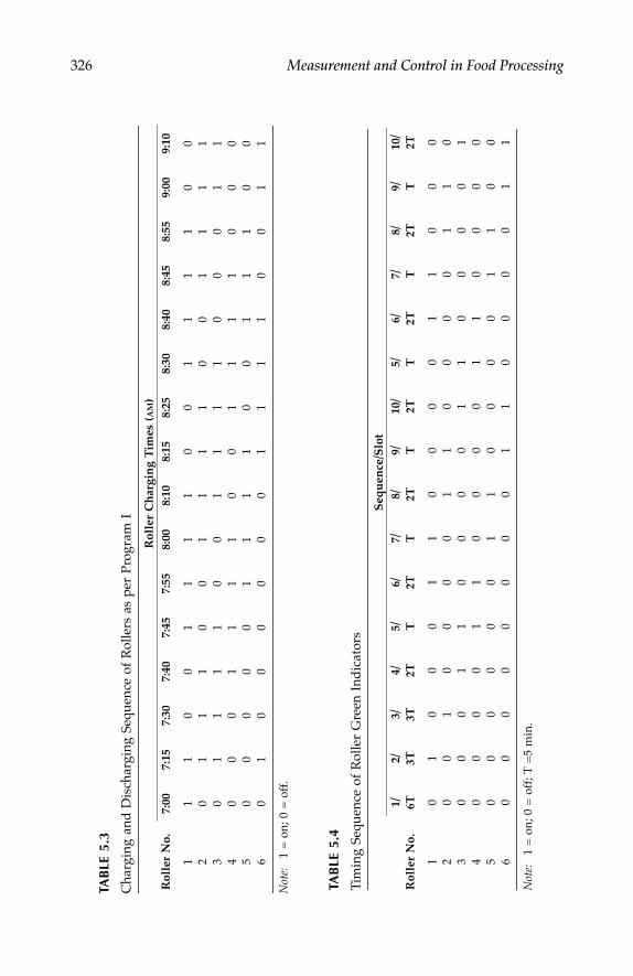
326 Measurement and Control in Food Processing
TAB
LE 5
.3
Cha
rgin
g an
d D
isch
argi
ng S
eque
nce
of R
olle
rs a
s pe
r Pr
ogra
m I
Rol
ler
No.
Rol
ler
Ch
argi
ng
Tim
es (
AM
)7:
007:
157:
307:
407:
457:
558:
008:
108:
158:
258:
308:
408:
458:
559:
009:
10
11
10
01
11
10
01
11
10
02
01
11
00
11
11
00
11
11
30
11
11
00
11
11
00
01
14
00
01
11
10
01
11
10
00
50
00
00
11
11
00
11
10
06
01
00
00
00
11
11
00
11
Not
e:1
= o
n; 0
= o
ff.
TAB
LE 5
.4
Tim
ing
Sequ
ence
of
Rol
ler
Gre
en I
ndic
ator
s
Seq
uen
ce/S
lot
Rol
ler
No.
1/ 6T2/ 3T
3/ 3T4/ 2T
5/ T6/ 2T
7/ T8/ 2T
9/ T10
/2T
5/ T6/ 2T
7/ T8/ 2T
9/ T10
/2T
10
10
00
11
00
00
11
00
02
00
10
00
01
10
00
01
10
30
00
11
00
00
11
00
00
14
00
00
11
00
00
11
00
00
50
00
00
01
10
00
01
10
06
00
00
00
00
11
00
00
11
Not
e:1
= o
n; 0
= o
ff; T
=5
min
.
7244.book Page 326 Wednesday, June 21, 2006 11:14 AM

Computer-Based Monitoring and Control 327
TAB
LE 5
.5
Tim
ing
Sequ
ence
of
Rol
ler
Red
Ind
icat
ors
Seq
uen
ce/S
lot
Rol
ler
No.
1/ 3T2/ 3T
3/ 2T4/ T
5/ 2T6/ T
7/ 2T8/ T
9/ 2T10
/T
5/ 2T6/ T
7/ 2T8/ T
9/ 2T10
/T
11
10
01
11
10
01
11
10
02
01
11
00
11
11
00
11
11
30
01
11
10
01
11
10
01
14
00
01
11
10
01
11
10
01
50
00
01
11
10
01
11
10
06
00
00
00
11
11
00
11
11
Not
e:1
= o
n; 0
= o
ff; T
=5
min
.
7244.book Page 327 Wednesday, June 21, 2006 11:14 AM

328 Measurement and Control in Food Processing
The digital output byte corresponding to roller green indicators G6through G1 is D6 through D0; the bits D15 through D7 are considered 0.Hence, the digital output byte (only low byte) for green indicators wastriggered as per table 5.4.
Additionally a flashing operation of the green and red indicators for 3 minbefore starting and finishing was included. For example, in table 5.4 after 6Tthe green light of roller number 1 should flash for 3 min, so 3 min before 3Tthe digital output of the low byte of the card changes from 0000 0000 to 00000001; that is, the decimal value of the low byte is flashing from 0 to 1. In asimilar manner, a flashing operation of 3 min of the red indicators beforefinishing is performed. Flashing of the green indicator makes the operatoraware of the starting or loading of a roller and flashing of the red indicatorinforms the operator about finishing or unloading of the roller.
5.7 Conclusion
A computer can be used extensively for performing complex monitoring andcontrol operations with the help of special hardware precisely at high speed.PC-based techniques can be made intelligent by programming in heuristicmethods such as fuzzy logic and artificial neural networks.
A general overview of computer-based measurement and control includ-ing examples of process control in the tea industry was presented in thischapter.
Methods of interfacing transducer signals to the computer have improvedsignificantly over the last decade. This has been made possible by the devel-opment of powerful interfacing modules supported by software. Todaysmart sensors can circumvent many problems that were insurmountableearlier. Linearization of sensor output is one such a problem that is still tobe addressed sufficiently with computer-based techniques.
Techniques like machine vision and E-nose-based odor detection and clas-sification using artificial intelligence are emerging fields that will gain impor-tance in food processing in the years to come.
References
1. Barney, G. C. 1985. Intelligent instrumentation: Microprocessor applications inmeasurement and control. Englewood Cliffs, NJ : Prentice Hall International.
2. Millman, J., and Halkia, C. C. 1972. Integrated electronics: Analog and digitalcircuits and systems. New York: McGraw-Hill International.
3. Bhuyan, M. 1997. An integrated PC based tea process monitoring and controlsystem. PhD Thesis, Department of Electronics, Gauhati University, India.
7244.book Page 328 Wednesday, June 21, 2006 11:14 AM

Computer-Based Monitoring and Control 329
4. Del Toro, V. 1985. Electric machines and power systems. New Delhi: Prentice Hallof India.
Further Reading
1. Borbora, B. C. 1992. Techno-economic development of tea industry and role ofelectronic process controlled instruments. Seminar on applications of electronicsin tea industry. Jorhat: Tea Research Association of India.
2. Moreira, R. G. 2001. Automatic controls for food processing systems. Gaithersburg,MD: Coultate TP.
3. Pinder, A. C., and Godfrey, G. 1993. Food process monitoring systems, London:Blackie Academic and Professional.
4. Cassel, D. A. 1983. Microcomputers and modern control engineering. Reston, VA:Reston.
5. Hunter, R. P. 1987. Automated process control systems (2nd ed.). Englewood, Cliffs,NJ: Prentice Hall.
7244.book Page 329 Wednesday, June 21, 2006 11:14 AM

7244.book Page 330 Wednesday, June 21, 2006 11:14 AM

331
Appendixes
APPENDIX A
SI Units
Quantity UnitSymbol Definition Name Symbol Definition
Base unitsLength Meter m —Mass Kilogram kg —Time Second sec —Electric current Ampere A —Thermodynamictemperature
Kelvin K —
Amount of substance Mole mol —Luminous intensity Candela cd —
Supplementary unitsPlane angle Radian rad —Solid angle Steradian sr —
Derived unitsω Angular velocity Radian per second rad/s rad/secQ Charge Coulomb C A.secC Capacity Farad Fs4.A2/kg-m2
G Conductance Siemen S χ-1
W Energy Joule J kg.m2/sec2
f Frequency Hertz Hz s-1
F Force Newton N kg.m/sec2
E Illuminance Lux lx lm/m2
L Inductance Henry H kg/m2/(sec2. A2)φ Luminous flux Lumen lm cd/sr
Luminous efficacy Lumen per watt lm/W lm/WMagnetic flux Weber Volt-sec V.sec
p Pressure Pascal Pa N/m2
P Power Watt W J/secR Resistance Ohm Ω kg/m2/(sec3. A2)S Specific heat Joule per kg-kelvin J/kg.K J/kg.Kλ Thermal conductivity Watt/meter-kelvin W/m.K W/m.KV Voltage Volt V A.Ω
Viscosityυ Kinematic viscosity Stokes Square meter
per secm2/sec
µ Absolute ordynamic viscosity
Poise Pa.sec N.sec/m2
7244.book Page 331 Wednesday, June 21, 2006 11:14 AM

332 Measurement and Control in Food Processing
APPENDIX B
English System of Units
Quantity English Unit Conversion to SI
Length Foot (ft) 1 ft = 30.48 cm Area Foot2 (ft2) 1 ft2 = 929.0304 cm2
Volume Foot3 (ft3) 1 ft3 = 28316.84 cm3
Force Pound (lb) 1 lb = 4.448 NMass Pound (lb) 1 lb = 454 gEnergy Foot-pound (ft-lb) 1 ft-lb = 1.356 JPressure Pound/in.2 (Psi) 1 Psi = 6897 PaPower Horsepower (hp)1 hp = 746 W
APPENDIX C
CGS Systems of Units
Quantity CGS Unit Equivalent SI Unit
Length Centimeter (cm) 100 cm = 1 mArea Centimeter2 (cm2) 10,000 cm2 = 1 m2
Volume Centimeter3 (cm3) 1,000,000 cm3 = 1 m3
Force Dyne 100,000 dyne = 1 NMass Gram (g) 1,000 g = 1 kgEnergy Erg 10,000,000 erg = 1 JPressure Dyne/cm2 10 dyne/cm2 = 1 Pa
APPENDIX D
Standard Prefixes
Multiple SI Prefix Symbol
1012 Tera T109 Giga G106 Mega M103 Kilo k102 Hecto h10 Deka da10–1 Deci d10–2 Centi c10–3 Milli m10–6 Micro m10–9 Nano n10–12 Pico p10–15 Femto f10–18 Atto a
7244.book Page 332 Wednesday, June 21, 2006 11:14 AM

Appendixes 333
APPENDIX E
Piping and Instrumentation Drawing Sensor Designations
First Letter Second Letter
A Analysis AlarmB BurnerC Conductivity ControlD DensityE Voltage Primary elementF FlowG Gaging Glass (sight tube)H HandI Current (electric) IndicateJ PowerK Time Control stationL Level LightM MoistureO OrificeP Pressure PointQ QuantityR Radioactivity RecordS Speed SwitchT Temperature TransmitU Multivariable MultifunctionV Viscosity ValveW Weight WellY RelayZ Position Drive
7244.book Page 333 Wednesday, June 21, 2006 11:14 AM

334 Measurement and Control in Food Processing
APPENDIX F
Standard Psychrometric Chart
Reprinted with permission. Copyright © 2005 kW Engineering, Inc., 306 17th Street, Suite 100, Oakland, CA 94612., All rights reserved. www.kw-engineering.com
7244.book Page 334 Wednesday, June 21, 2006 11:14 AM

335
Index
absolute humidity, definition, 130in dryers, 250
absolute temperature, 66, 69, 184AC bridge, 31, 79accelerometer, 36actuator,
definition, 85interfacing, 309, 312in tea withering, 97types, 86
adaptive control, 258, 293–295ADC,
in data acquisition, 308, 309in E-Nose interfacing, 219, in tea withering monitoring, 322microprocessor based hygrometer, 137,
138tea withering control, 129working of, 316–319
alarm, in particle size detection, 231in remote data acquision, 308in timer, 279
amplifier, for computer interfacing, 312, 317,
319–321for digital sensors, 81, for electronic controller, 259–264for hygrometer, 135, 136for photo voltaic cell, 44 for piezeoelectric sensor, 36, for thermal sensor, 71for thermocouple, 39in dc resistance moisture meter, 120, 121in IR moisture meter 122in refractometer, 181, 182in RF moisture meter, 114in spectroscopy, 236instrumentation type, 127, 128pH electrode, 187pneumatic type 100–101
analog controller, 258analog signal processing, 81
anemometer, hot wire, 71, 72ANN,
pattern recognition, 209spice flavor classification, 220tea flavor classification, 216
ash content, as impurity in sugar, 8determination of, in milk, 235
atmospheric control, 245automatic control,
components for, 85in fuzzy control, 300need in food industry, 244in industry, 28, 29
bacteria, as cause of off-flavor in milk, 200controlling of, 277detection of, 237, 238 in fruit juice, 3, related to brix of food, 177related to humidity for food, 130
baffle-nozzle dtector, 99, 100batch,
enzyme sensor in, 197mode of control, 14
beef tenderness, detection of 226beer, flavor measurement of, 210–212flow meter for, 158, 161industrial processing, 4–6
bellow, 101–103belt feeder, 164bimetallic thermal switch, 260, 261biosensor, 195–198black tea,
color matching of, 148dryer control for, 254
manufacturing process, 9–12stalk seperator for, 239texture detection of, 227
bottling, automation for, 289of soft drink, 6, 7 pressure injection in, 62
7244.book Page 335 Wednesday, June 21, 2006 11:14 AM

336 Measurement and Control in Food Processing
servomotor in, 92temperature measurement in, 155viscosity in, 168
bridge circuit, in E-Nose, 208in resistive humidity sensors, 72, 73 in RTD 156in strain gage, 55, 59, 63in temperature sensors, 65, 66
brix, of soft drinks, 4, 6 measurement of, 33, 177–182using refractometer, 33
calomel electrode, 185, 186, 196capacitive sensors,
for hygrometer, 134principle of, 31, various forms, 77–79 See also transducer
capillary tube viscometer, 169–171carbonation, in soft drinks, 6, carbonate, in bottled water, 232chemoresistive E-Nose sensor, 204, 205, 208color,
as a parameter in tea dryer, 253–254as parameter in food sorting, 287–289in food processing, 2, 4, 5, 7, 8, 9, 10, 11, 13 fuzzy control of, 298measuring, matching of, 139–152 of banana, 214of stalk in tea 238, 239sensing of, using RTD, 43
colorimeter, 146computer control, 258, 290, 291conducting polymer, 204, 205, 211
See also E-Noseconnective tissue of beef, 223, 224connector arrangement for computer
interface, 311control,
algorithm, 295computer based in tea withering 321–326cooling surface area, 245, 271fan direction in tea withering, 97, 98,
268–272for brix in sugar, 178for dryer, 253–258for level in particle size analyzer, 231for temperature in viscometer, 171parameters, 16
control motorin tea dryer, 254various types, 89
controlled variable in tea drying, 253
controller, adaptive, 294–296deivative, 23, 264, 265devices for, 84–86discrete type, 290–293electronic type, 258–265feedback types, 14, 15feedforward, 255fuzzy logic, 297–301intelligent, 293, 296on–off, 16PI, 21PID, 22–24 proportional, 17–21ratio type, 272, 273servo driver type, 90
conveyor, in food sorter, 289in dryer, 247, 250–257in stalk sepeartor, 239
Coriolis flowmeter, 157–161critical angle refractometer, 180, 182DAC, 315, 316, 317, 318data acquisition,
computer based, 306–312in biosensor, 197in colour detection of food, 146in E-Nose systems, 213–216in RF moisture meter, 116in tea withering, 128, 322, 323
DC conductance, in moisture measurement, 117
DC motor, 85, 88, 89, 90, 92conveyor speed, 255in autotritalizer, 232
DC servomotor, 90derivative controller, 23, 264, 265
See also controllerdiaphragm,
pressure sensor, 58, 60, 61, 62, 78, 100, 101, 103,
valves, in E–nose system, 213differential amplifier, 136differential pressure, flowmeter in ratio controler, 273 in viscometer, 171
digital control, 312digital image, of tea, 146–148digital transducer, 32, 80, 81
See also transducerdiscrete controller, 290–293
See also controllerdry and weigh, in moisture measurement,
110, 119dry bulb temperature, 131, 133, 135
7244.book Page 336 Wednesday, June 21, 2006 11:14 AM

Index 337
dryer, indicator for, 284model of, 252, 253temperature control in, 245–249types, 248
drying characteristics, 252dynamic viscosity, 166, 170
See also viscosityElectrical,
humidity meter, 134motor, 86solenoid, 86
electronically controlled, valve, 275Engler viscometer, 170
See also viscosityE-Nose,
commercial, 210for beer flavor, 210for fruit ripeness, 215for tea and spice flavor, 214–220types, 204–207
enzyme sensor, 193–199error detector, 85
in adaptive controller, 295fat content,
in food, 110, 155, 167, 221, 235detection of, 237discriminate in beef, 226enzyme, for breaking of, 193unit for meat, 179, 237
feature extraction, in E-Nose, 207–209in texture detection, 228
feedback control, 14, 15, 16, 19, 25in dryer, 251–255
feedforward control, 255feeder, 162–165final control element, 17, 85, 96, 97
in food dryer, 255fish,
bacteria detection in, 238coloring, 139enzymes in, 193flavor of, 202freshness detection of, 199pH of, 183
flavor detection, of beer, 210–213of fruit ripeness, 213, 214of tea and spice, 210, 214–220
flow, control of air, in tea withering, 97control of, in E-Nose, 212control of, in storage atmosphere, 277, 278 in ratio control, 271
measurement of, (See flow meter)Newtonian, 166of air, in pneumatic devices, 101of food, 5, 9–16, 249–257
flow meter, Coriolis, 160, 161, 162for solid, 163hot wire anemometer, 71, 72magnetic, 158mass, 159positive displacement, 162pulse transducer, 46turbine, 162
fluorescence, in beef tenderness detection, 144
foreign body, detection of, 238fuzzy logic controller, 296–298, 301, 330
See also controllergauge factor-strain gauge, 55, 58, 59, 62glass electrode,
in ISFET sensor, 190, 196in pH measurement, 184–187
GPIB, 315hardware,
in ladder diagram, 291, 292interfacing, 312, 322
headspace, 203, 211–213, 215heat and mass transfer, 246, 249high temperature, 8, 13, 109, 153, 157histogram, 149, 150, 151, 227humidity,
as process parameter, 4, 9, 10, 29, 130definitions of, 130, 131effect in drying of food, 246, 247, 250, 251,
252, 256, 257effect in E-Nose, 205, 215, 216, effect in food preservation, 277effect in tea withering, 266in fuzzy control, 298measurement of, 131–138monitoring of using computer, 323–326sensors for, 31, 32, 72, 73
hygrometer, electrical, 134electronic, 135fluidic, 133hair, 131microprocessor based, 135–138wet and dry bulb, 131–133
IEEE 488 interface, 315, 316image processing of food color, 225, 226, 240,
289inductive transducer, 72industrial process, 11, 98, 308
7244.book Page 337 Wednesday, June 21, 2006 11:14 AM

338 Measurement and Control in Food Processing
infrared, heating, 111meat content analyzer 237moisture meter, 119, 122, 252, 257spectroscopy, 234, 235
integral controller, 21, 263See also controller
integrator, 21, 23, 31, 259intelligent controller, 293, 296
See also controllerinteractive model, 254, 255interface, 113, 137, 162, 212, 310, 312–315, 321ISFET, 188–193, 198, 199jams and jellies, 9kinematic viscosity, 333
See also viscosityladder diagram, 291, 292level measurement, 78, 79light scattering, turbidity meter 140, 141linearized model, of pschychrometric chart,
137liquid expansion, thermometer 260LM335, 69, 70, 71load cell,
computer interfacing of, 322, 323for weighing, in tea industry, 98, 126–129in food texture detection 222piezoelectric, 33starin gauge based, 63
logic control, 267, 268, 292, 298LVDT, 76, 172machine vision, 148, 253magnetic transducer, 32meat content, determination of, 237microprocessor, 16, 29, 32, 80, 135, 137, 161,
182, 278microwave,
oven, 98tempering, 98in moisture content detection, 111absorption, 111–113dryer, in meat analyzer, 237
MIMO, 13, 252, 253, 254, 277minerals,
as flavor defect in milk, 200in wine, detection of, 236
moisture content, as disturbance, 296 conductivity technique, 116–122control, 245, 246, 250–257, 280, 287definitions, 110in drying, 32, 97, 126in food, 4, 5, 8, 9, 11, 12, 109IR method, 122microwave meter 111, 112
radio frequency meter, 113MOSFET,
E-Nose, 204, 207enzyme sensor, 198isolation amplifier, 36pH sensor, 188
neural network, 208, 216, 245, 296, 330Newtonian flow, 166–168
in viscometer, 175nozzle,
in screw feeder, 163pnematic detector, 99–103
olfactory system, of human, 201, 202operational amplifier, 187, 258–260, 320optical,
absorption, in turbidity measurement, 142, 143
reflectance, in turbidity measurement, 144, 146
organoleptic panel, 202overdrying, of tea, 251, 253, 286particle size, detection of, 229–231, 288PCA, 208, 209, 213, 216–218, 220, pH,
analyzer, for bottled water, 232–234calomel electrode, 185–187control of, in milk, 193control of, in sugar manufacturing, 143definition and scale, 183glass electrode, 184ISFET sensor, 187–190, 198measuring circuit, in enzyme sensor, 196of food, 3–6, 8, 9, 13, 29, 30, 108of wine, 189signal processing, 187
photoelectric transducer, 41PID,
controller, 22, 23fuzzy based, 300OPAMP circuit, 259tempertaute control, 98
piezoelectric E-Nose, 206, 208transducer, 30, 33, 35, 36
pitot tube, type viscometer, 157plastic food, 168PLC, 271, 292pneumatic, actuator, 163, 289
controller, 98, 99device, 98transmitter, 101
polymer, E-Nose sensor, 204, 205, 206, 208, 211–213
positive displacement flow meter, 157
7244.book Page 338 Wednesday, June 21, 2006 11:14 AM

Index 339
potentiometer, applications, 122, 128, 171, 177, 213, 225,
232construction, 52, 53, 54in controller, 20
programmable logic controller, 271, 292See also PLC
programmable timer, 279, 282, 283proportional controller, 18–21, 24,
OPAMP circuit, 259, 262protein,
detection of, in milk powder, 235 enzyme, 193in meat, 237of food, 4
pulse generating transducer, 46, 47radioactive,
instrumentation, 47, 49, 50 transducer, 30, 32, 81
ratio control, in food pickling, 272, 273Redwood viscometer, 170
See also viscometerrefractometer,
in brix, 179–182in food color, 145in syrup content, 6
relay controller, 291resistive transducer, 31, 51–73, 134
See also transducerrolling in tea, 9, 10
timing indicator for, 279–281, 326rotary vane feeder, 163rotating cylinder viscometer, 170, 174–176,
288See also viscometer
Saybolt viscometer, 169, 170See also viscometer
screw feeder, 163, 164self-generating transducer, 31servomotor, 90–92
in feeder, 163soft drinks, 6, 177, 234stalk seperator, 238, 239, 289stepper motor, 88, 89
construction, 92, 93driver, 96, 314in refractometer, 145
storage atmosphere control,, 277, 278strain gauge, 31, 55–62, 312, 313, 320sugar,
by IR technique, 122control of, 182, 296flow meter for, 159, 160, 162, 163humidity in storage of, 130in bottled water, 232
in milk powder, 235in ratio control, 272 measurement of, 177–180particle size, 230role in food processing, 5–8, 130, 139, 214temperature for storage of, 152turbidity measurement of, 139, 143viscometer for, 167
tea industry, 9–12temperature measurement, 36, 69, 133, 152,
153, 155, 156, 253, 277tempering, monitoring of, 155tenderness,
detection, 220, 221of beef, 226, 227
texture, 5, 8detection of tea, 147electromechanical method, 220–222machine vision method, 225–229
thermal sensor, semiconductor, 32, 39, 135, 136
thermistor, 31, 37, 66–69, in chocolate tempering, 156
thermocouple, 29, 36, 37, 38, 39, 40AD conversion, 318in hygrometer, 135installation, 154interfacing, 312, materials, 153
thermometer, fluidic, 133for dryer, 246in capillary viscometer, 171in manual control, 15, 29in psychrometer, 131platinum, 156resistive, 31RTD, 65
timer, 231, 269, 282, 284, 285, 293, 326, 327transducer,
capacitive, 31, 77–79, 134digital, 32, 80–83in biosensor, 194magnetic, 31, 73–77magnetoelectric, 44–47photoelectric, 41–44piezoelectric, 33, pneumatic 313pulse, 32, radioactive, 47–51relative humidity, 266resistive, 31, 51–73, 134selection, 83–84self generating, 31thermo-emf, 38–40
7244.book Page 339 Wednesday, June 21, 2006 11:14 AM

340 Measurement and Control in Food Processing
types, 30variable parameter, 31weight sensing, in feeder, 164
turbidity, basic meter, 139in sugar refining, 143light scattering meter, 141optical absorption meter, 142standrads and units, 140
turbine flow meter, 32, 33, 162, 273Twaddel, 179U-rod refractometer, 182UV, 211, 224, 234valves,
as control component, 86–88, as final control element, 97computer interfacing, 314control, 274electronically controlled, 276 in E-Nose sampling, 203in on–off controller, 17in storage atmosphere control, 278sizing, 275, types, 274
viscometer,
capillary tube, 170–172contrave, 176Engler, 170Redwood, 170rotating cylinder, 174–176Saybolt, 169variable area, 172, 173
viscosity, control in chocolate, 265definition and units, 165, 166dynamic, 166, 170for control valve, 273in flow metering, 157, 159, 161, 162kinematic, 333measurement of, (See viscometer)reduction by enzymes, 193role of in food, 4, 6, 29, 167, 168, 169
volatile compounds, in tea, 210, 234in tropical fruits, 234
voltage to frequency converter, 81Wheatstone bridge circuit, 42, 55, 59, 72, 156,
208, 320wine, analysis of, 236Young modulus, in strain gauge, 35
7244.book Page 340 Wednesday, June 21, 2006 11:14 AM

Copyright © 2022 FDOKUMEN