Entropy 2014, 16, 1134-1168; doi:10.3390/e16021134

entropy ISSN 1099-4300

www.mdpi.com/journal/entropy

Article

Signal Processing for the Measurement of the Deuterium/Hydrogen Ratio in the Local Interstellar Medium

Diego Francisco Rodríguez Moreno 1,*, Peter Wurz 1, Lukas Saul 1, Maciej Bzowski 2,

Marzena Aleksanda Kubiak 2, Justyna Maria Sokół 2, Priscilla Frisch 3,

Stephen Anthony Fuselier 4, David John McComas 4, Eberhard Möbius 5

and Nathan Schwadron 5

1 Physics Institute, University of Bern, Sidlerstrasse 5, Bern 3012, Switzerland;

E-Mails: peter.wurz@space.unibe.ch (P.W.); luke.saul@space.unibe.ch (L.S.) 2 Space Research Centre, Polish Academy of Sciences, Bartycka 18A, Warsaw 00-716, Poland;

E-Mails: bzowski@cbk.waw.pl (M.B.); mkubiak@cbk.waw.pl (M.A.K.);

jsokol@cbk.waw.pl (J.M.S.) 3 Department of Astronomy and Astrophysics, University of Chicago, 5640 S. Ellis Avenue,

Chicago, IL 60637, USA; E-Mail: frisch@oddjob.uchicago.edu 4 Southwest Research Institute, San Antonio, TX 78228-0510, USA and University of Texas at San

Antonio, San Antonio, TX 78249, USA; E-Mails: sfuselier@swri.edu (S.A.F.);

DMcComas@swri.edu (D.J.M.) 5 Space Science Center and Department of Physics, University of New Hampshire, 39 College Road,

Durham, NH 03824, USA; E-Mails:eberhard.moebius@unh.edu (E.M.);

N.Schwadron@unh.edu (N.S.)

* Author to whom correspondence should be addressed; E-Mail: diego.rodriguez@space.unibe.ch;

Tel.: +41-31-631-8546; Fax: +41-31-631-4405.

Received: 9 August 2013; in revised form: 18 December 2013 / Accepted: 11 February 2014 /

Published: 24 February 2014

Abstract: We report on a comprehensive signal processing procedure for very low signal

levels for the measurement of neutral deuterium in the local interstellar medium from a

spacecraft in Earth orbit. The deuterium measurements were performed with the IBEX-Lo

camera on NASA’s Interstellar Boundary Explorer (IBEX) satellite. Our analysis technique for

these data consists of creating a mass relation in three-dimensional time of flight space to

accurately determine the position of the predicted D events, to precisely model the tail of

the H events in the region where the H tail events are near the expected D events, and then

to separate the H tail from the observations to extract the very faint D signal. This interstellar D

OPEN ACCESS

Entropy 2014, 16 1135

signal, which is expected to be a few counts per year, is extracted from a strong terrestrial

background signal, consisting of sputter products from the sensor’s conversion surface. As

reference we accurately measure the terrestrial D/H ratio in these sputtered products and

then discriminate this terrestrial background source. During the three years of the mission

time when the deuterium signal was visible to IBEX, the observation geometry and orbit

allowed for a total observation time of 115.3 days. Because of the spinning of the spacecraft

and the stepping through eight energy channels the actual observing time of the interstellar

wind was only 1.44 days. With the optimised data analysis we found three counts that

could be attributed to interstellar deuterium. These results update our earlier work.

Keywords: energetic neutral atoms; deuterium; D/H ratio; ISM; 3D-TOF analysis; IBEX-Lo

1. Introduction

Measurements of the interstellar wind by the Interstellar Boundary Explorer (IBEX) satellite [1] in

Earth orbit provide a supplementary means to observe the D/H ratio in the local interstellar medium for

telescopic observations. According to the standard cosmological model, deuterium was produced in

significant amounts only during primordial nucleosynthesis within the first 100–1,000 s of the universe.

It is destroyed in the interiors of stars much faster than it is produced by the other natural processes that

produce insignificant amounts. Over time, baryonic matter is processed in stars where deuterium is

destroyed by nuclear reactions (astration). Deuterium-poor and metal-rich material is returned to the

interstellar medium in supernova explosions and stellar winds. Nearly all deuterium found in nature is

believed to have been produced in the Big Bang. Within our galaxy, deuterium is removed from

interstellar gas through astration and possibly through the depletion of deuterium onto dust grains, and

replenished by the accretion of pristine material onto the galaxy [2–5]. As a result, measurements of the D

abundance in different locations of the galaxy provide important tests for models of primordial

nucleosynthesis and for the chemical evolution of the galaxy and intergalactic medium.

The mean deuterium abundance in the low density Local Bubble within 100 pc is D/H = 15.6 ± 4 ppm [6].

However, Linsky et al. [6] have found that deuterium abundances in the global interstellar medium

vary within a factor four, with a complex dependence on hydrogen column densities. Before IBEX,

the deuterium abundance in the Local Interstellar Cloud (LIC) could only be investigated using

spectroscopic measurements of the heavily blended deuterium and hydrogen Lyman alpha lines

towards nearby stars. The closest star representing the LIC is Sirius, where the D/H ratio of 16 ± 4 ppm

is typical of the Local Bubble interior [7]. In our initial analysis, the D/H measurements by direct

sampling on IBEX were found to be consistent with the Sirius measurements [8]. Here we present the

details of the analytical technique and an updated D/H value for the Local Interstellar Medium (LISM).

Entropy 2014, 16 1136

1.1. Interstellar Wind at 1 AU

The LISM consists of warm, relatively dilute, partially ionised interstellar gas surrounding the

Sun [9–11]. The Sun moves through the low density, warm, partially ionised LIC, where fluxes of far

ultraviolet radiation are high, the fractional abundance of deuterium in molecular form is expected to

be insignificant.

The Sun continuously ejects coronal plasma as a solar wind (mostly protons and electrons together

with frozen-in solar magnetic field that inflates a plasma bubble in the interstellar medium known

as the heliosphere. The heliosphere effectively excludes the LISM plasma from the nearest 100 AU

around the Sun. The interaction between the solar wind and LIC determines the shape and structure of

the heliosphere (e.g., [12,13]); exploring this interaction is one of the major scientific objectives of

IBEX [1].

Neutral interstellar atoms of the interstellar wind have different fates as they interact with the Sun

and the solar wind plasma, which affects the transport and survival of the atoms from the LISM to 1

AU. While approaching the inner heliosphere, the interstellar wind is depleted of many neutral species

by ionisation processes, and also affected by the Sun’s gravitational field (modified by radiation

pressure for H and D). The characteristic flow pattern and density structure that is formed has a cavity

close to the Sun, and particles experience gravitational focusing on the downwind side for all species

except H [14,15]. Ionisation processes that affect the interstellar neutrals are: ultraviolet (UV)

photoionisation, charge exchange (CEX) with solar wind ions, and electron impact ionisation [16–19].

However, with respect to the energy dependent charge exchange cross section we note that the speeds

of the cold H and D atoms are nearly stationary compared to heliospheric ions (protons and alpha

particles) that could CEX with them. Thus, the physical parameters of interstellar neutrals can be

directly measured and provide the best paradigm for modelling and understanding the interplanetary

environments of astrospheres [14].

In the case of helium, the dominant ionisation process is UV ionisation outside of 1 AU, and

within ~1 AU there is a steep radial dependence of electron impact ionisation that produces large

ionisation rates [20]. He flows through the heliospheric boundary mostly unimpeded because it has a

high ionisation potential and low cross section for CEX with solar wind alpha particles and protons.

In contrast, for hydrogen, a substantial fraction interacts with the plasma in the heliosheath via

charge exchange: in the outer heliosheath with the interstellar proton population, which is compressed

against, the heliopause and in the inner heliosheath with the solar wind protons. CEX losses are much

larger than losses by UV ionisation [16], with both processes having a solar cycle dependence. In

addition to being a loss process for neutral H and D in the heliosphere, CEX also results in the creation

of the secondary population of neutral H and D, which are neutralised protons and deuterons from the

outer heliosheath [12]. Both the primary and secondary populations enter the heliosphere, where they

are subject to strong CEX and photoionisation losses. As a result, most of the neutral hydrogen

becomes ionised and does not reach 1 AU where IBEX is located. At 1 AU, the residual interstellar

wind is composed mostly of helium [21], with a small fraction of hydrogen and others constituents,

whose abundances relative to helium decrease with increasing solar activity because of filtration.

The cross sections for photoionisation, CEX, and electron impact ionisation of D are practically

identical to that for H, thus leading to identical H and D ionisation rates [22]. However, the dynamics

Entropy 2014, 16 1137

do differ [22,23]: (1) the thermal speed of D vTh,D in the LIC is smaller, vTh,D = vTh,H/√2 [23], thus the

reaction rates are slightly different [23]; and (2) the radiation pressure does not counterbalance

gravitational effects as it does approximately for H. In addition radiation pressure is a strong function

of radial velocities of individual D atoms relative to the Sun because of the Doppler effect and the

non-flat profile of the solar Lyman-α emission line that supplies the Lyman-α flux in the heliosphere.

By contrast, owing to its larger atomic mass and much weaker flux in the resonant solar 58.4 nm line,

He is not affected by radiation pressure. Effectively, the radiation pressure for D is expected to be in

between the pressure for H and the (zero) pressure for He. Thus, during the IBEX observations along

Earth orbit, the peak of the D signal is expected after the peaks of He and O, and before the maximum

of H [23].

1.2. Overview of the IBEX Mission

NASA’s IBEX mission was designed to investigate the interaction of the heliosphere with the

surrounding interstellar medium via the observation of Energetic Neutral Atoms (ENAs) from a near

Earth vantage point [1,24]. The IBEX spacecraft was launched on 19 October 2008 into a highly

elliptical, near-equatorial Earth orbit of ~3 × 50 RE (with RE the Earth radius), to avoid the interference

from ENA emission from the Earth’s magnetosphere as much as possible. IBEX is a Sun-pointing,

spinning satellite, whose spin axis is re-oriented toward the Sun after completion of each 7–8 day orbit

so that complete full-sky ENA maps are obtained over a period of 6 months. IBEX recorded the first

all-sky maps of ENAs produced by the interaction of the heliosphere with the local interstellar medium

at heliocentric distances of about 100 AU [25–28].

IBEX samples the interstellar wind distributions at 1 AU in a plane that is approximately

perpendicular to the Earth-Sun line, which is equivalent to observing ENAs that arrive from the

heliospheric boundary or beyond at the perihelia of their trajectories, independent of its flow direction

at infinity.

The IBEX payload consists of two single-pixel ENA cameras with large geometric factors,

IBEX-Lo [29] and IBEX-Hi [30], whose Fields-of-View (FoV) lie perpendicular to the Sun-pointed

spin axis. Their combined energy range is [10, 6000 eV] with overlap between 300 and 2000 eV.

A single Combined Electronics Unit (CEU) controls these sensors, stores data, and is the payload

interface to the spacecraft bus [1,24].

1.3. Expected Fluxes of Interstellar Deuterium at Earth Orbit

Models of the dynamics of D inside of the heliosphere show that fluxes of D will be entirely in

the energy range of IBEX-Lo with deuterium fluxes expected to be quite low, of the order of

0.015 cm−2 s−1 [22]. The resulting D signal is at the level of single counts per year [22,23]. However,

Kubiak et al. [23], predict that IBEX-Lo would be able to detect interstellar neutral deuterium for

selected times of the year at specific energies. Clearly, it is very challenging to identify these few

deuterium atoms, even with the advanced background suppression techniques used in IBEX-Lo [31].

The elemental ratio for interstellar deuterium to hydrogen is expected to be in the range from 10−5 and

10−2 at Earth orbit [22].

Entropy 2014, 16 1138

1.4. IBEX-Lo Sensor

The IBEX-Lo sensor is a camera for energetic neutral atoms [29,32]. It maximises collection of the

relatively weak heliospheric neutral atom signal while effectively suppressing background sources of

local ions, electrons, and UV [31]. It detects neutral atoms in the energy range 0.01 to 2 keV in

8 logarithmic steps with wide energy bands. ENAs from the interstellar wind are the brightest ENA

signal in the sky, apart from the magnetosphere of the Earth. The backgrounds present in the IBEX-Lo

measurements from various sources are well below the signal of the main interstellar neutrals [31].

The sensor entrance subsystem is based on a cylindrical architecture with an annular collimator,

which repels electrons and ions, and allows only neutral atoms to enter (Figure 1). Unfortunately, the

high voltage for ion suppression failed in flight, thus associated background sources are higher than

originally anticipated. The collimater defines a field of view of 7° × 7° in three 90° angular sectors

(called the low resolution sectors) and 3.5° × 3.5° in the fourth angular sector (the high angular

resolution sector).

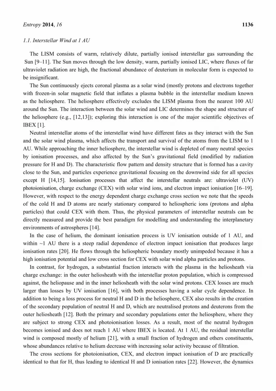
Figure 1. Cross-section of the IBEX-Lo sensor showing the primary components (from [29]).

The sensor is rotationally symmetric about the centreline axis of the figure. Electrons,

neutrals, and ions all enter the sensor through the collimator. Neutrals pass through the

collimator and strike a conversion surface. A fraction of these incident neutrals leave the

conversion surface as negative ions and pass through the electrostatic analyser. Secondary

and photoelectrons from the conversion surface are deflected by two concentric rings of

permanent magnets away from the entrance of ESA. Negative ions exit the ESA, are

further accelerated and enter a triple coincidence TOF mass spectrometer. In this

subsystem, the ion mass is determined.

Entropy 2014, 16 1139

A fraction of the interstellar and heliospheric neutrals that pass through the collimator are converted

to negative ions in the ENA-to-ion conversion subsystem. The neutrals are converted on a high yield,

chemically inert, diamond-like carbon conversion surface [26,33]. The negative ions leaving the

conversion surface are accelerated into an electrostatic analyser (ESA), which sets the energy passband

for the sensor. The ESA has been designed to accept a large angular range of backscattered and

sputtered products from the conversion surface [32]. In normal sensor operations, the eight energy

steps are sampled on a 2-spin per energy step cadence so that the full energy range is covered in

16 spacecraft spins.

Finally, negative ions exiting the ESA are further accelerated to 16 keV, and then are mass-analysed

in a time-of-flight (TOF) mass spectrometer. The entire TOF ion optics section floats at a post-acceleration

(PAC) high voltage of 16 kV. This acceleration voltage helps straighten out negative ion trajectories

between the ESA exit and TOF entrance. The high ion energy allows a TOF measurement with

sufficient mass resolution after energy loss in the entrance foil [33]. The TOF analysis subsystem is a

carbon foil-based TOF ion mass spectrometer that uses a triple coincidence detection scheme, shown

in Figure 2. For each registered atom three times of flight (TOF0, TOF1, and TOF2) are measured

independently from each other and are subsequently compared to efficiently eliminate background,

which is very important for the detection of the low fluxes of the LISM D atoms.

When the negative ions enter into the mass spectrometer they release secondary electrons from the

first carbon foil. These secondary electrons are focused on the outermost radial anode of the

microchannel plate (MCP) detector and constitute the first start pulse (start 1, a in Figure 2). As the

negative ions pass through the first C-foil, a fraction of them become neutral again. The ions and

neutrals pass a second C-foil and again release secondary electrons. These electrons are focused on the

innermost radius of the MCP and constitute the second start pulse (start 2, or c in Figure 2). Finally,

after passing through the second C-foil, the ions and neutrals strike the MCP. The signal from these

ions and neutrals constitutes a stop pulse (stop, or b0 to b3 in Figure 2).

TOF0 is the time of flight of the ion between the first start and the stop signals (or the time obtained

between the C-foil 1 and the MCP). TOF1 is the time between the second ultrathin carbon foil and the

MCP detector, where the ion is detected. TOF2 is the time between the first and the second carbon foil.

The TOF2 section has a higher mass resolution than TOF1, because only the energy and angular

straggling from the C-foil 1 affects the mass resolution. The TOF3 is the delay line signal. TOF3

(anode 3) determines the quadrant where the stop signal is registered. Each TOF is determined

separately and encoded to 11 bits (0.16 ns resolution, [29]).

An ion measured in a single TOF section (TOF0, TOF1, or TOF2) is referred to as a double

coincidence measurement (one of two possible starts and a stop). An ion that is measured in all three

TOF channels satisfies the triple coincidence (requires both the two start and a stop signals).

Additionally, valid triple events are required to pass a checksum test, which establishes that the TOF

needed to cover the distance from the C-foil 1 to the stop in MCP is about equal to the sum of the TOF

required from the first to the second C-foil and the TOF measured between the C-foil 2 and a stop

(effectively requiring that TOF0 ≈ TOF2 + TOF1) to assure consistency for a real particle moving

properly through the IBEX-Lo TOF unit. This checksum test assures that background from cosmic

rays and other penetrating radiation is effectively removed. However, the checksum test leaves a range

of possible TOFs for each time of flight channel to account for energy and angular straggling in the

Entropy 2014, 16 1140

carbon foils. Details of this detection technique are given in earlier publications [29,34]. The

triple-coincidence detection is designed to effectively reject random background while maintaining

high detection efficiency for negative ions. In this analysis we only use valid triple events.

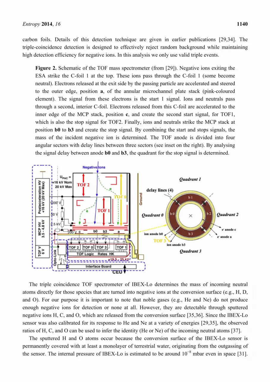
Figure 2. Schematic of the TOF mass spectrometer (from [29]). Negative ions exiting the

ESA strike the C-foil 1 at the top. These ions pass through the C-foil 1 (some become

neutral). Electrons released at the exit side by the passing particle are accelerated and steered

to the outer edge, position a, of the annular microchannel plate stack (pink-coloured

element). The signal from these electrons is the start 1 signal. Ions and neutrals pass

through a second, interior C-foil. Electrons released from this C-foil are accelerated to the

inner edge of the MCP stack, position c, and create the second start signal, for TOF1,

which is also the stop signal for TOF2. Finally, ions and neutrals strike the MCP stack at

position b0 to b3 and create the stop signal. By combining the start and stops signals, the

mass of the incident negative ion is determined. The TOF anode is divided into four

angular sectors with delay lines between three sectors (see inset on the right). By analysing

the signal delay between anode b0 and b3, the quadrant for the stop signal is determined.

The triple coincidence TOF spectrometer of IBEX-Lo determines the mass of incoming neutral

atoms directly for those species that are turned into negative ions at the conversion surface (e.g., H, D,

and O). For our purpose it is important to note that noble gases (e.g., He and Ne) do not produce

enough negative ions for detection or none at all. However, they are detectable through sputtered

negative ions H, C, and O, which are released from the conversion surface [35,36]. Since the IBEX-Lo

sensor was also calibrated for its response to He and Ne at a variety of energies [29,35], the observed

ratios of H, C, and O can be used to infer the identity (He or Ne) of the incoming neutral atoms [37].

The sputtered H and O atoms occur because the conversion surface of the IBEX-Lo sensor is

permanently covered with at least a monolayer of terrestrial water, originating from the outgassing of

the sensor. The internal pressure of IBEX-Lo is estimated to be around 10−8 mbar even in space [31].

Entropy 2014, 16 1141

At this pressure, the water layer would be replenished within ~103 s, if it were somehow removed

(which cannot happen in a sensor always pointed about 90° away from the Sun).

Together with H and O, D is sputtered off the conversion surface according to its abundance in the

terrestrial water layer. IBEX-Lo will also detect D− ions with a terrestrial origin that are sputtered

primarily by interstellar He atoms, because terrestrial hydrogen is accompanied by 155.76 ± 0.7 ppm

of deuterium. Thus, there is a substantial D foreground that competes with purely interstellar D

atoms [23]. Therefore, depending on their source, we speak about two types of deuterium collected by

IBEX-Lo at 1 AU: a terrestrial component, which is the product of sputtering by interstellar helium,

and an interstellar component from the interstellar neutral wind, i.e., external deuterium of interstellar

origin. In this analysis we pay careful attention to correctly account for the terrestrial deuterium foreground.

Because the IBEX spacecraft orbits the Earth and its observations are in a plane perpendicular to the

Sun-Earth line, there are two opportunities during each year to observe the interstellar wind: first

between January and March (Spring season), when the Earth travels into the direction of the gas flow

of the interstellar neutral wind, and second between October and December (fall season) when the

Earth recedes from the flow direction. In the spring season, the interstellar gas velocity is highest in the

IBEX reference frame. This higher velocity compared to the fall season results in higher apparent

energy of interstellar atoms, and thus in a higher detection efficiency [29]. In the fall season the

relative speed between the interstellar neutral flow and IBEX is low, thus leading to significantly lower

efficiency. The optimal time for detection of a faint signal, like D, is thus the spring passage of each

year. Tarnopolski and Bzowski [22] predicted a total deuterium flux of 0.015 cm−2 s−1.

2. Data Analysis

2.1. Observation Strategy and Data Selection

To derive the D/H ratio, we used IBEX-Lo data from all the orbits of the spring passage throughout

years: 2009, 2010 and 2011. During these years the solar activity increased, appreciably reducing the

H signal (and thus also the D signal) in 2011, and producing an even stronger reduction of the H signal

in 2012 [38]. The data of the spring 2012 orbits, when IBEX-Lo was operated in a special mode for

measuring interstellar O, could not be used for our investigation because of their low H signal.

We use triple coincidence events collected in the four lowest energy channels of IBEX-Lo with

central energies E1 = 14.5 eV, E2 = 28.5 eV, E3 = 55.5 eV, and E4= 102 eV, respectively [29].

In energy bins 1 to 3 we find sputtered H and D (i.e., the terrestrial H and D) from interstellar He.

Theory predicts that the interstellar deuterium signal is located only in energy bin 3 [22,23] to be

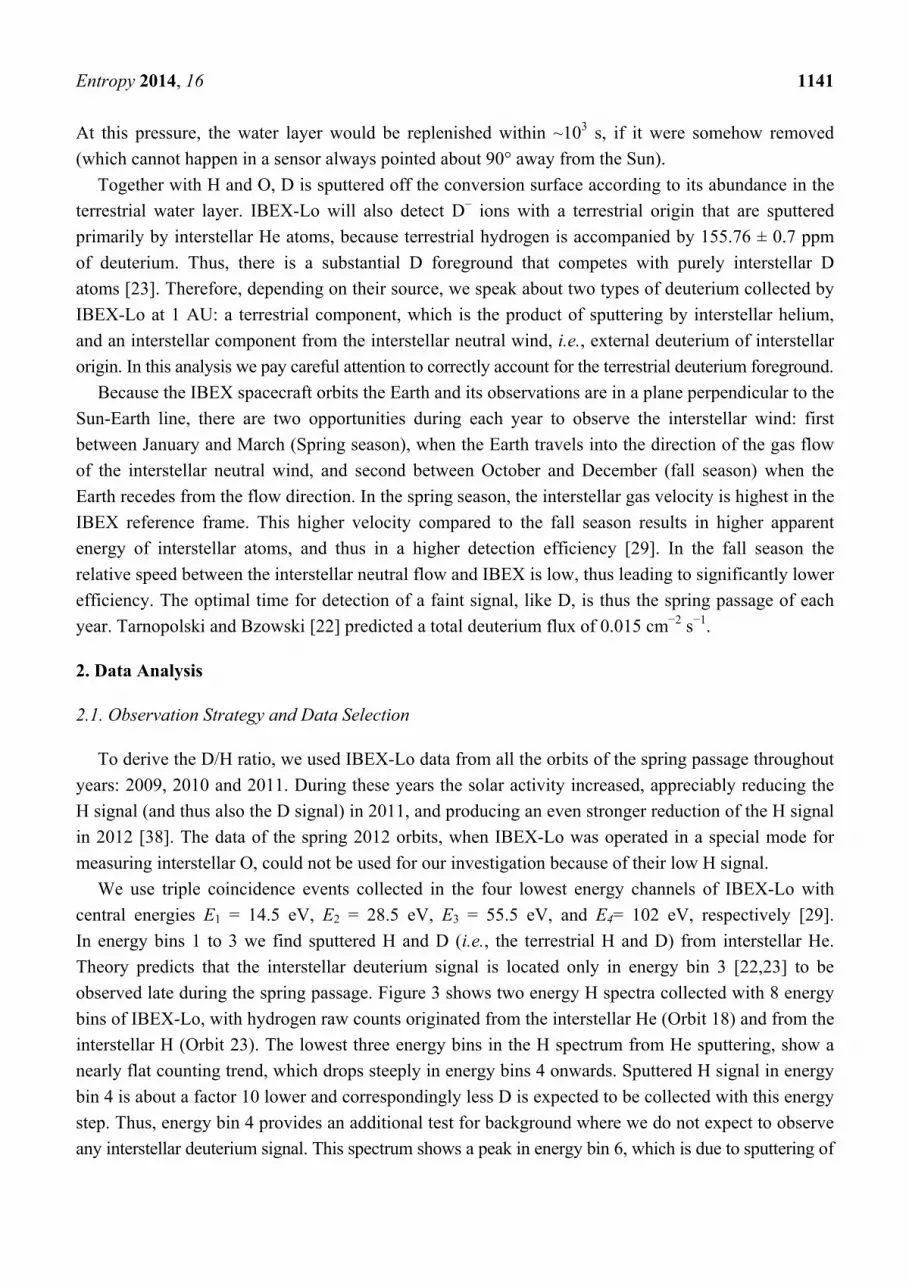
observed late during the spring passage. Figure 3 shows two energy H spectra collected with 8 energy

bins of IBEX-Lo, with hydrogen raw counts originated from the interstellar He (Orbit 18) and from the

interstellar H (Orbit 23). The lowest three energy bins in the H spectrum from He sputtering, show a

nearly flat counting trend, which drops steeply in energy bins 4 onwards. Sputtered H signal in energy

bin 4 is about a factor 10 lower and correspondingly less D is expected to be collected with this energy

step. Thus, energy bin 4 provides an additional test for background where we do not expect to observe

any interstellar deuterium signal. This spectrum shows a peak in energy bin 6, which is due to sputtering of

Entropy 2014, 16 1142

interstellar O and Ne [39]. The energy spectrum for interstellar H via direct ionisation on the

conversion surface is clearly different from the sputtered H spectrum [21].

Figure 3. The green line describes the energy spectra of hydrogen raw counts taken shortly

after the interstellar helium peak (He LISM, orbit 18), and the orange line to data collected

during the interstellar hydrogen peak (H LISM, orbit 23) with the magnetospheric

background removed [38].

2.2. Maxima of Principal Interstellar Wind Components

The origin of the collected deuterium signal varies with ecliptic longitude, since it depends on

which is the main component of neutral interstellar wind (helium or hydrogen) during the spring

season. The flux maxima for interstellar He, D, and H should be observed by IBEX in temporal

sequence along ecliptic longitude. The He and H components show a clear offset in ecliptic longitude

of their respective flux maxima, about 35° between the respective peaks [21], which is mainly caused

by the differing radiation pressures on He and H [21]. The ratio of radiation pressure to gravitational

force progresses from negligible for He, becoming the strongest for H, with D in between [22]. This

sequence was validated by observations of the interstellar H and He peaks with the IBEX-Lo data from

the first two spring passes in 2009 and 2010 [21], as is shown in the upper part of Figure 4 labelled

Measurements. The interstellar neutral D maximum is expected to occur two IBEX orbits after the He

signal peak, and approximately one orbit before the H peak [23]. The expected position of the D peak

in ecliptic longitude provides a crucial consistency test of our measurement of interstellar neutral

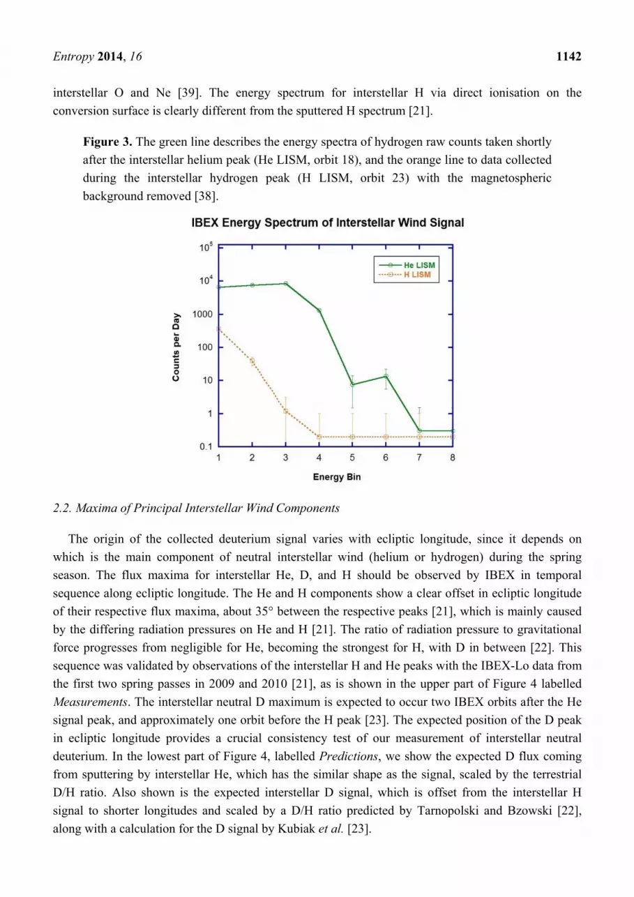
deuterium. In the lowest part of Figure 4, labelled Predictions, we show the expected D flux coming

from sputtering by interstellar He, which has the similar shape as the signal, scaled by the terrestrial

D/H ratio. Also shown is the expected interstellar D signal, which is offset from the interstellar H

signal to shorter longitudes and scaled by a D/H ratio predicted by Tarnopolski and Bzowski [22],

along with a calculation for the D signal by Kubiak et al. [23].

Entropy 2014, 16 1143

To summarise, Figure 4 shows the comparison between the existing measurements of the He and H

interstellar wind components, and the predicted D signal. The interstellar He peak is stable in

longitude, latitude, width, and amplitude from year to year, while the hydrogen peak is observed to

vary significantly from year to year [21,38]. The maximum of interstellar He is found in the first and

second week of February. Therefore, the maximum of the terrestrial deuterium from the conversion

surface must be located also at the same time. The interstellar hydrogen begins to be measured in the

last week of February, significantly overlapping with the hydrogen from sputtering by interstellar He.

In the first week of March this interference starts to diminish as increasing ecliptic longitude until

vanishes. The measurements show that only at the end of the spring passage, when the interstellar wind

component is no longer helium (interstellar He is significantly lower), the pure interstellar hydrogen

can be measured directly. Then, the deuterium measurement would be almost completely free from

additions of helium sputter products, which means that it is unambiguously of interstellar origin.

Figure 4. Signal of He and H components of the interstellar wind as function of the

day-of-year in Earth orbit, normalised to the He peak, starting on the first of January of

each year. In the measurement panel, data from the first two spring passes of IBEX in 2009

and 2010 are shown (from [21]). In the lower part, predictions for the expected D signal are

shown for the sputtered D (terrestrial D in energy bins 1 to 3) and interstellar D only in

energy bin 3. Also, the time intervals are indicated, which group the orbits in time intervals

1 to 5. For reference, an additional x-axis shows the ecliptic longitude in degrees, referring

to the beginning of the DOY.

Entropy 2014, 16 1144

2.3. Determination of the Deuterium Location in the TOF Spectra—3D-TOF Method

2.3.1. First Approach. Using one TOF Dimension

In the present section, we show the successive development of the analysis method used to obtain

the position of a species in the three-dimensional TOF space, and the subsequent counting of the D

events at this location [8]. In this description also included are unsuccessful attempts, because they

gave us direction how to continue our analysis, so therefore they are an important part of the method

as such.

We initially analysed the data collected during individual orbits for the three lowest energy bins of

IBEX-Lo, in the three different TOF channels separately. We will be referring to such type of TOF

spectra analysis as the one dimensional method. An example for the TOF data and the one dimensional

analysis is shown in Figure 5.

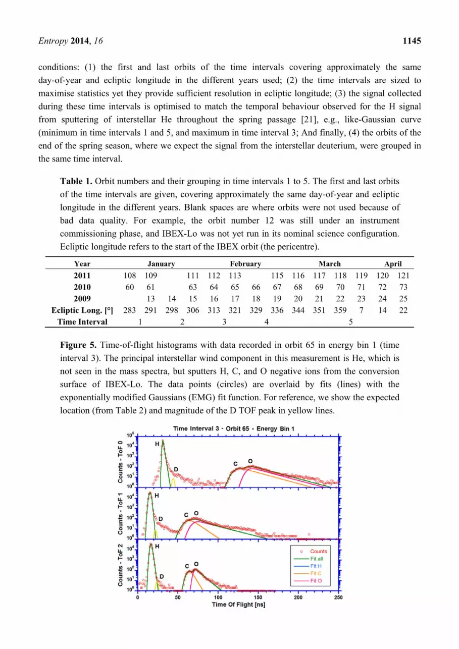
The data collected for energy bin 3 of IBEX-Lo during orbit 65 (period of 9–17 February 2010) at

the maximum interstellar He flux, are shown as a histogram of spin phase versus day-of-year (DOY) in

Figure 6. The spin phase is the heliospheric latitude in spacecraft coordinates with the ecliptic north at

a spin phase of 0.5. The signal from the neutral interstellar wind is clearly observed as the horizontal

band that crosses from left to right (in DOY) that is centred at spin phase of 0.75 (the ecliptic plane)

and spanning in values 0.69 to 0.80. The red rectangle identified shows the selection of data with an

optimised range in spin phase for signal-to-noise, which is applied for further analysis. On the right

side of Figure 6 we show the histograms of events collected with the lowest four energy bins, against

spin phase. The maxima of the interstellar wind signal in energy bin 1 to 3 show clearly a constant

value near to 103 events, with an abrupt reduction of counts for energy bin 4 (~102 events). Such

behaviour is expected for the interstellar helium signal and in agreement with calibration [38], see also

energy spectrum for interstellar Helium shown in Figure 3. The red dashed lines over the histogram

that bracket the rectangle in Figure 6, exclude the base of the signal peak at the level of 1% of the peak

value, to optimise the signal/noise ratio.

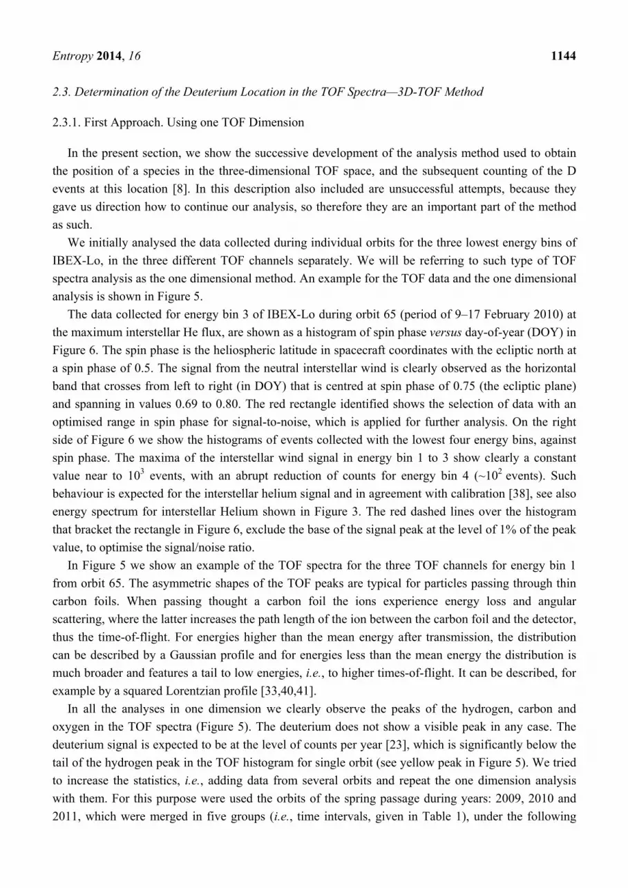
In Figure 5 we show an example of the TOF spectra for the three TOF channels for energy bin 1

from orbit 65. The asymmetric shapes of the TOF peaks are typical for particles passing through thin

carbon foils. When passing thought a carbon foil the ions experience energy loss and angular

scattering, where the latter increases the path length of the ion between the carbon foil and the detector,

thus the time-of-flight. For energies higher than the mean energy after transmission, the distribution

can be described by a Gaussian profile and for energies less than the mean energy the distribution is

much broader and features a tail to low energies, i.e., to higher times-of-flight. It can be described, for

example by a squared Lorentzian profile [33,40,41].

In all the analyses in one dimension we clearly observe the peaks of the hydrogen, carbon and

oxygen in the TOF spectra (Figure 5). The deuterium does not show a visible peak in any case. The

deuterium signal is expected to be at the level of counts per year [23], which is significantly below the

tail of the hydrogen peak in the TOF histogram for single orbit (see yellow peak in Figure 5). We tried

to increase the statistics, i.e., adding data from several orbits and repeat the one dimension analysis

with them. For this purpose were used the orbits of the spring passage during years: 2009, 2010 and

2011, which were merged in five groups (i.e., time intervals, given in Table 1), under the following

Entropy 2014, 16 1145

conditions: (1) the first and last orbits of the time intervals covering approximately the same

day-of-year and ecliptic longitude in the different years used; (2) the time intervals are sized to

maximise statistics yet they provide sufficient resolution in ecliptic longitude; (3) the signal collected

during these time intervals is optimised to match the temporal behaviour observed for the H signal

from sputtering of interstellar He throughout the spring passage [21], e.g., like-Gaussian curve

(minimum in time intervals 1 and 5, and maximum in time interval 3; And finally, (4) the orbits of the

end of the spring season, where we expect the signal from the interstellar deuterium, were grouped in

the same time interval.

Table 1. Orbit numbers and their grouping in time intervals 1 to 5. The first and last orbits

of the time intervals are given, covering approximately the same day-of-year and ecliptic

longitude in the different years. Blank spaces are where orbits were not used because of

bad data quality. For example, the orbit number 12 was still under an instrument

commissioning phase, and IBEX-Lo was not yet run in its nominal science configuration.

Ecliptic longitude refers to the start of the IBEX orbit (the pericentre).

Year January February March April

2011 108 109 111 112 113 115 116 117 118 119 120 121

2010 60 61 63 64 65 66 67 68 69 70 71 72 73

2009 13 14 15 16 17 18 19 20 21 22 23 24 25

Ecliptic Long. [°] 283 291 298 306 313 321 329 336 344 351 359 7 14 22

Time Interval 1 2 3 4 5

Figure 5. Time-of-flight histograms with data recorded in orbit 65 in energy bin 1 (time

interval 3). The principal interstellar wind component in this measurement is He, which is

not seen in the mass spectra, but sputters H, C, and O negative ions from the conversion

surface of IBEX-Lo. The data points (circles) are overlaid by fits (lines) with the

exponentially modified Gaussians (EMG) fit function. For reference, we show the expected

location (from Table 2) and magnitude of the D TOF peak in yellow lines.

Entropy 2014, 16 1146

Figure 6. The left panel is the histogram of spin phase over observation time of neutral

interstellar wind (ISN) recorded in energy bin 3 of IBEX-Lo during orbit 65, the maximum

signal from interstellar He. DOY is starting on 1 January 2008. The spin phase is the

heliospheric latitude in spacecraft coordinates with the ecliptic plane being at spin phase of

0.75 (0.25). The north ecliptic pole (NP) is at a spin phase of0.5 and the south ecliptic pole

(SP) is at0.0 (1.0). The interstellar wind signal can be seen as a wide horizontal strip across

the figure between 0.69 and 0.80 in spin phase. The right panel shows a histogram for the

time period, with maxima roughly at the ecliptic plane, for the energy bins 1 to 4 (9116,

10046, 10463, and 1824 counts) respectively.

All time intervals are defined as a combination of six successive orbits that share approximately the

same observation times in each year, same ecliptic longitude [8]. This combination of six orbits is

repeated for the time intervals 1 through 4. Owing to the low expected interstellar deuterium fluxes [22,23],

for time interval 5 we combine six orbits in March and April of each of the three years used. In the

lower part of Figure 4, we show the different time intervals with their temporal and ecliptic longitude

coverage during the spring passage orbits. We applied the one dimensional analysis to this way of data

grouping, but the results were similar to those obtained for individual orbits.

Then, we extended the analysis to another orbit grouping, merging the time intervals: in temporal

sequence of pairs, those with He as principal component of interstellar wind, and finally created single

file with the all the data available, by merging the five time intervals. Unfortunately, the deuterium

signal remained below the hydrogen tail despite increasing the statistics. In summary no identifiable

deuterium peak was observed with the one-dimensional analysis.

To improve the analysis, we tried a series of indirect methods that should allow extracting the

deuterium events from the flank of the hydrogen peak. The first method implemented was to fit a

mathematical function to the H peak, subtract the fitted function from the hydrogen signal to isolate the

Entropy 2014, 16 1147

deuterium peak. We fit the hydrogen and other relevant mass peaks, in each of the three TOF spectra

for each of the first three energy channels of IBEX-Lo and five orbit grouping intervals to obtain the fit

parameters (peak position, area, width, asymmetry, and then FWHM), which were very useful later in

the development of the final method. The fit function used was an Exponentially Modified Gaussian

(EMG), which correctly describes the observed peak shape in one dimension (Equation (1)). The EMG

is a mathematical function resulting from a convolution of a Gaussian with an exponential function:

20 1 32 1 2( ) exp erf

22 2 23 3 32 2 33

aa ta a t ai aiEMG tia a aa aa

(1)

where EMG(ti) describes the number of counts per TOF channel (with i = 0, 1, 2 for TOF0, TOF1, and

TOF2). The parameter a0 describes the area under the peak, a1 is the peak position, a2 is the peak

width, and a3 characterises the peak asymmetry. The averages of the peak positions for H, C, and O

from fitting these TOF spectra with the EMG function are summarised in Table 2.

Table 2. Estimated TOF values in nanoseconds for H, C, and O obtained from EMG peak

fitting of data taken for the different groupings of orbits (time intervals 1 to 5), energy bins

(1, 2, and 3), and TOFs during the spring passage. The values of the observable and

unobservable species peaks were calculated using the mass equations (MEQ).

Species H mass = 2 He C O

Tech EMG MEQ EMG MEQ EMG MEQ EMG MEQ EMG MEQ

TOF0 29.525 29.331 - 42.416 - 59.854 119.196 119.145 135.945 136.074

TOF1 13.935 14.108 - 21.656 - 30.869 59.721 59.698 67.513 67.574

TOF2 14.467 14.339 - 22.228 - 31.604 60.298 60.276 67.960 68.020

Although the peak of hydrogen is fairly good natured, a precise fit of this peak with its tail over

five decades, was not possible. We spent a lot of time trying to use careful fitting and to do the

subtraction, but in the end we had to give up on a D measurement from a single TOF channel. Indeed,

the correct isolation of the deuterium events from the H tail has been the biggest challenge faced here

in our analysis efforts. In any given single TOF channel, the H peak is wide enough to also have some

contribution (though more than three orders of magnitude below the H peak) at the expected D

location. After intensely investigating the 1D TOF analysis, we arrived at the conclusions that a direct

method of observation of the deuterium signal is not possible, only an indirect method and that

comprises the use of the three TOF channels would have any chance of success.

2.3.2. Analysis in Two TOF Dimensions

We created two dimensional TOF histograms that were created from combination of two TOFs, and

by collapsing of third TOF dimension. These 2D TOF histograms were also employed for data

visualization (see Figure 7, with TOF0 versus TOF2 with TOF1 collapsed), and produced for each

energy bin and each time interval. The obvious result of the use of the two TOF dimensions is the

significant improvement in the visualisation of the data. When attending to the details, the 2D histogram

Entropy 2014, 16 1148

explains qualitatively why the searching of the deuterium peak with one dimension method did not

give a useful result.

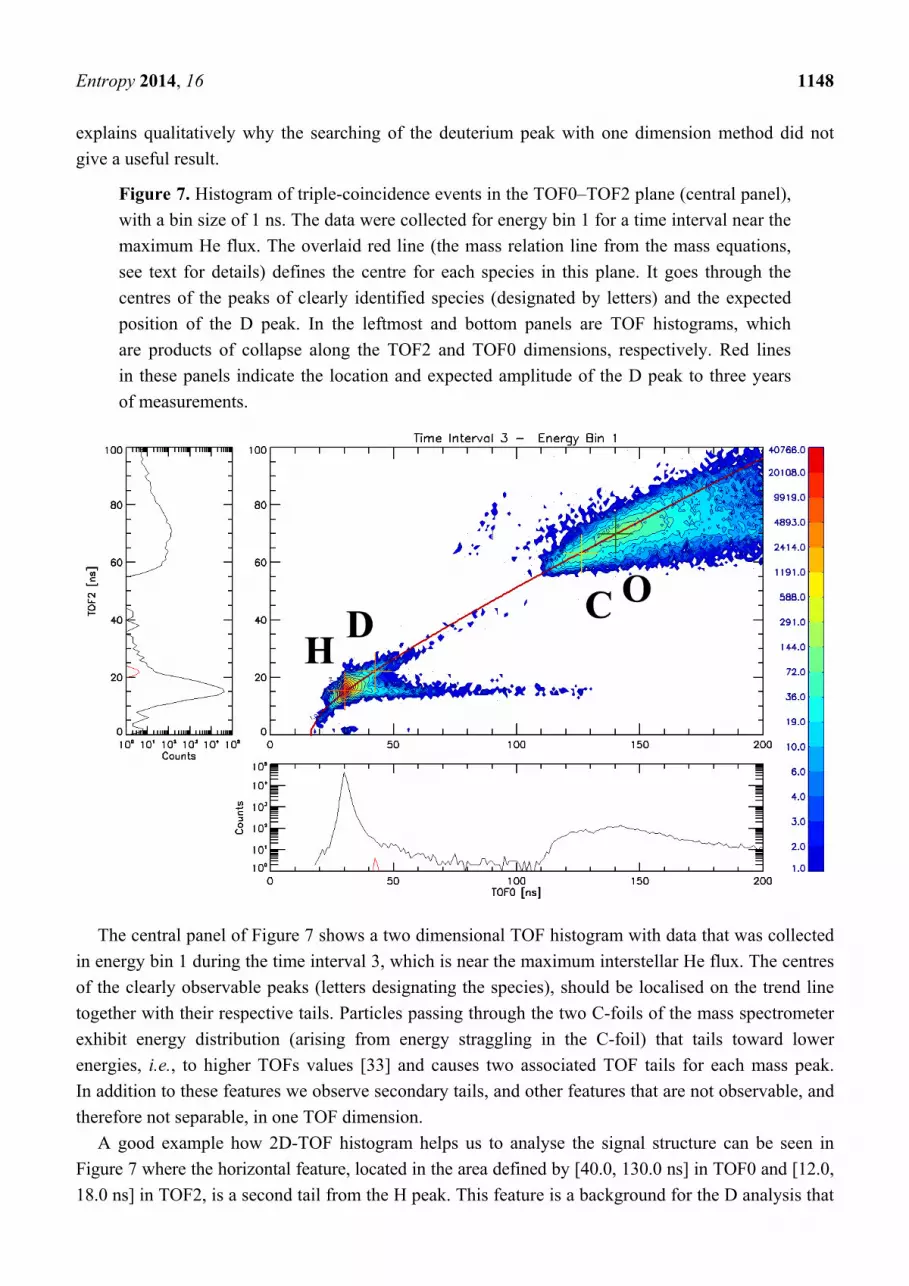
Figure 7. Histogram of triple-coincidence events in the TOF0–TOF2 plane (central panel),

with a bin size of 1 ns. The data were collected for energy bin 1 for a time interval near the

maximum He flux. The overlaid red line (the mass relation line from the mass equations,

see text for details) defines the centre for each species in this plane. It goes through the

centres of the peaks of clearly identified species (designated by letters) and the expected

position of the D peak. In the leftmost and bottom panels are TOF histograms, which

are products of collapse along the TOF2 and TOF0 dimensions, respectively. Red lines

in these panels indicate the location and expected amplitude of the D peak to three years

of measurements.

The central panel of Figure 7 shows a two dimensional TOF histogram with data that was collected

in energy bin 1 during the time interval 3, which is near the maximum interstellar He flux. The centres

of the clearly observable peaks (letters designating the species), should be localised on the trend line

together with their respective tails. Particles passing through the two C-foils of the mass spectrometer

exhibit energy distribution (arising from energy straggling in the C-foil) that tails toward lower

energies, i.e., to higher TOFs values [33] and causes two associated TOF tails for each mass peak.

In addition to these features we observe secondary tails, and other features that are not observable, and

therefore not separable, in one TOF dimension.

A good example how 2D-TOF histogram helps us to analyse the signal structure can be seen in

Figure 7 where the horizontal feature, located in the area defined by [40.0, 130.0 ns] in TOF0 and [12.0,

18.0 ns] in TOF2, is a second tail from the H peak. This feature is a background for the D analysis that

Entropy 2014, 16 1149

completely masks the D peak when collapsed to a 1D-TOF0 histogram, as shown in the lower panel of

Figure 7. The red lines in this panel show an estimate of the D peak in the D histograms for this

measurement. The same situation occurs for the other two TOFs pair combinations (see different

panels Figure 8). Thus to minimise the impact of background from these secondary tails on the D

signal we rely to a large part on the analysis in three TOF dimensions.

The observed trend line shows that the centres of each species are located on a line in 2D TOF

space. We can identify mathematical expressions, i.e., mass equations; that relate the masses of a

species with their time-of-flights. These mass equations are derived from their TOF positions, which

already were accurately determined by fit in the 1D TOF spectra. The mass equations allow an analytic

interpolation to find the TOF position of species not investigated during instrument calibration nor are

directly observed in the flight data. The comparison between the locus of deuterium derived by this

method and estimates based on instrument simulation [8] were highly favourably.

The mass equations were established as cubic functions that describe the relation between the

atomic masses of H, C, and O based on TOF measurements. Initially we used quadratic functions to

carry out this task but after completing the entire process, which will be described below, the accuracy

of the predicted peak positions for the three clearly observed TOF peaks was insufficient. For that

reason we used cubic functions that gave a better approximation. By dropping the linear terms in the

cubic functions we achieved the best agreement with the measured peak positions.

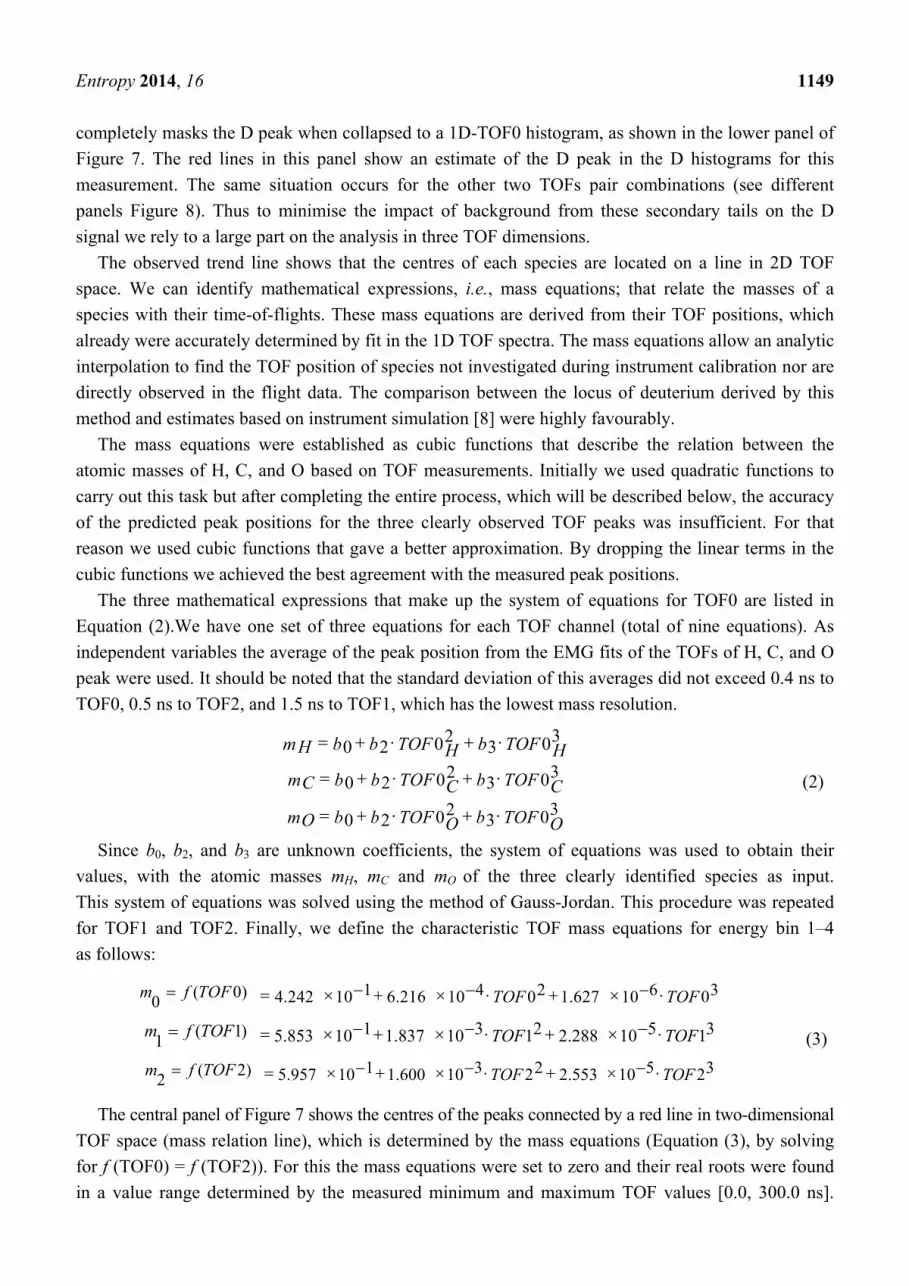
The three mathematical expressions that make up the system of equations for TOF0 are listed in

Equation (2).We have one set of three equations for each TOF channel (total of nine equations). As

independent variables the average of the peak position from the EMG fits of the TOFs of H, C, and O

peak were used. It should be noted that the standard deviation of this averages did not exceed 0.4 ns to

TOF0, 0.5 ns to TOF2, and 1.5 ns to TOF1, which has the lowest mass resolution.

320 00 2 3m b b TOF b TOFH H H

320 00 2 3m b b TOF b TOFC C C

320 00 2 3m b b TOF b TOFO O O

(2)

Since b0, b2, and b3 are unknown coefficients, the system of equations was used to obtain their

values, with the atomic masses mH, mC and mO of the three clearly identified species as input.

This system of equations was solved using the method of Gauss-Jordan. This procedure was repeated

for TOF1 and TOF2. Finally, we define the characteristic TOF mass equations for energy bin 1–4

as follows:

1 4 2 6 3( 0) 4.242 10 6.216 10 0 1.627 10 00m f TOF TOF TOF

1 3 2 5 3( 1) 5.853 10 1.837 10 1 2.288 10 11m f TOF TOF TOF

1 3 2 5 3( 2) 5.957 10 1.600 10 2 2.553 10 22m f TOF TOF TOF

(3)

The central panel of Figure 7 shows the centres of the peaks connected by a red line in two-dimensional

TOF space (mass relation line), which is determined by the mass equations (Equation (3), by solving

for f (TOF0) = f (TOF2)). For this the mass equations were set to zero and their real roots were found

in a value range determined by the measured minimum and maximum TOF values [0.0, 300.0 ns].

Entropy 2014, 16 1150

Then the curve shown depends on the TOF combination that is chosen for the plot (TOFi · TOFj, with

i, j = 0, 1, 2; TOF0 and TOF2 in this example). As shown in Figure 7, the model line clearly passes

through the centres of the peaks for the identified species. So this line determines a solution that allows

us to predict where the centre for a selected mass is located in the absence of a distinct peak.

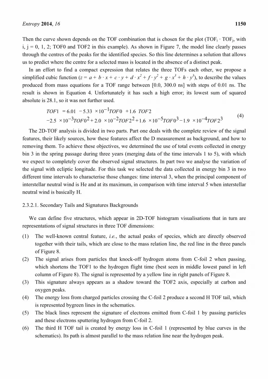
In an effort to find a compact expression that relates the three TOFs each other, we propose a

simplified cubic function (z = a + b · x + c · y + d · x2 + f · y2 + g · x3 + h · y3), to describe the values

produced from mass equations for a TOF range between [0.0, 300.0 ns] with steps of 0.01 ns. The

result is shown in Equation 4. Unfortunately it has such a high error; its lowest sum of squared

absolute is 28.1, so it was not further used.

11 6.01 5.33 10 0 1.6 23 2 2 2 5 3 4 32.5 10 0 2.0 10 2 1.6 10 0 1.9 10 2

TOF TOF TOF

TOF TOF TOF TOF

(4)

The 2D-TOF analysis is divided in two parts. Part one deals with the complete review of the signal

features, their likely sources, how these features affect the D measurement as background, and how to

removing them. To achieve these objectives, we determined the use of total events collected in energy

bin 3 in the spring passage during three years (merging data of the time intervals 1 to 5), with which

we expect to completely cover the observed signal structures. In part two we analyse the variation of

the signal with ecliptic longitude. For this task we selected the data collected in energy bin 3 in two

different time intervals to characterise those changes: time interval 3, when the principal component of

interstellar neutral wind is He and at its maximum, in comparison with time interval 5 when interstellar

neutral wind is basically H.

2.3.2.1. Secondary Tails and Signatures Backgrounds

We can define five structures, which appear in 2D-TOF histogram visualisations that in turn are

representations of signal structures in three TOF dimensions:

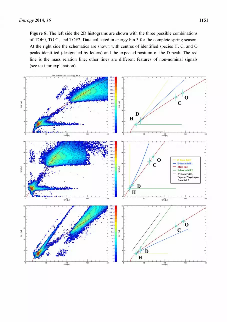
(1) The well-known central feature, i.e., the actual peaks of species, which are directly observed

together with their tails, which are close to the mass relation line, the red line in the three panels

of Figure 8.

(2) The signal arises from particles that knock-off hydrogen atoms from C-foil 2 when passing,

which shortens the TOF1 to the hydrogen flight time (best seen in middle lowest panel in left

column of Figure 8). The signal is represented by a yellow line in right panels of Figure 8.

(3) This signature always appears as a shadow toward the TOF2 axis, especially at carbon and

oxygen peaks.

(4) The energy loss from charged particles crossing the C-foil 2 produce a second H TOF tail, which

is represented bygreen lines in the schematics.

(5) The black lines represent the signature of electrons emitted from C-foil 1 by passing particles

and these electrons sputtering hydrogen from C-foil 2.

(6) The third H TOF tail is created by energy loss in C-foil 1 (represented by blue curves in the

schematics). Its path is almost parallel to the mass relation line near the hydrogen peak.

Entropy 2014, 16 1151

Figure 8. The left side the 2D histograms are shown with the three possible combinations

of TOF0, TOF1, and TOF2. Data collected in energy bin 3 for the complete spring season.

At the right side the schematics are shown with centres of identified species H, C, and O

peaks identified (designated by letters) and the expected position of the D peak. The red

line is the mass relation line; other lines are different features of non-nominal signals

(see text for explanation).

Entropy 2014, 16 1152

The background features 1 to 4 do not give any contribution to the D measurement in three

dimensions, even though in the 1D-TOF representation they completely mask the D signal. The 3D

analysis allows separating their apparent contributions from the deuterium signal. The most important

background feature in our analysis is the feature 5, which is close to the mass line, thus close to the

expected position of D. However, we find that the separation is large enough that the background at the

D peak is not detected.

Based on time-of-flight analysis alone, there is in principle, no easy way to distinguish a particle

with larger mass going into the mass spectrometer compared to a lighter one that has lost more energy

in the C-foil at the TOF entrance. However, the H TOF tail (feature 5 from above list) shows a small

angle with the mass relation line, leaving the D signal free of contamination by the H tail. This is easily

seen by comparing the left and right panels of Figure 8 for each 2D histogram. Moreover, as will be

seen in the next section, the intensity of this tail will be strong reduced at the time interval 5, where is

expected to see the signal of interstellar deuterium.

2.3.2.2. Intensity Variations

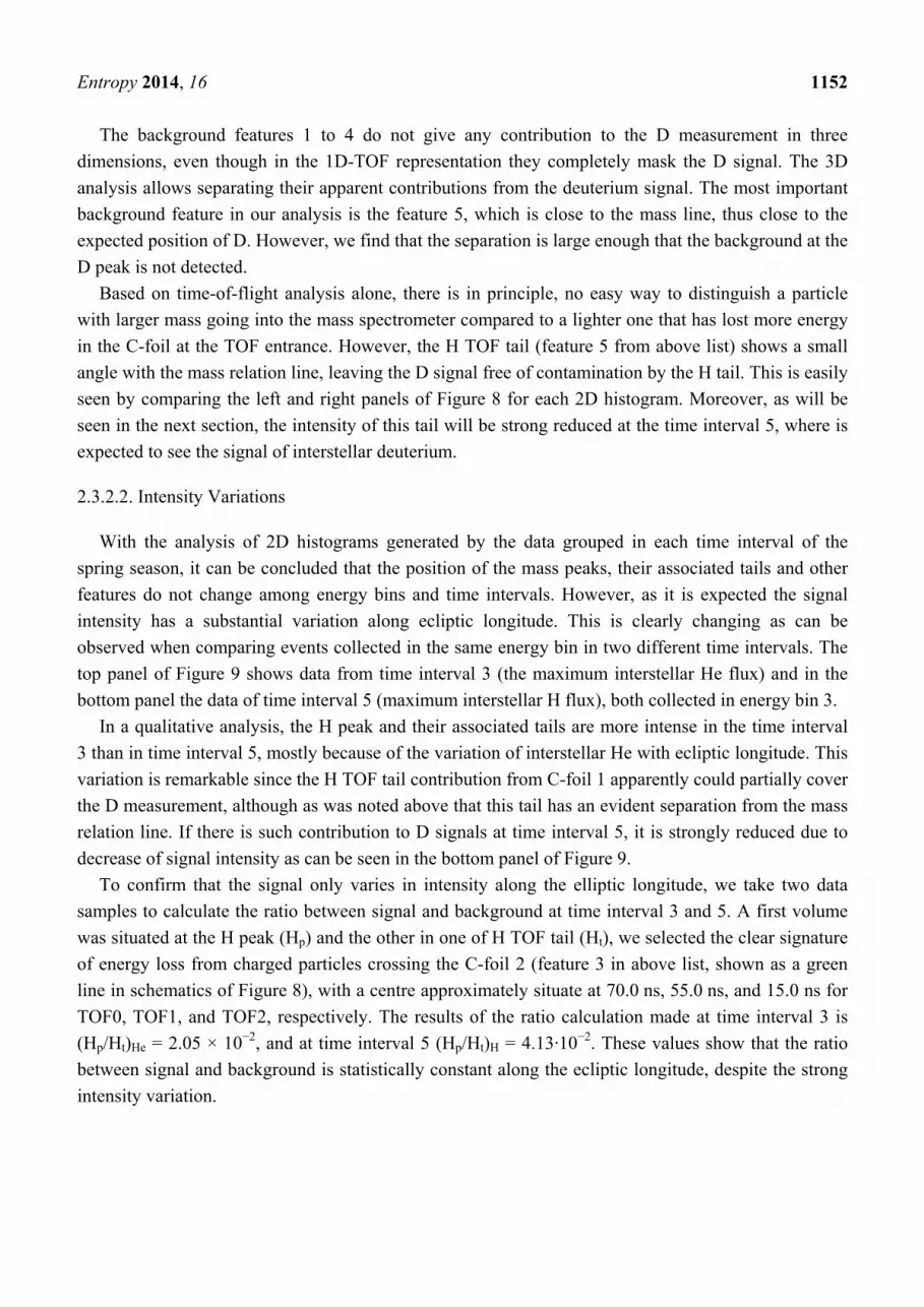
With the analysis of 2D histograms generated by the data grouped in each time interval of the

spring season, it can be concluded that the position of the mass peaks, their associated tails and other

features do not change among energy bins and time intervals. However, as it is expected the signal

intensity has a substantial variation along ecliptic longitude. This is clearly changing as can be

observed when comparing events collected in the same energy bin in two different time intervals. The

top panel of Figure 9 shows data from time interval 3 (the maximum interstellar He flux) and in the

bottom panel the data of time interval 5 (maximum interstellar H flux), both collected in energy bin 3.

In a qualitative analysis, the H peak and their associated tails are more intense in the time interval

3 than in time interval 5, mostly because of the variation of interstellar He with ecliptic longitude. This

variation is remarkable since the H TOF tail contribution from C-foil 1 apparently could partially cover

the D measurement, although as was noted above that this tail has an evident separation from the mass

relation line. If there is such contribution to D signals at time interval 5, it is strongly reduced due to

decrease of signal intensity as can be seen in the bottom panel of Figure 9.

To confirm that the signal only varies in intensity along the elliptic longitude, we take two data

samples to calculate the ratio between signal and background at time interval 3 and 5. A first volume

was situated at the H peak (Hp) and the other in one of H TOF tail (Ht), we selected the clear signature

of energy loss from charged particles crossing the C-foil 2 (feature 3 in above list, shown as a green

line in schematics of Figure 8), with a centre approximately situate at 70.0 ns, 55.0 ns, and 15.0 ns for

TOF0, TOF1, and TOF2, respectively. The results of the ratio calculation made at time interval 3 is

(Hp/Ht)He = 2.05 × 10−2, and at time interval 5 (Hp/Ht)H = 4.13·10−2. These values show that the ratio

between signal and background is statistically constant along the ecliptic longitude, despite the strong

intensity variation.

Entropy 2014, 16 1153

Figure 9. Variability of the intensity is shown by comparing data collected in two time

intervals of spring season in energy bin 3. There are remarkable differences in intensity

that can be identified in the signal and background. In the top panel data for the maximum

He flux are shown (time interval 3), and in the bottom panel data for maximum H flux are

shown (time interval 5).

Entropy 2014, 16 1154

2.3.2.3. Alternative Methods

At this point, we have to mention two alternative methods done in 2D-TOF that although they were

not successful, gave us a guidance how to continue our analysis. The first method is the subtraction of

a fitted H peak from the signal in two dimensions, again with putting particular emphasis on H TOF

tail. For this reason, we extend the modelling of the hydrogen peak made with EMG to other

asymmetric functions. The tailed functions for which we obtained better results than with the EMG

were: Lorentz, Pearson IV, Gauss-Lorentz, and Student T.

The method is schematically is as follows: the H peak is fit in each one dimensional TOF spectra

with a tailed function, which produces a group of parameters by each dimension (TOF0, TOF1, and

TOF2), later it is selected a TOF combination to analyse (i.e., TOF0–TOF2 collapsing TOF1 in Figure 10),

then multiplying the two fit functions with their respective parameters together with the unitary

bivariate Gaussian function, giving us a preliminary H peak mask in two dimensions (Equation (5)).

( , ) ( ) ( , )( )Mask t t EMG t Bi Gauss t tEMG tx y y y x yx x (5)

The initial fit function has to be adjusted to the signal before making the subtraction. To accomplish

this we selected the same pair combination of TOF flight data and collapse the third TOF. The two

dimensional structures of the signal and the initial fit function were overlapping and after several

iterations a good fit was accomplished, as indicated by a χ2 minimum, but taking into account the

asymmetry parameters, which describes the tail of the peak. Finally, the resulting fit function is

subtracted from signal, expecting to set free the D peak in two TOF dimension.

The main problem of matching the H tail is that with a little variation of the asymmetry parameter

(i.e., a3 in the EMG function, see Equation (1)) produces a dramatic change in the modelled tail.

Contrary to our expectation, the EMG function that worked very well for one dimensional TOF spectra

(Figure 6) did not do well in two dimensions (see left and bottom panels in Figure 10). The best

modelling was accomplished with Student T function, after several fitting iterations and fixing the

position and width parameters of the peak. However, the result proved unsuccessful for a reliable

detection of the D signal.

Another approach was to take advance of mass relation line and 3D-TOF space to eliminate the

background of secondary tails, leaving only the central volume near mass relation line where the

species peaks are observed. The method basically is the selection of events in the vicinity of the mass

relation line, and discarding events that are outside of a defined distance to the mass relation line.

Thus, we define a range in two TOF dimension selected for analysis (i.e., TOF0–TOF2, shown in

Figure 11), based on the mass relation line, from which we calculate two parallels lines (referring to

major and minor values respectively in each TOF axis), optimising the distance between them to

making sure of take most events from signal are inside and most events from background are

discarded. In 3D-TOF analysis, we can imagine two walls running together to mass relation line,

which similarly determine two limits for data analysis; the result is a slice which shows the central

feature of the signal with the background eliminated. We found that the H tail contribution to the D

signal was reduced by three orders of magnitude. Changing the width of this slice, significantly

changed the result, which, unfortunately, made this technique too parameter dependent. However, this

is still one of the better techniques of examining our three dimensions data.

Entropy 2014, 16 1155

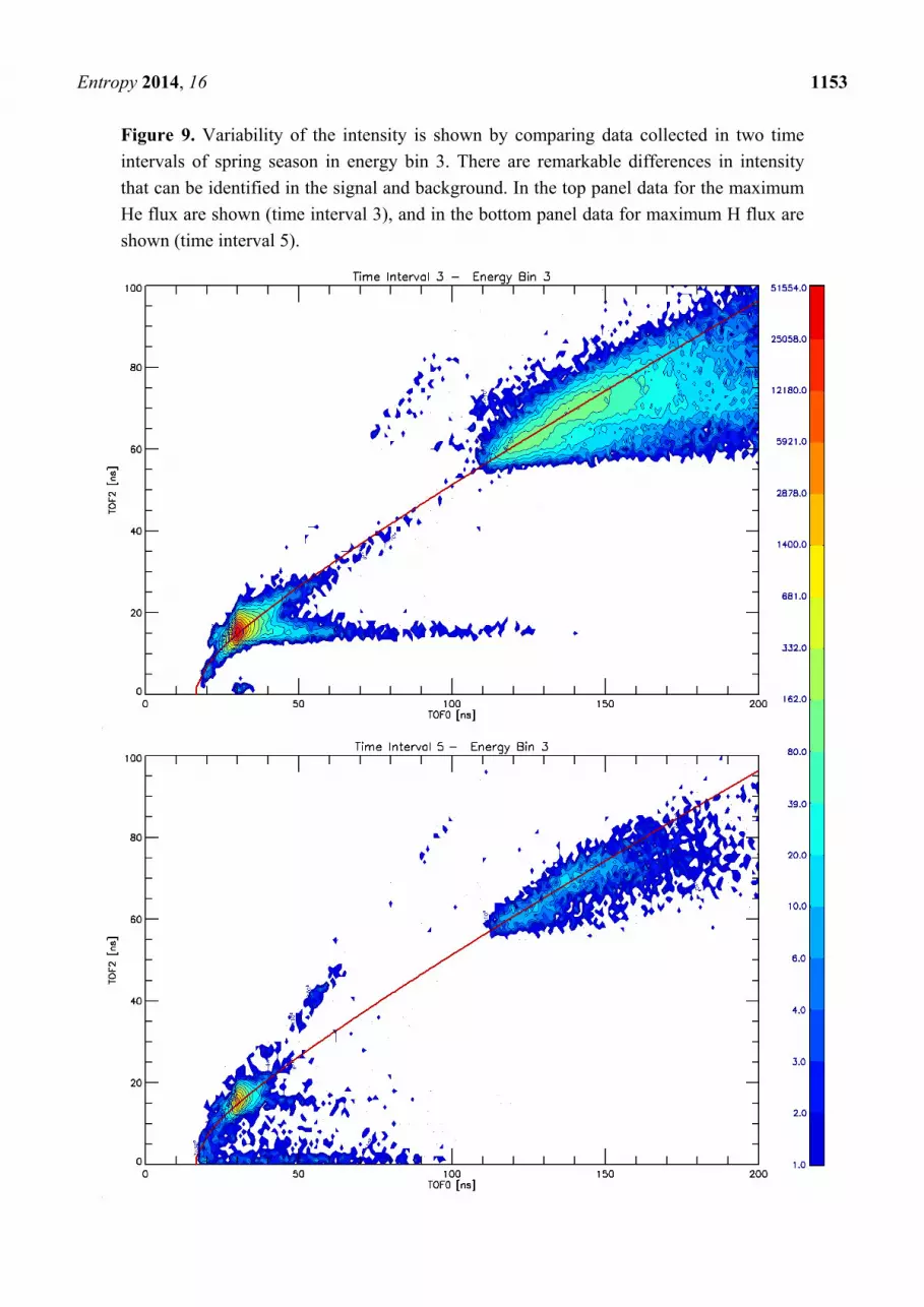
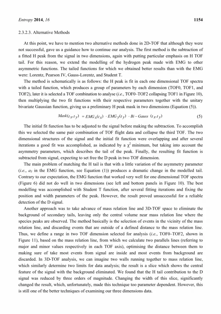
Figure 10. Histogram of triple-coincidence events in the TOF0–TOF2 plane (central panel)

with data collected in energy bin 3 at time interval 3. The H peak is created from

parameters of the EMG fit (the red lines in the centre panel). Although the fit function

matched the H peak reasonably well, it is not good enough at the H tail where deuterium is

located, see the blue lines in the left and bottom panels. As reference, the location and

expected amplitude of the deuterium peak is indicated by a red line in the left and bottom

side panels.

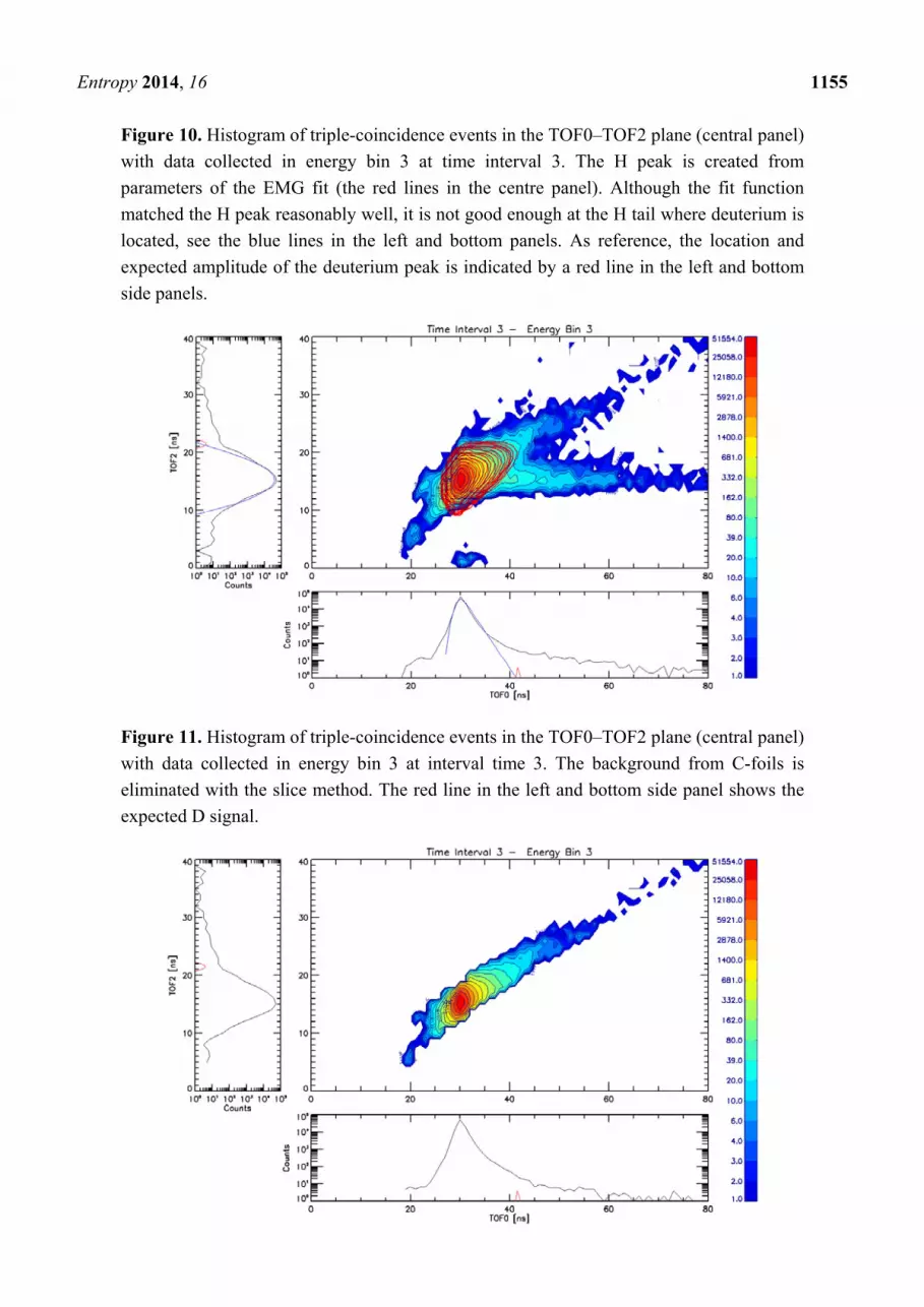
Figure 11. Histogram of triple-coincidence events in the TOF0–TOF2 plane (central panel)

with data collected in energy bin 3 at interval time 3. The background from C-foils is

eliminated with the slice method. The red line in the left and bottom side panel shows the

expected D signal.

Entropy 2014, 16 1156

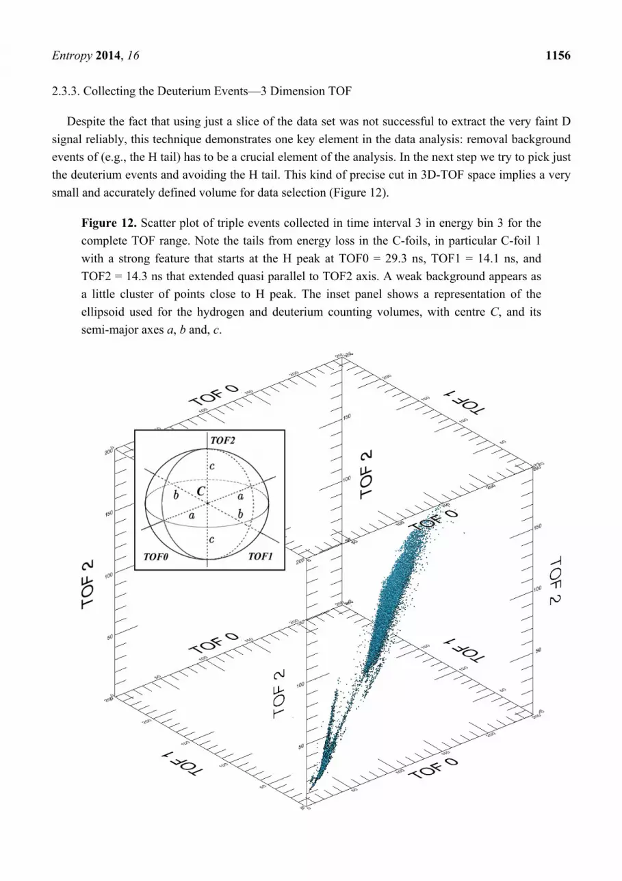
2.3.3. Collecting the Deuterium Events—3 Dimension TOF

Despite the fact that using just a slice of the data set was not successful to extract the very faint D

signal reliably, this technique demonstrates one key element in the data analysis: removal background

events of (e.g., the H tail) has to be a crucial element of the analysis. In the next step we try to pick just

the deuterium events and avoiding the H tail. This kind of precise cut in 3D-TOF space implies a very

small and accurately defined volume for data selection (Figure 12).

Figure 12. Scatter plot of triple events collected in time interval 3 in energy bin 3 for the

complete TOF range. Note the tails from energy loss in the C-foils, in particular C-foil 1

with a strong feature that starts at the H peak at TOF0 = 29.3 ns, TOF1 = 14.1 ns, and

TOF2 = 14.3 ns that extended quasi parallel to TOF2 axis. A weak background appears as

a little cluster of points close to H peak. The inset panel shows a representation of the

ellipsoid used for the hydrogen and deuterium counting volumes, with centre C, and its

semi-major axes a, b and, c.

Entropy 2014, 16 1157

To define the size of volume that will be located at the expected location of deuterium in 3D TOF

space, we assume that the width of the H and D peak approximately comply with

D H ⁄ , H√2, so that we can compute an approximate value of the deuterium peak

width with Equation (6). In one dimension the H peak is very clearly identified [8], obtaining its σH

values is a straightforward task from the fit parameters, then the range for counting events of

deuterium is determined from the sigma σH taking the hydrogen peak as a Gaussian distribution near its

top. From the analysis of each TOF channel we obtain σH = 0.6609 ns, 1.2969 ns, and 1.155 ns, for

TOF0, TOF1, and TOF2, respectively.

2.35482FWHM D

D (6)

This gives us σD = 0.9347 ns, 1.8341 ns, and 1.6335 ns for the three TOF channels. For two

dimensions (whichever possible linear combination between two TOFs), the counting range becomes

an ellipse, since the widths of the TOF peaks are different in each TOF channel. Both areas are

determined by hydrogen and deuterium sigma, respectively, as was described above. In others words,

we are working at the plus-minus one sigma level when collecting events. In three dimensions, we

have to simultaneously analyse all three TOFs, the volume allowing us to count the events is an

ellipsoid described by Equation (7):

2 2 2) ) )( 0 ( 1 ( 20 1 2 12 2 2

TOF TOF TOFC C C

a b c

(7)

where a, b, and c are the semi-major axes of the ellipsoid in the three coordinates given by the

Gaussian widths. The constants C0, C1, and C2 define the ellipsoid centre. TOF0, TOF1, and TOF2 are

the time-of-flight data. The less than or equal to condition is used to collect the events inside the

ellipsoid. Equation 7 defines the volume in the three dimensional TOF space where the H and D events

are counted (terrestrial, interstellar or of both origins). The semi-major axis (a, b, and c) are depending

on the species under evaluation: the hydrogen or deuterium values. The Ci values for hydrogen volume

were taken directly from fits position parameters, because the well-defined position of its peak, these

are constant for further calculations (see Figure 13).

For the ellipsoid centre of deuterium, Ci, we have to make a comprehensive search of the most

likely position of deuterium events for the three times-of-flight dimensions, which is based on the mass

equations and TOF simulations. These positions can be represented as a small cloud of points in the

3D-TOF space. We also included other possible values we did not take into account before, and we

created a grid in 3D-TOF space with a grid spacing of 0.05 ns. The created search cube is defined in

nanoseconds as follows: TOF0 = [40.0, 45.0 ns], TOF1= [18.0, 23.0 ns] and, TOF2 = [19.0, 24.0 ns].

Notice as the range of times is very wide, with 5 ns in each TOF dimension. Then, the number of

possible deuterium ellipsoid centres for analyses is 106, however, this big number will be strongly

reduced by other restrictions.

We analysed the data collected in energy bins 1, 2, 3, and 4 of IBEX-Lo in each time interval of the

spring season. Counting at each time interval and their respective energy bins, the H and D events and

then calculate the D/H ratio. For this purpose, we create two volumes for counting events, one for the

Entropy 2014, 16 1158

H peak with position and widths completely defined and constants for the whole search procedure, and

one for the D peak with widths defined by Equation 7, and with its centre location variable.

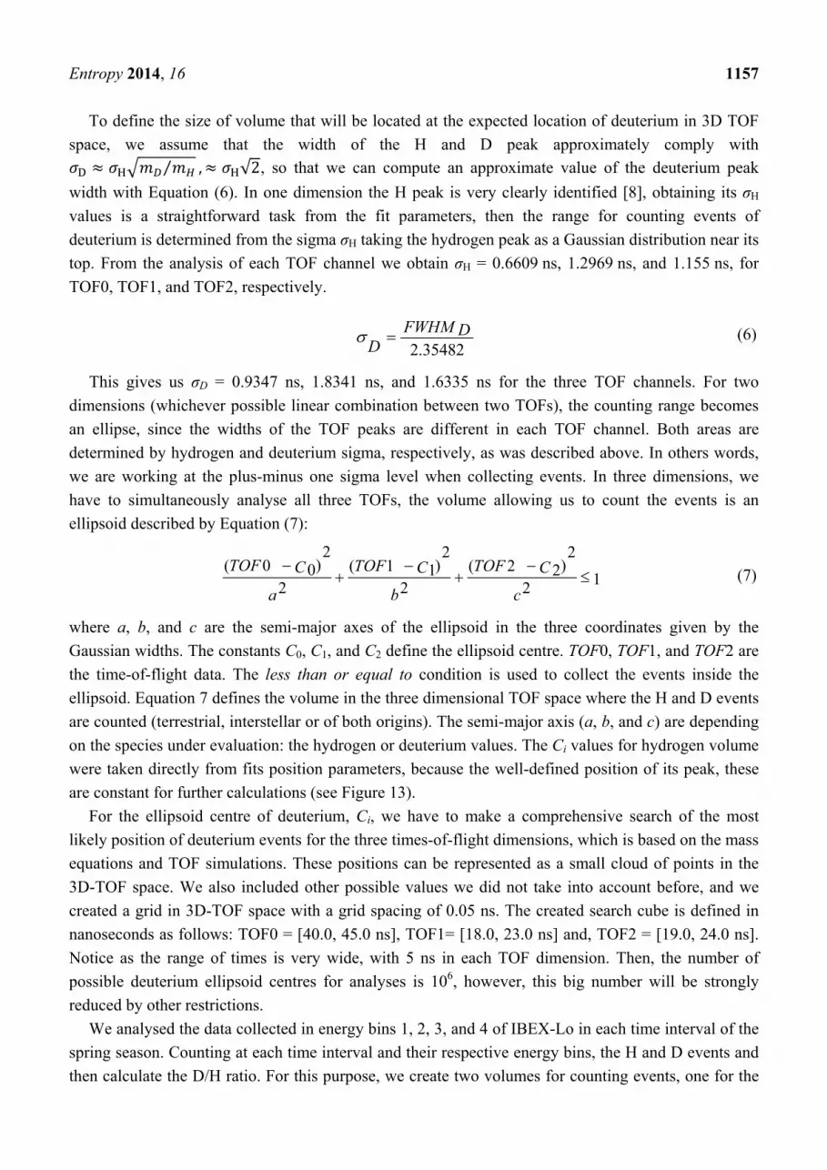
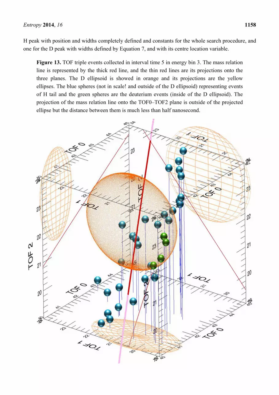
Figure 13. TOF triple events collected in interval time 5 in energy bin 3. The mass relation

line is represented by the thick red line, and the thin red lines are its projections onto the

three planes. The D ellipsoid is showed in orange and its projections are the yellow

ellipses. The blue spheres (not in scale! and outside of the D ellipsoid) representing events

of H tail and the green spheres are the deuterium events (inside of the D ellipsoid). The

projection of the mass relation line onto the TOF0–TOF2 plane is outside of the projected

ellipse but the distance between them is much less than half nanosecond.

Entropy 2014, 16 1159

The initial stage to find the most likely location ellipsoid centre of deuterium volume was to define

some constraints for the D counting results: (1) the number of D events collected at the time interval 5

to energy bins 1 and 2, must be equal or less than one (no signal expected); (2) In same time interval 5,

the D counts in energy bin 3 have to be as large as possible; (3) In energy bin 4 the counts have to be

equal to zero (no signal expected); (4) for other time intervals (1 to 4), the number of counts between

energy bins 1 to 3 has to show similar values between them (at least considering statistical fluctuations) and

drop steeply in energy bin 4, as it is expected [38]. With these criteria the number of potential D centres

was drastically reduced to 302.

The next limitation imposed to potential D centre locations is that the average of the D/H ratio in

complete spring season, calculated without considering the D/H ratio measured in energy bin 3 in time

interval 5 (because we expected that it is interstellar origin) is near to the terrestrial D/H ratio ~1.5·10−4.

This condition results in a reduction of the number of potential centre locations to 11.

The final constraint imposed was the counting of H and D signal along the ecliptic longitude should

match the temporal behaviour observed for the H sputtering signal from interstellar He, i.e., the

Gaussian-like curve (low at the flanks in time intervals 1 and 5, and maximum in time interval 3). This

criterion reduced the number of potential centre locations to 3. Finally, we arrived at the deuterium

peak centre in the 3-D TOF space that fulfils all the constraints listed above, This is located at 40.57

ns, 20.65 ns, and 23.21 ns for TOF0, TOF1, and TOF2, respectively (Figure 13).

The analytical results for the selected D centre locations will be shown in the next section. We have

to notice that not necessarily the centre of the ellipsoid and some of expected position or a particular

event of deuterium match, but the distance between the final three locations do not differ by more than

0.5 ns in each TOF dimension. Another remarkable issue is the size of D ellipsoid, which is of the

order of 1 ns, and slightly less in the TOF0 axis. If we considerer this small volume for D counting,

we are clearly not considering some of the real D events candidates, since we are working at the

plus-minus one sigma level when collecting events, both for H and D. However, with the small

collection volume we are fully removing the H tail. Those H ions that had just enough energy lost in

the C-foil 1, thus to look like D events in TOF2, have a slightly different energy loss than D through

the C-foil 2 and so will be outside the small collection ellipsoid.

The utility of the use of three dimensions TOF space and histogramming in two dimensions is

evident: the mass equations give us an accurate position of the D peak, the analysis of the H tails

allows to separate their contribution to the deuterium signal. Inspection of the 2D histogrammes gives

an explanation for background observed in one dimension. Only the 3D analysis was successful to pick

out and count the correct D events. Figure 14 shows a schematic representation of three dimensions

TOF method.

Entropy 2014, 16 1160

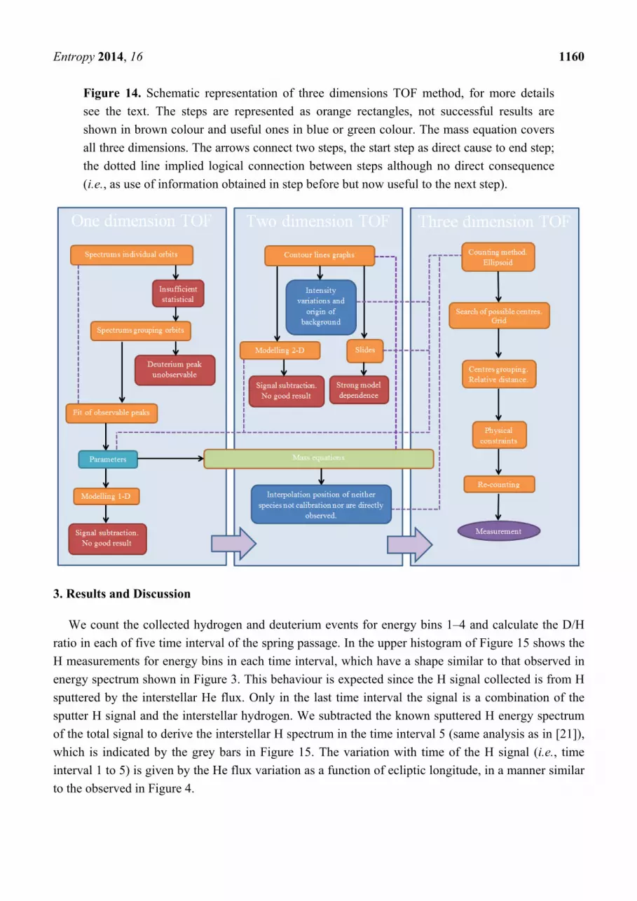
Figure 14. Schematic representation of three dimensions TOF method, for more details

see the text. The steps are represented as orange rectangles, not successful results are

shown in brown colour and useful ones in blue or green colour. The mass equation covers

all three dimensions. The arrows connect two steps, the start step as direct cause to end step;

the dotted line implied logical connection between steps although no direct consequence

(i.e., as use of information obtained in step before but now useful to the next step).

3. Results and Discussion

We count the collected hydrogen and deuterium events for energy bins 1–4 and calculate the D/H

ratio in each of five time interval of the spring passage. In the upper histogram of Figure 15 shows the

H measurements for energy bins in each time interval, which have a shape similar to that observed in

energy spectrum shown in Figure 3. This behaviour is expected since the H signal collected is from H

sputtered by the interstellar He flux. Only in the last time interval the signal is a combination of the

sputter H signal and the interstellar hydrogen. We subtracted the known sputtered H energy spectrum

of the total signal to derive the interstellar H spectrum in the time interval 5 (same analysis as in [21]),

which is indicated by the grey bars in Figure 15. The variation with time of the H signal (i.e., time

interval 1 to 5) is given by the He flux variation as a function of ecliptic longitude, in a manner similar

to the observed in Figure 4.

Entropy 2014, 16 1161

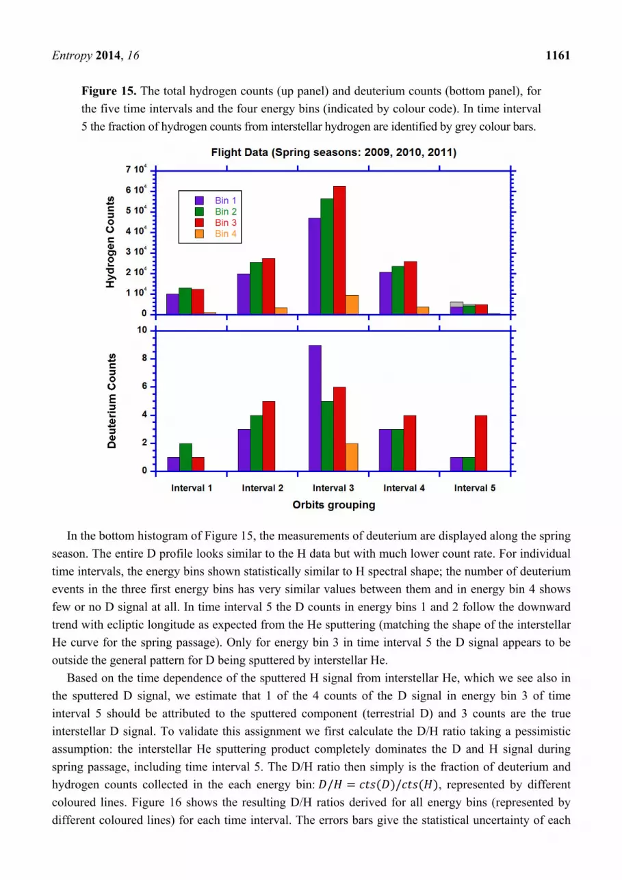
Figure 15. The total hydrogen counts (up panel) and deuterium counts (bottom panel), for

the five time intervals and the four energy bins (indicated by colour code). In time interval

5 the fraction of hydrogen counts from interstellar hydrogen are identified by grey colour bars.

In the bottom histogram of Figure 15, the measurements of deuterium are displayed along the spring

season. The entire D profile looks similar to the H data but with much lower count rate. For individual

time intervals, the energy bins shown statistically similar to H spectral shape; the number of deuterium

events in the three first energy bins has very similar values between them and in energy bin 4 shows

few or no D signal at all. In time interval 5 the D counts in energy bins 1 and 2 follow the downward

trend with ecliptic longitude as expected from the He sputtering (matching the shape of the interstellar

He curve for the spring passage). Only for energy bin 3 in time interval 5 the D signal appears to be

outside the general pattern for D being sputtered by interstellar He.

Based on the time dependence of the sputtered H signal from interstellar He, which we see also in

the sputtered D signal, we estimate that 1 of the 4 counts of the D signal in energy bin 3 of time

interval 5 should be attributed to the sputtered component (terrestrial D) and 3 counts are the true

interstellar D signal. To validate this assignment we first calculate the D/H ratio taking a pessimistic

assumption: the interstellar He sputtering product completely dominates the D and H signal during

spring passage, including time interval 5. The D/H ratio then simply is the fraction of deuterium and

hydrogen counts collected in the each energy bin: / / , represented by different

coloured lines. Figure 16 shows the resulting D/H ratios derived for all energy bins (represented by

different coloured lines) for each time interval. The errors bars give the statistical uncertainty of each

Entropy 2014, 16 1162

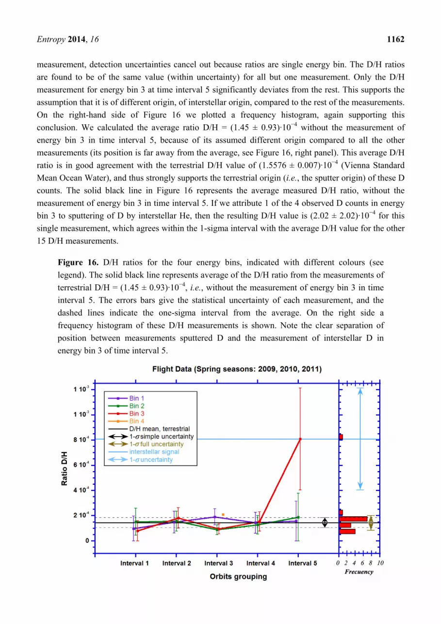
measurement, detection uncertainties cancel out because ratios are single energy bin. The D/H ratios

are found to be of the same value (within uncertainty) for all but one measurement. Only the D/H

measurement for energy bin 3 at time interval 5 significantly deviates from the rest. This supports the

assumption that it is of different origin, of interstellar origin, compared to the rest of the measurements.

On the right-hand side of Figure 16 we plotted a frequency histogram, again supporting this

conclusion. We calculated the average ratio D/H = (1.45 ± 0.93)·10−4 without the measurement of

energy bin 3 in time interval 5, because of its assumed different origin compared to all the other

measurements (its position is far away from the average, see Figure 16, right panel). This average D/H

ratio is in good agreement with the terrestrial D/H value of (1.5576 ± 0.007)·10−4 (Vienna Standard

Mean Ocean Water), and thus strongly supports the terrestrial origin (i.e., the sputter origin) of these D

counts. The solid black line in Figure 16 represents the average measured D/H ratio, without the

measurement of energy bin 3 in time interval 5. If we attribute 1 of the 4 observed D counts in energy

bin 3 to sputtering of D by interstellar He, then the resulting D/H value is (2.02 ± 2.02)·10−4 for this

single measurement, which agrees within the 1-sigma interval with the average D/H value for the other

15 D/H measurements.

Figure 16. D/H ratios for the four energy bins, indicated with different colours (see

legend). The solid black line represents average of the D/H ratio from the measurements of

terrestrial D/H = (1.45 ± 0.93)·10−4, i.e., without the measurement of energy bin 3 in time

interval 5. The errors bars give the statistical uncertainty of each measurement, and the

dashed lines indicate the one-sigma interval from the average. On the right side a

frequency histogram of these D/H measurements is shown. Note the clear separation of

position between measurements sputtered D and the measurement of interstellar D in

energy bin 3 of time interval 5.

Entropy 2014, 16 1163

In the following we assess the statistical significance of this measurement. Assuming the 6 deuterium

counts at time interval 5 are Poisson distributed sputtered D, then the statistical probability for 4 counts

in one of the three energy bins and a total six counts (Figure 15), i.e., for a µp = 6/3, is 9%. This means

that the confidence for true detection of interstellar D in energy bin 3 is 91%. The probability for

0 counts in an energy bin in time interval 5 is 13%. The statistically significant excess of counts at

energy step 3 in time interval 5 is strong evidence that these D atoms are of interstellar origin. We also

can perform a similar counting statistics analysis for just energy bin 3 in time interval 5 (see the

distribution in the right panel of Figure 16). Collecting four counts in this channel while the average

due to sputtered terrestrial D is one or less results in a probability of less than 4%. This reasoning

based solely on Poisson statistics for this energy bin and time interval can be taken as evidence that we

have detected interstellar D with a better than 96% confidence level. Other possibility is developing a

statistical hypothesis test. We propose two hypotheses, the null hypothesis, which assumes that all the

events collected in energy bin 3 in time interval 5 are from sputtering H, and the alternative hypothesis

which assumes that at least three of these events are from interstellar D. Using as expected mean and

the standard deviation equal to one, the results of one sample two-tailed t-test to p-value or alpha (α)

level is equals 0.0093 with a standard error of difference of 50%, this difference is considered to be

statistically very significant, and the null hypothesis can be rejected. Figure 16, right panel, shows the

histogram of all D/H measurements together with uncertainties: the simple uncertainty is the standard

deviation of the D/H measurements and the full uncertainty considers also the uncertainty of the

individual measurement for the combined uncertainty. By comparing the full uncertainty with the

uncertainty of the measurement in energy bin 3 at time interval 5 we see that they are separated by 1-sigma.

In the three years of the IBEX mission time, the observation geometry and orbit allowed for a total

observation time in time interval five (see Figure 4) of 115.3 days. However, the effects of the spinning

spacecraft as well as the stepping through 8 energy channels mean that we are only observing the

interstellar wind for a total time of 1.44 days, in which about ~2 counts for interstellar deuterium are

expected in time interval 5 [23].

To obtain the interstellar D/H ratio, we need to convert the interstellar D and interstellar H counts

into physical fluxes, because interstellar D and H arrive at 1 AU with different energy, and thus in

different energy bins. To first order, we can assume the same detection efficiency for D and H in

IBEX-Lo, since the ionisation during the scattering from the conversion surface is an electronic

process [33,42] and should not be affected by the heavier D nucleus. The good agreement, within error

bars, of the D/H ratio for the sputtered signal with the terrestrial value supports this assumption.

For the interstellar H flux we have to consider the counts in energy bin 1 and energy bin 2 (see

Table 3), which are converted to a physical H flux using the IBEX-Lo calibration [43]. We arrive at

D/H = (4.04 ± 2.75)·10−4 at 1 AU, where the statistical errors and the instrument calibration

uncertainty have been considered. To refine this result, we take the difference between the terrestrial

D/H and our measurement of the sputtered D/H to calibrate the detection efficiency for D based on the

H measurement, in the absence of a laboratory calibration for D. Thus, we have to correct our

measurement of the interstellar D/H with the factor 1.5576/1.45 = 1.075. This results in an interstellar

D/H ratio of (4.34 ± 2.96)·10−4 at 1 AU. We have to apply an additional correction for the different

viewing times of interstellar D and interstellar H in interval 5 (see Figure 4). The viewing time for

interstellar H is derived from the measurements [21] as 95.7 %, and the viewing time for interstellar

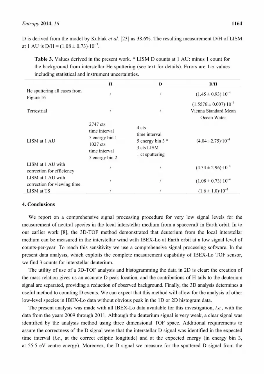
Entropy 2014, 16 1164

D is derived from the model by Kubiak et al. [23] as 38.6%. The resulting measurement D/H of LISM

at 1 AU is D/H = (1.08 ± 0.73)·10−3.

Table 3. Values derived in the present work. * LISM D counts at 1 AU: minus 1 count for

the background from interstellar He sputtering (see text for details). Errors are 1-σ values

including statistical and instrument uncertainties.

H D D/H

He sputtering all cases from Figure 16

/ / (1.45 ± 0.93)·10–4

Terrestrial / / (1.5576 ± 0.007)·10–4

Vienna Standard Mean Ocean Water

LISM at 1 AU

2747 cts time interval 5 energy bin 1

1027 cts

time interval 5 energy bin 2

4 cts

time interval 5 energy bin 3 *

3 cts LISM 1 ct sputtering

(4.04± 2.75)·10–4

LISM at 1 AU with correction for efficiency

/ / (4.34 ± 2.96)·10–4

LISM at 1 AU with correction for viewing time

/ / (1.08 ± 0.73)·10–4

LISM at TS / / (1.6 ± 1.0)·10–3

4. Conclusions

We report on a comprehensive signal processing procedure for very low signal levels for the

measurement of neutral species in the local interstellar medium from a spacecraft in Earth orbit. In to

our earlier work [8], the 3D-TOF method demonstrated that deuterium from the local interstellar

medium can be measured in the interstellar wind with IBEX-Lo at Earth orbit at a low signal level of

counts-per-year. To reach this sensitivity we use a comprehensive signal processing software. In the

present data analysis, which exploits the complete measurement capability of IBEX-Lo TOF sensor,

we find 3 counts for interstellar deuterium.

The utility of use of a 3D-TOF analysis and histogramming the data in 2D is clear: the creation of

the mass relation gives us an accurate D peak location, and the contributions of H-tails to the deuterium

signal are separated, providing a reduction of observed background. Finally, the 3D analysis determines a

useful method to counting D events. We can expect that this method will allow for the analysis of other

low-level species in IBEX-Lo data without obvious peak in the 1D or 2D histogram data.

The present analysis was made with all IBEX-Lo data available for this investigation, i.e., with the

data from the years 2009 through 2011. Although the deuterium signal is very weak, a clear signal was

identified by the analysis method using three dimensional TOF space. Additional requirements to

assure the correctness of the D signal were that the interstellar D signal was identified in the expected

time interval (i.e., at the correct ecliptic longitude) and at the expected energy (in energy bin 3,

at 55.5 eV centre energy). Moreover, the D signal we measure for the sputtered D signal from the

Entropy 2014, 16 1165

interstellar He flux follows exactly the temporal evolution of the interstellar He signal, and shows the

characteristic energy spectra for a sputtered signal. The measured D/H ratio for this terrestrial signal

is in good agreement with the terrestrial D/H value, as expected, demonstrating the capability of

IBEX-Lo to measure the D/H ratio.

We find for the interstellar deuterium a value of D/H = (1.08 ± 0.73)·10−3 at 1 AU, which is an

update to our earlier value [8]. This D/H value at 1 AU can be transferred to the D/H value at the

heliospheric termination shock at 100 AU by accounting for the transport and ionisation loss during the

transit from the termination shock to Earth orbit [23], which gives D/H = (1.6 ± 1.0)·10−5. This value is

equal to the LISM value if the filtration at the termination shock and the secondary populations for

H and D in the heliosheath are the same. Our D/H value is consistent with the D/H ratio inferred

by Hubble spectroscopy of a line of sight measurement of the LIC (1.6 ± 0.4)·10−5 [7]. The D/H

ratio we measure for the interstellar signal at Earth orbit (1 AU) is also in good agreement with

theoretical predictions by Tarnopolski and Bzowski [22] assuming a D/H value of 1.6·10−5 in the local

interstellar medium.

Our present analysis has large uncertainty and is thus only of limited use for a detailed scientific

discussion. It does demonstrate, however, that in situ measurements of interstellar D from the inner

heliosphere are possible. For optimised IBEX-Lo observations, to be performed during the upcoming

solar minimum period in about 2019, it is estimated that the detection of interstellar D with IBEX-Lo is

improved by a factor of up to 10 [8], with a corresponding improvement in accuracy of the D/H ratio.

Acknowledgments

This work is supported by the Swiss National Science Foundation. M. Bzowski, M.A. Kubiak,

and J.M. Sokół were supported by the Polish Ministry for Science and Higher Education grant

N-N203-513-038, managed by the Polish National Science Center. The work by US authors was

supported by the IBEX mission, which is funded as a part of NASA’s Explorer Program.

Conflicts of Interest

The authors declare no conflict of interest.

References

1. McComas, D.J.; Allegrini, F.; Bochsler, P.; Bzowski, M.; Collier, M.; Fahr, H.; Fichtner, H.;

Frisch, P.; Funsten, H.O.; Fuselier, S.A.; et al. IBEX interstellar boundary explorer. Sp. Sc. Rev.

2009, 146, 11–33.

2. Linsky, J.L. Atomic Deuterium/hydrogen in the galaxy. Sp. Sc. Rev. 2003, 106, 49–60.

3. Linsky, J.L. D/H nearby interstellar cloud structures. Sp. Sc. Rev. 2007, 130, 367–375.

4. Prodanovic, T.; Fields, B.D. FUSE deuterium observations: A strong case for galactic infall.

J. Cosmol. Astropart. P 2008, 9, 003.

5. Yuan, Y.; Neufeld, D.A.; Sonnentrucker, P.; Melnick, G.J.; Watson, D.M. Spitzer observations of

shock-excited hydrogen deuteride in IC 443C, HH 7, and HH 54: Probing the gas-phase deuterium

abundance in the dense interstellar medium. Astrophys. J. 2012, 753, 126.

Entropy 2014, 16 1166

6. Linsky, J.L.; Draine, B.T.; Moos, H.W.; Jenkins, E.B.; Wood, B.E.; Oliveira, C.; Blair, W.P.;

Friedman, S.D.; Gry, C.; Knauth, D.; et al. What is the total deuterium abundance in the local

galactic disk? Astrophys. J. 2006, 647, 1106–1124.

7. Hébrard, G.; Mallouris, C.; Ferlet, R.; Koester, D.; Lemoine, M.; Vidal-Madjar, A.; York, D.

Ultraviolet observations of Sirius A and Sirius B with HST-GHRS. An interstellar cloud with a

possible low deuterium abundance. Astron. Astrophys. 1999, 350, 643–658.

8. Rodríguez, M.D.F.; Wurz, P.; Saul, L.; Bzowski, M.; Kubiak, M.A.; Sokół, J.M.; Frisch, P.;

Fuselier, S.A.; McComas, D.J.; Möbius, E.; et al. Evidence for direct detection of interstellar

deuterium in the Local Interstellar Medium by IBEX. Astron. Astrophys. 2013, 557, 125.

9. Frisch, P.C.; Redfield, S.; Slavin, J.D. The interstellar medium surrounding the sun. Annu. Rev.

Astron. Astr. 2011, 49, 237–279.

10. McComas, D.J.; Alexashov, D.; Bzowski, M.; Fahr, H.; Heerikhuisen, J.; Izmodenov, V.; Lee,

M.A.; Möbius, E.; Pogorelov, N.; Schwadron, N.A.; et al. The Heliosphere’s interstellar

interaction: No bow shock. Science 2012, 336, 1291–1293.

11. Slavin, J.D.; Frisch, P.C. The boundary conditions of the heliosphere: Photoionization models

constrained by interstellar and in situ data. Astron. Astrophys. 2008, 491, 53–68.

12. Baranov, V.B.; Malama, Y.G. Model of the solar wind interaction with the local interstellar

medium—Numerical solution of self-consistent problem. J. Geophys. Res. 1993, 98, 15157–15163.

13. Müller, H.R.; Frisch, P.C.; Florinski, V.; Zank, G.P. Heliospheric response to different possible

interstellar environments. Astrophys. J. 2006, 647, 1491–1505.

14. Fahr, H.J. Change of interstellar gas parameters in stellar-wind-dominated astrospheres: Solar

case. Astron. Astrophys. 1978, 66, 103–117.

15. Fahr, H.J. Interstellar hydrogen subject to a net repulsive solar force field. Astron. Astrophys.

1979, 77, 101–109.

16. Bzowski, M.; Sokół, J.M.; Tokumaru, M.; Fujiki, K.; Quémerais, E.; Lallement, R.; Ferron, S.;

Bochsler, P.; McComas, D.J. Solar Parameters for Modelling the Interplanetary Background.

In Cross-Calibration of Past and Present Far UV Spectra of Solar System Objects and the

Heliosphere, ISSI Scientific Report Series 13; Bonnet, R.M., Quémerais, E., Snow, M., Eds.;

Springer Science + Business Media: New York, NY, USA, 2013; Chapter 3, pp. 67–138.

17. Bzowski, M.; Sokół, J.M.; Kubiak, M.A.; Kucharek, H. Modulation of neutral interstellar He, Ne,

O in the heliosphere. Survival probabilities and abundances at IBEX. Astron. Astrophys. 2013,

557, A50.

18. McMullin, D.R.; Bzowski, M.; Möbius, E.; Pauluhn, A.; Skoug, R.; Thompson, W.T.; Witte, M.;

von Steiger, R.; Ruciński, D.; Judge, D.; et al. Coordinated observation of local interstellar helium

in the heliosphere: Heliospheric conditions that affect the interstellar gas inside the heliosphere.

Astron. Astrophys. 2004, 426, 885–895.

19. Ruciński, D.; Cummings, A.C.; Gloeckler, G.; Lazarus, A.J.; Möbius, E.; Witte, M. Ionization

processes in the heliosphere. Rates and methods of their determination, Sp. Sc. Rev. 1996, 78, 73–84.

20. Ruciński, D.; Fahr, H.J. The influence of electron impact ionization on the distribution of interstellar

helium in the inner heliosphere; possible consequences for determination of interstellar helium

parameters. Astron. Astrophys. 1989, 224, 290–298.

Entropy 2014, 16 1167

21. Saul, L.; Wurz, P.; Rodriguez, D.; Scheer, J.; Möbius, E.; Schwadron, N.; Kucharek, H.; Leonard, T.;

Bzowski, M.; Fuselier, S.; et al. Local interstellar neutral hydrogen sampled in situ by IBEX.

Astrophys. J. Suppl. S 2012, 198, 14.

22. Tarnopolski, S.; Bzowski, M. Detectability of neutral interstellar deuterium by a forthcoming

SMEX mission IBEX. Astron. Astrophys. 2008, 483, L35–L38.

23. Kubiak, M.A.; Bzowski M.; Sokół, J.M.; Möbius, E.; Rodriguez, D.F.; Wurz, P.; McComas, D.J.

Assessment of detectability of neutral interstellar deuterium by IBEX observations. Astron. Astrophys.

2013, 556, A39.

24. McComas, D.; Allegrini, F.; Bochsler, P.; Bzowski, M.; Collier, M.; Fahr, H.; Fichtner, H.; Frisch, P.;

Funsten, H.; Fuselier, S.; et al. The Interstellar Boundary Explorer (IBEX). In Aip Conference

Proceedings, Proceedings of the 3rd International Conference of the Institute-of-Geophysics-and-

Planetary-Physics, University California Riverside, Riverside, CA, USA, February 2004; 719, pp.

162–181.

25. Funsten, H.O.; Allegrini, F.; Crew, G.B.; de Majistre, R.; Frisch, P.C.; Fuselier, S.A.; Gruntman, M.;

Janzen, P.; McComas, D.J.; Möbius, E.; et al. Structures and spectral variations of the outer heliosphere

in ibex energetic neutral atom maps. Science 2009, 326, 964–966.

26. Fuselier, S.A.; Allegrini, F.; Funsten, H.O.; Ghielmetti, A.G.; Heirtzler, D.; Kucharek, H.;

Lennartsson, O.W.; McComas, D.J.; Möbius, E.; Moore, T.E.; et al. Width and variation of the

ENA flux ribbon observed by the interstellar boundary explorer. Science 2009, 326, 962–964.

27. McComas, D.J.; Allegrini, F.; Bochsler, P.; Bzowski, M.; Christian, E.R.; Crew, G.B.; DeMajistre, R.;

Fahr, H.; Fichtner, H.; Frisch, P.C.; et al. Global observations of the interstellar interaction from

the interstellar boundary explorer (IBEX). Science 2009, 326, 959–962.

28. Schwadron, N.A.; Bzowski, M.; Crew, G.B.; Gruntman, M.; Fahr, H.; Fichtner, H.; Frisch, P.C.;

Funsten, H.O.; Fuselier, S.; Heerikhuisen, J.; et al. Comparison of interstellar boundary explorer

observations with 3D global heliospheric models. Science 2009, 326, 966–968.

29. Fuselier, S.A.; Bochsler, P.; Chornay, D.; Clark, G.; Crew, G.B.; Dunn, G.; Ellis, S.; Friedmann,

T.; Funsten, H.O.; Ghielmetti, A.G.; et al. The IBEX-Lo sensor. Sp. Sc. Rev. 2009, 146, 117–147.

30. Funsten, H.O.; Allegrini, F.; Bochsler, P.; Dunn, G.; Ellis, S.; Everett, D.; Fagan, M.J.; Fuselier, S.A.;

Granoff, M.; Gruntman, M.; et al. The interstellar boundary explorer high energy (IBEX-Hi) neutral

atom imager. Sp. Sc. Rev. 2009, 146, 75–103.

31. Wurz, P.; Fuselier, S.A.; Möbius, E.; Funsten, H.O.; Brandt, P.C.; Allegrini, F.; Ghielmetti, A.G.;

Harper, R.; Hertzberg, E.; Janzen, P.; et al. IBEX backgrounds and signal-to-noise ratio. Sp. Sc. Rev.

2009, 146, 173–206.

32. Wieser, M.; Wurz, P.; Möbius, E.; Fuselier, S.A.; Hertzberg, E.; McComas, D.J. The ion-optical

prototype of the low energy neutral atom sensor of the Interstellar Boundary Explorer Mission

(IBEX). Rev. Sci. Instrum. 2007, 78, 124502.

33. Wurz, P. Detection of Energetic Neutral Atoms. In The Outer Heliosphere: Beyond the Planets;

Scherer, K., Fichtner, H., Marsch, E., Eds.; Copernicus Gesellschafte. V.: Katlenburg-Lindau,

Germany, 2000; 265, pp. 251–288.

Entropy 2014, 16 1168

34. Möbius, E.; Kucharek, H.; Granoff, M.; King, B.; Longworth, S.; Saul, L.; Fuselier, S.; Hertzberg, E.;

Livi, S.; Paschalidis, N.; et al. Time-of-Flight Detector System with Low Background Performance

for the IBEX-Lo Sensor. In AGU Fall Meeting Abstracts, Proceedings of the 30th International

Cosmic Ray Conference, Mérida, Yucatán, Mexico, July 2007; Caballero, R., D’Olivo, J.C.,

Medina-Tanco, G., Nellen, L., Sánchez, F.A., Valdés-Galicia, J.F., Eds.; Universidad Nacional

Autónoma de México, México, México, 2008; Volumen 1, pp. 841–844.

35. Möbius, E.; Kucharek, H.; Clark, G.; O’Neill, M.; Petersen, L.; Bzowski, M.; Saul, L.; Wurz, P.;

Fuselier, S.A.; Izmodenov, V.V.; et al. Diagnosingthe neutral interstellar gas flow at 1 AU with

IBEX-Lo. Sp. Sc. Rev. 2009, 146, 149–172.

36. Wurz, P.; Saul, L.; Scheer, J.A.; Möbius, E.; Kucharek, H.; Fuselier, S.A. Negative helium generation

upon surface scattering: Application in space science. J. Appl. Phys. 2008, 103, 054904.

37. Möbius, E.; Bochsler, P.; Bzowski, M.; Heirtzler, D.; Kubiak, M.A.; Kucharek, H.; Lee, M.A.;

Leonard, T.; Schwadron, N.A.; Wu, X.; et al. Interstellar gas flow parameters derived from interstellar

boundary explorer-Lo observations in 2009 and 2010: Analytical analysis. Astrophys. J. Suppl. S

2012, 198, 11.

38. Saul, L.; Bzowski, M.; Fuselier, S.; Kubiak, M.; McComas, D.; Möbius, E.; Sokól, J.; Rodriguez, D.;

Scheer, J.; Wurz, P. Local interstellar hydrogen’s disappearance at 1 AU: Four years of IBEX in

the rising solar cycle. Astrophys. J. 2013, 767, 130.

39. Bochsler, P.; Petersen, L.; Möbius, E.; Schwadron, N.A.; Wurz, P.; Scheer, J.A.; Fuselier, S.A;

McComas, D.J.; Bzowski, M.; Frisch, P.C. Estimation of the Neon/Oxygen abundance ratio at the

heliospheric termination shock and in the local interstellar medium from IBEX observations.

Astrophys. J. Suppl. S 2012, 198, 13.

40. Beiersdorfer, P.; Roquemore, A.L.; Kaita, R. Characteristics of compact solid-target charge exchange

analyzers for energetic ion diagnostics on tokamaks. Rev. Sci. Instrum. 1987, 58, 2092–2098.

41. Mikheev, S.; Ryzhov, Y.; Shkarban, I.; Yurasova, V. Inelastic losses of low-energy ions transmitted

through thin films. Nucl. Instrum. Meth. B. 1993, 78, 86–90.

42. Wurz, P.; Wieser, M.E; Scheer, J.A. Particle scattering off surfaces: Application in space science.

eJSSNT 2006, 4, 394–400.

43. Rodriguez, M.D.F.; Saul, L.; Wurz, P. Fuselier, S.A.; Funsten, H.O.; McComas, D.J.; Möbius, E.

IBEX-Lo observations of energetic neutral hydrogen atoms originating from the lunar surface.

Planet. Sp. Sci. 2012, 60, 297–303.

© 2014 by the authors; licensee MDPI, Basel, Switzerland. This article is an open access article

distributed under the terms and conditions of the Creative Commons Attribution license

(http://creativecommons.org/licenses/by/3.0/).