Mean mesoscale global ocean currents from geodetic pre-GOCE MDTs with a synthesis of the North...

Mean mesoscale global ocean currents from geodetic pre-GOCE

MDTs with a synthesis of the North Pacific circulation

M. L. Vianna1 and V. V. Menezes2

Received 5 May 2009; revised 30 July 2009; accepted 29 September 2009; published 27 February 2010.

[1] A new milestone in satellite geodesy is about to be completed with the expectedavailability of the high-resolution data from the already in-orbit Global Ocean CirculationExplorer (GOCE) satellite. There are still some open questions related to capability ofrecovering mean mesoscale (50 km plus) geostrophic circulation (MGC) patterns fromobservational Gravity Recovery and Climate Experiment (GRACE)-based geodetic MeanDynamic Topography (MDTs), which we examine here in detail. A new set of globalgeodetic MDTs with high grid resolutions was computed (0.1� and 0.25�) based on thenewest EGM08 and GRACE GGM02 geoid models. The high resolution coupled to goodmesoscale feature discrimination was derived using efficient filtering procedure based onsingular spectrum analysis. The new solutions were contrasted with five important MDTs,including the hybrid and the geodetic MDTs, through empirical orthogonal functionsanalysis, which permit the determination of the mutual correlation among the MDTs, andestablishment of error bounds. The methodology made viable a detailed and robustanalysis of the North Pacific Ocean circulation based on theseMGCs including comparisonswith known results from other studies. We prove the superiority of the geodetic EGM08 (asopposed to hybrid) MDT models by obtaining less noisy and more intense and slenderwestern boundary currents and their recirculations, the bifurcations at the Shatsky Rise, andthe known mean eddies in the low-latitude shear region (NEC-NECC).

Citation: Vianna, M. L., and V. V. Menezes (2010), Mean mesoscale global ocean currents from geodetic pre-GOCE MDTs with a

synthesis of the North Pacific circulation, J. Geophys. Res., 115, C02016, doi:10.1029/2009JC005494.

1. Introduction

[2] In 2008, about 1 year before the recent successfullaunch of the European Space Agency’s Global OceanCirculation Explorer (GOCE) satellite, an international teameffort was able to complete the mission of producing thenewest generation geodetic satellite geoid model with thesame resolution of the altimeter-derived mean sea surface(MSS) models: the Earth Gravity Model 2008, EGM08 forshort, with degree/order 2190 [Pavlis et al., 2008]. At thesame time, the Danish National Space Center made availablea new global MSS model based on 12 years of multisatellitealtimetric observations [Andersen and Knudsen, 2008]. Withthese two newest models, a high-resolution geodetic meandynamic ocean topography (denoted as MDT by ocean-ographers and DOT by geodesists, to distinguish from thedynamic topography used by geodynamicists) can beobtained. The term geodetic here refers to MDTs deriveddirectly as MDT =MSS - Geoid, where the geoid models arebased only on the gravity data. In its computation, no oceanmeasurements are utilized to recover the small wavelengthportion of the MDT spectrum. The MDTs that use oceanic

data in the computation are otherwise denoted here as hybridMDTs.[3] For oceanography, the importance of the geodetic

MDTs is related to the fact that these are based on spatiallyhomogeneous observational data and are not dependent onreference depths: The MDT-derived geostrophic currents areabsolute and are thus applicable to estimate current velocitiesin regions where barotropic currents predominate (e.g.,Kuroshio Extension and Antarctic Circumpolar Current).More importantly, it is now known from data assimilationexperiments that any increase in accuracy of the MDT con-straint in the numerical circulation model, the more realisticthe output time-dependent circulation is obtained [see, e.g.,Bingham and Haines, 2006; Castruccio et al., 2008].[4] The great advantage of the MDTs computed with

EGM08 over the ones computed with any Gravity Recoveryand Climate Experiment (GRACE) geoid model is that theformer do not have the large-amplitude striation-type noisethat plagued all of the ones based on the latter using morethan degree/order 120 spherical harmonic coefficients[Tapley et al., 2005; Vianna et al., 2007; Bingham et al.,2008]. Therefore, the EGM08-based MDTs offer the attrac-tive possibility of becoming sufficiently accurate at the smallspectral wavelength band by use of adequate filteringmethods, which is of great interest to the mapping of oceancurrents and data assimilation.[5] Since the launch of GRACE mission in 2002, an

increased number of studies in methodologies to compute

JOURNAL OF GEOPHYSICAL RESEARCH, VOL. 115, C02016, doi:10.1029/2009JC005494, 2010ClickHere

for

FullArticle

1VM Oceanica LTDA, Sao Jose dos Campos, Brazil.2VM Oceanica LTDA, Arraial do Cabo, Brazil.

Copyright 2010 by the American Geophysical Union.0148-0227/10/2009JC005494$09.00

C02016 1 of 17

http://dx.doi.org/10.1029/2009JC005494

MDTs employing different techniques and filters have beenpublished [e.g., Rio and Hernandez, 2004; Maximenko andNiiler, 2004; Rio et al., 2005; Jayne, 2006; Vianna et al.,2007; Bingham et al., 2008], and others are dedicated toevaluation of the efficiency and accuracy of these MDTs[e.g., Vossepoel, 2007]. Now, just before the new milestoneis completed with the expected availability of data from thealready in-orbit GOCE satellite, we are faced with two mainquestions:[6] 1. Can the late generation of geodetic GRACE-based

MDTs effectively resolve mean spatial mesoscale (a scale of50 km plus) ocean circulation patterns and realistic westernboundary current intensities?[7] 2. How do the geostrophic currents derived from

geodetic MDT models compare with those obtained byhybrid ones?[8] In section 2, we examine these questions beginning

by the computation of a new set of global geodetic MDTswith better grid resolutions than the ones presently avail-able. These MDTs are based on EGM08 and the GGM02(GRACE Gravity Model 2) geoids. In their computation, weemploy a more efficient filtering methodology that permitsto remove the noise without smoothing out the true oceansignals. Then, in section 3, a global statistical comparison ofnine MDT solutions is performed.[9] Most of the studies of ocean circulation based on

satellite-derived MDTs have been focused in the AtlanticOcean, e.g., Geoid and Ocean Circulation in the NorthAtlantic (GOCINA) project [see, e.g., Bingham and Haines,2006, and references therein]. Despite its paramount impor-tance for global climate predictions, very little have beendedicated to the North Pacific [e.g., Gourdeau et al., 2003;Zhang et al., 2007]. On the other hand, this region is a veryinteresting test bed to study the MDT-derived currentsbecause of the large body of knowledge already achievedon its circulation patterns on all spatial scales. We describein section 4 a study aimed at answering the first questionstated above, by choosing the North Pacific Ocean as ourtarget region. The main conclusions are stated in section 5.

2. Observational MDT Models

[10] In the present study, we compute four global obser-vational MDTs. These were obtained as the differencebetween a mean sea surface derived from satellite altimetryand a geoid model computed with the aid of the GRACEdata. Three different geoid models have been used: thenewest EGM08, the GGM02S, and the GGM02C. The latterones belong to the GRACE Gravity Model 02 [Tapley et al.,2005], where the S denotes a model based solely onGRACE data and C denotes a combined geoid model fromthe GRACE data and terrestrial gravity information. Toattain the best possible high wave number accurate MDT foreach geoid/MSS models, we have applied a more efficientfilter method, which we used with relative success for theweak current region of the South Atlantic Ocean [Vianna etal., 2007]. The details of each MDT computations arepresented in sections 2.1–2.3. From the MDTs, we generatethe respective geostrophic circulation fields (MGC), usingthe standard geostrophic equation and excluding theequatorial region (±2�) and any intensity data larger than150 cm/s.

2.1. VMC07 MDT

[11] This geodetic global MDT, designated here asVMC07, was constructed through an informal partnershipbetween us and Don Chambers of the CSR/University ofTexas. The unfiltered data were obtained by difference, in apointwise approach, the GGM02C [Tapley et al., 2005],from the multisatellite MSS field GSFC00 [Wang, 2001].Both the MSS and the GGM02C data were mapped onto a0.25� � 0.25� global grid by Don Chambers betweenlatitudes of ±65�.[12] The GGM02C model is based on 363 days of

GRACE data spanning from April 2002 to December2003 combined with gravity information of the EGM96gravity model. It is supplied to degree and order 360, usesthe Topex/Poseidon (T/P) Earth Ellipsoid, and the MeanTide convention. The GSFC00 represents the MSS for the1993–1998 period. It was computed from a combination ofmultisatellite altimeter data: 6 years of T/P, ERS-1 35-dayphase C and phase G, ERS-1 geodetic phases E and F,3 years of ERS-2, and Geosat Exact Repeat Mission (ERM)and Geodetic Mission (GM). All the data were adjusted tothe T/P mean profile. The grid size of the GSFC00 MSS is2 min.[13] As explained by Vianna et al. [2007], this MDT has a

very complex high-amplitude noise pattern dominated bymeridional noncontinuous striations, caused by the com-mission errors in the geoid [Bingham et al., 2008; Jayne,2006]. Such commission errors are intrinsic to the low-lowone-dimensional (1-D) gradiometry technology used by theGRACE system (intersatellite distance measurements)[Hofmann-Wellenhof and Moritz, 2006].[14] Besides the commission errors, there are others in the

MDT model caused by a disparity between the high-featureresolution MSS and the lower-resolution geoid. This dis-parity results from the true small-scale geoidal featurescontained in the high-resolution MSS, which are not can-celed by the difference of it from the lower-resolution geoidmodel. Therefore, some signatures contained in the MDTappear as spurious data and should be filtered out with theminimum possible actual MDT signal attenuation. Somedetails on these noises have been discussed by Jayne [2006]for the North Atlantic and by Bingham et al. [2008]. Asnoted by Vianna et al. [2007], most published works to dateuse heavy Gaussian filtering, or other traditional Fourier-based filters (e.g., Hanning). These filters may wash out partof the commission and omission error field maintainingonly the large-scale signal (accuracy of a few centimeters atscales greater than 400 km), but at the cost of attenuatingand even losing some important oceanic features (e.g.,western boundary currents).[15] In obtaining VMC07, we applied a more efficient

singular spectrum analysis (SSA)-based filter. It is efficientnear boundary discontinuities, works well with short datasets, and does not smooth out large amplitude nonperiodicpeaks which in general represent true ocean signals. Themethod generates automatically a sequence of filters, whichbehave more like a series of efficient adaptive interpolators.The other advantage of our filter is the fact that it is basedon the space covariance structure of the 1-D data sets.[16] The SSA filter is made through expansion of the

input data signal in a series of so-called reconstructedcomponent (RC) modes. If all modes are summed, we

C02016 VIANNA AND MENEZES: PACIFIC CURRENTS FROM GEODETIC MDTS

2 of 17

C02016

recover the original signal, but any truncated sum representsa so-called adaptively filtered signal. We classify the infor-mation carried in each RC by finding through maximumentropy spectral analysis the wavelength L of the Fouriercomponent carrying the maximum energy. Our filter con-sists in selecting a subset of RCs where the correspondingLs are chosen by the user as adequate to their analysis. Thechosen RCs in this subset are then summed, giving the mostsatisfactory adaptive filter which separates signal from noisefor the particular problem [Vianna et al., 2007].[17] The adopted SSA filtering strategy used here con-

sisted in two steps, as done by Vianna et al. [2007]. First,we remove the meridional striations with a 1-D filter in theoceanic segments of each latitude circle, and next weremove other noises from the striation-free data by usinga two-dimensional (2-D) lat-lon filter. In both filters, onlyoceanic data are considered, limited by land boundaries:unless otherwise noted, land data are excluded. For datasegments with less than 10 grid points, no filtering is done(e.g., straits).[18] In the 1-D filter, we choose a subset of RCs where L

are off the interval (WL ± 1), being WL the quasi-meridionalstriae wavelength. Since WL increases poleward, we mod-eled it with the regression WL = 0.0554 * abs(LAT) +2.3698. Here the latitude LAT, WL, and L are in degrees.This modeled striation wavelength is not exact, and to takethe uncertainty into account, we introduced the above-mentioned narrow bandwidth of 2�(±1) in the filteringinterval.[19] The second step is the 2-D filtering of the remaining

noise. After several tests, with 2-D isotropic and anisotropicfilters, we found that different solutions offer good com-promises between noise elimination and preservation ofcirculation features. The better solution was found to be theanisotropic 6� (latitude circle segments) by 3� (meridionalsegments).[20] One should be cautious when interpreting the SSA

filtering jargon used here. When we state that we arechoosing, e.g., only RCs with L greater than 10�, this doesnot mean that these RCs exclude short pulses with rapidlocalized oscillations (e.g., wavelength of 2�), as would bethe case of a Fourier analysis component wavelength L. Ifmost of the energy in a RC containing a small spike-likesignal, but the RC is dominated by a long wavelengthspectral maximum, this does not mean that the spike willbe washed away in this RC.

2.2. New EGM08-Based MDTs

[21] A new generation of geodetic MDTs is being cur-rently derived by differencing the newest multisatelliteDNSCMSS08 (Danish National Space Center) from thevery high-resolution ultimate pre-GOCE Earth GravitationalModel 2008 (EGM08) [Pavlis et al., 2008]. One benefit ofthis high-resolution geoid model is that the known merid-ional striations that are present in the GRACE-only solu-tions, as shown for VMC07, are eliminated almost totally.[22] The EGM08 model was constructed under Nikolaos

Pavlis and collaborators of the U.S. National GeospatialIntelligence Agency (NGA) EGM Development Team. Theimportant steps required for computation of the EGM08were completed in the last 3 years (2006–2008). Thisgravitational model is a combination solution based on

ITG-GRACE03S, surface gravity, and altimeter gravity overthe ocean. It is complete to spherical harmonic degree andorder 2159 and contains additional coefficients extending todegree 2190 and order 2159. The NGA has been distributingit since November 2008 for oceanographic applications with1 � 1-min resolution, referenced to the T/P Earth Ellipsoidand in the Mean Tide convention. This model represents anenormous step forward just before the new milestone,expected by the future GOCE three-dimensional (3-D)gradiometry data hopefully to be furnished by the alreadyin-orbit GOCE satellite. The DNSCMSS08 has a resolutionof 2� 2 min, representing a MSS for the 1993–2004 period.It was computed by Andersen and Knudsen [2008] from acombination of multisatellite altimeter data: 12 years of T/Pand Jason-1, ERS-1 ERM and GM, ERS-2 ERM, Envisat,Geosat GM, Geosat Follow On, and IceSat.[23] There are already various MDT models based on

DNSCMSS08 and EGM08 available through the Internet,as the JPL MDT model presented by the CSR with 0.5� �0.5� grid (JPL08), filtered with a 111-km width Gaussiansmoother (D. Chambers, private communication, 2008),the DNSC MDT (DNSC08) with two different resolutions(1� 1 min and 2� 2 min), filtered with a Gaussian smootherof 75 km half width, all complete to degree/order 2160.These two EGM08-based MDTs (JPL08 and DNSC08) areincluded in the statistical comparisons. Another model basedon the EGM08 is the NGAMDTmodel offered in 1� 1 min,but with the spherical harmonic expansion truncated atdegree/order 180 (their DOT2008A). For oceanographicapplications, the geostrophic circulations derived from theDNSC models are too noisy, needing further filtering, whilethe NGA model does not have adequate resolution useful forexamining important mean mesoscale circulation featuresknow to exist from oceanographic measurements.[24] To support our study presented here, we computed

two new EGM08-based MDTs one with 0.25� � 0.25�, andanother one with 0.1� � 0.1�, which is the resolutioncompatible with some of the present-day data-assimilativeOcean Global Circulation Models (OGCMs). These MDTmodels are based on the DNSCMSS08/EGM08 data, exceptthat the filtering is done with the SSA method. We obtainedthe raw data file by courtesy of Don Chambers ofCSR/University of Texas. It has a 2-min grid resolutionobtained from very high degree order spherical harmonicsexpansion to degree/order 2156. Before filtering, this orig-inal MDTwas linearly interpolated into the 0.25� and a 0.1�grids. Since the EGM08-basedMDT fields are not dominatedby striations, as is the case of the GRACE-only MDTs,because of the new altimeter-derived gravity data that wereincluded in the EGM08 computations, we could skip the firststep (elimination of striae) in our filtering procedure.We onlyapplied the second step, which is the 2-D filtering as inVMC07, since there still remains a large amplitude noisefield to be washed away.[25] After several tests to determine the most adequate

filter parameters for each model independently and globally,trying to balance the resulting intensity and width of thewestern boundary currents and also resolve known meanrecirculations with the least noise interferences, we arrivedat the two new models, the VM08 (0.25� � 0.25�) and theVM08-HR (the high resolution 0.1� � 0.1�). The chosenSSA filter parameters were 5� (latitude circle segments) by


3 of 17

C02016

2� (meridional segments) for VM08 and 2� (latitude circlesegments) by 2� (meridional segments) for VM08-HR.

2.3. Bingham-Haines-Hughes MDT

[26] In a recent work, Bingham et al. [2008] show apossible advantage of a spectral model for computation of asatellite-only MDT as compared with the pointwise method,in relation to the noise field. According the authors, thespectral MDT requires less filtering to remove noise andensures that the omission errors from the MSS and theGeoid model are matched.[27] The Bingham-Haines-Hughes MDTs, hereafter

called BHH08, are obtained by the spectral approach andsubsequently mapped onto a 0.5� � 0.5� global grid. Thisapproach consists of differencing the GGM02S model[Tapley et al., 2005] from the altimetric CLS01 MSS, bothrepresented by spherical harmonic expansions and truncatedat the same spectral harmonic degree/order l, m. It should benoted that this geoid was computed with GRACE gravitydata only. This model has been supplied to degree and order160, referenced to the T/P Earth Ellipsoid and the MeanTide convention. The CLS01 represents the MSS for the1993–1999 period. Since MSS are defined only over theoceans, Bingham et al. [2008] use the GGM02C expandedto degree and order 200 as a proxy in the undefined landregions to produce a globally complete extended MSSsurface.[28] Here we filtered a higher-resolution degree-order

l = 160 MDT (BHH08-L160) kindly supplied by RoryBingham (R. Bingham, private communication, 2008). TheBHH08-L160 is dominated by the geoid commission error,represented by the high-amplitude meridional noncontinuousstriations such as was found in the VMC07 MDT. To removethis complex noise pattern, we adopted the same SSA filterand procedure as we have done for VMC07, but with animportant difference: The land data are included in theanalysis since the BHH08 MDT has a continuation over thecontinents. The quasi-meridional striae wavelength WL wasmodeled in a similar way as VMC07, but with the differentregression fit WLBHH08 = 2 + exp(0.0005*LAT2 - 0.8135),where the latitude LAT and WL are in degrees. After severaltests, we found the best 2-D filter solution was a anisotropicone with 10� (latitude circle segments) by 6� (meridionalsegments). For more details, see section 2.1. Besides theBHH08-L160, we have studied the MDT with degree-order80 (with a Gaussian filter with radius of 200 km applied)

computed by Bingham et al. [2008] that we refer hereafter asBHH08-L80.

3. Intercomparison Statistics of Global MDTs andMean Current Intensities

[29] In this section, we present some simple statistics ofthe comparison between the four MDTs we have filteredwith five broadly known MDTs: the Rio05 [Rio et al., 2005],the Maximenko-Niiler [Maximenko and Niiler, 2004], theBHH-L80, the JPL08, and the DNSC08 (Table 1). It isimportant to stress that these MDTs have different time-averaging periods, since the MSSs are computed withdifferent sets of altimetric data. Although interannual vari-ability can potentially introduce differences in the resultantgeostrophic circulations, some authors have found that theeffect may not be significant [Bingham and Haines, 2006].[30] We compare both the MDTs and the MDT-derived

mean current intensities (MCIs), using the VM08-HR asthe reference. The VM08-HR was chosen as reference as ithas been computed with the newest geoid and MSS models,has the better spatial resolution, and is less noisy thanDNSC08. It presents all major current systems: Kuroshioand Kuroshio Extension, Gulf Stream, Loop, Florida,Agulhas, Antarctic Circumpolar, and the weaker zonalAzores and St. Helena Currents, the latter crossing overthe Tristan da Cunha Islands in the South Atlantic. Theseappear with more intensity than the other solutions, besidesthe mean mesoscale features known from oceanographicstudies (Figure 1).[31] Comparing MDT differences means obtaining differ-

ence statistics more related to the lower wave numberspectral band, while the MCI statistics is more related tothe higher wave number band. For the comparisons, theMDT/MCI fields were standardized between 65�S and�65�N and linearly interpolated into 0.25� � 0.25� grids,including the VM08-HR.[32] We also evaluate the correlation between the VM08-

HR and the other fields by expanding each pair (VM08-HR,X) into two empirical orthogonal functions (EOF) modes.Here, each of the Xs represents another field, e.g., Rio05.These EOF analyses were done for the MDTs and the MCIs.The first EOF mode gives a measure of the pair correlationby its maximum total variance, and the best correlated map,while the second gives the residual map of each pair fromthe best correlated one. This method is introduced here tooffer another way to distinguish where the local differences

Table 1. Basic Data on the Nine MDTs Discussed in This Work, Including Averaging Interval, Grid Resolution, Data Type Used/Model

Approach, MSS/Geoid Models, and Filtering Methodsa

MDT Time Period Resolution Type/Approach MSS/Geoid Filter

VM08-HR 1993–2004 0.1� � 0.1� Geodetic/pointwise DNSC08/EGM08 SSAVM08 1993–2004 0.25� � 0.25� Geodetic/pointwise DNSC08/EGM08 SSAVMC07 1993–1998 0.25� � 0.25� Geodetic/pointwise GSFC00/GGM02C SSABHH08-L160 1993–1999 0.5� � 0.5� Geodetic/spectral CLS01/GGM02S SSABBH08-L80 1993–1999 0.5� � 0.5� Geodetic/spectral CLS01/GGM02S GaussRio05 1993–1999 0.5� � 0.5� Hybrid/(hydro & drifters) CLS01/EG03S GaussMaxNi04 1993–1998 0.5� � 0.5� Hybrid/drifters GSFC00/GGM01 AveJPL08 1993–2004 0.5� � 0.5� Geodetic/pointwise DNSC08/EGM08 GaussDNSC08 1993–2004 2(1)0 � 2(1)0 Geodetic/pointwise DNSC08/EGM08 Gauss

aGauss is short for Gaussian filter, Ave for averaging filter, SSA for Singular Spectrum Analysis, and EG03S for Eigen-Grace 03S. Model approach ispoint or spectral.


4 of 17

C02016

were stronger as compared with VM08-HR. Table 2 showsthe explained variance by each EOF mode.[33] Table 3 presents the classical statistics used when

comparing two spatial fields. In Table 3, we see that theRio05 MDT has the more distinct spatial mean value. Thisfact as noted by Vossepoel [2007] is caused by the inclusionof dynamic height relative to 1500 m from Levitus clima-tology. The differing mean values between each MDT is oneof the reasons which suggests that the gradient data (e.g.,from geostrophic circulation) are more useful for compar-isons, since they are not affected by the spatial mean. Thesn, a measure of the effect of the weight of the necessaryfiltering to eliminate noise, shows that the heaviest filtering

was the one applied to BHH08-L160, since it presentsheavy striping, which gives a very large sn (61.04 cm),analogously to VMC07 (15.26 cm). As mentioned before,these MDTs have a very complex high-amplitude noisedominated by meridional noncontinuous striations due tothe commission errors in the geoid. Although the MDTsshow different mean and sn values, their standard deviationsare similar, being between 56 and 57.5 cm. The centeredRMS differences values ranged from 1.10 to 6.92 cm, beingthe lowest with the JPL08 and the highest with BHH-L160,as expected. The JPL08 as well as the VM08 and theDNSC08 use the same data set as VM08-HR, the maindifference being the filtering method used, and the BHH08-

Figure 1. (a) The high-resolution EGM08-based VM08-HR MDT and (b) corresponding Meangeostrophic Current Intensity (MCI).


5 of 17

C02016

L80 and the BHH08-L160 are smoother MDTs, because oflarger omission errors. It should be noticed that the VMC07,which is a geodetic MDT, has a smaller RMS difference(4.06 cm) than the two hybrid MDT solutions (5.18 cm).[34] On the other hand, the MCI global statistics show not

so homogeneous results, as expected. As can be seen inTable 3, the DNSC08 has the highest MCI-s (18.93 cm/s)and the highest MCI-m (15.70 cm/s) which gives highercurrent velocities. However, this MCI has also the largestRMS difference (11.24 cm/s) although it has been computedwith same EGM08 geoid and DNSC08MSS models as theVM08-HR. The other EGM08 MCIs have much smallerRMS difference, being 7.96 cm/s for VM08 and 5.10 cm/sfor JPL08. Looking at the MCI maps, we see that DNSC08presents a excessive noise, pointing into the necessity of amore efficient filtering to reduce this noise. Surprisingly,BHH08-L160, a smoother MDT, has also a high mean andstandard deviation values. These values are higher thanBHH08-L80, VMC07, JPL08, and VM08. The BHH08-L160 also has a higher RMS difference (10.59 cm/s). Thisresult can only be understood by looking the residue mapfrom the second EOF mode (not shown) that explains20.15% of the covariance. The largest values in the MCIresidue map are located along the coasts on the north IndianOcean, and around the islands between Australia and Asia,where the residue attains more than 50 cm/s, while at mostother coasts it only attains 5 cm/s.[35] This might be due to the fact that the filtering was

done (on purpose) for BHH08-L160 without taking intoaccount the continental and island boundaries (the BHH08unfiltered MDT has a continuation over land with GGM02Cdata). Disregarding these two examples, we notice that thegeodetic solutions (except BHH08-L80) present greateraverages and standard deviations than the hybrid ones, thelargest values being those of VM08-HR.[36] The examples discussed in the present section also

show that the global single number statistics do not offer thebest explanatory way to distinguish which MDT/MCI pair isthe most interesting for oceanography, since such statisticsgive only a rough measure of their mutual coherence.[37] In Table 2, the number one EOF modes (M1) are

proxies of the correlation with VM08-HR, while the numbertwo EOF modes (M2) represent the residue maps. Bylooking at Table 2, we notice that the worst MDT covari-ance is with the Rio05 (90.58%) while the others presentvalues of about 99%. Moreover, the MDT residue map ofRio05 has a much higher sEOF with a value of 9.09 cm and

it is completely off scale as compared to all others. InRio05, the residue values range from �60 cm to 0 cm(Figure 2), while in all others the values are ±12 cm (notshown). In the Rio05 map, the areas around the most intensewestern boundary currents and their extensions (e.g., GulfStream, Agulhas, Kuroshio, and Brazil-Malvinas Conflu-ence) show the smallest residues in the map (less than 5 cm),while immediately poleward of these areas it changesabruptly to more than 35 cm. The residues are generallylarger than 25 cm in most of the global ocean, except near theabove-cited western boundary current regions.[38] Since the computation of the Rio05 MDT is very

complex, we do not know for sure the reason for such aresult of the analysis. However, the results suggest thatRio05 might be negatively influenced by the use of hydro-graphic dynamic height data with a reference depth, sincethis effect is not seen with the MaxNi04, where such datawere not used in the MDT computation, and the covarianceis 99.27% and sEOF is three times lower than the Rio05ones. To draw a more complete picture, we also evaluate theEOF between the MaxNi04 and Rio05, both being hybridMDT solutions. The results are slightly worse than thosebetween VM08-HR and Rio05. The covariance of the firstEOF mode is only 88.98%. For the second EOF modes, i.e.,the residue maps, the covariance is 11.02% and the sEOF is10.82 cm. Figure 2b shows the residue EOF map computedbetween MaxNi04 and Rio05. As can be seen, the residuesare of the same order as that between VM08-HR and Rio05(Figure 2a).[39] As expected, the MCI covariances are smaller than

those of the MDTs, ranging from 79.8% (BHH08-L160) to88.62% (JPL08). The MCI residue maps (mode 2) are veryinstructive: They show that the strongest deviations areobserved in the western equatorial Pacific between 10�Nand 20�S in all MCIs. The smaller MCI deviations are foundwith JPL08, which is very coherent with VM08-HR, but hascurrents with smaller amplitudes. In addition, in the Rio05,the largest residue amplitudes is (surprisingly) in the westernboundary currents (WBC) areas. The deviations there appearas parallel lines possibly because of WBC axis displace-ments relative to the ones obtained with VM08-HR. Thismay be exemplified for the Florida/Gulf Stream, where theaxis displacement is of the order of 1.5� to the east.[40] By using the EOF technique, we may form compo-

sites of maximally correlated MDTs from any number N ofinput MDTs. These composites are obtained as the first EOF

Table 3. Simple Statistics of the MDTs and MCIsa

MDT m s RMSD snVM08-HR 19.64 (11.05) 57.24 (14.63) - 4.17VM08 19.78 (8.85) 57.24 (11.88) 1.61(7.96) 4.66VMC07 43.21 (8.72) 57.49 (11.60) 4.06(9.11) 15.26BHH08-L160 48.22 (9.15) 56.69 (13.34) 6.92(10.59) 61.04BBH08-L80 49.86 (6.33) 57.27 (7.57) 5.17(9.49) -Rio05 168.99 (7.75) 56.06 (8.99) 5.18(9.52) -MaxNi04 6.58 (7.12) 57.44 (7.61) 5.18(9.05) -JPL08 20.02 (9.75) 57.17 (12.46) 1.10(5.10) -DNSC08 47.33 (15.70) 57.03 (18.93) 2.01(11.24) -

aThe values are in cm for MDT and cm/s for MCI. The last column hasvalues only for SSA-filtered MDTs. The values in parenthesis show thestatistics of MCIs. MCIs are spatial means m, standard deviations s of eachfield, centered pattern of RMS difference RMSD between each MDT/MCIand the VM08-HR, and the standard deviations of MDT noise sn.

Table 2. EOF Data for the Pair Formed by VM08-HR and the

Eight Other MDTs/MCIsa

Fields MDT-M1 MDT-M2 MCI-M1 MCI-M2

VM08 99.83 (57.20) 0.17 (2.29) 87.34 (12.74) 12.66 (4.07)VMC07 98.84 (56.76) 1.16 (2.88) 82.60 (12.86) 17.40 (3.62)BHH08-L160 99.15 (56.73) 0.85 (4.29) 79.85 (12.23) 20.15 (5.77)BBH08-L80 98.66 (56.65) 1.34 (3.43) 85.88 (13.34) 14.12 (2.25)Rio05 90.58 (48.71) 9.42 (9.09) 82.29 (13.06) 17.71 (3.13)MaxNi04 99.27 (57.03) 0.73 (3.13) 86.17 (13.29) 13.83 (2.14)JPL08 99.25 (57.11) 0.75 (2.51) 88.62 (12.46) 11.38 (4.17)DNSC08 99.32 (56.83) 0.68 (1.84) 85.66 (11.91) 14.34 (5.02)

aExplained variance by each of the two EOF modes in percent. The firsttwo columns refer to MDTs and the last ones to MCIs. The first EOF modeis denoted as M1 and the second one as M2. The values in parenthesis showthe spatial standard deviations sEOF, in cm for MDT and cm/s for MCI.


6 of 17

C02016

mode of the input MDT ensemble, while the higher modesgive the residual maps associated with the uncertainties,which can be seen as a measure of the error field. Fromthese new composites, corresponding geostrophic circula-tion fields are generated as usual. This method helps us toevaluate whether a mesoscale feature observed in a MGCfield can be a robust and realistic feature, or it might besimply a noise artifact. We remind the reader that thecomposite MDTs are in 0.25� � 0.25� grids. The compo-sites are formed by different ensembles that we refer to asVM08-C (C1 to C6). The following ensembles are usedhere:[41] [C1]: all the nine MDTs (VM08-HR, VM08,

VMC07, BHH08-L160, BHH08-L80, Rio05, MaxNi04,JPL08, and DNSC08),[42] [C2]: all MDTs except DNSC08,[43] [C3]: all MDTs except Rio05 and DNSC08,[44] [C4]: all MDTs except Rio05,[45] [C5]: formed by geodetic MDT representatives of

each geoid model, one for EGM08 (VM08-HR), one for

GGM02C (VMC07) and one for GGM02S (BHH-L160),and the two hybrid solutions,[46] [C6]: same as C5 but without Rio05.[47] Table 4 shows the results of these ensemble analysis.

We can see that the best correlated ensembles are those thatdo not have Rio05 in its composition, i.e., the C3, C4, andC6. The covariance in this case is about 98%, while whenRio05 is used the covariance is 92% �94%. The betterresults are obtained when we consider all MDTs excludingRio05 and DNSC08, the C3 (98.34%). This result points outthat the field of geodetic MDT modeling already achievedits most important goals for oceanography even before theGOCE data become available and suggests that Rio05 maybe considered an outlier in relation to the other MDTs.[48] Apart from the global statistics previously described,

we retrieved the local speeds and the widths across themajor WBCs: Gulf Stream, Florida, Agulhas, AgulhasExtension, and Kuroshio. The Gulf Stream values werecomputed for each MCI field as the average velocitybetween 35�N and 36�N along 77�W–73�W, the Floridacurrent as the average between 30�N and 31�N along

Figure 2. Residue map (EOF2) between (a) Rio05 and VM08-HR MDTs and (b) Rio05 and MaxNi04.The two residue maps are very similar, exhibiting a relatively off scale lack of homogeneity in the Rio05MDT as compared to the other MDTs.


7 of 17

C02016

82�W–76�W, and the Agulhas current as the averagebetween 33.5�S and 34.5�S along 25�E–33�E. The AgulhasExtension values were obtained with a transect along 25�Ebetween 45�S and 39�S and Kuroshio along 135�E between30�N and 36�N. It is important to stress that all of thesecomputations were made with the respective original MCIfields and not with the interpolated ones used for the globalcomparison.[49] Table 5 shows the local speeds (centimeters per

second) defined as the maximum current in the longitudinal/latitudinal segments described here and the widths (degree)for each MCI field, except for DNSC08. The DNSC08currents were not included there due to the excessive noisein this MDT, which generates large spikes in the MCI. Onlytwo MCIs have a well-defined Florida Current (VM08-HRand JPL08), and for this reason only the widths of this currentare recorded.[50] When we compare the intensity and the width of the

WBCs in Table 5, the nature of the MDT differences (e.g.,steeper or weaker MDT gradients) becomes more apparent.As we can see, the largest speeds and more slenderWBCs areobtained in VM08-HR. The other EGM08 solutions alsopresent intense and slender WBCs, which have even higherspeeds than the hybrid ones. The VMC07, although com-puted with an older generation of geoid/MSS models, alsogives good WBC results comparable to the hybrids ones.The larger widths and smaller intensities of the WBCcurrents are obtained with the GRACE-only solutions, aswe already expected, but BHH08-L160 shows better resultsthan BHH08-L80 in this respect.

4. North Pacific Ocean Circulation

[51] This section describes the observed MDT-basedsurface circulation features of that ocean. Succinct descrip-tions of the origin of the Pacific western current system andits simplified dynamics can be found in the work of Qiu and

Lukas [1996] and in chapters 8–10 of Regional Oceanog-raphy: An Introduction by Tomczak and Godfrey [2003].Figure 3 shows the large-scale circulation pattern super-imposed on the mean dynamic topography obtained fromthe VM08-HR solution. The three gyre circulations (tropi-cal, subtropical, subpolar), the Costa Rica Dome, and theTehuantepec Bowl are clearly seen.[52] In the western Pacific, the Kuroshio originates off the

Philippine coast, as the northward branch from the NorthEquatorial Current (NEC) bifurcation. The latitude of thenear-surface NEC bifurcation has been estimated from time-dependent Sverdrup theory by Qiu and Lukas [1996] asbeing around 14.2�N–15.3�N, using a wind climatologycomputed between 1961 and 1992. The southern branch ofthe bifurcation is known as the Mindanao Current (MC).The MC is a slender (100–200 km wide) current whichbecomes well developed at 8�N, with a core intensity of80–100 cm/s near the surface, with decreasing intensitydown to 500 m, where the flow direction reverses into aweak and wider Mindanao Undercurrent (5 cm/s) down tothe bottom.

4.1. Western NEC

[53] Figure 4 illustrates the mean geotrophic circulation inthe NEC-NECC (North Equatorial Counter Current) regionfrom two different MDTs: the high-resolution VM08-HR(Figure 4a) and the composite VM08-C3 (Figure 4b).Although we have analyzed all the MGCs, we choose toshow only these two. We recall that the composite VM08-C3MDT explains 98.34% of the total variance (see section 3).[54] In all MGCs studied, the NEC is located between

8�N and 18�N with speeds of 15–50 cm/s. We note that at18�N–20�N a weak westward current (10 cm/s), which isnot part of the NEC, is seen west of 140�E, merging at thewestern boundary with the Kuroshio. From VM08-HR, thiscurrent appears to be a southern return flow from one of thebands of the double-banded North Pacific Subtropical

Table 4. Explained Covariance for Each Composite MDT in Percenta

N Ensemble M1 M2 (Residue)

VM08-C1 9 All MDTs 94.55 (56.04) 4.47 (2.46)VM08-C2 8 All MDTS except DNSC08 94.10 (55.95) 4.99 (2.49)VM08-C3 7 All MDTS except DNSC08 and Rio05 98.34 (57.03) 0.80 (2.54)VM08-C4 8 All MDTs except Rio05 98.30 (57.04) 0.71 (2.44)VM08-C5 5 VM08-HR, VMC07, BHH08-L160, MaxNi04, Rio05 92.41 (54.92) 6.83 (3.65)VM08-C6 4 VM08-HR, VMC07, BHH08-L160, MaxNi04 98.33 (57.15) 0.94 (1.71)

aColumn one shows the number of MDTs in each ensemble, column two shows the MDTs in ensembles, and columns three and four the covariance ofthe two first EOF modes. In parenthesis, the spatial standard deviations are in cm.

Table 5. Local Speeds and Widths of Western Boundary Currents From Each of the MCI Mapsa

MDT GS FLO AGU AGUE KURO

VM08-HR 87.09 [1.7�] 92.30 [2.0�] 89.76 [3.0�] 39.11 [2.5�] 96.61 [1.7�]VM08 53.21 [4.0�] 34.14 [-] 70.87 [4.0�] 38.29 [2.9�] 96.11 [2.0�]VMC07 39.53 [5.0�] 24.33 [-] 80.67 [3.0�] 40.00 [2.5�] 54.55 [3.3�]BHH08-L160 23.77 [6.0�] 18.22 [-] 36.89 [5.0�] 17.15 [4.0�] 44.30 [3.6�]BHH08-L80 18.54 [5.7�] 15.29 [-] 19.10 [4.0�] 12.00 [4.0�] 28.87 [4.0�]Rio05 63.62 [3.7�] 57.54 [-] 66.26 [3.0�] 26.75 [2.2�] 98.62 [2.6�]MAXNi04 47.34 [3.2�] 53.13 [-] 42.57 [3.0�] 29.97 [2.5�] 65.49 [2.0�]JPL08 74.23 [3.9�] 73.30 [3.0�] 63.89 [3.0�] 35.41 [2.3�] 76.07 [2.5�]

aThe widths are in brackets. Units are cm/s for speeds and degrees for widths. The DNSC08 currents were not included due to large spikes in the MCI,and only two MCIs have a well-defined Florida Current. GS, Gulf Stream; FLO, Florida Current; AGU, Agulhas Current; AGUE, Agulhas Extension; andKURO, Kuroshio.


8 of 17

C02016

Countercurrent(STCC), which is described by, e.g., Kobashiand Kawamura [2002]. The current at 18�N–20�N has beennoted since at least the work of Wyrtki [1975]. This looksvery clear as a relatively high zonal ridge in the VM08-HRMDT. We will return to the STCC shortly.[55] A difference among the MGCs is that in the new

high-resolution VM08-HR the NEC appears as a meander-ing flow between 10�N and 16�N, with 20 cm/s all the wayto the west of the Marianas Islands (see Figure 4a). Adouble-maximum intensity is seen at 128–130�E centeredat 10�N and 12�N, with this (apparent) southern branchcorresponding to the Mindanao Eddy flow. In the low-resolution ones, the NEC appears as a broad westward flow,with mean value of 25 cm/s and no double maximum isvisible at 130�E (e.g., Figure 4b). This double-maximumsignature is also detected in JPL08 and VM08 but not themeandering structure. The VM08-HR pattern is consistentwith Qu et al. [1998]. We also observed that the NEC flowis influenced by Marianas archipelago at 145�E. When theNEC hits at the eastern side of the Marianas archipelago, itgenerates an anticyclonic lee eddy, with its southern limbflowing through a gap north of Guam (where it attains40–50 cm/s), forming a closed loop current around theislands with meridional size of 4�. Although the latterstructure is robust (from analysis of VM08-C3), the currentamplitude may be smaller.

4.2. Mindanao Current

[56] While in all MGCs, the NEC westward flow seemsto hit the coast and veer to the north at 10�N–12�N, 126�E(origin of the Kuroshio), the southward branch (MindanaoCurrent) does not have a clear southward flow signatureclose to the coast at all. Moreover, the bifurcation latitude ofthe NEC is unclear in all MGCs except in Rio05. In Rio05,the MC signature of divergent flow lines is detected around10�N, 130�E, which is very far from the shore, and the MCclosure to the south is not present.

[57] However, a strong mean southward Acoustic DopplerCurrent Profiler (ADCP)-measured MC jet (100 cm/s) isobserved hugged to the slope, with a width of 200 km at thesurface and progressively thinner at depth down to 500 m[Wijffels et al., 1995; Qu et al., 1998], and therefore itssignature should be expected to appear in all of the MGCs.Although our VM08-HR does have the adequate featureresolution (0.1� � 0.1�), it is not detected by it either. To seewhether a even higher resolution MDT could show thecorrect signature, we studied the original 2 min dataaround Mindanao (not shown), and the result did not change.[58] It is really interesting that theMC signature is not seen

in any of the recent GRACE-based MDT/MGCs, includingthe EGM08 ones. Actually, all of GRACE-based MGCs givea very strong opposite (erroneous) flow (>80 cm/s northward;see Figure 5 for VM08-HR), including the satellite-only onestudied recently by Bingham et al. [2008], with degree-order80. We analyzed a higher-resolution degree-order 160 MDT,the BHH08-L160, and the same effect occurs: a strongnorthward flow close to the Mindanao coast. These factsindicate that the problem resides on a highly faultyGRACE-based global geoid model near the east coast ofthe Mindanao island, or perhaps on the MSS grid.[59] This failure is probably due to many adverse local

conditions playing a role in concert: the presence of the verydeep (8000 m plus) and slender Philippine Trench (50 kmacross), hugged to the mountain coast of a large island(Mindanao) (Figure 5). In such a setting, there is certainly alarge jump in the Bougher anomaly field at sea level, maybeeven larger than 100 milligals in less than 50 km, asobserved in the recent airborne gravity survey aroundTaiwan [Hwang et al., 2007]. This causes a large jump ofthe order of 10 m in less than 50 km, which is probably thereason for large error strip east of Mindanao seen in allGRACE-based MDTs.[60] To accommodate these small-scale steep gravity

gradients in future geoid models, it seems that a moreefficient alternative to the traditional spherical harmonic

Figure 3. The EGM08-based 0.1� � 0.1� VM08-HR MDT on the North Pacific Ocean (color) with therespective surface geostrophic flow lines superposed. Only the large-scale flow is exhibited here,showing the gyre structure (tropical, subtropical, and subpolar) and the southeastern quasi-stationaryrecirculation eddies (Costa Rica Dome and Tehuantepec Bowl). The equatorial cutoff is made at 3�N.


9 of 17

C02016

expansion method of solution of the geodetic problem usedtoday should be developed. There are many questions whichhave not been resolved yet, and we can point out some ofthese here: does the GRACE-measured local gravity gradi-ent data have sufficient resolution, but is just improperlyinverted into the global geoid model (e.g., a local Gibbsphenomenon spike), or does the measuring system limitedresolution in the zonal direction simply fail in detecting thehigh-amplitude discontinuity? Is this problem due only tothe lack of local airborne or ship gravity measurements inthe combined geoid models as EGM08? Would it be relatedto the land-ocean transition of the altimeter data whichinterfere with the MSS estimates?[61] Only with the future small-wavelength resolution of

the GOCE gradiometer data, it will be possible to obtaindirectly the answer to these questions. It is interesting tonote that this problem only appeared in relation to theMindanao Current. In other places where the conditionsare similar to Mindanao (e.g., the Puerto Rican trench

and island, the Peru-Chile and Trench and the Andes),the adjacent MDT-derived currents do not present suchinconsistencies.

4.3. Eddies Along the NEC-NECC Shear Region

[62] To the east of this erroneous quasi-meridional strip,GRACE-based MGCs exhibit the well-known cyclonicMindanao Eddy very clearly around 8�N, 130�E while thehybrid MGCs (Rio05 and MaxNi04) do not. The VM08-HRalso exhibits a cyclonic mean eddy located around the PalauIsland at 8�N, 135�E. Heron et al. [2006] find a very similarmean eddy slightly to the east of Palau, and named it PalauEddy. The current intensity in the Mindanao Eddy is 50 cm/sat the north and south limbs and 20 cm/s on east and west.Our Palau Eddy recorded here is stronger, with intensityaround 80 cm/s. There are other cyclonic eddies to the eastof these two, in the 6�N–9�N eddy channel (the 135�E–150�E strip), the channel being better known as the MidanaoDome (MD) [see Tozuka et al., 2002, and references therein].

Figure 4. The currents in the shear region between the NEC and NECC from (a) VM08-HR and (b) thecomposite VM08-C3. The speeds are in color, and the direction is in flow lines. We can notice in both amean eddy channel centered at 7�N. The mean cyclonic eddies there appear as robust features, featuringthe known Mindanao (130�E–133�E) and Palau (133.5�E–135.5�E) eddies. However, notice that theMindanao Current direction is wrong (northward) in the VM08-HR MGC, while it is absent in VM08-C3because of the coarse continental masking used in most MDTs that compose it.


10 of 17

C02016

This eddy channel can also be seen in other MGCs but not soclearly as in VM08-HR. It should be noted the VM08-C3also presents this eddy channel signature as can be seen inFigure 4b.

4.4. Western NECC

[63] The Mindanao Dome is the shear region between thewestward NEC and the eastward NECC. East of 135�E, it isfound to have maximum speeds of 45 cm/s between 2�Nand 5�N [Heron et al., 2006]. The position of the NECC inall MGCs is between 2�N and 6�N. In VM08-HR, theNECC appears as a meandering current with intensitymaximum reaching 110 cm/s at 133�E, 5�N, between thecyclonic Mindanao and the anticyclonic eddy known asHalmahera Eddy. It is lower (50 cm/s) in VMC07. In thehybrid MGCs, the NECC is broader, and the speed maxi-mum is 50 cm/s. In the 140�E–150�E strip, the intensity islower than upstream (50 cm/s in VM08-HR).[64] Since the VM08-HR shows a remarkable signature

of several other cyclonic eddies in the eddy channel, webased our description of the mean eddies in the channel onthis MGC (see Figure 4a). The presence of small-scale eddyfeatures in a mean circulation may seem quite strange tosome authors [e.g., Castruccio et al., 2008], who (possiblyimplicitly) assume that such eddies are due to westwardpropagating Rossby waves. However, our results in thisrespect seem to be consistent with those reported by Heronet al. [2006], in the sense that their 1993–2000 averageannual mean upper layer currents from their Naval Research

Laboratory Layered Ocean Model (NLOM) runs, alsopresent mean mesoscale eddies. The difference is in thelongitudinal position of their eddies relative to those seen inVM08-HR, which may be due to different intervals for timeaverages used in the NLOM and VM08-HR.[65] The observation that these eddies are not washed out

from the averaging process may be indicative that thesemight be formed mostly from other processes, one candidatebeing a nonlinear stationary end state of a barotropicinstability of the shear flow between the NEC and NECC[see Dritschel, 1989], an idea also suggested by Heron et al.[2006].[66] We can notice about six elliptic cyclonic and three

anticyclonic eddies centered around 130�E–150�E, 7.6�N,with longitudinal (latitudinal) diameters of 2(3) degrees.Heron et al. [2006] report on a newly found trace of acyclonic eddy centered at 6�N, 136�E, where they call it theMicronesian Eddy. In VM08-HR, a cyclonic eddy is clearlyseen, but its position is slightly to the northeast (7�N,138�E), with spatially varying currents of 40 cm/s maxi-mum. At least three new cyclonic eddies to the east deservenotice and are named here at the first time for futurereference: at 8�N, 144�E (Micronesian-West Eddy), at7�N, 147�E (Micronesian-East Eddy), and 6�N, 151�E(Truck Eddy). The three anticyclonic eddies in the MDare smaller and less intense. The mesoscale eddies in theMD, all well resolved in VM08-HR, might be really quasi-stationary mesoscale features, as are the known Mindanao,Palau, and Micronesian Eddies. These results indicate thatthere is a need of ship cruises on the MD axis along 8�N toobtain more ADCP data to better characterize the presenceof the MDT-detected cyclonic eddy train.[67] It is interesting to mention that Castruccio et al.

[2008], using the satellite-only MDT from Bingham et al.[2008] instead of a hybrid one (e.g., Rio05), find difficultiesbetween 5�N and 10�N. However, it is to be noted thatCastruccio et al. [2008] show that altimeter data assimila-tion based on the GRACE-based MDT give better results, ascompared to the observed Tropical Atmosphere-Ocean(TAO)-based data, than using the prognostic model-generatedmean Sea Surface Height (SSH). It is interesting that theseauthors found in the model-assimilated mean 1993–1998SSH output small eddy structures inside an eddy channelcentered at 7�N (their Figure 5 (bottom)), which they argue asbeing unrealistic because these do not appear in the MDTused. They conjecture in their section 4.3 that there might be aGRACE MDT deficiency around 10�N due to the steepgradients caused by the NECC ridge and suggest that arefinement of the geoid could mitigate the problem. On thebasis of our analysis, we may state that their conjecture iscorrect: We could resolve these mean mesoscale MDT-derived features, which are seen in the newly refined 0.1�� 0.1� resolution VM08-HR.[68] As to the weaker Halmahera Eddy, it appears cen-

tered at 4�N, 132�E [e.g., Heron et al., 2006]. Its signatureis present in VM08-HR as an eddy that does not close in itssouthern limb at 2�N and is related to the large meanderpeak of the NECC at 6�N, 132�E. Apart from the Halma-hera Eddy, in the simulations of Heron et al. [2006] there isa mean anticyclonic eddy train in the NECC thermoclinetrough (or the NECC MDT dome), which is antisymmetricto the MD. This eddy train slanted equatorward in the

Figure 5. Detailed map of the adjacent coast to Mindanao.The Smith-Sandwell 2-min bathymetry around Mindanao(in color), showing the presence of the slender and 8 kmdeep trench. The current vectors obtained from VM08-HRare superposed, showing the area where the erroneousnorthward Mindanao Current is obtained; see the text fordetails.


11 of 17

C02016

NLOM simulation is not present in any MGC, includingVM08-HR. The anticyclonic eddy at 5�N–139�E by Heronet al. [2006] eddy train (the Caroline Eddy) is thus notpresent in the MDT/MGCs. We will not discuss the eddysignatures south of 3�N, which pertains to the equatorialTropical Instability Wave channel.

4.5. Kuroshio Upstream

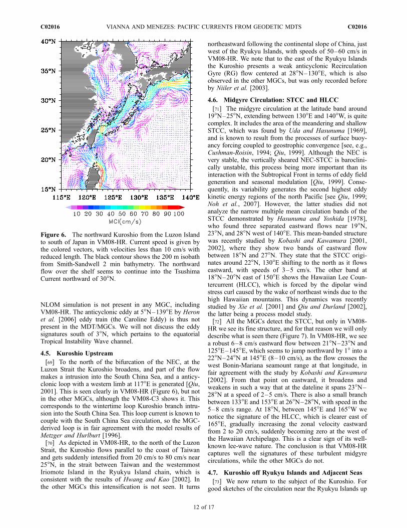
[69] To the north of the bifurcation of the NEC, at theLuzon Strait the Kuroshio broadens, and part of the flowmakes a intrusion into the South China Sea, and a anticy-clonic loop with a western limb at 117�E is generated [Qiu,2001]. This is seen clearly in VM08-HR (Figure 6), but notin the other MGCs, although the VM08-C3 shows it. Thiscorresponds to the wintertime loop Kuroshio branch intru-sion into the South China Sea. This loop current is known tocouple with the South China Sea circulation, so the MGC-derived loop is in fair agreement with the model results ofMetzger and Hurlburt [1996].[70] As depicted in VM08-HR, to the north of the Luzon

Strait, the Kuroshio flows parallel to the coast of Taiwanand gets suddenly intensified from 20 cm/s to 80 cm/s near25�N, in the strait between Taiwan and the westernmostIriomote Island in the Ryukyu Island chain, which isconsistent with the results of Hwang and Kao [2002]. Inthe other MGCs this intensification is not seen. It turns

northeastward following the continental slope of China, justwest of the Ryukyu Islands, with speeds of 50–60 cm/s inVM08-HR. We note that to the east of the Ryukyu Islandsthe Kuroshio presents a weak anticyclonic RecirculationGyre (RG) flow centered at 28�N–130�E, which is alsoobserved in the other MGCs, but was only recorded beforeby Niiler et al. [2003].

4.6. Midgyre Circulation: STCC and HLCC

[71] The midgyre circulation at the latitude band around19�N–25�N, extending between 130�E and 140�W, is quitecomplex. It includes the area of the meandering and shallowSTCC, which was found by Uda and Hasunuma [1969],and is known to result from the processes of surface buoy-ancy forcing coupled to geostrophic convergence [see, e.g.,Cushman-Roisin, 1994; Qiu, 1999]. Although the NEC isvery stable, the vertically sheared NEC-STCC is baroclini-cally unstable, this process being more important than itsinteraction with the Subtropical Front in terms of eddy fieldgeneration and seasonal modulation [Qiu, 1999]. Conse-quently, its variability generates the second highest eddykinetic energy regions of the north Pacific [see Qiu, 1999;Noh et al., 2007]. However, the latter studies did notanalyze the narrow multiple mean circulation bands of theSTCC demonstrated by Hasunuma and Yoshida [1978],who found three separated eastward flows near 19�N,23�N, and 28�N west of 140�E. This mean-banded structurewas recently studied by Kobashi and Kawamura [2001,2002], where they show two bands of eastward flowbetween 18�N and 27�N. They state that the STCC origi-nates around 22�N, 130�E shifting to the north as it flowseastward, with speeds of 3–5 cm/s. The other band at18�N–20�N east of 150�E shows the Hawaiian Lee Coun-tercurrent (HLCC), which is forced by the dipolar windstress curl caused by the wake of northeast winds due to thehigh Hawaiian mountains. This dynamics was recentlystudied by Xie et al. [2001] and Qiu and Durland [2002],the latter being a process model study.[72] All the MGCs detect the STCC, but only in VM08-

HR we see its fine structure, and for that reason we will onlydescribe what is seen there (Figure 7). In VM08-HR, we seea robust 6–8 cm/s eastward flow between 21�N–23�N and125�E–145�E, which seems to jump northward by 1� into a22�N–24�N at 145�E (8–10 cm/s), as the flow crosses thewest Bonin-Mariana seamount range at that longitude, infair agreement with the study by Kobashi and Kawamura[2002]. From that point on eastward, it broadens andweakens in such a way that at the dateline it spans 23�N–28�N at a speed of 2–5 cm/s. There is also a small branchbetween 133�E and 153�E at 26�N–28�N, with speed in the5–8 cm/s range. At 18�N, between 145�E and 165�W wenotice the signature of the HLCC, which is clearer east of165�E, gradually increasing the zonal velocity eastwardfrom 2 to 20 cm/s, suddenly becoming zero at the west ofthe Hawaiian Archipelago. This is a clear sign of its well-known lee-wave nature. The conclusion is that VM08-HRcaptures well the signatures of these turbulent midgyrecirculations, while the other MGCs do not.

4.7. Kuroshio off Ryukyu Islands and Adjacent Seas

[73] We now return to the subject of the Kuroshio. Forgood sketches of the circulation near the Ryukyu Islands up

Figure 6. The northward Kuroshio from the Luzon Islandto south of Japan in VM08-HR. Current speed is given bythe colored vectors, with velocities less than 10 cm/s withreduced length. The black contour shows the 200 m isobathfrom Smith-Sandwell 2 min bathymetry. The northwardflow over the shelf seems to continue into the TsushimaCurrent northward of 30�N.


12 of 17

C02016

to the Sea of Japan area, we refer to Figure 10.11b of Tomczakand Godfrey [2003]; see also the study of Guo et al. [2006].[74] In this area, the circulation is well depicted by all

MGCs based on EGM08, but only in the VM08-HR wenote that a parallel northward flow over the Chinesecontinental shelf (depth less than 200 m) with a speed of15–25 cm/s seem to merge with the offshore Kuroshio(60 cm/s), west of the Ryukyu (see Figure 6). South of Japan,a complex observed crossroads is suggestive that the shelfcurrent is more connected to the flows in the China Sea thanwith the upstream Kuroshio. This northward flow separatesfrom the Kuroshio at 31�N and continues strait into theTsushima Warm Current (TSWC) across the Korea Straitinto the Sea of Japan with a speed of 15 cm/s. The Kuroshio,on the other hand, turns east crossing the Tokara Strait at130�E, 30�N. We note that although the TSWC appears,possibly, as a weak western branch of a Kuroshio bifurcation[Tomczak and Godfrey, 2003] in VM08-HR we do not seethe flow structure as a bifurcation. It is quite interesting thatthis complex circulation pattern [Isobe, 1999; Guo et al.,2006, and references therein] seems to be consistent withthose obtained in VM08-HR (Figure 6), except that the veryvariable Taiwan Warm Current [Zhu et al., 2004] betweenTaiwan and mainland China is not resolved.[75] The other MGCs do not have sufficient resolution in

the inland seas to see any details, as is the case of the narrowSea of Japan and the China Seas. At this point, it isworthwhile to mention that the China Coastal Current isalso clearly seen in VM08-HR (Figure 6) between 31�N and36�N, 120�E–124�E, with speeds between 50and 65 cm/snear the East China Sea western boundary, retroflecting at30�N into a return current, the Yellow Sea Warm Current,which is also recorded in Figure 10.11b of Tomczak andGodfrey [2003].

4.8. Kuroshio-Honshu

[76] After crossing the Tokara Strait, south of Honshu, theKuroshio attains its maximum intensity in all MGCs, andthis maximum is around 100 cm/s in all the EGM08-basedMGCs, its width is around 150 km in VM08-HR (see Table5 for the maximum speeds along 135�E and Figure 6). This

high-speed signature is also partly seen in Rio05. It isinteresting to mention that the coarse land masks used inthe lower-resolution hybrid MDTs goes beyond the 1000 misobath: They only show part of the Kuroshio south ofJapan. Moreover, all other MGCs show a broader Kuroshio(greater than 200 km) with speeds less than 40 cm/s south ofHonshu. This is one clear example of the superiority of thenonhybrid EGM08-based MDTs, which in most cases doesnot need in situ measured oceanic data inversion to achievea realistically slender and high-speed mean current veryclose to the slope at the western boundary (one and onlyexception was already described: the Mindanao Currentcase).[77] The above-described Kuroshio speed maximum, up-

stream of the Izu-Ogasawara Ridge, coincides with thepresence of the largest southern RG of the Kuroshio. Thislarge and intense southern RG is totally located to the westof the Izu Ridge in all MGCs studied here (29�N–32�N;132�E–140�E), except in Rio05, where its closed lines gobeyond 140�E. The highest speeds are seen in VM08-HRand VMC07, as being in the 15–20 cm/s range in thesouthern limb of the RG, being half of that in the otherMGCs. This large mean RG is present in the surface currentmaps of Niiler et al. [2003]. However, most of the recentstudies have focused on the RGs of the Kuroshio ExtensionJet (KE) [Qiu and Chen, 2005; see Chen et al., 2007, andreferences therein].

4.9. Kuroshio Extension

[78] After crossing the Izu Ridge, the Kuroshio separatesfrom the Japan coast near the 1000 m isobath at 142�E,35�N, where it becomes the KE (Figure 8). This is notpossible to be accurately observed in the hybrid MGCs dueto the coarse land mask. There is an increase in speed at theseparation region in all the EGM08-based MGCs, especiallyin VM08-HR (60 cm/s). The mean latitudinal position of theseparation point of the axis of the Kuroshio from the slopeof Japan, and the mean KE path, has considerable climaticimportance and has been used as metrics for assessment ofhigh-resolution OGCMs.

Figure 7. Eastward zonal current map showing the STCC between 22�N and 24�N, where a bifurcationis seen east of the Marianas Islands and the Hawaiian Lee Countercurrent (HLCC) at 18�N west ofHawaii. The 1000-m isobath is shown in the black line.


13 of 17

C02016

[79] Recently, Kelly et al. [2007] carried out a detailedstudy on a few metrics for measuring the performance of thenonassimilative 0.08� resolution Hycom on the KE againstobservational data. One of their results is that the modelmean SSH-derived axis is biased to the south, since twothings happen: (1) the Kuroshio separation is 33.5�N, fartoo south as compared to their Generalized Digital Envi-ronmental Model (GDEM) climatology-derived axis, wherethe corresponding latitude is 35�N; and (2) this bias ismaintained downstream up to 153�E.[80] The separation point in VM08-HR is at 35�N, which

agrees with the one based on the GDEM dynamic heightclimatology [Kelly et al., 2007], and the results seen in thefigures of Niiler et al. [2003]. However, the VM08-HRmain KE axis does not agree with any axis derived by Kellyet al. [2007] downstream of 153�E, which is much to thenorth relative to VM08-HR. Both of their axes (model andclimatology) reach 36.5�N at 165�E, while in VM08-HR themain KE axis is at 34�N at same longitude. Nevertheless, inthe VM08-HR the KE has two axes: the main one centeredat 32�N and a secondary one spanning 36.5�N–38.5�N(with speed around 12 cm/s). Our results are consistent withthe results of Niiler et al. [2003] since they also resolve theKE into two branches being the main axis at 34�N. Wespeculate that the KE axes downstream of 153�E from Kellyet al. [2007] seem to match better with the weaker north KEbranch (see Figure 8).[81] It is worthwhile to point out that the KE region does

not seem to have a zero velocity reference, as top-to-bottomlowered ADCP measurements prove [Qiu, 2002]. There-fore, all of the results based on GRACE-derived MDTs, asthe VM08-HR result, can disagree with relative dynamicheight data, since no approximately zero-velocity referenceis available. This lack of a zero-reference depth implies aproblem for geostrophic velocity determinations from thethermal wind equation, if one wants to diagnostically esti-

mate total surface currents from altimetry. The use of anaccurate absolute satellite-derived MDT (e.g., VM08-HR)may contribute to the determination of absolute geostrophiccirculation of the KE from altimetry.[82] We notice that in all EGM08-based MGCs two mean

KE meanders are seen, with crests along 35�N, at 143�E andat 149�E, respectively (e.g., VM08-HR in Figure 9). Of theother MGCs, only the VMC07 shows the two, whileMaxNi04 and Rio05 only show some signature.

4.10. KE Southern Recirculation Gyres

[83] In addition to these meanders, two well-known RGsare clearly depicted south of the KE in all EGM08-basedMGCs and VMC07 along 33�N, one centered at 143�E andthe other (which has a three-celled structure) at 148�E(Figure 9). However, in the climatological study of theKuroshio-Oyashio system east of Japan by Qu et al. [2001],the two recirculation cells are not resolved in their surfaceMDH/2000 db data, being only resolved at depth into twoseparate RGs with their depth-integrated 1000–2000 MDHdata (relative to 2000 db).[84] The strong variability of the southern KE RGs has

been recently studied by Qiu and Chen [2005], while thevertical structure was studied by Chen et al. [2007]. Theseauthors estimated the mean surface velocity in the westernRG as 35 cm/s, based on profiling float measurements in theperiod from May to November 2004. In VM08-HR, themean speed is around 10–15 cm/s (Figure 8). We point out,in addition, that the 15 cm/s isovelocity line in VM08-HRseems to represent a major RG supercell spanning between142�E and 154�E, containing these two component RGs.[85] On the other hand, in the hybrid MGCs there is only

one weak RG of the KE to the west of the Shatsky Rise. InMaxNi04, it appears centered at 31�N, 143�E, and in Rio05it is centered at 32�N, 148�E, meaning that MaxNi04 sees

Figure 8. The Kuroshio Extension at 35�N and Oyashio Extension at 38�N in VM08-HR. Currentspeed is given by the colored vectors, with speeds less than 10 cm/s reduced in length. The graytopographic contour line shows the 4000 m isobath from Smith-Sandwell 2-min bathymetry, used toshow the Izu-Ogasawara Ridge and the Shatsky Rise.


14 of 17

C02016

the western RG, and Rio05 sees the eastern one but not bothare detected.

4.11. KE Bifurcations

[86] The KE is known to present flow bifurcationsassociated with the meanders. The first one is around143�E, where the northern branch interacts with the Sub-Arctic Current, while the southern branch is the knownmain KE. This KE branch presents the second main KEbifurcation, which may be formed upstream, over or down-stream of the Shatsky Rise [Mizuno and White, 1983;Hurlburt and Metzger, 1998; Niiler et al., 2003; Qiu andChen, 2010]. The hybrid MGCs, VMC07, and the otherEGM08-based MGCs present the signatures of these bifur-cations but do not resolve these in detail as VM08-HR does,so we based our description of the KE bifurcation structuresmainly on this MGC.[87] In the VM08-HR, we see a complex pattern formed

by a series of KE bifurcations and mergers (Figure 8). First,at the 143�E meander position the KE splits into southern(main) and northern (secondary) branches, where the latterstabilizes around 38�N and almost merges with the Sub-Arctic Current (North Pacific Current). Next, the main KEclearly bifurcates again at 148�E–150�E generating a weaknorthern flowing current which merges at 38�N with thenorthern branch. Subsequently, part of this northern branchturns south and merges back into the main KE over theShatsky Rise at 158�E. The region between the northern andsouthern branches becomes a bulge between 150�E–160�and 34�N–37�N. It corresponds to the 1978–1979 springpattern of Mizuno and White (their Figure 2b), whichincludes small interior recirculation eddies. The same patternis seen by Niiler et al. [2003], especially in their Figure 8a.[88] In a zooming of VM08-HR into the bulge region, we

notice a dipole of coherent small-scale recirculation eddieswith 3� diameter, upstream of the Shatsky Rise (Figure 8).

The cyclonic recirculation eddy is also present (not shown)in JPL08 and VM08, Rio05 and VMC07, although in thelatter two it appears with very weak westward velocity of1–2 cm/s. One independent evidence to the reality of thissmall northern mean cyclonic recirculation eddy is itspresence in the vertical section of geostrophic velocity at155�E from Qu et al. [2001], which is confined between33�N and 37�N (their Figure 9f). Another independentevidence is seen in some figures of Niiler et al. [2003],especially in their Figure 8a, where this exact (northern)cyclonic recirculation is also present.[89] To the lee of the Shatsky Rise, the northern branch of

the KE continues at 37�N up to 170�W while the main KEpresents another bifurcation near 160�E before the EmperorSeamounts. At 170�E–172�E, we clearly see three KEbranches: one with speeds 11 cm/s at 32�N, and other with10 cm/s at 36�N, and the one originating at 143�E stabilizingat 40�N around 8 cm/s (Figure 10).

5. Conclusion

[90] This work reports on the computation of four newfiltered versions of MDTs (two based on EGM08, one onGGM02C, and one GGM02S) and presents a condenseddescription of the presently most important observationalMDTs for global ocean circulation studies just prior to thenear-future availability of the GOCE data.[91] One difficulty for using observational satellite-

derived MDTs to correct the mean sea surface bias ofOGCMs with altimetric data assimilation is the lack ofMDTs with high grid resolution and adequate mesoscalefeature discrimination (good accuracy at short wavelengths),plus the additional difficulty of obtaining an associated MDTerror field. The grid resolution of some widely distributedMDT (e.g., 0.5� � 0.5�) is still unnecessarily coarse formesoscale oceanographic applications. This may be in part

Figure 9. The southern recirculation gyres of the Kuroshio Extension in the VM08-HR MDT (in color),with the flow lines superposed. Also seen are the Kuroshio Front (with clockwise flow lines turning fromthe south) and the Oyashio Front (with anticlockwise turning flow lines from the north).


15 of 17

C02016

due to the use of standard filtering which damps the short-scale MDT signals giving the impression that early GRACE-based MDTs do not resolve the mesoscale. This workshows that with more efficient filters even with GGM02Cat 0.25� � 0.25� resolution (degree/order 360) known meanmesoscale oceanic mesoscale features are reproduced, whilewith the recent high-resolution EGM08-based MDTs it ispossible to map the circulation even in small adjacent seas tomajor ocean basins (Bering Sea, South China Sea, Sea ofOkhotsk, seen in figures but not studied here).[92] The paper analyzes a small set of MDTs by use of

EOF analysis, where error fields may be estimated at least toshow where the estimates of mean current features arerobust and realistic. The western boundary currents andassociated recirculations are more intense and slender whenderived from the new EGM08-based MDTs than the onesobtained from previous GRACE-based or hybrid MDTs.[93] We used the North Pacific Ocean as a test bed for the

new high-resolution VM08-HR MGC, focusing on bothlong-scale and small-scale circulation features. Some meanmesoscale eddy features have been established as trulyrealistic in the North Pacific, through results from long timein situ measurements reported by various authors. Oneexample described here is related to the zonal NEC andNECC in the western tropical Pacific, where a sequence ofmean eddies in between them is clearly depicted with thenew generation of high-resolution MDTs. The reality ofthese eddies in a long-term mean circulation is confirmed byrecent work by other authors [Heron et al., 2006]. Therobustness of these features is also confirmed by comparing

results from various MDTs and associated MGCs obtainedby different filtering techniques. This result casts in doubtthe concept that mean small-scale circulation features in aMDT are as a rule only reflecting the dependence on theend-points of the averaging intervals, although interannualmodulations cannot be ruled out.[94] We also discussed the important question of the

erroneous geodetically derived Mindanao Current, a soleexception in the realistic recovery of western boundarycurrent structure and their extensions by the geodetic/altimetricmethod. It presents a challenge to the scientific communityinvolved with the geodetic and altimetric data analysis. Wehope that novel algorithms for the processing of the GOCEdata in a regional setting can solve this near-coastal problemand pass the test of recovering of this well-known near coastalopen-ocean western boundary current. This might requiremethods of global data synthesis different from the classicalspherical harmonic expansion method used in global physicalgeodesy. The MDT/MGC files studied here are available inNetCDF at http://www.oceantopography.vmoceanica.com/.

[95] Acknowledgments. This work would not have been possiblewithout a large number of people and organizations that offered their MDTfiles freely and easily through the Internet: the CLS Space OceanographyDivision for Rio05 MDT, JPL for the JPL08 MDT, Nikolai Maximenko andPeter Niiler for MaxNi04 MDT, and Ole Andersen for the DNSC08 files.Special thanks are owed to Don Chambers who supplied us with theunfiltered EGM08-based and GGM02C MDTs and to Rory Bingham whokindly supplied us with his several satellite-only GRACE-based MDTs atdifferent degree/order cutoffs. We are also indebted to two anonymousreviewers for their competent criticism and important suggestions.

Figure 10. The recirculations inside the bulge created by the splitting of the KE into two branches westof the Shatsky Rise, with subsequent merging (splitting is at 152�E and the merger at 159�E). Thecirculation structure in the bulge is a tripole, with a stronger cyclonic and two weaker anticyclonic eddies.Smith-Sandwell 2-min bathymetry in color shows the Shatsky Rise.


16 of 17

C02016

ReferencesAndersen, O. B., and P. Knudsen (2008), The DNSC08MSS global meansea surface, paper presented at EGU General Assembly 2008, Vienna,13–18 April.

Bingham, R., and K. Haines (2006), Mean dynamic topography: Intercom-parisons and errors, Philos. Trans. R. Soc. A, 364, 903–916, doi:10.1098/rsta.2006.1745.

Bingham, R. J., K. Haines, and C. W. Hughes (2008), Calculating theocean’s mean dynamic topography from a mean sea surface and a geoid,J. Atmos. Oceanic Technol., 25(10), 1808–1822, doi:10.1175/2008JTE-CHO568.1.

Castruccio, F., J. Verron, L. Gourdeau, J.-M. Brankart, and P. Brasseur(2008), Joint altimetric and in situ data assimilation using the GRACEmean dynamic topography: A 1993–1998 hindcast experiment in thetropical Pacific Ocean, Ocean Dyn., 58, 43–63, doi:10.1007/s10236-007-0131-4.

Chen, S., B. Qiu, and P. Hacker (2007), Profiling float measurements of therecirculation gyre south of the Kuroshio Extension in May to November2004, J. Geophys. Res., 112, C05023, doi:10.1029/2006JC004005.

Cushman-Roisin, B. (1994), Introduction to Geophysical Fluid Dynamics,320 pp., Prentice-Hall, Englewood Cliffs, N. J.

Dritschel, D. (1989), On the stabilization of a two-dimensional vortex stripby adverse shear, J. Fluid Mech., 206, 193–221.

Gourdeau, L., J. M. Lemoine, M. H. Rio, and F. Hernandez (2003),Estimating mean dynamic topography in the tropical Pacific Oceanfrom gravity and altimetry satellites, Geophys. Res. Lett., 30(20), 2062,doi:10.1029/2003GL018200.

Guo, X., Y. Miyazawa, and T. Yamagata (2006), The Kuroshio onshoreintrusion along the shelf break of the East China Sea: The origin of theTsushima warm curent, J. Phys. Oceanogr., 36, 2205–2231.

Hasunuma, K., and K. Yoshida (1978), Splitting the subtropical gyre in thewestern North Pacific, J. Oceanogr. Soc. Jpn., 34, 160–172.

Heron, S. F., E. J. Metzger, and W. J. Skirving (2006), Seasonal variationsof the ocean surface circulation in the vicinity of Palau, J. Oceanogr., 62,413–426.

Hofmann-Wellenhof, B., and H. Moritz (2006), Physical Geodesy, 2nd ed.,403 pp., Springer, Vienna.

Hurlburt, H., and E. Metzger (1998), Bifurcation of the Kuroshio Extensionat the Shatsky Rise, J. Geophys. Res., 103, 7549–7566.

Hwang, C., and R. Kao (2002), TOPEX/POSEIDON-derived space-timevariations of Kuroshio current: Applications of a gravimetric geoid andwavelet analysis, Geophys. J. Int., 151, 835–847.

Hwang, C., Y. S. Hsiao, H. C. Shih, M. Yang, K. Chen, R. Forsberg, andA. V. Olesen (2007), Geodetic and geophysical results from a Taiwanairborne gravity survey: Data reduction and accuracy assessment,J. Geophys. Res., 112, B04407, doi:10.1029/2005JB004220.

Isobe, A. (1999), The Taiwan-Tsushima warm current system: Its path andthe transformation of the water mass in the East China Sea, J. Oceanogr.,55, 185–195.

Jayne, S. (2006), Circulation of the North Atlantic Ocean from altimetryand the Gravity Recovery and Climate Experiment geoid, J. Geophys.Res., 111, C03005, doi:10.1029/2005JC003128.

Kelly, K. A., L. Thompson, W. Cheng, and E. J. Metzger (2007), Evalua-tion of HYCOM in the Kuroshio Extension region using new metrics,J. Geophys. Res., 112, C01004, doi:10.1029/2006JC003614.

Kobashi, F., and H. Kawamura (2001), Variation of sea surface heightat periods of 65–220 days in the subtropical gyre of the North Pacific,J. Geophys. Res., 106, 26,817–26,831.

Kobashi, F., and H. Kawamura (2002), Seasonal variation and instabilitynature of the North Pacific subtropical countercurrent and HawaiianLee countercurrent, J. Geophys. Res., 107(C11), 3185, doi:10.1029/2001JC001225.

Maximenko, N. A., and P. P. Niiler (2004), Hybrid decade-mean global sealevel with mesoescale resolution, in Recent Advances in Marine Scienceand Technology, edited by N. Saxena, pp. 55–59, PACON Int., Honolulu.

Metzger, J. P., and H. E. Hurlburt (1996), Coupled dynamics of the SouthChina Sea, the Sulu Sea, and the Pacific Ocean, J. Geophys. Res., 101,12,331–12,352.

Mizuno, K., and W. White (1983), Annual and interannual variability in theKuroshio current system, J. Phys. Oceanogr., 13, 1847–1867.

Niiler, P. P., N. A. Maximenko, G. G. Pantelev, T. Yamagata, andD. B. Olson (2003), Near-surface dynamical structure of the KuroshioExtension, J. Geophys. Res., 108(C6), 3193, doi:10.1029/2002JC001461.

Noh, Y., B. Y. Yim, S. H. You, J. H. Yoom, and B. Qiu (2007), Seasonalvariation of eddy kinetic energy of the north Pacific subtropical counter-current simulated by an eddy-resolving OGCM, Geophys. Res. Lett., 34,L07601, doi:10.1029/2006GL029130.

Pavlis, N. K., S. A. Holmes, S. C. Kenyon, and J. K. Factor (2008), Anearth gravitational model to degree 2160: EGM2008, paper presented atEGU General Assembly 2008, Vienna, 13–18 April.

Qiu, B. (1999), Seasonal eddy field modulation of the north Pacificsubtropical countercurrent: TOPEX/POSEIDON observations and theory,J. Phys. Oceanogr., 29, 2468–2471.

Qiu, B. (2001), Kuroshio and Oyashio currents, in Encyclopedia of OceanSciences, pp. 1413–1425, Academic, New York.

Qiu, B. (2002), The Kuroshio Extension system: Its large-scale variabilityand role in the midlatitude ocean-atmosphere interaction, J. Oceanogr.,58, 57–75.

Qiu, B., and S. Chen (2005), Variability of the Kuroshio Extension jet,recirculation gyre and mesoscale eddies on decadal timescales, J. Phys.Oceanogr., 35, 2090–2103.

Qiu, B., and S. Chen (2010), Eddy-mean flow interactions in the decadally-modulating Kuroshio Extension system, Deep Sea Res., in press.

Qiu, B., and T. S. Durland (2002), Interaction between an island and theventilated thermocline: Implications for the Hawaiian Lee countercurrent,J. Phys. Oceanogr., 32, 3408–3426.

Qiu, B., and R. Lukas (1996), Seasonal and interannual variability of theNorth Equatorial current, the Mindanao current, and the Kuroshio alongthe Pacific western boundary, J. Geophys. Res., 101, 12,315–12,330.

Qu, H. T., H. Mitsudera, and T. Yamagata (1998), On the western boundarycurrents in the Philippine Sea, J. Geophys. Res., 103, 7537–7548.

Qu, T., H. Mitsudera, and B. Qiu (2001), A climatological view of theKuroshio/Oyashio system east of Japan, J. Phys. Oceanogr., 31,2575–2589.

Rio, M.-H., and F. Hernandez (2004), A mean dynamic topographycomputed over the world ocean from altimetry, in situ measurements,and a geoid model, J. Geophys. Res., 109, C12032, doi:10.1029/2003JC002226.

Rio, M. H., P. Schaeffer, F. Hernandez, and J. M. Lemoine (2005), Theestimation of the ocean mean dynamic topography through the combina-tion of altimetric data, in situ measurements and GRACE geoid: Fromglobal to regional studies, paper presented at GOCINA Workshop,GOCINA Project, Eur. Union, Luxembourg.

Tapley, B., et al. (2005), GGM02: An improved Earth Gravity Field Modelfrom GRACE, J. Geod., 79, 467–478, doi:0.1007/s00190-005-0480-z.

Tomczak, M., and J. S. Godfrey (2003), Regional Oceanography: AnIntroduction, Daya Publ. House, Delhi.

Tozuka, T., T. Kagimoto, Y. Matsumoto, and T. Yamagata (2002), Simu-lated multiscale variations in the western tropical Pacific: The Mindanaodome revisited, J. Phys. Oceanogr., 32, 1338–1359.

Uda, M., and K. Hasunuma (1969), The eastward subtropical counter-current in the western North Pacific Ocean, J. Oceanogr. Soc. Jpn.,25, 201–210.

Vianna, M. L., V. V. Menezes, and D. P. Chambers (2007), A highresolution satellite-only GRACE-based mean dynamic topography of theSouth Atlantic Ocean, Geophys. Res. Lett., 34, L24604, doi:10.1029/2007GL031912.

Vossepoel, F. (2007), Uncertainties in the mean ocean dynamic topographybefore the launch of the gravity field and steady-state ocean circulationexplorer (GOCE), J. Geophys. Res., 112, C05010, doi:10.1029/2006JC003891.

Wang, Y. (2001), GSFC00 mean sea surface, gravity anomaly, and verticalgravity gradient from satellite altimeter data, J. Geophys. Res., 106,31,167–31,174.

Wijffels, S., E. Firing, and J. Toole (1995), Themean structure and variabilityof the Mindanao current at 8N, J. Geophys. Res., 100, 18,421–18,435.

Wyrtki, K. (1975), Fluctuations of the dynamic topography in the PacificOcean, J. Phys. Oceanogr., 5, 450–459.

Xie, S.-P., W. T. Liu, Q. Liu, and M. Nonaka (2001), Far-reaching effects ofthe Hawaiian islands on the Pacific Ocean–atmosphere system, Science,292, 2057–2060, doi:10.1126/science.1059781.

Zhang, Z., Y. Lu, and H. Hsu (2007), Detecting surface geostrophic currentsusing wavelet filter from satellite geodesy, Sci. Chin. Ser. D: Earth Sci.,50(6), 918–926.

Zhu, J., C. Chen, P. Ding, C. Li, and H. Lin (2004), Does the Taiwan warmcurrent exist in winter?, Geophys. Res. Lett., 31, L12302, doi:10.1029/2004GL019997.

��V. V. Menezes, VM Oceanica LTDA, Tr Santa Cruz, 70/102, Arraial do

Cabo, RJ 2893-0000, Brazil. ([email protected])M. L. Vianna, VM Oceanica LTDA, R Manoel Bandeira 210, Sao Jose

Campos, SP 1224-0710, Brazil. ([email protected])


17 of 17

C02016

Mean mesoscale global ocean currents from geodetic pre-GOCE MDTs with a synthesis of the North...

Documents

Transcript of Mean mesoscale global ocean currents from geodetic pre-GOCE MDTs with a synthesis of the North...