ME3000 Analog Electronics Lab 5 Practical Op-Amp Circuits

http://dreamcatcher.asia/cw ______________________________________________________________________

ME3000 Analog Electronics Lab 5 - 1/22

ME3000 Analog Electronics

Lab 5

Practical Op-Amp Circuits

This courseware product contains scholarly and technical information and is protected by copyright laws and international treaties. No part of this publication may be reproduced by any means, be it transmitted, transcribed, photocopied, stored in a retrieval system, or translated into any language in any form, without the prior written permission of Acehub Vista Sdn. Bhd. The use of the courseware product and all other products developed and/or distributed by Acehub Vista Sdn. Bhd. are subject to the applicable License Agreement. For further information, see the Courseware Product License Agreement.

Objective

i) To understand typical operational amplifier circuits and their characteristics

Equipment Required

i) ME3000-M2 Analog Electronics Training Kit ii) Digital Multimeter, recommendation : Agilent 34405A or U2741A iii) 50 MHz Oscilloscope or equivalent, recommendation : Agilent DSO1002A 60 MHz or

U2701A iv) 10 MHz Function Generator or equivalent, recommendation : Agilent 33220A or U2761A v) Dual Output (+/- 12V, 0.5A) DC Power Supply, recommendation : Agilent E3631A

Accessories Required

i) 1 x 4-way power supply cable ii) 1 x BNC(m)-to-grabber clips coaxial cable iii) 6 x jumper cables terminated with grabber clips at both ends iv) 1 x antistatic wrist strap

Caution: An electrostatic discharge generated by a person or an object coming in contact with electrical components may damage or destroy the training kit. To avoid the risk of electrostatic discharge, please wear the antistatic wrist strap and observe the handling precautions and recommendations contained in the EN100015-1 standard. Do not connect or disconnect the device while it is being energized.



1. Introduction

An operational amplifier (op-amp) is an integrated circuit capable of amplifying the voltage difference between its two input terminals. As shown in Figure 1, a general purpose op-amp has two input terminals which are the non-inverting (+) and inverting () inputs, a single output terminal, and two voltage supply terminals (V+ and V-). Most of the op-amps require dual power supplies (±5 Vdc, ±15 Vdc, and so forth), but some op-amps (such as LM3900) may be powered from a single supply.

V+

Output+

-

V-

Non-inverting input

Inverting input

Figure 1 – Op-Amp Circuit Symbol

The simplest form of an op-amp comes in an 8-pin IC package, such as the commonly used 741. The connection diagram for the 741 op-amp is depicted in Figure 2.

Figure 2 – 741 Op-Amp Connection Diagram

An op-amp has the following three important characteristics:

High open-loop gain High input impedance Low output impedance

Different configurations of a negative feedback network are used to reduce voltage gain of op-amps to produce practical and linear circuits. In the following experiments, five typical op-amp configurations are introduced, namely the inverting amplifier, summing amplifier, non-inverting amplifier, differential amplifier, and buffer.



2. Inverting Amplifier

1. Locate the Inverting/Summing Amplifier section on the ME3000-M2 training kit. 2. Disconnect all the jumpers located in the Inverting/Summing Amplifier section. 3. Insert jumpers J22 and J24 to construct an inverting amplifier circuit shown in Figure 3.

+15 V

V-

V+2

3

-15 V

7

4

6Vin

Vout

R1=100k

Rf =200k

–

+

TP7

TP9

GNDGND

J22

J24

Figure 3 – Inverting Amplifier Schematic Diagram

4. With Vin(pp) = 1.0 V, predict Vout(pp) using the following equation:

inf

out VR

RV

1 , negative () sign indicates a 180o phase shift

5. Connect the function generator output using the BNC-to-grabber clips coaxial cable and CH1

probe of the oscilloscope to TP7 (Vin). Connect the CH2 probe of the oscilloscope to TP9 (Vout). Connect the instrument references to the GND terminals.

6. Connect the power supply to the training kit using the 4-way power supply cable. Set the dual channel output voltages to exactly +15 V and -15 V, respectively. Set both current limits to 0.5 A. Turn on the power supply. Refer to Appendix for details.

7. Apply a 1.0 V peak-to-peak sine wave of 1 kHz to input Vin of the inverting amplifier. 8. Set the trigger source to CH1. Set Time/div to display two cycles of the waveforms on the

screen. Set Volt/div of CH1 and CH2 to clearly display the waveforms. Sketch the waveforms. 9. Use the multimeter to measure Vout(pp) (this measured value should be close to the predicted

value) and record the phase shift of Vout with respect to Vin (). Calculate the ratio of Vout(pp)/Vin(pp).

10. Turn off the power supply and disconnect all the cables from the Inverting/Summing Amplifier section.



3. Summing Amplifier

1. The Inverting Amplifier section on the ME3000-M2 training kit can be modified into a Summing Amplifier.

2. Insert jumper J23 to construct a two-input summing amplifier circuit shown in Figure 4.

+15 V

V-

V+2

3

-15 V

7

4

6

V1

Vout

R1=100k

Rf =200k

–

+

TP7

TP9

GNDGND

J22J24

V2 R2=100k

TP8 J23

Figure 4 – Two-Input Summing Amplifier Schematic Diagram

3. With V2 = 2 V, predict Vout when V1 = –1 V, 0 V, and +1 V using following equation:

1 21

( )fout

RV V V

R


probe of the oscilloscope to TP7 (V1). Connect the CH2 probe of the oscilloscope to TP9 (Vout). Connect the instrument references to the GND terminals.

5. Connect TP15 (–7.5 V ~ +7.5 V adjustable DC voltage source) to TP8 (V2) using the jumper cable.

6. Connect the power supply to the training kit using the 4-way power supply cable. Set the dual channel output voltages to exactly +15 V and -15 V, respectively. Set both current limits to 0.5 A. Turn on the power supply.

7. Adjust the potentiometer VR1 to obtain V2 = 1.0 V. Use the multimeter to measure V2. 8. Apply a 2.0 V peak-to-peak sine wave of 1 kHz to input V1 of the summing amplifier. 9. Set the trigger source to CH1. Set Time/div to display two cycles of the waveforms on the

screen. Set Volt/div of CH1 and CH2 to clearly display the waveforms. Sketch the waveforms. 10. Measure Vout when V1 = –1 V, 0 V, and +1 V. 11. Slowly adjust V2 by turning VR1. Observe how Vout changes when V2 is varied between 0 V

and 5V. Comment on your observation. 12. Turn off the power supply and disconnect all the cables from the Inverting/Summing Amplifier

section.



4. Non-Inverting Amplifier

1. Locate the Non-Inverting Amplifier section on the ME3000-M2 training kit. 2. Disconnect all the jumpers located in the Non-inverting Amplifier section. 3. Insert jumpers J25 and J26 to construct a non-inverting amplifier circuit shown in Figure 5.

+15 V

V-

V+2

3

-15 V

7

4

6

Vin

Vout

R1=10k

Rf =20k

–

+GND

GND

TP11

TP10

J26

J25

Figure 5 – Non-Inverting Amplifier Schematic Diagram

4. With Vin(pp) = 1.0 V, predict Vout(pp) using the following equation:

1

1 fout in

RV V

R




7. Apply a 1.0 V peak-to-peak sine wave of 1 kHz to input Vin of the inverting amplifier. 8. Set the trigger source to CH1. Set Time/div to display two cycles of the waveforms on the

screen. Set Volt/div of CH1 and CH2 to clearly display the waveforms. Sketch the waveforms. 9. Measure Vout(pp) (this measured value should be close to the predicted value) and record the

phase shift of Vout with respect to Vin (). Calculate the ratio of Vout(pp)/Vin(pp). 10. Turn off the power supply and disconnect all the cables from the Non-inverting Amplifier

section.



5. Differential Amplifier

1. Locate the Differential Amplifier section on the ME3000-M2 training kit. 2. Disconnect all the jumpers located in the Differential Amplifier section. 3. Insert jumpers J27, J28, J29, and J30 to construct a differential amplifier circuit shown in

Figure 6.

+15 V

V-

V+2

3

-15 V

7

4

6

V2

Vout

R1=100k

R2 =200k

–

+V1

R3=100k

+15 V

VR15k

R4=200k

2.2k

2.2k

-15 V

TP15(-7.5V~7.5V)

TP14

GND

J27TP12

J29

J28

J30

TP13

GND

Figure 6 – Differential Amplifier Schematic Diagram

4. With V2 = 2 V, predict Vout when V1 = –1 V, 0 V, and +1 V using the following equation:

22 1

1out

RV V V

R


probe of the oscilloscope to TP13 (V1). Connect the CH2 probe of the oscilloscope to TP14 (Vout). Connect the instrument references to the GND terminals.

6. Connect TP15 (–7.5 V ~ +7.5 V adjustable DC voltage source) to TP12 (V2) using the jumper cable.

7. Connect the power supply to the training kit using the 4-way power supply cable. Press Set the dual channel output voltages to exactly +15 V and -15 V, respectively. Set both current limits to 0.5 A. Turn on the power supply.

8. Apply a 2.0 V peak-to-peak sine wave of 1 kHz to the input V1 of the differential amplifier. Adjust the potentiometer to obtain V2 = 1.0 V. Use the multimeter to measure V2.

9. Set the trigger source to CH1. Set Time/div to display two cycles of the waveforms on the screen. Set Volt/div of CH1 and CH2 to clearly display the waveforms. Sketch the waveforms.

10. Measure Vout when V1 = –1 V, 0 V, and +1 V. Sketch the V1 and Vout waveforms. 11. Slowly adjust V2 by turning VR1. Observe how Vout changes when V2 is varied between 0 V

and 5 V. Comment on your observation and compare with the results of the summing amplifier.

12. Turn off the power supply and disconnect all the cables from the Differential Amplifier section.



6. Buffer Circuit

+15 V

V+2

3

-15 V

7

4

6–

+Vin

VoutV-TP16

GND

TP17

GND

Figure 7 – Buffer Schematic Diagram

1. Locate the Buffer Circuit section on the ME3000-M2 training kit. 2. Disconnect all the jumpers located in the Buffer Circuit section. 3. Connect the function generator output using the BNC-to-grabber clips coaxial cable and CH1



5. Apply a 1.0 V peak-to-peak sine wave of 1 kHz to input Vin. Measure Vout(pp) and record the phase shift of Vout with respect to Vin (). Calculate the ratio of Vout(pp)/Vin(pp). Sketch the Vin and Vout waveforms.

6. The next experiment tests the buffer ability to reduce loading effect. 7. Disconnect the function generator and oscilloscope from TP16 and TP17. 8. Connect the function generator output and CH1 of the oscilloscope to TP19. The function

generator forms a high impedance source with R19 at TP18. 9. Connect TP18 to TP20 using the jumper cable. This connects the high impedance source to

the load circuit (R20), as shown in 10. Figure 8.

Function generator R20 1k

TP19

GND

High impedance source

TP18

Load

TP20 TP21R19 10k

VloadVsource

GND

Figure 8 – Setup to Study the Loading Effect



11. Connect CH2 of the oscilloscope to TP21. 12. Set the trigger source to CH1. Set Time/div to display two cycles of the waveforms on the

screen. Set Volt/div of CH1 and CH2 to clearly display the waveforms. Sketch the Vsource and Vload waveforms.

13. Measure Vload(pp). 14. Disconnect TP18 from TP20. 15. Connect TP18 to TP16 (Vin of the buffer) and TP20 to TP17 (Vout of the buffer), as shown in

Figure 9. 16. Using the oscilloscope, observe and sketch the Vsource and Vload waveforms.

Function generator

R20 1k

TP19

GND

High impedance source

TP18

Load

TP20 TP21R19 10k

Vload

Vsource

+15 V

V+2

3

-15 V

7

4

6–

+V-TP16

TP17

GND

Vout

Vin

Figure 9 – Buffer Connections to Minimize the Loading Effect

17. Measure Vout(pp). Comment on your observation. 18. Turn off the power supply and disconnect all the cables from the Buffer Circuit section.



7. Design Problem: Comparator

1. A comparator compares two voltages or currents and switches its output between two discrete values to indicate which is larger.

2. A basic op-amp connection to form a comparator is shown in Figure 10.

+15 V

V+2

3

-15 V

7

4

6–

+V1

VoutV-

V2

1 2

1 2

15 ,

15 ,out

out

V V V V

V V V V

Figure 10 – Basic Op-Amp Comparator Schematic Diagram

3. By reconnecting the jumpers at the differential amplifier section, construct a comparator circuit

that compares a 2 Vpp, 1 kHz sine wave signal against a constant voltage value of 0.7 V, and produces a positive output when the sine wave is greater than 0.7 V.

4. Rearrange the circuit so that the output voltage is positive when the sine wave is smaller than 0.7 V.



Appendix: Tips on Using Agilent E3631A Triple Output DC Power Supply Supplying +5 V, +15 V, and 15 V to the ME3000-M2 training kit:

Press Power to turn on the E3631A. The E3631A has three adjustable output supplies namely +6 V, +25 V, and 25 V. By default, all outputs are disabled (the OFF annunciator is turned on), the +6 V supply is selected, and the knob is ready for voltage control.

Adjust the knob to +5 V. Press Display Limit and set the current limit to 0.5 A. Next, set the supply to +25 V (positive supply). Set the voltage to +15 V and current limit to

0.5 A. Repeat the same procedure for –25 V (negative supply) to set the voltage to 15 V and current limit to 0.5 A.

Connect the E3631A to the ME3000 training kit as shown below. Enable the power supply outputs by pressing Output On/Off. The CV and +25 V

annunciators should turn on. Caution: If the CC annunciator is turned on, disable the output and check whether this is due

to the current limit setting or faulty connection. Upon completion of each experiment and before making any connection on the training kit,

ensure that the power supply output is disabled by pressing Output On/Off.

ME3000-M2 Training Kit

Power Supply

(E3631A)

com – +

25 V 6 V

– +

4-way connector



Appendix: Tips on How to Use the Agilent U2741A USB Modular Digital Multimeter Front Panel of the Agilent U2741A USB Modular Digital Multimeter

Figure B-1 – Front Panel of the Digital Multimeter Setting Up the Connection

1. Connect the digital multimeter to the PC using a USB cable.

2. Power on the digital multimeter.

3. Launch the Agilent IO Control and the Agilent Measurement Manager (AMM).

4. The Select USB Device dialog box will appear displaying the connected U2741A devices. To start the application, select a U2741A device and click OK to establish the connection

5. The U2741A can only be operated via the USB interface. On the front panel of the U2741A, there are two LED indicators. The power indicator lights up once the U2741A is powered on. There is a system error if the indicator blinks after the U2741A is powered on. The USB indicator will only blink when there is data exchange activity between the U2741A and the PC.

6. You can control the U2741A via the Agilent Measurement Manager (AMM) for U2741A or via SCPI commands sent through the USB interface from your own application programs.

7. Launch the Agilent IO Control and AMM. 8. The Select USB Device dialog box will appear displaying the connected U2741A devices. To

start the application, select a U2741A device and click OK to establish the connection. You may start to use the digital multimeter now.

Measuring DC Voltage

1. The DC voltage measurement function of the U2741A has the following features: five ranges to select: 100 mV, 1 V, 10 V, 100 V, and 300 V; or auto range input impedance is 10 MΩ for all ranges (typical) input protection is 300 V on all ranges (HI terminal)



2. Make the connection as shown in Figure B-2 in order to measure DC voltage. You can control the U2741A via the Agilent Measurement Manager (AMM) software for U2741A or via SCPI commands sent through the USB interface from your own application programs.

Figure B-2 – Measuring DC Voltage

3. If you are using the AMM, select the DCV function located at the top-left corner. Set the desired range under Range section. A suitable range should be selected to give the best measurement resolution. The reading is displayed and updated continuously.

4. If you are using SCPI commands, enter MEASure[:VOLTage]:DC? in order to make a DC voltage measurement.

Measuring DC Current

1. The DC current measurement function of the U2741A has the following features: three ranges to select: 10 mA, 100 mA, 1 A, and 2 A; or auto range input impedance is 10 MΩ for all ranges (typical) input protection fuse is 2 A, voltage rating 250 V on all ranges

2. Make the connection as shown in Figure in order to measure DC current. You can control the U2741A via the Agilent Measurement Manager (AMM) software for U2741A or via SCPI commands sent through the USB interface from your own application programs.

Figure B-3 – Measuring DC Current

3. If you are using the AMM, select the DCI function located at the top-left corner. Set the desired range under the Range section. A suitable range should be selected to give the best measurement resolution. The reading is displayed and updated continuously.

4. If you are using SCPI commands, enter MEASure:CURRent[:DC]? in order to make a DC current measurement.



Appendix: Tips on How to Use the Agilent U2761A USB Modular Function Generator

Front Panel of the Agilent U2761A USB Modular Function Generator

Figure A-1 – Front Panel of the U2761A Setup Connection

9. Connect the function generator to the PC using a USB cable. 10. Power on the function generator. 11. Launch the Agilent IO Control and the Agilent Measurement Manager (AMM). 12. The Select USB Device dialog box will appear displaying the connected U2761A devices. To

start the application, select a U2761A device and click OK to establish the connection. 13. Click Output to enable or disable the output of the function generator after the desired

parameters are set. 14. The U2761A is able to output five standard waveforms that are Sine, Square, Ramp,

Triangle, Pulse, and DC. 15. You can select one of the three built-in Arbitrary waveforms or create your own custom

waveforms. 16. You can also internally modulate Sine, Square, Ramp, Triangle, and Arbitrary waveforms

using AM, FM, PM, FSK, PSK, or ASK. 17. The linear or logarithmic frequency sweeping is available for Sine, Square, Ramp, Triangle,

and Arbitrary waveforms. 18. Table A- shows which output functions are allowed with modulation and sweep. 19. Each √ indicates a valid combination. If you change to a function that is not applicable for

modulation, or sweep; then the modulation or mode will be disabled.

Table A-1 – Output Functions

Sine Square Ramp Triangle Pulse DC Arbitrary

AM, FM, PM, FSK, PSK, ASK Carrier √ √ √ √ √

AM, FM, PM Internal Modulation √ √ √ √ √

FSK, PSK, ASK Internal Modulation √

Sweep Mode √ √ √ √ √



Agilent Measurement Manager Soft Front Panel (Function Generator)

Figure A-2 – Graphic User Interface of the Agilent Measurement Manager (Function Generator)

Figure A-2 shows the graphic user interface of the Agilent Modular Function Generator under the Agilent Measurement Manager (AMM). Table A- shows the features of each panel of the interface.

Table A-2 – Features of the AMM Function Generator Interface

No. Panel Features

1 Waveform Pattern Selection Select various types of output function by clicking the buttons.

2 Waveform Parameters Configure the function parameters (Frequency, Amplitude, and Offset)

3 Waveform Pattern Display Display a graph representation of the output function

4 Modes of Waveform Configure to modulation mode or sweep mode

5 Status Display Display the parameters and status of the configured output waveform

6 Trigger & Output Enable/Disable

Enable/disable the Trigger and Output buttons (they are highlighted when enabled and grey when disabled)



Function Limitation If you change to a function where the maximum frequency is less than the current function, the frequency will be adjusted to the maximum value for the new function. For example, if you are currently outputting a 20 MHz sine wave and then change to the Ramp function, the U2761A will automatically adjust the output frequency to 200 kHz (the upper limit for Ramp). As shown in Table A-, the output frequency range depends on the function currently selected. The default frequency is 1 kHz for all functions.

Table A-3 – Output Frequency Range

Function Minimum Frequency Maximum Frequency

Sine 1 µHz 20 MHz Square 1 µHz 20 MHz Ramp, Triangle 1 µHz 200 MHz Pulse 500 µHz 5 MHz DC Not applicable Not applicable

Arbitrary 1 µHz 200 kHz 2 MHz (U2761A Option 801)

Amplitude Limitation The default amplitude is 1 Vpp (into 50 Ω) for all functions. If you change to a function where the maximum amplitude is less than the current function, the amplitude will automatically adjust to the maximum value for the new function. This may occur when the output units are Vrms or dBm due to the differences in crest factor for the various output functions. For example, if you output a 2.5 Vrms Square wave (into 50 Ω) and then change to the Sine wave function, the U2761A will automatically be adjusted the output amplitude to 1.768 Vrms (the upper limit for Sine wave in Vrms). Duty Cycle Limitations For Square waveforms, the U2761A may not be able to use the full range of duty cycle values at higher frequencies as shown below:

20% to 80% (frequency 10 MHz) 40% to 60% (frequency 10 MHz)

If you change to a frequency that cannot produce the current duty cycle, the duty cycle is automatically adjusted to the maximum value for the new frequency. For example, if you currently have the duty cycle set to 70% and then change the frequency to 12 MHz, the U2761A will automatically adjusts the duty cycle to 60% (the upper limit for this frequency). Output Termination This configuration applies to output amplitude and offset voltage only. The U2761A has a fixed series output impedance of 50 Ω to the device output connector. If the actual load impedance is different from the specified value, the amplitude and offset levels will be incorrect.

The range of the output termination is 1 Ω to 10 kΩ, or Infinite. The default value is 50 Ω. The output termination setting is stored in volatile memory and upon power-off or after a

remote interface reset, the setting will return to a default value. If you specify a 50 Ω termination but are actually terminating into an open circuit, the actual

output will be twice the value specified. For example, if you set the offset to 100 mVDC (and specify a 50 Ω load) but are terminating the output into an open circuit, the actual offset will be 200 mVDC.



If you change the output termination setting, the output amplitude and offset levels are automatically adjusted (no error will be generated). For example, if you set the amplitude to 5 Vpp and then change the output termination from 50 Ω to high impedance, the amplitude value will double to 10 Vpp. If you change from high impedance to 50 Ω, the displayed amplitude value will drop to half.

You cannot specify the output amplitude in dBm if the output termination is currently set to high impedance. The units are automatically converted to Vpp.

You may configure the output termination by clicking Tools in the menu bar. Select Waveform Gen followed by the Output Setup tab; input the desired load impedance value on the Impedance Load panel, and select the unit from the drop down list; or select High Z for high impedance load.



Appendix: Tips on How to Use the Agilent U2701A USB Modular Oscilloscope Front Panel of the Agilent U2701A USB Modular Oscilloscope

Figure B-1 – Front Panel of the U2701A Setup Connection

1. Connect the oscilloscope to the PC using a USB cable. 2. Power on the oscilloscope. 3. Launch the Agilent IO Control and the Agilent Measurement Manager (AMM). 4. The Select USB Device dialog box will appear displaying the connected U2701A devices. To

start the application, select a U2701A device and click OK to establish the connection. 5. Figure B-2 shows the general graphical user interface of the Agilent Modular Oscilloscope on

the Agilent Measurement Manager.

Figure B-2 – Graphical User Interface of the Agilent Measurement Manager (Oscilloscope)



Agilent Measurement Manager Soft Front Panel (Oscilloscope)

Figure B-311 – Soft Front Panel of the Oscilloscope

Figure B-311B-3 shows the graphic user interface of Agilent Modular Oscilloscope under Agilent Measurement Manager together with the label of each panel. Table B-1B-1 shows the features of each panel of the interface.

Table B-1 – Features of the AMM Oscilloscope Interface

No. Panel Description

1 Oscilloscope toolbar Consists of oscilloscope tools

2 Waveform Acquisition tab Displays the time-domain waveform for the oscilloscope

3 FFT Analysis tab Displays the FFT spectrum of the signal

4 Configuration summary Displays the configured functions and settings

5 Waveform graph display Displays the output of the data acquired

6 Scope control tabs Consists of all the sub functions of the oscilloscope

7 Measurement Results panel Displays the measurement results of the scope operations

8 Status tab Displays the status panel, which shows the history of operations

9 Refresh rate Displays the graph update rate in frame/sec.

10 Video Sampling Rate Displays the video sampling rate (in number of samples per second taken from a continuous signal)

11 Calibration Delta Temp. indicator

Displays the calibration delta temperature of the connected device

Analog Controls



The analog control panel of the interface consists of a vertical control and a horizontal control that are used to control and set the waveform of the graph display. The vertical control is used to change the vertical scale and position of the waveform. The soft front panel of the vertical system control is shown in Figure .

Figure B-4 – Soft Front Panel of the Vertical System Control

1. To display waveform from channel 1 / channel 2, click 1 / 2 or press the shortcut key F5 / F6. 2. To toggle the channel on or off, click the channel buttons on the vertical control panel or click

the toolbar to toggle the channel on or off, as shown below.

Figure B-512 – Channel On/Off Mode

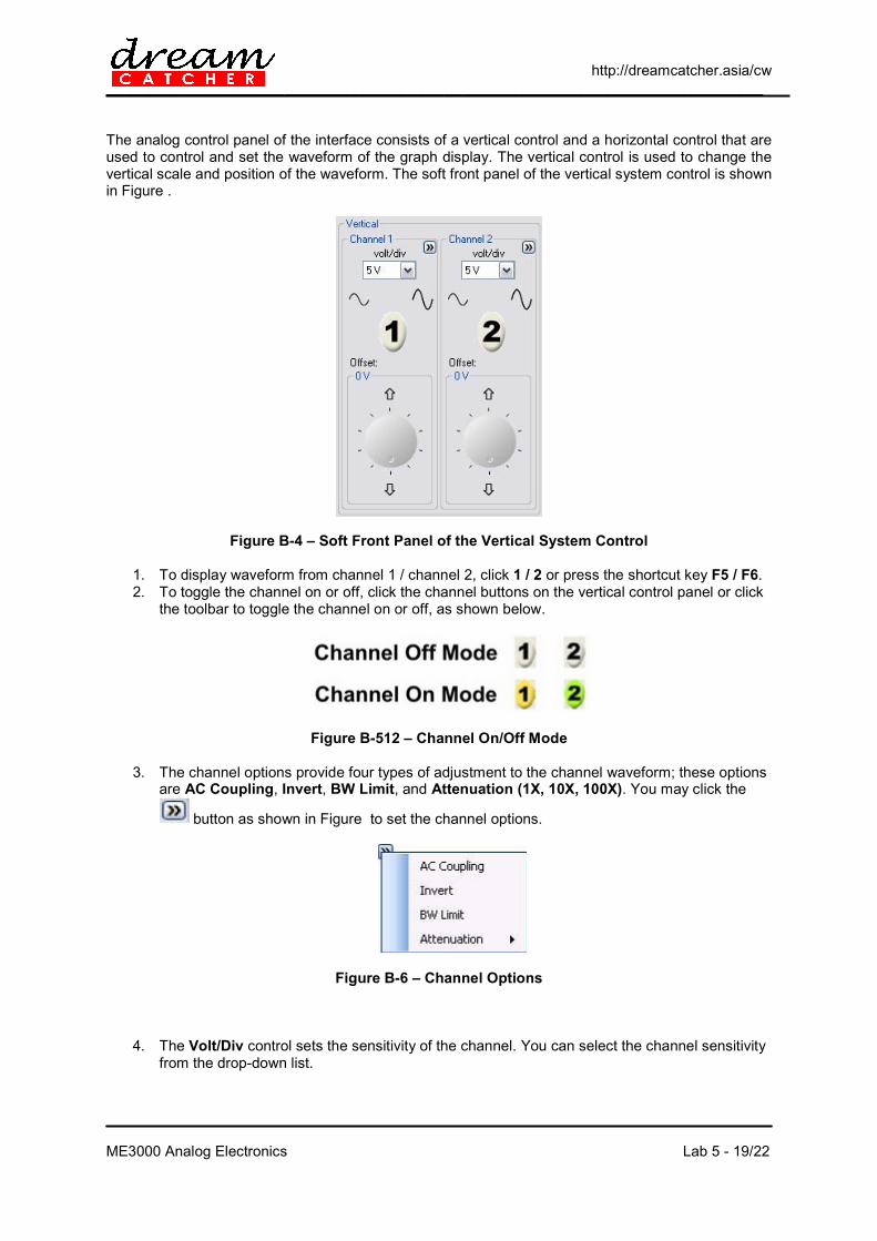
3. The channel options provide four types of adjustment to the channel waveform; these options are AC Coupling, Invert, BW Limit, and Attenuation (1X, 10X, 100X). You may click the

button as shown in Figure to set the channel options.

Figure B-6 – Channel Options 4. The Volt/Div control sets the sensitivity of the channel. You can select the channel sensitivity

from the drop-down list.



5. You can also use the button or button to increase or decrease the sensitivity of both channel 1 and channel 2.

6. You can also configure the offset of the oscilloscope by using the offset control as shown in Figure . The offset is used to configure the position of the ground relative to the center of the display.

Figure B-7 – Soft Front Panel of the Offset Control

7. The oscilloscope shows the time per division in the scale readout. As all waveforms use the same time base, the oscilloscope only displays one value for all channels.

8. The horizontal controls allow you to adjust the horizontal scale and position of waveforms. The horizontal center of the screen is the time reference for waveforms. Changing the horizontal scale causes the waveform to expand or contract in the center of the screen. It provides functions of Time Base, Delay, and Mode for the horizontal scale adjustment. This is shown in Figure B-813.

Figure B-813 – Soft Front Panel of the Horizontal System Controls

9. Time base allows you to control how often the values are digitized. The soft front panel of the time-base control is shown in Figure B-914.

Figure B-914 – Soft Front Panel of the Time-Base Control

10. You may click or to increase or decrease the horizontal sweep speed.

11. Select the time base from the drop-down list to adjust the horizontal sweep speed. 12. Delay setting allows you to set the specific location of the trigger event with respect to the

time reference position. When the delay time knob is turned, the trigger point will move to the



left or right of the waveform graph display. You may adjust the delay time to change the trigger point. This is shown in Figure .

Figure B-10 – Soft Front Panel of the Delay Control and Trigger Point

13. You may click or to increase or decrease the delay time. 14. The oscilloscope offers three types of horizontal mode functions, which are Main Mode, Roll

Mode, and XY Mode. You may select the horizontal mode by clicking the drop-down list under Mode.

Measurement and Cursor Controls

1. The Measurements & Cursors button is located on the toolbar of the soft front panel.

2. Click to activate the automated measurement and cursor system. This will display the window as shown below:

Figure B-11 – Soft Front Panel of the Measurement and Cursor Controls

3. The oscilloscope provides three types of settings for marker property, which are Auto,

Manual, and Off. 4. Auto marker automatically places the cursors on the graph based on the selected

measurements.



5. Manual marker allows the cursors to be placed manually on the graph for customized measurements. This will enable the Cursors panel.

6. Off will disable the graph markers from the graph display. 7. If the Manual marker is selected, the Cursors control will be enabled. This is shown in Figure

.

Figure B-12 – Cursor Controls

8. X Cursors places two cursors on the X-Axis of the waveforms to measure the time difference between the two cursors (X2 minus X1). Delta X denotes the time difference.

9. Y Cursors places two cursors on the Y-Axis of the waveforms to measure the voltage difference between the two cursors (Y2 minus Y1). Delta Y denotes the voltage difference.

AutoScale and Run/Stop

1. AutoScale automatically configures the oscilloscope to best display the input signal by analyzing any waveforms connected to the channel and external trigger inputs. If AutoScale fails, your current setup will remain unchanged.

2. Click on the oscilloscope toolbar or via the Tools menu once you have obtained a running signal.

3. The auto scaling may take awhile for the application to analyze and adjust the waveform. 4. Once the auto scaling has completed, you will see a best fit waveform displayed on your

graph. 5. Use the Run/Stop button to manually start or stop the oscilloscope acquisition system for

acquiring waveform data.

6. You may click or to start or stop acquiring the waveform.

ME3000 Analog Electronics Lab 5 Practical Op-Amp Circuits

Documents

Transcript of ME3000 Analog Electronics Lab 5 Practical Op-Amp Circuits