Mathematics for engineering students, Analytical geometry ...
374
-
Upload
khangminh22 -
Category
Documents
-
view
1 -
download
0
Transcript of Mathematics for engineering students, Analytical geometry ...


Class_AAi4__
Book l_KJl_
CopghtN°__\aQ,
l
COPYRIGHT DEPOSIT.

The D. Van Nostrand Companyintend this book to be sold to the Public
at the advertised price, and supply it to
the Trade on terms which will not allow
of discount.


Carneafe ttecbnfcal Scbools ttext JSoofts
MATHEMATICSFOR
ENGINEERING STUDENTS
BY
S. S. KELLER and W. F. KNOXCARNEGIE TECHNICAL SCHOOLS
ANALYTICAL GEOMETRY AND CALCULUS
NEW YORK:
D. VAN NOSTRAND COMPANY23 MURRAY AND 27 WARREN STS.
I907

jUBRARY of CONGRESSTwo Copies Received
NOV 21 1907opyr'urht Entry
GLASS C*.XXCi NOi
/ 92&o3copy e.
Copyright, 1907, by
D. VAN NOSTRAND COMPANY.
Stanbope press
F. H. OILSON COMPANYBOSTON, U. S. A.

PREFACE.
Much that is ordinarily included in treatises on Analy-
tics and Calculus, has been omitted from this book, not
because it was regarded as worthless,: but because it
was considered quite unnecessary for the student of
engineering.
In Analytics the attention is called, at the beginning, to
the fact that the commonest experiences of life lie at the
basis of the subject, and at all stages of its development
the student is encouraged to consider the matters pre-
sented in the most informal and untechnical way.
In the Calculus a somewhat radical departure has been
attempted, in order to avoid the difficult and somewhat
mystifying subject of limits, or rather to approach similar
ends by less technical paths.
The average engineer will assert that he never uses the
Calculus in his practical experience, and it is the author's
ambition to make it effective as a tool, believing, as they
do, that it is not used because it has never been presented
in sufficiently simple and familiar terms.
S. S. K.
Carfiegie Technical Schools,
Pittsburg, Pa.


ANALYTICAL GEOMETRY.
CHAPTER I.
Article i. Analytical Geometry may be called the
science of relative position. The principles upon which the
results of Analytical Geometry are based, are drawn directly
from daily experience.
When we measure or estimate distance, it is always from
some definite starting point previously fixed.
i Si
Fig. i.
For instance, most of our cities are laid out with refer-
ence to two streets intersecting each other at right angles.

2 Analytical Geometry.
If it is desired to indicate the position of a certain building
in such city, it is customary to say, " it is located so manysquares north or south and so many squares east or west."
Let the double lines in Fig. i represent the reference
streets, and the lines parallel to them, the streets running
in the same direction, then the point A would be accu-
rately located, by saying it lies two squares east and three
squares north.
The government lays out the public lands upon the
same system; locating two lines intersecting at right angles
(called the Principal Meridian and the Base Line, respec-
tively) as reference lines. Then lines run parallel to these
at intervals of six miles, divide the territory into squares
each containing 36 square miles. In this region any piece of
land is easily located by indicating its distances by squares
from these two reference lines. In short, since our knowl-
edge is practically all relative, the principles of Analytical
Geometry lie at the foundation of all our accurate thinking.
Art. 2. The two intersecting lines are called Co-ordinate
Axes, and their point of intersection is called the Origin.
In the system most frequently used, the axes meet at
right angles, and hence it is known as the rectangular
system. In comparatively rare instances it is desirable to
have the lines oblique to each other, when the system is
known as oblique.
Art. 3. The vertical axis is called the axis of ordinates
and the horizontal axis, the axis of abscissas.
Art. 4. Distances are always measured from either axis,
parallel to the other; hence when the system is rectangular,
the distances mean always perpendicular distances. The
distance of any point from the axis of ordinates (right or
left), measured parallel to the axis of abscissas, is called
the abscissa of the point, usually represented by x. The

Analytical Geometry. 3
distance from the axis of abscissas (up or down), measured
parallel to the axis of ordinates, is called the ordinate of the
point, usually represented by y.
Art. 5. Clearly if we would be accurate we must dis-
tinguish between distance to the right and to the left, and
upward and downward. For instance, suppose it is required
to locate a point whose abscissa, x = 5 and ordinate, y = 2
;
it is plain that the point might be located in any one of
four positions: to the right 5 units and up 2 units; to the
left 5 and up 2; to the right 5 and down 2; or to the left
5 and down 2.
If, however, it is agreed that abscissas measured to the
right from .the axis of ordinates shall be called plus, and
those to the left, minus; and that ordinates measured up-
ward from the axis of abscissas shall be called plus, and
those downward, minus, there need be no confusion.
* = +5i3/= + 2 will then indicate definitely the first
position referred to above; x = —5, ^ = +2, the second;
x = + 5> y = — 2 the third, and x = —5, y= — 2, the fourth.
Art. 6. The intersecting axes evidently divide the sur-
Fig. 2.
rounding space into four parts called quadrants, numbered
I, 2, 3,4, from the axis of abscissas (usually called the X-axis)

Analytical Geometry.
around to the left back to the X-axis again. Thus XOY is
quadrant i; X'OY is quadrant 2; X'OY' is quadrant 3
(Fig. 2).
Art. 7. To locate a point let it be required to locate the
point x = —5, y = + 3 J [written for brevity (—5, 3^)].
Let the axes be XOX' and YOX' as in Fig. 3.
By what has been said the point is located 5 units to the
left of the Y-axis and 3^ units above the X-axis.
Since, it is a matter of relative position only, any con-
venient unit may be used, if it is maintained to the end of
the problem; say in this case \"-
Then measuring 5 units or f" to the left on the X-axis,
and from there 3 J units or ^2- = y7/' upward parallel to
8
the Y-axis we locate the point P as in Fig. 3.
The point (0,2) is clearly on the Y-axis, 2 units above the
Y
,P(-5,3£)
-5. (0,2)
(li.O)
Y'
Fig. 3.
origin, because the abscissa is zero, and since the abscissa
is the distance from the Y-axis, this point being at no dis-
tance, must be on the Y-axis. Likewise, the point (ij,
o) is on the X-axis i\ units to the right.
Locate the following points:
1. (3,2). (- 2>-1)1 (ii-3i)i (°» r )> (- 2
> 0)1
(o, o) (- 6, 5), (f, - f).

Analytical Geometry.5
2. The points (o, 2 J), ( - 3, -2) and (1$, - 2 J)
are the vertices of a triangle. Construct it.
3. Construct the quadrilateral whose vertices are
(- 1, 2), (3, 5). (2
,~ 3) and (- 2, - 2).
4. An equilateral triangle has its vertex at the point
(o, 4) and its base coincides with the X-axis. Find the co-
ordinates of its other vertices and the length of its sides.
5. The two extremities of a line are at the points (—3, 4)
and (5, 4). What is its position relative to the axes?
6. How far is the point (— 3, 4) from the origin?
7. The extremities of a line are at the points (3, 5) and
(— 2, 1), respectively. Construct it.
8. The extremities of a line are at the points (— 3, —5)and (3, 5). Show that it is bisected at the origin.
9. By similar triangles find the point midway between
(- 2, 5) and (4, - 1).
10. A line crosses the axes at the points (15, o) and
(o, 8). What is its length between the axes.
THE POLAR SYSTEM.
Art. 8. Since two dimensions are sufficient to locate a
point in a plane, it is readily possible to use an angle and
a distance, instead of two distances.
By convention the angle is estimated from a fixed line
around counter-clockwise; the revolving line, called the
radius vector, is pivoted at the left end of the fixed line,
which is called the initial line, and the pivotal point is
known as the pole.
The angle is estimated either in degrees, minutes, and
seconds or in radians.
Art. 9. A radian is defined as the central angle which
is measured by an arc equal in length to the radius.

6 Analytical Geometry.
Since the circumference of a circle is equal to 27zr (where
r is the radius and tz = 3.1416) and also contains 360 ,
27ZT = 360°
?6o° 180and — ^ 1 radian.
2TZ TZ
Hence the number of radians in any angle
180 180
That is, the number of radians in an angle is the same
fraction of tz, that the angle is of 180 .
For example
6o° = tz radians = — tz radians.180 3
22 2—— tz radians =180
tz radians.
225^ —2- tz radians = -5 tz radians, etc.180 4
Art. 10. It is agreed for the sake of uniformity that
an angle described by the radius vector from its original
position of coincidence with the initial line, counter-clock-
wise, shall be positive; in the contrary direction, nega-
tive.
That when the distance to the point is measured
along the radius vector forward, it shall be positive;
when measured on the radius vector produced back-
ward through the pole it shall be negative. For example,
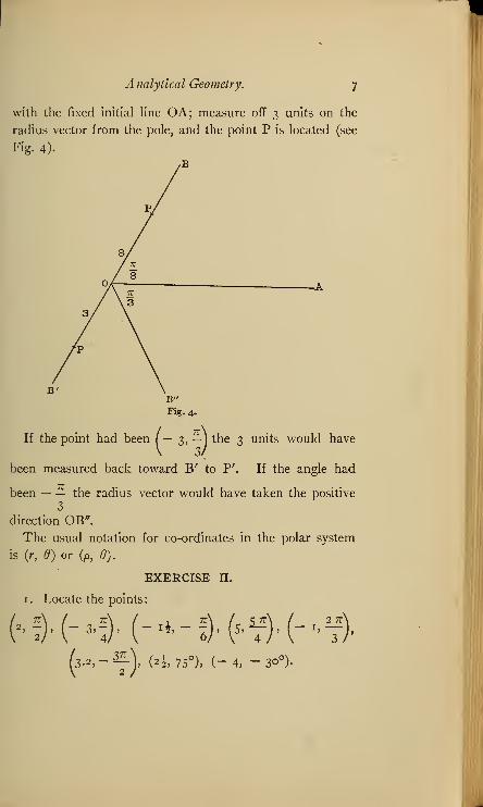
the point (3, -j would be located thus (Fig. 4) :
Draw an indefinite line OB (representing the radius
vector) making an angle of — radians = — of 180 = 6o°3 3
Analytical Geometry. 7
with the fixed initial line OA; measure off 3 units on the
radius vector from the pole, and the point P is located (see
Fig. 4).
If the point had been(— 3, — j
the 3 units would have
been measured back toward B' to P'. If the angle had
been the radius vector would have taken the positive
3
direction OB".
The usual notation for co-ordinates in the polar system
is (r, 0) or (/>, 0).
EXERCISE II.
1. Locate the points:
K)-M)< (-*-!)•(s'V"M--7).
(3 - 2 '
_2f)'
(2i '750)
'
(-4> _3°0) -
8 Analytical Geometry.
2. Express the following radians in degrees:
2 4 8 8 16
3. Express in radians
:
35 , 40 , 45°, 6 7 i°, 75°, 150°, 120°, -225,- 195°.
4. Construct the triangle whose vertices are,
(3h
l)•(''.-$' and (" 5'4)'
5. Construct the quadrilateral whose vertices are,
(5,f), (3, f), (
s,-a)
r
(3,_^.
What kind of quadrilateral is it ?
6. The extremities of a line are the points (6, —J and
(—6, — —V How is the line situated with reference to
8/
the initial line ?
7. Construct the equilateral triangle whose base coin-
cides with the initial line and whose vertex is the point
8. The co-ordinates of a point are (5, —J.Give three
other ways of denoting the same point.
AREA OF A TRIANGLE.
Art. 11. The system of rectangular co-ordinates affords a
ready method of expressing the area of any triangle when
the co-ordinates of its vertices are known.

Analytical Geometry. 9
Let ABC (Fig. 5) be any triangle. Draw the perpen-
diculars AD, BE and CF from the vertices to the ^-axis.
Then the co-ordinates of A = (OD, AD); of
Fig. 5.
B = (OE, BE); of C = (OF, CF); say,(- *', /), (*", /')
and (%"', y"').
Now the figure ABCFD is made up of the trapezoids
ABED, and BCFE; and if from ABCFD we take ACFDthe triangle ABC remains, that is,
ABED + BCFE - ACFD = ABC. . . (a)
By geometry, area ABED = \ (AD + BE) DE.
But AD = /, BE = /', and DE = DO + OE= -x'
+ x".
.-. area ABED = J (y' + y") (x" - x f
).
Also area BCFE = \ (BE + CF) EF.
But BE = y", CF =f and EF = OF- OE = x"'-x".
.'. area BCFE =!(/ + /") (*"' - *")
Again; area ACFD = J (AD + CF) DF.
But AD - /, CF=/"andDF=DO +OF = - xf+ x"''.
.-. area ACFD = (/ + /") (x"f - a/).

10 Analytical Geometry.
Substituting in (a):
Area ABC = J (/ + y") (x" - x') + i (/' + /")
(V" - x") - J (/ + y"f
) {x"f - x') =
i tyty _ xy + ^/y _ ^y// _j_ xy _,<;//'^The symmetrical arrangement of the accents in this
expression is manifest.
Example: Find the area of the triangle whose vertices are
(2, 3), (- 1, 4) and (3, - 6). Let (2, 3) be (V, /);
(- 1, 4) be O", /'), and (3, - 6) be (*»', /"). Then
area= i [(- 1 X 3>-(2X 4) + (3 X 4)-(-iX-6)+ (2 X - 6) - (3 X 3)]= H-3-6 +12-6-12-9]= — 12.
The minus sign has no significance except to indicate
the relation of the trapezoids.
(r'<e>) B(r
//(0"j
c {r"\0[")
Fig. 6.
Po/ar System : A reference to Fig. 6 will show that a
similar process will give the area of ABC, when its vertices
are given in polar co-ordinates.
For area ABC = ABO + OBC - OAC.
Area ABO = J AO X OB sin AOB.AO = /, OB = r» and AOB = (0' - Q").
A similar treatment of OBC and AOC will give the areas
of all the triangles.

CHAPTER II.
LOCI.
Art. 12. Whenever the relation between the abscissa
and ordinate of every point on a line is the same, the expres-
sion of this relation in the form of an equation is said to
give the equation of the line. For example, if the ordinate
is always 4 times the abscissa for every point on a line,
y = 4 x is called the equation of the line.
Again, if 3 times the abscissa is equal to 5 times the
ordinate plus 2, for every point on a line, then 3 x = 5 y + 2
is the line's equation.
Art. 13. Clearly since an equation represents the rela-
tion between the abscissa x and the ordinate y for every
point on a line, if either co-ordinate is known for any point
on the line, the other one may be found by substituting
the known one in the equation and .solving it for the
unknown.
For example, let 2 y = 7 x — 1 be the equation for a
line, and a point is known to have the abscissa, x = 2.
To find its ordinate, substitute x = 2 in the equation;
2 y = 7 (2) — 1 = 14 — 1 = iy,y*= 6£. Therefore the
ordinate corresponding to the abscissa, x = 2, is 6J.
Further, if the equation is given, the whole line may be
reproduced by locating its points. If x for example be
given a series of values from o to 10 inclusive, by substi-
tuting these values in the equation, the corresponding
values of y are found, and 11 points are thus located on
the desired line. If more points are needed the range of

12 Analytical Geometry.
values for x may be indefinitely extended, and if these
points are joined, we have the line. For example, let the
equation of a line be x2 + y2 = 9, to reproduce the curve
represented. For convenience in calculating solve for y;
y = ±\/g — x2.
Then give x a series of values to locate points on this line.
Iix = y = ±\/VZ x2 = ±3-Iix = 1 y'= ± v9 - 1 = ±Vs == ± 2.83.
Iix = 2 y = ±V9 - 4 = ±^J-= ± 2.24.
Iix = 3 y = ±Vg -9 = ±Vo == 0.
Iix = 4 y = ± v9 - 16 = ±V- y= an in
The last value for v shows that the point whose abscissa
is 4 is not on the curve at all; and since any larger values
of x would continue to give imaginary values for y, the
curve does not extend beyond x = 3.
Since we have given x only positive values so far, all
our points so determined lie to the right of the Y-axis.
To make the examination complete, let x take a series of
negative value thus
:
If x = - 1 y=±\/g-i=±Vs=± 2.83.
If x = — 2 y = ± V9 - 4 = ± V5 = ± 2.24.
If x = - 3 y = ± Vo -9=0= Vo.
The similarity of these results shows that the curve is
symmetrical with respect to the axes, that is, it is alike
on both sides of the axes.
If now these points are located with respect to the axes
XXr and YYr and are joined, the result is an approxima-
tion to the curve; it is only an approximation because the
points are few and not close enough together.
The result is shown in Fig. 7, using i inch as a unit for

Analytical Geometry. J3
scale. The points are (o, + 3), (o, — 3) [being A and
A' in the figure], (1, VS), (1, - V8) [being B and B'],
(2, V5), 0». - Vj) [being C and C'], (3, o) [G],
(- i, V8),_(- i, - V8) [D and D'] (- 2,V5~)
(- 2. - V5 ) [E and E'] and (- 3, o) [F].
Fig. 7.
Clearly if more points are needed to trace the curve
accurately through them (as is the case here), it is neces-
sary to take more values of x between —3 and +3, for
example
:
x= o y= ± V9 = ± 3.
X = .2 y = ± V9 - .04 = ± V8.96 = ± 2.99 .
x = .4 y = ± V9 - .16= ± V8.84= ± 2.97.
x = .6 y = ± v9- .36 = ± V8.64 = ± 2.94.
#= .8 y = ± v9- .64 = ± V8.36 = ± 2.89.
# = 1 y = ± v9- 1 = ± V8 = ± 2.83, etc.
Making a similar table for the corresponding negative
values of x, the result is three times as many points on the
14 Analytical Geometry.
curve as before, and as they are closer together the curve
is much more readily drawn through them, and it will be
much more accurate.
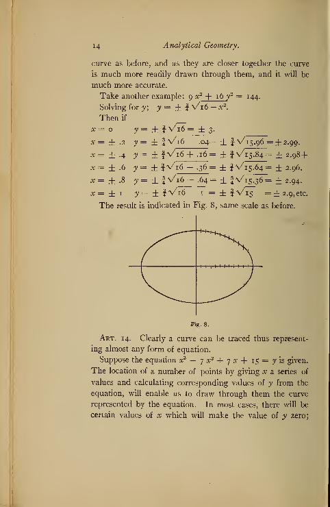
Take another example: 9 x2-f 16 y
2 = 144.
Solving for y; y = ± f \/i6 — x2.
Then if _x = o y = ± j V16 = ± 3.
x= ± .2 y = ± i Vi 6 — .04= ± f ^15.96 = ± 2.99.
x = ± .4 y = ± IV16+ .16 = ± }V/i 5 .84 = ± 2.98+
x = ± .6 y = ± IV16 - .36 = ± fv/i5.64= ± 2.96.
x = ± .8 v = ± IV16 - .64 = ± {^15.36 = ± 2.94.
# = -j- 1 y =±l\/i6 c = ± f V15 = ±2.9, etc.
The result is indicated in Fig. 8, same scale as before.
Fig. 8.
Art. 14. Clearly a curve can be traced thus represent-
ing almost any form of equation.
Suppose the equation 7 x2 + 7 x + 15 = y is given.
The location of a number of points by giving x a series of
values and calculating corresponding values of y from the
equation, will enable us to draw through them the curve
represented by the equation. In most cases, there will be
certain values of x which will make the value of y zero;

Analytical Geometry. 15
such values of x will be roots of the equation x3 — 7 x2
+ 7 x + 15= o, that is, these values of x indentically
satisfy this equation.
But if y is zero for a point, the point must be on the
X-axis, for by definition the value of y is the distance
from the X-axis to the point, hence the curve must cross
the X-axis at those points where y is zero. If then none
of the values given to x make y exactly zero, but do make
y change from a positive value for one value of x to a
negative value for the next, or vice versa, it must pass
through zero to change from one sign to the other, and
hence the curve must cross the X-axis.
As an illustration, takt he equation x* — 5 x2 + x
+ 11 = y. As before make a table of values of x and y,
and locate the points as follows:
If X = y = 11.
x= .5 y = iQ-375-
X = I y = 8.
x = 1.5 y = 4.625.
X = 2 y = 1.
x= 2.5 y = - 2.125.
x= 3 y = - 4-
x= 3-5 y = - 3-875.
x = 4 y = — 1.
a?= 4.5 y = 5-375-
#= — 1 y = 4-
x= - 1.5 y= - 5- I2 5-
The curve connecting these points crosses the X-axis at
three points; one between 2 and 2.5; one between 4 and
4.5, and one between — 1, and — 1.5. Hence the three
roots of the equation x3 — 5 x 2 + x + 11= o are be-
tween 2 and 2.5; between 4 and 4.5, and between — 1 and
~ i-5-

1
6
Analytical Geometry.
If the values of x in the above table had been taken
closer together, the points of crossing would have been
more accurately known.
INTERSECTIONS.
Art. 15. The point (or points) in which two lines
intersect, being common to both lines, its co-ordinates
must satisfy both equations, that is, the equations of the
two lines are simultaneous for this point (or these points)
and hence if the equations be solved as simultaneous by
any of the processes explained in algebra, the resulting
values of x and y will be the co-ordinates of the point (or
points) of intersection. For example :
To find the points of intersection of the circle x2 + y2 =
24 and the parabola y2 = 10 x. By substitution of the
value of y2 from the parabola equation in the circle equa-
tion,
x2 + 10 x = 24 x2 + 10 x + 25 = 49.
x + 5 = ± 7 x = 2, or — 12
y= ±V2o, or, ±\/— i2,
o.
The second pair of values for y being imaginary shows
there are but two real points of intersection, (2, + V20)
and (2, — v 20). Verify by construction.
EXERCISE III.
Loci with Rectangular Co-ordinates.
1. Express the equation of the line for every point of
which the ordinate is f of its abscissa.
2. Express the equation of the line for every point of
which f the bascissa equals f of the ordinate + i.

Analytical Geometry. 17
3. Express the equation of the line, for every point of
which 9 times the square of its abscissa plus 16 times the
square of its ordinate equals 144.
4. Construct the locus of x2 = 8 y.
5. Construct the locus of (x — 2)2 + y
2 = 36.
6. Construct the locus of xy =• 16.
7. Construct the locus of x2 + 4 y2 = 4.
8. Construct the locus of 25 x2 — 36 y2 = 900.
9. Construct the locus of 3 x — 2 y = 5.
10. Construct the locus of J x — f = —- y.
11. Construct the locus of x = 7.
12. Construct the locus of y = — 5.
Find the points of intersection of:
13. (x — i)2 + (j — 2)
2 = 16 and 2 y — x ^= 3.
14. 2 x - 3 y = 7 and J rv + y = f
.
15. x2 + y2 = 9 and x2 = 8 y.
16. #2 + y2 == 16 and 2 x2 + 3 y
2 = 6.
17. x2 + v2 = 25 and 4 y = 3 ae + 25.
18. Find the vertices of the trangle whose sides are
x — y = 1.
2i + y= 5 and 3 y — 2 x = 7.
Art. 16. If the equation of a locus is expressed in polar
co-ordinates, the method of procedure is exactly similar
to the cases already discussed.
The presence of trigonometric functions introduces no
difficulties. For example: To construct the locus of
r = 4(1 — cos 6). Give d a series of values, and com-
puting r for each, as follows:
If 6 = o, r = o since cos 0=1.r = 4 (1 — .996) = .016.
r = 4 (1 - .98) = .08.
r= 4 (1 - .97) = .12.
If = 5°,
If (9 = ro°
If = i5°,

i8 Analytical Geometry.
If 6 = 20°, r = 4 (i - -94) = -24-
if e = 3 o°, r = 4 (i - .87) = .52.
if e = 4o°, r= 4 (1 - .77) = -92.
if e = 50 ,r = 4 (1 — ,64) = 1.44.
If d = 6o°, r = 4 (1 - .5 ) =2. ,etc
Fig. 9.
Completing the table to 6
curve as in Fig. 9.
360 and plotting we get a
TRANSCENDENTAL LOCI.
Art. 17. Certain curves have what are known as trans-
cendental equations, that is, equations which cannot be
solved alone by the algebraic processes of addition, sub-
traction, multiplication, and division.
I — COS d
16
Analytical Geometry. 19
For example, y — log x.
The loci of such equations are found in the usual way,
by giving to one of the co-ordinates a series of values and
finding corresponding values for the other from tables.
EXERCISE IV.
1. Find the locus of r2 = 9 cos 2 6.
2. Find the locus of r =10 cos 6.
3. Find the locus of r =
4. Find the locus of r =5 + 3 cos d
5. Construct v = sin x.
6. Construct x = log y.
MISCELLANEOUS CURVES.
Art. 18. Curve-plotting is very widely applied in all
modern scientific research, to represent graphically the
results of observation. This method of presentation has
the immense advantage of showing at a glance the com-
plete result of an investigation.
For example, if a test is made of the speed of an engine
relative to its steam pressure, the pressures being repre-
sented as abscissas (by x) and the corresponding speeds as
ordinates (by y), a smooth curve drawn through the points
determined by these co-ordinates will reveal at once the
behavior of the engine. Especially does this method aid
in comparisons of different series of observations of the
same kind.

20 Analytical Geometry.
Suppose, for example, it is desired to represent thus
graphically the course of a case of fever.
The observations are as follows: —
7 a.m. temperature ioo
8 A.M.a
ioof
9 A.M. a IOlf
IO A.M.a I02§
II A.M.:( IO3
12 M.It I03*
I P.M.a IO3
2 P.M.it
I02f
3 P.M.a IOI
Regarding the time of taking observations as abscissas
and the temperatures as ordinates, using any desired scale,
the result may be represented as follows, in Fig. 10.
I
1
103° <^•>
102°
101°
100°
J<*" s
v
>f \sr
IM : 1 INI•
7 8 9 10 II 12 I 2 3 4Fig. 10.
Fig. 10.
The figure shows at a glance that the maximum was at
noon.

Analytical Geometry. 21
Again; in the test of an I-beam the following observations
were taken.
TEST OF CAST-IRON.
Stress Pounds. Unit Elongation.
6,95° 4-97
12,940 11.44
6,110 6.06
1. 1 2 (permanent set)
4,640 4.16
8,780 7-63
12,300 10.78
15,420 i5- 2
11,900 12.38
8,37o 9.42
4,960 6.66
IJ 3 2.41
Plot the curve.

>1
CHAPTER III.
THE STRAIGHT LINE. to
Art. 19. Since two points determine a straight line
and two points imply two conditions, there will be in the
equation to a straight line, two fixed quantities (called
constants), which must be predetermined for every straight
Fig. 11.
line. These constants may be furnished by two fixed points,
or by a point and an angle, evidently.
To determine the equation of a given straight line, then,
it is necessary to express the relation between the co-ordi-
nates of any (that is, every) point on the line, in terms of
the two given constants.

Analytical Geometry. 23
Suppose first we take a point on the y-axis, through
which the line must pass, and determine its posi-
tion by giving its distance from the origin measured on
this axis.
Call this distance, b; and say the line makes an angle a
with the #-axis; the angle to be estimated as in trigo-
nometry, positively, that is, counter-clockwise, from the
#-axis.*
It is required, then, to determine the relation between
the co-ordinates of any point P, selected at random, on the
line AB (Fig. it), using b and any convenient function of a.
Drawing thej_ PR, OR = abscissa of P = x,
PR = ordinate of P"= y, OS = b.
Z BTR = a.
The character of the figure would suggest the use of the
similar triangles TSO and TPR, but a simple observation
shows that only the sides b and y are known; on the other
hand we know the angle a, and a line through S 11 to the
x-axis, from S to PR, will be equal in length to OR and
will also make the angle a with AB (alternate angles of
parallel lines).
Call this line SN. Then in the triangle SPN, Z PSN= a SN = OR = *, and PN = PR - NR = PR - SO= y — b. PN and SN being respectively opposite and
adjacent to a in the right triangle SPN, we have,
PN y - btan a = —- = -
SN x
* The conventions as to positive and negative direction for lines,
and positive and negative revolution for angles, is maintained in
Analytical Geometry, as indeed is necessary in order to accomplish
consistent results.

24 Analytical Geometry.
Let tan a be represented by m;
then m = 2_Z_?
x
mx = y — b
y = mx + b
which expresses the relation between the co-ordinates of
of any point, P, and hence of every point on the line in
terms of the known constants m and b. .'. y= mx + b
y
(A)
Fig. 12.
is the equation of AB. Had the line crossed the first quad-
rant the construction would have been as in Fig. 12 and
we would have
NPtanPSN= —>SN
or tan (180 — a) =
— tan a =
— m =
x
b — y
x
b — yx
y = mx + b as before.

Analytical Geometry. 25
m is called the slope of the line and b its ^-intercept. The
equation is called the slope equation of a line.
If m = o in the equation to a straight line, then it takes
the form y = b, which is plainly (since if m =0, a = o)
a line||
to the #-axis. If b = o, the equation becomes
v = ;;lt, which is the equation of a line through the origin,
making an angle whose tangent is m with the x-axis, etc.
Since a may be either acute or obtuse depending upon
whether the line crosses the 2d or 4th, or the 1st or 3d
quadrants; and b may be either plus or minus depending
upon the position of the point of intersection with ;y-axis,
above or below the origin, the form,
y = — mx + b represents a line crossing quad. I,
y = mx + b represents a line across quad. II,
y = — mx — b represents a line across quad. Ill,
y = mx — b represents a line across quad. IV.
Art. 20. If the line be determined by two points (xf
,y')
and (x", y"); to -find its equation.
Let AB (Fig. 13) be the line, P and Q the points (xf
, yf
)
and (x", /'), respectively.
Take any point P r whose co-ordinates are (x, y). Draw
QR, P'S and PT J_ to the x-axis, also PL J_ to QR, as
it is clearly here a case for similar triangles.
Then in the similar triangles PLQ and PKP',
P'K:KP::QL:LP, or g- = -gt.
But FK = PrS - KS = P'S - PT = y - /
KP = HP - HK = yf - x,
QL = QR - LR = QR - PT = f - /,

26 Analytical Geometry.
and LP = LH + HP = - x" + x'.
y — y' y" — yr
X* X" + x'
or symmetrically, y — y _ y" — yf
*-V »/v vV »/v
(changing sign of both) which gives an equation between
x, y, x', /, x" , and /' as required.
B\.#",y")V' y
\L H K\P(z',*/')
#-It £3 T
Fig. 13-
The same result might be reached by a purely analytical
method having the slope equation of a line given.
Let the slope equation of the line AB be y = mx -f b.
Since it must pass through the points P, P' and Q, the
co-ordinates of these points must satisfy the equation of

A nalytical Geometry. 2 7
the line, since the equation must give the relation between
the co-ordinates of every point on the line.
Hence, substituting these co-ordinates successively in
the equation y = mx + b, we know that the three following
equations must be true, if P, P' and Q are on the line:
y = mx' -f b (1)
y = mx + b (2)
y= mx" + b (3)
But since the line is to be determined only by the two
points P and Q, neither m nor b are known, and hence
must be eliminated.
Subtracting (1) from (2) and (1) from (3), we get
y — yf = m (x — xf
) . . . (4)
and y — y' = m (x" — xf
) ... (5)
divide (4) by (5);y-=^-
f= "LJZJL
,
y — y x" — x
y-s = y-y .... . . (B)x — xf x" — xr
For example: Find the equation of the line through
(- 2,3) and (-4, - 6).
Let (V, /) be (- 2, 3) and (V', /) be (4, - 6)*.
Substituting in (B),
* = « = — ^ , or 2 3/ t 3 x = o.x + 2 4 + 2 2
* Since (B) is perfectly symmetrical it is a matter of indifference
which point be called (xf
,y') and which, (x", y"). The results are
the same. It is to be observed that x and y with accent marks
usually mean definite points, while general co-ordinates are repre-
sented by unaccented x and y. So that substitutions are always
made for the accented variables, when definite points are involved.
28 Analytical Geometry.
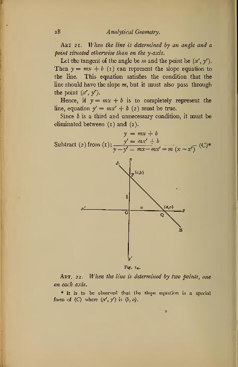
Art 21. When the line is determined by an angle and a
point situated otherwise than on the y-axis.
Let the tangent of the angle be m and the point be (x', y').
Then y = mx + b (i) can represent the slope equation to
the line. This equation satisfies the condition that the
line should have the slope m, but it must also pass through
the point (V, /).
Hence, if y = mx + b is to completely represent the
line, equation y' = mx' + b (2) must be true.
Since b is a third and unnecessary condition, it must be
eliminated between (1) and (2).
y = mx + b
V — mx/ + bSubtract (2) from (1);
y-yf mx- mxf =m (x —x')(C)'
y
Fig. 14.
Art. 22. When the line is determined by two points, one
on each axis.
* It is to be observed that the slope equation is a special
form of (C) where (xf
,y') is (b, o).
Analytical Geometry. 29
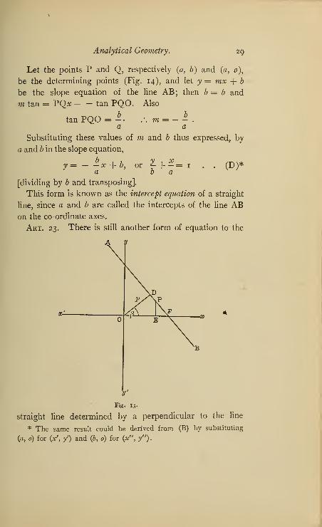
Let the points P and Q, respectively (0, b) and (a, 0),
be the determining points (Fig. 14), and let y = mx + b
be the slope equation of the line AB ; then b — b and
m tan = PQx = - tan PQO. Also
tanPQO = -• .-. m=-- .
a a
Substituting these values of m and b thus expressed, by
a and b in the slope equation,
6
y = - -x + b, or f + -=i . . (D)*a b a
[dividing by b and transposing].
This form is known as the intercept equation of a straight
line, since a and & are called the intercepts of the line ABon the co-ordinate axes.
Art. 23. There is still another form of equation to the
y
straight line determined by a perpendicular to the line
* The same result could be derived from (B) by substituting
(a, o) for (*', /) and (6, o) for (x", y").

30 Analytical Geometry.
from the origin, and the angle which this perpendicular
makes with the #-axis.
Let OD be a J_ to the line AB from the origin, and /?
the angle it makes with the #-axis. Let P (x, y) be any
point on the line.
Drawing the ordinate (PE) of P, we have two similar
right triangles ODF (F being the point where AB crosses
the x-axis) and PEF.
Then PE : OD : : EF : DF [homologous sides].
Call OD, p, and OF, a, then above proportion becomes
y : p : : (a — x) : DF.
But in the right triangle ODF,
, and DF = p tanp sin /?
cos /? cos /?
I p \ p sin B
\cos p ) cos p
7T~= P \
— « — x) [extremes*and means]cos p \cos p )
or 2-—5J- = —P—^ — x [dividing by p]cos p cos p
that is, y sinft + x cos /? = p (E)
This is called the normal equation, p being known as a
normal.
The line AB is plainly a tangent to a circle with O as a
centre and p as a radius, hence we are practically deter-
mining the line AB as a tangent to a given circle, the posi-
tion of the radius being fixed by the angle /?.
Exercise: By determining the values of a and b from the
intercept equation, \- ~= i, in terms of ^ and /?, derive
the normal equation from the intercept equation.

Analytical Geometry. 3i
Art. 24. Each equation has its characteristic form.
For instance, the slope equation y = mx + b, has the
form of a first degree equation solved for y, hence if any
first degree equation be solved for y, it may be compared
directly with this slope equation. For example, given the
equation 2 y — 3 x = 8. Solving for y, y = § x + 4; com-
paring this with the typical form; m = § and b = 4.
Hence the locus of 2 v — 3 x = 8 may be constructed
as follows, remembering the meaning of m and b, (Fig. 16).
First to construct any line making an angle whose tan-
gent is § with the x-axis. By trigonometry if we lay off
on the y-axis a distance 3 and on the x-axis a distance 2
Fig. 16.
(remembering that the angle must be measured from right
to left), the line DE, drawn through the points so deter-
mined makes an angle whose tangent is f with the x-axis,
OFfor tan. FLO = 7^ = h hence any line drawn to ED
makes the same angle. If this line is drawn through the

32 Analytical Geometry.
point G, 4 units above the origin (b = 4), it will be the
required line, as AB in the figure.
In this case m = § being positive shows that the line
crosses either the 2d or 4th quadrants, and b = 4 being
positive shows it is the 2d, hence the construction.
If m is negative, it crosses either the 1st or 3d quadrants,
and the sign of b will determine which one. Hence in every
case we know where to make the construction for m.
It is usually easier to make use of two points for the con-
struction of straight lines, and these points are most easily
determined on the axes, where the line crosses them.
Since the equation of a line expresses the relation between
the co-ordinates of every point on the line, it will express
the relation for these points on the line where it cuts the
axes; but at these points either x or y is o, depending on
whether it is the y or the #-axis. Hence to find the inter-
/ /A
yFig. 17.
cept on the #-axis, set y = o in the equation (for at the
point of crossing y = o); the value of x will then be the
x-intercept. Likewise, to find the ^-intercept set x = o
in the equation.

Analytical Geometry. 3$
In the preceding example,
2 y - 3 x = 8.
Set y = o, 0-31= 8
x= — § (# — intercept).
Set #=0 2 y — 0=8.;y= 4 (j — intercept).
Hence measuring — f to the left on the #-axis and 4
upward on the v-axis, the line passes through these two
points.
Art. 25. The characteristic property of the intercept
equation is that the right hand member of the equation is 1,
and the other member consists of the sum of two fractions
whose numerators are respectively x and y. For example,
to put the equation 3 # — 4 y = 7 into intercept form.
To make the right side 1, the equation must be divided
by 7.
.; ** - \y= 1 (1)
To change the left hand side to the sum of two fractions
having x and y only for numerators, the equation may be
written thus:
5+-?-- 1,
I ~icomparing this with the type form,
x . v
a b
evidently a = § and b = — }.
These values may be verified by the method indicated in
the last article.
Let y— o in (1), then f x — o = 1 x = | = a.
Let x = o, then o — — = 1,
7
y = -I = b.
What is typical of the normal equation ?

34 Analytical Geometry.
Art. 26. Any equation of the first degree in two vari-
ables represents a straight line.
Any equation of the first degree in two variables may-
be represented by
A* + By = C.
This equation may be put in the form
?=-§*+ § (A')
which is clearly the slope equation of a straight line, whose
A . C Aslope is — — and y — intercept, — ; that is, m = and
Again: The equation Ax + By = C may be put in
x vthe form — + £= 1 (Dj) which is the intercept form,
A BC C
where _ and — are the two intercepts.A B F
Again: To put Ax + By = C in the normal form,
x cos /? + y sin /? = p, it is necessary to express cos /?,
sin /? and p in terms of A, B and C (Fig. 18). It has
been shown above that the intercepts OM and ON (MNC C
being the line) are — and — •
Since Z OMN = Z PON = ft in the right triangle
MON,
X BSin p =
^> VA2 + B 2 VA2 + B 2
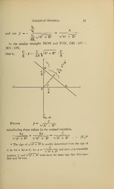
Analytical Geometry. 35
and cos /? =*^-^ \/A2 + B 2 VA 2 + B 2
A^In the similar triangles MON and PON, OM : OP :
MN : ON,
thatis,C S#!{ £.^A. + B i
:
C
y
B
Whence -^ + B„
substituting these values in the normal equation,
Ax By = C
VA 2 + B 2 VA2 + B 2 VA^+B 2• ' (
E i)*
* The sign of s/A2 + B 2is readily determined from the sign of
C in A* + By = C, for p = ^^ + ^and since p is essentially
positive, C and Va2 + B 2 must have the same sign that this equa-
tion may be true.
36 Analytical Geometry.
which is plainly obtained from Ax + By = C, by
dividing through by VA 2 + B 2, that is, the square root
of the sum of the squares of the coefficients of x and y.
For example, to put 3 x + 4 v = 9 m the normal form:
In this case Va2 + B 2 = V3 2 + 42 = V25~= 5-
Dividing then by 5; 3^ + 4^=9 becomes
-2 x + —y = —,
5 5 5
where 2- = Cos /?, — = sin /? and *- = p.
5 5 5
From the above it is seen that a general equation Ax +By = C can assume any of the type forms for a straight
line, hence it may always represent a straight line.
Art. 26 (a). Another method of reducing Ax + By = Cto the normal form, is easily derived from the following
consideration
:
If two equations both represent the same" straight line,
they cannot be independent equations, but one must be
obtained from the other, by multiplying it through by
some constant factor, like
2 x ~ 3 y — I and 8x- 12 y =4.
That is, all the coefficients in one are the same number
of times the corresponding coefficients in the other, as
8=4X2, 12 = 4X3 and 4 = 4 X 1.
Now if A^ + By = C and x cos /? + y sin /? = p are
to represent the same straight line,ABCthen = ~r-- = — = if, say;
cos p sin p pthat is, A = n cos /? (1)
B = » sin J3 (2)
C=np (3)

Analytical Geometry. 37
To find n, square (1) and (2) and add;
A2 = n 2 cos2
pB 2 = n 2 sin2
/?
A2 + B 2 = n2(sin
2/? + cos 2
/?) = n 2
[since sin2/? + cos2
/? = 1]
or w =
P =
Va2 + B 2
A
sin
Va 2 + B 2
B
Va2 + B 2
C
Va2+B 2
[from (1)]
[from (2)]
For sign of V
A
2 + B 2, see note in Art. 26.
Art. 27. From what was said about intersections under
loci, it is clear that if two equations representing straight
lines are combined as simultaneous, the resulting values
of x and y are the co-ordinates of their point of intersection.
For example:
Let 2 x- 3 y= 5 (1)
x + $y= 17 (2)
be the equations of two lines.
Multiplying (2) by 2 and subtracting;
2X - 3^=52 x + 10 y = 34
i 3 y= 29
y — f!> whence x = Tf
.
That is, these two lines intersect at the point (Tf , f|).
Verify by construction.

38 Analytical Geometry.
EXERCISE VI.
Straight Line.
What are the slope and intercepts of the following lines?
Construct them.
I. 2 y = 3 # + 1. 2. 3^ + 21 + 7=0.3. 5 y = _ x - 6. 4- 4 y ~ 7 x + 1 = o.
5. f #- 1 £?= ij. 6. £y- 2x + 3 =? + £*•
7. x + y= o. 8. y= - 3.
9. A line having the slope § cuts the ;y-axis at the point
(o, — 3). What is its equation?
10. What are the vertices of the triangle whose sides are
2 y — # + 1 = 0, $y -{- x = 2, x = — 2 v + 1 ?
II. Find the vertices of the quadrilateral whose sides are
x = y, y + x = 2, 3 y — 2X= 5, 2 x -\- y = — 1.
12. The vertices of a triangle are (2, o), (—3, 1),
(— 5, —4). What are the equations of its sides?
13. A line passes through (— 3, 2) and makes an angle
of 45 with the ^c-axis. What is its equation ?
14. What is the equation to the common chord of the
circles (x — i) 2 + (y — s)2 = 50 and x2 + y
2 = 25?
15. The points (6, 8) and (8, 4) are on a circle. What
is the equation of a chord joining them ?
16. Which of the following points are on the line
2;y = -3*- 2; (2, 1), (-2, f), (2, - 2), (5, 2)?
17. What is the slope of the line through (1, — 6) and
(-3,5)?18. What slope must a line with the ^-intercept — 3
have that it may pass through (—3, 2)?
19. Show that (1, 5) lines on the line joining (o, 2)
and (2, 8).
20. Show that the line joining (— 1, |) and (3, — 2)
passes through the origin.
Analytical Geometry. 39
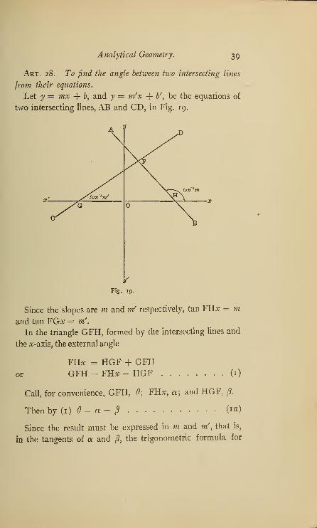
Art. 28. To find the angle between two intersecting lines
jrom their equations.
Let y = mx + b, and y = m'x + b', be the equations of
two intersecting lines, AB and CD, in Fig. 19.
Fig. 19.
Since the slopes are m and mf respectively, tan FHx = mand tan FGx = m'.
In the triangle GFH, formed by the intersecting lines and
the x-axis, the external angle
FHx = HGF + GFHor GFH=FH*-HGF (1)
Call, for convenience, GFH, d; FHx, a; and HGF, /9.
Then by (1) 6 = a - ? (10)
Since the result must be expressed in m and m', that is,
in the tangents of a and /?, the trigonometric formula for

4o Analytical Geometry.
the tangent of the difference of two angles (a — 3) must
be used, that is,
. ( ox tan a — tan 8 m — mftan (a — p) = •— =
i + tan a tan p i + mm!
But since = a —/?, tan 6 = tan (a — /?).
.*. tan d = • (F)i + mm
Which enables us to calculate 6 from m and m''. For
example, to find the angles between the two lines
2 X _ 3y = j
andi x +i y = j± m
Putting these equations in the slope form, they become,
y= I* -
1
y = - %x + |.
Since two lines intersecting always form two angles,
which are supplementary with each other, and since the
only difference that can result in the formula_,
a m — m'tan =
i + mm'
from interchanging m and mris a reversal of sign, that is,
a change from the value of 6 to its supplement, unless it
is distinctly specified, that the angle of intersection is the
acute or obtuse angle, it makes no difference which slope
be called m or mf.
Say in above, m = f and m' = — f
.
Substituting in formula (F),
8.— f_3\ 8.-L3 .5 9.
tan = —« { 4J = &-Xjl = .af = f| = 4 .9 i6y.i + (f) (-1) i-| i
4V
A table of logarithmic functions will show from this
value that 6 = 78 - 30' - 12" -f
.
Make the construction and test with protractor.

Analytical Geometry. 41
Art. 29. To find condition for perpendicularity or
parallelism of lines from their equations.
In formula (F),
, a m — m'tan a =
1 -+- mm
When the lines arej_, 6= 90 , and.", tan 6 = 00; that is,
m — m — 00 •
1 + mm'
Since a fraction whose numerator is finite equals 00 only
when its denominator = o, .*. in this case
1 + mm' — o or m' — — — (a)m
That is, two lines are perpendicular to each other when
their slopes are negative reciprocals.
For example, 3 x — 2 y = 5 and 2^ + 3^=11 are
perpendiculars.
When the lines are parallel, = o and hence,
tan = o.
m, ,• m — m' ,I hat is, =0 or m — m = o.
1 + mm
Whence m = m' (b)
That is, their slopes are equal. These conditions enable
us to readily draw a perpendicular or a parallel to a given
line through a given point.
For we can find the slope of the J_ from the slope of
the given line by (a) and of the parallel by (b).
Then the use of the formula for a line through a given
point with a given slope will give the required equation.
Example: Find the equation of aj_ to 3^ + 2^=5

42 Analytical Geometry.
through the point (— i, 3). The slope of 3 x + 2 y = 5
is — f \y = — I x + f], hence the slope of the J_ is
3
The type equation for a line with a given slope through
a given point is y — y' = m (x — x') (C)
Here m = f , xf = — 1 and / = 3.
Substituting; y — 3 = f (#.-+ 1)
or 3 y ~ 21= 11.*
Art. 30. In Art. 11 it was shown how the area of a
triangle may be found when the co-ordinates of its vertices
{x",y")
Fig. 20.
are known. By the equation for a line through two given
points, the equations of the sides may now be found, and
* Comparing this equation to the _L with the original equation
it will be seen that the coefficients of x and y have simply inter-
changed, and one of them has changed sign, which suggests
a method of writing the 1 to a line. See example at end of
chapter.

Analytical Geometry. 43
from them the angles by formula (F). Also we mayerect J_'s to the sides, at any point. It will now be shown
in Art. 31 how the lengths of the sides may be easily
obtained.
Art. 31. To find the length of a line between two given
points.
Let the points be (x', /) and (x", /'), respectively A and
B in Fig. 20.
Draw AF and BCJ_ to the x-axis. They are y' and /'
respectively. OF = x/ and OC = — x". Draw also AH||
to the x-axis.
Then in the right triangle, ABH, AB 2 = AH 2 + BTP-
Call AB, L (length of AB). Then L2 = (OF + OC) 2 +(BC - AF) 2 = (x' - x") 2 + if - y'Y or since (x'-x") 2
= (x" - x') 2.
L = (x// — x') 2 + (/' — y')2 (written symmetrically).
Example : Find the distance between (1, — § ) and (|, J).
Call the first (x', y') and the second (x", y").
Then I = V(|- i) 2 + (1 + f
)
2 = V^TV + II
Art. 32. To find the co-ordinates of a point which
divides a line between two given points into segments having
a given ratio.
Say the ratio is p : q, the points are (xf
, yf
) and (x", y")
(A and B in Fig. 21) and the required point P (x, y).
Draw BH, PG and AF J_ to the x-axis, and AK||
to the
x-axis.
Then AF = /, PG = y, and BH = /'. Also OF = x',
OG - x, and OH = x" . Also AP : PB : : p : q.
To find PG and OG in terms of (x', /) and {x", f)PG - PN + NG = PN + AF. (1)

44 Analytical Geometry.
Since the triangles APN and ABK are similar, PN : BK :
AP : AB,
that is, PN : (BH - AF) : : AP : AB,
or PN : y" - y : : p : p + q.
P + q
... PG = y = * & ~ yf)
+ / [from (i)],
P + q
or y-Pf+W' <C
P + q
<!>r
B
^^P=^|A
|S In
r
*
H G i
Fig. 21.
Likewise,
OG = OH + HG = OH + KN - a* + (^ ~ *") g
(J)
Analytical Geometry. 45
If the point is to bisect the line then p = q, and the
formulae become
y = Pf + P/ = f + /2 p 2
(O
and x = ^ x—^~ = J—- .... (df)2 p 2
Art. 33. To find the distance from a given point to a
given line.
Since parallel lines are everywhere equally distant, the
expedient suggests itself of drawing a line through the
given point parallel to the given line, and determining the
distance between these two lines at the most convenient
point.
Again, since perpendicular distance of course is meant,
the normal equation is naturally suggested, because it is
determined by a perpendicular from the origin.
Clearly, since these two lines are parallel, the angle /? in
the equation will be the same for both, and they will differ
only in the value of p. Also the difference in the values of
p for the two will be their distance apart, that is, will be
the distance from the given point to the given line.
Then let x cos /? and y sin [} = p, (E), be the equation to
the given line and x cos /? + y sin /? = p' be the equation
of a parallel line.
If this line passes through the given point (V, /) then
it must be satisfied by (x', yf
).
.'. x' cos /? + / sin /? = f (2)
where
p' - p= ±d (3)
[d being the required distance]. The + sign will result
when the point-line is farther from the origin than the
given line; the minus sign, otherwise.

46 Analytical Geometry.
From (3), p' = p ±d.
.'. (2) becomes xfcos ft
-\- y' sinft= p ± d.
or ± d = *' cos /? + / sin /? - p (G)
Since any equation to a straight line may be put in nor-
mal form, the above expression is always applicable. Bytaking advantage of the general form of normal equation,
Ax + By- = C. • (E
x )
VA2 + B 2 VA2 + B 2 VA2 + B*
the formula (G) becomes easier of application. For in
above equations we know that
Acorresponds to cos p.VA2 + B 2
B
VA2 + B^
\/A 2T- 3
corresponds to sin /?,
and — corresponds to p.
+ d= Ax'
+ ^
(GO
VA2 +B 2 VA2 + B 2 VA 2 + B<
Ax'+ By - c
Va2+b 2
This formula (G') may be stated thus:
To find the distance from a given point to a given line,
put the equation oj the line into the form Ax + Bv — C = o.
Substitute for x and y the co-ordinates of the given point
and divide the left hand member of the equation by the square
root of the sum of the squares of the coefficients oj x and y.
The quotient is the required distance.
Example: Find distance from (— 2, 3) to 3 x + 4 y = — 9-
Comparing Ax + Bv = C,
A= 3, B = 4, C= - 9, and*' = -2,/= 3.

Analytical Geometry. 47
. ± d _ Ax + By - C = 3 (- 2) + 4 (3) ~ (-9)
Va2 + B 2 VFT?-6 + 12+9 = I5_ =
3
Vli 5""
Since it is merely distance wanted, the sign of d is not
important.
SYSTEMS OF LINES.
Art. 34. Since parallel lines have the same slope, but
different intercepts, and since the slope is determined
entirely by the coefficients of x and y, the equations of
parallel lines can differ only in the absolute term.
Thus Ax + By = K is the equation of a line||
to Ax+ By = C. Then two equations that differ only in their
absolute terms represent parallel lines.
Again; since the relation between the slopes of perpen-
dicular lines is given by the equation m' — — — , and mm
and mfare determined by dividing the coefficient of x by
the coefficient of y in the equations of the perpendicular
lines, if the coefficients of x and y be interchanged and the
sign of one of them reversed, the relation m' = willm
be satisfied. The absolute term of course will be different
in the two equations.
Thus, Bx — Ay = L is the equation of a line perpen-
dicular to Ax + By = C.
Again; (Ax + By - C) + K (A'x + B'v - C r
) = o (1)
is the equation of a line through the intersection point of
Ax + By = C (2) and A'x + B'y = C . . . . (3)
For, transposing C and C in (2) and (3),

48 Analytical Geometry.
Ax + By - C - o.
A'x + B'v - C = o.
Let (V, /) represent their intersection point. Since
this point is on both lines, it satisfies both equations; hence,
Ax' + By' - C = o (4)
and AV + By - C = o (5)
multiply (5) by K and add to (4)
;
(A*' + B/ - C) + K (AV + By - C) = o (6)
If (V, y) be substituted in (1) we get (6), but we know
(6) is true.
.*. (x', y') satisfies (1), and hence (1) is the equation of
a line through (V, /). Since K is an undetermined con-
stant, we can get the equations of any number of lines
through (xf
, y) by giving K different arbitrary values.
Example: To find equation of a line through the inter-
section of 3 x — 5 y = 6 and 2 x + y = 9.
By above formula the equation is,
(3 x - 5 y - 6) + K (2 x + y - 9) = o.
If the line must also pass through another point, say
(3, — 1), K may be determined. For substituting (3, — 1)
for x and y,
(9 + 5 ~ 6) + K (6 - 1 - 9) = o,
whence K = 2 and above equation becomes
(3^-5^-6) + 2 (2 x + y - 9) = o,
or 7 x — 3 y = 24.
Example : Find the line X to ^—3^=5 through
(2,-1). Its equation by Art. 34 is
$x+ y= k.
Since (2, — 1) must satisfy it, 6 — 1 = k, or k= 5.
Hence 3 x + y = 5 is the required line.
Analytical Geometry. 49
EXERCISE VII.
1. Find the equation of a line whose intercepts are — 3
and - 5.
2. Put the following into symmetrical form and deter-
mine their intercepts.
1 . y -j- 2- + < = -
3j 2 x - 3 y2
x + y = 1.
3. The points (5, 1), (— 2, 3) and (1, — 4) are the
vertices of a triangle. Find the equations of its medians.
4. In Ex. 3, find the equations of the altitude lines.
5. What are the angles of the triangle in Ex. 3 ?
6. What is the equation of the line J_ to 2^—37=5through (— 1, 2)?
7. What is the equation of line||
to 2 # — 3 y = 5
through (— 1, 2)?
8. What is the angle between y -f 2 x = 5 and
3 v — x = 2?
9. The points (8, 4) and (6, 8) are on a circle whose
centre is (1, 3). What is the equation of the diameter J_
to the chord joining the two points ?
10. What are the co-ordinates of the point dividing the
line joining (— 3, — 5) and (6, 9) in the ratio 1:3?11. Prove that the diagonals of a parallelogram bisect
each other.
12. Show that lines joining (3, o), (6, 4), (— 1, 3)
form a right triangle.
13. The vertices of a triangle are (4, 3), (2, — 2), (— 3, 5).
Show that the line joining the mid-points of any two sides
is parallel to, and equal to \ of, the third side.

50 Analytical Geometry.
14. Show that (- 2, 3), (4, 1), (5, 3), and (-1, 5) are
the vertices of a parallelogram.
15. Show that the line joining (3, — 2) with (5, 1) is
perpendicular to the line joining (10, o) and (13, — 2).
16. (2, 1), (—4, —3), and (5 — 1) are the mid-points
of the sides of a triangle. What are its vertices ?
17. Three of the vertices of a parallelogram are (2, 3),
(-4, 1), (- 5,-2). What is the fourth?
18. Find the point of intersection of the medians of the
triangle whose vertices are (1, 2), (— 5, —3), (7 — 6).
19. What is the distance from the point (— 2, 3) to the
line $ x = 12 y — 7?
20. Find the distance between the sides of the parallelo-
gram in Ex. 14.
21. Change 3 x — 4y = 5 to the normal form.
22. Find the co-ordinates of the points trisecting the
line joining (2, 1) and (— 3, — 2).
23. Find the distance from (2, 5) to 2 x — ^ y — 6.
24. Find the altitude and base of the triangle whose vertex
is (3, 1) and whose base is the line joining (f , 1) and (4,— §).
25. Find the area of the quadrilateral whose vertices are
(6,8), (-4,0), (-2,-6), (4,-4).
26. Find the angles of the parallelogram whose vertices
are (1, 2), (- 5, -3), (7, - 6) (1, - 11).
27. _One side of an equilateral triangle joins the points
(2,V3) and (— 1, 4\/s). What are the equations of the
other sides?
28. What is the equation of a line passing through the
intersection of the lines 3 x — y = 5, and 2 x + 3 y = 7
and the point (— 3, 5)?
29. By Art. 34, find the equations to the medians of the
triangle whose sides are y = 2X + 1, y+x + i=oand 5 x = 2 y + 2.

Analytical Geometry
.
51
30. Find the co-ordinates of the centre of the circle cir-
cumscribing the triangle whose vertices are (3, 4), (1, — 2),
31. The base of a triangle is 2 b and the difference of the
squares of the other two sides is d2. Find the locus of the
vertex.

CHAPTER IV.
TRANSFORMATION OF CO-ORDINATES.
Art. 35. It sometimes simplifies an equation to change
the position of the axes of reference or even to change the
inclination of these axes from a right to an oblique angle,
1
B
V 1r
TP1
1
1
!
I
1
'CV*1
1
1
0' A D
Fig. 22.
or both. To accomplish this it is only necessary to express
the original co-ordinates of any point on the line in terms
of new co-ordinates determined by the new axes and neces-
sary constants.
Art. 36. To change the position of the origin without
changing the direction of the axes or their inclination.
Let P be any point on a given line whose equation is to
be transformed.
Let its co-ordinates be x = OC and y = PC (Fig. 22),
52

Analytical Geometry. 53
referred to the axes OX and OY. Let O'X' and O'Y' be
new axes, such that the origin O' is at the distance O'A =a,
from the axis OY, and at the distance O'B = b, from OY.Extend PC to D_[_ to O'X', since the direction of the
axes is not changed.
Then the co-ordinates of P with respect to the new axes
are xf = O'D and / = PD.
Now, OC = AD = O'D - O'A, or x = x' -a )(U)
PC = PD - CD = PD - O'B, or y = / - b )
{ }
It will be observed that (—a, — b) are the co-ordinates of
the new origin referred to the old axes, hence the old co-or-
dinates are equal to the new plus the co-ordinates of the
new origin, plus being taken in the algebraic sense.
Example: What will the equation x2— 4 x + y2 — 6 y = 3
become, if the origin is moved to the point (2, 3), direction
being unchanged ?
Here, x = xf + 2 and y = yf + 3-
Substituting,
{x' + 2)2 - 4 (*'+ 2 ) + (/+3)
2-6 (/+ 3 ) = 3.
Expanding and collecting, x' 2 +y ' 2 = 16 or dropping
accents; .r2 + y
2 = 16, which indicates how an equation
may be simplified by transferring the axes.
Art. 37. To change the direction of the axes, the angle
remaining a right angle.
Let O'X" and O'Y* be the new axes, the axis O rX" mak-
ing the angle with the old X-axis, and the new origin O'
being at the point (a, b).
Let the old co-ordinates of P [OD and PD in the figure]
be (x, y) and the new co-ordinates [O'A and PA in the
figure] be {xf
, /). Draw O rC and BA||to OX and AE J_
to OX, then Zs AO rC and BPA both equal d.
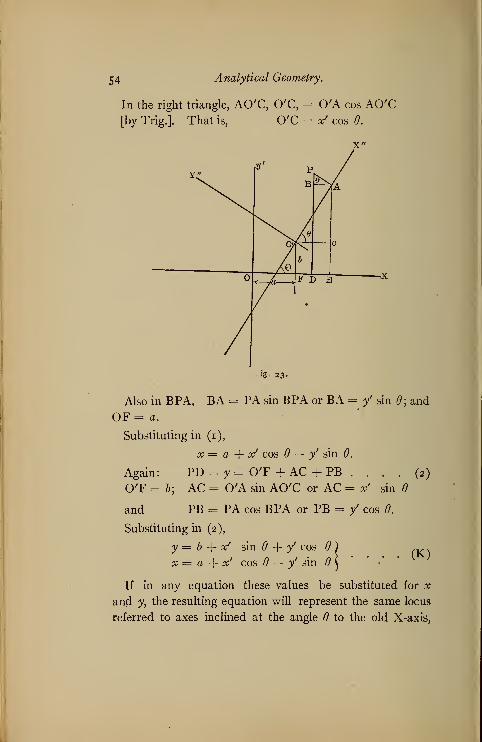
OD= *= OF + O'C- BA . . . (1)
54 Analytical Geometry.
In the right triangle, AO'C, O'C, = O'A cos AO'C[by Trig.]. That is, O'C = *' cos 0.
«g- 23.
Also in BPA, BA = PA sin BPA or BA = / sin 0; and
OF= a.
Substituting in (1),
x = a + oc? cos — y sin d.
Again: PD = y = O'F + AC + PB . . . . (2)
OrF = b; AC - (TA sin AO'C or AC - x' sin
and PB = PA cos BPA or PB = / cos d.
Substituting in (2),
y = b + 00' sin d + yf cos ^ )
x = a -\- xfcos ^ — y sin 6 \
(K)
If in any equation these values be substituted for x
and y, the resulting equation will represent the same locus
referred to axes inclined at the angle d to the old X-axis,
Analytical Geometry. 55
with the origin at (a, b). As a rule the origin remains
the same, hence a = o, b = o, and (K) becomes,
y = x' sin 6 + yfcos d ) ,^,.
x = x cos a — y sin
Example: What does equation 3 # — 2 v = 5 become
when the inclination of the axes is changed 30 ?
Here sin 30 = h; cos 30 = \ \/3
and y = J a/ + h \ZJY,x=\\/zx' - £/.
Substituting, 3 (JV3^-i/)-2 (i^+iV3/)=5or (I VI- i)*'- (l+V3)/= 5-
Art. 38. A very similar procedure in the case where
the axes are changed from rectangular to oblique, and the
origin moved to the point (a, b), gives rise to the formulae,
y = b + xrsin d + y' sin </> ) ,j.
x = a + #' cos -\- y' cos <£ J
# and cf) being, respectively, the angles made by the new
Y-axis and Y-axis with the old X-axis.
When the origin is not changed,
a = o and b = o, and (J) becomes
v = xrsin # + V sin
x = a/ cos + / cos(JO
Art. 39. To change the co-ordinates jrom rectangular
to polar.
The method is entirely similar to the foregoing; the find-
ing of the simplest equational relation between the old
and the new co-ordinates, using necessary constants.
In Fig. 24, let O' be the pole and O'N the initial line,
the co-ordinates of O' being (a, b); the rectangular co-
ordinates of P being (x, y) and the polar, (r, 0), respec-

56 Analytical Geometry.
tively, OB, PB, OT, and Z PO'N in the figure. The angle
between the initial line and the X-axis is<f>.
It is then simply a question of expressing x and y in
terms of r, 6 and<f>.
The right triangle usually supplies the simplest relations,
so we draw O'AJJo PB, giving us the right triangle PO'A
involving r, 6 and O'A = FB, a part of x.
Fig. 2 4-
Then OB = x = OF + FB = OF + O'A,
or x = a + r cos (6 + <j>)
[since O'A = O rP cos PO'A = r cos (d + 0)].
Also, PB = y = AB
yor
PA = O'F + PA,
b + rsin (6 + <f>))
x = a + r cos (6 + <j>) )
If the initial line is||to the X-axis, <j> = o and (K) becomes
y = b -f r sin ^ )
^ = a + r cos (9 \
(K)
(K')

Analytical Geometry. 57
If the pole is at the origin, a = o and b = o
.
y=r sin 6}and *=,cos# ^
Art. 40. To change from polar to rectangular co-ordi-
nates.
It is here necessary only to solve equations (K"), say,
for r and 0, as (K") gives the usual form.
Thus, squaring equations (K"),
y2 = r
2sin2 6
x2 = r2 cos 2
6.
Add; x2 + y2 = r
2(sin
2 d + cos20) = r
2
[since sin 2 6 + cos 2 = 1].
Dividing the first equation in (K") by the second,
y r sin . a at. 1 V* = = tan or = tan — x *- .
# r cos x
Example: Change to rectangular form
r2 cos 2 d = a 2
.
Substituting in above equation, remembering that
cos 2 = cos 2 — sin2 = cos2(9 (1 — tan 2
0)
__ 1 - tan 2
= _ 1 - tan 2
sec 21 + tan 2 6
r
(»" + »') (Sri)""''
or. x2 — v2 = a 2.

58 Analytical Geometry.
EXERCISE VIII.
Transformation of Co-ordinates.
1. What does y2 = 2 px become when the origin is
moved toj— *-
> o ) without changing the direction of the
axes?
2. What does a 2
y2 + b
2x2 = a2b2 become when the
origin is moved to ( , o ), axes remaining parallel ?
3. What does y2 + x2 + 4 y — 4 x— S = o become when
origin is moved to (2, — 2) ?
4. What does y2 = 8 x become when the axes are turned
through 6o°, origin remaining the same?
5. What does y2 = 2 px become when the origin is
moved to the point (m, n)?
6. What does a 2
y2 + b
2x2 = a2b2 become when the
origin is moved to (h, k)?
7. What does 2 x/3 x + 2 y = 9 become when the axes
are turned 30 , origin remaining the same ?
8. What does 62x2 — a 2
y2 = a 2
b 2 become when the
Y-axis is turned to the right, cot_1 — > and the X-axis to
a
the right, tan-1 — [observe negative angle] ?
a
9. Transform the polar equation p = a (1+2 cos 6)
to a rectangular equation with the origin at the pole, and
the initial line coincident with the X-axis.
10. Change (x2 + y2
)
2 = a 2 (x2 — y2) to the polar equa-
tion under the conditions of Ex. 9.
a'11. Change p
2 = to rectangular co-ordinates,cos 2 6
conditions remaining the same.

Analytical Geometry. 59
12. Change to rectangular co-ordinates, under samen
conditions, p = a sec2 — -
2
13. p = a sin 2#:
14. p =1 — cos o
15. Change to polar co-ordinates, under same conditions,
f = '
2 a — x
16. 4 a 2x = 2 ay2 — xy2.
17. 4$ -f yl = a§
18. 4 X2 + 9 / = 36.

CHAPTER V.
THE CIRCLE.
Art. 41. To find the equation to the circle.
Remembering the definition for the equation of a locus,
namely, that it must represent every point on that locus, it
is only necessary as usual to find the relation between the
co-ordinates of any point on the circle in terms of the ne-
cessary constants, which are plainly in this case, the co-ordi-
nates of the centre and the radius.
Let P be any point on the circle A, the co-ordinates of
whose centre are (h, k). The condition determining the
D c
Fig. 25.
curve is that every point on it is equally distant from its
centre. Draw the co-ordinates of P [PC, OC] and call
them (x, y), also AB J_ to PC, forming the right triangle
APB, involving r and parts of x and y.
60
Analytical Geometry. 61
Then AB 2 +PB 2 =AP2 ....... (i)
AB = DC = OC - OD = x - h,
PB = PC - BC = PC - AD = y - k.
Substituting in (i): (* - hf + (y - kf = r2
. . (L)
Performing indicated operations in (L) and collecting,
x2 + y2 — 2 hx — 2 ky = r
2 — h2 — k 2.
Calling - 2 h, m; - 2 k, n and (h2 + k 2 - r
2), R 2
for simplicity, (L) becomes,
x2 + y2 + mx + ny + R2 = o . . . . (L r
)
It is evident from (I/) that any equation of the second
degree between two variables in which no term containing
the product of the variable occurs, and where the coefficients
of the second power terms are either unity or both the
same, is the equation of a circle.
Putting (I/) in the characteristic form (L) by adding
. m2 n2
to both sides -f-—
,
4 4
m2fi
we have, x2-f- mx + — -{- y
2-\- nx + —
4 4
4 4
or, (*+-) 2 + (y+ -) 2
2 2
m2. n2
-pi _ ra2 + n2 — 4
R
2
- R4 4 4
Comparing with (L), we find
h = ZLJH k = - — • r2 = ^ 2 + ^ 2 ~ 4 R2
.
2 2 4
wi nThat is, the co-ordinates of the centre are ( , ),
2 2
and the radius is J \/m2 + « 2 — 4 R2
.

62 Analytical Geometry.
Example: Find the co-ordinates of the centre and the
radius of x2 + y2 — 2 x + 6 y — 26 = o.
Comparing this with (L/), x2 + y2 + mx + ny +R2 =0,
we find, m= — 2, n = 6, R2 = — 26; hence the co-ordi-
nates of the centre.
, m n. , — 2 6, f N( , ),are ( , ) = (1, -3),22 22
and the radius
= iVw2 +w2 - 4 R2
iV4 +36 ~ (-104)
iV I44 = 6.
This equation put in form (L) would be,
(x— 1) + (y + 3)2 = 36.
Art. 42. As it takes three conditions to determine a
circle, and as the above equations contain three arbitrary
constants, if three conditions are given that will furnish
three simultaneous independent equations^ between these
constants, their values can be found, and hence the equation
to the circle.
The three conditions may be, for instance, three given
points on the circle, or two given points and the radius, etc.
Example: Find the equation for the circle passing through
the points (3, 3), (1, 7), (2, 6).
Taking the general equation,
x2 + y2 + mx + ny + R 2 = o . . . (V)
these three points must each satisfy this equation if it is to
represent the circle passing through them, since they are
on it. Hence, substituting them successively for x and y
in (I/), we get three equations between m, n and R2 as
follows:

Analytical Geometry. 63
9 + 9 + 3 m + 3 n + R2 = o
1 + 49 + m + 7 « + R 2 = o Y
4 + 36 + 2 w + 6 « + R2 = o
3*1 + 3 w + R2 = - 18 '.. . . (1)
m + 7 » + R2 = — 50 (2)
2 m + 6 w + R2 = — 40 (3
)
Subtract (2) from (1) and (2) from (3).
2 m — 4 n = 32 or m — 2 » = 16 ... (4)
m — m = 10 . . . (5)
Subtract (5) from (4); n = — 6.
whence w = 4,
and R2 = — 12.
Substituting these values of the constants in (I/),
x2-\- y
2-j- 4X — 6 y — 12 = 0,
the required equation.
Art. 43. When the origin is at the centre of the circle,
h and k are both zero, and the equation becomes,
x2 + /=r2 (L")
which is the form usually encountered.
Art. 44. The polar equation is readily derived from
(L) by making the substitutions for transformation from
rectangular to polar co-ordinates, taking the X-axis as
initial line and the pole at the origin.
Then y = p sin d,
x = p cos 6,
k = p' sin 0',
h = p' cos a,
where (p, 6) are the polar co-ordinates of any point on the
circle and (p', df
) are the polar co-ordinates of the centre.
Making these substitutions in (L), we get :
(p cos 6 - p' cos d')2 + (p sin d - p' sin d'f = r
2,
or, p2 cos2 6 — 2 pp' cos 6 cos Q' + p' 2 cos 2 Q' +P
2sin
2 Q - 2 pp' sin 6 sin Q' + p2 sin 2 0' = r
2.

64 Analytical Geometry.
Collecting, ^(cos2 + sin 20) + p' 2 (cos2 0' + sin
2 0')
— 2 ppf(cos cos 0' + sin sin 0') = r
2.
whence
p2 + P
' 2 - 2 PPf cos ((9 - 0')= r
2
[since cos2 6 + sin 2 6 = i
and cos O' cosr+ sin sin d'= cos (6 - 0')\
TANGENTS AND NORMALS.
Art. 45. To find the equation of a tangent to the
circle x2 + y2 = r
2. Since a line may be determined by
two conditions, and a tangent must be perpendicular to a
radius and touch the circle at one point, the radius being
in this case the distance from the origin to the line furnishes
one condition and the point of tangency another.
Knowing the equation to a line determined by two points,
(X"y")
Fig. 26.
and taking these two points on the circle, we are able to
convert this condition in the special case of the tangent
into the point of tangency and the distance from the origin.
The equation of a line through two points (#', /) and
(*",/) is,
?-/=£f^(*-*') • • • (B)

Analytical Geometry. 65
Let these two points be B and C on circle O, then
(x', yf
) and (of, /') must satisfy the equation to the
circle; hence
xn + y'2 = r2
(2)
*"2 +/'2 = r2
(3)
If these conditions be imposed on (x', yf) and (x", y") in
equation (B), it will become a secant line to the circle.
Subtracting (2) from (3),
of2 - x'2 + y"2 - yn = o,
or, x»2 - x'2 = - if2 - /2
);
factoring, (of - xf
) (of +x')=- (/'-/) (/'+/),
f - V x" + x'whence J— jj= - -j——-.
x" — x' y" + y
Comparing (B) with the equation to a straight line
having a given slope and passing through a given point,
y-y' = $z~, (*-*'.)..•
(B)
y — y' = m (x — x') (C)
V — VIt is evident that — = m, so that the slope of a
x" — x
line through two given points (xf
, yf
) and {xff
,y") is repre-
f_ - ysented by
x„ _ ^'
yff — yf %" + x'
Hence the value of l —, , — , representsof — x y" + y
the slope of a secant line to the circle, and if this value
be substituted in (B) the result will be the equation of a
secant line through the point (V, /) with the slope
_ x" + x f
f +/''

66 Analytical Geometry.
Then if (V', y") is taken nearer and nearer to (x', yf
)
the secant will approach the position of the tangent at
(V, /), and when (x", /') coincides with (V, /) it will
be the tangent. Clearly we are at liberty to take (x", y")
where we please, since it was any point on the circle.
Substituting in (B), y — yf = — ———- (x — x').
y" + /Making x" = x' and y" = y
f
,
y - y = - — (x ~ x') = - — {x - x');2 y y
clearing of fractions, yy' — yn = — xxf + x' 2
;
transposing, xx' + yy' = xn + y'2.
But by (2), x'2 +/ 3 = r
2.
.-. xx' + yy = r2 (Tc)
Evidently it would serve as well to make (V, yf
) approach
(x", y"), only the line would then be tangent at (x", y).
In (Tc) the accented variables always represent the point
of tangency.
Example: What is the equation of the tangent to the
circle x2 + y2 = 10 at (— 1, 3) ?
Here r2 = 10, x* = — 1 and / = 3.
Substituting in (Tc ), —x + 3 y = ioor 3y-x-io=o.Observe that (V, /) is point of tangency, not (x, y);
never substitute the co-ordinates of point of tangency "for
the general co-ordinates x and y.
Again: find equation of tangent to the circle x2 + y2 = 9,
from the point (5, 7^) outside the circle.
The equational form is, xx' + yy' = 9 . . . . (1) and
it remains to find point of tangency (V, /). The point
(5, 71) being on this tangent must satisfy its equation, but it
is not the point of tangency and must not be substituted for

Analytical Geometry. 67
(x, y). Hence substituting in (1), — 5 x* + y> / = g. (2)
Also, since (xf
, yf
) is on the circle it must satisfy circle
equation; that is,
*'2 +/ 2 =9 (3)
Combining the simultaneous equations (2) and (3), we get,
xf = V59 or - W / = ~ If or VV-That is, there are two tangents, as we know by Geometry;
namely, 63 X — 16 y = 195 and 4 y — 3 x = 15. [Gotten
by substituting these values of (V, 3/) in (Tc ).]
CIRCLE.
Art. 46. To express the equation of a tangent to a
circle in terms of its slope.
Evidently the tangent being a simple straight line maybe determined by its slope as well as by the point of tan-
gency, if the slope be such that the line will touch the circle.
Hence it is a question of determining this necessary value
of m. If we take the general slope equation to a straight
line and find a relation between m, b and r such that the
line will touch the circle of radius, r, it is sufficient.
Again, regarding the tangent as the limiting position of
the secant line, as its two points of intersection with the
circle approach coincidence (as in Art. 45), if we combine
the slope equation of a straight line with the equation to a
circle, we get in general their two points of intersection
expressed in the constants they contain; if then we deter-
mine (by Algebra) the conditions these constants must
fulfil among themselves that the two points of intersection
shall coincide, or become one point, we have the desired
result.
Let y = mx -\- b, (1) be the slope equation of a straight
line, and x2 + y2 = r2
, (2) be the equation to a circle.

68 Analytical Geometry.
Regarding (i) and (2) as simultaneous, and substituting
the value of y from (1) in (2), we get a quadratic in xy
whose two roots are the abscissas respectively of the two
points of intersection.
We get then, x2-f- (mx -f b)
2 = r2
,
x2 + m2x2 + 2 mbx + b2 = r2
,
(1 + m2) x2 + 2 w£w -f (b
2 — r2) =0. (3)
By the theory of quadratics in algebra we know that the
two values of x will be the same in (3 ) if it can be separated
into two equal factors, that is, if it is a perfect square.
By the binomial theorem it will be a perfect square
if the middle term is twice the product of the square roots
of the first and last terms (like a2 + 2 ab + b2).
Hence (3) will have two equal values of x (that is, equal
roots) if
2 mbx = 2 y/(i + ?n2
) (b2 — r
2) x2
,
or squaring; if 4 m 2b2x2 = 4 (1 + m2
) (b2 — r2 ) x2 =
4 (b2x2 — r2x2 + b
2m2x2 — r2m2x2
),
dividing by 4 x2; b
2m2 = b2 — r2 + b
2m2 — r2m2
,
b2 = r2 + r2m2 = r
2(1 + m2
),
or & = ± r \/i + m2.
If this condition be fulfilled, clearly the equation of the
secant y = mx + b will become the equation of the tangent
y = mx ± ry/i + m2 ... (T Cj ro )
The ± sign indicates that there will be two tangents with
the same slope, as should be the case, having ^-intercepts
numerically equal, but opposite in sign, or vice versa.
Example : Find the value of b in y = T\ x + b, that the
line may be tangent to the circle x2 + y2 = 25.

Analytical Geometry. 69
By condition formula, b = ± ryi — »i2
,
we must have, b = ± 5 \/i — ^64 = ± 5 . 2S9 = ± __L
225 > 225 3
Hence the equations of the tangents are
8 , 17 , 8 17y = — x — and v = — x —
,
x 5 3 J 5 3
or 15 y =8x + 85 and 15 y = 8 .v— 85.
.\rt. 47. The normal to any curve at a specified point
is denned as the line perpendicular to the tangent at that
point.
It is evident from geometry that the normal to the circle
at any point is the radius drawn to that point.
Since the normal is perpendicular to the tangent, if the
slope of the tangent is known the slope of the normal is
readilv found I in' = ), and as it must pass throughV * /
the point of tangency, we have all the conditions necessary
to determine its equation.
To find the equation of the normal to the circle x2 + y2=r2
.
Let the point of tangency be (V, /). The equation to
the tangent at this point is xx* + yy' = r, or in slope form,
\J r • x'y= —-— x H— (1), and its slope is — — •
y y ySince the normal is perpendicular to it, its slope is
1 V
yThe equation of a line through (V, /) with slope m' is
y-y'= m' (x - x') . . . . [by (C)]
\J
But, m' is here equal to —
,
/

7o Analytical Geometry.
hence the normal equation is y — y' = -— (x — x/
),x
or x'y — xy' = xyf — x'y',
whence y — -L x (Nc)x'
This may be written in slope form, using the slope of the
tangent, m, by substituting for -_, the slope of the normal,
its valuem
xy= - -m
or my + x = o.
Art. 48. To find the length oj a tangent jrom any point
to the circle x2 + y2 = r
2.
By Art. 31, if (xv yx )be the given point and (V, /)
the point of tangency, the length (d) of a line between them
is, d2 = {xx- x') 2 + (yt
- yf
)
2 = x 2 + y2 - 2 (x
xx* +
yxy') + x '2 + y* 2
>Dut ^ (
x'i y') is on th e circle and (xv yx )
on the tangent, x'2 + yn = r
2 and xxxf + y x
y' = r2
.
.-. ^2= X 2 +y 2 - 2 r2 + r
2 = x 2 + y* - r2
. (D c )
If the origin is not at the centre of the circle, it is easy
to show in exactly the same way from equation (L), that
d = V(x1- h) 2 + {y1
- kf - r2
.
Art. 49. The locus of points from which equal tangents
may be drawn to two given circles is called the radical
axis of these circles. Having the above expression for
the length of a tangent to any circle, it is only necessary to

Analytical Geometry. 71
equate the two values of d for the two given circles, in order
to find the equation to the radical axis.
Let the circles be,
{x-hf + (v - k) 2 = r\ (Q)Ov-;;z) 2 + (v-/*) 2 =R2,(C
2 )
be any point on the radical axis to these circles.
If dxand d
2are the tangent lengths from (x
x , yx )to (Q)
and (C 2 ) respectively, then,
,.-W„_.*=« 'andlet(^)
^ = \/(*i - hf + (y, - kfand rf
2 = v/
(3pi~~ mf + (?i
~" n ) ~ ^ •
But ^ = J2or ^2 = d
2
2.
.-. fo - hf + (ft- &)
2 - r2 = (x
t- m) 2
+ iyi -n) 2 -R2(3)
Since (xx , yx )
substituted in the equation
(x - h) 2 + (y - k) 2 - r2 = (x- m) 2 + (y-n) 2 - R2
(4)
gives (3) which we know to be true, then (xx , yx )
satisfies (4).
But (xx , yx ) is any point on the radical axis, hence every
point on that axis satisfies (4), and .*. (4) is the equation
of the radical axis to (Cx )
and (C 2 ).
SUBTANGENT AND SUBNORMAL.
Art. 50. The Subtangent for any point on a curve is
the distance along the x-axis from the foot of the ordinate
of the point of tangency to the intersection of the tangent
with that axis.
The Subnormal for any point on a curve is the distance
measured on the x-axis from the foot of the ordinate of
the point of tangency to the intersection of the normal
with that axis.
Let O [Fig. 27] be a circle, PT a tangent at P (V, /),
OP a normal at the same point, PA the ordinate (yf
) of P.
Then AT = subtangent and OA = subnormal for P.

7 2 Analytical Geometry.
To find their values, it is to be observed that the subtangent
AT = OT - OA. OT = the x-intercept of the tangent,
which is found as in any other straight line by setting
Fig. 27.
y = o in its equation (y = o being the ordinate of the
point T). Then in equation (Tc ) setting y = o, we get
xx' + o = r27
or x = OT =X
Also, OA = x'.
.-. AT = r2x> = r2 ~ x' 2
=
x x'
_ / :
x'
The subnormal, OA = xfevidently.
Example: The subtangent for the point (3, 4) on a
circle is — . What is the equation of the circle?
3
Y* X 1
6
Here x' = 3, V = 4 and — = — •
From this last equation ° = —f
3 3
whence r2 — 25; r = 5.
Then the equation to the circle is #2 + y2 = 25.

Analytical Geometry. 73
The origin is taken at the centre of the circle in these
discussions because that is the usual form encountered,
and the processes are exactly the same wherever the origin
may be; the greater simplicity of results recommending
this form of equation for explanation.
INTERSECTIONS.
Art. 51. By what has been said in general about the
intersections of lines, it follows that if two circles intersect,
the points of intersection will be readily found by combining
the two equations as simultaneous. If the circles are
tangent, the unknowns x and y will have each one value,
or rather each will have its values coincident.
Example: Find where
( x2 + y2 — 4#+ 2 y = o (1) ) ,
\ 2 T 2 / { \mtersect.
\x2 + y2 - 2y=4 (2) $
Subtracting (1) from (2), 4 # — 4 y = 4,
or x- y= 1 . . . . (3)
Substituting value of x from (3) [x = y + i]in (2),
;y2 + 2v + i+v2 -2;y=4,
2 f =3, y=± x/Jj
whence from (3), x = 1 ± \/%.
The points of intersection are then (1 + \/f , a/|) and
(1 - VI, - VI)-Plot the figure and verify results.
(3) Is evidently the common chord, for both points
satisfy it, and it is the equation of a straight line.
Art. 52. A circle through the intersections of two given
circles.
Tf{x2 + y
2 + A* + By + C = o (1) )
11\ ->,->, a ,-r. . ,-. / w are anv two circles,^x2 + y
2 + At* + B^ + Q = o (2) J
*
then (x2 + ./ + Ax + By + C) +n (x2 +y2 + A,x -f By + Q) = o . . . (3)

74 Analytical Geometry.
is the equation of a circle through the intersections of (i)
and (2). For since (3) is a combination of (1) and (2) it
must contain the conditions that are common to both, and
the only conditions common to both, in general, are their
points of intersection. (3) is the equation to a circle, for
it can be put in the form,
(1 + ri) x2 + (1 + n) y2 + (A + A
tn) x +
(B +B in)y+ (C + Cln) = o,
2 . 2 . A + Axn
,B + B,n
,C + Q«
or x2 + y2
-\ !x— x + ! *— y -\ ! *- = o,
1 + » 1 + n 1 + n
which is clearly the equation to a circle of the general form.
Further, (3) is satisfied by any point that satisfies both
(1) and (2). for (3) is made up exclusively of (1) and (2).
If a third condition be supplied, n can be determined and
a definite circle through (1) and (2) results.
EXERCISE.
The Circle.
What are the co-ordinates of the centre and the radii of
following circles?
1. x2 + y2 — 2 x + 4 y = 11.
2. x2 + y2 — 6 y = o.
3. x2 + y2 + x - 3 y = y\
4. 3X2 + sy2 — 8 x — 2 y = 102 J.
5. x2 + y2 + 8 x = S3-
6. x2 + y2 + 6 * + 8 y = - 9.
7. 4 x2 + 4 v2 - 2 a; + y = - TV8. 8 x2 + 8 y
2 - 16 * - 16 y = 56^

Analytical Geometry. 75
Write the equations for the following circles, (h, k)
being the co-ordinates of the centre, and r the radius.
9. h = — 2 k = 3 p = 4J
10. // = J & = 2\ r = 4
1 1
.
& = ! k = — J ^ = V6
12. h = o k = i f = 5
Find the equations for tangent and normal to following
circles:
13. x2 +/= 9 at (- ij, 3).
14. x2 + f = 6 at (i§).
15. x2 +/= 36 at (- 3, - 5).
16. x2 + y2 = 25 at point whose abscissa is 3.
17. x2-\- y
2 = 16 at point whose ordinate is — ^/j.
18. (x - 2)2 + (J
- i) 2 = 100 at (6, 7).
19. x2 + (y - 3)2 = 25 at (3, ?).
20. x2 + y2 = 20 at (?, 2).
Find the intersection points of the following:
21. #2 + y2 = 25 and x2
-f ;y
2 + 14 x + 13 = o.
22. x2 + ;y
2 = 6 and a;2 + y
2 = 8 x — 8.
23. x2 +y2 — 2x — 4y —1=0,and 2 x2 + 2^2 — 8 x — 12 y + 10= o.
24. x2 + y2 = 4, and x2 + ;y
2 + 2 # — 3 = o.
25. Find the equation of the circle passing through the
intersections of x2 + y2 = 9 and 3 .r
2 + $y2 — 6x + 8y = i,
which also passes through the point (4, — 5).
26. Find the equation of the circle passing through the
intersections of x2 + y2 = 16 and x2 + y
2 + 2 x = 8,
which also passes through the point (— 1, 2).
27. Find the equation of the circle through the three
points (o, o), (2, 3), and (3, 4). What are the co-ordinates
of its centre and its radius ?
28. Find the equation of the circle through the points
(2, ~ 3), (3> ~ 4), and (- 2, - 1).

76 Analytical Geometry.
29. Find the equation of the circle through the points
(- 4, ~ 4); (~ 4, - 2); (- 2, + 2).
30. Find the equation of the circle passing through the
origin and having x and ^-intercepts respectively 6 and 8.
31. Find the equation of a circle circumscribing the tri-
angle whose sides are x + 2 y = o, 3 x — 2 y = 6, and
x-y= 5.
32. Find the equation of a circle passing through (1, 5)
and (4, 6) and having its centre on the line y — x + 4 = o.
33. Find the equation of a circle through (3, o) and
(2, 7) whose radius is 5.
34. Find the equation of a circle having the line joining
(f, f) to the origin as its diameter.
35. Plot by points the circular curve whose chord is
30' and sagitta, 9/.

CHAPTER VI.
CONIC SECTIONS.
Art. 53. The sections of a right circular cone made by
a plane intersecting it at varying angles with its axis, are
called conic sections.
If the plane is parallel to an element of the cone the
intersection is called a parabola.
If the plane cuts all the elements of one nappe of the
cone, the section is called an ellipse.
When the plane is parallel to the base of the right cone
the ellipse becomes a circle.
If the plane cuts both nappes of the cone, the section is
called a hyperbola.
The hyperbola evidently has two branches (where it
intersects the two nappes). All these sections are called
collectively conies.
Art. 54. The equation of a conic.
From the standpoint of analytical geometry, a conic is
denned as a curve, the distances of whose points from a
fixed straight line, called the directrix, and from a fixed
point, called the focus, bear a constant ratio to each other.
This ratio is called the eccentricity of the conic. It can be
readily proved geometrically that this definition follows
from the definitions of Art. 53.
In Fig. 28 let P be any point on a conic, the ^-axis the
directrix, and F the focus. Draw AP perpendicular to
the directrix, PB perpendicular to x-axis, and join P and
PFF. Call the constant ratio e: then — = e,
PA77
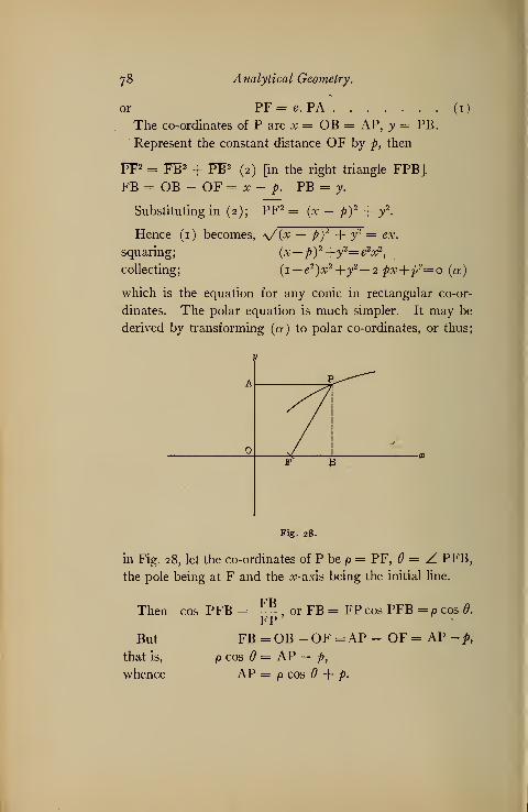
78 Analytical Geometry.
or PF = e. PAThe co-ordinates of P are x = OB = AP, y = PB.
Represent the constant distance OF by p, then
PF2 = FB 2
FB = OB -
- PB 2(2) [in the right triangle FPB].
OF = x - p. PB - y.
Substituting in (2); PF2 = (x - p)2 + f.
(1)
Hence (1) becomes, \/(x — pf -f y2 = ^^.
squaring; (x— p)2 +y2=e2x2
,
collecting; (1 — e2 )x2
-\-y2— 2 px-\-p ?
--=o (a)
which is the equation for any conic in rectangular co-or-
dinates. The polar equation is much simpler. It may be
derived by transforming (a) to polar co-ordinates, or thus;
A P^-^"
v/ 1
F B
Fig. 28.
in Fig. 28, let the co-ordinates of P be p = PF, 6 = Z PFB,
the pole being at F and the #-axis being the initial line.
Then cos PFB
But
that is,
whence
FBFP
FB=OB-OF =
p cos = AP - p,
AP = p cos + p
, or FB = FP cos PFB =p cos 0.
AP- OF= AP-£,

Analytical Geometry.
Substituting in (i); p = e (p cos + p) =
Transposing and collecting;
p (i — e cos 6) = cp.
=-.
ep•
pi — e cos
79
ep cos + ep.
Art. i>y
THE PARABOLA.
The parabola is defined in analytical geom-
etry as a curve, every point of which is equally distant from
a -fixed point arid a fixed straight line. This definition is
in entire accord with Art. 53.
Clearly from this definition A r
e = 1 in the parabola, hence (a)
becomes y2 — 2 px + p
2 = o,
or y2 = 2 px — p
2(1). As it
is usually convenient to have
the origin at the vertex O (in
Fig. 29) of the parabola, and
as the vertex is midway between
the directrix and the focus by definition, the above equa-
tion is transformed to new axes having their origin at the
vertex by substituting [xf + -)
for x and leaving y un-
Fig. 29-
changed.
The co-ordinates of the new origin are [*-j o) with
respect to the old, hence the transformation equations are
as above,
Off -f £. and y — y';
2
(1) then becomes y' 2 = 2 p (x; + 2.) — p
2 = 2 px'
,
2
or [dropping accents] y2 = 2 px (B)
The equation is derived directly from the definition, thus:

80 Analytical Geometry.
In Fig. 29, let P be any point on the parabola; AC, the
directrix, O the vertex and the origin. Draw AP||and
PB perpendicular to the jc-axis, and let F be the focus.
Then if DF be represented by p, OF will equal - by defi-2
nition.
PF = PA (a) [by definition of parabola].
But PF = yJvW + FB*"= x/PB5 + (OB - OF) 2
= v^2+(*-!)
2
'
and PA = OB + DO = x + £.2
Substituting in (a); 4/^2 _j_ fx _ P\ = x.+ Z.,
squaring; y2 + fx - t \ = fx + *
j ,
y2 +/- px + it = ^+ /w + ^A
;y2 = 2 />x, as before.
From its equation, the characteristic property of a para-
bola is, that the ratio of the square of the ordinate of any
point on it to the abscissa of that point is a constant, for
y2
2— = 2 p. This relation is used in physics to show that thex
path of a projectile is a parabola. When the curve is
symmetrical to the j-axis as in Fig. 30, the equation takes
the form, x2 = 2 py.
As an exercise prove this last equation.
Art. 56. If in the equation to the parabola (B), the
abscissa of the focus (F), x = * be substituted, the2

Analytical Geometry. 81
resulting values of y are the ordinates of the points on
the parabola immediately over and under the focus;
-.#(£)-*thus
whence y = ± p.
These two ordinates together, extending from the point
Fig- 3°-
above the focus to the point below on the curve, form what
is called the latus rectum. (GH, Fig. 29.)
The latus rectum evidently equals 2 p, and is often called
the double ordinate through the focus.
Art. 57. To construct the parabola.
First Method. The definition suggests a simple mechan-
ical means of constructing the parabola. Let the edge of
a T-square (AB, Fig. 31) represent the directrix; adjust a
triangle to it, with its other edge on the axis, as DEC.Attach one end of a string whose length is EC, at C and
the other end at F. Keeping the string taut against the
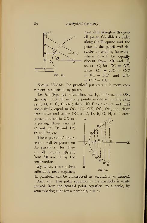
Analytical Geometry.
Fig. 31.
base of the triangle with a pen-
cil (as at G) slide the ruler
along the T-square and the
point of the pencil will de-
scribe a parabola, for every-
where it will be equally
distant from AB and F,
as at G; for EG = GF,
since GF = E'C - GC= EC - GC and E'G= E'C - GC
Second Method: For practical purposes it is more con-
venient to construct by points.
Let AB (Fig. 32) be the directrix; F, the focus, and OX,
the axis. Lay off as many points as desired on the axis,
as C, D, E, G, H, etc.; then with F as a centre and radii
successively equal to OC, OD, OE, OG, OH, etc., draw
arcs above and below OX, at C, D, E, G, H, etc.; erect
perpendiculars to OX in- atersecting these arcs at
C' and C", D' and D",
E' and E", etc.
These points of inter-
section will be points on
the parabola, for they
are all equally distant
from AB and F by the
construction.
By taking these points
sufficiently near together,
the parabola can be constructed as accurately as desired.
Art. 58. The polar equation to the parabola is easily
derived from the general polar equation to a conic, by
remembering that for a parabola, e = 1.
Fig. 32.

Analytical Geometry. 83
Hence o — —e cos '
becomes p = —- cos
Art. 59. It is evident from the form of the parabola
equation, y2 = 2 px, that x cannot be negative without
making y imaginary, hence no point on the parabola
y2 = 2 px can lie to the left of the Y-axis; that is, the curve
has but one branch lying to the right of the Y-axis. In
order to represent a parabola lying to the left of the origin,
the equation would have to take the form
y2 = — 2 px,
so that negative values of x would make y2 positive.
In this latter case no positive value of x would satisfy.
EXERCISE.
What are the equations of the parabolas passing through
the following points, and what is the latus rectum in each
case?
I. (1,4); 2. (2,3); 3.(i
i); 4. (3,-4).
5. The equation of a parabola is y2 — 4 x. What
abscissa corresponds to the ordinate 7 ?
6. What is the equation of the chord of the parabola
y2 — 8 x, which passess through the vertex and the nega-
tive end of the latus rectum ?
7. In the parabola y2 = 9 x, what ordinate corresponds
to the abscissa 4? Construct the following parabolas.
8. y2 = 6 x. 9. x2 = 9 y.
10. y2 = — 4 x. 11. x2 = — 8 y.
12. For what points on the parabola y2 = 8 x will
ordinate and abscissa be equal ?
13. What are the co-ordinates of the points on the
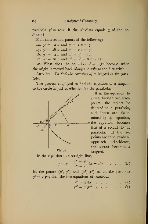
84 Analytical Geometry.
parabola y2 = 10 x, if the abscissa equals % of the or-
dinate ?
Find intersection points of the following:
14. y2 = 4X and y = 2^—5.
15. y2 = 18 x and y =2^—5.
16. y2 = 4 # and #2 + ^
2 = 12.
17. v2 = 16 x and x2 + v2 — 8 x = 33.
18. What does the equation y2 = 2 ^w become when
the origin is moved back along the axis to the directrix ?
Art. 60. To find the equation of a tangent to the para-
bola.
The process employed to find the equation of a tangent
to the circle is just as effective. for the parabola.
If in the equation to
a line through two given
points, the points be
situated on a parabola,
and hence are deter-
mined by its equation,
-X the equation becomes
that of a secant to the
parabola. If the two
points are then made to
approach coincidence,
the secant becomes aFig. 33-
In the equation to a straight line,
tangent.
y (x — xf
)(B)
x" — x
let the points (V, /) and {x", y") be on the parabola
y2 = 2 px; then the two equations of condition
>'2 =•*.**/ (2)
(3)
2 px'
/'2 = 2 pof

Analytical Geometry. 85
arise from substituting these values in the parabola
equation.
Subtracting (2) from (3);
y"2 - yn = 2 px" - 2 px' = 2 p (x* - stf).
Factoring; (7* - /) (/' + /) = 2 p {x" — x').
Dividing through by (/' + /) (x" — x'),
y" — y' _ 2 px" - x'~ y" +yr
Substituting this value of the slope — «*--, in (B);x" — x
y — yf = *— (x — x') (4), which is now the equa-
y" + /
tion of a secant line to the parabola, say ABC (Fig. 33),
the point B being (x", y") and C being (x1
', /).
If now the point B approach C, (x", y") approaches
(xf
,y') and eventually x" = xf and y " = y
f
, and the secant
ABC becomes the tangent DCE.Making x" = x', y" = y' in (4), it becomes,
y _ y = £ {x _ y}
(Tj>)>
y
which is the equation to the tangent DCE at the point
« /)•
Simplifying (Tp ), yyf — y
n = px — px'
yyf — 2 px' = px — px' [since y
n = 2 px'\
or yyf = p (x + x') (Tp
r
)[transposing, collecting and
factoring].
Corollary: The tangent intercept on the X-axis, OD, is
found by setting y = o in (Tp ).
Whence o = p (x + xf
),
x = — xf
.

86 Analytical Geometry.
That is, the intercept is equal to the abscissa of the point
of tangency, with opposite sign.
Art. 6i. The equation to the normal.
Since the normal is perpendicular to the tangent through
the same point, it has the same equation except for its
slope, which is given by the relation for perpendicular lines,
, im = — — •
m
In the tangent equation m = %- •
y
Hence the normal equation is
/-/= ~ £(*-*) (N,).
P
In Fig. 33, CG is the normal at C.
Art. 62. The equation of the tangent in terms 0} its
slope.
As in the case of the circle it is only necessary to deter-
mine the constants in the slope equation of •& straight line,
so that it has but one point in common with the parabola.
The equations to parabola and line are,
y2 = 2 px (1)
and y = mx + b (2)
Eliminating y, to find the intersection equation for x,
(mx + b) 2 = 2 px,
m2x2 + 2 mbx + b2 = 2 px,
m2x2 + (2 mb — 2 p) x + b 2 = o . . (3)
The two values of x in equation (3 ) will be the abscissas
of the two points of intersection. These two points will
coincide if the two values of x are the same, and this can

Analytical Geometry. 87
only occur if m 2x2 + (2 mb — 2 p) x + b2
is a perfect
square.
By the binomial theorem this is the case, if
x2 {mb — p)2 = vi
2x2b2
or m 2b2 — 2 />/»£ + p
2 = w 262
,
whence 2 />//*& = />2
6-Jt.2 w
Substituting this value of b in (2),
? = mx + -2. (Tm ).
2 mwhich is the equation of the tangent in terms of its slope.
Art. 63. Equation to the normal in terms of the slope
of the tangent.
Combining (Tm p ) with the equation to the parabola,
we get the co-ordinates of the point of tangency in terms of
m and p. Since the normal passes through this point it is
necessary to know these co-ordinates.
Combining then, yn = 2 pxr
and yf = mxf + J—
,
2 mwe get x f = —*—L . y' = — \x\ y
f being point of tangency].2 wr 7/z
The slope of the normal is mr = [since it is perpen-m
dicular to the tangent, whose slope is m\The equation to a line through a given point with a
given slope, m', is y — y* = m' (x — x') (C)
Substituting in (C) values of xf
, /, and mf
,
y-t--l (x- -*7 ),w w 2 m
7^3v + m 2x = pm2 + 2- (Nj, m )
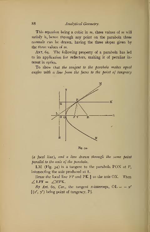
88 Analytical Geometry.
This equation being a cubic in m, three values of m will
satisfy it, hence through any point on the parabola three
normals can be drawn, having the three slopes given by
the three values of m.
Art. 64. The following property of a parabola has led
to its application for reflectors, making it of peculiar in-
terest in optics.
To show that the tangent to the parabola makes equal
angles with a line from the focus to the point of tangency
Fig. 34-
(a focal line), and a line drawn through the same point
parallel to the axis of the parabola.
LM (Fig. 34) is a tangent to the parabola PON at P,
intersecting the axis produced at L.
Draw the focal line FP and PK||to the axis OX. Then
ZLPF= ZMPK.By Art. 60, Cor., the tangent ^-intercept, OL = — x'
[(x', /) being point of tangency, P].

Analytical Geometry. 89
Also OF = L [by structure of the parabola].2
.•. LF = x' + t- [the sign of x' is neglected for we2
want only absolute length].
Let QS be the directrix. Then
PF = PQ = GT = GO + OT = £ + x'. [OT =*'.]2
.*. LF = PF, and triangle LPF is isosceles;
:nce ZLPF:= Z PLF.
But ZPLF = Z MPK [since PK is||
to]
ZLPF:= Z MPK.
Let PR be the normal; then Z FPR = z RPK[since Z LPF = Z MPK, and LPR = MPR, being right
angles].
Since the angles of incidence and reflection are always
equal for light reflected from any surface, it follows that
light issuing from a source at F would be reflected from the
surface of a paraboloid mirror in parallel lines, (as PK).
Art. 65. The diameter of any conic may be defined as
the locus of the middle points of any series of parallel
chords.
A chord is understood to be a straight line joining any
two points on the curve. In Fig. 35, AB being the locus
of the middle points of the system of parallel chords, of
which CD is one, is a diameter of the parabola PON.Art. 66. To -find the equation of a diameter in terms of
the slope of its system of parallel chords.

90 Analytical Geometry.
Draw (Fig. 35) a series of chords (like CD)||
to each
other. To determine the locus of the middle points of
these chords, that is, the diameter corresponding to them.
Let the equation of any one of the chords, as CD, be
and y
y = mx2
2 px
(1),
(2) be the parabola equation.
If (1) and (2*) be combined as simultaneous, the co-ordi-
nates of C and D, the points of intersection, will be found.
First to find the abscissa, eliminating y by substituting
;
Fig. 35.
(mx + b) 2 = 2 px,
m2x2 + 2 mbx + b2 = 2 px,
x2 + (2 mb — 2 p) x
m (3)
Now in a quadratic of the form z 2 + az + b = o, the sum

Analytical Geometry. 91
of the two values of the unknown equals the coefficient (a)
of the first power of the unknown with its sign changed.*
Hence the two values of * in (3), which are the abscissas
respectively of C and D, added together, equal the coeffi-
cient of x in (3 ) with its sign changed.
Call the co-ordinates of C and D respectively (xf
, /)and O", /')•
Then *' + ** = - 2mb ~ 2 P.
m 2
Eliminating * from (1) and (2), we get from (1)
*= y-- b
m
Substituting in (2); y2 = —^- %-
m
f -iPi + iPi =. . . . (4)m m
by principle cited above, y' + y" = —*- •
m
In Art. 32 it was shown that the co-ordinates of the
middle point of a line joining (V, y') and (V', /') are,
(x'+x" /+f\
*Tnz*+az+b=o, z==-* + Va 2 ~4b
— a — \/a 2 — 4 band
. — a + \/a 2 — 4b — a — \/a2 — 4bbut +
2 2
coefficient of 2 with its sign changed.
92 Analytical Geometry.
Calling the co-ordinates of the middle point (E) of CD,(X, Y).
Then X = *'+*" = - "»-» ... (5)2 TO
2 KiJ
and Y = t±f = j!(6)
2 mRemembering that an equation to a line must express
a constant relation between the co-ordinates of every point
on that line, it is clear that b cannot form a part of the equa-
tion we are seeking, for b, the ^-intercept, of the chords,
is different for every chord, but m is constant, since the
chords are all parallel. It would ordinarily be necessary
then to eliminate b between (5) and (6), but in this case
(6) does not contain b and hence it represents the true
equation for the diameter. We will designate it thus:
?-£ (D*>
It evidently represents every point on this diameter, for
CD was any chord, and hence the expression for its middle
point will apply equally well to all the chords.
Cor. I : The form of this equation shows that the diam-
eter is always parallel to the X-axis, that is, to the axis of
the parabola.
Cor. II : Combining (Dp ) with the parabola equation,
we get the co-ordinates of their point of intersection, (A).
y2 = 2 px,
Py = Lm
whence -£— = 2 px
2 'y
2 m* m

Analytical Geometry. 93
By Art. 63 it was found that the tangent whose slope is
m touches the parabola at the point (—*—- , —), )which is A
\2 mr m J
here. Hence in this case the tangent at A has the same
slope, m, as the parallel chords, and is, therefore,||to them.
That is, the tangent at the end of a diameter is parallel to
its system of parallel chords.
Definition: The chord that passes through the focus is
called the parameter of its diameter.
Art. 67. The two following propositions are interesting
as applications of the principles already discussed.
To find the equation to the locus of the intersection of
tangents perpendicular to each other.
It is plainly necessary to find the concordant equations
of any two perpendicular tangents and by combining their
equations get their intersection point.
The slope equation for any tangent is
y = mx + — (1)2 m
then y = m'x -\ ^—, (2) will represent any other tangent.
2 m'
If the two tangents are perpendicular to each other then
mf = — —, and (2) becomes, y = — -
. . (3)m m 2
Subtracting (3) from (1),
o=(w + -jx + £ I m +— ); whence x = — ^ •
\ m] 2 \ m) 2
This equation being the combination of (1) and (3)
represents their intersection, that is, it is the equation of
b .
the locus of all intersections. But x = — £ is the equa-2
tion of the directrix, hence all tangents to the parabola
94 Analytical Geometry.
that are perpendicular to each other intersect on the
directrix.
Art. 68. To find the locus of the intersection of any tan-
gent, with the perpendicular upon it from the focus.
The equation of any tangent line is y = mx + —,(i).
2 m
The equation to a line through the focus having the slope
mf is by (C), y = mf tx — —J,
(2). The focus being the
point [*-o)
. Since (2) is perpendicular to (t), mf = ,
\2 /J m
hence (2) becomes y = (x — £-), or y= + -*-, (3).m \ 2 / m 2 m
Subtracting (3) from (1), o =[ 1 + —
) x.
\ m)
Whence x — o,
But x — o is the equation of the Y-axis, .'. every tangent
to the parabola intersects the perpendicular upon it from
the focus on the Y-axis.
Art. 69. It is sometimes desirable to express the
equation of a parabola with reference to a point of tangency
as origin, and with the tangent and a diameter through
the point of tangency as axes.
Knowing the co-ordinates of the point of tangency in
terms of the tangent slope and knowing that the diameter
is||
to the axis, it is easy to apply the transformation
equations in Art. 38.
Remembering that the new X-axis (a diameter) is parallel
to the old, hence = o, and that tan <+> = m, since the
new Y-axis is a tangent and cf> is the angle it makes with
the old X-axis.

Analytical Geometry. 95
Also (a, b) the co-ordinates of the new origin become,
\2 m l m I
( x = a + xf cos # + y cos 0,E1uatlons \y=b+x'sm0 + y'sm<f>,
become, x = —*-f-
#' + V cos2 w2
[since cos # = cos 0=1].
y = -*- + / sin #
[since sin = sin = o].
Substituting in the parabola equation,
y2 = 2 /w,
we get,
or since
7> cos
[-£ + / sin<£ ) = 2 p (—£— + cc* + y' cos 6
),
\;» / \ 2 ra2
/
sinm = tan
sin / \2 sin2
/
/T\QQS^+ 2 py^Q§& + / 2 sin
2 =
j^sQOS2(/>
sin
/2 sin 2
+ 2 /w' + 2 ^5^qos
2^',
^(gj}*— *""*-
Since esc2
<f)— cot 2 0+1
m+ 1,
this may be written, ^2 = —|- # -f 2 ^,w2
or 2 _ 2 ft(i + ^ 2
)
;>r

96 Analytical Geometry.
where m is the tangent's slope, or the tangent of the
angle it makes with the axis of the parabola.
Art. 70. The parabola is of practical interest also in
its application to trajectories.
By the laws of physics a projected body describes a
path, determined by the resultant of the forces of projec-
tion and of gravity acting together upon the moving body
[neglecting air resistance].
In a given time, /, with a velocity, v, a body will move a
space, s = vt. (1). Meanwhile it falls through a space
S = — gt2
. (2) [g = acceleration by gravity.]2
Square (1) and divide by (2) .
s g
It is easy to see that the horizontal distance, s, which
the body would move if undiverted by gravity, is like an
abscissa, and that the vertical space, S, that the body
would fall by action of gravity, is like an ordinate.
Also is clearly a constant, (like 2 p).g
s^1
2 1) 2 1)
Hence —= or s2 = S is exactly like y
2 = 2 px.S g i
That is, the path of a projectile is a parabola, if we neglect
the resistance of the air.
EXERCISE.
Find the equations of the tangents to each of the followr
ing parabolas:
1. y2 = 6x at (f, 4).
2. y2 = 9 x at (4, 6).
3. x2 = 6 y at (6, 6).

Analytical Geometry. 97
f= - 4X at (- 1, 2)
y2 = 4 ax at (V, /).
f = 8 x at (4 - i, ?).
f= - s* at (?- 4 ).
/= if* at (6, ?).
Find the equation of the normal to each of the pre-
ceding parabolas.
10. Find the equations of the tangents to the parabola
y2 = 8 x from the exterior point (i, 3).
11. Find the equation of the tangent to y2 = 9 x par-
allel to the line 2 y = 3 # — 5.
12. Find the equation of the tangent to the parabola
y2 = 4 .v perpendicular to the line y + 3 # = 1.
13. Find the slope equation of the tangent to the para-
bola x2 = 2 ^ry.
14. Find the equation of the tangent to the parabola
y2 = 8 x from the point (1, 4).
15. Find the equation to the tangent at the lower end of
the latus rectum.
16. The equation to a chord of the parabola y2 = 4 x
is 5 y — 2 x — 12 = o. What is the equation of the
diameter bisecting it ?
17. What is the equation of the parabola referred to
this diame er and the tangent at its extremity?
18. In the parabola y2 = 8 x, what is the parameter of
the diameter whose equation is y = 16?
19. What is the equation of the parabola to which
2y=3#4-8is tangent ?
20. The equation of a tangent to the parabola y2 — 9 x
is 3 y — x = 11. What is the equation of the diameter
through the point of tangency?
21. What is the equation to the chord of the parabola
y2 = 6 x, which is bisected at the point (3, 4) ?
98 Analytical Geometry.
22. The base of a triangle is 10 and the sum of the
tangents of the base angles is 2. Show that the locus of
the vertex is a parabola and find its equation.
23. The equation to a diameter of the parabola y2 =9 x,
is y = — 3. Find the equation of its parameter.
24. Find the equation of the diameter to the parabola
x2 = 2 py.
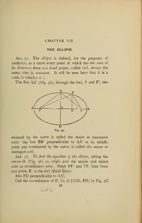
CHAPTER VII.
THE ELLIPSE.
Art. 71. The ellipse is defined, for the purposes of
analytics, as a curve every point of which has the sum of
its distances from two fixed points, called foci, always the
same; that is, constant. It will be seen later that it is a
conic in which e < 1.
The line AA' (Fig. 36), through the foci, F and F', ter-
B
1 v. \ \
riF> D F J
B'
Fig. 36.
minated by the curve is called the major or transverse
axis: the line BB' perpendicular to AA' at its middle
point and terminated by the curve, is called the minor or
conjugate axis.
Art. 72. To find the equation of the ellipse, taking the
centre O (Fig. 36) as origin and the major and minor
axes as co-ordinates axes. Draw PF' and PF, lines from
any point, P, to the foci (focal lines).
Also PD perpendicular to AA'.
Call the co-ordinates of P, (x, y) [(OD, PD) in Fig. 36]
99
LOFC.

ioo Analytical Geometry.
represent | AA' = OA, by a; \ BB' = OB, by b, PF, by
r; PF', by /; OF = \ FF', by c.
It is required to find the relation between PD and OD,using the constants, a, b, and c. The right triangles PDFand PDF', immediately suggest the means, as they contain
together the co-ordinates (x, y) and part of the constants,
and also PF and PF' whose sum is a constant by definition.
In PDF, PF 2 = PD 2 + DF2,
or r2 = y
2 + (c — x) 2,
r=Vy2 + (c~ ocf (i)
In PDF' PF' 2 = PD 2 + DF2,
or r'2 — y
2 + (c + x) 2
or r' = V/ + (c + x)< (2)
By definition r + r' = a constant; let us try to deter-
mine this constant. Since the points A and A' are on the
ellipse they must obey this definition ; hence FA -f F'A =this constant.
But F'A + FA - FF' + 2 FA.
Also F'A + FA = FA' + FA' = 2 F^A' + F'F.
That is, pf + 2 FA = 2 F'A' + pf,
whence FA = F'A'.
.-. FA + F'A = F'F' + 2 FA = F'F + FA + F'A' = 2 a.
.'. r + r' = 2 a.
Adding (1) and (2);
V?2 + (c- x) 2 + vV + (c + x) 2 = r + r'= 2a (3)
Transposing and squaring;
f + (c + x) 2 = 4 a 2 - 4 a V>2 + {c- x) 2 + f+ (c-x) 2
/+/-f 2a-f f =4fl2 - 4<z \Zy2 + (c — x) 2
+ T + / — 2 ex -\- yr.
whence — 4 ex + 4 a 2 = 4 a \/y2 + (c — x) 2
.

Analytical Geometry. 101
Dividing by 4 and squaring again;
c2x2 — 2jjycx + a 4 = a 2
y2 + a2
c2—2j^tx-\-a 2x2
a 2
y2 + (a
2 - c2) x2 = a 2
(a2 - c
2
) (4)
The form of this equation may be readily changed by
expressing c in terms of a and b.
The point B being on the ellipse,
BF + BF' = 2 a,
but BF = BF' (since BB' is perpendicular to AA' at its
middle).
BF= a.
In the right triangle BOF,
BP = 5^2 + 5^2 = b2 + c
2}
that is, a2 = b2 + c
2
or b 2 = a2 — c2
.
Substituting in (4)
a 2
y2 + b 2x2 = a 2
b2 (Ae ).
The form of this equation shows that the curve is sym-
metrical with respect to its two axes.
Corollary: The polar equation to the ellipse is that of
the conic in general,
epp= «'1 — e cos
where p = distance from directrix to focus and e < 1.
Art. 73. There are, by definition, two latera recta, one
through each focus. Since they are ordinates, their values
are found by substituting in the equation the abscissas of
the foci, that is, x = ±.c= ± \Ja2 — b2
.
Substituting this value of x in (Ac ),
a2y2 + b
2 {a2 - b2) = a 2b2
,
u 2 b* . b2
whence y* = — y = ± — •
That is, 2 y = latus rectum =
a
a

102 Analytical Geometry.
Art. 74. To find the value oj p in the ellipse.
In Fig. 37, NF' = p in general equation to a conic.
A'F'Also —— = e, since A' is a point on the conic A'B AB'
A JN
(the ellipse), whence A'F' = e A'N '•• (1)
Also AF' = eAN, (2). [Since A is a point on conic]
Add (1) and (2);
A'F' + AF' = e (A'N + AN) = e (A'N + A'N + AAr
)
or Kkf = e{2 ArN + 2 ArO) = 2 e (A'N + A'O) = 2 e ON,
that is, 2 a = 2 e ON or ON = - (3)
Subtract (1) from (2);
AF' - A'F' = e (AN - A'N) = e AA' = 2 a*.
But AF' - A'F' = AF' - FA[since FA = A'F', Art. 82] = FF' = 2 c.
2 ae = 2 c [since FF' — 2 c\
c = ae (4)
B'
Fig. 37-
Again, NF' = NO - OF' = 5L _ c = - -e e
XTTV a — ae2 a (1 — e2
)
that is, NF' = p = = — L•
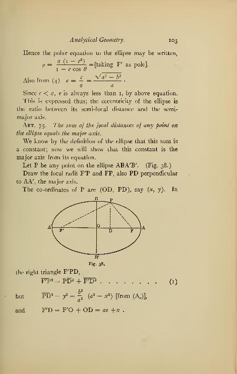
Analytical Geometry. 103
Hence the polar equation to the ellipse may be written,
a (1 - e2)
1 — e cos[taking F' as pole].
Also from (4) e = — = •
a a
Since c < a, eh always less than 1, by above equation.
This is expressed thus; the eccentricity of the ellipse is
the ratio between its semi-focal distance and the semi-
major axis.
Art. 75. The sum oj the focal distances of any point on
the ellipse equals the major axis.
We know by the definition of the ellipse that this sum is
a constant; now we will show that this constant is the
major axis from its equation.
Let P be any point on the ellipse ABA'B'. (Fig. 3%.)
Draw the focal radii F'P and FP, also PD perpendicular
to AA', the major axis.
The co-ordinates of P are (OD, PD), say (x, y). In
I
\ \\ \
I F' D FJ
B'
Fig. 38.
the right triangle F'PD,
FT 2 = PD 2 + FD2
but PD 2 = y2 = ¥ (a2 - x2
)[from (Ae )],
and F'D = F'O + OD = ae +x .
(1)

104 Analytical Geometry.
Substituting these values in (i).
FP~2 = - (a2 - x2
) + (ae + x) 2 = b 2 - ^-^- + a2 e2
a 2 a 2
+ 2 aex + x2 = Ir— —-
—
{- a 2 — l/ + 2 aex + x2,
a 2
r • 2 a 2 - ^2
i 2 , , O 2 - 62)*2
[since e* = J= a z + 2 aex + *—
•
a 2 a 2
b2 x2
[adding — —— an(i x2] = a 2 + 2 aex + e2 x2
a2 — o
2
[for — x2 = e2 x2
].
a2
;. FrP= a + ex (1)
By similar process in the right triangle FPD,
FP = a — ex (2)
Adding (1) and (2). FrP + FP = 2 a.
Since F'P and FP are any two focal radii, the sum of
the focal radii of any point equals 2 a.
To Construct the Ellipse.
Art. 76. The definition of the ellipse, as a curve the
sum of the distances of whose points is constant and always
equal to the major axis, gives us the method of construction.
First Method : Take a cord the length of the major axis,
and attach its extremities at the two foci with a pencil
caught in the loop thus formed, and keeping the cord
stretched, describe a curve. It will be an ellipse, for the
sum of the distances of the pencil point from the two points
of attachment (the foci) will always equal the length of
the cord, that is, the major axis.
Second Method: Taking one of the foci as centre and any
radius less than the major axis, describe two arcs above
and below the major axis, then with the other focus as

Analytical Geometry. i°5
centre and a radius equal to the difference between the
major axis and the first radius, describe intersecting arcs.
These points of intersection will be points on the ellipse, for
the sums of their distances from the foci will equal the
sum of the radii, that is, the major axis. As many points
as desired may be located in this way, and the curve joining
them will be an ellipse.
Fig. 39.
As in Fig. 39 let AA' be the major axis, F and F' the
foci. Taking, say, AB as radius and F' as centre describe
arcs m and mf.
Then taking A'B as radius, and F as centre describe
arcs n and n'\ their intersections R and S will be points on
the ellipse.
Taking any desired number of points as C, D, etc.,
perform the same operation, thus determining any desired
number of points. A smooth curve through these points
will be an approximate ellipse.
Art. 76a. The two following methods of ellipse con-
struction are used by draftsmen. The first based upon
the relation between the ordinates of points on the ellipse
and those on the auxiliary circles as shown in Art. 97give a true ellipse; the second gives what is known as a
circular-arc-ellipse and is only an approximation.

io6 Analytical Geometry .
First Method : Let O be the centre of the ellipse- AA'the major axis; BB' the minor axis; BCB' the minor circle
and ADA' the major circle. (Fig. 39a.) Take any num-
ber of points on the major circle as R, S, T, etc.
From these points draw radii and ordinates, and through
the points of intersection of the radii with the minor circle,
draw lines||
to the major axis, AA'. Where these parallels
Fig. 39a.
intersect the ordinates will be points on the ellipse. The
points may be made as close together as desired by draw-
ing a great number of radii. A smooth curve joining these
points will form the ellipse. Take the point S, its radius, OS,
and its intersection with BCB', P. Draw PN.
In the triangle OSN'OP : OS : : N'N : SN',
that is, b : a : : y : /, hence N is a point on the
ellipse.
Second Method : This is known as the three centre
method, or three point method, and is approximate only.
Let AA' and BB' be the axes, intersecting at O (Fig. 39ft).

Analytical Geometry. 107
Complete the rectangle BOA'D and draw the diagonal A'B.
From D draw the line DE perpendicular to A'B and pro-
duce it to meet BB' at C; with C as a centre and BC as
radius describe arc MM; with E (whose DC cuts AA') as
centre and A'E as radius describe arc A'N'.
With O as centre and OB as radius describe arc BF,
Fig. 39b.
cutting AA' at F. On A'F as diameter construct the
semicircumference A'B"F, cutting B'B produced upward
at B." Lay off BB" from O toward B' to C. With C as
centre and CC as radius describe arc RS.
Lay OB" from A' on AA' to R'. With E as centre and
ER' as radius draw arc R'S', intersecting arc RS at T.
With T as a centre and suitable radius, an arc described
will touch A'N' and MN, and complete the elliptic quadrant
A rB. A similar construction to the right of BB r and also
below AA' will complete the ellipse.

108 Analytical Geometry.
EXERCISE.
What are the axes and eccentricities of the following
ellipses
:
i. 9 x2 + 16 y2 = 144. 3. x2 + 9 y
2 = 81.
2. 2 ^2 + 4 ;y
2 = 16. 4. J #2 + I y
2 = 1.
5. In an ellipse, half the sum of the focal distances of
any point is 4', and half the distance between foci is 3'.
What is the ellipse equation ?
6. In a given ellipse the sum of the focal radii of any
point is 10", and the difference of the squares of half this
sum and of half the distance between the foci is 16. Whatis the equation to the ellipse ?
7. The eccentricity of an ellipse is f and the distance of
the point whose abscissa is f from the nearer focus is 3.
What is the equation to the ellipse ?
8. The major axis of an ellipse is 34", and the distance
between foci is 16". What is its equation ?
9. Find equation of the ellipse, in which the major
axis is 14" and the distance between foci = V 3 times the
minor axis.
10. In the ellipse 2 x2 + y 2 = 8, what are the co-ordi-
nates of the point, whose abscissa is twice its ordinate?
What are the axes?
11. What are the co-ordinates of the point, on
the ellipse 4 x2 + 16 y2 = 64, whose ordinate is 3 times its
abscissa ?
12. Find the intersection points of 9 x2-\- 16 y
2 = 2$
and 2 y — x = 3.
13. Find the intersection points of the ellipse
16 y2 + 9 x2 = 288, and the circle x2 + y
2 = 25.
14. In Ex. 13, find the equation of the common chord.
15. Find the angle between the tangents to the ellipse

Analytical Geometry. 109
and circle of Ex. 13 at the point of intersection whose
co-ordinates are both positive.
16. An arch is an arc of the ellipse whose major axis is
30', and its chord, which is parallel to the major axis and is
bisected by the minor axis, is 24' long. The greatest height
of the arc is 8'. Find the equation of the ellipse and plot
the arc.
17. A section of the earth through the poles is approx-
imately an ellipse; a section parallel to the equator is a
circle. What is the circumference of the Tropic of Cancer,
the angle at the centre of the earth between a line to any
point on it and a line to a point on the equator being 23°-27' ?
18. If two points on a straight line, distant respectively
a and b, from its extremity, be kept on the Y-axis and X-
axis, respectively, as the line is moved around, the extremity
will describe an ellipse, whose axes are 2 a and 2 b.
From this, suggest a method of construction for the ellipse.
Art. 77. Tangent to the Ellipse.
The method of finding the tangent equation is exactly
similar to that for the circle and for the parabola,
equation (B)
Taking
w-y-y/ xT-a/(x — x*).
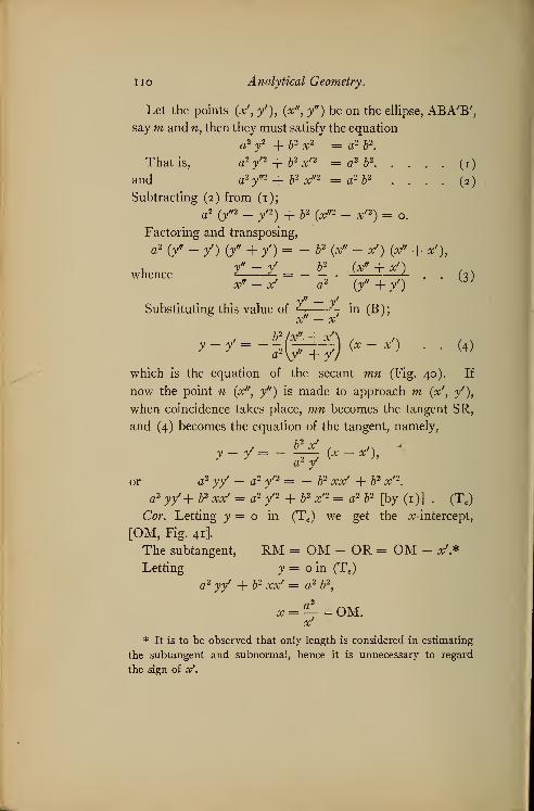
no Analytical Geometry.
Let the points (V, /), (x", y") be on the ellipse, ABA'B',
say m and n, then they must satisfy the equation
a2y
2 +b2 x2 = a2b2
.
That is, a2yn
-\-b2x'2 = a2 b2
(i)
and a2 y"2 +b2 x"2 = a2b2 .... (2)
Subtracting (2) from (1);
a2 (y/2 _ y 2) + b 2 ^,2 _ x,2^ = 0>
Factoring and transposing,
a2 (y> _ y) (y/ + y)= _ 52 ^ _ ^ ^ +^whence ^ = - *
. ^±^1 . . (3)
Substituting this value of A £- in (B);x" — x
b 2!x"+x'\
a 2 \y" +?)(x - x') . . (4)
which is the equation of the secant mn (Fig. 40). If
now the point n (x", f) is made to approach m (V, /),
when coincidence takes place, mn becomes the tangent SR,
and (4) becomes the equation of the tangent, namely,
, b2 xf
, ,v -«
y - 7 = ——> (* ~ x j>a* y
or a2 yy' — a2yn = — b
2 xxf + b2 x'2.
a2 yy'+ b2 xx' = a2 y'2 + b2x'
2 = a2b2 [by (1)] . (Te )
Cor. Letting y = o in (Te ) we get the ^-intercept,
[OM, Fig. 41].
The subtangent, RM = OM - OR = OM - #'.*
Letting y = o in (Te )
a2 yy/ _|_ 2 xxf = a2p^
a 2
x = — = OM.x'
* It is to be observed that only length is considered in estimating
the subtangent and subnormal, hence it is unnecessary to regard
the sign of xf.
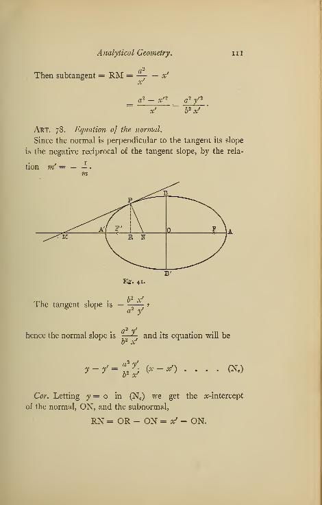
Analytical Geometry. in
Then subtangent = RM = —— — x'
a 2 — xn _ a 2 y'2
b2 x>
Art. 78. Equation oj the normal.
Since the normal is perpendicular to the tangent its slope
is the negative reciprocal of the tangent slope, by the rela-
tion m' = — — •
m
^^^BP^
A7 F' F \
^^M R N
Fig. 41.
The tangent slope is — b2 x'
a2 y'
a 2 /hence the normal slope is —— and its equation will beb2 xr
y~ y,==<
¥b (* " ^ (Ne)
Cor. Letting y = o in (Ne ) we get the ^-intercept
of the normal, ON, and the subnormal,
RN = OR - ON = *f - ON.

ii2 Analytical Geometry.
y = o in (Ne ), y- y = a2 y'
b2 x'(x -x'),
— y = a2 yb2 xf
(X -*'),
- ¥ xf = a2 x -- a- x',
X = a 2 -a 2
b2x' = (
RN = %'a2 -b2
x' = b 2 xf
.Thena
Art. 79. Slope equation of
Let y = mx + c (1)
be a secant line to the ellipse a 2y
2 + b2 x2 = a 2
b2
. (2)
Combining (1) and (2) to find points of intersection,
a 2 (mx + c)2 + b
2 x2 = a2 b2.
a2 m2 x2 + 2 a 2 mcx + a 2c2 + b2 x2 = a 2 b2
.
x2 (a2 m2 + b2) + 2 a2 ?wc# + (a
2c2 — a 2
b2) = o.
Now if this secant becomes a tangent the two points of
intersection, whose abscissas are given by ihis equation,
become one point, the point of tangency. As we know
the condition that this equation should have equal roots is
(a2 m2 + b2) {a2
c2 - a2
b2) = {a2 mc) 2
,
or, a*^c2 — a 4 m2 b2 + a 2
b2c2 — a2 ¥ = a^ynl^
or c2 = a2 m2 + b
2,
c = ± \/a2 m 2 + b2
.
Substituting this value of c in (1) it becomes the equa-
tion of the tangent in terms of m, a and b, that is, the slope
equation of the tangent,
y= mx± V'a2 m 2 + b2 (Te , m)
Art. 80. To draw a tangent to the ellipse.
It will be observed that the tangent to the ellipse has the

Analytical Geometry. "3
same .v-intercept as the tangent to a circle having the
major axis for a diameter; hence to draw a tangent to an
ellipse on the major axis as a diameter, construct a circle
and produce the ordinate of the point of tangency to meet
the circle. This point on the circle and the point of tan-
Fig. 42.
gency on the ellipse will have the same abscissa, and hence
the ^-intercept of the tangents to the circle at this point
and to the ellipse will cut the X-axis in the same point.
Draw a tangent to the circle at this point and join the
point of intersection with X-axis with the point of tangency
on the ellipse. The last line will be a tangent to the ellipse
at the required point. (Fig. 42.)
P = point of tangency; P' = the point in which the
ordinate of P cuts the circle; R = intersection of circle-
tangent, RP', with the axis.
Then RP is the tangent to the ellipse.
Supplemental Chords.
Art. 81. The chords drawn from any point on an
ellipse to the extremities of the major axis are called sup-
plemental chords.
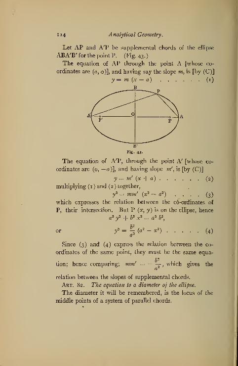
H4 Analytical Geometry.
Let AP and A'P be supplemental chords of the ellipse
ABA'B' for the point P. (Fig. 43.)
The equation of AP through the point A [whose co-
ordinates are (a, o)], and having say the slope m, is [by (C)]
y = m (x — a) (1)
B
The equation of A'P, through the point A' [whose co-
ordinates are (o, —a)], and having slope m', is [by (C)]
y = m' [x + a) (2)
multiplying (1) and (2) together,
y2 = mm' (x2 — a2
) .... (3)
which expresses the relation between the co-ordinates of
P, their intersection. But P (x, y) is on the ellipse, hence
a2y
2 + b 2 x2 = a 2b2
,
orb2
, 2
1a 1x2
) (4)
Since (3) and (4) express the relation between the co-
ordinates of the same point, they must be the same equa-
b2
tion; hence comparing; mm! — — , which gives the
relation between the slopes of supplemental chords.
Art. 82. The equation to a diameter of the ellipse.
The diameter it will be remembered, is the locus of the
middle points of a system of parallel chords.

Analytical Geometry. JI 5
Let RS be any one of a system of parallel chords of the
ellipse ABA'B' (Fig. 44), and T its middle point.
Let y= mx + c (1) be the equation of RS, and a2y2
+ b2 x2 = a 2
b2(2) be the ellipse equation. Combining (1)
and (2), we get an equation whose roots are the abscissas
of R and S, respectively, if y be eliminated; an equation
whose roots are the ordinates of R and S, if x be eliminated.
Eliminating y; a2 (mx + c)2 + b2 x2 = a 2
b2
,
a2 m2 x2 + 2 a2 mxc + a2c2 + b2 x2 = a 2 b2
,
2 a2 mcx2 + x + a - a2
b2 = o
a2 m2 + b2
Let the two roots of (3 ) be represented by x' and x".
Then by the structure of a quadratic,
, . ,, 2 a 2 mcx? + x" = — —— — •
a2 m2 + b2
Calling the ordinates of T, (X, Y),
xf + x" a 2 mc
(3)
then X =2 a2 m2 + b 2
Eliminating x from (1) and (2)
2 2 . b2 y2 - 2 b 2 yc + b
2c2
a2y
2H L
f
(4) [by Art. 32]
a 2b2
,
a2 b 2,

n6 Analytical Geometry.
a2 m2y
2 + b2y
2 — 2 b2 yc + b2c2 = a2 &2 w2
,
?2
2
2
2 ,^2 ?+ b2 c2 -a 2b2 m2 = o ... (5)
a2 w2 + b2
Calling the two roots of (5), y' and /',
2b2C
... y + f = +a2 m2 + b2
'
and Y = /±y:i +*»*.
. . . (6)2 a2 w2 + b2 \'
Since c is a variable it must be eliminated between (4)
and (6), for we must express the relations between the
co-ordinates of these mid-points of the chords in terms of
constants to get the true equation of their locus.
Divide (6 by (4)
+ b2c
Y a 2 m2 + b2
X — a 2 mc
- b2
a2 m
a 2 m2 + b2
b 2
y — — x .
*
a z mThat is, y = — x (D c )
a 2 m
is the equation of the diameter, since it expresses a constant
relation between the co-ordinates of the mid-point of RS,
and RS stands for any one of the parallel chords, mis a
constant because the chords being parallel, all have the
same slope. The form of this equation shows that the
diameters pass through the centre, since the constant or
intercept term is missing.
Since this equation represents any diameter whatever,
it follows that any chord passing through the centre of the
ellipse is a diameter, and hence bisects a system of parallel
chords.

A nalytical Geometry
.
117
Conjugate Diameters.
Art. 83. It will be observed in the equation
b2 b
2b2
x, the slope is — —— ; that is, it is
a 1 m a* mdivided by m, the slope of the chords.
If a system of chords be drawn parallel to this first diam-
eter, their slope will be that of this diameter, namely,
b2
a2 mThe slope of the diameter corresponding to this system
of chords, by above principle, will be
- - - — =a2 a2 m
Hence the equation of this second diameter is y = mx.
The slope of this diameter is the same as that of the
chords of the first; hence each is parallel to the chords of
the system determining the other.
Such diameters are called conjugate diameters and are
determined by the condition that the product of their
slopes is,
°2
t r n ^ / t>2\ b2
-for (w)X- ^— = - -2
'
a1 \a z m) az
Art. 84. Tangents at the extremities of conjugate diameters.
The farther a chord is from the centre the nearer together
are its intersection points with the ellipse, evidently. Since
the mid-point must always lie between these intersection
points, in any system of parallel chords, as the chords are
drawn farther and farther from the centre, their points of
intersection and their mid-points approach coincidence,
and eventually the chord becomes a tangent at the end of
the diameter, when the three points coincide.

n8 Analytical Geometry.
Hence the tangent at the extremity of a diameter is
parallel to its system of chords.*
This fact, combined with the relation between conjugate
diameters, denned in Art. 83, enables us to readily draw
any pair of conjugate diameters. Thus: at the extremity
of any diameter draw a tangent to the ellipse; the diameter
drawn parallel to this tangent will be the conjugate to the
given diameter.
Art. 85. The co-ordinates 0} extremities of a diameter
in terms of the co-ordinates of the extremity of its conjugate.
Fig. 45.
Let the co-ordinates of R, the extremity of the diameter
RS, be (V, /), to find the co-ordinates of R'.
* This may be shown analytically thus: The intersection pointb 2
of the diameter y = — —^— x with the ellipse a 2 y2 + b2 x2
\/a2 m2 + b2and= a2 b2
, is (by combining equations) x' =
b2
= /-£—.-j- Taking the tangent equation (T«), and substituting
these points for points of tangency, we find the slope of the tangent
at x', y', to be m, but this is the slope of the chords. Hence tangent
is parallel to chords.

Analytical Geometry. 119
Draw the tangent (Fig. 45) MN at R. By (Te ) its
equation is a2 yy' + b2 xx' = a 2
b2
.
Then the equation to R'S' is a2 yy' + b2 xxf =0 . . (1)
since it is parallel to MN, but is drawn through the origin,
hence the absolute term is o.
Let the ellipse equation be as usual, a 2y + b
2 x2 = a 2b2
.
Since {xf
,yf
) is on the ellipse;
a2 / 2 + b2 x'
2 = a2 b2
(2)
If (1) and the ellipse equation be combined, the resulting
values of x and y will be the co-ordinates of the points of
intersection, R' and S'.
• Substituting the value of y from (1 ) in the ellipse equation,
a2(~f*X'\ 2 + b
2 x2 = a 2b2,
\ a 2
yr
J
+ b2 x2 = a2 b2
,
b4 x2x'2
,2 A /2a" y
b2 x2(b
2 x'2 + a2 y' 2) =aH2
a2 y'2
b2 x2 (a 2 b 2) = 2
a2 / 2
[Since b2 xf 2 + a 2 y'2 = a 2
b2,
point (x', /) being on the ellipse.]
a2 V 2
Whence x2 = —-—
»
5 2
bxf
and hence y = =f—a

120 Analytical Geometry.
Art. 86. The length of conjugate diameters. Draw the
co-ordinates RT and R'T' of R and R' respectively, R and
R' being the extremities of conjugate diameters. (Fig. 46.)
Then if (OT, RT) are (- x f
, /), (OT', R'T') are
In the right triangles ORT and OR'T'
OR2 = OT2 + RT2 = x'2 + y\
b2x'
2
andOR,2=OT,2 + R,T/2a 2
yn
b2
Then OR 2 + OR' x/2 +a 2 / 2
+ y 2 +b2 x'2
_ b 2 x'2 + a 2 y' 2 a 2 y' 2 + b2 x'2
b2 a 2
a 2b2 ^a 2
b2
\, h2= —— + =a 2 + b2
}
b2 a 2
for since (x', yf) is on the ellipse,
b2 x'2 + a2
yn = a 2
b2
.
That is, the sum of the squares of any pair of conjugate
diameters equals the sum of the squares of the axes.
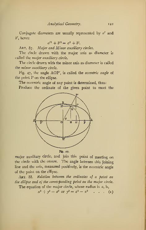
Analytical Geometry. 121
Conjugate diameters are usually represented by a! and
b'yhence
a'2 + b'
2 = a2 + 62
.
Art. 87. Major and Minor auxiliary circles.
The circle drawn with the major axis as diameter is
called the major auxiliary circle.
The circle drawn with the minor axis as diameter is called
the minor auxiliary circle.
Fig. 47, the angle AOP', is called the eccentric angle of
the point P on the ellipse.
The eccentric angle of any point is determined, thus:
Produce the ordinate of the given point to meet the
Fig. 47.
major auxiliary circle, and join this point of meeting on
the circle with the centre. The angle between this joining
line and the axis, measured positively, is the eccentric angle
of the point on the ellipse.
Art. 88. Relation between the ordinates of a point on
the ellipse and of the corresponding point on the major circle.
The equation of the major circle, whose radius is a, is,
+ y2 = a2 or y a' - x' (1)

122 Analytical Geometry.
Call the Point P' (Fig. 47), (xf
,y") and P, (x', /).
(Observe P' and P have the same abscissa.)
Then from (1), y"2 = a2 — x'2(2)
b 2
Also, y'2 = - (a 2 — x' 2
) (3) (from ellipse equation).
Dividing (3) by (2)
2_1 =- \
yff2 a
or ^— = — > whence V : y" : : b : a.y" a
That is, //^ ordinate of any point on the ellipse is to the
ordinate of the corresponding point on the major circle as
the semi-minor axis is to the semi-major axis.
Corollary: Let Q be the intersection of OP' with the minor
circle. (Fig. 47.)
Join Q with P.
Then since OQ = b and OP' = a,
and / : y" : : b : a, / : f : : OQ : OP',
or PD : P'D : : OQ : OP'.
That is, QP is parallel to OD; that is, parallel to the
axis.
Hence RP, the prolongation of QP, to BB', equals OD =the abscissa of P and Pr
. This furnishes another method
of drawing an ellipse. Thus:
Draw two concentric circles with the given major and
minor axes as diameters, respectively, in their normal
positions.
Make any angle with the major axis, as AOPrin Fig. 47,
and let the terminal line of this angle intersect the two
circles in Q and P' respectively. Then the intersection of
the abscissa, RQ, of Q, with the ordinate, P'D, of P', will
be a point on the ellipse.

Analytical Geometry. 12
This may be shown by analytical means, purely, for
(Fig. 47) in the right triangle OP'D, OD (= RP) =OP' cos P'OD = a cos cf>, say, and drawing QE perpen-
dicular to OA,
PD = QE = OQ sin QOD = b sin </>, but the values
a cos<f>
for x, and b sin <j> for y, satisfy the ellipse equation.
a2y
2 +b 2 x2 = a 2b2
,
thus, a 2b2 sin2 $ + a2
b2 cos2
cf>= a2
b2
,
sin2<f)+ cos2
<j) = i,
hence since OD and PD are the co-ordinates of P, P is on
the ellipse.
Art. 89. The eccentric angle between two conjugate
diameters.
Let the eccentric angle of R' (V, y'), the extremity of
R'S' be 6, and that of R (- & , +—Y the extremity of
1
/ A>\ §
>^h\ T'J
Fig. 48.
the conjugate diameter RS be(f>.
(Fig. 48.)
Then in the right triangle OP'T',

124 Analytical Geometry.
cos P'OT' = 511 or cos = - . . (i)OF a
WIn the right triangle OP"T,
-(RT)P"T />
sin P'OT =— =. . [Art. 88]
OP" OP" L J
a_/hS\
b\a) x'That is, sin (180 —
(f>)= sin
<f>= —-—— = — . . (2)
a a
.'. sin cj) = cos 6 from (1) and (2),
whence by trigonometry,
(j> = 90 + 6 or(f>— 6 = 90°
That is, the difference between the eccentric angles of
the extremities of conjugate diameters is a right angle.
Art. 90. By combining the slope equations of two
perpendicular diameters, both expressed in terms of the
slope of one, it is readily proved, as was done under the
parabola, that the locus of their intersections is a circle,
whose equation is
x* + f = a2 + b\
This circle is called the director circle. Also by a similar
process it can be shown that the major auxiliary circle is
the locus oj the intersection of a tangent with the perpendic-
ular to it from a focus.
Art. 91. The ellipse possesses a physical property,
somewhat similar to that possessed by the parabola, namely:
The angle formed by.the focal mdii to any point on the
ellipse is bisected by the normal at that point.
Geometry tells us that the bisector of an angle of a tri-
angle divides the opposite side into segments proportional

Analytical Geometry. "5
to the other sides, hence, if we can prove (Fig. 49) that
F'N : FN : : F'P : FP our proposition is established. It is
necessary then to find values for these four lines in the
same terms. ON the x-intercept of the normal was found
in Art. 78, Cor. to be
where x' is the point of tangency.
Fig. 49.
Let P (Fig. 49) be (x', /).
Then FN = F'O + ON = c + e2x' = ae + e2x',
(since — = e, hence ae),
But
FN = FO - ON = ae - e2x'.
F'P = a + ex' and FP = a - exf. . (Art. 75)
ae + e2x' _ e{a + ex') _ a + exr
ae — e2x' e(a — ex') a — ex'
F'N F'P
FN FPor F'N : FN : : F'P : FP.
It follows from the law of reflection for vibrations, that
if light or sound issue from one focus of an ellipse it will
be reflected to the other focus.
I

126 Analytical Geometry.
Art. 92. The area oj an ellipse.
Draw the major auxiliary circle to the ellipse ABA'B',
and construct rectangles as indicated in Fig. 50.
Then the area of one of these rectangles in the ellipse as
mnpo is
Area mnpo = mn X pn.
Let the points on the ellipse beginning with p be (V, y'),
(#", y"), {xf"^ /"), etc., and the corresponding points on
the circle beginning with R, be (xf
, y x ),{oc"
y y 2 ),(x"
f
, y 3 ) etc.
Then Area mnpo = (x' — x") y'
.
The corresponding rectangle in the circle
mnRS = (xf — x") yv
. m^RS _ lx' — x"\ y x _ y t __ a
mnpo \x' — x") yr yf
b
As this is a typical rectangle each circle rectangle is to
each ellipse rectangle as a is to b, hence by the law of con-
tinued proportion, the sum of all the circle rectangles is to
the sum of all the ellipse rectangles as a is to b.
As the above expression is independent of the size or
Fig. 50.
number of the individual rectangles the relation is the
same when the number of rectangles becomes infinite. But

Analytical Geometry. 127
in this latter case the sum of the areas approach, respec-
tively, the area of the circle and that of the ellipse; hence,
finally,
Area of the circle _ a
Area of the ellipse b
That is, area of the ellipse = — times the area of thea
circle, but area of the circle = ~a 2.
.'. area of the ellipse = — . -a? = nab.a
EXERCISE.
What are the equations of the tangents to the following
ellipses ?
1. x2 + 4 y2 = 4 at the point (f , J).
2. 4 x2 + 9 y2 = 36 at the point (1, f V2).
3. x2 + 3 y2 =
3 at tne Pomt (l> i)-
4. 9 :v2 + 25 v2 = 225 at the point (4, ?).
5. 25 x2 + 100 y2 = 25 at the point (?, 2).
6. x2 + 2 y2 = 18 at the point (?, 1).
7. Find the normal equation to the above ellipses.
8. What are the equations of the tangents to the ellipse
16 y2 + 9 x2 = 144 from the point (— 3, 2) ?
9. What is the equation of the tangent to the ellipse
9 x2 + 25 y2 = 225, that is parallel to the line 10 y—Sx = 5.
10. What is the equation of the tangent to the ellipse
x2 + 4 y2 = 4, that is parallel to the line V31 = 1 ?
11. What is the equation of the tangent to the ellipse
4 x2 + 9 y2 = 36, which is perpendicular to the line
y- 3 x= 5?

128 Analytical Geometry.
12. The subtangent to an ellipse, whose eccentricity is
f, is f . What is the ellipse equation ?
13. Find the equation of the tangent to the ellipse in
terms of the eccentric angle of the point of tangency.
14. What are the equations of the tangents to the ellipse
— + — = 1, which form an equilateral triangle with the
9 4,
axis?
15. What is the equation of the diameter conjugate to
4y + 9 X = ° ?
16. 2 y -{- x = 12 and 2 y = ^ x -f- 3 are supplementary
chords of an ellipse. What is its equation ?
17. The middle point of a chord of the ellipse 2$ y2
-{- 9X2
= 225 is (— 5, 1). What is the equation of the chord?
18. The equation of a diameter to the ellipse 4 x2 + 16 y= 64 is 4 y = x. What is the equation of a tangent to the
ellipse at the end of its conjugate diameter?
19. Find the equation of the tangents to the ellipse
2-*- -j— = i, which makes an angle whose tangent is 316 9
with the line 2 y = x — 1.
20. Find the equation of the normal to the ellipse x2-\-
4 y2 = 4, which is parallel to the line 4 x — 3 y = 7.
21. Show that the product of the perpendiculars from
the two foci upon any tangent is equal to the semi-minor
axis.
22. Find the equation to a diameter of the ellipse
— + 2L = itwhich bisects the chords parallel to
16 9
3 x - 5 = 9.
23. Find the locus of the centres of circles which pass
through (1, 3) and are tangent internally to x2 + y2 = 25.

Analytical Geometry. 129
x2 y2
24. The equation of an ellipse is — + *— = i.
169 144
What is the eccentric angle of the point whose abscissa
is 5?
25. Find the equation of the chord joining the points
of contact [called the chord of contact] of two tangents to
the ellipse 9 x2 + 16 y2 = 144, drawn from (4, 3) outside
the ellipse.
26. Find the locus of the vertices of triangles having the
base 2 a, and the product of the tangents of their base
angles - •
27. The minor axis of an ellipse is 18, and its area is
equal to that of a circle whose diameter is 24. What is
the equation to the ellipse ?
28. The axes of an ellipse are 40 and 50. Find the
areas of the two parts into which it is divided by the latus
rectum.
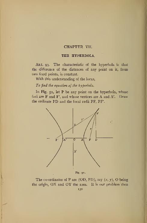
CHAPTER VII.
THE HYPERBOLA.
Art. 93. The characteristic of the hyperbola is that
the difference of the distances of any point on it, from
two fixed points, is constant.
With this understanding of the locus,
To find the equation of the hyperbola.
In Fig. 51, let P be any point on the hyperbola, whose
foci are F and F', and whose vertices are A and A'. Drawthe ordinate PD and the focal radii PF, PF'.
Fig. 51.
The co-ordinates of P are (OD, PD), say (x, y), O being
the origin, OX and OY the axes. It is our problem then
130

Analytical Geometry. 131
to find a relation between OD and PD, and the right tri-
angle PFD suggests itself.
In the right triangle PFD, PF2 = PD 2 + FD 2(1).
Call the focal distance OF, c. Then (1 ) becomes,
pp = r2 = y
2 + ^ _ cy [since FD = OD _ AF =x _ cj
r = vV + (x - cf (2)
In the right triangle F'PD,
PF/2 = PD 2 + F'D 2. That is, r
n = y2 + (x + cf [since
F'D = OD + OF' = x + c] or / = \/y2 + {x+cf (3)
By definition, r1 — r = constant = 2 m, say.
Subtract (2) from (3);
\/y2 + (^ + c) 2 — VV + (^ — c)2 =/— r = 2 m.
Transpose and square;
X+X+2oc + <H= 4m2 + 4m \/y2 + (x — c) 2
-\- yK+xk — 2 ex -}- c\.
Transpose, collect, and divide by 4;
m \/y2 + (x — c)2 = ex — m2
.
Square again;
m2y2 + m2 x2 — 2 m^a. + m2
e2 = e
2 x2 — 2 ?^2~-ea:+ m4.
Collect; m2y
2 + (m2 — c2) x2 = m2 (m2—c2
) . . (4)
To determine m it is only necessary to give • x and ysuitable values, or rather to give y the particular value o,
since the above equation is true for every point on the
hyperbola. We then get the value of x for the vertex, since
the ordinates of A and A' are o.
Letting y = o in (4)
(m2 — c2) x2 = m2 (m2 — e
2),
132 Analytical Geometry.
whence x2 = m2; x = ± m,
but x here equals OA or OA',
hence m = OA or OA';
that is, 2 m = the major axis AA'. As in the ellipse
call AA', 2 a; then m = a, and (4) becomes,
a2
y2 + (a 2 - c
2) x2 = a2
(a2 - c
2) . . . (5)
Let c2 - a2 = b
2,
which by analogy with the ellipse we may call the minor
axis. We shall see that this is justified. Then (5) becomes,
a 2y
2 — b2 x2 = — a 2b2
,
or b2 x2 - a 2
y2 = a 2 b
2 (AA )
Art. 94. A glance at the figure will show that c is
greater than a}hence the eccentricity,
c . .
e = — is > 1.
a
Then in the polar equation for conies
p = —**—„ (« > 1).1 — e cos (7
and by a process exactly like that in Art. 84, this becomes
for the hyperbola,
a (e2 - 1)
P = n'
1 — e cos
Art. 95. To determine b in the -figure of a hyperbola.
The relation c2 — a2 = b
2, immediately suggests a right
triangle with c as hypotenuse. Hence with c as radius
and A or A' as centre, describe arcs cutting the y-axis at
B and B r, OB will equal
b, or BB' = 2 b; for OB 2 = AB 2 - OA2 = c2 - a2.

A nalytical Geometry. S3
It is plain that the curve does not cut this minor axis,
for, setting x = o [the abscissa of any point on BB' = o]
in (Ah ),
a T a 2b 2
y — ± V— b 2 = ± b\/— i, an imaginary value.
Art. 96. To find the length of the focal radii for anypoint, r and /.
or
Fig. 51a.
In Fig. 51a, PF2 = r2 = PD 2 + FD 2
,
r2 = y2 + (x - c) 2
. .
Since e = — » c = ae,a
and (1) becomes,
r2 = y
2 + (x — ae) 2,
(1)
or y2 + x2 — 2 aex + a2
e2
.

134 Analytical Geometry.
By (Ah ),f =b-2
(x2 -a2).
az
b2 x2— b2 + x2 — 2 aex + a 2 e2
a1
b2 x2 + a2 x2
b2 — 2 aex + a 2e2
a"
= (fl2 + P%2 - 2 _ 2 aex + a2 e2_ put ^2 + p
= c2] = —— — b2 — 2 aex -\- a 2
e2 = e2 x2 — 2 aex
+ a2e2 — b
2 = e2 x2 — 2 aex + a2 [since a2
e2 — b2
- b2 = c2 -b2 = a2
]
a 2c2
.'. r= ex- a (3)
By exactly similar treatment of (3) Art. 93, we get,
/ = ex + a (4)
Subtract (3) from (4), / — r = 2 a, which shows that
the constant difference r' — r is always equal to the major
axis.
Art. 97. A comparison of the ellipse and hyperbola
equations shows that if in the ellipse equation — b2
is sub-
stituted for + b2
, the hyperbola equation results; hence
since the fundamental processes in deriving tangent, nor-
mal, and diameter equations are the same for all curves,
the equations for these lines in relation to the hyperbola
can be derived from the corresponding equations in the
ellipse by substituting — b2 for b
2.
Analytical Geometry. 135
For example
:
(a) The ellipse tangent has the equation,
a2yy
f + b2 xx f = a2b2
,
hence the hyberbola tangent is,
a 2 yy' — b2 xx' = — a2 b2
or b2 xxf — a 2yy
r = a2 b2. . . . (Th )
The slope form is,
y = mx ± \/a2m2 - b2
. . . . (Thm )
(b) The normal equation for the ellipse is,
y- y' = TT^ (* "" *')'bl x
hence the normal equation for the hyperbola is,
?-/=-££<*-*') • • •(N»)
(c) The subtangent then is , and the subnormalx
b 2 x'is —"—
, the same as for the ellipse.a2
(d) The equation for a diameter of the ellipse is,
b2
y= — *,azm
hence a diameter to the hyperbola is,
b 2
y = -7— *.
Conjugate diameters are defined in the same way, hence
the product of their slopes, m and mf
, say, is
b2
mm' = — [— 62 replaces 62
].
a2

136 Analytical Geometry.
Art. 98. As the ellipse becomes a circle when its axes
become equal, for when b = a,
a 2y
2 + b2 x2 = a 2
b2 becomes y
2 + x2 = a2,
so if the axes of a hyperbola become equal, we call it an
equilateral hyberbola, which is the hyperbola-analogue of
the circle.
In b2 x2 — a 2
y2 = a 2
b2
, let b = a; then x2 — y2 = a 2
is the equation of an equilateral hyperbola.
Art. 99. The latus rectum of the hyperbola is readily
found from its equation by setting
x = ± c = ± \/a 2 + b2
.
Whence b2(a
2 + b2)- a2
y2 = a 2
b2
b4
, b2
y2 = -
2, y = ± -
a2 a
2 b2 ...2 y = — = latus rectum, since it is the
a
double ordinate through the focus.
EXERCISE.
What are the axis and eccentricities of the following
hyperbolas
:
1. 2 x2 — 3 y2 — 9. 2. x2 — 4 y
2 = 4.
3. 16 y2 - 9 x
2 = 144. 4- 5 x2 ~ 8 r* = 15-
5. 9 y2 — 4 x2 = — 36. 6. 4 y
2 — 3 x2 = 12.
7. #2 — 16 y2 = 16. 8. 4 x2 — 16 y
2 = — 64.
9. What is the equation of a hyperbola, if half the dif-
ference of the focal radii for any point is 7, and half the
distance between foci is 9 ?

Analytical Geometry. 137
10. What is the equation of the hyperbola, whose con-
jugate axis is 6 and eccentricity, ij?
11. The co-ordinates of a certain point on a hyperbola,
whose major axis is 20, are x = 6, y = 4. Find its equa-
tion.
12. The eccentricity of a hyperbola is if, and the longer
focal radius of the point x = 5, is 32. Find hyperbola
equation.
13. In a hyperbola 2 a = 20, and the latus rectum = 5
Find its equation.
14. The conjugate axis = 10, and the transverse axis is
twice the conjugate. Find the equation.
15. The conjugate axis =16 and the transverse axis
= I of the distance between foci. Find the equation.
16. In the hyperbola 25 x2 — 4 y2 = 100, find the
co-ordinates of the point whose ordinate is 2* times its
abscissa.
17. In the hyperbola 25 x2 — 169 y2 = 4225, find the
focal radii of the point whose ordinate is 10 y/2.
Find the intersection points of the following :
18. 16 y2 — 4 x2 = 16 and 2 x — y = 3.
X A. V I19. -LJ-~ = — and 3 y — 2^ + 8=0.
4 9 9
20. 9 y2 — 16 x2 = 144 and x2 + y
2 = 36.
21. 9 y2 — 6 x2 = 36 and 4 x2 + 9 y
2 = 36.
22. 16 x2 — 25 y2 = 400 and 4 x2 + 16 ;y
2 = 16.
23. x2 — v2 = — 50 and x2-\- y
2 = 100.
24. Find the equation of the tangent to the hyperbola
16 y2 — 9 x2 = 144 at the point (V
6, 5).
25. At what angle do 'the curves in Ex. 22 inter-
sect?

i3» Analytical Geometry.
CONSTRUCTION OF THE HYPERBOLA.
Art. ioo. The definition of the hyperbola suggests a
method of mechanical construction similar to that for the
ellipse.
Since the difference between the focal radii is constant,
if a fixed length of string be taken, attached at the two
foci, and the same amount subtracted from each of two
branches, continually, the hyperbola results.
Fig. 52-
In Fig. 52, let a straight edge of length / + 2 a, be
pivoted at F', and one end of a string of length I be fastened
to its free end, N, and attached to the focus F, at its other
end.
A pencil pressed against the straight edge, keeping the
string stretched (as at P), will describe the right branch
of the hyperbola. For at any point as at P,
PF' - PF = (FN - PN) - (NPF - PN) =FN - NPF = l + 2a-l= 2a.

Analytical Geometry. 139
The other branch may be described similarly by pivot-
ing at F, and attaching the string at F'.
Second Method : The hyperbola may also be constructed
by points, making use of the definition. Let AA' [Fig. 52
(a)] be the major axis, F and F' the foci and O the centre.
Fig. 52a.
Let LK [Fig. 52 (b)] = AA'. Extend LK and take any
number of points on LK produced as P, R, S, T, etc. With
Fig. 52b.
LP > LK as radius and F and F', successively, as centres
describe arcs as at G, H, G' and H'; with the same centres
and KP as radius, describe intersecting arcs at G, H, G'
and H'. The intersections will be points on the ellipse for
the radii LP — KP = LK = AA'. The same process
with points R, S, T, etc., will give as many points as desired.
A smooth curve through these points will be the hyperbola.

140 Analytical Geometry.
CONJUGATE HYPERBOLA.
Art. toi. The hyperbola whose axis coincides with
the axis of ordinates is called the conjugate hyberbola to the
one whose axis is the #-axis. MBN — RB'S (Fig. 53).
Fig. 53-
Its equation is readily found to be
a2y
2 - b2x2 = a 2b2
.
Art. 102. If the equations of two conjugate diameters
be combined with the equation to the original hyperbola,
it will be found that the results will be imaginary for one
of the diameters, showing that both diameters do not
touch the original hyperbola. Thus:
Let y=mx (1)

Analytical Geometry. 141
and y =— (2)a2w
be conjugate diameters.
Combining these with
b2x2 - a2y2 = a2
b2
(3)
we get from (1) and (3),
2 a262
b2 — a2m2
from (2) and (3),
a2w2 — tf
If &2 — a2m2
is plus, a 2w2 — b2 must be minus, hence
if the first x2is plus, and hence x, real, the second x2
is
minus, and hence x, imaginary, or vice versa.
But if (2) be combined with the conjugate hyperbola,
a2
y2 — b
2x2 — a 2b2
}
" 2
which is real,• a-rrr
., a2b2
. ,
II — r~T ls real-
b2 — a2m2
Hence conjugate diameters intersect, one, the original
hyperbola, the other, its conjugate, as aa' and bb' (Fig. 53) .
ASYMPTOTES.
Art. 103. An asymptote of the hyperbola may be
defined as a tangent at a point whose co-ordinates are
infinite, which, nevertheless, intersects at least one of the
co-ordinates, axes at a finite distance from the origin.
To find the equation of the asymptotes then, it is neces-

142 Analytical Geometry.
sary to determine a line that will touch the hyperbola at
infinity (Fig. 54).
(1)
NFig- 54-
Let the equation of a line be
y = mx + c . .
and the equation to the hyperbola be
b2x2 - a 2
y2 = a 2
b2(2)
Combining (1) and (2),
b2x2 — a2m2x2 — 2 a 2mcx — a2
c2 = a2
b2,
or x2(b
2 — a2m 2)— 2 a2mcx — (a
2c2 + a2
b2) = o
wherein the values of x are the abscissas of the point of
intersection. By the theory of equations, these values will
be infinite if the coefficient of
that is, if
x' = o,
a"m
or m = ± —a

Analytical Geometry. 143
For in the typical quadratic, ax2 + bx + c = o
— b + V^2 - 4 ac — & - V&2 — 4 acx = ! or - •
2 a 2 a
In either case if the denominator 2 a = o or a = o the
values of x will be infinite, having a denominator o; but a
is the coefficient of x2; hence the rule.
.\ if m = ± — the line y = mx + c meets the hyperbolaa
b2x2 — a2
y2 = a2
b2at infinity.
We found, however, in Art. 107, that the slope equation,
of the tangent to the hyperbola is,
y = mx ± \/a2m2 — b2
;
that is, in y = mx + c, if c = ±\/a2m2 — b2
} y = mx + c
becomes a tangent.
If m = ± —, however,
a
a2m2 - b2=— - b
2 = b2 - b2 = o.
a2
.'. at infinity 3/ = mx + c becomes a tangent if c = o
and m = ± — • Hence the equation to an asymptote is
a
y = — # or y = x.a a
The form of these equations shows that the asymptotes
pass through the origin.
Art. 104. Relation between the equations of the asymp-
totes and that of the hyperbola.
Clearing the two above equations of fractions, trans-
posing and multiplying together,
(ay — bx) (ay + bx) = o,
or a2y
2 — b2x2 = o or b2x2 — a 2
y2 — o.
144 Analytical Geometry.
Comparing this with b2x2 — a 2y
2 = a 2b2
, it is observed that
they are the same except for the constant term a 2b2
, hence
given its two asymptotes it is easy to write the equation of
the hyperbola, or vice versa.
If y = — x and y = — — x are the equations of thea a
asymptotes to a hyperbola, its equation may be written,
b 2x2 - a2y
2 ± C = o (n)
the minus sign of C indicating the primary hyperbola; the
plus sign, its conjugate. If in addition a point is given
through which the hyperbola must pass, C can be deter-
mined.
For example : The asymptotes of a hyperbola are y = J x
and y = — J x. If the hyperbola passes through the
point (6, 2X^2), to find its equation. The equation will be
(2 y — x) (2 y + x) ± C = o
or 4 y2 — x2 ± C = o.
Substituting;
4 (2 V2) 2 - (6)2 ± C= o,
whence C = ± 4, whence 4 y2 — x2 ± 4 = o are the equa-
tions to primary and conjugate hyperbola.
Corollary: The same principle will clearly apply no matter
where the origin is taken, since both hyperbola and asymp-
totes are referred to the same point as origin, and hence
the relation between their equations remains the same.
For example, if 2 y — 3 x — 1 = and y-\-2x-\-^=o,
are the asymptotes of a hyperbola, its equation is,
(y + 2 x + 3) (2 y - 3 x - 1) ± C - o.
Art. 105. It is often desirable to refer the equation of a
hyperbola to its asymptotes as axes.

A nalytical Geometry. *45
By determining the angles made by the new axes (the
asymptotes) and the old, and using the transformation
equations (J'), Art. 38, the result is most readily
achieved.
These equations are
6 = reflex Z *ON
y =
X =
= xfsin
= x' cos
6 +y'
+ /sin (j>) \COS
(f)))
N == z- xON, 6 = MO*
(JO
(Fig- 55 )•
Fig. 55-
Since the new axes are asymptotes, their slopes are
H— and — — from their equations, that is,
a a
tanb
.
Jtan = &_
a a

146 Analytical Geometry.
whence by Goniometry,
sin 6 = ,
b, cos =
Va2 + b2
'
Va2 + b2
'
• , b r asin =
, cos =Va2 + b
2 Va2 + b2
Substituting these values in (J'),
Va2 + 62
Va2 + 62
Substituting (1) and (2) in the hyperbola equation,
b2x2 — a 2
y2 = a 2
b2
,
a2b2
, , , , x , a262
(/ + *') 2 - ~^~ (/ - *') 2 = M2,
a2 + b2 ' ' a2 + 6 2
or (/ + x') 2 - (/ - x') 2 = a2 +P,
whence 4 x'y' = a2 + &2
.
Dropping accents,
4 xy= a2 + b2 = c2
. . . . (Afl> h )
which is the equation of a hyperbola referred to its asymp-
totes.
It shows that the co-ordinates of a hyperbola referred to
its asymptotes vary inversely as one another.
Art. 106. Equation of the tangent to the hyperbola
referred to its asymptotes.
Pursuing exactly the same method as before, we deter-
mine the equation of a secant line and revolve this line to a
tangent position.

Analytical Geometry. 147
The equations of any line through (x', y') and (x", y") is
y - y - $^i (* - *o • • • (fi
)
If the points (x', /) and (x", /') are on the hyperbola,
they must satisfy $xy = c2
.
.'. 41'/ = c2
(1)
4X"y» = c2
(2)
Subtracting (1) from (2) and simplifying;
x"y — x'y' =0 or x"y" = x'yf
. . . (3
)
Subtracting x"y' from both sides to get the value of —
'
x"— xf
x"f _ yy _ xf
yf _ x»y'
.
Factoring; x" (y" - /) = - y'(x" - x')
or y~
y =- y~
.
%A/ *V vV
Substituting in B,
y — yf = — „ (x — x') (4). [The equation of a secant.]
As the points approach coincidence x" approaches x'
and y" approaches y', and eventually x" = x', y" = y'.
Substituting in (4);
y - y = - 2j (X - x')
x
whence x'y — x'y' = — xyf + x'y
x'y + xy' = 2 x'y',
or y- + ^=* CT4 .)y x

148 Analytical Geometry.
EXERCISE.
Tangents and Asymptotes.
Find the equation of a tangent to the following hyper-
bolas:
2 x2 — 3 y2 — 12, at (12, 2).
2. 16 y2 — g x2 = 144, at (4 v 3, 6).
3. x2 - 4 7*= 4 at (?, |).
4. 16 x2 - 9^2 = 144 at (?, 3).
5. 25 v2 - 16 x2 = 400 at (3f, ?).
6. 36 y2 - 25 *2 = 900 at (3 J, ?).
7. Find the normal to each of the above.
8. What points on a hyperbola have equal subtangent
and subnormal ?
9. What are the equations of the tangents to the hyper-
bola 16 x2 — 9 y2 = 144, parallel to the line 3 y— 5^ + 3=0?
10. What are the equations of the tangents to the hyper-
bola x2 — 4 y2 = 4, perpendicular to the line y = — 2 # + 3 ?
11. What is the equation of the normal to the hyperbola
x2 — 4 y2 — 4, perpendicular to the line y — — 2 x -f 3 ?
12. Find the equations of the common tangents to
16 x2 — 25 y2 = 400 and x2 + y
2 = 9.
13. Find the slope equation of a tangent a 2
^2 — b
2x2 =a2b
2.
14. Find the equations of tangents to the hyperbola
2 x2 — y2 = 3, drawn through the point (3, 5).
15. Find the equations of tangents drawn from (2, 5) to
the hyperbola 16 x2 — 25 y2 = 400.
16. Find the equations of the tangents to the hyperbola
16 y2 — 9 x2 = — 144, which with the tangent at the
vertex form an equilateral triangle.
17. Find the angle between the asymptotes of the hyper-
bola t6 x2 — 25 y2 = 400.
Analytical Geometry. 149
18. What is the equation of the hyperbola having
y — 2 x + 7 = o and 3 x + 3 y — 5 = o for its asymp-
totes, if it passes through (o, 7 ) ?
19. Show that the perpendicular from the focus of a
hyperbola to its asymptote equals the semi-conjugate axis.
20. Find the equations of the tangents to the hyperbola
9 y2 — 4 x2 — 56 at the points where y — x = o intersects it.
21. A tangent to the hyperbola g x2 — 25 y2 = 22$ has
the x-intercept = — 3. Find its equation.
22. Two tangents are drawn to 9 x2 — 4 v2 = 36 from
(1, 2). Find the equation of the chord joining the points
of contact.
23. The product of the distances from any point on a
hyperbola to its asymptotes is constant. What is the
constant ?
24. Show that the sum of the squares of the reciprocals
of the eccentricities of conjugate hyperbolas equals unity.
25. The equation of a directrix of the hyperbola
b2x2 — a2
y2 = a 2
b2
, being
x = — [c = Va2 + b2
\c
show that the major auxiliary circle passes through the
points of intersection of the directrix with the asymptotes.
Art. 107. Supplemental chords.
Supplemental chords in the hyperbola are denned as
they were in the circle and ellipse, hence from the relation
between ellipse and hyperbola the relation between the
slopes of supplemental chords in the hyperbola is,
b2
mm' = —^ [putting — b2 for b
2 in ellipse condition].
Since this is also the relation between the slopes of conjugate

i5° Analytical Geometry.
diameters, it follows that there is a pair of diameters parallel
to every pair of supplemental chords, which suggests an
easy method of drawing conjugate diameters.
Art. 108. The 'eccentric angle.
Since the ordinates of the hyperbola do not cut the
auxiliary circles, the eccentric angle of a point is not so
Fig. 56.
readily determined as in the ellipse and a more arbitrary
definition is necessary. The angle<f>
so determined that
x = a sec cf) and y = b tan<f),
is called the eccentric angle for the point (x, y). These
values will satisfy the equation
b2x2 - a2
y2 = a2
b2
;
for substituting;
a2b2 sec2
<£ - a2b2 tan2
<f>= a2
b2,

Analytical Geometry. 151
or sec2(j) — tan2
<f>= 1.
which is true by goniometry.
To construct this angle for a given point, the auxiliary
circles [with radii a and b] are drawn. (Fig. 56.)
Let P be any point on the hyperbola. Draw its ordinate
PD and from the foot of PD draw a tangent to the major
auxiliary circle touching it at C, then Z. COD = cj> for
point P, (x, y).
For, draw BE a parallel tangent to the minor circle, then
in the right triangle OCD,
cos COD = — = - [OD = abscissa of P]OD x
L J
or x = a sec COD (1)
Again in the right triangle OBEBF
tan BOE = tan COD = —- ... (2)OBThe triangles COD and BOE are similar.
.-. OB :OC : : BE : CD,whence
BE _. OB X CD __ OBVOD 2 - OC2 _ b\/l
OC OC a
or BE 2 = — (x2 - a 2).
a 2
But y2 = -' (x2 - a 2
) from (A, ). .-, BE = y.a 1
Hence from (2) tan COD = <-
b
or y= Man COD ... (3)
Comparing (1) and (3) with the condition equations
for cf>, we see that COD = <£.
Hence the eccentric angle is found by drawing from

r 52 Analytical Geometry.
the foot of the ordinate of a point, a tangent to the major
auxiliary circle. Then the angle formed with the axis by
the radius drawn to the point of tangency is the eccentric
angle for that point. The eccentric angle is used to best
advantage in the calculus.
Art. 109. There are two interesting geometrical prop-
erties of the hyperbola when referred to its asymptotes.
(a) The product of the intercepts oj any tangent on the
asymptotes is the same.
Let BPC (Fig. 57) be a tangent at P, then its intercepts
on Ox and Oy (OB and OC), respectively, will be found
by setting successively y = o and x = o in its equation,
(x', y being point P),
£ 4-- =2/ X
whence x = OB = 2 x'
and y= OC= 2/

Analytical Geometry. 153
multiplying; OB . OC = 4 x' yf = a2 + b 2
(a constant).
Since xfy' is on the hyperbola 4 x'y' = a2 + ft2
.
(6) TVze area a/ ///e triangle formed by a tangent and the
asymptotes is constant. The area of the triangle BOC(Fig. 57), by trigonometry, is
Area BOC = sin . BOC = sin 2 <h
2 2
[COA = BOA = 0, Art. 105] = OB . OC sin <£ cos </>
[since sin 2 = 2 sin cf> cos cj) ]=
b a nhOB . OC. / =OB . OC
\/a2 + b2 Va2 + b
2 ~" ' a 2 +62
'
But OB . OC = a2 + &2
.
.*. area BOC = (a2 + o 2) _^_ = ab.K
a2 + b2
That is, the area of this triangle always equals the product
of the semi-axes.
EXERCISE.
General Examples.
1. If y = 3 x -\- 15 is a chord of the hyperbola
36 x2 — 16 y2 = 576, what is the equation of the supple-
mentary chord ?
2. The point (5, f ) lies on the hyperbola 4 x2 — 9 ;y
2=36.
Find the equations of the diameter through this point and
of its conjugate.
3. Find the equation of the line passing through a focus
of a hyperbola and a focus of its conjugate hyperbola.
4. Find the angle between a pair of conjugate diameters
of the hyperbola, b2x2 — a2
y2 = a 2b2
.

154 Analytical Geometry.
5. Find the equation of the chord of the hyperbola
9 x2 — 16 y2 = 144, which is bisected by the point (2, 3).
6. Show that the locus of the vertex of a triangle, whose
base is constant, and the product of the tangents of its base
angels is a negative constant, is a hyperbola.
7. Show that the eccentric angles of the extremities of
a pair of conjugate diameters are complementary.
8. What is the equation of the focal chord which is
bisected by the line y = 6 x?
9. In the hyperbola 9 x2 — 16 y2 = 144, what is the
equation of the diameter conjugate to y — 3^=0?10. Show that tangents at the ends of conjugate diam-
eters intersect on the asymptotes.
11. The base of a triangle is 2 b and the difference of
the other sides is 2 a. Show that the locus of the vertex is
a hyperbola. [Take the middle of the base as origin.]
12. For what point of the hyperbola xy = 12 is the sub-
tangent = 4?
13. Show that an ellipse and hyperbola which have the
same foci intersect at right angles.
14. What are the equations of the tangents to the hyper-
bola x2 — 4 y2 = 4, which are perpendicular to the asymp-
totes ?
15. In the hyperbola 25 x2 — 16 y2 = 400, find the
equations of conjugate diameters that cut at an angle
of 45°.
16. In the hyperbola 16 x2 — 25 y2 = 400, what are
the co-ordinates of the extremity of the diameter conjugate
to 25 y + 16 x = o?
17. In the hyperbola 4 x2 — 9 y2 = 36, the equation of a
diameter is 3 y — 2 x = o. What is the equation of any
one of its system of chords ?

CHAPTER VIII.
HIGHER PLANE CURVES.
Art. ioi. There are several other curves known as
Higher Plane Curves because their equations are more
complex, that are used extensively in engineering. These
we will consider briefly.
THE CYCLOID.
The cycloid, much used in gear teeth, is the curve gener-
ated by a point on the circumference of a circle of given
radius, as the circle rolls along a straight line. The circle
may be called the generator circle, and the straight line the
directrix.
Fig. 58.
To -find its equation. Let P( Fig. 58) be the generating
point, r the radius CP, OE = x and PE = y for P, and
call Z PCB, 0.
Then PE = CD - CB = r - r cos 6.
J 55

156 Analytical Geometry.
That is, y = r — r cos (1)
Also x = OE = OD - ED = OD - PB = rd -r sin 6 (2)
Since 6 is an extra variable, its elimination is necessary.
From (1) cos = r ~ y = 1 — 2-,
r r
whence
1 — cos 6 = vers 6 = 2. or = vers-1 2. .
Substituting this value of 6 in (2),
x = r vers x 2- — ? in(vers x —
J
or x = r vers x 2- — >/2 ^ _ y* #
For vers-1 2- = #,
r
Z. = vers d=i — cos 0,?*
! _ 1 = COS 0, /?L^^2
\ = COS2 0.
x _ (L^f\ = "?-y8
= , _ C0S2 d = sin2 ^
Whence sin = —^—2- 2—
,
and r sin 6 = r sin (vers-1
<-J =V'2 ry — y
2

Analytical Geometry. 157
CONSTRUCTION OF THE CYCLOID.
Art. hi. From the nature of the development of the
cycloid, it is readily constructed by points. The first
method to be shown produces an accurate cycloid if suffi-
cient points be taken.
The second method, which is employed in mechanical
drawing, gives a cycloid of sufficient approximation.
First Method : Let M be the generator circle in its
middle position, and XX' the directrix. Make OV equal
\ the circumference of M. Divide the semi-circumference
OCN into 6 equal parts, also OV into 6 equal parts. Then
K '-4s!g^---^
cx(° \
NB'/ \B
M)
kI \A /y t s
—1
—
R—
+
P^- |
Q P #
—
x
Fig. 59-
clearly the 6 points on OCN would exactly coincide with
the 6 points on OV if the circle were rolled back toward V.
Through the division points on OCN: A, B, C, D, E,
draw lines parallel to the directrix. Now if the circle were
revolved toward V until A and P coincided, then N would
be on the level now occupied by E, that is, it would be
somewhere on the parallel through E; N would still be the
same distance from A that it now is; hence if we take a
radius AN, with P as a centre, we will cut the parallel
through E in the place where N was when A was at P.
Likewise with Q as a centre and radius BN, cut the parallel
through D, and we have the position of N when B was at
Q. The same process continued will give all the succes-

i58 Analytical Geometry.
sive positions of N, and if these be joined by a smooth
curve, we have the cycloid described by N.
Art. 112. Second Method: This approximate construc-
tion used in mechanical drawing is based on the fact that
for very small arcs the arc does not sensibly differ from its
chord, so the divisions are " stepped off " with the com-
passes, thus really getting chords not arcs, but by taking
the distances small enough, any degree of approximation
may be attained.
Draftsmen use this slightly modified method, which
gives a sufficient approximation, as follows:
Fig. 60.
Fig. 60. Let MN be the directrix and C the generator
circle. Lay off any small distance on MN a sufficient
number of times choosing the distance small enough so that
as a chord it would not sensibly differ from its arc, as AB.
Then AB, BC, CD, etc., will practically equal corresponding
arcs on C. Draw a series of circles (or parts of them)
having the radius of C. These represent the generator
circle in its successive positions.
From B, C, D, etc., successively " step off " with com-
passes on the arc passing through them, 1, 2, 3, etc., units
(as AB). These will give points on the cycloid as A', B',
C, D', etc. The curve drawn through these points will be
a very good approximation.
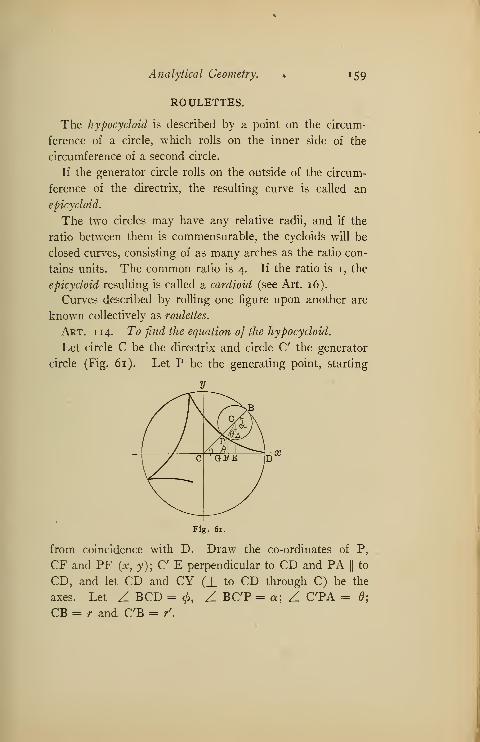
Analytical Geometry. *59
ROULETTES.
The hypocydoid is described by a point on the circum-
ference of a circle, which rolls on the inner side of the
circumference of a second circle.
If the generator circle rolls on the outside of the circum-
ference of the directrix, the resulting curve is called an
epicycloid.
The two circles may have any relative radii, and if the
ratio between them is commensurable, the cycloids will be
closed curves, consisting of as many arches as the ratio con-
tains units. The common ratio is 4. If the ratio is 1, the
epicycloid resulting is called a cardioid (see Art. 16).
Curves described by rolling one figure upon another are
known collectively as roulettes.
Art. 114. To find the equation of the hypocydoid.
Let circle C be the directrix and circle C the generator
circle (Fig. 61). Let P be the generating point, starting
y
Fig. 61.
from coincidence with D. Draw the co-ordinates of P,
CF and PF (x, y);CE perpendicular to CD and PA||to
CD, and let CD and CY (J_ to CD through C) be the
axes. Let Z BCD = 0, Z BC'P = a; Z C'PA = 6;
CB = r and C'B = /.

160. Analytical Geometry.
Then CF = CE - FE = CE - PA = CC' cos -C'P cos d or x = (r — r') cos
(f>— r' cos 6.
Extend C'P to meet CD at G; Z C'GD = d, and
a = cj) + C'GC =<f> + (180 - 0)
[a is exterior angle of triangle C'GC].
Hence a — <j> = 180 — d.
cos (a —<f>)
= cos (180 — 6) = — cos [Goniometry].
Substituting in (i);
x = (r — r') cos cf> + / cos (a — 0) . . (2)
Likewise, ;y= (r — /) sin cj) — r' sin (a. — cj)) . . .(3)
But since arc BD = arc BP by method of descrip-
tion of the hypocycloid rd> = r' a, or a =-~•
r
Substituting in (2) and (3);
a; = (f — /) cos(f>+ / cos ' ^-
. . (a)r
y = (r — /) sin d> — r' sin - '-%. . (b)
r'
If<f>
be eliminated between (a) and (&) the rectangular
equation for the hypocycloid results, but in this general
form the equation would be exceedingly complicated.
But if r = 4 rf
, as is customary, the result is compara-
tively simple, thus:
(a) becomes; x = f r cos </> -f i r cos 3 <£.
(ft) becomes; y = f r sin <£ — ^ r sin 3 0,
or » = - (3 cos (/>+ cos 3 <£) . . (a')
4
and y = _ (3 sin <£ — sin 3 0) . . (&')
4
By Trigonometry j3 cos ^ + cos 3 ^ = 4 cos^
.
) 3 sin <£ — sin 3 <£ = 4 sin3

Analytical Geometry. 161
Hence (af
) becomes x = r cos3cf> . (a")
and (b') becomes y = r sin3
<f>. (b")
Combining {a") and (b"); x$ = r* cos2<j>,
yl = ^§ sin2 <^
Add; *3 + yi
Art. 115.
sin 2<£ = 1
J,r% [since cos 2
<£
T(7 construct the hypocycloid.
Let C be the directrix; (Fig. 62) C the generator circle;
P the generating point. Divide the quadrant P'K into 8
equal parts and the semicircle PE' into 4 equal parts. Let
P start at P', then when A' and A coincide as the circle CK
Fig. 62.
rolls, P will be at the distance DD' from P' and at the dis-
tance AT from A. Hence with P' as a centre and DD'as radius describe an arc intersecting another described
with A as centre and AT as radius. This intersection
point will be a point on the hypocycloid.
When B' is at B, P will be at the distance BB' from P'
and at the distance BT from B. The intersection of arcs
described with centres P' and B and radii BB' and BT,
respectively, will be a second point on the hypocycloid,
and so on.

162 Analytical Geometry.
Evidently the greater the number of equal parts into
which the quadrant and the generator circle are divided
the more accurate will be the hypocycloid.
If the ratio of the radii of the two circles is 3, the entire
directrix will be divided into 3 times as many parts as the
circumference of the generator circle and similarly for any
ratio. In the figure 62 the ratio is 4.
Art. 116. Draftsman's method 0} constructing the hypo-
cycloid.
This method is almost exactly similar to that described
for the cycloid, using, however, angular division of the
directrix, which is now a circumference.
F
Fig. 63. Let C be the centre of the directrix and C the
generator circle. " Step off " on the circumference of C
any small equal arcs as AB, BD, DE, etc.; at A, B, D, etc.,
draw tangent circles equal to C. From A, B, C, D, E, etc.,

Analytical Geometry. 163
successively " step off "1, 2, 3, 4, etc., times the distance
AB, the resulting points ^ill determine the hypocycloid.
An exactly similar process will produce the epicycloid, if
the generator circle be rolled on the outside.
Art. 117. Another form of roulette is the involute,
which is described by a fixed point on a straight line, that
rolls as a tangent on a fixed circle. Let C (Fig. 64) be the
directrix circle and MN the initial position of the line.
Fig. 64.
" Step off " any small equal arcs on the circumference of
C as AB, BD, DE, etc. Draw tangents at the points of
division and beginning with A stepoff, successively 1, 2,
3, 4, etc., times the distance AB on the tangent lines. The
resulting points will determine an involute. Any curve
whatever will produce an involute in this way, but the
circle is most commonly used. A gear tooth is made up
of cycloid, evolute, and circular arc in varying proportions.
SPIRALS.
Art. 118. A spiral is described by a point receding,
according to some fixed law, along a straight line that
revolves about one of its points. There are a number of

164 Analytical Geometry.
spirals, one of which will illustrate this type of curve. Therevolving line is called the radius vector and the angle it
makes, in any position, with the initial line, is called the
vectorial angle.
The hyperbolic spiral is the curve generated by a point,
which moves so that the product of radius vector and
vectorial angle is constant.
Fig. 65.
Calling the radius vector, r; the vectorial angle 6 and the
constant C, we have by definition,
r 6= C.
To construct it when C = 11, then r = — •
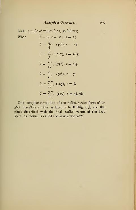
Analytical Geometry. 165
Make a table of values for r, as follows;
When = o, r = 00 , ^ = 3^.
= *, (45°), r= i4.
4
7T
3
' (6o°), r = 10.5
5£12
(75°), r = 8.4.
7T
2(9o°), r = 7.
Z_E (105), r == 6.12
0= ^, (i35), r=4§,etc.12
One complete revolution of the radius vector from o° to
360 describes a spire, as from 00 to B [Fig. 65], and the
circle described with the final radius vector of the first
spire, as radius, is called the measuring circle.


ELEMENTARY CALCULUS.
.67


ELEMENTARY CALCULUS,
CHAPTER I.
FUNDAMENTAL PRINCIPLES.
Art. i. Variables and constants. Suppose we wish to
plot a curve, corresponding to the relation y = x3 + 2 x2
— 5 x — 6; and for this purpose assign to x certain arbi-
trary values, calculating from these the corresponding and
dependent values of y. Now in such a case both x and y
are variable quantities, x being called an independent,
and y a dependent variable.
In general: A Variable is a quantity which is subject to
continual change of value, while an Independent Variable
is supposed to assume any arbitrary value, and a Depen-
dent Variable, is determined when the value of the Inde-
pendent Variable is known.
Examples : y = x*, y = tan x, y = log x.
In the above examples x is the independent, and y the
dependent variable.
When a quantity does not change or alter its value such
as iz — 3. 141 59 . . . , it is called a Constant Quantity, or
simply a Constant.
Art. 2. Functions. Let us again take the equation
y = x3 + 2 x2 — 5 x — 6 ; we know that for every value
of x there is a corresponding value of y; not necessarily
different, for if x = 3, v = o, and if # = 2, y = o, but
169
170 Elementary Calculus.
nevertheless to each value of x there corresponds a certain
definite value of y. When two quantities, x and y, are
related in this manner we say that y is a function of x.
In the examples given above, namely, y = tan x, y = x4
,
y = log x, we see that in each case if we assign a value
to x there corresponds a definite y value; we therefore call
y a function of x.
Again, if we note the barometer readings corresponding
to each hour of the day, we can involve the observations
in a curve, and we say that the height of the barometer is a
function of the time, because to each change in the time
there corresponds a certain definite barometric height.
It is equally true that the barometer readings are a func-
tion of the time.
In general, A quantity P is a junction of a quantity Q,
when to every value which Q can assume there corresponds
a certain definite value 0} P.
It is customary to express the term " function of " by
the symbols F, /, (Phi); thus we write sin x = F (x),
sin x = / (x) or, sin x = cj> (x), meaning that the sine of
an angle is a quantity which assumes certain definite values
dependent upon the size of the angle x. Again, if y— cos x,
then y = f (x) or in the case of an equation such as
y = x3-\- 2 x2 — 5 x — 6 we may also write y = f (x).
This latter mode of expressing an equation briefly by
the symbol y — F (x) or y = j (x) is in very general use.
From the definition of a function, given above, we see
that if an expression involves any quantity, it is itself a
function of that quantity; for example, —— is a function of
x, since this fraction has a definite value corresponding to
each change in the value of x, likewise 3 cos a + 5 tan a
is a function of a.

Elementary Calculus. 171
Further, the area of a triangle is a function of its base
and also of its altitude. Such a double relation is indicated
thus: area A = / (b, h), while the area of a square is a
function of its side. If x is a side and y the area, then
y = x2; we may write this equation in the general form
y = / (x). Again, the volume of a sphere is a function of
its radius, or V =<f>
(r).
Art. 3. Object of the Differential Calculus. In algebra,
geometry, and trigonometry, the quantities which enter
into the calculations are fixed; they have absolute unchang-
ing values.
Now, suppose we wish to find the greatest value that ycan assume, between x = 3 and x = 2 when y = x3 + 2 x2
— 5 x — 6. Here we have two variables, x and y, entering
into the calculation, each of which may have an infinite
number of values and from which one special value of x
is sought, which is defined by the condition imposed.
A problem, such as the above, involving the relation of
two or more variable quantities, comes within the province
of the differential calculus. In general the differential
calculus supplies us with a means of obtaining informa-
tion regarding the properties of quantities, the number of
whose values are infinite, and which vary according to
some known law.
One of the chief advantages of the calculus lies in the
comparative simplicity with which complex problems
involving variable quantities are solved, problems, which
if attacked by other methods, would require long and
tedious operations and sometimes be impossible of solu-
tion.
Art. 4. The Differential Coefficient. Suppose an ob-
server to take notice of a passing bicyclist, and to estimate
his speed at 10 miles an hour; now, a statement to this

17 2 Elementary Calculus.
effect would imply that the bicycle at the moment of obser-
vation was travelling with a velocity, which if maintained
for the next hour, would cause the rider to cover 10 miles.
It does not follow, however, that this will be the case, for
5 seconds later the speed of the bicyclist might be either
reduced or accelerated; further, the above statement in
no way refers to the velocity of the bicycle prior to the
time of observation, having reference to the speed only, at
the exact moment when the bicyclist passed the observer.
Should it be desired to make an accurate determination
of the speed of the machine, we might place two electrical
contacts in its path, which on closing would cause the
time taken in traversing the space between them to be
automatically registered. Then if v = velocity, s = space,
st = time, we have v = — as a measure of the velocity.
In choosing a position for the second contact, we would
undoubtedly select a point near to the first; because the
speed of the machine at the moment of passing the first
contact would be unlikely to remain constant for a space
say of ioo yards, but would be less liable to change in 10
yards, less in i yard, still less in i foot, and so on.
Hence it is, that if we wish to obtain an accurate result,
giving the velocity of a body at the moment of passing a
certain point, we measure as short a, portion of its path as
is practicable, and divide by the correspondingly small
time interval.
Let us now examine a case of uniform motion ; suppose a
point to travel a distance of 30 miles in 6 hours with uni-
form velocity. Now, uniform velocity implies that equal
lengths of path are traversed in equal times, no matter how
small are the time intervals considered. Hence a point
travelling 30 miles in 6 hours, at uniform speed, travels

Elementary Calculus. 173
5 miles in 1 hour, 1 mile in one-fifth of an hour, and so on,
as indicated in the following table
:
Space described(in miles)
.
Time(in hours).
Velocity(in miles per hour)
.
SO 6 v = _226
= 5
5 1 V = 5
1
= 5
11
5
V = 1
.2
= 5
1 1V = .1 = 5
10 50 .02
1 1V — .01 = 5
100 500 .002
1 1V = .000001 = 5
1000000 5000000 .0000002
1 1- V = .000000000001 = 5
I000000000000 5000000000000 .0000000000002
Now it is most important to note, that no matter how
small the space traversed may be, even if beyond all possi-
bility of measurement and conception, the ratio of any
such exceedingly small space to the minute time interval
taken in traversing it, invariably gives as a quotient 5,
in the example cited. The last space taken, which is
.000000000001 miles is equivalent to about one-six hundred
millionth of an inch, while the corresponding time interval
is .0000000000002 hours, which is approximately three
billionths of a second; the ratio - is nevertheless equal to
5, giving a velocity of five miles an hour.

174 Elementary Calculus.
In general we may state that the ratio of two quantities,
each of which is so small as to be entirely beyond our com-
prehension, may, nevertheless, result in an appreciable and
practically useful quotient, a fact which should be most
carefully noted.
When we wish in general to indicate that we are consid-
ering a small finite space, we employ the symbol As, while
AsAt is used to express a short time interval. Thus —
A*
means that we are comparing a small space with a corre-
spondingly small time interval.
In the example above, we have:
4^ =5 or As = 5 . At.At
Carrying this conception still further we may consider
As to become smaller than any imaginable quantity; in
other words, that the space taken is infinitely small This
we indicate by ds, and call ds a differential of space.
The same process of reasoning applied to "A^ gives dt
as representing an infinitely small time interval or a differ-
ential of time. We often refer to ds and dt simply as differ-
entials. The infinite reduction of the space and time will
not affect the value of their ratio. We will still have
— = c and ds = c . dt.
dt5 5
The value of the ratio of two differentials such as ds
and dt, is referred to by German mathematicians as a
differential quotient; hence 5, in our case, is called a
differential quotient.
Again, if we write the expression, -j- = 5 in the formdt
ds = 5 . dt, then 5 becomes a coefficient, for it multiplies

Elementary Calculus. J 75
the differential of the dependent variable dt and is there-
fore called a differential coefficient.
For the present the student might consider a differen-
tial quotient, in general, as the value of the ratio of two differ-
entials; while the term differential coefficient implies the
same quantity regarded as that factor of the differential of
the independent variable which makes it equal to the differ-
ential of the dependent variable.
It will be found later that these conceptions are suscep-
tible of a deeper meaning and lead to results of great prac-
tical value.
Progress in the study of the calculus, primarily depends
upon the thorough understanding of the meaning of the
differential quotient or coefficient. Much misunderstand-
ing has arisen from the fact, that when we have such
expressions as above, viz. —=5 and also ds = 5. dt, it is
dt
customary to speak of the 5 in either case as a differential
coefficient; in the former case it is strictly a quotient, which
quotient becomes a coefficient when we write ds = 5. dt.
Art. 5. Rates of Increase.
Suppose we have a square Ax(see Fig. 1), a side of which
A, A 2 A 3
Fig. 1.
is of unit length; further imagine that while the left lower
corner remains fixed, the sides are capable of continuous

176 Elementary Calculus.
uniform extension, so that the square A1assumes larger
and larger proportions, thus passing, during this continuous
expansion, through the dimensions shown by A2 , A 3 , A4,
in which the side of each new square is one unit greater
than that of the preceding. Now by an inspection of
Aj, A2 , A 3 , A4 , we see that
Square.Side in Linear Area in Square Area Increase in
Units
.
Units. Square Units.
Aa
I I
A2 2 43
A3 3 9
5
7A 4 4 16
Note that if the side of each square is increased by addi-
tions of one linear unit, the area increases by 3, 5, and 7
square units, and as the side lengthens, the greater is the
proportionate increase oj area, in fact the square might be
considered as growing with an accellerated inerease of area.
As before said we are considering that the square continu-
ously expands; now in order to compare the increase in
area with the increasing length of the side, we find it con-
venient to assume an arbitrary unit of time. Hence we
say the rate of increase oj the square is greater than the rate
oj increase of its side.
This assumption, which is very general, enables us to
compare the relative rate of increase or decrease of any
two mutually dependent quantities. Thus we say the rate
of increase of the volume of a sphere, in units of volume, is
greater than the rate of increase of its diameter,' in linear
units, and so on.
Let us return to the case of the bicycle and the observer
(Art. 4); we found, that if we wished to calculate the actual

Elementary Calculus. 177
speed of the bicycle at the moment of passing the point of
observation, then the smaller the space measured, the more
accurate would be our results; this would clearly hold if
the bicyclist passed the observer with an accelerated velocity.
Now this case is similar to that of the square above men-
tioned, for suppose the side of the square, which is con-
tinuously lengthening, pass through the point at which
x = 3 linear units, we might ask ourselves, what is the
relation of the rate of increase of area of the square, at the
moment when x = 3 to the rate of linear increase of its
side.
Let the side x = 3 centimetres, and let y be the area of
the square on x; we thus get
y = x2 = 9. Now let the side x
receive a small increase, called
an increment, which we will
represent by Ax (read, delta x),
let A x = 0.1 centimeters; thus x
becomes x + Ax= 3 + 0.1 = 3.1.
Upon the increased side describe
a second square; we now have
two squares (see Fig. 2), and
the increase in area of y, due
to the increment Ax, is represented by the shaded strip;
this increment, which we will call Ay, is obviously an
increment of area. We thus have:
Area of square on (x + Ax) = {x-\-Ax) 2= (3.i) 2=9.6i.
Area of square on x = x2 = (3)2 =9.
Difference (x + Ax) 2—
x
2 = Ay =0.61.
Now the difference Ay = 0.61, is the increase in area of
the square y, in square centimetres, during the time
that x increased from x = 3 to #=3.1 centimetres; intro-

178 Elementary Calculus.
during the arbitrary unit of time before alluded to, we
say:
Rate of increase of square y _ 0.61 _ Ay _ ,
Rate of increase of side x .1 Ax
We will now tabulate a number of values, calculated
exactly as above, for —2-, for x = 3 centimetres:
Ax
If Ax = 0.1 then —2. = '-— = 6.1Ax .1
A Ay .0601 £Ax = .01 —z = = 6.01.Ax .01
A Ay .006001 ,Ax = .001 -~ — = 6.001.
Ax .001
* Ay .00000060000001 ,Ax = .0000001 —*- — = 6.0000001.Ax .0000001
We thus see that —^ approaches the value 6 more andAx
more nearly, the less the increment Ax.
If Ax is infinitely small, in other words becomes the
differential dx, then the number of zeroes to the right hand
of the decimal point before the one would be infinite, and
the value of the quotient would be truly 6. If Ax becomes
a differential of length, dx, then Ay, becomes a differential
of area, dy; and as the quotient 6 is the result of the com-
parison of these two differentials, it is, therefore, a differen-
tial quotient; thus we write:
dx
TT the rate of increase of the squareHence we say — ^— = 6 at
the rate of increase 01 the side
moment when the side is 3 units in length. As before

Elementary Calculus. 179
mentioned we sometimes write dy = 6 dx; here, six figures
as the coefficient oj the differential dx 0} the independent
variable, and is therefore called a differential coefficient. Wemight calculate this differential quotient in another man-
ner, which would lead us to a more general result; thus,
taking x = 3, and .*. y = x2 = 9 and Ax = .001, the side
x becomes x + Ax. Now area of square,
x2 + 2 x (Ax) + Ax( (x + Ax) 2 = (3 + .001)
2 = 9 + 2 (3) (.001) + .000001
7 x2 = 32 = 9
By subtraction; A^= 2 (3) (.001) + .000001
2 (x) (Ax) + A?
Dividing by Ax = .001, we get —+ = 2 (3) + .001.Ax
Now if Ax becomes dx, then the number of zeroes before
the 1 in the last term would be infinite and we would have
f -a(3)-&dx
Now 3 is the length of the side x, which is as we see
introduced into the calculation in a perfectly general way,
as is also the factor 2. Thus if x = 8 and Ax = .00001
then -~- = 2 (8) + .00001Ax
2 (#) + Axand similarly for any other values of x and Ax. Hence
it woidd seem that we might write for the differential
quotient the general value —• = 2 x, where x representsdx
the length of a side at any moment. If x = 7 then 2 x =14, and since dy = 2 xdx, we find that the rate of in-
crease of the square in square units =14 times the rate
of increase of the side in linear units at the moment whenthe side is 7 units in length. We will now approach

i8o Elementary Calculus.
AxP-2 Ax
Ax
this matter more generally and see if the result above
indicated is a rigid truth.
Art. 6. Geometrical view oj the differential coefficient
of y = x2.
Suppose we have a square the side of which is x (see
Fig. 3). The area x2, we call y, thus we have y= x2
.
Now let x receive an incre-
ment Ax, then x + Ax can be
considered as the side of a lar-
ger square (x + Ax) 2. Com-
pleting the construction shown
in Fig. 3, we notice that the
difference between the squares
(x + Ax) 2 and x2, which is
(x + Ax2) — x2
, is made up
of two rectangles Pxand P
2
together with the small square
S. The rectangles have each
an area of x . Ax and the square S of Ax . Ax = Ax2.
These parts taken together represent the increase Ay of
the square y when x changes to x + Ax, in virtue of its
increment Ax. We thus get :
Av= 2.x. Ax+ Ax2
(Increase of square y) = (Two rectangles PxP
2 . ) +(Square S.).
We further notice that the square S is much less in area
than the two rectangles Vland P
2 . Now the smaller the
increment Ax, the narrower become the rectangles and
the less the relative area of S. This is easily seen, for sup-
pose Ax is exceedingly small, then the rectangles Pj and
P2may be represented by long thin lines (see black line
Fig. 4), while S is reduced to their intersection.
Fig. 3.

Elementary Calculus. 1S1
If now we consider the lines representing these rectangles
to be infinitely thin, then the sides of the squares become
infinitely short, while the lines
representing the rectangles re-
main of finite length, hence it
would take an infinite number
of such squares to make one of
the rectangles. Clearly the
square S tends to vanish if
the rectangles become infinitely
narrow, that is if Ax changes
to dx then (dx) 2is evanes-
cent, that is, tends to vanish.
Ax
We had above,
If Ax becomes dx then
and
Ay
dy
dy
dx
Fig. 4.
2 xAx + (Ax) 2.
2 xdx
2 x.
We thus find that if y = x2, then
dy
dx2 x. In other
words we have found that if a quantity y (in our case the
area of a square) is dependent upon another x (here the
side of a square), in such a manner that y = x2, then the
rate of increase of y at any moment, compared to the rate of
increase of x at the same moment, is =2 x, which latter
quantity is called the differential quotient of the expres-
sion y or more generally, the differential coefficient
of x2 with respect to x.
Art. 7. Differential coefficient of y = x2. Analytical
method.
We will now examine a general analytical method of
obtaining the differential coefficient of x2 with respect to x in
the case of the function y = x2.

182 Elementary Calculus.
Given y= x2,
then y + Ay = (x + Ax) 2 = x2 + 2 xAx + Ax2,
now y + Ay = x2 + 2 xAx + Ax2,
and v = x2.
Subtracting; Ay = 2 xAx + Ax2.
.'. ~ = 2 x -f Ax.Ax
If Ax becomes dx then the value of Ax alone tends to
vanish or is evanescent.
dy-*- — 2 x.dx
Hence again we find if y = x2, then the differential
quotient of the expression y — x2is 2 x; which is also the
differential coefficient of x2 with respect to x, for 2 x is the
multiplier of the differential dx of the independent variable
x when we write -2- = 2 x in the form of dy'= 2 x . dx.dx
Art. 8. Differential coefficient of y = x3.
We will now take another case; if y = / (x) and the
function be such that y = x3, what is the relation of dy
to dx?
Suppose x to be a straight line, then x3will represent
the volume of a cube = y.
Now let x increase by Ax, then x + Ax will form the side
of a second larger cube whose volume is y + Ay.
Now if we examine Fig. 5, we see that Ay which is the
difference in volume of the two cubes, (x + Ax)3 and x3,
is made up of three slabs each of dimensions x. x . Ax= x2Ax together with three parallelopipidons of dimen-
sions x . Ax . Ax = x . Ax2 and of one cube of volume
Ax . Ax . Ax = Ax3.

Elementary Calculus. • 183
Hence we have Ay = 3 x2 Ax -f- 3 x Ax2 + Ax3,
and
Fig. 5.
If Ax becomes dx then,
dy _dx
3 x2 + 3 x . dx + (dx) 2
Now both 3^;.^ and (dx) 2 are evanescent, but remember-
ing the ratio of the infinitely small quantities dy, dx, is finite,
it is in fact the quotient 3 x2.
Hence if y = x3 then — = 3 x2
,
dx
or dy = 3 x2 dx.
Therefore the differential coefficient of y = x3, with
regard to x, is 3 x2 and the expression dy = 3 x2dx means
that at any moment the rate of increase of the volume in

184 Elementary Calculus.
units of volume is 3 x2 times the rate of increase of the side
in linear units.
If the sides be 2 inches and the increment Ax is .001
then —2- = 3x2 +sxAx + Ax2.
Ax
.'. ^ = 3(4) +3(2)(-ooi) + (.ooi) 2.
= 12 + -006 + .OOOOOI.
Obviously if Ax becomes evanescent, the value of the
right hand member becomes =12.
.*. when —? becomes '—, then -2- = 12.
Ax dx dx
This result we could obtain at once from the previous
expression -^- = 3 x2; for putting x = 2,
dx
we get -2- = 3 (4)= 12.dx
Meaning, that a/ the moment when the side x is two
units in length, the volume of the cube increases 12 times
as fast in units of volume as the side in linear units.
Art. 9. d.c. of y = x3, analytically. Orders of Infini-
tesimals.
If y = x3,
then y + Ay = (x + Ax)3.
.'. y + Ay = x3 + 3 x2Ax + 3 x Ax2 + Ax3
,
y = x3.
Subtracting; Ay = 3 x2Ax + 3 * A? + Ax3-
And if Ax becomes dx,
then dy= 3 x2 dx -f 3 x (dx) 2 + (dx) 3.
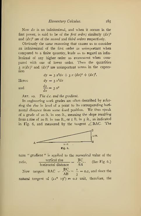
Elementary Calculus. 185
Now dx is an infinitesimal, and when it occurs in the
first power, is said to be of the first order; similarly (dx) 2
and (dx)3 are of the second and third orders respectively.
Obviously the same reasoning that causes us to consider
an infinitesimal of the first order as unimportant when
compared to a finite quantity, leads us to regard an infin-
itesimal of any higher order as evanescent when com-
pared with one of lower order. Then the quantities
3 x(dx) 2 and (dx)3 are unimportant terms in the expres-
sion
dy = 3 x2dx + 3 x (dx) 2 + (dx)3.
Hence dy = 3 x2dx
and -r~ = 3 x2dx
Art. 10. The dx. and the gradient.
In engineering work grades are often described by refer-
ring the rise in level of a point to its corresponding hori-
zontal distance from some fixed position. We thus speak
of a grade of 20 ft. in 100 ft., meaning the slope resulting
from arise of 20 ft. in 100 ft., or 1 ft. in 5 ft., as indicated
in Fig. 6, and measured by the tangent Z BAC. The
1 FT,
Fig. 6.
term " gradient " is applied to the numerical value of the
vertical rise BC /c, J?-„ a n
ratio,:
—:
= — (See .tig. 6.)horizontal distance AB
BC iNow tangent BAC = -7^-= - = 0.2, and since the
natural tangent of (ii° 19') = 0.2 unit, therefore, the

i86 Elementary Calculus.
gradient of the slope AC is 0.2, and the angle BAC is approx-
imately ii° 19'.
Suppose a straight line AB to make an angle DCB with
the #-axis. (See Fig. 7.)
Fig. 7-
Let the co-ordinates of any point Q on AB be x and y.
Let x be increased by Ax, and y by Ay.
Completing the construction shown in Fig. 7, we have
PQ _ RQ'CP
RQ'QR
tan Z DCB =
and
QRAy .
A*
(by similar triangles),
Hence 4^ = tangent Z DCB.Ax
If the increment Ax becomes infinitely small, then
&- = tangent Z DCB.ax
This means that in the case of a linear function, that is,
a function whose graph is a straight line, the ratio of an
infinitely small increment of the v-ordinate to dx gives the

. Elementary Calculus. i8 7
tangent of the angle which the straight line makes with the
#-axis, and therefore its gradient.
We will now test this numerically by the following
example.
Given the linear function, y = 0.7 x + 2, to find the
differential coefficient with respect to x, namely, the value
ofdy
dx
We have
then
Hence
But
Subtracting;
and
and hence the gradient of the line.
y = 0.7 x + 2,
y + Ay = 0.7 (x + Ax) + 2.
y + Ay = 0.7 x + 0.7 Ax + 2.
y = 0.7 x + 2.
Ay = 0.7 Ax.
Ay
dy
dx0.7.
Now 0.7 is the approximate natural tangent of 35 .
Hence by differentiating the
function y = 0.7 x + 2 we
have not only found the
ratio of the increase of the
ordinate to the abscissa
at any moment, but also the
gradient of the line and
hence the angle it makes
with the x-axis.
The line AB, Fig. 8, was
plotted from the equation
y = 0.7 x + 2, and the angle BAx will be found, upon
measurement with a protractor, to be approximately 35 .
Fig. 8.
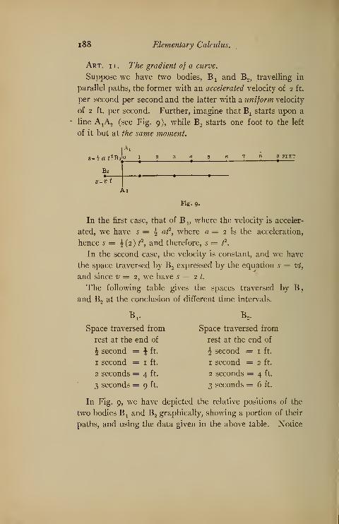
x88 Elementary Calculus.
Art. ii. The gradient of a curve.
Suppose we have two bodies, Btand B
2 , travelling in
parallel paths, the former with an accelerated velocity of 2 ft.
per second per second and the latter with a uniform velocity
of 2 ft. per second. Further, imagine that Bxstarts upon a
line AXA
2 (see Fig. 9), while B2starts one foot to the left
of it but at the same moment.
B2•
8 = V t
A 2
Fig. 9.
In the first case, that of B v where the velocity is acceler-
ated, we have s = J at2
, where a = 2 is the acceleration,
hence s = J (2) t2
, and therefore, s = t2
.
In the second case, the velocity is constant, and we have
the space traversed by B2expressed by the equation 5 = vt,
and since v = 2, we have s = 2 t.
The following table gives the spaces traversed by B,
and B2at the conclusion of different time intervals.
b,.
Space traversed from
rest at the end of
J second = J ft.
1 second = 1 ft.
2 seconds = 4 ft.
3 seconds = 9 ft.
B2 .
Space traversed from
rest at the end of
J second = 1 ft.
1 second = 2 ft.
2 seconds = 4 ft.
2 seconds = 6 ft.
In Fig. 9, we have depicted the relative positions of the
two bodies Bxand B
2graphically, showing a portion of their
paths, and using the data given in the above table. Notice
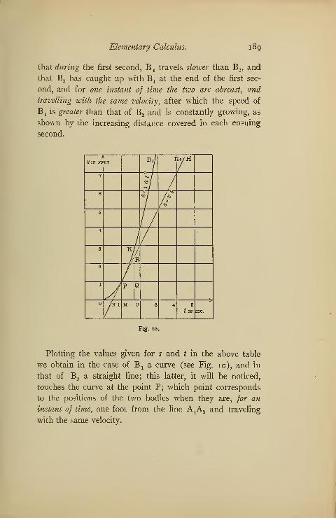
Elementary Calculus. 189
that during the first second, Bxtravels slower than B
2 , and
that B2has caught up with B
xat the end of the first sec-
ond, and for one instant of time the two are abreast, and
travelling with the same velocity, after which the speed of
Bxis greater than that of B
2and is constantly growing, as
shown by the increasing distance covered in each ensuing
second.
Sin fi ET Bi/ Ir7
6°°l /5s
/ ^
5
4
/3 K
/2
/ r1J P Q
/N 1 M 2 3 4 5
/t IN SEC.
Fig. 10.
Plotting the values given for s and / in the above table
we obtain in the case of Bta curve (see Fig. io), and in
that of B2a straight line; this latter, it will be noticed,
touches the curve at the point P; which point corresponds
to the positions of the two bodies when they are, for an
instant of time, one foot from the line A2A
2and traveling
with the same velocity.

190 Elementary Calculus.
We have already said (Art. 10) that the gradient of a
line is measured by the tangent of the angle that the line
makes with the abscissa; but if a line is a geometrical tan-
gent to a curve, then at the point of tangency the two have
the same direction. Hence the slope of the geometrical
tangent to a curve, at a point, shows the steepness of the
curve at that point, but the gradient of the line is measured
by the tangent of its abscissa angle. We thus have the fol-
lowing definition: The gradient of a curve at any point
is measured by the tangent of the angle which the geometrical
tangent, at that point, makes with the abscissa.
Now the gradient of the line NH is measured by
MP 1tan MNP = = — = 2, and this quantity is also aNM J
measure of the gradient of the curve at the point P, from
the above definition.
Let us now take increments to the ordinates of P; let the
time increment of t he At = PQ, in both the case of the
curve, and that of the line; for the space increment we
have, for the line, A.? = QR, and for the curve, As = QK.
Hence for the line, —- = —— ,
At PQ
f fu As QK QR + RKfor the curve, -—
- = ^—- = -^ ! •
At PQ PQ
Now clearly in this case if At is infinitely small, then
dsthe latter expression becomes — , as can be inferred from
dt
the figure.
dsHence — at the point P has the same value for both the
dt
line and curve, namely — = 2.
dt

Elementary Calculus. 191
That is, the value of the differential quotient of the
dsfunction s =t2
, for the point P (1, 1), namely — = 2, is
at
the tangent of the angle the geometric tangent makes
at P.
We will now see if this statement is susceptible to a
general application.
Let y = / (x) be any curve of which a portion of the
y'
V
St
7/ /*
QAx
K / 1
Ntf 13
?
Fig. ii.
graph is shown in Fig. 11. Suppose the point P upon
y = J (x) has the co-ordinates OM = x and MP = y.
If MB = Ax then QK = Ay, and the ratio of the rate
of increase of the function y to the rate of increase of the
independent variable x, will be expressed by -—- • Now
AyAx
= tan KNB ; which latter is the tangent of the angle
that the geometrical secant NK makes with the x-axis.
192 Elementary Calculus.
The value of ~~- will depend upon the size of the incre-
ment Ax, as we have already seen, except in the case of a
straight line when the function is linear. Further the
value of yis dependent upon the position of the point P,
Axas can be readily inferred from the figure, for if P were
moved to the right, then an increment Ax would bring
about an immensely increased corresponding increment,
Ay, because of the steeper slope of the curve, and there-
fore -~- would assume a greater value.Ax
If, however, Ax is gradually decreased, then the point Kwill continually approach the point P, while the secant
NK will cut the abscissa at a more and more acute
angle, until finally, when Ax = dx, the secant will
take its limiting position AH, which is the geometric
tangent to the curve y = / (x) at the point P, and we have
^ = tanHOM.dx
It is important to notice that the value of — dependsdx
wholly on the direction of the curve at the point P, and,
therefore, expresses its gradient at this point.
Hence, if y=f (x), then the differential coefficient of
this function is equal to the tangent of the angle which the
geometric tangent to the curve at any point upon it makes
with the x-axis, while, at the same time it expresses the
gradient of the curve at that point.
From Art. 9, we know that if y = x3 then -* = 3 x2;
dx
putting x => 1.1 we find 3 x2 = 3 (i.i)2 = 3.63, therefore

Elementary Calculus. !93
= 3.63; which on referring to a table is found to be thedx
natural tangent of 74 36'.
We thus have found that given y = x3 , the ratio of
the rate of increase of the ordinate to that of the
abscissa at a point where abscissa is 1.1, is 3.63. This
latter is the gradient of the curve at that point, while
the geometrical tangent makes an angle of 74 36' with
the x'-axis.
Let us test the above calculation by actually plotting the
curve and drawing the tangent. Fig. 12 shows a part of
V'
10
y=x 3
3^^^^K
^^R 1 25X
Fig. 12.
the curve, while P is that point whose abscissa is 1.1. If
the angle KR# be measured, it will be found to be about
20 , but the angle which the tangent to the curve at Pmakes with the .v-axis, is, according to our previous calcu-
lation, 74 36'; the discrepancy is due to the fact that the
unit of measurement used on the ^-axis is 10 times that
used on the v-axis.
In order that the tangent should represent the true
gradient of the curve at P, we must refer the ordinates and
abscissas to the same scale, or we will not obtain the true
comparative rate of increase of y to x. Tan 20 = 0.363
(nearly), or t!q of the true value.

94 Elementary Calculus.
In order to make this important point quite clear, we
have plotted the curve y = x3 a second time (see Fig. 13),
y k
2
y = x*
/P
1
I 2• /R \
Fig. 13-
and have used the same scale for both ordinates and
abscissas. Upon measuring the angle PR# with a pro-
tractor it will be found to be 74 36' approximately, which
corresponds with the result -~ = 3.63.dx
ILLUSTRATIVE EXAMPLES.
I. Derive the differential coefficient of the function
y = 2 x2 — 3^ + 1.
Now, y + Ay = 2 (x + Ax) 2 - 3 (x + A*) + 1.
.*. y + Ay = 2 x2+ 4X Ax + 2 Ax2 — 3 x — 3 Ax +1
but, ^ = 2 3* + :}
Elementary Calculus. 195
Subtracting; Ay = 41 A1-3 A1 + 2 Ax.
.'. — = 4# — 3 + 2 Ax.Ax
If Ax becomes dx, then 2 dx is evanescent.
Hence — = 4 x — 3.
II. Find the gradient of the curve x2 — x + 2 = y at
the point where x = 1.15, and the angle the geometrical
tangent at this point makes with the x-axis.
y = x2 — x + 2,
y + Ay = (x + Ax) 2 — (x + Ax) + 2,
y + Ay = x2 + 2 x Ax + Ax — x — Ax + 2,
y = x2 — x +2.
.'. Ay = 2 x Ax — Ax + Ax .
—— = 2 x — 1 + Ax. Hence -2- = 2 x — 1.
Ax dx
To find the gradient of the curve at the point where
x= 1. 1 5 we substitute as follows:
-_-- = 2 x - 1 = 2 (1.15) - 1 = 1.30.ax
Hence 1.30 is the gradient required, and since tan 52
26' = 1.30, we find, therefore, that the geometrical tan-
gent at the point where x— 1.15 makes an angle of 52
26' with the x-axis.
III. Find the rate at which the area of a square is in-
creasing at the instant when the side is 6 feet long, suppos-
ing the latter to be subject to uniform increase of length at
the rate of 4.5 feet per second.

196 Elementary Calculus.
Let x = length of side,
y = x2 = area.
By Art. 7, dy = 2 x dx,
that is, the rate of variation of area = 2 x times the rate of
variation of the side.
Substituting the given values, we get
dy = 2 (6) (4.5 ) = 54 sq. ft. per second.
EXERCISE I.
Find the differential coefficient of the following five
functions by the method of Art. 7.
1. y = 2 x2 — 3.
2. y= (*.- 2) O + 3).
23- w = —
•
4- V = X4.
5-
X — I
^C + I
6. Plot the graph of x2 + 3 # — 2 = y.
(a) What can you tell about the roots of the equation
from the appearance of the graph ?
(b) Find the general expression for the gradient of the
curve at any point.
(c) Find the angle which the geometrical tangent makes
with the curve at those points on it where x = o, x = —j,
X = — f , X = — 2.
(d) Draw tangents at the points where x = — f and
3: = — 2, and test your answers to question c by actual
measurement.
(e) What effect would it have upon the gradient of the
graph at any point, if the scale for the v-axis was made
10 times as large as that of the ^-axis?

Elementary Calculus. 197
(/) If y = / (x) and—^ = a for a certain x value, whatdx
does this imply?
7. Differentiate the function s = \at2 with respect to /.
What does the result mean?
8. A man cuts a circular plate of brass the diameter of
which is 4 inches; after heating he finds the diameter to
have increased by .006 of an inch. What is the increase of
area?
9. If x be the side of a cube which is increasing uni-
formly at the rate of 0.5 inch per second per second, at
what rate is the volume increasing at that instant when
the side is exactly 2 inches in length?
10. If a body travels with an accelerated velocity of 2
ft. per second per second, and we call the space traversed
at the end of the first "second s, show by arithmetical
computation that if As is any positive increase of s, then
A 5-r— approaches more nearly the actual momentary velocity
of the body at the end of the first second, the smaller As
is taken.
CHAPTER II.
DIFFERENTIATION.
I. Algebraic and Transcendental Functions.
Art. 12. An Algebraic Function is one in which the
only operations indicated are, addition, subtraction, multi-
plication, division, involution, and evolution; further, such
a function must be expressed by a finite number of terms,
and any exponents involved must be constant. Examples
of algebraic functions are,
21 / \i / \* ^x2 + 1 x — ix* + 2 x, (x — my, (x — ny, -
.
(x - 4)
In distinction to the above we have the so-called Tran-
scendental Functions, which cannot be expressed algebrai-
cally in a finite number of terms; examples of which are as
follows:
sin x, tan x, vers x, loge x, ex .
The Binomial Theorem.
In works on algebra a general proof of the following
expansion may be found:
(a + b)n = an + nan~ x b + n
(n ~ T ) an~2
b2
I . 2
n(n-i) (n-2) (n-s)a„_3 ^ +
1.2.3
For* convenience we will put n = Cv — = C2 , etc.;1 . 2
we thus get,
(a + b)n = an + Q an
~lb + C2
an~2b2 + C
3an~3
b3 + . . .
108
Elementary Calculus. 199
Art. 13. Differentiation of axn and xn
.
If y = axn,
then y + Ay = a (x + Ax) n.
Expanding the right-hand member, as explained in the
previous paragraph, and multiplying through by a, we get
y + Ay = axn + a Cta;"-
1 A x + a C2xn~2 (A x) 2
+ aC3x"-3 (Ax)3 + .. . .
But, y = ax\
.*. Ay = aC^"-1 Ax + a C2xn-2 (Ax) 2
+ a C3xn-3 (Ax) 3+ . . .
and ^ =aC1xn-1+aC
2xn~2Ax+aC
3xn-Ji(Axy + . . .
Ax
If Ax becomes dx, then all the terms of the right-hand
member after the first are evanescent (Art. 6); and remem-
bering Ct= n (see Art. 12), we get
—2- = anx'1-1.
dx
Now if in the function y = axn, a = 1,
we get y = xn,
and _Z = wx"-1.
ax
To differentiate y = x11 with respect to x. First, multiply
x by the index and then obtain the new power by diminish-
ing the index by unity.
Example : y = x4;—^- = 4 x4-1 — 4 x3
.
ox
To differentiate y = axn; differentiate the function xn and
multiply the result by the constant.
Example : y = 5 x3;— = 5 (3) x
3-1 = 15 x2.
ax
200 Elementary Calculus.
The results above obtained are true for all values of n,
whether positive, negative, or fractional ; the proof of the
latter two cases is simple, and is left as an exercise for the
student.
Examples : y =2 dx
- 1 aH»-2
1 = - 2 #-2
-4
>
y =3 dx
9 2
5 3
u 6 4* — — X*.
5
Example:* y = 2 VsF.\ y = 2x*;-2- =ax 3
4
zVx'
Art. 14. Difj;erentiation of c5 constant.
We have defined a constant is a quantity which does not
change or alter its value. Hence if k is a, constant, A*
= and -— =Ax
0, thereforedx
Art. 15. Differentiation of a sum.
Suppose y = u + 2/, when both z* and z> are functions
of x. Now if x becomes x + Ax, then « and z; become
u + Aw and v + Av, respectively, and we get,
y + Ay = u + Aw + ^ + Av.
But y = « + v.
.*. Ay = Au -f At;.
tv -j u a .Ay Au . At;Divide by Ax; . . 7-^-= - \- -— •
' Ax Ax Ax
* If the function involves a radical which can be reduced to the
11
form x° , then express the radical as a fractional power and proceed
as above.

Elementary Calculus. 201
If Ax becomes dx,
to. du , dv
dx dx dx
In a similar manner we can show that if
y = u ± v ± w ±
thendy_ _ du dv dw_
,
dx dx dx dx
By Art. 14,
Hence, the differential coefficient of the sum of several
functions is the sum of the differential coefficients of the
several parts, due regard being given to the signs.
Example: )»= 313 - 5 x2 + 2 x -{- 3.
i® = o.dx
dy 2 .
. . -*- = 9 x* — 10 x + 2.
Art. 16. Differentiation of a product.
If y = u . v where u and v are each functions of x, re-
quired the value of — •
dxIn order to obtain a clear idea of the meaning of the
above function, suppose u = 5 x and v = 3 x. Then
g luxAy^
D C
63
mn
A B
5 r Au
Fig. 14.
u . v can be geometrically represented by a rectangle ABCD(see Fig. 14), two of whose opposite sides are each of

202 Elementary Calculus.
length u = 5 x, while those adjacent are represented by
v = sx.
If x is increased by Ax then,
u + Au = 5 (x + Ax) = 5 x + 5 Ax = AE,
and v + Av = 3 (x + Ax) = 3 x + 3 Ax = AG.
Hence Au = 5 Ax and Av = 3 Ax.
Completing the figure as shown, we see that Ay, which is
the difference in area between the rectangles AEFG and
ABCD, is made up of three small rectangles whose areas
are obviously 3 x (5 Ax), 5 x (3 Ax), and (5 Ax) (3 Ax),
respectively.
Hence Ay = 3 x (5 Ax) + 5x (3 Ax) + (5 Ax) (3 Ax).
•'•zr = 3 x (5) + 5 x (3) + 5 (3 Ax).Ax
Now if Ax is a small decimal say 0.0000001, clearly the
last term, which represents the least of the rectangles, will
tend to vanish; therefore, if Ax becomes dx, we have
~ = 3* (5) + 5* (3) • • • • (1)
But u = 5 x and t; = 3 x,
dxand the differential of the first function is — = 5 and that
du
of the second is — = 7.
dx *
Hence substituting in (1);
dy __ du . &u_
dx dx dx
In general if y = u . v;
y + Ay = (w + Aw) (v + Av).

Elementary Calculus, 203
.*. y + Ay = uv + ^Aw + mAv + Az/. Av,
but y = av.
Hence Ay = I'Az* + uAv + Azz . Ai\
Dividing by Ax;
Ay Az* . Az/ . Au *-^ = w— + « -j— + — Az/.Ax Ax Ax Ax
If Ax becomes dx then — Az/ = — dv which is evanes-Ax dx
cent, for although the quotient —- is finite, it is multiplieddx
by the differential dv, and therefore tends to vanish.
tt dy dx,
dvHence -*- — v— + u —-
•
dx du dx
Again if y = u . v . w;
then putting u . v = z
we get y=z.w,
j dy dz . dw , sand -*- = w — + z— (a)dx dx dx
But since z = u . v,
dz du . dz>.'. = V \- u •
dx dx dx
dzSubstituting this value of — in (a)
dx
dy du . dv . dwwe get, -L.. = vw — + uw— + uv—
.
dx dx dx dx
A like form can be found for the differential coefficient of
any number of variables.
Hence, the Differential Coefficient of a Product of several
variables, is the sum of the products of the differential coeffi-
cients of each variable multiplied by all the others.
204 Elementary Calculus.
Exa tuple: y = (3 x + 2) (5 x — 6)
dy
dx
= (5^-6) (3) + (3 * + 2) (5).
.'.-/- = 30 x- 8.ax
Art 17. Differentiation of a quotient.
Letu
y = -,
when vf and v are functions of x.
We have, u = vy,
du dv . dy
dx dx dx
•
dy _ du dv
dx dx dx
but_ u . dy __ du u dv
v dx dx v * dx
du u dv
anddy _ dx v dx
dx v
Multip lying numerator and denominator by v we get
du dv
dy dx dx
dx v2
Hence, the Differential Coefficient of a fraction whose num-
erator and denominator are variables, is equal to the product
of the denominator and the differential coefficient of the
numerator minus the numerator times the differential coeffi-
cient of the denominator, the whole divided by the square
of the denominator.
Elementary Calcidus. 205
If y = - where c is a constant, then, since the differentialV
of a constant is zero, we get,
dv
dy dx _ c dv
v2 dx
Example: y = ,
I + x2
, . 2X d (1 — x) , N d (1 + #2)
(1 + X2)
* ' — (1 — x)—*
—
! '—
dy __ dx dx
dx~ (1 + x2)
2
_ (1 -f x2) (— 1) — (1 — x) (2 #)
(1 + x2
)2
dy _ x2 — 2 x — 1
dx (1 + ^2)2
Art. 18. Differentiation of a junction 0} a junction.
Suppose we wish to evaluate V x2 + 3^ + 2, when
x = 1, 2, etc. Putting
V x2 + 3 x + 2 = y and x 2-\- 3 x + 2 = z,
then y = Vz
if x = 1, 2 = 6 and y = ^6 = 1.817
x = 2, 2 = 12 and y = ^/ 12 = 2.289.
Clearly 2 is a function of x, and further the value of y
depends upon that of 2, hence y is also a function of 2. Wethus see that y is a function of 2 which in turn is a function
of x, and we therefore say that y is a function of a
function.
This latter term is sometimes puzzling at first, and care

206 Elementary Calculus.
should be taken that it is thoroughly understood. Let
us take the general case
y = F (z)
and z = j (x).
Now if x undergoes a small change in value then z will
change likewise.
If x becomes x + Ax,
z becomes z + Az,
butAy _ Ay Az
Ax Az ' Ax[An identity, found
by multiplying and
dividing —2- by Az.]Ax
and if Ax becomes dx,
thendy dy dz
dx dz dx
Hence, if y= F(z) and z= f(x), the differential coeffi-
cient of y, with respect to x, is equal to the product of the
differential coefficient of y with respect to z, times the differ-
ential coefficient of z with respect to x.
Example I: y-= \/u, to find ^L,dx
where x2 + 3-= u.
Since y.= \/u,
we have, y = F (u] ) and u - /(*)
From the above,dy
dx
_ dy
du
du
dx
but y =; U%.
dy _idu 2
uh- 1I= — u~2 2
(*» + 3)-*;

Elementary Calculus. 207
and since u = x2 + 3,
du.'.— = 2 x,
ax
In general we would proceed thus:
Given, y = \/x2 + 3,
•'. y= (*2
+3)K
L==L(x
2 _j_3^ ^ 2 x =
dx 2 v x2 + 3
Example II: y = (x3 + 2) (x + 3)3
.
Here we have a product, hence by Art. 16 we get,
dy / 1 \3 d (tf3 + 2)
,
-T" = + 3)3
-
V
,
; +ax dx
/ -3 1 \ d (x + 3)3
/ \(a3 + 2)v
'
o;(1)
dx
As the expression (x + 3)3
is a function of a function,
, d (X3 + 2) 2 , Nwe have, —
2
!—'- = 3 x* (2)dx
andd(-\+i)3 =3(x+ 3 y.
d(x+^ = 3 (x+ 3 y.i . . (3)dx dx
Substituting (2) and (3) in (1) we find,
= (* + 3)3
- 3^2 + O3 + 2 )' 3 + 3)2,
and — = 6 x5 + 45 x4 + 54 ^ + 6 #2 + 36 x -f- 135.

208 Elementary Calculus.
EXERCISE II.
I. y = 5 x3 + 3 x2 -x+2. 2. y = ax2 + bx + c.
3-7 — •
4- y = —2= - *"2
.
a j x2j
5- ? = 3 *§ - 5 ** + 7 ~ 8 x* + 2 # -S.
6.<y = {/x. 7- y= V*4
-
8. y = x2$fx.
9- y= 17=-
IO. )/
x2^/ x3
ii. y= V# v^12. y= ^/^71 3 . ^= (x2 + 2)
2.
14. y = a (3 x2 — 2 x + i) 2.
16. y = (ax2 + £w + c) n -
17. y = (3^2 - 2)~ 2.
18. y = y/2 x3 + 3 x.
19. y =v^2 -3^
20. y = \/x~+~b + \/# — b.
221. y = — =•
^(i-*3)2
22. y= (2X+1) (3 # — 2).
23. 3/ = X2(2 ^ + 1).
24. y = (* + 1) (x2 — x + 1).
25. ^ = A\/l — x2.

Elementary Calculus. 209
26. y = X2 \/2 X2 — I.
y =-7 h
27. 4v* 2 - *.X2
28. y =x2 — 3 x + 1
x2 — I
29. y =b — x
b + x
3°- y =lb - x
\b +x'
3*- y =(x2 -b) 2
(x* - by
32. y =
y =
X2
33-\/x — I
a/* + 1
y =X
34-<s/b
2 - x2
y =X
3b-\/a2 — x2 — x
36. y =
y =
4/1 - <s/x
1 + \/x
\/l + X — \/l — #o7-
\/i + x +\/i — X
38. y = V |(i + *2n
'
y =xn
39-(1 + x) w
\/i — X2 + x\/40. y -
Vi-
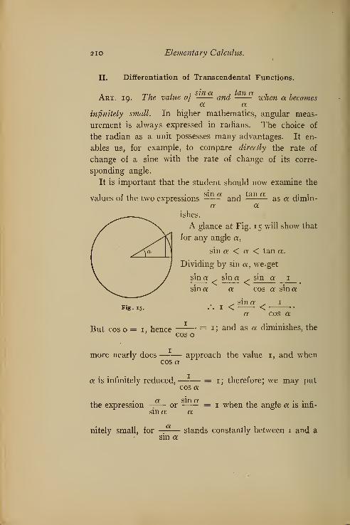
2IO Elementary Calculus.
II. Differentiation of Transcendental Functions.
. n 7 r sm a 7 tan a 7 LArt. 19. 1 he value 0) ana when a becomesa a
infinitely small. In higher mathematics, angular meas-
urement is always expressed in radians. The choice of
the radian as a unit possesses many advantages. It en-
ables us, for example, to compare directly the rate of
change of a sine with the rate of change of its corre-
sponding angle.
It is important that the student should now examine the
values of the two expressions and as a dimin-a a
ishes.
A glance at Fig. 15 will show that
for any angle a,
sin a < a < tan a.
Dividing by sin a, we. get
sin a: sin a; sin a 1
sin a a cos a sin a
Fig. 15.
But cos 0=1, hence
sin a 1
a cos a
= 1 ; and as a diminishes, thecos o
more nearly does approach the value 1, and whencos a
a is infinitely reduced, = 1; therefore; we may putcos a
the expression -— or = 1 when the angle a is inn-sin a: a
nitely small, fora
sin astands constantly between 1 and a

Elementary Calculus. 211
quantity, , which continually approaches i, as(cos a)
shown by the inequality, hence —:
must itself approachsin a
1 in advance of , and will reach it when ar-cos a cos a
rives at that value.
. • tan a sin a 1 u , , ...Again, = . , but we have seen that
a a cos a
each of the expressions and tends to approacha cos a
the value unity as the angle diminishes; hence we may put
= 1 Svhen a is infinitely small.a
Art. 20. Differentiation of y = sin x and y = cos x.
If y = sin x,
then y + Ay = sin (x + Ax).
y + Ay = sin x cos Ax + cos x sin Ax.
And y = sin x.
.'. Ay = sin x cos Ax — sin x + cos x sin Ax.
.'. Ay = sin x (cos Ax — 1) + cos x sin Ax.
Hence -—2- = —— (cos Ax — 1 ) + cos x— >
Ax Ax Ax
but when Ax is infinitely small,
cos Ax = 1 and —
.*. when Ax becomes dx, then
dy
dx
dy
A , sin Axcos Ax = 1 and — = 1.
Ax
J- = 1 (o) + cos X (1)dx
= COS X.dx

212 Elementary Calculus.
In an exactly similar manner to the above we may show
that if y — cos %, -2- = — sin x.dx
Art. 2i. Differentiation of y = /an# a»<2 y= co/tf.
If y = tan x,
. , sin #then y =
D A 4. *. <fy C0S # • ^ (Sln X ) ~ Sln ^ (C0S X )J3y Art. 17, -f~ = * '— * '->
ax cosz x
dy _ cos x . cos x — sin x (— sin #)
dy _ cos23; -f sin2 x
dx cos2 #
dy d (tan x) 1 ,' = —i l = . . = sec x.dx dx cos 2 x
In like manner, if y = cot #, we may show that
dy 1 2
dx sm2 x
Art. 22. Differentiation of y = sec x and y= cosec x.
If y = sec x, then y =cosx
Differentiating, we find
dy sin #-*— — = tan x sec x.dx cos2 x
ro . sin a; sin* 1 , -i
[Since = —-— . = tan x sec x.J

Elementary Calculus. 213
Similarly, when y = cosec x, then y= -— ,
sin x
. dy cos x ,
and -JL- = : = — cot x esc x.dx sin2 x
The following convenient table should be committed to
memory :*
dy dyy=smx] -J- = cos x y=cosx; -f- = — sm#
dx dx
dy o dy 9y = tan x; -^- = sec"
1 x v = cot #; —• — — csc^ #dx dx
y = sec x; — = tan # sec xdx
y = cosec x; -+- = — cot x esc #.
Since vers x = 1 — cos x, if ^ = vers x,
we have y = 1 — cos #, and, therefore, -2- = sin #;dx
also if v = covers x = 1 — sin #, -2- = — cos x.dx
EXERCISE III.
1. y= tan (bx). 2. y = cos — •
x
3. V = sin (3 x2). 4. v = tan \A«c.
5- ^ = 3 cos (^n)- 6. v = 6 sin — •
7. v = sin (1 + ax2). 8. y = cos
\/*x
9. v = sin5x. 10. y = cos4 a^ . x2
.
* Note that //^e differential coefficients of all the co-functions have
a negative sign. The significance of this will be seen later.

214 Elementary Calculus.
ii. y = — tan (nx). 12. y= cos5(3 x).
n 15
13. y = cosn x sinn x.
14. ;y = cot x + J cot3x.
tan3 x15. v = x — tanx +
16. y =
3
sin x + cos x
sin # cos x
17. ;y = tan x (sin x).
sin 71 #is. y =
cosw x
19. y = \/a cos 2a; + b sin 2 #.
20. y = sin a# (sin x) a.
Of what functions are the following the differential co-
efficients:
dy • 421. -f- = 5 sin4 # cos x.
ax
22. -2- = a [cos (& + ax) + sin (6 — ax)].ax
«
23- /" = 3 tan 3 x sec 3 #.ax
24. — = — 20 x cos42 x2
sin 2 x2.
25. 2 mcotmt cosec mx.

Elementary Calculus. 215
DIFFERENTIATION OF LOGARITHMIC ANDEXPONENTIAL FUNCTIONS.
The series y = A + Bx -\- Cx2 + Dx3 + . . .
Art. 23. Consider the geometric series,
1 + i + (i)2 + (if +
the value of which when the number of terms is infinite is
2. We can approach this value to any required degree
of accuracy by taking a sufficient number of terms.
The general notation for such a series is as follows:
y = A + Bx + Cx2 + Bx3 + . . .
when A, B, C, etc., are constants. The calculation of
numerical quantities and of experimental results is often
referred to a series of this form.
In order to calculate the logarithms of numbers, we
make use of a series in which x either is equal to or in-
volves the quantity whose logarithm is sought, and hence
the latter can be calculated to any required degree of
accuracy.
Such a series to be of practical value should possess the
following properties : it must converge rapidly, so that
it will not require a large number of terms to be taken
before the necessary accuracy is reached, and it must be
convenient of computation.
The binomial theorem supplies us with an expression
of the form y = A + Bx + Cx2 + Bx3. . . ; and it
has been found that the determination of the value of
when n becomes infinite, forms a suitable start-
ing-point from which to begin investigations with a view of
obtaining a practical logarithmic series. This will be
discussed in its proper place.
( + 0"

21
6
Elementary Calculus.
Art. 24. The value oj (1 ^— )when n becomes in-
\ n)finite.
Suppose in the expression ( 1 + —)we put n = 00 , we
1 ^]
= (1 + o)°°= 100
; now i°° is indeter-
minate, for infinity has no definite value; we regard the
symbol 00 as referring to a magnitude which is greater than
any we can conceive.
We shall refer to the matter of indeterminate forms in a
subsequent article. In the mean time we shall show that
by approaching the calculation in another manner we can
obtain a more definite result for the evaluation off1 + —
J
V n)when n = qo .
By the Binomial Theorem, we have
( IT. 1 . n (n — 1) /i N2
1 + n .1
* J 1
n 1.2 \n,
n (n—i) (n — 2) /i\ 3
1.2.3 w(n — i\ In — i\ In — 2\
M / + \ n A n I; u
1.2 I.2.3
= ! + ! + V W + V nj\ njj1.2 1.2.3
If w = 00}then terms such as — » — , etc., vanish;
= 2.71828
We will put e = 2.71828.
n n
2 + -^ +—x-—
1.2 1.2.3

Elementary Calculus. 217
The evaluation of e to any required degree of accuracy
can be conveniently performed as follows :
1 .000000
2 1 .000000
3 0.500000
4 0.166667
5 0.041667
6 0.008333
7 0.001389
8 0.000198
9 0.000025
0.000003
adding; 2.718281 = e.
Now if ax = N then loga N = x. If then we can obtain a
convenient series for ex we shall be able to calculate the
logarithms of numbers to the base e; for if ex = N1?then
loge Nt= x. Let us, therefore, endeavor to develop a series
for ex .
Art. 25. The expansion of ex and the logarithmic series.
If n = qo then,
But
1 + nx
KT-*Kf
i_ , nx (nx—i) /i_V
w 1.2 \w/
. ^Jg (rac— 1) (nx
1.2.3
,- 1 (nx
Z2 :
&)'
1) +
(nx — 1) (njc —2)
Z3+

218 Elementary Calculus.
x2 (n - ^)= I+x -r^ V *J +
Z2 n
x2(n — i-
) x In — -)
/J> n . n
X> (i - J-)
* (. - -M (« - -M, V nx I \ nx
)
,
Now if w = oo then the terms —> — > etc., vanish.w# nx
Hence we have/y»« /y*3 /y»4
Z2 /3 /4
Now put x = 2 then
e2 =I+2 + ^-+ § + 5*
r
1.2 I.2.3 1-2.3.4- 3i_ + . . .
2.3-4.5= i + 2 + 2 + 1.333 + °-66 7 + 0-267 + . . .
= 7.266.
Hence we have log,, 7.266 = 2 nearly.
It is obvious that the above series would be far from
practical, since it converges slowly and it would be diffi-
cult to obtain the logarithms of consecutive integers. It
is, however, easily possible to obtain either by elementary
mathematics, or by an application of the calculus (see
Art. 54) the following series,
x2 ^ „4X3 X 4
loge (1 + x) = x — 1 +234
Elementary Calculus. 219
This is known as the Logarithmic Series, and by its means
we could calculate many logarithms, but since it also con-
verges slowly and only between the values x = + i and
x = — 1 , it is not suitable for general logarithmic compu-
tation. From this latter series we can, however, obtain the
following:
Loge (Z + i)
= log* z + 2 r—-— +—-— +—-—
;
L2Z + 1 3 (2Z + 1) 5(2Z+i) 5
+7(2Z + i) 7 *
*
}This series is most convenient for our purpose, for in-
stance if Z = 1, then
loge 2 = loge 1 + 2 -
L-4TT-+.
.3 3 (3)3
5 (5)5
.-. Loge 2 = 0.6931.
And in a similar manner the logarithms of other quantities
could be calculated.
Art. 26. The logarithmic modulus. Logarithms cal-
culated to the base e are known as Napierian logarithms,
because of their introduction by Napier; they are also called
Natural Logarithms. This latter term was applied because
they appeared first in the investigation conducted for the
purpose of discovering a method for calculating logarithms.
The base e is used exclusively in higher mathematics, but
this system is not suitable for practical computation; the
student will be aware that for the latter purpose the base
10 is chosen.
We will now show how logarithms to the base e can be
transformed to the base 10 and vice versa.
Let y = log, x and z = log10
x,
then ey = x and 10s = x.
.'. ev = 102 .

220 Elementary Calculus.
I. To transform log10 x to log, x, we had
ey = io3.
.*. y log, <? = z log, 10.
But log, e = i and log, 10 = 2.30258, and since y = loge x
and z = log10
x,
:. log,x= 2.30258 log10 x.
The quantity 2.30258 is called the Modulus of the Nap-
ierian logarithms and is often denoted by M. In this
notation we have
log, x = M log10
x.
II. To transform log, x to log10 x }
we had
ey = io*.
•*• 7 log10
e = z log10 10.
Now y = log, x and log10 e = 0.43429, while log10 10 = 1
and z = log10 x.
Hence log10x = 0.43429 log, x.
The quantity 0.43429 is called the Modulus of the Briggs
System and is denoted by m. We therefore have,
log10 x = m log, x.
Art. 27. The relation between M and m.
We have log10 x = m log, x and log, x = M log10 x.
Now loge*= i^Sio^.
Substituting in the second equation above we get
^Sio£ = M . log10 x.m
.'. M =— and m = —m M
or M . m = 1.
Hence to transform logarithms from the base a to the
base b multiply byT
• Note log, a =loga b loga e
Elementary Calculus. 221
Art. 28. The d. c. of y =loge x. We will now write Inx
for loge x.
We have y = Inx.
.'. y + Ay = ln(x + Ax)
Ay = ln{x + Ax) — Inx = In I ]•
Multiplying by — we get,Ax
i. M~* ln (1 + ^) = ln(i + ^)t.Ax Ax \ x J \ x J
Hence —2- = - In [1 + —W.A# # \ x )
If A# becomes dx then —^ = o, while —— = oo
.
x Ax
Putting —-= n then — = -, and
A„v x n
( +^- (+;)which for w = 00 is equal to e (Art. 24).
Hence we get -2— = — /we,dx x
but /we = 1,
</y _ i_
Art. 29. 77*e d. c. of y = logax,
y = logax,
.*. av = x.
ylna = Inx,
.'. y = Inx .
Ina

222 Elementary Calculus.
But by Art. 26, = loga e.
log, a
.'. y = Inx . loga e,
and -2- = — logn e.
Note loga ^ is a constant, .'. -—^— = o, hence the sec-
ond term in the differentiation of the product is zero.
»„, The d. c. of y = a-T
Art. 30. '—*
y = ax
:. Iny = x Ina,
.'. — . -2- = Ina.
y dx
- —2- = ax /wa .
dx
Art. 31.T/ze d. c. of y = ex andy
y = e-
-. ^ = 1 + ^ H f-
1.2 1.2.3
+ - + •
1.2.3.4Differentiating each term we get,
dy
dx
dy
dx
Hence
This is a function of great importance, and is the only
one known whose differential coefficient is equal to the
function itself. The appearance of ex and eax
in many

Elementary Calculus. 223
physical formulae makes these quantities of particular
interest to the student, who will have no difficulty in show-
ing that when y = eax then -2- = aeax by a process similar
dx
to the above.
Art. 32. The d.c. oj y = uv. Let y = uv when both
u and v are functions of x.
Iny = v Inu.
1 dy 1 du . j dv
y dx u dx dx
If we now multiply by u° we get,
dy v 1 du , v 7 dx>-*- = vuv~l — + uv Inudx dx dx
Hence, to differentiate a function of the form y = uv;
first, differentiate as though u were variable and v constant,
{as when y = xn ,-2- = nxn~l
) ; second, as though v weredx
variable and u constant (as when y = ax ,— = axlnx)dx
and take the sum of the results.
The following table gives the differential coefficients thus
found:
y = logpc
;
dy
dx
1
X
y = logax
;
dy
dx= - logae.
X
y= a*;
dy
dx— ax log,, a.
y= ex ;
dy
dx= ex .
y = e™;
dy = ae"*.

224 Elementary Calculus.
EXERCISE IV.
i. y = In (2 x2 - 1). 2. y = 3 x3 In (5 x2 + x).
3. 3/ = e* . xa. 4. y = xx .
5. y = ex sin x. 6. y = aln (\/x + a)
7. y = alnx. 8. y = cos (/woe).
9. y = In (Inx). 10. y= (ex)x
.
11. y = (#*)*. 12. y = —1 + e*
13. y = e ax sin nx. 14. -y - '»m'ex — *e~
15. y= xx ' 16. yex + e
-x
I
17. y = log cot ex. 18. y = a V(a2—**).
19. y = te — In (a — \/a2 — x2).
20. y = In1 — cos Jg
1 + cos x
21 . y = In (-+ x + \/x2 + bx + a )
.
22. ;y = a"n *. 23. ;y = ex .
24. 3; = x uvw (u, v and w are functions of x).
25. y = ea* (cos ux) k.
III. Differentiation of the Inverse Trigonometrical
Functions.
Art. ^^. When we wish to express in symbols that
y is an angle whose sine is x, we write y = sin-1
x, and
similarly if we write y = cos-1 x, y = tan-1 x. we mean that
y is an angle whose cosine or tangent is x. Now sin^1
J
= 30 , from which we at once obtain the inverse expres-
sion sin 30 = J; clearly, if y = sin-1 x then x = sin y.

Elementary Calculus. 225
The German mathematicians write y = arc sin x instead
of y = sin-1 x2
. The former expression may be read y is
an arc whose sine is x. A similar interpretation is given
to y = arc tan x and y = arc sec x, and so on.
The inverse trigonometrical functions y = sin-1
x,
y = cos-1 x, etc., are of great importance in the Integral
Calculus.
Art. 34. The d. c. of y = sin~ x x and y = cos^x.
If y = sin-1
x,
then x = sin y,
and tfo = cos y . dy = \A — sin2y dy.
dy _ 1
Hence
dx \/i — sin2y
dx \/i — x2
The sign of the root depends upon that of cos y in the
expression dx = cos y dy. For angles in the first quadrant
this is clearly positive.
By a similar process the student will find that if
y = cos-1 x,
thendy
dx \A ~ %2
Art. 35. The d. c. of y = tan- 1 x and cot-1
If y = tan-1 x,
then x = tan y,
and dx = sec 2y dy = (1 + tan2
y) dy.
• ^Z. — 1'
" dx 1 + tan2y
dy 1Hence
dx 1 -\- x
Similarly, if y = cot-1
x,-f-dx 1 + x2

226 Elementary Calculus.
Art. 36. The d.c. of y = sec- 1 x and y = cosec-1
x.
If y = sec_1
x,
then x = sec y,
dx = sec y tan y dy = sec y \/sec 2 y — ijy,
Hence -^~
dv_= 1
dx sec v \/sec2 y
dy
dx x\/x2 — 1
In like manner, if y = cosec-1 #,
dy 1
then ~r~ = —^x xv^2
1
Art. 37. The d.c. of y — vers-1 x and covers'1x.
If y = vers-1
#,
then x = vers y = 1 — cos y,
dx = sin y dy = \/ 1 — cos2y dy,
dx = \/i — (1 — vers y)2 dy
= V 2 vers v — vers2 v dy
= \/ 2 x — x2 dy.
. dy_ = 1
dx v 2 X — X2
Similarly, if y= covers _1x, then -^- == — , -
dx \/ 2 x — x2
Note that the differential coefficients of all the co-inverse
functions have a negative sign, and that in each case where
a root occurs any ambiguity of sign may be disposed of by
referring to some previous function of y.

Elementary Calculus. 227
The following table gives the above results in concise
form:
dy__ 1
y = sin-1 x;
dx v i-x2
1 dyy = cos-1 ^;
dx \/ 1— x 2
y = tan-1 x;dy_^ 1
dx 1 4- x2
y = cot- 1 x; -2- = f—dx 1 + xr
dy _ 1y = sec
_i x;
y = cosec _1x;
dx x\/x2—i
dy _ Ldx x\/x2 —
y = vers-1 x\.1 „. dy _ 1
dx \/ 2 x — x'
i dy L_y = covers-1 x;
dx v 2 x — x2
EXERCISE V.
1. y = sin- 1(2 x). 2. y = tan- 1
3 a 2.
3. y = cos- 1 - . 4. y = sin- 1 /a ~ x
\
5. v = cos^xA*- 6. y = sin-1 \/i + jc2
.
7. y = tan- - 1 -4=. 8. y = tan- 1 l/*
*'.
V^ > 1 — x
9. v = arc sin 2 ajc3
. 10. v = arc tana
\/i — x2

228 Elementary Calculus.
i
ii. y = b arc cot ~~i= . 12. y = a . sin-1
j—-—
)
\a — xj
, • 1 n -f m cos x13. y = sin
-1
w + n cos x
IS- y - cot-' y/r _
14. y = cot-1 x^/j -- X2
.
X
X
16. y = sec-1 ax3
. i7- 3/ = x . etan_1*
.
18. y = elnx
. 19. y = ex sin-1
2 x.
20.X
y = covers-1 — •
a21.
1#
v = vers-1 — •
X
22. y = cot-1
23. y= arc cos ycos x.
& 2/i
24. y = arc cos — •
yx2n + 1
25. 3/ = J cot-1/
' 7 + i sec_1—r"
V 1 — jr 2r-

CHAPTER III.
INTEGRATION.
Art. 38. In Chapter I we found that if y = f(x) be
the equation to a curve, then the Differential Coefficient
-2- expresses:dx
(1) The rate of change of the function as compared with
the rate of change of the independent variable.
(2) The gradient of the curve at any point.
Now suppose the differential coefficient of a certain
function y = f(x) be given; would it be possible to obtain
a law which would enable us to find the original function
from which the given differential coefficient has been
derived? For example, if — = 3 ax2 or dy = 3 ax2. dx,
dx
of what function is 3 ax2 the differential coefficient?
Let us examine the following table:
If y = ax, y = ax2, y = ax3
, y = ax4. . .
then
dy = a dx, dy = 2 ax * dx, dy = 3 ax2 dx, dy = 4 ax3 dx.
a 2 0, o axIf y = — x2
, y = — x3,
2 3 4
dy = ax . dx, dy = ax2<fo, dy = ax3 dx
(I) Notice, that in each case, if we multiply the differ-
ential coefficient by x, or, what is the same, raise the power
of x in the differential coefficient by unity, we obtain the
229

230 Elementary Calculus.
index of x in the original function. (In differentiating we
diminished the power of x by unity.)
(II) Again, if we divide by the increased power we
obtain the numerical factor of the original function in each
case.
(III) The constant factor a remains unaltered.
(IV) The differential disappears.
Take the general case, -2- = axn or dy= axn dx. Apply-dx
ing the above rules we obtain the original function,
y = aw + 1
Note if we differentiated this latter expression, we would
have &- = —^— (» + 1) x n+1~\dx » + 1
and hence, dy = axn. dx.
The process of finding a function when its differential
coefficient is given, is called Integration, and we would say
in the above case we had integrated the expression axn . dx.
We have now the following rule:
To integrate a differential of the form axn dx, first raise the
power of x by unity, then divide by the raised power; omit
the differential of the variable.
Example: Suppose dy = 3 x15 dx.
Integrating, we find y = 3 — = — xlQ.
16 16
Art. 39. It was supposed by Leibnitz, that a function
was made up of an infinite number of infinitely small differ-
ences (differentials), and that their sum made up the func-

Elementary Calculus. 231
tion. Hence, to show that the sum was to be taken, the
letter S was used. We might thus write S dy = S (3 x2 dx),
and, therefore, y = x3.
Later, for convenience, instead of the letter S the symbol
was employed. This symbol, it will be noticed, is simply/an elongated S. It is called the Integral sign, and the
process which it represents, Integration. The word
"Integrate" means uto form into one whole, or to give
the sum total of."
In modern mathematics we would write:
Given dy = 3 x2 dx.
I dy = I 3 x2 dx,
read, (The integral of dy) = (the integral of 3 x2 dx).
.'. y = x3.
Notice that the integral sign, I , is only a symbol, which
can be looked upon as meaning that we are to find the
function whose derivative with respect to x is a certain
given quantity. Thus / 3 x2 dx = x3, can be read, the
function whose derivative with respect to x is 3 x2 dx, is x3.
We see from the above discussion that Integration maybe looked upon as the inverse of Differentiation. In fact,
problems of Integral Calculus are dependent upon an
inverse operation to those of Differential Calculus.
Art. 40. The constant of integration. Let us now
take the equation y = x2. If we plot the corresponding
graph we shall obtain a curve, known as a parabola, which
232 Elementary Calculus.
will cut the ^-axis at y = o; from the equations, y = x2+ i,
y = x2 + 2, y = x2 + 3, etc., and again y = x2 — 1,
y = #2 — 2, v = #2 — 3, etc., we obtain a series of similar
curves, with coincident axes, which will cut the v-axis
at points y = 1, y = 2, y = 3, etc., and also at 3/ = — 1,
?= ~ 2, ? = - 3, etc.
A general expression for all such curves would be
y = x2 + C, where C is a constant. When the value of
C is known, then a particular curve is indicated.
Let us take the differential coefficient — = 2 x. or
dy = 2 x dx. By integration we have from
dy = 2 x dx,
dx
y = x".
But — = 2 x would be obtained by differentiating andx
infinite number of expressions of the form y — x2 + C.
There is nothing to tell us definitely from which special
function the 2 x has been obtained, hence we see that we
must write:
Givendy-f-= 2X,ax
or dy = 2 x dx,
then j dy = \ 2 x dx,
and y = x2 + C.
C is called a constant of Integration, and must always be
added when integrating an expression about which nothing
more is known than that it is the differential coefficient of
a certain function. An expression such as 1 2 x dx = x2 + C

Elementary Calculus. 233
is called an Indefinite Integral, because, from the given
data, the function cannot be definitely determined. In
practical problems we can generally obtain one or more
conditions which will indicate the required functions.
Suppose, for instance, we had given dy = 2 x dx and the
condition that the curve pass through the point x = 2,
y= 5-
We have by integration, y = x2 + C.
.'. substituting, 5=4 + C,
and C = 1.
Hence the function is definitely found to be y = x2 + 1
.
This expression obtained from the Indefinite Integral is
called a Definite Integral.
Take dv = a dt.
Here / dv= I adt.
at + C
where a is the original acceleration, due to gravity, and
C the constant of integration. Now if the condition is
imposed that the body starts from rest, when t = o,
v = o, and .'. C = o, and we get the definite integral
v = at, where C stands for the initial velocity, which is
zero in this case.
From the above we see that strictly,
axn dx = a — + C,n + 1
and therefore, I 3 x4 dx = -^ x5 + C.
In practice, however, the constant of integration is often
understood. We shall refer again to the integration con-
stant in a later article.
234 Elementary Calculus.
Art. 41. A constant factor may be placed outside the
integration sign. The differential of ax is a dx,
hence, a . dx = ax =a I dx.fRule. If an expression to be integrated has a constant
factor, this factor may be placed without the integration
sign.
Art. 42. The integration oj a sum or difference. In the
Differential Calculus, we found
d (u ± v ± w) _ du_,dv_ dw_
dx dx dx dx'
or d (u ± v ± w) = du ± dv ± dw,
hence / (du ± dv ± dw) = I du ± I dv ± j dw.
Ride. The integral of an algebraic sum is equal to the
algebraic sum of the integrals of the various term's.
Art. 42a. A problem of integral calculus geometrically
considered. Mechanics supplies us with the following
relation
:
v = at
where v = velocity, a = acceleration, and / = time. In
Chapter I we realized that v = — where 5 = space trav-dt
ersed in the time /.
Henceds
and ds = at dt.
.'. / ds = j at dt.
.*. s = J at2 .
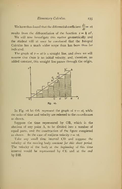
Elementary Calculus. 235
We have thus found that the differential coefficientds
dtat
results from the differentiation of the function s = \ at2
.
We will now investigate this matter geometrically and
the student will at once be convinced that the Integral
Calculus has a much wider scope than has been thus far
indicated.
The graph of v = at is a straight line, and since we will
assume that there is no initial velocity, and, therefore, no
added constant, this straight line passes through the origin.
in
GbL
f/w/\ 1/ "1
J/ 1, i
0- c D
Fig. 16.
In Fig. 16 let OA represent the graph of v = at, while
the units of time and velocity are referred to the co-ordinates
as shown.
Suppose the time represented by OB, which is the
abscissa of any point A, to be divided into a number of
equal parts, and the construction of the figure completed
as shown. In the case of uniform velocity s = vt.
Take any small time interval CD and suppose the
velocity of the moving body constant for this short period.
The velocity of the body at the beginning of this time
interval would be represented by CE and at the end
by DEL

236 Elementary Calculus.
Since s = vt is the space traversed by the body during
the time represented by CD, then, under the supposition,
that throughout this short time interval a constant velocity
equal to CE is maintained, CE X CD or the area of the
rectangle CDFE would geometrically represent the space
traversed.
Again, since DH represents the final velocity at the end
of the time interval CD, then the area of the rectangle
CDHG would represent the space traversed, under the
supposition that throughout the time CD this latter velocity
be constantly maintained. The actual space traversed
would be more than the first result would indicate, and
less than the latter.
Now the complete space traversed would be clearly more
than that represented by the shaded rectangles and less
than that indicated by the larger rectangles, of which
CDHG is a representative. The difference or error would
be given by the sum of the small rectangles, pne of which
is EFHG.Now the sum of these latter is equal to the rectangle
D'BAK'. But the area of D'BAK' can be infinitely reduced
by making the time interval small, and when the latter is
dt or infinitely small, the area of D'BAK' is evanescent. In
this case the error or difference disappears and the whole
space traversed during the time OB is represented by the
area of the triangle OAB.
Now the area of the triangle OAB = § . OB X BA.
But OB = / and BA = v.
Hence OAB = J t . v — it .at,
or area of OAB = J at2
.
But the area of OAB represents s,
.'. s= i at2
.

Elementary Calculus. 237
/
Hence we find that when we integrate thus, I ds =
at . dt, and find s = J a/2, we have really obtained the
sum of an infinite number of elementary areas, each v . at
or at . J/, the total of which gives the space traversed by
the body during the time /, and moving in accordance with
the law v = at.
The summation of elementary areas with a view of
obtaining a result indicated by their total is a marked
feature of the Integral Calculus.
Art. 43. The definite integral. Should it be required
to determine the space traversed by a moving body under
the law v = at during a finite time interval CD we might
proceed thus: putting OD = t2and OC = t
x(Fig. 17), and
integrating ds I = / at . dt, we get s = \ at2 + C, as we
have already seen, and if the initial velocity is zero we
have s = \ at2
.
The space traversed from zero to t2
is represented by the

238 Elementary Calculus.
area of the triangle ODH = ^ at22
, and that from zero to
tv by the area of OCE = J at2
.
Subtracting, we have \ at2
2 — \ at2 = area CDHE, which
gives the required space traversed. In the language of the
Integral Calculus we express the above as follows :
J5
atdt = I at2dt — I at
xdt= \ at
22 — \ at
2,
t2 J Jor thus,
hatdt = [J at2^ = i at 2 - \ at
2.£
The integral / atdt is called a Definite Integral; t2 andJt
t
ttare referred to as the superior or upper, and inferior or
lower limit, respectively. We read the expression thus: the
integral from ttto t2
of at . dt.
It will be noticed that the quantity enclosed in brackets
is the solution of the general or indefinite integral, and
that the solution of the definite integral is obtained by sub-
stituting first the upper limit, then the lower, and taking
the difference.
The constant is clearly made to disappear by taking the
difference between the integrals formed by giving two
successive values to the independent variable.
To find the value 0} a definite integral solve the general
integral, then substitute first the upper, then the lower limit,
and take the difference. This process will be made clear
by the following simple example:
Required the space traversed between 5th and 7th seconds,
given the acceleration equal to 4 feet per second per second.
5= f7
at ,dt=[i at2\\
.'. * = 'i-4. (7)2 -i'4-(5) 2 =48sq.ft.
Elementary Calculus. 239
INTEGRATION OF GENERAL FORMS.
Art. 44. It is to be observed that in the formula,
/xn + l
axn dx = a (A)n + 1
x stands for any expression whatever. Hence, whenever
we have a quantity, monomial or polynomial, raised to any
power and the differential of this quantity (without its
exponent), formula (A) applies.
Example. I (2 x3 — 3 x2 + 5)* (x2 — x) dx = what?
Since a constant does not affect differentiation, it does not
affect integration, so that we are always at liberty to intro-
duce a constant factor behind the integral, if at the same
time we divide the integral by the same factor, in order
that the value be not altered. But no expression contain-
ing the variable can be removed from behind the integral or
introduced in any way.
In the example above,
d{2 x3 — 3 x2 + 5) = (6 x2 — 6 x) dx = 6 (x2 — x) dx.
Hence if the expression {x2 — x) dx be multiplied by 6, it
becomes the differential of 2 x3 — 3 x2 + 5 and we get
form (A); thus,
(2 x3 — 3 x2 + 5 )* (x2 — x) dx =
(2 x3 — 3 x2 + 5)* (6 x2 + 6 x) dx =
zHz [Like (A)], [where 2 = 2 x3 — 3 x2 + 5].
(2 x3 — 3 x2 +5)^ (x2 — #) <fo
^ (2 x* — 3 x2 + 5)S _ (2 x3 — 3x2 + 5)1
I i5
240 Elementary Calculus.
. p xdxAgaln Jv^^ =what?
/xdx
ye2 — x2
- i f (>2 - *2 )~* (~ 2 *<&) = - (r
2 - x2)
since — 2 x dx = d(r2 — x2).
TRIGONOMETRIC INTEGRALS AND LOGINTEGRALS.
Art. 45. Since integration is the reverse of differen-
tiation, we easily derive the following, by reversing the
formulae for differentiation:
I cos x dx = sin x + c.
/ sin x dx = — cos x + c.
I sec 2 xdx= tan x + c.
I esc 2 x dx = — cot x + £•
I sec x tan x dx = sec # -f- c.
I esc # cot x dx = — esc x + c.
/dx
\/i — x2sin
-1 x + c, or — cos-1 # + c.

Elementary Calculus. 241
fdx = tan- 1 x + c.
J 1 + x2
I—
,= sin
-1-f c or — cos-1 —\- c.
1 x 1 1 .»_ 1 3£ 1
tan-1 h c or cot-1 — + c.
a a a
\/a2 — x~
r dx = 1
J a2 + x2 a
— = log x + c, etc.
Put these all into rules.
EXERCISE VI.
Integrate
:
1. 1 x^ dx. 2. I (x — 2)2 dx.
3-J (3 * + 5)
§ <&.
4. / (2 x2 — 4 # + 5 )* (x — 1 ) dx.
5. / (x2 — i)i xdx. 6. / (x2 + 3 x) 2 dx.
7- f(5*§ ~ 3** + i)<&. 8. p5
~ 1dx.
J J x — 1
/xdx Ac3 — 2 x2 + 1 »
7-= ;• 10. / :
—
— ax(x2 + 1)* J X2
11. / (1 — x)3 \/x dx. 12. I (\/n —\/xY dx
J3- I (3 x2 — tf
3)* (2 x — x2
) dx.

242 Elementary Calculus.
16. / cos3 x sin x dx. 17. I (1 — cos x) 2 sin dx.
18. I tan^ # sec2 x dx. 19. I cot3 x esc 2 # <fo.
/ sec 2 x tan # d#. 21. I esc3 x cot x dx.20
22.
24.
32.
34-
/tanxd#. 2^. /sin x cos #
26. / cos x2 # dx. 27. f e3* d#./ cosx2 xdx. 27.
J<
Q C xdx r (x2-h'i) (foe
J^2 + i J^3 + 3^ -2
J ^ + 1 J x*
/2 x — 3 , /^3 sec 2 x dx
nr+3 33\T
If.
2^ + 3 J tan x
sin x dx
cos#
Art. 46. The sine curve; harmonic motion. Suppose
Pt
(Fig. 18) is a body moving in a circle with uniform
velocity, the centre of the circle being O ; let P2be a second
body moving in the fixed diameter AB, but in such a man-
ner that P2 always maintains a position at the foot of the

Elementary Calculus. 243
perpendicular from Ptupon AB. Now the body P
2 travels
backwards and forwards upon the diameter and its velocity
y' ,
1P1p3
B\
p2 |A X
Fig. 18.
will be at a maximum as it passes O and diminishes as it
approaches B and A ; such motion executed by P2
is called
Simple Harmonic Motion.
The distance from O to A or B is called the Amplitude.
If we fix upon any point in AB, then, once at each complete
revolution of Px , the body P
2will pass this fixed point,
travelling in the same direction. The time thus occupied by
P2in completing such a cycle of motion is called a Period.
The motion of a tuning fork, an oscillating pendulum and
an alternating current, are good examples of periodic
motion. The change of position or motion of the particle
P2
is clearly a function of the time, and further since each
cycle of motion recurs periodically, we say that the Simple
244 Elementary Calculus.
Harmonic Motion of a point is a periodic function of
time.
In general a Periodic Function is one, the value of
which recurs at fixed intervals, while the variable increases
uniformly.
In Fig. 18, suppose OP is a revolving radius, and tracing
a constantly increasing angle, a.
Putting the radius of the circle equal to unity
then sin a = P2Pi,
or in general y — sin a.
.*. y = sin (a + 2 k).
Evidently, then, y = sin a is a periodic function, and
the period is the time taken to complete one revolution.
This is equal to 271 divided by the angular velocity, which
we will call 0. We thus have the Period T=6
The Frequency, or the number of periods in a second, is
'•FNote that = 2 n . — , and .'.6=2 nj.
In electrical work the number of alternations per minute
is often used instead of the frequency. From the annexed
diagram it will be seen that the motion of the Point P3
is
exactly similar to that of P2 , excepting that when P
2is at
the extremity of its path, where the instantaneous velocity
is zero, the point P3is passing through the O with its maxi-
mum velocity and so on.
Calling the radius of the circle a (the Amplitude), we have,

Elementary Calculus. 245
but
or
cos (90 -v \js. y- a)=
dpf a'
cos (90 -- a) = sin a,
y = a cos (90 — a).
'. y = a sin a,
y — a sin (a + 2 7:).
Hence we see that y = a sin a represents the Simple
Harmonic Motion of the point P3 ; where a is the Ampli-
tude and a the angle described from a fixed starting
point, and is the product of the angular velocity and time,
a = dt, we generally write y = a sin dt.
Note that since the sine can never be greater than + 1 or
less than — 1, hence the maximum and minimum values
of sin 6t are + 1 and — 1, respectively.
We will now draw a graph of the Simple Harmonic
Function y = sin a:
If a = y = a = 154
y = 0.707
ita = —
4y = 0.707 a = 7T y =
7ta = —
2?= 1 a = 1ZE
4y = - .707
a = IE2
y= - 1
a = 7 7T
4y = - .707
;y = o.

246 Elementary Calculus.
Referring a, expressed in radians to the #-axis, and
using the same scale as the ordinate, we obtain a sinuous
or wavy curve, known as the Curve of Sines or the Har-
monic Curve. If the motion of the point giving rise to
this graph be made quicker or slower, the undulations of
the curve will be more widely spread or brought nearer
together.
Increase in Amplitude gives increased rise to the undu-
lations and vice versa.
Fig. (18a) shows the same curve plotted by another
Fig. 18a.
method; the student should have no difficulty in understand-
ing the principle after an inspection of the figure. It will
be noticed that the curve does not begin upon the x-axis,
but that the periodic time is counted from the instant that
the point Pthas passed through the angle e. This angle
e is called by electrical engineers the lead; when negative
it is known as the lag.
The term Phase is used to denote the interval of time
that has elapsed since the point P passed through its initial
position at A, and hence e is often called the Phase Con-
stant.
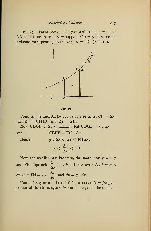
Elementary Calculus. 247
Art. 47. Plane areas. Let y = f(x) be a curve, and
AB a fixed ordinate. Now suppose CD = y be a second
ordinate corresponding to the value # = OC (Fig. 19).
Fig. rg.
Consider the area ABDC, call this area u, let CF = Ax,
then Au = CFHD, and Ay = GH.Now CDGF < Au < CEHF ; but CDGF = y . Ax,
and CEHF = FH . Ax.
Hence y . Ax < Aw < FHA*.
.*• y < -r- < FH.Ax
Now the smaller A# becomes, the more nearly will yAu
and FH approach — in value; hence when Ax becomesAxdu
dx, then FH = y = — and du = y . dx.dx
Hence if any area is bounded by a curve (y = f(x)), a
portion of the abscissa, and two ordinates, then the differen-
248 Elementary Calculus.
tial of such area (du) is equal to the product of the termi-
nating ordinate (y) and dx.
Adopting the notation of the last paragraph we have,
for the Definite Integral which expresses the area bounded
by the curve, part of the abscissa, and two ordinates, a
and b, this expression
x y . dx.
Or since y — J(x) we might write I j(x)dx.
NoTe: y . dx gives a numerical measure of an arer
which may be found as follows:
(I) Integrate the given differential expression, or as
we say find the indefinite integral.
(II) Substitute the given limits, first the higher, then
the lower; subtract the latter resulting expression from the
former.

CHAPTER IV.
TANGENTS, SUBTANGENTS, NORMALS ANDSUBNORMALS.
Art. 48. In Analytic Geometry it was found that the
form
y — y' = m (x — x') (C)
expressed the equation of a straight line in terms of its
slope (m) and a fixed point (V, y').
As any curve may be regarded as generated by a point
moving according to a definite law> expressed by its equa-
tion, the direction of a curve at any point is the direction in
which this point (taken as the generating point) is moving
at the instant. But the generating point if not constrained
to move in the curve, would at any instant move off in a
straight line (by the first law of motion) and this straight
line would be tangent to the curve at the point of departure;
hence
:
The slope of a curve at any point is the slope of its tan-
gent at that point, slope meaning as usual the tangent of
the angle made with the x-axis.
In equation (C), if {xf', y
f
) is a point on a given curve,
and m is the slope of the tangent at that point, then (C)
is the equation of the tangent at (x', yf). But if y = f (x)
(where / (x) is any expression containing only x and
known quantities) is the equation to a curve it has been
shown that — = the slope of the tangent to the curve, and if
dx
the coordinates of a definite point on the curve, like (xf
, /),249

250 Elementary Calculus.
be substituted in the value of -f~ , it will then representdx
the slope of the tangent at that point; say{
-j— ]= slope of the
tangent at (x'fy').
Then (C) becomes
'-'-SL.*" ••
• (T)
which is clearly the tangent equation at (V, y').
Art. 49. From these considerations an expression for
the subtangent is readily found, in exactly the same way
as described in Analytic Geometry (see Art. 50).
Since the normal is a perpendicular to the tangent at the
point of tangency (x', /), its equation will be,
'' - - (¥) «* - *0 • • •(N)
\aX /x', y'
by the relation between the slopes of J_ lines as developed
in Analytic Geometry.
This equation may be written:
y - / = - f-^\ (x - x'),
\dy/x>,y
dx dvif we understand — to represent the reciprocal of— •
dy dx
As in the case of the subtangent the subnormal is
readily found by determining its ^-intercept from its equa-
tion (N).

Elementary Calculus. 25 1
Let
then
whence
y = o in (N),
/ = - — (x- x'),dy x>,y
;> + y>(<!f\=0C . (Fig. 20)
Fig. 20.
But subnormal, BC = OC - OB [P = (V, /)]
\dx) x>,y> J W/^,rCorollary : The lengths of tangent and normal are
readily found, since they are the hypotenuses, respectively,
of the triangles APB and BPC.
AP 2= AB 2+ PB 2=/ 2 f**-)2
+ /2\dy I x',y
-<•[+&..}and PC
2 =PB 2+ BC2 = /2fi + ^Y 1L V**/ x>,y>\
Example : Find equation of tangent, subtangent and
subnormal to the ellipse 16 x2 + 25 y2 = 400 at (3, 3 J).

252 Elementary Calculus.
From 16 x2 + 25 y2 = 400
dy
dx=- 16 X
25 y
At the point (3, 33-) this becomes,
&h'- - 16X3.
25 x V6-3L
5
Hence tangent equation LS
[(*', /) = (3,34)1
y- _i6
5 55),
or sy + 3* - 25 = 0,
also(£)
--,--1Vty /a?' .2/'
—^r
.
Hence subtangent = / '£) .- (4_i6_
3
and subnormal = / f— ) = — (
— -) = — — •
\dx
/
x>,y' 5 V 5/ 25
Art. 50. Subtangent, subnormal, etc., in polar co-ordi-
nates.
Using the Polar System, subtangent and subnormal are
defined as follows:
The subtangent and subnormal are respectively the dis-
tances cut off by tangent and normal from the pole on a
line drawn through it J_ to the radius vector of the tan-
gency point, as OT and ON (Fig. 21).

Elementary Calculus. 253
Calling the angle TPO between radius vector and tan-
gent, {ftj we have in the right traingles OPT and OPN,
Fig. 21.
subtangent, OT = OP tan TPO = p tan (p. Subnormal,
ON = OP tan OPN = p cot <b (since OPN = 90 - TPO)The angle
<fiis determined thus:
Let ACE be any curve (Fig. 22), the co-ordinates of C
Fig. 22.
being (p, 6), and of A being (p + Ap, 6 + A0). Then
AB = \p and AOC = Ad. Tan BAC = — [since AdH AB L

254 Elementary Calculus.
is a very small angle the arc BC does not differ sensibly
from a tangent at B, say]. Whence
tan BAC = eM
(arc BC = pA#, since an arc = its angle multiplied by the
radius). As the point A approaches C, the secant ACapproaches the position of a tangent at C (FG) and BACapproaches the value </» (OCG), hence, finally,
tan (p = -dp
•t a
Hence polar subtangent = p tan <p = p2—
,
dp
and polar subnormal = p cot df = —- •
dd
EXERCISE VII.
i. Find the length of tangent and normal for the para-
bola y2 = 16 x at x = 4.
2. Find the length of subtangent and subnormal to the
ellipse 9 x2 + 16 y2 = 144 at (6, 6 y/$).
3. Find the equations of tangent and normal to
y2 = 16 x3
at (1, 4).
4. Find the length of the normal to x2(x + y) = 4 (x — y)
at (o, o).
5. Find where the tangent to yax = x3 — a3is parallel
to the x-axis.
6. Find where the normal is _L to the x-axis on the curve,
f = x2(8 - x).
7. Find the angle at which x2 = y2 + 9 intersects
4 x2 + 9 y2 = 36.

Elementary Calculus. 255
8. In the equilateral hyperbola x2 — y2 — 16. The
area of the triangle formed by a tangent and the co-
ordinate axes is constant and equal to 16. Prove it.
9. At what angle do y2 = 8 x and x2 + y
2 = 20 intersect?
10. Show that the subtangent to the parabola y2 = 2 px
is twice the abscissa of the point of tangency.
n. Show that in a circle the length of the normal is
constant.
12. The equation of the tractrix being
x = \/a2 - y2 + - log
v7
7,
2 a + \/a2 — y2
show that the length of the tangent is constant.

CHAPTER V.
SUCCESSIVE DIFFERENTIATIONS.
Art. 51. Since -2— is, in general, purely a function of
x, its differential coefficient may be found as readily as that
d2yof the original function. It is usually symbolized thus, —~ •
dxFor example, if y = 3 x3 + 2 x2 — 5 x%,
-2-* = gx2-\- 4X — § x~%,
dx
f£= 18* + 4 + 1*-*.CLX
Likewise the differential of this second differential may be
found in the same way, and is symbolized as —\\ thedxr
fourth differential coefficient as — ; the n thas —- • It
dx4 dxn
sometimes happens that the successive differential coeffi-
cient may be written by analogy after three or four have
been found. For example :
y = xm,
mxm—1dy _dx
—2 = m (m — 1) xm-2,
dx2
dty = m (m — 1) (m — 2) x— o\ -v-W—
3
dx3
256

Elementary Calculus. 257
dny ( \ / x—— = m (m — 1) \m — 2) . . .
dxn
(m — n + 1 ) x m~n
If the function be an implicit function of x and y, it is
not necessary to put it in explicit form, as the previously
found derivatives may be used to find successively each
higher one. For example:
x2 + y2 = r2
. . . . (1)
Take ^-derivative : 2 x + 2 y
solving for -2-
,
dx
dx00
dy x
dx y(3)
dyy — x——
d2y _
ydx
dx2 y2 (4)whence
substituting value of ^— already found from (3) in (4),dx
+ -d2y _ y _ _ x2 + y
2 _ _ r^
dx2y
2y3 /
2 2 dy- 3 r y —
—
d?y ^x_ 3 r2x
d*3"
v6~~
v5 '
eC '
MACLAURIN'S AND TAYLOR'S FORMULAE.
Art. 52. It is frequently useful for purposes of calcula-
tion to express the value of a function in the form of a
series. For example, in algebra, the binomial theorem
enables us to develop a binomial raised to any power into a
series of powers of the single quantities involved, as,
(a + b)4 = a 4 + 4 a3 b + 6 a2
b2 + 4 a b
3 + b\ etc.

258 Elementary Calculus.
Likewise the logarithms of numbers and the trigonometric
functions are computed from series.
Hence a general method for the expression of any func-
tion of x, say, in series, would prove exceedingly useful.
But such a series has utility only when its sum is a finite
quantity. In general, series have an unlimited number of
terms, and clearly, unless the sum of these terms is a finite
quantity, it is utterly useless. A series whose sum is finite
is called a convergent series.
It is only with such series that we shall deal here. Let
it be required to develop f(x) into a series of powers of
(x — m) say. Supposing such a development possible, let
f(x) = A + B (x - m) + C (x - mf + D (x - mf,etc (a)
Differentiate (a) successively:
/'(*) = B + 2 C (x - m) + 3 D (x - mf+ 4 E (x — m)3 + ' etc.
f"(x) = 2 C + 6 D (x - m) + 12 E (x - mf +
f"{x) = 6 D + 24 E [x - m) +fw(x) = 24 E +
Since x is assumed to have any value, let
x = m.
Then f(m) = A or A =/(»);
f{m) = B, B = f(m);
rim) = 2 C,Z2 '
/"'(») =3. 2 -D, D = CM;
Z3
/*v(w ) = 4 . 3 . 2 E, E = ^) , etc.
Z4

Elementary Calculus. 259
Substituting in (a)
t(x) = j(m) + f{m) (x - m) + tll&L {x-mf
1 fUI(m) , N o , fr
v (m) , , 4 , /UN+ *—*
—
'- (x — mf + *—*—'- ix — my + . . . (b)
Example: Develop log x in powers of (x — 2).
/ (#) = log*, / (2) = log 2.
A'
/"(*)= -S' /"(2)=-i.
rw = ^ r(2) = *.
/IV(*) = --
4. /
IV(2)= -I, etc.
Hence log x = log 2 + \ (x — 2) — \ (x — 2)2
+ i(x- 2)3 - %(x- 2)
4 +
Art. 53. If in formula (b), m be made o, which is
clearly permissible, since no restrictions were placed on its
value, the formula becomes the development for f{x) in
terms of x:
/(*)= /(o)+/'(o)x+ Q^-x2 +Q^a:3
+ ££>**+ (b)Z4
where /(o), /'(o), etc., mean the values of fix), fix), etc.,
when x is replaced by o.
Example : Develop cos x in terms of x.
f (x) = cos x, f (o) = cos o = 1.
f (x) = — sin x, ff
(°) = — sin o = o.
F'(x) = — cos#, f"(o) — — coso= — 1.

260 Elementary Calculus.
/"'(*) = sin x, /'"(o) = sin o = o.
/iv (^ = cos Xj /IV (o) = cos o = i, etc.
Substituting in (b):
x2 x*Cos x = i —
. -f--—
, etc.,
Z.2 Z4'
which is the expression from which cos x is computed.
For example, to find cos 30 = cos ( — rad.)
»
(-) (-)' (-)'
cxx. 3o°= 1-^ +^L -X-L + etc. (w= 3.1416.)2 24 720
I = I.
W _ (. 5 2 3 6)4
24 24= -00313
I-003I3
M..2
- .I3708
- -I37II
approx. 720
- .OOOO3
cos 30 = .86602
- -13711
The series (b) (and its special form bj is known as
Maclaurin's Series from its discoverer.
Art. 54. It is frequently necessary to express a func-
tion of two quantities in the form of a series of powers of
one of them, as for example, f(h + x) in powers of x.
The process is entirely analogous to that employed in
the development of Maclaurin's Series, and the result is
known as Taylor's formula.
Assuming that }(h + x) can be developed in powers of
x, and regarding h as constant:
Let }{h + x) = A + Bx + Cx2 + Bx3 + Ex4 + (c)

Elementary Calculus. 261
Taking the derivatives with respect to x,
f(x + h) = B + 2 Cx + 3 Di2 +4Ei3 +...f'{p +k)= 2 C + 6 Da; + 12 Ex2 + . . .
/"'(# -f- h) = 6 D + 24 Ex + . . .
/*(* + A) = 24 E + . . .
Since this series must be true for all values of x}being an
identity, it is true when x = o; hence setting x = o in this
series of equations we are enabled to determine the con-
stants, thus:
A = f(h).
B = /'(/>).
c f"(h)
Z2
E = fzihL (6 = 3 x 2 x 1 = zs ).
Substituting in (c)
/(* + fc) = jilt) + f(/t) * + J^l x2 + l^lx3
Z4
Where /(/i), /'(/*)> etc -> mean the values of f(x+h), f'(x+h),
etc., when x = o.
Art. 55. It will be evident upon consideration, that the
binomial theorem as encountered in algebra is a special
form of Taylor's formula. The utility of these develop-
ments of Maclaurin and Taylor, depends upon the rapidity
vvith which they converge.

262 Elementary Calculus.
As the series developed by these two formulae is usually
infinite, there is always a residual error in taking the sum
of a limited number of terms as the value of the function
thus expanded. A discussion of this error is unnecessary
here; it will be sufficient for us now to observe that a
series has satisfactory convergence, if the successive terms
decrease rapidly in value, and after a limited number of
terms, approach zero.
It is usuallly an effective test of convergence, when the
nth term of a series can be readily expressed, to find the
ratio between the (n + i) th and 11th terms. If this ratio
approaches zero as n approaches infinity, the series is con-
vergent, otherwise divergent, and hence, useless for prac-
tical purposes.
Example : To test convergency of sine-series.
x3. .v
5.v
7,
sin x = x + . . .
Z3 Z5 U(-1) n-l
A.2U
Inspection of the relation between the coefficients of v,
the denominators, and the corresponding term number,
gives the nth term as above. The (n + 1)* term like-
wise is,
A.2 n + 1
If then the value approached by the ratio,
/ 2 ft —I— T—
—
as n approaches infinity,
Z_2 n — 1
is zero, the series is convergent, otherwise not.

Elementary Calculus. 263
/_2 11 + 1 x-r
o if n = 00
.
{211 -\- i) 2 n
Z.2 n — 1
Hence the sine-series is convergent.
It is to be observed that it is only the absolute values of
the terms that are considered, as the sign does not affect
the ratio. There are numerous more complicated tests
for convergency, but they do not come within the scope of
this book.
EXERCISE VIII.
1. y=4x3 -8x2 +2»-i, find —-2
•
ax
2. y = x3, find -2«
dx6
dny7.. y = xn , find —— •
4. y = x log x, find —~ •
dx2
5. y= log (e* + e-x), find p- •
dx6
6. y= e* (x2 - 4 x+ 8), find^ .
dx3
1 ^ j d4y
8. y= xMogx, find^X
9. y = x3 — — find —2 •
10. y = log sin x, find —^
.
' & '
dx 4

264 Elementary Calculus.
11. y = sin 2 x, find —~-dx3
x2 d?v12. y = , find —?-*
1 — x dx2
13. y = e2x (x2 — 2 x + i),fmd ~^-
dxA
dny14. y = eax , find —— •
dxn
15. y = exsin x}show —^ 2 -2- + 2 v = o.
dx2 dx
ex -f- c—x
</2/v
16. y = , express -4 in terms of y.'ex _ x-x
f ^2 '
17. ;y = ^2ex , show that —^= 6^(x+ 1) + y.
18. z = 1 + #e2,find —-
•
dx2
19. x3 - 3 axy + y3
, find —|-
20. 62*2 -a2
;y
2 = a262
, find^.
21. y2 = 2 £#, find —\-
dx
22. xy — c2
, find —?•y' dx3
23. «•+*= ay, find ^.
a 1 & x \ d y24. 3/ = —
(<?^" -f-
0- —], find
—-5 in terms of y and a.
2 \ ) dx
25. f = a2x, find -Z.
dx2
26. # = r vers-1
2. — \A ry — y2
, find —^ in termsr ax'
5
of 3/ and r.

Elementary Calculus. 265
EXERCISE IX.
Expand by Maclaurin's formula:
1. sin x (in powers of x).
2. tan-1^.
3. \ogx (in powers of (x — 1))
4. (in powers of x).1 — x
5. ex (in powers of (x — 2)).
6. — (in powers of (x — h)).x
Expand by Taylor's formula in powers of x:
7. sin (n + x). 10. log sin (h + x).
8. \A— *2- JI - sec (a + *)•
9. ea+x
. 12. (a — #)n .
CHAPTER VI.
EVOLUTION OF INDETERMINATE FORMS.
Art. 56. Functions of a variable which reduce to such
forms as — — , o, 00, etc., for certain values of the vari-o 00
able are called indeterminate, because we are unable to divide
o by o, or 00 by 00 directly, but must approach the quotients
by a circuitous path.
The consideration of a definite example may make the
idea clearer.
-v5 j
Take for example, when x = 1.
x — 1
Clearly, = — when x = 1.
x — 1 o
But also = - when x = 1,x — I o
, x3 — 8 o ,
and — = — when x = 2,x — 2 o
, 2 X — X2 — I O ,
and — = — when x = 1.
3 # — 2 x — 1 o
Evidently — does not mean the same thing in all theseo
cases, nor in the multitude of similar cases that might be
cited. Having practically an infinite number of possible
values then, the expression — is indeterminate. It willo
be recalled that in discussing the differential quotient, it
266
Elementary Calculus. 267
was remarked that although two quantities may each be
too small (or too large) for individual comprehension,
they might yet have a finite, readily expressible ratio, if
they belonged to the same order of smallness (or largeness).
To use a somewhat inadequate illustration, two typhoid
bacilli, though each hopelessly beyond the reach of our
ordinary senses, could be readily compared with one another
and their relative size could be expressed by a very simple
number. Although a bacillus is not infinitely small, the
same illustration may be extended indefinitely. As the
chemist has to approach the problem of his inconceivably
small atom and the astronomer of his inconceivably vast
distances, indirectly, so we will have to deal with our zeroes
and infinities.
To return to the expressionx— 1
Before giving x any definite value, divide the numerator
by the denominator, then = x4 + x3 +x2 + x-{- 1.
x — 1
If in this expression we give x a, constantly decreasing
value >i, the integral function will clearly approach more
and more nearly the value 5, while the fraction approaches
the value — . It is easy to infer then that when x is actuallyo
1, the value of — becomes exactly 5.
Again the expression
2 x — x2 — 1
3 x2 — 2 x —1
may be shown to approach — J as x approaches 00
,
if we first divide both numerator and denominator by
x2.

268 Elementary Calculus.
Art. 57. To find a general method jor evaluating an
indeterminate.
Let -f^-f-= — when x = a.
<p(x) o
By Maclaurin's formula,
/(*) = HP) + f(fi) (*-«) + -^ (* - af
+ tt) (x _«)3 + .
2
..
0(x) = 0(a) + 0'(a) (* - a) + ^^ (* - a)2
+ £l(x-af+ ...
But j(a) = o and (a) = o by hypothesis.
. /(*) =
f(a) (x - a) +i^) (* - a)2+ ^^ (* - a)
3 + ...Z2 /3
0(a) (x - a) + 41i*) (* - a) 2 + £^£1 (* - af + . . .
Z.2 Z3
/'(a) +/^I (x - a ) + ¥^(x - a) 2 + . . .
= Z2 Z3
,,, N , 0"(a) , N .
6'" (a),, 2 .
9 (a) + (# — a) + t—!_£(# — ay + ...
(dividing numerator and denominator by x — a)
= ' ^(since (5; — a), (x— a)2
, etc. = o when x = a).0'(a)
If T7T~r still equals — for x = a,
(#) o
it is clear that the expression reduces to ')
', if /'(#)
0"(#) •

Elementary Calculus. 269
<f>'(x) are replaced by their values, o, and numerator and
denominator be again divided by x — a.
Hence when xLJ = _ ior x = a,(p{x) o
/(*)_ r(*) - /'wetc
A rule may be stated thus
:
Take the successive derivatives of numerator and denom-
inator (as distinct functions) until a derivative is found,
say fn (x), which is not zero for x = a. Then,
' ^ ' = ' ^ 'is the value sought.
cf)n (x) <j)(x)
^ t7 ^ , , tan x — sin x cos x oExample : Evaluate = —
,
x3 o
when x = o.
tt tan x — sin x cos x __ j(x)
x3(f>(x)
Xs 3X2
(taking derivatives).
}'(x) • oThis expression corresponding to ' v '
still equals _ •
(f>(x) o
Hence taking second derivative,
tan x — sin x cos x __ sec2 x — cos2 x + sin
2 x
Xs3#
2
2 sec x tan x -\- 2 cos x sin x + 2 sin x cos x
6 xsec x tan x + 2 sin x cos x
(collecting and dividing by 2).

7o Elementary Calculus.
This is still - • Taking third derivative f"^o
50"'(*)
sec3 x -f sec x tan2 x + 2 cos
2 x — 2 sin2jg _ 3_
3 3
= 1, when x = o.
. tan x — sin x cos x
.v3
= 1, when x = o.
Art. 58. If ^ ' . = — when ^ = a, a simple trans-6{x) 00
formation reduces the expression to the form —; for
o
iW =M = °[or:c= „.
cj>(x) I o
If /(#) = o and (f>(x) = co for x = a,
then /(#) . <j)(x) = o . go, an indeterminate,
but /(*) .<£(*) = ^=--I_ o
</>(x)
By using the logarithms of the functions as an interme-
diate step, expressions like i00
, o00
,00 °, etc., may be
reduced likewise to — For example, let j(x) = 1 ando
<f>(x) = co, when x = a.
Then /0)]^> = i°°.
Let v=[/(x)]*(*>.
Taking the log of both sides
:
Log y = <j>(x) log /(.x) = ° '^ ' = — when x = a.1 o

Elementary Calculus. 271
In these cases we get eventually the logarithm of the
function, from which the function itself is readily found.
/ x \ tan 3™-
Example : Evaluate (2 1 2 a|when x = a,
irx
/ X \ tan TT*- «
Let y = (2 - -J
2 a
log (2 - -)
Then log y = tan— log (2 - ~)= ^ CU = 2.
cot »
2 a
,\ log y.
iog (-:-) _ -lullcot H. _ _*
. .,.2 **— CSC2 « 2« '2a
I I
2 a — x a 2,= — = — , when x = a.
_£- csc2 nX X_
7t
2a 2a 2a
That is, log y = log (2 - ~Yn
Ta = \ when x = a.
tan™- _2_.*. (2 — a) 2 a = e n .
1
Example : Evaluate (a * -1 ) x, when # = 00
.
— _i
(ax - 1) x= (a
00 - 1) 00 = (a°- 1) oo = 0.00,
when # = 00
.

272 Elementary Calculus
But (a* - i)xa* - 1 o
1 o
a;
_L JL
a — 1 — a log a
when x — 00
.
EXERCISE X.
Evaluate:
1.°^ ^
, when y = 1.
gX g—
X
2. , when x = 1.
tan :v
^— = a * loga = log a,
3-4 x sin # — 2 7r , ;r-
, when x =- .
COS # 2
4-2 I whpn 8 — n
*
cos2 # i — sin # 2
5- —, , when #= 1.
x*-1
6. (sin v) /aw yfwhen v = - •
2
7-e* + g~* — 2 ,
, when z = 0.
8. *
—
!—'-, when x = o.
when # = 00.
Elementary Calculus. 273
sin-* x ,
10. ;— , when x = o.tan x
ey sin y — y — y2
,
losr sin 2 # ,
12. —s—;
, when x = o.log sin #
13. ( /«* — i)#, when# = 00.
14-'— , when x = 1.
6* — 6 x — 1
15. : •
, when x = 1.log » log x
i 2
16. (cos 2d) , when # = o.
17. (logx)*- 1, when #= 1.
loo; x ,
10. —e—, when # = o.
esc x
19. (1 — tan x) sec 2 x, when a; = -4
20. 6-* log #, when x = 00
.
[log (e + z)]*, when z = o.
[2 )tan — , when # = w.
\ 7?/ 2»
23. () ,
when x = o.
7rxsec —
24- : ; -,whenx=i.log (1 - x)

274 Elementary Calculus.
25. cot x, when x = o.x
, I — COS X ,
26. , when x = o.
# — sin-1 x ,
27. —, when x = o.
28. 2 X sin — , when # = 00
.
2 X
29. (sin #) ', when x = o.
30. .t e*, when x = o.
31-
32. i °x" *"'—
- — , when jc = — .
sin a; + cos x — 1 2
33- —=—H ^^ ^, when* =3.r - x' - 5 1 - 3
\/y tan y u34. — / ,
when 3; = o.
35. # tan x — — sec #, when # = — .
2 2
36•(+*;• when 2 = 00
.
CHAPTER VII.
MAXIMA AND MINIMA.
Art. 59. When a function has a maximum value it is
an increasing function until it reaches the value then a
decreasing function just afterward, otherwise this value
would not be a maximum. Since the derivative of a func-
tion is the ratio between its increase and the increase of its
independent variable, if the function is increasing with the
variable the derivative will be positive; if it is decreasing
as the variable increases the derivative will be negative.
Hence when a function passes through a maximum value
its derivative changes from positive to negative, and in
order to do this it must pass through the value zero, if it is
continuous. A similar process of reasoning shows that
when a function passes through a minimum value the deri-
vative also passes through zero from negative to positive.
It is to be remembered that since a function depends upon
its variable for its value, it can be made to take any number
of values, as near together as we please, by giving the
variable a suitable series of values, that is provided always
that the function is continuous.
A graphic illustration may make this plainer.
Since in general any function may be represented graph-
ically by a curve, let the curve AB, Fig. 23, represent
y = /(*).
Since the derivative of a function, represented by a
curve, is the slope of its tangent at any given point, the
change of the derivative and the tangent slope are synony-
275

276 Elementary Calculus.
mous. Suppose T is a maximum point for the value
x = OD. A glance at the figure will show that starting,
say with the tangent MN at A, the slope of this tangent as
the point of tangency moves from A to T will be constantly
positive (the inclination being an acute angle, as AMO ) but
constantly decreasing; at T the slope will be zero, for the
tangent, RS, is parallel to the .T-axis; beyond the point T,
the inclination of the tangent is an obtuse angle asj PQ#,and hence its tangent is negative, but it will still decrease
Fig. 23.
in general. Therefore, as indicated, the derivative of the
function which is always equal to these slopes, will pass
from positive to negative through zero. But a function
may pass through zero or infinity without changing its
sign, so even when the derivative is zero there may not be a
maximum or minimum. Hence it is necessary to deter-
mine in a given case whether a maximum or minimum
exists.
Recall the fact cited above, that the slope decreases to
zero before a maximum and continues to decrease (because
it is negative) after a maximum, hence the derivative is a

Elementary Calculus. 277
decreasing function at a maximum, hence its derivative,
that is, the second derivative of the original function, will
be negative from our definition of a derivative.
An examination of the figure around the point F (a
minimum) will show that at a minimum the slope, and
hence the derivative, passing from negative to positive
through zero, is an increasing function, hence its deriva-
tive, that is, the second derivative of the function, is
positive. This suggests a general method for determining
maxima and minima, as follows :
Since the first derivative is always zero at a maximum or
minimum point, if the first derivative is found and set
equal to zero, the value of the variable found from this
equation will, in general, be one of the co-ordinates (usually
the abscissa) of the maximum or minimum point on the
curve representing the function. To determine whether
it is a maximum or minimum, the second derivative is
found, and if it is negative in value for this value of the
variable, the point is a maximum; if positive, it is a minimum.
Art. 60. It may happen that the second derivative is
also zero for this value of the variable, and hence indeter-
minate as to sign. In this case it is clearly desirable to
expand the function in the neighborhood of this value of
the variable that its character may be more readily seen.
If (Jx) is the function, and x = a be the value found from
f(x) = o, then f(a — h) and f(a -f h) will represent the
value of the function immediately before and immediately
after, respectively, its value for x = a, h being a quantity
which can be made as small as desired.
By Taylor's formula:
f(X + h) = ax) + f(*)A+£g£ + rzig£ + . .
.

278 Elementary Calculus.
j{x - h) = f(x) - j'{x)h + ^-^ h2 - Q^U3 +
Replacing x by the value a, and transposing }{a),
f(a +h)- j{a) = f{a)h + £&L h2 + ?-"&Z.2 Z3
+
f(a -h)- j(a)=-f'{a)h + 1^1 h 2 = ^^- h* + . . .
Now since h is to be taken exceedingly small, its square,
cube, etc., in the developments will be insignificant, and
hence the values of the above expressions will practically
equal the first terms of their development. That is,
f(a + h) — }{a) will have the same sign as f'(a)h, and
I (a— h) — f(a) will have the sign of — f'{a)h. But if
there is a maximum or minimum at a, j(a + h) and j(a— h)
must have the same value, because if it increases to a
maximum it must decrease beyond the maximum, and
hence have the same value just before and just after, as
the sun has the same altitude at the same time before noon
and after, noon being its maximum elevation.
But the only way f'(a)h and — f(a)h could both have
the same value would be, that both equal zero, that is, that
f{a) = o [f'{a) being value of f'{x) when x— a], which
verifies our former conclusion.
If f'(a) = o, then,
j{a + h)- f(a) = tl^L h2 + r{a) ^ J-
and
Z2 Z3
r(a) , 2 /"'(«) isf(a -h)~ }{a) = ±^± W - L^l
Since h is so small, h2is much larger than h3
or any
higher power, hence }{a + h) — }(a) and }(a — h) — f(a)

Elementary Calculus. 279
are determined by '^a ' h2
, and hence are positive if f"(a)
is positive, and negative if f"(a) is negative
for /" (a) determines the sign of the term ' ^' h2
.
But, when }{a + h) — }{a) and f(a — h) — f(a) are
both negative, f(a) is a maximum, since it is greater
than the values on either side of it [}(a + h) and f(a — h)];
likewise, when they are both positive, f{a) is a minimum.
But these conditions prevail, respectively, when f" (a) is
negative and when f"(a) is positive, which verifies our
second conclusion above.
If f'{a) is also zero, then,
/(a+ /0 -/(a) ^-^U3 +^ /*'+.. .
and
M ; /W/3 Z4
A course of reasoning exactly as before, will show that
for a turning value (maximum or minimum)
'—K—l- Jr and — ;—±-L h 3 must equal zero,Z3 Z3
that is, /"'(a) = o,
and when /iv (a) is positive there is a minimum; when f
iv (a)
is negative there is a maximum, etc.
Hence the rule:
A function has a maximum or minimum value at x =a,
if any number of the successive derivatives, beginning with
the first, is zero for x = a, provided the first that does not
equal zero is of even order, being negative for a maximumand positive for a minimum.
280 Elementary Calculus.
The values of the variable which cause the first deriva-
tives of a function to vanish are called critical values.
Example: Find turning values of (x — i)B(x — 2)
2.
/(*)= (X- I)3 (X- 2)
2
/'(*) = 3 (X - I)2(X - 2)
2 + 2(X - l)3 (*-2)
whence (x — i)2(x — 2) (5 x — 8) = o,
x= 1, i, 2, f.
f"(x) = 2 (* - 1) (* - 2) (5 * - 8) + (* - i)2
(5 * - 8)
+ 5 (*- i)2 (x- 2).
When x= ij"{x)= o.
x = 2, /"(#) = 2 (positive).
* = f, /"(#) = -if (negative).
Hence for # = 2, there is a minimum,
and for x = f , there is a maximum.
Since /"(#) = o for x — 1, it is necessary to find the
third and fourth derivatives.
}'"{x) = 2 (30 x2 — 84 x + 57) = 6 when # = 1.
Hence there is neither maximum nor minimum at x = 1.
Example : What are the dimensions of the cylindrical
vessel of largest contents that can be made from 3234
square inches of tin plate, not counting waste?
Since 3234 square inches will constitute the surface of the
cylinder (one base) when completed,
2 nrh + nr2 = 3234 (1)
Volume = 7tt*h (2)
which is to be a maximum.
From (I) ft=3»34-^ = joaa^r _ 22.1;
2 7^ 2 f|_ 7 J
Elementary Calculus. 281
Substituting in (2)
27 1020 Tzr — Tir3
7i f 3,wrh = - —= —(1029 r — r).2 2
Since a constant does not change value it cannot affect
a maximum or minimum, hence any constant factor maybe ignored, in searching for turning values.
Say then, / (r) = 1029 r ~ r*i
?(r)= 1029 - sr2 = o,
whence r2 = 343, r = 7 V 7.
j,f{r) = — 6 r which is negative, hence r = 7 V7 gives a
maximum.
From (1) h= 7 V7 for f = 7V7. Hence the cylinder
will have greatest contents when its radius equals its
altitude.
EXERCISE XI.
Find maxima or minima
:
!. yj=JL. 2 .(* + 9)(*-2)
f4 X
(x *?
r — y+ 1
f + y- 1
1 i- ^ I — X
6^2 + 2 M + 3 ,
u2 + I
7. Divide a line i' long into two parts, such that their
product will be a maximum.
8. Find the greatest rectangle that can be inscribed in
a circle of radius 6".
9. Find the volume of the greatest cylinder inscribed in
a sphere of 8" radius.
10. Find the greatest cone in the same sphere.
11. Show that it takes the least amount of sheet iron to
make a cylindrical tank closed at both ends, when its
diameter equals its height.

282 Elementary Calculus.
12. Find the greatest cylinder that can be inscribed in
a right cone of radius, r, and height, h.
13. Calling the E.M.F. of a cell, E; internal resistance r,
external resistance, R, and current, C, C = and ther+ R
power, P = RC2. What value of R will make P a maxi-
mum?14. Find the shortest straight line that can be drawn
through a given point (w, n) and limited by the axes.

CHAPTER VIII.
PARTIAL DERIVATIVES.
Art. 6i. Up to this time functions of one independent
variable only have been considered, but an expression
may be a function of two or more independent variables.
A function of two variables, x and y say, is symbolized
thus:
/ (*, y), <f> (*, y), F(x, y), etc.
Continuous functions only give important general results,
and a function of two variables is continuous about any
specific values of these variables, say x = h, y = k, when
the function runs through an unbroken series of values (as
near together as we please) as its variables run through
corresponding series of consecutive values, in the vicinity
of h and k.
Art. 62. The derivative of a function of two (or more)
variables found by considering all the variables except one,
as constants, is called its partial derivative with respect to
the variable that changes. For example, 4 xy + 3 y2
is
the partial derivative with respect to x of the function
2 x?y + 3 xy2-f y
3(regarding y as a constant) and is
represented thus:
— (2 x2y + 3 xy2 + y
3) = 4 xy + 3 y
2-
--\
If z = 2 x2
y + 3 xy2 + y3
, then —-*= 4 xy + 3 y2
. (1
)
ox
Likewise the partial differential, with respect to x, is repre-
sented thus:
283
284 Elementary Calculus.
d~xz = 4 xy dx + 3 y2 dx (2)
~\
Evidently oxz =^ dx, since (2) equals (1) multiplied by dx.ox
Similarly, dyz= (2 x2 + 6 xy + 3 y
2) dy (3)
By the principles of differentiation already known,
dz = 4xydx + 2 x2 dy + 3 y2 dx + 6 #7 dv + 3^
2dy. (4)
A comparison of (2), (3) and (4) will show that
dz = o xz + dyz= —dx + -^-dy.
ox oy
That is, in this case the total differential equals the sum
of the partial differentials.
In Art. 4, and succeeding articles, it was explained that
a differential quotient (or derivative) was the ratio of the
increase of a function to the increase of its variable when
these increments were indefinitely small. TJhis may be
expressed thus: if y = }(x),
dy fix + Ax) — fix) A ,—
-
- = — -— *-*—', as Ax approaches o.dx Ax ri^
Likewise in a function of two variables, x and y say, if
z = f (xy)
dz_ = / (x + Ax, y)-
/ (x, y) as Ax i Qdx Ax
[( = ) is a symbol meaning " approaches."]
Also |i = /(^,y+ Ay)-/fey)as Ay ^
ov Av
in the first case y remaining constant while x changes to
x + Ax, and in the second x remaining constant while ychanges to y + Ay.

Elementary Calculus. 285
Now let these changes take place together in the same
function and we have,
z + A2 = / (x + Ax, y + Ay) . . . (a)
But the result would plainly be the same, if instead of
changing simultaneously, x should change while y remained
constant and then y would change while x + Ax remained
constant.
From (a), Az = } (x + Ax, y + Ay) - j (x, y),
or changing successively,
Az = / (x + Ax, y) - f (x, y)
+ f(x+Ax,y+Ay)-f(x + Ax, y).
Az _ / (x + Ax, y) - j (x, y)
Ax Ax
[
/ (x + Ax, y + Ay) - } (x + Ax, y) ^Ay
_
Ay Ax'
(Multiplying and dividing the last two terms by Ay, and
dividing through by Ax.) By definition of derivative,
/ (x + Ax, y) -} (x, y) , A _^ -, _ dz_— Las Aoo- oj- ^ ,
and
f(x+Ax,y+ Ay)-f(x + Ax,y) , A^ ^ o] =^ .
Ay dy
That is, |L=|L + |i§L or(fe =|2. (fc+f?L (jy.ax ox oy ax ox oy
Hence the result found in the specific example above is
shown to be general for all continuous functions, namely:
The total differential equals the sum of the partial differen-
tials, each being multiplied by the differential oj its inde-
pendent variable.
This rule could be easily inferred from the rules already
286 Elementary Calculus.
enunciated for the differentiation of specific forms as, for
example, the product of two or more variables, wherein
the differential is found by regarding all the variables but
one successively as constant, and taking the sum of the
results.
Art. 63. In implicit functions, which are presented
most frequently for partial differentiation, the form is
/ (x, y) = o.
An implicit function, it will be remembered, is one in
which the variables are thrown together in the various terms,
and the function is not solved explicitly for any one, like
3 x2y — xy + 7 ocy
3, etc.
From our rule,
whence
/;—
dx1 u,y — w,
oy
dy
3/ (x, y)
dx
3/
, or shortly, ±!= §*dx df
dy
dx df (x, y)
dx
The same process applies to any number of variables,
for example, if
w= <f)(x, y, z),
dw = -^ dx+ -^ dy + -^ dz, etc.ox oy ' oz
Art. 64. If y is itself a function of x, say y = <f>(x),
then the form
dz _ dz_ . dz dy
dx dx dy dx

Elementary Calculus. 287
is most effective, for—^ can be found from y = <b(x).ax
Example : z = tan-1— and x2 + 4 y
2 = 1.
x
By formula,
3/tan-'^ 3/tan-1^dz __\ x_/
, \ xj dy
dx dx dy dx
~2 y 2
a;2 x _
>dv_
.2 + , ..2* ^ (a )
1 +^ 1 + if *or x 2.
From a-2 + 4 / = 1 ; y
2 =', y = i v^i — ^2
>
4
. 4? * x r . \/i-x2
iwhence -z-= ,,
= since y = —dx 2Vi-r 4 y L 2 J
Substituting in (a),
*L = 2 ? *2
= _ /*2
2>,\
(foe x2 + 4 v22 v (x
2 + 4 v2
) \ 2 y /
= _ *2 +4?2
= _ _L_[Since *2 + 4 v2 = 1].
2 y 2 y
Art. 65. Successive partial differentiation.
A function of two or more variables may have successive
partial derivatives for the same reason that was given for
the successive total differentiation of a function containing
but one variable.
The process is indicated thus:
9 O/V SV. 9.(M = 9V,
etc.d# (dy) dxdy ' 3x (3x) dx2 '
288 Elementary Calculus.
It is readily shown that
3 2/ ay
d#3;y oyox
EXERCISE XII.
Find^dx
by partial derivatives:
i. a2
^2 + &V = a2
b2
.
2.
2 a — x
3- (x2 + v2
)
2 = a2(x
2 - y2).
4- 9 ay2--= x (x - 3 a)
2.
6. ** + / = a*.
y. x= r vers-1 - — V2 r^ — y
5
.
8. z = tan-1 2- ; show that x — + v —- = o.
9. z = log (tan x + tan 7 + tan u); show that
3z . . 3z ,• 9z
sin 2 ^ 7— + sin 2 y —- + sin 2 ^ —- = 2.
ox oy ou
10. x3 + y3
-f 3 a#;y = o; find -f- .
dx
11. z = afy + #;y2
; show thatdxdy dydx
Elementary Calculus. 289
12. s = =- ; show that — + —- + — = o.
VV + y2 + «2 d* dy2 du2
13. 2= 2 + ;y
2)*, y= logx; find-^| .
14. 3 = W2 - *2 - y2' f = r
2 - jc2
; find ^ .
ox

CHAPTER IX.
DERIVATIVES OF ARCS, AREAS, VOLUMES, ETC.
Art. 66. The most important applications of the deriva-
tive have to do with curves whose equations are known.
By the principle or minute increments the characteristics
of a curve of irregular curvature are discovered.
In dealing with curves it will be helpful to regard them
as described by a point moving according to a fixed law,
and at any given instant having the direction of a tangent
line to the curve at the position of the point at that instant.
Length of an Arc.
Art. 67. Let AB be an arc of any curve (Fig. 24),
P and Q two positions of the describing point, d and <j> the
Fig. 24.
angles made respectively by PQ, and the tangent at P,
MN, with the #-axis, to find the length of the arc PQ.
Draw the co-ordinates of P and Q, (OT, PT) (OS, QS).
Then TS = PR = Ax and QR = Ay.
290
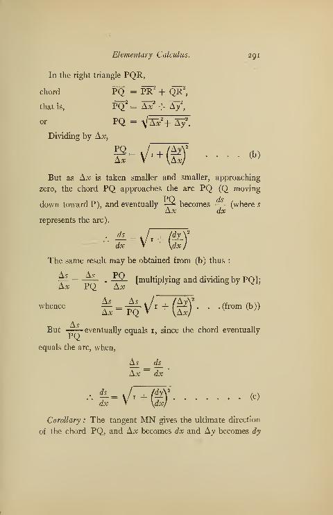
Elementary Calculus. 291
In the right triangle PQR,
chord PQ = PR2
+ QR2
,
that is, PQ2 = Ax + ~Ay\
or PQ = yJAx + ~^y>
Dividing by Ax,
PQ.-V-+^f (b)
But as Ax is taken smaller and smaller, approaching
zero, the chord PQ approaches the arc PQ (Q moving
down toward P), and eventually -^ becomes — (where sAx dx
represents the arc).
dx V \dx)
The same result may be obtained from (b) thus :
As AAx PQ Ax
—^- [multiplying and dividing by PQ];
AsBut -— eventually equals 1, since the chord eventually
equals the arc, when,
As ds_
Ax ~~ dx
Corollary : The tangent MN gives the ultimate direction
of the chord PQ, and Ax becomes dx and Ay becomes dy

292 Elementary Calculus.
at the same time. Since by what has been said in Art. 11,
from (c)
or
Likewise,
tan d> = -2dx
dsT- - Vi + tan
2<j> = sec 0,dx
dx ,— = cos cp
.
ds
dy
dssin
<fi.
Volume of Solid of Revolution.
Art. 68. Let the arc LN revolve about the #-axis,
(Fig. 25) to find the volume whose surface is generated by
M
Fig. 25.
MN = Asta portion of LN. This volume plainly lies
between the volumes generated by the rectangles TNRQand MPRQ. Since these will be cylinders, calling the
volume generated by MNRQ (MN, the chord), AV, we
have,
it (y + Ay) 2Ax > AV> ny2Ax
[x = OQ, y = MQ, Ax = QR, Ay = NP].
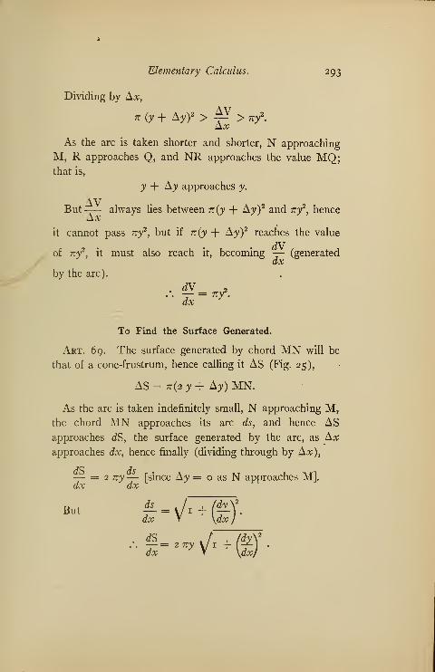
Elementary Calculus. 293
Dividing by Ax,
n(y + Ay) 2 > ^ > ny\Ax
As the arc is taken shorter and shorter, N approaching
M, R approaches Q, and NR approaches the value MQ;that is,
y + Ay approaches y.
But—— always lies between n(y + Ay) 2 and ny2, hence
Axit cannot pass ny2
, but if n(y + Ay) 2reaches the value
of ny2, it
by the arc).
of ny2, it must also reach it, becoming —- (generated
ax
dV 2
Tx=ny '
To Find the Surface Generated.
Art. 69. The surface generated by chord MN will be
that of a cone-frustrum, hence calling it AS (Fig. 25),
AS = tt(2 y + Ay) MN.
As the arc is taken indefinitely small, N approaching M,the chord MN approaches its arc ds, and hence ASapproaches dS, the surface generated by the arc, as Axapproaches dx, hence finally (dividing through by Ax),
— = 2 ny— [since Ay = o as N approaches M].dx dx
£=\M£)'dS— = 2 nydx V- + O'

CHAPTER X.
DIRECTION OF BENDING AND CURVATURE.
Art. 70. A curve is said to be concave upward, at a given
point, when immediately before and after this point it lies
above the tangent line at that point.
It is concave downward when it lies below the tangent
line.
If the curvature changes concavity at a point, that point
is called a point of inflection.
In Fig. 26 the curve is concave downward at A, concave
Fig. 26.
upward at B, and has a point of inflection at C. It is
evident that at a point of inflection the tangent line crosses
the curve.
It is clear also that the conditions for downward con-
cavity are the same as for a maximum, and for upward
concavity are the same as for a minimum.
Since the second derivative is negative for a maximumand positive for a minimum, at a point of inflexion where
294

Elementary Calculus. 295
the curve changes from one to the other, the second deriva-
tive must change from positive to negative or vice versa,
that is, it must pass through zero (or infinity), hence solv-
ing the equation,
fix) = o,
gives the point (or points) of inflection if such exist. If
fix) = o changes sign for this value (or these values),
there is a point of inflexion.
8 a3Example : Examine y = —
2for inflexion.
/(*) =
/'(*) = -
ocr + 4 a'
8 a3
x2 + 4 a2
i6a3x
(x2 + 4 a2
Y
i» {v \ _ i6as(sx
2 - 4 a2) .
; {X) ~(x
2 + 4 a2
f >
when m - l6
f 2
(3/- ^^o.(x
2 + 4 a2
)3
,2 a
Substitute in fix), x= —-= + h and x= 2JL _ fo
V3 V3
successively, where h is as small as we please.
Then j"{x)
i6a3 La2 + 4jt + h2 -4a2\
3 V3

296 Elementary Calculus
14 ah
w3
l6a»(±^+hA
and f'(x) =
/4al + Aa| +A2 + 4a2yV 3 V3 /
V 3 V3 /
Since h is so small, the denominator is positive in both
cases, but for the same reason —-= > h2, hence the second
value of f"{x) is negative and the first positive, and hence
x = —— \y = — is a point of inflection, as is also
V3 L 2 J
—,—), by the same proof.
V 3 2 /
CURVATURE.
Art. 71. If two curves have the same tangent at a
point of intersection they are said to have contact of the
-first order: that is, if y = f(x) and y = F(x) are the equa-
tions of the curves, then for a point of intersection the
equations are simultaneous and we may combine them
any way we please to find p, and
f(P)=F(p) (1)
Also their tangents being the same,
np) = f'(p).
[The values of }'{x) and F' (x) when x = p] . . . (2)
So these are the conditions for contact of the first order.
If in addition f(p) = F»(p),
they are said to have contact of the second order, and so on.

Elementary Calculus. 297
In general, a straight line has only contact of the first
order with a curve, because the two equations above (1)
and (2) (one function representing the straight line, the
other the curve), are just sufficient to determine the two
arbitrary constants for the equation of a straight line, since
two simultaneous equations furnish only enough conditions
to determine two unknowns.
Likewise a circle requiring three conditions may have
contact of the second order, for three equations will then
be required, namely:
KP) = F(#),
l'(p) = ¥'(p),
np) = p'(p).
Total Curvature.
Art. 72. The total curvature of a continuous arc, of
which the bending is in the same direction, is measured by
the angle that the tangent swings through, as the point of
Fig. 27.
tangency moves from one end of the arc to the other; or
what is the same thing it is the difference between the slopes
at these two points. In Fig. 27 the total curvature of the
arc MN is </>' —<f>= A<£, say. It is evident from geometry
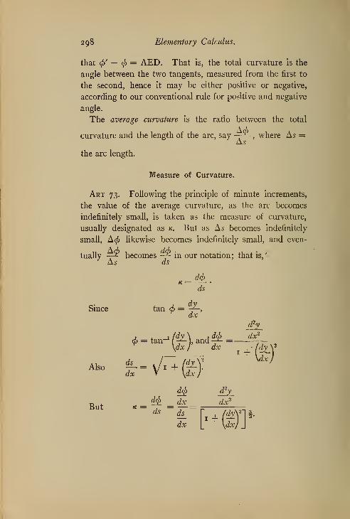
298 Elementary Calculus.
that <// —<f>= AED. That is, the total curvature is the
angle between the two tangents, measured from the first to
the second, hence it may be either positive or negative,
according to our conventional rule for positive and negative
angle.
The average curvature is the ratio between the total
curvature and the length of the arc, say —~ , where As =As
the arc length.
Measure of Curvature.
Art 73. Following the principle of minute increments,
the value of the average curvature, as the arc becomes
indefinitely small, is taken as the measure of curvature,
usually designated as k. But as As becomes indefinitely
small, Acf> likewise becomes indefinitely small, and even-
tuallyA0As
Since
Also
But
becomes -*- in our notation; that is,'
ds
dcf)
ds
tan d> = -f- t
dx
&y
dx y \dx
)
v Ktj
ds
d$
dx
ds_
dx
d2
y
dx2
[• + ©':
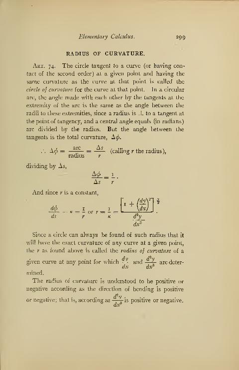
Elementary Calculus. 299
RADIUS OF CURVATURE.
Art. 74. The circle tangent to a curve (or having con-
tact of the second order) at a given point and having the
same curvature as the curve at that point is called the
circle of curvature for the curve at that point. In a circular
arc, the angle made with each other by the tangents at the
extremity of the arc is the same as the angle between the
radii to these extremities, since a radius is _L to a tangent at
the point of tangency, and a central angle equals (in radians)
arc divided by the radius. But the angle between the
tangents is the total curvature, A<£.
dividing
A<£ = ai;
c = —s— (calling r the radius),radius r
by As,
M_ = L.As r
'
ince r is a constant,
d<j> 1 1 [ + ©1*
— k — — or y -— — —as y k d2
y
dx2
Since a circle can always be found of such radius that it
will have the exact curvature of any curve at a given point,
the r as found above is called the radius of curvature of a
• • dv d vgiven curve at any point for which — and —«£- are deter-
dx dx2
mined.
The radius of curvature is understood to be positive or
negative according as the direction of bending is positive
d?vor negative; that is, according as —-j is positive or negative.
axr
300 Elementary Calculus.
EVOLUTE AND INVOLUTE.
Art. 75. As every point on a curve in general has a
different centre of curvature, that is, the centre of its curva-
ture circle is different, these centres describe a locus as
the point on which the curve moves along. This locus is
called the evolute of the curve. It will be seen later on that
this name is peculiarly appropriate.
The curve itself is called the involute of its evolute.
Involute arcs are used extensively in modern gears,
where the evolute is usually a circle.
Art. 76. To find the equation of the evolute, let the
curve equation be y = }{x) (1)
The equation to a circle is,
(x - hf + (y - kf = r2
. . . . (2)
If this be the curvature circle at the point (x, y) on
J = Kx )> tnen ^e x and y in (2) have the same value as
in (1) for that point, by definition of circle of curvature.
Taking derivative of (2) twice with respect to x,
(x - h) + (y - k) £ = o . . . . (3)
< +(£)
!
+ <*-*>-&=° • • w
Eliminating y between (3) and (4),
dx\_ \dxl J , dxj \dx) Jx — h = — r-^—^-J, or h = x-
d2
y'
cPy
dx2 dx2
(Si)
+
(
dx2 dx2
y- k =- -j^' ork=y+ Jy' c&)

As we know
Elementary Calculus.
r =d2
y
dx2
301
(6)
If no particular point on the curve be taken (5J, (53 )
and y = f{x) will, by combination, give the equation of
dy , tf<
dx
y -/(*).
Example : Find the evolute of the hyperbola ay =
the evolute of y = /(#), ~ and -^- being found from
c2
y = -r • • • 'to fr = /(*)!a
Here
whence
and
Substituting in (5J and (52 ),
dy c_
dx x
d?y _ 2 c*
dx2 x3
x — h =
c2
\j*l
^"L x2I _ c* + a*
^2"
2 a32^a3
*+4*=—^_
2£X3
c4 + X4
From (2), /* =ci + *4
+ x= ^+3**2 X3
2 X3
to
(3)
(4)
From (3), & = c'
x. + 3, (orsince^= — from (1))
2 c2x x
= c*+ x*
±. <L- 3c* + x4
X (5)

302 Elementary Calculus.
Adding and subtracting successively (4) and (5),
h+ k= c* + 3 c"x2 + 3^ + *°
= (g2 + ^2
)
3
2 c2x* 2 c
2x*
h ~~ k = TT~ •
2 clxi
Extracting cube root and then squaring,
Subtract;
(h + kf - (h - k)
(h + tf-(c
2 +x2)
2
x2 (2c2y'
<*- k)% = (c
2 - x2
)
2
X2 {2C2f
. (h . h\% -4 c
2x2Ac'
x2 (2c2y (2 c
2)
2 (2 C2)
(2 ,7
The equation to the evolute is then,
§= 2(2C2
r = (16 C2Y= (4 C)l
(2 o
where h and £ are the general co-ordinates, like x and y
in the usual form.
PROPERTIES OF THE EVOLUTE.
Art. 77. An important relation between evolute and
involute is the following: The difference between any two
radii of curvature equals the length of the arc of the evolute
between the two centres of curvature from which they are
drawn. This important fact is proved thus:
Let (V, yf
) be any point on the curve y = (fx); R, the
radius of curvature for this point; (h, k), the correspond-
ing centre of curvature, and a the angle R makes with the

Elementary Calculus. 303
rt-axis. Then the equation of R, passing through (V, y')
and making angle a with the Y-axis, is
y — yf = tan a (x — x') (1)
But R also passes through (h, k), hence (h, k) must sat-
isfy (1).
.-. (k - /) = tana (h - x')y
k —Vwhence *- = tan a.
h —x'
Squaring and adding 1 to both sides,
'- a 2—L- = 1 + tan2 a= sec2 a . (2)(Ji — x') 2
But since R extends from (h, k) to (V, y') its length is
given by Analytics as,
(*.- x') 2 + (k- yy= r2.
Substituting in (2), inverting both sides and extracting
square root,
h-x'R
cos a.
whence h — x' = R cos a, or h = x' + R cos a ) , *
and & — 3/ = R sin a, or k = / + R sin a )
Differentiating (3), [x', y', R and a are all functions of x'\
dh = dxf + cos a dR — R sin a da ) , ,
,
dk = dy' + sin a dR + R cos a da )
d%By Art. 67 — = cos cf> or dx = cos ^ds
and — = sin <j) or dy = sin dsds
(4)
Since the tangent to y = j(x) is also tangent to the cur-
vature circle at (V, yf
), R is J_ to this tangent, hence
a = 90 + </>, whence cos cf>— sin a and sin <j> = — cos a.
304 Elementary Calculus.
Also da = dcf>.
dx' = sin a ds.
Substituting in (4), dyf = — cos a ds.
By Art. 74d<l> _ 1 _ Kds R '
or since dcj) = da,
da
and (4) finally becomes,
— = -; that is, ds = Rda.
ds R'
dx' — R sin a da,
dy' = — R cos a da.
Substituting these values in (3d),
all — RTsimx^ + cos a dR — RTsm^t^a = cos a Rd.
dk = — Rco^ek(fa + sin a dR + Rcos^Ja: = sin a dR.
Squaring and adding,
~dh2+~dk
2 = (cos 2 a+sin 2 a)5R 2 = dR 2
[since cos 2 a + sin 2 a = 1].
But (h, k) being a point on the evolute, letting 5 be the
length of an arc from this point,
JL = yj 1 + (J^V oil? =~dh2 + dk 2
. (By Art. 67.)
.*. J?"= dR2, or (fa = ± </R,
which means that R either increases or decreases, but in
either case changes just as fast as s.
It follows from this, that the end of a stretched string
unwinding from the evolute will describe its involute, or a
straight line rolling on the evolute as a tangent, any point
on it describes an involute. This latter method is used
by draftsmen to draw gear teeth.

Elementary Calculus. 305
ENVELOPES.
Art. 78. The equations of curves, in general, contain
one or more constants, and when these constants vary the
result is a family of curves, having the same generic quali-
ties, but differing in the constant. For example, in the
equation to a straight line,
y = mx + b.
If m varies, the result is a set of straight lines passing
through the same point, (0, b), and making different angles
with the .v-axis. Again in the ellipse equation,
<z2+
*» '
if a and b both vary, but always obeying the condition,
a2 — b2 = c
2[c
2 being a constant],
the result is a family of ellipses with the same foci but
different axes.
. The locus of the intersections of consecutive curves of a
family, as the points of intersection approach coincidence,
that is, when the constant (or constants) changes by infini-
tesmial increments, is called the envelope of this family.
TO FIND THE EQUATION OF AN ENVELOPE.
Art. 79. Let / (x, y, m) = p, be the equation of a
curve, m being originally a constant. Then
/ (x, y, m + Am) = o
will represent the curve immediately adjacent to
/ (x, y, m) = o,
Aw being indefinitely small, when m is allowed to vary.

306 Elementary Calculus.
From / (x, y, w) = o (i)
and / (x, y, m + Aw) = o .... (2)
we get by subtracting and dividing by Aw,
/ (x, y,m + Aw) -/ (x, y, m) = p ^ ^w
But by Art. 62 (3) may be represented by
3/ (X y, m)
hence
as Aw = o,w
or more simply,
df(x,y,m )
dm
¥=°dm (4)
By definition of envelope (4) represents a point on the
envelope, since it is the intersection of two consecutive
curves j(x, y, w) = o and f(x, y, w + Am)* o, as they
approach coincidence, for in (3) these equations were
combined. If now w be eliminated between (4) and (1),
we get an equation free from the variable m, but deter-
mined by the condition (4), which gives a point in the
envelope, hence the result is the equation for this envelope.
The varying constant is called the variable parameter.
Example : Find the envelope of the straight line system
y = mx + b where b is determined by the relation
b = — (p being a constant),w
Hence y = mx + -2—; y — mx — — = o;
(y—mx -)m), of \ m . p
whence —L = — = — x + -^ = o,
dm dm m*

Elementary Calculus. 307
combining, y = mx -\—— ...... (1
)
m
and — x + -£- = o (2)m2
To eliminate m, we get from (2),
m2 = £ . (3)x
i>2
squaring (1), v2 = m2x2 + 2 px + -*--. . . (4)
msubstituting value of m2 from (3) and (4),
y2 = px -{- 2 px + px = 4 px,
which shows that the envelope is a parabola.
Art. 80. It follows readily from the fact that the
evolute of a curve is the locus of its centres of curvature,
and that the radii are all normals to the curve (being _L
to the tangents of each point), that the envelope of the nor-
mals to any curve is its evolute, since these normals (the
radii) always pass through the centres of curvature, which
all lie on the evolute.
EXERCISE XIII.
1. Find the points of inflection of the curve
64
x2 + 16
2. Find the equation of the line through the points of
inflection of the curve y (x2 + 4) = x.
3. Find the radius of curvature of the parabola x2 = 8 yat the origin.
4. Find the radius of curvature of
y .2
y2 = —: at x = a.
2 a — x
308 Elementary Calculus.
5. Find the radius of curvature of the hyperbola
4 x2 — 16 y2 = 64.
6. Find the radius of curvature of the hypocycloid
xi + yi = ai
7. Find the evolute of the parabola y2 = 2 px.
8. Find the evolute of the hyperbola xy = c2
.
9. Find the co-ordinates of the centre of curvature of
4 x2 + gy
2 = 36 at (Vs, *)
10. Find the co-ordinates of the centre of curvature of
y2 = 9* at (3, 3).
1 1
.
Find the points on the ellipse a 2
y2
-f b2x2 = a2
62
,
where the curvature is a maximum and a minimum respec-
tively.
12. Find the radius of curvature of the cycloid,
x = r vers-1 - — \/2 rJ ~ J
2at the point whose ordinate
r
is 2 r.
13. Find the evolute of the circle, x2 + y2 = r
2.
14. Find the envelope of x cos 3^6 + y sin 3^ =
a (cos 20)2
,being the variable parameter.
15. Find the envelope of a straight line in the first quad-
rant which terminates in the co-ordinate axes, and makes a
constant area with the axes.
16. Find the envelope of a variable ellipse with constant
area, n ab.
17. Find the envelope of y2 = m(x — m) where m is
the variable parameter.

CHAPTER XI.
INTEGRATION AS A SUMMATION.
Art. 8i. Integration has been considered, heretofore,
merely as the reverse of differentiation. We will now
consider its real and much more important meaning.
Let <j>(x) be such a function of x that its first deriva-
tive will be a given function, /(x); that is, denoting the
first derivative by an accent,
tf \ JLtf \ 4>(X + A#) — <1>(X) A/(x) = 9 (x) = -^ -z-
—
yv ' as Ax =o,ax
whence <f)(x + ax) — <j>(x) = /(x) Ax . . . (m)
In the language of integrals we may write,
// (x) dx — <f>(x).
Suppose in <fi(x), x to start with a value h and change to
a value k, <f>(x) would change from <j>(h) to </>(k), the
difference would be expressed by,
Suppose again that instead of one jump from h to k,
x changes by minute increments, say making n successive
changes of Ax each, then the successive steps would be,
4>(h + Ax) - <j, (h) = / (/z)Ax {by (m)]
cj)(h + 2 Ax) - <j>(h + Ax) = f(h + Ax)Ax
<f>(h + 3 Ax) - <f>(h + 2 Ax) = /(A + 2 Ax)
Ax${h+ n Ax)-0(/*+(rc-i)Ax) = f(h+(n-i ) Ax)Ax
309

X
310 Elementary Calculus.
adding
<f>(h + nAx) - <j>(h) = f(h)Ax + }{h + \x)\x +jQi + 2 Ax)A* + /(ft + wAx)Ax;
or since h + wAx = k, by our hypothesis <f>(k) — <f>(h)
= J(h)Ax + }(h+Ax)Ax + f(h +2 Ax) Ax + +.
The left hand side of this equation may evidently be
gotten by integrating f(x)dx, and then taking the difference
between the values of this integral when x = k and when
x = h, for by hypothesisJf(x)dx = <j>(x).
This is usually written
l
/(x)dx= <j>(k) - <f>(h)
'h
and is known as a definite integral as was shown in a spe-
cific case under Art. 43.
The right hand member is plainly a sum qf n terms, as
x = o and hence as n = 00, for there cannot be an infi-
nitely small increment unless there is an infinite number of
terms.
For brevity such a sum may be indicated thus:
'V f(x) Ax[
^v being the symbol for summation] .
When Ax = o, this is modified to
f(x)dx,'h
which brings us back to our integral symbol, for we have
found that this sum is actually equal to the definite integral
of j(x)dx (namely, <j>(k) — <f>(h)) fhence definite integra-
tion is a summation.
Art. 82. Let us see what is the further significance of
this series whose sum we have been finding.
X
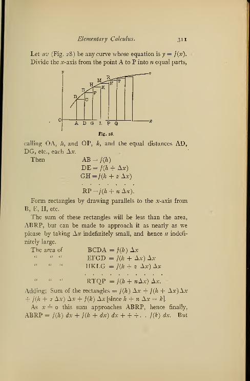
Elementary Calculus. 3"
Let liv (Fig. 28) be any curve whose equation is y = /(x).
Divide the x-axis from the point A to P into n equal parts,
A D G L P Q
Fig. 28.
calling OA, h, and OP, k, and the equal distances AD,DG, etc., each Ax.
Then AB = /(/*)
DE= f(h+ Ax)
GH =/(/* + 2 Ax)
KP=f(h + nAx).
Form rectangles by drawing parallels to the x-axis from
B, E, H, etc.
The sum of these rectangles will be less than the area,
ABRP, but can be made to approach it as nearly as we
please by taking Ax indefinitely small, and hence n indefi-
nitely large.
The area of BCDA = f(h) Ax" " EFGD = f(h + Ax) Ax" " HKLG = f(h+ 2 Ax) Ax
" " RTQP = f(h + nAx) Ax.
Adding; Sum of the rectangles = f(h) Ax + f(h + Ax)Ax
+ j{h + 2 Ax) Ax + j{k) Ax [since h + n Ax = k\
As x = o this sum approaches ABRP, hence finally,
.ABRP = j(h) dx + f(h + dx) dx + + + . . f(k) dx. But
312 Elementary Calculus.
the right Hand side is the same as obtained in the last article
and shown equal to I f(x)dx, hence
areaABRP= fk}(x)dx.
The area would, be given as well by solving the equation
for x, say x = F (y) and integrating / F(y)dy, since the
rectangles could as easily be formed with respect to the
;y-axis and summed.
That is, the definite integral of f(x)dx between fixed
limits, where y= f(x) is the equation of the curve, is the
area bounded by the curve, the x-axis, and the two ordinates
corresponding respectively to these limits, which are the
abscissas in this case.
Example : Find the area of the parabola y2 = 8 x,
between the origin and the point (2, 4). Here the limits
are o and 4, the two bounding ordinates, and we have,
rvYxdx^vi f2
x*dx= § v? rT( 2 )§-o§]=-.Jo Jo Jo [_ J 3
Corollary : Clearly if we reverse the limits we get the
same absolute result, but with contrary sign, that is,
fk
f(x)dx = - f } (x) dx.Jh Jk
It is also evident that we can take the area from y = h
to y = jj (being between h and k) and then the area from
y=jtoy=k, and if the curve be continuous, the sum
of these results will be the same as if we went directly from
h to k. That is,
fk
f(x)dx= fJf(x)dx+ f
L
f(x)dx.J h J h JJ

Elementary Calculus. 313
Thus a definite integral may be readily expressed as the
sum of any number of definite integrals, if the difference
between their limits taken together equals the difference
between the original limits.
It must be carefully observed that f (x)dx does not
become infinite between the limits. When that occurs the
integral must be broken up into parts leading up to the gap
on either side.
Art. 83. Remembering that definite integration is a
summation between the limits, if the expression for the
length of an arc
=\M:-i^dx,which represents any infinitesimal arc whatever of the
curve, y=f(x), be integrated betwreen the limits repre-
senting the co-ordinates of its extremities, the result will
be the sum of all the infinitesimal arcs making up the
total arc and hence the length of this arc, that is,
s being the arc from abscissa h to abscissa k.
Example : Find the circumference of the circle,
x2 + y2 = r
2.
Taking derivative; — = —dx \/ r
2 - x2
~+r dxwhence s = 2 I ( 1 + ———-j dx = 2 r I
J-r V r2 -x2
} J_ r Vr2 -x2
= 2r[Sin
'1
-r]Z=2r
[
E2 -{-f)] =27:r-

314 Elementary Calculus.
It is to be observed that the limits — r and r, which are
the extreme values of x, give the length of the semi-circum-
ference only, and hence the factor 2 above.
SURFACE OF REVOLUTION.
Art. 84. It has been shown (Art 69) that the surface
of revolution for a variable point, (x, y) on an arc, is given
by the formula,
*-»
V
i+ ®'*where the revolving arc is indefinitely small.
By the same reasoning as before, the surface generated
by an arc of any length will be then,
s=2*IV i+(S)^
where h and k represent the abscissas respectively, of the
two ends of the arc.
SOLID OF REVOLUTION.
Art. 85. In exactly the same way, using the expres-
sion found in Art. 68 for solid of revolution,
dv = ny2 dx,
which represents an infinitely thin strip,
v= n I y2 dx,
gives us the volume between the limits h and k.
Art. 86. Clearly we are at liberty to divide a given
area into strips as we please and to apply the same reason-
ing to their summation, so that any one of the above for-
Elementary Calculus. 315
mulae may be expressed in terms of y, if the limits be
determined according to y. For example, we may write,
for the length of the arc, if a and b are ^-limits, etc.
EXERCISE XIV.
1. Find the length of an arc of the cissoid y2 =
2 a — xfrom x = o to x' = a.
2. Find the total length of the cycloid
x = r vers-1 - — V2 ry — y2
.
r
3. Find the length of the hypocycloid x3 + y3 = r.
9 / x x \
4. Find the length of the catenary y = - ( e~ + e ~a)
from the origin to the point whose abscissa is b.
5. Find the length of ay2 =x3 from (o, o) to (3 a, 3V3 a).
6. Find the circumference of the circle,
(*- 2)2 + (y+ i)
2 = 16.
7. Find the length of y = log x from x = 1 to x = 4.
8. Find the area of the ellipse.
9. Find the area of the circle in Ex. 6.
10. Find the area of the parabola y2 = 8 x, between
the origin and the double ordinate corresponding to x = 2.
n. Find the area of the hypocycloid.
12. Find the area of the circle x2 + y2 + 2 rx = o.
8 a3
13. Find the area bounded by y2 = — -, the ordi-
x2 + 4 a2
nate a, and the axes.
316 Elementary Calculus.
14. Find the area bounded by the axes and the line
a
15. Find the area between the #-axis and one loop of
the sine curve y = sin x.
Find the surface generated by revolving about the x-axis
the following curves:
16. The parabola y2 = 2 px from x = o to x = p.
"17. The circle (x — 3)2 + (y — a)
2 = 2 5 above the
#-axis.
18. The ellipse 9 x2 + 16 y
2 = 144.
19. The line - -+- 2. = 1 between the axes.a ^
20. The catenary from x = o to x = a.
21. Find the surfaces generated by revolving about the
;y-axis in Examples 16, 18, and 20.
Find the volumes generated by revolving the following
curves about the #-axis:
22. The ellipse— + ^— = 1.
a2 b2
23. The circle x2 + y2 = r
2.
24. The hypocycloid.
25. The witch y =x2 + 4 a2
26. The line—f- - = 1 between the axes.a b
27. Find the volume generated about the v-axis by the
ellipse.
MISCELLANEOUS APPLICATION.
Art. 87. Since our determination of volume depends
on our ability to divide our solid into sections, whose areas

Elementary Calculus. 317
can be generally expressed, and then summed, any solid
for which this is possible may be estimated.
For example, let it be required to find the volume de-
scribed by a rectangle moving from a fixed point, its plane
remaining parallel to its first position, one side varying as
its distance from this point, the other side, as the square of
this distance, the rectangle becoming a square 5' on the
side, at a distance of 4/ from the point.
Take the line _L to the plane of the rectangle through its
middle as the x-axis. Let v be one side and w the other,
then by conditions,, x being its distance from the point
taken as origin at any time,
v : x : : 5 : 4, whence v = ^—,
4
c xw : x2: : 5 : 16, whence w = -—
.
16
Hence the area of the rectangle at the distance x (being any
point between o and 4) is,
2< x3
VW = —J .
64
This area representing any section of the solid, if mul-
tiplied by dx, thus forming an infinitesimal slice, and
summed between o and 4, will evidently give the total
volume; hence volume =|| I Xs dx= -£$% [x4]
4 = 25 cubic1/0 °
feet.
Again : To find the part of the contents of a cylindrical
bucket of oil remaining in it, after the oil has been poured
out, until half the bottom is exposed (see Figure 29).
Let EGH be any section of the remaining contents,
taken parallel to the axes. Take the origin at the centre
of the base and the co-ordinate axes as the axis of the
cylinder and a diameter of the base.

318 Elementary Calculus.
Then since EGH and DOC are similar,
GH = VBG X GA = Vr2 - x2 [where OG is *],
and EH : CD : : GH : OC,
or EH = h vV2 - x2
[where h = altitude and r = radius of base].
Hence area EGH = 4 EH X GH = hh ^ ~ x^
r
hif - x2) dx _ 2_hr2
r 32 J-r= contents remaining.
EXERCISE XV.
MISCELLANEOUS PROBLEMS.
1. Find the volume generated by an isosceles triangle of
altitude, h, moving with its plane always perpendicular to
the plane of a circle of radius, r, and having always the
ordinates of the circle for bases.
2. What is the volume generated when the circle in
Ex. 3, is replaced by an ellipse whose axes are 2 a, and 2 b?
3. Through the diameter of the upper base of a right
Elementary Calculus, 319
cylinder, whose altitude is h and radius, r, two planes are
passed, touching the base at the two extremities of a diam-
eter. Find the portion of the cylinder between the planes.
4. Two right cylinders each of radius 3 in., intersect each
other at right angles, their axes intersecting. Find com-
mon volume.
5. Find the volume of a pyramid whose altitude is h
and area of base B.
6. Find volume of a curve whose height is h and radius r.
7. In cutting a notch in a log, the sloping face of the
notch makes an angle of 45 with the horizontal face. The
log is 3 ft. in diameter; how much wood is cut out?
8. A right circular cone has a small circle of a sphere of
radius 6 in. as base, and its vertex is at the surface. If the
vertex angle of the cone is 30 , what is the volume of the
sphere outside the cone?
9. A square hole is cut through the axis of a grindstone
for a bearing. The grindstone is 18 in. in diameter, 2 in.
thick at the circumference, and 4 in. at the centre, and has
conical faces. If the hole is 3 in. square, how much material
is removed?

CHAPTER XII.
INTEGRATION BY PARTS.
Art. 8>8>. It is frequently a great aid in integration to
separate the parts of an expression containing two factors,
thus producing either a re-arrangement or a change in
form of the integral.
This is readily accomplished by using the formula for
differentiating the product of two factors,
d(uv) = udv + vdu.
Transposing, udv = d(uv) — vdu.
Taking the integral of both sides,
• • • (B)/ udv = uv — 1 vdi
Example
:
l x2 cos x dx = what ?
Let x2 = u and cos x dx = dv
then du = 2 x dx and v = sin x.
Substituting in the formula (B),
I udv = j x2 cos x dx = x2 sin x — 2 j x sin x dx.
Where the x2 cos x dx is now made to depend upon the
integration of x sin x dx, in which the exponent of x is one
less than in the original expression. If we treat this inte-
gral the same way, using (B) again, letting x = u, du will
320

Elementary Calculus. 321
equal d(x) = dx, which eliminates x from the final inte-
gral; then
2 / x sin x dx = — 2 x cos x +
2 1 cos x dx = — 2 x cos x + 2 sin c
by putting x = u and sin x dx = dv,
whence dx = dw, — cos x = v.
.". 1 x2 cos # dx = x2sin # — 2 1 # sin x dx = x2
sin x—
[— 2 x cos jc + 2 sin x] = x2sin x + 2 # cos x — 2 sin x.
In using the formula (B) no general rule of application
can be given for choosing the value for u and for dv, except
that they should be so chosen that one factor may be made
to disappear eventually or to take such a value that in
combination with the other, it may form an integrable
part of the original expression. For example, in the
expression
x2 tan_1x dx,/•
dv can only equal x2dx since x2dx is the only integrable
part; tan-1 x dx having no known simple integral, then
u = tan-1
x, dv = x2dx,
j dx x3
du — , v = —3
x3 tan"and udv = x2 tan * x dx =
3
-\ iffy* t£? = * ~ i"T72
[dividing * by x2 + ll
322 Elementary Calculus.
. i C tf3 dx i P , i P2 x dx
. . — I = — I xa^c — — I
3Ji + ^23 J 6ji + x2
= •7- -^-log(i + x2).
6 6
^X/ teLIl .X OC2
THence x2 tan
-1 x dx = 1 log (1 + x2).
3 6 6
EXERCISE XVI.
Integrate by parts:
1. Ixsm2xdx. 9. / cot-1 x dx.
2. / ex cos x dx. 10. / xn log * dx.
3. / ex sin x dx. 11. / zeazdz.
4. jxsec2xdx. 12. I y tan2 ydy.
k. I at sin x dx. 1 o- I / ax -
DJ J V x + 2
6. / x tan_1x d#. 14. /
°^ u un
.
7- fx2 cot^xdx. I5 J
(\ogx)dx^
. I log sin x esc x cot x dx. 16. jx2 cos~1 xdx.
INTEGRATION BY SUBSTITUTION.
Art. 89. An expression may often be simplified by
substituting another variable for a part of the expression
to be integrated. No general rule can be given, it being
largely a matter for the exercise of originality.
Elementary Calculus. 323
An example or two may aid:
* = what ?
xVx2 - a2
Let x = —
,
y
then dx — % •
Substituting,
_ ^Z
/dx r y
2 C dy
xVx2 -a2= J i_ /i_ _ ^2
=" JVi-fl2 /
1 r ady 1 -1 / \= I — y = — cos * (a)/)
a J V 1 - a2 y2 ay
1 _, a 1 *x= — cos *— = — sec * —a x a a
what ?Again; /— —
-
J 3 xr — 2 x +
/dx f*
3 dx
3
x
2 — 2X+| J gx2 — 6^+5[multiplying and dividing by 3].
Let (3 x — 1 ) = y, then dy = 3^ and
r—^— = r_^L = l tan-i zj 3 x2 - 2 ^ + 1 j r + 4 2 2
1 . _i 3 x — 1= - tan 1 * .
2 2
The suggestion (3 x — 1 ) = y comes from the fact that
9 x2 — 6 x + 5 can be put in the form,
9 x2 -6x+i + 4= (3 # — 1 )
2 + 4j

324 Elementary Calculus,
and the formula
= — tan-1— is immediately suggested.
a2 + x2 a a
Art. 90. Expressions containing the form \/x2+ax+bcan usually be integrated by making the substitution,
\/x2 + ax + b= y — x.
Example
:
j
dxp
Vx2 + x -
Let \/x2 + x — 2 = y — x.
x2 + x — 2 = y2 — 2 yx + x2
;
whence x = -*- .
1 + 23/
dx2 y + 4f- 2f-4d = 2(f + y -2)
(i + zy) 2(i + 2>;)
2 7
v2"4~ 2 *
#2 + # — 2 = 3/ — # = y — -^
1 + 2 y
_ y + 2 y2 — y
2 — 2 _ y2 + y — 2
J V X2 + X- 2 J 1
1 + 2y 1 + 2y
V y — 1
+ 2y)'
y2 + y- 2
dy
Vx2 + x - 2 J y2 + y - 2
1 + 2y
y = log (1 + 2y)1 + 2 y/;
= log (i + 2 X + 2VV2 + # — 2) .
Art. 91. Expressions containing the form \/—x2+ ax -\-b,
where — x2 + ax + b can be resolved into two first degree
factors, can be integrated by making the substitution,
V— x2 + ax + b = \/(m — x) (n — x) = (m — x)y

Elementary Calculus. 325
or (n — x)y, where {m — x)
and {n — x) are the factors of — x2 + ax + b
xdxExample
:
I
J= ?
V 2 + 2 X —
V^2 + 3 X — 2 X2 = V(l + 2 #) (2 — X) = (2 — #))>,
whence x = 2y ~ I, dx = IQ ^
-f- , etc.2 + y
2(2 + ;y
2)2
EXERCISE XVII.
Integrate by substitution:
/x dx— [substitute z3 for x].
x* + 1
[substitute z6 for #].2
c^_J xi + x%
J X1 - a;1
x — Xs
5. f ^ dy[substitute Vy2 + 1 = z].
J vy + 1
- [substitute a2 — x2 = z3].
(a2 - x2 )*
RC__^_x_dx__J \ — x — 2 X2
9 . r *_ .
J ZVz2 - 2
o. C^Ay-y2
dy.J yl

326
ii.
12.
13-
14-
*5
fJ xV^x2 + 4X — i/x dx
Elementary Calculus,
dx
V2 + 5x
/x2 dx
(x- i) 4
J xVx4 + X2 + I
/ x dx
(i_- x) 3 *
•^ Vx — I
far* ifr
*/ \A ax — x2
substitute x = — •
[substitute x — 1 = z\.
[substitute ez = x].
set x H c=
x
REDUCTION FORMULAE.
Art. 92. Integrals of the general form
Txm (a + bxn^ dx
are exceedingly common, as
/x2\/a2 — x2 dx, / , /
J (a2 - x2Y Jdx
v 2 ax — x2
etc.
Take for example,
/x3 dx
(a2 - x2
f

Elementary Calculus. 327
/x3 dx5 , can
(a2 — x2
y/x dx-, the expression is
(a2 - x2
yintegrable, for the latter integral is in the form xndx or
can be readily reduced to it by inserting the factor 2.
dxAgain / —
J (a(a2 - x2f
can be found if it can be made to
depend upon I = sin — .
J (a 2 -x2)^ a
In the former case the exponent of x (when the expres-
sion is in the formf*.
(. +W*)is to be decreased,
and in the latter the exponent of the parenthesis is to be
decreased.
If then a general method can be devised for expressing
/ xm (a + bxnY dx in terms of other integrals where
m or p (or both) is increased or decreased as the case mayrequire, many of these forms can be integrated.
The process in one case will suffice to show how these
formulae, four in number, known as reduction formula,
are found. The formula for integration by parts is used,
as it is necessary to break up the original expression.
In I xm (a+ boc"Y dx, then,
let u = xm-n+l and dv = (a + bxn)p xn~x dx [xmdx
= (xm-n+1 )(xn
-1dx)]
Substituting in I udv = uv — I vdu ..... (B)
/ nb(p+ 1)

328 Elementary Calculus.
m ~ n + *fxm~n (a + bxnY+1 dx . . . (1)
nb(p+ 1) J
Since du = (m - n + 1) #m-n^ and v = K ^ -1 •
nb(p+ 1)
But I xm-n (a+bxn)p+1dx=
fxm~n (a+bxn
)(a+bxnYdx
[since zp+1 = 2.zp]
= a rxm~n (a + bxn)p dx + b
Jxm (a + £wn )
p dx
[multiplying out].
Substituting in (1) above,
fxm (a + bxnYdx = —~"+1(a+ bxnY+1
_J ' nb(p+ 1)
'("-"+ 1) f*— (a + ft*"/,** _
nb (p + 1) Jb(m-n+i) r
xm(a+ bxnydx ( 2 )nb (/> + 1) J
Transposing the last term of (2) and collecting,
bjnp±jn±_ll rPdx = x>»-n+Ha+ b*"Y«
nb (p + 1) J »ft (p+ 1)
a (m — n
1) Jnb (p +bjnp-j- m + 1)
Dividing by »6(*+i) '
/m( .*. n\Pl Xm~n+1 (a+ bxnY+1
xm {a+bxnydx= -
b (np + ni + 1)
a(m-n+ 1) C m_n ^ + bxny dx < _ (A)b (np + m + i)J
Here xm (a + foc")^ dx is plainly made to depend upon
the integral 1 xm~n (a + bxn ) dx, which is exactly like
it except that the exponent of x, [m], is reduced by n.

Elementary Calculus. 329
The other three formulas are as follows:
/
/
/
(B)
xm (a + bx*)?dx=xm+1 (a + bxn-Z +np + m + 1
& Cxm (a + bxny-x dx ....np + m + 1 J
.vm (a + o„v
n )P ax = L
a (m +1)
- b(np + 1l + "' + I} f*»+» (« + ^n
)p <& . (C)
a (;» +1) J
xm ra + oxny dx= - xm+1(a + bxn
)P+1
an(p+ 1)
+ np + m + n+i C n(fl + bxny+1& . . (D)
aw (/> + 1) J
(A) decreases m by w.
(B ) decreases p by unity.
(C) increases m by ».
(D ) increases p by unity.
In using these formulae, the expression to be integrated
is carefully inspected, and the known integrable form to
which it is to be reduced, is decided upon, then the formula
[(A), (B), (C), or (D)] suited to this reduction is applied.
Clearly these formulae may all be applied to one example
successively, or any one of them may be used any number
of times until the desired form is reached. These for-
mulae fail when the constants have such a value that the
denominators of the fractions reduce to zero. For ex-
ample, in (A) b (np + m + 1) must not reduce to o, etc.
Example: I x2V'a2 — x2 dx = ?

S3 Elementary Calculus.
Here the form desired is plainly
dx . ! x= sin-
Va2 - x2 a
To accomplish this, x2 must reduce to x2 = i and (a2 — x2
)^
must reduce to (a2 — x2
)*. That is, m must be decreased
by 2 and ^ by i (why can it not be reduced to the form
/xdx—. To accomplish this, (A) must be used to
Vfl2 — x2
reduce xm to xm~n , and (B) to reduce p to p — i.
Comparing f*^*-**- /*<.._*)»&
with /jcm + bxn)p dx
m= 2, n = 2, p — ^, a= a2, b = — i
using (A) then,
/V(a2 -x2)* <&= * (a2j *2) * -
-^- f(a2 -*2)*^ ........ (i)
[since xm~n = x2~2= x° — i].
Applying (B) to I (a 2 — x2)% dx, where m = o, n = 2,
^ = i}a = a2
,5 = — i
21 f( « - *»)-* ,**=y^2
- **)*+
2 J 2
a2 C dx x (a2 — x2)* . a2
. ,x—/
= —* *~ H sin-1 - •
2 J vV - x2 2 2 a

Elementary Calculus. 331
Substituting this value of I {a 2—
x
2)* dx in (1),
J 48• 1 x
sin -1 - »
a
where / x2 V# 2 — x2 dx is completely integrated. The value
of these formulae lies in the ability to see the integrable
form that lies within the original expression, and to select
the appropriate reduction formula. It is a matter for
observation and ingenuity purely.
Again JV^T^^what?Here the required form is I
—
- = vers-1 - •
J V 2 ax — x2 a
To put I V'2 ax — x2 dx in the form / xm (a + bxn)p dx,
take out x from under the radical, and we have
/ x? (2 a —x)?dx.
This must be reduced to
r dx r dx f _* / n 1 jI = /
-= —- = I x~* (2 a — x)-* dx.
J 2 ax — x' J x* (2 a — xy JSince n = 1, here xm~n = x%~x = x~* the desired form
for x, hence (A) is needed. Also p is to be reduced to
p — 1. [J — 1. = — H hence (B) is also needed. Apply-
ing these successively we get the desired form. Only prac-
tice and experience can give facility in the use of these
formulae, and familiarity with the simpler integral forms
is desirable, that the inspection of the expression to be
integrated should be effective.

332 Elementary Calculus.
EXERCISE XVIII.
Integrate
:
i. / O2 + 62)* dx.
7>A/2 ry - y
2 dy.
2 ax — x£
2. lVr2 — x2 dx. n xdxJ 8. /
3. / x2(r
2 — x2)% dx.
<J Cw 2 ax — x2
x2 dx 9 ' J
fv
4- /y/x2 — a
x3
dxa
x\/~i
6' J (a2 - z
2 )i* IL JVJ
12. / — [substitute first z = x — il.
J (x2 — 2# + 5)2
j. T/„ 2 . „2N3 j„ r x? drx
X3
13. J(a2 +x2)Ux. I7< f-^
^f (x2 - a2 )i ^ ,
I4J^-^^ l8 . f^-x'dx
/»*J x
\/i — 2 z — z2dz.
/' xr dx
10.yy + oay.V^T-^
RATIONAL FRACTIONS.
Art. 93. If the fractions —-— and -— be added1 — x 2 + 3 x
together, we get,
3 , 5 _ 11 +4 x 11 + 4 x
1 — x 2 + 3X (1 — x) (2 -\- 3 x) 2 + x — 3 X2
Elementary Calculus. 333
It will be observed that the numerator of the sum gives
no indication of the numerators of the component fractions,
but that the denominator does indicate directly the denomi-
nators of the components. If the denominator is in the
form indicated in the final fraction above, it is easy to
factor it.
So that we may regard every rational fraction whose
denominator is factorable as made up of simpler fractions
having respectively the factors as denominators. If it is
required to integrate, for example,
" + 4X2dx,
2 + X — 3 Xz
it is clearly a gain to be able to express this fraction as the
sum (algebraic sum of course is meant) of two or more
simpler fractions; for when we discover that,
11 + 41 _ _j 5—1 >
2 + x — $ x 1 — x 2 + 3^
we get the integral readily, since
—2
—
dx= —3 log (i — x) and 1—- =-^log (2+ 3^:).
1 -
x
J 2 + 3 x 3
Since we know that this decomposition is possible, for
every denominator factor we set a fraction with a letter, or
letters, for numerator, which we determine by the principle
of identities.
It is necessary to descriminate between first degree and
second degree factors, as will appear, hence we have four
cases, as follows:
(a) where the factors are linear only, and not repeated.
(b) where the factors are linear and repeated.
(c) where the factors are quadratic and not repeated.
{d) where the factors are quadratic and repeated.

334 Elementary Calculus.
Case (a).
: in t
component fraction of the form
For every linear factor in the denominator there is a
Ax ± a
}(x)Suppose the fraction is l\-L
; where F (x) = (x ± a)
F(x)
(x±b) (x±c) . . . (x± n).
Then
/(*) = A{
B|
C|
NF(x) (x ± a) (x±b) (x±c)' x±n
The original fraction should be a proper fraction, that is,
the degree of the numerator should be less than that of
the denominator, to avoid complications. If this is not the
case in the given fraction, it can be made so, by dividing
numerator by denominator until the remainder fraction
fulfills this condition. The remainder is, then decom-
posed and the integral quotient added to the result. Anexample will make the process plainer:
(x2 — i ) dx
s(x2 - 4) (4*2 - 1)
= ?
(x2 — 4) (4X2 — 1) (x — 2) (x + 2) (2 x — 1) (2 x + 1)
A B C D~~ X — 2 X + 2 2 X — I 2X+I
It is to be remembered that this is an identity, not a mere
equation, as the two sides must be exactly the same, when
cleared of fractions by our hypothesis, A, B, C and D being
used because we do not immediately know what their
values are.
Elementary Calculus. 335
Clearing; x2 — 1 = A (# + 2) (2 # — 1) (2^+ i) + B(x— 2) (2 x— 1) (2 x + 1)+ C (x — 2) (x + 2) (2 x + 1) +D (# — 2)(# + 2) (2 x — 1). Since this is an identity it is
true for any value of x whatever; hence we can give x such
values that the terms will all disappear but one, and thereby
find the unknown constant it contains. For example, if we
let x = 2, all the terms containing (x — 2) will reduce to o,
hence
22 - i = 3 = A (4) (3) (5) + o + o + o = 60 A,
whence A = 2V
Let x = — 2, and all terms containing x + 2 will reduce
to o ; hence (- 2)
2 - 1 = 3 - o + B (- 4) (- 5) (- 3)
+ o + 0= - 60 B,
whence B = — 2V
Let x = J ; then
(i)2 - 1 = - I = o + o + C (- i) (|) (2) = - J/C,
whence C = + to*
Let x = — J ; then
-(i)2-i = -f = o + o + o + D (_ f) (f) (_ 2 )=_¥Dj
whence D = — t1q.
rp, C (x2 — 1) dx _ j_ f* dx _i_ C d&
J (x2 — 4) (4X2 — 1) 20J x — 2 20 J X +
_i_ C_dx_ _ _i fIO J 2X- I IO J
dx _2
2 x + 1
= 2V log (x - 2) - ^V log (x + 2) + 2V log (2 x - 1)
- 2V log (2* + 1).
j 1
(x — 2) (2 x — 1) (by the principles of
(x + 2) (2 x + 1) logarithms.)
336 Elementary Calculus.
Case (b).
In using indeterminate coefficients of any sort, it is a
cardinal principle that every possible case that may arise
must be provided for in the supposition used.
Suppose —-— , ~^—1 — x (1
-
- X 2 X2 + I j j jo> and — -are added
- xf dnu(1 - xf
3 5 - x
1 — x "^(1 — x) 2
3 x2 + 1 7 — 12 x + x2
(1 — x)3 ~(1 — x) 3
Here the (1 — x)3 gives no indication directly of the
factor (1 — x) 2, that has disappeared in it. If (1 — x)3
is
separated into linear factors they would all be alike (1 — x),
(1 — x), (1 — x), and there would be no separation at all,
neither would the fractions having denominators (1 — x) 2
and (1 — x)3 be provided for. That nothing may be
omitted it is necessary then to provide a fraction for each
of these, hence for every factor of the form (x ± a)n a
series of fractions is assumed, thus:
}(x) A B(x ± a)n ~~ (x ± a)n
+(x ± a) 71-1
C N+ (x± a)n
~2 ' '' (x±a)>
thus accounting for all the powers.
/'%*> r j^2 ^~ ~=z ?
X5 (x + 1)2
As this is an improper fraction, divide numerator by
denominator,
p5 -5*2 -3 „ rxdx _ 2 rdx + 3
r^-oc2 -,J x2 (x + i)
2 - J J^ 3 Jx2(x+i) 2
x3 - x2 - 1 A ,
'B , C,
D= ~~„ "i~1—:—:
tz—
r
x2 {x + I.)2 X2 x (x + i)
2 X + I

Elementary Calculus. 337
[Thus accounting for all the powers of x and of (x + 1).]
Clearing;
x3 - x2 - 1 = A (x+ i)2 + Bx (x+ i)
2 + Cx2 + Dx2 (x+ 1).
Let x = — 1 ; then
(- i)3 - (- i)2 - 1 = - 3 = o + o + C (- i)
2 + o = C,
C=-3-Let x = o; then
0-0-1= -i=A(i) 2 + o + o + o=AA= - 1.
Since no rational value of x will cause the other terms to
disappear, we will give x any small values to get two
simultaneous equations for the two remaining constants,
B and D.
Let x = 1 ; then
i3 - (i)
2 - 1 = - 1 = A ( 2 )2 + B (1) ( 2 )
2 + C (i)2
+ D(l) 2(2),
or since A = — 1, and C = —3
-i=- 4 +4B-3 + 2D
whence 2B + D= 3 (1)
Let x = 2 ; whence
3 B + 2D= 4 (2 )
Combining (1) and (2)
B= 2 andD= - 1.
Hence,
/ x3 — x2 — 1 _ Cdx Cdx _ C dx
x2 {x+ i) 2 " J x22
J x3J (x+1) 2
—— = - + 2 log x H log (x + 1)X + 1 x X + 1

338 Elementary Calculus.
= ±x±l + \og^— [collecting].x(x+i) X + 1
x5 — < x2 — 3 # 2. 12 a? + 3 . , x2
a = — — 2 x -\ a + 3 log .
X2 (X + i) 2 ^(^+l) #+I
Case (c).
If for a factor of the second degree we set a fraction of
Athe form — -, we overlook the possibility of the
x2 + a x +Bxform— , since this is also a proper fraction, but
x2 + ax + b
if both are combined in one thus getting the most general
form, all contingencies are provided for. So for factors of
the form x2 + ax + b, we have fractions of the form
Ax + Bx2 + ax+ b
„ }(x) Ax + B . Cx + D .
Hence \\ = -:7 + — — + . • .
<pl(x) xl + ax + b xl + cx + a
where<fi
(x) = (x2 + ax -\- b) (x2 + cx + d) ( . . .)
Example: / dx = ?' J(x+i)(x2 +i)
2 x2 + 1 A , Bap + C J., , v . 1. i
[(# + 1) is linear].(x+i)(f-fi) # + 1 x2 + 1
Clearing;
2x2 + 1= A(jc2 + 1) + (^+ 1) (Bx+[C) (1)
It is plain that no rational value of x will make x2 + 1
equal to zero, and in general with quadratic factors this
process is useless. Either x can be given any arbitrary
values as in the last case or the following method be fol-

Elementary Calculus. 339
lowed; a method that is entirely general and can be used
in every case if preferred.
Multiplying out in (1);
2 x2 + 1 = Ax2 + A + Bx2 + Cx + Bx + C.
Collecting;
2x2 + 1= (A + B)x2 + (C + B)x + (A+C).
Since this is an identity, the coefficients of like powers of x
on the two sides are identical; that is,
A + B = 2 coefficients of x2.
C + B = o since there is no x on the left.
A + C = 1 absolute terms.
Combining these as simultaneous:
B=i A=|, C=-J.
^ r (2x2 + i)dx = 3 r dx|
1 C x - 1dx
' J (x + 1 ) ipc2 + 1 ) 2JX+I 2jX2 +l
dx3 / * dx 1 C xdx _ 1 /*_
J X + I 2 J X2 + I 2J X2 + I
= I log (# + i ) + J log (x2 + 1 — i tan -1 x.
Case (d)
The same reasoning that was used in case (b), will show
that for every factor of the form (x2 + ax + b) n there is a
series of fractions with numerators of the form Ax + Band denominators successively, (x2 + ax + b) n
,(x2 + ax
+ b) n-\ (x2 + ax + b) n~2
. . . O2 + ax + &)•
Example:
x2 -2x+i_A +B Cx + D Ex + F Gx +H
x 2 (x2 + 2)
3 x2 x (x2 + 2)
3 (x2 + 2 )2 x2 + 2

34° Elementary Calculus.
EXERCISE XIX.
Separate into rational fractions and integrate:
i- / -= — dx. IO /x dx j
J X2 + X~6 J (X2_ 4)(9JC2_ l)
*
3 x2+2X dx.- J'f^'y_
... ft3. f 5 x+ x2— dx ^^J (i- Xf{2-7,xf 12. I —————dx./%) x -\- x 3
dx..X\l+X2)(l-2X) f
2X2 -X-ldx
Px* - 2 x + 5 dx J (x2+x+i)(x-i)
JOC2 +2X- 3
X '
C(2X -l)dxC (x-6)dx J 4- J
'
^3 +I
7
8
9
1
19.
(x — 6) dx
x3 — 6 x2 + 9 x
r (2x-i)dx 15. /4—J {x^ + xf J (
^_I/V - 2 + 1 , l6 f (* + 6)<fo
J ( z2 + 2 )3
2-
' J 5X-4X2 -
r <**dx I7
n^ + i)^J(x-i)0+i) 2
"
'' JxA +x2 +i
f f + 2 y- 2d
J (y- 1) (;y3 -;y2 + y- 1)
±4fa
dx_x3
;2
(x2 + 1 ) (x2 — X + I
)
f-
J (*2 +3)3
21. f —r dx.ar + X//6 x "I
- 1dx.
(X+ 2)3 (X-I)
/Z3 — I
r+ 222

Elementary Calculus. 341
x3 — x + 1
)(*2 -2*4
ar — 1
(#2 + 2)
S
+ I
/X~ -
—z ax.(*
2 +iw
f ar5 - 1
215. I aa;^ J (.T
2 +2) 2
, fa X4 — 2 X3 + X2 — 2 X •
J x3 (x+ i) 2 (x2 + i)

CHAPTER XIII.
TRIGONOMETRIC INTEGRALS.
Art. 94. The integration of the more complex trig-
onometric functions can often be accomplished by substi-
tution, sometimes by breaking up the expression taking
advantage of the relations known to exist between the
different functions. There are very few general rules and
the chief assets are originality and a knowledge of the
simpler integrable forms. A few cases may be noted,
however.
Art. 95. Integrals of the form / sm m xcosn xdx
where either m or n is a positive, odd integer.
Say m is odd; then since sin2 x = 1 — cos2#,
TO—
1
I sinm # cosn # dx = 1 (1 — cos2#) cosn x sin # d#
TO —
1
= — I (1 — cos 2 x) cosn xd (cosx).
m —
1
— 12
[For sin m x = sinw " sin x = (1 — cos2 x) sin x.]
Since m is odd, m — 1 is even and hence can be2
expanded by the binomial theorem; then each term mul-
tiplied by cosn x d (cos x) becomes an integral of the form
342

Elementary Calculus. 343/x n+1 C dxx -"dx = ,or — = log x, and the result is
n + 1 J x
easily found.
If n is odd, the cos x is reduced to sin x and the same
process followed.
/COS X dx= ?sinx
/cos3 x j C 1 — sin 2 x j C d (sin x)ax = I cos xax= I
—* -
sin x J sin x J sin x
— / sin x d (sin x) = log sin x — \ sin2x.
If w + n is an even negative whole number,
1 sinw x cosn dx may be put in the form
/cos 71 X f*— sin m+n xdx = / cotn xcsc~(m + n)xdx, or,sinn x J
/Sin^X
cos m+n,y^ = / tanm x sec - (m + n) x facos 71 X J
Since w + w is an even negative integer, — (tn+n)will be a positive even integer, hence leaving sec2 xdx as
the d (tanx), sec - <™+ »i) - 2 x can be expressed entirely in
terms of the tangent by the relation sec 2 x = 1 + tan2x.
. a dx= ? Here *# + »=— 6 + 2=— 4.sin
b x
Hence
/—— dx = / sin-4 xdx= I cot2 x esc 4 x dx.
sinb x J sin 2 x J
The cot 2 x + 1 = esc 2 x, hence,
1 cot2 x esc 4 x dx = / cot2 x (1 + cot2 x) csc2 xdx

344 Elementary Calculus.
= - f (cot4 x + cot2 x) d (cot*) = - ^l£_£2^£.
J 3 5
Art. 96. If the integral is in the form, / sec2w x dx or
I csc2n xdx, where n and m are positive integers, the
expressions can be readily put in the forms,
1m — 2
(tan2 x + 1
)
sec2 x dx
= (tan2 x+ 1) m~ 1 d (tsm x)
2 H — 2
and (cot2 * + 1 )
2esc 2 # dx
= — (cot2 * +i) n-1 d (cot*)
which are both readily integrable, since m — 1 and n — 1
are both integers and the parentheses may be expanded.
Example: / — = ?
J COS X
—^— = I sec6 xdx= I (tan2 x + 1 )2sec2 * dx
cos6 x J J
= f (tan2x+ i) 2 d(tanx)
= / tan4 #d (tan#) + 2 / tan2 x d (tan x) + / sec 2 xdx
= tan^ +2teD»* +tan ^
5 3
Art. 97. If the integral is of the form,
secw x tann x dx or I cscw * cotn x dx,I secw * tann x dx or I
Elementary Calculus. 345
where m is anything, and n is a positive odd integer, it may
be reduced to
secm-i x tann_1 x sec x tan x dxf— I sec™--1 x tan"—1 x d (sec#),
/= — I esc 171-1 x cot 11-1 x d (esc x),
or I cscm_1 x cotn_1 # esc x cot # dx
and since n is odd, »- — 1 is even and tan x and cot x can
be expressed in terms of sec x and esc x respectively by
the relations, tan2^ = sec 2 x — 1 and cot2 x = esc2 x — 1.
Art. 98. If the integrals are in the forms,
/ tanm xdx or I cotm x dx,
they may be put in the forms,
j tanm~2x. tan2 xdx= j tanm~2 x (sec2 x — i)dx,
and I cotm_2 x. cot2x^ = / cotm_2 ^ (csc2 a;— i) dx.
If these are multiplied out, the first term is always inte-
grable and the exponent of tan:x; or cotx is reduced by 2
in the second term; thus each application of the process
reduces the exponent m, until an integrable form is reached.
Example: I (tan4 x) dx — ?
tan4 xdx = j tan2 x (sec2 x — 1 ) dx

346 Elementary Calculus.
= / tan2 x d (tan x) — / tan2 x dx
— I (sec2 x — i ) dx
I sec2 x dx +J
tan*x
1
sec2 x dx + f <fo
3
tan3 xtan # + x.
3
Art. 99. When m and w are both positive integers the
multiple angle formulae may be used to simplify, namely,
.0 1 — cos 2 xsin'
1 x = >
2 1 + cos 2 #cos"
5 # = — 3
2
sin 2 #sin # cos x =
Example: JW.cc*,*-?
I sin4 # cos2 # <fo = / (sin # cos x) 2 sin2 # dx
r/sin22 x\ /i — cos 2 #\
= i I sin2 2 x dx — \ I sin22 # cos 2 x dx
= tV / (1 ~ cos 4%) dx — TV / sin22 x cos 2 5f i (2 1)
= TV I dx — ^ I C0S4X d (4X)— TV I sin2 2xd (sin 2 #)
= tV - F? sin 4 x - ?V sin32 x.
Elementary Calculus. 347
Art. ioo. The following formulae will be useful, but
their derivation is not necessary here.
dx
m+n cos x \Zm2 — n 2tan
tanX \
2
m + 11
I m — n -
where m > n,
ordx
m + n cos x \/n2 _ m2log
tan — — * in + mn — mV
, x ,
tan—
h
2 in —m
n — mwhere m < n.
The integration ofdx
is made to depend uponm + n sin x
the same form by first substituting x = z + 90 .
e«* sin nx dx = ^ (<* sin rc* - g cos gag)
a 2 + rc2
e°* cos nx dx = g'* fo sin ^ + fl CQS "*)
.
a2 + w2
EXERCISE XX.
r dx
J cos 4 #
s-
smu x cos" x
dx
sec2 x sin" x
/ esc 4 x dx.
/tan3 x
cos 4 x
6. / cot3 x esc3 x dx.
7- 1 tan3 x <fo.
8. 1 cos x tan3 x dx.
9- / tan 4 x <fo.
j10. / (tanx+ cotx) 2<fo.

34$ Elementary Calculus.
ii. fcofxdx. 16. f——dx.J J COS4 X
12. fcos*xsm*xdx. 17. />**<**
.
«/ J COS3 #
J cos2 X J COS4 #
/sin5 x r dx7= <fc. 19. J—
.
cos x V cos x J cos 4 x sin2 x
/' sin3 x (ix (>
/~'
20. I sin4 x cos4 # (foe.
Vi + cos # J
21, I sec3 x dx [set sec # = y\.
J si
(fo C dx22.
23
sin x cos' #
/cos3 x c
sin5 x
/sec mx j—- dx.cor mx
25
26
J 3 - 5 si3 — 5 sin #
(fo
4+5 sin 2 rv
32. / ewx (sin mx — cos mx) (fo.
33. / ex cos 3 x dx.
34. / e3* (cos 2 # + sin 2 x) dx.
27.J 13 - 5 cos x
28.C dx
J 16 + 6 cos x
29. I ex sin 2 x (fo.
30. / e2x sin 4 x (fo.
31. / e2* cos x (fo.

Elementary Calculus. 349
Integrate the following by multiple angle formulae:
35. / sin2 x cos 4 x dx. 37. I sin2 cos2 x dx.
36 . f—**.. 38. [*£?-£ dx.
J sm 4 x cos4 x J cos4 x
MULTIPLE INTEGRALS.
Art. ioi. As we learned that a given function may have
a number of successive derivatives, it immediately follows
that a multiple derivative admits of successive integration,
thus recovering the lower derivatives and eventually the
original function. This process is indicated by repeating
the integral sign, thus,
JSP.dx3
Suppose we have, for example,
&y 2 ,—*- = 2 xl + 3 x.dx3 d
This is what is known as a differential equation. To find
the relation between y and x it is necessary to integrate
three times, since the third derivative is involved. It
follows then, that
— = 2 x2 dx + 3 x dx,dx2
or d (
—
-)= 2 x2 dx + $x dx.
\dx2)
Integrating,
g = 2 fx2 dx+ 3 fxdx=^? +$^-+Cl ;
d)=
3
2 x^ 3 xdx + —— dx + Q dx.
3 2

350 Elementary Calculus.
Integrating,
-^=§ fx*dx+i fxtdx+Ct fdx
= i x4 + i x
3 + Cx* + C 2 ;
dv = — d*H— dx + Cxxdx + C2
dx.6 2
Integrating,
/yJ> ,y.4 /"* ^30 8 2
Q, C2 , and C 3 are the constants of integration which may
be determined in specific cases by the given conditions of
the problem. This process is useful in finding the equa-
tions of curves, when certain attributes expressed in terms of
their derivatives are given, for example, their radii of curva-
ture, although a general application to this end requires
a general knowledge of differential equations.
INTEGRATION OF A TOTAL DIFFERENTIAL.
Art. 102. Where several variables are involved it is
necessary to reverse the process of partial differentiation,
thus integrating for one variable at a time, regarding the
others as constant. In the case of a function of two vari-
ables say, z = f (x, y), the expression for the total differ-
ential is,
, dz , . dz ,dz= —dx+ — dy.ox oy
Say a differential is given in the form P dx + Q dy,
where P and Q are functions of x and y. If the function
is not originally in this form, it may be made to assume it
by grouping.

Elementary Calculus. 351
The question arises, is there a function z, of x and y,
which will have the expression P dx + Q dy for its differ-
ential?
02 uzComparing P dx + Q dy with —dx+— dy, it is appar-
ox dy
ent that if there is such a function,
P = — and Q - —- .
ox oy
Differentiating these equations with respect to y and x
respectively,
— _ 9 2z
and 3Q_ A2
1
But
dy 3y3x 3x 3x9y
d 2z d 2
z
dydx dxdy
. 3P = 3Q3v 3x
And when this is true the function z exists, not otherwise.
Example : 3 x2 dx + 3 y2 dy — 3 ax dy — 3 ay o*x, to find
/ (*, y)-
Put this in the form P dx + Q dv,
(3 x2 - 3 ay) Ox + (sf - 3 ax) ^.
Here P = 3 x2 — 3 ay, Q = 3 y2 — 3 ax.
Since
p =3 x
2 -3 0^ Q =8
3 7
3P_dy
: - 3a3x
3«-
3P_dy -P and .exists.
OX
P = 3 x2 --
3 av.
3z
BxP =3 x2 — 3 ay.

35 2 Elementary Calculus.
Integrating this with respect to x, y being constant,
zp = x3 — 3 axy [Zp means partial value of z].
Since the terms in Q, which contain x, have already been
integrated in P, as will be evident if we remember how
partial differentiation is effected, it remains only to inte-
grate the terms in Q containing y alone, with respect to y.
Since Q = 3 y2 — 2 ax, the integration of the term 3 y
2,
containing only y, gives v3.
Adding this to the partial integral already found in zp ,
the total integral becomes,
3 = x3 — 3 axy + y3
.
Hence to integrate an expression of the form P dx + Q dy,
integrate P with respect to x, then integrate the terms in Qnot containing x, and add the results.
DEFINITE MULTIPLE INTEGRALS.
Art. 103. Evidently the conception of multiple integral
may include definite integration, where the limits of inte-
gration are determined for each variable separately.
/r f y/r2 _ X2
I (x2 + y2) dxdy
01/
means that the definite integral of this expression is taken
for y (x remaining constant) between the limits o and
\Zr2 — x2, then the integral of this result with respect to x,
between o and r.
We integrate first for the outside differential.
Thus,
(*r f**Sri - x°- f*r I ^3\ vV - «2
I 1 (x2 + y2) dx dy =
J(x2v+—
)
dxJo Jo Jo V 3 /o

Elementary Calculus.
V2 + 2 X2^
353
= fr
Vr 2 - x2 (r2 + 2 x2
\ dx= - fVr2- x2 dx +
fr
x2 Vr2 -x2 dx3 Jo
-XT— Vr2-*2 * -sin-1-+ — (2^2-r2)\/r2-^2
6 6 r 12
. r4
. ill ;rr4
H 'Sin- 1 - = —12 ;-J 8
AREAS AND MOMENTS OF INERTIA.
Art. 104. The determination of areas comes readily
under the process of double integration. Take the circle
(Fig. 30) for example. Divide the circle up into minute
/ \I \r A
1
r 7\ /
\ yFig. 30.
squares, by lines drawn parallel respectively to the x-axis
and the y-axis, and let those parallel to the v-axis be at a
distance A.v apart; those parallel to the v-axis, Ay apart.
Then the area of each square is \x . Ay. The sum of all
these squares will be less than the area of the circle by the
minute spaces bounded by the sides of the extreme squares
and the circumference. But as A.v and Ay approach o,
these spaces also approach o, and eventually the sum of
the squares represents the actual area of the circle, that is,
354 Elementary Calculus.
when Ax . Ay becomes dx . dy. We have learned that
definite integration is a summation, hence if we integrate
along a line parallel to the x-axis, that is for y, we get a
strip parallel to the x-axis, and then integrating parallel to
the v-axis, that is for x, we sum these strips and hence we
get the circle area. Since we must take limits for y, that
will apply to any strip, these limits or rather one of them
will be variable, and should be a function of x.
Taking the origin at the centre, the circle equation is
y2 =. r
2 — X2,
whence y = vV — x2.
Since the value of y represents any point on the circle, it
will represent the distance of any strip from the #-axis,
hence starting with the v-axis and integrating to the right
along a parallel to the x-axis, the lower limit o is the same
for all strips (the starting point always being at the y-axis)
and the upper limit for any one will then be Vr2 — x2(the
outer end of the strip).
Then these strips are integrated parallel to the v-axis,
from the x-axis, to the extreme distance of the last one
from the x-axis, that is, r.
We express all this,
= fr
Vr2- x2 dx =J If Vr2 -x2 + -sin-1 -!
= — , the area of a quadrant.4
— X 4 = Ttr2
, the area of the circle.

Elementary Calculus. 355
MOMENTS OF INERTIA.
Art. 105. The moment of inertia of a plane area about
a given point in its plane is denned in mechanics, as the
sum of the products of the area of each infinitesimal portion
by the square of its distance from the point.
Taking the point as origin and laying out the strips
parallel to the axes, taking the axes in a position most
convenient for laying out the strips, we have by Analytic
Geometry, that the distance of any point (x, y) from the
point (origin) is
Vx2 + y\
Also by the last article the area of any infinitesimal square
is dx dy.
Since an infinitesimal square is practically a point, we
have then the moment of inertia of any square is
(x2 + y2) dx dy.
Integrating this parallel to the ^-axis with proper limits,
determined as in the last article, and then parallel to the
^-axis with limits indicating the extreme of area, we have
the required sum. Calling the moment of inertia, I; the
limits for v-integration, (0, a) [where a is a function of x];
those for ^-integration, (o, b), the result is expressed,
«7o *J
(x2 + y2) dx dy.
This was illustrated in Art. 100. The same process maybe used in polar co-ordinates by taking radial strips, in-
stead of rectangular ones.

356 Elementary Calculus.
EXERCISE XXI.
By double integration find the following:
1. The area between y3 = x and x3 = y.
2. The area between y2 = 8 x and x2 = 8 y.
3. The area between y2 = 6 x and
;y
2 = iox- #2.
4. Find the segment of the circle x2 + y2 = 16 cut off
by the line 3/ — # = 4.
5". Find the area between y2 = 2 px and the line y = 2 x.
6. Find the moment of inertia about the origin of the
circle (x — i) 2 + (y — 2)2 = 9.
7. Find the moment of inertia of a right triangle, about
the origin, legs of length 6 in. and 8 in. respectively forming
the axes.
8. Find the moment of inertia of the area in Ex. 5.
9. Find the moment of inertia of the segment in Ex. 4.

Zhe Dan IFtostranbSetter of
XLcxt Boohs12 mo, !£>alf iLeat&er . . . MtmrateD
241 Pages Price $1.25 Net
&ct)mall & £>l)acft
"Plane Geometry"330 Pages Price $1.75 Net
£>rt)mall, C. 115.
"FIRST COURSEIN
Analytical Geometry"290 Pages Price $1.75Net
Cain, WLm. (#tof.)University of North Carolina
"BRIEF COURSEIN THE
Calculus"
30T Pages, Price $1.75
Ctituartj 2L. Botnser, 3L3L.2XT(utgers College
ELEMENTARY TREATISESON
" Analytical Geometry'(Embracing Plane Geometry)
451 Pages Price S2.25
"DIFFERENTIAL AND INTEGRALCalculus
'
511 Pages Price $3.00
"Analytic Mechanics"(Seventeenth Edition)
298 Pages Price $2.50
" Hydromechanics"(Fifth Edition)
627 Pages Price $2.00
uPractical Mathematics"
Revised by
C. ®. Stnott, 2>. &c«, $&.&&and
12mo Cloth, 100 Pages Price $1.25 Net
C. $. dftmtyer, ($rof.)
"INTEGRATION byTRIGNOMETRIGand
Imaginary Substitution"(JntroDuction 6? 3. TButkitt fflJebft, prof.)
Stevens Institute.
OTHER VOLUMES IN PREPARATION
20. $an J12o£tranti CompanyPublishers and Booksellers
23 Murray and 27 Warren Sts., New York


NOV 21 I90S