Mathematics for Engineering Applications
434
INTRODUCTORY Mathematics for Engineering Applications KULDIP S. RATTAN + NATHAN W. KLINGBEIL
-
Upload
khangminh22 -
Category
Documents
-
view
2 -
download
0
Transcript of Mathematics for Engineering Applications

Introductory
Mathematics for Engineering Applications
KuldIp S. rAttAn + nAthAn W. KlIngbEIl


IntroductoryMathematics forEngineeringApplications
Kuldip S. RattanWright State University
Nathan W. KlingbeilWright State University
VP & Publisher: Don FowleyEditor: Dan SayreEditorial Assistant: Jessica KnechtMarketing Manager: Chris RuelMarketing Assistant: Marissa CarrollDesigner: Kenji NgiengAssociate Production Manager: Joyce Poh
This book was set by Aptara Corporation.
Founded in 1807, John Wiley & Sons, Inc. has been a valued source of knowledge and understanding formore than 200 years, helping people around the world meet their needs and fulfill their aspirations. Ourcompany is built on a foundation of principles that include responsibility to the communities we serveand where we live and work. In 2008, we launched a Corporate Citizenship Initiative, a global effort toaddress the environmental, social, economic, and ethical challenges we face in our business. Among theissues we are addressing are carbon impact, paper specifications and procurement, ethical conductwithin our business and among our vendors, and community and charitable support. For moreinformation, please visit our website: www.wiley.com/go/citizenship.
Copyright c© 2015 John Wiley & Sons, Inc. All rights reserved. No part of this publication may bereproduced, stored in a retrieval system or transmitted in any form or by any means, electronic,mechanical, photocopying, recording, scanning or otherwise, except as permitted under Sections 107 or108 of the 1976 United States Copyright Act, without either the prior written permission of thePublisher, or authorization through payment of the appropriate per-copy fee to the Copyright ClearanceCenter, Inc. 222 Rosewood Drive, Danvers, MA 01923, website www.copyright.com. Requests to thePublisher for permission should be addressed to the Permissions Department, John Wiley & Sons, Inc.,111 River Street, Hoboken, NJ 07030-5774, (201)748-6011, fax (201)748-6008, websitehttp://www.wiley.com/go/permissions.
Evaluation copies are provided to qualified academics and professionals for review purposes only, foruse in their courses during the next academic year. These copies are licensed and may not be sold ortransferred to a third party. Upon completion of the review period, please return the evaluation copy toWiley. Return instructions and a free of charge return mailing label are available at www.wiley.com/go/returnlabel. If you have chosen to adopt this textbook for use in your course, please accept this bookas your complimentary desk copy. Outside of the United States, please contact your local salesrepresentative.
ISBN 978-1-118-14180-9 (Paperback)
Printed in the United States of America
10 9 8 7 6 5 4 3 2 1

Contents
1 STRAIGHT LINES INENGINEERING 1
1.1 Vehicle during Braking 1
1.2 Voltage-Current Relationshipin a Resistive Circuit 3
1.3 Force-Displacement in aPreloaded Tension Spring 6
1.4 Further Examples of Linesin Engineering 8
Problems 19
2 QUADRATIC EQUATIONSIN ENGINEERING 32
2.1 A Projectile in a VerticalPlane 32
2.2 Current in a Lamp 36
2.3 Equivalent Resistance 37
2.4 Further Examples ofQuadratic Equations inEngineering 38
Problems 50
3 TRIGONOMETRY INENGINEERING 60
3.1 Introduction 60
3.2 One-Link Planar Robot 60
3.2.1 Kinematics of One-LinkRobot 60
3.2.2 Inverse Kinematics ofOne-Link Robot 68
3.3 Two-Link Planar Robot 72
3.3.1 Direct Kinematics ofTwo-Link Robot 73
3.3.2 Inverse Kinematics ofTwo-Link Robot 75
3.3.3 Further Examples ofTwo-Link Planar Robot 79
3.4 Further Examples ofTrigonometry inEngineering 89
Problems 97
4 TWO-DIMENSIONALVECTORS INENGINEERING 106
4.1 Introduction 106
4.2 Position Vector in RectangularForm 107
4.3 Position Vector in PolarForm 107
4.4 Vector Addition 110
4.4.1 Examples of VectorAddition inEngineering 111
Problems 123
5 COMPLEX NUMBERSIN ENGINEERING 132
5.1 Introduction 132
5.2 Position of One-Link Robot asa Complex Number 133
iii
iv Contents
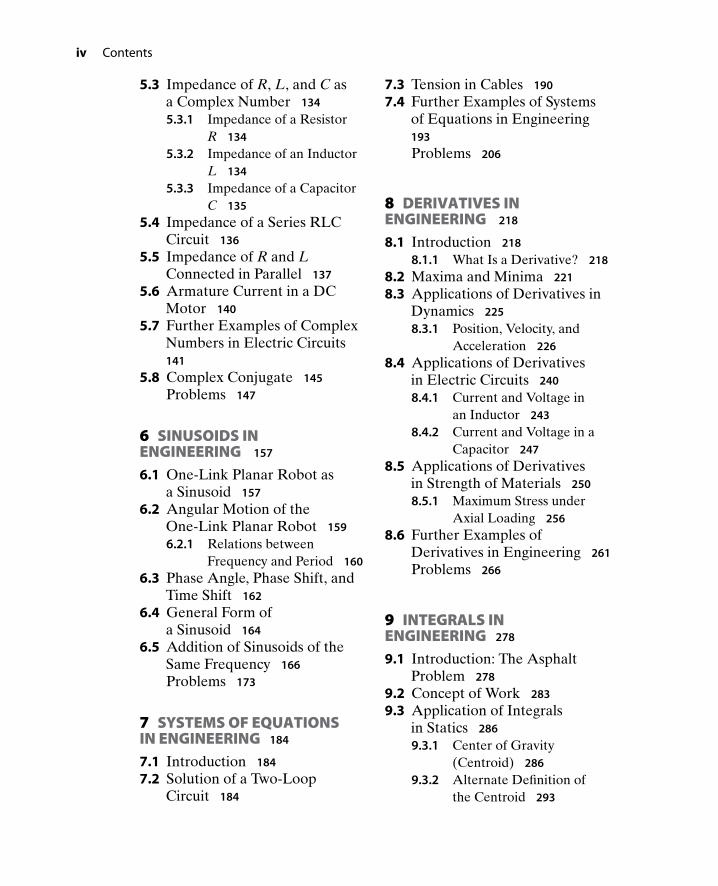
5.3 Impedance of R, L, and C asa Complex Number 134
5.3.1 Impedance of a ResistorR 134
5.3.2 Impedance of an InductorL 134
5.3.3 Impedance of a CapacitorC 135
5.4 Impedance of a Series RLCCircuit 136
5.5 Impedance of R and LConnected in Parallel 137
5.6 Armature Current in a DCMotor 140
5.7 Further Examples of ComplexNumbers in Electric Circuits141
5.8 Complex Conjugate 145
Problems 147
6 SINUSOIDS INENGINEERING 157
6.1 One-Link Planar Robot asa Sinusoid 157
6.2 Angular Motion of theOne-Link Planar Robot 159
6.2.1 Relations betweenFrequency and Period 160
6.3 Phase Angle, Phase Shift, andTime Shift 162
6.4 General Form ofa Sinusoid 164
6.5 Addition of Sinusoids of theSame Frequency 166
Problems 173
7 SYSTEMS OF EQUATIONSIN ENGINEERING 184
7.1 Introduction 184
7.2 Solution of a Two-LoopCircuit 184
7.3 Tension in Cables 190
7.4 Further Examples of Systemsof Equations in Engineering193
Problems 206
8 DERIVATIVES INENGINEERING 218
8.1 Introduction 218
8.1.1 What Is a Derivative? 218
8.2 Maxima and Minima 221
8.3 Applications of Derivatives inDynamics 225
8.3.1 Position, Velocity, andAcceleration 226
8.4 Applications of Derivativesin Electric Circuits 240
8.4.1 Current and Voltage inan Inductor 243
8.4.2 Current and Voltage in aCapacitor 247
8.5 Applications of Derivativesin Strength of Materials 250
8.5.1 Maximum Stress underAxial Loading 256
8.6 Further Examples ofDerivatives in Engineering 261
Problems 266
9 INTEGRALS INENGINEERING 278
9.1 Introduction: The AsphaltProblem 278
9.2 Concept of Work 283
9.3 Application of Integralsin Statics 286
9.3.1 Center of Gravity(Centroid) 286
9.3.2 Alternate Definition ofthe Centroid 293

Contents v
9.4 Distributed Loads 296
9.4.1 Hydrostatic Pressureon a RetainingWall 296
9.4.2 Distributed Loads onBeams: StaticallyEquivalent Loading 298
9.5 Applications of Integrals inDynamics 302
9.5.1 Graphical Interpretation309
9.6 Applications of Integrals inElectric Circuits 314
9.6.1 Current, Voltage, andEnergy Stored in aCapacitor 314
9.7 Current and Voltage in anInductor 322
9.8 Further Examples of Integralsin Engineering 327
Problems 334
10 DIFFERENTIAL EQUATIONSIN ENGINEERING 345
10.1 Introduction: The LeakingBucket 345
10.2 Differential Equations 346
10.3 Solution of Linear DEQ withConstant Coefficients 347
10.4 First-Order DifferentialEquations 348
10.5 Second-Order DifferentialEquations 374
10.5.1 Free Vibration of aSpring-Mass System 374
10.5.2 Forced Vibration of aSpring-Mass System 379
10.5.3 Second-Order LC Circuit386
Problems 390
ANSWERS TO SELECTEDPROBLEMS 401
INDEX 417
Preface
This book is intended to provide first-year engineering students with a comprehen-sive introduction to the application of mathematics in engineering. This includesmath topics ranging from precalculus and trigonometry through calculus and dif-ferential equations, with all topics set in the context of an engineering applica-tion. Specific math topics include linear and quadratic equations, trigonometry, 2-Dvectors, complex numbers, sinusoids and harmonic signals, systems of equations andmatrices, derivatives, integrals, and differential equations. However, these topics arecovered only to the extent that they are actually used in core first- and second-yearengineering courses, including physics, statics, dynamics, strength of materials, andelectric circuits, with occasional applications from upper-division courses. Additionalmotivation is provided by a wide range of worked examples and homework problemsrepresenting a variety of popular engineering disciplines.
While this book provides a comprehensive introduction to both the mathtopics and their engineering applications, it provides comprehensive coverage ofneither. As such, it is not intended to be a replacement for any traditional mathor engineering textbook. It is more like an advertisement or movie trailer. Indeed,everything covered in this book will be covered again in either an engineering ormathematics classroom. This gives the instructor an enormous amount of freedom− the freedom to integrate math and physics by immersion. The freedom to lever-age student intuition, and to introduce new physical contexts for math without theconstraint of prerequisite knowledge. The freedom to let the physics help explainthe math and the math to help explain the physics. The freedom to teach math toengineers the way it really ought to be taught − within a context, and for a reason.
Ideally, this book would serve as the primary text for a first-year engineeringmathematics course, which would replace traditional math prerequisite requirementsfor core sophomore-level engineering courses. This would allow students to advancethrough the first two years of their chosen degree programs without first complet-ing the required calculus sequence. Such is the approach adopted by Wright StateUniversity and a growing number of institutions across the country, which are nowenjoying significant increases not only in engineering student retention but also inengineering student performance in their first required calculus course.
Alternatively, this book would make an ideal reference for any freshmanengineering program. Its organization is highly compartmentalized, which allowsinstructors to pick and choose which math topics and engineering applications tocover. Thus, any institution wishing to increase engineering student preparation and
vi

Preface vii
motivation for the required calculus sequence could easily integrate selected topicsinto an existing freshman engineering course without having to find room in thecurriculum for additional credit hours. Finally, this book would provide an outstand-ing resource for nontraditional students returning to school from the workplace, forstudents who are undecided or are considering a switch to engineering from anothermajor, for math and science teachers or education majors seeking physical contextsfor their students, or for upper-level high school students who are thinking aboutstudying engineering in college. For all of these students, this book represents a one-stop shop for how math is really used in engineering.

Acknowledgement
The authors would like to thank all those who have contributed to the developmentof this text. This includes their outstanding staff of TA’s, who have not only pro-vided numerous suggestions and revisions, but also played a critical role in the successof the first-year engineering math program at Wright State University. The authorswould also like to thank their many colleagues and collaborators who have joined intheir nationwide quest to change the way math is taught to engineers. Special thanksgoes to Jennifer Serres, Werner Klingbeil and Scott Molitor, who have contributeda variety of worked examples and homework problems from their own engineeringdisciplines. Thanks also to Josh Deaton, who has provided detailed solutions to allend-of-chapter problems. Finally, the authors would like to thank their wives andfamilies, whose unending patience and support have made this effort possible.
This material is based upon work supported by the National Science Founda-tion under Grant Numbers EEC-0343214, DUE-0618571, DUE-0622466 and DUE-0817332. Any opinions, findings, and conclusions or recommendations expressed inthis material are those of the authors and do not necessarily reflect the views of theNational Science Foundation.
viii

CHAPTER1
Straight Lines inEngineering
In this chapter, the applications of straight lines in engineering are introduced. It isassumed that the students are already familiar with this topic from their high schoolalgebra course. This chapter will show, with examples, why this topic is so impor-tant for engineers. For example, the velocity of a vehicle while braking, the voltage-current relationship in a resistive circuit, and the relationship between force anddisplacement in a preloaded spring can all be represented by straight lines. In thischapter, the equations of these lines will be obtained using both the slope-interceptand the point-slope forms.
1.1 VEHICLE DURING BRAKINGThe velocity of a vehicle during braking is measured at two distinct points in time, asindicated in Fig. 1.1.
t, s v(t), m/s1.5 9.752.5 5.85
Figure 1.1 A vehicle while braking.
The velocity satisfies the equation
v(t) = at + vo (1.1)
where vo is the initial velocity in m/s and a is the acceleration in m/s2.
(a) Find the equation of the line v(t) and determine both the initial velocity vo andthe acceleration a.
(b) Sketch the graph of the line v(t) and clearly label the initial velocity, the acceler-ation, and the total stopping time on the graph.
The equation of the velocity given by equation (1.1) is in the slope-intercept formy = mx + b, where y = v(t), m = a, x = t, and b = vo. The slope m is given by
m =𝚫 y
𝚫 x=
y2 − y1
x2 − x1.
1

2 Chapter 1 Straight Lines in Engineering
Therefore, the slope m = a can be calculated using the data in Fig. 1.1 as
a =v2 − v1
t2 − t1= 5.85 − 9.75
2.5 − 1.5= −3.9 m/s2
.
The velocity of the vehicle can now be written in the slope-intercept form as
v(t) = −3.9 t + vo.
The y-intercept b = vo can be determined using either one of the data points. Usingthe data point (t, v) = (1.5, 9.75) gives
9.75 = −3.9 (1.5) + vo.
Solving for vo gives
vo = 15.6 m/s.
The y-intercept b = vo can also be determined using the other data point (t, v) =(2.5, 5.85), yielding
5.85 = −3.9 (2.5) + vo.
Solving for vo gives
vo = 15.6 m/s.
The velocity of the vehicle can now be written as
v(t) = −3.9 t + 15.6 m/s.
The total stopping time (time required to reach v(t) = 0) can be found by equatingv(t) = 0, which gives
0 = −3.9 t + 15.6.
Solving for t, the stopping time is found to be t = 4.0 s. Figure 1.2 shows the velocity ofthe vehicle after braking. Note that the stopping time t = 4.0 s and the initial velocity
( -intercept)
0
15.6
4.0
Stopping time
1
0
Velocity, m/s
a 3.90 m/s2
v0Initial velocity, y
x( -intercept)
t, s
Figure 1.2 Velocity of the vehicle after braking.

1.2 Voltage-Current Relationship in a Resistive Circuit 3
vo = 15.6 m/s are the x- and y-intercepts of the line, respectively. Also, note that theslope of the line m = −3.90 m/s2 is the acceleration of the vehicle during braking.
1.2 VOLTAGE-CURRENT RELATIONSHIPIN A RESISTIVE CIRCUITFor the resistive circuit shown in Fig. 1.3, the relationship between the applied voltageVs and the current I flowing through the circuit can be obtained using Kirchhoff’svoltage law (KVL) and Ohm’s law. For a closed-loop in an electric circuit, KVL statesthat the sum of the voltage rises is equal to the sum of the voltage drops, i.e.,
Kirchhoff’s voltage law: ⇒∑
Voltage rise = ∑Voltage drop.
VS
R VRI
V
Vs, V I, A10.0 0.120.0 1.1
Figure 1.3 Voltage and current in a resistive circuit.
Applying KVL to the circuit of Fig. 1.3 gives
Vs = VR + V. (1.2)
Ohm’s law states that the voltage drop across a resistor VR in volts (V) is equal to thecurrent I in amperes (A) flowing through the resistor multiplied by the resistance Rin ohms (Ω), i.e.,
VR = I R. (1.3)
Substituting equation (1.3) into equation (1.2) gives a linear relationship between theapplied voltage Vs and the current I as
Vs = I R + V. (1.4)
The objective is to find the value of R and V when the current flowing through thecircuit is known for two different voltage values given in Fig. 1.3.
The voltage-current relationship given by equation (1.4) is the equation of astraight line in the slope-intercept form y = mx + b, where y = Vs, x = I, m = R, andb = V. The slope m is given by
m = R =Δ yΔ x
=ΔVs
Δ I.
Using the data in Fig. 1.3, the slope R can be found as
R = 20 − 101.1 − 0.1
= 10 Ω.
4 Chapter 1 Straight Lines in Engineering
Therefore, the source voltage can be written in slope-intercept form as
Vs = 10 I + b.
The y-intercept b = V can be determined using either one of the data points. Usingthe data point (Vs, I) = (10, 0.1) gives
10 = 10 (0.1) + V.
Solving for V gives
V = 9 V.
The y-intercept V can also be found by finding the equation of the straight line usingthe point-slope form of the straight line (y − y1) = m(x − x1) as
Vs − 10 = 10(I − 0.1) ⇒ Vs = 10 I − 1.0 + 10.
Therefore, the voltage-current relationship is given by
Vs = 10 I + 9. (1.5)
Comparing equations (1.4) and (1.5), the values of R and V are given by
R = 10 Ω, V = 9 V.
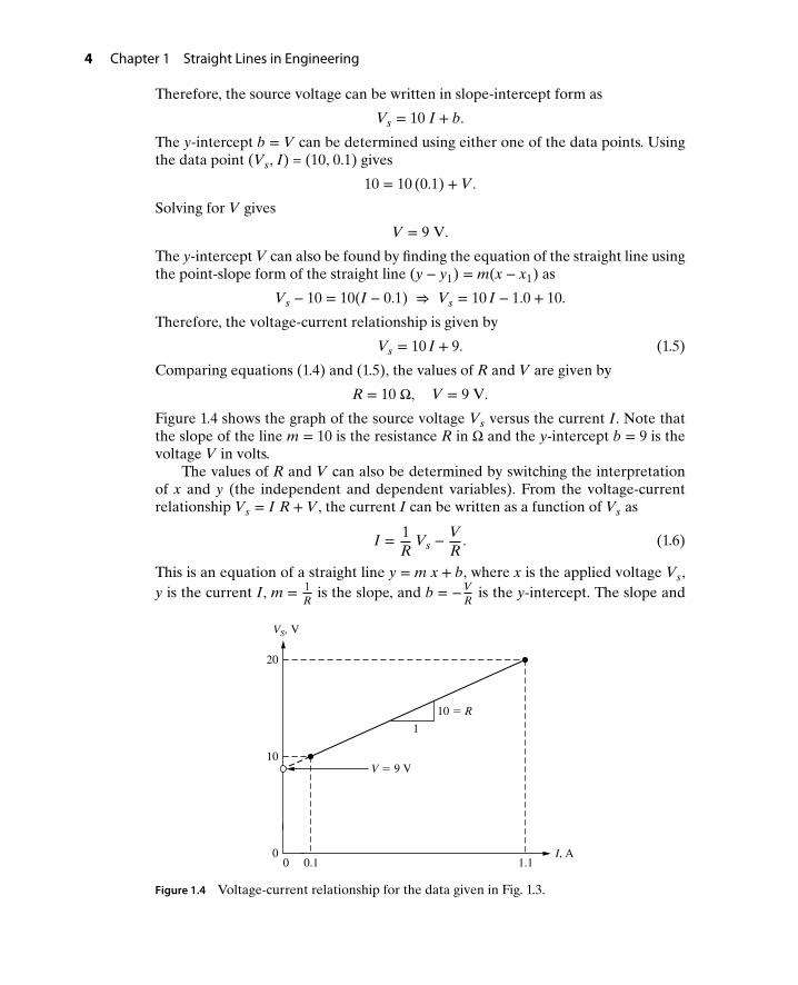
Figure 1.4 shows the graph of the source voltage Vs versus the current I. Note thatthe slope of the line m = 10 is the resistance R in Ω and the y-intercept b = 9 is thevoltage V in volts.
The values of R and V can also be determined by switching the interpretationof x and y (the independent and dependent variables). From the voltage-currentrelationship Vs = I R + V, the current I can be written as a function of Vs as
I = 1R
Vs −VR. (1.6)
This is an equation of a straight line y = m x + b, where x is the applied voltage Vs,y is the current I, m = 1
Ris the slope, and b = −V
Ris the y-intercept. The slope and
0
10
20
0
1
1.10.1
10 R
V 9 V
VS, V
I, A
Figure 1.4 Voltage-current relationship for the data given in Fig. 1.3.
1.2 Voltage-Current Relationship in a Resistive Circuit 5
y-intercept can be found from the data given in Fig. 1.3 using the slope-interceptmethod as
m =Δ yΔ x
= Δ IΔVs
.
Using the data in Fig. 1.3, the slope m can be found as
m = 1.1 − 0.120 − 10
= 0.1.
Therefore, the current I can be written in slope-intercept form as
I = 0.1 Vs + b.
The y-intercept b can be determined using either one of the data points. Using thedata point (Vs, I) = (10, 0.1) gives
0.1 = 0.1 (10) + b.
Solving for b gives
b = −0.9.
Therefore, the equation of the straight line can be written in the slope-intercept formas
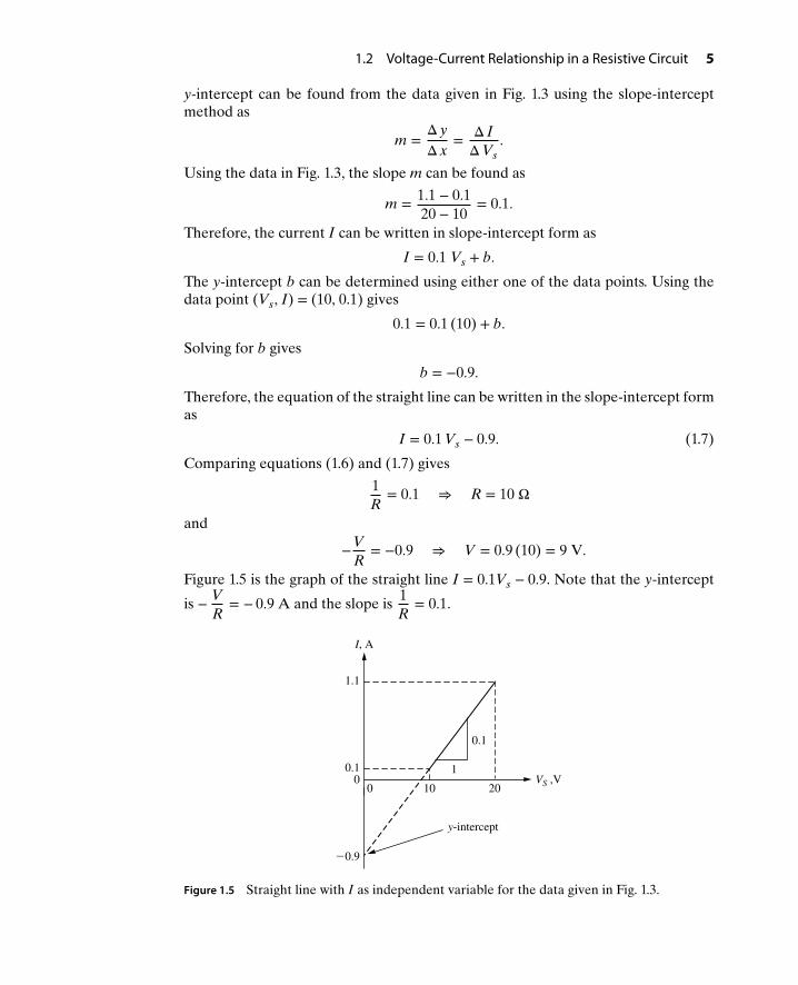
I = 0.1 Vs − 0.9. (1.7)
Comparing equations (1.6) and (1.7) gives
1R
= 0.1 ⇒ R = 10 Ω
and
−VR
= −0.9 ⇒ V = 0.9 (10) = 9 V.
Figure 1.5 is the graph of the straight line I = 0.1Vs − 0.9. Note that the y-intercept
is − VR
= − 0.9 A and the slope is 1R
= 0.1.
y-intercept
1
0.1
0 10 20
0.9
1.1
0.10
I, A
VS ,V
Figure 1.5 Straight line with I as independent variable for the data given in Fig. 1.3.

6 Chapter 1 Straight Lines in Engineering
1.3 FORCE-DISPLACEMENT IN A PRELOADEDTENSION SPRINGThe force-displacement relationship for a spring with a preload fo is given by
f = k y + fo, (1.8)
where f is the force in Newtons (N), y is the displacement in meters (m), and k is thespring constant in N/m.
y
fk
f , N y, m1 0.15 0.9
Figure 1.6 Force-displacement in a preloaded spring.
The objective is to find the spring constant k and the preload fo, if the values of theforce and displacement are as given in Fig. 1.6.
Method 1 Treating the displacement y as an independent variable, the force-displacement relationship f = k y + fo is the equation of a straight line y = mx + b,where the independent variable x is the displacement y, the dependent variable y isthe force f , the slope m is the spring constant k, and the y-intercept is the preload fo.The slope m can be calculated using the data given in Fig. 1.6 as
m = 5 − 10.9 − 0.1
= 40.8
= 5.
The equation of the force-displacement equation in the slope-intercept form cantherefore be written as
f = 5y + b.
The y-intercept b can be found using one of the data points. Using the data point(f , y) = (5, 0.9) gives
5 = 5 (0.9) + b.
Solving for b gives
b = 0.5 N.
Therefore, the equation of the straight line can be written in slope-intercept form as
f = 5y + 0.5. (1.9)
Comparing equations (1.8) and (1.9) gives
k = 5N∕m, fo = 0.5N.
1.3 Force-Displacement in a Preloaded Tension Spring 7
Method 2 Now treating the force f as an independent variable, the force-
displacement relationship f = ky + fo can be written as y = 1k
f −fo
k. This relation-
ship is the equation of a straight line y = mx + b, where the independent variablex is the force f , the dependent variable y is the displacement y, the slope m is the
reciprocal of the spring constant 1k
, and the y-intercept is the negated preload
divided by the spring constant −fo
k. The slope m can be calculated using the data
given in Fig. 1.6 as
m = 0.9 − 0.15 − 1
= 0.84
= 0.2.
The equation of the displacement y as a function of force f can therefore be writtenin slope-intercept form as
y = 0.2f + b.
The y-intercept b can be found using one of the data points. Using the data point(y, f ) = (0.9, 5) gives
0.9 = 0.2 (5) + b.
Solving for b gives
b = −0.1.
Therefore, the equation of the straight line can be written in the slope-intercept formas
y = 0.2f − 0.1. (1.10)
Comparing equation (1.10) with the expression y = 1k
f −fo
kgives
1k= 0.2 ⇒ k = 5 N/m
and
−fo
k= −0.1 ⇒ fo = 0.1 (5) = 0.5 N.
Therefore, the force-displacement relationship for a preloaded spring given inFig. 1.6 is given by
f = 5y + 0.5.

8 Chapter 1 Straight Lines in Engineering
1.4 FURTHER EXAMPLES OF LINES IN ENGINEERING
Example1-1
The velocity of a vehicle follows the trajectory shown in Fig. 1.7. The vehicle startsat rest (zero velocity) and reaches a maximum velocity of 10 m/s in 2 s. It thencruises at a constant velocity of 10 m/s for 2 s before coming to rest at 6 s. Write theequation of the function v(t); in other words, write the expression of v(t) for timesbetween 0 and 2 s, between 2 and 4 s, between 4 and 6 s, and greater than 6 s.
10
0 2 4 6
v(t), m/s
t, s
Figure 1.7 Velocity profile of a vehicle.
Solution The velocity profile of the vehicle shown in Fig. 1.7 is a piecewise linear functionwith three different equations. The first linear function is a straight line passingthrough the origin starting at time 0 sec and ending at time equal to 2 s. The secondlinear function is a straight line with zero slope (cruise velocity of 10 m/s) startingat 2 s and ending at 4 s. Finally, the third piece of the trajectory is a straight linestarting at 4 s and ending at 6 s. The equation of the piecewise linear function canbe written as
(a) 0 ≤ t ≤ 2:
v(t) = mt + b
where b = 0 and m = 10 − 02 − 0
= 5. Therefore,
v(t) = 5t m/s.
(b) 2 ≤ t ≤ 4:
v = 10 m/s.
(c) 4 ≤ t ≤ 6:
v(t) = mt + b,
where m = 0 − 106 − 4
= −5 and the value of b can be calculated using the data
point (t, v(t)) = (6, 0) as
0 = −5 (6) + b ⇒ b = 0 + 30 = 30.
1.4 Further Examples of Lines in Engineering 9
The value of b can also be calculated using the point-slope formula for thestraight line
v − v1 = m(t − t1),
where v1 = 0 and t1 = 6. Thus,
v − 0 = −5(t − 6).
Therefore,
v(t) = −5(t − 6).
or
v(t) = −5t + 30 m/s.
(d) t > 6:
v(t) = 0 m/s.
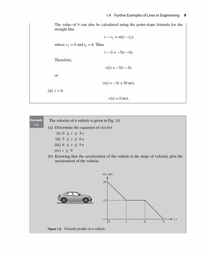
Example1-2
The velocity of a vehicle is given in Fig. 1.8.
(a) Determine the equation of v(t) for
(i) 0 ≤ t ≤ 3 s
(ii) 3 ≤ t ≤ 6 s
(iii) 6 ≤ t ≤ 9 s
(iv) t ≥ 9
(b) Knowing that the acceleration of the vehicle is the slope of velocity, plot theacceleration of the vehicle.
0 3 6 9
24
12
v(t), m/s
t, s
Figure 1.8 Velocity profile of a vehicle.

10 Chapter 1 Straight Lines in Engineering
Solution (a) The velocity of the vehicle for different intervals can be calculated as
(i) 0 ≤ t ≤ 3 s:
v(t) = mt + b,
where m = 12 − 243 − 0
= −4 m/s2 and b = 24 m/s. Therefore,
v(t) = −4t + 24 m/s.
(ii) 3 ≤ t ≤ 6 s:
v(t) = 12 m/s.
(iii) 6 ≤ t ≤ 9 s:
v(t) = mt + b,
where m = 0 − 129 − 6
= −4 m/s2 and b can be calculated in slope-intercept
form using point (t, v(t)) = (9, 0) as
0 = −4(9) + b.
Therefore, b = 36 m/s and
v(t) = −4t + 36 m/s.
(iv) t > 9 s:
v(t) = 0 m/s.
(b) Since the acceleration of the vehicle is the slope of the velocity in each interval,the acceleration a in m/s2 is given by
a =
⎧⎪⎪⎨⎪⎪⎩
−4; 0 ≤ t ≤ 3 s
0; 3 ≤ t ≤ 6 s
−4; 6 ≤ t ≤ 9 s
0; t > 9 s
The plot of the acceleration is shown in Fig. 1.9.
4
0 3 6 9
Acceleration, m/s2
t, s
Figure 1.9 Acceleration profile of the vehicle in Fig. 1.8.
1.4 Further Examples of Lines in Engineering 11
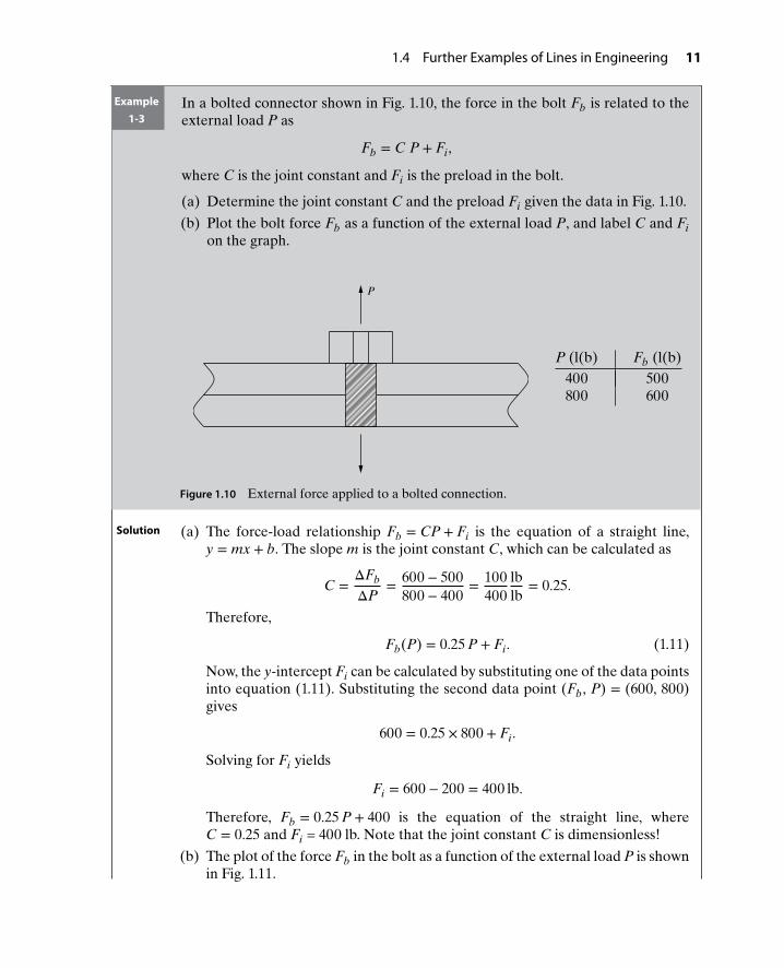
Example1-3
In a bolted connector shown in Fig. 1.10, the force in the bolt Fb is related to theexternal load P as
Fb = C P + Fi,
where C is the joint constant and Fi is the preload in the bolt.
(a) Determine the joint constant C and the preload Fi given the data in Fig. 1.10.
(b) Plot the bolt force Fb as a function of the external load P, and label C and Fion the graph.
P
P (l(b) Fb (l(b)400 500800 600
Figure 1.10 External force applied to a bolted connection.
Solution (a) The force-load relationship Fb = CP + Fi is the equation of a straight line,y = mx + b. The slope m is the joint constant C, which can be calculated as
C =ΔFb
ΔP= 600 − 500
800 − 400= 100
400lblb
= 0.25.
Therefore,
Fb(P) = 0.25 P + Fi. (1.11)
Now, the y-intercept Fi can be calculated by substituting one of the data pointsinto equation (1.11). Substituting the second data point (Fb, P) = (600, 800)gives
600 = 0.25 × 800 + Fi.
Solving for Fi yields
Fi = 600 − 200 = 400 lb.
Therefore, Fb = 0.25 P + 400 is the equation of the straight line, whereC = 0.25 and Fi = 400 lb. Note that the joint constant C is dimensionless!
(b) The plot of the force Fb in the bolt as a function of the external load P is shownin Fig. 1.11.

12 Chapter 1 Straight Lines in Engineering
600
0 400 800
500 1
C
Fb (lb)
Fi 400
(400, 500)
(800, 600)
P (lb)
Figure 1.11 Plot of the bolt force Fb as a function of the external load P.
Example1-4
For the electric circuit shown in Fig. 1.12, the relationship between the voltage Vand the applied current I is given by V = (I + Io)R. Find the values of R and I0 ifthe voltage across the resistor V is known for the two different values of the currentI as shown in Fig. 1.12.
RI Io V
I, amp V, volt0.1 1.20.2 2.2
Figure 1.12 Circuit for Example 1-4.
Solution The voltage-current relationship V = R I + R Io is the equation of a straight liney = mx + b, where the slope m = R can be found from the data given in Fig. 1.12 as
R = ΔVΔI
= 2.2 − 1.20.2 − 0.1
= 10.1
voltamp
= 10 Ω.
Therefore,
V = 10(I) + 10 I0. (1.12)
The y-intercept b = 10 I0 can be found by substituting the second data point(2.2, 0.2) in equation (1.12) as
2.2 = 100 × 0.2 + 10 I0.
Solving for I0 gives
10 I0 = 2.2 − 2 = 0.2,

1.4 Further Examples of Lines in Engineering 13
which gives
I0 = 0.02 A.
Therefore, V = 10 I + 0.2; and R = 10 Ω and I0 = 0.02 A.
Example1-5
The output voltage vo of the operational amplifier (Op–Amp) circuit shown in
Fig. 1.13 satisfies the relationship vo =(−100
R
)vin +
(1 + 100
R
)vb, where R in
kΩ is the unknown resistance and vb is the unknown voltage. Fig. 1.13 gives thevalues of the output voltage for two different values of the input voltage.
(a) Determine the value of R and vb.
(b) Plot the output voltage vo as a function of the input voltage vin. On the plot,clearly indicate the value of the output voltage when the input voltage is zero(y-intercept) and the value of the input voltage when the output voltage is zero(x-intercept).
R kΩ
100 kΩ
vinvb
voOP−AMP
vin, V vo, V5 5
10 − 5
Figure 1.13 An Op–Amp circuit as a summing amplifier.
Solution (a) The input-output relationship vo =(−100
R
)vin +
(1 + 100
R
)vb is the equa-
tion of a straight line, y = mx + b, where the slope m = −100R
can be found
from the data given in Fig. 1.13 as
−100R
=Δvo
Δvin= −5 − 5
10 − 5= −10
5= −2.
Solving for R gives R = 50 Ω. Therefore,
v0 =(−100
50
)vin +
(1 + 100
50
)vb
= −2 vin + 3 vb. (1.13)
The y-intercept b = 3 vb can be found by substituting the first data point(v0, vin) = (5, 5) in equation (1.13) as
5 = −2 × 5 + 3 vb.
14 Chapter 1 Straight Lines in Engineering
Solving for vb yields
3 vb = 5 + 10 = 15,
which gives vb = 5 V. Therefore, vo = −2 vin + 15, R = 50 Ω, and vb = 5 V. Thex-intercept can be found by substituting vo = 0 in the equation vo = −2 vin + 15and finding the value of vin as
0 = −2 vin + 15,
which gives vin = 7.5 V. Therefore, the x-intercept occurs at Vin = 7.5 V.
(b) The plot of the output voltage of the Op–Amp as a function of the input voltageif vb = 5 V is shown in Fig. 1.14.
0 5 10
5
5
15
m 2 R
100
vo, V
y−intercept b 3, vb 15 V
x−intercept 7.5 V
vin, V
Figure 1.14 An Op–Amp circuit as a summing amplifier.
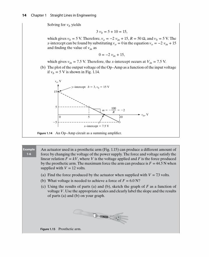
Example1-6
An actuator used in a prosthetic arm (Fig. 1.15) can produce a different amount offorce by changing the voltage of the power supply. The force and voltage satisfy thelinear relation F = kV, where V is the voltage applied and F is the force producedby the prosthetic arm. The maximum force the arm can produce is F = 44.5 N whensupplied with V = 12 volts.
(a) Find the force produced by the actuator when supplied with V = 7.3 volts.
(b) What voltage is needed to achieve a force of F = 6.0 N?
(c) Using the results of parts (a) and (b), sketch the graph of F as a function ofvoltage V. Use the appropriate scales and clearly label the slope and the resultsof parts (a) and (b) on your graph.
Figure 1.15 Prosthetic arm.

1.4 Further Examples of Lines in Engineering 15
Solution (a) The input-output relationship F = k V is the equation of a straight line y = m x,where the slope m = k can be found from the given data as
k = 44.512
= 3.71 N/V.
Therefore, the equation of the straight line representing the actuator force Fas a function of applied voltage V is given by
F = 3.71 V. (1.14)
Thus, the force produced by the actuator when supplied with 7.3 volts is foundby substituting V = 7.3 in equation (1.14) as
F = 3.71 × 7.3
= 27.08 N.
(b) The voltage needed to achieve a force of 6.0 N can be found by substitutingF = 6.0 N in equation (1.14) as
6.0 = 3.71 V
V = 6.03.71
= 1.62 volts. (1.15)
(c) The plot of force F as a function of voltage V can now be drawn as shown inFig. 1.16.
44.5
6.0
1.62 7.3 120
27.1
F, N
V, volt
m k 3.71
Figure 1.16 Plot of the actuator force verses the applied voltage.

16 Chapter 1 Straight Lines in Engineering
Example1-7
The electrical activity of muscles can be monitored with an electromyogram(EMG). The following root mean square (RMS) value of the amplitude measure-ments of the EMG signal were taken when a woman was using her hand gripmuscles to ensure a lid was tight on a jar.
EMG
A, V F, N0.0005 1100.00125 275
Figure 1.17 Amplitude measurements of theEMG signal.
The RMS amplitude of the EMG signal satisfies the linear equation
A = mF + b (1.16)
where A is the RMS value of the EMG amplitude in V, F is the applied muscleforce in N, and m is the slope.
(a) Determine the value of m and b.
(b) Plot the RMS amplitude A as a function of the applied muscle force F.
(c) Using the equation of the line from part (a), find the RMS value of the ampli-tude for a muscle force of 200 N.
Solution (a) The input-output relationship A = mF + b is the equation of a straight liney = mx + b, where the slope m can be found from the EMG data given in thetable (Fig. 1.17) as
m = ΔAΔF
= 0.00125 − 0.0005275 − 110
= 0.00075165
= 4.55 × 10⁻⁶ VN.
The y-intercept b can be found by substituting the first data point (A, F)= (0.0005, 110) in equation (1.16) as
0.0005 = 4.55 × 10⁻⁶(110) + b.
Solving for b yields
b = 5 × 10⁻⁷ ≈ 0.
Therefore, the equation of the straight line representing the RMS amplitudeas a function of applied force is given by
A = 4.55 × 10⁻⁶ F. (1.17)
(b) The plot of the RMS amplitude as a function of the applied muscle force isshown in Fig. 1.18.
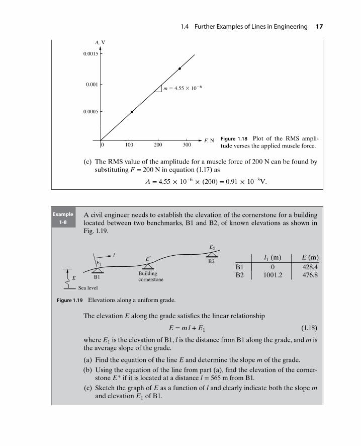
1.4 Further Examples of Lines in Engineering 17
F, N 1000 200 300
A, V
0.0005
0.001
0.0015
m 4.55 10 6
Figure 1.18 Plot of the RMS ampli-tude verses the applied muscle force.
(c) The RMS value of the amplitude for a muscle force of 200 N can be found bysubstituting F = 200 N in equation (1.17) as
A = 4.55 × 10−6 × (200) = 0.91 × 10⁻³V.
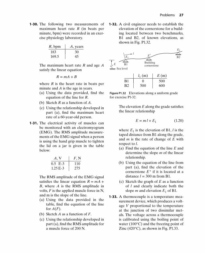
Example1-8
A civil engineer needs to establish the elevation of the cornerstone for a buildinglocated between two benchmarks, B1 and B2, of known elevations as shown inFig. 1.19.
B2*
Sea level
cornerstone
Building
E2
E
lE1
B1
E l1 (m) E (m)B1 0 428.4B2 1001.2 476.8
Figure 1.19 Elevations along a uniform grade.
The elevation E along the grade satisfies the linear relationship
E = m l + E1 (1.18)
where E1 is the elevation of B1, l is the distance from B1 along the grade, and m isthe average slope of the grade.
(a) Find the equation of the line E and determine the slope m of the grade.
(b) Using the equation of the line from part (a), find the elevation of the corner-stone E ∗ if it is located at a distance l = 565 m from B1.
(c) Sketch the graph of E as a function of l and clearly indicate both the slope mand elevation E1 of B1.

18 Chapter 1 Straight Lines in Engineering
Solution (a) The equation of elevation given by equation (1.18) is a straight line in the slope-intercept form y = mx + b, where the slope m can be found from the elevationdata given in Fig. 1.19 as
m = ΔEΔl
= 476.8 − 428.41001.2 − 0
= 48.41001.2
= 0.0483.
The y-intercept E1 can be found by substituting the first data point (E, l) =(428.4, 0) in equation (1.18) as
428.4 = 0.0483 × (0) + E1
Solving for E1 yields
E1 = 428.4 m.
Therefore, the equation of the straight line representing the elevation as a func-tion of distance l is given by
E = 0.0483 l + 428.4 m. (1.19)
(b) The elevation E ∗ of the cornerstone can be found by substituting l = 565 m inequation (1.19) as
E ∗ = 0.0483 × (565) + 428.4 = 455.7 m.
(c) The plot of the elevation as a function of the length is shown in Fig. 1.20.
428.4
y-intercept
0 565
476.8
1
0.0483 m
E1
E*455.7
l, m
Elevation, m
E2
Cornerstone
1001.2
Figure 1.20 Elevation along a uniform grade.

Problems 19
P R O B L E M S
1-1. A constant force F = 2 N is applied toa spring and the displacement x is mea-sured as 0.2 m. If the spring force anddisplacement satisfy the linear relationF = k x, find the stiffness k of the spring.
x
fk
F (N) x (m)2 0.2
Figure P1.1 Displacement of a spring inproblem P1-1.
1-2. The spring force F and displacementx for a close-wound tension spring aremeasured as shown in Fig. P1.2. Thespring force F and displacement x sat-isfy the linear equation F = k x + Fi,where k is the spring constant and Fi isthe preload induced during manufactur-ing of the spring.(a) Using the given data in Fig. P1.2,
find the equation of the line for thespring force F as a function ofthe displacement x, and determinethe values of the spring constant kand preload Fi.
(b) Sketch the graph of F as a functionof x. Use appropriate axis scalesand clearly label the preload Fi, thespring constant k, and both givendata points on your graph.
F (N) x (cm)34.5 1.557.0 3.0
Figure P1.2 Close-wound tension spring forproblem P1-2.
1-3. The spring force F and displacementx for a close-wound tension springare measured as shown in Fig. P1.3.
The spring force F and displacement xsatisfy the linear equation F = k x + Fi,where k is the spring constant and Fi isthe preload induced during manufactur-ing of the spring.(a) Using the given data, find the equa-
tion of the line for the spring forceF as a function of the displacementx, and determine the values of thespring constant k and preload Fi.
(b) Sketch the graph of F as a functionof x and clearly indicate both thespring constant k and preload Fi.
F (N) x (cm)135 25222 50
Figure P1.3 Close-wound tension spring forproblem P1-3.
1-4. In a bolted connection shown in Fig.P1.4, the force in the bolt Fb is givenin terms of the external load P as Fb =C P + Fi.(a) Given the data in Fig. P1.4, deter-
mine the joint constant C and thepreload Fi.
P
P (l(b) Fb (l(b)100 200600 400
Figure P1.4 Bolted connection for problem P1-4.

20 Chapter 1 Straight Lines in Engineering
(b) Plot the bolt force Fb as a functionof the load P and label C and Fi onthe graph.
1-5. Repeat problem P1-4 for the data givenin Fig. P1.5.
P
Fb (l(b) P (l(b)300 280660 1000
Figure P1.5 Bolted connection for problem P1-5.
1-6. The velocity v(t) of a ball thrown up-ward satisfies the equation v(t) = vo +at, where vo is the initial velocity of theball in ft/s and a is the acceleration inft/s2.(a) Given the data in Fig. P1.6, find
the equation of the line represent-ing the velocity v(t) of the ball, anddetermine both the initial velocityvo and the acceleration a.
(b) Sketch the graph of the line v(t),and clearly indicate both the initialvelocity and the acceleration onyour graph. Also determine thetime at which the velocity is zero.
v(t)v(t) (ft/s) t (s)
67.8 1.03.4 3.0
Figure P1.6 A ball thrown upward with an initialvelocity vo(t) in problem P1-6.
1-7. The velocity v(t) of a ball thrown up-ward satisfies the equation v(t) = vo +at, where vo is the initial velocity of theball in m/s and a is the acceleration inm/s2.(a) Given the data in Fig. P1.7, find
the equation of the line represent-ing the velocity v(t) of the ball, anddetermine both the initial velocityvo and the acceleration a.
(b) Sketch the graph of the line v(t), andclearly indicate both the initial ve-locity and the acceleration on yourgraph. Also determine the time atwhich the velocity is zero.
v(t)v(t) (m/s) t (s)
3.02 0.11.06 0.3
Figure P1.7 A ball thrown upward with aninitial velocity vo(t) in problem P1-7.
1-8. A model rocket is fired in the verticalplane. The velocity v(t) is measured asshown in Fig. P1.8. The velocity satisfiesthe equation v(t) = vo + at, where vo isthe initial velocity of the rocket in m/sand a is the acceleration in m/s2.(a) Given the data in Fig. P1.8, find
the equation of the line represent-ing the velocity v(t) of the rocket,and determine both the initial ve-locity vo and the acceleration a.
v(t) v(t) (m/s) t (s)
34.3 0.519.6 2.0
Figure P1.8 A model rocket fired in the verticalplane in problem P1-8.

Problems 21
(b) Sketch the graph of the line v(t)for 0 ≤ t ≤ 8 seconds, and clearlyindicate both the initial velocityand the acceleration on your graph.Also determine the time at whichthe velocity is zero (i.e., the timerequired to reach the maximumheight).
1-9. A model rocket is fired in the verticalplane. The velocity v(t) is measured asshown in Fig. P1.9. The velocity satisfiesthe equation v(t) = vo + at, where vo isthe initial velocity of the rocket in ft/sand a is the acceleration in ft/s2.(a) Given the data in Fig. P1.9, find
the equation of the line represent-ing the velocity v(t) of the rocket,and determine both the initialvelocity vo and the acceleration a.
(b) Sketch the graph of the line v(t) for0 ≤ t ≤ 10 seconds, and clearlyindicate both the initial velocityand the acceleration on your graph.Also determine the time at whichthe velocity is zero (i.e., the timerequired to reach the maximumheight).
v(t) v(t) (ft/s) t (s)
128.8 1.032.2 4.0
Figure P1.9 A model rocket fired in the vertical planein problem P1-9.
1-10. The velocity of a vehicle is measured attwo distinct points in time as shown inFig. P1.10. The velocity satisfies the re-lationship v(t) = vo + at, where vo is theinitial velocity in m/s and a is the accel-eration in m/s2.
(a) Find the equation of the line v(t),and determine both the initial ve-locity vo and the acceleration a.
(b) Sketch the graph of the line v(t), andclearly label the initial velocity, theacceleration, and the total stoppingtime on the graph.
v(t) (m/s) t (s)30 1.010 2.0
Figure P1.10 Velocity of a vehicle during brakingin problem P1-10.
1-11. The velocity of a vehicle is measured attwo distinct points in time as shown inFig. P1.11. The velocity satisfies the re-lationship v(t) = vo + at, where vo is theinitial velocity in ft/s and a is the accel-eration in ft/s2.(a) Find the equation of the line v(t),
and determine both the initial ve-locity vo and the acceleration a.
(b) Sketch the graph of the line v(t), andclearly label the initial velocity, theacceleration, and the total stoppingtime on the graph.
v(t) (ft/s) t (s)112.5 0.537.5 1.5
Figure P1.11 Velocity of a vehicle during brakingin problem P1-11.
1-12. The velocity v(t) of a vehicle duringbraking is given in Fig. P1.12. Determinethe equation for v(t) for(a) 0 ≤ t ≤ 2 s(b) 2 ≤ t ≤ 4 s(c) 4 ≤ t ≤ 6 s

22 Chapter 1 Straight Lines in Engineering
0 2 4 6
30
15
t, s
v(t), m/s
Figure P1.12 Velocity of a vehicle during braking inproblem P1-12.
1-13. A linear trajectory is planned for a robotto pick up a part in a manufacturing pro-cess. The velocity of the trajectory ofone of the joints is shown in Fig. P1.13.Determine the equation of v(t) for(a) 0 ≤ t ≤ 1 s(b) 1 ≤ t ≤ 3 s(c) 3 ≤ t ≤ 4 s
10
0 1 3 4t, s
v(t), m/s
Figure P1.13 Velocity of a robot trajectory.
1-14. The acceleration of the linear trajectoryof problem P1-13 is shown in Fig. P1.14.Determine the equation of a(t) for
(a) 0 ≤ t ≤ 1 s(b) 1 ≤ t ≤ 3 s(c) 3 ≤ t ≤ 4 s
0 1 3 4
10
10
a(t), m/s2
t, s
Figure P1.14 Acceleration of the robot trajectory.
1-15. The temperature distribution in a well-insulated axial rod varies linearly withrespect to distance when the tempera-ture at both ends is held constant asshown in Fig. P1.15. The temperaturesatisfies the equation of a line T(x) =C1 x + C2, where C1 and C2 are con-stants of integration with units of F/ftand F, respectively(a) Find the equation of the line T(x),
and determine both constants C1and C2.
(b) Sketch the graph of the line T(x) for0 ≤ x ≤ 1.5 ft, and clearly label C1and C2 on your graph. Also, clearlyindicate the temperature at the cen-ter of the rod (x = 0.75 ft).
x
T(x) (F) x (ft)30 0.070 1.5
Figure P1.15 Temperature distribution in awell-insulated axial rod in problem P1-15.

Problems 23
1-16. The temperature distribution in a well-insulated axial rod varies linearly withrespect to distance when the tempera-ture at both ends is held constant asshown in Fig. P1.16. The temperaturesatisfies the equation of a line T(x) =C1 x + C2, where C1 and C2 are con-stants of integration with units of C/mand C, respectively.(a) Find the equation of the line T(x),
and determine both constants C1and C2.
(b) Sketch the graph of the line T(x) for0 ≤ x ≤ 0.5 m, and clearly label C1and C2 on your graph. Also, clearlyindicate the temperature at the cen-ter of the rod (x = 0.25 m).
x
T(x) (C) x (m)0 0.0
20 0.5
Figure P1.16 Temperature distribution in awell-insulated axial rod in problem P1-16.
1-17. The voltage-current relationship for thecircuit shown in Fig. P1.17 is given byOhm’s law as V = I R, where V is theapplied voltage in volts, I is the currentin amps, and R is the resistance of theresistor in ohms.(a) Sketch the graph of I as a function
of V if the resistance is 5 Ω.
V
I
R = 5 Ω+−
Figure P1.17 Resistive circuit for problem P1-17.
(b) Find the current I if the appliedvoltage is 10 V.
1-18. A voltage source Vs is used to applytwo different voltages (12V and 18V)to the single-loop circuit shown in Fig.P1.18. The values of the measuredcurrent are shown in Fig. P1.18. Thevoltage and current satisfy the linear re-lation Vs = IR + V, where R is the resis-tance in ohms, I is the current in amps,and Vs is the voltage in volts.(a) Using the data given in Fig. P1.18,
find the equation of the line for Vsas a function of I, and determine thevalues of R and V.
(b) Sketch the graph of Vs as a functionof I and clearly indicate the resis-tance R and voltage V on the graph.
VS
I R
V
Vs (volt) I (amp)12.0 0.7518.0 1.5
Figure P1.18 Single-loop circuit for problemP1-18.
1-19. Repeat problem P1-18 for the datashown in Fig. P1.19.
VS
I R
V
Vs (volt) I (amp)9.0 2.0
18.0 5.0
Figure P1.19 Single-loop circuit for problemP1-19.

24 Chapter 1 Straight Lines in Engineering
1-20. Repeat problem P1-18 for the datashown in Fig. P1.20.
VS
I R
V
Vs (volt) I (amp)1.5 242.5 32
Figure P1.20 Single-loop circuit for problem P1-20.
1-21. A linear model of a diode is shown inFig. P1.21, where Rd is the forward resis-tance of the diode and VON is the volt-age that turns the diode ON. To deter-mine the resistance Rd and voltage VON ,two voltage values are applied to thediode and the corresponding currentsare measured. The applied voltage VSand the measured current I are givenin Fig. P1.21. The applied voltage andthe measured current satisfy the linearequation Vs = I Rd + VON .(a) Find the equation of the line for Vs
as a function of I and determine theresistance Rd and the voltage VON .
Rd
VON
I
VS
Vs (volt) I (amp)5.0 0.086
10.0 0.186
Figure P1.21 Linear model of a diode for problemP1-21.
(b) Sketch the graph of VS as a func-tion of I, and clearly indicate the re-sistance Rd and the voltage VON onthe graph.
1-22. Repeat problem P1-21 for the data givenin Fig. P1.22.
Rd
VON
I
VS
Vs (volt) I (amp)2.0 0.0356 0.135
Figure P1.22 Linear model of a diode for problemP1-22.
1-23. The output voltage, vo, of the Op–Ampcircuit shown in Fig. P1.23 satisfies
the relationship vo =(
1 + 100R
) (vin2
)−(
100R
)vb, where R is the unknown resis-
tance in kΩ and vb is the unknown volt-age in volts. Fig. P1.23 gives the valuesof the output voltage for two differentvalues of the input voltage.
R kΩ
vinvb
Op−Amp
vo100 kΩ
100 kΩ
100 kΩ
vin, V vo, V5 3.5
10 11
Figure P1.23 An Op–Amp circuit as a summingamplifier for problem P1.23.

Problems 25
(a) Determine the equation of the linefor vo as a function of vin and findthe values of R and vb.
(b) Plot the output voltage vo as a func-tion of the input voltage vin. On theplot, clearly indicate the value ofthe output voltage when the inputvoltage is zero (y-intercept) and thevalue of the input voltage when theoutput voltage is zero (x-intercept).
1-24. The output voltage, vo, of the Op–Amp circuit shown in Fig. P1.24 satisfies
the relationship vo = −(
v2 +100R
vin
),
where R is the unknown resistancein kΩ, vin is the input voltage, andv2 is the unknown voltage. Fig. P1.24gives the values of the output voltagefor two different values of the inputvoltage vin.(a) Find the equation of the line for vo
as a function of vin and determinethe values of R and v2.
(b) Plot the output voltage vo as a func-tion of the input voltage vin. Clearlyindicate the value of the outputvoltage when the input voltage iszero (y-intercept) and the value ofthe input voltage when the outputvoltage is zero (x-intercept).
OP−AMP
vo
v2
vinR kΩ
100 kΩ
100 kΩ
vin, V vo, V5 − 4.5
10 − 7.0
Figure P1.24 An Op–Amp circuit for problemP1-24.
1-25. A DC motor is driving an inertial loadJL shown in Fig. P1.25. To maintain aconstant speed, two different values ofthe voltage ea are applied to the mo-tor. The voltage ea and the current iaflowing through the armature windingof the motor satisfy the relationshipea = ia Ra + eb, where Ra is the resis-tance of the armature winding in ohmsand eb is the back-emf in volts. Fig-ure P1.25 gives the values of the cur-rent for two different values of theinput voltage applied to the armature ofthe DC motor.
(a) Find the equation of the line for eaas a function of ia and determine thevalues of Ra and eb.
(b) Plot the applied voltage ea as a func-tion of the current ia. Clearly indi-cate the value of the back-emf eband the winding resistance Ra.
Load
ia
eb
Gear ratio 20
Tm
θm, ωm
Jm
Ra
Jtach
TACH
JL
Motorea
etach
ea, V ia, A2 0.54 1.25
Figure P1.25 Voltage-current data of a DC motorfor problem P1-25.
1-26. Repeat problem P1-25 for the datashown in Fig. P1.26.

26 Chapter 1 Straight Lines in Engineering
Load
ia
eb
Gear ratio 20
Tm
θm, ωm
Jm
Ra
Jtach
TACH
JL
Motorea
etach
ia, A ea, V1.0 5.02.25 10.0
Figure P1.26 Voltage-current data of a DC motorin problem P1-26.
1-27. In the active region, the output volt-age vo of the n-channel enhancement-type MOSFET (NMOS) circuit shownin Fig. P1.27 satisfies the relationshipvo = VDD − RD iD, where RD is theunknown drain resistance and VD is theunknown drain voltage. Fig. P1.27 gives
G
VDD
S
vi
vo
RD
iD
iD, mA vo, V4 82 10
Figure P1.27 n-channel enhancement-type MOSFET.
the values of the output voltage for twodifferent values of the drain current.Plot the output voltage vo as a functionof the input drain current iD. On theplot, clearly indicate the values of RDand VDD.
1-28. Repeat problem P1-27 for the data givenin Fig. P1.28.
G
VDD
S
vi
vo
RD
iD
vo, V iD, mA0 105 5
Figure P1.28 NMOS for P1-28.
1-29. An actuator used in a prosthetic armcan produce different amounts of forceby changing the voltage of the powersupply. The force and voltage satisfy thelinear relation F = kV, where V is thevoltage applied and F is the force pro-duced by the prosthetic arm. The maxi-mum force the arm can produce is 30.0N when supplied with 10 V.(a) Find the force produced by the
actuator when supplied with 6.0 V.(b) What voltage is needed to achieve a
force of 5.0 N?(c) Using the results of parts (a) and
(b), sketch the graph of F as a func-tion of voltage V. Use the appropri-ate scales and clearly label the slopeand the results of parts (a) and (b).
Problems 27
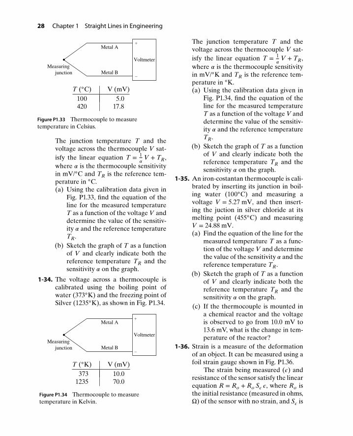
1-30. The following two measurements ofmaximum heart rate R (in beats perminute, bpm) were recorded in an exer-cise physiology laboratory.
R, bpm A, years183 30169.5 45
The maximum heart rate R and age Asatisfy the linear equation
R = mA + B
where R is the heart rate in beats perminute and A is the age in years.(a) Using the data provided, find the
equation of the line for R.(b) Sketch R as a function of A.(c) Using the relationship developed in
part (a), find the maximum heartrate of a 60-year-old person.
1-31. The electrical activity of muscles canbe monitored with an electromyogram(EMG). The RMS amplitude measure-ments of the EMG signal when a personis using the hand grip muscle to tightenthe lid on a jar is given in the tablebelow:
A, V F, N0.5 E-3 1101.25 E-3 275
The RMS amplitude of the EMG signalsatisfies the linear equation R = mA +B, where A is the RMS amplitude involts, F is the applied muscle force in N,and m is the slope of the line.(a) Using the data provided in the
table, find the equation of the linefor A(F).
(b) Sketch A as a function of F.(c) Using the relationship developed in
part (a), find the RMS amplitude fora muscle force of 200 N.
1-32. A civil engineer needs to establish theelevation of the cornerstone for a build-ing located between two benchmarks,B1 and B2, of known elevations, asshown in Fig. P1.32.
B2
Sea level
Buildingcornerstone
E2
E
lE1
B1
E*
l1 (m) E (m)B1 0 500B2 500 600
Figure P1.32 Elevations along a uniform gradefor exercise P1-32.
The elevation E along the grade satisfiesthe linear relationship
E = m l + E1 (1.20)
where E1 is the elevation of B1, l is thetaped distance from B1 along the grade,and m is the rate of change of E withrespect to l.(a) Find the equation of the line E and
determine the slope m of the linearrelationship.
(b) Using the equation of the line frompart (a), find the elevation of thecornerstone E ∗ if it is located at adistance l = 300 m from B1.
(c) Sketch the graph of E as a functionof l and clearly indicate both theslope m and elevation E1 of B1.
1-33. A thermocouple is a temperature mea-surement device, which produces a volt-age V proportional to the temperatureat the junction of two dissimilar met-als. The voltage across a thermocoupleis calibrated using the boiling point ofwater (100C) and the freezing point ofZinc (420C), as shown in Fig. P1.33.
28 Chapter 1 Straight Lines in Engineering
Metal B
Measuring
junction
Voltmeter
Metal A
T (C) V (mV)100 5.0420 17.8
Figure P1.33 Thermocouple to measuretemperature in Celsius.
The junction temperature T and thevoltage across the thermocouple V sat-isfy the linear equation T = 1
𝛼V + TR,
where 𝛼 is the thermocouple sensitivityin mV/C and TR is the reference tem-perature in C.(a) Using the calibration data given in
Fig. P1.33, find the equation of theline for the measured temperatureT as a function of the voltage V anddetermine the value of the sensitiv-ity 𝛼 and the reference temperatureTR.
(b) Sketch the graph of T as a functionof V and clearly indicate both thereference temperature TR and thesensitivity 𝛼 on the graph.
1-34. The voltage across a thermocouple iscalibrated using the boiling point ofwater (373K) and the freezing point ofSilver (1235K), as shown in Fig. P1.34.
Metal B
Measuring
junction
Voltmeter
Metal A
T (K) V (mV)373 10.0
1235 70.0
Figure P1.34 Thermocouple to measuretemperature in Kelvin.
The junction temperature T and thevoltage across the thermocouple V sat-isfy the linear equation T = 1
𝛼V + TR,
where 𝛼 is the thermocouple sensitivityin mV/K and TR is the reference tem-perature in K.(a) Using the calibration data given in
Fig. P1.34, find the equation of theline for the measured temperatureT as a function of the voltage V anddetermine the value of the sensitiv-ity 𝛼 and the reference temperatureTR.
(b) Sketch the graph of T as a functionof V and clearly indicate both thereference temperature TR and thesensitivity 𝛼 on the graph.
1-35. An iron-costantan thermocouple is cali-brated by inserting its junction in boil-ing water (100C) and measuring avoltage V = 5.27 mV, and then insert-ing the juction in silver chloride at itsmelting point (455C) and measuringV = 24.88 mV.(a) Find the equation of the line for the
measured temperature T as a func-tion of the voltage V and determinethe value of the sensitivity 𝛼 and thereference temperature TR.
(b) Sketch the graph of T as a functionof V and clearly indicate both thereference temperature TR and thesensitivity 𝛼 on the graph.
(c) If the thermocouple is mounted ina chemical reactor and the voltageis observed to go from 10.0 mV to13.6 mV, what is the change in tem-perature of the reactor?
1-36. Strain is a measure of the deformationof an object. It can be measured using afoil strain gauge shown in Fig. P1.36.
The strain being measured (𝜖) andresistance of the sensor satisfy the linearequation R = Ro + Ro S𝜖 𝜖, where Ro isthe initial resistance (measured in ohms,Ω) of the sensor with no strain, and S𝜖 is

Problems 29
the gauge factor (a multiplier with NOunits).(a) Using the given data, find the equa-
tion of the line for the sensor’s re-sistance R as a function of the strain𝜖, and determine the values of thegauge factor S𝜖 and initial resistanceRo.
(b) Sketch the graph of R as a functionof 𝜖, and clearly indicate Ro on yourgraph.
Active
grid length
End loops
End loops
Solder tabs
Grid
Alignment
marks
Backing and
encapsulation
R, Ω 𝜖, m/m100 0102 0.01
Figure P1.36 Foil strain gauge to measure strain inproblem P1-36.
1-37. Repeat problem P1-36 for the datashown in Fig. P1.37.
1-38. To determine the concentration of apurified protein sample, a graduatestudent used spectrophotometry tomeasure the absorbance given in thetable below:
c (𝜇g/ml) a
3.50 0.3428.00 0.578
The concentration-absorbance relation-ship for this protein satisfies a linearequation a = m c + ai, where c is theconcentration of a purified protein, a is
Active
grid length
End loops
End loops
Solder tabs
Grid
Alignment
marks
Backing and
encapsulation
R, Ω 𝜖, m/m50 052 0.02
Figure P1.38 Foil strain gauge to measure strain inproblem P1-38.
the absorbance of the sample, m is thethe rate of change of absorbance a withrespect to concentration c, and ai is they-intercept.(a) Find the equation of the line
that describes the concentration-absorbance relationship for thisprotein and determine the slope mof the linear relationship.
(b) Using the equation of the line frompart (a), find the concentration ofthe sample if this sample had anabsorption of 0.486.
(c) If the sample is diluted to a con-centration of 0.00419 𝜇g/ml, whatwould you expect the absorption tobe? Would this value be accurate?
(d) Sketch the graph of absorbance aas a function of concentration c andclearly indicate both the slope mand the y-intercept.
1-39. Repeat problem P1-38 if the absorption-concentration data for another sampleis obtained as
c (𝜇g/ml) a
4.00 0.358.50 0.65

30 Chapter 1 Straight Lines in Engineering
1-40. A chemistry student is perform-ing an experiment to determine thetemperature-volume behavior of a gasmixture at constant pressure and quan-tity. Due to technical difficulties, hecould only obtain values at two tem-peratures as shown in the table below:
T (C) V (L)50 1.0898 1.24
The student knows that the gas volumedirectly depends on temperature, that is,V(T) = m T + K, where V is the volumein L, T is the temperature in C, K is they-intercept in L, and m is the slope of theline in L/C.(a) Find the equation of the line that
describes the temperature-volumerelationship of the gas mixture anddetermine the slope m of the linearrelationship.
(b) Using the equation of the line frompart (a), find the temperature of thegas mixture if the volume is 1.15 L.
(c) Using the equation of the line frompart (a), find the volume of the gasif the temperature is 70C.
(d) Sketch the graph of the volume-temperature relationship for the gasmixture from −300C to 100C andclearly indicate both the slope mand the y-intercept. What is the sig-nificance of the temperature whenV = 0 L?
1-41. To obtain the linear relationship be-tween the Fahrenheit and Celsius tem-perature scales, the freezing and boilingpoint of water is used as given in thetable below:
T (F) T (C)32 0
212 100
The relationship between the tempera-tures in Fahrenheit and Celsius scalessatisfies the linear equation T (F) =a T (C) + b.(a) Using the given data, find the equa-
tion of the line relating the Fahren-heit and Celsius scales.
(b) Sketch the graph of T (F) as a func-tion of T (C), and clearly indicatea and b on your graph.
(c) Using the graph obtained in part(b), find the temperature interval inC if the temperature is between20F and 80F.
1-42. A thermostat control with dial markingfrom 0 to 100 is used to regulate the tem-perature of an oil bath. To calibrate thethermostat, the data for the tempera-ture T (F) versus the dial setting R wasobtained as shown in the table below:
T (F) R
110.0 20.040.0 40.0
The relationship between the tempera-ture T in Fahrenheit and the dial settingR satisfies the linear equation T (F) =a R + b.(a) Using the given data, find the equa-
tion of the line relating the temper-ature to the dial setting.
(b) Sketch the graph of T (F) as a func-tion of R, and clearly indicate a andb on your graph.
(c) Calculate the thermostat settingneeded to obtain a temperature of320F.
1-43. In a pressure-fed journal bearing, forcedcooling is provided by a pressurizedlubricant flowing along the axial di-rection of the shaft (the x-direction)as shown in Fig. P1.43. The lubricant

Problems 31
Bearing
Groove
Journal
l
y
c x
Ps
p(x), psi x, in.24 0.512 1.5
Figure P1.43 Pressure-fed journal bearing.
pressure satisfies the linear equation
p(x) =ps
lx + ps,
where ps is the supply pressure and l isthe length of the bearing.(a) Using the data given in the table
(Fig. P1.43), find the equation ofthe line for the lubricant pressurep(x) and determine the values of the
supply pressure ps and the bearinglength l.
(b) Calculate the lubricant pressurep(x) if x is 1.0 in.
(c) Sketch the graph of the lubricantpressure p(x), and clearly indicateboth the supply pressure ps and thebearing length l on the graph.

CHAPTER2
Quadratic Equationsin Engineering
In this chapter, the applications of quadratic equations in engineering are introduced.It is assumed that students are familiar with this topic from their high school algebracourse. A quadratic equation is a second-order polynomial equation in one variablethat occurs in many areas of engineering. For example, the height of a ball thrownin the air can be represented by a quadratic equation. In this chapter, the solutionof quadratic equations will be obtained by three methods: factoring, the quadraticformula, and completing the square.
2.1 A PROJECTILE IN A VERTICAL PLANESuppose a ball thrown upward from the ground with an initial velocity of 96 ft/sreaches a height h(t) after time t s as shown in Fig. 2.1. The height is expressedby the quadratic equation h(t) = 96 t − 16 t2 ft. Find the time t in seconds whenh(t) = 80 ft.
h(t) = 96 t − 16 t2
Figure 2.1 A ball thrown upward to a height of h(t).
Solution:
h(t) = 96 t − 16 t2 = 80
or
16 t2 − 96 t + 80 = 0. (2.1)
Equation (2.1) is a quadratic equation of the form ax2 + bx + c = 0 and will be solvedusing three different methods.
32
2.1 A Projectile in a Vertical Plane 33
Method 1: Factoring Dividing equation (2.1) by 16 yields
t2 − 6 t + 5 = 0. (2.2)
Equation (2.2) can be factored as
(t − 1)(t − 5) = 0.
Therefore, t − 1 = 0 or t = 1 s and t − 5 = 0 or t = 5 s. Hence, the ball reaches theheight of 80 ft at 1 s and 5 s.
Method 2: Quadratic Formula If ax2 + bx + c = 0, then the quadratic formula tosolve for x is given by
x = −b ±√
b2 − 4ac2a
. (2.3)
Using the quadratic formula in equation (2.3), the quadratic equation (2.2) can besolved as
t = 6 ±√
36 − 202
= 6 ± 42
.
Therefore, t = 6 − 42
= 1 s and t = 6 + 42
= 5 s. Hence, the ball reaches the height of
80 ft at 1 s and 5 s.
Method 3: Completing the Square First, rewrite the quadratic equation (2.2) as
t2 − 6 t = −5. (2.4)
Adding the square of(−6
2
)(one-half the coefficient of the first-order term) to both
sides of equation (2.4) gives
t2 − 6 t +(−6
2
)2
= −5 +(−6
2
)2
,
or
t2 − 6 t + 9 = −5 + 9. (2.5)
Equation (2.5) can now be written as
(t − 3)2 = (±√
4)2
or
t − 3 = ±2.
Therefore, t = 3 ± 2 or t = 1, 5 s. To check if the answer is correct, substitute t = 1 andt = 5 into equation (2.1). Substituting t = 1 s gives
16 × 1 − 96 × 1 + 80 = 0,

34 Chapter 2 Quadratic Equations in Engineering
which gives 0 = 0. Therefore, t = 1 s is the correct time when the ball reaches a heightof 80 ft. Now, substitute t = 5 s,
16 × 52 − 96 × 5 + 80 = 0,
which again gives 0 = 0. Therefore, t = 5 s is also the correct time when the ballreaches a height of 80 ft.
It can be seen from Fig. 2.2 that the height of the ball is 80 ft at both 1 s and5 s. The ball is at 80 ft and going up at 1 s, and it is at 80 ft and going down at 5 s.Hence, the maximum height of ball must be halfway between 1 and 5 s, which is1 + ((5 − 1)∕2) = 3 s. Therefore, the maximum height can be found by substitutingt = 3 s in h(t), which is h(3) = 96(3) − 16(3)2 = 144 ft. These three points (heightat t = 1, 3, and 5 s) can be used to plot the trajectory of the ball. However, to plot thetrajectory accurately, additional data points can be added. The height of the ball att = 0 is zero since the ball is thrown upward from the ground. To check this, substi-tute t = 0 in h(t). This gives h(0) = 96(0) − 16(0)2 = 0 ft. The time when the ball hitsthe ground again can be calculated by equating h(t) = 0. Therefore,
96 t − 16 t2 = 0
6 t − t2 = 0
t (6 − t) = 0.
Therefore, t = 0 and 6 − t = 0 or t = 6 s. Since the ball is thrown in the air from theground (h(t) = 0) at t = 0, it will hit the ground again at t = 6 s. Using these datapoints, the trajectory of the ball thrown upward with an initial velocity of 96 ft/s isshown in Fig. 2.2.
00
50
80
100
144
1 2 3
hmax
4 5 6t, s
h(t), ft
Figure 2.2 The height of the ball thrown upward with an initial velocity of 96 ft/s.
Suppose now you wish to find the time t in seconds when the height of the ball reaches144 ft. Setting h(t) = 144 gives
h(t) = 96 t − 16 t2 = 144.
2.1 A Projectile in a Vertical Plane 35
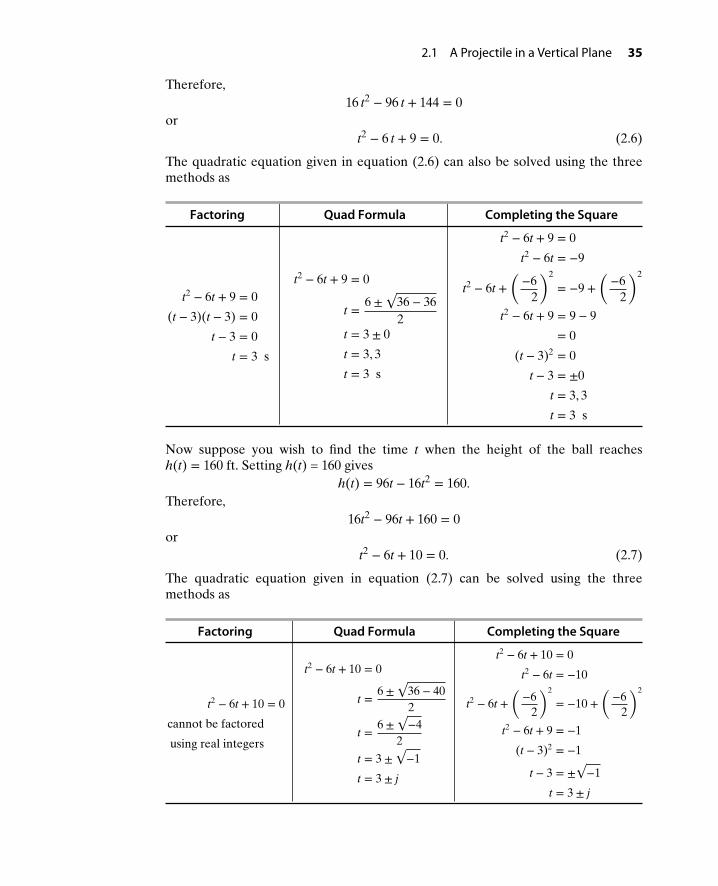
Therefore,16 t2 − 96 t + 144 = 0
ort2 − 6 t + 9 = 0. (2.6)
The quadratic equation given in equation (2.6) can also be solved using the threemethods as
Factoring Quad Formula Completing the Square
t2 − 6t + 9 = 0
(t − 3)(t − 3) = 0
t − 3 = 0
t = 3 s
t2 − 6t + 9 = 0
t = 6 ±√
36 − 362
t = 3 ± 0
t = 3, 3
t = 3 s
t2 − 6t + 9 = 0
t2 − 6t = −9
t2 − 6t +(−6
2
)2
= −9 +(−6
2
)2
t2 − 6t + 9 = 9 − 9
= 0
(t − 3)2 = 0
t − 3 = ±0
t = 3, 3
t = 3 s
Now suppose you wish to find the time t when the height of the ball reachesh(t) = 160 ft. Setting h(t) = 160 gives
h(t) = 96t − 16t2 = 160.Therefore,
16t2 − 96t + 160 = 0or
t2 − 6t + 10 = 0. (2.7)
The quadratic equation given in equation (2.7) can be solved using the threemethods as
Factoring Quad Formula Completing the Square
t2 − 6t + 10 = 0
cannot be factored
using real integers
t2 − 6t + 10 = 0
t = 6 ±√
36 − 402
t = 6 ±√−4
2
t = 3 ±√−1
t = 3 ± j
t2 − 6t + 10 = 0
t2 − 6t = −10
t2 − 6t +(−6
2
)2
= −10 +(−6
2
)2
t2 − 6t + 9 = −1
(t − 3)2 = −1
t − 3 = ±√−1
t = 3 ± j

36 Chapter 2 Quadratic Equations in Engineering
In the above solution i = j =√−1 is the imaginary number, therefore the roots of
the quadratic equation are complex. Hence, the ball never reaches the height of160 ft. The maximum height achieved is 144 ft at 3 s.
2.2 CURRENT IN A LAMPA 100 W lamp and a 20 Ω resistor are connected in series to a 120 V power supply asshown in Fig. 2.3. The current I in amperes satisfies a quadratic equation as follows.Using KVL,
120 = VL + VR.
100 W
I
20 Ω
120 VVL
VR
LAMP
+
+
−
−
−
+
Figure 2.3 A lamp and a resistor connected to a 120 V supply.
From Ohm’s law, VR = 20 I. Also, since the power is the product of voltage and
current, PL = VL I = 100 W, which gives VL = 100I
. Therefore,
120 = 100I
+ 20 I. (2.8)
Multiplying both sides of equation (2.8) by I yields
120 I = 100 + 20 I2. (2.9)
Dividing both sides of equation (2.9) by 20 and rearranging gives
I2 − 6 I + 5 = 0. (2.10)
The quadratic equation given in equation (2.10) can be solved using the threemethods as
Factoring Quad Formula Completing the Square
I2 − 6I + 5 = 0
(I − 1)(I − 5) = 0
I = 1, 5 A
I2 − 6I + 5 = 0
I = 6 ±√
36 − 202
I = 3 ± 2
I = 1, 5 A
I2 − 6I + 5 = 0
I2 − 6I +(−6
2
)2
= −5 +(−6
2
)2
I2 − 6I + 9 = −5 + 9
(I − 3)2 = 4
I − 3 = ±2
I = 3 ± 2
I = 1, 5 A

2.3 Equivalent Resistance 37
Note that the two solutions correspond to two lamp choices.
Case I: For I = 1 A,
VL = 100I
= 1001
= 100 V.
Case II: For I = 5 A,
VL = 1005
= 20 V.
Case I corresponds to a lamp rated at 100 V, and Case II corresponds to a lamp ratedat 20 V.
2.3 EQUIVALENT RESISTANCESuppose two resistors are connected in parallel, as shown in Fig. 2.4. If the equivalent
resistance R =R1R2
R1 + R2= 100 Ω and R1 = 4R2 + 100 Ω, find R1 and R2.
RR1 R2
Figure 2.4 Equivalent resistance of two resistors connected in parallel.
The equivalent resistance of two resistors connected in parallel as shown in Fig. 2.4is given by
R1R2
R1 + R2= 100 Ω. (2.11)
Substituting R1 = 4R2 + 100 Ω in equation (2.11) gives
100 =(4 R2 + 100)(R2)(4 R2 + 100) + R2
=4 R2
2 + 100 R2
5 R2 + 100. (2.12)
Multiplying both sides of equation (2.12) by 5R2 + 100 yields
100 (5 R2 + 100) = 4 R22 + 100 R2. (2.13)
Simplifying equation (2.13) gives
4 R22 − 400 R2 − 10,000 = 0. (2.14)
Dividing both sides of equation by (2.14) by 4 gives
R22 − 100 R2 − 2500 = 0. (2.15)
38 Chapter 2 Quadratic Equations in Engineering
Equation (2.15) is a quadratic equation in R2 and cannot be factored with wholenumbers. Therefore, R2 is solved using the quadratic formula as
R2 =100 ±
√10,000 − 4(−2500)
2=
100 ±√
2(10,000)2
.
Therefore,
R2 = 100 ± 100√
22
= 50 ± 50√
2.
Since R2 canot be negative,
R2 = 50 + 50√
2 = 120.7 Ω.
Substituting the value of R2 in R1 = 4R2 + 100 Ω yields
R1 = 4(120.7) + 100 = 582.8 Ω.
Therefore, R1 = 582.8 Ω and R2 = 120.7 Ω.
2.4 FURTHER EXAMPLES OF QUADRATICEQUATIONS IN ENGINEERING
Example2-1
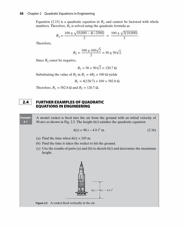
A model rocket is fired into the air from the ground with an initial velocity of98 m/s as shown in Fig. 2.5. The height h(t) satisfies the quadratic equation
h(t) = 98 t − 4.9 t2 m. (2.16)
(a) Find the time when h(t) = 245 m.
(b) Find the time it takes the rocket to hit the ground.
(c) Use the results of parts (a) and (b) to sketch h(t) and determine the maximumheight.
h(t) = 98 t − 4.9 t2
Figure 2.5 A rocket fired vertically in the air.

2.4 Further Examples of Quadratic Equations in Engineering 39
Solution (a) Substituting h(t) = 245 in equation (2.16), the quadratic equation is given by
−4.9 t2 + 98 t − 245 = 0. (2.17)
Dividing both sides of equation (2.17) by −4.9 gives
t2 − 20 t + 50 = 0. (2.18)
The quadratic equation given in equation (2.18) can be solved using the threemethods used in Section 2.1 as
Factoring Quad Formula Completing the Square
t2 − 20t + 50 = 0
can’t befactored with
whole numbers
t2 − 20t + 50 = 0
t =20 ±
√400 − 2002
t = 10 ±√
50
t = 10 ± 7.07
t = 2.93, 17.07 s
t2 − 20t + 50 = 0
t2 − 20t = −50
t2 − 20t + 100 = −50 + 100
(t − 10)2 = 50
t − 10 = ±√
50
t = 10 ± 7.07
t = 2.93, 17.07 s
(b) Since the rocket hit the ground at h(t) = 0,
h(t) = 98 t − 4.9 t2 = 0
4.9 t (20 − t) = 0.
Therefore, t = 0 s and t = 20 s. Since the rocket is fired from the ground att = 0 s, the rocket hits the ground again at t = 20 s.
(c) The maximum height should occur halfway between 2.93 and 17.07 s. Therefore,
tmax = 2.93 + 17.072
= 202
= 10 s.
Substituting t = 10 s into equation (2.16) yields
hmax = 98(10) − 4.9(10)2 = 490 m.
The plot of the rocket trajectory is shown in Fig. 2.6. It can be seen from thisfigure that the rocket is fired from the ground at a height of zero at 0 s, crossesa height of 245 m at 2.93 s, and continues moving up and reaches the maxi-mum height of 490 m at 10 s. At 10 seconds, it starts its downward descent andafter crossing the height of 245 m again at 17.07 s, it reaches the ground againat 20 s.

40 Chapter 2 Quadratic Equations in Engineering
0 2.93 17.074 8 12 16 200
100
200
245
300
400
490hmax
t, s
h(t), m
Figure 2.6 The height of the rocket fired vertically in the air with an initial velocity of 98 m/s.
Example2-2
The equivalent resistance R of two resistors R1 and R2 connected in parallel asshown in Fig. 2.4 is given by
R =R1R2
R1 + R2. (2.19)
(a) Suppose R2 = 2R1 + 4 Ω and the equivalent resistance R = 8.0 Ω. Substitutethese values in equation (2.19) to obtain the following quadratic equationfor R1:
2R21 − 20R1 − 32 = 0.
(b) Solve for R1 by each of the following methods:
(i) Completing the square.
(ii) The quadratic formula. Also, determine the value of R2 corresponding tothe only physical solution for R1.
Solution (a) Substituting R2 = 2R1 + 4 and R = 8.0 in equation (2.19) gives
8.0 =R1(2 R1 + 4)
R1 + (2 R1 + 4)=
2 R21 + 4 R1
3 R1 + 4. (2.20)
Multiplying both sides of equation (2.20) by (3R1 + 4) yields
8.0(3 R1 + 4) = 2 R21 + 4 R1,
or
24.0 R1 + 32.0 = 2 R21 + 4 R1. (2.21)
Rearranging terms in equation (2.21) gives
2 R21 − 20 R1 − 32 = 0. (2.22)

2.4 Further Examples of Quadratic Equations in Engineering 41
(b) The quadratic equation given in equation (2.22) can be now be solved to findthe values of R1.
(i) Method 1: Completing the square:
Dividing both sides of equation (2.22) by 2 gives
R21 − 10 R1 − 16 = 0. (2.23)
Taking 16 on the other side of equation (2.23) and adding(−10
2
)2
= 25 to
both sides yields
R21 − 10 R1 + 25 = 16 + 25. (2.24)
Now, writing both sides of equation (2.24) as squares yields
(R1 − 5)2 = (±√
41)2 = (± 6.4)2.
Therefore,
R1 − 5 = ± 6.4,
which gives the values of R1 as 5 + 6.4 = 11.4 Ω and 5 − 6.4 = −1.4 Ω.Since the value of R1 cannot be negative, R1 = 11.4 Ω and R2 = 2R1 + 4 =2(11.4) + 4 = 26.8 Ω.
(ii) Method 2: Solving equation (2.22) using the quadratic formula:
R1 =20 ±
√(−20)2 − 4(2)(−32)
4
= 20 ±√
6564
= 20 ± 25.64
= 11.4,−1.4.
Since R1 cannot be negative, R1 = 11.4 Ω. Substituting R1 = 11.4 Ω inR2 = 2 R1 + 4 gives
R2 = 2(11.4) + 4 = 26.8 Ω.
Example2-3
An assembly of springs shown in Fig. 2.7 has an equivalent stiffness k, given by
k = k1 +k1k2
k1 + k2. (2.25)
If k2 = 2k1 + 4 lb/in. and the equivalent stiffness is k = 3.6 lb/in., find k1 and k2 asfollows:
(a) Substitute the values of k and k2 into equation (2.25) to obtain the followingquadratic equation for k1:
5k21 − 2.8 k1 − 14.4 = 0. (2.26)

42 Chapter 2 Quadratic Equations in Engineering
(b) Using the method of your choice, solve equation (2.26) and determine thevalues of both k1 and k2.
k1
k1 k2
Figure 2.7 An assembly of three springs.
Solution (a) Substituting k2 = 2 k1 + 4 and k = 3.6 in equation (2.25) yields
3.6 = k1 +k1(2 k1 + 4)
k1 + (2 k1 + 4)= k1 +
2 k21 + 4 k1
3 k1 + 4. (2.27)
Multiplying both sides of equation (2.27) by (3k1 + 4) gives
3.6(3 k1 + 4) = k1(3 k1 + 4) + 2 k21 + 4 k1
10.8 k1 + 14.4 = 3 k21 + 4 k1 + 2k2
1 + 4 k1
10.8 k1 + 14.4 = 5 k21 + 8 k1. (2.28)
Rearranging terms in equation (2.28) gives
5 k21 − 2.8 k1 − 14.4 = 0. (2.29)
(b) The quadratic equation (2.29) can be solved using the quadratic formula as
k1 =2.8 ±
√(−2.8)2 − 4(5)(−14.4)
10
= 2.8 ± 17.210
= 2.0, −1.44.
Since k1 cannot be negative, k1 = 2.0 lb/in. Now, substituting k1 = 2.0 in k2 =2 k1 + 4 yields
k2 = 2(2) + 4 = 8.0.
Therefore,
k2 = 8.0 lb/in.
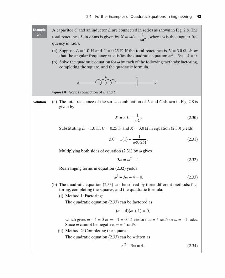
2.4 Further Examples of Quadratic Equations in Engineering 43
Example2-4
A capacitor C and an inductor L are connected in series as shown in Fig. 2.8. The
total reactance X in ohms is given by X = 𝜔L − 1𝜔C
, where 𝜔 is the angular fre-
quency in rad/s.
(a) Suppose L = 1.0 H and C = 0.25 F. If the total reactance is X = 3.0 Ω, showthat the angular frequency 𝜔 satisfies the quadratic equation 𝜔2 − 3𝜔 − 4 = 0.
(b) Solve the quadratic equation for𝜔 by each of the following methods: factoring,completing the square, and the quadratic formula.
CL
Figure 2.8 Series connection of L and C.
Solution (a) The total reactance of the series combination of L and C shown in Fig. 2.8 isgiven by
X = 𝜔L − 1𝜔C
. (2.30)
Substituting L = 1.0 H, C = 0.25 F, and X = 3.0 Ω in equation (2.30) yields
3.0 = 𝜔(1) − 1𝜔(0.25)
. (2.31)
Multiplying both sides of equation (2.31) by 𝜔 gives
3𝜔 = 𝜔2 − 4. (2.32)
Rearranging terms in equation (2.32) yields
𝜔2 − 3𝜔 − 4 = 0. (2.33)
(b) The quadratic equation (2.33) can be solved by three different methods: fac-toring, completing the squares, and the quadratic formula.
(i) Method 1: Factoring:
The quadratic equation (2.33) can be factored as
(𝜔 − 4)(𝜔 + 1) = 0,
which gives 𝜔 − 4 = 0 or 𝜔 + 1 = 0. Therefore, 𝜔 = 4 rad/s or 𝜔 = −1 rad/s.Since 𝜔 cannot be negative, 𝜔 = 4 rad/s.
(ii) Method 2: Completing the squares:
The quadratic equation (2.33) can be written as
𝜔2 − 3𝜔 = 4. (2.34)
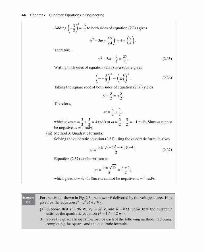
44 Chapter 2 Quadratic Equations in Engineering
Adding(−3
2
)2
= 94
to both sides of equation (2.34) gives
𝜔2 − 3𝜔 +
(94
)= 4 +
(94
).
Therefore,
𝜔2 − 3𝜔 + 9
4= 25
4. (2.35)
Writing both sides of equation (2.35) as a square gives(𝜔 − 3
2
)2
=(±5
2
)2
. (2.36)
Taking the square root of both sides of equation (2.36) yields
𝜔 − 32= ±5
2.
Therefore,
𝜔 = 32± 5
2,
which gives 𝜔 = 32+ 5
2= 4 rad/s or 𝜔 = 3
2− 5
2= −1 rad/s. Since 𝜔 cannot
be negative, 𝜔 = 4 rad/s.
(iii) Method 3: Quadratic formula:
Solving the quadratic equation (2.33) using the quadratic formula gives
𝜔 =3 ±
√(−3)2 − 4(1)(−4)
2. (2.37)
Equation (2.37) can be written as
𝜔 = 3 ±√
252
= 3 ± 52
,
which gives 𝜔 = 4,−1. Since 𝜔 cannot be negative, 𝜔 = 4 rad/s.
Example2-5
For the circuit shown in Fig. 2.3, the power P delivered by the voltage source Vs isgiven by the equation P = I2 R + I VL.
(a) Suppose that P = 96 W, VL = 32 V, and R = 8 Ω. Show that the current Isatisfies the quadratic equation I2 + 4 I − 12 = 0.
(b) Solve the quadratic equation for I by each of the following methods: factoring,completing the square, and the quadratic formula.

2.4 Further Examples of Quadratic Equations in Engineering 45
Solution (a) Substituting P = 96 W, VL = 32 V, and R = 8 Ω into the power deliveredP = I2 R + I VL yields
96 = I2(8) + I(32). (2.38)
Dividing both sides of equation (2.38) by 8 gives
12 = I2 + 4 I. (2.39)
Rearranging terms in equation (2.39) yields
I2 + 4 I − 12 = 0. (2.40)
(b) The quadratic equation given in equation (2.40) can be solved by three differ-ent methods: factoring, completing the squares, and the quadratic formula.
(i) Method 1: Factoring:
The quadratic equation (2.40) can be factored as
(I + 6)(I − 2) = 0,
which gives I + 6 = 0 or I − 2 = 0. Therefore, I = −6 A or I = 2 A.
(ii) Method 2: Completing the square:
The quadratic equation (2.40) can be written as
I2 + 4 I = 12. (2.41)
Adding(
42
)2
= 4 to both sides of equation (2.41),
I2 + 4 I + 4 = 12 + 4. (2.42)
Writing both sides of equation (2.42) as a square yields
(I + 2)2 = (± 4)2. (2.43)
Taking the square root of both sides of equation (2.43) gives
I + 2 = ± 4.
Therefore,
I = −2 ± 4,
which gives I = −2 − 4 = −6 A or I = −2 + 4 = 2 A.
(iii) Method 3: Quadratic formula:
Solving the quadratic equation (2.40) using the quadratic formula gives
I =−4 ±
√(4)2 − 4(1)(−12)
2. (2.44)
Equation (2.44) can be written as
I = −4 ±√
642
= −4 ± 82
= −2 ± 4,
which gives I = −2 − 4 = −6 A or I = −2 + 4 = 2 A.
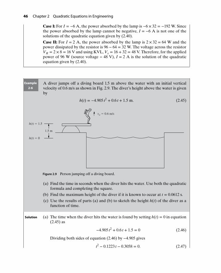
46 Chapter 2 Quadratic Equations in Engineering
Case I: For I = −6 A, the power absorbed by the lamp is −6 × 32 = −192 W. Sincethe power absorbed by the lamp cannot be negative, I = −6 A is not one of thesolutions of the quadratic equation given by (2.40).
Case II: For I = 2 A, the power absorbed by the lamp is 2 × 32 = 64 W and thepower dissipated by the resistor is 96 − 64 = 32 W. The voltage across the resistorVR = 2 × 8 = 16 V and using KVL, Vs = 16 + 32 = 48 V. Therefore, for the appliedpower of 96 W (source voltage = 48 V), I = 2 A is the solution of the quadraticequation given by (2.40).
Example2-6
A diver jumps off a diving board 1.5 m above the water with an initial verticalvelocity of 0.6 m/s as shown in Fig. 2.9. The diver’s height above the water is givenby
h(t) = −4.905 t2 + 0.6 t + 1.5 m. (2.45)
vo = 0.6 m/s
h(t) = 1.5
1.5 m
h(t) = 0
Figure 2.9 Person jumping off a diving board.
(a) Find the time in seconds when the diver hits the water. Use both the quadraticformula and completing the square.
(b) Find the maximum height of the diver if it is known to occur at t = 0.0612 s.
(c) Use the results of parts (a) and (b) to sketch the height h(t) of the diver as afunction of time.
Solution (a) The time when the diver hits the water is found by setting h(t) = 0 in equation(2.45) as
−4.905 t2 + 0.6 t + 1.5 = 0 (2.46)
Dividing both sides of equation (2.46) by −4.905 gives
t2 − 0.1223 t − 0.3058 = 0. (2.47)

2.4 Further Examples of Quadratic Equations in Engineering 47
The quadratic equation given in equation (2.47) can be solved using thequadratic formula and completing the square as outlined below.
(i) Method 1: Quadratic formula:
Solving the quadratic equation (2.47) using the quadratic formula gives
t =0.1223 ±
√(0.1223)2 − 4(1)(−0.3058)
2. (2.48)
Equation (2.48) can be written as
t = 0.1223 ±√
1.23822
= 0.1223 ± 1.11272
= 0.0612 ± 0.5563,
which gives t = 0.0612 − 0.5563 = −0.495 s or t = 0.0612 + 0.5564 = 0.617 s.Since the time cannot be negative, it takes 0.617 s for the diver to hit thewater.
(ii) Method 2: Completing the square:
The quadratic equation (2.47) can be written as
t2 − 0.1223 t = 0.3058. (2.49)
Adding(−0.1223
2
)2
= 0.0037 to both sides gives
t2 − 0.1223 t + 0.015 = 0.3058 + 0.0037. (2.50)
Writing both sides of equation (2.50) as a perfect square yields
(t − 0.0612)2 = (±√
0.3095)2. (2.51)
Taking the square root of both sides gives
t − 0.0612 = ± 0.5563.
Therefore,
t = 0.0612 ± 0.5563,
which gives t = 0.0612 − 0.5563 = −0.495 s or t = 0.0612 + 0.5563 = 0.617 s.Since the time cannot be negative, it takes 0.617 s for the diver to hit thewater.
(b) The maximum height of the diver is found by substituting t = 0.0612 in equa-tion (2.45) as
hmax = h(0.0612) = −4.905(0.0612)2 + 0.6(0.0612) + 1.5 = 1.518 m.
(c) Using the results of parts (a) and (b), the diver’s height after jumping from thediving board is plotted as shown in Fig. 2.10.

48 Chapter 2 Quadratic Equations in Engineering
0 0.0612 0.2 0.3 0.4 0.5 0.617 0.70
0.5
1
1.518
t, s
h(t), m
Figure 2.10 Height of the diver after jumping from the diving board.
Example2-7
Pipeline Through Parabolic Hill: A level pipeline is required to pass through a hillhaving the parabolic profile
y = − 0.004 x2 + 0.3 x. (2.52)
The origin of the x- and y-coordinates is fixed at elevation zero near the base ofthe hill, as shown in Fig. 2.11.
Pipeline path
0 xA xB
x, m
y, m
B A2
Tunnel
exit
Tunnel
entry
Hill profile
Figure 2.11 Pipeline path through a parabolic hill.
(a) Write the quadratic equation for a pipeline elevation of y = 2 m.
(b) Solve the quadratic equation found in part (a) to determine the positions of thetunnel entry xA and exit xB using both the quadratic formula and completingthe square.
(c) Find the length of the tunnel.
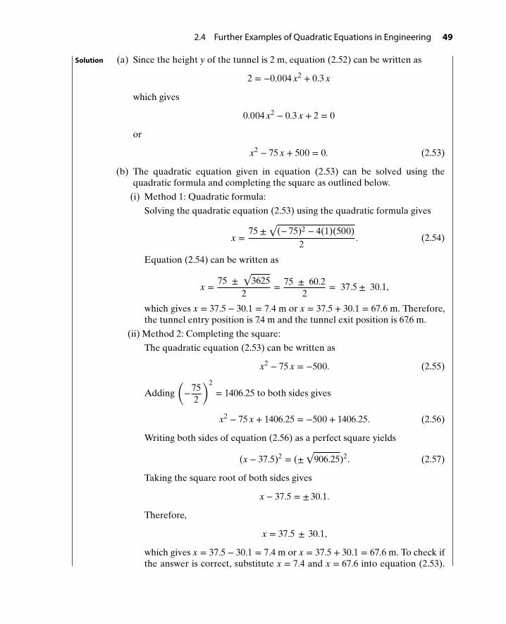
2.4 Further Examples of Quadratic Equations in Engineering 49
Solution (a) Since the height y of the tunnel is 2 m, equation (2.52) can be written as
2 = −0.004 x2 + 0.3 x
which gives
0.004 x2 − 0.3 x + 2 = 0
or
x2 − 75 x + 500 = 0. (2.53)
(b) The quadratic equation given in equation (2.53) can be solved using thequadratic formula and completing the square as outlined below.
(i) Method 1: Quadratic formula:
Solving the quadratic equation (2.53) using the quadratic formula gives
x =75 ±
√(− 75)2 − 4(1)(500)
2. (2.54)
Equation (2.54) can be written as
x = 75 ±√
36252
= 75 ± 60.22
= 37.5 ± 30.1,
which gives x = 37.5 − 30.1 = 7.4 m or x = 37.5 + 30.1 = 67.6 m. Therefore,the tunnel entry position is 7.4 m and the tunnel exit position is 67.6 m.
(ii) Method 2: Completing the square:
The quadratic equation (2.53) can be written as
x2 − 75 x = −500. (2.55)
Adding(−75
2
)2
= 1406.25 to both sides gives
x2 − 75 x + 1406.25 = −500 + 1406.25. (2.56)
Writing both sides of equation (2.56) as a perfect square yields
(x − 37.5)2 = (±√
906.25)2. (2.57)
Taking the square root of both sides gives
x − 37.5 = ± 30.1.
Therefore,
x = 37.5 ± 30.1,
which gives x = 37.5 − 30.1 = 7.4 m or x = 37.5 + 30.1 = 67.6 m. To check ifthe answer is correct, substitute x = 7.4 and x = 67.6 into equation (2.53).
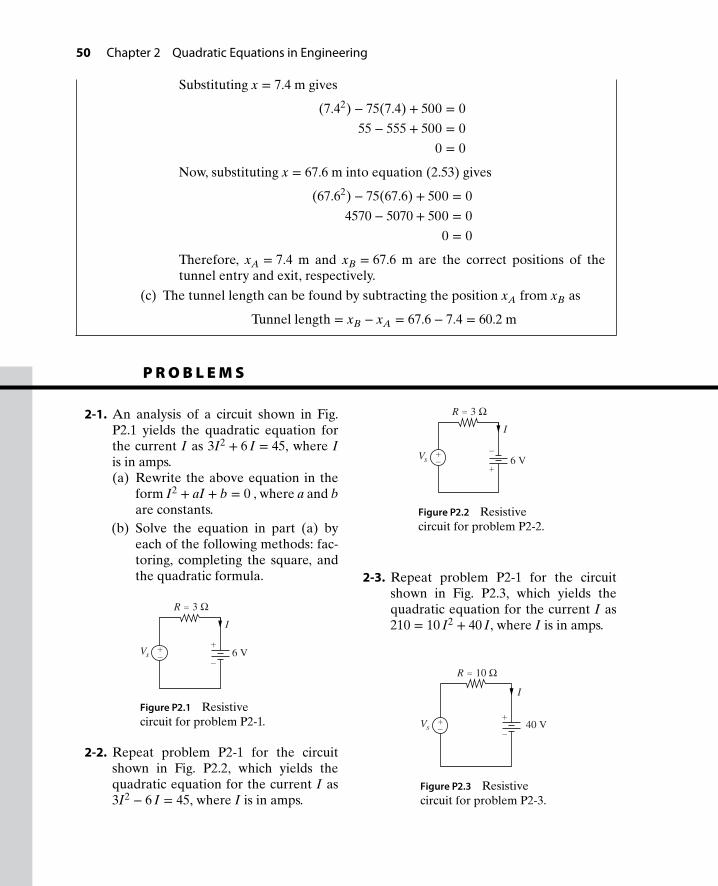
50 Chapter 2 Quadratic Equations in Engineering
Substituting x = 7.4 m gives
(7.42) − 75(7.4) + 500 = 0
55 − 555 + 500 = 0
0 = 0
Now, substituting x = 67.6 m into equation (2.53) gives
(67.62) − 75(67.6) + 500 = 0
4570 − 5070 + 500 = 0
0 = 0
Therefore, xA = 7.4 m and xB = 67.6 m are the correct positions of thetunnel entry and exit, respectively.
(c) The tunnel length can be found by subtracting the position xA from xB as
Tunnel length = xB − xA = 67.6 − 7.4 = 60.2 m
P R O B L E M S
2-1. An analysis of a circuit shown in Fig.P2.1 yields the quadratic equation forthe current I as 3I2 + 6 I = 45, where Iis in amps.(a) Rewrite the above equation in the
form I2 + aI + b = 0 , where a and bare constants.
(b) Solve the equation in part (a) byeach of the following methods: fac-toring, completing the square, andthe quadratic formula.
6 V
I
R = 3 Ω
+−
Vs−
+
Figure P2.1 Resistivecircuit for problem P2-1.
2-2. Repeat problem P2-1 for the circuitshown in Fig. P2.2, which yields thequadratic equation for the current I as3I2 − 6 I = 45, where I is in amps.
6 V
I
R = 3 Ω
+−
Vs+
−
Figure P2.2 Resistivecircuit for problem P2-2.
2-3. Repeat problem P2-1 for the circuitshown in Fig. P2.3, which yields thequadratic equation for the current I as210 = 10 I2 + 40 I, where I is in amps.
I
40 V Vs
R = 10 Ω
+
−+−
Figure P2.3 Resistivecircuit for problem P2-3.
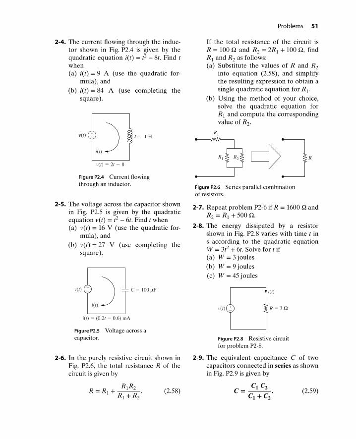
Problems 51
2-4. The current flowing through the induc-tor shown in Fig. P2.4 is given by thequadratic equation i(t) = t2 − 8t. Find twhen(a) i(t) = 9 A (use the quadratic for-
mula), and(b) i(t) = 84 A (use completing the
square).
+−v(t)
i(t)
L = 1 H
v(t) = 2t − 8
Figure P2.4 Current flowingthrough an inductor.
2-5. The voltage across the capacitor shownin Fig. P2.5 is given by the quadraticequation v(t) = t2 − 6t. Find t when(a) v(t) = 16 V (use the quadratic for-
mula), and(b) v(t) = 27 V (use completing the
square).
v(t)
i(t)
C = 100 μF
i(t) = (0.2t − 0.6) mA
+−
Figure P2.5 Voltage across acapacitor.
2-6. In the purely resistive circuit shown inFig. P2.6, the total resistance R of thecircuit is given by
R = R1 +R1R2
R1 + R2. (2.58)
If the total resistance of the circuit isR = 100 Ω and R2 = 2R1 + 100 Ω, findR1 and R2 as follows:(a) Substitute the values of R and R2
into equation (2.58), and simplifythe resulting expression to obtain asingle quadratic equation for R1.
(b) Using the method of your choice,solve the quadratic equation forR1 and compute the correspondingvalue of R2.
R2R1
R1
R
Figure P2.6 Series parallel combinationof resistors.
2-7. Repeat problem P2-6 if R = 1600 Ω andR2 = R1 + 500 Ω.
2-8. The energy dissipated by a resistorshown in Fig. P2.8 varies with time t ins according to the quadratic equationW = 3t2 + 6t. Solve for t if(a) W = 3 joules(b) W = 9 joules(c) W = 45 joules
v(t) R = 3 Ω
i(t)
+−
Figure P2.8 Resistive circuitfor problem P2-8.
2-9. The equivalent capacitance C of twocapacitors connected in series as shownin Fig. P2.9 is given by
C =C1 C2
C1 + C2. (2.59)

52 Chapter 2 Quadratic Equations in Engineering
If the total capacitance is C = 120 𝜇Fand C2 = C1 + 100 𝜇F, find C1 and C2as follows:(a) Substitute the values of C and C2
in equation (2.59) and obtain thequadratic equation for C1.
(b) Solve the quadratic equation forC1 obtained in part (a) by eachof the following methods: factor-ing, completing the square, and thequadratic formula. Also, computethe corresponding values of C2.
C1 C2
C
Figure P2.9 Series combination oftwo capacitors.
2-10. Repeat problem P2-9 if C = 75 𝜇F andC2 = C1 + 200 𝜇F.
2-11. The equivalent capacitance C of threecapacitors connected in series-parallelas shown in Fig. P2.11 is given by
C = 25 +C1 C2
C1 + C2. (2.60)
If the total capacitance is C = 125 𝜇Fand C2 = C1 + 100 𝜇F, find C1 and C2as follows:(a) Substitute the values of C and C2
in equation (2.60) and obtain thequadratic equation for C1.
(b) Solve the quadratic equation for C1obtained in part (a) by complet-ing the square and the quadraticformula. Also, compute the corre-sponding values of C2.
C1 C2
C
25 μF
Figure P2.11 Series combination of two capacitors.
2-12. The equivalent inductance L of two in-ductors connected in parallel as shownin Fig. P2.12 is given by
L =L1 L2
L1 + L2. (2.61)
If the total inductance L = 80 mH andL1 = L2 + 300 mH, find L1 and L2 asfollows:(a) Substitute the values of L and L1
in equation (2.61) and obtain thequadratic equation for L2.
(b) Solve the quadratic equation for L2obtained in part (a) by complet-ing the square, and the quadraticformula. Also, compute the corre-sponding values of L1.
L1 L2 L
Figure P2.12 Parallel combination of twoinductors.
2-13. Repeat problem P2-12 if L = 150 mHand L1 = L2 + 400 mH.
2-14. The equivalent inductance L of three in-ductors connected in series-parallel asshown in Fig. P2.14 is given by
L = 125 +L1 L2
L1 + L2. (2.62)
(a) Suppose L2 = L1 + 200 mH andthat the equivalent inductance isL = 200 mH. Substitute thesevalues in equation (2.62) and obtain

Problems 53
the following quadratic equation:
L21 + 50 L1 − 15, 000 = 0. (2.63)
(b) Solve the quadratic equation (2.63)for L1 by each of the followingmethods: factoring, completing thesquare, and the quadratic formula.
125 mH
L1 L2 L
Figure P2.14 Series-parallel combination ofthree inductors.
2-15. A model rocket is launched in the verti-cal plane at time t = 0 s as shown in Fig.P2.15. The height of the rocket (in feet)satisfies the quadratic equation h(t) =64 t − 16 t2.(a) Find the value(s) of the time t when
h(t) = 48 ft.(b) Find the value(s) of the time t when
h(t) = 60 ft.(c) Find the time required for the
rocket to hit the ground.(d) Based on your solution to parts (a)
through (c), determine the maxi-mum height of the rocket andsketch the height h(t).
h(t) = 64 t − 16 t2
Figure P2.15 A model rocket forproblem P2-15.
2-16. The ball shown in Fig. P2.16 is droppedfrom a height of 1000 meters. The ballfalls according to the quadratic equationh(t) = 1000 − 4.905t2. Find the time t inseconds for the ball to reach a heighth(t) of
(a) 921.52 m (b) 686.08 m
(c) 509.5 m (d) 0 m
1000 m
h(t)
Figure P2.16 A ball droppedfrom a height of 1000 m.
2-17. At time t = 0, a ball is thrown verticallyfrom the top of the building at a speed of56 ft/s, as shown in Fig. P2.17. The heightof the ball at time t is given by
h(t) = 32 + 56t − 16t2 ft.
v = 56 ft/s
32 ft
h(t)
Figure P2.17 A ball thrown verticallyfrom the top of a building.

54 Chapter 2 Quadratic Equations in Engineering
(a) Find the value(s) of the time t whenh(t) = 32 ft.
(b) Find the time required for the ballto hit the ground.
(c) Use the results to determine themaximum height, and sketch theheight h(t) of the ball.
2-18. Two springs connected in series shownin Fig. P2.18 can be represented by asingle equivalent spring. The stiffness ofthe equivalent spring is given by
keq =k1k2
k1 + k2, (2.64)
where k1 and k2 are the spring con-stants of the two springs. If keq = 1.2 N/mand k2 = 2k1 − 1 N/m, find k1 and k2 asfollows:(a) Substitute the values of keq and k2
in equation (2.64) and obtain thequadratic equation for k1.
(b) Solve the quadratic equation for k1obtained in part (a) by complet-ing the square, and the quadraticformula. Also, compute the corre-sponding values of k2.
k1 k2
Figure P2.18 Series combination of two springs.
2-19. The equivalent stiffness of a series-parallel combination of three springsshown in Fig. P2.19 is given by
k = k2 +k1k2
k1 + k2. (2.65)
If k1 = k2 + 2 lb/in and the equivalentstiffness is k = 1.75 lb/in, find k1 and k2as follows:(a) Substitute the values of k and k1
into equation (2.65) and obtain thequadratic equation for k2.
(b) Using the method of your choice,solve the quadratic equation
obtained in part (a) and determinethe values of k2. Also, find thevalues of k1.
k2
k1 k2
Figure P2.19 Series-parallel combination of threesprings.
2-20. An assembly of three springs connectedin series as shown in Fig. P2.20 has anequivalent stiffness k given by
k =k1 k2 k3
k2 k3 + k1 k3 + k1 k2. (2.66)
(a) Suppose k2 = 6 lb/in., k3 = k1 + 8lb/in., and the equivalent stiffness isk = 2 lb/in. Substitute these valuesinto equation (2.66) to obtain thefollowing quadratic equation:
4 k21 + 8 k1 − 96 = 0. (2.67)
(b) Solve equation (2.67) for k1 by eachof the following methods: (i) fac-toring, (ii) quadratic formula, and(iii) completing the square. For eachcase, determine the value of k3corresponding to the only physicalsolution for k1.
k1
k2
k3
k
Figure P2.20 Seriescombination ofthree springs.
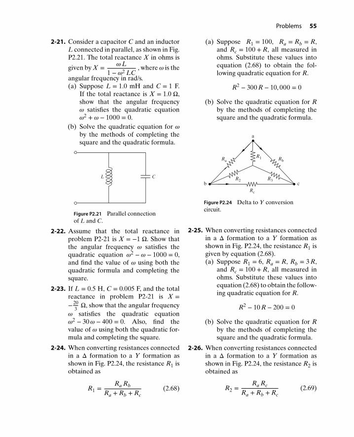
Problems 55
2-21. Consider a capacitor C and an inductorL connected in parallel, as shown in Fig.P2.21. The total reactance X in ohms is
given by X = 𝜔L1 − 𝜔2 LC
, where 𝜔 is the
angular frequency in rad/s.(a) Suppose L = 1.0 mH and C = 1 F.
If the total reactance is X = 1.0 Ω,show that the angular frequency𝜔 satisfies the quadratic equation𝜔2 + 𝜔 − 1000 = 0.
(b) Solve the quadratic equation for 𝜔
by the methods of completing thesquare and the quadratic formula.
CL
Figure P2.21 Parallel connectionof L and C.
2-22. Assume that the total reactance inproblem P2-21 is X = −1 Ω. Show thatthe angular frequency 𝜔 satisfies thequadratic equation 𝜔2 − 𝜔 − 1000 = 0,and find the value of 𝜔 using both thequadratic formula and completing thesquare.
2-23. If L = 0.5 H, C = 0.005 F, and the totalreactance in problem P2-21 is X =− 20
3Ω, show that the angular frequency
𝜔 satisfies the quadratic equation𝜔2 − 30𝜔 − 400 = 0. Also, find thevalue of 𝜔 using both the quadratic for-mula and completing the square.
2-24. When converting resistances connectedin a Δ formation to a Y formation asshown in Fig. P2.24, the resistance R1 isobtained as
R1 =Ra Rb
Ra + Rb + Rc(2.68)
(a) Suppose R1 = 100, Ra = Rb = R,and Rc = 100 + R, all measured inohms. Substitute these values intoequation (2.68) to obtain the fol-lowing quadratic equation for R.
R2 − 300 R − 10, 000 = 0
(b) Solve the quadratic equation for Rby the methods of completing thesquare and the quadratic formula.
RaR1
R2 R3
Rb
Rc
a
cb
Figure P2.24 Delta to Y conversioncircuit.
2-25. When converting resistances connectedin a Δ formation to a Y formation asshown in Fig. P2.24, the resistance R1 isgiven by equation (2.68).(a) Suppose R1 = 6, Ra = R, Rb = 3 R,
and Rc = 100 + R, all measured inohms. Substitute these values intoequation (2.68) to obtain the follow-ing quadratic equation for R.
R2 − 10 R − 200 = 0
(b) Solve the quadratic equation for Rby the methods of completing thesquare and the quadratic formula.
2-26. When converting resistances connectedin a Δ formation to a Y formation asshown in Fig. P2.24, the resistance R2 isobtained as
R2 =Ra Rc
Ra + Rb + Rc(2.69)

56 Chapter 2 Quadratic Equations in Engineering
(a) Suppose R2 = 12, Ra = R, Rb = 3 R,and Rc = 100 + R, all measured inohms. Substitute these values intoequation (2.69) to obtain the follow-ing quadratic equation for R.
R2 + 40 R − 1200 = 0
(b) Solve the quadratic equation for Rby the methods of completing thesquare and the quadratic formula.
2-27. When converting resistances connectedin a Δ formation to a Y formation asshown in Fig. P2.24, the resistance R3 isobtained as
R3 =Rb Rc
Ra + Rb + Rc(2.70)
(a) Suppose R3 = 36, Ra = R, Rb = 3 R,and Rc = 100 + R, all measured inohms. Substitute these values intoequation (2.70) to obtain the follow-ing quadratic equation for R.
R2 + 40 R − 1200 = 0
(b) Solve the quadratic equation for Rby the methods of completing thesquare and the quadratic formula.
2-28. The characteristic equation of a seriesRLC circuit shown in Fig. P2.28 is givenas
s2 + RL
s + 1L C
= 0. (2.71)
(a) If R = 7 Ω, L = 1 H, and C = 0.1 F,solve the quadratic equation (2.71)for the values of s (called the eigen-values of the system) using themethods of completing the squareand the quadratic formula.
(b) Repeat part (a) if R = 10 Ω, L = 1
H, and C = 125
F.
R
L−
+
i(t)
vc (0)
t = 0
C
Figure P2.28 Series RLC circuitfor problem P2-28.
2-29. The characteristic equation of a parallelRLC circuit shown in Fig. P2.29 is givenas
s2 + 1R C
s + 1L C
= 0. (2.72)
If R = 200 Ω, L = 50 mH, and C =0.2 𝜇F, solve the quadratic equation(2.72) for the values of s by the meth-ods of completing the square and thequadratic formula.
iL (0)
CL R v(t)
−
+
t = 0
Figure P2.29 Parallel RLC circuit forproblem P2-29.
2-30. The characteristic equation of a mass,spring, and damper system shown in Fig.P2.30 is given by
m s2 + c s + k = 0. (2.73)
(a) If m = 1 kg, c = 3 Ns/m, and k = 2N/m, solve the quadratic equation(2.73) for the values of s using themethods of completing the squareand the quadratic formula.
(b) Repeat part (a) if m = 1 kg, c = 2Ns/m, and k = 1 N/m.

Problems 57
c
x (displacement)
f (force)
k
m
Figure P2.30 Mass, spring, and damper system forproblem P2-30.
2-31. The perimeter of a rectangle shown inFig. P2.31 is given by
P = 2(
AL
+ L). (2.74)
Perimeter = 30 m
Area = 36 m2
W
L
Figure P2.31 A rectangle of length Land width W.
If the perimeter P = 30 m and the areaA = W × L = 36 m2, find the length Land width W as follows:(a) Substitute the values of P and A
in equation (2.74) and obtain thequadratic equation for L.
(b) Solve the quadratic equation for Lobtained in part (a) by complet-ing the square, and the quadraticformula. Also, compute the corre-sponding values of W.
2-32. A diver jumps off a diving board 2.0 mabove the water with an initial verticalvelocity of 0.981 m/s as shown in Fig.P2.32. The height h(t) above the wateris given by
h(t) = −4.905 t2 + 0.981t + 2.0 m.
(a) Find the time in seconds when thediver hits the water. Use both thequadratic formula and completingthe square.
(b) Find the maximum height of thediver if it is known to occur att = 0.1 s.
(c) Use the results of parts (a) and (b)to sketch the height h(t) of the diver.
2-33. A level pipeline is required to passthrough a hill having a parabolic profile
y = − 0.005 x2 + 0.35 x. (2.75)
The origin of the x- and y-coordinates isfixed at elevation zero near the base ofthe hill, as shown in Fig. P2.33.
vo = 0.981 m/s
h(t) = 2.0
2.0 m
h(t) = 0
Figure P2.32 Diver jumping off a diving board.

58 Chapter 2 Quadratic Equations in Engineering
0x, m
y, m
B A3
Hill profile
Pipeline path
Tunnelentry
Tunnelexit
xA xB
Figure P2.33 Pipeline path through a parabolic hill.
(a) Write the quadratic equation for apipeline elevation of y = 3 m.
(b) Solve the quadratic equation foundin part (a) to determine the posi-tions of the tunnel entry xA and exitxB using both the quadratic formulaand completing the square.
(c) Find the length of the tunnel.
2-34. A research group is using a drop testto measure the force of attenuation ofa helmet liner they designed to reducethe occurance of brain injuries for sol-diers and athletes. The helmet attachedto a weight is propelled downward withan initial velocity vi of 3 m/s from aninitial height of 30 m. The behavior ofthe falling helmet is characterized bya quadratic equation h(t) = 30 − 3 t −4.9 t2.(a) Write the quadratic equation for
time t when the helmet and weighthit the ground, i.e., h(t) = 0 m.
(b) Solve the quadratic equation for tobtained in part (a) by complet-ing the square, and the quadraticformula.
2-35. The modulus of elasticity (E) is a mea-sure of a material’s resistance to de-formation; the larger the modulus, thestiffer the material. During fabricationof a ceramic material from a powderform, pores were generated that affectthe strength of the material. The mag-nitude of elasticity is related to volume
fraction porosity P by
E = 304 (1 − 1.9 P + 0.9 P2). (2.76)
(a) If a porous sample of silicon nitridehas a modulus of elasticity of E =209 GPa, obtain the quadratic equa-tion for volume fraction porosity P.
(b) Solve the quadratic equation foundin part (a) using both the methodsof completing the square and thequadratic formula.
(c) Repeat parts (a) and (b) to find thevolume fraction porosity of a sili-con nitride sample with a modulusof elasticity of 25 GPa.
2-36. Consider the following reaction havingan equilibrium constant of 4.66 × 10⁻³
at a certain temperature:
A(g) + B(g) C(g)
If 0.300 mol of A and 0.100 mol of Bare mixed in a container and allowed toreach equilibrium, the concentrationsof A = 0.300 − x and B = 0.100 − xreaction that form the concentration ofC = 2x are related to the equilibriumconstant by the expression
4.66 × 10−3 =(2 x)2
(0.300 − x) (0.100 − x).
(a) Write the quadratic equation for x.(b) Solve the quadratic equation found
in part (a) by completing the squareand the quadratic formula.
(c) Find the equilibrium concentrationA, B, and C.
2-37. Consider the following reaction hav-ing an equilibrium constant of 1.00 at1105K temperature:
CO(g) + H2O(g) CO2(g) + H2(g)
Suppose the feed to a reactor con-tains 1.000 mol of CO and 2.000 mol

Problems 59
of H2O(g), and the reaction mixturecomes to equilibrium at 1105 K. Theconcentrations of CO = 1.000 − x andH2O = 2.000 − x reaction that form theconcentration of CO2 = x and H2 = xare related to the equilibrium constantas
1.00 = 2x(1.000 − x) (2.000 − x)
(a) Write the quadratic equation for x.(b) Solve the quadratic equation found
in part (a) by completing the squareand the quadratic formula.
(c) Find the equilibrium concentrationof CO, H2O, CO2, and H2.
2-38. An engineering co-op wants to hire anasphalt contractor to widen the truckentrance to the corporate headquartersas shown in Fig. P2.38.
hNew asphalt
b
Figure P2.38 New asphalt dimensions of thecorporate headquarters driveway.
The height h is required to be 10 ft. morethan the width b, and the total area ofthe new asphalt is given by
A = 12
b(10 + b). (2.77)
(a) If A = 200 sq. ft., obtain thequadratic equation for b.
(b) Solve the quadratic equation foundin part (a) by completing the squareand the quadratic formula.
(c) Find the dimensions of the widthand height.
2-39. Repeat problem P2-38 if the total areaof the new asphalt needs to be 300 sq. ft.
2-40. A city wants to hire a contractor to builda walkway around the swimming poolin one of its parks. The dimensions ofthe walkway along with the dimensionsof the pool are shown in Fig. P2.40. Thearea of the walkway is given by
A = (50 + 5 x)(30 + 2 x) − 1500
(a) If A = 4500 sq. ft., obtain thequadratic equation for x.
(b) Solve the quadratic equation foundin part (a) by completing the squareand the quadratic formula.
Wal
kw
ay
30 ft
50 ft4x
x
x
30 + 2x
50 + 5x
Swimming pool
Walkway
Walkway
Walkway
Figure P2.40 Walkway around the swimming pool.
CHAPTER3
Trigonometry inEngineering
3.1 INTRODUCTIONIn this chapter, the direct (forward) and inverse (reverse) kinematics of one-linkand two-link planar robots are considered to explain the trigonometric functions andtheir identities. Kinematics is the branch of mechanics that studies the motion of anobject. The direct or forward kinematics is the static geometric problem of deter-mining the position and orientation of the end-effector (hand) of the robot from theknowledge of the joint displacement. In general, the joint displacement can be linearor rotational (angular). But in this chapter, only rotational motion is considered. Fur-thermore, it is assumed that the planar robot is wristless (i.e., it has no end-effectoror hand) and that only the position but not the orientation of the tip of the robot canbe changed.
Going in the other direction, the inverse or reverse kinematics is the problem ofdetermining all possible joint variables (angles) that lead to the given Cartesian po-sition and orientation of the end-effector. Since no end-effector is considered in thischapter, the inverse kinematics will determine the joint angle(s) from the Cartesianposition of the tip.
3.2 ONE-LINK PLANAR ROBOTConsider a one-link planar robot of length l (Fig. 3.1) that is being rotated in thex-y plane by a motor mounted at the center of the table, which is also the locationof the robot’s joint. The robot has a position sensor installed at the joint that givesthe value of the angle 𝜃 of the robot measured from the positive x-axis. The angle𝜃 is positive in the counterclockwise direction (0 to 180) and it is negative in theclockwise direction (0 to −180). Therefore, as the joint rotates from 0 to 180 and0 to −180, the tip of the robot moves on a circle of radius l (the length of the linkof the robot) as shown in Fig. 3.2. Note that 180 = 𝜋 radians.
3.2.1 Kinematics of One-Link Robot
In Fig. 3.2, the point P (tip of the robot) can be represented in rectangular or Carte-sian coordinates by a pair (x, y) or in polar coordinates by the pair (l, 𝜃). Assuming
60

3.2 One-Link Planar Robot 61
x
Motor
P(x, y)
x
y
Link
l
y
θ
Figure 3.1 One-link planar robot.
that the length of the link l is fixed, a change in the angle 𝜃 of the robot changes theposition of the tip of the robot. This is known as the direct or forward kinematics ofthe robot. The position of the tip of the robot (x, y) in terms of l and 𝜃 can be foundusing the right-angle triangle OAP in Fig. 3.2 as
cos(𝜽) =Adjacent sideHypotenuse
= xl
⇒ x = l cos(𝜃) (3.1)
sin(𝜽) =Opposite sideHypotenuse
=yl
⇒ y = l sin(𝜃) (3.2)
O
l
B
Ax
yy(counterclockwise direction)
(clockwise direction)
Hypotenuse
x
y
P(x, y)
Opposite side
Adjacent side
θ
Positive θ
0 ≤ ≤ 180θ
Negative θ
−180 ≤ ≤ 0 θ
Figure 3.2 Circular path of the one-link robot tip.

62 Chapter 3 Trigonometry in Engineering
Example3-1
Use the one-link robot to find the values of cos(𝜃) and sin(𝜃) for 𝜃 = 0, 90, −90,and 180. Also, find the values of x and y.
Solution Case I: 𝜃 = 0
By inspection,
x = l cos(0) = l ⇒ cos(0) = 1
y = l sin(0) = 0 ⇒ sin(0) = 0x
y
O l P
= 0°θ
Case II: 𝜃 = 90
By inspection,
x = l cos(90) = 0 ⇒ cos(90) = 0
y = l sin(90) = l ⇒ sin(90) = 1 O
l
P
x
y
= 90°θ
Case III: 𝜃 = −90
By inspection,
x = l cos(−90) = 0 ⇒ cos(−90) = 0
y = l sin(−90) = −l ⇒ sin(−90) = −1 O
l
P
x
y
= −90°θ
Case IV: 𝜃 = 180
By inspection,
x = l cos(180) = −l ⇒ cos(180) = −1
y = l sin(180) = 0 ⇒ sin(180) = 0 OlPx
y
= 180°θ

3.2 One-Link Planar Robot 63
Example3-2
Find the position P(x, y) of the robot for 𝜃 = 45, −45, 135, and −135.
Solution Case I: 𝜃 = 45
x = l cos(45) = l√2
⇒ cos(45) = 1√2
y = l sin(45) = l√2
⇒ sin(45) = 1√2 O
45°
l
P(x, y)
x
y
y =
x = l
2
l
2
√⎯
√⎯
Case II: 𝜃 = −45
x = l cos(−45) = l√2
⇒ cos(−45) = 1√2
y = l sin(−45) = − l√2
⇒ sin(−45) = − 1√2
O
l
x
y
P(x, y)
y = −
x =
−45°
l
2
l
2
√⎯
√⎯
Case III: 𝜃 = 135
x = l cos(135) = − l√2
⇒ cos(135) = − 1√2
y = l sin(135) = l√2
⇒ sin(135) = 1√2
O
l
y
P(x, y)
x
135°45°
x = −
y = l
2
l
2
√⎯
√⎯
Case IV: 𝜃 = −135
x = l cos(−135) = − l√2
⇒ cos(−135) = − 1√2
y = l sin(−135) = − l√2
⇒ sin(−135) = − 1√2
O
l
x
y
P(x, y)
45°
−135°
x = −
y = −
l
2
l
2
√⎯
√⎯

64 Chapter 3 Trigonometry in Engineering
Examples 3-1 and 3-2 show that in the first quadrant (0 < 𝜃 < 90), both thesin and cos functions are positive. Since the other trigonometric functions (tan =sin/cos, cot = 1/tan, sec = 1/cos, and csc = 1/sin, for example) are functions of sinand cos functions, all the trigonometric functions are positive in the first quadrant,as shown in Fig. 3.3. In the second quadrant, sin and csc are positive and all therest of the trigonometric functions are negative. In the third quadrant, both the sinand cos functions are negative. Therefore, only the tan and cot are positive. Finally,in the fourth quadrant, only the cos and sec are positive. To remember this, one ofthe phrases commonly used is “All Sin Tan Cos.” Another is “All Students TakeCalculus,” which is certainly true of engineering students!
(all trigonometric functions are positive)
2nd Quadrant
3rd Quadrant 4th Quadrant
x
y
sin +ve
cos −ve
(sin is positive)
1st Quadrantsin +ve
cos +ve
(tan is positive) (cos is positive)
sin −ve
cos −ve
sin −ve
cos +ve
Figure 3.3 Trigonometric functions in the four quadrants.
The values of sin and cos functions for 𝜃 = 0, 30, 45, 60, and 90 are givenin Table 3.1. The values of sin and cos functions for many other angle can be foundusing Table 3.1, as explained in the following examples.
TABLE 3.1 Values of sine and cosine functions for common angles.
Angle
deg 0 30 45 60 90
(rad) (0) (𝜋6
) (𝜋4
) (𝜋3
) (𝜋2
)
sin√
04= 0
√14= 1
2
√24= 1√
2
√34=
√3
2
√44= 1
cos√
44= 1
√34=
√3
2
√24= 1√
2
√14= 1
2
√04= 0
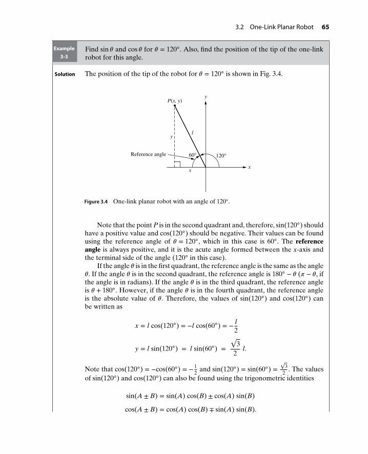
3.2 One-Link Planar Robot 65
Example3-3
Find sin 𝜃 and cos 𝜃 for 𝜃 = 120. Also, find the position of the tip of the one-linkrobot for this angle.
Solution The position of the tip of the robot for 𝜃 = 120 is shown in Fig. 3.4.
x
120°
x
y
60°
P(x, y)
Reference angle
l
y
Figure 3.4 One-link planar robot with an angle of 120.
Note that the point P is in the second quadrant and, therefore, sin(120) shouldhave a positive value and cos(120) should be negative. Their values can be foundusing the reference angle of 𝜃 = 120, which in this case is 60. The referenceangle is always positive, and it is the acute angle formed between the x-axis andthe terminal side of the angle (120 in this case).
If the angle 𝜃 is in the first quadrant, the reference angle is the same as the angle𝜃. If the angle 𝜃 is in the second quadrant, the reference angle is 180 − 𝜃 (𝜋 − 𝜃, ifthe angle is in radians). If the angle 𝜃 is in the third quadrant, the reference angleis 𝜃 + 180. However, if the angle 𝜃 is in the fourth quadrant, the reference angleis the absolute value of 𝜃. Therefore, the values of sin(120) and cos(120) canbe written as
x = l cos(120) = −l cos(60) = − l2
y = l sin(120) = l sin(60) =√
32
l.
Note that cos(120) = −cos(60) = − 12
and sin(120) = sin(60) =√
32
. The valuesof sin(120) and cos(120) can also be found using the trigonometric identities
sin(A ± B) = sin(A) cos(B) ± cos(A) sin(B)
cos(A ± B) = cos(A) cos(B) ∓ sin(A) sin(B).
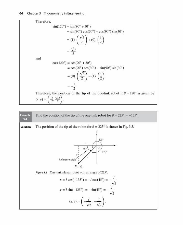
66 Chapter 3 Trigonometry in Engineering
Therefore,
sin(120) = sin(90 + 30)
= sin(90) cos(30) + cos(90) sin(30)
= (1)
(√3
2
)+ (0)
(12
)
=√
32
andcos(120) = cos(90 + 30)
= cos(90) cos(30) − sin(90) sin(30)
= (0)
(√3
2
)− (1)
(12
)
= −12.
Therefore, the position of the tip of the one-link robot if 𝜃 = 120 is given by
(x, y) =(
−l2,√
3 l2
).
Example3-4
Find the position of the tip of the one-link robot for 𝜃 = 225 = −135.
Solution The position of the tip of the robot for 𝜃 = 225 is shown in Fig. 3.5.
45°−135°
O
y
x225°
l
y
P(x, y)
x
Reference angle
Figure 3.5 One-link planar robot with an angle of 225.
x = l cos(−135) = −l cos(45) = − l√2
y = l sin(−135) = −sin(45) = − l√2
(x, y) =
(− l√
2, − l√
2
).
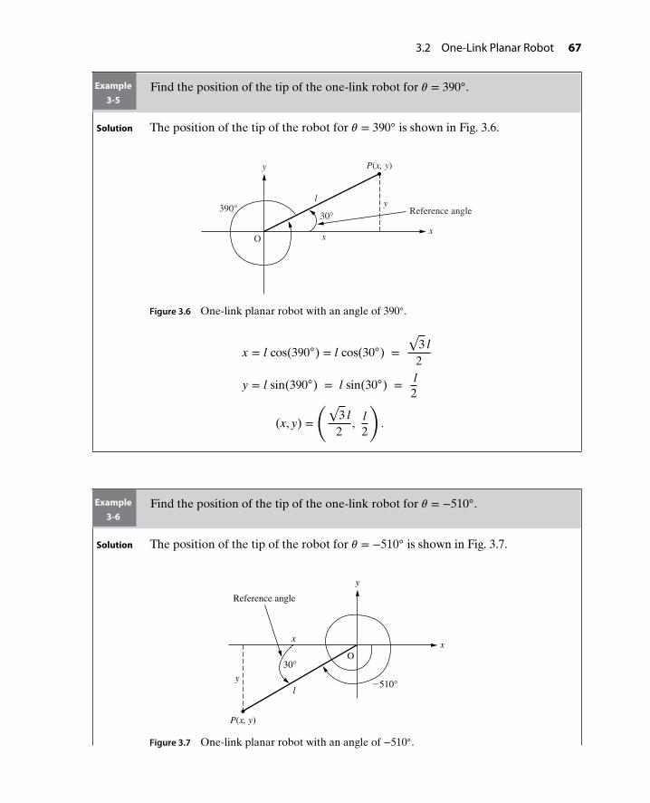
3.2 One-Link Planar Robot 67
Example3-5
Find the position of the tip of the one-link robot for 𝜃 = 390.
Solution The position of the tip of the robot for 𝜃 = 390 is shown in Fig. 3.6.
O
P(x, y)
y
x
Reference angle
l
30°x
y
390°
Figure 3.6 One-link planar robot with an angle of 390.
x = l cos(390) = l cos(30) =√
3 l2
y = l sin(390) = l sin(30) = l2
(x, y) =
(√3 l2
, l2
).
Example3-6
Find the position of the tip of the one-link robot for 𝜃 = −510.
Solution The position of the tip of the robot for 𝜃 = −510 is shown in Fig. 3.7.
P(x, y)
O
−510°
30°
Reference angle
x
ly
x
y
Figure 3.7 One-link planar robot with an angle of −510.
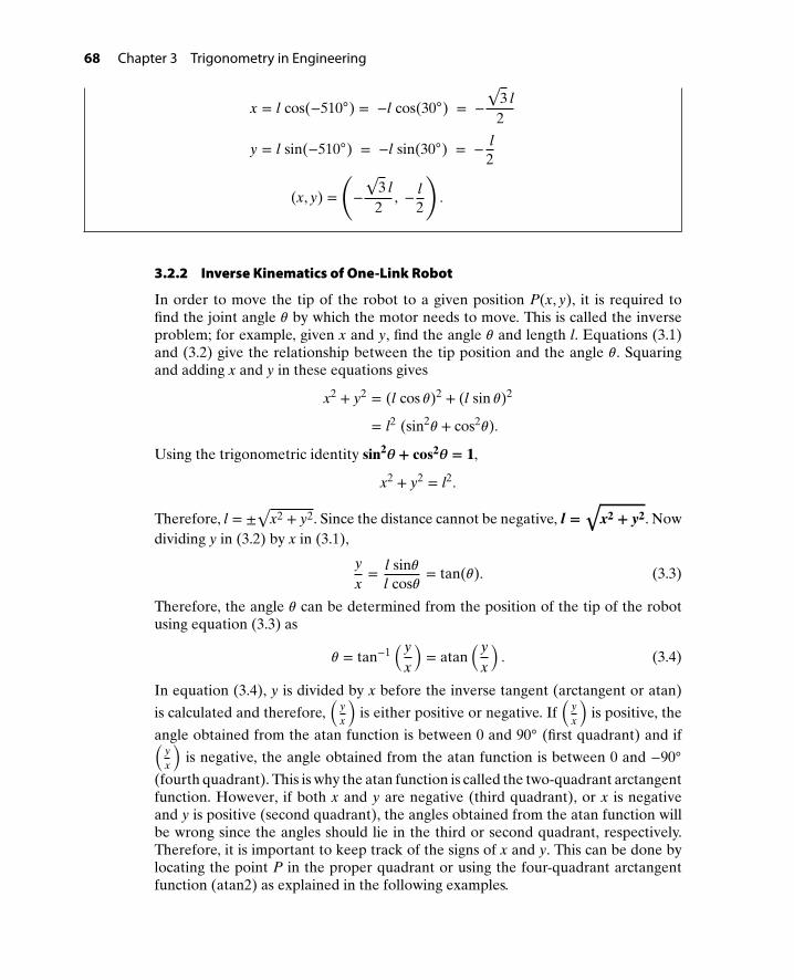
68 Chapter 3 Trigonometry in Engineering
x = l cos(−510) = −l cos(30) = −√
3 l2
y = l sin(−510) = −l sin(30) = − l2
(x, y) =
(−√
3 l2
, − l2
).
3.2.2 Inverse Kinematics of One-Link Robot
In order to move the tip of the robot to a given position P(x, y), it is required tofind the joint angle 𝜃 by which the motor needs to move. This is called the inverseproblem; for example, given x and y, find the angle 𝜃 and length l. Equations (3.1)and (3.2) give the relationship between the tip position and the angle 𝜃. Squaringand adding x and y in these equations gives
x2 + y2 = (l cos 𝜃)2 + (l sin 𝜃)2
= l2 (sin2𝜃 + cos2
𝜃).
Using the trigonometric identity sin2𝜽+ cos2
𝜽 = 1,
x2 + y2 = l2.
Therefore, l = ±√
x2 + y2. Since the distance cannot be negative, l =√
x2 + y2. Nowdividing y in (3.2) by x in (3.1),
yx= l sin𝜃
l cos𝜃= tan(𝜃). (3.3)
Therefore, the angle 𝜃 can be determined from the position of the tip of the robotusing equation (3.3) as
𝜃 = tan−1(y
x
)= atan
(yx
). (3.4)
In equation (3.4), y is divided by x before the inverse tangent (arctangent or atan)
is calculated and therefore,(
yx
)is either positive or negative. If
(yx
)is positive, the
angle obtained from the atan function is between 0 and 90 (first quadrant) and if(yx
)is negative, the angle obtained from the atan function is between 0 and −90
(fourth quadrant). This is why the atan function is called the two-quadrant arctangentfunction. However, if both x and y are negative (third quadrant), or x is negativeand y is positive (second quadrant), the angles obtained from the atan function willbe wrong since the angles should lie in the third or second quadrant, respectively.Therefore, it is important to keep track of the signs of x and y. This can be done bylocating the point P in the proper quadrant or using the four-quadrant arctangentfunction (atan2) as explained in the following examples.
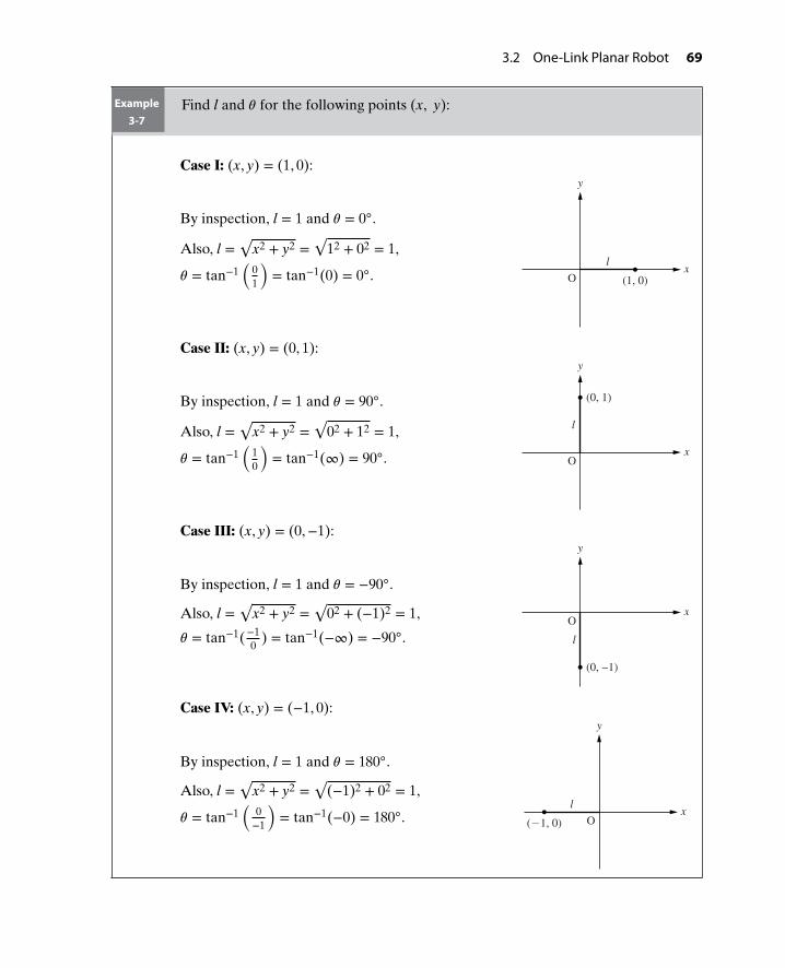
3.2 One-Link Planar Robot 69
Example3-7
Find l and 𝜃 for the following points (x, y):
Case I: (x, y) = (1, 0):
By inspection, l = 1 and 𝜃 = 0.
Also, l =√
x2 + y2 =√
12 + 02 = 1,
𝜃 = tan−1(
01
)= tan−1(0) = 0. (1, 0)
y
lx
O
Case II: (x, y) = (0, 1):
By inspection, l = 1 and 𝜃 = 90.
Also, l =√
x2 + y2 =√
02 + 12 = 1,
𝜃 = tan−1(
10
)= tan−1(∞) = 90.
(0, 1)
y
l
xO
Case III: (x, y) = (0,−1):
By inspection, l = 1 and 𝜃 = −90.
Also, l =√
x2 + y2 =√
02 + (−1)2 = 1,
𝜃 = tan−1(−10
) = tan−1(−∞) = −90.
(0, −1)
y
l
xO
Case IV: (x, y) = (−1, 0):
By inspection, l = 1 and 𝜃 = 180.
Also, l =√
x2 + y2 =√
(−1)2 + 02 = 1,
𝜃 = tan−1(
0−1
)= tan−1(−0) = 180. (−1, 0)
y
lx
O

70 Chapter 3 Trigonometry in Engineering
But a calculator will give an answer of 0. For this case, the calculator answer mustbe adjusted as explained in example 3-10.
Example3-8
Find the values of l and 𝜃 if (x, y) =(
1√2, 1√
2
).
l =√
x2 + y2 =
√√√√√(1√2
)2
+
(1√2
)2
= 1,
𝜃 = tan−1
⎛⎜⎜⎜⎝1√2
1√2
⎞⎟⎟⎟⎠= tan−1(1) = 45.
l
x
y
O
,
l
2
l
2
l
2
l
2
θ
)( √⎯ √⎯
√⎯
√⎯
Example3-9
Find the values of l and 𝜃 if (x, y) =(
1√2, − 1√
2
).
l =√
x2 + y2 =
√√√√√(1√2
)2
+
(− 1√
2
)2
= 1,
𝜃 = tan−1
⎛⎜⎜⎜⎝− 1√
2
1√2
⎞⎟⎟⎟⎠= tan−1(−1) = −45.
l
O
y
x
−
−, )
l
2
l
2
l
2
l
2
θ
(
√⎯
√⎯
√⎯ √⎯
Example3-10
Find the values of l and 𝜃 if (x, y) =(− 1√
2, − 1√
2
).
l =√
x2 + y2 =
√√√√√(− 1√
2
)2
+
(− 1√
2
)2
= 1,
𝜃 = tan−1
⎛⎜⎜⎜⎝− 1√
2
− 1√2
⎞⎟⎟⎟⎠= tan−1(1) = 45.
l
y
xO
45°−
,
1
2
1
21
2
− 1
2
− 1
2− 1
2
θ
)( √⎯ √⎯
√⎯√⎯
√⎯√⎯

3.2 One-Link Planar Robot 71
The answer 𝜃 = 45 obtained in example 3-10 is incorrect, and it is the same value
obtained in example 3-8 where (x, y) =(
1√2, 1√
2
). Remember that the calculator
function tan−1(
yx
)always returns a value in the range of −90 ≤ 𝜃 ≤ 90. To obtain
the correct answer, it is best to find the quadrant the point lies in and then correct theproblem accordingly. Since, in this case, the point lies in the third quadrant, the angleshould lie between −90 and −180. The correct answer, therefore, can be obtainedby subtracting 180 from angle obtain using tan−1
(yx
). The other method is to obtain
the reference angle and then add the reference angle to −180. Therefore, the correctanswer is 𝜃 = 45 − 180 = −135.
The correct answer can also be obtained using the atan2(y, x) function. The
atan2(y, x) function computes the tan−1(
yx
)function but uses the sign of both x and
y to determine the quadrant in which the resulting angle lies. The atan2(y, x) functionis sometimes called a four-quadrant arctangent function and returns a value in therange−𝜋 ≤ 𝜃 ≤ 𝜋 (−180 ≤ 𝜃 ≤ 180). Most of the programming languages includingMATLAB have the atan2(y, x) function predefined in their libraries. (Note that the
atan2 function requires both x and y values separately instead of(
yx
).) Therefore,
using MATLAB gives
atan2
(− 1√
2,− 1√
2
)= −2.3562 rad
= −135. (3.5)
Example3-11
Find the values of l and 𝜃 if (x, y) = (−0.5, 0.25).
l =√
x2 + y2 =√
(−0.5)2 + (0.25)2 = 0.559
Using your calculator,
𝜃 = tan−1(
0.25− 0.5
)= tan−1(−0.5) = −26.57. −0.5
0.25l
(−0.5, 0.25)
Reference angle
y
xO
−26.57°26.57°
θ
The answer 𝜃 = −26.57 obtained in example 3-11 is clearly incorrect. The correctangle can be obtained using one of the following three methods.
Method 1: Obtain the reference angle and then subtract the reference angle from180.
𝜃 = 180 − reference angle
= 180 − tan−1(
0.250.5
)= 180 − 26.57
= 153.4. (3.6)
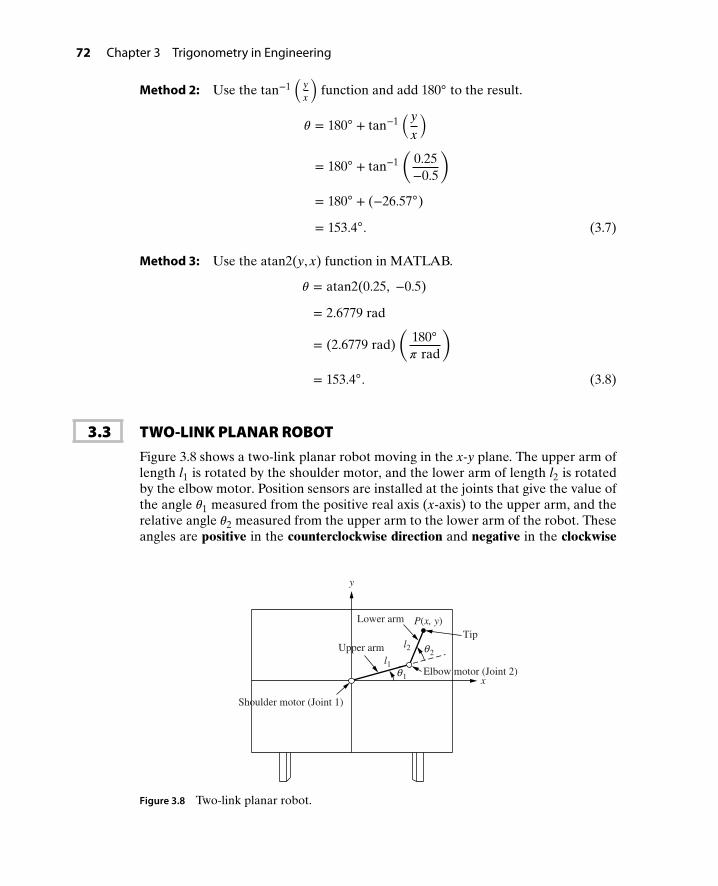
72 Chapter 3 Trigonometry in Engineering
Method 2: Use the tan−1(
yx
)function and add 180 to the result.
𝜃 = 180 + tan−1(y
x
)
= 180 + tan−1(
0.25−0.5
)= 180 + (−26.57)
= 153.4. (3.7)
Method 3: Use the atan2(y, x) function in MATLAB.
𝜃 = atan2(0.25, −0.5)
= 2.6779 rad
= (2.6779 rad)(
180
𝜋 rad
)= 153.4. (3.8)
3.3 TWO-LINK PLANAR ROBOTFigure 3.8 shows a two-link planar robot moving in the x-y plane. The upper arm oflength l1 is rotated by the shoulder motor, and the lower arm of length l2 is rotatedby the elbow motor. Position sensors are installed at the joints that give the value ofthe angle 𝜃1 measured from the positive real axis (x-axis) to the upper arm, and therelative angle 𝜃2 measured from the upper arm to the lower arm of the robot. Theseangles are positive in the counterclockwise direction and negative in the clockwise
Shoulder motor (Joint 1)
P(x, y)
l2
Lower arm
l1
x
y
Elbow motor (Joint 2)
Tip
Upper arm
1θ
2θ
Figure 3.8 Two-link planar robot.

3.3 Two-Link Planar Robot 73
direction. In this section, both the direct and inverse kinematics of the two-link robotare derived.
3.3.1 Direct Kinematics of Two-Link Robot
The direct kinematics of the two-link planar robot is the problem of finding theposition of the tip of the robot P(x, y) if the joint angles 𝜃1 and 𝜃2 are known. Asillustrated in Figs. 3.8 and 3.9,
x = x1 + x2 (3.9)
y = y1 + y2. (3.10)
From the right-angle triangle OAP1,
x1 = l1 cos 𝜃1 (3.11)
y1 = l1 sin 𝜃1. (3.12)
Similarly, using right-angle triangle P1BP,
x2 = l2 cos(𝜃1 + 𝜃2) (3.13)
y2 = l2 sin(𝜃1 + 𝜃2). (3.14)
l2
l1
y
yy2
y1
x1
x2
P1 B
A
x
Ox
P(x, y)
1θ
1θ1θ
2θ 2θ+
Figure 3.9 Two-link planar robot.
Substituting equations (3.11) and (3.13) into equation (3.9) gives
x = l1 cos 𝜃1 + l2 cos(𝜃1 + 𝜃2). (3.15)
Similarly, substituting equations (3.12) and (3.14) into equation (3.10) yields
y = l1 sin 𝜃1 + l2 sin(𝜃1 + 𝜃2). (3.16)
Equations (3.15) and (3.16) give the position of the tip of the robot in terms of jointangles 𝜃1 and 𝜃2.

74 Chapter 3 Trigonometry in Engineering
Example3-12
Find the position, P(x, y), of the tip of the robot for the following configurations.Also, sketch the orientation of the robot in the x-y plane.
Solution Case I: 𝜃1 = 𝜃2 = 0
By inspection:
x = l1 + l2 and y = 0.
Using equations (3.15) and (3.16):
x = l1 cos(0) + l2 cos(0 + 0) = l1 + l2
y = l1 sin(0) + l2 sin(0 + 0) = 0.
O
P(x, y)
l1 l2x
x = l1 + l2
y
Case II: 𝜃1 = 180, 𝜃2 = 0
By inspection:
x = −(l1 + l2) and y = 0.
Using equations (3.15) and (3.16):
x = l1 cos(180) + l2 cos(180 + 0)= l1(−1) + l2(−1) = −(l1 + l2)
y = l1 sin(180) + l2 sin(180 + 0)= l1(0) + l2(0) = 0.
O
P(x, y)
l2 l1x
x = −(l1 + l2)
y
Case III: 𝜃1 = 90, 𝜃2 = −90
By inspection:
x = l2 and y = l1.
Using equations (3.15) and (3.16):
x = l1 cos(90) + l2 cos(90 − 90)= l1(0) + l2(1) = l2
y = l1 sin(90) + l2 sin(90 − 90)= l1(1) + l2(0) = l1.
O
P(x, y)
l1l2
x
y
−90°
90°
Case IV: 𝜃1 = 45, 𝜃2 = −45
Using equations (3.15) and (3.16):
x = l1 cos(45) + l2 cos(45 − 45)
= l1
(1√2
)+ l2(1) = l1√
2+ l2
y = l1 sin(45) + l2 sin(45 − 45)
= l1
(1√2
)+ l2(0) = l1√
2. O
P(x, y)l1 l2x
y
−45°
45°

3.3 Two-Link Planar Robot 75
3.3.2 Inverse Kinematics of Two-Link Robot
The inverse kinematics of the two-link planar robot is the problem of finding thejoint angles 𝜃1 and 𝜃2 if the position of the tip of the robot P(x, y) is known. Thisproblem can be solved using a geometric solution or an algebraic solution. In thischapter, only the algebraic solution will be carried out.
Example3-13
Find the joint angles 𝜃1 and 𝜃2 if the position of the tip of the robot is given byP(x, y) = (12, 6) as shown in Fig. 3.10. Assume l1 = l2 = 5
√2.
1
l2
P1
6
O
5
5
P(12, 6)
x
y
2
2
θ
2θ√⎯
√⎯
Figure 3.10 Two-link configuration to find 𝜃1 and 𝜃2.
Solution In the algebraic solution, the joint angles 𝜃1 and 𝜃2 are determined using the Pascallaws of cosines and sines. The Pascal law of cosines can be used to find the unknownangles of a triangle if the three sides of the triangle are known. For example, if thethree sides of the triangle shown in Fig. 3.11 are known, the unknown angle 𝛾 canbe found using the Law of Cosines as
a2 = b2 + c2 − 2 b c cos 𝜸 (3.17)
or
cos 𝛾 = b2 + c2 − a2
2 b c.
a
b
c
γα
Figure 3.11 A triangle with an unknown angle and three known sides.

76 Chapter 3 Trigonometry in Engineering
Similarly, if the two sides (a and c) and the angle (𝛾) of the triangle shown inFig. 3.11 are known, the unknown angle 𝛼 can be found using the Law of Sines as
sin 𝜶
c=
sin 𝜸
aor
sin 𝛼 = ca
sin 𝛾.
Solution for 𝜃2: In Fig. 3.10, the angle 𝜃2 can be obtained from triangle OPP1formed by joining points O and P. In this triangle (Fig. 3.12), three sides are knownand one of the angles 180 − 𝜃2 is unknown. Applying the law of cosines to the tri-angle OP1P gives
O
P(12, 6)
P1
122 + 6
2 = 180
6
12
180 −
25
25
2θ2θ
√⎯
√⎯√⎯⎯⎯⎯⎯⎯⎯
√⎯⎯⎯
Figure 3.12 Using the law of cosines to find 𝜃2.
(√180
)2=(
5√
2)2
+(
5√
2)2
− 2(
5√
2) (
5√
2)
cos(180 − 𝜃2)
180 = 50 + 50 − 100 cos(180 − 𝜃2)
80 = −100 cos(180 − 𝜃2)
−0.8 = cos(180 − 𝜃2). (3.18)
Since cos(180 − 𝜃2) = −cos 𝜃2, equation (3.18) can be written as cos 𝜃2 = 0.8. Forthe positive value of cos 𝜃2, 𝜃2 lies either in the first or fourth quadrant based onthe values of sin 𝜃2 as shown in Fig. 3.13. If the value of sin 𝜃2 is positive, angle 𝜃2is positive. However, if sin 𝜃2 is negative, angle 𝜃2 is negative.
0.6
−0.6
0.8x
y
= −36.872θ
= 36.872θ
Figure 3.13 Two solutions of 𝜃2.

3.3 Two-Link Planar Robot 77
Therefore, there are two possible solutions of 𝜃2, 𝜃2 = 36.87 and 𝜃2 = −36.87. InFig. 3.14, the positive solution 𝜃2 = 36.87 is called the elbow-up solution and thenegative solution 𝜃2 = −36.87 is called the elbow-down solution.
12O
6
P(12, 6)
= 36.87°
= −36.87°
Elbow up
Elbow down
2θ
2θ
Figure 3.14 Elbow-up and elbow-down solutions of 𝜃2.
Elbow-Up Solution for 𝜽1: The angle 𝜃1 for the elbow-up solution is shown inFig. 3.15. The angle 𝜃1 + 𝛼 can be obtained from Fig. 3.15 as
tan(𝜃1 + 𝛼) = 612
𝜃1 + 𝛼 = tan−1(
612
)𝜃1 + 𝛼 = 26.57
𝜃1 = 26.57 − 𝛼. (3.19)
6
P(12, 6)
P1
x
y
12
Elbow up
= 36.87°143
.13°
O
α
1θ
2θ
Figure 3.15 Elbow-up configuration to find angle 𝜃1..
The angle 𝛼 needed to find 𝜃1 in equation (3.19) can be obtained using the law ofsines or cosines from the triangle OP1P shown in Fig. 3.16. Using the law of sinesgives
sin 𝛼
5√
2= sin 143.13√
180.

78 Chapter 3 Trigonometry in Engineering
Therefore,
sin 𝛼 = 5√
2√180
sin 143.13
= 0.3164.
Since the robot is in the elbow-up configuration, the angle 𝛼 is positive. Therefore,
𝛼 = sin−1(0.3164)
𝛼 = 18.45.
P
P1
122 + 6
2
180
25
25
143.13°
O
α√⎯⎯⎯⎯⎯⎯⎯√⎯⎯⎯
=
√⎯
√⎯
Figure 3.16 Elbow-up configuration to find angle 𝛼.
Substituting 𝛼 = 18.45 into equation (3.19) yields
𝜃1 = 26.57 − 18.45 = 8.12.
Therefore, the inverse kinematic solution for the tip position P(12, 6) when theelbow is up is given by
𝜃1 = 8.12 and 𝜃2 = 36.87.
Elbow-Down Solution for 𝜽1: The angle 𝜃1 for the elbow-down solution is shownin Fig. 3.17. The angle 𝜃1 − 𝛼 can be obtained from Fig. 3.17 as
tan(𝜃1 − 𝛼) = 612
𝜃1 − 𝛼 = tan−1(
612
)𝜃1 − 𝛼 = 26.57
𝜃1 = 26.57 + 𝛼. (3.20)
O
6
P1
x
y
P(12, 6)
Elbow down
12
= 36.87°
143.13
°
α
1θ
2θ
Figure 3.17 Elbow-down configuration to find angle 𝜃1.

3.3 Two-Link Planar Robot 79
The angle 𝛼 needed to find 𝜃1 in equation (3.20) can be obtained using either thelaw of sines or cosines for the triangle OP1P shown in Fig. 3.18. Using the law ofcosines gives(
5√
2)2
=(
5√
2)2
+(√
180)2
− 2(
5√
2) (√
180)
cos 𝛼.
Therefore,
0 = 180 − 2(
5√
2) (√
180)
cos 𝛼
cos 𝛼 = 180
2 ×√
180 × 5√
2cos 𝛼 = 0.9487
𝛼 = cos−1(0.9487)
𝛼 = 18.43.
PP1
O
25
25
143.13°
122 + 6
2 =180
α√⎯
√⎯
√⎯⎯⎯⎯⎯⎯⎯√⎯⎯⎯
Figure 3.18 Elbow-down configuration to find angle 𝛼.
Substituting 𝛼 = 18.43 into equation (3.20) yields
𝜃1 = 26.57 + 18.43 = 45.
Therefore, the inverse kinematic solution for the tip position P(12, 6) when theelbow is down is given by
𝜃1 = 45 and 𝜃2 = −36.87.
3.3.3 Further Examples of Two-Link Planar Robot
Example3-14
Consider a two-link planar robot, with positive orientations of 𝜃1 and 𝜃2 as shownin Fig. 3.19.
(a) Suppose 𝜃1 = 2 𝜋
3rad, 𝜃2 = 5 𝜋
6rad, l1 = 10 in., and l2 = 12 in. Sketch the orien-
tation of the robot in the x-y plane, and determine the x and y coordinates ofpoint P(x, y).
(b) Suppose now that the same robot is located in the first quadrant and orientedin the elbow-up position, as shown in Fig. 3.19. If the tip of the robot is locatedat the point P(x, y) = (12, 16), determine the values of 𝜃1 and 𝜃2.
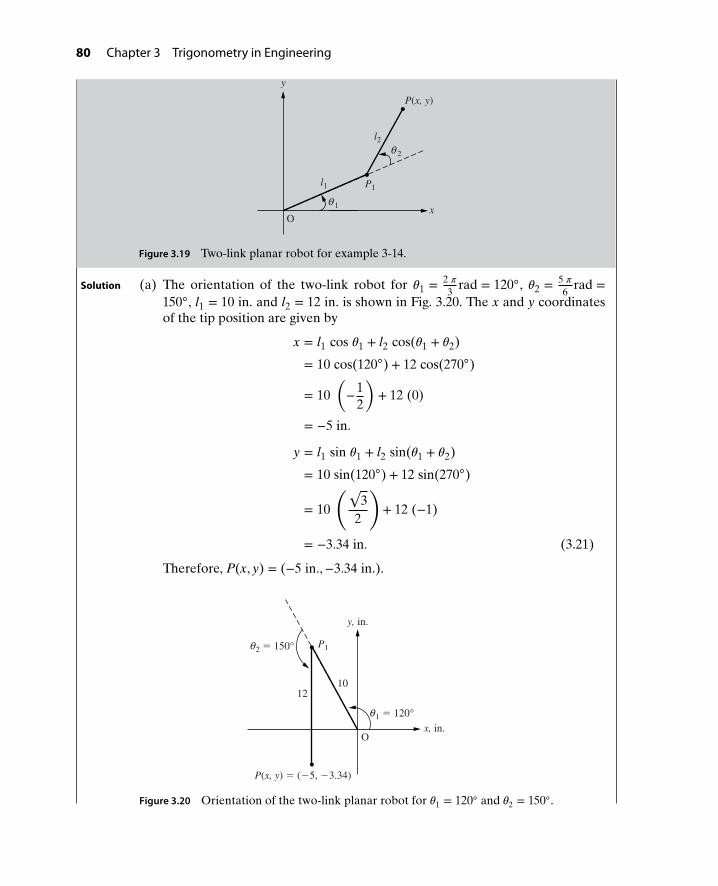
80 Chapter 3 Trigonometry in Engineering
y
O
l2
l1
P(x, y)
P1
x1θ
2θ
Figure 3.19 Two-link planar robot for example 3-14.
Solution (a) The orientation of the two-link robot for 𝜃1 = 2 𝜋
3rad = 120, 𝜃2 = 5 𝜋
6rad =
150, l1 = 10 in. and l2 = 12 in. is shown in Fig. 3.20. The x and y coordinatesof the tip position are given by
x = l1 cos 𝜃1 + l2 cos(𝜃1 + 𝜃2)
= 10 cos(120) + 12 cos(270)
= 10(−1
2
)+ 12 (0)
= −5 in.
y = l1 sin 𝜃1 + l2 sin(𝜃1 + 𝜃2)
= 10 sin(120) + 12 sin(270)
= 10
(√3
2
)+ 12 (−1)
= −3.34 in. (3.21)
Therefore, P(x, y) = (−5 in.,−3.34 in.).
O
1012
P(x, y) = (−5, −3.34)
P1
x, in.
y, in.
2 = 150°θ
1 = 120°θ
Figure 3.20 Orientation of the two-link planar robot for 𝜃1 = 120 and 𝜃2 = 150.

3.3 Two-Link Planar Robot 81
(b) For the two-link robot located in the first-quadrant as shown in Fig. 3.19, theangle 𝜃2 can be found using the law of cosines on the triangle OP1P shownin Fig. 3.21. The unknown angle 180 − 𝜃2 and the three sides of the triangleOP1P are shown in Fig. 3.21. Using the law of cosines gives
202 = 102 + 122 − 2(10)(12) cos(180 − 𝜃2)
400 = 244 + 240 cos 𝜃2
156 = 240 cos 𝜃2 ⇒ cos 𝜃2 = 0.65. (3.22)
Since the robot is in the elbow-up configuration, the angle 𝜃2 is positive and isgiven by 𝜃2 = cos−1(0.65) = 49.46. Also, from Fig. 3.21, the angle 𝜃1 + 𝛼 canbe determined using the right-angled triangle OAP as
tan(𝜃1 + 𝛼) = 1612
⇒ 𝜃1 = tan−1(
1612
)− 𝛼.
Therefore,
𝜃1 = 53.13 − 𝛼. (3.23)
O
1
P(x, y) = (12, 16)
P1
12
12
10
A
16
122 +
162 =
20
α180 −
2 θ
θ
√⎯⎯⎯⎯⎯⎯⎯⎯
Figure 3.21 The triangle OP1P to find the angles 𝜃1 and 𝜃2.
The angle 𝛼 can be found from the triangle OP1P using either the law of cosinesor the law of sines. Using the law of sines gives
sin 𝛼
12=
sin(180 − 𝜃2)20
.
Therefore,
sin 𝛼 = 1220
sin(180 − 49.46)
= 0.4560
𝛼 = sin−1(0.4560)
𝛼 = 27.13.
Substituting 𝛼 = 27.13 in equation (3.23) yields
𝜃1 = 53.13 − 27.13 = 26.0.

82 Chapter 3 Trigonometry in Engineering
Example3-15
Consider a two-link planar robot with positive orientations of 𝜃1 and 𝜃2 as shownin Fig. 3.19. Suppose 𝜃1 = 120, 𝜃2 = −30, l1 = 8 cm, and l2 = 4 cm.
(a) Sketch the orientation of the robot in the x-y plane.
(b) Determine the x and y coordinates of point P(x, y).
(c) Determine the distance from point P to the origin.
Solution (a) The orientation of the two-link robot for 𝜃1 = 120, 𝜃2 = −30, l1 = 8 cm, andl2 = 4 cm is shown in Fig. 3.22.
30°
120°
8
4
P(x, y)
P1
x, cm
y, cm
O
Figure 3.22 Orientation of the two-link planar robot for 𝜃1 = 120 and 𝜃2 = −30.
(b) The x- and y-coordinates of the tip position are given by
x = l1 cos 𝜃1 + l2 cos(𝜃1 + 𝜃2)
= 8 cos(120) + 4 cos(90)
= 8(−1
2
)+ 4 (0)
= −4 cm.
y = l1 sin 𝜃1 + l2 sin(𝜃1 + 𝜃2)
= 8 sin(120) + 4 sin(90)
= 8
(√3
2
)+ 4 (1)
= 10.93 cm.
Therefore, P(x, y) = (−4 cm, 10.93 cm).

3.3 Two-Link Planar Robot 83
(c) The distance from the tip P(x, y) to the origin is given by
d =√
x2 + y2
=√
(−4)2 + (10.93)2
= 11.64 cm.
Therefore, the distance from the tip of the robot to the origin is 11.64 cm.
Example3-16
Consider a two-link planar robot with positve orientations of 𝜃1 and 𝜃2 as shownin Fig. 3.19.
(a) Suppose 𝜃1 = 135, 𝜃2 = 45 and l1 = l2 = 10 in. Sketch the orientation of therobot in the x-y plane, and determine the x and y coordinates of point P(x, y).
(b) Suppose now that the tip of the same robot is located in the second quad-rant and oriented in the elbow-up position as shown in Fig. 3.23. If the tip ofthe robot is located at the point P(x, y) = (−17.07 in., 7.07 in.), determine thevalues of 𝜃1 and 𝜃2.
O
P1
−17.07
7.07
10
P(x, y)
y, in.
x, in.
10
1θ
2θ
Figure 3.23 Two-link planar robot in the elbow-up position withP(x, y) = (−17.07 in., 7.07 in.).
Solution (a) The orientation of the two-link robot for 𝜃1 = 135, 𝜃2 = 45, and l1 = l2 =10 in. is shown in Fig. 3.24. The x and y coordinates of the tip position aregiven by
x = l1 cos 𝜃1 + l2 cos(𝜃1 + 𝜃2)
= 10 cos 135 + 10 cos 180
= 10
(−√
22
)+ 10 (−1)
= −17.07 in.
y = l1 sin 𝜃1 + l2 sin(𝜃1 + 𝜃2)
= 10 sin 135 + 10 sin 180
= 10
(√2
2
)+ 10(0)
= 7.07 in. (3.24)

84 Chapter 3 Trigonometry in Engineering
Therefore, P(x, y) = (−17.07 in., 7.07 in.).
45°
135°
P(x, y) 10
10
y, in.
x, in.
P1
O
Figure 3.24 The orientation of the two-link planar robot with 𝜃1 = 135, and 𝜃2 = 45.
(b) The angle 𝜃2 can be found using the law of cosines on the triangle OP1P inFig. 3.25. The unknown angle 180 − 𝜃2 and the three sides of the triangle OP1Pare shown in Fig. 3.25. Using the law of cosines gives
(18.48)2 = 102 + 102 − 2(10)(10) cos(180 − 𝜃2)
341.4 = 200 + 200 cos 𝜃2
141.4 = 200 cos 𝜃2 ⇒ cos 𝜃2 = 0.707.
Since the robot is in the elbow-up configuration, angle 𝜃2 is positive and isgiven by 𝜃2 = cos−1(0.707) = 45.0. Also, from Fig. 3.25, the angle 𝜃1 + 𝛼 canbe determined using the right-angled triangle OAP as
𝜃1 + 𝛼 = atan2(7.07,−17.07)
𝜃1 + 𝛼 = 157.5.
Therefore,𝜃1 = 157.5 − 𝛼. (3.25)
P1
−17.07
10
7.0710
P(x, y)
A
y, in.
x, in.
17.07 2 + 7.07 2
= 18.477
O
1θα
√⎯⎯⎯⎯⎯⎯⎯⎯⎯⎯⎯⎯2
θ180 −
2θ
Figure 3.25 The triangle OP1P to find the angles 𝜃1 and 𝜃2.
The angle 𝛼 can be found from the triangle OP1P using either the law of cosinesor the law of sines. Using the law of cosines gives
102 = (18.48)2 + 102 − 2(10)(18.48) cos 𝛼
−341.4 = −369.54 cos 𝛼
0.9239 = cos 𝛼.

3.3 Two-Link Planar Robot 85
Therefore, 𝛼 = 22.5. Substituting 𝛼 = 22.5 in equation (3.25) yields
𝜃1 = 157.5 − 22.5 = 135.0.
Example3-17
Consider a two-link planar robot with positive orientations of 𝜃1 and 𝜃2 as shownin Fig. 3.19.
(a) Suppose 𝜃1 = −135, 𝜃2 = −45, and l1 = l2 = 10 in. Sketch the orientation ofthe robot in the x-y plane, and determine the x- and y-coordinates of pointP(x, y).
(b) Suppose now that the tip of same robot is located in the third quadrant and ori-ented in the elbow-down position (clockwise direction), as shown in Fig. 3.26.If the tip of the robot is located at point P(x, y) = (−17.07 in.,−7.07 in.),determine the values of 𝜃1 and 𝜃2.
−17.07
10
P(x, y)10 P1
−7.07
x, in.
y, in.
O
1θ
2θ
Figure 3.26 Two-link planar robot in the elbow-down positionwith P(x, y) = (−17.07 in.,−7.07 in.).
Solution (a) The orientation of the two-link robot for 𝜃1 = −135, 𝜃2 = −45, and l1 = l2 =10 in. is shown in Fig. 3.27. The x- and y-coordinates of the tip position aregiven by
x = l1 cos 𝜃1 + l2 cos(𝜃1 + 𝜃2)
= 10 cos(−135) + 10 cos(−180)
= 10
(−√
22
)+ 10 (−1)
= −17.07 in.
y = l1 sin 𝜃1 + l2 sin(𝜃1 + 𝜃2)
= 10 sin(−135) + 10 sin(−180)
= 10
(−√
22
)+ 10(0)
= −7.07 in.
Therefore, P(x, y) = (−17.07 in.,−7.07 in.).
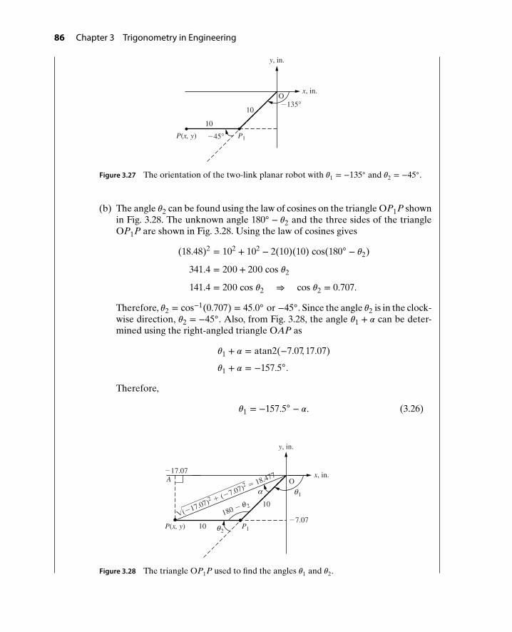
86 Chapter 3 Trigonometry in Engineering
P1P(x, y)
10
10
x, in.
y, in.
−135°
−45°
O
Figure 3.27 The orientation of the two-link planar robot with 𝜃1 = −135 and 𝜃2 = −45.
(b) The angle 𝜃2 can be found using the law of cosines on the triangle OP1P shownin Fig. 3.28. The unknown angle 180 − 𝜃2 and the three sides of the triangleOP1P are shown in Fig. 3.28. Using the law of cosines gives
(18.48)2 = 102 + 102 − 2(10)(10) cos(180 − 𝜃2)
341.4 = 200 + 200 cos 𝜃2
141.4 = 200 cos 𝜃2 ⇒ cos 𝜃2 = 0.707.
Therefore, 𝜃2 = cos−1(0.707) = 45.0 or −45. Since the angle 𝜃2 is in the clock-wise direction, 𝜃2 = −45. Also, from Fig. 3.28, the angle 𝜃1 + 𝛼 can be deter-mined using the right-angled triangle OAP as
𝜃1 + 𝛼 = atan2(−7.07, 17.07)
𝜃1 + 𝛼 = −157.5.
Therefore,
𝜃1 = −157.5 − 𝛼. (3.26)
O
−17.07
−7.07P(x, y) 10
10
P1
A
y, in.
x, in.
(−17.07)2 + (−7.07)
2 = 18.477
√⎯⎯⎯⎯⎯⎯⎯⎯⎯⎯⎯⎯⎯⎯⎯⎯⎯⎯
2θ180 −
1θα
2θ
Figure 3.28 The triangle OP1P used to find the angles 𝜃1 and 𝜃2.
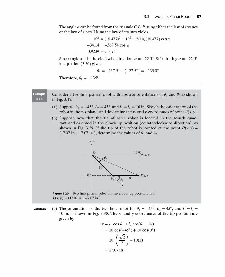
3.3 Two-Link Planar Robot 87
The angle 𝛼 can be found from the triangle OP1P using either the law of cosinesor the law of sines. Using the law of cosines yields
102 = (18.477)2 + 102 − 2(10)(18.477) cos 𝛼
−341.4 = −369.54 cos 𝛼
0.9239 = cos 𝛼.
Since angle 𝛼 is in the clockwise direction, 𝛼 = −22.5. Substituting 𝛼 = −22.5
in equation (3.26) gives
𝜃1 = −157.5 − (−22.5) = −135.0.
Therefore, 𝜃1 = −135.
Example3-18
Consider a two-link planar robot with positive orientations of 𝜃1 and 𝜃2 as shownin Fig. 3.19.
(a) Suppose 𝜃1 = −45, 𝜃2 = 45, and l1 = l2 = 10 in. Sketch the orientation of therobot in the x-y plane, and determine the x- and y-coordinates of point P(x, y).
(b) Suppose now that the tip of same robot is located in the fourth quad-rant and oriented in the elbow-up position (counterclockwise direction), asshown in Fig. 3.29. If the tip of the robot is located at the point P(x, y) =(17.07 in., −7.07 in.), determine the values of 𝜃1 and 𝜃2.
P110
17.07O
10
−7.07 P(x, y)
x, in.
y, in.
1θ
2θ
Figure 3.29 Two-link planar robot in the elbow-up position withP(x, y) = (17.07 in., −7.07 in.)
Solution (a) The orientation of the two-link robot for 𝜃1 = −45, 𝜃2 = 45, and l1 = l2 =10 in. is shown in Fig. 3.30. The x- and y-coordinates of the tip position aregiven by
x = l1 cos 𝜃1 + l2 cos(𝜃1 + 𝜃2)
= 10 cos(−45) + 10 cos(0)
= 10
(√2
2
)+ 10(1)
= 17.07 in.
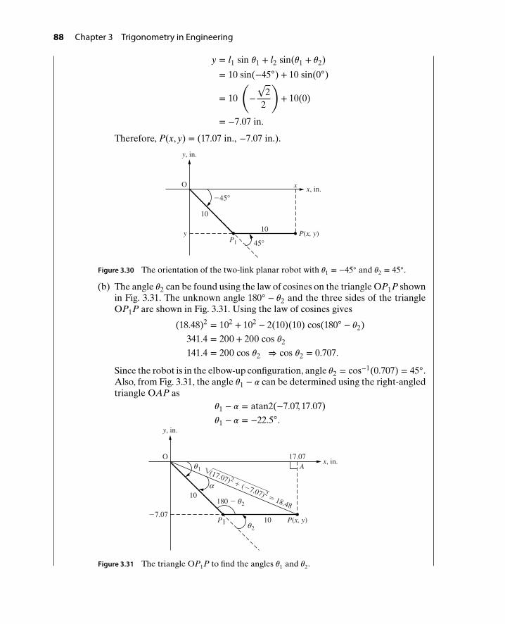
88 Chapter 3 Trigonometry in Engineering
y = l1 sin 𝜃1 + l2 sin(𝜃1 + 𝜃2)
= 10 sin(−45) + 10 sin(0)
= 10
(−√
22
)+ 10(0)
= −7.07 in.
Therefore, P(x, y) = (17.07 in., −7.07 in.).
O
10
10P(x, y)
P1
−45°
45°
x
y
y, in.
x, in.
Figure 3.30 The orientation of the two-link planar robot with 𝜃1 = −45 and 𝜃2 = 45.
(b) The angle 𝜃2 can be found using the law of cosines on the triangle OP1P shownin Fig. 3.31. The unknown angle 180 − 𝜃2 and the three sides of the triangleOP1P are shown in Fig. 3.31. Using the law of cosines gives
(18.48)2 = 102 + 102 − 2(10)(10) cos(180 − 𝜃2)
341.4 = 200 + 200 cos 𝜃2
141.4 = 200 cos 𝜃2 ⇒ cos 𝜃2 = 0.707.
Since the robot is in the elbow-up configuration, angle 𝜃2 = cos−1(0.707) = 45.Also, from Fig. 3.31, the angle 𝜃1 − 𝛼 can be determined using the right-angledtriangle OAP as
𝜃1 − 𝛼 = atan2(−7.07, 17.07)
𝜃1 − 𝛼 = −22.5.
P(x, y)10
10
17.07
P1
O
A
y, in.
x, in.
−7.07
(17.07) 2 + (−7.07) 2
= 18.48
1θ √⎯⎯⎯⎯⎯⎯⎯⎯⎯⎯⎯⎯⎯⎯⎯⎯⎯α
2θ
180 − 2θ
Figure 3.31 The triangle OP1P to find the angles 𝜃1 and 𝜃2.

3.4 Further Examples of Trigonometry in Engineering 89
Therefore,
𝜃1 = −22.5 + 𝛼. (3.27)
The angle 𝛼 can be found from the triangle OP1P using either the law of cosinesor the law of sines. Using the law of cosines yields
102 = (18.48)2 + 102 − 2(10)(18.48) cos 𝛼
−341.4 = −369.5 cos 𝛼
0.9239 = cos 𝛼.
Since angle 𝛼 is in the clockwise direction, 𝛼 = −22.5. Substituting 𝛼 = −22.5
in equation (3.27) gives
𝜃1 = −22.5 + (−22.5) = −45.0.
Therefore, 𝜃1 = −45.
3.4 FURTHER EXAMPLES OF TRIGONOMETRYIN ENGINEERING
Example3-19
A one-link planar robot of length l = 1.5 m is moving in the x-y plane. If the jointangle 𝜃 = −165, locate the tip P(x, y) of the robot in the x-y plane.
Solution The tip of the one-link robot for 𝜃 = −165 is shown in Fig. 3.32. It can be seenfrom this figure that the tip is located in the third quadrant and the reference angleis 15. Since both the sin and cos functions are negative in the third quadrant, theposition P(x, y) of the tip is given by
x = 1.5 cos(165) = −1.5 cos(15) = −1.5 × 0.9659 = −1.449 m
y = 1.5 sin(165) = −1.5 sin(15) = −1.5 × 0.2588 = −0.388 m
1.5 m
x
y
−165°
P(x, y)
Figure 3.32 One-link planar robot for Example 3-19.

90 Chapter 3 Trigonometry in Engineering
Example3-20
The x- and y-components of the tip of a one-link planar robot are given as −10 cmand 5 cm, respectively. Locate the tip of the robot in the x-y plane. Also, find thelength l of the link and the angle 𝜃.
Solution The tip of the one-link robot with x = −10 cm and y = 5 cm is shown in Fig. 3.33.The length l is given by
l =√
(−10)2 + (5)2 =√
100 + 25 =√
125 = 11.18 cm.
5 cm
Ox
y
l
−10.0 cm
P(x, y)
θ
Figure 3.33 One-link planar robot for example 3-20.
Since the tip of the robot is in the second quadrant, the angle 𝜃 is given by
𝜃 = 180 − atan(
510
)= 180 − atan(0.5)
= 180 − 26.57
= 153.4.
Using the atan2(y, x) function in MATLAB, the angle 𝜃 is given by
𝜃 = atan2(5,−10)
= 2.6779 rad
= (2.6779 rad)(
180
𝜋 rad
)= 153.4.
Example3-21
In Example 1-8, the civil engineer calculated the elevation of the building corner-stone located between two benchmarks shown in Fig. 1.19. The same engineer isnow required to calculate the angle of inclination and horizontal distance betweenthe two benchmarks, as shown in Fig. 3.34.

3.4 Further Examples of Trigonometry in Engineering 91
B1x, m
y, m
476.8
428.4
Δy
Δx
L
B2
θ
Figure 3.34 Elevation between the two benchmarks.
The distance L between the two benchmarks B1 and B2 is 1001.2 m, and theirelevations are 428.4 m and 476.8 m, respectively.
(a) Find the angle of inclination 𝜃 of the grade. Also, calculate the percent grade,ΔyΔx
× 100.
(b) Calculate the horizontal distance between the two benchmarks.
(c) Check the results of part (b) using the Pythagorean theorem.
Solution (a) The angle of inclination 𝜃 can be determined from the right-angle triangleshown in Fig. 3.34 as
sin 𝜃 =ΔyL
=E2 − E1
L
= 476.8 − 428.41001.2
= 0.0483.
Therefore, the angle of inclination 𝜃 = sin−1 (0.0483) = 2.768. The percentgrade can now be calculated as
Percent grade =ΔyΔx
× 100
= 100 × tan 𝜃
= 100 × tan(2.768)
= 4.84%.

92 Chapter 3 Trigonometry in Engineering
(b) The horizontal distance between the two benchmarks can be calculated as
Δx = L cos𝜃
= (1001.2) cos(2.468)
= (1001.2) (0.99883)
= 1000.0 m. (3.28)
(c) The horizontal distance can also be calculated using the Pythagoreantheorem as
Δx =√
L2 − Δy2
=√
(1001.2)2 − (48.4)2
= 1000 m.
Example3-22
Consider the position of the toes of a person sitting in a chair, as shown in Fig. 3.35.
P(x, y)
x, in.
y, in.
l1
l1
l2
1θ
2θ
Figure 3.35 Toes position of a person sitting on a chair.
(a) Suppose 𝜃1 = −30, 𝜃2 = 45, l1 = 20 in., and l2 = 5 in. Determine the x- andy-coordinates of the position of the toes P(x, y).
(b) Now suppose that the same leg is positioned such that the tip of the toes islocated in the first quadrant and oriented in the ankle-up position (counter-clockwise direction) as shown Fig. 3.36. If the end of the toes are located atP(x, y) = (19.5 in., 2.5 in.), determine the values of 𝜃1 and 𝜃2.
P(19.5, 2.5)
520
x
y
O 1θ2θ
Figure 3.36 Ankle-up position.

3.4 Further Examples of Trigonometry in Engineering 93
Solution (a) The x- and y-coordinates of the toes position can be calculated as
x = l1 cos 𝜃1 + l2 cos(𝜃1 + 𝜃2)
= 20 cos(−30) + 5 cos(−30 + 45)
= 20
(√3
2
)+ 5(0.9659)
= 22.15 in.
y = l1 sin 𝜃1 + l2 sin(𝜃1 + 𝜃2)
= 20 sin(−30) + 5 sin(−30 + 45)
= 20(−1
2
)+ 5(0.2588)
= −18.71 in.
Therefore, P(x, y) = (22.15 in., −18.71 in.).
(b) The angle 𝜃2 can be found using the law of cosines on the triangle OP1P shownin Fig. 3.37. The unknown angle 180 − 𝜃2 and the three sides of the triangleOP1P are shown in Fig. 3.37. Using the law of cosines gives
(19.66)2 = 202 + 52 − 2(20)(5) cos(180 − 𝜃2)
386.5 = 425 − 200 cos(180 − 𝜃2)
−38.5 = −200 cos(180 − 𝜃2) ⇒ cos(180 − 𝜃2) = 0.1925
x
y
180 −
A
5
P(19.5, 2.5)
20
(19.5)2 + (2.5)2 = 19.66
P1
O
α
1θ
√⎯⎯⎯⎯⎯⎯⎯⎯⎯⎯⎯⎯⎯
2θ
2θ
Figure 3.37 The triangle OP1P to find the angles 𝜃1 and 𝜃2.
Since the leg is in the ankle-up configuration, (180 − 𝜃2) = cos−1(0.1925) =78.9. Therefore, 𝜃2 = 101.1. Also, from Fig. 3.37, the angle 𝜃1 + 𝛼 can be de-termined using from the triangle OP1P using either the law of cosines or thelaw of sines. Using the law of sines yields
sin(𝜃1 + 𝛼)5
=sin(180 − 𝜃2)
19.66.

94 Chapter 3 Trigonometry in Engineering
Therefore,
sin(𝜃1 + 𝛼) = 519.66
sin 78.9
𝜃1 + 𝛼 = 14.45. (3.29)
The angle 𝛼 can be found from the right-triangle OAP shown in Fig. 3.37 as
𝛼 = atan2(2.5, 19.5) = 7.31.
Substituting the value of 𝛼 in equation (3.29) gives
𝜃1 = 14.45 − 𝛼
= 14.45 − 7.31
or
𝜃1 = 7.14.
Example3-23
In a motion capture study of a runner, one frame shows the subject support-ing her weight on one leg, as shown in Fig. 3.38. The length of the foot segment(from ankle to toe) is 7.9 in. and the length of the lower leg (from ankle to knee)is 17.1 in.
(a) Given the angles shown in Fig. 3.38, find the position of the knee if the runner’stoes touch the ground at the point x = y = 0.
Toes
Ankle
x
82.4°
37.2°
yKnee
Figure 3.38 Position of the runner’s leg during motion capture study.
(b) Now suppose that the same leg is positioned such that the knee is locatedin the second quadrant and oriented in the knee-down position (clockwisedirection) as shown Fig. 3.39. If the end of the toes are located at P(x, y) =(−4 in., 24 in.), determine the values of 𝜃1 and 𝜃2.

3.4 Further Examples of Trigonometry in Engineering 95
y, in.
(−4, 24)
Ankle
Toes
Knee
x, in.
1θ
2θ
Figure 3.39 Position of the runner’s leg to find 𝜃1 and 𝜃2.
Solution (a) Using the angles 𝜃1 and 𝜃2 shown in Fig. 3.40, the x- and y-coordinates of theknee position are calculated as
x = l1 cos 𝜃1 + l2 cos(𝜃1 + 𝜃2)
= 7.9 cos(142.8) + 17.1 cos(142.8 − 97.6)
= 7.9 (−0.7965) + 17.1(0.7046)
= 5.76 in.
y = l1 sin 𝜃1 + l2 sin(𝜃1 + 𝜃2)
= 7.9 sin(142.8) + 17.1 sin(142.8 − 97.6)
= 7.9 (0.6046) + 17.1(0.7096)
= 16.9 in.
Therefore, P(x, y) = (5.76 in., 16.9 in.).
P(x, y)
17.1
37.2°
Ankle
Toesx, in.
y, in.
82.4°
= 142.8°7.9
Knee
1θ
= −97.6°2θ
Figure 3.40 Angle 𝜃1 and 𝜃2 to find the position of the knee.

96 Chapter 3 Trigonometry in Engineering
(b) The angle 𝜃2 can be found using the law of cosines on the triangle TAK shownin Fig. 3.41. The unknown angle 180 − 𝜃2 and the three sides of the triangleTAK are shown in Fig. 3.41. Using the law of cosines gives
(24.33)2 = 7.92 + 17.12 − 2(7.9)(17.1) cos(180 − 𝜃2)
592 = 425 − 270.18 cos(180 − 𝜃2)
167 = 270.18 cos(𝜃2) ⇒ cos(𝜃2) = 0.6181 ⇒ 𝜃2 = 51.82.
P−4 T
17.1
x, in.
K(−4, 24)
24.33
24
A7.9
y, in.
αβ
1θ
180 − 2θ2θ
Figure 3.41 The triangle TAK to find the angles 𝜃2.
Also from Fig. 3.41, the angle 𝛼 can be determined from the triangle TAK usingeither the law of cosines or the law of sines. Using the law of sines yields
sin(𝛼)17.1
=sin(180 − 𝜃2)
24.33.
Therefore,
sin(𝛼) = 17.124.33
sin 129.2
which gives
𝛼 = 33.
The angle 𝛽 can be found from the right-triangle TKP shown in Fig. 3.41 as
𝛽 = atan2(24,−4) ⇒ 𝛽 = 99.46.
Angle 𝜃1 can now be found by adding angles 𝛼 and 𝛽 as shown in Fig. 3.41 as
𝜃1 = 𝛼 + 𝛽
= 51.82 + 99.46
= 151.28.
Therefore, 𝜃1 = 151.8. Also, since the robot is in the knee-down configuration,the angle 𝜃2 = −51.82.

Problems 97
P R O B L E M S
3-1. A laser range finder records the distancefrom the laser to the base and from thelaser to the top of a building as shown inFig. P3.1. Find the angle 𝜃 and the heightof the building.
h
75 m
Range finder
100 m
θ
Figure P3.1 Using a range finder to find the heightof a building.
3-2. The eyes of a 7 ft 4 in. player are 82 in.from the floor, as shown in Fig. P3.2. Ifthe height of the basketball hoop is 10 ftfrom the floor, find the distance l and an-gle 𝜃 from the player’s eye to the hoop.
l
10 ft
82 in.
156 in.
θ
Figure P3.2 A basketball player in front of thebasketball hoop.
3-3. Repeat problem P3-2 if the player’sheight is 72 in.
3-4. To calculate the property tax, a city hiresa coop student to determine the area ofdifferent lots in a new subdivision. The
coop student calculates the area of lot 1shown in Fig. P3.4 as 94,640 m2. Is thisthe correct answer? If not, find the cor-rect answer.
Lot 1200 m
300 m
30°
Figure P3.4 Dimension of lot 1 in the newsubdivision.
3-5. The same coop student calculates thearea of lot 2 shown in Fig. P3.5 as50,000 m2. Is this the correct answer? Ifnot, find the correct answer.
Lot 2200 m
300 m
120°
Figure P3.5 Dimension of lot 2 in the newsubdivision.
3-6. A laser beam is directed through a smallhole in the center of a circle of radius1.73 m. The origin of the beam is 5 mfrom the circle as shown in Fig. P3.6.
Laser
5 m
1.73
Beam
θ
Figure P3.6 Laser beam for problem P3-6.
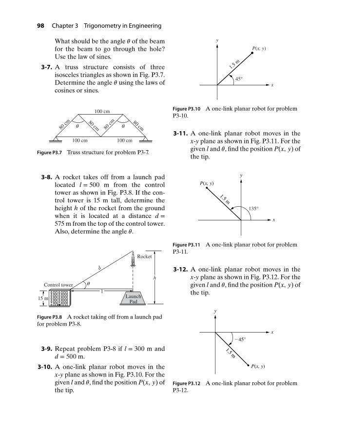
98 Chapter 3 Trigonometry in Engineering
What should be the angle 𝜃 of the beamfor the beam to go through the hole?Use the law of sines.
3-7. A truss structure consists of threeisosceles triangles as shown in Fig. P3.7.Determine the angle 𝜃 using the laws ofcosines or sines.
100 cm
100 cm
100 cm
80 cm
80 cm80 cm
80 cm
θ θ
Figure P3.7 Truss structure for problem P3-7.
3-8. A rocket takes off from a launch padlocated l = 500 m from the controltower as shown in Fig. P3.8. If the con-trol tower is 15 m tall, determine theheight h of the rocket from the groundwhen it is located at a distance d =575 m from the top of the control tower.Also, determine the angle 𝜃.
l
h
15 m
Rocket
Control tower
LaunchPad
d
θ
Figure P3.8 A rocket taking off from a launch padfor problem P3-8.
3-9. Repeat problem P3-8 if l = 300 m andd = 500 m.
3-10. A one-link planar robot moves in thex-y plane as shown in Fig. P3.10. For thegiven l and 𝜃, find the position P(x, y) ofthe tip.
y
x
P(x, y)
45°
1.5 m
Figure P3.10 A one-link planar robot for problemP3-10.
3-11. A one-link planar robot moves in thex-y plane as shown in Fig. P3.11. For thegiven l and 𝜃, find the position P(x, y) ofthe tip.
x
y
1.5 m
P(x, y)
135°
Figure P3.11 A one-link planar robot for problemP3-11.
3-12. A one-link planar robot moves in thex-y plane as shown in Fig. P3.12. For thegiven l and 𝜃, find the position P(x, y) ofthe tip.
1.5 m
P(x, y)
x
y
−45°
Figure P3.12 A one-link planar robot for problemP3-12.

Problems 99
3-13. A one-link planar robot moves in thex-y plane as shown in Fig. P3.13. For thegiven l and 𝜃, find the position P(x, y) ofthe tip.
y
P(x, y)
1.5 m
−135°
x
Figure P3.13 A one-link planar robot for problemP3-13.
3-14. Consider the one-link planar robotshown in Fig. P3.14.
l
x
yy
P(x, y)
x
y
O
θ
Figure P3.14 A one-link planar robot for problemP3-14.
If l = 5 cm, sketch the position of thetip of the robot and determine the (x, y)coordinates of position P for(a) 𝜃 = 𝜋
4rad
(b) 𝜃 = 4𝜋4
rad
(c) 𝜃 = −135
(d) 𝜃 = −𝜋
4rad
3-15. Repeat problem P3-14 if l = 10 in. and(a) 𝜃 = 150
(b) 𝜃 = −2𝜋3
rad
(c) 𝜃 = 420
(d) 𝜃 = −9𝜋4
rad
3-16. Consider again the one-link planarrobot shown in Fig. P3.14. Determinethe length l and angle 𝜃 if the tip of therobot is located at the following pointsP(x, y).(a) P(x, y) = (3, 4) cm(b) P(x, y) = (−4, 3) cm(c) P(x, y) = (−3,−3) cm(d) P(x, y) = (5,−4) cm
3-17. Repeat problem P3-16 if(a) P(x, y) = (4, 2) in.(b) P(x, y) = (−2, 4) in.(c) P(x, y) = (−5,−7.5) in.(d) P(x, y) = (6,−6) in.
3-18. Consider the two-link planar robotshown in Fig. P3.18.
y
l1
l2
P(x, y)
xO
P1
1θ
2θ
Figure P3.18 A two-link planar robot for problemP3-18.
Sketch the orientation of the robotand determine the (x, y) coordinates ofpoint P for(a) 𝜃1 = 30, 𝜃2 = 45, l1 = l2 = 5 cm(b) 𝜃1 = 30, 𝜃2 = −45, l1 = l2 = 5 cm
(c) 𝜃1 = 3𝜋4
rad, 𝜃2 = 𝜋
2rad, l1 = l2 =
5 cm
(d) 𝜃1 = 3𝜋4
rad, 𝜃2 = −𝜋
2rad, l1 = l2 =
5 cm(e) 𝜃1 = −30, 𝜃2 = 45, l1 = l2 = 5 cm

100 Chapter 3 Trigonometry in Engineering
(f) 𝜃1 = −30, 𝜃2 = −45, l1 = l2 =5 cm
(g) 𝜃1 = −3𝜋4
rad, 𝜃2 = 𝜋
2rad, l1 = l2 =
5 cm
(h) 𝜃1 = −3𝜋4
rad, 𝜃2 = −𝜋
2rad, l1 =
l2 = 5 cm
3-19. Suppose that the two-link planar robotshown in Fig. P3.18 is located in the firstquadrant and is oriented in the elbow-up position. If the tip of the robot islocated at the point P(x, y) = (9, 9),determine the values of 𝜃1 and 𝜃2.Assume l1 = 6 in. and l2 = 8 in.
3-20. Suppose that the two-link planar robotshown in Fig. P3.18 is located in the firstquadrant and is oriented in the elbow-down position. If the tip of the robotis located at the point P(x, y) = (10, 5),determine the values of 𝜃1 and 𝜃2.Assume l1 = 6 in. and l2 = 8 in.
3-21. Consider the two-link planar robot withl1 = l2 = 5 in. and oriented in the elbow-up position, as shown in Fig. P3.21. If thetip of the robot is located at the pointP(x, y) = (7.5,−2.8), determine thevalues of 𝜃1 and 𝜃2.
P(7.5, −2.8)5
5
y, in.
x, in.O
1θ
2θ
Figure P3.21 A two-link planar robot for problemP3-21.
3-22. Consider the two-link planar robotwith l1 = l2 = 5 in. and oriented in theelbow-down position as shown in Fig.P3.22. If the tip of the robot is locatedat the point P(x, y) = (4.83,−8.36),determine the values of 𝜃1 and 𝜃2.
O
5
y, in.
5
x, in.
P(4.83, −8.36)
1θ
2θ
Figure P3.22 A two-link planar robot for problemP3-22.
3-23. Consider a two-link planar robot withl1 = l2 = 10 cm and oriented in theelbow-down position as shown in Fig.P3.23. If the tip of the robot is located atthe point P(x, y) = (−17, −1), determinethe values of 𝜃1 and 𝜃2.
1010
P −1
y, cm
x, cm−17 O
2θ
1θ
Figure P3.23 A two-link planar robot for problemP3-23.
3-24. Consider a two-link planar robot withl1 = l2 = 10 cm and oriented in theelbow-up position as shown in Fig.P3.24. If the tip of the robot is located
−16.73
O
y, cm
x, cm
P
10
−4.5
10 1θ
2θ
Figure P3.24 A two-link planar robot for problemP3-24.

Problems 101
at the point P(x, y) = (−4.5,−16.73),determine the values of 𝜃1 and 𝜃2.
3-25. Consider a two-link planar robot ori-ented in the elbow-up position as shownin Fig. P3.25. If the tip of the robotis located at the point P(x, y) =(−13, 12), determine the values of 𝜃1and 𝜃2. Assume l1 = 10 in. and l2 = 8 in.
−13
O
−1
P
10
8
12
x
y
2θ
1θ
Figure P3.25 A two-link planar robot for problemP3-25.
3-26. Consider a two-link planar robot ori-ented in the elbow-down position asshown in Fig. P3.26. If the tip of therobot is located at the point P(x, y) =(−1, 15), determine the values of 𝜃1 and𝜃2. Assume l1 = 10 in. and l2 = 8 in.
10
y
8
P
−1 Ox
15
2θ
1θ
Figure P3.26 A two-link planar robot for problemP3-26.
3-27. Consider a two-link planar robot ori-ented in the elbow-up position as shownin Fig. P3.27. If the tip of the robotis located at the point P(x, y) =(13.66 cm, −3.66 cm), determine the
values of 𝜃1 and 𝜃2 using the laws ofcosines and sines.
−3.66 cm
10 cm
13.66 cm
P(x, y)
x
y
10 cm
1θ
2θ
Figure P3.27 A two-link planar robot for problemP3-27.
3-28. An airplane travels at a heading of 60
northwest with an air speed of 500 mphas shown in Fig. P3.28. The wind isblowing at 30 southwest at a speed of50 mph. Find the magnitude of thevelocity V and the angle 𝜃 of the planerelative to the ground using the laws ofsines and cosines.
S
E
500
50
V
W
N
x
y
60°
30°
θ
Figure P3.28 Velocity of an airplane for problemP3-28.
3-29. A large barge is crossing a river at aheading of 30 northwest with a speedof 12 mph against the water as shownin Fig. P3.29. The river flows due eastat a speed of 4 mph. Find the magni-tude of the velocity V and the angle 𝜃
of the barge using the laws of sines andcosines.
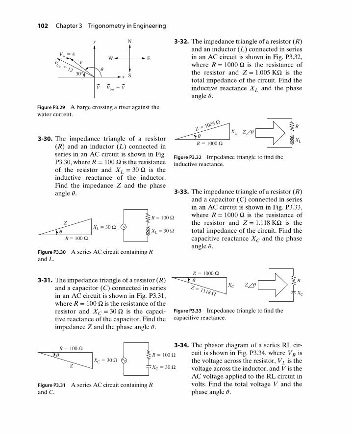
102 Chapter 3 Trigonometry in Engineering
Vw = 4
30°
VW E
N
S
V = Vbw + V
x
y
Vbw = 12 θ
Figure P3.29 A barge crossing a river against thewater current.
3-30. The impedance triangle of a resistor(R) and an inductor (L) connected inseries in an AC circuit is shown in Fig.P3.30, where R = 100 Ω is the resistanceof the resistor and XL = 30 Ω is theinductive reactance of the inductor.Find the impedance Z and the phaseangle 𝜃.
ZXL = 30 Ω
XL = 30 Ω
R = 100 Ω
R = 100 Ωθ
Figure P3.30 A series AC circuit containing Rand L.
3-31. The impedance triangle of a resistor (R)and a capacitor (C) connected in seriesin an AC circuit is shown in Fig. P3.31,where R = 100 Ω is the resistance of theresistor and XC = 30 Ω is the capaci-tive reactance of the capacitor. Find theimpedance Z and the phase angle 𝜃.
ZXC = 30 Ω
R = 100 Ω
XC = 30 Ω
R = 100 Ωθ
Figure P3.31 A series AC circuit containing Rand C.
3-32. The impedance triangle of a resistor (R)and an inductor (L) connected in seriesin an AC circuit is shown in Fig. P3.32,where R = 1000 Ω is the resistance ofthe resistor and Z = 1.005 KΩ is thetotal impedance of the circuit. Find theinductive reactance XL and the phaseangle 𝜃.
RZ
R = 1000 Ω
Z = 1005 Ω
XL
XL
θθ
Figure P3.32 Impedance triangle to find theinductive reactance.
3-33. The impedance triangle of a resistor (R)and a capacitor (C) connected in seriesin an AC circuit is shown in Fig. P3.33,where R = 1000 Ω is the resistance ofthe resistor and Z = 1.118 KΩ is thetotal impedance of the circuit. Find thecapacitive reactance XC and the phaseangle 𝜃.
Z = 1118 Ω
R = 1000 Ω
XC Z
XC
Rθθ
Figure P3.33 Impedance triangle to find thecapacitive reactance.
3-34. The phasor diagram of a series RL cir-cuit is shown in Fig. P3.34, where VR isthe voltage across the resistor, VL is thevoltage across the inductor, and V is theAC voltage applied to the RL circuit involts. Find the total voltage V and thephase angle 𝜃.

Problems 103
VVL = 5 V
VR = 10 V
L
R
θ
Figure P3.34 Phasor diagram of an RL circuit.
3-35. The phasor diagram of a series RC cir-cuit is shown in Fig. P3.35, where VR isthe voltage across the resistor, VC is thevoltage across the capacitor, and V is theAC voltage applied to the RL circuit involts. Find the total voltage V and thephase angle 𝜃.
V
VR = 20 V
VC = 5 V V
C
Rθ
Figure P3.35 Phasor diagram of an RC circuit.
3-36. A three-phase AC system has a trig-onal planar configuration as shown inFig. P3.36. The voltage of each phase is100 V and the angle between the ad-jacent phase is 120. Find the voltagebetween phase a and b (i.e., find Vab).
+
+−−
+
c
120°
n
ab
Vab
−
100 V 100 V
Figure P3.36 Three-phase AC system.
3-37. Consider the elevation between the twobenchmarks shown in Fig. P3.37. Thedistance L between the benchmarks B1and B2 is 500 m, and their elevations are500 m and 600 m, respectively.
500.0
600.0B2
x, m
L
B1
y, m
θ
Δy
Δx
Figure P3.37 Elevation between the twobenchmarks.
(a) Find the angle of inclination 𝜃 ofthe grade. Also calculate the per-cent grade.
(b) Calculate the horizontal distancebetween the benchmarks.
(c) Check the results in part (b) usingthe Pythagorean theorem.
3-38. Repeat problem P3-37 if the distance Lbetween the two benchmarks is 200 m.
3-39. Consider the elevation between the twobenchmarks shown in Fig. P3.39. Thedistance L between the benchmarks B1and B2 is 200 m, and their elevations are500 m and 400 m, respectively.
L
400.0
y, m
B2
B1
x, mΔx
500.0
Δy
θ
Figure P3.39 Elevation between the twobenchmarks for problem P3-39.

104 Chapter 3 Trigonometry in Engineering
(a) Find the angle of inclination 𝜃 ofthe grade. Also calculate the per-cent grade.
(b) Calculate the horizontal distancebetween the benchmarks.
(c) Check the results in part (b) usingthe Pythagorean theorem.
3-40. Repeat problem P3-39 if the distance Lbetween the two benchmarks is 100 m.
3-41. To find the height of a building, a sur-veyor measures the angle of the build-ing from two different points A and Bas shown in Fig. P3.41. The distancebetween the two points is 10 m. Find theheight h of the building.
A
h
10 m
60°40°
B
Figure P3.41 Survey set up to find the height of abuilding.
3-42. The gas boron trifluoride (BF3) has atrigonal planar configuration as shownin Fig. P3.42. The B-F bond length is 1.3Angstrom. Adjacent fluoride moleculesform a 120 angle. Find the distancebetween adjacent fluoride molecules.
120°B
F
F F
Figure P3.42 Planar configuration of borontrifluoride.
3-43. The force exerted on the kneecap bythe quadriceps and patellar tendons areshown in Fig. P3.43. The force exertedby the quadriceps is 38 N and the forceby the patellar is 52 N.(a) Find the magnitude of the resultant
force.(b) What is the angle the patellar forms
with the horizontal, as indicated inthe Fig. P3.43?
FPatellar
FQuadriceps
FResultant
θ
Figure P3.43 Forces exerted on the knee.
3-44. Repeat P3-43 if the force exerted by thequadriceps is 30 N and the force by thepatellar is 40 N.
3-45. Consider the position of the toes of aperson sitting in a chair as shown inFig. P3.45.
O
Ankle
P(14.3, −19.82)
Toes
y, in.
x, in.Knee
20
5
1θ
2θ
Figure P3.45 Ankle-up position of the leg.
(a) Suppose 𝜃1 = −45, 𝜃2 = 30, l1 =20 in., and l2 = 5 in. Determine the

Problems 105
x and y coordinates of the positionof the toes P(x, y).
(b) Now suppose that the leg is posi-tioned such that the tip of thetoes is located in the fourth quad-rant and oriented in the ankle-upposition (counterclockwise direc-tion) as shown Fig. P3.45. If theend of the toes are located atP(x, y) = (14.33 in., −19.82 in.), de-termine the values of 𝜃1 and 𝜃2.
3-46. In a motion capture study of a runner,one frame shows the subject support-ing her weight on one leg, as shown inFig. P3.46. The length of the foot
segment (from ankle to toe) is 8 in. andthe length of the lower leg (from ankleto knee) is 18 in.(a) Given the angles shown in
Fig. P3.46(a), find the position ofthe knee if the runner’s toes touchthe ground at the point x = y = 0.
(b) Now suppose that the same leg ispositioned such that the knee islocated in the second quadrant andoriented in the knee-down position(clockwise direction), as shown inFig. P3.46. If the toes are locatedat P(x, y) = (−6.25 in., 25 in.), de-termine the values of 𝜃1 and 𝜃2.
y
30°
60°
x
Knee
Toes
Ankle
Knee(−6.25, 25)
Toesx, in.
Ankle
y, in.
2θ
1θ
(a) During a motion capture study. (b) To find 𝜃1 and 𝜃2.
Figure P3.46 Position of the runner’s leg.
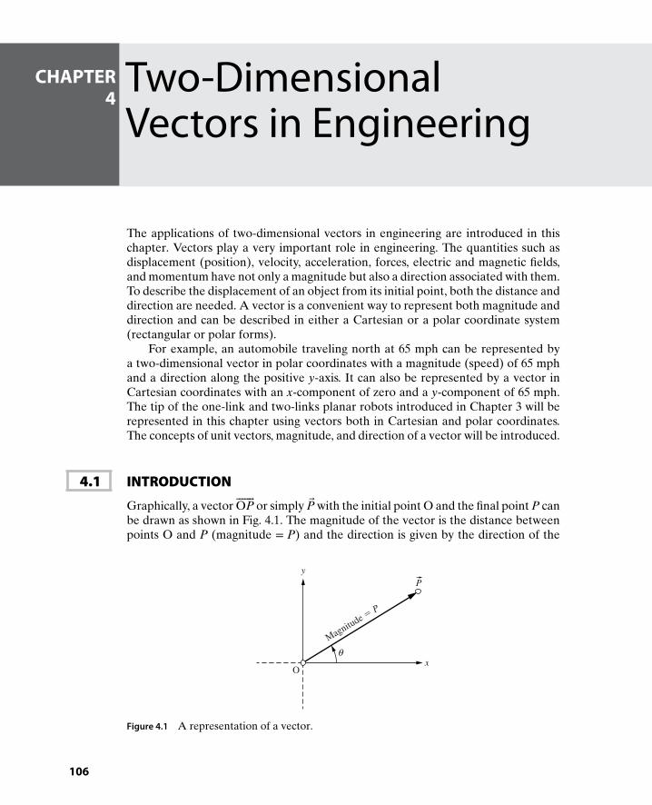
CHAPTER4
Two-DimensionalVectors in Engineering
The applications of two-dimensional vectors in engineering are introduced in thischapter. Vectors play a very important role in engineering. The quantities such asdisplacement (position), velocity, acceleration, forces, electric and magnetic fields,and momentum have not only a magnitude but also a direction associated with them.To describe the displacement of an object from its initial point, both the distance anddirection are needed. A vector is a convenient way to represent both magnitude anddirection and can be described in either a Cartesian or a polar coordinate system(rectangular or polar forms).
For example, an automobile traveling north at 65 mph can be represented bya two-dimensional vector in polar coordinates with a magnitude (speed) of 65 mphand a direction along the positive y-axis. It can also be represented by a vector inCartesian coordinates with an x-component of zero and a y-component of 65 mph.The tip of the one-link and two-links planar robots introduced in Chapter 3 will berepresented in this chapter using vectors both in Cartesian and polar coordinates.The concepts of unit vectors, magnitude, and direction of a vector will be introduced.
4.1 INTRODUCTION
Graphically, a vector OP or simply P with the initial point O and the final point P canbe drawn as shown in Fig. 4.1. The magnitude of the vector is the distance betweenpoints O and P (magnitude = P) and the direction is given by the direction of the
Ox
y
Magnitu
de = P
P
θ
Figure 4.1 A representation of a vector.
106

4.3 Position Vector in Polar Form 107
arrow or the angle 𝜃 in the counterclockwise direction from the positive x-axis asshown in Fig. 4.1. The arrow above P indicates that P is a vector. In many engineeringbooks, the vectors are also written as a boldface P.
4.2 POSITION VECTOR IN RECTANGULAR FORM
The position of the tip of a one-link robot represented as a 2-D vector P (Fig. 4.2)can be written in rectangular form as
P = Px i + Py j,
where i is the unit vector in the x-direction and j is the unit vector in the y-directionas shown in Fig. 4.2. Note that the magnitude of the unit vectors is equal to 1. Thex- and y-components, Px and Py, of the vector P are given by
Px = P cos 𝜃
Py = P sin 𝜃.
x
y
Px
Py
P
P
j
i
θ
Figure 4.2 One-link planar robot as a position vector in Cartesian coordinates.
4.3 POSITION VECTOR IN POLAR FORM
The position of the tip of a one-link robot represented as a 2-D vector P (Fig. 4.2)can be also be written in polar form as
P = P∠𝜃.
where P is the magnitude and 𝜃 is the angle or direction of the position vector P, andcan be obtained from the Cartesian components Px and Py as
P =√
P2x + P2
y
𝜃 = atan2(Py, Px).

108 Chapter 4 Two-Dimensional Vectors in Engineering
Example4-1
The length (magnitude) of a one-link robot shown in Fig. 4.2 is given as P = 0.5 mand the direction is 𝜃 = 30. Find the x- and y-components Px and Py and write Pin rectangular vector notation.
Solution The x- and y-components Px and Py are given by
Px = 0.5 cos 30
= 0.5
(√3
2
)= 0.433 m
Py = 0.5 sin 30
= 0.5(
12
)= 0.25 m.
Therefore, the position of the tip of the one-link robot can be written in vectorform as
P = 0.433 i + 0.25 j m.
Example4-2
The length of a one-link robot shown in Fig. 4.2 is given as P =√
2 m and thedirection is 𝜃 = 135. Find the x- and y-components Px and Py and write P in vectornotation.
Solution The x- and y-components Px and Py are given by
Px =√
2 cos 135 = −√
2 cos 45
= −√
2
(1√2
)= −1.0 m
Py =√
2 sin 135 =√
2 sin 45
=√
2
(1√2
)= 1.0 m.
Therefore, the position of the tip of the one-link robot can be written in vectorform as
P = −1.0 i + 1.0 j m.
Example4-3 The x- and y-components of the one-link robot are given as Px =
√3
4m and
Py = 14
m, as shown in Fig. 4.3. Find the magnitude (length) and direction of the
robot represented as a position vector P.

4.3 Position Vector in Polar Form 109
y
x
P41
4
3
P
θ
√⎯
Figure 4.3 One-link planar robot for Example 4-3.
Solution The length (magnitude) of the one-link robot is given by
P =√
P2x + P2
y
=
√√√√√(√3
4
)2
+(
14
)2
= 0.5 m
and the direction 𝜃 is given by
𝜃 = atan2
(14
,
√3
4
)
= 30.
Therefore, the position of the one-link robot P can be written in polar form as
P = 0.5∠30m.
The position of the tip can also be written in Cartesian coordinates as
P =√
34
i + 14
j m.
Example4-4
A person pushes down on a vacuum cleaner with a force of F = 20 lb at an angle of−40 relative to ground, as shown in Fig. 4.4. Determine the horizontal and verticalcomponents of the force.

110 Chapter 4 Two-Dimensional Vectors in Engineering
40 Fy
Fx
x
yF =
20 lb
Figure 4.4 A person pushing a vacuum cleaner.
Solution The x- and y-components of the force are given by
Fx = F cos (−40)
= 20 cos 40
= 15.32 lb
Fy = F sin (−40)
= −20 sin 40
= −12.86 lb.
Therefore, F = 15.32 i − 12.86 j lb.
4.4 VECTOR ADDITION
The sum of two vectors P1 and P2 is a vector P written as
P = P1 + P2. (4.1)
Vectors can be added graphically or algebraically. Graphically, the addition of twovectors can be obtained by placing the initial point of P2 on the final point of P1 andthen drawing a line from the initial point of P1 to the final point of P2, forming atriangle as shown in Fig. 4.5.
P2
O
P1
P
Figure 4.5 Graphical addition of two vectors.
Algebraically, the addition of two vectors given in equation (4.1) can be carried
out by adding the x- and y-components of the two vectors. Vectors P1 and P2 can bewritten in Cartesian form as
P1 = Px1 i + Py1 j (4.2)
P2 = Px2 i + Py2 j. (4.3)

4.4 Vector Addition 111
Substituting equations (4.2) and (4.3) into equation (4.1) gives
P = (Px1 i + Py1 j ) + (Px2 i + Py2 j )
= (Px1 + Px2) i + (Py1 + Py2) j
= Px i + Py j
where Px = Px1 + Px2 and Py = Py1 + Py2. Therefore, addition of vectors alge-braically amounts to adding their x- and y-components.
4.4.1 Examples of Vector Addition in Engineering
Example4-5
A two-link planar robot is shown in Fig. 4.6. Find the magnitude and angle of the
position of the tip of the robot if the length of the first link P1 = 1√2
m, the length
of the second link P2 = 0.5 m, 𝜃1 = 45, and 𝜃2 = −15. In other words, write P inpolar coordinates.
P1 P
45°
P2
15° P2
Py2
Py1
x
y
Px1 Px2
O
P1
P
θ
Figure 4.6 Position of two-link robot using vector addition.
Solution The x- and y-components of the first link of the planar robot P1 can be written as
Px1 = P1 cos 45
=
(1√2
) (1√2
)
= 0.5 m
Py1 = P1 sin 45
=
(1√2
) (1√2
)
= 0.5 m.

112 Chapter 4 Two-Dimensional Vectors in Engineering
Therefore, P1 = 0.5 i + 0.5 j m. Similarly, the x- and y-components of the secondlink P2 can be written as
Px2 = P2 cos 30
= 0.5
(√3
2
)= 0.433 m
Py2 = P2 sin 30
= 0.5(
12
)= 0.25 m.
Therefore, P2 = 0.433 i + 0.25 j m. Finally, since P = P1 + P2,
P = (0.5 i + 0.5 j ) + (0.433 i + 0.25 j )
= 0.933 i + 0.75 j.
The magnitude and direction of the vector P are given by
P =√
(0.933)2 + (0.75)2 = 1.197 m.
𝜃 = atan2(0.75, 0.933) = 38.79.
Therefore, P = 1.197∠38.79m.
Example4-6
A sinusoidal current is flowing through the RL circuit shown in Fig. 4.7. The voltagephasors (vector used to represent voltages and currents in AC circuits) across theresistor R = 20 Ω and inductor L = 100 mH are given as VR = 2 ∠0V and VL =3.77 ∠90V, respectively. If the total voltage phasor V across R and L is V = VR +VL, find the magnitude and phase (angle) of V.
V
VR
L = 100 mH
R = 20 Ω
i = 100 sin(120 πt) mA
++
−
−
VL
+
−
Figure 4.7 Sum of voltage phasors in an RL circuit.

4.4 Vector Addition 113
Solution The x- and y-components of the voltage phasor VR are given by
VRx = 2 cos 0
= 2.0 V
VRy = 2 sin 0
= 0 V.
Therefore, VR = 2.0 i + 0 j V. Similarly, the x- and y-components of the voltagephasor VL are given by
VLx = 3.77 cos 90
= 0 V
VLy = 3.77 sin 90
= 3.77 V.
Therefore, VL = 0 i + 3.77 j V. Finally, since V = VR + VL,
V = (2.0 i + 0 j ) + (0 i + 3.77 j )
= 2.0 i + 3.77 j V.
Thus, the magnitude and phase of the total voltage phasor V are given by
V =√
(2.0)2 + (3.77)2 = 4.27 V
𝜃 = atan2(3.77, 2.0) = 62.05.
Therefore, V = 4.27∠62.05V.
Example4-7
A ship travels 200 miles at 45 northeast, then 300 miles due east as shown inFig. 4.8. Find the resulting position of the ship.
x
N
S
EW
45°P
y
P 1 = 200
0
P2 = 300
θ
Figure 4.8 Resulting position of the ship after travel.

114 Chapter 4 Two-Dimensional Vectors in Engineering
Solution The x- and y-components of the position vector P1 are given by
Px1 = P1 cos 45
= 200
(1√2
)
= 141.4 mi
Py1 = P1 sin 45
= 200
(1√2
)
= 141.4 mi.
Therefore, P1 = 141.4 i + 141.4 j mi. Similarly, the x- and y-components of the po-sition vector P2 are given by
Px2 = P2 cos 0
= 300 (1)
= 300 mi
Py2 = P2 sin 0
= 300 (0)
= 0 mi.
Therefore, P2 = 300 i + 0 j mi. Finally, since P = P1 + P2,
P = (141.4 i + 141.4 j ) + (300 i + 0 j )
= 441.4 i + 141.4 j mi.
Thus, the distance and direction of the ship after traveling 200 miles northeast andthen 300 miles east are given by
P =√
(441.4)2 + (141.4)2 = 463.5 mi
𝜃 = atan2(141.4, 441.4) = 17.76.
Therefore, P = 463.5∠17.76 miles. In other words, the ship is now located at463.5 miles, 17.76 northeast from its original location.
Example4-8
Relative Velocity: An airplane is flying at an air speed of 100 mph at a heading of30 southeast, as shown in Fig. 4.9. If the velocity of the wind is 20 mph due west,determine the resultant velocity of the plane with respect to the ground.

4.4 Vector Addition 115
N
S
EW
30°x
y
Vag = 20
Vpa = 100
Vpg
θ
Figure 4.9 Velocity of the plane relative to ground.
Solution The x- and y-components of the velocity of the plane relative to air, Vpa, are givenby
Vxpa = Vpa cos (−30)
= 100
(√3
2
)= 86.6 mph
Vypa = Vpa sin (−30)
= −100(
12
)= −50.0 mph.
Therefore, Vpa = 86.6 i − 50.0 j mph. Similarly, the x- and y-components of the
velocity of air (wind) relative to ground Vag are given by
Vxag = Vag cos (180)
= 20 (−1)
= −20 mph
Vyag = Vag sin (180)
= 20 (0)
= 0 mph.
Therefore, Vag = −20 i + 0 j mph. Finally, the velocity of the plane relative to
ground Vpg = Vpa + Vag is given by
Vpg = (86.6 i − 50 j ) + (−20 i + 0 j )
= 66.6 i − 50 j mph.
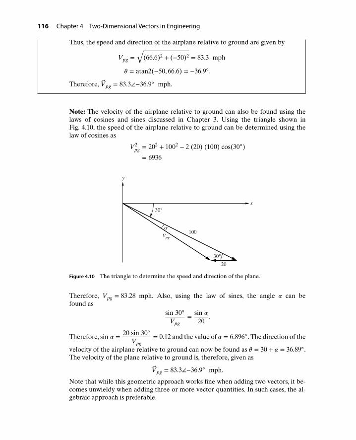
116 Chapter 4 Two-Dimensional Vectors in Engineering
Thus, the speed and direction of the airplane relative to ground are given by
Vpg =√
(66.6)2 + (−50)2 = 83.3 mph
𝜃 = atan2(−50, 66.6) = −36.9.
Therefore, Vpg = 83.3∠−36.9 mph.
Note: The velocity of the airplane relative to ground can also be found using thelaws of cosines and sines discussed in Chapter 3. Using the triangle shown inFig. 4.10, the speed of the airplane relative to ground can be determined using thelaw of cosines as
V2pg = 202 + 1002 − 2 (20) (100) cos(30)
= 6936
100
20
x
y
Vpg
30°
30°
α
Figure 4.10 The triangle to determine the speed and direction of the plane.
Therefore, Vpg = 83.28 mph. Also, using the law of sines, the angle 𝛼 can befound as
sin 30
Vpg= sin 𝛼
20.
Therefore, sin 𝛼 = 20 sin 30
Vpg= 0.12 and the value of 𝛼 = 6.896. The direction of the
velocity of the airplane relative to ground can now be found as 𝜃 = 30 + 𝛼 = 36.89.The velocity of the plane relative to ground is, therefore, given as
Vpg = 83.3∠−36.9 mph.
Note that while this geometric approach works fine when adding two vectors, it be-comes unwieldy when adding three or more vector quantities. In such cases, the al-gebraic approach is preferable.

4.4 Vector Addition 117
Example4-9
Static Equilibrium: A 100 kg object is hanging from two cables of equal length asshown in Fig. 4.11. Determine the tension in each cable.
g = 9.81 m/sec2
45° 45°
100 kg
Figure 4.11 An object hanging from two cables.
Solution The free-body diagram (FBD) of the system shown in Fig. 4.11 can be drawn asshown in Fig. 4.12.
100 kg
45°45°
T2
W = mg = (100)(9.81) = 981 N
x
y
T2 sin 45°T1 sin 45°
T2 cos 45°T1 cos 45°
T1
Figure 4.12 Free-body diagram of the system shown in Fig. 4.11.
It is assumed that the system shown in Fig. 4.11 is in static equilibrium (not accel-erating), and therefore the sum of all the forces are equal to zero (Newton’s firstlaw), i.e.,
∑F = 0
or
T1 + T2 + W = 0. (4.4)
The x- and y-components of the tension T1 are given by
Tx1 = −T1 cos 45
= −T1
(1√2
)N
Ty1 = T1 sin 45
= T1
(1√2
)N.

118 Chapter 4 Two-Dimensional Vectors in Engineering
Therefore, T1 = −T1√
2i +
T1√2
j N. Similarly, the x- and y-components of the ten-
sion T2 and weight W are given by
Tx2 = T2 cos 45
= T2
(1√2
)N
Ty2 = T2 sin 45
= T2
(1√2
)N
Wx = W cos (−90)
= 0 N
Wy = W sin (−90)
= −981 N.
Therefore, T2 =T2√
2i +
T2√2
j N and W = 0 i + −981 j N. Substituting T1, T2,
and W into equation (4.4) gives(−
T1√2
i +T1√
2j
)+
(T2√
2i +
T2√2
j
)+ (0i − 981j ) = 0
(−
T1√2+
T2√2
)i +
(T1√
2+
T2√2− 981
)j = 0. (4.5)
In equation (4.5), the x-component is the sum of the forces in the x-direction andthe y-component is the sum of forces in the y-direction. Since the right-hand sideof equation (4.5) is zero, the sum of forces in the x- and y-directions are zero, or∑
Fx = 0 and∑
Fy = 0. Therefore,
∑Fx =
(−
T1√2+
T2√2
)= 0 (4.6)
and,
∑Fy =
(T1√
2+
T2√2
)− 981 = 0. (4.7)
Adding equations (4.6) and (4.7) gives2 T2√
2= 981 or T2 = 693.7 N. Also, from
equation (4.6), T2 = T1. Therefore, both cables have the same tension, that is,T1 = T2 = 693.7 N.
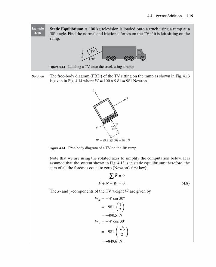
4.4 Vector Addition 119
Example4-10
Static Equilibrium: A 100 kg television is loaded onto a truck using a ramp at a30 angle. Find the normal and frictional forces on the TV if it is left sitting on theramp.
TV
g30°
Figure 4.13 Loading a TV onto the truck using a ramp.
Solution The free-body diagram (FBD) of the TV sitting on the ramp as shown in Fig. 4.13is given in Fig. 4.14 where W = 100 × 9.81 = 981 Newton.
x
FN
30°
W = (9.81)(100) = 981 N
y
Figure 4.14 Free-body diagram of a TV on the 30 ramp.
Note that we are using the rotated axes to simplify the computation below. It isassumed that the system shown in Fig. 4.13 is in static equilibrium; therefore, thesum of all the forces is equal to zero (Newton’s first law):∑
F = 0
F + N + W = 0. (4.8)
The x- and y-components of the TV weight W are given by
Wx = −W sin 30
= −981(
12
)= −490.5 N
Wy = −W cos 30
= −981
(√3
2
)= −849.6 N.
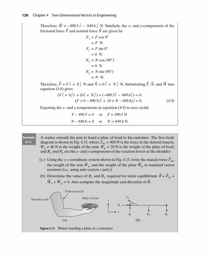
120 Chapter 4 Two-Dimensional Vectors in Engineering
Therefore, W = −490.5 i − 849.6 j N. Similarly, the x- and y-components of thefrictional force F and normal force N are given by
Fx = F cos 0
= F N
Fy = F sin 0
= 0 N
Nx = N cos (90)
= 0 N
Ny = N sin (90)
= N N.
Therefore, F = F i + 0 j N and N = 0 i + N j N. Substituting F, N, and W intoequation (4.8) gives
(F i + 0 j ) + (0 i + N j ) + (−490.5 i − 849.6 j ) = 0
(F + 0 − 490.5) i + (0 + N − 849.6) j = 0. (4.9)
Equating the x- and y-components in equation (4.9) to zero yields
F − 490.5 = 0 ⇒ F = 490.5 N
N − 849.6 = 0 ⇒ N = 849.6 N.
Example4-11
A waiter extends his arm to hand a plate of food to his customer. The free-bodydiagram is shown in Fig. 4.15, where Fm = 400 N is the force in the deltoid muscle,Wa = 40 N is the weight of the arm, Wp = 20 N is the weight of the plate of food,and Rx and Ry are the x- and y-components of the reaction forces at the shoulder.
(a ) Using the x-y coordinate system shown in Fig. 4.15, write the muscle force Fm,the weight of the arm Wa, and the weight of the plate Wp in standard vectornotation (i.e., using unit vectors i and j).
(b) Determine the values of Rx and Ry required for static equilibrium: R + Fm +Wa + Wp = 0. Also compute the magnitude and direction of R.
Plate of food
Deltoid muscle
Shoulder joint
Wa Wp
Fm
30°Rx
Ry
y
x
(a) (b)
Figure 4.15 Waiter handing a plate to a customer.
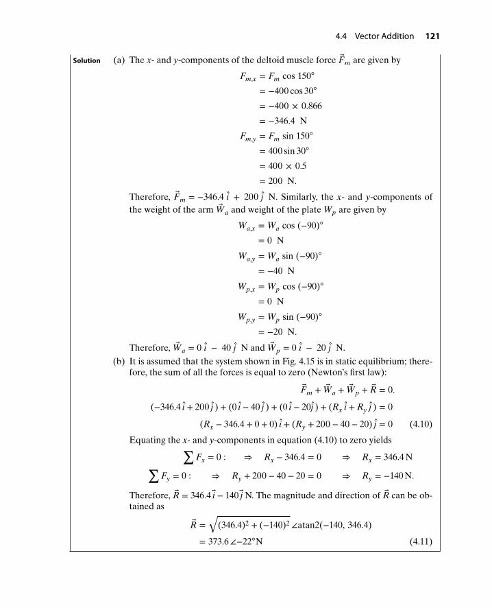
4.4 Vector Addition 121
Solution (a) The x- and y-components of the deltoid muscle force Fm are given by
Fm,x = Fm cos 150
= −400 cos 30
= −400 × 0.866
= −346.4 N
Fm,y = Fm sin 150
= 400 sin 30
= 400 × 0.5
= 200 N.
Therefore, Fm = −346.4 i + 200 j N. Similarly, the x- and y-components ofthe weight of the arm Wa and weight of the plate Wp are given by
Wa,x = Wa cos (−90)
= 0 N
Wa,y = Wa sin (−90)
= −40 N
Wp,x = Wp cos (−90)
= 0 N
Wp,y = Wp sin (−90)
= −20 N.
Therefore, Wa = 0 i − 40 j N and Wp = 0 i − 20 j N.
(b) It is assumed that the system shown in Fig. 4.15 is in static equilibrium; there-fore, the sum of all the forces is equal to zero (Newton’s first law):
Fm + Wa + Wp + R = 0.
(−346.4 i + 200 j ) + (0 i − 40 j ) + (0 i − 20j ) + (Rx i + Ry j ) = 0
(Rx − 346.4 + 0 + 0) i + (Ry + 200 − 40 − 20) j = 0 (4.10)
Equating the x- and y-components in equation (4.10) to zero yields∑Fx = 0 : ⇒ Rx − 346.4 = 0 ⇒ Rx = 346.4 N∑
Fy = 0 : ⇒ Ry + 200 − 40 − 20 = 0 ⇒ Ry = −140 N.
Therefore, R = 346.4 i − 140 j N. The magnitude and direction of R can be ob-tained as
R =√
(346.4)2 + (−140)2 ∠atan2(−140, 346.4)
= 373.6∠−22N (4.11)
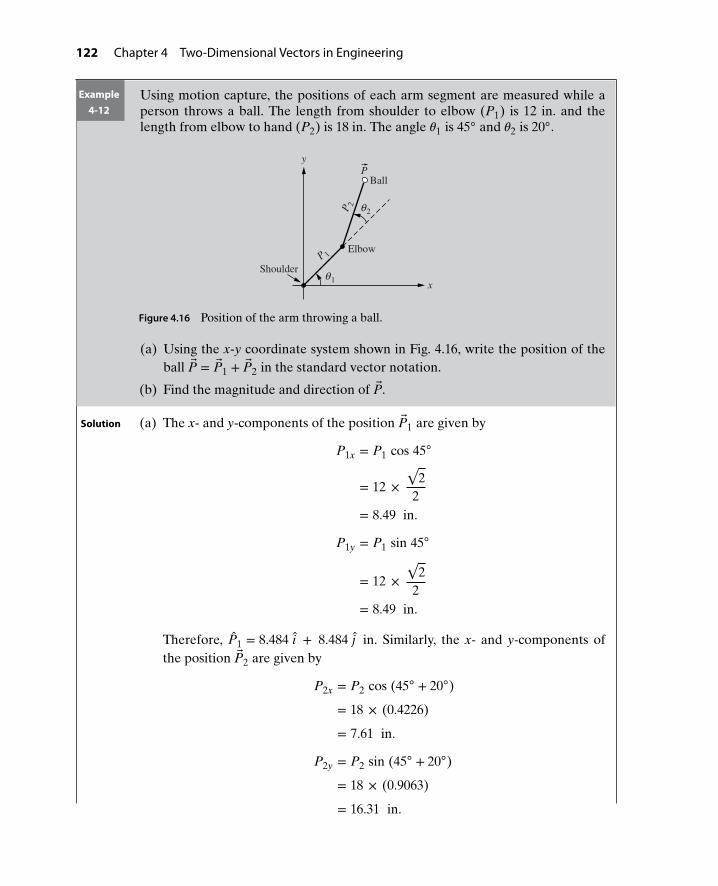
122 Chapter 4 Two-Dimensional Vectors in Engineering
Example4-12
Using motion capture, the positions of each arm segment are measured while aperson throws a ball. The length from shoulder to elbow (P1) is 12 in. and thelength from elbow to hand (P2) is 18 in. The angle 𝜃1 is 45 and 𝜃2 is 20.
Shoulder
y
Ball
ElbowP 1
P 2
x
P
2θ
1θ
Figure 4.16 Position of the arm throwing a ball.
(a) Using the x-y coordinate system shown in Fig. 4.16, write the position of theball P = P1 + P2 in the standard vector notation.
(b) Find the magnitude and direction of P.
Solution (a) The x- and y-components of the position P1 are given by
P1x = P1 cos 45
= 12 ×√
22
= 8.49 in.
P1y = P1 sin 45
= 12 ×√
22
= 8.49 in.
Therefore, P1 = 8.484 i + 8.484 j in. Similarly, the x- and y-components ofthe position P2 are given by
P2x = P2 cos (45 + 20)
= 18 × (0.4226)
= 7.61 in.
P2y = P2 sin (45 + 20)
= 18 × (0.9063)
= 16.31 in.
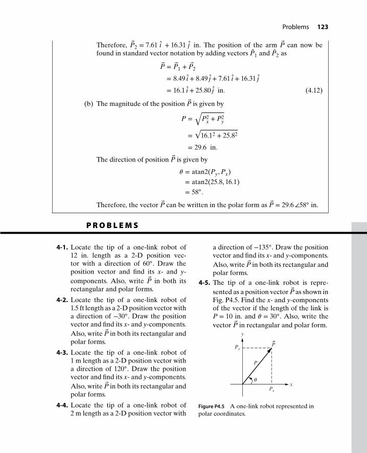
Problems 123
Therefore, P2 = 7.61 i + 16.31 j in. The position of the arm P can now befound in standard vector notation by adding vectors P1 and P2 as
P = P1 + P2
= 8.49 i + 8.49 j + 7.61 i + 16.31 j
= 16.1 i + 25.80 j in. (4.12)
(b) The magnitude of the position P is given by
P =√
P2x + P2
y
=√
16.12 + 25.82
= 29.6 in.
The direction of position P is given by
𝜃 = atan2(Py, Px)
= atan2(25.8, 16.1)
= 58.
Therefore, the vector P can be written in the polar form as P = 29.6∠58 in.
P R O B L E M S
4-1. Locate the tip of a one-link robot of12 in. length as a 2-D position vec-tor with a direction of 60. Draw theposition vector and find its x- and y-components. Also, write P in both itsrectangular and polar forms.
4-2. Locate the tip of a one-link robot of1.5 ft length as a 2-D position vector witha direction of −30. Draw the positionvector and find its x- and y-components.Also, write P in both its rectangular andpolar forms.
4-3. Locate the tip of a one-link robot of1 m length as a 2-D position vector witha direction of 120. Draw the positionvector and find its x- and y-components.Also, write P in both its rectangular andpolar forms.
4-4. Locate the tip of a one-link robot of2 m length as a 2-D position vector with
a direction of −135. Draw the positionvector and find its x- and y-components.Also, write P in both its rectangular andpolar forms.
4-5. The tip of a one-link robot is repre-sented as a position vector P as shown inFig. P4.5. Find the x- and y-componentsof the vector if the length of the link isP = 10 in. and 𝜃 = 30. Also, write thevector P in rectangular and polar form.
y
P
Py
Px
x
P
θ
Figure P4.5 A one-link robot represented inpolar coordinates.

124 Chapter 4 Two-Dimensional Vectors in Engineering
4-6. Repeat problem P4-5 if P = 14.42 cmand 𝜃 = 123.7.
4-7. Repeat problem P4-5 if P = 15 cm and𝜃 = −120.
4-8. Repeat problem P4-5 if P = 6 in. and𝜃 = −60.
4-9. The x- and y-components of a vectorP shown in Fig. P4.9 are given as Px =2 cm and Py = 3 cm. Find the magnitude
and direction, and write the vector P inits rectangular and polar forms.
y
x
P
Py
PxO
P
θ
Figure P4.9 A position vector for problem P4-9.
4-10. The x- and y-components of a vectorP shown in Fig. P4.10 are given asPx = 3 in. and Py = −4 in. Find themagnitude and direction, and write thevector P in its rectangular and polarforms.
x
y
3
4P
P
θ
Figure P4.10 A position vector for problem P4-10.
4-11. The x- and y-components of a vector Pshown in Fig. P4.11 are given as Px =−1.5 cm and Py = 2 cm. Find the magni-tude and direction, and write the vectorP in its rectangular and polar forms.
−1.5x, cm
P
y, cm
2P
θ
Figure P4.11 A position vector for problem P4-11.
4-12. The x- and y-components of a vectorP shown in Fig. P4.12 are given asPx = −1 in. and Py = −2 in. Find themagnitude and direction, and write thevector P in its rectangular and polarforms.
x, in.
y, in.
P
−1
−2P
θ
Figure P4.12 A position vector for problem P4-12.
4-13. A state trooper investigating an acci-dent pushes a wheel (shown in Fig. 4.13)to measure skid marks. If a trooper ap-plies a force of 20 lb at an angle of𝜃 = 45, find the horizontal and verticalforces acting on the wheel.
θ
Figure P4.13 A wheel to measure skid marks.

Problems 125
4-14. Repeat problem P4-13 if the trooper isapplying a force of 10 lb at an angle of𝜃 = 60.
4-15. In a RL circuit, the voltage across theinductor VL leads the voltage across theresistor by 90 as shown in Fig. P4.15. IfVR =10 V and VL = 5 V, find the totalvoltage V = VR + VL.
VR
V
R
VR = 10 V
L
V
VL = 5 V VL
++
−
−+
−θ
Figure P4.15 Voltage phasor diagram of RL circuit.
4-16. Repeat problem P4-15 if VR =10 V andVL = 15 V.
4-17. In an RC circuit, the voltage across thecapacitor VC lags the voltage across theresistor by −90 as shown in Fig. P4.17.If VR = 20 V and VC = 5 V, find thetotal voltage V = VR + VC.
VR
VC
R
CV
VR = 20 V
VC = 5 VV
+
−+
−
θ
Figure P4.17 Voltage phasor diagram of RC circuit.
4-18. Repeat problem P4-17 if VR = 10 V andVL = 20 V.
4-19. In an electrical circuit, voltage V2 lagsvoltage V1 by 30 as shown in Fig. P4.19.
30°15 V
10 V
V2
V1
Figure P4.19 Voltages V1 and V2 for problemP4-19.
Find the sum of the two voltages; inother words, find V = V1 + V2.
4-20. In an electrical circuit, voltage V2 leadsvoltage V1 by 60 as shown in Fig. P4.20.Find the sum of the two voltages; inother words, find V = V1 + V2.
10 V
20 V
60° V1
V2
Figure P4.20 Voltages V1 and V2 for problemP4-20.
4-21. An airplane travels at a heading of 45
northeast with an air speed of 300 mph.The wind is blowing at 30 southeast at aspeed of 40 mph as shown in Fig. P4.21.Find the speed (magnitude of thevelocity V) and the direction 𝜃 of theplane relative to the ground using vectoraddition. Check your answer by findingthe magnitude and direction using thelaws of sines and cosines.
y
Sx
30°
45°300
40
VW
N
E
θ
Figure P4.21 Velocity of airplane for problemP4-21.
4-22. An airplane travels at a heading of −60
with an air speed of 500 mph. The windis blowing at 30 at a speed of 50 mphas shown in Fig. P4.22. Find the speed(magnitude of the velocity V) and the
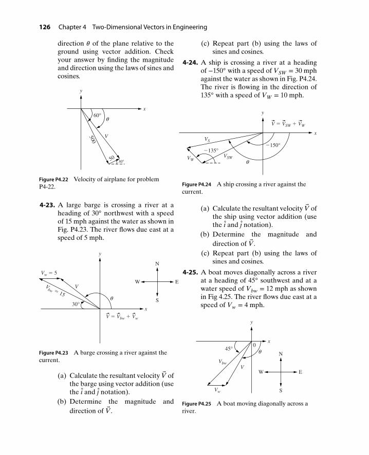
126 Chapter 4 Two-Dimensional Vectors in Engineering
direction 𝜃 of the plane relative to theground using vector addition. Checkyour answer by finding the magnitudeand direction using the laws of sines andcosines.
500
x
5030°
y
V
60°θ
Figure P4.22 Velocity of airplane for problemP4-22.
4-23. A large barge is crossing a river at aheading of 30 northwest with a speedof 15 mph against the water as shown inFig. P4.23. The river flows due east at aspeed of 5 mph.
30°
V
x
y
Vbw = 15
Vw = 5
S
W
N
E
V = Vbw + Vw
θ
Figure P4.23 A barge crossing a river against thecurrent.
(a) Calculate the resultant velocity V ofthe barge using vector addition (usethe i and j notation).
(b) Determine the magnitude anddirection of V.
(c) Repeat part (b) using the laws ofsines and cosines.
4-24. A ship is crossing a river at a headingof −150 with a speed of VSW = 30 mphagainst the water as shown in Fig. P4.24.The river is flowing in the direction of135 with a speed of VW = 10 mph.
y
x
VSWVW
VS
−150°−135°
V = VSW + VW
θ
Figure P4.24 A ship crossing a river against thecurrent.
(a) Calculate the resultant velocity V ofthe ship using vector addition (usethe i and j notation).
(b) Determine the magnitude anddirection of V.
(c) Repeat part (b) using the laws ofsines and cosines.
4-25. A boat moves diagonally across a riverat a heading of 45 southwest and at awater speed of Vbw = 12 mph as shownin Fig 4.25. The river flows due east at aspeed of Vw = 4 mph.
0
y
x
V
Vw
Vbw
S
45°
W
N
E
θ
Figure P4.25 A boat moving diagonally across ariver.

Problems 127
(a) Determine the resultant velocity
V of the boat, which is given byV = Vbw + Vw. In so doing, expressall vectors using standard vectornotation (i.e., using unit vectors iand j ). Given your result for V, alsodetermine the magnitude V anddirection 𝜃.
(b) Repeat part (a) using the laws ofsines and cosines.
4-26. A two-link planar robot is shown inFig. P4.26.(a) Calculate the position of the tip P of
the planar robot using vector addi-tion (use the i and j notation).
(b) Determine the magnitude anddirection of the position of the robottip. In other words, write vector Pin the polar form.
(c) Repeat part (b) using the laws ofsines and cosines.
O
P
x
120°
y
8
4
PP2
P1
θ
Figure P4.26 A two-link robot located for problemP4-26.
4-27. A two-link planar robot is shown inFig. P4.27.(a) Calculate the position of the tip P of
the planar robot using vector addi-tion (use the i and j notation).
(b) Determine the magnitude anddirection of P.
(c) Repeat part (b) using the laws ofsines and cosines.
O
P
y, in.
8
60°
150°7.25
x, in.
P
P1
P2
θ
Figure P4.27 A two-link robot for problem P4-27.
4-28. A two-link planar robot is shown inFig. P4.28.(a) Calculate the position of the tip P of
the planar robot using vector addi-tion (use the i and j notation).
(b) Determine the magnitude anddirection of the position of the robottip. In other words, write vector Pin the polar form.
(c) Repeat part (b) using the laws ofsines and cosines.
P
Ox, in.
y, in.
14.14
−45°
−135°
21.21
P
P1
P2
θ
Figure P4.28 A two-link robot for problem P4-28.
4-29. A two-link planar robot is shown inFig. P4.29.

128 Chapter 4 Two-Dimensional Vectors in Engineering
(a) Calculate the position of the tip P ofthe planar robot using vector addi-tion (use the i and j notation).
(b) Determine the magnitude anddirection of P.
(c) Repeat part (b) using the laws ofsines and cosines.
12
y, cm
O
−135°
30°
P
x, cm
28.28
P
P1
P2
θ
Figure P4.29 A two-link robot for problem P4-29.
4-30. A 200 lb weight is suspended by twocables as shown in Fig. P4.30.(a) Determine the angle 𝛼.
(b) Express T1 and T2 in rectangularvector notation and determine thevalues of T1 and T2 required forstatic equilibrium (i.e., T1 + T2 +W = 0).
4-31. A weight of 100 kg is suspended fromthe ceiling by cables that make 30 and60 angles with the ceiling as shown in
Fig. P4.31. Assuming that the weight isnot moving (T1 + T2 + W = 0), find thetensions T1 and T2.
60°
100 kg
30°
T1T2
g = 9.81 m/sec2
Figure P4.31 A weight suspended from two cablesfor problem P4-31.
4-32. A vehicle weighing 10 kN is parkedon an inclined driveway, as shown inFig. P4.32.(a) Determine the angle 𝜃.
(b) Express the normal force N, thefrictional force F, and the weight Win rectangular vector notation.
(c) Determine the values of F and N re-quired for equilibrium (i.e., F + N +W = 0).
4 m
FN
W = 10 kN
10 m
x
y
g θ
Figure P4.32 A vehicle parked on an inclineddriveway for problem P4-32.
45°
45°
200 lb
x
y
200 lb
10 ft5 ft
T1 T2
α
α
Figure P4.30 A weight suspended from two cables for problem P4-30.

Problems 129
4-33. A vehicle weighing 2000 lb is parkedon an inclined driveway, as shown inFig. P4.33.(a) Determine the angle 𝜃.
(b) Express the normal force N, thefrictional force F, and the weight Win rectangular vector notation.
(c) Determine the values of F and Nrequired for equilibrium (i.e., F +N + W = 0).
10 ft
FN
W = 2000 lb
17.32 ft
x
y
θ
Figure P4.33 A vehicle parked on an inclineddriveway for problem P4-33.
4-34. A crate of weight W = 100 lb sits ona ramp oriented at 27 degrees relativeto ground, as shown in Fig. P4.34. Thefree-body diagram showing the externalforces is also shown in Fig. P4.34.(a) Using the x-y coordinate system
shown in Fig. P4.34, write the fric-tion force F and the normal force Nin rectangular vector notation (i.e.,in terms of unit vectors i and j ).
(b) Determine the values of F and Nrequired for static equilibrium; inother words, find the values of F andN if F + N + W = 0.
100 lb
W
FN27°
x
y
Figure P4.34 A crate resting on a ramp for problemP4-34.
4-35. A 500 N television sits on an inclinedramp, as shown in Fig. P4.35. Thefree-body diagram showing the externalforces is also shown in Fig. P4.35.(a) Determine the angle 𝜃.(b) Using the x-y coordinate system
shown in Fig. P4.35, write the fric-tion force F and the normal force Nin rectangular vector notation (i.e.,in terms of unit vectors i and j ).
(c) Determine the values of F and Nrequired for static equilibrium; inother words, find the values of F andN if F + N + W = 0.
W
FN
8.66 ft
15 ft
500 N
x
y
θ
Figure P4.35 A crate resting on an inclined rampfor problem P4-35.
4-36. A two-bar truss supports a weight ofW = 750 lb as shown in Fig. P4.36. Thetruss is constructed such that 𝜃 = 38.7.(a) Using the positive x-y coordinate
system shown in Fig. P4.36, writethe forces F1, F2, and weight W inrectangular vector notation (i.e., interms of unit vectors i and j ).
(b) Determine the values of F1 and F2
such that F1 + F2 + W = 0.
4-37. A two-bar truss is subjected to a verticalload P = 346 lb, as shown in Fig. P4.37.The truss is constructed such that 𝜃1 =39.6 and 𝜃2 = 62.4.(a) Using the positive x-y coordinate
system shown in Fig. P4.37, writethe forces F1, F2, and P in rectan-gular vector notation (i.e., in termsof unit vectors i and j ).
(b) Determine the values of F1 and F2
such that F1 + F2 + P = 0.
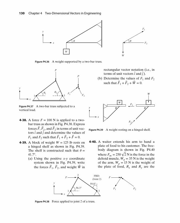
130 Chapter 4 Two-Dimensional Vectors in Engineering
W
x
yF1
F2
W
θ θ
Figure P4.36 A weight supported by a two-bar truss.
31
P
P
F1 F2
x
y
1θ 2θ
Figure P4.37 A two-bar truss subjected to avertical load.
4-38. A force F = 100 N is applied to a two-bar truss as shown in Fig. P4.38. Expressforces F, F1, and F2 in terms of unit vec-tors i and j and determine the values ofF1 and F2 such that F1 + F2 + F = 0.
4-39. A block of weight W = 125 lb rests ona hinged shelf as shown in Fig. P4.39.The shelf is constructed such that 𝜃 =41.7.(a) Using the positive x-y coordinate
system shown in Fig. P4.39, writethe forces F1, F2, and weight W in
rectangular vector notation (i.e., interms of unit vectors i and j ).
(b) Determine the values of F1 and F2
such that F1 + F2 + W = 0.
W
x
y
W
F1
F2
θ θ
Figure P4.39 A weight resting on a hinged shelf.
4-40. A waiter extends his arm to hand aplate of food to his customer. The free-body diagram is shown in Fig. P4.40where Fm = 250
√2 N is the force in the
deltoid muscle, Wa = 35 N is the weightof the arm, Wp = 15 N is the weight ofthe plate of food, Rx and Ry are the
F2
31
59.0°56.3°
FBD:
(Joint 2)
x
y
F1 F2
F
Figure P4.38 Force applied to joint 2 of a truss.

Problems 131
Plate of food
Deltoid muscle
Shoulder joint
y
x
Fm
Rx
Ry Wa Wp
θ
Figure P4.40 Waiter handing a plate to a customer.
x- and y-components of the reactionforces at the shoulder, and 𝜃 = 45.(a) Using the x-y coordinate system
shown in Fig. P4.40, write the del-toid muscle force Fm, the weight ofthe arm Wa, and the weight of theplate Wp in the standard vector no-tation (i.e., using unit vectors i andj).
(b) Determine the values of Rx andRy required for static equilibrium:
R + Fm + Wa + Wp = 0. Also com-pute the magnitude and directionof R.
4-41. Repeat problem P4-40 if Fm = 50 lb,Wa = 7 lb, Wp = 3 lb, and 𝜃 = 30
4-42. Using motion capture, the positions P1
and P2 of each arm segment are mea-sured while a person throws a ball. Thelength from shoulder to elbow (P1) is10 in. and the length from elbow to thehand holding the ball (P2) is 13 in. Theangle 𝜃1 is 60 and 𝜃2 is 65.
(a) Using the x-y coordinate systemshown in Fig. P4.42, write the posi-tion of the ball P = P1 + P2 in stan-dard vector notation.
(b) Determine both the magnitude anddirection of P.
x
y
Shoulder
Ball
Elbow
P2
P1
P
1θ
2θ
Figure P4.42 Position of the arm throwing a ball.
4-43. Repeat problem P4-42 if P1 = 1 ft, P2 =1.5 ft, 𝜃1 = 45, and 𝜃2 is 60.
CHAPTER5
Complex Numbersin Engineering
5.1 INTRODUCTIONComplex numbers play a significant role in all engineering disciplines, and a goodunderstanding of this topic is necessary. However, it is especially important for theelectrical engineer to master this topic. Although imaginary numbers are not com-monly used in daily life, in engineering and physics they are in fact used to representphysical quantities such as impedance of RL, RC, or RLC circuit.
Complex numbers are numbers that consist of two parts, one real and one imag-inary. An imaginary number is the square root of a negative real number (−1). Thesquare root of a negative real number is said to be imaginary because there is no realnumber that gives a negative number after it has been squared. The imaginary num-ber
√−1 is represented by the letter i by mathematicians and by almost all the engi-
neering disciplines except electrical engineering. Electrical engineers use the letter jto represent imaginary number because the letter i is used in electrical engineeringto represent current. To remove this confusion,
√−1 will be represented by the letter
j throughout this chapter.In general, imaginary numbers are used in combination with a real number to
form a complex number, a + bj, where a is the real part (real number) and bj is theimaginary part (real number times the imaginary unit j). The complex number isuseful for representing two-dimensional variables where both dimensions are phys-ically significant and are represented on a complex number plane (which looks verysimilar to the Cartesian plane discussed in Chapter 4). On this plane, the imaginarypart of the complex number is measured by the vertical axis (on the Cartesian plane,this is the y-axis) and the real number part goes on the horizontal axis (x-axis on theCartesian plane). The one-link robot discussed in Chapter 3 could be described usinga complex number where the real part would be its component in the x-directionand the imaginary part would be its component in the y-direction. Note that theexample of one-link planar robot is used only to show similarities between the two-dimensional vector and the complex number. The position of the tip of the robot isgenerally not described by a complex number.
In many ways, operations with complex numbers follow the same rules as thosefor real numbers. However, the two parts of a complex number cannot be combined.
132
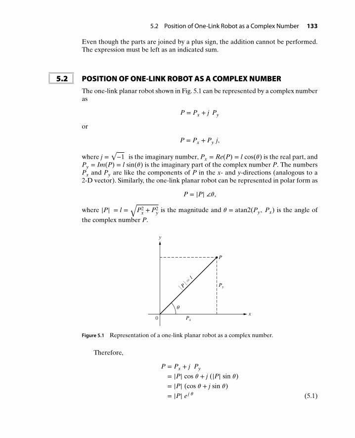
5.2 Position of One-Link Robot as a Complex Number 133
Even though the parts are joined by a plus sign, the addition cannot be performed.The expression must be left as an indicated sum.
5.2 POSITION OF ONE-LINK ROBOT AS A COMPLEX NUMBERThe one-link planar robot shown in Fig. 5.1 can be represented by a complex numberas
P = Px + j Py
or
P = Px + Py j,
where j =√−1 is the imaginary number, Px = Re(P) = l cos(𝜃) is the real part, and
Py = Im(P) = l sin(𝜃) is the imaginary part of the complex number P. The numbersPx and Py are like the components of P in the x- and y-directions (analogous to a2-D vector). Similarly, the one-link planar robot can be represented in polar form as
P = |P| ∠𝜃,
where |P| = l =√
P2x + P2
y is the magnitude and 𝜃 = atan2(Py, Px) is the angle of
the complex number P.
xPx
Py
P
y
0
∣ P ∣ =
l
θ
Figure 5.1 Representation of a one-link planar robot as a complex number.
Therefore,
P = Px + j Py
= |P| cos 𝜃 + j (|P| sin 𝜃)
= |P| (cos 𝜃 + j sin 𝜃)
= |P| e j 𝜃 (5.1)

134 Chapter 5 Complex Numbers in Engineering
where cos 𝜃 + j sin 𝜃 = e j𝜃 is Euler’s formula. The complex number written as inequation (5.1) is known as the exponential form of the complex number and canbe used to express the cosine and sine functions. The cosine function is the real partof the exponential function and the sine function as the imaginary part of the expo-nential function; i.e.,
cos𝜃 = Re(e j 𝜃)
and
sin𝜃 = Im(e j 𝜃)
In summary, a point P in the rectangular plane (x-y plane) can be described as avector or a complex number as
P = Px i + Py j⋯⋯ vector form
P = Px + j Py ⋅ ⋅⋯⋯ complex number in rectangular form
P = |P| ∠𝜃 ⋅ ⋅ ⋅ ⋅⋯⋯ complex number in polar form
P = |P| e j 𝜃 ⋅ ⋅ ⋅ ⋯⋯ complex number in exponential form
5.3 IMPEDANCE OF R, L, AND C AS A COMPLEX NUMBER5.3.1 Impedance of a Resistor R
The impedance of the resistor shown in Fig. 5.2 can be written as ZR = R Ω, whereR is the resistance in ohms (Ω). If R = 100 Ω, the impedance of the resistor can bewritten as a complex number in rectangular and polar forms as
ZR = R Ω= 100 Ω= 100 + j 0 Ω= 100 ∠0Ω= 100 e j 0Ω.
R
Figure 5.2 A resistor.
5.3.2 Impedance of an Inductor L
The impedance of the inductor shown in Fig. 5.3 can be written as ZL = j𝜔L Ω, whereL is the inductance in henry (H) and 𝜔 = 2𝜋f is the angular frequency in rad/s (f isthe linear frequency or frequency in hertz (Hz)). If L = 25 mH and f = 60 Hz, theimpedance of the inductor can be written as a complex number in rectangular and

5.3 Impedance of R, L, and C as a Complex Number 135
polar forms as
ZL = j 𝜔 L Ω
= j (2 𝜋 60) (0.025) Ω
= 0 + j 9.426 Ω
= 9.426 ∠90Ω
= 9.426 e j 90Ω.
L
Figure 5.3 An inductor.
5.3.3 Impedance of a Capacitor C
The impedance of the capacitor shown in Fig. 5.4 can be written as ZC = 1j𝜔C
Ω,
where C is the capacitance in farad (F) and 𝜔 is the angular frequency in rad/s. IfC = 20 𝜇F and f = 60 Hz, the impedance of the capacitor can be written as a complexnumber in rectangular form as
ZC = 1j 𝜔 C
Ω
= 0 + 1j (120 𝜋) (20 ∗ 10−6)
Ω
= 0 + 132.6j
Ω
= 0 + 132.6j
(jj) Ω
= 0 +132.6 j
j2Ω
= 0 − 132.6 j Ω
where j2 = (√−1)2 = −1. The impedance of the capacitor can also be written in polar
and exponential form as
ZC = 132.6 ∠−90Ω
= 132.6 e−j 90Ω.
C
Figure 5.4 A capacitor.

136 Chapter 5 Complex Numbers in Engineering
5.4 IMPEDANCE OF A SERIES RLC CIRCUITThe total impedance of the series RLC circuit shown in Fig. 5.5 is given by
ZT = ZR + ZL + ZC (5.2)
where ZR = R Ω, ZL = j𝜔L Ω, and ZC = 1j𝜔C
Ω.
L
R
C
Figure 5.5 A series RLC circuit.
For the values of R = 100 Ω, L = 25 mH, C = 20 𝜇F, and 𝜔 = 120𝜋 rad/s, theimpedance of R, L, and C were calculated in Section 5.3 as
ZR = 100 + j 0 ΩZL = 0 + j 9.426 ΩZC = 0 − j 132.6 Ω.
Since ZT = ZR + ZL + ZC, the total impedance of the series RLC circuit can be cal-culated as
ZT = (100 + j 0) + (0 + j 9.426) + (0 − j 132.6) Ω= (100 + 0 + 0) + j (0 + 9.426 + (−132.6)) Ω= 100 − j 123.174 Ω.
Therefore, the total impedance of the series RLC circuit shown in Fig. 5.5 in rectan-gular form is ZT = 100 − j 123.174 Ω. The polar and exponential forms of the totalimpedance can be calculated from the rectangular form as
Polar Form: ZT = |ZT | ∠𝜃, where
|ZT | = √1002 + (−123.174)2
= 158.7 Ω𝜃 = atan2(−123.174, 100)
= −50.93.
Therefore, ZT = 158.7 ∠−50.93Ω.
Exponential Form: ZT = |ZT | e j 𝜃 = 158.7 e−j 50.93Ω.
Note: The addition and subtraction of complex numbers is best done in the rectan-gular form. If the complex numbers are given in the polar or exponential form, they
5.5 Impedance of R and L Connected in Parallel 137
should be converted to rectangular form to carry out the addition or subtraction ofthese complex numbers. However, if the result is needed in the polar or exponentialform, the conversion from the rectangular to polar or exponential forms is carriedout as a last step.
In summary, the addition and subtraction of two complex numbers can be carriedout using the following steps.
Addition of Two Complex Numbers: The addition of two complex numbers Z1 =a1 + j b1 and Z2 = a2 + j b2 can be obtained as
Z = Z1 + Z2
= (a1 + j b1) + (a2 + j b2)
= (a1 + a2) + j (b1 + b2)
= a + j b.
Therefore, the real part, a, of the addition of complex numbers, Z, is obtained byadding the real parts of the complex numbers being added, and the imaginary partof the addition of the two complex numbers is obtained by adding the imaginaryparts of complex numbers being added.
Subtraction of Two Complex Numbers: Similarly, the subtraction of the two com-plex numbers Z1 and Z2 can be obtained as
Z = Z1 − Z2
= (a1 + j b1) − (a2 + j b2)
= (a1 − a2) + j (b1 − b2)
= c + j d.
Therefore, the real part, c, of the subtraction of two complex numbers Z1 and Z2(Z1 − Z2) is obtained by subtracting the real part a2 of complex numbers Z2 fromthe real part a1 of complex number Z1. Similarly, the imaginary part of the subtrac-tion of the two complex numbers Z1 − Z2 is obtained by subtracting the imaginarypart b2 of complex number Z2 from the imaginary part b1 of complex number Z1,respectively.
5.5 IMPEDANCE OF R AND L CONNECTED IN PARALLELThe total impedance Z of a resistor R connected in parallel with an inductor L asshown in Fig. 5.6 is given by
Z =ZR ZL
ZR + ZL
where ZR = R Ω and ZL = j𝜔L Ω.

138 Chapter 5 Complex Numbers in Engineering
RZ
ZRZL
L
Figure 5.6 A parallel RL circuit.
For R = 100 Ω, L = 25 mH and𝜔 = 120 𝜋 rad/s, the impedances of R and L werecalculated in Section 5.3 as
ZR = 100 + j 0 Ω= 100 e j 0Ω
ZL = 0 + j 9.426 Ω= 9.426 e j 90Ω.
Since Z =ZR ZL
ZR + ZL, the total impedance of the R connected in parallel with L can
be calculated as
ZT =(100 e j 0)(9.426 e j 90)
(100 + j 0) + (0 + j 9.426)
= 942.6 e j 90
100 + j 9.426
= 942.6 e j 90
100.443 e j 5.384
= 9.384 e j 84.62
= 9.384 ∠84.62.
Therefore, the total impedance of a 100 Ω resistor connected in parallel with a25 mH inductor in the polar form is Z = 9.384 ∠84.62Ω. The rectangular form ofthe total impedance can be calculated from the polar form as
Z = 9.384 cos(84.62) + j 9.384 sin(84.62)
= 0.88 + j 9.34 Ω.
Therefore, Z = 0.88 + j 9.34 Ω.Note that the multiplication and division of complex numbers can be carried
out in rectangular or polar forms. However, it will be shown in Section 5.7 that it isbest to carry out these operations in polar form. If the complex numbers are givenin rectangular form, they should be converted to polar form and the result of themultiplication or division is then obtained in the polar form. However, if the result isneeded in rectangular form, the conversion from polar to rectangular form is carried
5.5 Impedance of R and L Connected in Parallel 139
out as a last step. The steps to carry out the multiplication and division in the polarform are explained next.
Multiplication of Complex Number in Polar Form: The multiplication of the twocomplex numbers Z1 = M1 ∠𝜃1 and Z2 = M2 ∠𝜃2 can be carried out as
Z = Z1 ∗ Z2
= M1 ∠𝜃1 ∗ M2 ∠𝜃2
= M1 e j∠𝜃1 ∗ M2 e j∠𝜃2
= (M1 M2) e j∠(𝜃1+𝜃2)
= (M1 M2) ∠(𝜃1 + 𝜃2)
= |Z| ∠𝜃.
Therefore, the magnitude |Z| of the multiplication of complex numbers given inpolar form is obtained by multiplying the magnitudes of complex numbers beingmultiplied and the angle ∠𝜃 of the resultant is the sum of the angles of the complexnumbers being multiplied. Note that this procedure is not restricted to multiplicationof two numbers only; it can be used for multiplying any number of complex numbers.
Division of Complex Number in Polar Form: The division of the two complex num-bers Z1 and Z2 in the polar form can be carried out as
Z =Z1
Z2
=M1 ∠𝜃1
M2 ∠𝜃2
=M1 e j∠𝜃1
M2 e j∠𝜃2
=M1
M2e j (∠(𝜃1−𝜃2))
=M1
M2∠(𝜃1 − 𝜃2)
= |Z| ∠𝜃.
Therefore, the magnitude |Z| of the division of two complex numbers given in polarform is obtained by dividing the magnitudes of dividend complex number Z1 by themagnitude of divisor complex number Z2. The angle ∠𝜃 of the resultant is obtainedby subtracting the angle of the divisor complex numbers Z2 from the angle of thedividend complex number Z1. Note that if the dividend or the divisor are the productof complex numbers, the product of all the dividend and the divisor complex numbers
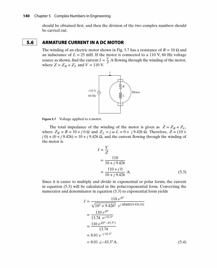
140 Chapter 5 Complex Numbers in Engineering
should be obtained first, and then the division of the two complex numbers shouldbe carried out.
5.6 ARMATURE CURRENT IN A DC MOTORThe winding of an electric motor shown in Fig. 5.7 has a resistance of R = 10 Ω andan inductance of L = 25 mH. If the motor is connected to a 110 V, 60 Hz voltagesource as shown, find the current I = V
ZA flowing through the winding of the motor,
where Z = ZR + ZL and V = 110 V.
I
Motor
R
L
110 V
60 Hz
Figure 5.7 Voltage applied to a motor.
The total impedance of the winding of the motor is given as Z = ZR + ZL,where ZR = R = 10 + j 0 Ω and ZL = j 𝜔 L = 0 + j 9.426 Ω. Therefore, Z = (10 +j 0) + (0 + j 9.426) = 10 + j 9.426 Ω, and the current flowing through the winding ofthe motor is
I = VZ
= 11010 + j 9.426
=110 + j 0
10 + j 9.426A. (5.3)
Since it is easier to multiply and divide in exponential or polar forms, the currentin equation (5.3) will be calculated in the polar/exponential form. Converting thenumerator and denominator in equation (5.3) to exponential form yields
I = 110 e j0√102 + 9.4262 e j atan2(9.426,10)
= 110 e j0
13.74 e j 43.3
= 110 e j(0−43.3)
13.74
= 8.01 e−j 43.3
= 8.01 ∠−43.3A. (5.4)

5.7 Further Examples of Complex Numbers in Electric Circuits 141
Therefore, the current flowing through the winding of the motor is 8.01 A. Thephasor diagram (vector diagram) showing the voltage and current vectors is shownin Fig. 5.8. It can be seen from Fig. 5.8 that the current is lagging (negative angle)the voltage by 43.3. The polar form of the current given in equation (5.4) can beconverted to rectangular form as
I = 8.01 e−j 43.3
= 8.01 (cos 43.3 − j sin 43.3)
= 5.83 − j 5.49 A.
Note: In general e± 𝜃 = cos 𝜃 ± j sin 𝜃 requires 𝜃 in radians. However, converting toradians is unnecessary for the purpose of multiplying and dividing complex numbers.
43.3°
110 V
8.01 A
V
I
Figure 5.8 The current and voltage vector.
5.7 FURTHER EXAMPLES OF COMPLEXNUMBERS IN ELECTRIC CIRCUITS
Example5-1
A current, I, flowing through the RL circuit shown in Fig. 5.9 produces a voltage,V = I Z, where Z = R + j XL. Find V if I = 0.1 ∠30A.
V↑I
R = 100 Ω
XL = 30 Ω
−
+
Figure 5.9 Current flowing through an RL circuit.
Solution The impedance Z of the RL circuit can be calculated as
Z = R + j XL Ω
= 100 + j 30 Ω.
The voltage V = I Z = (0.1 ∠30)(100 + j 30) V will be calculated by multiply-ing the two complex numbers using their rectangular forms as well as theirpolar/exponential forms to show that it is much easier to multiply complex num-bers using the polar/exponential forms.

142 Chapter 5 Complex Numbers in Engineering
Rectangular Form Polar/Exponential Form
I = 0.1 ∠30 I = 0.1 ∠30 = 0.1 e j 30A
= 0.1 (cos 30 + j sin 30) Z = 100 + j 30
= 0.0866 + j 0.05 A =√
1002 + 302 ∠atan2 (30, 100)
Z = 100 + j 30 Ω = 104.4 ∠16.7 = 104.4 e j 16.7Ω
V = I Z V = I Z
= (0.0866 + j 0.05)(100 + j 30) = (0.1 e j 30)(104.4 e j 16.7)
= 8.66 + j 2.598 + j 5 + 1.5 j 2 = (10.44) e j(30+16.7)
= 8.66 + j 2.598 + j 5 + 1.5 (−1) = (10.44) ∠46.7V
= 7.16 + j 7.598
= 10.44 ∠46.7V
Example5-2
In the voltage divider circuit shown in Fig. 5.10, the impedance of the resistor isgiven by Z1 = R. The total impedance of the inductor and capacitor in series isgiven by Z2 = j XL + 1
jXC, where j =
√−1. Suppose R = 10, XL = 10, and XC =
20, all measured in ohms:
(a) Express the impedance Z1 and Z2 in both rectangular and polar forms.
(b) Suppose the source voltage is V = 100√
2∠45V. Compute the voltage V1given by
V1 =Z2
Z1 + Z2V. (5.5)
V
R
C
L
V1
+
−
Figure 5.10 Voltage divider circuit for Example 5-2.
Solution (a) The impedance Z1 can be written in rectangular form as
Z1 = R
= 10 + j 0 Ω.
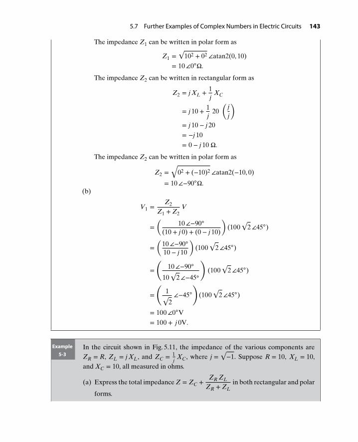
5.7 Further Examples of Complex Numbers in Electric Circuits 143
The impedance Z1 can be written in polar form as
Z1 =√
102 + 02 ∠atan2(0, 10)
= 10∠0Ω.
The impedance Z2 can be written in rectangular form as
Z2 = j XL + 1j
XC
= j 10 + 1j
20(
jj
)= j 10 − j 20
= −j 10
= 0 − j 10 Ω.
The impedance Z2 can be written in polar form as
Z2 =√
02 + (−10)2 ∠atan2(−10, 0)
= 10∠−90Ω.(b)
V1 =Z2
Z1 + Z2V
=(
10∠−90
(10 + j 0) + (0 − j 10)
)(100
√2∠45)
=(
10∠−90
10 − j 10
)(100
√2∠45)
=
(10∠−90
10√
2∠−45
)(100
√2∠45)
=
(1√2∠−45
)(100
√2∠45)
= 100∠0V
= 100 + j 0V.
Example5-3
In the circuit shown in Fig. 5.11, the impedance of the various components areZR = R, ZL = j XL, and ZC = 1
jXC, where j =
√−1. Suppose R = 10, XL = 10,
and XC = 10, all measured in ohms.
(a) Express the total impedance Z = ZC +ZR ZL
ZR + ZLin both rectangular and polar
forms.

144 Chapter 5 Complex Numbers in Engineering
(b) Suppose a voltage V = 50√
2∠45V is applied to the circuit shown in Fig. 5.11.Find the current I flowing through the circuit if I given by
I = VZ
(5.6)
Solution (a) The impedance ZR can be written in rectangular and polar forms as
ZR = R
= 10 + j 0 Ω= 10∠0Ω.
Z
C
LR
Figure 5.11 Total impedance of the circuit for Example 5-3.
The impedance ZL can be written in rectangular and polar forms as
ZL = j XL
= 0 + j 10 Ω= 10∠90Ω.
The impedance ZC can be written in rectangular and polar forms as
ZC = 1j
XC
= −j XC
= 0 − j 10 Ω= 10∠−90Ω.
The total impedance can now be calculated as
Z = ZC +ZR ZL
ZR + ZL
= 0 − j 10 +(10∠0) (10∠90)
(10 + j 0) + (0 + j 10)
= 0 − j 10 + 100∠90
(10 + j 10)

5.8 Complex Conjugate 145
= 0 − j 10 + 100∠90
10√
2∠45
= 0 − j 10 + 5√
2∠45
= 0 − j 10 + 5 + j 5
= 5 − j 5 Ω
= 5√
2∠−45Ω.
(b)
I = VZ
= 50√
2∠45
5√
2∠−45
= 10∠90A
= 0 + j 10 A.
Example5-4
A sinusoidal voltage source vs = 100 cos(100 t + 45) V is applied to a series RLCcircuit. Write the voltage source vs in the exponential form.
Solution Since cos(𝜃) = Re(e j 𝜃), therefore, the voltage source vs can be written in theexponential form as
vs = Re(100 e j(100 t+45))V.
Example5-5
A sinusoidal current source is = 100 sin(120𝜋 t + 60) mA is applied to a parallelRL circuit. Write the current source is in the exponential form.
Solution Since sin(𝜃) = Im(e j 𝜃), therefore, the current source is can be written in the expo-nential form as
is = Im(100 e j(120𝜋 t+60))mA.
5.8 COMPLEX CONJUGATEThe complex conjugate of a complex number z = a + j b is
z∗ = a − j b.
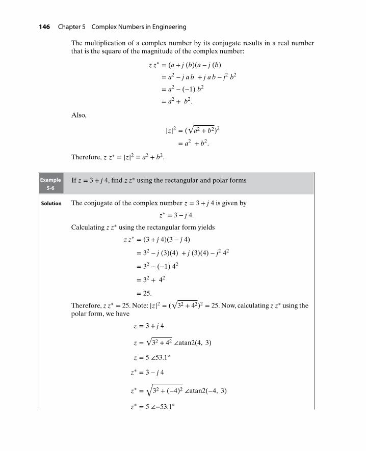
146 Chapter 5 Complex Numbers in Engineering
The multiplication of a complex number by its conjugate results in a real numberthat is the square of the magnitude of the complex number:
z z∗ = (a + j (b)(a − j (b)
= a2 − j a b + j a b − j2 b2
= a2 − (−1) b2
= a2 + b2.
Also,
|z|2 = (√
a2 + b2)2
= a2 + b2.
Therefore, z z∗ = |z|2 = a2 + b2.
Example5-6
If z = 3 + j 4, find z z∗ using the rectangular and polar forms.
Solution The conjugate of the complex number z = 3 + j 4 is given by
z∗ = 3 − j 4.
Calculating z z∗ using the rectangular form yields
z z∗ = (3 + j 4)(3 − j 4)
= 32 − j (3)(4) + j (3)(4) − j2 42
= 32 − (−1) 42
= 32 + 42
= 25.
Therefore, z z∗ = 25. Note: |z|2 = (√
32 + 42)2 = 25. Now, calculating z z∗ using thepolar form, we have
z = 3 + j 4
z =√
32 + 42 ∠atan2(4, 3)
z = 5 ∠53.1
z∗ = 3 − j 4
z∗ =√
32 + (−4)2 ∠atan2(−4, 3)
z∗ = 5 ∠−53.1

Problems 147
z z∗ = (5 ∠53.1)(5 ∠−53.1)
= (5)(5)∠(53.1 − 53.1)
= 25 ∠0
= 25.
Therefore, z z∗ = 25. Note that the complex conjugate of a complex number inpolar form has the same magnitude as the complex number, but the angle of thecomplex conjugate is the negative of the angle of the complex number.
P R O B L E M S
5-1. In the series RL circuit shown inFig. P5.1, voltage VL leads voltage VRby 90 (i.e., if the angle of VR is 0, theangle of VL is 90). Assume VR =1 ∠0V and VL = 1 ∠90V.(a) Write VR and VL in rectangular
form.(b) Determine V = VR + VL in both its
rectangular and polar forms.(c) Write the real and imaginary parts
of V.
VR
L
R
V
VL
+
−
+
−
Figure P5.1 A series RL circuit for problem P5-1.
5-2. Repeat problem P5-1 if VR =10 ∠−45V and VL = 5 ∠45V.
5-3. Repeat problem P5-1 if VR =9 ∠−26.6V and VL = 4.5 ∠63.4V.
5-4. In the RC circuit shown in Fig. P5.4,voltage VC lags voltage VR by 90 (i.e.,if the angle of VR is 0, the angle of
VC is −90). Assume VR = 1 ∠0V andVC = 1 ∠−90V.(a) Write VR and VC in rectangular
form.(b) Determine V = VR + VC in both its
rectangular and polar forms.(c) Write the real and imaginary parts
of V.
VR
C
R
V
VC
+
−
+
−
Figure P5.4 RC circuit for problem P5-4.
5-5. Repeat problem P5-4 if VR = 9.5∠18.44V and VC = 3.16 ∠−71.56V.
5-6. Repeat problem P5-4 if VR = 10 ∠60Vand VC = 17.32 ∠−30V.
5-7. In the parallel RL circuit shown inFig. P5.7, the total current I is the sum ofthe currents flowing through the resistor(IR) and the inductor (IL). Assume iR =100 ∠0mA and iL = 200 ∠−90mA.(a) Write IR and IL in rectangular form.

148 Chapter 5 Complex Numbers in Engineering
(b) Determine I = IR + IL in both itsrectangular and polar forms.
(c) Write the real and imaginary partsof I.
RLI
IL IR
↑
Figure P5.7 A parallel RL circuit for problem P5-7.
5-8. Repeat problem P5-7 if IR =0.707 ∠45A and IL = 0.707 ∠−45A.
5-9. Repeat problem P5-7 if IR =86.6 ∠30𝜇A and IL = 50 ∠−60𝜇A.
5-10. In the parallel RC circuit shown inFig. P5.10, the total current I is thesum of the currents flowing through theresistor (IR) and the capacitor (IC).Assume IR = 83.2 ∠−33.7mA and IC =55.5 ∠56.3mA.(a) Write IR and IL in rectangular form.(b) Determine I = IR + IL in both its
rectangular and polar forms.(c) Write the real and imaginary parts
of I.
C RI
IC IR
↑
Figure P5.10 A parallel RC circuit for problemP5-10.
5-11. Repeat problem P5-10 if IR = 0.5∠0mA and IC = 0.2 ∠90mA.
5-12. Repeat problem P5-10 if IR = 0.929∠−21.8A and IC = 0.37 ∠68.2A.
5-13. The output voltage across the capacitorin a series RLC circuit is measured by anoscilloscope as vo(t) = 15 cos(120𝜋 t −60) V. Write the voltage vo(t) in theexponential form.
5-14. The current flowing through the resis-tor in a parallel RL circuit is givenas iR(t) = 5 sin(5𝜋 t + 30) mA. Writethe current iR(t) in the exponentialform.
5-15. A resistor, capacitor, and an induc-tor are connected in series as shownin Fig. P5.15. The total impedanceof the circuit is Z = ZR + ZL + ZC,where ZR = R Ω, ZL = j𝜔L Ω, and
ZC = 1j 𝜔 C
Ω. For a particular design
R = 100 Ω, L = 500 mH, C = 25 𝜇 F,and 𝜔 = 120 𝜋 rad/s.(a) Determine the total impedance Z in
rectangular form.(b) Determine the total impedance Z in
polar form.(c) Determine the complex conjugate
Z∗ and compute the product Z Z∗.
L
R
C
Figure P5.15 RLC circuit for problem P5-15.
5-16. Two circuit elements are connectedin series as shown in Fig. P5.16. Theimpedance of the first circuit elementis Z1 = R1 + j XL1. The impedance ofthe second circuit element is Z2 =R2 + j XL2, where R1 = 10 Ω, R2 = 5 Ω,XL1 = 25 Ω, and XL2 = 15 Ω.(a) Determine the total impedance,
Z = Z1 + Z2.

Problems 149
(b) Determine the magnitude andphase of the total impedance; inother words find Z = |Z| ∠𝜃.
XL2R2XL1R1
Z1 Z2
Figure P5.16 Two circuit elements in series forproblem P5-16.
5-17. An RC circuit is subjected to an alter-nating voltage source V as shown inFig. P5.17. The relationship between thevoltage and current is V = I Z, whereZ = R − j XC. For a particular design,R = 4 Ω and XC = 2 Ω.(a) Find I if V = 120 ∠30V.(b) Find V if I = 7.0 ∠45A.
I
R
C
V
Figure P5.17 RC circuit subjected to an alternatingvoltage source for problem P5-17.
5-18. A series-parallel electric circuit consistsof the components shown in Fig. P5.18.The values of the impedance of the two
components are Z1 =−j𝜔 C
and Z2 =R + j𝜔L, where C = 5 𝜇F, R = 100 Ω,L = 0.15 H, 𝜔 = 120𝜋 rad/s, and j =√−1.
(a) Write Z1 and Z2 as complex num-bers in both their rectangular andpolar forms.
(b) Write down the complex conjugateof Z2 and calculate the productZ2 Z∗
2.(c) Calculate the total impedance Z =
Z1 Z2
Z1 + Z2of the circuit. Write the
total impedance in both its rectan-gular and polar forms.
R
Z1 Z2
L
C
Figure P5.18 Impedance of series-parallelcombination of circuit elements for problem P5-18.
5-19. The circuit shown in Fig. P5.19 con-sists of a resistor R, an inductor L,and a capacitor C. The impedance ofthe resistor is Z1 = R Ω, the impedanceof the inductor is Z2 = j 𝜔 L Ω, andthe impedance of the capacitor is Z3 =
1j 𝜔 C
Ω, where j =√−1. For a particu-
lar design, R = 100 Ω, L = 15 mH, C =25 𝜇F, and 𝜔 = 120𝜋 rad/s.(a) Compute the quantity Z2 + Z3, and
express the result in both rectangu-lar and polar forms.
(b) Compute the quantity Z1 + Z2 +Z3, and express the result in bothrectangular and polar forms.
(c) Compute the transfer function H =Z2 + Z3
Z1 + Z2 + Z3and express the result
in both rectangular and polar forms.(d) Determine the complex conjugate
of H and compute the productH H∗.
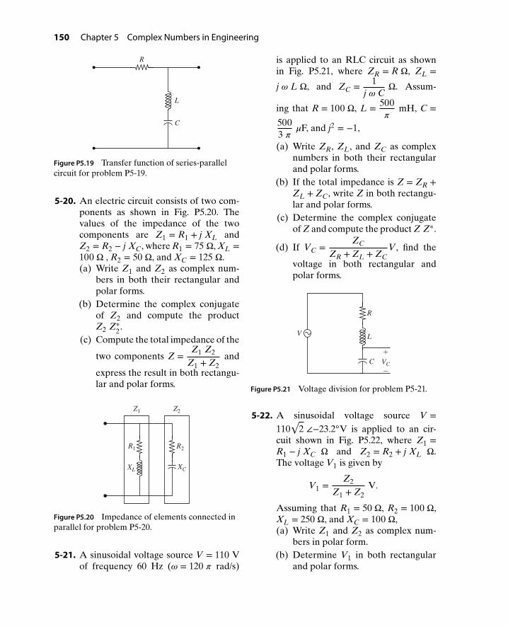
150 Chapter 5 Complex Numbers in Engineering
L
R
C
Figure P5.19 Transfer function of series-parallelcircuit for problem P5-19.
5-20. An electric circuit consists of two com-ponents as shown in Fig. P5.20. Thevalues of the impedance of the twocomponents are Z1 = R1 + j XL andZ2 = R2 − j XC, where R1 = 75 Ω, XL =100 Ω , R2 = 50 Ω, and XC = 125 Ω.(a) Write Z1 and Z2 as complex num-
bers in both their rectangular andpolar forms.
(b) Determine the complex conjugateof Z2 and compute the productZ2 Z∗
2.(c) Compute the total impedance of the
two components Z =Z1 Z2
Z1 + Z2and
express the result in both rectangu-lar and polar forms.
Z1 Z2
R2
XCXL
R1
Figure P5.20 Impedance of elements connected inparallel for problem P5-20.
5-21. A sinusoidal voltage source V = 110 Vof frequency 60 Hz (𝜔 = 120 𝜋 rad/s)
is applied to an RLC circuit as shownin Fig. P5.21, where ZR = R Ω, ZL =j 𝜔 L Ω, and ZC = 1
j 𝜔 CΩ. Assum-
ing that R = 100 Ω, L = 500𝜋
mH, C =5003 𝜋
𝜇F, and j2 = −1,
(a) Write ZR, ZL, and ZC as complexnumbers in both their rectangularand polar forms.
(b) If the total impedance is Z = ZR +ZL + ZC, write Z in both rectangu-lar and polar forms.
(c) Determine the complex conjugateof Z and compute the product Z Z∗.
(d) If VC =ZC
ZR + ZL + ZCV, find the
voltage in both rectangular andpolar forms.
V
R
C
L
VC
+
−
Figure P5.21 Voltage division for problem P5-21.
5-22. A sinusoidal voltage source V =110
√2 ∠−23.2V is applied to an cir-
cuit shown in Fig. P5.22, where Z1 =R1 − j XC Ω and Z2 = R2 + j XL Ω.The voltage V1 is given by
V1 =Z2
Z1 + Z2V.
Assuming that R1 = 50 Ω, R2 = 100 Ω,XL = 250 Ω, and XC = 100 Ω,(a) Write Z1 and Z2 as complex num-
bers in polar form.(b) Determine V1 in both rectangular
and polar forms.

Problems 151
(c) Determine the complex conjugateof Z1 and compute the productZ1 Z∗
1.
L
C
V
R2
R1
Z1
V1Z2
+
−
Figure P5.22 Voltage division for problem P5-22.
5-23. An electric circuit consists of a resis-tor R, an inductor L, and a capacitorC, connected as shown in Fig. P5.23.The impedance of the resistor is ZR =R Ω, the impedance of the inductor isZL = j𝜔L Ω, and the impedance of the
capacitor is ZC = 1j 𝜔 C
Ω, where j =√−1. Suppose R = 9 Ω, L = 3 mH, C =
250 𝜇F, and 𝜔 = 1000 rad/s.
C
L
R
Figure P5.23 Series-parallel combination of R, L,and C for problem P5-23.
(a) Write ZR, ZL, and ZC as complexnumbers in both rectangular andpolar form.
(b) Calculate the total impedance ofthe inductor-capacitor parallel com-bination, which is given as ZLC =
ZL ZC
ZL + ZC. Express the result in both
rectangular and polar forms.(c) Now suppose that the total
impedance of the circuit is Z =ZR + ZLC. Determine the totalimpedance in both rectangular andpolar forms.
(d) Determine the complex conjugateof Z and compute the product Z Z∗.
5-24. In the circuit shown in Fig. P5.24,the impedances of the various com-ponents are ZR = R Ω, ZL = j XL Ω,
and ZC = 1j
XC, where j =√−1. Sup-
pose R = 120 Ω, XL = 120√
3 Ω, and
XC = 1
50√
3Ω.
(a) Express the impedance ZR, ZL, andZC as complex numbers in bothrectangular and polar forms.
(b) Now, suppose that the totalimpedance of the circuit is Z =
ZC +ZR ZL
ZR + ZL. Determine the
total impedance and express the re-sult in both rectangular and polarforms.
(c) Determine the complex conjugateof Z and compute the product Z Z∗.
Z
C
R L
Figure P5.24 A capacitor connected in series with aparallel combination of resistor and inductor forproblem P5-24.
5-25. In the RC circuit shown in Fig. P5.25,the impedances of R and C are given

152 Chapter 5 Complex Numbers in Engineering
as ZR = R Ω and ZC = −j XC Ω, wherej =
√−1. Suppose R = 100 Ω and XC =
50 Ω.(a) Express the impedances ZR and ZC
as complex numbers in both rectan-gular and polar forms.
(b) Find the total impedance Z = ZR +ZC as a complex number in bothrectangular and polar forms.
(c) If V = 100∠0V, find the current
I = VZ
as a complex number in both
rectangular and polar forms.(d) Knowing the current in part (c), find
the voltage phasors VR = I ZR andVC = I ZC in both rectangular andpolar forms.
(e) Show that the KVL is satisfied forthe circuit shown in Fig. P5.25; inother words, show V = VR + VC.
R
V
I
C
Figure P5.25 An RC circuit for problem P5-25.
5-26. In the RL circuit shown in Fig. P5.26,the impedances of R and L are givenas ZR = R Ω and ZC = j XL Ω, wherej =
√−1. Suppose R = 100 Ω and XL =
50 Ω.
L
V
R
I
Figure P5.26 An RL circuit for problem P5-26.
(a) Express the impedances ZR and ZLas complex numbers in both rectan-gular and polar forms.
(b) Find the total impedance Z = ZR +ZL as a complex number in bothrectangular and polar forms.
(c) If V = 100∠0V, find the current
I = VZ
as a complex number in both
rectangular and polar forms.(d) Knowing the current in part (c), find
the voltage phasors VR = I ZR andVL = I ZL in both rectangular andpolar forms.
(e) Show that the KVL is satisfied forthe circuit shown in Fig. P5.26; inother words, show V = VR + VL.
5-27. A resistor, capacitor, and inductorare connected in series as shown inFig. P5.27. The total impedance of thecircuit is Z = ZR + ZL + ZC, whereZR = R Ω, ZL = j𝜔L Ω, and ZC =
1j 𝜔 C
Ω. For a particular design, R =
100 Ω, L = 500 mH, C = 25 𝜇F, and𝜔 = 120 𝜋 rad/s.
V
I
R
C
L
Figure P5.27 RLC circuit for problem P5-27.
(a) Express the impedances ZR, ZL,and ZC as complex numbers in bothrectangular and polar forms.
(b) Determine the total impedance Zin both its rectangular and polarforms.
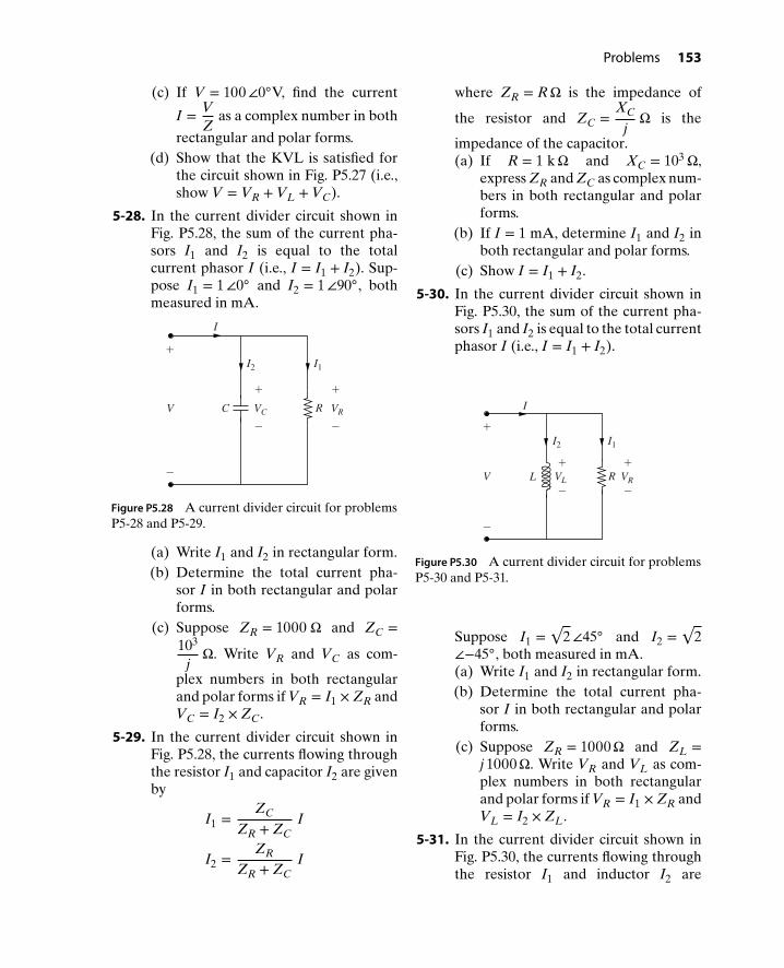
Problems 153
(c) If V = 100∠0V, find the current
I = VZ
as a complex number in both
rectangular and polar forms.(d) Show that the KVL is satisfied for
the circuit shown in Fig. P5.27 (i.e.,show V = VR + VL + VC).
5-28. In the current divider circuit shown inFig. P5.28, the sum of the current pha-sors I1 and I2 is equal to the totalcurrent phasor I (i.e., I = I1 + I2). Sup-pose I1 = 1∠0 and I2 = 1∠90, bothmeasured in mA.
RC
I1
I
V VR
+
−
VC
+
−
+
−
I2
Figure P5.28 A current divider circuit for problemsP5-28 and P5-29.
(a) Write I1 and I2 in rectangular form.(b) Determine the total current pha-
sor I in both rectangular and polarforms.
(c) Suppose ZR = 1000 Ω and ZC =103
jΩ. Write VR and VC as com-
plex numbers in both rectangularand polar forms if VR = I1 × ZR andVC = I2 × ZC.
5-29. In the current divider circuit shown inFig. P5.28, the currents flowing throughthe resistor I1 and capacitor I2 are givenby
I1 =ZC
ZR + ZCI
I2 =ZR
ZR + ZCI
where ZR = RΩ is the impedance of
the resistor and ZC =XC
jΩ is the
impedance of the capacitor.(a) If R = 1 kΩ and XC = 103 Ω,
express ZR and ZC as complex num-bers in both rectangular and polarforms.
(b) If I = 1 mA, determine I1 and I2 inboth rectangular and polar forms.
(c) Show I = I1 + I2.
5-30. In the current divider circuit shown inFig. P5.30, the sum of the current pha-sors I1 and I2 is equal to the total currentphasor I (i.e., I = I1 + I2).
R
I
V L
I1
VR
+
−VL
+
−
I2
+
−
Figure P5.30 A current divider circuit for problemsP5-30 and P5-31.
Suppose I1 =√
2∠45 and I2 =√
2∠−45, both measured in mA.(a) Write I1 and I2 in rectangular form.(b) Determine the total current pha-
sor I in both rectangular and polarforms.
(c) Suppose ZR = 1000Ω and ZL =j 1000Ω. Write VR and VL as com-plex numbers in both rectangularand polar forms if VR = I1 × ZR andVL = I2 × ZL.
5-31. In the current divider circuit shown inFig. P5.30, the currents flowing throughthe resistor I1 and inductor I2 are

154 Chapter 5 Complex Numbers in Engineering
given by
I1 =ZL
ZR + ZLI
I2 =ZR
ZR + ZLI
where ZR = RΩ is the impedance ofthe resistor and ZL = j XLΩ is theimpedance of the inductor.(a) If R = 1 kΩ and XL = 103 Ω,
express ZR and ZL as complex num-bers in both rectangular and polarforms.
(b) If I = 1 mA, determine I1 and I2 inboth rectangular and polar forms.
(c) Show I = I1 + I2.
5-32. In the Op–Amp circuit shown inFig. P5.32, the output voltage Vo isgiven by
Vo = −ZC
ZRVin
where ZR = R Ω is the impedance ofthe resistor and ZC = −j XC Ω is theimpedance of the capacitor.(a) If R = 2 kΩ and XC = 1 kΩ,
express ZR and ZC as complex num-bers in both rectangular and polarforms.
(b) If Vin = 10∠0V, determine Vo inboth rectangular and polar forms.
R
C
+Vcc
−Vcc Vo
++
−
−
Vin+−
Figure P5.32 An Op–Amp circuit for problemP5-32.
5-33. In the Op–Amp circuit shown inFig. P5.33, the output voltage Vo is givenby
Vo = −ZR
ZCVin
where ZR = R Ω is the impedance ofthe resistor and ZC = −j XC Ω is theimpedance of the capacitor.(a) If R = 1 kΩ and XC = 2 kΩ,
express ZR and ZC as complex num-bers in both rectangular and polarforms.
(b) If Vin = 5∠90V, determine Vo inboth rectangular and polar forms.
R
C +Vcc
−Vcc Vo
+
−
Vin
+−
+−
Figure P5.33 An Op–Amp circuit for problemP5-33.
5-34. In the Op–Amp circuit shown inFig. P5.34, the output voltage Vo isgiven by
Vo = −ZR2 + ZC
ZR1Vin
where ZR1 = R1 Ω is the impedanceof the resistor R1, ZR2 = R2 Ω is theimpedance of the resistor R2, andZC = −j XC Ω is the impedance of thecapacitor.(a) If R1 = 1 kΩ, R2 = 2 kΩ, and XC =
2 kΩ, express ZR1, ZR2, and ZC ascomplex numbers in both rectangu-lar and polar forms.
(b) If Vin = 2∠45V, determine Vo inboth rectangular and polar forms.

Problems 155
C
R1
R2
+Vcc
−Vcc Vo
+
−
+−
Vin+−
Figure P5.34 An Op–Amp circuit for problemP5-34.
5-35. In the Op–Amp circuit shown inFig. P5.35, the output voltage Vo isgiven by
Vo = −ZR2
ZR1 + ZCVin
where ZR1 = R1 Ω is the impedanceof the resistor R1, ZR2 = R2 Ω is theimpedance of the resistor R2, andZC = −j XC Ω is the impedance of thecapacitor.(a) If R1 = 1.5 kΩ, R2 = 1 kΩ and XC =
0.5 kΩ, express ZR1, ZR2, and ZC ascomplex numbers in both rectangu-lar and polar forms.
(b) If Vin = 1∠−45V, determine Vo inboth rectangular and polar forms.
CR1
R2
+Vcc
−Vcc VoVin
+
−
+−
+−
Figure P5.35 An Op–Amp circuit for problemP5-35.
5-36. In the Op–Amp circuit circuit shownin Fig. P5.36, the output voltage Vo is
given by
Vo = −ZR2 + ZC2
ZR1 + ZC1Vin
where ZR1 = R1 Ω is the impedanceof the resistor R1, ZR2 = R2 Ω is theimpedance of the resistor R2, ZC1 =−j XC1 Ω is the impedance of thecapacitor C1, and ZC2 = −j XC2 Ω is theimpedance of the capacitor C2.(a) If R1 = 10 kΩ, R2 = 5 kΩ, XC1 =
2.5 kΩ, and XC2 = 5 kΩ, expressZR1, ZR2, ZC1, and ZC2 as complexnumbers in both rectangular andpolar forms.
(b) If Vin = 1.5∠0V, determine Vo inboth rectangular and polar forms.
R2 C2
+Vcc
−Vcc
+−
Vo
+
−
R1 C1
Vin+−
Figure P5.36 An Op–Amp circuit for problemP5-35.
5-37. The Delta-to-Yee (Δ-Y) and Yee-to-Delta (Y-Δ) conversions are used inelectrical circuits to find the equiva-lent impedances of complex circuits.In the circuit shown in Fig. 5.37, theimpedances Za, Zb, and Zc connectedin the Delta interconnection can be con-verted into their equivalent impedancesZ1, Z2, and Z3 connected in the Yeeinterconnection. The impedances Z1,Z2, and Z3 can be written in term of

156 Chapter 5 Complex Numbers in Engineering
impedances Za, Zb, and Zc as
Z1 =Za Zb
Za + Zb + Zc
Z2 =Za Zc
Za + Zb + Zc
Z3 =Zc Zb
Za + Zb + Zc. (5.7)
(a) If Za = 20 Ω, Zb = −j 10 Ω, andZc = 20 + j 50 Ω, express Za, Zb,and Zc as complex numbers in bothrectangular and polar forms.
(b) Determine Z1, Z2, and Z3 in bothrectangular and polar forms.
Za
Z2Z1
Z3
ZcZb
Figure P5.37 Impedances connected in Delta andYee interconnections.
5-38. Repeat problem P5-37 if Za = 10 Ω,Zb = j 20 Ω, and Zc = 20 + j 10 Ω.
5-39. In the circuit shown in Fig. 5.37, theimpedances Z1, Z2, and Z3 connectedin the Yee interconnection can be con-verted into their equivalent impedancesZa, Zb, and Zc connected in the Deltainterconnection as
Za =Z1 Z2 + Z2 Z3 + Z3 Z1
Z3
Zb =Z1 Z2 + Z2 Z3 + Z3 Z1
Z2
Zc =Z1 Z2 + Z2 Z3 + Z3 Z1
Z1. (5.8)
(a) If Z1 = 2.5 − j 2.5 Ω, Z2 = 17.5 +j 7.5 Ω, and Z3 = 3.75 − j 8.75 Ω,express Z1, Z2, and Z3 as complexnumbers in polar form.
(b) Determine Za, Zb, and Zc in bothrectangular and polar forms.
5-40. Repeat problem P5-39 if Z1 = 3.33 +j 3.33 Ω, Z2 = 5.0 − j 1.66 Ω, and Z3 =3.5 + j 10.6 Ω.

CHAPTER6
Sinusoids inEngineering
A sinusoid is a signal that describes a smooth repetitive motion of an object thatoscillates at a constant rate (frequency) about an equilibrium point. The sinusoidhas the form of a sine (sin) or a cosine (cos) function (discussed in Chapter 3) andhas applications in all engineering disciplines. These functions are the most impor-tant signals because all other signals can be constructed from sine and cosine signals.A few examples of a sinusoid are the motion of a one-link planar robot rotating ata constant rate, the oscillation of an undamped spring-mass system, and the voltagewaveform of an electric power source. For example, the frequency of the voltagewaveform associated with electrical power in North America is 60 cycles per second(Hz), whereas in many other parts of the world this frequency is 50 Hz. In thischapter, the example of a one-link robot rotating at a constant rate will be used todevelop the general form of a sinusoid and explain its amplitude, frequency (bothlinear and angular), phase angle, and phase shift. The sum of sinusoids of the samefrequency will also be explained in the context of both electrical and mechanicalsystems.
6.1 ONE-LINK PLANAR ROBOT AS A SINUSOIDA one-link planar robot of length l and angle 𝜃 is shown in Fig. 6.1. It was shown inChapter 3 that the tip of the robot has coordinates x = l cos 𝜃 and y = l sin 𝜃. Vary-ing 𝜃 from 0 to 2𝜋 radians and assuming l = 1 (l has units of x and y), the plots ofy = l sin 𝜃 and x = l cos 𝜃 are shown in Figs. 6.2 and 6.3, respectively.
y
x
y
x
lθ
Figure 6.1 A one-link planar robot.
157
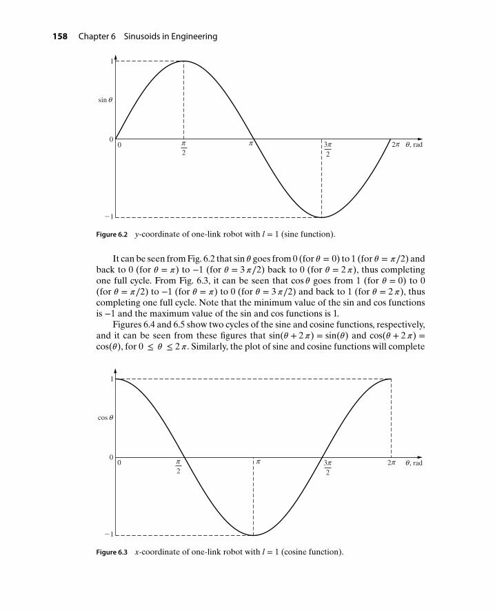
158 Chapter 6 Sinusoids in Engineering
2
0
1
−1
0 3 2
2
, rad
sinθ
θπ π π π
Figure 6.2 y-coordinate of one-link robot with l = 1 (sine function).
It can be seen from Fig. 6.2 that sin 𝜃 goes from 0 (for 𝜃 = 0) to 1 (for 𝜃 = 𝜋∕2) andback to 0 (for 𝜃 = 𝜋) to −1 (for 𝜃 = 3𝜋∕2) back to 0 (for 𝜃 = 2𝜋), thus completingone full cycle. From Fig. 6.3, it can be seen that cos 𝜃 goes from 1 (for 𝜃 = 0) to 0(for 𝜃 = 𝜋∕2) to −1 (for 𝜃 = 𝜋) to 0 (for 𝜃 = 3𝜋∕2) and back to 1 (for 𝜃 = 2𝜋), thuscompleting one full cycle. Note that the minimum value of the sin and cos functionsis −1 and the maximum value of the sin and cos functions is 1.
Figures 6.4 and 6.5 show two cycles of the sine and cosine functions, respectively,and it can be seen from these figures that sin(𝜃 + 2𝜋) = sin(𝜃) and cos(𝜃 + 2𝜋) =cos(𝜃), for 0 ≤ 𝜃 ≤ 2𝜋. Similarly, the plot of sine and cosine functions will complete
, rad0
0
1
−1
2
3 2
2
cosθ
π π π π θ
Figure 6.3 x-coordinate of one-link robot with l = 1 (cosine function).

6.2 Angular Motion of the One-Link Planar Robot 159
, rad0
0
1
−1
2432 3
2
7
2
3
2
sinθ
π π π π π π π π θ
Figure 6.4 Two cycles of the sine function.
another cycle from 4𝜋 to 6𝜋 and so on for every 2𝜋. Thus, both the sine and cosinefunctions are called periodic functions with period T = 2𝜋 rad. Since 𝜋 = 180, theperiod of the sine and cosine functions can also be written as 360.
6.2 ANGULAR MOTION OF THE ONE-LINK PLANAR ROBOTSuppose now that the one-link planar robot shown in Fig. 6.1 is rotating with anangular frequency 𝜔, as shown in Fig. 6.6.
, rad0
0
1
−1
2433
2
7
2
23
2
cosθ
π π π π π π π π θ
Figure 6.5 Two cycles of the cosine function.

160 Chapter 6 Sinusoids in Engineering
l
x
y
x
y
= θ ω t
Figure 6.6 A one-link planar robot rotating at a constant angular frequency 𝜔.
The angle traveled in time t is given by 𝜃 = 𝜔 t. Therefore, y(t) = l sin(𝜃) =l sin(𝜔 t) and x(t) = l cos(𝜃) = l cos(𝜔 t). Suppose the robot starts from 𝜃 = 0 at timet = 0 s and takes t = 2𝜋s to complete one revolution. Since 𝜃 = 𝜔 t, the angular fre-
quency is 𝜔 = 𝜃
t= 2𝜋rad
2𝜋s= 1 rad/s, and the time period to complete one cycle is
T = 2𝜋s. The resulting plots of y = l sin t and x = l cos t are shown in Figs. 6.7 and 6.8,respectively. The x- and y-components oscillate between l and −l, where the length lis the amplitude of the sinusoids.
t, s
y = l sin t
00
l
−l
2
3
2
2π π π π
Figure 6.7 The y-component of the one-link planar robot completing one cycle in 2𝜋 s.
6.2.1 Relations between Frequency and Period
In Figs. 6.7 and 6.8, it took 2𝜋s to complete one cycle of the sinusoidal signals, and itwas found that 𝜔 = 1 rad/s (i.e., in 1 s, the robot went through 1 radian of rotation).

6.2 Angular Motion of the One-Link Planar Robot 161
t, s2
3 2
2
x = l cos t
00
l
−l
π π π π
Figure 6.8 The x-component of the one-link planar robot completing one cycle in 2𝜋s.
Since one revolution (cycle) = 2𝜋rad, a robot rotating at 1 rad/s would go through1/2𝜋 cycles in 1s. This is called the linear frequency or simply frequency f , with unitsof cycle/s (s−1). Therefore, the relationship between the angular frequency 𝜔 andlinear frequency f is given by
𝝎 = 2𝝅f .
By definition, the period T is defined as the number of seconds per cycle, whichmeans f is the reciprocal of T. In other words,
f = 1T.
Since 𝜔 = 2𝜋f ,
𝝎 = 2𝝅T
.
Solving for T gives
T = 2𝝅𝝎
.
The above relations allow the computation of f , 𝜔, or T when only one of the threeis given. For example, assume that a one-link robot of length l goes through two
revolutions (i.e., 4𝜋rad) in 2𝜋s. The angular frequency is 𝜔 = 4𝜋rad2𝜋s
= 2 rad/s, the
period is T = 2𝜋∕2 = 𝜋s, and the frequency is f = 2∕2𝜋 = 1∕𝜋Hz. Therefore, y(t) =l sin(𝜔 t) = l sin(2 t) and x(t) = l cos(𝜔 t) = l cos(2 t); and their plots are as shown inFigs. 6.9 and 6.10, respectively.

162 Chapter 6 Sinusoids in Engineering
y = l sin (2t)
0
l
−l
t, s02
3
2
2π π π π
Figure 6.9 The y-component of one-link planar robot completing two cycles in 2𝜋s or𝜔 = 2 rad/s.
x = l cos (2t)
0
l
−l
t, s02
3
2
2π π π π
Figure 6.10 The x-component of one-link planar robot completing one cycle in 2𝜋s or𝜔 = 2 rad/s.
6.3 PHASE ANGLE, PHASE SHIFT, AND TIME SHIFTSuppose now that a robot of length l = 10 in. starts rotating from an initial position𝜃 = 𝜋/8 rad and takes T = 1 s to complete one revolution, as shown in Fig. 6.11. Atany time t, the x- and y-components are given by
x(t) = l cos 𝜃
= l cos (𝜔 t + 𝜙)
= l cos(𝜔 t + 𝜋
8
)

6.3 Phase Angle, Phase Shift, and Time Shift 163
x
y
10
(x, y)t = 0
tω
θ
πϕ = /8 = Phase angle
Figure 6.11 One-link planar robot starting rotation from an angle of 𝜋/8 rad.
and
y(t) = l sin 𝜃
= l sin (𝜔 t + 𝜙)
= l sin(𝜔 t + 𝜋
8
).
Since l = 10, 𝜔 = 2𝜋∕T = 2𝜋∕1 = 2𝜋rad/s, and 𝜙 = 𝜋/8 rad, the x- andy-components of the one-link robot are given by
x(t) = 10 cos(
2𝜋t + 𝜋
8
)and
y(t) = 10 sin(
2𝜋t + 𝜋
8
), (6.1)
where𝜙 = 𝜋/8 is called the phase angle. Since𝜙 represents a shift from the zero phaseto a phase of 𝜋/8 rad, it is sometimes called a phase shift. Therefore, the phase shiftis a shift in radians or degrees. If the phase angle is positive, the sinusoid shifts to theleft as shown in Fig. 6.12, but if the phase angle is negative, the sinusoid will shift tothe right. For example, the value of the sinusoid given by equation (6.1) is not zeroat time t = 0. Since the phase angle is positive, the sinusoid given by equation (6.1)is shifted to the left.
The time shift is the time it takes the robot moving at a speed 𝜔 to pass throughthe phase shift 𝜙. Setting 𝜃 = 𝜔 t gives
time shift =Phase angle
Angular frequency= 𝜙
𝜔
=
𝜋
82𝜋
= 116
s.
Note that the phase angle used to calculate the time shift must be in rad.

164 Chapter 6 Sinusoids in Engineering
y (t)
t, s
−10
10
0
16
11
8
16
10 sin
1
16
15−
π )(
Figure 6.12 Plot of the sine function shifted to the left a phase angle of 𝜋∕8 (positive phaseangle).
6.4 GENERAL FORM OF A SINUSOIDThe general expression of a sinusoid is
x(t) = A sin(𝜔 t + 𝜙) (6.2)
where A is the amplitude, 𝜔 is the angular frequency, and 𝜙 is the phase angle.
Example6-1
Consider a cart of mass m moving on frictionless rollers as shown in Fig. 6.13. Themass is attached to the end of a spring of stiffness k.
x(t)
k
Frictionless rollers
m
Figure 6.13 Harmonic motion of a spring-mass system.
Suppose that the position of the mass x(t) is given by
x(t) = 2 sin(
6𝜋t + 𝜋
2
)m. (6.3)

6.4 General Form of a Sinusoid 165
(a) Determine the amplitude, linear and angular frequencies, period, phase angle,and time shift.
(b) Find x(t) at t = 2.0 s.
(c) Find the time required for the system to reach its maximum negativedisplacement.
(d) Plot the displacement x(t) for 0 ≤ t ≤ 3 s.
Solution (a) Comparing the position of the mass x(t) = 2 sin(
6𝜋t + 𝜋
2
)to the general
expression of equation (6.2) gives
Amplitude A = 2 m
Angular frequency 𝜔 = 6𝜋 rad/s
Phase angle 𝜙 = 𝜋
2rad.
Since the angular frequency is 𝜔 = 2𝜋f , the linear frequency f is given by
f = 𝜔
2𝜋= 6𝜋
2𝜋= 3 Hz,
and the period of the harmonic motion is given by
T = 1f= 1
3s.
The time shift can be determined from the phase angle and the angularfrequency as
Time shift = 𝜙
𝜔
=(𝜋
2
) (1
6𝜋
)
= 112
s.
(b) To find x(t) at t = 2.0 s, substitute t = 2.0 in equation (6.3), which gives
x(2) = 2 sin(
6𝜋(2) + 𝜋
2
)= 2 sin
(12𝜋 + 𝜋
2
)= 2 sin(12.5𝜋)
= 2 sin(12.5𝜋 − 12𝜋)
= 2 sin(𝜋
2
)= 2.0 m.

166 Chapter 6 Sinusoids in Engineering
In obtaining x(2), 12𝜋 was subtracted from the angle 12.5𝜋 to find the valueof sin(12.5𝜋). It should be noted that an integer multiple of 2𝜋 can always beadded or subtracted from the argument of sine and cosine functions. This isdone because the sine and cosine functions are periodic with a period of 2𝜋.
(c) The displacement reaches the first maximum negative displacement of −2 m
when sin (𝜃) = sin(
6𝜋t + 𝜋
2
)= −1 or 𝜃 = 6𝜋t + 𝜋
2= 3𝜋
2. Solving for t gives
6𝜋t + 𝜋
2= 3𝜋
2
⇒ 6𝜋t = 3𝜋2
− 𝜋
2= 𝜋
⇒ t = 𝜋
6𝜋or
t = 16
s.
(d) The plot of the displacement x(t) for 0 ≤ t ≤ 3 s is shown in Fig. 6.14.
t, s
x(t), m
32100
−2
2
Figure 6.14 Harmonic motion of the mass-spring system for 3 seconds.
6.5 ADDITION OF SINUSOIDS OF THE SAME FREQUENCYAdding two sinusoids of the same frequency but different amplitudes and phasesresults in another sinusoid (sin or cos) of the same frequency. The resulting amplitudeand phase are different from the amplitude and phase of the two original sinusoids,as illustrated with the following example.
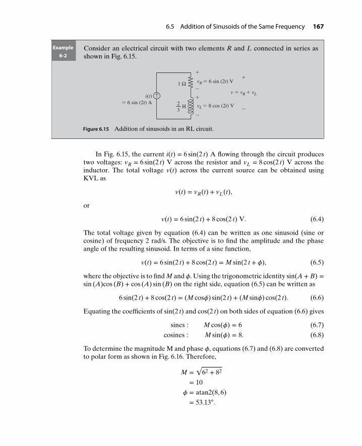
6.5 Addition of Sinusoids of the Same Frequency 167
Example6-2
Consider an electrical circuit with two elements R and L connected in series asshown in Fig. 6.15.
v = vR + vL
1 Ω
2
3H
i(t)= 6 sin (2t) A
vR = 6 sin (2t) V
vL = 8 cos (2t) V
+
+
−
−−
+
↑
Figure 6.15 Addition of sinusoids in an RL circuit.
In Fig. 6.15, the current i(t) = 6 sin(2 t) A flowing through the circuit producestwo voltages: vR = 6 sin(2 t) V across the resistor and vL = 8 cos(2 t) V across theinductor. The total voltage v(t) across the current source can be obtained usingKVL as
v(t) = vR(t) + vL(t),
or
v(t) = 6 sin(2 t) + 8 cos(2 t) V. (6.4)
The total voltage given by equation (6.4) can be written as one sinusoid (sine orcosine) of frequency 2 rad/s. The objective is to find the amplitude and the phaseangle of the resulting sinusoid. In terms of a sine function,
v(t) = 6 sin(2 t) + 8 cos(2 t) = M sin(2 t + 𝜙), (6.5)
where the objective is to find M and 𝜙. Using the trigonometric identity sin(A + B) =sin (A)cos (B) + cos (A) sin (B) on the right side, equation (6.5) can be written as
6 sin(2 t) + 8 cos(2 t) = (M cos𝜙) sin(2 t) + (M sin𝜙) cos(2 t). (6.6)
Equating the coefficients of sin(2 t) and cos(2 t) on both sides of equation (6.6) gives
sines : M cos(𝜙) = 6 (6.7)
cosines : M sin(𝜙) = 8. (6.8)
To determine the magnitude M and phase 𝜙, equations (6.7) and (6.8) are convertedto polar form as shown in Fig. 6.16. Therefore,
M =√
62 + 82
= 10
𝜙 = atan2(8, 6)
= 53.13.

168 Chapter 6 Sinusoids in Engineering
M
xM cos = 6
M sin = 8
y
ϕ
ϕ
ϕ
Figure 6.16 Determination of magnitude and phase of the resulting sinusoid in an RL circuit.
Therefore, v(t) = 6 sin(2 t) + 8 cos(2 t) = 10 sin(2 t + 53.13) V. The amplitude of thevoltage sinusoid is 10 V, the angular frequency is 𝜔 = 2 rad/s, the linear frequencyis f = 𝜔∕2𝜋 = 2∕2𝜋 = 1∕𝜋Hz, the period is T = 𝜋 = 3.142 s, the phase angle =53.13 = (53.13) (𝜋rad∕180) = 0.927 rad, and the time shift can be calculated as
t = 𝜙
𝜔
= 0.9272
= 0.464 s.
The plot of the voltage and current waveforms is shown in Fig. 6.17. It can be seenfrom Fig. 6.17 that the voltage waveform is shifted to the left by 0.464 s (time shift).
−10
−6
−0.464 2.678 3.142 t, s
6
Voltage
Current
0
0
10
Figure 6.17 Voltage and current relationship for an RL circuit.

6.5 Addition of Sinusoids of the Same Frequency 169
In other words, the voltage in the RL circuit leads the current by 53.3. It will beshown later that it is opposite in an RC circuit, where the voltage waveform lags thecurrent.
Note: The voltage v(t) can also be represented as one sinusoid using the cosinefunction as
v(t) = 6 sin(2 t) + 8 cos(2 t) = M cos(2 t + 𝜙1). (6.9)
The amplitude M and the phase angle 𝜙1 can be determined using a proce-dure similar to that outlined above. Using the trigonometric identity cos(A + B) =cos (A) cos (B) − sin (A) sin (B) on the right side of equation (6.9) gives
6 sin(2 t) + 8 cos(2 t) = (−M sin𝜙1) sin(2 t) + (M cos𝜙1) cos(2 t). (6.10)
Equating the coefficients of sin(2 t) and cos(2 t) on both sides of equation (6.10) gives
sines : M sin(𝜙1) = −6 (6.11)
cosines : M cos(𝜙1) = 8. (6.12)
To determine the magnitude M and phase 𝜙1, equations (6.11) and (6.12) are con-verted to polar form as shown in Fig. 6.18.
M
y
xM cos 1 = 8
M sin 1 = −6
1
ϕ
ϕ
ϕ
Figure 6.18 Determination of magnitude and phase for a cosine function.
Therefore,
M =√
62 + 82
= 10
𝜙1 = atan2(−6, 8)
= −36.87
Therefore, v(t) = 6 sin(2 t) + 8 cos(2 t) = 10 cos(2 t − 36.87) V.This expression can also be obtained directly from the sine function using the
trig identity sin 𝜃 = cos(𝜃 − 90). Therefore,
10 sin(2 t + 53.13) = 10 cos ( (2 t + 53.13) − 90)
= 10 cos(2 t − 36.87).
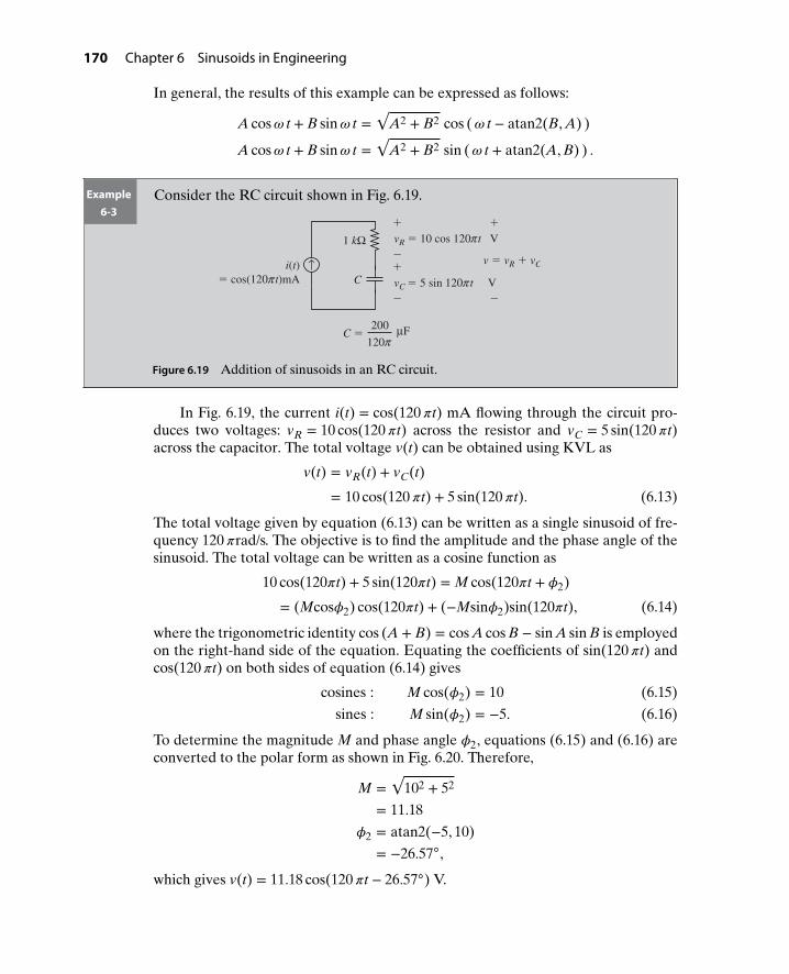
170 Chapter 6 Sinusoids in Engineering
In general, the results of this example can be expressed as follows:
A cos𝜔 t + B sin𝜔 t =√
A2 + B2 cos (𝜔 t − atan2(B, A) )
A cos𝜔 t + B sin𝜔 t =√
A2 + B2 sin (𝜔 t + atan2(A, B) ) .
Example6-3
Consider the RC circuit shown in Fig. 6.19.
v = vR + vC
C = F
C
1 kΩ
i(t)= cos(120 t)mA
vR = 10 cos 120 t V
vC = 5 sin 120 t V
+ +
−+
− −
↑π
π
π
μ
π
200
120
Figure 6.19 Addition of sinusoids in an RC circuit.
In Fig. 6.19, the current i(t) = cos(120𝜋t) mA flowing through the circuit pro-duces two voltages: vR = 10 cos(120𝜋t) across the resistor and vC = 5 sin(120𝜋t)across the capacitor. The total voltage v(t) can be obtained using KVL as
v(t) = vR(t) + vC(t)
= 10 cos(120𝜋t) + 5 sin(120𝜋t). (6.13)
The total voltage given by equation (6.13) can be written as a single sinusoid of fre-quency 120𝜋rad/s. The objective is to find the amplitude and the phase angle of thesinusoid. The total voltage can be written as a cosine function as
10 cos(120𝜋t) + 5 sin(120𝜋t) = M cos(120𝜋t + 𝜙2)
= (Mcos𝜙2) cos(120𝜋t) + (−Msin𝜙2)sin(120𝜋t), (6.14)
where the trigonometric identity cos (A + B) = cos A cos B − sin A sin B is employedon the right-hand side of the equation. Equating the coefficients of sin(120 𝜋t) andcos(120𝜋t) on both sides of equation (6.14) gives
cosines : M cos(𝜙2) = 10 (6.15)
sines : M sin(𝜙2) = −5. (6.16)
To determine the magnitude M and phase angle 𝜙2, equations (6.15) and (6.16) areconverted to the polar form as shown in Fig. 6.20. Therefore,
M =√
102 + 52
= 11.18
𝜙2 = atan2(−5, 10)
= −26.57,
which gives v(t) = 11.18 cos(120𝜋t − 26.57) V.

6.5 Addition of Sinusoids of the Same Frequency 171
M
2
y
xM cos 2 = 10
M sin 2 = −5
ϕ
ϕ
ϕ
Figure 6.20 Determination of magnitude and phase of the resulting sinusoid in an RC circuit.
The amplitude of the voltage sinusoid is 11.8 V, the angular frequency is 𝜔 =120𝜋rad/s, the linear frequency is f = 𝜔/2𝜋 = 60 Hz, the period is T = 16.7 ms, thephase angle is −26.57, and the time shift is 1.23 ms.
The plot of the voltage and current waveforms is shown in Fig. 6.21. It can beseen from the figure that the voltage waveform is shifted to the right by 1.23 ms(time shift). In other words, the voltage in this RC circuit lags the current by 26.57.
t, ms
1.23 ms
11.18
1.00
−1.01.23 ms
0 1.23 16.7
Current in mA
Voltage in V
−11.18
Figure 6.21 Voltage and current relationship for an RC circuit.
Example6-4
A hip implant is subjected to a cyclic load during a fatigue test, as shown in Fig. 6.22.The load applied to the hip implant is given by
F(t) = 250 sin(6𝜋t) + 1250 N
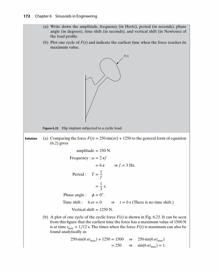
172 Chapter 6 Sinusoids in Engineering
(a) Write down the amplitude, frequency (in Hertz), period (in seconds), phaseangle (in degrees), time shift (in seconds), and vertical shift (in Newtons) ofthe load profile.
(b) Plot one cycle of F(t) and indicate the earliest time when the force reaches itsmaximum value.
F(t)
Figure 6.22 Hip implant subjected to a cyclic load.
Solution (a) Comparing the force F(t) = 250 sin(𝜋t) + 1250 to the general form of equation(6.2) gives
amplitude = 250 N.
Frequency : 𝜔 = 2𝜋f
= 6𝜋 ⇒ f = 3 Hz.
Period : T = 1f
= 13
s.
Phase angle : 𝜙 = 0.
Time shift : 6𝜋t = 0 ⇒ t = 0 s (There is no time shift.)
Vertical shift = 1250 N.
(b) A plot of one cycle of the cyclic force F(t) is shown in Fig. 6.23. It can be seenfrom this figure that the earliest time the force has a maximum value of 1500 Nis at time tmax = 1∕12 s. The times when the force F(t) is maximum can also befound analytically as
250 sin(6𝜋tmax) + 1250 = 1500 ⇒ 250 sin(6𝜋tmax)
= 250 ⇒ sin(6𝜋tmax) = 1.

Problems 173
Therefore,
6𝜋tmax = 𝜋
2, 3𝜋
2, ⋅ ⋅ ⋅,
which gives
tmax = 112
, 14⋅ ⋅ ⋅ s.
Therefore, the earliest time the maximum force occurs is t = 1∕12s.
1,500
1,250
1,000
Force, N
00 1/12 1/6 1/4 1/3 t, s
Figure 6.23 One cycle of the force F(t).
P R O B L E M S
6-1. The tip of a one-link robot is locatedat 𝜃 = 0 at time t = 0 s as shown in Fig.P6.1. It takes 1 s for the robot to movefrom 𝜃 = 0 to 𝜃 = 2𝜋rad. If l = 5 in., plotthe x- and y-components as a functionof time. Also find the amplitude, fre-quency, period, phase angle, and timeshift.
t = 0x
l
y
Figure P6.1 Rotating one-link robot starting at𝜃 = 0.
6-2. The tip of a one-link robot is locatedat 𝜃 = 𝜋∕6 rad at time t = 0 s, as shownin Fig. P6.2. It takes 2 s for the robotto move from 𝜃 = 𝜋∕6 rad to 𝜃 = 𝜋∕6 +2𝜋rad. If l = 10 in., plot the x- andy-components as a function of time.Also find the amplitude, frequency,period, phase angle, and time shift.
x
l
y
/6
t = 0
π
Figure P6.2 Rotating one-link robot starting at𝜃 = 30.

174 Chapter 6 Sinusoids in Engineering
6-3. The tip of a one-link robot is located at𝜃 = −𝜋∕4 rad at time t = 0 s as shown inFig. P6.3. The robot is rotating at an an-gular frequency of 2𝜋rad/s. If l = 20 cm,plot the x- and y-components as a func-tion of time. Also find the amplitude,frequency, period, phase angle, and timeshift.
x
y
l4
t = 0
−π
Figure P6.3 Rotating one-link robot starting at𝜃 = −45.
6-4. The tip of a one-link robot is locatedat 𝜃 = 𝜋∕2 rad at t = 0 s as shown inFig. P6.4. It takes 4 s for the robot tomove from 𝜃 = 𝜋∕2 rad to 𝜃 = 𝜋∕2 +2𝜋rad. If l = 10 cm, plot the x- andy-components as a function of time.Also find the amplitude, frequency,period, phase angle, and time shift.
t = 0
y
/2l
xπ
Figure P6.4 Rotating one-link robot starting at𝜃 = 90.
6-5. The tip of a one-link robot is located at𝜃 = 3𝜋∕4 rad at time t = 0 s as shownin Fig. P6.5. It takes 2 s for the robot tomove from 𝜃 = 3𝜋∕4 rad to 𝜃 = 3𝜋∕4 +2𝜋rad. If l = 15 cm, plot the x- andy-components as a function of time.
Also find the amplitude, frequency,period, phase angle, and time shift.
t = 0
x
l
y
3
4
π
Figure P6.5 Rotating one-link robot starting at𝜃 = 135.
6-6. The tip of a one-link robot is located at𝜃 = 𝜋rad at time t = 0 s as shown in Fig.P6.6. It takes 3 s for the robot to movefrom 𝜃 = 𝜋rad to 𝜃 = 3𝜋rad. If l = 5 cm,plot the x- and y-components as a func-tion of time. Also find the amplitude,frequency, period, phase angle, and timeshift.
t = 0x
y
l
π
Figure P6.6 Rotating one-link robot starting at𝜃 = 180.
6-7. A spring-mass system moving in they-direction has a sinusoidal motion asshown in Fig. P6.7. Determine the am-plitude, period, frequency, and phaseangle of the motion. Also, write the ex-pression for y(t).
6-8. A spring-mass system moving in thex-direction has a sinusoidal motion asshown in Fig. P6.8. Determine the am-plitude, period, frequency, and phaseangle of the motion. Also, write the ex-pression for x(t).
6-9. Repeat problem P6-8 for the sinusoidalmotion shown in Fig. P6.9.

Problems 175
k
m
y(t) 0.5 t, s0.250
−2
0
y(t), cm
2
Figure P6.7 Sinusoidal motion of a spring-mass system in the y-direction for problem P6-7.
x(t)k
Frictionless rollers
m
t, s
−5
00
x(t), cm
5
130
115
Figure P6.8 Sinusoidal motion of a spring-mass system in the x-direction for problem P6-8.
x(t)k
Frictionless rollers
m
0.9 t, s0.40
−10
0−0.1
x(t), in.
10
Figure P6.9 Motion of a spring-mass system in the x-direction for problem P6-9.
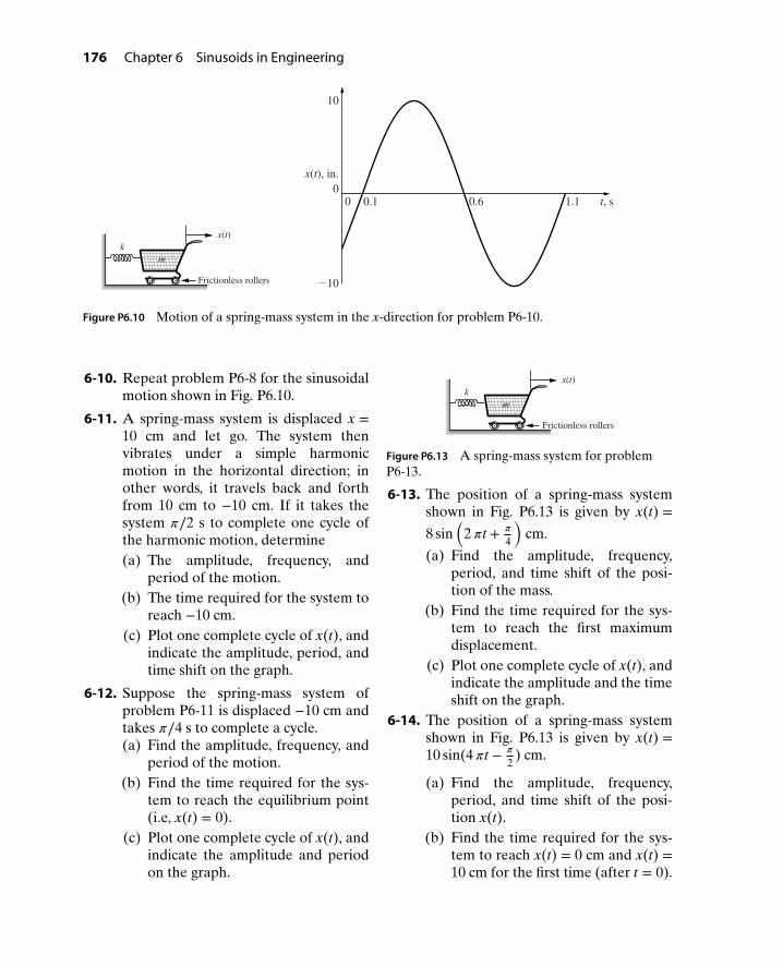
176 Chapter 6 Sinusoids in Engineering
x(t)k
Frictionless rollers
m
t, s1.10.60.10
−10
0
10
x(t), in.
Figure P6.10 Motion of a spring-mass system in the x-direction for problem P6-10.
6-10. Repeat problem P6-8 for the sinusoidalmotion shown in Fig. P6.10.
6-11. A spring-mass system is displaced x =10 cm and let go. The system thenvibrates under a simple harmonicmotion in the horizontal direction; inother words, it travels back and forthfrom 10 cm to −10 cm. If it takes thesystem 𝜋∕2 s to complete one cycle ofthe harmonic motion, determine(a) The amplitude, frequency, and
period of the motion.(b) The time required for the system to
reach −10 cm.(c) Plot one complete cycle of x(t), and
indicate the amplitude, period, andtime shift on the graph.
6-12. Suppose the spring-mass system ofproblem P6-11 is displaced −10 cm andtakes 𝜋∕4 s to complete a cycle.(a) Find the amplitude, frequency, and
period of the motion.(b) Find the time required for the sys-
tem to reach the equilibrium point(i.e, x(t) = 0).
(c) Plot one complete cycle of x(t), andindicate the amplitude and periodon the graph.
x(t)k
Frictionless rollers
m
Figure P6.13 A spring-mass system for problemP6-13.
6-13. The position of a spring-mass systemshown in Fig. P6.13 is given by x(t) =8 sin
(2𝜋t + 𝜋
4
)cm.
(a) Find the amplitude, frequency,period, and time shift of the posi-tion of the mass.
(b) Find the time required for the sys-tem to reach the first maximumdisplacement.
(c) Plot one complete cycle of x(t), andindicate the amplitude and the timeshift on the graph.
6-14. The position of a spring-mass systemshown in Fig. P6.13 is given by x(t) =10 sin(4𝜋t − 𝜋
2) cm.
(a) Find the amplitude, frequency,period, and time shift of the posi-tion x(t).
(b) Find the time required for the sys-tem to reach x(t) = 0 cm and x(t) =10 cm for the first time (after t = 0).
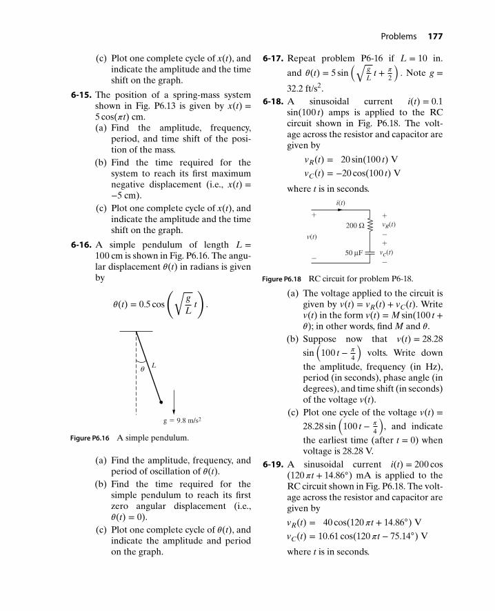
Problems 177
(c) Plot one complete cycle of x(t), andindicate the amplitude and the timeshift on the graph.
6-15. The position of a spring-mass systemshown in Fig. P6.13 is given by x(t) =5 cos(𝜋t) cm.(a) Find the amplitude, frequency,
period, and time shift of the posi-tion of the mass.
(b) Find the time required for thesystem to reach its first maximumnegative displacement (i.e., x(t) =−5 cm).
(c) Plot one complete cycle of x(t), andindicate the amplitude and the timeshift on the graph.
6-16. A simple pendulum of length L =100 cm is shown in Fig. P6.16. The angu-lar displacement 𝜃(t) in radians is givenby
𝜃(t) = 0.5 cos
(√gL
t
).
g = 9.8 m/s2
Lθ
Figure P6.16 A simple pendulum.
(a) Find the amplitude, frequency, andperiod of oscillation of 𝜃(t).
(b) Find the time required for thesimple pendulum to reach its firstzero angular displacement (i.e.,𝜃(t) = 0).
(c) Plot one complete cycle of 𝜃(t), andindicate the amplitude and periodon the graph.
6-17. Repeat problem P6-16 if L = 10 in.
and 𝜃(t) = 5 sin(√
gL
t + 𝜋
2
). Note g =
32.2 ft/s2.6-18. A sinusoidal current i(t) = 0.1
sin(100 t) amps is applied to the RCcircuit shown in Fig. P6.18. The volt-age across the resistor and capacitor aregiven by
vR(t) = 20 sin(100 t) V
vC(t) = −20 cos(100 t) V
where t is in seconds.
v(t)
i(t)
vR(t)
vc(t) 50 μF
200 Ω+
−
+
−+
−
Figure P6.18 RC circuit for problem P6-18.
(a) The voltage applied to the circuit isgiven by v(t) = vR(t) + vC(t). Writev(t) in the form v(t) = M sin(100 t +𝜃); in other words, find M and 𝜃.
(b) Suppose now that v(t) = 28.28
sin(
100 t − 𝜋
4
)volts. Write down
the amplitude, frequency (in Hz),period (in seconds), phase angle (indegrees), and time shift (in seconds)of the voltage v(t).
(c) Plot one cycle of the voltage v(t) =28.28 sin
(100 t − 𝜋
4
), and indicate
the earliest time (after t = 0) whenvoltage is 28.28 V.
6-19. A sinusoidal current i(t) = 200 cos(120𝜋t + 14.86) mA is applied to theRC circuit shown in Fig. P6.18. The volt-age across the resistor and capacitor aregiven by
vR(t) = 40 cos(120𝜋t + 14.86) V
vC(t) = 10.61 cos(120𝜋t − 75.14) V
where t is in seconds.

178 Chapter 6 Sinusoids in Engineering
(a) The voltage applied to the circuitis given by v(t) = vR(t) + vC(t).Write v(t) in the form v(t) =M cos(120𝜋t + 𝜃); in other words,find M and 𝜃.
(b) Suppose now that v(t) = 41.38cos (120𝜋t) volts. Write down theamplitude, frequency (in Hz),period (in seconds), phase angle (indegrees), and time shift (in seconds)of the voltage v(t).
(c) Plot one cycle of the voltage v(t) =41.38 cos (120𝜋t), and indicate theearliest time (after t = 0) when volt-age is −41.38 V.
6-20. A series RL circuit is subjected toa sinusoidal voltage of frequency120𝜋rad/s, as shown in Fig. P6.20. Thecurrent i(t) = 10 cos(120𝜋t) A is flow-ing through the circuit. The voltageacross the resistor and inductor aregiven by vR(t) = 10 cos(120𝜋t) and
vL(t) = 12 cos(
120𝜋t + 𝜋
2
)volts, where
t is in seconds.
R = 1 Ω, L = mH10
R
v(t)
i(t)
L
+
+−
−
vR (t)
vL (t)
π
+−
Figure P6.20 A series RL circuit for problem P6-20.
(a) Write down the amplitude, fre-quency (in Hz), period (in seconds),phase shift (in degrees), and timeshift (in seconds) of the voltagevL(t).
(b) Plot one cycle of the voltage vL(t),and indicate the earliest time aftert = 0 when the voltage is maximum.
(c) The total voltage across the cir-cuit is given by v(t) = vR(t) + vL(t).Write v(t) in the form v(t) =M cos(120𝜋t + 𝜃), in other words,find M and 𝜃.
6-21. A series RL circuit is subjected toa sinusoidal voltage of frequency20𝜋rad/s, as shown in Fig. P6.20. Thecurrent i(t) = 500 sin(20𝜋t) mA is flow-ing through the circuit. The voltageacross the resistor and inductor aregiven by vR(t) = 0.5 sin(20𝜋t) and
vL(t) = 0.1 sin(
20𝜋t + 𝜋
2
)volts, where
t is in seconds.
(a) Write down the amplitude, fre-quency (in Hz), period (in seconds),phase shift (in degrees), and timeshift (in seconds) of the voltagevL(t).
(b) Plot one cycle of the voltage vL(t),and indicate the earliest time aftert = 0 when the voltage is minimum.
(c) The total voltage across the circuit isgiven by v(t) = vR(t) + vL(t). Writev(t) in the form v(t) = M cos(20𝜋t +𝜃), in other words, find M and 𝜃.
6-22. A sinusoidal voltage v(t) = 10 sin(1000 t) V is applied to the RLC circuitshown in Fig. P6.22. The current i(t) =0.707sin(1000 t + 45) flowing throughthe circuit produces voltages across R,L, and C of
vR(t) = 7.07 sin(1000 t + 45) V
vL(t) = 7.07 sin(1000 t + 135) V
vC(t) = 14.14 sin(1000 t − 45) V.
(a) Write down the amplitude, fre-quency (in Hz), period (in seconds),phase shift (in radians), and timeshift (in ms) of the current i(t) =0.707 sin(1000 t + 45) A.
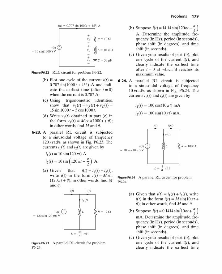
Problems 179
+−
−
−
−
i(t) = 0.707 sin(1000t + 45°) A
R = 10 Ω
C = 50 μF
L = 10 mHv(t)
= 10 sin(1000t) V vL
vC
vR
+
+ +
Figure P6.22 RLC circuit for problem P6-22.
(b) Plot one cycle of the current i(t) =0.707 sin(1000 t + 45) A and indi-cate the earliest time (after t = 0)when the current is 0.707 A.
(c) Using trigonometric identities,show that v1(t) = vR(t) + vC(t) =15 sin 1000 t − 5 cos 1000 t.
(d) Write v1(t) obtained in part (c) inthe form v1(t) = M cos(1000 t + 𝜃);in other words, find M and 𝜃.
6-23. A parallel RL circuit is subjectedto a sinusoidal voltage of frequency120𝜋rad/s, as shown in Fig. P6.23. Thecurrents i1(t) and i2(t) are given by
i1(t) = 10 sin(120𝜋t) A
i2(t) = 10 sin(
120𝜋t − 𝜋
2
)A.
(a) Given that i(t) = i1(t) + i2(t),write i(t) in the form i(t) = M sin(120𝜋t + 𝜃); in other words, find Mand 𝜃.
L = mH100
i(t) i1 (t)
i2 (t)
L R = 12 Ωv(t)= 120 sin(120 t) V
+−
π
π
Figure P6.23 A parallel RL circuit for problemP6-23.
(b) Suppose i(t)= 14.14 sin(120𝜋t − 𝜋
4
)A. Determine the amplitude, fre-quency (in Hz), period (in seconds),phase shift (in degrees), and timeshift (in seconds).
(c) Given your results of part (b), plotone cycle of the current i(t), andclearly indicate the earliest timeafter t = 0 at which it reaches itsmaximum value.
6-24. A parallel RL circuit is subjectedto a sinusoidal voltage of frequency10𝜋rad/s, as shown in Fig. P6.24. Thecurrents i1(t) and i2(t) are given by
i1(t) = 100 cos(10𝜋t) mA
i2(t) = 100 sin(10𝜋t) mA.
L = mH1
i(t) i1(t)
i2(t)
L R = 100 Ωv(t)= 10 sin(10 t) V
π
π+−
Figure P6.24 A parallel RL circuit for problemP6-24.
(a) Given that i(t) = i1(t) + i2(t), writei(t) in the form i(t) = M sin(10𝜋t +𝜃); in other words, find M and 𝜃.
(b) Suppose i(t)= 0.1414 sin(10𝜋t + 𝜋
4
)mA. Determine the amplitude, fre-quency (in Hz), period (in seconds),phase shift (in degrees), and timeshift (in seconds).
(c) Given your results of part (b), plotone cycle of the current i(t), andclearly indicate the earliest time

180 Chapter 6 Sinusoids in Engineering
after t = 0 at which it reaches itsmaximum value.
6-25. Consider the RC circuit shown inFig. P6.25, where the currents arei1(t) = 2 sin(120𝜋t) A and i2(t) =2√
3 sin(120𝜋t + 𝜋
2) A.
i(t) i1(t)
i2(t)
C Rv(t) +−
Figure P6.25 A parallel RC circuit for problemP6-25.
(a) Given that i(t) = i1(t) + i2(t),write i(t) in the form i(t) = M sin(120𝜋t + 𝜙) A; in other words, findM and 𝜙.
(b) Suppose now that i(t) = 4 sin(120𝜋t + 𝜋
3
)A. Determine the
amplitude, frequency (in Hz),period (in seconds), phase shift(in degrees), and time shift (inseconds).
(c) Given your results of part (b), plotone cycle of the current i(t), andclearly indicate the earliest timeafter t = 0 at which it reaches itsmaximum value.
6-26. Consider the RC circuit shown in Fig.P6.25, where the currents are i1(t) =100 cos(100𝜋t + 𝜋
4) mA and i2(t) =
500 cos(100 t + 3𝜋4
) mA.(a) Given that i(t) = i1(t) + i2(t), write
i(t) in the form i(t) = M sin(100 t +𝜙) A; in other words, find M and 𝜙.
(b) Suppose now that i(t) = 0.51 sin(100 t + 146.31)A. Determine theamplitude, frequency (in Hz),period (in seconds), phase shift
(in degrees), and time shift (inseconds).
(c) Given your results of part (b), plotone cycle of the current i(t), andclearly indicate the earliest timeafter t = 0 at which it reaches itsmaximum value.
6-27. Two voltages v1(t) = 10 sin(100𝜋t −45) V and v2(t) = 10 sin(100𝜋t) V areapplied to the Op–Amp circuit shownin Fig. P6.27.
−
+−+
+VCC
−VCC vo (t)
28.28 kΩ
28.28 kΩ
20 kΩv1 (t)
v2 (t)
−+
−+
Figure P6.27 An Op–Amp circuit for problemP6-27.
(a) Write down the amplitude, fre-quency (in Hz), period (in seconds),phase shift (in radians), and timeshift (in seconds) of the voltagev1(t).
(b) Plot one cycle of the voltage v1(t),and indicate the earliest time aftert = 0 when the voltage is 10 V.
(c) The output voltage vo(t) is given by
vo(t) = −(√
2 v1(t) + v2(t))
. Write
vo(t) in the form vo(t) = M cos(100𝜋t + 𝜃); in other words, find Mand 𝜃).
6-28. Repeat problem P6-27 if v1(t) =10 cos(100𝜋t + 90) V and v2(t) = 3 sin(100𝜋t + 𝜋
4) V.
6-29. Two voltages v1(t) = 10√
2 sin(
500𝜋t −
3𝜋4
)V and v2(t) = 5 sin(500𝜋t) V are
applied to the Op–Amp circuit shown inFig. P6.29.

Problems 181
+Vcc
−Vcc
+Vcc
−Vcc
−+
−+
v1(t)
+
−
vo(t)
v2(t)28.28 kΩ
28.28 kΩ 28.28 kΩ
−
−
+
+
Figure P6.29 An Op–Amp circuit for problem P6-29.
(a) Write down the amplitude, fre-quency (in Hz), period (in seconds),phase angle or phase shift (in radi-ans), and time shift (in seconds) ofthe voltage v1(t).
(b) Plot one cycle of the voltage v1(t),and indicate the earliest time aftert = 0 when the voltage is 10
√2 V.
(c) The output voltage vo(t) is givenby vo(t) = v1(t) + v2(t). Write vo(t)in the form vo(t) = M sin(500𝜋t +𝜃) (i.e., find M and 𝜃).
6-30. A pair of springs and masses vibrateunder simple harmonic motion, asshown in Fig. P6.30. The positionsof the masses in inches are given
by y1(t) = 5√
2 cos(
2𝜋t + 𝜋
4
)and
y2(t) = 10 cos(2𝜋t), where t is inseconds.(a) Write down the amplitude, fre-
quency (in Hz), period (in seconds),phase shift (in degrees), and timeshift (in seconds) of the position ofthe first mass y1(t).
(b) Plot one cycle of the position y1(t),and indicate the earliest time aftert = 0 when the position is zero.
(c) The vertical distance between thetwo masses is given by 𝛿(t) = y1(t) −y2(t). Write 𝛿(t) in the form 𝛿(t) =M sin(2𝜋t + 𝜃); in other words,find M and 𝜃.
6-31. Suppose the positions of the massesin problem P6-30 are given by
y1(t) y2(t)
Figure P6.30 A pair of springs and masses forproblem P6-30.
y1(t) = 8 sin(
4𝜋t + 𝜋
3
)and y2(t) =
6 cos(4𝜋t), where t is in seconds.(a) Write down the amplitude, fre-
quency (in Hz), period (in seconds),phase shift (in degrees), and timeshift (in seconds) of the position ofthe first mass y1(t).
(b) Plot one cycle of the position y1(t),and indicate the earliest time aftert = 0 when the position is zero.
(c) Write 𝛿(t) = y1(t) − y2(t) in theform 𝛿(t) = M cos(4𝜋t + 𝜃); inother words, find M and 𝜃.
6-32. Two oscillating masses are connected bya spring as shown in Fig. P6.32. The posi-tions of the masses in inches are given by
x1(t) = 5√
2 cos(
2𝜋t + 𝜋
4
)and x2(t) =
10 cos(2𝜋t), where t is in seconds.(a) Write down the amplitude, fre-
quency (in Hz), period (in seconds),

182 Chapter 6 Sinusoids in Engineering
x2(t)x1(t)
Figure P6.32 Two oscillating masses for problemP6-32.
phase shift (in degrees), and timeshift (in seconds) of the position ofthe first mass x1(t).
(b) Plot one cycle of the position x1(t),and indicate the earliest time aftert = 0 when the position is zero.
(c) The elongation of the spring is givenby 𝛿(t) = x2(t) − x1(t). Write 𝛿(t) inthe form 𝛿(t) = M sin(2𝜋t + 𝜙); inother words, find M and 𝜙.
6-33. Now assume that the positions of twomasses in problem P6-31 are given
by x1(t) = 8 sin(
4𝜋t + 𝜋
4
)and x2(t) =
16 cos(4𝜋t), where t is in seconds.(a) Write down the amplitude, fre-
quency (in Hz), period (in seconds),phase shift (in degrees), and timeshift (in seconds) of the position ofthe first mass x1(t).
(b) Plot one cycle of the position x1(t),and indicate the earliest time aftert = 0 when the position is zero.
(c) Write 𝛿(t) = x2(t) − x1(t) in theform 𝛿(t) = M cos(4𝜋t + 𝜙); inother words, find M and 𝜙.
6-34. A manufacturing plant employs aheater and a conveyer belt motoron the same 220 V service line asshown in Fig. P6.34. The voltages across
VT(t)
+ VH(t) −
MotorHeater
+ VM(t) −
+
−
Figure P6.34 Conveyer motor and heaterconnected across the 220 V service line.
the heater and motor are given byVH(t) = 66 cos(120𝜋t) V and VM(t) =180 cos(120𝜋t + 𝜋
3) V, where t is in
seconds.
(a) Write down the amplitude, fre-quency (in Hz), period, phase angle(in degrees), and phase shift (inseconds) of the voltage across themotor, VM(t).
(b) Plot one cycle of the motor voltageVM(t), and indicate the earliest timewhen the voltage is maximum.
(c) Write the voltage VM(t) in theform VM(t)=A sin(120𝜋t) + B cos(120𝜋t) (i.e., find A and B).
(d) The total voltage is VH(t) + VM(t).Write VT(t) in the form VT(t) =V cos (120𝜋t + 𝜃) (i.e., find Vand 𝜃).
6-35. Repeat problem P6-34 if VH(t) =100 sin(120𝜋t) V and VM(t) = 164 sin(120𝜋t + 70) V.
6-36. In the three-phase circuit shown in Fig.P6.36, vab(t) = van(t) − vbn(t), wherevan(t) = 120 sin(120𝜋t) V and vbn(t) =120 sin(120𝜋t − 120) V are the line-to-neutral voltages and vab is the line-to-line voltage of the three-phase system.
(a) Write down the amplitude, fre-quency (in Hz), period, phase angle(in degrees), and phase shift (in sec-onds) of the voltage, vbn(t).
(b) Plot one cycle of the line-to-neutralvoltage vbn(t), and indicate theearliest time when the voltage ismaximum.
(c) Write the line-to-line voltage vab(t)in the form vab(t) = A sin(120𝜋t) +B cos(120𝜋t) (i.e., find A and B).
(d) Write vab(t) in the form vab(t) =V cos(120𝜋t + 𝜃) (i.e., find Vand 𝜃).

Problems 183
a
c
van
vbn
vcn
b
n
Figure P6.36 A balanced three-phase circuit.
6-37. In the three-phase circuit shown in Fig.P6.36, vbc(t) = vbn(t) − vcn(t), wherevbn(t) = 120 sin(120𝜋t − 120) V andvcn(t) = 120 sin(120𝜋t + 120) V arethe line-to-neutral voltages and vbc isthe line-to-line voltage of the three-phase system.(a) Write down the amplitude, fre-
quency (in Hz), period, phase angle(in degrees), and phase shift (in sec-onds) of the voltage, vcn(t).
(b) Plot one cycle of the line-to-neutralvoltage vcn(t), and indicate theearliest time when the voltage isminimum.
(c) Write the line-to-line voltage vbc(t)in the form vbc(t) = A sin(120𝜋t) +B cos(120𝜋t) (i.e., find A and B).
(d) Write vbc(t) in the form vbc(t) =V cos (120𝜋t + 𝜃) (i.e., find Vand 𝜃).
6-38. In the three-phase circuit shown in Fig.P6.36, vca(t) = vcn(t) − van(t), wherevcn(t) = 120 sin(120𝜋t + 120) V andvan(t) = 120 cos(120𝜋t − 90) V arethe line-to-neutral voltages and vca isthe line-to-line voltage of the three-phase system.(a) Write down the amplitude, fre-
quency (in Hz), period, phase angle(in degrees), and phase shift (in sec-onds) of the voltage, van(t).
(b) Plot one cycle of the line-to-neutralvoltage van(t), and indicate the ear-liest time when the voltage reaches60 V.
(c) Write the line-to-line voltage vca(t)in the form vca(t) = A sin(120𝜋t) +B cos(120𝜋t) (i.e., find A and B).
(d) Write vca(t) in the form vca(t) =V cos(120𝜋t + 𝜃) (i.e., find Vand 𝜃).
6-39. The hip implant shown in Fig. P6.39is subjected to a cyclic load during afatigue test. The load applied to the hipimplant is given by
F(t) = 200 sin(5𝜋t) + 1000 N
F(t)
Figure P6.39 Hip implant subjected to a cyclic load.
(a) Write down the amplitude, fre-quency (in Hz), period (in seconds),phase angle (in degrees), time shift(in seconds), and vertical shift (inN) of the load profile.
(b) Plot one cycle of F(t) and indicatethe earliest time when the forcereaches its maximum value.
6-40. Repeat problem P6-39 if F(t) =15 sin(10𝜋t) + 75 N.

CHAPTER7
Systems of Equationsin Engineering
7.1 INTRODUCTIONThe solution of a system of linear equations is an important topic for all engineeringdisciplines. In this chapter, the solution of 2 × 2 systems of equations will be carriedout using four different methods: substitution method, graphical method, matrixalgebra method, and Cramer’s rule. It is assumed that the students are alreadyfamiliar with the substitution and graphical methods from their high school algebracourse, while the matrix algebra method and Cramer’s rule are explained in detail.The objective of this chapter is to be able to solve the systems of equations encoun-tered in beginning engineering courses such as physics, statics, dynamics, and DCcircuit analysis. While the examples given are limited to 2 × 2 systems of equations,the matrix algebra approach is applicable to linear systems having any number ofunknowns and is suitable for immediate implementation in MATLAB.
7.2 SOLUTION OF A TWO-LOOP CIRCUITConsider a two-loop resistive circuit with unknown currents I1 and I2 as shown inFig. 7.1. Using a combination of Kirchhoff’s voltage law (KVL) and Ohm’s law, asystem of two equations with two unknowns I1 and I2 can be obtained as
10 I1 + 4 I2 = 6 (7.1)
12 I2 + 4 I1 = 9. (7.2)
6 Ω
9 VI2I16 V 4 Ω
8 Ω
+−
+−
Figure 7.1 A two-loop resistive circuit.
184

7.2 Solution of a Two-Loop Circuit 185
Equations (7.1) and (7.2) represent a system of equations for I1 and I2 that can besolved using the four different methods outlined as follows:
1. Substitution Method: Solving equation (7.1) for the first variable I1 gives
10 I1 = 6 − 4 I2
I1 =6 − 4 I2
10. (7.3)
The current I2 can now be solved by substituting I1 from equation (7.3) intoequation (7.2), which gives
12 I2 + 4(
6 − 4 I2
10
)= 9
12 I2 + 2.4 − 1.6 I2 = 9
10.4 I2 = 6.6
I2 = 6.610.4
I2 = 0.6346 A. (7.4)
The current I1 can now be obtained by substituting the value of the second vari-able I2 from equation (7.4) into equation (7.3) as
I1 =6 − 4(0.6346)
10I1 = 0.3462 A.
Therefore, the solution of the system of equations (7.1) and (7.2) is given by
(I1, I2) = (0.3462 A, 0.6346 A).
2. Graphical Method: Begin by assuming I1 as the independent variable and I2as the dependent variable. Solving equation (7.1) for the dependent variable I2gives
10 I1 + 4 I2 = 6
4 I2 = −10 I1 + 6
I2 = −52
I1 +32. (7.5)
Similarly, solving equation (7.2) for I2 gives
4 I1 + 12 I2 = 9
12 I2 = −4 I1 + 9
I2 = −13
I1 +34. (7.6)
Equations (7.5) and (7.6) are linear equations of the form y = m x + b. Thesimultaneous solution of equations (7.5) and (7.6) is the intersection point of thetwo lines. The plot of the two straight lines along with their intersection point is

186 Chapter 7 Systems of Equations in Engineering
shown in Fig. 7.2. The intersection point, (I1, I2)≈ (0.35 A, 0.63 A), is the solutionof the 2 × 2 system of equations (7.1) and (7.2).
1.0 1.5 2.00.5
0.5
2.0
1.5
1.0
0.0
0.0
5
2
3
2I2 = −− I1 +−
1
3
3
4I2 = −− I1 +−
I2, A
I1, A
Solution: (I1, I2) = (0.35, 0.63)
Figure 7.2 Plot of 2 × 2 system of equations (7.1) and (7.2).
Note that the graphical method gives only approximate results; therefore, thismethod is generally not used when an accurate result is needed. Also, if the twolines do not intersect, then one of the following two possibilities exist:
(i) The two lines are parallel lines (same slope but different y-intercepts) and thesystem of equations has no solution.
(ii) The two lines are parallel lines with same slope and y-intercept (the two lineslie on top of each other; they are the same line) and the system of equationshas infinitely many solutions. In this case, the two equations are dependent(i.e., one equation can be obtained by performing linear operations on theother equation).
3. Matrix Algebra Method: The matrix algebra method can also be used to solvethe system of equations given by equations (7.1) and (7.2). Rewriting the systemof equations (7.1) and (7.2) in the form so that the two variables line up gives
10 I1 + 4 I2 = 6 (7.7)
4 I1 + 12 I2 = 9. (7.8)
Now, writing equations (7.7) and (7.8) in matrix form yields[10 44 12
] [I1I2
]=[
69
]. (7.9)

7.2 Solution of a Two-Loop Circuit 187
Equation (7.9) is of the form Ax = b, where
A =[
10 44 12
](7.10)
is a 2 × 2 coefficient matrix,
x =[
I1I2
](7.11)
is a 2 × 1 matrix (column vector) of unknowns, and
b =[
69
](7.12)
is a 2 × 1 matrix on the right-hand side (RHS) of equation (7.9). For any systemof the form Ax = b, the solution is given by
x = A−1 b
where A−1 is the inverse of the matrix A. For a 2 × 2 system of equations where
A =[
a bc d
],
the inverse of the matrix A is given by
A−1 = 1Δ
[d −b−c a
]where Δ = |A| is the determinant of matrix A and is given by
Δ =|||| a bc d
||||= a d − b c.
Note that if Δ = |A| = 0, A−1 does not exist. In other words, the system of equa-tions Ax = b has no solution. Now, for the two-loop circuit problem,
A =[
10 44 12
]
=[
a bc d
].
The inverse of matrix A is given by
A−1 = 1Δ
[d −b−c a
]
= 1Δ
[12 −4−4 10
]

188 Chapter 7 Systems of Equations in Engineering
where Δ = |A| = a d − c b = (10) (12) − (4) (4) = 104. Therefore, the inverse ofmatrix A can be calculated as
A−1 = 1104
[12 −4−4 10
]
=⎡⎢⎢⎢⎣
326
− 126
− 126
552
⎤⎥⎥⎥⎦. (7.13)
The solution of the system of equations x =[
I1I2
]can now be found by multiplying
A−1 (given by equation (7.13)) with the column matrix b (given by equation(7.12)) as
x = A−1 b[I1I2
]=⎡⎢⎢⎢⎣
326
− 126
− 126
552
⎤⎥⎥⎥⎦[
69
]
=⎡⎢⎢⎢⎣
326
(6) +(− 1
26
)(9)(
− 126
)(6) +
(552
)(9)
⎤⎥⎥⎥⎦=⎡⎢⎢⎢⎣
18 − 926
−12 + 4552
⎤⎥⎥⎥⎦=[
0.34620.6346
].
The solution of the system of equations (7.1) and (7.2) is therefore given by
(I1, I2) = (0.3462A, 0.6346A).
4. Cramer’s Rule: For any system Ax = b, the solution of the system of equationsis given by
x1 =|A1||A| , x2 =
|A2||A| ,… xi =|Ai||A|
where |Ai| is obtained by replacing the ith column of the matrix A with the col-umn vector b. Writing the 2 × 2 system of equations
a11 x1 + a12 x2 = b1
a21 x1 + a22 x2 = b2
in matrix form as [a11 a12a21 a22
] [x1x2
]=[
b1b2
],

7.2 Solution of a Two-Loop Circuit 189
Cramer’s rule gives the solution of the system of equations as
x1 =
||||b1 a12b2 a22
|||||||| a11 a12a21 a22
||||=
a22 b1 − a12 b2
a11 a22 − a12 a21,
x2 =
|||| a11 b1a21 b2
|||||||| a11 a12a21 a22
||||=
a11 b2 − a21 b1
a11 a22 − a12 a21.
For the two-loop circuit, the 2 × 2 system of equations is[10 44 12
] [I1I2
]=[
69
].
Using Cramer’s rule, the currents I1 and I2 can be determined as
I1 =
||||6 49 12
||||||||10 44 12
||||=
6(12) − 9(4)10(12) − 4(4)
= 36104
= 0.3462 A,
I2 =
||||10 64 9
||||||||10 44 12
||||=
10(9) − 4(6)10(12) − 4(4)
= 66104
= 0.6346 A.
Therefore, I1 = 0.3462 A and I2 = 0.6346 A. Note that Cramer’s rule is probablyfastest for solving 2 × 2 systems but not faster than MATLAB.

190 Chapter 7 Systems of Equations in Engineering
7.3 TENSION IN CABLESAn object weighing 95 N is hanging from a roof with two cables as shown inFig. 7.3. Determine the tension in each cable using the substitution, matrix algebra,and Cramer’s rule methods.
Since the system shown in Fig. 7.3 is in equilibrium, the sum of all the forcesshown in the free-body diagram must be equal to zero. This implies that all the forcesin the x- and y-directions are equal to zero (see Chapter 4). The components of thetension T1 in the x- and y-directions are given by −T1 cos(45) N and T1 sin(45) N,respectively. Similarly, the components of the tension T2 in the x- and y-directionsare given by T2 cos(30) N and T2 sin(30) N, respectively. The components of theobject weight is 0 N in the x-direction and −95 N in the y-direction. Summing all theforces in the x-direction gives
−T1 cos(45) + T2 cos(30) = 0
−0.7071 T1 + 0.8660 T2 = 0. (7.14)
y
x
95 N
95 N
T1 T2
45°
45°
30°
30°
Figure 7.3 A 95 N object hanging from two cables.
Similarly, summing the forces in the y-direction yields
T1 sin(45) + T2 sin(30) = 95
0.7071 T1 + 0.5 T2 = 95. (7.15)
Equations (7.14) and (7.15) make a 2 × 2 system of equations with two unknowns T1and T2 that can be written in matrix form as[
−0.7071 0.86600.7071 0.5
] [T1T2
]=[
095
]. (7.16)
The solution of the system of equations (T1 and T2) will now be obtained using threemethods: the substitution method, the matrix algebra method, and Cramer’s rule.
1. Substitution Method: Using equation (7.14), the second variable T2 is found interms of the first variable T1 as
0.8660 T2 = 0.7071 T1
T2 = 0.8165 T1. (7.17)
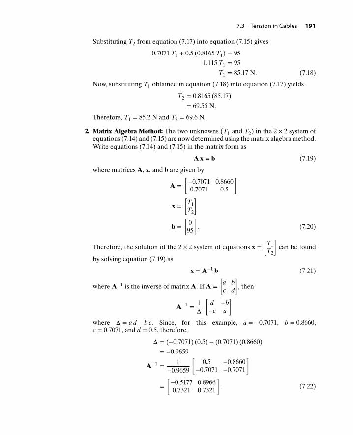
7.3 Tension in Cables 191
Substituting T2 from equation (7.17) into equation (7.15) gives
0.7071 T1 + 0.5 (0.8165 T1) = 95
1.115 T1 = 95
T1 = 85.17 N. (7.18)
Now, substituting T1 obtained in equation (7.18) into equation (7.17) yields
T2 = 0.8165 (85.17)
= 69.55 N.
Therefore, T1 = 85.2 N and T2 = 69.6 N.
2. Matrix Algebra Method: The two unknowns (T1 and T2) in the 2 × 2 system ofequations (7.14) and (7.15) are now determined using the matrix algebra method.Write equations (7.14) and (7.15) in the matrix form as
A x = b (7.19)
where matrices A, x, and b are given by
A =[−0.7071 0.86600.7071 0.5
]
x =[
T1T2
]
b =[
095
]. (7.20)
Therefore, the solution of the 2 × 2 system of equations x =[
T1T2
]can be found
by solving equation (7.19) as
x = A−1 b (7.21)
where A−1 is the inverse of matrix A. If A =[
a bc d
], then
A−1 = 1Δ
[d −b−c a
]where Δ = a d − b c. Since, for this example, a = −0.7071, b = 0.8660,c = 0.7071, and d = 0.5, therefore,
Δ = (−0.7071) (0.5) − (0.7071) (0.8660)
= −0.9659
A−1 = 1−0.9659
[0.5 −0.8660
−0.7071 −0.7071
]
=[−0.5177 0.89660.7321 0.7321
]. (7.22)
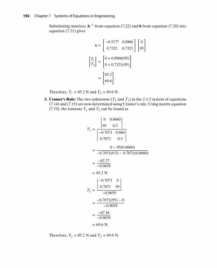
192 Chapter 7 Systems of Equations in Engineering
Substituting matrices A−1 from equation (7.22) and b from equation (7.20) intoequation (7.21) gives
x =
[−0.5177 0.8966
0.7321 0.7321
][0
95
]
[T1T2
]=
[0 + 0.8966(95)
0 + 0.7321(95)
]
=
[85.2
69.6
].
Therefore, T1 = 85.2 N and T2 = 69.6 N.
3. Cramer’s Rule: The two unknowns (T1 and T2) in the 2 × 2 system of equations(7.14) and (7.15) are now determined using Cramer’s rule. Using matrix equation(7.19), the tensions T1 and T2 can be found as
T1 =
|||||0 0.8660
95 0.5
||||||||||−0.7071 0.866
0.7071 0.5
|||||=
0 − 95(0.8660)−0.7071(0.5) − 0.7071(0.8660)
= −82.27−0.9659
= 85.2 N
T2 =
|||||−0.7071 0
0.7071 95
|||||−0.9659
=−0.7071(95) − 0
−0.9659
= −67.16−0.9659
= 69.6 N.
Therefore, T1 = 85.2 N and T2 = 69.6 N.

7.4 Further Examples of Systems of Equations in Engineering 193
7.4 FURTHER EXAMPLES OF SYSTEMSOF EQUATIONS IN ENGINEERING
Example7-1
Reaction Forces on a Vehicle: The weight of a vehicle is supported by reactionforces at its front and rear wheels as shown in Fig. 7.4. If the weight is W = 4800 lb,the reaction forces R1 and R2 satisfy the equation:
R1 + R2 − 4800 = 0 (7.23)
Also, suppose that
6 R1 − 4 R2 = 0. (7.24)
(a) Find R1 and R2 using the substitution method.
(b) Write the system of equations (7.23) and (7.24) in the matrix form A x = b,
where x =[
R1R2
].
(c) Find R1 and R2 using the matrix algebra method. Perform all computations byhand and show all steps.
(d) Find R1 and R2 using Cramer’s rule.
R1 R2
W
Figure 7.4 Reaction forces acting on a vehicle.
Solution (a) Substitution Method: Using equation (7.23), find R1 in terms of R2 as
R1 = 4800 − R2. (7.25)
Substituting R1 from equation (7.25) into equation (7.24) gives
6 (4800 − R2) − 4 R2 = 0
28, 800 − 6 R2 − 4 R2 = 0
10 R2 = 28, 800
R2 = 2880 lb. (7.26)
Now, substituting R2 from equation (7.26) into equation (7.25) yields
R1 = 4800 − 2880
= 1920 lb.
Therefore, R1 = 1920 lb and R2 = 2880 lb.

194 Chapter 7 Systems of Equations in Engineering
(b) Writing equations (7.23) and (7.24) in the matrix form gives[1 16 −4
] [R1R2
]=[
48000
]. (7.27)
(c) Matrix Algebra Method: From the matrix equation (7.27), the matrices A, x,and b are given by
A =[
1 16 −4
](7.28)
b =[
48000
](7.29)
x =[
R1R2
]. (7.30)
The reaction forces can be found by finding the inverse of matrix A and thenmultiplying this with column matrix b as
x = A−1 b
where
A−1 = 1|A|[−4 −1−6 1
](7.31)
and
|A| = |||| 1 16 −4
||||= (1)(−4) − (6)(1)
= −10. (7.32)
Substituting equation (7.32) in equation (7.31), the inverse of matrix A isgiven by
A−1 = 1−10
[−4 −1−6 1
]
=[
0.4 0.10.6 −0.1
]. (7.33)
The reaction forces can now be found by multiplying A−1 in equation (7.33)with matrix b given in equation (7.29) as
x =[
0.4 0.10.6 −0.1
] [4800
0
][
R1R2
]=[
(0.4)(4800) + 0(0.6)(4800) + 0
]
=[
19202880
].
Therefore, R1 = 1920 lb and R2 = 2880 lb.

7.4 Further Examples of Systems of Equations in Engineering 195
(d) Cramer’s Rule: The reaction forces R1 and R2 can be found by solving thesystem of equations (7.23) and (7.24) using Cramer’s rule as
R1 =
|||| 4800 10 −4
||||−10
=(4800)(−4) − (0)(1)
−10= 1920.
R2 =
|||| 1 48006 0
||||−10
=(1)(0) − (6)(4800)
−10= 2880.
Therefore, R1 = 1920 lb and R2 = 2880 lb.
Example7-2
External Forces Acting on a Truss: A two-bar truss is subjected to external forcesin both the horizontal and vertical directions as shown in Fig. 7.5. The forces F1and F2 satisfy the following system of equations:
0.8 F1 + 0.8 F2 − 200 = 0 (7.34)
0.6 F1 − 0.6 F2 − 100 = 0. (7.35)
(a) Find F1 and F2 using the substitution method.
(b) Write the system of equations (7.34) and (7.35) in the matrix form A x = b,
where x =[
F1F2
].
(c) Find F1 and F2 using the matrix algebra method. Perform all computations byhand and show all steps.
(d) Find F1 and F2 using Cramer’s rule.
8 ft
200 lb
F1
F2100 lb 100 lb
6 ft
6 ft
200 lb
Figure 7.5 A truss subjected to external forces.

196 Chapter 7 Systems of Equations in Engineering
Solution (a) Substitution Method: Using equation (7.34), find force F1 in terms of F2 as
0.8 F1 = 200 − 0.8 F2
F1 = 250 − F2. (7.36)
Substituting F1 from equation (7.36) into equation (7.35) gives
0.6 (250 − F2) − 0.6 F2 = 100
250 − 2 F2 = 166.67
F2 =(250 − 166.67)
2= 41.67 lb. (7.37)
Now, substituting F2 from equation (7.37) into equation (7.36) yields
F1 = 250 − 41.67
= 208.33 lb.
Therefore, F1 = 208.33 lb and F2 = 41.67 lb.
(b) Writing equations (7.34) and (7.35) in the matrix form yields[0.8 0.80.6 −0.6
] [F1F2
]=[
200100
]. (7.38)
(c) Matrix Algebra Method: Writing matrix equation in (7.38) in the form A x = bgives
A =[
0.8 0.80.6 −0.6
](7.39)
b =[
200100
](7.40)
x =[
F1F2
]. (7.41)
The forces F1 and F2 can be found by finding the inverse of matrix A and thenmultiplying this with matrix b as
x = A−1 b
where
A−1 = 1|A|[−0.6 −0.8−0.6 0.8
](7.42)
and
|A| = |||| 0.8 0.80.6 −0.6
||||= (0.8)(−0.6) − (0.6)(0.8)
= −0.96. (7.43)

7.4 Further Examples of Systems of Equations in Engineering 197
Substituting equation (7.43) in equation (7.42), the inverse of matrix A isgiven by
A−1 = 1−0.96
[−0.6 −0.8−0.6 0.8
]
=[
0.625 0.8330.625 −0.833
]. (7.44)
The forces F1 and F2 can now be found by multiplying A−1 in equation (7.44)by column matrix b given in equation (7.40) as
x =[
0.625 0.8330.625 −0.833
] [200100
][
F1F2
]=[
(0.625)(200) + (0.833)(100)(0.625)(200) + (−0.833)(100)
]
=[
208.3341.67
]lb
Therefore, F1 = 208.33 lb and F2 = 41.67 lb.
(d) Cramer’s Rule: The forces F1 and F2 can be found by solving the system ofequations (7.34) and (7.35) using Cramer’s rule as
F1 =
|||| 200 0.8100 −0.6
||||−0.96
=(200)(−0.6) − (100)(0.8)
−0.96= 208.33 lb
F2 =
|||| 0.8 2000.6 100
||||−0.96
=(0.8)(100) − (0.6)(200)
−0.96= 41.67 lb
Therefore, F1 = 208.33 lb and R2 = 41.67 lb.
Example7-3
Summing Op-Amp Circuit: A summing Op-Amp circuit is shown in Fig. 7.6. Ananalysis of the Op-Amp circuit shows that the conductances G1 and G2 in mho ()satisfy the following system of equations:
10 G1 + 5 G2 = 125 (7.45)
9 G1 − 19 = 4 G2. (7.46)
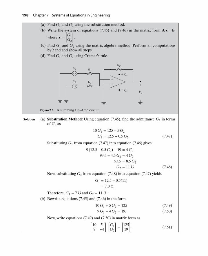
198 Chapter 7 Systems of Equations in Engineering
(a) Find G1 and G2 using the substitution method.
(b) Write the system of equations (7.45) and (7.46) in the matrix form A x = b,
where x =[
G1G2
].
(c) Find G1 and G2 using the matrix algebra method. Perform all computationsby hand and show all steps.
(d) Find G1 and G2 using Cramer’s rule.
+
−
−Vcc
+Vcc
+−
GF
G1
G2
V1
Vo
+−
V2
+−
Figure 7.6 A summing Op-Amp circuit.
Solution (a) Substitution Method: Using equation (7.45), find the admittance G1 in termsof G2 as
10 G1 = 125 − 5 G2
G1 = 12.5 − 0.5 G2. (7.47)
Substituting G1 from equation (7.47) into equation (7.46) gives
9 (12.5 − 0.5 G2) − 19 = 4 G2
93.5 − 4.5 G2 = 4 G2
93.5 = 8.5 G2
G2 = 11 . (7.48)
Now, substituting G2 from equation (7.48) into equation (7.47) yields
G1 = 12.5 − 0.5(11)
= 7.0 .
Therefore, G1 = 7 and G2 = 11 .
(b) Rewrite equations (7.45) and (7.46) in the form
10 G1 + 5 G2 = 125 (7.49)
9 G1 − 4 G2 = 19. (7.50)
Now, write equations (7.49) and (7.50) in matrix form as[10 59 −4
] [G1G2
]=[
12519
]. (7.51)

7.4 Further Examples of Systems of Equations in Engineering 199
(c) Matrix Algebra Method: Writing the matrix equation in (7.64) in the formA x = b gives
A =[
10 59 −4
](7.52)
b =[
12519
](7.53)
x =[
G1G2
]. (7.54)
The admittance G1 and G2 can be found by finding the inverse of matrix Aand then multiplying this with matrix b as
x = A−1 bwhere
A−1 = 1|A|[−4 −5−9 10
](7.55)
and
|A| = |||| 10 59 −4
||||= (10)(−4) − (5)(9)
= −85. (7.56)Substituting equation (7.56) in equation (7.55), the inverse of matrix A isgiven as
A−1 = 1−85
[−4 −5−9 10
]
=⎡⎢⎢⎢⎣
485
585
985
−1085
⎤⎥⎥⎥⎦. (7.57)
The admittance G1 and G2 can now be found by multiplying A−1 in equation(7.57) and the column matrix b given in equation (7.53) as
x =⎡⎢⎢⎢⎣
485
585
985
−1085
⎤⎥⎥⎥⎦[
12519
]
[G1
G2
]=
⎡⎢⎢⎢⎢⎣
(485
)(125) +
(5
85
)(19)(
985
)(125) +
(−10
85
)(19)
⎤⎥⎥⎥⎥⎦=⎡⎢⎢⎢⎣
(100 + 19)17
(225 − 38)17
⎤⎥⎥⎥⎦=[
711
].
Therefore, G1 = 7 and G2 = 11 .

200 Chapter 7 Systems of Equations in Engineering
(d) Cramer’s Rule: The admittance G1 and G2 can be found by solving the systemof equations (7.45) and (7.46) using Cramer’s rule as
G1 =
|||||125 5
19 −4
|||||−85
=(125)(−4) − (19)(5)
−85
= 7
G2 =
|||||10 125
9 19
|||||−85
=(10)(19) − (9)(125)
−85
= 11 .
Therefore, G1 = 7 and G2 = 11 .
Example7-4
Force on the Gastrocnemius Muscle: A driver applies a steady force of FP = 30 Nagainst a gas pedal, as shown in Fig. 7.7. The free-body diagram of the driver’s footis also shown. Based on the x-y coordinate system shown, the force of the gastroc-nemius muscle Fm and the weight of the foot WF satisfy the following system ofequations:
Fm cos 60 − WF cos 30 = Rx (7.58)
Fm sin 60 − WF sin 30 = Ry − FP. (7.59)
where Rx and Ry are the reactions at the ankle.
(a) Suppose Rx = 70√3
N and Ry = 120 N. Write the system of equations in terms
of Fm and WF .
(b) Find Fm and WF using the substitution method.
(c) Write the system of equations (7.58) and (7.59) in the matrix form A x = b,
where x =[
FmWF
].
(d) Find Fm and WF using the matrix algebra method. Perform all computationsby hand and show all steps.
(e) Find Fm and WF using Cramer’s rule.
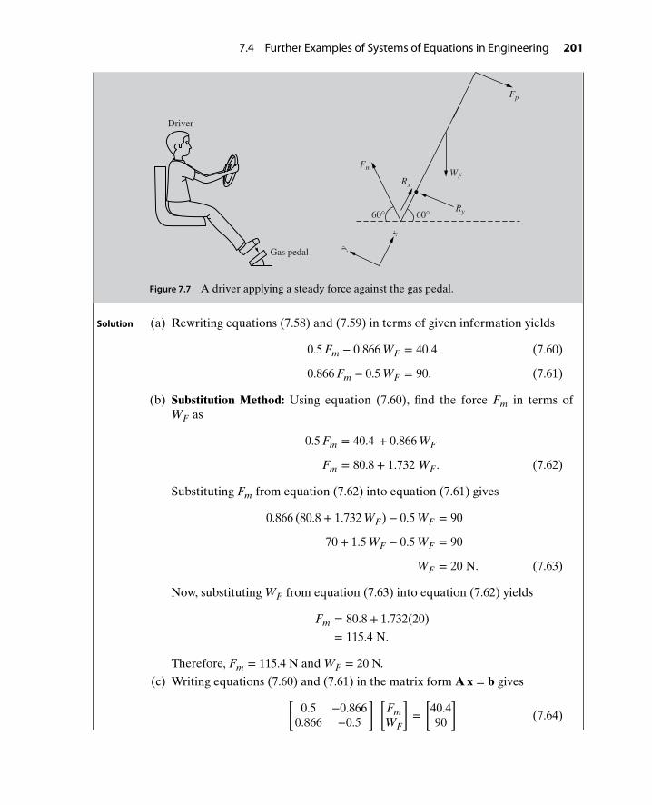
7.4 Further Examples of Systems of Equations in Engineering 201
Gas pedal
Driver
Fm
Rx
y
x
Fp
WF
Ry60°60°
Figure 7.7 A driver applying a steady force against the gas pedal.
Solution (a) Rewriting equations (7.58) and (7.59) in terms of given information yields
0.5 Fm − 0.866 WF = 40.4 (7.60)
0.866 Fm − 0.5 WF = 90. (7.61)
(b) Substitution Method: Using equation (7.60), find the force Fm in terms ofWF as
0.5 Fm = 40.4 + 0.866 WF
Fm = 80.8 + 1.732 WF . (7.62)
Substituting Fm from equation (7.62) into equation (7.61) gives
0.866 (80.8 + 1.732 WF) − 0.5 WF = 90
70 + 1.5 WF − 0.5 WF = 90
WF = 20 N. (7.63)
Now, substituting WF from equation (7.63) into equation (7.62) yields
Fm = 80.8 + 1.732(20)
= 115.4 N.
Therefore, Fm = 115.4 N and WF = 20 N.
(c) Writing equations (7.60) and (7.61) in the matrix form A x = b gives[0.5 −0.866
0.866 −0.5
] [FmWF
]=[
40.490
](7.64)

202 Chapter 7 Systems of Equations in Engineering
where
A =[
0.5 −0.8660.866 −0.5
], (7.65)
b =[
40.490
], (7.66)
and x =[
FmWF
]. (7.67)
(d) Matrix Algebra Method: The forces Fm and WF can be found by finding theinverse of the matrix A and then multiplying this by vector b as
x = A−1 b,
where
A−1 = 1|A|[
−0.5 0.866−0.866 0.5
], (7.68)
and |A| = |||| 0.5 −0.8660.866 −0.5
||||= (0.5)(−0.5) − (0.866)(−0.866)
= 0.5. (7.69)
Substituting equation (7.69) in equation (7.68), the inverse of matrix A is givenas
A−1 = 10.5
[−0.5 0.866−0.866 0.5
]
=[ −1.0 1.732
−1.732 1.0
]. (7.70)
The forces Fm and WF can now be found by multiplying A−1 in equation (7.70)and the column matrix b given in equation (7.66) as
x =[ −1.0 1.732
−1.732 1.0
] [40.490
][
FmWF
]=[−1.0 (40.4) + 1.732 (90)
−1.732 (40.4) + 1.0 (90)
]
=[
115.420.0
]N.
Therefore, Fm = 115.4 N and WF = 20 N.

7.4 Further Examples of Systems of Equations in Engineering 203
(e) Cramer’s Rule: The forces Fm and WF can be found by solving the system ofequations (7.60) and (7.61) using Cramer’s rule as
Fm =
|||| 40.4 −0.86690 −0.5
||||0.5
=(40.4)(−0.5) − (90)(−0.866)
0.5= 115.4 N
WF =
|||| 0.5 40.40.866 90
||||0.5
=(0.5)(90) − (0.866)(40.4)
0.5= 20.0 N.
Therefore, Fm = 115.4 N and WF = 20 N.
Example7-5
Two-Component Blending of Liquids: An environmental engineer wishes to blenda single mixture of insecticide spray solution of volume V = 1000 L and concentra-tion C = 0.15 from two spray solutions of concentrations c1 = 0.12 and c2 = 0.17.The required volumes of the two spray solutions v1 and v2 can be determined froma system of equations describing conditions for volume and concentration, respec-tively, as
v1 + v2 = V (7.71)
c1 v1 + c2 v2 = C V (7.72)
(a) Knowing that V = 1000 L, c1 = 0.12, c2 = 0.17, and C = 0.15, rewrite the sys-tem of equations in terms of v1 and v2.
(b) Find v1 and v2 using the substitution method.
(c) Write the system of equations (7.71) and (7.72) in the matrix form A x = b,
where x =[
v1v2
].
(d) Find v1 and v2 using the matrix algebra method. Perform all computations byhand and show all steps.
(e) Find v1 and v2 using Cramer’s rule.
Solution (a) Rewriting equations (7.71) and (7.72) in terms of the given information yields
v1 + v2 = 1000 (7.73)
0.12 v1 + 0.17 v2 = 150. (7.74)

204 Chapter 7 Systems of Equations in Engineering
(b) Substitution Method: Using equation (7.73), find the volume v2 in terms of v1as
v2 = 1000 − v1. (7.75)
Substituting v2 from equation (7.75) into equation (7.74) gives
0.12 v1 + 0.17 (1000 − v1) = 150
0.12 v1 + 170 − 0.17 v1 = 150
−0.05 v1 = −20
v1 = 400. (7.76)
Now, substituting v1 from equation (7.76) into equation (7.75) yields
v2 = 1000 − 400
= 600.
Therefore, v1 = 400 L and v2 = 600 L.
(c) Writing equations (7.73) and (7.74) in matrix form A x = b gives[1 1
0.12 0.17
] [v1v2
]=[
1000150
], (7.77)
where
A =[
1 10.12 0.17
], (7.78)
b =[
1000150
], (7.79)
and x =[
v1v2
]. (7.80)
(d) Matrix Algebra Method: The volumes v1 and v2 can be found by finding theinverse of the matrix A and then multiplying this by column vector b as
x = A−1 b,
where
A−1 = 1|A|[
0.17 −1−0.12 1
](7.81)
and |A| = |||| 1 10.12 0.17
||||= (1)(0.17) − (0.12)(1)
= 0.05. (7.82)

7.4 Further Examples of Systems of Equations in Engineering 205
Substituting equation (7.82) in equation (7.81), the inverse of matrix A is givenas
A−1 = 10.05
[0.17 −1
−0.12 1
]
=
[3.4 −20
−2.4 20
]. (7.83)
The volumes v1 and v2 can now be found by multiplying A−1 in equation (7.83)and the column vector b given in equation (7.79) as
x =
[3.4 −20
−2.4 20
] [1000
150
][
v1
v2
]=
[3.4 (1000) − 20 (150)
−2.4 (1000) + 20 (150)
]
=[
400600
].
Therefore, v1 = 400 L and v2 = 600 L.
(e) Cramer’s Rule: The volumes v1 and v2 can be found by solving the system ofequations (7.73) and (7.74) using Cramer’s rule as
v1 =
|||||1000 1
150 0.17
|||||0.05
=(1000)(0.17) − (150)(1)
0.05
= 400
v2 =
|||||1 1000
0.12 150
|||||0.05
=(1)(150) − (0.12)(1000)
0.05
= 600.
Therefore, v1 = 400 L and v2 = 600 L.

206 Chapter 7 Systems of Equations in Engineering
P R O B L E M S
7-1. Consider the two-loop circuit shownin Fig. P7.1. The currents I1 and I2(in A) satisfy the following system ofequations:
16 I1 − 9 I2 = 110 (7.84)
20 I2 − 9 I1 + 110 = 0. (7.85)
110 V 110 V
7 Ω 11 Ω
9 ΩI1 I2
+−
+−
Figure P7.1 Two-loop circuit for problem P7-1.
(a) Find I1 and I2 using the substitutionmethod.
(b) Write the system of equations(7.84) and (7.85) in the matrix form
A I = b, where I =[
I1I2
].
(c) Find I1 and I2 using the matrixalgebra method. Perform all com-putations by hand and show allsteps.
(d) Find I1 and I2 using Cramer’s rule.
7-2. Consider the two-loop circuit shownin Fig. P7.2. The currents I1 and I2(in A) satisfy the following system ofequations:
18 I1 − 10 I2 − 246 = 0 (7.86)
22 I2 − 10 I1 = −334. (7.87)
246 V 334 V
8 Ω 12 Ω
10 ΩI1 I2
+−
+−
Figure P7.2 Two-loop circuit for problem P7-2.
(a) Find I1 and I2 using the substitutionmethod.
(b) Write the system of equations(7.86) and (7.87) in the matrix form
A I = b, where I =[
I1I2
].
(c) Find I1 and I2 using the matrixalgebra method. Perform all com-putations by hand and show allsteps.
(d) Find I1 and I2 using Cramer’s rule.
7-3. Consider the two-loop circuit shownin Fig. P7.3. The currents I1 and I2(in A) satisfy the following system ofequations:
1100 I1 + 1000 I2 − 9 = 0 (7.88)
1100 I2 + 1000 I1 = 0. (7.89)
9 V
100 Ω 100 Ω
1 kΩI1I2
+−
Figure P7.3 Two-loop circuit for problem P7-3.
(a) Find I1 and I2 using the substitutionmethod.
(b) Write the system of equations(7.88) and (7.89) in the matrix form
AI = b, where I =[
I1I2
].
(c) Find I1 and I2 using the matrixalgebra method. Perform all com-putations by hand and show allsteps.
(d) Find I1 and I2 using Cramer’s rule.
7-4. Consider the two-node circuit shownin Fig. P7.4. The voltages V1 and V2(in V) satisfy the following system of

Problems 207
equations:
4 V1 − V2 = 20 (7.90)
−3 V1 + 8 V2 = 40. (7.91)
10 V 20 V
10 Ω 30 Ω
20 Ω 20 Ω
V1 V220 Ω
+−
+−
Figure P7.4 Two-node circuit for problem P7-4.
(a) Find V1 and V2 using the substitu-tion method.
(b) Write the system of equations(7.90) and (7.91) in the matrix form
A V = b, where V =[
V1V2
].
(c) Find V1 and V2 using the matrixalgebra method. Perform all com-putations by hand and show allsteps.
(d) Find V1 and V2 using Cramer’s rule.
7-5. Consider the two-node circuit shownin Fig. P7.5. The voltages V1 and V2(in V) satisfy the following system ofequations:
17 V1 = 10 V2 + 50 (7.92)
11 V2 − 6V1 − 42 = 0. (7.93)
10 V 21 V
20 Ω 30 Ω
50 Ω 20 Ω
V1 V210 Ω
+−
+−
Figure P7.5 Two-node circuit for problem P7-5.
(a) Find V1 and V2 using the substitu-tion method.
(b) Write the system of equations(7.92) and (7.93) in the matrix form
A V = b, where V =[
V1V2
].
(c) Find V1 and V2 using the matrixalgebra method. Perform all com-putations by hand and show allsteps.
(d) Find V1 and V2 using Cramer’s rule.
7-6. Consider the two-node circuit shownin Fig. P7.6. The voltages V1 and V2(in V) satisfy the following system ofequations:
0.2 V1 − 0.1 V2 = 4 (7.94)
0.3 V2 − 0.1 V1 + 2 = 0. (7.95)
4 A 2 A10 Ω 5 Ω
V1 V210 Ω↑
↑
Figure P7.6 Two-node circuit for problem P7-6.
(a) Find V1 and V2 using the substitu-tion method.
(b) Write the system of equations (7.94)and (7.95) in the matrix form A V =
b, where V =[
V1V2
].
(c) Find V1 and V2 using the matrixalgebra method. Perform all com-putations by hand and show allsteps.
(d) Find V1 and V2 using Cramer’s rule.
7-7. An analysis of the circuit shown inFig. P7.7 yields the following system of

208 Chapter 7 Systems of Equations in Engineering
equations:
−4 V2 + 7 V1 = 0 (7.96)
2 V1 − 7 V2 + 10 = 0. (7.97)
10 V
R5R2R1
V1 R3
= 40 ΩR4
= 5 Ω
20 Ω 20 Ω10 Ω
+−
+
−V2
+
−
Figure P7.7 Two-node circuit for problem P7-7.
(a) Find V1 and V2 using the substitu-tion method.
(b) Write the system of equations(7.96) and (7.97) in the matrix form
AV = b, where V =[
V1V2
].
(c) Find V1 and V2 using the matrixalgebra method. Perform all com-putations by hand and show allsteps.
(d) Find V1 and V2 using Cramer’s rule.
7-8. A summing Op-Amp circuit is shownin Fig. 7.6. An analysis of the Op-Ampcircuit shows that the admittances G1and G2 in mho () satisfy the followingsystem of equations:
5 G1 − 145 = −10 G2 (7.98)
−9 G2 + 71 = −4 G1. (7.99)
(a) Find G1 and G2 using the substitu-tion method.
(b) Write the system of equations(7.98) and (7.99) in the matrix form
A G = b, where G =[
G1G2
].
(c) Find G1 and G2 using the matrixalgebra method. Perform all com-putations by hand and show allsteps.
(d) Find G1 and G2 using Cramer’s rule.
7-9. A summing Op-Amp circuit is shown inFig. 7.6. An analysis of the Op-Amp cir-cuit shows that the admittances G1 andG2 in mho () satisfy the following sys-tem of equations:
10 G1 + 10 G2 = 0.2 (7.100)
5 G1 + 15 G2 = 0.125. (7.101)(a) Find G1 and G2 using the substitu-
tion method.(b) Write the system of equations
(7.100) and (7.101) in the matrix
form A G = b, where G =[
G1G2
].
(c) Find G1 and G2 using the matrixalgebra method. Perform all com-putations by hand and show allsteps.
(d) Find G1 and G2 using Cramer’s rule.
7-10. A 20 kg object is suspended by twocables as shown in Fig. P7.10. The ten-sions T1 and T2 satisfy the followingsystem of equations:
0.5 T1 = 0.866 T2 (7.102)
0.5 T2 + 0.866 T1 = 196. (7.103)
20 kgg = 9.8 m/sec2
x
y
60°30°
60° 30°
W
T1
T2
Figure P7.10 A 20 kg object suspended by twocables for problem P7-10.
(a) Write the system of equations(7.100) and (7.101) in the matrixform A T = b, where
T =[
T1T2
].

Problems 209
In other words, find matrices Aand b. What are the dimensions of Aand b?
(b) Find T1 and T2 using the matrixalgebra method. Perform all matrixcomputation by hand.
(c) Find T1 and T2 using Cramer’s rule.
7-11. A 100 lb weight is suspended by twocables as shown in Fig. P7.11. The ten-sions T1 and T2 satisfy the followingsystem of equations:
0.6 T1 + 0.8 T2 = 100 (7.104)
0.8 T1 − 0.6 T2 = 0. (7.105)
(a) Write the system of equations(7.104) and (7.105) in the matrixform A x = b, where
x =[
T1T2
].
In other words, find matrices Aand b.
(b) Find T1 and T2 using the matrixalgebra method. Perform all matrixcomputation by hand and show allsteps.
(c) Find T1 and T2 using Cramer’s rule.
x
y
36.87°
100 lb 100 lb
T2T153.13°
Figure P7.11 A 100 lb weight suspended by twocables for problem P7-11.
7-12. A two-bar truss supports a weight ofW = 750 lb as shown in Fig. P7.12. Theforces F1 and F2 satisfy the followingsystem of equations:
0.866 F1 = F2 (7.106)
0.5 F1 = 750. (7.107)
(a) Write the system of equations(7.106) and (7.107) in the matrixform A F = b, where
F =[
F1F2
].
In other words, find matrices Aand b.
(b) Find F1 and F2 using the matrixalgebra method. Perform all matrixcomputation by hand and show allsteps.
(c) Find F1 and F2 using Cramer’s rule.
W
W
F2
F1
x
y
30°30°
Figure P7.12 A two-bar truss supporting a weightfor problem P7-12.
7-13. A 10 kg object is suspended from a two-bar truss shown in Fig. P7.13. The forcesF1 and F2 satisfy the following system ofequations:
0.707 F1 = F2 (7.108)
0.707 F1 = 98.1. (7.109)
W
W
x
y
F2
F1
45°45°
Figure P7.13 An object suspended from a two-bartruss for problem P7-13.

210 Chapter 7 Systems of Equations in Engineering
(a) Write the system of equations(7.108) and (7.109) in the matrixform A F = b, where
F =[
F1F2
].
In other words, find matrices Aand b.
(b) Find F1 and F2 using the matrixalgebra method. Perform all matrixcomputation by hand and show allsteps.
(c) Find F1 and F2 using Cramer’s rule.
7-14. A F = 100 N force is applied to a two-bar truss as shown in Fig. P7.14. Theforces F1 and F2 satisfy the followingsystem of equations:
−0.5548 F1 − 0.8572 F2 = −100 (7.110)
0.832 F1 = 0.515F2. (7.111)
(a) Write the system of equations(7.110) and (7.111) in the matrixform A F = b, where
F =[
F1F2
].
In other words, find matrices A andb.
(b) Find F1 and F2 using the matrixalgebra method. Perform all matrixcomputation by hand and show allsteps.
(c) Find F1 and F2 using Cramer’s rule.
F2
3
FBD
1
F
F1 F2
x
y56.3°
59.0°
Figure P7.14 A 100 N force applied to a two-bartruss for problem P7-14.
7-15. A force F = 200 lb is applied to a two-bar truss as shown in Fig. P7.15. Theforces F1 and F2 satisfy the followingsystem of equations:
0.866 F1 + 0.707 F2 = 200 (7.112)
0.5 F1 − 0.707 F2 = 0. (7.113)
(a) Write the system of equations(7.112) and (7.113) in the matrixform A F = b, where
F =[
F1F2
].
In other words, find matrices Aand b.
(b) Find F1 and F2 using the matrixalgebra method. Perform all matrixcomputation by hand and show allsteps.
(c) Find F1 and F2 using Cramer’s rule.
F2
3
FBD
1
F
F1 F2
x
y60° 30°
Figure P7.15 A 200 lb force applied to a two-bartruss for problem P7-15.
7-16. The weight of a vehicle is supportedby reaction forces at its front and rearwheels as shown in Fig. P7.16. If theweight of the vehicle is W = 4800 lb,the reaction forces R1 and R2 satisfy thefollowing system of equations:
R1 + R2 − 4800 = 0 (7.114)
6 R1 − 4 R2 = 0. (7.115)
(a) Find R1 and R2 using the substitu-tion method.
(b) Write the system of equations(7.114) and (7.115) in the matrix

Problems 211
form A x = b, where
x =[
R1R2
].
In other words, find matrices Aand b.
(c) Find R1 and R2 using the matrixalgebra method. Perform all matrixcomputation by hand and show allsteps.
(d) Find R1 and R2 using Cramer’s rule.
R1 R2
W
Figure P7.16 A vehicle supported by reactionforces.
7-17. Solve problem P7-16 if the system ofequations are given by equations (7.116)and (7.117).
R1 + R2 − 3000 = 0 (7.116)
7 R1 − 3 R2 = 0. (7.117)
7-18. Solve problem P7-16 if the system ofequations are given by (7.118) and(7.119).
R1 + R2 = 5000 (7.118)
4 R1 = 6 R2. (7.119)
7-19. A vehicle weighing W = 10 kN is parkedon an inclined driveway (𝜃 = 21.8)as shown in Fig. P7.19. The forces Fand N satisfy the following system ofequations:
0.9285 F = 0.3714 N (7.120)
0.9285 N + 0.3714 F − 10 = 0 (7.121)
where forces F and N are in kN.
(a) Write the system of equations(7.120) and (7.121). in the matrixform A x = b, where
x =[
FN
].
In other words, find matrices Aand b.
(b) Find F and N using the matrixalgebra method. Perform all matrixcomputations by hand and show allsteps.
(c) Find F and N using Cramer’s rule.
W
N
F
F NFBD
g
W
x
y θ
θ
Figure P7.19 A truck parked on an inclineddriveway.
7-20. A vehicle weighing W = 2000 lbis parked on an inclined driveway(𝜃 = 35) as shown in Fig. P7.19. Theforces F and N satisfy the following sys-tem of equations:
−0.8192 F + 0.5736 N = 0 (7.122)
0.8192 N + 0.5736 F = 2000. (7.123)
where forces F and N are in lb. Solveparts (a)–(c) of problem P7-19 for sys-tem of equations given by (7.122) and(7.123).
7-21. A 100 lb crate weighing W = 100 lbis pushed against an incline (𝜃 = 30)with a force of Fa = 30 lb as shown inFig. P7.21. The forces Ff and N satisfythe following system of equations:
0.866 Ff − 0.5N + 30 = 0 (7.124)
0.866 N + 0.5 Ff − 100 = 0. (7.125)
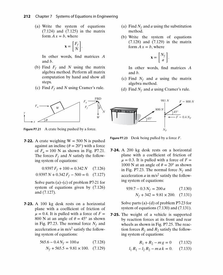
212 Chapter 7 Systems of Equations in Engineering
(a) Write the system of equations(7.124) and (7.125) in the matrixform A x = b, where
x =[
FfN
].
In other words, find matrices Aand b.
(b) Find Ff and N using the matrixalgebra method. Perform all matrixcomputation by hand and show allsteps.
(c) Find Ff and N using Cramer’s rule.
FBD
Ff
N
Fa
W
W
Fa
x
y
θ
θ
Figure P7.21 A crate being pushed by a force.
7-22. A crate weighing W = 500 N is pushedagainst an incline (𝜃 = 20) with a forceof Fa = 100 N as shown in Fig. P7.21.The forces Ff and N satisfy the follow-ing system of equations:
0.9397 Ff + 100 = 0.342 N (7.126)
0.9397 N + 0.342 Ff − 500 = 0. (7.127)
Solve parts (a)–(c) of problem P7-21 forsystem of equations given by (7.126)and (7.127).
7-23. A 100 kg desk rests on a horizontalplane with a coefficient of friction of𝜇 = 0.4. It is pulled with a force of F =800 N at an angle of 𝜃 = 45 as shownin Fig. P7.23. The normal force Nf andacceleration a in m/s2 satisfy the follow-ing system of equations:
565.6 − 0.4 Nf = 100 a (7.128)
Nf + 565.5 = 9.81 × 100. (7.129)
(a) Find Nf and a using the substitutionmethod.
(b) Write the system of equations(7.128) and (7.129) in the matrixform A x = b, where
x =[
Nfa
].
In other words, find matrices Aand b.
(c) Find Nf and a using the matrixalgebra method.
(d) Find Nf and a using Cramer’s rule.
F = 800 N
F = 0.4 NF
NF
981 N
800 N
45°
45°
Figure P7.23 Desk being pulled by a force F.
7-24. A 200 kg desk rests on a horizontalplane with a coefficient of friction of𝜇 = 0.3. It is pulled with a force of F =1000 N at an angle of 𝜃 = 20 as shownin Fig. P7.23. The normal force Nf andacceleration a in m/s2 satisfy the follow-ing system of equations:
939.7 − 0.3 Nf = 200 a (7.130)
Nf + 342 = 9.81 × 200. (7.131)
Solve parts (a)–(d) of problem P7-23 forsystem of equations (7.130) and (7.131).
7-25. The weight of a vehicle is supportedby reaction forces at its front and rearwheels as shown in Fig. P7.25. The reac-tion forces R1 and R2 satisfy the follow-ing system of equations:
R1 + R2 − m g = 0 (7.132)
l1 R1 − l2 R2 − m a k = 0. (7.133)

Problems 213
(a) Write the system of equations(7.132) and (7.133) if l1 = 2 m,l2 = 1.5 m, k = 1.5 m, g = 9.81 m/s2,m = 1000 kg, and a = 5 m/s2.
(b) For the system of equations foundin part (a), find R1 and R2 using thesubstitution method.
(c) Write the system of equations in thematrix form A x = b, where
x =[
R1R2
].
In other words, find matrices Aand b.
(d) Find R1 and R2 using the matrixalgebra method.
(e) Find R1 and R2 using Cramer’s rule.
W = mg
Gk
ma
Fl2l1
R1 R2
Figure P7.25 A vehicle supported by reactionforces.
7-26. Repeat problem P7-25, if l1 = 2 m, l2 =1.5 m, k = 1.5 m, g = 9.81 m/s2, m =1000 kg, and a = −5 m/s2.
7-27. Repeat problem P7-25, if l1 = 2 m,l2 = 2 m, k = 1.5 m, g = 9.81 m/s2, m =1200 kg, and a = 4.5 m/s2.
7-28. Repeat problem P7-25, if l1 = 2 m, l2 =2 m, k = 1.5 m, g = 9.81 m/s2, m =1200 kg, and a = −4.5 m/s2
7-29. A driver applies a steady force of FP =25 N against a gas pedal, as shown inFig. P7.29. The free-body diagram of thedriver’s foot is also shown. Based on the
x-y coordinate system shown, the forceof the gastrocnemius muscle Fm and theweight of the foot WF satisfy the follow-ing system of equations:
Fm cos 45 − WF cos 30 = Rx (7.134)
Fm sin 45 − WF sin 30 = Ry − FP.
(7.135)
Gas pedal
Driver
Fm Rx
y
x
Fp
WF
Ry60°45°
Figure P7.29 A driver applying a steady forceagainst the gas pedal.
(a) Knowing that Rx = 70∕√
2 N andRy = 105 N, rewrite the system ofequations (7.134) and (7.135) interms of Fm and WF .
(b) Find Fm and WF using the substitu-tion method.
(c) Write the system of equationsobtained in part (a) in the matrix
form A x = b, where x =[
FmWF
].

214 Chapter 7 Systems of Equations in Engineering
(d) Find Fm and WF using the matrixalgebra method. Perform all com-putations by hand and show allsteps.
(e) Find Fm and WF using Cramer’srule.
7-30. An environmental engineer wishes toblend a single mixture of insecticidespray solution of volume V = 500 L witha specified concentration C = 0.2 fromtwo spray solutions of concentrationc1 = 0.15 and c2 = 0.25. The requiredvolumes of the two spray solutions v1and v2 can be determined from a sys-tem of equations describing conditionsfor volume and concentration, respec-tively as
v1 + v2 = V (7.136)
c1 v1 + c2 v2 = C V (7.137)
(a) Knowing that V = 500 L, c1 = 0.15,c2 = 0.25, and C = 0.2, rewrite thesystem of equations (7.136) and(7.137) in terms of v1 and v2.
(b) Find v1 and v2 using the substitutionmethod.
(c) Write the system of equationsobtained in part (a) in the matrix
form A x = b, where x =[
v1v2
].
(d) Find v1 and v2 using the matrixalgebra method. Perform all com-putations by hand and show allsteps.
(e) Find v1 and v2 using Cramer’s rule.
7-31. Repeat problem P7-30 if V = 400 L, C =0.25, c1 = 0.2, and c2 = 0.4.
7-32. Consider the two-loop circuit shownin Fig. P7.32. The currents I1 and I2(in A) satisfy the following system of
equations:
(0.1 s + 1) I1 − I2 = 100s
(7.138)
−1 I1 +(
1 + 2s
)I2 = 0. (7.139)
0.1 s Ω
1 ΩI1 I2
+−
2s− Ω
100s—– V
Figure P7.32 Two-loop circuit for problem P7-32.
(a) Find I1 and I2 using the substitutionmethod.
(b) Write the system of equations(7.138) and (7.139) in the matrix
form A I = b, where I =[
I1I2
].
(c) Find I1 and I2 using the matrix alge-bra method.
(d) Find I1 and I2 using Cramer’s rule.
7-33. Consider the two-loop circuit shownin Fig. P7.33. The currents I1 and I2(in A) satisfy the following system ofequations:
(0.2 s + 10) I1 − 0.2 s I2 = 100s
(7.140)
−0.2 s I1 +(
0.2 s + 10s
)I2 = 0. (7.141)
10 Ω
0.2 s ΩI1 I2
+−
10s— Ω
100s—– V
Figure P7.33 Two-loop circuit for problem P7-33.
(a) Find I1 and I2 using the substitutionmethod.

Problems 215
(b) Write the system of equations(7.140) and (7.141) in the matrix
form A I = b, where I =[
I1I2
].
(c) Find I1 and I2 using the matrix alge-bra method.
(d) Find I1 and I2 using Cramer’s rule.
7-34. Consider the two-node circuit shownin Fig. P7.34. The voltages V1 and V2(in V) satisfy the following system ofequations:(
5s+ 0.1
)V1 − 0.1 V2 = 0.1
s(7.142)(
0.1 + 5s
)V2 − 0.1 V1 = 0.2
s. (7.143)
V2V1
↑ ↑
10 Ω
0.2 s Ω 5s— Ω
0.1s— A 0.2
s— A
Figure P7.34 Two-loop circuit for problem P7-34.
(a) Write the system of equations(7.142) and (7.143) in the matrix
form A V = b, where V =[
V1V2
].
(b) Find V1 and V2 using the matrixalgebra method.
(c) Find V1 and V2 using Cramer’s rule.
7-35. A mechanical system along with its freebody diagram is shown in Fig. P7.35,where f = 50 N is the applied force. Thelinear displacements X1(s) and X2(s) ofthe two springs in the s-domain satisfythe following system of equations:
40 X1(s) − 40 X2(s) = 50s
(7.144)
−40 X1(s) +(s2 + 65
)X2(s) = 0 (7.145)
(a) Write the system of equations(7.144) and (7.145) in the matrixform A X(s) = b, where X(s) =[
X1(s)X2(s)
].
(b) Find the expressions of X1(s) andX2(s) using the matrix algebramethod.
(c) Find the expressions of X1(s) andX2(s) using Cramer’s rule.
7-36. Fig. P7.36 shows a system with two-masselements and two springs. The mass m1is pulled with a force f = 100 N, and thedisplacements X1(s) and X2(s) of thetwo masses in the s-domain satisfy the
X1X2
f = 50 N
X1
40 (X1 − X2)
X2
m25 X2m = 1 kg f = 50 N k2 = 25 N k1 = 40 N
Figure P7.35 Mechanical system for problem P7-35.
X1X2
f = 100 Nf = 100 N
X1
50 (X1 − X2)
X2
50 X2m2 = 2 kg m1 = 2 kg m2 = 2 kg m1 = 2 kg
k2 = 50 N k1 = 50 N
Figure P7.36 Mechanical system for problem P7-36.

216 Chapter 7 Systems of Equations in Engineering
following system of equations:
(2 s2 + 50
)X1(s) − 50 X2(s) = 100
s(7.146)
−50 X1(s) +(2 s2 + 100
)X2(s) = 0
(7.147)
(a) Write the system of equations(7.146) and (7.146) in the matrixform A X(s) = b, where X(s) =[
X1(s)X2(s)
].
(b) Find the expressions of X1(s) andX2(s) using the matrix algebramethod.
(c) Find the expressions of X1(s) andX2(s) using Cramer’s rule.
7-37. A co-op student at a composite materi-als manufacturing company is attemp-ting to determine how much of twodifferent composite materials to makefrom the available quantities of carbonfiber and resin. The student knows thatComposite A requires 0.15 pounds ofcarbon fiber and 1.6 ounces of poly-mer resin while Composite B requires3.2 pounds of carbon fiber and2.0 ounces of polymer resin. If the avail-able quantities of carbon fiber and resinare 15 pounds and 10 ounces, respec-tively, the amount of each compositeto manufacture satisfies the system ofequations:
0.15 xA + 3.2 xB = 15 (7.148)
1.6 xA + 2.0 xB = 10, (7.149)
where xA and xB are the amountsof Composite A and B (in pounds),respectively.(a) Find xA and xB using the substitu-
tion method.
(b) Write the system of equations(7.148) and (7.149) in the matrix
form A x = b, where x =[
xAxB
].
(c) Find xA and xB using the matrixalgebra method. Perform computa-tion by hand and show all steps.
(d) Find xA and xB using Cramer’s rule.
7-38. Repeat parts (a)–(d) of problem P7-37if Composite A requires 1.6 pounds ofcarbon fiber and 0.5 ounces of poly-mer resin while Composite B requires1.75 pounds of carbon fiber and0.78 ounces of polymer resin. If theavailable quantities of carbon fiber andresin are 17 pounds and 12 ounces,respectively, the amount of each com-posite to manufacture satisfies the sys-tem of equations (7.150) and (7.151).
0.16 xA + 2.5 xB = 17 (7.150)
1.75 xA + 0.78 xB = 12. (7.151)
7-39. A structural engineer is performing afinite element analysis on an aluminumtruss support structure subjected to aload as shown in Fig. P7.39. By the finite
F = 5000 lb
12 in. 36 in.
24 in.
Figure P7.39 Finite element idealization of trussstructure subject to loading.
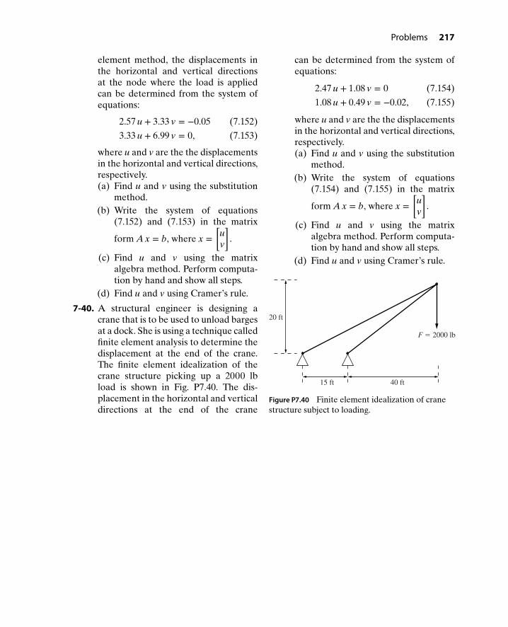
Problems 217
element method, the displacements inthe horizontal and vertical directionsat the node where the load is appliedcan be determined from the system ofequations:
2.57 u + 3.33 v = −0.05 (7.152)
3.33 u + 6.99 v = 0, (7.153)
where u and v are the the displacementsin the horizontal and vertical directions,respectively.(a) Find u and v using the substitution
method.(b) Write the system of equations
(7.152) and (7.153) in the matrix
form A x = b, where x =[
uv
].
(c) Find u and v using the matrixalgebra method. Perform computa-tion by hand and show all steps.
(d) Find u and v using Cramer’s rule.
7-40. A structural engineer is designing acrane that is to be used to unload bargesat a dock. She is using a technique calledfinite element analysis to determine thedisplacement at the end of the crane.The finite element idealization of thecrane structure picking up a 2000 lbload is shown in Fig. P7.40. The dis-placement in the horizontal and verticaldirections at the end of the crane
can be determined from the system ofequations:
2.47 u + 1.08 v = 0 (7.154)
1.08 u + 0.49 v = −0.02, (7.155)
where u and v are the the displacementsin the horizontal and vertical directions,respectively.(a) Find u and v using the substitution
method.(b) Write the system of equations
(7.154) and (7.155) in the matrix
form A x = b, where x =[
uv
].
(c) Find u and v using the matrixalgebra method. Perform computa-tion by hand and show all steps.
(d) Find u and v using Cramer’s rule.
F = 2000 lb
15 ft 40 ft
20 ft
Figure P7.40 Finite element idealization of cranestructure subject to loading.
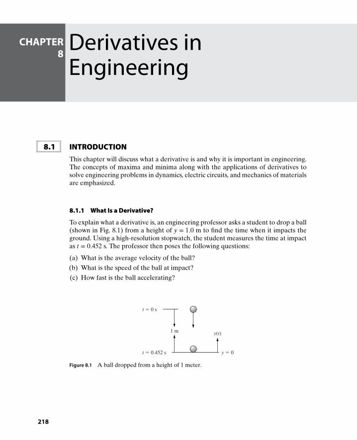
CHAPTER8
Derivatives inEngineering
8.1 INTRODUCTIONThis chapter will discuss what a derivative is and why it is important in engineering.The concepts of maxima and minima along with the applications of derivatives tosolve engineering problems in dynamics, electric circuits, and mechanics of materialsare emphasized.
8.1.1 What Is a Derivative?
To explain what a derivative is, an engineering professor asks a student to drop a ball(shown in Fig. 8.1) from a height of y = 1.0 m to find the time when it impacts theground. Using a high-resolution stopwatch, the student measures the time at impactas t = 0.452 s. The professor then poses the following questions:
(a) What is the average velocity of the ball?
(b) What is the speed of the ball at impact?
(c) How fast is the ball accelerating?
1 m y(t)
y = 0t = 0.452 s
t = 0 s
Figure 8.1 A ball dropped from a height of 1 meter.
218

8.1 Introduction 219
Using the given information, the student provides the following answers:
(a) Average Velocity, υ: The average velocity is the total distance traveled per unittime, i.e.,
υ = Total distanceTotal time
=𝚫 y
𝚫 t=
y2 − y1
t2 − t1
= − 0 − 1.00.452 − 0
= − 1.00.452
= −2.21 m/s.
Note that the negative sign means the ball is moving in the negative y-direction.
(b) Speed at Impact: The student finds that there is not enough information to findthe speed of ball when it impacts the ground. Using an ultrasonic motion detectorin the laboratory, the student repeats the experiment and collects the data givenin Table 8.1.
TABLE 8.1 Additional data collected from the dropped ball.
t, s 0 0.1 0.2 0.3 0.4 0.452
y(t), m 1.0 0.951 0.804 0.559 0.215 0
The student then calculates the average velocity v = Δy∕Δt in each interval.
For example, in the interval t = [0, 0.1], v = 0.951 − 1.00.1 − 0
= −0.490 m/s. The aver-
age velocity in the remaining intervals is given in Table 8.2.
TABLE 8.2 Average velocity of the ball in different intervals.
Interval [0, 0.1] [0.1, 0.2] [0.2, 0.3] [0.3, 0.4] [0.4, 0.452]
v , m/s −0.490 −1.47 −2.45 −3.44 −4.13
The student proposes an approximate answer of −4.13 m/s as the speed ofimpact with ground, but claims that he/she would need an infinite (∞) numberof data points to get it exactly right, i.e.,
v(t = 0.452) = lim t → 0.452y(0.452) − y(t)
0.452 − t.
The professor suggests that this looks like the definition of a derivative, i.e.,
v(t) = lim Δ t → 0y(t + Δ t) − y(t)
Δ t=
dydt
where Δ t = 0.452 − t.
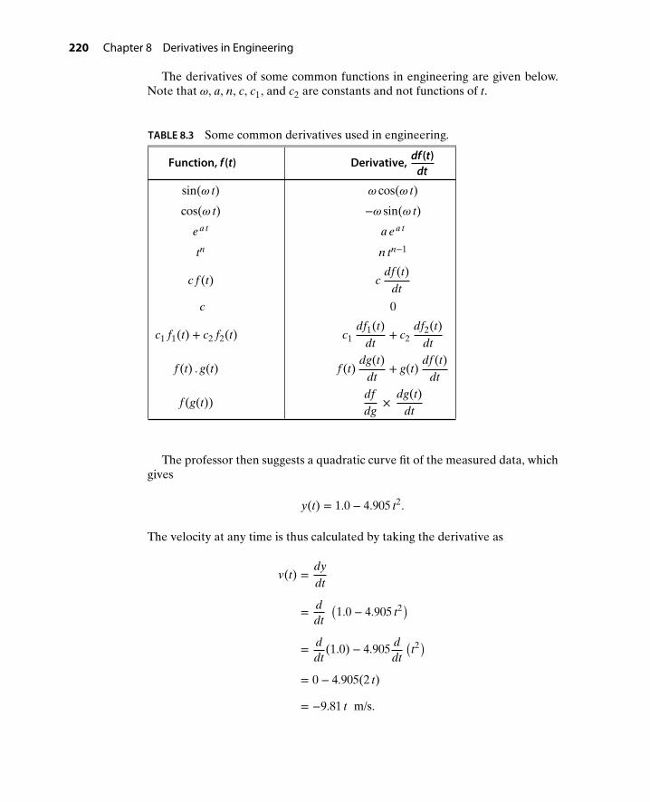
220 Chapter 8 Derivatives in Engineering
The derivatives of some common functions in engineering are given below.Note that 𝜔, a, n, c, c1, and c2 are constants and not functions of t.
TABLE 8.3 Some common derivatives used in engineering.
Function, f (t) Derivative,df (t)
dt
sin(𝜔 t) 𝜔 cos(𝜔 t)
cos(𝜔 t) −𝜔 sin(𝜔 t)
e a t a e a t
tn n tn−1
c f (t) cdf (t)
dt
c 0
c1 f1(t) + c2 f2(t) c1df1(t)
dt+ c2
df2(t)dt
f (t) . g(t) f (t)dg(t)
dt+ g(t)
df (t)dt
f (g(t))dfdg
×dg(t)
dt
The professor then suggests a quadratic curve fit of the measured data, whichgives
y(t) = 1.0 − 4.905 t2.
The velocity at any time is thus calculated by taking the derivative as
v(t) =dydt
= ddt
(1.0 − 4.905 t2)
= ddt
(1.0) − 4.905 ddt
(t2)
= 0 − 4.905(2 t)
= −9.81 t m/s.
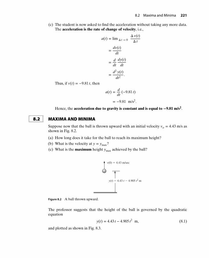
8.2 Maxima and Minima 221
(c) The student is now asked to find the acceleration without taking any more data.The acceleration is the rate of change of velocity, i.e.,
a(t) = lim Δ t → 0Δ v(t)Δ t
=dv(t)
dt
= ddt
dy(t)dt
=d2 y(t)
dt2.
Thus, if v(t) = −9.81 t, then
a(t) = ddt
(−9.81 t)
= −9.81 m/s2.
Hence, the acceleration due to gravity is constant and is equal to −9.81 m/s2.
8.2 MAXIMA AND MINIMASuppose now that the ball is thrown upward with an initial velocity vo = 4.43 m/s asshown in Fig. 8.2.
(a) How long does it take for the ball to reach its maximum height?
(b) What is the velocity at y = ymax?
(c) What is the maximum height ymax achieved by the ball?
v(0) = 4.43 m/sec
y(t) = 4.43 t − 4.905 t2 m
Figure 8.2 A ball thrown upward.
The professor suggests that the height of the ball is governed by the quadraticequation
y(t) = 4.43 t − 4.905 t2 m, (8.1)
and plotted as shown in Fig. 8.3.

222 Chapter 8 Derivatives in Engineering
y(t), m
ymax
tmax00 t, s
Figure 8.3 The height of the ball thrown upward.
Based on the definition of the derivative, the velocity v(t) at any time t is theslope of the line tangent to y(t) at that instant, as shown in Fig. 8.4. Therefore, at thetime when y = ymax, the slope of the tangent line is zero (Fig. 8.5).
y(t), m
t, s
Δy
t
Δt
dydt— = lim
Δt → 0
t + Δt00
ΔyΔt—
Figure 8.4 The derivative as the slope of the tangent line.
For the problem at hand, the velocity is given by
v(t) =dy(t)
dt
= ddt
(4.43 t − 4.905 t2)
= 4.43 − 9.81 t m/s. (8.2)

8.2 Maxima and Minima 223
y(t), m
t, s
ymax
tmax00
dydt— = v(t) = 0
Figure 8.5 The slope of the tangent line at maximum height.
Given equation (8.2), the student answers the professor’s questions as follows:
(a) How long does it take to reach maximum height? At the time of maximum height
t = tmax, v(t) =dy(t)
dt= 0. Hence, setting v(t) in equation (8.2) to zero gives
4.43 − 9.81tmax = 0
tmax = 4.439.81
or
tmax = 0.4515 s.
Therefore, it takes 0.4515 s for the ball to reach the maximum height.
(b) What is the velocity at y = ymax? Since the slope of the height at t = tmax is zero,the velocity at y = ymax is zero. The plot of the velocity, v(t) = 4.43 − 9.81 t fortimes t = 0 to t = 0.903 s, is shown in Fig. 8.6. It can be seen that the velocityis maximum at t = 0 s (initial velocity = 4.43 m/s), reduces to 0 at t = 0.4515 s(t = tmax), and reaches a minimum value (−4.43 m/s) at t = 0.903 sec.
(c) The maximum height: The maximum height can now be obtained by substitutingt = tmax = 0.4515 s in equation (8.1) for y(t)
ymax = y(tmax)
= 4.43 (0.4515) − 4.905 (0.4515)2
= 1.0 m.

224 Chapter 8 Derivatives in Engineering
0
4.43
−4.43t, s
v(t), m/s
0 0.903tmax = 0.4515
Figure 8.6 The velocity profile of the ball thrown upward.
It should be noted that the derivative of a function is zero both at the pointswhere the value of the function is maximum (maxima) and where the value of thefunction is minimum (minima). So if the derivative is zero at both maxima andminima, how can one tell whether the value of the function found earlier is a maxi-mum or a minimum? Consider the function shown in Fig. 8.7, which has local maxi-mum and minimum values. As discussed earlier, the derivative of a function at a
t
y(t)
00
dy(t)dt—— > 0
dy(t)dt—— > 0
dy(t)dt—— < 0
dy(t)dt—— < 0
dy(t)dt—— = 0, ——– < 0 (maxima)
d2y(t)
dt2
dy(t)dt—— = 0, ——– > 0 (minima)
d2y(t)
dt2
Figure 8.7 Plot of a function with local maximum and minimum values.

8.3 Applications of Derivatives in Dynamics 225
point is the slope of the tangent line at that point. At its maximum value, the deriva-tive (slope) of the function shown in Fig. 8.7 changes from positive to negative. Atits minimum value, the derivative (slope) of the function changes from negative topositive. In other words, the rate of change of the derivative (or the second derivativeof the function) is negative at maxima and positive at minima. Therefore, to test formaxima and minima, the following rules apply:
At a Local Maximum:
dy(t)dt
= 0,d2y(t)
dt2< 0
At a Local Minimum:
dy(t)dt
= 0,d2y(t)
dt2> 0
To test whether the point where the slope (first derivative) of the trajectory of theball thrown upward is zero is a maximum or a minimum, the student obtains thesecond derivative of the height as
d2y(t)
dt2= d
dt(4.43 − 9.81 t) = −9.81 < 0.
Therefore, the point where the slope of the trajectory of the ball is zero is a maximumand thus the maximum height is 1.0 m.
In general, the procedure of finding the local maxima and minima of any functionf (t) is as follows:
(a) Find the derivative of the function with respect to t; in other words, find f ′(t) =df (t)
dt.
(b) Find the solution of the equation f ′(t) = 0; in other words, find the values of twhere the function has a local maximum or a local minimum.
(c) To find which values of t gives the local maximum and which values of t gives the
local minimum, determine the second derivative(
f ′′(t) = d2f (t)dt2
)of the function.
(d) Evaluate the second derivative at the values of t found in step (b). If the second
derivative is negative(
d2f (t)dt2
< 0)
, the function has a local maximum for those
values of t; however, if the second derivative is positive, the function has a localminimum for these values.
(e) Evaluate the function, f (t), at the values of t found in step (b) to find the maxi-mum and minimum values.
8.3 APPLICATIONS OF DERIVATIVES IN DYNAMICSThis section demonstrates the application of derivatives in determining the velocityand acceleration of an object if the position of the object is given. This section alsodemonstrates the application of derivatives in sketching plots of position, velocity,and acceleration.

226 Chapter 8 Derivatives in Engineering
8.3.1 Position, Velocity, and Acceleration
Suppose the position x(t) of an object is defined by a linear function with parabolicblends, as shown in Fig. 8.8. This motion is similar to a vehicle starting from rest andaccelerating with a maximum positive acceleration (parabolic position) to reach aconstant speed, cruising at that constant speed (linear position), and then coming tostop with maximum braking (maximum negative acceleration, parabolic position).
As discussed previously, velocity v(t) is the instantaneous rate of change of theposition (i.e., the derivative of the position) and is given by
v(t) = limΔt → 0Δx(t)Δt
or
v(t) =dx(t)
dt.
Therefore, the velocity v(t) is the slope of the position x(t) as shown in Fig. 8.9. Itcan be seen from Fig. 8.9 that the object is starting from rest, moves at a linearvelocity with positive slope until it reaches a constant velocity, cruises at that con-stant velocity, and comes to rest again after moving at a linear velocity with a negativeslope.
x(t), m
t, s
Parabolic blend
Linear function
Figure 8.8 Position of an object as a linear function with parabolic blends.
The acceleration a(t) is the instantaneous rate of change of the velocity (i.e., thederivative of the velocity):
a(t) =dv(t)
dt,

8.3 Applications of Derivatives in Dynamics 227
0
Constant velocity
Linea
r velo
city Linear velocity
t, s
v(t), m/s
Figure 8.9 Velocity of the object moving as a linear function with parabolic blends.
or
a(t) =d2 x(t)
dt2.
Therefore, the acceleration a(t) is the slope of the velocity v(t), which is shown inFig. 8.10. It can be seen from Fig. 8.10 that the object starts with maximum positiveacceleration until it reaches a constant velocity, cruises with zero acceleration, andthen comes to rest with maximum braking (constant negative acceleration).
0 t, s
a(t), m/s2
Figure 8.10 Acceleration of the object moving as a linear function with parabolic blends.
The following examples will provide some practice in taking basic derivatives usingthe formulas in Table 8.3.
Example8-1
The motion of the particle shown in Fig. 8.11 is defined by its position x(t).Determine the position, velocity, and acceleration at t = 0.5 seconds if
(a) x(t) = sin (2𝜋t) m
(b) x(t) = 3 t3 − 4 t2 + 2 t + 6 m
(c) x(t) = 20 cos(3𝜋t) − 5 t2 m

228 Chapter 8 Derivatives in Engineering
v(t)
x(t)
Figure 8.11 A particle moving in the horizontal direction.
Solution (a) The velocity and acceleration of the particle can be obtained by finding thefirst and second derivatives of x(t), respectively. Since
x(t) = sin 2𝜋t m, (8.3)
the velocity is
v(t) =dx(t)
dt
= ddt
(sin 2𝜋t)
or
v(t) = 2𝜋cos 2𝜋t m/s. (8.4)
The acceleration of the particle can now be found by differentiating thevelocity as
a(t) =dv(t)
dt
= ddt
(2𝜋cos 2𝜋t)
= (2𝜋) ddt
(cos 2𝜋t)
= (2𝜋) (−2𝜋 sin 2𝜋t)
or
a(t) = −4𝜋2 sin 2𝜋t m/s2. (8.5)
The position, velocity, and acceleration of the particle at t = 0.5 s can now becalculated by substituting t = 0.5 in equations (8.3), (8.4), and (8.5) as
x(0.5) = sin (2𝜋(0.5)) = sin𝜋 = 0 m
v(0.5) = 2𝜋cos (2𝜋(0.5)) = 2𝜋cos 𝜋 = −2𝜋 m/s
a(0.5) = −4𝜋2 sin (2𝜋(0.5)) = −4𝜋2 sin𝜋 = 0 m/s2.
(b) The position of the particle is given by
x(t) = 3 t3 − 4 t2 + 2 t + 6 m. (8.6)

8.3 Applications of Derivatives in Dynamics 229
The velocity of the particle can be calculated by differentiating equation (8.6)as
v(t) =dx(t)
dt
= ddt
(3 t3 − 4 t2 + 2 t + 6)
= 3 ddt
(t3) − 4 ddt
(t2) + 2 ddt
(t) + 6 ddt
(1)
= 3 (3 t2) − 4 (2t) + 2 (1) + 6 (0)
or
v(t) = 9 t2 − 8 t + 2 m/s. (8.7)
The acceleration of the particle can now be obtained by differentiatingequation (8.7) as
a(t) =dv(t)
dt
= ddt
(9 t2 − 8 t + 2)
= 9 ddt
(t2) − 8 ddt
(t) + 2 ddt
(1)
= 9 (2 t) − 8 (1) + 2 (0)
or
a(t) = 18 t − 8 m/s2. (8.8)
The position, velocity, and acceleration of the particle at t = 0.5 s can now becalculated by substituting t = 0.5 in equations (8.6), (8.7), and (8.8) as
x(0.5) = 3 (0.5)3 − 4 (0.5)2 + 2 (0.5) + 6 = 6.375 m
v(0.5) = 9 (0.5)2 − 8 (0.5) + 2 = 0.25 m/s
a(0.5) = 18 (0.5) − 8 = 1.0 m/s2.
(c) The position of the particle is given by
x(t) = 20 cos(3𝜋t) − 5 t2 m. (8.9)
The velocity of the particle can be calculated by differentiating equation (8.9)as
v(t) =dx(t)
dt
= ddt
(20 cos(3𝜋t) − 5 t2)
= 20 ddt
(cos (3𝜋t) ) − 5 ddt
(t2)
= 20 (−3𝜋 sin (3𝜋t) ) − 5 (2 t)

230 Chapter 8 Derivatives in Engineering
or
v(t) = −60𝜋 sin(3𝜋t) − 10 t m/s. (8.10)
The acceleration of the particle can now be obtained by differentiatingequation (8.10) as
a(t) =dv(t)
dt
= ddt
(−60𝜋 sin(3𝜋t) − 10 t)
= −60𝜋 ddt
(sin(3𝜋t)) − 10 ddt
(t)
= −60𝜋 (3𝜋 cos(3𝜋t)) − 10 (1).
or
a(t) = −180𝜋2 cos(3𝜋t) − 10 m/s2 (8.11)
The position, velocity, and acceleration of the particle at t = 0.5 s can now becalculated by substituting t = 0.5 in equations (8.9), (8.10), and (8.11) as
x(0.5) = 20 cos (3𝜋(0.5)) − 5 (0.5)2
= 20 cos(
3𝜋2
)− 5 (0.25)
= 0 − 1.25
= −1.25 m
v(0.5) = −60𝜋 sin (3𝜋(0.5)) − 10 (0.5)
= −60𝜋 sin(
3𝜋2
)− 5
= 60𝜋 − 5
= 183.5 m/s
a(0.5) = −180𝜋2 cos (3𝜋(0.5)) − 10
= −180𝜋2 cos(
3𝜋2
)− 10
= −180𝜋2 (0) − 10
= −10 m/s2.
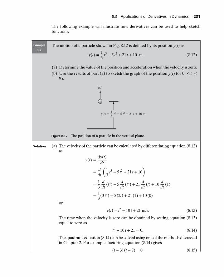
8.3 Applications of Derivatives in Dynamics 231
The following example will illustrate how derivatives can be used to help sketchfunctions.
Example8-2
The motion of a particle shown in Fig. 8.12 is defined by its position y(t) as
y(t) = 13
t3 − 5 t2 + 21 t + 10 m. (8.12)
(a) Determine the value of the position and acceleration when the velocity is zero.
(b) Use the results of part (a) to sketch the graph of the position y(t) for 0 ≤ t ≤
9 s.
y(t) = − t3 − 5 t2 + 21 t + 10 m3
1
v(t)
Figure 8.12 The position of a particle in the vertical plane.
Solution (a) The velocity of the particle can be calculated by differentiating equation (8.12)as
v(t) =dy(t)
dt
= ddt
(13
t3 − 5 t2 + 21 t + 10)
= 13
ddt
(t3) − 5 ddt
(t2) + 21 ddt
(t) + 10 ddt
(1)
= 13
(3 t2) − 5 (2t) + 21 (1) + 10 (0)
or
v(t) = t2 − 10 t + 21 m/s. (8.13)
The time when the velocity is zero can be obtained by setting equation (8.13)equal to zero as
t2 − 10 t + 21 = 0. (8.14)
The quadratic equation (8.14) can be solved using one of the methods discussedin Chapter 2. For example, factoring equation (8.14) gives
(t − 3) (t − 7) = 0. (8.15)

232 Chapter 8 Derivatives in Engineering
The two solutions of equation (8.15) are given as:
t − 3 = 0 ⇒ t = 3 s
t − 7 = 0 ⇒ t = 7 s
Note that quadratic equation (8.14) can also be solved using the quadratic for-mula, which gives
t =10 ±
√102 − 4(1)(21)2(1)
= 10 ±√
162
= 10 ± 42
= 10 − 42
, 10 + 42
or
t = 3, 7 s.
Therefore, the velocity is zero at both t = 3 s and t = 7 s. To evaluate theacceleration at these times, an expression for the acceleration is needed. Theacceleration of the particle can be obtained by differentiating the velocity ofthe particle (equation (8.13)) as
a(t) =dv(t)
dt
= ddt
(t2 − 10 t + 21)
= ddt
(t2) − 10 ddt
(t) + 21 ddt
(1)
or
a(t) = 2 t − 10 m/s2. (8.16)
The position and acceleration at time t = 3 s can be found by substituting t = 3in equations (8.12) and (8.16) as
y(3) = 13
(3)3 − 5 (3)2 + 21 (3) + 10 = 37 m
a(3) = 2(3) − 10 = −4 m/s2.
Similarly, the position and acceleration at t = 7 s can be found by substitutingt = 7 in equations (8.12) and (8.16) as
y(7) = 13
(7)3 − 5 (7)2 + 21 (7) + 10 = 26.3 m
a(7) = 2(7) − 10 = 4 m/s2.

8.3 Applications of Derivatives in Dynamics 233
(b) The results of part (a) can be used to sketch the graph of the position y(t).It was shown in part (a) that the velocity of the particle is zero at t = 3 s andt = 7 s. Since the velocity is the derivative of the position, the derivative ofthe position at t = 3 s and t = 7 s is zero (i.e., the slope is zero). What thismeans is that the position y(t) has a local minimum or maximum at t = 3 s andt = 7 s. To check whether y(t) has a local minimum or maximum, the secondderivative (acceleration) test is applied. Since the acceleration at t = 3 s is neg-ative (a(3) = −4 m/s2), the position y(3) = 37 m is a local maximum. Since theacceleration at t = 7 s is positive (a(7) = 4 m/s2), the position y(7) = 26.3 m isa local minimum. This information, along with the positions of the particle att = 0 (y(0) = 10 m) and t = 9 (y(9) = 37 m), can be used to sketch the positiony(t), as shown in Fig. 8.13.
y(t), m
0 3 70
26.3
37
t, s
Local maxima
Local minima
Figure 8.13 The approximate sketch of the position y(t) of Example 8-2.
Derivatives are frequently used in engineering to help sketch functions for which noequation is given. Such is the case in the following example, which begins with a plotof the acceleration a(t).
Example8-3
The acceleration of a vehicle is measured as shown in Fig. 8.14. Knowing that theparticle starts from rest at position x = 0 and travels a total of 16 m, sketch plots ofthe position x(t) and velocity v(t).

234 Chapter 8 Derivatives in Engineering
x(t)
0 2 4 6
2
−2
t, s
a(t), m/s2
Figure 8.14 Acceleration of a vehicle for Example 8-3.
Solution (a) Plot of Velocity: The velocity of the vehicle can be obtained from the accel-eration profile given in Fig. 8.14. Knowing that v(0) = 0 m/s and a(t) = dv(t)
dt(i.e., a(t) is the slope of v(t)), each interval can be analyzed as follows:
0 ≤ t ≤ 2 s :dv(t)
dt= a(t) = 2 ⇒ v(t) is a line with slope = 2.
2 < t ≤ 4 s :dv(t)
dt= a(t) = 0 ⇒ v(t) is constant.
4 < t ≤ 6 s :dv(t)
dt= a(t) = −2 ⇒ v(t) is a line with slope = −2.
The graph of the velocity profile is shown in Fig. 8.15.
0
2
1
−2
1
4
2 4 6
v(t), m/s
t, s
Figure 8.15 The velocity profile for Example 8-3.
(b) Plot of Position: Now, use the velocity, v(t), to construct the position x(t).Knowing that x(0) = 0 m and v(t) = dx(t)
dt(i.e., v(t) is the slope of x(t)), each
interval can be analyzed as follows:
(i) 0 ≤ t ≤ 2 s: v(t) is a straight line with a slope of 2 starting from origin(v(0) = 0); therefore, v(t) = dx(t)
dt= 2 t m/s. From Table 8.3, the position of
the vehicle must be a quadratic equation of the form
x(t) = t2 + C. (8.17)

8.3 Applications of Derivatives in Dynamics 235
This can be checked by taking the derivative, for example, v(t) = dx(t)dt
=ddt
(t2 + C) = 2 t m/s. Therefore, the equation of position given by (8.17) iscorrect. The value of C is obtained by evaluating equation (8.17) at t = 0and substituting the value of x(0) = 0 as
x(0) = 0 + C
0 = 0 + C
C = 0.
Therefore, for 0 ≤ t ≤ 2 s, x(t) = t2 is a quadratic function with a positiveslope (concave up) and x(2) = 4 m, as shown in Fig. 8.16.
(ii) 2 < t ≤ 4 s: v(t) has a constant value of 4 m/s, for example, v(t) = dx(t)dt
= 4.Therefore, x(t) is a straight line with a slope of 4 m/s starting with a valueof 4 m at t = 2 s as shown in Fig. 8.16. Since the slope is 4 m/s, the positionincreases by 4 m every second. So during the two seconds between t = 2 andt = 4, its position increases by 8 m. And since the position at time t = 2 s was4 m, its position at time t = 4 s will be 4 m + 8 m = 12 m. The equation ofposition for 2 < t ≤ 4 s can be written as
x(t) = 4 + 4 (t − 2) = 4 t − 4 m.
(iii) 4 < t ≤ 6 s: v(t) is a straight line with a slope of −2 m/s; therefore, x(t) is aquadratic function with decreasing slope (concave down) starting at x(4) =12 m and ending at x(6) = 16 m with zero slope. The resulting graph of theposition is shown in Fig. 8.16.
16
12
4
00 2 4 6
x(t), m
t, s
Figure 8.16 The position of the particle for Example 8-3.

236 Chapter 8 Derivatives in Engineering
Example8-4
The position of the cart moving on frictionless rollers shown in Fig. 8.17 is given by
x(t) = cos(𝜔t) m,
where 𝜔 = 2𝜋.
(a) Find the velocity of the cart.
(b) Show that the acceleration of the cart is given by a(t) = −𝜔2cos(𝜔t) m/s2, where𝜔 = 2𝜋.
x(t)
k
Frictionless rollers
m
Figure 8.17 A cart moving on frictionless rollers.
Solution (a) The velocity v(t) of the cart is obtained by differentiating the position x(t) as
v(t) =dx(t)
dt
= ddt
(cos(2𝜋t))
= −2𝜋 sin(2𝜋t) m/s.
(b) The acceleration a(t) of the cart is obtained by differentiating the position v(t)as
a(t) =dv(t)
dt
= ddt
(−2𝜋 sin(2𝜋t))
= −2𝜋 ddt
(sin(2𝜋t))
= −(2𝜋)2 sin(2𝜋t) m/s2.
Note that the second derivative of sin(𝜔t) or cos(𝜔t) is the same function scaled by−𝜔2, for example
d2
dt2sin(𝜔t) = −𝜔2 sin(𝜔t)
d2
dt2cos(𝜔t) = −𝜔2 cos(𝜔t)

8.3 Applications of Derivatives in Dynamics 237
Example8-5
An object of mass m moving at velocity v0 impacts a cantilever beam (of lengthl and flexural rigidity EI) as shown in Fig. 8.18. The resulting displacement of thebeam is given by
y(t) =v0
𝜔sin𝜔t (8.18)
where 𝜔 =√
3 E Im l3
is the angular frequency of displacement. Find the following:
(a) The maximum displacement ymax.
(b) The values of the displacement and acceleration when the velocity is zero.
y(t)
l
m
v0, m/s
Figure 8.18 A mass impacting a cantilever beam.
Solution (a) The maximum displacement can be found by first finding the time tmax whenthe displacement is maximum. This is done by equating the derivative of the
displacement (or the velocity) to zero, (i.e., v(t) =dy(t)
dt= 0). Since v0 and 𝜔
are constants, the derivative is given by
v(t) =dy(t)
dt
=v0
𝜔
ddt
(sin𝜔t)
=v0
𝜔(𝜔 cos𝜔t)
or
v(t) = v0 cos 𝜔t m/s. (8.19)
Equating equation (8.19) to zero gives
v0 cos 𝜔tmax = 0 ⇒ cos𝜔tmax = 0. (8.20)
The solutions of equation (8.20) are
𝜔tmax = 𝜋
2, 3𝜋
2, … ,

238 Chapter 8 Derivatives in Engineering
or
tmax = 𝜋
2𝜔, 3𝜋
2𝜔, … . (8.21)
Therefore, the displacement of the beam has local maxima or minima at thevalues of t given by equation (8.21). To find the time when the displacement ismaximum, the second derivative rule is applied. The second derivative of thedisplacement is obtained by differentiating equation (8.19) as
d2y(t)
dt2= vo
ddt
(cos𝜔t)
= v0 (−𝜔 sin𝜔t)
ord2y(t)
dt2= −v0 𝜔 sin 𝜔t m/s2. (8.22)
The value of the second derivative of the displacement at 𝜋
2𝜔is given by
d2y(
𝜋
2𝜔
)dt2
= −v0 𝜔 sin(𝜋
2
)< 0.
Similarly, the value of the second derivative of the displacement at 3𝜋2𝜔
is given
by
d2y(
3𝜋2𝜔
)dt2
= −v0 𝜔 sin(
3𝜋2
)> 0.
Therefore, the displacement is maximum at time
tmax = 𝜋
2𝜔. (8.23)
The maximum displacement can be found by substituting tmax = 𝜋
2𝜔into
equation (8.18) as
ymax =v0
𝜔sin(𝜔 tmax)
=v0
𝜔sin 𝜋
2
=v0
𝜔
=v0√3 E Im l3
or
ymax = v0
√m l3
3 E I.
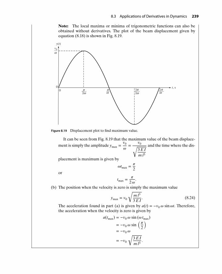
8.3 Applications of Derivatives in Dynamics 239
Note: The local maxima or minima of trigonometric functions can also beobtained without derivatives. The plot of the beam displacement given byequation (8.18) is shown in Fig. 8.19.
y(t)
00 t, s
v0—
—2—– 3
2—– 2—–ππππω ωωω
ω
Figure 8.19 Displacement plot to find maximum value.
It can be seen from Fig. 8.19 that the maximum value of the beam displace-
ment is simply the amplitude ymax =v0
𝜔=
v0√3 E Im l3
and the time where the dis-
placement is maximum is given by
𝜔tmax = 𝜋
2or
tmax = 𝜋
2𝜔.
(b) The position when the velocity is zero is simply the maximum value
ymax = v0
√m l3
3 E I. (8.24)
The acceleration found in part (a) is given by a(t) = −v0 𝜔 sin𝜔t. Therefore,the acceleration when the velocity is zero is given by
a(tmax) = −v0 𝜔 sin (𝜔 tmax)
= −v0 𝜔 sin(𝜋
2
)= −v0 𝜔
= −v0
√3 E Im l3
.
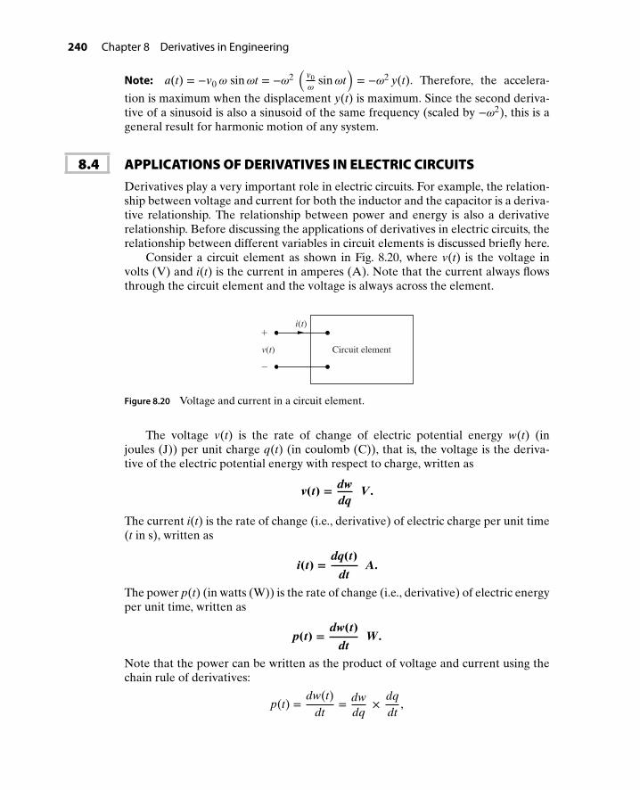
240 Chapter 8 Derivatives in Engineering
Note: a(t) = −v0 𝜔 sin𝜔t = −𝜔2(
v0𝜔
sin𝜔t)= −𝜔2 y(t). Therefore, the accelera-
tion is maximum when the displacement y(t) is maximum. Since the second deriva-tive of a sinusoid is also a sinusoid of the same frequency (scaled by −𝜔2), this is ageneral result for harmonic motion of any system.
8.4 APPLICATIONS OF DERIVATIVES IN ELECTRIC CIRCUITSDerivatives play a very important role in electric circuits. For example, the relation-ship between voltage and current for both the inductor and the capacitor is a deriva-tive relationship. The relationship between power and energy is also a derivativerelationship. Before discussing the applications of derivatives in electric circuits, therelationship between different variables in circuit elements is discussed briefly here.
Consider a circuit element as shown in Fig. 8.20, where v(t) is the voltage involts (V) and i(t) is the current in amperes (A). Note that the current always flowsthrough the circuit element and the voltage is always across the element.
Circuit element
−
+i(t)
v(t)
Figure 8.20 Voltage and current in a circuit element.
The voltage v(t) is the rate of change of electric potential energy w(t) (injoules (J)) per unit charge q(t) (in coulomb (C)), that is, the voltage is the deriva-tive of the electric potential energy with respect to charge, written as
v(t) = dwdq
V .
The current i(t) is the rate of change (i.e., derivative) of electric charge per unit time(t in s), written as
i(t) =dq(t)
dtA.
The power p(t) (in watts (W)) is the rate of change (i.e., derivative) of electric energyper unit time, written as
p(t) =dw(t)
dtW .
Note that the power can be written as the product of voltage and current using thechain rule of derivatives:
p(t) =dw(t)
dt= dw
dq×
dqdt
,

8.4 Applications of Derivatives in Electric Circuits 241
or
p(t) = v(t) × i(t). (8.25)
The chain rule of derivative is a rule for differentiating composition of functions; forexample, if f is a function of g and g is a function of t, then the derivative of compositefunction f (g(t)) with respect to t can be written as
dfdt
=dfdg
×dgdt
. (8.26)
For example, the function f (t) = sin(2𝜋t) can be written as f (t) = sin(g(t)), whereg(t) = 2𝜋t. By the chain rule of equation (8.26),
dfdt
=dfdg
×dgdt
= ddt
(sin(g)) × ddt
(2𝜋t)
= cos(g) × ddt
(2𝜋t)
= cos(g) × (2𝜋)
= 2𝜋 cos(2𝜋t).
The chain rule is also useful in differentiating the power of sinusoidal function such asy1(t) = sin2(2𝜋t) or the power of the polynomial function such as y2(t) = (2t + 10)2.The derivatives of these functions are obtained as
dy1
dt= d
dt
((sin(2𝜋t))2)
= 2 (sin(2𝜋t))1 × ddt
(sin(2𝜋t))
= 2 sin(2𝜋t) × (2𝜋 cos(2𝜋t))
= 4𝜋 sin(2𝜋t) cos(2𝜋t)
and
dy2
dt= d
dt
((2t + 10)2)
= 2 (2t + 10)1 × ddt
(2t + 10)
= 2 (2t + 10) × (2)
= 4 (2t + 10)
The following example will illustrate some of the derivative relationships discussedabove.

242 Chapter 8 Derivatives in Engineering
Example8-6
For a particular circuit element, the charge is
q(t) = 150
sin 250𝜋t C (8.27)
and the voltage supplied by the voltage source shown in Fig. 8.21 is
v(t) = 100 sin 250𝜋t V. (8.28)
Element
i(t)
v(t) +−
Figure 8.21 Voltage applied to a particular circuit element.
Find the following quantities:
(a) The current, i(t).
(b) The power, p(t).
(c) The maximum power pmax delivered to the circuit element by the voltagesource.
Solution (a) Current: The current i(t) can be determined by differentiating the charge q(t)as
i(t) =dq(t)
dt
= ddt
(150
sin 250𝜋t)
= 150
(250𝜋 cos 250𝜋t)
or
i(t) = 5𝜋 cos 250𝜋t A. (8.29)
(b) Power: The power p(t) can be determined by multiplying the voltage given inequation (8.28) and the current calculated in equation (8.29) as
p(t) = v(t) i(t)
= (100 sin 250𝜋t) (5𝜋 cos 250𝜋t)
= 500𝜋(sin 250𝜋t) (cos 250𝜋t)
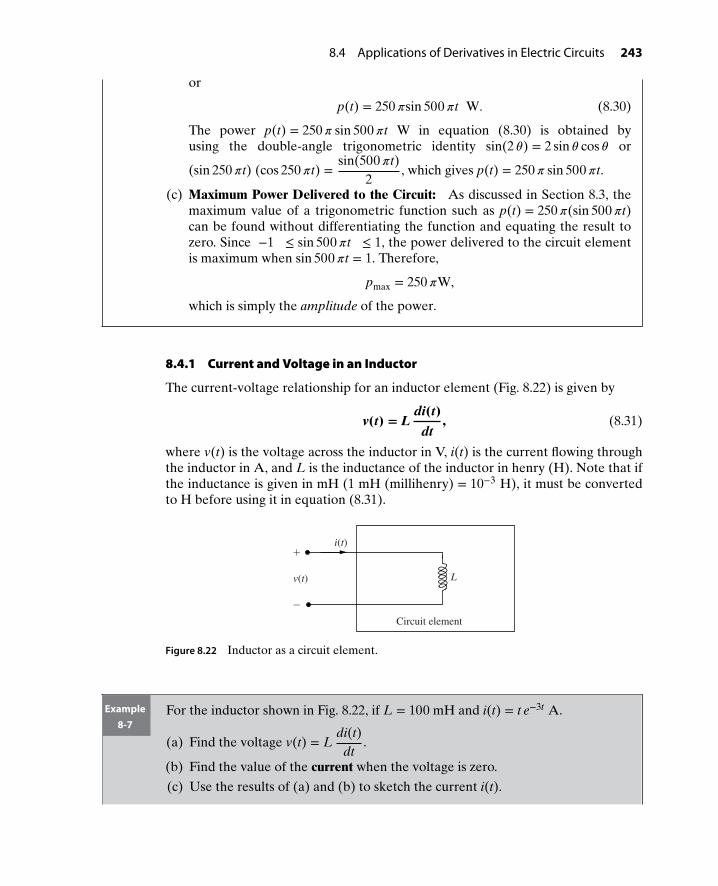
8.4 Applications of Derivatives in Electric Circuits 243
or
p(t) = 250𝜋sin 500𝜋t W. (8.30)
The power p(t) = 250𝜋 sin 500𝜋t W in equation (8.30) is obtained byusing the double-angle trigonometric identity sin(2 𝜃) = 2 sin 𝜃 cos 𝜃 or
(sin 250𝜋t) (cos 250𝜋t) =sin(500𝜋t)
2, which gives p(t) = 250𝜋 sin 500𝜋t.
(c) Maximum Power Delivered to the Circuit: As discussed in Section 8.3, themaximum value of a trigonometric function such as p(t) = 250𝜋(sin 500𝜋t)can be found without differentiating the function and equating the result tozero. Since −1 ≤ sin 500𝜋t ≤ 1, the power delivered to the circuit elementis maximum when sin 500𝜋t = 1. Therefore,
pmax = 250𝜋W,
which is simply the amplitude of the power.
8.4.1 Current and Voltage in an Inductor
The current-voltage relationship for an inductor element (Fig. 8.22) is given by
v(t) = Ldi(t)
dt, (8.31)
where v(t) is the voltage across the inductor in V, i(t) is the current flowing throughthe inductor in A, and L is the inductance of the inductor in henry (H). Note that ifthe inductance is given in mH (1 mH (millihenry) = 10−3 H), it must be convertedto H before using it in equation (8.31).
Circuit element
v(t) L
+
−
i(t)
Figure 8.22 Inductor as a circuit element.
Example8-7
For the inductor shown in Fig. 8.22, if L = 100 mH and i(t) = t e−3t A.
(a) Find the voltage v(t) = Ldi(t)
dt.
(b) Find the value of the current when the voltage is zero.
(c) Use the results of (a) and (b) to sketch the current i(t).

244 Chapter 8 Derivatives in Engineering
Solution (a) The voltage v(t)is determined as
v(t) = Ldi(t)
dt
= (100 × 10−3)di(t)
dtor
v(t) = 0.1di(t)
dt,
where di(t)dt
= ddt
(t e−3t). To differentiate the product of two functions (t ande−3t), the product rule of differentiation (Table 8.3) is used:
ddt
(f (t) g(t)) = f (t) ddt
(g(t)) + g(t) ddt
(f (t)). (8.32)
Substituting f (t) = t and g(t) = e−3 t in equation (8.32) gives
ddt
(t e−3t) = (t)
(ddt
(e−3t))+(
ddt
(t)) (
e−3t)= (t)
(−3 e−3t) + (1)
(e−3t)
= e−3t (−3 t + 1) . (8.33)
Therefore,
v(t) = 0.1 e−3t (−3 t + 1) V. (8.34)
(b) To find the current when the voltage is zero, first find the time t when the volt-age is zero and then substitute this time in the expression for current. Settingequation (8.34) equal to zero gives
0.1 e−3t (−3 t + 1) = 0.
Since e−3t is never zero, it follows that (−3 t + 1) = 0, which gives t = 1∕3 sec.Therefore, the value of the current when the voltage is zero is determined bysubstituting t = 1∕3 into the current i(t) = t e−3 t, which gives
i(
13
)=(
13
)e−3
(13
)
= 13
e−1
or
i = 0.123 A.
(c) Since the voltage is proportional to the derivative of the current, the slopeof the current is zero when the voltage is zero. Therefore, the current i(t) ismaximum (imax = 0.123 A) at t = 1∕3 s. Also, at t = 0, i(0) = 0 A. Using thesevalues along with the values of the current at t = 1 s (i(1s) = 0.0498 A) and att = 2 s (i(2s) = 0.00496 A), the approximate sketch of the current can be drawn

8.4 Applications of Derivatives in Electric Circuits 245
as shown in Fig. 8.23. Note that i = 0.123 A must be a maximum (as opposedto a minimum) value, since it is the only location of zero slope and is greaterthan the values of i(t) at either t = 0 or t = 2 s. Hence, no second derivative testis required!
t, s
i(t), A
imax = 0.123
0.14
0.12
0.1
0.08
0.06
0.02
00.5 1 1.5 2 2.5 30
0.04
Figure 8.23 Approximate sketch of the current waveform for Example 8-7.
As seen in dynamics, derivatives are frequently used in circuits to sketch functionsfor which no equations are given, as illustrated in the following example:
Example8-8
For the given input voltage (square wave) shown in Fig. 8.24, plot the current i(t)and the power p(t) if L = 500 mH. Assume i(0) = 0 A and p(0) = 0 W.
0
−9
L
v(t), V
v(t)
i(t) 9
8642+− t, s
Figure 8.24 A square wave voltage applied to an inductor.
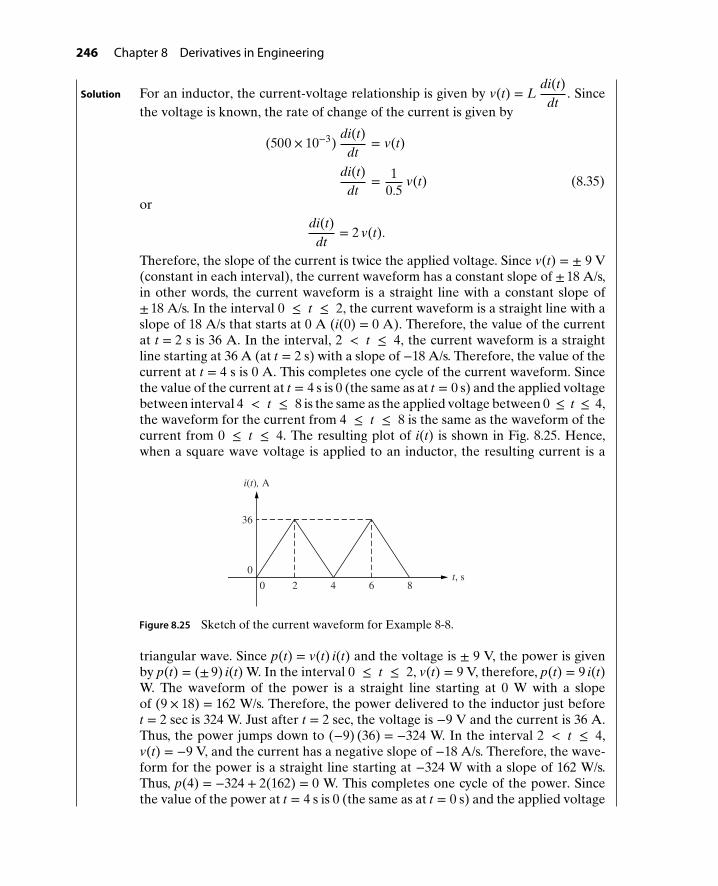
246 Chapter 8 Derivatives in Engineering
Solution For an inductor, the current-voltage relationship is given by v(t) = Ldi(t)
dt. Since
the voltage is known, the rate of change of the current is given by
(500 × 10−3)di(t)
dt= v(t)
di(t)dt
= 10.5
v(t) (8.35)
ordi(t)
dt= 2 v(t).
Therefore, the slope of the current is twice the applied voltage. Since v(t) = ± 9 V(constant in each interval), the current waveform has a constant slope of ± 18 A/s,in other words, the current waveform is a straight line with a constant slope of± 18 A/s. In the interval 0 ≤ t ≤ 2, the current waveform is a straight line with aslope of 18 A/s that starts at 0 A (i(0) = 0 A). Therefore, the value of the currentat t = 2 s is 36 A. In the interval, 2 < t ≤ 4, the current waveform is a straightline starting at 36 A (at t = 2 s) with a slope of −18 A/s. Therefore, the value of thecurrent at t = 4 s is 0 A. This completes one cycle of the current waveform. Sincethe value of the current at t = 4 s is 0 (the same as at t = 0 s) and the applied voltagebetween interval 4 < t ≤ 8 is the same as the applied voltage between 0 ≤ t ≤ 4,the waveform for the current from 4 ≤ t ≤ 8 is the same as the waveform of thecurrent from 0 ≤ t ≤ 4. The resulting plot of i(t) is shown in Fig. 8.25. Hence,when a square wave voltage is applied to an inductor, the resulting current is a
0
0
36
2 4 86
i(t), A
t, s
Figure 8.25 Sketch of the current waveform for Example 8-8.
triangular wave. Since p(t) = v(t) i(t) and the voltage is ± 9 V, the power is givenby p(t) = (± 9) i(t) W. In the interval 0 ≤ t ≤ 2, v(t) = 9 V, therefore, p(t) = 9 i(t)W. The waveform of the power is a straight line starting at 0 W with a slopeof (9 × 18) = 162 W/s. Therefore, the power delivered to the inductor just beforet = 2 sec is 324 W. Just after t = 2 sec, the voltage is −9 V and the current is 36 A.Thus, the power jumps down to (−9) (36) = −324 W. In the interval 2 < t ≤ 4,v(t) = −9 V, and the current has a negative slope of −18 A/s. Therefore, the wave-form for the power is a straight line starting at −324 W with a slope of 162 W/s.Thus, p(4) = −324 + 2(162) = 0 W. This completes one cycle of the power. Sincethe value of the power at t = 4 s is 0 (the same as at t = 0 s) and the applied voltage

8.4 Applications of Derivatives in Electric Circuits 247
and current in the interval 4 ≤ t ≤ 8 are the same as the voltage and current inthe 0 ≤ t ≤ 4, the waveform for the power from 4 ≤ t ≤ 8 is the same as thewaveform of the power from 0 ≤ t ≤ 4. The resulting plot of p(t) is shown inFig. 8.26, and is typically referred to as a sawtooth curve.
0
0
324
2 4 6 8
−324
p(t), W
t, s
Figure 8.26 Sketch of the power for Example 8-8.
8.4.2 Current and Voltage in a Capacitor
The current-voltage relationship for a capacitive element (Fig. 8.27) is given by
i(t) = Cdv(t)
dt, (8.36)
where v(t) is the voltage across the capacitor in V, i(t) is the current flowing throughthe capacitor in A, and C is the capacitance of the capacitor in farad (F). Note thatif the capacitance is given in 𝜇F (10−6 F), it must be converted to F before using it inequation (8.36).
Example8-9
Consider the capacitive element shown in Fig. 8.27 with C = 25 𝜇F and v(t) =20 e−500 t sin 5000𝜋t V. Find the current i(t).
Circuit element
i(t)
v(t)
+
−
C
Figure 8.27 Capacitor as a circuit element.

248 Chapter 8 Derivatives in Engineering
Solution The current i(t) can be found by using equation (8.36) as
i(t) = Cdv(t)
dt.
Substituting the value of C gives
i(t) = (25 × 10−6)dv(t)
dt,
wheredv(t)
dt= d
dt(20 e−500 t sin 5000𝜋t). To differentiate the product of the two
functions e−500 t and sin 5000𝜋t, the product rule of differentiation is required. Let-ting f (t) = e−500 t and g(t) = sin 5000𝜋t,
ddt
(20 e−500tsin 5000𝜋t) = 20 ×[
e−500 t ddt
(sin 5000𝜋t)
+(sin 5000𝜋t) ddt
(e−500 t)]
= 20 × [(e−500 t) (5000𝜋 cos 5000𝜋t)
+(sin 5000𝜋t)(−500 e−500 t)]
= 10,000 e−500 t (10𝜋cos 5000𝜋t − sin 5000𝜋t).
Therefore,
i(t) = 25 × 10−6(
10,000 e−500t (10𝜋cos 5000𝜋t − sin 5000𝜋t))
or
i(t) = 0.25 e−500 t (10𝜋cos 5000𝜋t − sin 5000𝜋t) A
Using the results of Chapter 6, this can also be written as i(t) =2.5𝜋e−500 t sin(5000𝜋t + 92) A.
Example8-10
The current shown in Fig. 8.28 is used to charge a capacitor with C = 20 𝜇F. Know-ing that i(t) = dq(t)
dt= C dv(t)
dt, plot the charge q(t) stored in the capacitor and the
corresponding voltage v(t). Assume q(0) = v(0) = 0.
i(t)
−2
2
2 4 51
i(t), A
t, ms0v(t)
+
−
C
4
−4
↑
Figure 8.28 Charging of a capacitor.

8.4 Applications of Derivatives in Electric Circuits 249
Solution (a) Charge: Since i(t) =dq(t)
dt, the slope of the charge q(t) is given by each con-
stant value of current in each interval, for example
0 ≤ t ≤ 1 ms :dq(t)
dt= 4 C/s
1 < t ≤ 2 ms :dq(t)
dt= −2 C/s
2 < t ≤ 4 ms :dq(t)
dt= 2 C/s
4 < t ≤ 5 ms :dq(t)
dt= −4 C/s
5 < t ≤ ∞ ms :dq(t)
dt= 0 C/s.
Therefore, the plot of the charge q(t) stored in the capacitor can be drawn asshown in Fig. 8.29. Note that since time t is in ms, the charge q(t) is in mC.
qmax = 6 mC
0
4
2
2 41 5
6
4
1
1−2
1
−44
2
q(t), mC
t, ms
Figure 8.29 Charge on the capacitor in Example 8-10.
(b) Voltage: To find the voltage across the capacitor, the relationship between thecharge and the voltage is first derived as:
i(t) = Cdv(t)
dt=
dq(t)dt
⇒dv(t)
dt= 1
Cdq(t)
dt.
Therefore, the derivative (slope) of the voltage v(t) is equal to the derivative(slope) of the charge q(t) multiplied by the reciprocal of the capacitance. Sub-stituting the value of C gives
dv(t)dt
= 120 × 10−6
dq(t)dt
,
or
dv(t)dt
= 50 × 103 dq(t)dt
.
The plot of the voltage is thus the same as the plot of the charge with the ordi-nate scaled by 50 × 103, as shown in Fig. 8.30.

250 Chapter 8 Derivatives in Engineering
0 1 2 4 5
100
200
300
v(t), V
t, ms
vmax = 300 V
Figure 8.30 Voltage across the capacitor.
Note that while the time is still measured in ms, the voltage is measured in volts.
8.5 APPLICATIONS OF DERIVATIVESIN STRENGTH OF MATERIALSIn this section, the derivative relationship for beams under transverse loadingconditions will be discussed. The locations and values of maximum deflections areobtained using derivatives, and results are used to sketch the deflection. This sectionalso considers the application of derivatives to maximum stress under axial loadingand torsion.
Consider a beam with elastic modulus E (lb/in.2 or N/m2) and second momentof area I (in.4 or m4) as shown in Fig. 8.31. The product E I is called the flexuralrigidity and is a measure of how stiff the beam is. If the beam is loaded with a dis-tributed transverse load q(x) (lb/in. or N/m), the beam deflects in the y-direction with
a deflection of y(x) (in. or m) and a slope of 𝜃(x) =dy(x)
dxin radians.
x
q(x)
y(x) (x)
Beam with flexural rigidity EI
y
θ
Figure 8.31 A beam loaded in the y-direction.
The internal moments and forces in the beam shown in Fig. 8.32 are given by theexpressions
Bending Moment: M(x) = EId 𝜽(x)
dx= EI
d2y(x)
dx2lb-in. or N-m (8.37)
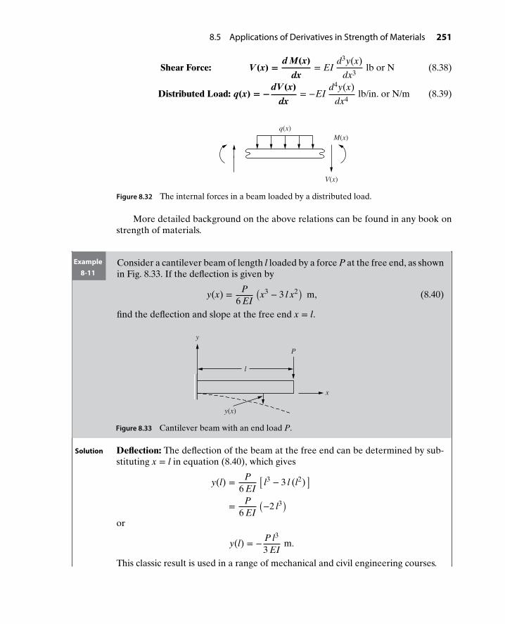
8.5 Applications of Derivatives in Strength of Materials 251
Shear Force: V(x) =d M(x)
dx= EI
d3y(x)
dx3lb or N (8.38)
Distributed Load: q(x) = −dV(x)
dx= −EI
d4y(x)
dx4lb/in. or N/m (8.39)
M(x)
q(x)
V(x)
Figure 8.32 The internal forces in a beam loaded by a distributed load.
More detailed background on the above relations can be found in any book onstrength of materials.
Example8-11
Consider a cantilever beam of length l loaded by a force P at the free end, as shownin Fig. 8.33. If the deflection is given by
y(x) = P6 EI
(x3 − 3 l x2) m, (8.40)
find the deflection and slope at the free end x = l.
x
P
l
y(x)
y
Figure 8.33 Cantilever beam with an end load P.
Solution Deflection: The deflection of the beam at the free end can be determined by sub-stituting x = l in equation (8.40), which gives
y(l) = P6 EI
[l3 − 3 l (l2)
]= P
6 EI
(−2 l3
)or
y(l) = − P l3
3 EIm.
This classic result is used in a range of mechanical and civil engineering courses.

252 Chapter 8 Derivatives in Engineering
Slope: The slope of the deflection 𝜃(x) can be found by differentiating thedeflection y(x) as
𝜃(x) =dy(x)
dx
= ddx
[ P6 EI
(x3 − 3 l x2)]
= P6 EI
[ddx
(x3) − 3 ld
dx(x2)
]= P
6 EI
[3 (x2) − 3 l (2 x)
]= P
6 EI
(3 x2 − 6 l x
)or
𝜃(x) = P2 EI
(x2 − 2 l x) rad. (8.41)
Note that the parameters P, l, E, and I are all treated as constants.The slope 𝜃(x) at the free end can now be determined by substituting x = l in.
equation (8.41) as
𝜃(l) = P2 EI
[l2 − 2 l (l)]
= P2 EI
(− l2)
or
𝜃(l) = − P l2
2 EIrad.
Note: It can be seen by inspection that both the deflection and the slope of deflec-tion are maximum at the free end, for example:
ymax = − P l3
3 EI
𝜃max = − P l2
2 EI.
It can be seen that doubling the load P would increase the maximum deflection andslope by a factor of 2. However, doubling the length l would increase the maximumdeflection by a factor of 8, and the maximum slope by a factor of 4!
Example8-12
Consider a simply supported beam of length l subjected to a central load P, asshown in Fig. 8.34. For 0 ≤ x ≤ 1/2, the deflection is given by
y(x) = P48 EI
(4 x3 − 3 l2 x
)m. (8.42)
Determine the maximum defection ymax, as well as the slope at the end x = 0.

8.5 Applications of Derivatives in Strength of Materials 253
y
x
P
y(x)
l
l2
Figure 8.34 A simply supported beam with a central load P.
Solution The deflection is maximum whendy(x)
dx= 𝜃(x) = 0. The slope of the deflection can
be found as
𝜃(x) =dy(x)
dx
= ddx
[ P48 EI
(4 x3 − 3 l2 x)]
= P48 EI
[ddx
(4 x3) − ddx
(3 l2 x)]
= P48 EI
[4 d
dx(x3) − 3 l2
ddx
(x)]
= P48 EI
[4(3 x2) − 3 l2(1)
]= P
48 EI
(12 x2 − 3 l2
)or
𝜃(x) = P16 EI
(4 x2 − l2
). (8.43)
To find the location of the maximum deflection, 𝜃(x) is set to zero and the resultingequation is solved for the values of x as
P16 EI
(4 x2 − l2) = 0 ⇒ 4 x2 − l2 = 0 ⇒ x = ± l2.
Since the deflection is given for 0 ≤ x ≤ l∕2, the deflection is maximum at x = l∕2.The value of the maximum deflection can now be found by substituting x = l∕2 in
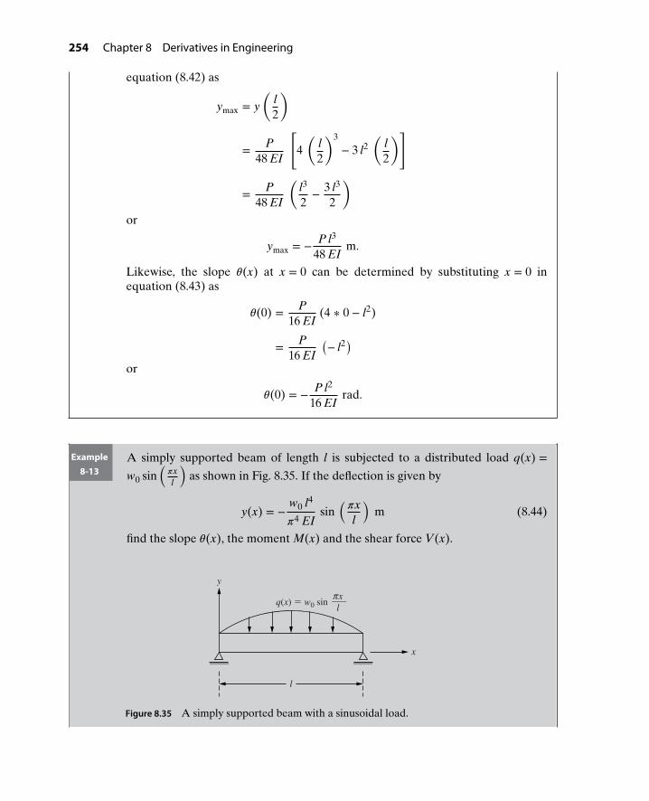
254 Chapter 8 Derivatives in Engineering
equation (8.42) as
ymax = y(
l2
)
= P48 EI
[4(
l2
)3
− 3 l2(
l2
)]
= P48 EI
(l3
2− 3 l3
2
)or
ymax = − P l3
48 EIm.
Likewise, the slope 𝜃(x) at x = 0 can be determined by substituting x = 0 inequation (8.43) as
𝜃(0) = P16 EI
(4 ∗ 0 − l2)
= P16 EI
(− l2
)or
𝜃(0) = − P l2
16 EIrad.
Example8-13
A simply supported beam of length l is subjected to a distributed load q(x) =w0 sin
(𝜋xl
)as shown in Fig. 8.35. If the deflection is given by
y(x) = −w0 l4
𝜋4 EIsin
(𝜋xl
)m (8.44)
find the slope 𝜃(x), the moment M(x) and the shear force V(x).
x
y
l
q(x) = w0 sin —–xl
π
Figure 8.35 A simply supported beam with a sinusoidal load.
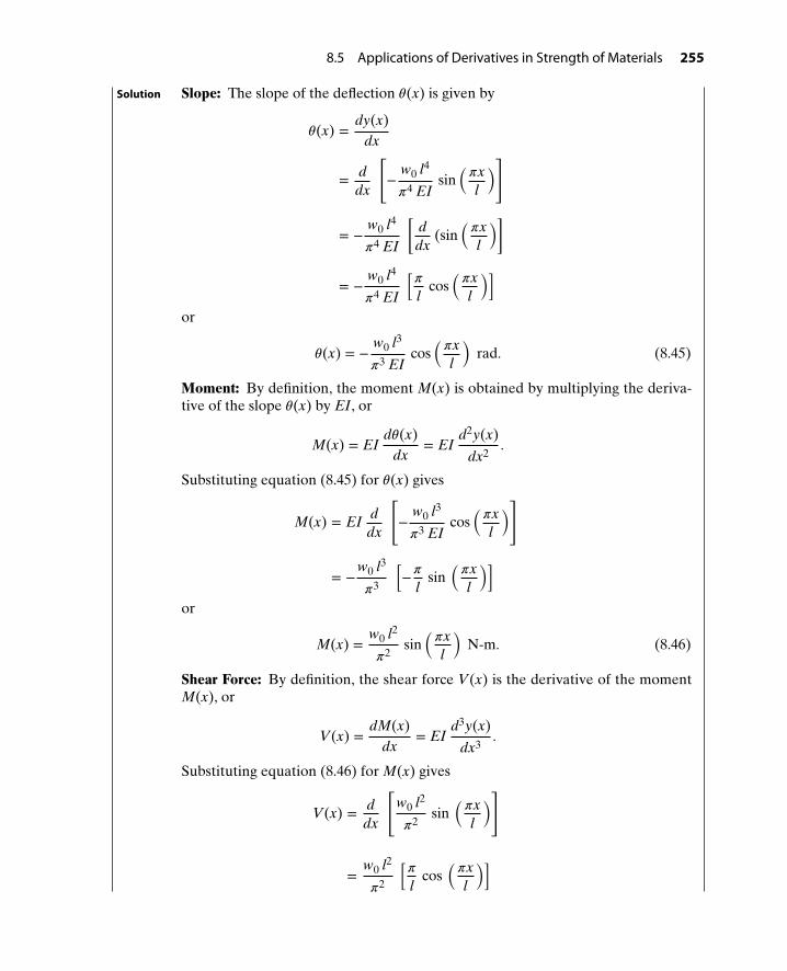
8.5 Applications of Derivatives in Strength of Materials 255
Solution Slope: The slope of the deflection 𝜃(x) is given by
𝜃(x) =dy(x)
dx
= ddx
[−
w0 l4
𝜋4 EIsin
(𝜋xl
)]
= −w0 l4
𝜋4 EI
[d
dx(sin
(𝜋xl
)]
= −w0 l4
𝜋4 EI
[𝜋
lcos
(𝜋xl
)]or
𝜃(x) = −w0 l3
𝜋3 EIcos
(𝜋xl
)rad. (8.45)
Moment: By definition, the moment M(x) is obtained by multiplying the deriva-tive of the slope 𝜃(x) by EI, or
M(x) = EId𝜃(x)
dx= EI
d2y(x)
dx2.
Substituting equation (8.45) for 𝜃(x) gives
M(x) = EId
dx
[−
w0 l3
𝜋3 EIcos
(𝜋xl
)]
= −w0 l3
𝜋3
[−𝜋
lsin
(𝜋xl
)]or
M(x) =w0 l2
𝜋2sin
(𝜋xl
)N-m. (8.46)
Shear Force: By definition, the shear force V(x) is the derivative of the momentM(x), or
V(x) =dM(x)
dx= EI
d3y(x)
dx3.
Substituting equation (8.46) for M(x) gives
V(x) = ddx
[w0 l2
𝜋2sin
(𝜋xl
)]
=w0 l2
𝜋2
[𝜋
lcos
(𝜋xl
)]
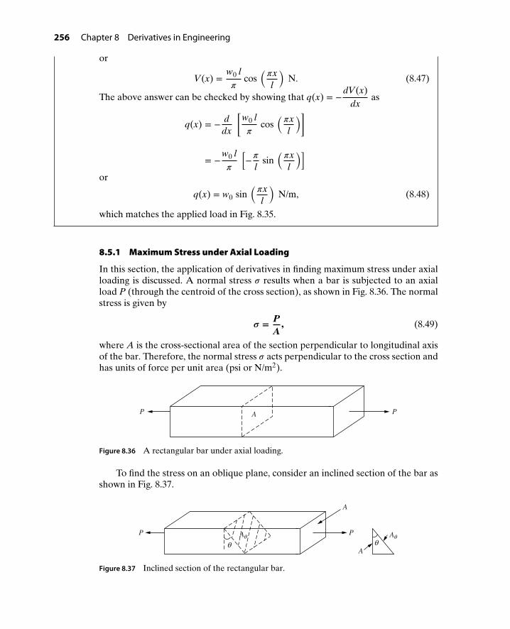
256 Chapter 8 Derivatives in Engineering
or
V(x) =w0 l𝜋
cos(𝜋xl
)N. (8.47)
The above answer can be checked by showing that q(x) = −dV(x)
dxas
q(x) = − ddx
[w0 l𝜋
cos(𝜋xl
)]
= −w0 l𝜋
[−𝜋
lsin
(𝜋xl
)]or
q(x) = w0 sin(𝜋xl
)N/m, (8.48)
which matches the applied load in Fig. 8.35.
8.5.1 Maximum Stress under Axial Loading
In this section, the application of derivatives in finding maximum stress under axialloading is discussed. A normal stress 𝜎 results when a bar is subjected to an axialload P (through the centroid of the cross section), as shown in Fig. 8.36. The normalstress is given by
𝝈 = PA
, (8.49)
where A is the cross-sectional area of the section perpendicular to longitudinal axisof the bar. Therefore, the normal stress 𝜎 acts perpendicular to the cross section andhas units of force per unit area (psi or N/m2).
P A P
Figure 8.36 A rectangular bar under axial loading.
To find the stress on an oblique plane, consider an inclined section of the bar asshown in Fig. 8.37.
P P
A
A
A Aθ θθθ
Figure 8.37 Inclined section of the rectangular bar.

8.5 Applications of Derivatives in Strength of Materials 257
The relationship between the cross-sectional area perpendicular to the longitudinalaxis and the area of the inclined plane is given by
A𝜃 cos 𝜃 = A
A𝜃 = Acos 𝜃
.
The force P can be resolved into components perpendicular to the inclined planeF and parallel to the inclined plane V. The free-body diagram of the forces actingon the oblique plane is shown in Fig. 8.38. Note that the resultant force in the axialdirection must be equal to P to satisfy equilibrium.
P
A
V
A
P
F
θ
θθ
Figure 8.38 Free-body diagram.
The relationship among P, F, and V can be found by using the right triangleshown in Fig. 8.39 as
F = P cos 𝜃
V = P sin 𝜃
V = P sin
F = P cos
P
θ
θ
θ
Figure 8.39 Triangle showing force P, F, and V.
The force perpendicular to the inclined cross section F produces a normal stress 𝜎𝜃(shown in Fig. 8.40) given by
𝜎𝜃 = FA𝜃
= P cos 𝜃A∕cos 𝜃
= P cos2 𝜃
A. (8.50)
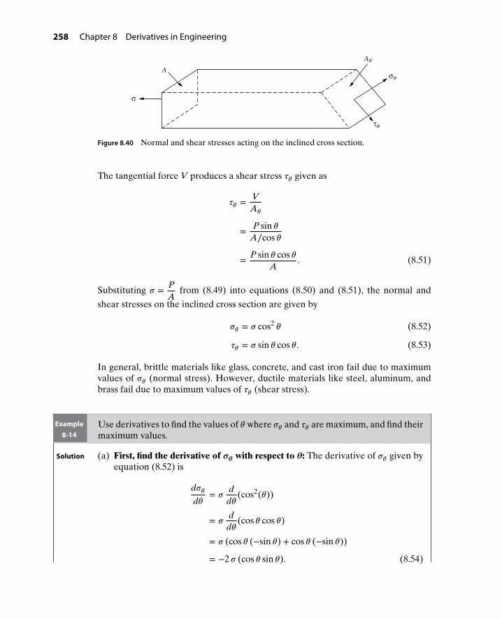
258 Chapter 8 Derivatives in Engineering
A
A
σ
τ
σ
θ
θ
θ
Figure 8.40 Normal and shear stresses acting on the inclined cross section.
The tangential force V produces a shear stress 𝜏𝜃 given as
𝜏𝜃 = VA𝜃
= P sin 𝜃
A∕cos 𝜃
= P sin 𝜃 cos 𝜃A
. (8.51)
Substituting 𝜎 = PA
from (8.49) into equations (8.50) and (8.51), the normal and
shear stresses on the inclined cross section are given by
𝜎𝜃 = 𝜎 cos2𝜃 (8.52)
𝜏𝜃 = 𝜎 sin 𝜃 cos 𝜃. (8.53)
In general, brittle materials like glass, concrete, and cast iron fail due to maximumvalues of 𝜎𝜃 (normal stress). However, ductile materials like steel, aluminum, andbrass fail due to maximum values of 𝜏𝜃 (shear stress).
Example8-14
Use derivatives to find the values of 𝜃 where 𝜎𝜃 and 𝜏𝜃 are maximum, and find theirmaximum values.
Solution (a) First, find the derivative of 𝝈𝜽
with respect to 𝜽: The derivative of 𝜎𝜃 given byequation (8.52) is
d𝜎𝜃d𝜃
= 𝜎d
d𝜃(cos2(𝜃))
= 𝜎d
d𝜃(cos 𝜃 cos 𝜃)
= 𝜎 (cos 𝜃 (−sin 𝜃) + cos 𝜃 (−sin 𝜃))
= −2 𝜎 (cos 𝜃 sin 𝜃). (8.54)
8.5 Applications of Derivatives in Strength of Materials 259
(b) Next, equate the derivative in equation (8.54) to zero and solve the resultingequation for the value of 𝜃 between 0 and 90 where 𝜎𝜃 is maximum. Therefore,−2 cos 𝜃 sin 𝜃 = 0, which gives
cos 𝜃 = 0 ⇒ 𝜃 = 90
or
sin 𝜃 = 0 ⇒ 𝜃 = 0.
Therefore, 𝜃 = 0 and 90 are the critical points; in other words, at 𝜃 =0 and 90, 𝜎𝜃 has a local maximum or minimum. To find the value of 𝜃 where𝜎𝜃 has a maximum, the second derivative test is performed. The second deriva-tive of 𝜎𝜃 is given by
d2𝜎𝜃
d𝜃2= d
d𝜃(−2 𝜎 cos 𝜃 sin 𝜃)
= −2 𝜎 dd𝜃
(cos 𝜃 sin 𝜃)
= −2 𝜎[
cos 𝜃 dd𝜃
(sin 𝜃) + dd𝜃
(cos 𝜃) (sin 𝜃)]
= −2 𝜎 [cos 𝜃(cos 𝜃) + (−sin 𝜃) sin 𝜃]
= −2 𝜎 (cos2𝜃 − sin2
𝜃)
or
d2𝜎𝜃
d𝜃2= −2 𝜎 cos 2 𝜃
where cos 2 𝜃 = cos2 𝜃 − sin2𝜃. For 𝜃 = 0,
d2𝜎𝜃
d𝜃2= −2 𝜎 < 0. So 𝜎𝜃 has a maxi-
mum value at 𝜃 = 0.
For 𝜃 = 90,d2𝜎𝜃
d𝜃2= −2 𝜎 cos(180) = 2 𝜎 > 0; therefore, 𝜎𝜃 has a minimum
value at 𝜃 = 90.
Maximum Value of 𝝈𝜽
: Substituting 𝜃 = 0 in equation (8.52) gives
𝜎max = 𝜎 cos2 (0) = 𝜎.
This means that the largest normal stress during axial loading is simply the appliedstress 𝜎!
260 Chapter 8 Derivatives in Engineering
Value of 𝜽 where 𝝉
𝜽
is maximum:
(a) First, find the derivative of 𝝉𝜽
with respect to 𝜽: The derivative of 𝜏𝜃 given byequation (8.53) is given by
d𝜏𝜃d𝜃
= dd𝜃
(𝜎 sin 𝜃 cos 𝜃)
= 𝜎d
d𝜃(sin 𝜃 cos 𝜃)
= 𝜎d
d𝜃
(sin 2 𝜃
2
)= 𝜎
2(2 cos 2 𝜃)
ord𝜏𝜃d𝜃
= 𝜎 cos 2 𝜃. (8.55)
(b) Next, equate the derivative in equation (8.55) to zero and solve the result-ing equation 𝜎 cos 2 𝜃 = 0 for the value of 𝜃 (between 0 and 90) where 𝜏𝜃 ismaximum:
cos 2 𝜃 = 0 ⇒ 2 𝜃 = 90 ⇒ 𝜃 = 45.
Therefore, 𝜏𝜃 has a local maximum or minimum at 𝜃 = 45. To find whether 𝜏𝜃has a maximum or minimum at 𝜃 = 45, the second derivative test is performed.The second derivative of 𝜏𝜃 is given by
d2𝜏𝜃
d𝜃2= d
d𝜃(𝜎 cos 2 𝜃)
= 𝜎 (−sin 2 𝜃)(2)
= −2 𝜎 sin 2 𝜃
For 0 ≤ 𝜃 ≤ 90 ⇒ 0 ≤ 2 𝜃 ≤ 180 ⇒ sin 2 𝜃 > 0, therefore,d2𝜏𝜃
d𝜃2<
0. Since the second derivative is negative, 𝜏𝜃 has a maximum value at 𝜃 = 45.
Maximum Value of 𝝉𝜽
: Substituting 𝜃 = 45 in equation (8.53) gives
𝜏max = 𝜎 sin 45, cos 45
= 𝜎
(√2
2
) (√2
2
)or
𝜏max = 𝜎
2at 𝜃 = 45.
Thus, the maximum shear stress during axial loading is equal to half the applied nor-mal stress, but at an angle of 45. This is why a tensile test of a steel specimen resultsin failure at a 45 angle.

8.6 Further Examples of Derivatives in Engineering 261
8.6 FURTHER EXAMPLES OF DERIVATIVES IN ENGINEERING
Example8-15
The velocity of a skydiver jumping from a height of 12,042 ft is shown in Fig. 8.41.
(a) Find the equation of the velocity v(t) for the five time intervals shown inFig. 8.41.
(b) Knowing that a(t) = dvdt
, find the acceleration a(t) of the skydiver for 0 ≤ t ≤
301 s.
(c) Use the results of part (b) to sketch the acceleration a(t) for 0 ≤ t ≤ 301 s.
y = 0 ft
y = 12,042 ft0
v(t), ft/s
t, s
−161
−30
0 5 28 31 271 301
(31, −30)
(28, −161)
(301, 0)
(271, −30)
(5, −161)
(a) A skydiver (b) Velocity profile
Figure 8.41 Velocity profile of the skydiver jumping from a height of 12,042 ft.
Solution (a) (i) 0 ≤ t ≤ 5 s: v(t) is linear with slope
m = −161 − 05 − 0
= − 32.2 ft/s.
Therefore, v(t) = −32.2 t ft/s.
(ii) 5 < t ≤ 28 s: v(t) is constant at
v(t) = −161 ft/s.
(iii) 28 < t ≤ 31 s: v(t) is linear with slope
m =−161 − (−30)
28 − 31
= −131− 3
= 43.67 ft/s.
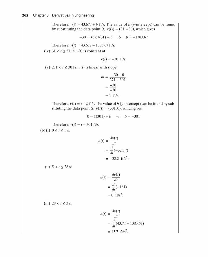
262 Chapter 8 Derivatives in Engineering
Therefore, v(t) = 43.67 t + b ft/s. The value of b (y-intercept) can be foundby substituting the data point (t, v(t)) = (31,−30), which gives
−30 = 43.67(31) + b ⇒ b = −1383.67
Therefore, v(t) = 43.67 t − 1383.67 ft/s.
(iv) 31 < t ≤ 271 s: v(t) is constant at
v(t) = −30 ft/s.
(v) 271 < t ≤ 301 s: v(t) is linear with slope
m = −30 − 0271 − 301
= −30−30
= 1 ft/s.
Therefore, v(t) = t + b ft/s. The value of b (y-intercept) can be found by sub-stituting the data point (t, v(t)) = (301, 0), which gives
0 = 1(301) + b ⇒ b = −301
Therefore, v(t) = t − 301 ft/s.
(b) (i) 0 ≤ t ≤ 5 s:
a(t) =dv(t)
dt
= ddt
(−32.3 t)
= −32.2 ft/s2.
(ii) 5 < t ≤ 28 s:
a(t) =dv(t)
dt
= ddt
(−161)
= 0 ft/s2.
(iii) 28 < t ≤ 3 s:
a(t) =dv(t)
dt
= ddt
(43.7 t − 1383.67)
= 43.7 ft/s2.

8.6 Further Examples of Derivatives in Engineering 263
(iv) 31 < t ≤ 271 s:
a(t) =dv(t)
dt
= ddt
(−30)
= 0 ft/s2.
(v) 271 < t ≤ 301 s:
a(t) =dv(t)
dt
= ddt
(t − 301)
= 1 ft/s2.
(c) The acceleration of the skydiver found in part (b) can be drawn as shown inFig. 8.42.
t, s
−32.2
43.67
3128 271 30150
1
a(t), ft/s2
Figure 8.42 The acceleration of the skydiver.
Example8-16
A proposed highway traverses a hilltop bounded by uphill and downhill gradesof 10% and −8%, respectively. These grades pass through benchmarks A and Blocated as shown in Fig. 8.43. With the origin of the coordinate axes (x, y) set atbenchmark A, the engineer has defined the hilltop segment of the highway by aparabolic arc:
y(x) = a x2 + b x (8.56)
which is tangent to the uphill grade at the origin.
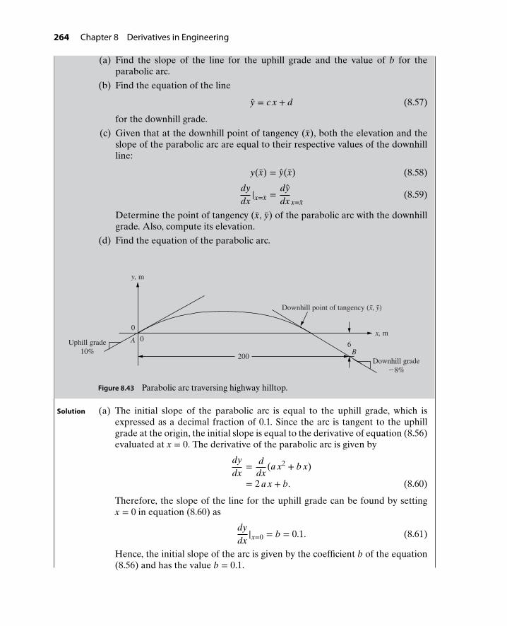
264 Chapter 8 Derivatives in Engineering
(a) Find the slope of the line for the uphill grade and the value of b for theparabolic arc.
(b) Find the equation of the line
y = c x + d (8.57)
for the downhill grade.
(c) Given that at the downhill point of tangency (x), both the elevation and theslope of the parabolic arc are equal to their respective values of the downhillline:
y(x) = y(x) (8.58)
dydx
|x=x =dydx x=x
(8.59)
Determine the point of tangency (x, y) of the parabolic arc with the downhillgrade. Also, compute its elevation.
(d) Find the equation of the parabolic arc.
Downhill point of tangency (x, y)
y, m
60A
0
200B
Uphill grade
10%
Downhill grade
−8%
x, m
Figure 8.43 Parabolic arc traversing highway hilltop.
Solution (a) The initial slope of the parabolic arc is equal to the uphill grade, which isexpressed as a decimal fraction of 0.1. Since the arc is tangent to the uphillgrade at the origin, the initial slope is equal to the derivative of equation (8.56)evaluated at x = 0. The derivative of the parabolic arc is given by
dydx
= ddx
(a x2 + b x)
= 2 a x + b. (8.60)
Therefore, the slope of the line for the uphill grade can be found by settingx = 0 in equation (8.60) as
dydx
|x=0 = b = 0.1. (8.61)
Hence, the initial slope of the arc is given by the coefficient b of the equation(8.56) and has the value b = 0.1.

8.6 Further Examples of Derivatives in Engineering 265
(b) The slope of the line (equation (8.57)) for the downhill grade is given byc = −0.08. Therefore, the equation of the line can be written as
y = −0.08 x + d. (8.62)
Since this line passes through benchmark B, the value of the y-intercept d canbe found by substituting the data point (200,−6) into equation (8.62) as
−6 = −0.08(200) + d
d = −6 + 16
d = 10.
Therefore, the equation of the line for the downhill slope is given by
y = −0.08x + 10. (8.63)
(c) Substituting x = x in equation (8.60) gives
dydx
|x=x = 2 a x + 0.1. (8.64)
Evaluating the derivative of equation (8.63) at x = x gives
dydx
|x=x = −0.08. (8.65)
Substituting equations (8.64) and (8.65) into equation (8.59) gives
2 a x + 0.10 = −0.08
a x = −0.09. (8.66)
Evaluating equations (8.56) and (8.62) at x and substituting the results in equa-tion (8.58) gives
a x2 + 0.1 x = −0.08 x + 10
x (a x + 0.18) = 10. (8.67)
Now, substituting the value of a x from equation (8.66) into equation (8.67),the value of x can be found as
x(−0.09 + 0.18) = 10
0.09 x = 10
x = 100.09
(8.68)
= 111.1 m. (8.69)
Thus, the point of tangency lies a horizontal distance of 111.1 m from bench-mark A. Its elevation y is obtained by substituting this value of x into

266 Chapter 8 Derivatives in Engineering
equation (8.63) as
y = y(x) = −0.08 x + 10
= −0.08(111.1) + 10
= 1.11 m.
Therefore, the downhill point of tangency is given by (111.1, 1.11) m.
(d) With the value of x known, the coefficient a for the parabolic arc can beobtained from equation (8.66) as
a x = −0.09
a = −0.09111.1
a = −0.00081 m−1. (8.70)
The equation for the parabolic arc may now be written by substituting thevalues of a and b from equations (8.70) and (8.61) into equation (8.56) as
y = −0.00081 x2 + 0.1 x.
P R O B L E M S
8-1. A model rocket is fired from the roof ofa 50 ft tall building as shown in Fig. P8.1.The height of the rocket is given by
y(t) = y(0) + v(0) t − 12
g t2 ft
g
y(t)
H
Figure P8.1 A rocket fired from top of a building inproblem P8-1.
where y(t) is the height of the rocketat time t, y(0) = H = 50 ft is the initialheight of the rocket, v(0) = 150 ft/s isthe initial velocity of the rocket, and g =32.2 ft/s2 is the acceleration due to grav-ity. Find the following:
(a) Write the quadratic equation for theheight y(t) of the rocket.
(b) The velocity v(t) = dy(t)dt
.
(c) The acceleration a(t) = dv(t)dt
=d2y(t)
dt2.
(d) The time required to reach themaximum height as well as the cor-responding height ymax. Use yourresults to sketch y(t).
8-2. Repeat problem P8-1 if H = 15 m,v(0) = 49 m/s and g = 9.8 m/2.
8-3. The height in the vertical plane of a ballthrown from the ground with an initialvelocity of v(0) = 250 m/s satisfies the

Problems 267
relationship
y(t) = v(0) t − 12
g t2 m.
where g = 9.8 m/s2 is the accelerationdue to gravity.
gy(t)
Figure P8.3 A projectile in the vertical plane.
Find the following:
(a) Write the quadratic equation for theheight y(t) of the ball.
(b) The velocity v(t) = dy(t)dt
.
(c) The acceleration a(t) = dv(t)dt
=d2y(t)
dt2.
(d) The time required to reach the max-imum height, as well as the cor-responding height ymax. Use yourresults to sketch y(t).
8-4. Repeat problem P8-3 if v(0) = 161 ft/sand g= 32.2 ft/s2.
8-5. The motion of a particle moving inthe horizontal direction as shown inFig. P8.5 is described by its position x(t).Determine the position, velocity, andacceleration at t = 3.0 s if
v(t)
x(t)
Figure P8.5 A particle moving in the horizontaldirection.
(a) x(t)= 4 cos(
23𝜋t)
+ 3 sin(
32𝜋t)
m.
(b) x(t) = 3 t5 − 5 t2 + 7t+ 2
√t m.
(c) x(t) = 2 e4 t + 3 e−5 t + 2 (et − 1) m.
8-6. The motion of a particle moving in thehorizontal direction is described by itsposition x(t). Determine the position,velocity, and acceleration at t = 1.5 s if(a) x(t) = 4 cos(5𝜋t) m.(b) x(t) = 4 t3 − 6 t2 + 7 t + 2 m.(c) x(t) = 10 sin(10𝜋t) + 5 e3 t m.
8-7. The motion of a particle in the verticalplane is shown in Fig. P8.7. The heightof the particle is given by
y(t) = t3 − 12 t2 + 36 t + 20 m.
(a) Find the values of position andacceleration when the velocity iszero.
(b) Use your results in part (a) to sketchy(t) for 0 ≤ t ≤ 9 s.
y(t) = t3 − 12 t2 + 36 t + 20 m
Figure P8.7 Motion of a particle in the verticalplane.
8-8. The motion of a particle in the verticalplane is shown in Fig. P8.8. The heightof the particle is given by
y(t) = 2 t3 − 15 t2 + 24 t + 8 m
(a) Find the values of the position andacceleration when the velocity iszero.
(b) Use your results in part (a) to sketchy(t) for 0 ≤ t ≤ 4 s.
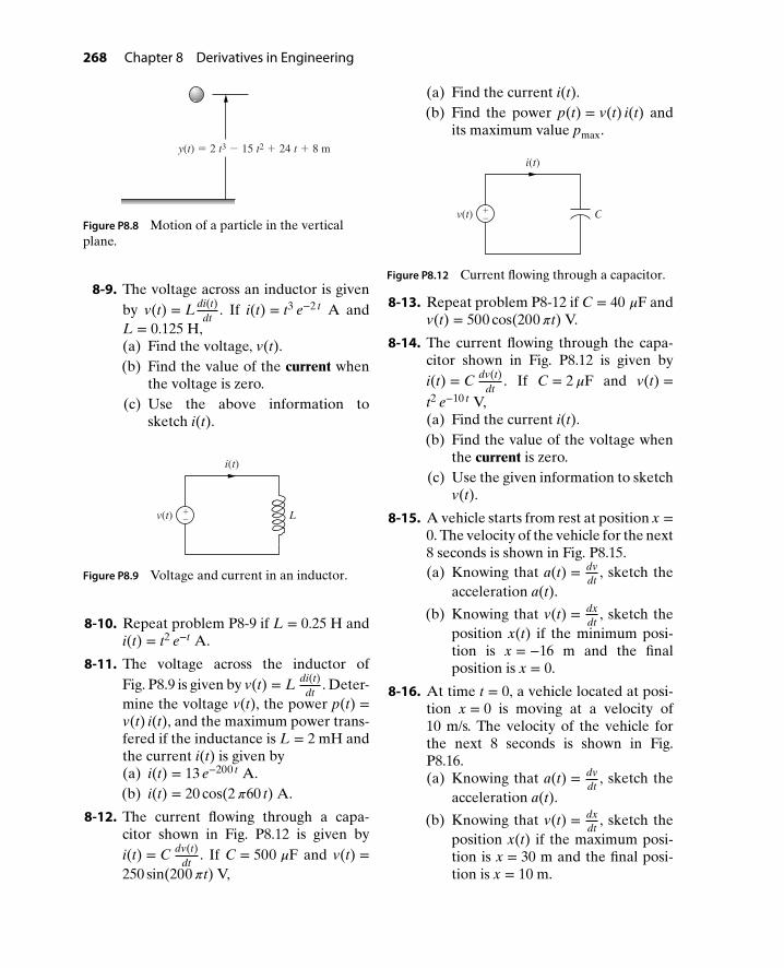
268 Chapter 8 Derivatives in Engineering
y(t) = 2 t3 − 15 t2 + 24 t + 8 m
Figure P8.8 Motion of a particle in the verticalplane.
8-9. The voltage across an inductor is givenby v(t) = L di(t)
dt. If i(t) = t3 e−2 t A and
L = 0.125 H,(a) Find the voltage, v(t).(b) Find the value of the current when
the voltage is zero.(c) Use the above information to
sketch i(t).
v(t) L
i(t)
+−
Figure P8.9 Voltage and current in an inductor.
8-10. Repeat problem P8-9 if L = 0.25 H andi(t) = t2 e−t A.
8-11. The voltage across the inductor ofFig. P8.9 is given by v(t) = L di(t)
dt. Deter-
mine the voltage v(t), the power p(t) =v(t) i(t), and the maximum power trans-fered if the inductance is L = 2 mH andthe current i(t) is given by(a) i(t) = 13 e−200 t A.(b) i(t) = 20 cos(2𝜋60 t) A.
8-12. The current flowing through a capa-citor shown in Fig. P8.12 is given byi(t) = C dv(t)
dt. If C = 500 𝜇F and v(t) =
250 sin(200𝜋t) V,
(a) Find the current i(t).(b) Find the power p(t) = v(t) i(t) and
its maximum value pmax.
C
i(t)
v(t) +−
Figure P8.12 Current flowing through a capacitor.
8-13. Repeat problem P8-12 if C = 40 𝜇F andv(t) = 500 cos(200𝜋t) V.
8-14. The current flowing through the capa-citor shown in Fig. P8.12 is given byi(t) = C dv(t)
dt. If C = 2𝜇F and v(t) =
t2 e−10 t V,(a) Find the current i(t).(b) Find the value of the voltage when
the current is zero.(c) Use the given information to sketch
v(t).
8-15. A vehicle starts from rest at position x =0. The velocity of the vehicle for the next8 seconds is shown in Fig. P8.15.(a) Knowing that a(t) = dv
dt, sketch the
acceleration a(t).
(b) Knowing that v(t) = dxdt
, sketch theposition x(t) if the minimum posi-tion is x = −16 m and the finalposition is x = 0.
8-16. At time t = 0, a vehicle located at posi-tion x = 0 is moving at a velocity of10 m/s. The velocity of the vehicle forthe next 8 seconds is shown in Fig.P8.16.(a) Knowing that a(t) = dv
dt, sketch the
acceleration a(t).
(b) Knowing that v(t) = dxdt
, sketch theposition x(t) if the maximum posi-tion is x = 30 m and the final posi-tion is x = 10 m.
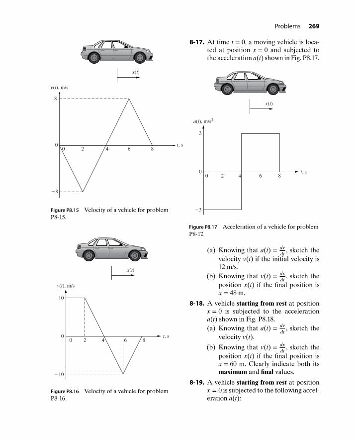
Problems 269
x(t)
−8
t, s
v(t), m/s
2 4 6 80
8
0
Figure P8.15 Velocity of a vehicle for problemP8-15.
x(t)
6 8
v(t), m/s
20
10
4
−10
t, s0
Figure P8.16 Velocity of a vehicle for problemP8-16.
8-17. At time t = 0, a moving vehicle is loca-ted at position x = 0 and subjected tothe acceleration a(t) shown in Fig. P8.17.
x(t)
t, s20
3
−3
04 6 8
a(t), m/s2
Figure P8.17 Acceleration of a vehicle for problemP8-17.
(a) Knowing that a(t) = dvdt
, sketch thevelocity v(t) if the initial velocity is12 m/s.
(b) Knowing that v(t) = dxdt
, sketch theposition x(t) if the final position isx = 48 m.
8-18. A vehicle starting from rest at positionx = 0 is subjected to the accelerationa(t) shown in Fig. P8.18.(a) Knowing that a(t) = dv
dt, sketch the
velocity v(t).
(b) Knowing that v(t) = dxdt
, sketch theposition x(t) if the final position isx = 60 m. Clearly indicate both itsmaximum and final values.
8-19. A vehicle starting from rest at positionx = 0 is subjected to the following accel-eration a(t):

270 Chapter 8 Derivatives in Engineering
x(t)
−10
10
00 2 4 6
a(t), m/s2
t, s
Figure P8.18 Acceleration of a vehicle for problemP8-18.
x(t)
−5
5
00 2 5 6
a(t), m/s2
t, s
Figure P8.19 Acceleration of a vehicle for problemP8-19.
(a) Knowing that a(t) = dvdt
, sketch thevelocity v(t).
(b) Knowing that v(t) = dxdt
, sketch theposition x(t) if the final position isx = 15 m. Clearly indicate both itsmaximum and final values.
8-20. A vehicle starting from rest at positionx = 0 is subjected to the following accel-eration a(t):
x(t)
0 2 13 15
10
−10
0 t, s
a(t), m/s2
Figure P8.20 Acceleration of a vehicle for problemP8-20.
(a) Knowing that a(t) = dvdt
, sketch thevelocity v(t).
(b) Knowing that v(t) = dxdt
, sketch theposition x(t) if the final position isx = 260 m. Clearly indicate both itsmaximum and final values.
8-21. The voltage across an inductor is givenin Fig. P8.21. Knowing that v(t) = L di(t)
dtand p(t) = v(t) i(t), sketch the graphs ofi(t) and p(t). Assume L = 2 H, i(0) =0 A, and p(0) = 0 W.
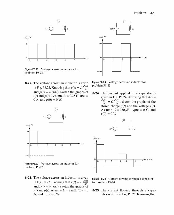
Problems 271
v(t) L
i(t)
+−
t, s00
6
1 2 3 4 5
v(t), V
Figure P8.21 Voltage across an inductor forproblem P8-21.
8-22. The voltage across an inductor is givenin Fig. P8.22. Knowing that v(t) = L di(t)
dtand p(t) = v(t) i(t), sketch the graphs ofi(t) and p(t). Assume L = 0.25 H, i(0) =0 A, and p(0) = 0 W.
v(t) L
i(t)
+−
00
6
4 5
−6
2 3t, s
1
v(t), V
Figure P8.22 Voltage across an inductor forproblem P8-22.
8-23. The voltage across an inductor is givenin Fig. P8.23. Knowing that v(t) = L di(t)
dtand p(t) = v(t) i(t), sketch the graphs ofi(t) and p(t). Assume L = 2 mH, i(0) = 0A, and p(0) = 0 W.
v(t) L
i(t)
+−
−10
10
00 1 2 3
t, ms
v(t), V
Figure P8.23 Voltage across an inductor forproblem P8-23.
8-24. The current applied to a capacitor isgiven in Fig. P8.24. Knowing that i(t) =dq(t)
dt= C dv(t)
dt, sketch the graphs of the
stored charge q(t) and the voltage v(t).Assume C = 250𝜇F, q(0) = 0 C, andv(0) = 0 V.
C
i(t)
v(t) +−
t, ms00 21 4 53 6
2
−1
i(t), A
Figure P8.24 Current flowing through a capacitorfor problem P8-24.
8-25. The current flowing through a capa-citor is given in Fig. P8.25. Knowing that

272 Chapter 8 Derivatives in Engineering
i(t) = dq(t)dt
= C dv(t)dt
, sketch the graphsof the stored charge q(t) and the volt-age v(t). Assume C = 250𝜇F, q(0) =0 C, and v(0) = 0 V.
C
i(t)
v(t) +−
0 2 3 4 5
2
1
−2
1
0t, ms
i(t), A
Figure P8.25 Current flowing through a capacitorfor problem P8-25.
8-26. The current flowing through a 500 𝜇Fcapacitor is given in Fig. P8.26. Know-ing that i(t) = C dv(t)
dt, plot v(t) for 0 ≤
t ≤ 4 sec if v(0) = −4 V, v(2) = 2 V,v(4) = 2 V, and the maximum voltageis 4 V.
C
i(t)
v(t) +−
00
2
1 2
−2
4 53 6t, s
i(t), mA
Figure P8.26 Current flowing through a capacitorfor problem P8-26.
8-27. A simply supported beam is subjectedto a load P as shown in Fig. P8.27. Thedeflection of the beam is given by
y(x) = P b x6 EI l
(x2 + b2 − l2), 0 ≤ x ≤l2
where EI is the flexural rigidity of thebeam. Find the following:(a) The location and the value of maxi-
mum deflection ymax.
(b) The value of the slope 𝜃 = dy(x)dx
atthe end x = 0.
y
x
P
CA B
a b
l
x = 0
Figure P8.27 A simply supported beam forproblem P8-27.
8-28. A simply supported beam is subjected
to a load P at x = L4
as shown in Fig.
P8.28. The deflection of the beam isgiven by
y(x) = − P128 EI
(7 L2 x − 16 x3), 0 ≤ x ≤L4
where EI is the flexural rigidity of thebeam. Find the following:(a) The equation of the slope 𝜃 = dy(x)
dx.
(b) The location and magnitude of max-imum deflection ymax.
(c) Evaluate both the deflection and
slope at x = 0 and x = L4
.
(d) Use the results of parts (b) and(c) to sketch the deflection y(x) for
0 ≤ x ≤L4
.

Problems 273
y
x
CA
P
B
L
4
L
x = 0
3L4
Figure P8.28 A simply supported beam forproblem P8-28.
8-29. A simply supported beam is subjectedto an applied moment Mo at its cen-ter x = L
2as shown in Fig. P8.29. The
deflection of the beam is given by
y(x) =Mo
6 EI L
(L2 x − 3 L x2
4− x3
),
0 ≤ x ≤L2
where EI is the flexural rigidity of thebeam. Find the following:(a) The equation for the slope 𝜃 = dy
dx.
(b) The location and the value of maxi-mum deflection ymax.
(c) Evaluate both the deflection andslope at the points A and B (x = 0and x = L
2).
(d) Use the results of parts (a)–(c) tosketch the deflection y(x) from x =0 to x = L
2.
y
L/2
L
Mo
x
B
A
Figure P8.29 A simply supported beam forproblem P8-29.
8-30. A simply supported beam is subjectedto a sinusoidal distributed load, asshown in the Fig. P8.30. The deflectiony(x) of the beam is given by
y(x) = −wo L4
16𝜋4 EIsin
(2𝜋 x
L
)where EI is the flexural rigidity of thebeam. Find the following:
w(x) = w0 sin
y
x
L
x2
Lπ )(
Figure P8.30 A simply supported beam forproblem P8-30.
(a) The equation for the slope 𝜃 = dydx
.
(b) The value of the slope where thedeflection is zero.
(c) The value of the deflection at thelocation where the slope is zero.
(d) Use the results of parts (b) and (c)to sketch the deflection y(x).
8-31. Consider a beam under a linear dis-tributed load and supported as shown inFig. P8.31. The deflection of the beam isgiven by
y(x) =w0
120 EI L(−x5 + 2 L2 x3 − L4 x)
where L is the length and EI is theflexural rigidity of the beam. Find thefollowing:(a) The location and value of the maxi-
mum deflection ymax.
(b) The value of the slope 𝜃 = dy(x)dx
atthe ends x = 0 and x = L.
(c) Use your results in (a) and (b) tosketch the deflection y(x).

274 Chapter 8 Derivatives in Engineering
x
L
y(x) q(x) = w0 x
L
Figure P8.31 A beam under linear distributed loadfor problem P8-31.
8-32. A fixed-fixed beam is subjected to asinusoidal distributed load, as shown inFig. P8.32.
w(x) = w0 cos
L
x
x
y
2
Lπ )(
Figure P8.32 A fixed-fixed beam subjected to asinusoidal distributed load.
The deflection y(x) is given by
y(x) = −w0 L4
16𝜋4 EI
[1 − cos
(2𝜋L
x)]
.
(a) Determine the equation for theslope 𝜃 = dy
dx.
(b) Evaluate both the deflection andthe slope at the points x = 0 andx = L.
(c) Determine both the location andvalue of the maximum deflection.
(d) Use your results of parts (b)and (c) to sketch the deflectiony(x), and clearly indicate both the
location and value of the maximumdeflection.
8-33. Consider the buckling of a pinned-pinned column under a compressiveaxial load P as shown in Fig. P8.33.
L
P
y(x)
x
Figure P8.33 A pinned-pinned column under acompressive axial load.
The deflection y(x) of the second buck-ling mode is given by
y(x) = −A sin(
2𝜋xL
),
where A is an undetermined constant.(a) Determine the equation for the
slope 𝜃 =dydx
.
(b) Determine the value of the slope atthe locations where the deflection iszero.
(c) Determine the value of the deflec-tion at the locations where the slopeis zero.
(d) Use your results of parts (b) and(c) to sketch the buckled deflectiony(x).
8-34. Consider the buckling of a pinned-fixedcolumn under a compressive load P asshown in Fig. P8.34.
The deflection y(x) of the buckledconfiguration is given by
y(x) = −A[
sin(
4.4934L
x)+ 0.97616
Lx]
where A is an undetermined constant.(a) Determine the equation for the
slope 𝜃 =dydx
.

Problems 275
x
L
y(t)
P
Figure P8.34 A pinned-fixed column under acompressive load.
(b) Evaluate both the deflection andthe slope at the points x = 0 andx = L.
(c) Determine the location and magni-tude of the maximum deflection.
(d) Use your results of parts (b) and(c) to sketch the buckled deflectiony(x).
8-35. Consider a beam under a uniform dis-tributed load and supported as shown inFig. P8.35. The deflection of the beam isgiven by
y(x) = −w48 EI
(2 x4 − 5 x3 L + 3 x2 L2)
where L is the length and EI is theflexural rigidity of the beam. Find thefollowing:
y(x)
x
w
L
Figure P8.35 A beam under uniform distributedload for problem P8-35.
(a) The location and value of the maxi-mum deflection ymax.
(b) The value of the slope 𝜃 =dy(x)
dxat
the ends x = 0 and x = L.(c) Use your results in (a) and (b) to
sketch the deflection y(x).
8-36. A cantilever beam is pinned at theend x = L, and subjected to an appliedmoment Mo as shown in Fig. P8.36. Thedeflection y(x) of the beam is given by
y(x) = −Mo
4 EI L(x3 − L x2)
where L is the length and EI is theflexural rigidity of the beam. Find thefollowing:(a) The equation of the slope 𝜃 =
dy(x)dx
.
(b) The location and magnitude of themaximum deflection ymax.
(c) Evaluate both the deflection andslope at the points A and B (x = 0and x = L).
(d) Use the results in parts (b) and (c)to sketch the deflection y(x) andclearly indicate the location of themaximum deflection on the sketch.
y
Mo
AB
L
x
Figure P8.36 A cantilever beam for problem P8-36.
8-37. Consider a shaft subjected to an appliedtorque T, as shown in Fig. P8.37. Theinternal normal and shear stresses atthe surface vary with the angle relative

276 Chapter 8 Derivatives in Engineering
to the axis and are given by equations(8.71) and (8.72), respectively.
𝜎𝜃 = 32 T𝜋d3
sin 𝜃 cos 𝜃 (8.71)
𝜏𝜃 = 16 T𝜋d3
(cos2𝜃 − sin2
𝜃) (8.72)
Find(a) the angle 𝜃 where 𝜎𝜃 is maximum(b) the angle 𝜃 where 𝜏𝜃 is maximum
d
T
T
θθ
θτ
σ
Figure P8.37 Applied torque and internal forces ina shaft.
8-38. The velocity of a skydiver jumpingfrom a height of 13,000 ft is shown inFig. P8.38.(a) Find the equation of the velocity
v(t) for the five time intervals shownin Fig. P8.38.
(b) Knowing that a(t) = dvdt
, sketch the
acceleration a(t) of the skydiver for0 ≤ t ≤ 180 s.
(c) Use the results of part (b) to sketchthe height y(t) for 0 ≤ t ≤ 180 s.
8-39. A proposed highway traverses a hill-top bounded by uphill and downhillgrades of 15% and −10%, respectively.These grades pass through benchmarksA and B located as shown in Fig. P8.39.With the origin of the coordinate axes(x, y) set at benchmark A, the engineerhas defined the hilltop segment of the
y = 0 ft
y = 13,000 ft
0
v(t), ft/s
t, s
−193.2
−18
0 6 24 27 162 180
(27, −18)
(24, −193.2)
(180, 0)
(162, −18)
(6, −193.2)
Figure P8.38 Velocity of a skydiver jumping from aheight of 13,000 ft.
highway by a parabolic arc
y(x) = a x2 + b x,
which is tangent to the uphill grade atthe origin.(a) Find the slope of the line for the up-
hill grade and the value of b for theparabolic arc.
(b) Find the equation of the line
y = c x + d
for the downhill grade.(c) Given that at the downhill point of
tangency (x), both the elevation andthe slope of the parabolic arc areequal to their respective values ofthe downhill line, for example,
y(x) = y(x)
dydx
|x=x =dydx x=x

Problems 277
y, m
x, m0A
0
BDownhill grade
−10%
300
8Uphill grade
15%
Downhill point of tangency (x, y)
Figure P8.39 Parabolic arc traversing highway hilltop.
determine the point of tangency(x, y) of the parabolic arc with thedownhill grade. Also, compute itselevation.
(d) Find the equation of the parabolicarc.

CHAPTER9
Integrals inEngineering
This chapter will discuss what integration is and why engineers need to know it. Itis important to point out that the objective of this chapter is not to teach techniquesof integration, as discussed in a typical calculus course. Instead, the objective of thischapter is to expose students to the importance of integration in engineering and toillustrate its application to the problems covered in core engineering courses such asphysics, statics, dynamics, and electric circuits.
9.1 INTRODUCTION: THE ASPHALT PROBLEMAn engineering co-op had to hire an asphalt contractor to widen the truck entranceto the corporate headquarters, as shown in Fig. 9.1. The asphalt extends 50 ft in thex- and y-directions and has a radius of 50 ft. Thus, the required asphalt is the areaunder the circular curve is given by
(x − 50)2 + (y − 50)2 = 2500. (9.1)
New asphalt
50 ft
50 ft
r = 50 ft
Figure 9.1 Driveway of corporate headquarters.
The asphalt company charges by the square foot and provides an estimate based on“eyeballing” the required area for new asphalt. The co-op asks a young engineer toestimate the area to make sure that the quote is fair. The young engineer proposes toestimate the area as a series of n inscribed rectangles as shown in Fig. 9.2. The area
278
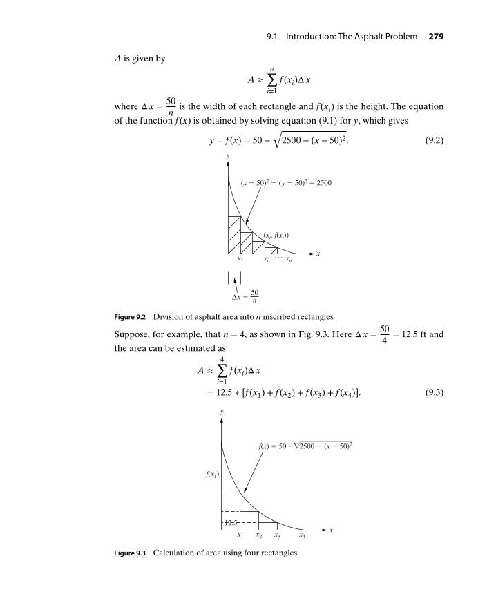
9.1 Introduction: The Asphalt Problem 279
A is given by
A ≈n∑
i=1
f (xi)Δ x
where Δ x = 50n
is the width of each rectangle and f (xi) is the height. The equation
of the function f (x) is obtained by solving equation (9.1) for y, which gives
y = f (x) = 50 −√
2500 − (x − 50)2. (9.2)
y
x1 xi xn... x
(x − 50)2 + (y − 50)2 = 2500
Δx = 50n
(xi, f(xi))
Figure 9.2 Division of asphalt area into n inscribed rectangles.
Suppose, for example, that n = 4, as shown in Fig. 9.3. Here Δ x = 504
= 12.5 ft and
the area can be estimated as
A ≈4∑
i=1
f (xi)Δ x
= 12.5 ∗ [f (x1) + f (x2) + f (x3) + f (x4)]. (9.3)
x
y
x1 x2 x3 x4
12.5
f(x) = 50 − 2500 − (x − 50)2
f(x1)
√⎯⎯⎯⎯⎯⎯⎯⎯⎯⎯⎯⎯⎯⎯
Figure 9.3 Calculation of area using four rectangles.
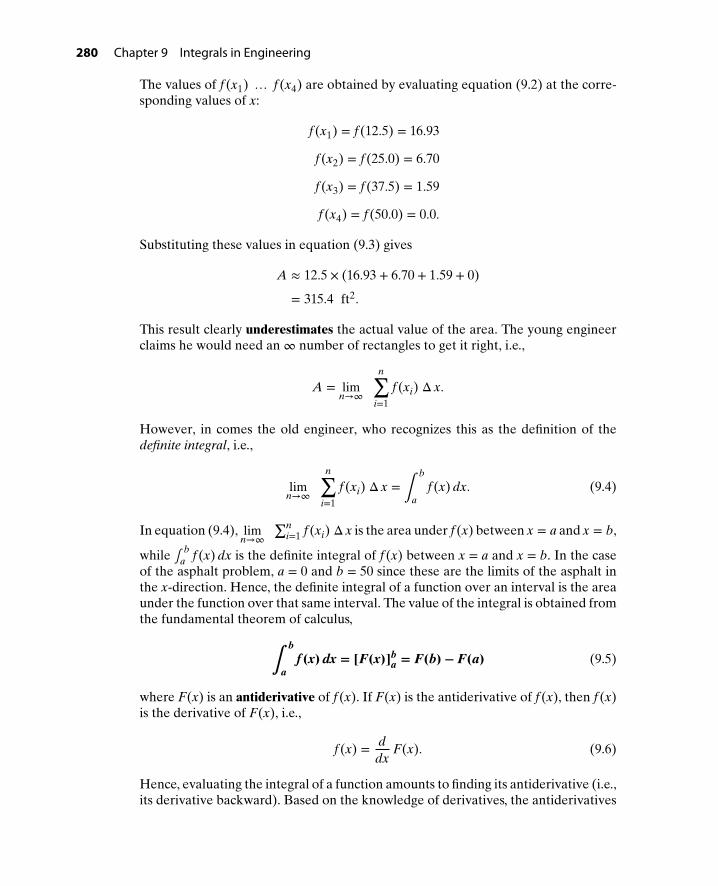
280 Chapter 9 Integrals in Engineering
The values of f (x1) … f (x4) are obtained by evaluating equation (9.2) at the corre-sponding values of x:
f (x1) = f (12.5) = 16.93
f (x2) = f (25.0) = 6.70
f (x3) = f (37.5) = 1.59
f (x4) = f (50.0) = 0.0.
Substituting these values in equation (9.3) gives
A ≈ 12.5 × (16.93 + 6.70 + 1.59 + 0)
= 315.4 ft2.
This result clearly underestimates the actual value of the area. The young engineerclaims he would need an ∞ number of rectangles to get it right, i.e.,
A = limn→∞
n∑i=1
f (xi) Δ x.
However, in comes the old engineer, who recognizes this as the definition of thedefinite integral, i.e.,
limn→∞
n∑i=1
f (xi) Δ x =∫
b
af (x) dx. (9.4)
In equation (9.4), limn→∞
∑ni=1 f (xi) Δ x is the area under f (x) between x = a and x = b,
while ∫b
a f (x) dx is the definite integral of f (x) between x = a and x = b. In the caseof the asphalt problem, a = 0 and b = 50 since these are the limits of the asphalt inthe x-direction. Hence, the definite integral of a function over an interval is the areaunder the function over that same interval. The value of the integral is obtained fromthe fundamental theorem of calculus,
∫b
af (x) dx = [F(x)]b
a = F(b) − F(a) (9.5)
where F(x) is an antiderivative of f (x). If F(x) is the antiderivative of f (x), then f (x)is the derivative of F(x), i.e.,
f (x) = ddx
F(x). (9.6)
Hence, evaluating the integral of a function amounts to finding its antiderivative (i.e.,its derivative backward). Based on the knowledge of derivatives, the antiderivatives

9.1 Introduction: The Asphalt Problem 281
(integrals) of sin (x) and xn can, for example, be written as
f (x) = sin (x) ⇒ F(x) = −cos (x) + C
f (x) = x2 ⇒ F(x) = x3
3+ C
f (x) = xn ⇒ F(x) = xn+1
n + 1+ C,
∫sin(x) dx = −cos x + C
∫x2 dx = x3
3+ C
∫xn dx = xn+1
n + 1+ C.
The previous integrals are called indefinite integrals since there are no limits a and b.Since F(x) is the antiderivative of f (x),
F(x) =∫
f (x) dx. (9.7)
Equations (9.6) and (9.7) show that differentiation and integration are inverse oper-ations; i.e.,
f (x) = ddx
F(x) = ddx ∫
f (x) dx = f (x)
F(x) =∫
f (x) dx =∫
ddx
F(x) dx = F(x).
TABLE 9.1 The antiderivatives of some commonfunctions in engineering.
Function, f (x) Antiderivative, F(x) = ∫ f (x) dx
sin(𝜔 x) − 1𝜔
cos(𝜔 x) + C
cos(𝜔 x) 1𝜔
sin(𝜔 x) + C
ea x 1a
ea x + C
xn 1n + 1
xn+1 + C
c f (x) c ∫ f (x) dx
f1(x) + f2(x) ∫ f1(x) dx + ∫ f2(x) dx
Note that in Table 9.1, a, c, n, and 𝜔 are constants as they do not depend on x. Withthis background, the young engineer finds the total area as the sum of all elementalareas dA, as shown in Fig. 9.4.

282 Chapter 9 Integrals in Engineering
x
x
y
0
dA = y(x) dx
y(x) = f(x)
x = 50 dx
Figure 9.4 Asphalt area with elemental area dA.
The total area is thus
A =∫
50
0dA =
∫
50
0y(x) dx.
Substituting the value of y(x) from equation (9.2) gives
A =∫
50
0(50 −
√2500 − (x − 50)2) dx
=∫
50
050 dx −
∫
50
0
√2500 − (x − 50)2 dx
= 50∫
50
0dx −
∫
50
0
√2500 − (x − 50)2 dx
= 50 [x]500 −
∫
50
0
√2500 − (x − 50)2 dx
= 50 (50 − 0) −∫
50
0
√2500 − (x − 50)2 dx
or
A = 2500 − I. (9.8)
The integral I = ∫50
0
√2500 − (x − 50)2 dx is not easy to evaluate by hand. How-
ever, this integral can be evaluated using MATLAB (or other engineering programs),which gives I = 625𝜋. Substituting I into equation (9.8) gives
A = 2500 − 625𝜋
A = 536.5 ft2.
In comes the oldest engineer, who notes that the result can be calculated withoutcalculus! The total area is simply the area of a square (of dimension 50 × 50) minus
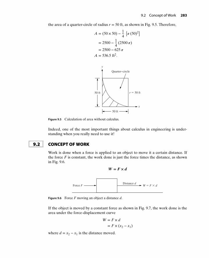
9.2 Concept of Work 283
the area of a quarter-circle of radius r = 50 ft, as shown in Fig. 9.5. Therefore,
A = (50 × 50) − 14
[𝜋 (50)2]
= 2500 − 14
(2500𝜋)
= 2500 − 625𝜋
A = 536.5 ft2.
Quarter−circle
50 ft
50 ft
x
y
r = 50 ft
Figure 9.5 Calculation of area without calculus.
Indeed, one of the most important things about calculus in engineering is under-standing when you really need to use it!
9.2 CONCEPT OF WORK
Work is done when a force is applied to an object to move it a certain distance. Ifthe force F is constant, the work done is just the force times the distance, as shownin Fig. 9.6.
W = F × d
Force F Distance d
W = F × d
Figure 9.6 Force F moving an object a distance d.
If the object is moved by a constant force as shown in Fig. 9.7, the work done is thearea under the force-displacement curve
W = F × d
= F × (x2 − x1)
where d = x2 − x1 is the distance moved.

284 Chapter 9 Integrals in Engineering
xx = x1
F
Distance d = x2 − x1 x = x2
Work
Figure 9.7 Work as area under a constant force curve.
If the force is not constant but is a function of x, as shown in Fig. 9.8, the area underthe curve (i.e., the work) must be determined by integration:
W =∫
x2
x1
F(x) dx
=∫
d
0F(x) dx. (9.9)
dx, m
0
F, N
Work = area under the curve
Figure 9.8 Work as area under a variable force curve.
Calculations used to find the work done by a variable force (equation (9.9)) aredemonstrated in the following examples.
Example9-1
The work done on the block shown in Fig. 9.7 is defined by equation (9.9). Ifd = 1.0 m, find the work done for the following forces:
(a) f (x) = 2 x2 + 3 x + 4 N
(b) f (x) = 2 sin(𝜋
2x)+ 3 cos
(𝜋
2x)
N
(c) f (x) = 4 e𝜋x N

9.2 Concept of Work 285
Solution (a) W =∫
d
0f (x) dx
=∫
1
0(2 x2 + 3 x + 4) dx
= 2∫
1
0x2 dx + 3
∫
1
0x dx + 4
∫
1
01 dx
= 2[
x3
3
]1
0+ 3
[x2
2
]1
0+ 4 (x)1
0
= 23
(1 − 0) + 32
(1 − 0) + 4 (1 − 0)
= 23+ 3
2+ 4
= 376
or
W = 6.17 N-m.
(b) W =∫
d
0f (x) dx
=∫
1
0
[2 sin
(𝜋
2x)+ 3 cos
(𝜋
2x)]
dx
= 2∫
1
0sin
(𝜋
2x)
dx + 3∫
1
0cos
(𝜋
2x)
dx
= 2
⎡⎢⎢⎢⎣−
cos(𝜋
2x)
𝜋
2
⎤⎥⎥⎥⎦1
0
+ 3
⎡⎢⎢⎢⎣sin
(𝜋
2x)
𝜋
2
⎤⎥⎥⎥⎦1
0
= 2[− 2𝜋
cos(𝜋
2x)]1
0+ 3
[2𝜋
sin(𝜋
2x)]1
0
= − 4𝜋
[cos
(𝜋
2x)]1
0+ 6
𝜋
[sin
(𝜋
2x)]1
0
= − 4𝜋
[cos(𝜋
2
)− cos(0)] + 6
𝜋[sin
(𝜋
2
)− sin(0)]
= − 4𝜋
(0 − 1) + 6𝜋
(1 − 0)
= 4𝜋+ 6
𝜋= 10
𝜋

286 Chapter 9 Integrals in Engineering
or
W = 3.18 N-m.
(c)
W =∫
d
0f (x) dx
=∫
1
0(4 e𝜋x) dx
= 4∫
1
0e𝜋x dx
= 4[
1𝜋
e𝜋x]1
0
= 4𝜋
[e𝜋 − e0]
= 4𝜋
[e𝜋 − 1]
or
W = 28.2 N-m.
Note: In all three cases, the distance moved by the object is 1.0 m, but the work(energy) expended by the force is completely different!
9.3 APPLICATION OF INTEGRALS IN STATICS9.3.1 Center of Gravity (Centroid)
The centroid, or center of gravity, of an object is a point within the object that repre-sents the average location of its mass. For example, the centroid of a two-dimensionalobject bounded by a function y = f (x) is given by a point G = (x, y) as shown in Fig.9.9. The average x-location x of the material is given by
x =∑
xi Ai∑
Ai(9.10)
y = y(x) = f(x)
Gx
y
A
x
y
Figure 9.9 Centroid of a two-dimensional object.
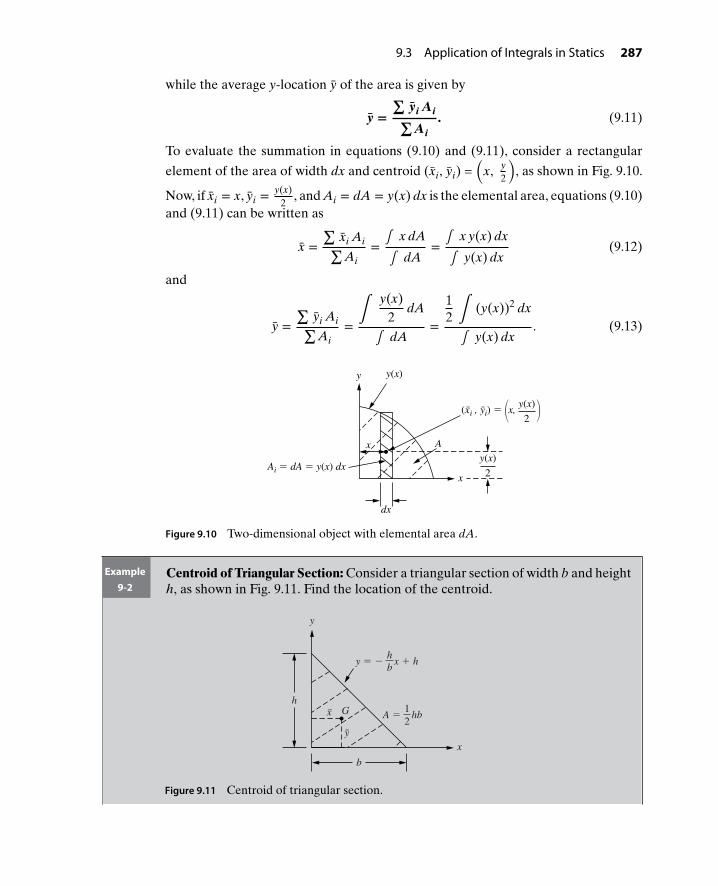
9.3 Application of Integrals in Statics 287
while the average y-location y of the area is given by
y =∑
yi Ai∑
Ai. (9.11)
To evaluate the summation in equations (9.10) and (9.11), consider a rectangular
element of the area of width dx and centroid (xi, yi) =(
x, y2
), as shown in Fig. 9.10.
Now, if xi = x, yi =y(x)
2, and Ai = dA = y(x) dx is the elemental area, equations (9.10)
and (9.11) can be written as
x =∑
xi Ai∑Ai
=∫ x dA
∫ dA=
∫ x y(x) dx
∫ y(x) dx(9.12)
and
y =∑
yi Ai∑Ai
=∫
y(x)2
dA
∫ dA=
12 ∫
(y(x))2 dx
∫ y(x) dx. (9.13)
x A
x
y
dx
y(x)
Ai = dA = y(x) dx
(xi , yi) = x,2
y(x)
y(x)
2
( )
Figure 9.10 Two-dimensional object with elemental area dA.
Example9-2
Centroid of Triangular Section: Consider a triangular section of width b and heighth, as shown in Fig. 9.11. Find the location of the centroid.
hy = − x + h
b
y
x
b
y
hGx
21
A = hb
Figure 9.11 Centroid of triangular section.

288 Chapter 9 Integrals in Engineering
Solution The two-dimensional triangular section shown in Fig. 9.11 is the area bounded bythe line
y(x) = −hb
x + h. (9.14)
The area of the section is given by
A =∫
b
0y(x) dx
or
A = 12
bh, (9.15)
which is simply the area of the triangle. The above result can also be obtained by
integrating y(x) = −hb
x + h with respect to x from 0 to b. Using the information
in equations (9.14) and (9.15), the x-location of the centroid is calculated fromequation (9.12) as
x =∫ x y(x) dx
∫ y(x) dx
=∫
b
0x(−h
bx + h
)dx
12
b h
= 2∫
b
0
(−h
bx2 + hx
)dx
bh
=(
2bh
) (−h
b
[x3
3
]b
0+ h
[x2
2
]b
0
)
=(
2bh
) (− h
3b(b3 − 0) + h
2(b2 − 0)
)
=(
2bh
) (−hb2
3+ hb2
2
)
=(
2bh
) (hb2
6
)or
x = b3.

9.3 Application of Integrals in Statics 289
Similarly, the y-location of the centroid is calculated from equation (9.13) as
y =
12 ∫
y2(x) dx
∫ y(x) dx
=(
12
) (2
b h
)∫
b
0
(−h
bx + h
)2
dx
=(
1h b
)∫
b
0
[(h2
b2
)x2 −
(2 hb
)x h + h2
]dx
=(
1h b
) (h2
b2
[x3
3
]b
0−(
2 h2
b
) [x2
2
]b
0+ h2 (x)b
0
)
=(
1h b
) (h2
3 b2(b3 − 0) − h2
b(b2 − 0) + h2 (b − 0)
)
=(
1h b
) (h2 b
3− h2 b + h2 b
)
=(
1b h
) (h2 b
3
)or
y = h3.
Thus, the centroid of a triangular section of width b and height h is given by (x, y) =(b3
, h3
). In the above example, the coordinates of the centroid were found by using
vertical rectangles. These coordinates can also be calculated using the horizontalrectangles, as shown in Fig. 9.12.
y
x
b
x
y
h
dy Ai = dA = x dy
hx + h y = −
b
(xi, yi) = 2x , y( )
Figure 9.12 Evaluation of centroid using horizontal elemental areas.
The area of the horizontal element is given by
Ai = dA = x dy = g(y)dy

290 Chapter 9 Integrals in Engineering
where x = g(y) = −bh
y + b is obtained by solving the equation of the line for x.
Therefore, the elemental area of the horizontal rectangle is given by
Ai = dA =(−b
hy + b
)dy.
The y-coordinate of the triangular section can be calculated as
y =∑
yi Ai∑Ai
=∫ y dA
A(9.16)
or
y =∫
h0 y
(−b
hy + b
)dy
12
b h
= 2b h ∫
h
0
(−b
hy2 + b y
)dy
= 2b h
[(−b
h
)∫
h
0y2 dy + [b]
∫
h
0y dy
]
= 2b h
[(− b
3h
)[y3]h
0 +(
b2
)[y2]h
0
]
= 2b h
[(− b
3h
)(h3 − 0) +
(b2
)(h2 − 0)
]
= 2b h
[−b h2
3+ b h2
2
]which gives
y = h3.
This is the same result previously found using the vertical rectangles!
Example9-3
The geometry of a cooling fin is described by the shaded area bounded by theparabola shown in Fig. 9.13.
(a) If the equation of the parabola is y(x) = −x2 + 4, determine the height h andthe width b of the fin.
(b) Determine the area of the cooling fin by integration with respect to x.
(c) Determine the x-coordinate of the centroid by integration with respect to x.
(d) Determine the y-coordinate of the centroid by integration with respect to x.

9.3 Application of Integrals in Statics 291
b
h
x, in.
y, in.
y(x) = −x2 + 4
Figure 9.13 Geometry of a cooling fin.
Solution (a) The equation of the parabola describing the cooling fin is given by
y(x) = −x2 + 4. (9.17)
The height h of the cooling fin can be found by substituting x = 0 in equation(9.17) as
h = y(0) = −02 + 4 = 4′′.
The width b of the fin can be obtained by setting y(x) = 0, which gives
y(x) = −x2 + 4 = 0 ⇒ x2 = 4 ⇒ x = ± 2.
Since the width of the fin must be positive, it follows that b = 2′′.
(b) The area A of the fin is calculated by integrating equation (9.17) from 0 to b as
A =∫
b
0y(x) dx
=∫
2
0(−x2 + 4) dx
=[−x3
3+ 4 x
]2
0
=[(
−23
3+ 4 (2)
)− (0 + 0)
]
or
A = 163
in.2.

292 Chapter 9 Integrals in Engineering
(c) The x-coordinate of the centroid can be found using the vertical rectangles asillustrated in Fig. 9.14. By definition,
x =∑
xi Ai∑Ai
h
y(x) = −x2 + 4
b
y, in.
x
dA = y(x) dxy(x)2
(xi, yi) = x,2
y(x)
x, in.
dx
( )
Figure 9.14 Determination of centroid using vertical rectangles.
where xi = x and Ai = dA = y(x) dx. Thus,
x =∫ xy(x) dx
A
=∫
20 x (−x2 + 4) dx
163
= 316 ∫
2
0(−x3 + 4 x) dx
= 316
[−x4
4+ 4 x2
2
]2
0
= 316
[(−24
4+ 2 (22)
)− (0 + 0)
]or
x = 1216
in.
Therefore, x = 34
in.
(d) Similarly, the y-coordinate of the centroid can be determined by integrationwith respect to x as
y =∑
yi Ai∑Ai

9.3 Application of Integrals in Statics 293
where yi =y(x)
2and Ai = y(x) dx. Thus,
y =
12 ∫
y2(x) dx
A
=
12 ∫
2
0(−x2 + 4)2 dx
163
= 332 ∫
2
0(x4 − 8 x2 + 16) dx
= 332
[x5
5− 8 x3
3+ 16 x
]2
0
= 332
[ (25
5− 8 23
3+ 16 (2)
)− (0 + 0 + 0)
]
= 332
[325
− 643
+ 32]
= 3[
15− 2
3+ 1
]
= 3[
315
− 1015
+ 1515
]
= 2415
or
y = 85.
Therefore, y = 85
in.
9.3.2 Alternate Definition of the Centroid
If the origin of the x-y coordinate system is located at the centroid as shown inFig. 9.15, then the x- and y-coordinates of the centroid are given by
x =∫ x dA
A= 0 (9.18)
y =∫ y dA
A= 0. (9.19)

294 Chapter 9 Integrals in Engineering
y
xG
Figure 9.15 Triangular section with origin at centroid.
Hence, an alternative definition of the centroid is the location of the origin such that∫ x dA = ∫ y dA = 0 (i.e., there is no first moment about the origin). As shown inFig. 9.16, this means that the first moment of the area about both the x- and y-axes iszero:
First moment of area about x-axis = Mx =∫
y dA = 0
First moment of area about y-axis = My =∫
x dA = 0.
dA
G
y
xx
dA
G
y
xy
Figure 9.16 First moment of area.
The above definition of the centroid is illustrated for a rectangular section in thefollowing example.
Example9-4
Show that the coordinates of the centroid of the rectangle in Fig. 9.17 are x = y = 0.
b/2
x
b
h
y
G
h/2
Figure 9.17 Rectangular section.

9.3 Application of Integrals in Statics 295
Solution The first moment of area about the y-axis can be calculated using vertical rectan-gles, as shown in Fig. 9.18, which gives
∫x dA =
∫
b2
− b2
x hdx
= h[
x2
2
] b2
− b2
= h2
(b2
4− b2
4
)= 0.
Hence, x =∫ xdA
A= 0.
dA = h dx
dx
x
b
h
y
G
Figure 9.18 x-coordinate of the centroid using vertical rectangles.
Similarly, the first moment of area about the x-axis can be calculated using horizontalrectangles, as shown in Fig. 9.19, which gives
∫y dA =
∫
h2
− h2
y b dy
= b[
y2
2
] h2
− h2
= b2
(h2
4− h2
4
)= 0.
Hence, y =∫ y dA
A= 0.

296 Chapter 9 Integrals in Engineering
dy
dA = b dy
x
b
h
y
G
Figure 9.19 y-coordinate of the centroid using horizontal rectangles.
9.4 DISTRIBUTED LOADSIn this section, integrals are used to find the resultant force due to a distributed load,as well as the location of that force required for statically equivalent loading. Theseare among the primary applications of integrals in statics.
9.4.1 Hydrostatic Pressure on a Retaining Wall
Consider a retaining wall of height h and width b that is subjected to a hydrostaticpressure from fluid of density 𝜌 (Fig. 9.20). The pressure acting on the wall satisfiesthe linear equation
p(y) = 𝜌 g y
where g is the acceleration due to gravity.
Retaining wall
h
g
b
y
p(y) = g y ρ
Figure 9.20 Hydrostatic force acting on the rectangular retaining wall.
The resultant force acting on the wall is calculated by adding up (i.e., integrating)all the differential forces dF shown in Fig. 9.22. Since pressure is force/unit area, thedifferential force is found by multiplying the value of the pressure at any depth y byan elemental area of the wall as
dF = p(y) dA
where dA = b dy.

9.4 Distributed Loads 297
p(y)
b
y
dF
dy
dA
Figure 9.21 Forces acting on the retaining wall.
The resultant force acting on the wall is obtained by integration as
F =∫
dF
=∫
h
0p(y) b dy
=∫
h
0𝜌 g y b dy
= 𝜌 g b∫
h
0y dy
= 𝜌 g b[
y2
2
]h
0
or
F =𝜌 g b h2
2.
p(y)
b
y
dF
dy
dA
Figure 9.22 Forces acting on the retaining wall.
Note that ∫ h0 p(y) b dy = b ∫
h0 p(y) dy is simply the width b times the area of the tri-
angle shown in Fig. 9.23. Therefore, the resultant force can be obtained from the areaunder the distributed load. Since this is a triangular load, the area can be calculated

298 Chapter 9 Integrals in Engineering
without using integration, and is given by
A = 12
(𝜌 g h)(h) =𝜌 g h2
2.
p(y)
y
h
g hρ
Figure 9.23 Area under hydrostatic pressure.
The resultant force is obtained by multiplying the area with the width b, which gives
F = b𝜌 g h2
2=
𝜌 g b h2
2.
9.4.2 Distributed Loads on Beams: Statically Equivalent Loading
Fig. 9.24 shows a simply supported beam with a distributed load applied over theentire length L. The distributed load w(x) varies in intensity with position x and hasunits of force per unit length (lb/ft or N/m). The goal is to replace the distributedload with a statically equivalent point load. As concluded in the previous section,the equivalent load R is the area under the distributed load, and is given by
R =∫
L
0w(x) dx. (9.20)
x
y
L
w(x)
Figure 9.24 Distributed load on a simply supported beam.
The equivalent load R and location l are shown in Fig. 9.25.To find the location of the statically equivalent force, the resultant load shown
in Fig. 9.25 must have the same moment about every point as the distributed load

9.4 Distributed Loads 299
x
y R
l
L
Figure 9.25 Beam with an equivalent point load.
shown in Fig. 9.24. For example, the moment (force times distance) about the pointx = 0 must be the same for both the distributed and equivalent loads. The momentM0 for the distributed load can be calculated by summing moments due to elementalloads dw, as shown in Fig. 9.26. Hence,
M0 =∫
xdw
=∫
L
0xw(x) dx. (9.21)
x
y
L
dw = w(x) dx
x
Figure 9.26 Beam with a small elemental load.
The moment M0 about the x = 0 point of the equivalent load R is given by
M0 = R l,
or
M0 = l∫
L
0w(x) dx. (9.22)
Equating the two moments in equations (9.21) and (9.22) gives
l∫
L
0w(x) dx =
∫
L
0xw(x) dx
or
l =∫
L0 xw(x) dx
∫L
0 w(x) dx. (9.23)

300 Chapter 9 Integrals in Engineering
Equation (9.23) is identical to equation (9.12) but with w(x) instead of y(x). Hence,it can be concluded that l = x, which is the x-coordinate of the centroid of the areaunder the load! Thus, for the purpose of statics, a distributed load can always bereplaced by its resultant force acting at its centroid.
Example9-5
Find the magnitude and location of the statically equivalent point load for thebeam of Fig. 9.27. Use your results to find the reactions at the support (Fig. 9.28).
x
y
L
w0L
w(x) = xw0
Figure 9.27 Simply supported beam with linear distributed load.
x
y
L
w0
R1 R2
Figure 9.28 Reaction forces acting at the supports.
Solution The resultant R is the area under the triangular load w(x), which is given by
R =∫
L
0w(x) dx
=∫
L
0
(w0
L
)xdx
=(w0
L
) (x2
2
)L
0
=(w0
L
) (L2
2− 0
)or
R = 12
w0 L.
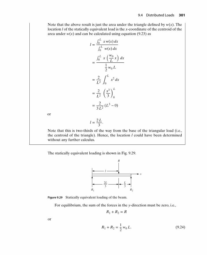
9.4 Distributed Loads 301
Note that the above result is just the area under the triangle defined by w(x). Thelocation l of the statically equivalent load is the x-coordinate of the centroid of thearea under w(x) and can be calculated using equation (9.23) as
l =∫
L0 x w(x) dx
∫L
0 w(x) dx
=∫
L0 x
(w0
Lx)
dx
12
w0 L
= 2L2 ∫
L
0x2 dx
= 2L2
(x3
3
)L
0
= 23 L2
(L3 − 0)
or
l = 2 L3
.
Note that this is two-thirds of the way from the base of the triangular load (i.e.,the centroid of the triangle). Hence, the location l could have been determinedwithout any further calculus.
The statically equivalent loading is shown in Fig. 9.29.
x
R
R1 R2
L3
2L3
l
Figure 9.29 Statically equivalent loading of the beam.
For equilibrium, the sum of the forces in the y-direction must be zero, i.e.,
R1 + R2 = R
or
R1 + R2 = 12
w0 L. (9.24)

302 Chapter 9 Integrals in Engineering
Also, the sum of moments about any point on the beam must be zero. Taking themoments about x = 0 gives
R2 L −(
12
w0 L)
2 L3
= 0
which gives
R2 L =w0 L2
3or
R2 =w0 L
3. (9.25)
Substituting equation (9.25) in equation (9.24) gives
R1 +w0 L
3=
w0 L2
.
Solving for R1 gives
R1 =w0 L
2−
w0 L3
or
R1 =w0 L
6. (9.26)
9.5 APPLICATIONS OF INTEGRALS IN DYNAMICSIt was discussed in Chapter 8 that if the position of a particle moving in the x-directionas shown in Fig. 9.30 is given by x(t), the velocity v(t) is the first derivative of theposition, and the acceleration is the first derivative of the velocity (second derivativeof the position):
v(t) =dx(t)
dt
a(t) =dv(t)
dt=
d2x(t)
dt2.
v(t), a(t)
x(t)
Figure 9.30 A particle moving in the horizontal direction.

9.5 Applications of Integrals in Dynamics 303
Now, if the acceleration a(t) of the particle is given, both the velocity v(t) and theposition x(t) can be determined by integrating with respect to t. Beginning with
dv(t)dt
= a(t) (9.27)
integrating both sides between t = t0 and any time t gives
∫
t
t0
dv(t)dt
dt =∫
t
t0
a(t) dt. (9.28)
By definition,∫
t
t0
dv(t)dt
dt = [v(t)]tt0
, so that equation (9.28) can be written as
[v(t)]tt0=∫
t
t0
a(t) dt
which gives
v(t) − v(t0) =∫
t
t0
a(t) dt
or
v(t) = v(t0) + ∫t
0a(t) dt. (9.29)
Thus, the velocity of the particle at any time t is equal to the velocity at t = t0 (initialvelocity) plus the integral of the acceleration from t = t0 to the time t. Now, giventhe velocity v(t), the position x(t) can be determined by integrating with respect to t.Beginning with
dx(t)dt
= v(t) (9.30)
integrating both sides between t = t0 and any time t gives
∫
t
t0
dx(t)dt
dt =∫
t
t0
v(t) dt. (9.31)
By definition,∫
t
t0
dx(t)dt
dt = [x(t)]tt0
, so that equation (9.31) can be written as
[x(t)]tt0=∫
t
t0
v(t) dt
which gives
x(t) − x(t0) =∫
t
t0
v(t) dt
or
x(t) = x(t0) + ∫t
t0
v(t) dt. (9.32)

304 Chapter 9 Integrals in Engineering
Thus, the position of the particle at any time t is equal to the position at t = t0 (initialposition) plus the integral of the velocity from t = t0 to the time t.
Example9-6
A ball is dropped from a height of 1.0 m at t = t0 = 0, as shown in Fig. 9.31. Findv(t), y(t), and the time it takes for the ball to hit the ground.
a = −9.81 m/s2y(t)
1.0 m
t = 0
Figure 9.31 A ball dropped from a height of 1 m.
Solution Since the ball is dropped from rest at time t = 0 sec, v(0) = 0 m/sec. Substitutingt0 = 0, a(t) = −9.81 m/s2, and v(0) = 0 in equation (9.29), the velocity at any time tcan be obtained as
v(t) = 0 +∫
t
0−9.81 dt
= −9.81 [t]t0
= −9.81 (t − 0)
or
v(t) = −9.81 t m/s.
Now, substituting v(t) into equation (9.32), the position y(t) of the ball at any timet can be obtained as
y(t) = y(0) +∫
t
0−9.81 t dt
= y(0) − 9.81[
t2
2
]t
0
= y(0) − 9.812
(t2 − 0
)y(t) = y(0) − 4.905 t2
.
Since the initial height is y(0) = 1 m, the position of the ball at any time t is givenby
y(t) = 1.0 − 4.905 t2 m.

9.5 Applications of Integrals in Dynamics 305
The time to impact is obtained by setting y(t) = 0 as
1.0 − 4.905 t2impact = 0,
which gives
4.905 t2impact = 1.
Solving for timpact gives
timpact =√
1.04.905
or
timpact = 0.452 s.
Example9-7
Suppose that a ball is thrown upward from ground level with an initial velocityv(0) = v0 = 4.43 m/s, as shown in Fig. 9.32. Find v(t) and y(t).
y(t)
a = −9.81 m/s2
v0 = 4.43 m/s
Figure 9.32 A ball thrown upward with an initial velocity.
Solution Substituting t0 = 0, v(0) = 4.43 m/s, and a(t) = −9.81 m/s2 into equation (9.29), thevelocity of the ball at any time t is given by
v(t) = 4.43 +∫
t
0−9.81 dt
= 4.43 − 9.81 [t]t0
= 4.43 − 9.81 (t − 0)
or
v(t) = 4.43 − 9.81 t m/s. (9.33)
Now substituting the velocity v(t) into equation (9.32), the position of the ball isgiven as
y(t) = y(0) +∫
t
0(4.43 − 9.81 t) dt
= y(0) + 4.43 [t]t0 − 9.81
[t2
2
]t
0
= y(0) + 4.43 (t − 0) − 9.812
(t2 − 0
)

306 Chapter 9 Integrals in Engineering
or
y(t) = y(0) + 4.43 t − 4.905 t2.
Since the initial position is y(0) = 0 m, the position of the ball at any time t is givenby
y(t) = 4.43 t − 4.905 t2 m.
Example9-8
A stone is thrown from the top of a 50 m high building with an initial velocity of10 m/s, as shown in Fig. 9.33.
50 m
y(t) = 0 m
v(0) = 10 m/s
a = −9.81 m/s2
y(0) = 50 m
Figure 9.33 A stone thrown from the top of a building.
Knowing that the velocity is
v(t) = v(0) +∫
t
0a(t) dt (9.34)
and the position is
y(t) = y(0) +∫
t
0v(t) dt (9.35)
(a) Find and plot the velocity v(t).
(b) Find and plot the position y(t).
(c) Determine both the time and the velocity when the stone hits the ground.
Solution (a) The velocity of the stone can be calculated by substituting v(0) = 10 m/s anda(t) = −9.81 m/s2 into equation (9.34) as
v(t) = v(0) +∫
t
0a(t) dt
= 10 +∫
t
0−9.81 dt
= 10 − 9.81 [t]t0
= 10 − 9.81 (t − 0)
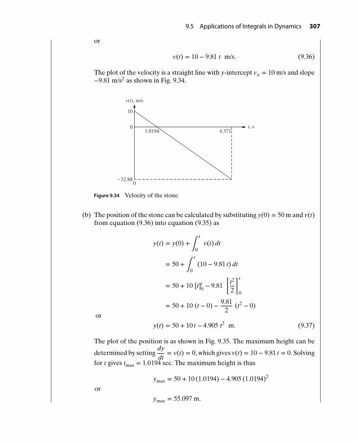
9.5 Applications of Integrals in Dynamics 307
or
v(t) = 10 − 9.81 t m/s. (9.36)
The plot of the velocity is a straight line with y-intercept vo = 10 m/s and slope−9.81 m/s2 as shown in Fig. 9.34.
4.3711.0194
10
0
0
v(t), m/s
t, s
−32.88
Figure 9.34 Velocity of the stone.
(b) The position of the stone can be calculated by substituting y(0) = 50 m and v(t)from equation (9.36) into equation (9.35) as
y(t) = y(0) +∫
t
0v(t) dt
= 50 +∫
t
0(10 − 9.81 t) dt
= 50 + 10 [t]t0 − 9.81
[t2
2
]t
0
= 50 + 10 (t − 0) − 9.812
(t2 − 0)
or
y(t) = 50 + 10 t − 4.905 t2 m. (9.37)
The plot of the position is as shown in Fig. 9.35. The maximum height can be
determined by settingdydt
= v(t) = 0, which gives v(t) = 10 − 9.81 t = 0. Solving
for t gives tmax = 1.0194 sec. The maximum height is thus
ymax = 50 + 10 (1.0194) − 4.905 (1.0194)2
or
ymax = 55.097 m.

308 Chapter 9 Integrals in Engineering
4.371 t, s
1.019400
y(t), m
50
ymax
Figure 9.35 Position of the stone.
(c) The time it takes for the stone to hit the ground can be calculated by settingthe position y(t) equal to zero as
y(t) = 50 + 10 t − 4.905 t2 = 0
or
t2 − 2.039 t − 10.194 = 0. (9.38)
The quadratic equation (9.38) can be solved by using one of the methodsdescribed in Chapter 2. For example, we can complete the square as
t2 − 2.039 t = 10.194
t2 − 2.039 t +(
2.0392
)2
= 10.194 +(
2.0392
)2
(t − 2.039
2
)2
= (±√
11.233)2
t − 1.0194 = ± 3.3516
t = 1.0194 ± 3.3516
or
t = 4.371,− 2.332 s. (9.39)
Since the negative time (t = −2.332 s) in equation (9.39) is not a possible solu-tion, it takes t = 4.371 s for the stone to hit the ground. The velocity when thestone hits the ground is obtained by evaluating v(t) at t = 4.371, which gives
v(4.371) = 10 − 9.81 (4.371) = −32.88 m/s.
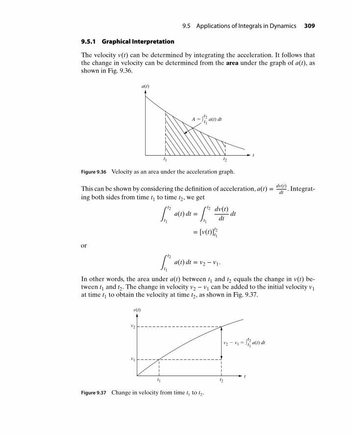
9.5 Applications of Integrals in Dynamics 309
9.5.1 Graphical Interpretation
The velocity v(t) can be determined by integrating the acceleration. It follows thatthe change in velocity can be determined from the area under the graph of a(t), asshown in Fig. 9.36.
tt2
t2t1
t1
a(t)
A = a(t) dt∫
Figure 9.36 Velocity as an area under the acceleration graph.
This can be shown by considering the definition of acceleration, a(t) = dv(t)dt
. Integrat-ing both sides from time t1 to time t2, we get
∫
t2
t1
a(t) dt =∫
t2
t1
dv(t)dt
dt
= [v(t)]t2t1
or
∫
t2
t1
a(t) dt = v2 − v1.
In other words, the area under a(t) between t1 and t2 equals the change in v(t) be-tween t1 and t2. The change in velocity v2 − v1 can be added to the initial velocity v1at time t1 to obtain the velocity at time t2, as shown in Fig. 9.37.
v2
v2 − v1 = a(t) dt
v(t)
v1
t1 t2t
t2t1
∫
Figure 9.37 Change in velocity from time t1 to t2.
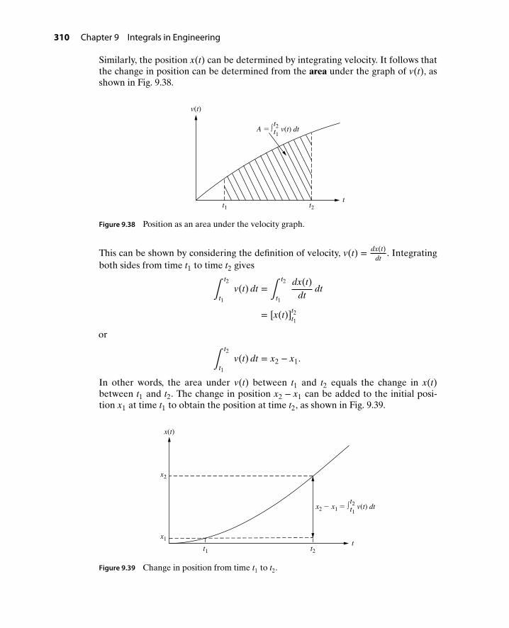
310 Chapter 9 Integrals in Engineering
Similarly, the position x(t) can be determined by integrating velocity. It follows thatthe change in position can be determined from the area under the graph of v(t), asshown in Fig. 9.38.
t1 t2t
v(t)
A = v(t) dtt2t1
∫
Figure 9.38 Position as an area under the velocity graph.
This can be shown by considering the definition of velocity, v(t) = dx(t)dt
. Integratingboth sides from time t1 to time t2 gives
∫
t2
t1
v(t) dt =∫
t2
t1
dx(t)dt
dt
= [x(t)]t2t1
or
∫
t2
t1
v(t) dt = x2 − x1.
In other words, the area under v(t) between t1 and t2 equals the change in x(t)between t1 and t2. The change in position x2 − x1 can be added to the initial posi-tion x1 at time t1 to obtain the position at time t2, as shown in Fig. 9.39.
x2
x(t)
x1
t1 t2t
x2 − x1 = v(t) dtt2t1
∫
Figure 9.39 Change in position from time t1 to t2.

9.5 Applications of Integrals in Dynamics 311
Example9-9
The acceleration of a vehicle is measured as shown in Fig. 9.40. Knowing that thevehicle starts from rest at position x = 0, sketch the velocity v(t) and position x(t)using integrals.
x(t)
020
2
−2
64t, s
a(t), m/s2
Figure 9.40 Acceleration of a vehicle for Example 9-9.
Solution (a) Velocity: Knowing v(0) = 0 and v(t) − v(t0) = ∫t
t0a(t) dt, 0 ≤ t ≤ 2 :
a(t) = 2 m/s2 = constant. Therefore, v(t) is a straight line with a slope of2 m/s2. Also, the change in velocity is
v2 − v0 =∫
2
0a(t) dt
or
v2 − v0 = area under a(t) between 0 and 2 s.
Thus,
v2 − v0 = (2) (2) = 4 (area of a rectangle),
which gives
v2 = v0 + 4.
Since v0 = 0,
v2 = 0 + 4 = 4 m/s.
2 < t ≤ 4 : Since a(t) = 0 m/s2, v(t) is constant. Also,
v4 − v2 =∫
4
2a(t) dt
= area under a(t) between 2 and 4 s
= 0.
Thus,
v4 = v2 + 0
= 4 + 0

312 Chapter 9 Integrals in Engineering
or
v4 = 4 m/s.
4 < t ≤ 6 : a(t) = −2 m/s2 = constant. Therefore, v(t) is a straight linewith a slope of −2 m/s2. Also, the change in v(t) is
v6 − v4 =∫
6
4a(t) dt
= area under a(t) between 4 and 6
= (−2) (2) (area of a rectangle)
or
v6 − v4 = −4.
Thus, v6 = v4 − 4
= 4 − 4
orv6 = 0 m/s.
The graph of the velocity obtained above is as shown in Fig. 9.41.
4
04 620
t, s
v(t), m/s
Figure 9.41 Velocity of the vehicle for Example 9-9.
(b) Position: Now use v(t) to sketch x(t) knowing that x(0) = 0 and x(t) − x(t0) =∫
tt0
v(t) dt.0 ≤ t ≤ 2 : v(t) is a linear function (straight line) with a slope of 2 m/s.
Therefore, x(t) is a quadratic function with increasing slope (concave up). Also,the change in x(t) is
x2 − x0 =∫
2
0v(t) dt
= area under v(t) between 0 and 2
= 12
(2) (4) (area of a triangle)
or
x2 − x0 = 4.

9.5 Applications of Integrals in Dynamics 313
Thus,
x2 = x0 + 4.
Since x0 = 0,
x2 = 0 + 4
or
x2 = 4 m.
2 < t ≤ 4 : v(t) has a constant value of 4 m/s. Therefore, x(t) is a straightline with a slope of 4 m/s. Also, the change in x(t) is
x4 − x2 =∫
4
2v(t) dt
= area under v(t) between 2 and 4
= (2) (4) (area of a rectangle)
or
x4 − x2 = 8.
Thus,
x4 = x2 + 8
= 4 + 8
or
x4 = 12 m.
4 < t ≤ 6 : v(t) is a linear function (straight line) with a slope of −2 m/s.Therefore, x(t) is a quadratic function with a decreasing slope (concave down).Also, the change in position is
x6 − x4 =∫
6
4v(t) dt
= area under v(t) between 4 and 6
= 12
(2) (4) (area of a triangle)
or
x6 − x4 = 4.
Thus,
x6 = x4 + 4
= 12 + 4
or
x6 = 16 m.

314 Chapter 9 Integrals in Engineering
The graph of the position obtained above is shown in Fig. 9.42.
020 4 6
8
4
12
16
t, s
Quadratic
Linear
Quadratic
x(t), m
Figure 9.42 Position of the particle for Example 9-7.
9.6 APPLICATIONS OF INTEGRALS IN ELECTRIC CIRCUITS9.6.1 Current, Voltage, and Energy Stored in a Capacitor
In this section, integrals are used to obtain the voltage across a capacitor when acurrent is passed through it (charging and discharging of a capacitor), as well as thetotal stored energy.
Example9-10
For t ≥ 0, a current i(t) = 24 e−40 t mA is applied to a 3𝜇 F capacitor, as shown inFig. 9.43.
(a) Given that i(t) = Cdv(t)
dt, find the voltage v(t) across the capacitor.
(b) Given that p(t) = v(t) i(t) =dw(t)
dt, find the stored energy w(t) and show that
w(t) = 12
C v2(t).
Assume that the capacitor is initially completely discharged; i.e., the initial voltageacross the capacitor and initial energy stored are zero.
i(t) v(t)C = 3 F
+
−
↑ μ
Figure 9.43 Current applied to a capacitor.

9.6 Applications of Integrals in Electric Circuits 315
Solution (a) Given i(t) = Cdv(t)
dt, it follows that
dv(t)dt
= 1C
i(t). (9.40)
Integrating both sides gives
∫
t
0
dv(t)dt
dt =∫
t
0
1C
i(t) dt
[v(t)]t0 = 1
C ∫
t
0i(t) dt
v(t) − v(0) = 1C ∫
t
0i(t) dt
or
v(t) = v(0) + 1C ∫
t
0i(t) dt. (9.41)
Substituting v(0) = 0 V, C = 3 × 10⁻⁶ F, and i(t) = 0.024 e−40 t A into equation(9.41), the voltage across the capacitor at any time t is given by
v(t) = 13.0 × 10⁻⁶ ∫
t
00.024 e−40 t dt
= 0.0243.0 × 10−6 ∫
t
0e−40 t dt
= 8000[− 1
40e−40 t
]t
0
= −800040
(e−40 t − e0 )
= −200 ( e−40 t − 1)
or
v(t) = 200 ( 1 − e−40 t) V.
(b) By definition, the power supplied to a capacitor is given by
p(t) =dw(t)
dt(9.42)
Integrating both sides of equation (9.42) gives
∫
t
0
dw(t)dt
dt =∫
t
0p(t) dt
[w(t)]t0 =
∫
t
0p(t) dt
w(t) − w(0) =∫
t
0p(t) dt

316 Chapter 9 Integrals in Engineering
or
w(t) = w(0) + ∫t
0p(t) dt. (9.43)
Since the energy stored in the capacitor at time t = 0 is zero, w(0) = 0. Thepower p(t) is given by
p(t) = v(t) i(t)
= 200 (1 − e−40 t) (0.024 e−40 t)
= (200) (0.024) e−40 t − (200 e−40 t) (0.024 e−40 t)
or
p(t) = 4.8 e−40 t − 4.8 e−80 t W. (9.44)
Substituting w(0) = 0 and p(t) from equation (9.44) into equation (9.43) gives
w(t) = 0 +∫
t
0(4.8 e−40 t − 4.8 e−80 t) dt
= 4.8[− 1
40e−40 t
]t
0− 4.8
[− 1
80e−80 t
]t
0
= −4.840
(e−40 t − 1) + 4.880
(e−80 t − 1)
= −0.12 e−40 t + 0.12 + 0.06 e−80 t − 0.06
or
w(t) = 0.06 e−80 t − 0.12 e−40 t + 0.06 J. (9.45)
To show that w(t) = 12
C v2(t), the quantity 12
C v2(t) can be calculated as
12
C v2(t) = 12
(3 × 10⁻⁶) (200 − 200 e−40 t)2
= (1.5 × 10⁻⁶)[2002 − 2(200)(200)e−40t + (200e−40t)2]
= (1.5 × 10⁻⁶)(4 × 10⁴ − 8 × 10⁴ e−40 t + 4 × 10⁴ e−80 t)
= 0.06 e−80 t − 0.12 e−40 t + 0.06 J. (9.46)
Comparison of equations (9.45) and (9.46) reveals that w(t) = 12
C v2(t).
Example9-11
The current i(t) shown in Fig. 9.44 is applied to a 20𝜇F capacitor. Sketch the
voltage v(t) across the capacitor knowing that i(t) = Cdv(t)
dt, or v(t) = v(t0) +
1C ∫
t
t0
i(t) dt. Assume that the initial voltage across the capacitor is zero (i.e.,
v(0) = 0 V).

9.6 Applications of Integrals in Electric Circuits 317
0
−2
−4
t, msi(t)0 1 2 4 5
4
2
i(t), A
C = 20 F v(t)
+
−
↑ μ
Figure 9.44 Current applied to a capacitor.
Solution Since C = 20𝜇F,
1C
= 120 × 10−6
= 106
20
= 102 × 104
20or
1C
= 50,000 F−1.
The voltage during each time interval can now be calculated as follows:
(a) 0 ≤ t ≤ 1 ms: t0 = 0, v(t0) = v0 = 0 V, and i(t) = 4 A = constant. Therefore,
v(t) = 1C ∫
i(t) dt is a straight line with positive slope. The voltage at time
t = 1 ms can be calculated as
v1 = v0 + 50,000∫
0.001
04 dt
= 0 + 200,000 [ t ]0.0010
= 200,000 (0.001 − 0)
or
v1 = 200 V.
The change in voltage across the capacitor between 0 and 1 ms can also becalculated without evaluating the integral (i.e., from geometry) as
v1 − v0 = 1C
× area under the current between 0 and 1 ms
= 50,000 [(4) (0.001)] (area of a rectangle)

318 Chapter 9 Integrals in Engineering
or
v1 − v0 = 200 V.
Therefore, v1 = v0 + 200 = 200 V.
(b) 1 ms < t ≤ 2 ms: t0 = 1 ms, v(t0) = v1 = 200 V, and i(t) = −2 A = constant.
Therefore, v(t) = 1C ∫
i(t) dt is a straight line of negative slope. The voltage
at t = 2 ms can be calculated as
v2 = v1 + 50,000∫
0.002
0.001(−2) dt
= 200 − 100,000 [ t ]0.0020.001
= 200 − 100,000 (0.002 − 0.001)
= 200 − 100
or
v2 = 100 V.
The change in voltage across the capacitor between 1 ms and 2 ms can also becalculated from geometry as
v2 − v1 = 1C
× area under the current waveform between 1 and 2 ms
= 50,000 [ (−2) (0.001) ]
v2 − v1 = −100 V
Therefore, v2 = v1 − 100 = 200 − 100 = 100 V.
(c) 2 ms < t ≤ 4 ms: t0 = 2 ms, v(t0) = v2 = 100 V, and i(t) = 2 A = constant.Therefore, v(t) = 1
C∫ i(t) dt is a straight line with positive slope. The voltage at
t = 4 ms can be calculated as
v4 = v2 + 50,000∫
0.004
0.0022 dt
= 100 + 100,000 [t]0.0040.002
= 100 + 100,000 (0.004 − 0.002)
= 100 + 100,000 (0.002)
= 100 + 200
or
v4 = 300 V.
The change in voltage across the capacitor between 2 ms and 4 ms can also becalculated from geometry as
v4 − v2 = 1C
× area under the current waveform between 2 and 4 ms
= 50,000 [ (2) (.002) ]

9.6 Applications of Integrals in Electric Circuits 319
or
v4 − v2 = 200 V.
Therefore, v4 = v2 + 200 = 100 + 200 = 300 V.
(d) 4 ms < t ≤ 5 ms: t0 = 4 ms, v(t0) = v4 = 300 V, and i(t) = −4 A = constant.Therefore, v(t) = 1
C∫ i(t) dt is a straight line with negative slope. The voltage
at t = 5 ms can be calculated as
v5 = v4 + 50,000∫
0.005
0.004(−4) dt
= 300 − 200,000 [t]0.0050.004
= 300 − 200,000 (0.005 − 0.004)
= 300 − 200,000 (0.001)
= 300 − 200
or
v5 = 100 V.
The change in voltage across the capacitor between 4 ms and 5 ms can also becalculated from geometry as
v5 − v4 = 1C
× area under the current waveform between 4 and 5 ms
= 50,000 [ (−4) (.001) ]
or
v5 − v4 = −200 V
Therefore, v5 = v4 − 200 = 300 − 200 = 100 V.
The sketch of the voltage across the capacitor is shown in Fig. 9.45.
00
100
200
300
1 2 54
v5
v(t), V
t, ms
v2
v1
v4
Figure 9.45 Voltage across the capacitor in Example 9-11.

320 Chapter 9 Integrals in Engineering
Example9-12
The sawtooth current i(t) shown in Fig. 9.46 is applied to a 0.5 F capaci-
tor. Sketch the voltage v(t) across the capacitor knowing that i(t) = Cdv(t)
dt
or v(t) = 1C ∫
i(t) dt. Assume that the capacitor is completely discharged at
t = 0 (i.e., v(0) = 0 V).
40
−2
2
t, s0 1 2 5
i(t), A
i(t) C = 0.5 F v(t)
+
−
↑
Figure 9.46 Sawtooth current applied to a capacitor.
Solution The voltage across the capacitor during different time intervals can be calculatedas follows:
(a) 0 ≤ t ≤ 1 s: i(t) is a straight line; therefore, v(t) = 1C∫ i(t) dt is a quadratic
function. The change in voltage across the capacitor between the time interval0 to 1 s can be calculated as
v1 − v0 = 1C ∫
t
0i(t) dt
= 10.5
(area under the current waveform between 0 and 1 s)
= 2[
12
(1)(−2)]
(area of a triangle)
or
v1 − v0 = −2.
Solving for v1 gives,
v1 = v0 + (−2)
= 0 − 2
orv1 = −2 V.
Also, since dv(t)dt
= 1C
i(t) is the slope of v(t) at time t, the slope of the voltage
at t = 0 is dvdt
= 10.5
(−2) = −4 V/s.
At t = 1 s, the slope of the voltage is dvdt
= 10.5
(0) = 0 V/s.
Therefore, v(t) is a decreasing quadratic function starting at v(0) = 0 V andending at −2 V, with a zero slope at t = 1 s.
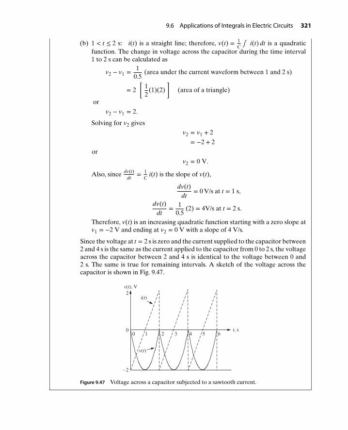
9.6 Applications of Integrals in Electric Circuits 321
(b) 1 < t ≤ 2 s: i(t) is a straight line; therefore, v(t) = 1C∫ i(t) dt is a quadratic
function. The change in voltage across the capacitor during the time interval1 to 2 s can be calculated as
v2 − v1 = 10.5
(area under the current waveform between 1 and 2 s)
= 2[
12
(1)(2)]
(area of a triangle)
or
v2 − v1 = 2.
Solving for v2 givesv2 = v1 + 2
= −2 + 2
or
v2 = 0 V.
Also, since dv(t)dt
= 1C
i(t) is the slope of v(t),
dv(t)dt
= 0 V/s at t = 1 s,
dv(t)dt
= 10.5
(2) = 4V/s at t = 2 s.
Therefore, v(t) is an increasing quadratic function starting with a zero slope atv1 = −2 V and ending at v2 = 0 V with a slope of 4 V/s.
Since the voltage at t = 2 s is zero and the current supplied to the capacitor between2 and 4 s is the same as the current applied to the capacitor from 0 to 2 s, the voltageacross the capacitor between 2 and 4 s is identical to the voltage between 0 and2 s. The same is true for remaining intervals. A sketch of the voltage across thecapacitor is shown in Fig. 9.47.
−2
2
0 t, s0 1 2 3 4 5 6
v(t), V
i(t)
v(t)
Figure 9.47 Voltage across a capacitor subjected to a sawtooth current.

322 Chapter 9 Integrals in Engineering
9.7 CURRENT AND VOLTAGE IN AN INDUCTORIn this section, integrals are used to find the current flowing through an inductorwhen it is connected across a voltage source.
Example9-13
A voltage v(t) = 10 cos(10 t) V is applied across a 100 mH inductor, as shown inFig. 9.48.
L = 100 mH
i(t)
v(t) +−
Figure 9.48 Voltage applied to an inductor.
(a) Suppose the initial current flowing through the inductor is i(0) = 10 A. Know-ing that v(t) = L di(t)
dt, integrate both sides of the equation to determine the
current i(t). Also, plot the current for 0 ≤ t ≤ 𝜋/5 s.
(b) Given your results in part (a), find the power p(t) = v(t) i(t) supplied to theinductor. If the initial energy stored in the inductor is w(0) = 5 J, find the storedenergy
w(t) = w(0) +∫
t
0p(t) dt, (9.47)
and show that w(t) = 12
L i2(t).
Solution (a) The voltage/current relationship for an inductor is given by
Ldi(t)
dt= v(t)
ordi(t)
dt= 1
Lv(t). (9.48)
Integrating both sides of equation (9.48) from an initial time t0 to time t gives
∫
t
t0
di(t)dt
= 1L ∫
t
t0
v(t) dt
[i(t)]tt0= 1
L ∫
t
t0
v(t) dt
i(t) − i(t0) = 1L ∫
t
t0
v(t) dt

9.7 Current and Voltage in an Inductor 323
or
i(t) = i(t0) + 1L ∫
t
t0
v(t) dt. (9.49)
Substituting t0 = 0, L = 0.1 H, i(0) = 10 A, and v(t) = 10 cos(10 t) V in equa-tion (9.49) gives
i(t) = 10 + 10.1 ∫
t
010 cos(10 t) dt
= 10 + 100[
110
sin(10 t)]t
0
= 10 + 10 ( sin 10 t − 0 )
or
i(t) = 10 + 10 sin 10 t A. (9.50)
The current i(t) obtained in equation (9.50) is a periodic function with fre-quency 𝜔 = 10 rad/s. The period is
T = 2𝜋𝜔
= 2𝜋10
or
T = 𝜋
5s.
Thus, the plot of i(t) is simply the sinusoid 10 sin (10 t) shifted upward by10 amps as shown in Fig. 9.49.
20
10
0
i(t), A
0t, s
/20π /10π /203π /5π
Figure 9.49 Current flowing through the inductor in Example 9-13.

324 Chapter 9 Integrals in Engineering
(b) The power p(t) supplied to the inductor is given by
p(t) = v(t) i(t)
= (10 cos (10 t)) (10 + 10 sin (10 t))
= 100 cos (10 t) + 100 sin (10 t) cos (10 t)
= 100 cos (10 t) + 50 (2 sin (10 t) cos (10 t))
= 100 cos (10 t) + 50 sin (20 t)
or
p(t) = 100 (cos (10 t) + 0.5 sin (20 t)) W. (9.51)
The energy stored in the inductor is given by
w(t) = w(0) +∫
t
0p(t) dt. (9.52)
Substituting w(0) = 5 J and p(t) calculated in equation (9.51) gives
w(t) = 5 +∫
t
0100 (cos (10 t) + 0.5 sin (20 t)) dt
= 5 + 100[
sin (10 t)10
]t
0+ 50
[−cos 20 t
20
]t
0
= 5 + 10 (sin (10 t) − 0) − 2.5 (cos (20 t) − 1)
or
w(t) = 7.5 + 10 sin (10 t) − 2.5 cos (20 t) J. (9.53)
To show that w(t) = 12
L i2(t), the quantity 12
L i2(t) can be calculated as
12
L i2(t) = 12
(0.1) (10 + 10 sin (10 t))2
= 0.05[
102 + 2(10)(10) sin (10 t) + (10 sin (10 t))2 ]= 0.05 (100 + 200 sin (10 t) + 100 sin2 (10 t)).
Noting that sin2 (10 t) =(
1 − cos (20 t)2
), we get
12
L i2(t) = 5 + 10 sin (10 t) + 5(
1 − cos (20 t)2
)= 5 + 10 sin (10 t) + 2.5 − 2.5 cos (20 t)
= 7.5 + 10 sin (10 t) − 2.5 cos (20 t) J, (9.54)
which is the same as equation (9.53).
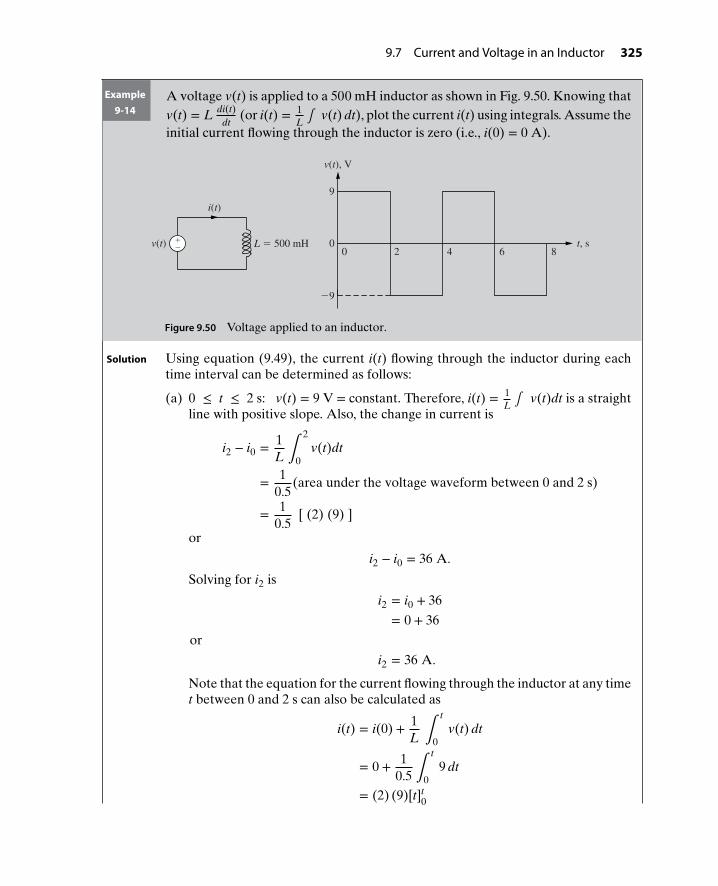
9.7 Current and Voltage in an Inductor 325
Example9-14
A voltage v(t) is applied to a 500 mH inductor as shown in Fig. 9.50. Knowing thatv(t) = L di(t)
dt(or i(t) = 1
L∫ v(t) dt), plot the current i(t) using integrals. Assume the
initial current flowing through the inductor is zero (i.e., i(0) = 0 A).
v(t), V
−9
0 t, s 0 2 4 6 8
9
L = 500 mH
i(t)
v(t) +−
Figure 9.50 Voltage applied to an inductor.
Solution Using equation (9.49), the current i(t) flowing through the inductor during eachtime interval can be determined as follows:
(a) 0 ≤ t ≤ 2 s: v(t) = 9 V = constant. Therefore, i(t) = 1L∫ v(t)dt is a straight
line with positive slope. Also, the change in current is
i2 − i0 = 1L ∫
2
0v(t)dt
= 10.5
(area under the voltage waveform between 0 and 2 s)
= 10.5
[ (2) (9) ]
or
i2 − i0 = 36 A.
Solving for i2 is
i2 = i0 + 36
= 0 + 36
or
i2 = 36 A.
Note that the equation for the current flowing through the inductor at any timet between 0 and 2 s can also be calculated as
i(t) = i(0) + 1L ∫
t
0v(t) dt
= 0 + 10.5 ∫
t
09 dt
= (2) (9)[t]t0

326 Chapter 9 Integrals in Engineering
or
i(t) = 18 t.
(b) 2 < t ≤ 4 s: v(t) = −9 V= constant. Therefore, i(t) = 1L∫ v(t) dt is a straight
line with a negative slope. Also, the change in current is
i4 − i2 = 10.5
(area under the voltage waveform between 2 and 4 s)
= 10.5
[ (2) (−9) ]
or
i4 − i2 = −36 A.
Solving for i4 gives
i4 = i2 − 36
= 36 − 36
or
i4 = 0 A.
Note that the equation for the current flowing through the inductor at any time tbetween 2 and 4 s can also be calculated as
i(t) = i(2) + 1L ∫
t
2v(t) dt
= 36 + 10.5 ∫
t
2−9 dt
= 36 − 18 [t]t2
= 36 − 18 (t − 2)
or
i(t) = −18 t + 72.
Since the current at t = 4 s is zero (the same as at t = 0) and the voltage applied tothe inductor between 4 and 8 s is the same as the voltage from 0 to 4 s, the currentflowing through the inductor between 4 and 8 s is identical to the current between0 and 4 s. The resulting current waveform (triangle wave) is shown in Fig. 9.51.
0 2 4 6 80
36
i(t), Ai(t) = −18t + 72
t, s
Figure 9.51 Current flowing through the inductor in Example 9-14.

9.8 Further Examples of Integrals in Engineering 327
9.8 FURTHER EXAMPLES OF INTEGRALS IN ENGINEERING
Example9-15
A biomedical engineer measures the velocity profiles of a belted and unbeltedoccupant during a 35 mph (≈ 16 m/s) frontal collison, as shown in Fig. 9.52.
(a) Knowing that x(t) = x(0) + ∫t
0 v(t)dt, find and plot the displacement x(t) of thebelted occupant for time 0 to 50 ms. Assume that the initial displacement att = 0 is 0 m (i.e., x(0) = 0 m).
(b) Find and plot the displacement x(t) of the unbelted occupant for time 0 to50 ms. Assume x(0) = 0 m.
(c) Based on the results of parts (a) and (b), how much farther did the unbeltedoccupant travel compared to the belted occupant?
Belted Occupant:
+X
Unbelted Occupant:
+X
v(t) = 16 cos(50 t)
v(t) = 0
0.050.0100
16
t, s
v(t), m/s
v(t) = 16 cos(10 t)
0.0500
16
t, s
v(t), m/s
π
π
Figure 9.52 Velocities of the belted and unbelted occupants during frontal collison.
Solution (a) The displacement of the belted occupant can be calculated using the expression
x(t) = x(0) +∫
t
0v(t)dt
(i) for 0 ≤ t ≤ 0.01 s
x(t) = 0 +∫
t
016 cos(50 𝜋t)dt = 16
[sin(50𝜋t)
50𝜋
]t
0= 16
50𝜋[sin(50𝜋t) − 0]
= 825𝜋
sin(50𝜋t) m. (9.55)
Therefore, x(0.01) = 825𝜋
sin(𝜋
2
)= 0.102 m.

328 Chapter 9 Integrals in Engineering
(ii) 0.01 ≤ t ≤ 0.05 s
x(t) = 0.102 +∫
t
00 dt
= 0.102 m. (9.56)
The displacement of the belted occupant during a frontal collison is shown inFig. 9.53.
t, s
x(t), m
0.102
00 0.01 0.05
Figure 9.53 Displacement of the belted occupant during a frontal collison.
(b) The displacement of the unbelted occupant for 0 ≤ t ≤ 0.05 s can becalculated as
x(t) = 0 +∫
t
016 cos(10𝜋t)dt
= 16[
sin(10𝜋t)10𝜋
]t
0
= 1610𝜋
[sin(10𝜋t) − 0]
= 85𝜋
sin(10𝜋t) m. (9.57)
Therefore, x(0.05) = 85𝜋
sin(𝜋
2
)= 0.509 m. The displacement of the unbelted
occupant is shown in Fig. 9.54.
(c) To find how much farther the unbelted occupant traveled during collison ascompared to the belted occupant, the total distance traveled by the belted oc-cupant in 50 ms is subtracted from the total distance traveled by the unbeltedoccupant as
Δ x = xunbelted(0.05) − xbelted(0.05)
= 0.509 − 0.102
= 0.407 m.

9.8 Further Examples of Integrals in Engineering 329
t, s
x(t), m
0.509
00 0.05
Figure 9.54 Displacement of the unbelted occupant during a frontal collison.
Example9-16
A biomedical engineer is evaluating an energy-absorbing aviation seat on a verticaldeceleration tower, as shown in Fig. 9.55. The acceleration profile of the drop cageis described by
a(t) = 500 sin(40𝜋t) m/s2.
(a) Knowing that v(t) = v(0) + ∫t
0 a(t)dt, find and plot the velocity v(t) of the dropcage. Assume the drop cage starts from rest at t = 0 s.
(b) What is the impact velocity vimpact of the drop cage if it takes 25 ms to hit theground?
(c) The total impulse I is equal to the change in momentum. For example I =Δp = pf − pi = mvimpact − mv0, where m is the mass of the system, vimpact is thefinal velocity, v0 is the initial velocity, p is the momentum, and I is the impulse.Find the total impulse after 25 ms. Assume that the total mass of the drop cage,seat, and crash test dummy is 1,000 kg.
Figure 9.55 Energy-absorbing aviation seat.

330 Chapter 9 Integrals in Engineering
Solution (a) The velocity of the cage can be calculated as
v(t) = v(o) +∫
t
0a(t)dt
= 0 +∫
t
0500 sin(40𝜋t)dt
= 500[−
cos(40𝜋t)40𝜋
]t
0
= − 50040𝜋
[cos(40𝜋t) − 1]
= 252𝜋
[1 − cos(40𝜋t)] m/s. (9.58)
(b) The velocity of the cage when it impacts the ground can be found by substitut-ing t = 25 ms = 0.025 s in equation (9.58) as
vimpact =252𝜋
[1 − cos ( 40𝜋(0.025) )]
= 252𝜋
[1 − cos(𝜋)]
= 252𝜋
[1 − (−1)]
= 502𝜋
= 7.96 m/s.
(c) The total impulse I can be found as
I = m vimpact − m v0
= (1000) (7.96) − (1000) (0)
= 7960kg m
s.
Example9-17
A civil engineer designs a building overhang to withstand a parabolic snow loading
per unit length p(x) = p(
1 − xL
)2, as shown in Fig. 9.56.
(a) Compute the resulting force V = ∫L
0 p(x)dx.
(b) Compute the corresponding moment M = ∫L
0 x p(x)dx.
(c) Locate the centroid of the loading x =∫
Lo x p(x) dx
∫L
0 p(x) dx= M
V.
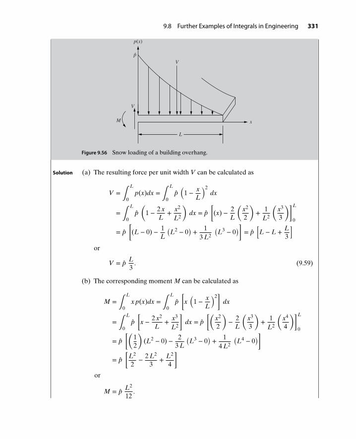
9.8 Further Examples of Integrals in Engineering 331
p
p(x)
x
V
M
L
V
Figure 9.56 Snow loading of a building overhang.
Solution (a) The resulting force per unit width V can be calculated as
V =∫
L
0p(x)dx =
∫
L
0p(
1 − xL
)2dx
=∫
L
0p(
1 − 2 xL
+ x2
L2
)dx = p
[(x) − 2
L
(x2
2
)+ 1
L2
(x3
3
)]L
0
= p[
(L − 0) − 1L
(L2 − 0
)+ 1
3 L2
(L3 − 0
)]= p
[L − L + L
3
]or
V = pL3. (9.59)
(b) The corresponding moment M can be calculated as
M =∫
L
0x p(x)dx =
∫
L
0p[
x(
1 − xL
)2]
dx
=∫
L
0p[
x − 2 x2
L+ x3
L2
]dx = p
[(x2
2
)− 2
L
(x3
3
)+ 1
L2
(x4
4
)]L
0
= p[(
12
)(L2 − 0) − 2
3 L
(L3 − 0
)+ 1
4 L2
(L4 − 0
)]
= p[
L2
2− 2 L2
3+ L2
4
]or
M = pL2
12.

332 Chapter 9 Integrals in Engineering
(c) The location of the centroid x can be found as
x = MV
=
p L2
12p L3
or x = L4.
Example9-18
A building overhang is subjected to a triangular snow loading p(x), as shown inFig. 9.57. The overhang is constructed from two metal face plates separated by anonmetallic core of thickness h. This sandwich beam construction deforms primar-ily due to shear deformation with deflection y(x) satisfying
y(x) = 1h G ∫
x
0
[∫
x
0p(x) dx − V
]dx, (9.60)
where V = p0L2
, p(x) = p0
(1 − x
L
), and G is the shear modulus.
(a) Evaluate (9.60) for the deflection y(x).
(b) Find the location and value of maximum deflection.
p(x)
x
V
M
p0
L
V
Core
h
Upper face plate
Lower face plate
(a) Cantilever overhang. (b) Sandwich construction.
Figure 9.57 Triangular snow loading of sandwich-constructed building overhang.
Solution (a) Substituting V = p0L2
and p(x) = p0
(1 − x
L
)into equation (9.60) gives
y(x) = 1h G ∫
x
0
[∫
x
0p0
(1 − x
L
)dx − p0
L2
]dx
= 1h G ∫
x
0
[p0
[x − x2
2 L
]x
0− p0
L2
]dx

9.8 Further Examples of Integrals in Engineering 333
= 1h G ∫
x
0
[p0
(x − x2
2 L
)− (0 − 0)
− p0
L2
]dx
=p0
h G ∫
x
0
[x − x2
2 L− L
2
]dx
=p0
h G
[x2
2− x3
6 L− L
2x]x
0
=p0
h G
[(x2
2− x3
6 L− L
2
)− (0 − 0 − 0)
]
=p0 x
2 h G
(x − x2
3 L− L
)or
y(x) = −p0 x
2 h G
[L − x
(1 − x
3 L
)]. (9.61)
(b) The location of the maximum value of the deflection can be found by equatingthe derivative of y(x) to zero as
dy(x)dx
= 0
ddx
(−
p0 x2 h G
[L − x
(1 − x
3 L
)])= 0
−p0
2 h G
(L − 2 x + 3 x2
3 L
)= 0
x2 − 2 x L + L2 = 0
(x − L)2 = 0.
Therefore, the deflection is maximum at x = L. The value of the maximumdeflection can now be obtained by substituting x = L in equation (9.61) as
y(L) = −p0 L2 h G
[L − L
(1 − L
3 L
)]= −
p0 L2 h G
(L3
)
= −p0 L2
6 h G.
Therefore, the maximum value of deflection isp0 L2
6 h G.

334 Chapter 9 Integrals in Engineering
P R O B L E M S
9-1. The profile of a gear tooth shown in Fig.P9.1(a) is approximated by the quad-ratic equation y(x) = − 4 k
lx (x − l).
y(x)
x
k
l0
0
Area, A
(a) The profile of a gear tooth.
x
y(x)k
l0
0
(b) The gear tooth area inscribed by six rectangles.
Figure P9.1 Area of a gear tooth for problem P9-1.
(a) Estimate the area A using six rect-angles of equal width (Δ x = l∕6), asshown in Fig. 9.1(b).
(b) Calculate the exact area by eval-uating the definite integral, A =
∫
l
0y(x) dx.
9-2. The profile of a gear tooth shown in Fig.P9.2 is approximated by the trigonomet-
ric equation y(x) = k2
(1 − cos
(2𝜋x
l
)).
(a) Estimate the area A usingeight rectangles of equal width
Δ x = l∕8, i.e.,
A =8∑
i=1
y(xi)Δ x.
(b) Calculate the exact area by integra-tion, i.e.,
A =∫
l
0y(x) dx.
Δxx
k
l
y
00
Area, A
Figure P9.2 Profile of a gear tooth for problemP9-2.
9-3. The velocity of an object as a func-tion of time is shown in Fig. P9.3. Theacceleration is constant during the first4 seconds of motion, so the velocity is alinear function of time with v(t) = 0 att = 0 and v(t) = 100 ft/s at t = 4 s. Thevelocity is constant during the last 6 s.(a) Estimate the total distance covered
(the area, A) under the velocitycurve using five rectangles of equalwidth (Δ t = 10∕5 = 2 s).
(b) Now estimate the total distance cov-ered using 10 rectangles of equalwidth.

Problems 335
(c) Calculate the exact area under thevelocity curve; i.e., find the totaldistance traveled by evaluating the
definite integral Δ x =∫
10
0v(t) dt.
(d) Calculate the exact area by addingthe area of the triangle and the areaof the rectangle bounded by thevelocity curve.
t, s1040
100
v(t), ft/s
Figure P9.3 The velocity of an object.
9-4. A particle is accelerated along a curvedpath of length l under the action of anapplied force f (x), as shown in Fig. P9.4.The total work done on the particle is
W =∫
l
0f (x) dx N-m.
If l = 4.0 m, determine the work donefor(a) f (x) = 8 x3 + 6 x2 + 4 x + 2 N.(b) f (x) = 4 e−2 x N.
(c) f (x) = 1 − 2 sin2(𝜋x2
)N.
Hint: Use a trigonometric identity.
xf(x)
Figure P9.4 A particle moving on a curved path.
9-5. A particle is accelerated along a curvedpath of length l = 3.0 m under theaction of an applied force f (x), as shownin Fig. P9.4. The total work done on theparticle is
W =∫
l
0f (x) dx.
Determine the work done for(a) f (x) = 2 x4 + 3 x3 + 4 x − 1 N.(b) f (x) = e−2 x (1 + e4 x) N.
(c) f (x) = 2 sin(𝜋xl
)+ 3 cos
(𝜋xl
)N.
9-6. When a variable force is applied to anobject, it travels a distance of 5 m. Thetotal work done on the object is given by
W =∫
5
0f (x) dx N-m.
Determine the work done if the force isgiven by(a) f (x) = (x + 1)3 N.
(b) f (x) = 10 sin(
𝜋
10x)
cos(
𝜋
10x)
N.
Hint: Use the double angle formula.
9-7. A triangular area is bounded by astraight line in the x-y plane, as shownin Fig. P9.7(a).(a) Find the equation of the line y(x).(b) Find the area A by integration,
A =∫
b
0y(x) dx.
(c) Find the centroid G by integrationwith vertical rectangles, as shown inFig. P9.7(b); in other words, find
x =∫
x dA
A=
∫x y(x) dx
Aand
y =∫
y2
dA
A=
12 ∫
(y(x))2 dx
A.
(d) Now solve for x as a function of y,and recalculate the y-coordinate ofthe centroid G by integration with

336 Chapter 9 Integrals in Engineering
y, cm
x, cm
y
Gx
y(x)9
120 3 6 90
6
3
Area, A
y, cm
x, cm
9
120 3 6 90
6
3 y(x)
y(x)/2
dx
dA = y(x) dx
(a) Area bounded by a straight line. (b) Vertical rectangles.
y, cm
x, cm
9
120 3 6 90
6
3 x(y)
x/2dy
dA = x(y) dy
(c) Horizontal rectangles.
Figure P9.7 Centroid of a triangular cross section.
horizontal rectangles, as shown inFig. P9.7(c), i.e.,
y =∫
y dA
A=
∫y x(y) dy
A.
9-8. An area in the x-y plane is bounded bythe curve y = k xn and the line x = b, asshown in Fig. P9.8.(a) Determine the area A by integra-
tion with respect to x.(b) Determine the coordinates of the
centroid G by integration withrespect to x.
(c) Evaluate your answer to part (b) forthe case n = 1.
x0 b
y = kxn
G
Area, A
y
kbn
Figure P9.8 Area bounded by a curved surface.
9-9. Consider the shaded area under the liney(x), as illustrated in Fig. P9.9.(a) Find the equation of the line y(x).
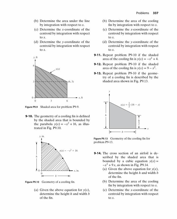
Problems 337
(b) Determine the area under the lineby integration with respect to x.
(c) Determine the x-coordinate of thecentroid by integration with respectto x.
(d) Determine the y-coordinate of thecentroid by integration with respectto x.
x, ft
y, ft
(6, 3)
y(x)6
0630
3
Figure P9.9 Shaded area for problem P9-9.
9-10. The geometry of a cooling fin is definedby the shaded area that is bounded bythe parabola y(x) = −x2 + 16, as illus-trated in Fig. P9.10.
h
y(x) = −x2 + 16
x, in.
y, in.
00
b
Figure P9.10 Geometry of a cooling fin.
(a) Given the above equation for y(x),determine the height h and width bof the fin.
(b) Determine the area of the coolingfin by integration with respect to x.
(c) Determine the x-coordinate of thecentroid by integration with respectto x.
(d) Determine the y-coordinate of thecentroid by integration with respectto x.
9-11. Repeat problem P9-10 if the shadedarea of the cooling fin is y(x) = −x2 + 4.
9-12. Repeat problem P9-10 if the shadedarea of the cooling fin is y(x) = 9 − x2.
9-13. Repeat problem P9-10 if the geome-try of a cooling fin is described by theshaded area shown in Fig. P9.13.
b
h
y
x
y(x) = (16 − x)12
h2
Figure P9.13 Geometry of the cooling fin forproblem P9-13.
9-14. The cross section of an airfoil is de-scribed by the shaded area that isbounded by a cubic equation y(x) =−x3 + 9 x, as shown in Fig. P9.14.(a) Given the above equation for y(x),
determine the height h and width bof the fin.
(b) Determine the area of the coolingfin by integration with respect to x.
(c) Determine the x-coordinate of thecentroid by integration with respectto x.
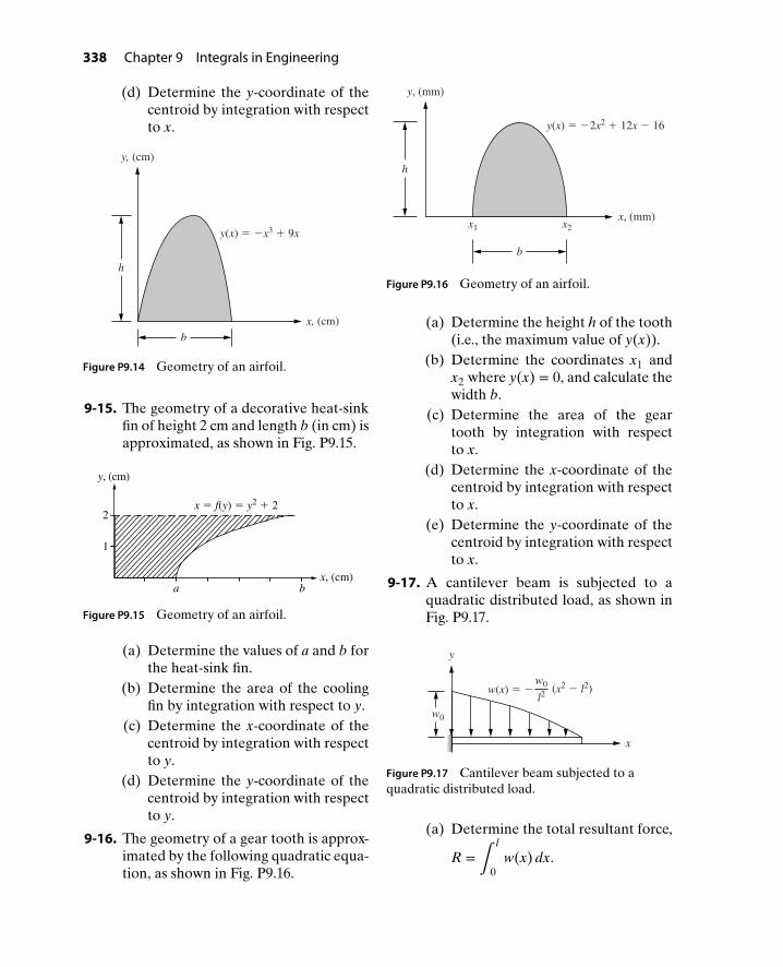
338 Chapter 9 Integrals in Engineering
(d) Determine the y-coordinate of thecentroid by integration with respectto x.
b
h
y(x) = −x3 + 9x
y, (cm)
x, (cm)
Figure P9.14 Geometry of an airfoil.
9-15. The geometry of a decorative heat-sinkfin of height 2 cm and length b (in cm) isapproximated, as shown in Fig. P9.15.
y, (cm)
x, (cm)ba
x = f(y) = y2 + 22
1
Figure P9.15 Geometry of an airfoil.
(a) Determine the values of a and b forthe heat-sink fin.
(b) Determine the area of the coolingfin by integration with respect to y.
(c) Determine the x-coordinate of thecentroid by integration with respectto y.
(d) Determine the y-coordinate of thecentroid by integration with respectto y.
9-16. The geometry of a gear tooth is approx-imated by the following quadratic equa-tion, as shown in Fig. P9.16.
y, (mm)
x, (mm)
b
x1 x2
h
y(x) = −2x2 + 12x − 16
Figure P9.16 Geometry of an airfoil.
(a) Determine the height h of the tooth(i.e., the maximum value of y(x)).
(b) Determine the coordinates x1 andx2 where y(x) = 0, and calculate thewidth b.
(c) Determine the area of the geartooth by integration with respectto x.
(d) Determine the x-coordinate of thecentroid by integration with respectto x.
(e) Determine the y-coordinate of thecentroid by integration with respectto x.
9-17. A cantilever beam is subjected to aquadratic distributed load, as shown inFig. P9.17.
x
y
w0
w0w(x) = − (x2 − l2)l2
Figure P9.17 Cantilever beam subjected to aquadratic distributed load.
(a) Determine the total resultant force,
R =∫
l
0w(x) dx.

Problems 339
(b) Determine the x-location of theresultant R; i.e., determine the cen-troid of the area under the dis-tributed load,
x =∫
l
0x w(x) dx
R.
9-18. A simply supported beam is subjectedto a quadratic distributed load, as shownin Fig. P9.18.
y
x
l
w0
w0w(x) = − x(x − 2l )l2
Figure P9.18 Simply supported beam subjectedto a quadratic distributed load.
(a) Determine the total resultant force,
R =∫
l
0w(x) dx.
(b) Determine the x-location of theresultant R; i.e., determine thecentroid of the area under thedistributed load,
x =∫
l
0x w(x) dx
R.
9-19. Determine the velocity v(t) and theposition y(t) of a vehicle that starts fromrest at position y(0) = 0 and is subjectedto the following accelerations:(a) a(t) = 40 t3 + 30 t2 + 20 t + 10 m/s2.(b) a(t) = 4 sin 2 t cos 2 t m/s2.
Hint: Use a trigonometric identity.
9-20. A particle starts from rest at aposition x(0) = 0. Find the velocity v(t)and position x(t) if the particle is sub-jected to the following accelerations:(a) a(t) = 6 t3 − 4 t2 + 7 t − 8 m/s2.(b) a(t) = 5 e−5 t + 𝜋
4cos (𝜋
4t) m/s2.
9-21. The acceleration of an automobile ismeasured as shown in Fig. P9.21. If theautomobile starts from rest at positionx(0) = 0, sketch the velocity v(t) andposition x(t) of the automobile.
x(t)
−10
10
0 2 140
16t, s
a(t), m/s2
Figure P9.21 The acceleration of an automobile.
9-22. A vehicle starting from rest at positionx(0) = 0 is subjected to the accelerationshown in Fig. P9.22.(a) Plot the velocity v(t) of the vehicle,
and clearly indicate both its maxi-mum and final values.
(b) Given your results of part (a), plotthe position x(t) of the vehicle, andclearly indicate both its maximumand final values.
9-23. A vehicle starting from rest at a positionx(0) = 0 is subjected to the accelerationshown in Fig. P9.23.(a) Plot the velocity v(t) of the vehicle,
and clearly indicate both its maxi-mum and final values.
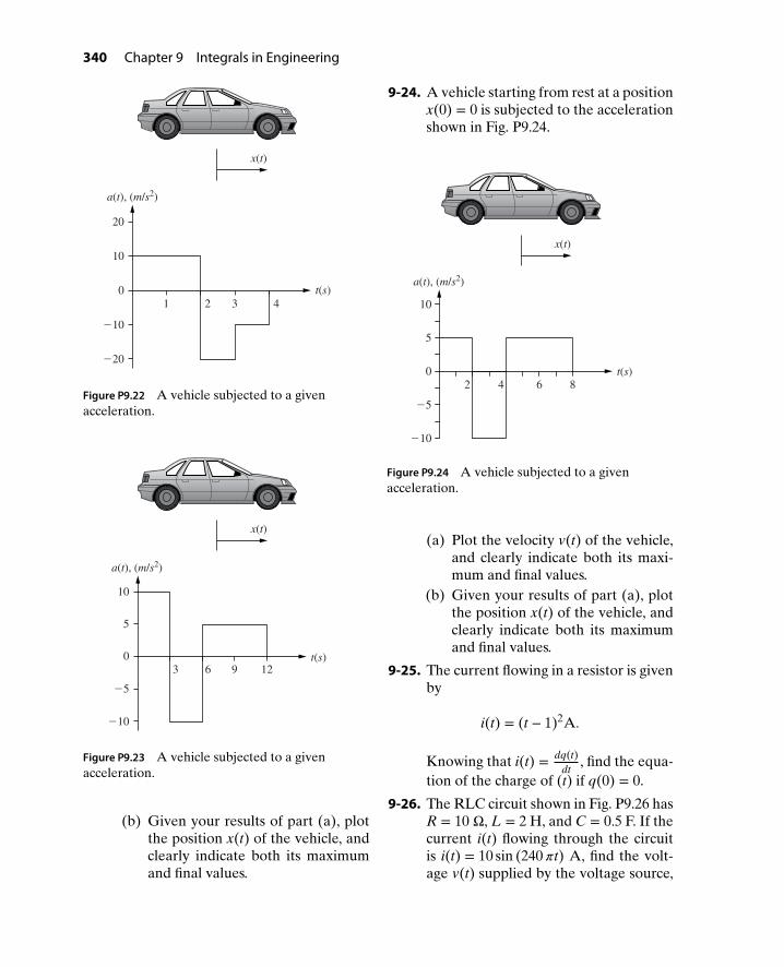
340 Chapter 9 Integrals in Engineering
x(t)
20
10
−10
t(s)41 3
−20
20
a(t), (m/s2)
Figure P9.22 A vehicle subjected to a givenacceleration.
x(t)
60
5
−5
123 9
−10
10
t(s)
a(t), (m/s2)
Figure P9.23 A vehicle subjected to a givenacceleration.
(b) Given your results of part (a), plotthe position x(t) of the vehicle, andclearly indicate both its maximumand final values.
9-24. A vehicle starting from rest at a positionx(0) = 0 is subjected to the accelerationshown in Fig. P9.24.
x(t)
40
5
−5
−10
10
82 6t(s)
a(t), (m/s2)
Figure P9.24 A vehicle subjected to a givenacceleration.
(a) Plot the velocity v(t) of the vehicle,and clearly indicate both its maxi-mum and final values.
(b) Given your results of part (a), plotthe position x(t) of the vehicle, andclearly indicate both its maximumand final values.
9-25. The current flowing in a resistor is givenby
i(t) = (t − 1)2A.
Knowing that i(t) = dq(t)dt
, find the equa-tion of the charge of (t) if q(0) = 0.
9-26. The RLC circuit shown in Fig. P9.26 hasR = 10 Ω, L = 2 H, and C = 0.5 F. If thecurrent i(t) flowing through the circuitis i(t) = 10 sin (240𝜋t) A, find the volt-age v(t) supplied by the voltage source,

Problems 341
which is given by:
v(t) = i R + Ldi(t)
dt+ 1
C ∫
t
0i(t) dt
v(t)
i(t)
R = 10 Ω
L = 2 H
C = 0.5 F
+−
Figure P9.26 A series RLC circuit.
9-27. An input voltage vin = 10 sin(10 t) V isapplied to an Op–Amp circuit as shownin Fig. P9.27.
−
+vcc
−vccvin= 10 sin (10t)
v0
−+
C = 10 F
R = 10 kΩ
+
μ
+−
Figure P9.27 An Op–Amp circuit for problemP9-27.
(a) The relationship between the inputand output of the Op–Amp is givenby
vin = −0.1dvo(t)
dt. (9.62)
Suppose that the initial output volt-age of the Op–Amp is zero. Inte-grate both sides of equation (9.62)to determine the voltage vo(t). Also,sketch the output voltage vo(t) forone cycle.
(b) Suppose that the instantaneouspower absorbed by the capacitoris p(t) = 100(1 − cos(10 t))sin (10 t)mW, and that the initial storedenergy is w(0) = 0. Knowing thatp(t) = dw(t)
dt, integrate both sides of
the equation to determine the totalstored energy w(t).
9-28. Repeat problem P9-27 if vin =10 e−10 t V.
9-29. Repeat problem P9-27 if vin = 10(1 − cos (100 t)) V.
9-30. An input voltage vin = 5 cos(20 t) V isapplied to an Op–Amp circuit as shownin Fig. P9.30. The relationship betweenthe input and output is given by
vo = −(
2 vin + 5∫
t
0vin(t)
)dt. (9.63)
Determine the voltage vo(t). Also,sketch the output voltage vo(t) for onecycle.
v0
+
−
+vcc
−vccvin= 5 cos (20t)
C = 20 F R = 20 kΩ
R = 10 kΩ
+−
−+
μ
Figure P9.30 An Op–Amp circuit for problemP9-30.
9-31. A current i(t) = 10 e−10 t mA is appliedto a 100𝜇F capacitor, as shown inFig. P9.31.(a) Suppose the initial voltage across
the capacitor is vo = 10 V. Knowingthat i(t) = C dvo(t)
dt, integrate both
sides of the equation to determine
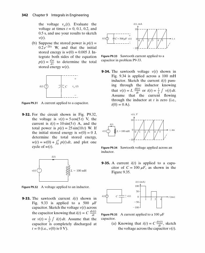
342 Chapter 9 Integrals in Engineering
the voltage vo(t). Evaluate thevoltage at times t = 0, 0.1, 0.2, and0.5 s, and use your results to sketchv(t).
(b) Suppose the stored power is p(t) =0.2 e−20 t W, and that the initialstored energy is w(0) = 0.005 J. In-tegrate both sides of the equationp(t) = d w
d tto determine the total
stored energy w(t).
−
i(t) C vo (t)↑
+
Figure P9.31 A current applied to a capacitor.
9-32. For the circuit shown in Fig. P9.32,the voltage is v(t) = 5 cos(5 t) V, thecurrent is i(t) = 10 sin(5 t) A, and thetotal power is p(t) = 25 sin(10 t) W. Ifthe initial stored energy is w(0) = 0 J,determine the total stored energy,w(t) = w(0) + ∫
t0 p(t) dt, and plot one
cycle of w(t).
L = 100 mH
i(t)
v(t) +−
Figure P9.32 A voltage applied to an inductor.
9-33. The sawtooth current i(t) shown inFig. 9.33 is applied to a 500 𝜇Fcapacitor. Sketch the voltage v(t) acrossthe capacitor knowing that i(t) = C dv(t)
dt
or v(t) = 1C∫ i(t) dt. Assume that the
capacitor is completely discharged att = 0 (i.e., v(0) is 0 V).
t, s
i(t), mA
C = 500 F
−10
10
i(t) v(t)0 1 2 3 4 50
+
−μ↑
Figure P9.33 Sawtooth current applied to acapacitor in problem P9-33.
9-34. The sawtooth voltage v(t) shown inFig. 9.34 is applied across a 100 mHinductor. Sketch the current i(t) pass-ing through the inductor knowingthat v(t) = L di(t)
dtor i(t) = 1
L∫ v(t) dt.
Assume that the current flowingthrough the inductor at t is zero (i.e.,i(0) = 0 A).
10
v(t), V
v(t)
i(t)
L =100 mH 5432100 t, ms
−10
+−
Figure P9.34 Sawtooth voltage applied across aninductor.
9-35. A current i(t) is applied to a capa-citor of C = 100 𝜇F, as shown in theFigure 9.35.
4321t (ms)
i(t) (mA)
v(t)i(t) C
50
100
0
−100
−50
+−↑
Figure P9.35 A current applied to a 100 𝜇Fcapacitor.
(a) Knowing that i(t) = C dv(t)dt
, sketchthe voltage across the capacitor v(t).
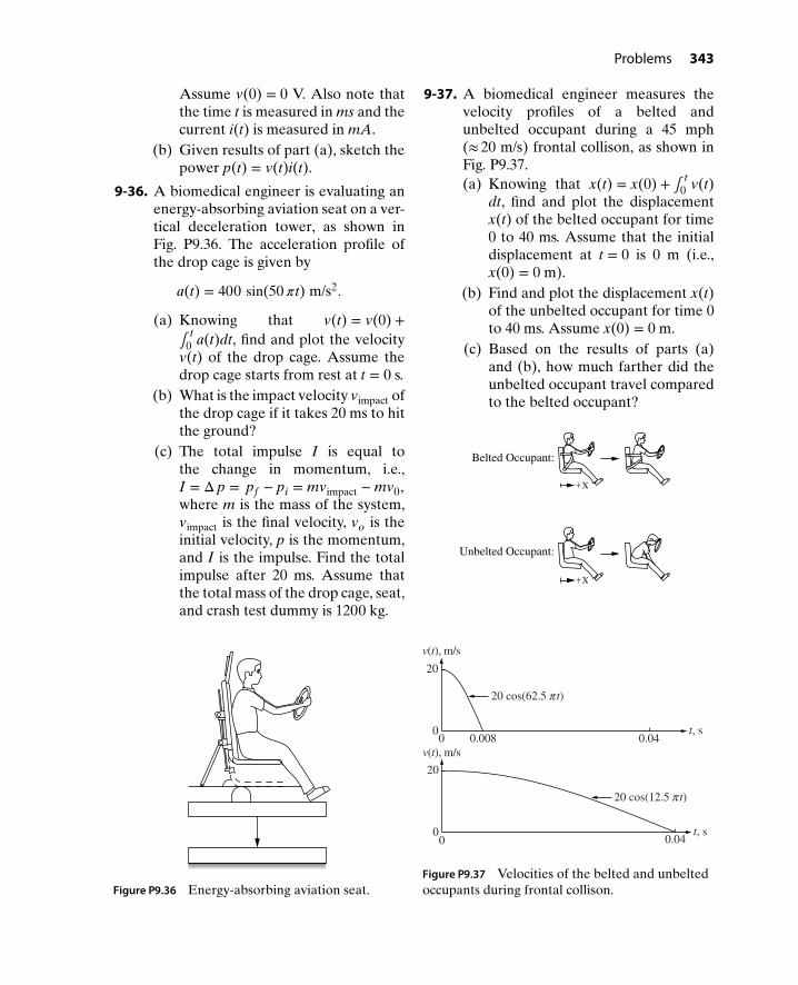
Problems 343
Assume v(0) = 0 V. Also note thatthe time t is measured in ms and thecurrent i(t) is measured in mA.
(b) Given results of part (a), sketch thepower p(t) = v(t)i(t).
9-36. A biomedical engineer is evaluating anenergy-absorbing aviation seat on a ver-tical deceleration tower, as shown inFig. P9.36. The acceleration profile ofthe drop cage is given by
a(t) = 400 sin(50𝜋t) m/s2.
(a) Knowing that v(t) = v(0) +∫
t0 a(t)dt, find and plot the velocity
v(t) of the drop cage. Assume thedrop cage starts from rest at t = 0 s.
(b) What is the impact velocity vimpact ofthe drop cage if it takes 20 ms to hitthe ground?
(c) The total impulse I is equal tothe change in momentum, i.e.,I = Δp = pf − pi = mvimpact − mv0,where m is the mass of the system,vimpact is the final velocity, vo is theinitial velocity, p is the momentum,and I is the impulse. Find the totalimpulse after 20 ms. Assume thatthe total mass of the drop cage, seat,and crash test dummy is 1200 kg.
Figure P9.36 Energy-absorbing aviation seat.
9-37. A biomedical engineer measures thevelocity profiles of a belted andunbelted occupant during a 45 mph(≈ 20 m/s) frontal collison, as shown inFig. P9.37.(a) Knowing that x(t) = x(0) + ∫
t0 v(t)
dt, find and plot the displacementx(t) of the belted occupant for time0 to 40 ms. Assume that the initialdisplacement at t = 0 is 0 m (i.e.,x(0) = 0 m).
(b) Find and plot the displacement x(t)of the unbelted occupant for time 0to 40 ms. Assume x(0) = 0 m.
(c) Based on the results of parts (a)and (b), how much farther did theunbelted occupant travel comparedto the belted occupant?
Belted Occupant:
+X
Unbelted Occupant:
+X
20 cos(62.5 t)
20 cos(12.5 t)
00
00
20
v(t), m/s
0.04
0.04
0.008t, s
t, s
v(t), m/s
20
π
π
Figure P9.37 Velocities of the belted and unbeltedoccupants during frontal collison.

344 Chapter 9 Integrals in Engineering
9-38. A civil engineer designs a buildingoverhang to withstand a triangularsnow loading per unit length p(x) =po
(1 − x
L
), as shown in Fig. P9.38.
(a) Compute the resulting force V =∫
L0 p(x)dx.
(b) Compute the correspondingmoment M = ∫
L0 x p(x)dx.
(c) Locate the position of the centroid
x =∫
Lo x p(x) dx
∫L
0 p(x) dx= M
V.
p(x)
x
V
M
po
L
V
Figure P9.38 Triangular snow loading on a buildingoverhang.
9-39. A building overhang is subjected to aparabolic snow loading p(x), as shownin Fig. P9.39. The overhang is con-structed from two metal face plateseparated by a nonmetallic core ofthickness h. This sandwich beam con-struction deforms primarily due toshear deformation with deflection y(x)satisfying
y(x) = 1h G ∫
x
0
[∫
x
0p(x) dx − V
]dx,
where V = p L3
, p(x) = p(
1 − xL
)2and
G is the shear modulus.(a) Show that the deflection of the
sandwich beam is given by
y(x)= −p xh G
L3− x
[12− x
3 L
(1 − x
4 L
)].
(b) Find the location and value of maxi-mum deflection y(x).
p
p(x)
x
V
M
L
V
(a) Cantilever overhang.
Core
h
Upper face plate
Lower face plate
(b) Sandwich construction.
Figure P9.39 Parabolic snow loading ofsandwich-constructed building overhang.
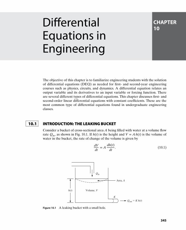
CHAPTER10
DifferentialEquations inEngineering
The objective of this chapter is to familiarize engineering students with the solutionof differential equations (DEQ) as needed for first- and second-year engineeringcourses such as physics, circuits, and dynamics. A differential equation relates anoutput variable and its derivatives to an input variable or forcing function. Thereare several different types of differential equations. This chapter discusses first- andsecond-order linear differential equations with constant coefficients. These are themost common type of differential equations found in undergraduate engineeringclasses.
10.1 INTRODUCTION: THE LEAKING BUCKETConsider a bucket of cross-sectional area A being filled with water at a volume flowrate Qin, as shown in Fig. 10.1. If h(t) is the height and V = A h(t) is the volume ofwater in the bucket, the rate of change of the volume is given by
dVdt
= Adh(t)
dt. (10.1)
Volume, V
Area, A
h(t)
Qin
Qout = K h(t)K
Figure 10.1 A leaking bucket with a small hole.
345
346 Chapter 10 Differential Equations in Engineering
Suppose the bucket has a small hole on the side through which water is leakingat a rate
Qout = K h(t) (10.2)
where K is a constant. In reality, Qout is not a linear function of h(t), but it isassumed here for simplicity. The constant K is an engineering design parameterthat depends on the size and shape of the hole, as well as the properties of thefluid. By conservation of volume, the volume of water in the bucket is given by
dVdt
= Qin − Qout. (10.3)
Substituting equations (10.1) and (10.2) into equation (10.3) gives
Adh(t)
dt= Qin − K h(t)
or
Adh(t)
dt+ K h(t) = Qin. (10.4)
Equation (10.4) is a first-order linear differential equation with constant coefficients.The objective is to solve the differential equation; in other words, determine theheight h(t) of the water when an input Qin and the initial condition h(0) are given.Before presenting the solution of this equation, a general discussion of differentialequations and the solution of linear differential equations with constant coefficientsis given.
10.2 DIFFERENTIAL EQUATIONSAn nth order linear differential equation relating an output variable y(t) and itsderivatives to some input function f (t) can be written as
Andny(t)
dtn + An−1dn−1y(t)
dtn−1+…+ A1
dy(t)dt
+ A0 y(t) = f (t) (10.5)
where the coefficients An, An−1,…, A0 can be constants, functions of y, or functionof t. The input function f (t) (also called the forcing function) represents everythingon the right-hand side of the differential equation. The solution of the differentialequation is the output variable, y(t).
For a second-order system involving position y(t), velocity dy(t)dt
, and accelerationd2y(t)
dt2, equation (10.5) takes the form
A2d2y(t)
dt2+ A1
dy(t)dt
+ A0 y(t) = f (t). (10.6)
Note that engineers often use a dot notation when referring to derivatives with
respect to time, for example, y(t) = dy(t)dt
, y(t) = d2y(t)dt2
, and so on. In this case, equation

10.3 Solution of Linear DEQ with Constant Coefficients 347
(10.6) can be written as
A2 y(t) + A1 y(t) + A0 y(t) = f (t). (10.7)
In many engineering applications, the coefficients An, An−1,…, A0 are constants (notfunctions of y or t). In this case, the differential equation given by equation (10.5) isknown as a linear differential equation with constant coefficients. For example, inthe case of a spring-mass system subjected to an applied force f (t), equation (10.8)is a second-order differential equation given by
m y(t) + k y(t) = f (t) (10.8)
where m is the mass and k is the spring constant. If the coefficients An, An−1,…, A0are functions of y or t, exact solutions can be difficult to obtain. In many cases, exactsolutions do not exist, and the solution y(t) must be obtained numerically (e.g., usingthe differential equation solvers in MATLAB). However, in the case of constantcoefficients, the solution y(t) can be obtained by following the step-by-step procedureoutlined below.
10.3 SOLUTION OF LINEAR DEQ WITHCONSTANT COEFFICIENTSIn general, the total solution for the output variable y(t) is the sum of two solutions:the transient solution and the steady-state solution.
1. Transient Solution, ytran(t) (also called the Homogeneous or ComplementarySolution): The transient solution is obtained using the following steps:
a. Set the forcing function f (t) = 0. This makes the right-hand side of equation(10.5) zero, i.e.,
Andny(t)
dtn + An−1dn−1y(t)
dtn−1+…+ A1
dy(t)dt
+ A0 y(t) = 0. (10.9)
b. Assume a transient solution of the form y(t) = cest, and substitute it into (10.9).
Note that dy(t)dt
= csest, d2y(t)dt2
= cs2 est, and so on, so that each term will containcest. Since the right-hand side of equation (10.9) is zero, canceling the cest willresult in a polynomial in s:
An sn + An−1 sn−1 +⋯ + A1 s + A0 = 0. (10.10)
c. Solve for the roots of the above equation, which is known as the characteristicequation. The roots are the n values of s that make the characteristic equationequal to zero. Call these values s1, s2,…, sn.
d. For the case of n distinct roots, the transient solution of the differential equa-tion has the general form
ytran(t) = c1 es1 t + c2 es2 t +…+ cn esn t
where the constants c1, c2, …, cn are determined later from the initial condi-tions of the system.
e. For the special case of repeated roots (i.e., two of the roots are the same), thesolution can be made general by multiplying one of the roots by t. For example,
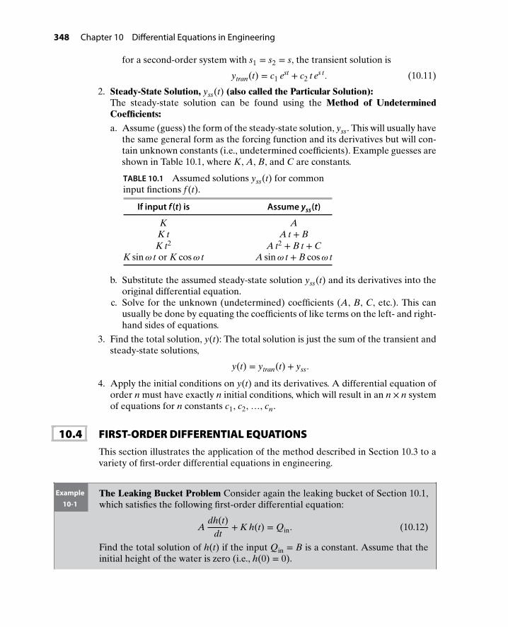
348 Chapter 10 Differential Equations in Engineering
for a second-order system with s1 = s2 = s, the transient solution is
ytran(t) = c1 est + c2 t es t. (10.11)
2. Steady-State Solution, yss(t) (also called the Particular Solution):The steady-state solution can be found using the Method of UndeterminedCoefficients:
a. Assume (guess) the form of the steady-state solution, yss. This will usually havethe same general form as the forcing function and its derivatives but will con-tain unknown constants (i.e., undetermined coefficients). Example guesses areshown in Table 10.1, where K, A, B, and C are constants.
TABLE 10.1 Assumed solutions yss(t) for commoninput finctions f (t).
If input f (t) is Assume yss(t)
K AK t A t + BK t2 A t2 + B t + C
K sin𝜔 t or K cos𝜔 t A sin𝜔 t + B cos𝜔 t
b. Substitute the assumed steady-state solution yss(t) and its derivatives into theoriginal differential equation.
c. Solve for the unknown (undetermined) coefficients (A, B, C, etc.). This canusually be done by equating the coefficients of like terms on the left- and right-hand sides of equations.
3. Find the total solution, y(t): The total solution is just the sum of the transient andsteady-state solutions,
y(t) = ytran(t) + yss.
4. Apply the initial conditions on y(t) and its derivatives. A differential equation oforder n must have exactly n initial conditions, which will result in an n × n systemof equations for n constants c1, c2, …, cn.
10.4 FIRST-ORDER DIFFERENTIAL EQUATIONSThis section illustrates the application of the method described in Section 10.3 to avariety of first-order differential equations in engineering.
Example10-1
The Leaking Bucket Problem Consider again the leaking bucket of Section 10.1,which satisfies the following first-order differential equation:
Adh(t)
dt+ K h(t) = Qin. (10.12)
Find the total solution of h(t) if the input Qin = B is a constant. Assume that theinitial height of the water is zero (i.e., h(0) = 0).
10.4 First-Order Differential Equations 349
Solution (a) Transient (Complementary or Homogeneous) Solution: Since the transientsolution is the zero-input solution, the input on the right-hand side (RHS) ofequation (10.12) is set to zero. Thus, the homogeneous differential equation ofthe leaking bucket is given by
Adh(t)
dt+ Kh(t) = 0. (10.13)
Assume that the transient solution of the height htran(t) is of the form given byequation (10.14):
htran(t) = cest. (10.14)
The constant s is determined by substituting htran(t) and its derivative into thehomogeneous differential equation (10.13). The derivative of htran(t) is givenby
dhtran(t)dt
= ddt
(cest)
= csest. (10.15)
Substituting equations (10.14) and (10.15) in equation (10.13) yields
A(csest) + K(cest) = 0.
Factoring out cest gives
cest(As + K) = 0
Since cest ≠ 0, it follows that
A s + K = 0. (10.16)
Equation (10.16) is the characteristic equation for the leaking bucket. Solvingequation (10.16) for s gives
s = −KA. (10.17)
Substituting the above value of s into equation (10.14), the transient solutionfor the leaking bucket is given by
htran(t) = ce−KA
t (10.18)
The constant c depends on the initial height of the water and cannot be deter-mined until the initial condition is applied to the total solution in part (d).
(b) Steady-State (Particular) Solution: The steady-state solution of a differentialequation is the solution to a particular input. Since the given input is Qin = B,the differential equation (10.12) can be written as
Adh(t)
dt+ Kh(t) = B. (10.19)
According to the method of undetermined coefficients (Table 10.1), the steady-state solution will have the same general form as the input and its derivatives.
350 Chapter 10 Differential Equations in Engineering
Since the input in this example is constant, the steady-state solution is assumedconstant to be
hss(t) = E, (10.20)
where E is a constant. The value of E can be determined by substituting hss(t)and its derivative into equation (10.19). The derivative of hss(t) is
dhss(t)dt
= ddt
(E)
= 0. (10.21)
Substituting equations (10.20) and (10.21) into equation (10.19) gives
A(0) + KE = B.
Solving for E gives
E = BK.
Therefore, the steady-state solution of the leaking bucket subjected to a con-stant input Qin = B is given by
hss(t) = BK. (10.22)
(c) Total Solution: The total solution for h(t) is obtained by adding the transientand the steady-state solutions as
h(t) = c e−KA
t + BK. (10.23)
(d) Initial Conditions: The constant c can now be obtained by substituting theinitial condition h(0) = 0 into equation (10.23) as
h(0) = c e−KA
(0) + BK
= 0
or
c (1) + BK
= 0,
which gives
c = −BK. (10.24)
Substituting the above value of c into equation (10.23) yields
h(t) = −BK
e−KA
t + BK
or
h(t) = BK
(1 − e−
KA
t). (10.25)

10.4 First-Order Differential Equations 351
Note that as t → ∞, h(t) → BK
; in other words, the total solution reaches thesteady-state solution. Thus, at steady state the height h(t) reaches a constantvalue of B
K. Physically speaking, the bucket continues to fill until the pressure
is great enough that Qout = Qin (i.e., dh(t)dt
= 0). That value depends only onBK
= QinK
. At time t = AK
sec, the bucket fills to a height of
h(
AK
)= B
K
(1 − e
−KA
(AK
))
= BK
(1 − e−1)
= BK
(1 − 0.368)
or
h(
AK
)= 0.632 B
K.
At time t = 5 A∕K s, the bucket fills to a height of
h(
5 AK
)= B
K
(1 − e
−KA
(5AK
))
= BK
(1 − e−5)
= BK
(1 − 0.0067)
or
h(
5 AK
)= 0.9933 B
K.
Thus, it takes t = A∕K s for the height to reach 63.2% of the steady-state valueand t = 5A∕K s to reach 99.33% of the steady-state value. The time t = A∕Ks is known as the time constant of the response and is usually denoted by theGreek letter 𝜏. The response of a first-order system (for example, the leakingbucket) can generally be written as
y(t) = steady-state solution(
1 − e−t𝜏
). (10.26)
The plot of the height h(t) for input Qin = B is shown in Fig. 10.2. It can be seenfrom this figure that after t = 5𝜏 s, the water level has, for all practical purposes,reached its steady-state value.

352 Chapter 10 Differential Equations in Engineering
t, s50
0
0.632
BK
h(t)
BK
AK
AK
Figure 10.2 Solution for h(t) for Qin = B and h(0) = 0.
Example10-2
Leaking Bucket with No Input Suppose now that Qin = 0, and that the initial heightof the water is h0 (Fig. 10.3). The height h(t) of the water is governed by the first-order differential equation
Adh(t)
dt+ Kh(t) = 0. (10.27)
Determine the total solution for h(t). Also, find the time it takes for the water tocompletely leak out of the bucket.
K
Volume, V
Qin = 0
Area, A
Qout = K h(t)
h(0) = h0
Figure 10.3 Leaking bucket with no input for Example 10-2.
10.4 First-Order Differential Equations 353
Solution (a) Transient Solution: The transient solution is identical to that of the previousexample and is given by
htran(t) = c1 e−KA
t.
(b) Steady-State Solution: Since the RHS of the differential equation (10.27) iszero (i.e., the input is zero), the steady-state solution is also zero:
hss(t) = 0.
(c) Total Solution: The total solution for the height h(t) is given by
h(t) = htran(t) + hss(t)
= c1 e−KA
t + 0
or
h(t) = c1 e−KA
t. (10.28)
(d) Initial Conditions: The constant c1 is determined by substituting the initialheight h(0) = h0 into equation (10.28) as
h(0) = c1 e−KA
(0) = h0
or
c1 (1) = h0,
which gives
c1 = h0.
Thus, the total solution for h(t) is
h(t) = h0 e−KA
t. (10.29)
The height h(t) given in equation (10.29) is a decaying exponential functionwith time constant 𝜏 = A∕K. At time t = A∕K s, the bucket empties to a heightof
h(
AK
)= h0 e
−KA
(AK
)
= h0 e−1
or
h(
AK
)= 0.368 h0.
At time t = 5AK
s, the bucket empties to a height of
h(
5 AK
)= h0 e
−KA
(5 AK
)
= h0 e−5
= 0.0067 h0

354 Chapter 10 Differential Equations in Engineering
or
h(
5 AK
)≈ 0.
The plot of the height is shown in Fig. 10.4. It can be seen from this figure thatthe height starts from the initial value h0 and decays to 36.8% of the initialvalue in one time constant 𝜏 = A∕K, and is approximately zero after five timeconstants.
h0
0.368 h0
00
h(t)
t, sec5A
KAK
Figure 10.4 Solution for h(t) with Qin = 0 and h(0) = h0.
Example10-3
Voltage Applied to an RC Circuit Find the voltage v(t) across the capacitor if aconstant voltage source vs(t) = vs is applied to the RC circuit shown in Fig. 10.5.Assume that the capacitor is initially completely discharged (i.e., v(0) = 0).
C
vR(t)
v(t)
R
−
+
+
−
i(t)
vs(t)+−
Figure 10.5 RC circuit with constant input for Example 10-3.
10.4 First-Order Differential Equations 355
The governing equation for v(t) follows from Kirchhoff’s voltage law (KVL), whichgives
vR(t) + v(t) = vs(t). (10.30)
From Ohm’s law, the voltage across the resistor is given by vR(t) = Ri(t). Sincethe resistor and capacitor are connected in series, the same current flows throughthe resistor and capacitor, i(t) = C dv(t)
dt. Therefore, vR(t) = RC dv(t)
dt, and equation
(10.30) can be written as
RCdv(t)
dt+ v(t) = vs(t). (10.31)
Equation (10.31) is a first-order differential equation with constant coefficients.This equation can also be written as
RCv(t) + v(t) = vs(t), (10.32)
where v(t) = dv(t)dt
. The goal is to solve the voltage v(t) if vs(t) = vs is constant andv(0) = 0.
Solution (a) Transient Solution: The transient solution is obtained by setting the right-hand side of the differential equation equal to zero as
RCv(t) + v(t) = 0, (10.33)
and assuming a solution of the form
vtran(t) = cest. (10.34)
The constant s is determined by substituting vtran(t) and its derivative intoequation (10.33). The derivative of vtran(t) is given by
dvtran(t)dt
= ddt
(cest) = csest. (10.35)
Substituting equations (10.34) and (10.35) in equation (10.33) yields
RC(csest) + (cest) = 0.
Factoring out cest gives
est(RCs + 1) = 0.
It follows that
RCs + 1 = 0, (10.36)
which gives
s = − 1RC
. (10.37)
Substituting the above value of s into equation (10.34) gives
vtran(t) = ce−1
RCt (10.38)

356 Chapter 10 Differential Equations in Engineering
The constant c depends on the initial voltage across the capacitor, which isapplied to the total solution in part (d).
(b) Steady-State Solution: For vs(t) = vs,
RC v(t) + v(t) = vs. (10.39)
Since the input to the RC circuit is constant, the steady-state solution of theoutput voltage v(t) is assumed to be
vss(t) = E, (10.40)
where E is a constant. The value of E can be determined by substituting vss(t)and its derivative in equation (10.39), which gives
RC(0) + E = vs.
Solving for E yields
E = vs.
Thus, the steady-state solution for the output voltage is
vss(t) = vs. (10.41)
(c) Total Solution: The total solution for v(t) is obtained by adding the transientand the steady-state solutions given by equations (10.38) and (10.41) as
v(t) = ce−1
RCt + vs. (10.42)
(d) Initial Conditions: The constant c can now be obtained by applying the initialcondition as
v(0) = ce−1
RC(0) + vs = 0
or
c (1) + vs = 0.
Solving for c gives
c = −vs. (10.43)
Substituting the above value of c into equation (10.42) yields
v(t) = −vs e−1
RCt + vs
or
v(t) = vs
(1 − e−
1RC
t). (10.44)
Note that as t → ∞, v(t) → vs (i.e., the total solution reaches the steady-statesolution). At steady state, the capacitor is fully charged to a voltage equal to the

10.4 First-Order Differential Equations 357
input voltage. While the capacitor is charging, the voltage across the capacitorat time t = RC s is given by
v(RC) = vs
(1 − e−
1RC
(RC))
= vs (1 − e−1)
= vs (1 − 0.368)
or
v = 0.632 vs.
Also, at time t = 5 RC s, the voltage across the capacitor is given by
v(5 RC) = vs
(1 − e−
1RC
(5 RC))
= vs (1 − e−5)
= vs (1 − 0.0067)
= 0.9933 vs
or
v ≈ vs.
Thus, it takes t = RC s for the voltage to reach 63.2% of the input voltageand at t = 5 RC s, the voltage reaches 99.33% of the input value. The timet = 𝜏 = RC s is the time constant of the RC circuit, which is a measure ofthe time required for the capacitor to fully charge. Typically, to reduce thecharge time of the capacitor, the resistance value of the resistor is reduced.The plot of the voltage v(t) is shown in Fig. 10.6. It can be seen from this figurethat it takes the response approximately 5𝜏 to reach the steady state, which isidentical to the result obtained for the leaking bucket with constant Qin.
RC 5RC
vs
0.632 vs
v(t), V
00
t, s
Figure 10.6 The voltage across the capacitor to a constant voltage in an RC circuitof Example 10-3.

358 Chapter 10 Differential Equations in Engineering
Example10-4
For the circuit shown in Fig. 10.7, the differential equation relating the output v(t)and input vs(t) is given by
0.5 v(t) + v(t) = vs(t). (10.45)
Find the output voltage v(t) across the capacitor if the input voltage vs(t) = 10 V.Assume that the initial voltage across the capacitor is zero (i.e., v(0) = 0).
vR(t)
v(t)
i(t)
vs(t)
R = 5 kΩ
C = 100 F
+
+
−
−
+− μ
Figure 10.7 RC circuit with input voltage vs(t).
Solution (a) Transient Solution: The transient solution is obtained by setting the right-hand side of the differential equation to zero as
0.5 v(t) + v(t) = 0, (10.46)
and assuming a solution of the form
vtran(t) = cest. (10.47)
Substituting the transient solution and its derivative into equation (10.46) andsolving for s gives
0.5(csest) + (cest) = 0
cest(0.5 s + 1) = 0
0.5 s + 1 = 0
s = −2.
Thus, the transient solution of the output voltage is given by
vtran(t) = ce−2 t (10.48)
where c will be obtained from the initial condition.
(b) Steady-State Solution: Since the input applied to the RC circuit is 10 V,equation (10.45) can be written as
0.5 v(t) + v(t) = 10. (10.49)
Since the input is constant, the steady-state solution of the output voltage v(t)is assumed to be
vss(t) = E, (10.50)

10.4 First-Order Differential Equations 359
where E is a constant. The value of E can be determined by substituting vss(t)and its derivative into equation (10.49) as
0.5 (0) + E = 10
which gives
E = 10 V.
Thus, the steady-state solution of the output voltage is given by
vss(t) = 10 V. (10.51)
(c) Total Solution: The total solution for v(t) is obtained by adding the transientand steady-state solutions given by equations (10.48) and (10.51) as
v(t) = ce−2 t + 10. (10.52)
(d) Initial Conditions: The constant c can now be obtained by applying the initialcondition (v(0) = 0) as
v(0) = ce−2 (0) + 10 = 0
or
c (1) + 10 = 0.
Solving for c gives
c = −10 V. (10.53)
Substituting the value of c from equation (10.53) into equation (10.52) yields
v(t) = −10 e−2 t + 10
or
v(t) = 10 (1 − e−2 t) V. (10.54)
Since the time constant is 𝜏 = 1∕2 = 0.5 s, it takes the capacitor 0.5 s to reach63.2% of the input voltage and approximately 5(0.5) = 2.5 s to fully charge toapproximately 10 V. The plot of the output voltage v(t) is shown in Fig. 10.8.

360 Chapter 10 Differential Equations in Engineering
0.5 2.5
6.32
v(t), V
00
t, s
10
Figure 10.8 The voltage across the capacitor in Example 10-4.
Example10-5
The differential equation for the capacitive circuit shown in Fig. 10.9 is given by
0.5 v(t) + v(t) = 0. (10.55)
Find the output voltage v(t) across the capacitor C as it discharges from an initialvoltage of v(0) = 10 V.
vR(t)
v(t)
−
+
−
i(t)
R = 5 kΩ
C = 100 F
v(0) = 10 V
+
μ
Figure 10.9 Discharging of a capacitor in an RC circuit.
Solution (a) Transient Solution: Since the left-hand side of the governing equation is thesame as that for the previous example, the transient solution of the outputvoltage is given by equation (10.48) as
vtran(t) = ce−2 t.

10.4 First-Order Differential Equations 361
(b) Steady-State Solution: Since there is no input applied to the circuit, the steady-state value of the output voltage is zero:
vss(t) = 0.
(c) Total Solution: The total solution for v(t) is obtained by the adding the tran-sient and the steady-state solutions, which gives
v(t) = ce−2 t.
(d) Initial Conditions: The constant c can now be obtained by applying the initialcondition (v(0) = 10 V) as
v(0) = ce−2 (0) = 10,
which gives
c = 10 V.
Thus, the output voltage is given by
v(t) = 10 e−2 t V.
While the capacitor is discharging, the voltage across the capacitor at time t =0.5 s (one time constant) is given by
v(0.5) = 10 e−2 (0.5)
= 10 e−1
or
v = 3.68 V.
Also, at time t = 2.5 s (five time constants), the voltage across the capacitor isgiven by
v(2.5) = 10 e−2 (2.5)
= 10 e−5
= 0.067
or
v ≈ 0.
The plot of the output voltage, v(t) is shown in Fig. 10.10. Mathematicallyspeaking, the response of a capacitor discharging in an RC circuit is identicalto the response of a leaking bucket with initial fluid height h0!

362 Chapter 10 Differential Equations in Engineering
00 0.5 2.5
t, sec
v(t), V
10
3.68
Figure 10.10 The voltage across the capacitor in Example 10-5.
Example10-6
Consider a voltage vs(t) applied to an RL circuit, as shown in Fig. 10.11. ApplyingKVL yields
R
LvL(t)
i(t)vR(t)
vs(t)
+ −+
−
+−
Figure 10.11 Voltage applied to an RL circuit.
vR(t) + vL(t) = vs(t), (10.56)
where vR(t) = R i(t) is the voltage across the resistor and vL(t) = Ldi(t)
dtis the
voltage across the inductor. Thus, equation (10.56) can be written in terms of thecurrent i(t) as
Ldi(t)
dt+ R i(t) = vs(t). (10.57)
If the applied voltage source is vs(t) = vs = constant, find the total solution for thecurrent i(t). Assume the initial current is zero (i(0) = 0).
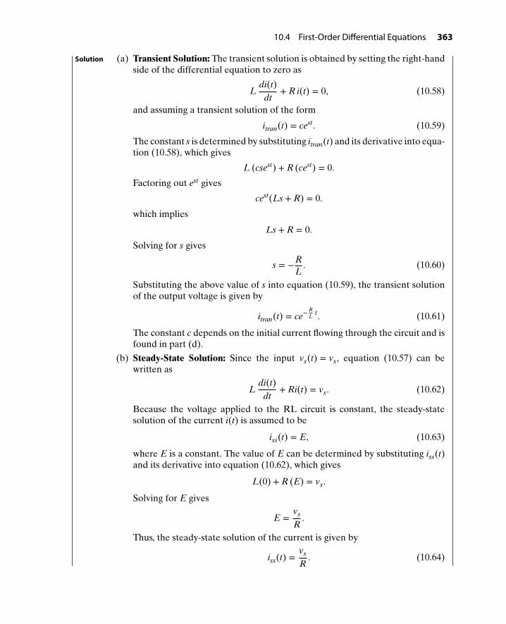
10.4 First-Order Differential Equations 363
Solution (a) Transient Solution: The transient solution is obtained by setting the right-handside of the differential equation to zero as
Ldi(t)
dt+ R i(t) = 0, (10.58)
and assuming a transient solution of the form
itran(t) = cest. (10.59)
The constant s is determined by substituting itran(t) and its derivative into equa-tion (10.58), which gives
L (csest) + R (cest) = 0.
Factoring out est gives
cest(Ls + R) = 0.
which implies
Ls + R = 0.
Solving for s gives
s = −RL. (10.60)
Substituting the above value of s into equation (10.59), the transient solutionof the output voltage is given by
itran(t) = ce−RL
t. (10.61)
The constant c depends on the initial current flowing through the circuit and isfound in part (d).
(b) Steady-State Solution: Since the input vs(t) = vs, equation (10.57) can bewritten as
Ldi(t)
dt+ Ri(t) = vs. (10.62)
Because the voltage applied to the RL circuit is constant, the steady-statesolution of the current i(t) is assumed to be
iss(t) = E, (10.63)
where E is a constant. The value of E can be determined by substituting iss(t)and its derivative into equation (10.62), which gives
L(0) + R (E) = vs.
Solving for E gives
E =vs
R.
Thus, the steady-state solution of the current is given by
iss(t) =vs
R. (10.64)

364 Chapter 10 Differential Equations in Engineering
(c) Total Solution: The total solution for the current i(t) is obtained by adding thetransient and the steady-state solutions given by equations (10.61) and (10.64)as
i(t) = ce−RL
t +vs
R. (10.65)
(d) Initial Conditions: The constant c can now be obtained by applying the initialcondition (i(0) = 0) to equation (10.65) as
i(0) = ce−RL
(0) +vs
R= 0.
or
c (1) +vs
R= 0
Solving for c gives
c = −vs
R. (10.66)
Substituting the above value of c into equation (10.65) gives
i(t) = −vs
Re−
RL
t +vs
Ror
i(t) =vs
R(1 − e−
RL
t) A. (10.67)
As t → ∞, i(t) → vs∕R (i.e., the steady-state solution). It takes the currentt = 𝜏 = L∕R s to reach 63.2% of its steady-state value vs∕R. The plot of the cur-rent i(t) is shown in Fig. 10.12. It can be seen that the current i(t) takes approx-imately 5𝜏 to reach the steady-state value, as obtained for both the charging ofa capacitor and the filling of a leaking bucket.
t, s50
0
0.632
vs
R
i(t), A
vs
R
LR
LR
Figure 10.12 The current flowing through an RL circuit.

10.4 First-Order Differential Equations 365
Example10-7
A constant voltage vs(t) = 10 V is applied to the RL circuit shown in Fig. 10.13.The circuit is described by the following differential equation:
0.1di(t)
dt+ 100 i(t) = 10. (10.68)
Find the current i(t) if the initial current is 50 mA (i.e., i(0) = 50 × 10−3).
R = 100 Ω
L = 100 mH
i(t)
vs(t)= 10 V
+−
Figure 10.13 RL circuit for Example 10-7.
Solution (a) Transient Solution: The transient solution is obtained by setting the right-hand side of the differential equation to zero as
0.1di(t)
dt+ 100 i(t) = 0, (10.69)
and assuming a solution of the form
itran(t) = cest. (10.70)
The constant s is determined by substituting itran(t) and its derivative into equa-tion (10.69) and solving for s as
0.1 (csest) + 100 (cest) = 0
cest(0.1s + 100) = 0
0.1s + 100 = 0
s = −1000. (10.71)
Substituting the value of s into equation (10.70), the transient solution of thecurrent is given by
itran(t) = ce−1000 t. (10.72)
The constant c depends on the initial current flowing through the circuit andwill be obtained by applying the initial condition to the total solution inpart (d).
(b) Steady-State Solution: Because the voltage applied to the RL circuit is con-stant (the right-hand side of equation (10.68) is constant), the steady-statesolution is assumed to be
iss(t) = E, (10.73)

366 Chapter 10 Differential Equations in Engineering
where E is a constant. The value of E can be determined by substituting iss(t)and its derivative into equation (10.68), which gives
0.1(0) + 100 (E) = 10.
Solving for E gives
E = 0.1 A.
Thus, the steady-state solution for the current is given by
iss(t) = 0.1 A. (10.74)
(c) Total Solution: The total solution is obtained by adding the transient and thesteady-state solutions given by equations (10.72) and (10.74) as
i(t) = ce−1000 t + 0.1 A. (10.75)
(d) Initial Conditions: The constant c can now be obtained by applying the initialcondition i(0) = 50 mA into equation (10.75) as
i(0) = ce−1000 (0) + 0.1 = 0.05
or
c (1) + 0.1 = 0.05.
Solving for c gives
c = −0.05. (10.76)
Substituting the value of c into equation (10.75) gives
i(t) = −0.05 e−1000 t + 0.1
or
i(t) = 0.1(
1 − 0.5 e−1000 t)
A. (10.77)
Note that as t → ∞, i(t) → 0.1 = 100 mA (i.e., the current reaches itssteady-state solution). It takes the current t = 𝜏 = 1∕1000 = 1 ms to reach0.1(1 − 0.5 × 0.368) = 0.0816 A or 81.6 mA. The value of the current at t = 𝜏 canalso be found from the expression: Initial value + 0.632× (Steady-state value −Initial value) or 50 + 0.632 × (100 − 50) = 81.6 mA. The plot of the currenti(t) is shown in Fig. 10.14. It can be seen from this figure that the current i(t)takes approximately 5𝜏 = 5 ms to reach the final value.
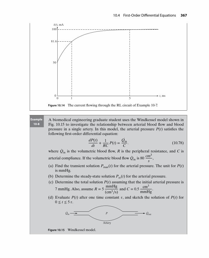
10.4 First-Order Differential Equations 367
51t, ms
i(t), mA
100
81.6
50
00
Figure 10.14 The current flowing through the RL circuit of Example 10-7.
Example10-8
A biomedical engineering graduate student uses the Windkessel model shown inFig. 10.15 to investigate the relationship between arterial blood flow and bloodpressure in a single artery. In this model, the arterial pressure P(t) satisfies thefollowing first-order differential equation:
dP(t)dt
+ 1RC
P(t) =Qin
C. (10.78)
where Qin is the volumetric blood flow, R is the peripheral resistance, and C is
arterial compliance. If the volumetric blood flow Qin is 80 cm3
s,
(a) Find the transient solution Ptran(t) for the arterial pressure. The unit for P(t)is mmHg.
(b) Determine the steady-state solution Pss(t) for the arterial pressure.
(c) Determine the total solution P(t) assuming that the initial arterial pressure is
7 mmHg. Also, assume R = 5mmHg
(cm3∕s)and C = 0.5 cm3
mmHg.
(d) Evaluate P(t) after one time constant 𝜏, and sketch the solution of P(t) for0 ≤ t ≤ 5 𝜏.
P
Artery
Qin Qout
Figure 10.15 Windkessel model.
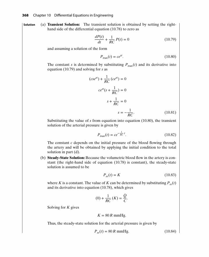
368 Chapter 10 Differential Equations in Engineering
Solution (a) Transient Solution: The transient solution is obtained by setting the right-hand side of the differential equation (10.78) to zero as
dP(t)dt
+ 1RC
P(t) = 0 (10.79)
and assuming a solution of the form
Ptran(t) = cest. (10.80)
The constant s is determined by substituting Ptran(t) and its derivative intoequation (10.79) and solving for s as
(csest) + 1RC
(cest) = 0
cest(s + 1RC
) = 0
s + 1RC
= 0
s = − 1RC
. (10.81)
Substituting the value of s from equation into equation (10.80), the transientsolution of the arterial pressure is given by
Ptran(t) = ce−1
RCt. (10.82)
The constant c depends on the initial pressure of the blood flowing throughthe artery and will be obtained by applying the initial condition to the totalsolution in part (d).
(b) Steady-State Solution: Because the volumetric blood flow in the artery is con-stant (the right-hand side of equation (10.78) is constant), the steady-statesolution is assumed to be
Pss(t) = K (10.83)
where K is a constant. The value of K can be determined by substituting Pss(t)and its derivative into equation (10.78), which gives
(0) + 1RC
(K) = QC.
Solving for K gives
K = 80 R mmHg.
Thus, the steady-state solution for the arterial pressure is given by
Pss(t) = 80 R mmHg. (10.84)

10.4 First-Order Differential Equations 369
(c) Total Solution: The total solution is obtained by adding the transient and thesteady-state solutions given by equations (10.82) and (10.84) as
P(t) = ce−1
RCt + 80 R mmHg. (10.85)
(d) Initial Conditions: The constant c can now be obtained by applying the initialcondition P(0) = 7 mmHg into equation (10.85) as
P(0) = ce−1
RC(0) + 80 R = 7.
Substituting R = 5 and C = 0.5 gives
c (1) + 400 = 7.
Solving for c gives
c = −393. (10.86)
Substituting the value of c into equation (10.85) gives
P(t) = −393 e−0.4 t + 400
or
P(t) = 400(1 − 0.9825 e−0.4 t) mmHg. (10.87)
Note that as t → ∞, P(t) → 400 mmHg (i.e., the pressure reaches itssteady-state solution). It takes the pressure t = 𝜏 = 1∕0.4 = 2.5 s to reach400(1 − 0.9825(0.368)) = 255.4 mmHg. The value of the pressure at t = 𝜏 canalso be found from the expression: Initial value + 0.632× (Steady-state value −Initial value) or 7 + 0.632 × (400 − 7) = 255.4 mmHg. The plot of the currentP(t) is shown in Fig. 10.16. It can be seen from this figure that it takes the pres-sure P(t) approximately 5𝜏 = 12.5 s to reach its final value.
t, s
P(t), mmHg
400
255.4
00 2.5 5 7.5 10 12.5
Figure 10.16 The blood pressure in a single artery.

370 Chapter 10 Differential Equations in Engineering
Example10-9
The differential equation for the RC circuit of Fig. 10.5 is given by
RCdv(t)
dt+ v(t) = vs(t). (10.88)
Find the output voltage v(t) if vs(t) = V sin𝜔 t and the initial voltage is zero (i.e.,v(0) = 0).
Solution (a) Transient Solution: The transient solution vtran(t) for the differential equation(10.88) is the same as that found in Example 10-3 and is given by
vtran(t) = ce−1
RCt. (10.89)
The constant c will be determined by applying the initial condition to the totalsolution in part (d).
(b) Steady-State Solution: Since vs(t) = V sin𝜔 t, equation (10.88) can be writtenas
RC v(t) + v(t) = V sin𝜔 t. (10.90)
According to Table 10.1, the steady-state solution of the output voltage v(t)has the form
vss(t) = A sin𝜔 t + B cos𝜔 t (10.91)
where A and B are constants to be determined. The values of A and B canbe found by substituting vss(t) and its derivative into equation (10.90). Thederivative of vss(t) is obtained by differentiating equation (10.91), which gives
vss(t) = A𝜔 cos𝜔 t − B𝜔 sin𝜔 t. (10.92)
Substituting equations (10.91) and (10.92) into equation (10.90) gives
RC(A𝜔 cos𝜔 t − B𝜔 sin𝜔 t) + A sin𝜔 t + B cos𝜔 t = V sin𝜔 t. (10.93)
Grouping like terms in equation (10.93) yields
(−RCB𝜔 + A) sin𝜔 t + (RCA𝜔 + B) cos𝜔 t = V sin𝜔 t. (10.94)
Comparing the coefficients of sin𝜔 t on both sides of equation (10.94) gives
−RCB𝜔 + A = V. (10.95)
Similarly, comparing the coefficients of cos𝜔 t on both sides of equation (10.94)gives
RCA𝜔 + B = 0. (10.96)
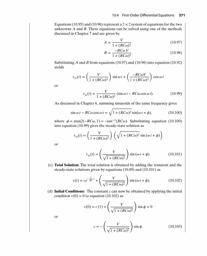
10.4 First-Order Differential Equations 371
Equations (10.95) and (10.96) represent a 2 × 2 system of equations for the twounknowns A and B. These equations can be solved using one of the methodsdiscussed in Chapter 7 and are given by
A = V1 + (RC𝜔)2
(10.97)
B = −RC𝜔V1 + (RC𝜔)2
. (10.98)
Substituting A and B from equations (10.97) and (10.98) into equation (10.92)yields
vss(t) =(
V1 + (RC𝜔)2
)sin𝜔 t +
(−RC𝜔V
1 + (RC𝜔)2
)cos𝜔 t
or
vss(t) = V1 + (RC𝜔)2
(sin𝜔 t − RC𝜔 cos𝜔 t). (10.99)
As discussed in Chapter 6, summing sinusoids of the same frequency gives
sin𝜔 t − RC𝜔 cos𝜔 t =√
1 + (RC𝜔)2 sin(𝜔 t + 𝜙), (10.100)
where 𝜙 = atan2(−RC𝜔, 1) = −tan−1(RC𝜔). Substituting equation (10.100)into equation (10.99) gives the steady-state solution as
vss(t) =(
V1 + (RC𝜔)2
) (√1 + (RC𝜔)2 sin (𝜔 t + 𝜙)
)or
vss(t) =
(V√
1 + (RC𝜔)2
)sin (𝜔 t + 𝜙). (10.101)
(c) Total Solution: The total solution is obtained by adding the transient and thesteady-state solutions given by equations (10.89) and (10.101) as
v(t) = ce−1
RCt +
(V√
1 + (RC𝜔)2
)sin (𝜔 t + 𝜙). (10.102)
(d) Initial Conditions: The constant c can now be obtained by applying the initialcondition v(0) = 0 to equation (10.102) as
v(0) = c (1) +
(V√
1 + (RC𝜔)2
)sin𝜙 = 0
or
c = −
(V√
1 + (RC𝜔)2
)sin𝜙. (10.103)

372 Chapter 10 Differential Equations in Engineering
Since 𝜙 = −tan−1(RC𝜔), the value of sin𝜙 can be found from the fourth-quadrant triangle shown in Fig. 10.17 as
sin𝜙 = −RC𝜔√1 + (RC𝜔)2
(10.104)
y
−RC
1x
1 + (RC ) 2ω
ω
ϕ√⎯⎯⎯⎯⎯⎯⎯⎯⎯⎯⎯
Figure 10.17 Fourth-quadrant triangle to find sin𝜙.
Substituting sin𝜙 from equation (10.104) into equation (10.103) yields
c = −
(V√
1 + (RC𝜔)2
) (−RC𝜔√
1 + (RC𝜔)2
)or
c = RC𝜔V1 + (RC𝜔)2
. (10.105)
Substituting the value of c from equation (10.105) into equation (10.102) gives
v(t) = RC𝜔V1 + (RC𝜔)2
e−1
RCt + V√
1 + (RC𝜔)2sin (𝜔 t + 𝜙). (10.106)
Note that as t → ∞, the total solution reaches the steady-state solution. Thus,the amplitude of the output voltage as t → ∞ is given by
|v(t)| = V√1 + (RC𝜔)2
. (10.107)
The amplitude of the input voltage vs(t) = V sin(𝜔 t) is given by|vs(t)| = V. (10.108)
Dividing the amplitude of the output at steady-state (equation (10.107)) by theamplitude of the input (equation (10.108)) gives
|v(t)||vs(t)| =V√
1 + (RC𝜔)2
Vor |v(t)||vs(t)| = 1√
1 + (RC𝜔)2. (10.109)

10.4 First-Order Differential Equations 373
Note that as 𝜔 → 0,
|v(t)||vs(t)| → 1.
This means that for low-frequency input, the amplitude of the output is aboutthe same as the input. However, as 𝜔 → ∞,
|v(t)||vs(t)| → 0.
This means that for high-frequency input, the amplitude of the output is closeto zero.
The RC circuit shown in Fig. 10.5 is known as a low-pass filter, because itpasses the low-frequency inputs but filters out the high-frequency inputs. Thiswill be further illustrated in Example 10-10.
Example10-10
Consider the low-pass filter of the previous example with RC = 0.5 andV = 10 V.
(a) Find the total solution v(t).
(b) Find the ratio|v(t)||vs(t)| as 𝜔 → ∞. Also plot the steady-state output for both
𝜔 = 0.1 rad/s and 10 rad/s.
Solution (a) The total solution for the output voltage is obtained by substituting RC = 0.5and V = 10 into equation (10.106) as
v(t) = 5𝜔1 + (0.5𝜔)2
e−2 t + 10√1 + (0.5𝜔)2
sin (𝜔 t − tan−10.5𝜔). (10.110)
(b) For 𝜔 = 0.1 rad/s, the ratio|v(t)||vs(t)| can be found from equation (10.109) as
|v(t)||vs(t)| = 1√1 + (0.5 ∗ 0.1)2
= 0.9988.
For 𝜔 = 10 rad/s, the ratio is given by
|v(t)||vs(t)| = 1√1 + (0.5 ∗ 10)2
= 0.1961.
As 𝜔 → ∞, the ratio|v(t)||vs(t)| → 0.
The plots of the output for 𝜔 = 0.1 and 10 rad/s are shown in Figs. 10.18 and 10.19,respectively. It can be seen that as 𝜔 increases from 0.1 to 10 rad/s, the amplitude ofthe steady-state output decreases from 10 ∗ (0.9988) = 9.988 V to 10 ∗ (0.1961) =

374 Chapter 10 Differential Equations in Engineering
1.961 V. It can be seen from equation (10.109) that if 𝜔 → ∞, the amplitude of theoutput will approach zero.
.
v(t), V
t, s062.83 125.66 188.490
−10
10
Figure 10.18 Output voltage for 𝜔 = 0.1 rad/s.
−2
00
2
3
v(t), V
t, s1.25 3.752.5 5
Figure 10.19 Output voltage for 𝜔 = 10 rad/s.
10.5 SECOND-ORDER DIFFERENTIAL EQUATIONS10.5.1 Free Vibration of a Spring-Mass System
Consider a spring-mass system in the vertical plane, as shown in Fig. 10.20, where k isthe spring constant, m is the mass, and y(t) is the position measured from equilibrium.
At the equilibrium position, the external forces on the block are shown in thefree-body diagram (FBD) of Fig. 10.21, where 𝛿 is the equilibrium elongation of thespring, mg is the force due to gravity, and k 𝛿 is the restoring force in the spring.
From equilibrium of forces in the y-direction,
k 𝛿 = mg,

10.5 Second-Order Differential Equations 375
gk
m
y(t)
Figure 10.20 Mass-spring system.
m
mg
kδ
Figure 10.21 Free-body diagram of the mass-spring system with no motion.
which gives
𝛿 =mgk
. (10.111)
This equilibrium elongation 𝛿 is also called the static deflection. Now, if the mass isdisplaced from its equilibrium position by the amount y(t), the FBD of the system isas shown in Fig. 10.22. Since the system is no longer in equilibrium, Newton’s second
m
mg
y(t)
k ( + y(t))δ
Figure 10.22 Free-body diagram of the mass-spring system displaced from equilibrium.
law (∑
F = m a) can be used to write the equation of motion as∑
Fy = m a = m y(t).
Summing the forces in Fig. 10.22 gives
mg − k(𝛿 + y(t)) = m y(t)

376 Chapter 10 Differential Equations in Engineering
or
mg − k 𝛿 − k y(t) = m y(t). (10.112)
Substituting 𝛿 from equation (10.111) gives
mg − k(mg
k
)− k y(t) = m y(t)
or
−k y(t) = m y(t),
which gives
m y(t) + k y(t) = 0. (10.113)
Equation (10.113) is a second-order differential equation for the displacement y(t)of the spring-mass system shown in Fig. 10.20.
Example10-11
Find the solution of equation (10.113) if the mass is subjected to an initial displace-ment of y(0) = A and let go. Note that the initial velocity is zero (y(0) = 0).
Solution (a) Transient Solution: Since the right-hand side of the equation is zero, assume atransient solution of the form
ytran(t) = cest.
The first and second derivatives of the transient solution are given by
ytran(t) = csest
ytran(t) = cs2est.
Substituting the transient solution and its derivatives into equation (10.113)yields
m(cs2 est) + k(cest) = 0.
Factoring out est gives
cest(ms2 + k) = 0
which implies that
ms2 + k = 0. (10.114)
Solving for s yields
s2 = − km
which gives
s = ±√
− km

10.5 Second-Order Differential Equations 377
or
s = 0 ± j
√km
where j =√−1. The two roots of the characteristic equation (10.114) are thus
s1 = + j√
km
and s2 = − j√
km
. Therefore, the transient solution is given by
ytran(t) = c1 es1 t + c2 es2 t
or
ytran(t) = c1 e j√
km
t + c2 e− j√
km
t (10.115)
where c1 and c2 are constants. Using Euler’s formula ej 𝜃 = cos 𝜃 + j sin 𝜃, equa-tion (10.115) can be written as
ytran(t) = c1
(cos
√km
t + j sin
√km
t
)+
c2
[cos
(−√
km
t
)+ j sin
(−√
km
t
)]. (10.116)
Since cos(−𝜃) = cos(𝜃) and sin(−𝜃) = −sin(𝜃), equation (10.116) can bewritten as
ytran(t) = c1
(cos
√km
t + j sin
√km
t
)+
c2
(cos
√km
t − j sin
√km
t
)
or
ytran(t) = (c1 + c2) cos
√km
t + j (c1 − c2) sin
√km
t.
This can be further simplified as
ytran(t) = c3 cos
√km
t + c4 sin
√km
t (10.117)
where c3 = c1 + c2 and c4 = j (c1 − c2) are real constants. Note that the con-stants c1 and c2 must be complex conjugates for ytran(t) to be real. Therefore,the transient solution of a mass-spring system can be written in terms of sines
and cosines with natural frequency 𝜔n =√
km
rad/s.
(b) Steady-State Solution: Since the RHS of equation (10.113) is already zero (noforcing function), the steady-state solution is zero, for example,
yss(t) = 0. (10.118)

378 Chapter 10 Differential Equations in Engineering
(c) Total Solution: The total solution for the displacement y(t) can be found byadding the transient and steady-state solutions from equations (10.117) and(10.118), which gives
y(t) = c3 cos
√km
t + c4 sin
√km
t. (10.119)
(d) Initial Conditions: The constants c3 and c4 are determined from using theinitial conditions y(0) = A and y(0) = 0. Substituting y(0) = A in equation(10.119) gives
y(0) = c3 cos(0) + c4 sin(0) = A (10.120)
or
c3 (1) + c4 (0) = A,
which gives
c3 = A.
Thus, the displacement of the mass is given by
y(t) = A cos
√km
t + c4 sin
√km
t. (10.121)
The velocity of the mass can be found by differentiating y(t) in equation(10.121) as
y(t) = −A
√km
sin
√km
t + c4
√km
cos
√km
t. (10.122)
The constant c4 can now be found by substituting y(0) = 0 in equation (10.122)as
y(0) = −A
√km
sin(0) + c4
√km
cos(0) = 0
or
−A (0) + c4
(√km
)= 0,
which gives
c4 = 0.
Thus, the total solution for the displacement is given by
y(t) = A cos
√km
t
or
y(t) = A cos𝜔n t.

10.5 Second-Order Differential Equations 379
The plot of the displacement y(t) is shown in Fig. 10.23. It can be seen that theamplitude of the displacement is simply the initial displacement A, and the
block oscillates at a frequency of 𝜔n =√
km
. Note that the natural frequency isproportional to the square root of the spring constant and is inversely propor-tional to the square root of the mass (i.e., the natural frequency increases withstiffness and decreases with mass). This is a general result for free vibration ofmechanical systems.
00
n
t, s
y(t)
2
ymax=A
−A
ππω
nω
Figure 10.23 Displacement of the spring for Example 10-11.
10.5.2 Forced Vibration of a Spring-Mass System
Suppose the spring-mass system is subjected to an applied force f (t), as shown inFig. 10.24.
f(t)
m
y(t)
g
k
Figure 10.24 Spring-mass system subjected to applied force.

380 Chapter 10 Differential Equations in Engineering
In this case, the derivation of the governing equation includes an additional forcef (t) on the right-hand side. Thus, the equation of motion of the system can be writtenas
m y(t) + k y(t) = f (t). (10.123)
Equation (10.123) is a second-order differential equation for the displacement y(t)of a mass-spring system subjected to a force f (t).
Example10-12
Find the solution to equation (10.123) if f (t) = F cos𝜔 t and y(0) = y(0) = 0. Also,
investigate the response as 𝜔 →√
km
.
Solution (a) Transient Solution: The transient solution is obtained by setting f (t) = 0, whichgives
m y(t) + k y(t) = 0.
This is the same as equation (10.113) for free vibration. Hence, the transientsolution is given by equation (10.117) as
ytran(t) = c3 cos
√km
t + c4 sin
√km
t, (10.124)
where c3 and c4 are real constants to be determined.
(b) Steady-State Solution: Since the forcing function is f (t) = F cos𝜔 t, the steady-state solution is of the form
yss(t) = A sin𝜔 t + B cos𝜔 t. (10.125)
The first and second derivatives of the steady-state solution are thus
yss(t) = A𝜔 cos𝜔 t − B𝜔 sin𝜔 t
yss(t) = −A𝜔2 sin𝜔 t − B𝜔
2 cos𝜔 t. (10.126)
Substituting yss(t), yss(t), and f (t) = F cos(𝜔 t) into equation (10.123) gives
m(−A𝜔2 sin𝜔 t − B𝜔
2 cos𝜔 t) + k(A sin𝜔 t + B cos𝜔 t) = F cos𝜔 t.
Grouping like terms yields
A(k − m𝜔2) sin𝜔 t + B(k − m𝜔
2) cos𝜔 t = F cos(𝜔 t). (10.127)
Equating the coefficients of sin𝜔 t on both sides of equation (10.127) yields
A(k − m𝜔2) = 0,
which gives
A = 0
(provided 𝜔 ≠
√km
).
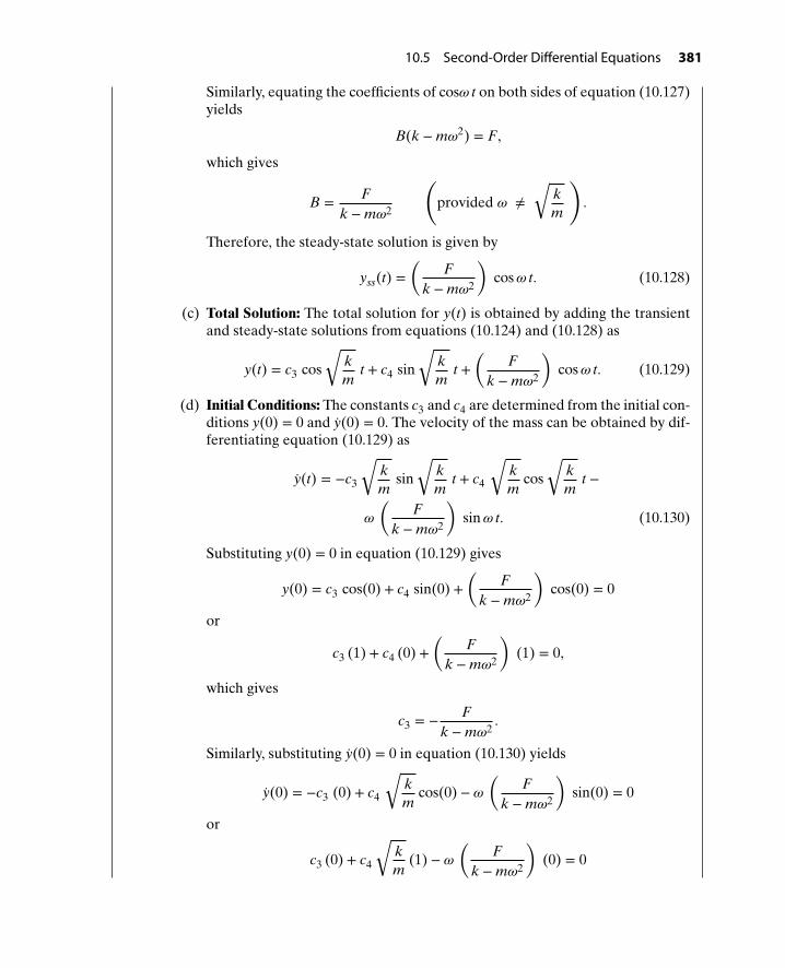
10.5 Second-Order Differential Equations 381
Similarly, equating the coefficients of cos𝜔 t on both sides of equation (10.127)yields
B(k − m𝜔2) = F,
which gives
B = Fk − m𝜔2
(provided 𝜔 ≠
√km
).
Therefore, the steady-state solution is given by
yss(t) =(
Fk − m𝜔2
)cos𝜔 t. (10.128)
(c) Total Solution: The total solution for y(t) is obtained by adding the transientand steady-state solutions from equations (10.124) and (10.128) as
y(t) = c3 cos
√km
t + c4 sin
√km
t +(
Fk − m𝜔2
)cos𝜔 t. (10.129)
(d) Initial Conditions: The constants c3 and c4 are determined from the initial con-ditions y(0) = 0 and y(0) = 0. The velocity of the mass can be obtained by dif-ferentiating equation (10.129) as
y(t) = −c3
√km
sin
√km
t + c4
√km
cos
√km
t −
𝜔
(F
k − m𝜔2
)sin𝜔 t. (10.130)
Substituting y(0) = 0 in equation (10.129) gives
y(0) = c3 cos(0) + c4 sin(0) +(
Fk − m𝜔2
)cos(0) = 0
or
c3 (1) + c4 (0) +(
Fk − m𝜔2
)(1) = 0,
which gives
c3 = − Fk − m𝜔2
.
Similarly, substituting y(0) = 0 in equation (10.130) yields
y(0) = −c3 (0) + c4
√km
cos(0) − 𝜔
(F
k − m𝜔2
)sin(0) = 0
or
c3 (0) + c4
√km
(1) − 𝜔
(F
k − m𝜔2
)(0) = 0

382 Chapter 10 Differential Equations in Engineering
which gives
c4 = 0.
Thus, the displacement of the mass is given by
y(t) = −(
Fk − m𝜔2
)cos
√km
t +(
Fk − m𝜔2
)cos𝜔 t (10.131)
or
y(t) =(
Fk − m𝜔2
) (cos𝜔 t − cos
√km
t
). (10.132)
Note that the results obtained above assumed that 𝜔 ≠
√km
. But nevertheless we
can investigate the behavior as 𝜔 gets very close to√
km
.
What is the response of y(t) as 𝜔 →√
km
? As 𝜔 →√
km
,
y(t) →(F
0
) (cos
√km
t − cos√
km
t)
= 00.
This is an “indeterminate” form and can be evaluated by methods of calculus notyet available to all students. However, the result can be investigated by picking
values of 𝜔 close to√
km
and plotting the results. For example, let k = m = F = 1,
and choose the values of 𝜔 = 0.9√
km
, 𝜔 = 0.99√
km
, and 𝜔 = 0.9999√
km
. The plotsof equation (10.132) for these values are as shown in Figs. 10.25, 10.26, and 10.27,
−15
−10
−5
5
10
15
0
0 20 40 60 80 100 120 140 160 180 200t, sec
y(t)
Figure 10.25 Displacement of the mass for 𝜔 = 0.9√
km
.
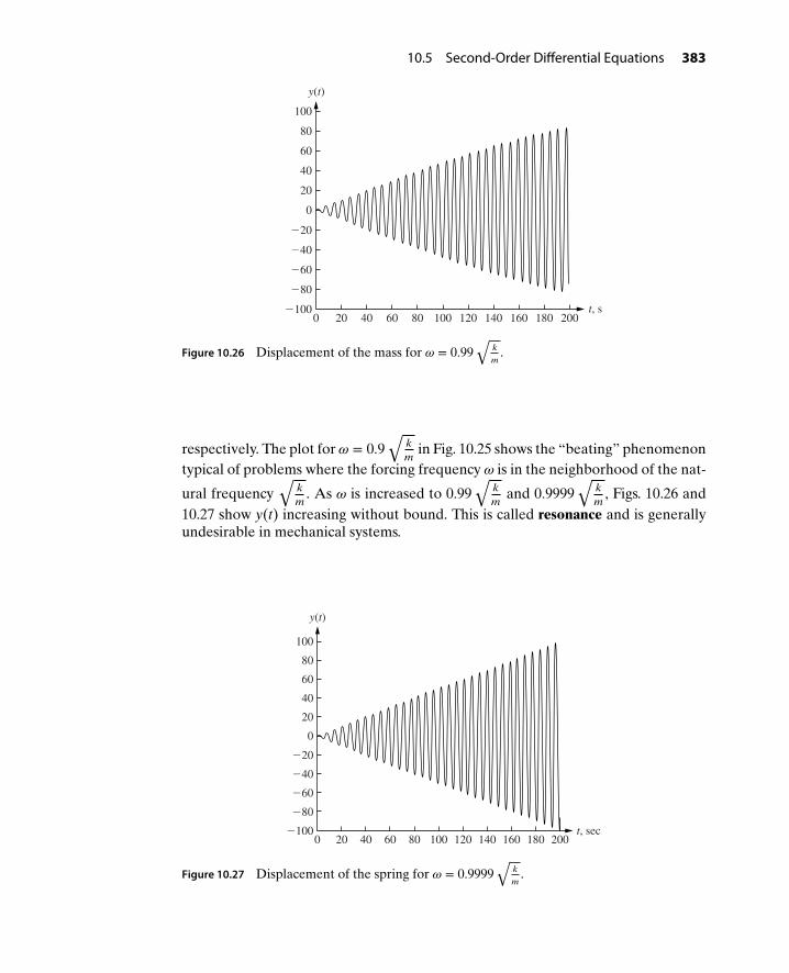
10.5 Second-Order Differential Equations 383
−100
−80
−60
−40
−20
20
40
60
80
100
0
0 20 40 60 80 100 120 140 160 180 200t, s
y(t)
Figure 10.26 Displacement of the mass for 𝜔 = 0.99√
km
.
respectively. The plot for 𝜔 = 0.9√
km
in Fig. 10.25 shows the “beating” phenomenontypical of problems where the forcing frequency 𝜔 is in the neighborhood of the nat-
ural frequency√
km
. As 𝜔 is increased to 0.99√
km
and 0.9999√
km
, Figs. 10.26 and10.27 show y(t) increasing without bound. This is called resonance and is generallyundesirable in mechanical systems.
0 20 40 60 80 100 120 140 160 180 200t, sec−100
−80
−60
−40
−20
20
40
60
80
100
0
y(t)
Figure 10.27 Displacement of the spring for 𝜔 = 0.9999√
km
.

384 Chapter 10 Differential Equations in Engineering
Example10-13
A biomedical engineer is designing a resistive training device to strengthen thelatissimus dorsi muscle. The task can be represented as a spring-mass system, asshown in Fig. 10.28. The displacement y(t) of the exercise bar satisfies the second-order differential equation
m y(t) + k y(t) = f (t) (10.133)
subject to the initial condition y(0) = E and y(0) = 0.
(a) Determine the transient solution ytran(t).
(b) Determine the steady-state solution yss(t) for the applied force shown inFig. 10.29.
(c) Determine the total solution, subject to the initial conditions.
m
k
f(t)
Figure 10.28 Spring-mass model of resistive training device.
210
H
f(t)
t
Figure 10.29 Applied force for resistive training device.
Solution (a) Transient Solution: The transient solution is obtained by setting the RHS ofequation (10.133) equal to zero as
md2y(t)
dt2+ k y(t) = 0 (10.134)
and assuming a solution of the form
ytran(t) = est.

10.5 Second-Order Differential Equations 385
Substituting the transient solution and its second derivative into equation(10.134) yields
m(s2 est) + k (est) = 0.
Factoring out est gives
est(m s2 + k) = 0,
which implies
m s2 + k = 0. (10.135)
Solving for s yields
s2 = − km
or
s = ± j
√km.
The two roots of equation (10.135) are s1 = + j√
km
and s2 = − j√
km
. Thus, thetransient solution is given by
ytran(t) = c3 cos
√km
t + c4 sin
√km
t, (10.136)
where c3 and c4 are real constants and√
km
is the natural frequency 𝜔n.
(b) Steady-State Solution: Since the forcing function is f (t) = H t∕2, the steady-state solution is of the form
yss(t) = A t + B. (10.137)
Substituting the yss(t) and yss(t) into equation (10.133) gives
m × 0 + k (A t + B) = H2
t. (10.138)
Equating the coefficients of t on both sides of equation (10.138) yields
kA = H2
which gives
A = H2k
.
Similarly, equating the constant coefficients on both sides of equation (10.138)yields
B = 0.

386 Chapter 10 Differential Equations in Engineering
Thus, the steady-state solution is given by
yss(t) =( H
2k
)t. (10.139)
(c) Total Solution: The total solution of the displacement y(t) can be found byadding the transient and steady-state solutions from equations (10.136) and(10.139), which gives
y(t) = c3 cos
√km
t + c4 sin
√km
t +( H
2k
)t. (10.140)
The constants c3 and c4 are determined using the initial conditions y(0) = Eand y(0) = 0. Substituting y(0) = E into equation (10.140) yields
y(0) = c3 cos(0) + c4 sin(0) +( H
2k
)(0) = E
or
c3 (1) + c4 (0) + 0 = E,
which gives
c3 = E.
The derivative of y(t) is obtained by differentiating equation (10.140) as
y(t) = −c3
√km
sin
√km
t + c4
√km
cos
√km
t + H2k
(10.141)
Substituting y(0) = 0 in equation (10.141) yields
0 = −c3 (0) + c4
√km
+( H
2k
)which gives
c4 = − H
2k√
k∕m.
Thus, the displacement of the exercise bar is given by
y(t) = E cos
√km
t −
(H
2k√
k∕m
)sin
√km
t + H2k
t.
10.5.3 Second-Order LC Circuit
A source voltage vs(t) is applied to an LC circuit, as shown in Fig. 10.30. ApplyingKVL to the circuit gives
vL(t) + v(t) = vs (10.142)

10.5 Second-Order Differential Equations 387
−
+
+ −
vs(t) C
L
vL (t)
v(t)
i(t)
+−
Figure 10.30 Voltage applied to an LC circuit.
where vL(t) = L di(t)dt
is the voltage across the inductor. Since the current flowing
through the circuit is given by i(t) = C dv(t)dt
, vL(t) can be written as vL(t) = LC d2v(t)dt2
.Substituting vL(t) into equation (10.142) yields
LCd2v(t)
dt2+ v(t) = vs(t). (10.143)
Equation (10.143) is a second-order differential equation for an LC circuit subjectedto forcing function vs(t).
Example10-14
Suppose the LC circuit of Fig. 10.30 is subjected to a voltage source vs(t) =V cos𝜔 t. Solve the resulting differential equation
LC v(t) + v(t) = V cos𝜔 t
subject to the initial condition v(0) = v(0) = 0. Note that since i(t) = Cdvdt
, the con-
dition v(0) = 0 means the initial current is zero.
Solution (a) Transient Solution: The transient solution is the solution obtained by settingthe RHS of equation (10.143) equal to zero
LCd2v(t)
dt2+ v(t) = 0, (10.144)
and assuming a solution of the form
ytran(t) = est.
Substituting the transient solution and its second derivative into the equation(10.144) yields
LC(s2 est) + (est) = 0.
Factoring out est gives
est(LC s2 + 1) = 0,
which implies
LC s2 + 1 = 0. (10.145)
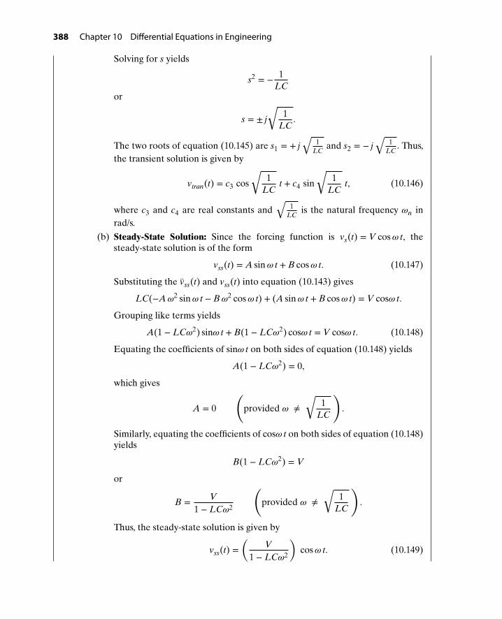
388 Chapter 10 Differential Equations in Engineering
Solving for s yields
s2 = − 1LC
or
s = ± j
√1
LC.
The two roots of equation (10.145) are s1 = + j√
1LC
and s2 = − j√
1LC
. Thus,the transient solution is given by
vtran(t) = c3 cos
√1
LCt + c4 sin
√1
LCt, (10.146)
where c3 and c4 are real constants and√
1LC
is the natural frequency 𝜔n inrad/s.
(b) Steady-State Solution: Since the forcing function is vs(t) = V cos𝜔 t, thesteady-state solution is of the form
vss(t) = A sin𝜔 t + B cos𝜔 t. (10.147)
Substituting the vss(t) and vss(t) into equation (10.143) gives
LC(−A𝜔2 sin𝜔 t − B𝜔
2 cos𝜔 t) + (A sin𝜔 t + B cos𝜔 t) = V cos𝜔 t.
Grouping like terms yields
A(1 − LC𝜔2) sin𝜔 t + B(1 − LC𝜔
2) cos𝜔 t = V cos𝜔 t. (10.148)
Equating the coefficients of sin𝜔 t on both sides of equation (10.148) yields
A(1 − LC𝜔2) = 0,
which gives
A = 0
(provided 𝜔 ≠
√1
LC
).
Similarly, equating the coefficients of cos𝜔 t on both sides of equation (10.148)yields
B(1 − LC𝜔2) = V
or
B = V1 − LC𝜔2
(provided 𝜔 ≠
√1
LC
).
Thus, the steady-state solution is given by
vss(t) =(
V1 − LC𝜔2
)cos𝜔 t. (10.149)
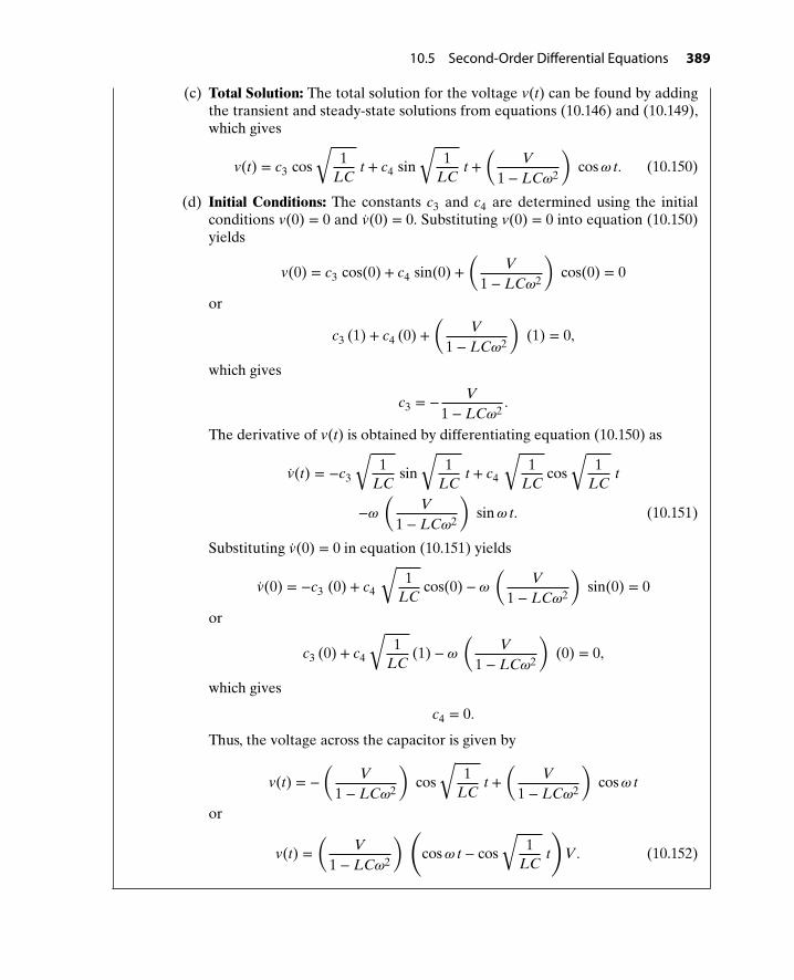
10.5 Second-Order Differential Equations 389
(c) Total Solution: The total solution for the voltage v(t) can be found by addingthe transient and steady-state solutions from equations (10.146) and (10.149),which gives
v(t) = c3 cos
√1
LCt + c4 sin
√1
LCt +
(V
1 − LC𝜔2
)cos𝜔 t. (10.150)
(d) Initial Conditions: The constants c3 and c4 are determined using the initialconditions v(0) = 0 and v(0) = 0. Substituting v(0) = 0 into equation (10.150)yields
v(0) = c3 cos(0) + c4 sin(0) +(
V1 − LC𝜔2
)cos(0) = 0
or
c3 (1) + c4 (0) +(
V1 − LC𝜔2
)(1) = 0,
which gives
c3 = − V1 − LC𝜔2
.
The derivative of v(t) is obtained by differentiating equation (10.150) as
v(t) = −c3
√1
LCsin
√1
LCt + c4
√1
LCcos
√1
LCt
−𝜔(
V1 − LC𝜔2
)sin𝜔 t. (10.151)
Substituting v(0) = 0 in equation (10.151) yields
v(0) = −c3 (0) + c4
√1
LCcos(0) − 𝜔
(V
1 − LC𝜔2
)sin(0) = 0
or
c3 (0) + c4
√1
LC(1) − 𝜔
(V
1 − LC𝜔2
)(0) = 0,
which gives
c4 = 0.
Thus, the voltage across the capacitor is given by
v(t) = −(
V1 − LC𝜔2
)cos
√1
LCt +
(V
1 − LC𝜔2
)cos𝜔 t
or
v(t) =(
V1 − LC𝜔2
) (cos𝜔 t − cos
√1
LCt
)V. (10.152)

390 Chapter 10 Differential Equations in Engineering
Note: A comparison of Examples 10-12 (spring-mass) and 10-14 (LC circuit) re-veals that the solutions are identical, with the following corresponding quantities:
Spring-Mass LC Circuit
y(t) v(t)m LCk 1F V
Although the two physical systems are entirely different, the math is exactly thesame. Such is the case for a wide range of problems across all disciplines of engi-neering. Make no mistake … if you want to study engineering, then a little bit ofmath can go an awfully long way.
P R O B L E M S
10-1. A faucet supplies fluid to a container ofcross-sectional area A at a volume flowrate Qin, as shown in Fig. P10.1. At thesame time, the fluid leaks out the bot-tom at a rate Qout = k h(t), where k isa constant. If the container is initiallyempty, the fluid height h(t) satisfies thefollowing first-order differential equa-tion and initial condition:
Adh(t)
dt+ k h(t) = Qin, h(0) = 0
h(t)
Qin
Qout = kh(t)
Figure P10.1 Leaking tank for problem P10-1.
(a) Determine the transient solution,htran(t).
(b) Suppose the faucet is turned onand off in a sinusoidal fashion,
so that Qin = Q2
(1 − sin𝜔 t). De-
termine the steady-state solution,hss(t).
(c) Determine the total solution h(t),subject to the initial condition.
10-2. The initial temperature of the hot cof-fee cup shown in Fig. P10.2 is T(0) =175F. The cup is placed in a room tem-perature of T∞ = 70F. The tempera-ture T(t) of the coffee at time t can beapproximated by Newton’s law of cool-ing as
dTdt
+ k T(t) = h T∞
where h is the convective heat transfercoefficient in Btu
ft2hF.
(a) Find the transient solution,Ttran(t). What is the time constantof the response?
(b) Find the steady-state solutionTss(t).
(c) Determine the total solution T(t).

Problems 391
Figure P10.2 A hot coffee cup placed in a roomtemperature of 70F.
(d) Sketch the total solution T(t).How long does it take for the tem-perature to reach 99% of the roomtemperature?
(e) Would increasing the value of h in-crease or decrease the time whenthe temperature of coffee reachesthe room temp?
(f) Would a lower or higher value of hbe best for a cup of coffee?
10-3. A constant voltage vs(t) = 10 V isapplied to the RC circuit shown inFig. P10.3. Assume that the switch hasbeen in position 1 for a long time.At t = 0, the switch is moved instan-taneously to position 2. For t ≥ 0, thevoltage v(t) across the capacitor satis-fies the following differential equationand initial condition:
RCdv(t)
dt+ v(t) = 0, v(0) = 10V.
(a) Find the transient solution, vtran(t).What is the time constant of theresponse?
(b) Find the steady-state solutionvss(t).
(c) Determine the total solution v(t).(d) Sketch the total solution v(t). How
long does it take for the responseto reach 99% of its steady-statevalue?
(e) Mark each of the following state-ments as true (T) or false (F):
Increasing the value ofresistance R will increase the timethe voltage v(t) reaches 99% of itssteady-state value.
Increasing the value ofcapacitance C will decrease thetime the voltage v(t) reaches 99%of its steady-state value.
Doubling the value of resis-tance R will double the time con-stant of the response.
Doubling the value ofcapacitance C will double the timeconstant of the response.
2
v(t)Cvs(t)
t = 0
5 k
R
1
+
−
+−
Ω
Figure P10.3 RC circuit for problem P10-3.
10-4. Repeat parts (a)–(d) of problem P10-3if R = 10 kΩ and C = 50 𝜇F.
10-5. Repeat parts (a)–(d) of problem P10-3if R = 20 kΩ and C = 100 𝜇F.
10-6. A constant voltage vs(t) = 10 V isapplied to the RC circuit shown inFig. P10.6. The voltage v(t) across thecapacitor satisfies the first-order differ-ential equation
RCdv(t)
dt+ v(t) = vs(t).
(a) Find the transient solution, vtran(t).What is the time constant of theresponse?
(b) Find the steady-state solutionvss(t).
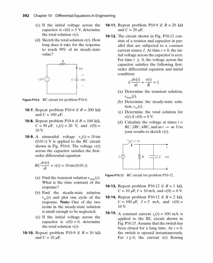
392 Chapter 10 Differential Equations in Engineering
(c) If the initial voltage across thecapacitor is v(0) = 5 V, determinethe total solution v(t).
(d) Sketch the total solution v(t). Howlong does it take for the responseto reach 99% of its steady-statevalue?
i(t)
vs(t)
R
v(t)C
+
−
+−
Figure P10.6 RC circuit for problem P10-6.
10-7. Repeat problem P10-6 if R = 200 kΩand C = 100 𝜇F.
10-8. Repeat problem P10-6 if R = 100 kΩ,C = 50 𝜇F, vs(t) = 20 V, and v(0) =10 V.
10-9. A sinusoidal voltage vs(t) = 10 sin(0.01 t) V is applied to the RC circuitshown in Fig. P10.6. The voltage v(t)across the capacitor satisfies the first-order differential equation
RCdv(t)
dt+ v(t) = 10 sin (0.01 t).
(a) Find the transient solution vtran(t).What is the time constant of theresponse?
(b) Find the steady-state solutionvss(t) and plot one cycle of theresponse. Note: One of the twoterms in the steady-state solutionis small enough to be neglected.
(c) If the initial voltage across thecapacitor is v(0) = 0, determinethe total solution v(t).
10-10. Repeat problem P10-9 if R = 10 kΩand C = 10 𝜇F.
10-11. Repeat problem P10-9 if R = 20 kΩand C = 20 𝜇F.
10-12. The circuit shown in Fig. P10.12 con-sists of a resistor and capacitor in par-allel that are subjected to a constantcurrent source I. At time t = 0, the ini-tial voltage across the capacitor is zero.For time t ≥ 0, the voltage across thecapacitor satisfies the following first-order differential equation and initialcondition:
Cdv(t)
dt+
v(t)R
= I.
(a) Determine the transient solution,vtran(t).
(b) Determine the steady-state solu-tion, vss(t).
(c) Determine the total solution forv(t) if v(0) = 0 V.
(d) Calculate the voltage at times t =RC, 2RC, 4RC, and as t → ∞. Useyour results to sketch v(t).
+
−
v(t)CI R
t = 0
↑
Figure P10.12 RC circuit for problem P10-12.
10-13. Repeat problem P10-12 if R = 1 kΩ,C = 10 𝜇F, I = 10 mA, and v(0) = 0 V.
10-14. Repeat problem P10-12 if R = 2 kΩ,C = 100 𝜇F, I = 5 mA, and v(0) =10 V.
10-15. A constant current is(t) = 100 mA isapplied to the RL circuit shown inFig. P10.15. Assume that the switch hasbeen closed for a long time. At t = 0,the switch is opened instantaneously.For t ≥ 0, the current i(t) flowing

Problems 393
through the resistor satisfies the fol-lowing differential equation and initialcondition:
LR
di(t)dt
+ i(t) = 0, i(0) = 50mA.
(a) Find the transient solution, itran(t).What is the time constant of theresponse?
(b) Find the steady-state solutioniss(t).
(c) Determine the total solution i(t).(d) Sketch the total solution i(t). How
long does it take for the responseto reach 99% of its steady-statevalue?
(e) Mark each of the following state-ments as true (T) or false (F):
Increasing the value of re-sistance R will increase the timethe voltage v(t) reaches 99% of itssteady-state value.
Increasing the value of in-ductance L will decrease the timethe voltage v(t) reaches 99% of itssteady-state value.
Doubling the value of resis-tance R will double the time con-stant of the response.
Doubling the value of in-ductance L will double the timeconstant of the response.
is(t) RL
i(t)
100 Ω
t = 0
↑
Figure P10.15 RL circuit for problem P10-15.
10-16. Repeat problem P10-15 if R = 100 Ωand L = 100 mH.
10-17. Repeat problem P10-15 if R = 100 Ωand L = 10 mH.
10-18. At time t = 0, an input voltage vin isapplied to the RL circuit shown inFig. P10.18. The output voltage v(t)satisfies the following first-order differ-ential equation:
dv(t)dt
+ RL
v(t) = RL
vin(t).
If the input voltage vin(t) = 10 volts,(a) Determine the transient solution,
vtran(t).(b) Determine the steady-state solu-
tion, vss(t).(c) Determine the total solution for
v(t), assuming the initial voltage iszero.
(d) Calculate the output voltage v(t)
at times t = LR
, 2 LR
, 4 LR
s, and as
t → ∞. Use your results to sketchv(t).
+
−
+−vin(t) v(t)R
L
Figure P10.18 RL circuit for problem P10-18.
10-19. Repeat problem P10-18 if R = 50Ωand L = 500 mH.
10-20. Repeat problem P10-18 if R = 10Ω,L = 200 mH, and vin(t) = 20 V.
10-21. The switch in the circuit shown inFig. P10.21 has been in position 1 for along time. At t = 0, the switch is movedinstantaneously to position 2. For t ≥ 0,the current i(t) flowing through the

394 Chapter 10 Differential Equations in Engineering
inductor satisfies the following differ-ential equation and initial condition:
0.2di(t)
dt+ 10 i(t) = 5, i(0) = −1A.
(a) Find the transient solution, itran(t).What is the time constant of theresponse?
(b) Find the steady-state solutioniss(t).
(c) Determine the total solution i(t).(d) Sketch the total solution i(t). How
long does it take for the responseto reach 99% of its steady-statevalue?
5 V
t = 0
i(t)
12
1 A50 Ω200 mH
10 Ω
−
+ ↑
Figure P10.21 RL circuit for problem P10-21.
10-22. A constant voltage source vin(t) = 10volts is applied to the Op–Amp circuitshown in Fig. P10.22. The output volt-age vo(t) satisfies the following first-order differential equation and initialconditions:
0.01dvo(t)
dt+ vo(t) = −vin(t),
vo(0) = 0 V.
(a) Find the transient solution,vo,tran(t).
(b) Find the steady-state solution vo,ssif vin = 10 V.
(c) If the initial output voltage isvo(0) = 0 V, determine the totalresponse.
(d) What is the time constant 𝜏 of theresponse? Plot the response vo(t)and give the values of vo at t = 𝜏,2 𝜏, and 5 𝜏.
vin= 10 V
+
−
+vcc
−vcc vo
−+
+−
C = 1 F
R2 = 10 kΩ
R1 = 10 kΩ
μ
Figure P10.22 Op–Amp circuit for problem P10-22.
10-23. A sinusoidal voltage source vin(t) =10 sin(10 t) volts is applied to the Op–Amp circuit shown in Fig. P10.23. Theoutput voltage vo(t) satisfies the fol-lowing first-order differential equationand initial conditions:
0.2dvo(t)
dt+ vo(t) = −2vin(t),
vo(0) = 0 V.
vin= 10 sin(10 t) V
+
−
+vcc
−vcc vo
−+
+−
C = 10 F
R2 = 20 kΩ
R1 = 10 kΩ
μ
Figure P10.23 Op–Amp circuit for problem P10-23.
(a) Find the transient solution,vo,tran(t). What is the time constant𝜏 of the response?

Problems 395
(b) Find the steady-state solution vo,ssif vin = 10 sin(10 t) V.
(c) If the initial output voltage isvo(0) = 0 V, determine the totalresponse.
10-24. The relationship between arterialblood flow and blood pressure in a sin-gle artery satisfies the following first-order differential equation:
dP(t)dt
+ 1RC
P(t) =Qin
C
where Qin is the volumetric blood flow,R is the peripheral resistance, and C isarterial compliance (all constant).
(a) Find the transient solution Ptran(t)for the arterial pressure. The unitfor P(t) is mmHg. What is the timeconstant of the arterial pressure?
(b) Determine the steady-state solu-tion Pss(t) for the arterial pressure.
(c) Determine the total solution P(t)assuming that the initial arterialpressure is 0.
(d) Evaluate P(t) at times t = RC, t =2 RC, t = 4 RC, and t → ∞ and useyour results to sketch P(t).
(e) Mark each of the following state-ments as true (T) or false (F):
Increasing the value of re-sistance R will increase the timeit takes for the arterial pressureP(t) to reach 99% of its steady-statevalue.
Increasing the value ofcapacitance C will decrease thetime it takes for the arterial pres-sure P(t) to reach 99% of its steady-state value.
Doubling the value of resis-tance R will double the time con-stant of the response.
Doubling the value ofcapacitance C will double the timeconstant of the response.
10-25. Repeat problem P10-24 if the volu-
metric blood flow Qin is 60 cm3
sand
the initial arterial pressure is 6 mmHg.
Also, assume R = 4mmHg
(cm3∕s)and C =
0.4 cm3
mmHg.
10-26. The displacement y(t) of a spring-masssystem shown in Fig. P10.26 is given by
0.25 y(t) + 10 y(t) = 0.
(a) Find the transient solution, ytran(t).(b) Find the steady-state solution of
the displacement yss.(c) Determine the total displacement
y(t) if the initial displacementy(0) = 0.2 m and the initial veloc-ity y(0) = 0 m/s.
(d) Sketch the total displacement y(t).
m = 0.25 kg
k = 10 N/m
y(t)
Figure P10.26 Mass-spring system for problemP10-26.
10-27. Repeat problem P10-26 if the dis-placement y(t) of a spring-mass (m =500 gm and k = 5 N/m) system shownis given by 0.5 y(t) + 5 y(t) = 0 andy(0) = 10 cm.
10-28. The displacement y(t) of a spring-masssystem shown in Fig. P10.28 is given by
y(t) + 25 y(t) = f (t).

396 Chapter 10 Differential Equations in Engineering
(a) Find the transient solution, ytran(t).(b) Find the steady-state solution
of the displacement yss if f (t) =10 N.
(c) Determine the total displacementy(t) if the initial displacementy(0) = 0 m and the initial velocityy(0) = 0 m/s.
(d) Sketch the total displacement y(t).
k = 25 N/m
m = 1 kg
y(t)f(t)
Figure P10.28 Mass-spring systems for problemP10-28.
10-29. Repeat problem P10-28 if the displace-ment y(t) of a spring-mass (m = 2 kgand k = 32 N/m) system is given by
2 y(t) + 32 y(t) = f (t)
and f (t) = 6 N, y(0) = 20 cm, andy(0) = 0.1 m/s.
10-30. A block of mass m is dropped from aheight h above a spring k, as shown inFig. P10.30. Beginning at the time ofimpact (t = 0), the position x(t) of theblock satisfies the following second-order differential equation and initialconditions:
m x(t) + k x(t) = m g x(0) = 0,
x(0) =√
2 g h.(a) Determine the transient solution
xtran(t), and determine the fre-quency of oscillation.
(b) Determine the steady-state solu-tion, xss(t).
(c) Determine the total solution x(t),subject to the initial conditions.
(d) Mark each of the following state-ments as true (T) or false (F):
Increasing the stiffnessk will increase the frequencyof x(t).
Increasing the height h willincrease the frequency of x(t).
Increasing the mass m willdecrease the frequency of x(t).
Doubling the height hwill double the maximum valueof x(t).
Doubling the mass m willdouble the maximum value of x(t).
g
k
m
h
x(t)
t = 0
Figure P10.30 Mass dropped on a spring.
10-31. Repeat parts (a)–(c) of problem P10-30if m = 500 g, k = 20 N/m, and g =9.8 m/s2.
10-32. Repeat parts (a)–(c) of problem P10-30if m = 1 kg, k = 30 N/m, and g =9.8 m/s2.
10-33. The displacement y(t) of the spring-mass system shown in Fig. P10.33 ismeasured from the equilibrium config-uration of the spring, where the static
deflection is 𝛿 =mgk
.

Problems 397
EquilibriumConfiguration:
Fcos( t)y(t)
UndeformedConfiguration:
= mg/k
g
k
m
k
mδ
ω
Figure P10.33 Mass-spring system for problemP10-33.
If m = 4 kg, k = 1.5 N/m, 𝜔 = 0.5 rad/s,and a sinusoidal force of 0.25 cos(0.5 t)is applied at t = 0, the displacementy(t) satisfies the second-order differen-tial equation
4 y(t) + 1.5 y(t) = 0.25 cos(0.5 t).
(a) Find the transient response ytran(t)of the system. What is the naturalfrequency of the response?
(b) Show that the steady-state solu-tion is given by
yss(t) = 0.5 cos(0.5 t).
Show all steps.(c) Assume the total solution is given
by
y(t) = c3 cos(√
0.375 t)
+ c4 sin(√
0.375 t) + 0.5 cos(0.5 t),
Given y(0) = 0.5 and y(0) = 0,show that c3 = 0 and c4 = 0. Showall steps.
(d) Given the total solution y(t) =0.5 cos(0.5 t), determine the mini-mum value of the deflection y(t)and the first time it reaches thatvalue.
10-34. Under static loading by a weight ofmass m, a rod of length L and axialrigidity AE deforms by an amount
𝛿 =mgLAE
, where g is the acceleration
due to gravity. However, if the mass isapplied suddenly (dynamic loading),vibration of the mass will ensue. If themass m is initially at rest, the deflec-tion x(t) satisfies the following second-order differential equation and initialconditions:
m x(t) + AEL
x(t) = mg,
x(0) = 0, x(0) = 0.
(a) Determine the transient solution,xtran(t).
(b) Determine the steady-state solu-tion, xss(t).
(c) Determine the total solution forx(t), subject to the given initialconditions.
(d) Calculate the maximum valueof the deflection x(t). How doesyour result compare to the staticdeflection 𝛿?
Static Loading: Dynamic Loading:
=mgLAE
m
AE Lg
m
AE L
x(t)δ
Figure P10.34 Rod under axial loading by a weightof mass m.
10-35. At time t = 0, a cart of mass m mov-ing at an initial velocity v0 impacts aspring of stiffness k, as illustrated inFig. P10.35.
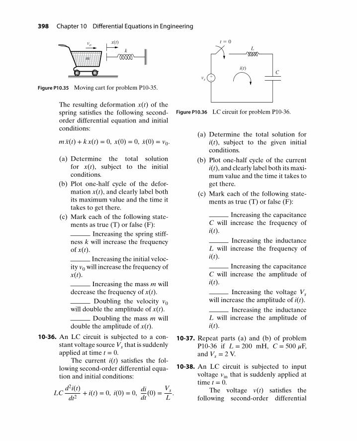
398 Chapter 10 Differential Equations in Engineering
x(t)
k
vo
m
Figure P10.35 Moving cart for problem P10-35.
The resulting deformation x(t) of thespring satisfies the following second-order differential equation and initialconditions:
m x(t) + k x(t) = 0, x(0) = 0, x(0) = v0.
(a) Determine the total solutionfor x(t), subject to the initialconditions.
(b) Plot one-half cycle of the defor-mation x(t), and clearly label bothits maximum value and the time ittakes to get there.
(c) Mark each of the following state-ments as true (T) or false (F):
Increasing the spring stiff-ness k will increase the frequencyof x(t).
Increasing the initial veloc-ity v0 will increase the frequency ofx(t).
Increasing the mass m willdecrease the frequency of x(t).
Doubling the velocity v0will double the amplitude of x(t).
Doubling the mass m willdouble the amplitude of x(t).
10-36. An LC circuit is subjected to a con-stant voltage source Vs that is suddenlyapplied at time t = 0.
The current i(t) satisfies the fol-lowing second-order differential equa-tion and initial conditions:
LCd2i(t)
dt2+ i(t) = 0, i(0) = 0, di
dt(0) =
Vs
L.
vs
t = 0
i(t)
L
+−
C
Figure P10.36 LC circuit for problem P10-36.
(a) Determine the total solution fori(t), subject to the given initialconditions.
(b) Plot one-half cycle of the currenti(t), and clearly label both its maxi-mum value and the time it takes toget there.
(c) Mark each of the following state-ments as true (T) or false (F):
Increasing the capacitanceC will increase the frequency ofi(t).
Increasing the inductanceL will increase the frequency ofi(t).
Increasing the capacitanceC will increase the amplitude ofi(t).
Increasing the voltage Vswill increase the amplitude of i(t).
Increasing the inductanceL will increase the amplitude ofi(t).
10-37. Repeat parts (a) and (b) of problemP10-36 if L = 200 mH, C = 500 𝜇F,and Vs = 2 V.
10-38. An LC circuit is subjected to inputvoltage vin that is suddenly applied attime t = 0.
The voltage v(t) satisfies thefollowing second-order differential

Problems 399
equation and initial conditions:
LCd2v(t)
dt2+ v(t) = vin, v(0) = 0, v(0) = 0.
+
−vin(t) v(t)
L
C+−
Figure P10.38 LC circuit for problem P10-38.
(a) Determine the transient solution,vtran(t). What is the frequency ofthe response?
(b) If vin = 10.0 V, determine thesteady-state solution, vss(t).
(c) Determine the total solution forv(t), subject to the given initialconditions.
(d) Calculate the maximum value ofv(t). Does your result depend onthe values of L and C?
10-39. Repeat parts (a)–(c) of problemP10-38 if L = 100 mH, C = 40 𝜇F, andvin = 10 V.
10-40. Repeat parts (a)–(c) of problemP10-38 if L = 40 mH, C = 400 𝜇F, andvin = 10 sin(100 t) V.
10-41. Repeat parts (a)–(c) of problemP10-38 if L = 40 mH, C = 400 𝜇F, andvin = 10 sin(245 t) V.
10-42. A biomedical engineer is designing aresistive training device to strengthenthe latissimus dorsi muscle. The taskcan be represented as a spring-masssystem, as shown in Fig. P10.28. Thedisplacement y(t) of the exercise barsatisfies the second-order differentialequation
m y(t) + k y(t) = f (t),
subject to the initial condition y(0) =0.01 m and y(0) = 0 m/s.(a) Determine the transient solution
ytran(t).(b) Determine the steady-state solu-
tion yss(t) for the applied forceshown in Fig. P10.42.
(c) Determine the total solution, sub-ject to the initial conditions.
0
0 1 2
f(t), N
t, s
0.1
Figure P10.42 Applied force for resistive trainingdevice for problem P10-42.
10-43. A rod of mass m and length l is pinnedat the bottom and supported by aspring of stiffness k at the top. Whendisplaced by a force f (t), its position isdescribed by the angle 𝜃(t), as shownin Fig. P10.43. For relatively smalloscillations, the angle 𝜃(t) satisfies thesecond-order differential equation
13
m l (t) + k l 𝜃(t) = f (t).
m, l
f(t)k
θ
Figure P10.43 Rod supported by a spring.
(a) Find the transient solution 𝜃tran(t),and determine the frequency ofoscillation.
400 Chapter 10 Differential Equations in Engineering
(b) Suppose f (t) = F cos𝜔 t. Deter-mine the steady-state solution,𝜃ss(t).
(c) Suppose now that f (t) = 0, andthat the initial conditions are𝜃(0) = 𝜋
18rad and (0) = 0 rad/s.
Determine the total solution, 𝜃(t).(d) Given your solution to part (c),
mark each of the following state-ments as true or false:
Increasing the length lwould decrease the frequency ofthe oscillation.
Increasing the mass mwould increase the frequency ofthe oscillation.
Increasing the stiffness kwould increase the frequency ofthe oscillation.
Increasing the mass mwould increase the amplitude ofthe oscillation.
Increasing the stiffness kwould decrease the amplitude ofthe oscillation.

Answers to SelectedProblems
Chapter 1
P1-1 k = 10 N/m
P1-3 (a) F = 3.48 x + 48 N
P1-5 (a) Fb(P) = 0.5 P + 160 lb
P1-7 (a) v(t) = −9.8 t + 4 m/s
P1-9 (a) v(t) = −32.2 t + 161.0 ft/s
P1-11 (a) v(t) = −75 t + 150 ft/s
P1-13 (a) v(t) = 10 t m/s
(b) v(t) = 10 m/s
(c) v(t) = −10 t + 40 m/s
P1-15 (a) T(x) = 26.67 x + 30F
(b) T(0.75) = 50F
P1-17 (b) I = 2 A
P1-19 (a) Vs = 3 I + 3 V
P1-21 Vs = 50 I + 0.7 V
P1-23 vo = 1.5 vin − 4 V
P1-25 ea = 2.667 ia + 0.667 V
P1-27 vo = −1000 iD + 12 V
P1-29 (a) F = 18 N
(b) V = 0.6 V
P1-31 (a) A(F) = 4.55 × 10⁻⁶F V
(c) A(200) = 9.091 × 10⁻⁴ V
P1-33 (a) T(V) = 0.04 V − 25C
P1-35 (a) T(V) = 18.1 V + 4.6C
(c) ΔT = 65.17C
P1-37 (a) R = 100 𝜀 + 50 Ω
P1-39 (a) a(c) = 0.0667 c + 0.0833
(b) c = 6.04 𝜇gml
(c) a(0.00419) = 0.0836
P1-41 (a) T(F) = 1.8 T(C) + 32F
(c) 68F ≤ T ≤ 176F
P1-43 (a) p(x) = −12 x + 30 psi, l = 2.5 in.
(b) p(1.0) = 18 psi
401
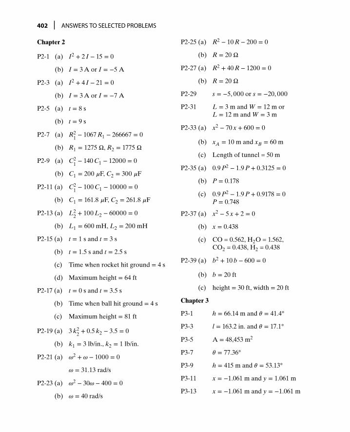
402 ANSWERS TO SELECTED PROBLEMS
Chapter 2
P2-1 (a) I2 + 2 I − 15 = 0
(b) I = 3 A or I = −5 A
P2-3 (a) I2 + 4 I − 21 = 0
(b) I = 3 A or I = −7 A
P2-5 (a) t = 8 s
(b) t = 9 s
P2-7 (a) R21 − 1067 R1 − 266667 = 0
(b) R1 = 1275 Ω, R2 = 1775 Ω
P2-9 (a) C21 − 140 C1 − 12000 = 0
(b) C1 = 200 𝜇F, C2 = 300 𝜇F
P2-11 (a) C21 − 100 C1 − 10000 = 0
(b) C1 = 161.8 𝜇F, C2 = 261.8 𝜇F
P2-13 (a) L22 + 100 L2 − 60000 = 0
(b) L1 = 600 mH, L2 = 200 mH
P2-15 (a) t = 1 s and t = 3 s
(b) t = 1.5 s and t = 2.5 s
(c) Time when rocket hit ground = 4 s
(d) Maximum height = 64 ft
P2-17 (a) t = 0 s and t = 3.5 s
(b) Time when ball hit ground = 4 s
(c) Maximum height = 81 ft
P2-19 (a) 3 k22 + 0.5 k2 − 3.5 = 0
(b) k1 = 3 lb/in., k2 = 1 lb/in.
P2-21 (a) 𝜔2 + 𝜔 − 1000 = 0
𝜔 = 31.13 rad/s
P2-23 (a) 𝜔2 − 30𝜔 − 400 = 0
(b) 𝜔 = 40 rad/s
P2-25 (a) R2 − 10 R − 200 = 0
(b) R = 20 Ω
P2-27 (a) R2 + 40 R − 1200 = 0
(b) R = 20 Ω
P2-29 s = −5, 000 or s = −20, 000
P2-31 L = 3 m and W = 12 m orL = 12 m and W = 3 m
P2-33 (a) x2 − 70 x + 600 = 0
(b) xA = 10 m and xB = 60 m
(c) Length of tunnel = 50 m
P2-35 (a) 0.9 P2 − 1.9 P + 0.3125 = 0
(b) P = 0.178
(c) 0.9 P2 − 1.9 P + 0.9178 = 0P = 0.748
P2-37 (a) x2 − 5 x + 2 = 0
(b) x = 0.438
(c) CO = 0.562, H2O = 1.562,CO2 = 0.438, H2 = 0.438
P2-39 (a) b2 + 10 b − 600 = 0
(b) b = 20 ft
(c) height = 30 ft, width = 20 ft
Chapter 3
P3-1 h = 66.14 m and 𝜃 = 41.4
P3-3 l = 163.2 in. and 𝜃 = 17.1
P3-5 A = 48,453 m2
P3-7 𝜃 = 77.36
P3-9 h = 415 m and 𝜃 = 53.13
P3-11 x = −1.061 m and y = 1.061 m
P3-13 x = −1.061 m and y = −1.061 m
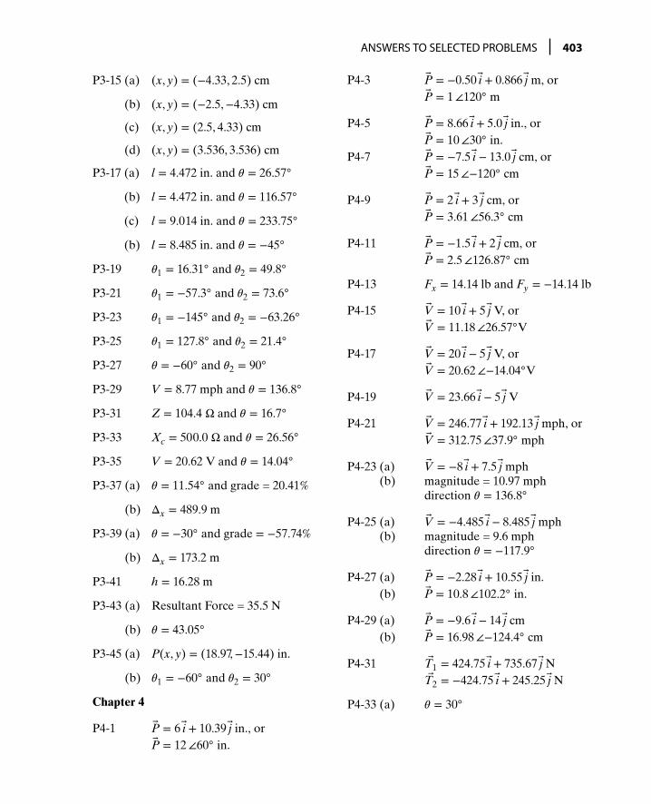
ANSWERS TO SELECTED PROBLEMS 403
P3-15 (a) (x, y) = (−4.33, 2.5) cm
(b) (x, y) = (−2.5,−4.33) cm
(c) (x, y) = (2.5, 4.33) cm
(d) (x, y) = (3.536, 3.536) cm
P3-17 (a) l = 4.472 in. and 𝜃 = 26.57
(b) l = 4.472 in. and 𝜃 = 116.57
(c) l = 9.014 in. and 𝜃 = 233.75
(b) l = 8.485 in. and 𝜃 = −45
P3-19 𝜃1 = 16.31 and 𝜃2 = 49.8
P3-21 𝜃1 = −57.3 and 𝜃2 = 73.6
P3-23 𝜃1 = −145 and 𝜃2 = −63.26
P3-25 𝜃1 = 127.8 and 𝜃2 = 21.4
P3-27 𝜃 = −60 and 𝜃2 = 90
P3-29 V = 8.77 mph and 𝜃 = 136.8
P3-31 Z = 104.4 Ω and 𝜃 = 16.7
P3-33 Xc = 500.0 Ω and 𝜃 = 26.56
P3-35 V = 20.62 V and 𝜃 = 14.04
P3-37 (a) 𝜃 = 11.54 and grade = 20.41%
(b) Δx = 489.9 m
P3-39 (a) 𝜃 = −30 and grade = −57.74%
(b) Δx = 173.2 m
P3-41 h = 16.28 m
P3-43 (a) Resultant Force = 35.5 N
(b) 𝜃 = 43.05
P3-45 (a) P(x, y) = (18.97,−15.44) in.
(b) 𝜃1 = −60 and 𝜃2 = 30
Chapter 4
P4-1 P = 6 i + 10.39 j in., orP = 12∠60 in.
P4-3 P = −0.50 i + 0.866 j m, orP = 1∠120 m
P4-5 P = 8.66 i + 5.0 j in., orP = 10∠30 in.
P4-7 P = −7.5 i − 13.0 j cm, orP = 15∠−120 cm
P4-9 P = 2 i + 3 j cm, orP = 3.61∠56.3 cm
P4-11 P = −1.5 i + 2 j cm, orP = 2.5∠126.87 cm
P4-13 Fx = 14.14 lb and Fy = −14.14 lb
P4-15 V = 10 i + 5 j V, orV = 11.18∠26.57V
P4-17 V = 20 i − 5 j V, orV = 20.62∠−14.04V
P4-19 V = 23.66 i − 5 j V
P4-21 V = 246.77 i + 192.13 j mph, orV = 312.75∠37.9 mph
P4-23 (a) V = −8 i + 7.5 j mph(b) magnitude = 10.97 mph
direction 𝜃 = 136.8
P4-25 (a) V = −4.485 i − 8.485 j mph(b) magnitude = 9.6 mph
direction 𝜃 = −117.9
P4-27 (a) P = −2.28 i + 10.55 j in.(b) P = 10.8∠102.2 in.
P4-29 (a) P = −9.6 i − 14 j cm(b) P = 16.98∠−124.4 cm
P4-31 T1 = 424.75 i + 735.67 j NT2 = −424.75 i + 245.25 j N
P4-33 (a) 𝜃 = 30

404 ANSWERS TO SELECTED PROBLEMS
(b) F = −0.866 F i + 0.5 F j lbN = 0.5 N i + 0.866 N j lbW = 0 i − 2000 j lb
(c) F = 1000 lbN = 1732.1 lb
P4-35 (a) 𝜃 = 30
(b) F = 0.866 F i + 0.5 F j NN = −0.5 N i + 0.866 N j N
(c) F = 250 N, N = 433 N
P4-37 (a) F1 = 0.7705 F1 i + 0.6374 F1 j lbF2 = −0.4633 F2 i + 0.8862 F2 j lbP = 0 i − 346 j lb
(b) F1 = 163.8 lb, F2 = 272.5 lb
P4-39 (a) F1 = −F1 i + 0 j lbF2 = 0.7466 F2 i + 0.6652 F2 j lbW = 0 i − 125 j lb
(b) F1 = 140.3 lb, F2 = 187.9 lb
P4-41 (a) Fm = −43.3 i + 25 j lbWa = 0 i − 7 j lbWp = 0 i − 3 j lb
(b) Rx = 43.3 lb, Ry = −15 lbR = 45.82 lb, Direction, 𝜃 = −19.11
P4-43 (a) P = 0.319 i + 2.156 j ft
(b) P = 2.18 ft, Direction, 𝜃 = 81.58
Chapter 5
P5-1 (a) VR = 1 + j 0 V and VL = 0 + j 1 V
(b) V = 1 + j 1 V, V = 1.414 ∠45V
P5-3 (a) VR = 8.05 − j 4.03 VVL = 2.02 + j 4.02 V
(b) V = 10.07 + j 0 V, V = 10.06 ∠0V
(c) Re(V) = 10.06 V, Im(V) = 0 V
P5-5 (a) VR = 9 + j 3 V, VC = 1 − j 3 V
(b) V = 10 + j 0 V, V = 10 ∠0V
(c) Re(V) = 10 V, Im(V) = 0 V
P5-7 (a) IR = 100 − j 0 mA andIL = 0 − j 200 mA
(b) I = 100 − j 200 mAI = 223.6 ∠−63.43mA
(c) Re(I) = 100 mA, Im(I) = −200 mA
P5-9 (a) IR = 75 + j 43.3 𝜇A andIL = 25 − j 43.3 𝜇A
(b) I = 100 + j 0 𝜇A, I = 100 ∠0𝜇A
(c) Re(I) = 100 𝜇A, Im(I) = 0 𝜇A
P5-11 (a) IR = 0.5 + j 0 mA andIC = 0 + j 0.2 mA
(b) I = 0.5 + j 0.2 mAI = 0.539 ∠21.8mA
(c) Re(I) = 0.5 mA, Im(I) = 0.2 mA
P5-13 vo(t) = Re(15 ej(120𝜋 t−60)
)V
P5-15 (a) Z = 100 + j 82.4 Ω
(b) Z = 129.6 ∠39.5Ω
(c) Z∗ = 100 − j 82.4 ΩZ Z∗ = 16, 789.9
P5-17 (a) I = 26.83 ∠56.57A, orI = 14.75 + j 22.39 A
(b) V = 31.3 ∠18.43VV = 29.69 + j 9.9 V
P5-19 (a) Z2 + Z3 = 0 − j 100.45 ΩZ2 + Z3 = 100.45 ∠−90Ω
(b) Z1 + Z2 + Z3 = 100 − j 100.45 ΩZ1 + Z2 + Z3 = 141.74 ∠−45.13Ω
(c) H = 0.502 − j 0.50 orH = 0.709 ∠−44.87
(d) H∗ = 0.502 + j 0.50H H∗ = 0.503

ANSWERS TO SELECTED PROBLEMS 405
P5-21 (a) ZR = 100 + j 0 Ω orZR = 100.0 ∠0Ω
ZL = 0 + j 60 Ω orZL = 60.0 ∠90Ω
ZC = 0 − j 50 Ω orZC = 50.0 ∠−90Ω
(b) Z = 100 + j 10 ΩZ = 100.5 ∠5.71Ω
(c) Z∗ = 100 − j 10 Ω, Z Z∗ = 10, 100
(d) VC = −5.45 − j 54.46 VVC = 54.73 ∠−95.71V
P5-23 (a) ZR = 9 + j 0 Ω orZR = 9 ∠0Ω
ZL = 0 + j 3 Ω orZL = 3 ∠90Ω
ZC = 0 − j 4 Ω orZC = 4 ∠−90Ω
(b) ZLC = 0 + j 12 Ω orZLC = 12 ∠90Ω
(c) Z = 9 + j 12 Ω orZ = 15 ∠53.13Ω
(d) Z∗ = 9 − j 12 Ω, Z Z∗ = 225
P5-25 (a) ZR = 100 + j 0 Ω orZR = 100 ∠0Ω
ZC = 0 − j 50 Ω orZC = 50 ∠−90Ω
(b) Z = 100 − j 50 Ω orZ = 111.8 ∠−26.57Ω
(c) I = 0.800 + j 0.400 A orI = 0.894 ∠26.57A
(d) VR = 80.0 + j 40.0 V orVR = 89.4 ∠26.57V
VC = 20.0 − j 40.0 V orVC = 44.7 ∠−63.43V
P5-25 (e) V = 100.0 − j 0 V orV = 100 ∠0V
P5-27 (a) ZR = 100 + j 0 Ω orZR = 100 ∠0Ω
ZL = 0 + j 188.5 Ω orZL = 188.5 ∠90Ω
ZC = 0 − j 106.1 Ω orZC = 106.1 ∠−90Ω
(b) Z = 100 + j 82.4 Ω orZ = 129.6 ∠39.5Ω
(c) I = 0.596 − j 0.491 A orI = 0.772 ∠−39.5A
(d) VR = 59.57 − j 49.11 V orVR = 77.2 ∠−39.5V
VL = 92.56 + j 112.3 V orVL = 145.5 ∠50.5V
VC = −52.1 − j 63.2 V orVC = 81.91 ∠−129.5V
(e) V = 100.0 + j 0 V orV = 100 ∠0V
P5-29 (a) ZR = 1000 + j 0 Ω orZR = 1000 ∠0Ω
ZC = 0 − j 1000 Ω orZC = 1000 ∠−90Ω
(b) I1 = 0.5 − j 0.5 mA orI1 = 0.7071 ∠−45mA
I2 = 0.5 + j 0.5 mA orI2 = 0.7071 ∠45mA
(c) I1 + I2 = 1 + j 0 mA orI1 + I2 = 1 ∠0mA
P5-31 (a) ZR = 1000 + j 0 Ω orZR = 1000 ∠0Ω
ZL = 0 + j 1000 Ω orZL = 1000 ∠90Ω

406 ANSWERS TO SELECTED PROBLEMS
P5-31 (b) I1 = 0.5 + j 0.5 mA orI1 = 0.7071 ∠45mA
I2 = 0.5 − j 0.5 mA orI2 = 0.7071 ∠−45mA
(c) I1 + I2 = 1 + j 0 mA orI1 + I2 = 1 ∠0mA
P5-33 (a) ZR = 1 + j 0 kΩ orZR = 1 ∠0kΩ
ZC = 0 − j 2 kΩ orZC = 2 ∠−90kΩ
(b) Vo = 2.5 + j 0 V orVo = 2.5 ∠0V
P5-35 (a) ZR1 = 1.5 + j 0 = 1.5 ∠0kΩZR2 = 1 + j 0 = 1 ∠0kΩZC = 0 − j 0.5 = 0.5 ∠−90kΩ
(b) Vo = −0.3578 + j 0.1789 V orVo = 0.4 ∠153.43V
P5-37 (a) Za = 20 + j 0 = 20 ∠0ΩZb = 0 − j 10 = 10 ∠−90ΩZc = 20 + j 50 = 53.85 ∠68.2Ω
(b) Z1 = −2.5 − j 2.5 = 3.54 ∠−135ΩZ2 = 17.5 + j 7.5 = 19.04 ∠23.2ΩZ3 = 3.75 − j 8.75 = 9.52 ∠−66.8Ω
P5-39 (a) Z1 = 2.5 − j 2.5 = 3.53 ∠−45ΩZ2 = 17.5 + j 7.5 = 19.04 ∠23.2ΩZ3 = 3.75 − j 8.75 = 9.52 ∠−66.8Ω
(b) Za = 72.4 − j 0 = 72.4 ∠0ΩZb = 5 − j 12.5 = 13.46 ∠−68.2ΩZc = 25 + j 10 = 26.92 ∠21.8Ω
Chapter 6
P6-1 Amplitude = l = 5 in.Frequency f = 1 Hz, 𝜔=2𝜋 rad/sPeriod = 1 sPhase angle 𝜙 = 0 radTime shift = 0 s
P6-3 Amplitude = l = 20 cmFrequency f = 1 Hz, 𝜔 = 2𝜋 rad/sPeriod = 1 sPhase angle 𝜙 = −𝜋∕4 radTime shift = 1∕8 s (to right)
P6-5 Amplitude = l = 15 cmFrequency f = 0.5 Hz, 𝜔 = 𝜋 rad/sPeriod = 2 sPhase angle 𝜙 = 3𝜋∕4 radTime shift = 3/4 s (to left)
P6-7 Amplitude = A = 2 cmFrequency f = 2 Hz, 𝜔 = 4𝜋 rad/sPeriod = 0.5 sPhase angle 𝜙 = 0 rady(t) = 2 sin(4𝜋 t) cm
P6-9 Amplitude = A = 10 in.Frequency f = 1 Hz, 𝜔 = 2𝜋 rad/sPeriod = 1 sPhase angle 𝜙 = 0.2𝜋 radx(t) = 10 sin(2𝜋 t + 0.2𝜋) in.
P6-11 (a) Amplitude = A = 10 cmFrequency f = 2∕𝜋 Hz, 𝜔 = 4 rad/sPeriod = 𝜋∕2 s
(b) t = 𝜋/4 s
P6-13 (a) Amplitude = A = 8 cmFrequency f = 1 Hz, 𝜔 = 2𝜋 rad/sPeriod = 1 sTime shift = 1/8 s (to left)
(b) t = 1/8 s
P6-15 (a) Amplitude = A = 5 cmFrequency f = 1/2 Hz, 𝜔 = 𝜋 rad/sPeriod = 2 s
(b) t = 1 s
P6-17 (a) Amplitude = A = 5 radFrequency f = 1 Hz, 𝜔 = 2𝜋 rad/sPeriod = 1 s
(b) t = 0.25 s

ANSWERS TO SELECTED PROBLEMS 407
P6-19 (a) v(t) = 41.38 cos(120𝜋 t) V
(b) Amplitude = 41.38 VFrequency f = 60 HzPeriod = T = 1/60 sPhase angle = 0
Time shift = 0 s
P6-21 (a) Amplitude = 0.1 VFrequency f = 10 HzPeriod = T = 1/10 sPhase angle = 𝜋/2 radTime shift = 1/40 s (to left)
(c) v(t) = 0.51 cos(20𝜋 t − 78.7) V
P6-23 (a) i(t) = 14.14 sin(120𝜋 t − 45) A
(b) Amplitude = 14.14 AFrequency f = 60 HzPeriod = T = 1/60 sPhase angle = −𝜋/4 radTime shift = 1/480 s (to right)
P6-25 (a) i(t) = 4 sin(120𝜋 t + 60) A
(b) Amplitude = 4 AFrequency f = 60 HzPeriod = T = 1/60 sPhase angle = 𝜋/3 rad = 60
Time shift = 1/360 s (to left)
P6-27 (a) Amplitude = 10 VFrequency f = 50 HzPeriod = T = 1/50 sPhase angle = −𝜋/4 rad = −45
Time shift = 1/400 s (to right)
(c) vo(t) = 22.36 cos(100𝜋 t + 63.4) V
P6-29 (a) Amplitude = 10√
2 VFrequency f = 250 HzPeriod = T = 1/250 sPhase angle = −3𝜋/4 rad = −135
Time shift = 3/2000 s (to right)
(c) vo(t) = 11.18 sin(500𝜋 t − 153.4) V
P6-31 (a) Amplitude = 8 in.Frequency f = 2 HzPeriod = T = 1/2 sPhase angle = 𝜋/3 rad = 60
Time shift = 1/12 s (to left)
(c) 𝛿(t)= 4.11 cos(4𝜋 t − 76.918) in.
P6-33 (a) Amplitude = 8 in.Frequency f = 2 HzPeriod = T = 1/2 sPhase angle = 𝜋/4 rad = 45
Time shift = 1/8 s (to left)
(c) 𝛿(t)= 11.79 cos(4𝜋 t + 28.68) in.
P6-35 (a) Amplitude = 164 VFrequency f = 60 HzPeriod = T = 1/60 sPhase angle = 7𝜋/18 rad = 70
Time shift = 7/2160 s (to left)
(c) vT(t) = 220 cos(120𝜋 t − 45) V
P6-37 (a) Amplitude = 120 VFrequency f = 60 HzPeriod = T = 1/60 sPhase angle = 2𝜋/3 rad = 120
Time shift = 1/180 s (to left)
(c) vbc(t) = 207.8 cos(120𝜋 t + 0) V
P6-39 (a) Amplitude = 200 NFrequency f = 5/2 HzPeriod = T = 2/5 sPhase angle = 0 rad = 0
Vertical shift = 1000 N
Chapter 7
P7-1 (a) I1 = 5.063 A, I2 = −3.22 A
(b)[
16 −9−9 20
] [I1I2
]=[
110−110
](c) I1 = 5.063 A, I2 = −3.22 A
(d) I1 = 5.063 A, I2 = −3.22 A

408 ANSWERS TO SELECTED PROBLEMS
P7-3 (a) I1 = 0.0471 A, I2 = −0.0429 A
(b)[
1100 10001000 1100
] [I1I2
]=[
90
]
(c) I1 = 0.0471 A, I2 = −0.0429 A
(d) I1 = 0.0471 A, I2 = −0.0429 A
P7-5 (a) V1 = 7.64 V, V2 = 7.98 V
(b)[
17 −10−6 11
] [V1V2
]=[
5042
]
(c) V1 = 7.64 V, V2 = 7.98 V
(d) V1 = 7.64 V, V2 = 7.98 V
P7-7 (a) V1 = 0.976 V, V2 = 1.707 V
(b)[
7 −42 −7
] [V1V2
]=[
0−10
]
(c) V1 = 0.976 V, V2 = 1.707 V
(d) V1 = 0.976 V, V2 = 1.707 V
P7-9 (a) G1 = 0.0175 , G2 = 0.0025
(b)[
10 105 15
] [G1G2
]=[
0.20.125
]
(c) G1 = 0.0175 , G2 = 0.0025
(d) G1 = 0.0175 , G2 = 0.0025
P7-11 (a)[
0.6 0.80.8 −0.6
] [T1T2
]=[
1000
]
(b) T1 = 60 lb, T2 = 80 lb
P7-13 (a)[
0.707 −10.707 0
] [F1F2
]=[
098.1
](b) F1 = 138.7 N, F2 = 98.1 N
(c) F1 = 138.7 N, F2 = 98.1 N
P7-15 (a)[
0.866 0.7070.5 −0.707
] [F1F2
]=[
2000
]
(b) F1 = 146.4 N, F2 = 103.5 N
(c) F1 = 146.4 N, F2 = 103.5 N
P7-17 (a) R1 = 900 lb, R2 = 2100 lb
(b)[
1 17 −3
] [R1R2
]=[
30000
]
(c) R1 = 900 lb, R2 = 2100 lb
(d) R1 = 900 lb, R2 = 2100 lb
P7-19 (a)[
0.9285 −0.37140.3714 0.9285
] [FN
]=[
010
]
(b) F = 3.714 kN, N = 9.285 kN
(c) F = 3.714 kN, N = 9.285 kN
P7-21 (a)[
0.866 −0.50.5 0.866
] [FN
]=[−30110
]
(b) F = 24.0 lb, N = 101.6 lb
(c) F = 24.0 lb, N = 101.6 lb
P7-23 (a) NF = 415.4 N, a = 4 m/s2
(b)[
0.4 1001 0
] [NFa
]=[
565.6415.4
]
(c) NF = 415.4 N, a = 4 m/s2
P7-25 (a) R1 + R2 = 98102 R1 − 1.5 R2 = 7500
(b) R1 = 6347.1 N, R2 = 3462.9 N
(c)[
1 12 −1.5
] [R1R2
]=[
98107500
]
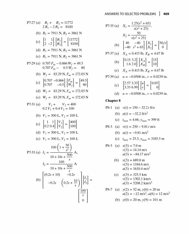
ANSWERS TO SELECTED PROBLEMS 409
P7-27 (a) R1 + R2 = 117722 R1 − 2 R2 = 8100
(b) R1 = 7911 N, R2 = 3861 N
(c)[
1 12 −2
] [R1R2
]=[
117728100
](d) R1 = 7911 N, R2 = 3861 N
(e) R1 = 7911 N, R2 = 3861 N
P7-29 (a) 0.707 Fm − 0.866 Wf = 49.50.707 Fm − 0.5 Wf = 80
(b) Wf = 83.29 N, Fm = 172.03 N
(c)[
0.707 −0.8660.707 −0.5
] [FmWf
]=[
49.580
](d) Wf = 83.29 N, Fm = 172.03 N
(e) Wf = 83.29 N, Fm = 172.03 N
P7-31 (a) V1 + V2 = 4000.2 V1 + 0.4 V2 = 100
(b) V1 = 300 L, V2 = 100 L
(c)[
1 10.2 0.4
] [V1V2
]=[
400100
](d) V1 = 300 L, V2 = 100 L
(e) V1 = 300 L, V2 = 100 L
P7-33 (a) I1 =100
(1 + 50
s2
)10 + 10s + 500
s
A,
I2 = 100
10 + 10s + 500s
A
(b)
⎡⎢⎢⎢⎣(0.2s + 10) −0.2s
−0.2s(
0.2s + 10s
)⎤⎥⎥⎥⎦[
I1I2
]=
⎡⎢⎢⎣100
s
0
⎤⎥⎥⎦
P7-35 (a) X1 =1.25(s2 + 65)
s(s2 + 25),
X2 = 50s(s2 + 25)
(b)[
40 −40−40 s2 + 65
] [X1X2
]=[
50∕s0
]P7-37 (a) XA = 0.415 lb, XB = 4.67 lb
(b)[
0.15 3.21.6 2.0
] [XAXB
]=[
1510
](c) XA = 0.415 lb, XB = 4.67 lb
P7-39 (a) u = −0.0508 in., v = 0.0239 in.
(c)[
2.57 3.333.33 6.99
] [uv
]=[
0.050
](d) u = −0.0508 in., v = 0.0239 in.
Chapter 8
P8-1 (a) v(t) = 150 − 32.2 t ft/s
(b) a(t) = −32.2 ft/s2
(c) tmax = 4.66, ymax = 399 ft
P8-3 (a) v(t) = 250 − 9.81 t m/s
(b) a(t) = −9.81 m/s2
(c) tmax = 25.5, ymax = 3185.5 m
P8-5 (a) x(3) = 7.0 mv(3) = 14.14 m/sa(3) = −84.17 m/s2
(b) x(3) = 689.8 mv(3) = 1184.6 m/sa(3) = 1610.4 m/s2
(c) x(3) = 325.5 kmv(3) = 1302.1 km/sa(3) = 5208.2 km/s2
P8-7 (a) y(2) = 52 m, y(6) = 20 ma(2) = −12 m/s2, a(6) = 12 m/s2
(b) y(0) = 20 m, y(9) = 101 m

410 ANSWERS TO SELECTED PROBLEMS
P8-9 (a) v(t) = 0.125 e−2 t (3 t2 − 2 t3) V
(b) i(0) = 0 A and i(1.5) = 0.168 A
P8-11 (a) v(t) = −5.2 e−200 t Vp(t) = −67.6 e−400 t Wpmax = 67.6 W at t = 0 s
(b) v(t) = −4.8𝜋 sin(120𝜋 t) Vp(t) = −48 sin(240𝜋 t) W
pmax = 48𝜋 W at t = 3480
s
P8-13 (a) i(t) = −4𝜋 sin(200𝜋 t) A
(b) p(t) = −1000𝜋 sin(400𝜋 t) Wpmax = 1000𝜋 W
P8-15 (a) 0 ≤ t ≤ 2 s: a(t) = −4 m/s2
2 < t ≤ 6 s: a(t) = 4 m/s2
6 < t ≤ 8 s: a(t) = −4 m/s2
(b) 0 ≤ t ≤ 2 s: quadratic withdecreasing slope/concave downx(t) = −2 t2 m/s, x(2) = −8 m
2 < t ≤ 6 s: quadratic withincreasing slope andzero slope at t = 4 s, therefore,xmin = −16 m at t = 4 s
x(6) = −16 + 12× 2 × 8 = −8 m
6 < t ≤ 8 s: quadratic withdecreasing slope,zero slope at t = 8 s
x(8) = −8 + 12× 2 × 8 = 0 m
P8-17 (a) 0 ≤ t ≤ 4 s: v(t) = 12 − 3 t m/s
4 < t ≤ 8 s: v(t) = −12 + 3 t m/s
t > 8 s: v(t) = 12 m/s
(b) 0 ≤ t ≤ 4 s: quadratic withdecreasing slope/concave downSlope = 0 at t = 4 s
x(4) = 0 + 12× 4 × 12 = 24 m
4 < t ≤ 8 s: quadratic withincreasing slope/concave up
x(8) = 24 + 12× 4 × 12 = 48 m
P8-19 (a) 0 ≤ t ≤ 2 s: linear withslope = 5 m/s2, since v(0) =0,v(t) = 5 t, and v(2) = 10 m/s
2 < t ≤ 5 s: linear withslope = −5 m/s2, since v(2) =10,v(t) = 10 − 5 (t − 2) = 20 − 5 tv(5) = −5 m/s
5 < t ≤ 6 s: linear withslope= 5 m/s2, since v(5)= −5 m/s,v(t) = −5 + 5(t − 5) = −30 + 5tv(6) = 0 m/s
t > 6 s: v(t) = 0 m/s
(b) 0 ≤ t ≤ 2 s: quadratic withincreasing slope/concave up
x(t) = 2.5 t2, x(2) = 10 m. Also,
x(2) = 0 + 12× 4 × 10 = 10 m
2 < t ≤ 5 s: quadratic withdecreasing slope/concave downzero slope at t = 4 s, therefore,
x(4) = 10 + (1∕2) × 2 × 10 = 20 mx(5) = 20 − (1∕2) × 1 × 5 = 17.5 m
5 < t ≤ 6 s: quadratic withincreasing slope, zero slope at t= 5,
x(6) = 17.5 − 12× 1 × 5 = 15 m
P8-21 Current:
0 ≤ t ≤ 1 s: linear with
slope = 12× 6 = 3 A/s
since i(0) = 0, i(t) = 3 t Ai(1) = 3 A
1 < t ≤ 2 s: linear withslope = 0 A/s, since i(1) = 3 A,i(t) = 3 A, and i(2) = 3 A
2 < t ≤ 3 s: linear withslope = 3 A/s, since i(2) = 3,i(t) = 3 + 3(t − 2) = −3 + 3ti(3) = 6 A

ANSWERS TO SELECTED PROBLEMS 411
P8-21 3 < t ≤ 4 s: linear withslope = 0 A/s, since i(3) = 6 A,i(t) = 6 A, and i(4) = 6 A
4 < t ≤ 5 s: linear withslope = 3 A/s, since i(4) = 6,i(t) = 6 + 3(t − 4) = −6 + 3ti(5) = 9 A
Power:
0 ≤ t ≤ 1 s: p(t) = 18 t W1 < t ≤ 2 s: p(t) = 0 W2 < t ≤ 3 s: p(t) = −18+
18 t W3 < t ≤ 4 s: p(t) = 0 W4 < t ≤ 5 s: p(t) = −36+
18 t W
P8-23 Current:
0 ≤ t ≤ 1 ms: linear with
slope = 12 × 10−3
× 10
= 5000 A/ssince i(0) = 0, i(t) = 5000 t Ai(1 × 10⁻³) = 5 A
1 < t ≤ 2 ms: linear with
slope = 12 × 10−3
(−10)
= −5000 A/ssince i(1 × 10⁻³) = 5 A,i(t) = 5 − 5000(t − 1 × 10⁻³)= 10 − 5000 t Ai(2 × 10⁻³) = 0
2 < t ≤ 3 ms: linear with
slope = 12 × 10−3
× 10 = 5000 A/s
since i(2 × 10⁻³) = 0,i(t) = 0 + 5000(t − 2 × 10⁻³)= −10 + 5000 t Ai(3 × 10⁻³) = 5 A
Power:
0 ≤ t ≤ 1 ms: p(t) = 50 × 103t W1 < t ≤ 3 ms: p(t) = − W
−100 + 50 × 103t
P8-25 Charge:
0 ≤ t ≤ 1 ms: q(t) = t mC1 < t ≤ 2 ms: q(t) = 1 mC2 < t ≤ 3 ms:q(t) = −3 + 3 t mC3 < t ≤ 4 ms: q(t) = t mC4 < t ≤ 5 ms: q(t) = 12 − 2 t mCt > 5 ms: q(t) = 2 mC
Voltage:
v(t) = 4000 q(t) V
P8-27 (a) x =√
l2 − b2
3
ymax = P b6EIl
√l2 − b2
3
(2 b2
3− 2 l2
3
)(b) 𝜃(0) = P b
6EIl(b2 − l2)
𝜃(l) = P b6EIl
(b2 + 2 l2)
P8-29 (a) 𝜃(x) =Mo
6EI L(L2 − 3
2L x − 3 x2)
(b) x = 0.345 L
ymax =0.0358 Mo L2
EI
(c) 𝜃(0) =Mo L6 EI
, y(0) = 0
𝜃
(L2
)= −
Mo L12 EI
, y(L
2
)= 0
P8-31 (a) x = L∕√
5
ymax = −0.00239 L4
EI
(b) 𝜃(0) = −Wo L3
120 EI𝜃(L) = 0
P8-33 (a) 𝜃(x) = 2𝜋 AL
cos(
2𝜋 xL
)(b) 𝜃(0) = −2𝜋 A
L
𝜃
(L2
)= 2𝜋 A
L
𝜃(L) = −2𝜋 AL
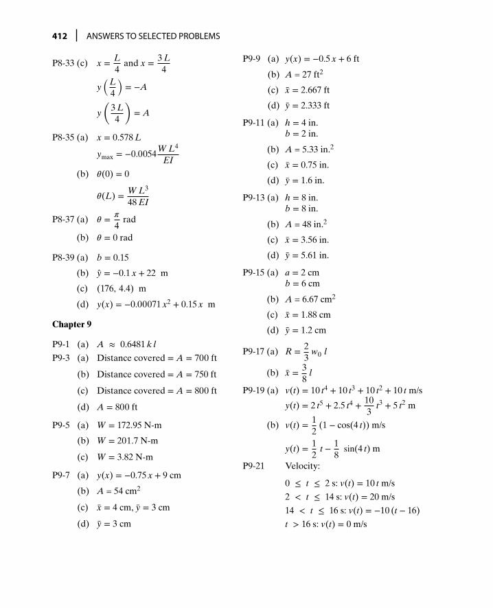
412 ANSWERS TO SELECTED PROBLEMS
P8-33 (c) x = L4
and x = 3 L4
y(L
4
)= −A
y(
3 L4
)= A
P8-35 (a) x = 0.578 L
ymax = −0.0054W L4
EI
(b) 𝜃(0) = 0
𝜃(L) = W L3
48 EI
P8-37 (a) 𝜃 = 𝜋
4rad
(b) 𝜃 = 0 rad
P8-39 (a) b = 0.15
(b) y = −0.1 x + 22 m
(c) (176, 4.4) m
(d) y(x) = −0.00071 x2 + 0.15 x m
Chapter 9
P9-1 (a) A ≈ 0.6481 k l
P9-3 (a) Distance covered = A = 700 ft
(b) Distance covered = A = 750 ft
(c) Distance covered = A = 800 ft
(d) A = 800 ft
P9-5 (a) W = 172.95 N-m
(b) W = 201.7 N-m
(c) W = 3.82 N-m
P9-7 (a) y(x) = −0.75 x + 9 cm
(b) A = 54 cm2
(c) x = 4 cm, y = 3 cm
(d) y = 3 cm
P9-9 (a) y(x) = −0.5 x + 6 ft
(b) A = 27 ft2
(c) x = 2.667 ft
(d) y = 2.333 ft
P9-11 (a) h = 4 in.b = 2 in.
(b) A = 5.33 in.2
(c) x = 0.75 in.
(d) y = 1.6 in.
P9-13 (a) h = 8 in.b = 8 in.
(b) A = 48 in.2
(c) x = 3.56 in.
(d) y = 5.61 in.
P9-15 (a) a = 2 cmb = 6 cm
(b) A = 6.67 cm2
(c) x = 1.88 cm
(d) y = 1.2 cm
P9-17 (a) R = 23
w0 l
(b) x = 38
l
P9-19 (a) v(t) = 10 t4 + 10 t3 + 10 t2 + 10 t m/s
y(t) = 2 t5 + 2.5 t4 + 103
t3 + 5 t2 m
(b) v(t) = 12
(1 − cos(4 t)) m/s
y(t) = 12
t − 18
sin(4 t) m
P9-21 Velocity:
0 ≤ t ≤ 2 s: v(t) = 10 t m/s
2 < t ≤ 14 s: v(t) = 20 m/s
14 < t ≤ 16 s: v(t) = −10 (t − 16)
t > 16 s: v(t) = 0 m/s

ANSWERS TO SELECTED PROBLEMS 413
P9-21 Position:
0 ≤ t ≤ 2 s: quadratic withincreasing slope/concave upx(t) = 5 t2, x(2) = 20 m
2 < t ≤ 14 s: linearx(t) = 20 (t − 1), x(14) = 260 m
14 < t ≤ 16 s: quadratic withdecreasing slope/concave down
x(16) = 260 + 12
(2)(20) = 280 m
P9-23 Velocity:
0 ≤ t ≤ 3 s: v(t) = 10 t m/s
3 < t ≤ 6 s: v(t) = −10(t − 6)
6 < t ≤ 12 s: v(t) = (t − 6)
t > 12 s: v(t) = 30 m/s
Position:
0 ≤ t ≤ 3 s: quadratic withincreasing slope/concave upx(t) = 5 t2, x(3) = 45 m
3 < t ≤ 6 s: quadratic withdecreasing slope/concave down
x(6) = 45 + 12
(3)(30) = 90 m
6 < t ≤ 12 s: quadratic withincreasing slope/concave up
x(16) = 90 + 12
(30)(6) = 180 m
P9-25 q(t) = 13
t3 − t2 + t C
P9-27 (a) vo(t) = 10 (cos(10 t) − 1) V
(b) w(t) = 7.5 + 2.5 cos(20 t)−10 cos(10 t) mJ
P9-29 (a) vo(t) = sin(100 t) − 100 t V
(b) w(t) = 7.5 + 2.5 cos(20 t)−10 cos(10 t) mJ
P9-31 (a) vo(t) = 10(1 − e−10 t
)+ 10 V
(b) w(t) = 0.01(1 − e−20 t
)+ 0.005 J
P9-33 v(0) = 0 V, v(1) = −10 V andv(2) = 0 V
0 ≤ t ≤ 2 s: quadratic withincreasing slope/concave up
Then simply repeat every 2 s
P9-35 (a) v(0) = 0 V, v(1) = 10 V,v(2) = 10 V, v(3) = 15 V,v(4) = 5 V andv(t) = 5 V for t > 4 s
Since i(t) is constant over eachinterval, v(t) is linear betweeneach interval
P9-37 (a) 0 ≤ t ≤ 0.008 s:
xbelted(t) = 0.102 sin(62.5𝜋 t) m
0.008 < t ≤ 0.04 s:
xbelted(t) = 0.102 m
(b) 0 ≤ t ≤ 0.04 s:
xunbelted(t) = 0.509 sin(12.5𝜋 t) m
(c) xunbelted(0.04) − xunbelted(0.04) =0.407 m
P9-39 (a) y(x) = − p xh G
( L3− x
2+ x2
3 L− x3
12 L2 )
P9-39 (b) x = L
ymax =p L2
12 h G
Chapter 10
P10-1 (a) htran(t) = C e−kA
t
(b) hss(t) = Q(A2 𝜔2 + k2
)×(k sin𝜔 t − A𝜔 cos𝜔 t)
(c) h(t) = Q
A2 𝜔2 + k2(A𝜔 e−
kA
t
+k sin𝜔 t − A𝜔 cos𝜔 t)
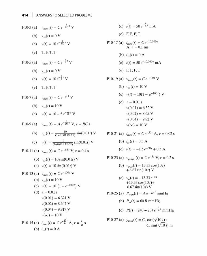
414 ANSWERS TO SELECTED PROBLEMS
P10-3 (a) vtran(t) = C e−1
RCt V
(b) vss(t) = 0 V
(c) v(t) = 10 e−1
RCt V
(e) T, F, T, T
P10-5 (a) vtran(t) = C e−12
t V
(b) vss(t) = 0 V
(c) v(t) = 10 e−12
t V
(e) T, F, T, T
P10-7 (a) vtran(t) = C e−120
t V
(b) vss(t) = 10 V
(c) v(t) = 10 − 5 e−120
t V
P10-9 (a) vtran(t) = A e−1
RCt V, 𝜏 = RC s
(b) vss(t) = 10(1+0.001 R2 C2)
sin(0.01t) V
(c) v(t) = 10(1+0.001 R2 C2)
sin(0.01t) V
P10-11 (a) vtran(t) = C e−2.5 t V, 𝜏 = 0.4 s
(b) vss(t) = 10 sin(0.01t) V
(c) v(t) = 10 sin(0.01t) V
P10-13 (a) vtran(t) = C e−100 t V
(b) vss(t) = 10 V
(c) v(t) = 10(1 − e−100 t
)V
(d) 𝜏 = 0.01 s
v(0.01) = 6.321 V
v(0.02) = 8.647 V
v(0.04) = 9.817 V
v(∞) = 10 V
P10-15 (a) itran(t) = C e−RL
t A, 𝜏 = LR
s
(b) iss(t) = 0 A
(c) i(t) = 50 e−RL
t mA
(e) F, F, F, T
P10-17 (a) itran(t) = C e−10,000 t
A, 𝜏 = 0.1 ms
(b) iss(t) = 0 A
(c) i(t) = 50 e−10,000 t mA
(e) F, F, F, T
P10-19 (a) vtran(t) = C e−100 t V
(b) vss(t) = 10 V
(c) v(t) = 10(1 − e−100 t) V
(e) 𝜏 = 0.01 s
v(0.01) = 6.32 V
v(0.02) = 8.65 V
v(0.04) = 9.82 V
v(∞) = 10 V
P10-21 (a) itran(t) = C e−50 t A, 𝜏 = 0.02 s
(b) iss(t) = 0.5 A
(c) i(t) = −1.5 e−50 t + 0.5 A
P10-23 (a) vo,tran(t) = C e−5 t V, 𝜏 = 0.2 s
(b) vo,ss(t) = 13.33 cos(10 t)+ 6.67 sin(10 t) V
(c) vo(t) = −13.33 e−5 t
+13.33 cos(10 t)+6.67 sin(10 t) V
P10-25 (a) Ptran(t) = A e−1
RCt mmHg
(b) Pss(t) = 60 R mmHg
(c) P(t) = 240 − 234 e−18
t mmHg
P10-27 (a) ytran(t) = C3 cos(√
10 t)+C4 sin(
√10 t) m
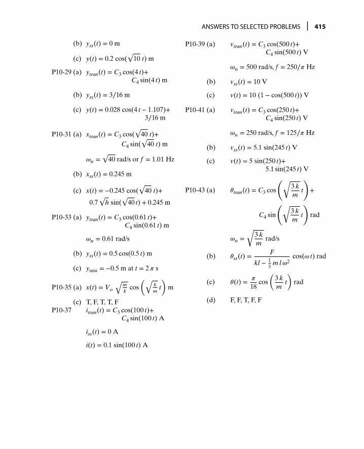
ANSWERS TO SELECTED PROBLEMS 415
(b) yss(t) = 0 m
(c) y(t) = 0.2 cos(√
10 t) m
P10-29 (a) ytran(t) = C3 cos(4 t)+C4 sin(4 t) m
(b) yss(t) = 3∕16 m
(c) y(t) = 0.028 cos(4 t − 1.107)+3∕16 m
P10-31 (a) xtran(t) = C3 cos(√
40 t)+C4 sin(
√40 t) m
𝜔n =√
40 rad/s or f = 1.01 Hz
(b) xss(t) = 0.245 m
(c) x(t) = −0.245 cos(√
40 t)+
0.7√
h sin(√
40 t) + 0.245 m
P10-33 (a) ytran(t) = C3 cos(0.61 t)+C4 sin(0.61 t) m
𝜔n = 0.61 rad/s
(b) yss(t) = 0.5 cos(0.5 t) m
(c) ymin = −0.5 m at t = 2𝜋 s
P10-35 (a) x(t) = Vo
√mk
cos(√
km
t)
m
(c) T, F, T, T, FP10-37 itran(t) = C3 cos(100 t)+
C4 sin(100 t) A
iss(t) = 0 A
i(t) = 0.1 sin(100 t) A
P10-39 (a) vtran(t) = C3 cos(500 t)+C4 sin(500 t) V
𝜔n = 500 rad/s, f = 250∕𝜋 Hz
(b) vss(t) = 10 V
(c) v(t) = 10 (1 − cos(500 t)) V
P10-41 (a) vtran(t) = C3 cos(250 t)+C4 sin(250 t) V
𝜔n = 250 rad/s, f = 125∕𝜋 Hz
(b) vss(t) = 5.1 sin(245 t) V
(c) v(t) = 5 sin(250 t)+5.1 sin(245 t) V
P10-43 (a) 𝜃tran(t) = C3 cos
(√3 km
t
)+
C4 sin
(√3 km
t
)rad
𝜔n =√
3 km
rad/s
(b) 𝜃ss(t) = F
kl − 13
m l𝜔2cos(𝜔 t) rad
(c) 𝜃(t) = 𝜋
18cos
(3 km
t)
rad
(d) F, F, T, F, F


INDEX
Acceleration, 221, 226–240Acceleration due to gravity, 221Addition of sinusoids of same frequency, 166–173,
See also under SinusoidsAddition of two complex numbers, 137Angular frequency, sinusoids, 161Angular motion of one-link planar robot,
159–162frequency and period, relations between,
160–162Antiderivative, 280Armature current in DC motor, 140–141Asphalt problem, 278–283Average velocity, 219
Bending moment, 250
Capacitor, 314–321current passing through, 247–250, 314–321energy stored in, 314–321impedance of, 135voltage across, 247–250, 314–321
Center of Gravity (Centroid), 286–293alternate definition of, 293–296determination using vertical rectangles, 292evaluation using horizontal elemental
areas, 89first moment of area, 294of triangular section, 86
Chain rule of derivative, 241Complementary solution, 347Complex conjugate, 145–147Complex numbers, 132–156
addition of two complex numbers, 137armature current in a DC motor, 140–141complex conjugate, 145–147division of complex number in polar form,
139–140examples, 141–145exponential form, 136impedance of a series RLC circuit, 136–137impedance of R, L, and C as a, 134–135
multiplication of complex number in polarform, 139
polar form, 136position of one-link robot as, 133–134subtraction of two complex numbers, 137
Cos(𝜃), 61Cramer’s Rule, 188–189, 192Current, 240
flowing in inductor, 322–326passing through a capacitor, 314–321
Definite integral, 280Deflection, 251Derivatives, 218–277
applications in dynamics, 225–240applications in electric circuits, 240–250applications in strength of materials, 250–260,
See also Material strengthchain rule of, 241definition, 218–221examples of, 261–266maxima and minima, 221–225
Differential equations (DEQ), 345–400first-order differential equations, 348–374leaking bucket, 345–346linear DEQ, solution with constant coefficients,
347–348second-order differential equations, 374–390,
See also separate entryDirect kinematics of two-link robot, 73–74Distributed loads, 251, 296–302
on beams, statically equivalent loading, 297–302hydrostatic pressure on a retaining wall,
296–297Division of complex number in polar form,
139–140Dynamics
derivatives applications in, 225–240integrals applications in, 302–314
Elbow-up solution for 𝜃1, 77–79Electric circuits, 314–321
417

418 INDEX
Electric circuits (continued )current and voltage in a capacitor,
314–321derivatives applications in, 240–250integrals applications in, 314–321
Energy stored in a capacitor, 314–321Equivalent resistance, 37–38Euler’s formula, 134Exponential form, complex numbers, 136
Factoring, 33First-order differential equations, 348–374Force-displacement relationship, 6–7Free-body diagram (FBD), 117, 119
Graphical method solution, for two-loop circuit,185–186
Homogeneous solution, 347Hydrostatic pressure on a retaining wall,
296–297
Impedanceof capacitor, 135of inductor, 134–135, 137–140of resistor, 134, 137–140of a series RLC circuit, 136–137
Indefinite integrals, 281Inductor
as a circuit element, 243current and voltage in, 243–247, 322–326impedance of, 134–135
Integrals, 278–344, See also Distributed loadsAsphalt problem, 278–283concept of work, 283–286, See also Workdefinite integral, 280in dynamics, 302–314in electric circuits, 314–321examples, 327–333indefinite integrals, 281inductor, current and voltage in, 322–326inverse operations, 281in statics, 286–296, See also Statics
Inverse kinematics of one-link robot, 68–72Inverse kinematics of two-link robot, 75–79Inverse operations, 281
Kirchhoff’s voltage law (KVL), 3, 184
Linear DEQ, solution with constant coefficients,347–348
steady-state solution, 348transient solution, 347
Linear frequency, sinusoids, 161Low-pass filter, 373
Material strength, derivatives applications in,250–260
bending moment, 250deflection, 251distributed load, 251maximum stress under axial loading,
256–260maximum value, 259minimum value, 259moment, 255shear force, 251, 255slope, 252
Matrix algebra method solutiontension in cables, 191–192for two-loop circuit, 186–188
Maxima, 221–225Maximum stress under axial loading,
256–260inclined section of the rectangular bar, 256normal and shear stresses acting on the inclined
cross section, 258rectangular bar under axial loading, 256
Method of undetermined coefficients, 348Minima, 221–225Moment, 255, 298Multiplication of complex number in polar form,
139
Newton’s first law, 117Newton’s second law, 375
Ohm’s law, 3, 184One-link planar robot
angular motion of, 159–162as a sinusoid, 157–159
Particular solution, 348Period, one-link planar robot, 161Phase angle, 162–164Phase shift, 162–164Polar form
complex numbers, 136position vector in, 107–110
Position, 226–240Position of one-link robot as a complex number,
133–134Position vector
in polar form, 107–110in rectangular form, 107
Power, 240
Quadratic equations, 32–59current in a lamp, 36–37equivalent resistance, 37–38examples, 38–50

INDEX 419
pipeline through parabolic hill, 48–50projectile in a vertical plane, 32–36resistors in parallel, 37
Quadratic formula, 33
Rectangular form, position vector in, 107Reference angle, 65Relative velocity, 114Repeated roots, 347Resistive circuit, voltage-current relationship
in, 3–5Resistor, impedance of, 134Resistors in parallel, 37Resonance, 383
Second-order differential equations, 374–390forced vibration of a spring-mass system,
379–386free vibration of a spring-mass system, 374–379second-order LC circuit, 386–390
Second-order LC circuit, 386–390Shear force, 251, 255Sin(𝜃), 61Sinusoids, 157–183
addition of sinusoids of same frequency,166–173
amplitude of, 160general form of, 164–166one-link planar robot as, 157–159phase angle, 162–164phase shift, 162–164sine function, two cycles of, 159time shift, 162–164
Slope, 252Slope-intercept method, 5Speed at impact, 219Spring-mass system
forced vibration of, 379–386free vibration of, 374–379
Static equilibrium, 117, 119Statically equivalent loading, 297–302Statics, integrals application in, 286–296
Center of Gravity (Centroid), 286–293, Seealso individual entry
Steady-state solution, 348Straight lines, 1–31
examples, 8–18force-displacement relationship, 6–7
slope-intercept method, 5vehicle during braking, 1–3voltage-current relationship in resistive
circuit, 3–5Substitution method solution
tension in cables, 190–191for two-loop circuit, 185
Subtraction of two complex numbers, 137Systems of equations, 184–217
examples, 193–205solution of a two-loop circuit, 184–189, See
also Tension in cables
Tension in cables, 190–192Cramer’s Rule, 192matrix algebra method, 191–192substitution method, 190–191
Time constant, 351, 357Time shift, 162–164Transient solution, 347Triangular section, centroid of, 86Trigonometry, 60–105
examples, 89–96one-link planar robot, 60–72reference angle, 65sine and cosine functions, values of, 64trigonometric functions in four
quadrants, 64two-link planar robot, 72–89
Two-dimensional vectors, 106–131free-body diagram (FBD), 117, 119position vectorrelative velocity, 114static equilibrium, 117, 119vector addition, 110–123
Two-loop circuit, solution of, 184–189
Vector addition, 110–123Velocity, 226–240Voltage, 240
in capacitor, 314–321in inductor, 322–326
Voltage-current relationship in resistivecircuit, 3–5
Work, 283–286as area under a constant force curve, 284as area under a variable force curve, 284


Useful MathematicalRelations
Algebra and GeometryArithmetic Operations
a(b + c) = ab + acab+ c
d= ad + bc
bda + c
b= a
b+ c
b
abcd
= ab× d
c
= adbc
Exponents and Radicals
xm xn = xm+n
xm
xn = xm−n
(xm)n = = xm n
x−n = 1xn
(x y)n = xn yn
(xy
)n
= xn
yn
x1∕n = n√
x
xm∕n = n√
xm
=(
n√
x)m
n√
x y = n√
x n√
y
n
√xy=
n√
xn√
y
Factoring Special Polynomials
x2 − y2 = (x + y) (x − y)
x3 + y3 = (x + y) (x2 − xy + y2)
x3 − y3 = (x − y) (x2 + xy + y2)Quadratic Formula
If a x2 + b x + c = 0. then
x = −b ±√
b2 − 4 a c2 a
Lines
Equation of line with slope m and y-intercept b:
y = mx + b
Slope of line through points P1(x1, y1)and P2(x2, y2):
m =y2 − y1
x2 − x1
Point-slope equation of line throughpoint P1(x1, y1) with slope m:
y − y1 = m (x − x1)
Point-slope equation of line throughpoint P2(x2, y2) with slope m:
y − y2 = m (x − x2)
Distance Formula
Distance between points P1(x1, y1) andP2(x2, y2):
d =√
(x2 − x1)2 + (y2 − y1)2
Area of a Triangle:
A = 12
b h
= 12
a b sin(𝜃)b
ha
θ
Equation, Area and Circumference ofCircle:
Equation:
(x − k)2 + (y − k)2 = r2
A = 𝜋 r2
C = 2𝜋 r
y
(h, k)
x
r
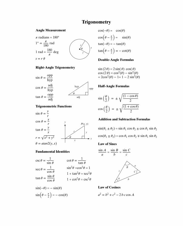
Trigonometry
Angle Measurement
𝜋 radians = 180
1 = 𝜋
180rad
1 rad = 180𝜋
deg
s = r 𝜃
rs
r
θ
Right-Angle Trigonometry
sin 𝜃 =opphyp
cos 𝜃 =adjhyp
tan 𝜃 =oppadj
hypopp
adj
θ
Trigonometric Functions
sin 𝜃 =yr
cos 𝜃 = xr
tan 𝜃 =yx
r =√
x2 + y2
𝜃 = atan2(y, x)
yr
x
y
xθ
P(x, y)
Fundamental Identities
csc 𝜃 = 1sin 𝜃
sec 𝜃 = 1cos 𝜃
tan 𝜃 = sin 𝜃
cos 𝜃
cot 𝜃 = 1tan 𝜃
sin2𝜃 +cos2𝜃 = 1
1 + tan2𝜃 = sec2𝜃
1 + cot2𝜃 = csc2𝜃
sin(−𝜃) = − sin(𝜃)
sin(𝜃 − 𝜋
2
)= − cos(𝜃)
cos(−𝜃) = cos(𝜃)
cos(𝜃 − 𝜋
2
)= sin(𝜃)
tan(−𝜃) = − tan(𝜃)
tan(𝜃 − 𝜋
2
)= − cot(𝜃)
Double-Angle Formulas
sin (2 𝜃) = 2 sin( 𝜃) cos( 𝜃)cos (2 𝜃) = cos2(𝜃) − sin2(𝜃)= 2cos2(𝜃) − 1= 1 − 2 sin2(𝜃)
Half-Angle Formulas
sin(𝜃
2
)= ±
√(1 − cos 𝜃)
2
cos(𝜃
2
)= ±
√(1 + cos 𝜃)
2
Addition and Subtraction Formulas
sin(𝜃1 ± 𝜃2) = sin 𝜃1 cos 𝜃2 ± cos 𝜃1 sin 𝜃2
cos(𝜃1 ± 𝜃2) = cos 𝜃1 cos 𝜃2 ∓ sin 𝜃1 sin 𝜃2
Law of Sines
sin Aa
= sin Bb
= sin Cc
C
a
b
c
A
B
Law of Cosines
a2 = b2 + c2 − 2 b c cos A

Differentiation Rules
ddt
(c) = 0
ddt
[c f (t)] = c f (t)
ddt
(c1 f (t) + c2 g(t)) = c1 f (t) + c2 g(t)
ddt
(c1 f (t) − c2 g(t)) = c1 f (t) − c2 g(t)
ddt
(tn) = n tn−1
Product Rule
ddt
[f (t) g(t)] = f (t) g(t) + f (t) g(t)
Quotient Rule
ddt
[f (t)g(t)
]=
g(t) f (t) − f (t) g(t)
[g(t)]2
Chain Rule
ddt
f (g(t)) =dfdg
×dgdt
Power Rule
ddt
(tn) = n tn−1
Integration Rules
∫ y dx = y x − ∫ x dy
∫ xn dx = xn+1
n + 1+ C, n ≠ −1
∫ ea x dx = ea x
a+ C
∫ sin(a x) dx = −cos(a x)
a+ C
∫ cos(a x) dx =sin(a x)
a+ C
∫ c f (x) dx = c ∫ f (x) dx
∫ [c1f (x) + c2g(x)]dx= c1 ∫ f (x)dx + c2 ∫ g(x)dx
Exponential Functions
ddt
(ea t) = a ea t
Trigonometric Functions
ddt
[sin (a t)] = a cos (a t)
ddt
[cos (a t)] = − a sin (a t)

Commonly UsedUnits in Engineering
Unit English SI Conversion FactorLength in. or ft m 1 in. = 0.0254mArea in.2 or ft2 m2 1550 in.2 = 1 m2
Volume in.3 or ft3 m3 61024 in.3 = 1 m3
Velocity in./s or ft/s m/s 1 in./s = 0.0254 m/sAcceleration in./s2 or ft/s2 m/s2 1 in./s2 = 0.0254m/s2
Force lb N 1 lb = 4.45 NPressure (Stress) lb/in.2 (psi) N/m2 (Pa) 1 psi = 6890 Pa
Mass lbm kg 1 lbm = 0.454 kgEnergy in.-lb or ft-lb N-m (J) 1 in.-lb = 0.113 JPower in.-lb/s or ft-lb/s W (J/s) 1 in.-lb/s = 0.113 W
Voltage Volts (V) Volts (V)Current Amps (A) Amps (A)
Resistance Ohms (Ω) Ohms (Ω)in.ductance Henrys (H) Henrys (H)Capacitance Farads (F) Farads (F)
Commonly Used Prefixes in EngineeringNano (n) 10−9
Micro (𝜇) 10−6
Milli (m) 10−3
Centi (c) 10−2
Kilo (K) 103
Mega (M) 106
Giga (G) 109