Proceedings of the International Conference on Engineering, Science, and Industrial Applications

Volume 1, 2 August 2017 ISSN 2521-3814

Publisher: Chulalongkorn Business School, Chulalongkorn University

Address: Chulalongkorn Business School, Chulalongkorn University

50th Memorial Building 8,

#254 Phayathai Rd,

Wang Mai, Khet Pathum Wan, Krung Thep Maha Nakhon 10330,

Bangkok, Thailand

Editor

Wachara Chantatub, Chulalongkorn University, Thailand

Associate Editors

Chian-Son Yu, Shih Chien University, Taiwan

Pimmanee Ratanawicha, Chulalongkorn University, Thailand

Jung-Fa Tsai, National Taipei University of Technology, Taiwan

Editorial Committee Members

Yannick Le Moullec, Tallinn University of Technology, Estonia Mohamad Azemi Mohd Noor, Universiti Kuala Lumpur, Malaysia Shinn-Liang Chang , National Formosa University, Taiwan Davendra Kumar Chauhan, Noida International University, India Laxman Gangwani, Texas Tech University Health Sciences Center, USA Abdul Razak Abdul Hadi, Universiti Kuala Lumpur, Malaysia Chao-Ching Ho, National Taipei University of Technology, Taiwan Yi-Chung Hu, Chung Yuan Christian University, Taiwan Yao-Huei Huang, Southwest Jiaotong University, China Feng-Jang Hwang, University of Technology Sydney, Australia Nor Zunanini Abd Kadir, University Kuala Lumpur, Malaysia

Ming-Hua Lin, Shih Chien University, Taiwan Chikako Morimoto, Tokyo Institute of Technology, Japan Adarsh Kumar Pandey, University of Malaya, Malaysia Sulaiman Sajilan, Universiti Kuala Lumpur Business School, Malaysia Dao Vu Truong Son, Vietnam national university, Vietnam Uthai Tanlamai, Chulalongkorn University, Thailand Aurelija Ulbinaite, Vilnius University, Lithuania Jen-Hung Wang, City University of Macau, Macao Lai Chin Wei, University Malaya, Malaysia

 

Table of Contents ICESI_0031 ................................................................................................................... 2

Milk Clotting Activity of Protease Extracted from Yatsin Biri Ginger Cultivar of Northwestern Nigeria ................................................................................................ 2

ICESI_0033 ................................................................................................................... 6 Extraction of titanium dioxide from ilmenite waste via caustic decomposition process .................................................................................................................... 6

ICESI_0043 ................................................................................................................. 12 Determination of Capability Indices of Chemical Oxygen Demand Using SBR for Water Treatment ................................................................................................... 12

ICESI_0068 ................................................................................................................. 23 Building a Long-Term Care Information System Based on the Whole Person Concept through Service-Oriented Architecture ................................................... 23

ICESI_0075 ................................................................................................................. 40 "Determination of the Emissions of Suspended Particles (PM10 AND PM2.5) by Wind Motion Through Mathematical Simulation in the Province of Chimborazo of the Year 2015" ...................................................................................................... 40

ICESI_0076 ................................................................................................................. 47 Study and analysis of NO2 emissions generated by motor vehicles in the “Terminal terrestre” area of Riobamba city, Ecuador ............................................................ 47

ICESI_0081 ................................................................................................................. 62 Biogenic Emissions of Non Methanogenic Volatile Organic Compounds in Ecuador.............................................................................................................................. 62

ICESI_0085 ................................................................................................................. 78 Local fault identification using Microtremor Analysis (case study: local fault in Surabaya river) ..................................................................................................... 78

ICESI_0092 ................................................................................................................. 88 OFDMA in LTE Mobile Communications ............................................................ 88

ICESI_0093 ............................................................................................................... 104 Experimental Investigations of a Parabolic Trough Collector ............................. 104

ICESI_0104 ............................................................................................................... 115 Modeling, Analysis and Design of Mechanical and Structural Systems Involving Uncertainties ....................................................................................................... 115

ICESI_0157 ............................................................................................................... 125 Moving Beyond Corporate Acceleration Programs: The Need for Community Entrepreneurial Acceleration Programs ............................................................. 125

ICESI_0163 ............................................................................................................... 139 Evaluating Triaxial Accelerometers and Force Sensitive Resistors in Building Interactive Freestanding Bags ............................................................................. 139

ICESI_0165 ............................................................................................................... 147 The Feasibility of Deploying Robotic Waiters in the Service Industry ................. 147

ICESI_0173 ............................................................................................................... 157 Optimization of Spray Drying Conditions for Momordica Charantia Rich Charantin Extract Powder .................................................................................. 157

 

 

ICESI_0031

Milk Clotting Activity of Protease Extracted from Yatsin Biri Ginger Cultivar of Northwestern Nigeria

*Murtala, Y., Bayero University, Nigeria

Babandi A., Bayero University, Nigeria

Babagana K., Bayero University, Nigeria

Shehu D., University of Malaya, Malaysia

*Corresponding Author

Abstract

The recurrent increase in prices of calf rennet and ethical considerations linked to the production of such enzymes for cheese making and related processes have ignited a flame of scientific enquiries on the possibility and suitability of their substitution by other enzymes of plant sources. In this research, partial characterization and milk clotting activity (MCA) of (NH4)2SO4 fraction of protease extracted from Yatsin Biri ginger rhizome cultivar of the family Zingiberaceae from northwestern Nigeria were analyzed. The protease extracted showed optimum activity at temperature near 50 °C and pH value of 5.5. Relative activity of the enzyme was also observed within a broad pH range of 4.5 to 7.0 accordingly. The enzyme was completely denatured at higher temperature of 100 °C and a pH range of 11.5. The milk clotting property of the protease indicated 2.83 and 1.81 folds of MCA and milk clotting specific activity (MCSA) respectively in relation to commercial calf rennet with MCA/PA ratio of 2.18. These properties of Yatsin Biri ginger protease, especially its milk clotting activity, make it a suitable candidate for substituting calf rennet application in the food industries, particularly in dairy and cheese making processes.

Keywords: Ginger protease, Milk clotting activity, Calf rennet, Characterization, Extraction.

 

1. Materials and Methods

Collection of Ginger (Zingiber officinale) Rhizome: The fresh ginger rhizome was collected from a harvesting site in Kagarko ginger farming area of Kaduna state, northwestern Nigeria. The sample was identified and authenticated as Yatsin Biri ginger cultivar at the Herbarium Unit of the Department of Plant Biology, Bayero University, Kano. The sample was issued with an accession number (BUKHAN 0299).

Preparation of Crude Extract: The fresh ginger rhizome was washed and minced. The minced sample (90g) was weighed and homogenized with 180 cm3 of distilled water. The homogenate was filtered through a piece of cheese cloth and the filtrate was centrifuged at 4000rpm for 30 minutes. The supernatant was collected and filtered through vacuum pump and 80 cm3 of the filtrate was used for ammonium sulphate precipitation while the remaining 100cm3 was used as crude extract and tested for the protease characteristics.

Protein Precipitation: The protein was precipitated using a modified method of Qiao et al. (2009).

Total Protein Concentration Determination: Total protein was determined using BioAssay Systems' QuantiChromTM protein assay kit based on an improved Coomassie Blue G method (Bradford, 1976) using Bovine Serum Albumin (BSA) as standard.

Protease Activity Assay: The proteases activity (ginger protease and calf rennet) was assayed using casein as substrate. The assay was carried out using a modified method of Tsuchida et al. (1986).

Milk-clotting activity assay: Milk-clotting activity (MCA) was measured by a modification of Hang et al. (2016) procedure.

2. Results

Table 1: Partial Purification of Ginger Protease Extracted from Yatsin Biri Ginger Cultivar from Northwestern Nigeria

Purification Steps

Total Protein (mg)

Proteolytic Activity (PA) (Units) a

Proteolytic Specific Activity (PSA) (Units/mg)

Purification Fold

% Yield

Crude Enzyme Extract

740.81 326.8 ± 10 0.44 - -

Ammonium Sulphate Precipitate b

103.02 77.7 ± 12 0.75 1.70 170%

a –One Unit of enzyme activity is the amount in micromoles of tyrosine equivalents released from casein per minute

b – Precipitation under 15% to 30% Saturation

 

Table 2: Milk Clotting Activities of Protease Extracted Yatsin Biri Ginger Cultivar and Calf Rennet

Milk Clotting Activity (MCA) (Units/cm3) a

Milk Clotting Specific Activity (MCSA) (Units/mg of Protein) b

MCA/PA Ratioc

Calf Rennet 60 0.91 - Ginger Protease 170 1.65 2.18 a – A unit (U) equals the amount (mg) of enzymes required to coagulate 1cm3 of reconstituted skim milk in 1 min at 50 0C and pH 5.5.

b – 103.02 mg total protein content for ginger protease and 65.7 mg of protein for calf rennet

c -- PA for ginger protease: 77.7 Units

Figure 1: Effect of pH on protease extracted from Yatsin Biri ginger protease

Figure 2: Effect of Temperature on Protease Extracted from Yatsin Biri Ginger Cultivar

3. Conclusion

‐10

0

10

20

30

40

50

60

70

80

90

1.5 3.5 5.5 7.5 9.5 11.5 13.5

Enzyme Activity (Units)

pH

0

10

20

30

40

50

60

70

80

0 10 20 30 40 50 60 70 80 90 100

Enzyme Activity (Units)

Temperature (ᵒC)

 

The one-step (ammonium sulphate) fraction of protease extracted from Yatsin Biri ginger rhizome cultivar of northwestern Nigeria showed optimum activity at temperature near 50 °C and a broad range of pH values of 4.5 to 7.5 with an optimum pH at 5.5. The enzyme protein was completely denatured at elevated temperature and alkaline pH. Additional characteristics of the protease obtained in this study, especially its milk clotting activity, broad pH range and moderate temperature make it a suitable candidate for application in the food industries, particularly in cheese making processes.

References

Bradford, M. M. 1976. Rapid and Sensitive Method for the Quantitation of Microgram Quantities of Protein Utilizing the Principle of Protein-Dye Binding. Analytical Biochemistry. 72: 248-254.

Hang, F., Peiyi, L., Qinbo, W., Jin, H., Zhengjun, W., CaixiaGao, Z. L., Hao, Z. and Wei, C. 2016. High Milk-Clotting Activity Expressed by the Newly Isolated Paenibacillus spp. Strain BD3526. Molecules, 21(73):1-1

Qiao, Y., Tong, J., Wei, S., Du, X. and Tang, X. 2009. Computer and computing technologies in agriculture II; In IFIP International Federation for Information Processing; Li, D., Chunjiang, Z., Eds.; Springer: Boston, MA, USA, pp. 1619–1628.

Tsuchida, O., Yamagota, Y. and Ishizuka, J. 1986. An Alkaline Proteinase of an Alkalophilic Bacillus spp. Curr Microbiol.14; 7-12

   

 

ICESI_0033

Extraction of titanium dioxide from ilmenite waste via caustic decomposition process

Huzaikha Awang, Universiti Malaysia Sabah, Malaysia

*Eddy F. Yusslee, Universiti Malaysia Sabah, Malaysia

Ahmad Mukifza, Universiti Malaysia Sabah, Malaysia

Shahril Yusof, Universiti Malaysia Sabah, Malaysia

*Corresponding Author

Abstract

Titanium dioxide (TiO2) has been successfully synthesized from ilmenite waste (98% purity) as raw material by caustic decomposition method using NaOH pellets and followed by sulphate process. The end product was then characterized by using Energy Dispersive X-ray (EDX) to identify its chemical composition, Field Emission Scanning Electron Microscope (FESEM) to investigate the particle morphology and size while X-Ray Diffraction (XRD) to analyse the crystallinity of the extracted titanium. It was found that the TiO2 percentage significantly increased with higher reaction temperature and reached its maximum value of 98.59% yield at 90°C. On the other hand, the acid concentrations (1M, 2M and 3M) also affect the product crystallinity and can be seen from the XRD results analysis

Keywords: Synthetic rutile, Titanium dioxide, Caustic hydrothermal, Sodium titanate.

 

1. Introduction

TiO2 is one of the transition metal oxides and semiconductors with a unique characteristics, good photocatalytic behavior compare to the pure metal. This superb photocatalyst behavior of TiO2 triggered a lot of researchers all over the world to extract and trying to enhance its photocatalytic behaviour by improvise the extracting method since 1923 until now (Jia et al., 2014). There were various extracting methods reported by previous researchers such as the template-assisted method (Suwarnkar et al., 2014), electrochemical anodic oxidation method (Zhang and Nicole, 2009), fiber laser ablation (Boutinguiza et al., 2013), modified molten salt process (Kozakova et al., 2011, Chen et al., 2013) hydrothermal treatment (Ou et al., 2007, Zhang et al., 2009) and etc.

In this study, the chosen method was caustic hydrothermal method as per reported by following researchers (Paulus et al., 2011, Mahdi et al., 2012). According to H. H. Ou, W. Paulus and E. M. Mahdi et al., the caustic hydrothermal method can produce the TiO2 in the powder form and this method can be simply modified in order to achieve a better characteristics of titanium powders (Mahdi et al., 2012). The effect of reaction temperature and acid concentrations on the caustic hydrothermal method were analysed by identifying their chemical composition, morphology and particle size and lastly, their crystallinity phase by using Electron Dispersive (EDX), Field Emission Scanning Electron Microscope (FESEM) and X-Ray Diffraction (XRD) respectively.

2. Materials and Methods

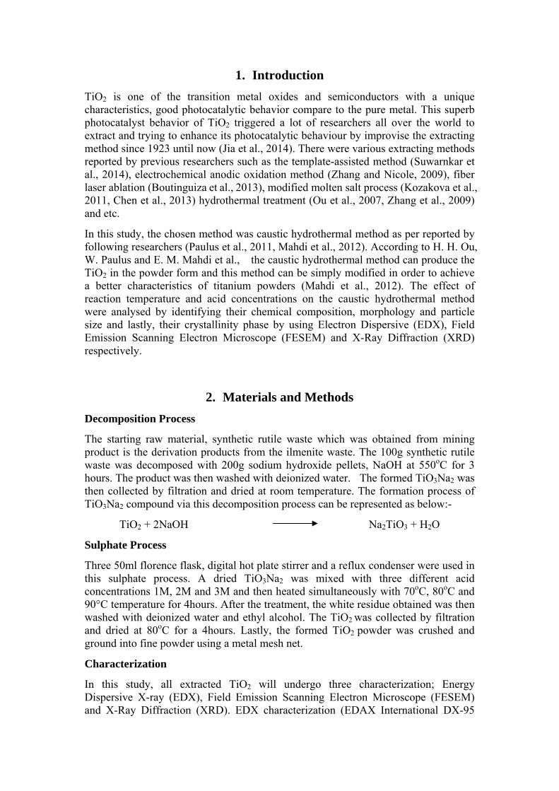
Decomposition Process

The starting raw material, synthetic rutile waste which was obtained from mining product is the derivation products from the ilmenite waste. The 100g synthetic rutile waste was decomposed with 200g sodium hydroxide pellets, NaOH at 550oC for 3 hours. The product was then washed with deionized water. The formed TiO3Na2 was then collected by filtration and dried at room temperature. The formation process of TiO3Na2 compound via this decomposition process can be represented as below:-

TiO2 + 2NaOH Na2TiO3 + H2O

Sulphate Process

Three 50ml florence flask, digital hot plate stirrer and a reflux condenser were used in this sulphate process. A dried TiO3Na2 was mixed with three different acid concentrations 1M, 2M and 3M and then heated simultaneously with 70oC, 80oC and 90°C temperature for 4hours. After the treatment, the white residue obtained was then washed with deionized water and ethyl alcohol. The TiO2 was collected by filtration and dried at 80oC for a 4hours. Lastly, the formed TiO2 powder was crushed and ground into fine powder using a metal mesh net.

Characterization

In this study, all extracted TiO2 will undergo three characterization; Energy Dispersive X-ray (EDX), Field Emission Scanning Electron Microscope (FESEM) and X-Ray Diffraction (XRD). EDX characterization (EDAX International DX-95

 

EDX spectrometer) was conducted to analyse the chemical composition of the sample. Three readings have been taken to get an average of extracted titanium percentage. The Field Emission Scanning Electron Microscope (FESEM) was used to identify the surface morphology / growth of extracted TiO2 and also to measure the particle size of extracted TiO2. X-Ray Diffraction (XRD) analysis was performed to identify the crystallinity of extracted TiO2. Besides that, this XRD results also shows us the crystalline phase of extracted TiO2 (Anatase or Rutile phase) with measureable crystallite size.

3. Results and Discussion

Effect of reaction temperature

Table 1 shows the percentage of extracted titanium for 1M, 2M and 3M acid concentrations treated at 70oC, 80oC and 90oC temperature for 4 hours of sulphate process. For the 1M samples, the value of titanium percentage were 81.14%, 88.17% and 94.72% while for the 2M samples were 83.09%, 94.48% and 96.44% after treated at 70oC, 80oC and 90oC temperature respectively. In addition, for the 3M samples, the value of titanium percentage also increased with 87.10%, 97.81% and 98.59% respectively. The result shows as temperature increased, higher percentage of extracted titanium obtained. The result was similar to that reported in S. Zhang’s (2010) research. In this temperature test parameter, we decided to choose 80°C temperature to be fixed in the next experimental works because from the table 1, we can see the percentage for 1M, 2M and 3M samples are highly increased at 80°C treatment compare to the 70°C and only shows a bit increment during the 90°C.

Table 1: Extracted titanium (wt%) under varies temperature for 1M, 2M and 3M acid concentration of sulphate process examined by EDX. (reaction time=

4hours)

Effect of acid concentration

Figure 1 shows the percentage of extracted TiO2 versus the temperature for the 1M, 2M and 3M samples. This graph clearly shows the effect of acid concentrations on titanium extraction under varying temperature at 4 hours reaction time. From this figure, we can see the reaction rates were increased due to the increasing of acid concentration from 1M, 2M and 3M. The result was similar to that reported in Li et al., 2007. According to E. M. Mahdi et al., this is because a high concentrated sulphuric acid are containing more protons (H+) and sulphate ion (SO4

2-) and lead to the increasing of leaching rate[11]. The reaction rate at 2M is higher than 1M samples and also shows a bit difference with the 3M samples. Besides that, as reported by

 

Lane (1991), using of excessively high acid concentration will not improve the leaching treatment, in fact it would cause a heavy burden to the H2SO4 regeneration system. Therefore, 2M acid concentration has been chosen for further experimental works.

Figure 1: Extracted titanium (wt%) of 1M, 2M and 3M treated samples

versus temperature examined by EDX.

FESEM results

Figure 2 shows the FESEM images of amorphous TiO2 before calcination and the crystalline TiO2 after calcination process at 650oC after treated with 1M, 2M and 3M acid concentration, 80oC and 4h reaction time. The growth of TiO2 crystals are compact to each other in spherical shape with high agglomeration and expected with a low crystallinity. The growth of crystalline TiO2 after calcination process shows the less particles aggregation and smaller amount of agglomeration. As can be seen from the images, the particles size getting smaller with the average 300nm.

Figure 2: Amorphous titania before calcination and crystalline titania calcinated at 650oC after treated with 1M,2M and 3M acid concentration, Temperature

80oC and Time = 4h.

XRD results

Figure 3 shows the XRD results of 1M, 2M and 3M TiO2 after the calcination process at 650oC. The XRD peak match with Titanium dioxide ICSD ref no. 03-065-5714

 

(Anatase) and 01-086-0147 (Rutile). We can see the crystallinity phase of treated samples after the calcination are quite high compare to the uncalcined samples. The broad diffraction peaks after the calcination also higher means that their crystalline sizes are smaller. From this figure, it shows the calcination process affected the crystallinity of TiO2. In this process 2M, 80°C and 4h conditions produce the best results by producing 94.48% titanium wettage (EDX). The Debye-Scherer calculations shows the produce crystallites average in 20-30nm in sizes.

Figure 3: The XRD results of 1M, 2M, and 3M extracted titanium after calcination

4. Conclusion

From the EDX results, the titanium wettage for 1M, 2M and 3M samples shows high increment at 80°C compare to their wettage at 70°C and 90°C temperatures. Characterization with FESEM and XRD, clearly show the amorphous growth at 2M and 3M acid concentration are almost similar and the crystallinity peak are the same. Further experimental works with 2M acid concentration are chosen for the sake of environmental and reducing in preparation cost by producing a lower acidic titanium waste. Hydrothermal method successfully proven to produce a titanium nanocrystals with the average sizes with 20-30nm. Both acid concentration and temperature were affecting the TiO2 growth while the calcination process can improve the crystallinity of extracted TiO2.

References

Jia, L., Liang, B., Lu, L., Yuan, S., Zheng, L,., Wang X. and Li, C. (2014) . Beneficiation of titania by sulfuric acid pressure leaching of Panzhihua ilmenite, Hydrometallurgy, 150, 92-98.

Suwarnkar, M. B., Dhabbe, R. S., Kadam, A. N. and Garadkar, K. M. (2014). Enhanced photocatalytic activity of Ag doped TiO2 nanoparticles synthesized by a microwave assisted method, Ceram. Int.40 (4), 5489-5496.

Zhang, S. and Nicol, M. J. (2009). An electrochemical study of the reduction and dissolution of ilmenite in sulfuric acid solutions, Hydrometallurgy 97 (3), 146-152.

 

Boutinguiza, M., Del Val, J., Riveiro, A., Lusquinos, F., Quintero, F., Comesana, R. and Pou, J. (2013). Synthesis of titanium oxide nanoparticles by Ytterbium fiber laser ablation, Phys. Procedia 41, 787-793.

Kozakova, Z., Mrlik, M., Edlack, M. S., Pavlinek,V. and Kuritka, I. (2011). Preparation of Tio 2 Powder By Microwave-Assisted Molten-Salt Synthesis, Proceeding of 2011 NanoCon, Brno, Czech Republic, Sept 21-23.

Chen, D., Zhao, L., Liu, Y., Qi, T., Wang, J. and Wang, L. (2013). A novel process for recovery of iron, titanium, and vanadium from titanomagnetite concentrates: NaOH molten salt roasting and water leaching processes, J. Hazard. Mater 244, 588-595.

Ou, H. H. and Lo, S. L. (2007). Review of titania nanotubes synthesized via the hydrothermal treatment: Fabrication, modification, and application, Sep. Purif. Technol.58, 179-191.

Zhang, Y., Qi, T. and Zhang, Y. (2009). A novel preparation of titanium dioxide from titanium slag, Hydrometallurgy 96(1), 52-5.

Paulus, W., Devi, P and Mahmoud, M. (2011). Fabrication Of Titania Nanotubes By A Modified Hydrothermal Method, Journal of Science and Technology 2(2), 15-24.

Mahdi, E. M., Hamdi, M., Yusoff, M. S. M. and Wilfred, P. (2012). Characterization of Titania Nanoparticles Synthesized by the Hydrothermal Method with Low Grade Mineral Precursors, J. Nano Res 21, 71-76.

Mozammel, M. and Mohammadzadeh, A. (2015). The influence of pre-oxidation and leaching parameters on Iranian ilmenite concentrate leaching efficiency: Optimization and measurement, Measurement 66, 184-194.

Zhang, S. and Nicol, M. J. (2010). Kinetics of the dissolution of ilmenite in sulfuric acid solutions under reducing conditions, Hydrometallurgy 103(1) 196-204.

Li, C., Liang, B. and Guo, L.H. (2007). Dissolution of mechanically activated Panzhihua ilmenites in dilute solutions of sulphuric acid, Hydrometallurgy 89 (1), 1-10.

Lane, D. A. (1991). Pollution Caused by Waste From the Titanium Dioxide Industry: Directive 89/428, 14 B.C. Int'l & Comp. L. Rev. 425, http://lawdigitalcommons.bc.edu/iclr/vol14/iss2/16 

   

 

ICESI_0043

Determination of Capability Indices of Chemical Oxygen Demand Using SBR for Water Treatment

* D. R. Prajapati, PEC University of Technology Chandigarh, India

*Corresponding Author

Abstract

To ensure the quality criteria of reuse waste water, proper monitoring of process parameters is to be taken care. For waste water treatment method, the Sequential batch reactor (SBR) is a promising technology which is being used worldwide. Waste water is categorized according to BOD, COD, TSS and bacterial presence. This paper deals with the determination of Chemical Oxygen Demand (COD) is one of the important parameters in the waste water that needs analysis in the water treatment. This paper deals with the determination of process capability, process capability ratio and process capability index of COD; using control charts and run rules. The revised process capabilities of COD have been calculated by eliminating the out of control data points. The results show that the process capability of stabilized process is 2.08. The computed lower process capability and the upper process capability are 1.79 and 2.37 respectively.

Keywords: Chemical oxygen Demand, Sequential batch reactor, X-bar and MR charts Process capability index, Run rules.

 

1. Introduction

As per the Centre for Public Health and Environmental Engineering (CPHEEO) estimates; about 70-80% of total water supplied for domestic use gets generated as waste water. The per capita waste water generation by the class-I cities and class-II towns, representing 72% of urban population in India, has been estimated to be around 98 LPCD while that from the National Capital Territory-Delhi alone (discharging 3,663 MLPD of waste waters, 61% of which is treated) is over 220 LPCD (CPCB, 1999). Many treatment methods for recycling of waste water are being used and documented in various research papers. Technology has been upgraded from time to time; depending on the increasing demand of such treatment plants. The conventional waste water treatment processes are expensive and require complex operations and maintenance. It is estimated that the total cost for establishing treatment system for the entire domestic waste water is around Rs. 7,560 Crores (CPCB, 2005). Sequencing batch reactors operate by a cycle of periods consisting of fill, react, settle, decant, and idle processes. The duration, oxygen concentration, and mixing in these periods could be altered according to the needs of the particular treatment plant. Appropriate aeration and decanting is essential for the correct operations of these plants. Aeration brings water and air in close contact in order to remove dissolved gases. The aerator should make the oxygen readily available to the micro-organisms.

Tam et al. (1986) treated milking center waste using sequencing batch reactors using 5.0 liters, acrylic and plastic bench-scale with three sequencing batch reactors. Mohamed and Saed (1995) and Samkutty et al. (1996) studied the SBR efficiency in the treatment of waste water from a dairy plant. Shewhart (1931) and Deming (1982) suggested a logical sequence of steps for conducting a process capability study referred as the Shewhart cycle. Sirianuntapiboon (2002) studied application of Granular Activated Carbon- Sequencing Batch Reactor (GAC-SBR) system for treating pulp and paper industry waste water by utilizing six reactors of 10 liters capacity. Pearn et al. (2005) conducted sensitivity investigation on process capability Cp and Cpm in the presence of gauge measurement errors and showed that the estimator with sample data contaminated by the measurement errors severely underestimates the true capability, resulting in imperceptible smaller test power. Debsarkar et al. (2006) studied sequencing batch reactor treatment for simultaneous organic carbon and nitrogen removal in a laboratory study, by using a reactor made in 5 mm thick Perspex sheet. Mahvi (2008) studied the discharge of domestic and industrial waste water to surface or ground water and conducted some investigations as a modification of sequencing batch reactor.

Asadi and Ziantizadeh (2012) statistically analyzed and optimized an aerobic SBR treating an industrial estate waste water using Response Surface Methodology (RSM). Rio et al. (2012) studied the aerobic granular sequencing batch reactor systems applied to the treatment of industrial effluents by using four lab scale sequencing batch reactors. Refaie (2013) used the process analytical technology (PAT) framework to optimize the performance of the waste water treatment process in the poultry industry. Two responses were of main manufacturer interest, including turbidity and sludge volume index (SVI). Carmen et al. (2014) applied new strategies for treating a cotton dyeing waste water, using Fenton’s oxidation-approach. It is concluded that the Fenton's process followed by coagulation/flocculation provided an effluent that meets the discharge limits, with global organic matter removals of 55.6%

 

for COD, 42.7% for BOD5 and 70.4% for DOC, and almost complete color reduction (99.6%). Prajapati (2016) presented the economic design of modified X-bar chart for auto correlated data and comparison with the economic design of Shewhart's X-bar chart. He attempted to counter autocorrelation by designing the modified X-bar chart; as the cost of operating a process control system is an important element in the economic design of control charts.

2. Introduction of SBR Technology

Sequential Batch Reactor (SBR) technology was installed which leads to fully automated sewage treatment plant in the one of the city of the northern India. This technology is based on the four processes; those are filling, aeration, settlement, and decantation. The heart of the SBR system is the control unit and automatic switches and valves that sequence and time the different operations. The ability to control the processes in time rather than space is crucial in SBR concept. The stabilization of the STP is little difficult especially when the desired BOD level goes beyond 10 mg/l. The process entirely depends upon the MLSS counts and Dissolved Oxygen. The installation consists of at least two identically equipped tanks with a common inlet, which can be switched between them. The tanks have a “flow through” system, with raw waste water (influent) coming in at one end and treated water (effluent) flowing out the other. While one tank is in settle/decant mode the other is aerating and filling. At the inlet is a section of the tank known as the bio-selector. This consists of a series of walls or baffles which direct the flow either from side to side of the tank or under and over consecutive baffles. This helps to mix the incoming Influent and the returned activated sludge (RAS), beginning the biological digestion process before the liquor enters the main part of the tank.

3. Analysis of data

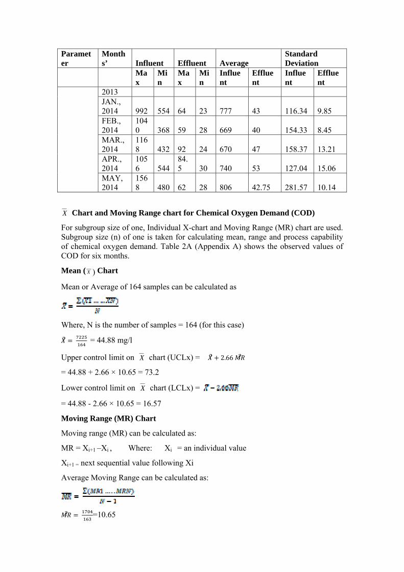
The data have been collected and analyzed for Chemical oxygen demand (COD) of waste water samples. Data analysis has been carried out by comparing the concentrations of pollutants at the inlet and outlet of the water treatment unit of city. The samples have been collected at the inlet and outlet of all the treatment units and analyzed as outlined in the standard methods for the examination of water and waste water. The data used for analyzing the parameters were taken on daily basis from Dec., 2013 to May, 2014.

Influent and effluent of wastewater were monitored and data were collected for maximum and minimum values from which standard deviations are also calculated. Table 1 shows the collected data and standard deviation of influent and effluent of SBR.

Table 1: Standard deviation of Influent and effluent of SBR

Parameter

Months’ Influent Effluent Average

Standard Deviation

Max

Min

Max

Min

Influent

Effluent

Influent

Effluent

COD DEC., 883 470 79 30 699 43 112.1 11.99

 

Parameter

Months’ Influent Effluent Average

Standard Deviation

Max

Min

Max

Min

Influent

Effluent

Influent

Effluent

2013 JAN., 2014 992 554 64 23 777 43 116.34 9.85 FEB., 2014

1040 368 59 28 669 40 154.33 8.45

MAR., 2014

1168 432 92 24 670 47 158.37 13.21

APR., 2014

1056 544

84.5 30 740 53 127.04 15.06

MAY, 2014

1568 480 62 28 806 42.75 281.57 10.14

X Chart and Moving Range chart for Chemical Oxygen Demand (COD)

For subgroup size of one, Individual X-chart and Moving Range (MR) chart are used. Subgroup size (n) of one is taken for calculating mean, range and process capability of chemical oxygen demand. Table 2A (Appendix A) shows the observed values of COD for six months.

Mean ( X ) Chart

Mean or Average of 164 samples can be calculated as

Where, N is the number of samples = 164 (for this case)

? = 44.88 mg/l

Upper control limit on X chart (UCLx) = ? 2.66 ?

= 44.88 + 2.66 × 10.65 = 73.2

Lower control limit on X chart (LCLx) =

= 44.88 - 2.66 × 10.65 = 16.57

Moving Range (MR) Chart

Moving range (MR) can be calculated as:

MR = Xi+1 –Xi , Where: Xi = an individual value

Xi+1 = next sequential value following Xi

Average Moving Range can be calculated as:

? =10.65

 

Where, number of samples (N) = 163 (for this case)

Upper control limit on MR chart (UCLMR) = 3.268

3.268 × 10.65 = 34.79

Lower control limit on MR chart (LCLMR)

LCLMR = 0

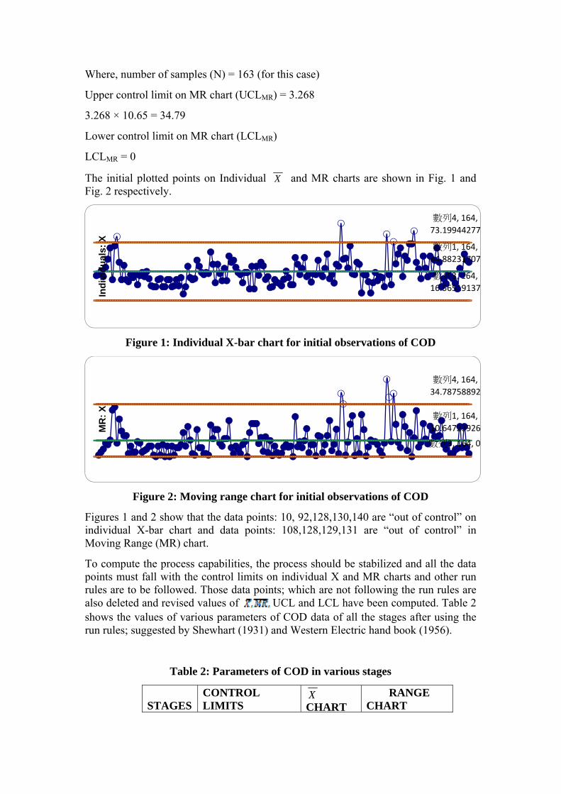
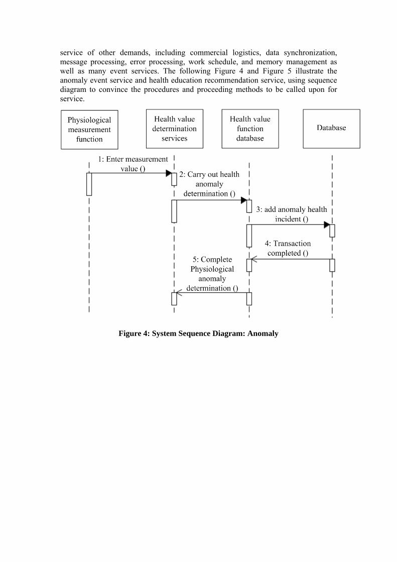
The initial plotted points on Individual X and MR charts are shown in Fig. 1 and Fig. 2 respectively.

Figure 1: Individual X-bar chart for initial observations of COD

Figure 2: Moving range chart for initial observations of COD

Figures 1 and 2 show that the data points: 10, 92,128,130,140 are “out of control” on individual X-bar chart and data points: 108,128,129,131 are “out of control” in Moving Range (MR) chart.

To compute the process capabilities, the process should be stabilized and all the data points must fall with the control limits on individual X and MR charts and other run rules are to be followed. Those data points; which are not following the run rules are also deleted and revised values of UCL and LCL have been computed. Table 2 shows the values of various parameters of COD data of all the stages after using the run rules; suggested by Shewhart (1931) and Western Electric hand book (1956).

Table 2: Parameters of COD in various stages

STAGES CONTROL LIMITS

XCHART

RANGE CHART

數列1, 164, 

44.88231707

數列3, 164, 

16.56519137

數列4, 164, 

73.19944277

Ind

ivid

ual

s: X

數列1, 164, 

10.64723926

數列3, 164, 0

數列4, 164, 

34.78758892

MR

: X

 

STAGES CONTROL LIMITS

XCHART

RANGE CHART

FIRST UCL 73.2 34.79 CL 44.88 10.65 LCL 16.57 0 SECOND UCL 68.74 30.76 CL 43.7 9.41 LCL 18.66 0 THIRD UCL 66.4 28.97 CL 42.82 8.87 LCL 19.23 0 FOURTH UCL 65.73 28.57 CL 42.48 8.74 LCL 19.22 0 FINAL UCL 67.9 29.59 CL 43 9.06 LCL 18.92 0

So after four stages, the final values of parameters of stabilized process are as follows:

Individual X Chart

UCL = 67.09, LCL = 18.92

MR-chart

UCL = 29.59, LCL = 0

From these process parameters; the process capabilities of COD are computed in the following section.

Process Capability Study of COD

The process capability of chemical oxygen demand (COD) is calculated and discussed in this section. Some parameters need to be calculated are:

Cp, Cpu, Cpl, Cpk and Cpm, USL, LSL, Target mean (T), estimated mean of the process (μ) and the estimated variability of the process (expressed as a standard deviation) is σ.

Process capability (Cp)

The upper and lower specifications limits for COD have been set as follows:

Upper specifications limits (USL) = 10.0

Lower specifications limits (LSL) = 0.0

The process capability is calculated by:

6

Where s = standard deviation and D2 is 1.128 constant for n=1 (from Statistics book).

 

For COD calculations the specifications limits are

USL = 10.00

LSL = 0.00

9.061.128

8.02

100 06? 8.02

2.08

Process Capability Indices

Cpk = min.[Cpu, Cpl]

Cpl = ?

= ∗ .

= 1.79

Cpk = 1.79

Cpk = min.[2.37, 1.79]

So, Cpk = 1.79

Thus, the process capability index (Cpk) and Process Capability ratio (Cp) of revised and acceptable COD are 1.79 and 2.08 respectively.

Many parameters; like mean, upper control limit, lower control limit as well as upper and lower process capabilities and process capability indices have been calculated in this section.

It may be noted that 6 Sigma, or 3times standard deviation (SD) above and below the average, represents statistically around 99.73% of all data produced by the process. Consequently, it can be inferred that a process capability of one is equivalent to in-specification results 99.73% of the time. A process capability of 1.33 (statistically 99.99% in-specification) is a common starting point, although this number is arbitrary. As a rule of thumb, minimum Cp values; in the range of 1.2 and 2.0, are generally appropriate but for higher risk applications, higher value of lower process capability (Cpl) is required.

4. Conclusions

In this study; it is assumed that data have a natural or normal distribution. The behavior of these parameters can be modeled and give accurate predictions for how well the parameters are controlled within defined limits. The results show that the process capability of COD is 2.08 that is enough to satisfy the specifications. The

 

final process capability of COD has been calculated by eliminating the out of control data points.

The value of COD should be less than 100 mg/l; as per the specification of CPCB. In stabilized situation, the process capability index (Cp) should be 1.64. Similarly, the lower process capability and the upper process capability should be 1.79 and 2.37 respectively.

The process average, average range and process capability have been found out for Chemical oxygen demand (COD) in this study. It is usually desirable to have greater assurance of process capability than 99.7% for all the manufacturing processes. Unfortunately, there is no set value of process capability which is universally considered as acceptable.

References

Asadi, A., Zinatizadeh, A.A.L., Sumathi, S., Rezaie, N. and Kiani, S. (2012). A comparative study on performance of two aerobic sequencing batch reactors with flocculated and granulated sludge treating an industrial estate waste water-process analysis and modeling, International Journal of Engineering Transactions, 26(2), 105-116.

Carmen, S.D., Rodrigues, R., Boaventura, A.R. and Madeira, L. M. (2014). A new strategy for treating a cotton dyeing wastewater - integration of physical-chemical and advanced oxidation processes,Int. J. of Environment and Waste Management,14(3),232 – 255.

CPCB. (1999). Status of water supply and Wastewater Collection Treatment &Disposal in Class I Cities,Control of Urban Pollution Series, CUPS/44/1999-2000.

CPCB. (2005). Performance status of common effluent treatment plants in India, Central Pollution Control Board, India.

Debsarkar, A., Mukherjee, S. And Datta S. (2006). Sequencing Batch Reactor (SBR) treatment for simultaneous organic carbon and nitrogen removal- a laboratory study, Journal. of Environ. Sci. and Engg. 48(3)169- 174.

Deming, W. E. (1982). Out of the Crisis, Unlimited Learning Resource, LLC, Winston-Salem, North Carolina.

Mahvi, A.H. (2008). Sequencing Batch Reactor: A promising Technology in waste water Treatment, Iran journal of Environ. Health Sciences Eng, 5(2), 79-90.

Mohamed, F. H. and Saed, M. A. A. (1995). Waste water management in a dairy farm, Water Science and Technology, 32(11), 1–11.

Prajapati D.R. (2016). Cost comparisons of modified X¯ chart for auto-correlated observations, International Journal of Metrology and Quality Engineering, Vol.7 (1), pp.102-110.

Pearn, W. L., Shu, M. H. and Hsu, B. M. (2005). Testing process capability based on Cpm in the presence of random measurement errors, Journal of applied statistics, 32(10), 1003-1024.

 

Refaie, A. A. (2013). Applying process analytical technology framework to optimize performance of waste water treatment process, Journal of Zhejiang University, 34, 1-9.

Rio, A.V., Figueroa, M., Arrojo, B., Corral, A., Campos, J. L., Torriello, G.A. and Mendez, R. (2012). Aerobic granular SBR systems applied to the treatment of industrial effluents, Journal of Environmental Management, 95, 88-92.

Samkutty, P. J., Gough, R. H., and McGrew, P. (1996). Biological treatment of dairy plant wastewater, 1. Journal of Environmental Science & Health Part A, 31(9), 2143-2153.

Shewhart, W. A. (1931). Economic control chart of quality of manufacturing product, Van Nostrand, New York.

Sirianuntapiboon, S. (2002).Application of Granulated Activated Carbon-sequential Batch reactor(GAC-SBR) system for treating pulp and paper industry wastewater, Thammasat Int. J. Sc. Tech., 7(1), 20-29.

Tam, P. C., Lo, K. V. and Bulley, N. R. (1986).Treatment of paper and pulp mill waste water by column type sequencing batch reactor,Can. Agric. Eng., 28, 125-130.

---------------------------------

Appendix 1A: Nomenclature

S. No.

Abbreviations

Full Form S. No.

Abbreviations

Full Form

1 COD Chemical Oxygen Demand

14 UCLR Upper control limit for R chart

2 BOD Biochemical Oxygen Demand

15 LCLR Lower control limit for R chart

3 SBR Sequential Batch Reactor

16 Max. Maximum

4 TSS Total Suspended Solids

17 Min. Minimum

5 SVI Sludge Volume Index 18 USL Upper Specification Limit

6 MA Moving Average 19 LSL Lower Specification Limit

7 MR Moving Range 20 MLSS Mixed Liquor Suspended Solids

8 Cp Process Capability 21 RAS Returned Activated Sludge

9 Cpk Process Capability Index

22 mg/l milligram per litre

10 Cpu Upper Process Capability

23 MLPD million litres per day

11 Cpl Lower Process capability

24 CPHEEO Centre for Public Health and Environmental Engineering Organization

 

S. No.

Abbreviations

Full Form S. No.

Abbreviations

Full Form

12 UCLX Upper control limit forX bar chart

25 CPCB Central Pollution Control Board

13 LCLX Lower control limit for X bar chart

26 STP Sewage Treatment Plant

Appendix 2A: Observations of COD (in mg/l)

Sr. No.

TSS

MR

Sr. No. TSS MR

Sr. No. TSS MR

Sr. No. TSS MR

1 41 42 39 11 83 37.3 6.3 124 36 8 2 42 1 43 37 2 84 45.3 8 125 40 4 3 45 3 44 38 1 85 39 6.3 126 39 1 4 40 5 45 56 18 86 32 7 127 30 9 5 49 9 46 50 6 87 32 0 128 81.5 51.56 57 8 47 44 6 88 58.6 26.6 129 42 39.57 68 11 48 42 2 89 52 6.6 130 32 10 8 37 31 49 44 2 90 42 10 131 74 42 9 70 33 50 43 1 91 48 6 132 52.5 21.510 79 9 51 64 21 92 58.6 10.6 133 62 9.5 11 54 25 52 52 12 93 40 18.6 134 68 6 12 37 17 53 34 18 94 42.6 2.6 135 40 28 13 51 14 54 52 18 95 34.6 8 136 60 20 14 37 14 55 43 9 96 42.6 8 137 56 4 15 35 2 56 36 7 97 42 0.6 138 72 16 16 42 7 57 48 12 98 56 14 139 72 0

17 39 3 58 36 12 99 42.7

5 13.2

5 140 84.5 12.518 42 3 59 60 24 100 40 2.75 141 53.9 30.619 32 10 60 54 6 101 48 8 142 47.5 6.4 20 41 9 61 56 2 102 62 14 143 38 9.5 21 44 3 62 49 7 103 38 24 144 60 22

22 40 4 63 44 5 104 42 4 145 48.2

5 11.7

5

23 45 5 64 42 2 10533.7

5 8.25 146 39.7

5 8.5

24 38 7 65 34 8 106 52 18.2

5 147 60 20.2

5 25 31 7 66 44 10 107 50 2 148 42.6 17.426 30 1 67 44 0 108 92 42 149 56 13.427 30 0 68 28 16 109 57 35 150 68 12 28 37 7 69 50 22 110 58 1 151 54 14 29 38 1 70 28 22 111 48.4 9.6 152 30 24 30 30 8 71 50 22 112 70 21.6 153 38 8

31 30 0 72 41.2

5 8.75 11342.7

5 27.2

5 154 33 5

 

Sr. No.

TSS

MR

Sr. No. TSS MR

Sr. No. TSS MR

Sr. No. TSS MR

32 37 7 73 54 12.7

5 114 42 0.75 155 42 9 33 37 0 74 50.5 3.5 115 54 12 156 40 2 34 30 7 75 37.3 13.2 116 52 2 157 38 2 35 31 1 76 40 2.7 117 24 28 158 33.5 4.5 36 37 6 77 29.3 10.7 118 42 18 159 28 5.5 37 31 6 78 30 0.7 119 41.5 0.5 160 48 20 38 39 8 79 37 7 120 35 6.5 161 42 6 39 23 16 80 34.3 2.7 121 24 11 162 62 20 40 30 7 81 33.3 1 122 34 10 163 56 6 41 50 20 82 31 2.3 123 44 10 164 54 2

44.8

8 10.6

5

Biographical Note

D. R. Prajapati is Associate Professor with teaching and research experience of more than 21 years and published more than 125 research papers in international and national journals of repute and in the proceedings of the conferences. He is also reviewer of more than 8 international journals. He also guided four Ph.D. and more than 24 post graduate theses and guiding 5 research scholars at present. He has also chaired international and national conference in India and abroad. He also organized two short term courses and two national conferences for the faculty of technical institutions and industries. He is also recipient of first D. N. Trikha research award for excellent research publications in international journal for the year 2009 in PEC University of Technology.

-------------------------------    

 

ICESI_0068

Building a Long-Term Care Information System Based on the Whole Person Concept through Service-Oriented

Architecture

*Chia Lun Lo, Fooying University, Taiwan

*Corresponding Author

Abstract

Although there are long-term care institutions that increase service efficiency and quality through the establishment of long-term care systems, the caring approach for long-term care emphasizes comprehensive health care, including the physical, mental, and spiritual state of older persons. Such care systems based on the whole person concept require constant cross-referencing and an emphasis on reminders for anomalous incidents. If the system establishment lacks integrated concepts, the system will then be unsuitable. This study aims to apply the concept of service-oriented architecture to integrate the previously dispersed and different operations of the long-term care system. This involves substituting the function module of the original system architecture with a service-based approach to provide a service interface. In addition, there must be a connection between the well-defined interface for the services and the formation of comprehensively integrated system architecture. Finally, the study assesses the system to support the actual improvement on the operational performance of personnel.

Keywords: Long-term care institutions, Service oriented architecture, Long-term care information management system.

 

1. Introduction

As the national health level improves and medical technology advances, the average life expectancy of the global population is prolonged, causing a rapid rise in the elderly population. The UN defines the world population structure and categorizes countries with a population aged 65 years or older who account for 7% of the total population as an “aging society,” 14% is known as an “aged society,” while 20% or more is known as a “super aged society.” Data from the UN Population Division show that the global population aged 65 years or older is projected to reach 25% by 2050, and one out of four persons will be 65 years or older [1]. By 2025, it is estimated that the elderly population in Taiwan will reach super aged society status as defined by the UN and that the percentage of the elderly population will reach as high as 35.5% by 2050 [2]. The speed of population aging in Taiwan has far surpassed most developed counties in Europe and the United States (as shown in Table 1).

Table 1: Population Projections for Persons Aged 65 Years or Older in Developed Countries (%)

Year County

2005 2011 2050

Taiwan 9.7 10.7 35.5

U.S. 12.4 13.0 20.0

Canada 13.2 14.1 25.7

U.K. 15.8 16.6 23.3

Sweden 17.3 17.2 25.0

German 19.3 20.6 26.0

Japan 20.0 31.2 42.1

The advent of the super aged society not only changed the demographic structure in Taiwan, but the issues derived from it, such as medical care, economy, psychology, social welfare, and policies, are drawing increasing attention. In particular, the majority of diseases associated with older persons are chronic and diverse; and the subsequent medical expenses are enormous. In the example of the United States, the percentage of older persons in 2000 accounted for 12.3% of the total population; however, this group accounted for 26.2% of the total consumption of the total medical budget there. Hence, the planning speed of the national policies and establishment of care institutions must also keep pace with the population’s aging.

The proportion of the disabled population within Taiwan is also quickly increasing as the population ages annually (see Table 2). The Taiwan’s total population is projected to experience negative growth after 2026, revealing a potentially serious issue with a significantly reduced working population. Due to industrialization and urbanization, traditionally large families are also transforming into smaller families, and the intention and ability of the family to provide home care is declining annually. A large elderly population needs long-term care and the effects brought by an aging population should not be overlooked. The WHO suggests that the advent of an aging society will bring not only the pressure of demographic structure transformation but also increasingly heavy loads on long-term care finance and labor [3]. Hence, future elder care and foster care can no longer be undertaken by a single family. How to

 

cope with the enormous elderly care demand has become a large challenge for the entire society.

Table 2: Taiwan’s Institutional Long-Term Care Demand Projection

To cope with the demand of the future long-term care population as well as implementing the “whole person care” frequently envisioned by the medical industry, the government of Taiwan has actively encouraged solutions in the past decade in an attempt to build the long-term care system. However, the effects fell behind expectations while the service resources and the growth of service requesters are still quite limited. In addition to the long-term care services that are divided into excessively different administrative systems in Taiwan, often leading to poor promotional performance, the limited care personnel in institutions causes older persons to perceive poor care quality or low service efficiency. However, the complex care work of long-term care institutions does also trigger a number of factors in poor care quality or low service efficiency. These include the pressure of care work and the lack of real-time updated care-related knowledge and laws. Studies suggest that the high turnover rate in care personnel can significantly and severely affect costs for medical-related institutions [4]. Although some long-term care institutions have attempted to develop a long-term care information system for improving care work, regular paperwork increased personnel work efficiency and reduced work fatigue. However, the small operational scale of most long-term care institutions has prevented them spending too much money on development costs for large information systems. Moreover, the complex care works at long-term care institutions while subsystems with independent development of operational process could not assist each other in care. Most IT companies lack knowledge of the long-term care domain, and find it difficult to develop and maintain such complex systems. Hence, the lack of system functions that meet actual long-term care demand prevents institutions from improving care quality through such systems.

This study develops a long-term care support system designed for domestic long-term care institutions. Due to its complexity, service-oriented architecture (SOA) has been used to eliminate large, cumbersome programs, using simplification and automation processes to save considerable costs. Such an approach not only can improve the operating efficiency of the long-term care information system, but also reduces the time and costs for program maintenance [5]. The study further discusses the suitable placement position for different data in an attempt to achieve a user-friendly interface and quickly integrate related care information for establishing a whole-person long-term care system.

2. Literature Review

Year 2016 2021 2026 2031 Disability Population Projection

542,271 641,342 758,541 900,494

National Population Projection

23,296,248 23,634,537 23,930,657 23,832,371

Proportion accounted for National Population

2.3% 2.7% 3.4% 3.8%

 

Structured programming has been proposed for discussion since 1980. Programming code for repeated use is regarded as media for implementing structured programming in addition to improving software performance and saving development costs. Post-1990s, structured programming was gradually replaced by object-oriented language due to the Internet boom. As the increasingly popular client/server and n-tier multi-layer architecture started to develop, the system is now no longer limited to operation on a single large server. Due to the increasing scale of the systems, people started to pay more attention to how to save development time in order to maintain such a large system through more convenient means. This led to the proposal of SOA. Post-2000, SOA became the standard, new-generation information system model [6].

The smallest unit of SOA is known as a “service” [7]. A service cannot be regarded as software but rather is defined as an independent operation needed for completing commercial operations. Many services have been proposed to form the architecture, and such service forms solutions combining many different types and procedure services. The use of a service-oriented service means the integration of distinctive information technology environments and improvements in stability to increase repeated usability of resources in order to reduce operational and development costs [8]. SOA mainly involves three roles, namely Service Provider, Service Requester, and Service Broker [9, 10]. The architecture of the three roles is shown in Figure 1 and described as follows:

(1) Service Provider: these are also service owners and execute the platform for a service. Service functions are provided for use by service requesters while service brokers use the specific details of the network services.

(2) Service Requester: the work of a service requester is to issue requests for a service. When certain functions of service requesters can be satisfied, the service requesters will issue a request and expect the service providers to provide satisfying services.

(3) Service Broker: here, the broker accepts the registration request from the service provider and processes query requests from the service requester. The service broker also authorizes the service provider to publish a service description. Service requesters may query proper items of service from the service broker in case they need services while attaining the service information from the broker.

Figure 1: Service-Oriented Architecture

 

In recent years, SOA has been widely applied in the medical field’s information systems [11-17]. In addition to improving actual development efficiency, users perceive satisfaction from the system use. Hence, the study proposes the concept of applying SOA architecture to institutional long-term care information systems. The care operation of each unit from the care process is regarded as an independent service provider, and when users bring up requests, the plan to meet user demand can be generated through the system proposed by this study.

3. Research Methods

System Functions

The long-term care information system developed in this study is called the UCARE system, which refers to the ubiquitous care for assisting long-term care institutions. In consideration of the limited labor and funds of the institutions, the design needs to establish an integrated system using the most efficient method of development. At the same time, due to the continuity of long-term care work and the different operating units involved in the care work, it is necessary to take into account the data generated from different operations. Data inter-passing is necessary and the development requires designing relevant system functions through SOA perspectives. Moreover, the current conditions of institution residents need to be analyzed with an emphasis on how to maintain resident health through the intervention of the information system.

The factors that affect health include physiology, psychology, diet, environment, and exercise. Physiology factors include drug habit, chronic disease control, unplanned medical care, health scale, and daily physiological measurements. The psychological factors include interpersonal interaction and mentality scale. Diet factors include nutrition scale assessment, nutrient control, and items of diet. Environment factors include health advocacy and health education video broadcasting. Exercise factors include the amount and number of exercises.

Nine subsystems have been defined from the aforementioned factors; these include, the physiological data collection system designed for physiology, health scale evaluation input system, anomaly reporting, and a follow-up system designed for psychology. The mobile platform-based anomaly reporting and follow-up system are used to record the residents’ interpersonal interactions. A dieting suggestion and reminder system has been built for dieting while the environment combines a television and multimedia center for residents to read health education. Finally, to provide a comprehensive assessment, other requirement data collected from the health condition analysis system and the results of residents’ health and physiological data are automatically screened. A digital educational learning system provides health education content suitable for the residents to read. The system function is presented in Figure 2.

 

Figure 2: System Function Chart

System Architecture

To complete, organize, and collect the care content provided from different data sources in the system’s care information database, we will need an environment that can be explored in different servers and establish connections as well as a format that allows for an exchange of data content. Therefore, this study selects Web Services to implement the hands-on practice and design from the SOA content. With regards to the connection method between the heterogeneous platforms and UCARE server used by the caregiver, in addition to using standard web protocol (HTTP protocols) to engage in management interface, the syndication agreement of the network summary is used for health events in an attempt to implement the low transmission amount needed for wireless transmission on mobile platforms and facilitating applications on mobile devices. The long-care system architecture designed from SOA is shown in Figure 3.

 

Figure 3: System Architecture and Basic Component Chart

Such architecture consists of five parts, namely the Service Broker Server, Health Event Server, Health Event Catalog Service Server, User Client, and Care Content Providing User Client. The functions and purposes are introduced in the follows:

(1) Service Broker Server

This includes a UDDI-based service database and Web Services processing components. The function is responsible for providing service requesters and service servers with a contact channel from the SOA. Under such architecture, the health event server publishes service information through the WSDL format, whereas the service broker server stores such content-providing server information in the UDDI server database. Supported by WSDL and UDDI standards, the health event server inquires from the service broker server through the SOAP format if the services of other servers can be acquired to facilitate the connection.

(2) Health Event Server

This plays the role of service provider in a SOA. The service of providing content includes the storage of databases for health event content and the component of management health events. After establishing database and services, the server submits the registration to the service broker server through the WSDL format to notify the service broker server through the provision of the service format and information.

Pure health event content provides a simpler server structure, meaning the components needed can only be used to access the database and process the Web Services requirement, in addition to establishing a connection with the data exchange. In practice, there are single servers that concurrently play the role of the health catalogue service server.

 

(3) Health Event Catalog Service Server

This is the most complex part of such architecture, containing the most functions and components. The main system function of this server storage also provides users with customized health event catalog architecture. Due to the need to process user information, the user interface, components, and the database for storing user information need to be administered to store the different user data and their health event requirement. One user can possess the requirement for multiple health catalogs. The server itself also needs one content database to provide content regarding the health event catalog. The content of such databases can be collected from the content of other health event catalogs. The server acts as a service requester in SOA that proposes queries to the service broker in addition to connecting to other service servers in an attempt to acquire content. The content can be provided by the server, implying that the same server hardware can concurrently own two roles, namely the health catalogue service server and health catalogue content server. Due to the design of multiple data sources, a specific component is required to organize the content data acquired from different resources. Therefore, repeated data are removed and the comparison data are updated to store the organized data into the database for access.

(4) User Client

This refers to the user environment of general users, and its form can be a desktop computer, laptop computer, Kiosk, or mobile phone, PDA, and even any web feed-supported reading devices that could be connected to the Internet. Users provide server connections with the long-term care system service through user interfaces to configure the styles and conditions for customized health events. The user interface most commonly used is presented through dynamic web technology, and executed and configured through supporting browsers.

(5) Care Content-Providing User Client

The role of care content-providing user client is the simplest form that aims to provide care content updates and is operated through a standard personal computer connecting to the Internet. To establish dynamic websites on the care content-providing user client, the content server terminal only requires a browser for operating data management. Alternatively, a Winform program can be developed to connect with the care content-providing user client for data changes. This method is more difficult to provide cross-platform services compared with the dynamic websites. Nonetheless, Winform program can provide operations that are more convenient and faster processing for large or specific data.

4. Results

System Description

The nine subsystems listed by the study include functions summarized as follows:

(1) Physiological Data Collection Subsystem

The purposes of this system establishment are to convert physiological measurement data into information, and to integrate with existing health care instruments of institutions to undergo monitoring of resident health conditions so the residents can measure resident cards through the automatic sensor at the health center and public

 

area. The system will automatically compare the physiological data that have been measured and collected in the database each time. In the event of the figures showing an anomaly or having not been measured, the system will initiate an alert for the caregiver and the residents to provide reminders and care recommendations. Caregivers can also check the residents’ physiological data for anomalous information daily and use such information as a reminder to establish and generate the reminder list.

(2) Health Data Input Subsystems

The purpose of the system establishment is to put the interview scale into electronic form and to coordinate with peripheral sensor equipments or televisions and computers with different interfaces in an attempt to complete the scale data input and simplify the input/output procedures of the scale data. The system also combines with other subsystems (collection of physiological data and medication records) to automatically collect the health information on the elderly population so the older persons will conveniently and freely record the physical function, mentality, social functions, and other physical and psychological conditions on the scale without interference to their everyday lives. The health conditions are traced over the long run to analyze effectively the root cause, prevent problems in advance, and post-supplement for diagnosis and treatment later.

(3) Personal Multimedia Center

The subsystem aims to establish simple and yet multi-functional personal information data in the residents’ room as an experiment to eliminate the elderly residents’ fear and repellence of high-tech equipment through an operating interface, such as TV display and remote control, which are familiar to people today. Residents are provided with an enjoyable and painless operating environment to enjoy TV, DVDs, music, and photo albums as well as other rich multimedia entertainment functions while switching to connect with the platform that displays the health information or various life-related messages and recommendations as transmitted from other subsystems. Such systems can facilitate the institutions with undertaking personalized health education information via the said platform so the residents can obtain relevant information via the most intuitive means.

(4) Reminders in Life and Health Data Query Subsystem

The subsystem establishes a reminder message processing mechanism that provides a consistent communication interface integrated with the events sent out by other subsystems into one reminder event list. This then sends reminder messages to the residents via text message. Meanwhile, some events (such as visitors, outgoing, and medical visits) can be pre-obtained during the care process. The caregivers are also permitted to establish foreseeable events from the maintenance interface. Such information can be integrated into common event categories to facilitate future caregivers with reminding residents through recordings. Residents can also play the recording from the personal multimedia center platform in the room. Additionally, residents may conduct health information queries from the multimedia center inside their rooms.

(5) Health Education and Digital Learning Subsystem

The subsystem is developed to provide institution administrators with configuration

 

of health education theme categories to classify the teaching material content. The association with the system resident chronic diseases through ICD9 disease coding can also be configured in an attempt to choose the appropriate health education video for residents to view. The residents will follow the medical instructions and enhance their own self-caring capacity when they can view personalized health education information from the multimedia center inside their room in a relaxed mode.

(6) Dieting Recommendation and Reminder Subsystem

The subsystem is established to allow for extended menu and recipe design functions that go beyond the existing meal ordering system in the market, which lacks professional recommendations and care for the dieting nutrition that are needed in personalized services.

(7) Anomaly Reporting Subsystem and Event Follow-up Subsystem

The main development goal of the anomaly reporting subsystem and event follow-up subsystem is to build the system into the personal handheld device platform and the staffs’ existing web platforms. The staff can immediately report the anomalous records from the handheld device to the platform upon discovering the red alert for residents’ psychological or physical health or any observation of anomaly events. The proper personnel will be notified immediately for handling the issue. The residents can also log in from the computers in the public area of the institutions to report the caregivers of the institutions and allow for quick processing.

(8) Health Condition Analysis Subsystem

Finally, for residents sent to the care institutions because their family could not take care of them, the family mostly cares to control quickly the health and comfort of the older persons staying at the institutions. Because of this, the health condition analysis subsystem is designed to allow family to control the health state of the older persons within the shortest time. Therefore, the residents’ personal health files need to be collected and integrated in a real-time process, starting from the checking in of the elderly to the gradual and faithful recording of the physical, psychological, and mental health state of the elderly. The elderly personal health files are established through the collection and organization of physique, interview, medical visits, and dieting information in order to present the overall health performance of the older persons. The older persons’ health conditions are also effectively traced through long-term records summaries, and analysis prevents issues in advance and post-supplements for diagnosis and treatment later. Hence, the main operations of the subsystem are divided into the personalized configuration of health analysis standards and the briefing operation process. This subsystem can provide medical care staff with residents’ long-term health analysis data and establish a health analysis chart to cooperate with the briefing operation process, so that the family of the elderly can immediately control the long-term health trends of the residents during their visits.

The nine subsystems are developed through the SOA architecture. The study divides the long-term care system into several main aspects of scope as follows. (1) The first is the back-end configuration for definition of long-term care knowledge. Due to the different physiques of each long-term care resident, the system emphasizes the customized care method and therefore the care personnel must define the physical thresholds of each resident through the maintenance functions provided by the system. The administrators may also duplicate the existing physical thresholds configured by

 

the system to customize modifications in the event that residents of similar categories check in, thereby accumulating the care knowledge attributed to long-term care institutions and preparing for the decision-making supporting system for the senior management to be derived from long-term care institutions. (2) The health event process service established through SOA and the unit service for SOA process service calling will complete one or several SOA-related process unit services, such as physiological measurement reminders, health education readings, dieting recommendations, and anomaly event follow-up reminders. (3) The third is the front-end of the long-term care system. After the residents or caregivers input daily physiological measurement, events, dieting records, and high-risk measurements through the system interface, the system will compare through personalized physiological signs and transmit proper health event recommendation values from knowledge definitions to the personal computers of the care personnel or the multimedia center platforms inside the resident rooms according to the different situations of the residents. These will be used as recommendations for care behaviors in the follow-up process.

Data Architecture Description

Data Integration Process

The system is distributed to a considerable number of subsystems through different operating processes in order to administer the processing rules. It is inevitable that many similar processes use identical data and rules. Hence, the system defines the corresponding modes and rules for each subsystem when analyzing the data rules and process rules. In the event the rules contain high consistency, they are listed as members of the service. The following three rules are described as follows.

The main tasks of the data rules aims to find out the storage position of data, data storage method, classification of data properties, and data processing method. The storage position of data is distributed in the memory, file folders and historical database, and backup device. Data storage method can be divided into memory, data files, and database, while the memory mainly contains data with the largest storage and access, the size of which can be estimated and data less frequently moved. For example, basic personal data files require authentication by many subsystems and can be taken into consideration for listing as members of service events. Data files are mainly stored with less frequently moved or less frequently accessed files (i.e., the various health threshold configuration files and the corresponding basic information files). The database is stored with data after changes, temporary cell tables of statistics reports, and the overall event summary data, including online data and personalized configuration files, pre-computed and completed statistics results service files, and report data as well as the log files configured for security reasons.

The process rules mainly define the method of data processing; in other words, to find the services that can be listed as health events. Such services are then divided into emergency processing, general processing, and batched processing according to the level of urgency. Emergency processing is mainly used in the processing of health state anomalies matched with an emergency nature. General processing is mostly used in tossing data back to a service event after daily health measurement in order to compare the results of personalized health threshold database. Batched processing refers to processing regular or fixed-frequency services (i.e. account processing and calculation of resident dieting nutrition). Moreover, the process rules also define

 

service of other demands, including commercial logistics, data synchronization, message processing, error processing, work schedule, and memory management as well as many event services. The following Figure 4 and Figure 5 illustrate the anomaly event service and health education recommendation service, using sequence diagram to convince the procedures and proceeding methods to be called upon for service.

Figure 4: System Sequence Diagram: Anomaly

 

Figure 5: System Sequence Diagram: Health Education Recommendation Service

System Assessment and Analysis Result

The study intends to assess whether if the care system of UCARE foster and care institutions developed through SOA can truly meet user demand. The measurement of users’ satisfaction after information introduction has become one of the considerably developed issues in the IS field. Several theoretical models with reliability and validity can be provided to explain why users adopt IT. In particular, DeLone and Mclean proposed IS Success Model in 1992 as the most famous system introduction assessment theory, which proposes that there are six constitutes affecting IS success, namely system quality, information quality, use, user satisfaction, personal influence, and organizational influence. In 2003, the model emphasized the concept of personal and organizational influence on updated effectiveness explaining that information quality and system quality will increase service quality, enhancing user intent and user satisfaction while the user intent and user satisfaction contribute to the organizational benefits. The medical care industry is one service industry, particularly in foster institutions where residents can take care of their own living while maintaining autonomous, in addition to choosing whether to stay at the institution. Hence, whether if system introduction can enhance perceived satisfaction, is more appropriate and commonly used as a means of assessing success for system introduction. In the experimental institution chosen for this study, the objects comprise care personnel and administrators. Taking into consideration the limitation in business and time for the institutions, only 20 representative care personnel have been selected to carry out the

 

system assessment results after the actual use of the system. The care personnel consisted of women aged between 24 and 40 years old with a degree in college or higher. Meanwhile, to understand the level of objective improvement after system intervention, we choose seven operations including health care consulting and guidance physiological measurement, living and health scale assessment, emergency medical service, medicine delivery service, flu vaccination, and dieting guidance, as the bench assessment operations. We first collected the actual time taken by the staff on paperwork before the system’s introduction and then verified the same operational time spent on the system in post-introduction. The comparison of the two shows us understanding of whether system intervention can improve work efficiency, save paperwork time, and care for residents in reality, in order to improve care quality.

In sum, employees of introducing institutions earn the highest scores in influencing system introduction to organization and personal operations, followed by information quality and functions while the lowest score is the perception to user interface. This could have resulted from the unfamiliarity to interface at its early introduction. The influence from the actual comparison of before and after introduction to care operation is shown in Table 1, and the results indicate efficacy in improving personnel work efficiency that can improve HR-related costs.

Table 3: Operating time differences between, before, and after the introduction of system

Operational items Before

intervention (min)

After intervention

(min)

Decrement (rate of decrease)

Cost reduction of labor

Dietary recommendations

120.0 28.0 -92.0(-76.67%) 360.64

Emergency medical services

100.5 73.7 -26.8(-26.67%) 105.21

Healthcare inquiries and counseling

55.5 11.5 -44.0(-79.28%) 172.48

Influenza vaccination

89.4 57.0 -32.4(-36.24%) 127.00

Life and health metrics and evaluations

113.5 63.7 -49.8(-43.88%) 195.37

Physiological measurements

84.5 10.3 -74.2(-87.81%) 291.06

Prescription delivery services

95.0 80.0 -15.0(-15.79%) 58.80

Total 658.4 324.2 -334.2(-50.76%) 1310.56

5. Conclusion

Research Findings

Despite social advancement in today’s society, the concept of sending older persons to foster homes (long-term care institutions) is still considered a non-filial act deeply rooted in the Chinese population. When the service quality of long-term care institutions fails, the descendants of the residents bear even greater pressure. Faced with the advent of an aging society and trends towards small families, it becomes

 

inevitable for foster institutions to take care of older persons rather than their families. Nonetheless, the unintentional human error in care personnel, lack of heritage mechanisms for specific care experience, and spending too much time in collecting health information and preparation of paperwork nursing care records found in the institutions, or the direct application of nursing system from acute medical institutions is insufficient to cope with long-term care; such issues mentioned will prevent the long-term care institutions from effectively improve care standards. Hence, the study integrates SOA to design an integrated institutional long-term care information management system. In particular, SOA not only saves time in data collection and costs for data integration but also drastically reduces programming codes and enhances programming application, in addition to saving operating time for long-term operations that require cross-referencing of data.

Hence, the study discovered the following qualifies of the SOA-based institutional long-term care information system. (1) Help the care personnel with collecting the various physiological and psychological care data of residents by automatically integrating them into the care list to spend the majority of the time and effort in the caring process and paying attention to the communication with residents, thereby improving care quality. (2) Automatic determinations of anomalous events: the main purpose is to remind caregivers with precautions so that no omission or negligence is found in executing care procedures. (3) Establish a care knowledge base and knowledge sharing platform: the health knowledge encountered during cumulative care process allows new care personnel to follow personalized care techniques and knowledge base while the long-term institutions will not lose valuable knowledge property due to the high turnover rate in care personnel, thereby assuring care quality while new care personnel be can immediately familiarized with the care business of residents, maintaining the due care quality. (4) Can integrate care data under heterogeneous systems or different subsystems. (5) The system can propose adjustments and recommendations for care methods according to the care knowledge base (such as recommendations for seeking medical help, dieting adjustment, or conduct health education).

Managerial Implications

As mentioned before, the institutional long-term care system architecture proposed by the study can substantially reduce care time while timely providing residents with health information to remind care personnel of precautions, thereby reducing health failure resulting from human error. For long-term care institutions, the system can establish a care knowledge base for different residents, accumulating older persons’ care information, knowledge, and experience, which does not reduce failure in cumulative care experience assets due to high turnover rate but also involves sharing the care knowledge of different cases in institutions, reducing the familiarizing time of care personnel. Hence, the use of the system can implement care experience into specific heritage and storage.

The use of this system not only assists administrators with establishing internal control mechanisms but also integrates care knowledge and comments with relevant specifications into the system through the strong scalability of the aforementioned SOA. Most importantly, due to the care work itself, at long-term care medical institutions, it acts as the core value and the computer grade of user client usually remains low. The system is built on three-layer architecture and such systems do not need re-installation or deployment of system to user clients. The convenience of use is

 

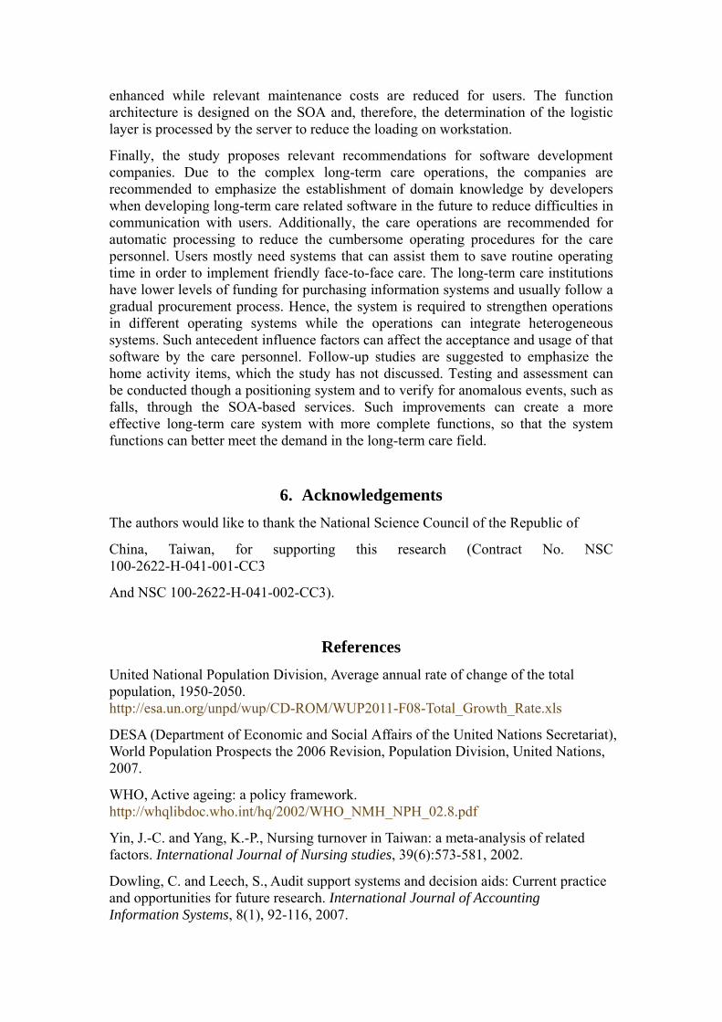
enhanced while relevant maintenance costs are reduced for users. The function architecture is designed on the SOA and, therefore, the determination of the logistic layer is processed by the server to reduce the loading on workstation.

Finally, the study proposes relevant recommendations for software development companies. Due to the complex long-term care operations, the companies are recommended to emphasize the establishment of domain knowledge by developers when developing long-term care related software in the future to reduce difficulties in communication with users. Additionally, the care operations are recommended for automatic processing to reduce the cumbersome operating procedures for the care personnel. Users mostly need systems that can assist them to save routine operating time in order to implement friendly face-to-face care. The long-term care institutions have lower levels of funding for purchasing information systems and usually follow a gradual procurement process. Hence, the system is required to strengthen operations in different operating systems while the operations can integrate heterogeneous systems. Such antecedent influence factors can affect the acceptance and usage of that software by the care personnel. Follow-up studies are suggested to emphasize the home activity items, which the study has not discussed. Testing and assessment can be conducted though a positioning system and to verify for anomalous events, such as falls, through the SOA-based services. Such improvements can create a more effective long-term care system with more complete functions, so that the system functions can better meet the demand in the long-term care field.

6. Acknowledgements

The authors would like to thank the National Science Council of the Republic of

China, Taiwan, for supporting this research (Contract No. NSC 100-2622-H-041-001-CC3

And NSC 100-2622-H-041-002-CC3).

References

United National Population Division, Average annual rate of change of the total population, 1950-2050. http://esa.un.org/unpd/wup/CD-ROM/WUP2011-F08-Total_Growth_Rate.xls

DESA (Department of Economic and Social Affairs of the United Nations Secretariat), World Population Prospects the 2006 Revision, Population Division, United Nations, 2007.

WHO, Active ageing: a policy framework. http://whqlibdoc.who.int/hq/2002/WHO_NMH_NPH_02.8.pdf

Yin, J.-C. and Yang, K.-P., Nursing turnover in Taiwan: a meta-analysis of related factors. International Journal of Nursing studies, 39(6):573-581, 2002.

Dowling, C. and Leech, S., Audit support systems and decision aids: Current practice and opportunities for future research. International Journal of Accounting Information Systems, 8(1), 92-116, 2007.

 

Erl, T., Service-Oriented Architecture: A Field Guide to Integrating Xml and Web Service. New Jersey, USA: Prentice Hall, 2004.

Cugola, C. and DiNitto, E., On adopting Content-Based Routing in service-oriented architectures. Information and Software Technology, 50(1-2), 22-35, 2008.

Uleman, R., Service oriented architecture unveiled. Geospatial Solutions, 16(6):30-33, 2006.

Brenner M. R., Unmehhopa M. R., Service-oriented architecture and web services penetration in next-generation networks. Bell Labs Technical Journal, 12(2):147-160, 2007.

Newcomer, E. and Lomow, G. Understanding SOA with Web Services. Indianapolis, IN: Addison Wesley, 2004.

Li, S.-H., Wang, C.-Y., Lu, W.-H., Lin, Y.-Y. And Yen, D. C., Design and Implementation of a telecare information platform. Journal of Medical Systems, 36(3):1629-1650, 2012.

Babamir, S. M. and Arabfard, M., Improving service accessibility in service-oriented HIS. Journal of Medical Systems, 36(6):4021 -4030, 2012.

Steurbaut, K., Colpaert, K., Van Hoecke, S., Steurbaut, S., Danneels, C., Decruyenaere, J. and De Turck, F., Design and evaluation of a service oriented architecture for paperless ICU tarification. Journal of Medical Systems, 36(3):1403-1416, 2012.

Chen, C.-H., Hsieh, S.-H., Su, Y.-S., Hsu, K.-P., Lee, H.-H., and Lai, F., Design and Implementation of web-based discharge summary note based on service-oriented architecture. Journal of Medical Systems, 36(1):335-345, 2012.

Hsieh, S.-H., Hsieh, S.-L., Cheng, P.-H. and Lai, F., E-health and healthcare enterprise information system leveraging service-oriented architecture. Telemedicine and E-health, 18(3):205-212, 2012.

De Capua, C., Meduri, A. and Morello, R. A smart ECG measurement system based on web-service-oriented architecture for telemedicine applications. IEEE Transactions on Instrumentation and Measurement, 59(10):2530-2538.

Park, E. and Nam, H. S., Interoperable real-time medical systems for assured healthcare services. IEICE Transactions on Communications, E95B(10):3100-3102, 2012.

   

 

ICESI_0075

"Determination of the Emissions of Suspended Particles (PM10 AND PM2.5) by Wind Motion Through

Mathematical Simulation in the Province of Chimborazo of the Year 2015"

*Rafaela Viteri, Escuela Superior Politecnica de Chimborazo, Ecuador

Marcel Paredes, National University of Chimborazo, Ecuador

Daniela Barberan, Escuela Superior Politecnica de Chimborazo, Ecuador

Hannibal Brito, Escuela Superior Politecnica de Chimborazo, Ecuador

*Corresponding Author

Abstract

The particulate matter analysis (PM10 and PM2.5) product of the wind power was carried out in 2015 at the Chimborazo province, using mathematical modeling established by the WRAP report, including mathematical formulae and their numerical conditions, in additions the use of wind speed meteorological data taken during the 2015 year in a sequence of 3 times a day. Using the ArcGis software, the emission mesh was obtained with an extension of 1 km2 for each cell and by the Spline tool that allows interpolating and linking wind speed data, the cover vegetation and land use map of 2014 year. Also values of the friction surface were determined for different soil types, obtaining the PM10 values and determining 15% as result for PM2.5, The type of soil wiyh longer length was grassland producing higher re-suspension of PM with a total of 17450, 164 g/m2 a month. The result of total PM10

emissions in re-suspension for 2015 year was 29236,245 g/m2 a month, of which 59,76% were issued in august caused by the strong winds that start at early hours of the day, the low cloudiness and for being the dries season in Ecuador. Consequently, Alausí and Guamote were the most affected with 94,299 g/m2 a month; in august and the least affected canton was Guano that in most of months except June did not get PM emissions. It is concluded, that this research method gives us a focus on improving the quantity of breathing air, due to the serious effects on human health and the environment that the particulate matter causes, needing strategies for pollution and providing power for atmospheric compounds being able to infer transport and chemical transformation.

Keywords: Natural Sciences, Mathematical, Simulation, Particulate matter (PM), Air pollution, Wind resuspension, Atmospheric emissions, Chimborazo (province), ArcGIS (software).

 

1. Introducion

The atmosphere is a complex system in which physical and chemical processes occur involving transport, dispersion and mixing with a variety of contaminants which have been emitted naturally and anthropogenic achieving greater or lesser incidence. It is influenced by weather conditions found during emission and can be one of the key points to predict the possible behavior by determining emissions of particulate matter (PM10 y PM2.5) by wind movement is the particular case of Chimborazo province during 2015. (JIMENO, A. 2016)

This research is based on the application of Eulerian mathematical model for variable discretization, where particulate matter (PM10 Y PM2,5) as a result of wind resuspension in Chimborazo determined during 2015 and this classic teaching method focused on improving air quality, helping to take measures to combat pollution, providing a new technique to do geo-referenced thematic maps with data obtained. (SÁNCHEZ, M.2010; VITERI M. 2012).

Based on the foregoing, the WRAP mathematical model was applied, consisting of mathematical formulas and their numerical conditions, jointly applying ArcGis software which the mesh emission in an area of 1 Km2 for each cell was obtained and by the Spline tool which allows interpolate and intersect the wind speed data, the vegetation cover map and land use on 2014, also threshold values of friction for different types of soils obtaining the values of PM10 and determining 15 % of the results for PM2,5 values. (WRAP, 2011; SÁNCHEZ, M. 2010)

After analysis, it was determined that the type of soil at greater length was the pasture in consequence produced PM resuspension with a total of 17480,164g/ m2/ month. The result of total PM10 emissions resuspension was 29236,245 g/m2/ month in 2015, of which 59.76% Guamote and Alausí were the most affected with 94.299 g month-1 for PM10 in August and Guano city was less affected.

Chimborazo province has different type of soils being an ideal place for the study and estimation of PM, obtaining a theoretical estimate information in order to compare, share and analyze whether for new research projects or for creating standards and control permissible limits for the sole sake of protecting the population of the province of Chimborazo. (MAGAP, 2016; Garcia, H. 2006)

2. Methodology The weather data of Chimborazo was obtained thanks to the contribution of the National Institute of Meteorology and Hydrology, through the 7 stations located within the province, providing data of wind speed in m s-1 for every month on 2015, which were taken three times per day throughout the year, because the atmosphere is a complex system in which physical and chemical processes occur involving transport, dispersion and mixing with a variety of contaminants. It has been emitted from natural and anthropogenic form may have a greater or lesser occurrence are influenced by weather conditions.

The mathematical model is based according to WRAP Fugitive report, created on 2006, requiring only the threshold values of friction for each type of dominant soil obtained in the mesh emissions created by ArcGis software with the Create Fishnet tool, determining the map has 100.6 km width and 110.6 km long, proceeding to the

 

development of cells of 1 km long by 1 km width, to determine the predominant type of soil in each cell for further study valuation, this is based on interpolations and intersections by Spline tool, using wind speed maps and combining with the vegetation coverage map, land use map and emissions mesh.

WRAP mathematical model was applied consisting of mathematical formulas and their numerical conditions, the threshold values of friction for different types of soil was determined by obtaining the values of PM10 and determining the 15% of the results for the values of PM2, 5 being the pasture the type of soil with the largest area which cause more PM resuspension a total of 17480,164g/m2/month. The result of total PM10 emissions on 2015 resuspension. It was 29236,245 g/m2/ month. Guamote and Alausí were the most affected cities with 94.299 g/month for PM10 on August and Guano was less affected.

3. Results and Discussion

The mesh of emissions provided a total number of 6188 cells in one square kilometer occupied from the total area of the Chimborazo province. Therefore, the vegetation cover map and land use map of the studied area was intersected with the mesh emissions map, a total of 2195 cells for grassland was determined considering more dominant due to the extension it occupies in the province, while the lower dominant

are lands in transition and infrastructure, they have two cells each.

 

Author: BARBERÁN, Daniela.

MAP 1: Mesh of emissions in the province of Chimborazo

Table 1: PM values obtained for each soil type

Soil type PM10

g/m2*monthPM2,5

g/m2*month % PM

Corn 55,949 8,392 0,191

Potato 11,421 1,713 0,039

Miscellaneous Undifferentiated 910,658 136,599 3,115

Fruit 17,966 2,695 0,061

Cereals 24,446 3,667 0,084

Area without vegetation cover 0,294 0,044 0,001

Herbaceous vegetation 1608,132 241,220 5,500

Paramus 4488,375 673,256 15,352

Shrub vegetation 0,821 0,123 0,003

Grasslands 17480,164 2622,025 59,789

Native forest 2360,865 354,130 8,075

Forest plantation 955,054 143,258 3,267

Miscellaneous cereals 1322,099 198,315 4,522

TOTAL 29236,245 4385,437 100,000 Made by: Vanessa Daniela Cadena Barberán

From the results it is determined that the soils with grasslands have more PM resuspension giving a total of 17480,164 g/m2/month. Considering it is the most extensive type of soil in the province and to the specific characteristics of the soil like they have low size vegetation, rich in organic matter, which usually occur in areas where there is little precipitation causing overgrazing because of livestock and goat spices, they are products marketed in the province.

The obtained value of the total emissions of PM10 in resuspended on 2015 is 29236,245 g/ m2/month, of which 59.76% were issued on August, since it is a month with 31 days, strong winds started early in the day, in addition to considering the cloudiness is very low. It is also one of the months with dry season in Ecuador and complemented with the most prevalent type of soil is grassland which produces a strong wind resuspension this month. PM2,5 emissions were 15% of PM10 emissions giving 124,54 g/m2/month.

November is characterized for being a month with the presence of rain and humidity. It obtained the minimum emission values for wind resuspension in 2015 producing only 0,018 to 12,721g/m2/month for PM10 distributed in the cantons of Alausí, Chunchi, Guamote and Riobamba.

From the analysis was determined the most affected cantons were Alausí and Guamote with 94,299 g/m2/month for PM10 on August.

 

Table 2: Average values obtained from PM for each month of 2015

Month Monthly

g/m2 *month

Weekly

g/m2 *week

Daily

g/m2* day

January 889,389 42,352 9,563

February 2710,449 129,069 32,267

March 1099,610 52,362 11,824

April 1253,435 59,687 13,927

May 1001,984 47,714 10,774

June 1172,628 55,839 13,029

July 434,503 20,691 4,672

August 16603,975 790,665 178,537

September 1989,100 94,719 22,101

October 836,988 39,857 9,000

November 413,910 19,710 4,599

December 830,273 39,537 8,928

Total 29236,245 1392,202 319,222

Made by: BARBERÁN, Daniela.

4. Conclusions

It was determined that the most affected areas by particulate matter in the province of Chimborazo (PM10 y PM2,5) are the cantons of Guamote and Alausí with 94,299 g/m2/month for PM10 in August.

The less affected canton by the presence of PM is Guano.

With the application of the mathematical model, the WRAP Fugitive report (Dust Handbook Countess Environmental) emissions at source was determined using wind speed maps, vegetation cover maps and land use maps of Ecuador.

A database of PM was created (2015) with the help of ArcGis software, which will be the base for mathematical modeling of an emissions inventory.

With the data from INAMHI and ArcGis coverage maps that helped identify emissions was developed.

 

Bibliography ARCGIS, ArcNews Online. p. 2-10, [En línea], 2016, [Consulta: 02-10-2016], Disponible en: http://www.esri.com/

BUÑAY, Socorro. Características de los pastizales en las tres regiones, litoral, Interandina y Amazonia, 09-11-2015 [blog], [Consulta: 03-01-2017], Disponible en: http://cienciasnaturalesff.blogspot.com/2015/11/caracteristicas-de-los-pastizales-en.html

CHALACÁN, Roberto. Evaluación de PM10 y PM2.5 en la ciudad de Riobamba afectada por el volcán Tungurahua y validación del método de análisis. (Tesis). (Ing. Ambiental). Escuela Superior Politécnica del Chimborazo, Facultad de Ciencias, Escuela de Ciencias Químicas, Riobamba -Ecuador. 15-08-2009, pp. 25-50.

CORPAIRE. Inventario de emisiones de gases de efecto invernadero. Sector energía. Autor: Juan Carlos Vaca, Quito 2014, pp. 6-31. [Consulta: 19-07-2016], Disponible en: file:///C:/Users/Usuario/Downloads/inven_gei_dmq_2011_energ%20.pdf

CUYABENO, Lodge. Clima del ecuador por regiones. 0 zonas climáticas del Ecuador, Edificio Shyris Park Avenida de los Shyris N36-188, Quito –Ecuador, 2016. [Blog], [Consulta: 03-01-2017], Disponible en: http://cuyabenolodge.com/turismo-amazonas/clima-de-ecuador.htm

GADPCH, Gobierno Autónomo Descentralizado de la Provincia de Chimborazo. Página principal. [En línea], 2016, [Consulta: 17-08-2016], Disponible en: http://www.chimborazo.gob.ec/chimborazo/

GAIBOR, Verónica. Determinación de la concentración de material particulado del centro histórico de la ciudad de Riobamba en el período 2014. (Tesis). (Ing. Ambiental). Escuela Superior Politécnica del Chimborazo, Facultad de Ciencias, Escuela de Ciencias Químicas, Riobamba -Ecuador. 2015, pp. XVI.

ECUADOR, TULSMA, Anexo 4, Norma de Calidad Ambiental, Quito – Ecuador, 23-05-2012, p. 3-13 [Consulta: 20-11-2016].

EMOV. Red de Monitoreo de Calidad del Aire. Inventario de emisiones. [En línea], 2016, [Consulta: 30-05-2016], Disponible en:http://www.emov.gob.ec/?q=content/red-de-monitoreo-de-la-calidad-del-aire

GARCÍA, Héctor. Evaluación del riesgo por emisiones de partículas en fuentes estacionarias de combustión. [En línea], Bogotá – Colombia, Universidad Nacional de Colombia, 2006, pp. 3-25, p. 6-20. [Consulta: 20-10-2016], Disponible en: https://books.google.com.ec/books?id=T87uEuVP84kC&pg=PA6&dq=material+particulado+2,5&hl=es&sa=X&ved=0ahUKEwjb376Fr5HOAhWIOyYKHbxtCe4Q6AEIGjAA#v=onepage&q=material%20particulado%202%2C5&f=false

INAMHI. Instituto Nacional de Meteorología e Hidrología del Ecuador. Boletín climatológico anual 2015. [En línea], No. 002, Quito – Ecuador, 2016, p. 3-10. [Consulta: 26-12-2016], Disponible en: http://www.serviciometeorologico.gob.ec/meteorologia/boletines/.pdf

INEC. Instituto Nacional de Estadísticas y Censos del Ecuador. Georeferenciación, estadísticas y censos del año 2010. [En línea], 2016, p, 6-12. [Consulta: 26-04-2016], Disponible en:http://www.ecuadorencifras.gob.ec/censo-de-poblacion-y-vivienda/

 

JIMENO, Antonio. La atmósfera. [En línea], 23-08-2016, [Consulta: 18-07-2016], Disponible en:http://www.aula2005.com/html/cn1eso/07atmósfera/07atmósferases.html

MAE. Ministerio del Ambiente Ecuador. Plan Nacional de la Calidad del Air. [En línea], República del Ecuador. Única Edición. Quito - Ecuador. 2010, Edición I, 20-05-2010, p. 3-20. [Consulta: 09-10-2016], Disponible en: http://www.ambiente.gob.ec/wp-content/uploads/downloads/2012/10/libro-calidad-aire-final.pdf,

MAGAP, Ministerio de Agricultura, Ganadería, Apicultura y Pesca del ecuador. Inventario de recursos naturales, nivel nacional. Geoportal del Agro Ecuatoriano: http. [En línea], Av. Amazonas y Av. Eloy Alfaro Código Postal: 170516, Quito-Ecuador., 03-08-2016, p. 5- 20 [Consulta: 19-10-2016], Disponible en: http://www.agricultura.gob.ec/,

NESTA. Windows to the universo. [En línea], 10-02-2009, [Consulta: 16-11-2016], Disponible en: http://www.windows2universe.org/earth/Atmosphere/clouds/optics.html

OMM, Comunicados de prensa. [En línea], Press Release Number: 2, La Organización Meteorológica Mundial confirma que 2015 es el año más caluroso jamás registrado, 25-01-2016, [Consulta: 26-12-2016], Disponible en: https://public.wmo.int/es/media/comunicados-de-prensa/la-organizaci%C3%B3n-meteorol%C3%B3gica-mundial-confirma-que-2015-es-ela%C3%B1o-m%C3%A1s

OMS. Organización mundial de la Salud. Guías de calidad del aire de la OMS relativas al material particulado, el ozono, el dióxido de nitrógeno y el dióxido de azufre. Resumen de la evaluación de los riesgos, p. 7-20. [En línea], 23-02-2006, Actualización mundial 2005. (Publicación). Ginebra - Suiza. 2006, pp. 1-25. [Consulta: 26-12-2016], Disponible en: http://apps.who.int/iris/bitstream/10665/69478/1/WHO_SDE_PHE_OEH_06.02_spa.pdf

SÁNCHEZ, María. Estimación de las Emisiones de PM10 y PM2.5 por Resuspensión Eólica en Ecuador durante el año 2010. (Tesis). (Ing. Ambiental). Universidad San Francisco de Quito, Colegio de Ciencias e Ingeniería, Quito – Ecuador, 20-05-2013, pp. 1-99. Disponible en: http://repositorio.usfq.edu.ec/bitstream/23000/2106/1/106835.pdf

VILLACRÉS, María. Evaluación de la contaminación atmosférica de la ciudad de Ambato relacionada con el material particulado. (Tesis). (Ing. Ambiental). Escuela Superior Politécnica del Chimborazo, Facultad de Ciencias, Escuela de Ciencias Químicas, Riobamba -Ecuador. 2015, pp. VI

VITERI, María. Estimación de las emisiones de compuestos orgánicos volátiles de la vegetación del ecuador durante el año 2010. . (Tesis). (Ing. Ambiental) Universidad San Francisco de Quito, Quito-Ecuador.2012.

WRAP, Fugitive Dust Handbook. [En línea], Countess Enviromental, Western Governor´s Association, Westlake Village, California, 06 de Septiembre del 2011. Publicado en el año 2011, pp. 129-133. [Consulta: 28-11-2016], Disponible en: http://ulpeis.anl.gov/documents/dpeis/references/pdfs/Countess_Environmental_2006_WRAP_Fugitive.pdf   

 

ICESI_0076

Study and analysis of NO2 emissions generated by motor vehicles in the “Terminal terrestre” area of Riobamba city,

Ecuador

Rafaela Viteri, Escuela Superior Politecnica de Chimborazo, Ecuador

*Marcel Paredes, National University of Chimborazo, Ecuador

Eliana Sanchez, Escuela Superior Politecnica de Chimborazo, Ecuador

Robert Tuqueres, Escuela Superior Politecnica de Chimborazo, Ecuador

*Corresponding Author

Abstract

Riobamba is the capital of the province of Chimborazo. It is located in the center of the country, in the “Cordillera de los Andes”, at 2,750 meters above sea level; radiation in this city is higher compared to the rest of the cities of the country due to its height. The population of the city is 458,581 inhabitants with an approximate of 47,064 motor vehicles; in fact, the bigger number of motor vehicles at Chimborazo province is located in this city. In spite of that, there are no studies of air quality in areas with the greatest influx of vehicles that will help us to quantify the degree of pollution in this city, monitoring has been the only study carried out to determine the behavior of certain pollutants in the atmosphere.

The object of this study is to measure the concentration of NO2, as this is the main precursor in the generation of tropospheric ozone, therefore through this research we will attempt to locate the vulnerable zones in the area that was selected to conduct the above-mentioned study.

The area of study is the “Terminal Terrestre” of Riobamba and its surroundings areas, due to its location as a central point were the majority of motor vehicles are located. Passive samplers were used for the monitoring of the contaminant concentration; the samplers were located in various points selected by applying the simple random sampling technique. Subsequently, the traffic flow in this area was analyzed using vehicular simulation software: VISSIM. In addition, a map was generated using the ArcGis software with the previously obtained data, in which, areas with the greatest concentration of NO2 can be identified and therefore the vulnerable zones can be displayed.

Keywords: Mathematical modeling, VISSIM, VERSIT, Air quality, NO2 emissions, Environmental engineering.

 

1. Introduction

Currently the use of fossil fuels, vehicular traffic and the consequences that these causes affect air quality and increase air pollution, becoming a serious problem; however this is one of the least studied subjects, due to the high costs performing these types of research. In Ecuador it would be of great importance to carry out these studies and be able to provide solutions to different cities in the country that suffer from this kind of pollution, especially to the most populated areas such as Quito, Guayaquil and Cuenca. The authorities have not taken the necessary measures to solve the problem despite the increase of vehicles and population.

The city of Riobamba is a city in constant growth, and therefore there is a continuous vehicular increase, which is shown in a study carried out in 2010, the study presents a projection that starts in the 2001 year in which there is a growth rate of 4.32%, until 2011 in which it shows the growth rate of vehicles as 7.81%, which means that this aspect will continue to change each year, these factors makes it the ideal place to conduct research on air quality, in addition it is worth mentioning that in the city and in the province there were studies carried out in 2008, which were not useful due to old data. (Masaquiza Yanzapanta & Vizuete Palacios, 2012)

This research concentrates its efforts on the analysis and study of NO2 emissions generated by the automotive presence in the bus terminal of Riobamba city during the second quarter of 2016, which includes three types of emissions: pollutant gases, evaporative emissions, life cycle emissions and exhaust emissions whose direct source is based on the use of fossil fuels. Due to its characteristics, NO2 is a precursor gas for the generation of tropospheric ozone. Therefore, through this research, it will be a question of locating the spots with more emissions, which could indicate higher production or NO2. This in turn would mean the generation of tropospheric ozone in greater quantity, by the NO2 emitted by the motor vehicles. (Puerto Martín & García Rodriguez, 1986)

It also quantifies the pollution produced by the automotive industry through passive indicators and taking different air samples in 32 strategic points according to the information described in the Air Quality Manual of the National Institute of Ecology of Mexico (Instituto Nacional de Ecología, 2013). The study was performed by using an absorbing liquid and plastic tubes, color analysis was carried out by sampling the reactions with compound A, based on Naphthylamine and Acetic Acid and a compound B, based on Sulfamic Acid and Acetic Acid and with the aid of a spectrophotometer UV visible determine the level of absorbance and concentration of the NO2 gas.

The samples were analyzed for ten weeks and the cartographic maps obtained at the ArcGIS 10.1 were utilized, allowing the space modeling of the data obtained by the monitoring stations of the Polytechnic School of Chimborazo. The number and vehicular preference of people, urban and interprovincial transports were determined through the application of the Vissim PTV software. Vehicle flow was measured in the study area, acceleration and deceleration because the results show a general reduction of speeds For the higher intensities due to the braking-acceleration patterns that contribute to increase the average emission factor and, therefore, the total emissions in the domain, especially the working days (Borge RQ, 2016), a simulation of vehicular traffic in a time of one hour for the emissions of NOx, CO2 and particulate material. As

 

well as designing with EnViver the maps which determine the behavior of motor vehicles.

Through this research we try to obtain significant data about the production of NO2 and its relation with temperature and radiation in the formation of the spots with higher concentrations, which are closely related to the production of stratospheric ozone. Therefore a study of this magnitude in the city of Riobamba is very useful, to obtain the data that will be valuable for future research or to develop the city's regulations to help control these emissions, without neglecting the efficiency of this method in comparison with other more expensive methods. (Borge, et al., 2015)

This project directly benefits the entire population of Riobamba city, due to limited data provided by the Ministry of the Environment, thus allowing a clear vision of the air quality that the city possesses, encouraging research and depth studies on the concentrations of NOx and NO2. The research indicates that the different emissions obtained after the analysis of the samples are visibly related to the volume of traffic during peak hours in the area, making it clear to the authorities that the necessary measures should be taken to improve the quality of the air in this area and other areas with a considerable flow of vehicle traffic.

2. Methodology

Location of the project

To begin, the area of had to be determined, the Terrestrial Terminal of the city of Riobamba was the pivot research area, this one represents a point of affluence suitable for the investigation, due to its centric location in the city and by its perimeter which is influenced by urban and interprovincial transportation; Conditions such as the altitude of the city and the influence of solar and vehicular radiation were also considered.

Quantification of the sample

To select the areas of study, we used simple random sampling, which consists of delimiting random points from a predetermined list. The temperature data were obtained from the meteorological station located at Escuela Superior Politécnica de Chimborazo.

Table 1-1: Sampling Coordinates of the Riobamba Bus Terminal

Area X Y Area X Y

1 760025 9816204 17 7599934 9816049

2 760008 9816200 18 759870 9815965

3 760005 9816175 19 759882 9815956

4 760032 9816184 20 759965 9815915

5 760060 9816160 21 760024 9816005

6 760045 9816199 22 760088 9816103

7 760052 9816205 23 760084 9816141

 

Area X Y Area X Y

8 760078 9816261 24 760117 9816112

9 760109 9816343 25 760171 9816062

10 760127 9816339 26 760180 9816074

11 760065 9816270 27 760245 9816178

12 759964 9816204 28 760217 9816214

13 759893 9816248 29 760059 9816176

14 759851 9816283 30 759798 9816256

15 759993 9816145 31 759895 9816112

16 759995 9816144 32 760094 9815954

Analysis and study procedure for NOx emissions

The vehicle counting was carried out by selecting different sampling points around the Bus Terminal, classifying them in cars, buses and trucks, for one hour, three times a day at each set point (Table 1-2), from 07:00 - 08:00, 13:00 - 14:00 and 16:30 - 17:30, respectively for ten weeks.

Table 1-2: Vehicular sampling areas

Vehicle Sampling Areas

Area X Y

1 759974 9816077

2 760018 9816163

3 760067 9816265

4 759957 9816216

5 760081 9816155

6 759937 9816178

The absorber was prepared by using the laboratory technique established by Manrique Carvajal & Ossa Morales in 2010, indicating that at the end of the same the reagent must be kept in a dark bottle and under refrigeration.

The samples were collected using passive samplers (diffusion tubes), which were placed at strategic points (light posts at 3 m high, due to an unrestricted airflow and is the recommended range for studies of air quality), in the vicinity of the bus Terminal of Riobamba city in order to monitoring atmospheric pollutants such as NO2 released by the combustion of motor vehicles. They were located in 32 points that were randomly chosen; among those chosen were those in which a large conglomeration of vehicles

 

was observed, the same one that was located from the avenue La Prensa between Rey Cacha and Jose Veloz, and the avenue Canónigo Ramos along with Daniel León Borja Avenue between Alfonso Villagómez and Jacinto Gonzáles.

For the sampling, passive monitoring was carried out with a background of the research in the city of Cochabamba (Bolivia) that used this type of monitoring for 8 years, as well as in Ecuador, which the results of the analyzes are endorsed by the Center of Environmental Studies of the University of Cuenca, who are pioneers in the installation of this network of monitoring.

In order to perform the air sampling, the absorber liquid and plastic tubes were used, placing them in the sampling zone, the tubes were placed at a height of 3 meters above the ground in the several points previously selected, these were subjected to The various surfaces with a "Transpore Nexcare 3M" tape for surgical use, removing the samples weekly, and then being taken to the laboratory for analysis.

Table 1-3: Absorbance concentration

STANDARD DISSOLUTIO

N

STANDARD CONCENTRATI

ON CALIBRATION

(µg/mL)

TUBE MASS NITRATE

(µg)

NITRITE CONCENTRATIO

N

TUBE (µg/mL)

ABSORBANCE A 541nm

A 120,00 6,00 1,481 2,14

B 90,00 4,50 1,111 1,60

C 60,00 3,00 0,741 1,05

D 30,00 1,50 0,370 0,54

E 15,00 0,75 0,185 0,27

Z 0,00 0,00 0,000 0,00

The standard calibration curve (Figure 1-1) and sampling values were performed to check if the absorbance of the samples match with those of the calibration curve. The red dots represent the values found during sampling, corresponding to Absorbance concentration (Table 1-3), while the celestial line is the standard calibration curve; it is observed that the trend is the same.

 

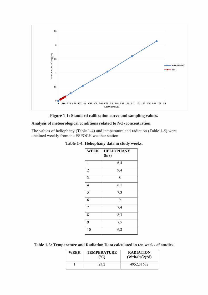
Figure 1-1: Standard calibration curve and sampling values.

Analysis of meteorological conditions related to NO2 concentration.

The values of heliophany (Table 1-4) and temperature and radiation (Table 1-5) were obtained weekly from the ESPOCH weather station.

Table 1-4: Heliophany data in study weeks.

WEEK HELIOPHANY (hrs)

1 6,4

2 9,4

3 8

4 6,1

5 7,3

6 9

7 7,4

8 8,3

9 7,5

10 6,2

Table 1-5: Temperature and Radiation Data calculated in ten weeks of studies.

WEEK TEMPERATURE (°C)

RADIATION (W*h/(mˆ2)*d)

1 23,2 4952,31672

0

0.5

1

1.5

2

2.5

0 0.08 0.16 0.24 0.32 0.4 0.48 0.56 0.64 0.72 0.8 0.88 0.96 1.04 1.12 1.2 1.28 1.36 1.44 1.52 1.6

CO

NC

EN

TR

AT

IÓN

(µ

g/m

³)

ABSORBANCE

absorbancia 2

ness

 

WEEK TEMPERATURE (°C)

RADIATION (W*h/(mˆ2)*d)

2 19,7 6263,77512

3 21,8 5651,7612

4 24,6 4821,17088

5 19,1 5345,75424

6 22,7 6088,914

7 23 5389,46952

8 23,7 5782,90704

9 24 5433,1848

10 22,3 4952,31672

Analysis through maps and simulations

A database was established using Excel to record the sampling stations located in areas of the bus terminal of Riobamba city in conjunction with the geographic coordinates presented in Table 1-2, an individual file was generated for the monthly and daily averages; This information was the basis for the implementation of the interpolation model.

ArcGIS 10.1 software was used for the elaboration of the dispersion maps, which allowed the spatial modeling of the data obtained by the monitoring stations, implementing the tool Geostatistical Analysis, which contains a set of procedures that gave shape to the cartography obtained for the present study.

The simulation was performed in the software Vissim PTV and through its tools the routes were drawn on the map; the number of vehicles was entered according to vehicular preference determining the flow according to the points of study in which they were, the simulation of NOx, CO2 and particulate matter emissions. Once the structure of the map was finished, it was possible to reproduce the vehicular traffic for one hour, generating a document with the respective results.

EnViVer was used to link the results obtained by the Vissim PTV software with the emission models. To determine the behavior of the cars (speed-time profile), the information was required in the Vissim traffic simulation software.

EnViVer linked the TNO VERSIT + emission model with the simulated traffic behavior in Vissim, so the software calculated the impact on the emissions of a motorway exit, roundabout, among others, and the dynamic management of traffic in emissions. It also visualized the impact of a traffic measurement on exhaust emissions on a map.

3. Results and discussion

 

Laboratory tests show that several points have a concentration that exceeds that established by TULSMA. BOOK VI Annex 4 of Air Quality for nitrogen oxides, which is 150 μg/m³ per day. The data shown in graphs showing maximum values and the daily average of NO2 concentrations obtained during the ten-weeks of field study.

Table 1-6. NOx concentration data for each area.

NOX (µg/m³) CONCENTRATION

AREA MAXIMUN VALUES DAILY AVERAGES

Area 1 162,1116287 158,8538504

Area 2 185,3900547 181,6644756

Area 3 167,6381615 164,2693225

Area 4 120,243956 117,827546

Area 5 134,311494 131,6123843

Area 6 121,0813094 118,6480721

Area 7 86,74981782 85,00650258

Area 8 114,5499525 112,2479687

Area 9 219,7215463 215,3060451

Area 10 161,6092166 158,3615347

Area 11 190,4141754 186,5876321

Area 12 210,5106583 206,2802582

Area 13 185,8924667 182,1567912

Area 14 112,3728335 110,1146008

Area 15 178,0213443 174,443846

Area 16 168,4755149 165,0898486

Area 17 182,5430529 178,8746869

Area 18 190,9165875 187,0799478

Area 19 135,6512595 132,925226

Area 20 122,0861336 119,6327034

Area 21 119,0716611 116,6788095

Area 22 131,6319629 128,9867008

Area 23 133,1391992 130,4636478

Area 24 115,889718 113,5608104

Area 25 121,4162508 118,9762826

 

NOX (µg/m³) CONCENTRATION

AREA MAXIMUN VALUES DAILY AVERAGES

Area 26 124,9331353 122,4224921

Area 27 122,4210749 119,9609139

Area 28 103,999299 101,90934

Area 29 162,2790993 159,0179556

Area 30 79,88351949 78,27818867

Area 31 103,1619455 101,0888139

Area 32 86,74981782 85,00650258

For week 1, it is observed in the graph that at a temperature of 23.2 ° C. the NO2 concentration at point 9 presents a value of 30.61 μg/m3, at point 11 it presents 26.52 μg/m3, the Point 12 with 29.32 μg/m³, point 13 with 25.89 μg/m³ and at point 18 it presents 26.59 μg/m³, considered these values to be the most relevant quantitatively in relation to the other sampling areas, while The lowest value corresponds to the point 30 that presents a concentration of 11.12 μg/m³, this is because this area is in a secondary route least frequented.

With a temperature of 19.7 °C in week 2, the concentration of NO2 at point 9 has a value of 31.27 μg/m3, point 11 with 27.10 μg/m3, point 12 with 29.96 μg/m³, point 13 with 26.45 μg/m³ and at point 18 with 27.17 μg/m³ are the most relevant quantitatively, while the lowest value corresponds to point 30 which presents a concentration of 11.36 μg/m3.

At week 3, at a temperature of 21.8 °C, the NO2 concentration at point 9 has a value of 30.87 μg/m3, point 11 with 26.75 μg/m3, point 12 with 29.57 μg/m³, point 13 with 26.11 μg/m³ and at point 18 it presents 26.82 μg/m³ considered the most relevant quantitatively, while the lowest value corresponds to the point 30 that presents a concentration of 11.22 μg/m³.

At a temperature of 24.6 °C, the NO2 concentration at point 9 has a value of 30.34 μg/m3, point 11 with 26.29 μg/m3, point 12 with 29.07 μg/m3, point 13 with 25.67 μg/m³ and at point 18 it presents 26.36 μg/m³, being the most relevant quantitatively, while the lowest value corresponds to the point 30 that presents a concentration of 11.03 μg/m³. At week 5, at a temperature of 19.1 °C, the NO2 concentration at point 9 has a value of 31.38 μg/m3, point 11 at 27.20 μg/m3, point 12 at 30.07 μg/m³, point 13 with 26.55μg/m³ and at point 18 it has 27.27μg/m³, the highest values being, while the lowest value corresponds to the point 30 which presents a concentration of 11.41 μg/m³. At a temperature of 22.7 °C, at week 6, the NO2 concentration at point 9 has a value of 30.70 μg / m 3, point 11 with 26.60 μg / m 3, point 12 with 29.41 μg/m³, point 13 with 25.97μg/m³ and at point 18 it presents 26.67μg/m³, the highest quantitatively, while the lowest value is point 30 which presents a concentration of 11.16 μg/m³. At week 7, an issue occurred with the sampler at point 11, since the sampling tube had been manipulated by non-researchers, thus presenting a value of 0.265 μg/m3, the temperature of the week being 23 °C, At point 9 it presents a value of 30.64 μg/m³,

 

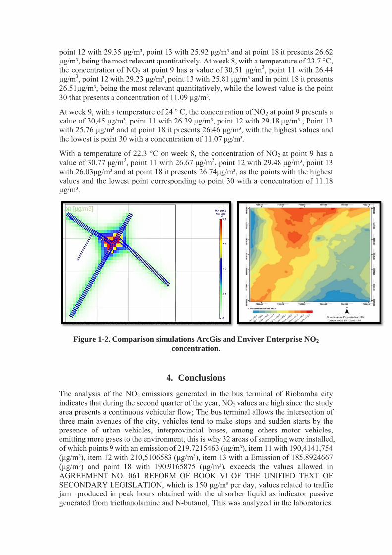
point 12 with 29.35 μg/m³, point 13 with 25.92 μg/m³ and at point 18 it presents 26.62 μg/m³, being the most relevant quantitatively. At week 8, with a temperature of 23.7 °C, the concentration of NO2 at point 9 has a value of 30.51 μg/m3, point 11 with 26.44 μg/m3, point 12 with 29.23 μg/m³, point 13 with 25.81 μg/m³ and in point 18 it presents 26.51μg/m³, being the most relevant quantitatively, while the lowest value is the point 30 that presents a concentration of 11.09 μg/m³.

At week 9, with a temperature of 24 ° C, the concentration of NO2 at point 9 presents a value of 30,45 μg/m³, point 11 with 26.39 μg/m³, point 12 with 29.18 μg/m³ , Point 13 with 25.76 μg/m³ and at point 18 it presents 26.46 μg/m³, with the highest values and the lowest is point 30 with a concentration of 11.07 μg/m³.

With a temperature of 22.3 °C on week 8, the concentration of NO2 at point 9 has a value of 30.77 μg/m3, point 11 with 26.67 μg/m3, point 12 with 29.48 μg/m³, point 13 with 26.03μg/m³ and at point 18 it presents 26.74μg/m³, as the points with the highest values and the lowest point corresponding to point 30 with a concentration of 11.18 μg/m³.

Figure 1-2. Comparison simulations ArcGis and Enviver Enterprise NO2 concentration.

4. Conclusions

The analysis of the NO2 emissions generated in the bus terminal of Riobamba city indicates that during the second quarter of the year, NO2 values are high since the study area presents a continuous vehicular flow; The bus terminal allows the intersection of three main avenues of the city, vehicles tend to make stops and sudden starts by the presence of urban vehicles, interprovincial buses, among others motor vehicles, emitting more gases to the environment, this is why 32 areas of sampling were installed, of which points 9 with an emission of 219.7215463 (μg/m³), item 11 with 190,4141,754 (μg/m³), item 12 with 210,5106583 (μg/m³), item 13 with a Emission of 185.8924667 (μg/m³) and point 18 with 190.9165875 (μg/m³), exceeds the values allowed in AGREEMENT NO. 061 REFORM OF BOOK VI OF THE UNIFIED TEXT OF SECONDARY LEGISLATION, which is 150 μg/m³ per day, values related to traffic jam produced in peak hours obtained with the absorber liquid as indicator passive generated from triethanolamine and N-butanol, This was analyzed in the laboratories.

 

Finally, the simulation in the Vissim 8 PTV software was performed prior to a vehicle count in the study area, which form the Daniel León Borja, Canónigo Ramos and La Prensa avenues; The Vissim software simulates traffic conditions and drivers' habits, recreating the vehicular flow of the study area in which it is determined (Figure 4-1) that the points of yellowish to reddish tonality are in which there is greater degree of emission of oxides of nitrogen, since the vehicles when stopping and starting again, release more combustion gases (Borge, et al., 2015) (Universidad Politécnica de Madrid, 2016). The simulations show similar color variations, however, in the ArcGIS map, the concentrations of nitrogen oxides used are those obtained in the laboratory after the monitoring and analysis of the samples; while the emission map generated by the Enviver Enterprise software (Figure 4-1) is the result of the values obtained after the vehicle count performed in the study area.

Bibliography

Air Quality and Pollution Control. Cheap VOC Tests. [En línea] 2012. [Consulta: 02 de Octubre de 2016.]. Disponible en: http://airqualitycontrol.blogspot.com/2012/06/cheap-ways-to-test-for-vocs.html.

AGAT Laboratorios. Muestreo de Aire Pasivo. [En línea] 2013. [Consulta: 27 de Agosto de 2016.]. Disponible en: http://www.agatlabs.com/Spanish/content/passiveair.html.

Álvarez, Jesús. Motores alternativos de combustión interna. Ediciones de la Universidad Politécnica de Catalunya, SL. Barcelona, 2005. pp 341 -342.

Bartual, José. Toma de muestras con captadores pasivos. [En línea] 2014. [Consulta: 14 de Septiembre de 2016.] Disponible en: http://www.insht.es/InshtWeb/Contenidos/Documentacion/FichasTecnicas/NTP/Ficheros/101a200/ntp_151.pdf

BIBLIOTECA LUIS ANGEL ARANGO. BANCO DE LA REPUBLICA DE COLOMBIA. [En línea]. 2011. Disponible en: http://www.banrepcultural.org/node/92123.

Borge, R, et al. Experimental Campaign in a Heavily Trafficked Roundabout in Madrid for the Assessment of Air Quality Monitoring Station Representativeness in Terms of Population Exposure to NO2. Kunshan : s.n., 2015.

BORGE, Rafael. (2016). Microscale traffic simulation and emission estimation in a heavilytrafficked roundabout in Madrid (Spain). Elsevier, 416. Disponible en:

https://www.researchgate.net/publication/303496191_Microscale_traffic_simulation_and_emission_estimation_in_a_heavily_trafficked_roundabout_in_Madrid_Spain

Cano, Eduardo. Motores y contaminación. [En línea]. 2014. Disponible en: http://www.abc.es/motor-reportajes/20140917/abci-contaminan-diesel-gasolina-201409161153.html.

Cheung, Paul. Naciones Unidas - Diseño de muestras para encuestas de hogar, directrices prácticas. [En línea] 2009. [Consulta: 26 de septiembre de 2016.] Disponible en: https://unstats.un.org/unsd/publication/seriesf/Seriesf_98s.pdf.

 

CNICE. Calidad de aire y temperatura. [En línea]. 2011. Disponible en: http://concurso.cnice.mec.es/cnice2005/93_iniciacion_interactiva_materia/curso/materiales/propiedades/temperatura.html.

Comisión Nacional del Medio Ambiente Chile. Inventario Nacional de Emisiones de Gases Efecto Invernadero. [En línea]. 2008. Disponible en: http://www.sinia.cl/1292/articles-50188_recurso_1.pdf.

Duffie, J.A., & Beckman, W. A. Solar Energineering of Thermal Processes. [En línea]. 4ª Edición. Hoboken (New Yersey- USA): Fohn Wiley & sons, 2005, pp. 1-133. [Consulta: 25 de noviembre de 2016]. Disponible en: Solar%20Engineering%20 of%Thermal%20 Processes,%204th%20Edition%20%20 GearTeam%20.pdf

Earth Observatory. Terra Tracks Pollution. [En línea] 2005. [Consulta: 25 de Octubre de 2016.] Disponible en: https://earthobservatory.nasa.gov/Features/Terra/.

ECODES. ECODES, Cambio climático. [En línea]. 2011. Disponible en: http://ecodes.org/cambio-climatico/.

Environmental Systems Research Institute, Inc. ArcGIS, Geografía aplicada para cada acción. [En línea] 2015. [Consulta: 29 de noviembre de 2016.] Disponible en: http://www.aeroterra.com/products/Plataforma/.

Etza, Ruth A. y Jean G. French. Impacto ambiental, aire. [En línea] Septiembre de 2000. Disponible en: http://cidbimena.desastres.hn/docum/ops/Edan/publicaciones/Impacto/ImpactoAll.pdf#page=347.

European Chemicals Agency. NOx (óxidos de nitrógeno). [En línea] 2016. [Consulta: 29 de Septiembre de 2016.] Disponible en: https://echa.europa.eu/substance-information/-/substanceinfo/100.030.234.

Fernandez, D. Control y eliminación de los NOx. [En línea] 2010. [Consulta: 09 de septiembre de 2016.] Disponible en: http://files.pfernandezdiez.es/CentralesTermicas/PDFs/33CT.pdf.

Fundación Centro de Recursos Ambientales de Navarra. Óxidos de nitrógeno (NOx = NO + NO2). [En línea] 2014. [Consulta: 30 de septiembre de 2016.] Disponible en: http://www.crana.org/es/contaminacion/mas-informacion_3/axidos-nitrageno-nox-no2.

FUNDACIÓN CRANA FUNDAZIOA. FUNDACIÓN CRANA, Óxido de nitrógeno. [En línea] 2014. Disponible en: http://www.crana.org/es/contaminacion/mas-informacion_3/axidos-nitrageno-nox-no2.

Galán, David. Implicación de los NOx en la química atmosférica. [En línea] 2006. [Consulta: 04 de octubre de 2016.] Disponible en: https://www.ucm.es/data/cont/media/www/pag-41377/2006%202%20david%20galan%20y%20otro.pdf.

Gobierno de Navarra. CRANA. Fundación Centro de Recursos Ambientales de Navarra. [En línea] 2008. Disponible en:

 

http://www.crana.org/es/contaminacion/mas-informacion_3/axidos-nitrageno-nox-no2.

Gonzalez, Raúl. Los gases contaminantes. twenergy. [En línea] 2012. [Consulta: 20 de agosto de 2016.] Disponible en: https://twenergy.com/a/los-gases-contaminantes-648.

GREEN FACTS. Dióxido de nitrógeno. [En línea] 2012. Disponible en: http://www.greenfacts.org/es/dioxido-nitrogeno-no2/.

IESA. Introducción a los métodos de encuestación y muestreo estadístico. [En línea] 2009. [Consulta: 25 de Septiembre de 2016.] Disponible en: http://www.iesa.csic.es/eventos/adjunto_6FEBRERO_2009.pdf.

Institulo Nacional de Estadística y Censos. Instructivo ArcGIS. [En línea] 2012. [Consulta: 28 de Noviembre de 2016.] Disponible en: http://www.inec.gob.ec/nuevo_inec/items/gestion_eficiente/cartografia/anexos/CAPACITACIONES/INSTRUCTIVOS%20AMANZANADO/ARCGIS.pdf.

Instituto Nacional de Ecología. Manual 1, Principios de medición de la Calidad del Aire. [En línea] 2013. [Consulta: 17 de octubre de 2016.] Disponible en: http://sinaica.inecc.gob.mx/archivo/guias/1-%20Principios%20de%20Medici%C3%B3n%20de%20la%20Calidad%20del%20Aire.pdf.

Instituto Nacional de Estadística y Censos. Estadísticas de transporte Ecuador. [En línea] 2013. Disponible en: http://www.ecuadorencifras.gob.ec/documentos/web-inec/Estadisticas_Economicas/Estadistica%20de%20Transporte/Publicaciones/Anuario_de_Estad_de_Transporte_2013.pdf.

López, Guillermo. Metodología de cálculo de NOx en generadores de vapor que queman gas natural. [En línea] 2010. [Consulta: 30 de Agosto de 2016.] Disponible en: http://www.redalyc.org/articulo.oa?id=61420351005.

Manrique Carvajal, Angelica María y Ossa Morales, Diana Marcela. Validación de los métodos espectrofotométricos para la determinación de SOx y NOx en muestras de aire. [En línea] 2010. Disponible en: http://repositorio.utp.edu.co/dspace/bitstream/handle/11059/1832/5430858M285.pdf?sequence=1.

Masaquiza Yanzapanta, Ángel Guillermo y Vizuete Palacios, José Enrique. Estudio técnico de un sistema integral de revisión vehicular para la provincia de Chimborazo en la ESPOCH. [En línea] (Tesis pregrado) Escuela Superior Politécnica de Chimborazo. 2012. Disponible en: http://dspace.espoch.edu.ec/bitstream/123456789/2260/1/65T00046.pdf.

MEXICALI. Departamento de calidad del aire. [En línea] 17 de OCTUBRE de 2011. Disponible en: http://www2.inecc.gob.mx/publicaciones/libros/618/vehiculos.pdf.

Mier, Manuel Antonio Montenegro. Vehículos, emisiones y combustión. Banco de la República de Colombia. [En línea] 2007. Disponible en: http://www.banrepcultural.org/blaavirtual/ciencias/sena/mecanica/gas-preconversion-vehiculos/gaspre5a.html.

 

MINISTERIO DE AGRICULTURA, ALIMENTACION Y MEDIO AMBIENTE DEL GOBIERNO DE ESPAÑA. Registro estatal de emisiones y fuentes contaminantes. [En línea] 2015. Disponible en: http://www.prtr-es.es/NOx-oxidos-de-nitrogeno,15595,11,2007.html.

Ministerio del Ambiente Ecuador. Inventario Preliminar de las Emisiones de Contaminantes del Aire , de los cantones Ambato, Riobamba, Sando Domingo de los colorados, Latacunga, Ibarra, Manta, Portoviejo, Esmeraldas y Milagro. [En línea] 2014. Disponible en: http://www.ambiente.gob.ec/wp-content/uploads/downloads/2014/05/Libro-Resumen-Inventario-13-02-2014-prensa.pdf.

Molina, Victor. Principios básicos motor de combustión interna. [En línea] 2015. [Consulta: 22 de Septiembre de 2016.] Disponible en: https://www.academia.edu/8103611/PRINCIPIOS_B%C3%81SICOS_MOTOR_DE_COMBUSTION_INTERNA?auto=download.

NATIONAL GEOGRAPHIC. Calentamiento global, contaminación del aire. NATIONAL GEOGRAPHIC.. [En línea] 2014. Disponible en: http://nationalgeographic.es/medio-ambiente/calentamiento-global/contaminacion-aire.

Organización Mundial de la Salud. Efectos nosivos en la salud por óxidos de nitrógeno. [En línea] 2014. Disponible en: http://who.int/mediacentre/factsheets/fs313/es/.

PTV GROUP. Transport planning, traffic engineering and traffic simulation. [En línea] 2014. Disponible en: http://vision-traffic.ptvgroup.com/es/productos/ptv-vissim/.

Puerto Albandoz, Justo y Lagares Barreiro, Paula. Población y muestra. Técnicas de muestreos. [En línea] 2001. Disponible en: http://optimierung.mathematik.uni-kl.de/mamaeusch/veroeffentlichungen/ver_texte/sampling_es.pdf.

Puerto Martín, A. y García Rodriguez, J.A. 1986. La Contaminación Atmosférica. Salamanca : s.n., 1986.

Rodrígues, Ernesto Bolaños. Muestreo y técnicas calidad del aire. UNIVERSIDAD AUTONOMA DEL ESTADO DE HIDALGO. [En línea] JUNIO de 2012. Disponible en: http://www.uaeh.edu.mx/docencia/P_Presentaciones/tizayuca/gestion_tecnologica/muestraMuestreo.pdf.

Sánchez, Carlos, Mendoza, Denisse y Castillo, Iveth. Validación y ajuste de modelos de radiación solar directa para la ciudad de Bogotá a partir de datos experimentales tomados en la Universidad Distrital Francisco José de Caldas. Grupo de Energías Alternativas, Universidad Distrital, Colombia. [En línea] 2015. Disponible en: http://www.cubasolar.cu/biblioteca/Ecosolar/Ecosolar15/HTML/articulo02.html.

SEMARNAT. Gestión ambiental, pasivos. [En línea] 2011. Disponible en: http://www.semarnat.gob.mx/archivosanteriores/temas/gestionambiental/Materiales%20y%20Actividades%20Riesgosas/sitioscontaminados/pasivos/pasivos.pdf.

 

Servicio Evaluación de la Calidad y Control Ambiental. Principales contaminantes del aire. [En línea] 2014. [Consulta: 17 de agosto de 2016.] Disponible en: http://www.montevideo.gub.uy/servicios-y-sociedad/limpieza-y-medio-ambiente/aire/principales-contaminantes-del-aire.

Sumano, Enrique Méndez. Cambio climático y gases de efecto invernadero. [En línea] 2008. [Consulta: 30 de Septiembre de 2016.] Disponible en: http://es.slideshare.net/CarlosMartinez106/word-resumen.

TEXTOS CIENTIFICOS. Transmisión de calor, radiación solar. [En línea]. 2013. Disponible en: http://www.textoscientificos.com/fisica/transmision-calor/radiacion.

Universidad de Murcia. Presencia de nitritos en alimentos, aireambiente. Open Course Ware. [En línea] 2008. Disponible en: http://ocw.um.es/cc.-de-la-salud/higiene-inspeccion-y-control-alimentario-1/practicas-1/practicas-carne-nitritos.

Universidad Politécnica de Madrid. Aplicación del modelo de microsimulación PTV VISSIM para el cálculo de emisiones del tráfico. Laboratorio de Modelización Ambiental. Tecn aire. [En línea] 08 de Junio de 2016. Disponible en: http://tecnaire-cm.org/wp-content/uploads/2016/06/CQuaassdorff_CIT2016_Vissim.pdf.

UNIVERSIDAD TECNOLOGICA NACIONAL DE ARGENTINA. Modelación de un evento meteorológico de mesoescala utilizando el modelo WRF. [En línea] 2011. Disponible en: http://www.uca.edu.ar/uca/common/grupo72/files/E7_Fern--ndez.pdf.

Universitat de Valencia. Técnicas de muestreo. [En línea] 2000. Disponible en: https://www.uv.es/ceaces/tex1t/3%20infemues/tecnicas.html.

VICENTE, LUIS RAMÍREZ. Proyecto descartes. [En línea] 2010. Disponible en: http://recursostic.educacion.es/secundaria/edad/4esofisicaquimica/4quincena12/4q12_centro.html.

VILLARREAL, David. NOx emisiones. [En línea] 2015. Disponible en: http://www.diariomotor.com/2015/09/25/nox-emisiones/.

   

 

ICESI_0081

Biogenic Emissions of Non Methanogenic Volatile Organic Compounds in Ecuador

Rafaela Viteri, Escuela Superior Politecnica de Chimborazo, Ecuador

*Marcel Paredes, National University of Chimborazo, Ecuador

Eliana Sanchez, Escuela Superior Politecnica de Chimborazo, Ecuador

Astudillo, I., Escuela Superior Politecnica de Chimborazo, Ecuador

*Corresponding Author

Abstract

Ecuador is one of the countries with a greater biodiversity in America; however, biogenic emissions has been never studied. Emissions of biogenic volatile organic compounds are important because of their potential influence on the formation of tropospheric ozone. Emissions of volatile organic compounds were estimated for the vegetation of Ecuador, for 2010, categorized in three groups in function of their reactivity: isoprene lifetime of 1 to 2 hours; monoterpenes, lifetime of 0.5 to 3 hours; and other volatile organic compounds, generally with a lifetime of 1 day. The basic model of Guenther was used, that considers the temperature and the photosynthetically active radiation as physical parameters with high influence. It was determinate hourly emissions, daily representative for each month, monthly and annual. Results were represented in georeferenced maps.

Total emissions arise to 1855.6 kt a-1, of which 1278.6 kt a-1 belongs to isoprene, 427.6 kt a-1 to monoterpenes and 149.3 kt a-1 to other volatile organic compounds. Highest emissions are located in zones with oil palm crops, in Santo Domingo and Esmeraldas provinces. Results provides valuable information to inventories of national emissions of air pollutants, and may be used to simulation studies of tropospheric ozone

Keywords: Biogenic emissions, Isoprene, Monoterpenes, Other volatile organic compounds, Model of Guenther.

 

1. Introduction Volatile organic compounds (VOCs) derived from both natural and anthropogenic sources play an important role in the atmospheric chemistry because they intervene in photochemical reactions that lead to the formation of secondary pollutants (Simon, Luchetta, & Torres, 2001). Under certain environmental conditions such as clear sky, high levels of radiation, temperature and pressure, VOCs react with nitrogen oxides (NOx), resulting in the formation of tropospheric ozone (O3) (Ghimire et al., 2016; Simon et al., 2001; Solmon, Sarrat, Serça, Tulet, & Rosset, 2004); they also react with hydroxyl radicals (•OH) and nitrate (•NO3), thus forming a great amount of secondary organic aerosols (SAO) (Ghimire et al., 2016; Kesselmeier et al., 2000).

In urban areas, VOCs that are usually derived from anthropogenic sources are emitted in larger amounts compared to biogenic volatile organic compounds (BVOCs), nevertheless the reactivity of the latter is high, which on average is estimated to be 223 times higher than that of VOCs generated from fuels. (Benjamin, Sudol, Bloch, & Winer, 1996). Therefore, BVOCs have a greater contribution to the formation of photochemical ozone and other secondary pollutant (Benjamin et al., 1996; Padhy & Varshney, 2005). The emissions of BVOCs in plants are the result of response and defence mechanisms against environmental stress caused by high temperature, solar radiation and the attack by herbivorous animals, insects and pathogens. (Benjamin et al., 1996; Ghimire et al., 2016; Kesselmeier et al., 2000).

BVOCs are classified into 4 categories: isoprene (C5H8), monoterpene (C10H16), reactive BVOCs and less reactive BVOCs (Ghimire et al., 2016). The annual flux of BVOCs from plants was estimated to be 1150 tg-C, which contained 44% isoprene, 11% monoterpenes, 22,5% reactive VOCs and 22,5% non-reactive VOCs. (Kansal, 2009); as a consequence, isoprenes, monoterpenes and reactive VOCs are the most relevant categories from an environmental point of view because they combine two key characteristics: abundance and reactivity.

According to numerous studies, it was determined that tropical forests worldwide (rainforests, savannas, etc.) contribute to an aproximate of 50% of all the emissions of BVOCs, whereas the farmlands and other forests (conifers y deciduous trees) generate from 10 to 20% of all the emissions (Hakola et al., 2003; Kansal, 2009). Therefore, the Amazon rainforest was identified as the major source of BVOCs because it is considered a continuous forest with enormous dimensions, however, despite its characteristics, little is known about VOCs release from representative plant species of this ecosystem (Kesselmeier et al., 2000).

The aim of the present study is to estimate the amount of VOCs released by the Ecuadorian vegetation during the year 2010 as great part of its territory is covered by forest and other agricultural crops, and has a great diversity of plant species. The proposed methodology includes the categorisation of BVOCs according to their typical lifetime and the application of a model proposed by Guenther who defines the emissions as a function of the solar radiation and the temperature. Additionally, we will employ emission factors which are established for a standard set of environmental conditions and specific for each plant species.

2. Methodology

 

For the estimation of emissions, we used the model proposed by Guenther et al, which considers such parameters as temperature, photosynthetically active solar radiation (PAR) and foliar density.

Estimation of isoprene emissions

The equation (1) used to estimate hourly isoprene emissions is as follows:

, , (1)

Where Eiso (k, each hour) is the hourly isoprene emission into the kth cell, is the standard isoprene emission factor with the j land-use category, ECF (T, P) is the environmental correction factor due to temperature PAR (adimensional), FBDj is the foliar biomass density of the j land-use category (g/m2) and A is the area of each grid cell (16 km2).

Additionally, the correction factor was calculated using th following equation (2):

, (2)

Where CT is the correction factor due to temperature and CP is the correction factor owing to PAR.

The daily estimation of isoprene emissions Eiso(K, daily) corresponds to the cumulative value of hourly emissions for an average day (24h). Whereas for the monthly calculation we used the following equation (3):

, 30 , (3)

Consequently, the annually estimations were calculated using the following equation (4):

, 12 , (4)

Regarding the emission factors, they are usually expressed under reference conditions considered to be standard, i.e. a temperature of 30°C (303 K) and a PAR of 1000 μmol m-2 s-1. Taking into account that under standard conditions, CL y CT have a value of 1; and as PAR increases, CL becomes asymptotic; on the other hand, CT increases until it reaches a temperature of 40°C, after which its value starts to decrease.

 

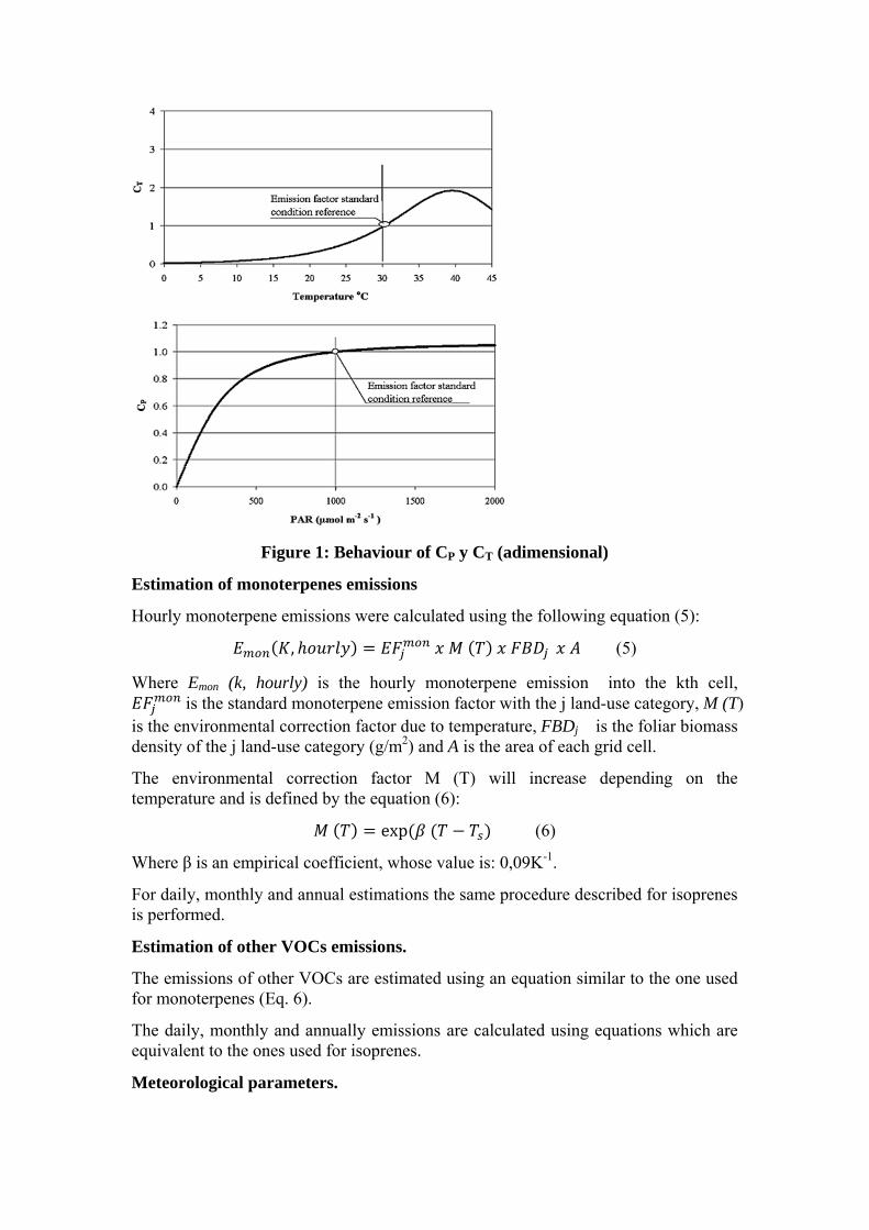
Figure 1: Behaviour of CP y CT (adimensional)

Estimation of monoterpenes emissions

Hourly monoterpene emissions were calculated using the following equation (5):

, (5)

Where Emon (k, hourly) is the hourly monoterpene emission into the kth cell, is the standard monoterpene emission factor with the j land-use category, M (T)

is the environmental correction factor due to temperature, FBDj is the foliar biomass density of the j land-use category (g/m2) and A is the area of each grid cell.

The environmental correction factor M (T) will increase depending on the temperature and is defined by the equation (6):

exp (6)

Where β is an empirical coefficient, whose value is: 0,09K-1.

For daily, monthly and annual estimations the same procedure described for isoprenes is performed.

Estimation of other VOCs emissions.

The emissions of other VOCs are estimated using an equation similar to the one used for monoterpenes (Eq. 6).

The daily, monthly and annually emissions are calculated using equations which are equivalent to the ones used for isoprenes.

Meteorological parameters.

 

Temperature maps of Ecuador for the year 2010 were generated with the aid of the Weather Research and Forecasting (WRF) Model version 3.2, using a grid of cells with 199 rows and 199 columns. Each cell is 4 Km on each side.

The meteorological results were processed in order to generate representative maps for each month of the year. These maps were then used to calculate the VOCs emissions.

Moreover, the data units related to PAR simulated in the present study were Wm-2. Therefore, we performed a unit conversion in order to calculate the parameter CL, considering that 1 Wm-2 is equal to 4.6 μmol m-2 s-1 and PAR represents 50% of the incident global solar radiation.

Plant species assignation for land use.

The map of land use for 2010 was provided by the Ministry of Agriculture, Livestock and Fisheries (MAGAP, 2010).

We conducted an analysis and a study of the plant composition of each land use in order to determine the principle species. Furthermore, the species assignation was performed according to the region of their location in order to collect accurate information and develop a precise inventory of emissions.

Emission factors.

The selection of emission factors was performed based on the literature and the available inventory for certain regions of the country. The sources of information that we employed are as follows:

Database of VOCs emission factors from Lancaster University (Lancaster University, 2002).

Emission factors published by Kesselmeier (Kesselmeier & Staudt, 1999).

Emission inventory published by the Europe Union (Unión Europea, 2011).

Emission inventory of BVOCs produced in the Peruvian Amazon forest (Limonchi, 2011).

Based on the emission factors of the plant species we obtained a defined value for land use.

Foliar biomass density.

In order to determine the foliar biomass density for land use, we used as a reference an undergraduate dissertation about the Determination of the Foliar Biomass of Plant Species from the ESPE - Army Polytechnic School (Flores & Flores, 2011).

3. Results and Discussion Meteorological conditions.

During the day, the maximum temperature was recorded at 14:00 and its value varied between 25 and 28 °C. Concerning the annual variations, the highest temperature was recorded in March with a value of 28.07 °C. In contrast, the lowest temperature was

 

recorded in August with a value of -3 °C due to the lack of cloudiness, allowing the atmospheric heat loss, which leads to the cooling of the Earth surface.

The maximum monthly radiation value of the year 2010 was recorded at midday and varied between 740 y 885 W m-2. On the other hand, the maximum solar radiation during the year occurred in January and reached a value of 884.39 W m-2, whereas in June and July the minimum radiation values were recorded with values of around 700 W m-2.

Emission factors according to the land use.

The emission factors for each land use were calculated based on the mean of the values of the most representative species. The tables 1, 2 and 3 show the emission factors that belong to each land use of different regions.

Table 1: Emission Factors for the land use of the Coast region.

Use Category Species Emission factor (µg g-1 h-1)

Isoprene Monoterpenes OVOC

1 Natural Forest

Brosimum utile, Campnosperma panamensis,

Carapa guianensis Aubl, Astrocaryum standleuanum, Castilla elastica, Cecropia

garciae, Conostegia cuatrecasii, Guarea

polymera, Hemiepifita Rhodospatha densinervia, Huamiriastrum procerum, Matisia alata, Nectandra

guadaripo, Otoba gordoniifolia , Phytelephas

aequatorialis, Poulsenia armata, Tetrathylacium

macrophylllum, Therobroma gileri, Wettinia

quinaria, Xanthosoma daguense, Osmunda

cinnamonea, Begonia glabra, Caryodaphnopsis,

Irbachia alata, Orchidaceae spp, Virola

dixonii, Vitex flavens, Ochroma pyramidale,

Brosimum utile, Campnosperma panamensis,

Muntingia calabura, Centrolobium patinensis,

Myroxylon balsamun, Pouteria sp, Carappa

guianensis, Bombax sp, Clarisia racemosa, Vitex

21.14 0.3 0

 

Use Category Species Emission factor (µg g-1 h-1)

Isoprene Monoterpenes OVOCgigantea, Ceiba

trichistandra, Guadua angustifolia, Acacia

farnesiana, Ficus insípida, Cochlospermum vitifolium,

Bursera graveolens , Prosopis spp, Cordia lutea , Eriotheca ruizii , Capparis mollis, Erythrina velutina,

Caesalpinia paraguariensis, Tillandsia usneoides,

Cochlospermum vitifolium, Weinmannia ovalis, Libidia

corymbosa, Acnistus arborescens, Macrolobium

stenosiphon, Ipomea pescaprae, Lantana

rugulosa, Cereus spp, Guazuma ulmifolia, Simira

ecuadorensis, Spondias purpúrea, Pithecellobium pausipinnata, Eugenia sp,

Leucaena trichodes, Pithecellobium excelsum, Zanthoxylum sp, Pisonia aculeata, Loxopterygium

huasango, Eriotheca ruizii, Geoffroea spinosa,

Centrolobium ochroxylum, Clusia polystigma, Protium aracouchini, Vitis vinifera, Chrysophyllum oliviforme,

Xanthoxylon Dugandi Stand, Carludovica palmata,

Guadua, Cibotium spp, Therobroma gileri,

Anthurium andreanum Linden

2 Tropical

arboricultureVegetación tropical

siempreverde 0 0 1.5

5 Cacao Theobroma cacao 0 0

6 Short-cycle

crops

Oryza sativa, Vicia faba, Manihot utilissima, Zea

mays, Carludovica palmata, Saccharum officinaru,

Passiflora edulis

0.024 0.186 0.475

 

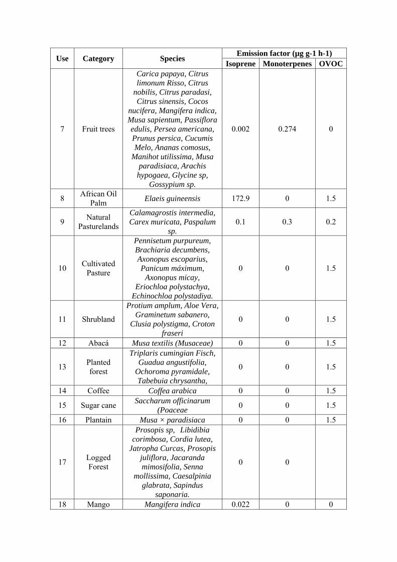
Use Category Species Emission factor (µg g-1 h-1)

Isoprene Monoterpenes OVOC

7 Fruit trees

Carica papaya, Citrus limonum Risso, Citrus

nobilis, Citrus paradasi, Citrus sinensis, Cocos

nucifera, Mangifera indica, Musa sapientum, Passiflora edulis, Persea americana, Prunus persica, Cucumis Melo, Ananas comosus,

Manihot utilissima, Musa paradisiaca, Arachis hypogaea, Glycine sp,

Gossypium sp.

0.002 0.274 0

8 African Oil

Palm Elaeis guineensis 172.9 0 1.5

9 Natural

Pasturelands

Calamagrostis intermedia, Carex muricata, Paspalum

sp. 0.1 0.3 0.2

10 Cultivated

Pasture

Pennisetum purpureum, Brachiaria decumbens, Axonopus escoparius, Panicum máximum,

Axonopus micay, Eriochloa polystachya,

Echinochloa polystadiya.

0 0 1.5

11 Shrubland

Protium amplum, Aloe Vera, Graminetum sabanero,

Clusia polystigma, Croton fraseri

0 0 1.5

12 Abacá Musa textilis (Musaceae) 0 0 1.5

13 Planted forest

Triplaris cumingian Fisch, Guadua angustifolia,

Ochoroma pyramidale, Tabebuia chrysantha,

0 0 1.5

14 Coffee Coffea arabica 0 0 1.5

15 Sugar cane Saccharum officinarum

(Poaceae 0 0 1.5

16 Plantain Musa × paradisiaca 0 0 1.5

17 Logged Forest

Prosopis sp, Libidibia corimbosa, Cordia lutea,

Jatropha Curcas, Prosopis juliflora, Jacaranda mimosifolia, Senna

mollissima, Caesalpinia glabrata, Sapindus

saponaria.

0 0

18 Mango Mangifera indica 0.022 0 0

 

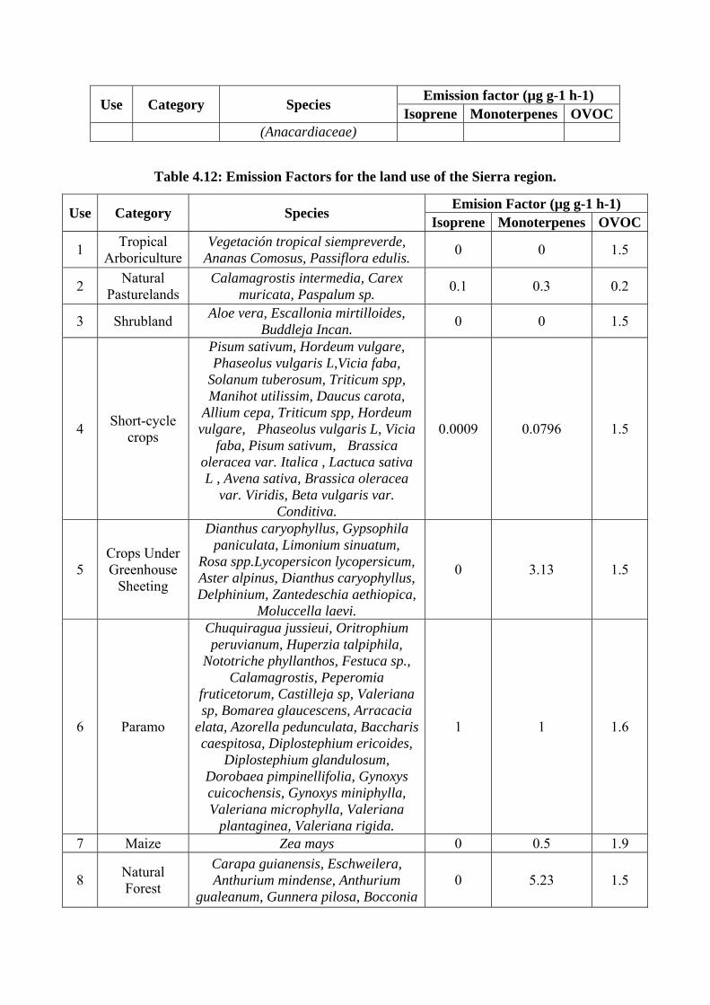
Use Category Species Emission factor (µg g-1 h-1)

Isoprene Monoterpenes OVOC(Anacardiaceae)

Table 4.12: Emission Factors for the land use of the Sierra region.

Use Category Species Emision Factor (µg g-1 h-1)

Isoprene Monoterpenes OVOC

1 Tropical

Arboriculture Vegetación tropical siempreverde,

Ananas Comosus, Passiflora edulis. 0 0 1.5

2 Natural

Pasturelands Calamagrostis intermedia, Carex

muricata, Paspalum sp. 0.1 0.3 0.2

3 Shrubland Aloe vera, Escallonia mirtilloides,

Buddleja Incan. 0 0 1.5

4 Short-cycle

crops

Pisum sativum, Hordeum vulgare, Phaseolus vulgaris L,Vicia faba,

Solanum tuberosum, Triticum spp, Manihot utilissim, Daucus carota,

Allium cepa, Triticum spp, Hordeum vulgare, Phaseolus vulgaris L, Vicia

faba, Pisum sativum, Brassica oleracea var. Italica , Lactuca sativa L , Avena sativa, Brassica oleracea

var. Viridis, Beta vulgaris var. Conditiva.

0.0009 0.0796 1.5

5 Crops Under Greenhouse

Sheeting

Dianthus caryophyllus, Gypsophila paniculata, Limonium sinuatum,

Rosa spp.Lycopersicon lycopersicum, Aster alpinus, Dianthus caryophyllus, Delphinium, Zantedeschia aethiopica,

Moluccella laevi.

0 3.13 1.5

6 Paramo

Chuquiragua jussieui, Oritrophium peruvianum, Huperzia talpiphila,

Nototriche phyllanthos, Festuca sp., Calamagrostis, Peperomia

fruticetorum, Castilleja sp, Valeriana sp, Bomarea glaucescens, Arracacia

elata, Azorella pedunculata, Baccharis caespitosa, Diplostephium ericoides,

Diplostephium glandulosum, Dorobaea pimpinellifolia, Gynoxys cuicochensis, Gynoxys miniphylla, Valeriana microphylla, Valeriana

plantaginea, Valeriana rigida.

1 1 1.6

7 Maize Zea mays 0 0.5 1.9

8 Natural Forest

Carapa guianensis, Eschweilera, Anthurium mindense, Anthurium

gualeanum, Gunnera pilosa, Bocconia 0 5.23 1.5

 

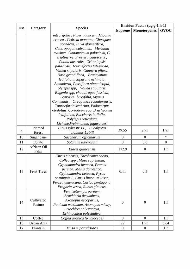
Use Category Species Emision Factor (µg g-1 h-1)

Isoprene Monoterpenes OVOCintegrifolia , Piper aduncum, Miconia crocea , Cedrela montana, Chusquea

scandens, Puya glomerifera, Centropogon calycinus, Meriania

maxima, Cinnamomum palaciosii, C. triplinerve, Freziera canescens , Cotula australis , Critoniopsis

palaciosii, Tournefortia fuliginosa, Vallea stipularis, Gunnera pilosa, Nasa grandiflora, Brachyotum ledifolium, Siparuna echinata,

Aamaderoi, Passiflora pinnatistipul, olylepis spp, Vallea stipularis,

Eugenia spp, chuquiragua jussieui, Gynoxys buxyfolia, Myrtus

Communis, Oreopanax ecuadorensis, Tournefortia scabrina, Podocarpus

oleifolius, Cortadeira spp, Brachyotum ledifolium, Baccharis latifolia,

Polylepis reticulata, Lichene,Weinmannia fagaroides,

9 Planted forest

Pinus sylvestris L, Eucalyptus globulus Labill

39.55 2.95 1.85

10 Sugar cane Saccharum officinarum 0 0 * 11 Potato Solanum tuberosum 0 0.6 0

12 African Oil

Palm Elaeis guineensis 172.9 0 1.5

13 Fruit Trees

Citrus sinensis, Theobroma cacao, Coffea spp , Musa sapientum,

Cyphomandra betacea, Prunus persica, Malus domestica,

Cyphomandra betacea, Pyrus communis L, Citrus limonum Risso,

Persea americana, Carica pentagona, Fragaria vesca, Rubus glaucus.

0.11 0.3 1.5

14 Cultivated

Pasture

Pennisetum purpureum, Brachiaria decumbens, Axonopus escoparius,

Panicum máximum, Axonopus micay, Eriochloa polystachya,

Echinochloa polystadiya.

0 0 1.5

15 Coffee Coffea arabica (Rubiaceae) 0 0 1.5 16 Urban Area 22 1.95 0.64 17 Plantain Musa × paradisiaca 0 0 1.5

 

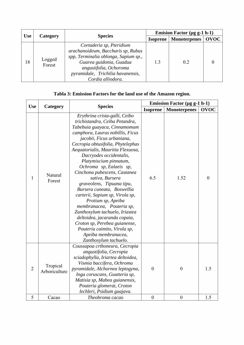
Use Category Species Emision Factor (µg g-1 h-1)

Isoprene Monoterpenes OVOC

18 Logged Forest

Cortaderia sp, Pteridium arachanoideum, Baccharis sp, Rubus spp, Terminalia oblonga, Sapium sp.,

Guarea guidonia, Guadua angustifolia, Ochoroma

pyramidale, Trichilia havanensis, Cordia alliodora.

1.3 0.2 0

 

Tabla 3: Emission Factors for the land use of the Amazon region.

Use Category Species Emission Factor (µg g-1 h-1)

Isoprene Monoterpenes OVOC

1 Natural Forest

Erythrina crista-galli, Ceibo trichistandra, Ceiba Petandra,

Tabebuia guayaca, Cinnamomum camphora, Laurus nobillis, Ficus

jacobii, Ficus urbaniana, Cecropia obtusifolia, Phytelephas Aequatorialis, Mauritia Flexuosa,

Dacryodes occidentalis, Platymiscium pinnatum,

Ochroma sp, Ealaeis sp, Cinchona pubescens, Castanea

sativa, Bursera graveolens, Tipuana tipu,

Bursera cuneata, Boswellia carterii, Sapium sp, Virola sp,

Protium sp, Apeiba membranacea, Pouteria sp,

Zanthoxylum tachuelo, Iriastea deltoidea, jacaranda copaia,

Croton sp, Perebea guianense, Pouteria caimito, Virola sp,

Apeiba membranacea, Zanthoxylum tachuelo.

6.5 1.52 0

2 Tropical

Arboriculture

Coussapoa crthoneura, Cecropia angustifolia, Cecropia

sciadophylla, Iriartea deltoidea, Vismia baccifera, Ochroma

pyramidale, Alchornea leptogyna, Inga coruscans, Guatteria sp, Matisia sp, Mabea guianensis,

Pouteria glomerat, Croton lechleri, Psidium guajava.

0 0 1.5

5 Cacao Theobroma cacao 0 0 1.5

 

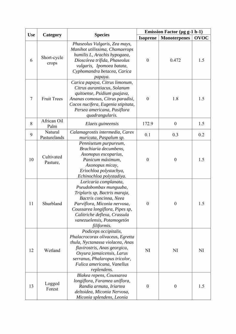
Use Category Species Emission Factor (µg g-1 h-1)

Isoprene Monoterpenes OVOC

6 Short-cycle

crops

Phaseolus Vulgaris, Zea mays, Manihot utilissima, Chamaerops

humilis L, Arachis hypogaea, Dioscórea trífida, Phaseolus vulgaris, Ipomoea batata,

Cyphomandra betacea, Carica papaya.

0 0.472 1.5

7 Fruit Trees

Carica papaya, Citrus limonum, Citrus aurantiacus, Solanum quitoense, Psidium guajava,

Ananas comosus, Citrus paradisi, Cocos nucifera, Eugenia stipitata,

Persea americana, Pasiflora quadrangularis.

0 1.8 1.5

8 African Oil

Palm Elaeis guineensis 172.9 0 1.5

9 Natural

Pasturelands Calamagrostis intermedia, Carex

muricata, Paspalum sp. 0.1 0.3 0.2

10 Cultivated Pasture,

Pennisetum purpureum, Brachiaria decumbens, Axonopus escoparius, Panicum máximum,

Axonopus micay, Eriochloa polystachya,

Echinochloa polystadiya.

0 0 1.5

11 Shurbland

Loricaria complanata, Pseudobombax munguuba,

Triplaris sp, Bactris maraja, Bactris concinna, Neea

Parviflora, Miconia nervosa, Coussarea longiflora, Pipes sp,

Calitriche deflexa, Crassula vanezuelensis, Potamogetón

filiformis.

0 0 1.5

12 Wetland

Podiceps occipitalis, Phalacrocorax olivaceus, Egretta thula, Nyctanassa violacea, Anas

flavirostris, Anas georgica, Oxyura jamaicensis, Larus

serranus, Phalaropus tricolor, Fulica americana, Vanellus

replendens.

NI NI NI

13 Logged Forest

Blakea repens, Coussarea longiflora, Faramea uniflora,

Randia armata, Iriartea deltoidea, Miconia Nervosa, Miconia splendens, Leonia

0 0 1.5

 

Use Category Species Emission Factor (µg g-1 h-1)

Isoprene Monoterpenes OVOCglycarpa, Billia rosea, Dacryodes

olivifera, Otoba glycycarpa, Compsoneura ulei, Iriartea

deltoidea.

Concerning the land use, it was determined that in Ecuador, the “African palm” is the major isoprene producer as well as Planted Forests. The latter have an emission factor of 79 μg g-1 h-1 due to the prevalence of eucalyptus in this land use. Consequently, it was determined that one of the provinces with the highest BVOCs emission is “Santo Domingo” which has a surface covered by African palm crops.

Moreover, “El Sebastián” (Capparis mollis) is a plant species with the highest isoprene emission factor (268 μg g-1 h-1), but with monoterpenes and OVOCs emission factors of 0 μg g-1 h-1. The tree tomato has the highest monoterpene emission factor with a value of 28.2 μg g-1 h-1 but lacks other emission factors related to other studied compounds.

VOCs plant emissions.

The BVOCs emission peak throughout the day was registered at 12:00 because isoprene emissions depend directly on PAR, which is consistent with the modelling of Guenther (2000) and Pahdy (2005), according to which the biogenic emission flow in a variety of landscapes is higher during the midday an it may vary depending on the season, cultivation stage, etc. The total annual BVOCs emissions are 1855.6 kt. Of these, 1278.6 kt/year are from the isoprene emissions, 427.6 kt/year are from monoterpene emissions and 149.3 kt/year are from OVOCs emissions; in terms of percentage, isoprene emissions represent 68,9% of the total annual emissions, whereas monoterpene and OVOCs represent 23,0% and 8,1%, respectively. These percentages follow a similar trend to published data of other studies Kahola (2003) y Pahdy (2005). Additionally, Kahola (2003) indicates that in the environmental air BVOCs emissions reach its maximum during summer and its minimum during winter; nevertheless, because Ecuador is located in a tropical zone, it lacks well-defined climatic seasons and for this reason BVOCs emissions are homogenous during the year.

We determined that the largest amount of emissions is produced during the month of March with a value of 1743 kt per month, whereas the emissions produced in August are the lowest, reaching a value of 77.3 kt per month (Table 4).

Considering the categories established in this study, it was determined that in Ecuador during the year 2010, the zones of Esmeraldas, Santo Domingo de los Tsáchilas and the Amazon region release approximately 2000 t km-2 of isoprene owing to the African palm plantations. Regarding the monoterpene emissions, the highest emissions were observed in the Amazon region with values that vary between 175 and 200 t km-2 a-1, which is attributed to the natural forest and the direct influence of temperature in that region. Finally, concerning OVOCs emissions, the Amazon region releases no emissions of this kind of compounds because the largest land use is a natural forest which has no emission factors due to its great endemism.

 

4. Conclusions Some BVOCs have high reactivity compared to VOCs produced anthropogenically. BVOCs play a very important role in the chemistry of the lower troposphere (Atkinson & Arey, 1998); this is the reason why BVOCs emissions are important.

The development of a VOCs emissions inventory have entailed a large study of the Ecuadorian vegetation, which is so diverse. Because there is a vast number of endemic species and the emission factors of isoprene, monoterpenes and OVOCs were scarce and confined to a determined group, many species were not included in the inventory. The database of Lancaster University was preferably used owing to its range of species. However, the species of this database are common in Europe, affecting its implementation in Ecuador.

During this study, we highlighted the importance of BVOCs emissions, showing quantitatively the values of each compound. We determined that the total annual emissions are 1855.6 kt, of which 1278.6 kt per month are from isoprene emissions, 427.6 kt per month are from monoterpenes emissions and 149.3 per month are due to OVOCs emissions.

It is important to underscore that Ecuador lacks defined climatic seasons, and thus the emissions are homogenous during the year, except in the months of March and April, in which the isoprene emissions are the highest due to the higher solar radiation; in contrast, in August the emissions are lower owing to the low temperatures during this month

MONTH Isoprene Monoterpenes OVOC TOTAL

t/month % t/month % t/month % t/month %

JANUARY 124208.2 9.71 36424.6 8.52 11633.7 7.79 172266.5 9.28

FEBRUARY 120596.3 9.43 35289.4 8.25 10804.1 7.24 166689.8 8.98

MARCH 133781.3 10.46 36152.2 8.45 12227.0 8.19 182160.5 9.82

APRIL 121726.1 9.52 31383.2 7.34 11674.9 7.82 164784.3 8.88

MAY 112112.7 8.77 33694.3 7.88 13345.2 8.94 159152.2 8.58

JUNE 93845.3 7.34 34294.8 8.02 10746.8 7.20 138886.9 7.49

JULY 97107.4 7.59 38733.6 9.06 11196.2 7.50 147037.2 7.92

AUGUST 31807.5 2.49 35132.6 8.22 14949.7 10.01 81889.8 4.41

SEPTEMBER 111324.2 8.71 35976.0 8.41 14220.7 9.52 161520.9 8.70

OCTOBER 117737.1 9.21 37963.7 8.88 13878.0 9.29 169578.8 9.14

NOVEMBER 110206.1 8.62 35829.3 8.38 11436.8 7.66 157472.2 8.49

DECEMBER 104134.4 8.14 36755.0 8.60 13196.1 8.84 154085.6 8.30

TOTAL 1278586.7 100.00 427628.7 100.00 149309.2 100.00 1855524.6 100.00

Tabla 5: VOCs emissions of Ecuadorian vegetation from 2010

 

References

Atkinson, R., & Arey, J. (1998). Atmospheric chemistry of biogenic organic compounds. Accounts of Chemical of Research , 574-583.

Benjamin, M. T., Sudol, M., Bloch, L., & Winer, A. M. (1996). Low-emitting urban forests: A taxonomic methodology for assigning isoprene and monoterpene emission rates. Atmospheric Environment, 30(9), 1437-1452. doi: http://dx.doi.org/10.1016/1352-2310(95)00439-4

Flores, N., & Flores, J. (2007). Determinación de la densidad de biomasa foliar de las especies vegetales y categorías de uso del suelo del dominio de análisis para la estimación de las emisiones del Distrito Metropolitano de Quito. Quito: CORPAIRE-ESPE

Ghimire, R. P., Kivimäenpää, M., Blomqvist, M., Holopainen, T., Lyytikäinen-Saarenmaa, P., & Holopainen, J. K. (2016). Effect of bark beetle (Ips typographus L.) attack on bark VOC emissions of Norway spruce (Picea abies Karst.) trees. Atmospheric Environment, 126, 145-152. doi: https://doi.org/10.1016/j.atmosenv.2015.11.049

Greenberg, J., Guenther, A., Zimmerman, P., Baugh, W., Geron, C., Davis, K., y otros. (1999). Tethered balloon measurements of biogenic VOCs in the atmospheric boundary layer. Atmospheric Environment , 855-867.

Guenther, A., Hewitt, C., Eriksson, D., Fall, R., Geron, C., Graedel, T., y otros. (1995). A global model of natural volatile organic compound emissions. Journak if Geophysical Research .

Hakola, H., Tarvainen, V., Laurila, T., Hiltunen, V., Hellén, H., & Keronen, P. (2003). Seasonal variation of VOC concentrations above a boreal coniferous forest. Atmospheric Environment, 37(12), 1623-1634. doi: https://doi.org/10.1016/S1352-2310(03)00014-1

Kansal, A. (2009). Sources and reactivity of NMHCs and VOCs in the atmosphere: A review. Journal of Hazardous Materials, 166(1), 17-26. doi: https://doi.org/10.1016/j.jhazmat.2008.11.048

Kesselmeier, J., Kuhn, U., Wolf, A., Andreae, M. O., Ciccioli, P., Brancaleoni, E., . . . Artaxo, P. (2000). Atmospheric volatile organic compounds (VOC) at a remote tropical forest site in central Amazonia. Atmospheric Environment, 34(24), 4063-4072. doi: http://dx.doi.org/10.1016/S1352-2310(00)00186-2

Langenheim, J. (1994). higher plant terpenoids: A phytocentric overview of their ecological roles. Journal of Chemical Ecology , 1223-1280.

Padhy, P. K., & Varshney, C. K. (2005). Emission of volatile organic compounds (VOC) from tropical plant species in India. Chemosphere, 59(11), 1643-1653. doi: https://doi.org/10.1016/j.chemosphere.2005.01.046

Simon, V., Luchetta, L., & Torres, L. (2001). Estimating the emission of volatile organic compounds (VOC) from the French forest ecosystem. Atmospheric Environment, 35, S115-S126. doi: http://dx.doi.org/10.1016/S1352-2310(00)00565-3

 

Solmon, F., Sarrat, C., Serça, D., Tulet, P., & Rosset, R. (2004). Isoprene and monoterpenes biogenic emissions in France: modeling and impact during a regional pollution episode. Atmospheric Environment, 38(23), 3853-3865. doi: https://doi.org/10.1016/j.atmosenv.2004.03.054

   

 

ICESI_0085

Local fault identification using Microtremor Analysis (case study: local fault in Surabaya river)

*Ayi Syaeful Bahri, Sepuluh Nopember Institute of Technology, Indonesia

Nizar Dwi Riyantiyo, Sepuluh Nopember Institute of Technology, Indonesia

Amien Widodo, Sepuluh Nopember Institute of Technology, Indonesia

Firman Syaifuddin, Sepuluh Nopember Institute of Technology, Indonesia

*Corresponding Author

Abstract

Region in this study is the capital city of Surabaya, East Java Province. This research will be focused on local fault that crosses the river city of Surabaya, because the river crossed by a bridge Surabaya in Dinoyo, Jagir, Wonokromo overpass bridge and dam Gunung Sari. Based on the geological conditions of the city of Surabaya in the form of alluvial basins and sandstone with clay and limestone sedimentary rocks, and crossed by fault Kendeng moving 5 millimeters per year. With the composition of sediment deposition in Surabaya, the region that has the geological conditions in the form of alluvial, tuff, sandstone and would have a great potential danger terhadapt intensity ground shaking due to amplification and the intensity of the earthquake. So the purpose of this study is to describe the local faults that exist around Surabaya river, which periodically if hit by an earthquake can move and cause damage to the existing infrastructure. The method used in this study using analysis of Horizontal to Vertical Spectral Ratio (HVSR) to determine the natural frequency response in the area and will be integrated with the data Vs30 to obtain the thickness of layers of sediment and in this research used inversion HVSR to imaging subdurface condition of local fault Surabaya river, so as to determine the danger zones around the fault of the Surabaya local river.

Keywords: Local fault, Mikrotremor, Horizontal to vertical spectral, Vs30, Sediment thickness, Inversion HVSR.

 

1. Introduction

Region in this study is the city of Surabaya is a local fault that crosses the river Surabaya, because the local faults around the crossing fly over of Wonokromo, Dinoyo bridge, Jagir bridge, Gunung Sari dam, and Jagir dam. Based on the geological conditions of the city of Surabaya in the form of basin alluvial deposits and sandstone with sedimentary rocks of clay and limestone, and crossed by fault Kendeng which moving 5 millimeters per year, cesarean Lasem is located in the north of the city of Surabaya ± 70km, fault Watukosek south of Surabaya stretches of Mojokerto up Madura ± 30 km, the fault is located on the south coast Grindulu Pacitan until Mojokerto ± 50 km. With the composition of sediment deposition in Surabaya, the region that has the geological conditions in the form of alluvial, tuff, sandstone and would have a great potential danger terhadapt intensity ground shaking due to amplification and the intensity of the earthquake (Nakamura et al).

Figure 1: Geological map sheets Surabaya and Sapulu (Sukardi, 1992)

Earthquakes are natural disasters that can not be predicted when it happened, but it can be done when the disaster risk reduction quake by studying geology surrounding area that has the potential earthquake. From BMKG data there are several earthquakes that occurred around the city of Surabaya, (March 22nd, 1836) in Mojokerto,(August 31st, 1902) Sedayu in the town of Gresik, (August 11st , 1939) northwest of the Java Sea, (June 19th, 1950) northwest of the Java Sea, (February 19th , 1967) in Malang, 2008 in the area of Ponorogo. To reduce the risk of disaster is there, then the measurement method microtremor Horizaontal to Vertical Spectral Ratio (HVSR) in Surabaya to map the damage from the earthquake-prone locations (microzonation map). According to Nakamura (1989) propose a method for estimating HVSR natural frequency and amplification of the local geology of the data microtremor. Subsequent developments, this method is able to estimate the vulnerability index of land (Nakamura, 1997), the index of the vulnerability of buildings (Sato et al., 2008; Quarter et al., 2010) and the interaction between the land and buildings (Gallipoli et al., 2004; Quarter et al., 2010). The advantages of this mikrotremor method, meruakan effective method is cheap and environmentally friendly, so it can be used in the area of the residence. There are several studies that the theme of microzonation city of Surabaya with the results of the vulnerability maps of land and buildings. From the results of these studies had results with the tendency that the area has a high degree of vulnerability is located in the eastern part of the city of Surabaya. In this study focused on local fault Surabaya river with the same type of rock formation units are alluvial.

2. Methodology

 

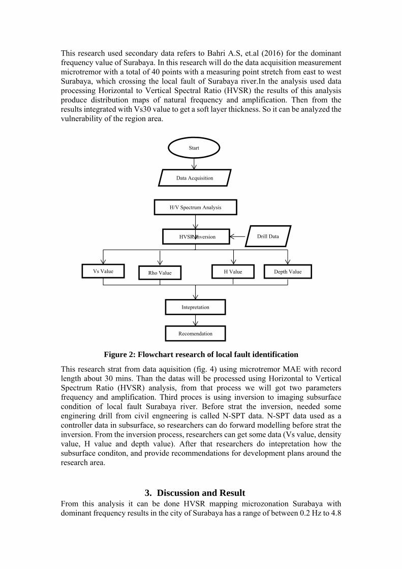
This research used secondary data refers to Bahri A.S, et.al (2016) for the dominant frequency value of Surabaya. In this research will do the data acquisition measurement microtremor with a total of 40 points with a measuring point stretch from east to west Surabaya, which crossing the local fault of Surabaya river.In the analysis used data processing Horizontal to Vertical Spectral Ratio (HVSR) the results of this analysis produce distribution maps of natural frequency and amplification. Then from the results integrated with Vs30 value to get a soft layer thickness. So it can be analyzed the vulnerability of the region area.

Figure 2: Flowchart research of local fault identification

This research strat from data aquisition (fig. 4) using microtremor MAE with record length about 30 mins. Than the datas will be processed using Horizontal to Vertical Spectrum Ratio (HVSR) analysis, from that process we will got two parameters frequency and amplification. Third proces is using inversion to imaging subsurface condition of local fault Surabaya river. Before strat the inversion, needed some enginering drill from civil engneering is called N-SPT data. N-SPT data used as a controller data in subsurface, so researchers can do forward modelling before strat the inversion. From the inversion process, researchers can get some data (Vs value, density value, H value and depth value). After that researchers do intepretation how the subsurface conditon, and provide recommendations for development plans around the research area.

3. Discussion and Result From this analysis it can be done HVSR mapping microzonation Surabaya with dominant frequency results in the city of Surabaya has a range of between 0.2 Hz to 4.8

Start

Data Acquisition

H/V Spectrum Analysis

HVSR Inversion Drill Data

Vs Value Rho Value H Value Depth Value

Intepretation

Recomendation

 

3,1

3,1

3,1

3,1

3,1

Hz. Where almost the entire city of Surabaya tend to have a low frequency between 0.2 to 2.4 Hz frequency response indicates this dominant with the composition of sediments in Surabaya, the region that has the geological conditions in the form of alluvial, tuff and sandstone ( Sukardi, 1992).

Figure 3: Frequency dominant map of Surabaya, red line is line aquisition microtremor and yellow rectangle is study area

This indicates it is for the area of Surabaya is a level of vulnerability Akiat earthquakes tend to be high on the results of the existing dominant frequency mapping. But there are interesting things that would be more specific to the study, there is local fault that crosses the river Surabaya. If look at (Fig. 6) in red circle, there is a low frequency between 0.2 to 1.6 Hz, which is right in the local fault location in Surabaya river when viewed from the geological map sheet Surabaya and Sapulu (Sukardi, 1992). So in this research we will try using inversion method of HVSR to know 2D section of subsurface on local fault of Surabaya river. After got data acquisition and processing data as much as 40 point measurement got contour and frequency depth map,

Figure 4. A) Frequency map of the study area with a frequency range of 2.1 Hz to 4 Hz. B) map of the sediment depth of 15 to 85m, the red line is indicated by the

surabaya river fault and the blue arrow line is the Surabaya river

When viewed from the dominant frequency map of areas with high frequencies of 3Hz to 4Hz, the Lidah anticline zone is located in the western Surabaya area and has an inverted correlation relationship with the depth of soft sediment depths of 15 meters to 35 meters. So if viewed from the map the spread of the dominant frequency and the depth of sedimentation in western Surabaya is more likely to have low vulnerability

 

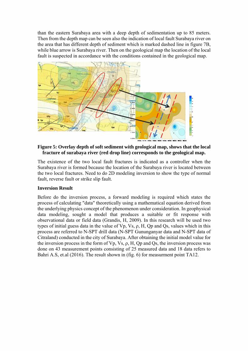
than the eastern Surabaya area with a deep depth of sedimentation up to 85 meters. Then from the depth map can be seen also the indication of local fault Surabaya river on the area that has different depth of sediment which is marked dashed line in figure 7B, while blue arrow is Surabaya river. Then on the geological map the location of the local fault is suspected in accordance with the conditions contained in the geological map.

Figure 5: Overlay depth of soft sediment with geological map, shows that the local fracture of surabaya river (red drop line) corresponds to the geological map.

The existence of the two local fault fractures is indicated as a controller when the Surabaya river is formed because the location of the Surabaya river is located between the two local fractures. Need to do 2D modeling inversion to show the type of normal fault, reverse fault or strike slip fault.

Inversion Result

Before do the inversion process, a forward modeling is required which states the process of calculating "data" theoretically using a mathematical equation derived from the underlying physics concept of the phenomenon under consideration. In geophysical data modeling, sought a model that produces a suitable or fit response with observational data or field data (Grandis, H, 2009). In this research will be used two types of initial guess data in the value of Vp, Vs, ρ, H, Qp and Qs, values which in this process are referred to N-SPT drill data (N-SPT Gununganyar data and N-SPT data of Citraland) conducted in the city of Surabaya. After obtaining the initial model value for the inversion process in the form of Vp, Vs, ρ, H, Qp and Qs, the inversion process was done on 43 measurement points consisting of 25 measured data and 18 data refers to Bahri A.S, et.al (2016). The result shown in (fig. 6) for measurment point TA12.

 

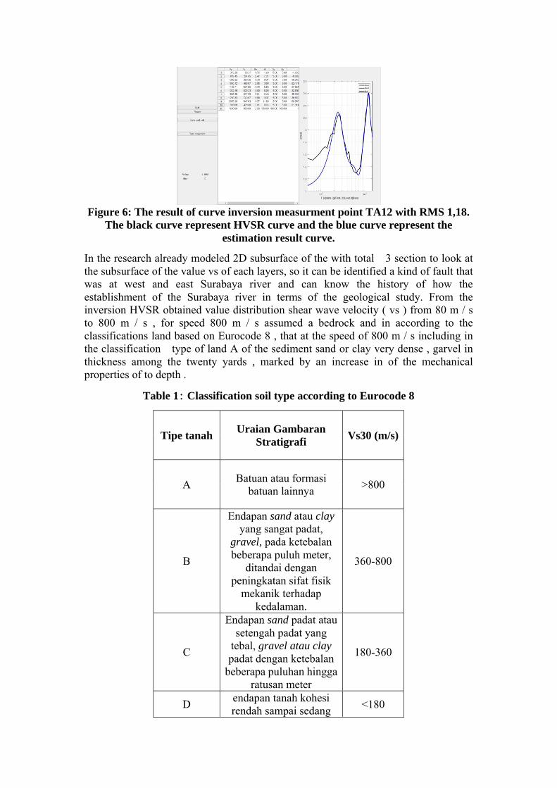
Figure 6: The result of curve inversion measurment point TA12 with RMS 1,18. The black curve represent HVSR curve and the blue curve represent the

estimation result curve.

In the research already modeled 2D subsurface of the with total 3 section to look at the subsurface of the value vs of each layers, so it can be identified a kind of fault that was at west and east Surabaya river and can know the history of how the establishment of the Surabaya river in terms of the geological study. From the inversion HVSR obtained value distribution shear wave velocity ( vs ) from 80 m / s to 800 m / s , for speed 800 m / s assumed a bedrock and in according to the classifications land based on Eurocode 8 , that at the speed of 800 m / s including in the classification type of land A of the sediment sand or clay very dense , garvel in thickness among the twenty yards , marked by an increase in of the mechanical properties of to depth .

Table 1: Classification soil type according to Eurocode 8

Tipe tanah Uraian Gambaran

Stratigrafi Vs30 (m/s)

A Batuan atau formasi

batuan lainnya >800

B

Endapan sand atau clay yang sangat padat,

gravel, pada ketebalan beberapa puluh meter,

ditandai dengan peningkatan sifat fisik

mekanik terhadap kedalaman.

360-800

C

Endapan sand padat atau setengah padat yang

tebal, gravel atau clay padat dengan ketebalan

beberapa puluhan hingga ratusan meter

180-360

D endapan tanah kohesi rendah sampai sedang

<180

 

Tipe tanah Uraian Gambaran

Stratigrafi Vs30 (m/s)

(degan atau tanpa beberapa lapisan kohesi rendah), terutama pada

tanah kohesi rendah

E

lapisan tanah terdiri dari aluvium pada permukaan

dengan nilai Vs tipe C atau D degan ketebalan

bervariasi 5 m hingga 20 meter, dibawah tanah ini

berupa material keras dengan Vs > 800

S1

Endapan terdiri dari atau mengandung, ketebalan lapisan 10 m pada tanah

lempung lunak atau lempung lanauan dengan

indeks plastisitan dan kadar air yang tinggi

<100 (indikasi)

S2

endapan tanah likuifiable, dari clay

sensitif, atau tanah lain yang tidak termasuk

dalam tipe A-E atau S1

In all section, based on classifications land eurocode 8 the layers near surface is the type E according to ( table 1) the layers alluvial with the Vs 50 m / s up to 100 m / s range of the depth of 5-10 meters purple color ( fig 7-9 ) , where this layer have trend equal to the depth to which inclined to each of a region of the western and east of Surabaya city. Then the layers below is type C range of value Vs 180 m / s until 360 m / s range of the depth of varying 20 m to 90 feet under a surface marked the contours of colored dark blue to light blue , then type D with range of value Vs 360-800 m / s is a hard layer of for depth of layers of varies 40 meters to 150 meters (as a lower limit ) marked the contours of green , yellow and orange .

From the first and second section (fig 7 and 8), can be intepreted based on geology conditions, that layer of hard in Surabaya have varying from west to east, the trend of deep layer to the shallow and gradually back to deep layer in eastward .An area with a hard layer of a shallow at the depth of 40 yards indicated as Lidah Anticlin is located on the west surabaya based on a map geology sheets Surabaya and Sapuluh ( Sukradi , 1992 ). From the inversion also got the local fault that controls the establishment of the surabaya , based on ( fig. 7 ) local fault defined by dashed red line indicated as fault because from the Vs profile decreased in geological phenomena expressed as gawir , while the red rectangle be indicated Surabaya river. From ( fig. 7 ) can be seen also how the establishment of Surabaya river, as indicated in the old time Lidah anticline was one but caused by tectonic proccess and the waekness area at Lidah

 

anticline, then it made some opportunities for Brantas river crossed the area and brought some Aluvium deposits.

On third section (fig. 9), based on the ground eurocode classification 8 the distribution Vs equal to the first and second section , which diferrent is the condition geology subsurface .Where the third section position through Guyangan anticline different with both section before, but on condition subsurface in eastern remains visible continuity of the local fault Surabaya river.Third of incisions can be seen also an indication of the local fault that existing on Guyangan anticline.

Figure 7: Cross-sectional model of propagation of shear wave velocity (Vs) passing through the local fault of Surabaya river, red dashed line is indicated as

fault, and the red rectangle is indicated as Surabaya river.

Figure 8: Cross-sectional model of propagation of shear wave velocity (Vs) passing through the local fault of Surabaya river, red dashed line is indicated as

fault, and the red circle is indicated as Surabaya river.

Lidah Anticline Lidah Anticline

Lidah Anticline

Guyangan 

 

Figure 9: Cross-sectional model of propagation of shear wave velocity (Vs) passing through the local fault of Surabaya river, red dashed line is indicated as

fault, the red circle is indicated as Surabaya river, and the purple rectangle is indicated as local fault on Guyangan Anticline.

4. Conclusion From the research can be concluded that:

1. The research obtained value frequency dominant by the range of 2.1 Hz to 4 Hz and value of the depth of soft layer 15 meters up to 80 feet below the surface.

2. From the inversion obatained distribution value Vs area research by the range of 0 m / s to 800 m / s spread from western to eastern research area.

3. From geological study can be seen also how the establishment of Surabaya river, as indicated in the old time Lidah anticline was one but caused by tectonic proccess and the waekness area at Lidah anticline, then it made some opportunities for Brantas river crossed the area and brought some Aluvium deposits.

References

Badan Geologi – Kementrian Energi dan Sumber Daya Mineral. 2015.”Mikrozonasi Bahaya Gempa Mataram” GEOMAGZ Majalah Geologi Populer Vol. 5

Bonnefoy-Claudet, S, Cotton, F., Bard, P.Y.(2006b). The nature of noise wavefield and its applications for site effects studies, Earth Science Reviews. doi:10.1016/j.earscirev.2006.07.004

Dian Nur Aini, Widya Utama, dan A. Syaeful Bahri. 2012. “Penaksiran Resonansi Tanah dan Bangunan Menggunakan Analisis Mikrotremor Wilayah Surabaya Jawa Timur”. Fisika, FMIPA. Institut Teknologi Sepuluh Nopember Surabaya

European research project. 2004. “Guidelines For Implementation Of The H/V Spectral Ratio Technique On Ambient Vibrations, Measurments, Processing And Interpretation”.

Fauzi, Ahmad, Masyhur Irsyam, dan Uasama Juniansyah Fauzi. 2014. “Empirical Correlation Of Shear Wave Velocity And N-Spt Value For Jakarta”. Int. J. Of GEOMATE, Sept 2014, Vol 7, No. 1 (SI. No. 13), pp. 980-984.

Gallipolia,M.R., M. Mucciarellia, R.R. Castroc, G. Monachesid, P. Contrie. (2004).Structure, soil–structure response and effects of damage based on observations of horizontal-to-vertical spectral ratios of microtremors. Soil Dynamics and Earthquake Engineering, Vol.24, pp:487–495

Grandis, H. 2009. “Pengantar Pemodelan Inversi Geofisika”. Jakarta: Himpunan Ahli Geofisika Indonesia (HAGI).

 

Nakamura, Y. 1989. “A Method For Dynamic Characteristicsestimation Of Subsurface Using Microtremor On The Ground Surface”. Quarterly report of Railway Technical Research Institute.

Nashir, Mochamad abied Lutfi., Ayi Syaeful Bahri .2013. “Karakterisasi Kerusakan Bangunan Wilayah Jawa Timr Menggunakan Analisis Mikrotremor”. Fisika, FMIPA. Institut Teknologi Sepuluh Nopember Surabaya

Sato, T., Y. Nakamura, J. Saita. The Change Of The Dynamic Characteristics Using Microtremor. The 14 th World Conference on Earthquake Engineering October 12-17, 2008, Beijing, China

Seismology Society of America. 1999. “Microtremor Measurments Used to Map Thickness of Soft Sediment”. Bulettin of the Seismology Society of America. Vol 89, No.1, pp. 250-259

Sukardi. 1992.” Geologi Lembar Surabaya & Sapulu, Jawa. Pusat Penelitian dan Pengembangan Geologi”. Pusat Penelitian dan Pengembangan Geologi.

Syaifuddin, Firman , dkk. 2016. “Microtremor Study of Gunung Anyar Mud Volcano, Surabaya, East Java”. AIP Conference Proceedings

Triwulan, Utama, W., Warnana, D.D., Sungkono. Vulnerability index estimation for building and ground using microtremor. Aptecs 2nd. International Seminar on applied Technology, Science and Arts. Graha Sepuluh Nopember, Institut Teknologi Sepuluh Nopember Surabaya. 21-22 Desember 2010.

Situs : http://web.ics.purdue.edu/~braile/edumod/slinky/slinky.html). Accessed 31 January 2017.

Situs : http://www.soiltest.sienconsultant.com/. Accsesed 14 May 2017.

   

 

ICESI_0092

OFDMA in LTE Mobile Communications

*Fanny P. Flores, National Polytechnic School, Ecuador

*Corresponding Author

Abstract

This paper aims to investigate, design, simulate, analyze and suggest possible improvements related to Orthogonal Frequency Division Multiple Access (OFDMA) in Long Term Evolution (LTE) mobile communications. Analysis and design are based on “ETSI TS 136 211 V10.0.0” technical specification, defined by the Third Generation Partnership Project (3GPP). The first section, “Introduction” contains a review of concepts defined by the 3GPP for LTE. Section two “Design and Simulation Settings”, contains block diagrams and parameters for the design. Different number of users and the introduction of fading are contemplated to create multiple scenarios. Moreover, OFDMA symbol design and Matlab Simulink diagrams are presented. The third section “Results and Analysis”, studies the results obtained in Matlab Simulink. The transmitted and received integer data are shown; as well as the error rate calculation. Also, modulated transmitted and received data are compared, and Bit Error Rate (BER) curves are analyzed. The last section, “Conclusions” contains the investigation conclusions and topics of interest for future study.

Keywords: Mobile communications, LTE, Downlink, OFDMA.

 

 

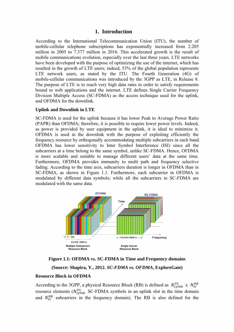
1. Introduction

According to the International Telecommunication Union (ITU), the number of mobile-cellular telephone subscriptions has exponentially increased from 2.205 million in 2005 to 7.377 million in 2016. This accelerated growth is the result of mobile communications evolution, especially over the last three years. LTE networks have been developed with the purpose of optimizing the use of the internet, which has resulted in the growth of LTE users; indeed, 53% of the global population represents LTE network users, as stated by the ITU. The Fourth Generation (4G) of mobile-cellular communications was introduced by the 3GPP as LTE, in Release 8. The purpose of LTE is to reach very high data rates in order to satisfy requirements bound to web applications and the internet. LTE defines Single Carrier Frequency Division Multiple Access (SC-FDMA) as the access technique used for the uplink, and OFDMA for the downlink.

Uplink and Downlink in LTE

SC-FDMA is used for the uplink because it has lower Peak to Average Power Ratio (PAPR) than OFDMA; therefore, it is possible to require lower power levels. Indeed, as power is provided by user equipment in the uplink, it is ideal to minimize it. OFDMA is used in the downlink with the purpose of exploiting efficiently the frequency resource by orthogonally accommodating multiple subcarriers in each band. OFDMA has lower sensitivity to Inter Symbol Interference (ISI) since all the subcarriers at a time belong to the same symbol, unlike SC-FDMA. Hence, OFDMA is more scalable and suitable to manage different users’ data at the same time. Furthermore, OFDMA provides immunity to multi path and frequency selective fading. According to the time axis, subcarriers duration is longer in OFDMA than in SC-FDMA, as shown in Figure 1.1. Furthermore, each subcarrier in OFDMA is modulated by different data symbols; while all the subcarriers in SC-FDMA are modulated with the same data.

Figure 1.1: OFDMA vs. SC-FDMA in Time and Frequency domains

(Source: Shapira, Y., 2012. SC-FDMA vs. OFDMA, ExploreGate)

Resource Block in OFDMA

According to the 3GPP, a physical Resource Block (RB) is defined as x resource elements ( SC-FDMA symbols in an uplink slot in the time domain and subcarriers in the frequency domain). The RB is also defined for the

 

downlink as x resource elements ( OFDMA symbols in a downlink slot in the time domain and subcarriers in the frequency domain).

, , and parameters are given in Tables 1.1 and 1.2.

Table 1.1: SC-FDMA RB parameters

Table 1.2: OFDMA RB parameters

(Source: 3GPP, 2011. ETSI TS 136 211 Technical Specification, Version 10.0.0)

The number of depends on the downlink bandwidth arranged in the cell; such that , . , where , 6 and . 110. Also, the number of symbols in a slot is configured depending on the Cyclic Prefix (CP) length. The CP is defined as the fragment of a symbol last part, which is copied at the beginning of that symbol to increase the separation between symbols, minimizing ISI. An OFDMA symbol is made up of null subcarriers (guard band and center subcarrier) and data (user data and reference signals). The length of the symbol is equal to the Fast Fourier Transform (FFT) size; such that the occupied subcarriers are part of the RBs, and the remaining subcarriers correspond to the null subcarriers. The relationship between slot, RB, resource elements and symbols is shown in Figure 1 (Appendix). In this figure, the RB consists of 7 symbols in time domain and 12 subcarriers in frequency domain. The difference between Channel Bandwidth, Transmission Bandwidth Configuration and Transmission Bandwidth is shown in Figure 2 (Appendix).

2. Design and Simulation Settings

Design is based on 3GPP technical specification, and simulation is developed with Matlab Simulink R2014a. Figure 2.1 shows the OFDMA transmitter and receiver scheme.

CONFIGURATION

Normal Cyclic Prefix

12

7

Extended Cyclic Prefix

12

6

CONFIGURATION

Normal Cyclic Prefix ∆ 15 12

7

Extended Cyclic Prefix

∆ 15 6

∆ 7.5 24 3

 

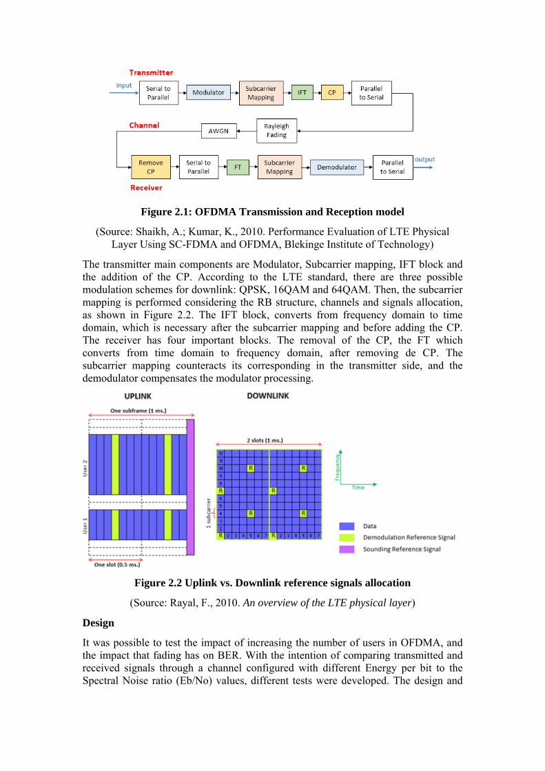
Figure 2.1: OFDMA Transmission and Reception model

(Source: Shaikh, A.; Kumar, K., 2010. Performance Evaluation of LTE Physical Layer Using SC-FDMA and OFDMA, Blekinge Institute of Technology)

The transmitter main components are Modulator, Subcarrier mapping, IFT block and the addition of the CP. According to the LTE standard, there are three possible modulation schemes for downlink: QPSK, 16QAM and 64QAM. Then, the subcarrier mapping is performed considering the RB structure, channels and signals allocation, as shown in Figure 2.2. The IFT block, converts from frequency domain to time domain, which is necessary after the subcarrier mapping and before adding the CP. The receiver has four important blocks. The removal of the CP, the FT which converts from time domain to frequency domain, after removing de CP. The subcarrier mapping counteracts its corresponding in the transmitter side, and the demodulator compensates the modulator processing.

Figure 2.2 Uplink vs. Downlink reference signals allocation

(Source: Rayal, F., 2010. An overview of the LTE physical layer)

Design

It was possible to test the impact of increasing the number of users in OFDMA, and the impact that fading has on BER. With the intention of comparing transmitted and received signals through a channel configured with different Energy per bit to the Spectral Noise ratio (Eb/No) values, different tests were developed. The design and

 

simulation consider one OFDMA symbol, based on LTE parameters shown in Table 2.1.

PARAMETER VALUE

Resource Block RB 15 12

7 Maximum occupied subcarriers 180 IFFT/FFT size 256

Normal CP ∆ 15 5.21 (first symbol of the

slot) Modulation 16QAM

Table 2.1: Simulation Parameters

The first scenario corresponds to two users in an Additive White Gaussian Noise (AWGN) environment. The symbol processing design is presented in Figure 3 (Appendix), and its corresponding diagram is in Figure 4 (Appendix). FDD is used in this paper, such that 100 of 150 subcarriers are assigned to User 1, and the other 50 to User 2. Consistent with the standard, there are maximum 180 occupied subcarriers; therefore, 30 subcarriers are used for reference signals (180-150), which are allocated according to the first symbol. Before inserting the reference signals and the null subcarriers into the frame, it is necessary to join both users’ data. To achieve this, two vectors of size 150 were created filling them with each user’s data and zeros. Then, both vectors are added; the first 100 elements of which correspond to User 1, and the last 50 to User 2. As the FFT size to be used is 256, there are 76 null subcarriers (256-180), which are considered as guard subcarriers in both sides of the frame and are filled with zeros with the purpose of building the Fourier signal walls. 38 of 76 subcarriers are allocated as left guard subcarriers, 37 as right guard subcarriers, and 1 remaining subcarrier corresponds to the center subcarrier, which is not transmitted in the downlink, in agreement with the standard. Finally, 19 subcarriers are estimated to be used as CP, based on 5.21μs. At the receiver, the CP is removed, which corresponds to the information of the first 19 subcarriers of the received symbol. Then, the 76 null subcarriers are removed, including the left guard subcarriers, right guard subcarriers and the center subcarrier. After removing the null subcarriers, the 30 reference signals are also removed. Finally, the resulting vector of size 150 is divided into two parts. The first 100 subcarriers correspond to the data that belongs to User 1 and the remaining 50 to User 2.

The second scenario is designed for five users in an AWGN environment. Its symbol processing design and Simulink diagram are like the previous scenario; the main difference is that 30 of 150 subcarriers are assigned to each user, 30 subcarriers are used for reference signals (180-150), which are allocated according to the first symbol of the downlink pattern.

Rayleigh fading is considered in the third and fourth scenarios, where 2 and 5 users are tested, respectively. The purpose of these scenarios is to analyze the effects of fading on BER curves in OFDMA. Simulink diagram for two users is shown in Figure 5 (Appendix).

Simulation Settings

 

This section describes the parameters configured in Simulink blocks for the scenario with 2 users in an AWGN environment. For Random Integer block, as modulation to be used is 16QAM, the M-ary number parameter is configured as 16. For user 1, 100 samples per frame are generated, and 50 samples per frame for user 2. As the source generates integers, it would cause confusion or estimation errors while calculating the BER, which is based on bits; therefore, the change from integer to bit is used. As explained previously, in order to join both users’ data, two vectors of size 150 are created, filling them with data and zeros, using Constants for Zero extension blocks. Furthermore, two vectors are created with the use of Vector Concatenate blocks; the first vector contains the 100 samples created by the Random Integer block for User 1 and 50 zeros originated by one of the constant blocks. The second vector is created by 100 zeros originated by the other constant block and at the end by the 50 samples of User 2. The Addition block is used to sum up the two vectors created previously to obtain another vector of size 150, with User 1 data at the beginning and User 2 data at the end of the vector. The signal entering into the Multiport Selector block is divided into 30 groups; each group contains 5 elements (1:5, 6:10…..146:150). This is to prepare the symbol to introduce the reference signals, according to the pattern of the first OFDMA symbol. Moreover, 38 subcarriers are used as left guard, 37 subcarriers correspond to right guard and one remaining is the central subcarrier. Thirty reference signals are generated to complete 180 occupied subcarriers. These signals are allocated one by one after each group generated by the Multiport Selector block, according to the pattern. Matrix Concatenate block receives 63 inputs. First, the left guard subcarriers; second, a reference signal, then the first block of 5 subcarriers from the Multiport selector, then another reference signal, until completing the 63 inputs with the last one, which corresponds to the right guard subcarriers input. To add the CP, the last 19 subcarriers of the OFDMA symbol are copied and inserted at its beginning. As the FFT length is 256, the last 19 subcarriers are from 238 to 256. After specifying the CP, the remaining symbol is transmitted, from 1 to 256.

Regarding AWGN channel, with the purpose of comparing how the transmitted signal is affected by the Eb/No ratio, three different values are configured Eb/No = 30 dB, 43 dB and 80 dB.

With respect to the receiver, the Selector block is used to remove the CP; hence, only subcarriers 20 to 275 are transmitted. Also, the FFT length to be used is 256 to contrast the effect of the IFFT block in the transmitter and due to the frame size. The FFT block allows the change from time domain to frequency domain. Then, the Selector block removes the null subcarriers. The Multiport Selector block removes the reference signals. The first output port of the block is configured with all the subcarriers to be transmitted: 2:6 8:12 14:18….176:180. The second output port is used to send the reference signals to be discarded: 1, 7, 13, 19….175. The Terminator block is used to discard the 30 reference signals configured in the second port of the Multiport Selector block. The Multiport Selector block is used to separate the frame into two streams. The first stream corresponds to the first 100 modulated subcarriers, and the other to the last 50 modulated subcarriers. 16QAM is used in demodulation during reception.

3. Results and Analysis

 

The transmitted and received integer data with different Eb/No values, the error rate and a comparison between the transmitted and received modulated data are presented for each scenario analyzed in this paper.

Two And Five Users (AWGN)

Regarding two users, Figure 6 (Appendix) shows twenty samples of 100 random integers generated by TX1; as well as 20 samples of 50 random integers that TX2 generates. In the first case, 30dB (a), RX1 received 2 errors and RX2 received 4 errors. With Eb/No = 43dB (b), both RX1 and RX2 did not receive any error, as in the last case when Eb/No = 80dB (c). Accordingly, as Eb/No increases, the number of errors decreases. In this case, it was possible to reach no errors with values close to 40dB. Figure 7 (Appendix) shows the Error rate, number of errors and number of comparisons that the block made. User 1 is receiving the double of bits compared to User 2, which is the expected result according to the design. Although both users receive errors when Eb/No=30dB (a), the highest Error rate value corresponds to the user with the lowest amount of information. As obtained in the results, for Eb/No=43dB (b) and Eb/No=80dB (c), all the data received is the same as the transmitted for both users, Error rate = 0 and no errors are detected in both cases. Figure 8 (Appendix) corresponds to User 1’s transmitted data after being modulated. The received data was tested configuring the channel with Eb/No = 30 dB (a), 43 dB (b) and 80 dB (c), and they are presented in Figure 9 (Appendix). 80dB is high enough for the system to receive all the symbols exactly as they were transmitted, the same happens with user 2. Three different Eb/No values were also used in the scenario with 5 users, as in the previous case. Now, the display sample size is 10 integers per user; however, it is important to consider that the total number of integers generated per user is 30 in this case. When Eb/No=30dB, in a sample of 10 integers, User 1 receives two errors, User 2 does not receive errors, User 3 registers one error, User 4 has two errors and User 5 does not register any error. On the other hand, when Eb/No = 43dB and 80dB, as in the previous scenario, no errors are received in the first 10 integers. The error rate calculation confirms that no errors were detected when Eb/No = 43 and 80dB. Additionally, tough the five users receive the same amount of data (30 integers), the number of errors is not the same in each case. Thus, the Error rate values are different. When Eb/No=80dB, it is possible to recover the signal exactly as it was transmitted; however, when Eb/No=43dB, the system can recognize the samples and no errors are transmitted. When Eb/No=30dB, it is not possible to recover a reliable signal; thus, errors were detected.

BER Results

The BER is one of the most important parameters to evaluate performance in digital communications. As two scenarios generating an OFDMA symbol were designed, with two and five users, respectively, the purpose of the following analysis is to compare the BER curves for both scenarios. The ideal condition for a given BER value corresponds to the curves that tend to the left, so they have the best performance. Based on this, user (1 of 5) has the best performance because at a certain BER value, its Eb/No corresponding value is the lowest. Furthermore, it is clear that user (1 of 2), which is the user receiving the most data, has an acceptable performance at high Eb/No values. Finally, the five users in the second scenario do not have the same BER curve behavior in spite of receiving the same amount of information. Figure 3.1 (right) shows the BER curves with and without fading for two and five users, respectively. In the first case, as stated previously, user (1 of 2) has better performance than user (2 of

 

2) approximately from Eb/No = 13dB onwards. Also, the performance for both users degrades when fading is added to the channel. The curves corresponding to the scenario without fading have better performance compared to those with fading.

(a) (b)

Note: “1 of 2”: User 1 performance of 2 User system, “1 of 5”: User 1 performance of 5 User system

Figure 3.1: BER Curves for 2 Users (a), and 5 Users (b) (AWGN vs. AWGN + Fading)

4. Conclusion

LTE is the last generation of mobile communications, characterized by its high network capacity, high data rate and a myriad of available services. When comparing 3G and LTE, one of the main differences between both generations is the downlink rate. This rate growth is necessary to offer services and applications that require more resources and are not tolerant to delays; for instance, multimedia, real time audio and video.

General Facts

In LTE, frequency is distributed according to the needs of each user; for instance, the resources provided to a user who is starting a videoconference, uploading a photo and downloading a .JPEG file outweigh the resources provided to another user who is only sending a message. On the other hand, as the number of users increases, the available frequency resources decrease. Consequently, some users may perceive slowness or even signal loss in environments with high demand. Thus, LTE is flexible but remains limited. To illustrate, two users were widely allocated within an OFDMA symbol in simulations, but five users had to be closely accommodated within a

 

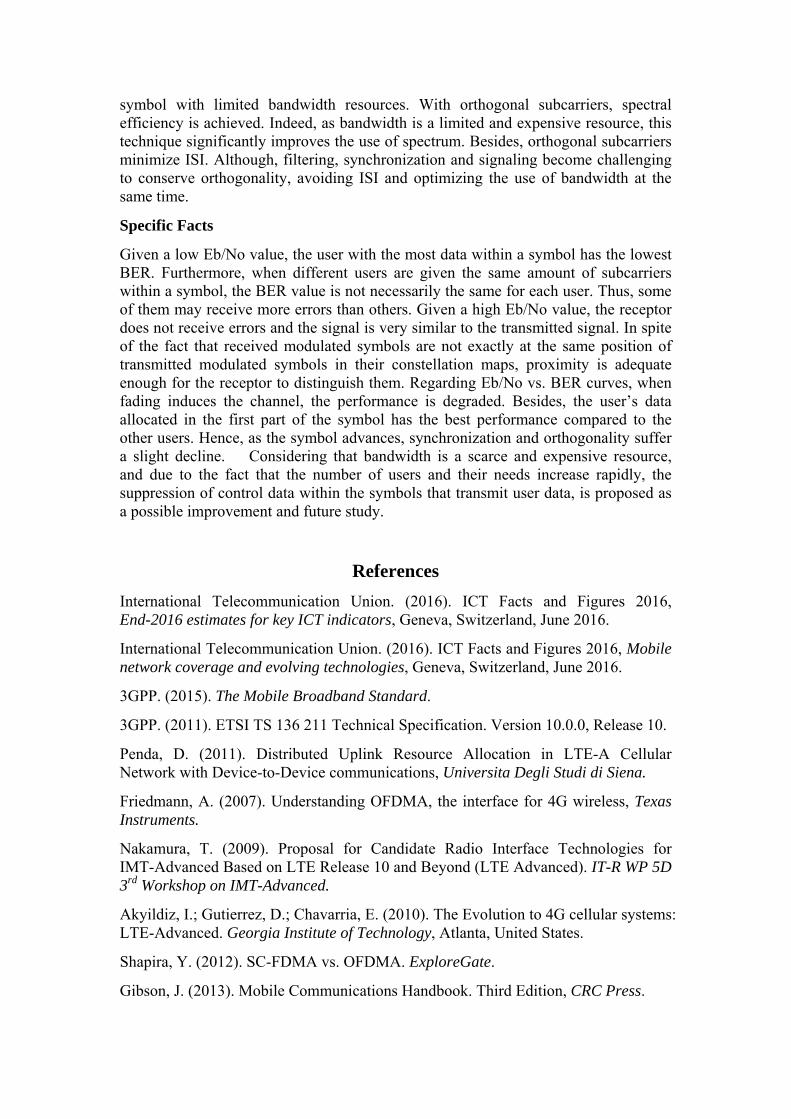
symbol with limited bandwidth resources. With orthogonal subcarriers, spectral efficiency is achieved. Indeed, as bandwidth is a limited and expensive resource, this technique significantly improves the use of spectrum. Besides, orthogonal subcarriers minimize ISI. Although, filtering, synchronization and signaling become challenging to conserve orthogonality, avoiding ISI and optimizing the use of bandwidth at the same time.

Specific Facts

Given a low Eb/No value, the user with the most data within a symbol has the lowest BER. Furthermore, when different users are given the same amount of subcarriers within a symbol, the BER value is not necessarily the same for each user. Thus, some of them may receive more errors than others. Given a high Eb/No value, the receptor does not receive errors and the signal is very similar to the transmitted signal. In spite of the fact that received modulated symbols are not exactly at the same position of transmitted modulated symbols in their constellation maps, proximity is adequate enough for the receptor to distinguish them. Regarding Eb/No vs. BER curves, when fading induces the channel, the performance is degraded. Besides, the user’s data allocated in the first part of the symbol has the best performance compared to the other users. Hence, as the symbol advances, synchronization and orthogonality suffer a slight decline. Considering that bandwidth is a scarce and expensive resource, and due to the fact that the number of users and their needs increase rapidly, the suppression of control data within the symbols that transmit user data, is proposed as a possible improvement and future study.

References

International Telecommunication Union. (2016). ICT Facts and Figures 2016, End-2016 estimates for key ICT indicators, Geneva, Switzerland, June 2016.

International Telecommunication Union. (2016). ICT Facts and Figures 2016, Mobile network coverage and evolving technologies, Geneva, Switzerland, June 2016.

3GPP. (2015). The Mobile Broadband Standard.

3GPP. (2011). ETSI TS 136 211 Technical Specification. Version 10.0.0, Release 10.

Penda, D. (2011). Distributed Uplink Resource Allocation in LTE-A Cellular Network with Device-to-Device communications, Universita Degli Studi di Siena.

Friedmann, A. (2007). Understanding OFDMA, the interface for 4G wireless, Texas Instruments.

Nakamura, T. (2009). Proposal for Candidate Radio Interface Technologies for IMT-Advanced Based on LTE Release 10 and Beyond (LTE Advanced). IT-R WP 5D 3rd Workshop on IMT-Advanced.

Akyildiz, I.; Gutierrez, D.; Chavarria, E. (2010). The Evolution to 4G cellular systems: LTE-Advanced. Georgia Institute of Technology, Atlanta, United States.

Shapira, Y. (2012). SC-FDMA vs. OFDMA. ExploreGate.

Gibson, J. (2013). Mobile Communications Handbook. Third Edition, CRC Press.

 

Anritsu Company. (2009). LTE Resources Guide. Rev 1010. United States.

4G Americas. (2014). LTE Carrier Aggregation Technology Development and Deployment Worldwide.

Sesia, S.; Toufik, I.; Baker, M. (2011). LTE The UMTS Long Term Evolution. Second Edition. John Wiley & Sons, Ltd.

Rayal, F. (2010). An overview of the LTE physical layer. Part II.

Shaikh, A.; Kumar, K. (2010). Performance Evaluation of LTE Physical Layer using SC-FDMA & OFDMA. Blekinge Institute of Technology.

Thacker, C. (2010). An initial design of an OFDM transceiver. University of Texas.

Ayeni, J. (2010). OFDM for 4G wireless communication systems. University of Hertfordshire.

Abichar, Z.; Peng, Y.; Chang, M. (2006). Basic WiMax System Modeling. Iowa State University, IEEE.

Appendix

Figure 1: Resource grid Source: 3GPP, 2011. ETSI TS 136 211 Technical Specification, Version 10.0.0

 

Source: Gibson, J., 2013. Mobile Communications Handbook, Third Edition.

Figure 2: Channel bandwidth Source: Anritsu Company, 2015. LTE Resources Guide, Rev. 1010

 

Figure 3: OFDMA 2 Users Design

Figure 4: OFDMA 2 Users (AWGN) Diagram

 

Figure 5: OFDMA 2 Users (AWGN + Rayleigh Fading) Diagram

 

(a) (b)

(c)

Figure 6: TX and RX Integer data (2 Users) Eb/No=30dB (a), 43dB (b), 80dB (c)

 

(a) (b) (c)

Figure 7: Error rate, Errors and Comparisons (2 Users) Eb/No=30dB (a), 43dB (b), 80dB (c)

Figure 8: Modulated TX Data (User 1 of 2)

 

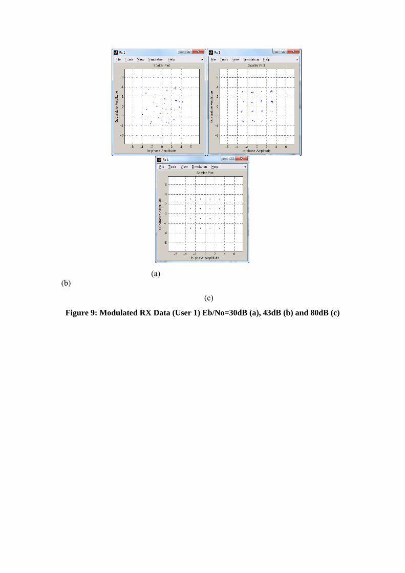
(a) (b)

(c)

Figure 9: Modulated RX Data (User 1) Eb/No=30dB (a), 43dB (b) and 80dB (c)

   

 

ICESI_0093

Experimental Investigations of a Parabolic Trough Collector

*S. K. Soni, Pec University of Technlogy Chandigarh India, India

Vikas Bhaskar, Pec University of Technlogy Chandigarh India, India

Ankit Yadav, Pec University of Technlogy Chandigarh India, India

Gaurav, Pec University of Technlogy Chandigarh India, India

*Corresponding Author

Abstract

It is being widely realized that for sustainable development, presently used energy mediums such as fossil fuels and nuclear power have to be quickly replaced by renewable energy sources. This paper deals with investigating the performance of solar parabolic trough collector (PTC) and the heat storage unit (HSU); which stores the heat in Phase change material (PCM) in the form of latent heat of fusion from the parabolic trough collector through Heat transfer fluid (HTF). The mean solar irradiation falling over the PTC and the heat gain in HTF was determined to calculate the efficiency of PTC. After that heat gain in PCM in the Heat storage unit (HSU) and its effectiveness is determined. The experiments were done with four combinations of different HTFs and PCMs using three different flow rates of 50, 100 and150 LPH with 12 experiments in total. It is concluded that flow rate have significant effect over the performance of both PTC and HSU. It is seen that flow rate of 100 LPH is found most suitable for Phase change material as above and below of this flow, the effectiveness of the HSU decreases. It is also found that Paraffin wax is more suited as PCM than water, as it stores more heat. Similarly; ethylene glycol solution is more efficient HTF; as it gives better efficiency of PTC than water as HTF.

Keywords: Parabolic trough collector, Heat storage unit, Heat transfer fluid, Flow rate, Phase change material, Solar energy storage.

 

1. Introduction

It is being widely realized that for sustainable development presently used energy mediums such as fossil fuels and nuclear power have to be quickly replaced by renewable energy sources. The latter are sustainable and have the potential to meet present and future projected global energy demands without inflicting any environmental impacts. Renewable energy sources such as solar, wind, hydropower and biogas are potential candidates to meet global energy requirements in a sustainable way. But the utilization of renewable resources is not on a very wide scale. In India itself; out of the total power generation only 28% comes from renewable resources and remaining 72% from non-renewable resources. So, there is a need to increase the power generation capacity through renewable resources.

The solar energy is not continuous and therefore requires some thermal energy storage device so that it can be used continuously. One such method is to store it in the form of latent heat in a phase change material. In this work solar energy collected by parabolic trough collector is absorbed by some fluid and then transferred to some phase change material and stored in the form of latent heat.

Hegazy et al. (2007) did experimental study of a parabolic trough collector with its sun tracking system designed and manufactured utilizing the existing Saudi technologies and available local materials. For the design of the PTC frame, a finite element model was developed and used to check the capability of the structure to absorb torsion and bending forces, under dead and wind loads.

Shukla et al. (2008) performed thermal cycling tests to check the stability in thermal energy storage systems on some selected organic and inorganic phase change materials (PCMs). The possibility of using these PCMs in thermal energy storage systems were examined on the basis of thermal, chemical and kinetic criteria. Organic and inorganic PCMs were selected to check their thermal stability. Shukla et al. (2009) studied use of a latent heat storage system using phase change materials (PCMs) is an effective way of storing thermal energy and has the advantages of high-energy storage density and the isothermal nature of the storage process. These papers summarize the investigation and analysis of the available thermal energy storage systems incorporating PCMs for use in different applications.

Veerappan et al. (2009) investigated the phase change behavior of 65 mol% capric acid and 35 mol% Lauric acid, Calcium chloride Hexahydrate, Noctadecane, n-Hexadecane, and n-Eicosane inside spherical enclosures to identify a suitable heat storage material. The parametric study concludes that, lower values of initial temperature did not make significant contribution on the solidified mass fraction of PCM. They observed that for solidification, initially there is a higher heat flux release for lower coolant fluid temperatures.

Hossain et al. (2011) studied the effect of thermal conductivity of the absorber plate of a solar collector on the performance of a thermo siphon solar water heater by using the alternative simulation system. The system is assumed to be supplied of hot water at 50 ◦C and 80 ◦C whereas both are used in domestic and industrial purposes, respectively. From this study, it is found that the solar water heater with a siphon system achieves system characteristic efficiency of 18% higher than that of the conventional system by reducing heat loss for the thermo-siphon solar water heater.

 

Yassen (2012) performed an experimental and theoretical study to determine the thermal efficiency of a parabolic trough solar collector. The experimentation was done during winter and summer at Tikrit-Iraq. They found that the experimental thermal efficiency of collector is less than the theoretical one in 7 to 15 percent.

Yadav et al. (2013) investigated a solar powered air heating system using parabolic trough collector. In this experimental setup, the reflected solar radiations were focused on absorber tube which was placed at focal length of the parabolic trough. In this setup, air was used as working fluid which collects the heat from absorber tube. To enhance the performance of parabolic trough, collector with different type of reflectors were used.

Sivaram et al. (2016) stated that solar parabolic trough collector (PTC) is the best recognized and commercial-industrial-scale, high temperature generation technology available today.

The present work deals with numerical and experimental investigations to study the performance of a small-scale solar PTC integrated with thermal energy storage system. Paraffin has been used as phase change material and water as heat transfer fluid, which also acts as sensible heat storage medium. Experiments were carried out to investigate the effect of mass flow rate on useful heat gain, thermal efficiency and energy collected/stored. A numerical model was developed for the receiver/heat collecting element (HCE) based on one dimensional heat transfer equations to study temperature distribution, heat fluxes and thermal losses.

2. Experimental Setup

The experimentation setup, showing various components (with specifications) is given in Figure 1.

Parabolic trough concentrator lined with a polished metal mirror (1m×1.06m,focal length -0.0265m,rim angle-900)

Supporting structure (M.S.angle 37mmx37mmx5mm )

Receiver tube or Absorber tube with Vacuum (OD=47 mm, ID=37 mm, Length= 1500 mm)

Heat Transfer Fluid (HTF)

Phase change material (PCM)

Heat storage unit(HSU): Water, Paraffin Wax

A.C Motor with pump (head- 3m with 350 LPH,0.025 kW)

Pyrometer (Range=0-1100 W/m2, Accuracy= ±5%,Resolution=0.3 W/m2)

Thermocouples with Digital Display Unit (J-type, Range=0-600 0C, Accuracy = ±5%)

Rota meter(Range =50-500 LPH)

 

Sensor interface: ( Vernier Lab Quest 2)

Figure 1: Experimental Setup

3. Experimental Results and Discussions

For the experimentation, Water and 50% Ethylene glycol solution is used as HTFs and Water and Paraffin wax as PCMs. For the operation manual tracking is done at an interval of 30 minutes. The heat gain in HTF and PCM is determined for every 30 minutes and according to it the efficiency of PTC and effectiveness of the HSU are determined. Finally, the efficiency of PTC and effectiveness of HSU are used as the parameter for the comparison of their performance with HTF, PCM and different flow rates.

Water as Heat Transfer Fluid and Phase Change Material

The water is the most commonly used fluid in heat transfer applications. It has a high specific heat capacity. The main drawback of this is that it may freeze in cold weather due to which some organic fluids are with water in different proportion but here we are using pure water as PCM and HTF. The properties of water are given in the table 1.

Table 1: Properties of water

Properties Value Density 1000Kg/m3

Specific heat 4.187 KJ/Kg-KBoiling point 100oC Freezing point 0oC

Water is made to flow inside the copper tubes with the help of the motor driven pump. The suction and delivery pipes from the pump are put inside a reservoir of water.

The Heat gain by HTF is calculated from the equation given below

Qh=mh ×ch × ∆Th Where:

mh = Mass Flow rate of HTF

Ch= Specific heat of HTF in KJ/Kg-k

 

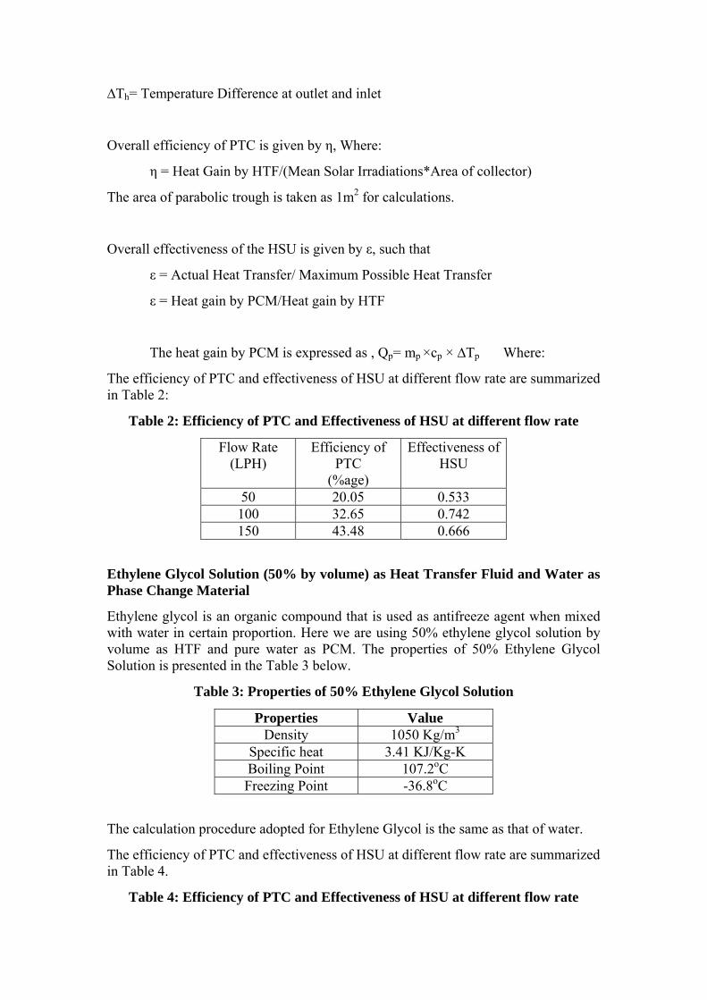
∆Th= Temperature Difference at outlet and inlet

Overall efficiency of PTC is given by η, Where:

η = Heat Gain by HTF/(Mean Solar Irradiations*Area of collector)

The area of parabolic trough is taken as 1m2 for calculations.

Overall effectiveness of the HSU is given by ε, such that

ε = Actual Heat Transfer/ Maximum Possible Heat Transfer

ε = Heat gain by PCM/Heat gain by HTF

The heat gain by PCM is expressed as , Qp= mp ×cp × ∆Tp Where:

The efficiency of PTC and effectiveness of HSU at different flow rate are summarized in Table 2:

Table 2: Efficiency of PTC and Effectiveness of HSU at different flow rate

Flow Rate (LPH)

Efficiency of PTC

(%age)

Effectiveness of HSU

50 20.05 0.533 100 32.65 0.742 150 43.48 0.666

Ethylene Glycol Solution (50% by volume) as Heat Transfer Fluid and Water as Phase Change Material

Ethylene glycol is an organic compound that is used as antifreeze agent when mixed with water in certain proportion. Here we are using 50% ethylene glycol solution by volume as HTF and pure water as PCM. The properties of 50% Ethylene Glycol Solution is presented in the Table 3 below.

Table 3: Properties of 50% Ethylene Glycol Solution

Properties Value Density 1050 Kg/m3

Specific heat 3.41 KJ/Kg-K Boiling Point 107.2oC Freezing Point -36.8oC

The calculation procedure adopted for Ethylene Glycol is the same as that of water.

The efficiency of PTC and effectiveness of HSU at different flow rate are summarized in Table 4.

Table 4: Efficiency of PTC and Effectiveness of HSU at different flow rate

 

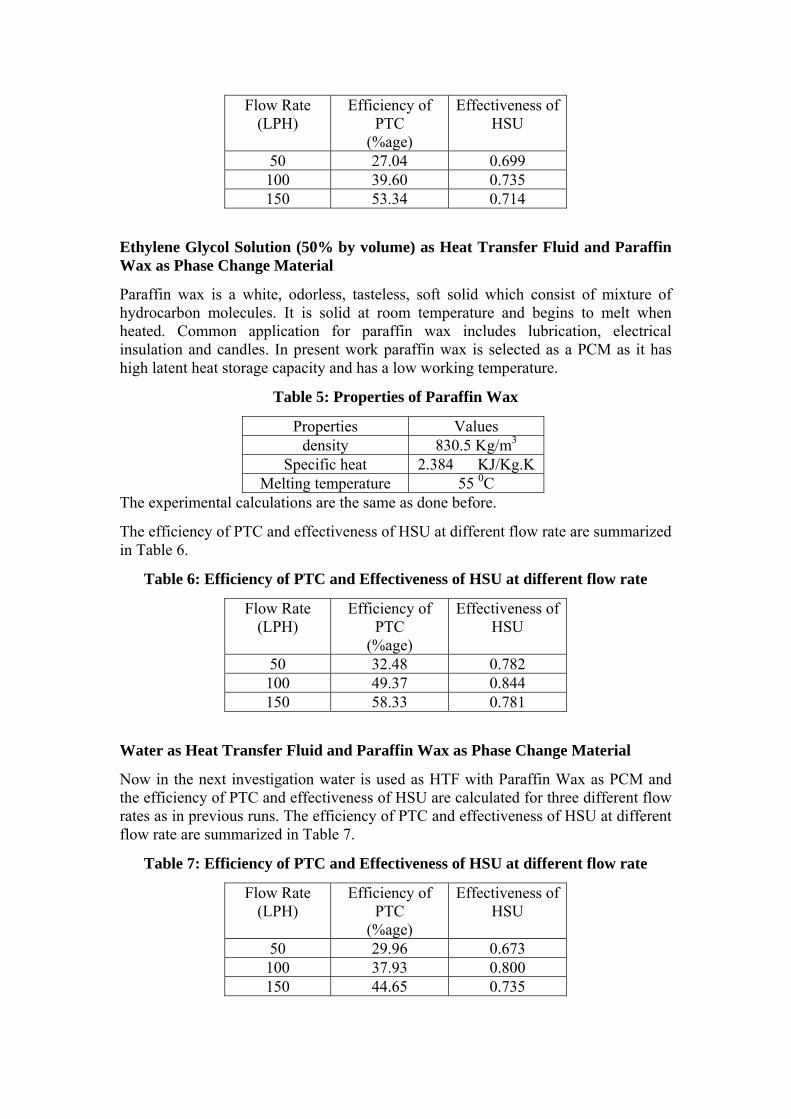
Flow Rate (LPH)

Efficiency of PTC

(%age)

Effectiveness of HSU

50 27.04 0.699 100 39.60 0.735 150 53.34 0.714

Ethylene Glycol Solution (50% by volume) as Heat Transfer Fluid and Paraffin Wax as Phase Change Material

Paraffin wax is a white, odorless, tasteless, soft solid which consist of mixture of hydrocarbon molecules. It is solid at room temperature and begins to melt when heated. Common application for paraffin wax includes lubrication, electrical insulation and candles. In present work paraffin wax is selected as a PCM as it has high latent heat storage capacity and has a low working temperature.

Table 5: Properties of Paraffin Wax

Properties Values density 830.5 Kg/m3

Specific heat 2.384 KJ/Kg.KMelting temperature 55 0C

The experimental calculations are the same as done before.

The efficiency of PTC and effectiveness of HSU at different flow rate are summarized in Table 6.

Table 6: Efficiency of PTC and Effectiveness of HSU at different flow rate

Flow Rate (LPH)

Efficiency of PTC

(%age)

Effectiveness of HSU

50 32.48 0.782 100 49.37 0.844 150 58.33 0.781

Water as Heat Transfer Fluid and Paraffin Wax as Phase Change Material

Now in the next investigation water is used as HTF with Paraffin Wax as PCM and the efficiency of PTC and effectiveness of HSU are calculated for three different flow rates as in previous runs. The efficiency of PTC and effectiveness of HSU at different flow rate are summarized in Table 7.

Table 7: Efficiency of PTC and Effectiveness of HSU at different flow rate

Flow Rate (LPH)

Efficiency of PTC

(%age)

Effectiveness of HSU

50 29.96 0.673 100 37.93 0.800 150 44.65 0.735

 

Comparison of efficiency of PTC and effectiveness of HSU with Water as both HTF and PCM for three different flow rates

The variation of efficiency of PTC and effectiveness of HSU are shown graphically in figure 2 and 3 respectively.

Figure 2: Variation of efficiency of PTC with Water as HTF and PCM both with different flow rates

Figure 3: Variation of effectiveness of HSU with Water as HTF and PCM both with different flow rates

Comparison of efficiency of PTC and effectiveness of HSU with Ethylene Glycol Solution (50% by volume) as HTF and Water as PCM for three different flow rates

The variation of efficiency of PTC and effectiveness of HSU are shown graphically in figure 4 and 5 respectively.

00.10.20.30.40.50.60.7

7:30‐8:00

8:00‐8:30

8:30‐9:00

9:00‐9:30

9:30‐10:00

10:00‐10:30

10:30‐11:00

11:00‐11:30

11:30‐12:00

12:00‐12:30

12:30‐1:00

1:00‐1:30

1:30‐2:00

2:00‐2:30

2:30‐3:00

3:00‐3:30

3:30‐4:00

Efficiency

Time(Hour)

50LPH

100LPH

150LPH

00.20.40.60.81

1.2

7:30‐8:00

8:00‐8:30

8:30‐9:00

9:00‐9:30

9:30‐10:00

10:00‐10:30

10:30‐11:00

11:00‐11:30

11:30‐12:00

12:00‐12:30

12:30‐1:00

1:00‐1:30

1:30‐2:00

2:00‐2:30

2:30‐3:00

3:00‐3:30

3:30‐4:00

Effectiveness

Time(Hours)

50LPH

100LPH

150LPH

 

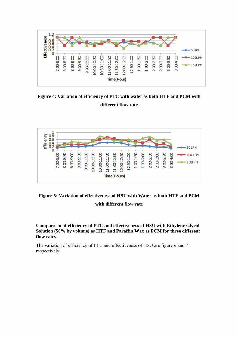
Figure 4: Variation of efficiency of PTC with water as both HTF and PCM with

different flow rate

Figure 5: Variation of effectiveness of HSU with Water as both HTF and PCM

with different flow rate

Comparison of efficiency of PTC and effectiveness of HSU with Ethylene Glycol Solution (50% by volume) as HTF and Paraffin Wax as PCM for three different flow rates.

The variation of efficiency of PTC and effectiveness of HSU are figure 6 and 7 respectively.

 

Figure 6: Variation of efficiency of PTC with Ethylene Glycol Solution (50% by volume) as HTF and Paraffin Wax as PCM with different flow rate

Figure 7: Variation of effectiveness of HSU with Ethylene Glycol Solution (50% by volume) as HTF and Paraffin Wax as PCM with different flow rate

Comparison of efficiency of PTC and effectiveness of HSU with Water as HTF and Wax as PCM for three different flow rates.

The variation of efficiency of PTC and effectiveness of HSU are shown in figure 8 and 9 respectively.

Figure 8: Variation of efficiency of PTC with Water as HTF and Paraffin Wax as PCM for three different flow rates

 

00.20.40.60.81

7:30‐8:00

8:00‐8:30

8:30‐9:00

9:00‐9:30

9:30‐10:00

10:00‐…

10:30‐…

11:00‐…

11:30‐…

12:00‐…

12:30‐1:00

1:00‐1:30

1:30‐2:00

2:00‐2:30

2:30‐3:00

3:00‐3:30

3:30‐4:00

Efficiency

Time(Hours)

50LPH

100LPH

150LPH

00.20.40.60.81

1.2

7:30‐8:00

8:00‐8:30

8:30‐9:00

9:00‐9:30

9:30‐10:00

10:00‐10:30

10:30‐11:00

11:00‐11:30

11:30‐12:00

12:00‐12:30

12:30‐1:00

1:00‐1:30

1:30‐2:00

2:00‐2:30

2:30‐3:00

3:00‐3:30

3:30‐4:00

Effectiveness

Time(Hours)

50LPH

100LPH

150LPH

0

0.2

0.4

0.6

7:30‐8:00

8:00‐8:30

8:30‐9:00

9:00‐9:30

9:30‐10:00

10:00‐…

10:30‐…

11:00‐…

11:30‐…

12:00‐…

12:30‐1:00

1:00‐1:30

1:30‐2:00

2:00‐2:30

2:30‐3:00

3:00‐3:30

3:30‐4:00

Efficiency

Time(Hours)

50LPH

100LPH

150LPH

 

Figure 9: Variation of effectiveness of HSU with Water as HTF and Paraffin Wax as PCM for three different flow rates

 

4. Conclusions

It is being widely realized that for sustainable development, presently used energy

mediums such as fossil fuels and nuclear power have to be quickly replaced by

renewable energy sources. The latter are sustainable and have the potential to meet

present and future projected global energy demands without inflicting any

environmental impacts. Renewable energy sources such as solar, wind, hydropower

and biogas are potential candidates to meet global energy requirements in a

sustainable way. India is blessed with large amount of solar radiations and has a great

potential to contribute majorly in the renewable energy production. After the analysis

of the experimental data and results, it can be concluded that the performance of PTC

is best when ethylene glycol solution (50% by volume) is used as HTF. The efficiency

of PTC increases with increase in flow rate of HTF for the given range (50-150) LPH.

Paraffin wax is more effective as PCM than Water and stores more heat than water.

Effectiveness of HSU comes out to be optimum for the flow rate of 100LPH as above

and below it the effectiveness of the HSU decreases.

References

Hegazy, Ahmed S.; ElMadany, Mohamed M. (2007).Design and experimental testing of a solar parabolic trough collector with its tracking system for salt-water desalination in arid areas of Saudi Arabia, Proceedings of the 7th Saudi Engineering Conference (SEC7),1-13

Hossain, M.S., Saidur, R., Fayaz, H., Rahim, N.A., Islam, M.R., Ahamed, J.U. and Rahman, M.M. (2011). Review on solar water heater collector and thermal energy

00.20.40.60.81

1.2

7:30‐8:00

8:00‐8:30

8:30‐9:00

9:00‐9:30

9:30‐10:00

10:00‐10:30

10:30‐11:00

11:00‐11:30

11:30‐12:00

12:00‐12:30

12:30‐1:00

1:00‐1:30

1:30‐2:00

2:00‐2:30

2:30‐3:00

3:00‐3:30

3:30‐4:00Ef

fectiveness

Time (Hours)

50LPH

100LPH

150LPH

 

performance of circulating pipe, Renewable and Sustainable Energy Reviews, Volume 15(8) p. 3801–381

Shukla, A., Buddhi, D. and Sawhney, R.L. (2008). Thermal cycling test of few selected inorganic and organic phase change materials, Renewable Energy, Volume 33 (12) p. 2606–2614

Shukla, A., Buddhi, D. and Sawhney, R.L. (2009). Solar water heaters with phase change material thermal energy storage medium: A review, Renewable and Sustainable Energy Reviews, Volume 13 (2009) 2119–2125

Sivaram, P.M., Nallusami, N. and Suresh, M. (2016). Experimental and numerical investigation on solar parabolic trough collector integrated with thermal energy storage unit, Int. journal of Energy Research, Volume 40 (11) p. 1564–1575.

Veerappan, M., Kalaiselvam, S., Iniyan, S. and Goic, R. (2009). Phase change characteristic study of spherical PCMs in solar energy storage, Solar Energy, Volume 83 p. 1245–1252.

Yadav,A.,Kumar,M.,Balram.(2013) Experimental study analysis of parabolic trough collector with various reflectors, World academy of Science ,Engineering and Technology,Inernationa; Journal of Mathematical,Computationa,Physical,Electrical and Computer Engineering volume 7 (12) p.1659-1663

Yassen, T.A., (2012). Experimental and Theoretical Study of a Parabolic Trough Solar Collector, Anbar Journal for Engineering Sciences Volume 5(1) p. 109-125

---------------------------------

Biographical Note

S. K. Soni is Associate Professor with teaching and research experience of more than 26 years and published more than 10 research papers in international and national journals of repute and in the proceedings of the conferences. He guided more than 10 post graduate theses. He organized one national conference for the faculty of technical institutions and industries.

   

 

ICESI_0104

Modeling, Analysis and Design of Mechanical and Structural Systems Involving Uncertainties

*Sambasiva Rao Singiresu, University of Miami, United State of America

*Corresponding Author

Abstract

Many practical engineering systems are too complex to be described by precise models and in exact terms, because real-life phenomena have to be simulated by mathematical approximations. Due to the impreciseness of many parameters involved in the system, it is impossible to perform the analysis and design computations using only crisp values. When the imprecise parameters are expressed as interval numbers, the response equations can be converted to the form of interval expressions. The required computations can then be carried using the rules of interval arithmetic. Compared to the analysis, design and optimization with crisp and precise variables, the computations with imprecise variables makes more sense in several situations. For example, the fiber content of a fiber-reinforced composite structure is a very important factor in predicting the strength of the structure. Due to the limitations of the manufacturing process used, its precise value may not be known. In such a case, interval analysis based computations can treat the fiber content as an interval number. This paper presents the application of interval analysis in the design and optimization of structural and mechanical systems.

Keyword: Uncertain systems, Interval analysis, Optimization, One-way clutch, Planar truss.

 

1. Introduction

Typically, imprecision present in a system can be described either as fuzziness or randomness (Kaufmann, 1991). If the system is fuzzy, it is possible to establish a connection between the interval method and the fuzzy analysis using the concept of -cuts. When the allowable interval ranges of physical variables are known, the vagueness of the statements could be described using the fuzzy set theory. The whole fuzzy set is divided (cut) into finite subsets by using discrete values of membership function. Each fuzzy subset represents the level (range) of imprecision corresponding to a specified value (membership function value). Thus, an interval can be used to describe a fuzzy subset. In mechanical and structural design, fuzzy information may be present in several input (design) parameters and boundary conditions of the system. By representing these design parameters using the -cuts approach, all the interval expressions involved in the analysis and design of the system can be evaluated at different fuzzy levels or values. Using this approach, designers can solve any imprecise problem and make precise and significant decisions based on the fuzzy set theory prediction. If the uncertain parameters are described by probability distributions, the response of the structure, such as displacements, strains and stresses, can be computed using probability principles. However, the numerical computation of the extreme values of the response quantities, which are needed in design equations, requires the modeling of tail portions of the probability distributions of the random variables, which is very difficult in practice.

The response of a structure or a machine is influenced by geometry, load and material property parameters. The geometry parameters, obtained through machining/manufacturing process, are usually specified as xx , where x denotes the mean (nominal) value and x represents the two-sided tolerance. Many types of loads, such as wind, earthquake and snow loads, are known to vary over specific ranges, P1 to P2. Similarly when material properties, such as yield stress and Young’s modulus, are determined through experiments, they are found to vary between two limiting values, y1 and y2. All these parameters can be denoted by simple ranges with no need to know either the preference information (which is needed in fuzzy modeling) or the probability distribution function (which is required in probabilistic modeling) of the parameters.

The optimum design of uncertain structural and mechanical systems is presented in this work by denoting the parameters by simple ranges or intervals so that interval analysis methods can be applied for predicting the behavior of structures. This implies that we need to apply interval arithmetic to every step of calculations. Since a specific interval variable may appear several times in different terms of the same equation, the order in which computations are carried will unnecessarily increase the interval ranges of the result to varying degrees. Thus, during actual programming, we need to adjust the order in which different interval parameters are considered in any specific equation. The purpose of changing the order of parameters is obvious - when the program executes the equation using interval parameters, the new order will not only minimize the computational time but also lead to a reduced interval ranges for the result. In addition, the truncation approach is used based on a comparison between the input range and the output range of the parameters. The purpose of truncation is to make reasonable modifications to the output range before conducting the next interval operation. Numerical examples are presented to illustrate the computational aspects of the method.

 

2. Interval Model

In the interval model, the uncertain parameters are represented as interval numbers. Some situations in which an uncertain parameter can be modeled as an interval number are indicated below (Rao, 1997):

1. When a machine part is to be produced with dimension x, it is often specified using a tolerance as for convenience of manufacturing. In this case, the actual dimension of the part is to be treated as an interval number as ( ).

2. In many engineering applications, external actions such as the wind load acting on a tall pressure vessel (P) may be known to vary over a range P1 to P2.

3. During the design stages, designers often conduct sensitivity studies by changing one or more parameters over specified range(s) and finding its influence on the response/design of the system. In such cases, the influence of an independent interval variable, x = ( ), on the dependent variable f can be represented as an

interval as f = ( ), where and denote the variations in f

caused by the changes and in x.

4. The performance characteristics of most engineering systems vary (degrade) during their lifetimes because of aging, creep, wear, corrosion and changes in operating conditions. The analysis and design of such systems should take care of the intervals of deviation of parameters from their nominal (initial) values.

When optimization techniques are used in conjunction with interval analysis, certain computational problems need to be resolved. With the use of theoretical interval arithmetic operations, the widths (intervals) of the response parameters have been observed to be wider than the true widths with an increase in the number and/or ranges of interval parameters. To limit the unnecessary growth of the intervals of the response parameters, an approximation technique, termed the truncation method, has been used. Another inherent difficulty with interval arithmetic is that the range of the response parameters depends on the order or sequence in which the various interval input variables are used during the computations. In order to overcome this difficulty, the ranges of the response parameters obtained from interval arithmetic are checked and corrected (if necessary) with those given by the combinatorial approach at certain stages of optimization (particularly during gradient computations).

An interval parameter represents the range of uncertainty of a design parameter. For each imprecise parameter, there are two numbers that represent the lower and upper bounds of the parameter. For example, an interval number can be denoted as

where the lower and upper bound values are given by

and where denotes the nominal value and

represents the tolerance on x. If the system is linear, the exact response can be computed using the combinatorial approach. If the response parameter is represented as

where denote the input interval parameters with

(1)

xx xxxx ,

xxxx ,

21, ffff 1f 2fx x

),(),( 21 xxxxx

xxxx 01 xxxx 02 0x x

),,,( 21 nxxxf nxxx ,,, 21

nixxxxx iiiii ,,2,1];,[],[ )2()1(

 

Then all possible values of f are given by:

(2)

Here fr denotes the value of the response parameter, f, at a particular combination of the end points of the intervals of . The response parameter can be denoted as an

interval number as:

(3)

Although this method, known as the combinatorial method, appears to be simple, it requires 2n analyses and becomes tedious and prohibitively expensive for most practical problems that contain large number of interval parameters. The interval analysis can be conducted using interval arithmetic operations. For example, if

and denote two interval numbers, a general arithmetic operation can be expressed as [2, 3]

(4)

Where denotes an arithmetic operation sign, such as +,, (or ·) or (or /).

Interval Arithmetic Operations

Equation (4) can be rewritten in a detailed manner as (Moore, 2009):

(5)

(6)

(7)

(8) Note that in equation (8), the division operation is not defined if

. Real numbers A and B are denoted by degenerate intervals and

, respectively, with and . Equation (4) indicates that interval addition and interval multiplication are both associative and commutative. While the subdistributive law and the inclusion monotonicity law hold true, we could extend the computations to matrices as well:

(9)

nkn

jir rkjixxxff 2,,2,1;2,1,2,1,2,1);,,,( )()(

2)(

1

nxxx ,,, 21

]max,min[],[ rr

rr

fffff

],[ aaA ],[ bbB

}|{],[],[, bybaxa

yxbbaa

],[],[],[ bababbaa

],[],[],[ bababbaa

)],,,max(),,,,[min(],[],[ bababababababababbaa

],[0]/1,/1[],[],/[],[ bbifbbaabbaa

],/[],[ bbaa

],[0 bb ],[ aa

],[ bb aa bb

)(][][]][[ rpcCBA ij

 

With and the

elements of the matrix [C] are given by

(10) Where the multiplication rule, equation (4), is to be used for each product .

Truncation Method

It has been observed that the interval arithmetic operations, given by Eq. (4), yield the exact range of a response parameter only if each interval variable occurs only once in the expression. Because it is not possible to rewrite complicated and/or implicit expressions (involving several interval variables in a nonlinear manner), there is no simple way to obtain the exact interval of response parameters in most practical systems. Under these circumstances, the widths of the response parameters grow with the number and/or ranges of the interval parameters. To limit the growth of intervals of response parameters for large amounts of uncertainties, a truncation method can be used. To describe the truncation method, let two interval values and

be used to find the computed output . If we use the central

values of the variables and to do the same (crisp)

calculation, we get the output . Then we use to judge the necessity of applying

truncation. In numerical experiments, compared to the combinatorial method, the truncation method is found to be fast and reasonably accurate (Rao, 1997).

3. Applications

Modeling of the clutch

The hub dimension a, the cylinder radius c, and the ring radius e are assumed to be fuzzy with linear membership functions (Rao, 2005; Lee, 2001). When analyzing tolerance outputs using interval approach, the input intervals or ranges corresponding to different levels of confidence (with different values of preference ) can be assumed. For different manufacturing processes, the dimensional variations may relate to different levels of , therefore various combinations of levels of can be generated for those dimensional variations. The interval or range corresponding to larger values of corresponds to increasing confidence with which the mechanism can be assembled with given uncertain input parameters. To simplify the analysis procedure, a common level of has been assigned for all the design variables. Corresponding to the level , the intervals of confidence of component dimensions are assumed to be:

),(][][][),(][][][ rqbbbBqpaaaA ijijijijijij

rjpibacq

kkjikij ,2,1;,2,1;

1

kjikba

],[ aaa ],[ bbb ],[ ccc

2/)(0 aaa 2/)(0 bbb

0c 0c

 

Figure 1: One-way clutch assembly and its dimensions

mm,

mm,

mm. (11)

Figure 2: Geometric feature variations of the one-way clutch assem

Figure 3 shows the fuzzy vector model of the one-way clutch. In this model, , , and are caused by variations in flatness, perpendicularity, circularity and

circularity respectively. These geometric variations are also assumed to be fuzzy triangular numbers with .The values of , and corresponding to a

given -cut are given by:

,

, (12)

Spring

Hub

Roller

Ring

ba e

cc

]0276.06726.27,0276.06174.27[],[ 31 aaaa a

]0114.04414.11,0114.04186.11[],[ 31 accc a

]0508.08508.50,0508.07492.50[],[ 31 aeee a

0.025A0.01

0.010A

0.003

a c e

01 a c e

]025.0025.0,025.0025.0[ a

]003.0003.0,003.0003.0[ c

 

.

Figure 3: Fuzzy vector model of the one-way clutch

The mechanical error analysis is conducted using the loop equations. These equations are solved using the bisection method and the modified Newton-Raphson iterative algorithm. The results obtained by considering tolearances on all the variables are shown in Table 1.

These results can be used in tightening/loosening tolerances on critical parameters in order to improve the assemblability of mechanisms and reduce the mechanical error in the output parameters. The results of interval analysis are compared with those given by the worst case analysis method and the statistical method. The fuzzy analysis method introduced in this work holds promise to be more realistic and accurate in the modeling and analysis of mechanical systems that contain imprecision in link lengths and geometric variations.

Table 1: -cut results of b and (with tolerances considered on all variables)

b (mm) (rad)

0.0 (4.7941, 4.8771) (0.1209, 0.1237)

0.2 (4.7953, 4.8741) (0.1211, 0.1235)

0.4 (4.7972, 4.8727) (0.1214, 0.1230)

0.6 (4.7996, 4.8723) (0.1217, 0.1228)

0.8 (4.8048, 4.8636) (0.1219, 0.1226)

1 4.8105 0.1225

]010.0010.0,010.0010.0[ e

a

a

2

Hub

e

b

c

1

e

c

c

c

c

1

1

 

Optimum Design of a Ten-bar truss

The 10-bar cantilever truss subjected to the loads shown in Fig.4 is considered. The stress limit on all members is psi and the displacement limit of inch is specified at all node points in the vertical direction. The cross-sectional areas of members are chosen as design variables. The minimum and maximum values of all design variables are prescribed to be 0.1 in2 and 100.0 in2, respecitively. The characteristics of interval naalysis and interval analysis-based optimization are studied through the following example.

Figure 4: A Ten-bar truss

Crisp optimization without interval analysis:

By assumming the design variables and preassigned parameters to be crisp (with no variability), the optimum solution is found. The details of the optimum design are indicated in Table 2. It can be seen that the stresses in elements 1, 7 and 9 reached their upper bound values while the stresses in elements 3, 4 and 8 reached their lower bound values at the optimum solution. In addition, the design variables corresponding to elements 2, 5, 6 and 10 attained their lower bound value of 0.1.

Table 2: Results of Crisp Optimization

Load & Nodal positions

Design Variables Stresses Minimum Weight

P(2y)=P(4y)=-100. 2, 4 – nodal points y – direction of dof

Density = 0.1 E=1.0E4

Node 1 - (720., 360.) Node 2 - (720., 0.)

Node 3 - (360., 360.) Node 4 - (360., 0.) Node 5 - (0., 360.) Node 6 - (0., 0.)

1 7.937868

2 0.100000

3 8.062132

4 3.937868

5 0.100000

6 0.100000

7 5.744722

8 5.568986

9 5.568986

10 0.100000

s[1]=24.999999 s[2]=15.533010 s[3]=-25.000000 s[4]=-24.999999

s[5]=1.450517E-007

s[6]=15.533010 s[7]=25.000000 s[8]=-24.999999 s[9]=24.9999999 s[10]=-21.966990

1593.180909

Uncertainty-based optimization using interval analysis:

000,25 0.2

PP

363636

 

The interval analysis is conducted at the optimum design point indicated in Table 1 by assuming the loads acting at nodes 2 and 4 along the y-direction to be interval numbers, (99,101). In addition, all the design variables are assumed to have a tolerance of

. Using finite element method, the analysis is conducted without and with truncation. The resulting intervals of stresses developed in the various elements are shown in Table 2. From Table 2, it can be seen that by using the truncation method, the interval ranges of stresses have been reduced. The ranges of stresses obtained with truncation were verified to be closer to the exact solution determined from the combinatorial method.

Table 3: Results with Interval Optimization (with Truncation)

Load & Nodal positions

Design Variables

Stresses Weight

P(2y)=P(4y)=(99. 101.) 2, 4 – nodal points y – direction of dof other parameters are fixed.

1 7.9379

2 0.1000

3 8.0621

4 3.9379

5 0.1000

6 0.1000

7 5.7447

8 5.5690

9 5.5690

10 0.1000

tolerance = 1.0E-3

s[1]=(24.72425, 25.274670) s[2]=(15.491200, 15.571268) s[3]=(-25.188247, -24.812515) s[4]=(-25.023999, -24.975343) s[5]=(-2.4584E-002, 2.7862E-002) s[6]=(15.521689, 15.561636) s[7]=(24.709005, 25.291837) s[8]=(-25.544487, -24.455637) s[9]=(23.809548, 26.190033) s[10]=(-22.451852, -21.472865)

1593.161339

4. Conclusion

The optimization of uncertain engineering systems, where the parameters are described in terms of intervals, is presented. Compared to the combinatorial approach which gives the exact ranges of the response parameters, the interval analysis approach with truncation is found to be simple, economical and fairly accurate. If the analysis is simple and involves only few arithmetic operations, the direct interval analysis and the truncation methods predict essentially the same ranges for the response parameters. As the number of input interval parameters and/or ranges of interval parameters increase, the interval ranges of optimum design variables and the optimum value of the objective function also increase. The optimization methodology presented in this work is quite general and can be used for the design of any uncertain engineering system when either the probability distribution functions or the preference information of uncertain parameters are unknown.

001.0

 

References

Kaufmann, A. and Gupta, M.M. (1991). Introduction to Fuzzy Arithmetic- Theory and Applications.

International Thomson Computer Press.

Rao, S.S. and Berke, L. (1997). Analysis of Uncertain Structural Systems Using Interval Analysis. AIAA

Journal, 35(4), 727-735.

Moore, R. E., Kearfott, R. B. and Cloud, M. J. (2009). Introduction to Interval Analysis, Society for

Industrial and Applied Mathematics (SIAM), Philadelphia, PA.

Rao, S.S. and Wu, W. (2005). Optimum tolerance allocation in mechanical assemblies using an interval

Method Engineering Optimization, 37(3), pp. 237-257.

Lin, E.E. and Zhang, H.C. (2001). Theoretical Tolerance Stackup Analysis Based on Tolerance Zone

Analysis, International Journal of Advanced Manufacturing Technology, 17, 257-262.

   

 

ICESI_0157

Moving Beyond Corporate Acceleration Programs: The Need for Community Entrepreneurial Acceleration

Programs

*Antonio Grilo, Universidade NOVA de Lisboa, Portugal

Tiago Mealha, Universidade NOVA de Lisboa, Portugal

Aneesh Zutshi, Universidade NOVA de Lisboa, Portugal

*Corresponding Author

Abstract

There is significant evidence of correlation between collaboration, innovation and growth of start-ups and large companies. Although there are different types of collaboration arrangements between corporates and startups it is a challenge select what type of collaboration shall be more adequate. This paper proposes a collaboration framework between corporates and startups according to the objectives, investment needed and working engagement between parties. The paper also discusses about the despite corporate accelerators programs have become a major trend in the form of Open Innovation for large and medium size companies there is also a clear challenge related with the efficiency of these programs. Based on 6 cases studies, we argue about the need to design more purposeful, more formal, more structured and more deliberate knowledge leaks that we designate as ‘Knowledge Effusion’. We also stress the need for fostering more effective open innovation within sectorial communities of innovation through deliberate ‘Knowledge Effusion’ on acceleration programs through the creation of what we designate as ‘Community Entrepreneurial Acceleration Programs’. The concept of communities is related with ‘cluster’ or ‘ecosystem’ i.e. it includes an extended domain of action from multiple stakeholders within an economic activity.

Keywords: Acceleration, Startups, Open innovation, Knowledge effusion.

 

1. Introduction Accelerators have become an important agent for the growth of new startups across

the world. They provide training and mentorship to startups and help them find

investors. Accelerator programs help entrepreneurs bring their technologies, ideas or

products into the marketplace and ideally lead entrepreneurs to develop viable

businesses (Chang, 2013; Cohen and Hochberg 2014). Corporate accelerators provide

a structured program and financial support for startups to transform their ideas into

real and concrete businesses (Abreu, et al. 2017; and Carvalho, et al. 2017). An

Accenture (2015) report shows a significant correlation between collaboration,

innovation and growth of start-ups and large companies in G20 countries. The report

indicates that collaboration between start-ups and large companies counts for 9

percent of large companies’ total revenue and this number is expected to mount to 20

percent in five years’ time. The survey of 1000 large companies and 1000

entrepreneurs, both termed the other partner as important for the firm’s innovation

and growth in the next three years. Yet, existing studies demonstrate that despite its

relevance and importance, the effectiveness of these collaborations is low, and the

open innovation processes engaging other parties like universities, suppliers is very

fragmented. Traditional corporate acceleration programs major focus for corporations

is to accelerate pre-seed, and early stage startups with innovative products and services

related with corporates’ core activities and markets (Clarisse et al. 2015). These

acceleration programs tend to be thematic by technology or market, and the engaged

stakeholders tend to be corporations innovation departments, entrepreneurs and early

stage startups, and external accelerator / incubators entities that manage the program

(Clarisse et al. 2015). Universities, suppliers and other ecosystem/cluster entities are

rarely engaged in these innovation events.

This paper will address how corporates and startups are collaborating through open

innovation processes. In section 2 we briefly present, based on previously done

literature review why and how corporates collaborate with startups. In section 3 we

propose a collaboration framework for corporate startups collaboration and present

some well-known examples extracted from literature. Section 4 argues about the

ineffectiveness of corporate acceleration programs as open innovation process.

Empirical evidence is brought on section 5 with 6 case studies from Portugal and Spain,

and is discussed the concept of ‘Knowledge Effusion’ and ‘Community

Entrepreneurial Acceleration Programs’. The paper concludes about the need to move

beyond from traditional corporate acceleration programs and further research on theory

and methods for

 

2. Why and how do Corporates collaborate with Startups? Based on two reports: ‘Winning Together: a guide to corporate-startup collaborations’

and ‘#500 Corporations: How do the World’s Biggest Companies Deal with the

Startup Revolution?’ four objectives that corporates tend to set up startup for

acceleration programs were identified:

Rejuvenate corporate culture

Solve business problem

Innovate brand

Expand into new markets

From the existing literature it is evident that there is a misconception that when

corporates collaborate with startups, the immediate goal is for acquisition or

investment. Actually, there are more ways available of engaging with startups besides

this two types. There are programs between the two sides that can diversify from low

to high involvement, low to high cost, risk averse to risk seeking and short term to

long term strategy (Bonzom and Netessine, 2016). Moreover, working with startups is

not reserved for the largest companies, also the medium-sized ones can harness a

collaboration. Once corporates have considered their goals, they need to focus on the

most appropriate program to work with startups. Corporates have been working with

other peers for a long time, and as the (Turiera and Cros, 2013) referred, “The

collaboration between two good ideas multiplies the result and the combination of

technologies, applications or services increase a solution’s value”.

Based from a literature review (Mealha, 2017), the types of collaboration can be:

Acquisition: to buy a startup for its product/service or its team, this last

commonly called acqui-hiring;

Investment: in expectation of getting a financial return, corporates can invest

directly in a startup through a subsidiary of the company or as a part of an

investment fund supported by private and public investors;

Business support: to create their own or support an acceleration or incubation

program;

Partnership: to jointly work with a startup for procurement or co-developing a

product or a service;

Support services: to provide resources to startups such as a co-working space and

free tools;

Events: to sponsor an event related to startups or to organize a hackathon or a

startup contest.

 

Although these types of collaboration arrangements between corporates and startups

exist, there is a challenge about what type of collaboration shall be more adequate.

3. Proposed Framework for Corporate Startup Collaboration Programs

The Cooperation Framework (Figure 1) is a flowchart model which shows the process

of corresponding the most suitable programs according to the corporates’ objectives

in engaging with startups and also depending on variables such as the budget and

involvement available. In many cases corporates are interested in working with

startups but do not know how to connect with them. This framework aims to simplify

and speed up the decision making that is fundamental in a more and more competitive

business industry. Althought each case is unique, the cooperation process has to be

thoughtful and based on several factors inside the company. Each kind of

collaboration with startups is beneficial and will add value to the corporate and

themselves in many ways but, according to the nature of the it will combine better

with the corporates’ goals.

Based on the extensive literature review (Mealha, 2017) it is possible to exemplify

some well-known examples from major corporations for each cooperation type, as

depicted in Table 1.

Apple, Facebook, Google, Twitter, Microsoft, Yahoo and Cisco are examples of

major companies who acquired startups. Apple from time to time buys smaller

technology companies. It was what happened to LearnSprout. Founded in 2012, the

startup allows schools and teachers to track students’ performance through a software.

It had raised 4.7 million dollars from several investors, which included Samsung

Ventures. In January of 2016, Apple decided to acquire the startup, returning the

investors’ money. In the same year, the massive corporation acquired Emotient, a

startup that uses artificial-intelligence technology to read people’s emotions by

analyzing facial expressions.

Facebook is also very interested in artificial-intelligence techniques. In order to

compete with Snapchat, the largest social media network acquired Masquerade, a

selfie app that lets people do face-swaps and record videos animations of themselves

and share them across social media. Facebook acquired the immersive audio startup

Two Big Ears and it will include the startup’s technology in its own virtual reality

projects.

Although companies like Google and Samsung acquires startups, they also have

venture capital arms, Google Ventures and Samsung Ventures respectively. Launched

 

in 2009, Google Ventures have invested in more of 300 startups so far. Two of those

startups are Plexxi and Helium. Plexxi provides products and solutions for scale-out

data center and cloud environments and Helium is a San-Francisco based startup that

creates smart sensors for enterprise environments. According to Forbes, GV have

invested 20 million dollars in Helium.

Samsung Ventures, created in 1999, provides seed, early stage, later stage, private

equity and debt financing investments. It lead a 20 million dollars investment in Afero,

an Internet of Things (IoT) platform that provides solutions for the next generation of

connected devices. Another startup in Samsung Ventures’ portfolio is Bitcasa, a

software service that opens up hardware to have infinite storage in the cloud.

Figure 1: The Cooperation Framework

Instead of acquiring or financially invest in startups, some corporates prefer to run

their own accelerators and incubators. It is the case of Accenture. Its accelerator is

called Fintech Innovation Lab, a 12-week program that happens in New York,

 

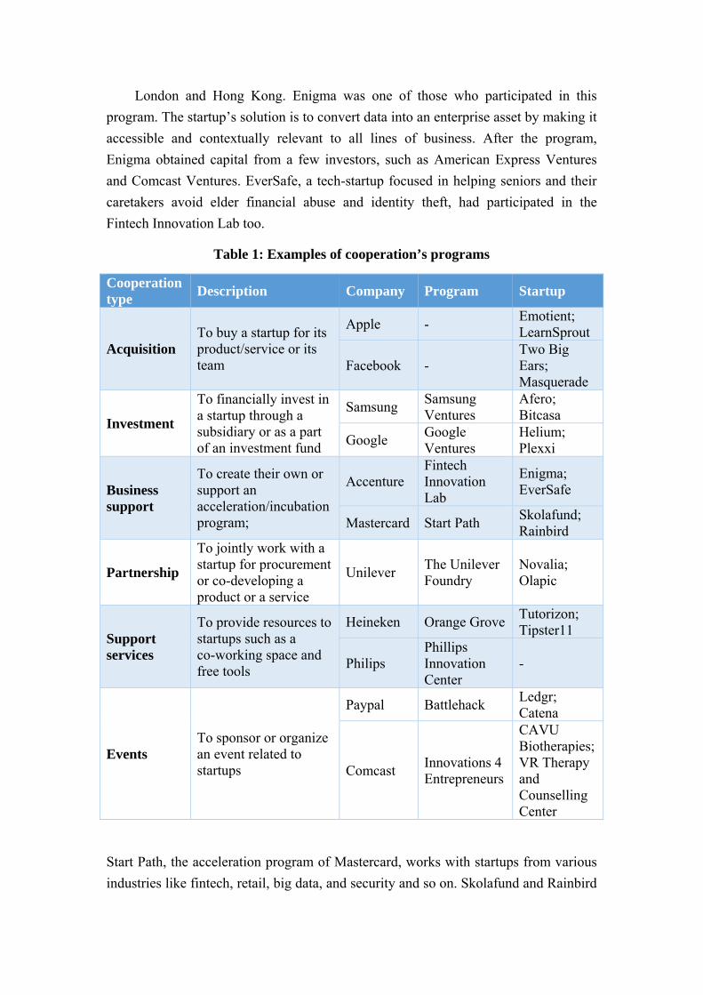
London and Hong Kong. Enigma was one of those who participated in this

program. The startup’s solution is to convert data into an enterprise asset by making it

accessible and contextually relevant to all lines of business. After the program,

Enigma obtained capital from a few investors, such as American Express Ventures

and Comcast Ventures. EverSafe, a tech-startup focused in helping seniors and their

caretakers avoid elder financial abuse and identity theft, had participated in the

Fintech Innovation Lab too.

Table 1: Examples of cooperation’s programs

Cooperation type

Description Company Program Startup

Acquisition To buy a startup for its product/service or its team

Apple - Emotient; LearnSprout

Facebook - Two Big Ears; Masquerade

Investment

To financially invest in a startup through a subsidiary or as a part of an investment fund

Samsung Samsung Ventures

Afero; Bitcasa

Google Google Ventures

Helium; Plexxi

Business support

To create their own or support an acceleration/incubation program;

Accenture Fintech Innovation Lab

Enigma; EverSafe

Mastercard Start Path Skolafund; Rainbird

Partnership

To jointly work with a startup for procurement or co-developing a product or a service

Unilever The Unilever Foundry

Novalia; Olapic

Support services

To provide resources to startups such as a co-working space and free tools

Heineken Orange Grove Tutorizon; Tipster11

Philips Phillips Innovation Center

-

Events To sponsor or organize an event related to startups

Paypal Battlehack Ledgr; Catena

Comcast Innovations 4 Entrepreneurs

CAVU Biotherapies; VR Therapy and Counselling Center

Start Path, the acceleration program of Mastercard, works with startups from various

industries like fintech, retail, big data, and security and so on. Skolafund and Rainbird

 

are tow startups that went through the accelerator: Skolafund is a web platform that

enables less-privileged undergraduates to crowdfund their scholarships from the

public, corporations and philanthropic organisations and Rainbird enables people to

take human and business knowledge and combine it with data to automate knowledge

work and deliver consultative systems.

As it was stated previously, Unilever has a partnership program with startups in order

to both parts jointly work to resolve business problems existing in Unilever’s brands.

Novalia, a U.K.-based technology startup that combines conductive print and

capacitive touch to create surfaces that act as sensors and speakers helped Knorr to

engage more interactively with its customers, bringing the retail store environment

alive. In its turn, Magnum was able to source user generated content from the Internet

and utilize it in their campaign through a partnership with Olapic, a startup that

aggregates images submitted by users on various social media channels and uses a

curation algorithm and human editors to identify which images are best suited to

specific use-cases for each brand.

There are companies that offer internal resources and services to startups. An example

of that is Heineken. Among with Netherlands Embassy in Athens, corporate sponsors,

charity foundations and universities, they have set a flexible space for young

entrepreneurs called Orange Grove. Besides the working space, they also offer others

services that include seminars, workshops, mentoring and legal and accounting

services. Tutorizon and Tipster11 are startups that had been through Orange Grove.

Tutorizon is a platform that connects students with tutors or private schools for

physical or online high school courses, foreign languages courses and university

courses. Regarding to Tipster11, it is an online game about sport predictions where

players can register for free and win prizes. Philips also engage with startups with

Philips Innovation Services by providing them consultancy resources such as medical

devices & equipment, manufacturing processes & systems, environment & safety, etc.

Finally, there also companies that organize events related to startup competitions or

hackathons. Paypal is one example of those companies. They organize the BattleHack,

a series of global hackathon contests where competitors are required to solve a local

problem by coding. In 2014, in San-Francisco, the winner was Ledgr, a mobile

application to help people keep track of things they lend out to family, friends or

strangers. In the same years, in Warsaw, the contest was won by Catena, a hardware

solution that creates an open trusted network marketplace for listing, discovering and

sharing electrical devices.

Innovations 4 Entrepreneurs is a startup competition event set by Comcast. The

startups CAVU Biotherapies and VR Therapy and Counselling Center participated in

 

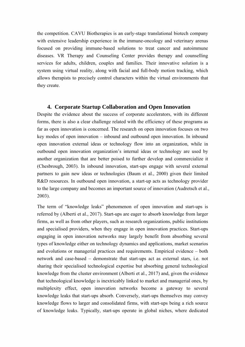
the competition. CAVU Biotherapies is an early-stage translational biotech company

with extensive leadership experience in the immune-oncology and veterinary arenas

focused on providing immune-based solutions to treat cancer and autoimmune

diseases. VR Therapy and Counseling Center provides therapy and counselling

services for adults, children, couples and families. Their innovative solution is a

system using virtual reality, along with facial and full-body motion tracking, which

allows therapists to precisely control characters within the virtual environments that

they create.

4. Corporate Startup Collaboration and Open Innovation Despite the evidence about the success of corporate accelerators, with its different

forms, there is also a clear challenge related with the efficiency of these programs as

far as open innovation is concerned. The research on open innovation focuses on two

key modes of open innovation – inbound and outbound open innovation. In inbound

open innovation external ideas or technology flow into an organization, while in

outbound open innovation organization’s internal ideas or technology are used by

another organization that are better poised to further develop and commercialize it

(Chesbrough, 2003). In inbound innovation, start-ups engage with several external

partners to gain new ideas or technologies (Baum et al., 2000) given their limited

R&D resources. In outbound open innovation, a start-up acts as technology provider

to the large company and becomes an important source of innovation (Audretsch et al.,

2003).

The term of “knowledge leaks” phenomenon of open innovation and start-ups is

referred by (Alberti et al., 2017). Start-ups are eager to absorb knowledge from larger

firms, as well as from other players, such as research organizations, public institutions

and specialised providers, when they engage in open innovation practices. Start-ups

engaging in open innovation networks may largely benefit from absorbing several

types of knowledge either on technology dynamics and applications, market scenarios

and evolutions or managerial practices and requirements. Empirical evidence – both

network and case-based – demonstrate that start-ups act as external stars, i.e. not

sharing their specialised technological expertise but absorbing general technological

knowledge from the cluster environment (Alberti et al., 2017) and, given the evidence

that technological knowledge is inextricably linked to market and managerial ones, by

multiplexity effect, open innovation networks become a gateway to several

knowledge leaks that start-ups absorb. Conversely, start-ups themselves may convey

knowledge flows to larger and consolidated firms, with start-ups being a rich source

of knowledge leaks. Typically, start-ups operate in global niches, where dedicated

 

technological knowledge is inextricably linked to a certain kind of market knowledge.

Given their immaturity in managerial processes and open innovation practices and

their eagerness in collaborating with key players in the field, for innovation-specific

matters, they might pay less attention in engaging in open innovation networks and

succumb to knowledge leaks to the benefit of their partners who can access through

them particular knowledge. Knowledge spill-overs have been studied in relation to

their geographical stickiness and as an important mechanism for growth (Krugman,

1991). Literature has over-stressed their positive role as externalities in innovation

generation and cluster scholars (e.g. Porter, 1990) have remarked how knowledge

spill-overs in specialized, geographically concentrated industries stimulate growth.

According to (Alberti et al. 2017), knowledge leaks shed new light even on the

literature on spill-overs, stressing the involuntary and unconscious side of knowledge

exchange as well as focussing on the micro-level of knowledge networking instead of

on the macro regional/cluster externalities.

5. Case Studies To understand the efficiency issues of open innovation between corporates and

startups, 6 case studies were developed. Apart from being some of the most

well-known brands nationally and internationally, Brisa Innovation, Repsol,

Corticeira Amorim, Vodafone, Portugal Telecom and Fidelidade have been engaging

with startups for a while. All of this have been setting programs with startups in

Portugal except Repsol that have their Repsol Energy Ventures program set in Spain.

Detailed description of each case studyt can be found in (Mealha, 2017). In this paper

we will describe the main results regarding some of the open innovation issues

between corporates and startups.

Table 2: The objectives in working with startups and what can these add to the

organization

Corporates The objectives in working with startups and what can these add

to the organization

Brisa Innovation

Expertise in several areas that the company unknowns. The

objectives are essentially to solves business problems, to rejuvenate

corporate culture and expand into new markets

Repsol

Flexibility, speed, a different approach to the market and a very

straightforward way of working. Objective: to expand into new

markets

 

Corporates The objectives in working with startups and what can these add

to the organization

Corticeira AmorimBring fresh ideas, new distribution channels and new business

models. The main objective of ACV is to enter in new markets

Vodafone Access to cutting-edge technologies before competition. Objectives:

innovate the brand and enter in new markets

Portugal Telecom

Reduction of the product development time. The aim of Blue Start

is to expand into new markets by creating new products and

services

Fidelidade Disruptive solutions. Objectives of Protechting: empower the

connection with startups and foster innovative solutions

Table 2 summarizes what startups bring to inside the organizations (from the

corporates point of view): expertise, flexibility, speed, new work methodologies, fresh

ideas, new distribution channels, new business models and new technologies. Among

others, all corporates share the same objectives by collaborating with startups: to

expand into new markets.

Table 3: The changes that happened inside the organization to collaborate with

startups

Corporates The changes that happened inside the organization to

collaborate with startups

Brisa Innovation

Since it is a subsidiary with innovation as the main focus, the

corporate’s employees are aware of the importance of innovate with

startups

Repsol The creation of the New Energy Business Unit

Corticeira AmorimChanges inside the organization: the involvement of the others

business units and openness to take risks

Vodafone Aware of the importance of innovation inside the organization

Portugal Telecom Alignment and aware the corporate’s business units

Fidelidade The establishment of the Innovation area.

Table 3 address what changes have occurred in corporation to collaborate with

startups. Besides align and aware the several departments of the organization, others

companies have chosen to create their own business units (Repsol and Fidelidade).

 

Table 4 describe the type collaboration type. Partnership and an acceleration program

are the most frequent type of program of the corporates interviewed to engage with

startups.

Table 5 summarizes the main difficulties while working with startups are the sensible

question of the intellectual property, expectations incompatibility, values mismatch

and a wrong perception they have of the corporate they look to work with. The most

important things for a startup are the team, how the idea is implemented and their

resilience.

Table 4: The type of collaboration programs established

Corporates The type of collaboration programs established

Brisa Innovation Partnership program

Repsol Repsol Energy Ventures- Investment

Corticeira Amorim Accelerator, Investment, Partnership and Support Services

Vodafone Vodafone Power Lab- Accelerator

Portugal Telecom Blue Start- Partnership program

Fidelidade Protechting- Accelerator

Table 5: The main difficulties in working with startups and the most critical

aspect for a startup

Corporates The main difficulties in working with startups and the most

critical aspect for a startup

Brisa Innovation Intellectual property

Repsol The startup’s team is the most critical aspect

Corticeira Amorim Expectations incompatibility or values mismatch

Vodafone How the idea is implemented and their resilience

Portugal Telecom Certain startups have a wrong perception of the corporate’s reality

and have a weak team

Fidelidade The most important thing for a startup is its team

These case studies demonstrate also two important dimensions. Firstly, corporate

acceleration programs play today a major role for companies (open) innovation, and it

acts both ways (inboud and outbound). Secondly, although ‘knowledge leaks’ are a

relevant process in the open innovation, it tends to be informal, unstructured and

 

cautious, and this may be the cause for the low effectiveness in term of results and

outcomes from these corporate startup accelerators, i.e. the low number of economical

relevant outputs for the high number of initiatives, people and startups involved.

Another very important result that emerged from the analysis of the case studies is

about how to make the ‘knowledge leaks’, more formal, more structured and more

deliberate with the goal to increase the effectiveness of corporate open innovation

programs. It has emerged that it could be possible to achieve this by extending its

nature from the corporation to a community and by fostering deliberate knowledge

leaks between the different parties involved – corporations, suppliers, startups,

universities, etc. Through community entrepreneurial acceleration programs.

We will designate this purposeful, more formal, more structured and more deliberate

knowledge leaks as ‘Knowledge Effusion’. In thermodynamics, ‘Effusion’ is the

process in which a gas escapes through a hole of diameter considerably smaller than

the mean free path of the molecules, whereas ‘Diffusion’ occurs through an opening

in which multiple particles can flow through simultaneously. From empirical evidence

from the case studies, we conclude that in open innovation processes corporate startup

collaboration programs, knowledge does not flow in diffusion mode, and rather in

effusion mode. Hence, we propose a novel concept of ‘Community Entrepreneurial

Acceleration Programs” that differ quite significantly from traditional corporate

acceleration programs, as its focus will be on inbound and outbound open innovation

for ‘knowledge effusion’ for a multitude of stakeholders. The engaged stakeholders

shall be of different nature: corporates, their suppliers, entrepreneurs, early stage and

scale ups, universities (education and research centres), investors, and other entities.

In the foreseen community acceleration program, each party will share their

knowledge about the emergent technology readiness, market needs and requirements,

research & development projects, education profiles, recruitment needs, funding

mechanism, etc. However, the acceleration program will push parties for action, and

parties are invited to work with each other on moving forward. For example,

corporations design and plan together with university research centres new research

projects; an early stage startup pivot and change their product / service to

accommodate a corporate market need; etc. This means that the ultimate goal of the

acceleration program is not to have the most promising startups measured in terms of

traction, rather that each stakeholder engaged in the program may have gained

significant ‘knowledge’ and developed action based on acquired knowledge. Key

Performance Indicators to measure success of the acceleration program will not be the

number of startup applications, or raised investment; rather the number of individual

actions with outputs developed by each stakeholder engaged in the acceleration

 

programs, and the total number of joint actions occurred at the end of the duration of

the program.

6. Conclusions Traditional corporate acceleration programs major focus for corporations is to

accelerate pre-seed, and early stage startups with innovative products and services

related with corporates’ core activities and markets. This paper presented a

collaboration framework between corporates and startups, and provided some

examples of its application. The paper also discusses, from an open innovation

perspective, how these collaboration processes are ineffective. We argue about the need

for a set of new mechanisms for fostering more effective open innovation within

sectorial communities of innovation through deliberate ‘Knowledge Effusion’ on

acceleration programs, i.e. creating what we designate as ‘Community Entrepreneurial

Acceleration Programs’. The concept of communities is related with ‘cluster’ or

‘ecosystem’ i.e. it includes an extended domain of action from multiple stakeholders

within an economic activity - corporations, suppliers, distributors, startups, third-party

logistics, universities, investors etc. Further research is needed to this understand, learn

and construct theory on how to make effective Knowledge Effusions on digital

technologies through entrepreneurial acceleration programs within sectorial

communities of companies.

References

Abreu, M., Grilo, A., Zutshi, A (2017). A Comparison between Nordic and

Mediterranean Start Up Ecosystems: Economic Sectors, Business and Pricing, Models.

In Proceedings of the 7th IEOM Morocco Conference, Rabat, Morocco, 10-13 April,

2017

Accenture. (2015). Harnessing the Power of Entrepreneurs to Open Innovation, 1–7.

https://www.accenture.com/us-en/~/media/Accenture/next-gen/B20/Accenture-G20-

YEA-2015-Open-Innovation-Executive-Summary.pdf. Accessed 23rd May 2017

Alberti, F. and Pizzurno, E. (2017). Oops, I did it again! Knowledge leaks in open

innovation networks with start-ups. European Journal of Innovation Management, Vol.

20 Iss 1 pp. 50 – 79

Audretsch, D.B. and Feldmann, M.P. (2003), “Knowledge spillovers and the

geography of innovation”, in Henderson, J.V. and Thisse, J. (Eds), Handbook of

 

Urban and Regional Economics, Vol. 4, North Holland Publishing, Amsterdam, pp.

2713-2739.

Baum, J.A.C., Calabrese, T. and Silverman, B.S. (2000), “Don’t go it alone: alliance

network composition and startups’ performance in Canadian biotechnology”,

Strategic Management Journal, Vol. 21 No. 3, pp. 267-294.

Bonzom, A. and Netessine, S. (2016). How do the world’s biggest companies Deal

with the Startup Revolution, INSEAD and 500 Corporations,

Carvalho, A, Grilo, A., Zutshi, A (2017). Accelerators Envision the Future. In

Proceedings of the 7th IEOM Morocco Conference, Rabat, Morocco, 10-13 April

Chang, C. (2013). Portfolio Company Selection Criteria: Accelerators vs Venture

Capitalists. Retrieved from http://scholarship.claremont.edu/cmc_theses/566/

Chesbrough, H.W. (2003), “The era of open innovation”, Sloan Management Review,

Vol. 44 No. 3, pp. 35-41.

Clarysse, B., Wright, M., & Hove, J. Van. (2015). A Look Inside Accelerators -

Building Businesses. Nesta, (February), 24.

Cohen, S., & Hochberg, Y. V. (2014). Accelerating Startups: The Seed Accelerator

Phenomenon. SSRN Electronic Journal, 1 – 16. http://doi.org/10.2139/ssrn.2418000

Krugman, P. (1991), Geography and Trade, MIT Press, Cambridge, MA.

Mealha, T. (2017). Corporate-Startup Collaborations. MSc Dissertation of Faculdade

de Ciências e Tecnologia da Universidade Nova de Lisboa

Porter, M.E. (1990), The Competitive Advantage of Nations, Free Press, New York,

NY.

Turiera, T., & Cros, S. (2013). Co-Business: 50 Examples of Business Collaboration.

Retrieved from

https://docs.google.com/viewerng/viewer?url=http://www.co-society.com/wp-content

/uploads/CO_business_2013.pdf, Accessed 23rd May 2017

   

 

ICESI_0163

Evaluating Triaxial Accelerometers and Force Sensitive Resistors in Building Interactive Freestanding Bags

Pawut Satitsuksanoh, Assumption University, Thailand

*Chayapol Moemeng, Assumption University, Thailand

Se Won Kim, Assumption University, ThailandAbstract

*Corresponding Author

Abstract

In martial arts, punching bags are important equip- ment used for training purposes. Widespread availability of small cheap micro-controllers and various types of sensors makes it possible to build an economical interactive punching bag. In this work, we evaluate the feasibility and the effectiveness of using commonly available COTS triaxial accelerometers and force sensitive resistors in building a cost-effective interactive punching bag. We present a mechanism to transform real time sensor data into a calibration model that can be used to optimize the level of correlation between the accelerometer and the force sensitive resistors. The results show that the accelerometers can detect the impact of punches as well as the force sensitive resistors do while offering the ground for building a model for categorizing different types of punches using the sensor outputs of the three axes. Therefore, a single triaxial accelerometer sensor module has the potential to reduce the necessity for multiple impact based sensors when building an interactive punching bag leading to simplification in the physical design and reduction in the materials cost. We also show that there are opportunities for improving the accuracy in detecting the levels of impacts and types of punches by means of a calibrated model of filtering noisy sensor data.

Keywords: Microcontroller, Triaxial accelerometer, Force sensitive resistance, Sensors.

 

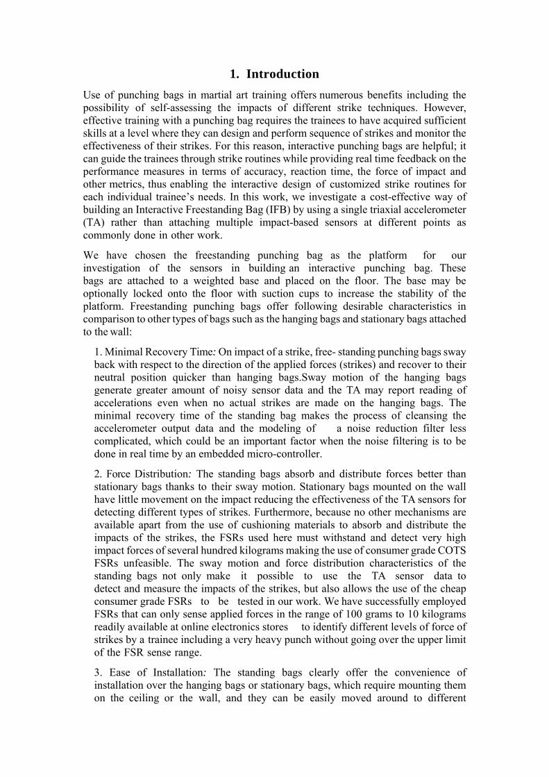
1. Introduction

Use of punching bags in martial art training offers numerous benefits including the possibility of self-assessing the impacts of different strike techniques. However, effective training with a punching bag requires the trainees to have acquired sufficient skills at a level where they can design and perform sequence of strikes and monitor the effectiveness of their strikes. For this reason, interactive punching bags are helpful; it can guide the trainees through strike routines while providing real time feedback on the performance measures in terms of accuracy, reaction time, the force of impact and other metrics, thus enabling the interactive design of customized strike routines for each individual trainee’s needs. In this work, we investigate a cost-effective way of building an Interactive Freestanding Bag (IFB) by using a single triaxial accelerometer (TA) rather than attaching multiple impact-based sensors at different points as commonly done in other work.

We have chosen the freestanding punching bag as the platform for our investigation of the sensors in building an interactive punching bag. These bags are attached to a weighted base and placed on the floor. The base may be optionally locked onto the floor with suction cups to increase the stability of the platform. Freestanding punching bags offer following desirable characteristics in comparison to other types of bags such as the hanging bags and stationary bags attached to the wall:

1. Minimal Recovery Time: On impact of a strike, free- standing punching bags sway back with respect to the direction of the applied forces (strikes) and recover to their neutral position quicker than hanging bags.Sway motion of the hanging bags generate greater amount of noisy sensor data and the TA may report reading of accelerations even when no actual strikes are made on the hanging bags. The minimal recovery time of the standing bag makes the process of cleansing the accelerometer output data and the modeling of a noise reduction filter less complicated, which could be an important factor when the noise filtering is to be done in real time by an embedded micro-controller.

2. Force Distribution: The standing bags absorb and distribute forces better than stationary bags thanks to their sway motion. Stationary bags mounted on the wall have little movement on the impact reducing the effectiveness of the TA sensors for detecting different types of strikes. Furthermore, because no other mechanisms are available apart from the use of cushioning materials to absorb and distribute the impacts of the strikes, the FSRs used here must withstand and detect very high impact forces of several hundred kilograms making the use of consumer grade COTS FSRs unfeasible. The sway motion and force distribution characteristics of the standing bags not only make it possible to use the TA sensor data to detect and measure the impacts of the strikes, but also allows the use of the cheap consumer grade FSRs to be tested in our work. We have successfully employed FSRs that can only sense applied forces in the range of 100 grams to 10 kilograms readily available at online electronics stores to identify different levels of force of strikes by a trainee including a very heavy punch without going over the upper limit of the FSR sense range.

3. Ease of Installation: The standing bags clearly offer the convenience of installation over the hanging bags or stationary bags, which require mounting them on the ceiling or the wall, and they can be easily moved around to different

 

locations. The ease of installation and relocation offered by the standing bags not only make it convenient for us to set up a design prototype for testing purposes, but also increases the usability of such interactive punching bags by the end users at home and in the gyms.

Related work

Micro controllers and embedded sensors have been widely adapted in sports in various forms such as wearable devices to help design training routines and measure vital statistics. Two major types of sensors used in these applications are motion-based sensors such as accelerometers and impact- based sensors like force sensitive resistors.

The effectiveness of the TA sensors in tracking activities are well documented in [1],

[2], and [3]. Data from the body- worn TA sensors are used in designated mathematical

models to identify the types of movement, such as walking, running, and staying still. TA sensors also have been used in training of martial arts as shown in [4], [5]. On the other hand, there are research work that demonstrate the use of impact-based sensors in martial arts training [6], [7], and [8]. Multiple body- worn sensors detect the impact of strikes on various places on the body of a trainee. Our focus is on creating an effective interactive training device that does not require the trainees to wear any extra gears in order to give the trainees of martial arts total freedom of movement.

A survey of research work on building interactive punching bags can be found from the Gamification in Sport resource collection (http://portal.scitech.au.edu/chayapol/index.php/gamification-in-sport/).

2. Methods

Our prototype platform for evaluating the effectiveness of the TA sensor and the FSR sensors in building an IFB consists of 9 FSR sensors and a TA sensor attached on a freestanding punching bag. The TA sensor is mounted on the top of the punching bag to detect the movement of the punching bag and record the real time changes in accelerations along the three axes. The FSR sensors are mounted at 3 heights: high, medium, and low. High ones detect face strikes (such as punches, head kicks, etc.), medium ones are for body strikes (such as body rips, knees, etc), and low ones are for leg strikes (mostly leg kicks). Figure 1 illustrates the configuration of our prototype IFB showing the positions of different sensors. Each height level employees 3 FSRs in order to identify the different angles of strikes. (see figure 2). Fh is the force / strike applied to a high level, Fm for medium, and Fl for low level.

 

Figure 1: The side view of an IFB with a weighted base.

Figure 2: Top view, angle of strikes

An Arduino module is used to read the real time sensor.

Data of the FSRs and the TA and transfer the data to a PC for analysis and processing. The sensors generate analog outputs as variations in voltage in response to the changes in the pressure applied in the case of the FSR and the changes in the accelerations in 3 axes in the case of the TA. These analog outputs from the sensors are input to the Arduino’s analog pins and are transformed into 10 bit resolution data ranging in values from 0 to 1023 by the Arduino’s internal ADC and the normalized sensor data are transferred to the PC from the Arduino via a serial communication. The capturing and the transfer of the real time sensor data are performed every 6 milliseconds. At each sampling point, following four different sets of data samples are recorded: the number of milliseconds since the start of a data sampling session, normalized sensor data output from the FSRs, normalized sensor data output on the X-axis, Y-axis and Z-axis of the TA.

For each data sampling session, a trainee was instructed to strike the IFB at various positions with different levels of forces. The following discussion is based on our analysis of the normalized data output from the TA and one FSR sensor.

 

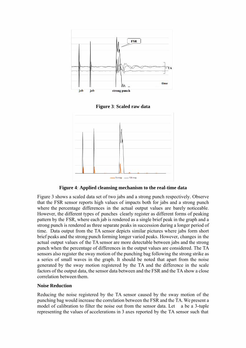
Figure 3: Scaled raw data

Figure 4: Applied cleansing mechanism to the real-time data

Figure 3 shows a scaled data set of two jabs and a strong punch respectively. Observe that the FSR sensor reports high values of impacts both for jabs and a strong punch where the percentage differences in the actual output values are barely noticeable. However, the different types of punches clearly register as different forms of peaking pattern by the FSR, where each jab is rendered as a single brief peak in the graph and a strong punch is rendered as three separate peaks in succession during a longer period of time. Data output from the TA sensor depicts similar pictures where jabs form short brief peaks and the strong punch forming longer varied peaks. However, changes in the actual output values of the TA sensor are more detectable between jabs and the strong punch when the percentage of differences in the output values are considered. The TA sensors also register the sway motion of the punching bag following the strong strike as a series of small waves in the graph. It should be noted that apart from the noise generated by the sway motion registered by the TA and the difference in the scale factors of the output data, the sensor data between and the FSR and the TA show a close correlation between them.

Noise Reduction

Reducing the noise registered by the TA sensor caused by the sway motion of the punching bag would increase the correlation between the FSR and the TA. We present a model of calibration to filter the noise out from the sensor data. Let a be a 3-tuple representing the values of accelerations in 3 axes reported by the TA sensor such that

 

, and --x be the data series of maximum values of TA’s x, y and z axes thus

The noise reduction function is defined as follow.

Where α is an arbitrary threshold which reduce the distance between neutral and peak data.

In order to reduce the peak in FSR, let v be a data output value reported by the activated FSR and subtract it with an arbitrary threshold β, such that

Thresholds α and β vary on the physical properties of the freestanding bag and sensitivity of the sensors. Therefore, optimizing these two variables results in higher correlation r between the TA and the FSR. A gradient descend search was performed to identify appropriate values of α and β.

3. Result and Discussion

In this work, we set α and β to 350 and 900 respectively to obtain the optimal correlation r. Figure 4 shows the noise- reduced data. Observe that the series of minor post waves that followed a strong punch have been cleansed. The correlation between the TA and the FSR before noise reduction is 58.04%, and the correlation after noise reduction is 84.98%, improved by 26.94%.

From the result, we can observe that the TA can be used to detect the strike as well as FSR does. However, the thresholds are an important factor in calibrating the precision in using the TA to detect strikes. If the manufacturing process of the punching bags can ensure a common standard for the physical properties the manufactured punching bags, the calibrated thresholds are expected to be applicable to all bags of the same range. However, there are factors to be concerned for an actual production. Incorporating both FSR and TA can help in improving the accuracy of the strike detection, especially when the interactive system guides the trainees to strike at a particular point and expects the strike at the indicated point.

1) The recoil mechanism of the standing bag affects the sway motion. In our setting, we use a hard spring coil which sway back quickly. Weighted-base freestanding bags sway bag slowly causing less noisy waves in the data; unfortunately, they do not always sway back to its original neutral position, which could affect the effectiveness of the calibrated value of α.

 

2) Resonance due to rapid strikes confuses the calculation as it cannot distinguish between noise and genuine rapid strikes.

Despite its capability to directly report different levels of force of impacts, the FSR is also prune to error due to various reasons including the followings:

1) When a strike does not land directly on a sensor, the sensor may fail to report any value at all or the value reported may just indicate a trigger not the actual force of impact.

2) The actual values reported by the FSR depends a lot on the cushioning materials and mechanism used to attach the sensors to the punching bag. How the physical configuration of the set up affects the data output by the FSR sensors are one of our future research directions.

4. Conclusion and Future Work

We have evaluated the use of a single TA sensors to detect different types of strikes and different levels of force of strikes on a freestanding punching bag as an alternative to using multiple FSR sensors as means of simplifying the physical design of an interactive punching bag and reducing the materials costs. We have highlighted the importance of a systematic calibration of sensor data output based on the physical setup of a particular punching bag configuration and have presented a model of calibration by means of filtering noisy data out of raw sensor data output, that can increase the correlation between the TA sensor and the FSR sensors. Fortunately, the calibrated variables in our model are very likely to be reusable for the punching bags sharing the similar physical configurations. This work also has provided strong evidence that a single TA sensor module may be used in building an interactive punching bag system as an alternative to utilizing multiple impact-based sensor giving rise to the simplification in the physical design and reduction in the materials costs.

However, there are challenges to be tackled in future research before a fully featured interactive punching bag utilizing only a single TA sensor module can be implemented. Although there is a high correlation between the output of the TA sensor and the FSR sensors, detecting precise location and the different levels of force of strikes on the punching bag based on the output of a single TA sensor module is unresolved. Furthermore, it’s not clear yet how to distinguish the sway motion caused by quick succession of multiple weak punches and the one that follows a strong punch.

References

N. Kern, B. Schiele, and A. Schmidt, “Multi-sensor activity context detection for wearable computing,” Ambient Intelligence, PP. PP 220–232, 2003.

L. Bao and S. S. Intille, “Activity recognition from user annotated acceleration data pervasive computing,” Pervasive Computing, VOL. 3001, PP. 1–17, 2004.

A. Bonomi, A. Goris, B. Yin, and K. Westerterp, “Detection of type, Duration, and intensity of physical activity using an accelerometer,” Med Sci Sports Exerc, 2009.

C. V. Bouten, K. R. Westerterp, M. Verduin, and J. D. Janssen, “Assessment of energy

 

expenditure for physical activity using a triaxial accelerometer.” Medicine & Science in Sports & Exercise, VOL. 26, NO. 12, PP. 1516–1523, 1994.

E. A. Heinz, K. S. Kunze, M. Gruber, D. Bannach, and P. Lukowicz, “Using wearable sensors for real-time recognition tasks in games of martial arts – an initial experiment,” in Proceedings of the 2006 IEEE Symposium on Computational Intelligence and Games, CIG’06. IEEE, MAY 2007, PP. 98–102.

E. H. Chi, J. Song, and G. Corbin, “"killer app" of wearablecomputing: wireless force sensing

body protectors for martial arts.” in Proceedings of the 17th annual ACM symposium on User

interface software and technology - UIST ’04, 2004, PP. 277– 285.

D. Giovanelli and E. Farella, “force sensing resistor and evaluation of technology for wearable body pressure sensing,” Journal of Sensors, VOL. 2016, PP. 1–13, 2016.

C. Falco, O. Alvarez, I. Castillo, I. Estevan, J. Martos, F. Mugarra, and A. Iradi, “Influence of the distance in a roundhouse kick’s execution time and impact force in teakwondo,” Journal of Biomechanics, VOL. 42, NO. 3, PP. 242–248, 2009.

   

 

ICESI_0165

The Feasibility of Deploying Robotic Waiters in the Service Industry

*Michael Lau, Newcastle University International Singapore, Singapore

Edwin Foo, Nanyang Polytechnic, Singapore

Aaron Cheong, Newcastle University International Sinagpore, Singapore

Seet Gl, Nanyang Technological University, Singapore

*Corresponding Author

Abstract

In paper, we present the design of a waiter robotic system for the service industry – the food outlets or restaurants. For such applications, we have considered and proposed a suitable mechanical and system design commensurate with the users’ requirements of cost and functionality. The engineering involved the robot design and eco-system. The tray conveying omni-directional robot is adjustable for different table heights and has a 3-tiered dumb-waiter for 3 trays. It is autonomous and it navigates using a map of the outlet. It is able to reach to within a 1 m of the target table and avoiding both mapped and unmapped obstacles. To supporting eco-system, we have worked on a docking system to ensure that diners get their food and return the trays easily and have designed a central computer system that will have the capability to interface with business system.

Positioning the robot to with 1 m accuracy requires a docking system to navigate the robot closer to various types of tables or furniture used in any outlet. This part requires fine tuning. Robustness is important and challenging to achieve. The interface with the owner’s business computer is business sensitive but is useful especially with the advent of NFC RFID and various type mobile apps. The growth opportunity for waiter robotic system is in this area as well.

Keywords: Design and applications, Autonomous omni-directional robot, Waiter robotic eco-system.

 

1. Introduction Service Jobs are next to go? There is an increase in the number of robots deployed in the service industry. The reasons often cited are the high cost of hiring and the difficulty in retaining workers in the industry. In some cases, the workers are elderly people who may find difficulty in coping with the demands of the tasks at hand, and robots assistance has been introduced. So complex to simple delivery robots can be found – Figure 1 (web pages)

Figure 1:

(a) Asimo in Henna-na Hotel (b) Savioke Relay Delivery robot (c) Keenon Robot

In Singapore, a seafood restaurant (Ang B, 2016) has deployed robots similar to that shown in Figure 2c. Each robot is reported to cost about $17,000, which is half of a human waiter's annual salary. One of the reasons is to enhance diners’ (especially those with children) experience rather than replacing waiters. Hotels (Lin M, 2016) are also introducing delivery and bell-boy robots that can cost about $100,000 each. The Singapore government is actively promoting service robots even for more basic tasks like free roaming tray collection robots in eateries and food courts (Figure 2a, Felicia Choo, 2017). Local companies like Techmetics (Figure 2c) and AiTech Robotics and Automation (Figure 2b, Atiyyah Mohd Said, 2017) have developed mobile robots for delivery of snacks, toiletries, and light refreshments.

Figure 2:

(a) A tray collecting robot (b) Aitech delivery robot (c) Techmetics delivery robot

In this paper, we will address some issues in the design of a waiter robotic system for the service industry, in particular for the food & beverage industry. Like a community of humans with different skills, robots can be intelligent, dexterous or can be basic but capable of doing the work intended. There is a similar in division of labour – robots with different capabilities. This is advantageous in environment where human labour is scarce, but humans, being versatile and adaptable, can better concentrate on jobs that required reasoning and dexterity. The robotic system has to be designed for the

 

work environment, for the tasks, at the appropriate cost and bring a different dining experience initially.

2. System Description The Robot

Typically, F&B outlets are quite tight in space. Robots with “hands” can take up space and delay operations. Hence a basic tray conveying robot with mecanum wheels are suitable for such environment.

Figure 3:

(a) The Beta-G waiter robot (b) the base of Beta-G and the mecanum wheels configuration

Beta-G (Figure 3a) was designed in 2 parts: the torso contains a three tier dumb-water to deliver trays of food and to allow for their collection. A draw bridge door and a roller belt system allow individual trays in each of the tier to be delivered or to be collected. The torso is mounted on a scissor table to vary the height of the draw bridge so that the robot can be used in different outlets. The base contains the power, the drives and the electronics. Motion control is based on a simple model (Figure 3b) and is given below.

The Mathematical Model

Consider one of the wheels. The wheel velocity is r , r is the radius of the wheel and is the wheel angular speed. The roller (shown in contact with the ground) velocity is

rrr where rr is the radius of the roller and r is the angular velocity of the roller. The robot velocity in the XR, YR and ZR axis (out of plane) directions can be represented by the vector Vp. For a wheel located at position A,

jikjikVV yxPA sincos llvvPA (1)

A kinematic constraint equation for the robot for this wheel can be written as:

VA·a = r cos  (2)

a is the unit vector along the roller spin axis as shown in the figure. Combining (1)

and (2) for each of the four wheels results in

 

(3)

With = /4 and since sin(/4) = cos(/4),

(4)

The input commands are the forward speed v at angle to XR and a change of

orientation given by the angular speed .

Writing , we can program the robot motion as:

(5)

If there is no need to change orientation, V = 0. Sideway motion is given by Vdc = Vds

with = 0. Inverse kinematics can easily be obtained as

(6)

The Navigation Sensors Suite

The robot has to navigate in tight space from point A to point B, avoiding furniture and humans along the way. It must have the means to know where it is. Knowing its location requires sensors. Each of the 4 motors has an attached encoder. A routine in the embedded controller reads the four values of i and the main computer uses equations (6) to provide an estimate of the robot’s pose. However, odometry for mecanum wheeled based robot can have accumulated errors due to the wheels slippage and are not used for mapping.

To estimate the orientation/heading of the robot, an off the shelf 9DOF IMU (Razor) is used. It has three sensors, an ITG-3200 (triple-axis gyro), ADXL345 (triple-axis accelerometer), and HMC58883L (triple-axis magnetometer). The Attitude Heading Reporting System (AHRS) routine on the IMU fuses data from the three sensors to provide an estimate of the robot heading/orientation. However, the digital compass of the IMU must be calibrated in the area where it is deployed to account for the

yx llrr

v

4cos

21

yx llrr

v

4sin

22

yx llrr

v

4cos

23

yx llrr

v

4sin

24

 

4

3

2

1

cossin

cos

cossinsincos

cossinsincos

cossinsincos

cossinsincos

rv

v

ll

ll

ll

ll

yx

yx

yx

yx 

yx llr

V

vr

V

vr

V

ds

dc

4sin2

4cos2

VV

VV

VV

VV

ds

dc

ds

dc

4

3

2

1

44321 rvx 44321 rv y yx llr 44321

 

presence of any significant iron in the environment, which can change the magnetic field orientation around the sensor and cause the AHRS to give a wrong heading. It can be challenging if the robot were to operate from an area with no significant presence of iron to one where there is. Some amount of planning must be done to decide when to ignore the AHRS readings.

Two LiDARs are mounted on the front and rear to provide for, localization, navigation and for obstacle avoidance. Ultra-sound and bumpers are installed at the bottom for both obstacles avoidance and safety reasons.

3. The Waiter Robot Systems Mapping the Environment or the Area of Operations

For all the numerous research on intelligent autonomous robots, it remains a difficult problem for robots to replace much of the human work in a real world environment of a restaurant. A viable approach is the integration of an autonomous robots and the appropriate environment. The term System in this paper will mean the physical robot, the eco-system and the development system that can be used for improvements and trouble shooting.

One approach is to use the robot to make a map of the area using SLAM (simultaneous localization and mapping). The robot can be navigated within the area by remote control or by its own. Once the map is available, it can be loaded to other robots. Alternatively, an efficient and quick way is to use HECTOR SLAM ((Kohlbrecher et al., 2013) developed for search and rescue robots.

A portable map (Figure 4a) maker comprises a Raspberry Pi installed with the HECTOR SLAM and connected to a 360° LiDAR. The algorithm does not require odometry and map produced very often resulted in a closed map – a map that does not closed around itself is considered inaccurate.

The stray lines produced (Figure 4b) are a result of reflective surfaces. To be useful for localizing the robot, the map has to be edited (Figure 4c) and stored in a suitable format. Unlike movements using behaviour based reaction to obstacles used by some vacuum cleaning robots, path planning using a map allows for planning ahead. Algorithms like A* (Harika Reddy 2013) and D* are available online. For rapid development of the robot navigation, the open source Robotics Operating Systems (ROS) was used. The ROS is installed in the robot NUC computer. Communications with a central computer is possible.

Figure 4

(a) Portable map maker (b) Map of the lift lobby. (c) An Edited map in ROS

 

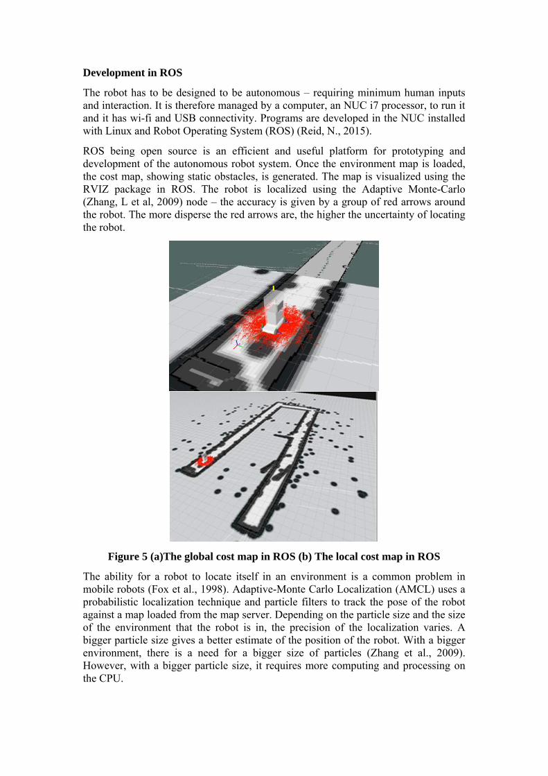
Development in ROS

The robot has to be designed to be autonomous – requiring minimum human inputs and interaction. It is therefore managed by a computer, an NUC i7 processor, to run it and it has wi-fi and USB connectivity. Programs are developed in the NUC installed with Linux and Robot Operating System (ROS) (Reid, N., 2015).

ROS being open source is an efficient and useful platform for prototyping and development of the autonomous robot system. Once the environment map is loaded, the cost map, showing static obstacles, is generated. The map is visualized using the RVIZ package in ROS. The robot is localized using the Adaptive Monte-Carlo (Zhang, L et al, 2009) node – the accuracy is given by a group of red arrows around the robot. The more disperse the red arrows are, the higher the uncertainty of locating the robot.

Figure 5 (a)The global cost map in ROS (b) The local cost map in ROS

The ability for a robot to locate itself in an environment is a common problem in mobile robots (Fox et al., 1998). Adaptive-Monte Carlo Localization (AMCL) uses a probabilistic localization technique and particle filters to track the pose of the robot against a map loaded from the map server. Depending on the particle size and the size of the environment that the robot is in, the precision of the localization varies. A bigger particle size gives a better estimate of the position of the robot. With a bigger environment, there is a need for a bigger size of particles (Zhang et al., 2009). However, with a bigger particle size, it requires more computing and processing on the CPU.

 

Path planning or path finding is done using the A* node (a process that performs computations). With a start and an end point identified, a path can be generated.

The robot control can be interfaced with a central computer that takes order and the diner is issued with a pager. When the food is ready, the pager is activated; it reads the RFID on the table which identifies its location. The robot can then navigate from its current location to the target location.

Testing and Evaluation

The robot navigation has been tested in a simulated environment comprising of a small room, a long corridor and a corridor leading to an open space. Figure 6 (Aaron 2016) shows the test area and the tests are available on video.

Figure 6

(a)Long corridor (b) turning from corridor to open space (c) wide open space

The advantage of using the portable map mapper is that all types of furniture appear as static obstacle and will have “dark space” marked around them in the cost map in ROS. In a dynamic situation where tables are moved about, they will be detected by the on-board lidar and treated as local cost map.

Many tests were done by inserting furniture (that was not present during the map making process) in the robot path and people walking towards the robot. The robot is able to avoid them all the time. The accuracy is such that the robot is able to reach to within 1 m of the target but not necessary always parallel to the target.

However, improvements are still in the work closer: the robot has to get close to about 0.5 m and parallel to the table. A docking algorithm is needed to navigate the robot closer and align it to the table to deliver the food by lowering the draw bridge and roll out a tray. Different methods using lidar lite sensors and pixy camera are in the works to get the robot to the right pose for delivery and collection.

Using Indoor Positing System (IPS)

It is also possible to use an Indoor Positioning System (IPS) which is provided by an industrial partner 1Rwave and which has developed it for the logistics industry to track the movement of goods and in the hospital to track the movement of patients. It is therefore suitable for dynamic tracking of many robots. It uses a meshed network of

 

wide placements of and overlapping RF readers and RFID tags. A map is not necessary as the locations of the robots and the tables where the diners sit can be tracked by a central computer. The tag locations can be downloaded from the 1Rwave cloud location engine.

With IPS, the robot will navigate using odometry, IMU and short range obstacle avoidance sensors. It does not require a path planning algorithm. The robot can navigate using behaviour based algorithms moving to its target and avoiding obstacles. Localization is from the network. Movement is generally faster than using path planning but the robot can get stuck. On the other hand, path finder allows for planning ahead.

Typically, pathfinding should be used for long paths with quasi or static obstacles, and movement is to be used for local fast changing (e.g. a person suddenly appearing close to a robot) and for short paths.

An evaluation was done using a room. For a good coverage, the tag has to be within range of at least 4 readers, with the antennal pointing towards the tag. The position error is about 1 ~ 2 metres. There may be high cost in setting up the appropriate configuration to position the robot close to the target. With IPS, the design of a docking strategy is more pressing. The implementation of such IPS is still being evaluated for optimum placements of readers given the spread of RFID tags. However, with the advent of Near Field Communication (NFC) tags, there is an advantage where orders and payments can be made using a mobile app when the robot is docked near the target table.

4. System Integration For it to be attractive, the waiter robotic system has to be integrated to a central computer that can interface with the F&B outlet’s order system. It has to be able to match the customer’s order with his/her location using, for example, a pager system. Pagers can read the RFID tag on the table and provide the location of the diner. The robot is localized on the map in ROS or with the IPS if it is used.

Figure 7: An integrated robotic system

Preliminary evaluation shows positive results. Customer order and diner’s table id and location can be programmed into it and the robot can make a point to point delivery. Integration with the client’s ordering system however is challenging.

Another not trivial issue is the design of furniture. A proper design will facilitate the effectiveness and efficiency of a robotic waiter system. The furniture will have

 

embedded RFID tag, processor and sensors for docking as part of its design. They must be also fit into the overall design of the food outlet, and hence has to be considered early.

5. Conclusion In this paper, a basic waiter robotic system has been conceived and discussed. The engineering of a robotic system for F&B outlet requires not just a robot, but a system. An intelligent dexterous arm robot is definitely not the main consideration. A utility tray conveying robot has been considered to be adequate, and built. In addition, the eco-system supporting the robot operations had been discussed. In addition, the modelling, programs developments, mapping, and navigation nodes have been developed and evaluated in ROS. The robot has successfully navigated from one point to another avoiding both static obstacles that had been mapped and dynamic obstacles as in furniture being introduced whilst the robot was navigating to its destination. The position accuracy is about a metre, and it is improved by including strategies to dock the robot closer to the table. Although a few docking methods and algorithms (which are not reported here) that bring the robot closer to the target were developed, they are not very robust yet.

IPS is another alternative to using path planning approach. With RFID tags, target table and robot location are communicated to the robot and behaviour based algorithm can be used to navigate the robot from point to point and reacting with appropriate behaviours e.g. going round an obstacle or following a row of tables. However, the implementation of the IPS system needs sufficient number of RFID readers to be optimally located in the area of operations. Otherwise the accuracy provided can be higher 1 metre.

To be really deployable in the food outlets, the waiter robotic system has to be integrated with the business system to allow for order, payments using NFC capabilities and mobile apps. In addition the docking system will require design of the furniture to include the embedded sensors and processor. This is the future work.

References

Ang Benson (2016), Robot Lucy at your service at newly opened Rong Heng Seafood,

The Strait Times Lifestye, http://www.straitstimes.com/lifestyle/food/robot-lucy-at-your-service

Lin M, (2016), Hotel to debut pair of robot service staff, The Straits Times

http://www.straitstimes.com/singapore/manpower/hotel-to-debut-pair-of-robot-service-staff [read 16 mar 2016]

Felicia Choo (2017), Koufu testing smart tray return robots, Straits Times,

http://www.straitstimes.com/singapore/finished-eating-robot-will-pause-for-your-tray [read 30 May 2017]

Atiyyah Mohd Said (2017), Jurutera minat pada mesin sejak kecil, Berita Harian

 

http://www.beritaharian.sg/setempat/jurutera-minat-pada-mesin-sejak-kecil [read 25th May 2017]

Kohlbrecher, S., Meyer, J., Graber, T., Petersen, K., von Stryk, O. and Klingauf, U (2013). Hector Open Source Modules for Autonomous Mapping and Navigation with Rescue Robots Proceedings of 17th RoboCup international symposium

Zhang, L., Zapata, R. and Lepinay, P. (2009). Self-adaptive Monte Carlo localization for mobile robots using range sensors. 2009 IEEE/RSJ International Conference on Intelligent Robots and Systems.

Harika Reddy (2013). PATH FINDING - Dijkstra’s and A* Algorithm’s, International Journal in IT and Engineering, pp. 1-15.

Reid, N. (2015). Autonomous navigation using ROS, IT showcase Proceedings, p89

Aaron Cheong (2016), Path Planning, Localization and Navigation for Autonomous Omnidirectional Robot, MPhil Thesis submitted to Newcastle University

   

 

ICESI_0173

Optimization of Spray Drying Conditions for Momordica Charantia Rich Charantin Extract Powder

A. Syahmi Zaini, Universiti Teknologi Malaysia, Malaysia

Mohd Johari Kamaruddin, Universiti Teknologi Malaysia, Malaysia

Noor Aiysah Aris, Universiti Teknologi Malaysia, Malaysia

Zuhaili Idham, Universiti Teknologi Malaysia, Malaysia

*Mohd Azizi Che Yunus, Universiti Teknologi Malaysia, Malaysia

*Corresponding author

Abstract

The main purpose of rich charantin extract powder production from Momordica Charantia are to identify the most influencing independent variables, their interactions and optimum value of variables. The independent variables were inlet temperature (160-200)oC, feed flow rate (2-4)mL/min, and nozzle size (0.5-1.5)mm. On the other hand, the responses were encapsulation efficiency and powder moisture content. Momordica Charantia have a lot of benefits on health such as antitumor, antimicrobial, antiviral, immunotoxic, antifertility and antimutagenic and have potential on controlling glucose levels in hyperglycemic states in Asian countries. The charantin powder was performed by co-current spray dryer, while response surface methodology will concluded the experimental result analysis. The optimum variables are inlet temperature 160oC, feed flow rate 2.00mL/min, and nozzle size 1.17mm will produce powder with 99.27% encapsulation efficiency and powder moisture content with 1.784%.

Keywords: Momordica charantia, Charantin, spray drying, Response surface methodology.

 

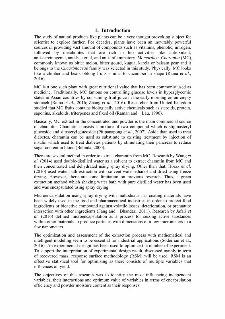
1. Introduction The study of natural products like plants can be a very thought provoking subject for scientist to explore further. For decades, plants have been an inevitably powerful sources in providing vast amount of compounds such as vitamins, phenolic, nitrogen, followed by metabolites that are rich in bio activities like antioxidant, anti-carcinogenic, anti-bacterial, and anti-inflammatory. Momordica. Charantia (MC), commonly known as bitter melon, bitter gourd, kugua, karela or balsam pear and it belongs to the Cucurbitaceae family was selected in this study. Physically, MC looks like a climber and bears oblong fruits similar to cucumber in shape (Raina et al., 2016).

MC is a one such plant with great nutritional value that has been commonly used as medicine. Traditionally, MC famous on controlling glucose levels in hyperglycemic states in Asian countries by consuming fruit juice in the early morning on an empty stomach (Raina et al., 2016; Zhang et al., 2016). Researcher from United Kingdom studied that MC fruits contains biologically active chemicals such as steroids, protein, saponins, alkaloids, triterpenes and fixed oil (Raman and Lau, 1996).

Basically, MC extract in the concentrated and powder is the main commercial source of charantin. Charantin consists a mixture of two compound which is stigmasteryl glucoside and sitosteryl glucoside (Pitipanapong et al., 2007). Aside than used to treat diabetes, charantin can be used as substitute to existing treatment by injection of insulin which used to treat diabetes patients by stimulating their pancreas to reduce sugar content in blood (Belinda, 2000).

There are several method in order to extract charantin from MC. Research by Wang et al. (2014) used double-distilled water as a solvent to extract charantin from MC and then concentrated and dehydrated using spray drying. Other than that, Horax et al. (2010) used water bath extraction with solvent water-ethanol and dried using freeze drying. However, there are some limitation on previous research. Thus, a green extraction method which shaking water bath with pure distilled water has been used and was encapsulated using spray drying.

Microencapsulation using spray drying with maltodextrin as coating materials have been widely used in the food and pharmaceutical industries in order to protect food ingredients or bioactive compound against volatile losses, deterioration, or premature interaction with other ingredients (Fang and Bhandari, 2011). Research by Jafari et al. (2016) defined microencapsulation as a process for seizing active substances within other materials to produce particles with dimensions of a few micrometers to a few nanometers.

The optimization and assessment of the extraction process with mathematical and intelligent modeling seem to be essential for industrial applications (Sodeifian et al., 2016). An experimental design has been used to optimize the number of experiment. To support the interpretation of experimental design result, discussed mainly in term of recovered mass, response surface methodology (RSM) will be used. RSM is an effective statistical tool for optimizing as there consists of multiple variables that influences oil yield.

The objectives of this research was to identify the most influencing independent variables, their interactions and optimum value of variables in terms of encapsulation efficiency and powder moisture content as their responses.

 

2. Materials and Methods Sample Preparation and Chemicals

The fresh MC fruits were purchased from a local market. The fruits were cut into small pieces after rinsed with distilled water and then sun dried for 3 days before grinding. In this study, dried MC were completely crushed using the blender (Philips). The particles size was measured by a milling and sieving (Retsch, Germany) to have an average size of 300µm. The ground sample was stored and keep in the freezer (Model Liebherr) until use. Ethanol, dichloromethane and petroleum ether were purchased from Merck, Malaysia. Standard charantin was purchased from ChromaDex.

Water Extraction

The water extraction was performed with shaking water bath instrument (NE5-28D Series Clifton, Nickel-Electro Limited, United Kingdom, UK) at the Centre of Lipids Engineering and Applied Research (CLEAR), Faculty of Chemical and Energy Engineering, Universiti Teknologi Malaysia. Shaking water bath extraction were conducted at ratio 1:20 (g:mL) (Horax et al., 2010) at 80oC as well as 6 hours of extraction.

Soxhlet Extraction

Soxhlet extraction was carried out over 10g of grounded MC and added to 4 round bottom flask with 200mL of different solvent each and run for 6 hours. The solvent used were distilled water, 95% ethanol, dichloromethane, and petroleum ether (Merck, Malaysia). After extraction, solvents were removed via rotary evaporator (Heidolph, German) and remaining oil yield then were stored in freezer (-20oC) until further analysis.

Sample Purification

Extracted oil were purify according to previous study with some modification (Pitipanapong et al., 2007). Concisely, 2 mL of methanol-water with ratio 1:1 was added to 0.2 g of extracted oil. The mixture was then sonicated for 15 min and centrifuged at 3500 rpm for 15 min to separate the supernatant from the precipitate. The precipitate was then added with 1 mL of methanol and repeated sonicated and centrifuged step. The purified solution was filtered through a 0.45 µm nylon membrane filter (Milipore, USA) before analyzed by High Performance Liquid Chromatography (HPLC). HPLC analysis was performed as previous study by Pitipanapong et al. (2007) with C-18 Inertsil ODS-3 column (5µm particle, 4.6mm x 250mm ID). The mobile phase was 100:2 (v/v) methanol-water and was delivered at a flow rate of 1mL/min. the UV detection wavelength was 204nm and the sample injection volume was 200 µL.

Spray Drying

A laboratory scale spray dryer (Buchi, SD-04, Switzerland) was used for the production of rich charantin extract powder from MC. Maltodextrin with DE 10-15 (Permula, Malaysia) is widely used as a carrier agent for drying of fruit juices by spray drying. About 20% of maltodextrin concentration was added to the filtered pulp until complete dissolution. The spray drying equipment has a drying chamber,

 

cyclone and two-fluid nozzle size with range (0.5–1.5)mm. The inlet temperature was (160–200)oC meanwhile the outlet temperature was monitored for its variation as a function of the pulp feeding. The pulp was feed using peristaltic pump at temperature 25oC and feed flow rate (2–4)mL/min was controlled by the pump rotation speed.

Encapsulation Efficiency

Encapsulation efficiency of MC powder extract was determined employing Eq. (1) with some modification from previous study (Idham et al., 2012) and expressed in percentage (%).

%

100% (1)

For total oil determination, 0.5g of powder were weight and dissolved with 1mL of distilled water and vortex for 30s at room temperature in order to destroy the microcapsule membrane. Consequently, 4mL of methanol was added to the samples then subjected to vortex at 2000 rpm for 5 min and filtered to a clean flask, which was left to evaporate and then was dried at 60oC until constant weight.

Surface oil was determined following a previous method of (Tonon et al., 2011) where 5 mL of methanol was added to 0.5g of powder and vortex for 5 min at room temperature and then filtered to a clean flask, left to evaporate and dried at 60oC until constant weight.

Moisture Content

About 1g of MC powder was weighted and placed in crucible and determined by drying the powder at temperature 105oC in the oven for 3 hours until constant weight was obtained. The final moisture content was calculated and expressed in terms of percent wet basis (wb), 100xkg water/kg wet material.

Experimental Design

Box Behnken design was applied for experimental design in order to optimize spray drying parameters of inlet temperature (X1), flow rate (X2), and nozzle size (X3) on encapsulation efficiency and moisture content by using RSM. Three coded levels of -1, 0 and +1 were assigned as the parameters for inlet temperature of (160–200)oC, flow rate of (2–4)mL/min and nozzle size of (0.5-1.5)mm respectively. The result obtained were analyzed using Design Expert Software version 6.0.4. The generalized response surface model, Eq (2) is given below:

Y = β0 + β1X1 + β2X2 + β3X3 + β11X12 + β22X2

2 + β33X32 + β12X1X2 + β13X1X3 +

β23X2X3

(2)

Where Y is the response calculated by the model; β0 is a constant regression; βi, βii, and βij are linear, squared and interaction coefficients, respectively. The X1, X2, and X3 are the coded independent variables.

 

3. Result and Discussion Rich Charantin Extracts from Momordica Charantia

 

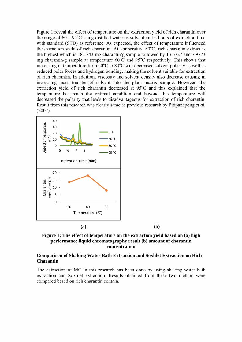
Figure 1 reveal the effect of temperature on the extraction yield of rich charantin over the range of 60 – 95oC using distilled water as solvent and 6 hours of extraction time with standard (STD) as reference. As expected, the effect of temperature influenced the extraction yield of rich charantin. At temperature 80oC, rich charantin extract is the highest which is 18.1743 mg charantin/g sample followed by 13.6727 and 7.9773 mg charantin/g sample at temperature 60oC and 95oC respectively. This shows that increasing in temperature from 60oC to 80oC will decreased solvent polarity as well as reduced polar forces and hydrogen bonding, making the solvent suitable for extraction of rich charantin. In addition, viscosity and solvent density also decrease causing in increasing mass transfer of solvent into the plant matrix sample. However, the extraction yield of rich charantin decreased at 95oC and this explained that the temperature has reach the optimal condition and beyond this temperature will decreased the polarity that leads to disadvantageous for extraction of rich charantin. Result from this research was clearly same as previous research by Pitipanapong et al. (2007).

(a) (b)

Figure 1: The effect of temperature on the extraction yield based on (a) high performance liquid chromatography result (b) amount of charantin

concentration

Comparison of Shaking Water Bath Extraction and Soxhlet Extraction on Rich Charantin

The extraction of MC in this research has been done by using shaking water bath extraction and Soxhlet extraction. Results obtained from these two method were compared based on rich charantin contain.

0

20

40

60

80

5 6 7 8

Detector response, 

mAU

Retention Time (min)

STD

60 °C

80 °C

95 °C

0

5

10

15

20

60 80 95

Charantin,

mg/g sample

Temperature (oC)

 

Figure 2: Comparison of Shaking water bath (SWB) and Soxhlet extraction on charantin contain

Figure 2 shows the comparison of charantin contain in MC from SWB extraction and Soxhlet extraction, where it was clearly shown that the charantin obtained from SWB is 18.1743 mg charantin/g sample are higher compared to the Soxhlet extraction with water as a solvent that can only extract 9.7782 mg charantin/g sample. This is because SWB with a constant shaking enhance the extraction efficiency as it increase the diffusion when shaking thus enabling better mass transfer of the compounds. On the other hand, the highest potential of charantin that could be extract is 58.5781 mg charantin/g sample by using dichloromethane. However, dichloromethane is not suitable to extract biomedicine compound as it is toxic and carcinogenic.

Analysis of Box-Behnken

The application of RSM employing Box-Behken design for three independent variables was taken to obtain the combination of values that optimizes the response within the region of the 3-D observation space. Table 1 shows the 17 trials run for the experimental result and predicted values that generated from Design Expert 6.0.4.

The two-factor interaction model showed relationship between independent variables of inlet temperature (X1), flow rate (X2), and nozzle size (X3) with dependent variables which is encapsulation efficiency (Y1) and moisture content (Y2).

Table 1: The experimental result and predicted values for 17 trials run

Run

Independent Variable Dependent Variables

Inlet Temperature

, X1 (oC)

Flow Rate, X2

(mL/min)

Nozzle Size,

X3

(mm)

Encapsulation Efficiency, Y1 (%)

Moisture Content, Y2 (%)

Experimental

Predicted

Experimental

Predicted

1 180.0 4.0 1.5 98.50 98.25 2.83 2.6230 2 180.0 3.0 1.0 98.84 97.66 2.01 2.0570 3 180.0 2.0 1.5 98.64 98.61 1.63 1.5840 4 160.0 4.0 1.0 96.60 96.73 3.01 2.8070 5 180.0 3.0 1.0 96.06 97.66 1.97 2.0570 6 180.0 3.0 1.0 97.07 97.66 1.61 2.0570 7 180.0 3.0 1.0 98.67 97.66 2.09 2.0570 8 160.0 3.0 1.5 n/a n/a n/a n/a 9 200.0 3.0 0.5 99.27 98.99 1.92 1.7790

10 180.0 2.0 0.5 97.46 97.07 1.60 1.4900 11 180.0 4.0 0.5 97.24 96.72 2.61 2.5290 12 160.0 2.0 1.0 98.38 98.34 1.76 1.7680 13 200.0 2.0 1.0 96.79 97.34 1.45 1.3060

18.17439.7782

26.2764

58.5781

5.7645

0

20

40

60

80

Water EtOH Dichloromethane Petroleum EtherCharan

tin,

mg charan

tin/g sam

ple

Solvent

SWB Soxhlet

 

Run

Independent Variable Dependent Variables

Inlet Temperature

, X1 (oC)

Flow Rate, X2

(mL/min)

Nozzle Size,

X3

(mm)

Encapsulation Efficiency, Y1 (%)

Moisture Content, Y2 (%)

Experimental

Predicted

Experimental

Predicted

14 180.0 3.0 1.0 97.28 97.66 1.39 2.0570 15 160.0 3.0 0.5 94.49 94.80 2.42 2.2400 16 200.0 4.0 1.0 97.52 98.24 2.16 2.3450 17 200.0 3.0 1.5 97.18 96.59 2.15 1.8730

Notes: n/a stands for not available as the product did not produce powder.

The interpretation of the results from equation 3 and 4 should be based on the magnitude and signs of the regression coefficients. The two-factor interaction model of rich charantin powder properties as shown below:

Y1 = 77.0633 + 0.1089X1 – 5.8260X2 + 36.9405X3 + 0.0314X1X2 – 0.1967X1X3

(3)

Y2 = 2.48103 – 0.011540X1 + 0.51947X2 + 0.094219X3 (4)

Table 2: ANOVA table for the encapsulation efficiency (two-factor interaction model)

Source Sum of squares

Degree of freedom

Mean Square F-value R2

Regression 14.9000 5 2.9800 4.0750 0.6708 Residual 7.3129 10 0.7313 TOTAL 22.2129 15

Table 3: ANOVA table for the powder moisture content (linear model)

Source Sum of squares

Degree of freedom

Mean Square F-value R2

Regression 2.5200 3 0.8400 10.6061 0.7257 Residual 0.9500 12 0.0792 TOTAL 3.4700 15

F-calculated for encapsulation efficiency and powder moisture content in ANOVA table were 4.075 and 10.6061 respectively. The F-value are smaller than F-tabulated for encapsulation efficiency F(5,10,0.01) which is 5.636 and bigger for moisture content which F(3,12,0.01) is 5.953. The result validated that 99% of confidence level where the null hypothesis for encapsulation efficiency is accepted meanwhile for moisture content not accepted as noise occur in the model.

The coefficient of determination (R2) for encapsulation efficiency and powder moisture content were 0.6708 and 0.7257 respectively. The value of R2 is a measure of total variation of observed values about the mean explained by the fitted model.

Effect of Encapsulation Efficiency

According to Eq (3), encapsulation efficiency was affected by all the independent variables. Figure 3 shows the influences of inlet temperature, flow rate and nozzle size variables on the encapsulation efficiency.

 

In this study, encapsulation efficiency obtained from all the experiments varied from 94.49 to 99.27% (Table 1). Figure 3 (a, b, and c) shows the influences of these variables derived from this response. Three independent variables were considered that affected the encapsulation efficiency. Table 2 analyzed the final model that two-factor interaction model of nozzle size had the most significant (p<0.05) effect.

(a) (b) (c)

Figure 3: Response surface for encapsulation efficiency at (a) flow rate 3mL/min, (b) nozzle size at 1.00mm and (c) inlet temperature at 180oC

However, the interaction between inlet temperature and nozzle size exhibited the highest significant influences on the encapsulation efficiency. Higher inlet temperature may affect the layer formation and the rate water evaporation, resulting the crust breaking down as well as less efficient encapsulation. The same behavior was observed by Mohammed et al. (2017) in the microencapsulation of Nigella sativa oil. Moreover, the interaction between nozzle size and flow rate exhibited least significant influences on the encapsulation efficiency. Increasing flow rate with constant nozzle size slightly change the encapsulation efficiency.

Effect of Powder Moisture Content

According to Eq (4), flow rate is the most significant independent variables that affect the result of powder moisture content. Figure 4 shows the response of moisture content that influence by these independent variables; inlet temperature, flow rate and nozzle size.

(a) (b) (c)

 

Figure 4: Response surface for moisture content at (a) nozzle size 1.00mm, (b) flow rate at 3.00mL/min and (c) inlet temperature at 180oC

Table 1 shows the result of moisture content that obtained from all experiments, varied from 1.39% to 3.01%. The powder moisture content was influence by all the independent variables as shown in figure 4 (a, b, and c). As mention early, the most influence independent variables was feed flow rate where by increasing the feed flow rate will increase the moisture content of the powder as shown in figure 4 (a) and (c). The contact time between droplets and drying air were reduce as higher feed flow rate were applied and result less efficient of heat transfer. In addition, larger droplet with smaller surface area were formed, results drying rate decreased. The same result was reported on spray drying of pink guava by Shishir et al. (2016). Besides that, higher of inlet temperature leads to lower moisture content (figure 4 (b)) as it resulting a greater driving force for water evaporation. Supporting result was report in the spray drying of red-fleshed pitaya according to M. Yunus et al. (2011).

Optimization of Spray Drying Process

The optimum process parameters for independent variables and responses were generated after limiting the preferred goal such as minimizing inlet temperature and feed flow rate, maximized encapsulation efficiency and minimizing powder moisture content. According to the software, the predicted optimum condition was obtained at 160oC inlet temperature, 2.00mL/min feed flow rate and 1.17mm nozzle size and gives response for 99.272% encapsulation efficiency and 1.784% powder moisture content.

4. Conclusion and Recommendation In conclusion, the outcome of this research work showed the optimization of spray drying conditions for MC extract by employing RSM. The encapsulation efficiency and powder moisture content were substantially influenced by inlet temperature, feed flow rate and nozzle size. The optimum conditions that allowed for encapsulation efficiency and moisture content of MC extract powder to be established at 160oC for inlet temperature, 2.00mL/min for feed flow rate and 1.17mm for nozzle size. The result of spray dried under optimized conditions exhibited 99.271% encapsulation efficiency and 1.784% powder moisture content. It was deemed necessary to perform further study for identification of charantin contain in MC extract powder.

5. Acknowledgement The authors thank the Department of Chemical and Energy Engineering of the “Universiti Teknologi Malaysia” as well as Ministry of Higher Education, MOHE, for the special support that made this research possible the financial support of Universiti Teknologi Malaysia under grant no R.J130000.7809.4F766.

References

Aris., N. A., Yunus., M. A. C., Yian., L. N., Idham., Z., Ramli., W. N. D., and Aziz., A. H. A. (2016). Effect of Particle Size on Bitter Gourd (Momordica charantia)

 

Extract Yield by Supercritical Carbon Dioxide Extraction. Symposium of Malaysian Chemical Engineers (SOMChE), 29, 1-6.

Azmir, J., Zaidul, I. S. M., Rahman, M. M., Sharif, K. M., Mohamed, A., Sahena, F., . . . Omar, A. K. M. (2013). Techniques for extraction of bioactive compounds from plant materials: A review. Journal of Food Engineering, 117(4), 426-436.

Belinda, O. (2000). Diabetes self-management. Herbal Supplements in Diabetes Management.

Belwal, T., Dhyani, P., Bhatt, I. D., Rawal, R. S., and Pande, V. (2016). Optimization extraction conditions for improving phenolic content and antioxidant activity in Berberis asiatica fruits using response surface methodology (RSM). Food Chem, 207, 115-124.

Fang, Z., and Bhandari, B. (2011). Effect of spray drying and storage on the stability of bayberry polyphenols. Food Chem, 129(3), 1139-1147.

Horax, R., Hettiarachchy, N., and Chen, P. Y. (2010). Extraction, Quantification, and Antioxidant Activities of Phenolics from Pericarp and Seeds of Bitter Melons (Momordica charantia) Harvested at Three Maturity Stages (Immature, Mature, and Ripe). Journal of Agricultural and Food Chemistry, 58(7), 4428-4433.

Idham, Z., Muhamad, I. I., and Sarmidi, M. R. (2012). Degradation Kinetics And Color Stability Of Spray‐Dried Encapsulated Anthocyanins From Hibiscus Sabdariffa L. Journal of Food Process Engineering, 35(4), 522-542.

Jafari, S. M., Mahdavi-Khazaei, K., and Hemmati-Kakhki, A. (2016). Microencapsulation of saffron petal anthocyanins with cress seed gum compared with Arabic gum through freeze drying. Carbohydr Polym, 140, 20-25.

Lee, N. Y., Setapar, S. H. M., Sharif, N. S. M., Ahmad, A., Khatoon, A., Yunus, M. A. C., and Muhamad, I. I. (2013). Extraction of rubber (Hevea brasiliensis) seed oil using supercritical carbon dioxide and soxhlet extraction. Research Journal of Chemistry and Environment, 17, 1-7.

Mohammed, N. K., Tan, C. P., Manap, Y. A., Alhelli, A. M., and Hussin, A. S. M. (2017). Process conditions of spray drying microencapsulation of Nigella sativa oil. Powder Technology.

Pitipanapong, J., Chitprasert, S., Goto, M., Jiratchariyakul, W., Sasaki, M., and Shotipruk, A. (2007). New approach for extraction of charantin from Momordica charantia with pressurized liquid extraction. Separation and Purification Technology, 52(3), 416-422.

Raina, K., Kumar, D., and Agarwal, R. (2016). Promise of bitter melon (Momordica charantia) bioactives in cancer prevention and therapy. Semin Cancer Biol, 40-41, 116-129.

Raman, A., and Lau, C. (1996). Anti-diabetic properties and phytochemistry of Momordica charantia L. (Cucurbitaceae). Phytomedicine, 2(4), 349-362.

Shishir, M. R. I., Taip, F. S., Ab Aziz, N., Talib, R. A., and Sarker, M. S. H. (2016). Optimization of Spray Drying Parameters for Pink Guava Powder Using RSM. Food Science and Biotechnology, 25(2), 461-468.

 

Sodeifian, G., Sajadian, S. A., and Saadati Ardestani, N. (2016). Optimization of essential oil extraction from Launaea acanthodes Boiss: Utilization of supercritical carbon dioxide and cosolvent. The Journal of Supercritical Fluids, 116, 46-56.

Tonon, R. V., Grosso, C. R. F., and Hubinger, M. D. (2011). Influence of emulsion composition and inlet air temperature on the microencapsulation of flaxseed oil by spray drying. Food Research International, 44(1), 282-289.

Wang, H. Y., Kan, W. C., Cheng, T. J., Yu, S. H., Chang, L. H., and Chuu, J. J. (2014). Differential anti-diabetic effects and mechanism of action of charantin-rich extract of Taiwanese Momordica charantia between type 1 and type 2 diabetic mice. Food Chem Toxicol, 69, 347-356.

Yunus, M., Lee, C., and Idham, Z. (2011). Effects of variables on the production of red-fleshed pitaya powder using response surface methodology. Jurnal Teknologi, 56, 15-29.

Yunus, M. A. C., and Ripin, A. (2001). Optimization of processing parameter for enhancing good quality of mango powder using response surface methodology. Symposium of Malaysian Chemical Engineers (SOMChE), 15, 427-434.

Zhang, F., Lin, L., and Xie, J. (2016). A mini-review of chemical and biological properties of polysaccharides from Momordica charantia. Int J Biol Macromol, 92, 246-253.