
Applications in Environmental Engineering Technology ... - UTHM
120
Applications in Environmental Engineering Technology Series 1
-
Upload
khangminh22 -
Category
Documents
-
view
1 -
download
0
Transcript of Applications in Environmental Engineering Technology ... - UTHM

Applications in Environmental
Engineering Technology
Series 1

ii

iii
Applications in Environmental
Engineering Technology
Series 1
SURAYA HANI ADNAN
NURAMIDAH HAMIDON
MOHAMMAD ASHRAF ABD RAHMAN
TUAN NOOR HASANAH TUAN ISMAIL
MOHAMAD HAIRI OSMAN
HARINA MD. AMIN
2017
© Penerbit UTHM
First Published 2018

iv
Copyright reserved. Reproduction of any articles, illustrations and content of this book
in any form be it electronic, mechanical photocopy, recording or any other form
without
any prior written permission from The Publisher’s Office of Universiti Tun Hussein Onn
Malaysia, Parit Raja, Batu Pahat, Johor is prohibited. Any negotiations are subjected to
calculations of royalty and honorarium.
Perpustakaan Negara Malaysia Cataloguing in Publication Data
Suraya Hani Adnan
Nuramidah Hamidon
Mohammad Ashraf Abd Rahman
Tuan Noor Hasanah Tuan Ismail
Mohamad Hairi Osman
Harina Md. Amin
Applications in Environmental Engineering Technology Series 1/ Suraya Hani
Adnan, Nuramidah Hamidon, Mohammad Ashraf Abd Rahman, Tuan Noor
Hasanah Tuan Ismail, Mohamad Hairi Osman, Harina Md. Amin
ISBN 978-967-2183-21-1
Published by:
Penerbit UTHM
Universiti Tun Hussein Onn Malaysia
86400 Parit Raja,
Batu Pahat, Johor
Tel: 07-453 7051
Fax: 07-453 6145
Website: http://penerbit.uthm.edu.my
E-mail: [email protected]
http://e-bookstore.uthm.edu.my
Penerbit UTHM is a member of
Majlis Penerbitan Ilmiah Malaysia
(MAPIM)
v
PREFACE
Environmental Engineering technology is an application of the environmental science to
conserve the natural environment and resources, and to curb the negative impacts of
human involvement. Sustainable development is the core of environmental technologies.
Environmental technology is also known as envirotech. That is where this book comes
in. The book confronts the reader with the applications in environmental engineering
technology that widely used today. The main focus of this book is on the waste disposal
management, air quality using houseplant, definition of Indoor Environmental Quality
(IEQ) and Indoor Air Quality (IAQ), carbon dioxide removal in palm oil, wastewater
matrix and characterisation, arsenic distribution in Johor, using concrete and windshield
glass waste as filteration to remove phosporus, cultivate aerobic ganular sludge with soy
sauce wastewater, modelling 2D hydrodynamic wave during spring tide at Tanjung
Pelepas and geophysic technology in defining the environmental impact in coastal area.
Each of these topics is vast thus we restrict our attention for each of these areas, for
example air quality, wastewater, use of concrete to remove the phosporus and simulation
of geophysic and hydrodinamics. The main contributors are from Department of
Environmental Engineering Technology, Faculty Engineering Technology, UTHM. We
thank all of our collaborators for their tremendous assistance in making this book
possible.
.
vi
CONTENTS
CHAPTER 1 A Study on the Awareness of Household Waste Separation in
Parit Raja, Johor: Residential Area
Mohamad Hambali Mohd Hatta, Roslinda Ali
1
CHAPTER 2 Houseplant Ability in Reducing Formaldehyde and Total
Volatile Organic Compounds (TVOCS) In Indoor Air of New
UTHM Pagoh Campus Building
Nor Haslina Hashim, Nur Effie Sazieana Anuar
17
CHAPTER 3 Carbon Dioxide Removal in Liquid and Gas using
Biogranules Containing Photosynthetic Pigment in Palm Oil
Mill Effluent Treatment
Mohamed Zuhaili Bin Mohamed Najib, Kamarul Aini Mohd
Sari, Rahmat Muslim, Nurdalila Saji, Mariah Awang,
Mohamad Ashraf Abd Rahman, Fatimah Mohamed Yusop and
Mohamad Faizal Bin Tajul Baharuddin
31
CHAPTER 4 Distribution of Arsenic in the Straits of Johor due to Local
Developmet
Faridahanim Ahmad, Shamila Azman, Mohd Ismid Mohd Said,
Hasnida Harun, Hazren A. Hamid, Nuramidah Hamidon
39
CHAPTER 5
Understanding the Wastewater Matrix and Characterisation
Hazren A. Hamid, Hasnida Harun, Norshuhaila Mohamed
Sunar, Faridahanim Ahmad
45
CHAPTER 6 Windshield Glass Waste as Sustainable Material in Concrete
Siti Nur Fateha Binti Mohd Paiz, Mimi Suliza Binti Muhamad,
Mohamad Hairi Bin Osman
61
CHAPTER 7 Cultivate Aerobic Granular Sludge with Soy Sauce Wastewater
Hasnida Harun, Hazren A. Hamid, Faridahanim Ahmad,
Norshuhaila Mohamed Sunar
67
CHAPTER 8 The Vertical Aerated Recycled Concrete Aggregate Filter
(VARCAF) for Removal of Phosphorus
Suraya Hani Adnan, Norwardatun Abd Roni, Rafidah
Hamdan, Nurain Izzati Mohd Yassin, Nurul Amirah
Kamarulzaman
77
CHAPTER 9 Characteristics of Hydrodynamics Wave at Port of Tanjung
Pelepas during Spring Tide by using Telemac-2D
Nur Aini Mohd Arish, Ikhwan Nasir Ismail, Nuramidah
Hamidon
83

vii
CHAPTER 10
Application of Geophysic Technology in Defining the
Environmental Impact at Coastal Area
Mohamad Faizal Tajul Baharuddin, Mohd Idrus Mohd
Masirin, Mohamed Zuhaili Mohamed Najib
93
CHAPTER 11 Indoor Environmental Quality (IEQ) and Indoor Air Quality
(IAQ)
Norshuhaila Mohamed Sunar, Umi Kalthsom Parjo, Menega
A/P Subramaniam, Abdul Mutalib bin Leman, Hazren A.
Hamid, Hasnida Harun.
109

viii
Applications in Environmental Engineering Technology Series 1 2018 ISBN 978-967-2183-21-1
1
CHAPTER 1
A STUDY ON THE AWARENESS OF HOUSEHOLD WASTE
SEPARATION IN PARIT RAJA, JOHOR: RESIDENTIAL AREA
Mohamad Hambali Bin Mohd Hatta, Roslinda Binti Ali
Faculty of Engineering Technology,
University Tun Hussien Onn Malaysia,
Batu Pahat, Johor, Malaysia
1.0 INTRODUCTION
Malaysia has set a target to become a developed nation by year 2020. This can be
achieved in the Eleventh Malaysia Plan (2016 - 2020) that was introduced by the
government which is the final step in order to provide a nation towards sustainable
development in terms of politic, economy and social. In order to realize this vision, the
government has defined six strategic thrusts to help Malaysia stay ahead of the
challenges and opportunities of the fast-changing global and political landscape.
Therefore, it demonstrates the commitment of Malaysia to renew and increase its
commitment to the environment and the long-term sustainability [1]. As a result, some
government agencies have been established such as Department of Environment (DOE)
to achieve goals which is to the prevention, abatement, and control of pollution and to
ensure that Malaysia’s precious environment and natural are conserved and protected for
present and future generations.
Solid waste management in Malaysia has recently approached a critical level,
especially in terms of the amount and composition. Generation of waste increased each
year by 3% due to many causes such as urban migration, affluence, and rapid
development [2] and increased drastically where it was expected to increase from about
9.0 million tons in 2000 to about 10.9 million tons in 2010, and finally to about 15.6 mil-
lion tons in 2020 [3]. In order to reduce this environmental problems at household level,
the community itself should play a role by practicing of waste separation.
Nowadays, household waste separation is very important and waste separation is
familiar in developed countries out there. However, in Malaysia waste separation is a
new thing and take a long period to be practice and environmental awareness among the
public generally is still not adequate [4]. The aim of this research is to investigate the
awareness of household waste separation in residential areas.

Applications in Environmental Engineering Technology Series 1 2018 ISBN 978-967-2183-21-1
2
1.2 LITERATURE REVIEW
The environmental problem is a global concern and it has no boundary. One of
the main cause that make environmental degradation is improper management in the
disposal of wastes. Waste can also be generated as a result activities of household.
Household waste considered as a type of municipal solid waste (MSW) and consists
mainly of plastics, paper, glass, metals, organics, wood and others. These wastes must be
predisposed accurately to assist keep environmental quality and human health, as well as
to preserve natural resources [5].
1.3 CONCEPT OF HOUSEHOLD WASTE
Management of municipal solid waste (MSW) is a major challenge for developed
countries, especially in the cities are growing rapidly and Malaysia is one of the most
successfully country to go through transition. A good MSW management must cover
waste generated from other sources like a commercial, industrial, institutional, and
municipal services [3]. Table 1 shows the sources of solid waste and the location where
wastes are generated.
Table 1: Sources of solid waste generation
Sources of Waste Locations where wastes are generated
Residential/Household Single and multifamily dwellings, terrace, semi-
detached, bungalow, apartments, cluster house, etc.
Commercial Stores, hotels, restaurants, markets, office buildings,
motels, shops, private school, etc.
Institutional Schools, hospitals, prisons, government centers,
universities, etc.
Municipal
Street cleaning, landscaping, parks, beaches,
recreational areas, water and wastewater treatment
plants, open spaces, alley, roadside litter, etc.
Agricultural Field and row crops, orchards, vineyards, dairies,
farm, etc.
Construction and
Demolition
New construction sites, road repair, renovation sites,
demolition of buildings, broken pavement, etc.
Industrial
Light and heavy manufacturing, fabrication,
construction sites, power and chemical plants, and
refineries.
(Adapted from Eeda, Ali, & Siong, 2012)
Solid waste composition refers to the various elements that the waste contains.
The composition of municipal solid waste is one of the factors to be considered before
proposing any management option [6]. Composition of solid waste can be classified into
organic and inorganic [7]. Table 1.2 describes the different types of waste and their

Applications in Environmental Engineering Technology Series 1 2018 ISBN 978-967-2183-21-1
3
sources. There are certain waste are inorganic but can be reused or recycled in fact it is
believed that a larger portion of the waste can be recycled, a part of can be converted to
compost, and only a smaller portion of it is real waste that has no use and has to be
discarded [8].
Table 1.2: Physical Composition of Household Solid Waste
Physical
Composition
Basic Classification Example
Organic Food Waste Vegetables, meats
Garden Waste Yard (leaves, grass, brush) waste, wood
Inorganic
Plastic Bottles, packaging, containers, bags, lids,
cups
Textile and Rubber Clothes, leather products
Paper and Box Paper scraps, cardboard, newspapers,
magazines, bags, boxes, wrapping paper,
telephone books, shredded paper, paper
beverage cu
Glass Bottles, broken glassware, light bulbs,
colored glass
Metal Cans, foil, tins, non-hazardous aerosol
cans, appliances (white goods), railings,
bicycles
(World Bank, 2012)
One of the steps taken by the Malaysian government in solving environmental
problems is waste minimization followed by 3R program, composting, incineration and
landfill. Solid waste management planning strategies need to support the waste
minimization. This is because waste minimization is best strategies for waste
management to reduce amount of waste generated [9].
1.4 Method of Waste Minimization
Waste minimization can be defined as the preventing and reducing waste at source
through the efficient use of raw materials, energy and water [10]. Waste minimization
strategies aim to strengthen awareness and encourage environmentally conscious
consumption patterns and consumer responsibility to reduce the overall levels of waste
[11]. In waste minimization hierarchy, the first option is waste reduce which offers the
best outcomes for the environment then followed by reuse, recycling, composting and
disposal. Figure 1 shows the reduction is the most preferred option while the landfill is
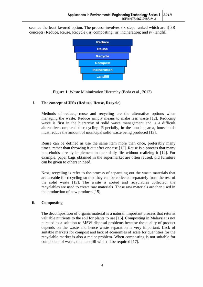
Applications in Environmental Engineering Technology Series 1 2018 ISBN 978-967-2183-21-1
4
seen as the least favored option. The process involves six steps ranked which are i) 3R
concepts (Reduce, Reuse, Recycle); ii) composting; iii) incineration; and iv) landfill.
Figure 1: Waste Minimization Hierarchy (Eeda et al., 2012)
i. The concept of 3R’s (Reduce, Reuse, Recycle)
Methods of reduce, reuse and recycling are the alternative options when
managing the waste. Reduce simply means to make less waste [12]. Reducing
waste is first in the hierarchy of solid waste management and is a difficult
alternative compared to recycling. Especially, in the housing area, households
must reduce the amount of municipal solid waste being produced [13].
Reuse can be defined as use the same item more than once, preferably many
times, rather than throwing it out after one use [12]. Reuse is a process that many
households already implement in their daily life without realizing it [14]. For
example, paper bags obtained in the supermarket are often reused, old furniture
can be given to others in need.
Next, recycling is refer to the process of separating out the waste materials that
are useable for recycling so that they can be collected separately from the rest of
the solid waste [13]. The waste is sorted and recyclables collected, the
recyclables are used to create raw materials. These raw materials are then used in
the production of new products [15].
ii. Composting
The decomposition of organic material is a natural, important process that returns
valuable nutrients to the soil for plants to use [16]. Composting in Malaysia is not
pursued as a solution to MSW disposal problems because the quality of product
depends on the waste and hence waste separation is very important. Lack of
suitable markets for compost and lack of economies of scale for quantities for the
recyclable market is also a major problem. When composting is not suitable for
component of waste, then landfill will still be required [17].
Applications in Environmental Engineering Technology Series 1 2018 ISBN 978-967-2183-21-1
5
iii. Incineration
Incineration is the most common thermal treatment process. Incineration is
defined as the combustion of solid and liquid waste in controlled incineration
facilities [18]. Process of incineration is carbon hydrogen and other elements in
the waste are combined with oxygen in the combustion air which generates heat
and also used to reduce waste materials to what was thought of as harmless ash
[14].
However, in Malaysia, the use of incinerators has been discontinued recently due
to the high cost of operation and poor technical expertise in maintaining the
incinerators [19]. This method has become a challenge to find an incineration
technology that is capable of incinerating wastes with high moisture content
accompanied by a low calorific value and at the same time operates at a low cost
in comparison to the relatively cheap landfilling method [20].
iv. Landfill
Landfilling is the most neglected area of SWM services [21]. Landfill can be
defined as a waste disposal site used for the controlled deposit of solid waste onto
or into land [22]. Landfill is by far the most commonly practiced waste disposal
method in the majority of countries. The preferred method practiced for the
disposal of MSW in Malaysia is through landfill and most of the sites are open
dumping areas [4]. This is because, landfill is the simplest and cheapest way of
disposing solid waste and it is also can deal with all kinds of materials in the solid
waste stream [23].
1.5 Household Waste Separation
Residents have a legal responsibility to ensure that all of their rubbish and waste
is disposed of properly. If they are not properly disposed it can cause diseases. The
government provides the concession companies, operators or the respective local
authorities to carry out the collection and disposal of municipal solid waste. The
objective is to provide effective, and an integrated, well-planned, well-managed, efficient
technologically advanced solid waste management system [24]. However, waste
management sector were faced with numerous challenges, such as a land shortage for
landfills and residents opposed to waste disposal facilities constructed near their homes.
One way to overcome these problems is with recycling, and the important prerequisite
for recycling is household waste separation at the source [25]. Source separation is one
of the prerequisites for successful and economically feasible recycling activities [26].
Household waste separation involves separating waste into common material
streams or categories for separate collection. This may be achieved using separate bin
services or verge side collections, or through direct delivery of specific wastes to drop-
off facilities [27]. In other countries, there are three or more bins in households for waste
separation. In Malaysia, prefer 3 recycling bins for paper, plastic and glass [28]. Table
1.3 show the recycle bins at home in many countries.

Applications in Environmental Engineering Technology Series 1 2018 ISBN 978-967-2183-21-1
6
Table 1.3: Recycling Bins at Household
(Adapted from Singh & Livina, 2015)
The way humans respond and co-operate on waste management issues is
influenced by their education, therefore, the public’s education is an essential element of
the success of any waste management program. Normally, Malaysian still have very low
awareness on the importance of involvement in waste separation. One’s attitudes based
on one’s perception of a behavior as positive or negative, right or wrong, pleasant or
unpleasant, or interesting or boring. Other than that, personal attitude had the strongest
correlation with waste separation intention [25]. Attitudes and perceptions toward waste
separation at source and rating of waste disposal issues in people’s minds and in the
scheme of official development plans have not been adequately considered which has
thus led to the recent upsurge in waste disposal problems in developing countries [26].
1.6 Rules and Regulations
An Act to provide for and regulate the management of controlled solid waste and
public cleansing for the purpose of maintaining proper sanitation and for matters
incidental thereto [29]. In order to manage solid waste in Malaysia in an efficient way so
can prevent from environmental degradation, the Solid Waste and Public Cleansing
Management Act 2007 (Act 672) has been introduced. SWMPC Act 2007 aim to provide
an act and regulate the management of solid waste and public cleansing in order to
maintain proper sanitation in the country [30].
Currently, the enforcement of the Act 672 is under Solid Waste Management and
Public Cleansing Corporation (SWMPCC) and this corporation has executive authority
to take over the solid waste management from the local authorities. Hence, it has brought
the confusion as well as overlapping power of enforcement between the corporation and
local authorities [31]. This Corporation works under the Federal government and the
function of the corporation includes every aspect that is deemed necessary to ensure the
implementation and success of an effective and integrated solid waste management plan
[32].
Types of Bins Country Name
2 Bins: Dry waste & wet waste Belgium, Serbia, Norway, Brazil,
Argentina, Russia, New Zealand,
Indonesia, Egypt
3 Bins: Paper, plastic & glass Philippines, Sri Lanka, Poland, Latvia,
Moldova, Malaysia
4 Bins: Paper, plastic, glass, & organic Bulgaria, Taiwan, Portugal, Spain
5 Bins: Paper, plastic, glass, organic & e-
waste
Finland

Applications in Environmental Engineering Technology Series 1 2018 ISBN 978-967-2183-21-1
7
1.7 Methodology
1.7.1 Research design adopted for the present studies
To meet those two objectives stated in the first chapter, the research design
adopted for this study is by using the quantitative methods. The residents is recognizing
as a representative of respondent, the simplicity and less time-consuming quantitative
method may help them to answer the question. The quantitative method statistical
analysis helps the researcher in providing a descriptive data that derive important facts
from the research. This is because, data collection obtained through this method simplify
comparisons between two or more variables. Hence, quantitative method suit for
researcher limitation because due to lack of time and budget.
The instrument of the quantitative method for primary data collection was by
using self-structured questionnaire. This method provides a quantitative method or data
collection, attitudes, or opinions of a population by studying a sample of that population
[33].
1.7.2 Questionnaire Construction
The survey questionnaire is designed based on the literature review in order to
answer the objectives of this research. The questionnaire template consists of 16
questions and is divided into three parts, as follows: 1) demographic profile; 2)
background of household waste; and 3) awareness on household waste separation. The
first section of the questionnaire enquires details on the background of the respondents.
Second section is concentrates on household waste produce by the respondent and the
last part of the survey enquires on the awareness of the respondents about household
waste separation.
1.7.3 Sampling design of the study
A sample is a finite part of a statistical population whose properties are studied to
gain information about the whole study [34]. The sampling is the process or method
involves taking a representative selection of the population and using the data collected
as research information [35]. Samples were collected in certain areas in Parit Raja due to
time and budget constraints. The questionnaire was distributed to the residential areas at
Taman Universiti, Taman Melewar and Taman Maju Jaya. This research involved the
quantitative method of data collection that took place in between September 2016 to
October 2016. A total 150 respondents were selected randomly to representative sample
of the target study. Table 1.4 shows the areas and the number of respondents in each area
that were chosen for the study.
Table 1.4: Number of respondents in chosen area
Areas Number of respondents
1. Taman Universiti 72
2. Taman Melewar 40
3. Taman Maju Jaya 38
Total 150 respondents

Applications in Environmental Engineering Technology Series 1 2018 ISBN 978-967-2183-21-1
8
1.7.4 Data Analysis
In this study, the data for quantitative self-structured questionnaire results will be
analyzed using statistical analysis software namely Statistical Package for Social
Sciences (SPSS, version 22.0) which are used for organizing, describing and analyzing
data from questionnaire survey. In order to produce information on the frequencies,
means and percentages, the data need to be analyzed through descriptive statistics.
Descriptive analysis can be define as to the transformation of raw data into a form that
will make them easy to understand and interpret also rearranging, ordering, and
manipulating data to generate descriptive information in data analysis [36]. Other than
that, it is suitable for measuring human perception, the objective of the study, the
available time and financial resources [37].
Other than that, this study using test of cross tabulation. Crosstabs can be defined
as form two-way and multiway table and measures of association for two-way table. A
cross tabulation is a two or more dimensional table that records the frequency of
respondents that have the specific characteristics described in the cells of the table. In
addition, cross tabulation tables provide a wealth of information about the relationship
between the variables [38].
1.8 Findings and Analysis
The data was collected by distributed the self-structured questionnaire at residential
areas Parit Raja, Johor. The data analysis and discussion in this chapter were divided
based 3 subtopics; i) demographic profile of the respondents; ii) background of
household waste; and iii) awareness on household waste separation.
1.8.1 Demographic profile
Table 1.5: Summary demographic profile of respondent
Variable Descriptions Frequency Percentage (%)
Housing Area Taman Universiti
Taman Melewar
Taman Maju Jaya
72
40
38
48
26.7
25.3
Gender Male 81 54
Female 69 46
Age 20 years and below 30 20
21 - 30 years 107 71.3
31 - 40 years 6 4
41 - 50 years 3 2
51 years and above 4 2.7
Education Level Secondary School 8 5.3
College/Institution 11 7.3
University 131 87.3
Results from Table 1.5 show that a total number of 150 respondents from
residential areas which are 72 respondents were from Taman Universiti, 40 respondents
were from Taman Melewar and another 38 respondents were from Taman Maju Jaya.
Applications in Environmental Engineering Technology Series 1 2018 ISBN 978-967-2183-21-1
9
Table 5 show that the total of 150 respondents indicates 54% (81 respondents) of
the respondents that took part in this survey was male and 46% (69 respondents) of
respondents were female.
In terms of age, Table 5 had shown that 20% (30 respondents) were between the
ages of below 20 years old; 71.3% (107 respondents) were between the ages of 21-30
years old; 4% (6 respondents) were between in the ages of 31-40 years old; 2% (3
respondents) were between of the ages of 41-50 years old and 2.7% (4 respondents) were
in the ages of above 51 years old.
From Table 5, it can be said that most of the respondents who took part in this
survey is received their education until tertiary level with the percentages 87.3% (131
respondents) and 7.3% (11 respondents) and secondary school at 5.3% (5.3 respondents).
Table 1.6: Cross tabulation between respondent’s education level and gender
Education Level Gender
Male Female
Frequency Percentage (%) Frequency Percentage (%)
Lower Education 4 4.9 4 5.8
Higher Education 77 95.1 65 94.2
Total 81 100 69 100
Table 1.6 above indicated that as a whole, majority of the respondents who took
part in this survey were from tertiary level educational background (142 respondents,
94.7%). From this amount male were 95.1% (77 respondents) and female were 94.2%
(65 respondents).
1.8.2 Background of Household Waste
i. Type of waste
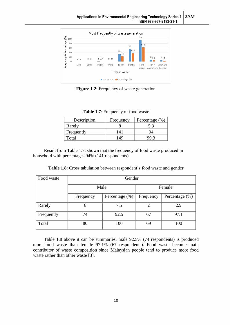
Result analysis from graph in Figure 1.2 show that the most frequently type of waste
produced from household in residential area was food waste with percentages 63.3% (95
respondents).
Applications in Environmental Engineering Technology Series 1 2018 ISBN 978-967-2183-21-1
10
Figure 1.2: Frequency of waste generation
Table 1.7: Frequency of food waste
Description Frequency Percentage (%)
Rarely 8 5.3
Frequently 141 94
Total 149 99.3
Result from Table 1.7, shown that the frequency of food waste produced in
household with percentages 94% (141 respondents).
Table 1.8: Cross tabulation between respondent’s food waste and gender
Food waste Gender
Male Female
Frequency Percentage (%) Frequency Percentage (%)
Rarely 6 7.5 2 2.9
Frequently 74 92.5 67 97.1
Total 80 100 69 100
Table 1.8 above it can be summaries, male 92.5% (74 respondents) is produced
more food waste than female 97.1% (67 respondents). Food waste become main
contributor of waste composition since Malaysian people tend to produce more food
waste rather than other waste [3].

Applications in Environmental Engineering Technology Series 1 2018 ISBN 978-967-2183-21-1
11
1.8.3 Awareness on Household Waste Separation
Table 1.9: Summary of awareness on household waste separation
Variable Description Frequency Percentage
(%)
Is the respondents
aware about the
program
Yes
No
72
78
48
52
Is the respondents
aware about the
concept 3R's
Yes
No
135
15
90
10
Is respondents
separate their
household waste
Yes
No
55
95
36.7
63.3
Why respondents
separate their waste
Because I see other people do it 2 1.3
I know waste separation waste
can save money
5 3.3
I know waste separation can
reduce environmental problems
30 20
I have seen waste separation on
the news (television, radio,
newspapers)
4 2.7
Avoid penalties 8 5.3
Waste separation is easy to do it 6 4
Why respondents do
not separate their
waste
I do not know about household
waste separation
12 8
I do not see the differences do
waste separation
9 6
I do not think it is my
responsibility
3 2
I do not see the importance of
the household waste separation
11 7.3
I do not have time to do it 31 20.7
Waste separation requires the
use of a lot of bins and plastic
28 18.7

Applications in Environmental Engineering Technology Series 1 2018 ISBN 978-967-2183-21-1
12
How far respondents
aware about rules and
regulation of waste
management
Really do not know 7 4.7
Do not know 34 22.7
Slightly know 67 44.7
Know 34 22.7
Extreme know 8 5.3
Result from Table 1.9 above shown that the residents is not aware about the
program of waste separation at sources with percentages 52% (78 respondents). Most of
respondents were aware about the concept of 3R’s with percentages 90% (135
respondents).
In terms of awareness, Table 1.9 above revealed that most of respondents were not
separate their household waste with percentages 63.3% (95 respondents) and separate
their household waste at 36.7% (55 respondents).
Table 1.9 shown that the majority of reason why residents separate their waste is
they know waste separation can reduce environmental problems with percentages 20%
(30 respondents) and most resident choose for why they do not separate their household
waste is they do not have time to do it with percentages 20.7% (31 respondents).
From Table 1.9 it can be summaries majority of total respondents were slightly
know (67 respondents, 44.7%) about rules and regulations of waste management.
1.9 Conclusions and Recommendation
People’s awareness is the most important the initial waste separations at an
individual level, from their workplace, public area, as well as households. In relation to
the first objective which is to investigate the awareness level on household waste
separation the residents staying in residential areas. Results achieved through
quantitative method which distribute self-structured questionnaire at residential areas.
Based on data analysis of survey it can conclude that majority of residents still lack of
awareness.
In relation to the second objective which is to determine residents involvement in
household waste separation within residential area. Result achieved through the same
with quantitative method. Based on data analysis of survey it can be conclude that most
of residents do not participate in household waste separation. A few of residents still take
a part on this program. Residents that separate their waste aware about the aim of waste
separation. This is because waste separation can minimize the environmental problems.
However, for those who do not separate their waste they give a reason they do not have
time to do it. The level of household participation in waste separation is alarmingly low
in the study area. This low participation in waste separation can lead to the low level of
awareness of environmental issues.
In conclusion, this study was successfully conducted and achieved the objective of
this research. The recommendation for further studies is waste separation has been
Applications in Environmental Engineering Technology Series 1 2018 ISBN 978-967-2183-21-1
13
carried out in the whole city, but the participation of the citizen should be improved.
More guidance, propaganda and regulations need to be developed and set up.
ACKNOWLEDGEMENT
The authors’ sincere appreciation goes to Universiti Tun Hussien Onn Malaysia, Dr
Hajah Roslinda Binti Ali for their support on the success of this study.
REFERENCES
[1] RMK11. (2015). Strengthening Infrastructure to Support Economic Expansion.
Rancangan Malaysia Kesebelas (Eleventh Malaysia Plan) : 2016-2020.
[2] Badgie, D., Samah, M. A. A., Manaf, L. A., & Muda, A. B. (2012). Assessment
of Municipal solid waste composition in Malaysia: Management, practice,
and challenges. Polish Journal of Environmental Studies, 21(3), 539–547.
[3] Abd Hamid, K. B., Ishak, M. Y., & Abu Samah, M. A. (2015). Analysis of
municipal solid waste generation and composition at administrative building
café in Universiti Putra Malaysia: A case study. Polish Journal of
Environmental Studies, 24(5), 1969–1982.
[4] Samsudina, M. D. M., & Dona, M. M. (2013). Municipal solid waste
management in Malaysia: Current practices, challenges and prospect. Jurnal
Teknologi, 62(1), 95–101.
[5] Hakami, B. A., & Seif, E. S. A. (2015). Household Solid Waste Composition and
Management in Jeddah City , Saudi Arabia : A planning model, 4(1), 1–10.
[6] Johari, A., Alkali, H., Hashim, H., Ahmed, S. I., & Mat, R. (2014). Municipal
solid waste management and potential revenue from recycling in Malaysia.
Modern Applied Science, 8(4), 37–49.
[7] World Bank. (2012). What a waste: a global review of solid waste management:
Waste Composition. Urban Development Series Knowledge Paper, 16–21.
[8] Fallis, A. . (2013). Attitudes, norms, identity and environmental behaviour: Using
an expanded theory of planned behaviour to predict participation in a
kerbside recycling programme. Journal of Chemical Information and
Modeling, 53(9), 1689–1699.
[9] Rossel, S. A., & Jorge, M. F. (1999). Cuban Strategy for Management and
Control of Waste. In A. Barrage, X. Edelmann (Eds.), Recovery, recycling,

Applications in Environmental Engineering Technology Series 1 2018 ISBN 978-967-2183-21-1
14
re-integration (R ‘99) congress proceedings, Vol. 1 (pp. 287–290).
Switzerland: EMPA
[10] Suckling, C. J. (2005). Waste Minimisation. Waste Minimisation, 146–152.
[11] Zugman, R., & Coutto, D. (2013). Waste Minimization Work Plan for 2012-
2013.
[12] Petzet, M., & Heilmeyer, F. (2012). Reduce Reuse Recycle. 13th
International Architecture Exhibition - La Biennale Di Venezia.
[13] William A. Worrell & P. Aarne Vesilind, (2012), Second Edition : Solid
Waste Engineering, United States of America.
[14] Eeda, N., Ali, H., & Siong, H. C. (2012). Urban Solid Waste Minimisation in
Malaysia - The case of Shah Alam City Hall , Selangor . Urban and Regional
Planning, 1–14.
[15] UN-Habitat. (2010). Solid Waste Management. Cities, 50, 257.
[16] Jason P. de Koff, B. D. L. and M. V. M. (2006). Home & Environment.
Ca.Uky.Edu.
[17] Sreenivasan, J., & Govindan, M. (2012). World ’ s largest Science ,
Technology & Medicine Open Access book publisher Solid Waste
Management in Malaysia – A Move Towards Sustainability.
[18] Pipatti, R., Sharma, C., Yamada, M., Svardal, P., Guendehou, G. H. S., Koch,
M., … IPCC. (2006). Incineration and open burning of waste. 2006 IPCC
Guidelines for National Greenhouse Gas Inventories, 5, 1–26.
[19] Abd Kadir, S. A. S., Yin, C. Y., Rosli Sulaiman, M., Chen, X., & El-Harbawi,
M. (2013). Incineration of municipal solid waste in Malaysia: Salient issues,
policies and waste-to-energy initiatives. Renewable and Sustainable Energy
Reviews, 24, 181–186.
[20] Sharifah ASAK, Abidin HZ, Sulaiman MR, Khoo KH, Ali H. Combustion
characteristics of Malaysian municipal solid waste and predictions of air flow
in a rotary kiln incinerator. Journal of Material Cycles andWaste
Management 2008;10:116–23.
[21] Unep. (2005). Solid Waste Management. India Infrastructure Report,
3(2005), 1–72.

Applications in Environmental Engineering Technology Series 1 2018 ISBN 978-967-2183-21-1
15
[22] September, U., Authority, E. P., Standards, A., Group, I. R., Asbestos, T.,
The, D., & Waste, A. (2009). Waste definitions, (June).
[23] Masirin, M. I. H. M., Ridzuan, M. B., Mustapha, S., & Don, R. A. @ M.
(2008). An overview of landfill management and technologies : a malaysian
case study at ampar tenang 1. Proceedings 1st National Seminar on
Environment, Development & Sustainability: Biological, Economical and
Social Aspects, 157–165.
[24] Omar, D. B. (2008). Waste management in the city of Shah Alam, Malaysia.
WIT Transactions on Ecology and the Environment, 109(May 2008), 605–
611.
[25] Zhang, D., Huang, G., Yin, X., & Gong, Q. (2015). Residents??? waste
separation behaviors at the source: Using SEM with the theory of planned
behavior in Guangzhou, China. International Journal of Environmental
Research and Public Health, 12(8), 9475–9491.
[26] Otitoju, T., & Seng, L. (2014). Municipal Solid Waste Management:
Household Waste Segregation in Kuching South City, Sarawak, Malaysia.
American Journal of Engineering Research (AJER), (06), 82–91.
[27] Hong Kong Waste Reduction Website. (2014). Source Separation of
Domestic Waste, (january).
[28] Singh, N., & Livina, A. (2015). Waste Separation at Household Level :
Comparison and Contrast Among 40 Countries. Social Science, 5(1), 558–
562.
[29] Laws of Malaysia. (2007). Solid Waste and Public Cleansing Management
Act 2007, 1–81.
[30] Fauziah, S. H., Zubaidah, S. B., Khairunnisa, A. K., & Agamuthu, P. (2009).
Public Perception on Solid Waste and Public Cleansing Management Bill
2007 towards Sustainable Waste Management in Malaysia. Proceedings for
International Solid Waste Association Congress, 90–91.
[31] Abas, M. A., & Wee, S. T. (2014). The Issues of Policy Implementation on
Solid Waste Management in Malaysia. International Journal of Conceptions
on Management and Social Sciences, 2(3), 12–17.
Applications in Environmental Engineering Technology Series 1 2018 ISBN 978-967-2183-21-1
16
[32] Jalil, A. (2010). Sustainable Development in Malaysia: A Case Study on
Household Waste Management. Journal of Sustainable Development, 3(3),
91–102.
[33] Creswell, J. W., & Plano Clark, V. L. (2011). Designing and conducting
mixed methods research (2nd ed.). Thousand Oaks, CA: Sage Publications,
Inc
[34] Fridah, W. M. (2002). Sampling in research. Profiles.Uonbi.Ac.Ke, 1–11.
[35] Latham, B. (2007). Sampling : What is it ? Quantitative Research Methods
ENGL 5377, 1, p. 1–12.
[36] J.Baker, M. (2002). Research Methods. The Marketing Review, (2001), 167–
193.
[37] Piper, D., & Scharf, A. (2004). Descriptive analysis - state of the art and
recent developments, (1).
[38] Yankees, R. S. (2011). Cross Tabulation Analysis. Qualtrics, Ico, 1–4.
Applications in Environmental Engineering Technology Series 1 2018 ISBN 978-967-2183-21-1
17
CHAPTER 2
HOUSEPLANT ABILITY IN REDUCING FORMALDEHYDE AND TOTAL
VOLATILE ORGANIC COMPOUNDS (TVOCs) IN INDOOR AIR OF NEW
UTHM PAGOH CAMPUS BUILDING
Nor Haslina Hashim, Nur Effie Sazieana Anuar
E-mail: [email protected] , [email protected]
Civil Engineering Technology Department,
University Tun Hussein Onn Malaysia, Pagoh Education Hub, 84600 Muar,
Johor
2.1 INTRODUCTION
People often think that air pollution is only about smog from car emission and
open burning. This actually called outdoor air pollution. It is more dangerous when it
comes to indoor air pollution which may occurs when certain air pollutants contaminate
the air of indoor areas. Indoor pollution such as chemical pollutants, dust particles and
microbiological pollutant emissions from people or building materials in the form of
either gases or tiny particles into the air are the primary cause of indoor air quality
problems in buildings. Formaldehyde is one of common chemical particles that leading
to indoor air pollution that can be recognised from their pungent odor. Previous studies
had stated that formaldehyde can be found in paints, sealants, and wood floors. Other
than formaldehyde, volatile organic compounds (VOCs) which may consist of benzene,
toluene, xylene, styrene, and limonene, also have been recorded as reason that lead to
problem related to indoor air pollution. Awareness about how dangerous indoor air
pollution had lead to many studies to investigate the type of contaminants that occupied
indoor air environment of buildings and their probably factors.
The purpose of this study is to find the potential way to help in reducing
formaldehyde concentration in indoor environment by using two selected identical
rooms, by placing a houseplant namely Boston Fern for a same determinate period. By
referring to Industry Code of Practice on Indoor Air Quality 2010 (ICOP IAQ 2010),
Indoor Air Quality (IAQ) parameters monitored to determine any change of readings
with the absence and presence of the houseplants. This study also included the
measuring awareness among building occupants toward formaldehyde emissions by
assessing the impact on their health, comfort and productivity (relating to SBS), by using
questionnaire method. The questionnaire distributed to building occupants which only
limited to occupants that own enclosed-room as work station.

Applications in Environmental Engineering Technology Series 1 2018 ISBN 978-967-2183-21-1
18
INDOOR AIR QUALITY (IAQ)
IAQ is a term that used to refer to the air quality within and around buildings and
structures,especially as it relates to the health and comfort of building occupants. This
evaluation has relation with health and comfort of buildings occupants which physically
and mentally will affect their work productivity [1]. It is necessary to evaluate the
parameter of indoor air assessment of building in order to approach total performance of
the building [2]. Generally, environmental parameters that define the IAQ such as
temperature, relative humidity, thermal comfort, and rate of ventilation are usually
depend significantly with the building design and operation [3]. In Malaysia, the
acceptable range for indoor air parameter and the allowable limits for indoor air
contaminants (as shown in Table 2.1 and Table 2.2, respectively) are stated in the
Industry Code of Practice on Indoor Air Quality 2010 [4], provided by Department of
Occupational and Health (DOSH) as a guidelines and also to protect the health of
workers and other occupants of abuilding. This practice is applicable in only non-
industrial workplaces.
Table 2.1: Acceptable Range for Indoor Air Parameter.
Parameter Acceptable Range
Air temperature 23-26C
Relative humidity 40-70%
Air movement 0.15-0.50 m/s
(Source: DOSH, 2010)
Table 2.2: The Maximum Limits of Indoor Air Contaminants.
Indoor air contaminants
(8 hour time weighted average air-bone
concentration)
Acceptable
limits
ppm *mg/m
3
Ventilation performance indicator
(a) Carbon dioxide, CO2 C1000
Chemical contaminants
(a) Carbon monoxide, CO 10
(b) Formaldehyde, HCHO 0.1
(c) Ozone 0.05
(d) Respirable particulates 0.15
(e) Total volatile organic compounds
(TVOC)
3
* Concentration at 25C, 1 atmospheric pressure
C is maximum ceiling limit that shall not be exceeded at any time.
(Source: DOSH, 2010)
FORMALDEHYDE AND TOTAL VOLATILE ORGANIC COMPOUNDS
(TVOCs)
Formaldehyde which also knows as formalin was first reported in 1859 by the
Russian chemist, Aleksandr Butlerov and conclusively identified in 1869 by August
Wilhelm Von Hofmann [6]. Formaldehyde (CHCO) with molar mass of 30.03 g.mol-1

Applications in Environmental Engineering Technology Series 1 2018 ISBN 978-967-2183-21-1
19
has a density and melting and boil point os 0.8153 gcm-3
and -92C and -21C,
respectively [9].
Formaldehyde is actually one of division of TVOCs but not detected by the gas
chromatographic methods commonly applied to TVOCs monitoring or analysis, hence
formaldehyde is often considered separately [8]. As already known, formaldehyde
concentrations in new buildings are claimed as several times higher than that in older
buildings [17] and widely produced by emission from a wide range of sources, including
wood based products, glue, paints, furniture, clothes and cleaning agents [11]. In
addition, veneering and preparation with acid-curing lacquer may cause long term
emissions of formaldehyde. Formaldehyde emission from wooden construction panels
has been regulated since the early 1980s [12].
It also had been said that office equipments such as photocopiers and laser
printers had potential to emit formaldehyde during their operation [7]. Experiments on
office equipments that operated using LCD or lasers had concluded that these office
equipments release high level of contaminants. This is because ink toner that used in are
contains methyl alcohol [13]. Printers and photocopiers also are sources of volatile
organic compounds (VOCs), which derive from the toner that undergoes heating during
the printing process [14].
TOTAL VOLATILE ORGANIC COMPOUNDS (TVOCS)
The US EPA defines VOCs as substances with vapor pressure greater than
0.1mmHg, while the Australian National Pollutant Inventory said TVOCs as any
chemical with carbon chains with a vapor pressure greater than 2mmHg at 25°C [4]. The
term ‘total’ used because combination of all VOCs materials in one monitoring. VOCs
actually consist of 300 types of compounds which have boiling point ranging from a
lower limit of 50-100˚C to an upper limit of 240-260˚C [5]. Indoor TVOCs
concentrations are generally higher than outdoor concentrations may be much higher
than typical ambient levels in newly constructed building, and also those building which
in renovation work or decoration process [17].
SICK BUILDING SYNDROME (SBS) ISSUES
Sick Building Syndrome (SBS) is a term that used to describe a situation where
the building occupants experience medical conditions acute health effects for no
apparent reason that seem to be linked directly to the time spent in the building, and may
disappear when they away from the building [1]. Numerous studies suggest that most of
people exposed to poor quality indoor air are higher than who are exposed to outdoor air
contamination. This perception is compatible with that the fact that many people pass
most of their times indoor as people spend 80–90% of their time within enclosed living
spaces [16]. Previous estimated that that over 30% of office workers have suffered from
SBS [9][17]. In general, tiredness; dry, irritated or itchy eyes and headache are among
top-three symptoms complained by occupants in the study where the outcome report
strongly depends on the occupants activities, their antibodies, period spending in the
building, building operation and maintenance, and the timing when the occupants have
been asked, as the mood of the occupants also can affect answer and their reaction [10].
Applications in Environmental Engineering Technology Series 1 2018 ISBN 978-967-2183-21-1
20
HEALTH EFFECTS BY FORMALDEHYDE EXPOSURE
Formaldehyde was positively correlated with increased SBS symptoms
prevalence [18]. For instance, health effects due to acute exposure to formaldehyde is
shown in Table 2.5 while long time exposure to formaldehyde will result in more serious
health effect as shown in Table 2.6.
Table 2.6: Health Effects Due to Short-time Exposure Towards Formaldehyde.
Health effect Description
i. Irritation Affect the mucus membrane, which leading to dermatitis, tearing
eyes, sneezing, and coughing. In the study that had conducted,
subjects that exposed to formaldehyde in the range of 0.25-
3.0ppm experienced eye, nose, and throat irritation.
ii. Acute poisoning Acute formaldehyde poisoning is from inhaling its fumes or from
swallowing its liquid phase. A study of 17 employees in a
pharmaceutical company who continuously inhaled formaldehyde
vapors showed symptoms of irritated eyes, sneezing, coughing,
chest congestion, fever, loss of appetite, and vomiting.
iii. Skin allergies Human skin sensitive and can caused allergies when have contact
with products with formaldehyde contains. An observation at a
mushroom farm where formaldehyde was sprayed to make the
mushroom whiter, 75% of the employees who exposed about
0.49-3ppm of the sprayed formaldehyde experience dermatitis on
their arms.
(Source: Kulle, 1993; Hao et al., 1998; Scheman et al., 1998; Wu & Wu, 2001)
Table 2.7: Health Effects Due to Long-term Exposure Towards Formaldehyde.
Health effect Description
i. Neurotoxicity Neurotoxicity is where the normal activities of the nervous
system altered by toxic substances called neurotoxins such as
formaldehyde, which can damage the nervous tissue. The
symptoms include headaches, dizziness, and memory loss
ii. Cellular change Formaldehyde at concentration above 2ppm cause cell failure in
the nasal lining where failed to repair cellular damage in nasal
lining.
iii. Carcinogenesis Carcinogenesis means initiation of cancer formation. Discussion
about formaldehyde as a possible carcinogen started in 1980
when the carcinogenicity of formaldehyde in rats after long-term
inhalation exposure.
(Source: Kim et al., 2011; Hester et al., 2003; Salthammer, 2015)
ABILITIES OF HOUSEPLANT IN REMOVING POLLUTANT IN INDOOR AIR
OF BUILDING
In 1980, NASA’s scientists discovered that houseplants could purify and
revitalize air [20]. Introducing houseplants into building indoor environment is seen as
alternative cost –effective solution to deal with polluted indoor environment problem
and also have a major role for improving the air quality. Moreover, houseplants also
Applications in Environmental Engineering Technology Series 1 2018 ISBN 978-967-2183-21-1
21
provide beauty sight and appear to have calming, spiritual effect on most people
[21][22]. It also have been indicated that houseplants can act as bio-filtration. It is a
bioreactor process where a contaminated air or water passed through a region with high
biological activity where the contaminants are neutralized by biological processes [23].
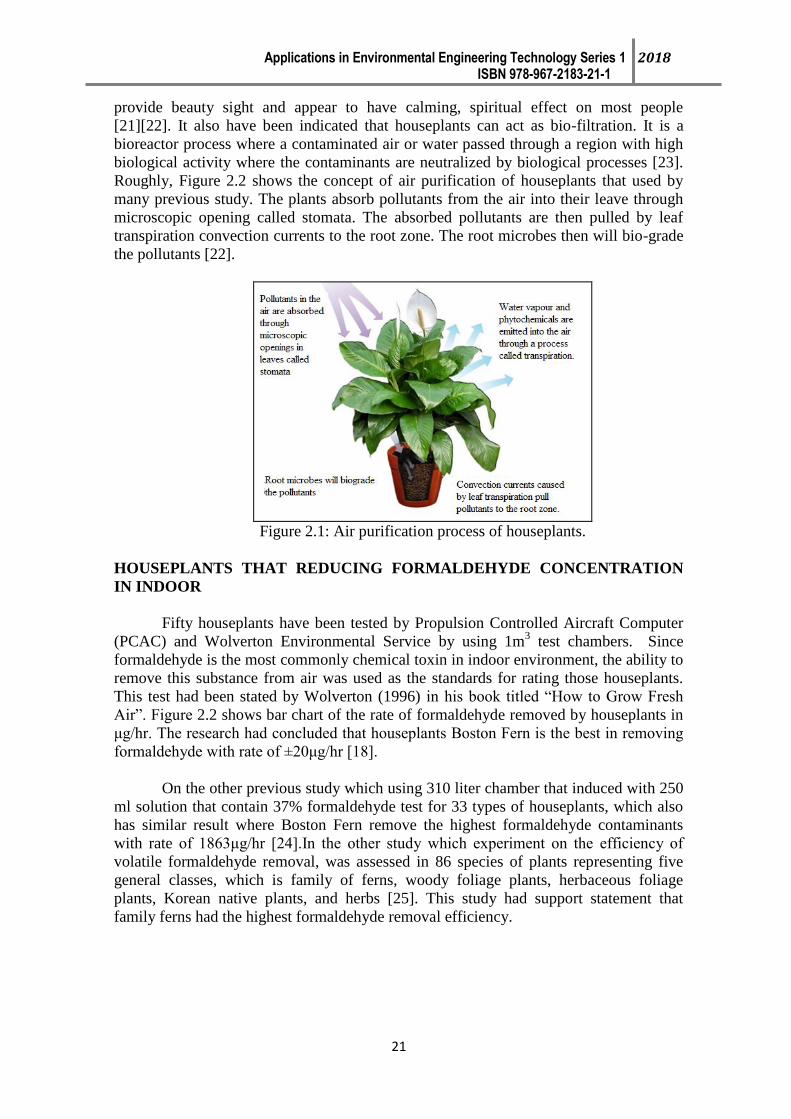
Roughly, Figure 2.2 shows the concept of air purification of houseplants that used by
many previous study. The plants absorb pollutants from the air into their leave through
microscopic opening called stomata. The absorbed pollutants are then pulled by leaf
transpiration convection currents to the root zone. The root microbes then will bio-grade
the pollutants [22].
Figure 2.1: Air purification process of houseplants.
HOUSEPLANTS THAT REDUCING FORMALDEHYDE CONCENTRATION
IN INDOOR
Fifty houseplants have been tested by Propulsion Controlled Aircraft Computer
(PCAC) and Wolverton Environmental Service by using 1m3 test chambers. Since
formaldehyde is the most commonly chemical toxin in indoor environment, the ability to
remove this substance from air was used as the standards for rating those houseplants.
This test had been stated by Wolverton (1996) in his book titled “How to Grow Fresh
Air”. Figure 2.2 shows bar chart of the rate of formaldehyde removed by houseplants in
μg/hr. The research had concluded that houseplants Boston Fern is the best in removing
formaldehyde with rate of ±20μg/hr [18].
On the other previous study which using 310 liter chamber that induced with 250
ml solution that contain 37% formaldehyde test for 33 types of houseplants, which also
has similar result where Boston Fern remove the highest formaldehyde contaminants
with rate of 1863μg/hr [24].In the other study which experiment on the efficiency of
volatile formaldehyde removal, was assessed in 86 species of plants representing five
general classes, which is family of ferns, woody foliage plants, herbaceous foliage
plants, Korean native plants, and herbs [25]. This study had support statement that
family ferns had the highest formaldehyde removal efficiency.

Applications in Environmental Engineering Technology Series 1 2018 ISBN 978-967-2183-21-1
22
0
2
4
6
8
10
12
14
16
18
20
Bo
sto
n F
ern
Flo
rist
's M
um
Ger
bera
Dai
sy
Dw
arf
Dat
e P
alm
Jan
et C
raig
Bam
bo
o P
alm
Kim
berl
ey Q
ueen
Fer
n
Ru
bb
er
Pla
nt
Engl
ish
Ivy
We
ep
ing
Fig
Pe
ace
Lily
Are
ca P
alm
Co
rn P
lan
t
Lad
y P
alm
Sch
eff
lera
Dra
gon
Tre
e
Wa
rne
cke
i
Lily
Tu
rf
Den
dro
bium
Orc
hid
Dum
b Ca
ne (
Exo
tica)
Tuli
p
Ficu
s A
lii
Kin
g o
f H
ear
ts
Pa
rlo
r P
alm
Ch
ine
se E
verg
ree
n
Spid
er
Pla
nt
Ban
ana
Aza
lea
Re
d E
me
rald
Ph
ilod
en
dro
n
Dum
b Ca
ne (
Cam
illa)
Ele
ph
an
t Ear
Ph
ilod
end
ron
Go
lde
n P
oth
os
No
rfo
lk Is
lan
d P
ine
Wax
Be
gon
ia
Pra
ye
r P
lan
t
Oak
Le
af I
vy
Ch
ristm
as C
actu
s
Lacy
Tre
e P
hilo
de
ndro
n
Arr
owhe
ad V
ne
He
art
-le
af
Ph
ilo
de
nd
ron
Lad
y Ja
ne
Pe
aco
ck P
lan
t
Po
inse
ttia
Cyc
lam
en
Mo
th O
rch
id
Urn
Pla
nt
Cro
ton
Sna
ke P
lan
t
Alo
e V
era
Kela
nch
oe
Figure 2.2: Chart of rate of formaldehyde removed by houseplants(μg/hr)
(Source: Wolverton, 1996)
2.2 METHODOLOGY
Houseplant namely Boston Fern (Nephrolepis exaltata) has selected for this
study. The four selected plants were having slightly similar in size and height with two
moths aged. Next, all pots of the plants also had approximately same number of leaves
(28-34 leaves) to ensure their total area leaves was approximately 1120-1360 cm2 per
plant.
Figure 2.3: Boston Fern
The main areas of interest for this study are two identical lecturer rooms which
have same designation; same floor area and ceiling height. Both rooms namely as Room
1and Room 2, have same ventilation system used (MVAC), receive same rate of
ventilation (0m/s), did not use any additional air filtration device and receive same
amount of daily sunlight. Figure 2.4(a), Figure 2.4(b), Figure 2.4(c) and Figure 2.4(d)
show the floor plan and the full view of both rooms.
Applications in Environmental Engineering Technology Series 1 2018 ISBN 978-967-2183-21-1
23
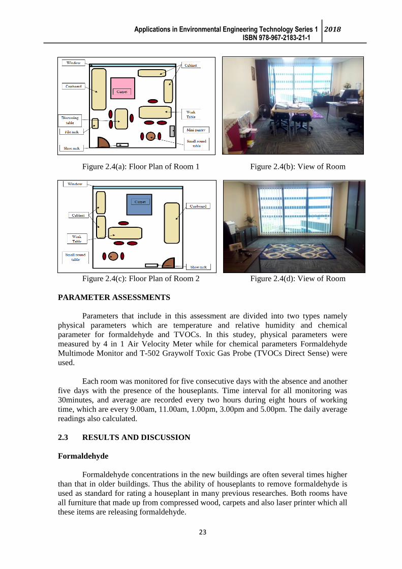
Figure 2.4(a): Floor Plan of Room 1 Figure 2.4(b): View of Room
Figure 2.4(c): Floor Plan of Room 2 Figure 2.4(d): View of Room
PARAMETER ASSESSMENTS
Parameters that include in this assessment are divided into two types namely
physical parameters which are temperature and relative humidity and chemical
parameter for formaldehyde and TVOCs. In this studey, physical parameters were
measured by 4 in 1 Air Velocity Meter while for chemical parameters Formaldehyde
Multimode Monitor and T-502 Graywolf Toxic Gas Probe (TVOCs Direct Sense) were
used.
Each room was monitored for five consecutive days with the absence and another
five days with the presence of the houseplants. Time interval for all monitoring was
30minutes, and average are recorded every two hours during eight hours of working
time, which are every 9.00am, 11.00am, 1.00pm, 3.00pm and 5.00pm. The daily average
readings also calculated.
2.3 RESULTS AND DISCUSSION
Formaldehyde
Formaldehyde concentrations in the new buildings are often several times higher
than that in older buildings. Thus the ability of houseplants to remove formaldehyde is
used as standard for rating a houseplant in many previous researches. Both rooms have
all furniture that made up from compressed wood, carpets and also laser printer which all
these items are releasing formaldehyde.

Applications in Environmental Engineering Technology Series 1 2018 ISBN 978-967-2183-21-1
24
Figure 2.5(a) and Figure 2.5(b) indicated the concentrations of formaldehyde
versus time for Room 1 and Room 2. Both of them showed similar pattern where the
readings of formaldehyde were higher during morning, gradually decreased during
afternoon and become slightly unchanged during evening. This observation may due to
Mechanical Ventilation and Air Conditioning (MVAC) system in where the system will
only operating during the working hours, which make the formaldehyde that released
from certain items suspended in the rooms.
Figure 2.5(a) Figure 2.5(b)
Figure 2.6: Average concentrations of Formaldehyde in both rooms
Average readings of formaldehyde concentration in both rooms as shown in
Figure 2.6, was way far lower than acceptable range indicated by DOSH 2010, which is
0.1 ppm. However for Room 1, the readings was still slightly higher than Room 2 even
after placement of Boston Fern, this may due to activities by the occupants. The
observation showed that the frequent used of laser printer due to the occupant in Room 1
activity gave the significant impact of formaldehyde concentration in Room 1 compared
to Room 2. In addition, the activity of video display unit usage for meeting purpose in
Room 1 was also observed as the other contributor of formaldehyde and TVOC
concentrations as well. Besides, the occupant was also used correction fluid and marker
0
5
10
15
20
25
30
35
40
9am 11am 1pm 3pm 5pm
HC
OH
(pp
b)
Formaldehyde (HCHO) vs Time Reading for Room 2
Day 1
Day 2
Day 3
Day 4
Day 5
Day 6
Day 7
Day 8
Day 9
Day 100
5
10
15
20
25
30
35
40
9am 11am 1pm 3pm 5pm
HC
HO
(p
pb
)
Formaldehyde (HCHO) vs Time Reading for Room 1
Day 1
Day 2
Day 3
Day 4
Day 5
Day 6
Day 7
Day 8
Day 9

Applications in Environmental Engineering Technology Series 1 2018 ISBN 978-967-2183-21-1
25
pen in the room. This eventually effects the concentration of formaldehyde concentration
readings.
Most important, the readings of formaldehyde for both rooms were drastically
decreased during the first day of placements of Boston Fern and continue decrease
readily until the end of monitoring. This shows the statement in line with Wolverton
(2010) which said that Boston Fern is good in reducing formaldehyde. However, the
formaldehyde concentration actually will decrease from time to time as claimed by
Salthammer et al. (2010) because items that release formaldehyde such as compressed
wood furniture in the room and carpets will release the contaminants lesser day by day.
TOTAL VOLATILE ORGANIC COMPOUNDS (TVOCS)
TVOCs had recently become priority of environmental interest among others
indoor pollutants. TVOCs is material that easy to volatiles with room temperature, and
example materials of TVOCs like benzene, toluene, xylene, styrene, and limonene
(Mahathir et al., 2014). TVOCs origins are building product emissions, human activities,
and infiltration of outdoor air. In other word, TVOCs are result from components
byproducts which produce toxic effects when it at high concentration (Allen et al.,
2016).
According to Figure 2.7(a) and Figure 2.7(b), each room had high initial readings
of TVOCs in the morning which was in range of 0.25-0.4ppm and decreased over time
throughout the day. This may caused by MVAC system in room was not operating
before working hours which make the TVOCs in indoor air suspended. After the air
conditioner activated a while, the air in the room then circulating as MVAC system also
will be activated and make the TVOCs readings decreased on the evening which usually
in range of 0.1-0.3ppm in Room 1 and 0.1-0.25ppm in Room 2.
Figure 2.7(a): TVOC in Room 1 Figure 2.7(b): TVOC in Room 2
In addition, the line graph shows in Figure 4.4, the TVOCs readings in
Room 1 were fluctuated but TVOCs readings in Room 2 were almost in consistent
pattern. This may because occupant of Room 1 carried out many activities in the room
and spend more times in the room compared to occupant of Room 2 which conduct
fewer activities and spend less time in the rooms. Occupant of Room 1 spend about 6-8
hours in the rooms whereas occupant Room 1 spend only about 0-2 hours in the rooms
every day with the air conditioning system switched on.
0
0.05
0.1
0.15
0.2
0.25
0.3
0.35
0.4
9am 11am 1pm 3pm 5pm
TVO
Cs
(pp
m)
TVO Cs vs Time Reading in Room 1
Day 1
Day 2
Day 3
Day 4
Day 5
Day 6
Day 7
Day 8
Day 9 0
0.05
0.1
0.15
0.2
0.25
0.3
0.35
0.4
9am 11am 1pm 3pm 5pm
TV
OC
s (p
pm
)
TVO Cs vs Time Reading in Room 2
Day 1
Day 2
Day 3
Day 4
Day 5
Day 6
Day 7
Day 8
Day 9

Applications in Environmental Engineering Technology Series 1 2018 ISBN 978-967-2183-21-1
26
Figure 2.8: Average concentrations of TVOC in both rooms
According to Figure 2.8, average TVOCs readings for every consecutive
monitoring day in both room were unstable but still under acceptable range that stated by
DOSH which is under 0.3 ppm. However, the pattern showed slightly decreased values
of TVOCs after presence of Boston Fern in both rooms which were in range of 0.15-
0.25ppm compared to readings prior to the presence of Boston Fern which was in the
range of 0.2-0.3ppm. There were a huge difference of readings in Day 5 and Day 6
showed by readings in Room 2.
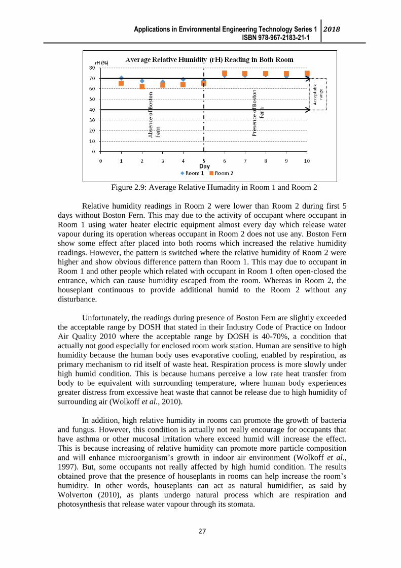
RELATIVE HUMIDITY
Figure 2.9 shows that both rooms have high relative humidity readings, either
with absence or presence of Boston Fern. This may due to problem of Motor Vehicle Air
Conditioning (MVAC) system. The air in the rooms does not well circulated, causing the
exceeded humid were still suspended in the room air.
However, relative humidity readings in Room 2 shows a obvious different range
of readings where the readings for Day 1 until Day 5 (absence of Boston Fern) were
between 60-70% while readings for Day 6 until Day 10 (presence of Boston Fern) were
slightly higher, between 70-80%. Besides, the average readings of relative humidity
readings as shown in Figure 4.6 also admitted that the relative humidity of both room
show increasing pattern during presence of Boston Fern.
Applications in Environmental Engineering Technology Series 1 2018 ISBN 978-967-2183-21-1
27
Figure 2.9: Average Relative Humadity in Room 1 and Room 2
Relative humidity readings in Room 2 were lower than Room 2 during first 5
days without Boston Fern. This may due to the activity of occupant where occupant in
Room 1 using water heater electric equipment almost every day which release water
vapour during its operation whereas occupant in Room 2 does not use any. Boston Fern
show some effect after placed into both rooms which increased the relative humidity
readings. However, the pattern is switched where the relative humidity of Room 2 were
higher and show obvious difference pattern than Room 1. This may due to occupant in
Room 1 and other people which related with occupant in Room 1 often open-closed the
entrance, which can cause humidity escaped from the room. Whereas in Room 2, the
houseplant continuous to provide additional humid to the Room 2 without any
disturbance.
Unfortunately, the readings during presence of Boston Fern are slightly exceeded
the acceptable range by DOSH that stated in their Industry Code of Practice on Indoor
Air Quality 2010 where the acceptable range by DOSH is 40-70%, a condition that
actually not good especially for enclosed room work station. Human are sensitive to high
humidity because the human body uses evaporative cooling, enabled by respiration, as
primary mechanism to rid itself of waste heat. Respiration process is more slowly under
high humid condition. This is because humans perceive a low rate heat transfer from
body to be equivalent with surrounding temperature, where human body experiences
greater distress from excessive heat waste that cannot be release due to high humidity of
surrounding air (Wolkoff et al., 2010).
In addition, high relative humidity in rooms can promote the growth of bacteria
and fungus. However, this condition is actually not really encourage for occupants that
have asthma or other mucosal irritation where exceed humid will increase the effect.
This is because increasing of relative humidity can promote more particle composition
and will enhance microorganism’s growth in indoor air environment (Wolkoff et al.,
1997). But, some occupants not really affected by high humid condition. The results
obtained prove that the presence of houseplants in rooms can help increase the room’s
humidity. In other words, houseplants can act as natural humidifier, as said by
Wolverton (2010), as plants undergo natural process which are respiration and
photosynthesis that release water vapour through its stomata.

Applications in Environmental Engineering Technology Series 1 2018 ISBN 978-967-2183-21-1
28
2.4 CONCLUSION
Percentage change value is measured of increase or decrease percentage which
represent the degree of change over time. From this study, it can be observed that the
presence of formaldehyde can reduced the folmaldehyde concentration up to 26% and
36.6 % for Room 1 and Room 2, respectively. While, the reduction of TVOCs were
recorded to be 15.5% and 18.9% for Room 1 and Room 2, respectively. However, the
present of this plant was also caused the increment in humadity around 2.8% to 6.1% for
both Rooms. As a conclusion, the presence of Bostern Fern in lecture room in Pagoh
Education Hub Administration Building can help in formaldehyde and TVOCs reduction
in order to maintain a clean air for good surrounding work area for staffs. The presence
also contribute to the indoor aesthetic for calm and relax feelings.
REFERENCES
[1] DOSH, Department of Occuputional Safety and Health (2010), Industry Code of
Practice on Indoor Air Quality 2010, Ministry of Human Resources Malaysia,
JKKP DP(S) 127/379/4-39
[2] Jones, A. P. (1999). Indoor Air Quality And Health. Atmospheric Environment,
33(28), 4535–4564.
[3] Sarbu, I., & Sebarchievici, C. (2013). Aspects Of Indoor Environmental Quality
Assessment In Buildings. Energy and Buildings, 60, 410–419.
[4] Yau, Y. H., Ding L.C., & Chew B.T. (2010). United Kingdom-Malaysia-Ireland
Engineering Science Conference 2011. Thermal Comfort And Indoor Air
Quality At Green Building In Malaysia.
[5] Barrese, E., Gioffrè, A., Scarpelli, M., Turbante, D., Trovato, R., & Iavicoli, S.
(2014). Occupational Diseases and Environmental Medicine, Indoor Pollution
in Work Office : VOCs , Formaldehyde and Ozone by Printer, (August Issue),
49–55.
[6] Dumas, T. (1982). Journal of Chromatography, Determination Of Formaldehyde
In Air By Gas Chromatography. A, 247(2), 289–295.
[7] Kim, K. J., Kil, M. J., Song, J. S., Yoo, E. H., Son, K.-C., & Kays, S. J. (2008)
Journal of the American Society for Horticultural Science, Efficiency Of
Volatile Formaldehyde Removal By Indoor Plants: Contribution Of Aerial Plant
Parts Versus The Root Zone. 133(4), 521–526.
[8] Wolkoff, P. (2013). International Journal of Hygiene and Environmental Health,
Indoor Air Pollutants in Office Environments: Assessment Of Comfort, Health,
and Performance., 216(4), 371–394.
[9] Salthammer, T., Mentese, S., & Marutzky, R. (2010). Chemical Reviews,
Formaldehyde In The Indoor Environment, 110(4).
[10] Andersen Helle V., Helene B. Klinke, Lis W. Funch, L. G. (2016). Test Results
and Assessment of Impact on Indoor Air Quality Environmental, Emission of
Formaldehyde from Furniture, (1815).

Applications in Environmental Engineering Technology Series 1 2018 ISBN 978-967-2183-21-1
29
[11] Mckone, T., Maddalena, R., Destaillats, H., Hammond, S. K., Hodgson, A.,
Russell, M., & Perrino, C. (2009). Indoor Pollutant Emissions from Electronic
Office Equipment.
[12] Destaillats, H., Maddalena, R. L., & Singer, B. C. (2007). Indoor Pollutants
Emitted by Office Equipment : A Review of Reported Data and Information
Needs, (4).
[13] Gesser, H. D. (1985). The Reduction of Indoor Formaldehyde Gas and that
Emanating From Urea Formaldehyde Foam Insulation ( UFFI ), 10, 305–307.
[14] Bourdin, D., Mocho, P., Desauziers, V., & Plaisance, H. (2014). Journal of
Hazardous Materials, Formaldehyde Emission Behavior of Building Materials :
On-Site Measurements and Modeling Approach to Predict Indoor Air
Pollution., 280, 164–173.
[15] Brasche, S., M. Bullinger, H. Gebhardt, V. Herzog, P. Hornung, B. Kruppa, E.
Meyer, M. Morfeld, R. Schwab, V. Mackensen, S. Winkens, and W. Bischof.
(1999). Proc. 8th Intl. Conf. Indoor Air Quality Climate. Factors Determining
Different Symptom Patterns of Sick Building Syndrome.
[16] Sakai, N., Yamamoto, S., Matsui, Y., Khan, F., & Talib, M. (2017). Science of
the Total Environment.Science of the Total Environment Characterization and
Source Profiling of Volatile Organic Compounds in Indoor Air of Private
Residences in Selangor State , Malaysia.
[17] Kamarul Aini Mohd Sari (2017), Module BNB 40103 Indoor Air Quality, Indoor
Air Pollution, Depatment of Civil Engineering Technology, Faculty of
engineering Technology, UTHM.
[18] Wolverton, B.C., 1996. How to Grow Fresh Air. Houseplants that Purify Your
Home or Office. Penguin Books, New York.
[19] Mahathir, M., Shamsuri, S., Leman, A. M., Sabree, M. A. R., & Shafii, H.
(2014). Proposed Study, Monitoring of Indoor Plants Application for Indoor Air
Quality Improvement
[20] Mahathir, M., Shamsuri, S., Leman, A. M., & Shafii, H., (2015). Indoor Plants
as Agents Deterioration of Gas Pollution, (August Issue), 10–11.
[21] Russell, J. A., Hu, Y., Chau, L., Pauliushchyk, M., Anastopoulos, I., Anandan,
S., & Waring, M. S. (2014). Applied and Environmental Microbiology Indoor-
Biofilter Growth And Exposure To Airborne Chemicals Drive Similar Changes
In Plant Root Bacterial Communities., 80(16), 4805–4813.
[22] Wolverton, B.C., Wolverton, D.J., 1993. Journal of Mississippi Academy of
Sciences Plants And Soil Microorganisms: Removal Of Formaldehyde, Xylene,
And Ammonia From The Indoor Environment. 32, 11e15.
[23] Kim, K. J., Jeong, M. I. I., Lee, D. W., Song, J. S., Kim, H. D., Yoo, E. H., Han,
S. W. (2010). Hort Science, Variation in Formaldehvde Removal Efficiency
among Indoor Plant Species., 45(10), 1489–1495.

Applications in Environmental Engineering Technology Series 1 2018 ISBN 978-967-2183-21-1
30
Applications in Environmental Engineering Technology Series 1 2018 ISBN 978-967-2183-21-1
31
CHAPTER 3
CARBON DIOXIDE REMOVAL IN LIQUID AND GAS USING
BIOGRANULES CONTAINING PHOTOSYNTHETIC PIGMENT
IN PALM OIL MILL EFFLUENT TREATMENT
Mohamed Zuhaili Bin Mohamed Najib, Kamarul Aini Mohd Sari, Rahmat Muslim,
Nurdalila Saji, Mariah Awang, Mohamad Ashraf Abd Rahman, Fatimah Mohamed
Yusop and Mohamad Faizal Bin Tajul Baharuddin
Faculty of Engineering Technology,
Universiti Tun Hussein Onn Malaysia, Parit Raja, Batu Pahat,
86400 Johor, Malaysia.
3.1 INTRODUCTION
Malaysia contributes 39 % of world palm oil production and 44 % of world exports [1].
According to [2], the total export of oil palm products in 2013 had increased by 4.3 % or
1.10 million tonnes to 25.66 million tonnes compared with 24.56 million tonnes in 2012.
Throughout the years, the crude palm oil (CPO) production has increased from only 1.3
million tonnes in 1975, to 4.1 million tonnes in 1985 and 7.8 million tonnes in 1995 to
17.56 million tonnes in 2009 [3]. Among all biomass by-products from the palm oil
industry which include the palm kernel shell (PKS) and empty fruit bunch (EFB), only
the palm oil mill effluent (POME) is not commercially re-used.
The palm oil production has resulted in a massive waste generation, as it was
estimated that nearly 60 million tonnes of POME was generated from a total of 421 palm
oil mills in Malaysia [4]. There are approximately 0.2 million tonnes of methane (CH4),
or 4 million tonnes of CO2 equivalent, being emitted from the entire palm oil industry in
Malaysia per year [5]. In addition, [6] had claimed that the average greenhouse gases
(GHG) emissions produced from processing one tonne CPO was 1100 kg CO2e. Also,
each tonne of POME was expected to generate approximately 28.13 m3 of biogas.
The conventional ponding system has been a less preferable method to reduce the
biological and chemical constituents of POME. Despite its being relatively simple and
reliable, it produces large amounts of sludge and takes up large land area. The ponding
system, especially the anaerobic process produces harmful and odorous gases such as
sulphur dioxide (SO2), CH4 and carbon dioxide (CO2) [7, 8].
According to [9], about 28.82 m3 of biogas produced from one tonne POME
consisted of 18.72 m3 CH4 and 10.08 m
3 CO2. Hence, the abundance of these gases in
the air may lead to global warming, climate change and danger to public health. Besides,

Applications in Environmental Engineering Technology Series 1 2018 ISBN 978-967-2183-21-1
32
the facultative ponding system also produces scum and tends to generate CO2 as a by-
product of biological reactions. Presently, there were some alternative treatments
proposed to be used for primary treatment of POME such as membrane filtration and
evaporation to overcome previous limitations [10, 11, 12]. Nevertheless, similar
problems still occur, such as the formation of scum, sludge floating problems, and high
energy consumption.
By combining the cultivation of photosynthetic microorganisms with biofixation
of CO2, the cost of culture media for an industrial scale can be minimized while the
carbon emission can be neutralized [13,14]. Nevertheless, the separation of
photosynthetic bacteria after wastewater treatment became an issue for practical
applications because of their poor solid-liquid separation [15,16].
Generally, granulation technology offers some advantages for industrial process
as the cells are entrapped into suitable gel matrices which most of their viability and
physiological activity are retained [17,18]. This study provides a potential alternative for
conventional activated sludge treatment as the technology offers reduction of CO2
emission from POME, as well simultaneously removing organic and nutrient, for a better
solid-liquid separation in wastewater. In other words, the benefits claim the promotion of
clean and efficient energy production technology especially for small footprint
wastewater treatment process.
In this chapter, biogranules containing photosynthetic pigments used were
developed by [19] in a sequencing batch reactor (SBR) using high strength agricultural
wastewater such as POME. The next section will explain the experimental setup of the
batch reactor and also discuss the capability of developed biogranules containing
photosynthetic pigments for removal of CO2 in liquid and gas phases. The experiments
results were then analyzed using the statistical analysis such as Minitab 17.
3.2 REMOVAL OF CARBON DIOXIDE IN GAS AND LIQUID
The wastewater used was the treated POME taken from the final pond (aerobic or algae
pond) of a local palm oil mill ponding system located at Bukit Besar, Kulai in Johor due
to its low organic content compared to raw POME generated directly from the factory.
In principal, in the ponding treatment system, the raw POME is channelled
through several ponds consisting of anaerobic, facultative and aerobic pond as shown in
Figure 3.1. These steps are important to allow biological conversion of diverse types
organic compounds into smaller readily degradable molecules depending on the
activities of indigenous microorganisms. In terms of biodegradability, [19] had stated
that the BOD/COD value of the POME used in this study was closer to 0.2 which makes
it biodegradable [20] because some of readily biodegradable organic molecules were
removed during previous treatment.
Initially, the collected sample was screened using a 2.35 mm sieve to remove any
debris and large particles. Next, the sample was stored in the cool room at temperature
about 4 oC. Additionally, the POME was autoclaved to reduce the oil and grease that
could affect aerobic granulation process [21] and also limit the rate of photosynthesis
due to low light penetration [22].

Applications in Environmental Engineering Technology Series 1 2018 ISBN 978-967-2183-21-1
33
Figure 3.1: Locations of the POME collected from palm oil mill ponding treatment
system
The CO2 is readily soluble in water as it presents in water in the form of a
dissolved gas. Normally, the surface waters possess less than 10 ppm of free CO2, while
some ground waters may easily exceed that concentration. Furthermore, the CO2
solubility is 200 times more than O2 for temperatures of 0-30 oC.
In this study, 50 mL bottles were employed where a dosage of 100 % CO2 gas
(initial concetration ≈ 400 ppm) was dispersed upon bubbling slowly through the 20 mL
POME to measure the CO2 in gas and liquid form as shown in Figure 3.2. It was
operated under the duration of light/dark cycles of 12:12 hours, by controlling the
lighting system to provide substantially constant illumination. The bottles were properly
sealed with parafilm to avoid any leakage of CO2 as well as other gases coming from
outside the bottles.
A portable CO2 meter (Extech EA80) was applied to detect the CO2 gas taken-up
from the headspace of the bottles while a titrimetric method HACH CO2 Test Kit (Model
CA-23) for CO2 in the liquid phase. This experiment was monitored for a few days
(approximately seven days) till the CO2 measurements become steady. In addition, the
FESEM-EDX (Carls Zeiss Supra 35 VPSEM) was used to analysed the morphological
changes and composition of the biogranules during the experiment.

Applications in Environmental Engineering Technology Series 1 2018 ISBN 978-967-2183-21-1
34
Figure 3.2: Schematic overview of CO2 removal test
3.3 RESULTS AND DISCUSSIONS
The graph plotted in Figure 3.3 compares the percentage of CO2 removal in gas with the
CO2 concentration in liquid for seven days. At the beginning, the removal of CO2 gas
increased to approximately 22 % and then slightly reduced to 19 % over the next three
days. In contrast, during that period, the CO2 concentration in liquid experiences an
upward trend starting the period at about 55 mg/L.
The CO2 level in liquid continued to rise gradually finishing at nearly 50 % (90
mg/L); the removal efficiency of CO2 gas improved from 19 to 27 % at the same time.
Nevertheless, the average CO2 removal in gas was inconsistent which the plotted data
went up and lastly falls below than 20 %. Interestingly, the CO2 concentration in liquid
tends to grow slowly throughout the experiment.
To sum up the results, it was believed that the CO2 removed from the air
increases proportionally with the percentage of CO2 removed in liquid. Additionally, the
overall decrement of CO2 gas in the atmosphere was caused by either the absorption of
CO2 into the liquid at atmospheric pressure or the biological fixation of CO2 by
photosynthetic microorganisms [23].
When examined using FESEM as shown in Figure 3.4, an interesting formation
of hexagonal crystals (expected to be calcite) about 7.0 µm in length was observed. This
finding was also found by [24]. Such phenomenon suggested it is related to dissolved
inorganic carbon (DIC) mechanism as it could served as a supplementary way to
sequester carbon [25]. With the increase availability of carbon source as a result of high
DIC concentration will influence several key enzymes in carbon metabolism such as
carbonic anyhydrase and Rubisco. A higher carboxylating activity will result increment
in photosynthesis [26].
CO2
meter
CO2 detector
Initial CO2 ≈
400 ppm
Gas
capturing
container
Air
pump
Microbial granules containing photosynthetic bacteria + POME
Fluorescent
lamps
Parafilm
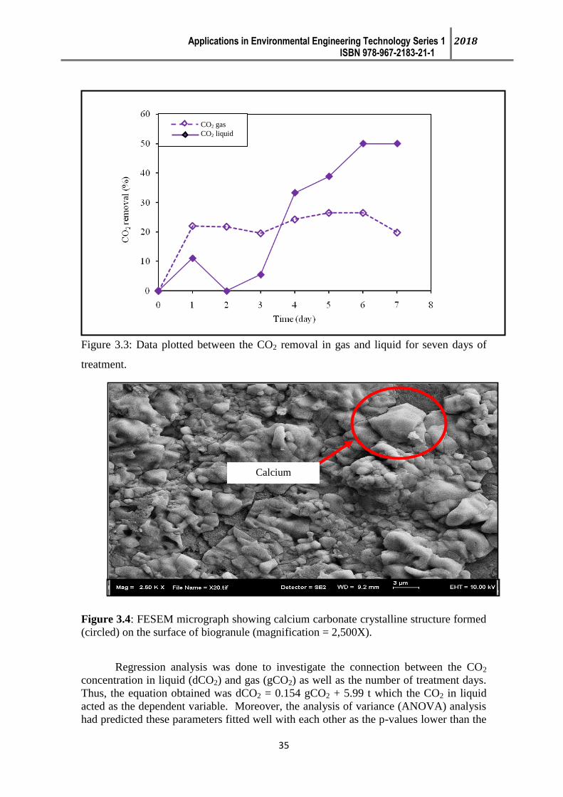
Applications in Environmental Engineering Technology Series 1 2018 ISBN 978-967-2183-21-1
35
Figure 3.3: Data plotted between the CO2 removal in gas and liquid for seven days of
treatment.
Figure 3.4: FESEM micrograph showing calcium carbonate crystalline structure formed
(circled) on the surface of biogranule (magnification = 2,500X).
Regression analysis was done to investigate the connection between the CO2
concentration in liquid (dCO2) and gas (gCO2) as well as the number of treatment days.
Thus, the equation obtained was dCO2 = 0.154 gCO2 + 5.99 t which the CO2 in liquid
acted as the dependent variable. Moreover, the analysis of variance (ANOVA) analysis
had predicted these parameters fitted well with each other as the p-values lower than the
CO2 gas
CO2 liquid
Calcium
carbonate
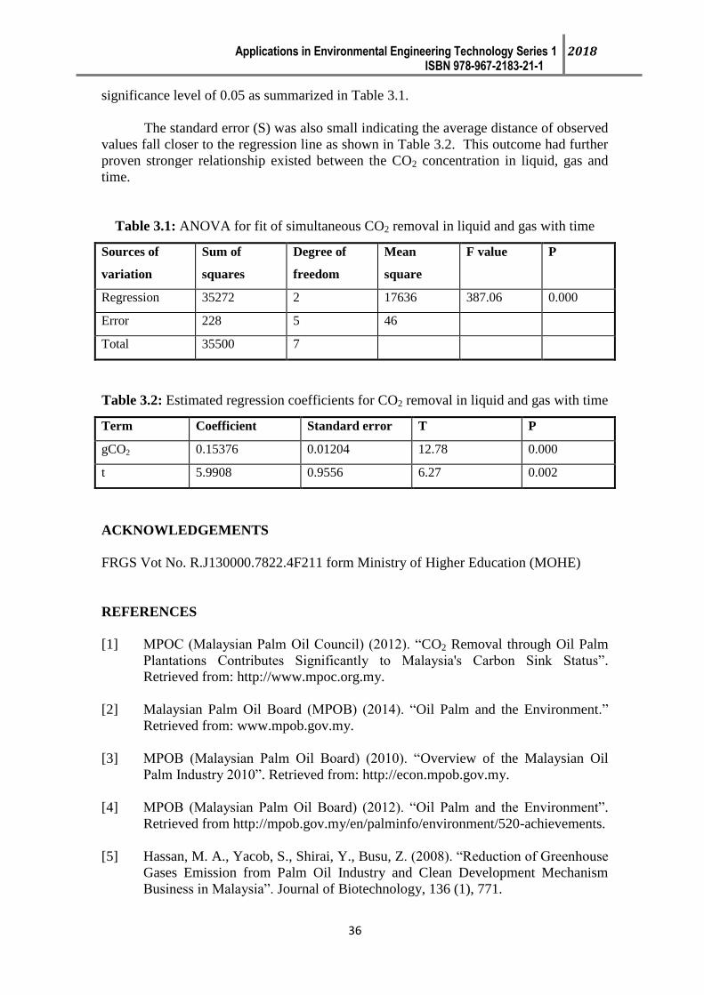
Applications in Environmental Engineering Technology Series 1 2018 ISBN 978-967-2183-21-1
36
significance level of 0.05 as summarized in Table 3.1.
The standard error (S) was also small indicating the average distance of observed
values fall closer to the regression line as shown in Table 3.2. This outcome had further
proven stronger relationship existed between the CO2 concentration in liquid, gas and
time.
Table 3.1: ANOVA for fit of simultaneous CO2 removal in liquid and gas with time
Sources of
variation
Sum of
squares
Degree of
freedom
Mean
square
F value P
Regression 35272 2 17636 387.06 0.000
Error 228 5 46
Total 35500 7
Table 3.2: Estimated regression coefficients for CO2 removal in liquid and gas with time
Term Coefficient Standard error T P
gCO2 0.15376 0.01204 12.78 0.000
t 5.9908 0.9556 6.27 0.002
ACKNOWLEDGEMENTS
FRGS Vot No. R.J130000.7822.4F211 form Ministry of Higher Education (MOHE)
REFERENCES
[1] MPOC (Malaysian Palm Oil Council) (2012). “CO2 Removal through Oil Palm
Plantations Contributes Significantly to Malaysia's Carbon Sink Status”.
Retrieved from: http://www.mpoc.org.my.
[2] Malaysian Palm Oil Board (MPOB) (2014). “Oil Palm and the Environment.”
Retrieved from: www.mpob.gov.my.
[3] MPOB (Malaysian Palm Oil Board) (2010). “Overview of the Malaysian Oil
Palm Industry 2010”. Retrieved from: http://econ.mpob.gov.my.
[4] MPOB (Malaysian Palm Oil Board) (2012). “Oil Palm and the Environment”.
Retrieved from http://mpob.gov.my/en/palminfo/environment/520-achievements.
[5] Hassan, M. A., Yacob, S., Shirai, Y., Busu, Z. (2008). “Reduction of Greenhouse
Gases Emission from Palm Oil Industry and Clean Development Mechanism
Business in Malaysia”. Journal of Biotechnology, 136 (1), 771.

Applications in Environmental Engineering Technology Series 1 2018 ISBN 978-967-2183-21-1
37
[6] Hosseini, S. E., Abdul Wahid, M. (2015). “Pollutant in Palm Oil Production
Process”. Journal of the Air and Waste Management Association, 65(7), 773-781.
[7] Kusrini, E., Lukita, M., Gozan, M., Susanto, B. H., Widodo, T. W., Nasution, D.
A., Wu, S., Rahman, A., Siregar, Y. D. I. (2016). “Biogas from Palm Oil Mill
Effluent: Characterization and Removal of CO2 Using Modified Clinoptilolite
Zeolites in a Fixed-Bed Column”. International Journal of Technology, 7(4),
625-634.
[8] Daelman, M.R.J., van Voorthuizen, E.M., van Dongen, U.D.J.M., Volke, E.I.P.,
van Loosdrecth, M.C.M. (2012). “Methane Emission during Municipal
Wastewater Treatment”. Water Research 46: 3657-3670.
[9] Mathews, J., Ardiyanto, A. (2015). “Estimation of Greenhouse Gas Emissions
for Palm Oil Biodiesel Production: A Review and Case Study within the Council
Directives 2009/28/EC of the European Parliament”. Journal of Oil Palm,
Environment and Health, 6, 25-41.
[10] Abdulrahman, N. H., Azhari, N. H. (2016). “An Integrated UMAS for POME
Treatment”. Journal of Water Reuse and Desalination, 7(1), 1-8.
[11] Amat, N. A., Tan, Y. H., Lau, W. J., Lai, G. S., Ong, C. S., Mokhtar, N. M., Sani,
N. A. A., Ismail, A. F., Goh, P. S., Chong, K. C., Lai, S. O. (2015). “Tackling
Colour Issue of Anaerobically-Treated Palm Oil Mill Effluent Using Membrane
Technology”. Journal of Water Process Engineering, 8, 221-226.
[12] Poh, P. E., Tan, D. T., Chan, E. S., Tey, B. T. (2015). “Current Advances of
Biogas Production via Anaerobic Digestion of Industrial Wastewater”. In
Ravindra, P. (Ed.). Advances in Bioprocess Technology (pp. 149-163).
Switzerland:Springer International Publishing.
[13] Moreira, D., Pires, J. C. (2016). “Atmospheric CO2 Capture by Algae: Negative
Carbon Dioxide Emission Path”. Bioresource Technology, 215, 371-379.
[14] de Morais, M. G., Costa, J. A. V. (2007). “Biofixation of Carbon Dioxide by
Spirulina Sp. And Scenedesmus Obliquus Cultivated in a Three-Stage Serial
Tubular Photobioreactor”. Journal of Biotechnology, 129, 439-445.
[15] Qin, L., Liu, Q., Meng, Q., Fan, Z., He, J., Liu, T., Shen, C., Zhang, G. (2017).
“Anoxic Oscillating MBR for Photosynthetic Bacteria Harvesting and High
Salinity Wastewater Treatment”. Bioresource Technology, 224, 69-77.
[16] Sheng, G. P., Yu, H. Q., Yu, Z. (2005). “Extraction of Extracellular Polymeric
Substances from the Photosynthetic Bacterium Rhodopseudomonas
Acidophila”. Applied Microbiology and Biotechnology, 67(1), 125-130.
[17] Sarma, S. J., Tay, J. H., Chu, A. (2017). “Finding Knowledge Gaps in Aerobic
Granulation Technology”. Trends in Biotechnology, 35(1), 66-78.

Applications in Environmental Engineering Technology Series 1 2018 ISBN 978-967-2183-21-1
38
[18] Venugopalan, V. P., Nancharaiah, Y. V., Mohan, T. V. K., Narasimhan, S. V.
(2005). “Biogranulation: Self-Immobilised Microbial Consortia for High
Performance Liquid Waste Remediation”. BARC Newsletter, 254, 1-7.
[19] Najib, M. Z. M., Ujang, Z., Salim, M. R., Ibrahim, Z. (2017). “Developed
Microbial Granules Containing Photosynthetic Pigments for Carbon Dioxide
Reduction in Palm Oil Mill Effluent”. International Biodeterioration and
Biodegradation, 116, 163-170.
[20] Yan, G., Cai, B., Chen, C., Wang, Q., Guo, S. (2015). “Biodegradability
Evaluation of Pollutants in Acrylonitrile Wastewaters based on Particle Size
Distribution”. Desalination and Water Treatment, 53(10), 2792-2798.
[21] González, J., Figueiras, F. G., Aranguren-Gassis, M., Crespo, B. G., Fernández,
E., Morán, X. A. G., Nieto-Cid, M. (2009). “Effect of a Simulated Oil Spill on
Natural Assemblages of Marine Phytoplankton Enclosed in Microcosms”.
Estuarine, Coastal and Shelf Science, 83(3), 265-276.
[22] Naing, A. H., Jeon, S. M., Park, J. S., Kim, C. K. (2016). “Combined Effects of
Supplementary Light and CO2 on Rose Growth and the Production of Good
Quality Cut Flowers”. Canadian Journal of Plant Science, 96(3), 503-510.
[23] Halmann, M. M., Steinberg, M. (1998). “Greenhouse Gas Carbon Dioxide
Mitigation: Science and Technology”. Florida: CRC Press LLC.
[24] Formia, A., Terranova, S., Antonaci, P., Pugno, N. M., Tulliani, J. M. (2015).
“Setup of Extruded Cementitious Hollow Tubes as Containing/Releasing Devices
in Self-Healing Systems”. Materials, 8(4), 1897-1923.
[25] Ramanan, R., Kannan, K., Deshkar, A., Yadav, R., Chakrabarti, T. (2010).
“Enhanced Algal CO2 Sequestration through Calcite Deposition by Chlorella Sp.
and Spirulina Platensis in a Mini-Raceway Pond”. Bioresource Technology,
101(8), 2616-2622
[26] Yang, Y., Gao, K. (2003). “Effects of CO2 Concentrations on the Freshwater
Microalgae, Chlamydomonas Reinhardtii, Chlorella Pyrenoidosa and
Scenedesmus obliquus (Chlorophyta)”. Journal of Applied Phycology, 15(5),
379-389.
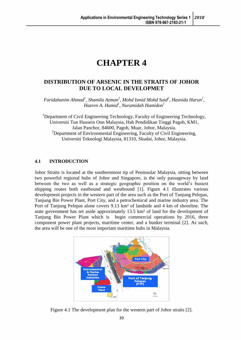
Applications in Environmental Engineering Technology Series 1 2018 ISBN 978-967-2183-21-1
39
CHAPTER 4
DISTRIBUTION OF ARSENIC IN THE STRAITS OF JOHOR
DUE TO LOCAL DEVELOPMET
Faridahanim Ahmad1, Shamila Azman
2, Mohd Ismid Mohd Said
2, Hasnida Harun
1,
Hazren A. Hamid1, Nuramidah Hamidon
1
1Department of Civil Engineering Technology, Faculty of Engineering Technology,
Universiti Tun Hussein Onn Malaysia, Hab Pendidikan Tinggi Pagoh, KM1,
Jalan Panchor, 84600, Pagoh, Muar, Johor, Malaysia. 2Department of Environmental Engineering, Faculty of Civil Engineering,
Universiti Teknologi Malaysia, 81310, Skudai, Johor, Malaysia.
4.1 INTRODUCTION
Johor Straits is located at the southernmost tip of Peninsular Malaysia, sitting between
two powerful regional hubs of Johor and Singapore, is the only passageway by land
between the two as well as a strategic geographic position on the world’s busiest
shipping routes both eastbound and westbound [1]. Figure 4.1 illustrates various
development projects in the western part of the area such as the Port of Tanjung Pelepas,
Tanjung Bin Power Plant, Port City, and a petrochemical and marine industry area. The
Port of Tanjung Pelepas alone covers 9.13 km² of landside and 4 km of shoreline. The
state government has set aside approximately 13.5 km² of land for the development of
Tanjung Bin Power Plant which is begin commercial operations by 2016, three
component power plant projects, maritime center, and a bunker terminal [2]. As such,
the area will be one of the most important maritime hubs in Malaysia.
Figure 4.1 The development plan for the western part of Johor straits [2].

Applications in Environmental Engineering Technology Series 1 2018 ISBN 978-967-2183-21-1
40
It is common knowledge that land use cause pollution to the estuarine ecosystem
by releasing undesired contaminants into waterways; such is agreed by researchers
around the world [3,4]. The development and traffic at the Johor Straits, as well as the
marine traffic at the Straits of Malacca and Singapore can cause harm to Pulai River
Estuary especially the mangrove and seagrass bed [5]. The seagrass bed is located at the
estuary and functions as a nursery and shelter for various vulnerable creatures such as
sea cucumbers, star fishes, and seahorses [6]. Seagrass beds represent one of the most
important ecological components in the coastal ecosystem; seagrass leaves act as
phytoremediators and cleanse seawater by absorbing dissolved metals [7]. Seagrass roots
play a role in shoreline protection by reducing coastal erosion from raging storms. The
estimation value for conservation of seagrass ecosystem is US$ 34,000 per hectare per
year [8]. The seagrass bed at Pulai estuary is approximately around of 3.15 km². The
public and environmentalists alike have raised their concerns about the severity of heavy
metal pollution caused by the development of petrochemical and maritime industries
along Pulai River and Straits of Johor. Arsenic (As) have to cause of various deleterious
effects in fish and to the aquatic ecosystem [9]. Hence, this study was conducted to
evaluate the distribution of these metals in water in order to establish the route taken by
the metals from land to the estuarine ecosystem.
4.2 MATERIALS AND METHOD
Pulai estuary receives water from upstream rivers, Malacca Straits and Singapore Straits.
Samples were collected on March 2012. Water samples from the rivers were collected
from 17 different locations (Figure 4.2). Sample collection from R11, R12, R13, R14,
R15, R16 and R17 were by speedboat, while the rest were done by land. Figure 4.3
shows pictures taken while collecting the samples from R1, and R5.
Figure 4.2 River sampling sites: R1-R17 in Red points.

Applications in Environmental Engineering Technology Series 1 2018 ISBN 978-967-2183-21-1
41
Figure 4.3 Pictures of sampling locations a) on-going road construction (R1), b) on-
going road construction at Paradin River (R5).
Water samples were collected at multiple locations both within and surrounding
the seagrass bed in order to determine the distribution of the designated metals within
the seagrass bed as a whole and around it. The distance from the mouth of Pulai River to
the seagrass bed is approximately 4.8 km. The water samples were collected and kept in
high density polyethylene bottles. ArcGIS 9 of ArcMap version 9.3 was used to
determine metal distribution via Kriging data interpolation method.
4.3 RESULT AND DISCUSSION
Figure 4.4 shows the flow distribution of As, all the way to the seagrass bed of Pulai
estuary. It is suggested that the metals originate upstream, flow into Pulai River and
subsequently into Pulai Estuary where the seagrass bed is located. The pollutants are
may due to nearby development, land use, and oil spills from ship. Undesired metal
contaminates were trapped on the seagrass bed due to high metals concentration in
seagrass bed area compared to metals concentration at the upstream river. The seagrass
bed’s ability to trap metal contaminats is evident that it is functioning well.
As pollution occurs more harshly near the estuary especially at the eastern side of
Pulai River. The highest ranges are 3.51µg/L-3.82µg/L .The level of As was above Class
E (mangroves, estuarine and river-mouth water) for the standards and criteria for
seawater quality as determined by the Department of Environment of Malaysia. The
permitted levels for As under Class E are below 2.9µg/L. The eastern side of Pulai
River, also known as mouth of Pulai River is where the Port of Tanjung Pelepas is
located. As of this writing, the expansion of the port is still on-going. Moreover,
development projects nearby such as the Tanjung Bin Power Plant also contributes to
metal contamination. Indeed, the [10] claims that 80% of marine pollutants come from
land-based activities either through deliberate dumping or run-off from activities such as
agriculture, sewage and disposal, and oil spilled down drains and rivers.

Applications in Environmental Engineering Technology Series 1 2018 ISBN 978-967-2183-21-1
42
Figure 4.4 Kriging data interpolation of As distribution.
The seagrass bed cleanses seawater by absorbing dissolved metals and is a bioindicator
that reflects the overall health of the aquatic ecosystem [11,12]. Aside from that, the
seagrass bed acts as a buffer zone to protect against shoreline erosion [13].
4.4 CONCLUSION
Economic activity such as construction and maritime hubs contribute to the release of
dissolved metals into rivers and damage the estuarine ecosystem. Nowadays, in the 21st
century we are faced with the challenge of balancing construction for the nation’s
economic needs with the duty of protecting the environment. Keen monitoring of road
constructions, development, and shipping transits should be practiced at all times, with
contingency plans devised for unpredicted circumstances. A combination of such efforts
will reduce the likelihood of metal contaminants entering the estuarine ecosystem. Such
is to ensure the survival of both the estuarine ecosystem and vulnerable marine species
habitat which are valuable for generations to come.
ACKNOWLEDGEMENT
The authors wish to thank the Ministry of Higher Education (MOHE) of Malaysia and
Universiti Teknologi Malaysia for financial support [UTM RUG Vot 03J65]. Aside from
that, the authors would also like to thank Professor Emeritus Gustaf Olsson and Sir
Sheikh Irfizzad bin Sheikh Ismail, and Mrs. Suhaida Ahmad for his professional opinion
and expertise he provided the many meaningful discussions.

Applications in Environmental Engineering Technology Series 1 2018 ISBN 978-967-2183-21-1
43
REFERENCES
[1] A. Rizzo, and J. Glasson, "Iskandar Malaysia," Cities, pp. 417-427, 2012.
[2] Khazanah Nasional, " Comprehensive development plan for South Johor
Economic Region 2006-2025," Kuala Lumpur, Malaysia, 2016.
[3] D. G. F. Cunha, M. D. C. Calijuri and M. C. Lamparelli, " A trophic state index
for tropical/subtropical reservoirs (TSItsr)," Ecol. Eng., no. 60, pp. 126-
134,2013.
[4] A. Serafim, R. Company, B. Lopes, C. Pereira, A. Cravo, V.F. Fonseca, S.
França, M. J. Bebianno and H. N. Cabral, " Evaluation of sediment toxicity in
different Portuguese estuaries: Ecological impact of metals and polycyclic
aromatic hydrocarbons," Coast Shelf Sci., vol. 130, pp. 30-41, 2013.
[5] M.H.B.M. Rusli, "Protecting vital sea lines of communication: A study of the
proposed designation of the Straits of Malacca and Singapore as a particularly
sensitive sea area," Ocean Coast Manage., vol. 57, pp. 79-94, 2012.
[6] C.K. Choo, R. Serina and H.M. Khor, "S.O.S Files A journey to Sungai Pulai,"
Gelang Patah, Malaysia, 2009.
[7] C. M. O. Macinnis and P.J. Ralph, " Towards a more ecologically relevant
assessment of the impact of heavy metals on the photosynthesis of the seagrass,
Zostera capricorni," Marine Poll. Bull., vol. 45, pp. 100-106, 2002.
[8] F. T. Short, B. Polidoro, S. R. Livingstone, K. E. Carpenter, S. Bandeira, J. S.
Bujang, H. P. Calumpong, T. J. B. Carruthers, R. G. Coles, W. C. Dennison, P.
L. A. Erftemeijer, M. D. Fortes, A. S. Freeman, T. G. Jagtap, A. H. M. Kamal,
G.A. Kendrick, K. W. Judson, Y. A. La Nafie, I. M. Nasution, R. J. Orth, A.
Prathep, J. C. Sanciangco, B. V. Tussenbroek, S. G. Vergara, M. Waycott, and J.
C. Zieman, " Extinction risk assessment of the world's seagrass species," Biol.
Cons., vol. 144, pp. 1961-1971, 2011.
[9] R. Eisler, "Handbook of Chemical Risk Assessment Health Hazards to Human,
Plants, and Animals, Three Volume Set," CRC Press, 2002.
[10] World Wide Fund for Nature, "Marine problems: Pollution. Publishing WWF,"
http://wwf.panda.org/about_our_earth/blue_planet/problems/pollution/, Accssed
27 November 2013, 2010.
[11] S. Costantini, R. Giordano, L. Ciaralli, and E. Beccaloni, " Mercury, cadmium
and lead evaluation in Posidonia oceanica and Codium tomentosum," Marine
Poll. Bull., vol. 22, pp. 362-363, 1991.
[12] C. M. O. Macinnis-Ng and P. J. Ralph, " Variations in sensitivity to copper and
zinc among three isolated populations of the seagrass, Zostera capricorni, "
Journal of Experimental Marine Biol. Ecol., vol. 302, pp. 63-83, 2004.

Applications in Environmental Engineering Technology Series 1 2018 ISBN 978-967-2183-21-1
44
[13] F. T. Short and R. G. Coles, " Global seagrass research methods," Elsevier
Sciences B.V., Amsterdam., pp. 2, 2001.

Applications in Environmental Engineering Technology Series 1 2018 ISBN 978-967-2183-21-1
45
CHAPTER 5
UNDERSTANDING THE WASTEWATER MATRIX AND
CHARACTERISATION
Hazren A. Hamid, Hasnida Harun, Norshuhaila Mohamed Sunar, Faridahanim
Ahmad
Department of Civil Engineering Technology (JTKA)
Faculty of Engineering Technology (FTK),
Universiti Tun Hussein Onn Malaysia
5.1 INTRODUCTION
Adsorption is a complex process, as it involves the interaction of various
parameters. Moreover, the complexity and variability of the wastewater matrix also has a
direct impact on the process performance [1]. However, in a real-world wastewater
treatment plant (WWTP), the water matrix will be far more complex. The composition
of wastewater is typically a complex water matrix, often containing a variety of organic
and inorganic compounds. In addition, wastewater varies in composition both temporally
and spatially (within a WWTP and between different wastewater streams). The variation
in wastewater composition may contribute to the inaccuracies and decreased predictive
capabilities of models for the optimisation of remediation of copper from the wastewater
matrix. Therefore, the main objective for this chapter is to study and determine not only
the concentrations of heavy metals and their variations in wastewater samples, but also
the physicochemical properties of the wastewater as characterised by Water Quality
Practices.
This chapter is divided into four sections. The first section is focused essentially
on the correct laboratory practice required, prior to ICP-MS instrumental analysis, to
ensure robust analytical data. The second section provides the results of the analysis of
heavy metal concentrations and their variability in the influent and effluent samples. The
Water Quality Practices, including the physicochemical parameters, are described in
third section. The final section describes benchmark experiments that basically inform
the effects of wastewater matrix characteristics (wastewater composition and its
variability) on the adsorbent’s capability to remediate Cu(II) from this matrix.
5.2 RESULTS AND DISCUSSIONS
Sources of contamination of ICP-MS instrumental analysis
The analysis of metals with low detection limits involving concentrations of parts
per billion or parts per trillion is a difficult and complicated process, requiring extra care
during sample preparation [2]. Table 5.1 shows the limit of detection (LoD) and limit of
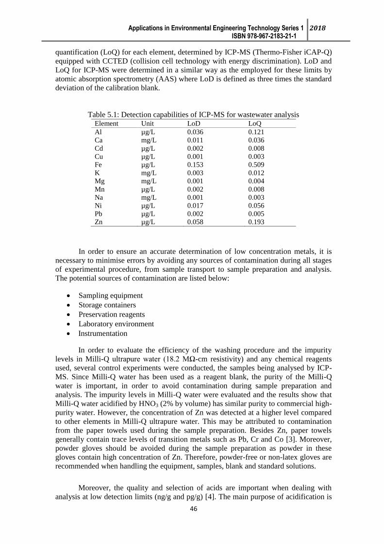
Applications in Environmental Engineering Technology Series 1 2018 ISBN 978-967-2183-21-1
46
quantification (LoQ) for each element, determined by ICP-MS (Thermo-Fisher iCAP-Q)
equipped with CCTED (collision cell technology with energy discrimination). LoD and
LoQ for ICP-MS were determined in a similar way as the employed for these limits by
atomic absorption spectrometry (AAS) where LoD is defined as three times the standard
deviation of the calibration blank.
Table 5.1: Detection capabilities of ICP-MS for wastewater analysis Element Unit LoD LoQ
Al µg/L 0.036 0.121
Ca mg/L 0.011 0.036
Cd µg/L 0.002 0.008
Cu µg/L 0.001 0.003
Fe µg/L 0.153 0.509
K mg/L 0.003 0.012
Mg mg/L 0.001 0.004
Mn µg/L 0.002 0.008
Na mg/L 0.001 0.003
Ni µg/L 0.017 0.056
Pb µg/L 0.002 0.005
Zn µg/L 0.058 0.193
In order to ensure an accurate determination of low concentration metals, it is
necessary to minimise errors by avoiding any sources of contamination during all stages
of experimental procedure, from sample transport to sample preparation and analysis.
The potential sources of contamination are listed below:
Sampling equipment
Storage containers
Preservation reagents
Laboratory environment
Instrumentation
In order to evaluate the efficiency of the washing procedure and the impurity
levels in Milli-Q ultrapure water (18.2 MΩ-cm resistivity) and any chemical reagents
used, several control experiments were conducted, the samples being analysed by ICP-
MS. Since Milli-Q water has been used as a reagent blank, the purity of the Milli-Q
water is important, in order to avoid contamination during sample preparation and
analysis. The impurity levels in Milli-Q water were evaluated and the results show that
Milli-Q water acidified by HNO3 (2% by volume) has similar purity to commercial high-
purity water. However, the concentration of Zn was detected at a higher level compared
to other elements in Milli-Q ultrapure water. This may be attributed to contamination
from the paper towels used during the sample preparation. Besides Zn, paper towels
generally contain trace levels of transition metals such as Pb, Cr and Co [3]. Moreover,
powder gloves should be avoided during the sample preparation as powder in these
gloves contain high concentration of Zn. Therefore, powder-free or non-latex gloves are
recommended when handling the equipment, samples, blank and standard solutions.
Moreover, the quality and selection of acids are important when dealing with
analysis at low detection limits (ng/g and pg/g) [4]. The main purpose of acidification is

Applications in Environmental Engineering Technology Series 1 2018 ISBN 978-967-2183-21-1
47
to avoid any metals being adsorbed onto the container walls. Therefore, HNO3 was used
for sample preparation and acid washing, as other acids such as H2SO4 and H3PO4 are
not suitable for analytical analysis by ICP-MS. This is because these acids do not
completely decompose in the plasma and can adhere to the interface components and ion
lenses causing signal instability [4]. Also, insoluble metal sulphates or phosphate may
form (depending on the acid used) and thus change the dissolved relevant metal ion
concentration. Furthermore, these acids have low purity levels compared to HNO3 and
HCl, causing further contamination of the samples [5].
According to Rodushkin et al., (2010), sample containers and glassware are
potential sources of contamination that require appropriate acid washing with dilute
nitric acid prior to use. The acid-washed laboratory glassware showed a significant
decrease in the contaminations and concentrations of selected elements. Also,
minimising the number of laboratory items used during the experimental process, and
keeping those washed items filled with acid, helps to reduce contamination.
The results show that acid-washed polypropylene sample tubes show lower
levels of contamination compared to acid-washed glassware. These results are in
agreement with the work of Rodushkin et al., (2010) who suggested that disposable
tubes made of polystyrene or polypropylene are much more suitable for ICP-MS sample
preparation. Moreover, glass sample containers should be avoided, as trace levels of
some metals in water commonly adsorb onto the glass wall, thus releasing measureable
concentrations of metals when acidic solutions are added. Moreover, a study assessing
metal contaminations leaching from a series of plastic recycling bottles during various
treatments has been reported [6]. The results revealed that heating and microwaving
significantly enhance antimony leaching from polyethylene terephthalate (PET) bottles.
Therefore, polypropylene and other plastic materials are more suitable for sample
storage. Similar sampling procedures were observed in other studies, where the collected
wastewater samples were stored in polypropylene containers prior to metal analysis [7].
The influence of storage time
The influence of storage time on heavy metal concentration is important, as ICP-
MS analysis can take several days (up to two days) due to instrument accessibility. The
stability of wastewater effluent was tested at different time intervals, prior to analysis by
ICP-MS. Monitoring the influence of storage time on the effluent was necessary, as it
allowed for the observation of any changes in wastewater quality during storage,
normally between 0 and 120 hours [8]. However, the impact of wastewater storage time
on water quality parameters is not necessary, as the adsorption process to remediate
Cu(II) from the wastewater matrix is performed using fresh effluent wastewater.
As shown in Table 5.2, the effluent samples do not show any significant changes
in heavy metal concentration during storage at 4 C for 72 or 120 hours. This
demonstrates that storage under these conditions does not affect the stability of heavy
metals. Besides proper storage, suitable sample containers, and acidification to a pH
below 2.0, have been used in this study, to minimise the precipitation and adsorption of
heavy metals on container walls.
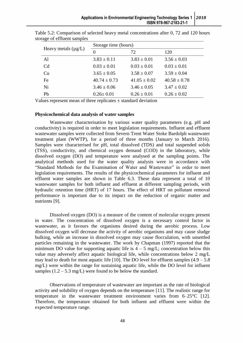
Applications in Environmental Engineering Technology Series 1 2018 ISBN 978-967-2183-21-1
48
Table 5.2: Comparison of selected heavy metal concentrations after 0, 72 and 120 hours
storage of effluent samples
Heavy metals (µg/L) Storage time (hours)
0 72 120
Al 3.83 ± 0.11 3.83 ± 0.01 3.56 ± 0.03
Cd 0.03 ± 0.01 0.03 ± 0.01 0.03 ± 0.01
Cu 3.65 ± 0.05 3.58 ± 0.07 3.59 ± 0.04
Fe 40.74 ± 0.73 41.05 ± 0.02 40.58 ± 0.78
Ni 3.46 ± 0.06 3.46 ± 0.05 3.47 ± 0.02
Pb 0.26± 0.01 0.26 ± 0.01 0.26 ± 0.02
Values represent mean of three replicates ± standard deviation
Physicochemical data analysis of water samples
Wastewater characterisation by various water quality parameters (e.g. pH and
conductivity) is required in order to meet legislation requirements. Influent and effluent
wastewater samples were collected from Severn Trent Water Stoke Bardolph wastewater
treatment plant (WWTP), for a period of three months (January to March 2016).
Samples were characterised for pH, total dissolved (TDS) and total suspended solids
(TSS), conductivity, and chemical oxygen demand (COD) in the laboratory, while
dissolved oxygen (DO) and temperature were analysed at the sampling points. The
analytical methods used for the water quality analysis were in accordance with
“Standard Methods for the Examination of Water and Wastewater” in order to meet
legislation requirements. The results of the physicochemical parameters for influent and
effluent water samples are shown in Table 6.3. These data represent a total of 10
wastewater samples for both influent and effluent at different sampling periods, with
hydraulic retention time (HRT) of 17 hours. The effect of HRT on pollutant removal
performance is important due to its impact on the reduction of organic matter and
nutrients [9].
Dissolved oxygen (DO) is a measure of the content of molecular oxygen present
in water. The concentration of dissolved oxygen is a necessary control factor in
wastewater, as it favours the organisms desired during the aerobic process. Low
dissolved oxygen will decrease the activity of aerobic organisms and may cause sludge
bulking, while an increase in dissolved oxygen may cause flocculation, with unsettled
particles remaining in the wastewater. The work by Chapman (1997) reported that the
minimum DO value for supporting aquatic life is 4 – 5 mg/L; concentration below this
value may adversely affect aquatic biological life, while concentrations below 2 mg/L
may lead to death for most aquatic life [10]. The DO level for effluent samples (4.9 – 5.8
mg/L) were within the range for sustaining aquatic life, while the DO level for influent
samples (1.2 – 5.3 mg/L) were found to be below the standard.
Observations of temperature of wastewater are important as the rate of biological
activity and solubility of oxygen depends on the temperature [11]. The realistic range for
temperature in the wastewater treatment environment varies from 6–25°C [12].
Therefore, the temperature obtained for both influent and effluent were within the
expected temperature range.

Applications in Environmental Engineering Technology Series 1 2018 ISBN 978-967-2183-21-1
49
Besides temperature, pH, a measure of the concentration of hydrogen ions in a
solution, is an important parameter in the operation of biological treatment units. An
increase in pH is due not only to industrial or other non-domestic discharges, but also to
the denitrification process [13]. As shown in Table 5.3, the pH of the samples were
within the permissible limit for wastewater, ranging from 6.0 to 9.0 . Moreover, all pH
values were also within the range set by the WHO for wastewater, ranging from 7.0 to
7.4 [14].
The TSS values of the influent and effluent were found to be in the range of 38.9
– 177.4 and 3.9–14.2 mg/L, respectively. According to literature, the wastewater can be
classified as follows: TSS < 100 mg/L as weak, 100 < TSS < 220 mg/L as medium, and
TSS > 220 mg/L as strong wastewater [15]. Therefore, TSS levels in influent and
effluent samples classified them as medium and weak wastewater, respectively.
Moreover, the permissible standard for TSS (for discharge) is 35 mg/L [16]. Therefore,
the effluent is safe to be discharged into the river, while the high TSS level in the
influent, due to the suspended particles from the waste, may affect aquatic life. However,
the mean values (0.5 g/L) obtained for TDS in both sampling points were within the
permissible limits stipulated by the WHO for wastewater [14].
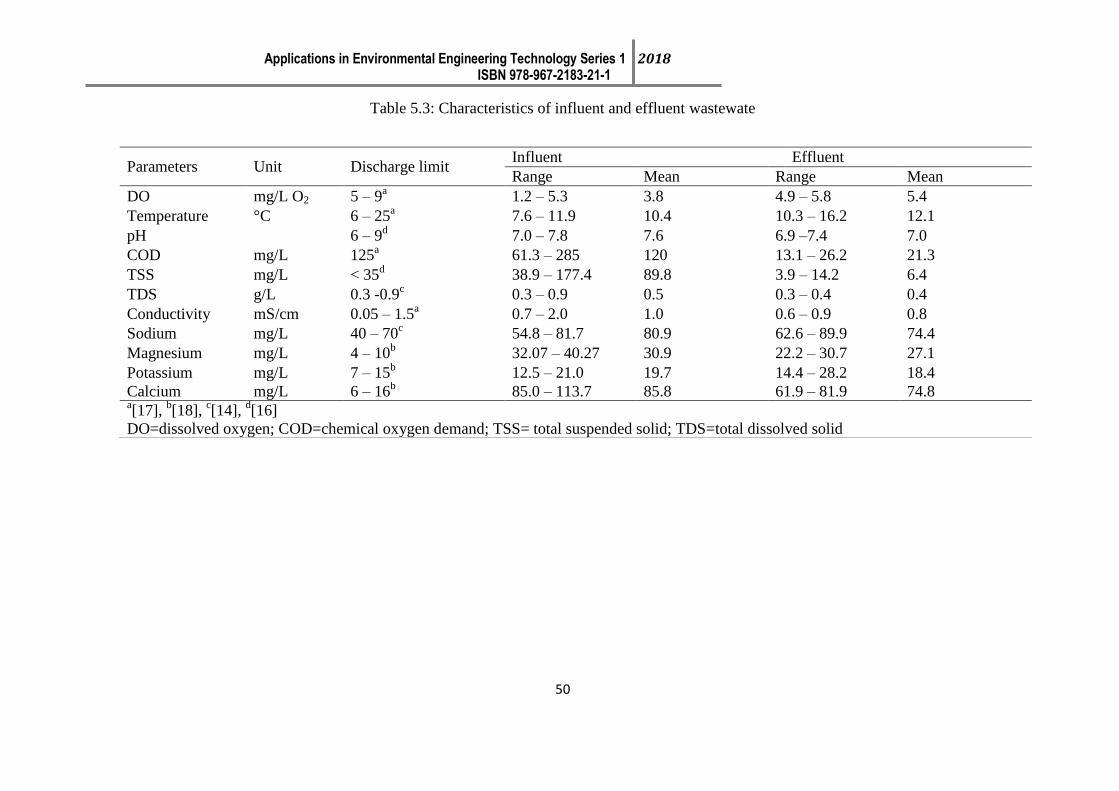
Applications in Environmental Engineering Technology Series 1 2018 ISBN 978-967-2183-21-1
50
Table 5.3: Characteristics of influent and effluent wastewate
Parameters Unit Discharge limit Influent Effluent
Range Mean Range Mean
DO mg/L O2 5 – 9a 1.2 – 5.3 3.8 4.9 – 5.8 5.4
Temperature °C 6 – 25a 7.6 – 11.9 10.4 10.3 – 16.2 12.1
pH
6 – 9d 7.0 – 7.8 7.6 6.9 –7.4 7.0
COD mg/L 125a 61.3 – 285 120 13.1 – 26.2 21.3
TSS mg/L < 35d 38.9 – 177.4 89.8 3.9 – 14.2 6.4
TDS
g/L 0.3 -0.9c
0.3 – 0.9 0.5 0.3 – 0.4 0.4
Conductivity mS/cm 0.05 – 1.5a 0.7 – 2.0 1.0 0.6 – 0.9 0.8
Sodium mg/L 40 – 70c
54.8 – 81.7 80.9 62.6 – 89.9 74.4
Magnesium mg/L 4 – 10b
32.07 – 40.27 30.9 22.2 – 30.7 27.1
Potassium mg/L 7 – 15b
12.5 – 21.0 19.7 14.4 – 28.2 18.4
Calcium mg/L 6 – 16b
85.0 – 113.7 85.8 61.9 – 81.9 74.8 a[17],
b[18],
c[14],
d[16]
DO=dissolved oxygen; COD=chemical oxygen demand; TSS= total suspended solid; TDS=total dissolved solid

Applications in Environmental Engineering Technology Series 1 2018 ISBN 978-967-2183-21-1
55
Conductivity measurements indicate the level of dissolved inorganic material
present. The biological nitrogen removal in wastewater treatment is the main cause of
the significant reduction in the conductivity of wastewater [19]. However, the increase in
the conductivity measurement of the influent indicates an unusual discharge, probably
from an industrial source. Moreover, the measurements obtained were in agreement with
other studies reported in the literature [20]. The conductivity of wastewater generally
ranges from 0.05 – 1.50 mS/cm, while some industrial wastewater is reported to have
higher conductivity measurements, up to 10.0 mS/cm [13].
Chemical Oxygen Demand (COD)
Chemical oxygen demand (COD) is one of the standard parameters, and provides
information on the level of organic contamination of wastewater. The procedure for the
determination of COD using the cuvette test. The COD of influent published in literature
was reported to be in the range of 200 to 600 mg/L [13]. Although the results for influent
were within this range, the COD concentrations of the influent during the sampling
periods were highly variable. However, it was observed that the measurements of
effluent samples consistently produced lower COD v alues than for influent samples.
COD levels of the effluent were stable for all sampling periods, at lower than 40
mg/L. This suggests that the high level of organic pollution due to anthropogenic activity
may have resulted in high values of COD in the influent. These results were in
agreement with the work of Gardner, Comber [21] who measured the characteristics of
final effluent from wastewater treatment plants around the UK. To summarise, variations
in water quality parameters were observed in both influent and effluent wastewater
samples. Table 5.4 summarises these water quality parameters for both influent and
effluent wastewater samples.
Table 5.4: Data for water quality parameters for influent and effluent wastewater
samples during February-March 2016
Parameters Influent
(average ± SD)
Effluent
(average ± SD)
Temperature (°C) 10.4 ± 0.9 12.1 ± 1.4
Dissolved oxygen (DO) (mg/L) 3.8 ± 4.2 5.3 ± 4.6
pH 7.6 ± 0.2 7.0 ± 0.1
Conductivity (mS/cm) 1.0 ± 0.3 0.8 ± 0.1
Chemical oxygen demand (COD) (mg/L) 120.4 ± 51.6 21.3 ± 4.1
Total suspended solid (TSS) (mg/L) 89.8 ± 37.3 6.4 ± 2.8
Total dissolved solid (TDS) (g/L) 0.5 ± 0.1 0.4 ± 0.1
*SD=standard deviation
Heavy metal concentration and its variation in influent and effluent wastewater
samples
The concentrations of heavy metals such as copper (Cu), cadmium (Cd),
chromium (Cr), iron (Fe), and lead (Pb) were determined using ICP-MS analysis of
influent and effluent samples taken from 10 different sampling periods at the Severn
Trent Water Stoke Bardolph WWTP. The concentration of heavy metals in influent and
effluent ranged from 0.01 – 439.05 µg/L and 0.006 – 99.82 µg/L, respectively. These
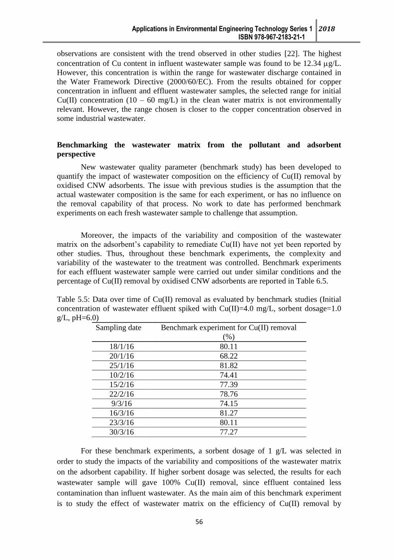
Applications in Environmental Engineering Technology Series 1 2018 ISBN 978-967-2183-21-1
56
observations are consistent with the trend observed in other studies [22]. The highest
concentration of Cu content in influent wastewater sample was found to be 12.34 g/L.
However, this concentration is within the range for wastewater discharge contained in
the Water Framework Directive (2000/60/EC). From the results obtained for copper
concentration in influent and effluent wastewater samples, the selected range for initial
Cu(II) concentration (10 – 60 mg/L) in the clean water matrix is not environmentally
relevant. However, the range chosen is closer to the copper concentration observed in
some industrial wastewater.
Benchmarking the wastewater matrix from the pollutant and adsorbent
perspective
New wastewater quality parameter (benchmark study) has been developed to
quantify the impact of wastewater composition on the efficiency of Cu(II) removal by
oxidised CNW adsorbents. The issue with previous studies is the assumption that the
actual wastewater composition is the same for each experiment, or has no influence on
the removal capability of that process. No work to date has performed benchmark
experiments on each fresh wastewater sample to challenge that assumption.
Moreover, the impacts of the variability and composition of the wastewater
matrix on the adsorbent’s capability to remediate Cu(II) have not yet been reported by
other studies. Thus, throughout these benchmark experiments, the complexity and
variability of the wastewater to the treatment was controlled. Benchmark experiments
for each effluent wastewater sample were carried out under similar conditions and the
percentage of Cu(II) removal by oxidised CNW adsorbents are reported in Table 6.5.
Table 5.5: Data over time of Cu(II) removal as evaluated by benchmark studies (Initial
concentration of wastewater effluent spiked with Cu(II)=4.0 mg/L, sorbent dosage=1.0
g/L, pH=6.0)
Sampling date Benchmark experiment for Cu(II) removal
(%)
18/1/16 80.11
20/1/16 68.22
25/1/16 81.82
10/2/16 74.41
15/2/16 77.39
22/2/16 78.76
9/3/16 74.15
16/3/16 81.27
23/3/16 80.11
30/3/16 77.27
For these benchmark experiments, a sorbent dosage of 1 g/L was selected in
order to study the impacts of the variability and compositions of the wastewater matrix
on the adsorbent capability. If higher sorbent dosage was selected, the results for each
wastewater sample will gave 100% Cu(II) removal, since effluent contained less
contamination than influent wastewater. As the main aim of this benchmark experiment
is to study the effect of wastewater matrix on the efficiency of Cu(II) removal by

Applications in Environmental Engineering Technology Series 1 2018 ISBN 978-967-2183-21-1
57
oxidised CNW adsorbents, it is important that the independent variable (benchmark
experiment) varies for ANN modelling, in order to detect the variation of wastewater
and the influence of this variable on the removal capability.
The results reported in Table 6.5 show that the percentage Cu(II) removal by
oxidised CNW adsorbents varies for each wastewater sample on different sampling
dates. Results over six weeks give an average 77.35 ± 4.15%. Although the difference
was low (around 4%), it is significant, and is likely to influence the efficiency and
capability of oxidised CNW adsorbents. Moreover, the results obtained only support and
covered only three months of sampling trips and focused on the effluent from only one
treatment plant. According to the United State EPA, the complexity of the wastewater
matrix depends on the number and volume of wastewater streams generated. The amount
and type of contamination found in wastewater will depend on the different industrial
activities realised in the area, the degree of urban development, and the type of treatment
facilities found around it .
The composition of wastewater in WWTPs depends on several factors, such as
compound physico-chemical properties, the climate conditions (temperature and sunlight
intensity), the type of treatment process employed, and the operational conditions of the
treatment process (temperature of operation and hydraulic retention time). Thus,
variations in water quality parameters were observed in both influent and effluent
wastewater samples, as shown in Table 6.4. For example, in the case of COD in influent
and effluent, the COD concentrations of the influent during the sampling periods were
highly variable. This indicated that the influent contained higher levels of organic
pollutants than did the effluent wastewater, which may have influenced the capability of
the adsorption process. Removal of Cu(II) from wastewater by an adsorption process is
dependent on the organic compound’s biodegradability, its volatility, and its ability to be
adsorbed onto adsorbents. Therefore, the composition of wastewater can vary
significantly from plant to plant, between different wastewater streams, and within a
plant at different times.
This demonstrates that the complexity of wastewater, in terms of its composition
and variability, affect the capability of the adsorbent to remediate Cu(II) from the
wastewater matrix. Moreover, the complexity and variation of wastewater composition
may also affect the accuracy and efficiency of mathematical modelling in predicting the
capability of this adsorbent to remediate spiked copper from the wastewater effluent.
ACKNOWLEDGEMENTS
Majlis Amanah Rakyat (MARA), Research Foundation-Flanders (FWO) for financial
support under the Odysseus program (grant G.0C60.13N) and KU Leuven for grant
OT/14/072, the Leverhulme Trust for MASS - Modelling and Analytics for a
Sustainable Society (Water, Energy and Food Nexus).
Applications in Environmental Engineering Technology Series 1 2018 ISBN 978-967-2183-21-1
58
REFERENCES
1. Hanafiah, M.A.K.M., et al., Enhanced adsorption of Pb(II) on chemically treated
neem (Azadirachta indica) leaf powder, in Material Science and Engineering
Technology Ii, K.M. Gupta, Editor. 2014. p. 128-133.
2. Zougagh, M., A.G. de Torres, and J.M.C. Pavon, Determination of cadmium in
water by ICP-AES with on-line adsorption preconcentration using DPTH-gel
and TS-gel microcolumns. Talanta, 2002. 56(4): p. 753-761.
3. Thomas, R., Practical Guide to ICP-MS: A Tutorial for Beginners, Third
Edition. 2013: CRC Press.
4. Rodushkin, I., E. Engstroem, and D.C. Baxter, Sources of contamination and
remedial strategies in the multi-elemental trace analysis laboratory. Analytical
and Bioanalytical Chemistry, 2010. 396(1): p. 365-377.
5. Balaram, V., Recent developments in analytical techniques for characterization
of ultra pure materials - An overview. Bulletin of Materials Science, 2005. 28(4):
p. 345-348.
6. Cheng, X., et al., Assessment of metal contaminations leaching out from
recycling plastic bottles upon treatments. Environmental Science and Pollution
Research, 2010. 17(7): p. 1323-1330.
7. Christophe, K., et al., Evaluation of heavy metals pollution of Nokoue Lake.
African Journal of Environmental Science and Technology, 2011. 5(3): p. 255-
261.
8. APHA, Standard Methods for the Examination of Water and Wastewater. 1998,
American Public Health Association: American Public Health Association:
Washington, D.C.
9. Merino-Solís, M., et al., The effect of the hydraulic retention time on the
performance of an ecological wastewater treatment system: An anaerobic filter
with a constructed wetland. Water, 2015. 7(3): p. 1149.
10. Chapman, D., Water Quality Assessment. A Guide to the use of Biota, Sediments
and water in Environmental Monitoring. 2 ed. 1997, E& FN Spon, London:
Taylor & Francis.
11. Spellman, F.R., Handbook of Water and Wastewater Treatment Plant
Operations, Third Edition. 2013: CRC Press.
12. Burton, F., et al., Wastewater Engineering: Treatment and Resource Recovery.
2013: McGraw-Hill Education.
13. WEF, Operation of Municipal Wastewater Treatment Plants in Manual of
Practice:Characterization and Sampling of Wastewater. 2007, Water
Environment Federation (WEF) p. 41.
14. WHO, Guidelines for the safe use of wastewater, excreta and greywater:
wastewater use in agriculture. 2006: WHO Press, World Health Organization. p.
222.

Applications in Environmental Engineering Technology Series 1 2018 ISBN 978-967-2183-21-1
59
15. Singh, S.N., G. Srivastava, and A. Bhatt, Physicochemical determination of
pollutants in wastewater in Dheradun. Current World Environment, 2012. 7(1):
p. 133-138.
16. CEC, Directive concerning urban wastewater treatment (91/271/EEC). 1991,
Council of the European Communities.
17. CEC, Directive of the European Parliament and of the Council on the quality of
fresh waters needing protection or improvement in order to support fish life
(2006/44/EC). 2006, Council of the European Communities (CEC).
18. Tchobanoglous, G., et al., Wastewater engineering: treatment, disposal, and
reuse. 1991: McGraw-Hill.
19. Levlin, E. Conductivity measurements for controlling municipal wastewater. in
In proceedings of a Polish-Swedish-Ukrainian Seminar. 2010.
20. Alonso, E., et al., Speciation as a screening tool for the determination of heavy
metal surface water pollution in the Guadiamar river basin. Chemosphere, 2004.
56(6): p. 561-570.
21. Gardner, M., et al., The significance of hazardous chemicals in wastewater
treatment works effluents. Science of the Total Environment, 2012. 437: p. 363-
372.
22. Sadrzadeh, M., et al., Neural network modeling of Pb2+
removal from wastewater
using electrodialysis. Chemical Engineering and Processing: Process
Intensification, 2009. 48(8): p. 1371-1381.

Applications in Environmental Engineering Technology Series 1 2018 ISBN 978-967-2183-21-1
60
Applications in Environmental Engineering Technology Series 1 2018 ISBN 978-967-2183-21-1
61
CHAPTER 6
WINDSHIELD GLASS WASTE AS SUSTAINABLE MATERIAL IN
CONCRETE
Siti Nur Fateha Binti Mohd Paiz, Mimi Suliza Binti Muhamad, Mohamad Hairi Bin
Osman.
1Department of Civil Engineering Technology,
Faculty of Engineering Technology,
Universiti Tun Hussein Onn Malaysia, Pagoh, Muar,
84600 Johor, Malaysia.
6.1 INTRODUCTION
Nowadays, the high demand of concrete has made it become one of the substantial
material in construction. The characteristic of the concrete meet the required criteria that
ensure it suitability for most construction process. However, it was estimated that the
consumption of concrete is now at an annual rate of about 5 billion tons of natural
aggregate, sand and gravel that has become one of the largest amount of raw material
utilizes [1]. Quarrying activity has severely damage the natural mountain landscape and
green vegetation of the environment. Concrete is the most broadly used construction
material [2], while aggregate makes 70% of its volume and consumes 8–12 million tons
of natural aggregate annually [3,4]. Aggregate resources has become scarce since many
countries have no limit on mining of aggregates [5].
Along with this situation, other resources alternatives for aggregate, such as sea sand
aggregate, waste concrete recycled aggregate, tailings production of aggregate and
artificial aggregates are studied [6]. Toward the effort to minimizing growing
environmental impact, researchers have been searching for efficient and innovative
solutions that can conserve non-renewable resources, in construction field [7].
Therefore, research on the reused materials such as windshield glass can be an
alternative material to meet the increasing demand of concrete making and the growing
problem of resource scarcity. This not only preserve the natural resource, but also
promote sustainability of the environment. Natural aggregates can be easily replaced by
Applications in Environmental Engineering Technology Series 1 2018 ISBN 978-967-2183-21-1
62
recycled concrete aggregates generated from construction and demolition waste that lead
toward savings of natural resources. Ecological aspects of the usage of recycled material
waste can save the natural aggregate and space of landfills. Economical aspect is shown
by the lower price of recycling and separation process in comparison with the higher
price of aggregate exploitation that is more energy-intensive.
6.2 GLASS
Glass is a 100% recyclable material with high performances and unique aesthetic
properties that make it suitable for various purposes. Glass is widely used through
manufactured products such as sheet glass, bottles, glassware, and windshield glass.
Unfortunately, the majority of glass waste is not being recycled and end up in the dump
site. Therefore, this has led to problems such as waste of natural resources and
environmental pollution [8]. Glass waste is a major component of the solid waste stream
in many countries. It can be found in many forms, including container glass and flat
glass (laminated glass). Although a small proportion of the post-consumer glass has been
recycled and reused, about 74% of the glass waste generated is dump in the landfill [9].
Due to the limited landfill space available and stringent environmental regulations, many
research on glass waste are conducted to develop efficient, economic and environmental
sound alternatives [8]. Advantages of utilizing glass waste is the low production and the
high strength material of concrete. Glass waste can be used in the construction field for
concrete production. The use of glass waste in concrete is economic as it will decrease
the production cost of concrete [10].
Recently, the use of recycled glass as aggregate in concrete has attracted wide research
interest. It is known that concrete containing glass aggregate has lower water absorption
and drying shrinkage. However, the use of glass in concrete may result in expansion due
to alkali-silica reaction. According to Topcu et al. [10], the higher content of silica in
clear glass can cause alkali-silica reaction expansion in concrete. In addition, finely
milled glass waste can be considered a pozzolanic addition that acts as a filler, reduce
porosity, permeability and yields denser mortars than the original materials, thus
increasing the durability.
6.3 THE USE OF CONCRETE FOR SUSTAINABILITY
Concrete can be categorized into three types which is lightweight concrete, normal
concrete and heavy concrete. Each types of concrete have different densities in which
lightweight concrete has a density of 1800-2000 kg /m3, while normal concrete has a
density between 2240-2400 kg /m3 and heavy concrete has a density greater than 2600
kg/m3. Concrete is very suitable for the use in construction work as it will harden when
mix with water. These properties are very important in building construction. In
addition, concrete will not rust, heat-resistant, durable, non-flammable and have high
compressive strenght [11]. Concrete is considered as an excellent and globally available
construction material that can be cast from sustainable material. Concrete components
typically are cast with the recycled or reused material. In addition, production of
concrete can save the landfills and minimize cement use by replace with waste materials.
Concrete has a long service life because of the reinforced of concrete durability ensures
the structural capability for many years. It can withstand natural disaster including
earthquake and floods. This resistance helps to minimize the need for replacement or
Applications in Environmental Engineering Technology Series 1 2018 ISBN 978-967-2183-21-1
63
repair. To enhance the energy efficiency, the inherent thermal mass of reinforced
concrete can absorbs heat during the day and releases it at night thus reducing heat,
ventilation and air condition cost. The cast-in-place concrete reinforcement offers a
monolithic approach to design. Few or no joins or connections needs to be maintain
which minimize the need of extensive maintenance compared to other construction
material. Therefore, this will provide long term durability of a concrete.
6.4 METHODOLOGY
The methodology involves the preparation of raw material based on DOE method and
the testing of sample. The laboratory work and test include sieve analysis, slump,
compressive, and tensile strength test. The aggregates were process by sieve analysis to
divide sample of coarse and fine aggregates into fraction of same particle size. The total
value of windshield glass as coarse aggregate used in concrete mixture is vary at 0, 10,
and 30%. A total of 36 units of 100 mm3 cubes and 6 units of 100 mm diameter of
cylinder were prepared for compressive and tensile strength test. Figure 6.1 shows the
flow chart of the methodology.
Figure 6.1 Flow Chart of Methodology
6.5 RESULT AND DISCUSSIONS
Table 3.2 shows the value of slump test with respect to the windshield glass waste used.
The slump increases from 75 mm to 120 mm with the increasing percentage of
windshield glass from 0 to 30%. This show that the increased of windshield glass in the
concrete mix result in poor cohesion and bonding in the cement paste.
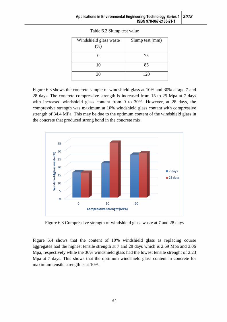
Applications in Environmental Engineering Technology Series 1 2018 ISBN 978-967-2183-21-1
64
Table 6.2 Slump test value
Windshield glass waste
(%)
Slump test (mm)
0 75
10 85
30 120
Figure 6.3 shows the concrete sample of windshield glass at 10% and 30% at age 7 and
28 days. The concrete compressive strength is increased from 15 to 25 Mpa at 7 days
with increased windshield glass content from 0 to 30%. However, at 28 days, the
compressive strength was maximum at 10% windshield glass content with compressive
strength of 34.4 MPa. This may be due to the optimum content of the windshield glass in
the concrete that produced strong bond in the concrete mix.
Figure 6.3 Compressive strength of windshield glass waste at 7 and 28 days
Figure 6.4 shows that the content of 10% windshield glass as replacing course
aggregates had the highest tensile strength at 7 and 28 days which is 2.69 Mpa and 3.06
Mpa, respectively while the 30% windshield glass had the lowest tensile strenght of 2.23
Mpa at 7 days. This shows that the optimum windshield glass content in concrete for
maximum tensile strength is at 10%.

Applications in Environmental Engineering Technology Series 1 2018 ISBN 978-967-2183-21-1
65
Figure 6.4 Tensile strength of windshield glass waste at 7 and 28 days
6.6 CONCLUSION
Windshield glass has the potential to be a substitute for coarse aggregate in concrete
with higher compressive and tensile strength achieved at the 10% of the windshield glass
content in the concrete. However, higher percentage (30%) is not suitable to be uses as
substitute because the bond between glass and concrete maybe is weaken. Therefore, it
can be conclude that 10% is the optimum percentage of windshield glass use in concrete.
The use of windshield glass in concrete mixing can lead to a better change in the
construction as it is more environmental friendly.
REFERENCES
[1] Lee T. Z (2016). The Characterisation of Concrete Containing Crushed Glass
and Ceramic Waste as Fine Aggregate Material. Universiti Tun Hussein
Onn Malaysia: Undergraduate’s thesis.
[2] Du H, Tan K. H. (2013). Use of waste glass as sand in mortar: Part I – Fresh,
mechanical and durability properties. Cement and Concrete Composites, 2013,
Volume 35, Issue 1, pg 109–117. DOI 10.1016/j.cemconcomp.2012.08.028.
[3] Jamilla Emi Sudo Lutif Teixeira ,João Luiz Calmon, Aline Silva Sauer, Geilma
Lima Vieira. (2014). Effects of Windshield Waste Glass on the
Properties of Structural Repair Mortars. Cement & Concrete Composites, 2014,
Volume 53, pg 88–96.
[4] Vikas Srivastava, Rakesh Kumar, P.K. Mehta. (2013). Concrete Made With
Waste Materials. Journal of Environment Nanotechnology, 2013, Volume
2, No.2, pg 102-106. ISSN(Print):2279-0748 ISSN(Online):2319-5541.

Applications in Environmental Engineering Technology Series 1 2018 ISBN 978-967-2183-21-1
66
[5] Gerry L., Ling T. C., Wong Y. L., Poon C. S. (2011). Effects of Crushed Glass
Cullet Sizes, Casting Methods and Pozzolanic Materials on ASR of
Concrete Blocks. Construction and Building Materials, 2011, Volume 25,
pg 2611–2618.
[6] Qu S. Y., Zheng B., Sun C. and Li J. (2014). Application of Ceramic Waste in
Concrete, The Open Civil Engineering Journal, 2014, Volume 8, pg 368-372.
[7] Mohamad J. Terro. (2006). Properties of Concrete Made With Recycled
Crushed Glass at Elevated Temperatures. Building and Environment, 2006,
Volume 41, pg 633–639.
[8] Vikas Srivastava, S. P. Gautam, V. C. Agarwal, P. K. Mehta. (2014). Glass
Wastes as Coarse Aggregate in Concrete. Journal of Environmental
Nanotechnology, 2014, Volume 3, pg 67-71. ISSN (Online): 2319-5541&
ISSN (Print) : 2279-0748.
[9] Mohd. Ahmed, Javed Mallick, Mohd. Abul Hasan. (2016). A study of factors
affecting the flexural tensile strength of concrete. Journal of King Saud
University – Engineering Sciences, 2016, Volume 28, Pg 147–156.
[10] Topcu, I. B. and Canbaz, M. (2004). Properties of concrete containing waste
glass. Cement and Concrete Research, 2004,Volume 34, pg 267-274.DOI
10.1016/j.cemconres.2003.07.003.
[11] Gajanan M. Sabnis. (2016). Green Building with Concrete: Sustainable Design
and Construction. Taylor & Francis Group, LLC, 2016, Second Edition,
International Standard Book Number-13:978-1-4987-0411-3(e-Book-PDF).
Applications in Environmental Engineering Technology Series 1 2018 ISBN 978-967-2183-21-1
67
CHAPTER 7
CULTIVATE AEROBIC GRANULAR SLUDGE WITH SOY
SAUCE WASTEWATER
Hasnida Harun, Nor Hazren Abdul Hamid, Faridah Hanim Ahmad, Norshuhaila
Mohamed Sunar
Department of Civil Engineering (Environmental),
Faculty of Engineering Technology, Universiti Tun Hussein Onn Malaysia
7.1 INTRODUCTION
Anaerobic Granular sludge was first found in anaerobic upflow sludge blanket
(UASB) reactors to treat industrial wastewaters at the end of the 1970s [1] while the
phenomenon of aerobic granular sludge was initiated by [2] with using domestic
wastewater operated under sequential batch reactor (SBR) system. Aerobic granular
sludge technology widely applied in treating nutrient and organic wastewater to meet the
water quality-based standards while anaerobic granular sludge treatment capable in save
the energy consumption and potentially in degrading activated sludge and treat
wastewater effectively [3]. Since both technologies promising an efficient treatment of
wastewater, combination of the two systems could anticipate a better wastewater
treatment from this time forth. Recently, researcher focused on integration of aerobic
treatment with anaerobic treatment in one SBR system for municipal and industrial
wastewater treatment. The integrated anaerobic aerobic granulation systems have proved
the efficiency in removing COD and have the ability to treat high OLR wastewater [4,
5]. Besides, the integrated anaerobic aerobic granulation is a straightforward system
where is no return sludge compared to the conventional system resulted less sludge
handling at the end of the process. The anaerobic aerobic granulation system favors less
equipment since the using of clarifiers and other equipment is eliminated and yet less
cost required compared to conventional system which demand large surface area.
Considering small surface area required due to the compact bioreactor of aerobic
anaerobic granulation system, the footprint produce from the system is minimal and
controllable.
Revolutions on the development of aerobic-anaerobic granulation are
varied in types of wastewater such as industrial pharmaceutical [6], livestock [7, 8],
palm oil mill effluent (POME) [9], dairy [10, 11, 12], petrochemical [13], landfill
leachates [14] and soybean processing [15] wastewater are fed in a SBR system to treat

Applications in Environmental Engineering Technology Series 1 2018 ISBN 978-967-2183-21-1
68
the wastewater. SBR technology has been success in removing nitrogen and phosphorus.
Soy sauce is a dark brown liquid produce by the soybean fermentation process as food
seasoning. Effluents from soy sauce wastewater are high in COD, Biochemical Oxygen
Demand (BOD) and Total Suspended Solids (TSS) therefore brown in color. Even
though the soy sauce wastewater is completely treated in biodegradation treatment as
used in most industrials, certain amount of color is remaining in the effluent [16]. In this
study, the anaerobic-aerobic granules were cultivated in an SBR fed with soy sauce
processing wastewater, which is an industrial wastewater that rich in proteins and starch.
The development of granular sludge and the effectiveness of anaerobic aerobic system in
treating soy sauce wastewater are focused in this paper.
7.2 REACTOR SETUP AND OPERATION
A column-type anaerobic-aerobic sludge reactor with internal diameter of 6.5cm and
100cm of height and a working volume 3.0 L were used. The influent was fed into the
reactor from the bottom of the column while the decanting of the effluent took place via
a 50 cm outlet port located from the bottom of the reactor, resulting 1.5L of mixed liquor
left in the reactor yielding 50% of volumetric exchange rate.
Air was introduced through fine air bubble stone by an air pump at the bottom of
the reactor at 1.5 cm/s of superficial air velocity. The reactor was monitored to be in
room temperature (25°C ± 3ºC). The reactor was operated at a cycle time of 6h, in
sequential mode: 5 min of feeding, 230 of reaction, 5min of settling, and 5 min of
withdrawal. During anaerobic phase, the wastewater in the reactor was allowed to
circulate to ensure homogenous distribution of substrate and biomass. Figure 7.1
illustrated the schematic diagram of the setup reactor.
Figure 7.1 schematic diagram of setup reactor.

Applications in Environmental Engineering Technology Series 1 2018 ISBN 978-967-2183-21-1
69
7.3 WASTEWATER COMPOSITION
Raw wastewater was collected from an industrial sauce plant once a week and was kept
at temperature of 4 °C [17] to prevent the wastewater from undergoing biodegradation
due to microbial activity [18]. The characteristics of the sauce wastewater were analyzed
and summarized in Table 7.1, in comparison with sauce wastewater as described in the
literature [16]. The influent pH value was observed within the range of 5.5 ±1.6. The
reactor was inoculated by 1.5 L of activated sludge form municipal wastewater treatment
plant, resulting an initial MLSS in the reactor is 5000mg/L.
Table 7.1 Characteristics of soy sauce wastewater used throughout this experiment.
Parameter [16] This study
pH 5.0 5.0-6.0
COD, mg/L 3200 7000-10000
Color, times 8000-10000 6500-8000
BOD5, mg/L 1900 2000-3000
SS, mg/L 900 750-1000
NH3-N, mg/L 85 100-200
7.4 ANALYTICAL METHODS
Wastewater in the reactor and the effluent samples were periodically analyzed for
suspended solids (SS), volatile suspended solids (VSS), mixed liquor suspended solid
(MLSS), mixed liquor volatile suspended solid (MLVSS),NH4-N, color and COD using
Standard Methods for the Examination of Water and Wastewater (APHA, 2005). The pH
and dissolve oxygen (DO) was measured by using a pH/DO meter (Orion 3-Star
Benchtop pH/DO Meter). The granule morphology of sludge was observed by a
scanning electronic microscope (FESEM-Zeiss Supra 35 VPFESEM). The granules
developed in the reactor’s column were analyzed for their physical characteristics which
include structural and morphological of granule, settling velocity, sludge volume index
(SVI) and granular strength.
The morphological and structural observations of the granules were carried out
by using a stereo microscope equipped with digital image processing and analyzer
(PAXITv6, ARC PAX-CAM). The settling velocity was determined by averaging the
time taken for an individual granule to settle at a certain height in a glass column filled
with tap water. The SVI assessment was carried out according to the procedure
described by [19].
7.5 STRUCTURAL AND MORPHOLOGICAL OF GRANULES
The seeding sludge of the reactor is the typical activated sludge with brown color with
fluffy, irregular shape and loosely clumps. Figure 7.2a shows seed sludge during the
initial inoculation stage, most of the flocculent sludge was washed out in the effluent
result only the good settled sludge remains. After two weeks inoculation, small granular
sludge with diameter 0.1-0.3mm was observed although the irregular sludge was still
dominant in the reactor as shown in Figure 7.2b. At this stage, the develop granules

Applications in Environmental Engineering Technology Series 1 2018 ISBN 978-967-2183-21-1
70
were easily crush into pieces when high shear force applied. Afterwards, the quantities
of average diameter of 0.3mm keep increasing. At this stage, the tiny yellow granules as
shown in Figure 7.2c were in irregular shape, where the spherical granules were about to
developed. At day 50 where the reactor reached steady state, mean diameter of granules
were about 1mm with spherical smooth surface and cleared defined boundary as shown
in Figure 7.2d.
[9] achieved 2.0-5.0mm diameter of matured granules after nine weeks operation
feed with palm oil mill effluent (POME) which larger than [15] that cultivated soybean-
processing wastewater about eight weeks operation and obtained 1.22 ± 0.85 mm
diameter of stable granules. A faster developed matured granules had been reported by
[20] which is only three weeks operation that fed using synthetic wastewater (glucose
and acetate) and achieve 2.0-7.0 mm diameter of granules. The seed sludge, aeration
rate, granules size and substrate composition is proved influenced the microbial of
granules developed [21].
Figure 7.2 Morphology of granular sludge. (a) Seed sludge during initial inoculation
from activated sludge. (b) Loose clump of granular sludge after two weeks inoculation.
(c) Granular sludge at day 50. (d) Matured granular sludge.
7.6 SLUDGE SETTLING AND BIOMASS PROFILE
The settling characteristic of sludge in certain time is described the sludge volume index
(SVI) besides the properties of sludge bed composition and morphology of sludge. The
SVI of seed sludge at the initial stage is about 100mL/g where was show the poor

Applications in Environmental Engineering Technology Series 1 2018 ISBN 978-967-2183-21-1
71
settling ability. During the start up, the reactor experience almost complete washout due
to the low settle ability of the seed sludge and short time of settle phase (i.e. 5 min). The
remaining sludge initiated the micro colonies consortium in the reactor [9].
The initial SVI of seed sludge before inoculation process was 210.5 mL/g. The
SVI of the inoculated granules gradually decreased after 20 days due to the granules
formation. At the end of the experiment, the settling velocity was improved as shown by
the low SVI value (32 mL/g) and the stable granules. The granules achieved 32-40 m/h
of average settling velocity which is in agreement with [20] which in rage of 30-35 m/h.
Granules began to form after 17 days of operation and mature granules were observed
after approximately 8 weeks. The change of biomass concentration and SVI values
throughout the experiment is shown in Figure 7.3. Additionally, the settling properties
are reflected in the biomass content in the reactor (MLSS, VSS), which is inversely
related to the efficiency of the settling.
Figure 7.3 The concentration of biomass during granulation process () MLSS, ()
MLVSS and () SVI.
The biomass concentration was keep increasing since day 1 until the end of the
operation eventhough during initial operation, most of biomass was drain off when the
effluent being discharged. The day 1 biomass concentration was about 2.5g/L and the
day 60 the biomass concentration was 8.2g/L. Due to the foaming conditions associate
with soy sauce wastewater, the MLSS value decreasing during the first and second week
operation. In the initial stage of operation, flocculent with good settling ability remained
in the reactor while most of floc-like sludge was washed-out into the effluent. The
MLSS began to improve on day-17 when small granules started to appear in the reactor.
When the flocculant sludge developed into granular sludge during week four, the
MLSS value increased and reached 8.2± 0.5 g/L. During theoperation until the end, the
MLVSS have same trend with MLSS which the initial value was 2.3g/L and at the end
operation, the value was 6.1g/L.
7.7 REACTOR PERFORMANCE AND REMOVAL EFFICIENCIES
Figure 7.4 and Figure 7.5 represent the removal performance profiles of COD and
ammonia during the process of granulation respectively. At the first week of operation,

Applications in Environmental Engineering Technology Series 1 2018 ISBN 978-967-2183-21-1
72
the removal percentage of COD and ammonia was 69% and 65% respectively. During
that stage, the effluent was not achieving good quality. After 22 days operation, removal
percentage of COD was stable although flocculent sludge was dominating in the reactor.
As the granular sludge slowly developed, the removal efficiency was improving
continuously up to 90% for COD and 93% for ammonia. The result of removal
percentage in this operation as in agreement by [11] in dairy wastewater which achieve
90% COD removal and 80% of ammonia removal using granulation technology.
The improving of removal percentage efficiency shown the existence of high
biological activities in the reactor [22]. The results of this study prove that seed sludge
developed in soy sauce wastewater is capable in treating high concentration of COD and
ammonia continuously. During the initial stage, the percentage ammonia remova was
irregular due to the developing and growth of flocculent sludge to granular sludge.
Figure 7.4 The COD concentration () COD influent, () COD effluent and () COD
removal.
Figure 7.5 The Ammonia concentration () Ammonia influent, () Ammonia effluent
and () Ammonia removal.

Applications in Environmental Engineering Technology Series 1 2018 ISBN 978-967-2183-21-1
73
7.8 CONCLUSION
Stable microbial granular sludge sucessfully cultivated in a single SBR system with the
soy sauce wastewater as feeding. Soy sauce wastewater is potentially treated using
granular sludge system. The microscopic examinations showed that the matured granules
depict a clear spherical-shaped outline boundary. Following granulation, good
accumulation of biomass in the reactor and good settling characteristics were observed.
When tested for COD and ammonia removal, the granules showed 90% and 93%
maximum removal, respectively indicating the feasibility of a single SBR system for the
treatment of soy sauce wastewater.
ACKNOWLEDGEMENTS
This research is funded by Universiti Teknologi Malaysia (UTM) under Research
University Grant (RUG-Grant Q.J130000.2501.01H54).
REFERENCES
[1] Lettinga G., van Velsen A.F.M., Hobma S.W., de Zeeuw W., Klapwijk A. (1980)
“Use of the upflow sludge blanket (USB) reactor concept for biological
wastewater treatment, especially for anaerobic treatment.” Biotechnology and
Bioengineering 22:699-734.
[2] Mishima K., Nakamura M. (1991) “Self-immobilization of aerobic activated
sludge - A pilot study of the Aerobic Upflow Sludge Blanket Process in
municipal sewage treatment.” Water Science and Technology 23:981-990.
[3] Wang J., Zhang Z.j., Zhang Z.f., Qaisar M., Zheng P. (2007) “Production and
application of anaerobic granular sludge produced by landfill.” Journal of
Environmental Sciences 19:1454-1460.
[4] Moy B.Y.P., Tay J.H., Toh S.K., Liu Y., Tay S.T.L. (2002) “High organic
loading influences the physical characteristics of aerobic sludge granules.”
Letters in Applied Microbiology 34:407-412.
[5] Schwarzenbeck N., Erley R., Mc Swain B.S., Wilderer P.A., Irvine R.L. (2004)
“Treatment of Malting Wastewater in a Granular Sludge Sequencing Batch
Reactor (SBR).” Acta hydrochimica et hydrobiologica 32:16-24.
[6] Inizan M., Freval A., Cigana J., Meinhold J. (2005) “Aerobic granulation in a
sequencing batch reactor (SBR) for industrial wastewater treatment.” pp. 335-
343.
[7] Kishida N., Tsuneda S., Kim J.H., Sudo R. (2009) “Simultaneous nitrogen and
phosphorus removal from high-strength industrial wastewater using aerobic
granular sludge.” Journal of Environmental Engineering 135:153-158.

Applications in Environmental Engineering Technology Series 1 2018 ISBN 978-967-2183-21-1
74
[8] Othman, I., Anuar, A. N., Ujang, Z., Rosman, N. H., Harun, H., & Chelliapan, S.
(2013). Livestock wastewater treatment using aerobic granular sludge.
Bioresource technology, 133, 630-634.
[9] Abdullah N., Ujang Z., Yahya A. (2011) “Aerobic granular sludge formation for
high strength agro-based wastewater treatment.” Bioresource Technology
102:6778-6781.
[10] Arrojo B., Mosquera-Corral A., Garrido J.M., Méndez R. (2004) “Aerobic
granulation with industrial wastewater in sequencing batch reactors.” Water
Research 38:3389-3399.
[11] Schwarzenbeck N., Borges J.M., Wilderer P.A. (2005) “Treatment of dairy
effluents in an aerobic granular sludge sequencing batch reactor.”Applied
Microbiology and Biotechnology 66:711-718.
[12] Wichern M., Lübken M., Horn H. (2008) “Optimizing sequencing batch reactor
(SBR) reactor operation for treatment of dairy wastewater with aerobic granular
sludge.” pp. 1199-1206.
[13] Caluwé, M., Dobbeleers, T., D'aes, J., Miele, S., Akkermans, V., Daens, D., ... &
Dries, J. (2017). Formation of aerobic granular sludge during the treatment of
petrochemical wastewater. Bioresource technology, 238, 559-567.
[14] Ren, Y., Ferraz, F., Lashkarizadeh, M., & Yuan, Q. (2017). Comparing young
landfill leachate treatment efficiency and process stability using aerobic granular
sludge and suspended growth activated sludge. Journal of water process
engineering, 17, 161-167.
[15] Su K.Z., Yu H.Q. (2005) “Formation and characterization of aerobic granules in
a sequencing batch reactor treating soybean-processing wastewater.”
Environmental Science and Technology 39:2818-2827.
[16] Lei Z., Ding A.Z., Wang J.S., Yu T. (2008) “Reuse of coagulation sludge:
Removal of color and COD from soy sauce wastewater by coagulation,
Shanghai.” pp. 379-381.
[17] Vijayaraghavan, K., Ahmad, D., Abdul Aziz, M.E., (2007). “Aerobic treatment
of palm oil mill effluent.” Journal of Environmental Management 82, 24–31.
[18] Chan, Y.J., Chong, M.F., Law, C.L., (2010). “Biological treatment of
anaerobically digested palm oil mill effluent (POME) using a lab-scale
sequencing batch reactor (SBR).” Journal of Environmental Management 91,
1738–1746.
[19] de Kreuk, M.K., Pronk, M., van Loosdrecht, M.C.M., (2005). “Formation of
aerobic granules and conversion processes in an aerobic granular sludge reactor
at moderate and low temperatures.” Water Research 39, 4476–4484.

Applications in Environmental Engineering Technology Series 1 2018 ISBN 978-967-2183-21-1
75
[20] Tay J.H., Liu Q.S., Liu Y. (2001) “Microscopic observation of aerobic
granulation in sequential aerobic sludge blanket reactor.” Journal of Applied
Microbiology 91:168-175.
[21] Gao D., Liu L., Liang H., Wu W.M. (2011) “Aerobic granular sludge:
Characterization, mechanism of granulation and application to wastewater
treatment.” Critical Reviews in Biotechnology 31:137-152.
[22] Muda, K., Aris, A., Salim, M. R., Ibrahim, Z., Yahya, A., van Loosdrecht, M. C.
M., Ahmad, A., et al. (2010). Development of granular sludge for textile
wastewater treatment. Water research, 44(15), 4341–50.

Applications in Environmental Engineering Technology Series 1 2018 ISBN 978-967-2183-21-1
76

Applications in Environmental Engineering Technology Series 1 2018 ISBN 978-967-2183-21-1
77
CHAPTER 8
THE VERTICAL AERATED RECYCLED CONCRETE
AGGREGATE FILTER (VARCAF) FOR REMOVAL OF
PHOSPHORUS
Suraya Hani Adnan, Norwardatun Abd Roni, Rafidah Hamdan, Nurain Izzati Mohd Yassin,
Nurul Amirah Kamarulzaman
Dept. of Civil Engineering Technology,
Faculty of Engineering Technology
Universiti Tun Hussein Onn Malaysia, Parit Raja, Batu Pahat,
86400 Johor, Malaysia.
8.1 INTRODUCTION
Eutrophication of fresh water bodies is one of the main problems facing aquatic
ecosystems. In developing countries, approximately 75% of domestic wastewater is
released to the environment without treatment (Rozari et al. 2016). Ayaz et al. (2012)
reported that eutrophication in receiving water bodies may occur when phosphorus
concentrations of nitrogen (N) was 6 mg/L. Therefore, proper treatment to remove
phosphorus from domestic wastewater to achieve the admissible level for natural
systems is needed.
Phosphorus (P) is an essential nutrient element for aquatic plants growth in
natural water system. However, excessive P loads to water bodies from industrial,
agricultural, household wastes may cause the overgrowth of aquatic plants or algae,
greatly accelerating the depletion of dissolved oxygen (DO) in waters, even leading to
serious eutrophication.
The management of the collected debris and waste causes real problems at the
environmental level. Apart from that, Recycled Concrete Aggregates (RCA) have
choose as part of our commitment to helping the environment and being sustainable.
Recycling of concrete is important because it helps to promote sustainable development
in the protection of natural resources, and reduces the disposal of demolition waste from
old concrete. Crushed waste concrete was used in this study to evaluate its performance
as an effective filter for phosphate reduction. Hence, in this study the RCA has been
choose to be the materials for filters the removal of phosphorus.

Applications in Environmental Engineering Technology Series 1 2018 ISBN 978-967-2183-21-1
78
8.2 EXPERIMENTAL
8.2.1 MATERIALS
The RCA was taken on thrown waste cubes produced from the Material Laboratory in
University Tun Hussein Onn Malaysia. Initially, the thrown waste cubes outside
laboratory were selected. Then the waste cubes were crushed by using the crushing
machines in order to produce the aggregates. Next the all aggregates are being sieves
into 5 mm to 30 mm by using sieve analysis process. The crushed samples was collected
and sieve through a 5 to 30 micrometer test sieve using a shaker, Endecott Lambard Rd.
London, model Sw193BR. The chemical microanalysis obtained from Energy-dispersive
X-ray spectroscopy (EDX) test.
Figure 8.1 : Energy-dispersive X-ray spectroscopy (EDX) test for RCA
8.2.2 COLUMN STUDY
Lab-scale vertical column filters study was developed to investigate the difference
between to size of RCA on the phosphorus removal efficiency using RCA as the
adsorbent. Six column filters with the inner diameter of 150 mm, 6 mm thickness and
total height 420 mm made from Perspex materials were set up with six different of
concentration synthetic wastewater which is 10 mg/L, 20 mg/L, 30 mg/L, 40 mg/L, 50
mg/L which was prepared by dissolving KH2PO4 (Potassium Dihydrogen Phosphate)
into distilled water. Synthetic wastewater was flowed via gravity from the influent tank
located at the higher level and connected to the influent point of each column filter. The
aeration was controlled to ensure tiny and uniform bubbles of air spread throughout the

Applications in Environmental Engineering Technology Series 1 2018 ISBN 978-967-2183-21-1
79
column filters. The sampling was done weekly for influent and effluent to test for
phosphorus removal.
Figure 8.2 : Schematic diagram of lab-scale varcaf
8.2.3 ANALYSIS METHODS
The concentration of Phosphorus was measured by the ammonium molybdate
spectrometric method using WESTCO Discrete Analyzer, model Smartchem 200,
France. The efficiency of removal of phosphorus was observed by determining the
removal percentage of the phosphorus using the following equation:
Removal percentage (%) :
in which the initial phosphorus concentration (influent) in mg/L and the final phosphorus
concentration (effluent) in mg/L.
8.3 RESULTS AND DISCUSSIONS
Figure 8.3 shows graph of percentage of Phosphorus removal with different size of RCA
vs different concentration of synthetic wastewater for RCA size 5 mm to 10 mm and 25
mm to 30 mm with six different concentration of synthetic wastewater which is 10 mg/L,
20 mg/L, 30 mg/L, 40 mg/L, 50 mg/L and distilled water. The highest percentage of P
removal is 99.54% which is in concentration 10mg/L for RCA size 5 mm to 10 mm
while the lowest percentage of P removal is 66.25% which is in concentration 50 mg/L
for RCA size 25 mm to 30 mm.
Generally it can be seen that the percentage of P removal decreasing as
concentration of synthetic wastewater increasing. From the graph for different size of
RCA which is 5mm to 10mm and 25mm to 30mm, it is obvious shown that RCA which
smallest size and lower concentration have the highest percentage of P removal. This

Applications in Environmental Engineering Technology Series 1 2018 ISBN 978-967-2183-21-1
80
results, shows the similarities finding with Akratos and Tsihrintzis (2007) found greater
removal efficiency of P removal for fine gravel is 89%, followed by medium gravel with
cattail 67% and cobbles (57%). Percentage of P removal efficiency was predominantly
affected by media size. This is because the smallest size of media, the greater surface
available for Calcium Oxide dissolution (Chazarenz et al., 2017). Secondly is the
Calcium (Ca) content in RCA. In EDX test it clearly shows to us in in previous sub-
chapter that RCA contain 26.60% of Ca. Ca is one of the element for enhanced
phosphorus adsorption. The porous surface structure of RCA also influenced the ability
RCA for removing the P (Xiou et al., 2016). The larger the porosity, the larger the
specific surface area where the adsorption of mechanism can take place.
Figure 8.3: Percentage of phosphorus removal with different size of RCA
Applications in Environmental Engineering Technology Series 1 2018 ISBN 978-967-2183-21-1
81
CONCLUSION
This study showed the higher percentage of removal of Phosphorus at lower
concentration synthetic wastewater which is 10mg/L is 99.54% which is RCA size 5 mm
to 10 mm and it was proved that RCA is one of the absorbent that is good efficiency for
removal of phosphorus.
ACKNOWLEDGEMENTS
We are grateful for the funding provided by University Tun Hussein Onn Malaysia;
GRANT FRGS VOT 1618.
REFERENCES
[1] Akratos, C. S., & Tsihrintitziz, V. A. (2007). Effect of temperature, HRT,
vegetation and porous media on removal efficiency of pilot-scale horizontal
subsurface flow constructed wetlands. Ecology Engineering Journal, 1, 173–191.
[2] Ayaz, S. C., Aktas, O., Findik, N., & Akca, L. (2012). Phosphorus removal and
effect of Adsorbent type in a constructed wetland system. Desalin. Journal of
Environmental Engineering, 37.
[3] Chazarenz, M., Surasyh, H., & Deskon, S. (2017). Biological phosphorus removal
process for wastewater treatment. International Conference of Science, 27.
[4] Rozari, P. De, Greenway, M., & Hanandeh, A. (2016). Phosphorus removal from
secondary sewage and septage using sand media amended with biochar in
constructed wetland mesocosms. Science of Total Environment, 3, 123–133.
[5] Vohla, C., Kõiv, M., & Mander, Ü. (2016). Filter Materials for Phosphorus
Removal from Wastewater in Treatment Wetlands – a Review, (January 2011).
http://doi.org/10.1016/j.ecoleng.2009.08.003.
[6] Xiou, J., Liang, C., & Liu, T. (2016). Removal of phosphorus by the core-shell bio-
ceramic/Zn-layered double hydroxides (LDHs) composites for municipal
wastewater treatment in constructed rapid infiltration system. Construction and
Building Materials 102, 10, 834–842.

Applications in Environmental Engineering Technology Series 1 2018 ISBN 978-967-2183-21-1
82

Applications in Environmental Engineering Technology Series 1 2018 ISBN 978-967-2183-21-1
83
CHAPTER 9
CHARACTERISTICS OF HYDRODYNAMICS WAVE AT PORT
OF TANJUNG PELEPAS DURING SPRING TIDE BY USING
TELEMAC-2D
Nur Aini Mohd Arish, Ikhwan Nasir Ismail
Civil Engineering Technology
Faculty of EngineeringTechnology,
Universiti Tun Hussein Onn Malaysia, Parit Raja, Batu Pahat,
86400 Johor, Malaysia.
9.1 INTRODUCTION
The Port of Tanjung Pelepas (PTP) located in the most southern tip in the State of Johor.
It is one of the largest and busiest container port in Malaysia. The development of PTP
has transformed the region in to a great development area [1]. A study has been done in
Tanjung Piai Johor, a location near the PTP. The study shows that the causes of erosion
at Tanjung Piai were coastal development such as land reclamation and port dredging.
Heavy shipping activities also had generating waves that disturbed the growth of the
existing mangroves [2]. Since the number of ships that went through PTP are keep on
increasing, this will possibility affect the surrounding area as in Tanjung Piai.
This research is intended to generate the hydrodynamic simulations using
computational fluid dynamics software that is TELEMAC 2D and to study the
characteristics of wave hydrodynamics at the Port of Tanjung Pelepas, Johor Malaysia.
Hydrodynamic model is comprehensive and detailed approach to represent the dynamics
of coastal water. Numerical calculation models can be used to simulate the flow of
water levels, sediment transport and salinity [3]. Hydrodynamic model may actually be
a physical model built to scale. However, almost all of hydrodynamic models used today
are based on a numerical model. Studies of the characteristic of hydrodynamics in
coastal areas in PTP is important and any development should be planned and well
designed to make sure an appropriate structure to be developed in the area.
9.2 RESEARCH METHOD
To conducting this study with systematic way and achieving the objectives stated, a
proper planning on work flow is needed. In this study, three main parts of work are
Applications in Environmental Engineering Technology Series 1 2018 ISBN 978-967-2183-21-1
84
planned that are data collection, creating simulation model (meshing) by intergrating
bathymetry data with the software Blue Kenue and analysis the collected data by using
the Telemac 2D. The hydrographic parameters used in this study are collected from
National Hydrography Center of Malaysia.
Telemac 2D
Telemac-2D is a computer software that calculates the free surface flow in natural water
bodies. It solves the equations of Saint-Venant two dimensions, better known as shallow
water equations (SWE) using the finite element method on unstructured triangular
elements [4]. Telemac is a software system designed to assess the environmental
processes on the surface of transient flow. Therefore, it can be used in marine and
coastal domain, estuaries, rivers and lakes. Hydrodynamic model can also be produced
in three dimensions using Telemac-3D software.Windows screen on Telemac 2D are
using Fortran code that users need to enter specific codes to start work. Hydrodynamic
model produced is easy to be converted from 2D to 3D calculations, 3D grid has the
same structure as the 2D in the horizontal plane. 2D and 3D models are largely similar in
scale with the most notable difference in the local area around coastal structures both
gave the same pattern of change in velocity [5]
Blue Kenue
Blue Kenue is computer software that is used to display the movement and hydraulic
characteristics. Blue Kenue also functions as a data processing, analysis and
visualization tool for hydraulic model [6]. In the production of hydrodynamic model,
Blue Kenue has been used for meshing works, integrating geospatial data with model
input and results data. Visualization by Blue Kenue is able to display diamensi 1 d, 2D,
3D, polar and spherical views that can be recorded as digital film or saved as images for
inclusion in reports or presentations.
9.3 DATA COLLECTION
Data collection consists of collecting data is needed for meshing and also analysis by
Telemac 2D. For meshing work, bathymetry data, map of the study area and Universal
Transverse Mercator (UTM) coordinates for the study area has been used for the model
simulation preparation. Bathymetry data is used for determination of the water depth of
the study area. While, map of the study area and Universal Transverse Mercator (UTM)
coordinates are used for creating the simulation surface model. Besides that, analysis
works by Telemac 2D will also need the Global Tidal Solution (tpxo) data for sea
current properties, moon phase period for neap tide and spring tide determination and
also wind speed together with wind direction to support the model that used in the
analysis section.
Creating Simulation Model (Meshing)
Model is created to support the analysed data to be shown in a graphical state and to help
researcher to easily view the properties of the sea area at a certain condition. This work
was done by using Blue Kenue software which firstly will traced the study area with a
map and coordinated by using Universal Transverse Mercator (UTM) coordinates system
to get the proper scaled area. Blue Kenue was developed by the Canadian Hydraulics
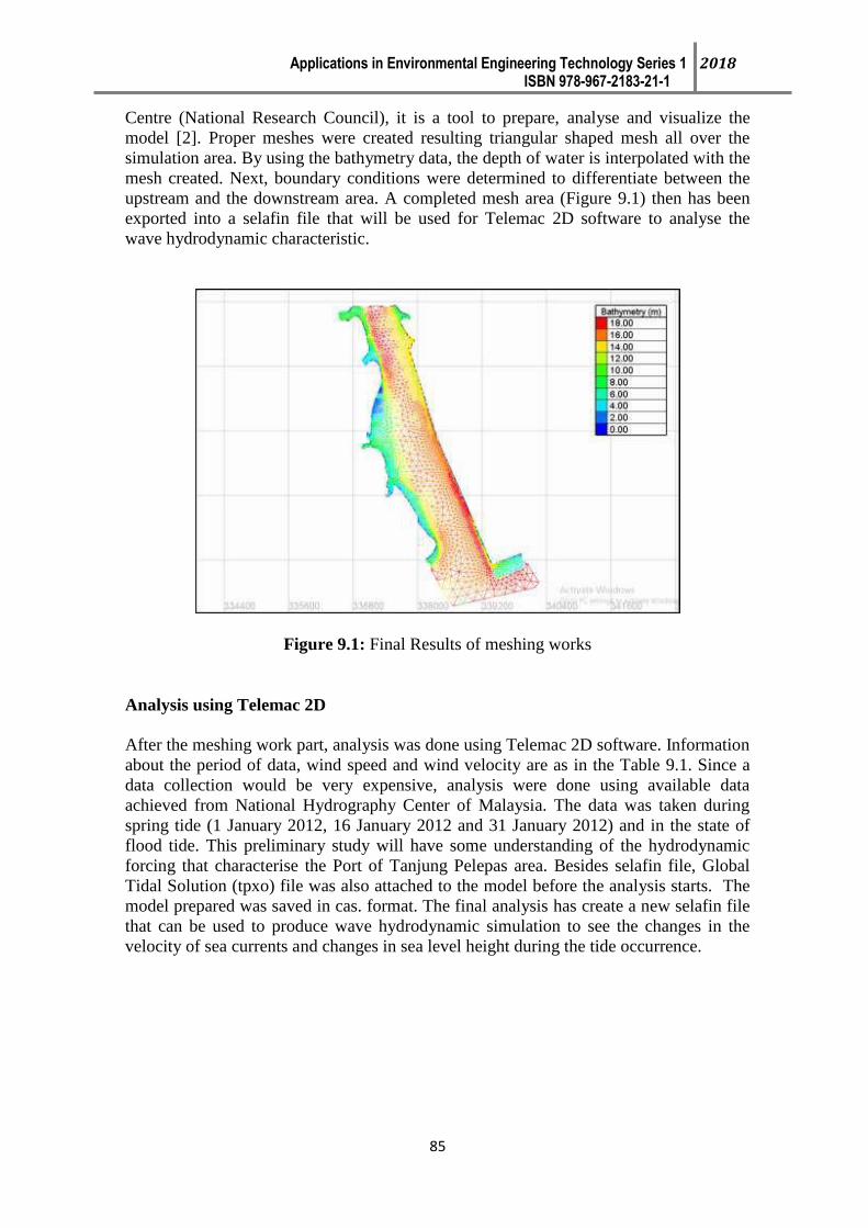
Applications in Environmental Engineering Technology Series 1 2018 ISBN 978-967-2183-21-1
85
Centre (National Research Council), it is a tool to prepare, analyse and visualize the
model [2]. Proper meshes were created resulting triangular shaped mesh all over the
simulation area. By using the bathymetry data, the depth of water is interpolated with the
mesh created. Next, boundary conditions were determined to differentiate between the
upstream and the downstream area. A completed mesh area (Figure 9.1) then has been
exported into a selafin file that will be used for Telemac 2D software to analyse the
wave hydrodynamic characteristic.
Figure 9.1: Final Results of meshing works
Analysis using Telemac 2D
After the meshing work part, analysis was done using Telemac 2D software. Information
about the period of data, wind speed and wind velocity are as in the Table 9.1. Since a
data collection would be very expensive, analysis were done using available data
achieved from National Hydrography Center of Malaysia. The data was taken during
spring tide (1 January 2012, 16 January 2012 and 31 January 2012) and in the state of
flood tide. This preliminary study will have some understanding of the hydrodynamic
forcing that characterise the Port of Tanjung Pelepas area. Besides selafin file, Global
Tidal Solution (tpxo) file was also attached to the model before the analysis starts. The
model prepared was saved in cas. format. The final analysis has create a new selafin file
that can be used to produce wave hydrodynamic simulation to see the changes in the
velocity of sea currents and changes in sea level height during the tide occurrence.
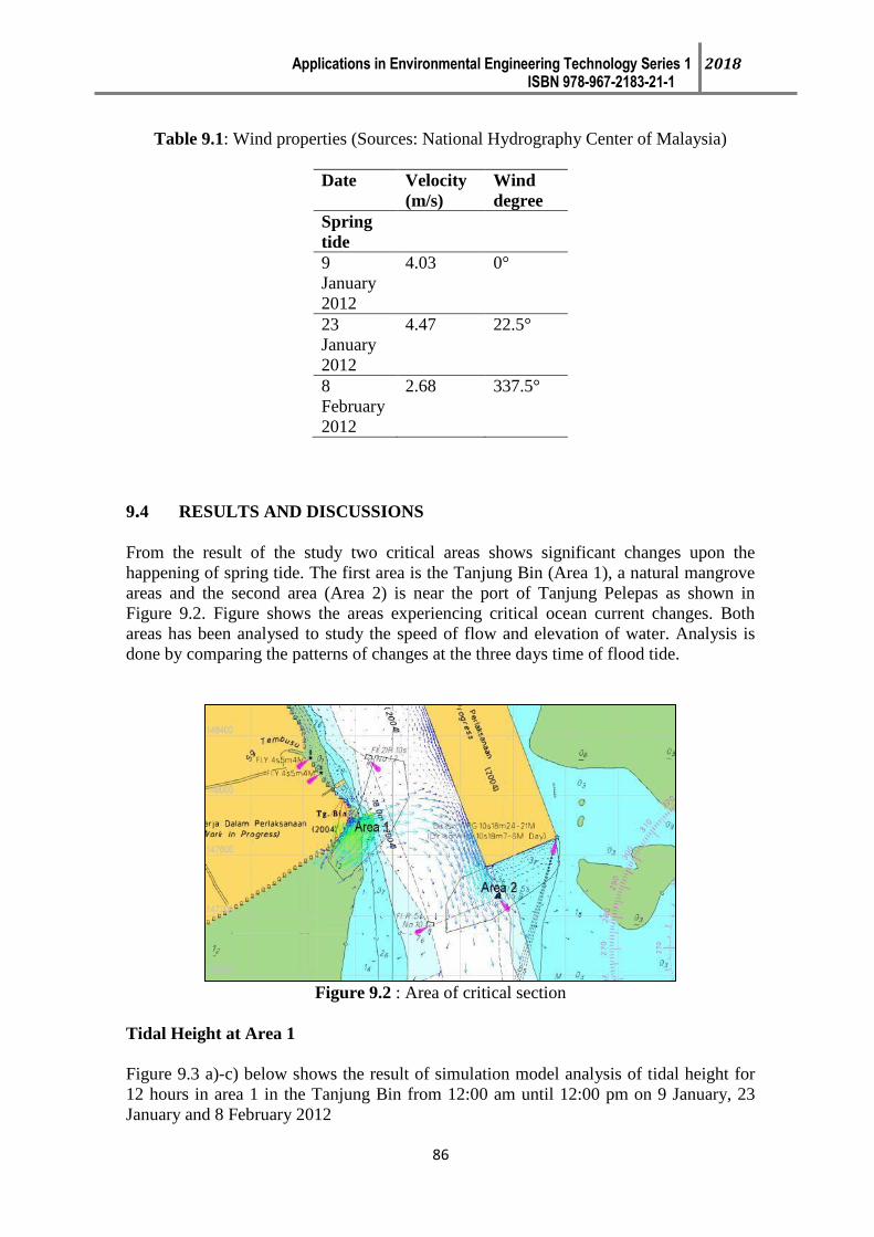
Applications in Environmental Engineering Technology Series 1 2018 ISBN 978-967-2183-21-1
86
Table 9.1: Wind properties (Sources: National Hydrography Center of Malaysia)
Date Velocity
(m/s)
Wind
degree
Spring
tide
9
January
2012
4.03 0°
23
January
2012
4.47 22.5°
8
February
2012
2.68 337.5°
9.4 RESULTS AND DISCUSSIONS
From the result of the study two critical areas shows significant changes upon the
happening of spring tide. The first area is the Tanjung Bin (Area 1), a natural mangrove
areas and the second area (Area 2) is near the port of Tanjung Pelepas as shown in
Figure 9.2. Figure shows the areas experiencing critical ocean current changes. Both
areas has been analysed to study the speed of flow and elevation of water. Analysis is
done by comparing the patterns of changes at the three days time of flood tide.
Figure 9.2 : Area of critical section
Tidal Height at Area 1
Figure 9.3 a)-c) below shows the result of simulation model analysis of tidal height for
12 hours in area 1 in the Tanjung Bin from 12:00 am until 12:00 pm on 9 January, 23
January and 8 February 2012
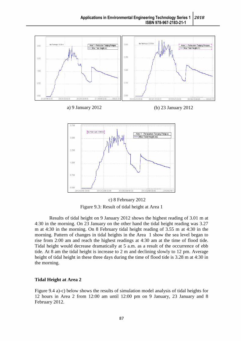
Applications in Environmental Engineering Technology Series 1 2018 ISBN 978-967-2183-21-1
87
Figure 9.3: Result of tidal height at Area 1
Results of tidal height on 9 January 2012 shows the highest reading of 3.01 m at
4:30 in the morning. On 23 January on the other hand the tidal height reading was 3.27
m at 4:30 in the morning. On 8 February tidal height reading of 3.55 m at 4:30 in the
morning. Pattern of changes in tidal heights in the Area 1 show the sea level began to
rise from 2:00 am and reach the highest readings at 4:30 am at the time of flood tide.
Tidal height would decrease dramatically at 5 a.m. as a result of the occurrence of ebb
tide. At 8 am the tidal height is increase to 2 m and declining slowly to 12 pm. Average
height of tidal height in these three days during the time of flood tide is 3.28 m at 4:30 in
the morning.
Tidal Height at Area 2
Figure 9.4 a)-c) below shows the results of simulation model analysis of tidal heights for
12 hours in Area 2 from 12:00 am until 12:00 pm on 9 January, 23 January and 8
February 2012.
a) 9 January 2012
(b) 23 January 2012
c) 8 February 2012

Applications in Environmental Engineering Technology Series 1 2018 ISBN 978-967-2183-21-1
88
Figure 9.4: Results of tidal heights at Area 2
For Area 2, the results of tidal heights on 9 January 2012 shows the highest
reading of 1.98 m at 4:30 in the morning. On 23 January on the tidal height reading is
2.69 m at 4:30 in the morning. On 8 February tidal height reading is 2.15 m at 4:30 in
the morning. Changes of tidal heights in the area started rising from 1:30 a.m. and
reached the highest reading at 4:30 am at the time of flood tide. Height of tidal has been
decreased dramatically at 5 a.m. as a results of the ebb tide. At 8 a.m there were very
few increasing of tidal height up to 1.5 m and it is declining slowly. Average height of
these three days during the flood tide is 2.27 m at 4:30 in the morning.
Sea Current at Area 1
Figure 9.5 a)-c) shows the results of the analysis of model simulating the velocity or
current for 12 hours in Area 1 in the Tanjung Bin from 12:00 am until 12:00 pm on 9
January, 23 January and 8 February 2012. Reading of velocity on 9 January 2012 shows
the highest sea currents velocity of 14.0071 m/s at 4:00 am. On 23 January the highest
velocity readings is 14.15 m/s at 4:00 am and on 8 February the highest reading of
velocity is 14.76 m/s at 4:00 am. Changes of sea currents velocity in Area 1 is increased
a) 9 January 2012
(b) 23 January 2012
c) 8 February 2012
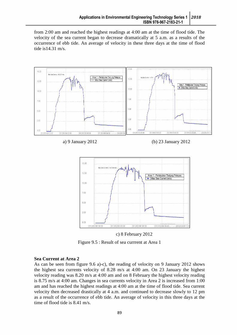
Applications in Environmental Engineering Technology Series 1 2018 ISBN 978-967-2183-21-1
89
from 2:00 am and reached the highest readings at 4:00 am at the time of flood tide. The
velocity of the sea current began to decrease dramatically at 5 a.m. as a results of the
occurrence of ebb tide. An average of velocity in these three days at the time of flood
tide is14.31 m/s.
Figure 9.5 : Result of sea currrent at Area 1
Sea Current at Area 2
As can be seen from figure 9.6 a)-c), the reading of velocity on 9 January 2012 shows
the highest sea currents velocity of 8.28 m/s at 4:00 am. On 23 January the highest
velocity reading was 8.20 m/s at 4:00 am and on 8 February the highest velocity reading
is 8.75 m/s at 4:00 am. Changes in sea currents velocity in Area 2 is increased from 1:00
am and has reached the highest readings at 4:00 am at the time of flood tide. Sea current
velocity then decreased drastically at 4 a.m. and continued to decrease slowly to 12 pm
as a result of the occurrence of ebb tide. An average of velocity in this three days at the
time of flood tide is 8.41 m/s.
a) 9 January 2012
(b) 23 January 2012
c) 8 February 2012

Applications in Environmental Engineering Technology Series 1 2018 ISBN 978-967-2183-21-1
90
Figure 9.6 : Results of sea current at Area 2
The direction of the currents for the three days of spring tide shows almost the same
pattern of direction. In the Area 1 it shows the sea current moves into Pulai River via
Tanjung Bin and partly towards Tanjung Pelepas. In the Area 2 the sea currents heading
into Pulai River but conflicted with the mainstream from the Area 1 which headed to the
area of Tanjung Pelepas causing currents could not get through the Pulai River from the
Area 2. Figure 9.7 shows simulation for the sea current direction for both areas.
a) 9 January 2012
(b) 23 January 2012
c) 8 February 2012

Applications in Environmental Engineering Technology Series 1 2018 ISBN 978-967-2183-21-1
91
Figure 9.7 : Current pattern during spring tide
9.5 CONCLUSIONS
Hydrodynamic simulation models can be created based on hydrographical parameters
such as wind waves, tidal currents and tidal height by using the software Telemac2D.
The results of all this simulation model has shown the features of hydrodynamics at the
Port of Tanjung Pelepas by showing the movement of the currents and the tidal heights
in the study area at the condition of spring tide and in a state of flood tide. The
following are the conclusions that has been made.
1. Construction of hydrodynamics simulation models using Telemac2D software in
Port of Tanjung Pelepas can be produced and shows the hydrodynamic
characteristics.
2. The average of highest velocity of the sea currents around the Port of Tanjung
Pelepas is 8.41 m/s while 14.31 m/s at Tanjung Bin during the spring tide.
3. The highest tidal height at the time of spring tide is 2.27 m at 4:00 am in the state
of flood tide around the Port of Tanjung Pelepas.
4. Bathymetry and terrain factor varying influence the characteristics of
hydrodynamics in coastal area as comparison made in Area 1 and Area 2.
ACKNOWLEDGEMENTS
We would like to thank the National Hydrography Center of Malaysia for providing the
valuable data for conducting the study.
REFERENCES
[1] Sulaiman, O. O., Saharuddin, A. H., & Kader, A. S. A. (2011). Sustainable
Maintenance of Navigation Channel: The Case of Port Tanjung Pelepas (PTP)
Port. Asian Social Science, 7(12), 175.

Applications in Environmental Engineering Technology Series 1 2018 ISBN 978-967-2183-21-1
92
[2] Awang, N. A., Jusoh, W. H. W., & Hamid, M. R. A. (2014). Coastal Erosion at
Tanjong Piai, Johor, Malaysia. Journal of Coastal Research, 71, 122–130.
http://doi.org/10.2112/SI71-015.1
[3] Chau, KW (2010) Modelling for coastal hydraulics and engineering, Taylor and
Francis Ltd., 231 pp.
[4] Samaras, A. G., Vacchi, M., Archetti, R., & Lamberti, A. (2013). Wave and
hydrodynamics modelling in coastal areas with TELEMAC and MIKE21. TUC
2013, 59.
[5] Christie, E., Li, M., & Moulinec, C. (2012). Comparison of 2d and 3d large scale
morphological modeling of offshore wind farms using HPC. Coastal
Engineering Proceedings, 1(33), 42.
[6] Abily, M., Duluc, C. M., & Gourbesville, P. (2014). Use of Standard 2D
Numerical Modeling Tools to Simulate Surface Runoff Over an Industrial Site:
Feasibility and Comparative Performance Survey Over a Test Case. In Advances
in Hydroinformatics (pp. 19-33). Springer Singapore.

Applications in Environmental Engineering Technology Series 1 2018 ISBN 978-967-2183-21-1
93
CHAPTER 10
APPLICATION OF GEOPHYSIC TECHNOLOGY IN
DEFINING THE ENVIRONMENTAL IMPACT AT COASTAL
AREA
1,2
Mohamad Faizal Tajul Baharuddin, 2 Mohd Idrus Mohd Masirin,
1 Mohamed
Zuhaili Mohamed Najib
1Department of Civil Engineering Technology,
Faculty of Engineering Technology,
Universiti Tun Hussein Onn Malaysia, Parit Raja, Batu Pahat,
86400 Johor, Malaysia.
2Research Center for Soft Soils, Office of Research, Innovation, Commercialization
and Consultancy,
Universiti Tun Hussein Onn Malaysia, Parit Raja, Batu Pahat,
86400 Johor, Malaysia.
10.1 INTRODUCTION
Knowledge on groundwater requirement for domestic water supply and
agricultural activity is important to ensure a holistic management approach of
groundwater aquifer. This scenario is more complex at costal area due to saltwater
contamination that restricted groundwater usage for water supply and agricultural
activity. Degree of salinity in groundwater aquifer should be suitable for both
requirements in order to ensure sustainability for both important socioeconomic
activities at coastal. Problem of saltwater contamination always related with seawater
intrusion phenomena due to proximity contact with sea. In Malaysia, the coastal zone of
Malaysia with a long coastline (4,800 km) and huge area (4.43 million ha), has a special
socio-economic and environmental significance, which supporting 70% of Malaysia’s
population. In addition, the Malaysian coastal zone is also the centre of economic
activities encompassing urbanization, agriculture, fisheries, aquaculture, oil and gas
exploitation, transportations and communication, and recreations (Syed Alwi, 1992).
Among the coastal regions in Malaysia, the west coast of Peninsular Malaysia is the
most developed socio-economically, with 57% of its coastline is utilized for agricultural
activities and 21% for housing, transportation, and recreational facilities (Abdullah and
Loi, 1992).

Applications in Environmental Engineering Technology Series 1 2018 ISBN 978-967-2183-21-1
94
Coastal area in Peninsular Malaysia has been identified as having the largest
prospect for groundwater supply (Suratman and Awang, 1998). Groundwater supply can
be extracted from alluvial, limestone, meta-sedimentary, and igneous aquifers.
Comparing to the other categories of aquifer, alluvial aquifer is highly productive by
generating an average of 30 m3/hr to 50 m3/hr groundwater yield (Suratman and Awang,
1998). The water quality is suitable for domestic purposes, with some localities having
brackish and saline water. Alluvial aquifer is vulnerable to seawater intrusion due to its
close proximity to the sea (Suratman and Awang, 1998). Seawater intrusion can cause
deterioration in the groundwater quality by changing the groundwater salinity. Among
the coastal areas in Peninsular Malaysia that has been identified as having the most
impact by seawater intrusion to the socioeconomic activities is Langat Basin which
situated at the most advance and well development area in Malaysia (JICA and DMGM,
2002).
The coastal plains of Malaysia in certain places are unsuitable for plant growth
due to salinity problem (Mohd Hashim, 2003). Several factors of salinity occurred in the
coastal area of Malaysia where the most significant factor is seawater intrusion to low
elevation coastal landform. Other factors that also influenced salinity problems are tidal
inundation, groundwater seepage and over-drainage of adjacent area. Various studies
showed agriculture activities such as oil palm, rice and turf grass had been affected by
salinity problem in the coastal area in Malaysia (Roa, 1982, Kimi, 1991 and Uddin et al.,
2012). The agriculture activity most affected by salinity problem in coastal area of
Malaysia is oil palm (Mohd Hashim, 2003). Coastal plains with relatively fertile alluvial
soils are found on the west coast of Peninsular Malaysia. Alluvial soils are also present
in some parts of the east coast. Based on the topography factor, areas with greater than
20° slopes are unsuitable for oil palm plantations. Hence, only 42% of the 33 million ha
of land in Malaysia is suitable for agricultural activity for oil palm (Abd. Ghani et al.,
2004), and most of these locations are in coastal areas.
However, previous studies focused on salinity problem in order to define the
suitability of agriculture towards soil salinity. There was limited study on the effect of
seawater intrusion into groundwater aquifer that relates to groundwater supply and
agriculture activities at the coastal area. Furthermore, groundwater for water supply and
agriculture used in coastal areas can be affected by sea level rise in the 21st century due
to climatic change (IPCC, 2001). Climatic change is expected to worsen the existing
environmental problems along the coastal areas. Future sea-level rise near coastal
aquifers may lead to a change in the present hydrogeological boundary. Saline
groundwater is thicker than before and more shifts to the landward coastal areas in the
future (IPCC 2007; Vaeret et al., 2009). The relationship between sea-level rise and
seawater intrusion can be estimated according to the Ghyben–Herzberg relationship
(sharp-interface model). This relationship states that the depth of the interface below the
mean sea level is equal to 40 times the height of the potentiometric surface above the
mean sea level. Therefore, a 1-m increase in sea level may cause a 40-m reduction in
freshwater thickness (Fetter 2002; Hiscock 2005; Abd-Elhamid 2010).
The problem might become very serious when the effects of sea-level rise were
to combine with the huge amount of water requirements for water supply and
agriculture. This phenomenon requires practical hydrogeological investigation methods
to assess the present status of seawater intrusion to groundwater system, especially in the
coastal area which extensively involved with demand of water supply and agricultural
activities. Three types of methods have commonly been used for seawater intrusion

Applications in Environmental Engineering Technology Series 1 2018 ISBN 978-967-2183-21-1
95
investigations: geochemical methods, geophysical methods and integrated method (Bear
and Cheng 2010). The best geophysical method to assign, particularly in seawater
intrusion investigations, is geo-electrical method (Loke 2010). Electrical resistivity
method is unique as it detects increased aquifer conductivity via increased pore-water
conductivity (Abdul Nassir et al. 2000). A number of studies have used the geo-electrical
method to study seawater intrusion into groundwater aquifers in coastal areas. Issar and
Levanon (1974) used the geo-electrical method and boreholes data to examine the extent
of aquifer and salinities in alluvial aquifers (with depths more than 180 m) beneath the
coastal plains of Arava valley in southern Israel. Ginzburg and Levanon (1976) used the
geo-electrical method and boreholes data to determine a boundary of fresh-saline water
aquifer along coastal area in Israel. Edet and Okereke (2001) used the geoelectrical
method and geochemical data to examine the extent of seawater intrusion in shallow
aquifers (with depths less than 300 m) beneath the coastal plains of Southeastern
Nigeria. Benkabbour et al. (2004) used the geo-electrical method to characterise
seawater intrusion in the Plioquaternary consolidated coastal aquifer of the Mamora
Plains in Morocco.Di Sipio et al. (2006) used the geoelectrical method and geochemical
data to obtain a better salinity profile of the groundwater system in Venice estuaries.
Awni (2006) used the two-dimensional (2D) geoelectrical method to detect sub-surface
freshwater and saline water in the alluvial shoreline of the Dead Sea in Jordan. Sherif et
al. (2006) integrated the geo-electrical and the hydro-geochemical methods to delineate
seawater intrusion in Wadi Ham, UAE. In Lagos, Nigeria, Adepelumi et al. (2009) used
the vertical electrical sounding survey to delineate seawater intrusion into the Lekki
Peninsula freshwater aquifer.
Baharuddin et al. (2009) used the geo-electrical method to study the effect of
seawater intrusion and shoreline physical changes in the coastal area of Selangor,
Malaysia. Hodlur et al. (2010) used the geo-electrical method and geochemical method
to identify the resolution of the freshwater and saline water aquifers in a coastal terrain
of Mahanadi Basin in India. Sikandar et al. (2010) used integrated a geo-electrical
resistivity survey and geochemistry measurements to investigate groundwater conditions
in Pakistan. Zouhri et al. (2010) combined the geo-electrical method and hydro-
geochemical method to determine the groundwater salinity at Rharb Basin in Western
Morocco. Sathish et al. (2011) combined the geo-electrical and the geochemical methods
to assess the zone of mixing between seawater and groundwater in the coastal aquifer in
South Chennai, in Tamil Nadu, India. Ebraheem et al. (2012) conducted a 2D earth
resistivity imaging survey in the Wadi Al Bih area in the Northern UAE to determine the
potential of the quaternary aquifer and its groundwater quality. Khalil et al. (2012) used
the geo-electrical method and time domain electromagnetic method to access seawater
intrusion into the groundwater system in the northwestern coast of Egypt. Maiti et al.
(2013) used neural network inversion using the geo-electrical methods to assess suitable
groundwater exploration at coastal area in Maharashtra, India. These studies demonstrate
that the geo-electrical method combined with other methods is effective for depicting
saline-water boundaries and studying the effects seawater intrusion. The advantages of
each of the methods supplement the limitation of the other methods. The most apparent
advantage of the combination technique is the reduction in study cost and time without
jeopardising the integrity of the data obtained (Maillet et al. 2005; Sathish et al. 2011).
In the present study, the combined the geo-electrical and the geochemical
methods were implemented, but emphasis was on the present seawater intrusion status,
water supply and oil palm cultivation at Carey Island, located in the Langat Basin on the
west coast of Peninsular Malaysia. The technique was aided by information related to
Applications in Environmental Engineering Technology Series 1 2018 ISBN 978-967-2183-21-1
96
the elevation, land cover and oil palm plant physiography. The elevation and land cover
discussed in the current work involves the physical changes in the coastal area that can
influence seawater intrusion distribution at coastal islands.
10.2 MATERIALS AND METHODS
Hydrogeology area
Eight monitoring wells (Figure 10.1) were installed in the unconfined aquifer:
four (MW6, MW11, MW12, MW13) in the northwest in the mangrove preserved area
and four (MW5, MW7, MW10, and MW14) in the southeast in the heavily eroded area
without mangrove. Additionally six other wells (MW1, MW2, MW3, MW4, MW8, and
MW9) were installed in the semi-confined aquifer in the southwest of the semi-confined
aquifer. The wells reached various depths (40, 50, and 80 m), respectively, with open
screens installed in the 34–36, 47–49, and 67–69 m depths for groundwater quality
sampling. Soil samples collected from the each of the well boreholes by rotary-washing
were visually examined and laboratory analysed. Soil classification followed the BS
1377 (1990): fine sand (0.063–0.1 mm); medium sand (0.1–0.4 mm); and coarse sand
(1–2 mm). Tests on the soil physical properties included particle-size distribution,
Atterberg limit, moisture content, specific gravity, and linear shrinkage. Surface
elevations were conducted to obtain topography information of the study area. The
precision of total station equipment, model GPT-3100N Series Top Con were used for
data acquisition of elevation for the fourteen (14) monitoring wells and also along a
route surveys. The reference datum is benchmarked to station BM No. 3082 obtained
from DSMM. The elevation of benchmarked station is 3.0458 m from mean sea level
(m.msl). Land-use mapping is useful for assessing the past and present land-use
activities change in Carey Island. The past land-use map was obtained from topography
map in the year 1974 published by The Department of Survey and Mapping Malaysia
(DSMM). Scale of the topography map ratio is 1:63360 which covered the whole of
Carey Island. As for the present land-use map, it is obtained from a modified land-use
map with ground mapping in the year 2010. The topography map (1974) and modified
land-use map with ground mapping (2010) are combined through a digitized process by
using AutoCAD software version 2009. The superimposed maps are used to interpret the
land-use activities change from the year 1974 to 2010. The 30 years of land-use
activities change are estimated in unit m2.
Subsurface Resistivity and Geochemistry Survey
Earth resistivity (ER) was measured following the traverse set up (Figure 10.1)
using a resistivity meter (ABEM Terrameter SAS4000 with electrode selector ES10-64).
Spread in two phases, the first phase data were collected in August 2009, November
2009, and February 2010; and the second phase data in December 2010. The former data
were used to establish a TDS-ER relationship in the vertical profile of the study area;
whereas the latter data were used to map out the subsurface resistivity in the horizontal
profile.
Groundwater monitoring was done once or twice a week, starting August 2009
until March 2011. Groundwater samples were collected from the monitoring wells by
using a bailer. Four groundwater quality parameters (conductivity, salinity, TDS, and
temperature) were measured using a water quality checker (YSI EC300) pre-calibrated
against a standard potassium chloride solution (conductivity 1.411 mS/cm) in

Applications in Environmental Engineering Technology Series 1 2018 ISBN 978-967-2183-21-1
97
accordance with the APHA (2005) procedures. Hydrogeochemical parameters measured
were major cations and anions. Collected groundwater samples were divided, kept in
two containers. For cation analysis, the groundwater samples were filtered by Whatman
42 filter paper and preserved with 2% nitric acid (HNO3). For anion analysis, the
groundwater samples were filtered and then preserved at a maintained 4C. The anion
analysis was done within 48 h of collection time. Cations analyzed were sodium (Na),
calcium (Ca), magnesium (Mg), potassium (K), and iron (Fe), on the Perkin Elmer
Inductive Coupled Plasma Optical Emission Spectrometer (ICP-OES) model Optima
3300RL. Anions analyzed were chloride (Cl−), sulfate (SO42−), nitrate (NO3−), and
bromide (Br−), on Dionex Ion Chromatography model ICS2000. The analyses were
done to standard methods (APHA 2005), a five-point calibration quantifying the
analyses with correlation co-efficient of the calibration curve between 0.995 and 0.999.
Fetter (2002) proposed the classification of groundwater salinity can be classified into
three types namely; fresh, brackish and saline by using TDS values. Freshwater are
classified with TDS values < 1000 mg/L, brackish water are classified as TDS values
ranging from 1000 mg/L to 10000 mg/L and TDS values > 10000 mg/L are classified as
saline groundwater. According to Interim National Water Quality Standards for
Malaysia (Department of Environment Malaysia, 2010), TDS values of < 1000 mg/L
required no treatment for water supply.
Figure 10.1: Locations of monitoring wells, resistivity survey lines, drainages system
and boundary between unconfined and semi-confined aquifers
L16
L7’
L5
L16’
L7
L15
Monitoring well (Auger Hole)
MW11
MW12
MW13
MW10
MW6
MW5
MW1
MW2
MW4
MW3
MW9
MW8
MW14
MW7
N
0 2700 m
Straits of
Malacca
101o20’45.91”
E
2o50’52.63”N
2o49’36.56”N
101o18’18.02”E
Ayer Hitam River
Scale
LEGENDS
B’
B
C’
C
A’
A Main canal
Estate boundary
Monitoring
well
Mangrove Reserve
Cross Section
Resistivity Survey
Aquifer boundary
SEMICONFINED (1
st Aquifer)
UNCONFINED (1
st Aquifer)
6
1
2
3
1,2,3 (Ngah, 1988)
8 (Baba, 2003)
675 1350 2025
8
(Ismail, 2008) 6
Tidal gate
Severely Eroded
L5’ L15’
L8 L8’
L14’
L14
L6 L6’
L13
L13’
L1
L1’
L9’ L9
L11 L11’
L10
L10’
L2
L2’
L3
L3’
L12
L12’
L4’
L4
L17
L17’
Drains

Applications in Environmental Engineering Technology Series 1 2018 ISBN 978-967-2183-21-1
98
In the first phase, a number of eight resistivity lines L18-L18’, L19-L19’, L17-
L17’, L5-L5’, L4-L4’, L3-L3’, L2-L2’, and L12-L12’ were set up, each crossing
respectively MW3, MW4, MW5, MW6, MW7, MW10, MW11, and MW12. No
resistivity lines were set up crossing other wells (MW1, MW2, MW8, MW9, MW13 and
MW14). In the second phase, a number of nineteen resistivity lines, L1 through L19,
were set up, and the lines crossing the wells were as indicated above for the first phase
and those not crossing other wells are as shown in Figure 10.3.
All the nineteen resistivity lines were each laid into the ground surface almost
perpendicular to the shoreline (Figure 10.3): sixteen lines in the N-S direction; and three
in the W-E direction of the study area. Each resistivity line (cable) was 400m long,
divided into four sections each 100m long (designated as 1st, 2
nd, 3
rd, and 4
th cables).
Using an initial electrode spacing of 5m intervals (for the middle 2nd
and 3rd
cables) and
10m intervals (for the end 1st and 4
th cables) a number of ten electrodes were pegged
each on the end 1st and 4
th cables; and twenty electrodes each on the middle 2
nd and 3
rd
cables, making a total of sixty one (61) electrodes for each 400m survey cable. The
spacing flexibility afforded by the Wenner array could thus propagate increasingly
denser resistivity in the vertical resistivity image profile near the subsurface (Hamzah et
al. 2006).
In the analysis, the measured resistivity data, which were merely apparent, were
subjected to inversion that resulted in a model of subsurface resistivity which
approximated the true subsurface resistivity distribution as described by Loke and
Barker (1996). The inversion was made possible using software RES2DINV as
previously described by (Dahlin and Loke (1998) and Loke et al. (2003). Using the same
technique, Loke (2013) later in the study of an alluvial setting, obtained high resistivity
(10 - 100 m) in the freshwater, in distinct contrast to the seawater with very low
resistivity (<0.2 m) due to high salt content. This same method was thus adopted in
the study analysis involving also alluvial soils.
In using the inversion technique, each entire profile block was divided into a
number of rectangular model cells based on the spread of the measured data (Loke and
Barker 1996). The data inversion was executed using the smoothness-constrained least
square method (deGroot-Hedlin and Constable 1990; Sasaki 1992) where the block’s
resistivity values (model parameters) were adjusted iteratively to obtain a true
distribution of resistivity (model response). The model parameters and response were
linked via a finite-difference method as described by Dey and Morrison (1979). Thus the
differences between the calculated and measured data in an initial model were
minimised using the root-mean-squared (RMS) method; and the iteration was continued
to an RMS error limit of less than 5% (Awni 2006), which was considered acceptable.
However, the model with the lowest RMS error is not always the most appropriate as it
can induce unrealistic variations in the resistivity model (Loke 2010b).
10.3 RESULTS OF RESISTIVITY AND CONDUCTIVITY
Resistivity and conductivity distributions was spatially analysed by interpolation
using the Kriging technique available in Surfer 8. The true (inverted 2D) vertical profiles
were converted into true (inverted 3D) horizontal profiles, shown in Figures 10.2 and
Applications in Environmental Engineering Technology Series 1 2018 ISBN 978-967-2183-21-1
99
10.3 for selected depths. Although the 3D images have apparently limited resolution due
the limited number of profiles examined in comparison to the survey area (100 km2), the
method has produced sufficiently better resistivity and conductivity distributions of the
different water types and oil palm tolerance toward salinity respectively.
The three colour codes are used to describe resistivity distribution for water
types: blue for freshwater (>10 ohm.m); green for brackish water (3-10 ohm.m); and red
for saline water (<3 ohm.m). The following discussion is only confined for
demonstrative purpose for the 2.5-5.0m depth [Figure 10.2a) and b)] of the unconfined
aquifer. In this water zone freshwater (horizontal) coverage is about 3km2, half that for
brackish-saline water (about 7.0km2). The dominancy of water brackishness/salinity was
due to seepage from the irrigation canals (profile L6-L6’near MW6, profile L7-L7’ and
profile L8-L8’ shown in Figure 10.1). The freshwater contamination in the shallow
aquifer was believed to be caused by seawater infiltrating from the irrigation canals. In
the same depths (2.5-5.0m) the saline water occurred mostly in the southwest (in the
reserved mangrove) due to tide moving from the mangrove to the bunds separating it
from the oil palm cultivation. In the past the bunds in the mangrove have been frequently
damaged, causing the saline water to overflow into the oil palm plantation, thus
contributing to the groundwater salinity in the southwest area. An important finding in
the study is the indication of freshwater availability in the midwest-study area as deep as
21.8 m into the aquifer beneath the mangrove as shown in Figure 10.3i). For depths
exceeding 7.8m the saline water occurrence was mainly due to seawater intrusion.
In the east close to profiles L1-L1’, L2-L2’ and L3-L3’, no freshwater appeared
at depths exceeding 7.80m [Figure 10.2c)] due to the saline-brackish water dominancy
resulting from seawater intrusion that seemed more dominant than on the western side.
In contrast there was freshwater in the west close to the mid-study area (profiles L2-L2’
and L3-L3’) in the 21.8 m depth [Figure 10.3 i)] underlying the brackish-saline water.
This observation has correlation with TDS in the monitoring wells on the eastern side in
the 36m depth, having concentrations twice (20,000 mg/L) as high as on the western side
(10,000 mg/L). Freshwater in the 30m-40m zone was less thick compared to the 10m-
20m zone, concentrating in the mid-aquifer over 10 - 30% of the mapped area. The
freshwater lens in these depths seemed to be isolated from the surrounding saline water
especially in the east, west and south directions, indicating saline water dominancy in
every direction. Conductivity distributions for the suitability of oil palm towards salinity
are represented by using different colour codes. The colour codes used are blue for
suitable ( > 0.4 S/m), green for moderately suitable (0.4 S/m < C < 0.2 S/m), and red for
not suitable (< 0.2 S/m).
The 3-D conductivity slice images at the depths of 2.5 m and 5.0 m [Figures 10.2
d)-f) and 3 j)-l)] showed that more than 80% of the area with conductivity values of 0.2
S/m is suitable for oil palm plantation. These results contradict with water type’s
distribution that showed almost 50% is suitable for water supply at the same depth
[Figures 10.2a)-b)]. The image also showed that some areas are moderately suitable and
not suitable for plantation, especially along the main agricultural canal drainages (mid-
study area) and areas near the coast with un-bund mangroves (west area). On the east
side area with severe coastal erosion, the area still exhibits suitable condition for oil
palm cultivation. The severe erosion in the area was mitigated by the construction of
man-made bund and well-developed roads that prevented the penetration of saline water
into the plantation ground surface. Contradict to the west coastal mangrove side, saline
water intrusion occurs during high tide when seawater floods the area. Mangrove plants

Applications in Environmental Engineering Technology Series 1 2018 ISBN 978-967-2183-21-1
100
that grow close to this coastal area are more tolerant towards salinity due to saline water
intrusion. Behind the mangrove reserved area, man-made bunds were constructed to
prevent saline water intrusion into the plantation area.
As for the severely eroded area on the east side, the moderate conductivity condition
(0.2–0.4 S/m) appeared at a depth of 7.8 m. This results showed a different condition in
the same depths of water type resistivity distribution [Figure 10.2 c)] where all east side
is coverage by brackish and saline water ( not suitable for water supply). On the west
side, a similar depth was still suitable for oil palm cultivation [Figure 10.2 f)]. The
conductivity value for the severely eroded area which is not suitable for oil palm
plantation was at 14.10 m depth [Figure 10.3 k)]. In the west side, where mangrove
forests still existed, the conductivity value suitable for plantation was at 21.80m depth
[Figure 10.3 l)].
10.4 DISCUSSIONS AND CONCLUSION
The 3-D resistivity and conductivity slice image revealed different groundwater
suitable salinity distribution and depth for water supply and oil palm in Carey Island.
The factor different results of groundwater salinity for two different socioeconomic
activities are due to water levels standard toward salinity for both are different. Water
level standard for water supply can be deduced as TDS < 1000 mg/l meanwhile for oil
palm requirement the TDS <5300 mg/l.
Other factors that determine the tolerance of water supply and oil palm for
groundwater salinity are different elevation height and land cover between the west and
east area as well as groundwater salinity distribution finding. The east area has a low
surface elevation and no mangroves covered the coastal area. Compared with the west
area, surface characteristics in the east area naturally provide a more conducive
environment for seawater intrusion into the groundwater system. The middle area
between east and west has a high topography, which prevents the migration of salinity
from the east to the west. The middle area also showed the dominance of brackish water
as a result of the seepage of saline water from the main canal that is located in this area.
As discussed by Scheineder and Kruse (2006), the variations in the hydrogeology
conditions, such as terrain effects, vegetation pattern and sea level rise, are among the
factors that can contribute to groundwater salinity. In this study, the terrain effect and
land cover were considered significant to seawater intrusion due to high variations (1.3-
2.3m) in the elevation and land cover of the study area. These might have a major
influence on the wider saline-brackish water distribution in the south-east where the
semi-confined aquifer was located where showed low elevation and no mangrove
covered compared to the west area.
According to the Ghyben-Herzberg assumption, a 0.5 m increase in the sea level
will reduce the thickness of freshwater storage by 20 m. The predicted sea level rise in
the 21st century will increase seawater intrusion in the area. Based on the predicted slope
from 2001 to 2010 by a sea level rise prediction study, which used the B1, A1B, and A2
scenarios from the Special Report on Emissions Scenarios, the mean sea level rise rate at
Port Klang is 0.387 m. Based on the Ghyben-Herzberg assumption and local scenario
sea-level rise prediction, the east area will become unsuitable for water supply and oil
palm plantation much sooner than the west area, which still has a mangrove forest.

Applications in Environmental Engineering Technology Series 1 2018 ISBN 978-967-2183-21-1
101
Figure 10.2: Resistivity and conductivity distribution relative to elevation from 2.5 to 7.8 m depths
MW7
MW11
MW12
MW6
MW5
MW7
MW10MW13
Straits of Malacca
Severe Erosion
Man
grove Area
MW7
MW11
MW12
MW6
MW5
MW7
MW10MW13
Straits of Malacca
Severe Erosion
Man
grove Area
MW7
MW11
MW12
MW6
MW5
MW7
MW10MW13
Stairts of Malacca
Severe Erosion
Man
grove Area
Straits of Malacca
MW12
MW11
MW6
MW10
MW5
MW11
Severe Erosion
MW7
MW13
Man
grove Area
MW7
MW11
MW12
MW6
MW5
MW7
MW10MW13
Straits of Malacca
Severe Erosion
Man
grove Area
MW7
MW11
MW12
MW6
MW5
MW7
MW10MW13
Straits of Malacca
Severe Erosion
Man
grove Area
MW7
024681012141618202224262830
00.0
5
0.1
0.1
5
0.2
0.2
5
0.3
0.3
5
0.4
0.4
5
0.5
0.5
5
0.6
0.6
5
0.7
0.7
5
0.8
0.8
5
0.9
0.9
5
1
Conductivity, S/m
Resistivity, Ohm.m
a) 2.5
m
b) 5.0
m
c) 7.8
m
e) 5.0 m
d) 2.5 m
f) 7.8
m Not to Scale

Applications in Environmental Engineering Technology Series 1 2018 ISBN 978-967-2183-21-1
102
Figure 10.3: Resistivity and conductivity distribution relative to elevation from 10.8 to 21.8 m depths
MW7
MW11
MW12
MW6
MW5
MW7
MW10MW13
Straits of Malacca
Severe Erosion
Man
grove Area
MW7
MW11
MW12
MW6
MW5
MW7
MW10MW13
Straits of Malacca
Severe Erosion
Man
grove Area
MW7
MW11
MW12
MW6
MW5
MW7
MW10MW13
Straits of Malacca
Severe Erosion
Man
grove Area
MW7
MW11
MW12
MW6
MW5
MW7
MW10MW13
Stairts of Malacca
Severe Erosion
Man
grove Area
MW7
MW11
MW12
MW6
MW5
MW7
MW10MW13
Straits of Malacca
Severe Erosion
Man
grove Area
MW7
MW11
MW12
MW6
MW5
MW7
MW10MW13
Stairts of Malacca
Severe Erosion
Man
grove Area
024681012141618202224262830
00.05
0.1
0.15
0.2
0.25
0.3
0.35
0.4
0.45
0.5
0.55
0.6
0.65
0.7
0.75
0.8
0.85
0.9
0.95
1
Resistivity, Ohm.m Conductivity, S/m
Not to Scale
g) 10.8 m
h) 14.1 m
i) 21.8 m m
j) 10.8
m
k) 14.1
m
l) 21.8 m

Applications in Environmental Engineering Technology Series 1 2018 ISBN 978-967-2183-21-1
103
ACKNOWLEDGEMENTS
The authors The authors would like to express their deepest appreciation to the Ministry of
Higher Education and Universiti Tun Hussein Onn Malaysia for supporting this research
under Research and Innovation Fund. Many thank are due to all research members for
their tremendous work and cooperation. The project has been made possible by a research
grant provided by the Institute of Ocean and Earth Science (IOES) University Malaya,
Kuala Lumpur, Malaysia.
REFERENCES
[1] Abdul Nassir, S.S.; Loke, M.H.; Lee C.Y., and Nawawi M.N.M., (2000). Salt-water
intrusion mapping by geoelectrical imaging surveys, Geophysical Prospecting,
48(4),
doi10.1046/j.13652478.2000.00209.x.http://web.ebscohost.com/ehost/pdf?vid=3&hid=1
13&sid=f505c08d-d330-4dc5-99bo-df1909144ee2%40sessionmgr109, 647-661p.
[2] Abdullah, S. and Loi, H.K., (1992). Keynote Address “Coastal Reclamation in
Malaysia”. Regional Seminar on Land Reclamation for Urban Development,
University Malaya, Kuala Lumpur, 10-11 August 1992. 1-11p.
[3] Adepelumi, A.; Ako, B.D.; Ajayi, T.R.; Afolabi, O., and Omotoso, E.J., (2009).
Delineation of saltwater intrusion into the freshwater aquifer of Lekki Peninsula,
Lagos, Nigeria Environmental Geology, 56(5), doi 10.1007/s00254-008-1194-
3.http://www.spingerlink.com/content/ekj1477561052r10/fulltext.pdf. 927-933p.
[4] Abd-Elhamid, H.F. (2010). A Simulation-Optimization Model to Study the Control of
Seawater Intrusion in Coastal Aquifers. (unpublished doctoral dissertation).
University of Exeter, United Kingdom.
[5] Abd.Ghani, E, Zakaria, Z.Z,, Wahid, M.B. (2004).Guidelines for palm oil industries,
Perusahaan Sawit di Malaysia, Millennium Edition. Malaysian Palm Oil Board,
Ministry of Plantation Industries & Commodities, Malaysia.
[6] APHA (2005). Standard methods for the examination of water and wastewater (21st
edn). American Public Health Association, Washington, DC.
[7] Awni, T.B. (2006). Use of electrical resistivity methods for detecting subsurface
fresh and saline water and delineating their interfacial configuration: a case study of
the eastern Dead Sea coastal aquifers, Jordan. Hydrogeol J, 14, 1277–1283.
[8] Baba, M.F., (2003). Geology Quaternary at Teluk Datuk area, State of Selangor
(Sheet 101). Geology Quaternary Report, Department of Mineral and Geoscience
Malaysia, Ministry of Natural Resources and Environment Malaysia, 1-32p.
Applications in Environmental Engineering Technology Series 1 2018 ISBN 978-967-2183-21-1
104
[9] Baharuddin, M.F.T.; Hashim, R., and Taib, S., (2009). Electrical imaging resistivity
study at the coastal area of Sungai Besar Selangor Malaysia. Journal of Applied
Sciences, ANSI, Vol 9, Issue 16, DOI: 10.3923/jas2009.2897.2906.
http://scialert.net/qredirect.php?doi=jas.2009.2897.2906&linkid=pdf. 2897-2906p.
[10] Bear, J., and Cheng,A.H.-D. (2010). Seawater intrusion. In Modeling Groundwater
Flow and Contaminant Transport, Springer Science &Business Media, 593–636.
[11] Benkabbour, B.; Toto, E.A., and Fakir, Y., (2004). Using DC resistivity method to
characterize the geometry and the salinity of the Plioquaternary consolidated coastal
aquifer of the Mamora plain, Morocco. Environmental Geology, 45(4), doi:
10.1007/s00254-003-0906-y. Available from:
http://www.spingerlink.com/content/3ejfg3cn4t89r141/fulltext.pdf. 518–526p.
[12] BS (British Standard) 1377 (1990). Part 2: Method of Test for Soils for Civil
Engineering Purposes. British Standard Institution, London, 1-68.
[13] Dahlin, T. and Loke, M.H., (1998). Resolution of 2D Wenner resistivity imaging as
assessed by numerical modelling, Journal of Applied Geophysics, 38(4), 237-249.
[14] deGroot-Hedlin, C. and Constable, S. (1990). Occam’s inversion to generate smooth,
two-dimensional models from magnetotelluric data. Geophysics, 55(12), 1613–1624.
[15] Department of Environment Malaysia (2010). Interim National Water Quality
Standards for Malaysia. Department of Environment, Malaysia.
[16] Dey, A. and Morrison, H.F., (1979). Resistivity modelling for arbitrarily shaped
two-dimensional structures. Geophysical Prospecting, 27(1), 106–136.
[17] Di Sipio, E.; Galgaro, A., and Zuppi, G.M., (2006). New geophysical knowledge of
groundwater systems in Venice estuarine environment, Estuarine, Coastal and Shelf
Science. 66,
doi:10.1016/j.ecss.2005.07.015.http://www.sciencedirect.com/science?_ob=MImg&
_imagekey=B6WDV-4H6PKWO-1-H&cdi=67768_user=15079, 6-12p.
[18] Ebraheem, A.M., Sherif, M.M., Al Mulla, M.M., Akram, S.F. and Shetty, A.V.
(2012). A geoelectrical and hydrogeological study for the assessment of groundwater
resources in Wadi Al Bih, UAE. Environ Earth Sci. 67 (3), 845-857.
[19] Edet, A.E., and Okereke, C.S., 2001. A regional study of saltwater intrusion in
southeastern Nigeria based on the analysis of geoelectrical and hydrochemical data.
Environmental Geology, 40, DOI: 10.1007/s002540100313.
http://www.springerlink.com/content/9ayfk79gu16xp5yw/fulltext.pdf, 1278-1289p.
[20] Fetter, C.W. (Eds). (2002). Applied Hydrogeology (4th
Ed), 1-598. New Jersey,
USA: Prentice Hall Inc.

Applications in Environmental Engineering Technology Series 1 2018 ISBN 978-967-2183-21-1
105
[21] Ginzburg, A., and Levanon, A., (1976). Determination of a salt-water interface by
electrical resistivity depth soundings, Hydrological Sciences Bulletin, 21:4,
http://dx.doi.org/10.1080/02626667609491674, 561-568p.
[22] Hamzah, U., Yaacup, R., Samsudin, A.R. and Ayub, M.S. (2006). Electrical imaging
of the groundwater aquifer at Banting, Selangor, Malaysia. Environ Geol, 49(8),
1156–1162.
[23] Hiscock, K., (2005). Hydrogeology principles and practise, Blackwell Publishing,
ISBN 0-632-05763-7. 244p.
[24] Hodlur, G.K.; Dhakate, R.; Sirisha, T., and Panaskar, D.B., (2010). Resolution of
freshwater and saline water aquifers by composite geophysical data analysis
methods, Hydrological Sciences Journal, 55:3, DOI: 10.1080/02626661003738217
http://dx.doi.org/10.1080/02626661003738217, 414-434p.
[25] IPCC. (2001). Climate Change 2001: Impacts, Adaptations, and Vulnerability:
contribution of working group II to the third assessment report of the
Intergovernmental Panel on Climate Change. McCarthy, J. J., Canziani, O. F.,
Leary, N. A., Dokken, D. J. and White, K. S. Cambridge University Press,
Cambridge, UK and New York, NY, USA.
[26] IPCC. (2007). Climate Change 2007: Impacts, Adaptations, and Vulnerability.
Contribution of Working Group II to the Fourth Assessment Report of the
Intergovernmental Panel on Climate Change, McCarthy, J. J., Canziani, O. F.,
Leary, N. A., Dokken, D. J. and White, K. S. Cambridge University Press,
Cambridge, UK.
[27] Ismail, R., (2008). Construction and Exploration of Deep Wells at Carey Island and
Kg Kelanang, Kuala Langat District, Banting Selangor. National Groundwater
Resources Study under Subproject groundwater resources for State of Selangor.
Report done by KS Global Sdn Bhd with collaboration Multical Card (M) Sdn Bhd
under instruction the Department of Mineral and Geoscience Selangor State,
Malaysia.
[28] Issar A., and Levanon, A., (1974). The uses of geophysical methods in
hydrogeological investigations in Israel, Hydrological Sciences Bulletin, 19:2, DOI:
10.1080/02626667409493899 http://dx.doi.org/10.1080/02626667409493899, 199-
217p.
[29] JICA and DMGM. (2002). The study on the sustainable groundwater resources and
environmental management for the Langat Basin in Malaysia. Japan International
Cooperation Agency (JICA) and Department Mineral and Geoscience Malaysia
(DMGM) Report, Vol 3.
[30] Kimi, S. (1991). Pengurusan tanah masin untuk penanaman padi. Teknologi
Kejuruteraan Pertanian, 2, 33-36.

Applications in Environmental Engineering Technology Series 1 2018 ISBN 978-967-2183-21-1
106
[31] Loke, M.H., (2010). Tutorial: 2-D and 3-D electrical imaging surveys,1-145.
[32] Loke, M.H., (2013). RES2DINV ver. 3.59 for Windows XP/Vista/7 for Rapid 2-D
Resistivity and IP Inversion using the least squares method, 1-148.
[33] Loke, M.H., Barker, R.D. (1996). Rapid least squares inversion of apparent
resistivity pseudosection using a quasi-Newton method. Geophysical Prospecting,
44(3), 131–152.
[34] Loke, M.H., Acworth, I. and Dahlin, T. (2003). A comparison of smooth and blocky
inversion methods 2-D electrical imaging surveys. Exploration Geophysics, 34(3),
182-187.
[35] Maillet, G.M., Rizzo, E., Revil, A. and Vella, C. (2005). High resolution electrical
resistivity tomography (ERT) in a transition zone environment: Application for
detailed internal architecture and infilling processes study of a Rhone River paleo-
channel. Marine Geophysical Researches, 26, 317–328.
[36] Mohd. Hashim, G. (2003). Salt-affected soils of Malaysia. A report prepared for the
Food and Agriculture Organisation of the United Nations (FAO).
[37] Ngah, D.S., (1988). Groundwater investigation for determination of suitability using
hand-pump at rural area of Kuala Langat District, Selangor Darul Ehsan, Report
No.GPH1/1988.Department of Mineral and Geosciences Malaysia, Ministry of
Natural Resources and Environment.
[38] Rao, A.K. (1982). Semi-detailed Soil Survey of the Padi-Growing Areas in Krian
District, Perak. Soils & Analytical Services Soil Survey Report no. 15, Ministry of
Agric. & Rural Development, Kuala Lumpur.
[39] Sasaki, Y. (1992). Resolution of resistivity tomography inferred from numerical
simulation. Geophys Prospect, 40, 453–464.
[40] Sathish, S., Elango, R. and Sarma, V. S. (2011). Assessment of seawater mixing in a
coastal aquifer by high resolution electrical resistivity tomography. Int. J. Environ.
Sci. Tech., 8 (3), 483-492.
[41] Schneider, J.C. and Kruse, S.E. (2006). Assessing selected natural and
anthropogenic impacts on freshwater lens morphology on small barrier islands: Dog
Island and St. George Island, Florida, USA. Hydrogeology Journal, 14, 131–145.
[42] Sherif , M., El Mahmoudi, A., Garamoon, H., Kacimov, A., Akram, S., Ebraheem,
A. and Shetty, A. (2006). Geoelectrical and hydrogeochemical studies for
delineating seawater intrusion in the Outlet of Wadi Ham, UAE, Environmental
Geology, 49(4), 536–551.

Applications in Environmental Engineering Technology Series 1 2018 ISBN 978-967-2183-21-1
107
[43] Sikandar, P.; Bakhsh, A.; Arshad, M., and Rana, T., (2010). The use of vertical
electrical sounding resistivity method for the location of low salinity groundwater
for irrigation in Chaj and Rachna Doabs. Environmental Earth Sciences, 60: DOI
10.1007/s12665-009-0255-6.
http://www.springerlink.com/content/234248866242342v/fulltext.pdf, 1113–1129p.
[44] Suratman, S., & Awang, N. (1998). Recent groundwater studies in the Klang Valley,
Selangor Malaysia (Vol. 24, p. 315).Warta Geologi Geological Society of Malaysia.
[45] Syed Alwi, S.M. (1992). The Coastal Zone in Malaysia, Processes, Issues and
Management Plan, 1-31. Malaysian National Conservation Strategy. Economic
Planning Unit, Kuala Lumpur.
[46] Uddin, M.K., Juraimi, A.S., Ismail, M.R., Rahim, M.A. and Radziah, O. (2012).
Effects of salinity stress on growth and ion accumulation of turfgrass species. Plant
Omics Journal, 5(3), 244-252.
[47] Været, L., Kelbe, B., Haldorsen, S. and Taylor, R.H. (2009). A modelling study of
the effects of land management and climatic variations on groundwater inflow to
Lake St Lucia, South Africa, Hydrogeology Journal, 17, 1949–1967.
[48] Zouhri, L.; Toto, E.A.; Carlier, E., and Debieche, T.H., (2010). Salinité des
ressources en eau: intrusion marine et interaction eaux–roches (Maroc occidental),
Hydrological Sciences Journal, 55:8, DOI:10.1080/02626667.2010.520561
http://dx.doi.org/10.1080/02626667.2010.520561, 1337-1347p.

Applications in Environmental Engineering Technology Series 1 2018 ISBN 978-967-2183-21-1
108
Applications in Environmental Engineering Technology Series 1 2018 ISBN 978-967-2183-21-1
109
CHAPTER 11
INDOOR ENVIRONMENTAL QUALITY (IEQ) AND INDOOR
AIR QUALITY (IAQ)
Norshuhaila Mohamed Sunar, Umi Kalthsom Parjo, Menega A/P Subramaniam, Abdul
Mutalib bin Leman, Hazren A. Hamid, Hasnida Harun.
Department of Civil Engineering Technology,
Faculty of Engineering Technology,
Universiti Tun Hussein Onn Malaysia,
86400 Johor, Malaysia.
11.1 INTRODUCTION
Good indoor air quality (IAQ) is required for the healthy indoor environment quality (IEQ);
whereas poor IAQ can cause a variety of diseases to the building occupants. Normally, the
health problems related to poor IAQ include respiratory problems, eye irritation, allergic
reactions, sinusitis, and others. In addition, the ventilation and air conditioning system in
enclosed work space also contribute to poor IAQ if not maintained properly. Thus, the
ventilation and air conditioning (VAC) system are obviously related to IAQ problems.
Additionally, the living organisms in building such as fungi, bacteria, and virus that are
inhaled by occupants can cause allergies, respiratory disorders, infectious diseases, and
hypersensitivity diseases. Also, organic chemical compounds that are released from the
maintenance, building products in sufficient quantities, VOC can cause irritation of the
nose, eyes, and throat, headache, dizziness, visual disorder, and memory impairment.
The IAQ in building can be undermined by microbial contaminants (like fungal and
bacteria), chemicals (such as carbon monoxide, formaldehyde), and allergens that accounted
health effects to the building’s occupants [1]. In Malaysia, the Department of Human
Resources had launched the Industry Code of Practice on IAQ (ICOP-IAQ) 2010 proposed
to identify the significant parameters distributed to the indoor air contamination. Therefore,
this chapter elaborated the details of indoor air quality as overview that included in this

Applications in Environmental Engineering Technology Series 1 2018 ISBN 978-967-2183-21-1
110
book series. The detail of indoor environment quality (IEQ) and indoor air quality (IAQ)
also provided in this chapter.
11.2 INDOOR ENVIRONMENTAL QUALITY (IEQ) AND INDOOR AIR
QUALITY (IAQ)
Indoor environmental quality (IEQ) is referred to the quality of environment condition in a
building which provides human health and wellbeing effect. The exposure to the
contaminants can cause the symptoms and poor health condition especially in non-industrial
buildings (enclosed work space) to the building’s occupants. There are various contaminants
(gases and particles) come from offices such as machines, cleaning products, construction
activities, furnishing, water-damaged building materials, microbial growth (fungal and
bacterial), insects and outdoor pollutants. Moreover, factors such as indoor temperature,
relative humidity, and ventilation in the building also have been identified influencing to the
indoor environment condition [2].
Meanwhile, indoor air quality (IAQ) is defined as the quality of indoor air in the
buildings and structures that influence to the building’s occupants’ health. According to
ICOP-IAQ by DOSH, the meaning of IAQ refers to the quality of air contains including the
air in the room and the air removed by the mechanical system. This was supported by World
Health Organization [3] in which IAQ is referring to the human health as follow;
“Health is a state of complete physical, mental and social well-being and not merely
the absence of disease or infirmity”.
The indoor air quality (IAQ) in any building can be undermined by microbial
contaminants (like fungal and microscopic organisms), chemicals, (for example, carbon
monoxide, formaldehyde), and allergens that can make wellbeing impacts to the building's
occupants [4,5]. Other than that, indoor air quality likewise influenced to bioaerosols,
characterized as airborne particles comprising of driving living beings, for example,
microscopic organisms, infection, fungi, or issuing from non-living beings as toxins, by-
results of microbial development, or sections of wiped out microorganisms [6].
11.3 INDOOR ENVIRONMENT QUALITY (IEQ)
The effect of poor IEQ is not only on physical health of the building occupants, but also on
their physiological health [7]. Basically, IEQ can be determined by many factors such as
lighting, air quality and damp conditions. Dampness, cleanliness and ventilation
characteristics are associated with building related symptoms [8]. Therefore, many health

Applications in Environmental Engineering Technology Series 1 2018 ISBN 978-967-2183-21-1
111
related problem was occurred due to this poor environment. The thermal comfort, indoor air
quality, noise level and illumination level are the four aspects to examine the IEQ [9]. Air
quality and freshness, the presence of light, thermal comfort and quality of acoustic are the
important factors of IEQ in healing environments, which affect occupant satisfaction
[10,11].
Variety of contaminants whether from machines inside the buildings, dust cleaners,
renovation works, water damaged building materials, carpets and furnishings,cigarette
smoke, perfumes, microbial growth, insects and outdoor pollutants are the common
contaminants faced by the building occupants [12]. How individuals respond to indoor
environment can also predicted through the indoor temperature, relative humidity and the
ventilation levels of a building. Energy consumption of buildings depends significantly on
the criteria used for the indoor environment (temperature, ventilation and lighting) [11].
Building related symptoms could be resolved by understanding the sources of indoor
environmental contaminants and by controlling them. There are 6 categories of IEQ which
shown in Figure 11.1 and Table 11.1 tabulated the definition of Indoor Environmental
Quality (IEQ) according to EN 15251.
Figure 11.1: Categories of Indoor Environmental Quality [13].
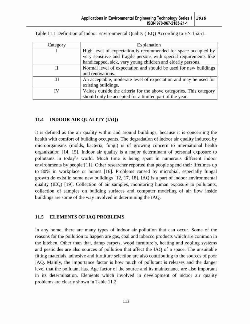
Applications in Environmental Engineering Technology Series 1 2018 ISBN 978-967-2183-21-1
112
Table 11.1 Definition of Indoor Environmental Quality (IEQ) According to EN 15251.
Category Explanation
I High level of expectation is recommended for space occupied by
very sensitive and fragile persons with special requirements like
handicapped, sick, very young children and elderly persons.
II Normal level of expectation and should be used for new buildings
and renovations.
III An acceptable, moderate level of expectation and may be used for
existing buildings.
IV Values outside the criteria for the above categories. This category
should only be accepted for a limited part of the year.
11.4 INDOOR AIR QUALITY (IAQ)
It is defined as the air quality within and around buildings, because it is concerning the
health with comfort of building occupants. The degradation of indoor air quality induced by
microorganisms (molds, bacteria, fungi) is of growing concern to international health
organization [14, 15]. Indoor air quality is a major determinant of personal exposure to
pollutants in today’s world. Much time is being spent in numerous different indoor
environments by people [11]. Other researcher reported that people spend their lifetimes up
to 80% in workplace or homes [16]. Problems caused by microbial, especially fungal
growth do exist in some new buildings [12, 17, 18]. IAQ is a part of indoor environmental
quality (IEQ) [19]. Collection of air samples, monitoring human exposure to pollutants,
collection of samples on building surfaces and computer modeling of air flow inside
buildings are some of the way involved in determining the IAQ.
11.5 ELEMENTS OF IAQ PROBLEMS
In any home, there are many types of indoor air pollution that can occur. Some of the
reasons for the pollution to happen are gas, coal and tobacco products which are common in
the kitchen. Other than that, damp carpets, wood furniture’s, heating and cooling systems
and pesticides are also sources of pollution that affect the IAQ of a space. The unsuitable
fitting materials, adhesive and furniture selection are also contributing to the sources of poor
IAQ. Mainly, the importance factor is how much of pollutant is releases and the danger
level that the pollutant has. Age factor of the source and its maintenance are also important
in its determination. Elements which involved in development of indoor air quality
problems are clearly shown in Table 11.2.
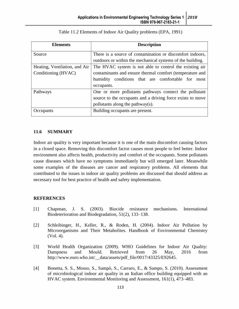
Applications in Environmental Engineering Technology Series 1 2018 ISBN 978-967-2183-21-1
113
Table 11.2 Elements of Indoor Air Quality problems (EPA, 1991)
Elements Description
Source
There is a source of contamination or discomfort indoors,
outdoors or within the mechanical systems of the building.
Heating, Ventilation, and Air
Conditioning (HVAC)
The HVAC system is not able to control the existing air
contaminants and ensure thermal comfort (temperature and
humidity conditions that are comfortable for most
occupants.
Pathways
One or more pollutants pathways connect the pollutant
source to the occupants and a driving force exists to move
pollutants along the pathway(s).
Occupants Building occupants are present.
11.6 SUMMARY
Indoor air quality is very important because it is one of the main discomfort causing factors
in a closed space. Removing this discomfort factor causes most people to feel better. Indoor
environment also affects health, productivity and comfort of the occupants. Some pollutants
cause diseases which have no symptoms immediately but will emerged later. Meanwhile
some examples of the diseases are cancer and respiratory problems. All elements that
contributed to the issues in indoor air quality problems are discussed that should address as
necessary tool for best practice of health and safety implementation.
REFERENCES
[1] Chapman, J. S. (2003). Biocide resistance mechanisms. International
Biodeterioration and Biodegradation, 51(2), 133–138.
[2] Schleibinger, H., Keller, R., & Roden, H. (2004). Indoor Air Pollution by
Microorganisms and Their Metabolites. Handbook of Environmental Chemistry
(Vol. 4).
[3] World Health Organization (2009). WHO Guidelines for Indoor Air Quality:
Dampness and Mould. Retrieved from 26 May, 2016 from
http://www.euro.who.int/__data/assets/pdf_file/0017/43325/E92645.
[4] Bonetta, S. S., Mosso, S., Sampò, S., Carraro, E., & Sampo, S. (2010). Assessment
of microbiological indoor air quality in an Italian office building equipped with an
HVAC system. Environmental Monitoring and Assessment, 161(1), 473–483.

Applications in Environmental Engineering Technology Series 1 2018 ISBN 978-967-2183-21-1
114
[5] Chapman, J. S. (2003). Biocide resistance mechanisms. International
Biodeterioration and Biodegradation, 51, 133–138.
[6] Douwes, J., Thorne, P., Pearce, N., & Heederik, D. (2003). Bioaerosol health effects
and exposure assessment: Progress and prospects. Annals of Occupational Hygiene,
47(3), 187–200.
[7] Ahmed, A. M., & El-Katatny, M. H. (2007). Entomopathogenic fungi as
biopesticides against the Egyptian cotton leaf worm, Spodoptera littoralis: between
biocontrol-promise and immunelimitation. Journal of Egyptian Society of
Toxicology, 1–26.
[8] Lee, M. C., Mui, K. W., Wong, L. T., Chan, W. Y., Lee, E. W. M., & Cheung, C. T.
(2012). Student learning performance and indoor environmental quality (IEQ) in air-
conditioned university teaching rooms. Building and Environment, 49(1), 238–244.
[9] Wong, J. K. W., Skitmore, M., Buys, L., & Wang, K. (2014). The effects of the
indoor environment of residential care homes on dementia suffers in Hong Kong: A
critical incident technique approach. Building and Environment, 73, 32-39.
[10] Lai, A. C. K., Mui, K. W., Wong, L. T., & Law, L. Y. (2009). An evaluation model
for indoor environmental quality (IEQ) acceptance in residential buildings. Energy
and Buildings, 41(9), 930–936.
[11] Sarbu, I., & Sebarchievici, C. (2013). Aspects of indoor environmental quality
assessment in buildings. Energy and Buildings, 60, 410–419.
[12] Parjo, U. K., Sunar, N. M., Leman, A M., Ideris, N. I. A, Gani, P., Emparan, Q., &
Er, C. M. (2015). Indoor Fungal Treatment by Using Potassium Sorbate as Bio-
Resistance Coating for Different Plasterboard Wall Finishings. Applied Mechanics
and Materials, 774, 1116–1120
[13] MacAulay, J. (2018) Toxic homes, toxic bodies. Educational Resources Site.
Retrieved from 22 March, 2018 from
http://www.healthyheating.com/CARP/CARP_Toxic_Homes_Toxic_Body_1.htm.
[14] Leman, A M., Omar, A R., Husain, A., Halmi, M. A, & Adam, N. M. (2006).
Monitoring of Indoor Air Quality for Improvement of Safety and Health Factor
Towards Sustainable Work. In Proceeding Of The International Symposium &
Exhibition On Sustainable Energy & Environment (ISESEE (pp. 173–179).
[15] Verdier, T., Coutand, M., Bertron, A., & Roques, C. (2014). A review of indoor
microbial growth across building materials and sampling and analysis methods.
Building and Environment, 80, 136–149.

Applications in Environmental Engineering Technology Series 1 2018 ISBN 978-967-2183-21-1
115
[16] Norhidayah, A., Chia-Kuang, L., Azhar, M. K., & Nurulwahida, S. (2013). Indoor
Air Quality and Sick Building Syndrome in Three Selected Buildings. Procedia
Engineering Malaysian Technical Universities Conference on Engineering &
Technology, 53, 93–98.
[17] Ismail, S. H., Deros, B. M., & Leman, A. M. (2010). Indoor air quality issues for
non-industrial work place. International Journal of Research and Reviews in Applied
Sciences, 5(3), 235–244.
[18] Er, C. M., Sunar, N. M., Leman, A. M., Othman, N., Emparan, Q., Parjo, U. K.,
Ideris, N. A. (2015). The Evaluation of Indoor Microbial Air Quality in Two New
Commissioning Higher Educational Buildings in Johor, Malaysia. Applied
Mechanics and Materials, 773-774(MAY), 1068–1072.
[19] Lee, M. C., Mui, K. W., Wong, L. T., Chan, W. Y., Lee, E. W. M., & Cheung, C. T.
(2012). Student learning performance and indoor environmental quality (IEQ) in air-
conditioned university teaching rooms. Building and Environment, 49(1), 238–244.
Applications in Environmental Engineering Technology Series 1 2018 ISBN 978-967-2183-21-1
116
Index ________________________________________________________________________________
C
Climate Change 33, 107
D Dissolved Oxygen 52, 55, 78.
E
Ecological 43,46,58,62
Ecosystem 43, 45, 78
Environment
G
Greenhouse 33, 39-40
I
Indoor Air Quality (IAQ) 18-19, 111-114.
Indoor Environmental Quality (IEQ) 111-114
P
Pollution 1,18,43,44,55,62,114
S
Solid Waste 1-6, 13-15, 62.
Simulation 84.
Sustainable 1, 57, 61-62, 78, 92, 107, 116
T
Temperature 19,24,26, 28, 34-35, 52-57, 66, 69, 70, 75, 82, 98, 112, 113, 115.
W
Water Quality 44, 49, 51-52, 55-58, 68, 96-99, 106.
Wastewater 2, 34, 39-40, 49-53, 55-59, 68-76, 78-82, 105.