PESIT BSC - Education for the Real World - Course Information – B.E. III sem CSE/ECE/ME/ISE 17MAT31 - 1

COURSE INFORMATION

17 MAT 31 - ENGINEERING MATHEMATICS – III

Faculty: Prof:Satya Vani NL., Prof:Girish VR, Prof.Ravikumar, Prof.Nagbhushan

No. of Hrs : 52

Course objectives:

This course will enable students to

• Comprehend and use of analytical and numerical methods in different engineering fields

• Apprehend and apply Fourier Series

• Realize and use of Fourier transforms and Z-Transforms

• Use of statistical methods in curve fitting applications

• Use of numerical methods to solve algebraic and transcendental equations, vector integration

and calculus of variation

No., of

Classes SYLLABUS TO BE COVERED

PERCENTAGE OF SYLLABUS

COVERED

REFEREN

CE

CHAPTER

%

CUMMULATIVE %

1-10

Module 1. Fourier Series

20

20

Periodic function, Dirichlet’s

condition

Fourier series of periodic functions

with period 2c

Fourier series of odd & even

functions

Half range Fourier series

Method of variation of parameters

Complex form of Fourier series

Practical Harmonic analysis

10-20

Module 2: Fourier Transforms &

Z-transform

20

Initial value and final

value theorems 20

Infinite Fourier transforms, Fourier

Sine and Cosine transforms

Inverse transform

Difference equations, basic

definition, z-transform-definition

Standard z-transforms, Damping

rule, Shifting rule

PESIT BSC - Education for the Real World - Course Information – B.E. III sem CSE/ECE/ME/ISE 17MAT31 - 2

Initial value and final value

theorems

Inverse z-transform

Module 4. Finite Differences &

Numerical Integration

20

60

Forward & Backward differences

Newton’s forward & Backward

interpolation formula

Newton’s divided difference

formula

Legrange’s interpolation & inverse

interpolation

Simpson’s 1/3 & 3/8 rules

Weddle’s rule

30-40

Module 5. Vector Integration

20

80

Line integration

Green’s theorem

Stoke’s & Gauss divergence

theorem

Variation of function and

Functional.

Euler’s equation, variational

problems

Geodesics, Hanging chain,

problems

40-52

Module 3. Statistical Methods &

Numerical Methods

20

100

Correlation & rank correlation

coefficient

Regression & regression coefficient

Lines of regression

Method of Least squares

approximation

Regula-Falsi method

Newton Raphson method

Course Outcomes:

• Use of periodic signals and Fourier series to analyze circuits

• Explain the general linear system theory for continuous-time signals and systems using the Fourier

Transform

• Analyze discrete-time systems using convolution and the z-transform • Use appropriate numerical

methods to solve algebraic and transcendental equations and also to calculate a definite integral

• Use curl and divergence of a vector function in three dimensions, as well as apply the Green's

Theorem, Divergence Theorem and Stokes' theorem in various applications

• Solve the simple problem of the calculus of variations

PESIT BSC - Education for the Real World - Course Information – B.E. III sem CSE/ECE/ME/ISE 17MAT31 - 3

The Prescribed Text books & Reference Books are mentioned below.

Text Books:

1. B. S. Grewal," Higher Engineering Mathematics", Khanna publishers, 42nd edition, 2013.

2. B.V.Ramana "Higher Engineering M athematics" Tata McGraw-Hill, 2006

Reference Books:

1. N P Bali and Manish Goyal, "A text book of Engineering mathematics" , Laxmi publications,

latest edition.

2. Kreyszig, "Advanced Engineering Mathematics " - 9th edition, Wiley,

3. H. K Dass and Er. Rajnish Verma ,"Higher Engineerig Mathematics", S. Chand, 1st ed,

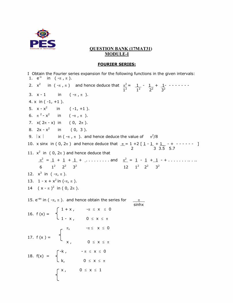
QUESTION BANK (17MAT31)

MODULE-I

FOURIER SERIES:

I Obtain the Fourier series expansion for the following functions in the given intervals: 1. e-x in ( -p , p ).

2. x2 in ( -p , p ) and hence deduce that p2 = 1 - 1 + 1- - - - - - - -

12 12 22 32 3. x - 1 in ( -p , p ).

4. x in ( -1, +1 ).

5. x - x2 in ( -1, +1 ).

6. p 2 - x2 in ( -p , p ).

7. x( 2p - x) in ( 0, 2p ).

8. 2x - x2 in ( 0, 3 ).

9. êx ê in ( -p , p ). and hence deduce the value of p2/8

10. x sinx in ( 0, 2p ) and hence deduce that p = 1 +2 [ 1 - 1 + 1_ - + - - - - - - ]

2 3 3.5 5.7 11. x2 in ( 0, 2p ) and hence deduce that

p2 = 1 + 1 + 1 + . . . . . . . . . and p2 = 1 - 1 + 1 - + . . . . . . . .. . ..

6 12 22 32 12 12 22 32

12. x3 in ( -p, p ).

13. 1 - x + x2 in (-p, p ).

14 ( x - p )2 in ( 0, 2p ).

15. e-ax in ( -p, p ). and hence obtain the series for __p__

sinhx 1 + x , -p £ x £ 0

16. f (x) = 1 - x , 0 £ x £ p

p, -p £ x £ 0

17. f (x ) = x , 0 £ x £ p

-k , - p £ x £ 0

18. f(x) =

k, 0 £ x £ p

x , 0 £ x £ 1

19. f(x) =

x - 21, 1 £ x £ 21

x2 , 0 £ x £ p 20. f(x) =

-( 2p - x)2 p £ x £ 2p px, 0 £ x £ 1

21. f(x) =

p ( 2 - x ) 1 £ x £ 2

x, 0 £ x £ p

22. f(x) =

2p - x, p £ x £ 2p

Hence deduce that p2 = 1 + 1 + 1 + - - - - - -

8 12 32 52

2, -2 £ x £ 0

23. f(x) =

x, 0 £ x £ 2

24. . Find the half - range cosine and half - range sine series for the following.

( a ). f (x) = x ( p - x ) in ( 0, p ).

( b ) f (x ) = x2 in ( 0, p ).

2k x, ( 0, 1/2 ) (c ) f (x ) =

2k (1 - x ), ( 1/2, 1 )

25.. Find the half range cosine series for the following:

(a) f (x ) = x in ( 0, 2 )

(b) f (x ) = (x - 1 )2 in ( 0, 1 )

x, 0 £ x £ 1

(c) f (x) = 2 - x, 1 £ x £ 2

cosx , 0 £ x £ ( p/2 )

(d) f (x) = 0, ( p/2 ) £ x £ p

26. . Find the half - range sine series for the following:

(a) f (x) = x3 in ( 0, 2 ). (b) f (x) = 1+x2 in ( 0, p ).

(1/4) - x, in ( 0, 1/2 )

(c) f (x) = x - (3/4), in ( 1/2, 1 )

cosx, 0 £ x £ ( p/4 )

(d) f (x) = sinx, (p/4) £ x £ ( p/2 )

27. Obtain the complex Fourier series expansion of e-x in (-1, 1).

28. Find the complex Fourier series for cos ax in (- p, p).

29. Expand y in terms of Fourier series using the table below.

X: 0 p /6 p/3 p/2 2p/3 5p /6

Y: 0 9.2 14.4 17.8 17.3 11.7

30. Determine the Fourier expansion , upto third harmonics, for the function f(q) defined by

the following table.

q0 30 60 90 120 150 180 210 240 270 300 330 360

F(q) 0.6 0.83 1.0 0.8 0.42 0 -0.34

-0.5 -0.2 0.67 0.7 0.5

31. The turning moment T on the crank-shaft of a steam engine for crank angle degrees is

given below:

q:

0 15 30 45 60 75 90 105 120 135 150 165

T: 0 2.7 5.2 7.0 8.1 8.3 7.9 6.8 5.5 4.1 2.6 1.2

Express T in a series of sine up to second harmonics.

MODULE-II

FOURIER TRANSFORMS :

I Define the complex Fourier transform of a function f(x) and give the inversion

formula. Use ‘a ’ as the parameter .

II Find the complex F.T. of the functions defined as follows:

eikx, a<x<b

1. f(x) = 0, otherwise

1 - x2, êxú < 1

2. f(x) = 0, otherwise

1 - êxú , êxú < a

3. f(x) = Hence show that sin2 t dt = p

0 , êxú >a>0 t2 2

0, x<p

4. Show that the F.T. of f(x) = 1, p<x<q is (1/Ö2p) eiqa - eipa

0, x>q ia

Ö2p , êxú < a

5. f(x) = 2a 0, otherwise

6. f(x) = êxú e- a êxú , ‘a’ is a positive constant

(a2 - x2)-1/2 , êxú < a

7. Show that F.T. of f(x) = is Öp/2 J0(aa)

0, otherwise

8. Show that the F.T. of the Dirac delta function F{d (x - a) } is 1/Ö2p eiaa

9. (i) f(x) = cosax2 and (ii) f(x) = sinax2 . Use the results

òò¥

¥-

¥

¥-

== 2

πdusinu ducosu 22

Show that the function e-x /2 is self reciprocal with respect to the complex F.T.

by finding the F.T. of e-a x , a>0

10. Find the inverse complex F.T. of (i) sin(aa) (ii) e-a êa ÷ , a>0

a

17. Define Fc(a) and Fs(a), the Fourier cosine and sine transforms, respectively,

of a function f(x).

18. Find the Fourier Cosine and Fourier sine transforms of e-ax, a>0. Hence deduce the

inversion formulae.

19. Find the Fourier Cosine transforms of :

(i) e-x (ii) 1 (iii) x2e-ax (iv) e-ax (v) f(x)= cosx, x>a

0<x<a 1 + x2 x

20. Find the Fourier Sine transforms of :

(i) e-x (ii) x (iii) xe-ax (iv) e-ax (v) sinx, 0<x<a

1 + x2 x f(x) = 0, x ³ a

1, 0<x<a

21. Find Fc(a) and Fs(a) of f(x) = 0, x ³a

22. Find the F.S.T. of e- êx ÷ and hence deduce that ò¥

-=+

0

m

2e

2

πdxsinmx

x1

x

28. Find f(x) if its sine transform is e-aa . Hence find the inverse sine transform of 1

a a

29. Find the Fourier Sine and Cosine transforms of xm-1, 0<m<1.

Hence find the same for (i) Öx & (ii) 1/Öx.

Z TRANSFORMS

I. Define a linear Difference Equations. II. Solve the following difference Equation.

(i) un+2-2un+1+un=0.

(ii) yn+1-2yncosα+yn-1=0. (iii) un+2-6un+1+9un=0.

(iv) uk+3-3uk+2+4uk=0. (v) un+1-2un+2un-1=0.

(vi) 4yn-yn+2=0.Given that y0=0,y1=2.

III. Define Z Transform of a function un and give the inversion.

IV. (i) Find the Z transform of Z(an).

(ii) Show that Z(np)= -Zdz

d Z(np-1),p being a +ve integer.

(iii) Show that Z(aun+bvn-cwn)=aZ(un)+bZ(vn)-cZ(wn).

(iv) Find the Z Transform of Z(nan).

(v) Show that Z(n2an)=3

22

)( aZ

ZaaZ

-

+.

(vi) Show that Z(cosnθ)=1cos2

)cos(2 +-

-

q

q

ZZ

ZZ

(vii) Show that Z(sinnθ)=1cos2

sin2 +- q

q

ZZ

Z.

(viii) Find the Z transform of Z(ancosnθ).

(ix) Find the Z Transform of Z(ansinnθ). (x) Find the Z Transform of (n+1)2.

V. Find the Z Transform of the following. (i) ean (ii) nean (iii) n2ean (iv) ancoshnθ

(v) etsin2t (vi) cos ÷ø

öçè

æ+

42

ppn

(vi) nCp(0≤p≤n). (vii) n+pCp.

VI. (i) If Z(un)=U(Z) then Z(un-k)= Z-kU(Z). (ii) If Z(un)=U(Z) then Z(un+k) =Zk[U(Z)-u0-u1Z

-1-u2Z-2-------uk-1Z-(k-1)]

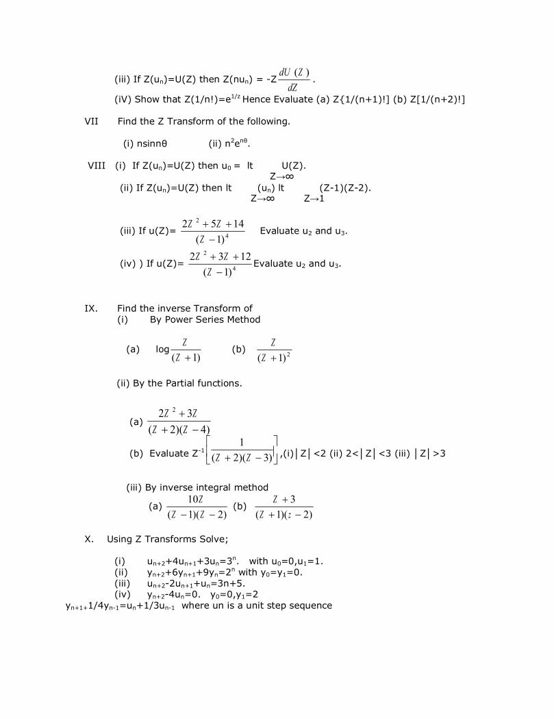
(iii) If Z(un)=U(Z) then Z(nun) = -ZdZ

ZdU )(.

(iV) Show that Z(1/n!)=e1/z Hence Evaluate (a) Z{1/(n+1)!] (b) Z[1/(n+2)!]

VII Find the Z Transform of the following.

(i) nsinnθ (ii) n2enθ.

VIII (i) If Z(un)=U(Z) then u0 = lt U(Z). Z→∞

(ii) If Z(un)=U(Z) then lt (un) lt (Z-1)(Z-2). Z→∞ Z→1

(iii) If u(Z)= 4

2

)1(

1452

-

++

Z

ZZ Evaluate u2 and u3.

(iv) ) If u(Z)= 4

2

)1(

1232

-

++

Z

ZZEvaluate u2 and u3.

IX. Find the inverse Transform of

(i) By Power Series Method

(a) log)1( +Z

Z (b)

2)1( +Z

Z

(ii) By the Partial functions.

(a) )4)(2(

32 2

-+

+

ZZ

ZZ

(b) Evaluate Z-1 úû

ùêë

é

-+ )3)(2(

1

ZZ ,(i)│Z│<2 (ii) 2<│Z│<3 (iii) │Z│>3

(iii) By inverse integral method

(a) )2)(1(

10

-- ZZ

Z (b)

)2)(1(

3

-+

+

zZ

Z

X. Using Z Transforms Solve;

(i) un+2+4un+1+3un=3n. with u0=0,u1=1.

(ii) yn+2+6yn+1+9yn=2n with y0=y1=0.

(iii) un+2-2un+1+un=3n+5. (iv) yn+2-4un=0. y0=0,y1=2

yn+1+1/4yn-1=un+1/3un-1 where un is a unit step sequence

MODULE3: STATISTICAL METHODS AND CURVE FITTING

1. Fit the straight line of the form y= a + bx to the given data

x: 0 5 10 15 20 25

y: 12 15 17 22 24 30

2. Fit a parabola cbxaxy ++= 2 to the following data.

x: 20 40 60 80 100 120

y: 5.5 9.1 14.9 22.8 33.3 46.0

3. Fit a curve of the form y=axb for the data

x: 1 2 3 4 5 6

y: 2.98 4.26 5.21 6.1 6.8 7.5

4. The following table gives the marks obtained by a student in two subjects in ten tests.

Find the coefficient of correlation.

Sub A : 77 54 27 52 14 35 90 25 56 60

Sub B: 35 58 60 40 50 40 35 56 34 42

5. Show that there is a perfect correlation between x & y .

x: 10 12 14 16 18 20

y: 20 25 30 35 40 45

6. A computer while calculating the correlation coefficient bet x & y from 25 pairs of

observations got the following constants n = 25, S x = 125, S x2 = 650, S y = 100, Sy

2

= 460& S xy = 508. Later it was discovered it had copied down the pairs (8, 12) & (6, 8) as

(6, 14) & (8, 6) respectively. Obtain the correct value of the correlation coefficient.

7. If q is the angle between two regression lines show that

22

x

yx2

r-1 tan

yσσ

σσ

rθ

+= and explain the significance when r = 0.

8. Find the lines of regression for the following data:

x: 1 2 3 4 5 6 7 8 9 10

y; 10 12 16 28 25 36 41 49 40 50

9. If the mean of x is 65, mean of y is 67, sx = 7. 5, sx = 3.5 & r = 0.8 find the value of x

corresponding to y= 75 & y corresponding to x = 70.

10. The two regression lines are x = 4y + 5 & 16y = x + 64 find the mean values of x, y & r.

11. In a partially destroyed laboratory record of correlation data only the following results are

legible. variance of y is 16, regression equations are y = x + 5, 16x = 9y - 94, find the

variance of x.

12. Fit a straight line to the data:

(a) x: 0 1 2 3 4

y: 1 1.8 3.3 4.5 6.3

(b) x: 1 2 3 4 5

y: 14 13 9 5 2

13. Fit a second degree parabola of the form y = ax2 + bx + c for the data:

x: 1 2 3 4 5

y: 1.8 5.1 8.9 14.1 19.8 . Estimate y for x = 2.5.

14. Fit an exponential curve of the form y = abx, for the following data:

x: 1 2 3 4 5 6 7

y: 87 97 113 129 202 195 193. Estimate y for x = 8

NUMERICAL METHODS I:

Solution of System of algebraic and transcendental equations :

1. Use Regular - falsi method to find a real root of the given equations.

1) sinx-coshx+1=0

2) x2-logex –12 = 0

3) cosx-3x+1=0

4) ex-3x=0

5) x4+2x2-16x+5=0 in (0.1)

6) 2x+log10x=7 in (3.5,4) correct to 3 decimal places

2. Use Newton Raphson method to find the real root of given equations

1 12 to 4 decimal places

2 cosx = x

3 x3+5x+3=0 in (1,2)

4 x2+ 4 sinx = 0 to 4 decimal places

5 x5-3.7 x4 +7.4 x3 – 10.8 x2 + 10.8x – 6.8=0

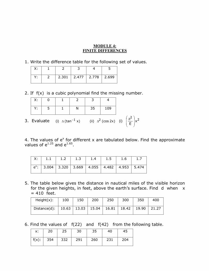
MODULE 4:

FINITE DIFFERENCES

1. Write the difference table for the following set of values.

X: 1 2 3 4 5

Y: 2 2.301 2.477 2.778 2.699

2. If f(x) is a cubic polynomial find the missing number.

X: 0 1 2 3 4

Y: 5 1 N 35 109

3. Evaluate )x(tan)i( 1-D )x2(cos)ii( 2D 22

xE

)i(÷÷

ø

ö

çç

è

æ D

4. The values of ex for different x are tabulated below. Find the approximate

values of e1.25 and e1.65.

X: 1.1 1.2 1.3 1.4 1.5 1.6 1.7

ex: 3.004 3.320 3.669 4.055 4.482 4.953 5.474

5. The table below gives the distance in nautical miles of the visible horizon

for the given heights, in feet, above the earth’s surface. Find d when x

= 410 feet.

Height(x): 100 150 200 250 300 350 400

Distance(d): 10.63 13.03 15.04 16.81 18.42 19.90 21.27

6. Find the values of f(22) and f(42) from the following table.

x: 20 25 30 35 40 45

f(x): 354 332 291 260 231 204

7. Find f(x) when x = 0.1604 from the table given below :

X: 0.160 0.161 0.162

f(x): 0.15931821 0.16030535 0.16129134

8. Estimate the values of (i) sin 380 and (ii) sin 220 from the

table given below.

x(degrees): 0 10 20 30 40

sin x: 0 0.17365 0.34202 0.50000 0.64279

9. Use Lagrange’s interpolation formula to find the value of y at x = 10 from

the following table.

X: 5 6 9 11

Y: 12 13 14 16

10. Given log 654 = 2.8156, log 658 = 2.8182, log 659 = 2.8189, log 661 =

2.8202,

find log 656 using Lagrange’s interpolation formula.

11. Given the following table, find f(22) using Newton’s divided difference formula.

x: 1.0 2.0 2.5 3.5 4.0

f(x): 84.289 87.138 87.709 88.363 88.568

12. Apply Newton - Gregory forward difference formula to find f (5) given that

f (0) = 2, f (2) = 7, f (4)=10, f (6) = 14, f (8) = 19, f (10) = 24.

13. Find the polynomial approximating f (x) using Newton- Gregory forward difference

formula, given f (4) = 1,f (6) = 3, f (8) = 8, f(10) = 20.

14. Apply Newton- Gregory backward difference formula to find the polynomial

approximating f (x), given f (0) = 2, f(1) = 3, f (2) = 12, f (3) = 16.

15. Find f (7) using Newton - Gregory backward difference formula given that :

f (2) = 7, f (4) = 16, f (6) = 21, f (8) = 24, f (10) = 30, f (12) = 35.

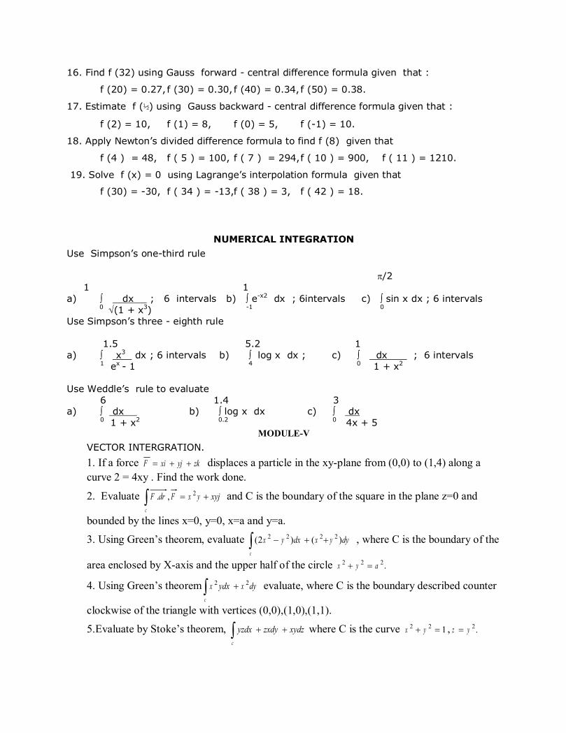
16. Find f (32) using Gauss forward - central difference formula given that :

f (20) = 0.27, f (30) = 0.30, f (40) = 0.34, f (50) = 0.38.

17. Estimate f (½) using Gauss backward - central difference formula given that :

f (2) = 10, f (1) = 8, f (0) = 5, f (-1) = 10.

18. Apply Newton’s divided difference formula to find f (8) given that

f (4 ) = 48, f ( 5 ) = 100, f ( 7 ) = 294, f ( 10 ) = 900, f ( 11 ) = 1210.

19. Solve f (x) = 0 using Lagrange’s interpolation formula given that

f (30) = -30, f ( 34 ) = -13,f ( 38 ) = 3, f ( 42 ) = 18.

NUMERICAL INTEGRATION

Use Simpson’s one-third rule

p/2

1 1

a) ò dx ; 6 intervals b) ò e-x2 dx ; 6intervals c) ò sin x dx ; 6 intervals

0 Ö(1 + x3) -1 0

Use Simpson’s three - eighth rule

1.5 5.2 1

a) ò x3 dx ; 6 intervals b) ò log x dx ; c) ò dx ; 6 intervals 1 ex - 1 4 0 1 + x2

Use Weddle’s rule to evaluate

6 1.4 3 a) ò dx b) ò log x dx c) ò dx

0 1 + x2 0.2 0 4x + 5 MODULE-V

VECTOR INTERGRATION.

1. If a force zkyjxiF ++= displaces a particle in the xy-plane from (0,0) to (1,4) along a

curve 2 = 4xy . Find the work done.

2. Evaluate xyjyxFdrF

c

+=ò 2,. and C is the boundary of the square in the plane z=0 and

bounded by the lines x=0, y=0, x=a and y=a.

3. Using Green’s theorem, evaluate ò ++-

c

dyyxdxyx )()2( 2222 , where C is the boundary of the

area enclosed by X-axis and the upper half of the circle .222 ayx =+

4. Using Green’s theorem ò +

c

dyxydxx 22 evaluate, where C is the boundary described counter

clockwise of the triangle with vertices (0,0),(1,0),(1,1).

5.Evaluate by Stoke’s theorem, ò ++

c

xydzzxdyyzdx where C is the curve 122 =+ yx , .2yz =

6.Evaluate by Stoke’s theorem ò ---

c

zdzydyyzdxyx 22)2( where C is the curve 122 =+ yx ,

corresponding to the surface of sphere of unit radius.

7.Evaluate ò òs

ndsF . using Gauss divergence theorem where S is the surface of the sphere

1222 =++ zyx and zkjyxiF 543 ++=