Mathematical Modelling of Circadian Signalling in Arabidopsis
236
Mathematical Modelling of Circadian Signalling in Arabidopsis A dissertation submitted to the University of Cambridge in partial fulfilment of the requirements for the degree of Doctor of Philosophy by Neil Dalchau Downing College, Cambridge December 2008
-
Upload
khangminh22 -
Category
Documents
-
view
1 -
download
0
Transcript of Mathematical Modelling of Circadian Signalling in Arabidopsis
Mathematical Modelling of CircadianSignalling in Arabidopsis
A dissertation submitted to theUniversity of Cambridge in partial
fulfilment of the requirements for thedegree of Doctor of Philosophy by
Neil Dalchau
Downing College, Cambridge
December 2008

Summary
Mathematical Modelling of Circadian Signalling in ArabidopsisNeil Dalchau
The circadian signalling network in Arabidopsis thaliana generates oscillations with negativefeedback loops of transcription factor binding, and regulates many developmental and phys-iological processes. Mathematical models have been proposed which describe the transcrip-tional and post-translational feedback loops generating oscillations, though do not incorporatethe interactions with cytosolic messengers such as Ca2+ and cADPR, or with metabolites suchas sucrose. The aim of this thesis is to use mathematical modelling to investigate how thecircadian clock regulates [Ca2+]cyt, how a cADPR-based feedback loop modulates circadianoscillations, and also how the circadian clock perceives changes in the availability of sucrose.Delay linear systems of ordinary differential equations were used to demonstrate how [Ca2+]cyt
is co-regulated by two pathways operating on different timescales, the first dependent on thetranscription factor CIRCADIAN CLOCK ASSOCIATED 1 (CCA1), and a light/dark-dependentcircadian clock-independent pathway. Simulated mutant analysis provided a potential role forthe red-light sensing PHYTOCHROME A (PHYA) in the light-dependent pathway and offeredpredictions for the dynamics of [Ca2+]cyt when system components are removed. A proposedfeedback loop between the second messenger cADPR and the circadian clock was investigatedin silico using a pairwise parameter perturbation method on mathematical models of the Ara-bidopsis central oscillator. Experimental observations from transient and persistent manipu-lations to cADPR synthesis could be explained with time-varying parametric perturbationsto mathematical oscillator models representing the effects of cADPR on clock gene expression,supporting the hypothesised cADPR-based feedback loop. Finally, the dependency of circadianoscillations in darkness on exogenous sucrose availability was investigated using the Three Loopmodel of the circadian clock. Mathematical analyses and experimental validation demonstratedthe involvement of GIGANTEA (GI) in the sucrose-sensing by the circadian clock, either by atranscriptional or post-translational mechanism. Further experimental evidence is presentedsupporting the hypothesis that sucrose up-regulates GI transcription. This thesis identifiescomponents of the circadian clock which serve as entry or exit points for cytosolic signallingand metabolic pathways involved in key physiological processes, and demonstrates the use ofmathematics to generate non-intuitive hypotheses for subsequent experimental validation incomplex biological systems.
i
Acknowledgements
Acknowledgements
By undertaking this project, I was committing to learning an entire academic discipline fromscratch. It is impossible to remember the many people who have explained biological princi-ples to me during my time in Cambridge, though I thank each and every one of them. Theenormity of this task would not have been possible without the patience and seemingly infi-nite enthusiasm of my supervisor, Dr. Alex Webb. I also applaud his ambition in combiningthe spheres of Biology and Engineering for the purpose of this project. I must also thank mysecond supervisor, Dr. Jorge Gonçalves, who provided stimulating discussions on the moremathematically rigorous considerations of mathematical modelling and control theory. Alsofrom the engineering community, I am very grateful to Dr. Guy-Bart Stan, who in addition tocritically reading my entire thesis has provided many interesting ideas to this project. I am alsovery grateful to most excellent Dr. Antony Dodd, with whom I had the pleasure of publishingan article in Science, and discussing a wealth of academic and completely non-academic topics.All of the other members of the Signal Transduction group contributed greatly to my scientificlife over the last three years, particularly Leon Baek, Dr. Katharine Hubbard and Dr. CarlosHotta. In particular, they have provided much of the data contained within this thesis, whichhas been used to great extent in the construction of mathematical models.
The majority of the funding for this project has come from the Biotechnology and BiologicalSciences Research Council (BBSRC), to whom I am very grateful. Additional funding has comein the form of a studentship from Downing College in memory of Dr. John Treherne and astudentship from the Department of Plant Sciences in memory of Frank Smart.
On a personal level, I am eternally grateful to my fantastic parents who have supported methrough the good and bad, with the provision of good food and liquidity (beer and otherwise).Also, my late grandmother Kathleen Dalchau, whose enthusiasm for numeracy sparked a loveof mathematics which has never faltered. My sanity has been kept in check by my close friendsGordon Francis, Andrew Dreier, Dr. Fiona Robertson and Anuphon Laohavisit, the latter pro-viding a competitive element to thesis submission and great Thai food. Finally, I am grateful toDr. Katy Coxon for being a fantastic girlfriend, providing me with food, beer and money, andeven for being an occasional dictionary of biological concepts.
ii

Disclaimer
Disclaimer
This dissertation does not exceed the word limit for the School of the Biological Sciences De-gree Committee and is the result of my own work and includes nothing which is the outcome ofwork done in collaboration except where specifically indicated in the text. Parts of this disser-tation are already published (Dodd et al., 2007) but no part of it has been submitted to anotherqualification.
iii

Table of Contents
Summary i
Acknowledgements ii
Disclaimer ii
Contents iv
List of Figures viii
List of Tables xi
List of Abbreviations xii
1 General Introduction 11.1 The Circadian Clock in Plants . . . . . . . . . . . . . . . . . . . . . . . . . . . . . . 2
1.1.1 Circadian control of physiology . . . . . . . . . . . . . . . . . . . . . . . . . 21.1.2 Transcriptional feedback loops and essential central oscillator compo-
nents in Arabidopsis . . . . . . . . . . . . . . . . . . . . . . . . . . . . . . . . 41.1.3 Mathematical models of the Arabidopsis circadian clock . . . . . . . . . . . 71.1.4 Molecular mechanisms of circadian control . . . . . . . . . . . . . . . . . . 91.1.5 Input pathways and entrainment . . . . . . . . . . . . . . . . . . . . . . . . 11
1.2 Calcium Signalling . . . . . . . . . . . . . . . . . . . . . . . . . . . . . . . . . . . . 141.2.1 Generation of [Ca2+]cyt gradients . . . . . . . . . . . . . . . . . . . . . . . . 141.2.2 Circadian control of [Ca2+]cyt in plants . . . . . . . . . . . . . . . . . . . . . 16
1.3 Mathematical Modelling of Biochemical Reaction Networks (BRNs) . . . . . . . . 191.3.1 Mass Action kinetics, Michaelis-menten and Hill equations . . . . . . . . . 191.3.2 Linear and Nonlinear Dynamical Systems . . . . . . . . . . . . . . . . . . . 22
2 Delay Linear Systems for the Circadian Regulation of [Ca2+]cyt 262.1 Introduction . . . . . . . . . . . . . . . . . . . . . . . . . . . . . . . . . . . . . . . . 262.2 Materials and Methods . . . . . . . . . . . . . . . . . . . . . . . . . . . . . . . . . . 31
2.2.1 Plant material and growth conditions . . . . . . . . . . . . . . . . . . . . . 312.2.2 Luminescence imaging . . . . . . . . . . . . . . . . . . . . . . . . . . . . . . 312.2.3 Data for estimation and validation of mathematical models . . . . . . . . 32
iv

TABLE OF CONTENTS
2.2.4 State-space time-delay systems . . . . . . . . . . . . . . . . . . . . . . . . . 342.2.5 Parameter estimation of delay linear systems . . . . . . . . . . . . . . . . . 372.2.6 Model selection - Akaike’s Information Criterion (AIC) . . . . . . . . . . . 402.2.7 Simulation of delay linear systems for comparison with input-output data 41
2.3 Results . . . . . . . . . . . . . . . . . . . . . . . . . . . . . . . . . . . . . . . . . . . 422.3.1 Regulation of [Ca2+]cyt by a CCA1-dependent pathway: Estimation of
single-input models . . . . . . . . . . . . . . . . . . . . . . . . . . . . . . . 422.3.2 Cross-validation of the single-input model: Selection of optimal order
and delay steps . . . . . . . . . . . . . . . . . . . . . . . . . . . . . . . . . . 432.3.3 Dual regulation of [Ca2+]cyt by CCA1 and light: Estimation of dual-input
model classes . . . . . . . . . . . . . . . . . . . . . . . . . . . . . . . . . . . 472.3.4 Cross-validation of the dual-input model classes . . . . . . . . . . . . . . . 512.3.5 Isolation of the pathways regulating [Ca2+]cyt through simulated mutation 562.3.6 Predicted [Ca2+]cyt phenotypes of a null mutation in the hidden state vari-
able . . . . . . . . . . . . . . . . . . . . . . . . . . . . . . . . . . . . . . . . . 592.3.7 Determination of internal structure for the CCA1–Light/Dark–[Ca2+]cyt-
X2 network . . . . . . . . . . . . . . . . . . . . . . . . . . . . . . . . . . . . 652.3.8 Frequency response of [Ca2+]cyt to CCA1 and Light/Dark . . . . . . . . . . 67
2.4 Discussion . . . . . . . . . . . . . . . . . . . . . . . . . . . . . . . . . . . . . . . . . 682.4.1 [Ca2+]cyt is regulated by a light/dark-dependent pathway and a hidden
variable . . . . . . . . . . . . . . . . . . . . . . . . . . . . . . . . . . . . . . 692.4.2 Simulated CCA1 mutant analysis reveals temporal information for the
regulation of [Ca2+]cyt by transitions between light and dark . . . . . . . . 702.4.3 The unconstrained internal structure of the 2nd order model complicates
the identification of X2 . . . . . . . . . . . . . . . . . . . . . . . . . . . . . . 722.4.4 Simulations of a mutation in the light/dark input pathway or the hidden
state variable . . . . . . . . . . . . . . . . . . . . . . . . . . . . . . . . . . . 732.4.5 Summary . . . . . . . . . . . . . . . . . . . . . . . . . . . . . . . . . . . . . 75
3 A Three Loop Model of the Arabidopsis Circadian Clock in the Absence of Exoge-nous Sucrose 763.1 Introduction . . . . . . . . . . . . . . . . . . . . . . . . . . . . . . . . . . . . . . . . 763.2 Materials and Methods . . . . . . . . . . . . . . . . . . . . . . . . . . . . . . . . . . 78
3.2.1 Measuring the effect of cold of CCA1 promoter activity with a microplateluminometer . . . . . . . . . . . . . . . . . . . . . . . . . . . . . . . . . . . . 78
3.2.2 Numerical solution of the Three Loop Model equations . . . . . . . . . . . . 803.2.3 Period and amplitude plots for associating exogenous sucrose availability
with single model parameter alterations . . . . . . . . . . . . . . . . . . . . 803.2.4 K-means clustering of simulated outputs . . . . . . . . . . . . . . . . . . . 813.2.5 Fine-tuning the Three Loop Model parameters for no exogenous sucrose
supply . . . . . . . . . . . . . . . . . . . . . . . . . . . . . . . . . . . . . . . 813.3 Results . . . . . . . . . . . . . . . . . . . . . . . . . . . . . . . . . . . . . . . . . . . 87
v

TABLE OF CONTENTS
3.3.1 [ATP]i does not limit Luciferase light emission after 60 hours of darkness . 873.3.2 Accounting for no exogenous sucrose with single-parameter modifica-
tions to the Three Loop Model . . . . . . . . . . . . . . . . . . . . . . . . . . . 883.3.3 Accounting for no exogenous sucrose with multiple-parameter modifica-
tions to the Three Loop Model . . . . . . . . . . . . . . . . . . . . . . . . . . . 943.3.4 Simulated mutant analysis . . . . . . . . . . . . . . . . . . . . . . . . . . . 101
3.4 Discussion . . . . . . . . . . . . . . . . . . . . . . . . . . . . . . . . . . . . . . . . . 1023.4.1 The N5 Model outperforms fine-tuned models . . . . . . . . . . . . . . . . 1033.4.2 GIGANTEA mediates sucrose modulation of the central oscillator in DD . 1043.4.3 A novel sugar signalling pathway . . . . . . . . . . . . . . . . . . . . . . . 1063.4.4 Summary . . . . . . . . . . . . . . . . . . . . . . . . . . . . . . . . . . . . . 107
4 GI-Mediated Sucrose Modulation of the Arabidopsis Circadian Clock 1084.1 Introduction . . . . . . . . . . . . . . . . . . . . . . . . . . . . . . . . . . . . . . . . 1084.2 Materials and Methods . . . . . . . . . . . . . . . . . . . . . . . . . . . . . . . . . . 109
4.2.1 Plant material and growth conditions . . . . . . . . . . . . . . . . . . . . . 1094.2.2 Imaging of luciferase activity for topical sucrose treatment . . . . . . . . . . 1094.2.3 Numerical approximation of peak and trough values of luc luminescence
data . . . . . . . . . . . . . . . . . . . . . . . . . . . . . . . . . . . . . . . . . 1104.2.4 Numerical solution of the Three Loop Model equations . . . . . . . . . . . . 110
4.3 Results . . . . . . . . . . . . . . . . . . . . . . . . . . . . . . . . . . . . . . . . . . . 1114.3.1 Simulated post-translational modification of GIGANTEA enables
sucrose-dependent oscillations in DD . . . . . . . . . . . . . . . . . . . . . 1114.3.2 Simulated effect of sucrose on GI protein levels in light-dark cycles . . . . 1124.3.3 Response of GI expression to topical sucrose treatment . . . . . . . . . . . 117
4.4 Discussion . . . . . . . . . . . . . . . . . . . . . . . . . . . . . . . . . . . . . . . . . 1214.4.1 The PostGI Model: GI protein stabilisation . . . . . . . . . . . . . . . . . . . 1214.4.2 Distinction of transcriptional and post-translational mechanisms . . . . . 1224.4.3 Summary . . . . . . . . . . . . . . . . . . . . . . . . . . . . . . . . . . . . . 123
5 Modelling a cADPR-Dependent Feedback Loop of the Circadian Clock 1245.1 Introduction . . . . . . . . . . . . . . . . . . . . . . . . . . . . . . . . . . . . . . . . 1245.2 Mathematical methods . . . . . . . . . . . . . . . . . . . . . . . . . . . . . . . . . . 127
5.2.1 Simulating effects of high and low [cADPR] on clock gene expressionwith the Interlocked Feedback Loop Model . . . . . . . . . . . . . . . . . . . . 127
5.2.2 Refinement of the pairwise parameter perturbation method and applica-tion to the Three Loop Model . . . . . . . . . . . . . . . . . . . . . . . . . . . 130
5.2.3 Calculation of period and phase in LL . . . . . . . . . . . . . . . . . . . . . 1325.3 Results . . . . . . . . . . . . . . . . . . . . . . . . . . . . . . . . . . . . . . . . . . . 133
5.3.1 Parameter perturbation analysis applied to the Interlocked Feedback LoopModel . . . . . . . . . . . . . . . . . . . . . . . . . . . . . . . . . . . . . . . . 133
vi

TABLE OF CONTENTS
5.3.2 A refined pairwise parameter perturbation method applied to the Inter-locked Feedback and Three Loop Models . . . . . . . . . . . . . . . . . . . . . . 142
5.4 Discussion . . . . . . . . . . . . . . . . . . . . . . . . . . . . . . . . . . . . . . . . . 1505.4.1 Transient stimulation of cADPR-regulated transcripts does not affect cir-
cadian period . . . . . . . . . . . . . . . . . . . . . . . . . . . . . . . . . . . 1535.4.2 Constant activation and suppression of cADPR-regulated transcripts al-
ters circadian period . . . . . . . . . . . . . . . . . . . . . . . . . . . . . . . 1545.4.3 Time of induction of ADPR cyclase affects downstream response . . . . . 1575.4.4 Summary . . . . . . . . . . . . . . . . . . . . . . . . . . . . . . . . . . . . . 158
6 General Discussion 1596.1 Linear systems identification reveals properties of the dual regulation of [Ca2+]cyt
by the circadian central oscillator and light . . . . . . . . . . . . . . . . . . . . . . 1616.2 Demonstration of a cADPR-dependent feedback loop in the circadian clock net-
work by a pairwise parameter perturbation method . . . . . . . . . . . . . . . . . 1626.2.1 Does [Ca2+]cyt mediate circadian clock regulation by cADPR? . . . . . . . 163
6.3 Possible roles for sucrose up-regulation of GI . . . . . . . . . . . . . . . . . . . . . 1656.4 A Light–Carbohydrate–Circadian Clock model . . . . . . . . . . . . . . . . . . . . 1676.5 Conclusions . . . . . . . . . . . . . . . . . . . . . . . . . . . . . . . . . . . . . . . . 167
7 Bibliography 168
A Central Oscillator Models 187A.1 Interlocked Feedback Loop model . . . . . . . . . . . . . . . . . . . . . . . . . . . 187
A.1.1 Equations . . . . . . . . . . . . . . . . . . . . . . . . . . . . . . . . . . . . . 187A.1.2 Parameters . . . . . . . . . . . . . . . . . . . . . . . . . . . . . . . . . . . . . 188
A.2 Three Loop model . . . . . . . . . . . . . . . . . . . . . . . . . . . . . . . . . . . . . 190A.2.1 Equations . . . . . . . . . . . . . . . . . . . . . . . . . . . . . . . . . . . . . 190A.2.2 Parameters . . . . . . . . . . . . . . . . . . . . . . . . . . . . . . . . . . . . . 191
B Dodd et al., (2007) – Published in Science 194
vii

List of Figures
1.1 A transcriptional/post-translational network describes the Arabidopsis circadianclock . . . . . . . . . . . . . . . . . . . . . . . . . . . . . . . . . . . . . . . . . . . . 5
1.2 The Three Loop model of the Arabidopsis circadian clock . . . . . . . . . . . . . . . . 81.3 Model for the generation of circadian [Ca2+]cyt oscillations . . . . . . . . . . . . . 18
2.1 [Ca2+]cyt oscillates in light-dark cycles and constant light but not in constant dark 272.2 Schematic for a mathematical model of circadian and light/dark regulation of
[Ca2+]cyt . . . . . . . . . . . . . . . . . . . . . . . . . . . . . . . . . . . . . . . . . . 302.3 CCA1:luc and AEQUORIN luminescence data provide input and output signals
for generation of linear state-space time-delay models . . . . . . . . . . . . . . . . 332.4 Estimation of SISO models for the regulation of [Ca2+]cyt by a CCA1-dependent
pathway . . . . . . . . . . . . . . . . . . . . . . . . . . . . . . . . . . . . . . . . . . 442.5 Correlation of single input model simulations to AEQUORIN luminescence data 452.6 Cross-validation of optimal-τCCA1 linear models for different orders with AE-
QUORIN luminescence data . . . . . . . . . . . . . . . . . . . . . . . . . . . . . . . 462.7 AICc performance of dual-input linear state-space time-delay systems for the
regulation of [Ca2+]cyt . . . . . . . . . . . . . . . . . . . . . . . . . . . . . . . . . . . 492.8 L0 models are more accurate than L1 models during estimation . . . . . . . . . . 502.9 Correlation of L0 dual-input model simulations to [Ca2+]cyt data . . . . . . . . . . 522.10 Cross-validation of 2nd order L0 models with AEQUORIN luminescence data . . 532.11 Cross-validation of 4th order L0 models with AEQUORIN luminescence data . . 542.12 Simulation of the response of [Ca2+]cyt to a mutation in CCA1 . . . . . . . . . . . 572.13 Comparing the [Ca2+]cyt oscillation phase of a simulated CCA1 mutant with cca1-
1 distinguishes τlight . . . . . . . . . . . . . . . . . . . . . . . . . . . . . . . . . . . . 582.14 Simulation of [Ca2+]cyt with a null mutation in the light/dark-dependent pathway 602.15 Simulations of the response of [Ca2+]cyt to a mutation in the hidden variable X2 . 622.16 Red- and blue-light photoreception by [Ca2+]cyt . . . . . . . . . . . . . . . . . . . . 642.17 The regulation of [Ca2+]cyt by CCA1 is a band-pass filter . . . . . . . . . . . . . . . 682.18 Mutations in core clock genes can lead to arrhythmic [Ca2+]cyt in LL . . . . . . . . 722.19 Mutations in core clock genes disrupt but do not remove [Ca2+]cyt oscillations in
light-dark cycles . . . . . . . . . . . . . . . . . . . . . . . . . . . . . . . . . . . . . . 73
viii

LIST OF FIGURES
3.1 Exogenous sucrose modulates circadian central oscillator gene expression in LLand DD . . . . . . . . . . . . . . . . . . . . . . . . . . . . . . . . . . . . . . . . . . . 79
3.2 Cold induced CCA1 promoter activity after 60 hours of darkness . . . . . . . . . . 883.3 Single parameter modifications enable steady state in DD and stable oscillations
in LL . . . . . . . . . . . . . . . . . . . . . . . . . . . . . . . . . . . . . . . . . . . . 903.4 K-means clustering of DD simulations reveals prediction of sucrose target . . . . 923.5 Cross-validation of the N5 Model to luc luminescence data in DD, LL, L16/D8
and L8/D16 . . . . . . . . . . . . . . . . . . . . . . . . . . . . . . . . . . . . . . . . 933.6 Parameter re-tuning of the Three Loop Model to account for no exogenous sucrose 963.7 Cross-validation of re-tuned Three Loop Models to luminescence data in DD, LL,
L16/D8 and L8/D16 . . . . . . . . . . . . . . . . . . . . . . . . . . . . . . . . . . . 983.8 The simulated LL phenotype of cca1 lhy depends on sucrose availability . . . . . 1023.9 Sucrose-dependent DD oscillations of CAB2:luc luminescence absent in gi-11 null
mutant . . . . . . . . . . . . . . . . . . . . . . . . . . . . . . . . . . . . . . . . . . . 1053.10 Schematic for possible sucrose-dependent pathways regulating GI . . . . . . . . . 106
4.1 Dark-dependent degradation of Y (GI) enables sucrose-dependent oscillations inDD . . . . . . . . . . . . . . . . . . . . . . . . . . . . . . . . . . . . . . . . . . . . . 113
4.2 Simulated sucrose-dependency of GI:GI-TAP protein cycling in L12/D12 . . . . . 1144.3 Calibration of the rate of constitutive 35S:GI expression . . . . . . . . . . . . . . . 1154.4 Simulated 35S:GI protein cycling in L12/D12 with the PostGI Model comparing
the availability of exogenous sucrose . . . . . . . . . . . . . . . . . . . . . . . . . . 1164.5 Simulated effects on oscillator transcript abundance of a sucrose dose after a
period of extended darkness . . . . . . . . . . . . . . . . . . . . . . . . . . . . . . . 1184.6 Sucrose amplifies circadian rhythms in DD and is a zeitgeber for GI . . . . . . . . 1194.7 Sucrose activates GI transcription as predicted by the N5 Model . . . . . . . . . . 120
5.1 Modulation of the Arabidopsis circadian clock by a cADPR-based feedback loop . 1265.2 Perturbation profiles applied to the Interlocked Feedback Loop Model . . . . . . . . . 1295.3 Parametric perturbations alter gene expression in the Interlocked Feedback Loop
Model . . . . . . . . . . . . . . . . . . . . . . . . . . . . . . . . . . . . . . . . . . . . 1315.4 Time of simulated induction of ADPR cyclase affects differential gene expression 1345.5 Frequency of candidate parameters in the Interlocked Feedback Loop Model . . . . . 1355.6 Frequency of component mRNA or protein affected by candidate perturbations
to the Interlocked Feedback Loop Model . . . . . . . . . . . . . . . . . . . . . . . . . . 1365.7 Transcript abundance returns to nominal oscillations after transient perturba-
tions in LL . . . . . . . . . . . . . . . . . . . . . . . . . . . . . . . . . . . . . . . . . 1385.8 Simulated transient activation of cADPR-regulated genes . . . . . . . . . . . . . . 1395.9 Simulated constant activation of cADPR-regulated genes . . . . . . . . . . . . . . 1405.10 Simulated suppression of cADPR-regulated genes . . . . . . . . . . . . . . . . . . 1415.11 Effect of transient perturbations on oscillation phase . . . . . . . . . . . . . . . . . 1435.12 Constant perturbations yield short period oscillations in LL . . . . . . . . . . . . 145
ix

LIST OF FIGURES
5.13 Simulated constant repression of cADPR yields a long period in LL . . . . . . . . 1465.14 The cADPR-based feedback loop is sensitive to the time of simulated
XVE:ADPRc induction . . . . . . . . . . . . . . . . . . . . . . . . . . . . . . . . . . 1475.15 Distribution of candidate perturbations over the parameters and components of
the Interlocked Feedback Loop Model . . . . . . . . . . . . . . . . . . . . . . . . . . . . 1495.16 Distribution of candidate perturbations over the parameters and components of
the Three Loop Model . . . . . . . . . . . . . . . . . . . . . . . . . . . . . . . . . . . . 1515.17 Overexpression of ADPR cyclase disrupts circadian oscillations of [Ca2+]cyt . . . 1555.18 Overexpression of ADPR cyclase disrupts circadian rhythms in leaf position . . . 156
6.1 Arabidopsis circadian clock network as demonstrated through mathematicalmodelling . . . . . . . . . . . . . . . . . . . . . . . . . . . . . . . . . . . . . . . . . 160
6.2 The Arabidopsis circadian clock may incorporate a cADPR–Ca2+–CML23/24 cy-tosolic loop . . . . . . . . . . . . . . . . . . . . . . . . . . . . . . . . . . . . . . . . . 165
x

List of Tables
2.1 Optimal choice of τCCA1 for each order of SISO models after parameter estimation 442.2 Optimal choice of τCCA1 for each order of single-input models after cross-validation 452.3 Optimal τCCA1 for each τlight in 2nd and 4th order L0 and L1 models . . . . . . . . . 482.4 Optimal choice of τCCA1 for each τlight of dual-input L0 models after cross-validation 532.5 Optimal choice of τCCA1 for each τlight of dual-input L0 models after cross-validation 542.6 Peak [Ca2+]cyt in simulated nyctohemeral cycles of a cca1 mutant . . . . . . . . . . 582.7 Entries of A determine potential for X2 to not be regulated by [Ca2+]cyt . . . . . . 662.8 Entries of B determine potential for missing links in the input regulation of the
hidden variable . . . . . . . . . . . . . . . . . . . . . . . . . . . . . . . . . . . . . . 66
3.1 Rescaled parameters for the NDTL Model . . . . . . . . . . . . . . . . . . . . . . . 833.2 Candidate single-parameter modifications simulated for K-means clustering . . . 893.3 Candidate parameter sets from fine-tuning . . . . . . . . . . . . . . . . . . . . . . 973.4 Averaged parameter alterations from re-tuning Three Loop Model for no exoge-
nous sucrose . . . . . . . . . . . . . . . . . . . . . . . . . . . . . . . . . . . . . . . . 1003.5 Simulated mutant analysis of Three Loop Model altered for no exogenous sucrose . 101
5.1 Occurrence of component mRNA or protein affected by candidate perturbationsto the Interlocked Feedback Loop Model . . . . . . . . . . . . . . . . . . . . . . . . . . 137
A.1 Optimal parameter set for Interlocked Feedback Loop model equations, deter-mined by simulated annealing (Locke et al., 2005b) . . . . . . . . . . . . . . . . . . 188
A.2 Optimal parameter set for Three Loop model equations, determined by simu-lated annealing (Locke et al., 2006) . . . . . . . . . . . . . . . . . . . . . . . . . . . 191
xi

List of Abbreviations
For ease of reference, this list of abbreviations has been separated into gene names and other
abbreviations.
List of Gene Name Abbreviations
A mathematical representation of PRR7/9 in Locke et al. (2006)AEQ AEQUORINCAB2 CHLOROPHYLL A/B BINDING PROTEIN 2CaM CALMODULINCAS CALCIUM SENSORCAT CATALASE (2 and 3)CCA1 CIRCADIAN CLOCK ASSOCIATED 1CCL CCR-LIKECCR COLD CIRCADIAN RHYTHM RNA BINDING (1 and 2; CCR2 is also
GRP8, CCR2 is also GRP7)CK CASEIN KINASE (1 and 2)CML CALMODULIN-LIKE (23 and 24)CO CONSTANSCRY CRYPTOCHROME (1, 2 and 3)CUL1 CULLIN 1ELF EARLY FLOWERING (3 and 4)FIO1 FIONA 1FKF1 FLAVIN-BINDING, KELCH REPEAT, F-BOX 1FLC FLOWERING LOCUS CFT FLOWERING LOCUS TGI GIGANTEAGRP GLYCINE RICH PROTEIN (7 and 8; GRP7 is also CCR2, GRP8 is also
CCR1)LHY LATE ELONGATED HYPOCOTYLLKP2 LOV/KELCH PROTEIN 2LUC LUCIFERASE
xii

List of Abbreviations
LUX LUX ARRHYTHMO (also PCL1)PCL1 PHYTOCLOCK 1 (also LUX)PHOT PHOTOTROPIN (1 and 2)PHY PHYTOCHROME (A, B, C, D and E)PIF3 PHYTOCHROME INTERACTING FACTOR 3PRR PSEUDO RESPONSE REGULATOR (1, 3, 5, 7 and 9)SFR6 SENSITIVE TO FREEZING 6SKP1 S-PHASE KINASE-ASSOCIATED PROTEIN 1SOC1 SUPPRESSOR OF OVEREXPRESSION OF CONSTANS 1TIC TIME FOR COFFEETOC1 TIMING OF CAB2 EXPRESSION 1 (also PRR1)X hypothetical gene proposed by Locke et al. (2005b)Y hypothetical gene proposed by Locke et al. (2005b)ZTL ZEITLUPE
Other Abbreviations
35SCaMV 35S cauliflower mosaic virus promoterABA abscisic acidABRE ABA-responsive elementADPRc ADP-ribosyl cyclaseAIC Akaike Information CriterionAICc second-order bias correction to AICBL blue lightBRN biochemical reaction network[Ca2+]cyt concentration of cytosolic-free Ca2+
CaBP Ca2+-binding proteinscADPR cyclic adenosine diphosphate ribosecAMP 3’, 5’-cyclic monophosphateCBS CCA1-binding siteCICR calcium-induced calcium releaseCONTSID continuous time systems identification toolbox (for MATLABTM)CT circadian timeDD constant darkEE evening elementER endoplasmic reticulumEtOH ethanolFOH first-order holdIP3 inositol 1,4,5-triphosphateL12/D12 12 h light, 12 h darkL16/D8 16 h light, 8 h darkL8/D16 8 h light, 16 h dark
xiii

List of Abbreviations
LD light-dark (no specific duration implied)LED light emitting diodeLL constant lightLOV Light, Oxygen and VoltageLSQ least-squaresLT low temperatureLTI linear time-invariantME morning elementMeOH methanolMH Metropolis HastingsMIMO multi-input multi-outputMS Murashige and Skoog mediumMYB V-Myb avian myeloblastosis viral oncogeneNAADP nicotinic acid adenine dinucleotide phosphateNaClO sodium hypochloriteNASC Nottingham Arabidopsis Stock CentreODE ordinary differential equationPEM prediction-error methodPI-PLC phosphatidyl inositol-specific phospholipase CPRC phase response curveQSSA quasi steady state assumptionQTL quantitative trait lociRAE relative amplitude errorRL red lightRyR ryanodine receptorS1P sphingosine 1-phosphateSA simulated annealingSAM shoot apical meristemSCF skp1/cullin/F-boxSCN suprachiasmatic nucleusSID systems identification toolbox (for MATLABTM)SISO single-input single-outputSPP sucrose phosphate phosphataseSPS sucrose phosphate synthaseSR sarcoplasmic reticulumSUS sucrose synthaseTAP tandem affinity purificationXVE 17-β-estradiol-inducible chimeric transcription factorWS WassilewskijaZOH zero-order holdZT zeitgeber time (i.e. time after dawn)
xiv
CHAPTER 1
General Introduction
The majority of eukaryotes and some prokaryotes have a molecular mechanism to synchronize
their physiology with changing light availability and temperature resulting from the rotation
of the planet. This is an autonomous oscillator known as a circadian clock. The timing of
many biochemical processes is controlled by the clock through a series of output pathways
which originate from central clock components with different oscillation phases. In addition,
the inter-phase relationship of clock components can vary according to the external photope-
riod, enabling specific seasonal responses. Circadian clocks have evolved independently in
cyanobacteria, plants, mammals and flies, leading to mechanisms with few common elements,
though in all cases consist of interlocking feedback loops in transcriptional control (Young &
Kay, 2001). In mammals, the suprachiasmatic nucleus (SCN) acts as a central pacemaker which
co-ordinates peripheral tissues via entrainment∗ signals (Bartness et al., 2001). The ’slave os-
cillators’ in peripheral tissues also exhibit autonomous cellular oscillations, which synchronize
via intercellular coupling to maintain a robust rhythm (Aton et al., 2005). In plants, it is thought
that all cells may sustain circadian rhythms (oscillations) independently, though it is speculated
that more than one oscillator mechanism exists (McClung, 2001). Independent oscillators have
been demonstrated by entraining different leaves to opposite phases, though the short duration
of this experiment does not rule out weak intercellular coupling (Thain et al., 2000). Possession
∗Entrainment is defined by Young & Kay (2001) as establishing the phase of a rhythm by providing an environ-mental signal, such as a light or temperature cycle, or a biological signal, such as a hormone pulse.
1

CHAPTER 1: General Introduction
of a circadian clock confers major benefits when its natural frequency (or free-running period)
is resonant with that of the external environment (Ouyang et al., 1998; Dodd et al., 2005b). In
Arabidopsis thaliana, it was shown that seedlings whose free-running clock period was similar
to the period of the environmental rhythm grew larger and produced more chlorophyll than
when placed in an environmental with an alternative period; wild-type seedlings performed
better in 24 h days over 20 h and 28 h days, while short-period mutants performed better in
20 h rhythms, and long-period mutants performed better in 28 h rhythms (Dodd et al., 2005b).
1.1 The Circadian Clock in Plants
1.1.1 Circadian control of physiology
Plant circadian clock output pathways regulate a variety of physiological and biochemical pro-
cesses, including photosynthesis, leaf movement, hypocotyl elongation, stomatal movement
and circumnutation (Gardner et al., 2006). Rhythmic control of these mechanisms enables opti-
misation of output with respective to the time of day, and also leads to competitive advantage
(Dodd et al., 2005b). While little is known about how temporal information is conferred to cell
physiology, there are examples of circadian control at many developmental stages (Yakir et al.,
2007). In contrast to mammals which have a central pacemaker, plant circadian rhythms are
thought to be cell autonomous, enabling circadian oscillations with different phases in differ-
ent organs (Thain et al., 2000). Furthermore, there are examples of periodic differences between
different cells (Thain et al., 2002), and different output pathways (Xu et al., 2007), suggesting
there are additional components present in some cells, or even the potential for multiple oscil-
lators in plants.
The circadian clock appears to be signalling temporal information very early in the devel-
opmental life-cycle in many plant species, including downy birch (Betula pubescens), Lapland
diapensia (Diapensia lapponica) and leatherleaf (Chamaedaphne calyculata), in which germination
is controlled by day-length (Yakir et al., 2007). In Arabidopsis, circadian gene expression is syn-
chronized as seeds are imbibed, supporting the notion that there is a functional clock in seeds
(Zhong et al., 1998). Immediately after germination, hypocotyls extend in a circadian-clock-
dependent manner, achieving maximal growth during the subjective evening and minimal
growth in the subjcetive morning in constant light (LL; Dowson-Day & Millar, 1999). The posi-
2

CHAPTER 1: General Introduction
tion of leafs and cotyledons also undergo circadian oscillations in many plants including Ara-
bidopsis, in which movements are caused by alternating growth on the upper and lower lamina
(Webb, 2003). Perhaps the best-characterized circadian-regulated developmental process how-
ever is the transition from vegetative to reproductive growth, or flowering time (Yakir et al.,
2007). Flowering time depends on the expression of FLOWERING LOCUS T (FT) and SUP-
PRESSOR OF OVEREXPRESSION OF CONSTANS 1 (SOC1), which activate the floral identity
genes in the shoot apical meristem (SAM; Imaizumi & Kay, 2006). Prior to inducing signals, the
transcription factor FLOWERING LOCUS C (FLC) represses FT expression to maintain the plant
in the vegetative phase (Hubbard, 2008). The regulation of FT, SOC1 and FLC relies on four ma-
jor pathways: the autonomous, vernalization, gibberellins and photoperiodic pathways (Boss
et al., 2004). The photoperiodic pathway culminates in the potentially indirect transcriptional
activation of FT by CONSTANS (CO), which encodes a protein that is stabilised by red and
blue light (Suárez-López et al., 2001; Valverde et al., 2004; Imaizumi & Kay, 2006). As CO is
expressed between 12 and 24 hours after dawn (between zeitgeber time† 12 or ZT12 and ZT24),
and CO protein will only accumulate during light, CO protein abundance is low in short days
(8 h light, 16 h dark cycles) and high in long days (16 h light, 8 h dark cycles; Suárez-López
et al., 2001). Therefore, indirect FT activation by CO occurs more in long days than in short
days, which enables photoperiodic control of the plants decision to flower.
Photosynthesis and carbon fixation are two of the most important cellular processes which
occur during daylight hours, and are optimised by a circadian clock resonant with the external
environment (Dodd et al., 2005b). Microarray analysis demonstrated that a large number of
genes involved in the light-harvesting reactions of photosynthesis are under circadian control;
most of the 22 circadian-regulated photosynthesis genes peaked around circadian time 4 (CT4‡;
Harmer et al., 2000). Photosynthesis results in the production of sugars, which are either con-
sumed, stored, or transported to nonphotosynthetic tissues; genes involved in all processes
which determine the fate of metabolic sugars are circadian-regulated (Harmer et al., 2000).
Starch mobilisation enzymes are also clock-controlled, indicating that the circadian clock is
also involved in maintaining carbon homeostasis (Harmer et al., 2000). At the single cell level,
circadian rhythms can be observed in the opening and closing of stomata (pores in the leaf;
†Zeitgeber is German for time-giver, and refers to stimuli which entrain circadian clocks. The correspondingzeitgeber time (ZT) is the time since the last entrainment stimulus.
‡Circadian time is defined as the subjective time through a ’normal’ 24 h day, in which 0 corresponds to subjectivedawn.
3

CHAPTER 1: General Introduction
Somers et al., 1998b). In Arabidopsis, the stomatal conductance is higher in the subjective day
than subjective night (Somers et al., 1998b), and in Vicia faba, rhythmic responsiveness to red
and blue light signals has been demonstrated (Gorton et al., 1993). Finally, there are circadian
oscillations in the concentration of cytosolic-free Ca2+ ([Ca2+]cyt; Johnson et al., 1995; Love et al.,
2004).
1.1.2 Transcriptional feedback loops and essential central oscillator components in
Arabidopsis
Significant progress in characterising the molecular mechanisms which generate and sustain
oscillations has been made since the identification of the first circadian clock mutants in Ara-
bidopsis by (Millar et al., 1995), in which TIMING OF CHLOROPHYLL A/B BINDING PROTEIN
1/PSEUDO RESPONSE REGULATOR 1 (TOC1/PRR1) was identified as an important compo-
nent. The toc1-1 mutation had oscillations in the expression of CHLOROPHYLL A/B BINDING
PROTEIN 2 (CAB2) and the movement of primary leaves with a short circadian period§, indi-
cating TOC1 to be an important gene in circadian rhythm generation (Millar et al., 1995).
Circadian oscillations are generated by networks of interlocking positive and negative tran-
scriptional feedback control loops (Figure 1.1). The first feedback loop identified involved
CIRCADIAN CLOCK ASSOCIATED 1 (CCA1), LATE ELONGATED HYPOCOTYL (LHY) and
TOC1/PRR1 (Alabadí et al., 2001). CCA1 and LHY encode light-induced MYB-like transcrip-
tion factors which are expressed in peak abundance around ZT2 (Wang & Tobin, 1998; Schaffer
et al., 1998). TOC1 expression is inhibited by the binding of CCA1/LHY heterodimers to a
conserved motif called the evening element (EE; AAATATCT) present in the promoter region
of many clock-associated genes, including TOC1 (Harmer et al., 2000; Alabadí et al., 2001). As
CCA1/LHY levels drop during the subjective day, TOC1 expression increases, and is most
highly expressed in the latter part of the subjective day (near ZT12; Alabadí et al., 2001). To
complete the loop, TOC1 indirectly activates CCA1/LHY, as demonstrated by the decreased
expression levels of CCA1/LHY in the recessive loss-of-function toc1-2 mutant (Alabadí et al.,
2001). High constitutive expression of CCA1 or LHY leads to constant low levels of TOC1, and
abolishes circadian oscillations in LL (Wang & Tobin, 1998; Schaffer et al., 1998; Alabadí et al.,
§The term circadian period will be used throughout this thesis, and refers to the oscillation period in constantlight, unless otherwise stated. The term short period is used to describe circadian oscillations with a period less thanthe wild-type oscillation of approximately 24 h, and correspondingly for long period rhythms.
4

CHAPTER 1: General Introduction
2001). As circadian oscillations persist in the toc1-2 mutant, the CCA1/LHY-TOC1 negative feed-
back loop is not the only loop capable of generating oscillations, a notion further demonstrated
by the short period oscillations in cca1, lhy, and cca1 lhy loss-of-function mutants (Alabadí et al.,
2001, 2002).
CCA1
Light
PHYA/B/D/E
CRY1/2/3
CCA1
LHY
LHY
LHY
CCA1
Y (GI)
TOC1
TOC1
Y (GI)
PRR9
PRR9
Evening element (EE)
Evening
element (EE)
PRR7
PRR7
PRR5
PRR5
Morning Loop
TOC1
ZTL
ELF4
ELF4
Evening Loop
ELF3
Y (GI)
Dark
Figure 1.1: A transcriptional/post-translational network describes the Arabidopsis circadian clock.The known molecular interactions in the Arabidopsis circadian clock may be classified into a ’morningloop’ (components represented by light green symbols), an ’evening loop’ (pink symbols), red and bluelight input pathways, and additional interacting components (peach symbols; see Gardner et al., 2006for a review). Proteins represented by ovals and mRNA/promoters by box-arrow symbol. Positiveinfluences between components represented by arrows (→) and negative influences by straight linearrows (a). Transient light activation represented by crooked yellow arrow. Broken TOC1 and Y (GI)protein symbols represent dark-induced proteolysis.
TOC1/PRR1 belongs to a five gene family of pseudo response regulators which additionally
includes PRR3, 5, 7, & 9 (Michael & McClung, 2003; Mizuno & Nakamichi, 2005; Farré et al.,
5

CHAPTER 1: General Introduction
2005; Nakamichi et al., 2005b; Salomé & McClung, 2005a). The time of peak abundance of these
transcripts forms a wave of expression (PRR9–PRR7–PRR5–PRR3–TOC1/PRR1) which appears
to be positively regulated by CCA1/LHY (Mizuno & Nakamichi, 2005). However, mutant anal-
yses have shown that the interconnectivity of these components in not a simple cascade. Loss
of function mutants prr7-3 and prr9-1 have slightly long periods, while prr7-3 prr9-1 double
mutants have periods 6 h longer than wild-type, suggesting there is a degree of redundancy
between these two components (Farré et al., 2005; Mizuno & Nakamichi, 2005; Nakamichi et al.,
2005b; Salomé & McClung, 2005b). Pseudo response regulators 3 and 5 have an opposite effect
on circadian period to PRR7/9, as single loss-of-function prr3-1 and prr5-3 mutants have slightly
short periods and prr3-1 prr5-3 double mutants have a 4 h period reduction (Nakamichi et al.,
2005b,a; Salomé & McClung, 2005b). The prr5-11 prr7-3 prr9-1 triple mutant is arrhythmic in LL
and DD demonstrating the necessity of the pseudo response regulators in the central oscillator
mechanism (Nakamichi et al., 2005b).
A few additional components of the Arabidopsis central oscillator have been described
as being essential for circadian rhythmicity, such as LUX ARRHYTHMO/PHYTOCLOCK1
(LUX/PCL1), EARLY FLOWERING 3 and 4 (ELF3/4). LUX encodes an evening-phased putative
Myb-like transcription factor, and has an EE motif in its promoter which is bound by CCA1
and LHY in vitro (Hazen et al., 2005; Onai & Ishiura, 2005). lux-1 mutants are arrhythmic in
LL, while high constitutive expression of LUX causes rapid dampening of oscillations in LL
and DD after transfer from entrained cycles (Hazen et al., 2005; Onai & Ishiura, 2005). ELF4 has
been proposed to form another feedback with the central oscillator, as light-induced expression
of ELF4 requires CCA1/LHY, while light-induced CCA1/LHY expression requires ELF4 (Kikis
et al., 2005). elf4 mutants are arrhythmic in LL, while over-expression of ELF4 increases circa-
dian period (Doyle et al., 2002; McWatters et al., 2007). ELF3 negatively regulates light input to
the central oscillator, enabling a gated¶ response to light at different times of day (Covington
et al., 2001). ELF3 encodes a PHYTOCHROME B (PHYB)-interacting protein which peaks in
expression during the subjective night, presumably to repress aberrant light resetting of the
central oscillator (Covington et al., 2001; Liu et al., 2001). The elf3-1 mutant has no detectable os-
cillations in the expression of classical clock markers CAB2 and COLD CIRCADIAN RHYTHM
¶The gating hypothesis was proposed by Kay & Millar (1992) to explain how CAB gene induction by phy-tochrome depends on the time of day, enabling transcription during the subjective morning (CT0) and suppressingtranscription after CT8. It is the circadian clock that enables this rhythmic responsiveness to regulatory signals.
6

CHAPTER 1: General Introduction
RNA BINDING 2/GLYCINE RICH PROTEIN 7 (CCR2/GRP7) in LL, though oscillations in DD
are unaffected (McWatters et al., 2000).
In recent publications, further genes have been found which disrupt circadian rhythms.
These include FIONA 1 (FIO1), for which loss-of-function mutants (fio1-1) have increased cir-
cadian periods (Kim et al., 2008b), and TIME FOR COFFEE (TIC), for which a severe low am-
plitude of circadian oscillations is present in tic-1 mutants (Hall et al., 2003; Ding et al., 2007).
However, these have so far not been positioned within the Arabidopsis circadian network.
1.1.3 Mathematical models of the Arabidopsis circadian clock
The architecture of circadian clocks is complex, comprising multiple interlocking loops of tran-
scriptional feedback and protein turnover which interact with small molecules and metabolites
(Imaizumi et al., 2007). The constituent components can be approximately classified into three
basic elements: input pathways whose primary role is to transduce information from the ex-
ternal environment, a central oscillator which maintains oscillations in the absence of external
stimuli, and output pathways which control physiology (Dunlap, 1999). However, there is sig-
nificant crosstalk between all three elements; input pathways are gated by the central oscillator,
output pathways can feed back to fine tune clock function, and external signals also contribute
to the control of circadian-regulated processes directly. Due to the complex interconnected na-
ture of circadian clocks, and the autonomous oscillatory properties, there has been significant
interest from mathematicians. Mathematical models of varying complexity have been derived
in many species (Goldbeter, 1995; Leloup et al., 1999; Ueda et al., 2001; Leloup & Goldbeter,
2003; Forger & Peskin, 2003; Locke et al., 2005a,b, 2006; Zeilinger et al., 2006), and have led to
the prediction of new components and the uncovering of design principles behind circadian
clocks (Locke et al., 2006; Rand et al., 2006).
Mathematical modelling has assisted the identification and positioning of further compo-
nents in the Arabidopsis circadian network which are essential for accurate time-keeping (Locke
et al., 2005a,b, 2006; Zeilinger et al., 2006). The first Arabidopsis clock model was based on the
basic CCA1/LHY-TOC1 negative feedback loop (Locke et al., 2005a), though was extended to
account for the short-period rhythms in toc1-1 mutants soon after (Locke et al., 2005b). Two
hypothetical genes (X and Y) were incorporated into an Interlocked Feedback Loop Model which
enabled good agreement between the oscillation phase of CCA1/LHY and TOC1, and accu-
7

CHAPTER 1: General Introduction
LHY/CCA1
PRR7/PRR9 Y (GI) TOC1
X
Figure 1.2: The Three Loop model of the Arabidopsis circadian clock.Schematic representation of the molecular mechanisms which comprise a three loop mathematicalmodel (Locke et al., 2006). LHY and CCA1 are represented by a single component gene, and similarlyfor PRR7/9. LHY/CCA1 and PRR7/9 form the ’morning loop’, while TOC1 and Y (GI) form the ’eveningloop’.
rately predicted the period phenotypes of circadian clock mutants (Locke et al., 2005b). X was
incorporated as the missing link for indirect TOC1 activation of CCA1/LHY transcription. To ac-
count for experimental observations in wild-type and cca1 lhy double mutants, the CCA1/LHY-
repressed Y gene was required to be both light-inducible and expressed in the late evening,
leading to a biphasic expression pattern in light-dark (LD) cycles. Consequently, light-activated
transcription of Y was increased in the simulated cca1 lhy double mutant. By comparing the
simulated expression profiles of Y with wild-type and cca1 lhy double mutant expression data
for known circadian-regulated transcripts, GIGANTEA (GI) was identified as a putative central
oscillator component (Locke et al., 2005b). Construction of a cca1 lhy gi triple loss-of-function
mutant provided experimental evidence that GI contributes at least 70% of the function of Y
(Locke et al., 2006). GI had already been established as a circadian-regulated gene which en-
codes a nuclear-localised protein, is essential for photoperiodic control of flowering time and
contains an EE in its promoter (Fowler et al., 1999; Park et al., 1999; Harmer et al., 2000; Huq
et al., 2000; Mizoguchi et al., 2005). In gi loss of function mutants, the period of oscillation is
reduced in LL, and oscillations are abolished in constant dark (DD; Mizoguchi et al., 2005).
Extensions to the Interlocked Feedback Loop Model have incorporated the proposed feed-
back loop between the light-inducible PRR7 & 9 and CCA1/LHY (Figure 1.2; Locke et al., 2006;
Zeilinger et al., 2006; Michael & McClung, 2003; Farré et al., 2005). Locke et al. (2006) describe a
Three Loop Model comprising the ’morning loop’ (CCA1/LHY-PRR7/9), the ’evening loop’ (Y/GI-
8

CHAPTER 1: General Introduction
TOC1) and the connecting CCA1/LHY-X-TOC1 loop. The PRR7/9 component was added to the
network to provide a feedback loop capable of generating circadian oscillations in toc1-2 loss-
of-function mutants, but also reflect the circadian period phenotypes of mutations to PRR7
and/or PRR9 (Locke et al., 2006).
1.1.4 Molecular mechanisms of circadian control
Transcriptional control is probably the best described mode of circadian regulation; as much
as 36% of the Arabidopsis genome is under circadian control (Harmer et al., 2000; Schaffer et al.,
2001; Michael & McClung, 2003; Edwards et al., 2006), and it has been suggested that the tran-
scription factors CCA1 and LHY are central to transcriptional regulation by the clock (Yakir
et al., 2007). CCA1 and LHY bind to the EE in vitro (Alabadí et al., 2001; Hazen et al., 2005;
Harmer & Kay, 2005), a conserved promoter element motif which is over-represented in clock-
controlled genes that show peak expression at the end of the subjective day (Harmer et al.,
2000). Construction of an artificial promoter comprising four tandem repeats of the EE and a
LUCIFERASE (LUC) bioluminescent reporter demonstrated that the EE is necessary and suffi-
cient to confer evening-phased circadian regulation (Harmer & Kay, 2005). In contrast, there
are evening-phased genes which do not have EEs in their promoters, and EEs are also present
in the promoters of some morning-phased genes (Harmer et al., 2000). Another conserved mo-
tif which differs from the EE by only one base pair is the CCA1-binding site (CBS) sequence
(AAAAATCT), which is present in the CAB1 promoter, but not over-represented in circadian-
regulated genes (Wang et al., 1997; Michael & McClung, 2002). However, changing the EE to
a CBS motif by site-directed mutagenesis has shown contradictory results, as peak expression
of CCR2 remains unaltered (Harmer & Kay, 2005), while CATALASE 3 (CAT3) is expressed in
anti-phase (Michael & McClung, 2002). These results suggest there might be further elements
in the CAT3 promoter required for phase determination in the circadian system. A ’morning
element’ (ME; AACCACGAAAAT) has been speculated to have a role in phase determination
through binding of an unknown transcriptional activator (Harmer & Kay, 2005). There are also
motifs such as the light-activation sequence G-box (CCACGTGG) and HEX (TGACGTGG) el-
ements which may play a role, though this has not been verified (Edwards et al., 2006; Michael
& McClung, 2003; Hudson & Quail, 2003).
The circadian clock can also exert post-transcriptional control (Yakir et al., 2007). CCR2
9

CHAPTER 1: General Introduction
is a clock-regulated RNA binding protein which regulates the splicing of its own transcript
and of the related COLD CIRCADIAN RHYTHM RNA BINDING 1/GLYCINE RICH PROTEIN
8 (CCR1/GRP8; Heintzen et al., 1997; Staiger & Apel, 1999; Staiger et al., 2003). CCR2 binds
to the 3’-untranslated region of CCR1/2 transcripts, favouring alternative splicing of truncated
versions of both transcripts, which are unstable and degrade quickly (Staiger et al., 2003). This
amounts to an effective negative feedback loop which prevents CCR1/2 from accumulating
unchecked. Transcript stability is also subject to circadian control in CCR-LIKE (CCL) and
SENESCENCE ASSOCIATED GENE 1 (SEN1), which have a longer half-life in the morning
than afternoon in LL (Lidder et al., 2005).
Post-translational mechanisms add another level of complexity to the function of circadian
clocks and are integral for circadian oscillations in protein abundance (Daniel et al., 2004; Dun-
lap, 1999). The protein kinase CK2 can phosphorylate CCA1 in vitro, and is important for nor-
mal functioning of the Arabidopsis central oscillator (Sugano et al., 1998; Daniel et al., 2004).
CK1 and CK2 also phosphorylate at least one protein in the circadian networks of Drosophila
melanogaster, cyanobacteria, Neurospora crassa and mammals, an event which commonly pre-
cedes targeting for proteasomal degradation (Gardner et al., 2006). The ubiquitination of the
phosphorylated protein is mediated by a conserved ubiquitin ligase complex known as the
SCF [Skp1 (S-phase kinase-associated protein 1)/cullin/F-box] complex (Deshaies, 1999). An
example of SCF-mediated ubiquitination is found in the Arabidopsis circadian clock, in which
the F-box protein ZEITLUPE (ZTL) and the related LOV (Light, Oxygen and Voltage)/KELCH
PROTEIN 2 (LKP2) target TOC1 protein for degradation (Más et al., 2003b). The importance of
the SCFZTL complex in TOC1 degradation has been demonstrated further by the characterisa-
tion of CULLIN 1 (CUL1), as cul1 loss-of-function mutants have a lengthened circadian period
similar to of ztl mutants (Harmon et al., 2008; Más et al., 2003b). The LOV domain present
in ZTL and LKP2 is similar to the chromophore-binding domain in PHOTOTROPIN (PHOT)
photoreceptors, and facilitates a light-induced conformational change which confers dark-
dependent degradation of TOC1 (Mizoguchi & Coupland, 2000; Imaizumi et al., 2003). The
dark-dependency of TOC1 protein degradation is reflected in all mathematical models of the
Arabidopsis circadian clock, through an increased rate of degradation in darkness (Locke et al.,
2005a,b, 2006; Zeilinger et al., 2006). Another protein containing a LOV domain is FLAVIN-
BINDING, KELCH REPEAT, F-BOX (FKF1), which interacts with GI to regulate the expression
10

CHAPTER 1: General Introduction
of CONSTANS in a blue-light dependent manner, contributing to the photoperiodic control of
flowering time (Sawa et al., 2007). GI also interacts with ZTL in a blue light-dependent manner,
leading to the stabilisation of both proteins (Kim et al., 2007b). GI undergoes a dark-induced
proteolysis by the 26S proteasome (N.B. This particular dark-dependent proteolysis mecha-
nism has so far not been incorporated into mathematical models of the Arabidopsis circadian
clock; David et al., 2006). Therefore, interplay between light signalling and the formation of
protein complexes appears to confer photoperiod-dependent regulation of output pathways
while additionally regulating central oscillator function.
1.1.5 Input pathways and entrainment
To prevent deviations from a 24 h period accumulating and leading to desynchrony with the
external environment, a resetting mechanism shifts the phase of the clock in response to en-
vironmental cues. This is known as entrainment. The transition from dark to light at dawn
is thought to be the principal entrainment signal in plants (Devlin, 2002). The phase change
resulting from a pulse of light is intimately linked to the subjective time it is applied. The
resulting phase response curve (PRC) may be plotted, which typically shows phase advances
prior to dawn, phase delays after dusk, and invariance during the subjective day (Devlin, 2002).
To protect the clock from aberrant environmental light pulses such as lightning flashes, a pro-
longed period of irradiation is required for entrainment (Nelson & Takahashi, 1991).
Light input to the central oscillator
Photoreception by the Arabidopsis circadian clock is mediated by the red-light sensing PHY-
TOCHROMES (PHY) A, B, D and E, and the blue-light sensing CRYPTOCHROMES (CRY) 1
and 2 (Somers et al., 2000; Devlin & Kay, 2000). Under low fluence rates of monochromatic
red light (RL) or blue light (BL), phyA null mutants have an altered circadian period of CAB2
expression, whereas phyB null mutants have altered circadian periods in high-fluence-rate RL
(Somers et al., 1998a; Devlin, 2002). phyA phyB double mutants have long circadian periods
in all fluence rates of RL and low-fluence-rate BL. Conversely, cry1 cry2 double mutants have
long circadian periods in all fluence rates of BL and low fluences of RL, indicating there is some
cross-talk between PHYs and CRYs in red- and blue-light responses (Somers et al., 1998a; De-
vlin & Kay, 2000). The RL sensitivity of PHYD and PHYE shows partial redundancy with PHYA
11
CHAPTER 1: General Introduction
and PHYB, as monogenic phyD and phyE mutants have wild-type periods, but polygenic phyA
phyB phyD and phyA phyB phyE mutants have longer periods than wild-type and phyA phyB
plants in RL (Devlin & Kay, 2000; Devlin, 2002). Red-light responses observed in phyA phyB
phyD and phyA phyB phyE have been speculated to be attributable to PHYC, though this has
not been demonstrated experimentally (Devlin & Kay, 2000; Devlin, 2002). A third photore-
ceptor family, PHOTOTROPINS (PHOT), mediate blue light responses in stomatal movements,
though there is no evidence for a role in BL input pathways to the clock (Salomé & McClung,
2005b).
While the PHY and CRY photoreceptor families act as inputs to the clock, they are also
rhythmic outputs, as their expression oscillates in LL and DD (Tóth et al., 2001). By measur-
ing the luminescence emitted from plants expressing LUCIFERASE (LUC) under the control
of promoters from photoreceptors, the circadian oscillations in photoreceptor expression was
analysed (Tóth et al., 2001). PHYC was maximally expressed at dawn, followed by PHYD and
PHYE at ZT2, PHYB, CRY1 and CAB2 at ZT6, and PHYA and CRY2 at ZT10. While transcripts
of all PHYs and CRYs have circadian oscillations, only PHYA, PHYB and PHYC appear to os-
cillate at the protein level (Harmer et al., 2000; Bognár et al., 1999; Hall et al., 2001; Sharrock &
Clack, 2002).
The contribution of red- and blue-light photoreceptors to accurate clock function has been
well studied, though the pathways through which light is transduced to the central oscilla-
tor remain largely unknown. Light has been demonstrated to up-regulate transcription of
CCA1/LHY, GI, ELF4 and PRR9 (Wang & Tobin, 1998; Martínez-García et al., 2000; Kim et al.,
2003; Farré et al., 2005; Kikis et al., 2005). There is also light/dark-dependent proteolysis of
clock proteins by the 26S proteasome (Más et al., 2003b; David et al., 2006). A component im-
portant for mediating phytochrome modulation of the circadian clock is the basic helix-loop-
helix transcription factor PHYTOCHROME INTERACTING FACTOR 3 (PIF3) which interacts
with PHYA and PHYB (Ni et al., 1998). PIF3 binds specifically to a G-box DNA-sequence mo-
tif present in various light-regulated gene promoters, including LHY and CCA1 (Ni et al., 1999;
Martínez-García et al., 2000). PIF3 reversibly binds the far-red (active) form of PHYB (PfrB), act-
ing as an entry point for phytochrome induction of G-box-containing promoters (Ni et al., 1999;
Martínez-García et al., 2000). There is also an interaction between PIF3 and PHYA, though
this is less well characterised (Ni et al., 1999). More recently, it has been found that PIF3 is
12

CHAPTER 1: General Introduction
rapidly phosphorylated by PHYA and PHYB, tagging the protein for proteosomal degradation
(Al-Sady et al., 2006).
The dynamics of PIF3 abundance was the basis for the light input pathway in mathematical
models of the Arabidopsis circadian clock, in which LHY/CCA1, PRR7/9 and Y (GI) are tran-
siently induced by light (Locke et al., 2005a,b, 2006; Zeilinger et al., 2006). For transient light ac-
tivation, both light and the presence of a PIF3-like protein (P(n); see Appendix A) are required.
Only during the early part of the light period – after a transition from darkness – will P(n) be
present, during which time it will be degrading quickly. In this way, the coincidence of light
and P(n) generates a transient light activation which is additionally capable of entrainment in
silico (Locke et al., 2005a).
Temperature perception
The circadian clock can also be entrained to temperature cycles (thermocycles), in which the
subjective day and night temperatures differ by at least 4◦C (Gardner et al., 2006). The involve-
ment of PRR7 and PRR9 is probable, as prr7 prr9 double mutants fail to entrain to 22◦C/18◦C
thermocycles (Salomé & McClung, 2005a,b). However, little else is known about the molecular
mechanisms which underpin temperature entrainment (Gardner et al., 2006).
Despite the Q10 law (the rate of a biochemical reaction approximately doubles as temper-
ature increases by 10◦C within a physiological range), circadian period remains stable over a
wide range of temperatures. Therefore, a mechanism must exist which enables an adaptation
in clock gene expression over varying temperatures to maintain a stable near 24 h circadian
period. This property of circadian clocks is pervasive across the eukaryotic kingdoms and
is known as temperature compensation (Pittendrigh, 1954). Natural allelic variations in Ara-
bidopsis accessions have been analysed for their contribution to measurable polygenic traits
such as oscillation period and amplitude at different temperatures, based on Quantitative Trait
Loci (QTL) analysis (Edwards et al., 2005). QTL analysis for period and amplitude of leaf
movement rhythms identified the flowering-time gene GI, the F-box protein ZTL and the tran-
scripion factor FLC as candidates for temperature-responsive QTL (Edwards et al., 2005). A
follow-up study identified flc mutants to have significant circadian period phenotypes at 27◦C,
but not at other temperatures, indicating a role for FLC in temperature compensation (Ed-
wards et al., 2006). A Bayesian clustering method identified the expression of LUX to coincide
13

CHAPTER 1: General Introduction
with temperature-dependent circadian period, and mathematical simulations suggest that the
change in LUX mRNA levels are sufficient to cause the period phenotype of flc mutants (Ed-
wards et al., 2006). Further mathematical modelling has indicated that the balance between the
expression of LHY/CCA1 and evening-expressed genes such as GI and LUX can largely account
for the temperature-specific phenotypes observed in gi loss of function mutants (Gould et al.,
2006).
1.2 Calcium Signalling
Ca2+ is a ubiquitous second messenger, which transduces both intercellular and intracellu-
lar signals in plants and mammals (Sanders et al., 2002; Berridge et al., 2003). Changes in the
concentration of cytosolic-free Ca2+ ([Ca2+]cyt) are thought to encode information, which are
perceived by downstream targets, or Ca2+-binding proteins (CaBP). Stimulus-induced Ca2+
signalling generally results in transient elevations or short-period oscillations (Berridge et al.,
2003; Hetherington & Brownlee, 2004). Resting levels of [Ca2+]cyt also oscillate with a circadian
rhythm in Arabidopsis, Nicotiana plumbaginifolia and SCN neurons (Johnson et al., 1995; Ikeda
et al., 2003). A proposed cytosolic feedback loop for the core circadian oscillator mechanism
involving [Ca2+]cyt is an emerging theme in the study of both mammal and plant cells, and
demonstrates the temporal flexibility in addition to the already established spatial flexibility of
Ca2+ as a second messenger (Dodd et al., 2007; Harrisingh et al., 2007; Harrisingh & Nitabach,
2008). While the position and physiological role of [Ca2+]cyt in circadian networks remains
largely unknown, due to the link with the transduction of environmental signals an appealing
hypothesis is that [Ca2+]cyt is involved in environmental sensing by circadian clocks through
feedback regulation of clock gene expression.
1.2.1 Generation of [Ca2+]cyt gradients
Ca2+ is maintained at low concentrations in the cytosol (∼100 nM) relative to internal stores
and the extracellular space (∼10 mM) because Ca2+ is cytotoxic. The maintenance of a safe
concentration is known as calcium homeostasis. Transient elevations in [Ca2+]cyt result from
the release of Ca2+ from internal organelles, such as the endoplasmic reticulum (ER), the vac-
uole (in plant cells) and the sarcoplasmic reticulum (SR; in mammalian muscle cells), or influx
from the external medium (Berridge et al., 2003), and result in an order of magnitude increase
14

CHAPTER 1: General Introduction
in [Ca2+]cyt before Ca2+ is pumped back out of the cytosol. A well-characterised Ca2+-signalling
system in plants is the control of stomatal closure in guard cells by ABA, which induces oscil-
lations of [Ca2+]cyt, the frequency of which determine the stomatal aperture (Allen et al., 2001;
Hetherington & Brownlee, 2004). ABA induces production of secondary messengers which
stimulate Ca2+ release from the ER and vacuole, or across the plasma membrane. Microin-
jection of the second messenger cyclic adenosine diphosphate ribose (cADPR) was shown to
increases guard cell [Ca2+]cyt (Leckie et al., 1998), while the cADPR inhibitor nicotinamide inter-
fered with ABA-induced stomatal closure (Leckie et al., 1998), demonstrating a role for cADPR
in mediating ABA signalling. Another important second messenger, inositol 1,4,5 triphosphate
(IP3), is generated by phosphatidyl inositol specific phospholipase C (PI-PLC), which is in turn
inhibited by the pharmacological inhibitor U73122. Inhibition of the PI-PLC-IP3 system with
U73122 was shown to interfere with ABA-induced stomatal closure and [Ca2+]cyt oscillations
(Staxen et al., 1999). Additionally, the amplitude and frequency of ABA-induced [Ca2+]cyt os-
cillations in guard cells has been shown to depend on the concentration of ABA applied exter-
nally in Commelina communis (Staxen et al., 1999) and Arabidopsis (Allen et al., 1999; MacRobbie,
2000). In other cells, cADPR and IP3 also induce Ca2+ release from vacuoles (Allen et al., 1995)
and inhibition of PI-PLC-IP3 by U73122 interferes with Ca2+ signalling induced by drought
and salinity (Knight et al., 1997). Other Ca2+-mobilising agents have been identified in plants,
including inositol hexophosphate (IP6), sphingosine 1-phosphate (S1P) and nicotinic acid ade-
nine dinucleotide phosphate (NAADP; Hetherington & Brownlee, 2004; Sanders et al., 2002).
The enzymes which synthesise Ca2+-mobilising second messengers have been well char-
acterised in mammals, though the corresponding enzymes in plants remain elusive. In mam-
malian cells, a multi-functional class of ADP-ribosyl cyclase (ADPRc) enzymes catalyse both
the cyclisation of NAD+ to produce cADPR and the hydrolysis of cADPR (Higashida et al.,
2001). Expression of an ADPR cyclase from the sea slug Aplysia in Arabidopsis resulted in in-
creased ADPR cyclase and hydrolase activity, though no homologues of the Aplysia ADPRc
or a form commonly found in mammalian vertebrates (CD38) could be identified within the
Arabidopsis genome (Sánchez et al., 2004). NAADP is also synthesised by ADPRc in mammals
so its synthesis in plants remains uncharacterised equivalent to cADPR. In contrast, of the five
known isoforms of mammal PI-PLC, there have been nine homologues identified in Arabidop-
sis, though specific functions of each isoform remain uncharacterised (Hunt et al., 2004).
15

CHAPTER 1: General Introduction
Stimulus-induced elevations in [Ca2+]cyt have been described mathematically, both through
the use of deterministic and stochastic formulations. An early model of IP3-dependent Ca2+ re-
lease assumed the existence of two distinct internal Ca2+ stores, one sensitive to IP3, and the
other sensitive to Ca2+ (Goldbeter et al., 1990). The aptly named Two Pool model is an excitable
system dependent on the contribution from an input variable (representing the rate of IP3 syn-
thesis) which leads to oscillations (through a Hopf bifurcation) or a stable steady state (Gold-
beter et al., 1990; Keener & Sneyd, 2001). More detailed models of the IP3 receptor have been
proposed and incorporate its tetrameric structure, which has been shown to enable fast acti-
vation by Ca2+, followed by inactivation by Ca2+ on a slower time scale (De Young & Keizer,
1992), as observed experimentally by Bezprozvanny et al. (1991). The role of ryanodine recep-
tors has been associated primarily with Calcium-Induced Calcium Release (CICR), in which
small increases in [Ca2+]cyt are amplified via positive feedback as Ca2+ binds ryanodine recep-
tors (Endo et al., 1970; Keener & Sneyd, 2001). Again, models of varying complexity exist, from
the simple CICR model in bullfrog sympathetic neurons by Friel (1995) to a detailed subunit-
based description of the ryanodine receptor (Tang & Othmer, 1994; Keener & Sneyd, 2001).
More recently, stochastic models have been proposed which account for the irregular spiking
pattern of intracellular Ca2+ oscillations, and also incorporate spatial properties such as wave
propagation (Falcke, 2003). The majority of mathematical modelling of intracellular Ca2+ dy-
namics is based on observations from mammalian cells, especially ventricular myocytes and
skeletal smooth muscle cells, so the extent to which these models are applicable to studies in
Arabidopsis remains uncertain. Furthermore, the short time-scale and single-cell nature of ex-
isting models contrasts with the whole-plant measurements of circadian [Ca2+]cyt oscillations
of interest in this thesis.
1.2.2 Circadian control of [Ca2+]cyt in plants
Investigating the role and regulation of Ca2+ in the plant circadian signalling network is com-
plicated by the observations that the mechanism driving oscillations of [Ca2+]cyt is necessarily
different from the mechanism controlling CAB2 expression, as the oscillation period differs be-
tween [Ca2+]cyt and CAB2 expression in constant red light (RR; in Nicotiana; Sai & Johnson,
1999) and for toc1-1 mutants in constant R+B light (in Arabidopsis; Xu et al., 2007). Circadian
[Ca2+]cyt oscillations have different circadian phases in different cell-types (Wood et al., 2001),
16

CHAPTER 1: General Introduction
so it is possible that the underlying mechanisms differ between cell types, providing an ex-
planation for the desynchrony of [Ca2+]cyt and CAB2 expression rhythms in RR. Alternatively,
there may be multiple circadian oscillators existing in each cell, as observed in the desynchrony
of output rhythms (bioluminescence and aggregation) in the single-celled dinoflagellate alga
Gonyaulax polyedra (Roenneberg & Morse, 1993).
Since the first observations of circadian oscillations of [Ca2+]cyt in Arabidopsis and Nicotiana,
progress has been made in elucidating their function, the pathways contributing to their regu-
lation, and the cellular messengers which mediate the Ca2+ release events leading to oscillatory
dynamics (Love et al., 2004; Dodd et al., 2006; Xu et al., 2007; Tang et al., 2007; Dodd et al., 2007;
Figure 1.3). [Ca2+]cyt appears to encode photoperiodic information, because nyctohemeral‖ os-
cillations of [Ca2+]cyt are photoperiod-responsive, reaching peak levels at ZT6 in short days and
ZT8 in long days, while light intensity further modulates the oscillation phase and amplitude
(Love et al., 2004). Interaction with the circadian clock also modulates short-term elevations of
[Ca2+]cyt resulting from low temperature (LT), as the amplitude of LT-induced Ca2+ transients
correlates with the basal circadian [Ca2+]cyt oscillation and the circadian variation of RD29A
transcript abundance, a marker of LT-signalling (Dodd et al., 2006). A reverse genetic screen
has identified a number of circadian clock genes to be important in the regulation of [Ca2+]cyt,
including central oscillator components CCA1 and ELF3, for which loss-of-function mutants
result in arrhythmia of [Ca2+]cyt in LL (Xu et al., 2007). The cca1-1 loss of function mutant has
circadian oscillations of CAB2, LHY, CATALASE 2 (CAT2) and CCR2 in LL, though with a short-
ened period (Green & Tobin, 1999). As [Ca2+]cyt is arrhythmic in cca1-1 mutants in LL, CCA1 is
a necessary component for the circadian control of [Ca2+]cyt (Xu et al., 2007). In contrast, elf3-1
mutants have no circadian oscillations of CAB2 and CCR2 expression in LL (Alabadí et al., 2001;
McWatters et al., 2000). As no circadian rhythms can be observed in elf3-1 mutants, it is not pos-
sible to derive a functional role for ELF3 in the regulation of basal [Ca2+]cyt from the observation
that [Ca2+]cyt is also arrhythmic (Xu et al., 2007). It was also shown that phyB mutants had no
circadian oscillations of [Ca2+]cyt in RR, cry1 mutants had no circadian oscillations of [Ca2+]cyt in
constant blue light (BB), while both phyB and cry1 mutants had reduced amplitude oscillations
of [Ca2+]cyt in LL (Xu et al., 2007). Therefore, PHYB and CRY1 are important for the circadian
control of [Ca2+]cyt in both short and long wavelengths of light, though it is unknown whether
‖’Nyctohemeral’ is defined as “pertaining to both day and night", but is commonly confused with ’diurnal’(pertaining to day) which is an antonym for ’nocturnal’ (pertaining to night).
17

CHAPTER 1: General Introduction
they contribute to the circadian regulation of [Ca2+]cyt upstream or downstream of CCA1 (Fig-
ure 1.3). Characterising the phenotype of a phyB cry1 double mutant for circadian [Ca2+]cyt
oscillations in LL is appealing, to establish whether PHYB and CRY1 alone are mediating clock
regulation of [Ca2+]cyt. Another appealing possibility is that light and dark signals modulate
circadian and nyctohemeral oscillations of [Ca2+]cyt independently of the central oscillator, and
that this effect is mediated by photoreceptors such as PHYB and CRY1.
GATE[Ca2+]cyt
ELF3
PHYB
CRY1,2(PHYA,B)
Red Light
Blue Light
Ca2+
LHY/
CCA1
PRR7/
PRR9Y (GI) TOC1
X
Ca2+
Ca2+
Figure 1.3: Model for the generation of circadian [Ca2+]cyt oscillations.Basal [Ca2+]cyt is regulated by a circadian oscillator and a light signalling pathway. Light and dark sig-nals appear to regulate [Ca2+]cyt independently from the central oscillator mechanism. CCA1 mediatesthe central oscillator regulation of [Ca2+]cyt, as cca1 loss-of-function mutants have no circadian oscilla-tions of [Ca2+]cyt in LL. Modified from Xu et al. (2007), with the central oscillator represented by thediagram in Locke et al. (2006).
Two models have been proposed for the generation of circadian oscillations in [Ca2+]cyt. The
first model proposes [Ca2+]cyt oscillations to follow similar oscillations in [Ca2+]ext via an IP3-
mediated pathway (Tang et al., 2007). The oscillations of [Ca2+]ext are thought to be driven by
rhythmic water fluxes resulting from stomatal movements, and are interpreted at the plasma
membrane by the Ca2+-sensing CAS (Tang et al., 2007; Webb, 2008). However, it has recently
been shown that CAS localises to the chloroplast rather than the plasma membrane (Weinl
et al., 2008), and furthermore circadian rhythms in stomatal movements and [Ca2+]cyt are not
functionally linked because the circadian periods of [Ca2+]cyt and stomatal movements are not
consistent in toc1-1 and ztl-1 mutants (Webb, 2008). A second model for the generation of circa-
dian [Ca2+]cyt oscillations implicates cADPR to be the primary second messenger, as inhibition
18
CHAPTER 1: General Introduction
of cADPR synthesis by nicotinamide abolishes circadian [Ca2+]cyt oscillations, while the IP3
inhibitor U73122 had no effect (Dodd et al., 2007). In addition, cADPR was shown to form a
feedback loop with the Arabidopsis circadian central oscillator mechanism, which might incor-
porate changes in [Ca2+]cyt (Dodd et al., 2007). The proposed cADPR-based feedback loop is
investigated further in Chapter 5.
1.3 Mathematical Modelling of Biochemical Reaction Networks
(BRNs)
Biological systems have traditionally been investigated through critical hypothesis testing, by
performing experiments which distinguish two possible outcomes. The overall aim is to pro-
pose conceptual models which describe the inner workings of a system, on which further in-
vestigations may be based. Before the prevalence of powerful computing resources, mathemat-
ical descriptions of these models were severely restricted, as large systems of equations would
need to be reduced to an approximation typically consisting of no more than three equations,
to enable a closed-form solution. Now, we may define systems of seemingly infinite num-
bers of components (computational models), with the only restriction being the time it takes to
simulate the underlying equations numerically. This has given rise to the derivation of many
computational models of complex BRNs, such as circadian clocks (Leloup et al., 1999; Ueda
et al., 2001; Leloup & Goldbeter, 2003; Forger & Peskin, 2003; Locke et al., 2006).
1.3.1 Mass Action kinetics, Michaelis-menten and Hill equations
Classical approaches to modelling BRNs rely on mass action kinetics, which is that the rate of
a reaction is proportional to the concentration of the reactants. The canonical example is to
consider an enzymatic reaction, in which enzyme E catalyses the conversion of a substrate S
to a product P via reversible formation of a complex SE, according to the following reaction
system:
S + Ek+−⇀↽−k−
SE k−→ P + E (1.1)
As S is consumed in the forward reaction forming the complex SE, the rate of change of [S]
(the concentration of S) has a negative term which is proportional to the product of [S] and [E],
19

CHAPTER 1: General Introduction
with rate k+. Also, the disassociation of the complex SE provides a positive term proportional
to [SE], with rate k−. Extending this idea to equations for [SE], [P] and [E], we form a nonlinear
system of ordinary differential equations which represents the complete reaction:
dsdt
= −k+se + k−c (1.2)
dcdt
= k+se− k−c− kc (1.3)
dedt
= −k+se + k−c + kc (1.4)
dpdt
= kc (1.5)
where s = [S], e = [E], c = [SE] and p = [P]. At this stage it is customary to invoke the equi-
librium approximation or the quasi-steady state assumption (QSSA; Keener & Sneyd, 2001),
which both lead to the same functional form for the rate of the reaction as a function of the
concentration of the substrate.
The equilibrium approximation relies on the assumption that the substrate is in instanta-
neous equilibrium with the complex. Therefore,
k+se = k−c (1.6)
Imposing a further assumption that the availability of the enzyme is approximately constant
enables us to write [E0] = [E] + [SE]. i.e. e0 = e + c or equivalently e = e0 − c. Substituting this
into Eqn. 1.6 and rearranging yields
c =se0
Ks + s(1.7)
where Ks = k−/k+. The product P accumulates with rate kc (Eqn. 1.5), and so the total enzy-
matic reaction rate V is a function of the concentration of substrate, s. i.e.
V(s) =dpdt
=ke0s
Ks + s=
VmaxsKs + s
(1.8)
where Vmax = ke0 is the maximum reaction rate.
Suppose instead we write the equations for s (Eqn. 1.2) and c (Eqn. 1.3) in the dimensionless
20

CHAPTER 1: General Introduction
variables (see Keener & Sneyd (2001) for a complete description of this approach)
σ =ss0
, x =ce0
, τ = k1e0t, κ =k−1 + k2
k1s0, ε =
e0
s0, α =
k−1
k1s0(1.9)
Then we obtain the following pair of differential equations
dσ
dτ= −σ + x(σ + α), (1.10)
εdxdτ
= σ− x(σ + κ) (1.11)
The QSSA is to take εdxdτ
= 0, which is valid providing ε is small, equivalent to e0 � s0. It
follows that
x =σ
σ + κ, (1.12)
dσ
dτ= − qσ
σ + κ, (1.13)
where q = κ − α =k2
k1s0. In terms of the original variables, we obtain the Michaelis-Menten
function
V =dpdt
= −dsdt
=k2e0s
s + Km=
Vmaxss + Km
, (1.14)
where Km =k−1 + k2
k1is the michaelis constant. This function has been shown to correspond
well with a number of characterised enzymatic reactions, and is now considered a first approx-
imation to describing the reactions in which the concentration of the substrate is much higher
than that of the enzyme (Keener & Sneyd, 2001).
The law of mass action has also been used to derive a reaction rate when the enzyme has
more than one binding site. This essentially leads to a chain of reactions with successive bind-
ing of substrate to complexes, eventually yielding the end-product. If the degree of coopera-
tivity between binding sites is large, then it can be shown that the rate of the reaction can be
described by a Hill equation (Keener & Sneyd, 2001)
dpdt
=Vsn
sn + θn (1.15)
where n is the number of binding sites, V and θ are constants. The steepness of the sigmoidal
Hill function is related to the number of binding sites n, becoming more switch-like as n is
21

CHAPTER 1: General Introduction
increased.
Mathematical models of the Arabidopsis circadian clock have shown that a combination of
Hill, Michaelis-menten and linear functions can accurately reproduce gene expression dynam-
ics observed experimentally (Locke et al., 2005a,b, 2006). In these models, the degradation
of gene products is assumed to follow michaelis-menten kinetics and transcriptional activa-
tion/inhibition follows a Hill functional relationship, even though the enzymes responsible
are mostly unknown. In addition to components which correspond to known network genes,
hypothetical components were proposed as necessary for robust circadian rhythm generation
(Locke et al., 2005b). Each component gene comprises a fixed structure of three state variables
representing mRNA, cytoplasmic protein and nuclear protein. The mRNA variable is an acti-
vator of cytoplasmic protein, which undergoes reversible translocation to the nucleus with a
rate proportional to the concentration of the protein in the compartment (cytoplasm or nucleus)
it came from. Upon prescribing a fixed structure of each component gene, identification of a
candidate model is completed by arranging the component genes in a network, and then iden-
tifying the values of the kinetic parameters in each hill/michaelis-menten/linear functional
representing the circadian clock BRN. As many of the molecular interactions have not been
investigated experimentally, the values of the kinetic parameters are not available in the lit-
erature. Instead, parameter optimisation algorithms have been used which iteratively search
through different parameter sets, assessing their performance by a cost function.
1.3.2 Linear and Nonlinear Dynamical Systems
The mathematical description of BRNs using functional approximations from mass action ki-
netics results in systems of nonlinear ordinary differential equations (ODEs). i.e.
x(t) = f (x(t), u(t); p), x ∈ Rn, p ∈ Rm, (1.16)
where x(t) denotes the vector of state variables, e.g. concentrations of the biochemical compo-
nents, u(t) denotes the external inputs and p denotes the vector of kinetic rate parameters.
Any mathematical model of an autonomous oscillator must have solutions which tend to-
wards a stable limit cycle. A limit cycle can be described as an isolated∗∗ periodic orbit (Khalil,
∗∗Isolated means that the periodic orbit is contained within an open subset that contains no other periodic orbits.This requirement ensures that a periodic orbit resulting from the existence of a centre point - in which a planarsystem has two purely imaginary complex conjugate eigenvalues - is not defined as a limit cycle. i.e. x = Ax with
22

CHAPTER 1: General Introduction
2002). i.e. x(t + T) = x(t), where T is the oscillation period. More formally, a periodic solution
to x = f (x), Γ, is a stable limit cycle if the ω-limit set of a solution with initial condition not on
Γ has Γ as its limit set (Perko, 2001). The ω-limit set represents the set of limit points a solution
to the ODE converges to as t → ∞ and contrasts with the α-limit set which is when t → −∞.
An unstable limit cycle is defined equivalently to the stable limit cycle but with the α-limit set.
The emergence of stable limit cycles in nonlinear systems is often dependent on the ex-
istence of a Hopf bifurcation. This is where a stable steady state loses stability as a pair of
complex conjugate eigenvalues of the linearisation around the stable point cross the imaginary
axis, in response to a parameter alteration. Proving global stability of a limit cycle in an ar-
bitrary nonlinear system is not possible, though it is possible to analyse local stability using
theory based on the Poincaré map (Khalil, 2002; Gonçalves & Yi, 2004). Through numerical
simulation, it is possible to establish whether a particular solution to a nonlinear system (pre-
scribed initial condition) converges to a limit cycle. The set of points in Rn from which the
system trajectory does converges to the limit cycle is known as the basin of attraction (Khalil,
2002), and is another global property which is difficult to characterise. In a model of a circa-
dian oscillator, the basin of attraction is an important concept, as it corresponds to the range of
cellular conditions (under any chemical stimulus, in wild-type or transgenic lines) from which
circadian oscillations may still continue. An alternative way of considering perturbations to
limit cycles is by employing control theoretic notions of robustness. Period sensitivity analysis
enables characterisation of robustness of oscillators to parameter perturbations, an approach
which has been applied to circadian oscillator models (Ingalls, 2004; Stelling et al., 2004). Struc-
tural perturbations may also be analysed by considering systems of the form (Trané, 2008)
x(t) = f (x(t), p) + f∆(x(t)), x ∈ Rn (1.17)
where f∆ is any function of the state variables x. Robustness may be analysed by finding
the smallest || f∆|| (for f∆ belonging to some class of functions) such that the limit cycle loses
stability or disappears (Trané, 2008).
Parameter selection for nonlinear ODE descriptions of BRNs can be extremely demanding
when the number of parameters is large. When the kinetic rate parameters have not been mea-
A =(
a bc −a
)and a2 + bc < 0.
23

CHAPTER 1: General Introduction
sured experimentally, parameters must be selected by solving an optimisation problem which
penalises model deviations from a prior belief of the outputs. When there is a large quantity
of experimental observations available, it may be possible to select parameters by optimis-
ing a cost function which fixes model simulations to measured data (Forger & Peskin, 2003).
However, previous parameter identification of nonlinear ODE models for the Arabidopsis cir-
cadian clock used a cost function comprised of ’quantitative experimental features’, which in
the case of autonomous oscillators are properties such as oscillation period, phase and ampli-
tude (Locke et al., 2005a,b, 2006; Zeilinger et al., 2006). Both approaches strongly favour the
identification of models which can exhibit limit cycle oscillations.
The complexity arising from parameter identification of nonlinear systems provides the
motivation for considering simpler model classes, such as linear time-invariant (LTI; Chen,
1998) or time-varying (Kim et al., 2008a) models. In dynamical systems theory, a general LTI
system is defined in terms of state variables, which may be observed or ’hidden’. Suppose
x ∈ Rn is the vector of state variables, then we define a general multi-input multi-output
(MIMO) linear system as:
x(t) = Ax(t) + Bu(t), y(t) = Cx(t) + Du(t) (1.18)
where y(t) ∈ Rp is the vector of p measured outputs, u(t) ∈ Rm is the vector of m inputs,
A ∈ Rnxn is the interconnectivity matrix, B ∈ Rnxm is the input matrix, C ∈ Rpxn is the output
matrix and D ∈ Rpxm is the feedforward matrix.
Parameter identification for continuous-time LTI systems (Eqn. 1.18) is relatively straight-
forward compared with nonlinear systems, as the theory of Systems Idenfication enables fast
and accurate computation and the inclusion of hidden (unmeasured) variables (Ljung, 1999).
Systems identification may also be thought of as black-box modelling, as models are com-
puted which relate input signals to output signals with no knowledge of the process transduc-
ing the signal. Algorithms to estimate continuous-time linear black-box models fall into two
classes, known as direct methods and indirect methods (Sinha, 2000). For indirect methods,
a discrete-time model is first computed from sampled input-output data, which is then con-
verted to a continuous-time representation; direct methods compute continuous-time models
directly, after first approximating the non-measurable time-derivatives of the (measured) state
variables (Canty et al., 2006). The Systems Identification Toolbox for MATLABTM (SID) has
24

CHAPTER 1: General Introduction
built-in routines for estimating continuous-time state-space models of the form in Eqn. 1.18 us-
ing indirect methods (e.g. prediction-error based maximum likelihood with the pem command
or subspace methods with n4sid; Ljung, 1999). A large variety of direct methods are available
in the CONTinuous Time Systems IDentification MATLABTM toolbox (CONTSID; Garnier &
Mensler, 2000). A number of comparisons of direct and indirect methods have been carried
out, concluding that direct methods avoid unnatural nonminimum phase character, produce
parameters which correspond with physical quantities and offer improved variance of parame-
ter estimates (Unbehauen & Rao, 1998; Canty et al., 2006). However, a major limitation of direct
methods is the inability to incorporate hidden states (unmeasurable system components).
Systems Identification originates from the field of automatic control, and many examples
can be found in the literature applied to industrial processes (Wang et al., 2004; Canty et al.,
2006). However, there have been examples of LTI systems modelling in medicine and neu-
rophysiology (Srikusalanukul et al., 2000; Apkarian et al., 1999), and more recently in signal
transduction pathways (Mettetal et al., 2008; Yildirim & Vidal, 2008). A drawback of using LTI
systems for modelling biological phenomena is that molecular interactions are inherently non-
linear. Nevertheless, many experiments are designed to measure activity in a ’linear range’,
providing some justification to the approximation of the input-output behaviour with LTI sys-
tems. Irrespective of the model class used, construction of a computational model must follow
a strong logical formalism, comprising data preprocessing, estimation, validation and predic-
tion. Under this formalism, a successful model validation for an LTI system inherently incor-
porates the validation of a linearity assumption. To obtain a predictive model, many cycles of
the iterative data processing-estimation-validation-prediction formalism may be necessary.
The philosophy undertaken in this thesis is to mathematically model interactions between
the circadian clock and physiology beginning with the simplest possible model class, and to
increase complexity as required. In particular, in Chapter 2 LTI systems are shown to be both
relevant and informative for uncovering properties of a largely uncharacterised biological sys-
tem from input-output data, though the input structure is shown to be multi-input after inval-
idation of a single-input formulation.
25

CHAPTER 2
Delay Linear Systems for the Circadian
Regulation of [Ca2+]cyt
2.1 Introduction
In this chapter, we will attempt to increase the mechanistic understanding of the interactions
between the circadian clock, the light signalling network and resting levels of cytosolic-free
Ca2+ ([Ca2+]cyt). Light perception is vital in plants, for co-ordinating light-dependent processes
such as photosynthesis and flowering. Periods of light and dark are anticipated by the cir-
cadian clock, which is known to in turn be regulated by light, both at transcriptional and
post-translational levels (Xu et al., 2007; Hotta et al., 2007). In addition, [Ca2+]cyt undergoes
short-term elevations in response to pulses of blue light (Baum et al., 1999; Harada et al., 2003),
and also mediates phytochrome phototransduction (Neuhaus et al., 1993; Bowler et al., 1994).
[Ca2+]cyt undergoes oscillations in constant light (LL) and light-dark (LD) cycles but tends to
a steady state in constant dark conditions (DD; Figure 2.1), indicating that the circadian clock
and the light signalling network are potent regulators of Ca2+-release mechanisms (Johnson
et al., 1995; Love et al., 2004; Xu et al., 2007). Through construction of mathematical models,
we have attempted to unravel some properties of the network which connects these three ele-
ments. In particular, we address whether light modulates [Ca2+]cyt purely via changes in clock-
26

CHAPTER 2: Delay Linear Systems for the Circadian Regulation of [Ca2+]cyt
associated gene expression, or whether there are distinct clock- and light/dark-dependent
pathways which regulate [Ca2+]cyt.
Time (h)0 12 24 36 48 60 72 84
AEQ
Lum
ines
cenc
e (p
hoto
ns /
1300
s)
5000
10000
15000
20000 LDLLDD
Figure 2.1: [Ca2+]cyt oscillates in light-dark cycles and constant light but not in constant dark.[Ca2+]cyt monitored by measuring luminescence from Arabidopsis seedlings transformed with 35S:aeq.Seedlings were grown and entrained in 12 h light, 12 h dark (LD) cycles for 10 days before measurementin LD (red squares), LL (open circles) and DD (closed circles). White bars indicate light, black barsindicate dark. Light availability for hatched bars are conditional on each trace, whereby white hatchedbars indicate subjective day, and grey hatched bars indicate subjective night. Modified from Xu et al.,2007.
Ca2+ is an ubiquitous second messenger in eukaryotes, which signals information via
changes in [Ca2+]cyt. In plants, elevations in [Ca2+]cyt have been observed in response to touch,
cold, light, fungal elicitors, abscisic acid (ABA), auxin and salt stress, occurring between 10
seconds and 60 minutes in duration (Hetherington & Brownlee, 2004). The longer time-scale
circadian and nyctohemeral (cycles of light and dark) oscillations are thought to encode in-
formation concerning photoperiod and light intensity, via changes in oscillation amplitude
and phase (Love et al., 2004). Ca2+ ions are released from internal stores such as the endo-
plasmic reticulum (ER) and the vacuole upon ligand binding to receptor channels. Inositol
triphosphate (IP3), cyclic adenosine diphosphate ribose (cADPR) and nicotinic acid adenine
dinucleotide phosphate (NAADP) have all been shown to mobilise Ca2+ from internal stores
(Lee, 1997). Nyctohemeral oscillations of [Ca2+]cyt are thought to depend on the Ca2+-sensing
receptor CAS, which regulates concentrations of IP3 (Tang et al., 2007), while circadian oscilla-
tions of [Ca2+]cyt are absent in plants treated with 50 mM nicotinamide, an inhibitor of cADPR
27

CHAPTER 2: Delay Linear Systems for the Circadian Regulation of [Ca2+]cyt
synthesis (see Chapter 5; Dodd et al., 2007). This suggests that there are multiple pathways
which contribute to the regulation of basal [Ca2+]cyt. A genetic study conducted concurrently
with the work presented in this chapter has revealed that both circadian-clock dependent and
light/dark-dependent pathways are able to modulate [Ca2+]cyt (Xu et al., 2007).
Light is interpreted in plant cells by photoreceptors, of which there are three known fami-
lies: the red/far-red light sensing PHYTOCHROMES (PHY) and the blue/UV-A light sensing
CRYPTOCHROMES (CRY) and PHOTOTROPINS (PHOT). There are five known genes be-
longing to the PHYTOCHROME family, the major forms being the photo-labile PHYA and
the photo-stable PHYB, and the less abundant PHYC, PHYD and PHYE. PHY are involved in
the regulation of flowering time, entrainment of the circadian clock, seed germination, shade
avoidance, transition to reproductive growth and de-etiolation (Somers et al., 1998a; Chen et al.,
2004; Franklin & Whitelam, 2005). There are three known CRY photoreceptors in Arabidopsis
(CRY1–3). CRY1 and CRY2 are also involved in the transition to reproductive-growth, de-
etiolation and entrainment of the circadian clock (Franklin et al., 2005), while the functions of
the mitochondria and chloroplast targeted CRY3 remain uncharacterised (Li & Yang, 2007) .
PHOT are associated with light-directed plant growth, chloroplast translocation and promote
stomatal opening (Franklin et al., 2005; Harada & Shimazaki, 2007).
Ca2+ is involved in red and blue light signalling in a number of pathways. The red-light
photoreceptor PHYA induces CHLOROPHYLL A/B BINDING PROTEIN (CAB2) expression and
photosystem I genes via Ca2+-dependent pathways (Bowler et al., 1994), while blue-light de-
pendent PHOT1 and PHOT2 evoke [Ca2+]cyt increases in response to blue light pulses, which
are unaffected by a cry1-304 cry2-1 double mutation (Baum et al., 1999; Harada et al., 2003). In
contrast, mutations in PHOT1 and PHOT2 have no effect on circadian and nycothemeral os-
cillations of [Ca2+]cyt (Hotta, 2007). In constant red light (RR), there are no circadian [Ca2+]cyt
oscillations in phyB-1 mutants, and in constant blue light (BB), oscillations of [Ca2+]cyt are ab-
sent in cry1-1 cry2-1 double mutants (Hotta, 2007).
The circadian clock is comprised of multiple interlocking feedback loops, which serve to
co-ordinate physiology with a 24 hour periodic environment. The first feedback loop identi-
fied involves CIRCADIAN CLOCK ASSOCIATED 1 (CCA1), LATE ELONGATED HYPOCOTYL
(LHY) and TIMING OF CAB EXPRESSION 1 (TOC1; Alabadí et al., 2001). CCA1 and LHY are
partially redundant myb-like transcription factors (Schaffer et al., 1998; Mizoguchi et al., 2002)
28

CHAPTER 2: Delay Linear Systems for the Circadian Regulation of [Ca2+]cyt
which bind as a dimer to the conserved ‘evening element’ motif (EE; AAAATATCT), present
in a significant proportion of circadian-regulated transcripts (Harmer et al., 2000). Constitutive
over-expression of CCA1 saturates all genes containing the EE, subsequently suppressing circa-
dian rhythm generation and resulting in arrhythmicity in several clock outputs (Wang & Tobin,
1998), including [Ca2+]cyt (Xu et al., 2007). cca1-1 mutants have short-period oscillations (Green
& Tobin, 1999), indicating that CCA1/LHY-TOC1 loop was not the only feedback loop capable of
generating oscillations. However, cca1 mutants have no circadian oscillations of [Ca2+]cyt in LL
(Xu et al., 2007), which implies that CCA1 is a necessary component for the control of [Ca2+]cyt
in LL, an observation that is critical for construction of a mathematical model for the regula-
tion of basal [Ca2+]cyt. Furthermore, although arrhythmia is observed in cca1-1, CCA1-OX and
LHY-OX in LL, there are still oscillations of [Ca2+]cyt in LD cycles, which appear to anticipate
dawn (Xu et al., 2007).
In this chapter, mathematical models are considered which have circadian clock associ-
ated and light/dark associated inputs, seeking to describe measurements of [Ca2+]cyt. [Ca2+]cyt
tends towards a steady state in DD (Figure 2.1), implying that the central oscillator is either ar-
rhythmic or does not contribute to the control of [Ca2+]cyt in the absence of light. To distinguish
these options, we tested whether the expression of circadian-regulated genes is oscillatory in
DD in the growth conditions used for measuring [Ca2+]cyt. We found that the availability of
exogenous sucrose enabled the plant circadian clock to sustain oscillations in DD (see Chap-
ter 3); circadian oscillations quickly disappear in the absence of exogenous sucrose and the
system tends to a steady state. How sucrose promotes oscillations in DD is unknown, and
so this previously unreported finding is investigated further in Chapters 3 & 4. In building a
mathematical model of the regulation of [Ca2+]cyt, data from plants grown in the absence of
exogenous sucrose were used. This had the slight drawback that it prevented use of previously
published mathematical models of the central oscillator as an input for [Ca2+]cyt, as they were
all derived using data from plant grown in the presence of exogenous sucrose, and correspond-
ingly exhibit stable oscillations in DD (Locke et al., 2005a,b, 2006; Zeilinger et al., 2006).
Ca2+ signalling is a topic well studied mathematically, as interest derives from the limit cy-
cle oscillations generated in response to various stimuli (Keener & Sneyd, 2001). Typically, these
models reflect specific receptor-binding activity, and often include spatial as well as temporal
dynamics, but at the single-cell level. Building a mathematical model of circadian [Ca2+]cyt sig-
29
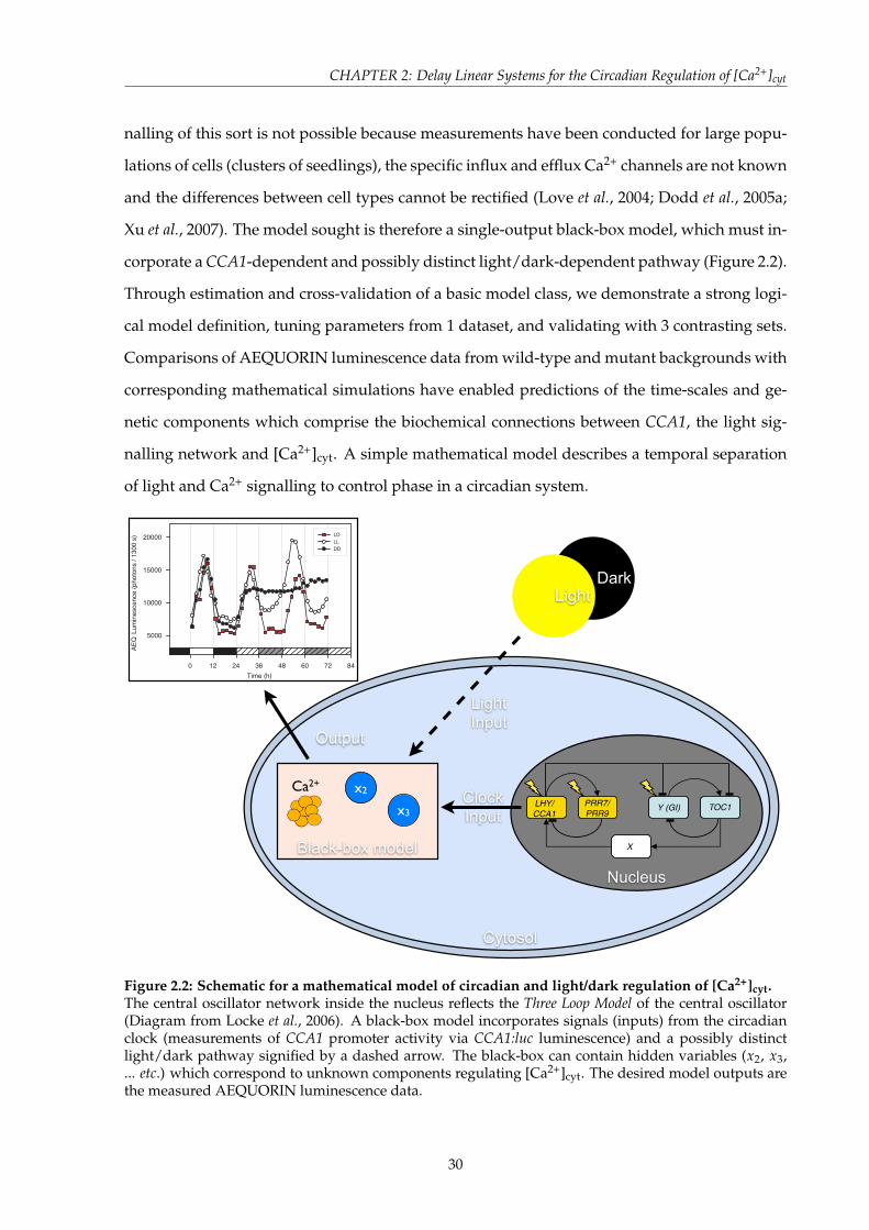
CHAPTER 2: Delay Linear Systems for the Circadian Regulation of [Ca2+]cyt
nalling of this sort is not possible because measurements have been conducted for large popu-
lations of cells (clusters of seedlings), the specific influx and efflux Ca2+ channels are not known
and the differences between cell types cannot be rectified (Love et al., 2004; Dodd et al., 2005a;
Xu et al., 2007). The model sought is therefore a single-output black-box model, which must in-
corporate a CCA1-dependent and possibly distinct light/dark-dependent pathway (Figure 2.2).
Through estimation and cross-validation of a basic model class, we demonstrate a strong logi-
cal model definition, tuning parameters from 1 dataset, and validating with 3 contrasting sets.
Comparisons of AEQUORIN luminescence data from wild-type and mutant backgrounds with
corresponding mathematical simulations have enabled predictions of the time-scales and ge-
netic components which comprise the biochemical connections between CCA1, the light sig-
nalling network and [Ca2+]cyt. A simple mathematical model describes a temporal separation
of light and Ca2+ signalling to control phase in a circadian system.
Ca2+
Results
A three-loop clock network accounts for additionalexperimental data
A short-period rhythm can exist in mutants with reduced TOC1function in some conditions (Alabadi et al, 2001; Mas et al,2003a). In order to test whether such residual rhythmicity wasdue to residual wild-type (WT) TOC1mRNA, we tested a TOC1deletion mutant (Supplementary information) for rhythmicexpression of CHLOROPHYLLA/B-BINDING PROTEIN2 (CAB2,
also known as LHCB1*1), a morning-expressed clock outputgene (Figure 1B). Plants of the Ws accession carrying the toc1-10 deletion had a rhythm of 20h period and reduced amplitudeunder constant light (LL) conditions. This was identical intiming to the rhythm of toc1-9 plants, which carry atermination codon within the first domain of the predictedTOC1 protein. Taken together, these data confirm previoussuggestions that a TOC1-independent oscillator can persist intoc1 plants (Mas et al, 2003a).The proposed PRR7/PRR9–LHY/CCA1 feedback loop pro-
vided a candidate mechanism to account for this oscillation.We therefore added this loop to the interlocked feedbackmodel (Figure 1A; Supplementary information) to create athree-loopmodel. As the mutant phenotypes of PRR7 and 9 areweak, apparently less than 1 h different from WT (Nakamichiet al, 2005), we grouped these genes together as one gene,PRR7/9, in our network equations (Supplementary informa-tion). LHY and CCA1 were grouped together as LHY (Lockeet al, 2005b). The first feedback loop involves LHY activatingPRR7/9 transcription (Farre et al, 2005), with PRR7/9 proteingoing on to repress LHY activation. The remainder of thenetwork follows our previous model (Locke et al, 2005b). LHYrepresses TOC1 and Y transcription; the dual, repressing andactivating role of LHY has experimental support (Harmer andKay, 2005). TOC1 protein activates X transcription, with Xactivating LHY transcription to form a second feedback loop.Yactivates TOC1 expression and TOC1 represses Yexpression,forming the third feedback loop. Light activates expression ofLHY, Y, and now also PRR7/9, because PRR9 has been shown tobe acutely light-activated (Ito et al, 2003).We used an extensive parameter search for the new and
altered components to test whether the three-loop networkcould account for the residual oscillations of a toc1 deletionmutant (Supplementary information). Our simulations showthat the PRR7/PRR9–LHY/CCA1 loop can generate the short-period rhythm of toc1 plants (Figure 1C), and its absence canresult in the very long period of prr7;prr9 double mutants(Supplementary Figure 1; Farre et al, 2005). Neither of theseobservations could be accounted for with our interlockedfeedback loop model (Locke et al, 2005b), which predictedarrhythmia or a long period under all conditions in simulationsof a toc1 null or loss-of-function mutants such as toc1-2 (6% ofWT RNA levels; Strayer et al, 2000) or the toc1 RNAi lines (10–15%, Mas et al, 2003a). Sensitivity analysis shows that thethree-loop model is similarly tolerant of parameter changes asthe interlocking-loop model (Supplementary information;Supplementary Figure 2).We now use the more realistic three-loop model to make
further predictions for Y’s role in the clock, and test thesepredictions against the experimental manipulation of GI.
GI is a component of Y
A simulated gi mutation (modelled by reducing Y translationby 70%) gives a 1 h reduction in the period of LHY mRNAoscillations (Figure 2A), which matches well with theobserved period of CAB expression rhythms in a gi nullmutant background (Figure 2B). According to our models, theY–TOC1 feedback loop generates the 18 h rhythm seen in anlhy;cca1mutant (Figure 2C andD). A reduction inY function in
LHY/CCA1
PRR7/PRR9
Y (GI) TOC1
X
2.5
1.5
0.5
00
4
3.5
2.5
1.5
0.5
00 20 40 60 80 100 120
1
2
3
24 48 72 96 120
1
2
Time (h)
Time (h)
Nor
mal
ised
lum
ines
cenc
eN
orm
alis
ed m
RN
A le
vel
W T CAB:LUCtoc1-9 CAB:LUCtoc1-10 CAB:LUC
W T LHY mRNAtoc1 LHY mRNA
A
B
C
Figure 1 The three-loop Arabidopsis clock model accounts for 20 h rhythmsin toc1 mutants. (A) Summary of the three-loop network, showing only genes(boxed), regulatory interactions (arrows) and the locations of light input (flashes).Two-component oscillators are distinguished by shading the gene names inyellow or blue. (B) CAB:LUCIFERASE (CAB:LUC) rhythms in WT (filledsquares), toc1-9 (open squares) and toc1-10 (open diamonds) under constantred light (10 mmol m!2 s!1). Luminescence values were normalised to theaverage over the whole time course. Time zero is the onset of constant light (LL).(C) Simulated expression levels of LHY mRNA in the WT (black solid line) andtoc1 backgrounds (green dotted line) in LL. Expression levels were normalised tothe average level of expression. Translation rate of TOC1 mRNA in thesimulated mutant is 1/1000 WT value.
Circadian feedback loop involving GIGANTEAJCW Locke et al
2 Molecular Systems Biology 2006 & 2006 EMBO and Nature Publishing Group
x2x3
ClockInput
LightInput
Output
Time (h)
0 12 24 36 48 60 72 84
AE
QLum
inescence (
photo
ns / 1
300 s
)
5000
10000
15000
20000 LD
LL
DD
LightDark
Cytosol
Nucleus
Black-box model
Figure 2.2: Schematic for a mathematical model of circadian and light/dark regulation of [Ca2+]cyt.The central oscillator network inside the nucleus reflects the Three Loop Model of the central oscillator(Diagram from Locke et al., 2006). A black-box model incorporates signals (inputs) from the circadianclock (measurements of CCA1 promoter activity via CCA1:luc luminescence) and a possibly distinctlight/dark pathway signified by a dashed arrow. The black-box can contain hidden variables (x2, x3,... etc.) which correspond to unknown components regulating [Ca2+]cyt. The desired model outputs arethe measured AEQUORIN luminescence data.
30

CHAPTER 2: Delay Linear Systems for the Circadian Regulation of [Ca2+]cyt
2.2 Materials and Methods
2.2.1 Plant material and growth conditions
Arabidopsis thaliana seedlings (Col-0) transformed with the cDNA of the LUCIFERASE (LUC)
coding sequence under the CCA1 promoter (CCA1:luc) were obtained from Nottingham Ara-
bidopsis Stock Centre (NASC). Experimental data from Col-0 Arabidopsis seedlings obtained
from members of the Signal Transduction Laboratory (Department of Plant Sciences, University
of Cambridge) have been used for mathematical modelling. Seeds were surface sterilised by
washing sequentially in 96% w/v ethanol (EtOH; Fisher Scientific, UK) for 1 min, in 50% w/v
sodium hypochlorite (NaClO; BDH Laboratories Supplies, UK) for 5 to 10 min and twice in
sterile deionised water. The seeds were resuspended in 0.1% w/v agar (Bactoagar; Difco, UK)
and plated on 90 mm round dishes (Sarstedt, Germany) containing sterile solid half strength
Murashige and Skoog media (MS media; Duchefa, Netherlands; pH 7.0) and 0.8% agar. The
plates were sealed with surgical micropore tape (3M, USA), stored in darkness at 4 ◦C for 2–3
days for seed stratification and transferred to a Sanyo MLR-35T growth cabinet set to 20 ◦C and
a 24 h periodic cycle of light and dark (L12/D12, L16/D8 or L8/D16; 60 µmol photons m-2 s-1).
2.2.2 Luminescence imaging
Arabidopsis seeds expressing CCA1:luc or 35S:aeq were surface sterilized as above, and sown
in clusters of 10-12 seeds inside rings made from 7.5 mm x 9 mm PVC tubes cut transversally
every 0.5 cm. After stratification, the plates were transferred to a growth cabinet set to LD con-
ditions for entrainment (20 ◦C; 60 µmol photons m-2 s-1). The AEQUORIN was reconstituted
by addition of 50 µl of 20 µM coelenterazine to each ring cluster once per day, two days prior
to measurement. 50 µl of 5 mM luciferin was added to seedlings expressing luc once per day, 2
days prior to measurement.
Before each experiment, a bright-field image was taken of the plate. Photon-counting
was conducted in a light-tight box using a Photek ICCD225 photon-counting camera system
(Photek, UK) mounted above the plate in complete darkness. The camera was controlled by
Photek IFS32 software, which programmed timing of all measurements automatically. Lumi-
nescence was measured for 1500 s every 2 h for 35S:aeq lines, and 800 s every 1 h for CCA1:luc.
The control box turned off the two arrays of blue and red light emitting diodes (LEDs) used
31

CHAPTER 2: Delay Linear Systems for the Circadian Regulation of [Ca2+]cyt
as light sources inside the box (100 µmol photons m-2 s-1; equal amounts of red light, 630 nm,
and blue light 475 nm) before starting the measurements. The software then saved the data,
and turned on the lights again after the measurements before starting a delay between mea-
surements. An additional control could be programmed to turn the LED arrays on and off
independently of the camera control to allow light/dark experiments.
Images saved by the automated camera system were analysed using the Photek IFS32 soft-
ware. The first 200 s of each measurement were discarded due to delayed chlorophyll fluores-
cence and 8-bit images were generated and pseudocoloured. Based on the bright-field image,
regions of interest were demarcated around each ring cluster and the total photon counts (lu-
minescence) were quantified.
2.2.3 Data for estimation and validation of mathematical models
We use the fact that CCA1 is necessary for circadian oscillations of [Ca2+]cyt in LL (Xu et al.,
2007) to define a proxy for the circadian clock as an input to a black-box model which describes
basal [Ca2+]cyt. The short-period loss-of-function cca1-1 mutant (Green & Tobin, 1999) has no
circadian oscillations of [Ca2+]cyt in LL (Xu et al., 2007), indicating that CCA1 mediates the
circadian control of [Ca2+]cyt. The CCA1:luc data obtained in Figure 2.3A was collected under
equivalent growth conditions to the measurements of [Ca2+]cyt in Figure 2.3A, which together
form an input-output pair. The dynamics monitored in this experiment include three important
elements for a mathematical description of [Ca2+]cyt: the oscillations of the circadian clock,
light/dark forcing, and tendency to steady state in DD. Therefore, this experiment represents a
good choice as a model training set. Both the input and output data are scale-free, as calibration
of the signals to concentrations of mRNA or cytosolic-free Ca2+ is inaccurate∗. To achieve a
suitable comparability of different experiments with different signal strengths, the CCA1:luc
luminescence data was normalised by dividing the whole data set by the maximum value in
the LD cycles.
A series of cross-validation tests were also applied to each model estimated. Plants express-
∗For stimulus-induced elevations in [Ca2+]cyt, AEQUORIN luminescence signals have been calibrated by usingan empirically derived calibration equation which relates [Ca2+]cyt to the ratio between the luminescence countsand the size of the AEQUORIN pool at the end of an experiment, Lt (Knight et al., 1996). The equation used was
− log[Ca2+]cyt= a[− log
(LcLt
)]+ b, where a and b are constants. For calibration of low [Ca2+]cyt, this equation has a
very low gradient, which means that a large change in luminescence corresponds to a small change in [Ca2+]cyt. Atlow luminescence levels, stochastic variation becomes more significant and as a result, our calibrations of [Ca2+]cythave been wide-ranging.
32

CHAPTER 2: Delay Linear Systems for the Circadian Regulation of [Ca2+]cyt
Time (h)-36 -24 -12 0 12 24 36 48 60 72
Rel
ativ
eCCA1:luc
Lum
ines
cenc
e
0.0
0.2
0.4
0.6
0.8
1.0
1.2A
Time (h)-36 -24 -12 0 12 24 36 48 60 72
AEQ
Lum
ines
cenc
e(p
hoto
ns /
1300
s)
4000
6000
8000
10000
12000
14000
16000
18000
20000B
Time (h)
-24 -12 0 12 24 36 48 60 72 84 96
Rel
ativ
eCCA1:luc
Lum
ines
cenc
e
0.0
0.2
0.4
0.6
0.8
1.0C
Time (h)
-24 -12 0 12 24 36 48 60 72 84 96
AEQ
Lum
ines
cenc
e(p
hoto
ns /
1300
s)
4000
6000
8000
10000
12000
14000
16000
18000
20000D
Time (h)
0 8 16 24 32 40 48 56
Rel
ativ
eCCA1:luc
Lum
ines
cenc
e
0.0
0.2
0.4
0.6
0.8
1.0E
Time (h)
-8 0 8 16 24 32
AEQ
Lum
ines
cenc
e(p
hoto
ns /
1300
s)
12000
14000
16000
18000
20000
22000
24000F
Time (h)
0 8 16 24 32 40 48 56
Rel
ativ
eCCA1:luc
Lum
ines
cenc
e
0.0
0.2
0.4
0.6
0.8
1.0G
Time (h)
-8 0 8 16 24 32
AEQ
Lum
ines
cenc
e (p
hoto
ns /
1300
s)
9000
10000
11000
12000
13000
14000
15000
16000H
Figure 2.3: CCA1:luc and AEQUORIN luminescence data provide input and output signals for gen-eration of linear state-space time-delay models.(A,C,E,G) Relative CCA1:luc luminescence quantified for 10 day old Arabidopsis seedlings, where openred circles represent mean average of clusters of seedlings integrated for 800 s. (B,D,F,H) AEQUORINluminescence quantified for 10 day old Arabidopsis seedlings, where open blue circles represent meanaverage of clusters of seedlings integrated for 1500 s. Seedlings were grown in entrained light-dark cy-cles prior to measurement in various conditions. Entrainment in L12/D12 photoperiod before transferto constant (A,B) dark or (C,D) light. Entrainment and measurement is in cycles of (E,F) L16/D8 or(G,H) L8/D16. Bars on abscissa represent light regime in each experiment. White indicates light, blackindicates dark, light grey is light in the subjective night and dark grey is dark in subjective daytime.Data collected by (A,E,G) Myself, (B,D) Dr. Carlos Hotta, University of Cambridge, UK, and (F,H) Dr.Katharine Hubbard, University of Cambridge, UK.
33

CHAPTER 2: Delay Linear Systems for the Circadian Regulation of [Ca2+]cyt
ing CCA1:luc or 35S:aeq were exposed to three alternative photoperiodic regimes and lumines-
cence quantified in each transgenic line. In addition to the DD estimation datasets (Figures
2.3A–B), this provided a total of four wild-type input-output datasets to assess model perfor-
mance (Figure 2.3):
1. L12/D12 cycles before transfer to DD (L12/D12–DD)
2. L12/D12 cycles before transfer to LL (L12/D12–LL)
3. Entrained L16/D8 cycles (long day conditions)
4. Entrained L8/D16 cycles (short day conditions)
2.2.4 State-space time-delay systems
Mathematical models were constructed to describe experimental observations of [Ca2+]cyt in
10 day old Arabidopsis seedlings (Figure 2.1), based on the expression of central oscillator
genes and the availability of light. The extent to which the CCA1-dependent and light/dark-
dependent pathways interact is not known, so their contribution is assumed independent
throughout. The potential for light to regulate [Ca2+]cyt via the clock is trivially covered by
considering a single-input model. The underlying pathways which transduce circadian and
light signalling events upstream of Ca2+ release have not been characterised, so these uncharac-
terised pathways are represented by delay parameters τi, as done previously (Herz et al., 1996;
Srividhya & Gopinathan, 2006; Sriram & Gopinathan, 2004). To model unknown pathways
as explicit hidden variables could give rise to large numbers of state variables, increasing the
complexity of parameter identification. Representing these pathways with delays reduces this
complexity to a single parameter (per input pathway). Furthermore, identification of suitable
delay steps may offer insight into the timing of [Ca2+]cyt regulation. Due to the black-box nature
of the problem, the simple model class of linear time-invariant (LTI) systems was chosen, as es-
timation of hidden states is possible through indirect systems identification (see Section 1.3.2).
A continuous-time formulation was used as the underlying process is inherently continuous
in time. Therefore, a single-output continuous-time state-space delay linear system with single
or multiple inputs was chosen as the basis for mathematical modelling the regulation of basal
[Ca2+]cyt in Arabidopsis.
34

CHAPTER 2: Delay Linear Systems for the Circadian Regulation of [Ca2+]cyt
The proposed use of linear systems to describe biological systems is controversial, as molec-
ular interactions are known to be both highly stochastic and nonlinear. We rationalise this de-
cision by virtue of the many analytical tools available for linear systems that are not possible
with nonlinear systems. These tools are utilised in this chapter to identify important properties
of the biochemical network that regulates basal [Ca2+]cyt, including the identification of hid-
den variables (Sections 2.3.1 and 2.3.3), similarity transformations (Sections 2.3.6 and 2.3.7) and
frequency response (Section 2.3.8). The sufficiency of linear systems in describing whole-plant
dynamics is also demonstrated as models can be successfully cross-validated.
Let x ∈ Rn be the vector of state variables, comprising a state which represents [Ca2+]cyt in
the 1st entry, and a further n− 1 unconstrained (‘hidden’) variables. Let u ∈ Rm be the vector
of inputs. We define the state-space time-delay system as follows.
dxdt
(t) = Ax(t) + Bu(t− τ)
y(t) = Cx(t)(2.1)
where A ∈ Rnxn is the matrix of interconnections, and B ∈ Rnxm is the input matrix.
Remarks
1. The transfer function representation of a delay linear system is related to the transfer
function of a standard linear system, and may be found in terms of A, B and C by taking
the Laplace transform of Eqn. 2.1. Let X(s) be the Laplace transform of x(t), U(s) of u(t)
etc., then
sX(s) = AX(s) + Be−sτU(s)
⇒ X(s) = (sI − A)−1Be−sτU(s)
⇒ Y(s) = C(sI − A)−1BUτ(s) = G(s)e−sτU(s)
where G(s) = C(sI − A)−1B is the matrix of transfer functions Tu→y for systems with
zero delay. The additional term e−sτ is not linear but may be thought of as an infinite-
dimensional linear system, so might be well-approximated by additional state variables.
2. The internal structure of state variables in (delay) linear systems is not fixed. This is espe-
cially important when there are more state variables than measured outputs (i.e. there are
35

CHAPTER 2: Delay Linear Systems for the Circadian Regulation of [Ca2+]cyt
hidden variables), and it is not possible to set each state variable to be a measured vari-
able (i.e. C as the identity matrix). A further consequence is that the dynamics of each
hidden variable are not fixed. This notion is well understood in Control Theory, though
we present a proof for completeness.
Proof. Suppose we have a general linear system (zero delay, without loss of generality)
with m inputs, p outputs, and n state variables given by:
dxdt
(t) = Ax(t) + Bu(t)
y(t) = Cx(t)(2.2)
where A ∈ Rnxn, B ∈ Rnxm and C ∈ Rpxn. Consider a similarity transformation T such
that x = Tz. Substituting into Eqn. 2.2 and taking the Laplace transforms leads to
sTZ(s) = ATZ(s) + BU(s)
⇒ Z(s) = T−1(sI − A)−1BU(s)
⇒ Y(s) = CTT−1(sI − A)−1BU(s)
= (C(sI − A)−1B)U(s)
= G(s)U(s)
as before, and therefore co-ordinate transformations do not affect input-output dynamics.
3. The elements of u may have different delays, and so in general is defined as
u(t− τ) =[
u1(t− τ1) u2(t− τ2) . . . um(t− τm)]T
(2.3)
Definition of the model classes
Models are proposed either in which light is assumed to regulate [Ca2+]cyt via changes in CCA1
expression, or via an independent pathway. Let y be the model output corresponding to mea-
sured AEQUORIN luminescence, uCCA1 the measured CCA1:luc luminescence signal and ulight
the light/dark input pathway. We first define the single input single-output (SISO) state-space
time delay system.
36

CHAPTER 2: Delay Linear Systems for the Circadian Regulation of [Ca2+]cyt
SISO Model.
dxdt
(t) = Ax(t) + buCCA1(t− τCCA1)
y(t) =(
1 0 . . . 0
)x(t)
(2.4)
where A ∈ Rnxn and b ∈ Rn are constant, and x ∈ Rn is the vector of state variables.
In the dual-input formulation, the light input pathway is considered to be a boolean variable.
This gives rise to two further model classes, L1 and L0, which are described as follows:
L1 and L0 Models.
dxdt
(t) = Ax(t) + B
uCCA1(t− τCCA1)
ulight(t− τlight)
y(t) =
(1 0 . . . 0
)x(t)
(2.5)
where A ∈ Rnxn and B ∈ Rnx2 are constant, and x ∈ Rn is the vector of state variables. The
boolean value of ulight differs for L1 and L0 as:
Model Light Dark
L1 1 0
L0 0 1
2.2.5 Parameter estimation of delay linear systems
There currently exists no published method of estimating the delay parameters explicitly, so
instead delay linear systems are estimated for a pre-specified generous range of delay values.
For two input systems, delay value pairs on an evenly-spaced grid are considered. While this
appears far from elegant, we are at least forced to cover all plausible combinations of delays,
obtaining a performance measure across the pre-specified range. Upon prescribing the delay
vector τ, the problem reduces to a standard systems identification problem and we are required
only to generate the input-output data pairs with the appropriate time-spacing. Therefore the
identification procedure consists of a data pre-processing stage in which the input-output data
pairs are defined, followed by the parameter estimation of A and B in Eqn. 2.1 using PEM.
For pre-processing of the input-output data, consider the output observations y(k) = y(t =
tk) for tk ∈ Ty where Ty is the set of time-points corresponding to the observations. Let u(l)i =
37

CHAPTER 2: Delay Linear Systems for the Circadian Regulation of [Ca2+]cyt
ui(t = tl) be the observations of the ith input for tl ∈ Tui where Tui is the set of time-points
corresponding to the observations of ui. Denote the input-output dataset subject to delays τ by
(uτ, y). We form (uτ, y) by finding values u1(tk− τ1), u2(tk− τ2), . . . for each tk ∈ Ty using linear
interpolation, which enables non-integer values of τ. We assume that the measured signal does
not deviate too far from the interpolated values. Finally, the dataset (uτ, y) is restricted to the
intersection of the existing data Ty ∩ Tuτ , so data outside this range are not considered.
Each linear system parameter set was estimated using the prediction-error method (PEM),
implemented in the Systems Identification Toolbox of MATLABTM (pem function; Ljung, 1999).
PEM falls under the class of indirect methods for continuous-time linear systems identification,
in which a discrete time system is estimated and converted back to continuous time. Suppose
we know x at t = tk, then x can be computed for any t = tk+1 > tk as
x(tk+1) = eA(tk+1−tk)x(tk) +∫ tk+1
tk
eA(tk+1−λ)Bu(λ)dλ (2.6)
If the observations obtained are uniformly spaced in time with sampling interval T and we
assume that the input u = uk is constant for tk < t < tk+1 (i.e. zero-order hold, ZOH), then we
obtain the discretisation of Eqn. 2.2:
xk+1 = Fxk + Guk (2.7)
where tk = t(kT), uk = u(kT), xk = x(kT), F = eAT, G =∫ T
0 eAτdτB. It now remains to estimate
the entries in F and G and then convert back to A and B. The prediction-error method seeks
to minimise the squared differences between each measured point and the model prediction
generated from the previous point (Ljung, 1999).
The output estimation data were further pre-processed so that the sample interval T
was consistent between the input dataset (CCA1:luc luminescence; Figure 2.3A) and the AE-
QUORIN luminescence output estimation data (Figure 2.3B). This also enabled suitable values
of ulight to be assigned across a dark to light transition. The implementation of the iterative
prediction-error minimization (PEM) algorithm in MATLABTM (pem function) only enables a
zero-order hold (ZOH) intersample behaviour. As AEQUORIN luminescence has been mea-
sured at odd-numbered hours relative to dawn, transitions between light and dark cannot be
accounted for, as a constant value of ulight 1 hour before a dark to light transition would not
38

CHAPTER 2: Delay Linear Systems for the Circadian Regulation of [Ca2+]cyt
switch until 1 hour after the switch in planta. Ignoring these considerations and applying the
same analysis as for single-input models would only enable estimation of models with light
input delays of 1 h, 3 h, 5 h etc. Otherwise, there are a number of options:
1. Re-measure AEQUORIN luminescence at even hours rather than odd hours. However,
when quantifying luminescence with a photon counting camera, there must be no exter-
nal light, so it would not be possible to measure a transition from dark to light.
2. Extra points could be appended to the output estimation dataset using the misdata func-
tion from the Systems Identification Toolbox in MATLABTM, which may be used for esti-
mating missing data points.
3. A crude estimation of the missing points yk could also be achieved by simply interpolat-
ing between the values yk−1 and yk+1 for each k.
To avoid potentially unhelpful additional experimentation, option 1 was rejected. Estimating
‘missing data’ treats missing points as extra parameters, vastly increasing the size of the pa-
rameter space. Since the number of ‘missing points’ is an order of magnitude larger than the
number of model parameters in the linear system, this method is highly undesirable and leads
to spurious results (simulation not shown). The third approach was simplest, and therefore
most appropriate. Therefore, all models were estimated using the output estimation data with
interpolated mid-points at even-valued times through the circadian cycle.
We sought to obtain the simplest model which accounted for the available data, and there-
fore assumed that the state-space realisations estimated are minimal. That is, the input-output
behaviour (transfer function) may be described by the minimum number of state variables.
Since our state-space realization is minimal, it is both controllable and observable (Chen, 1998).
The state-space realisation was fixed in controller canonical form, to guarantee controllability
of the resulting system (Chen, 1998). The pem command in MATLABTM has an option to return
state-space models in a variant of the controller canonical form, defined as follows:
dxdt
=
0 1 0 . . . 0
0 0 1 . . . 0...
. . ....
0 0 . . . 0 1
a1 a2 a3 . . . an
x +
b11 . . . b1m...
...
bn1 . . . bnm
u (2.8)
39

CHAPTER 2: Delay Linear Systems for the Circadian Regulation of [Ca2+]cyt
y =(
1 0 . . . 0
)x (2.9)
Further options of the pem function were set, to achieve the desired linear state-space model.
Continuous-time models are estimated by setting the sample interval equal to 0, achieved by
setting the options ’Ts’,0. We assumed the input signals were noise-free, as this both im-
proved the resulting model performances (data not shown) and reflected the knowledge that
the CCA1:luc luminescence signal is an order of magnitude brighter than AEQUORIN lumines-
cence and as such has a more desirable signal-to-noise ratio. To implement this assumption, we
enforced the Kalman matrix to be 0 by including ’Disturbance’,’None’ in the pem function
call. In summary, models were estimated throughout by issuing the following command:
MODEL = pem(data,n,’Ts’,0,’SSParameterization’,’Canonical’, ...
’DisturbanceModel’,’None’)
where n is the model order sought.
2.2.6 Model selection - Akaike’s Information Criterion (AIC)
Selection of the optimal delays is achieved by selecting the model with the best performance.
The Akaike Information Criterion (AIC; Akaike, 1974) offers a method for assessing perfor-
mance, relative to the number of estimated parameters. This criterion incorporates two penalty
terms: a measure of the distances between experimental data and simulated output, and a
term proportional to the number of parameters. A normalisation of the AIC is implemented in
MATLABTM as
AIC =2(k− log L)
N(2.10)
where L is the maximised value of the likelihood function, k is the number of estimated param-
eters (including the initial conditions) and N is the number of data-points. Assuming Gaussian
noise with covariance matrix Λ, the logarithm of the likelihood function is given by
l(θ, Λ) = log L(θ, Λ) = −12
N
∑i=1
εi(θ)− N2
log(det Λ) (2.11)
40

CHAPTER 2: Delay Linear Systems for the Circadian Regulation of [Ca2+]cyt
where εi is the difference between the measured value yi and simulated output yi. Maximising
the log-likelihood with respect to θ and Λ gives (Ljung, 1999)
lmax(θ, Λ) =N2
(1 + log V) (2.12)
where V is the loss function given by
V = det
(1N
N
∑i=1
εi(θ)εi(θ)T
)(2.13)
The AIC offers a method for comparing models of the same order with different delays, and
also models of varying order. In our analysis, we use the small sample (second-order bias cor-
rection) version of the AIC, AICc (Hurvich & Tsai, 1989). The normalised AICc can be evaluated
as
AICc = AIC +2k(k + 1)
N(N − k− 1)(2.14)
with N,k as above.
2.2.7 Simulation of delay linear systems for comparison with input-output data
The estimation of continuous-time linear systems implicitly solves the model equations in a
discretised form, forcing a zero-order hold (ZOH) intersample behaviour for the input sig-
nal u. For cross-validation purposes, the performance of each estimated model is evaluated
using a first-order hold (FOH, linear interpolation) intersample behaviour, to better approxi-
mate the continuous-time nature of the CCA1:luc luminescence input signal. These simulations
were conducted for each of the four CCA1:luc luminescence datasets available (Figure 2.3). The
model equations were solved numerically using the ode23 solver in MATLABTM (Shampine
& Reichelt, 1997) and simulated outputs were obtained every 0.2 h for analysis of oscillation
phase.
To quantify the performance during cross-validation, Pearson’s product-moment sample
correlation coefficient (r) was computed between AEQUORIN luminescence data and corre-
sponding simulated output using MATLABTM’s corr function. The sample correlation coeffi-
41

CHAPTER 2: Delay Linear Systems for the Circadian Regulation of [Ca2+]cyt
cient between vectors x and y is defined as
r(x, y) :=N
∑i=1
(xi − x||xi − x||2
· yi − y||yi − y||2
)(2.15)
where x and y are the sample means of x and y respectively and N is the number of entries
in x and y. For each of the wild-type datasets available for estimation and cross-validation, rD
(L12/D12–DD), rL (L12/D12–LL), rLD (L16/D8) and rSD (L8/D16) are defined accordingly.
For graphical display of each models performance, the simulated outputs are rescaled so
they overlap with the measured data according to the linear map y 7→ ay + b which solves the
minimisation problem
mina,b
N
∑i=1
(y(i) − ay(i) − b)2 (2.16)
where y(i) is the ith AEQUORIN luminescence sample, and y(i) the corresponding simulated
output. Note that the calculation of the sample correlation r is invariant to linear rescal-
ings of this type. The minimisation problem (Eqn. 2.16) is solved using the polyfit function
in MATLABTM.
2.3 Results
2.3.1 Regulation of [Ca2+]cyt by a CCA1-dependent pathway: Estimation of single-
input models
In this section, models are presented in which [Ca2+]cyt is regulated by a single pathway, which
is dependent on the expression of CCA1. The SISO model class Eqn. 2.4 was used to test the
hypothesis that light regulates basal [Ca2+]cyt via changes in the expression of CCA1. Pre-
processing the input-output data is necessary for estimation of the SISO model. As the input
signal tends towards zero in DD, we must ensure that the output approaches zero also. To
enforce this, the average of the output signal between t = 19 h and t = 63 h (equal to 12457
photons / 1300 s) was subtracted from the output estimation vector and Eqn. 2.1 was changed
42

CHAPTER 2: Delay Linear Systems for the Circadian Regulation of [Ca2+]cyt
to
dxdt
(t) = Ax(t) + Bu(t− τCCA1)
y(t) = Cx(t) + d(2.17)
where d is the steady value of the output signal y.
The system matrices A and B were estimated for τCCA1 ranging between 0 h and 10 h in
0.1 h increments (Figure 2.4). For estimation of 1st and 2nd order models, AICc was a reasonably
smooth function of the delay parameter τCCA1 (Figure 2.4A). However, numerical instabilities
could be observed in the estimation of 3rd and 4th order systems. The AICc of the best delay
choice decreased as the model order was increased (Table 2.1), though inspection of the sim-
ulated output with respect to the estimation dataset revealed a lack of improvement beyond
2nd order (Figure 2.4B). In keeping with the philosophy that the lowest order should be se-
lected for equivalent performance, these results suggest that AICc may not be penalising extra
parameters sufficiently.
2.3.2 Cross-validation of the single-input model: Selection of optimal order and
delay steps
Cross-validation tests were carried out to see whether the models estimated were applicable to
alternative conditions (Section 2.2.3). The sample correlation coefficients (rD, rL, rLD and rSD;
Eqn. 2.15) were computed between model simulated output and AEQUORIN luminescence
data (Figure 2.5) using a first-order hold (FOH, linear interpolation) intersample definition.
The sample correlation coefficient values for 1st order models were very low for large ranges
in τCCA1, indicating a poor validation. However, performance improved for rD (Figure 2.5A)
and rL (Figure 2.5B) when τCCA1 was greater than 10 h. 2nd–4th order models showed greater
homogeneity across this range of τCCA1, achieving higher performance than 1st order models in
all datasets compared for nearly all τCCA1 (Figure 2.5). However, it was difficult to distinguish
the performance of higher order systems with only the sample correlation coefficients rD, rL,
rLD and rSD.
For each model order, an optimal delay was chosen that maximised a weighted sum of the
43

CHAPTER 2: Delay Linear Systems for the Circadian Regulation of [Ca2+]cyt
Table 2.1: Optimal choice of τCCA1 for each order of SISO models after parameter estimation.Entries correspond to the minimum AICc value observed over the range of τCCA1 for each model orderup to 4.
Order τCCA1 AICc
1 10.0 15.122 9.1 13.593 8.5 13.194 0.5 13.12
CCA1 Delay (h)
0 2 4 6 8 10 12
AIC
c
12
13
14
15
16
17
1st Order 2nd Order3rd Order4th Order
A
Time (h)
-48 -36 -24 -12 0 12 24 36 48 60 72
AEQ
Lum
ines
cenc
e (p
hoto
ns /
1300
s)
4000
6000
8000
10000
12000
14000
16000
18000
20000Data1st Order2nd Order3rd Order4th Order
B
Figure 2.4: Estimation of SISO models for the regulation of [Ca2+]cyt by a CCA1-dependent pathway.Relative CCA1:luc and AEQUORIN luminescence data from Arabidopsis seedlings entrained to L12/D12cycles before transfer to DD (Figure 2.3) were pre-processed to reflect each value of τCCA1 between 0 hand 15 h in 0.1 h increments. Continuous-time linear state-space models of orders 1 to 4 were computedwith the pem function in the Systems Identification Toolbox for MATLABTM(Ljung, 1999). (A) AICc wascomputed for each model estimated by adding the output of the aic function in MATLABTM (Ljung,1999) to the second-order bias correction as in Eqn. 2.14. (B) Simulated output for models with τCCA1corresponding to the lowest AICc for each order 1 to 4 (see Table 2.1 for values). Simulated output valuesobtained from the compare function in MATLABTM. Bars on abscissa represent light availability, whiteindicates light, black indicates dark, and dark grey indicates darkness during subjective daytime.
44

CHAPTER 2: Delay Linear Systems for the Circadian Regulation of [Ca2+]cyt
CCA1 Delay (h)0 2 4 6 8 10
Cor
rela
tion
coef
ficie
nt,
r D
0.0
0.2
0.4
0.6
0.8
1.0A
CCA1 Delay (h)0 2 4 6 8 10
Cor
rela
tion
coef
ficie
nt,
r L
0.0
0.2
0.4
0.6
0.8
1.0
1st Order2nd Order3rd Order4th Order
B
CCA1 Delay (h)0 2 4 6 8 10
Cor
rela
tion
coef
ficie
nt,
r LD
0.0
0.2
0.4
0.6
0.8
1.0C
CCA1 Delay (h)0 2 4 6 8 10 12
Cor
rela
tion
coef
ficie
nt,
r SD
0.0
0.2
0.4
0.6
0.8
1.0D
Figure 2.5: Correlation of single input model simulations to AEQUORIN luminescence data.Model equations were solved numerically with MATLABTM’s ode23 solver (Shampine & Reichelt, 1997)to provide simulations of experimental conditions. Each linear model estimated was stimulated bythe first 24 h of relative CCA1:luc luminescence data in light-dark cycles until transients disappeared.Then the appropriate full input dataset was fed into the model and outputs taken at time-points corre-sponding to measured AEQUORIN luminescence. The sample correlation coefficient between simulatedmodel output and AEQUORIN luminescence data was computed using the corr function in MATLABTM.Simulations reflect (A) entrainment to L12/D12 cycles before transfer to DD, (B) entrainment to L12/D12cycles before transfer to LL, (C) entrainment to L16/D8 cycles and (D) entrainment to L8/D16 cycles.
Table 2.2: Optimal choice of τCCA1 for each order of single-input models after cross-validation.Entries correspond to the minimum value of rw = nDrD + nLrL + nLDrLD + nSDrSD for each model order.rD, rL, rLD and rSD are the sample correlation coefficient values between simulated model output andAEQUORIN luminescence data from seedlings in experimental conditions L12/D12–DD, L12/D12–LL,L16/D8 and L8/D16 respectively. nD, nL, nLD and nSD are the corresponding numbers of observationsin each dataset.
Order τCCA1 rw1 4.0 101.122 3.9 132.663 4.2 134.564 4.2 133.12
45

CHAPTER 2: Delay Linear Systems for the Circadian Regulation of [Ca2+]cyt
sample correlation coefficients, defined as
rw := nDrD + nLrL + nLDrLD + nSDrSD (2.18)
where the nd are the number of observations in dataset d (see Table 2.2 for optimal locations).
This enabled us to analyse complexity with respect to the estimation and validation datasets.
The simulated outputs in each condition are plotted for optimal-delay choices for each order
(1–4) in Figure 2.6. As observed during the estimation of each model, 1st order models per-
Time (h)-72 -48 -24 0 24 48 72 96
AEQ
Lum
ines
cenc
e (p
hoto
ns /
1300
s)
4000
6000
8000
10000
12000
14000
16000
18000
20000Data1st Order2nd Order3rd Order4th Order
A
Time (h)-24 0 24 48 72 96
AEQ
Lum
ines
cenc
e (p
hoto
ns /
1300
s)
4000
6000
8000
10000
12000
14000
16000
18000
20000B
Time (h)-8 0 8 16 24 32
AEQ
Lum
ines
cenc
e (p
hoto
ns /
1300
s)
12000
14000
16000
18000
20000
22000
24000C
Time (h)-8 0 8 16 24 32
AEQ
Lum
ines
cenc
e (p
hoto
ns /
1300
s)
8000
10000
12000
14000
16000
18000D
Figure 2.6: Cross-validation of optimal-τCCA1 linear models for different orders with AEQUORINluminescence data.Linear state-space model equations solved numerically with MATLABTM’s ode23 solver (solid lines;Shampine & Reichelt, 1997). For each order, models were simulated for the optimal choice of τCCA1,defined as the minimum of the weighted sum of sample correlation coefficients, rw (Eqn. 2.18; see Ta-ble 2.2 for values). AEQUORIN luminescence data from Figure 2.3 (open circles), with interpolatedmid-points at even-valued time-points also used for model estimation (crosshairs). Simulated outputsscaled to overlap with AEQUORIN luminescence data by finding the best linear scaling of the formay + b, where y is the simulated output. a and b are the solutions to mina,b ∑Nd
i (y(i) − ay(i) − b)2 wherey(i) are the measured AEQUORIN luminescence values and Nd is the number of data values. Solutionfound using the polyfit function in MATLABTM. Bars on abscissa represent light regime in each exper-iment/simulation. White indicates light, black indicates dark, light grey (B) is light in the subjectivenight and dark grey (A) is dark in subjective daytime.
46

CHAPTER 2: Delay Linear Systems for the Circadian Regulation of [Ca2+]cyt
formed poorly and no improvement could be seen above 2nd order, indicating that the most
suitable number of state variables is 2 in this model class. Optimal-τCCA1 2nd–4th order models
were unable to reproduce a non-oscillatory tendency towards steady state in DD (Figure 2.6A),
though they produced oscillations in LL with the appropriate phase (Figure 2.6B). The phase of
the oscillation peaks in entrained L16/D8 (Figure 2.6C) and L8/D16 (Figure 2.6D) cycles were
also accurate to within 1 hour. However, for all model orders, simulated outputs did not well
characterise the tendency towards a constant steady state in DD (Figure 2.6A), nor were they
able to distinguish amplitude between L12/D12 cycles and LL (Figure 2.6B). Furthermore, the
rapid increase in [Ca2+]cyt following dark to light transitions in L16/D8 and L8/D16 was not
predicted by the SISO models (Figures 2.6C,D).
2.3.3 Dual regulation of [Ca2+]cyt by CCA1 and light: Estimation of dual-input
model classes
To investigate the possibility that [Ca2+]cyt is independently regulated by the central oscillator
(CCA1) and light/dark, two-input continuous-time linear systems with delays (τi, distinct) at
each input were estimated. For the L1 model class (ulight = 1, light; ulight = 0, dark), the same
output translation (Eqn. 2.17) as for the SISO model was used, as both inputs approach zero in
DD. However, for the L0 model (ulight = 0, light; ulight = 1, dark), the DD steady state becomes
x2 + b12 + d (x2 6= 0), providing some choice in the assignment of d. The minimum level of
AEQUORIN luminescence across the estimation dataset (d = 5818.6) was taken in an effort to
reproduce the locally constant basal level in the dark phase of L12/D12 cycles (Figure 2.3B),
during which both CCA1:luc luminescence and light input values are near 0.
Two-input linear state-space models were computed using PEM for τCCA1 = 0, 0.1, . . . , 10
and τlight = 0, 1, . . . , 5, similarly to the method in Section 2.3.1. Each combination of delay pa-
rameter pairs, models up to 4th order, and both model classes (L1 and L0) were considered.
As the model order increased, the variability between neighbouring values of τCCA1 increased,
presumably as a result of the numerical instabilities of the PEM algorithm (Figure 2.7). 1st order
models performed better for larger τlight in both the L1 (Figure 2.7B) and L0 (Figure 2.7A) light
input classes, with AICc being a smooth function of τCCA1 throughout. The 2nd order models
were optimised by τCCA1 near 8 h for L1 (Figure 2.7D) and 4 h for L0 (Figure 2.7C), though
the distinction between different choices of τlight was very small. Due to the high variability be-
47

CHAPTER 2: Delay Linear Systems for the Circadian Regulation of [Ca2+]cyt
tween neighbouring values of τCCA1, it was not possible to conclude about the optimal pathway
delays for 3rd (Figures 2.7E,F) and 4th (Figures 2.7G,H) order models.
The AICc performance was analysed for the best choice of τCCA1 over different orders, τlight
and light input scheme (see Table 2.3 for values). Optimal-τCCA1 model performance showed
some similarity between light schemes L1 and L0 for each order (Figure 2.8A,B). Increasing from
1 to 2 internal states represented the largest improvement in the AICc. However, in both cases
4 states was optimal. We suspected that AICc did not penalise extra parameters sufficiently for
deciding the most suitable model order. Also plotted are the AICc performances for models
for no delays (τCCA1= 0, τlight= 0), which demonstrate that the provision of a nonzero τCCA1 in
2nd order models may be accounted for by an additional state variable (Figure 2.8A). Despite
obtaining similar AICc scores, the simulated output of 2nd order models (with optimal choice of
τCCA1) using the L0 scheme described the AEQUORIN luminescence data with more accuracy
than the optimal-τCCA1 L1 models; L0 models gave similar outputs irrespective of τlight and
reflected the rapid loss of oscillations seen after a period of extended dark (Figure 2.8C), while
2nd order L1 models had undesirable damped oscillations in DD (Figure 2.8D). Optimal-τCCA1
4th order L0 models obtained a near-perfect fit to the estimation data for all τlight investigated
(Figure 2.8E), and again were more representative of the AEQUORIN luminescence data than
L1 models, which appeared to exhibit some higher-frequency modes (Figure 2.8F). These results
indicated a clear preference towards the L0 light scheme.
Table 2.3: Optimal τCCA1 for each τlight in 2nd and 4th order L0 and L1 models.Entries correspond to the values of τCCA1 which minimise the AICc for each choice of τlight for 2nd and4th order models in both L0 and L1 light regimes. AICc was computed for each model estimated byadding the output of the aic function in MATLABTM (Ljung, 1999) to the second-order bias correction asin Eqn. 2.14.
L0 L1Order 2 4 2 4τlight τCCA1 AICc τCCA1 AICc τCCA1 AICc τCCA1 AICc
0 3.8 13.17 0.0 11.77 7.4 13.23 8.5 12.131 4.5 13.12 0.5 11.95 8.1 13.17 9.1 12.182 5.5 13.41 0.4 11.95 8.1 13.26 5.4 12.773 3.5 13.33 0.3 11.66 8.3 13.35 8.6 12.264 4.2 13.36 0.1 11.66 9.0 13.48 9.6 12.455 4.4 13.29 0.1 11.68 9.0 13.47 2.6 12.60
48

CHAPTER 2: Delay Linear Systems for the Circadian Regulation of [Ca2+]cyt
CCA1 Delay (h)0 2 4 6 8 10
AIC
c
11
12
13
14
15
16
17
τlight = 0 hτlight = 1 hτlight = 2 hτlight = 3 hτlight = 4 hτlight = 5 h
1st Order
A
CCA1 Delay (h)0 2 4 6 8 10
AIC
c
11
12
13
14
15
16
17
1st Order
B
CCA1 Delay (h)0 2 4 6 8 10
AIC
c
11
12
13
14
15
16
17
2nd Order
C
CCA1 Delay (h)0 2 4 6 8 10
AIC
c
11
12
13
14
15
16
17
2nd Order
D
CCA1 Delay (h)0 2 4 6 8 10
AIC
c
11
12
13
14
15
16
17
3rd Order
E
CCA1 Delay (h)0 2 4 6 8 10
AIC
c
11
12
13
14
15
16
17
3rd Order
F
CCA1 Delay (h)0 2 4 6 8 10
AIC
c
11
12
13
14
15
16
17
4th Order
G
CCA1 Delay (h)0 2 4 6 8 10
AIC
c
11
12
13
14
15
16
17
4th Order
H
Figure 2.7: AICc performance of dual-input linear state-space time-delay systems for the regulationof [Ca2+]cyt.Relative CCA1:luc and AEQUORIN luminescence data from Arabidopsis seedlings entrained to L12/D12cycles before transfer to DD were pre-processed to reflect each value of τCCA1 in between 0 h and 10 hin 0.1 h increments and τlight between 0 h and 5 h in 1 h increments. The light input was defined to be(A,C,E,G) 0 during light, and 1 during dark, or (B,D,F,H) 1 during light, and 0 during dark. Continuous-time linear state-space models were then computed with the pem function in the Systems IdentificationToolbox for MATLABTM(Ljung, 1999). AICc was computed for each model estimated by adding theoutput of the aic function in MATLABTM (Ljung, 1999) to the second-order bias correction as in Eqn. 2.14.The number of state variables in each model was (A,B) 1, (C,D) 2, (E,F) 3, and (G,H) 4.
49
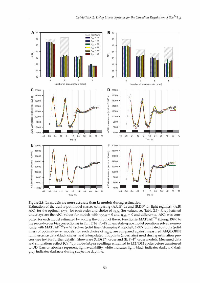
CHAPTER 2: Delay Linear Systems for the Circadian Regulation of [Ca2+]cyt
Number of states (model order)1 2 3 4
AIC
c
10
11
12
13
14
15
16
17No Delaysτlight = 0 hτlight = 1 hτlight = 2 hτlight = 3 hτlight = 4 hτlight = 5 h
A
Number of states (model order)1 2 3 4
AIC
c
10
11
12
13
14
15
16
17B
Time (h)-48 -36 -24 -12 0 12 24 36 48 60 72
AEQ
Lum
ines
cenc
e (p
hoto
ns /
1300
s)
4000
6000
8000
10000
12000
14000
16000
18000
20000C
Time (h)-48 -36 -24 -12 0 12 24 36 48 60 72
AEQ
Lum
ines
cenc
e (p
hoto
ns /
1300
s)
4000
6000
8000
10000
12000
14000
16000
18000
20000D
Time (h)-48 -36 -24 -12 0 12 24 36 48 60 72
AEQ
Lum
ines
cenc
e (p
hoto
ns /
1300
s)
4000
6000
8000
10000
12000
14000
16000
18000
20000E
Time (h)-48 -36 -24 -12 0 12 24 36 48 60 72
AEQ
Lum
ines
cenc
e (p
hoto
ns /
1300
s)
4000
6000
8000
10000
12000
14000
16000
18000
20000F
Figure 2.8: L0 models are more accurate than L1 models during estimation.Estimation of the dual-input model classes comparing (A,C,E) L0 and (B,D,F) L1 light regimes. (A,B)AICc for the optimal τCCA1 for each order and choice of τlight (for values, see Table 2.3). Grey hatchedunderlays are the AICc values for models with τCCA1= 0 and τlight= 0 and different n. AICc was com-puted for each model estimated by adding the output of the aic function in MATLABTM (Ljung, 1999) tothe second-order bias correction as in Eqn. 2.14. (C–F) Linear state-space model equations solved numer-ically with MATLABTM’s ode23 solver (solid lines; Shampine & Reichelt, 1997). Simulated outputs (solidlines) of optimal-τCCA1 models, for each choice of τlight, are compared against measured AEQUORINluminescence data (black circles) and interpolated midpoints (crosshairs) used during estimation pro-cess (see text for further details). Shown are (C,D) 2nd order and (E, F) 4th order models. Measured dataand simulations reflect [Ca2+]cyt in Arabidopsis seedlings entrained to L12/D12 cycles before transferredto DD. Bars on abscissa represent light availability, white indicates light, black indicates dark, and darkgrey indicates darkness during subjective daytime.
50

CHAPTER 2: Delay Linear Systems for the Circadian Regulation of [Ca2+]cyt
2.3.4 Cross-validation of the dual-input model classes
Estimation of the dual-input model class revealed that the way in which we define the light
input, and in turn the system steady state, had a profound effect on the resulting performance
and optimal delay-parameter choices. Defining light to be 0, and dark to be 1 (L0) enabled a
much closer fit to the estimation data for all orders (Figure 2.8). Depending on the value of τlight,
the optimal choice of τCCA1 was between 3.5 h and 5.5 h for 2nd systems, and between 0 h and
0.5 h for 4th order systems (Table 2.3). This provided evidence that additional state variables
can account for the delay between CCA1 expression and the regulation of [Ca2+]cyt. Almost no
difference could be observed in the simulated outputs between the different lengths of τlight
tested. This indicated that the linear state-space description was insensitive to this delay, and
able to account for it implicitly in the choice of system matrices A and B. In order to select the
most appropriate mathematical description of the regulation of [Ca2+]cyt, we needed to better
distinguish between different choices of the light delay τlight.
Cross-validation was performed for the L0 models with the AEQUORIN luminescence data
from Figure 2.3, as done for the single-input models in Section 2.3.2, computing the correlations
rD, rL, rLD and rSD for each 2nd and 4th order L0 model estimated (Figure 2.9). The sample
correlation coefficients were a smooth function of τCCA1 for each choice of τlight in the 2nd order
model class (Figure 2.9). With respect to the dataset used for estimation (L12/D12–DD), the
best choice of τCCA1 was between 4.5 h and 5.6 h, for all τlight (Figure 2.9A). The optimal choice
of τCCA1 was shorter for validation sets L12/D12–LL (2.5–4.5 h; Figure 2.9C) and L8/D16 (0.8–
1.1 h; Figure 2.9G). For L16/D8 cycles, the optimal choice of τCCA1 was very high when τlight≤
1 h (τCCA1> 9 h) and very low when τlight≥ 2 h (τCCA1< 0.2 h; Figure 2.9E). The performance of
4th order models with respect to sample correlation at optimised choices of τCCA1 was generally
no better than for 2nd order models, though showed less dependence on the value of τCCA1
(Figures 2.9B,D,F,H). A marked improvement was seen in 4th order models when comparing
L16/D8 cycles (Figure 2.9F), though they performed poorly in L8/D16 cycles (Figure 2.9H).
In conclusion, the additional 2 state variables offered a very minor improvement to a given
model’s ability to match the shape of the AEQUORIN luminescence data, though were able
to shorten the delay steps required between input and output signals. However, no further
progress was made in selecting the most appropriate choice of τlight by considering the sample
correlation coefficients.
51

CHAPTER 2: Delay Linear Systems for the Circadian Regulation of [Ca2+]cyt
CCA1 Delay (h)0 2 4 6 8 10 12
Cor
rela
tion
coef
ficie
nt,
r D
0.5
0.6
0.7
0.8
0.9
1.0
tlight = 0 htlight = 1 htlight = 2 htlight = 3 htlight = 4 htlight = 5 h
A
CCA1 Delay (h)0 2 4 6 8 10 12
Cor
rela
tion
coef
ficie
nt,
r D
0.5
0.6
0.7
0.8
0.9
1.0B
CCA1 Delay (h)0 2 4 6 8 10 12
Cor
rela
tion
coef
ficie
nt,
r L
0.5
0.6
0.7
0.8
0.9
1.0C
CCA1 Delay (h)0 2 4 6 8 10 12
Cor
rela
tion
coef
ficie
nt,
r L
0.5
0.6
0.7
0.8
0.9
1.0D
CCA1 Delay (h)0 2 4 6 8 10 12
Cor
rela
tion
coef
ficie
nt,
r LD
0.5
0.6
0.7
0.8
0.9
1.0E
CCA1 Delay (h)0 2 4 6 8 10 12
Cor
rela
tion
coef
ficie
nt,
r LD
0.5
0.6
0.7
0.8
0.9
1.0F
CCA1 Delay (h)0 2 4 6 8 10 12
Cor
rela
tion
coef
ficie
nt,
r SD
0.5
0.6
0.7
0.8
0.9
1.0G
CCA1 Delay (h)0 2 4 6 8 10 12
Cor
rela
tion
coef
ficie
nt,
r SD
0.5
0.6
0.7
0.8
0.9
1.0H
Figure 2.9: Correlation of L0 dual-input model simulations to [Ca2+]cyt dataModel equations were solved numerically with MATLABTM’s ode23 solver (Shampine & Reichelt, 1997)to provide simulations of experimental conditions. Each linear model estimated was stimulated by thefirst 24 h of relative CCA1:luc luminescence data and corresponding light input (L0) values in light-darkcycles until transients disappeared. Then the appropriate full input dataset was fed into the model andoutputs taken at time-points corresponding to measured AEQUORIN luminescence. The sample corre-lation coefficient between simulated model output and AEQUORIN luminescence data computed usingthe corr function in MATLABTM for (A,C,E,G) 2nd order, and (B,D,F,H) 4th order models. (A,B) Entrain-ment to L12/D12 cycles before transfer to DD. (C,D) Entrainment to L12/D12 cycles before transfer toLL. (E,F) Entrainment to L16/D8 cycles. (G,H) Entrainment to L8/D16 cycles.
52
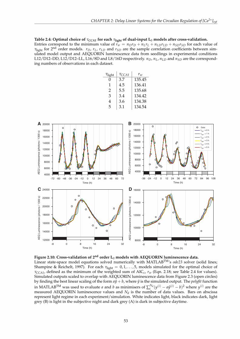
CHAPTER 2: Delay Linear Systems for the Circadian Regulation of [Ca2+]cyt
Table 2.4: Optimal choice of τCCA1 for each τlight of dual-input L0 models after cross-validation.Entries correspond to the minimum value of rw = nDrD + nLrL + nLDrLD + nSDrSD for each value ofτlight for 2nd order models. rD, rL, rLD and rSD are the sample correlation coefficients between sim-ulated model output and AEQUORIN luminescence data from seedlings in experimental conditionsL12/D12–DD, L12/D12–LL, L16/8D and L8/16D respectively. nD, nL, nLD and nSD are the correspond-ing numbers of observations in each dataset.
τlight τCCA1 rw
0 3.7 135.451 4.5 136.412 5.5 135.683 3.4 134.424 3.6 134.385 3.1 134.54
Time (h)-72 -60 -48 -36 -24 -12 0 12 24 36 48 60 72
AEQ
Lum
ines
cenc
e (p
hoto
ns /
1300
s)
4000
6000
8000
10000
12000
14000
16000
18000
20000A
Time (h)-36 -24 -12 0 12 24 36 48 60 72 84 96 108
AEQ
Lum
ines
cenc
e (p
hoto
ns /
1300
s)
4000
6000
8000
10000
12000
14000
16000
18000
20000Dataτlight = 0 h τlight = 1 h τlight = 2 h τlight = 3 h τlight = 4 h τlight = 5 h
B
Time (h)-8 0 8 16 24 32
AEQ
Lum
ines
cenc
e (p
hoto
ns /
1300
s)
12000
14000
16000
18000
20000
22000
24000C
Time (h)-8 0 8 16 24 32
AEQ
Lum
ines
cenc
e (p
hoto
ns /
1300
s)
8000
10000
12000
14000
16000D
Figure 2.10: Cross-validation of 2nd order L0 models with AEQUORIN luminescence data.Linear state-space model equations solved numerically with MATLABTM’s ode23 solver (solid lines;Shampine & Reichelt, 1997). For each τlight = 0, 1, . . . , 5, models simulated for the optimal choice ofτCCA1, defined as the minimum of the weighted sum of AICc, rw (Eqn. 2.18; see Table 2.4 for values).Simulated outputs scaled to overlap with AEQUORIN luminescence data from Figure 2.3 (open circles)by finding the best linear scaling of the form ay + b, where y is the simulated output. The polyfit functionin MATLABTM was used to evaluate a and b as minimisers of ∑Nd
i (y(i) − ay(i) − b)2 where y(i) are themeasured AEQUORIN luminescence values and Nd is the number of data values. Bars on abscissarepresent light regime in each experiment/simulation. White indicates light, black indicates dark, lightgrey (B) is light in the subjective night and dark grey (A) is dark in subjective daytime.
53

CHAPTER 2: Delay Linear Systems for the Circadian Regulation of [Ca2+]cyt
Table 2.5: Optimal choice of τCCA1 for each τlight of dual-input L0 models after cross-validation.Entries correspond to the minimum value of rw = nDrD + nLrL + nLDrLD + nSDrSD for each value ofτlight for 4th order models. rD, rL, rLD and rSD are the sample correlation coefficients between sim-ulated model output and AEQUORIN luminescence data from seedlings in experimental conditionsL12/D12–DD, L12/D12–LL, L16/8D and L8/16D respectively. nD, nL, nLD and nSD are the correspond-ing numbers of observations in each dataset.
τlight τCCA1 rw
0 5.5 133.101 0.1 134.492 7.0 135.773 0.3 131.324 3.1 133.395 1.2 133.39
Time (h)-72 -60 -48 -36 -24 -12 0 12 24 36 48 60 72
AEQ
Lum
ines
cenc
e (p
hoto
ns /
1300
s)
4000
6000
8000
10000
12000
14000
16000
18000
20000A
Time (h)-36 -24 -12 0 12 24 36 48 60 72 84 96 108
AEQ
Lum
ines
cenc
e (p
hoto
ns /
1300
s)
2000
4000
6000
8000
10000
12000
14000
16000
18000
20000Dataτlight = 0 h τlight = 1 h τlight = 2 h τlight = 3 h τlight = 4 h τlight = 5 h
B
Time (h)-8 0 8 16 24 32
AEQ
Lum
ines
cenc
e (p
hoto
ns /
1300
s)
12000
14000
16000
18000
20000
22000
24000C
Time (h)-8 0 8 16 24 32
AEQ
Lum
ines
cenc
e (p
hoto
ns /
1300
s)
9000
10000
11000
12000
13000
14000
15000
16000D
Figure 2.11: Cross-validation of 4th order L0 models with AEQUORIN luminescence data.Linear state-space model equations solved numerically with MATLABTM’s ode23 solver (solid lines;Shampine & Reichelt, 1997). For each τlight = 0, 1, . . . , 5, models simulated for the optimal choice ofτCCA1, defined as the minimum of the weighted sum of AICc, rw (Eqn. 2.18; see Table 2.5 for values).Simulated outputs scaled to overlap with AEQUORIN luminescence data from Figure 2.3 (open circles)by finding the best linear scaling of the form ay + b, where y is the simulated output. The polyfit functionin MATLABTM was used to evaluate a and b as minimisers of ∑Nd
i (y(i) − ay(i) − b)2 where y(i) are themeasured AEQUORIN luminescence values and Nd is the number of data values. Bars on abscissarepresent light regime in each experiment/simulation. White indicates light, black indicates dark, lightgrey (B) is light in the subjective night and dark grey (A) is dark in subjective daytime.
54
CHAPTER 2: Delay Linear Systems for the Circadian Regulation of [Ca2+]cyt
Candidate models for each choice of τlight were selected by maximising the weighted sum of
sample correlation coefficients rw (Eqn. 2.18) over τCCA1 (Tables 2.4, 2.5). The simulated outputs
of these optimal-τCCA1 models were then compared with the measured AEQUORIN lumines-
cence data. Almost no difference was observed between different choices of τlight when con-
sidering the simulated outputs of 2nd order models in L12/D12–DD conditions (Figure 2.10A).
All were able to match the oscillation phase in L12/D12 cycles but failed to maintain a stable
level during the dark phase of these cycles. This gave the effect of an early anticipation of
dawn, which was not observed experimentally. The tending behaviour towards steady state
in DD was well represented in all cases. 4th order models had some dissimilarity across the
range of τlight (Figure 2.11A). In L12/D12 cycles, only the optimal-τCCA1 models corresponding
to τlight= 1 h and τlight= 2 h had smooth oscillations, while a very small second oscillation
could be seen in the dark phase of the other τlight models. This slightly biphasic oscillation
was observed in the measured AEQUORIN luminescence signal, but it is not clear whether
the 4th order delay linear systems models accurately accounted for this behaviour. There was
also a range of troughs observed around 28 h into DD. The best model in this regard was the
optimal-τCCA1 model corresponding to τlight= 5 h, which did not ‘dip’ far below the measured
AEQUORIN luminescence signal. This residual oscillation in DD was also seen in the 2nd order
models (Figure 2.10A), representing a shortfall of the model class.
The predictive capabilities of each optimal-τCCA1 model were then analysed through com-
parison with AEQUORIN luminescence data from L12/D12–LL conditions, entrained L16/8D
cycles and entrained L8/D16 cycles (Figures 2.10B–D & 2.11B–D). 4th order models continued
to exhibit biphasic behaviour in LL, representing a major shortfall. [Ca2+]cyt undergoes smooth
oscillations in LL (Johnson et al., 1995; Love et al., 2004; Xu et al., 2007), and this must be a strict
criterion for a mathematical description to honour. Furthermore, similar erroneous biphasism
is predicted in long-day conditions (Figure 2.11C) and short-day conditions (Figure 2.11D). In
this respect, 4th order models should be rejected at this stage, as they have been over-fitted to
exhibit the small oscillation observed in L12/D12 cycles.
The 2nd order models were unable to match the estimation data as accurately as the higher
order systems, but their predictive capabilities were much greater. Smooth oscillations were
observed in LL, which had a lower amplitude than the oscillations in L12/D12 cycles (Fig-
ure 2.10B). For some choices of τlight (1, 2, and 3 h), a raised baseline was also observed be-
55

CHAPTER 2: Delay Linear Systems for the Circadian Regulation of [Ca2+]cyt
tween L12/D12 and LL. For all 2nd order models, simulated output peaked between 8.6–8.8 h
after dawn (to the nearest 0.2 h) in entrained L16/D8 cycles, while the measured AEQUORIN
luminescence signal peaked 7 h after dawn (Figure 2.10C). In entrained L8/D16 cycles, the 2nd
order models peaked 6.4–7.8 h after dawn, while the measured signal peaked 5 h after dawn
(Figure 2.10D). Therefore, the model simulations predict a slightly later phase of [Ca2+]cyt com-
pared to the data presented. The equivalent AEQUORIN luminescence data published in Love
et al. (2004) have a later phase (9 h after dawn in L16/D8 cycles; 7 h after dawn in L8/D16
cycles), which agrees more closely with the model predictions. The trough values of the 2nd
order models in L16/D8 cycles agreed with the measured AEQUORIN luminescence data (Fig-
ure 2.10C), though were earlier than measured data in L8/D16 cycles (Figure 2.10D). The dif-
ference between the broadness of the [Ca2+]cyt oscillation in L16/D8 cycles and L8/D16 cycles
in Love et al. (2004) was also predicted by the 2nd order models, despite not being clearly visible
in the AEQUORIN luminescence data used for cross-validation.
2.3.5 Isolation of the pathways regulating [Ca2+]cyt through simulated mutation
L0 models of 2nd order have been demonstrated to represent a good description of the regula-
tion of basal [Ca2+]cyt in wild-type plants, though it has proved difficult to distinguish models
resulting from different assignments of τlight. This motivated us to isolate each input pathway
for further investigation. Simulations were carried out in which either the CCA1-dependent
pathway or the light/dark-dependent pathway was impaired. By comparison with experi-
mental data, this enabled parallels to be drawn between mathematical predictions and mutant
phenotypes.
Predicted [Ca2+]cyt phenotypes of a null mutation in CCA1
To predict possible effects of a mutation in CCA1, optimal-τCCA1 2nd order L0 models (Table 2.4)
were simulated in the same range of photoperiodic conditions investigated previously (Fig-
ure 2.3), defining the CCA1 input to be constantly zero (Figure 2.12). In DD, simulated output
continued to rise to a high steady state value, larger than any value seen during L12/D12 cy-
cles (Figure 2.12A). In LL, simulated output continued to fall instead, eventually reaching the
steady state of the system corresponding to zero input (x = 0, y = d; Eqn. 2.17; Figure 2.12B).
The model simulated outputs oscillated with a piecewise triangular waveform in L12/D12,
56

CHAPTER 2: Delay Linear Systems for the Circadian Regulation of [Ca2+]cyt
Time (h)-72 -60 -48 -36 -24 -12 0 12 24 36 48 60 72
AEQ
Lum
ines
cenc
e (p
hoto
ns /
1300
s)
7000
8000
9000
10000
11000
12000
13000
14000
15000A
Time (h)-36 -24 -12 0 12 24 36 48 60 72 84 96 108
AEQ
Lum
ines
cenc
e (p
hoto
ns /
1300
s)
5000
6000
7000
8000
9000
10000
11000
12000
13000τlight = 0 hτlight = 1 hτlight = 2 hτlight = 3 hτlight = 4 hτlight = 5 h
B
Time (h)-8 0 8 16 24 32
AEQ
Lum
ines
cenc
e (p
hoto
ns /
1300
s)
6000
8000
10000
12000C
Time (h)-8 0 8 16 24 32
AEQ
Lum
ines
cenc
e (p
hoto
ns /
1300
s)
9000
10000
11000
12000
13000
14000
15000D
Figure 2.12: Simulation of the response of [Ca2+]cyt to a mutation in CCA1.Simulations (solid lines) reflect removal of the CCA1-dependent pathway, by setting the input pathwayequal to zero throughout. Linear state-space model equations solved numerically with MATLABTM’sode23 solver (Shampine & Reichelt, 1997). For each τlight = 0, 1, . . . , 5, models simulated for the optimalchoice of τCCA1, defined as the minimum of the weighted sum of correlations with cross-validation testdata, rw (Eqn. 2.18; see Table 2.4 for values). Bars on abscissa represent light regime in each simulation.White indicates light, black indicates dark, light grey (B) is light in the subjective night and dark grey(A) is dark in subjective daytime.
L16/D8 and L8/D16 cycles for all τlight, as a result of ulight switching between 0 and 1 (Figures
2.12A,C,D). When the light input was equal to 1 (darkness), the simulated output increased
with a gradient which was inversely proportional to the length of the dark period (Table 2.6).
An equal and opposite effect was observed when the light input was 0 (light), as the simulated
output declined at a rate inversely proportional to the length of the light period. The timing
of these transitions depended on the light delay parameter τlight, with the transitions occurring
later as a result of a longer delay (Table 2.6).
Simulations of a CCA1 mutant were compared with measured AEQUORIN luminescence
from the cca1-1 null mutant allele in an entrained L12/D12 cycle (Xu et al., 2007). In cca1-1,
[Ca2+]cyt peaked 3.6 h after dawn, 4 h earlier than wild-type (Xu et al., 2007). We found that
the models with low τlight offered the closest agreement to this observation (Figure 2.13; see
57

CHAPTER 2: Delay Linear Systems for the Circadian Regulation of [Ca2+]cyt
Table 2.6: Peak [Ca2+]cyt in simulated nyctohemeral cycles of a cca1 mutant.2nd order L0 models simulated with uCCA1 ≡ 0 in entrained light-dark cycles, and peak time calculated tothe nearest 0.2 h. Models selected for the optimal choice of τCCA1 for each τlight, defined as the minimumof the weighted sum of correlations with cross-validation test data, ρw (Eqn. 2.18). Linear state-spacemodel equations solved numerically with MATLABTM’s ode23 solver (Shampine & Reichelt, 1997).
τlight τCCA1 L12/D12 L16/D8 L8/D160 3.7 4.4 5.4 3.61 4.5 4.4 4.8 4.02 5.5 4.0 4.2 3.83 3.4 5.6 6.4 5.04 3.6 6.6 7.4 6.05 3.1 7.0 8.0 6.4
Time (h)0 12 24
AEQ
Lum
ines
cenc
e (p
hoto
ns /
40 s
)
600
800
1000
1200
1400
1600
1800cca1 -1τlight = 0 h (r = 0.916)τlight = 1 h (r = 0.878)τlight = 2 h (r = 0.841)τlight = 3 h (r = 0.860)τlight = 4 h (r = 0.747)τlight = 5 h (r = 0.700)
Figure 2.13: Comparing the [Ca2+]cyt oscillation phase of a simulated CCA1 mutant with cca1-1 dis-tinguishes τlight.AEQUORIN luminescence measured in 10 day old Arabidopsis seedlings entrained to L12/D12 cyclesby photon counting luminometry (red circles). Equivalent simulations of AEQUORIN luminescencefrom optimal-τCCA1 2nd order L0 models for different choices of τlight (solid lines; see Table 2.6 for valuesof τCCA1 corresponding to each τlight, and times of peak [Ca2+]cyt). Linear state-space model equationssolved numerically with MATLABTM’s ode23 solver (Shampine & Reichelt, 1997). Values of r in thelegend are the sample correlation coefficient between measured AEQUORIN luminescence and modelsimulation at the corresponding time-points. Bars on abscissa are white for light, and black for dark.AEQUORIN luminescence data reproduced from Xu et al. (2007).
58

CHAPTER 2: Delay Linear Systems for the Circadian Regulation of [Ca2+]cyt
Table 2.6 for peak times), indicating that τlight should be no larger than 2 h. Therefore, the light
regulation of [Ca2+]cyt operates on a faster timescale than the CCA1-dependent regulation of
[Ca2+]cyt, which appeared to occur after a delay 3.5–5.5 hours (see Table 2.3).
Predicted [Ca2+]cyt phenotypes of a null mutation in the light/dark-input pathway
To establish the effect of a mutation in the light/dark input pathway regulating [Ca2+]cyt, candi-
date L0 models (Table 2.4) were simulated under the cross-validation photoperiodic conditions,
defining the light input to be equal to 1 throughout (Figure 2.14). Note that the choice of light
input value is arbitrary, as a constant applied at the input represents only a change in the out-
put translation d of Eqn. 2.17. Under the simulated light mutant scheme, we predict [Ca2+]cyt to
essentially follow the dynamics of the CCA1:luc luminescence signal used as the model input,
subject to the relevant delay τCCA1 (Figure 2.14). Simulated output increased after a period of
extended darkness, but in contrast to the wild-type simulation, declined again before steadily
increasing to the steady state (Figure 2.14A). In LL, simulated output continued to oscillate with
the shape of the response closely matching the CCA1:luc luminescence signal (Figure 2.14B). In
L16/D8 cycles, simulated output peaked 8–9 h after dawn, which was similar to the wild-type
simulations, but the accumulation started later and was sharper (Figure 2.14C). There was a
lag between the transition from dark to light and the following increase in simulated output,
indicating that the light input pathway is required for the increase in [Ca2+]cyt following a dark
to light transition. The decline of simulated output in L16/D8 was also similar to wild-type
data, undertaking a steady fall to a trough value around dawn. In entrained L8/D16 cycles,
there was also some similarity between simulated light mutants and wild-type observations
(Figure 2.14D), whereby simulated [Ca2+]cyt peaked 7–8 h before dusk, declined quickly, and
remained low during the last 8 hours of darkness before dawn.
2.3.6 Predicted [Ca2+]cyt phenotypes of a null mutation in the hidden state variable
A limitation of using linear systems with hidden states is that structural and quantitative infor-
mation is lost due to the invariance of input-output relationships to similarity transformations
(see Section 2.2.4). Single-output linear state-space models were estimated in a fixed realisation
similar to the controller canonical form (Eqn. 2.8; Chen, 1998), whereby one state variable is
the measured signal and the other state variables are hidden (unconstrained). By comparing
59

CHAPTER 2: Delay Linear Systems for the Circadian Regulation of [Ca2+]cyt
Time (h)-72 -60 -48 -36 -24 -12 0 12 24 36 48 60 72
AEQ
Lum
ines
cenc
e (p
hoto
ns /
1300
s)
10000
12000
14000
16000
18000
20000
22000τlight = 0 hτlight = 1 hτlight = 2 hτlight = 3 hτlight = 4 h τlight = 5 h
A
Time (h)-36 -24 -12 0 12 24 36 48 60 72 84 96 108
AEQ
Lum
ines
cenc
e (p
hoto
ns /
1300
s)
10000
12000
14000
16000
18000
20000
22000B
Time (h)-8 0 8 16 24 32
AEQ
Lum
ines
cenc
e (p
hoto
ns /
1300
s)
8000
10000
12000
14000
16000
18000
20000
22000C
Time (h)-8 0 8 16 24 32
AEQ
Lum
ines
cenc
e (p
hoto
ns /
1300
s)
10000
12000
14000
16000
18000
20000
22000D
Figure 2.14: Simulation of [Ca2+]cyt with a null mutation in the light/dark-dependent pathway.Simulations (solid lines) reflect removal of the light/dark-dependent pathway, by setting the light inputpathway equal to one throughout. The CCA1-dependent pathway is assumed to be unaffected, and thewild-type data (Figure 2.3) is used for these simulations. Linear state-space model equations solvednumerically with MATLABTM’s ode23 solver (Shampine & Reichelt, 1997). For each τlight = 0, 1, . . . , 5,models simulated for the optimal choice of τCCA1, defined as the minimum of the weighted sum of AICrw (Eqn. 2.18; see Table 2.4 for values). Bars on abscissa represent light regime in each simulation. Whiteindicates light, black indicates dark, light grey (B) is light in the subjective night and dark grey (A) isdark in subjective daytime.
AEQUORIN luminescence data from wild-type and mutant backgrounds with corresponding
model simulations we found that a 2nd order system offered the most suitable level of com-
plexity, implying the existence of one hidden state variable (namely X2). Without structural or
quantitative information, it is not possible to predict the dynamics of X2, though the potential
effects of a mutation in X2 were classified by considering a family of co-ordinate transforma-
tions.
Consider a candidate model given by Eqn. 2.1. Applying a similarity transformation T such
that Tz = x yields:
Tz(t) = ATz(t) + Bu(t− τ) (2.19)
60

CHAPTER 2: Delay Linear Systems for the Circadian Regulation of [Ca2+]cyt
i.e. z(t) = T−1ATz(t) + T−1Bu(t− τ) = Az(t) + Bu(t− τ) (2.20)
y = CTz = Cz (2.21)
We therefore define the generalised system matrices A, B and C as
A = T−1AT (2.22)
B = T−1B (2.23)
C = CT (2.24)
As the A matrix is estimated in controller canonical form and the similarity transformation
must preserve the measured variable x1 (i.e. C = C) we obtain the following forms for A, B
and T:
A =
0 1
a1 a2
, B =
b11 b12
b21 b22
, T =
1 0
t1 t2
(2.25)
Substitution into the generalised system matrices yields
A = T−1AT =
t1 t2
−t21 + a2t1 + a1
t2−t2 + a2
(2.26)
B = T−1B =
b11 b12
−b11t1 + b21
t2
−b12t1 + b22
t2
(2.27)
While there is uncertainty about the true dynamics of the hidden variable X2, it is straightfor-
ward to classify the set of dynamics which correspond to a simulated mutation in the hidden
variable. i.e. X2≡ 0. In this case, the generalised system reduces to a first order ODE given by:
dx1
dt(t) = t1x1(t) +
(b11 b12
)u(t− τ) (2.28)
where t1 becomes a free parameter. If t1 ≥ 0, then the system is unstable, and x1 will grow in
magnitude unboundedly. Even if the real underlying system does go unstable in the absence of
a functional X2, [Ca2+]cyt will either saturate, or lead to cell death since Ca2+ is cytotoxic. This
means we may not observe prolonged increases/decreases in [Ca2+]cyt. If t1 < 0, the mutated
61
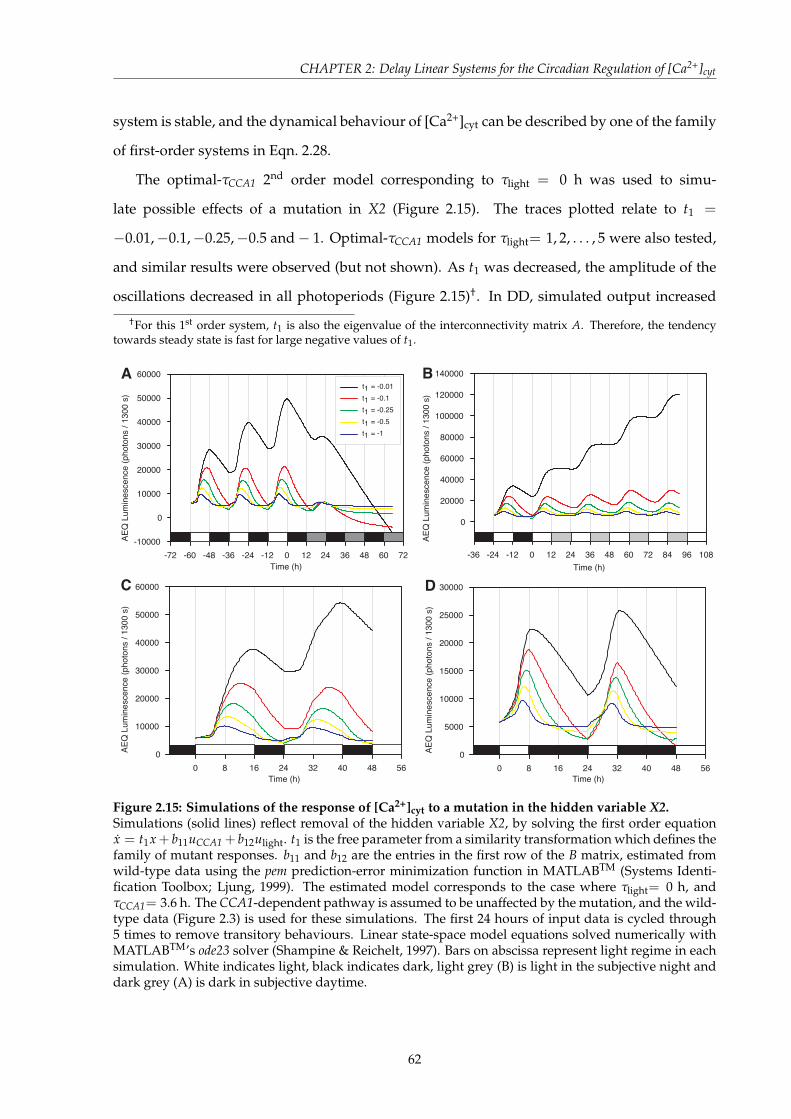
CHAPTER 2: Delay Linear Systems for the Circadian Regulation of [Ca2+]cyt
system is stable, and the dynamical behaviour of [Ca2+]cyt can be described by one of the family
of first-order systems in Eqn. 2.28.
The optimal-τCCA1 2nd order model corresponding to τlight = 0 h was used to simu-
late possible effects of a mutation in X2 (Figure 2.15). The traces plotted relate to t1 =
−0.01,−0.1,−0.25,−0.5 and− 1. Optimal-τCCA1 models for τlight= 1, 2, . . . , 5 were also tested,
and similar results were observed (but not shown). As t1 was decreased, the amplitude of the
oscillations decreased in all photoperiods (Figure 2.15)†. In DD, simulated output increased
†For this 1st order system, t1 is also the eigenvalue of the interconnectivity matrix A. Therefore, the tendencytowards steady state is fast for large negative values of t1.
Time (h)-72 -60 -48 -36 -24 -12 0 12 24 36 48 60 72
AEQ
Lum
ines
cenc
e (p
hoto
ns /
1300
s)
-10000
0
10000
20000
30000
40000
50000
60000t1 = -0.01t1 = -0.1t1 = -0.25t1 = -0.5t1 = -1
A
Time (h)-36 -24 -12 0 12 24 36 48 60 72 84 96 108
AEQ
Lum
ines
cenc
e (p
hoto
ns /
1300
s)
0
20000
40000
60000
80000
100000
120000
140000B
Time (h)0 8 16 24 32 40 48 56
AEQ
Lum
ines
cenc
e (p
hoto
ns /
1300
s)
0
10000
20000
30000
40000
50000
60000C
Time (h)0 8 16 24 32 40 48 56
AEQ
Lum
ines
cenc
e (p
hoto
ns /
1300
s)
0
5000
10000
15000
20000
25000
30000D
Figure 2.15: Simulations of the response of [Ca2+]cyt to a mutation in the hidden variable X2.Simulations (solid lines) reflect removal of the hidden variable X2, by solving the first order equationx = t1x + b11uCCA1 + b12ulight. t1 is the free parameter from a similarity transformation which defines thefamily of mutant responses. b11 and b12 are the entries in the first row of the B matrix, estimated fromwild-type data using the pem prediction-error minimization function in MATLABTM (Systems Identi-fication Toolbox; Ljung, 1999). The estimated model corresponds to the case where τlight= 0 h, andτCCA1= 3.6 h. The CCA1-dependent pathway is assumed to be unaffected by the mutation, and the wild-type data (Figure 2.3) is used for these simulations. The first 24 hours of input data is cycled through5 times to remove transitory behaviours. Linear state-space model equations solved numerically withMATLABTM’s ode23 solver (Shampine & Reichelt, 1997). Bars on abscissa represent light regime in eachsimulation. White indicates light, black indicates dark, light grey (B) is light in the subjective night anddark grey (A) is dark in subjective daytime.
62

CHAPTER 2: Delay Linear Systems for the Circadian Regulation of [Ca2+]cyt
to an intermediate value but decreased again to low levels, irrespective of t1 (Figure 2.15A).
This prediction contrasted with the wild-type simulation, providing a criterion for identifying
genes/components corresponding to the hidden variable X2. In LL, the oscillation troughs
were higher, and amplitude lower than in L12/D12 cycles for all t1, as observed in the wild-
type simulation (Figure 2.15B). Furthermore, for t1 near 0, the simulated output increased in
steps corresponding to the times when CCA1:luc was high (Figure 2.15B), illustrating how both
X2 and the light input pathway are responsible for decreasing the simulated ouput in the dark
phase following a period of light, as well as elevating the simulated output in prolonged dark-
ness. Simulations of entrained L16/D8 cycles led to a similar behaviour to that observed in
simulated light mutants (Figure 2.14C), whereby there was a lag between the onset of light,
and a corresponding increase in [Ca2+]cyt (Figure 2.15C). However, the oscillation phase varied
over a large range, from 7.6 h (t1 = −1) to 16 h (t1 = −0.01) after dawn, being progressively
later for values of t1 approaching 0. For entrained L8/D16 cycles, the oscillation phase was
between 6.2 h (t1 = −1) and 8.8 h (t1 = −0.01) after dawn. In conclusion, there was an overlap
between predictions for [Ca2+]cyt in simulated light input mutations and x2 mutants, which
suggested that an as-yet unidentified molecular component (X2) was critical for transducing
light information to [Ca2+]cyt. For example, X2 may represent components of the light sig-
nalling network, which transduce wavelength-specific light availability and are also regulated
by the circadian clock.
As X2 is required for the increase in [Ca2+]cyt following a dark to light transition, it is possi-
ble that X2 incorporates one or a subset of the photoreceptors. Many photoreceptors undergo
increased promoter activity in DD (Tóth et al., 2001). PHYA:luc and PHYB:luc luminescence
increases sharply 12 h after transition from light to continual darkness (Tóth et al., 2001), which
coincides with the observed [Ca2+]cyt increase. PHYA and PHYB protein levels are also high in
7-day old dark-grown seedlings, but arrhythmic in light-dark cycles (Sharrock & Clack, 2002).
It would be interesting to see if these proteins accumulate in extended darkness after entrained
L12/D12 cycles. We compared our model predictions with the available AEQUORIN lumi-
nescence data for mutant lines in L16/D8 and L8/D16 conditions. We found that the phyA-201
mutant allele led to a delayed increase in [Ca2+]cyt at the dark to light transition, and also a later
phase of oscillation (11.3 h after dawn; Figure 2.16A; Hubbard, 2008). This experimental obser-
vation coincided well with the prediction of a mutation in X2 when t1 & −0.5 (see Figure 2.16B
63

CHAPTER 2: Delay Linear Systems for the Circadian Regulation of [Ca2+]cyt
for comparison), implicating PHYA to be one or all of the hidden variable X2.
Time (h)
-8 0 8 16 24 32
AEQ
lum
ines
cenc
e (p
hoto
ns /
1500
s)
2000
2500
3000
3500
4000
4500
5000
2000
3000
4000
5000
6000
7000LerphyA-201
A
Time (h)
16 24 32 40 48 56
Sim
ulat
ed A
EQ lu
min
esce
nce
14000
16000
18000
20000
22000
5000
10000
15000
20000
25000
30000Wild-typex2 Mutant (t 1 = -0.1)
B
Time (h)
8 16 24 32 40 48 56 64 72
AEQ
Lum
ines
cenc
e (p
hoto
ns /
1500
s)
1000
1500
2000
2500
3000
3500
4000
4500C
Figure 2.16: Red- and blue-light photoreception by [Ca2+]cyt.Seedlings were grown for approximately 12 days in entrained cycles of 16 h light, 8 h dark (100 µmol m-2
s-1). (A) Seedlings imaged under mixed red and blue light (80 µmol m-2 s-1), with traces representative ofthe [Ca2+]cyt oscillation in wild-type (Ler; black circles) and phyA-201 mutant (red open circles) seedlings.(B) Simulation of candidate L0 model (τCCA1=3.7 h, τlight=0 h) in L16/D8 cycles, comparing wild-type(black line) and x2 mutant with t1 = −0.1 (red line) backgrounds. (C) Seedlings imaged under singlewavelengths of R light (60 - 80 µmol m-2 s-1). White bars indicate mixed R + B light and red bars indicateR (black bars represent darkness). Data in (A) and (C) collected by Dr. Katharine Hubbard, Universityof Cambridge, UK. Modified from Hubbard (2008).
The assumption that t1 is negative may not be correct, in which case the simulated x2 mu-
tant will lead to an unstable system, resulting in unbounded increases in [Ca2+]cyt. In fact, for
t1 & −0.01, the model still predicts [Ca2+]cyt to increase persistently in LL (Figure 2.15B), and
attains progressively higher levels in LD cycles which increase faster for longer photoperiods
(Figure 2.15C–D). In searching through the available AEQUORIN luminescence data, we found
this behaviour occurred in seedlings entrained to 16 h monochromatic red light, 8 h dark cy-
cles (Figure 2.16C, Hubbard, 2008). Xu et al. (2007) observed similar unbounded increases in
[Ca2+]cyt in wild-type Arabidopsis under constant blue light (BB), indicating that both blue and
64

CHAPTER 2: Delay Linear Systems for the Circadian Regulation of [Ca2+]cyt
red light are required for the decrease in [Ca2+]cyt following the elevation after dawn. Trans-
genic manipulations in CRY1, CRY2 and PHYB all reduced both the accumulation in BB and
the amplitude in LL (Xu et al., 2007). It was also observed that [Ca2+]cyt undergoes stable os-
cillations in RR in wild-type plants, but accumulates unboundedly in RR in the phyB-5 mutant
allele. When viewed together with the model predictions of a mutation in X2, there is evidence
which suggests X2 incorporates many elements of the light signalling network, both red- and
blue-light dependent.
2.3.7 Determination of internal structure for the CCA1–Light/Dark–[Ca2+]cyt-X2
network
Each linear model estimated was fixed into controller canonical form (Eqn. 2.8). The inter-
nal structure of these systems with hidden states is not fixed, as similarity transformations
can re-structure the state variables while preserving the input-output behaviour. Therefore,
we considered the second-order generalised system (Equations 2.26–2.27) to establish whether
particular entries in A and B could be zero, and thus determining some structural information.
The generalised A matrix is given by
A = T−1AT =
t1 t2
−t21 + a2t1 + a1
t2−t2 + a2
(2.29)
To assess the possibility that [Ca2+]cyt does not influence the hidden variable X2, we need only
consider the entries in A from the estimated models. Assuming t2 6= 0 (as otherwise the system
would decouple into two first order equations), we derive a condition for the (2,1) position of
A (a21) to be zero:
a21 = 0
⇔ −t21 + a2t1 + a1 = 0
⇔ t1 =a2
2±
√a2
2 + 4a1
2
This value of t1 exists provided the discriminant of the quadratic equation is non-negative. i.e
a22 + 4a1 ≥ 0. The values of a2
2 + 4a1 corresponding to the optimal-τCCA1 2nd order models from
Table 2.4 were all positive, implying that it is possible that X2 does not depend on [Ca2+]cyt in
65

CHAPTER 2: Delay Linear Systems for the Circadian Regulation of [Ca2+]cyt
these model formulations (see Table 2.7).
Table 2.7: Entries of A determine potential for X2 to not be regulated by [Ca2+]cyt.Each row represents a 2nd order linear state-space model, based on the delay between the light inputand the system (τlight). In each case, the optimal τCCA1 is selected based on cross-validation tests. The ai
are the entries from the A matrix estimated (see Eqn. 2.25). a22 + 4a1 is the discriminant of the quadratic
equation which is the solution to the (2,1) entry of A being zero.
τlight τCCA1 a1 a2 a22 + 4a1
0 3.6 -0.0187 -0.3879 0.07571 4.5 -0.0290 -0.6240 0.27342 5.5 -0.0580 -1.2901 1.43233 4.3 -0.0303 -0.5936 0.23104 3.6 -0.0230 -0.4244 0.08805 3.7 -0.0242 -0.4291 0.0874
The generalised form of B can also be considered to investigate potential missing links in
the input structure regulating X2. In particular, is X2 regulated by both the circadian clock
and light, or just one of these pathways? The (2,1) entry of B is zero if and only if t1 =b21
b11,
while the (2,2) entry is zero if and only if t1 =b22
b12. We found that for the same optimal-τCCA1
models investigated above, t1 must be chosen between −0.4 and −1.5 (depending on which
model used) for any entries in B to be zero (Table 2.8). As the values of t1 which correspond to
b21 = 0 and b22 = 0 are distinct, it is not possible for both b21 and b22 to be zero. Therefore, it
is not possible to say with any certainty whether there are direct causal relationships between
the input pathways and X2.
Table 2.8: Entries of B determine potential for missing links in the input regulation of the hiddenvariable.Each row represents a 2nd order linear state-space model, based on the delay between the light inputand the system (τlight). In each case, the optimal τCCA1 is selected based on cross-validation tests. Thebij are the entries from the B matrix estimated (see Eqn. 2.25). b21/b11 is the value of t1 (from similaritytransformation T defined in Eqn. 2.25) which must be chosen for the (2,1) entry of B to be 0. b22/b12 isthe corresponding value of t1 which results in the (2,2) entry being 0.
τlight τCCA1 b11 b21 b21/b11 b12 b22 b22/b12
0 3.6 4857.9 -2017.3 -0.41526 -1155 647.95 -0.5611 4.5 6295 -3942.1 -0.62623 -1795.7 1372.4 -0.764262 5.5 11414 -14823 -1.2986 -3538.7 5079.3 -1.43543 4.3 6111.6 -3671.7 -0.60078 -1082.6 902.43 -0.833584 3.6 5055.6 -2181.8 -0.43156 -362.9 349.91 -0.964195 3.7 5101.7 -2224.4 -0.43602 -194.61 287.19 -1.4757
66

CHAPTER 2: Delay Linear Systems for the Circadian Regulation of [Ca2+]cyt
2.3.8 Frequency response of [Ca2+]cyt to CCA1 and Light/Dark
The frequency response of each pathway regulating [Ca2+]cyt was computed for the candidate
L0 model with τCCA1= 3.7 h and τlight= 0 h. A transfer function representation of the transfer
functions from each input to the output was first computed by finding the Laplace transform
of each side of the state-space linear system of ODEs (Eqn. 2.1), which reduces to
Y(s) =(
G1(s) G2(s))U1(s)
U2(s)
= G(s)Uτ(s) (2.30)
where G(s) := C(sI − A)−1B is partitioned into G1 := TuCCA1→y and G2 := Tulight→y by the
columns of B, U1(s) := L(uCCA1(t − τCCA1)) and U2(s) := L(ulight(t − τlight)). The resulting
transfer functions were
G1(s) =4804.1101(s− 0.001965)(s + 0.3454)(s + 0.05543)
(2.31)
G2(s) =−1099.4179(s− 0.1513)(s + 0.3454)(s + 0.05543)
(2.32)
The magnitude and phase were then computed for G1 and G2 in the frequency range ω ∈
[10−4, 1] rad/h using the bode function in MATLABTM (Laub, 1981), with the magnitude |G(jω)|
converted to decibel units as 20 log |G(jω)|. G1 was found to be a band-pass filter with peak
magnitude at ω = 0.140023 rad/h, which corresponds to a frequency of 2π/ω = 44.87 h
(Figure 2.17). In particular, G1 dominates the system response over circadian periods (between
12 h and 48 h) and has a phase angle near 0 in this range. At lower frequencies (oscillations
with larger periods), G2 dominates the system response with a phase angle near 0 (Figure 2.17).
The frequency response analysis demonstrates the requirement for two independent regulators
of [Ca2+]cyt, and suggests that the regulation by the circadian clock is specifically enhanced
over circadian timescales (periods near 24 h) and suppressed at lower or higher frequencies
(Figure 2.17).
67

CHAPTER 2: Delay Linear Systems for the Circadian Regulation of [Ca2+]cyt
Mag
nitu
de (d
B)
40
50
60
70
80
t = 12 ht = 48 h
Frequency (rad / h)0.0001 0.001 0.01 0.1 1 10
Phas
e (d
eg)
-270
-180
-90
0
90
180
CCA1 - Ca 2+
Light - Ca 2+
Figure 2.17: The regulation of [Ca2+]cyt by CCA1 is a band-pass filter.The bode magnitude (top) and phase (bottom) plots are shown for the candidate L0 model withτCCA1= 3.7 h and τlight= 0 h. The magnitude plot displays the amplitude of the response of the transferfunction G to a frequency ω in decibel units (i.e. 20 log |G(jω)|) and the phase plot shows the phaseangle ∠G(jω). For each input pathway (CCA1–[Ca2+]cyt, black lines, and Light/Dark–[Ca2+]cyt, redlines) transfer function representations were obtained as G(s) = C(sI − A−1)B to enable computationof |G(jw)| and ∠G(jω) with the bode function in MATLABTM (Laub, 1981). Blue dashed lines indicatethe frequencies corresponding to periods (τ) between 48 h and 12 h.
2.4 Discussion
Mathematical models were derived to increase understanding of the regulation of basal
[Ca2+]cyt by the circadian clock and the light signalling network. Three model classes were
investigated: a single-input single-output system which maps CCA1:luc luminescence data to
AEQUORIN luminescence data (SISO model; Eqn. 2.4) and two dual-input systems which ad-
ditionally track the availability of light and dark, switching between 1 and 0 (L1) or 0 and 1 (L0)
respectively (Eqn. 2.5). In all cases, the uncharacterised but assumed present pathway interme-
diates were modelled as delay parameters τCCA1 and τlight. The black-box nature of the problem
suggested that the underlying model should be as simple as possible, attempting to describe
the fundamental dynamics of the system. Therefore, we have started by using continuous-time
68

CHAPTER 2: Delay Linear Systems for the Circadian Regulation of [Ca2+]cyt
linear state-space systems, subject to delays on the input signals (Eqn. 2.1). While there were
drawbacks of using simple models, it was still possible to successfully validate a model, and in
doing so learn properties of the network, including timescales and novel components.
2.4.1 [Ca2+]cyt is regulated by a light/dark-dependent pathway and a hidden vari-
able
Estimation of models which considered [Ca2+]cyt to be regulated by a CCA1-dependent path-
way alone were unable to reproduce the observed transition to DD. In L12/D12, [Ca2+]cyt is low
during the night, and after a prolonged period of darkness increases to an intermediate level,
and undergoes very low amplitude (if any) oscillations (Figure 2.3B). Optimal prediction-error
single-input models continued to oscillate, irrespective of the model order (number of state
variables; Figure 2.4B), which indicated that the single-input model class used was not suf-
ficient to describe the available AEQUORIN luminescence data. The optimal choice of τCCA1
decreased as the model order was increased, which suggested that the additional state variables
were accounting for the delay in the system (Table 2.1). Inspection of the model performance
in the cross-validation conditions revealed that the models were generally able to track the cor-
rect phase and amplitude of oscillation in L12/D12 cycles, but were unable to distinguish the
reduced amplitude in LL (Figure 2.6). Furthermore, in the absence of a functional CCA1, this
model class predicts a constant level of [Ca2+]cyt in LD cycles. However, recent published data
has shown that the cca1-1 mutant still undergoes oscillations in LD, albeit with a significantly
altered waveform (Xu et al., 2007).
The dual-input model class enabled simulated [Ca2+]cyt to cycle in nyctohemeral cycles
when the CCA1-dependent pathway was removed (Figure 2.12). The two dual-input model
classes L0 (light = 0, dark = 1) and L1 (light = 1, dark = 0) were compared for their perfor-
mance with respect to the wild-type estimation data (L12/D12–DD; Figure 2.7). While both
dual-input models offered improvement in AICc over the single-input class during estimation,
models which responded to light as a nonzero input (L1) did not perform as well as those
which responded to dark in simulation (L0; Figure 2.8), and through comparison of AICc (Ta-
ble 2.3). The optimal choice of τCCA1 during estimation was much lower for L0 models, with
L1 yielding unrealistically high τCCA1 (Table 2.3), further pointing to a dark-dependent activa-
tion of [Ca2+]cyt. We interpret this as [Ca2+]cyt being regulated by a light-labile photoreceptor
69

CHAPTER 2: Delay Linear Systems for the Circadian Regulation of [Ca2+]cyt
(i.e. PHYA). 2nd order models were optimised by τCCA1 ranging between 3.5 h and 4.5 h, while
4th order models preferred τCCA1 near 0, again suggesting that the additional state variables
were accounting for the delay between CCA1 expression and Ca2+-release. However, neither
estimation nor cross-validation simulations were able to distinguish between varying τlight, as
simulated outputs were very similar (Figures 2.10, 2.11). Cross-validation suggested 2nd order
models represented a more accurate description of the available measured data than 4th order
models, which were prone to over-fitting due to the number of estimated parameters. We con-
clude that [Ca2+]cyt is regulated by a CCA1-dependent pathway approximately 4 h in duration,
a light/dark-dependent pathway of unknown timescale and a hidden variable X2.
2.4.2 Simulated CCA1 mutant analysis reveals temporal information for the regu-
lation of [Ca2+]cyt by transitions between light and dark
To distinguish different delay lengths between the light/dark-input pathway and [Ca2+]cyt
(τlight), simulations of a null mutation in CCA1 were carried out in which the CCA1 input was
considered to be 0 throughout (Figure 2.12). In light-dark cycles, simulated [Ca2+]cyt peaked at
times which positively correlated with τlight (see Table 2.6). This provided the first distinction
between alternative choices of τlight, and by comparing simulations with AEQUORIN lumines-
cence data in the cca1-1 null allele, this indicated that τlight should be no longer than 2 hours in
duration. Simulation of the candidate models revealed that [Ca2+]cyt can still oscillate in light-
dark cycles and anticipate dawn in the absence of a circadian regulator (Figure 2.12), though
the phase of the oscillation is shifted with respect to the dual-control (wild-type) system. To
provide further validation and to hypothesise potential roles of other clock components, we
compared these simulations with AEQUORIN luminescence measured in a variety of clock
gene mutant backgrounds under LL (Figure 2.18) and L12/D12 (Figure 2.19).
In LL, [Ca2+]cyt does not oscillate in the cca1-1 mutant background, though it is not possible
to distinguish the level of [Ca2+]cyt relative to the wild-type (Figure 2.18A; Xu et al., 2007). In
CCA1-ox, there is a clear peak of [Ca2+]cyt 5.2 h after the transition from dark at t = 0 which
coincides (in value) with the wild-type (Figure 2.18B; Xu et al., 2007), before [Ca2+]cyt undergoes
a steady decline to low levels relative to the wild-type oscillation. The tendency towards the
low steady state was equivalent to the behaviour predicted by candidate models for [Ca2+]cyt
under LL when the CCA1 input pathway was suppressed (Figure 2.12B), further supporting
70

CHAPTER 2: Delay Linear Systems for the Circadian Regulation of [Ca2+]cyt
the dual-input delay linear systems representation for the regulation of basal [Ca2+]cyt. The
LHY-ox trace shows a similar phenotype, whereby [Ca2+]cyt peaks 3.9 h after the transition
from dark to light, before stabilising at a relatively low level. The similarity might be attributed
to the functional similarity between CCA1 and LHY (Schaffer et al., 1998; Wang & Tobin, 1998;
Mizoguchi et al., 2002), with over-expression of both proteins leading to similar effects on gene
expression downstream of CCA1 but upstream of [Ca2+]cyt. For elf3-1, [Ca2+]cyt stabilises at a
high level in LL, relative to the levels after transfer from dark to light (Figure 2.18D). The shape
of this response agrees most closely with simulated [Ca2+]cyt in DD (both simulated wild-type
and CCA1 mutant; see Figures 2.10A & 2.12A), indicating that ELF3 can regulate the light-input
pathway. ELF3 has already been observed to regulate the circadian control of light input to the
central oscillator (McWatters et al., 2000; Covington et al., 2001), and so the [Ca2+]cyt phenotype
in LL appeared to suggest a similar mechanism, whereby ELF3 mediates the light control of
[Ca2+]cyt (Xu et al., 2007).
In entrained L12/D12 cycles, each of these four mutant backgrounds (cca1-1, CCA1-OX,
LHY-OX and elf3-1) still produce oscillations [Ca2+]cyt. In cca1-1, [Ca2+]cyt peaks 3.6 h after
dawn in response to the light/dark input pathway, undergoes a steady decline before increas-
ing in anticipation of dawn. In the absence of a circadian regulator, it is surprising that [Ca2+]cyt
increases in anticipation of dawn. However, our candidate models have also predicted this
behaviour in the absence of a circadian input (Figure 2.13). Therefore, we can attribute this
behaviour to second-order dynamics (in response to step inputs), which we have shown are re-
quired for a suitable description of the system. In contrast to measurements of [Ca2+]cyt in LL,
CCA1-OX and LHY-OX lead to different phenotypes in LD (Figures 2.19B,C). Overexpression
of CCA1 has almost no effect on L12/D12 oscillations of [Ca2+]cyt relative to wild-type, which
peak 7 h after dawn and remain low during the dark phase (Figure 2.19B). However, overex-
pression of LHY causes [Ca2+]cyt to peak later (11 h after dawn), then decline throughout the
dark, reaching the lowest level at 1 h before dawn (Figure 2.19C). The elf3-1 mutation affects
the L12/D12 [Ca2+]cyt oscillation only in the first 3 hours after dawn, resulting in peaks both
3 h and 7 h after dawn. The initial increase in [Ca2+]cyt after transition from dark to light is con-
trolled by the light/dark input pathway, while the CCA1-input pathway comes into effect after
a delay of ≈ 4 h. Therefore, mutation in ELF3 affects the light/dark input pathway, agreeing
with the observed effects in LL described in the previous paragraph (Figure 2.18D).
71

CHAPTER 2: Delay Linear Systems for the Circadian Regulation of [Ca2+]cyt
Time in LL (h)0 12 24 36 48 60 72 84 96 108
AEQ
Lum
ines
cenc
e (p
hoto
ns /
40 s
)
600
800
1000
1200
1400
1600
1800
Wild-typecca1-1
A
Time in LL (h)0 12 24 36 48 60 72 84 96 108
AEQ
Lum
ines
cenc
e (p
hoto
ns /
40 s
)
1000
1500
2000
2500
3000
3500
Wild-typeCCA1-ox
B
Time in LL (h)0 12 24 36 48 60 72 84 96 108
AEQ
Lum
ines
cenc
e (p
hoto
ns /
40 s
)
600
800
1000
1200
1400
1600
1800Wild-typeLHY-ox
C
Time in LL (h)0 12 24 36 48 60 72 84 96 108
AEQ
Lum
ines
cenc
e (p
hoto
ns /
1300
s)
5000
10000
15000
20000
25000
30000
Wild-typeelf3-1
D
Figure 2.18: Mutations in core clock genes can lead to arrhythmic [Ca2+]cyt in LL.AEQUORIN luminescence in cca1-1 (A), CCA1-OX (B), LHY-OX (C), and elf3-1 (D) under LL (100µmol m-2 s-1) measured using photon-counting luminescence (A–C) or photon-counting imaging (D).Seedlings entrained under L12/D12 for 7 d before transfer to LL. Grey boxes indicate subjective nightin LL. Data collected by (A–C) Dr. Xiaodong Xu, Vanderbilt University, USA, and (D) Dr. Carlos Hotta,University of Cambridge, UK. Modified from Xu et al. (2007).
2.4.3 The unconstrained internal structure of the 2nd order model complicates the
identification of X2
The structure of the candidate 2nd order L0 model (τCCA1= 3.7 h, τlight= 0 h) was investigated
because the causal relationships between the hidden state (X2) and the inputs and output of
the model are not fixed (see Section 2.2.4, Remark 2). By considering generalised interconnec-
tivity (A; Eqn. 2.26) and input (B; Eqn. 2.27) matrices defined in terms of a suitable similarity
transformation, it was found that X2 is at least regulated by a CCA1-dependent or light/dark-
dependent pathway or both (Table 2.8), though nothing could be established regarding the
interconnectivity of [Ca2+]cyt and X2 (Table 2.7). Therefore, the identification of biochemical
components which constitute the role of X2 is not straightforward from considering the effect
of mutations in X2 on the dynamics of [Ca2+]cyt, because a mutation in the hidden state X2 may
72

CHAPTER 2: Delay Linear Systems for the Circadian Regulation of [Ca2+]cyt
Time (h)0 12 24
AEQ
Lum
ines
cenc
e (p
hoto
ns /
40 s
)
600
800
1000
1200
1400
1600
1800cca1-1
A
Time (h)0 12 24
AEQ
Lum
ines
cenc
e (p
hoto
ns /
1300
s)
1000
1500
2000
2500
3000
3500
4000CCA1-ox
B
Time (h)0 12 24
AEQ
Lum
ines
cenc
e (p
hoto
ns /
1300
s)
6000
7000
8000
9000
10000
LHY-ox
C
Time (h)0 12 24
AEQ
Lum
ines
cenc
e (p
hoto
ns /
1300
s)
4000
5000
6000
7000
8000
9000elf3-1
D
Figure 2.19: Mutations in core clock genes disrupt but do not remove [Ca2+]cyt oscillations in light-dark cycles.AEQUORIN luminescence in cca1-1 (A), CCA1-OX (B), LHY-OX (C), and elf3-1 (D) under 12 h light, 12 hdark cycles (100 µmol m-2 s-1) measured using photon-counting luminescence (A) or photon-countingimaging (B–D). Seedlings entrained under L12/D12 for 7 d before the start of the experiment. Blackboxes indicate night and white boxes indicate day. Data collected by (A) Dr. Xiaodong Xu, VanderbiltUniversity, USA, and (B,C,D) Dr. Carlos Hotta, University of Cambridge, UK. Modified from Xu et al.(2007).
not remove the complete light/dark dependency of [Ca2+]cyt, nor may it remove the circadian
regulation by a CCA1-dependent pathway.
2.4.4 Simulations of a mutation in the light/dark input pathway or the hidden state
variable
The optimal-τCCA1 2nd order L0 models were simulated under the cross-validation photoperi-
odic regimes with the light/dark input set to a constant throughout, in order to predict po-
tential effects of a mutation in the light/dark input pathway which regulates [Ca2+]cyt (Fig-
ure 2.14). In light-dark cycles, there were only subtle differences between simulated wild-type
and simulated mutations in the light/dark input pathway. The oscillations in L12/D12 had a
73

CHAPTER 2: Delay Linear Systems for the Circadian Regulation of [Ca2+]cyt
broader trough in the simulated mutations in the light/dark input pathway, compared with
the nominal model configuration (Figure 2.14A). After transfer from L12/D12 to DD, the out-
put of the simulated mutant increased to an intermediate level similar to wild-type data and
simulation, but it was followed by a decline back to a relative low level before steadily increas-
ing again (Figure 2.12A). Constant light oscillations of [Ca2+]cyt in the simulated mutations in
the light/dark input pathway had a similar amplitude to the light-dark cycles (Figure 2.12B).
In entrained L16/D8 cycles, there was a lag between dark to light transition and the daytime
[Ca2+]cyt increase, indicating that the light/dark input pathway is required to elevate [Ca2+]cyt
in the early part of the day. However, this did not lead to a significantly delayed oscillation
phase in light-dark cycles.
The candidate 2nd order model with τlight equal to 0 h was investigated for the effect of a
mutation in the hidden state variable X2. This led to a family of 1st order systems given by
x = t1x + b11uCCA1 + b12ulight, where t1 is a free parameter. We found that for t1 < 0, [Ca2+]cyt
did not stabilise at an intermediate level in DD, as observed in wild-type traces (Figure 2.15A).
In addition, there was a clear lag between the onset of light and a corresponding increase in
[Ca2+]cyt under entrained L16/D8 cycles (Figure 2.15C). An identical prediction resulted from
simulations of a mutation in the light/dark input pathway (Figure 2.14C), indicating that X2
is required for the light-induced elevation in [Ca2+]cyt at the transition from dark to light in
entrained cycles. In fact, the dark to light transitory behaviours resulting from simulations of
X2 and light/dark input pathway mutants corresponded well in all entrained cycles investi-
gated (L12/D12, Figures 2.14A, 2.15A; L8/D16, Figures 2.14D, 2.15D). However, in contrast to
the simulated mutations in the light/dark input pathway, we found a broad range of oscil-
lation phase in L16/D8 cycles (between 7.6 h and 16 h after dawn), which differed from the
corresponding wild-type phase.
Despite the difficulties of obtaining structural information from delay linear systems mod-
els, from these simulated mutant analyses it was possible to predict specific light/dark-
associated components to function in a light/dark – X2 pathway which regulates [Ca2+]cyt.
By comparing experimental measurements of [Ca2+]cyt in photoreceptor mutants with the dy-
namics of simulated x2 mutants, PHYA was found to be a candidate regulator of [Ca2+]cyt.
The phyA-201 mutant had impaired LD oscillations of [Ca2+]cyt similar to simulated x2 mutants
with t1 = −0.1 (Figures 2.16A,B). Since the delayed increase at the dark to light transition was
74

CHAPTER 2: Delay Linear Systems for the Circadian Regulation of [Ca2+]cyt
also seen in simulations of a mutation in the light/dark input pathway, it is likely that PHYA
mediates the light/dark – X2 regulation of [Ca2+]cyt. Further experiments with wavelength-
specific light sources indicated that a blue-light dependent component is required to decrease
[Ca2+]cyt during the latter part of the day (Figure 2.16C). Simulated x2 mutants with t1 & −0.01
also had this behaviour, with model output progressively increasing during each LD cycle (Fig-
ure 2.15C). Therefore, it is possible that blue light photoreception is also encoded in the hidden
component X2.
2.4.5 Summary
Experimental studies have used reverse genetic techniques to elucidate some conceptual un-
derstanding of how [Ca2+]cyt is regulated by the circadian clock and light/dark (Xu et al., 2007;
Hotta, 2007; Hubbard, 2008). In this chapter, these observations were used to construct math-
ematical descriptions of the interactions between [Ca2+]cyt, light/dark signals and the central
oscillator gene CCA1 based on AEQUORIN and CCA1:luc luminescence data. We found that
the regulation of [Ca2+]cyt by CCA1 occurs through a pathway of approximately 4 h in duration
and operates as a band-pass filter for frequencies corresponding to circadian periods (between
12 h and 48 h). [Ca2+]cyt is regulated by light/dark signals immediately (τlight= 0) whereby the
absence of light (dark) contributes a nonzero signal, though this pathway dominates the sys-
tem response at low frequencies. The most appropriate systems descriptions were 2nd order,
while an additional 2 hidden states could account for the CCA1 delay but resulted in mod-
els which could not be successfully cross-validated. Comparing simulations of the 2nd order
models with the available experimental data enabled us to attribute phenotypes to removal of
model components. The hidden variable appears to represent the action of the red-light sensi-
tive phytochromes, and also the blue-light sensitive cryptochromes, despite the model not in-
corporating explicit dependencies on red and blue light signals. Contained within this chapter
are many more simulations of mutant behaviours which have not been observed experimen-
tally thus far, but provide specific behaviours which may be attributed to model components
if and when they are observed. These behaviours have provided a bank of predictions which
can be used to identify currently unknown components in the network of dual-regulation of
[Ca2+]cyt.
75

CHAPTER 3
A Three Loop Model of the Arabidopsis
Circadian Clock in the Absence of
Exogenous Sucrose
3.1 Introduction
Sucrose is a major output of photosynthesis and is vital as an energy source for plants
(Buchanan et al., 2002). Until recently, the role of metabolic sugars in the plant circadian central
oscillator had not been studied (Knight et al., 2008). However, in LL oscillations in the concen-
tration of cytosolic-free Ca2+ ([Ca2+]cyt) are absent in Arabidopsis seedlings grown on agar media
containing 3% sucrose (Johnson et al., 1995), indicating a role for sugars in regulating at least
one circadian output. In this chapter, mathematical modelling has been used to study sugar
availability as an input to the circadian central oscillator, and to predict target mechanisms.
Furthermore, these predictions have been validated experimentally.
Sucrose accounts for the majority of fixed carbon during photosynthesis and serves as the
principal long-distance transporter in many plants (Buchanan et al., 2002). Sucrose is a nonre-
ducing sugar because there is a stable glycosidic bond between the potentially reactive carbonyl
carbons glucose and fructose, providing protection from oxidation (Buchanan et al., 2002). Su-
76

CHAPTER 3: A Three Loop Model of the Arabidopsis Circadian Clock in the Absence of Exogenous Sucrose
crose synthesis occurs in the cytosol through a pathway of two enzymes. Sucrose-phosphate
synthase (SPS) catalyses the synthesis of sucrose-6-phosphate (Suc6P), which is then hydrol-
ysed by sucrose-phosphate phosphatase (SPP) into sucrose (Lunn & MacRae, 2003). This
sequence of reactions associates a large negative free energy change and is therefore essen-
tially irreversible (Buchanan et al., 2002). Sucrose may also be synthesised by sucrose syn-
thase (SUS), though this enzyme is more commonly associated with degradation of sucrose,
yielding fructose and uridine diphosphate glucose (UDP-glucose; Baud et al., 2004). Invertase
(β–D-fructofuranosidase) also breaks down sucrose, yielding glucose and fructose (Tymowska-
Lalanne & Kreis, 1998). In Arabidopsis, there are six known genes encoding sucrose synthase
enzymes (AtSus1-6; Baud et al., 2004; Barratt et al., 2001), four encoding SPPs (Lunn et al.,
2000), four encoding SPSs (Lunn & MacRae, 2003), and four encoding invertases (Atβfruct1-
4; Tymowska-Lalanne & Kreis, 1998).
When the synthesis and subsequent export of sucrose cannot keep pace with photosynthe-
sis, fixed carbon enters the hexose phosphate pool, and is stored in the chloroplast as starch
(Buchanan et al., 2002). At night, the reserve of starch is broken down and converted to su-
crose. The timing of these events might benefit from control by the circadian clock, though
while sucrose and starch accumulate during the day and decline at night, their concentrations
do not oscillate in LL or DD (Bläsing et al., 2005; Lu et al., 2005). However, transcript abundance
of genes encoding starch-degradation enzymes follow the light-dark profiles almost exactly, re-
main low in DD, but continue to oscillate in LL (Lu et al., 2005). In tomato, SPS activity oscillates
in LL and light-dark cycles, though SPS protein levels remain constant (Jones & Ort, 1997). In
addition to the synthesis of carbohydrates being regulated by the circadian clock, there is also
evidence which suggests sucrose in turn regulates the oscillator mechanism. Sucrose represses
PHYA signal transduction pathways (Dijkwel et al., 1997); PHYA mediates light input to the cir-
cadian clock, and is also under circadian control (Hall et al., 2001). Kurepa et al. (1998) studied
the effect of exogenous sucrose supply on Arabidopsis seedlings, and found that gi-3 mutants
contained higher endogenous [Suc]i than wild-type for all exogenous supply concentrations
tested and flowering time in the dark was influenced by exogenous sucrose in gi-3. A recent
article published after the work in this chapter was conducted, established SENSITIVE TO
FREEZING 6 (SFR6) to be important in sucrose modulation of transcript abundance of CCA1,
TOC1 and GI (Knight et al., 2008). sfr6 mutants had diminished responses to sucrose treatment,
77

CHAPTER 3: A Three Loop Model of the Arabidopsis Circadian Clock in the Absence of Exogenous Sucrose
including its effect on flowering time (Knight et al., 2008).
The majority of circadian research in Arabidopsis is conducted with plants grown on agar
media containing 3% sucrose (Millar et al., 1995; Alabadí et al., 2001; Mizoguchi et al., 2005), and
as such the mathematical models correspond to these growth conditions (Locke et al., 2005a,b,
2006; Zeilinger et al., 2006). Our measurements of [Ca2+]cyt are from plants grown in the absence
of exogenous sucrose, as exogenous supply of 3% sucrose inhibits oscillations in LL (Johnson
et al., 1995). In DD, [Ca2+]cyt does not have circadian oscillations in the absence of sucrose
(Xu et al., 2007), though plants grown with 3% exogenous sucrose have circadian oscillations
of CCA1, LHY, TOC1, GI, ELF3, ELF4 and CCR2 expression (Alabadí et al., 2002; Ding et al.,
2007). As mathematical Arabidopsis circadian clock models have oscillations in DD, we were
prevented from using them as an input to a mathematical model for the circadian regulation of
[Ca2+]cyt (Locke et al., 2005b, 2006; Zeilinger et al., 2006; see Chapter 2 for mathematical models
of [Ca2+]cyt regulation). Furthermore, the fact that there are circadian oscillations in DD with 3%
exogenous sucrose and a tendency towards a steady state in the absence of exogenous sucrose
(which is also noted by Oguchi et al., 2004) motivated us to investigate the interactions between
sucrose and the circadian network in Arabidopsis.
In this chapter, we have attempted to re-design the Three Loop Model of the central oscillator
(Locke et al., 2006) to account for our data measuring central oscillator gene expression in Ara-
bidopsis seedlings grown without exogenous sucrose. The data in Figure 3.1 forms the training
set to achieve such a model, and further experimentation has been carried out to both validate
new models and test predictions of the target(s) of sucrose in the circadian network.
3.2 Materials and Methods
3.2.1 Measuring the effect of cold of CCA1 promoter activity with a microplate lu-
minometer
Cold-induced CCA1 promoter activity was measured for plants grown on 0.8% (w/v) agar
media containing 90 mM sucrose (Fisher Scientific, UK), 90 mM mannitol (BDH Laboratory
Supplies, UK) or no added sugars. Transgenic Arabidopsis seedlings expressing CCA1:luc were
grown in L12/D12 cycles for 10 days at constant 19◦C, then transferred to DD for 48 h. Individ-
ual seedlings were then incubated overnight in luminometer cuvettes containing 1 ml of 1 mM
78

CHAPTER 3: A Three Loop Model of the Arabidopsis Circadian Clock in the Absence of Exogenous Sucrose
Time (h)0 24 48 72 96 120
Nor
mal
ised
CC
A1:lu
c L
umin
esce
nce
0
2
4
10
15 H2O90 mM Mannitol 90 mM Sucrose
A
Time (h)0 24 48 72 96 120
Nor
mal
ised
CC
A1:lu
c L
umin
esce
nce
0
2
6
9
12B
Time (h)0 24 48 72 96 120
Nor
mal
ised
TOC
1:lu
c L
umin
esce
nce
0
1
2
3
4
5
6H2O90 mM Mannitol 90 mM Sucrose
C
Time (h)0 24 48 72 96 120
Nor
mal
ised
TOC
1:lu
c L
umin
esce
nce
0.0
0.5
1.0
1.5
2.0
2.5D
Time (h)0 24 48 72 96 120
Nor
mal
ised
GI:l
uc L
umin
esce
nce
0
1
2
3
10
20
H2O90 mM Mannitol 90 mM Sucrose
E
Time (h)0 24 48 72 96 120
Nor
mal
ised
GI::
luc
Lum
ines
cenc
e
0
1
2
3
4
5F
Period in DD (h)
20 22 24 26 28 30 32 34 36
Rel
ativ
e Am
plitu
de E
rror (
RAE
)
0.00
0.25
0.50
0.75
1.00CCA1:luc H2OCCA1:luc MannitolCCA1:luc SucroseTOC1:luc H2OTOC1:luc MannitolTOC1:luc SucroseGI:luc H2OGI:luc MannitolGI:luc Sucrose
G
Period in LL (h)
22.5 23.0 23.5 24.0 24.5 25.0 25.5 26.0 26.5
Rel
ativ
e Am
plitu
de E
rror (
RAE
)
0.00
0.25
0.50
0.75
1.00H
Figure 3.1: Exogenous sucrose modulates circadian central oscillator gene expression in LL and DD.10 day-old Arabidopsis seedlings grown on agar media containing 90 mM sucrose (red symbols), 90 mMmannitol (open symbols), or no additional sugars (closed symbols), were entrained to L12/D12 cyclesbefore transfer to constant (A,C,E,G) dark, or (B,D,F,H) light. Luminescence emitted from seedlingsexpressing (A,B) CCA1:luc, (C,D) TOC1:luc, or (E,F) GI:luc was quantified for 800 s for each datapointusing an automated photon counting camera. (G,H) Summary plot showing the mean estimated periodplus standard deviation was calculated by FFT-NLLS analysis and plotted against the relative amplitudeerror (RAE) of the rhythms plus standard deviation. All data obtained from Seong Jin Baek (personalcommunication). Bars in abscissa are white during light, black during darkness, light grey for light duringsubjective night, and dark grey for dark during subjective day.
79

CHAPTER 3: A Three Loop Model of the Arabidopsis Circadian Clock in the Absence of Exogenous Sucrose
luciferin. Luminescence emitted from each cuvette was measured with a photon-counting lu-
minometer (Electron Tubes, Ruislip, UK) for 60 s to obtain a reference signal, then placed in
a frozen cuvette rack (IsoPack; Eppendorf, Germany) to maintain the temperature of the cu-
vettes at approximately 0◦C for 2, 3, or 6 h. Following cold treatment, cuvettes were left at
room temperature for 15 min to activate the temperature-dependent luciferase enzyme activity,
then luminescence was measured for 240 s.
3.2.2 Numerical solution of the Three Loop Model equations
Throughout this chapter, the Three Loop Model (Locke et al., 2006) has been used to investigate
potential roles of sucrose in the circadian signalling network of Arabidopsis. Both the standard
form of the equations (A.14–A.29), and a non-dimensionalised form (see Section 3.2.5) were
solved numerically with MATLABTM’s ode15s stiff equation solver (Shampine & Reichelt, 1997)
throughout. In general, the equations were solved for 600 h to remove transients before ob-
taining the desired time-points, initialising the solution as a vector of 1’s∗. To obtain specific
time-points from the solution matrices (which will not be available explicitly in general), linear
interpolation was used between the points lying either side of the desired time.
3.2.3 Period and amplitude plots for associating exogenous sucrose availability
with single model parameter alterations
The Three Loop Model of the central oscillator (Equations A.14–A.29; Locke et al., 2006) was
used to investigate whether single parameter alterations could explain dynamical differences
dependent on the exogenous supply of sucrose. For each parameter p, we associate a relative
parameter value pr, which is equal to 1 at it’s nominal value (Table A.2). Oscillation period and
amplitude in LL and DD were computed for pr = 10−2, 10−1.99, 10−1.98, . . . , 102 corresponding
to each model parameter considered. The light activating qi’s and the light protein parameters
p5, m15 and k13 (Eqn. A.26) were not considered, as they do not influence the state trajectory
in constant conditions. The model equations (A.14–A.29) were simulated as in Section 3.2.2 for
600 h in both LL and DD, with the refine option in the odeset defined as 10†. In each case, the
∗The initial condition was defined as a point on the limit cycle for the nominal equations and parameter values inLocke et al. (2006), though the limit cycle solution for (parametrically) perturbed systems is not known in advance.An arbitrary initial condition checks the existence of an attractive periodic orbit and a long solution time enablesconvergence close to the limit cycle.
†The refine option set to a value n simply generates n times as many points, independently of the solver toler-ances. Refining the solution vectors enables a more accurate prediction of the time and value of peak and trough
80

CHAPTER 3: A Three Loop Model of the Arabidopsis Circadian Clock in the Absence of Exogenous Sucrose
state vector was initialised as a vector of 1’s. The peak and trough values of [LHY mRNA]‡ were
then located and used to evaluate period and amplitude. Period was taken as the difference in
time of the final two peak values, while the amplitude was expressed as the fold ratio between
the last peak and trough values in the simulation.
3.2.4 K-means clustering of simulated outputs
Simulated outputs from single-parameter alterations (Section 3.3.2) were classified into 8 cat-
egories using a K-means clustering algorithm (Macqueen, 1967). The kmeans function in
MATLABTM (Statistics Toolbox; Seber, 2004) was used to implement the algorithm, setting the
distance measure to be 1 − ρ, where ρ is the sample correlation coefficient (Eqn. 2.15). The
correlation distance measure enabled scale-free clustering with respect to the shape of the sim-
ulated outputs, which was important for comparison with data from bioluminescent reporters.
Numerical solutions for [LHY mRNA] were obtained for 2 cycles (48 h) of L12/D12 followed
by 120 h of DD according to the method of Section 3.2.2. The solution values corresponding to
experimentally determined CCA1:luc luminescence were then used for K-means clustering.
3.2.5 Fine-tuning the Three Loop Model parameters for no exogenous sucrose sup-
ply
The Three Loop Model of the Arabidopsis clock (Equations A.14–A.29; Locke et al., 2006) was again
used to investigate potential roles for sugar signalling in the circadian network, this time al-
lowing all model parameters to vary (see Section 3.3.3 for results). Luciferase luminescence data
from plants grown without exogenous sucrose in the growth media was used to re-estimate
the model parameters. At the time of undertaking this work, only the CCA1:luc and TOC1:luc
experiments in L12/D12–LL and L12/D12–DD of Figure 3.1 were available, while GI:luc ex-
periments were conducted later. In contrast to the single-parameter method (Section 3.2.3), the
light-activation terms involving q1, q2 and q4 were included (as dark to light transitions were
present in the training datasets), but not the parameters which define the light input protein
(p5, m15, k13 and q3). Therefore, we were required to design an optimisation scheme which min-
imised the difference between measured data and simulation over the 73 model parameters.
values in an oscillation, of particular importance when computing period and amplitude from a numerical solutionof differential equations.
‡The choice of state variable is arbitrary for computation of period, though [LHY mRNA] was selected as ourearliest observations which motivated this work came from measurements of CCA1:luc luminescence.
81

CHAPTER 3: A Three Loop Model of the Arabidopsis Circadian Clock in the Absence of Exogenous Sucrose
Non-dimensionalisation of the Three Loop Model equations
As the dimension of a search space is increased, the quantity of experimental observations re-
quired for selection also increases. Each unknown parameter introduces uncertainty into the
dynamical model’s representation of the underlying biological system. There is also structural
uncertainty, as the equations may not correctly represent the true underlying molecular inter-
actions. In this chapter, we assume that the Three Loop model represents a sufficient structural
representation of the molecular interactions between the gene products it defines, in order to
distinguish the effects of exogenous sucrose supply. Therefore, dynamical differences result-
ing from altered sucrose levels may be represented by changes in the kinetic rate parameters
which define the underlying molecular interactions. To reduce the size of the optimisation
search space, we non-dimensionalised the model equations by re-scaling the state variables
to the michaelis degradation constants ki, resulting in a reduction in the size of the parameter
space to 63 variables. This was permissible as the target data were scale-free, and would require
us to rescale the simulated outputs for a suitable comparison with these data in any case.
Let c(m)L = k1c(m)
L , c(c)L = k2c(c)
L , etc. By defining ρi (i = L,T,X,Y,A) as the ratio between
the cytoplasmic and nuclear protein scales (i.e. k2/k3 for LHY), and applying some parameter
rescalings (Table 3.1), we define the Non-Dimensionalised Three Loop (NDTL) Model:
dc(m)L
dt=
(gα
0
gα0 + c(n)α
A
)(Θlight(t)
(q1c(n)
P + n0
)+
n1c(n)a
X
ga1 + c(n)a
X
)−
m1c(m)L
1 + c(m)L
(3.1)
dc(c)L
dt= p1c(m)
L − r1c(c)L + r2c(n)
L −m2c(c)
L
1 + c(c)L
(3.2)
dc(n)L
dt= ρL(r1c(c)
L − r2c(n)L )−
m3c(n)L
1 + c(n)L
(3.3)
dc(m)T
dt=
n2c(n)b
Y
gb2 + c(n)b
Y
( gc3
gc3 + c(n)c
L
)−
m4c(m)T
1 + c(m)T
(3.4)
dc(c)T
dt= p2c(m)
T − r3c(c)T + r4c(n)
T − ((1−Θlight(t))m5 + m6)c(c)
T
1 + c(c)T
(3.5)
dc(n)T
dt= ρT(r3c(c)
T − r4c(n)T )− ((1−Θlight(t))m7 + m8)
c(n)T
1 + c(n)T
(3.6)
dc(m)X
dt=
n3c(n)d
T
gd4 + c(n)d
T
−m9c(m)
X
1 + c(m)X
(3.7)
82

CHAPTER 3: A Three Loop Model of the Arabidopsis Circadian Clock in the Absence of Exogenous Sucrose
dc(c)X
dt= p3c(m)
X − r5c(c)X + r6c(n)
X −m10c(c)
X
1 + c(c)X
(3.8)
dc(n)X
dt= ρX(r5c(c)
X − r6c(n)X )−
m11c(n)X
1 + c(n)X
(3.9)
dc(m)Y
dt=
(Θlight(t)q2c(n)
P +(Θlight(t)n4 + n5)ge
5
ge5 + c(n)e
T
)(g f
6
g f6 + c(n) f
L
)−
m12c(m)Y
1 + c(m)Y
(3.10)
dc(c)Y
dt= p4c(m)
Y − r7c(c)Y + r8c(n)
Y −m13c(c)
Y
1 + c(c)Y
(3.11)
dc(n)Y
dt= ρY(r7c(c)
Y − r8c(n)Y )−
m14c(n)Y
1 + c(n)Y
(3.12)
dc(n)P
dt= (1−Θlight(t))p5 −
m15c(n)P
k13 + c(n)P
− q3Θlight(t)c(n)P (3.13)
dc(m)A
dt= Θlight(t)q4c(n)
P +n6c(n)g
L
gg7 + c(n)g
L
−m16c(m)
A
1 + c(m)A
(3.14)
dc(c)A
dt= p6c(m)
A − r9c(c)A + r10c(n)
A −m17c(c)
A
1 + c(c)A
(3.15)
dc(n)A
dt= ρA(r9c(c)
A − r10c(n)A )−
m18c(n)A
1 + c(n)A
(3.16)
Table 3.1: Rescaled parameters for the NDTL Model.
Three Loop Model equations (A.14–A.29) non-dimensionalised by rescaling each state variable by its as-
sociated michaelis constant of degradation (ki, i = 1, . . . , 12, 14, 15, 16). Rescaling the model parameters
as defined in this table leads to the NDTL Model equations (3.1–3.16). The values given correspond to
the nominal parameter values defined by Locke et al. (2006).
Name Definition Value Name Definition Value
q1 q1/k1 1.7539 p3 p3k7/k8 21.2321
n0 n0/k1 0.0209 r6 r6k9/k8 85.1865
g0 g0/k16 1.6383 m10 m10/k8 0.3286
n1 n1/k1 3.2668 ρX k8/k9 0.0388
g1 g1/k9 0.1834 m11 m11/k9 0.1954
m1 m1/k1 0.8357 q2 q2/k10 1.388
p1 p1k1/k2 1.2683 n4 n4/k10 0.0495
r2 r2k3/k2 0.1377 n5 n5/k10 0.0953
Continued on next page
83
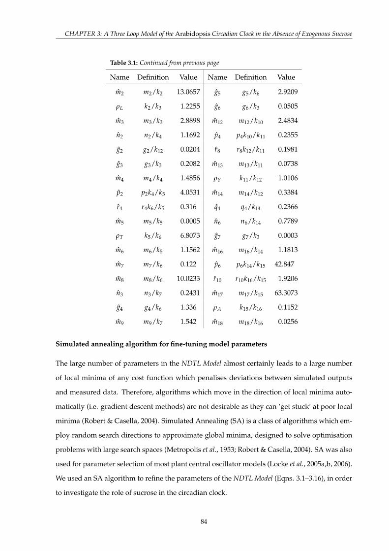
CHAPTER 3: A Three Loop Model of the Arabidopsis Circadian Clock in the Absence of Exogenous Sucrose
Table 3.1: Continued from previous page
Name Definition Value Name Definition Value
m2 m2/k2 13.0657 g5 g5/k6 2.9209
ρL k2/k3 1.2255 g6 g6/k3 0.0505
m3 m3/k3 2.8898 m12 m12/k10 2.4834
n2 n2/k4 1.1692 p4 p4k10/k11 0.2355
g2 g2/k12 0.0204 r8 r8k12/k11 0.1981
g3 g3/k3 0.2082 m13 m13/k11 0.0738
m4 m4/k4 1.4856 ρY k11/k12 1.0106
p2 p2k4/k5 4.0531 m14 m14/k12 0.3384
r4 r4k6/k5 0.316 q4 q4/k14 0.2366
m5 m5/k5 0.0005 n6 n6/k14 0.7789
ρT k5/k6 6.8073 g7 g7/k3 0.0003
m6 m6/k5 1.1562 m16 m16/k14 1.1813
m7 m7/k6 0.122 p6 p6k14/k15 42.847
m8 m8/k6 10.0233 r10 r10k16/k15 1.9206
n3 n3/k7 0.2431 m17 m17/k15 63.3073
g4 g4/k6 1.336 ρA k15/k16 0.1152
m9 m9/k7 1.542 m18 m18/k16 0.0256
Simulated annealing algorithm for fine-tuning model parameters
The large number of parameters in the NDTL Model almost certainly leads to a large number
of local minima of any cost function which penalises deviations between simulated outputs
and measured data. Therefore, algorithms which move in the direction of local minima auto-
matically (i.e. gradient descent methods) are not desirable as they can ‘get stuck’ at poor local
minima (Robert & Casella, 2004). Simulated Annealing (SA) is a class of algorithms which em-
ploy random search directions to approximate global minima, designed to solve optimisation
problems with large search spaces (Metropolis et al., 1953; Robert & Casella, 2004). SA was also
used for parameter selection of most plant central oscillator models (Locke et al., 2005a,b, 2006).
We used an SA algorithm to refine the parameters of the NDTL Model (Eqns. 3.1–3.16), in order
to investigate the role of sucrose in the circadian clock.
84

CHAPTER 3: A Three Loop Model of the Arabidopsis Circadian Clock in the Absence of Exogenous Sucrose
Consider the following nonlinear system:
x = f (x, p) (3.17)
where x ∈ Rn is the state vector comprising concentrations of mRNA and protein in the cy-
toplasm and nucleus of the 5 model components LHY (LHY/CCA1), TOC1, X, Y (GI) and A
(PRR7/9), and p ∈ Rm is the vector of m model parameters. We seek p which minimizes the
‘difference’ between model simulation and luc luminescence data for seedlings grown without
exogenous sucrose. We took the standard LSQ (least squares) approach, minimising the 2-norm
of the residuals between data and simulated output.
∆(p) := ∑d∈D
Nd
∑i=1
e(p)/Nd (3.18)
where D is the set of luc luminescence data, Nd the number of observations in experiment
d ∈ D and e(p) the residual between data and simulated model output with parameters p.
The denominator Nd ensures an equal contribution from each experiment, irrespective of the
number of observations. There have been no previous attempts to calibrate luminescence data
to actual concentrations of mRNA, so we assumed that the measured luminescence is a linear
function of [mRNA]. Therefore, we define the residual norm e by solving a linear regression
problem.
e(p) := mina,b||axd(p) + b− yd||2 (3.19)
where yd is the vector of luciferase luminescence measurements from dataset d, and xd the as-
sociated simulated output. This scheme ensures that the dynamics of the optimised model are
not constrained by the signal strength of the luc reporter system.
The cost function in Eqn. 3.18 was evaluated by obtaining solutions for simulated [LHY
mRNA] and [TOC1 mRNA] at the time-points corresponding to the LL and DD luc lumines-
cence data as in Section 3.2.2. The polyfit function in MATLABTM was then used to find the
minimisers a and b in Eqn. 3.19 to compute e(p) for each dataset, which were then substituted
into Eqn. 3.18 to find ∆(p). The dynamics of [Y (GI) mRNA] were not incorporated into the cost
function as the corresponding measurements of GI:luc only became available shortly before
85

CHAPTER 3: A Three Loop Model of the Arabidopsis Circadian Clock in the Absence of Exogenous Sucrose
writing this thesis. Instead, GI expression is compared during cross-validation (Section 3.3.3).
SA algorithms generate a Markov chain of proposal solutions p which converge on a local
minimum of the cost function ∆(p). At each iteration, a new proposal p1 is generated which
is based on the current state p. Then, we move to the new state according to some acceptance
probability a(p, p1, T). Here, T is the ‘cooling’ parameter, which is a decreasing function (of the
iteration) designed to reduce the acceptance probability of non-improvement states later in the
chain. The most commonly used acceptance function corresponds to the Metropolis-Hastings
(MH) algorithm (Kirkpatrick et al., 1983) defined as
a(p, p1, T) := min{
1 , exp(
∆(p)− ∆(p1)T
)}(3.20)
Due to the large number of parameters and the additional uncertainty that the model equa-
tions are a sufficient description of the underlying system, we ran the algorithm many times,
obtaining many local minima. The MH formulation defined the acceptance of proposal param-
eter sets (Eqn. 3.20), where the cooling parameter was taken to be a normalised linear function
of the iteration number. In addition, an adaptive cooling method was used on the search direc-
tion. At each iteration, we propose a random search direction in an N-dimensional projection
PN comprised of N randomly chosen parameters, where N := dα∆e and α is a constant. Each
of these N parameters (pi) are moved to pi which is gaussian-distributed with mean pi and
variance σ2, where σ := β∆ and β is another constant. This adaptive scheme enabled us to
fine-tune the parameters more efficiently, as the parameters are perturbed less at each iteration
as we approach local minima of the cost function.
Initial approximate minimisers of Eqn. 3.18 often had an undesirable behaviour in entrained
light-dark (L16/D8 or L8/D16) cycles. The system trajectory did not converge to a limit cycle
oscillation, but instead had autonomous oscillatory behaviour with a period near to but not ex-
actly 24 h occurred in addition to periodic behaviour from 24 h periodic light-dark forcing. This
could be seen most clearly in simulated [TOC1 mRNA], which could be described as a biphasic
24 h oscillation in which the phase difference between the two peaks was changing each cycle
(increasing progressively by ≈ 1 h. To eradicate solutions with this behaviour, a second term
was added to the cost function (Eqn. 3.18) to penalise systems which generated trajectories with
multiple periods in these alternative photoperiods. The model equations (3.1–3.16) were simu-
lated under L16/D8 and L8/D16 conditions for 840 h, and the first 600 h discarded as transitory
86

CHAPTER 3: A Three Loop Model of the Arabidopsis Circadian Clock in the Absence of Exogenous Sucrose
in each case. The times of local maxima and minima of simulated [TOC1 mRNA] were then
computed for t ∈ [600 840], as t(1)max, t(2)
max, . . . , t(p)max and t(1)
min, t(2)min, . . . , t(q)
min respectively. Then,
allowing for biphasic oscillations, we defined the entrainment cost term as
∆LDent :=
∣∣∣∣∣∣∣∣∣∣∣∣∣
∣∣∣∣∣∣∣∣∣∣∣∣∣
t(5)max
t(6)max...
t(p)max
−
t(1)max
t(2)max...
t(p−4)max
∣∣∣∣∣∣∣∣∣∣∣∣∣
∣∣∣∣∣∣∣∣∣∣∣∣∣2
+
∣∣∣∣∣∣∣∣∣∣∣∣∣
∣∣∣∣∣∣∣∣∣∣∣∣∣
t(5)min
t(6)min...
t(q)min
−
t(1)min
t(2)min...
t(q−4)min
∣∣∣∣∣∣∣∣∣∣∣∣∣
∣∣∣∣∣∣∣∣∣∣∣∣∣2
(3.21)
for LD as L16/D8 and L8/D16. Therefore the complete cost function used in Section 3.3.3 was
∆(p) = eDDLHY(p) + eDD
TOC1(p) + eLLLHY(p) + eLL
TOC1(p) + ∆L16/D8ent (p) + ∆L8/D16
ent (p) (3.22)
3.3 Results
3.3.1 [ATP]i does not limit Luciferase light emission after 60 hours of darkness
The measured luminescence signal from CCA1:luc expressing Arabidopsis seedlings grown in
DD is lower in the absence of exogenous sucrose supply. During glycolysis, the metabolism of
sucrose generates ATP (Buchanan et al., 2002). Therefore, exogenous supply of sucrose might
increase [ATP]i, leading to higher light emission from the Luciferase enzyme. To control for the
possibility that reduced light emission in plants grown in the absence of exogenous sucrose
prevents observation of circadian oscillations in CCA1:luc, TOC1:luc and GI:luc luminescence
due to low [ATP]i, cold-induced promoter activity of CCA1 was measured after a period of
extended darkness. Plants were exposed to cold treatments of 2, 3 and 6 h in duration, and the
activity of the cold-inducible CCA1 promoter was monitored with photon-counting luminom-
etry as described in Section 3.2.1. Irrespective of whether sucrose was available in the growth
media, large increases in promoter activity were observed after each of the three cold shock
durations tested (Figure 3.2). As growing plants in DD on sucrose-supplemented media did
not increase the relative luminescence after a cold shock, we conclude that in DD ATP avail-
ability was not limiting the reaction which enables luciferase to emit light in the presence of it’s
substrate luciferin.
87

CHAPTER 3: A Three Loop Model of the Arabidopsis Circadian Clock in the Absence of Exogenous Sucrose
Growth media supplementdH2O 90 mM Mannitol 90 mM Sucrose
Fold
incr
ease
in C
CA1
::luc
lum
ines
cenc
e
0
1
2
3
4
5
62h3h6h
Figure 3.2: Cold induces CCA1 promoter activity after 60 hours of darkness.Arabidopsis seedlings were grown on agar media containing H2O, 90 mM mannitol or 90 mM sucrose andentrained under L12/D12 cycles for 10 d before transfer to DD for 60 h. Luminescence was quantifiedfor 60 s in a luminometer to obtain basal activity. Cold treatment was then administered for 2 h (dark redbars), 3 h (orange bars) or 6 h (green bars), left for 15 minutes at 19◦C before quantifying luminescencefor 240 s. Bars indicate average of cold-induced luminescence divided by basal luminescence for eachcondition (n = 12).
3.3.2 Accounting for no exogenous sucrose with single-parameter modifications to
the Three Loop Model
Identifying single parameter alterations as potential sucrose targets
After prolonged darkness, circadian oscillations in promoter activity of central oscillator genes
were present in plants grown with exogenous sucrose (90 mM), while CCA1 and TOC1 ex-
pression in plants without exogenous sucrose (H2O or 90 mM mannitol controls) tended to a
steady state (Figure 3.1). Oscillations in GI:luc were present in the absence of exogenous su-
crose, though with a lower amplitude and longer period than in the presence of exogenous
sucrose (Figures 3.1E,G). We sought single parameter alterations to the Three Loop Model of the
Arabidopsis circadian clock (Locke et al., 2006) which could predict a loss of oscillations in DD
whilst retaining circadian rhythmicity in LL.
Period and amplitude of oscillation were computed as functions of each model parameter
to assess rhythmicity of single-parameter alterations to the Three Loop Model. Parameters were
identified in which increases and decreases in their relative value led to a loss of rhythmicity
in DD, while retaining oscillations in LL. As examples, n3 . 0.2 (Figure 3.3A) and n5 . 0.3
88

CHAPTER 3: A Three Loop Model of the Arabidopsis Circadian Clock in the Absence of Exogenous Sucrose
(Figure 3.3B) had oscillation fold ratios near 1 in DD implying arrhythmicity, though > 10 in LL
implying stable oscillations. Parameter alterations for values of pr which produced LL periods
between 20 h and 30 h and a DD oscillation fold ratio < 1.1 were shortlisted. This candidate
set of parameter alterations included over one-third (26/70) of all parameters (Figure 3.3C).
Table 3.2: Candidate single-parameter modifications simulated for K-means clustering.Shortlist of parameters which could be modified to achieve a loss of oscillations in DD (oscillation foldratio no greater than 1.1), while retaining stable oscillations in LL (oscillation fold ratio greater than 1.1and period between 20 and 30 h). The candidate parameter regions (increases or decreases) analysedfor their median value are indicated in this table. Each candidate-region median value was used tosimulate the model equations in L12/D12 before transfer to DD. Simulations were then classified into8 clusters by K-means clustering (Macqueen, 1967), with 1− ρ as the distance measure where ρ is thecross-correlation. Implementation was in MATLABTM with the kmeans function (Stastistics Toolbox;Seber, 2004).
Decreases IncreasesParameter Rel. Value Cluster Parameter Rel. Value Cluster
n3 0.0692 5 g2 19.5 5n5 0.0525 2 g7 43.65 7g 0.0617 7 m3 51.29 4α 0.02 8 m6 20.89 5g5 0.0145 5 m8 25.7 5m3 0.0115 1 m9 13.8 5k1 0.0288 6 m12 19.0546 5k3 0.0155 4 m13 74.131 5k4 0.055 5 m14 19.5 5k7 0.0692 5 m17 11.749 7k10 0.0513 5 k3 63.0957 3k11 0.0129 5k12 0.0513 5k15 0.0102 7p2 0.055 5p4 0.0513 5r7 0.0129 5
Comparing single-parameter alterations with CCA1:luc luminescence data
Candidate perturbations that best matched CCA1:luc luminescence measurements in DD in the
absence of exogenous sucrose were identified by simulation of each candidate perturbation and
comparison with the experimental data (Figure 3.1A). For each candidate parameter, the me-
dian value in the range of candidate decreases or increases (both if required) was selected for
simulation (indicated by the red crosses in Figure 3.3C; Table 3.2). Simulations of LHY mRNA
in entrained L12/D12 cycles before transfer to DD were categorized into 8 clusters using a
K-means algorithm (Macqueen, 1967; see Section 3.2.4 for details; Table 3.2; Figure 3.4). Seven-
89

CHAPTER 3: A Three Loop Model of the Arabidopsis Circadian Clock in the Absence of Exogenous Sucrose
Relative Parameter Value
0.01 0.1 1 10
Osc
illat
ion
fold
rat
io
1
10
100
1000
10000
Per
iod
(h)
16
18
20
22
24
26
28
30A
Relative Parameter Value
0.01 0.1 1 10
Osc
illat
ion
fold
rat
io
1
10
100
1000
Per
iod
(h)
0
5
10
15
20
25
30
Constant Dark (DD)Constant Light (LL)
B
Relative Parameter Value0.01 0.1 1 10 100
Para
met
er
r7
p4
p2
k15
k12
k11
k10
k7
k4
k3
k1
m17
m14
m13
m12
m9
m8
m6
m3
g7
g5
g2
αgn5
n3
Nominalvalue5
55
75
55
55
4 36
75
55
55
51 4
75
58
72
5C
Figure 3.3: Single parameter modifications enable steady state in DD and stable oscillations in LL.The Three Loop Model (Locke et al., 2006; Equations A.14–A.29) was simulated under LL and DD for 600 hto assess how the model can reproduce the behaviours seen when plants are grown in the absence ofexogenous sucrose. Period and oscillation fold ratio plotted as functions of the relative values of (A) n3(maximum rate of X transcription, and (B) n5 (maximum light-independent rate of Y (GI) transcription.A,B) Period was computed as the time difference between the last two peak values of simulated [LHYmRNA]. Oscillation fold ratio (amplitude) was computed by dividing the value of the last local max-imum by the value of the last local minimum of [LHY mRNA]. (C) Points indicate regions of relativeparameter value for which LL period is between 20 h and 30 h, and DD oscillations fold ratio is less than1.1. Red numbers located at the relative parameter values used for K-means clustering of simulatedoutput in DD, the number itself denoting which cluster the trajectory belongs to (see Figure 3.4, andTable 3.2 for values).
90

CHAPTER 3: A Three Loop Model of the Arabidopsis Circadian Clock in the Absence of Exogenous Sucrose
teen of the twenty-eight candidate parameter alterations led to sharp light-induced oscillations
in LD cycles, before a fast suppression towards zero in DD (Figure 3.4E). Seven candidates
achieved steady state in DD with a slowly decaying amplitude oscillation (Figures 3.4D,F,G),
while another two candidates showed no distinction between L12/D12 cycles and DD (Fig-
ures 3.4A,C). The candidate corresponding to Figure 3.4B showed significant similarity to the
measured CCA1:luc luminescence data (Figure 3.1A). In both measured data and simulation,
the signal undergoes a medium-sized oscillation peaking approximately 12 h into DD, before
settling at a constant low value (≈ 0). Further parameter inspection revealed that by taking n5
to be 0.25 of its nominal value enabled the closest match to the target dynamics of CCA1 ex-
pression. This was defined as the (candidate) N5 Model. Our candidate model therefore offered
a prediction for the effect of supplementing growth media with 90 mM sucrose. The biological
interpretation of this prediction is that sucrose up-regulates the light-independent transcription
rate of Y, which is believed to be the GIGANTEA (GI) gene (Locke et al., 2005b, 2006).
Cross-validation of the N5 Model with wild-type data
Simulations of the N5 Model were compared with measured luc luminescence data in the ab-
sence of exogenous sucrose, to assess the wider applicability of this candidate model. In DD,
simulations of all model components converged quickly to a low steady state, as reflected by
CCA1:luc and TOC1:luc luminescence data. However, the persistence of circadian oscillations
of GI:luc luminescence in DD was not predicted by the N5 Model (Figure 3.5A). The timing of
peak expression for simulated LHY, TOC1 and Y/GI was accurate in the L12/D12 cycles before
transfer to DD (Figure 3.5A). In LL, oscillations in simulated LHY and TOC1 peaked earlier
than the measured data, indicating that a lag occurs after transfer from L12/D12 cycles to LL
which was not predicted by the N5 Model (Figure 3.5B). In contrast, simulated Y/GI peaked later
than GI:luc luminescence in LL (Figure 3.5B). In light-dark cycles, the shape of the N5 Model os-
cillations contrasted with the corresponding luc luminescence data for each model component,
though the oscillation phase was accurate (Figures 3.5C,D). In particular, the model accurately
predicted the phase shifts of peak TOC1 and GI expression when comparing L16/D8 cycles
(Figure 3.5C) and L8/D16 cycles (Figure 3.5D).
91
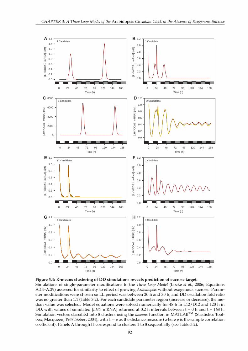
CHAPTER 3: A Three Loop Model of the Arabidopsis Circadian Clock in the Absence of Exogenous Sucrose
Time (h)
0 24 48 72 96 120 144 168
[LH
Y/C
CA
1 m
RN
A] (
nM)
0.0
0.2
0.4
0.6
0.8
1.0
1.2
1.4
1.61 Candidate
A
Time (h)
0 24 48 72 96 120 144 168
[LH
Y/C
CA
1 m
RN
A] (
nM)
0.0
0.2
0.4
0.6
0.8
1.0
1.21 Candidate
B
Time (h)
0 24 48 72 96 120 144 168
[LH
Y/C
CA
1 m
RN
A] (
nM)
0
2000
4000
6000
80001 Candidate
C
Time (h)
0 24 48 72 96 120 144 168
[LH
Y/C
CA
1 m
RN
A] (
nM)
0.0
0.2
0.4
0.6
0.8
1.0
1.22 Candidates
D
Time (h)
0 24 48 72 96 120 144 168
[LH
Y/C
CA
1 m
RN
A] (
nM)
0.0
0.2
0.4
0.6
0.8
1.0
1.217 Candidates
E
Time (h)
0 24 48 72 96 120 144 168
[LH
Y/C
CA
1 m
RN
A] (
nM)
0.0
0.2
0.4
0.6
0.8
1.0
1.21 Candidate
F
Time (h)
0 24 48 72 96 120 144 168
[LH
Y/C
CA
1 m
RN
A] (
nM)
0.0
0.2
0.4
0.6
0.8
1.0
1.24 Candidates
G
Time (h)
0 24 48 72 96 120 144 168
[LH
Y/C
CA
1 m
RN
A] (
nM)
0.0
0.2
0.4
0.6
0.8
1.0
1.21 Candidate
H
Figure 3.4: K-means clustering of DD simulations reveals prediction of sucrose target.Simulations of single-parameter modifications to the Three Loop Model (Locke et al., 2006; EquationsA.14–A.29) assessed for similarity to effect of growing Arabidopsis without exogenous sucrose. Param-eter modifications were chosen so LL period was between 20 h and 30 h, and DD oscillation fold ratiowas no greater than 1.1 (Table 3.2). For each candidate parameter region (increase or decrease), the me-dian value was selected. Model equations were solved numerically for 48 h in L12/D12 and 120 h inDD, with values of simulated [LHY mRNA] returned at 0.2 h intervals between t = 0 h and t = 168 h.Simulation vectors classified into 8 clusters using the kmeans function in MATLABTM (Stastistics Tool-box; Macqueen, 1967; Seber, 2004), with 1− ρ as the distance measure (where ρ is the sample correlationcoefficient). Panels A through H correspond to clusters 1 to 8 sequentially (see Table 3.2).
92

CHAPTER 3: A Three Loop Model of the Arabidopsis Circadian Clock in the Absence of Exogenous Sucrose
Time (h)
0 24 48 72 96 120
0.0
0.5
1.0
0.0
0.5
1.0CCA1:lucN5 model
A
Time (h)
0 24 48 72 96 120
Rel
ativ
e lu
min
esce
nce
0.0
0.5
1.0
Sim
ulat
ed [m
RN
A] (
nM)
0.5
1.0
1.5
2.0
TOC1:lucN5 model
Time (h)
0 24 48 72 96 120
0.0
0.5
1.0
1.5
2.0
0.00
0.02
0.04
0.06
0.20
0.22GI:lucN5 model
Time (h)
0 24 48 72 96 120
0.0
0.5
1.0
0.0
0.5
1.0B
Time (h)
0 24 48 72 96 120
Rel
ativ
e lu
min
esce
nce
0.0
0.5
1.0
Sim
ulat
ed [m
RN
A] (
nM)
0.5
1.0
1.5
2.0
Time (h)
0 24 48 72 96 120
0.0
0.5
1.0
1.5
2.0
0.00
0.02
0.04
0.06
0.20
0.22
Time (h)
0 8 16 24 32 40 48
0.0
0.5
1.0
0.0
0.5
1.0
C
Time (h)
0 8 16 24 32 40 48
Rel
ativ
e lu
min
esce
nce
0.0
0.5
1.0
Sim
ulat
ed [m
RN
A] (
nM)
0.5
1.0
1.5
Time (h)
0 8 16 24 32 40 48
0.0
0.5
1.0
1.5
2.0
0.00
0.02
0.04
0.06
0.18
0.20
Time (h)
0 8 16 24 32 40 48
0.0
0.5
1.0
0.0
0.5
1.0
D
Time (h)
0 8 16 24 32 40 48
Rel
ativ
e lu
min
esce
nce
0.0
0.5
1.0
Sim
ulat
ed [m
RN
A] (
nM)
0.5
1.0
1.5
Time (h)
0 8 16 24 32 40 48
0.0
0.5
1.0
1.5
2.0
0.00
0.02
0.04
0.06
0.26
0.28
Figure 3.5: Cross-validation of the N5 Model to luc luminescence data in DD, LL, L16/D8 and L8/D16.Comparison of simulations of the N5 Model (blue lines) with corresponding (relative) measured lumines-cence data (open circles) for LHY (top panels), TOC1 (middle panels) and GI (bottom panels). Three LoopModel equations with n5 set to 0.25 of the nominal value were solved numerically using MATLABTM’sode15s solver (Shampine & Reichelt, 1997). (A) Entrainment to L12/D12 cycles before transfer to DD, (B)entrainment to L12/D12 cycles before transfer to LL, (C) L16/D8 cycles, and (D) L8/D16 cycles. Datacollected by Katharine Hubbard and Seong Jin Baek, (University of Cambridge, personal communication).In abscissa, white bars indicate light, black bars indicate dark, dark grey indicates dark in subjectivedaytime and light grey indicates light in subjective night-time.
93

CHAPTER 3: A Three Loop Model of the Arabidopsis Circadian Clock in the Absence of Exogenous Sucrose
3.3.3 Accounting for no exogenous sucrose with multiple-parameter modifications
to the Three Loop Model
Fine-tuning of the Three Loop Model parameters
In this section, the possibility that sucrose modulation of the central oscillator can be described
mathematically by a change in multiple parameters of the Three Loop Model is considered (Locke
et al., 2006). This contrasts to the previous section in which only single parameter modifications
were considered. The system equations were first non-dimensionalised to reduce the size of the
search space (NDTL Model, Equations 3.1–3.16), then the resulting system parameters (Table 3.1)
were retuned based on experimental data from seedlings grown on agar media in the absence
of exogenous sucrose (Figure 3.1). Parameters were selected through minimisation of a cost
function which penalised deviation from experimental data or led to the onset of multiple
periodic oscillations (see Section 3.2.5). The optimisation method was initialised at the non-
dimensionalised parameter set corresponding to the nominal model configuration of equations
A.14–A.29 (see Table 3.1 for corresponding parameter values).
The modified SA algorithm (Section 3.2.5) was able to produce many solutions, which
matched the target datasets with accuracy. Four hundred independent trials were run for 1000
iterations each with α = 0.5 and β =1003
, providing an array of trial-optimal solutions (defined
as the parameter sets corresponding to the minimum cost function value attained over each
trial). The cost function values corresponding to the trial-optimal solutions were distributed
bimodally, indicating that in many cases the algorithm was unable to avoid poor local minima
(∆(p) & 0.2; Figure 3.6A). However, in some cases the algorithm reached parameter sets for
which ∆(p) < 0.2 within the first 200 iterations (Figure 3.6B). In Figures 3.6B–F two models
are considered (see Table 3.3 for parameter values). Model 1 corresponds to the trial-optimal
solution with the lowest value of ∆(p) observed over the four hundred trials, while Model 5
represents the 5th lowest ∆(p), but the lowest for which there were no oscillations in DD for
both simulated LHY (Figure 3.6C) and TOC1 mRNA (Figure 3.6D). The four lowest scoring
models (i.e. Model 1, Model 2, Model 3 and Model 4) had damped oscillations in simulated [LHY
mRNA] after transfer to DD (Figure 3.6C). The small amplitude of the oscillations seemingly
did not increase the cost function enough to select away from these parameter sets. However,
no oscillations were seen in Model 1 or Model 5 for simulated [TOC1 mRNA] in DD, and both
also accurately reproduced the oscillations of CCA1:luc and TOC1:luc luminescence observed
94

CHAPTER 3: A Three Loop Model of the Arabidopsis Circadian Clock in the Absence of Exogenous Sucrose
in L12/D12 (Figure 3.6D). Many parameter sets explored during the optimisation were able
to distinguish between the lower amplitude oscillations of CCA1:luc luminescence in LL than
in LD cycles; this was also true of Model 1 and Model 5 (Figure 3.6E). The candidate models
were also capable of predicting the larger amplitude oscillations of TOC1:luc luminescence in
LL over those observed in L12/D12 (Figure 3.6F).
Cross-validation of fine-tuned models with wild-type data
Validation tests were performed to assess the wider applicability of the models derived in this
section. It was important to compare simulated dynamics of Y (GI) with measurements of
GI:luc, as GI expression was not part of the selection criteria for fine-tuned models and addi-
tionally, GI transcription was implicated as a sucrose target in Section 3.3.2. In L12/D12 cycles,
simulated [Y (GI) mRNA] from Model 1 and Model 5 increased transiently at dawn before in-
creasing until dusk, then quickly decreased to a constant low level in the dark phase (Figures
3.7A–B). GI:luc luminescence did not show such a large transient increase at dawn but increased
until dusk, then decreased similar to the simulations of the two candidate models. Upon trans-
fer to DD, GI:luc luminescence emitted from plants grown both in the presence and absence of
exogenous sucrose continued to oscillate with a low amplitude rhythm, whereas Model 1 and
Model 5 both predicted constant low [Y (GI) mRNA] in DD (Figure 3.7A). In LL, GI:luc lumines-
cence oscillated with slightly less amplitude than in L12/D12 cycles, peaking 2–3 hours before
subjective dusk, while simulated [Y (GI) mRNA] of both models had oscillations that peaked
1–2 hours after subjective dusk (Figure 3.7B). In both Model 1 and Model 5, LL oscillations of
simulated [Y (GI) mRNA] had biphasic oscillations, as seen in the nominal model configura-
tion (Locke et al., 2006), though this was not seen in our measurements of GI:luc luminescence,
both in the presence and absence of exogenous sucrose (Figure 3.7B).
Next, oscillations of CCA1, TOC1 and GI expression in light-dark cycles of differing pho-
toperiods were considered (Figures 3.7C–H). CCA1:luc luminescence oscillated in L16/D8 cy-
cles with a peak 2 h after dawn, before declining to a constant low level reached at dusk (Fig-
ure 3.7C). In L8/D16 cycles, CCA1:luc luminescence oscillated with a peak 2 h after dawn, de-
creased to a constant low level by dusk, then increased 3 h before dawn (Figure 3.7D). Model 1
and Model 5 were both able to reproduce the change in width of oscillation between L16/D8
and L8/D16 cycles and anticipated dawn in L8/D16, though only Model 1 anticipated dawn at
95

CHAPTER 3: A Three Loop Model of the Arabidopsis Circadian Clock in the Absence of Exogenous Sucrose
Cost function (Δ)0.14 0.16 0.18 0.20 0.22 0.24 0.26
Freq
uenc
y
0
2
4
6
8
10
12
14
16
18A
Iteration0 200 400 600 800 1000
Cos
t fun
ctio
n (Δ
)
0.10
0.15
0.20
0.25
0.30
0.35
0.40
0.45
Model 1Model 5
B
Time (h)0 12 24 36 48 60 72 84 96 108 120 132
Rel
ativ
e lu
min
esce
nce
0.0
0.2
0.4
0.6
0.8
1.0C
Time (h)-24 -12 0 12 24 36 48 60 72 84 96 108 120 132
Rel
ativ
e lu
min
esce
nce
0.0
0.2
0.4
0.6
0.8
1.0D
Time (h)0 12 24 36 48 60 72 84 96 108 120 132
Rel
ativ
e lu
min
esce
nce
0.0
0.2
0.4
0.6
0.8
1.0E
Time (h)0 12 24 36 48 60 72 84 96 108 120 132
Rel
ativ
e lu
min
esce
nce
0.0
0.2
0.4
0.6
0.8
1.0F
Figure 3.6: Parameter re-tuning of the Three Loop Model to account for no exogenous sucrose.Parameters from the NDTL Model (Eqns. 3.1–3.16) were optimised with respect to a cost function corre-sponding to the data in Figure 3.1 using a Simulated Annealing algorithm over 400 independent trialsof 1000 iterations each. (A) Lowest costs of each trial displayed as a histogram. (B) The lowest cost func-tion value achieved as a function of the iteration number is plotted for two models: Model 1 (blue line)corresponds to the lowest cost attained over all 400 trials, while Model 5 (red line) corresponds to the5th lowest score. (C – F) Comparison of measured luminescence data (open circles) with correspondingsimulations of Model 1 (blue line) and Model 5 (red line). For each model, the simulated output (y) wasrescaled with values a and b which minimised mina,b ∑i (yi − ayi − b)2 where the yi are the measuredluminescence values. (C) CCA1:luc luminescence measured in entrained L12/D12 cycles before trans-fer to DD at t = 36, and rescaled simulations of [LHY mRNA]. (D) TOC1:luc luminescence in entrainedL12/D12 cycles before transfer to DD at t = 36, and rescaled simulations of [TOC1 mRNA]. (E) CCA1:lucluminescence measured in entrained L12/D12 cycles before transfer to LL at t = 24, and rescaled sim-ulations of [LHY mRNA]. (F) TOC1:luc luminescence in entrained L12/D12 cycles before transfer to LLat t = 24, and rescaled simulations of [TOC1 mRNA]. Luminescence data in D, E and F were obtainedfrom Seong-Jin Baek (personal communication).
96

CHAPTER 3: A Three Loop Model of the Arabidopsis Circadian Clock in the Absence of Exogenous Sucrose
Table 3.3: Candidate parameter sets from fine-tuning.A Metropolis-hastings algorithm was used to refine the NDTL Model parameters, based on CCA1:luc andTOC1:luc luminescence data. Model 1 corresponds to the parameter set with lowest cost function duringoptimisation, and Model 5 the 5th lowest cost overall, but lowest of models which tend to steady state inDD. Tabulated values are the relative parameter sets based on the values in Table 3.1.
Parameter Model 1 Model 5 Parameter Model 1 Model 5q1 1.1620 1.8689 m7 1.4205 0.3447q2 0.1930 0.6184 m8 1.0212 1.0498q4 1.2855 1.5719 m9 1.3556 0.7569n0 0.6599 0.9832 m10 0.7353 0.9643n1 0.3931 0.6578 m11 1.1935 0.9847n2 0.7852 0.8166 m12 1.6672 1.3404n3 2.3971 2.6644 m13 1.0295 0.8325n4 1.3212 2.0471 m14 1.0243 0.5075n5 0.5990 0.3222 m16 1.2139 0.9445n6 1.2228 0.9435 m17 0.6810 1.1407a 1.1040 0.6665 m18 1.5128 1.4185b 2.1621 1.6100 p1 0.6290 0.4971c 1.3502 1.6279 p2 1.4066 1.1454d 0.7824 1.6591 p3 1.2930 0.5408e 1.2389 1.4814 p4 0.8127 1.0030f 1.6439 1.0295 p6 0.8485 1.1129g 0.5568 0.7329 r1 0.8686 0.6608α 1.5077 1.4316 r2 0.3801 0.5359g0 1.4030 1.4133 r3 0.5565 1.1744g1 1.1038 1.0409 r4 0.6094 1.1017g2 0.8166 1.1862 r5 1.4205 0.7415g3 1.2856 0.7802 r6 0.6103 1.7480g4 0.7379 0.3949 r7 0.6581 2.2134g5 0.8031 0.6612 r8 0.5266 1.1484g6 1.8767 0.7370 r9 1.1112 1.0065g7 1.1953 0.4917 r10 1.1925 0.7078m1 0.7560 1.0997 ρL 0.7413 0.7910m2 0.7207 0.9365 ρT 1.3384 1.0044m3 1.2693 1.5396 ρX 0.9911 0.7587m4 1.3819 1.3328 ρY 0.9219 0.8465m5 1.5939 0.9055 ρA 0.9196 1.1095m6 0.1991 0.8877
97

CHAPTER 3: A Three Loop Model of the Arabidopsis Circadian Clock in the Absence of Exogenous Sucrose
Time (h)0 12 24 36 48 60 72 84 96 108 120 132 144
Rel
ativ
eG
I:luc
lum
ines
cenc
e
0.0
0.5
1.0
1.5
2.0
Sim
ulat
ed [
Y (G
I) m
RN
A] (n
M)
0.00
0.02
0.04
0.06
0.08
0.10
0.12
0.14DataModel 1Model 5
A
Time (h)0 12 24 36 48 60 72 84 96 108 120 132
Rel
ativ
eG
I:luc
lum
ines
cenc
e
0.0
0.5
1.0
1.5
2.0
Sim
ulat
ed [
Y (G
I) m
RN
A] (n
M)
0.00
0.02
0.04
0.06
0.08
0.10
0.12
0.14B
Time (h)0 8 16 24 32 40 48 56
Rel
ativ
eC
CA1
:luc
lum
ines
cenc
e
0.0
0.2
0.4
0.6
0.8
1.0
1.2
1.4
1.6
Sim
ulat
ed [
LHY/
CC
A1 m
RN
A] (n
M)
0
1
2
3
4C
Time (h)0 8 16 24 32 40 48 56
Rel
ativ
eC
CA1
:luc
lum
ines
cenc
e0.0
0.2
0.4
0.6
0.8
1.0
1.2
1.4
1.6
Sim
ulat
ed [
LHY/
CC
A1 m
RN
A] (n
M)
0
1
2
3
4D
Time (h)0 8 16 24 32 40 48 56
Rel
ativ
eTO
C1:
luc
lum
ines
cenc
e
0.0
0.2
0.4
0.6
0.8
1.0
1.2
Sim
ulat
ed [
TOC
1 m
RN
A] (n
M)
0.0
0.2
0.4
0.6
0.8
1.0
1.2
1.4E
Time (h)0 8 16 24 32 40 48 56
Rel
ativ
eTO
C1:
luc
lum
ines
cenc
e
0.0
0.2
0.4
0.6
0.8
1.0
1.2
Sim
ulat
ed [
TOC
1 m
RN
A] (n
M)
0.0
0.2
0.4
0.6
0.8
1.0F
Time (h)0 8 16 24 32 40 48 56
Rel
ativ
eG
I:luc
lum
ines
cenc
e
0.0
0.5
1.0
1.5
2.0
Sim
ulat
ed [
Y (G
I) m
RN
A] (n
M)
0.00
0.02
0.04
0.06
0.08
0.10
0.12
0.14
0.16G
Time (h)0 8 16 24 32 40 48 56
Rel
ativ
eG
I:luc
lum
ines
cenc
e
0.0
0.2
0.4
0.6
0.8
1.0
1.2
1.4
1.6
Sim
ulat
ed [
Y(G
I) m
RN
A] (n
M)
0.00
0.02
0.04
0.06
0.08
0.10
0.12
0.14
0.16H
Figure 3.7: Cross-validation of re-tuned Three Loop Models to luminescence data in DD, LL, L16/D8and L8/D16.Comparison of (relative) measured luminescence data (open circles; left axes) with corresponding simu-lations of Models 1 (blue line; right axes) and 5 (red line; right axes). (A) GI:luc luminescence in L12/D12cycles before transfer to DD at t = 36 (Seong Jin Baek, personal communication), versus correspondingsimulations of [Y (GI) mRNA]. (B) GI:luc luminescence in L12/D12 cycles before transfer to LL at t = 24(Seong Jin Baek, personal communication), versus corresponding simulations of [Y (GI) mRNA]. (C,E,G)L16/D8 cycles. (D,F,H) L8/D16 cycles. (C,D) Relative CCA1:luc luminescence compared with simu-lated [LHY mRNA]. (E,F) Relative TOC1:luc luminescence (Katharine Hubbard, personal communication)compared with simulated [TOC1 mRNA]. (G,H) Relative GI:luc luminescence (Katharine Hubbard, per-sonal communication) compared with simulated [Y (GI) mRNA]. In abscissa, white bars indicate light,black bars indicate dark, dark grey indicates dark in subjective daytime and light grey indicates light insubjective night-time. 98

CHAPTER 3: A Three Loop Model of the Arabidopsis Circadian Clock in the Absence of Exogenous Sucrose
the correct time in L16/D8 (Figures 3.7C,D). TOC1:luc luminescence had biphasic oscillations
in L16/D8 and L8/D16, achieving peak levels 1 h after dawn and at dusk (Figures 3.7E,F). Both
candidate models had biphasic oscillations of [TOC1 mRNA] in L16/D8 cycles (Figure 3.7E),
though the peak 1–2 hours after dawn was smaller than for TOC1:luc luminescence. Only
Model 1 had two distinguishable peaks of [TOC1 mRNA] in L8/D16 cycles (Figure 3.7F). GI:luc
luminescence also had biphasic oscillations in L16/D8 and L8/D16 cycles, though the light-
induced peak at dawn was smaller than the peak just before dusk (Figures 3.7G,H). Model 1
and Model 5 both had exaggerated light-induced peaks relative to GI:luc luminescence, though
timing of both peaks was accurate (Figures 3.7G,H). However, a very sharp decline in simu-
lated [Y (GI) mRNA] was seen at the transition from light to dark in both candidate models.
Parameter analysis implicates GI as a sucrose-target
Parameters associated with Y (GI) mRNA were frequently altered when fine-tuning the Three
Loop Model parameters to data collected in the absence of exogenous sucrose. The parameter
alterations were considered on the following levels: the mean of all parameter sets visited dur-
ing each of the 400 x 1000 iterations, the mean of the trial-optimal solutions (parameter sets
corresponding to the lowest cost function scores in each trial), and the mean of the best (low-
est ∆(p)) 30 trial-optimal solutions (Table 3.4). On all three levels considered, n5 was reduced
more on average than any other parameter, and further note that this was the same parameter
identified in the single-parameter analysis of Section 3.3.2. In the best 30 trial optimal solutions,
n5 decreased by 56% while the second largest reduction (g, the hill coefficient of A activation
by LHY) was only by 30%, providing further confidence that n5 should be reduced to account
for an absence of exogenous sucrose (Table 3.4). The acute light activation of Y (GI; q2) was
also reduced frequently during optimisation, though not to the same extent as n5 on average
(Table 3.4). The largest parameter increase was seen for n4 (maximum light-dependent tran-
scription rate of Y), increasing to at least double that of any other parameter on average, and
93% in the best 30 trial-optimal solutions. The maximum degradation rate of Y (GI) mRNA
(m12) also increased frequently during the optimisation. Inspection of equation 3.10 reveals
that the four parameters which changed the most (n4, q2, n5 and m12) are all associated with Y
(GI) mRNA§.
§Through non-dimensionalisation of the model equations, these parameters were all rescaled by dividing byk10 (see Table 3.1). However, changing our choice of scale would not influence our conclusions greatly, as both
99

CHAPTER 3: A Three Loop Model of the Arabidopsis Circadian Clock in the Absence of Exogenous Sucrose
Table 3.4: Averaged parameter alterations from re-tuning Three Loop Model for no exogenous sucrose.Parameters from the NDTL Model (Eqns. 3.1–3.16) were optimised with respect to a cost function corre-sponding to the data in Figure 3.1 using a Simulated Annealing algorithm over 400 independent trialsof 1000 iterations each. Each of the three columns represents average parameter changes ordered bysize, with top 5 decreases and top 5 increases displayed. The leftmost column is the average over theentire solution set, comprising 400 x 1000 parameter sets. The middle column represents the average ofthe trial-optimal solutions (parameter sets corresponding to the lowest cost function score in each trial),while the rightmost column considers the best 30 of these trial-optimal solutions. For a description ofthe parameters in this table, see Table A.2.
Whole solution set Trial-optimal solutions Best 30 trial-optimal solutionsParameter Relative Value Parameter Relative Value Parameter Relative Value
n5 0.8089 n5 0.6962 n5 0.4426q2 0.8926 q2 0.8462 g 0.7025m1 0.8981 m1 0.8775 m6 0.7433n6 0.9094 p1 0.8866 q2 0.7474n1 0.9157 n6 0.8923 ρL 0.7686...
......
......
...m3 1.1139 q1 1.1722 n3 1.2605m4 1.1410 m4 1.1779 p2 1.2643m16 1.1675 m16 1.2225 α 1.3947m12 1.1949 m12 1.3764 m12 1.4062n4 1.4093 n4 1.7687 n4 1.9363
Our parameter analysis suggested that sucrose acts to up-regulate the transcription of GI.
In the Three Loop Model, transcription of GI is considered to be a decreasing function of the
availability of LHY/CCA1 or TOC1 nuclear protein (Locke et al., 2006). When there is light,
transcription occurs with rate n4 + n5, and in the dark this rate reduces to n5. Both the analysis
in this section and in Section 3.3.2 indicated that n5 should be set at least 50% lower without
90 mM exogenous sucrose. However, the fine-tuning method in this section predicts the change
in n4 + n5 to be minor (= 0.2506 with 90 mM exogenous sucrose, nominal Three Loop Model;
= 0.2389 without 90 mM exogenous sucrose, top 30 pareto-optimal parameter sets). Therefore,
these mathematical analyses predict that addition of 90 mM sucrose increases the rate of GI
transcription in the dark by over 100%, and in the light by only 5%. As [Suc]i undergoes a
diurnal rhythm (Lu et al., 2005), we interpret our analysis to mean that exogenous sucrose does
not affect the central oscillator when [Suc]i is already high. This also explains why circadian
oscillations in LL are not affected greatly by addition of 90 mM sucrose (see Figures 3.1B,D,F),
and indicates the importance of studying the circadian network in LD cycles and DD.
parameter increases and parameter decreases are seen in the parameters comprising Equation 3.10.
100

CHAPTER 3: A Three Loop Model of the Arabidopsis Circadian Clock in the Absence of Exogenous Sucrose
3.3.4 Simulated mutant analysis
To further test the parameter-modified models, we performed a simulated mutant analysis,
as done in a previous attempt to mathematically model the central oscillator (Zeilinger et al.,
2006). The N5 Model, Model 1 and Model 5 were investigated for the effect of mutations to central
oscillator components (Table 3.5). The N5 Model predicted a period-shortening in LL for toc1
null (3.6 h) and gi null (3.3 h) mutations (Table 3.5), agreeing with published experimental data
(Millar et al., 1995; Mizoguchi et al., 2005). However, Model 1 and Model 5 predicted LL arrhyth-
mia for toc1 and gi null mutants (Table 3.5). Despite there being a relative lack of published
luc luminescence data for seedlings grown without exogenous sucrose, CAB2:luc luminescence
has short-period oscillations in toc1-1 mutants (Xu et al., 2007) and [Ca2+]cyt has short-period
oscillations in gi-2 mutants (Dr. F. Robertson, personal communication). Therefore, the N5 Model
is more capable of reproducing mutant phenotypes than the fine-tuned models.
Table 3.5: Simulated mutant analysis of Three Loop Model altered for no exogenous sucrose.Simulated circadian period computed for the Three Loop Model, the N5 Model, Model 1 and Model 5 byfinding the time difference between successive peaks of simulated [LHY mRNA] after 600 h in LL. Mu-tant periods are displayed as the deviation from the simulated wild-type period. Mutants were sim-ulated as in Zeilinger et al. (2006). For ztl, the numbers in brackets corresponds to reducing all TOC1degradation rates by one-half, rather than only the dark-dependent rates (unbracketed values; see Lockeet al., 2006). Asterisks indicate very low amplitude oscillations, which are unlikely to be detectable ex-perimentally, and so can be considered arrhythmic.
Genotype Three Loop N5 Model 1 Model 5Wild-type 23.8 24.0 25.5 25.6
cca1 -0.6 -0.6 -0.6 0.5cca1 lhy -6.0 arr. arr. -10.2∗
toc1 -3.4 -3.6 arr. arr.gi -1.2 -3.3 arr. -5.3∗
prr7 prr9 5.5 arr. 14.1 16.0∗
ztl 0 (1.07) 0 (0.52) 0 (0.58) 0 (0.53)
In general, simulations of central oscillator gene knockout mutants with the N5 Model had
similar phenotypes to the nominal Three Loop Model, i.e. the majority of LL period phenotypes
are predicted to be unaffected by sucrose. However, a reduction in n5 led to a loss of oscillations
in LL in a simulated cca1 lhy double mutant (Figure 3.8, Table 3.5). This contrasts with the ob-
servation that LL oscillations persist with decaying amplitude in cca1 lhy double mutants in the
presence of 90 mM exogenous sucrose (Locke et al., 2006)¶. The simulations with the N5 Model
¶The majority of circadian research in Arabidopsis is conducted with seedlings grown in the presence of exoge-nous sucrose. A search of the literature found no experimental data for measurements of gene promoter activity incca1 lhy double mutants.
101

CHAPTER 3: A Three Loop Model of the Arabidopsis Circadian Clock in the Absence of Exogenous Sucrose
therefore predict exogenous sucrose to increase the amplitude/persistence of LL oscillations in
cca1 lhy. This prediction represents a good validation test for the N5 Model.
Time (h)
0 24 48 72 96 120
Rel
ativ
e si
mul
ated
[LH
Y/C
CA
1 m
RN
A] (
nM)
0.0
0.2
0.4
0.6
0.8
1.0
0.0
0.2
0.4
0.6
0.8
1.0 Wild-typecca1 lhy
Three Loop model
N5 model
Figure 3.8: The simulated LL phenotype of cca1 lhy depends on sucrose availability.Simulated [LHY mRNA] in LL comparing a cca1 lhy double mutant (red lines) with wild-type (blacklines) for the nominal Three Loop Model (top panel; 3% exogenous sucrose) and the N5 Model (bottompanel; no exogenous sucrose). Model equations were solved numerically using MATLABTM’s ode15sstiff equation solver (Shampine & Reichelt, 1997). cca1 lhy mutant was simulated by setting p1 (rate ofLHY translation) equal to 1/1000 of the nominal value, as done in Locke et al. (2006).
3.4 Discussion
The effects of supplying exogenous sucrose to Arabidopsis seedlings include suppression of
circadian oscillations of [Ca2+]cyt in LL (Johnson et al., 1995) and larger amplitude circadian
oscillations of clock gene promoter activity in DD (Figure 3.1). Our measurements of [Ca2+]cyt
(Love et al., 2004; Xu et al., 2007; Chapter 2) were conducted in the absence of exogenous sucrose
and demonstrate circadian oscillations in LL but no oscillations in DD. Published models of the
central oscillator mechanism were derived using data from plants grown with 3% exogenous
102

CHAPTER 3: A Three Loop Model of the Arabidopsis Circadian Clock in the Absence of Exogenous Sucrose
sucrose (Locke et al., 2005a,b, 2006; Zeilinger et al., 2006), rendering them inappropriate as an
input to a model for the circadian regulation of [Ca2+]cyt. Therefore, we sought to obtain a mod-
ification to the Three Loop Model which could account for the dynamical differences observed
for CCA1:luc and TOC1:luc luminescence in LL and DD in the absence of exogenous sucrose.
3.4.1 The N5 Model outperforms fine-tuned models
The set of single-parameter alterations to the Three Loop Model were explored for potential su-
crose targets. When the (light-independent) rate of Y (GI) transcription was reduced to one-
quarter of the nominal value, simulated [LHY mRNA] accurately reproduced CCA1:luc lumi-
nescence data in DD in the absence of exogenous sucrose (Figures 3.4B, 3.1A). This candidate
modification to the Three Loop Model was defined as the N5 Model. Enabling all parameters
to vary led to a much wider range of possible dynamics in the model components. The pa-
rameters were constrained to match the measured CCA1:luc and TOC1:luc luminescence data
with model simulations and a reduction in n5 in addition to an increase in n4 was required to
account for no exogenous sucrose (Table 3.4). Model 1 and Model 5 were considered as further
candidate models. Both the single-parameter (Section 3.3.2) and the fine-tuning (Section 3.3.3)
approaches were based on observations of CCA1:luc and TOC1:luc luminescence, as GI:luc lu-
minescence data had not been collected at the time of conducting the work. Therefore, it was
assumed that all oscillator components were arrhythmic in DD, an assumption that is not valid
given the observed oscillations of GI:luc in the absence of exogenous sucrose (Figure 3.1E).
However, it would not be possible to modify parameters of the Three Loop Model to exhibit os-
cillations in Y (GI) but not TOC1, as TOC1 is present in all feedback loops containing Y (GI),
and feedback is required for oscillations. Consequently, our experimental observations in the
absence of exogenous sucrose demonstrate that a structural element is incorrect in the Three
Loop Model of the central oscillator.
Cross-validation of the three candidate models with wild-type data confirmed that experi-
mentally observed dynamics were frequently predicted by the models. However, a simulated
mutant analysis demonstrated that the fine-tuned models were not robust to simulated muta-
tion. Only the N5 Model predicted LL oscillations to persist in toc1 null and gi null mutants, as
observed experimentally for [Ca2+]cyt and CAB2:luc. One explanation for the failure of the fine-
tuned models is that the 63 non-dimensionalised parameters were not constrained sufficiently
103

CHAPTER 3: A Three Loop Model of the Arabidopsis Circadian Clock in the Absence of Exogenous Sucrose
by the cost function (Eqn. 3.22) to produce models capable of accurately predicting mutant
phenotypes. All of the analysis presented in this chapter suggests that the equation for [Y (GI)
mRNA] (Eqn. A.23) should be modified to account for no exogenous sucrose. Therefore, the
search space for fine-tuning might be reduced significantly by considering only the parameters
appearing in this equation. Additionally, inclusion of mutant data in the cost function may
guide the optimisation algorithm toward more representative parameter sets. However, it is
important not to rule out the possibility that the model equations themselves may be insuffi-
cient to describe the differences resulting from the availability of exogenous sucrose.
Also resulting from our simulated mutant analysis of the N5 Model was the prediction that
LL oscillations in cca1 lhy double mutants are less persistent in the absence of sucrose (Fig-
ure 3.8). We found no published data for oscillations of cca1 lhy double mutants in the absence
of exogenous sucrose, so additional experimentation is required to validate the prediction. This
prediction represents a stringent test of the N5 Model because it distinguishes the availability
of sucrose, unlike simulations of other clock gene mutations when compared with the nominal
Three Loop Model (Table 3.5).
3.4.2 GIGANTEA mediates sucrose modulation of the central oscillator in DD
Thus far, mathematical investigations have generated hypotheses that GIGANTEA mediates
the sucrose sensing of the central oscillator. Both the N5 Model and fine-tuned models hy-
potheses suggest the (light-independent) rate of GI transcription is unaffected by exogenous
sucrose in the light, when sucrose is being produced by the cell. The models predicted a null
mutation in GI to remove the ability of the central oscillator to perceive sucrose. This leads to
the expectation of no circadian oscillations in DD in gi null mutants, irrespective of the avail-
ability of exogenous sucrose. CAB2:luc luminescence was measured by a collaborator in the
Webb Laboratory (Seong Jin Baek) in seedlings grown under L12/D12 cycles before transfer
to DD in wild-type WS (Wassilewskija) plants and gi-11 null mutants (Figure 3.9; Ding et al.,
2007). Large amplitude oscillations in CAB2:luc luminescence were present in wild-type plants
grown with 90 mM exogenous sucrose, while osmotic control lines (90 mM mannitol) had no
oscillations after transfer from L12/D12 (Figure 3.9). However, the gi-11 mutant had no oscil-
lations in sucrose-supplemented or mannitol-supplemented growth media, as predicted by the
mathematical analysis. Therefore, GI at least mediates the sucrose modulation of the central
104

CHAPTER 3: A Three Loop Model of the Arabidopsis Circadian Clock in the Absence of Exogenous Sucrose
oscillator in DD.
Time (h)
0 12 24 36 48 60 72 84 96 108 120
Nor
mal
ised
C
AB
2:lu
c L
umin
esce
nce
0
2
4
15
20 WS 90 mM ManWS 90 mM Sucgi-11 90 mM Mangi-11 90 mM Suc
Figure 3.9: Sucrose-dependent DD oscillations of CAB2:luc luminescence absent in gi-11 null mutant.Luminescence measured in Arabidopsis seedlings expressing CAB2:luc entrained and measured inL12/D12 cycles, then transferred to DD. Compared are wild-type WS (closed and open circles), andgi-11 null mutants (red and green circles). Seedlings grown on agar media containing either 90 mMmannitol (closed and red circles) or 90 mM sucrose (open and green circles). Each point represents thenormalised average luminescence of 4 clusters of 10–12 seedlings measured for 800 s every hour. Datanormalised by dividing each data-point by the average over the whole trace. Raw data collected bySeong Jin Baek, Department of Plant Sciences, University of Cambridge.
A potential alternative explanation for the loss of circadian rhythms of CAB2:luc in gi-11
mutants is that GI forms a critical feedback loop with a sucrose sensing gene, and by breaking
this loop, circadian oscillations cannot persist in DD. If this were the case, then a mutation in
the sucrose-sensing gene with which GI interacts would have an identical effect on DD cir-
cadian oscillations. GI contributes to two feedback loops in the Three Loop Model of the Ara-
bidopsis circadian clock, the GI–TOC1 evening loop and also the connecting LHY–GI–TOC1–X
loop. Therefore, it was important to establish the sensitivity of toc1, cca1 and lhy mutants to
exogenous sucrose supply. Circadian oscillations of CCR2:luc persist in DD in cca1-1 and cca1-1
lhy RNAi mutants grown in the presence of 90 mM exogenous sucrose, but are absent in gi-3
and toc1 RNAi mutants (Alabadí et al., 2002; Mizoguchi et al., 2005). This suggests that sucrose
targets the GI–TOC1 loop. However, recent experimental work in our laboratory has shown
that oscillations of CAB2:luc luminescence persist in DD in the toc1-2 null mutant (Seong Jin
Baek, personal communication). As suppression of TOC1 abolishes CCR2 rhythms but not CAB2
rhythms in DD, it is possible that different oscillator components are driving the expression of
105

CHAPTER 3: A Three Loop Model of the Arabidopsis Circadian Clock in the Absence of Exogenous Sucrose
these genes. For instance, rhythmic regulation of TOC1 by GI (Locke et al., 2006) might mediate
CCR2 expression in DD, with CAB2 more directly associated with GI. Nevertheless, our obser-
vations indicate that TOC1 is not a necessary oscillator component for rhythmic behaviour in
DD. A mutation in TIME FOR COFFEE (TIC; tic-1) results in arrhythmia in DD and LL (Ding
et al., 2007), so it is unlikely that TIC is involved in sucrose-sensing. We found no other muta-
tions which had arrhythmic phenotypes in DD in the presence of exogenous sucrose, accentu-
ating the importance of the gi-3 and gi-11 mutations insensitivity to sucrose.
3.4.3 A novel sugar signalling pathway
In work recently published by Knight et al. (2008), sfr6 mutants were shown to be insensitive
to exogenous sucrose supply. The authors also speculated that TOC1 or GI might be a target
of a Suc–SFR6 pathway. Taken together with the results of this chapter, this forms a plausible
hypothesis for a novel sugar signalling pathway for circadian regulation (Figure 3.10). The
potential interaction between SFR6 and GI should be studied in planta to characterise this path-
way.
Results
A three-loop clock network accounts for additionalexperimental data
A short-period rhythm can exist in mutants with reduced TOC1function in some conditions (Alabadi et al, 2001; Mas et al,2003a). In order to test whether such residual rhythmicity wasdue to residual wild-type (WT) TOC1mRNA, we tested a TOC1deletion mutant (Supplementary information) for rhythmicexpression of CHLOROPHYLLA/B-BINDING PROTEIN2 (CAB2,
also known as LHCB1*1), a morning-expressed clock outputgene (Figure 1B). Plants of the Ws accession carrying the toc1-10 deletion had a rhythm of 20h period and reduced amplitudeunder constant light (LL) conditions. This was identical intiming to the rhythm of toc1-9 plants, which carry atermination codon within the first domain of the predictedTOC1 protein. Taken together, these data confirm previoussuggestions that a TOC1-independent oscillator can persist intoc1 plants (Mas et al, 2003a).The proposed PRR7/PRR9–LHY/CCA1 feedback loop pro-
vided a candidate mechanism to account for this oscillation.We therefore added this loop to the interlocked feedbackmodel (Figure 1A; Supplementary information) to create athree-loopmodel. As the mutant phenotypes of PRR7 and 9 areweak, apparently less than 1 h different from WT (Nakamichiet al, 2005), we grouped these genes together as one gene,PRR7/9, in our network equations (Supplementary informa-tion). LHY and CCA1 were grouped together as LHY (Lockeet al, 2005b). The first feedback loop involves LHY activatingPRR7/9 transcription (Farre et al, 2005), with PRR7/9 proteingoing on to repress LHY activation. The remainder of thenetwork follows our previous model (Locke et al, 2005b). LHYrepresses TOC1 and Y transcription; the dual, repressing andactivating role of LHY has experimental support (Harmer andKay, 2005). TOC1 protein activates X transcription, with Xactivating LHY transcription to form a second feedback loop.Yactivates TOC1 expression and TOC1 represses Yexpression,forming the third feedback loop. Light activates expression ofLHY, Y, and now also PRR7/9, because PRR9 has been shown tobe acutely light-activated (Ito et al, 2003).We used an extensive parameter search for the new and
altered components to test whether the three-loop networkcould account for the residual oscillations of a toc1 deletionmutant (Supplementary information). Our simulations showthat the PRR7/PRR9–LHY/CCA1 loop can generate the short-period rhythm of toc1 plants (Figure 1C), and its absence canresult in the very long period of prr7;prr9 double mutants(Supplementary Figure 1; Farre et al, 2005). Neither of theseobservations could be accounted for with our interlockedfeedback loop model (Locke et al, 2005b), which predictedarrhythmia or a long period under all conditions in simulationsof a toc1 null or loss-of-function mutants such as toc1-2 (6% ofWT RNA levels; Strayer et al, 2000) or the toc1 RNAi lines (10–15%, Mas et al, 2003a). Sensitivity analysis shows that thethree-loop model is similarly tolerant of parameter changes asthe interlocking-loop model (Supplementary information;Supplementary Figure 2).We now use the more realistic three-loop model to make
further predictions for Y’s role in the clock, and test thesepredictions against the experimental manipulation of GI.
GI is a component of Y
A simulated gi mutation (modelled by reducing Y translationby 70%) gives a 1 h reduction in the period of LHY mRNAoscillations (Figure 2A), which matches well with theobserved period of CAB expression rhythms in a gi nullmutant background (Figure 2B). According to our models, theY–TOC1 feedback loop generates the 18 h rhythm seen in anlhy;cca1mutant (Figure 2C andD). A reduction inY function in
LHY/CCA1
PRR7/PRR9
Y (GI) TOC1
X
2.5
1.5
0.5
00
4
3.5
2.5
1.5
0.5
00 20 40 60 80 100 120
1
2
3
24 48 72 96 120
1
2
Time (h)
Time (h)
Nor
mal
ised
lum
ines
cenc
eN
orm
alis
ed m
RN
A le
vel
W T CAB:LUCtoc1-9 CAB:LUCtoc1-10 CAB:LUC
W T LHY mRNAtoc1 LHY mRNA
A
B
C
Figure 1 The three-loop Arabidopsis clock model accounts for 20 h rhythmsin toc1 mutants. (A) Summary of the three-loop network, showing only genes(boxed), regulatory interactions (arrows) and the locations of light input (flashes).Two-component oscillators are distinguished by shading the gene names inyellow or blue. (B) CAB:LUCIFERASE (CAB:LUC) rhythms in WT (filledsquares), toc1-9 (open squares) and toc1-10 (open diamonds) under constantred light (10 mmol m!2 s!1). Luminescence values were normalised to theaverage over the whole time course. Time zero is the onset of constant light (LL).(C) Simulated expression levels of LHY mRNA in the WT (black solid line) andtoc1 backgrounds (green dotted line) in LL. Expression levels were normalised tothe average level of expression. Translation rate of TOC1 mRNA in thesimulated mutant is 1/1000 WT value.
Circadian feedback loop involving GIGANTEAJCW Locke et al
2 Molecular Systems Biology 2006 & 2006 EMBO and Nature Publishing Group
SFR6
Suc
(Knight et al,2008)
Light
Cytosol
Nucleus
Figure 3.10: Schematic for possible sucrose-dependent pathways regulating GI.Circadian clock network reflecting the Three Loop Model of the central oscillator (Locke et al., 2006). Su-crose regulated by the availability of light, as a product of photosynthesis. Sucrose regulates SFR6(Knight et al., 2008), and also regulates GI (Figure 3.9). Dashed line indicates potential interaction be-tween SFR6 and GI, as speculated by Knight et al. (2008).
106

CHAPTER 3: A Three Loop Model of the Arabidopsis Circadian Clock in the Absence of Exogenous Sucrose
3.4.4 Summary
The results presented in this chapter have shown that mathematical modelling can lead to
predictions of biological function. Parameter analysis implicated GI to participate in sucrose-
sensing within the circadian network and this prediction was validated experimentally (Fig-
ure 3.9). This work also demonstrates the importance of carefully selecting the conditions un-
der which circadian research is conducted. Firstly, supplementing agar media with sucrose
affects circadian function. Secondly, both light/dark cycles and constant dark conditions pro-
vide dynamical information absent in constant light conditions. This research provides results
into an emerging area of circadian research, as interactions between the circadian network and
cytosolic signalling and metabolic events are being explored (Dodd et al., 2007; Yin et al., 2007;
Imaizumi et al., 2007; O’Neill et al., 2008; Harrisingh & Nitabach, 2008).
107

CHAPTER 4
GI-Mediated Sucrose Modulation of the
Arabidopsis Circadian Clock
4.1 Introduction
In this chapter, the demonstration that GIGANTEA mediates sucrose modulation of the central
oscillator (Chapter 3) is built upon. Using a combination of mathematical and experimental
approaches, the mechanism of regulation of GI by sucrose is investigated. There is particular
focus on the possibility that sucrose targets a post-translational mechanism which accelerates
GI protein degradation (David et al., 2006).
Dark-dependent GI degradation was demonstrated using transgenic Arabidopsis plants ex-
pressing functional, epitope-tagged GI proteins for monitoring GI protein levels in L12/D12
cycles (David et al., 2006). The tandem affinity purification (TAP) system was used to moni-
tor GI protein under the control of its endogenous promoter (GI:GI-TAP) or a constitutive 35S
promoter (35S:GI-TAP) in a gi-2 mutant background. As GI:GI-TAP compensates for the misex-
pressed GI protein in a gi-2 mutant background, the resulting line has an essentially wild-type
phenotype. Expression of 35S:GI-TAP in the gi-2 mutant background corresponds to replacing
the endogenous GI with promoter with a constitutive promoter, thereby removing the respon-
siveness of GI expression to its transcription factors. It was found that 35S:GI plants had os-
108

CHAPTER 4: GI-Mediated Sucrose Modulation of the Arabidopsis Circadian Clock
cillations of GI in L12/D12 cycles, despite there being no rhythmic transcription of GI (David
et al., 2006). Therefore, GI protein is degraded at different rates, depending on the availability
of light. Treating gi-2 35S:GI plants with (26S) proteasome inhibitors led to higher levels of
GI protein in darkness, indicating that the 26S proteasome was involved in the dark-induced
proteolysis of GI (David et al., 2006).
All published models of the Arabidopsis circadian clock include a dark-dependent TOC1
protein degradation mechanism (Locke et al., 2005a,b, 2006; Zeilinger et al., 2006). This mecha-
nism represents the targeted degradation of TOC1 by ZTL, as described by Más et al. (2003a).
However, dark-induced proteolysis of GI protein by the 26S proteasome (David et al., 2006) is
not accounted for in any of the mathematical oscillator models, as GI degradation is deemed to
be independent of the availability of light. In Chapter 3, it was established that GI is a neces-
sary component for sucrose-sensing by the central oscillator in DD (Figure 3.9). Mathematical
analyses indicated that GI is regulated transcriptionally by sucrose, though this was not tested
experimentally. By incorporating a term for dark-dependent GI degradation into the equations
of the Three Loop Model, the possibility that sucrose regulates GI proteolysis is investigated.
Experimental methods are proposed to distinguish between the possibilities that sucrose reg-
ulates GI via transcriptional, post-translational or both transcriptional and post-translational
control, and preliminary experimental data are presented.
4.2 Materials and Methods
4.2.1 Plant material and growth conditions
In this chapter, transgenic Arabidopsis thaliana seedlings transformed to express LUCIFERASE
(LUC) under the control of the GI promoter have been used to investigate sucrose modulation
of the central oscillator. The seed line was obtained from Dr. S. Davis (Ding et al., 2007; Max
Planck Institute for Plant Breeding Research, Germany).
4.2.2 Imaging of luciferase activity for topical sucrose treatment
Circadian rhythms of luciferase luminescence were measured before and after automated treat-
ment of 90 mM sucrose or 90 mM mannitol. Arabidopsis WS seeds were surface-sterilized as
described previously (Section 2.2.1), stratified at 4◦C for 2 d in darkness, and germinated in
109

CHAPTER 4: GI-Mediated Sucrose Modulation of the Arabidopsis Circadian Clock
96-well plates, with each well containing 150 µl of half-strength Murashige and Skoog medium
(Sigma) and 0.8 % (w/v) agar. Seedlings were grown in 12 h light/ 12 h dark (LD12/12) for
12 d at constant 19◦C, then treated with 100 µl of 1 mM luciferin and placed in darkness for
36 h or 48 h.
Automated sucrose/mannitol treatment and photon counting was conducted using a mi-
croplate microfunctional plate reader (Fluostar OPTIMA, BMG Labtech, Germany). Lumines-
cence was quantified in 30 min intervals for 12 s. Sucrose/mannitol treatment was adminis-
tered after 24 h of measurement, before further measurement for 60-84 h.
4.2.3 Numerical approximation of peak and trough values of luc luminescence data
The timing of oscillation peaks and troughs were approximated using a computational algo-
rithm based on K-means clustering (Macqueen, 1967). Experimental data was pre-processed by
removing linear trends using the detrend function in MATLABTM. Turning points were then
identified, defined as data-points lying between two higher values in the case of a local mini-
mum, or two lower values in the case of a local maximum. Each of these extremal points were
considered candidates if they were greater than the average of all data values (for local maxima;
average is 0 for detrended data), or lower than the average data-value (for local minima). The
candidate turning points were then clustered by the times of their occurrence using the kmeans
function in MATLABTM (Seber, 2004), with the squared Euclidean distance as the algorithm
distance measure. The number of clusters returned was selected as the number of peaks and
troughs expected by visual inspection of the data. The averages of clustered times were then
taken as the oscillation peaks and troughs accordingly.
4.2.4 Numerical solution of the Three Loop Model equations
The Three Loop Model equations and variants thereof have been solved numerically throughout
this chapter as described in Section 3.2.2.
110

CHAPTER 4: GI-Mediated Sucrose Modulation of the Arabidopsis Circadian Clock
4.3 Results
4.3.1 Simulated post-translational modification of GIGANTEA enables sucrose-
dependent oscillations in DD
The equations of the Three Loop Model were modified to include terms for dark-dependent
degradation of Y (GI), using the same functional form as used to describe the ZTL-mediated
degradation of TOC1 (Equations A.18–A.19; Locke et al., 2005b, 2006). In doing so, we define
the PostGI Model in which Eqn. A.24 and A.25 respectively become
dc(c)Y
dt= p4c(m)
Y − r7c(c)Y + r8c(n)
Y − ((1−Θlight(t))m13 + m13)c(c)
Y
k11 + c(c)Y
(4.1)
dc(n)Y
dt= r7c(c)
Y − r8c(n)Y − ((1−Θlight(t))m14 + m14)
c(n)Y
k12 + c(n)Y
(4.2)
where m13 and m14 are the dark-dependent degradation rates of Y (GI) protein in the cytoplasm
and nucleus respectively. Values of m13 and m14 were explored to evaluate whether this modifi-
cation might describe the difference in gene expression between plants grown with and without
exogenous sucrose. To achieve a suitable scaling of the new parameters, the values were based
on the corresponding light/dark-independent counterparts m13 and m14 respectively by a scale
factor d. i.e.
m13 := dm13
m14 := dm14
(4.3)
An increase in d corresponds to an increase in the dark-dependent degradation of GI. There-
fore, d = 0 implies the rate of GI proteolysis in is independent of the availability of light, while
a high value of d indicates high dark-induced GI proteolysis. Increasing d led to simulated
outcomes that were similar to measured data for LHY/CCA1 and TOC1 in the absence of exoge-
nous sucrose (Figure 4.1). As d was increased, DD oscillations of simulated [LHY/CCA1 mRNA]
(Figure 4.1A) and [TOC1 mRNA] (Figure 4.1B) decreased in amplitude, and for d = 3 and
d = 4.5 overlapped well with corresponding luc luminescence data. In LL, oscillations were
independent of d (m13 and m14) and so the period of simulated outputs were unaffected. When
simulating the transfer from entrained L12/D12 cycles to LL, the oscillation phase depended
on the value of d for both simulated [LHY/CCA1 mRNA] (Figure 4.1C) and [TOC1 mRNA] (Fig-
111

CHAPTER 4: GI-Mediated Sucrose Modulation of the Arabidopsis Circadian Clock
ure 4.1D). Dark-dependent GI degradation led to phase advances of 2.4 h (d = 1.5), 3 h (d = 3)
or 4.5 h (d = 4.5) relative to the nominal limit cycle oscillation (d = 0; Figure 4.1E). As dark-
induced proteolysis is absent in the light, the system dynamics are independent of d in LL and
the limit cycle trajectory will be the same for each d, implying that simulated circadian period
will be unaffected by d. However, a phase change resulted from the different dynamics present
in L12/D12 cycles prior to transfer to LL, whereby there was a positive correlation between the
value of d and the phase advance (Figure 4.1E). The mathematical analysis suggested that the
availability of sucrose might decrease the rate of GI turnover in darkness. This provided an
alternative predicted mechanism for GI-mediated sucrose-sensing by the central oscillator to
the mechanism presented in Chapter 3.
4.3.2 Simulated effect of sucrose on GI protein levels in light-dark cycles
The PostGI Model was used to simulate the effect of exogenous sucrose supply on GI protein
cycling in L12/D12 for wild-type (gi-2 GI:GI-TAP) and GI-overexpressing lines (gi-2 35S:GI-
TAP) under the hypothesis that sucrose stabilises GI protein. An absence of exogenous sucrose
was simulated using the PostGI Model equations with d = 3 (recall that d is the relative rate
of dark-dependent GI degradation when compared with the dark-independent rate in Locke
et al., 2006). A presence of exogenous sucrose was investigated taking d = 0 which corresponds
to the nominal Three Loop Model and also with d = 0.5 which reflects a contribution from the
difference in endogenous sucrose levels resulting from photosynthesis, even when [Suc]i is
buffered with exogenous sucrose. The PostGI Model with d = 0.5 therefore corresponds to the
hypothesis that the rate of GI degradation is a function of sucrose rather than the availability
of light.
Simulated GI protein cycling in wild-type Arabidopsis
Simulated L12/D12 cycles of [GI protein] in a wild-type background showed only minor dif-
ferences between the three values of d investigated (Figure 4.2). For d = 3 (no exogenous
sucrose), simulated [Y (GI) protein] (cytoplasmic plus nuclear) peaked earlier (ZT7.6) than for
d = 0 (ZT11.4) and d = 0.5 (ZT10; Figure 4.2). The shape of the oscillation was skewed by
increasing d, though large amplitude oscillations were still present in L12/D12 (Figure 4.2).
Therefore, assuming that sucrose stabilises GI protein, it would be unexpected for exogenous
112

CHAPTER 4: GI-Mediated Sucrose Modulation of the Arabidopsis Circadian Clock
Time (h)
0 12 24 36 48 60 72 84 96 108 120 132 144
CC
A1:
luc
Lum
ines
cenc
e(p
hoto
ns /
800
s)
0
5000
10000
15000
20000
25000
Sim
ulat
ed [
LHY
/CC
A1
mR
NA
] (nM
)
0.0
0.2
0.4
0.6
0.8
1.0
1.2
1.4
1.6
Datad = 0d = 1.5d = 3d = 4.5
A
Time (h)
0 12 24 36 48 60 72 84 96 108 120 132 144
TO
C1:
luc
Lum
ines
cenc
e(p
hoto
ns /
800
s)
0
500
1000
1500
2000
2500
Sim
ulat
ed [
TO
C1
mR
NA
] (nM
)
0.0
0.5
1.0
1.5
2.0
2.5B
Time (h)
0 12 24 36 48 60 72 84 96 108 120 132 144
CC
A1:
luc
Lum
ines
cenc
e(p
hoto
ns /
800
s)
0
1000
2000
3000
4000
5000
6000
7000
Sim
ulat
ed [
LHY
/CC
A1
mR
NA
] (nM
)
0.0
0.2
0.4
0.6
0.8
1.0
1.2
1.4
1.6C
Time (h)
0 12 24 36 48 60 72 84 96 108 120 132 144
TO
C1:
luc
Lum
ines
cenc
e(p
hoto
ns /
800
s)
0
1000
2000
3000
4000
5000
Sim
ulat
ed [
TO
C1
mR
NA
] (nM
)
0.0
0.5
1.0
1.5
2.0
2.5D
d0 1.5 3 4.5
0
1.5
3
4.5
d01.534.5 0
1.5
3
4.5
Time of oscillationpeak in LL (h, CT)
0.00
5.95
11.90
17.85
LHY mRNATOC1 mRNA
E
Figure 4.1: Dark-dependent degradation of Y (GI) enables sucrose-dependent oscillations in DD.Three Loop Model equations (A.14–A.29) modified to include dark-dependent degradation terms (Equa-tions 4.1–4.2). Rate of dark-dependent degradation parameters m13 and m14 were defined in terms ofcorresponding dark-independent parameters as m13 = dm13 and m14 = dm14, for a constant d to be pre-scribed. Modified model equations were simulated for d = 0, 1.5, 3, 4.5 in (A,B) 48 h of L12/D12 followedby 96 h of DD, and (C,D) 48 h of L12/D12 followed by 96 h of LL. (A,C) Simulated [LHY/CCA1 mRNA](solid lines) compared with CCA1:luc luminescence (open circles). (B,D) Simulated [TOC1 mRNA] (solidlines) compared with TOC1:luc luminescence (open circles). (E) Time of oscillation peak in the 5th cycleof LL after entrained L12/D12 cycles as a function of d (radial axis), expressed in modulo 23.8 (limitcycle period in LL) with 0 corresponding to the start of constant light (t = 24 in Figures 4.1C,D).
113
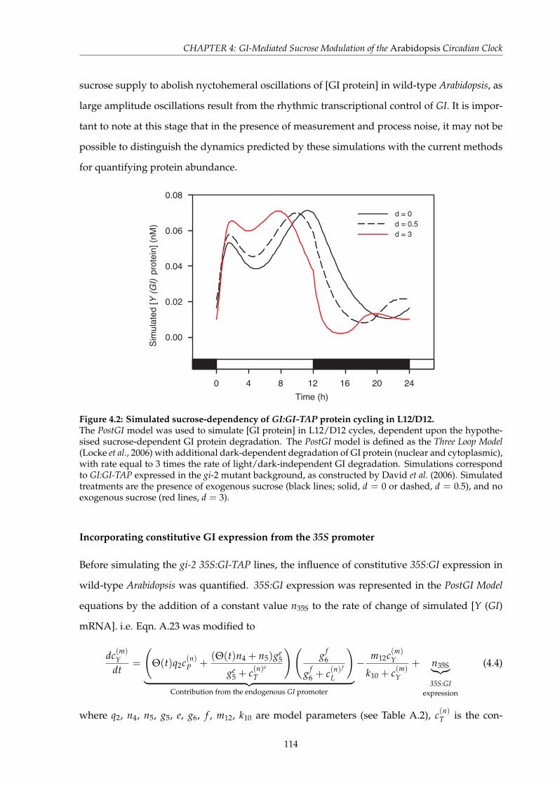
CHAPTER 4: GI-Mediated Sucrose Modulation of the Arabidopsis Circadian Clock
sucrose supply to abolish nyctohemeral oscillations of [GI protein] in wild-type Arabidopsis, as
large amplitude oscillations result from the rhythmic transcriptional control of GI. It is impor-
tant to note at this stage that in the presence of measurement and process noise, it may not be
possible to distinguish the dynamics predicted by these simulations with the current methods
for quantifying protein abundance.
Time (h)0 4 8 12 16 20 24
Sim
ulat
ed [Y
(GI)
pro
tein
] (nM
)
0.00
0.02
0.04
0.06
0.08
d = 0d = 0.5d = 3
Figure 4.2: Simulated sucrose-dependency of GI:GI-TAP protein cycling in L12/D12.The PostGI model was used to simulate [GI protein] in L12/D12 cycles, dependent upon the hypothe-sised sucrose-dependent GI protein degradation. The PostGI model is defined as the Three Loop Model(Locke et al., 2006) with additional dark-dependent degradation of GI protein (nuclear and cytoplasmic),with rate equal to 3 times the rate of light/dark-independent GI degradation. Simulations correspondto GI:GI-TAP expressed in the gi-2 mutant background, as constructed by David et al. (2006). Simulatedtreatments are the presence of exogenous sucrose (black lines; solid, d = 0 or dashed, d = 0.5), and noexogenous sucrose (red lines, d = 3).
Incorporating constitutive GI expression from the 35S promoter
Before simulating the gi-2 35S:GI-TAP lines, the influence of constitutive 35S:GI expression in
wild-type Arabidopsis was quantified. 35S:GI expression was represented in the PostGI Model
equations by the addition of a constant value n35S to the rate of change of simulated [Y (GI)
mRNA]. i.e. Eqn. A.23 was modified to
dc(m)Y
dt=
(Θ(t)q2c(n)
P +(Θ(t)n4 + n5)ge
5
ge5 + c(n)e
T
)(g f
6
g f6 + c(n) f
L
)︸ ︷︷ ︸
Contribution from the endogenous GI promoter
−m12c(m)
Y
k10 + c(m)Y
+ n35S︸︷︷︸35S:GI
expression
(4.4)
where q2, n4, n5, g5, e, g6, f , m12, k10 are model parameters (see Table A.2), c(n)T is the con-
114

CHAPTER 4: GI-Mediated Sucrose Modulation of the Arabidopsis Circadian Clock
centration of simulated nuclear TOC1 protein, c(n)L is the concentration of simulated nuclear
LHY/CCA1 protein, Θ(t) is the boolean light value, and c(n)P is the concentration of a simu-
lated light-labile protein in the nucleus (see Appendix A.2 for further details). n35S was chosen
so that simulated [Y (GI) mRNA] was higher than for simulated wild-type (n35S = 0) at all times
through entrained L10/D14 cycles (without exogenous sucrose), as observed by Mizoguchi
et al. (2005)∗. As these experiments were conducted in the absence of exogenous sucrose, the
PostGI Model with d = 3 was used to investigate the effect of varying n35S. We found that
n35S = 0.2 nM h−1 yielded sufficiently high levels of simulated GI expression (Figure 4.3).
Time (h)
0 4 8 12 16 20 24
Sim
ulat
ed [Y
(GI)
mR
NA]
(nM
)
0.00
0.05
0.10
0.15
0.20
0.25
0.30
0.35
Wild-typen35S = 0.2
Figure 4.3: Calibration of the rate of constitutive 35S:GI expression.The PostGI model was used to calibrate the rate of constitutive 35S:GI expression which agrees withRT-PCR measurements of GI mRNA by Mizoguchi et al. (2005). The PostGI model is defined as theThree Loop Model (Locke et al., 2006) with additional dark-dependent degradation of GI protein (nuclearand cytoplasmic), with rate equal to 3 times the rate of light/dark-independent GI degradation. Theequations were then modified to include a constant rate n35S of Y (GI) mRNA synthesis. Model equationswere solved numerically with MATLABTM’s ode15s stiff equation solver for 324 h in L10/D14 cycles,with the final 24 h displayed. Compared are simulated wild-type (black line; n35S = 0) and simulated35S:GI (red line; n35S = 0.2). Bars on abscissa are open indicating light, and closed indicating dark.
Simulated GI protein cycling in GI-overexpressing Arabidopsis
Having obtained an approximation for the rate of constant increase in simulated GI mRNA pro-
duction resulting from 35S:GI expression which corresponded with experimental data, it was
possible to simulate the gi-2 35S:GI-TAP line by removing the contribution of the endogenous
∗Note we did not consider the light-induced peak of expression shortly after dawn, as this was not observed byMizoguchi et al. (2005), and was only slightly affected over a large range of n35S.
115
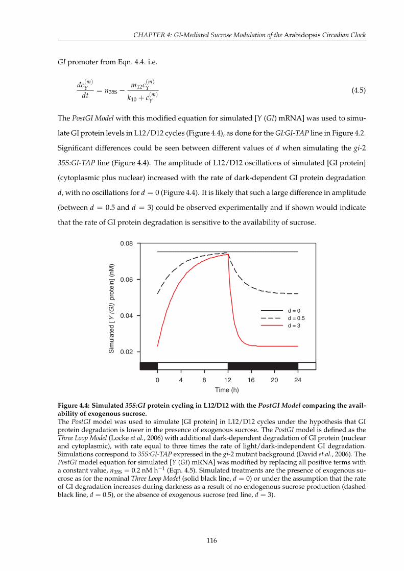
CHAPTER 4: GI-Mediated Sucrose Modulation of the Arabidopsis Circadian Clock
GI promoter from Eqn. 4.4. i.e.
dc(m)Y
dt= n35S −
m12c(m)Y
k10 + c(m)Y
(4.5)
The PostGI Model with this modified equation for simulated [Y (GI) mRNA] was used to simu-
late GI protein levels in L12/D12 cycles (Figure 4.4), as done for the GI:GI-TAP line in Figure 4.2.
Significant differences could be seen between different values of d when simulating the gi-2
35S:GI-TAP line (Figure 4.4). The amplitude of L12/D12 oscillations of simulated [GI protein]
(cytoplasmic plus nuclear) increased with the rate of dark-dependent GI protein degradation
d, with no oscillations for d = 0 (Figure 4.4). It is likely that such a large difference in amplitude
(between d = 0.5 and d = 3) could be observed experimentally and if shown would indicate
that the rate of GI protein degradation is sensitive to the availability of sucrose.
Time (h)0 4 8 12 16 20 24
Sim
ulat
ed [Y
(GI)
pro
tein
] (nM
)
0.02
0.04
0.06
0.08
d = 0d = 0.5d = 3
Figure 4.4: Simulated 35S:GI protein cycling in L12/D12 with the PostGI Model comparing the avail-ability of exogenous sucrose.The PostGI model was used to simulate [GI protein] in L12/D12 cycles under the hypothesis that GIprotein degradation is lower in the presence of exogenous sucrose. The PostGI model is defined as theThree Loop Model (Locke et al., 2006) with additional dark-dependent degradation of GI protein (nuclearand cytoplasmic), with rate equal to three times the rate of light/dark-independent GI degradation.Simulations correspond to 35S:GI-TAP expressed in the gi-2 mutant background (David et al., 2006). ThePostGI model equation for simulated [Y (GI) mRNA] was modified by replacing all positive terms witha constant value, n35S = 0.2 nM h−1 (Eqn. 4.5). Simulated treatments are the presence of exogenous su-crose as for the nominal Three Loop Model (solid black line, d = 0) or under the assumption that the rateof GI degradation increases during darkness as a result of no endogenous sucrose production (dashedblack line, d = 0.5), or the absence of exogenous sucrose (red line, d = 3).
116

CHAPTER 4: GI-Mediated Sucrose Modulation of the Arabidopsis Circadian Clock
4.3.3 Response of GI expression to topical sucrose treatment
The effect of topical sucrose treatment on central oscillator promoter activity was investigated,
in an attempt to distinguish whether sucrose modulates GI expression via transcriptional or
post-translational regulation. The mathematical models which were modified to account for
an absence of exogenous sucrose were used to predict how gene expression responds to topi-
cal treatment of sucrose. Then, the corresponding in vivo experiments were conducted to test
the contrasting hypothesised transcriptional (N5) and post-translational (PostGI) models for
sucrose-sensing by GI.
Simulated response of N5 Model and PostGI Model to sucrose treatment
The N5 Model and the PostGI Model (with d = 3) were used to simulate [LHY/CCA1 mRNA],
[TOC1 mRNA], Y (GI) mRNA], and [PRR7/PRR9 mRNA] in the absence of exogenous sucrose
in L12/D12 cycles before transfer to DD for 60 or 72 h (Figure 4.5). At these points, the modified
model equations were switched with the nominal Three Loop Model configuration (Equations
A.14–A.29) to simulate an immediate increase in exogenous sucrose corresponding to topical
treatment of 90 mM sucrose. With no prior knowledge of the rate of uptake of sucrose into
the cell, it was assumed that [Suc]i increases immediately following treatment. Furthermore,
using the nominal Three Loop Model implicitly assumed that [Suc]i increases following topical
addition to levels equivalent to seedlings grown on a 90 mM sucrose-supplemented growth
media. GI:luc luminescence increased within the first 30 min (first data-point) following sucrose
treatment in vivo (Figure 4.6), indicating that the assumption that [Suc]i increases immediately
after addition of 90 mM sucrose might be justified.
Simulated sucrose treatment resulted in re-established circadian oscillations of all model
components for both the N5 Model and the PostGI Model in DD (Figure 4.5). The time through
the circadian cycle at which simulated sucrose treatment was applied (with respect to the last
zeitgeber, a dark to light transition) did not affect simulated output because near-steady state
levels were reached after 60 h in DD, and thus an identical stimulus (simulated sucrose treat-
ment) was applied to a near-identical initial condition. After simulated sucrose treatment with
both the N5 Model and PostGI Model, simulated [LHY/CCA1 mRNA] had oscillations which
increased in amplitude with the first peak occurring 11.2–11.4 h after simulated treatment (Fig-
ure 4.5). Oscillations continued with increasing amplitude slowly approaching the nominal
117

CHAPTER 4: GI-Mediated Sucrose Modulation of the Arabidopsis Circadian Clock
Time (h)-24 0 24 48 72 96 120 144
Rel
ativ
e si
mul
ated
[mR
NA]
0.0
0.2
0.4
0.6
0.8
1.0
1.2LHY/CCA1TOC1Y (GI)
A
Time (h)-24 0 24 48 72 96 120 144
Rel
ativ
e si
mul
ated
[mR
NA]
0.0
0.2
0.4
0.6
0.8
1.0
1.2B
Figure 4.5: Simulated effects on oscillator transcript abundance of a sucrose dose after a period ofextended darkness.Three Loop Model (Equations A.14–A.29; Locke et al., 2006) modified to reflect absence of exogenoussucrose, simulated in DD after entrainment to L12/D12 cycles. Simulated effect of dosing seedlings with90 mM sucrose by switching from modified to nominal model configuration at t = 60. Modificationsto the Three Loop Model are (A) a reduction in n5 to 25 % of its nominal value, and (B), incorporatingdark-dependent degradation of Y (GI) protein as in Equations 4.1–4.2 with d = 3.
Three Loop Model oscillation trajectory. The slow recovery to the nominal oscillation was also in-
dicative of the other model component [mRNA] levels following simulated sucrose treatment
(Figure 4.5A). As the nominal Three Loop Model equations corresponded to seedlings treated
topically with 90 mM sucrose after simulating an absence of exogenous sucrose with both the
N5 Model and the PostGI Model, both of the resulting trajectories will converge on the same limit
cycle trajectory. However, the transient tending behaviour distinguished the two hypotheses
generated by the models in silico. With the N5 Model, simulated [Y (GI) mRNA] increased
sharply following simulated sucrose treatment because the rate of Y (GI) transcription was in-
creased by a factor of 4 (Figure 4.5A). However, with the PostGI Model simulated [Y (GI) mRNA]
remained constant for approximately 4 h following sucrose treatment and then decreased (Fig-
ure 4.5B). This was because GI protein levels were increased initially (degradation rate of Y/GI
protein decreases by a factor of 4) which activates TOC1 transcription; only after TOC1 protein
has accumulated will GI transcription be inhibited leading to a decrease in simulated [Y (GI)
mRNA].
Sucrose treatment in vivo
The in vivo analysis of topical sucrose treatment supported the hypothesis that sucrose mod-
ulates GI transcription. When seedlings were treated with 90 mM sucrose at CT0, GI:luc in-
118

CHAPTER 4: GI-Mediated Sucrose Modulation of the Arabidopsis Circadian Clock
Time since treatment (h)
-24 0 24 48 72
GI:l
ucLu
min
esce
nce
(pho
tons
/ 12
s)
0
1000
2000
3000
4000
5000
6000
70000
2000
4000
6000
8000A
+ 90 mM Sucrose
+ 90 mM Mannitol
Time since treatment (h)
-24 0 24 48 72
GI:l
uc L
umin
esce
nce
(pho
tons
/ 12
s)
0
1000
2000
3000
4000
50000
5000
10000
15000
20000
25000
30000B
+ 90 mM Sucrose
+ 90 mM Mannitol
Time since sucrose addition (h)
0 12 24 36 48 60 72
Trough
Peak
CT0 TreatmentCT12 Treatment
C
Figure 4.6: Sucrose amplifies circadian rhythms in DD and is a zeitgeber for GI.Rhythms of GI promoter activity quantified for seedlings treated (at t = 0) with 100 µl of 90 mM sucrose(top panels) or 90 mM mannitol (bottom panels) after (A) 60 h (CT0), or (B) 72 h (CT12) darkness. (A,B)GI:luc luminescence quantified using a multi-functional 96 well plate reader for 12 s every 30 min. Tracesare the total signal from a single well containing 2-3 seedlings (coloured thin lines), and the averagesignal (dashed thick line) for sucrose-treatment (n = 12) or mannitol-treatment (n = 4). Bars on abscissaare grey, subjective day; black, subjective night. (C) Oscillation peaks and troughs calculated for (A) and(B) by clustering turning points in the averaged datasets (n = 12; Section 4.2.3).
119

CHAPTER 4: GI-Mediated Sucrose Modulation of the Arabidopsis Circadian Clock
creased initially, and continued to oscillate with increasing signal (Figure 4.6A). An immediate
increase in signal and oscillation amplitude of GI:luc luminescence also occurred in seedlings
treated with 90 mM sucrose at CT12 (Figure 4.6B). The osmotic control of 90 mM mannitol
did not increase GI:luc luminescence transiently and the decaying amplitude oscillations ap-
proached steady state.
The times of oscillation peaks and troughs of GI:luc luminescence were approximated us-
ing a simple clustering algorithm of turning points in the dataset (Section 4.2.3). The timing
of these peaks and troughs remained approximately the same relative to the time of sucrose
treatment comparing application at CT0 and CT12 (Figure 4.6C). Therefore, sucrose might be a
zeitgeber for GI because it re-entrains circadian oscillations in GI expression. GI promoter activ-
ity increased in response to topical sucrose treatment, which coincided with the prediction of
the N5 Model for simulated [Y (GI) mRNA], but contrasted with the corresponding simulation
using the PostGI model (Figure 4.7). This provided evidence for the hypothesis that sucrose
increases the basal rate of GI transcription.
Time since sucrose treatment (h)
-12 0 12 24
Sim
ulat
ed [
Y (
GI)
mR
NA
] (nM
)
0.00
0.02
0.04
0.06
0.08
0.10
0.12
GI:l
uc L
umin
esce
nce
(pho
tons
/ 12
s)
0
1000
2000
3000
4000
5000
6000N5 modelPostGI modelGI:luc (Treated CT0)GI:luc (Treated CT12)
-Suc +Suc
Figure 4.7: Sucrose activates GI transcription as predicted by the N5 Model.Mathematical simulation of [Y (GI) mRNA] in constant dark after simulated sucrose treatment (solidlines) compared with corresponding GI:luc luminescence data (red circles). 14-day-old Arabidopsisseedlings expressing GI:luc were entrained in L12/D12 cycles before transfer to DD for 60 h (dark redcircles, CT0) or 72 h (light red circles, CT12), then treated with 100 µl of 90 mM sucrose (data as in Fig-ure 4.6). Corresponding simulations using the N5 Model (light blue line, Figure 4.5A) and the PostGIModel (dark blue line, Figure 4.5B) were conducted by numerical integration of the Three Loop Modelequations with the ode23s stiff equation solver in MATLABTM.
120

CHAPTER 4: GI-Mediated Sucrose Modulation of the Arabidopsis Circadian Clock
4.4 Discussion
After demonstrating the necessity of a functional GI for sucrose modulation of the central os-
cillator in DD in Chapter 3, it was investigated whether GI was regulated at the transcriptional
or post-translational level. The analysis in Chapter 3 also suggested that the rate of GI tran-
scription was increased in the presence of exogenous sucrose. Here it was determined that a
dark-dependent GI protein degradation mechanism might account for sucrose-dependent os-
cillations in DD. However, comparisons of the dynamics of GI:luc luminescence with model
simulations following a step change in exogenous sucrose availability suggests transcriptional
rather than post-translational regulation of GI confers responsiveness to sucrose.
4.4.1 The PostGI Model: GI protein stabilisation
The PostGI Model was defined to account for dark-induced proteolysis of GI by the 26S pro-
teasome (David et al., 2006). For simplicity, it was assumed that degradation occurred both in
the cytosol and the nucleus and the dark-independent degradation rate was unaltered from
the nominal Three Loop Model (Eqn. 4.3). Therefore, GI degradation increases in the dark in
the absence of exogenous sucrose by rates m13 nM h-1 in the cytosol and m14 nM h-1 in the
nucleus (Equations 4.1–4.2). All other Three Loop Model parameters were kept at their nomi-
nal rates, which is a potential shortfall of the PostGI model. In particular, the new mechanism
affected the simulated light-dark cycles of [TOC1 mRNA], forcing a biphasic oscillation (Fig-
ures 4.1B,D). However, the nominal Three Loop Model does not accurately describe light-dark
oscillations of TOC1 expression (compare Figures 3.1D and 4.1D).
As the relative rate of dark-dependent GI degradation (d = m13/m13 = m14/m14) was
increased, the amplitude of DD oscillations was suppressed. The first peak of simulated
[LHY/CCA1 mRNA] remained unaffected, similar to that observed for CCA1:luc luminescence
in the absence of exogenous sucrose. Therefore, a high rate of dark-dependent degradation of
GI corresponded to dynamical behaviours when there is no exogenous sucrose supply, and a
lower rate corresponded to exogenous supply of sucrose. This is equivalent to saying that ex-
ogenous sucrose stabilises GI protein in the dark. Presumably, a high level of [Suc]i during light
(photosynthesis) would have the same (stabilising) effect, providing a possible explanation for
the proposed dark-dependency of GI protein degradation (David et al., 2006).
121

CHAPTER 4: GI-Mediated Sucrose Modulation of the Arabidopsis Circadian Clock
4.4.2 Distinction of transcriptional and post-translational mechanisms
Simulations of the N5 Model from Chapter 3 were compared with the PostGI Model to deter-
mine conflicting predictions that could be exploited to establish the most likely model of GI-
mediated sucrose modulation of the circadian clock. To establish whether GI is regulated tran-
scriptionally by sucrose, the effect of topical sucrose treatment on GI expression in DD was
investigated both in silico and in vivo. The possibility that sucrose regulates GI at the post-
translational was investigated by comparing L12/D12 oscillations of GI protein in the presence
and absence of sucrose in both wild-type and GI-overexpressing backgrounds. In tandem,
these experiments might distinguish between three possible hypotheses for the modes of GI
regulation by sucrose: only transcriptional control, only post-translational contol, or dual tran-
scriptional and post-translational control.
Sucrose regulates GI transcriptionally and is a zeitgeber for GI expression
The effect of topical sucrose treatment was measured in GI:luc expressing plants. By compar-
ison with simulations of the N5 Model and the PostGI Model, evidence was found supporting
the hypothesis that sucrose up-regulates GI transcription, as GI expression increased follow-
ing topical sucrose treatment, a prediction of the N5 Model (Figures 4.5, 4.6, 4.7). It was also
found that the oscillations in GI:luc luminescence resulting from sucrose treatment were not
dependent on the circadian time of application, indicating that sucrose is a zeitgeber for GI in
DD (Figure 4.6C). It would be interesting to measure the response of other circadian markers
in response to a topical sucrose treatment. These can include promoter-luc fusions analogous
to GI:luc, and also crossed into a range of mutant backgrounds. Of particular interest would be
the gi-11 null mutant, to establish whether topical sucrose treatment is perceived by the Ara-
bidopsis central oscillator only via GI, or through multiple pathways. It is clear that additional
experimental characterisation of the effect of topical sucrose treatment would unravel further
properties of the interactions between sugar signalling pathways and oscillator components,
and also of the circadian central oscillator mechanism itself.
A protein assay for determining whether sucrose exerts post-translational control of GI
To establish whether sucrose regulates GI at the post-translational level, the PostGI Model was
used to simulate L12/D12 cycles of [Y (GI) protein] in the presence (d = 0 or d = 0.5), no
122

CHAPTER 4: GI-Mediated Sucrose Modulation of the Arabidopsis Circadian Clock
dark-induced GI proteolysis) and absence (d = 3) of exogenous sucrose (Section 4.3.2). First,
the experiments of David et al. (2006) which demonstrated the dark-dependent proteolysis of
GI were simulated. This experiment offers a clear distinction between sucrose modulating GI
transcript or protein by the following argument. If sucrose only regulates GI transcriptionally,
as predicted by the N5 Model, then the gi-2 35S:GI-TAP line will be insensitive to sucrose, as the
native GI promoter is dysfunctional. However, a sucrose-dependency in the gi-2 GI:GI-TAP line
would be expected due to the presence of the native GI promoter. In contrast, if sucrose only
regulates GI post-translationally (PostGI Model), then only a small sucrose-dependency might
be seen for gi-2 GI:GI-TAP (Figure 4.2), but a significant sucrose-dependency would be seen
in gi-2 35S:GI-TAP (Figure 4.4). Due to the limited potential to characterise quantifiable differ-
ences in protein abundance in vivo, only stark differences may be observed such as the strong
suppression of L12/D12 GI protein cycles by sucrose hypothesised to exist in the gi-2 35S:GI
background by the PostGI Model. Therefore, the proposed combination of experiments may
only answer whether or not GI protein is regulated by sucrose, and not distinguish control of GI
transcriptionally. However, combined with the evidence presented in Figure 4.7 which demon-
strates GI expression is increased by topical sucrose treatment (as predicted by the N5 Model),
we feel there would be sufficient evidence to discriminate whether sucrose regulates GI only
transcriptionally, only post-translationally, or both at the transcriptional and post-translational
levels. The proposed protein experiments are currently being conducted by a collaborating
member of the Webb Laboratory (Seong Jin Baek).
4.4.3 Summary
The central oscillator perceives [Suc]i via changes in the abundance of GI. The results presented
above provided preliminary evidence for a transcription-based, rather than post-translational
mechanism. However, a critical test has been designed which will elucidate the true underlying
mechanism, the possible outcomes of which have been simulated using the N5 Model and the
PostGI Model. This work represents further progress towards a model integrating carbohydrate
metabolism into the circadian signalling network in Arabidopsis.
123

CHAPTER 5
Modelling a cADPR-Dependent
Feedback Loop of the Circadian Clock
5.1 Introduction
In this chapter, the position and function of cyclic adenosine diphosphate ribose (cADPR) in
the circadian oscillator network in Arabidopsis thaliana is addressed in silico. Recent work has
shown that cADPR mediates the circadian control of [Ca2+]cyt, whilst also regulating the central
oscillator mechanism (Dodd et al., 2007). However, it is not clear which central oscillator genes
interpret the action of circadian cADPR signalling.
cADPR is a Ca2+ mobilising second messenger in animals and plants (Clapper et al., 1987;
Navazio et al., 2001; Galione et al., 1991). cADPR was first identified by Lee et al. (1989) in sea
urchin eggs, and described as a cyclic metabolite of NAD+ with intracellular Ca2+-mobilising
activity. cADPR is synthesised from NAD+ by the membrane-bound ADP-ribosyl (ADPR)
cyclase enzyme (Lee & Aarhus, 1991), and broken down by cADPR-hydrolase (Lee & Aarhus,
1993) in the presence of nicotinamide. At high concentrations, cADPR binds to ryanodine
receptors (RyR), promoting calcium-induced calcium release (CICR; Galione et al., 1991). There
are no known homologs of ADPR cyclase (or hydrolase) in plants, though cADPR has been
shown to promote Ca2+ release from the vacuoles of beet storage root (Allen et al., 1995). cADPR
124

CHAPTER 5: Modelling a cADPR-Dependent Feedback Loop of the Circadian Clock
also mediates abscisic acid (ABA) induced gene expression in response to cold, drought and
salt stress (Wu et al., 1997), and stomatal closure (Leckie et al., 1998).
In Arabidopsis, [cADPR] has circadian oscillations in constant light (LL) which achieve peak
levels 8 hours after subjective dawn, while in CCA1-ox (constitutive overexpressor of CCA1),
[cADPR] does not oscillate and remains at a constant low level (Figure 5.1A; Dodd et al., 2007).
cADPR synthesis is inhibited by nicotinamide, a by-product of the cyclisation of NAD+ by
ADPR cyclase (Sethi et al., 1996). Treatment of 50 mM nicotinamide significantly reduces cADPR
synthesis in Arabidopsis, and has the additional effect of abolishing circadian oscillations of
[Ca2+]cyt (Figure 5.1B; Dodd et al., 2007). The Ca2+-sensor CAS has been suggested to contribute
to diurnal variations [Ca2+]cyt via an IP3-based pathway (Tang et al., 2007). However, treating
Arabidopsis seedlings with the IP3 inhibitor U73122 or the plasma-membrane channel blocker
GdCl3 had no effect on circadian oscillations of [Ca2+]cyt (Dodd et al., 2007). Therefore, cADPR
mediates the circadian control of [Ca2+]cyt.
In addition to being an output of the Arabidopsis circadian clock, there is evidence that
cADPR forms a cytosolic feedback loop with the central oscillator (Dodd et al., 2007). In a
bioinformatic study comparing the set of circadian-regulated transcripts with sets of tran-
scripts regulated by signalling molecules, cADPR was identified to be commonly associated
with circadian regulation. The overlap between cADPR- and circadian-regulated transcripts
was the most statistically significant overlap, and included central oscillator genes LHY, CCA1,
GI and PRR7 (Figure 5.1C; Dodd et al., 2007). In Arabidopsis seedlings which express an ADP-
ribosyl cyclase enzyme from Aplysia kurodai under the control of a β-estradiol-inducible pro-
moter (XVE:ADPRc), changes in clock gene transcript abundance were measured 6 hours after
application of β-estradiol (Sánchez et al., 2004). Both LHY and CCA1 transcripts abundance was
decreased relative to wild-type plants, while expression of GI, PRR5, PRR7 and CRY1 was in-
creased (Sánchez et al., 2004). Therefore, transient increases in [cADPR] resulting from induced
ADPR cyclase expression results in altered clock gene expression, implying that cADPR regu-
lates the circadian clock. Further evidence for a cADPR-based feedback loop was identified as
treatment with the cADPR inhibitor nicotinamide increased circadian period of CAB2, CCA1,
LHY and TOC1 transcript abundance (Figure 5.1E) and oscillations of leaf position in LL (Fig-
ures 5.1F,G; Dodd et al., 2007). However, there was no circadian phenotype when measuring
circadian oscillations of leaf movement in the XVE:ADPRc line (Figure 5.1H; Dodd et al., 2007).
125

CHAPTER 5: Modelling a cADPR-Dependent Feedback Loop of the Circadian Clock
Time in constant light (h)24 36 48 60 72
[cAD
PR] p
mol
μg
prot
ein
-1
0.0
0.1
0.2
0.3
0.4
0.5
0.6Col-0 wild-typeCCA1-ox
A
Time in constant light (h)
0 12 24 36 48 60 72 84 96
Lum
ines
cenc
e (p
hoto
ns 1
300
s-1)
0
1000
2000
3000
4000
5000H2050 mM mannitol50 mM nicotinamide
B
938 252 2282
Circadian-regulatedtranscripts
Sanchez et al .(2004)
cADPR-regulatedtranscripts
C
CCA1 LHY GI APRR7lo
g 2 F
old
Cha
nge
-6
-4
-2
0
2
4
Upper limit
Lower limit
D
Period (h)
23 24 25 26 27 28 29
pMM
C
0.00
0.01
0.02
0.03
0.04
0.05E
CAB2
TOC1
CCA1LHY
Time in constant light (h)0 24 48 72 96 120 144 168 192
Mea
n no
rmal
ised
leaf
pos
ition
0.96
0.98
1.00
1.02
1.0450 mM mannitol50 mM nicotinamide
F
Time of maximum peak height (h)
0 4 8 12 16
peak1
peak2
peak3
peak4
peak5
peak6
0 4 8 12 16
G
Time in constant light (h)0 24 48 72 96 120 144 168 192
Mea
n no
rmal
ised
leaf
pos
ition
0.98
0.99
1.00
1.01XVE:EMPTYXVE:ADPRc
H
Figure 5.1: Modulation of the Arabidopsis circadian clock by a cADPR-based feedback loop.(A) Circadian rhythm of [cADPR] in LL present in Col-0 wild-type and absent in CCA1-ox plants. (B)Circadian rhythm of [Ca2+]cyt is abolished with 50 mM nicotinamide (red circles). Control lines are50 mM mannitol (black triangles) or water (black circles). (C) There is a significant overlap betweencircadian- and cADPR-regulated transcripts (Sánchez et al., 2004; Dodd et al., 2007). (D) Log2 fold changeof transcript abundance 6 h after induction of Aplysia ADPR cyclase (Sánchez et al., 2004). (E) Circadianperiod increases after treatment every 3 h with 50 mM nicotinamide (red) or water (black). Multiple-measures correction (pMMC) describes the goodness of fit. (F) Circadian rhythm of leaf position aftertreatment with 50 mM nicotinamide (red) or 50 mM mannitol (black). (G) Time of circadian peaks ofleaf position in seedlings treated with 10 mM (left panel) or 50 mM (right panel) nicotinamide (redcircles), mannitol (black triangles) or water (black circles). (H) Circadian rhythm of leaf position afterinduced expression of XVE:ADPRc (green line) or XVE:EMPTY control (black line). (A,B,F,H) Bars on x-axis indicate light during subjective daytime (white bars) and subjective night-time (grey bars), or dark(black bars). Modified from Dodd et al. (2007). 126

CHAPTER 5: Modelling a cADPR-Dependent Feedback Loop of the Circadian Clock
5.2 Mathematical methods
Mathematical models of the Arabidopsis circadian clock were used to investigate the effects of
manipulating [cADPR] levels. All existing models of the central oscillator mechanism con-
sider only gene-gene interactions and activation/degradation by light (Locke et al., 2005a,b,
2006; Zeilinger et al., 2006). There has so far been no attempt to incorporate the effect of small
molecules, where knowledge of interactions with central oscillator genes is limited. Elevated
[cADPR] has a pronounced effect on circadian-regulated genes (Sánchez et al., 2004), though the
mechanism responsible has not been characterised. In this chapter, we assume that the wild-
type oscillating levels of cADPR are implicitly accounted for in mathematical descriptions of
the central oscillator as the circadian period is approximately 24 h rather than the long period
when cADPR synthesis is suppressed with nicotinamide (Figure 5.1F; Dodd et al., 2007). We
assume further that the effect of elevated [cADPR] can be described by perturbing the reactions
defined by the model, through altering the parameters which define these reactions.
The motivation for investigating the role of cADPR of the circadian clock network derived
from a set of experimental observations that were seemingly uncorrelated or contradictory.
Induced expression of ADPR cyclase was shown to have a large effect on the transcript abun-
dance of circadian clock genes in Arabidopsis (Sánchez et al., 2004), without affecting circadian
period or phase relative to wild-type plants (Figure 5.1H). Initially, we considered using sen-
sitivity analysis to identify how the oscillation period varied as a function of each parameter
value. However, existing methods are based on linear approximations and therefore corre-
spond to small deviations from the nominal parameter values (Ingalls & Sauro, 2003; Ingalls,
2004). Due to the large deviations in gene expression being investigated, the ’local’ approach
was not suitable. Instead, simulation methods were designed to analyse the effect of large pa-
rameter perturbations to the kinetic parameters of the mathematical circadian clock models,
considering the existing experimental data already available (Figure 5.1).
5.2.1 Simulating effects of high and low [cADPR] on clock gene expression with
the Interlocked Feedback Loop Model
In general, we can describe the Interlocked Feedback Loop Model by a nonlinear system
x = f (x, p) (5.1)
127

CHAPTER 5: Modelling a cADPR-Dependent Feedback Loop of the Circadian Clock
where x ∈ Rn is a vector of concentrations of mRNA, protein in the nucleus and cytoplasm for
each gene, and p ∈ Rm is the vector of m model parameters (see Appendix A.1 for a detailed
description of the model). The simplest method for altering the parameters is to assume that
the effect of elevated [cADPR] on the circadian clock is immediate and sustained at a constant
level. Suppose that ADPR cyclase is induced at t = τ, then we define the constant perturbation
pC(t) as follows
pC(t) :=
p0, t ≤ τ
rp0, t > τ(5.2)
where p0 is the nominal value of the parameter p, and r > 0 is the perturbation amplitude.
Induction of XVE:ADPRc by β-estradiol was shown to continually increase [cADPR] over
20 hours (Sánchez et al., 2004). However, the effect on transcript abundance was most pro-
nounced 6 hours after application of β-estradiol. The activity of the ADPR cyclase enzyme was
also higher at 16 h than 6 h. This suggests that the effect on downstream gene expression of
increased ADPR cyclase activity, presumably via cADPR, is transient. We supposed that the
effect of elevated [cADPR] on the circadian clock increases initially after induction and then
decreases back to the normal operating conditions. By assuming linear uptake and exponential
decay of the inducer, we define the (additive) transient perturbation pT(t).
pT(t) :=
p0, t ≤ τ
p0 + rte1− ttmax
tmax, t > τ
(5.3)
where r is the ratio between the perturbed and nominal parameter values at the peak time
t = tmax. Peak times were tested that related to the peak change in gene expression (tmax = 6),
peak ADPR cyclase activity (tmax = 16) and peak [cADPR] (tmax = 20; Figure 5.2.1). The most
representative profile of the experiment used to find suitable parameter perturbations is the
exponential profile which peaks 6 hours after simulated induction, as it is the downstream
effect of cADPR which is being modified through parameter perturbation.
The performance of parameter perturbations was assessed by comparing simulated gene
expression values with the data published in Sánchez et al. (2004) as follows. The model
equations (Equations A.1–A.13) were simulated in L16/D8 cycles and at t = τ subjected to
a parameter perturbation. To ease the computational burden, a series of initial conditions was
128

CHAPTER 5: Modelling a cADPR-Dependent Feedback Loop of the Circadian Clock
Time (h)
-48 -24 0 24 48 72 96 120 144
Am
plitu
de
0.0
0.2
0.4
0.6
0.8
1.0
1.2
Time of ADPR cyclase induction
Figure 5.2: Perturbation profiles applied to the Interlocked Feedback Loop Model.Graphical representation of each perturbation profile, applied at t = 0. Constant perturbation (Eqn. 5.2,black trace), and transient perturbations (Eqn. 5.3) with tmax = 6 (red trace), tmax = 16 (green trace) andtmax = 20 (blue trace) are plotted for unit amplitude (A = 1). Modified from Figure S4A in Dodd et al.(2007).
computed as the numerical solution at different integer times along the limit cycle of the unper-
turbed Interlocked Feedback Loop model. The initial conditions therefore correspond to different
values of the perturbation time τ. At t = τ + 6, the fold change of LHY ( fLHY), TOC1 ( fTOC1)
and Y ( fY) mRNA was computed relative to the equivalent unperturbed simulation. Therefore,
only one quarter of the limit cycle was analysed for fold changes in simulated gene expres-
sion, meaning that obtaining numerical solutions was very fast. A cost function was defined to
assess how close each perturbation was to the target values.
‖e‖2 =√
( fLHY − 0.056)2 + ( fTOC1 − 1)2 + ( fY − 3.732)2) (5.4)
The target value for the LHY component, 0.056, was calculated as the arithmetic mean of the
fold changes in LHY and CCA1 expression. Similarly, the value for Y was taken to be the
fold change in GI, as GI is considered to be the most likely identity of Y (Locke et al., 2006).
Since TOC1 was not found to be significantly regulated by ADPR cyclase (Sánchez et al., 2004),
the target value was set as 1. No restriction was imposed on the change in X mRNA as it’s
identity remains unknown. Variants of the cost function were also investigated, in particular
by normalising each squared bracket by the target value, or the square of the target value.
However, this had the effect of rewarding perturbations for which fLHY was very close to 0.056,
129

CHAPTER 5: Modelling a cADPR-Dependent Feedback Loop of the Circadian Clock
whilst only weakly penalising deviations of fTOC1 and fY from their target values (data not
shown). Parameter perturbations were retained as candidates if they achieved a cost function
score less than 2.
An algorithm was defined that systematically tested perturbations in the rate constants of
the Interlocked Feedback Loop Model for their ability to match the observed fold changes in LHY,
CCA1, TOC1 and GI which resulted from transient induction of XVE:ADPRc (Sánchez et al.,
2004). Initially, parameters were perturbed singly as this gave the potential to establish predic-
tions for cADPR targets in the central oscillator mechanism and reflected our prior assumption
that cADPR targets few rather than all components. However, despite exploring a range of am-
plitudes for all perturbation profiles (Figure 5.2.1), we found no examples for which ‖e‖ < 2.
Parameters were thus perturbed in pairs to cover as much of the parameter space as possi-
ble. Furthermore, this was in keeping with the philosophy that only very few components are
directly regulated by the cADPR-mediated pathway. Each perturbation was conducted for a
random linear combination of each parameter pair ((
532
)= 1378 choices) and a range of am-
plitudes r (between -1 and 1). An example of simulated output after imposing perturbations in
this way can be seen in Figure 5.3.
Figure 5.3 illustrates how a transient perturbation (with tmax = 6) to a (hill exponent of LHY
activation by X) and p1 (rate of LHY translation) can yield altered gene expression close to the
target values ( fLHY = 0.002, fTOC1 = 1.001, fY = 3.719, ‖e‖2 = 0.054). Note that in this example,
parameters that directly affect Y mRNA have not been perturbed. The result of perturbations
to oscillating systems is by no means intuitive.
5.2.2 Refinement of the pairwise parameter perturbation method and application
to the Three Loop Model
Initially, the Interlocked Feedback Loop Model was used for investigating cADPR-mediated
changes in clock gene expression. After publication of the results (Dodd et al., 2007), the pa-
rameter perturbation method was refined and applied to the Three Loop Model in an attempt
to find a coherent prediction for the target of a cADPR-based feedback loop for the central os-
cillator. The decision to switch models reflected increased confidence in the Three Loop model’s
ability to match experimentally observed behaviours and was additionally motivated by the
inclusion of the extra component A (PRR7/9). The transient perturbation (pT) was redefined as
130

CHAPTER 5: Modelling a cADPR-Dependent Feedback Loop of the Circadian Clock
Time (hours)0 4 8 12 16 20 24
Sim
ulat
ed [
LHY/
CC
A1 m
RN
A] (n
M)
0.0
0.2
0.4
0.6
0.8
1.0
1.2NominalPerturbed
A
Time (hours)0 4 8 12 16 20 24
Sim
ulat
ed [
TOC
1 m
RN
A] (n
M)
0.0
0.5
1.0
1.5
2.0B
Time (hours)0 4 8 12 16 20 24
Sim
ulat
ed [
X m
RN
A] (n
M)
0.00
0.02
0.04
0.06
0.08
0.10
0.12
0.14
0.16C
Time (hours)0 4 8 12 16 20 24
Sim
ulat
ed [
Y m
RN
A] (n
M)
0.00
0.05
0.10
0.15
0.20D
fY =
perturbednominal 0.0092
0.0340= ≈ 3.7
Figure 5.3: Parametric perturbations alter gene expression in the Interlocked Feedback Loop Model.Simulated induction of ADPR cyclase (red traces) is compared against wild-type expression (blacktraces) in the Interlocked Feedback Loop Model (Locke et al., 2005b). Model equations (Equations A.1–A.13) were solved numerically with Θlight set to reflect long-day (16 h light, 8 h dark) conditions. Theconcentrations of mRNA for the model components LHY (A), TOC1 (B), X (C) and Y (D) are plottedagainst time. The transient perturbation (Eqn. 5.3) was imposed at t = 16 to parameters a and p1. Whiteand black bars indicate light and dark respectively.
a multiplicative perturbation to the nominal parameter set p0
pT(t) :=
p0, t ≤ τ
(1 + r−16 te1− t
6 )p0, t > τ(5.5)
where r is relative parameter value at the peak time t = 6. For each pair of parameters, 100 tri-
als were simulated for each perturbation in which random values were assigned for r (constant
perturbation, Eqn. 5.2 or transient perturbation, Eqn. 5.5). In both cases, these values relate the
largest relative deviation from the nominal value. So, we chose a distribution on the positive
real line with mean 1, by assigning r = 10u where u is a uniformly distributed random number
over the closed interval [-2,2]. In this section, a cost function was not used to assess how close
a perturbation matched the data from Sánchez et al. (2004). Instead, perturbations were consid-
ered candidates when fLHY (fold change in [LHY mRNA] 6 hours after simulated induction of
ADPR cyclase) was less than 0.1, 0.5 < fTOC1 < 2, and fY > 2.5. This avoided the issues of nor-
malisation when using a cost function, as discussed in the previous section. For analysis of the
131

CHAPTER 5: Modelling a cADPR-Dependent Feedback Loop of the Circadian Clock
Three Loop Model, a further constraint of fA > 2 was considered. A represents the influence of
PRR7 – which was significantly up-regulated by increased [cADPR] (Figure 5.1D) – and PRR9
which did not appear in the dataset and thus not significantly regulated by cADPR. Candidate
parameter perturbations were again removed if the state trajectory did not return to the limit
cycle in simulated LL.
The 100 random perturbations were conducted for each pairwise combination of param-
eters from the Interlocked Feedback Loop Model (Locke et al., 2005b) and the Three Loop Model
(Locke et al., 2006). Two perturbation profiles (transient and constant) were imposed at each
hourly time over the 24 hour day. Since only a small dataset is available to guide our anal-
ysis, a more general look at possible effects of elevated [cADPR] is presented. Distributions
are presented which illustrate properties of LL oscillations after simulated induction of ADPR
cyclase. In addition, we attempted to characterise regions of the model which when perturbed,
matched experimentally observed behaviours. The results of these analyses are presented in
Section 5.3.2.
5.2.3 Calculation of period and phase in LL
The set of candidate perturbations was refined by removing cases where the perturbation led
to a loss of rhythmicity in LL. This is reasonable since there is no arrhythmic phenotype after
induction of ADPR cyclase (Figure 5.1H). The period and amplitude of oscillation in LL was
computed to assess rhythmicity. The relevant model equations were solved numerically with
MATLABTM as before, except that ode23s was used for certain perturbations that could not be
resolved by ode15s. Θlight was varied to reflect two cycles of diurnal conditions (12 h light,
12 h dark) followed by 196 hours of LL. The perturbations were imposed at the last dark to
light transition, as per our experimental data. The time difference of the last two peak values
of simulated [LHY mRNA] was used to estimate period T. The ratio between the last local
maxima and local minima provide an amplitude estimate A. For the transient perturbations,
the phase φ was computed relative to the unperturbed period T as follows.
φ := (τ − τ +T2
) mod T − T2
(5.6)
where τ is the time of the last peak value of [LHY mRNA] in the unperturbed case, τ for the
perturbed case. This definition ensures that the phase lies in the interval [− T2 , T
2 ].
132

CHAPTER 5: Modelling a cADPR-Dependent Feedback Loop of the Circadian Clock
5.3 Results
5.3.1 Parameter perturbation analysis applied to the Interlocked Feedback Loop
Model
Time of induction of candidate perturbations
The observed changes in gene expression after transient induction of XVE:ADPRc might vary
depending on the time that the inducer chemical is applied. This is because non-stimulated
expression of circadian clock-associated genes varies over the course of the day. Sánchez et al.
(2004) did not report the time at which they applied the inducer chemical. We found that the
number of random pairwise perturbations that could be considered candidates varied greatly
depending on the time at which the perturbation was imposed (Figure 5.4). A bimodal distri-
bution prevailed for the constant perturbation and the transient perturbation with tmax equal
to 6 h and 16 h, with a broad peak centred at ZT15 (cluster B) and a smaller peak at ZT0 (cluster
A; Figure 5.4A; Dodd et al., 2007). For the transient perturbation with tmax = 20, only cluster B
was observed.
Frequency of individual parameters represented by candidate set of perturbations
The candidate parameter pairs were analysed for the frequency at which each individual pa-
rameter was represented to obtain a prediction of the point of entry of the proposed cADPR-
dependent feedback loop into the Arabidopsis circadian clock network. In general, there was a
reasonably uniform distribution over the parameters, indicating that there are many ways of
perturbing the model to achieve the relevant fold changes in transcript abundance (Figure 5.5).
The most frequently represented parameter in the set of candidate constant perturbations was
g2 (constant of TOC1 activation by Y) occurring in 5.30% of the combined total of candidate
parameter perturbations∗, followed by r3 (rate of TOC1 nuclear import; 4.15%) and g5 (con-
stant of Y inactivation by TOC1; 3.74%; Figure 5.5A). The same three parameters were also the
most frequently occurring in the candidate set of transient perturbations with tmax = 6 h (g2 –
4.97%, g5 – 4.59%, r3 – 5.82%; Figure 5.5B) and tmax = 16 h (g2 – 5.17%, g5 – 6.38%, r3 – 10.29%;
Figure 5.5C), while r3 (12.72%) and g5 (7.52%) were most frequently considered candidate tran-∗The occurrence of parameters in each candidate set is a percentage of the total of all parameter occurrences,
which is precisely twice the number of candidate perturbations as each candidate perturbation involves two pa-rameters. Therefore, if a parameter comprises 10% of a candidate set, then it must occur in 20% of all candidatepairwise parameter perturbations.
133

CHAPTER 5: Modelling a cADPR-Dependent Feedback Loop of the Circadian Clock
Time of simulated induction of ADPRc (ZT, h)
0 5 10 15 20
Freq
uenc
y of
par
amet
er p
airs
with
erro
r nor
m <
2
0
500
1000
1500
2000
2500
3000
3500
B
AA
A
Time of simulated induction of ADPRc (ZT, h)
0 5 10 15 20
Freq
uenc
y of
par
amet
er p
airs
with
erro
r nor
m <
2
0
500
1000
1500
2000
2500B
Time of simulated induction of ADPRc (ZT, h)
0 5 10 15 20
Freq
uenc
y of
par
amet
er p
airs
with
erro
r nor
m <
2
0
500
1000
1500
2000
2500C
Time of simulated induction of ADPRc (ZT, h)
0 5 10 15 20
Freq
uenc
y of
par
amet
er p
airs
with
erro
r nor
m <
2
0
500
1000
1500
2000D
Figure 5.4: Time of simulated induction of ADPR cyclase affects differential gene expression.The number of pairwise parameter perturbations that altered clock transcript abundance with errornorm < 2, depended on the time of simulated induction of ADPR cyclase. The distribution of can-didate perturbations for the time of simulated induction of ADPR cyclase is plotted for (A) constantperturbations and transient perturbations with (B) tmax = 6, (C) tmax = 16 and (D) tmax = 20. Bimodaldistributions show two candidate clusters (A and B) indicated by the dark red ovals. Modified fromFigure S4B in Dodd et al. (2007).
sient perturbations with t20 = 20 h (Figure 5.5D). Each of the frequently represented parameters
identified appear in different equations of the reaction system suggesting they are unrelated.
However, they all correspond to reactions which belong to the negative feedback loop between
TOC1 and Y (see Equations A.1–A.13). Therefore, this analysis suggests that cADPR targets
the TOC1–Y negative feedback loop, which results in the fold changes in clock gene expression
reported by Sánchez et al. (2004).
The state variables which correspond to the candidate parameter perturbations were next
analysed to obtain a more general prediction for the point of entry of cADPR into the Arabidop-
sis circadian clock network. Figure 5.6 illustrates the frequency at which each mRNA or protein
was directly affected by candidate perturbations. Additionally, these results are expressed as
percentages of the total candidate state occurrences (Table 5.1). The most frequently repre-
134

CHAPTER 5: Modelling a cADPR-Dependent Feedback Loop of the Circadian Clock
Parameter
n 1 n 2 n 3 n 4 n 5 a b c d e f g 1 g 2 g 3 g 4 g 5 g 6m
1m
2m
3m
4m
6m
8m
9m
10m
11m
12m
13m
14k 1 k 2 k 3 k 4 k 5 k 6 k 7 k 8 k 9 k 10 k 11 k 12 p 1 p 2 p 3 p 4 r 1 r 2 r 3 r 4 r 5 r 6 r 7 r 8
Freq
uenc
y
0
500
1000
1500
2000
2500AFr
eque
ncy
0
500
1000
1500
2000
2500B
Parameter
n 1 n 2 n 3 n 4 n 5 a b c d e f g 1 g 2 g 3 g 4 g 5 g 6m
1m
2m
3m
4m
6m
8m
9m
10m
11m
12m
13m
14k 1 k 2 k 3 k 4 k 5 k 6 k 7 k 8 k 9 k 10 k 11 k 12 p 1 p 2 p 3 p 4 r 1 r 2 r 3 r 4 r 5 r 6 r 7 r 8
Freq
uenc
y
0
500
1000
1500
2000
2500
3000
3500C
Parameter
n 1 n 2 n 3 n 4 n 5 a b c d e f g 1 g 2 g 3 g 4 g 5 g 6m
1m
2m
3m
4m
6m
8m
9m
10m
11m
12m
13m
14k 1 k 2 k 3 k 4 k 5 k 6 k 7 k 8 k 9 k 10 k 11 k 12 p 1 p 2 p 3 p 4 r 1 r 2 r 3 r 4 r 5 r 6 r 7 r 8
Freq
uenc
y
0
500
1000
1500
2000
2500
3000
3500D
Parameter
n 1 n 2 n 3 n 4 n 5 a b c d e f g 1 g 2 g 3 g 4 g 5 g 6m
1m
2m
3m
4m
6m
8m
9m
10m
11m
12m
13m
14k 1 k 2 k 3 k 4 k 5 k 6 k 7 k 8 k 9 k 10 k 11 k 12 p 1 p 2 p 3 p 4 r 1 r 2 r 3 r 4 r 5 r 6 r 7 r 8
Figure 5.5: Frequency of candidate parameters in the Interlocked Feedback Loop Model.Frequency of each model parameter occurring in the set of candidate perturbations (‖e‖ < 2, Eqn. 5.4),for (A) constant perturbations, and transient perturbations with (B) tmax = 6, (C) tmax = 16 and (D)tmax = 20.
135

CHAPTER 5: Modelling a cADPR-Dependent Feedback Loop of the Circadian Clock
sented model component in the set of candidate constant perturbations was TOC1 mRNA, fol-
lowed by TOC1 protein and Y protein (see Table 5.1 for percentages; Figure 5.6A). TOC1 protein
was the most represented in all transient perturbations, followed by TOC1 mRNA, providing
evidence that TOC1 mediates cADPR-feedback to the circadian clock mechanism (Figure 5.6).
A prediction that TOC1 mRNA is the point of entry for cADPR regulation in the circadian
clock seems surprising, as TOC1 expression was unchanged in XVE:ADPRc and constrained to
be invariant in the perturbation analysis. Therefore, this prediction implies that large transient
changes in the expression of other clock genes may be mediated by changes in TOC1 transcript
abundance, which itself returns to basal levels within 6 h. This prediction exemplifies the po-
tential for mathematical analyses to generate non-intuitive hypotheses.
LHY/
CC
A1
LHY/
CC
A1
TOC
1
TOC
1
X m
RN
A
X Pr
otei
n
Y m
RN
A
Y Pr
otei
n
Freq
uenc
y
0
2000
4000
6000
8000
10000A
mR
NA
Prot
ein
Prot
ein
mR
NA
X m
RN
A
X Pr
otei
n
Y m
RN
A
Y Pr
otei
n
Freq
uenc
y
0
2000
4000
6000
8000
10000B
LHY/
CC
A1
LHY/
CC
A1
TOC
1
TOC
1
mR
NA
Prot
ein
Prot
ein
mR
NA
X m
RN
A
X Pr
otei
n
Y m
RN
A
Y Pr
otei
n
Freq
uenc
y
0
2000
4000
6000
8000
10000C
LHY/
CC
A1
LHY/
CC
A1
TOC
1
TOC
1
mR
NA
Prot
ein
Prot
ein
mR
NA
X m
RN
A
X Pr
otei
n
Y m
RN
A
Y Pr
otei
n
Freq
uenc
y
0
2000
4000
6000
8000D
LHY/
CC
A1
LHY/
CC
A1
TOC
1
TOC
1
mR
NA
Prot
ein
Prot
ein
mR
NA
Figure 5.6: Frequency of component mRNA or protein affected by candidate perturbations to theInterlocked Feedback Loop Model.Frequency of each component mRNA or protein occurring in the set of candidate perturbations (‖e‖ < 2,Eqn. 5.4), for (A) constant perturbations, and transient perturbations with (B) tmax = 6, (C) tmax = 16and (D) tmax = 20. The parameter frequency data in Figure 5.5 is binned into the 8 model componentsaccording to the equations in which each model parameter appears (see Equations A.1–A.13). Eachprotein on the x-axis corresponds to the combination of cytoplasmic and nuclear protein for each modelgene.
136

CHAPTER 5: Modelling a cADPR-Dependent Feedback Loop of the Circadian Clock
Table 5.1: Occurrence of component mRNA or protein affected by candidate perturbations to the In-terlocked Feedback Loop Model.Values represent the occurrence of component mRNA or protein corresponding to the parameters be-longing to each candidate set of perturbations (‖e‖ < 2, Eqn. 5.4). The data in Figure 5.6 is expressedfor each component as the percentage of the total occurrences of all components in the set of candidateperturbations.
Constant Transient perturbationsState variable perturbation tmax = 6 h tmax = 16 h tmax = 20 hLHY mRNA 6.83 8.99 5.10 5.19LHY protein 10.10 10.61 10.45 11.76TOC1 mRNA 21.02 18.37 19.57 18.27TOC1 protein 19.78 23.21 26.49 29.23X mRNA 4.70 4.08 3.80 3.67X protein 9.13 9.01 7.88 6.05Y mRNA 10.74 12.84 14.33 15.52Y protein 17.69 12.89 12.38 10.29
The circadian clock is robust to transient manipulations of the cADPR-based feedback loop
Transient perturbations to limit cycle oscillations do not affect the period of oscillation. As t
tends towards ∞, the perturbation to the nominal parameter value decreases towards 0 (see
Eqn. 5.3). Providing that the trajectory never leaves the region of attraction, then the trajec-
tory will return to its nominal oscillation and the period remains unchanged. However, this
excursion may incur some phase change.
The candidate perturbations were applied to simulations of LL after transfer from L12/D12
cycles (Figure 5.7). At t = 0, the perturbations were imposed (transient with tmax = 6 in this
figure). Figure 5.7B illustrates the return to the nominal limit cycle (from t = 12 for clarity).
The resulting phase change was calculated by comparing the difference between the final peak
value of [LHY mRNA] relative to the unperturbed simulation (Figure 5.8), as explained in Sec-
tion 5.2.3. Transient perturbations that peak after 6 hours do not incur a large phase change
in general (Figures 5.8A and 5.8B). Nearly all perturbations from cluster A resulted in a phase
change of less than 3 hours (Figure 5.8A). Most perturbations from cluster B also yielded no
large phase change, however there were also a subset that resulted in anti-phase oscillations
(Figure 5.8B). Candidate transient perturbations that peak after 16 or 20 hours and returned
to the limit cycle had a reasonably uniform distribution of phase relative to the unperturbed
trajectory (Figures 5.8C–F).
Constant perturbations (Eqn. 5.2) had large effects on the dynamical characteristics of the
137

CHAPTER 5: Modelling a cADPR-Dependent Feedback Loop of the Circadian Clock
0.0
0.2
0.4
0.6
0.8
1.0
1.2
1.4
Time (hours)
-48 -24 0 24 48 72 96 120
Sim
ulat
ed [m
RN
A] (n
M)
0.00
0.05
0.10
0.15
A LHY/CCA1
Y (GI)
Simulated [ LHY/CCA1 mRNA] (nM)
0.0 0.1 0.2 0.3 0.4 0.5 0.6 0.7
Sim
ulat
ed [
Y m
RN
A] (n
M)
0.00
0.02
0.04
0.06
0.08
0.10
0.12t = 12
B
Figure 5.7: Transcript abundance returns to nominal oscillations after transient perturbations in LL.Transient perturbation (Eqn. 5.3, tmax = 6) applied to parameters k5 (michaelis constant of cytoplasmicTOC1 protein degradation) and p2 (translation rate of TOC1) of the Interlocked Feedback Loop Model (Lockeet al., 2005b). Perturbation imposed at the transition from light-dark cycles (12 hours light, 12 hoursdark) to LL (t = 0, red traces). Black traces indicate corresponding unperturbed simulation. (A) [LHYmRNA] (top) and [Y mRNA] (bottom panel) plotted against time. (B) [Y mRNA] plotted against [LHYmRNA] from t = 12 (for clarity). Black bars on abscissa indicate darkness, white bars light and greybars subjective dark under LL.
Interlocked Feedback Loop Model. A constant perturbation takes the assumption that elevated
[cADPR] has a continual effect on downstream genes. While constantly high responses were
not been observed experimentally in response to induced expression of ADPR cyclase (Sánchez
et al., 2004), the simulations may correspond to the overexpression of target genes of cADPR
which alter clock function. Candidate constant perturbations were simulated as for the tran-
sient perturbations, solving the model equations (Equations A.1–A.13) in light-dark cycles be-
fore transfer to LL for 120 hours. The period of oscillation was computed as explained previ-
ously (Section 5.2.3) and plotted against the error norm score achieved by each candidate con-
stant perturbation imposed at ZT0 (Figure 5.9A) and ZT15 (Figure 5.9B), which indicated that
the time of simulated ADPR cyclase induction gave rise to contrasting behaviours. When in-
duction commenced within cluster A (ZT23–ZT1), 69.41% of candidate constant perturbations
had circadian periods < 24.5 h. In contrast, 70.36% of candidate perturbations from cluster B
had circadian periods > 25.5 h, with the distribution centred near 28 h (Figure 5.9B).
138

CHAPTER 5: Modelling a cADPR-Dependent Feedback Loop of the Circadian Clock
Simulated phase change (h)-15 -10 -5 0 5 10 15
Erro
r Nor
m
0.8
1.0
1.2
1.4
1.6
1.8
2.0
2.2
Freq
uenc
y
0
100
200
300
400
500A ZT0
Simulated phase change (h)-15 -10 -5 0 5 10 15
Erro
r Nor
m
0.2
0.4
0.6
0.8
1.0
1.2
1.4
1.6
1.8
2.0
2.2
Freq
uenc
y
0
100
200
300
400
500B ZT15
Simulated phase change (h)-15 -10 -5 0 5 10 15
Erro
r Nor
m
0.6
0.8
1.0
1.2
1.4
1.6
1.8
2.0
2.2
Freq
uenc
y
0
100
200
300
400
500C ZT0
Simulated phase change (h)-15 -10 -5 0 5 10 15
Erro
r Nor
m
0.2
0.4
0.6
0.8
1.0
1.2
1.4
1.6
1.8
2.0
2.2
Freq
uenc
y
0
100
200
300
400
500D ZT15
Simulated phase change (h)-15 -10 -5 0 5 10 15
Erro
r Nor
m
1.2
1.4
1.6
1.8
2.0
2.2
Freq
uenc
y
0
100
200
300
400
500E ZT0
Simulated phase change (h)-15 -10 -5 0 5 10 15
Erro
r Nor
m
0.2
0.4
0.6
0.8
1.0
1.2
1.4
1.6
1.8
2.0
2.2
Freq
uenc
y
0
100
200
300
400
500F ZT15
Figure 5.8: Simulated transient activation of cADPR-regulated genes.Illustration of phase change in LL oscillations after transient perturbations (Eqn. 5.3). Equations A.1–A.13 were solved for 2 days of diurnal (12 h light, 12 h dark) cycles t = 0 to t = 48, followed by 196 hof LL, up to t = 240. Perturbation was imposed at t = 48, as per experimental protocol employed fordata shown in Figure 5.1H. Phase change computed as φ = (τ− τ + T
2 ) mod T− T2 , where τ, τ are the
times of the last peak values of simulated [LHY mRNA], and T the nominal period of oscillation in LL.Candidate perturbations that did not yield oscillations were removed from this analysis. Phase changeis compared against error norm score (black dots, left axis), and displayed as a frequency of candidatesat each hourly phase change (dark yellow bars, right axis). Plots relate candidate transient perturbationswith (A,B) tmax = 6, (C,D) tmax = 16, (E,F) tmax = 20, where the cyclase was induced at (A,C,E) ZT0 and(B, D, F) ZT15. Modified from Figure 3A in Dodd et al. (2007).
139

CHAPTER 5: Modelling a cADPR-Dependent Feedback Loop of the Circadian Clock
Simulated period (h)10 20 30 40
Erro
r Nor
m
0.2
0.4
0.6
0.8
1.0
1.2
1.4
1.6
1.8
2.0
2.2
Freq
uenc
y
0
50
100
150
200
250
300
350A ZT0
Simulated period (h)5 10 15 20 25 30 35 40 45
Erro
r Nor
m
0.2
0.4
0.6
0.8
1.0
1.2
1.4
1.6
1.8
2.0
2.2
Freq
uenc
y
0
50
100
150
200
250
300
350B ZT15
Figure 5.9: Simulated constant activation of cADPR-regulated genes.Period is shown for candidate constant perturbations which had error norm score < 2 after inductionat (B) ZT0 (cluster A) and (B) ZT15 (cluster B). Equations A.1–A.13 were solved numerically in LL for300 h, and period computed as the time difference between the final two peak values of LHY mRNA.Periods lying between 10 and 40 hours are compared against error norm score (black dots, left axis), anddisplayed as frequency for each hourly period in the range (dark yellow bars, right axis). Modified fromFigure 3B in Dodd et al. (2007).
After simulating constant activation of cADPR-regulated genes, we sought to find how sup-
pression of cADPR targets might influence the central oscillator. This analysis corresponded to
experimentally inhibiting cADPR synthesis, which can be achieved through constant addition
of nicotinamide (Sethi et al., 1996). Addition of nicotinamide yields a dose-dependent length-
ening of circadian period in LL, by approximately 1 hour with 10 mM nicotinamide, and by
140

CHAPTER 5: Modelling a cADPR-Dependent Feedback Loop of the Circadian Clock
3 hours with 50 mM nicotinamide (Dodd et al., 2007). Suppression of cADPR synthesis was
simulated by reversing the sign of perturbation amplitude r of the candidate constant pertur-
bations and computing the circadian period. It was found that candidate perturbations had
longer periods than wild-type (unperturbed) for both clusters A (ZT0, 94.39% with period >
25.5 h) and B (ZT15, 55.09% with period > 25.5 h).
Simulated period (h)10 20 30 40
Erro
r Nor
m
0.2
0.4
0.6
0.8
1.0
1.2
1.4
1.6
1.8
2.0
2.2
Freq
uenc
y
0
50
100
150
200
250
300
350A ZT0
Simulated period (h)5 10 15 20 25 30 35 40 45
Erro
r Nor
m
0.00.20.40.60.81.01.21.41.61.82.02.2
Freq
uenc
y
0
50
100
150
200
250
300
350B ZT15
Figure 5.10: Simulated suppression of cADPR-regulated genes.Period is computed for candidate constant perturbations with A set to have opposite sign. Candidatesare those with error norm score < 2 after simulated induction at (A) ZT0 (cluster A) and (B) ZT15 (clusterB). Equations A.1–A.13 were solved numerically in LL for 300 h, and period computed as the timedifference between the final two peak values of LHY mRNA. Resulting periods lying between 10 and 40hours are compared against error norm score (black dots, left axis), and displayed as frequency for eachhourly period in the range (dark yellow bars, right axis). Modified from Figure 3C in Dodd et al. (2007).
141

CHAPTER 5: Modelling a cADPR-Dependent Feedback Loop of the Circadian Clock
5.3.2 A refined pairwise parameter perturbation method applied to the Interlocked
Feedback and Three Loop Models
In this section, a refined pairwise parameter perturbation method is applied to both the Inter-
locked Feedback and Three Loop Models. The new method treats alterations in cADPR-regulated
gene expression as multiplicative, rather than additive perturbations to model parameters.
Pairwise perturbations applied to the Three Loop Model were considered candidates according
to whether or not the simulated fold change in PRR7/9 ( fA) was greater than 2, as observed
experimentally for PRR7 (Sánchez et al., 2004). It was important to consider fA > 2 as an
additional criterion to fLHY < 0.1, 0.5 < fTOC1 < 2 and fY > 2.5 as the effect of parameter
perturbations on simulated PRR7/9 expression may be informative. Conversely, not imposing
fA > 2 enabled comparison with the results for the Interlocked Feedback Loop Model and from
the additive perturbation method in Section 5.3.1, and additionally covers the possibility that
PRR7 makes only a minor contribution to the combined PRR7/9 component in the Three Loop
Model.
Transient manipulations to the cADPR-based feedback loop may have no effect on simu-
lated oscillation phase
The distribution of phase in LL after transient perturbations was centred near to the nominal
unperturbed phase (Figure 5.11). The Interlocked Feedback Loop Model had a reasonably uniform
distribution of phase in response to transient perturbations, though did indicate a possible
phase advance of approximately 3 hours (Figure 5.11A). The same method applied to the Three
Loop Model without imposing fA > 2 had a slight tendency toward a phase change of zero
(Figure 5.11B). In almost 30% of rhythmic trials, the phase change lies between -1.5 hours and
1.5 hours. Imposing fA > 2 significantly reduced the number of candidate perturbations and
led to a uniform distribution of phase in response to transient perturbations (Figure 5.11B).
Constant manipulations to the cADPR-based feedback loop affect simulated circadian pe-
riod
Simulated constant activation of cADPR yielded a shortened period in LL (Figure 5.12). For
analysing period, constant perturbation candidates were removed if the amplitude of oscilla-
tion (LHY mRNA) was less than one tenth of the value seen in the wild-type. Periods between
142

CHAPTER 5: Modelling a cADPR-Dependent Feedback Loop of the Circadian Clock
Phase change (hours)-10 -5 0 5 10
Freq
uenc
y
0
200
400
600
800
1000
1200A
Interlocked
Phase change (hours)-10 -5 0 5 10
Freq
uenc
y
0200400600800
100012001400160018002000B
Figure 5.11: Effect of transient perturbations on oscillation phase.Histogram plot of phase change of LL oscillations after transient perturbations (Eqn. 5.3). EquationsA.1–A.13 (Interlocked) and A.14–A.29 (Three Loop) were solved numerically for 48 h of L12/D12 cycles(from t = 0 to t = 48), followed by 196 h of LL, (up to t = 240). Perturbation was imposed at t = 24,as per experimental protocol employed for data shown in Figure 5.1H. Phase change computed as φ =(τ− τ + T
2 ) mod T− T2 , where τ, τ are the times of the last peak values of simulated [LHY mRNA], and
T the nominal period of oscillation in LL. Candidate perturbations that did not yield oscillations wereremoved from this analysis. Plots relate perturbations to (A) the Interlocked Feedback Loop Model (Lockeet al., 2005b) and (B) the Three Loop Model (Locke et al., 2006). In (B), dark portions of the upright barsindicate the candidate parameter perturbations for which fA (fold change in simulated [A mRNA] was> 2), while the whole bar represents no constraint on fA.
143

CHAPTER 5: Modelling a cADPR-Dependent Feedback Loop of the Circadian Clock
10 and 40 hours were considered, as periods outside this range are not physiological and un-
likely to be observed experimentally. The distribution of period of the Interlocked Feedback Loop
Model equations in response to pC (Eqn. 5.2) was bimodal, with means at 22 h and 15.5 h (Fig-
ure 5.12A). Approximately 77% of periods were less than the nominal period of 24.95 h. Distri-
bution of period for candidate constant perturbations to the Three Loop Model were also bimodal
in general (Figure 5.12B). Most perturbations for which fA < 2 had periods near 20.5 h, while
those with fA > 2 oscillated with a period near 17.5 h. Approximately 79% of periods were less
than the nominal period of 23.8 h.
Simulated constant suppression of cADPR yielded a longer period in LL (Figure 5.13). Sup-
pression of cADPR was simulated by imposing the candidate perturbations with the reciprocal
of their relative parameter value r in Eqn. 5.2. As for simulated activation of cADPR, periods
between 10 and 40 h were considered that had an amplitude (LHY mRNA) greater than one-
tenth of the unperturbed oscillation. 75% of candidate constant (reciprocal) perturbations to
the Interlocked model predicted a period increase. The distribution of periods suggested an
increase to around 30 h (Figure 5.13A). The period of reciprocal constant perturbations to the
Three Loop Model was greater than the unperturbed oscillation in 91% of rhythmic trials. Periods
in the range 27–29 h were most frequent (Figure 5.13B).
The cADPR-based feedback loop is sensitive to the time of simulated XVE:ADPRc induction
Time-dependent effects of elevated [cADPR] were evaluated for the refined method as
done previously in Section 5.3.1. The shape of the distribution over the time of simulated
XVE:ADPRc induction of candidate perturbations to the Interlocked Feedback Loop Model was al-
most identical between transient and constant perturbation profiles, and showed slight bipha-
sism (Figures 5.14A–B). XVE:ADPRc induction times approaching the light to dark transition
(CT13–16) comprised 59.2% of candidate transient perturbations and 57.3% (Figure 5.14A) of
candidate constant perturbations (Figure 5.14B). There was also a cluster of candidate pertur-
bations at the dark to light transition (CT23–0) comprising 6.8% of transient perturbations
(Figure 5.14A) and 3.78% of constant perturbations (Figure 5.14B). The distribution over the
time of simulated XVE:ADPRc induction of simulated candidate perturbations to the Three
Loop Model was also bimodal, with peaks at approximately CT12 and CT19 (Figures 5.14C–D).
The larger clusters at CT18–20 comprised 37.79% of the candidate set of transient perturbations
144

CHAPTER 5: Modelling a cADPR-Dependent Feedback Loop of the Circadian Clock
Period (hours)10 15 20 25 30 35 40
Freq
uenc
y
0
20
40
60
80
100
120
140
160
180NominalPeriod
(24.95 h)
A
Interlocked
Period (hours)10 15 20 25 30 35 40
Freq
uenc
y
0
1000
2000
3000
4000NominalPeriod
(23.81 h)
B
Figure 5.12: Constant perturbations yield short period oscillations in LL.Histogram plot of the LL period after constant perturbations (Eqn. 5.2). Equations A.1–A.13 (Inter-locked) and A.14–A.29 (Three Loop) were solved numerically for 2 days of diurnal (12 h light, 12 hdark) cycles t = 0 to t = 48, followed by 196 h of LL, up to t = 240. Perturbation was imposed att = 24, as per experimental protocol employed for data shown in Figure 5.1H. Period was computedas the time difference between the last two peak values of simulated [LHY mRNA]. Candidate pertur-bations that did not yield oscillatory solutions or an amplitude at least one tenth of the wild-type wereremoved from this analysis. Periods outside the range [10,40] are not plotted, as they are deemed non-physiological. Plots relate perturbations to (A) the Interlocked Feedback Loop Model (Locke et al., 2005b)and (B) the Three Loop Model (Locke et al., 2006). In (B), dark portions of the upright bars indicate thecandidate parameter perturbations for which fA (fold change in simulated [A mRNA] was > 2), whilethe whole bar represents no constraint on fA.
145

CHAPTER 5: Modelling a cADPR-Dependent Feedback Loop of the Circadian Clock
Period (hours)10 15 20 25 30 35 40
Freq
uenc
y
0
100
200
300
400
500
600
700NominalPeriod
(24.95 h)
A
Interlocked
Period (hours)10 15 20 25 30 35 40
Freq
uenc
y
0
200
400
600
800
1000
1200NominalPeriod
(23.81 h)
B
Figure 5.13: Simulated constant repression of cADPR yields a long period in LL.Histogram plot of the LL period after constant perturbations (Eqn. 5.2) with maximal value r set to bethe reciprocal of candidate values for simulated high [cADPR]. Equations A.1–A.13 (Interlocked) andA.14–A.29 (Three Loop) were solved numerically for 2 days of diurnal (12 h light, 12 h dark) cyclest = 0 to t = 48, followed by 196 h of LL, up to t = 240. Perturbation was imposed at t = 24, asper experimental protocol employed for data shown in Figure 5.1H. Period was computed as the timedifference between the last two peak values of simulated [LHY mRNA]. Candidate perturbations thatdid not yield oscillatory solutions or an amplitude at least one tenth of the wild-type were removed fromthis analysis. Periods outside the range [10,40] are not plotted, as they are deemed non-physiological.Plots relate perturbations to (A) the Interlocked Feedback Loop Model (Locke et al., 2005b) and (B) the ThreeLoop Model (Locke et al., 2006). In (B), dark portions of the upright bars indicate the candidate parameterperturbations for which fA (fold change in simulated [A mRNA] was > 2), while the whole bar representsno constraint on fA.
146

CHAPTER 5: Modelling a cADPR-Dependent Feedback Loop of the Circadian Clock
(Figure 5.14C) and 39.13% of the candidate set of constant perturbations (Figure 5.14D) when
imposing no constraint on fA, with 57.98% of transient perturbations and 39.77% of constant
perturbations for the candidate sets imposing fA > 2. Candidate perturbations applied at
CT11–13 comprised 21.38% of the transient set (Figure 5.14C) and 23.27% of the constant set
(Figure 5.14D) when imposing no constraint on fA, with 21.67% of transient perturbations and
30.65% constant perturbations for the candidate sets imposing fA > 2.
Time of Induction (CT)0 4 8 12 16 20 24
Freq
uenc
y
0
500
1000
1500
2000
2500
3000
3500A
Time of Induction (CT)0 4 8 12 16 20 24
Freq
uenc
y
0
200
400
600
800
1000
1200
1400
1600B
Time of Induction (CT)0 4 8 12 16 20 24
Freq
uenc
y
0
500
1000
1500
2000
2500C
Time of Induction (CT)0 4 8 12 16 20 24
Freq
uenc
y
0
500
1000
1500
2000
2500D
Figure 5.14: The cADPR-based feedback loop is sensitive to the time of simulated XVE:ADPRc in-duction.Plot displays the number of random pairwise perturbations that matched the target fold changes insimulated gene expression, similar to the measured values in Sánchez et al. (2004). The fold change insimulated [LHY mRNA] ( fLHY) was required to be < 0.1, 0.5 < fTOC1 < 2 and fY > 2.5. Perturbationprofiles applied were (A,C) transient (Eqn. 5.3) or (B,D) constant (Eqn. 5.2). (A,B) Perturbations appliedto the Interlocked Feedback Loop Model (Locke et al., 2005b). (C,D) Perturbations applied to the Three LoopModel (Locke et al., 2006), with the dark portion of the upright bars relating candidate perturbations withfA > 2 (fold change in simulated [PRR7/9 mRNA]) imposed.
147

CHAPTER 5: Modelling a cADPR-Dependent Feedback Loop of the Circadian Clock
Predicting oscillator gene targets of the cADPR-based feedback loop
The perturbations to the mathematical models of the Arabidopsis circadian clock which achieved
fold changes in gene expression relative to the nominal oscillation which were equivalent to ex-
perimental observations (Sánchez et al., 2004) were analysed for the identity of parameters in
each candidate set. Figure 5.15 indicates the frequency at which each of the Interlocked Feed-
back Loop Model parameters were one of a candidate pair, and also with which model compo-
nent the candidate parameters are associated. The most frequently represented parameter in
the set of candidate transient perturbations was m8 (maximum light-independent degradation
rate of nuclear TOC1 protein) occurring in 10.14% of the combined total of candidate parame-
ter perturbations, followed by k1 (michaelis constant of LHY mRNA degradation) comprising
6.98% and r4 (rate of TOC1 transport out of the nucleus) comprising 6.03% of the candidate
set (Figure 5.15A). On a model component level, parameters associated with TOC1 protein
were the most frequently represented in the candidate set of transient perturbations compris-
ing 29.05% of the total set (Figure 5.15C). The set of candidate constant perturbations was more
evenly distributed among the model parameters, as the most frequently occurring parameter
(k6, michaelis constant of cytoplasmic TOC1 degradation) accounted for only 5.58% of the total
set (Figure 5.15B). At the model component level, parameters associated with the dynamics
of X protein were most frequently represented in the candidate set of constant perturbations
comprising 21.31% of the total set, while TOC1 protein accounted for 17.74% of the candidate
set (Figure 5.15D). The results from using multiplicative perturbations contrast with results in
the previous section when additive perturbations were used (compare Figures 5.15C,D with
Figure 5.6). This indicates that the predictions of cADPR targets are sensitive to the methods
used in this chapter and are consequently untrustworthy.
The candidate parameter perturbations to the Three Loop Model were next analysed, first for
the case where there is no restriction on the fold change in simulated [PRR7/PRR9 mRNA] ( fA;
indicated by the full bars in Figure 5.16). There were four parameters which accounted for more
than 5% of the total set of candidate transient perturbations (g0 – constant of LHY inactivation
by A, m17 – maximum rate of cytoplasmic A protein degradation, k1 – michaelis constant of
LHY mRNA degradation and p2 – rate of TOC1 translation; Figure 5.16A). g0, m17 and p2 were
also frequently represented in the candidate set of constant perturbations, in addition to c (hill
exponent of TOC1 inactivation by LHY; Figure 5.16B). Parameters which define the dynamics
148

CHAPTER 5: Modelling a cADPR-Dependent Feedback Loop of the Circadian Clock
Freq
uenc
y
0
1000
2000
3000
4000
5000A
Parameter
n 1 n 2 n 3 n 4 n 5 a b c d e f g 1 g 2 g 3 g 4 g 5 g 6m
1m
2m
3m
4m
6m
8m
9m
10m
11m
12m
13m
14k 1 k 2 k 3 k 4 k 5 k 6 k 7 k 8 k 9 k 10 k 11 k 12 p 1 p 2 p 3 p 4 r 1 r 2 r 3 r 4 r 5 r 6 r 7 r 8
Freq
uenc
y
0
200
400
600
800
1000
1200B
Parameter
n 1 n 2 n 3 n 4 n 5 a b c d e f g 1 g 2 g 3 g 4 g 5 g 6m
1m
2m
3m
4m
6m
8m
9m
10m
11m
12m
13m
14k 1 k 2 k 3 k 4 k 5 k 6 k 7 k 8 k 9 k 10 k 11 k 12 p 1 p 2 p 3 p 4 r 1 r 2 r 3 r 4 r 5 r 6 r 7 r 8
Frequency
LHY
mR
NA
LHY
Prot
ein
TOC
1 m
RN
A
TOC
1 Pr
otei
n
X m
RN
A
X Pr
otei
n
Y m
RN
A
Y Pr
otei
n
Freq
uenc
y
0
2000
4000
6000
8000
10000
12000C
Frequency
LHY
mR
NA
LHY
Prot
ein
TOC
1 m
RN
A
TOC
1 Pr
otei
n
X m
RN
A
X Pr
otei
n
Y m
RN
A
Y Pr
otei
n
Freq
uenc
y
0
1000
2000
3000
4000
5000D
Figure 5.15: Distribution of candidate perturbations over the parameters and components of the In-terlocked Feedback Loop Model.Perturbations to the Interlocked Feedback Loop Model (Locke et al., 2005b) analysed for the resulting changein gene expression 6 hours after simulated induction of ADPR cyclase. (A,C) Transient and (B,D) con-stant perturbations considered candidates if fLHY < 0.1, fTOC1 ∈ [0.5, 2] and fY > 2.5, and remainrhythmic when simulated in LL (Figure 5.7). (A, B) Frequency of each model parameter consideredcandidate. (C, D) Frequency of each component mRNA or protein directly influenced by candidateparameter perturbation.
149

CHAPTER 5: Modelling a cADPR-Dependent Feedback Loop of the Circadian Clock
of LHY mRNA (23.73%) and TOC1 protein (20.65%) were most frequently represented in the
set of candidate transient perturbations (Figure 5.16C) and were also frequently represented
in the set of candidate constant perturbations (LHY mRNA – 17.66%, TOC1 protein – 14.91%)
though A protein accounted for an additional 18.58% of this candidate set (Figure 5.16D).
Imposing the PRR7/9 criterion of fA > 2 leads to very different results in the parameter
and component analysis for perturbations to the Three Loop Model (Figure 5.16). The most fre-
quently occurring parameter in the set of candidate transient perturbations (k14 – michaelis
constant of A mRNA degradation) accounted for 30.98% of the candidate set (Figure 5.16A),
while parameters which define the dynamics of A mRNA comprise 47.02% of the candidate set
(Figure 5.16C). In the candidate set of constant perturbations (imposing fA > 2), k14 accounts
for 9.4% of the total set, while the related m16 (maximum rate of A mRNA degradation; 14.18%
of total) and n6 (maximum rate of A transcription; 15.81% of total) were also frequently one
of a candidate pair of parameters (Figure 5.16B). Parameters which define the dynamics of A
mRNA comprised 43.68% in the candidate set of constant perturbations (Figure 5.16D). These
results indicate that direct control over PRR7/9 mRNA is required for pairwise multiplicative
parameter perturbations to yield the changes in expression of LHY/CCA1, TOC1, GI and PRR7
(target fold changes include fA > 2) observed by Sánchez et al. (2004).
5.4 Discussion
cADPR levels were manipulated in vivo and in silico to assess how a cADPR-dependent path-
way might act as a regulatory feedback loop in the Arabidopsis circadian clock. [cADPR]
was increased in vivo using an Aplysia kurodai ADP-ribosyl cyclase fused to a 17-β-estradiol-
inducible promoter (XVE:ADP-ribosyl cyclase; Sánchez et al., 2004). [cADPR] increased contin-
ually over 20 h, to levels over 30-fold higher than in wild-type plants (Sánchez et al., 2004).
cADPR-regulated transcript abundance was affected more after 6 h than 20 h, suggesting that
inducible over-expression of ADP-ribosyl cyclase has a transient effect on downstream gene
expression. Simulations were performed to mimic potential effects of altered cADPR- and
circadian-regulated transcript abundance on clock function. It was assumed that these effects
could be approximated by varying model parameters in a time-dependent fashion, such that
the most pronounced change occurred at 6 h (Sections 5.3.1 & 5.3.2), 16 h or 20 h (only Section
5.3.1), times which correspond to peak changes in gene expression, ADPR cyclase activity and
150

CHAPTER 5: Modelling a cADPR-Dependent Feedback Loop of the Circadian Clock
Freq
uenc
y
0
200
400
600
800
1000
1200
1400
1600
1800A
Parameter
n 0 n 1 n 2 n 3 n 4 n 5 n 6 a b c d e f g α g 0 g 1 g 2 g 3 g 4 g 5 g 6 g 7 m1
m2
m3
m4
m5
m6
m7
m8
m9
m10
m11
m12
m13
m14
m16
m17
m18
k 1 k 2 k 3 k 4 k 5 k 6 k 7 k 8 k 9 k 10 k 11 k 12 k 14 k 15 k 16 p 1 p 2 p 3 p 4 p 6 r 1 r 2 r 3 r 4 r 5 r 6 r 7 r 8 r 9 r 10
Parameter
n 0 n 1 n 2 n 3 n 4 n 5 n 6 a b c d e f g α g 0 g 1 g 2 g 3 g 4 g 5 g 6 g 7 m1
m2
m3
m4
m5
m6
m7
m8
m9
m10
m11
m12
m13
m14
m16
m17
m18
k 1 k 2 k 3 k 4 k 5 k 6 k 7 k 8 k 9 k 10 k 11 k 12 k 14 k 15 k 16 p 1 p 2 p 3 p 4 p 6 r 1 r 2 r 3 r 4 r 5 r 6 r 7 r 8 r 9 r 10
Freq
uenc
y
0
500
1000
1500
2000B
Frequency
LHY
mR
NA
LHY
Prot
ein
TOC
1 m
RN
A
TOC
1 Pr
otei
n
X m
RN
A
X Pr
otei
n
Y m
RN
A
Y Pr
otei
n
A m
RN
A
A Pr
otei
n
Freq
uenc
y
0
2000
4000
6000
8000C
Frequency
LHY
mR
NA
LHY
Prot
ein
TOC
1 m
RN
A
TOC
1 Pr
otei
n
X m
RN
A
X Pr
otei
n
Y m
RN
A
Y Pr
otei
n
A m
RN
A
A Pr
otei
n
Freq
uenc
y
0
1000
2000
3000
4000
5000
6000
7000D
Figure 5.16: Distribution of candidate perturbations over the parameters and components of the ThreeLoop Model.Perturbations to the Three Loop Model (Locke et al., 2006) analysed for the resulting change in gene ex-pression 6 hours after simulated induction of ADPR cyclase. (A,C) Transient and (B,D) constant per-turbations considered candidates if fLHY < 0.1, fTOC1 ∈ [0.5, 2] and fY > 2.5, and remain rhythmicwhen simulated in LL (Figure 5.7). Dark portions of each bar represent candidates for fA > 2, and lightportions for fA < 2. (A,B) Frequency of each model parameter considered candidate. (C,D) Frequencyof each component mRNA or protein directly influenced by candidate parameter perturbation.
151
CHAPTER 5: Modelling a cADPR-Dependent Feedback Loop of the Circadian Clock
[cADPR] respectively.
Randomly weighted two-parameter linear combinations were perturbed according to each
profile, and assessed for a goodness of fit to published fold changes of gene expression
(Eqn. 5.4; Figure 5.1D; Sánchez et al., 2004). The restriction on the number of parameters al-
lowed to vary represents a potential flaw of the parameter perturbation methods used in this
chapter. Also, as the number of model parameters is large and the published data comprises
only a single data-point, we expect a large number of perturbations to achieve a close fit. In
addition, the time at which XVE:ADPRc is induced was not known. The high level of uncer-
tainty might explain the inconsistencies between target predictions from the additive and mul-
tiplicative perturbation methods (Figures 5.6 and 5.15). In spite of this, simulations of transient
activation, constant activation and constant suppression yielded predictions about circadian
phenotypes over the set of candidate pairwise parameter perturbations. Success of pairwise
perturbations was also analysed with respect to the time of simulated induction of ADPR cy-
clase.
Two models were used to simulate clock transcript abundance in response to inducible
expression of Aplysia ADPR cyclase: the Interlocked Feedback Loop Model (Locke et al., 2005b),
and the Three Loop Model (Locke et al., 2006). In Section 5.3.1, parameters were perturbed
additively, (p(t) = p + δ(t)), while multiplicative perturbations (p(t) = pδ(t)) were investi-
gated in Section 5.3.2. The results remained moderately consistent between the two models
and the perturbation definition (additive or multiplicative) used to simulate clock transcript
abundance. After transient perturbations (a transient increase in [cADPR]), oscillation phase
was unaffected (Figures 5.8, 5.11), while constant perturbations (constantly high [cADPR]) led
to a shorter circadian period (Figures 5.9, 5.12) and constant perturbations with the amplitude
inverted (constantly low [cADPR]) led to a lengthening of circadian period (Figures 5.10, 5.13).
Furthermore, these predictions correspond well with experimental observations after cADPR
levels have been altered in vivo, as transient induction of XVE:ADPRc does not alter circadian
period of phase (Figure 5.1H), and inhibition of cADPR synthesis with nicotinamide increases
circadian period in LL (Figure 5.1E).
152

CHAPTER 5: Modelling a cADPR-Dependent Feedback Loop of the Circadian Clock
5.4.1 Transient stimulation of cADPR-regulated transcripts does not affect circa-
dian period
The set of candidate transient (exponential profile) parameter perturbations were applied to
simulations of gene expression in plants entrained to L12/D12 cycles before being transferred
to LL. These simulations indicated how transient alterations in transcript abundance will not
affect the free-running oscillation shape, providing that the alteration isn’t so large that the
state trajectory leaves the basin of attraction of the limit cycle (Figure 5.7A). Since induction of
XVE:ADPRc does not lead to a change in the period of oscillation for leaf position, we can con-
clude that the change in gene expression is not large enough for loss of rhythmicity. The tran-
sient effect therefore does not affect circadian period, but there is a possibility of a phase change
as a result of the excursion of the state trajectory from its nominal oscillation. By considering
the range of parameter perturbations that yield the same alterations in transcript abundance
of core clock components, the distribution of the resulting phase change was approximated,
despite not knowing the actual cADPR targets (Figures 5.8 and 5.11). Transient perturbations
which peaked after 6 hours gave distributions clearly centred around 0, though also had a con-
siderable proportion of examples where the deviation from the nominal oscillation phase was
large. Therefore, it is not possible to conclude with any certainty whether we might expect
transient elevations in cADPR to alter circadian phase.
From these analyses, it was found that the central oscillator mechanism was phase robust
to a large subset of transient perturbations corresponding to transient stimulation of the pro-
posed cADPR-based feedback loop. In constant conditions (LL) the difference between the
oscillation phase of the perturbed and unperturbed trajectories of the Three Loop model was less
than approximately 1.5 h in almost 30% of candidate perturbations (Figure 5.11B). Therefore,
in the face of large alterations to transcript and protein abundance, up to 24 hours in dura-
tion, the Arabidopsis circadian clock can maintain a steady free-running behaviour. Possessing
phase robustness to transient signalling events (or any uncertainty) is a major advantage for a
circadian oscillator, as varied external conditions should induce signalling pathways (such as
those involving cADPR and [Ca2+]cyt) but should not affect the timing of circadian clock gene
expression in general.
Robustness of oscillation properties is pervasive in circadian networks and has been ob-
served in response to a wide range of molecular or environmental uncertainties. The autonomy
153

CHAPTER 5: Modelling a cADPR-Dependent Feedback Loop of the Circadian Clock
of mammalian circadian oscillators is thought to be robust to mutations in circadian clock genes
as unstable oscillators are compensated for by intercellular coupling (Liu et al., 2007). Mathe-
matical analysis of 3’, 5’-cyclic monophosphate (cAMP) oscillations during the Dictyostelium
discoideum aggregation phase of starvation-induced development has also indicated that peri-
odic robustness is enhanced by the presence of molecular noise and intercellular coupling (Kim
et al., 2007a). It has been suggested that robustness properties also result from a complex net-
work of interactions. However, Rand et al. (2004, 2006) and Stelling et al. (2004) suggest that
complex circadian networks offer precision and flexibility, whilst also preventing catastrophic
failure such as the loss of autonomous oscillations in favour of a stable steady state. The results
discussed in this section appear to offer an observation of precision. Somehow the Arabidopsis
circadian network is able to recover from large perturbations in gene expression resulting from
cytosolic signalling events involving important second messengers cADPR and Ca2+, whilst
also maintaining accurate phase tracking.
5.4.2 Constant activation and suppression of cADPR-regulated transcripts alters
circadian period
A constant change in the rate constants of an oscillatory nonlinear system will change the free-
running period in general. Due to these rate constant modifications, the state variables will
undergo an alternative trajectory and converge on a new limit cycle oscillation (or a stable
steady state), and so oscillation properties such as period, phase and amplitude are likely to
change. Equivalent analyses to transient perturbations were performed for constant perturba-
tions, in order to see how period might be affected given the observed changes in clock gene
expression (Sánchez et al., 2004). This analysis corresponds to the situation in which there is
constitutive affect on cADPR-regulated genes, of similar magnitude to that observed 6 hours
after XVE:ADPRc induction. Figure 5.9 indicated that (additive) constant parameter perturba-
tions were able to reproduce the target fold changes in gene expression (Sánchez et al., 2004)
more often when imposed at ZT15 than at ZT0. In addition, the distribution of period resulting
from alternative induction times showed almost opposite results, with a short period predicted
for ZT0, and long period predicted for ZT15. (Multiplicative) constant parameter perturbations
were applied to both models of the central oscillator considered (Figure 5.12). In this analysis,
both distributions were bimodal, showing two peaks both less than the nominal period of os-
154

CHAPTER 5: Modelling a cADPR-Dependent Feedback Loop of the Circadian Clock
cillation. In general, the analysis presented indicates that we would expect to see a shortened
period in LL following constitutive regulation downstream of cADPR.
35S:ADPRc Line 2
Time in continuous light (h)
12 24 36 48 60 72 84 96 108
0.000
0.001
0.002
0.003
0.004
0.005
35S:ADPRc Line 1
Nor
mal
ized
aeq
uorin
lum
ines
cenc
e
0.000
0.001
0.002
0.003
0.004
0.005
0.006
WT
0.000
0.001
0.002
0.003
0.004
0.005
0.006
Figure 5.17: Overexpression of ADPR cyclase disrupts circadian oscillations of [Ca2+]cyt.Overexpression of ADP ribosyl cyclase in two independent lines reduced the robustness of circadian[Ca2+]cytoscillations relative to the wild type. Each trace is the aequorin luminescence from one clusterof 15-20 seedlings (Love et al., 2004). Seedlings were previously entrained for 10 d to cycles of 12 hlight and 12 h darkness. The luminescence signal was normalised to the total aequorin content of theseedling cluster to compensate for higher aequorin content in Line 2. Total aequorin was measured bydischarging available aequorin using 2 M CaCl2 dissolved in 20 % ethanol (Dodd et al., 2006). Modifiedfrom Dodd et al. (2007).
Circadian rhythms were measured in Arabidopsis plants expressing the ADPR cyclase en-
zyme from Aplysia kurodai under the control of a constitutive Cauliflower Mosaic Virus (CaMV)
35S promoter (35S:ADPRc; Figure 5.17; Dodd et al., 2007). Circadian oscillations of [Ca2+]cyt ap-
peared to have increased variability when ADPR cyclase was constitutively expressed, though
they were still rhythmic, with the same period and phase of wild-type lines (Figure 5.17).
One explanation for the increased variability (or loss of robustness) is that the expression of
35S:ADPRc and/or [cADPR] may not be homogenous across different cells/cell types. Such
variability would be averaged when measurements are conducted at the whole-plant level,
and it is likely that the same average period and phase could be observed. An alternative ex-
155

CHAPTER 5: Modelling a cADPR-Dependent Feedback Loop of the Circadian Clock
planation is that increased variability results from hypersensitivity to aberrant fluctuations in
the environment, as the ’gain’ of the feedback loop is increased when ADPR cyclase is more
abundant. Circadian oscillations in leaf position were also measured in the 35S:ADPRc lines
and showed peaks that were slightly earlier than the wild-type control, though neither the de-
viations in period or phase were statistically significant (Figure 5.18; Dodd et al., 2007). This
means that neither [Ca2+]cyt nor leaf movement data reflect the period-shortening phenotype
predicted by simulation. However, increased variability was seen in leaf position between
different experiments, providing a further demonstration of the regulation of circadian clock
output by a cADPR-based pathway (Figure 5.18C).
Time in continuous light (h)
0 24 48 72 96 120 144 168 192
Mea
n no
rmal
ized
leaf
pos
ition
0.96
0.97
0.98
0.99
1.00
1.01
1.02
Ws-2 wild type35S:ADPRc line 1
A
Time in continuous light (h)
0 24 48 72 96 120 144 168 192
Mea
n no
rmal
ized
leaf
pos
ition
0.97
0.98
0.99
1.00
1.01
1.02
Ws-2 wild type35S:ADPRc line 2
B
C
Period estimate (h)21 22 23 24 25 26 27
Pro
port
ion
of p
lant
s (%
)
0
10
20
30Wild type (Ws-2)35S:ADPRc
Figure 5.18: Overexpression of ADPR cyclase disrupts circadian rhythms in leaf position.Circadian rhythms of leaf position in two independently transformed lines that constitutively over-express Aplysia ADPR cyclase 35S:ADPRc (red lines/bars) compared with Ws-2 wild-type (blacklines/bars). Seedlings grown for 10 days in 12 h light, 12 h dark cycles before transfer to continuouslight conditions (t=0). (A,B) Traces indicate averages of experiments from each 35S:ADPRc expressingline, with corresponding wild-type controls, n = 52-54. Bars on x-axis in indicate light during subjectivedaytime (white bars) and subjective night-time (hatched bars). (C) Histogram and box-plot indicatesthe distribution of oscillation period in individual plants from each genotype. All data collected byKatharine Hubbard, University of Cambridge, UK. Figure modified from Dodd et al. (2007).
The effect of suppressing the cADPR-dependent pathway was also investigated. The mag-
156

CHAPTER 5: Modelling a cADPR-Dependent Feedback Loop of the Circadian Clock
nitudes of each candidate parameter perturbation were inverted, and then applied again to
simulations of LL after entrained L12/D12 cycles. For negated additive perturbations (Fig-
ure 5.10), the candidate set from ZT0 (cluster A) gave a circadian period which was longer
than for the unperturbed oscillation (Figure 5.10A), while the set from ZT15 (cluster B) gave
periodic invariance on average (Figure 5.10B). The reciprocated multiplicative perturbations
(Figure 5.13) gave a more conclusive picture, showing a strong tendency towards a lengthen-
ing of circadian period in LL. This prediction agrees very well with the long period behaviour
of plants treated continuously with the cADPR inhibitor nicotinamide (Figures 5.1E–G).
The simulations of constant activation/suppression of cADPR-regulated genes have been
selected based on the same data for transient perturbations. In particular, the ability to repro-
duce the changes in gene expression resulting from a transient increase in cADPR after induc-
tion of XVE:ADPRc. Therefore, we have assumed that constant perturbations should behave
the same as transient perturbations in the short term, a shortfall of this parameter perturba-
tion method. It would be interesting to measure gene expression comparing wild-type with
35S:ADPRc and untreated with nicotinamide treated, so that we can build a better model of the
cADPR-dependent pathway. With such data, it would be possible to generate clear predictions
of the target(s) of the pathway, which could be validated with the experimentally observed
behaviours.
5.4.3 Time of induction of ADPR cyclase affects downstream response
The set of candidate perturbations were analysed for the parameters, states and induction times
that were well-represented. Due to the very small quantity of data available to guide the selec-
tion process, no parameters or states were largely over-represented (Figures 5.5, 5.6, 5.15, 5.16).
However, across all methods and models tested, there was a strikingly consistent distribution
in the time of simulated induction of candidate perturbations. The induction time distribution
resulting from the Interlocked Feedback Loop Model (Locke et al., 2005b) had large peaks centred
at ZT15 (Figures 5.4 & 5.14A,B). The equivalent analysis for the Three Loop Model (Locke et al.,
2006) showed almost all candidate perturbations to lie between ZT10 and ZT21. In all cases,
inducing XVE:ADPRc during the night led to closer matches to the target fold changes in gene
expression. This suggests that the effects of cADPR are time-specific. Interestingly, the times
of candidate perturbations coincide with the times during which [cADPR] is low. It would
157

CHAPTER 5: Modelling a cADPR-Dependent Feedback Loop of the Circadian Clock
be interesting to investigate a variety of induction times experimentally, and to plot the corre-
sponding phase response curve (PRC). This would enable a more stringent test of the central
oscillators phase robustness to transient elevations in [cADPR].
5.4.4 Summary
Despite knowing little about how the cADPR-dependent feedback loop exerts it’s effect on
the central oscillator, the series of simulations presented in this chapter have agreed well with
measured circadian phenotypes in vivo. The most important concept illustrated in this chapter
is that changes in gene expression do not necessarily lead to changes in period or phase. A
transient change will not lead to a change in period, provided measurements are taken suffi-
ciently long after the transient behaviour. A phase robustness of the central oscillator has been
observed where accurate phase-tracking persists after extensive perturbations. Also observed
was that the constant suppression of the proposed feedback loop with nicotinamide has impor-
tant consequences for the circadian control of physiology. Computer simulations have helped
to explain why a variety (and sometimes an absence) of behaviours can result from a variety of
system manipulations. As knowledge of the molecular mechanisms which underpin biological
systems improves, computer simulations will become increasing informative. The demonstra-
tion of a cADPR-based feedback loop within the Arabidopsis circadian network represents a
novel demonstration of the incorporation of cytosolic elements in circadian clocks.
158

CHAPTER 6
General Discussion
The aim of this thesis was to build mathematical models of the interactions between the cir-
cadian clock and physiological input/output pathways in Arabidopsis, to test hypotheses pro-
posed from prior experimental work and increase functional understanding at a systems level.
Resting levels of [Ca2+]cyt appear to be regulated by both circadian clock dependent and distinct
light-dependent pathways (Xu et al., 2007). A strong logical derivation of simple mathematical
models revealed that these pathways are necessary to describe existing experimental obser-
vations in silico, though operate on different timescales and dominate [Ca2+]cyt regulation at
different frequencies (Chapter 2). [Ca2+]cyt might mediate a proposed cADPR-based feedback
loop with the central oscillator, as treating plants with the cADPR inhibitor nicotinamide abol-
ishes circadian oscillations of [Ca2+]cyt in LL (Dodd et al., 2007). A random pairwise parameter
perturbation method was used to demonstrate that transient elevations in [cADPR] can lead
to large changes in central oscillator transcript abundance without affecting free-running pe-
riod, while constant suppression of a cADPR-based loop increases circadian period (Chapter 5;
Dodd et al., 2007). The observation that circadian [Ca2+]cyt oscillations in LL are also abolished
in plants grown in the presence of exogenous sucrose (Johnson et al., 1995) motivated investi-
gation of the effect of exogenous sucrose on the circadian clock. In constant dark, oscillations
of CCA1 and TOC1 expression were absent when exogenous sucrose was not supplemented
to the growth media (see Figure 3.1). The results of Chapter 3 suggested that GI transcription
159

CHAPTER 6: General Discussion
is up-regulated by sucrose, with the N5 model defined as a correction to the Three Loop Model
(Locke et al., 2006) to account for an absence of exogenous sucrose by reducing the rate of GI
transcription. Also, the necessity of a functional GI in conferring sucrose-responsiveness was
demonstrated by measuring sucrose-dependent DD oscillations of CAB2 expression in wild-
type and gi-11 loss of function mutants. The mechanism through which sucrose modulates GI
expression was explored in Chapter 4, with evidence for transcriptional regulation presented.
However, dark-induced GI proteolysis was also shown to be a candidate target of sucrose with
the rate of GI degradation being correlated with simulated sucrose availability in silico, sug-
gesting GI may be controlled at both transcriptional and post-translational levels (Chapter 4).
These results form a basis for a systems approach to understanding a complex network of inter-
actions between the central oscillator, the light signalling network, carbohydrate metabolism
and Ca2+-based cytosolic signalling.
Ca2+
Results
A three-loop clock network accounts for additionalexperimental data
A short-period rhythm can exist in mutants with reduced TOC1function in some conditions (Alabadi et al, 2001; Mas et al,2003a). In order to test whether such residual rhythmicity wasdue to residual wild-type (WT) TOC1mRNA, we tested a TOC1deletion mutant (Supplementary information) for rhythmicexpression of CHLOROPHYLLA/B-BINDING PROTEIN2 (CAB2,
also known as LHCB1*1), a morning-expressed clock outputgene (Figure 1B). Plants of the Ws accession carrying the toc1-10 deletion had a rhythm of 20h period and reduced amplitudeunder constant light (LL) conditions. This was identical intiming to the rhythm of toc1-9 plants, which carry atermination codon within the first domain of the predictedTOC1 protein. Taken together, these data confirm previoussuggestions that a TOC1-independent oscillator can persist intoc1 plants (Mas et al, 2003a).The proposed PRR7/PRR9–LHY/CCA1 feedback loop pro-
vided a candidate mechanism to account for this oscillation.We therefore added this loop to the interlocked feedbackmodel (Figure 1A; Supplementary information) to create athree-loopmodel. As the mutant phenotypes of PRR7 and 9 areweak, apparently less than 1 h different from WT (Nakamichiet al, 2005), we grouped these genes together as one gene,PRR7/9, in our network equations (Supplementary informa-tion). LHY and CCA1 were grouped together as LHY (Lockeet al, 2005b). The first feedback loop involves LHY activatingPRR7/9 transcription (Farre et al, 2005), with PRR7/9 proteingoing on to repress LHY activation. The remainder of thenetwork follows our previous model (Locke et al, 2005b). LHYrepresses TOC1 and Y transcription; the dual, repressing andactivating role of LHY has experimental support (Harmer andKay, 2005). TOC1 protein activates X transcription, with Xactivating LHY transcription to form a second feedback loop.Yactivates TOC1 expression and TOC1 represses Yexpression,forming the third feedback loop. Light activates expression ofLHY, Y, and now also PRR7/9, because PRR9 has been shown tobe acutely light-activated (Ito et al, 2003).We used an extensive parameter search for the new and
altered components to test whether the three-loop networkcould account for the residual oscillations of a toc1 deletionmutant (Supplementary information). Our simulations showthat the PRR7/PRR9–LHY/CCA1 loop can generate the short-period rhythm of toc1 plants (Figure 1C), and its absence canresult in the very long period of prr7;prr9 double mutants(Supplementary Figure 1; Farre et al, 2005). Neither of theseobservations could be accounted for with our interlockedfeedback loop model (Locke et al, 2005b), which predictedarrhythmia or a long period under all conditions in simulationsof a toc1 null or loss-of-function mutants such as toc1-2 (6% ofWT RNA levels; Strayer et al, 2000) or the toc1 RNAi lines (10–15%, Mas et al, 2003a). Sensitivity analysis shows that thethree-loop model is similarly tolerant of parameter changes asthe interlocking-loop model (Supplementary information;Supplementary Figure 2).We now use the more realistic three-loop model to make
further predictions for Y’s role in the clock, and test thesepredictions against the experimental manipulation of GI.
GI is a component of Y
A simulated gi mutation (modelled by reducing Y translationby 70%) gives a 1 h reduction in the period of LHY mRNAoscillations (Figure 2A), which matches well with theobserved period of CAB expression rhythms in a gi nullmutant background (Figure 2B). According to our models, theY–TOC1 feedback loop generates the 18 h rhythm seen in anlhy;cca1mutant (Figure 2C andD). A reduction inY function in
LHY/CCA1
PRR7/PRR9
Y (GI) TOC1
X
2.5
1.5
0.5
00
4
3.5
2.5
1.5
0.5
00 20 40 60 80 100 120
1
2
3
24 48 72 96 120
1
2
Time (h)
Time (h)
Nor
mal
ised
lum
ines
cenc
eN
orm
alis
ed m
RN
A le
vel
W T CAB:LUCtoc1-9 CAB:LUCtoc1-10 CAB:LUC
W T LHY mRNAtoc1 LHY mRNA
A
B
C
Figure 1 The three-loop Arabidopsis clock model accounts for 20 h rhythmsin toc1 mutants. (A) Summary of the three-loop network, showing only genes(boxed), regulatory interactions (arrows) and the locations of light input (flashes).Two-component oscillators are distinguished by shading the gene names inyellow or blue. (B) CAB:LUCIFERASE (CAB:LUC) rhythms in WT (filledsquares), toc1-9 (open squares) and toc1-10 (open diamonds) under constantred light (10 mmol m!2 s!1). Luminescence values were normalised to theaverage over the whole time course. Time zero is the onset of constant light (LL).(C) Simulated expression levels of LHY mRNA in the WT (black solid line) andtoc1 backgrounds (green dotted line) in LL. Expression levels were normalised tothe average level of expression. Translation rate of TOC1 mRNA in thesimulated mutant is 1/1000 WT value.
Circadian feedback loop involving GIGANTEAJCW Locke et al
2 Molecular Systems Biology 2006 & 2006 EMBO and Nature Publishing Group
PHYA
SucPhotosynthesis
Internal stores
cADPR4h
CRY1/2
BLRL
x2
Nucleus
Cytosol
Black-boxmodel
LightDark
Figure 6.1: Arabidopsis circadian clock network as demonstrated through mathematical modelling.Diagram depicting the major findings presented in this Thesis. [Ca2+]cyt is regulated by a CCA1-dependent pathway of duration 4 h and a light/dark-dependent pathway with no delay (Chapter 2).A hidden state (X2) is also required for model accuracy and represents biochemical components in-cluding PHYA. cADPR is an important component in the circadian clock-[Ca2+]cyt network, acting asa mediator of the CCA1-dependent pathway and forming a feedback loop with the central oscillator(Chapter 5). Finally, sucrose regulates the central oscillator via changes in GI expression (Chapter 3). GIis regulated at the transcriptional or possibly also at the post-translational level (Chapter 4).
160

CHAPTER 6: General Discussion
6.1 Linear systems identification reveals properties of the dual regu-
lation of [Ca2+]cyt by the circadian central oscillator and light
Systems identification theory provides a powerful tool for estimation of dynamical models
from input-output data alone (Ljung, 1999). The basic theory enables direct estimation of
discrete-time linear systems, with unknown system components or delays being accounted
for by hidden variables. With a suitable transformation, the discrete-time formulation can be
converted to a continuous-time linear system. The provision of hidden variables in systems
identification methods enabled the derivation of a surprisingly accurate linear systems repre-
sentation of the regulation of [Ca2+]cyt by the circadian clock and an independent light/dark
input pathway (Chapter 2). Predictive capability was ensured through a strong logical model
derivation, as estimation was conducted from only a single input-output dataset, leaving all re-
maining data for cross-validation. In this way, model properties which could not be estimated
directly with PEM such as the values of delay parameters used to represent the uncharacterised
input pathways (τCCA1 and τlight) and the optimal number of state variables n could be assessed.
In particular, it was found that CCA1-dependent modulation of [Ca2+]cyt occurs after a lag of
3–4 h while changes in the availability of light are transduced within an hour. As the num-
ber of hidden variables was increased, model performance with respect to the estimation data
improved and sensitivity to τCCA1 decreased indicating that beyond n = 2 (optimal after cross-
validation), additional state variables were accounting for the delay between CCA1 expression
and changes in [Ca2+]cyt. The second, necessary state variable (termed X2) may therefore rep-
resent one or a number of other components/factors, such as a biochemical component not
explicitly defined in the model that is regulated by the circadian clock, light/dark availability,
or both. e.g. cADPR, PHY, CRY (Figure 6.1). An approximation to an essential nonlinearity,
such as an interaction in the input pathways, or a density-dependent change in [Ca2+]cyt may
also be represented by X2.
A drawback of LTI state-space systems is the loss of structural information between state
variables when there is at least one hidden state, as can be seen by applying a similarity trans-
formation T which preserves the measured state variables and redefines hidden variables as
arbitrary linear combinations of all state variables. A further consequence of the degrees of free-
dom in LTI state-space models is that the dynamics of hidden variables are not fixed. However,
161

CHAPTER 6: General Discussion
a family of simulations was presented in (Section 2.3.6) which represents the possible input-
output behaviour when the hidden component is dysfunctional (set constant). Comparison of
the simulated dynamics with measurements of [Ca2+]cyt in a range of mutant Arabidopsis lines
enabled identification of PHYA to be a candidate component for X2, despite non-uniqueness
of the simulated dynamics. When taken together with the findings of Xu et al. (see Figure 1.3;
2007), the biological interpretation of these results is that X2 represents the signal transduc-
tion of the red-light sensing PHYs and the blue-light sensing CRYs to [Ca2+]cyt and may also
incorporate circadian signals. Additionally, X2 and [Ca2+]cyt may form a feedback loop, sug-
gesting that at least one of the components represented by X2 is itself regulated by [Ca2+]cyt
(see Figure 6.1 for an overview of these conclusions). It remains unclear at which point the two
input pathways converge with respect to cADPR, which may be accounted for by τCCA1, or X2.
Measurement of AEQUORIN luminescence from plants treated with 50 mM nicotinamide and
placed in light-dark cycles may elucidate whether cADPR mediates the light/dark regulation
of [Ca2+]cyt, as nicotinamide suppresses cADPR-mediated [Ca2+]cyt oscillations in LL (Dodd
et al., 2007).
6.2 Demonstration of a cADPR-dependent feedback loop in the
circadian clock network by a pairwise parameter perturbation
method
A simplistic view of circadian clock architecture is a three-stage system comprising input path-
ways, a central oscillator mechanism and output pathways (Dunlap, 1999). Transcriptome
analyses have demonstrated a ubiquitous cellular regulation by circadian clocks in Arabidop-
sis, quoting values of 5–95% of transcripts undergoing rhythmic control (Harmer et al., 2000;
Edwards et al., 2006; Covington & Harmer, 2007; Covington et al., 2008). Several physiological
outputs of the circadian clock have been well characterised at a component level, such as the
photoperiodic control of flowering time, in which FT undergoes a photoperiod-dependent reg-
ulation by the coincidence of CO expression and light (Suárez-López et al., 2001). The notion of
a return integration of physiological signals into circadian clock gene expression is now emerg-
ing in chronobiology as cytosolic feedback loops have been proposed in plants and mammals
which are associated with [Ca2+]cyt (Chapter 5; Dodd et al., 2007; O’Neill et al., 2008; Hastings
162
CHAPTER 6: General Discussion
et al., 2008). There is a clear benefit for circadian clocks to respond to signalling pathways, in-
corporating environmental information that may enable frequency of amplitude modulation of
the circadian rhythm. Using pairwise parameter perturbations in a mathematical model of the
Arabidopsis circadian clock, we showed that manipulating levels of the Ca2+-mobilising cADPR
in vivo may lead to a variety of behaviours in circadian clock function (Chapter 5; Dodd et al.,
2007). In particular, transient manipulations to the proposed cADPR-based loop leads to large
changes in clock gene expression (Sánchez et al., 2004) without affecting circadian period or
phase of [Ca2+]cyt or leaf movements (Dodd et al., 2007). However, sustained changes can affect
circadian period, demonstrating further that cADPR regulates the central oscillator mechanism.
These results indicate that the central oscillator mechanism can incorporate cytosolic messages,
while achieving some degree of period and phase robustness to these same signals. A similar
cytosolic loop has been demonstrated in SCN neurons, in which a cAMP/Ca2+-dependent loop
interacts with the transcriptional/post-translational oscillator network (O’Neill et al., 2008).
6.2.1 Does [Ca2+]cyt mediate circadian clock regulation by cADPR?
A functional significance for the circadian regulation of basal [Ca2+]cyt has not been estab-
lished, as few downstream elements have been identified. However, recent work conducted
in the Webb laboratory has found that a putative Ca2+-reponsive cis element mediates Ca2+-
induced LHY expression (Dr. M. J. Gardner unpublished). The ABA-responsive element
(ABRE; CACGTG[T/C/G]) was identified as a Ca2+-sensor while probing transcriptional re-
sponses to changes in [Ca2+]cyt resulting from treatment with CaM antagonists and Ca2+ chan-
nel blockers (Kaplan et al., 2006). It was also shown in this study that a tetramer of ABRE
elements is sufficient to confer transcriptional activation in response to Ca2+ transients (Kaplan
et al., 2006). LHY transcriptional activation in response to Ca2+ transients was reduced in trans-
genic Arabidopsis with a 110 bp deletion in the LHY promoter which spans the location of ABRE
elements in the LHY sequence, providing evidence that the ABRE confers Ca2+-responsiveness
in LHY. ABRE elements are also found in the promoters of circadian clock genes CCA1, PRR7,
PRR9 and LUX, though not in the promoters of TOC1, GI, PRR5, ZTL, ELF3 or ELF4. Therefore,
the proposed cADPR-Ca2+ pathway may feed back into multiple points of the central oscil-
lator network, and is seemingly more associated with the CCA1/LHY-PRR7/9 morning loop.
The hypothesis that a cADPR-associated pathway targets the morning loop of the Arabidopsis
163

CHAPTER 6: General Discussion
clock agrees with the prediction from Chapter 5 when considering perturbations which ap-
proximately matched the target changes in gene expression of all model components. i.e. The
PRR7/9 component must be increased following transient cADPR increases in addition to the
reduction in CCA1/LHY, the increase in Y/GI and invariance of TOC1. A large proportion of
these perturbations suggested PRR7/9 mRNA to be the most likely point of entry for the pro-
posed cADPR-based loop (see Figure 5.16).
An experimental study conducted concurrently with this research identified the putative
Ca2+-sensors CML23 and CML24 as potential mediators of cADPR feedback to the central oscil-
lator (Hubbard, 2008). A cml23-2 cml24-4 double mutant was found to have a circadian period
approximately 2 h longer than wild-type. However, when treated with 50 mM nicotinamide,
the period phenotype of the cml23-2 cml24-4 double mutant could not be seen with respect
to nicotinamide-treated wild-type plants, both of which had approximately 28 h circadian pe-
riods. These results suggest that CML23 and CML24 belong to the same feedback loop as,
and act downstream of, cADPR, though they do not confer the total extent of central oscillator
Ca2+-responsiveness. A compelling hypothesis suggested by these results is that a cADPR–
Ca2+–CML23/24 pathway induces morning oscillator gene expression via an interaction with
the ABRE promoter element (Figure 6.2).
The ABRE and CML23/24 studies provide a basis for the construction of a mathematical
model of the Arabidopsis circadian clock network incorporating the proposed cytosolic feed-
back loop. Such a model could be used to further investigate the central oscillator’s period
and phase robustness to Ca2+ transients. Also, using a similar strategy to that used by Locke
et al. (2005b), it may be possible to incorporate hypothetical components to represent unknown
pathway intermediates in the network, then infer properties which may be used to predict
their identities∗. For example, in Figure 2 a delay of 3–4 h was used to represent an unknown
pathway connecting CCA1 expression and a resulting increase in [Ca2+]cyt. This delay could be
replaced by hypothetical genes according to the mRNA–cytoplasmic protein–nuclear protein
formalism employed by Locke et al. (2006; see Eqns. A.14–A.29). In this way, it may be possible
to predict properties of genes encoding ADPR cyclase enzymes, as no homologs of mammalian
ADPR cyclases have been found in Arabidopsis thus far. Hypothetical components may also be
∗In deriving the Interlocked Feedback Loop model, J. C. Locke and colleagues defined hypothetical components Xand Y to provide a network capable of reproducing experimental observations (Locke et al., 2005b). They went onto demonstrate that the dynamics of Y showed a biphasic oscillation similar to that seen for the expression of GI.Further experimental testing revealed that GI may contribute 70–100% of the component Y (Locke et al., 2006).
164

CHAPTER 6: General Discussion
Cytoplasm
Nucleus
PRR7/9
PRR7/9 CCA1/LHY
CCA1/LHY
CML23/24
cADPR
Ca2+ TOC1GI
GI
TOC1
ADPR Cyclase
X
X
EE
EE?ABRE
ABRE
?
Figure 6.2: The Arabidopsis circadian clock may incorporate a cADPR–Ca2+–CML23/24 cytosolic loop.Diagram shown describes the Three Loop Model of the central oscillator (Locke et al., 2006), with an ad-ditional feedback loop involving an assumed ADPR cyclase enzyme, cADPR, Ca2+, and CML23/24, asproposed by Hubbard (2008). Black symbols in the nucleus (shaded region) represent mRNA, while inthe cytoplasm are proteins (circles), enzymes (diamonds), small molecules (ellipses) and unknown bio-chemical components (dashed outline rectangles). Unknown components are placed overlapping thenucleus and cytoplasm, as their location is unknown. Arrows may indicate activation or inactivation,while dashed arrows represent possible interactions which have not been demonstrated experimentally.
incorporated into candidate models to test hypotheses concerning the network of interactions
which precede ABRE-mediated transcriptional control downstream of cADPR. In particular,
do CML23 and/or CML24 mediate the Ca2+-responsiveness of ABRE or regulate the central
oscillator through an alternative mechanism? Also, to what extent are additional unknown
components responsible for cADPR-feedback to the central oscillator?
6.3 Possible roles for sucrose up-regulation of GI
In Chapters 3 & 4, it was investigated how in constant darkness the availability of exogenous
sucrose was required for Arabidopsis seedlings to exhibit stable oscillations in the expression
of central oscillator genes CCA1 and TOC1 (see Figure 3.1). A relationship between sucrose
and the transcriptional activation of Y (GI) was shown to be accountable for experimental ob-
servations in silico, and was also demonstrated in vivo. It was also demonstrated that a post-
translational GI mechanism may confer additional or all sucrose-sensing in the circadian clock
165

CHAPTER 6: General Discussion
network, though experimental work is still ongoing (Chapter 4). An appealing hypothesis
is that sucrose-sensing is integrated to central oscillator function via a pathway mediated by
SFR6, as sfr6 mutants have reduced expression of TOC1 and GI in the presence of sucrose rel-
ative to wild-type Arabidopsis (Knight et al., 2008). In this publication, the authors speculate a
role for GI in sucrose-sensing and observe that a reduction in model parameters corresponding
to GI expression can account in part for the dynamics of sfr6 plants. However, they do not con-
sider gene expression in DD, which may provide more distinguishable observations, as was
seen in this thesis.
As investigations into sucrose-sensing by the circadian clock are in their infancy, there have
been few suggestions for a physiological role of such a pathway connecting sucrose to the
central oscillator. A simple proposal is that the circadian clock may adapt timing or ampli-
tude in response to the current metabolic state at the cellular level, in order to optimise the
starch:sucrose balance. It is known that starch degradation enzymes are under the control of
the circadian clock in Arabidopsis (Lu et al., 2005), indicating that there is feedback between the
central oscillator and the carbohydrate metabolic network. Is it possible that this feedback loop
is capable of generating oscillations? This possibility provides an explanation for the observ-
able circadian oscillations of GI:luc in DD in the absence of exogenous sucrose (Figure 3.1E), as a
sucrose/starch–clock feedback loop may generate approximately circadian oscillations. If true,
this further suggests that sucrose and starch content may continue to oscillate in DD when
seedlings are not exposed to exogenous sucrose. Furthermore, this may represent an early
mechanism for the optimisation of photosynthetic output, which precedes the development of
a transcriptional oscillator in photosynthetic organisms.
Sucrose accumulates during photosynthesis and therefore may act as a proxy for a light
signal. In Chapter 4, it was demonstrated that sucrose is a zeitgeber for GI which confers stable
oscillations in many, if not all, circadian regulated processes (see Figure 4.6). As light is an im-
portant zeitgeber in circadian systems, sucrose may provide environmental cues for cells which
do not perceive light. i.e. root tissue. It has recently been shown that a circadian clock func-
tions in root tissue, which is a slave version of the known network in aerial tissue† (James et al.,
2008). The root clock differs functionally from the clock in shoots, as there is no EE inhibition
†The majority of circadian research is conducted using luciferase imaging and gene expression data from wholeplants. As aerial tissue comprises a significant proportion of developing Arabidopsis seedlings, we may attribute theknown biochemical interactions to a large subset of aerial tissue types.
166

CHAPTER 6: General Discussion
by CCA1/LHY heterodimers, and critically depends on a sucrose-related signal for synchro-
nization to the shoot clock, as addition of sucrose disrupts circadian oscillations in roots. As GI
is transcriptionally regulated by sucrose, GI may also mediate shoot–root synchronization of
circadian oscillations by sucrose. If so, then gi-11 null mutants may show impaired oscillations
or arrhythmicity in LD cycles, depending on the extent to which GI mediates the sucrose signal.
This provides an alternative physiological role of sucrose input to the central oscillator, though
it is likely that both are important.
6.4 A Light–Carbohydrate–Circadian Clock model
Mathematical modelling could be used to further understand the functional relationship be-
tween sugar metabolism and the circadian clock. Based on the results of Chapter 3, the rate of
GI transcription is positively correlated with [Suc]i (see Section 3.3.3). Functional understand-
ing could be increased by constructing a mathematical model of carbohydrate metabolism sub-
ject to light availability (as an input). It may then be possible to couple this model with the N5
model (or a refined model of the Arabidopsis clock in the absence of exogenous sucrose) to predict
functional forms of GI transcriptional activation by sucrose. It may also be possible to test the
hypothesis that SFR6 mediates the sucrose-based connection between these two subsystems.
Further subsystems may then be connected, such as a model of red- and blue-light photore-
ception via PHY and CRY and/or the cADPR–Ca2+–CML23/24 cytosolic loop proposed by
Hubbard (2008).
6.5 Conclusions
The results of this thesis have demonstrated how the Arabidopsis circadian clock network re-
sponds to signalling and metabolic pathways, and suggests mechanisms through which these
responses are perceived. Mathematical methods have been shown to elucidate biological func-
tion at the molecular level when the complete interaction network is unknown. Importantly,
the molecular mechanisms uncovered by this thesis have important consequences at the cellu-
lar and organismal levels, many of which have been demonstrated experimentally. The results
of this thesis demonstrate why there is a growing interplay between mathematical and experi-
mental methods for investigating biological systems.
167

CHAPTER 7
Bibliography
Akaike, H. (1974). A new look at the statistical model selection. IEEE Trans. Automatic Control,
19, 716–723.
Al-Sady, B., Ni, W., Kircher, S., Schäfer, E. & Quail, P.H. (2006). Photoactivated phytochrome
induces rapid PIF3 phosphorylation prior to proteasome-mediated degradation. Mol Cell, 23,
439–446.
Alabadí, D., Oyama, T., Yanovsky, M.J., Harmon, F.G., Más, P. & Kay, S.A. (2001). Reciprocal
regulation between TOC1 and LHY/CCA1 within the Arabidopsis circadian clock. Science, 293,
880–883.
Alabadí, D., Yanovsky, M.J., Más, P., Harmer, S.L. & Kay, S.A. (2002). Critical role for CCA1 and
LHY in maintaining circadian rhythmicity in Arabidopsis. Curr Biol, 12, 757–761.
Allen, G.J., Muir, S.R. & Sanders, D. (1995). Release of Ca2+ from individual plant vacuoles by
both InsP3 and cyclic ADP-ribose. Science, 268, 735–737.
Allen, G.J., Kwak, J.M., Chu, S.P., Llopis, J., Tsien, R.Y., Harper, J.F. & Schroeder, J.I. (1999).
Cameleon calcium indicator reports cytoplasmic calcium dynamics in Arabidopsis guard cells.
Plant J, 19, 735–747.
Allen, G.J., Chu, S.P., Harrington, C.L., Schumacher, K., Hoffmann, T., Tang, Y.Y., Grill, E. &
168

CHAPTER 7: Bibliography
Schroeder, J.I. (2001). A defined range of guard cell calcium oscillation parameters encodes
stomatal movements. Nature, 411, 1053–1057.
Apkarian, A.V., Darbar, A., Krauss, B.R., Gelnar, P.A. & Szeverenyi, N.M. (1999). Differentiating
cortical areas related to pain perception from stimulus identification: temporal analysis of
fMRI activity. J Neurophysiol, 81, 2956–2963.
Aton, S.J., Colwell, C.S., Harmar, A.J., Waschek, J. & Herzog, E.D. (2005). Vasoactive intestinal
polypeptide mediates circadian rhythmicity and synchrony in mammalian clock neurons.
Nat Neurosci, 8, 476–483.
Barratt, D.H., Barber, L., Kruger, N.J., Smith, A.M., Wang, T.L. & Martin, C. (2001). Multiple,
distinct isoforms of sucrose synthase in pea. Plant Physiol, 127, 655–664.
Bartness, T.J., Song, C.K. & Demas, G.E. (2001). SCN efferents to peripheral tissues: implications
for biological rhythms. J Biol Rhythms, 16, 196–204.
Baud, S., Vaultier, M.N. & Rochat, C. (2004). Structure and expression profile of the sucrose
synthase multigene family in Arabidopsis. J Exp Bot, 55, 397–409.
Baum, G., Long, J.C., Jenkins, G.I. & Trewavas, A.J. (1999). Stimulation of the blue light pho-
totropic receptor NPH1 causes a transient increase in cytosolic Ca2+. Proc Natl Acad Sci U S
A, 96, 13554–13559.
Berridge, M.J., Bootman, M.D. & Roderick, H.L. (2003). Calcium signalling: dynamics, home-
ostasis and remodelling. Nat Rev Mol Cell Biol, 4, 517–529.
Bezprozvanny, I., Watras, J. & Ehrlich, B.E. (1991). Bell-shaped calcium-response curves of
Ins(1,4,5)P3- and calcium-gated channels from endoplasmic reticulum of cerebellum. Nature,
351, 751–754.
Bläsing, O.E., Gibon, Y., Günther, M., Höhne, M., Morcuende, R., Osuna, D., Thimm, O., Us-
adel, B., Scheible, W.R. & Stitt, M. (2005). Sugars and circadian regulation make major con-
tributions to the global regulation of diurnal gene expression in Arabidopsis. Plant Cell, 17,
3257–3281.
Bognár, L.K., Hall, A., Adám, E., Thain, S.C., Nagy, F. & Millar, A.J. (1999). The circadian clock
169

CHAPTER 7: Bibliography
controls the expression pattern of the circadian input photoreceptor, phytochrome B. Proc
Natl Acad Sci U S A, 96, 14652–14657.
Boss, P.K., Bastow, R.M., Mylne, J.S. & Dean, C. (2004). Multiple pathways in the decision to
flower: enabling, promoting, and resetting. Plant Cell, 16 Suppl, S18–S31.
Bowler, C., Neuhaus, G., Yamagata, H. & Chua, N.H. (1994). Cyclic GMP and calcium mediate
phytochrome phototransduction. Cell, 77, 73–81.
Buchanan, B., Gruissem, W. & Jones, R. (2002). Biochemistry & Molecular Biology of Plants. Wiley,
1st edn.
Canty, N., O’Mahony, T., O’Connor, B. & Kelly, P. (2006). Comparison of direct and indirect
continuous-time system identification methods on a pasteurisation process. In Irish Signals
and Systems Conference, 2006. IET, 427–432.
Chen, C. (1998). Linear System Theory and Design: Theory and Design. Oxford University Press.
Chen, M., Chory, J. & Fankhauser, C. (2004). Light signal transduction in higher plants. Annu
Rev Genet, 38, 87–117.
Clapper, D.L., Walseth, T.F., Dargie, P.J. & Lee, H.C. (1987). Pyridine nucleotide metabolites
stimulate calcium release from sea urchin egg microsomes desensitized to inositol trisphos-
phate. J Biol Chem, 262, 9561–9568.
Covington, M.F. & Harmer, S.L. (2007). The circadian clock regulates auxin signaling and re-
sponses in Arabidopsis. PLoS Biol, 5, e222.
Covington, M.F., Panda, S., Liu, X.L., Strayer, C.A., Wagner, D.R. & Kay, S.A. (2001). ELF3
modulates resetting of the circadian clock in Arabidopsis. Plant Cell, 13, 1305–1315.
Covington, M.F., Maloof, J.N., Straume, M., Kay, S.A. & Harmer, S.L. (2008). Global transcrip-
tome analysis reveals circadian regulation of key pathways in plant growth and develop-
ment. Genome Biol, 9, R130.
Daniel, X., Sugano, S. & Tobin, E.M. (2004). CK2 phosphorylation of CCA1 is necessary for its
circadian oscillator function in Arabidopsis. Proc Natl Acad Sci U S A, 101, 3292–3297.
170

CHAPTER 7: Bibliography
David, K.M., Armbruster, U., Tama, N. & Putterill, J. (2006). Arabidopsis GIGANTEA protein is
post-transcriptionally regulated by light and dark. FEBS Lett, 580, 1193–1197.
De Young, G.W. & Keizer, J. (1992). A single-pool inositol 1,4,5-trisphosphate-receptor-based
model for agonist-stimulated oscillations in Ca2+ concentration. Proc Natl Acad Sci U S A, 89,
9895–9899.
Deshaies, R.J. (1999). SCF and Cullin/Ring H2-based ubiquitin ligases. Annu Rev Cell Dev Biol,
15, 435–467.
Devlin, P.F. (2002). Signs of the time: environmental input to the circadian clock. J Exp Bot, 53,
1535–1550.
Devlin, P.F. & Kay, S.A. (2000). Cryptochromes are required for phytochrome signaling to the
circadian clock but not for rhythmicity. Plant Cell, 12, 2499–2510.
Dijkwel, P.P., Huijser, C., Weisbeek, P.J., Chua, N.H. & Smeekens, S.C. (1997). Sucrose control of
phytochrome A signaling in Arabidopsis. Plant Cell, 9, 583–595.
Ding, Z., Millar, A.J., Davis, A.M. & Davis, S.J. (2007). TIME FOR COFFEE encodes a nuclear
regulator in the Arabidopsis circadian clock. Plant Cell, 19, 1522–1536.
Dodd, A.N., Love, J. & Webb, A.A.R. (2005a). The plant clock shows its metal: circadian regu-
lation of cytosolic free Ca2+. Trends Plant Sci, 10, 15–21.
Dodd, A.N., Salathia, N., Hall, A., Kévei, E., Tóth, R., Nagy, F., Hibberd, J.M., Millar, A.J. &
Webb, A.A.R. (2005b). Plant circadian clocks increase photosynthesis, growth, survival, and
competitive advantage. Science, 309, 630–633.
Dodd, A.N., Jakobsen, M.K., Baker, A.J., Telzerow, A., Hou, S.W., Laplaze, L., Barrot, L., Po-
ethig, R.S., Haseloff, J. & Webb, A.A.R. (2006). Time of day modulates low-temperature Ca
signals in Arabidopsis. Plant J, 48, 962–973.
Dodd, A.N., Gardner, M.J., Hotta, C.T., Hubbard, K.E., Dalchau, N., Love, J., Assie, J.M., Robert-
son, F.C., Jakobsen, M.K., Gonçalves, J., Sanders, D. & Webb, A.A.R. (2007). The Arabidopsis
circadian clock incorporates a cADPR-based feedback loop. Science, 318, 1789–1792.
Dowson-Day, M.J. & Millar, A.J. (1999). Circadian dysfunction causes aberrant hypocotyl elon-
gation patterns in Arabidopsis. Plant J, 17, 63–71.
171

CHAPTER 7: Bibliography
Doyle, M.R., Davis, S.J., Bastow, R.M., McWatters, H.G., Kozma-Bognár, L., Nagy, F., Millar,
A.J. & Amasino, R.M. (2002). The ELF4 gene controls circadian rhythms and flowering time
in Arabidopsis thaliana. Nature, 419, 74–77.
Dunlap, J.C. (1999). Molecular bases for circadian clocks. Cell, 96, 271–290.
Edwards, K.D., Lynn, J.R., Gyula, P., Nagy, F. & Millar, A.J. (2005). Natural allelic variation in
the temperature-compensation mechanisms of the Arabidopsis thaliana circadian clock. Genet-
ics, 170, 387–400.
Edwards, K.D., Anderson, P.E., Hall, A., Salathia, N.S., Locke, J.C.W., Lynn, J.R., Straume, M.,
Smith, J.Q. & Millar, A.J. (2006). FLOWERING LOCUS C mediates natural variation in the
high-temperature response of the Arabidopsis circadian clock. Plant Cell, 18, 639–650.
Endo, M., Tanaka, M. & Ogawa, Y. (1970). Calcium induced release of calcium from the sar-
coplasmic reticulum of skinned skeletal muscle fibres. Nature, 228, 34–36.
Falcke, M. (2003). On the role of stochastic channel behavior in intracellular Ca2+ dynamics.
Biophys J, 84, 42–56.
Farré, E.M., Harmer, S.L., Harmon, F.G., Yanovsky, M.J. & Kay, S.A. (2005). Overlapping and
distinct roles of PRR7 and PRR9 in the Arabidopsis circadian clock. Curr Biol, 15, 47–54.
Forger, D.B. & Peskin, C.S. (2003). A detailed predictive model of the mammalian circadian
clock. Proc Natl Acad Sci U S A, 100, 14806–14811.
Fowler, S., Lee, K., Onouchi, H., Samach, A., Richardson, K., Morris, B., Coupland, G. & Put-
terill, J. (1999). GIGANTEA: a circadian clock-controlled gene that regulates photoperiodic
flowering in Arabidopsis and encodes a protein with several possible membrane-spanning
domains. EMBO J, 18, 4679–4688.
Franklin, K.A. & Whitelam, G.C. (2005). Phytochromes and shade-avoidance responses in
plants. Ann Bot (Lond), 96, 169–175.
Franklin, K.A., Larner, V.S. & Whitelam, G.C. (2005). The signal transducing photoreceptors of
plants. Int J Dev Biol, 49, 653–664.
Friel, D.D. (1995). [Ca2+]i oscillations in sympathetic neurons: an experimental test of a theo-
retical model. Biophys J, 68, 1752–1766.
172

CHAPTER 7: Bibliography
Galione, A., Lee, H.C. & Busa, W.B. (1991). Ca2+-induced Ca2+ release in sea urchin egg ho-
mogenates: modulation by cyclic ADP-ribose. Science, 253, 1143–1146.
Gardner, M.J., Hubbard, K.E., Hotta, C.T., Dodd, A.N. & Webb, A.A.R. (2006). How plants tell
the time. Biochem J, 397, 15–24.
Garnier, H. & Mensler, M. (2000). The CONTSID toolbox: a matlab toolbox for continuous-time
system identification. In 12th IFAC Symposium on System Identification, 851–856.
Goldbeter, A. (1995). A model for circadian oscillations in the Drosophila period protein (PER).
Proc Biol Sci, 261, 319–324.
Goldbeter, A., Dupont, G. & Berridge, M.J. (1990). Minimal model for signal-induced Ca2+ os-
cillations and for their frequency encoding through protein phosphorylation. Proc Natl Acad
Sci U S A, 87, 1461–1465.
Gonçalves, J. & Yi, T.M. (2004). Drosophila circadian rhythms: Stability robustness analysis
and model reduction. In Symposium on Mathematical Theory of Networks and Systems, Leuven,
Belgium.
Gorton, H.L., Williams, W.E. & Assmann, S.M. (1993). Circadian rhythms in stomatal respon-
siveness to red and blue light. Plant Physiol, 103, 399–406.
Gould, P.D., Locke, J.C.W., Larue, C., Southern, M.M., Davis, S.J., Hanano, S., Moyle, R., Milich,
R., Putterill, J., Millar, A.J. & Hall, A. (2006). The molecular basis of temperature compensa-
tion in the Arabidopsis circadian clock. Plant Cell, 18, 1177–1187.
Green, R.M. & Tobin, E.M. (1999). Loss of the circadian clock-associated protein 1 in Arabidopsis
results in altered clock-regulated gene expression. Proc Natl Acad Sci U S A, 96, 4176–4179.
Hall, A., Kozma-Bognár, L., Tóth, R., Nagy, F. & Millar, A.J. (2001). Conditional circadian regu-
lation of PHYTOCHROME A gene expression. Plant Physiol, 127, 1808–1818.
Hall, A., Bastow, R.M., Davis, S.J., Hanano, S., McWatters, H.G., Hibberd, V., Doyle, M.R.,
Sung, S., Halliday, K.J., Amasino, R.M. & Millar, A.J. (2003). The TIME FOR COFFEE gene
maintains the amplitude and timing of Arabidopsis circadian clocks. Plant Cell, 15, 2719–2729.
Harada, A. & Shimazaki, K. (2007). Phototropins and blue light-dependent calcium signaling
in higher plants. Photochem Photobiol, 83, 102–111.
173

CHAPTER 7: Bibliography
Harada, A., Sakai, T. & Okada, K. (2003). phot1 and phot2 mediate blue light-induced transient
increases in cytosolic Ca2+ differently in Arabidopsis leaves. Proc Natl Acad Sci U S A, 100,
8583–8588.
Harmer, S.L. & Kay, S.A. (2005). Positive and negative factors confer phase-specific circadian
regulation of transcription in arabidopsis. Plant Cell, 17, 1926–1940.
Harmer, S.L., Hogenesch, J.B., Straume, M., Chang, H.S., Han, B., Zhu, T., Wang, X., Kreps, J.A.
& Kay, S.A. (2000). Orchestrated transcription of key pathways in Arabidopsis by the circadian
clock. Science, 290, 2110–2113.
Harmon, F., Imaizumi, T. & Gray, W.M. (2008). CUL1 regulates TOC1 protein stability in the
Arabidopsis circadian clock. Plant J, 55, 568–579.
Harrisingh, M.C. & Nitabach, M.N. (2008). Circadian rhythms. integrating circadian timekeep-
ing with cellular physiology. Science, 320, 879–880.
Harrisingh, M.C., Wu, Y., Lnenicka, G.A. & Nitabach, M.N. (2007). Intracellular Ca2+ regulates
free-running circadian clock oscillation in vivo. J Neurosci, 27, 12489–12499.
Hastings, M.H., Maywood, E.S. & O’Neill, J.S. (2008). Cellular circadian pacemaking and the
role of cytosolic rhythms. Curr Biol, 18, R805–R815.
Hazen, S.P., Schultz, T.F., Pruneda-Paz, J.L., Borevitz, J.O., Ecker, J.R. & Kay, S.A. (2005). LUX
ARRHYTHMO encodes a Myb domain protein essential for circadian rhythms. Proc Natl Acad
Sci U S A, 102, 10387–10392.
Heintzen, C., Nater, M., Apel, K. & Staiger, D. (1997). AtGRP7, a nuclear RNA-binding protein
as a component of a circadian-regulated negative feedback loop in Arabidopsis thaliana. Proc
Natl Acad Sci U S A, 94, 8515–8520.
Herz, A.V., Bonhoeffer, S., Anderson, R.M., May, R.M. & Nowak, M.A. (1996). Viral dynamics
in vivo: limitations on estimates of intracellular delay and virus decay. Proc Natl Acad Sci U S
A, 93, 7247–7251.
Hetherington, A.M. & Brownlee, C. (2004). The generation of Ca2+ signals in plants. Annu Rev
Plant Biol, 55, 401–427.
174

CHAPTER 7: Bibliography
Higashida, H., Hashii, M., Yokoyama, S., Hoshi, N., Chen, X.L., Egorova, A., Noda, M. &
Zhang, J.S. (2001). Cyclic ADP-ribose as a second messenger revisited from a new aspect of
signal transduction from receptors to ADP-ribosyl cyclase. Pharmacol Ther, 90, 283–296.
Hotta, C.T. (2007). Positioning Ca2+ within the circadian signalling networks. Ph.D. thesis, Univer-
sity of Cambridge.
Hotta, C.T., Gardner, M.J., Hubbard, K.E., Baek, S.J., Dalchau, N., Suhita, D., Dodd, A.N. &
Webb, A.A.R. (2007). Modulation of environmental responses of plants by circadian clocks.
Plant Cell Environ, 30, 333–349.
Hubbard, K. (2008). Identification of Calcium Signalling Elements in the Arabidopsis Circadian Net-
work. Ph.D. thesis, University of Cambridge.
Hudson, M.E. & Quail, P.H. (2003). Identification of promoter motifs involved in the network of
phytochrome A-regulated gene expression by combined analysis of genomic sequence and
microarray data. Plant Physiol, 133, 1605–1616.
Hunt, L., Otterhag, L., Lee, J.C., Lasheen, T., Hunt, J., Seki, M., Shinozaki, K., Sommarin, M.,
Gilmour, D.J., Pical, C. & Gray, J.E. (2004). Gene-specific expression and calcium activation
of Arabidopsis thaliana phospholipase C isoforms. New Phytologist, 162, 643–654.
Huq, E., Tepperman, J.M. & Quail, P.H. (2000). GIGANTEA is a nuclear protein involved in
phytochrome signaling in Arabidopsis. Proc Natl Acad Sci U S A, 97, 9789–9794.
Hurvich, C.M. & Tsai, C.L. (1989). Regression and time series model selection in small samples.
Biometrika, 76, 297–307.
Ikeda, M., Sugiyama, T., Wallace, C.S., Gompf, H.S., Yoshioka, T., Miyawaki, A. & Allen, C.N.
(2003). Circadian dynamics of cytosolic and nuclear Ca2+ in single suprachiasmatic nucleus
neurons. Neuron, 38, 253–263.
Imaizumi, T. & Kay, S.A. (2006). Photoperiodic control of flowering: not only by coincidence.
Trends Plant Sci, 11, 550–558.
Imaizumi, T., Tran, H.G., Swartz, T.E., Briggs, W.R. & Kay, S.A. (2003). FKF1 is essential for
photoperiodic-specific light signalling in Arabidopsis. Nature, 426, 302–306.
175

CHAPTER 7: Bibliography
Imaizumi, T., Kay, S.A. & Schroeder, J.I. (2007). Circadian rhythms. daily watch on metabolism.
Science, 318, 1730–1731.
Ingalls, B.P. (2004). Autonomously oscillating biochemical systems: parametric sensitivity of
extrema and period. Syst Biol (Stevenage), 1, 62–70.
Ingalls, B.P. & Sauro, H.M. (2003). Sensitivity analysis of stoichiometric networks: an extension
of metabolic control analysis to non-steady state trajectories. J Theor Biol, 222, 23–36.
James, A.B., Monreal, J.A., Nimmo, G.A., Kelly, C.L., Herzyk, P., Jenkins, G.I. & Nimmo, H.G.
(2008). The circadian clock in arabidopsis roots is a simplified slave version of the clock in
shoots. Science, 322, 1832–1835.
Johnson, C.H., Knight, M.R., Kondo, T., Masson, P., Sedbrook, J., Haley, A. & Trewavas, A.
(1995). Circadian oscillations of cytosolic and chloroplastic free calcium in plants. Science,
269, 1863–1865.
Jones, T.L. & Ort, D.R. (1997). Circadian regulation of sucrose phosphate synthase activity in
tomato by protein phosphatase activity. Plant Physiol, 113, 1167–1175.
Kaplan, B., Davydov, O., Knight, H., Galon, Y., Knight, M.R., Fluhr, R. & Fromm, H. (2006).
Rapid transcriptome changes induced by cytosolic Ca2+ transients reveal ABRE-related se-
quences as Ca2+-responsive cis elements in Arabidopsis. Plant Cell, 18, 2733–2748.
Kay, S.A. & Millar, A.J. (1992). The Molecular Genetics of Biological Rhythms, chap. 4. Circadian-
Regulated cab Gene Transcription in Higher Plants, 73–89. Dekker, New York.
Keener, J. & Sneyd, J. (2001). Mathematical Physiology. Springer, 1st edn.
Khalil, H.K. (2002). Nonlinear Systems. Prentice Hall.
Kikis, E.A., Khanna, R. & Quail, P.H. (2005). ELF4 is a phytochrome-regulated component of a
negative-feedback loop involving the central oscillator components CCA1 and LHY. Plant J,
44, 300–313.
Kim, J., Heslop-Harrison, P., Postlethwaite, I. & Bates, D.G. (2007a). Stochastic noise and syn-
chronisation during dictyostelium aggregation make camp oscillations robust. PLoS Comput
Biol, 3, e218.
176

CHAPTER 7: Bibliography
Kim, J., Bates, D.G., Postlethwaite, I., Heslop-Harrison, P. & Cho, K.H. (2008a). Linear time-
varying models can reveal non-linear interactions of biomolecular regulatory networks using
multiple time-series data. Bioinformatics, 24, 1286–1292.
Kim, J., Kim, Y., Yeom, M., Kim, J.H. & Nam, H.G. (2008b). FIONA1 is essential for regulating
period length in the Arabidopsis circadian clock. Plant Cell, 20, 307–319.
Kim, J.Y., Song, H.R., Taylor, B.L. & Carré, I.A. (2003). Light-regulated translation mediates
gated induction of the Arabidopsis clock protein LHY. EMBO J, 22, 935–944.
Kim, W.Y., Fujiwara, S., Suh, S.S., Kim, J., Kim, Y., Han, L., David, K., Putterill, J., Nam, H.G.
& Somers, D.E. (2007b). ZEITLUPE is a circadian photoreceptor stabilized by GIGANTEA in
blue light. Nature, 449, 356–360.
Kirkpatrick, S., Gelatt, C.D. & Vecchi, M.P. (1983). Optimization by simulated annealing. Sci-
ence, 220, 671–680.
Knight, H., Trewavas, A.J. & Knight, M.R. (1996). Cold calcium signaling in Arabidopsis involves
two cellular pools and a change in calcium signature after acclimation. Plant Cell, 8, 489–503.
Knight, H., Trewavas, A.J. & Knight, M.R. (1997). Calcium signalling in Arabidopsis thaliana
responding to drought and salinity. Plant J, 12, 1067–1078.
Knight, H., Thomson, A.J.W. & McWatters, H.G. (2008). SENSITIVE TO FREEZING 6 (SFR6)
integrates cellular and environmental inputs to the plant circadian clock. Plant Physiol.
Kurepa, J., Smalle, J., Montagu, M.V. & Inzé, D. (1998). Effects of sucrose supply on growth and
paraquat tolerance of the late-flowering gi-3 mutant. Plant Growth Regulation, 26, 91–96.
Laub, A. (1981). Efficient multivariable frequency response computations. Automatic Control,
IEEE Transactions on, 26, 407–408.
Leckie, C.P., McAinsh, M.R., Allen, G.J., Sanders, D. & Hetherington, A.M. (1998). Abscisic
acid-induced stomatal closure mediated by cyclic ADP-ribose. Proc Natl Acad Sci U S A, 95,
15837–15842.
Lee, H.C. (1997). Mechanisms of calcium signaling by cyclic ADP-ribose and NAADP. Physiol
Rev, 77, 1133–1164.
177

CHAPTER 7: Bibliography
Lee, H.C. & Aarhus, R. (1991). ADP-ribosyl cyclase: an enzyme that cyclizes NAD+ into a
calcium-mobilizing metabolite. Cell Regul, 2, 203–209.
Lee, H.C. & Aarhus, R. (1993). Wide distribution of an enzyme that catalyzes the hydrolysis of
cyclic ADP-ribose. Biochim Biophys Acta, 1164, 68–74.
Lee, H.C., Walseth, T.F., Bratt, G.T., Hayes, R.N. & Clapper, D.L. (1989). Structural determina-
tion of a cyclic metabolite of NAD+ with intracellular Ca2+-mobilizing activity. J Biol Chem,
264, 1608–1615.
Leloup, J.C. & Goldbeter, A. (2003). Toward a detailed computational model for the mammalian
circadian clock. Proc Natl Acad Sci U S A, 100, 7051–7056.
Leloup, J.C., Gonze, D. & Goldbeter, A. (1999). Limit cycle models for circadian rhythms based
on transcriptional regulation in Drosophila and Neurospora. J Biol Rhythms, 14, 433–448.
Li, Q.H. & Yang, H.Q. (2007). Cryptochrome signaling in plants. Photochem Photobiol, 83, 94–101.
Lidder, P., Gutiérrez, R.A., Salomé, P.A., McClung, C.R. & Green, P.J. (2005). Circadian con-
trol of messenger RNA stability. association with a sequence-specific messenger RNA decay
pathway. Plant Physiol, 138, 2374–2385.
Liu, A.C., Welsh, D.K., Ko, C.H., Tran, H.G., Zhang, E.E., Priest, A.A., Buhr, E.D., Singer, O.,
Meeker, K., Verma, I.M., Doyle, F.J., Takahashi, J.S. & Kay, S.A. (2007). Intercellular coupling
confers robustness against mutations in the SCN circadian clock network. Cell, 129, 605–616.
Liu, X.L., Covington, M.F., Fankhauser, C., Chory, J. & Wagner, D.R. (2001). ELF3 encodes a
circadian clock-regulated nuclear protein that functions in an Arabidopsis PHYB signal trans-
duction pathway. Plant Cell, 13, 1293–1304.
Ljung, L. (1999). Systems Identification: Theory for the User. Prentice Hall.
Locke, J.C.W., Millar, A.J. & Turner, M.S. (2005a). Modelling genetic networks with noisy and
varied experimental data: the circadian clock in Arabidopsis thaliana. J Theor Biol, 234, 383–393.
Locke, J.C.W., Southern, M.M., Kozma-Bognár, L., Hibberd, V., Brown, P.E., Turner, M.S. &
Millar, A.J. (2005b). Extension of a genetic network model by iterative experimentation and
mathematical analysis. Mol Syst Biol, 1, 2005.0013.
178

CHAPTER 7: Bibliography
Locke, J.C.W., Kozma-Bognár, L., Gould, P.D., Fehér, B., Kevei, E., Nagy, F., Turner, M.S., Hall,
A. & Millar, A.J. (2006). Experimental validation of a predicted feedback loop in the multi-
oscillator clock of Arabidopsis thaliana. Mol Syst Biol, 2, 59.
Love, J., Dodd, A.N. & Webb, A.A.R. (2004). Circadian and diurnal calcium oscillations encode
photoperiodic information in Arabidopsis. Plant Cell, 16, 956–966.
Lu, Y., Gehan, J.P. & Sharkey, T.D. (2005). Daylength and circadian effects on starch degradation
and maltose metabolism. Plant Physiol, 138, 2280–2291.
Lunn, J.E. & MacRae, E. (2003). New complexities in the synthesis of sucrose. Curr Opin Plant
Biol, 6, 208–214.
Lunn, J.E., Ashton, A.R., Hatch, M.D. & Heldt, H.W. (2000). Purification, molecular cloning, and
sequence analysis of sucrose-6F-phosphate phosphohydrolase from plants. Proc Natl Acad Sci
U S A, 97, 12914–12919.
Macqueen, J. (1967). Some methods of classification and analysis of multivariate observations.
In Proceedings of the Fifth Berkeley Symposium on Mathematical Statistics and Probability, 281–297.
MacRobbie, E.A. (2000). ABA activates multiple Ca2+ fluxes in stomatal guard cells, triggering
vacuolar K+(Rb+) release. Proc Natl Acad Sci U S A, 97, 12361–12368.
Martínez-García, J.F., Huq, E. & Quail, P.H. (2000). Direct targeting of light signals to a promoter
element-bound transcription factor. Science, 288, 859–863.
McClung, C.R. (2001). Circadian rhythms in plants. Annu Rev Plant Physiol Plant Mol Biol, 52,
139–162.
McWatters, H.G., Bastow, R.M., Hall, A. & Millar, A.J. (2000). The ELF3 zeitnehmer regulates
light signalling to the circadian clock. Nature, 408, 716–720.
McWatters, H.G., Kolmos, E., Hall, A., Doyle, M.R., Amasino, R.M., Gyula, P., Nagy, F., Millar,
A.J. & Davis, S.J. (2007). ELF4 is required for oscillatory properties of the circadian clock.
Plant Physiol, 144, 391–401.
Metropolis, N., Rosenbluth, A.W., Rosenbluth, M.N., Teller, A.H. & Teller, E. (1953). Equations
of state calculations by fast computing machines. The Journal of Chemical Physics, 21, 1087–
1092.
179

CHAPTER 7: Bibliography
Mettetal, J.T., Muzzey, D., Gómez-Uribe, C. & van Oudenaarden, A. (2008). The frequency
dependence of osmo-adaptation in Saccharomyces cerevisiae. Science, 319, 482–484.
Michael, T.P. & McClung, C.R. (2002). Phase-specific circadian clock regulatory elements in
Arabidopsis. Plant Physiol, 130, 627–638.
Michael, T.P. & McClung, C.R. (2003). Enhancer trapping reveals widespread circadian clock
transcriptional control in Arabidopsis. Plant Physiol, 132, 629–639.
Millar, A.J., Carré, I.A., Strayer, C.A., Chua, N.H. & Kay, S.A. (1995). Circadian clock mutants
in Arabidopsis identified by luciferase imaging. Science, 267, 1161–1163.
Mizoguchi, T. & Coupland, G. (2000). ZEITLUPE and FKF1: novel connections between flow-
ering time and circadian clock control. Trends Plant Sci, 5, 409–411.
Mizoguchi, T., Wheatley, K., Hanzawa, Y., Wright, L., Mizoguchi, M., Song, H.R., Carré, I.A.
& Coupland, G. (2002). LHY and CCA1 are partially redundant genes required to maintain
circadian rhythms in Arabidopsis. Dev Cell, 2, 629–641.
Mizoguchi, T., Wright, L., Fujiwara, S., Cremer, F., Lee, K., Onouchi, H., Mouradov, A., Fowler,
S., Kamada, H., Putterill, J. & Coupland, G. (2005). Distinct roles of GIGANTEA in promoting
flowering and regulating circadian rhythms in Arabidopsis. Plant Cell, 17, 2255–2270.
Mizuno, T. & Nakamichi, N. (2005). Pseudo-response regulators (PRRs) or true oscillator com-
ponents (TOCs). Plant Cell Physiol, 46, 677–685.
Más, P., Alabadí, D., Yanovsky, M.J., Oyama, T. & Kay, S.A. (2003a). Dual role of TOC1 in the
control of circadian and photomorphogenic responses in Arabidopsis. Plant Cell, 15, 223–236.
Más, P., Kim, W.Y., Somers, D.E. & Kay, S.A. (2003b). Targeted degradation of TOC1 byZTL
modulates circadian function in Arabidopsis thaliana. Nature, 426, 567–570.
Nakamichi, N., Kita, M., Ito, S., Sato, E., Yamashino, T. & Mizuno, T. (2005a). The Arabidopsis
pseudo-response regulators, PRR5 and PRR7, coordinately play essential roles for circadian
clock function. Plant Cell Physiol, 46, 609–619.
Nakamichi, N., Kita, M., Ito, S., Yamashino, T. & Mizuno, T. (2005b). PSEUDO-RESPONSE
REGULATORS, PRR9, PRR7 and PRR5, together play essential roles close to the circadian
clock of Arabidopsis thaliana. Plant Cell Physiol, 46, 686–698.
180

CHAPTER 7: Bibliography
Navazio, L., Mariani, P. & Sanders, D. (2001). Mobilization of Ca2+ by cyclic ADP-ribose from
the endoplasmic reticulum of cauliflower florets. Plant Physiol, 125, 2129–2138.
Nelson, D.E. & Takahashi, J.S. (1991). Sensitivity and integration in a visual pathway for circa-
dian entrainment in the hamster (Mesocricetus auratus). J Physiol, 439, 115–145.
Neuhaus, G., Bowler, C., Kern, R. & Chua, N.H. (1993). Calcium/calmodulin-dependent and
-independent phytochrome signal transduction pathways. Cell, 73, 937–952.
Ni, M., Tepperman, J.M. & Quail, P.H. (1998). PIF3, a phytochrome-interacting factor necessary
for normal photoinduced signal transduction, is a novel basic helix-loop-helix protein. Cell,
95, 657–667.
Ni, M., Tepperman, J.M. & Quail, P.H. (1999). Binding of phytochrome B to its nuclear signalling
partner PIF3 is reversibly induced by light. Nature, 400, 781–784.
Oguchi, T., Sage-Ono, K., Kamada, H. & Ono, M. (2004). Characterization of transcriptional os-
cillation of an Arabidopsis homolog of PnC401 related to photoperiodic induction of flowering
in Pharbitis nil. Plant Cell Physiol, 45, 232–235.
Onai, K. & Ishiura, M. (2005). PHYTOCLOCK 1 encoding a novel GARP protein essential for
the Arabidopsis circadian clock. Genes Cells, 10, 963–972.
O’Neill, J.S., Maywood, E.S., Chesham, J.E., Takahashi, J.S. & Hastings, M.H. (2008). cAMP-
dependent signaling as a core component of the mammalian circadian pacemaker. Science,
320, 949–953.
Ouyang, Y., Andersson, C.R., Kondo, T., Golden, S.S. & Johnson, C.H. (1998). Resonating circa-
dian clocks enhance fitness in cyanobacteria. Proc Natl Acad Sci U S A, 95, 8660–8664.
Park, D.H., Somers, D.E., Kim, Y.S., Choy, Y.H., Lim, H.K., Soh, M.S., Kim, H.J., Kay, S.A. &
Nam, H.G. (1999). Control of circadian rhythms and photoperiodic flowering by the Ara-
bidopsis GIGANTEA gene. Science, 285, 1579–1582.
Perko, L. (2001). Differential Equations and Dynamical Systems. Springer.
Pittendrigh, C.S. (1954). On temperature independence in the clock system controlling emer-
gence time in Drosophila. Proc Natl Acad Sci U S A, 40, 1018–1029.
181

CHAPTER 7: Bibliography
Rand, D.A., Shulgin, B.V., Salazar, D. & Millar, A.J. (2004). Design principles underlying circa-
dian clocks. J R Soc Interface, 1, 119–130.
Rand, D.A., Shulgin, B.V., Salazar, J.D. & Millar, A.J. (2006). Uncovering the design principles
of circadian clocks: mathematical analysis of flexibility and evolutionary goals. J Theor Biol,
238, 616–635.
Robert, C.P. & Casella, G. (2004). Monte Carlo Statistical Methods. Springer, 2nd edn.
Roenneberg, T. & Morse, D. (1993). Two circadian oscillators in one cell. Nature, 362, 362–364.
Sai, J. & Johnson, C.H. (1999). Different circadian oscillators control Ca2+ fluxes and Lhcb gene
expression. Proc Natl Acad Sci U S A, 96, 11659–11663.
Salomé, P.A. & McClung, C.R. (2005a). PSEUDO-RESPONSE REGULATOR 7 and 9 are partially
redundant genes essential for the temperature responsiveness of the Arabidopsis circadian
clock. Plant Cell, 17, 791–803.
Salomé, P.A. & McClung, C.R. (2005b). What makes the arabidopsis clock tick on time? A
review on entrainment. Plant, Cell & Environment, 28, 21–38.
Sánchez, J.P., Duque, P. & Chua, N.H. (2004). ABA activates ADPR cyclase and cADPR induces
a subset of ABA-responsive genes in Arabidopsis. Plant J, 38, 381–395.
Sanders, D., Pelloux, J., Brownlee, C. & Harper, J.F. (2002). Calcium at the crossroads of signal-
ing. Plant Cell, 14 Suppl, S401–S417.
Sawa, M., Nusinow, D.A., Kay, S.A. & Imaizumi, T. (2007). FKF1 and GIGANTEA complex
formation is required for day-length measurement in Arabidopsis. Science, 318, 261–265.
Schaffer, R., Ramsay, N., Samach, A., Corden, S., Putterill, J., Carré, I.A. & Coupland, G. (1998).
The late elongated hypocotyl mutation of Arabidopsis disrupts circadian rhythms and the pho-
toperiodic control of flowering. Cell, 93, 1219–1229.
Schaffer, R., Landgraf, J., Accerbi, M., Simon, V., Larson, M. & Wisman, E. (2001). Microarray
analysis of diurnal and circadian-regulated genes in Arabidopsis. Plant Cell, 13, 113–123.
Seber, G.A.F. (2004). Multivariate Observations. John Wiley and Sons.
182
CHAPTER 7: Bibliography
Sethi, J.K., Empson, R.M. & Galione, A. (1996). Nicotinamide inhibits cyclic ADP-ribose-
mediated calcium signalling in sea urchin eggs. Biochem J, 319 ( Pt 2), 613–617.
Shampine, L.F. & Reichelt, M.W. (1997). The MATLAB ODE Suite. SIAM J. Sci. Comp., 18, 1–22.
Sharrock, R.A. & Clack, T. (2002). Patterns of expression and normalized levels of the five Ara-
bidopsis phytochromes. Plant Physiol, 130, 442–456.
Sinha, N.K. (2000). Identification of continuous-time systems from samples of input-output
data: An introduction. Sãdhanã, 25, 75–83.
Somers, D.E., Devlin, P.F. & Kay, S.A. (1998a). Phytochromes and cryptochromes in the entrain-
ment of the Arabidopsis circadian clock. Science, 282, 1488–1490.
Somers, D.E., Webb, A.A., Pearson, M. & Kay, S.A. (1998b). The short-period mutant, toc1-1,
alters circadian clock regulation of multiple outputs throughout development in Arabidopsis
thaliana. Development, 125, 485–494.
Somers, D.E., Schultz, T.F., Milnamow, M. & Kay, S.A. (2000). ZEITLUPE encodes a novel clock-
associated PAS protein from Arabidopsis. Cell, 101, 319–329.
Srikusalanukul, W., Bruyne, F.D. & McCullagh, P. (2000). Modelling of peripheral lymphocyte
migration: system identification approach. Immunol Cell Biol, 78, 288–293.
Sriram, K. & Gopinathan, M.S. (2004). A two variable delay model for the circadian rhythm of
Neurospora crassa. J Theor Biol, 231, 23–38.
Srividhya, J. & Gopinathan, M.S. (2006). A simple time delay model for eukaryotic cell cycle. J
Theor Biol, 241, 617–627.
Staiger, D. & Apel, K. (1999). Circadian clock-regulated expression of an RNA-binding protein
in Arabidopsis: characterisation of a minimal promoter element. Mol Gen Genet, 261, 811–819.
Staiger, D., Zecca, L., Kirk, D.A.W., Apel, K. & Eckstein, L. (2003). The circadian clock regu-
lated RNA-binding protein AtGRP7 autoregulates its expression by influencing alternative
splicing of its own pre-mRNA. Plant J, 33, 361–371.
183

CHAPTER 7: Bibliography
Staxen, I., Pical, C., Montgomery, L.T., Gray, J.E., Hetherington, A.M. & McAinsh, M.R.
(1999). Abscisic acid induces oscillations in guard-cell cytosolic free calcium that involve
phosphoinositide-specific phospholipase C. Proc Natl Acad Sci U S A, 96, 1779–1784.
Stelling, J., Gilles, E.D. & Doyle, F.J. (2004). Robustness properties of circadian clock architec-
tures. Proc Natl Acad Sci U S A, 101, 13210–13215.
Sugano, S., Andronis, C., Green, R.M., Wang, Z.Y. & Tobin, E.M. (1998). Protein kinase CK2
interacts with and phosphorylates the Arabidopsis circadian clock-associated 1 protein. Proc
Natl Acad Sci U S A, 95, 11020–11025.
Suárez-López, P., Wheatley, K., Robson, F., Onouchi, H., Valverde, F. & Coupland, G. (2001).
CONSTANS mediates between the circadian clock and the control of flowering in Arabidopsis.
Nature, 410, 1116–1120.
Tang, R.H., Han, S., Zheng, H., Cook, C.W., Choi, C.S., Woerner, T.E., Jackson, R.B. & Pei, Z.M.
(2007). Coupling diurnal cytosolic Ca2+ oscillations to the CAS-IP3 pathway in Arabidopsis.
Science, 315, 1423–1426.
Tang, Y. & Othmer, H.G. (1994). A model of calcium dynamics in cardiac myocytes based on
the kinetics of ryanodine-sensitive calcium channels. Biophys J, 67, 2223–2235.
Thain, S.C., Hall, A. & Millar, A.J. (2000). Functional independence of circadian clocks that
regulate plant gene expression. Curr Biol, 10, 951–956.
Thain, S.C., Murtas, G., Lynn, J.R., McGrath, R.B. & Millar, A.J. (2002). The circadian clock that
controls gene expression in Arabidopsis is tissue specific. Plant Physiol, 130, 102–110.
Trané, C. (2008). Robustness Analysis of Intracellular Oscillators with Application to the Circadian
Clock. Ph.D. thesis, KTH School of Electrical Engineering.
Tymowska-Lalanne, Z. & Kreis, M. (1998). Expression of the Arabidopsis thaliana invertase gene
family. Planta, 207, 259–265.
Tóth, R., Kevei, E., Hall, A., Millar, A.J., Nagy, F. & Kozma-Bognár, L. (2001). Circadian clock-
regulated expression of phytochrome and cryptochrome genes in Arabidopsis. Plant Physiol,
127, 1607–1616.
184

CHAPTER 7: Bibliography
Ueda, H.R., Hagiwara, M. & Kitano, H. (2001). Robust oscillations within the interlocked feed-
back model of Drosophila circadian rhythm. J Theor Biol, 210, 401–406.
Unbehauen, H. & Rao, G.P. (1998). A review of identification in continuous-time systems. An-
nual Reviews in Control, 22, 145–171.
Valverde, F., Mouradov, A., Soppe, W., Ravenscroft, D., Samach, A. & Coupland, G. (2004).
Photoreceptor regulation of constans protein in photoperiodic flowering. Science, 303, 1003–
1006.
Wang, L., Gawthrop, P., Chessari, C., Podsiadly, T. & Giles, A. (2004). Indirect approach to
continuous time system identification of food extruder. Journal of Process Control, 14, 603–615.
Wang, Z.Y. & Tobin, E.M. (1998). Constitutive expression of the CIRCADIAN CLOCK ASSOCI-
ATED 1 (CCA1) gene disrupts circadian rhythms and suppresses its own expression. Cell, 93,
1207–1217.
Wang, Z.Y., Kenigsbuch, D., Sun, L., Harel, E., Ong, M.S. & Tobin, E.M. (1997). A Myb-related
transcription factor is involved in the phytochrome regulation of an Arabidopsis Lhcb gene.
Plant Cell, 9, 491–507.
Webb, A.A.R. (2003). The physiology of circadian rhythms in plants. New Phyt., 160, 281–303.
Webb, A.A.R. (2008). The chloroplast as a regulator of Ca2+ signalling. New Phytol, 179, 568–570.
Weinl, S., Held, K., Schlücking, K., Steinhorst, L., Kuhlgert, S., Hippler, M. & Kudla, J. (2008).
A plastid protein crucial for Ca2+-regulated stomatal responses. New Phytol, 179, 675–686.
Wood, N.T., Haley, A., Viry-Moussaïd, M., Johnson, C.H., van der Luit, A.H. & Trewavas, A.J.
(2001). The calcium rhythms of different cell types oscillate with different circadian phases.
Plant Physiol, 125, 787–796.
Wu, Y., Kuzma, J., Maréchal, E., Graeff, R., Lee, H.C., Foster, R. & Chua, N.H. (1997). Abscisic
acid signaling through cyclic ADP-ribose in plants. Science, 278, 2126–2130.
Xu, X., Hotta, C.T., Dodd, A.N., Love, J., Sharrock, R., Lee, Y.W., Xie, Q., Johnson, C.H. &
Webb, A.A.R. (2007). Distinct light and clock modulation of cytosolic free Ca2+ oscillations
and rhythmic CHLOROPHYLL A/B BINDING PROTEIN2 promoter activity in Arabidopsis.
Plant Cell, 19, 3474–3490.
185

CHAPTER 7: Bibliography
Yakir, E., Hilman, D., Harir, Y. & Green, R.M. (2007). Regulation of output from the plant circa-
dian clock. FEBS J, 274, 335–345.
Yildirim, M.A. & Vidal, M. (2008). Systems engineering to systems biology. Mol Syst Biol, 4, 185.
Yin, L., Wu, N., Curtin, J.C., Qatanani, M., Szwergold, N.R., Reid, R.A., Waitt, G.M., Parks, D.J.,
Pearce, K.H., Wisely, G.B. & Lazar, M.A. (2007). Rev-erbα, a heme sensor that coordinates
metabolic and circadian pathways. Science, 318, 1786–1789.
Young, M.W. & Kay, S.A. (2001). Time zones: a comparative genetics of circadian clocks. Nat
Rev Genet, 2, 702–715.
Zeilinger, M.N., Farré, E.M., Taylor, S.R., Kay, S.A. & Doyle, F.J. (2006). A novel computational
model of the circadian clock in Arabidopsis that incorporates PRR7 and PRR9. Mol Syst Biol,
2, 58.
Zhong, H.H., Painter, J.E., Salomé, P.A., Straume, M. & McClung, C.R. (1998). Imbibition, but
not release from stratification, sets the circadian clock in Arabidopsis seedlings. Plant Cell, 10,
2005–2017.
186

APPENDIX A
Central Oscillator Models
A.1 Interlocked Feedback Loop model
A.1.1 Equations
dc(m)L
dt= Θ(t)q1c(n)
P +n1c(n)a
X
ga1 + c(n)a
X
−m1c(m)
L
k1 + c(m)L
(A.1)
dc(c)L
dt= p1c(m)
L − r1c(c)L + r2c(n)
L −m2c(c)
L
k2 + c(c)L
(A.2)
dc(n)L
dt= r1c(c)
L − r2c(n)L −
m3c(n)L
k3 + c(n)L
(A.3)
dc(m)T
dt=
n2c(n)b
Y
gb2 + c(n)b
Y
( gc3
gc3 + c(n)c
L
)−
m4c(m)T
k4 + c(m)T
(A.4)
dc(c)T
dt= p2c(m)
T − r3c(c)T + r4c(n)
T − ((1−Θ(t))m5 + m6)c(c)
T
k5 + c(c)T
(A.5)
dc(n)T
dt= r3c(c)
T − r4c(n)T − ((1−Θ(t))m7 + m8)
c(n)T
k6 + c(n)T
(A.6)
dc(m)X
dt=
n3c(n)d
T
gd4 + c(n)d
T
−m9c(m)
X
k7 + c(m)X
(A.7)
dc(c)X
dt= p3c(m)
X − r5c(c)X + r6c(n)
X −m10c(c)
X
k8 + c(c)X
(A.8)
187

APPENDIX A: Central Oscillator Models
dc(n)X
dt= r5c(c)
X − r6c(n)X −
m11c(n)X
k9 + c(n)X
(A.9)
dc(m)Y
dt=
(Θ(t)q2c(n)
P +(Θ(t)n4 + n5)ge
5
ge5 + c(n)e
T
)(g f
6
g f6 + c(n) f
L
)−
m12c(m)Y
k10 + c(m)Y
(A.10)
dc(c)Y
dt= p4c(m)
Y − r7c(c)Y + r8c(n)
Y −m13c(c)
Y
k11 + c(c)Y
(A.11)
dc(n)Y
dt= r7c(c)
Y − r8c(n)Y −
m14c(n)Y
k12 + c(n)Y
(A.12)
dc(n)P
dt= (1−Θ(t))p5 −
m15c(n)P
k13 + c(n)P
− q3Θ(t)c(n)P (A.13)
A.1.2 Parameters
Table A.1: Optimal parameter set for Interlocked Feedback Loop model equations, determined by sim-ulated annealing (Locke et al., 2005b)
Name Value Description
q1 2.4515 Coupling constant of light activation of LHY transcriptionn1 5.1694 Maximum light-independent LHY transcription ratea 3.3064 Hill coefficient of activation by protein Xg1 0.8767 Constant of activation by protein Xm1 1.5283 Maximum rate of LHY mRNA degradationk1 1.8170 Michaelis constant of LHY mRNA degradationp1 0.8295 Rate constant of LHY mRNA translationr1 16.8363 Rate constant of LHY transport into nucleusr2 0.1687 Rate constant of LHY transport out of nucleusm2 20.4400 Maximum rate of cytoplasmic LHY degradationk2 1.5644 Michaelis constant of cytoplasmic LHY degradationm3 3.6888 Maximum rate of nuclear LHY degradationk3 1.2765 Michaelis constant of nuclear LHY degradationn2 3.0087 Maximum TOC1 transcription rateb 1.0258 Hill coefficient of activation by protein Yg2 0.0368 Constant of activation by protein Yg3 0.2658 Constant of repression by LHYc 1.0258 Hill coefficient of repression by protein Y
m4 3.8231 Maximum rate of TOC1 mRNA degradationk4 2.5734 Michaelis constant of TOC1 mRNA degradationp2 4.3240 Rate constant of TOC1 mRNA translationr3 0.3166 Rate constant of TOC1 transport into nucleusr4 2.1509 Rate constant of TOC1 transport out of nucleus
Continued on next page
188

APPENDIX A: Central Oscillator Models
Table A.1: Continued from previous page
Name Value Description
m5 0.0013 Maximum rate of light-dependent cytoplasmic TOC1 degradationm6 3.1741 Maximum rate of light-independent cytoplasmic TOC1 degradationk5 2.7454 Michaelis constant of cytoplasmic TOC1 degradationm7 0.0492 Maximum rate of light-dependent nuclear TOC1 degradationm8 4.0424 Maximum rate of light-independent nuclear TOC1 degradationk6 0.4033 Michaelis constant of nuclear TOC1 degradationn3 0.2431 Maximum transcription rate of protein Xd 1.4422 Hill coefficient of activation by TOC1g4 0.5388 Constant of activation by TOC1m9 10.1132 Maximum rate of degradation of protein X mRNAk7 6.5585 Michaelis constant of protein X mRNA degradationp3 2.1470 Rate constant of X mRNA translationr5 1.0352 Rate constant of protein X transport into nucleusr6 3.3017 Rate constant of protein X transport out of nucleus
m10 0.2179 Maximum rate of degradation of cytoplasmic protein Xk8 0.6632 Michaelis constant of cytoplasmic protein X degradation
m11 3.3442 Maximum rate of degradation of nuclear protein Xk9 17.1111 Michaelis constant of nuclear protein X degradationq2 2.4017 Coupling constant of light activation of Y mRNA transcriptionn4 0.0857 Light-dependent component of Y transcriptionn5 0.1649 Light-independent component of Y transcriptiong5 1.1780 Constant of repression by TOC1g6 0.0645 Constant of repression by LHYe 3.6064 Hill coefficient of repression by TOC1f 1.0237 Hill coefficient of repression by LHY
m12 4.2970 Maximum rate of degradation of protein Y mRNAk10 1.7303 Michaelis constant of protein Y mRNA degradationp4 0.2485 Rate constant of Y mRNA translationr7 2.2123 Rate constant of protein Y transport into nucleusr8 0.2002 Rate constant of protein Y transport out of nucleus
m13 0.1347 Maximum rate of degradation of cytoplasmic protein Yk11 1.8258 Michaelis constant of cytoplasmic protein Ydegradationm14 0.6114 Maximum rate of degradation of nuclear protein Yk12 1.8066 Michaelis constant of nuclear protein Y degradationp5 0.5000 Light-dependent production of protein Pk13 1.2000 Michaelis constant of protein P degradationm15 1.2000 Maximum rate of protein P degradationq3 1.0000 Coupling constant of light activation of protein P degradation
189

APPENDIX A: Central Oscillator Models
A.2 Three Loop model
A.2.1 Equations
dc(m)L
dt=
(gα
0
gα0 + c(n)α
A
)(Θlight(t)
(q1c(n)
P + n0
)+
n1c(n)a
X
ga1 + c(n)a
X
)−
m1c(m)L
k1 + c(m)L
(A.14)
dc(c)L
dt= p1c(m)
L − r1c(c)L + r2c(n)
L −m2c(c)
L
k2 + c(c)L
(A.15)
dc(n)L
dt= r1c(c)
L − r2c(n)L −
m3c(n)L
k3 + c(n)L
(A.16)
dc(m)T
dt=
n2c(n)b
Y
gb2 + c(n)b
Y
( gc3
gc3 + c(n)c
L
)−
m4c(m)T
k4 + c(m)T
(A.17)
dc(c)T
dt= p2c(m)
T − r3c(c)T + r4c(n)
T − ((1−Θlight(t))m5 + m6)c(c)
T
k5 + c(c)T
(A.18)
dc(n)T
dt= r3c(c)
T − r4c(n)T − ((1−Θlight(t))m7 + m8)
c(n)T
k6 + c(n)T
(A.19)
dc(m)X
dt=
n3c(n)d
T
gd4 + c(n)d
T
−m9c(m)
X
k7 + c(m)X
(A.20)
dc(c)X
dt= p3c(m)
X − r5c(c)X + r6c(n)
X −m10c(c)
X
k8 + c(c)X
(A.21)
dc(n)X
dt= r5c(c)
X − r6c(n)X −
m11c(n)X
k9 + c(n)X
(A.22)
dc(m)Y
dt=
(Θlight(t)q2c(n)
P +(Θlight(t)n4 + n5)ge
5
ge5 + c(n)e
T
)(g f
6
g f6 + c(n) f
L
)−
m12c(m)Y
k10 + c(m)Y
(A.23)
dc(c)Y
dt= p4c(m)
Y − r7c(c)Y + r8c(n)
Y −m13c(c)
Y
k11 + c(c)Y
(A.24)
dc(n)Y
dt= r7c(c)
Y − r8c(n)Y −
m14c(n)Y
k12 + c(n)Y
(A.25)
dc(n)P
dt= (1−Θlight(t))p5 −
m15c(n)P
k13 + c(n)P
− q3Θlight(t)c(n)P (A.26)
dc(m)A
dt= Θlight(t)q4cn
P +n6c(n)g
L
gg7 + c(n)g
L
−m16c(m)
A
k14 + c(m)A
(A.27)
dc(c)A
dt= p6c(m)
A − r9c(c)A + r10c(n)
A −m17c(c)
A
k15 + c(c)A
(A.28)
190

APPENDIX A: Central Oscillator Models
dc(n)A
dt= r9c(c)
A − r10c(n)A −
m18c(n)A
k16 + c(n)A
(A.29)
A.2.2 Parameters
Table A.2: Optimal parameter set for Three Loop model equations, determined by simulated annealing(Locke et al., 2006)
Name Value Description
q1 4.1954 Coupling constant of light activation of LHY transcriptionn0 0.05 Maximum light-dependent LHY transcription rateg0 1.0 Constant of repression by APRR7/9α 4.0 Hill coefficient of repression by APRR7/9n1 7.8142 Maximum light-independent LHY transcription ratea 1.2479 Hill coefficient of activation by protein Xg1 3.1383 Constant of activation by protein Xm1 1.999 Maximum rate of LHY mRNA degradationk1 2.392 Michaelis constant of LHY mRNA degradationp1 0.8295 Rate constant of LHY mRNA translationr1 16.8363 Rate constant of LHY transport into nucleusr2 0.1687 Rate constant of LHY transport out of nucleusm2 20.4400 Maximum rate of cytoplasmic LHY degradationk2 1.5644 Michaelis constant of cytoplasmic LHY degradationm3 3.6888 Maximum rate of nuclear LHY degradationk3 1.2765 Michaelis constant of nuclear LHY degradationn2 3.0087 Maximum TOC1 transcription rateb 1.0258 Hill coefficient of activation by protein Yg2 0.0368 Constant of activation by protein Yg3 0.2658 Constant of repression by LHYc 1.0258 Hill coefficient of repression by protein Y
m4 3.8231 Maximum rate of TOC1 mRNA degradationk4 2.5734 Michaelis constant of TOC1 mRNA degradationp2 4.3240 Rate constant of TOC1 mRNA translationr3 0.3166 Rate constant of TOC1 transport into nucleusr4 2.1509 Rate constant of TOC1 transport out of nucleusm5 0.0013 Maximum rate of light-dependent cytoplasmic TOC1 degradationm6 3.1741 Maximum rate of light-independent cytoplasmic TOC1 degradationk5 2.7454 Michaelis constant of cytoplasmic TOC1 degradationm7 0.0492 Maximum rate of light-dependent nuclear TOC1 degradationm8 4.0424 Maximum rate of light-independent nuclear TOC1 degradationk6 0.4033 Michaelis constant of nuclear TOC1 degradationn3 0.2431 Maximum transcription rate of protein X
Continued on next page
191

APPENDIX A: Central Oscillator Models
Table A.2: Continued from previous page
Name Value Description
d 1.4422 Hill coefficient of activation by TOC1g4 0.5388 Constant of activation by TOC1m9 10.1132 Maximum rate of degradation of protein X mRNAk7 6.5585 Michaelis constant of protein X mRNA degradationp3 2.1470 Rate constant of X mRNA translationr5 1.0352 Rate constant of protein X transport into nucleusr6 3.3017 Rate constant of protein X transport out of nucleus
m10 0.2179 Maximum rate of degradation of cytoplasmic protein Xk8 0.6632 Michaelis constant of cytoplasmic protein X degradation
m11 3.3442 Maximum rate of degradation of nuclear protein Xk9 17.1111 Michaelis constant of nuclear protein X degradationq2 2.4017 Coupling constant of light activation of Y mRNA transcriptionn4 0.0857 Light-dependent component of Y transcriptionn5 0.1649 Light-independent component of Y transcriptiong5 1.1780 Constant of repression by TOC1g6 0.0645 Constant of repression by LHYe 3.6064 Hill coefficient of repression by TOC1f 1.0237 Hill coefficient of repression by LHY
m12 4.2970 Maximum rate of degradation of protein Y mRNAk10 1.7303 Michaelis constant of protein Y mRNA degradationp4 0.2485 Rate constant of Y mRNA translationr7 2.2123 Rate constant of protein Y transport into nucleusr8 0.2002 Rate constant of protein Y transport out of nucleus
m13 0.1347 Maximum rate of degradation of cytoplasmic protein Yk11 1.8258 Michaelis constant of cytoplasmic protein Y degradationm14 0.6114 Maximum rate of degradation of nuclear protein Yk12 1.8066 Michaelis constant of nuclear protein Y degradationp5 0.5000 Light-dependent production of protein Pk13 1.2000 Michaelis constant of protein P degradationm15 1.2000 Maximum rate of protein P degradationq3 1.0000 Coupling constant of light activation of protein P degradationq4 2.4514 Coupling constant of light activation of LHY transcriptiong 1.0258 Hill coefficient of activation by LHYn6 8.0706 Maximum light-independent APRR7/9 transcription rateg7 0.0004 Constant of activation by LHY
m16 12.2398 Maximum rate of APRR7/9 mRNA degradationk14 10.3617 Michaelis constant of APRR7/9 mRNA degradationp6 0.2907 Rate constant of APRR7/9 mRNA translationr9 0.2528 Rate constant of APRR7/9 protein movement out of nucleus
Continued on next page
192
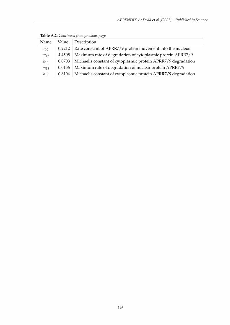
APPENDIX A: Dodd et al.,(2007) – Published in Science
Table A.2: Continued from previous page
Name Value Description
r10 0.2212 Rate constant of APRR7/9 protein movement into the nucleusm17 4.4505 Maximum rate of degradation of cytoplasmic protein APRR7/9k15 0.0703 Michaelis constant of cytoplasmic protein APRR7/9 degradationm18 0.0156 Maximum rate of degradation of nuclear protein APRR7/9k16 0.6104 Michaelis constant of cytoplasmic protein APRR7/9 degradation
193

APPENDIX B
Dodd et al., (2007) – Published in Science
194

BMAL1-NPAS2–dependent transcription activa-tion (19–21) while enhancing Rev-erba–mediatedtranscription repression, providing a potentialmeans of maintaining the amplitude of circadianrhythms.
Expression of the gene encoding ALAS1,the rate-limiting enzyme in heme biosynthesis,increased in response to peroxisome proliferatoractivated receptor coactivator–1a (29), a regu-lator of mitochondriogenesis that increases fluxthrough the Krebs cycle (30). This first and rate-limiting enzyme in heme biosynthesis requiressuccincyl CoA, a Krebs cycle intermediate(17, 29). Gluconeogenesis competes with theKrebs cycle for metabolic intermediates whosedepletion compromises heme biosynthesis as wellas mitochondrial oxidative metabolism (fig. S13).The ability of Rev-erba to function as a receptorfor heme could provide a general mechanismfor coordinating these processes.
References and Notes1. F. Gachon, E. Nagoshi, S. A. Brown, J. Ripperger, U. Schibler,
Chromosoma 113, 103 (2004).2. S. M. Reppert, D. R. Weaver, Annu. Rev. Physiol. 63, 647
(2001).3. P. L. Lowrey, J. S. Takahashi, Annu. Rev. Genomics
Hum. Genet. 5, 407 (2004).4. A. Kohsaka, J. Bass, Trends Endocrinol. Metab. 18, 4 (2007).
5. M. Stratmann, U. Schibler, J. Biol. Rhythms 21, 494 (2006).6. M. Akashi, T. Takumi, Nat. Struct. Mol. Biol. 12, 441 (2005).
7. N. Preitner et al., Cell 110, 251 (2002).8. T. K. Sato et al., Neuron 43, 527 (2004).9. L. Yin, M. A. Lazar, Mol. Endocrinol. 19, 1452 (2005).
10. M. F. Ceriani et al., J. Neurosci. 22, 9305 (2002).11. K. Oishi et al., J. Biol. Chem. 278, 41519 (2003).12. S. Panda et al., Cell 109, 307 (2002).13. K. Oishi et al., FEBS Lett. 580, 127 (2006).14. R. D. Rudic et al., PLoS Biol. 2, e377 (2004).15. F. W. Turek et al., Science 308, 1043 (2005); published
online 21 April 2005 (10.1126/science.1108750).16. H. Atamna, Ageing Res. Rev. 3, 303 (2004).17. P. Ponka, Am. J. Med. Sci. 318, 241 (1999).18. A. S. Tsiftsoglou, A. I. Tsamadou, L. C. Papadopoulou,
Pharmacol. Ther. 111, 327 (2006).19. E. M. Dioum et al., Science 298, 2385 (2002); published
online 20 November 2002 (10.1126/science.1078456).20. K. Kaasik, C. C. Lee, Nature 430, 467 (2004).21. D. Boehning, S. H. Snyder, Science 298, 2339
(2002).22. E. de Rosny et al., Biochemistry 45, 9727 (2006).23. J. Reinking et al., Cell 122, 195 (2005).24. S. Sassa, A. Kappas, J. Clin. Investig. 71, 625 (1983).25. Y. Zhu, T. Hon, W. Ye, L. Zhang, Cell Growth Differ. 13,
431 (2002).26. J. A. Ripperger, Chronobiol. Int. 23, 135 (2006).27. G. Adelmant, A. Begue, D. Stehelin, V. Laudet, Proc. Natl.
Acad. Sci. U.S.A. 93, 3553 (1996).28. L. Yin, J. Wang, P. S. Klein, M. A. Lazar, Science 311,
1002 (2006).29. C. Handschin et al., Cell 122, 505 (2005).30. S. C. Burgess et al., J. Biol. Chem. 281, 19000 (2006).31. We thank R. Gampe, D. Steger, T. Stanley, M. Walker,
J. Williams, and T. Willson for helpful discussions. Thiswork was supported by National Institute of Diabetesand Digestive and Kidney Diseases grant R01 DK45586(M.A.L.).
Supporting Online Materialwww.sciencemag.org/cgi/content/full/1150179/DC1Materials and MethodsFigs. S1 to S13References
6 September 2007; accepted 28 September 2007Published online 15 November 2007;10.1126/science.1150179Include this information when citing this paper.
The Arabidopsis CircadianClock Incorporates acADPR-Based Feedback LoopAntony N. Dodd,1 Michael J. Gardner,1 Carlos T. Hotta,1 Katharine E. Hubbard,1Neil Dalchau,1 John Love,1* Jean-Maurice Assie,1 Fiona C. Robertson,1 Mia Kyed Jakobsen,1†Jorge Gonçalves,2 Dale Sanders,3 Alex A. R. Webb1‡Transcriptional feedback loops are a feature of circadian clocks in both animals and plants.We show that the plant circadian clock also incorporates the cytosolic signaling molecule cyclicadenosine diphosphate ribose (cADPR). cADPR modulates the circadian oscillator’s transcriptionalfeedback loops and drives circadian oscillations of Ca2+ release. The effects of antagonists ofcADPR signaling, manipulation of cADPR synthesis, and mathematical simulation of the interactionof cADPR with the circadian clock indicate that cADPR forms a feedback loop within the plantcircadian clock.
Circadian clocks are adaptations to thedaily rotation of the planet. In plants andcyanobacteria, benefits occur when the
clock is resonant with the environment (1–3).This requires the oscillator to be robust yet flex-
ible, which may explain the evolution of molec-ular clocks with multiple feedback loops (4–6).We tested the hypothesis that plant circadian os-cillators also incorporate cytosolic signaling mol-ecules because there are circadian rhythms in the
Fig. 5. Suppression of the expression of gluconeogenic genes and glucose production in liver cellstreated with hemin. (A) Expression of G6Pase and PEPCK genes in HepG2 cells treated with eitherDMSO or hemin (6 mM) for 6 hours. Amounts of mRNA were quantitated by RT-PCR and normalized tocyclophilin. Mean ± SD of three independent experiments is shown. *P < 0.05 compared with control byStudent’s t test. (B) Expression of G6Pase gene in HepG2 cells treated with control or ALAS1-targetingsiRNA and then stimulated with DMSO or hemin for 16 hours. Mean ± SD (n = 3),*P < 0.05 comparedwith siRNA control treated with DMSO. (C) Effect of hemin on the expression of G6Pase gene in cellsdepleted of Rev-erba. Mean ± SD (n = 3), *P <0.05 compared with DMSO-treated cells transfected withcontrol siRNA. Pound symbol indicates P < 0.05 compared with DMSO-treated cells transfected withcontrol siRNA. (D) Effect of hemin on the occupancy of Rev-erba, HDAC3, NCoR, or acetylated H3 (Ac-H3)at the G6Pase promoter in cells. Results of hemin-treatment are normalized to DMSO results. Mean ±SD (n = 4). *P < 0.05 compared with control. (E) Primary mouse hepatocytes were treated withdexamethasone and 8-(4-chlorophenyl-thio)-adenosine 3!,5!-cyclic monophosphate along with DMSO orhemin for 16 hours, then glucose in the medium was measured. Mean ± SD of triplicate samples isshown, and four independent experiments gave similar results. *P < 0.05 compared with control.
www.sciencemag.org SCIENCE VOL 318 14 DECEMBER 2007 1789
REPORTS
on
Mar
ch 1
0, 2
008
www.
scie
ncem
ag.o
rgDo
wnlo
aded
from

concentration of cytosolic free Ca2+ ([Ca2+]cyt)(7, 8). We investigated the function within theplant circadian system of cyclic adenosine di-phosphate ribose (cADPR), a cytosolic ligandthat promotes the release of Ca2+ into the cytosolfrom internal stores through cation channels (9).
To identify potential interactions betweenplant circadian and Ca2+ signaling pathways, weexamined the overlap between a circadian tran-scriptome and transcriptomes for known regu-lators of [Ca2+]cyt (table S1) (10). We obtained anew near whole-genome transcriptome in con-stant light (LL) under conditions allowing cir-cadian [Ca2+]cyt oscillations (10, 11). This wasnecessary because previous circadian transcriptanalyses used plants grown on 3% sucrose(12, 13), which abolishes circadian [Ca2+]cytoscillations (7). On the basis of a threshold mul-tiple measures–corrected probability of rhythmic-ity (pMMC) of 0.15, 2282 (12.08%) transcriptswere circadian-regulated (spreadsheet S1 andfig. S1) (12, 14).
A cADPR-regulated transcript set (15) hadthe most statistically significant overlap withour circadian transcriptome [(Fig. 1A and tableS1) P = 5.15 ! 10–52]. The overlap was signif-icantly larger than the 93 transcripts expectedfor a chance overlap of two similarly sized data-sets selected randomly from the Arabidopsis ge-nome. We noted that 252 transcripts were bothcircadian- and cADPR-regulated (Fig. 1A andspreadsheet S2). There was a phase relationbetween circadian- and cADPR-regulation of tran-script abundance: The majority of cADPR–up-regulated rhythmic transcripts reached peakabundance at zeitgeber time (ZT) ZT8 or ZT12,and the majority of cADPR-repressed rhythmictranscripts reached peak abundance betweenZT20 and ZT4 (Fig. 1B).
Because a phase relation existed betweencircadian- and cADPR-regulated genes and thecircadian-regulated evening element was signif-icantly overrepresented in cADPR–up-regulatedgenes (spreadsheet S3), we reasoned that cADPRsignaling might be circadian-regulated (12, 15).We measured [cADPR] in extracts of aerial tis-sues of seedlings in LL (10). [cADPR] wascircadian-regulated, because [cADPR] was sig-nificantly higher during subjective light (mean ±SEM, 0.27 ± 0.04 pmol ! µg protein–1) thansubjective dark (0.16 ± 0.02 pmol ! µg protein–1)(Fig. 2, A and B, and fig. S2), [cADPR] var-iations persisted through the second and thirddays of LL and were eliminated in plants over-
expressing CIRCADIAN CLOCK ASSOCIATED1(CCA1-ox) (Fig. 2A). CCA1-ox abolishes allknown plant circadian rhythms (2, 16).
We tested whether circadian [cADPR] varia-tions cause circadian rhythms of [Ca2+]cyt. UnderLL, we monitored [Ca2+]cyt in seedlings treatedevery 3 hours with Ca2+ signaling antagonists(Fig. 2, C and D). Nicotinamide (10 mM) re-duced the amplitude of the [Ca2+]cyt oscillation,and 50 mM nicotinamide abolished the oscilla-tion (Fig. 2C) (10). Nicotinamide is an antago-nist of cADPR signaling that, at 50 mM, inhibitsthe synthesis of cADPR from NAD+ by aden-osine diphosphate ribosyl cyclase (ADPRc) (17).Circadian [Ca2+]cyt oscillations were unaltered byGdCl3, which inhibits extracellular Ca2+ influx(18) (Fig. 2D), and the phospholipase C (PLC)inhibitor U73122, which inhibits production ofinositol 1,4,5-trisphosphate (IP3) at 1 µM (19)(Fig. 2D). Arabidopsis ADPRc activity (10, 20)was inhibited in vitro by 40 mM nicotinamide(fig. S3), which suggests that nicotinamide pre-vents cADPR synthesis in plants. Because 50 mMnicotinamide abolished circadian [Ca2+]cyt oscil-lations, and circadian [cADPR] and [Ca2+]cyt al-terations had a similar phase, circadian cADPRoscillations are likely to drive circadian [Ca2+]cytrhythms.
Several genes encoding components of thecircadian clock are cADPR-regulated (15).GIGANTEA (GI), CRYPTOCHROME2 (CRY2),GLYCINE-RICH BINDING PROTEIN7 (GRP7),GRP8, and PSEUDO-RESPONSE REGU-LATOR5 (PRR5) and PRR7 are cADPR–up-regulated, and LATE ELONGATED HYPOCOT-YL (LHY) and CCA1 are down-regulated. TIMINGOF CHLOROPHYLL A/B BINDING PROTEIN(TOC1) is unaffected (spreadsheet S2) (15). Tounderstand how circadian function might be af-fected by cADPR-induced changes in transcriptabundance, we performed a simulation using apreviously described mathematical model (21).In that model, 13 equations define an approxi-mation for the Arabidopsis circadian oscillator.We controlled the parameters of this model toconstrain CCA1/LHY, GI, and TOC1 transcriptsto adopt the fold-changes that are caused bycADPR in plants (figs. S4 and S5) (10, 15). First,we constrained the parameters transiently, be-cause increasing cADPR synthesis by inducingthe Aplysia ADPR cyclase gene, fused to a b-estradiol–inducible promoter (XVE:ADPRc),causes transient alterations in clock transcriptsalthough [cADPR] remains elevated (15).Depending on the parameters that were con-strained, there was a short disruption to themodeled oscillator that sometimes caused phasechanges, but the period remained 24 hours (Fig.3A and fig. S5C). Next, we constrained the pa-rameters continuously to evaluate the effects ofcontinuous cADPR-induced alteration in clocktranscripts. Depending on the parameters that wereconstrained, the circadian period often changedand remained altered throughout the simulation(Fig. 3B). Finally, we inverted the permanent con-
straint of the parameters to understand the pos-sible effects of removal of cADPR-regulation ofclock transcripts. Most of the parameters that didnot lead to arrhythmia caused the simulations torun with a longer period (Fig. 3C). Thesesimulated outcomes provided a framework withwhich to interpret the effects of cADPR on theplant circadian clock.
We experimentally tested how transient[cADPR]-induced alterations in circadian clocktranscripts affect circadian behavior. We elevated[cADPR] in two independent lines by inducingthe XVE:ADPRc transgene (15) with 100 µMb-estradiol. [cADPR] increased 13.5-fold (line 1)and 27-fold (line 2) relative to controls (fig. S6).The circadian period and phase of leaf positionwere unaltered when XVE:ADPRc was inducedat ZT2 under LL (Fig. 4A and fig. S7, A, B, andG), or at two times during the final LD cyclebefore LL (fig. S7, C to G). Circadian [Ca2+]cytoscillations were unaltered by XVE:ADPRc in-duction (Fig. 4B). The invariance of circadianperiod may be explained by the simulatedevidence that transient cADPR-induced alterationsin oscillator transcripts do not alter circadianperiod. This invariance also reveals remarkablestability of the oscillator.
We investigated whether continuous [cADPR]synthesis alters circadian behavior. We over-expressed Aplysia ADPRc using the constitutive35S promoter (35S:ADPRc) (10). This approx-imately doubled [cADPR] [0.38 ± 0.09 pmol !µg protein–1 (line 1); 0.45 ± 0.13 pmol ! µg
1Department of Plant Sciences, University of Cambridge,Downing Street, Cambridge CB2 3EA, UK. 2Department ofEngineering, University of Cambridge, Trumpington Street,Cambridge CB2 1PZ, UK. 3Department of Biology, Universityof York, York YO10 5YW, UK.
*Present address: School of Biosciences, Geoffrey PopeBuilding, University of Exeter EX4 4QD, UK.†Present address: Institute for Plant Biology, CopenhagenUniversity, Thorvaldsensvej 40, 1871 Frederiksberg, Denmark.‡To whom correspondence should be addressed. E-mail:[email protected]
Fig. 1. Circadian- and cADPR-regulated transcriptsoverlap significantly. (A) The numbers of circadian-and cADPR-regulated transcripts (15), and thenumber common to both transcriptomes. (B) Theproportion of circadian-regulated transcripts thatwere cADPR-regulated, binned according to thecircadian peak of abundance.
14 DECEMBER 2007 VOL 318 SCIENCE www.sciencemag.org1790
REPORTS
on
Mar
ch 1
0, 2
008
www.
scie
ncem
ag.o
rgDo
wnlo
aded
from

protein–1 (line 2), 0.23 ± 0.05 pmol ! µgprotein–1 (wild type); n = 5]. [cADPR] was notmeasured over a circadian time course becauseof poor 35S:ADPRc plant growth, which was
consistent with a lesion to stress and circadi-an signaling (2, 3). The mean period of circa-dian rhythms in leaf position was unaltered in35S:ADPRc [P = 0.51 by two-sample t test
(fig. S8, A and B)]. However, there was a broaderperiod length distribution comparedwith the wildtype when all replicates with all lines were con-sidered, as indicated by both the spread and sig-nificantly different standard deviation [(Fig. 4C)Ws-2 wild type: SD = 0.71 hours, spread = 22.3to 25.8 hours, n = 45; 35S:ADPRc: SD = 0.96hours, spread = 21.9 to 26.3 hours, n = 106; testof homogeneity of variances Levene statistic =5.81, P = 0.017**]. ADPRc overexpression dis-turbed the sinusoidal circadian [Ca2+]cyt oscilla-tions (fig. S9) and increased the relative amplitudeerror (RAE) (22) of the oscillations [(Fig. 4D)wild-type RAE, 0.28 ± 0.02; line 1, 0.42 ± 0.03;line 2, 0.55 ± 0.06]. The greater RAE indicated apoorer Fourier fit to the data. Because [Ca2+]cytimages were obtained from groups of 15 to 20seedlings (23), the increased RAE of circadian[Ca2+]cyt oscillations could reflect increasedvariability of the [Ca2+]cyt oscillation period be-tween individuals. The simulations suggested thatoscillator period is affected by high [cADPR](Fig. 3B). We found that 35S:ADPRc affectedoscillator period by increasing variability, whichmight be a consequence of differing levels ofcADPR between seedlings and cells having dif-ferent effects on period.
Finally, we investigated how continuously sup-pressed cADPR signaling affected the clock bytreating seedlings with nicotinamide. The circadianperiod of rhythms of leaf position was significant-ly longer with 10 mM or 50 mM nicotinamidecompared with water and osmotic controls. Theperiod increase was nicotinamide concentration–dependent [(Fig. 4, E and F, and table S2)control period 23.6 ± 0.3 hours; 10 mM nic-otinamide, 24.5 ± 0.3 hours, P < 0.001; 50 mMnicotinamide, 26.6 ± 0.4 hours, P = 0.002;comparisons by two-sample t tests]. Circadianrhythms of leaf position were unaltered by otherchemical modifiers of Ca2+ signaling [CaCl2,GdCl3, LaCl3, EGTA, or U73122 (table S2)]. At50 mM, nicotinamide also lengthened circadianperiod of CAB2:luciferase luminescence [nico-tinamide, 25.3 ± 0.4 hours; 50 mM mannitol,26.6 ± 0.5 hours (Fig. 4G and fig. S10)], the
Fig. 2. [cADPR] oscillates with a circadian rhythm and a cADPR signaling antagonist inhibitscircadian [Ca2+]cyt oscillations. (A) [cADPR] during 48 hours of constant light in Col-0 wild type andarrhythmic CCA1-ox (n = 5; ± SEM). Seedlings were transferred to LL 24 hours before sampling. (B)Data from (A) binned according to subjective day and night, P values from two-sample t testsindicated. (C and D) Circadian [Ca2+]cyt oscillations in 11-day-old seedlings dosed every 3 hourswith (C) nicotinamide, mannitol (osmotic control), or water; (D) GdCl3 and U73122. n = 12;greatest SEM for each panel at top right. On x axes are black bars, darkness; white bars, light,hatched bars, subjective dark under LL.
Fig. 3. Constraint of a mathematicalmodel for the Arabidopsis circadianclock (21) to explore how cADPR-induced alterations in CCA1/LHY, GI,and TOC1 transcript abundance alterclock function. (A) Transient constraintof model parameters to impose cADPR-induced alterations in clock tran-script abundance caused variable phasechanges that depended on parametersconstrained. (B and C) For uniform pa-rameter constraints analogous to contin-uous cADPR signaling (B) and repression(C), the period changed by a magni-tude that depended on the parameters constrained. (A to C) Each pointrepresents a different parameter pair that correctly constrained simulatedtranscripts when cADPR synthesis was induced between ZT20 to 6 or ZT20 to24 (crosses) and ZT11 to 19 (circles); explained in fig. S5B. Broken lines
indicate period or phase of unperturbed simulated oscillator. Phase andperiod calculated after simulated 480 hours in LL; arrhythmic simulationsexcluded from plots because perturbation of cADPR signals in plants (Fig. 4)did not cause arrhythmia.
www.sciencemag.org SCIENCE VOL 318 14 DECEMBER 2007 1791
REPORTS
on
Mar
ch 1
0, 2
008
www.
scie
ncem
ag.o
rgDo
wnlo
aded
from

period of CAB2 transcript abundance [(Fig. 4H)50 mM nicotinamide, 26.0 hours; H2O control,23.3 hours; 50 mM mannitol, 22.3 hours], andCCA1, TOC1, and LHY transcript abundance(Fig. 4H) (10). Inhibition of cADPR synthesis,
therefore, lengthened the period of the clock andits outputs.
Our data demonstrate the existence of afeedback loop within the plant circadian clockthat incorporates cADPR, because [cADPR] is
regulated by the circadian oscillator and cADPR,in turn, regulates the abundance of clock gene tran-scripts. Circadian oscillations in [cADPR] alsoregulate circadian [Ca2+]cyt oscillations. It hasbeen suggested that diurnal variations in [Ca2+]cytare regulated by the Ca2+ sensor CAS throughan IP3-mediated system (24). Our data indicatethat IP3 does not contribute to the control of cir-cadian [Ca2+]cyt oscillations (Fig. 2D). Thecircadian feedback loop incorporating cADPRmay interface the clock with exogenous stimulithat transiently elevate intracellular [cADPR] and[Ca2+]cyt and so optimize the adaptive value ofcircadian control during unpredictable short-termenvironmental variations. We have established thatcytosolic signaling molecules represent a hithertounrecognized class of circadian clock components.
References and Notes1. Y. Ouyang, C. R. Andersson, T. Kondo, S. S. Golden,
C. H. Johnson, Proc. Natl. Acad. Sci. U.S.A. 95, 8660 (1998).2. A. N. Dodd et al., Science 309, 630 (2005).3. R. M. Green, S. Tingay, Z. Y. Wang, E. M. Tobin,
Plant Physiol. 129, 576 (2002).4. D. A. Rand, B. V. Shulgin, J. D. Salazar, A. J. Millar,
J. Theor. Biol. 238, 616 (2006).5. S. Panda, J. B. Hogenesch, S. A. Kay, Nature 417, 329
(2002).6. D. Alabadí et al., Science 293, 880 (2001).7. C. H. Johnson et al., Science 269, 1863 (1995).8. M. Ikeda et al., Neuron 38, 253 (2003).9. G. J. Allen, S. R. Muir, D. Sanders, Science 268, 735 (1995).
10. Materials and methods are available on Science Online.11. Microarray data deposited at ArrayExpress (www.ebi.ac.
uk/arrayexpress/), accession E-TABM-331.12. S. L. Harmer et al., Science 290, 2110 (2000).13. K. D. Edwards et al., Plant Cell 18, 639 (2006).14. M. Straume, Methods Enzymol. 383, 149 (2004).15. J. P. Sánchez, P. Duque, N. H. Chua, Plant J. 38, 381 (2004).16. Z. Y. Wang, E. M. Tobin, Cell 93, 1207 (1998).17. J. K. Sethi, R. M. Empson, A. Galione, Biochem. J. 319,
613 (1996).18. A. A. Véry, J. M. Davies, Proc. Natl. Acad. Sci. U.S.A. 97,
9801 (2000).19. I. Staxén et al., Proc. Natl. Acad. Sci. U.S.A. 96, 1779 (1999).20. R. M. Graeff, T. F. Walseth, K. Fryxell, W. D. Branton,
H. C. Lee, J. Biol. Chem. 269, 30260 (1994).21. J. C. Locke et al., Mol. Syst. Biol. 1, E9 (2005).22. J. D. Plautz et al., J. Biol. Rhythms 12, 204 (1997).23. J. Love, A. N. Dodd, A. A. R. Webb, Plant Cell 16, 956
(2004).24. R. H. Tang et al., Science 315, 1423 (2007).25. The authors thank N.-H. Chua for inducible XVE:ADPRc
lines; H. Okamoto, S. Takasawa, H.-C. Lee, and R. Graefffor Aplysia ADPRc; H.-C. Lee, R. Graeff, E. Zocchi, andS. Bruzzone for advice; B. Handley for programmingassistance; and J. C. Gray, E. A. C. MacRobbie, and J. Carrfor critical reading. Research funded by the U.K.Biotechnology and Biological Sciences Research Council(BBSRC), the Royal Society of London, the BroodbankFoundation Cambridge, the Gates Foundation, CorpusChristi College Cambridge, Coordenação deAperfeiçoamento de Pessoal de Nível Superior (CAPES)Brazil, and the Danish Research Council.
Supporting Online Materialwww.sciencemag.org/cgi/content/full/1146757/DC1Materials and MethodsFigs. S1 to S10Tables S1 to S2ReferencesSpreadsheets S1 to S3
20 June 2007; accepted 27 September 2007Published online 15 November 2007;10.1126/science.1146757Include this information when citing this paper.
Fig. 4. The circadian clock and its outputs are altered by continuous disruption of cADPR signaling. (Aand B) XVE:ADPRc induction at ZT2 on day 1 of LL, (A) circadian rhythm of leaf position (n = 30 to 32)and (B) analysis of circadian [Ca2+]cyt oscillations; P values from two-sample t test comparisons of periodto control are indicated and were not significant. Relative amplitude error quantifies the rhythmicrobustness (0 is sine wave and 1 is poor Fourier fit; n = 4; mean ± SEM). In (A), black is 100 mM b-estradiol (XVE inducer), gray is empty vector control (P = 0.38 in two-sample t test period comparisonwith induced plants), broken line, 0.1% DMSO solvent control (P = 0.32). (C and D) In 35S:ADPRc, (C)distribution of period lengths of circadian rhythms of leaf position for all replicates and both lines; (D)analysis of circadian [Ca2+]cyt oscillations for 35S:ADPRc line 1, line 2, and Ws-2 wild type. (E) Circadianrhythm of leaf position of seedlings treated at ZT2 with a single dose of 50 mM nicotinamide or 50 mMmannitol (n = 46). (F) Time of circadian peaks of leaf position in seedlings treated as for (E) (n = 5 to26). (G) Circadian rhythm of CAB2:luciferase luminescence in seedlings dosed every 3 hours with 50 mMnicotinamide (mannitol control shown for clarity). (H) Circadian period of CAB2 (triangles), TOC1(circles), LHY (squares), and CCA1 (diamonds) transcript abundance in seedlings dosed every 3 hours with50 mM nicotinamide. (E to H) Treatment designations: open is H2O control; gray is mannitol control;black is nicotinamide. For comparability with (E and F), alterations in circadian rhythms of [Ca2+]cyt andCAB2 promoter activity after single doses of 50 mM nicotinamide are in fig. S10.
14 DECEMBER 2007 VOL 318 SCIENCE www.sciencemag.org1792
REPORTS
on
Mar
ch 1
0, 2
008
www.
scie
ncem
ag.o
rgDo
wnlo
aded
from

Supporting Online Material Dodd et al.
1
Supporting Figures
Supporting Fig. S1. Verification of microarray analysis by comparison of the
multiple measures-corrected probability statistic of rhythmicity (pMMC) of selected
array transcripts with RT-PCR analysis on the same mRNA samples.
RT-PCR pMMC
0.00 0.04 0.08 0.12 0.16
Mic
roarr
ay p
MM
C
0.00
0.04
0.08
0.12
CAB2
TOC1
PRR9 CCA1
GI
r = 0.94

Supporting Online Material Dodd et al.
2
Time in constant light (h)
24 36 48 60 72
[cA
DP
R] pm
ol µ
g p
rote
in-1
0.0
0.2
0.4
0.6
0.8
1.0
1.2
Supporting Fig. S2. Circadian oscillations of [cADPR] measured in an identical but
independent experiment from Fig. 2A. [cADPR] during 48 h of constant light in Col-0
wild type (n = 5; ± s.e.m.), measured using a coupled cycling assay (described in this
Supporting Material). Tissue was from seedlings germinated/grown on 0.5 x MS,
0.8 % (w/v) agar for 3 weeks under 12 h light, 12 h dark and transferred to continuous
light 24 h before sampling.

Supporting Online Material Dodd et al.
3
[nicotinamide] (mM)
0 20 40 60 80
Extr
acta
ble
AD
PR
cycla
se
activity
(flu
ore
sce
nce
un
its m
in-1
)
-0.01
0.00
0.01
0.02
0.03
0.04
0.05
Supporting Fig. S3. Nicotinamide inhibits ADPRc activity from Arabidopsis tissue
extracts, in vitro. ADPRc activity was measured by monitoring ADPRc-mediated
synthesis of fluorescent cyclic GDP-ribose from nicotinamide guanine dinucleotide
(1) (n = 5; ± s.e.m.).

Supporting Online Material Dodd et al.
4
Sim
ula
ted [L
HY
] m
RN
A(n
M)
0.0
0.2
0.4
0.6
0.8
1.0
1.2
1.4
Unpertubed simulated mRNA concentration
Perturbed simulated mRNA concentration
Time (h)
0 8 16 24 32 40 48
[Y] m
RN
A (
nM
)
0.00
0.05
0.10
0.15
[LH
Y] m
RN
A (
nM
)
0.0
0.2
0.4
0.6
0.8
1.0
1.2
Unperturbed simulated mRNA concentration
Simulated transcript mRNA concentration
ALHY mRNA
Y mRNA
B
Simulated time (h)
-48 -24 0 24 48 72 96 120
Sim
ula
ted
[Y
] m
RN
A (
nM
)
0.00
0.04
0.08
0.12
0.16
Simulated time (h)
-48 -24 0 24 48 72 96 120
Sim
ula
ted
[Y
] m
RN
A (
nM
)
0.00
0.04
0.08
0.12
0.16
Sim
ula
ted [L
HY
] m
RN
A(n
M)
0.0
0.2
0.4
0.6
0.8
1.0
1.2
1.416 h peak exponentialperturbation
20 h peak exponentialperturbation
Supporting Fig. S4. Examples of estimation and simulation of cADPR-induced
alterations to a model (2) of the circadian clock. A, Under 16 h light / 8 h dark,
estimation of cADPR-induced (3) alterations in LHY and Y (GI) transcript abundance,
for the parameter pair with the lowest error norm (goodness-of-fit of simulated to real
data). This best fit was a perturbation that commenced at ZT13 and peaked 6 h later.
B, For exponential perturbation profiles that commenced at 0 h and peaked at 16 h or
20 h, simulated oscillations in LHY and Y mRNA concentration for perturbation of the
parameter pair with the lowest error norm.

Supporting Online Material Dodd et al.
5
Simulated time (h)
-48 -24 0 24 48 72 96 120144
Am
plit
ude
0.0
0.2
0.4
0.6
0.8
1.0
1.2
6 h peak exponential perturbation
16 h peak exponential perturbation
20 h peak exponential perturbation
Step perturbation ppp δ+=ˆ
A
Sim
ula
ted [
LH
Y]
mR
NA
(nM
)
0.0
0.2
0.4
0.6
0.8
1.0
1.2
1.4
Unpertubed
Perturbed
Simulated time (h)
-48 -24 0 24 48 72 96 120
Sim
ula
ted [Y
mR
NA
] (n
M)
0.00
0.04
0.08
0.12
0.16 Unperturbed
Perturbed
C
B
Time of peak of perturbation (ZT, h)0 6 12 18 24
Fre
quency
of
para
mete
r pairs
with e
rror
norm
< 2
0
500
1000
1500
2000
2500B
A A
Supporting Fig. S5. Systematic perturbation of a mathematical model for the
Arabidopsis circadian oscillator (2), to investigate how cADPR-mediated changes in
clock transcript abundance alter clock function. A, parameter perturbation profiles
used to simulate changes in cADPR signal magnitude ( ppp δ−=ˆ profile for cADPR
pathway suppression not shown). B, The number of perturbed parameter-pairs leading
to changes in clock transcript abundance with error norm < 2 depended on time of
induction, and separated into two clusters (marked A and B). C, Simulated
oscillations in [LHY] and [Y] mRNA for perturbation of the parameter pair with
lowest error norm, for an exponential (transient) perturbation profile that commenced
at 0 h and peaked at 6 h. Note the period invariance. Error norm is the goodness-of-fit
of simulated to real data (3). cADPR-induced changes in oscillator transcript
abundance: lower values indicate a closer match. Black bars on abscissa indicate
darkness, white bars: light, hatched: subjective dark under LL.
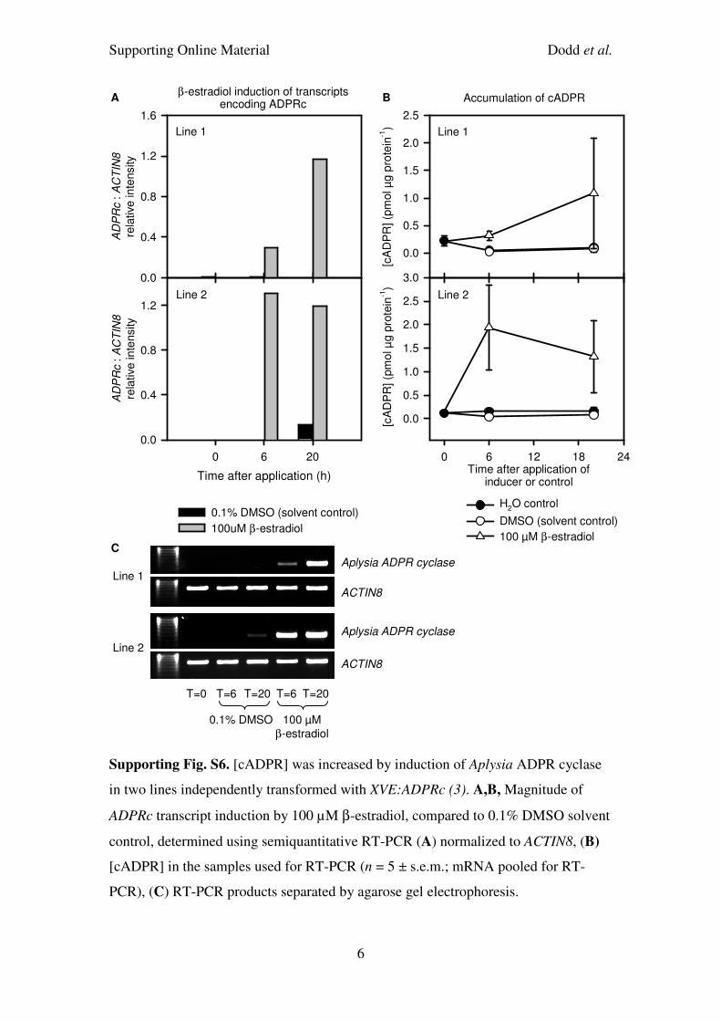
Supporting Online Material Dodd et al.
6
Time after application ofinducer or control
0 6 12 18 24
[cA
DP
R] (p
mo
l µ
g p
rote
in-1
)
0.0
0.5
1.0
1.5
2.0
2.5
3.0
H2O control
DMSO (solvent control)
100 µM β-estradiol
[cA
DP
R] (p
mol µ
g p
rote
in-1
)
0.0
0.5
1.0
1.5
2.0
2.5
Line 1
Line 2
Accumulation of cADPRβ-estradiol induction of transcripts
encoding ADPRcA B
Line 1
AD
PR
c : A
CT
IN8
rela
tive
in
tensity
0.0
0.4
0.8
1.2
1.6
Line 2
Time after application (h)
0 6 20
AD
PR
c : A
CT
IN8
rela
tive
in
tensity
0.0
0.4
0.8
1.2
0.1% DMSO (solvent control)
100uM β-estradiol
T=0 T=6 T=20 T=6 T=20
0.1% DMSO 100 µM
β-estradiol
Aplysia ADPR cyclase
ACTIN8
Aplysia ADPR cyclase
ACTIN8
Line 1
Line 2
C
Supporting Fig. S6. [cADPR] was increased by induction of Aplysia ADPR cyclase
in two lines independently transformed with XVE:ADPRc (3). A,B, Magnitude of
ADPRc transcript induction by 100 µM β-estradiol, compared to 0.1% DMSO solvent
control, determined using semiquantitative RT-PCR (A) normalized to ACTIN8, (B)
[cADPR] in the samples used for RT-PCR (n = 5 ± s.e.m.; mRNA pooled for RT-
PCR), (C) RT-PCR products separated by agarose gel electrophoresis.

Supporting Online Material Dodd et al.
7
A B
Period estimate (h)20 22 24 26 28 30 32
Rela
tive
am
plit
ude
err
or
0.0
0.2
0.4
0.6
Period estimate (h)20 22 24 26 28 30 32
Rela
tive
am
plit
ude
err
or
0.0
0.2
0.4
0.6
Period estimate (h)
22 24 26 28 30 32
Rela
tive a
mplit
ude
err
or
0.0
0.2
0.4
0.6
Time of maximum leaf height (h)0 4 8 12 16
peak1
peak2
peak3
peak4
peak5
peak6
Time of maximum leaf height (h)
0 4 8 12 16
peak1
peak2
peak3
peak4
peak5
peak6
Time of maximum leaf height (h)0 4 8 12 16
peak2
peak3
peak4
peak5
peak6
Empty vector (control), 100 µM β-estradiol
XVE:ADPRc, 0.1% DMSO control
XVE:ADPRc, 100 µM β-estradiol
C D
E F
Induced under LL, ZT2Induced under LL, ZT2
Induced under LD, ZT2 Induced under LD, ZT2
Induced under LD, ZT8 Induced under LD, ZT8
Aplysia ADPR cyclase
ACTIN8
G
+++ –––
ZT2 LD ZT2 LLZT8 LD
Supporting Fig. S7. Circadian rhythms of leaf position were unaltered by induction
of Aplysia ADPR cyclase (3). Seedlings transformed with XVE:ADPRc or
XVE:[Empty vector] were dosed with 100 µM β-estradiol or 0.1% DMSO solvent
control A,B, two hours after the onset of constant light, C,D, two hours or E,F, six
hours after dawn on the final light-dark cycle before transfer to continuous light.

Supporting Online Material Dodd et al.
8
Time-lapse imaging commenced 24 h after β-estradiol application. A,C,E, Variation
in period estimates in rhythmic replicate seedlings (n = 5 – 13). B,D,F, Time of
circadian peak of leaf position for each 24 h period (n = 5 – 16; mean ± s.e.m.). G,
ADPRc transcripts were verified by semiquantitative RT-PCR to have been induced in
representative seedlings used to monitor leaf position for each induction time. The
induction time (ZT), and whether induction occurred under the final light-dark cycle
before constant light (LD) or on Day 1 of constant light (LL), is indicated above the
gel. Identical samples were either induced with 100 µM β-estradiol or treated as a
control with 0.1 % DMSO (+ and – below gel, respectively).

Supporting Online Material Dodd et al.
9
Time in continuous light (h)
0 24 48 72 96 120 144 168 192
Mea
n n
orm
aliz
ed
lea
fpositio
n
0.97
0.98
0.99
1.00
1.01
1.02
Ws-2 wild type
35S:ADPRc line 2
Time in continuous light (h)
0 24 48 72 96 120 144 168 192
Mean n
orm
aliz
ed leaf
positio
n
0.96
0.97
0.98
0.99
1.00
1.01
1.02
Ws-2 wild type
35S:ADPRc line 1
A
B
Supporting Fig. S8. Circadian rhythms of leaf position in two lines (A,B) that
constitutively overexpressed Aplysia ADPR cyclase (35S:ADPRc). n = 52 - 54.

Supporting Online Material Dodd et al.
10
35S:ADPRc Line 2
Time in continuous light (h)
12 24 36 48 60 72 84 96 108
Norm
alized a
equori
nlu
min
escence
0.000
0.001
0.002
0.003
0.004
0.005
35S:ADPRc Line 1
Norm
alized a
equori
nlu
min
escence
0.000
0.001
0.002
0.003
0.004
0.005
0.006
WT
Norm
aliz
ed a
equori
nlu
min
escence
0.000
0.001
0.002
0.003
0.004
0.005
0.006
Supporting Fig. S9. Overexpression of ADP ribosyl cyclase in two independent lines
reduced the robustness of circadian [Ca2+
]cyt oscillations relative to the wild type.
Each trace is the aequorin luminescence from one cluster of 15-20 seedlings (4).
Seedlings were previously entrained for 10 d to cycles of 12 h light and 12 h darkness.
The luminescence signal was normalized to the total aequorin content of the seedling
cluster to compensate for higher aequorin content in Line 2. Total aequorin was
measured by discharging available aequorin using 2 M CaCl2 dissolved in 20 %
ethanol (5).

Supporting Online Material Dodd et al.
11
Time in constant light (h)0 24 48 72 96
CA
B2
:lu
c lum
ine
sce
nce
(pho
ton
s 7
00
s-1
)
0
5000
10000
15000
Time in constant light (h)0 24 48 72 96
Ae
qu
ori
n lu
min
escen
ce
(ph
oto
ns 1
30
0s
-1)
0
1000
2000
3000
50 mM mannitol
50 mM nicotinamide
A
B
[Ca2+
]cyt
CAB2:luciferase
Supporting Fig. S10. Circadian [Ca2+
]cyt oscillations were partially inhibited by
discontinuous application of 50 mM nicotinamide, which caused the circadian
oscillator to adopt a longer period. These data indicate that partial inhibition of
circadian [Ca2+
]cyt oscillations by nicotinamide was sufficient to alter the functioning
of the circadian clock. A, Rhythms of aequorin luminescence had a longer circadian
period and lower amplitude than controls when dosed 48 h and 24 h before constant
light with 50 mM nicotinamide (period estimates: 50 mM nicotinamide, 24.6 ± 0.7 h,
n = 20; 50 mM mannitol, 23.6 ± 0.4 h; n = 8; H2O control, omitted from (A) for
clarity, 23.8 ± 0.4 h; n = 20; period of [Ca2+
]cyt in presence of 50 mM nicotinamide is
significantly different from the other two treatments (one-way ANOVA, p < 0.0001
with Tukey-Kramer post-test, p < 0.001 for both controls). B, Circadian rhythm of
CAB2:luciferase luminescence after single dose of 50 mM nicotinamide at ZT2
(mannitol control shown for clarity; H2O control was comparable; period estimates:
50 mM nicotinamide, 25.7 h ± 0.1 h; H2O control, 24.4 h ± 0.1 h; 50 mM mannitol,
24.7 h ± 0.1 h). A, B Grey circles = 50 mM mannitol, black circles = 50 mM
nicotinamide.

Supporting Online Material Dodd et al.
12
Supporting Tables
Treatment Overlap with circadian Significance Significance
Observed Expected (p-value ) (E-value)
Blue light 145 135 2.38 x 10-02
1.62
Brassinolide (7) 63 41 1.80 x 10-04
3.74
Brassinolide (8) 59 33 8.93 x 10-06
* 5.05
cADPR 252 93 5.15 x 10-52
* 51.28
cGMP 133 100 1.60 x 10-04
3.79
Cold 195 92 1.23 x 10-24
* 23.91
IAA (7) 32 27 5.05 x 10-02
1.29
IAA (8) 51 40 1.64 x 10-02
1.79
LPS 76 48 1.77 x 10-05
4.75
OG 28 26 7.70 x 10-02
1.11
Red light 237 96 6.64 x 10-41
* 40.17
SNAP 75 40 9.50 x 10-08
* 7.02
Supporting Table S1. Comparison of circadian-regulated transcripts to transcripts
regulated by blue light (6), brassinolide (7, 8), cADPR (3), cyclic guanosine
monophosphate (cGMP) (9), cold (10), indole-3-acetic acid (IAA) (7, 8),
lipopolysaccharide (LPS) (11), oligogalcturonide (OG) (12), red light (13) and S-
Nitroso-N-acetylpenicillamine, (SNAP, a nitric oxide donor) (14). Transcripts
regulated by cADPR shared both the greatest numerical overlap and the most
statistically significant overlap with circadian-regulated transcripts. Red light- and
cold-regulated transcripts had large but less significant overlaps with the set of
circadian-regulated transcripts. The threshold for statistical significance was
considered to be p < 1 x 10⁻⁵
, as indicated by single asterisks on the table.

Supporting Online Material Dodd et al.
13
Antagonist H2O control Additional control a
Rhythmic seedlings
(%)
Period (h) ± s.e.m n Rhythmic seedlings
(%)
Period (h) ± s.e.m n Statistical significance
Rhythmic seedlings
(%)
Period (h) ± s.e.m n Statistical significance
10 mM CaCl2 72.9 23.81 ± 0.3 16 66.7 24.09 ± 0.6 14 p=0.68 50 mM EGTA 68.2 24.25 ± 0.4 17 71.7 23.56 ± 0.3 20 p=0.16 65.2 24.19 ± 0.7 16 p=0.94 1 mM GdCl3 62.5 24.18 ± 0.6 13 66.7 24.09 ± 0.6 14 p=0.92 10 mM LaCl3 60.9 24.15 ± 0.6 17 71.7 23.56 ± 0.3 20 p=0.40 80.4 23.83 ± 0.3 15 p=0.65 10 mM nicotinamide
80.4 24.50 ± 0.3 21 71.7 23.56 ± 0.3 20 p=0.03* 80.4 23.83 ± 0.3 15 p=0.12 50 mM nicotinamide
b
65.2 25.60 ± 0.3 21 71.7 23.56 ± 0.2 20 p<0.01** 65.2 24.19 ± 0.6 16 p=0.06 50 mM nicotinamide
b
76.6 26.59 ± 0.4 8 93.8 23.79 ± 0.3 15 p<0.01** 81.3 24.08 ± 0.5 14 p<0.01**
1 µM U73122 87.5 24.90 ± 0.7 12 93.8 23.79 ± 0.2 15 p=0.14 71.9 24.78 ± 0.3 10 p=0.88
a Additional controls for EGTA, LaCl3 and nicotinamide were appropriate concentrations of mannitol; control for U73122 was inactive analogue
of antagonist U73343; control for CaCl2 and GdCl3 was H2O.
b Results from two independent experiments with 50 mM nicotinamide.
Supporting Table S2. Effect of pharmacological modifiers of Ca2+
homeostasis on circadian rhythms of leaf position. Total replicate numbers
and nature of controls specified in table. The pharmacological agents were used modify [Ca2+
]cyt as follows: External CaCl2 causes transient
elevations in [Ca2+
]cyt (15); EGTA reduces the magnitude of stimulus-induced [Ca2+
]cyt transients (16); GdCl3 and LaCl3 inhibit extracellular
Ca2+
influx by blocking plasma membrane ion channels (17); 50 mM nicotinamide inhibits ADP ribosyl cyclase-dependent synthesis of cADPR
(Fig. 2E, (18)); 1 µM U73122 inhibits InsP3 synthesis by phospholipase C (19). p-values are outcome from two-sample t-test comparison of the
period of inhibitor-treated seedlings against controls.

Supporting Online Material Dodd et al.
14
Supporting Materials & Methods
Microarray analysis of mature leaf circadian transcriptome
Arabidopsis thaliana Col-0 seeds were germinated in 48-unit trays containing a 1:1
mix of potting compost and vermiculite. Seeds were stratified at 4 °C for 48 h and
germinated and grown at 20 °C under 12 h light / 12 h dark; 150 µmol photons m-2
s-1
.
Plants were transferred to LL after 26 days growth, and harvesting of leaf material
commenced 48 h after the start of LL. When harvesting began, no incipient
inflorescences were visible within rosettes, rosettes were not senescent, and all aerial
tissue was harvested with the exception of any dead cotyledons. Tissue was
subsequently harvested every 4 h for a 24 h period.
RNA isolation was performed using TRIzol Reagent (Invitrogen, UK). Contaminating
DNA was degraded by 30 min incubation at 37 °C with RQ1 RNase-free DNase 1
(Promega), and RNA purified using an RNeasy column (Qiagen, Germany). Poly(A)+
RNA was isolated from 500 µg total RNA using PolyATract (Promega). RNA was
reverse transcribed (RT) into cDNA with Superscript II RNase H- reverse
transcriptase (Invitrogen), using 2.4 µg DNase-treated total RNA with 1 µg oligo
(dT)12-18 primer and 200 U Superscript II RT, at 42 °C for 50 min. RT was then
inactivated by incubation at 65 °C for 10 min.
Double-stranded cDNA synthesis (20) was performed using 3 µg total RNA and 100
ng anchored Eberwine oligo(dT)21-T7 primer (5′-GCA TTA GCG GCC AAA TTA
ATA CGA CTC ACT ATA GGG AGA T21 V-3′; V = A, C or G). Double-stranded
cDNA was extracted using phase-lock gel heavy tubes (Eppendorf, Germany), and
purified from primers and unincorporated nucleotides using BioGel P-6 microspin
columns (BioRad, USA). cDNA was linearly amplified and labelled with amino-allyl
UTP by in vitro transcription for 5 h at 37°C using the RiboMax™ kit (Promega,
USA). Fluorescent dyes were chemically conjugated onto the amino-allyl labelled
targets (21). Labelled cRNA was purified from unincorporated dyes using Qiagen
RNeasy Cleanup columns (Qiagen, Germany). The appropriate Cy3- and Cy5-
labelled samples were subsequently combined and hydrolysed into 60 - 600 bp
fragments by incubation for 15 min in RNA fragmentation buffer (Ambion, UK).
Oligonucleotide microarrays were obtained from D. Galbraith (Univ. Arizona). To
reduce technical variation, all microarray slides were from a single print batch

Supporting Online Material Dodd et al.
15
(02.07.02.072-110). Circadian analysis was based on a common reference design: all
cRNA samples from plants from 48 h to 72 h in LL were hybridized against the same
reference (48 h) sample. Three biological replicates were used for each time-point.
Labelled cDNA was added to 36 µl preheated (42°C) formamide-based hybridization
buffer (MWG Biotech, Germany) and pipetted onto microarray slides. Slides were
incubated at 42°C for 18 h in a light-proof water bath. Arrays were then washed in
light proof slide boxes: twice for 5 min in 2 x SSC (saline sodium citrate), 0.5% (v/v)
SDS preheated to 55°C, three times for 5 min in 0.5 x SSC at room temperature and
twice for 5 min in 0.05 x SSC at room temperature. 20 x SSC was 3 M sodium
chloride, 0.3 M sodium citrate, pH 7.0.
Slides were scanned (Axon 4000B Scanner, Axon Instruments, USA) and spot finding
performed with GenePix Pro 5 (Axon) using diameters between 10 µm and 20 µm.
Microarray elements were re-annotated using the latest A. thaliana genome
annotations from The Arabidopsis Information Resource (TAIR,
http://www.arabidopsis.org). Data were normalised and microarrays compared using
GeneSpring (Silicon Genetics, USA). Transcripts with circadian rhythms were
identified using a modified version of COSOPT (22, 23), with a period window of 16
- 32 h, and all patterns with multiple measure corrected probability (pMMC) ≤ 0.15
were considered to be circadian regulated and used for further analysis. 18,891
transcripts were consistently detected across the seven timepoints.
Transcriptome comparison and analysis
Circadian-regulated transcripts were placed into groups (bins) according to the
zeitgeber time of their maximal relative abundance. The TAIR IDs of transcripts in
each bin were then compared to those found in the total dataset for cADPR-regulated
transcripts using a custom Python script (http://www.python.org). The absolute
number of transcripts in common in each comparison was expressed as a percentage
of the total number of transcripts in each circadian time bin. We used SIFT (24) to
identify motifs that were over-represented in the promoter regions of genes regulated
by cADPR. The evening element (AAAATATCT, (22)) was the most significantly
over-represented motif in the promoters of genes encoding cADPR-upregulated
transcripts. The element occurred in the 1 kb upstream regions of 119 of 578 (20.6%)
genes encoding transcripts up-regulated by cADPR. The binomial distribution

Supporting Online Material Dodd et al.
16
implemented in SIFT reported the probability of this occurrence as 2x10-28
(sequences
with associated probabilities lower than 1x10⁻⁵
are regarded as significant). In
contrast, the evening element occurred in only 19 of the 354 (5.4%) promoters of
genes encoding transcripts down-regulated by cADPR. This was below the expected
background frequency for the motif. Additionally, the second most significant motif
recognised by SIFT in the promoters of genes encoding transcripts up-regulated by
cADPR was the G-box (CACGTG), an abscisic acid response element (ABRE)-
related sequence, which had an associated probability of just 4.17x10⁻¹¹
.
Determination of [cADPR] and ADP ribosyl cyclase activity
For measurement of [cADPR] over a circadian timecourse, Col-0 seedlings were
grown on 0.5 x MS, 0.8 % (w/v) agar for 20 days under 12 h light, 12 h dark and
transferred to continuous light 24 h before sampling, to ensure that the [cADPR]
timecourse incorporated the second and third days under constant conditions. cADPR
was extracted from 0.2 g of previously powdered and liquid N2-frozen aerial tissue.
cADPR was extracted in 0.7 M perchloric acid and measured using a fluorescence-
based cycling assay (25). The cADPR-dependent increase in fluorescence was
measured over an 8 hour period at 25 °C, and a parallel assay was performed for each
replicate to control for potential incomplete enzymatic removal of NAD+ (25).
[cADPR] was normalized to the protein concentration of the extract. ADP ribosyl
cyclase activity was determined using the fluorescent surrogate of NAD+, NGD
+ (1),
using 1 g of fresh aerial tissue that was desalted using Sephadex G25 (Amersham PD-
10 columns) and subsequently concentrated using protein concentration spin columns
(VivaScience VS0291). ADP ribosyl cyclase activity was measured at 25 °C.
Imaging of aequorin and luciferase activities
Circadian rhythms of aequorin and luciferase luminescence were measured using a
Photek IFS32 photon counting camera as described previously (4). Sterile solutions of
Ca2+
-signalling antagonists mixed with 5 µM coelenterazine or 5 mM luciferin were
applied topically to seedlings either immediately after each integration time-point, or
in a single dose mixed with 5 µM coelenterazine, depending on the type of
experiment being performed. It was ensured that the aerial tissue of seedlings (leaves,
cotyledons and hypocotyls) were coated with the inhibitor solution. Circadian period
and phase estimates, and relative amplitude errors (RAE), were obtained using Fast-
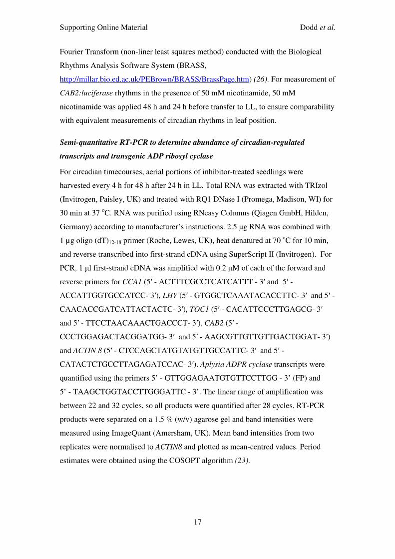
Supporting Online Material Dodd et al.
17
Fourier Transform (non-liner least squares method) conducted with the Biological
Rhythms Analysis Software System (BRASS,
http://millar.bio.ed.ac.uk/PEBrown/BRASS/BrassPage.htm) (26). For measurement of
CAB2:luciferase rhythms in the presence of 50 mM nicotinamide, 50 mM
nicotinamide was applied 48 h and 24 h before transfer to LL, to ensure comparability
with equivalent measurements of circadian rhythms in leaf position.
Semi-quantitative RT-PCR to determine abundance of circadian-regulated
transcripts and transgenic ADP ribosyl cyclase
For circadian timecourses, aerial portions of inhibitor-treated seedlings were
harvested every 4 h for 48 h after 24 h in LL. Total RNA was extracted with TRIzol
(Invitrogen, Paisley, UK) and treated with RQ1 DNase I (Promega, Madison, WI) for
30 min at 37 oC. RNA was purified using RNeasy Columns (Qiagen GmbH, Hilden,
Germany) according to manufacturer’s instructions. 2.5 µg RNA was combined with
1 µg oligo (dT)12-18 primer (Roche, Lewes, UK), heat denatured at 70 oC for 10 min,
and reverse transcribed into first-strand cDNA using SuperScript II (Invitrogen). For
PCR, 1 µl first-strand cDNA was amplified with 0.2 µM of each of the forward and
reverse primers for CCA1 (5′ - ACTTTCGCCTCATCATTT - 3′ and 5′ -
ACCATTGGTGCCATCC- 3′), LHY (5′ - GTGGCTCAAATACACCTTC- 3′ and 5′ -
CAACACCGATCATTACTACTC- 3′), TOC1 (5′ - CACATTCCCTTGAGCG- 3′
and 5′ - TTCCTAACAAACTGACCCT- 3′), CAB2 (5′ -
CCCTGGAGACTACGGATGG- 3′ and 5′ - AAGCGTTGTTGTTGACTGGAT- 3′)
and ACTIN 8 (5′ - CTCCAGCTATGTATGTTGCCATTC- 3′ and 5′ -
CATACTCTGCCTTAGAGATCCAC- 3′). Aplysia ADPR cyclase transcripts were
quantified using the primers 5’ - GTTGGAGAATGTGTTCCTTGG - 3’ (FP) and
5’ - TAAGCTGGTACCTTGGGATTC - 3’. The linear range of amplification was
between 22 and 32 cycles, so all products were quantified after 28 cycles. RT-PCR
products were separated on a 1.5 % (w/v) agarose gel and band intensities were
measured using ImageQuant (Amersham, UK). Mean band intensities from two
replicates were normalised to ACTIN8 and plotted as mean-centred values. Period
estimates were obtained using the COSOPT algorithm (23).
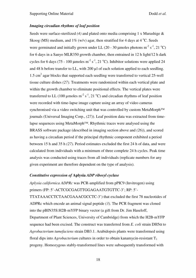
Supporting Online Material Dodd et al.
18
Imaging circadian rhythms of leaf position
Seeds were surface-sterilized (4) and plated onto media comprising 1 x Murashige &
Skoog (MS) medium, and 1% (w/v) agar, then stratified for 4 days at 4 oC. Seeds
were germinated and initially grown under LL (20 - 30 µmoles photons m-2
s-1
, 21 oC)
for 6 days in a Sanyo MLR350 growth chamber, then entrained in 12 h light/12 h dark
cycles for 6 days (75 - 100 µmoles m-2
s-1
, 21 oC). Inhibitor solutions were applied 24
and 48 h before transfer to LL, with 200 µl of each solution applied to each seedling.
1.5 cm2 agar blocks that supported each seedling were transferred to vertical 25-well
tissue culture dishes (27). Treatments were randomized within each vertical plate and
within the growth chamber to eliminate positional effects. The vertical plates were
transferred to LL (100 µmoles m-2
s-1
, 21 oC) and circadian rhythms of leaf position
were recorded with time-lapse image capture using an array of video cameras
synchronised via a video switching unit that was controlled by custom MetaMorph™
journals (Universal Imaging Corp., (27)). Leaf position data was extracted from time-
lapse sequences using MetaMorph™. Rhythmic traces were analysed using the
BRASS software package (described in imaging section above and (26)), and scored
as having a circadian period if the principal rhythmic component exhibited a period
between 15 h and 35 h (27). Period estimates excluded the first 24 h of data, and were
calculated from individuals with a minimum of three complete 24 h cycles. Peak time
analysis was conducted using traces from all individuals (replicate numbers for any
given experiment are therefore dependent on the type of analysis).
Constitutive expression of Aplysia ADP ribosyl cyclase
Aplysia californica ADPRc was PCR-amplified from pPIC9 (Invitrogen) using
primers (FP: 5’-ACTCGCGAGTTGGAGAATGTGTTC-3’; RP: 5’-
TTATAAACCTCTAACGAAACGCCTC-3’) that excluded the first 78 nucleotides of
ADPRc which encode an animal signal peptide (3). The PCR fragment was cloned
into the pBIN35S:H2B-mYFP binary vector (a gift from Dr. Jim Haseloff,
Department of Plant Sciences, University of Cambridge) from which the H2B-mYFP
sequence had been excised. The construct was transferred from E. coli strain DH5α to
Agrobacterium tumefaciens strain DB3.1. Arabidopsis plants were transformed using
floral dips into Agrobacterium cultures in order to obtain kanamycin-resistant T1
progeny. Homozygous stably-transformed lines were subsequently transformed with

Supporting Online Material Dodd et al.
19
pJAA 35S:APOAEQUORIN, which conferred phosphinothricin resistance for
selection of 35S:APOAEQUORIN transformed lines.
Simulation of effect of cADPR on the Arabidopsis circadian clock
Simulating transient effects of cADPR upon the oscillator
Inducible expression of ADPRc by β-estradiol leads to transient alterations in
circadian clock transcript abundance. To characterize the signal of this pathway, the
parameters of the Locke model equations for the plant circadian clock (2) were
perturbed as time-varying functions p$(t) = p+δ(t), where p$ is the vector of perturbed
model parameters, p the nominal parameter vector, and δ the perturbation profiles
(Fig. 3A). These profiles are characterised by two distinct classes. The first class
reflects the observed transient nature of the pathway after induction of XVE:ADPRc,
and will be referred to as the exponential profile due to the exponential function in its
definition.
δ(t)= Ate
-βt
β (1)
where A is the amplitude of the perturbation at its peak, t=β. To remain consistent
with the published data (3), three peak times were tested. [cADPR] peaked 20 hours
after induction, the activity of the ADPR cyclase enzyme at 16 hours, and peak
ADPRc transcript abundance occurred, in general, at 6 hours. The other class of
perturbations assumes a constant and immediate change in cellular processes
(δ = constant), and will be referred to as the step-change perturbation.
Selection of candidate Locke model parameters
Published cADPR-induced fold-changes in clock gene transcript abundance (3) were
used to assess the goodness of fit of each pair of parameters under the time-varying
profiles of Fig. 3A. The Locke model equations (2) were simulated under long day
conditions (16 hours light, 8 hours dark), in line with the experimental conditions
used by Sánchez et al. (3). These simulations were performed both with and without
the perturbation imposed, and the fold change in the concentration of mRNA for each
component calculated 6 hours after the start of the perturbation. A variety of

Supporting Online Material Dodd et al.
20
perturbation amplitudes were tested in an effort to cover as much of parameter space
as possible. The calculated fold changes were then compared with the target values
found experimentally through evaluation of a cost function, namely the 2-norm of the
error vector e.
22
1
2
2)732.3()1()056.0( −+−+−= YTOCLHY fffe (2)
The target value for LHY/CCA1, 0.056, was calculated as the arithmetic mean of the
fold changes in LHY and CCA1 transcript abundance. Similarly, the value for Y was
taken to be the fold change in GI. Since TOC1 was not found to be regulated
significantly by cADPR (3), the target value was set as 1. No restriction was imposed
on the change in X mRNA. Parameters were retained as candidates if they achieved a
cost function score less than 2.
Simulations of the parameter pairs with lowest observed cost are plotted for the
exponential perturbations (peaking at 6 hours after induction) in Supplementary
Figure 3a. The red traces (perturbed simulation) clearly show suppression of LHY
along with upregulation of Y (GI). It is important to note that the time in the diurnal
cycle at which the seedlings were treated with β-estradiol is not known, and so
simulations were carried out at each integer time (Fig. S5B).
Calculation of phase for unsustained perturbations
To assess the extent to which the phase of oscillation was changed, each perturbation
was simulated for 480 hours. The time of the final peak value of LHY mRNA, )(
max
pt ,
was noted and compared with the unperturbed equivalent, )(
max
ut . The differences
)(
max
pt - )(
max
ut reflect the phase change and are plotted against the error norm score (Eqn.
2) calculated for parameter perturbation cluster A (induction at ZT0) and B (induction
at ZT15) in Fig. 3A. Candidate parameters from the exponential perturbation profile
peaking after 6 hours do not alter the phase of oscillation significantly for cluster A (4
hours). However, cluster B perturbations appear to lie in two groups: one of which
does not alter phase, and one that does alter phase. The corresponding analyses for the
exponential perturbations which peak after 16 and 20 hours are shown in Supporting
Fig. S4B.

Supporting Online Material Dodd et al.
21
Calculation of period for sustained (step-change) perturbations
The candidate parameter pairs for the step-change perturbation were analysed through
simulation for 480 hours, and the period was calculated as being the difference in time
of the final two peak values of LHY mRNA. Here the choice of component and of
location in the state trajectory is arbitrary, so these choices were made for
convenience of computation. The duration of the simulation was chosen to be
sufficiently long that any transient behaviour had disappeared at the point of
calculation. The period for each candidate parameter pair is plotted against the error
norm score (Eqn. 2) for parameter clusters A and B in Fig. 3B. Periods below 15
hours and above 40 hours were deemed non-circadian and removed from these
graphs, in addition to the cases where the state trajectory tended to steady state.
This analysis corresponds to simulating continuous activation of transcripts regulated
by cADPR, and observing effects on oscillator period under constant light conditions.
Continuous suppression of cADPR-regulated transcripts was simulated by negating
each parameter perturbation about the nominal values (p$=p-δ). Oscillator period was
calculated using the same method as before for parameter clusters A and B and is
plotted against the error norm score in Fig. 3C.

Supporting Online Material Dodd et al.
22
References for Supporting Online Material
1. R. M. Graeff et al. J. Biol. Chem. 269, 30260-30267 (1994).
2. J. C. Locke et al. Mol. Syst. Biol. Epub 2005 Jun 28 (2005).
3. J. P. Sánchez, P. Duque, N. H. Chua. J. P. Sánchez, P. Duque, N. H. Chua. Plant J.
38, 381-395 (2004).
4. J. Love, A. N. Dodd, A. A. R. Webb. Plant Cell 16, 956-966 (2004).
5. A. N. Dodd et al. Plant J. 48, 962-973 (2006).
6. Y. Jiao et al. Plant Physiol. 133, 1480-1493 (2003).
7. H. Goda et al. Plant Physiol. 134, 1555-1573 (2004).
8. J. L. Nemhauser, T. C. Mockler, J. Chory PLoS Biol 2: e258.
doi:10.1371/journal.pbio.0020258 (2004).
9. F. J. M. Maathuis. Plant J. 45, 700-711 (2006).
10. J. T. Vogel et al. Plant J. 41, 195-211 (2005).
11. D. Zelder et al. Proc. Natl. Acad. Sci. USA. 101, 15811-15816 (2004).
12. R. Moscatiello, P. Marianai, D. Sanders, F.J.M. Maathius. J. Exp. Bot. 57, 2846-
2865 (2006).
13. J. M. Tepperman, T. Zhu, H. S. Chang, X. Wang, P. H. Quail. Proc. Natl. Acad.
Sci. USA 98, 9437-9442 (2001).
14. M Parani et al. Plant Biotech. J. 2, 359-366 (2004).
15. M. R. McAinsh, A. A. R. Webb, Taylor, J. E., A. M. Hetherington. Plant Cell 7,
1207-1219 (1995).
16. A. Haley et al. Proc. Natl. Acad. Sci. USA 92, 4124-4128 (1995).
17. A. A. Véry, J. M. Davies. Proc. Natl. Acad. Sci. USA 97, 9801-9806 (2000).
18. J. K. Sethi, R. M. Empson, A. Galione. Biochem. J. 319, 613-617 (1996).
19. I. Staxén et al. Proc Natl. Acad. Sci. USA 96, 1779-1784.
20. L. R. Baugh, A. A. Hill, E. L. Brown, C. P. Hunter. Nucleic Acids Res. 29, E29
(2001).

Supporting Online Material Dodd et al.
23
21. P. A. C. ’t Hoen, F. de Kort, G. J. B. van Ommen, J. T. den Dunnen. Nucleic
Acids Res. 31, E20 (2003).
22. S. L. Harmer et al. Science 290, 2110-2113 (2000).
23. M. Straume. Meth. Enzymol. 383, 149-166 (2004).
24. M. E. Hudson, P. H. Quail, P.H. Plant Physiol. 133, 1605-1616 (2003).
25. R. M. Graeff, H. C. Lee. Biochem. J. 361, 379-384 (2002).
26. J. D. Plautz et al. J. Biol. Rhythms 12, 204-217 (1997).
27. M. J. Dowson-Day, A. J. Millar. Plant J. 17, 63-71 (1999).