Mathematical model of retractions: Facts, analysis and ... - OSF

HAL Id: hal-03201385https://hal.archives-ouvertes.fr/hal-03201385

Preprint submitted on 18 Apr 2021

HAL is a multi-disciplinary open accessarchive for the deposit and dissemination of sci-entific research documents, whether they are pub-lished or not. The documents may come fromteaching and research institutions in France orabroad, or from public or private research centers.

L’archive ouverte pluridisciplinaire HAL, estdestinée au dépôt et à la diffusion de documentsscientifiques de niveau recherche, publiés ou non,émanant des établissements d’enseignement et derecherche français ou étrangers, des laboratoirespublics ou privés.

Mathematical model of retractions: Facts, analysis andrecommendations

Abdon Atangana, Seda Igret Araz

To cite this version:Abdon Atangana, Seda Igret Araz. Mathematical model of retractions: Facts, analysis and recom-mendations. 2021. hal-03201385

https://hal.archives-ouvertes.fr/hal-03201385

https://hal.archives-ouvertes.fr

Mathematical model of retractions: Facts, analysis andrecommendations

Abdon ATANGANA1,a, Seda IGRET [email protected], Institute for Groundwater Studies,

Faculty of Natural and Agricultural Sciences, University of the Free State,

South AfricaaDepartment of Medical Research, China Medical University Hospital,

China Medical University, Taichung, [email protected], Department of Mathematics Education, Siirt University, Turkey.

April 14, 2021

Abstract

The high rate of new retraction from different publishers nowadays is alarming. By readingreasons or retractions notes, one will conclude that there are fair and unfair retractions. Toprotect the integrity of research, the practice of fair retraction should be performed and authorsshould be responsible for their wrong doings. On the other hand, attention should be devotedto unfair retractions, especially retraction notes indicating that the authors did not agree withthe retraction. The aim of this paper is to provide a discussion by presenting first the statisticalanalysis of retraction data from ten different publishers ranging between the year 2000 and2020. Secondly, to provide a forecast up to 2050 and see which of the publishers will have moreor less retractions. The aim of such prediction is a wakeup call to authors, reviewers, editorsand publishers to be more mindful of what they are doing. Most importantly, publishers mustput all mechanisms in place to avoid unfair retractions. A list of possible causes of high ratesof unfair and fair retractions have been presented to help different actors to take actions. Amathematical model with a system of seven ordinary differential equations depicting a possiblescenario of retraction dynamic is constructed in this work. Different analyses were performedfor deterministic and stochastic versions. Finally a discussion and recommendations were madeto restore the dignity of those authors that have been victims of unfair retractions.

Keywords and phrases: Retractions, statistical analysis, unfair retractions, mathematicalmodel of retractions, simulations and recommendations.

1 Introduction

Generally speaking, research or scientific papers are some pieces of academic writing in which the au-thors provide analysis, interpretations and even arguments based on comprehensive self-determiningresearch. Scientists, to communicate their latest findings, write a scientific paper with the aim tocommunicate it to the rest of the world through a journal. However for this paper to be published

1

in a journal, they are procedures to be followed. The paper is prepared by one or more than oneauthors, after identifying a suitable journal, the paper is submitted. The journal assigns the paperto an editor who is an expert in the field to check whether or not the paper is suitable for pub-lication. If the editor finds the paper interesting, he then assigns it to two or more independentreviewers who are also experts in the field. The reviewers provide their report, and give their scien-tific opinion whether the paper will be accepted with (minor or major revision) or rejected. Finally,the editor will communicate the report to the corresponding author, if the editor suggest rejection,then the process stops, however, if revisions are required, the author will then perform the revisionsand resubmit for further evaluations and finally if reviewers and editor are satisfied then the paperis accepted and send under production for publication. There are also few steps that have to befollowed before the paper can appear online. However, it had been noticed that published papersimperfections, to solve this problem, a new concept was suggested, the retraction. For those who arenot aware of this process, a retraction is in simple terms an action to remove from a journal a pub-lished paper. One of the earlier retractions can be traced back as early as 1756, the concerned paperin philosophical transactions of the royal society [4-13]. Since then, the number of retracted papershas increased each year, especially in the last 5 years the number of retracted papers has increasedexponentially. Some authors have represented some analysis and even given suggestions to enhancethe process of retraction, nevertheless, the number keeps on increasing. The question that has beenasked by several academic structures is to know why more retraction? However, before giving somereasons that have been raised, we will like to note that, there are two types of retraction, fairlyretractions where the paper contains serious errors that cannot be corrected, plagiarism, and manyother unethical reasons. However, there are also unfair retractions where the paper is retracteddue to unjustifiable reasons. In this paper, a statistical analysis of collected data from a retractiondatabase will be performed [3]. A mathematical model depicting a dynamic about retraction willbe proposed and studied using some mathematical analysis. A prediction will be done with theaim to warn researchers, publishers and editors to take serious steps to help low down the curve ofretraction.

2 Statistical analysis of the retracted papers by some pub-lishers

An effort made by a database has led to a collection of some retracted papers from different publish-ers and their respective journals. We have considered retracted research papers (Case report papers,conference abstract and other retractions are not considered here) from 2000 to 2020, the collecteddata were taken for 11 publishers including Elsevier, Springer, Wiley and son, Taylor & Francis, Hin-dawi, Springer-Nature, MPDI, AAAS, BMJ, De Gruyter. An approximate total number of retractedpapers from each of the mentioned publishers is listed in table below. The table below shows thatElsevier, Springer and Wiley are the leading publishers in terms of yearly retraction, while BMJ isthe publisher with less retractions. In this section, we perform some statistical analysis of collectedfor each publisher, our analysis will then consist of correlation of retraction between publishers, achart representing yearly percentages of retractions for each publisher, an accumulative graph ofretraction for each publisher from 2000 to 2020, prediction up to 2050 for each publisher and finallyfitting using moving average. The predictions show that, only the year 2050, Elsevier would retracta maximum number of 800 papers, an average number of 600 or a minimum number of 400. With

2

the same prediction, Springer would retract a maximum number of 650 papers, an average numberof 550 papers or a minimum number of 450 papers. Wiley would retract a maximum number of320, average of 230 or a minimum number of 90. But Springer Nature would in 2050 accumulatea maximum number of 70 papers, an average number of 55 or a minimum number of 40 papers.Nature would retract a maximum number of 35 papers, or an average of 25 or a minimum of 12.Hindawi which is also one of the mega publishers would retract 130 as maximum, 100 as average or50 minimum. For MDPI, a maximum number of 80 papers would be retracted, or an average of 50 ora minimum of 9. For AAAS publishers, a maximum number of 6 papers would be retracted or evenzero retraction, a similar prediction for the publisher BMJ 10 maximum or 1 as minimum. Finally,Taylor and Francis, would have a maximum number of 230 retractions, or a minimum number of 45.Table 1 represents total numbers of the retractions made by 11 publishers from 2000 to 2020.

Table 1. Total number of retracted papers by some publishers.

Table 2 presents a mutual relationship of the retraction data between 11 publishers from 2000to 2020.

Table 2. Correlation about publishers.

Accumulative numbers of retractions made by different publishers are represented in Figure 1. Thegraphs show that Elsevier, Springer and Wiley are the three leading publishers in terms of yearlyretraction. Yearly numbers of retractions made by Elsevier, Springer, Wiley, Taylor & Francis,

3

Hindawi, SpringerNature, Nature, MDPI, BMJ and AAAS are presented from Figure 2 to 12. MDPIand Hindawi although being mega publishers have less yearly retractions compared to the top three.At this point one would think that this is due to them being open access publishers, a statementthat cannot be justified at this state as a proper investigation needs to be done to see if open accessjournals retract less papers.

Figure 1. Accumulative data for retracted papers for the considered publishers.

4

Figure 2. Numbers of retracted papers for Elsevier.

Figure 3.Numbers of retracted papers for Springer.

5

Figure 4.Numbers of retracted papers for Wiley.

,

Figure 5. Numbers of retracted papers for SpringerNature.

6

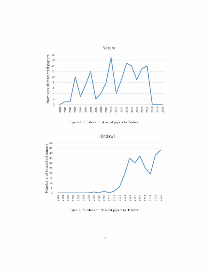
Figure 6. Numbers of retracted papers for Nature.

Figure 7. Numbers of retracted papers for Hindawi.

7

Figure 8. Numbers of retracted papers for MDPI.

Figure 9. Numbers of retracted papers for AAAS.

8

Figure 10. Numbers of retracted papers for Taylor&Francis.

Figure 11. Numbers of retracted papers for BMJ.

9

Figure 12. Numbers of retracted papers for De Gruyter.

We present in Figure 13 to 23 the charts depicting yearly percentages of retraction of the tenconsidered publishers.

Figure 13. Numbers of retracted papers for Elsevier.

10

Figure 14. Numbers of retracted papers for Springer.

Figure 15. Numbers of retracted papers for Wiley.

11

Figure 16. Numbers of retracted papers for SpringerNature.

Figure 17. Numbers of retracted papers for Nature.

12

Figure 18. Numbers of retracted papers for Hindawi.

Figure 19. Numbers of retracted papers for MDPI.

13

Figure 20. Numbers of retracted papers for AAAS.

Figure 21. Numbers of retracted papers for Taylor&Francis.

14

Figure 22. Numbers of retracted papers for BMJ.

Figure 23. Numbers of retracted papers for De Gruyter.

Figures 24 to 34 represent predictions obtained from 95 percent of the forecast sheet for the ten

15

chosen publishers from 2020 to 2050.

Figure 24. Prediction for numbers of retracted papers in Elsevier.

Figure 25. Prediction for numbers of retracted papers in Springer.

16

Figure 26. Prediction for numbers of retracted papers in Wiley.

Figure 27. Prediction for numbers of retracted papers in SpringerNature.

17

Figure 28. Prediction for numbers of retracted papers in Nature.

Figure 29. Prediction for numbers of retracted papers in Hindawi.

18

Figure 30. Prediction for numbers of retracted papers in MDPI.

Figure 31. Prediction for numbers of retracted papers in AAAS.

19

Figure 32. Prediction for numbers of retracted papers in Taylor&Francis.

Figure 33. Prediction for numbers of retracted papers in BMJ.

20

Figure 34. Prediction for numbers of retracted papers in De Gruyter.

In Figure 35 to 45, we attempt to fit collected data from each publisher using a statistical methodcalled moving average.

Figure 35. Fitting for retracted papers in Elsevier.

21

Figure 36. Fitting for retracted papers in Springer.

Figure 37. Fitting for retracted papers in Wiley.

22

Figure 38. Fitting for retracted papers in SpringerNature.

Figure 39. Fitting for retracted papers in Nature.

23

Figure 40. Fitting for retracted papers in Hindawi.

Figure 41. Fitting for retracted papers in MDPI.

24

Figure 42. Fitting for retracted papers in AAAS.

Figure 43. Fitting for retracted papers in Taylor&Francis.

25

Figure 44. Fitting for retracted papers in BMJ.

Figure 45. Fitting for retracted papers in De Gruyter.

With the analysis presented above, the next question one would like to answer is the following:Why is there a high rate of retraction? Some authors have reacted to this question and have

26

attempted to supply a list of items that could be the main driving reasons for high numbers ofretractions nowadays. Such a list will be presented below.1. Authors are always under pressure to be productive with no financial support.2. Reviewers are not doing their job properly only they are interested in getting citations.3. Editors are loaded with high number of submissions therefore have no time to access the

content of the papers properly.4. Editors are discriminative.5. The appointment of the editorial board is impartial as it only covers some specific continent.6. Publishers have no experience, as they take impartial decisions.7. Envy among peers, which lead some readers to target some authors.8. Readers have connections with editorial boards or publishers.9. Authors have 24 hours to check and reply for his galley-proofs which with no doubt put the

author under pressure.10. A sponsored company has to report retractions.11. Pub peer allows anonymous individuals to post comments on published papers, even when

those individuals are not experts in the field. Such comments are sometimes used to retract papers.12. Some authors manipulate their results.13. Plagiarism.Beside the high number of retracted papers, the second question that has been raised by many

authors is to know why only the author is the victim or responsible for the retraction? Except formanipulation of results, especially experimental research, the authors should not only be responsiblefor a retraction for the following reasons.A submitted paper by an author does follow some steps before the paper can be accepted and

published. Indeed the aim of submission is for the paper to be evaluated by some supposedly expertsin the field.a) After a submission, the editor-in-chief of the journal identifies a suitable editor who is

expert in the field. The editor have to read the content of the paper and suggest rejection or thepeer review process.b) In case of peer reviewer process, two or more than three experts in the fields are approached

by the handling editors, who will read the paper, evaluate the content of the paper and finally writereports that will also be evaluated by the handling editor.c) If the reports suggest revisions, the handling editor will forward the comments to the

corresponding author, who will be asked to perform those revisions and resubmit the paper forfurther evaluations.d) After the resubmission the handling editor can accept the paper or send it again for second

round for peer review if the paper is finally accepted by reviewers, the editor can accept it or stillas for some revisions.e) Finally if the paper is accepted by the handling editor, the paper is sent to production for

publication.

27

3 A mathematical model of retraction with classical differ-entiation

Several reasons have been listed that could be considered as main causes of high rate of yearlyretractions from different publishers, indeed this could vary from one journal to another accordinglyto who is the editor in chief and who is the publisher. In big publishers like Elsevier there aremore factors that could lead to their high numbers of yearly retraction, this will be a discussion foranother research. In this section, we present a mathematical model depicting a possible scenario ofthe dynamic of retraction. To achieve this, we consider some classes including: S (t) which is theclass of published paper susceptible to be retracted, R (t) is the class of retracted papers, RT (t) isthe class of fairly retracted papers, RF (t) is the class of unfairly retracted papers, BE (t) is the classof unfair editors, who contribute to retracting unfairly papers published by some authors, GE (t) isthe class of fair editors, they should be appointed more in different editorial board to insure fairnessin terms of acceptance, rejections, and retraction. D (t) is the class of papers that are reportedby a retraction database. A possible system of ordinary differential equations depicting retractionscenario is given below as:

·S (t) = Λ− βS (GE + τBE) + κ5BE (1)·R (t) = βS (GE + τBE)− (1− ψ1)ϕ1R− (1− ψ2)ϕ2R·RT (t) = ψ1ϕ1R− κ1RT·RF (t) = ψ2ϕ2R− κ2RF·GE (t) = (1− ψ1)ϕ1R− κ3GE·BE (t) = (1− ψ2)ϕ2R− (κ4 + κ5)BE·D (t) = κ1RT + κ2RF + κ3GE + κ4BE

with the initial conditions

S (0) = S0, R (0) = R0, RT (0) = R0F , GE (0) = G0

E , BE (0) = B0E , D (0) = D0. (2)

In Figure 46, a diagram that takes into account retraction scenarios is provided to better understandsuch processes.

28

Figure 46. Flow chart for the retraction model.

Before proceeding, we insure that all solutions are positive.

·S (t) = Λ− βS (GE + τBE) + κ5BE , ∀t ≥ 0 (3)

≥ −βS (GE + τBE) , ∀t ≥ 0

≥ −βS (|GE |+ τ |BE |) , ∀t ≥ 0,

≥ −βS(

supt∈DGE

|GE |+ τ supt∈DBE

|BE |), ∀t ≥ 0

≥ −βS (‖GE‖∞ + τ ‖BE‖∞) , ∀t ≥ 0

≥ −βSM, ∀t ≥ 0.

Since GE (t) represents the class of good editors and BE (t) represents editors with bad judgements,then

‖BE‖∞ < M1 <∞, ‖GE‖∞ < M2 <∞. (4)

Thus·S (t) ≥ −βMS (t) , ∀t ≥ 0 (5)

andS (t) ≥ S0 exp [−βMt] , ∀t ≥ 0. (6)

29

Using same routine, we should that ∀t ≥ 0

R (t) ≥ R0 exp [− ((1− ψ1)ϕ1 + (1− ψ2)ϕ2) t] (7)

RT (t) ≥ R0T exp [−κ1t]

RF (t) ≥ R0F exp [−κ2t]

GE (t) ≥ G0E exp [−κ3t]

BE (t) ≥ B0E exp [− (κ4 + κ5) t]

D (t) ≥ 0

as the sum of positive functions.We next show that under some conditions the retraction model has a unique system of solutions.

We define the following norm‖g‖∞ = inf

t∈Dg

|g (t)| . (8)

We reformulate the system of equations as

·S (t) = F1 (t, S,R,RT , RF , GE , BE , D) (9)·R (t) = F2 (t, S,R,RT , RF , GE , BE , D)·RT (t) = F3 (t, S,R,RT , RF , GE , BE , D)·RF (t) = F4 (t, S,R,RT , RF , GE , BE , D)·GE (t) = F5 (t, S,R,RT , RF , GE , BE , D)·BE (t) = F6 (t, S,R,RT , RF , GE , BE , D)·D (t) = F7 (t, S,R,RT , RF , GE , BE , D) .

The following properties need to be verified

(i) ∀i ∈ 1, 2, 3, 4, 5, 6, 7

|Fi (xi, t)|2 ≤ ki(

1 + |xi|2). (10)

(ii) ∀i ∈ 1, 2, 3, 4, 5, 6, 7

∣∣Fi (x1i , t)− Fi

(x2i , t)∣∣2 ≤ ki ∣∣x1

i − x2i

∣∣2 . (11)

30

We start with the class F1 (S, t)

|F1 (S, t)|2 = |Λ− βS (GE + τBE) + κ5BE |2 (12)

≤ 3Λ2 + 3β2 |S|2 |GE + τBE |2 + 3κ25 |BE |

2

≤ 3Λ2 + 6β2 |S|2 |GE |2 + 6β2 |S|2 τ2 |BE |2 + 3κ25 |BE |

2

≤ 3Λ2 + 6β2 |S|2 supt∈DGE

∣∣G2E

∣∣2 + 6β2 |S|2 τ2 supt∈DBE

∣∣B2E

∣∣+ 3κ25 supt∈DBE

∣∣B2E

∣∣≤

(3Λ2 + 3κ2

5

∥∥B2E

∥∥∞)(

1 +6β2

(∥∥G2E

∥∥∞ + τ2

∥∥B2E

∥∥∞)

3Λ2 + 3κ25 ‖B2

E‖∞|S|2

)

under the condition that6β2(‖G2

E‖∞+τ2‖B2E‖∞)

3Λ2+3κ25‖B2E‖∞

< 1, then

|F1 (S, t)|2 ≤ k1

(1 + |S|2

). (13)

Also ∣∣F1

(S1, t

)− F1

(S2, t

)∣∣2 =∣∣−β (GE + τBE)

(S1 − S2

)∣∣2 (14)

≤ β2 |GE + τBE |2∣∣S1 − S2

∣∣2≤ 2β2

∣∣G2E

∣∣+ 2β2τ2∣∣B2

E

∣∣ ∣∣S1 − S2∣∣2

≤ 2β2

(sup

t∈DGE

∣∣G2E

∣∣+ τ2 supt∈DBE

∣∣B2E

∣∣) ∣∣S1 − S2∣∣2

≤ 2β2K∣∣S1 − S2

∣∣2≤ k1

∣∣S1 − S2∣∣2 .

Using same routine, we can have the following

|F2 (R, t)|2 = |βS (GE + τBE)− ((1− ψ1)ϕ1 + (1− ψ2)ϕ2)R|2 (15)

≤ 4β2∥∥S2

∥∥∞(∥∥G2

E

∥∥∞ + τ2

∥∥B2E

∥∥∞)

+ 2 ((1− ψ1)ϕ1 + (1− ψ2)ϕ2)2 |R|2

≤ 4β2∥∥S2

∥∥∞K + 2 ((1− ψ1)ϕ1 + (1− ψ2)ϕ2)

2 |R|2

≤ 4β2∥∥S2

∥∥∞K

(1 +

2 ((1− ψ1)ϕ1 + (1− ψ2)ϕ2)2

4β2 ‖S2‖∞K|R|2

)

under the condition that 2((1−ψ1)ϕ1+(1−ψ2)ϕ2)2

4β2‖S2‖∞K< 1, then

|F2 (R, t)|2 ≤ k2

(1 + |R|2

). (16)

Also ∣∣F2

(R1, t

)− F2

(R2, t

)∣∣2 =∣∣− ((1− ψ1)ϕ1 + (1− ψ2)ϕ2)

(R1 −R2

)∣∣2 (17)

≤ 2(

(1− ψ1)2ϕ2

1 + (1− ψ2)2ϕ2

2

) ∣∣R1 −R2∣∣2

≤ k2

∣∣R1 −R2∣∣2 .

31

For the function F3,

|F3 (RT , t)|2 = |ψ1ϕ1R− κ1RT |2 (18)

≤ 2ψ21ϕ

21

∣∣R2∣∣+ 2κ2

1 |RT |2

≤ 2ψ21ϕ

21 supt∈DR

∣∣R2∣∣+ 2κ2

1 supt∈DRT

|RT |2

≤ 2ψ21ϕ

21

∥∥R2∥∥∞

(1 +

2κ21

2ψ21ϕ

21 ‖R2‖∞

|RT |2)

under the condition that 2κ212ψ21ϕ

21‖R2‖∞

< 1, then

|F3 (RT , t)|2 ≤ k2

(1 + |RT |2

). (19)

Also ∣∣F3

(R1T , t)− F3

(R2T , t)∣∣2 = κ2

1

∣∣(R1T −R2

T

)∣∣2 (20)

≤ 3

2κ2

1

∣∣(R1T −R2

T

)∣∣2≤ k3

∣∣(R1T −R2

T

)∣∣2 .For the function F4,

|F4 (RF , t)|2 = |ψ2ϕ2R− κ2RF |2 (21)

≤ 2ψ22ϕ

22

∣∣R2∣∣+ 2κ2

2 |RF |2

≤ 2ψ22ϕ

22 supt∈DR

∣∣R2∣∣+ 2κ2

2 supt∈DRF

|RF |2

≤ 2ψ22ϕ

22

∥∥R2∥∥∞

(1 +

2κ22

2ψ22ϕ

22 ‖R2‖∞

|RF |2)

under the condition that 2κ222ψ22ϕ

22‖R2‖∞

< 1, then

|F4 (RF , t)|2 ≤ k4

(1 + |RF |2

). (22)

Also ∣∣F4

(R1F , t)− F4

(R2F , t)∣∣2 = κ2

2

∣∣R1F −R2

F

∣∣2 (23)

≤ 3

2κ2

2

∣∣R1F −R2

F

∣∣2≤ k3

∣∣R1F −R2

F

∣∣2 .

32

For the function F5,

|F5 (GE , t)|2 = |(1− ψ1)ϕ1R− κ3GE |2 (24)

≤ 2 (1− ψ1)2ϕ2

1

∣∣R2∣∣+ 2κ2

3 |GE |2

≤ 2 (1− ψ1)2ϕ2

1 supt∈DR

∣∣R2∣∣+ 2κ2

3 supt∈DRT

|GE |2

≤ 2 (1− ψ1)2ϕ2

1

∥∥R2∥∥∞

(1 +

2κ23

2 (1− ψ1)2ϕ2

1 ‖R2‖∞|GE |2

)

under the condition that 2κ232(1−ψ1)2ϕ21‖R2‖∞

< 1, then

|F5 (GE , t)|2 ≤ k5

(1 + |GE |2

). (25)

Also ∣∣F5

(G1E , t)− F5

(G2E , t)∣∣2 ≤ 3

2κ2

3

∣∣G1E −G2

E

∣∣2 (26)

≤ k5

∣∣G1E −G2

E

∣∣2 .For the function F6,

|F6 (BE , t)|2 = |(1− ψ2)ϕ2R− (κ4 + κ5)BE |2 (27)

≤ 2 (1− ψ2)2ϕ2

2

∣∣R2∣∣+ 4

(κ2

4 + κ25

)|BE |2

≤ 2 (1− ψ2)2ϕ2

2 supt∈DR

∣∣R2∣∣+ 4

(κ2

4 + κ25

)|BE |2

≤ 2 (1− ψ2)2ϕ2

2

∥∥R2∥∥∞

(1 +

4(κ2

4 + κ25

)2 (1− ψ2)

2ϕ2

2 ‖R2‖∞|BE |2

)

under the condition that4(κ24+κ25)

2(1−ψ2)2ϕ22‖R2‖∞< 1, then

|F6 (BE , t)|2 ≤ k6

(1 + |BE |2

). (28)

Also ∣∣F6

(B1E , t)− F6

(B2E , t)∣∣2 ≤ 2

(κ2

4 + κ25

) ∣∣B1E −B2

E

∣∣2 (29)

≤ k6

∣∣G1E −G2

E

∣∣2 .For the function F7,

|F7 (D, t)|2 = |κ1RT + κ2RF + κ3GE + κ4BE |2 (30)

≤ |κ1RT + κ2RF + κ3GE + κ4BE |2(

1 + ε |D|2)

≤ 4

(κ2

1 supt∈DRT

∣∣R2T

∣∣+ κ2 supt∈DRF

∣∣R2F

∣∣+ κ3 supt∈DGE

∣∣G2E

∣∣+ κ4 supt∈DBE

∣∣B2E

∣∣)(1 + ε |D|2)

≤ 4(κ2

1

∥∥R2T

∥∥∞ + κ2

∥∥R2F

∥∥∞ + κ3

∥∥G2E

∥∥∞ + κ4

∥∥B2E

∥∥∞) (

1 + ε |D|2)

33

under the condition that ε < 1, then

|F7 (D, t)|2 ≤ k6

(1 + |D|2

).

Also ∣∣F7

(D1, t

)− F7

(D2, t

)∣∣2 ≤ k7

∣∣D1 −D2∣∣2 .

Finally if

max

6β2(‖G2

E‖∞+τ2‖B2E‖∞)

3Λ2+3κ25‖B2E‖∞

, 2((1−ψ1)ϕ1+(1−ψ2)ϕ2)2

4β2‖S2‖∞K,

2κ212ψ21ϕ

21‖R2‖∞

,2κ22

2ψ22ϕ22‖R2‖∞

,2κ23

2(1−ψ1)2ϕ21‖R2‖∞,

4(κ24+κ25)2(1−ψ2)2ϕ22‖R2‖∞

, ε

< 1, (31)

the model of the retraction has a unique system of solutions. In the absence of fake retractions andbad editors, the equilibrium points will be

Λ− βS∗G∗E = 0 (32)

βS∗G∗E − (1− ψ1)ϕ1R∗ − (1− ψ2)ϕ2R

∗ = 0

ψ1ϕ1R∗ − κ1R

∗T = 0

(1− ψ1)ϕ1R∗ − κ3G

∗E = 0.

After solving above, we obtain

S∗ =Λ

βG∗E=

κ3

β (1− ψ1)ϕ1

((1− ψ1)ϕ1 + (1− ψ2)ϕ2) (33)

R∗ =Λ

(1− ψ1)ϕ1 + (1− ψ2)ϕ2

R∗T =ψ1ϕ1

κ1

Λ

(1− ψ1)ϕ1 + (1− ψ2)ϕ2

G∗E =(1− ψ1)ϕ1

κ3

Λ

(1− ψ1)ϕ1 + (1− ψ2)ϕ2

.

However in the presence of false retraction and bad editors, the equilibrium points would be

Λ− βS∗ (G∗E + τB∗E) + κ5B∗E = 0 (34)

βS∗ (G∗E + τB∗E)− ((1− ψ1)ϕ1 + (1− ψ2)ϕ2)R∗ = 0

ψ1ϕ1R∗ − κ1R

∗T = 0

ψ2ϕ2R∗ − κ2R

∗F = 0

(1− ψ1)ϕ1R∗ − κ3G

∗E = 0

(1− ψ2)ϕ2R∗ − (κ4 + κ5)B∗E = 0.

34

By solving above system, we obtain

R∗ =Λ (κ4 + κ5)

κ5 (1− ψ1)ϕ1 + κ4 ((1− ψ1)ϕ1 + (1− ψ2)ϕ2), (35)

R∗T =ψ1ϕ1

κ1

Λ (κ4 + κ5)

κ5 (1− ψ1)ϕ1 + κ4 ((1− ψ1)ϕ1 + (1− ψ2)ϕ2),

R∗F =ψ2ϕ2

κ2

Λ (κ4 + κ5)

κ5 (1− ψ1)ϕ1 + κ4 ((1− ψ1)ϕ1 + (1− ψ2)ϕ2),

G∗E =(1− ψ1)ϕ1

κ3

Λ (κ4 + κ5)

κ5 (1− ψ1)ϕ1 + κ4 ((1− ψ1)ϕ1 + (1− ψ2)ϕ2),

B∗E =(1− ψ2)ϕ2

(κ4 + κ5)

Λ (κ4 + κ5)

κ5 (1− ψ1)ϕ1 + κ4 ((1− ψ1)ϕ1 + (1− ψ2)ϕ2)

=Λ (1− ψ2)ϕ2

κ5 (1− ψ1)ϕ1 + κ4 ((1− ψ1)ϕ1 + (1− ψ2)ϕ2).

Finally

S∗ =((1− ψ1)ϕ1 + (1− ψ2)ϕ2)R∗

β (G∗E + τB∗E). (36)

Before proceeding with the stability analysis of equilibrium points, we will first present the conditionsunder which the classes of BE (t) and RF (t) are declining. Using elementary calculus, we know thefunction BE (t) will decrease if

·BE (t) < 0⇒ (1− ψ2)ϕ2R− (κ4 + κ5)BE < 0 (37)

(1− ψ2)ϕ2

(κ4 + κ5)<

BER.

RF (t) will decline if and only if

·RF (t) < 0⇒ ψ2ϕ2R− κ2RF < 0 (38)ψ2ϕ2

κ2<

RFR

< 1.

To investigate if classes will have concavity,we study the sign of their respective second derivatives.Therefore

d·BEdt

= (1− ψ2)ϕ2

·R− (κ4 + κ5)

·BE

= (1− ψ2)ϕ2 [βS (GE + τBE)− ((1− ψ1)ϕ1 + (1− ψ2)ϕ2)R] (39)

− (κ4 + κ5) ((1− ψ2)ϕ2R− (κ4 + κ5)BE) .

Thend·BEdt

< 0 (40)

35

if

(1− ψ2)ϕ2 [βS (GE + τBE)− ((1− ψ1)ϕ1 + (1− ψ2)ϕ2)R] (41)

− (κ4 + κ5) ((1− ψ2)ϕ2R− (κ4 + κ5)BE) < 0.

A fortiori

(1− ψ2)ϕ2 [βτBE − ((1− ψ1)ϕ1 + (1− ψ2)ϕ2)R] (42)

− (κ4 + κ5) ((1− ψ2)ϕ2R− (κ4 + κ5)BE) < 0

and

(1− ψ2)ϕ2βτBE − (1− ψ2)ϕ2 ((1− ψ1)ϕ1 + (1− ψ2)ϕ2)R (43)

− (κ4 + κ5) (1− ψ2)ϕ2R− (κ4 + κ5)2BE < 0

or ((1− ψ2)ϕ2βτ + (κ4 + κ5)

2)BE −

[(1− ψ2)ϕ2 ((1− ψ1)ϕ1 + (1− ψ2)ϕ2)

+ (κ4 + κ5) (1− ψ2)ϕ2

]R < 0. (44)

Therefore

(1− ψ2)ϕ2βτ + (κ4 + κ5)2

(1− ψ2)ϕ2 ((1− ψ1)ϕ1 + (1− ψ2)ϕ2) + (κ4 + κ5) (1− ψ2)ϕ2

<R

.BE. (45)

Similarly

d·RFdt

= ψ2ϕ2

·R− κ2

·RF (46)

= ψ2ϕ2

(βS (GE + τBE)

− ((1− ψ1)ϕ1 + (1− ψ2)ϕ2)R

)− κ2 (ψ2ϕ2R− κ2RF ) .

Thus d·RF

dt < 0 if

ψ2ϕ2 (βτBE − ((1− ψ1)ϕ1 + (1− ψ2)ϕ2)R)− κ2ψ2ϕ2R+ κ22RF < 0. (47)

Since S > RF a fortiori S (GE + τBE) > RF(ψ2ϕ2β + κ2

2

)RF − ((1− ψ1)ϕ1 + (1− ψ2)ϕ2 + κ2ψ2ϕ2)R < 0. (48)

Therefore d·RF

dt < 0 if and only if

RFR

<(1− ψ1)ϕ1 + (1− ψ2)ϕ2 + κ2ψ2ϕ2

ψ2ϕ2β + κ22

. (49)

36

We now investigate the sign of the Lyapunov energy associated to this system.

L (S,R,RT , RF , BE , GE , D) =

(S − S∗ − S∗ log

S∗

S

)+

(R−R∗ −R∗ log

R∗

R

)(50)

+

(RT −R∗T −R∗T log

R∗TRT

)+

(RF −R∗F −R∗F log

R∗FRF

)+

(BE −B∗E −B∗E log

B∗EBE

)+

(GE −G∗E −G∗E log

G∗EGE

).

By taking its derivative, we have

dL (t)

dt=

(1− S∗

S

)·S +

(1− R∗

R

)·R+

(1− R∗T

RT

)·RT (51)

+

(1− R∗F

RF

)·RF +

(1− B∗E

BE

)·BE +

(1− G∗E

GE

)·GE .

Putting all together, we obtain

dL (t)

dt=

(1− S∗

S

)(Λ− βS (GE + τBE) + κ5BE) (52)

+

(1− R∗

R

)(βS (GE + τBE)− ((1− ψ1)ϕ1 + (1− ψ2)ϕ2)R)

+

(1− R∗T

RT

)(ψ1ϕ1R− κ1RT ) +

(1− R∗F

RF

)(ψ2ϕ2R− κ2RF )

+

(1− B∗E

BE

)((1− ψ2)ϕ2R− (κ4 + κ5)BE)

+

(1− G∗E

GE

)((1− ψ1)ϕ1R− κ3GE)

and

dL (t)

dt=

(S − S∗S

)(Λ− β (S − S∗) ((GE −G∗E) + τ (BE −B∗E)) + κ5 (BE −B∗E)) (53)

+

(R−R∗R

)(β (S − S∗) ((GE −G∗E) + τ (BE −B∗E))− ((1− ψ1)ϕ1 + (1− ψ2)ϕ2) (R−R∗))

+

(RT −R∗T

RT

)(ψ1ϕ1 (R−R∗)− κ1 (RT −R∗T )) +

(RF −R∗F

RF

)(ψ2ϕ2 (R−R∗)− κ2 (RF −R∗F ))

+

(BE −B∗E

BE

)((1− ψ2)ϕ2 (R−R∗)− (κ4 + κ5) (BE −B∗E))

+

(GE −G∗E

GE

)((1− ψ1)ϕ1 (R−R∗)− κ3 (GE −G∗E)) .

37

Arranging above, one can find

dL (t)

dt= − (S − S∗)2

S(βGE + τB∗E) +

(S − S∗)2

S(βG∗E + τB∗E) + Λ + κ5BE − κ5B

∗E −

S∗

SΛ (54)

+κ5S∗

SB∗E −

(R−R∗)2

R((1− ψ1)ϕ1 + (1− ψ2)ϕ2) + βSGE − βSG∗E − βS∗GE

+βS∗G∗E + βτSBE − βτSB∗E − βτS∗BE + βτS∗B∗E −R∗

RβSGE +

R∗

RβSG∗E − κ5

S∗

SBE

+R∗

RβS∗GE −

R∗

RβS∗G∗E −

R∗

RβτSBE +

R∗

RβτSB∗E +

R∗

RβτS∗BE −

R∗

RβτS∗B∗E

− (RT −R∗T )2

RTκ1 + ψ1ϕ1R− ψ1ϕ1R

∗ − R∗TRT

ψ1ϕ1R+R∗TRT

ψ1ϕ1R∗ − (RT −R∗T )

2

RTκ2

+ψ2ϕ2R− ψ2ϕ2R∗ − R∗F

RFψ2ϕ2R+

R∗FRF

ψ2ϕ2R∗ − (BE −B∗E)

2

BE(κ4 + κ5) + (1− ψ2)ϕ2R

− (1− ψ2)ϕ2R∗ − B∗E

BE(1− ψ2)ϕ2R+

B∗EBE

(1− ψ2)ϕ2R∗ − (GE −G∗E)

2

GEκ3

+ (1− ψ1)ϕ1R− (1− ψ1)ϕ1R∗ − G∗E

GE(1− ψ1)ϕ1R+

G∗EGE

(1− ψ1)ϕ1R∗.

Here, we write

L1 =(S − S∗)2

S(βG∗E + τB∗E) + Λ + κ5BE + κ5

S∗

SB∗E + βSGE (55)

+βS∗G∗E + βτSBE + βτS∗B∗E +R∗

RβSG∗E

+R∗

RβS∗GE +

R∗

RβτSB∗E +

R∗

RβτS∗BE

+ψ1ϕ1R+R∗TRT

ψ1ϕ1R∗ +

B∗EBE

(1− ψ2)ϕ2R∗

+ψ2ϕ2R+R∗FRF

ψ2ϕ2R∗ + (1− ψ2)ϕ2R

+ (1− ψ1)ϕ1R+G∗EGE

(1− ψ1)ϕ1R∗

38

and

L2 =(S − S∗)2

S(βGE + τB∗E) + κ5B

∗E +

S∗

SΛ + βSG∗E + βS∗GE (56)

+(R−R∗)2

R((1− ψ1)ϕ1 + (1− ψ2)ϕ2) + βτSB∗E + βτS∗BE

+R∗

RβSGE + κ5

S∗

SBE +

R∗

RβS∗G∗E +

R∗

RβτSBE +

R∗

RβτS∗B∗E

+(RT −R∗T )

2

RTκ1 + ψ1ϕ1R

∗ +R∗TRT

ψ1ϕ1R+(RT −R∗T )

2

RTκ2

+ψ2ϕ2R∗ +

R∗FRF

ψ2ϕ2R+(BE −B∗E)

2

BE(κ4 + κ5) + (1− ψ2)ϕ2R

∗

+B∗EBE

(1− ψ2)ϕ2R+(GE −G∗E)

2

GEκ3 + (1− ψ1)ϕ1R

∗ +G∗EGE

(1− ψ1)ϕ1R.

If L1 < L2, then the Lyapunov energy will be negative. If L2 < L1, then the energy will be positive.If L1 = L2, the situation right now will be unchanged.

4 Numerical solution for retraction model

In this section, we will present Atangana-Seda scheme to solve the suggested mathematical modelwith classical case. We recall our problem

d

dtS (t) = Λ− βS (GE + τBE) + κ5BE (57)

d

dtR (t) = βS (GE + τBE)− ((1− ψ1)ϕ1 + (1− ψ2)ϕ2)R

d

dtRT (t) = ψ1ϕ1R− κ1RT

d

dtRF (t) = ψ2ϕ2R− κ2RF

d

dtGE (t) = (1− ψ1)ϕ1R− κ3GE

d

dtBE (t) = (1− ψ2)ϕ2R− (κ4 + κ5)BE

d

dtD (t) = κ1RT + κ2RF + κ3GE + κ4BE .

39

For simplicity, we write above equation as follows;

d

dtS (t) = S∗ (t, S,R,RT , RF , GE , BE , D) (58)

d

dtR (t) = R∗ (t, S,R,RT , RF , GE , BE , D)

d

dtRT (t) = R∗T (t, S,R,RT , RF , GE , BE , D)

d

dtRF (t) = R∗F (t, S,R,RT , RF , GE , BE , D)

d

dtGE (t) = G∗E (t, S,R,RT , RF , GE , BE , D)

d

dtBE (t) = B∗E (t, S,R,RT , RF , GE , BE , D)

d

dtD (t) = D∗ (t, S,R,RT , RF , GE , BE , D) .

After integrating above and putting Newton polynomial into these equations, we can solve our modelas follows

Sn+1 = Sn +

2312S∗ (tn, S

n, Rn, RnT , RnF , G

nE , B

nE , D

n) ∆t− 4

3S∗ (tn−1, S

n−1, Rn−1, Rn−1T , Rn−1

F , Gn−1E , Bn−1

E , Dn−1)

∆t+ 5

12S∗ (tn−2, S

n−2, Rn−2, Rn−2T , Rn−2

F , Gn−2E , Bn−2

E , Dn−2)

∆t

(59)

Rn+1 = Rn +

2312R

∗ (tn, Sn, Rn, RnT , R

nF , G

nE , B

nE , D

n) ∆t− 4

3R∗ (tn−1, S

n−1, Rn−1, Rn−1T , Rn−1

F , Gn−1E , Bn−1

E , Dn−1)

∆t+ 5

12R∗ (tn−2, S

n−2, Rn−2, Rn−2T , Rn−2

F , Gn−2E , Bn−2

E , Dn−2)

∆t

Rn+1T = RnT +

2312R

∗T (tn, S


nE , B

nE , D

n) ∆t− 4

3R∗T

(tn−1, S

n−1, Rn−1, Rn−1T , Rn−1

F , Gn−1E , Bn−1

E , Dn−1)

∆t+ 5

12R∗T

(tn−2, S

n−2, Rn−2, Rn−2T , Rn−2

F , Gn−2E , Bn−2

E , Dn−2)

∆t

Rn+1F = RnF +

2312R

∗F (tn, S


nE , B

nE , D

n) ∆t− 4

3R∗F

(tn−1, S

n−1, Rn−1, Rn−1T , Rn−1

F , Gn−1E , Bn−1

E , Dn−1)

∆t+ 5

12R∗F

(tn−2, S

n−2, Rn−2, Rn−2T , Rn−2

F , Gn−2E , Bn−2

E , Dn−2)

∆t

Gn+1E = GnE +

2312G

∗E (tn, S


nE , B

nE , D

n) ∆t− 4

3G∗E

(tn−1, S

n−1, Rn−1, Rn−1T , Rn−1

F , Gn−1E , Bn−1

E , Dn−1)

∆t+ 5

12G∗E

(tn−2, S

n−2, Rn−2, Rn−2T , Rn−2

F , Gn−2E , Bn−2

E , Dn−2)

∆t

Bn+1E = BnE +

2312B

∗E (tn, S


nE , B

nE , D

n) ∆t− 4

3B∗E

(tn−1, S

n−1, Rn−1, Rn−1T , Rn−1

F , Gn−1E , Bn−1

E , Dn−1)

∆t+ 5

12B∗E

(tn−2, S

n−2, Rn−2, Rn−2T , Rn−2

F , Gn−2E , Bn−2

E , Dn−2)

∆t

Dn+1 = Dn +

2312D


nF , G

nE , B

nE , D

n) ∆t− 4

3D∗ (tn−1, S

n−1, Rn−1, Rn−1T , Rn−1

F , Gn−1E , Bn−1

E , Dn−1)

∆t+ 5

12D∗ (tn−2, S

n−2, Rn−2, Rn−2T , Rn−2

F , Gn−2E , Bn−2

E , Dn−2)

∆t

.

40

5 A stochastic model of retraction with classical differentia-tion

In this section, we add stochastic component to our model as follows

dS (t) = (Λ− βS (GE + τBE) + κ5BE) dt+ σ1S (t) dB1 (t) (60)

dR (t) = (βS (GE + τBE)− ((1− ψ1)ϕ1 + (1− ψ2)ϕ2)R) dt+ σ2R (t) dB2 (t)

dRT (t) = (ψ1ϕ1R− κ1RT ) dt+ σ3RT (t) dB3 (t)

dRF (t) = (ψ2ϕ2R− κ2RF ) dt+ σ4RF (t) dB4 (t)

dGE (t) = ((1− ψ1)ϕ1R− κ3GE) dt+ σ5GE (t) dB5 (t)

dBE (t) = ((1− ψ2)ϕ2R− (κ4 + κ5)BE) dt+ σ6BE (t) dB6 (t)

dD (t) = (κ1RT + κ2RF + κ3GE + κ4BE) dt+ σ7D (t) dB7 (t) .

where Bi (t) and σi, i = 1, 2, 3, 4, 5, 6, 7 represents Brownian motion and density of randomness,respectively.

5.1 Extinction of retraction and BE class

We present a discussion underpinning a possible extinction of retraction and BE class. Let usconsider the following formula [14-16]

〈γ (t)〉 =1

t

∫ t

0

γ (τ) dτ. (61)

At the threshold R0 for the retraction model is defined as

R0 =β(

(1− ψ1)ϕ1 + (1− ψ2)ϕ2 +σ222

) . (62)

Theorem. Under the condition that R0 >σ21σ

22σ

23σ

24σ

25σ

26σ

27

2 and (S,R,RF , RT , GE , BE , D) representthe system solution of the retraction model, with initial condition (S (0) , R (0) , RF (0) , RT (0) , GE (0) , BE (0) , D (0)) ∈R7

+. If R0 < 1, then

limt→∞

〈logR (t)〉t

< 0, limt→∞

〈logRF (t)〉t

< 0, limt→∞

〈logRT (t)〉t

< 0 and limt→∞

〈logBE (t)〉t

< 0. (63)

41

That is R (t)→ 0 exponentially which implies the retraction will cease with unit probability. Also

limt→∞

1

t

∫ t

0

S (τ) dτ = 0, (64)

limt→∞

1

t

∫ t

0

R (τ) dτ = 0,

limt→∞

1

t

∫ t

0

RF (τ) dτ = 0,

limt→∞

1

t

∫ t

0

RT (τ) dτ = 0,

limt→∞

1

t

∫ t

0

GE (τ) dτ = 0,

limt→∞

1

t

∫ t

0

BE (τ) dτ = 0,

limt→∞

1

t

∫ t

0

D (τ) dτ = 0.

Proof. To achieve our proof, we first convert the system to integral equation to obtain

S (t)− S (0)

t= (Λ− β 〈S (GE + τBE)〉+ κ5 〈BE〉) +

σ1

t

∫ t

0

S (τ) dB1 (τ) (65)

R (t)−R (0)

t= (β 〈S (GE + τBE)〉 − ((1− ψ1)ϕ1 + (1− ψ2)ϕ2) 〈R〉) +

σ2

t

∫ t

0

R (τ) dB2 (τ)

RT (t)−RT (0)

t= (ψ1ϕ1 〈R〉 − κ1 〈RT 〉) +

σ3

t

∫ t

0

RT (τ) dB3 (τ)

RF (t)−RF (0)

t= (ψ2ϕ2 〈R〉 − κ2 〈RF 〉) +

σ4

t

∫ t

0

RF (τ) dB4 (τ)

GE (t)−GE (0)

t= ((1− ψ1)ϕ1 〈R〉 − κ3 〈GE〉) +

σ5

t

∫ t

0

GE (τ) dB5 (τ)

BE (t)−BE (0)

t= ((1− ψ2)ϕ2 〈R〉 − (κ4 + κ5) 〈BE〉) +

σ6

t

∫ t

0

BE (τ) dB6 (τ) .

Nevertheless, applying Ito formula on R (t) class yields

d logR (t) ≤ β −

(1− ψ1)ϕ1 + (1− ψ2)ϕ2 +σ2

2

2

+ σ2dB2 (τ) . (66)

42

Integrating and dividing by t yields

logR (t)− logR (0)

t= β −

(1− ψ1)ϕ1 + (1− ψ2)ϕ2 +

σ22

2

+σ2

t

∫ t

0

dB2 (τ) (67)

≤

(1− ψ1)ϕ1 + (1− ψ2)ϕ2 +σ2

2

2

β

(1− ψ1)ϕ1 + (1− ψ2)ϕ2 +σ222

− 1

+σ2

t

∫ t

0

dB2 (τ)

Noting that

M (t) =σ2

t

∫ t

0

dB2 (τ) (68)

A function that has been known to be local continuous martingale andM (0) = 0. But by limt→∞M (t) ,we have

limt→∞

supM (t)

t= 0. (69)

But R0 < 1, thus

limt→∞

suplogR (t)

t≤(

(1− ψ1)ϕ1 + (1− ψ2)ϕ2 +σ2

2

2

)(R0 − 1) ≤ 0. (70)

The above leads tolimt→∞

〈R (t)〉 = 0. (71)

ThenRT (t)−RT (0)

t= (ψ1ϕ1 〈R〉 − κ1 〈RT 〉) +

σ3

t

∫ t

0

dB3 (τ) (72)

and

limt→∞

RT (t)−RT (0)

t= lim

t→∞ψ1ϕ1 〈R〉 − lim

t→∞κ1 〈RT 〉+ lim

t→∞

σ3

t

∫ t

0

dB3 (τ) (73)

0 = limt→∞

ψ1ϕ1 〈R〉 − limt→∞

κ1 〈RT 〉 .

This implieslimt→∞

〈RT (t)〉 = 0. (74)

By using the same routine, we obtain

limt→∞

〈RF (t)〉 = 0, (75)

limt→∞

〈GE (t)〉 = 0, (76)

limt→∞

〈BE (t)〉 = 0, (77)

limt→∞

〈S (t)〉 = 0 (78)

which completes the proof.

43

5.2 Existence of unique global positive solution

In this section, we present the existence of a unique positive solution of the suggested model.Theorem. For the set of initial conditions S∗ (0) = (S (0) , R (0) , RT (0) , RF (0) , GE (0) , BE (0) , D (0)) ∈

R7+, there exists a nonnegative solution S

∗ (t) = (S (t) , R (t) , RT (t) , RF (t) , GE (t) , BE (t) , D (t))of the stochastic model on t ≥ 0 and the problem solution will maintain in R7

+ with unit probability.Proof. As the coeffi cient of the equation are locally continuous in Lipschitz sense for the given

initial size of population (S (0) , R (0) , RT (0) , RF (0) , GE (0) , BE (0) , D (0)) ∈ R7+, so there must

exist a unique solution (i.e. local solution) (S (t) , R (t) , RT (t) , RF (t) , GE (t) , BE (t) , D (t)) ont ∈ [0, κe) , where κe denote the explosion time. In order to show that actually the solution is global,one has to prove that in fact a.s. κe =∞. Let us consider a positive real number l0 and large enoughso that all of the initial values of the states lie within

1l0, l0

. Further, let us define the stopping

time

κl =

t ∈ [0, κe) : 1

l ≥ min S (t) , R (t) , RT (t) , RF (t) , GE (t) , BE (t) , D (t)or max S (t) , R (t) , RT (t) , RF (t) , GE (t) , BE (t) , D (t) ≥ l

(79)

for each nonnegative integer l greater than or equal to l0.We assumed here that inf φ =∞ whenever φ denotes the empty set. By looking into the definition

of stopping time, one can say that κl is monotonically increasing l →∞. Set liml→∞ κl = κ∞ withκe ≥ κ∞ a.s.If for all nonnegative values of t, we show that κ∞ = ∞ a.s. then we can say that κe = ∞ and

a.s. (S (t) , R (t) , RT (t) , RF (t) , GE (t) , BE (t) , D (t)) ∈ R7+. Thus, we have to prove that κe = ∞

a.s. If the conclusion is assumed to be false, then there must exist two constants 0 < T and ε ∈ (0, 1)such that

P T ≥ κ∞ > ε. (80)

Next, we will define a function H : R7+ → R+ from the C2 space, such that

H (S,R,RT , RF , GE , BE , D) = S +R+RT +RF +GE +BE +D − 7 (81)

− (logS + logR+ logRT + logRF + logGE + logBE + logD) .

By using the fact that ∀y > 0, y − 1 − log y ≥ 0, one can notice that H ≥ 0. Further assume that

44

l0 < l and 0 < T and by applying the Ito formula on above, we obtain

dH (S,R,RT , RF , GE , BE , D) =

(1− 1

S

)dS + σ1 (S − 1) dB1 (t) (82)

+

(1− 1

R

)dR+ σ2 (R− 1) dB2 (t)

+

(1− 1

RT

)dRT + σ3 (RT − 1) dB3 (t)

+

(1− 1

RF

)dRF + σ4 (RF − 1) dB4 (t)

+

(1− 1

GE

)dGE + σ5 (GE − 1) dB5 (t)

+

(1− 1

BE

)dBE + σ6 (BE − 1) dB6 (t)

+

(1− 1

D

)dD + σ7 (D − 1) dB7 (t) (83)

= LH (S,R,RT , RF , GE , BE , D) dt+ σ1 (S − 1) dB1 (t)

σ2 (R− 1) dB2 (t) + σ3 (RT − 1) dB3 (t)

+σ4 (RF − 1) dB4 (t) + σ5 (GE − 1) dB5 (t)

+σ6 (BE − 1) dB6 (t) + σ7 (D − 1) dB7 (t) .

In above, H : R7+ → R+ may be defined through the relation written below

dH (S,R,RT , RF , GE , BE , D) =

(1− 1

S

)(Λ− βS (GE + τBE) + κ5BE) (84)

+

(1− 1

R

)(βS (GE + τBE)

− ((1− ψ1)ϕ1 + (1− ψ2)ϕ2)R

)+

(1− 1

RT

)(ψ1ϕ1R− κ1RT )

+

(1− 1

RF

)(ψ2ϕ2R− κ2RF )

+

(1− 1

GE

)((1− ψ1)ϕ1R− κ3GE)

+

(1− 1

BE

)((1− ψ2)ϕ2R− (κ4 + κ5)BE)

+

(1− 1

D

)(κ1RT + κ2RF + κ3GE + κ4BE) (85)

+σ2

1 + σ22 + σ2

3 + σ24 + σ2

5 + σ26 + σ2

7

2

45

and

LH (S,R,RT , RF , GE , BE , D) = Λ + β (GE + τBE) + κ5BE + κ1 (86)

+βS (GE + τBE) + ((1− ψ1)ϕ1 + (1− ψ2)ϕ2)

+ψ2ϕ2R+ κ2 + (1− ψ1)ϕ1R+ κ3 + (1− ψ2)ϕ2R

+ψ1ϕ1R+ κ4 + κ5 + κ1RT + κ2RF + κ3GE + κ4BE

+

ΛS + βS (GE + τBE) + κ5BE

S + ((1− ψ1)ϕ1 + (1− ψ2)ϕ2)R

+βS(GE+τBE)R + ψ1ϕ1

RRT

+ κ1RT + ψ2ϕ2RRF

+ κ2RF

(1− ψ1)ϕ1RGE

+ κ3GE +(

(1− ψ2)ϕ2RBE

+ (κ4 + κ5)BE

)+ 1D (κ1RT + κ2RF + κ3GE + κ4BE)

+σ2

1 + σ22 + σ2

3 + σ24 + σ2

5 + σ26 + σ2

7

2≤ Λ + + ((1− ψ1)ϕ1 + (1− ψ2)ϕ2) + κ4 + κ5 + κ1 + κ2 + κ3

+σ2

1 + σ22 + σ2

3 + σ24 + σ2

5 + σ26 + σ2

7

2= K.

Here the formulation of K shows that it is positive and independent the state variables as well asindependent variable. Therefore

dH (S,R,RT , RF , GE , BE , D) ≤ Kdt+ σ1 (S − 1) dB1 (t) (87)

+σ2 (R− 1) dB2 (t) + σ3 (RT − 1) dB3 (t)

+σ4 (RF − 1) dB4 (t) + σ5 (GE − 1) dB5 (t)

+σ6 (BE − 1) dB6 (t) + +σ7 (D − 1) dB7 (t) .

Integrating both side of above equation from 0 to κl ∧ T, we have

E [H (S (κl ∧ T ) , R (κl ∧ T ) , RT (κl ∧ T ) , RF (κl ∧ T ) , GE (κl ∧ T ) , BE (κl ∧ T ) , D (κl ∧ T ))]

≤ H ((S (0) , R (0) , RT (0) , RF (0) , GE (0) , BE (0) , D (0))) + E

[∫ κl∧T

0

K

](88)

≤ H ((S (0) , R (0) , RT (0) , RF (0) , GE (0) , BE (0) , D (0))) + TK.

Setting Ωl = T ≥ κl for l1 ≤ l and thus P (Ωl) ≥ ε. Note that for each w in Ωl, there must exist atleast one Fc (κl, w) , I (κl, w) , IP (κl, w) , IN (κl, w) , R (κl, w) , D (κl, w) which equals 1

l or l. Hence(S (κl) , R (κl) , RT (κl) , RF (κl) , GE (κl) , BE (κl) , D (κl)) is not less than l− log l−1 or log l−1+ 1

l .As a result,(

log l − 1 +1

l

)∧ E (l − log l − 1) ≤ H (S (κl) , R (κl) , RT (κl) , RF (κl) , GE (κl) , BE (κl) , D (κl)) .

(89)From above, we can write

H (S (0) , R (0) , RT (0) , RF (0) , GE (0) , BE (0) , D (0)) + TK

≥ E [1ΩwH (S (κl) , R (κl) , RT (κl) , RF (κl) , GE (κl) , BE (κl) , D (κl))] (90)

≥ ε

[(l − log l − 1) ∧

(log l − 1 +

1

l

)].

46

Here the notation 1Ωw represents the indicator function of Ω. By letting l → ∞ will lead to thecontradiction∞ > H (S (0) , R (0) , RT (0) , RF (0) , GE (0) , BE (0) , D (0))+TK =∞, which impliesthat κ∞ =∞ a.s. and the completes the proof.

6 Optimal control for retraction model

In this section, we present optimality conditions for retraction model by using the Pontryagin’smaximum principle [19]. It is reasonable to first talk about the goals before adding the controlfunctions to the proposed model. Although we do not want any researcher’s article to be retracted,but if there is truly a scientific mistake identified, retraction should be inevitable. What should beconsidered is the real reason behind the retracted article. In short, if there will be a retraction ofany article, the decision should be made fairly. Although we do not want to see any article beingretracted, we at least don’t want to see wrongly retracted articles and malicious editors. Well-intentioned editors and at least fairly withdrawn articles will increase the trust in publishers andencourage authors to put in their efforts to produce better and quality publications.To present the retraction model with control function, four possible control strategies are added

to our model. The control variable u1 is the reconsideration by objective reviewers, u2 describesa second for the retracted paper to be reconsidered by another journal or publisher. The controlvariable u3 stands for the fairness of the editorial board. The control variable u4 is the extraopportunity given by the good editors for authors to defend themselves.Our model with control functions can be modified as follows

·S (t) = Λ− βS (GE + τBE) + κ5BE + u2D + u4R (91)·R (t) = βS (GE + τBE)− (1− ψ1)ϕ1R− (1− ψ2)ϕ2R− u4R·RT (t) = ψ1ϕ1R− κ1RT − u1R·RF (t) = ψ2ϕ2R− κ2RF + u1R+ u1R·GE (t) = (1− ψ1)ϕ1R− κ3GE + u3BE·BE (t) = (1− ψ2)ϕ2R− (κ4 + κ5)BE − u3BE·D (t) = κ1RT + κ2RF + κ3GE + κ4BE − u2D.

The objective functional can be represented by;

min(u1,u2,u3,u4)∈U

J (u1, u2, u3, u4) =

∫ T

0

(c1R+ c2BE + c3RT − c4GE+k1u

21 + k2u

22 + k3u

23 + k4u

24

)dt (92)

on the set

U =

(u1, u2, u3, u4) ∈ L∞ (0, T )× L∞ (0, T )× L∞ (0, T )× L∞ (0, T ) :0 ≤ u1 (t) ≤ u1, 0 ≤ u2 (t) ≤ u2, 0 ≤ u3 (t) ≤ u3, 0 ≤ u4 (t) ≤ u4,

. (93)

The parameters c1, c2, c3, c4, k1, k2, k3, k4 are the weighted parameters. The existence of the controlfunctions[20] can be satisfied under the following conditions:

47

• The set of U is nonempty, convex, bounded and closed.

• The Lipschitz property of the state system is hold.

• The integrand of objective functional with respect to the controls is convex on the set U.

By the help of Pontryagin’s Maximum Principle, we can write the Hamiltonian H given by

H = k1u21 + k2u

22 + k3u

23 + k4u

24 + c1R+ c2BE + c3RT − c4GE

+λ1 (Λ− βS (GE + τBE) + κ5BE + u2D + u4R)

+λ2 (βS (GE + τBE)− ((1− ψ1)ϕ1 + (1− ψ2)ϕ2)R− u4R)

+λ3 (ψ1ϕ1R− κ1RT − u1R)

+λ4 (ψ2ϕ2R− κ2RF + u1R)

+λ5 ((1− ψ1)ϕ1R− κ3GE + u3BE)

+λ6 ((1− ψ2)ϕ2R− (κ4 + κ5)BE − u3BE)

+λ7 (κ1RT + κ2RF + κ3GE + κ4BE − u2D) .

Then, we have the following necessary conditions

dλ1

dt= −∂H

∂S= −(λ2 − λ1)β (GE + τBE)

dλ2

dt= −∂H

∂R= −

(λ1 − λ2)u4 + ((1− ψ1)ϕ1 + (1− ψ2)ϕ2)c1 + +λ3ψ1ϕ1 + λ4ψ2ϕ2 + (λ4 − λ3)u1

+λ5 (1− ψ1)ϕ1 + λ6 (1− ψ2)ϕ2

dλ3

dt= − ∂H

∂RT= −c3 − λ3κ1 + λ7κ1

dλ4

dt= − ∂H

∂RF= −−λ4κ2RF + λ7κ2 (94)

dλ5

dt= − ∂H

∂GE= −−c4 + (λ2 − λ1)βS − λ5κ3 + λ7κ3

dλ6

dt= − ∂H

∂BE= −

c2 + (λ2 − λ1)βSτ + λ5u3

−λ6 (κ4 + κ5 + u3) + λ7κ4

dλ7

dt= −∂H

∂D= −λ1u2D − λ7u2

with the transversality conditions λk (tf ) = 0 for k = 1, 2, 3, 4, 5, 6, 7 and control variables are given

48

by

u1 =R (t) (λ3 − λ4)

2k1

u2 =D (t) (λ7 − λ1)

2k2

u3 =BE (t) (λ6 − λ5)

2k3

u4 =R (t) (λ2 − λ1)

2k4. (95)

Thus, the optimality conditions are given by

u∗1 = min

u1,max

0,R (t) (λ3 − λ4)

2k1

u∗2 = min

u2,max

0,D (t) (λ7 − λ1)

2k2

u∗3 = min

u3,max

0,BE (t) (λ6 − λ5)

2k3

u∗4 = min

u4,max

0,R (t) (λ2 − λ1)

2k4

. (96)

7 Numerical solution of the model with classical derivative

We will now present Atangana-Seda scheme to solve for the suggested mathematical model fordifferent differential operators. We start with classical case for numerical solution of retractionmodel

d

dtS (t) = Λ− βS (GE + τBE) + κ5BE + σ1G1 (t, S)B1′ (t) (97)

d

dtR (t) = βS (GE + τBE)− ((1− ψ1)ϕ1 + (1− ψ2)ϕ2)R+ σ2G2 (t, R)B2′ (t)

d

dtRT (t) = ψ1ϕ1R− κ1RT + σ3G3 (t, RT )B3′ (t)

d

dtRF (t) = ψ2ϕ2R− κ2RF + σ4G4 (t, RF )B4′ (t)

d

dtGE (t) = (1− ψ1)ϕ1R− κ3GE + σ5G5 (t, GE)B5′ (t)

d

dtBE (t) = (1− ψ2)ϕ2R− (κ4 + κ5)BE + σ6G6 (t, BE)B6′ (t)

d

dtD (t) = κ1RT + κ2RF + κ3GE + κ4BE + σ7G7 (t,D)B7′ (t) .

49

After integrating above and putting Newton polynomial into these equations, we can solve our modelas follows

Sn+1 = Sn +

2312S∗ (tn, S


nE , B

nE , D

n) ∆t− 4

3S∗ (tn−1, S

n−1, Rn−1, Rn−1T , Rn−1

F , Gn−1E , Bn−1

E , Dn−1)

∆t+ 5

12S∗ (tn−2, S

n−2, Rn−2, Rn−2T , Rn−2

F , Gn−2E , Bn−2

E , Dn−2)

∆t

+σ1

512G1 (tn−2, S) (B1 (tn−1)−B1 (tn−2))− 4

3G1 (tn−1, S) (B1 (tn)−B1 (tn−1))+ 23

12G1 (tn, S) (B1 (tn+1)−B1 (tn))

(98)

Rn+1 = Rn +

2312R


nF , G

nE , B

nE , D

n) ∆t− 4

3R∗ (tn−1, S

n−1, Rn−1, Rn−1T , Rn−1

F , Gn−1E , Bn−1

E , Dn−1)

∆t+ 5

12R∗ (tn−2, S

n−2, Rn−2, Rn−2T , Rn−2

F , Gn−2E , Bn−2

E , Dn−2)

∆t

+σ2

512G2

(tn−2, R

n−2)

(B2 (tn−1)−B2 (tn−2))− 4

3G2

(tn−1, R

n−1)

(B2 (tn)−B2 (tn−1))+ 23

12G2 (tn, Rn) (B2 (tn+1)−B2 (tn))

Rn+1T = RnT +

2312R

∗T (tn, S


nE , B

nE , D

n) ∆t− 4

3R∗T

(tn−1, S

n−1, Rn−1, Rn−1T , Rn−1

F , Gn−1E , Bn−1

E , Dn−1)

∆t+ 5

12R∗T

(tn−2, S

n−2, Rn−2, Rn−2T , Rn−2

F , Gn−2E , Bn−2

E , Dn−2)

∆t

+σ3

512G3

(tn−2, R

n−2T

)(B3 (tn−1)−B3 (tn−2))

− 43G3

(tn−1, R

n−1T

)(B3 (tn)−B3 (tn−1))

+ 2312G3 (tn, R

nT ) (B3 (tn+1)−B3 (tn))

Rn+1F = RnF +

2312R

∗F (tn, S


nE , B

nE , D

n) ∆t− 4

3R∗F

(tn−1, S

n−1, Rn−1, Rn−1T , Rn−1

F , Gn−1E , Bn−1

E , Dn−1)

∆t+ 5

12R∗F

(tn−2, S

n−2, Rn−2, Rn−2T , Rn−2

F , Gn−2E , Bn−2

E , Dn−2)

∆t

+σ4

512G4

(tn−2, R

n−2F

)(B4 (tn−1)−B4 (tn−2))

− 43G4

(tn−1, R

n−1F

)(B4 (tn)−B4 (tn−1))

+ 2312G4 (tn, R

nF ) (B4 (tn+1)−B4 (tn))

Gn+1E = GnE +

2312G

∗E (tn, S


nE , B

nE , D

n) ∆t− 4

3G∗E

(tn−1, S

n−1, Rn−1, Rn−1T , Rn−1

F , Gn−1E , Bn−1

E , Dn−1)

∆t+ 5

12G∗E

(tn−2, S

n−2, Rn−2, Rn−2T , Rn−2

F , Gn−2E , Bn−2

E , Dn−2)

∆t

+σ5

512G5

(tn−2, G

n−2E

)(B5 (tn−1)−B5 (tn−2))

− 43G5

(tn−1, G

n−1E

)(B5 (tn)−B5 (tn−1))

+ 2312G5 (tn, G

nE) (B5 (tn+1)−B5 (tn))

50

Bn+1E = BnE +

2312B

∗E (tn, S


nE , B

nE , D

n) ∆t− 4

3B∗E

(tn−1, S

n−1, Rn−1, Rn−1T , Rn−1

F , Gn−1E , Bn−1

E , Dn−1)

∆t+ 5

12B∗E

(tn−2, S

n−2, Rn−2, Rn−2T , Rn−2

F , Gn−2E , Bn−2

E , Dn−2)

∆t

+σ6

512G6

(tn−2, B

n−2E

)(B6 (tn−1)−B6 (tn−2))

− 43G6

(tn−1, B

n−1E

)(B6 (tn)−B6 (tn−1))

+ 2312G6 (tn, B

nE) (B6 (tn+1)−B6 (tn))

Dn+1 = Dn +

2312D


nF , G

nE , B

nE , D

n) ∆t− 4

3D∗ (tn−1, S

n−1, Rn−1, Rn−1T , Rn−1

F , Gn−1E , Bn−1

E , Dn−1)

∆t+ 5

12D∗ (tn−2, S

n−2, Rn−2, Rn−2T , Rn−2

F , Gn−2E , Bn−2

E , Dn−2)

∆t

+σ7

512G7

(tn−2, D

n−2)

(B7 (tn−1)−B7 (tn−2))− 4

3G7

(tn−1, D

n−1)

(B7 (tn)−B7 (tn−1))+ 23

12G7

(tn−1, D

n−1)

(B7 (tn+1)−B7 (tn))

.

8 Numerical solution of the model with the Atangana-Baleanufractional derivative

To add into the mathematical model of retraction an effect of non-locality, especially a crossoverbehavior from stretched exponential to power law, the time derivative in the classical model isconverted to the Atangana-Baleanu fractional derivative. The analysis of existence and uniquenessof the system solutions for this model will not be presented here. However, we will only presenta numerical solution of the model using numerical method based on the step-Newton polynomialinterpolation that was suggested by Atangana and Seda.

AB0 Dα

t S (t) = (Λ− βS (GE + τBE) + κ5BE) (99)AB0 Dα

t R (t) = (βS (GE + τBE)− ((1− ψ1)ϕ1 + (1− ψ2)ϕ2)R)AB0 Dα

t RT (t) = (ψ1ϕ1R− κ1RT )AB0 Dα

t RF (t) = (ψ2ϕ2R− κ2RF )AB0 Dα

t GE (t) = ((1− ψ1)ϕ1R− κ3GE)AB0 Dα

t BE (t) = ((1− ψ2)ϕ2R− (κ4 + κ5)BE)AB0 Dα

t D (t) = (κ1RT + κ2RF + κ3GE + κ4BE) .

Above system can be solved by the following numerical scheme based on Newton polynomial

Sn+1 =1− αAB (α)

S∗ (tn, Sn, Rn, RnT , R

nF , G

nE , B

nE , D

n) (100)

+α (∆t)

α

AB (α) Γ (α+ 1)

n∑j=2

S∗(tj−2, S

j−2, Rj−2, Rj−2T , Rj−2

F , Gj−2E , Bj−2

E , Dj−2)×Π

51

+α (∆t)

α

AB (α) Γ (α+ 2)

n∑j=2

S∗(tj−1, S

j−1, Rj−1, Rj−1T , Rj−1

F , Gj−1E , Bj−1

E , Dj−1)

−S∗(tj−2, S

j−2, Rj−2, Rj−2T , Rj−2

F , Gj−2E , Bj−2

E , Dj−2) × Σ

+α (∆t)

α

2AB (α) Γ (α+ 3)

n∑j=2

S∗(tj , S

j , Rj , RjT , RjF , G

jE , B

jE , D

j)

−2S∗(tj−1, S

j−1, Rj−1, Rj−1T , Rj−1

F , Gj−1E , Bj−1

E , Dj−1)

+S∗(tj−2, S

j−2, Rj−2, Rj−2T , Rj−2

F , Gj−2E , Bj−2

E , Dj−2)×∆

Rn+1 =1− αAB (α)

R∗ (tn, Sn, Rn, RnT , R

nF , G

nE , B

nE , D

n)

+α (∆t)

α

AB (α) Γ (α+ 1)

n∑j=2

R∗(tj−2, S

j−2, Rj−2, Rj−2T , Rj−2

F , Gj−2E , Bj−2

E , Dj−2)×Π

+α (∆t)

α

AB (α) Γ (α+ 2)

n∑j=2

R∗(tj−1, S

j−1, Rj−1, Rj−1T , Rj−1

F , Gj−1E , Bj−1

E , Dj−1)

−R∗(tj−2, S

j−2, Rj−2, Rj−2T , Rj−2

F , Gj−2E , Bj−2

E , Dj−2) × Σ

+α (∆t)

α

2AB (α) Γ (α+ 3)

n∑j=2

R∗(tj , S


jE , B

jE , D

j)

−2R∗(tj−1, S

j−1, Rj−1, Rj−1T , Rj−1

F , Gj−1E , Bj−1

E , Dj−1)

+R∗(tj−2, S

j−2, Rj−2, Rj−2T , Rj−2

F , Gj−2E , Bj−2

E , Dj−2)×∆

Rn+1T =

1− αAB (α)

R∗T (tn, Sn, Rn, RnT , R

nF , G

nE , B

nE , D

n)

+α (∆t)

α

AB (α) Γ (α+ 1)

n∑j=2

R∗T

(tj−2, S

j−2, Rj−2, Rj−2T , Rj−2

F , Gj−2E , Bj−2

E , Dj−2)×Π

+α (∆t)

α

AB (α) Γ (α+ 2)

n∑j=2

R∗T

(tj−1, S

j−1, Rj−1, Rj−1T , Rj−1

F , Gj−1E , Bj−1

E , Dj−1)

−R∗T(tj−2, S

j−2, Rj−2, Rj−2T , Rj−2

F , Gj−2E , Bj−2

E , Dj−2) × Σ

+α (∆t)

α

2AB (α) Γ (α+ 3)

n∑j=2

R∗T

(tj , S


jE , B

jE , D

j)

−2R∗T

(tj−1, S

j−1, Rj−1, Rj−1T , Rj−1

F , Gj−1E , Bj−1

E , Dj−1)

+R∗T

(tj−2, S

j−2, Rj−2, Rj−2T , Rj−2

F , Gj−2E , Bj−2

E , Dj−2)×∆

Rn+1F =

1− αAB (α)

R∗F (tn, Sn, Rn, RnT , R

nF , G

nE , B

nE , D

n)

+α (∆t)

α

AB (α) Γ (α+ 1)

n∑j=2

R∗F

(tj−2, S

j−2, Rj−2, Rj−2T , Rj−2

F , Gj−2E , Bj−2

E , Dj−2)×Π

52

+α (∆t)

α

AB (α) Γ (α+ 2)

n∑j=2

R∗F

(tj−1, S

j−1, Rj−1, Rj−1T , Rj−1

F , Gj−1E , Bj−1

E , Dj−1)

−R∗F(tj−2, S

j−2, Rj−2, Rj−2T , Rj−2

F , Gj−2E , Bj−2

E , Dj−2) × Σ

+α (∆t)

α

2AB (α) Γ (α+ 3)

n∑j=2

R∗F

(tj , S


jE , B

jE , D

j)

−2R∗F

(tj−1, S

j−1, Rj−1, Rj−1T , Rj−1

F , Gj−1E , Bj−1

E , Dj−1)

+R∗F

(tj−2, S

j−2, Rj−2, Rj−2T , Rj−2

F , Gj−2E , Bj−2

E , Dj−2)×∆

Gn+1E =

1− αAB (α)

G∗E (tn, Sn, Rn, RnT , R

nF , G

nE , B

nE , D

n)

+α (∆t)

α

AB (α) Γ (α+ 1)

n∑j=2

G∗E

(tj−2, S

j−2, Rj−2, Rj−2T , Rj−2

F , Gj−2E , Bj−2

E , Dj−2)×Π

+α (∆t)

α

AB (α) Γ (α+ 2)

n∑j=2

G∗E

(tj−1, S

j−1, Rj−1, Rj−1T , Rj−1

F , Gj−1E , Bj−1

E , Dj−1)

−G∗E(tj−2, S

j−2, Rj−2, Rj−2T , Rj−2

F , Gj−2E , Bj−2

E , Dj−2) × Σ

+α (∆t)

α

2AB (α) Γ (α+ 3)

n∑j=2

G∗E

(tj , S


jE , B

jE , D

j)

−2G∗E

(tj−1, S

j−1, Rj−1, Rj−1T , Rj−1

F , Gj−1E , Bj−1

E , Dj−1)

+G∗E

(tj−2, S

j−2, Rj−2, Rj−2T , Rj−2

F , Gj−2E , Bj−2

E , Dj−2)×∆

Bn+1E =

1− αAB (α)

B∗E (tn, Sn, Rn, RnT , R

nF , G

nE , B

nE , D

n)

+α (∆t)

α

AB (α) Γ (α+ 1)

n∑j=2

B∗E

(tj−2, S

j−2, Rj−2, Rj−2T , Rj−2

F , Gj−2E , Bj−2

E , Dj−2)×Π

+α (∆t)

α

AB (α) Γ (α+ 2)

n∑j=2

B∗E

(tj−1, S

j−1, Rj−1, Rj−1T , Rj−1

F , Gj−1E , Bj−1

E , Dj−1)

−B∗E(tj−2, S

j−2, Rj−2, Rj−2T , Rj−2

F , Gj−2E , Bj−2

E , Dj−2) × Σ

+α (∆t)

α

2AB (α) Γ (α+ 3)

n∑j=2

B∗E

(tj , S


jE , B

jE , D

j)

−2B∗E

(tj−1, S

j−1, Rj−1, Rj−1T , Rj−1

F , Gj−1E , Bj−1

E , Dj−1)

+B∗E

(tj−2, S

j−2, Rj−2, Rj−2T , Rj−2

F , Gj−2E , Bj−2

E , Dj−2)×∆

Dn+1 =1− αAB (α)

D∗ (tn, Sn, Rn, RnT , R

nF , G

nE , B

nE , D

n)

+α (∆t)

α

AB (α) Γ (α+ 1)

n∑j=2

D∗(tj−2, S

j−2, Rj−2, Rj−2T , Rj−2

F , Gj−2E , Bj−2

E , Dj−2)×Π

53

+α (∆t)

α

AB (α) Γ (α+ 2)

n∑j=2

D∗(tj−1, S

j−1, Rj−1, Rj−1T , Rj−1

F , Gj−1E , Bj−1

E , Dj−1)

−D∗(tj−2, S

j−2, Rj−2, Rj−2T , Rj−2

F , Gj−2E , Bj−2

E , Dj−2) × Σ

+α (∆t)

α

2AB (α) Γ (α+ 3)

n∑j=2

D∗(tj , S


jE , B

jE , D

j)

−2D∗(tj−1, S

j−1, Rj−1, Rj−1T , Rj−1

F , Gj−1E , Bj−1

E , Dj−1)

+D∗(tj−2, S

j−2, Rj−2, Rj−2T , Rj−2

F , Gj−2E , Bj−2

E , Dj−2)×∆

where

Π = [(n− j + 1)α − (n− j)α] , (101)

Σ =

[(n− j + 1)

α(n− j + 3 + 2α)

− (n− j)α (n− j + 3 + 3α)

],

∆ =

(n− j + 1)α

[2 (n− j)2

+ (3α+ 10) (n− j)+2α2 + 9α+ 12

]− (n− j)α

[2 (n− j)2

+ (5α+ 10) (n− j)+6α2 + 18α+ 12

] .

9 Numerical solution of the fractional-stochastic model withthe Atangana-Baleanu fractional derivative

More complex nonlocality could be added to the model. While the classical model predicts thefuture using only the initial condition and the model generator that is driven by the exponentialfunction, such a model is known to be Markovian as it does not take into account memory effect[1,2]. Although the model containing the Atangana-Baleanu fractional derivative takes into accountcrossover effect, randomness is not considered here. To include into our model randomness, we adda stochastic component to the model with Atangana-Baleanu derivative [17]. Again, no differentanalysis will be done here, only, we will provide a numerical solution using a numerical scheme basedon the Newton polynomial interpolation [18].

AB0 Dα

t S (t) = (Λ− βS (GE + τBE) + κ5BE) + σ1S (t)B1′ (t) (102)AB0 Dα

t R (t) = (βS (GE + τBE)− ((1− ψ1)ϕ1 + (1− ψ2)ϕ2)R) + σ2R (t)B2′ (t)AB0 Dα

t RT (t) = (ψ1ϕ1R− κ1RT ) + σ3RT (t)B3′ (t)AB0 Dα

t RF (t) = (ψ2ϕ2R− κ2RF ) + σ4RF (t)B4′ (t)AB0 Dα

t GE (t) = ((1− ψ1)ϕ1R− κ3GE) + σ5GE (t)B5′ (t)AB0 Dα

t BE (t) = ((1− ψ2)ϕ2R− (κ4 + κ5)BE) + σ6BE (t)B6′ (t)AB0 Dα

t D (t) = ((1− ψ2)ϕ2R− (κ4 + κ5)BE) + σ7D (t)B7′ (t) .

54

The following numerical scheme with Newton polynomial is given by

Sn+1 =1− αAB (α)

S∗ (tn, Sn, Rn, RnT , R

nF , G

nE , B

nE , D

n) (103)

+α (∆t)

α

AB (α) Γ (α+ 1)

n∑j=2

S∗(tj−2, S

j−2, Rj−2, Rj−2T , Rj−2

F , Gj−2E , Bj−2

E , Dj−2)×Π

+α (∆t)

α

AB (α) Γ (α+ 1)

n∑j=2

σ1G1 (tj−2, S) (B1 (tj−1)−B1 (tj−2))×Π

+α (∆t)

α

AB (α) Γ (α+ 2)

n∑j=2

[σ1G1 (tj−1, S) (B1 (tj)−B1 (tj−1))−σ1G1 (tj−2, S) (B1 (tj−1)−B1 (tj−2))

]× Σ

+α (∆t)

α

2AB (α) Γ (α+ 3)

n∑j=2

σ1G1 (tj , S) (B1 (tj−1)−B1 (tj))−2σ1G1 (tj−1, S) (B1 (tj)−B1 (tj−1))+σ1G1 (tj−2, S) (B1 (tj−1)−B1 (tj−2))

×∆

+α (∆t)

α

AB (α) Γ (α+ 2)

n∑j=2

S∗(tj−1, S

j−1, Rj−1, Rj−1T , Rj−1

F , Gj−1E , Bj−1

E , Dj−1)

−S∗(tj−2, S

j−2, Rj−2, Rj−2T , Rj−2

F , Gj−2E , Bj−2

E , Dj−2) × Σ

+α (∆t)

α

2AB (α) Γ (α+ 3)

n∑j=2

S∗(tj , S


jE , B

jE , D

j)

−2S∗(tj−1, S

j−1, Rj−1, Rj−1T , Rj−1

F , Gj−1E , Bj−1

E , Dj−1)

+S∗(tj−2, S

j−2, Rj−2, Rj−2T , Rj−2

F , Gj−2E , Bj−2

E , Dj−2)×∆

Rn+1 =1− αAB (α)

R∗ (tn, Sn, Rn, RnT , R

nF , G

nE , B

nE , D

n)

+α (∆t)

α

AB (α) Γ (α+ 1)

n∑j=2

R∗(tj−2, S

j−2, Rj−2, Rj−2T , Rj−2

F , Gj−2E , Bj−2

E , Dj−2)×Π

+α (∆t)

α

AB (α) Γ (α+ 1)

n∑j=2

σ2G2

(tj−2, R

j−2)

(B2 (tj−1)−B2 (tj−2))×Π

+α (∆t)

α

AB (α) Γ (α+ 2)

n∑j=2

R∗(tj−1, S

j−1, Rj−1, Rj−1T , Rj−1

F , Gj−1E , Bj−1

E , Dj−1)

−R∗(tj−2, S

j−2, Rj−2, Rj−2T , Rj−2

F , Gj−2E , Bj−2

E , Dj−2) × Σ

+α (∆t)

α

2AB (α) Γ (α+ 3)

n∑j=2

R∗(tj , S


jE , B

jE , D

j)

−2R∗(tj−1, S

j−1, Rj−1, Rj−1T , Rj−1

F , Gj−1E , Bj−1

E , Dj−1)

+R∗(tj−2, S

j−2, Rj−2, Rj−2T , Rj−2

F , Gj−2E , Bj−2

E , Dj−2)×∆

55

+α (∆t)

α

AB (α) Γ (α+ 2)

n∑j=2

[σ2G2

(tj−1, R

j−1)

(B2 (tj)−B2 (tj−1))−σ2G2

(tj−2, R

j−2)

(B2 (tj−1)−B2 (tj−2))

]× Σ

+α (∆t)

α

2AB (α) Γ (α+ 3)

n∑j=2

σ2G2

(tj , R

j)

(B2 (tj−1)−B2 (tj))−2σ2G2

(tj−1, R

j−1)

(B2 (tj)−B2 (tj−1))+σ2G2

(tj−2, R

j−2)

(B2 (tj−1)−B2 (tj−2))

×∆

Rn+1T =

1− αAB (α)

R∗T (tn, Sn, Rn, RnT , R

nF , G

nE , B

nE , D

n)

+α (∆t)

α

AB (α) Γ (α+ 1)

n∑j=2

R∗T

(tj−2, S

j−2, Rj−2, Rj−2T , Rj−2

F , Gj−2E , Bj−2

E , Dj−2)×Π

+α (∆t)

α

AB (α) Γ (α+ 1)

n∑j=2

σ3G3

(tj−2, R

j−2T

)(B3 (tj−1)−B3 (tj−2))×Π

+α (∆t)

α

AB (α) Γ (α+ 2)

n∑j=2

R∗T

(tj−1, S

j−1, Rj−1, Rj−1T , Rj−1

F , Gj−1E , Bj−1

E , Dj−1)

−R∗T(tj−2, S

j−2, Rj−2, Rj−2T , Rj−2

F , Gj−2E , Bj−2

E , Dj−2) × Σ

+α (∆t)

α

2AB (α) Γ (α+ 3)

n∑j=2

R∗T

(tj , S


jE , B

jE , D

j)

−2R∗T

(tj−1, S

j−1, Rj−1, Rj−1T , Rj−1

F , Gj−1E , Bj−1

E , Dj−1)

+R∗T

(tj−2, S

j−2, Rj−2, Rj−2T , Rj−2

F , Gj−2E , Bj−2

E , Dj−2)×∆

+α (∆t)

α

AB (α) Γ (α+ 2)

n∑j=2

σ3G3

(tj−1, R

j−1T

)(B3 (tj)−B3 (tj−1))

−σ3G3

(tj−2, R

j−2T

)(B3 (tj−1)−B3 (tj−2))

× Σ

+α (∆t)

α

2AB (α) Γ (α+ 3)

n∑j=2

σ3G3

(tj , R

jT

)(B3 (tj−1)−B3 (tj))

−2σ3G3

(tj−1, R

j−1T

)(B3 (tj)−B3 (tj−1))

+σ3G3

(tj−2, R

j−2T

)(B3 (tj−1)−B3 (tj−2))

×∆

Rn+1F =

1− αAB (α)

R∗F (tn, Sn, Rn, RnT , R

nF , G

nE , B

nE , D

n)

+α (∆t)

α

AB (α) Γ (α+ 1)

n∑j=2

R∗F

(tj−2, S

j−2, Rj−2, Rj−2T , Rj−2

F , Gj−2E , Bj−2

E , Dj−2)×Π

+α (∆t)

α

AB (α) Γ (α+ 1)

n∑j=2

σ4G4

(tj−2, R

j−2F

)(B4 (tj−1)−B4 (tj−2))×Π

56

+α (∆t)

α

AB (α) Γ (α+ 2)

n∑j=2

R∗F

(tj−1, S

j−1, Rj−1, Rj−1T , Rj−1

F , Gj−1E , Bj−1

E , Dj−1)

−R∗F(tj−2, S

j−2, Rj−2, Rj−2T , Rj−2

F , Gj−2E , Bj−2

E , Dj−2) × Σ

+α (∆t)

α

2AB (α) Γ (α+ 3)

n∑j=2

R∗F

(tj , S


jE , B

jE , D

j)

−2R∗F

(tj−1, S

j−1, Rj−1, Rj−1T , Rj−1

F , Gj−1E , Bj−1

E , Dj−1)

+R∗F

(tj−2, S

j−2, Rj−2, Rj−2T , Rj−2

F , Gj−2E , Bj−2

E , Dj−2)×∆

+α (∆t)

α

AB (α) Γ (α+ 2)

n∑j=2

σ4G4

(tj−1, R

j−1F

)(B4 (tj)−B4 (tj−1))

−σ4G4

(tj−2, R

j−2F

)(B4 (tj−1)−B4 (tj−2))

× Σ

+α (∆t)

α

2AB (α) Γ (α+ 3)

n∑j=2

σ4G4

(tj , R

jF

)(B4 (tj−1)−B4 (tj))

−2σ4G4

(tj−1, R

j−1F

)(B4 (tj)−B4 (tj−1))

+σ4G4

(tj−2, R

j−2F

)(B4 (tj−1)−B4 (tj−2))

×∆

Gn+1E =

1− αAB (α)

G∗E (tn, Sn, Rn, RnT , R

nF , G

nE , B

nE , D

n)

+α (∆t)

α

AB (α) Γ (α+ 1)

n∑j=2

G∗E

(tj−2, S

j−2, Rj−2, Rj−2T , Rj−2

F , Gj−2E , Bj−2

E , Dj−2)×Π

+α (∆t)

α

AB (α) Γ (α+ 1)

n∑j=2

σ5G5

(tj−2, G

j−2E

)(B5 (tj−1)−B5 (tj−2))×Π

+α (∆t)

α

AB (α) Γ (α+ 2)

n∑j=2

G∗E

(tj−1, S

j−1, Rj−1, Rj−1T , Rj−1

F , Gj−1E , Bj−1

E , Dj−1)

−G∗E(tj−2, S

j−2, Rj−2, Rj−2T , Rj−2

F , Gj−2E , Bj−2

E , Dj−2) × Σ

+α (∆t)

α

2AB (α) Γ (α+ 3)

n∑j=2

G∗E

(tj , S


jE , B

jE , D

j)

−2G∗E

(tj−1, S

j−1, Rj−1, Rj−1T , Rj−1

F , Gj−1E , Bj−1

E , Dj−1)

+G∗E

(tj−2, S

j−2, Rj−2, Rj−2T , Rj−2

F , Gj−2E , Bj−2

E , Dj−2)×∆

+α (∆t)

α

AB (α) Γ (α+ 2)

n∑j=2

σ5G5

(tj−1, G

j−1E

)(B5 (tj)−B5 (tj−1))

−σ5G5

(tj−2, G

j−2E

)(B5 (tj−1)−B5 (tj−2))

× Σ

+α (∆t)

α

2AB (α) Γ (α+ 3)

n∑j=2

σ5G5

(tj , G

jE

)(B5 (tj−1)−B5 (tj))

−2σ5G5

(tj−1, G

j−1E

)(B5 (tj)−B5 (tj−1))

+σ5G5

(tj−2, G

j−2E

)(B5 (tj−1)−B2 (tj−2))

×∆

57

Bn+1E =

1− αAB (α)

B∗E (tn, Sn, Rn, RnT , R

nF , G

nE , B

nE , D

n)

+α (∆t)

α

AB (α) Γ (α+ 1)

n∑j=2

B∗E

(tj−2, S

j−2, Rj−2, Rj−2T , Rj−2

F , Gj−2E , Bj−2

E , Dj−2)×Π

+α (∆t)

α

AB (α) Γ (α+ 1)

n∑j=2

σ6G6

(tj−2, B

j−2E

)(B6 (tj−1)−B6 (tj−2))×Π

+α (∆t)

α

AB (α) Γ (α+ 2)

n∑j=2

B∗E

(tj−1, S

j−1, Rj−1, Rj−1T , Rj−1

F , Gj−1E , Bj−1

E , Dj−1)

−B∗E(tj−2, S

j−2, Rj−2, Rj−2T , Rj−2

F , Gj−2E , Bj−2

E , Dj−2) × Σ

+α (∆t)

α

2AB (α) Γ (α+ 3)

n∑j=2

B∗E

(tj , S


jE , B

jE , D

j)

−2B∗E

(tj−1, S

j−1, Rj−1, Rj−1T , Rj−1

F , Gj−1E , Bj−1

E , Dj−1)

+B∗E

(tj−2, S

j−2, Rj−2, Rj−2T , Rj−2

F , Gj−2E , Bj−2

E , Dj−2)×∆

+α (∆t)

α

AB (α) Γ (α+ 2)

n∑j=2

σ6G6

(tj−1, B

j−1E

)(B6 (tj)−B6 (tj−1))

−σ6G6

(tj−2, B

j−2E

)(B6 (tj−1)−B6 (tj−2))

× Σ

+α (∆t)

α

2AB (α) Γ (α+ 3)

n∑j=2

σ6G6

(tj , B

jE

)(B6 (tj−1)−B6 (tj))

−2σ6G6

(tj−1, B

j−1E

)(B6 (tj)−B6 (tj−1))

+σ6G6

(tj−2, B

j−2E

)(B6 (tj−1)−B6 (tj−2))

×∆

Dn+1 =1− αAB (α)

D∗ (tn, Sn, Rn, RnT , R

nF , G

nE , B

nE , D

n)

+α (∆t)

α

AB (α) Γ (α+ 1)

n∑j=2

D∗(tj−2, S

j−2, Rj−2, Rj−2T , Rj−2

F , Gj−2E , Bj−2

E , Dj−2)×Π

+α (∆t)

α

AB (α) Γ (α+ 1)

n∑j=2

σ7G7

(tj−2, D

j−2)

(B7 (tj−1)−B7 (tj−2))×Π

+α (∆t)

α

AB (α) Γ (α+ 2)

n∑j=2

D∗(tj−1, S

j−1, Rj−1, Rj−1T , Rj−1

F , Gj−1E , Bj−1

E , Dj−1)

−D∗(tj−2, S

j−2, Rj−2, Rj−2T , Rj−2

F , Gj−2E , Bj−2

E , Dj−2) × Σ

+α (∆t)

α

2AB (α) Γ (α+ 3)

n∑j=2

D∗(tj , S


jE , B

jE , D

j)

−2D∗(tj−1, S

j−1, Rj−1, Rj−1T , Rj−1

F , Gj−1E , Bj−1

E , Dj−1)

+D∗(tj−2, S

j−2, Rj−2, Rj−2T , Rj−2

F , Gj−2E , Bj−2

E , Dj−2)×∆

58

+α (∆t)

α

AB (α) Γ (α+ 2)

n∑j=2

[σ7G7

(tj−1, D

j−1)

(B7 (tj)−B7 (tj−1))−σ7G7

(tj−2, D

j−2)

(B7 (tj−1)−B7 (tj−2))

]× Σ

+α (∆t)

α

2AB (α) Γ (α+ 3)

n∑j=2

σ7G7

(tj , D

j)

(B7 (tj−1)−B7 (tj))−2σ7G7

(tj−1, D

j−1)

(B7 (tj)−B7 (tj−1))+σ7G7

(tj−2, D

j−2)

(B7 (tj−1)−B7 (tj−2))

×∆.

10 Numerical simulation

In this section, we present the numerical simulations for the suggested model with the Atangana-Baleanu fractional derivative. Here, firstly we consider deterministic model

AB0 Dα

t S (t) = Λ− βS (GE + τBE) + κ5BE (104)AB0 Dα

t R (t) = βS (GE + τBE)− ((1− ψ1)ϕ1 + (1− ψ2)ϕ2)RAB0 Dα

t RT (t) = ψ1ϕ1R− κ1RTAB0 Dα

t RF (t) = ψ2ϕ2R− κ2RFAB0 Dα

t GE (t) = (1− ψ1)ϕ1R− κ3GEAB0 Dα

t BE (t) = (1− ψ2)ϕ2R− (κ4 + κ5)BEAB0 Dα

t D (t) = κ1RT + κ2RF + κ3GE + κ4BE

with the initial conditions

S (0) = 2000, R (0) = 0, RT (0) = 0, RF (0) = 0, GE (0) = 250, BE (0) = 200, D (0) = 0. (105)

We depict simulations with the parameters

Λ = 1000, β = 0.15, τ = 0.01, ψ1 = 0.5, ϕ1 = 0.25, ψ2 = 0.2, ϕ2 = 0.15,

κ1 = 0.1, κ2 = 0.1, κ3 = 0.3, κ4 = 0.01, κ5 = 0.2.

59

In Figures 47, 48, 49 and 50, numerical simulations for deterministic model are performed for differentvalues of fractional orders.

Figure 47. Retraction classes for suggested model for α = 1.

Figure 48. Retraction classes for suggested model for α = 0.92.

60



61

To capture randomness, we consider the following fractional stochastic model with Atangana-Baleanufractional derivative

AB0 Dα







t D (t) = ((1− ψ2)ϕ2R− (κ4 + κ5)BE) + σ7D (t)B7′ (t)

where initial data is as follows

S (0) = 2000, R (0) = 0, RT (0) = 0, RF (0) = 0, GE (0) = 250, BE (0) = 200, D (0) = 0. (107)

Also the parameters are chosen as

Λ = 1000, β = 0.15, τ = 0.01, ψ1 = 0.5, ϕ1 = 0.25, ψ2 = 0.2, ϕ2 = 0.15, (108)

κ1 = 0.1, κ2 = 0.1, κ3 = 0.3, κ4 = 0.01, κ5 = 0.2, σ1 = 0.01, σ2 = 0.12,

σ3 = 0.11, σ4 = 0.21, σ5 = 0.014, σ6 = 0.013, σ7 = 0.011.

The numerical simulations for stochastic model are provided Figure in 51, 52, 53 and 54 for differentfractional orders and density of randomness.

Figure 51. Retraction classes for suggested model for α = 1 and σ2 = 0.12, σ3 = 0.11, σ4 = 0.21.

62

Figure 52. Retraction classes for suggested model for α = 0.92 and σ2 = 0.12, σ3 = 0.11, σ4 = 0.21.


63


11 Comparison between the retraction model and data

In this section, the compatibility of the model is tested by making a comparison between the proposedmodel and the data we have obtained from the Retraction Watch Database for some publishers.While the Atangana-Baleanu derivative model is discussed here, it can be easily seen from thesimulations that the compatibility of the model is achieved successfully with the help of fractionalderivatives. During the simulations, the data covers a period from 2000 to 2020, which correspondsto a total period of 21 years. For comparison of each case, we consider the following fractionalstochastic model with Atangana-Baleanu fractional derivative

AB0 Dα







t D (t) = ((1− ψ2)ϕ2R− (κ4 + κ5)BE) + σ7D (t)B7′ (t) .

To compare the model with Elsevier retraction data, we consider the following initial conditions

S (0) = 2000, R (0) = 6, RT (0) = 0, RF (0) = 0, GE (0) = 250, BE (0) = 200, D (0) = 0 (110)

64

and the parameters

Λ = 600, β = 0.15, τ = 0.21, ψ1 = 0.5, ϕ1 = 0.25, ψ2 = 0.25, ϕ2 = 0.45, (111)

κ1 = 0.2, κ2 = 0.4, κ3 = 0.3, κ4 = 0.01, κ5 = 0.2, σ1 = 0.13, σ2 = 0.21,

σ3 = 0.15, σ4 = 0.14, σ5 = 0.02, σ6 = 0.012, σ7 = 0.05.

The numerical simulations for stochastic model are provided Figure in 55, 56 and 57 for differentfractional order and density of randomness.

Figure 55. Comparison between model and Elsevier data for α = 0.9 and σ2 = 0.21.

65



66

For comparison between the model and Springer retraction data, we consider the following initialconditions

S (0) = 225, R (0) = 2, RT (0) = 0, RF (0) = 0, GE (0) = 75, BE (0) = 70, D (0) = 0 (112)

and the parameters

Λ = 2000, β = 0.15, τ = 0.21, ψ1 = 0.5, ϕ1 = 0.25, ψ2 = 0.25, ϕ2 = 0.45, (113)

κ1 = 0.2, κ2 = 0.4, κ3 = 0.3, κ4 = 0.01, κ5 = 0.2, σ1 = 0.13, σ2 = 0.21,

σ3 = 0.15, σ4 = 0.14, σ5 = 0.02, σ6 = 0.012, σ7 = 0.05.

The numerical simulations for stochastic model are performed Figure in 58 and 59 for differentfractional order and density of randomness.

Figure 58. Comparison between model and Springer data for α = 0.75 and σ2 = 0.21.

67

Figure 59. Comparison between model and Springer data for α = 0.7 and σ2 = 0.21.

To compare the model with Wiley retraction data, we consider the following initial conditions

S (0) = 125, R (0) = 2, RT (0) = 0, RF (0) = 0, GE (0) = 75, BE (0) = 70, D (0) = 0 (114)

and the parameters

Λ = 50, β = 0.15, τ = 0.21, ψ1 = 0.5, ϕ1 = 0.25, ψ2 = 0.25, ϕ2 = 0.45, (115)

κ1 = 0.2, κ2 = 0.4, κ3 = 0.3, κ4 = 0.01, κ5 = 0.2, σ1 = 0.13, σ2 = 0.21,

σ3 = 0.15, σ4 = 0.14, σ5 = 0.02, σ6 = 0.012, σ7 = 0.05.

The numerical simulations for stochastic model are provided Figure in 60, 61 and 62 for differentfractional order and density of randomness.

68

Figure 60. Comparison between model and Wiley data for α = 0.85 and σ2 = 0.21.


69


For comparison between the model and Taylor&Francis retraction data, the following initial condi-tions are chosen as

S (0) = 150, R (0) = 0, RT (0) = 0, RF (0) = 0, GE (0) = 75, BE (0) = 70, D (0) = 0 (116)

and the parameters

Λ = 20, β = 0.15, τ = 0.21, ψ1 = 0.5, ϕ1 = 0.25, ψ2 = 0.25, ϕ2 = 0.45, (117)

κ1 = 0.2, κ2 = 0.4, κ3 = 0.3, κ4 = 0.01, κ5 = 0.2, σ1 = 0.13, σ2 = 0.21,

σ3 = 0.15, σ4 = 0.14, σ5 = 0.02, σ6 = 0.012, σ7 = 0.05.

The numerical simulations for stochastic model are depicted Figure in 63, 64 and 65 for differentfractional order and density of randomness.

70

Figure 63. Retraction classes for suggested model for α = 1 and σ2 = 0.21.

Figure 64. Retraction classes for suggested model for α = 0.95 and σ2 = 0.21.

71

Figure 65. Retraction classes for suggested model for α = 0.97and σ2 = 0.21.

12 Conclusion and prediction

Retraction was introduced to protect the body of knowledge at least only correct results should berecorded, while erroneous results, plagiarized results and manipulated results should be removedfrom the database of collection of knowledge. However, in the last few decades, the numbers ofyearly retracted papers have attracted attention of many actors including researchers, industries,medical bodies and publishers. An effort to record those retracted papers has led to a sponsoredcompany that has been reporting information about retracted papers. However, it has been noticedthat there are many papers that have been wrongly retracted for some different reasons. Few reasonsbeside those listed before, the retraction has nowadays become what is called in French “reglementde compte”. A particular author can be targeted by a group of researchers because he has beenlisted on the prestigious list made by a fair, non-racial, non-discriminatory organization called Webof Science. This group will send comments to different journals with the aim to retract all highlycited papers, several other mechanisms are being used to reach their target, for example Pubpeer aninternational blog where anonymous individuals will post comments even if they are not expert inthe field. With an accumulation of comments the journal is obligated to start an investigation, andsometimes this leads to retraction of the paper as the publisher wishes to protect the integrity of thejournal by letting down the author that suffered to write the paper, while in the case of erroneousportion of the paper, a Corrigendum could have been submitted. We therefore prepared this paperof course we know that this paper could also join the class RF and finally D however, at least toinform different actors involved in the process of publication and retraction how alarming the yearlynumbers of new retractions are. It is a wake-up call for big publishers to revise their process of

72

retraction. With the statistical analysis presented here and the predictions made from 2020 to 2050,of course we do not confirm that such predictions are absolutely true, however, at least they revealan element of truth that should be considered seriously. Thus, few recommendations will be listedhere, while we do not say these will help flatten the curve of retraction, at least only fairly retractioncould be recorded. We now suggest a procedure that could be used to retract papers fairly.1) The handle editor should be contacted then he should give a valid reason why he acceptedthe

paper in the first place.2) Reviewers that were involved in the process of peer review should be contacted and providea

clear reason why they provided positive reports.3) Their reasons could now be evaluated by the editor in chief of the journal together with thejour-

nal manager and the publisher, at this point the comments sent by the reader can be comparedwiththe reasons given by the editor and reviewers.4) If the publisher, the journal manager and the editor-in-chief are not able to take a decision,

then they should seek advice from a reliable and fair researcher that can evaluate the commentssubmitted by the reader, editor reasons, and reviewers reports.5) Alternatively each publisher should set an independent team that reflects all the back-ground,

at least a team comprising people from different continents, and genders that could be used to fairlysettle the retraction matters.6) Comments posted by anonymous individuals on Pub-Peer should not be considered, at least

if the individual is not identified to be an expert in the field. For example, a Covid-19 paperpublished by a mathematician may not be understood by a researcher in the medical field thereforehis comments on a mathematical paper should not be considered. Additionally to the above list,the author should be given the opportunity to re-publish his paper even after retraction, in facthaving a paper retracted does not always mean the main idea developed in the paper is useless, thepaper canbe revised, and resubmitted for publication. Therefore, we suggest that a willing publisherlaunch a new journal that will collect all retracted papers that have been corrected by the authorswith an editorial board reflecting all disciplines.

References

[1] Atangana A., Baleanu D., New fractional derivatives with non-local and non-singular kernel,Theory and Application to Heat Transfer Model, Thermal Science, 20 (2), 2016, 763-769.

[2] Atangana A., Extension of rate of change concept:From local to nonlocal operators with appli-cations, Results in Physics, 19, 2021, 103515.

[3] The Retraction Watch Database, http://retractiondatabase.org/RetractionSearch.aspx?Aspx

AutoDetectCookieSupport=1.

[4] Coudert FX., Correcting the Scientific Record: Retraction Practices in Chemistry and MaterialsScience, Chemistry of Materials, 2019, 31, 10, 3593—3598.

[5] Vuong QH., The limitations of retraction notices and the heroic acts of authors who correctthe scholarly record: An analysis of retractions of papers published from 1975 to 2019, TheAssociation of Learned &Professional Society Publishers, 2019.

73

[6] Budd JM, Sievert M, Schultz TR (1998) Phenomena of retraction: reasons for retraction andcitations to the publications. JAMA 280: 296—297

[7] Cokol M., Iossifov I., Rodriguez-Esteban R., Rzhetsky A., How many scientific papers shouldbe retracted?, EMBO Rep. 2007 May; 8(5): 422—423.

[8] Moylan EC., Kowalczuk MK., Why articles are retracted: a retrospective cross-sectional studyof retraction notices at BioMed Central,

[9] Marcus A, Oransky I. What studies of retraction show us. J Microbiol. Biol Educ 2014;15:151—4.

[10] Grieneisen ML, Zhang M. A comprehensive survey of retracted articles from the scholarlyliterature. PLoS One 2012;7:e44118.

[11] Nath, S. B., Marcus, S. C., & Druss, B. G. (2006). Retractions in the research literature:Misconduct or mistakes? Medical Journal of Australia, 185(3), 152—154.

[12] Fang, F. C., Steen, R. G., & Casadevall, A. (2012). Misconduct accounts for the majority ofretracted scientific publications. Proceedings of the National Academy of Sciences of the UnitedStates of America, 109 (42), 17028—17033.

[13] Lei, L., & Zhang, Y. (2018). Lack of improvement in scientific integrity: An analysis of WoSretractions by Chinese researchers (1997—2016). Science and Engineering Ethics, 24(5), 1409—1420.

[14] Din A., et al. Mathematical analysis of dengue stochastic epidemic model, Results in Physics,19, 2020.

[15] Zhao Y, Jiang D.The threshold of a stochastic SIRS epidemic model with saturated incidence,Applied Mathematics Letters, 2014; 34:90-3.

[16] Zhao Y., Jiang D., The threshold of a stochastic SIS epidemic model with vaccination, AppliedMathematics and Computation, 243, 2014, 718-727.

[17] Atangana A., Araz SI., Nonlinear equations with global differential and integral operators:Existence, uniqueness with application to epidemiology. Results in Physics, 103593, 2020.

[18] Atangana A, Araz SI., New numerical scheme with Newton polynomial: Theory, Methods andApplications, Academic Press, Elsevier, 2021, ISBN:9780323854481.

[19] L.S. Pontryagin, V.G. Boltyanskii, R.V. Gamkrelidze, E.F. Mishchenko, The MathematicalTheory of Optimal Processes, Wiley, New York, 1962.

[20] Araz SI., Analysis of a Covid-19 model: Optimal control, stability and simulations, AlexandriaEngineering Journal, 60, (1), 2021.

74

Mathematical model of retractions: Facts, analysis and ... - OSF

Documents

Transcript of Mathematical model of retractions: Facts, analysis and ... - OSF