xxvii

SURFACE AND GROUNDWATER

QUALITY OF ENUGU URBAN AREA

By

Mary Nkiru Ezemonye

B.Sc (U.N.N), M.Sc (U.N.N)

(PG/Ph.D/03/35002)

A Thesis submitted to the School of Postgraduate Studies and the

Department of Geography, University of Nigeria, Nsukka in Partial

Fulfilment of the Requirements for the Degree of

Doctor of Philosophy

Department of Geography,

University of Nigeria, Nsukka.

2009

xxviii

CERTIFICATION

Mrs Mary Nkiru Ezemonye, a postgraduate student in the Department of Geography,

specialising in Hydrology and Water Resources, has satisfactorily completed the

requirement for course and research work for the degree of Doctor of Philosophy

(Ph.D) in Geography. The work embodied in this thesis is original and has not been

submitted in part or full for any other diploma or degree of this or any other

university.

______________________

_____________________

Prof. R.N.C. Anyadike (External

Examiner)

(Supervisor)

__________________________

Dr. I.A. Madu

Head, Department of Geography)

2009

xxix

ABSTRACT

The central aim of this study is to determine the quality of the surface and ground

water and to determine the Water Quality Index (WQI) cum the prevalent water

related diseases identifiable in Enugu urban area where rapid population growth has

not been matched by development of facilities. The study used primary data: water

samples from rivers and wells and patient records from fifty hospitals in Enugu.

Ambient monitoring of the water sources was observed for one year. Values for 16

selected physical, chemical and biological parameters were determined from

laboratory analysis and these were compared to the World Health Organisation

(WHO) Guideline for drinking water. Twelve parameters were within acceptable

limits; while four exceeded the WHO maximum permissible levels. It was observed

that all the rivers and wells sampled had very high bacteriological contaminations.

On the bases of values obtained per parameter, seasonal and spatial variations were

observed to exist between rivers and wells. The WQI obtained for the rivers and wells

utilizing nine of the sampled parameters showed that generally, there were of average

quality i.e. between 50 and 67. In some months WQI ranging from 35 to 47 were

obtained indicating that there were months the water sources recorded qualities that

were just fair. Water related diseases were treated in all the sampled hospitals in the

urban area. The four major water related diseases were detected while the wards

showed variations in seasonal prevalence patterns. To ensure the maintenance of

already existing water quality and to reduce the rate of further deterioration of the

rivers and wells, it was suggested that the National Water Policy should be reviewed

and the overlap of functions of the Ministries mandated to manage the water quality

properly redefined. There is a dare need to monitor the water bodies, create data base

and utilize them in the management of water quality. The enforcement of existing

laws needs better planning so as to achieve compliance to set standards. Community

involvement in water quality management is also advocated for. This will be achieved

through formal and informal education. The need for sensitization of the populace as

regards sterilization of all sources of water abstracted can not be over emphasized.

xxx

LIST OF FIGURES

FIGURES PAGE

Fig 1 Location of Enugu urban in Enugu state……………. 13

Fig 2 Enugu urban area showing the L.G.As………………….. 14

Fig 3 Geological map of Enugu urban area…………………… 15

Fig 4 Map of Enugu showing the rivers……………………… 16

Fig 5 Soils of Enugu urban area………………………………. 24

Fig 6 Map of Enugu showing major wards……………………. 25

Fig 7 Map of Enugu showing sample sites……………………. 30

Fig 8 Comparison of river temperatures to WHO’s MPL ……… 48

Fig 9 Comparison of river pH to WHO’s MPL ……. ……………..48

Fig 10 Comparison of river turbidity levels to WHO’s MPL ……… 50

Fig 11 Comparison of river total dissolved solids to WHO’s MPL ….. 51

Fig 12 Comparison of river conductivity levels to WHO’s MPL ………53

Fig 13 Comparison of river total hardness levels to WHO’s MPL …… 54

Fig 14 Comparison of river dissolved oxygen levels to WHO’s MPL...57

Fig 15 Comparison of river biochemical oxygen demand levels to WHO’s

MPL ……… …………………………………………… 57

Fig 16 Comparison of river phosphate levels to WHO’s MPL ……….60

Fig 17 Comparison of river sodium levels to WHO’s MPL ………... 60

Fig 18 Comparison of river sulphate levels to WHO’s MPL ……….. 62

Fig 19 Comparison of river iron levels to WHO’s MPL …………. 63

Fig 20 Comparison of river Ammonia levels to WHO’s MPL ……. . 65

Fig 21 Comparison of river calcium levels to WHO’s MPL ………… 68

Fig 22 Comparison of river nitrate levels to WHO’s MPL …………… 68

Fig 23 Comparison of river fecal coliform bacteria levels to WHO’s MPL

……………………………………………………………………69

Fig 24 Comparison of temperature of wells to WHO’s MPL ………. 71

Fig 25 Comparison of pH of wells to WHO’s MPL ………………. 72

Fig 26 Comparison of Turbidity levels of wells to WHO’s MPL …… 73

Fig 27 Comparison of total dissolved solids levels of wells to WHO’s MPL …

74

Fig 28 Comparison of conductivity of wells to WHO’s MPL ……….. 75

xxxi

Fig 29 Comparison of total hardness levels of wells to WHO’s MPL … 76

Fig 30 Comparison of dissolved oxygen levels of wells to WHO’s MPL

…………………………………………………………77

Fig 31 Comparison of biochemical oxygen demand levels of wells to WHO’s

MPL…………………………………………………….78

Fig 32 Comparison of Phosphate levels wells to WHO’s MPL …………79

Fig 33 Comparison of sodium levels of wells to WHO’s MPL …………80

Fig 34 Comparison of sulphate levels of wells to WHO’s MPL ……… 81

Fig 35 Comparison of Ammonia levels of wells to WHO’s MPL …… 82

Fig 36 Comparison of calcium levels of wells to WHO’s MPL ……… 83

Fig 37 Comparison of nitrate levels of wells to WHO’s MPL ………. 84

Fig 38 Comparison of well fecal coliform bacteria levels of WHO’s

MPL………………………………………………………… 85

Fig 39 Rainy season temperature variation pattern of the rivers……. 88

Fig 40 Dry season temperature variation pattern of the rivers………. 88

Fig 41 Rainy season pH variation pattern of the rivers……………… 90

Fig 42 Dry season pH variation pattern of the rivers……………….. 90

Fig 43 Rainy season turbidity variation pattern of the rivers………... 92

Fig 44 Dry season turbidity variation pattern of the rivers…………... 92

Fig 45 Rainy season total dissolved solids variation pattern of the rivers 94

Fig 46 Dry season total dissolved solids variation pattern of the rivers 95

Fig 47 Rainy season conductivity variation pattern of the rivers…….. 95

Fig 48 Dry season conductivity variation pattern of the rivers………. 96

Fig 49 Rainy season hardness variation pattern of the rivers………… 97

Fig 50 Dry season hardness variation pattern of the rivers…………... 97

Fig 51 Rainy season dissolved oxygen variation pattern of the rivers…..98

Fig 52 Dry season dissolved oxygen variation pattern of the rivers…....99

Fig 53 Rainy season biochemical oxygen demand variation pattern of the

rivers………………………………………………………. 101

Fig 54 Dry season biochemical oxygen demand variation pattern of the

rivers……………………………………………………….. 101

Fig 55 Rainy season phosphate variation pattern of the rivers……. 102

xxxii

Fig. 56 Dry season phosphate variation pattern of the rivers -----------102

Fig. 57 Rainy season sodium variation pattern of the rivers -------------103

Fig. 58 Dry season sodium variation pattern of the rivers ----------------104

Fig. 59 Rainy season sulphate variation pattern of the rivers ------------105

Fig. 60 Dry season sulphate variation pattern of the rivers ---------------105

Fig. 61 Rainy season iron variation pattern of the rivers -------------------107

Fig. 62 Dry season iron variation pattern of the rivers ---------------------107

Fig. 63 Rainy season ammonia variation pattern of the rivers -----------109

Fig. 64 Dry season ammonia variation pattern of the rivers --------------109

Fig. 65 Rainy season calcium variation pattern of the rivers --------------110

Fig. 66 Dry season calcium variation pattern of the rivers ----------------111

Fig. 67 Rainy season nitrate variation pattern of the rivers ------------- -112

Fig. 68 Dry season nitrate variation pattern of the rivers -----------------112

Fig. 69 Rainy season fecal coliform bacteria variation pattern of the rivers -----114

Fig. 70 Dry season fecal coliform bacteria variation pattern of the rivers -------114

Fig. 71 Seasonal temperature pattern of the rivers -------------------------116

Fig. 72 Seasonal pH pattern of the rivers -------------------------------------117

Fig. 73 Seasonal turbidity pattern of the rivers ------------------------------119

Fig. 74 Seasonal total dissolved solids pattern of the rivers ----------------120

Fig. 75 Seasonal conductivity pattern of the rivers ---------------------------122

Fig. 76 Seasonal total hardness pattern of the rivers ------------------------122

Fig. 77 Seasonal dissolved oxygen pattern of the rivers ---------------------124

Fig. 78 Seasonal biochemical oxygen decimal pattern of the rivers -------------125

Fig. 79 Seasonal phosphate pattern of the rivers ----------------------------------127

Fig. 80 Seasonal sodium pattern of the rivers --------------------------------------127

xxxiii

Fig. 81 Seasonal sulphate pattern of the rivers -------------------------------------128

Fig. 82 Seasonal iron pattern of the rivers -------------------------------------------130

Fig. 83 Seasonal ammonia pattern of the rivers ------------------------------------131

Fig. 84 Seasonal calcium pattern of the rivers ---------------------------------------132

Fig. 85 Seasonal nitrate pattern of the rivers -----------------------------------------133

Fig. 86 Seasonal nitrate fecal pattern of the rivers ---------------------------------134

Fig. 87 Rainy season temperature variation pattern of the rivers ----------------135

Fig. 88 Dry season temperature variation pattern of the rivers -------------------135

Fig. 89 Rainy season pH variation pattern of the rivers ----------------------------136

Fig. 90 Dry season pH variation pattern of the rivers ------------------------------137

Fig. 91 Rainy season turbidity variation of the rivers -------------------------------138

Fig. 92 Dry season turbidity variation of the rivers ---------------------------------138

Fig. 93 Rainy season total dissolved solids variation of the rivers ----------------139

Fig. 94 Dry season total dissolved solids variation of the rivers ------------------140

Fig. 95 Rainy season conductivity variation of the rivers --------------------------141

Fig. 96 Dry season conductivity variation of the rivers -----------------------------141

Fig. 97 Rainy season total hardness variation pattern of the rivers --------------142

Fig. 98 Dry season total hardness variation pattern of the rivers ----------------143

Fig. 99 Rainy season dissolved oxygen variation pattern of the rivers-----------144

Fig. 100 Dry season dissolved oxygen variation pattern of the rivers -----------145

Fig. 101 Rainy season biochemical oxygen demand variation pattern of the rivers -146

Fig. 102 Dry season biochemical oxygen demand variation pattern of the rivers ---147

Fig. 103 Rainy season phosphate variation pattern of the wells-------------------148

Fig. 104 Dry season phosphate variation pattern of the wells -------------------148

Fig. 105 Rainy season sodium variation pattern of the wells ----------------------149

xxxiv

Fig. 106 Dry season sodium variation pattern of the wells ------------------------150

Fig. 107 Rainy season sulphate variation pattern of the wells --------------------151

Fig. 108 Dry season sulphate variation pattern of the wells -----------------------151

Fig. 109 Rainy season ammonia variation pattern of the well --------------------153

Fig. 110 Dry season ammonia variation pattern of the wells ----------------------153

Fig. 111 Rainy season nitrate variation pattern of the wells ----------------------154

Fig 112 Dry season nitrate variation pattern of the wells -------------------------155

Fig. 113 Rainy season fecal variation pattern of the wells--------------------------156

Fig. 114 Dry season fecal variation pattern of the wells ---------------------------156

Fig. 115 Seasonal temperature pattern of the wells --------------------------------159

Fig. 116 Seasonal pH pattern of the wells -------------------------------------------160

Fig. 117 Seasonal turbidity pattern of the wells ------------------------------------161

Fig. 118 Seasonal total dissolved solid pattern of the wells-----------------------162

Fig. 119 Seasonal conductivity pattern of the wells --------------------------------163

Fig. 120 Seasonal hardness pattern of the wells ------------------------------------164

Fig. 121 Seasonal dissolved oxygen pattern of the wells --------------------------165

Fig. 122 Seasonal pattern of biochemical oxygen demand of the wells ----------166

Fig. 123 Seasonal phosphate pattern of the wells -----------------------------------167

Fig. 124 Seasonal sodium pattern of the wells ---------------------------------------168

Fig. 125 Seasonal sulphate pattern of the wells -------------------------------------169

Fig. 126 Seasonal ammonia pattern of the wells -------------------------------------170

Fig. 127 Seasonal nitrate pattern of the wells ----------------------------------------171

Fig. 128 Seasonal fecal coliform bacteria pattern of the wells ---------------------172

Fig. 129 January water-related diseases prevalence pattern in the Enugu urban--197

Fig. 130 February water-related prevalence pattern in the Enugu urban -------198

xxxv

Fig. 131March water-related diseases prevalence pattern in the Enugu urban ----198

Fig. 132 April water-related diseases prevalence pattern in the Enugu urban ---199

Fig. 133 May water- related diseases prevalence pattern in the Enugu urban ----200

Fig. 134 June water- related diseases prevalence pattern in the Enugu urban ----201

Fig. 135 July water- related diseases prevalence pattern in the Enugu urban -----201

Fig. 136 August water- related diseases prevalence pattern in the Enugu urban--202

Fig.136 September water- related diseases prevalence pattern in the Enugu urban--------

--------------------------------------------------------------------------------------------203

Fig137 October water- related diseases prevalence pattern in the Enugu urban--203

Fig139 November water- related diseases prevalence pattern in the Enugu urban---------

--------------------------------------------------------------------------------------------204

Fig. 140 December water- related diseases prevalence pattern in the Enugu urban-------

-------------------------------------------------------------------------------------------205

Fig. 141 Monthly percentage of water-related diseases in Enugu urban ---------206

Fig. 142 transmission routes of water-borne disease in Enugu urban ------------207

Fig. 143 Seasonal pattern of water-borne diseases in Enugu urban --------------219

Fig. 144 Seasonal pattern of water-washed disease in Enugu urban ------------232

Fig. 145 Seasonal pattern of water-based diseases in Enugu urban -------------236

Fig. 146 Seasonal pattern water-related vector diseases in Enugu urban ------250

xxxvi

CHAPTER I

INTRODUCTION

1 .1 Background of the Study.

Water, a colorless, tasteless, and odorless liquid is one of the most important

natural resources, solely because it has no other substitute and without it, life is

impossible. Man can exist for many days; even weeks without food but cannot survive

for more than two or three days without water. Water is thus an essential raw material

for human life and the presence of a reliable source of water is a very important factor

in the establishment and smooth running of any community.

When water is absent or scarce people would have to adopt a life style, which

requires moving from place to place in search of water especially as the available

water supply gets exhausted or the quality becomes compromised.

In an ideal situation, water of good quality should be readily available for

consumption by each household. In the same vein the taps should run on hourly and

daily basis such that water when ever it is needed can be utilized. This is because

access to safe drinking water is essential to health, a basic human requirement and a

component for health protection. This is why the United Nations General Assembly

declared the period from 2005 to 2015 as the International Decade for Action, Water

For Life.

At present, regular water supply is not the situation in Nigeria. Water supply

is grossly inadequate. The absolute and relative scarcity of water supplied in urban

areas of developing countries is further compounded by the inequality of water supply

within the urban areas. As has been identified by Ezenwaji (2003), water supplies in

urban areas are at two extremes. The two extremes are:-

1 .The high-income district where the rich and economically well/off live and

virtually every water consumer has an in-house connection.

2 .The low income district where households demand low quantity of water

and lack in-house connection.

In the high-income district, the quantity of water demanded is very high,

while the quantity supplied is low. Also the low-income districts are supplied with

little or nothing. This definitely leaves much to be desired as there is always a big

difference between the amount of water supplied to the urban rich and the urban poor.

xxxvii

The quantity of water therefore readily available at least effort to households in

developing countries of Africa is usually inadequate and of very low quality. This is

because the populace tends to depend on and to use water abstracted from very poor

quality sources such as ponds, flood waters and highly polluted rivers in times of

scarcity.

An earlier estimate by Tebutt (1983) indicated that as many as 200 million

people are without safe water supply and adequate sanitation. A World Bank report of

1996 specified that more than five million people in developing countries of the world

do not have access to safe and potable water supplies. And Cech (2005) is also of the

opinion that 1.1 billion people were still using water from unimproved sources in sub-

Sahara Africa and 42% of the population is still without potable water supply. The

water supply situation has thus hardly improved over the years. Instead water

inadequacy has continued to prevail, while the residents of these urban areas spend

long hours in search of water. A lot of money is also spent to purchase water some of

which are of highly compromised quality. The implication of the above facts, as has

been observed by Agberemi (2003), is that over 200,000 deaths occur annually due to

water and sanitation related diseases.

It is well known that clean water and adequate sanitation are pre-requisites for

a healthy living. The links between water quality and health risks are also well

established .Where potable and safe water are unavailable water-related diseases will

continue to increase at a frightening rate and a lot of human activities will be unable

to take place. Safe and potable water availability is thus a very critical factor in all

forms of socio-economic development of any country. Its unavailability, will limit

progress to a very large extent.

The challenge now is not only the problem of obtaining minimum quantity of

water necessary to sustain life; rather it is also that of the quality of water

available(WHO, 2002).The value of water is a function of the water quality. However,

human population is currently pressing against the limits of available water resources

in many parts of the world such that the quality of water is put at a risk. Unless very

efficient and effective measures are put in place and taken, the quality will continue to

deteriorate.

Even if the United Nations Millennium Development Goal which aims to cut the

proportion of those without safe access to water by half is met, many will still perish

in the next 5 to 10 years if the quality of water sources that serve as intake sources are

xxxviii

not monitored. There is therefore always a major need for proper water monitoring

and management as man must continue to use his water resources but cannot continue

to compromise the quality of this resource. The compromise of water quality maybe

possible only when the population of the area is very low and the resource is limitless.

All too often, water is considered quite adequate for man as long as there has

been no obvious mortality, which can be ascribed to known pollutants. Thus the

degradation of water quality often passes unnoticed. To ensure sustainability of our

urban water resources, we must ensure that the quality and quantity are properly

monitored. Whether our water resources will provide the required services depends on

how well we employ quality monitoring as a management tool.

Water quality is the physical, chemical and biological characteristics of water.

Water quality monitoring is a fundamental tool in the management and planning of

water. It can be used to define existing water quality status, detect trends, or establish

causes and sources of water quality problems that serve management needs

(Mbajiogu, 2003).Water quality monitoring gives rise to more information driven

management programmes that can be implemented. It is also necessary to be able to

enforce laws developed on the basis of water quality. To even evaluate the efficiency

of any management programmes instituted on the bases of existing water quality,

further quality monitoring is a needed step.

It is clear that ensuring adequate water supply will necessitate continuous

monitoring of water quality of our urban areas as urbanization increases. Water

monitoring offers a measure of hope for identifying, planning and managing our water

resources.

1.2 Statement of the Research Problem.

The search for fresh water to drink, to bath in, to irrigate crops etc, etc is

as old as civilization. Across the ages, cities have thrived where the supply is

abundant and have collapsed in the face of water scarcity.

It is noteworthy that the amount of water on earth is constant and cannot be

increased or decreased. For land-based forms of life however about 97% of water is

not available for consumption because of its salinity(Davie,2002).Even the 3% that is

fresh water often is not readily available for human use as much of it is either locked

in glacial ice or is stored underground. It is also important to point out that water as a

geographical entity is not distributed uniformly over the surface of the earth. This

xxxix

uneven distribution of surface and groundwater means that many parts of the world

exist without reliable sources of water.

Man in every corner of the globe is however making increasing demands

upon the water resources in his surrounding and thereby altering it. This demand is

constantly increasing not only because of the rapid population growth, but also due to

the increase in the standard of living.

Despite the technological progress characterizing the modern era and the

fact that most of the earth’s surface is covered by oceans, the availability of fresh

water remains a pressing concern throughout the world. This is because water may be

in abundance in an area, but safe water sources may not readily be accessible to the

people as the unsafe nature of the water will make meeting supply difficult.

In Nigeria, water supply for public consumption and use is the constitutional

responsibility of the three tiers of government (i.e. the Federal, State and Local

Governments).There are also supplementary supplies by private individuals

necessitated by the inadequacy of supply by the governments. The water inadequacies

stem from the fact that most of the water works, established before 1920, have

experienced no expansion and are dysfunctional (Ibeziako, 1985; Anyadike and

Ibeziako, 1987; Agberemi, 2003; Ezenwaji, 2003).

This situation of dysfunctional water works has resulted in the old water works

still supplying about 10-15% of the entire demand for many urban areas. Even with

the external support to State governments over the years, full capacity functioning of

water projects has remained unachieved in Nigerian urban centers. Thus many more

people have been using the same amount of water/ facilities for different purposes.

This means that urban population demands on its water resources have been on

the increase, and the water quality has experienced remarkable changes. Thus

obtaining water in Nigerian urban areas is becoming increasingly more of an issue of

quality rather than just that of quantity available for use. Water shortages can occur

not only from the standpoint of quantity, but also that of quality. This is especially

true in situations where the quality of water is so poor that its utilization for any

meaningful purpose is highly reduced or impossible.

Enugu which is currently the capital of Enugu State of Nigeria has served as

the Headquarters of Eastern Nigeria as well as the capital of the former East Central

State, and Anambra State. It started as a mining town and has gradually become an

important administrative, educational, commercial and industrial centre. Enugu has

xl

experienced and is still experiencing increased migration from the rural areas of

Nigeria. This has resulted in increased population of fewer than 100 in 1909 to a

population of 772,664 in 2006(Hair, 1962; National Population Commission, 2006)

Rapid urbanization, industrialization and urban development with their

attendant environmental problems have continued in Enugu and have created stress on

water availability and quality. The supply situation has continued to deteriorate, and

some sections of the urban area no longer receive water from the public water supply.

In these sections of the town experiencing acute water supply shortage, the residents

have resorted to intensive utilization of any available surface and ground waters. To

ensure they meet their needs, the residents tend to compromise on standards. They

utilize whatever quality of water is available. This utilization of compromised water

has intensified incidents of water-related and induced diseases among the urban

dwellers.

A healthy environment is one in which the water quality supports and protects

health. Ensuring adequate water supply and the protection of surface and ground

waters of Enugu urban area will necessitate continuous monitoring of water quality as

urbanization and industrialization increases. Poor water quality usually becomes a

major constraint on development if not adequately considered within a given

development programme. This is because water resource conditions are

complementary to many other development inputs.

It is this normally neglected aspect of water management/water quality

monitoring that necessitated this study. This study is considered important because the

quality of water and its suitability for use is a function of its physical, chemical and

biological properties. Also reversing the damage done to any water resource is usually

complicated and expensive. It is thus very important to minimize further harm

through quality monitoring.

One way of achieving this is by ascertaining what the quality of the urban

waters is and taking measures to ensure that the quality is not further reduced. To

even enlighten the populace on the state of their water bodies, enforce laws and

evaluate the effectiveness of any management programmes developed, water quality

monitoring is absolutely necessary. Water quality monitoring offers a measure of

hope for planning and management of our water resources.

1.3 Aim and Objectives of the Study.

xli

The aim of this study is to determine the quality of surface and ground waters

of Enugu Urban in Enugu State.

To achieve our stated aim, the following objectives have been set to

i. Investigate the quality of surface and ground water sources in Enugu urban

area in relation to the World Health Organization standard.

ii. Determine seasonal and spatial quality variation patterns of the surface and

ground water sources in the area of study.

iii. Develop a water quality index for surface and ground waters of Enugu

urban.

iv. Identify the common water-related diseases prevalent in the study area.

v. Suggest appropriate measures for improving and managing the quality of the

water resources of the urban area.

1.4 Literature Review.

Water is an essential element for survival. It is a vital resource in all

spheres of human endeavor. For instance, a person needs to drink about three litres of

fresh water per day in order to maintain adequate hydration. According to Bartram

and Helmer (1996), aquatic ecosystems throughout the world are threatened or

impaired by a diversity of pollutants as well as destructive landuse and water

management practices. The contamination of drinking water has become a major

challenge to the environmentalist and water resource managers in the rapidly

developing countries. Also as indicated by Commission for Sustainable Development

(1997), the world faces a worsening series of local and regional water problems.

These problems intensify as rivers, groundwater and lakes are being severely

contaminated by human, industrial and agricultural wastes.

A growing number of regions according to Giles and Brown (1997) face

increasing water stress because more people are polluting water and demanding more

of it for various uses. Water quality is thus declining in many places as the resource is

being damaged, in most cases irreparably by human socio-economic activities.

Demand for fresh water however will continue to rise even as the water quality

deteriorates. According to Robarts (1998), the world faces worsening water quality

problems.

Water quality is degraded as pollutants are added to water bodies. Fried (1975)

defined water pollution as a phenomenon, which is the modification of the physical,

xlii

chemical and biological properties of water; restricting its use in various applications

it normally plays a part. Novotny (2003) also expressed the view that water pollution

can be defined as the introduction by man directly or indirectly of substances or

energy into rivers and estuaries, which results in such deleterious effects as harm to

living resources, hazardous to human health, hindrance to marine activities,

impairment of quality of use of water and reduction of amenities. Strahler and Strahler

(1974) also defined pollution as the artificially induced degradation of natural

groundwater quality. A definition of the term water pollution usually reflects

degradation in water quality.

Water quality is usually measured in terms of the concentration of constituents

in the water and it is classified relative to intended use. The concentration of the

constituents simply expresses the status of water in physical, chemical and biological

terms (Fried, 1975; Bartram and Helmer, 1996; Fishburne, 1999).

Many factors have been suggested by authors as the reason for water quality

degradation. For instance, Mitchell (1989) is of the opinion that increased volume of

industrial and domestic waste pollutes the water course. Strahler and Strahler (1974)

are of the view that rapid urbanization makes radical physical changes in water flow

and it also pollutes surface water with a large variety of wastes. Leaky (1970)

attributed water pollution to increase in population and rapid urbanization while

Ogboru (2001) warned that the greatest hazard in Nigeria today is that of water borne

diseases whose neglect he attributed to the ignorance of people about water quality.

Egboge (1971) states that stream water runoff is a major source of water pollution.

This non-point source also pollutes urban areas. Water pollution sources can thus be

either point or non-point sources.

Various studies have been carried out by researchers and some of these are

aimed at river quality assessment and monitoring in various parts of the world. Some

have also developed models for predicting river quality downstream for better water

management and control. Some others have targeted understanding the spatial and

temporal changes of water quality. Thoman (1972) studied the quality of Delaware

River and identified zones of pollution along the river. He also developed a water

quality model for the river. Harkins (1972) developed a river quality index, which can

be used to assess water quality; while O’ Conner (1972) applied multi-attribute

scaling procedures for the development of indices of water quality.

xliii

Gleick (1993) reported that drinking water with cadmium was toxic and

usually results in anemia, poor metabolism or death at high concentration. Also

Bowell et al (1996) observed that high concentrations of magnesium and sulphates in

water have laxative effects on human beings. Miller et al (1998) studied the impact of

dairy production on Utah waterways. They identified bacterial pollution as the major

source of the waterway’s pollution.

Zekster et al (1993) are of the opinion that groundwater is generally a very

good drinking water source because of the natural purification properties of the soil. It

is used for various activities especially in areas where surface water is scarce. There is

no limit to the possible pollutants in groundwater and the causes of groundwater

pollution are closely associated with man’s use of water (Agar and Langmuir. 1971,

Berk and Yare; 1977; Noss, 1989).

United States Environmental Protection Agency (1975) warned also that once

contaminated groundwater is difficult to clean because groundwater moves slowly

and contaminants do not spread or mix quickly. Crane and More (1984) suggest

therefore that the prevention of contamination is the best way for protecting

groundwater quality.

According to Dillion (1997) the pollution of groundwater supplies by

sanitation is a universal problem and it is particularly severe for communities in low-

lying islands. Falkland (1991) studied the Fecal pollution of groundwater by sewage

from septic tanks. He concluded that Fecal contamination of groundwater caused the

closure of well at Kiritimatic and Majuro, Marshall Island. Beswick (1985) reported

that the density of on-site disposal was creating a groundwater risk for intensively

occupied parts of Cayman Islands. Lenonard (1982) working in Australia, indicated

that pollution arises from disposal of waste in disused sand pit in south East

Melbourne and this constituted a major local problem.

Thomas and Foster (1986) reported concentration of nitrates in groundwater in

Bermuda. Other studies such as Bryson (1988), Andrews (1988) and Nemickas et al

(1989) have all identified elevated nitrate concentrations in groundwater as being due

to infiltration from septic tanks. Canter et al (1988) have reported that septic tanks

used by about 70 million people discharge large volumes of domestic wastewater

annually into groundwater. Dillion (1997) is also of the opinion that septic tanks are

the leading contributors to the total volume of wastewater discharged into the

subsurface and these are strongly linked to the incidences of water borne diseases.

xliv

Yates and Yates (1988) identified septic tanks as causes of water borne

diseases such as Gastroenteritis, Hepatitis A and Typhoid. While Rafique et al (2003)

worked on groundwater of Thar Desert, Pakistan and investigated the water quality

parameters and noted that most of the water samples do not meet the World Health

Organization (WHO) standard for drinking water especially in respect of chemical

contents of the water. Bokar et al (2003) working in Changchun China, mapped

contaminant index based on Chinese standard for groundwater quality. They found

out that the groundwater is not suitable for drinking due to the presence of high

concentration of nitrate. Murad and Krishnamruthy(2003) working in eastern United

Arab Emirates, identified factors controlling groundwater quality using a chemical

isotopic approach found that agricultural practices are a possible source. Wallis et al

(1996) surveyed raw and treated water samples from 72 municipalities in Canada and

found that Gravid cysts were present in 21% of raw water samples and that human-

infective Gravid cysts are commonly found on raw surface water and sewage.

Different aspects of water quality have been studied in Africa .For instance,

Bowel et al (1996) working in Tanzania assessed the biogeochemical factors affecting

groundwater in Makutuapora aquifer and noted that the water was affected by

chemicals than by microbial activity. Gyan-Boakye and Dapaach- Siakwan (1999) are

of the opinion that the most prominent water quality problem in Ghana’s groundwater

is excessive iron concentration. Also Keraita et al (2003) studying waste management

and its effect on water quality of Ghana, concluded that the level of Fecal

contaminations in streams of the city were exceptionally high due to the city’s waste

water poor management.

Iwugo et al (2003) studied pollution management approach in South Africa

and concluded that river forum is the basis of catchment’s management. Egboka

(1983) assessed the aquifer performance of groundwater in Nsukka environment

utilizing pump tests and grain size analysis. Akujieze (1984) identified lack of

adequate toilet facilities as a factor that affects safe groundwater quality. Ezeigbo

(1987) specified that urbanization process and waste disposal systems are some of the

factors that help in deterioration of water quality in Anambra State. Also Iloputaife

(1988) working in central Anambra State, discovered that the quality of groundwater

is highly controlled by the geology and human activities in the area.

Ogboru (2001) examined the nature of environmental pollution and its effect

on shallow wells as a source of water to Ondo town. The result indicated that the

xlv

shallow nature of wells in Ondo aid pollution of the wells. Erah, Akujieze and Oteze

(2002) studied the levels of chemical and microbial contamination of boreholes and

open wells in Benin and concluded that indiscriminate location of septic tanks, soak-

away pits and pit latrine plus poor waste disposal constitute major health concern.

Andrew (2000) working in Kaduna found out that 80% of water samples analyzed did

not conform to the WHO standard for drinking water. He maintained that the major

sources of groundwater contamination were pit toilets, stagnant dirty water in gutters

and heaps of refuse. Egbulem (2003) also worked in Kano, Nigeria and identified

sources of groundwater contamination as being mainly from human activities and that

bacterial counts were generally higher in rainy season. He also pointed out that water

quality in terms of bacterial count did not confirm to the WHO standard. Omenano et

al (2003) studied water quality in Nigeria. They concluded that government owned

public water utilities (GPWU) do not adhere to WHO water quality standards, while

privately owned water enterprises (POWE) are forced to conform to these standards.

Studies on surface water quality assessment and other issues have been

undertaken in several parts of Nigeria. These include studies by Egboge, 1971;

Faniran, 1981, Akintola et al, 1980; Akhionbare, 1980; Oluwande, 1980; Ajayi and

Osibanyo, 1981; Ndiokwere, 1984; Ude, 1984; Udeze,1990; KaKulu et al, 1992;

Udonsi, 1992; Martins et al, 1996; Nwachukwu et al, 1988; Efobi, 2001; Ogboru,

2001; Ovuawah and Hymore, 2001; Ikhile, 2002; Phenol et al, 2002; Bashire et al,

2002, Nnodu et al ,2002; Bayou, 2003; Imoobe et al, 2003; Ahmed, 2003, Omenano,

2003, Akpabio et al, 2004.

Stott (1979) is of the opinion that generally, due to increasing pollution of

water resource by man’s activities, it can be argued that the problem of water quality

are now much more difficult and demanding than that of quantity. Although water

quality studies have been handled from various dimensions and on different water

bodies, water quality decline is still very significant and continuous.

Most water resource studies in Nigeria although they concentrate on either of

these aspects –river water quality or groundwater quality the sampling strategy

employed is one period oriented sampling. Works such as this (ambient monitoring

programme) geared towards evaluating the quality of the water resources of an urban

area and drawing conclusions regarding the situation of the water bodies through the

utilization of standard water quality indexing method have not been done for any

Nigerian urban center. An ambient monitoring programme when employed helps to

xlvi

describe conditions or long term trends in water quality monitoring parameter over a

period of one year or more. This study provides information on the water quality of an

urban area based on an ambient monitoring of her water resources. It further provides

water quality index for the surface and ground water thus providing an overview of

the state of urban water quality.

1.5 The Study Area.

Enugu is the capital and major city of Enugu State of Nigeria. The city is

located approximately between latitude 06 30 and

06˚ 40΄ North and longitude 070

20 and 0

7 35 East of the equator (Fig 1) at an altitude of 209.3 meters above sea level.

It covers an area of about 145.8 sq kms. Enugu urban is made up of three Local

Governments namely Enugu North, Enugu South and Enugu East. It is bounded in the

north east by Isi-Uzo Local Government Area, in the north west by Igbo Etite local

government area, in the west by Udi Local Government Area, in the south by Nkanu

West Local Government Area, and east by Nkanu West Local Government Area( Fig

2)

1.5.1 Relief, Drainage and Geology.

The topographical features of Enugu can be classified into two: to the west is

the escarpment, which is erosional and is continually eroded by the east flowing river

and to the east are the Cross River plains and lowlands that are generally low and of

monotonous relief (Jennings 1959).Enugu lies at the foot of the escarpment, on the

Cross River plains (Ofomata 2002).

The geology of Enugu consists of false bedded sandstones, which are

associated with the top of the escarpment; sandstones and rocks of the lower coal

measures (Mamu formation) dominate the middle and lower slopes of the escarpment

facing the city, while the plain is underlain by sandstones and shales (Umeji,2002)

(Fig 3). In this economically important coal-bearing horizon round Enugu, five coal

seams varying in thickness from a few centimeters to 3.5 meters crop out at the upper

reaches of the Asata river, Ogbete river, Aria river, Ekulu river (Umeji,2002).

According to Otiji (1988), the coal/bearing part of the formation is mainly of fresh

water and low salinity sandstones, shale, mudstone and sand-shale.

Both features (the escarpment and the plains) are dissected by streams. These

streams with their deeply incised valley upstream, take their source from the eastern

slopes of the escarpment. The main streams flowing through Enugu are the Ogbete,

xlvii

Aria, Asata, Immaculate and Ekulu together with their numerous tributaries (Fig 4).

These streams provide a good drainage system for the city and also depict a Badly

permanent water-table level in the highly porous sandstones and shales of the plains

(Jennings, 1959).

FIG 1

xlviii

FIG 2

xlix

FIG 3

l

FIG 4

li

The headwaters of Ekulu river with a length of about 27km, take their source

from the northeastern part of the Enugu escarpment at a height of about 330m above

sea level. It drains the northern outskirts of the city thereby draining Ekulu and

Abakpa Nike areas. It flows east for about 9.5km and then turns north-eastward for

almost 8.0km distance after passing the bridge at Abakpa Nike (Chukwu, 1995).

Asata river has its headwaters in the scarp slopes at an elevation of

approximately 300 meters in the western part of Enugu. It flows Northeast wards for

almost 5km before receiving its tributaries-Aria, Immaculate and Ogbete rivers. The

rivers drain the Government Reserved Area (GRA), Coal Camp (Ogbete layout),

Uwani and the Central Business District (CBN) area of Enugu urban area. The rivers

experience extreme seasonal fluctuations in volume because they receive their main

supplies of water during the rainy season.

The drainage pattern is controlled by the nature of the rocks over which the

rivers flow and because the rocks are composed of homogenous strata of similar

resistance to erosion the drainage network is dendritic.

Water is drawn by gravity through the pore spaces in rocks to the zone of

saturation. Coarse-grained, poorly-cemented and porous sandstone is a suitable

medium through which the groundwater body receives its recharge and replacement.

lii

Some parts of Enugu are underlain by coal and shale beds with low permeability, thus

flow of groundwater is virtually prevented (Umeji, 2002).

1.5.2 Climate:

The climate of Enugu is a tropical wet and dry type according to

Koppen’s classification system with a clear cycle of seasons. Rainfall over the city is

high, with annual totals ranging from 1,600mm to more than 2,000mm. Rainfall

normally occurs during the rainy season and the onset of rainy season on average is

March and the end is October (Anyadike, 2002). The average length of the rainy

season months is 260 days. The dry season lasts from late October to mid March.

There is thus a pronounced wet and dry season and this affects the river regimes, with

lower-water flow in the dry season. According to Anyadike (2002), the period of soil

moisture deficiency lasts from late December to April; soil moisture recharge lasts

from May to September; soil moisture is surplus September to October; and soil

moisture utilization lasts from November to December. This seasonal rainfall pattern

has a lot of implication for water resources in the area. It also dominates the

agricultural calendar of the peri urban environment.

Temperatures are high, usually varying between 25º C and 29º C, reaching

the maximum with the approach of the rainy season. The hottest months are February,

March and April. During these months, the temperature gets as high as 30.50 C.

Enugu also experiences a short spell of harmattan sub-season occurring between

December and February.

The main vegetation of the study area is the derived savanna with fringing

forests along the river courses (Adejuwon, 1971; Igbozurike, 1978; Areola, 1980).

The types of soil found in Enugu urban were derived from underlying rock

formation and according to Ofomata (1975, 1978) three types of soils can be

distinguished within the urban area. These include the ferrallitic soils, Lithosols and

the hydromorphic soils (Fig 5).

liii

FIG 5

liv

1.5.3 Growth and development of Enugu.

The modern city of Enugu dates from the discovery and development in 1909

of coal in the sandstones (Jennings, 1959). The present site of the city was a wooded

tract of farm land belonging to and separating farm settlements in Udi district: Ngwo,

Akagbe, Abor and Nike (Okoye, 1977). The first settlers were Mr. W. J. Leck, a

British mining engineer and a group of Laborers from Onitsha.

Their settlement in Enugu in 1917 resulted in two separate residential quarters

being built; one for the Europeans and the other for the indigenous settlers, these two

settlement separated by the Ogbete river were later known as the Government

Reserved Area (lying north of the river) and Ogbete or Coal Camp (lying to the south

of the river).

The opening of the mines (Iva mine, 1971; Hayes mine, 1951; and Ekulu

mine, 1960) however attracted new miners and tradesmen into Enugu. As the

population of miners in the settlement increased, more trades were attracted to it

mainly from the former Eastern Region. In this manner, the population of the town

gradually increased (Hair, 1962).

Although coal mining provided the initial impetus for the growth of the town,

the function Enugu has performed as an administrative headquarters in the last 60

(sixty) years, has helped in her population growth. The introduction of regionalization

in Nigeria in 1956 resulted in Enugu becoming the capital of the former Eastern

Nigeria. After the creation of 12 states out of the former regions in 1967, Enugu

lv

became the capital of East-Central State of Nigeria. It became the capital of Anambra

State in 1976 after the creation of 19 States and also maintained this of state capital

after the creation of 36 States in 1996. It is to date still the state capital of Enugu

State. With this its continued administrative function, many workers have continued

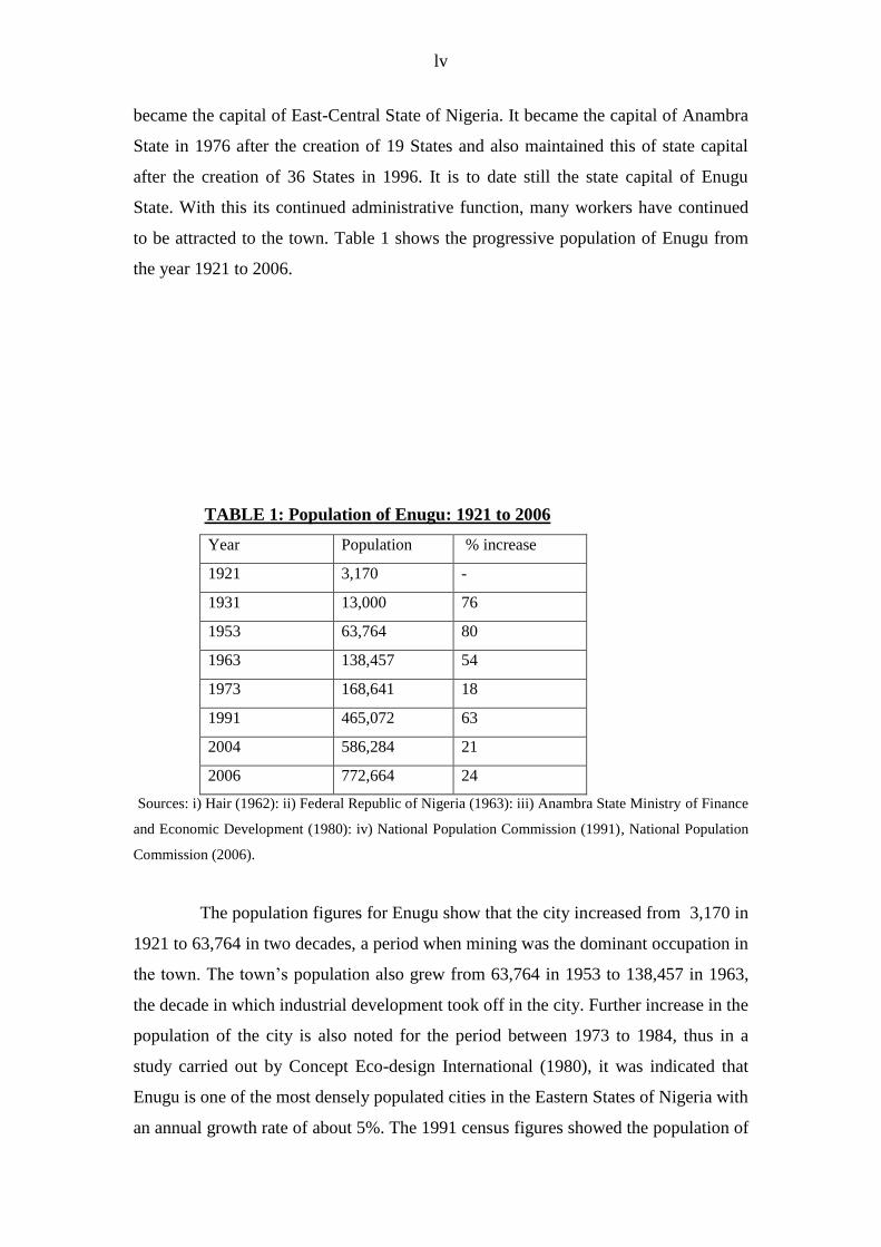
to be attracted to the town. Table 1 shows the progressive population of Enugu from

the year 1921 to 2006.

TABLE 1: Population of Enugu: 1921 to 2006

Year Population % increase

1921 3,170 -

1931 13,000 76

1953 63,764 80

1963 138,457 54

1973 168,641 18

1991 465,072 63

2004 586,284 21

2006 772,664 24

Sources: i) Hair (1962): ii) Federal Republic of Nigeria (1963): iii) Anambra State Ministry of Finance

and Economic Development (1980): iv) National Population Commission (1991), National Population

Commission (2006).

The population figures for Enugu show that the city increased from 3,170 in

1921 to 63,764 in two decades, a period when mining was the dominant occupation in

the town. The town’s population also grew from 63,764 in 1953 to 138,457 in 1963,

the decade in which industrial development took off in the city. Further increase in the

population of the city is also noted for the period between 1973 to 1984, thus in a

study carried out by Concept Eco-design International (1980), it was indicated that

Enugu is one of the most densely populated cities in the Eastern States of Nigeria with

an annual growth rate of about 5%. The 1991 census figures showed the population of

lvi

Enugu urban to be 465,072 people. The population of Enugu urban has continued to

grow till date and is estimated to be 586,284 people in 2004, while the 2006

population is 772,664.

Enugu has experienced high rate of population growth as the National

Population Commission 1991 stipulated that an annual growth rate of 3% has been

experienced between 1991 and 2004. The implication of the high rate population

growth in Enugu urban is excessive pressure on the water resources of the urban area.

1.5.4 Residential Structure of Enugu Urban.

For the purpose of this study, Enugu is divided into 10 major residential wards

as was utilized for the 1991 census (Fig 6). These residential areas are as follows:

1. Ogbete (Coal Camp): This is one of the oldest residential areas in Enugu.

It occupies the southern sector to the extreme west of the city. It is bounded to

the north by the Ogbete stream and occupies an area of about 5.2 square kilometers.

The houses in this area are mostly bungalows and have outhouses, separately

detached kitchens and toilet houses. Most of the people residing in this area are of the

low-income group being mainly petty traders and artisans.

2. Ogui: Ogui is a high-density old residential area and it has at the eastern

part of the city. It occupies an area of about 3.6 sq kms. Most of the houses found

in this area are bungalows, but a good number are storey buildings. It is inhabited

by petty traders, artisans, teachers and low-income civil servants.

3. Asata: Asata lies east of Ogui residential area and is separated from the latter by

a small tributary of the Asata River. It occupies an area of about 5.0 sq kms.

Some of the houses in this residential area are fenced and each contains the main

house, a kitchen, bathroom and toilet. Most of the residents are mainly civil servants

and petty traders. It however houses mostly the middle-income earners. Hand dug

wells abound in this area.

lvii

4. Uwani: This residential layout lies to the southern part of the city. It occupies an

area of about 3.3 sq kms.

Storey buildings and bungalows are predominant in this area. Some of the

houses possess modern amenities like water taps and water closet systems, while

some possess no modern facilities. Generally, this ward is built up and devoid of

open spaces. Senior civil servants and other professional reside in this area.

Residents of this area, depend a great deal on hand-dug wells found in most

compounds.

5. Achara layout: Achara layout lies south of Uwani. It occupies an area of about

5.0 sq kms. Most houses in this area primarily are storey buildings of modern

architectural design with modern facilities.

A few bungalows are however found in this area and some of these

bungalows have no modern facilities like taps and water closet systems. People from

all walks of life reside in this area. Generally, Achara layout is noted for the fact that

the residents depend heavily on groundwater supply.

6. New Haven: This is a medium density area, located at the extreme northern

section of the city. It is bounded to the north by a railway line and to the south by the

Asata River. It occupies an area of about 3.3 sq kms.

It comprises both storey buildings and bungalows. Some of the houses are

self-contained. Hand dug wells are uncommon here. Both the low and upper income

people reside in this residential area.

7. Iva Valley: Iva valley is an old residential area located in the eastern part of the

city. It occupies an area of about 10.9 sq kms and it is the third largest ward in Enugu.

It consists mainly of bungalows and make shift houses that possess no form modern

facilities like water closet systems and ‘boy’ quarters.

Most of the residents in this ward are mainly petty traders, ex-coal

mineworkers, and artisans.

8. Abakpa Nike: Abakpa Nike lies to the extreme north of the city and is bounded

to the south by the Ekulu River. The government low cost housing estate is located in

this area and it is occupied by the high and middle class civil servants.

lviii

It occupies an area of about 11.8 sq km, the second largest ward in Enugu. It is

also very densely populated. Some of the bungalows and storey buildings in this ward

are of modern architectural design with modern facilities. Both the low, middle and

high income workers reside in this residential area.

lix

FIG 6: MAP OF ENUGU SHOWING MAJOR WARDS Source: Fieldwork, 2006.

N

IGBO ETITI ISI UZO

0 1 2 3 4 5

LEGEND

Local Government Boundary

Ward Boundary

Rivers

Urban Boundary

INDEPENDENCE LAYOUT

ACHARA LAYOUT/ MARY LAND

COAL CAMP

UWANI

OGUI

ASATA

NEW HEAVEN

ABAKPA NIKE

IVA - VALLEY

GRA

lx

9. Independence layout: This residential area lies in the eastern part of the city. It

occupies an area of about 9.8 sq kms.

Most of the buildings in this area are storey buildings, while some are duplexes

with modern facilities. The houses are mostly of modern architectural designs and are

often set in the midst of large lawns. It is a low density area occupied mostly by the

upper income workers. Hand dug wells are hardly found in this residential area.

10. Government Reserved Area (G.R.A): this area lies in the northern part of the

city. It is bounded to the north by the Ekulu River and occupies an area of about 15.5

sq kms. It is the largest ward in this city.

The initial buildings were of British Colonial architectural designs. The houses

are predominantly bungalows and storey buildings set in the midst of large lawns and

gardens. The outstanding character of this ward is its openness and low housing

density.

Some government offices also exist here and it is the senior civil servants,

business proprietors and the upper income class that reside here. Hand dug wells and

bore holes are found in few houses.

1.5.5 Industrial and Institutional Structure of the City

Even though Enugu started as a coal mining settlement, coal mining is no

longer its primary industry (Okoye, 1975). At present, its dominant economic function

is administrative and commerce.

From the nineteen fifties, Enugu began to expand its industrial base by adding

manufacturing industries to its extractive industry. The first industrial estate for

Enugu was established at the satellite town of Emene in 1961. A smaller industrial

zone also exists at the Ogbete industrial estate. Apart from these, other small

manufacturing industries are located in different parts of the city.

Educational institutions in Enugu have increased in number over the years.

The town has more than 1,000 primary schools and 320 secondary schools (private

schools inclusive). It also has over eight higher institutions and these educational

institutions are located in different parts of the town.

1.5.6 Sample Location for Surface Waters.

lxi

The five major surface water sites (Fig 7) were as follows:-

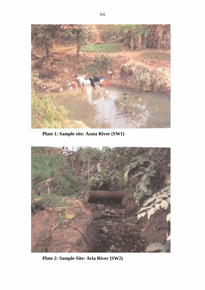
1. Asata river (Designated as SWI).

This sample site is located on the Asata river and the sample collection

point was from the location point with GPS reading of

N06.27.336,E007.30.430.This site is at the point where the Asata river flows

across the Ogui road( close to the Ogui road Zenith bank)(Plate 1). Domestic and

municipal effluents especially those generated from the Artisan market are

deposited into the water at various points around this site. A block industry, fuel

station, and car washing centre exist close to the bank of this river at this sample

site. Urban agriculture where animal dung is utilized is also practiced along the

banks of the river by the inhabitants of the railway quarters.

2. Aria river (Designated as SW2).

This sample station located on the Aria which flows through the Government

Reserved Area and has a GPS reading of N06.28.941, E007.28.925.This sample site is

located where most of the human activities take place along the river. A lot of

residential buildings (e.g. the Onitsha Road flats), a filling station, market and a

mechanic workshop are located close to this sample site, while a market also exists

close by. The river serves as a waste dump site for the waste originating from the

market and neighboring residential areas (Plate 2).

3. Ekulu river (Designated as SW3)

This river which has its source outside the Enugu urban area flows through the

Abakpa Nike residential area. The sample station with a GPS reading of N06.51.647,

E007.24.448 is situated where most of the activities such as collection of water for

domestic activities, sand quarrying, washing of cloths take place. Waste dump sites

also exist at the river banks (Plate 3).

lxii

Plate 1: Sample site: Asata River (SW1)

Plate 2: Sample Site: Aria River (SW2)

lxiii

Plate 3: Sample Site: Ekulu River (SW3)

4. Ogbete river (Designated as SW 4)

This river flows through the Coal Camp ward. The sample station with a

GPS reading of N06.26.940, E007.28.923 is situated were a shanty residential area

bothers the river (Plate 4). The University of Nigeria teaching hospital and the Ogbete

market are also major facilities along the banks of this river. These facilities all utilize

the river as waste dump sites.

5. Immaculate river (Designated as SW 5)

This river serves as a divide between the Coal Camp and Uwani wards. It

has its origin from outside the urban area. The sample station with a GPS reading of

N06.25.401, E007.29.769., has a lot of residential buildings and motor mechanic

workshops close to its banks. It is utilized by both wards for various domestic

activities. At times of scarcity it serves as the only source of water supply especially

for the Coal Camp ward where the use of hand dug wells is not practiced (Plate 5).

lxiv

Plate 4: Sample Site: Ogbete River (SW4)

Plate 5: Sample Site: Immaculate River (SW5)

lxv

FIG 7

lxvi

1.6 Research Methodology.

The survey universe consists of:

All the surface water bodies that flow through the urban center namely: Asata

River, Aria River, Ekulu River, Ogbete River, and Immaculate River.

Ground water sources i.e. hand dug wells located in different wards where

they are found and utilized.

Hospitals in the urban area.

Data that was used in this thesis was sourced form primary and secondary

sources. Comprehensive field work was carried out from January 2006 to

December 2006.

1.6.1 Field Work Procedure for Collecting Surface and Ground water Samples.

In selecting the sample stations, the researcher was guided strictly by the

objectives of the study, the human activities that take place within the urban area,

wards through which the rivers flow, accessibility of the stations and the cost of

analyzing each selected parameter. Based on previously mentioned facts, the surface

water bodies in Enugu were identified and a sample site was selected per river. The

sample station was selected in such a manner that the site is located about 2 kms away

from the area of concentration of human activities.

On the issue of selecting sample sites for ground water survey, wards in the

urban area that have hand dug wells were first identified. The selection of a sample

site in each identified ward was governed by the acceptance of such residents to

allow the monthly samples to be collected from their hand dug wells. Five

wards(namely: Asata, Abakpa, Achara Layout, Ogui and Uwani) were identified as

being dependent on hand dug wells are major sources of their water supply, while

the other wards did not have hand dug wells at all.

This entailed having one major sample site in each of the five wards where

hand dug wells are utilized, and then sampling from four(4) other sites that lie

three(3) kilometers radius( north, south, east , west )of the major sample site(Fig 7).

The sample sites are as follows:

HDW 1: The sample sites represent Abakpa Nike ward. The major sample site was

selected from one of the houses on Ugbene Street (N06.28.868, E007.30.877) (Plate

6). In this part of the ward, virtually every house has a hand dug well as they find it

lxvii

very easy to intercept water at shallow depths. The houses in this area also occur very

close to each other such that the wells are dug in any available space regardless of

how close it is to the septic tank.

Plate 6: Sample Site: Abakpa(representing Abakpa ward) (HDW1)

HDW 2: The sample sites represent Achara Layout ward. The major sample site

was selected from one of the houses on Igbaram Street (N06.25.401,

E007.29.779)(Plate 7 ).This area has a lot of high rise houses and because of sever

water shortages arising from the fact that they are rarely supplied water by the Water

Board each compound has its own hand dug well( Plate 7).

HDW 3: The sample sites represent Uwani ward. The major sample site was

selected from one of the houses on Edozien Street (N0625.401. E007.29.779).This

area experiences water scarcity such that the residents of this ward depend on hand

dug wells for their regular water supply (Plate 8).

lxviii

Plate 7: Sample Site: Achara layout (Representing Achara layout ward) (HDW2)

Plate 8: Sample Site: Uwani (Representing Uwani ward) (HDW3)

lxix

HDW 4: The sample sites represent Ogui ward. The major sample site was selected

from one of the houses on Edinbury Road (N06.25.763, E007.31.420).This area

experiences water scarcity and hand dug wells are common features in this ward (

Plate 9).

Plate 9: Sample site: Ogui (Representing Ogui ward) (HDW 4)

HDW 5: The sample sites represent Asata ward. The major sample site was selected

from one of the houses on Udi Road (Plate 10). Due to the inability of the residents of

this ward to obtain water from the Water Board, they depend on hand dug wells found

in their various compounds for their water supply.

lxx

Plate 10: Sample Site: Asata (Representing Asata Ward) (HDW5) Note: The

well is attached to a toilet house.

On the whole, 10 sample stations were maintained (five surface water sites

and five ground water sites (Fig 7).The water samples were preserved and analyzed at

the Edo State Environmental Laboratory, Benin City.

In Nigeria, the Federal and States Governments are guided in their

environmental policy by the recommendations of the WHO and FAO (McDonald

and Kay, 1988). WHO drinking water quality guidelines have thus formed the basis

for testing. The full range of parameters have not been utilized in this work because

of resource constraints and also based on the fact that this is permissible. The

selected physico-chemical and biological parameters are as:-

Temperature, Turbidity, Total Dissolved solid, pH, Conductivity, Dissolved

Oxygen, Biochemical Oxygen Demand, Hardness, Phosphates, Nitrate, Sulphate,

Ammonia, Calcium, Iron, Sodium.

lxxi

1.6.2 Method of Laboratory Analysis of Water Samples.

1.6.2.1 Temperature: The surface water temperatures were determined in situ

using a mercury-in-glass thermometer lowered at a depth between 0.5 and 1

meter until a constant reading is attained (approximately 2 minutes). The

temperature is then recorded in Celsius. The recording was done between 3-4

pm.

1.6.2.2 pH: The pH was determined in situ using a Suntex Digital pH Meter. The

meter probe was immersed into the sub-surface water (6 meters) and the pH read from

the meter.

1.6.2.3 Conductivity (µSCM): The water conductivity values were determined in

situ using the Suntex 120 Conductivity Meter. The meter probe was immersed into the

surface water (6 meters) and the values were read from the conductivity meter.

1.6.2.4 Turbidity: The turbidity (optical clarity of water) was measured using a

simple device called a turbidimeter (a Suntex Digital Turbidity Meter Model was

used).The turbidimeter is an optical device that measures the scattering of light and

provides a relative measure of turbidity in Nephelometer Turbidity Units (NUT).

1.6.2.5 Total Dissolved Solids: The gravimetric method was used to determine

surface water total dissolved solids (TDS) with a filter membrane apparatus in

accordance with APHA 2540D Protocol. A 100ml aliquot of the water sample was

filtered through a dry pre-weighed 0.45 µm filter paper. The filter was then oven dried

at 105C for one hour ( i.e. evaporated to dryness). After drying, the filter paper was

cooled and weighed. The difference in weight gives the total dissolved solids (TDS).

1.6.2.6 Dissolved Oxygen: Dissolved oxygen (DO) was determined by the Azide

modification of Winkler’s method adapted for the HACH DR 2010equipment for

standard methods. Clean 60ml glass-stopper BOD bottle was filled to over flowing

with water samples directly from source. Fixation in the field was carried out by

adding the contents of Dissolved Oxygen 2 powder pillows. The bottle stoppers were

restored and the content was thoroughly mixed by rotation and inversion until a

lxxii

flocculent brownish precipitate was produced. The bottles were stored away in

darkened containers under water until their contents were titrated in the laboratory.

Before titration, the contents Dissolved Oxygen 3 powdered pillow (sulphamic acid)

was added, thoroughly mixed, and aliquots of 20ml with 0.200n sodium thiosulphate

using the HACH Digital Titration, until the sample changed from yellow to

colourless. Using starch indicator towards the end of the titration remarkably

improved the end point from deep blue to colourless. The number of digits from the

digital counter window multiplied by 0.1 gave the concentration of dissolved oxygen

in mg/l.

1.6.2.7 Biochemical Oxygen Demand: A Darkened bottle was used to collect the

water sample. The sample was incubated for 5 days at 20(i.e. room temperature) in a

light-tight drawer. After 5 days, the level of dissolved oxygen was determined by

conducting the dissolved oxygen test. The biochemical oxygen demand level was then

determined by subtracting this dissolved oxygen from the dissolved oxygen level

found in the original sample taken 5 days previously. The values are expressed in

mg/l.

1.6.2.8 Total Hardness: This was determined using ETDA titrating procedure

(i.e. using the solution of the sodium salt of ethlinediaminetetraacetic acid as the

titrating agent and Epitome Black T (a dye which serves as an indicator to show when

all the hardness ions have been complexed. The hardness is then calculated from the

titration result and expressed as mg/l.

1.6.2.9 Calcium: This was determined using the tritimetric EDTA method.

Eriochrome black was used as the indicator. A known volume of sample was titrated

with EDTA titrant to reach from pink to purple end point. The calcium content is

calculated after the tirantand and the results are expressed in mg/l.

1.6.2.10 Sulphate: Sulphate was determined turbidimetrically with UV/Visible

spectrophotometer at a wavelength of 425nm in accordance with ASTM D4130. The

method is based on precipitated of sulphate with barium chloride (precipitating agent).

Prior to analysis of the samples the equipment was calibrated with sulphate working

standards prepared in-house from neat sulphate salts. The result was recorded in mg/l.

lxxiii

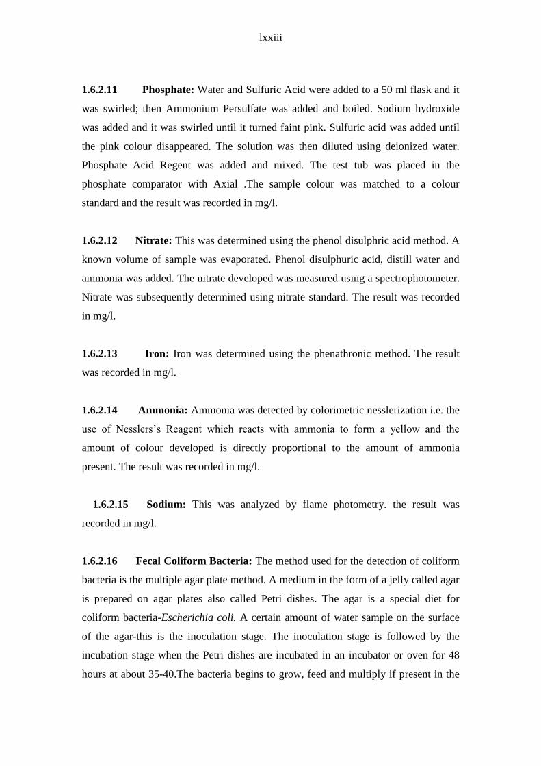
1.6.2.11 Phosphate: Water and Sulfuric Acid were added to a 50 ml flask and it

was swirled; then Ammonium Persulfate was added and boiled. Sodium hydroxide

was added and it was swirled until it turned faint pink. Sulfuric acid was added until

the pink colour disappeared. The solution was then diluted using deionized water.

Phosphate Acid Regent was added and mixed. The test tub was placed in the

phosphate comparator with Axial .The sample colour was matched to a colour

standard and the result was recorded in mg/l.

1.6.2.12 Nitrate: This was determined using the phenol disulphric acid method. A

known volume of sample was evaporated. Phenol disulphuric acid, distill water and

ammonia was added. The nitrate developed was measured using a spectrophotometer.

Nitrate was subsequently determined using nitrate standard. The result was recorded

in mg/l.

1.6.2.13 Iron: Iron was determined using the phenathronic method. The result

was recorded in mg/l.

1.6.2.14 Ammonia: Ammonia was detected by colorimetric nesslerization i.e. the

use of Nesslers’s Reagent which reacts with ammonia to form a yellow and the

amount of colour developed is directly proportional to the amount of ammonia

present. The result was recorded in mg/l.

1.6.2.15 Sodium: This was analyzed by flame photometry. the result was

recorded in mg/l.

1.6.2.16 Fecal Coliform Bacteria: The method used for the detection of coliform

bacteria is the multiple agar plate method. A medium in the form of a jelly called agar

is prepared on agar plates also called Petri dishes. The agar is a special diet for

coliform bacteria-Escherichia coli. A certain amount of water sample on the surface

of the agar-this is the inoculation stage. The inoculation stage is followed by the

incubation stage when the Petri dishes are incubated in an incubator or oven for 48

hours at about 35-40.The bacteria begins to grow, feed and multiply if present in the

lxxiv

water. Colonies of the bacteria are counted under the microscope and the number

recorded.

1.6.3 Field Work Procedure for Hospital Sampling.

The main procedure for obtaining information from hospitals was through

hospital records generated from hospitals in Enugu urban area. To qualify as a sample

site, a hospital had to have the facility for admitting patients or be a clinic that treats

up to 100 patients per month. This criterion was decided upon by the researcher to

ensure the possibility of working with hospitals with high patronage. However, only

hospitals that were willing (after being promised by the researcher never to mention

the hospital name) were utilized for the study.

On the whole, five hospitals were selected per ward, making a total of 50. In

each month therefore these hospitals were visited. Information regarding patients was

extracted from the hospital cards. To determine patients that qualified for the study,

the residential address of each patient played a major role. Each visit, the researcher

would identify from the hospital records the patients who reside in any of the wards in

Enugu that visited the hospital. Such patients then were considered to be qualified.

The researcher, working with the help of the nurses, extracted the illness the patient

was diagnosed as suffering from. The number of patients that were treated for water-

related diseases per month was recorded. The most frequently occurring water-related

illnesses were determined.

1.6.4 Documentary Materials.

Relevant documents from the State Water Corporation, Ministries, and

hospitals were collected and reviewed. Additional information was also obtained from

library and internet search.

1.6.5 Field Observations.

Field observation helped a great deal in keeping the researcher informed

about the actual situation of things on ground. For instance, we were able to identify

the various types of wastes normally deposited directly into the surface water bodies

especially those that flow close to residential areas and market places. This enabled us

to appreciate the water analysis (results) obtained from the water samples.

lxxv

It was also possible to determine the wards that were utilizing ground water

resources due to regular water shortages.

The GPS readings of the sample sites were determined using GPS 12 Garmin Model

(Serial Number 36209488) obtained from the Faculty of Life Science, University of

Benin, Benin city.

1.6.6 The Water Quality Index Methodology utilized

Traditional approaches to assessing water quality are based on a

comparison of experimentally determined parameter values with existing guidelines

as has been conducted in Chapter Two of this work. The use of this methodology

allows for proper identification of contamination sources. However it does not readily

give an overview of the spatial and temporal trends in the overall water quality in a

watershed (Debels, Figueroa, Urrutia, Barra, and Niell (2005).

One of the major difficult tasks also facing environmental and water

managers is how to transfer the interpretation of the complex physical, chemical and

biological parameters into information that is understandable to technical and policy

individuals as well as the general public. The general public, political decision-makers

and non-technical water managers usually do not have the time and the training to

study and understand traditional, technical review of water quality data

(Brown,1970).This is because the quality of water is defined in terms of its physical,

chemical and biological parameters (Sargaonkar and Deshpande, 2003).

Internationally, there have been a number of attempts to produce a method

that meaningfully integrates the data sets and converts them into information (Nagels,

Colley and Smith, 2001).Thus a number of indices have been developed to summarize

water quality data in an easily expressible and understood format (Couillard and

Lefebvre, 1985).

Water Quality Index (WQI) according to Boyacioglu (2007) was first

proposed by Horton in 1965 and since then a lot of consideration has been given to

the development of ‘water quality index’ methods with the intent of providing a tool

for simplifying the reporting of water quality data (Liou, Lo and Wang, 2004). Thus

various methods of calculating water quality index have been developed e.g. the

standard method developed by the National Sanitation Foundation (NSF) (developed

in the early 1970s by the Environmental Protection Agency (EPA) Region 10)

(NSFWQI) (Mitchell and Stapp, 1993) and the Universal Water Quality Index

lxxvi

(UWQI) developed by Boyacioglu, 2007). All methods are targeted at utilizing

physical, chemical and biological parameters to arrive at a value that indicates the

state of the health condition of the water body.

The Water Quality Index (WQI) is a useful tool for communicating water

quality information to the lay public and to legislative decision makers; it is not a

complex predictive model for technical and scientific application (McClelland, 1974).

It is basically a mathematical means of calculating a single value from multiple test

results. It thus provides a single number like a grade that expresses overall water

quality at a certain location and time based on several water quality

parameters(Veerabhadram,1998).The index result represents the level of water quality

in a given water basin e.g. river or stream, lake etc. This can give an indication of the

health of the water shed at various points and can be used to keep track of and analyze

changes over time; compare a water supply’s quality with other water supplies in the

region or from around the world. To determine our WQI, the standard method

developed by the National Sanitation Foundation (NSFWQI) was utilized.

The Water Quality Index (WQI) is a unit less number ranging from 0-100.

A scale rates the quality of the water as follows:

Range(Water

Quality Index

value)

Quality(Rank)

91-100 Excellent

71-90 Good

51-70 Average(Medium)

25-50 Bad

0-25 Very Bad

To determine the WQI, nine parameters were measured and used thus

creating a worksheet presented as appendix A. The parameters are Biochemical

Oxygen Demand, Dissolved Oxygen, Fecal coliform, Nitrates, pH, Temperature,

Total dissolved solids, Phosphate and Turbidity.

The Q-value for each parameter was calculated and recorded on the worksheet

(Appendix A). The Q-value for each parameter was then multiplied by the weight

factor and recorded as Total column (Appendix A). The total column values were

lxxvii

added up to determine the overall WQI for the water sources tested (Appendix B to

Y).

The index result obtained was compared to the WQI categorization scheme to

determine the water quality rating for the water sources tested.

1.6.7 Methods of Data Analysis.

In handling the data generated from the water samples and hospital

records, appropriate statistical and cartographic techniques were used to analyze and

present the results of the study. The figures (diagrams) utilized in this research gave

the opportunity of portraying the visual image of the phenomenon under discussion.

Basic statistical parameters such as percentages mean standard deviations, standard

errors of estimates, line graphs, Cluster bars etc were used to deduce patterns and

relationships. The major analytical tools were the ANOVA and the National

Sanitation Foundation Water Quality Index Method.

1.6.8 PLAN OF THE THESIS.

This thesis is presented in seven chapters.

Chapter one is the introduction devoted to the discussion of the background of

the study, the research problem, aim and objectives of the study, the area of study,

literature review and research methodology. Chapter two reflects what the physical,

chemical and bacteriological conditions of the surface and groundwater sources are

like. Under this part, the comparison of the laboratory results of surface and

groundwater samples to the World Health Organization guideline for drinking water

was carried out.

Chapter three discusses the detected variations between the parameters on

seasonal bases and the spatial variations evidenced by the field study are highlighted.

This provided information on the quality variation patterns between surface and

groundwater.

In chapter four, the monthly and annual water quality indices of surface and

groundwater resources are calculated and the findings discussed. Based on the

resulting water quality indices, inferences are made regarding the quality (health) of

the water resources of Enugu urban area.

lxxviii

Chapter five deals with the incidents and prevalence of water-related diseases

identified in the study area. The seasonal and spatial dimensions of the water-related

diseases are discussed.

In chapter six the environmental and policy implications of the detected water

quality were discussed. Emphasizes were laid on the likely implication of

disregarding the resultant water quality in the urban area.

Chapter seven summaries the various findings. Also measures that can be taken

to ensure quality improvement of the urban water resources were indicated.

CHAPTER TWO.

COMPARATIVE ANALYSES OF SURFACE AND GROUNDWATER

RESOURCES OF ENUGU URBAN AREA.

lxxix

2.1 Selected parameters for laboratory analysis and the World Health

Organization guidelines for drinking water.

Various authors such as Rodier (1975), Grower (1980), Ellis (1989) and

Uzoukwu, Ngoka and Nneji (2004) are of the opinion that water quality is commonly

defined by its physical, chemical, biological and aesthetic (appearance and smell)

characteristics. Water quality is determined by the kinds and amounts of substances

dissolved and suspended in the water and what these substances do to inhabitants of

the ecosystem (Johnson, Holmanand and Holniquist, 2000; Davie, 2002).It is thus the

concentration of these substances that determine the water quality and its suitability

for a particular purpose(Curtis,2001).Water quality standards are thus objectives that

are recognized in enforcing environmental laws, regulation and comprehensive water

management.

In the case of Nigeria, the government is guided in its environmental policy by

the recommendations of the World Health Organization (WHO) and Food and

Agricultural Organization (FAO) (McDonald and Kay, 1988). Nabila and Kehinde

(2003) are also of the opinion that the WHO standards serve as guideline for Nigeria

policy issues. The Nigerian National Water Supply and Sanitation policy objectives

also justify this assertion.

The policy which has as its aim ensuring that good water quality standards are

maintained by water supply undertakings has six objectives to achieve this aim. Two

of these are as follows:

i) Monitor and protect the quality of raw water sources for drinking water.

ii) The WHO drinking water quality guidelines shall be the baseline for the National

drinking water quality standard.

The WHO International Standard for drinking water was first prepared in 1958

and revised in 1963 and 1971. In the 1980s its philosophy and content were changed

significantly to become the global guideline for drinking water quality (WHO1993,

1998).Till date the WHO produces international norms on water quality and human

health in the form of guidelines that are used as the basis for regulation and standard

setting in developed and developing countries world-wide. The water quality criteria,

objective and standards had to be developed based on vigorous scientific knowledge.

The WHO guidelines for drinking water prescribe minimum numerical guideline

values for constituents of water as indicators of water quality.

lxxx

Based on the fact that this study is an ambient monitoring programme

(monitoring of a few parameters on a routine monthly basis for at least one year), the

results of this research are limited to sixteen (16) of the standard parameters stipulated

by the WHO. The standard parameters utilized are shown in Table 2.

Table 2: Selected parameters for laboratory Analysis

Parameter Unit of measurement Maximum

Permissible

Level

Temperature ºC 25

Ph 7.0-8.5

Turbidity NTU 5

Total Dissolved

Solid(TDS)

Mg/l 500

Conductivity µ/SCM 1

Total Hardness Mg/l 500

Dissolved Oxygen Mg/l 3.0

Biochemical Oxygen

Demand

Mg/l 2

Phosphate Mg/l 5.0

Sodium Mg/l 100

Sulphate Mg/l 200

Iron Mg/l 0.3

Ammonia Mg/l 45

Calcium Mg/l 75

Nitrate Mg/l 10

Fecal Coliform Bacteria cfu/100ml 0

Source: WHO (1988, 2004)

2.2 Comparison of Laboratory Results of Surface and Groundwater

Sources to the World Health Organization (WHO) Guideline for

Drinking-Water.

The surface water sources under study are the five major rivers in the study area

(Fig 4). They are namely:

Asata river (SW I )

Aria river (SW 2 )

Ekulu river (SW 3 )

Ogbete river (SW4 )

Immaculate river ( SW 5 )

2.2.1 Temperature of the urban rivers.

The water temperature of a river is very important for water quality. It is

often a good indicator of contamination. Any sudden change in temperatures of say

groundwater suggests that the water is contaminated, possibly from industrial

discharges (Dixey, 1972). It is thus an important indicator of the overall quality of a

lxxxi

body of water (Mitchell, Stapp and Bixby, 2002).Many of the physical, chemical and

biological characteristics of a river are directly affected by temperature.

Temperature influences: the amount of oxygen that can be dissolved in water

(solubility of gases), the rate of photosynthesis by algae and large aquatic plants, the

metabolic rates of aquatic organisms, the sensitivity of organisms to toxic wastes,

parasites and diseases.

From the result of the field study, the highest temperature value

recorded in any of the rivers was 27ºC, while the lowest was 23ºC (Table 3).

TABLE 3: Temperature values of rivers in Enugu urban area.(C)

SAMPLE SITES

Months SW 1 SW 2 SW3 SW4 SW5

January 25 25 25 25 25

February 26 26 26 26 26

March 27 27 27 27 27

April 23 23 23 23 23

May 23 23 23 23 23

June 26 26 26 26 26

July 25 25 25 25 25

August 24 24 24 24 24

September 23 23 23 23 23

October 23 23 23 23 23

November 25 25 25 25 25

December 25 25 25 25 25

Source: field work (2006)

The temperatures of the rivers were generally within the WHO Maximum

Permissible Level (MPL) of 25ºC except for some months when the temperature

exceeded the WHO’s MPL.The rivers/months in which temperatures exceeded the

WHO’s MPL are shown in Figure 8 and they include the following:

Asata river (SW 1): February, March and July.

Aria river (SW 2): March and July.

Ekulu river (SW 3): February, March and June.

Ogbete river (SW 4): February, March and July.

Immaculate river (SW 5): February, March and July.

2.2.2 pH of the urban rivers.

The pH vale is used to describe the intensity of acidity of a solution

(Mitchell and Stapp, 1993). Water contains both hydrogen ions (H+) and hydroxide

ions (OH-). To determine the pH of a solution, the relative concentration of both

ions must be measured. The pH is a measure of the concentration of hydrogen ions

lxxxii

of liquids and substances. It is derived from the manner in which the hydrogen ion

concentration is calculated. It is the negative logarithm of the hydrogen ions (H+)

concentration. Each measured liquid has a pH value on a scale that ranges from 0 to

14(Clescen, Greenbery and Eaton, 1998); with neutral solutions at pH7 and acidic

solution from 0-7 and alkaline solution from 7 -14. Most natural waters have a pH

from 4 to 9 and majority are slightly alkaline, above 7 due to bicarbonates of

calcium and magnesium dissolved in the water.

From the laboratory analyses, the highest level of pH concentration for the 12

months under study was recorded in Ekulu river (SW 3) with a pH value of 7.29 in

February, while the lowest level of concentration was recorded in Asata river in

September with a pH value of 4.45(Table 4).

TABLE 4: pH values of rivers in Enugu urban area.

SAMPLE SITES

Months SW 1 SW 2 SW 3 SW 4 SW 5

January 6.53 5.557 6.2 6.11 6.15

February 6.75 6.78 7.29 6.91 6.97

March 6.49 6.5 6.34 6.31 6.65

April 6.52 6.62 6.67 6.73 6.56

May 6.5 6.51 6.88 6.61 7.15

June 6.31 6.25 6.35 6.41 6.39

July 6.6 6.69 6.47 6.5 6.5

August 6.06 6.11 5.95 6.02 6.22

September 5.21 5.33 4.76 4.54 5.36

October 6.47 7 5.49 5.41 6.02

November 4.91 5.05 5.37 5.3 5.51

December 6.25 6.51 6.32 6.05 6.75

Source: Field work (2006).

A comparison of the pH values obtained from laboratory analyses to the

WHO’s MPL of 7/8.5 indicate that the pH values for all the rivers fall within the

WHO’s MPL for the 12 months of study (Fig 9)

lxxxiii

Fig 8: Comparison of River temperature to WHO’s MPL

Fig 9: Comparison of river pH levels to WHO’s MPL.

2.2.3 Turbidity of the urban rivers.

Turbidity is a measure of relative clarity of water (Davie, 2002).Turbidity of

natural waters is caused by the presence of components such as clay, mud, organic

materials, bacteria, lime or rust held in colloid at suspension. The greater the turbidity,

the murkier the water is. Turbidity increases as a result of suspended solids in the

water that reduce the transmission of light (Hach, 1979).

FIG 9:Comparism of river pH levels to WHO(MPL)

0

1

2

3

4

5

6

7

8

J F M A M J J A S O N D

Months of the year

pH

lev

el

SW1

SW2

SW3

SW4

SW5

WHO(MPL)WHO’s MPL

Fig 8: Comparism of river temperatures to WHO(MPL)

21

22

23

24

25

26

27

28

J F M A M J J A S O N D

Months of the year

Te

mp

era

ture

( c

)

SW1

SW2

SW3

SW4

SW5

WHO(MPL)WHO’s MPL

lxxxiv

Table 5 and Figure 10 indicate that generally, the turbidity level for all the rivers

exceeded the WHO’s MPL of 5 NTU in most of the months. Low levels were

however recorded in some months. The low turbidity months were as follows:

Asata river (SW 1): February, May.

Aria river (SW 2): July, August, September.

Ekulu river (SW 3): March, May, July, August and December.

Ogbete river (SW 4): May, June, July, August and October.

Immaculate river (SW 5): August, September and November.

TABLE 5: Turbidity values of rivers in Enugu urban area.(NTU)

SAMPLE SITES

Months SW1 SW2 SW3 SW4 SW5

January 5 53 5 10 5

February 2 7 23 6 20

March 5 11 4 7 8

April 7 58 7 13 33

May 3 13 1 2 23

June 6 74 9 3 16

July 10 5 4 2 8

August 10 2 0 0 3

September 14 3 6 5 3

October 10 12 7 2 14

November 7 10 5 5 2

December 12 17 3 10 9

Source: Field work (2006).

2.2.4 Total Dissolved Solids of the urban rivers.

Total dissolved solids are the solid matter in water. Dissolved solids in a

natural water usually composed of the sulphate, bicarbonate and chloride of calcium,

magnesium and sodium (Michaud, 1991).

Table 6 indicates that the highest value for total dissolved solids in all the rivers

in Enugu urban area was 260 mg/l. The value occurred in November in Immaculate

river (SW 5), while the least occurred in Aria river in August.

TABLE 6: Total Dissolved Solids of rivers in Enugu urban area.(mg/l)

lxxxv

SAMPLE SITES

Months SW1 SW2 SW3 SW4 SW5

January 67 53 86 87 54

February 68 7 97 103 43

March 56 11 79 82 100

April 100 58 60 100 81

May 67 13 92 81 37

June 60 74 78 87 47

July 60 5 75 87 43

August 57 2 61 81 39

September 78 3 68 92 58

October 78 12 92 68 58

November 28 10 150 250 260

December 30 17 156 134 220

Source: Field work (2006).

Generally for all the rivers, the dissolved solids levels were within the WHO’s

MPL of 500 mg/l (Fig 11).

Fig 10: Comparison of rivers turbidity levels to WHO’s MPL

Fig 10: Comparism of rivers turbidity levels to WHO(MPL)

0

10

20

30

40

50

60

70

80

J F M A M J J A S O N D

Months of the year

Tu

rdid

ity(N

TU

)

SW1

SW2

SW3

SW4 SW5

SW5

WHO(MPL)WHO’s MPL

lxxxvi

Fig 11: Comparison of rivers total dissolved solids to WHO’s MPL

2.2.5 Conductivity of the urban rivers.

Conductivity is an index of the total ionic content of water. This is the

capacity of water for conveying electrical current and is directly related to the

concentration of ionized substances in the water. A rapid method of estimating the

dissolved salts in water sample is by measurement of its electrical conductivity

(Holden, 1970). It gives useful indication of the total concentration of ionic solutes

and therefore measures the freshness or otherwise of a water body.

Changes in conductivity of a sample, according to Hutton (1983) may signal

changes in mineral composition of raw water, seasonal variations in reservoirs,

intrusion of sea or saline waters by over pumping and pollution from industrial

wastes. Potable water should therefore not have high conductivity.

From the laboratory analysis showing the conductivity level in each of the

rivers (Table 7) and depicted in Figure 12, it can be seen that all the rivers have

values that are within the WHO’s MPL of 75 mg/l.

TABLE 7: Conductivity values of rivers in Enugu urban area.(µSCM)

Fig 11: Comparism of rivers total dissolved solids to WHO(MPL)

0

50

100

150

200

250

300

J F M A M J J A S O N D

Months of the year

To

tal

Dis

so

lved

so

lid

s (

Mg

/l)

SW 1

SW 2

SW 3

SW 4

SW 5

WHO(MPL)500 WHO’s MPL

lxxxvii

SAMPLE SITES

Months SW1 SW2 SW3 SW4 SW5

January 0.16 0.56 0.18 0.19 0.1

February 0.14 0.59 0.21 0.21 0.92

March 0.07 0.03 0.13 0.1 0.05

April 0.07 0.03 0.11 0.16 0.06

May 0.14 0.07 0.19 0.17 0.07

June 0.12 0.09 0.16 0.18 0.09

July 0.1 0.06 0.11 0.12 0.06

August 0.1 0.07 0.09 0.11 0.06

September 0.12 0.08 0.11 0.14 0.09

October 0.1 0.07 0.09 0.12 0.08

November 0.11 0.07 0.45 0.06 0.02

December 0.02 0.01 0.45 0.04 0.03

Source: Field work (2006).

2.2.6 Total Hardness of the urban rivers.

The total hardness is the sum of temporary or carbonate hardness and

permanent or non-carbonate hardness (Barth, 1990). Water hardness is due to the

presence of sulphate, chlorides, calcium and magnesium (Betz and Nell, 1950).

Hardness as measured is made up of alkaline earth metals, mainly calcium and

magnesium ions.

Knowledge of the hardness of water is of great importance especially from the

standpoint as hard water consumes excessive quantities of soap, forming curd and

depositing on the hair, fabrics and glass ware. In terms of industrial uses, it is the

chief source of scale in heating equipment, boilers and pipelines (Barth, 1990).

From Table 8 and Figure 13, it is observed that all the rivers have hardness

values that are within the WHO’s MPL of 100 mg/l.

TABLE 8: Total hardness of rivers in Enugu urban area. (mg/l)

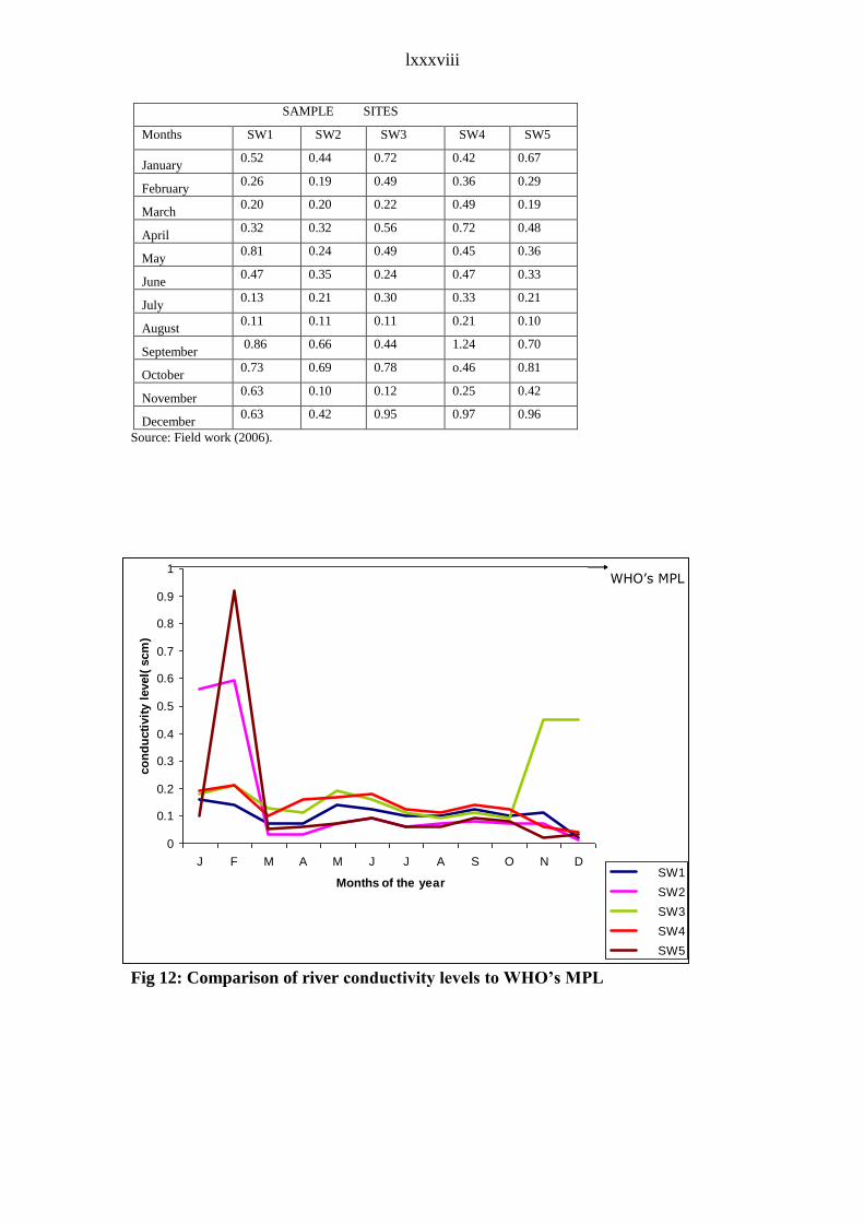
lxxxviii

SAMPLE SITES

Months SW1 SW2 SW3 SW4 SW5

January 0.52 0.44 0.72 0.42 0.67

February 0.26 0.19 0.49 0.36 0.29

March 0.20 0.20 0.22 0.49 0.19

April 0.32 0.32 0.56 0.72 0.48

May 0.81 0.24 0.49 0.45 0.36

June 0.47 0.35 0.24 0.47 0.33

July 0.13 0.21 0.30 0.33 0.21

August 0.11 0.11 0.11 0.21 0.10

September 0.86 0.66 0.44 1.24 0.70

October 0.73 0.69 0.78 o.46 0.81

November 0.63 0.10 0.12 0.25 0.42

December 0.63 0.42 0.95 0.97 0.96

Source: Field work (2006).

Fig 12: Comparison of river conductivity levels to WHO’s MPL

Fig 12: Comparism of river conductivity levels to WHO(MPL)

0

0.1

0.2

0.3

0.4

0.5

0.6

0.7

0.8

0.9

1

J F M A M J J A S O N D

Months of the year

co

nd

ucti

vit

y l

evel(

scm

)

SW1

SW2

SW3

SW4

SW5

WHO(MPL)WHO’s MPL

lxxxix

Fig 13: Comparison of total hardness of rivers to WHO’s MPL

2.2.7 Dissolved Oxygen of the urban rivers.

The oxygen content of water depends on a number of physical, chemical,

biological and microbiological processes (IHD-WHO, 1978). Water in contact with

air contains a certain quantity of oxygen depending on atmospheric pressure, the

temperature, and the content of dissolved salts.

Deviation in the concentration of oxygen from the equilibrium maybe caused

by sharp changes in the temperature of water, physico/chemical and chemical

process such as the use of oxygen for oxidation of substances or the absorption of

oxygen during the corrosion of metals, and biochemical processes such as the

aerobic biochemical oxidation of organic matter, the breathing of aquatic organisms

or the production of oxygen during the process of photosynthesis (Davie, 2002).

The measurement of oxygen in water is important because it is one of the

practical indications of the purity, indicating its biological state, the predominant

process in it, the destruction of organic substances and the intensity of self

purification (Ehinger, 1995).

Organic polluting materials added to water consume oxygen such that if there

are oxygen-consuming pollutants in water, concentration of dissolved oxygen is

affected. If there are no oxygen consuming pollutants in water, the concentration of

FIG 13:Comparism of total hardness of rivers to WHO(MPL)

0

0.2

0.4

0.6

0.8

1

1.2

1.4

J F M A M J J A S O N D

Months of the year

Hard

ness(m

g/l

)

SW1

SW2

SW3

SW4

SW5

`

WHO’s MPL

xc

oxygen present will be determined by the water temperature and its salt content

(Mara, 1978).Oxygen is the key component for the survival of most aquatic

organisms. The concentration varies from species to species. It is also important in

determining the corrosiveness of water.

Values of dissolved oxygen were determined by laboratory analyses and are

presented in Table 9.

TABLE 9: Dissolved Oxygen values for rivers in Enugu urban area.

SAMPLE SITES

Months SW1 SW2 SW3 SW4 SW5

January 1 1.6 6.7 3.1 0.6

February 8.7 9.7 9.7 8.7 8.8

March 4 4 3.6 4 3.8

April 1.7 1.7 1.7 1.4 2.7

May 4.6 5 4.4 3.9 5.1

June 5.9 5.6 4.9 4.5 4.9

July 5.4 5.4 5.4 4.8 5.2

August 5.8 5.6 5.4 3.6 5

September 7.3 7.8 6.3 6 6.8

October 4.7 4.8 5.4 3.6 5

November 7.3 7.8 6.3 6 6.8

December 4.5 5.8 5.5 5.7 5.8

Source: Field work (2006).

The dissolved oxygen values for all the rivers in most months of the year

exceeded the WHO’s MPL of 3.0 mg/l except in April for all the rivers and in

January for Asata, Ogbete and Immaculate rivers (Fig 14).

2.2.8 Biochemical Oxygen Demand (BOD ) of the urban rivers.

Biochemical Oxygen Demand is a measure of the amount of oxygen used by

microorganisms in the aerobic oxidation of organic matter (Michaud and Noel, 1991).

When organic matter decomposes, it is fed upon by aerobic bacteria. In this process

organic matter is broken down and oxidized (combined with oxygen).Aerobic bacteria

may decompose organic matter at such a fast rate that dissolved oxygen decreases

causing a biochemical oxygen demand. Nutrients are prime factor to high biochemical

oxygen demand (Carter, 1985).

Values of BOD determined by laboratory analyses are presented in Table10.

xci

TABLE 10: Biochemical oxygen demand values of rivers in Enugu urban

area.

SAMPLE SITES

Months SW 1 SW 2 SW 3 SW 4 SW 5

January 7.2 2.8 1 2.5 2.4

February 2.4 2.3 2.4 9.7 3.1

March 1.9 1.9 0.9 2.1 1.4

April 1.4 0.4 0.9 1.6 1.1

May 4.1 4 3.9 4.1 3.9

June 1 1 3.2 1.4 0.3

July 0.4 0.3 0.4 0.9 0.7

August 0.5 0.4 0.3 0.5 0.4

September 0.4 0.7 0.3 0.5 0.3

October 0.5 1 0.4 0.3 0.4

November 3.2 1.7 1.9 0.7 0.7

December 2.1 2.6 0.9 0.7 1.9

Source: Field work (2006).

From Table 10, the highest BOD for all the rivers was 9.7 mg/l, while the lowest

level was 0.3 mg/l. There were monthly variations in BOD levels in the rivers as

regards the months that had values that exceeded the WHO’s MPL of 2.0 mg/l. As

depicted in Fig 15, the months in which the BOD levels exceeded the WHO’s level

were as follows:

Asata river (SW 1): February, May and November.

Aria river (SW 2): February, May and December.

Ekulu river (SW 3): February, May and July.

Ogbete river (SW 4): January and February.

Immaculate river (SW 5): January, February and May.

On the average each river had a three (3) months period in which the BOD

exceeded the WHO‘s MPL, while in the other months of the year, the BOD levels

were within the WHO acceptable level.

xcii

Fig 14: Comparison of river dissolved oxygen levels to WHO’s MPL

Fig 15: Comparison of river biochemical oxygen demand levels to WHO’s MPL

2.2.9 Phosphate of the urban rivers.

Fig 14: Comparism of river dissolved oxygen levels to

WHO(MPL)

0

2

4

6

8

10

12

J F M A M J J A S O N D

Months of the year

Dis

so

lved

oxyg

en

(mg

/l)

SWS 1

SWS2

SWS3

SWS4

SWS5

WHO(MPL)WHO’s MPL

Fig 15: Comparism of river Biochemical oxygen Demand levels to

WHO(MPL)

0

2

4

6

8

10

12

J F M A M J J A S O N D

Months of the year

Bio

ch

em

ical

oxyg

en

dem

an

d(m

g/l

)

SW1

SW2

SW3

SW4

SW5

WHO(MPL)WHO’s MPL

xciii

Phosphorous is usually present in natural water as phosphate. In unpolluted

bodies of water, phosphates are formed mainly during biological processes of

transformation of organic substances to inorganic phosphates (Michaud, 1991).

Organic phosphate is a part of living plants and animals, their by-products, and

their remains (Canter, 1985; Barth, 1990).Inorganic phosphates include the ions

bonded to soil particles and phosphates present in laundry detergents. Phosphorous

comes from several sources such as human wastes, animal wastes, industrial wastes

and human disturbance of the land and its vegetation.

Phosphorous is an essential element for life. It is a plant nutrient needed for

growth and a fundamental element in the metabolic reactions of plants animals.

Plant growth is limited by the amount of phosphorus available. The natural scarcity

of phosphorous can be explained by its attraction to organic and soil particles. Any

unattached or free phosphorous in the form of inorganic phosphates is rapidly taken

up by algae and large aquatic plants.

Based on the fact that algae only require small amounts of phosphorous to live,

excess phosphorous causes extensive algal growth called “blooms” (Clexen,

Greenberg and Eaton, 1998). Algal blooms are a classic symptom of cultural

eutrophication.This is the human caused enrichment of water with nutrients, usually

phosphorous. Considerable irregular increases in the concentration of phosphates

may indicate a presence of pollutants.

The values of phosphate determined from laboratory analyses (Table 11)

indicate that three rivers (Asata, Aria and Ekulu) had phosphate concentration levels

that were within the WHO’s MPL of 5.0 mg/l. While two rivers (Ogbete and

Immaculate) had one month each (January and October respectively) in which the

phosphate concentration levels exceeded the WHO’s MPL of 5.0 mg/l (Fig 16).

TABLE 11: Phosphate values of rivers in Enugu urban area.(mg/l)

xciv

SAMPLE SITES

Months SW 1 SW2 SW3 SW4 SW5

January 3.9 4.54 3.65 5.77 3.29

February 2.1 3.92 3.29 3.29 2.96

March 4.16 2.33 3.12 2.62 2.04

April 1.6 1.9 4.8 1.6 2.1

May 0.26 0.53 1.04 0.13 0.25

June 0 0.02 0.13 0.17 0.38

July 0.32 0.02 0.02 0.02 0.13

August 0.11 0.13 0.06 0.09 0.02

September 1.43 0.32 1.76 0.08 0.8

October 0.14 0.16 1.76 4.72 5.19

November 0 0.02 0.01 0.01 0.01

December 0.01 0.01 0.01 0.01 0.01

Source: Field work (2006).

It is noteworthy however that despite the fact that the phosphate concentration

levels for rivers in Enugu urban area generally fall within the WHO’s MPL, the

phosphate levels are however high in some months as the total phosphate

concentration of non-polluted waters are usually less than 0.1 mg/l(Egboge, 1971).

2.2.10 Sodium of the urban rivers.

Sodium is present in appreciable amounts in almost all natural waters. Under

natural conditions, the range of concentrations is quite broad. However, in the

majority of rivers, lakes and bodies of water, their content is usually small compared

to other chief components (Mitchell, Stapp and Bixby, 2000). Its considerable

increase maybe connected with the pollution from industrial and household sewage.

Values of sodium obtained from laboratory analyses shown in Table 12 , and

depicted in Figure 17, show that the sodium level in all the rivers were within the

WHO’s MPL of 100 mg/l.

TABLE 12: Sodium values of rivers in Enugu urban area.

SAMPLE SITES

Months SW1 SW2 SW3 SW4 SW5

January 8.4 1.5 3.3 2.9 26.5

February 9.7 34 1.2 12.1 10.7

March 15.1 15 21 13.8 7.3

April 15.1 15.1 21.6 15.4 8.6

May 9.2 15.1 18 10.6 5.5

June 10.1 10.1 17.5 14.1 8.3

July 1.31 0.76 1.64 1.3 0.71

August 1.21 0.79 1.28 1.25 0.68

September 0.71 0.44 0.63 0.56 0.42

October 0.57 0.86 0.22 3.1 1.66

November 2.25 0.59 1.4 1.22 4.17

December 1.4 0.37 2.05 1.21 0.74

Source: Field work (2006).

xcv

Fig 16: Comparison of river phosphate levels to WHO’s MPL

Fig 17: Comparison of river sodium levels to WHO’s MPL

Fig16: Comparism of river phosphate levels to WHO(MPL)

0

1

2

3

4

5

6

7

J F M A M J J A S O N D

Months of the year

Ph

osp

hate

level(

mg

/l)

SW1

SW2

SW3

SW4

SW5

WHO(MPL)WHO’s MPL

Fig 17: Comparism of river sodium levels to WHO(MPL)

0

5

10

15

20

25

30

35

40

J F M A M J J A S O N D

Months of the year

So

diu

m l

evel(

mg

/l)

SW1

SW2

SW3

SW4

SW5

WHO(MPL)WHO’s MPL

xcvi

2.2.11 Sulphate of the urban rivers.

The supply of sulphate ions in surface, ground and underground waters under

natural conditions is due to the reaction of water with sulphate-containing rock and

other compounds (Michand and Noel, 1991). Increase in sulphate concentration

maybe related to pollution of the body of water by runoff water which contains

relatively large quantities of organic and mineral compounds of sulphur (Mitchell,

Stapp and Bixby, 2000).

The value of sulphate concentration in Enugu urban rivers shown in Table 13

indicates that Asata river (SW 1) had the highest value in the month of March (9.7

mg/l), where Figure 18 indicates further that generally all the rivers had values that

are within the WHO’s MPL of 200 mg/l.

TABLE 13: Sulphate values of rivers in Enugu urban area

SAMPLE SITES

Months SW1 SW2 SW3 SW4 SW5

January 0 0.7 0.1 0.6 0

February 2.3 8.4 7.4 6.6 1.8

March 9.7 0 0 0.6 0.6

April 2.4 2.3 1.6 7.4 4.7

May 0.3 0.4 0.4 1.8 5

June 0.3 0 0.4 3 1.9

July 0.1 0.4 0.1 0.6 0.4

August 0.1 0.2 0.1 0.2 0.3

September 0.3 0.7 0.7 0.1 0.6

October 1.2 0.6 2.5 1.6 0.6

November 0.1 0.1 0.1 0.1 0

December 0.6 0 1.1 0.7 0.2

Source: Field work (2006)

xcvii

Fig 18: Comparison of river sulphate levels to WHO’s MPL

2.2.12 Iron of the urban rivers.

Iron is found in a great variety of forms; in solution, colloids and suspensions

and in organic and mineral complexes in various states of valence (Mara, 1978).

Iron is present in most surface and subsurface waters. In polluted surface water, the

concentration of iron varies. For some industrial applications, not even a trace of

iron can be tolerated (Davis, 2002).

Irregular increases in the concentration of iron indicate a possible pollution

by waste waters of metallurgical and metal-processing industries and some mine

waters containing iron, when exposed to the air, so that oxygen can enter, become

turbid and highly unacceptable from the aesthetic view/point (Michaud and Noel,

1991).

Values of iron determined from laboratory analyses are presented in Table 14

and this is depicted in Figure 19.

Fig 18: Comparism of river sulphate levels to WHO(MPL)

0

2

4

6

8

10

12

J F M A M J J A S O N D

Months of he year

Ph

osp

hate

level(

mg

/l)

SW1

SW2

SW3

SW4

SW5

WHO(MPL)

WHO’s MPL

xcviii

TABLE 14: Iron content of rivers in Enugu urban area.

SAMPLE SITES

Months SW 1 SW2 SW 3 SW 4 SW5

January 0.01 0.1 0.03 0.03 0.2

February 0 0 0.01 0.01 0.2

March 0 0 0.1 0.1 0.2

April 0.1 0.1 0.1 0.2 0.2

May 0.1 0.1 0.17 0.1 0.1

June 0.1 0.1 0.1 0.1 0.1

July 0.1 0.1 0.1 0.1 0.1

August 0.1 0.1 0.1 0.1 0.1

September 0.1 0.1 0.1 0.1 0.1

October 0.1 0 0.1 0.1 0.2

November 0.1 0 0 0.1 0.1

December 0.1 0 0 0 0.1

Source: Field work (2006).

From Table 14 and Figure 19, it is observed that all the rivers have iron

values that are within the WHO’s MPL of 0.3 mg/l.

Fig 19: Comparison of river iron levels to WHO’s MPL

0

0.05

0.1

0.15

0.2

0.25

J F M A M J J A S O N D

Months of the year

SW1

SW2

SW3

SW4

SW5

WHO(MPL)

WHO’s MPL

Iron level(m

g/l)

0

0.05

0.1

0.15

0.2

0.25

J F M A M J J A S O N D

Months of the year

SW1

SW2

SW3

SW4

SW5

WHO(MPL)

WHO’s MPLWHO’s MPL

Iron level(m

g/l)

xcix

2.2.13 Ammonia of the urban rivers.

The presence of ammonia ions in unpolluted water is connected with the

process of the biochemical decomposition of protein substances (Mara, 1978).An

increase in the concentration of ammonium-ions therefore, is observed when aquatic

organisms are dying off especially in the zone of aggregation(layers of increased

density of phyto- and bacteria plankton(IHD-WHO,1978). Ammonia ions can be

formed during the anaerobic reduction of nitrates and nitrites.

A product of microbiological activity, ammonia is sometimes accepted as

chemical evidence of sanitary pollution when encountered in raw surface waters,

which has suffered de-oxygenation and denitrification due to sewage contamination or

contamination by industrial effluents and excremental pollution (Barth, 1990).

Thus the amplitude of seasonal fluctuations of ammonium ions reflects the

nutrition of the body of water and its pollution by organic nitrogen-containing

substances contained in household and industrial sewage(especially from the food

industry).

Values of ammonia determined from laboratory analyses presented in

Table15, indicate that the highest level was recorded in Ogbete river (SW4) in the

month of June.

TABLE 15: Ammonia values for rivers in Enugu urban area(mg/l)

SAMPLE SITES

Months SW1 SW2 SW3 SW4 SW5

January 0.93 0.36 0.57 3.23 0.46

February 0.9 0.32 0.22 0.22 0.38

March 0.78 1.58 3.31 1.81 2.12

April 1.69 2.62 1.96 2.42 2.31

May 1.12 0.78 2.31 1.81 1.23

June 6.92 7.1 5.45 8.72 6.57

July 0.06 0.11 0.09 0.01 0.01

August 0.09 0.06 0.12 0.04 0.09

September 0.12 0.03 0.1 0.1 0.04

October 1.23 0.63 2.46 1.63 0.28

November 0.91 0.01 0.02 0.03 0.01

December 0.71 0.01 0.01 0.02 0.01

Source: Field work (2006).

The ammonia level in all the rivers were within the WHO ‘s MPL of 45 mg/l as is

depicted by Figure 20.

c

Fig 20: Comparison of river ammonia levels to WHO’s MPL

2.2.14 Calcium of the urban rivers.

Calcium ions are present both in surface and in underground waters which

they penetrate as a result of the interaction between the water and the minerals in the

soil or rock (Maidment, 1993).The natural concentration of calcium maybe

influenced by industrial waste.

The calcium values obtained (Table16) and depicted in Figure 21, indicate

that all the rivers had calcium levels that were within the WHO’s MPL of 75 mg/l.

TABLE 16: Calcium values for rivers in Enugu urban area(mg/l)

SAMPLE SITES

Months SW1 SW2 SW3 SW4 SW5

January 2.01 1.95 2.02 2.41 1.81

February 1.8 1.95 2.09 2.6 1.87

March 2.05 2.08 2.62 2.63 1.78

April 2.62 2.53 2.67 2.82 2.01

May 2.69 2.55 2.93 2.94 2.51

June 2.83 2.73 2.93 3.04 2.59

July 3 2.95 3.05 3.4 2.59

August 2.89 2.98 3.05 3.4 2.51

September 2.91 2.98 3.01 2.94 2.67

October 2.5 2.54 2.76 2.62 2.01

November 2.5 2.02 2.03 2.61 2.05

December 2.21 2.02 2.05 2.55 2.09

Source: Field work (2006)

Fig 20:Comparism of river ammonia levels to WHO(MPL)

0

1

2

3

4

5

6

7

8

9

10

J F M A M J J A S O N D

Months of the year

Am

mo

nia

level(

mg

/l)

SW1

SW2

SW3

SW4

SW5

WHO(MPL)WHO’s MPL

ci

2.2.15 Nitrate of the urban rivers.

Nitrates appear in water chiefly as a result of biochemical oxidation of ammonia

or the reduction of nitrates (Barth, 1990; Michaud and Noel, 1991).Nitrates are the

end-product of the biochemical oxidation of ammonia and nitrogen from organic

matter, and a measure of the original quantity of organic matter with which a water

is associated.

Nitrates in water can originate from agricultural fertilizers, sewage, industrial

and packing house wastes, drainage from livestock feeding areas, farm manures and

legumes (Davis, 2002).Increased concentration of nitrates may indicate Fecal

pollution of the body of water in the proceeding period.

High nitrate content in potable water is harmful for children and cause

anaemia (Methaemogloanaemia) (Dasgusta, 2004). Nitrates in conjunction with

phosphates stimulate the growth of algae, causing eutrophication with other related

difficulties associated with excess algae growth.

Values of nitrate presented in Table 17 and also depicted by Figure 22,

indicate that with the highest nitrate concentration level of 3.31 mg/l occurring in

Ogbete river, the nitrate levels of all the rivers were below the WHO’s MPL of 10

mg/l.

Table 17: Nitrate content of rivers in Enugu urban area(mg/l)

SAMPLE SITES

Months SW1 SW2 SW3 SW4 SW5

January 0.03 0.01 0.01 0.04 0.04

February 0.03 0.07 0.07 0.22 0.04

March 0.04 0.06 0.05 0.27 0.04

April 0.05 0.05 0.05 0.34 0.07

May 0.06 0.04 0.01 0.01 0.01

June 0.01 0.01 0.03 0.01 0.01

July 0.26 1.54 0.11 0.06 0.17

August 1.74 0.2 0.21 0.14 0.2

September 1.77 1.54 1.89 3.31 2.06

October 1.45 1.03 1.04 1.37 0.94

November 1.3 0.06 0.08 0.03 0.03

December 0.02 0.01 0.01 0.01 0

Source: Field work (2006)

2.2.16 Fecal coliform bacteria of the urban rivers.

cii

Fecal coliform bacteria are microscopic animals that live in the intestine of

warm-blooded animals (Mara, 1978; Micheall, Stapp and Bixby, 2000).They also

live in the waste material or faeces excreted from the intestinal tract. When fecal

coliform bacteria are present in high numbers in a water sample, it means that the

water may have received fecal matter from one source or another.

They are living organisms and multiply quickly when conditions are

favourable for growth and die in large numbers when they are not. Fecal coliform

bacteria indicate the potential presence of disease carrying organism. Organisms

such as Escherichia Coli, fecal Streptococcus and Clostridium Perfingens are known

as indicator bacteria of which E Coli is the most widely used because it is of

undoubted fecal origin(IHD-WHO,1978).

The concentration of fecal coliform must therefore be monitored in order to

determine the likelihood of contamination by microbiological organisms. The

common source of coliforms and pathogenic bacteria is raw sewage.

Values of fecal coliform bacteria determined from laboratory analyses are presented

in Table18 .The table shows that all the rivers had Fecal coliform counts that

exceeded the WHO’s MPL of 0cf/100 ml in all the months under study (Fig 23).

TABLE 18: Fecal coliform bacteria content of rivers in Enugu urban area

SAMPLE SITES

Months SW1 SW2 SW3 SW4 SW5

January 1.3 1 1 3 1

February 0.3 1 1 1 2

March 1 1 1 2 2

April 3 3 2 2 2

May 10 0 2 2 2

June 12 4 7 10 7

July 2 2 2 2 9

August 2 2 2 2 2

September 9 2 2 2 2

October 90 90 25 30 2

November 9 90 20 90 5

December 89 14 43 53 19

Source: Field work (2006).

ciii

Fig 21: Comparison of river calcium levels to WHO’s MPL

Fig 22: Comparison of river nitrate levels to WHO’s MPL

Fig 22:Comparism of river nitrate levels to WHO(MPL)

0

0.5

1

1.5

2

2.5

3

3.5

J F M A M J J A S O N D

Months of the year

Nit

rate

level(

mg

/l)

SW1

SW2

SW3

SW4

SW5

WHO(MPL)

WHO’s MPL

Fig 21:Comparism of river calcium levels to WHO(MPL)

0

0.5

1

1.5

2

2.5

3

3.5

4

J F M A M J J A S O N D

Months of the year

Calc

ium

level(

mg

/l)

SW1

SW2

SW3

SW4

SW5

WHO(MPL)

WHO’s MPL

civ

Fig 23: Comparison of river fecal coliform bacteria levels to WHO’s MPL

2.2.17 Comparison of Annual Values of the Selected Parameters of Rivers to

the WHO’s Guideline for Drinking Water.

The annual mean values of all the parameters presented in table 19, show that

the mean temperature for all the rivers was 24ºC. These mean values for all the rivers

indicate that on average, the temperature values for the year were within the WHO’s

MPL.

The pH mean values for all the rivers indicate that the rivers in Enugu urban

area are slightly acidic for most parts of the year but they were within the WHO’s

MPL (Table 19).The annual mean turbidity, dissolved oxygen values and fecal

coliform levels for all the rivers exceeded the WHO’s MPL.While the conductivity,

hardness, total dissolved solids, phosphate, sodium, sulphate, Iron, ammonia, calcium

and nitrate for all the rivers were within acceptable limits.

The mean values of the river biochemical oxygen demand also shows that two

rivers-Asata (SW1) and Ogbete (SW4) had values that exceeded the WHO’s MPL,

while three rivers namely Aria (SW2), Ekulu (SW3) and Immaculate (SW5) had

values that were within the WHO’s MPL.

Fig 23:Comparism of river faecal coliform bacteria levels to

WHO(MPL)

0

10

20

30

40

50

60

70

80

90

100

J F M A M J J A S O N D

Months of the year

Faecal

co

lifo

rm b

acte

ria

level(

cf/

100m

l)

SW1

SW2

SW3

SW4

SW5

WHO(MPL)

WHO’s MPL

cv

TABLE 19: Annual mean values of selected Parameters of rivers in Enugu urban

Parameters SAMPLES SITES

SW 1 SW 2 SW 3 SW 4 SW 5

Temperature 24.58 24.58 24.58 24.58 24.58

pH 6.22 6.24 6.17 6.07 6.35

Turbidity 7.58 22.08 6.16 5.41 12.00

Total dissolved solids 62.41 22.08 91.16 104..33 86.66

Conductivity 0.1 0.14 0.19 0.13 0.13

Hardness 0.47 0.32 0.45 0.53 0.45

Dissolved Oxygen 5.07 5.4 5.44 4.60 5.04

Biochemical Oxygen Demanded 2.09 1.59 1.37 2.08 1.38

Phosphate 1.16 1.15 1.63 1.54 1.43

Sodium 6.25 7.88 7.48 6.46 6.27

Sulphate 1.45 1.15 1.20 1.94 1.34

Iron 0.07 0.05 0.07 0.08 0.14

Ammonia 1.28 1.13 1.38 1.67 1.12

Calcium 2.50 2.44 2.60 2.83 2.20

Nitrate 0.56 0.38 0.29 0.48 0.30

Fecal Coliform bacteria 19.05 17.5 9.00 16.58 4.58

Source: Fieldwork, 20006.

2.3 Comparison of laboratory results of hand dug wells to the WHO’s

guideline for drinking water.

The hand-dug wells under study are hand dug wells found in five residential

wards in Enugu urban area (Fig 7). These hand-dug wells exist in wards where

groundwater resources serve as the major source of water supply for domestic and

other purposes.

These hand-dug wells for this study are designated as follows:

HDW 1: Abakpa Nike wells.

HDW 2: Uwani wells

HDW 3: Achara Layout wells

HDW 4: Ogui wells.

HDW 5: Asata wells.

2.3.1 Temperature of the urban wells.

cvi

The result of the laboratory analyses presented in Table 20 indicates that the

highest temperature value occurred in all the wells in the month of March (27) and the

least was recorded in all the wells in the months of April, May and September.

TABLE 20: Temperature of wells in Enugu urban area.(ºC)

SAMPLE SITES

Months HDW1 HDW2 HDW3 HDW4 HDW5

January 25 25 25 26 25

February 26 26 26 25 26

March 27 27 27 27 27

April 23 23 23 23 23

May 23 23 23 23 23

June 26 26 26 26 26

July 25 25 25 25 25

August 24 24 25 24 24

September 23 23 24 23 23

October 25 25 25 25 25

November 25 25 25 25 25

December 25 25 25 25 25

Source: Field work (2006)

In most of the months, the wells had temperature values that were within the

WHO’s MPL of 25ºC except for some months when the wells had various values

that exceeded the WHO’s MPL especially in March with 27˚ but also in February

and June.

The wells in Abakpa Nike (HDW 1), Uwani (HDW 2), Achara layout (HDW 3) and

Asata (HDW 5) all had values that exceeded the WHO’s MPL in the same months.

However the wells in Ogui and Asata also had high values in January and July (Fig

24).

Fig 24: Comparison of temperature levels of wells to WHO’s MPL

Fig 24:Comparism of temperature levels of wells to WHO(MPL)

0

5

10

15

20

25

30

J F M A M J J A S O N D

Months of the year

Tem

pera

ture

( C

)

HDW1

HDW2

HDW3

HDW4

HDW5

WHO(MPL)WHO’s MPL

cvii

2.3.2 pH of the urban wells.

The highest pH value obtained for the wells (Table 21 ) was 8.20 occurring in

the wells in Asata in the month of February, while the least value(3.22) was obtained

for the wells in Abakpa Nike in the month of September.

TABLE 21: pH values of wells in Enugu urban area

SAMPLE SITES

Months HDW1 HDW 2 HDW 3 HDW 4 HDW 5

January 3.64 5.21 6.25 3.88 5.59

February 7.13 6.3 7.67 4.92 8.2

March 3.31 5.21 6.56 4.71 6.25

April 5.82 6.64 6.71 5.82 6.32

May 4.45 5.66 6.59 5.3 5.49

June 4.08 5.01 5.51 4.31 5.76

July 4.72 4.32 4.36 4.42 5.85

August 4.99 5.38 4.86 4.92 6.09

September 3.22 4.12 4.55 5.78 5.41

October 3.83 5.49 4.86 4.13 6.01

November 3.33 4.2 3.87 6.06 5.25

December 4.02 5.64 5.87 4.82 6.33

Source: Field work (2006)

All the wells had values that were within the WHO’s MPL of 7.0/8.5 except for

the wells in Abakpa Nike (HDW1) and Asata (HDW5) that had high values in the

month of February (Fig 25).

Fig 25: Comparison of pH levels of wells to WHO’s MPL

Fig 25:Comparism of pH levels of wells to WHO(MPL)

0

1

2

3

4

5

6

7

8

9

J F M A M J J A S O N D

Months of the year

pH

level

HDW1

HDW2

HDW3

HW4

HDW5

WHO(MPL)WHO’s MPL

cviii

2.3.3 Turbidity of the urban wells.

From the results obtained (Table 22), the turbidity level for the entire well

exceeded the WHO’s MPL of 5 NTU in most months (Fig 26). However, values

lower than the WHO’s level was obtained in the following months:

HDW I: May-September.

HDW 2: June-September, November.

HDW 3: January

HDW 4: June, October, November.

HDW 5: December.

TABLE 22: Turbidity values of wells in Enugu urban area(NTU)

SAMPLE SITES

Months HDW1 HDW2 HDW3 HDW4 HDW5

January 26 27 3 7 9

February 6 6 6 5 10

March 7 6 5 6 14

April 59 7 6 6 12

May 0 6 10 10 10

June 0 2 10 3 12

July 0 2 10 3 12

August 0 3 10 10 10

September 2 3 9 10 12

October 19 6 9 4 23

November 24 1 10 3 10

December 11 6 1 10 4

Source: Field work (2006)

Fig 26: Comparison of turbidity levels of wells to WHO’s MPL

Fig 26:Comparism of turbidity levels of wells to WHO(MPL)

0

10

20

30

40

50

60

70

J F M A M J J A S O N D

Months of the year

Tu

rbid

ity l

evel(

NT

U)

HDW1

HDW2

HDW3

HDW4

HDW5

WHO(MPL)WHO’s MPL

cix

2.3.4 Total Dissolved Solid of the urban wells.

Table 23 indicates that the highest value recorded for all the wells was

2100 mg/l. This value occurred in the month of December in the wells in Abakpa

(HDW1).

TABLE 23: Total Dissolved Solids of wells in Enugu urban area(mg/l)

SAMPLE SITES

Months HDW1 HDW2 HDW3 HDW4 HDW5

January 541 143 432 363 245

February 359 316 326 334 263

March 50 81 96 560 66

April 74 100 74 100 100

May 585 181 625 192 238

June 347 153 311 352 213

July 442 85 487 313 312

August 869 254 142 203 201

September 68 32 38 320 32

October 60 261 39 770 33

November 1500 250 250 1500 150

December 2100 890 130 360 120

Source: Field work (2006)

The total dissolved solids exceeded the WHO’s MPL of 500mg/l (Fig 27) in the

wells (except the wells in Asata (HDW 5)) in various months as follows:

HDW 1: January, May, August, November, December.

HDW 2: December

HDW 3: May

HDW 4: March, October and November.

The values for the wells in Asata (HDW 5) were all within the WHO’s MPL.

Fig 27: Comparison of total dissolved solids levels of wells to WHO’s MPL

Fig 27:Comparism of total dissolved solids of wells to

WHO(MPL)

0

500

1000

1500

2000

2500

J F M A M J J A S O N D

Months of the year

To

tal

dis

so

lved

so

lid

(mg

/l)

HDW1

HDW2

HDW3

HDW4

HDW5

WHO(MPL) WHO’s MPL

cx

2.3.5 Conductivity of the urban wells.

Conductivity levels as obtained from the laboratory analyses are presented in

Table 24.

TABLE 24: Conductivity of wells in Enugu urban area(µSCM)

SAMPLE SITES

Months

HDW1 HDW2 HDW3 HDW4 HDW5

January 1.19 0.32 0.94 0.75 0.56

February 0.77 0.66 0.67 0.7 0.55

March 0.59 0.32 0.66 0.38 0.28

April 0.25 0.2 0.41 0.19 0.1

May 1.21 0.39 1.29 0.4 0.49

June 0.73 0.32 0.65 0.73 0.44

July 0.55 0.13 0.57 0.39 0.38

August 0.92 0.32 0.35 0.26 0.49

September 0.62 0.39 0.4 0.36 0.35

October 0.59 0.34 0.49 0.89 0.43

November 0.03 0.02 0.04 0.03 0.06

December 0.14 0.11 0.06 0.08 0.11

Source: Field work (2006)

This shows that the wells had conductivity level that were within the WHO’s MPL of

1µSCM in most of the months in the wells in Uwani, Ogui and Asata.

The months in which the WHO’s MPL were exceeded are depicted in Figure

28.

Fig 28: Comparison of conductivity of wells to WHO’s MPL

Fig 28:Comparism of conductivity of wells to WHO(MPL)

0

0.2

0.4

0.6

0.8

1

1.2

1.4

J F M A M J J A S O N D

Months of the year

Co

nd

ucti

vit

y (

SC

M)

HDW1

HDW2

HDW3

HDW4

HDW5

WHO(MPL)WHO’s MPL

Conductivity (

µSC

M)

Fig 28:Comparism of conductivity of wells to WHO(MPL)

0

0.2

0.4

0.6

0.8

1

1.2

1.4

J F M A M J J A S O N D

Months of the year

Co

nd

ucti

vit

y (

SC

M)

HDW1

HDW2

HDW3

HDW4

HDW5

WHO(MPL)WHO’s MPL

Fig 28:Comparism of conductivity of wells to WHO(MPL)

0

0.2

0.4

0.6

0.8

1

1.2

1.4

J F M A M J J A S O N D

Months of the year

Co

nd

ucti

vit

y (

SC

M)

HDW1

HDW2

HDW3

HDW4

HDW5

WHO(MPL)WHO’s MPLWHO’s MPL

Conductivity (

µSC

M)

cxi

2.3.6 Total Hardness of the urban wells.

Results of the laboratory analyses shown as Table 25 and Figure 29 indicate

that all the wells had values that were within the WHO’s MPL of 100 mg/l.

TABLE 25: Total Hardness values of wells in Enugu urban area(mg/l)

SAMPLE SITES

Months

HDW1 HDW2

HDW3 HDW4 HDW5

January 0.76 0.75 1 0.92 0.84

February 0.02 0.53 0.3 0.72 0.54

March 0.36 0.42 0.48 0.13 0.44

April 0.4 0.7 0.4 0.32 0.56

May 0.36 0.6 0.52 0.46 0.48

June 0.3 0.32 0.35 0.4 0.48

July 0.31 0.09 0.37 0.14 0.49

August 0.8 0.35 0.29 0.2 0.75

September 1.1 1.3 1.89 2.7 3.26

October 0.98 0.45 1.58 3.01 11.29

November 0.18 0.21 0.21 0.38 0.16

December 0.74 0.52 0.51 2.36 1.03

Source: Field work (2006)

Fig 29: Comparison of total hardness levels of wells to WHO’s MPL

Fig 29: Comparism of total hardness levels of wells to

WHO(HDL)

0

2

4

6

8

10

12

J F M A M J J A S O N D

Months of the year

To

tal

hard

ness(m

g/l

)

HDW1

HDW2

HDW3

HDW4

HDW5

WHO(MPL)

WHO’s MPL

cxii

2.3.7 Dissolved Oxygen of the urban wells.

Values of dissolved oxygen presented as Table 26, indicate that the

dissolved oxygen for all the wells under study exceeded the WHO’s MPL of 3.0 mg/l

in all the months of the year except for the month of January when all the wells had

dissolved oxygen levels that were within the WHO’s MPL (Fig 30).

TABLE 26: Dissolved Oxygen levels of rivers in Enugu urban area

SAMPLE SITES

Months

HDW1 HDW2 HDW3 HDW4

HDW5

January 1.3 1.1 2.5 0.8 0.6

February 9.3 9.3 9.5 9.6 9.5

March 3.6 4.5 4.8 3.5 2.6

April 2.5 3.4 1 2.8 3.4

May 5.1 5.3 3.7 4.8 5.4

June 4.8 4.9 5 6.4 5

July 5.3 5.4 5.2 5.4 5.3

August 6.5 5.4 5.4 5.3 5.4

September 4.8 4.5 5.1 4.9 4.7

October 5.1 4.9 5 4.5 4.1

November 6.6 5.3 5.1 4.7 6.9

December 5.9 5.8 6.1 5.7 6.1

Source: Field work (2006)

Fig 30: Comparison of dissolved oxygen of wells to WHO’s MPL

FIG 30: Comparism of dissolved oxygen of wells WHO (MPL)

0

2

4

6

8

10

12

J F M A M J J A S O N D

Months of the year

Dis

so

lved

Oxyg

en

(mg

/l)

HDW1

HDW2

HDW3

HDW4

HDW5

WHO (MPL)WHO’s MPL

cxiii

2.3.8 Biochemical Oxygen Demand of the urban wells.

The biochemical oxygen demands of the wells are shown in Table 27.

TABLE 27: Biochemical Oxygen Demand of wells in Enugu urban area.(mg/l)

SAMPLE STATIONS

MONTHS HDW1 HDW2 HDW3 HDW4 HDW5

January 4.01 4 5.3 1 1.9

February 1.55 2.82 1.63 0.3 4.93

March 0.63 1.74 2.08 1 1.5

April 0.7 4.1 4.6 0.6 2.4

May 3.9 4 3.8 4.15 4

June 0.14 0.42 0.42 0.3 4.2

July 0.17 0.47 0.24 0.47 0.25

August 0.14 0.5 0.53 0.6 0.75

September 0.3 0.56 0.35 0.41 0.23

October 0.34 0.31 0.35 0.65 0.41

November 0.71 2.14 0.95 2.62 2.14

December 0.71 0.71 0.96 2.14 0.71

Source: Field work (2006)

Table 27 shows that the WHO (MPL) of 2.0 MG/L was exceeded in all the wells in

different months (Fig 31) as follows:

HDW 1: January and May,

HDW 2: January, April and May.

HDW 3: January, April, and May.

HDW 4: May, November, and December.

HDW 5: February, May, June and November.

Fig

31: Comparison of biochemical oxygen demand levels of wells to WHO’s MPL

Fig 31:Comparism of biochemical oxygen demand levels of

wells to WHO(MPL)

0

1

2

3

4

5

6

J F M A M J J A S O N D

Months of the year

Bio

ch

em

ica

l o

xy

ge

n d

em

an

d le

ve

l(m

g/l)

HDW1

HDW2

HDW3

HDW4

HDW5

WHO(MPLWHO’s MPL

cxiv

2.3.9 Phosphate of the urban wells.

From Table 28 and Figure 32 it can be seen that the WHO’s MPL for

phosphate was exceeded only in the wells in Asata in the month of March. In all the

other months the wells had phosphate levels that were within the WHO’s MPL.

TABLE 28: Phosphate levels of wells in Enugu urban area.(mg/l)

SAMPLE SITES

Months HDW1 HDW2 HDW3 HDW4 HDW5

January 3.29 2.35 1.72 4.39 4.39

February 2.5 2.82 4.08 2.82 3.92

March 7.45 2.06 2.76 2.15 3.01

April 4.1 1.4 2.3 1.1 1.4

May 0.08 0.13 0.19 0.16 0.11

June 0.27 0.11 0.2 0.17 0.2

July 0.06 0.11 0.06 0.19 0.06

August 0.03 0.02 0.09 0.03 0.06

September 1.59 0.63 1.16 0.05 1.53

October 0.33 0.65 1.16 0.05 1.53

November 0 0 0 0 0

December 0.01 0 0.001 0.01 0.01

Source: Field work (2006)

Fig 32: Comparison of phosphate levels of wells to WHO’s MPL

2.3.10 Sodium of the urban wells.

FIG 32: Comparism of Phosphate levels of wells to WHO (MPL)

0

1

2

3

4

5

6

7

8

J F M A M J J A S O N D

Months of the year

Ph

os

ph

ate

le

ve

l (m

g/l)

HDW1

HDW2

HDW3

HDW4

HDW5

WHO (MPL)WHO’s MPL

cxv

Values of sodium obtained (Table 29 and shown as Fig 33) indicate that all

the wells had concentration levels that were within the WHO’s MPL of 100 mg/l.

TABLE 29: Sodium concentration levels of wells in Enugu urban area. (Mg/l)

SAMPLE SITES

Months HDW 1 HDW2 HDW3 HDW4 HDW5

January 2.1 2.1 24 26.4 25.2

February 19.8 4.4 28.7 3.5 25.1

March 61.5 46.7 60.4 41.5 37.3

April 62.1 46.7 60.4 41.5 37.3

May 5.5 28.7 40.2 24.1 25.6

June 38.8 19.8 25.3 24.8 21.3

July 5.13 1.99 5.36 4.89 4.2

August 5.93 3.78 4.24 3.29 4.52

September 3.04 2.31 2.43 1.9 1.87

October 1.78 1.75 0.06 0.32 2.76

November 5.7 5.62 5.81 13.68 2.13

December 5.39 3.72 1.95 3.16 3.91

Source: Field work (2006).

Fig 33: Comparison of sodium levels of wells to WHO’s MPL

2.3.11 Sulphate of the urban wells.

FIG 33: Comparism of Sodium levels of wells to WHO (MPL)

0

10

20

30

40

50

60

70

J F M A M J J A S O N DMonths of Year

So

diu

m l

evel

(mg

/l)

HDW1

HDW2

HDW3

HDW4

HDW5

WHO(MP)WHO’s MPL

cxvi

The sulphate level in the wells from Table 30 and Fig 34 indicate that all

the wells had sulphate levels that were within the WHO’s MPL of 200mg/l.

TABLE 30: Sulphate levels of wells in Enugu urban area.

SAMPLE SITES

Months HDW 1 HDW2 HDW3 HDW4 HDW5

January 0.51 0.51 0.48 0.43 0.51

February 3.81 18.18 3.03 3.05 0.91

March 0.61 0 0 0 0

April 13.39 3.21 8.42 1.33 0.73

May 5.03 1.58 1.82 0.67 2.24

June 2.71 0 0.57 0.57 1.57

July 1.42 0.34 0.63 0.26 0.15

August 0.96 0.13 0.09 0.19 0.29

September 0.44 0.05 0.63 0.72 0.78

October 0.46 0.17 0.54 1.23 1.37

November 0.01 0.01 0 0.04 0.03

December 0.03 0.13 1.13 1.09 0.01

Source: Field work (2006)

Fig. 34: Comparison of Sulphate levels of wells to WHO’s MPL

2.3.12 Ammonia of the urban wells.

FIG 34:Comparism of sulphate levels of wells to WHO(MPL)

0

1

2

3

4

5

6

7

8

J F M A M J J A S O N D

Months of the year

Su

lph

ate

le

ve

l(m

g/l)

HDW1

HDW2

HDW3

HDW4

HDW5

WHO(MPL)WHO’s MPL

cxvii

The laboratory analyses in Table 31 indicate that all the wells had ammonia

levels that were within the WHO’s MPL of 45 mg/l (Fig 35).

TABLE 31: Ammonia levels of wells in Enugu urban area.(mg/l)

SAMPLE SITES

Months HDW I HDW2 HDW3 HDW4 HDW5

January 4.23 4.23 3.73 3.54 0.36

February 1.19 0.53 1.78 3.27 0.06

March 2.31 3.04 3.77 1.92 1.23

April 1.23 3.15 9 2.77 2.42

May 1.23 0.8 3.02 0.16 1.23

June 7.3 7.12 7.72 8.7 7.08

July 0.09 0.04 0.04 0.01 0.01

August 0.59 0.05 0.01 0.02 0.01

September 0.19 0.04 0.17 0.09 0.14

October 0.46 0.2 0.54 1.23 1.37

November 0.01 0.02 0.07 0.14 0.01

December 0.01 0.05 0.029 0.01 0.02

Source: Field work (2006)

Fig 35: Comparison of Ammonia levels of wells to WHO’s MPL

2.3.13 Calcium of the urban wells.

FIG 35: Comparism of Ammonia levels of the wells to WHO (MPL)

0

1

2

3

4

5

6

7

8

9

10

J F M A M J J A S O N D

Months of the year

Am

mo

nia

le

ve

l (m

g/l

)

HDW1

HDW2

HDW3

HDW4

HDW5

WHO(MPL)WHO’s MPL

FIG 35: Comparism of Ammonia levels of the wells to WHO (MPL)

0

1

2

3

4

5

6

7

8

9

10

J F M A M J J A S O N D

Months of the year

Am

mo

nia

le

ve

l (m

g/l

)

HDW1

HDW2

HDW3

HDW4

HDW5

WHO(MPL)WHO’s MPLWHO’s MPL

cxviii

From Table 32 and Figure 36, it can be observed that all the wells had

values that were within the WHO’s MPL of 75 mg/l.

TABLE 32: Calcium levels of wells in Enugu urban area.

SAMPLE SITES

Months HDW1 HDW2 HDW3 HDW4 HDW5

January 8.01 8.08 10 9.65 9.77

February 8.05 9.01 8.02 9.71 8.04

March 10.1 9.72 8.54 9 8.54

April 10.01 9.03 10 11.24 10.03

May 11.55 10.22 11.35 11.52 11.25

June 13.11 12.52 11.46 12.72 11.25

July 16.2 17.76 12.56 12.78 15.2

August 18.2 17.94 18.02 18.07 18.32

September 12.01 15.25 18 11.03 12.01

October 12.25 11 12.23 9.72 10.11

November 9.4 11.08 11.42 9.83 10.24

December 9.72 10.01 11.05 9.04 10.04

Source: Field work (2006).

Fig 36: Comparison of calcium levels of wells to WHO’s MPL

2.3.14 Nitrate of the urban wells.

Fig 36:Comparism of calcium levels of wells to WHO(MPL)

0

2

4

6

8

10

12

14

16

18

20

J F M A M J J A S O N D

Months of the year

Calc

ium

level(

mg

/l)

HDW1

HDW2

HDW3

HDW4

HDW5

WHO(MPL)WHO’s MPL

cxix

Values of nitrate obtained (Table 33) indicate that all the wells had values

that were within the WHO’s MPL of 10 mg/l. This is depicted also in Figure 37.

TABLE 33: Nitrate levels of wells in Enugu urban area

SAMPLE SITES

Months HDW1 HDW2 HDW3 HDW4 HDW5

January 0.01 0.01 0.03 0.04 0.36

February 0.03 0.07 0.56 0.01 0.06

March 0.05 0.01 0.46 0.04 1.23

April 0.08 0.01 0.64 0.05 2.42

May 0.01 0.04 0.01 0.02 1.23

June 0.01 0.01 0.01 0.05 7.08

July 0.09 0.09 0.06 0.06 0.01

August 0.09 0.03 0.09 0.06 0.01

September 0.14 1.2 0.17 0.69 0.14

October 1.48 1.03 1.51 1.39 1.37

November 0.02 0.01 0 1.33 0.03

December 0 0.01 0.02 0.01 0.02

Source: Field work (2006).

Fig 37: Comparison of nitrate levels of wells to WHO’s MPL

2.3.15 Fecal coliform bacteria of the urban wells.

Fig 37:Comparism of nitrate levels of wells toWHO(MPL)

-1

0

1

2

3

4

5

6

7

8

J F M A M J J A S O N D

Months of the year

Nit

rate

level(

mg

/l)

HDW1

HDW2

HDW3

HDW4

HDW5

WHO(MPL)WHO’s MPL

cxx

The results of the fecal coliform analysis as in Table 34 and Figure 38, show

that all the wells had coliform levels that exceeded the WHO’s MPL of 0cfu/100ml in

all the months of the year.

TABLE 34: Fecal coliform bacteria levels of wells in Enugu urban area. (cfu/100ml)

SAMPLE SITES

Months HDW1 HDW2 HDW3 HDW4 HDW5

January 1 1 3 0 2

February 3 3 0 3 1

March 3 3 3 3 3

April 2 1 4 2 4

May 2 1 4 1 1

June 9 9 9 7 7

July 2 2 2 2 2

August 2 2 2 2 2

September 2 9 2 18 2

October 9 2 2 18 9

November 5 2 3 3 17

December 3 2 5 11 12

Source: Field work (2006)

Fig 38: Comparison of well fecal coliform bacteria levels to WHO’s MPL

2.3.16 Comparison of Annual Values of Selected Parameters of Wells to the

WHO’s Guideline for Drinking Water.

Fig 38:Comparism of well faecal coliform bacteria levels to

WHO(MPL)

0

2

4

6

8

10

12

14

16

18

20

J F M A M J J A S O N D

Months of the year

Facal

co

lifo

rm b

acte

ria l

evel

HDW1

HDW2

HDW3

HDW4

HDW5

WHO(MPL)WHO’s MPL

cxxi

The annual mean values of all the parameters for the wells presented

in Table 35 show that on the average, the temperature, pH, conductivity, hardness,

biochemical oxygen demand, phosphate, sodium, sulphate, ammonia, calcium and

nitrate levels for the year were within the WHO’s MPL.

The annual turbidity, dissolved oxygen and the fecal coliform levels (mean

values) for all the wells exceeded the WHO’s MPL.While the total dissolved solids

for the wells in four locations were within acceptable limits; one location exceeded

the WHO’s MPL.

The annual mean values (Table 35) indicate that the fecal coliform levels

exceeded the WHO’s MPL thus indicating that the wells in Enugu urban area show

high levels of fecal contamination.

TABLE 35: Annual mean values selected Parameters of wells in Enugu Urban

Parameters SAMPLES SITES

HDW1 HDW2 HDW 3 HDW 4 HDW 5

Temperature 24 24.58 24.58 24.58 24.58

pH 4.3 5.2 5.6 4.9 6.0

Turbidity 12.8 6.2 7.4 6.4 11.5

TDS 582 228 245 447 164

Conductivity 0.63 0.29 0.54 0.43 0.35

Hardness 0.52 0.52 0.62 0.97 1.69

Dissolved Oxygen 5.06 4.98 4.86 4.86 4.91

Biochemical Oxygen Demand 1.10 1.81 1.76 1.18 1.95

Phosphate 1.64 0.85 1.14 0.92 1.35

Sodium 18.06 13.96 21.57 15.75 15.93

Sulphate 2.44 2.02 1.44 0.79 0.71

Calcium 11.5 11.8 11.8 11.1 11.23

Ammonia 1.57 1.60 2.48 1.82 1.16

Nitrate 0.16 0.21 0.29 0.31 1.16

Fecal Coliform bacteria 3.5 3.0 3.2 5.8 5.1

CHAPTER THREE

cxxii

SEASONAL AND SPATIAL PATTERNS OF SURFACE AND GROUND

WATER QUALITY VARIATIONS.

3.1 Seasonal and Spatial Patterns of Water Quality Variations in the Urban

Rivers.

3.1.1 Temperature Variation Pattern of the rivers.

3.1.1.1 Rainy Season Period.

The temperature values for the various rivers for this season range from 23C

to 26C as is shown in Table 3. The month of July was the month in which all the

rivers had their highest temperature values for this season. It is noteworthy that the

temperature values for the five rivers were consistent each month (Fig 39) but inspite

of this, there were monthly variations between the rivers.

3.1.1.2 Dry Season period

During this season, the temperature range of the rivers was 23C to 27C

(Table 3).The temperature values for the rivers were consistent at each sample period

each month (Fig 40), while monthly variations occurred between the rivers. Based on

the temperatures obtained from fieldwork, there are no signs of thermal pollution as

the values lie within the values for tropical waters (Egboge, 1971).

A comparison of the temperatures for the two seasons (Figs 39 and 40)

indicates that the temperatures were generally higher during the dry season than the

rainy season for all the rivers. The variations both monthly and between rivers are

indicative of seasonal and spatial variations.

cxxiii

Fig 39: Rainy season temperature variation pattern of the rivers

Fig 40: Dry season temperature variation pattern of the rivers

Fig 39:Rainy season temperature variation pattern of the

rivers

21.5

22

22.5

23

23.5

24

24.5

25

25.5

26

26.5

A M J J A S

Months of the year

Tem

pera

ture

level(

C)

SW1

SW2

SW3

SW4

SW5

Fig 40:Dry season temperature variation pattern of the rivers

21

22

23

24

25

26

27

28

O N D J F M

Months of the year

Tem

pera

ture

level(

C)

SW1

SW2

SW3

SW4

SW5

cxxiv

3.1.2 The pH Variation Pattern of the Rivers

3.1.2.1 Rainy Season period

Rainy season pH values of rivers in Enugu urban area as shown in Table 4

indicate that the rivers are generally acidic; while rivers Ekulu (SW3) and Ogbete

(SW4) were highly acidic in the month of September (Fig 41). Monthly variations

occurred between the rivers. These rivers experience a lot of influence from runoff

from surface areas and the decomposition of wastes from the residential and market

areas (Plates 3 and 4).

3.1.2.2. Dry Season period.

The dry season pH values for all the rivers (Table 4) indicate that they are

acidic in nature with the acidity being slightly high in river Asata in the month of

November. This high acidity is associated with effluents from the Artisan market. The

acidity levels generally vary from river to river and from month to month during this

season.

The dry season and rainy season pH values (Figs 41 and 42) do not depict

a discernible variation pattern. This is buttressed by an ANOVA test that yielded an

F-critical value of 2.53, indicating that the variation between the pH levels of the

rivers is not significant. Spatial variations however exist as pH values for the rivers

vary from river to river (as is shown by Table 4).

cxxv

Fig 41: Rainy season pH variation pattern of the rivers

Fig 42: Dry season pH variation pattern of the rivers

Fig 41: Rainy season pH variation pattern of the rivers

0

1

2

3

4

5

6

7

8

A M J J A S

Months of the year

pH

level

SW1

SW2

SW3 SW4

SW4

SW5

Fig 42: Dry season pH variation pattern of the rivers

0

1

2

3

4

5

6

7

8

O N D J F M

Months of the year

pH

level

SW1

SW2

SW3

SW4

SW5

cxxvi

3.1.3 Turbidity Variation Pattern of the Rivers

3.1.3.1 Rainy Season period.

The turbidity levels of the rivers during this period range between 0-74 NTU

(Table 5 ).This trend indicates that the turbidity is high in the rivers. Aria river (SW 2)

recorded a high turbidity level during this period (Fig 43). From this figure, it can be

seen that turbidity levels of the rivers vary from month to month and between rivers.

Very low values were observed in the months of July, August and September.

The high turbidity levels recorded in some of these rivers are attributable to

high farming activities along the banks of the rivers, increase in the rate of runoff,

excavation and discharge of wastes into the rivers.

3.1.3.2 Dry Season Period.

The turbidity levels ranged from 2-53 NTU (Table 5). The highest turbidity

level occurred in the month of January; coinciding with the period of (sometimes)

first rain that usually introduces increased solid contents into the river. Monthly

variations do exist between the rivers thus depicting spatial and seasonal variations

(Fig 44).

cxxvii

Fig 43: Rainy season turbidity variation pattern of the rivers

Fig 44: Dry season temperature variation pattern of the rivers

Fig 43: Rainy season turbidity variation pattern of the rivers

0

10

20

30

40

50

60

70

80

A M J J A S

Months of the year

Tu

rbid

ity l

evel(

NT

U)

SW 1

SW 2

SW 3

SW 4

SW 5

Fig 44:Dry season turbidity variation pattern of the rivers

0

10

20

30

40

50

60

O N D J F M

Months of the year

Tu

rbid

ity l

evel(

NT

U)

SW 1

SW 2

SW 3

SW 4

SW 5

cxxviii

3.1.4 Total Dissolved Solids Variation Pattern of the Rivers.

3.1.4.1 Rainy Season Period.

The concentration of dissolved solids in the rivers range from 3mg/l to

100mg/l (Table 6).The rainy season total dissolved solids had the highest values in

rivers Asata (SW1) and Ogbete (SW4)(Fig.45) in the month of April. Generally,

monthly variations occurred during this season and dissolved solids levels varied

among the rivers. The sources of the dissolved solids include urban land runoff,

farming activities and solid wastes/sewages dumped along the banks of the rivers.

3.1.4.2 Dry Season Period

The levels of dissolved solids in the rivers range from 7 to 260mg/l, with the

highest value being recorded in the month of November in Immaculate river (SW5)

(Fig. 46).During this period, variations existed monthly and between rivers in terms of

the dissolved solid content of the rivers.

Seasonally as is shown by Figures 45 and 46 the levels of dissolved

solids varied for the two seasons among all the rivers.

3.1.5 Conductivity Variation Pattern of the rivers

3.1.5.1 Rainy Season

Conductivity values for the rivers during this period range from 0.03 to

0.19µSCM (Table 7). These values are very low and indicative of the fact that the

rivers are fresh water rivers. According to Wrights (1982), low conductivity can be

ascribed to highly leached laterite soils. Inspite of these low values, variations

occurred between the rivers monthly and spatially (Fig. 47).

cxxix

3.1.5.2 Dry Season Period.

The values were generally low for all the rivers, ranging from 0.01 to

0.1µSCM (Table 7). Inspite of the low values, variations also existed monthly and

among rivers (Fig 48).

Generally, conductivity levels were higher in the dry season months than in

the rainy season months as is depicted by Figures 47 and 48.

Fig 45: Rainy season total dissolved solids variation pattern of the rivers

Fig 45:Rainy season total dissolved solids variation pattern of

the rivers

0

20

40

60

80

100

120

A M J J A S

Months of the year

To

tal

dis

so

lved

so

lid

s(m

g/l

)

SW 1

SW 2

SW 3

SW 4

SW 5

Fig 45:Rainy season total dissolved solids variation pattern of

the rivers

0

20

40

60

80

100

120

A M J J A S

Months of the year

To

tal

dis

so

lved

so

lid

s(m

g/l

)

SW 1

SW 2

SW 3

SW 4

SW 5

cxxx

Fig 46: Dry season total dissolved solids variation pattern of the rivers

Fig 47: Rainy season conductivity variation pattern of the rivers

Fig 46:Dry season total dissolved solids variation pattern of the

rivers

0

50

100

150

200

250

300

O N D J F M

Months of the year

To

tal

dis

so

lved

so

lid

s (

mg

/l)

SW 1

SW 2

SW 3

SW 4

SW 5

Fig 46:Dry season total dissolved solids variation pattern of the

rivers

0

50

100

150

200

250

300

O N D J F M

Months of the year

To

tal

dis

so

lved

so

lid

s (

mg

/l)

SW 1

SW 2

SW 3

SW 4

SW 5

Fig 47:Rainy season conductivity variation pattern of the rivers

0

0.02

0.04

0.06

0.08

0.1

0.12

0.14

0.16

0.18

0.2

A M J J A S

Months of the year

Co

nd

ucti

vit

y l

evel(

SC

M )

SW 1

SW 2

SW 3

SW 4

SW 5Fig 47:Rainy season conductivity variation pattern of the rivers

0

0.02

0.04

0.06

0.08

0.1

0.12

0.14

0.16

0.18

0.2

A M J J A S

Months of the year

Co

nd

ucti

vit

y l

evel(

SC

M )

SW 1

SW 2

SW 3

SW 4

SW 5

Fig 48:Dry season conductivity variation pattern of the rivers

0

0.1

0.2

0.3

0.4

0.5

0.6

0.7

0.8

0.9

1

O N D J F M

Months of the year

Co

nd

ucti

vit

y l

evel(

SC

M )

SW 1

SW 2

SW 3

SW 4

SW 5

c

Fig 48:Dry season conductivity variation pattern of the rivers

0

0.1

0.2

0.3

0.4

0.5

0.6

0.7

0.8

0.9

1

O N D J F M

Months of the year

Co

nd

ucti

vit

y l

evel(

SC

M )

SW 1

SW 2

SW 3

SW 4

SW 5

c

cxxxi

Fig 48: Dry season conductivity variation pattern of the rivers

3.1.6 Total Hardness Variation Pattern of the Rivers

3.1.6.1 Rainy Season Period

Total hardness values for this period ranged between 0.10 to 0.86mg/l (Table

8). The highest value at this period occurred in the month of September in Asata river

(SW1), while the lowest value occurred in the month of August in Immaculate river.

It is observable that there are variations in the monthly values obtained within this

season and between the rivers as is shown by Figure 49.

3.1.6.2 Dry Season Period.

The values ranged from 0.10 to 0.97 mg/l (Table 8). The highest value

occurred in Ogbete river (SW4) in the month of December, while the lowest value for

this period was recorded in the month of November in Aria river. Generally, as is

depicted by Figs 49 and 50, four rivers (Asata, Aria, Ekulu and Immaculate) have

cxxxii

higher levels of dry season hardness, while river Ogbete(SW4) had its hardness mean

value (0.57mg/l) being higher in rainy season than in dry season (0.49mg/l).

Spatially, there are thus variations in the total hardness of the rivers for both

the rainy and dry season periods. For both seasons, the waters are soft waters.

Fig 49: Rainy season hardness variation pattern of the rivers

Fig 50: Dry season hardness variation pattern of the rivers

3.1.7 Dissolved Oxygen Variation Pattern of the Rivers

Fig 49:Rainy season hardness variation pattern of the rivers

0

0.2

0.4

0.6

0.8

1

1.2

1.4

A M J J A S

Months of the year

Ha

rdn

es

s(m

g/l)

SW1

SW2

SW3

SW4

SW5Fig 49:Rainy season hardness variation pattern of the rivers

0

0.2

0.4

0.6

0.8

1

1.2

1.4

A M J J A S

Months of the year

Ha

rdn

es

s(m

g/l)

SW1

SW2

SW3

SW4

SW5

Fig 50:Dry season hardness variation pattern of the rivers

0

0.2

0.4

0.6

0.8

1

1.2

O N D J F M

Months of the year

Ha

rdn

es

s le

ve

ls(m

g/l)

SW1

SW2

SW3

SW4

SW5Fig 50:Dry season hardness variation pattern of the rivers

0

0.2

0.4

0.6

0.8

1

1.2

O N D J F M

Months of the year

Ha

rdn

es

s le

ve

ls(m

g/l)

SW1

SW2

SW3

SW4

SW5

cxxxiii

3.1.7.1 Rainy Season Period.

The values for this season ranged between 1.4 to7.8 mg/l; with the highest

value occurring in the month of November and the least in the month of April (Table

9). The monthly dissolved oxygen concentrations levels of the rivers were high in all

the rainy season months (Fig 51), except in April, when lower dissolved oxygen

demand is attributable to the fact that the water bodies were utilized extensively as

waste receptacles. Monthly and spatial variations occurred during this season.

3.1.7.2 Dry Season Period

Monthly values ranged from 0.6mg/l to 9.7mg/l during this period (Table

9).The highest value occurred in the month of February in Ekulu river, while the

lowest value occurred in the month of January in Immaculate river.

Monthly and seasonally, there were variations among the rivers in terms of

their oxygen demand levels. The rainy season values were generally higher than the

values obtained for the dry season (Fig 52).

Fig 51: Rainy season temperature variation pattern of the rivers

Fig 51:Rainy season dissolved oxygen variation pattern of the

rivers

0

1

2

3

4

5

6

7

A M J J A S

Months of the year

Dis

so

lved

oxyg

en

level(

mg

/l)

SW1

SW2

SW3

SW4

SW5

Fig 51:Rainy season dissolved oxygen variation pattern of the

rivers

0

1

2

3

4

5

6

7

A M J J A S

Months of the year

Dis

so

lved

oxyg

en

level(

mg

/l)

SW1

SW2

SW3

SW4

SW5

Fig 52:Dry season dissolved oxygen variation pattern of the

rivers

0

2

4

6

8

10

12

O N D J F M

Months of the year

Dis

so

lved

oxyg

en

level(

mg

/l)

SW1

SW2

SW3

SW4

SW5

Fig 52:Dry season dissolved oxygen variation pattern of the

rivers

0

2

4

6

8

10

12

O N D J F M

Months of the year

Dis

so

lved

oxyg

en

level(

mg

/l)

SW1

SW2

SW3

SW4

SW5

cxxxiv

Fig 52: Dry season temperature variation pattern of the rivers

3.1.8 Biochemical Oxygen Demand Variation Pattern of the Rivers

3.1.8.1 Rainy Season Period

The biochemical oxygen demand range for this period was between 0.3 to

4.1mg/l (Table 10). The highest value occurred in rivers Asata (SW3) and Ogbete

(SW4) in the month of May (Fig. 53). The months of July, August and September

recorded lower values, while all the rivers generally recorded high biochemical

oxygen demand in the month of May. The values were however low in all the rivers

and this is because chemical and biological constituents requiring oxygen were low

during this period. This is attributable to the fact that the rainy season flows aid the

dilution of the water.

3.1.8.2 Dry Season Period

The values at this period ranged from 0.3 to 9.7mg/l (Table 10), with the

highest value occurring in river Ogbete (SW4) in the month of February and the least

also in river Ogbete (SW4) in the month of October (Fig 54). Monthly and seasonal

variations occurred in biochemical oxygen demand of the rivers.

cxxxv

3.1.9 Phosphate Variation Pattern of the Rivers

3.1.9.1 Rainy Season Period

The phosphate levels during this season had a range between 0mg/l to 4.8mg/l

(Table 11). Figure 55 shows that the highest value occurred in Ekulu river (SW3) in

the month of April and the lowest value was recorded in Asata river in the month of

June. The phosphate levels were generally low in the months of June, July, and

August. The monthly values observed also indicate variations among the rivers.

Dry Season Period.

The dry season phosphate concentrations ranged from 0 to 5.19mg/l as is shown in

Table 11 indicating that while the levels of phosphate were relatively low, and had

varying concentrations, the levels were very negligible for all the rivers in the months

of November and December (Fig 56).

The seasonal pattern as depicted by Figs 55 and 56 show that the dry season

phosphate concentration was higher than the rainy season for all rivers in Enugu

urban area.

Fig 53:Rainy season biochemical oxygen demand variation

pattern of the rivers

0

0.5

1

1.5

2

2.5

3

3.5

4

4.5

A M J J A S

Months of the Year

Bio

ch

em

ical

oxyg

en

dem

an

d(m

g/l

)

SW 1

SW 2

SW 3

SW 4

SW 5

Fig 53:Rainy season biochemical oxygen demand variation

pattern of the rivers

0

0.5

1

1.5

2

2.5

3

3.5

4

4.5

A M J J A S

Months of the Year

Bio

ch

em

ical

oxyg

en

dem

an

d(m

g/l

)

SW 1

SW 2

SW 3

SW 4

SW 5

cxxxvi

Fig 53: Rainy season biochemical oxygen demand variation pattern of the rivers

Fig 54: Dry season biochemical oxygen demand variation pattern of the

rivers

Fig 54:Dry season biochemical oxygen demand variation pattern

of the rivers

0

2

4

6

8

10

12

O N D J F M

Months of the year

Bio

ch

em

ical

oxyg

en

dem

an

d(m

g/l

)

SW 1

SW 2

SW 3

SW 4

SW 5

Fig 54:Dry season biochemical oxygen demand variation pattern

of the rivers

0

2

4

6

8

10

12

O N D J F M

Months of the year

Bio

ch

em

ical

oxyg

en

dem

an

d(m

g/l

)

SW 1

SW 2

SW 3

SW 4

SW 5

Fig 55:Rainy season phosphate variation pattern of the rivers

0

1

2

3

4

5

6

A M J J A S

Months of the year

Ph

osp

hate

level(

mg

/l)

SW 1

SW 2

SW 3

SW 4

SW 5Fig 55:Rainy season phosphate variation pattern of the rivers

0

1

2

3

4

5

6

A M J J A S

Months of the year

Ph

osp

hate

level(

mg

/l)

SW 1

SW 2

SW 3

SW 4

SW 5

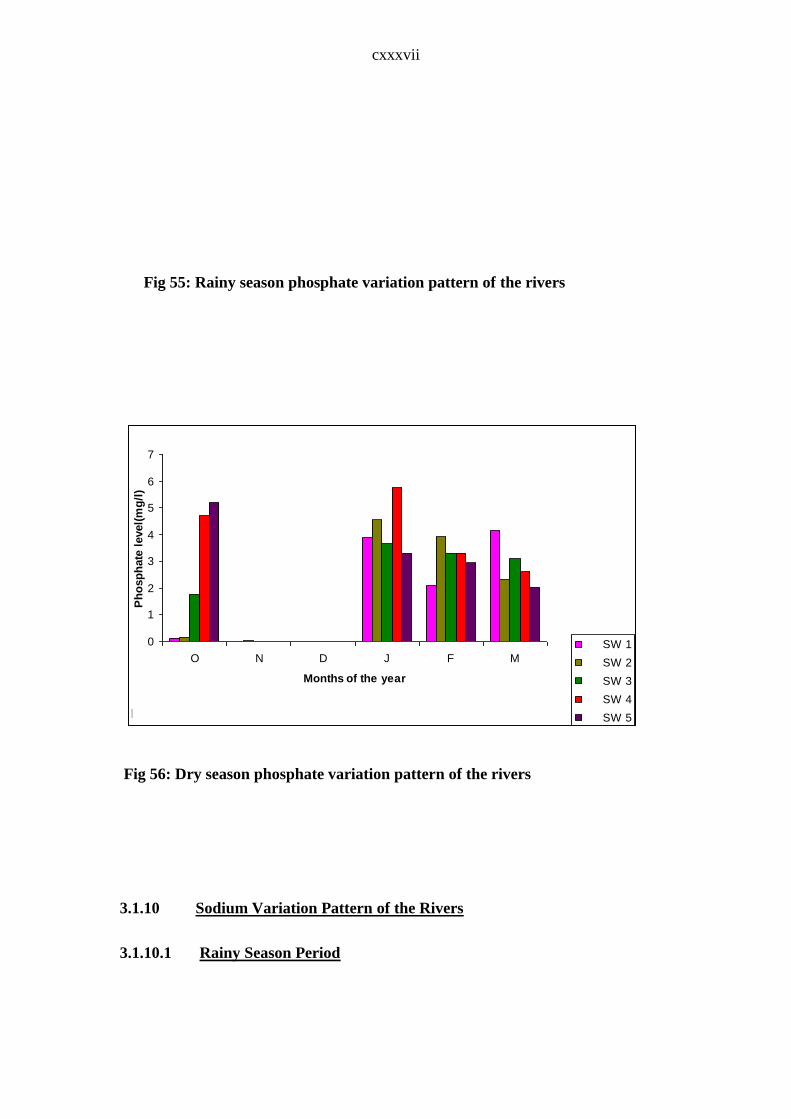
cxxxvii

Fig 55: Rainy season phosphate variation pattern of the rivers

Fig 56: Dry season phosphate variation pattern of the rivers

3.1.10 Sodium Variation Pattern of the Rivers

3.1.10.1 Rainy Season Period

Fig 56:Dry season phosphate variation pattern of the rivers

0

1

2

3

4

5

6

7

O N D J F M

Months of the year

Ph

osp

hate

level(

mg

/l)

SW 1

SW 2

SW 3

SW 4

SW 5Fig 56:Dry season phosphate variation pattern of the rivers

0

1

2

3

4

5

6

7

O N D J F M

Months of the year

Ph

osp

hate

level(

mg

/l)

SW 1

SW 2

SW 3

SW 4

SW 5

cxxxviii

The sodium levels of the rivers ranged from 0.42mg/l to 21.6mg/l as is shown

in Table 12. The values indicate that river Ogbete (SW4) had the highest value during

this season, while Immaculate (SW5) had the least level (0.42mg/l) in the month of

September. The monthly values (Fig 57) indicate a decrease in the monthly sodium

level from June to September thus showing that there was variation in sodium

concentration within and between the rivers.

3.1.10.2 Dry Season Period

The season’s range was between 0.22 to 26.5mg/l occurring in rivers Ekulu

(SW 3) in the month of October and Immaculate (SW5) in the month of January.

The pattern revealed by the dry season values indicates that the sodium level

of the rivers was lower in the months of October, November and December (Fig 58).

Variations occurred within the months and the rivers.

Fig 57: Rainy season sodium variation pattern of the rivers

Fig 57:Rainy season sodium variation pattern of the rivers

0

5

10

15

20

25

A M J J A S

Months of the year

So

diu

m l

evel(

mg

/l)

SW1

SW2

SW3

SW4

SW5Fig 57:Rainy season sodium variation pattern of the rivers

0

5

10

15

20

25

A M J J A S

Months of the year

So

diu

m l

evel(

mg

/l)

SW1

SW2

SW3

SW4

SW5

Fig 58:Dry season sodium variation pattern of the rivers

0

5

10

15

20

25

30

35

40

O N D J F M

Months of the year

So

diu

m l

evel(

mg

/l)

SWS 1

SWS2

SWS3

SWS4

SWS5Fig 58:Dry season sodium variation pattern of the rivers

0

5

10

15

20

25

30

35

40

O N D J F M

Months of the year

So

diu

m l

evel(

mg

/l)

SWS 1

SWS2

SWS3

SWS4

SWS5

cxxxix

Fig 58: Dry season sodium variation pattern of the rivers

3.1.11 Sulphate Variation Pattern of the Rivers

3.1.11.1 Rainy Season Period

The values range between 0 to 7.4mg/l as is indicated in Table 13.The lowest

value was recorded in Aria (SW2) river in the month of June, while the highest value

occurred in the month of April in Ogbete (SW4) river. Very low values were

generally observed in the months of July, August and September. The values indicate

monthly variations among the rivers within this season (Fig 59).

3.1.11.2 Dry Season Period

The season’s range was from 0 to 9.7mg/l. The highest value for this season

occurred in Asata (SW 1) river in the month of March while the lowest value occurred

in various river during different months (Fig 60). From the pattern depicted by this

figure, it is observable that variations exist between the levels of sulphate

concentration in the rivers.

Generally, the pattern depicted by these two seasons (Figs 59 and 60) shows that

sulphate levels are higher in dry season in three rivers (Asata (SW1), Aria (SW2), and

Ekulu (SW3); while two rivers namely Ogbete (SW4) and Immaculate (SW5) had

higher values in the rainy than the dry season.

Fig 59:Rainy season sulphate variation pattern of the rivers

0

1

2

3

4

5

6

7

8

A M J J A S

Months of the year

Su

lph

ate

level(

mg

/l)

SW1

SW2

SW3

SW4

SW5Fig 59:Rainy season sulphate variation pattern of the rivers

0

1

2

3

4

5

6

7

8

A M J J A S

Months of the year

Su

lph

ate

level(

mg

/l)

SW1

SW2

SW3

SW4

SW5

cxl

Fig 59: Rainy season sulphate variation pattern of the rivers

Fig. 60: Dry season sulphate variation pattern of the rivers

3.1.12 Iron Variation Pattern of the Rivers

3.1.12.1 Rainy Season Period

Fig 60:Dry season sulphate variation pattern of the rivers

0

2

4

6

8

10

12

O N D J F M

Months pf the year

Su

lph

ate

level(

mg

/l)

SW1

SW2

SW3

SW4

SW5Fig 60:Dry season sulphate variation pattern of the rivers

0

2

4

6

8

10

12

O N D J F M

Months pf the year

Su

lph

ate

level(

mg

/l)

SW1

SW2

SW3

SW4

SW5

cxli

The concentration of iron in the different rivers in this season as is shown in

Table 14, indicate that the range is between 0.1 to 0.2mg/l. Consistent values were

recorded in all the rivers in the months of June, July, August, and September (Fig 61).

Variations however occurred in two months (April and May).

From Fig 61 it can be seen that in April, three rivers (Asata (SW1), Aria

(SW2) and Ekulu (SW3)) had consistent values of 0.1 mg/l, while in the month of

May all the rivers had the same iron concentration level, only one river (Ekulu

(SW3)) had a different concentration level.

3.1.12.2 Dry Season Period

Iron concentrations for this period ranges between 0 to 0.2mg/l. Generally,

Immaculate (SW5) had higher values during this season. Consistent values were

recorded in three rivers (Asata (SW1), Ekulu (SW3) and Immaculate (SW5) in the

months of October and November (Fig 62).

In some of the months, the iron concentration levels were negligible for rivers

like Aria (SW2), Ekulu (SW3) and Ogbete (SW4). Inspite of the consistent iron

levels in the rivers, variation is still observable monthly and spatially in for both

seasons.

Fig 61:Rainy season iron variation pattern of the rivers

0

0.05

0.1

0.15

0.2

0.25

A M J J A S

Months of the year

Iro

n l

evel(

mg

/l)

SW1

SW2

SW3

SW4

SW5Fig 61:Rainy season iron variation pattern of the rivers

0

0.05

0.1

0.15

0.2

0.25

A M J J A S

Months of the year

Iro

n l

evel(

mg

/l)

SW1

SW2

SW3

SW4

SW5

cxlii

Fig. 61: Rainy season iron variation pattern of the rivers

Fig. 62: Dry season iron variation pattern of the rivers

3.1.13 Ammonia variation pattern of the Rivers

3.1.13.1 Rainy Season Period

Fig 62:Dry season iron variation pattern of the rivers

0

0.05

0.1

0.15

0.2

0.25

O N D J F M

Months of the year

Iro

n l

evel

(mg

/l)

SW1

SW2

SW3

SW4

SW5

cxliii

The range of ammonia content of the rivers is from 0.06 to 8.72mg/l (Table

15). The highest value for this season was recorded in Ogbete (SW4) in June, while

very low ammonia levels were recorded in the months of July, August and September

(Fig 63).

Monthly and Spatial variations occurred during this season as figure also

depicts that negligible ammonia levels were observed for rivers Ogbete (SW4) and

Immaculate (SW5) in July. Very low values were recorded in August and September

for all the rivers.

3.1.13.2 Dry Season Period

Ammonia levels for the period range from 0 to 3.311mg/l (Table 15). The

dry season highest ammonia level was recorded in Ekulu (SW3) river in the month of

March. Figure 64 shows that four rivers (Aria (SW2), Ekulu (SW3), Ogbete (SW4)

and Immaculate (SW5) had negligible ammonia levels in the months of November

and December.

Generally, higher ammonia levels occurred at the beginning of the rainy

season for all the rivers. There are, however, more months with very low ammonia

levels in the rainy than the dry season.

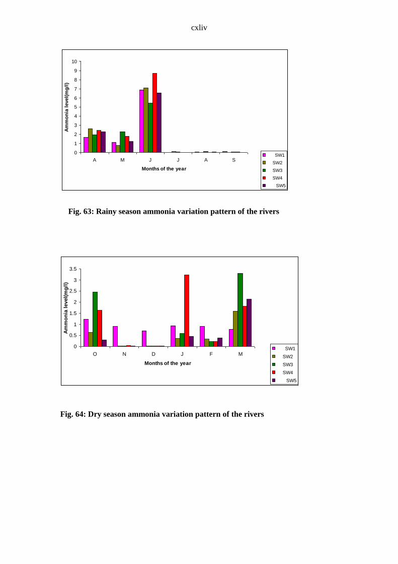
cxliv

Fig 63:Rainy season ammonia variation pattern of the rivers

0

1

2

3

4

5

6

7

8

9

10

A M J J A S

Months of the year

Am

mo

nia

level(

mg

/l)

SW1

SW2

SW3

SW4

SW5Fig 63:Rainy season ammonia variation pattern of the rivers

0

1

2

3

4

5

6

7

8

9

10

A M J J A S

Months of the year

Am

mo

nia

level(

mg

/l)

SW1

SW2

SW3

SW4

SW5

Fig. 63: Rainy season ammonia variation pattern of the rivers

Fig. 64: Dry season ammonia variation pattern of the rivers

Fig 64:Dry season ammonia variation pattern of the rivers

0

0.5

1

1.5

2

2.5

3

3.5

O N D J F M

Months of the year

Am

mo

nia

level(

mg

/l)

SW1

SW2

SW3

SW4

SW5Fig 64:Dry season ammonia variation pattern of the rivers

0

0.5

1

1.5

2

2.5

3

3.5

O N D J F M

Months of the year

Am

mo

nia

level(

mg

/l)

SW1

SW2

SW3

SW4

SW5

cxlv

3.1.14 Calcium Variation Pattern of the Rivers

3.1.14.1 Rainy Season Period

Calcium content of rives range between 2.01 to 3.05mg/l (Table 16). The

highest value for this season was recorded in river Ogbete (SW4) in two months (July

and August), while very low calcium levels were recorded in river Immaculate (SW5)

(Fig 65). Spatial and monthly variations occurred in terms of the calcium content of

the rivers.

3.1.14.2 Dry Season Period

The dry season range is from 0.02 to 3.23mg/l.The highest value for this

season was recorded in river Ekulu (SW3), while very low calcium levels were

recorded in river Immaculate (SW5)(Fig 66). Generally, monthly and spatial

variations occurred during this season as depicted by Figs 65 and 66.

Fig 65: Rainy season calcium variation pattern of the rivers

Fig 65:Rainy season calcium variation pattern of the rivers

0

0.5

1

1.5

2

2.5

3

3.5

4

A M J J A S

Months of the year

Cali

um

level(

mg

/l)

SW1

SW2

SW3

SW4

SW5Fig 65:Rainy season calcium variation pattern of the rivers

0

0.5

1

1.5

2

2.5

3

3.5

4

A M J J A S

Months of the year

Cali

um

level(

mg

/l)

SW1

SW2

SW3

SW4

SW5

cxlvi

Fig 66: Dry season calcium variation pattern of the rivers

3.1.15 Nitrate Variation Pattern of the Rivers

3.1.15.1 Rainy Season Period

Nitrate levels for this period ranges between 0.01-3.31mg/l (table 17). The

highest nitrate level for this season occurred in Ogbete (SW4) river. Figure 67 shows

that very low nitrate levels were recorded in the first three months of this season. In

the month of June very negligible nitrate levels were observed. Inspite of this,

monthly and spatial variations occurred.

3.1.15.2 Dry Season Period

The levels of nitrate in the rivers during this period range from 0-

1.45mg/l (Table 17). The highest value for this season was recorded in river Asata

(SW1). From Fig. 68, it can be seen that all the rivers had their highest nitrate levels

for the season in the month of October. Apart from Asata (SW1) in November, all the

Fig 66:Dry season calium variation pattern of the rivers

0

0.5

1

1.5

2

2.5

3

O N D J F M

Months of the year

Calc

ium

level(

mg

/l)

SW1

SW2

SW3 SW4

SW4

SW5Fig 66:Dry season calium variation pattern of the rivers

0

0.5

1

1.5

2

2.5

3

O N D J F M

Months of the year

Calc

ium

level(

mg

/l)

SW1

SW2

SW3 SW4

SW4

SW5

cxlvii

other rivers had very low (and some negligible) nitrate levels in November,

December, January, February and March (Fig 68).

Generally, each season had a month in which all the rivers recorded higher

nitrate levels. While it was September for the rainy season it was October for the dry

season (Figs 67 and 68).

Fig 67: Rainy season nitrate variation pattern of the rivers

Fig 67:Rainy season nitrate variation pattern of the rivers

0

0.5

1

1.5

2

2.5

3

3.5

A M J J A S

Months of the year

Nit

rate

level(

mg

/l)

SW1

SW2

SW3

SW4

SW5Fig 67:Rainy season nitrate variation pattern of the rivers

0

0.5

1

1.5

2

2.5

3

3.5

A M J J A S

Months of the year

Nit

rate

level(

mg

/l)

SW1

SW2

SW3

SW4

SW5

Fig 68:Dry season nitrate variation pattern of the rivers

0

0.2

0.4

0.6

0.8

1

1.2

1.4

1.6

O N D J F M

Months of the year

Nit

ate

level(

mg

/l)

SW1

SW2

SW3

SW4

SW5Fig 68:Dry season nitrate variation pattern of the rivers

0

0.2

0.4

0.6

0.8

1

1.2

1.4

1.6

O N D J F M

Months of the year

Nit

ate

level(

mg

/l)

SW1

SW2

SW3

SW4

SW5

cxlviii

Fig 68: Dry season nitrate variation pattern of the rivers

3.1.16 Fecal Coliform Variation Pattern of the Rivers

3.1.16.1 Rainy Season Period

The rainy season fecal coliform count ranges from 2-12 cfu/100mls. The

highest fecal coliform level for this season was recorded in River Asata (SW1) in

June. Figure 69 shows a negligible level in Aria (SW2) in March. The same levels

were recorded for all the rivers in August.

Generally three rivers (Ekulu, Ogbete and Immaculate), had the same levels in

most of the months with the exception of June. Inspite of the same fecal coliform

levels recorded for most months and rivers (Fig 69), spatial and monthly variations

occurred during this season.

3.1.16.2 Dry Season Period

Fecal coliform levels during this period ranges form 1-90 per 100mls. The

levels were high in different months and rivers (Fig 70). Generally from Fig. 70, it can

be seen that the fecal coliform levels of all the rivers were negligible from January to

March in comparism to the other levels recorded during this season.

There are thus higher fecal coliform levels in the dry than the rainy season

in the rivers.

cxlix

Fig 69: Rainy season fecal coliform bacteria variation pattern of the rivers

Fig 70: Dry season fecal coliform bacteria variation pattern of rivers

Fig 70:Dry season faecal coliform bacteria variation pattern of

the rivers

0

10

20

30

40

50

60

70

80

90

100

O N D J F M

Months of the year

F

eacal

co

lifo

m b

acte

ria

level(

c/1

00m

g)

SW1

SW2

SW3

SW4

SW5

Fig 70:Dry season faecal coliform bacteria variation pattern of

the rivers

0

10

20

30

40

50

60

70

80

90

100

O N D J F M

Months of the year

F

eacal

co

lifo

m b

acte

ria

level(

c/1

00m

g)

SW1

SW2

SW3

SW4

SW5

Fig 69:Rainy season faecal coliform bacteria variation pattern

of the rivers

0

2

4

6

8

10

12

14

A M J J A S

Months of the year

Faecal

co

lifo

rm b

acte

ria l

evel

(cf/

100m

g)

SW1

SW2

SW3

SW4

SW5

Fig 69:Rainy season faecal coliform bacteria variation pattern

of the rivers

0

2

4

6

8

10

12

14

A M J J A S

Months of the year

Faecal

co

lifo

rm b

acte

ria l

evel

(cf/

100m

g)

SW1

SW2

SW3

SW4

SW5

cl

3.2 Seasonal and Spatial Patterns of River Water Quality.

3.2.1 Annual Temperature variation pattern of the rivers

3.2.1.1 Rainy and dry season variations

The rainy season mean temperatures as shown in Table 36 for all the river

was 24C, thus indicating no variation in the seasonal pattern of the temperature for

all the rivers. The dry season mean temperature for all the rivers is 25ºC also

indicating that the rivers had no variation in their temperature readings throughout this

season.

Inspite of none seasonal variations, the dry season temperatures were higher in

all the rivers as depicted by Fig 71. Also there was no spatial variation in terms of

temperature as the rivers generally all the same reading for each season.

TABLE 36: Rainy season mean values of selected parameters for rivers in Enugu

urban area

Parameters Sample Sites

SW1 SW2 SW3 SW4 SW5

Temperature 24 24 24 24 24

pH 6.20 6.25 6.18 6.13 6.36

Turbidity 8.33 25.83 4.50 4.16 14.3

Total dissolved Solids 70.33 25.83 72.33 88.00 50.83

Conductivity 0.18 0.06 0.12 0.14 0.07

Hardness 0.45 0.31 0.35 0.57 0.35

Dissolved Oxygen 5.11 5.18 4.68 4.03 4.95

Biochemical Oxygen Demand 1.03 1.13 1.50 1.05 1.11

Phosphate 0.62 0.48 1.30 0.34 0.61

Sodium 6.27 7.04 10.10 7.20 4.03

Sulphate 0.58 0.66 0.55 2..18 2..15

Iron 0.10 0.10 o.11 0.12 0.12

Ammonia 0.91 0.48 1.09 1.15 0.54

Calcium 2..82 2..78 2..94 3.09 2..48

cli

Nitrate 0.64 0.56 0.38 0.64 0.40

Fecal Coliform 31.76 32.83 15.16 29.83 5.16

TABLE 37: Dry season mean values of selected parameters for rivers in Enugu

urban area.

PARAMETERS SAMPLE SITES

SW1 SW2 SW3 SW4 SW5

Temperature 25 25 25 25 25

pH 6.23 6.23 6.16 6.01 6.34

Turbidity 6.83 18.33 7.83 6.66 9.66

Total Dissolved Solids 54.5 18.33 110 120.66 122.5

Total Hardness 0.49 0.34 0.54 0.49 0.55

Dissolved Oxygen 5.03 5.61 6.20 5.18 5.13

Biochemical Oxygen Demand 2.88 2.05 1.25 2.66 1.65

Phosphate 1.71 1.83 1.97 2.73 2.25

Sodium 6.23 8.72 4.86 5.72 8.51

Conductivity 0.01 0.22 0.25 0.12 0.02

Sulphate 2.31 1.63 1.86 1.70 0.53

Iron 0.05 0.01 0.04 0.05 0.16

Ammonia 1.23 0.63 2.46 1.63 0.28

Calcium 2.50 2.54 2.76 2.62 2.01

Nitrate 1.45 1.03 1.04 1.37 0.94

Fecal coliform 4 2.1 2.6 6.3 7.3

Fig 71:Seasonal temperature pattern of the rivers

23.4 23.6 23.8 24 24.2 24.4 24.6 24.8 25 25.2

SW1

SW2

SW3

SW4

SW5

Riv

ers

Temperature C

DRY

RAIN

Temperature °C

Fig 71:Seasonal temperature pattern of the rivers

23.4 23.6 23.8 24 24.2 24.4 24.6 24.8 25 25.2

SW1

SW2

SW3

SW4

SW5

Riv

ers

Temperature C

DRY

RAIN

Temperature °C

clii

Fig 71: Seasonal temperature pattern of the rivers

3.2.2 Annual pH variation pattern of the rivers

3.2.2.2 Rainy and Dry season annual variations

The mean pH values for the rainy season (table 36) for the rivers varied

with river Immaculate (SW5) having the highest value and Ogbete (SW4) the lowest

value. This indicates that the river acidity in decreasing order is as follows:

Immaculate (SW5), Aria (SW2), Asata (SW1), Ekulu (SW3) and Ogbete (SW4).

The mean pH values for the dry season (table 37) indicate that acidity level in

decreasing order is as follows: Immaculate (SW5), Aria (SW2), Asata (SW1), Ekulu

(SW3) and Ogbete (SW4). For the two seasons there were no variations in terms of

the acidity levels of the rivers except for Ogui river (Fig 72).

Fig 72: Seasonal pH pattern of the rivers

Fig 72:Seasonal pH pattern of the rivers

5.8 5.9 6 6.1 6.2 6.3 6.4

SW1

SW2

SW3

SW4

SW5

Riv

ers

pH level

DRY

RAINY

Fig 72:Seasonal pH pattern of the rivers

5.8 5.9 6 6.1 6.2 6.3 6.4

SW1

SW2

SW3

SW4

SW5

Riv

ers

pH level

DRY

RAINY

cliii

3.2.3 Annual turbidity variation pattern of the rivers

3.2.3.1 Rainy and dry season variations

The mean values obtained for the rainy season (Table 36) indicate that

turbidity levels are highest in Aria river (SW2) and lowest in Ogbete (SW4) river. In

decreasing order, the turbidity level in the rivers is as follows: Aria river (SW2)

Immaculate river (SW5), Asata river (SW1), Ekulu river (SW3) and Ogbete (SW4).

The dry season mean values (Table 37) indicate that river Aria (SW2) had the

highest turbidity levels, while the turbidity levels were lowest in Ogbete (SW4) river.

In decreasing order, the turbidity level of the rivers is as follows: Aria river (SW2)

Immaculate river (SW5), Asata river (SW1), Ekulu river (SW3) and Ogbete (SW4).

Spatial variation is thus observable in terms of turbidity amongst all the rivers.

There was no particular season in which all the rivers had either high or low

turbidity (Fig 73). Rather variations occurred in terms of the seasons of high or low

turbidity spatially and seasonally. Three rivers namely rivers Asata (SW1), Aria

(SW2) and Immaculate (SW5) located in different parts of the urban area, had higher

turbidity in the rainy season, while the two rivers (Ekulu(SW4) and Ogbete(SW4)

others had higher turbidity in the dry season(Fig 73).

Fig 73: Seasonal turbidity pattern of the rivers

0 5 10 15 20 25 30

SW1

SW2

SW3

SW4

SW5

Sam

ple

sit

es

Turbidity level(mg/l)

DRY

RAINYFig 73: Seasonal turbidity pattern of the rivers

0 5 10 15 20 25 30

SW1

SW2

SW3

SW4

SW5

Sam

ple

sit

es

Turbidity level(mg/l)

DRY

RAINY

cliv

Fig 73: Seasonal turbidity pattern of the rivers

3.2.4 Annual Total dissolved solids variation pattern of the rivers

3.2.4.1 Rainy and Dry season variations

The rainy season mean values (Table 36) indicate that River Ogbete

(SW4) had the highest level of total dissolved solids within this season, while Aria

river (SW2) had the lowest level. In decreasing order therefore the levels of dissolved

solids in the rivers were as follows: Ogbete (SW 4), Ekulu (SW3), Asata (SW1),

Immaculate (SW5) and Aria (SW 2).

The dry season mean values (Table 37) show that Immaculate river (SW5)

had the highest mean value with the lowest value occurring for Aria river. In

decreasing order the level of dissolved solids in the river are as follows: Immaculate

(SW5), Ogbete (SW4), Ekulu (SW3), Asata (SW1) and Aria (SW2).

For the rainy and dry seasons, as depicted by the seasonal cluster bars

(Fig 74), three rivers (Ekulu (SW3), Ogbete (SW4) and Immaculate (SW5) had, the

dissolved solid levels that were higher in the dry season; while two rivers Asata

clv

(SW1) and Aria (SW2) had higher dissolved solids in the rainy season. This indicates

variations seasonally and spatially.

Fig 74: Seasonal total dissolved solids pattern of the rivers

3.2. 5 Annual Conductivity variation pattern of the rivers

3.2.5.1 Rainy and dry season variations of the rivers

The rainy season mean values (Table 36) indicate that conductivity was

highest at this period in River Asata (SW1) and lowest in River Aria (SW2).

Conductivity levels at this period in decreasing order were thus as follows: Asata

(SW1), Ogbete (SW4), Ekulu (SW3), Immaculate (SW5) and Aria (SW2).

The dry season mean values (Table 37) indicate that River Ekulu (SW3) had

the highest values, while river Asata (SW1) had the lowest values. Conductivity in

deceasing order in the rivers in this season, were as follows: Ekulu (SW3), Aria

(SW2), Ogbete (SW4), Immaculate (SW5) and Asata (SW1).

A comparison of the conductivity levels among the rivers for the dry and

rainy seasons indicate that three rivers (Aria (SW2), Ekulu (SW3) and Immaculate

Fig 74: Seasonal total dissolved solids pattern of the rivers

0 20 40 60 80 100 120 140

SW1

SW2

SW3

SW4

SW5

Sam

ple

sit

es

Total dissolved solids(mg/l)

DRY

RAINYFig 74: Seasonal total dissolved solids pattern of the rivers

0 20 40 60 80 100 120 140

SW1

SW2

SW3

SW4

SW5

Sam

ple

sit

es

Total dissolved solids(mg/l)

DRY

RAINY

clvi

(SW5)) all had higher conductivity levels in the dry season (Fig 75).River Ogbete

(SW4) and Asata (SW1) had higher conductivity in the rainy season. Season and

spatial variation was thus observed.

3.2. 6 Annual total hardness variation pattern of the rivers

3.2.6.1 Rainy and Dry season variations of the rivers.

For both seasons the water are soft water.

The mean values for the rainy season total hardness for all the rivers (Table 36)

indicate that there were slight variations among the rivers. Ogbete (SW4) river with a

mean value of 0.57mg/l had the highest total hardness, while Aria (SW2) river had the

lowest (0.31mg/l). In decreasing order, the levels of hardness in the river were as

follows: Ogbete (SW4), Asata (SW1), Immaculate (SW5), Ekulu (SW3) and Aria

(SW2).

The highest dry season mean value for total hardness occurred for river Ekulu

(SW3) and the lowest for Aria (SW2). Rainy and dry season comparism (Fig 76)

shows that seasonal and spatial variations occurred between the rivers in terms of the

river hardness as four rivers) had higher hardness during the dry season. River Ogbete

(SW4) had the highest hardness value in the rainy season.

clvii

Fig 75: Seasonal conductivity pattern of the rivers

Fig 76: Seasonal total hardness pattern of the rivers

Fig 75: Seasonal conductivity pattern of the rivers

0 0.05 0.1 0.15 0.2 0.25 0.3

SW1

SW2

SW3

SW4

SW5

Sam

ple

sit

es

Conductivity level(SCM)

DRY

RAINYFig 75: Seasonal conductivity pattern of the rivers

0 0.05 0.1 0.15 0.2 0.25 0.3

SW1

SW2

SW3

SW4

SW5

Sam

ple

sit

es

Conductivity level(SCM)

DRY

RAINY

Fig 76: Seasonal total hardness pattern of the rivers

0 0.1 0.2 0.3 0.4 0.5 0.6

SW1

SW2

SW3

SW4

SW5

Sam

ple

sit

es

Toatal hardness level(mg/l)

DRY

RAINYFig 76: Seasonal total hardness pattern of the rivers

0 0.1 0.2 0.3 0.4 0.5 0.6

SW1

SW2

SW3

SW4

SW5

Sam

ple

sit

es

Toatal hardness level(mg/l)

DRY

RAINY

clviii

3.2. 7 Annual dissolved oxygen variation pattern of the rivers

3.2.7.1 Rainy and dry seasons annual variations of the rivers.

The mean values for the rainy season dissolved oxygen content for all the

rivers (Table 36) indicate that there were slight variations among the rivers. Aria

(SW2) river with a mean value of 5.18mg/l had the highest dissolved oxygen content,

while Ogbete (SW5) river had the lowest (4.03mg/l).In decreasing order, the

dissolved oxygen concentrations for the rivers in the rainy season were as follows:

Aria (SW2), Asata (SW1), Immaculate (SW5), Ekulu (SW3) and Ogbete (SW 4).

The dry season dissolved oxygen mean values (Table 37) indicate that River

Ekulu (SW3) had the highest oxygen demand, while Asata (SW1) had the lowest.

This also reveals that in decreasing order, the dissolved oxygen content was as

follows: Ekulu (SW3), Aria (SW2), Ogbete (SW4), Immaculate (SW5) and Asata

(SW1).

Rainy and dry season comparism (Fig 77) shows that seasonal and spatial

variations occurred between the rivers. As four (4) rivers (Aria (SW2), Ekulu (SW3),

Ogbete (SW4), and Immaculate (SW 5) had higher dissolved oxygen demand levels

in the dry season than in the rainy season. Only river Asata (SW1) had higher oxygen

demand level in the rainy season.

Fig 77:Seasonal dissolved oxygen pattern of the rivers

0 1 2 3 4 5 6 7

SW1

SW2

SW3

SW4

SW5

Sam

ple

sit

es

Dissolved oxygen(mg/l)

DRY

RAINYFig 77:Seasonal dissolved oxygen pattern of the rivers

0 1 2 3 4 5 6 7

SW1

SW2

SW3

SW4

SW5

Sam

ple

sit

es

Dissolved oxygen(mg/l)

DRY

RAINY

clix

Fig 77: Seasonal dissolved oxygen pattern of the rivers

3.2. 8 Annual biochemical oxygen demand variation pattern of the rivers

3.2.8.1 Rainy and dry season variations of the rivers.

The mean values for biochemical oxygen demand for all the rivers in

the rainy season (Table 36) indicate little variations among the rivers; Ekulu (SW3)

having the highest biochemical oxygen demand and Asata (SW1) having the least. In

decreasing order, the biochemical oxygen demand levels in the rivers were as follows:

Ekulu (SW3), Aria (SW2), Immaculate (SW5), Ogbete (SW4), and Asata (SW1)

Mean values for the dry season period (Table 37) indicate that in decreasing

order, the biochemical oxygen demand of the rivers is as follows: Asata (SW1)

Ogbete (SW4), Aria (SW2), Immaculate (SW5) and Ekulu (SW 3).

A comparison of the biochemical oxygen demand between the rivers for

the dry and rainy seasons( Fig 78) indicate that four rivers (Asata, Aria, Ogbete and

Immaculate had higher dry season biochemical oxygen demand; while only Ekulu

river had higher rainy season values. These indicate seasonal and spatial variations.

Fig 78:Seasonal biochemical oxygen demand pattern of the

rivers

0 0.5 1 1.5 2 2.5 3

SW1

SW2

SW3

SW4

SW5

Sam

ple

sta

tio

ns

Biochemical oxygen demand level(mg/l)

DRY

RAINY

Fig 78:Seasonal biochemical oxygen demand pattern of the

rivers

0 0.5 1 1.5 2 2.5 3

SW1

SW2

SW3

SW4

SW5

Sam

ple

sta

tio

ns

Biochemical oxygen demand level(mg/l)

DRY

RAINY

clx

Fig 78: Seasonal biochemical oxygen demand pattern of the rivers

3.2. 9 Annual Phosphate variation pattern of the rivers

3.2.9.1 Rainy and dry season variations of the rivers.

The rainy season mean values of phosphate for the rivers range between

0.34 to 0.62mg/l (Table 35) indicating that there was slight variation among the rivers.

The mean values also indicate a pattern that shows that the rivers had decreasing

phosphate concentration in this order: Ekulu (SW3), Asata (SW 1), Immaculate

(SW5), Ogbete (SW4) and Aria (SW2).

The dry season mean values of phosphate concentrations in the rivers

(Table 36) indicate that river Ogbete (SW4) recorded the highest level while Asata

(SW1) recorded the lowest level. It also shows that the rivers had a decreasing

phosphate concentration in the following order: Ogbete (SW4), Immaculate (SW5),

Ekulu (SW3), Aria (SW 2) and Asata (SW1).

A comparison of the phosphate levels between the rivers for the dry and rainy

seasons (Fig 79) indicate that the dry season concentration was higher than the rainy

season concentration for all the rivers in Enugu urban area. This also indicates that the

rivers had no spatial variation in terms of phosphate concentration for the seasons.

clxi

3.2. 10 Annual Sodium variation pattern of the rivers

3.2.10.1 Rainy and dry season variations of the rivers

The rainy season mean values (Table 36) indicate that sodium level was

highest at this period in river Ekulu (SW1) and lowest in river Immaculate (SW5).

Sodium levels at this period in decreasing order were thus as follows: Ekulu (SW3),

Ogbete (SW4), Aria (SW2), Asata (SW1), and Immaculate (SW5). However the dry

season mean values (Table 37) reveal that in decreasing order, the sodium levels were

as follows: Aria (SW2), Immaculate (SW5), Asata (SW1), Ogbete (SW4) and Ekulu

(SW3). The pattern revealed by the rainy and dry season’s sodium levels indicates

that variations occurred in the two seasons. Two rivers, Ekulu (SW3) and Ogbete

(SW4), had higher rainy season mean values, two rivers Aria (SW2) and Immaculate

(SW5), had higher dry season mean values; while river Asata recorded no variation in

the mean values of the two seasons(Fig 80 ).

Spatial variation thus does exist among the rivers in terms of sodium

concentrations for both seasons.

Fig 79:Seasonal phosphate pattern of the rivers

0 0.5 1 1.5 2 2.5 3

SW1

SW2

SW3

SW4

SW5

Sam

ple

sit

es

Phosphate level(mg/l)

DRY

RAINYFig 79:Seasonal phosphate pattern of the rivers

0 0.5 1 1.5 2 2.5 3

SW1

SW2

SW3

SW4

SW5

Sam

ple

sit

es

Phosphate level(mg/l)

DRY

RAINY

clxii

Fig 79: Seasonal phosphate pattern of the rivers

Fig 80: Seasonal sodium pattern of the rivers

3.2. 11 Annual sulphate variation pattern of the rivers

3.2.11.1 Rainy and dry season variations of the rivers

The rainy season mean values for the rivers range between 0.55 to 2.18

mg/l (Table 36) indicating that there was variation among the rivers. The mean values

also indicate a pattern that shows that the rivers had decreasing sulphate concentration

in this order: Ogbete (SW4), Immaculate (SW5), Aria (SW2), Asata (SW1) and Ekulu

(SW3).The dry season sulphate mean values (Table 37) indicate a level of

Fig 80:Seasonal sodium pattern of the rivers

0 2 4 6 8 10 12

SW1

SW2

SW3

SW4

SW5

Sam

ple

sit

es

Sodium level(mg/l)

DRY

RAINYFig 80:Seasonal sodium pattern of the rivers

0 2 4 6 8 10 12

SW1

SW2

SW3

SW4

SW5

Sam

ple

sit

es

Sodium level(mg/l)

DRY

RAINY

clxiii

concentration in this decreasing order: Asata (SW1), Ekulu (SW3), Ogbete (SW4),

Aria (SW2) and Immaculate (SW5).

Generally, the pattern depicted by these two seasons (Fig 81) shows that

sulphate levels were higher in dry season in three (3) rivers (Asata (SW1), Aria

(SW2), and Ekulu (SW3); while 2 rivers namely Ogbete (SW4) and Immaculate

(SW5) had higher values in the rainy than the dry season (Fig 81).This is indicative of

the fact that there were seasonal variations in the sulphate levels of rivers in Enugu

urban area.

Fig 81: Seasonal sulphate pattern of the rivers

3.2. 12 Annual iron variation pattern of the rivers

3.2.12.1 Rainy and dry season variations of the rivers.

The rainy season mean values for the rivers range between 0.10 to 0.12

mg/l (Table 36) showing that the rivers all have values below 1 mg/l during thus

season. The mean values also indicate a pattern that shows that the rivers had

decreasing iron content in the following order: Ogbete (SW4) and Immaculate (SW5)

have the same concentration level; Ekulu (SW3), Aria (SW2) and Asata (SW1) have

Fig 81:Seasonal sulphate pattern of the rivers

0 0.5 1 1.5 2 2.5

SW1

SW2

SW3

SW4

SW5

Sam

ple

sit

es

Sulphate(mg/l)

DRY

RAINYFig 81:Seasonal sulphate pattern of the rivers

0 0.5 1 1.5 2 2.5

SW1

SW2

SW3

SW4

SW5

Sam

ple

sit

es

Sulphate(mg/l)

DRY

RAINY

clxiv

the same concentration level. Minimal variations however do occur among the rivers

in terms of their iron content during this period.

The dry season mean values the iron content of the rivers (Table 37) range from 0 to

0.1mg/l. Four of the rivers( Asata (SW1), Aria (SW2),Ekulu (SW3), Ogbete (SW4)

have a mean value of 0 mg/l, while only Immaculate river (SW5) had a value of

0.1mg/l.

Seasonal and spatial variations occurred in the iron content levels of the

rivers. Four rivers (Asata (SW1), Aria (SW2), Ekulu (SW3) and Ogbete (SW4)) had

higher rainy season values while Immaculate (SW5) river had higher values in the dry

season than the rainy season (Fig 82).

Fig 82:Seasonal iron pattern of the rivers

0 0.05 0.1 0.15 0.2

SW1

SW2

SW3

SW4

SW5

Sam

ple

sit

es

Iron(mg/l)

DRY

RAINYFig 82:Seasonal iron pattern of the rivers

0 0.05 0.1 0.15 0.2

SW1

SW2

SW3

SW4

SW5

Sam

ple

sit

es

Iron(mg/l)

DRY

RAINY

clxv

Fig 82: Seasonal iron pattern of the rivers

3.2. 13 Annual ammonia variation pattern of the rivers

3.2.13.1 Rainy and dry season variations of the rivers.

The rainy season ammonia mean values range from 0.48mg/l in Aria

(SW2) to 1.15mg/l in Ogbete river (SW4) to 0.48 mg/l in Aria (SW2) rver (Table 36).

In decreasing order the pattern of ammonia level in the rivers is as follows: Ogbete

(SW4), Ekulu (SW3), Asata (SW1), Immaculate (SW5) and Aria (SW2).

The dry season mean values for the rivers range from 0.28 mg/l in

Immaculate (SW5) river to 2.46 mg/l in river Ekulu (SW3) (Table 37). The mean

values indicate a pattern of decrease as follows: Ekulu (SW3), Ogbete (SW4), Asata

(SW1), Aria (SW2), Immaculate (SW5). This indicates that spatial variation occurred

between the rivers.

The pattern revealed by the two seasons indicates that ammonia levels of

rivers were higher in the rainy season than the dry season (Fig 83). Seasonal spatial

variation occurred among the rivers also.

clxvi

Fig 83: Seasonal ammonia pattern of the rivers

3.2. 14 Annual calcium variation pattern of the rivers

3.2.14.1 Rainy and dry season variations of the rivers.

The rainy season mean values for calcium range from 2.48 mg/l in

Immaculate (SW5) river to 3.09 mg/l in Ogbete river (SW4) to (Table 36). The rainy

season mean value (Table 36) for the rivers indicate a calcium concentration in

decreasing order as follows: Ogbete (SW4), Aria (SW2), Immaculate (SW5), Ekulu

(SW3) and Asata (SW1).The dry season mean values of calcium concentrations in the

rivers(Table 37) in decreasing order is as follows: Ekulu (SW3), Ogbete (SW4), Aria

(SW2), Asata (SW1) and Immaculate (SW5).

Generally, the rainy season calcium concentrations for all the rivers were higher

than the dry season concentrations (Fig 84).

3.2. 15 Annual nitrate variation pattern of the rivers

3.2.15.1 Rainy and dry season variations of the rivers.

The rainy season mean values for nitrate range from 0.38 mg/l in Ekulu

(SW3) river to 0.64mg/l in Ogbete (SW4) and Asata (SW1) (Table 36).These rainy

season mean values obtained (Table 36), indicate that nitrate level is highest in Asata

(SW1) and Ogbete (SW4) river and lowest in Ekulu (SW3) river. Thus the level of

Fig 83:Seasonal ammonia pattern of the rivers

0 0.5 1 1.5 2 2.5

SW1

SW2

SW3

SW4

SW5

Sam

ple

sit

es

Ammonia(mg/l)

DRY

RAINYFig 83:Seasonal ammonia pattern of the rivers

0 0.5 1 1.5 2 2.5

SW1

SW2

SW3

SW4

SW5

Sam

ple

sit

es

Ammonia(mg/l)

DRY

RAINY

clxvii

nitrate concentration among the rivers at this period in decreasing order is as follows:

Asata (SW1) and Ogbete (SW4), Aria (SW2), Immaculate (SW5), Ekulu (SW3).

The pattern revealed by the two seasons indicates that the nitrate levels of all the

rivers were higher in the rainy season than in the dry season (Fig 85). There was thus

seasonal spatial variation among the rivers.

Fig 84: Seasonal calcium pattern of the rivers

Fig 84:Seasonal calcium pattern of the rivers

0 0.5 1 1.5 2 2.5 3 3.5

SW1

SW2

SW3

SW4

SW5

Sam

ple

sit

es

Calcium level(mg/l)

DRY

RAINYFig 84:Seasonal calcium pattern of the rivers

0 0.5 1 1.5 2 2.5 3 3.5

SW1

SW2

SW3

SW4

SW5

Sam

ple

sit

es

Calcium level(mg/l)

DRY

RAINY

Fig 85:Seasonal nitrate pattern of the rivers

0 0.1 0.2 0.3 0.4 0.5 0.6 0.7

SW1

SW2

SW3

SW4

SW5

Sam

ple

sit

es

Nitrate level(mg/l)

DRY

RAINYFig 85:Seasonal nitrate pattern of the rivers

0 0.1 0.2 0.3 0.4 0.5 0.6 0.7

SW1

SW2

SW3

SW4

SW5

Sam

ple

sit

es

Nitrate level(mg/l)

DRY

RAINY

clxviii

Fig 85: Seasonal nitrate pattern of the rivers

3.2. 16 Annual Fecal Coliform Variation Pattern of the Rivers

3.2.15.1 Rainy and dry season variations of the rivers.

The mean rainy season values obtained for the rivers (Table 36)

indicate that Aria (SW2) river had the highest coliform levels, while Immaculate

(SW5) river had the lowest. In decreasing order, the coliform levels in the rivers were

as follows: Aria (SW2), Asata (SW1), Ogbete (SW4), Ekulu (SW3) and Immaculate

(SW5).

While the dry season mean values (Table 37) indicate that the coliform levels in the

rivers in decreasing order are as follows: Asata (SW1) and Aria(SW2), Ogbete

(SW4), Ekulu (SW3) and Immaculate (SW5).

Seasonal variation pattern (Fig 86) depicts that the fecal coliform levels were

higher in the dry season than the rainy season.

Fig 86:Seasonal feacal pattern colifom bacteria level

0 5 10 15 20 25 30 35

SW1

SW2

SW3

SW4

SW5

Sa

mp

le s

ite

s

Feacal coliform bacteria level( cfu/l)DRY

RAINYFig 86:Seasonal feacal pattern colifom bacteria level

0 5 10 15 20 25 30 35

SW1

SW2

SW3

SW4

SW5

Sa

mp

le s

ite

s

Feacal coliform bacteria level( cfu/l)DRY

RAINY

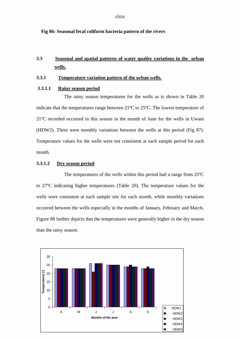
clxix

Fig 86: Seasonal fecal coliform bacteria pattern of the rivers

3.3 Seasonal and spatial patterns of water quality variations in the urban

wells.

3.3.1 Temperature variation pattern of the urban wells.

3.3.1.1 Rainy season period

The rainy season temperatures for the wells as is shown in Table 20

indicate that the temperatures range between 21ºC to 25ºC. The lowest temperature of

21ºC recorded occurred in this season in the month of June for the wells in Uwani

(HDW2). There were monthly variations between the wells at this period (Fig 87).

Temperature values for the wells were not consistent at each sample period for each

month.

3.3.1.2 Dry season period

The temperatures of the wells within this period had a range from 25ºC

to 27ºC indicating higher temperatures (Table 20). The temperature values for the

wells were consistent at each sample site for each month, while monthly variations

occurred between the wells especially in the months of January, February and March.

Figure 88 further depicts that the temperatures were generally higher in the dry season

than the rainy season.

Fig 87:Rainy season temperature variation pattern of the wells

0

5

10

15

20

25

30

A M J J A S

Months of the year

Te

mp

era

ture

( C

)

HDW1

HDW2

HDW3

HDW4

HDW5Fig 87:Rainy season temperature variation pattern of the wells

0

5

10

15

20

25

30

A M J J A S

Months of the year

Te

mp

era

ture

( C

)

HDW1

HDW2

HDW3

HDW4

HDW5

clxx

Fig 87: Rainy season temperature variation pattern of the wells

Fig 88: Dry season temperature variation pattern of the wells

3.3.2 The pH variation pattern of the urban wells.

3.3.2.1 Rainy season period.

The pH of the wells ranges between 3.0 to 6.0 (Table 21) and these

values are indicative of the fact that the waters are acidic. From Table 21 it is

observable that there were monthly variations in the pH values of the wells during this

season. The pH values were higher (slightly acidic) in the well located at Asata

(HDW5),while theother wells in Abakpa (HDW1), Uwani(HDW2), Achara layout

(HDW3) and Ogui (HDW4) had lower pH values. Spatial variations were thus

observed during this season (Fig 89).

Fig 88:Dry season temperature variation pattern of the wells

24

24.5

25

25.5

26

26.5

27

27.5

O N D J F M

Months of the year

Te

mp

era

ture

( C

)

HDW1

HDW2

HDW3

HDW4

HDW5Fig 88:Dry season temperature variation pattern of the wells

24

24.5

25

25.5

26

26.5

27

27.5

O N D J F M

Months of the year

Te

mp

era

ture

( C

)

HDW1

HDW2

HDW3

HDW4

HDW5

clxxi

3.2.2.2 Dry season period.

The dry season pH values have a range between 3.0 to 7.0 (Table 21).The

well waters at this period are also acidic in nature except for the month of February,

when the well in Abakpa (HDW1), Achara layout (HDW3) and Asata (HDW5) were

alkaline in nature. This was also the month in which all the wells recorded high pH

values except for the wells in Ogui (HDW4) (Fig 90).

Seasonal and spatial variations occurred during the rainy and the dry season.

Fig 89: Rainy season pH variation pattern of the wells

Fig 90: Dry season pH variation pattern of the wells

FIG 89 : Rainy season pH variation pattern of the wells

0

1

2

3

4

5

6

7

8

A M J J A S

Months of the year

pH

HDW1

HDW2

HDW3

HDW4

HDW5FIG 89 : Rainy season pH variation pattern of the wells

0

1

2

3

4

5

6

7

8

A M J J A S

Months of the year

pH

HDW1

HDW2

HDW3

HDW4

HDW5

Fig 90:Dry season pH variation pattern of the wells

0

1

2

3

4

5

6

7

8

9

O N D J F M

Months of the year

pH

(un

its

)

HDW1

HDW2

HDW3

HW4

HDW5Fig 90:Dry season pH variation pattern of the wells

0

1

2

3

4

5

6

7

8

9

O N D J F M

Months of the year

pH

(un

its

)

HDW1

HDW2

HDW3

HW4

HDW5

clxxii

3.3.3 Turbidity variation pattern of the urban wells.

3.3.3.1 Rainy season period.

Turbidity levels of the wells range between 0 to 59 NTU (Table 22).The

wells with the highest level of turbidity were those located at Abakpa (HDW1), while

those located at Uwani (HDW5) had the lowest level during this season. From Fig. 91

it can be seen that monthly and spatial variations occurred in terms of the turbidity

levels of wells in Enugu; with the well in Abakpa (HDW1) having the highest value.

3.3.3.2 Dry season period.

The turbidity level of the wells ranged between 1 to 27 NTU (Table 22).

Generally, the dry season turbidity values were higher than the rainy season values.

Figs. 91 and 92 show that there were monthly and spatial variations in the turbidity

level of the wells during the rainy and dry seasons.

Fig 91:Rainy season turbidity variation pattern of the wells

0

10

20

30

40

50

60

70

A M J J A S

Months of the year

Tu

rbid

ity

le

ve

l(N

TU

)

HDW1

HDW2

HDW3

HDW4

HDW5Fig 91:Rainy season turbidity variation pattern of the wells

0

10

20

30

40

50

60

70

A M J J A S

Months of the year

Tu

rbid

ity

le

ve

l(N

TU

)

HDW1

HDW2

HDW3

HDW4

HDW5

clxxiii

Fig 91: Rainy season turbidity variation pattern of the wells

Fig 92: Dry season turbidity variation pattern of the wells

3.3.4 Total Dissolved Solids variation pattern of the urban wells.

3.3.4.1 Rainy season period.

The range of the rainy season total dissolved solids lies between 32 to 869

mg/l (Table 23). The highest total dissolved solid level was recorded during this

season in the wells located at Abakpa (HDW1) in the month of August, while the

lowest levels were also recorded during this season in two locations (Uwani (HDW2)

and Asata (HDW5).

Figure 93 shows that monthly and spatial variations occurred in the turbidity

levels of the wells in the rainy season.

3.3.4.2 Dry season period.

Fig 92:Dry season turbidity variation pattern of the wells

0

5

10

15

20

25

30

O N D J F M

Months of the year

Tu

rbid

ity

le

ve

l(N

TU

)

HDW1

HDW2

HDW3

HDW4

HDW5Fig 92:Dry season turbidity variation pattern of the wells

0

5

10

15

20

25

30

O N D J F M

Months of the year

Tu

rbid

ity

le

ve

l(N

TU

)

HDW1

HDW2

HDW3

HDW4

HDW5

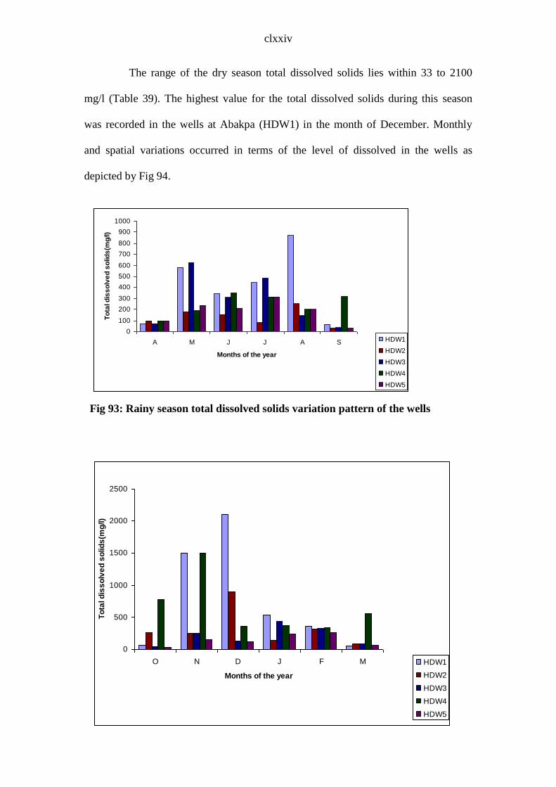
clxxiv

The range of the dry season total dissolved solids lies within 33 to 2100

mg/l (Table 39). The highest value for the total dissolved solids during this season

was recorded in the wells at Abakpa (HDW1) in the month of December. Monthly

and spatial variations occurred in terms of the level of dissolved in the wells as

depicted by Fig 94.

Fig 93: Rainy season total dissolved solids variation pattern of the wells

Fig 93:Rainy season total dissolved solids variation pattern of

the wells

0

100

200

300

400

500

600

700

800

900

1000

A M J J A S

Months of the year

To

tal d

iss

olv

ed

so

lid

s(m

g/l)

HDW1

HDW2

HDW3

HDW4

HDW5

Fig 93:Rainy season total dissolved solids variation pattern of

the wells

0

100

200

300

400

500

600

700

800

900

1000

A M J J A S

Months of the year

To

tal d

iss

olv

ed

so

lid

s(m

g/l)

HDW1

HDW2

HDW3

HDW4

HDW5

Fig 94:Dry season total dissolved solid variation pattern of

the wells

0

500

1000

1500

2000

2500

O N D J F M

Months of the year

To

tal d

iss

olv

ed

so

lid

s(m

g/l)

HDW1

HDW2

HDW3

HDW4

HDW5Fig 94:Dry season total dissolved solid variation pattern of

the wells

0

500

1000

1500

2000

2500

O N D J F M

Months of the year

To

tal d

iss

olv

ed

so

lid

s(m

g/l)

HDW1

HDW2

HDW3

HDW4

HDW5

clxxv

Fig 94: Dry season total dissolved solids variation pattern of the wells

3.3.5 Conductivity variation pattern of the urban wells.

3.3.5.1 Rainy season period.

Conductivity of well water within this period ranged between 0.1 to

1.29µ SCM (Table 24). The rainy season had higher conductivity values, with he

highest value for both seasons occurring within this season in the wells in Achara

layout (HDW3) in the month of March (Fig 95).

3.3.5.2 Dry season period

The conductivity range was between 0 to 1.19µSCM (Table 24).

Conductivity was highest during this season in the wells in Abakpa (HDW1).And

conductivity was generally very low in the months of November and December in all

the wells (Fig 96).

Monthly and spatially variations are observed within this period.

Fig 95: Rainy season conductivity variation pattern of the wells

Fig 95:Rainy season conductivity variation pattern of the wells

0

0.2

0.4

0.6

0.8

1

1.2

1.4

A M J J A S

Months of the year

Co

nd

uc

tiv

ity

le

ve

l( s

cm

)

HDW1

HDW2

HDW3

HDW4

HDW5Fig 95:Rainy season conductivity variation pattern of the wells

0

0.2

0.4

0.6

0.8

1

1.2

1.4

A M J J A S

Months of the year

Co

nd

uc

tiv

ity

le

ve

l( s

cm

)

HDW1

HDW2

HDW3

HDW4

HDW5

Fig 96:Dry season conductivity variation pattern of the wells

0

0.2

0.4

0.6

0.8

1

1.2

1.4

O N D J F M

Months of the year

Co

nd

uc

tiv

ity

le

ve

l( s

cm

)

HDW1

HDW2

HDW3

HDW4

HDW5Fig 96:Dry season conductivity variation pattern of the wells

0

0.2

0.4

0.6

0.8

1

1.2

1.4

O N D J F M

Months of the year

Co

nd

uc

tiv

ity

le

ve

l( s

cm

)

HDW1

HDW2

HDW3

HDW4

HDW5

clxxvi

Fig 96: Dry season conductivity variation pattern of the wells

3.3.6 Total hardness variation pattern of the urban wells.

3.2.6.1 Rainy season period.

Total hardness of the wells in the rainy season had a range between 0.2

to 3.26 mg/l (Table 25).Figure 97 shows that the highest values for all the wells in the

five locations occurred in the month of September with the highest hardness value

occurring in the wells in Asata (HDW5). The lower values were recorded in the

months of April to August. Monthly and seasonal variations occurred during this

period.

3.3.6.2 Dry season period.

The values range between 0.1to1.0 mg/l during this season (Table 25). The

highest values occurred in all the wells in the month of October; with the highest

value for this month occurring in the wells in Asata (HDW5) (Fig 98).

Very low values occurred in the month of November for all the wells. The

wells located in Asata (HDW5) had the highest hardness values both in the rainy and

the dry seasons.

Fig 97:Rainy season total hardness variation pattern of the

wells

0

0.5

1

1.5

2

2.5

3

3.5

A M J J A S

Months of the year

To

tal h

ard

ne

ss

(mg

/l)

HDW1

HDW2

HDW3

HDW4

HDW5

Fig 97:Rainy season total hardness variation pattern of the

wells

0

0.5

1

1.5

2

2.5

3

3.5

A M J J A S

Months of the year

To

tal h

ard

ne

ss

(mg

/l)

HDW1

HDW2

HDW3

HDW4

HDW5

clxxvii

Fig 97: Rainy season total hardness variation pattern of the wells

Fig. 98: Dry season total hardness variation pattern of the wells

Fig 98:Dry season total hardness variation pattern of the wells

0

2

4

6

8

10

12

O N D J F M

Months of the year

To

tal h

ard

ne

ss

(mg

/l)

HDW1

HDW2

HDW3

HDW4

HDW5Fig 98:Dry season total hardness variation pattern of the wells

0

2

4

6

8

10

12

O N D J F M

Months of the year

To

tal h

ard

ne

ss

(mg

/l)

HDW1

HDW2

HDW3

HDW4

HDW5

clxxviii

3.3.7 Dissolved Oxygen variation pattern of the urban wells.

3.3.7.1 Rainy season period.

The rainy season dissolved oxygen for the wells had a range between 1.0

to 6.5 mg/l (Table 26). From Fig. 99 it can be seen that the lowest dissolved oxygen

content was recorded in the month of April in the wells located in Achara layout

(HDW3). Dissolved oxygen of the wells during this season was highest in two

different months in two different wells (i.e. wells located in Ogui (HDW4) and

Abakpa (HDW5)) in June and August respectively (Fig 99). Monthly and spatial

variations thus exist between the wells in terms of their dissolved oxygen content.

3.3.7.2 Dry season period.

The dissolved oxygen content of the well waters range from 0.6 to 9.6

mg/l (Table 26). Fig. 100 shows that all the wells had high dissolved oxygen content

during this season in the month of February. However the well waters in Ogui

(HDW4) had the highest level. The lowest dissolved oxygen content occurred in

January for all the wells. Monthly and season variations occurred in all the wells

during this season.

The dissolved oxygen content for the wells were higher in the rainy season than

the dry season (Figs 99 and 100).

Fig 99:Rainy season dissolved oxygen variation pattrern of

the wells

0

1

2

3

4

5

6

7

A M J J A S

Months of the year

Dis

so

lve

d o

xy

ge

n(m

g/l)

HDW1

HDW2

HDW3

HDW4

HDW5

Fig 99:Rainy season dissolved oxygen variation pattrern of

the wells

0

1

2

3

4

5

6

7

A M J J A S

Months of the year

Dis

so

lve

d o

xy

ge

n(m

g/l)

HDW1

HDW2

HDW3

HDW4

HDW5

clxxix

Fig 99: Rainy season dissolved oxygen variation pattern of the wells

Fig 100: Dry season dissolved oxygen variation pattern of the wells

Fig 100:Dry season dissolved oxygen variation pattern of the

wells

0

2

4

6

8

10

12

O N D J F M

Months of the year

Dis

so

lve

d o

xy

ge

n(m

g/l)

HDW1

HDW2

HDW3

HDW4

HDW5

Fig 100:Dry season dissolved oxygen variation pattern of the

wells

0

2

4

6

8

10

12

O N D J F M

Months of the year

Dis

so

lve

d o

xy

ge

n(m

g/l)

HDW1

HDW2

HDW3

HDW4

HDW5

clxxx

3.8 Biochemical Oxygen Demand variation pattern of the urban wells.

3.3.8.1 Rainy season period.

The range is between 0.1 to 4.6 mg/l (Table 27). Figure 101 shows that

monthly and spatial variations occurred within this season as the highest level of

biochemical oxygen demand for all the wells during this season occurred in the month

of April, with all the wells generally having high values in the month of May. The

wells in Asata (HDW5) also had high biochemical oxygen demand in the month of

June, while the other stations had very low biochemical oxygen demand levels. The

lowest values were recorded in the months of June and August in the wells in Abakpa

(HDW1).

3.3.8.2 Dry season period.

The dry season biochemical oxygen had a range of 0.3 to 4.9mg/l. From

Fig. 102 it can be seen that the lowest biochemical oxygen demand was recorded in

the month of February for the wells in Ogui (HDW4); while the highest value

occurred in January for the wells in Achara layout (HDW3). Monthly and spatial

variations occurred in spite of the fact that some months had the same biochemical

oxygen demand levels.

Fig 101:Rainy season biochemical oxygen demand variation

pattern of the wells

0

0.5

1

1.5

2

2.5

3

3.5

4

4.5

5

A M J J A S

Months of the year

Bio

ch

em

ica

l o

xy

ge

n d

em

an

d(m

g/l)

HDW1

HDW2

HDW3

HDW4

HDW5

Fig 101:Rainy season biochemical oxygen demand variation

pattern of the wells

0

0.5

1

1.5

2

2.5

3

3.5

4

4.5

5

A M J J A S

Months of the year

Bio

ch

em

ica

l o

xy

ge

n d

em

an

d(m

g/l)

HDW1

HDW2

HDW3

HDW4

HDW5

clxxxi

Fig 101: Rainy season biochemical oxygen demand variation pattern of the

wells

Fig 102: Dry season biochemical oxygen demand variation pattern of the wells

Fig 102: Dry season biochemical oxygen demand variation

pattern of the wells

0

1

2

3

4

5

6

O N D J F M

Months of the year

Bio

ch

em

ica

l o

xy

ge

n d

em

an

d(m

g/l)

HDW1

HDW3

HDW3

HDW4

HDW5

Fig 102: Dry season biochemical oxygen demand variation

pattern of the wells

0

1

2

3

4

5

6

O N D J F M

Months of the year

Bio

ch

em

ica

l o

xy

ge

n d

em

an

d(m

g/l)

HDW1

HDW3

HDW3

HDW4

HDW5

clxxxii

3.3.9 Phosphate variation pattern of the urban wells.

3.3.9.1 Rainy season period.

The phosphate concentration for the rainy season varied between the

values of 0 to 1.5 mg/l (Table 28). Fig. 103 shows that monthly and spatial variations

occurred within this season as the highest level of phosphate for all the wells during

this season occurred in the month of April, with the wells in Abakpa (HDW1) having

the highest value. Very low values were generally recorded in all the wells in the

months of May, June, July and August. The lowest values however occurred in the

month of August.

3.3.9.2 Dry season period.

The range of the values obtained from the field work range between 0 to

7.4 mg/l (Table 28). Monthly and spatial variations occurred during this season as is

shown by Fig 104. From Fig 104, it can be seen that the highest level of phosphate for

all the wells during this season occurred in the month of March, with the wells in

Abakpa (HDW1) having the highest value. Very negligible phosphate levels occurred

for all the wells in the months of November and December.

Fig 103:Rainy season phosphate variation pattern of the wells

0

0.5

1

1.5

2

2.5

3

3.5

4

4.5

A M J J A S

Months of the year

Ph

os

ph

ate

le

ve

l(m

g/l)

HDW1

HDW2

HDW3

HDW4

HDW5Fig 103:Rainy season phosphate variation pattern of the wells

0

0.5

1

1.5

2

2.5

3

3.5

4

4.5

A M J J A S

Months of the year

Ph

os

ph

ate

le

ve

l(m

g/l)

HDW1

HDW2

HDW3

HDW4

HDW5 Fig 103:Rainy season phosphate variation pattern of the wells

0

0.5

1

1.5

2

2.5

3

3.5

4

4.5

A M J J A S

Months of the year

Ph

os

ph

ate

le

ve

l(m

g/l)

HDW1

HDW2

HDW3

HDW4

HDW5Fig 103:Rainy season phosphate variation pattern of the wells

0

0.5

1

1.5

2

2.5

3

3.5

4

4.5

A M J J A S

Months of the year

Ph

os

ph

ate

le

ve

l(m

g/l)

HDW1

HDW2

HDW3

HDW4

HDW5

clxxxiii

Fig 103: Rainy season phosphate variation pattern of the wells

Fig 104: Dry season phosphate variation pattern of the wells

3.3.10 Sodium variation pattern of the urban wells.

3.3.10.1 Rainy season period.

The sodium level of wells ranged between 1.8 to 62.1 mg/l (Table 29).

Fig 105 indicates that monthly and spatial variations occurred during this season as

the sodium level of all the wells decreased from the month of April to the month of

September. The highest values for this season for all the wells occurred in the month

of April; while the lowest values were recorded in September in all the wells.

3.3.10.2 Dry season period

The level of sodium in the well waters ranged between 0.06 to 61.5

mg/l. The highest values occurred in the month of March with the wells in Abakpa

having the highest sodium level; while the lowest level occurred in the month of

October in the wells in Achara layout(HDW3)(Fig 106). Monthly and spatial

variations thus occurred within this season.

Fig 104:Dry season phosphate variation pattern of the wells

0

1

2

3

4

5

6

7

8

O N D J F M

Moths of the year

Ph

os

ph

ate

(mg

/l)

HDW1

HDW2

HDW3

HDW4

HDW5Fig 104:Dry season phosphate variation pattern of the wells

0

1

2

3

4

5

6

7

8

O N D J F M

Moths of the year

Ph

os

ph

ate

(mg

/l)

HDW1

HDW2

HDW3

HDW4

HDW5

clxxxiv

Fig 105: Rainy season sodium variation pattern of the wells

Fig 106: Dry season sodium variation pattern of the wells

3.3.11 Sulphate variation pattern of the urban wells.

3.3.11.1 Rainy season variation.

Rainy season sulphate values were between 0 to 13.3 mg/l (Table 30).

Monthly and spatial variations occurred as is depicted in Fig .107. It shows that higher

FIG 105:Rainy season sodium variation pattern of the wells

0

10

20

30

40

50

60

70

A M J J A S

Months

so

diu

m(m

g/l)

HDW1

HDW2

HDW3

HDW4

HDW5FIG 105:Rainy season sodium variation pattern of the wells

0

10

20

30

40

50

60

70

A M J J A S

Months

so

diu

m(m

g/l)

HDW1

HDW2

HDW3

HDW4

HDW5

FIG 106:Dry season sodium variation pattern of the wells

0

10

20

30

40

50

60

70

O N D J F M

Months

so

diu

m(m

g/l)

HDW1

HDW2

HDW3

HDW4

HDW5FIG 106:Dry season sodium variation pattern of the wells

0

10

20

30

40

50

60

70

O N D J F M

Months

so

diu

m(m

g/l)

HDW1

HDW2

HDW3

HDW4

HDW5

clxxxv

sulphate levels occurred during this season with Abakpa having the highest level in

the month of April. The sulphate level in all the wells decreased from the month of

April to September.

3.3.11.2 Dry season period.

Sulphate values for the dry season range from 0 to 18.1 mg/l (table 30).

Generally, the sulphate levels were very low (Fig 108) except in the month in the

month of February, when the wells in Uwani (HDW2) had the highest level for the

season. Inspite of the low levels recorded during this season, variations occurred

monthly and spatially (Fig 108).

Fig 107: Rainy season sulphate variation pattern of the wells

FIG 107:Rainy season sulphate variation pattern of the wells

0

2

4

6

8

10

12

14

16

A M J J A S

months

su

lph

ate

(mg

/l)

HDW1

HDW2

HDW3

HDW4

HDW5FIG 107:Rainy season sulphate variation pattern of the wells

0

2

4

6

8

10

12

14

16

A M J J A S

months

su

lph

ate

(mg

/l)

HDW1

HDW2

HDW3

HDW4

HDW5

FIG 108:Dry Season sulphate variation pattern of the wells

0

2

4

6

8

10

12

14

16

18

20

O N D J F M

Months of the year

su

lph

ate

(mg

/l)

HDW1

HDW2

HDW3

HDW4

HDW5FIG 108:Dry Season sulphate variation pattern of the wells

0

2

4

6

8

10

12

14

16

18

20

O N D J F M

Months of the year

su

lph

ate

(mg

/l)

HDW1

HDW2

HDW3

HDW4

HDW5

clxxxvi

Fig 108: Dry season sulphate variation pattern of the wells

3.3.12 Ammonia variation pattern of the urban wells.

3.3.12.1 Rainy season period.

The rainy season ammonia values range between 0.09 to 8.7 mg/l

(Table 31). ). Figure 109 shows that monthly and spatial variations occurred within

this season as the highest level of ammonia for all the wells during this season

occurred in the month of April, with all the wells generally having high values in the

month of June.

Very low values were recorded in all the wells in the month of July, August

and September. Even within the low value months, variations still occurred among the

wells with the wells in Achara layout having the highest ammonia levels.

3.3.12.2 Dry season period.

The ammonia range for the dry season was within the range of 0.01 to

4.2mg/l (Table 31). Ammonia levels in the wells were very low in the months of

November and December as is depicted in Fig 110. Four sites( Abakpa (HDW1),

clxxxvii

Uwani (HDW2), Achara layout (HDW3) and Ogui (HDW4)) had high values in July

with the wells in Abakpa(HDW1) and Uwani(HDW2) recording the highest values in

this month of July (Fig 110). The dry season ammonia levels were generally higher in

the months of January, February and March.

Fig 109: Rainy season ammonia variation pattern of the wells

FIG 109:Rainy season ammonia variation pattern of the wells

0

1

2

3

4

5

6

7

8

9

10

A M J J A S

Months

Am

mo

nia

(mg

/l)

HDW1

HDW2

HDW3

HDW4

HDW5FIG 109:Rainy season ammonia variation pattern of the wells

0

1

2

3

4

5

6

7

8

9

10

A M J J A S

Months

Am

mo

nia

(mg

/l)

HDW1

HDW2

HDW3

HDW4

HDW5

FIG 110: Dry season ammonia variation pattern of the

wells

0

0.5

1

1.5

2

2.5

3

3.5

4

4.5

O N D J F M

Months

Am

monia

(mg/l)

HDW1

HDW2

HDW3

HDW4

HDW5

FIG 110: Dry season ammonia variation pattern of the

wells

0

0.5

1

1.5

2

2.5

3

3.5

4

4.5

O N D J F M

Months

Am

monia

(mg/l)

HDW1

HDW2

HDW3

HDW4

HDW5

clxxxviii

Fig 110: Dry season ammonia variation pattern of the wells

3.3.13 Nitrate variation pattern of the urban wells.

3.3.13.1 Rainy season period.

The rainy season nitrate values were within the range of 0 to 7.0 mg/l

(Table 33). Generally, the nitrate levels were very low in all the wells and negligible

in some wells the (Fig 111).The lowest values during this period were observed in the

months of July and August. Inspite of the low values, the highest nitrate level was

recorded in the month of June in Asata. Monthly and spatial variations occurred

during this season.

3.3.13.2 Dry season period.

Nitrate values for the dry season range between 0 to 1.2 mg/l (Table 33).

Figure 112 shows that monthly and spatial variations occurred within this season as

the highest level of nitrate for all the wells during this season occurred in the month of

October, with the highest value in the month of June. Very low values were recorded

for all the wells in the month of December.

clxxxix

Fig. 111: Rainy season nitrate variation pattern of the wells

Fig. 112: Dry season nitrate variation pattern of the wells

3.3.14 Fecal coliform bacteria variation pattern of the urban wells.

3.3.14.1 Rainy season period.

The rainy season fecal coliform level range is from 1 to 18 cf/100ml

(Table 34). From Fig 113 the highest fecal coliform level occurred in the month of

FIG 111:Rainy season nitrate variation pattern of the wells

0

1

2

3

4

5

6

7

8

A M J J A S

Months

Nitra

te(m

g/l)

HDW1

HDW2

HDW3

HDW4

HDW5FIG 111:Rainy season nitrate variation pattern of the wells

0

1

2

3

4

5

6

7

8

A M J J A S

Months

Nitra

te(m

g/l)

HDW1

HDW2

HDW3

HDW4

HDW5

FIG 112:Dry season nitrate variation pattern of the wells.

0

0.2

0.4

0.6

0.8

1

1.2

1.4

1.6

O N D J F M

Months

Nitra

te(m

g/l)

HDW1

HDW2

HDW3

HDW4

HDW5FIG 112:Dry season nitrate variation pattern of the wells.

0

0.2

0.4

0.6

0.8

1

1.2

1.4

1.6

O N D J F M

Months

Nitra

te(m

g/l)

HDW1

HDW2

HDW3

HDW4

HDW5

cxc

September in the well waters in Ogui (HDW4). The levels were generally high in the

month of June for all the wells and the coliform level was the same for all the wells in

July and August. Variations thus occurred monthly and spatially in terms of the fecal

coliform levels of the wells.

3.3.14.2 Dry season period.

The coliform level at this period ranged between 0 and 17. From figure

114 the highest fecal coliform level occurred in the month of October in the well

waters in Ogui (HDW4). The levels were generally consistent for all the wells in the

month of March. Monthly and spatial variations occurred in the coliform levels of the

wells.

Fig. 113: Rainy season fecal coliform bacteria variation pattern of the wells

FIG 113:Rainy season faecal coliform bacteria variation pattern of the wells

0

2

4

6

8

10

12

14

16

18

20

A M J J A S

Months of the year

Fe

ca

l c

olifo

rm b

ac

teri

a(c

fu/1

00

mls

)

HDW1

HDW2

HDW3

HDW4

HDW5

FIG 113:Rainy season faecal coliform bacteria variation pattern of the wells

0

2

4

6

8

10

12

14

16

18

20

A M J J A S

Months of the year

Fe

ca

l c

olifo

rm b

ac

teri

a(c

fu/1

00

mls

)

HDW1

HDW2

HDW3

HDW4

HDW5

FIG 114:Dry season fecal coliform bacteria variation pattern of the wells

0

2

4

6

8

10

12

14

16

18

20

O N D J F M

Months of the year

Fecal

co

lifo

rm b

acte

ria(c

fu/1

00m

ls)

HDW1

HDW2

HDW3

HDW4

HDW5FIG 114:Dry season fecal coliform bacteria variation pattern of the wells

0

2

4

6

8

10

12

14

16

18

20

O N D J F M

Months of the year

Fecal

co

lifo

rm b

acte

ria(c

fu/1

00m

ls)

HDW1

HDW2

HDW3

HDW4

HDW5

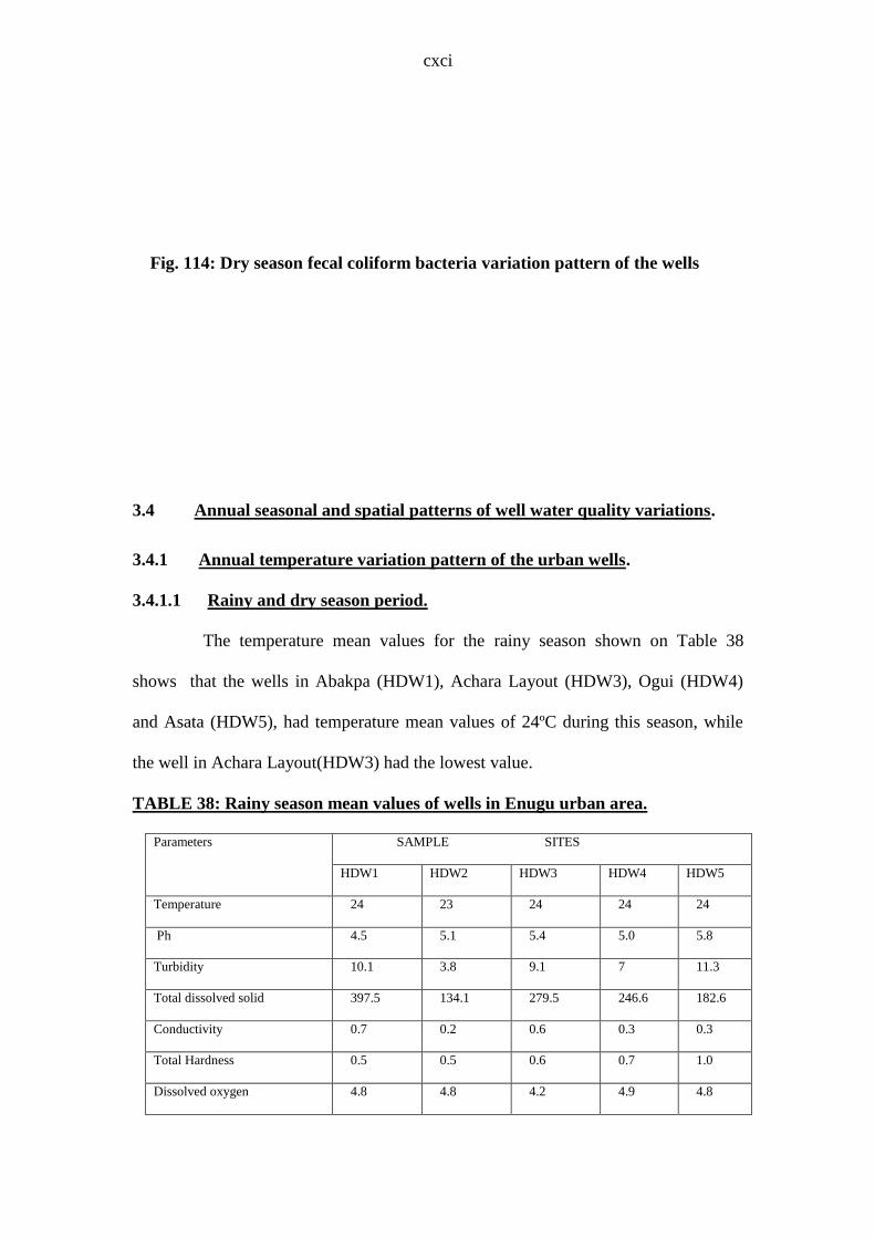
cxci

Fig. 114: Dry season fecal coliform bacteria variation pattern of the wells

3.4 Annual seasonal and spatial patterns of well water quality variations.

3.4.1 Annual temperature variation pattern of the urban wells.

3.4.1.1 Rainy and dry season period.

The temperature mean values for the rainy season shown on Table 38

shows that the wells in Abakpa (HDW1), Achara Layout (HDW3), Ogui (HDW4)

and Asata (HDW5), had temperature mean values of 24ºC during this season, while

the well in Achara Layout(HDW3) had the lowest value.

TABLE 38: Rainy season mean values of wells in Enugu urban area.

Parameters SAMPLE SITES

HDW1 HDW2 HDW3 HDW4 HDW5

Temperature 24 23 24 24 24

Ph 4.5 5.1 5.4 5.0 5.8

Turbidity 10.1 3.8 9.1 7 11.3

Total dissolved solid 397.5 134.1 279.5 246.6 182.6

Conductivity 0.7 0.2 0.6 0.3 0.3

Total Hardness 0.5 0.5 0.6 0.7 1.0

Dissolved oxygen 4.8 4.8 4.2 4.9 4.8

cxcii

Biochemical Oxygen demand 0.8 1.6 1.6 1.0 1.9

Phosphate 1.0 0.4 0.6 0.2 0.5

Sodium 20.0 17.2 22.9 16.7 15.7

Sulphate 3.9 0.8 2.0 0.6 0.9

Ammonia 1.7 1.8 3.3 1.9 1.8

Calcium 13.5 13.7 13.5 12.8 13.0

Nitrate 0.0 0.2 0.1 0.1 1.8

Fecal coliform 3.1 4 3.8 5.3 3

The dry season mean values for the wells(Table 39) also indicate that the wells in

Abakpa (HDW1), Achara layout (HDW3), Ogui (HDW4), and Asata (HDW5) had

means of 25ºC, while Uwani (HDW2) had a mean of 22ºC(Table 39)

Fig. 115 further depicts that the temperatures were generally higher in the

dry season than the rainy season.

TABLE 39: Dry season mean values of wells in Enugu urban area.

Parameters SAMPLE SITES

HDW1 HDW2 HDW3 HDW4 HDW5

Temperature 25 22 25 25 25

Ph 4.2 5.3 5.8 4.7 6.2

Turbidity 15.5 8.6 5.6 5.8 11.6

Total dissolved solid 768.3 323.5 212.1 647.8 146.1

Conductivity 0.5 0.2 0.4 0.4 0.3

Total Hardness 0.5 0.4 0.6 1.2 2.3

Dissolved oxygen 5.3 5.1 5.5 4.8 4.9

Biochemical Oxygen demand 1.3 1.9 1.8 1.2 1.9

Phosphate 2.2 1.3 1.6 1.5 2.1

Sodium 16.0 10.7 20.1 14.7 16.0

Sulphate 0.9 3.1 0.8 0.9 0.4

Ammonia 1.3 1.3 1.6 1.6 0.5

Calcium 9.5 9.8 10.2 9.4 9.4

Nitrate 0.2 0.19 0.43 0.47 0.5

cxciii

Fecal coliform 4 2.1 2.6 6.3 7.3

Fig 115: Seasonal temperature pattern of the wells

3.4.2 Annual pH variation pattern of the urban wells.

3.4.2.1 Rainy and dry season period.

The rainy season mean pH values presented on Table 38 emphasizes the acidic

nature of the well waters. The acidic levels of the well waters occur in the following

decreasing order: Asata (HDW5), Achara layout (HDW3), Uwani (HDW2), Ogui

(HDW4), Abakpa (HDW1).

FIG 115:Seasonal temperature pattern of the wells

20 21 22 23 24 25 26

HDW1

HDW2

HDW3

HDW4

HDW5

Sam

ple

sit

es

Temperature level( C )

DRY

RAINY

Temperature Level (°C)

FIG 115:Seasonal temperature pattern of the we lls

20 21 22 23 24 25 26

HDW1

HDW2

HDW3

HDW4

HDW5

Sa

mp

le s

ite

s

Tempera ture leve l( C )

DRY

RAINY

Temperature Level (°C)

cxciv

The dry season mean values (Table 39) indicate that the wells had acidity

levels in the following decreasing order: Asata (HDW5), Achara layout (HDW3),

Uwani (HDW2), Ogui (HDW4) and Abakpa (HDW1).

A comparison of the annual seasonal pH values of the wells (Fig 116) indicates

that for the wells in Uwani(HDW2),Achara layout(HDW3) and Asata(HDW5)), the

pH values were higher in the dry season than the rainy season; while for Abakpa

(HDW1)and Ogui(HDW4) the wells had higher pH values in the rainy season than the

dry season.

Fig. 116: Seasonal pH pattern of the wells

3.4.3 Annual turbidity variation pattern of the urban wells.

3.4.3.1 Rainy and dry season period.

From the mean values obtained (Table 38), the wells with the highest

level of turbidity were those located at Abakpa (HDW1), while those located at

Uwani (HDW2) had the lowest level during this season. The wells had turbidity levels

Fig 116:Seasonal pH pattern of the wells

0 1 2 3 4 5 6 7

HDW1

HDW2

HDW3

HDW4

HDW5

Sa

mp

le s

ite

s

pH LEVEL

DRY

RAINY

pH level

Fig 116:Seasonal pH pattern of the wells

0 1 2 3 4 5 6 7

HDW1

HDW2

HDW3

HDW4

HDW5

Sa

mp

le s

ite

s

pH LEVEL

DRY

RAINY

pH level

cxcv

in the following decreasing order: Abakpa (HDW1), Asata (HDW5), Achara layout

(HDW3), Ogui (HDW4) and Uwani (HDW2).

The highest level of dry season turbidity occurred in the wells in Abakpa

(HDW1) and the lowest value was recorded in the wells in Achara layout (HDW3)

(Table 39).

In decreasing order, the turbidity of the wells is as follows: Abakpa (HDW1), Asata

(HDW5), Uwani (HDW2), Ogui (HDW4) and Achara layout (HDW3).

Generally, Fig. 117 and shows that turbidity was higher in the dry season

months in Abakpa (HDW1), Uwani (HDW2) and Asata (HDW5), than in the rainy

season months. On the other hand, two wells (Achara layout (HDW3) and Ogui

(HDW4) had higher turbidity levels in the rainy season than the dry season. This also

is evidence that there is spatial variation between the wells in terms of well water

turbidity levels.

Fig 117: Seasonal turbidity pattern of the wells

3.4.4 Annual total dissolved solids variation pattern of the urban wells.

FIG 117:Seasonal turbidity pattern of the wells

0 5 10 15 20

HDW1

HDW2

HDW3

HDW4

HDW5

Sa

mp

le s

ite

s

Turbidity level(NTU)

DRY

RAINYFIG 117:Seasonal turbidity pattern of the wells

0 5 10 15 20

HDW1

HDW2

HDW3

HDW4

HDW5

Sa

mp

le s

ite

s

Turbidity level(NTU)

DRY

RAINY

cxcvi

3.4.4.1 Rainy and dry season period.

The rainy season mean values (Table 38) indicate that Abakpa (HDW1)

wells had the highest total dissolved solids. While Uwani (HDW2) wells had the least.

In decreasing order the levels of total dissolved solids in the wells was therefore as

follows: Abakpa (HDW1), Achara layout (HDW3), Ogui (HDW4), Asata (HDW5)

and Uwani (HDW2).

The dry season mean values (Table 39) indicate that the level of total dissolved

solids in the wells occurred in the following decreasing order: Abakpa (HDW1), Ogui

(HDW4), Uwani (HDW2), Achara layout (HDW3). The total dissolved solids were

higher in the wells in Abakpa (HDW1), Uwani (HDW2) and Ogui (HDW4) in the dry

season than the rainy season (Fig 118).Those Achara layout (HDW3) and Asata

(HDW5) were higher in the rainy season period than the dry season.

Fig. 118: Seasonal total dissolved solids pattern of the wells

3.4.5 Annual conductivity variation pattern of the urban wells.

3.4.5.1 Rainy and dry season period.

FIG 118: Seasonal total dissolved solids pattern of the wells

0 200 400 600 800 1000

HDW1

HDW2

HDW3

HDW4

HDW5

Sa

mp

le s

ite

s

Total Dissolved Solids(mg/l)

DRY

RAINY

FIG 118: Seasonal total dissolved solids pattern of the wells

0 200 400 600 800 1000

HDW1

HDW2

HDW3

HDW4

HDW5

Sa

mp

le s

ite

s

Total Dissolved Solids(mg/l)

DRY

RAINY

cxcvii

The rainy season mean values(Table 38) indicate that the wells in Abakpa

(HDW1) had the highest conductivity level with the lowest occurring in Uwani

(HDW2). The conductivity levels in decreasing order were as follows: Abakpa

(HDW1), Achara layout (HDW3), Ogui (HDW4) and Asata (HDW5), Uwani

(HDW2).

The dry season mean values (Table 39) show that in decreasing order, the

conductivity levels were as follows: Abakpa (HDW1), Achara layout (HDW3), Ogui

(HDW4), Asata (HDW5) and Uwani (HDW2). Generally, conductivity was higher in

the rainy season than in the dry season as is depicted in Figure 119.

Fig 119: Seasonal conductivity pattern of the wells

3.4.6 Annual Total hardness variation pattern of the urban wells.

3.4.6.1 Rainy and dry season period.

The wells in Asata (HDW5) had the highest rainy season hardness mean

value, while Abakpa wells (HDW1) had the lowest (Table 38). The total hardness of

the wells in decreasing order was as follows: Asata (HDW1), Ogui (HDW4), Achara

layout (HDW3), Uwani (HDW2) and Abakpa (HDW1).

FIG 119: Seasonal conductivity pattern of the wells

0 0.1 0.2 0.3 0.4 0.5 0.6 0.7 0.8

HDW1

HDW2

HDW3

HDW4

HDW5

Sa

mp

le s

ite

s

Conductivity level( SCM)

DRY

RAINYFIG 119: Seasonal conductivity pattern of the wells

0 0.1 0.2 0.3 0.4 0.5 0.6 0.7 0.8

HDW1

HDW2

HDW3

HDW4

HDW5

Sa

mp

le s

ite

s

Conductivity level( SCM)

DRY

RAINY

cxcviii

Asata (HDW5) wells had the highest dry season hardness mean value (Table

39), while Uwani (HDW2) had the lowest. In decreasing order, the levels of water

hardness for this season were as follows: Asata (HDW5), Ogui (HDW4), Achara

layout (HDW3), Abakpa (HDW1).

The seasonal pattern of water hardness depicted in Fig. 120, shows that the

water hardness was higher in the wells in Ogui (HDW4) and Asata (HDW5) in the

dry season. The other wells in Abakpa (HDW1), Uwani (HDW2) and Achara layout

(HDW3) had no variations for either season under consideration.

Fig 120: Seasonal total hardness pattern of the wells

3.4.7 Annual dissolved oxygen variation pattern of the urban wells.

3.4.7.1 Rainy and dry season periods.

The rainy season mean values (Table 38); show that the wells in Ogui

(HDW4) had the highest dissolved oxygen level, while Achara layout (HDW3) had

the lowest level. In decreasing order, the dissolved oxygen levels were as follows:

FIG 120:Seasonal hardness pattern of the wells

0 0.5 1 1.5 2 2.5

HDW1

HDW2

HDW3

HDW4

HDW5

Sa

mp

le s

ite

s

Hardness level (mg/l)

DRY

RAINYFIG 120:Seasonal hardness pattern of the wells

0 0.5 1 1.5 2 2.5

HDW1

HDW2

HDW3

HDW4

HDW5

Sa

mp

le s

ite

s

Hardness level (mg/l)

DRY

RAINY

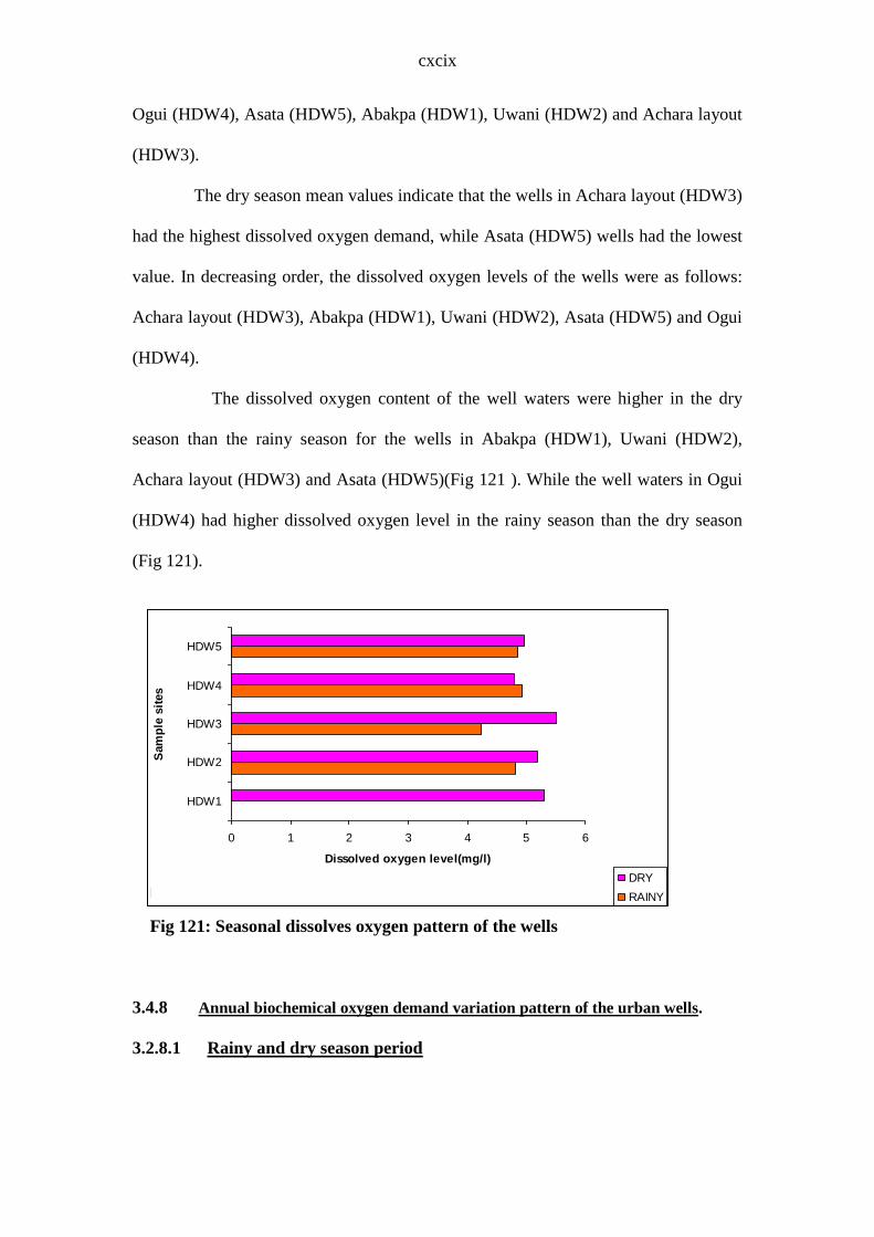
cxcix

Ogui (HDW4), Asata (HDW5), Abakpa (HDW1), Uwani (HDW2) and Achara layout

(HDW3).

The dry season mean values indicate that the wells in Achara layout (HDW3)

had the highest dissolved oxygen demand, while Asata (HDW5) wells had the lowest

value. In decreasing order, the dissolved oxygen levels of the wells were as follows:

Achara layout (HDW3), Abakpa (HDW1), Uwani (HDW2), Asata (HDW5) and Ogui

(HDW4).

The dissolved oxygen content of the well waters were higher in the dry

season than the rainy season for the wells in Abakpa (HDW1), Uwani (HDW2),

Achara layout (HDW3) and Asata (HDW5)(Fig 121 ). While the well waters in Ogui

(HDW4) had higher dissolved oxygen level in the rainy season than the dry season

(Fig 121).

Fig 121: Seasonal dissolves oxygen pattern of the wells

3.4.8 Annual biochemical oxygen demand variation pattern of the urban wells.

3.2.8.1 Rainy and dry season period

FIG 121:Seasonal dissolved oxygen pattern of the wells

0 1 2 3 4 5 6

HDW1

HDW2

HDW3

HDW4

HDW5

Sam

ple

sit

es

Dissolved oxygen level(mg/l)

DRY

RAINYFIG 121:Seasonal dissolved oxygen pattern of the wells

0 1 2 3 4 5 6

HDW1

HDW2

HDW3

HDW4

HDW5

Sam

ple

sit

es

Dissolved oxygen level(mg/l)

DRY

RAINY

cc

From the rainy season mean values obtained (Table 38), it is observable

that the wells in Uwani (HDW2) had the highest value during this season, while the

wells in Ogui had the lowest value. The biochemical oxygen demand levels of the

wells in decreasing order were as follows: Asata (HDW5), Uwani (HDW2), Achara

layout (HDW3), Ogui (HDW4) and Abakpa (HDW1).

The dry season mean values obtained (Table 39), indicate that the wells in Uwani

(HDW2) had the highest level, while those in Ogui (HDW4) had the least. The

biochemical oxygen demand levels of the wells in decreasing order are as follows:

Uwani (HDW2), Asata (HDW5), Achara layout (HDW3), Abakpa (HDW1) and Ogui

(HDW4).

Generally, all the wells in four locations had higher biochemical oxygen

demand levels in the dry season than the rainy season (Fig 122) with the exception of

the wells in Asata (HDW5) that had higher value in the rainy season.

Fig 122: Seasonal biochemical oxygen demand pattern of the wells

3.4.9 Annual phosphate variation pattern of the urban wells.

3.2.9.1 Rainy and dry season period

FIG 122:Seasonal pattern of Biochemical Oxygen Demand of

the wells

0 0.5 1 1.5 2 2.5

HDW1

HDW2

HDW3

HDW4

HDW5

Sa

mp

le s

ite

s

Biochemical Oxygen Demand level(mg/l)

DRY

RAINY

FIG 122:Seasonal pattern of Biochemical Oxygen Demand of

the wells

0 0.5 1 1.5 2 2.5

HDW1

HDW2

HDW3

HDW4

HDW5

Sa

mp

le s

ite

s

Biochemical Oxygen Demand level(mg/l)

DRY

RAINY

cci

The rainy season phosphate mean values (Table 38) indicate that the wells

in Abakpa (HDW1) had the highest phosphate level, while those in Ogui (HDW4) had

the least. The phosphate levels in decreasing order is as follows: Abakpa (HDW1),

Achara layout (HDW3), Asata (HDW5), Uwani (HDW2) and Ogui (HDW4).The dry

season mean values for this season (Table 39); indicate that phosphate levels were

highest in the wells in Asata (HDW5) and least in Uwani (HDW2).

The dry season phosphate levels of all the wells were all higher than the

rainy season levels (Fig 123).

Fig 123: Seasonal phosphate pattern of the wells

3.4.10 Annual sodium variation pattern of the urban wells.

3.4.10.1 Rainy and dry season period

The means for the wells in the rainy season (Table 38) indicate that the wells

in Achara layout (HDW3) had the highest sodium level, while the wells in Asata

(HDW5) had the lowest concentration. In decreasing order, the levels of sodium in the

Fig 123: Seasonal phosphate pattern of the wells

0 0.5 1 1.5 2 2.5

HDW1

HDW2

HDW3

HDW4

HDW5

Sam

ple

sit

es

phosphate(mg/l)

DRY

RAINYFig 123: Seasonal phosphate pattern of the wells

0 0.5 1 1.5 2 2.5

HDW1

HDW2

HDW3

HDW4

HDW5

Sam

ple

sit

es

phosphate(mg/l)

DRY

RAINY

ccii

well waters are as follows: Achara layout (HDW3), Abakpa (HDW1), Uwani

(HDW2), Ogui (HDW4) and Asata (HDW5).

The dry season mean values (Table 39) show that Achara layout (HDW4)

wells had the highest values, while the wells in Uwani (HDW2) had the least. The

sodium level pattern in decreasing order is as follows: Achara layout (HDW3), Asata

(HDW5), Abakpa (HDW1), Ogui (HDW4) and Uwani (HDW2).

Figure 124 shows that the wells in four location( (Abakpa (HDW1), Uwani

(HDW2), Achara layout (HDW3) and Ogui (HDW4)) had higher sodium

concentrations in the rainy season than the dry season While the wells in Asata

(HDW5) had higher sodium concentration in the dry season; thus indicating spatial

variation in the levels of sodium in well waters in Enugu.

Fig 124: Seasonal sodium pattern of the wells

3.4.11 Annual sulphate variation pattern of the urban wells.

3.4.11.1 Rainy and dry season period

Rainy season mean values (Table 38) indicate that Abakpa (HDW1)

had the highest sulphate levels while; Ogui (HDW4) had the lowest. The sulphate

FIG 124: Seasonal sodium pattern of the wells

0 5 10 15 20 25

HDW1

HDW2

HDW3

HDW4

HDW5

Sa

mp

le s

ite

s

sodium level(mg/l)

DRY

RAINYFIG 124: Seasonal sodium pattern of the wells

0 5 10 15 20 25

HDW1

HDW2

HDW3

HDW4

HDW5

Sa

mp

le s

ite

s

sodium level(mg/l)

DRY

RAINY

cciii

concentration in decreasing order is as follows: Abakpa (HDW1), Achara layout

(HDW5), Uwani (HDW2) and Ogui (HDW4).

The dry season mean values in Table 39 indicate that Uwani (HDW2) had

the highest sulphate level during this period while Asata (HDW5) wells had the

lowest value. The sulphate concentration for this period was as follows: Uwani

(HDW2), Ogui (HDW4), Abakpa (HDW1), Achara layout (HDW3) and Asata

(HDW5).

From Fig 125, it is observable that the wells in Uwani (HDW2), Ogui

(HDW4) had sulphate levels that were higher in the dry season than the rainy season,

while those in Abakpa (HDW1), Achara layout (HDW3) and Asata (HDW5) had

higher rainy season sulphate levels.

Fig 125: Seasonal sulphate pattern of the wells

3.4.12 Annual ammonia variation pattern of the urban wells.

3.4.12.1 Rainy and dry season period

The rainy season mean values (Table 38) show that the highest

ammonia values were recorded in wells in Achara layout (HDW3), while the lowest

occurred in Abakpa (HDW1). The pattern exhibited in decreasing order is as follows:

FIG 125: Seasonal sulphate pattern of the wells

0 1 2 3 4 5

HDW1

HDW2

HDW3

HDW4

HDW5

Sa

mp

le s

ite

s

Sulphate(mg/l)

DRY

RAINYFIG 125: Seasonal sulphate pattern of the wells

0 1 2 3 4 5

HDW1

HDW2

HDW3

HDW4

HDW5

Sa

mp

le s

ite

s

Sulphate(mg/l)

DRY

RAINY

cciv

Achara layout (HDW3), Ogui (HDW4), Uwani (HDW2), Asata (HDW5), and Abakpa

(HDW1).

The mean values obtained for the dry season ammonia (Table 39) indicate

that the wells in Achara layout (HDW3) had higher values, while the wells in Asata

(HDW5) had the least. The level of ammonia concentration in decreasing order is as

follows: Achara layout (HDW3), Ogui (HDW4), Abakpa (HDW1), Uwani (HDW2)

and Asata (HDW5).

From Fig 126, it is observable that the rainy season ammonia levels were

higher than the dry season levels.

Fig 126: Seasonal ammonia pattern of the wells

3.4.13 Annual nitrate variation pattern of the urban wells.

3.4.13.1 Rainy and dry season periods.

The rainy season mean values (Table 38) show that the wells in Asata

(HDW5) had the highest values within this period, while the wells in Abakpa

(HDW1) had the lowest. The pattern arising from these mean values indicate that the

FIG 126: Seasonal ammonia pattern of the wells

0 0.5 1 1.5 2 2.5 3 3.5

HDW1

HDW2

HDW3

HDW4

HDW5

Sa

mp

le s

ite

s

Ammonia level(mg/l)DRY

RAINYFIG 126: Seasonal ammonia pattern of the wells

0 0.5 1 1.5 2 2.5 3 3.5

HDW1

HDW2

HDW3

HDW4

HDW5

Sa

mp

le s

ite

s

Ammonia level(mg/l)DRY

RAINY

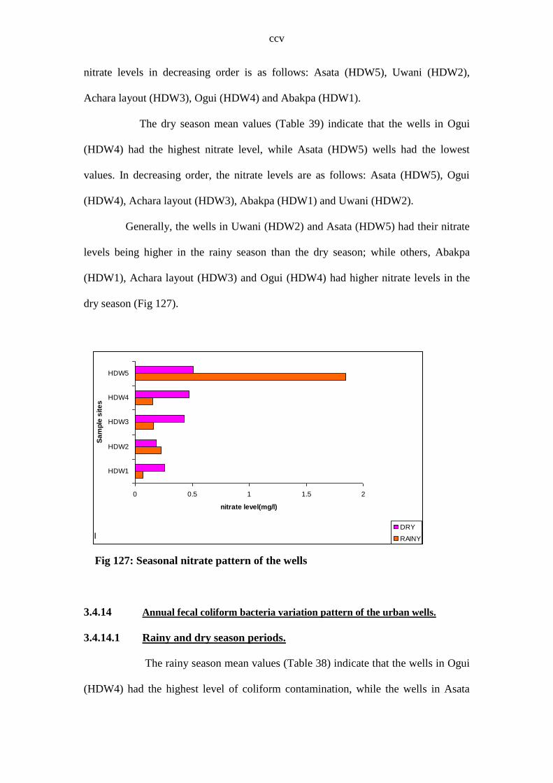
ccv

nitrate levels in decreasing order is as follows: Asata (HDW5), Uwani (HDW2),

Achara layout (HDW3), Ogui (HDW4) and Abakpa (HDW1).

The dry season mean values (Table 39) indicate that the wells in Ogui

(HDW4) had the highest nitrate level, while Asata (HDW5) wells had the lowest

values. In decreasing order, the nitrate levels are as follows: Asata (HDW5), Ogui

(HDW4), Achara layout (HDW3), Abakpa (HDW1) and Uwani (HDW2).

Generally, the wells in Uwani (HDW2) and Asata (HDW5) had their nitrate

levels being higher in the rainy season than the dry season; while others, Abakpa

(HDW1), Achara layout (HDW3) and Ogui (HDW4) had higher nitrate levels in the

dry season (Fig 127).

Fig 127: Seasonal nitrate pattern of the wells

3.4.14 Annual fecal coliform bacteria variation pattern of the urban wells.

3.4.14.1 Rainy and dry season periods.

The rainy season mean values (Table 38) indicate that the wells in Ogui

(HDW4) had the highest level of coliform contamination, while the wells in Asata

FIG 127: Seasonal nitrate pattern of the wellsnitrate

0 0.5 1 1.5 2

HDW1

HDW2

HDW3

HDW4

HDW5

Sa

mp

le s

ite

s

nitrate level(mg/l)

DRY

RAINYFIG 127: Seasonal nitrate pattern of the wellsnitrate

0 0.5 1 1.5 2

HDW1

HDW2

HDW3

HDW4

HDW5

Sa

mp

le s

ite

s

nitrate level(mg/l)

DRY

RAINY

ccvi

(HDW5) had the lowest level. The pattern of coliform contamination in decreasing

order is as follows: Ogui (HDW4), Uwani (HDW2), Achara layout (HDW3), Abakpa

(HDW1) and Asata (HDW5).

The dry season mean values (Table 39) show that the wells with the highest

coliform level were the wells in Asata (HDW5), while those with the lowest level

were those in Uwani (HDW2).The pattern of coliform concentration in the well

waters in decreasing order is as follows: Asata (HDW5), Ogui (HDW4), Abakpa

(HDW1), Achara layout (HDW3) and Uwani (HDW2).

Fig. 128 shows that wells in Abakpa (HDW1), Ogui (HDW4) and Asata

(HDW5) had their coliform levels being higher in the dry season than the rainy

season. On the other hand, wells in Uwani (HDW2) and Achara layout (HDW3) had

coliform levels that were higher in rainy season than the dry season. This pattern

shows that there is seasonal and spatial variation in terms of coliform levels in wells

found in Enugu urban area.

Fig 128: Seasonal fecal coliform bacteria pattern of the wells

FIG 128:Seasonal faecal coliform bacteria pattern of the wells

0 1 2 3 4 5 6 7 8

HDW1

HDW2

HDW3

HDW4

HDW5

Sa

mp

le s

ite

s

Faecal coliform bacteria level(cfU/100ml)

DRY

RAINY

Fecal coliform bacteria level(cfU/100ml)

FIG 128:Seasonal faecal coliform bacteria pattern of the wells

0 1 2 3 4 5 6 7 8

HDW1

HDW2

HDW3

HDW4

HDW5

Sa

mp

le s

ite

s

Faecal coliform bacteria level(cfU/100ml)

DRY

RAINY

Fecal coliform bacteria level(cfU/100ml)

ccvii

CHAPTER FOUR

QUALITY INDICES OF RIVERS AND GROUNDWATER IN ENUGU

URBAN AREA.

4.1 Water Quality Index (WQI) of Rivers in Enugu Urban.

In line with the procedure of NSFWQI discussed in section 1.6 , the

monthly WQI for the five rivers within Enugu Urban were calculated and the

worksheets are presented in Appendices B to M. The results obtained were compared

to the WQI categorization scale to determine the water quality rating (WQI) for the

rivers and this is presented as Table 40.

TABLE 40: Monthly Water Quality Index (WQI) of rivers in Enugu urban Months SWI SW2 SW3 SW4 SW5

January WQI 54 52 60 56 58

Scale Average Average Average Average Average

February WQI 58 58 60 53 53

Scale Average Average Average Average Average

March WQI 59 59 59 57 58

Scale Average Average Average Average Average

April WQI 59 55 57 58 56

Scale Average Average Average Average Average

May WQI 60 47 58 63 65

Scale Average Bad Average Average Average

June WQI 63 59 60 63 62

Scale Average Average Average Average Average

July WQI 66 65 66 66 63

Scale Average Average Average Average Average

August WQI 65 66 65 67 66

Scale Average Average Average Average Average

ccviii

September WQI 53 63 61 60 63

Scale Average Average Average Average Average

October WQI 50 61 58 50 56

Scale Bad Average Average Bad Average

November WQI 55 56 58 56 61

Scale Average Average Average Average Average

December WQI 58 61 59 58 60

Scale Average Average Average Average Average

The WQI for Asata river (SW1) from January to December 2006 are

presented in Table 40. The WQI obtained range from 50 to 66. From the table it is

observable that Asata river (SW1) had a WQI of 54 in January and from February to

August the WQI increased from 58 to 65. This is indicative of a better water quality

level for seven months. A decrease in WQI was however noted from the month of

September and this persisted till December. It is observable that the river had 11

months of average (medium) WQI, while only one month (October) had a WQI that

was bad.

Aria river (SW2) from January to December had WQI that range from 52

to 66. From Table 40, it is observable that the river (SW2) had a WQI of 52 in

January and from February to April the WQI increased to 55 and these are indicative

of higher water quality than that in the month of January. A decrease in WQI was

however noted in the month of May after which an increase occurred till December.

The river had 11 months of average WQI, while only one month (May) had a WQI

that was bad. The noted increase and decrease in WQI is indicative of the fact that

water quality within the river was not constant rather variation occurred monthly with

poorer quality occurring between January and June.

Ekulu river (SW3) from January to December had WQI that range from 58

to 66. From Table 40, it is observable that the river (SW3) had a WQI of 60 in

January and February. From March to May the WQI decreased and from June to

September the WQI increased. A decrease however occurred again from October to

December. Inspite of the noted variation in the WQI the river had 12 months of

average WQI.

Ogbete river (SW4) from January to December had WQI that range from 50

to 67. From Table 40, it is observable that the river (SW4) had a WQI of 56 in

January and then a decrease in February. From the month of March, the WQI

increased till the month of September when a decrease in the WQI occurred. An

ccix

increase was however noted in the months of November and December. The river had

11 months of average WQI and one month of bad WQI.

Immaculate river (SW5) from January to December had WQI that range

from 53 to 66. From Table 40, it is observable that the river (SW5) had a WQI of 58

in January and then a decrease in February. In the month of March, the WQI

increased, and then a decrease occurred in April. A consistent increase occurred from

May to December. The river had 12 months of average WQI.

4.2 Comparative analysis of the monthly WQI of the rivers in Enugu urban.

4.2.1 Monthly rating of the rivers based on their WQI.

The WQI for the rivers in the month of January was from 52 to 60. The

river with the highest rating was Ekulu (SW3), while the river with the lowest rating

was Aria river (SW2). The ranking of the rivers based on their WQI (Appendix Z)

thus shows that Ekulu river had the highest WQI, Immaculate river ranked second,

Ogbete river ranked third, Asata river ranked fourth while Aria river had the lowest

WQI. Ekulu river was thus healthier than the other rivers in January. Aria river had

the lowest health level in this month.

In the month of February, the WQI ranged between 53 and 60. The river

with the highest rating was Ekulu (SW3), while the rivers with the lowest rating were

Ogbete (SW4) and Immaculate river (SW5). The ranking of the rivers based on their

WQI (Appendix Z) thus shows that Ekulu river had the highest WQI, Asata (SW1)

and Aria (SW2) rivers ranked second, while Ogbete (SW4) and Immaculate (SW5)

rivers had the lowest WQI. Ekulu river was thus healthier than the other rivers in

February. Ogbete (SW4) and Immaculate (SW5) rivers had the lowest health level in

this month.

The WQI for the rivers in March was from 57 to 59. Three rivers (Asata

(SW1), Aria (SW2), and Ekulu (SW3) with the same WQI (59) had the highest rating,

while the river with the lowest rating was Ogbete river (SW4). The ranking of the

rivers based on their WQI (Appendix Z) thus shows that Asata (SW1), Aria (SW2),

and Ekulu (SW3) rivers had the highest WQI, Immaculate (SW5) river ranked second,

while Ogbete river had the lowest WQI. Rivers Asata, Aria, and Ekulu were thus

healthier than the other two rivers in the month of March. While Ogbete river had the

lowest health level in March.

ccx

In the month of April, the WQI ranged between 55 and 60. The river with

the highest rating was Asata (SW1), while the river with the lowest rating was Aria

(SW4). The ranking of the rivers based on their WQI (Appendix Z) thus shows that

Asata river had the highest WQI, Ogbete (SW4) river ranked second, Ekulu(SW3)

ranked third, Immaculate river ranked fourth , while Aria(SW2) river had the lowest

WQI. Asata river was thus healthier than the other rivers in April. Aria (SW2) river

had the lowest health level in this month.

The WQI ranged between 47 and 65 in May. The river with the highest

rating was Immaculate (SW5), while the river with the lowest rating was Aria (SW2).

The ranking of the rivers based on their WQI (Appendix Z) thus shows that

Immaculate river had the highest WQI, Ogbete (SW4) river ranked second, Asata

(SW1) ranked third, Ekulu (SW3)river ranked fourth , while Aria(SW2) river had the

lowest WQI. Immaculate (SW5) river was thus healthier than the other rivers. Aria

(SW2) river had the lowest health level in May.

The WQI for the rivers in June was from 59 to 63. Two rivers Asata (SW1)

and Ogbete (SW4), with the same WQI of 63 had the highest rating, while the river

with the lowest rating was Aria river (SW2). The ranking of the rivers based on their

WQI (Appendix Z) thus shows that Asata (SW1) and Ogbete (SW4) rivers had the

highest WQI, Immaculate (SW5) river ranked third, Ekulu (SW3) river ranked fourth

while Aria (SW2) had the lowest WQI. Rivers Asata and Ogbete were thus healthier

than the other three rivers in the month of June. While Aria (SW2) river had the

lowest health level in June.

The WQI for the rivers in July was from 63 to 66. Three rivers (Asata

(SW1), Ekulu (SW3) and Ogbete (SW4) with the same WQI (66) had the highest

rating, while the river with the lowest rating was Immaculate river (SW5). The

ranking of the rivers based on their WQI (Appendix Z) thus shows that Asata (SW1),

Ekulu (SW3) and Ogbete(SW4) rivers had the highest WQI, Aria (SW2) river ranked

fourth, while Immaculate river had the lowest WQI. Rivers Asata, Ekulu and Ogbete

were thus healthier than the other two rivers in the month of March. While

Immaculate river had the lowest health level in July.

The WQI ranged between 65 and 67 in August. The river with the highest

rating was Ogbete (SW4), while the rivers with the lowest ratings were Asata (SW1)

and Ekulu (SW3). The ranking of the rivers based on their WQI (Appendix Z) thus

shows that Ogbete river had the highest WQI, Aria (SW2) and Immaculate (SW5)

ccxi

rivers ranked second, while Asata (SW1) and Ekulu (SW3) rivers had the lowest

WQI. Ogbete (SW4) river was thus healthier than the other rivers while Asata (SW1)

and Ekulu (SW3) rivers had the lowest health level in August.

The WQI for the rivers in September was from 53 to 63. Two rivers Aria

(SW2) and Immaculate (SW5) with the same WQI (63) had the highest rating, while

the river with the lowest rating was Asata river (SW1). The ranking of the rivers

based on their WQI (Appendix Z) thus shows that Aria (SW2) and Immaculate (SW5)

rivers had the highest WQI, Ekulu (SW3) river ranked third, Ogbete (SW4) ranked

fourth, while Asata (SW1) river had the lowest WQI. Rivers Aria and Immaculate

were thus healthier than the other three rivers; while Asata river had the lowest health

level in this month.

In October, the WQI ranged between 50 and 61. The river with the highest

rating was Aria (SW2), while the rivers with the lowest rating were Asata (SW1) and

Ogbete (SW4). The ranking of the rivers based on their WQI (Appendix Z) thus

shows that Aria (SW2) river had the highest WQI, Ekulu (SW3) river ranked second,

Immaculate (SW5) ranked third, while Asata (SW1) and Ogbete (SW4) rivers had the

lowest WQI. Aria river was thus healthier than the other rivers in October, while

Asata and Ogbete rivers had the lowest health level in this month.

The WQI ranged between 55 and 61 in November. The river with the

highest rating was Immaculate (SW5), while the river with the lowest rating was

Asata (SW1). The ranking of the rivers based on their WQI (Appendix Z) thus shows

that Immaculate river had the highest WQI, Ekulu (SW3) river ranked second, Aria

(SW2) and Ogbete (SW4) ranked third, while Asata (SW1) river had the lowest WQI.

Immaculate (SW5) river was thus healthier than the other rivers, while Asata (SW1)

river had the lowest health level in August.

In December, the WQI ranged between 58 and 61. The river with the

highest rating was Aria (SW2), while the rivers with the lowest rating were Asata

(SW1) and Ogbete (SW4). The ranking of the rivers based on their WQI (Appendix

Z) thus shows that Aria (SW2) river had the highest WQI, Immaculate (SW5) river

ranked second, Ekulu river (SW3) ranked third, while Asata (SW1) and Ogbete

(SW4) rivers had the lowest WQI. Aria river was thus healthier than the other rivers

in December, while Asata and Ogbete rivers had the lowest health level in this month.

From the ranking of the WQI, it is observable that rivers Asata (SW1), Aria

(SW2) and Ekulu (SW3) all had four months in which they had the highest WQI.

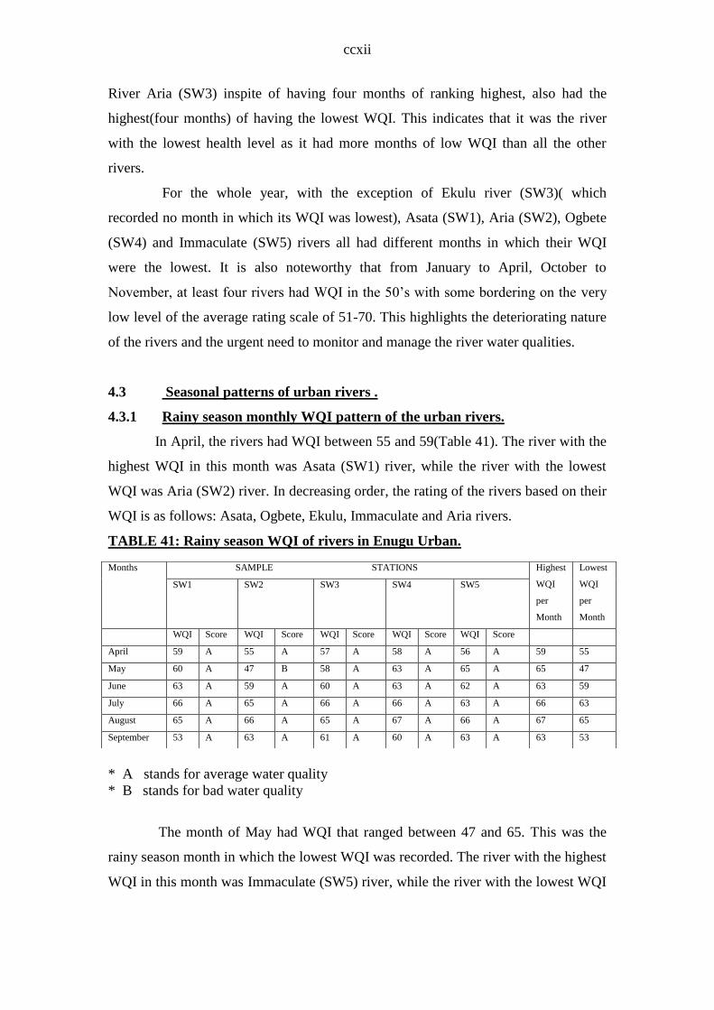
ccxii

River Aria (SW3) inspite of having four months of ranking highest, also had the

highest(four months) of having the lowest WQI. This indicates that it was the river

with the lowest health level as it had more months of low WQI than all the other

rivers.

For the whole year, with the exception of Ekulu river (SW3)( which

recorded no month in which its WQI was lowest), Asata (SW1), Aria (SW2), Ogbete

(SW4) and Immaculate (SW5) rivers all had different months in which their WQI

were the lowest. It is also noteworthy that from January to April, October to

November, at least four rivers had WQI in the 50’s with some bordering on the very

low level of the average rating scale of 51-70. This highlights the deteriorating nature

of the rivers and the urgent need to monitor and manage the river water qualities.

4.3 Seasonal patterns of urban rivers .

4.3.1 Rainy season monthly WQI pattern of the urban rivers.

In April, the rivers had WQI between 55 and 59(Table 41). The river with the

highest WQI in this month was Asata (SW1) river, while the river with the lowest

WQI was Aria (SW2) river. In decreasing order, the rating of the rivers based on their

WQI is as follows: Asata, Ogbete, Ekulu, Immaculate and Aria rivers.

TABLE 41: Rainy season WQI of rivers in Enugu Urban.

* A stands for average water quality

* B stands for bad water quality

The month of May had WQI that ranged between 47 and 65. This was the

rainy season month in which the lowest WQI was recorded. The river with the highest

WQI in this month was Immaculate (SW5) river, while the river with the lowest WQI

Months SAMPLE STATIONS Highest

WQI

per

Month

Lowest

WQI

per

Month

SW1 SW2 SW3 SW4 SW5

WQI Score WQI Score WQI Score WQI Score WQI Score

April 59 A 55 A 57 A 58 A 56 A 59 55

May 60 A 47 B 58 A 63 A 65 A 65 47

June 63 A 59 A 60 A 63 A 62 A 63 59

July 66 A 65 A 66 A 66 A 63 A 66 63

August 65 A 66 A 65 A 67 A 66 A 67 65

September 53 A 63 A 61 A 60 A 63 A 63 53

ccxiii

was Aria (SW2) river. In decreasing order, the rating of the rivers based on their WQI

is as follows: Immaculate, Ogbete, Asata, Ekulu and Aria rivers.

In June, the rivers had WQI between 59 and 63(Table 41). The rivers with the

highest WQI in this month were Asata (SW1) and Ogbete (SW4) rivers, while the

river with the lowest WQI was Aria (SW2) river. In decreasing order, the rating of the

rivers based on their WQI is as follows: Asata, Ogbete, Immaculate, Ekulu and Aria

rivers.

The month of July had WQI that ranged between 63 and 66. Three rivers

(Asata (SW1), Ekulu (SW3), Ogbete (SW4), had the highest WQI in this month. The

river with the lowest WQI was Immaculate (SW5) river. In decreasing order, the

rating of the rivers based on their WQI is as follows: Asata, Ekulu, Ogbete, Aria and

Immaculate.

In August, the rivers had WQI between 65 and 67(Table 41); all WQI were

high in comparism with other WQI obtained. The river with the highest WQI in this

month was Ogbete (SW4) river, while two river (Asata (SW1), and Ekulu (SW3) had

the lowest WQI. In decreasing order, the rating of the rivers based on their WQI is as

follows: Ogbete, Aria, Immaculate, Ekulu, and Asata rivers.

The month of September had WQI that ranged between 53 and 63. Two rivers

(Aria (SW2) and Immaculate (SW5), had the highest WQI in this month. The river

with the lowest WQI was Asata (SW1) river. In decreasing order, the rating of the

rivers based on their WQI is as follows: Aria, Immaculate, Ekulu, Ogbete and Asata.

From the ranking of the WQI for the rainy season(Appendix A1) ,it is

observable that two of the rivers, Asata (SW1) and Ogbete (SW4),had three months

in which they had the highest WQI, while Aria (SW3) had the highest number of

months of low WQI. Ekulu (SW3) and Ogbete (SW4) did not have any months in

which they had the lowest WQI. This indicates that Aria (SW2) river was the river

with the lowest health level in the rainy season as it had more months of low WQI

than all the other rivers. Asata (SW1) was the second and Immaculate (SW5) river

was the third in terms of low WQI

Ekulu (SW3) and Ogbete (SW4) rivers had no months in which their WQI

was the lowest for all the rivers and thus they were the rivers with the better health

levels in the rainy season.

ccxiv

4.4.2 Dry season monthly WQI pattern of the urban rivers.

In October, the rivers had WQI between 50 and 61 (Table 42). This was the

dry season month in which the lowest WQI were recorded. The river with the highest

WQI in this month was Aria (SW2) river, while the rivers with the lowest WQI were

Asata (SW1) and Ogbete rivers. In decreasing order, the rating of the rivers based on

their WQI is as follows: Aria, Ekulu, Immaculate, Asata and Ogbete.

The month of November had WQI that ranged between 55 and 61. The river

with the highest WQI in this month was Immaculate (SW5) river, while the river with

the lowest WQI was Asata river (SW1) . In decreasing order, the rating of the rivers

based on their WQI is as follows: Immaculate, Ekulu, Aria and Ogbete (had the same

WQI), Asata rivers.

TABLE 42: Dry season WQI of rivers in Enugu urban.

In December, the rivers had WQI between 58 and 61(table 42). The river with the

highest WQI in this month was Aria (SW2), while the rivers with the lowest WQI were

Asata (SW1) and Ogbete (SW4) rivers. In decreasing order, the rating of the rivers based

on their WQI is as follows: Aria, Immaculate, Ekulu, Asata and Ogbete (had the same

WQI) rivers.

The month of January had WQI that ranged between 52 and 60. The river with the

highest WQI in this month was Ekulu (SW3), while the river with the lowest WQI was

Aria (SW2) river. In decreasing order, the rating of the rivers based on their WQI is as

follows: Ekulu, Immaculate Ogbete, Asata and Aria.

In February, the rivers had WQI between 53 and 60 (Table 42). The river with the

highest WQI in this month was Ekulu (SW3) river, while two river (Ogbete (SW4), and

Months SAMPLE STATIONS Highest

WQI

per

Month

Lowest

WQI

per

Month

SW1 SW2 SW3 SW4 SW5

WQI Score WQI Score WQI Score WQI Score WQI Score

October 50 B 61 A 58 A 50 B 56 A 61 50

November 55 A 56 A 58 A 56 A 61 A 61 55

December 58 A 61 A 59 A 58 A 60 A 61 58

January 54 A 52 A 60 A 56 A 58 A 60 52

February 58 A 58 A 60 A 53 A 53 A 60 53

March 59 A 59 A 59 A 57 A 58 A 59 57

ccxv

Immaculate (SW5) had the lowest WQI. In decreasing order, the rating of the rivers based

on their WQI is as follows: Ekulu, Asata and Aria (had same WQI), Ogbete and

Immaculate (had same WQI) rivers.

The month of March had WQI that ranged between 57 and 59. Three rivers, Asata

(SW1), Aria (SW2) and Ekulu (SW3), had the highest WQI in this month. The river with

the lowest WQI was Ogbete river (SW4). In decreasing order, the rating of the rivers based

on their WQI is as follows: Asata, Aria and Ekulu (all had the same WQI), Immaculate,

and Ogbete.

From the ranking of the WQI for the dry season (Appendix A2), it is observable

that two of the rivers-Aria (SW2) and Ekulu (SW3), had three months in which they had

the highest WQI, while three rivers namely Asata (SW1) Aria (SW2) Ogbete (SW4) had

one month of low WQI each (this was also the highest number of low WQI pre well

recorded during this season). Ekulu (SW3) and Immaculate (SW5) did not have any

months in which they had the lowest WQI.

Ekulu river (SW3) was the river with the highest health level in the dry season as

it had more months of high WQI than all the other rivers. Aria (SW2) and Immaculate

(SW5) were the second, while Asata (SW1) and Ogbete (SW5) rivers were the least

healthy.

4.5 WQI Seasonal pattern for each urban river.

4.5.1 Rainy and Dry season WQI seasonal patterns per river.

The rainy season WQI for Asata (SW1) river ranged between 53 and 66

(Table 41). The highest WQI was recorded in July (66). This was the period of mid-

rainy season and the lowest WQI was recorded in the month of April, this was the

beginning of the rainy season.

The dry season WQI for Asata (SW1) river ranged between 50 and 59

(Table 42). The highest WQI was recorded in the month of March (59) this was the

period of the end of dry season and the lowest WQI was recorded in the month of

October, this was the beginning of the dry season.

WQI for Aria (SW2) river in the rainy season ranged between 47 and 66 (Table

41).The highest WQI was recorded in the month of August (66) this was the period of

the ending of the rainy season and the lowest WQI was recorded in the month of May

(47), the beginning of the rainy season.

ccxvi

The dry season WQI for Aria (SW2) river ranged between 52 and 61(Table

42). The highest WQI was recorded in two (October and December) of the dry season

months these were the beginning of dry season. The lowest WQI was recorded in

January, the mid dry season.

River Ekulu (SW3) in the rainy season had WQI that ranged from 57 to

66(Table 41). The highest WQI was recorded in July (66) this was the period of mid

rainy season and the lowest WQI was recorded in April (57), the beginning of the

rainy season.

The dry season WQI for Ekulu (SW3) river ranged from 58 to 60(Table

42). The highest WQI was recorded in two (January and February) of the dry season

months; these were the ending of dry season. The lowest WQI was recorded in two

months (October and November), the beginning of the dry season.

The rainy season WQI for Ogbete (SW4) river ranged between 58 and 67

(Table 41). The highest WQI was recorded in August (67) and the lowest WQI was

recorded in the month of April (58), this was the beginning of the rainy season.

The dry season WQI for Ogbete (SW1) river ranged between 50 and

58(Table 42). The highest WQI was recorded in the month of December (58) this was

the period of the mid dry season. The lowest WQI was recorded in the month of

October; this was the beginning of the dry season.

River Immaculate (SW5) in the rainy season had WQI that ranged from 56

to 66(Table 41). The highest WQI was recorded in August (66) this was the period of

end of rainy season and the lowest WQI was recorded in the month of April (56), the

beginning of the rainy season.

The dry season WQI for Immaculate (SW5) river ranged from 53 to 61(Table

42). The highest WQI was recorded in the month of November (61) this was the

period of the beginning of the dry season. The lowest WQI was recorded in the month

of February; coinciding with the end of the dry season.

4.6 Water Quality Index (WQI) of the Urban Wells .

ccxvii

The monthly WQI for wells within Enugu urban was calculated and the

worksheet is presented as Appendix N to Y. The results obtained were compared to

the WQI categorization scale to determine the water quality rating for the wells and

this is presented as Table 43

TABLE 43: Monthly Water Quality Index(WQI) of wells in Enugu urban

Months HDW1 HDW2 HDW3 HDW4 HDW5

January WQI 41 52 53 35 54

Scale Bad Average Average Bad Average

February WQI 61 56 46 53 59

Scale Average Average Bad Average Average

March WQI 51 55 57 49 55

Scale Average Average Average Bad Average

April WQI 51 58 54 58 55

Scale Average Average Average Average Average

May WQI 55 61 57 61 59

Scale Average Average Average Average Average

June WQI 57 60 58 57 52

Scale Average Average Average Average Average

July WQI 59 56 57 59 60

Scale Average Average Average Average Average

August WQI 58 63 61 60 65

Scale Average Average Average Average Average

September WQI 55 57 55 57 56

Scale Average Average Average Average Average

October WQI 55 62 54 51 53

Scale Average Average Average Average Average

November WQI 52 60 59 60 54

Scale Average Average Average Average Average

December WQI 56 59 62 54 63

Scale Average Average Average Average Average

The WQI for Abakpa (HDW1) wells from January to December 2006 are

presented in Table 43. The WQI obtained range from 41 to 61. From Table 43 it is

observable that Abakpa(HDW1) had a low WQI of 41 in January an improved WQI

in February, and from March to December fluctuations were observed in the well’s

WQI. It is observable that the well had 11 months of average WQI, while only one

month (January) had a WQI that was bad.

The wells in Uwani (HDW2) from January to December had WQI that range

from 52 to 63. From Table 43, it is observable that the wells (HDW2) had a WQI of

ccxviii

52 in January and from February to May the WQI increased to 61. A decrease in WQI

was however noted from the month of June to September after which an increase

occurred till December. The well had 12 months of average WQI.

The wells in Achara layout (HDW3) from January to December had WQI

that range from 46 to 62. From Table 43, it is observable that they (HDW3) had a

WQI of 53 in January and a low WQI of 46 in February. From March to July, the

WQI values fluctuated and a decrease occurred from September to November before

an increase occurred again in the month of December. The wells had 11 months of

average WQI, while only one month (February) had a WQI that was bad.

The wells in Ogui (HDW4) from January to December had WQI that range

from 35 to 61. It is also observable that the wells (HDW4) had a low WQI of 35 in

January and then an increase in February (53). The WQI for March was a low WQI of

49, after which the WQI fluctuated between 54 and 61 till the month December. The

well had 10 months of average WQI and 2 months of bad WQI.

The wells in Asata (HDW5) from January to December had WQI that range

from 52 to 65. From Table 43, it is observable that the well (HDW5) had a WQI of 54

in January and then an increase in February. In the months of March/ April, the WQI

decreased and an increase occurred in May. The WQI fluctuated within the range of

52 to 63 from June to December. The river had 12 months of average WQI.

4.7 Comparative analyses of the monthly WQI of the wells.

4.7.1 Monthly rating of the wells based on their WQI.

The WQI for the wells in January was from 35 to 54. The wells in Asata

(HDW5) had the highest rating, while the wells with the lowest rating were the wells

in Ogui (HDW4). The ranking of the wells based on their WQI (Appendix A3) thus

shows that wells in Asata had the highest WQI, Achara layout wells ranked second,

Uwani wells ranked third, Abakpa wells ranked fourth while Ogui wells had the

lowest WQI. Asata wells were thus healthier than the other wells in January. Ogui

wells had the lowest health level in this month.

In February, the WQI of the wells ranged between 53 and 61. The wells with the

highest rating were the wells in Abakpa (HDW1), while the wells with the lowest

rating were Achara layout (HDW3) wells. The ranking of the wells based on their

WQI (Appendix A3), shows that Abakpa (HDW1) wells had the highest WQI, Asata

(HDW5) wells ranked second, Uwani (HDW2) wells ranked third, Ogui (HDW4)

ccxix

wells ranked fourth while Achara layout wells(HDW3) had the lowest WQI. The

wells in Abakpa were thus healthier than the other wells in February. Achara layout

wells had the lowest health level in this month.

The WQI for the wells in March ranged between 49 and 57. The wells with

the highest rating were the wells in Achara layout (HDW3), while the wells with the

lowest rating were Ogui (HDW4) wells. The ranking of the wells based on their WQI

(Appendix A3) shows that Achara layout (HDW3) wells, had the highest WQI, Uwani

(HDW2) and Asata (HDW5) wells ranked second, Abakpa (HDW1) wells ranked

fourth and Ogui (HDW4) wells had the lowest WQI. Achara layout (HDW3) wells

were thus healthier than the other wells in the month of March. On the other hand,

Ogui (HDW4) wells had the lowest health level.

In April, the WQI for the wells ranged between 51 and 58. The wells with

the highest rating were the wells in Uwani (HDW2) and Ogui (HDW4), while the

wells with the lowest rating were Abakpa (HDW1) wells. The ranking of the rivers

based on their WQI (Appendix A3) shows that Uwani (HDW2) and Ogui (HDW4)

had the highest WQI, Asata (HDW5) wells ranked third, Achara layout wells ranked

fourth, while Abakpa wells had the lowest WQI. Uwani (HDW2) and Ogui (HDW4)

wells were thus healthier than the other wells in April. Abakpa (HDW1) wells had the

lowest health level in this month.

The WQI of the wells ranged between 55 and 61 in May. The wells with

the highest rating were also the wells in Uwani (HDW2) and Ogui (HDW4), while the

wells with the lowest rating were also Abakpa (HDW1) wells. The ranking of the

rivers based on their WQI (Appendix A3) shows that Uwani (HDW2) and Ogui

(HDW4) had the highest WQI, Asata (HDW5) wells ranked third, Achara layout

(HDW3) wells ranked fourth, while Abakpa wells had the lowest WQI. Just as was

experienced in April, Uwani (HDW2) and Ogui (HDW4) wells were thus healthier

than the other wells in May. Abakpa (HDW1) wells had the lowest health level in this

month.

The WQI for the wells in June was from 52 to 60. The wells with the

highest rating were also the wells in Uwani (HDW2), while the wells with the lowest

rating were Asata (HDW5) wells. The ranking of the wells based on their WQI

(Appendix A3) thus shows that the wells in Uwani (HDW2) had the highest WQI,

Achara layout (HDW3) wells ranked second, Abakpa (HDW1) and Ogui (HDW4)

wells ranked third, while Asata (HDW5) wells had the lowest WQI. Uwani (HDW2)

ccxx

wells were also healthier than the other wells in June just as they were in April and

May. Asata (HDW1) wells had the lowest health level in this month.

The WQI for the wells in July ranged from 56 to 60. The wells with the

highest rating were the wells in Asata (HDW5), while the wells with the lowest rating

were Uwani (HDW2) wells. The ranking of the rivers based on their WQI (Appendix

A3) thus shows that the wells in Asata (HDW5) had the highest WQI, , Abakpa

(HDW1) and Ogui (HDW4) wells ranked second, Achara layout (HDW3) wells

ranked fourth, Uwani (HDW2) wells had the lowest WQI. Asata (HDW5) wells were

healthier than the other wells in July. Uwani (HDW2) wells had the lowest health

level in this month.

For the month of August, the WQI ranged between 58 and 65. The wells

with the highest rating were the wells in Asata (HDW5), while the wells with the

lowest ratings were Abakpa (HDW1). The ranking of the rivers based on their WQI

(Appendix A3) thus shows that Asata (HDW5), Uwani (HDW2) wells ranked second,

Achara layout (HDW3) wells ranked third, Ogui (HDW4) wells ranked fourth,

Abakpa (HDW1) wells had the lowest WQI. Asata (HDW5) wells were thus healthier

than the other wells while Abakpa (HDW1) wells had the lowest health level in

August.

The WQI for the wells in September was from 55 to 57. The wells in

Uwani (HDW2) and Ogui (HDW4) with the same WQI of 57 had the highest rating,

while the wells with the lowest rating were the wells in Abakpa (HDW1) and Achara

layout (HDW3). The ranking of the rivers based on their WQI (Appendix A3) thus

shows that Uwani (HDW2) and Ogui (HDW4) wells had the highest WQI, Asata

(HDW5) wells ranked third, Ogbete (HDW4) ranked fourth, while Abakpa (HDW1)

and Achara layout (HDW3) wells had the lowest WQI.Uwani (HDW2) and Ogui

(HDW4) wells were thus healthier than the other three wells; while Abakpa (HDW1)

and Achara layout (HDW3) wells had the lowest health level in September.

In October, the WQI ranged between 51 and 62. The wells with the highest

rating were Uwani (HDW2) wells, while the wells with the lowest rating were Ogbete

(HDW4). The ranking of the rivers based on their WQI (Appendix A3) thus shows

that Uwani (HDW2) wells had the highest WQI, Abakpa (HDW1) wells ranked

second, Achara layout (HDW3) wells ranked third, Asata (HDW5) ranked fourth, and

were Ogbete (HDW4) had the lowest WQI. Uwani (HDW2) wells were thus healthier

ccxxi

than the other wells in October, while Ogbete (HDW4) wells had the lowest health

level in.

The WQI ranged between 52 and 60 in November. The wells with the

highest rating were Uwani (HDW2) and Ogbete (HDW4) wells, while the wells with

the lowest rating were Abakpa (HDW1) wells. The ranking of the wells based on their

WQI (Appendix A3) thus shows that Uwani (HDW2) and Ogbete (HDW4) wells had

the highest WQI, Achara layout (HDW3) wells ranked third, Asata (HDW5) ranked

fourth, while Abakpa (HDW1) wells had the lowest WQI. Uwani (HDW2) wells were

thus healthier than the other wells, while Abakpa (HDW1) wells had the lowest health

level in November.

In December, the WQI ranged between 54 and 63. The wells with the

highest rating were Asata (HDW5) wells, while the wells with the lowest rating were

Ogbete (HDW4) wells. The ranking of the wells based on their WQI (Appendix A3)

thus shows that Asata (HDW5) had the highest WQI, Achara layout (HDW3) wells

ranked second, Uwani (HDW2) ranked third, Abakpa (HDW1) ranked fourth, while

Ogbete (HDW4) wells had the lowest WQI. Asata (HDW5) wells were thus healthier

than the other wells in December, while Ogbete (HDW4) had the lowest health level.

From the ranking of the WQI (Appendix A3), it is observable that the wells

in Uwani (HDW2) had six months in which they had the highest WQI. The wells in

Asata (HDW5) had four months of having the highest WQI. The other wells Abakpa

(HDW1), Achara layout (HDW3) and Ogui (HDW4) had only one month each of

having the highest WQI. This indicates that the wells in Uwani had the highest health

level as they had more months of high WQI. The wells in Ogui had the lowest health

level as they had more months of low WQI.

4.8 Seasonal patterns of the urban wells

4.8.1 Rainy season monthly WQI patterns of the urban wells.

In April, the wells had WQI between 51 and 58(Table 44). The wells

with the highest WQI in this month were Uwani (HDW2) wells, while the wells with

the lowest WQI were Abakpa (HDW1) wells. In decreasing order, the rating of the

wells based on their WQI is as follows: Uwani and Ogui wells, Asata, Achara layout

and Abakpa.

TABLE 44: Rainy season WQI of wells in Enugu Urban

Months SAMPLE STATIONS Highest

WQI

per

Month

Lowest

WQI

per

Month

ccxxii

For the month of May the wells had WQI that ranged between 55 and 61.

The wells with the highest WQI in this month were Uwani (HDW2) wells and Ogui

(HDW4), while the wells with the lowest WQI were Abakpa (HDW1) wells. In

decreasing order, the rating of the wells based on their WQI is as follows: Uwani and

Ogui, Asata, Achara layout and Abakpa wells.

In June, the wells had WQI between 52 and 60(table 44). The wells with the

highest WQI in this month were Uwani (HDW2) wells, while the wells with the

lowest WQI were Asata (HDW5). In decreasing order, the rating of the wells based on

their WQI is as follows: Uwani, Achara layout, Abakpa, Ogui, and Asata.

The month of July had WQI that ranged between 57 and 60. Asata (HDW5)

had the highest WQI in this month. The wells with the lowest WQI were Uwani

(HDW2) wells. In decreasing order, the rating of the rivers based on their WQI is as

follows: Asata, Ogui, Abakpa, Achara layout, Uwani.

In August, the rivers had WQI between 58 and 65(Table 44). The wells with

the highest WQI in this month were Asata (HDW4) wells, while Abakpa wells had

the lowest WQI. In decreasing order, the rating of the wells based on their WQI is as

follows: Asata, Uwani, Achara layout, Ogui, Abakpa.

The month of September had WQI that ranged between 55 and 57. Wells

in Uwani (HDW2) and Ogui (HDW4) had the highest WQI in this month. The wells

with the lowest WQI were Abakpa (HDW1) wells. In decreasing order, the rating of

the rivers based on their WQI is as follows: Uwani and Ogui, Asata, Abakpa, Achara

layout.

From the ranking of the WQI for the rainy season (Appendix A4), it is

observable that wells in Uwani (HD2) had four months in which they had the highest

WQI, while Abakpa (HDW1) wells had the highest number of months of low WQI.

The wells in Achara layout (HDW3) and Ogui (HDW4) did not have any months in

HDW1 HDW2 HDW3 HDW4 HDW5

WQI Score WQI Score WQI Score WQI Score WQI Score

April 51 A 58 A 54 A 58 A 55 A 58 51

May 55 A 61 A 57 A 61 A 59 A 61 55

June 57 A 60 A 58 A 57 A 52 A 60 52

July 59 A 56 A 57 A 59 A 60 A 60 57

August 58 A 63 A 61 A 60 A 65 A 65 58

September 55 A 57 A 55 A 57 A 56 A 57 55

ccxxiii

which they had the lowest WQI. This indicates that Abakpa wells were the wells with

the lowest health level in the rainy season as it had more months of low WQI than all

the other wells.

4.8.2 Dry season monthly WQI patterns of the urban wells.

In October, the wells had WQI between 51 and 62 (Table 45). The wells with

the highest WQI in this month were Uwani (HDW2) wells, while the wells with the lowest

WQI were Ogui (HDW4). In decreasing order, the rating of the rivers based on their WQI

is as follows: Uwani, Abakpa, Achara layout, Asata and Ogui.

The month of November had WQI that ranged between 52 and 60. The wells

with the highest WQI in this month were Uwani (HDW2) and Ogui (HDW4) wells,

while the wells with the lowest WQI were Asata (HDW5) wells. In decreasing order,

the rating of the wells based on their WQI is as follows: Uwani and Ogui (had the

same values), Achara layout, Asata, Abakpa.

TABLE 45: Dry season WQI of wells in Enugu Urban

Months SAMPLE STATIONS Highest

WQI

per

Month

Lowest

WQI

per

Month

HDW1 HDW2 HDW3 HDW4 HDW5

WQI Score WQI Score WQI Score WQI Score WQI Score

October 55 A 62 A 54 A 51 F 53 A 62 51

November 52 A 60 A 59 A 60 A 58 A 60 52

December 56 A 59 A 62 A 54 A 63 A 63 54

January 41 B 52 A 53 A 35 B 54 A 54 35

February 61 A 56 A 46 B 53 A 59 A

61 46

March 51 A 55 A 57 A 49 A 55 A 57 49

ccxxiv

In December, the wells had WQI between 54 and 63(Table 45). The wells

with the highest WQI in this month were Asata (HDW5) wells, while the wells with the

lowest WQI were Ogui (HDW4) wells. In decreasing order, the rating of the rivers based

on their WQI is as follows: Asata, Achara layout, Uwani, Abakpa, and Ogui.

The month of January had WQI that ranged between 35 and 54. This was

also the month in which the lowest WQI was recorded. The wells with the highest

WQI in this month were Asata (HDW5) wells, while the wells with the lowest WQI

were Ogui (HDW4) wells. This pattern was also obtainable in the month of

December. In decreasing order, the rating of the wells based on their WQI is as

follows: Asata, Achara layout, Uwani, Abakpa, and Ogui.

In February, the wells had WQI between 46 and 61 (Table 45). The wells

with the highest WQI in this month were Abakpa (HDW1) wells, while Achara layout

(HDW3) wells, had the lowest WQI. In decreasing order, the rating of the wells based

on their WQI is as follows: Abakpa, Asata, Uwani, Ogui, Achara layout.

The month of March had WQI for the wells that ranged between 49 and 57.

The wells with the highest WQI in this month were Achara layout (HDW3) wells,

while Ogui (HDW4) had the lowest WQI in this month. In decreasing order, the rating

of the rivers based on their WQI is as follows: Achara layout, Uwani and Asata (had

the same WQI), Abakpa and Ogui.

From the ranking of the WQI of wells for the dry season (Appendix A5), it is

observable that the wells in Uwani (HDW2) and Asata (HDW5) had two months in

which they had the highest WQI, while the wells in Achara layout (HDW3) and Ogui

(HDW4) had only one month of having the highest WQI. On the other hand, Ogui

(HDW4) had four months of low WQI; Abakpa (HDW1) and Achara layout (HDW3)

had only one month of having the lowest WQI. Uwani (HDW2) and Asata (HDW5)

wells did not have any month in which they had the lowest WQI.

Based on the fact that for the dry season, Uwani (HDW2) and Asata

(HDW5) wells had the highest number of months (two) in which they had the highest

health level in the dry season as they had more months of high WQI than all the other

wells. Ogui (HDW4) wells which had more months (four) of low WQI than the other

wells were the least healthy in terms of low WQI in the dry season.

4.9 Seasonal pattern of WQI of the urban wells.

4.9.1 Rainy and dry season WQI patterns.

ccxxv

The rainy season WQI for the wells in Abakpa (HDWI) ranged between

51 and 59(Table 44). The highest WQI was recorded in the month of July (59) this

was the period of mid rainy season and the lowest WQI was recorded in the month of

April (51), this was the beginning of the rainy season.

The dry season WQI for the wells in Abakpa (HDW1) ranged between 41 and

61(Table 45). The highest WQI was recorded in the month of February (61) this was

the period of the end of dry season and the lowest WQI was recorded in the month of

January (41), this was the beginning of the dry season.

WQI for Uwani (HDW2) wells in the rainy season ranged between 57 and 63

(Table 44). The highest WQI was recorded in the month of August (63) this was the

period of the ending of the rainy season and the lowest WQI was recorded in the

month of September (57), also the end of the rainy season.

The dry season WQI for Uwani (HDW2) wells ranged between 52 and 62(Table 45).

The highest WQI was recorded in October (62), this was the beginning of dry season. The

lowest WQI was recorded in January (52), the mid dry season.

Achara layout (HDW3) wells in the rainy season had WQI that ranged from 57 to

61(Table 44). The highest WQI was recorded in September (61) this was the period of the

end of the rainy season and the lowest WQI was recorded in the month of April (54), the

beginning of the rainy season.

The dry season WQI for Achara layout (HDW3) wells ranged from 46 to 59(Table

45). The highest WQI was recorded in November the beginning of dry season. The lowest

WQI was recorded in February, the end of the dry season.

The rainy season WQI for Ogui (HDW4) wells ranged between 57 and 61 (Table

44). The highest WQI was recorded in May (61) this was beginning of rainy season and the

lowest WQI was recorded in June and September (57), these occurred mid and end of the

rainy season.

The dry season WQI for Ogui (HDW4) wells ranged between 35 and 60(Table

45). The highest WQI was recorded in November (60) this was at the beginning of the dry

season. The lowest WQI was recorded in October; this also was the beginning of the dry

season.

Asata (HDW5) wells in the rainy season had WQI that ranged from 52 to

65(Table 44). The highest WQI was recorded in August (65) this was the period of end of

rainy season and the lowest WQI was recorded in June (52), the mid rainy season.

ccxxvi

The dry season WQI for Asata (HDW5) wells ranged from 53 to 63(Table 45). The

highest WQI was recorded in the month of December (63) this was mid dry season. The

lowest WQI was recorded in October; this was the beginning of the dry season.

4.10 Comparative analysis of the monthly Water Quality Indices(WQI) of

rivers and wells in Enugu urban area.

A comparism of the WQI of the rivers and wells in Enugu urban presented

in Appendix A6 shows that in the month of January, the WQI range for both were

between 35 and 58. The highest WQI for this month was recorded by a river, while

the lowest was recorded by a well. The rivers had WQI that ranged between 54 and 58

only, while the wells had a WQI range of 35 to54.

The WQI of four rivers(Asata(SW1), Ekulu(SW3), Ogbete(sw4) and

Immaculate(SW5) exceeded the WQI for all the wells, while only one

river(Aria(SW2)) had a WQI that was either the same with the wells(Uwani(HDW2))

but the other wells had WQI that exceeded that of Aria(SW2) river. Generally, the

WQI for the rivers exceeded the WQI of the wells in January thus indicating that the

rivers had a better quality than the wells.

In February, the WQI ranges for both were between 46 and 61. In this

month, wells in Achara layout had WQI that were below average (medium).

However, the highest WQI for this month was recorded by a well, while the lowest

was recorded also by a well. The entire river WQI exceeded the WQI of the wells.

This reveals that for February, the water quality of the rivers were better than those of

the wells.

The rivers and wells in March had WQI that range between 49 and 59. The

highest WQI for this month was recorded by a river, while the lowest was recorded by

a well. The rivers had WQI that ranged between 57 and 59 only, while the wells had a

WQI range of 49 to 57. In this month, wells in Ogui had WQI that was below average.

The entire river WQI exceeded the WQI of the wells. This shows that for March, the

water quality of the rivers were better than those of the wells.

In April, the WQI ranges for both were between 51 and 59. The highest

WQI for this month was recorded by a river, while the lowest was recorded also by a

well. The rivers all had WQI that exceeded the WQI of the wells. This reveals that

the rivers were healthier in April than wells.

ccxxvii

The rivers and wells in May had WQI that range between 47 and 65. The

highest WQI for this month was recorded by a river, while the lowest was recorded

also by a well. The rivers had WQI that ranged between 47and 65, while the wells had

a WQI range of 55 to 61. In this month, Aria (SW2) river had a WQI that was below

average (medium). The other river WQI exceeded the WQI of the wells. This shows

that for May, the water quality of the rivers were better than those of the wells with

the exception of Aria river.

In June, the WQI range for both were between 52 and 63. The highest WQI

for this month was recorded by rivers, while the lowest was recorded also by a well.

The rivers all had WQI that exceeded the WQI of the wells.This reveals that the

month of June had healthier rivers than wells.

The rivers and wells in July had WQI that range between 57 and 66. The

highest WQI for this month were recorded by rivers, while the lowest was recorded

by a well. The rivers had WQI that ranged between 63 and 66, while the wells had a

WQI range of 56 to 60. The rivers all had WQI that exceeded the WQI of the wells.

This shows that for July, the water quality of the rivers were better than those of the

wells.

In August, the WQI range for both was between 58 and 67. The highest

WQI for this month was recorded by rivers, while the lowest was recorded also by a

well. The rivers all had WQI that exceeded the WQI of the wells. This reveals that the

month of August had healthier rivers than wells.

The rivers and wells in September had WQI that range between 53 and 63.

The highest WQI for this month was recorded by a river, and the lowest was also

recorded by a river. The rivers had WQI that ranged between 53 and 63, while the

wells had a WQI range of 55 to 57. In this month, Asata (SW1) river had a WQI that

was below those of the wells. However, the other rivers had WQI that exceeded the

WQI of the wells. This shows that for the month of September, the water quality of

the rivers were better than those of the wells with the exception of Asata river.

In October, the WQI range for both was between 50 and 62. The highest

WQI for this month was recorded by a well, and the lowest was also recorded by

rivers. The rivers had WQI that ranged between 50 and 61, while the wells had a WQI

range of 51 to 62. In this month, two rivers (Asata (SW1) and Ogbete (SW4)) had

WQI that was below those of the wells. However, the other rivers had WQI that

exceeded the WQI of the wells. This shows that for the month of October, the water

ccxxviii

quality of the rivers were better than those of the wells with the exception of Asata

and Ogbete rivers.

The rivers and wells in November had WQI that range between 52 and 61.

The highest WQI for this month was recorded by a river, and the lowest was recorded

by a well. The rivers had WQI that ranged between 55 and 61, while the wells had a

WQI range of 52 to 60. In this month, the rivers on average had WQI that exceeded

the WQI of the wells. This shows that for the month of November, the water quality

of the rivers were better than those of the wells.

In December, the WQI range for both was between 54 and 63. The highest

WQI for this month was recorded by a well, and the lowest was also recorded by a

well also. The rivers had WQI that ranged between 58 and 61, while the wells had a

WQI range of 54 to 63. In this month, the rivers on average had WQI that exceeded

the WQI of the wells. This shows that for the month of December, the water quality of

the rivers were better than those of the wells.

CHAPTER FIVE

PREVALENCE PATTERN AND THE SPATIAL DIMENSIONS OF WATER-

RELATED DISEASES IN ENUGU URBAN AREA.

5.1 Introduction

Water quality has a vital impact on people's health. A large percentage of the

infectious and parasitic diseases that plague the developing world are associated with

inadequate water quality and sanitation level.

In some countries like Nigeria, rivers and lakes have become receptacles for a vile

assortment of wastes (including untreated or partially treated municipal sewage, toxic

industrial effluents, and harmful chemicals). Based on this practice, the supply of freshwater

available is shrinking, as many freshwater resources become increasingly reduced in quality.

Caught between finite and increasingly polluted water supplies on one hand and

rapidly rising demand from population growth and development on the other, very major

human health problems have arisen. These problems are heightened by the failure to provide

even the most basic water services for the populace.

ccxxix

Gleick (1998) is of the opinion that this failure to provide safe drinking water and

adequate sanitation services to all people is perhaps the greatest development and health failure

of the 21st century; while the most serious consequence of this failure is widespread water-

related diseases and death. Water-related diseases are a human tragedy as about 2.3 billion

people in the world suffer from diseases that are linked to water (Kristof, 1997; Vanderslice et

al, 1996). It also prevents millions of people from leading healthy lives, and undermines

development efforts (Nash, 1993; Olshansky et al 1997).

This problem of water-related diseases is one of the most serious public health crisis

facing developing countries today as water-related diseases exact a terrible toll on human

health. One-quarter of all people attending hospitals are ill from water-related diseases and in

some urban centers, water-related diseases make up a high proportion of all illnesses among

adults and children. As the number of people living with HIV and AIDS increases the

problems become more obvious as people living with AIDS are more likely to be infected with

water-related diseases.

In this chapter the aim is to identify the water-related diseases prevalent in the urban

area and the seasonality pattern of the four major water-related diseases.

5.2 Monthly prevalence pattern of water-related diseases in the wards of

Enugu Urban area.

The World Health Organization (1996) defines water-related disease as any

significant or widespread adverse effects on human health, such as death, disability, illness

or disorders, caused directly or indirectly by the condition, or changes in the quality and

quantity of any waters. The causes of water-related disease include micro-organisms,

parasites, toxins and chemical contamination of water. According to Hunter (1997),

prevalence refers to the number of cases of a disease in a defined population at a particular

point in time. A survey was carried out to determine the pattern of monthly prevalence of

water-related diseases in the wards in Enugu urban area for the year 2006. The result

obtained is presented in table 46.

TABLE 46: Monthly total of water-related disease prevalence in Enugu urban

Month Number of patients

treated

Percentage

value

ccxxx

January 425 11

February 431 11

March 304 8

April 244 6

May 271 7

June 438 12

July 311 8

August 224 6

September 280 7

October 290 8

November 263 7

December 332 9

Grand Total 3813 100%

Source: Field work, 2006.

Table 46 indicates that in January, 425(11 %) people were treated for water-

related diseases. In this month as is depicted in Fig 129, the ward that had the highest

number of cases of water-related diseases was Coal Camp with a percentage value of

16.7 %, while the lowest number of patients was from three wards- New Haven,

Independence Layout and Ogui (6 % respectively).

Fig 129: January water-related diseases prevalence pattern in Enugu urban

6% 8%

16%

16%

12%

16%

7%

6%

6% 7%

Ogui Achara layout Asata Abakpa Iva valley Coal camp Uwani New haven Independence layout G.R.A

ccxxxi

In February (Fig. 130) a total of 433 patients were treated for water-related

diseases and this number constituted 11 % of the total number treated for the whole

year (table 46). Of the 433 patients in February, the ward with the highest number of

residents that were treated for water-related diseases was Abakpa and Asata (14%

respectively) (Fig 130), while the least number of patients was recorded in two wards

namely Independence layout and Government Reserved Area (G.R.A); each having a

percentage contribution of 5 %.

For the 304 patients (8 %) (Table 46) that were treated for water-related

diseases in the month of March, Fig 131 shows that Achara Layout with a percentage

value of 14 % had the highest number of patients while Independence Layout that had

12 patients (4 %) had the lowest.

Fig. 130: February water-related diseases prevalence pattern in Enugu urban

9%

13%

14%

14% 8%

13%

10%

9%

5% 5%

Ogui Achara layout Asata Abakpa Iva valley Coal camp Uwani New haven Independence layout G.R.A

n

ccxxxii

Fig. 131: March water-related diseases prevalence pattern in Enugu urban

In the month of April, 244 people (constituting 6 %) who attended the

hospitals were treated for water-related diseases (Table 46). Fig 132 shows that the

wards with the highest number of patients were Iva valley and Coal Camp each

contributing 13%.The ward with the lowest number of patients on the other hand was

Ogui contributing 6 % for the month.

13%

14%

7%

13% 10%

13%

11%

10%

4% 5%

Ogui Achara layout Asata Abakpa Iva valley Coal camp Uwani New haven Independence layout G.R.A

ccxxxiii

Fig. 132: April water-related diseases prevalence pattern in Enugu urban

From Table 46, it can be seen that during the month of May, 271 patients

attended the hospitals for water-related diseases. This number represents 7 % of the

total. While Figure 133 showing the percentage contribution of each ward in May

indicates that the wards that had the highest number of patients were Uwani and New

haven. Each of these wards contributed 13 %, while Achara Layout contributing 6 %

was the ward with the lowest number of patients for this month.

6%

10%

13%

13%

12% 12%

7%

12%

8%

7%

Ogui Achara layout Asata Abakpa Iva valley Coal camp Uwani New haven Independence layout G.R.A

ccxxxiv

Fig. 133: May water-related diseases prevalence pattern in Enugu urban

In June, 438 patients, representing 12 %, were treated for water-related

diseases. This was the month in which the hospitals recorded the highest number of

patients that were treated for water-related diseases. During this period as is shown in

Figure 134, the ward with the highest number of patients was Abakpa with a

percentage contribution of 15 %, while two wards- Independence Layout and the

Government Reserved Area (G.R.A) had the lowest number of patients contributing 5

% respectively.

A total of 311 patients representing 8 % were treated of a water-related disease

in July. From Fig 135, it is observable that within this month, there were two wards

(Coal Camp and Uwani) that recorded the highest incidents of water-related diseases.

Each of them had a percentage contribution of 15 %, while the lowest contributing

ward was Independence Layout (5 %).

9%

6%

9%

9%

12%

12%

13%

13%

10%

7%

Ogui Achara layout Asata Abakpa Iva valley Coal camp Uwani New haven Independence layout G.R.A

ccxxxv

Fig. 134: June water-related diseases prevalence pattern in Enugu urban

Fig. 135: July water-related diseases prevalence pattern in Enugu urban

For the month of August, 224 patients representing 6 %( Table 46) reported

ill with various types of water-related diseases. Within this month as is depicted in

Fig. 136, the ward with the highest number of patients that presented with water-

related diseases was Uwani representing 18 %, while the ward with the lowest number

was New Haven with a percentage contribution of 2 %.

9%

11%

7%

15%

13%

11%

12%

12%

5% 5%

Ogui Achara layout Asata Abakpa Iva valley Coal camp Uwani New haven Independence layout G.R.A

8%

8%

10%

12%

10% 15%

15%

9%

5% 8%

Ogui Achara layout Asata Abakpa Iva valley Coal camp Uwani New haven Independence layout G.R.A

ccxxxvi

Fig 136: August water-related diseases prevalence pattern in Enugu urban

In September, 280 patients representing 7 % (Table 46) were treated for

water-related diseases. From Fig 137, the wards that had the highest number of

patients suffering from water-related diseases were Achara Layout and Iva Valley

each with a percentage contribution of 15 %; while the G.R.A. had the lowest number

of cases ; contributing only 3% during this month.

For the month of October, 290 patients presented with water-related diseases

and this represents 8 % of the annual total (Table 46). Fig. 138 showing the hospital

visitation pattern for October indicates that the ward contributing the highest number

of patients was Coal camp, while the lowest contributing ward was Independence

Layout.

7%

10%

11%

13%

15%

13%

18%

2%

6% 5%

Ogui Achara layout Asata Abakpa Iva valley Coal camp Uwani New haven Independence layout G.R.A

ccxxxvii

Fig 137: September water-related diseases prevalence pattern in Enugu urban

Fig. 138: October water-related diseases prevalence pattern in Enugu

urban

14%

15%

5%

13% 15%

14%

13%

4% 4% 3%

Ogui Achara layout Asata Abakpa Iva valley Coal camp Uwani New haven Independence layout G.R.A

5%

10%

16%

13%

10%

21%

11%

5%

4% 5%

Ogui Achara layout Asata Abakpa Iva valley Coal camp Uwani New haven Independence layout G.R.A

ccxxxviii

Table 46 shows that 263 patients were treated for water-related diseases

November and this represents 7 %. During this month, the wards with the highest

number of hospital visitations were Ogui and Achara layout both with a percentage

value of 15.The ward with the lowest number of patients was the G.R.A. with a 5 %

contribution (Fig 139).

Fig. 139: November water-related diseases prevalence pattern in Enugu urban

In December, 332 patients representing 9 % presented with water-related

diseases. The ward with the highest number of patients was Abakpa (17 %), while the

G.R.A contributed the lowest (5 %) (Fig 140).

15%

15%

10%

13% 11%

8%

7%

10%

6% 5%

Ogui Achara layout Asata Abakpa Iva valley Coal camp Uwani New haven Independence layout G.R.A

ccxxxix

Fig. 140: December water-related diseases prevalence pattern in Enugu urban

A ranking of the prevalence dimensions for the year (Table 46) and (Fig 141)

indicates that the month of June ranked first, showing that this was the period the

highest number of patients were treated for water-related diseases. February ranked

second, January ranked third, December ranked fourth, July ranked fifth, March

ranked sixth, October ranked seventh, September ranked eighth, May ranked ninth,

November ranked tenth, April ranked eleventh, while August ranked twelfth(the

lowest number of patients were treated during this month).

12%

15%

8%

17% 12%

11%

7%

7%

6% 5%

Ogui Achara layout Asata Abakpa Iva valley Coal camp Uwani New haven Independence layout G.R.A

ccxl

Fig. 141: Monthly percentages of water-related diseases prevalence pattern in

Enugu urban

5.2 Seasonal Dimensions of Water-related Diseases in Enugu Urban.

Water-related diseases recognized in this study are categorized into four

distinct types. They are as follows:

5.2.1 Water-borne diseases: These diseases are "dirty-water" diseases—those

caused by water that has been contaminated by human, animal, or chemical wastes

(Alberin et al, 1996). They are illnesses caused by drinking water contaminated by

human or animal faeces which contain pathogenic micro organisms (i.e. they are

fecal-oral in nature) (Alam, 1989). Water-borne diseases thus spread through water

containing human or animal faeces and urine, either when you drink such water

directly or you eat food that has been cleaned with it (Basch, 1990). The fecal-oral

route of disease transmission is depicted in Fig 143.

11%

11%

8%

6%

7%

12%

8%

6%

7%

8%

7%

9%

Jan Feb Mar Apr May Jun Jul Aug Sep Oct Nov Dec

ccxli

Fig 142: Transmission routes of water-borne diseases

Source: Brandley, 1994

Contaminated water thus causes a range of diseases that can be life-threatening.

Lack of clean water for domestic activities and lack of proper sanitation facilities are to

be blamed for most of the water-borne diseases. The spread of these diseases is very

rapid.

The major water-borne diseases are - cholera and other diarrhea diseases;

dysentery, typhoid fever; polio; roundworm; whipworm; shigella; meningitis and

hepatitis A and E. Human beings and animals can act as hosts to the bacterial, viral, or

protozoa organisms that cause these diseases.

5.2.1.1 Seasonal dimensions of water-borne diseases in Ogui.

A total of 140 patients from Ogui were treated for water-borne diseases in

the rainy and dry season as is shown in table 47.

Faeces

Water Flies Hands

Food

Mouth

Faeces

Water Flies Hands

Food

Mouth

ccxlii

Table 47: Prevalence Pattern of water-borne diseases in Enugu Urban.

Months Wards of the urban area

Ogui Achara

layout

Asata Abakpa Iva valley Coal

camp

Uwani New

Haven

Independence

layout

G.R.A Total

(all

wards

)

January 12 17 28 16 11 30 9 8 2 4 137

February 17 20 30 37 14 22 15 6 3 2 166

March 22 20 8 32 30 32 18 8 3 0 173

April 10 5 12 9 18 14 6 7 3 12 96

May 12 7 15 10 21 7 12 11 1 8 104

June 25 20 10 12 20 22 15 4 5 7 140

July 10 20 17 9 10 15 12 10 5 3 111

August 5 6 4 11 13 10 5 0 0 0 54

September 3 10 9 5 23 12 18 7 5 3 95

October 9 20 20 20 22 23 17 6 3 7 140

November 3 17 15 15 8 0 7 12 7 0 91

December 12 27 8 12 14 9 12 3 0 3 100

Total for each

ward

140 189 176 188 204 196 146 82 37 49 1407

Source: Field work 2006

Of these 140 patients, the seasonal prevalence pattern shown as Tables 48

and 49 reveal that 65(46.4 %) were treated in the rainy season, while 75(53.6 %) were

treated in the dry season. In the rainy season, patients were highest in the month of

June and lowest in September.

Table 48: Rainy season prevalence of water-borne diseases in Ogui,

Months Water -borne Diseases

Diarrhea Cholera Typhoid Dysentery Hepatitis Total %

April 3 1 5 1 0 10 15.4

May 4 0 5 1 2 12 18.5

June 2 2 15 2 4 25 38.5

July 1 0 7 1 1 10 15.4

August 2 0 3 0 0 5 7.6

September 0 0 3 0 0 3 4.6

Total 12 3 38 5 7 65

Disease % 18.4 4.6 58.5 7.7 10.8 100%

Source: Field work, 2006.

ccxliii

Table 49: Dry season prevalence of water-borne diseases in Ogui

Months Water -borne Diseases

Diarrhea Cholera Typhoid Dysentery Hepatitis Total %

October 5 1 3 0 0 9 12

November 0 0 3 0 0 3 4

December 2 0 6 0 4 12 16

January 2 0 8 2 0 12 16

February 3 0 11 0 3 17 22.7

March 10 2 6 2 2 22 29.3

Total 22 3 37 4 9 75

Disease % 29.3 4 49.4 5.3 12 100%

Source: Field work, 2006

The dry season patients were highest in March and lowest in November. For

both seasons, the disease with the highest number of patients was typhoid fever which

had a percentage value of 58.5 % for the rainy season and 49.4 % in the dry season.

5.2.1.2 Seasonal dimensions of water-borne diseases in Achara layout.

189 patients from Achara layout were treated for water-borne diseases

for the year 2006 in the rainy and dry seasons. Seasonal prevalence patterns of this

are shown in Tables 50 and 51.

Table 50: Rainy season prevalence of water borne diseases in Achara layout.

Months Water -borne Diseases

Diarrhea Cholera Typhoid Dysentery Hepatitis Total %

April 5 0 0 0 0 5 7.4

May 0 0 7 0 0 7 10.3

June 3 2 14 0 1 20 29.4

July 5 1 10 1 3 20 29.4

August 3 0 3 0 0 6 8.8

September 1 1 5 1 2 10 14.7

Total 17 4 39 2 6 68

Disease % 25 4 57.4 2.9 8.8 100%

Source: Field work, 2006.

Table 51: Dry season prevalence of water-borne diseases in Achara layout.

ccxliv

Months Water -borne Diseases

Diarrhea Cholera Typhoid Dysentery Hepatitis Total %

October 12 0 6 0 2 20 16.5

November 2 0 12 0 3 17 14.1

December 10 0 16 0 1 27 22.3

January 3 0 12 0 2 17 14.1

February 1 0 16 2 1 20 16.5

March 3 3 12 1 1 20 16.5

Total 31 3 74 3 10 121

Disease % 25.6 2.4 61.2 2.5 8.3 100%

Source: Field work, 2006.

From Table 50, it can be seen that the number of cases in the rainy

season was highest in June and July, while it was lowest in April. The dry season

patients (Table 51) were highest in the month of December and lowest in November

and January.

In both seasons, the disease with the highest number of patients was typhoid

fever which had a percentage value of 57.4 % for the rainy season and 61.2 % in the

dry season while cholera contributing 5.9 % in the rainy season and 2.4 % in the dry

season had the lowest incidents for both seasons.

The number of people that were treated for water-borne diseases in Achara

Layout therefore were more in the dry season (64 %) than in the rainy season (36 %).

5.2.1.3 Seasonal dimensions of water-borne diseases in Asata.

A total of 176 patients from Asata were treated for water borne diseases in

the rainy and dry season as is shown in Table 47. The seasonal patterns shown as

tables 52 and 53 reveal that of the 176 patients, 67(38 %) were treated in the rainy

season, while 109(62 %) were treated in the dry season.

Table 52: Rainy season prevalence of water-borne diseases in Asata

Months Water -borne Diseases

Diarrhea Cholera Typhoid Dysentery Hepatitis Total %

April 7 0 3 0 2 12 17.9

May 3 0 7 4 1 15 22.4

June 3 0 3 2 2 10 14.9

July 3 2 10 0 2 17 25.4

August 0 0 4 0 0 4 6

September 5 0 2 1 1 9 13.4

Total 21 2 29 7 8 67

Disease % 31.3 3 43.3 10.5 11.9 100%

Source: Field work, 2006.

Table 53: Dry season prevalence of water borne diseases in Asata.

ccxlv

Months Water -borne Diseases

Diarrhea Cholera Typhoid Dysentery Hepatitis Total %

contribution

October 6 0 11 2 1 20 18.3

November 3 3 7 2 0 15 13.8

December 5 1 2 0 0 8 7.3

January 10 0 15 0 3 28 25.7

February 9 0 18 2 1 30 27.6

March 3 0 5 0 0 8 7.3

Total 36 4 58 6 5 109

Disease % 33 3.7 53.2 5.5 4.6 100%

Source: Field work, 2006.

From Tables 52 and 53, it is observable that in the rainy season, the patients

were highest in July and lowest in August. The dry season patients were highest in

February and lowest in December. For both seasons, the disease with the highest

number of patients was typhoid fever which had a percentage value of 43.3 % for the

rainy season and53.2 % in the dry season.

5.2.1.4 Seasonal dimensions of water-borne diseases in Abakpa.

Of the 188 patients from this ward(Table 47) who were treated for

water-borne diseases in the rainy and dry season, 56(30%) were treated in the rainy

season while 132(70%) were treated in the dry season.

The seasonal prevalence patterns shown as Tables 54 and 55 indicate that the

patients were highest in June, while being lowest in September. The dry season

patients were highest in February and lowest in December.

Table 54: Rainy season prevalence of water-borne diseases in Abakpa.

Months Water- borne Diseases

Diarrhea Cholera Typhoid Dysentery Hepatitis Total %

April 5 0 4 0 0 9 16.1

May 3 0 3 1 3 10 17.8

June 3 3 4 0 2 12 21.4

July 3 0 6 0 0 9 16.1

August 3 1 5 1 1 11 19.6

September 2 0 2 1 0 5 9

Total 19 4 24 3 6 56

Disease % 33.9 7.1 42.9 5.4 10.7 100%

Source: Field work, 2006.

Table 55: Dry season prevalence of water-borne diseases in Abakpa.

Months Water-borne Diseases

ccxlvi

Diarrhea Cholera Typhoid Dysentery Hepatitis Total %

October 6 0 11 2 1 20 15.2

November 3 3 7 0 2 15 11.4

December 7 0 3 0 2 12 9.1

January 6 0 10 0 0 16 12.1

February 7 2 18 5 5 37 28

March 32 0 0 0 0 32 24.4

Total 61 5 49 7 10 132

Disease % 46.2 3.8 37.1 5.3 7.6 100%

Source: Field work, 2006.

In both seasons, the disease with the highest number of patients was typhoid

fever which had a percentage value of 42.9 % for the rainy season and 37.1 % for the

dry season. Cholera contributing 5.9 % in the rainy season and 2.4 % in the dry

season had the lowest incidents for both seasons.

5.2.1.5 Seasonal dimensions of water-borne diseases in Iva Valley.

204 patients from Iva valley were treated for water borne diseases in

the rainy and dry season as is shown in Table 47.

The rainy and dry season patterns (Tables 56 and 57) indicate that of the 204

patients, 105(51.5 %) were treated in the rainy season, while 99(48.5%) were treated

in the dry season.

Table 56: Rainy season prevalence of water-borne diseases in Iva valley.

Months Water -borne Diseases

Diarrhea Cholera Typhoid Dysentery Hepatitis Total %

April 3 3 10 1 1 18 17.1

May 5 1 10 3 2 21 20

June 6 0 11 2 1 20 19.0

July 1 1 6 0 2 10 9.5

August 4 0 4 2 3 13 12.4

September 6 1 12 4 0 23 22

Total 25 6 53 12 9 105

Disease % 23.8 5.7 50.5 11.4 8.6 100%

Source: Field work, 2006.

Table 57: Dry season prevalence of water-borne diseases in Iva valley.

Months Water-borne Diseases

ccxlvii

Diarrhea Cholera Typhoid Dysentery Hepatitis Total %

October 7 0 9 4 2 22 22.2

November 6 0 2 0 0 8 8.1

December 3 1 9 1 0 14 14.1

January 3 0 7 0 1 11 11.2

February 5 0 4 5 0 14 14.1

March 12 0 9 2 7 30 30.3

Total 36 1 40 12 10 99

Disease % 36 1 41 12 10 100%

Source: Field work, 2006.

In the rainy season, the patients were highest in September and lowest in July.

The dry season patients were highest in March and lowest in November. For both

seasons, the disease with the highest number of patients was typhoid fever which had

a percentage of 50.5 % for the rainy season and 41 % in the dry season. The disease

with the lowest number of patients was cholera for both seasons

5.2.1.6 Seasonal dimensions of water-borne diseases in Coal camp.

Of the 196 patients from Coal camp who were treated for water borne

diseases in the rainy and dry season table 48 , 80(41 %) were treated in the rainy

season while 116(59 %) were treated in the dry season.

The seasonal prevalence patterns shown as Tables 58 and 59 indicate that the

rainy season patients were highest in June, while being lowest in May. The dry season

patients were highest in March and lowest in November as no patients reported for the

treatment of any of the water borne diseases.

Table 58: Rainy season prevalence of water-borne diseases in Coal Camp.

Months Water -borne Diseases

Diarrhea Cholera Typhoid Dysentery Hepatitis Total %

April 4 1 5 4 0 14 17.5

May 1 1 3 2 0 7 8.8

June 9 0 7 2 4 22 27.5

July 4 0 6 5 0 15 18.7

August 3 0 6 0 1 10 12.5

September 2 0 7 3 0 12 15

Total 23 2 34 16 5 80

Disease % 28.8 2.5 42.5 20 6.2 100%

Source: Field work, 2006.

Table 59: Dry season prevalence of wate- borne diseases in Coal Camp.

Months Water Borne Diseases

ccxlviii

Diarrhea Cholera Typhoid Dysentery Hepatitis Total %

October 5 2 12 0 4 23 19.8

November 0 0 0 0 0 0 0

December 7 0 1 1 0 9 7.8

January 10 0 16 2 2 30 25.8

February 5 1 12 2 2 22 19

March 12 0 11 2 7 32 27.6

Total 39 3 52 7 15 116

Disease % 33.6 2.6 44.8 6.1 12.9 100%

Source: Field work, 2006.

In both seasons, the disease with the highest number of patients was typhoid

fever which had a percentage value of 42.5 % for the rainy season and 44.8 % in the

dry season. Cholera contributing 2.5 % in the rainy season and 2.6 % in the dry

season had the lowest incidents for both seasons.

5.2.1.7 Seasonal dimensions of water-borne diseases in Uwani.

A total of 146 patients from this ward were treated for water-borne

diseases in the rainy and dry season as is shown in Table 47.

The seasonal patterns shown as Tables 60 and 61 indicate that of the 146 patients,

68(46.6 %) were treated in the rainy season, while 78(53.4 %) were treated in the dry

season.

Table 60: Rainy season prevalence of water-borne diseases in Uwani.

Months Water -Borne Diseases

Diarrhea Cholera Typhoid Dysentery Hepatitis Total %

April 2 1 2 1 0 6 8.8

May 1 0 8 1 2 12 17.6

June 3 0 9 3 0 15 22.1

July 3 1 6 1 1 12 17.6

August 0 0 5 0 0 5 7.4

September 6 1 8 2 1 18 26.5

Total 15 3 38 8 4 68

Disease % 22 4.4 55.9 11.8 5.9 100%

Source: Field work, 2006.

Table 61: Dry season prevalence of water-borne diseases in Uwani.

Months Water -Borne Diseases

ccxlix

Diarrhea Cholera Typhoid Dysentery Hepatitis Total %

October 4 1 10 1 1 17 21.8

November 2 0 4 0 1 7 9

December 2 1 6 1 2 12 15.4

January 6 0 3 0 0 9 11.5

February 3 0 12 0 0 15 19.2

March 5 0 10 2 1 18 23.1

Total 22 2 45 4 5 78

Disease % 28.3 2.6 57.6 5.1 6.4 100%

Source: Field work, 2006.

In the rainy season, the patients were highest in September and lowest in

August. The dry season patients were highest in March and lowest in November. For

both seasons, the disease with the highest number of patients was typhoid fever which

had a percentage value of 55.9 % for the rainy season and 57.6 % in the dry season.

Cholera was the disease that contributed the least (4.4% in the rainy season and 2.6%

in the dry season).

The dry season typhoid fever patients were however more than the rainy

season patients, while the rainy season cholera patients were more than the dry

season.

5.2.1.8 Seasonal dimensions of water-borne diseases in New Haven.

Of the 82 patients from New Haven who were treated for water-

borne diseases in the rainy and dry season (Tables 47), 39(47.6 %) were treated in the

rainy season while 43(52.4 %) were treated in the dry season.

From the rainy season pattern shown as Table 62, it is observable that the

patients were highest in March, and lowest in August. The dry season pattern (Table

63) patients were highest in November and lowest in December.

Table 62: Rainy season prevalence of water-borne diseases in New Haven.

Months Water -borne Diseases

Diarrhea Cholera Typhoid Dysentery Hepatitis Total %

April 0 0 5 1 1 7 17.9

May 8 0 2 0 1 11 28.2

June 2 0 0 0 2 4 10.3

July 3 0 5 1 1 10 25.7

August 0 0 0 0 0 0 0

September 2 0 2 0 3 7 17.9

Total 15 0 14 2 8 39

Disease % 38.5 0 35.9 5.1 20.5 100%

Source: Field work, 2006.

ccl

Table 63: Dry season prevalence of water-borne diseases in New Haven.

Months Water-borne Diseases

Diarrhea Cholera Typhoid Dysentery Hepatitis Total %

October 3 0 3 0 0 6 14

November 2 1 7 1 1 12 27.9

December 3 0 0 0 0 3 6.9

January 2 0 6 0 0 8 18.6

February 4 0 1 1 0 6 14

March 2 0 2 2 2 8 18.6

Total 16 1 19 4 3 43

Disease % 37.2 2.3 44.2 9.3 7 100%

Source: Field work, 2006.

In both seasons, the disease with the highest number of patients was typhoid

fever which had a percentage value of 35.9 % for the rainy season and 44.2 % in the

dry season. Cholera which contributed nothing in the rainy season and only 2.6 % in

the dry season had the lowest incidents for both seasons. The typhoid fever patients

were more in the dry than the rainy season and the cholera patients were also more in

the dry than the rainy season.

5.2.1.9 Seasonal dimensions of water-borne diseases in Independence Layout.

37 patients from Independence layout were treated for water-borne

diseases in the rainy and dry seasons as is shown in Table 47. The rainy and dry

season patterns (Tables 64 and 65) indicate that of the 37 patients, 19(51.4 %) were

treated in the rainy season, while 18(48.6%) were treated in the dry season.

Table 64: Rainy season prevalence of water-borne diseases in Independence Layout.

Months Water- borne Diseases

Diarrhea Cholera Typhoid Dysentery Hepatitis Total %

April 1 0 2 0 0 3 15.8

May 0 0 0 0 1 1 5.3

June 3 0 0 0 2 5 26.3

July 2 0 2 1 0 5 26.3

August 0 0 0 0 0 0 0

September 2 0 1 0 2 5 26.3

Total 8 0 5 1 5 19

Disease % 42.1 0 26.3 5.3 26.3 100%

Source: Field work, 2006.

Table 65: Dry season prevalence of water-borne diseases in Independence layout.

Months Water -borne Diseases

Diarrhea Cholera Typhoid Dysentery Hepatitis Total %

ccli

October 0 0 3 0 0 3 16.7

November 1 1 4 0 1 7 38.9

December 0 0 0 0 0 0 0

January 2 0 0 0 0 2 11

February 1 0 1 0 1 3 16.7

March 0 0 2 1 0 3 16.7

Total 4 1 10 1 2 18

Disease % 22.2 5.6 55.6 5.6 11 100%

Source: Field work, 2006.

In the rainy season, the patients were highest in June, July and September

and lowest in August. The dry season patients were highest in November and lowest

in December. For both seasons, the disease with the highest number of patients was

typhoid fever which had a percentage value of 26.3 % for the rainy season and 55.6 %

in the dry season. Cholera with a percentage of 0 in rainy and 5.6 in dry season

contributed the least. The typhoid fever patients were more in the dry than the rainy

season and the cholera patients were also more in the dry than the rainy season.

5.3.1.10 Seasonal dimensions of water-borne diseases in Government

Reserved Area (G.R.A).

A total of 49 patients from this ward were treated for water-borne

diseases in the rainy and dry season as is shown in Table 47.

The seasonal patterns shown as Tables 66 and 67 indicate that of the 49 patients,

33(67.4 %) were treated in the rainy season, while 16(32.6 %) were treated in the dry

season.

Table 66: Rainy season prevalence of water-borne diseases in G.R.A.

Months Water -borne Diseases

Diarrhea Cholera Typhoid Dysentery Hepatitis Total %

April 2 0 7 1 2 12 36.4

May 6 0 2 0 0 8 24.2

June 2 0 3 1 1 7 21.2

July 1 1 0 1 0 3 9.1

August 0 0 0 0 0 0 0

September 1 0 2 0 0 3 9.1

Total 12 1 14 3 3 33

Disease % 36.4 3.0 42.4 9.1 9.1 100%

Source: Field work, 2006.

Table 67: Dry season prevalence of water-borne diseases in G.R.A.

Months Water -borne Diseases

Diarrhoea Cholera Typhoid Dysentery Hepatitis Total %

cclii

October 0 0 0 0 0 0 0

November 1 0 4 0 2 7 43.8

December 2 0 1 0 0 3 18.7

January 0 0 2 0 2 4 25

February 1 0 1 0 0 2 12.5

March 0 0 0 0 0 0 0

Total 4 0 8 0 4 16

Disease % 25 0 50 0 25 100%

Source: Field work, 2006.

In the rainy season, patients were highest in April and lowest in August. The

dry season patients were highest in November and lowest in March. For both seasons,

the disease with the highest number of patients was typhoid fever which had a

percentage value of 42.4% for the rainy season and 50% in the dry season. Cholera

was the disease that contributed the least ((3 %) in the rainy season and in the dry

season cholera and dysentery contributed nothing).

The foregone discussion shows that water-borne diseases do occur in

Enugu and higher incidents were recorded in the dry season than in the rainy season.

Spatially, seven wards (namely Ogui, Achara layout, Asata, Abakpa, Coal

camp, Uwani and New Haven) had more dry season patients than the rainy season;

while only three wards (namely Iva valley, Independence layout and Government

Reserved Area (G.R.A) had higher incidents in the rainy season (Fig 143).Typhoid

fever was the most frequently occurring illness for both seasons, while cholera was

the least frequent illness for both seasons.

ccliii

FIG 143 SEASONAL PATTERN OF WATER BORNE DISEASES IN ENUGU URBAN

Source: Fieldwork, 2006.

N

IGBO ETITI ISI UZO

IVA - VALLEY

GRA

ABAKPA NIKE

ASATA

INDEPENDENCE LAYOUT

NEW HEAVEN

ACHARA LAYOUT/ MARY LAND

COAL CAMP

OGUI

UWANI

0 1 2 3 4 5

LEGEND

Local Government Boundary

Ward Boundary

Urban Boundary

Areas of Dry Season Prevalence

Areas of rainy season prevalence

ccliv

5.2.2 Water -washed diseases:

These diseases consist of diseases that develop where clean freshwater is

scarce (Lankinen et al, 1994). They are called ‘water-washed’ or ‘water scarce’

because they are caused by lack of proper sanitation and hygiene. Thus water washed

diseases thrive whenever there is scarcity of fresh water, insufficient good quality

water for washing and personal hygiene, or where there is skin or eye contact with

contaminated water(Dwight et al, 2005).

These diseases include scabies, trachoma and flea, lice and tick-borne disease.

Many other diseases include leprosy, tuberculosis, whooping cough, tetanus, and

diphtheria (Fechem et al, 1977; Feuerstein, 1997).

5.2.2.1 Water-washed seasonal dimensions in Ogui.

A total of 12 patients from Ogui were treated for water-washed diseases in the

rainy and dry season as shown in Table 68.

Table 68: Number of Patients treated for water-washed diseases in Enugu urban

Source: Field work, 2006.

The seasonal patterns shown as Tables 69 and 70, indicate that of the 12 patients,

3(25 %) were treated in the rainy season, while 9(75%) were treated in the dry season. In

the rainy season, the patients for water-washed diseases were only in the months of June

and July and July with the latter month having the higher morbidity. There were no cases

of water-washed diseases noted in the hospitals in four of the rainy months (April, May,

August and September) (Table 69).

Months Wards of the urban area

Ogui Achara

layout

Asata Abakpa Iva

valley

Coal

camp

Uwani New

Haven

Independence

layout

G.R.A Total (all

wards)

January 5 4 10 10 9 5 2 0 0 0 45

February 3 5 3 7 1 6 1 4 0 0 30

March 1 0 0 2 0 3 0 0 0 0 6

April 0 0 7 5 2 0 0 1 0 0 15

May 0 2 3 0 0 0 2 0 0 0 7

June 1 0 5 6 10 0 0 0 0 0 22

July 2 0 1 3 0 0 0 4 0 0 10

August 0 1 0 3 4 0 0 0 0 0 8

September 0 0 1 0 5 0 0 0 0 0 6

October 0 0 3 0 0 3 3 0 0 0 9

November 0 0 0 0 0 0 0 0 0 0 0

December 0 0 0 8 5 0 0 0 0 0 13

Total per ward 12 12 33 44 36 17 8 9 0 0 171

cclv

Table 69: Rainy season prevalence of water-washed diseases in Ogui.

Month Water -washed Diseases

Trachoma Skin

infection

Leprosy Tuberculosis Whopping

cough

Tetanus Diphtheria Total % per

month

April 0 0 0 0 0 0 0 0 0

May 0 0 0 0 0 0 0 0 0

June 0 1 0 0 0 0 0 1 33.3

July 0 1 0 1 0 0 0 2 66.7

August 0 0 0 0 0 0 0 0 0

September 0 0 0 0 0 0 0 0 0

Total 0 2 0 1 0 0 0 3

% per

disease

0 66.7 0 33.3 0 0 0 100%

Source: Field work, 2006.

Table 70: Dry season prevalence of water-washed diseases in Ogui.

Month Water -washed Diseases

Trachoma Skin

Infectio

n

Leprosy Tuberculosis Whopping

cough

Tetanus Diphtheria Total % per

month

April 0 0 0 0 0 0 0 0 0

May 0 0 0 0 0 0 0 0 0

June 0 0 0 0 0 0 0 0 0

July 0 0 0 5 0 0 0 5 55.6

August 0 0 0 2 0 1 0 3 33.3

September 0 0 0 1 0 0 0 1 11.1

Total 0 0 0 8 0 1 0 9

% per

disease

0 0 0 88.9 0 11.1 0 100%

Source: Field work, 2006.

For the dry season as indicated by Table 70, patients were treated for water-

washed diseases in only three dry season months and they were highest in the month of

January while in three months October, November, and December no patients were treated

for water-washed disease.

For both seasons, there was a variation with regard to the disease with the highest

number of patients. Skin infection was the most prevalent with a percentage contribution of

66.7 % for the rainy season while leprosy was the most prevalent (88.9 %) in the dry

season.

cclvi

5.2.2.2 Seasonal dimensions of water-washed diseases in Achara Layout.

Table 68 shows that 12 patients from Achara Layout were treated for water-

washed diseases. Of the 12 patients, 3(25%) were treated in the rainy season, while

9(75%) were treated in the dry season (Tables 71 and 72).

Table 71: Rainy season prevalence of water-washed diseases in Achara Layout .

Month Water -washed Diseases

Trachoma Skin

infection

Leprosy Tuberculosis Whopping

cough

Tetanus Diphtheria Total % per

month

April 0 0 0 0 0 0 0 0 0

May 0 2 0 0 0 0 0 2 66.7

June 0 0 0 0 0 0 0 0 0

July 0 0 0 0 0 0 0 0 0

August 0 1 0 0 0 0 0 1 33.3

September 0 0 0 0 0 0 0 0 0

Total 0 3 0 0 0 0 0 3

% per

disease

0 100 0 0 0 0 0 100%

Source: Field work, 2006.

Table 72: Dry season prevalence of water-washed diseases in Achara Layout.

Month Water -washed Diseases

Trachoma Skin

infection

Leprosy Tuberculosis Whopping

cough

Tetanus Diphtheria Total % per

month

October 0 0 0 0 0 0 0 0 0

November 0 0 0 0 0 0 0 0 0

December 0 0 0 0 0 0 0 0 0

January 0 0 0 3 0 1 0 4 44.4

February 2 0 0 2 0 1 0 5 55.6

March 0 0 0 0 0 0 0 0 0

Total 0 0 0 5 0 2 0 9

% per

disease

22.2 0 0 55.6 0 22.2 0 100%

Source: Field work, 2006.

In the rainy season( Table 71) , water-washed disease patients reported only in

two of the months( May and August )and the higher number was recorded in May,

while no patient reported for the treatment of any of the water-washed diseases in the

other four months. The dry season patients (Table 72) were treated only in January

cclvii

and February. In the other dry season months (October, November, December and

March) patients were not treated for water-washed diseases.

In the rainy season, the disease with the highest number of patients was skin

infection which had a percentage value of 100 %. It was thus the only significant

water-washed disease in this ward during this period. On the other hand, tuberculosis

contributing 55.6 % was the most significant water-washed disease in the dry season.

5.2.2.3 Seasonal dimension of water-washed diseases in Asata.

A total of 33 patients from Asata were treated for water washed diseases in

the rainy and dry season as is shown in Table 68.

The rainy and dry season patterns presented as Tables further indicate that of

the 33 patients, 17(51.5 %) were treated in the rainy season, while 16(48.5 %) were

treated in the dry season(Table 73 and 74).

Table 73: Rainy season prevalence of water-washed diseases in Asata.

Month Water -washed Diseases

Trachoma Skin

infection

Leprosy Tuberculosis Whopping

cough

Tetanus Diphtheria Total % per

month

April 0 4 0 3 0 0 0 7 41.2

May 0 1 0 2 0 0 0 3 17.7

June 1 3 0 1 0 0 0 5 29.5

July 0 0 0 1 0 0 0 1 5.8

August 0 0 0 0 0 0 0 0 0

September 0 0 0 1 0 0 0 1 5.8

Total 1 8 0 8 0 0 0 17

% per

disease

5.8 47.1 0 47.1 0 0 0 100%

Source: Field work, 2006.

Table 74: Dry season prevalence of water-washed diseases in Asata.

Month Water -washed Diseases

cclviii

Trachoma Skin infection Leprosy Tuberculosis Whopping cough Tetanus Diphtheria Total % per

month

October 0 1 0 2 0 0 0 3 18.7

November 0 0 0 0 0 0 0 0 0

December 0 0 0 0 0 0 0 0 0

January 2 6 0 2 0 0 0 10 62.6

February 0 0 0 3 0 0 0 3 18.7

March 0 0 0 0 0 0 0 0 0

Total 2 7 0 7 0 0 0 16

% per disease 12.6 43.7 0 43.7 0 0 0 100%

Source: Field work, 2006.

From Table 73, it is observable that in the rainy season, patients were highest in

the month of April and lowest in August. The dry season patients were highest in the

month of January and lowest in three months- November, December and March

(Table 74). For both seasons, the diseases with the highest number of patients were

skin infection and tuberculosis. While skin infection had a percentage value of 47.1 %

for the rainy season, tuberculosis had a value of 43.7 % in the dry season.

5.2.2.4 Seasonal dimensions of water-washed diseases in Abakpa.

Of the 44 patients from Abakpa that were treated for water-washed

diseases in the rainy and dry season Table 68, 17(38.6%) were treated in the rainy

season while 27(61.4%) were treated in the dry season (Tables 75 and 76).

Table 75: Rainy season prevalence of water-washed diseases in Abakpa.

Month Water -washed Diseases

cclix

Trachoma Skin

infection

Leprosy Tuberculosis Whopping

cough

Tetanus Diphtheria Total % per

month

April 0 1 0 4 0 0 0 5 29.5

May 0 0 0 0 0 0 0 0 0

June 0 4 0 1 0 1 0 6 35.3

July 2 0 0 1 0 0 0 3 17.6

August 0 0 0 3 0 0 0 3 17.6

September 0 0 0 0 0 0 0 0 0

Total 2 5 0 9 0 1 0 17

% per

disease

11.8 29.4 0 52.9 0 5.9 0 100%

Source: Field work, 2006.

Table 76: Dry season prevalence of water-washed diseases in Abakpa.

Month Water- washed Diseases

Trachoma Skin infection Leprosy Tuberculosis Whopping

Cough

Tetanus Diphtheria Total % per

month

October 0 0 0 0 0 0 0 0 0

November 0 0 0 0 0 0 0 0 0

December 0 2 0 6 0 0 0 8 29.6

January 1 7 0 2 0 0 0 10 37

February 0 2 0 5 0 0 0 7 26

March 0 0 0 0 0 2 0 2 7.4

Total 1 11 0 13 0 2 0 27

% per disease 3.7 40.8 0 48.1 0 7.4 0 100%

Source: Field work, 2006.

The seasonal prevalence patterns shown as Tables 75 and 76 indicate that in

the rainy season water-washed disease patients were highest in June, while no patients

reported in May and September for treatment. The dry season patients were highest in

the month of January and in October and November no patient reported for treatment.

For both seasons, the disease with the highest number of patients was

tuberculosis (47.1%) in rainy season and 43.7% in dry season. Leprosy, whopping

cough and diphtheria were the water-washed diseases that had no patients in the dry

and rainy seasons.

In Abakpa, the patients treated for water-washed diseases in the dry season

(61.4 %) were more than in the rainy season (38.6 %).

5.2.2.5 Seasonal dimensions of water-washed diseases in Iva Valley.

cclx

Thirty-six patients from this ward were treated for water-washed

diseases in the rainy and dry seasons as shown in table 68.

The rainy and dry season patterns indicate that 21 representing 58.3 % were

treated in the rainy season, while 99(41.7%) were treated in the dry season (Tables 77

and 78).

Table 77: Rainy season prevalence of water-washed diseases in Iva Valley.

Month Water -washed Diseases

Trachoma Skin

infection

Leprosy Tuberculosis Whopping

cough

Tetanus Diphtheria Total % per

month

April 0 1 0 1 0 0 0 2 9.5

May 0 0 0 0 0 0 0 0 0

June 2 3 0 4 0 1 0 10 47.6

July 0 0 0 0 0 0 0 0 0

August 0 0 0 4 0 0 0 4 19.1

September 0 1 0 4 0 0 0 5 23.8

Total 2 5 0 13 0 1 0 21

%per disease 9.5 23.8 0 61.9 0 4.8 0 100%

Source: Field work, 2006.

Table 78: Dry season prevalence of water-washed diseases in Iva Valley.

Month Water -washed Diseases

Trachoma Skin

infection

Leprosy Tuberculosis Whopping

cough

Tetanus Diphtheria Total % per

month

October 0 0 0 0 0 0 0 0 0

November 0 0 0 0 0 0 0 0 0

December 0 3 0 2 0 0 0 5 33.3

January 1 2 0 5 0 1 0 9 60

February 0 0 0 1 0 0 0 1 6.7

March 0 0 0 0 0 0 0 0 0

Total 1 5 0 8 0 1 0 15

%per disease 6.7 33.3 0 53.3 0 6.7 0 100%

Source: Field work, 2006.

In the rainy season, patients were highest in June while in May and July no

patients were treated for water-washed diseases. The dry season patients were highest

in the month of January and October, November and March no patients were treated

for any of the water-washed diseases. For both seasons, the disease with the highest

cclxi

number of patients was tuberculosis which had a percentage value of 61.9% for the

rainy season and 53.3% for the dry season. Leprosy, whopping cough and diphtheria

had no reported incidence in both seasons.

5.2.2.6 Seasonal dimensions of water-washed diseases in Coal Camp.

Of the17 patients from Coal Camp that were treated for water- washed

diseases in the rainy and dry seasons (Table 68), no patient was treated in the rainy

season. All those treated for the water-washed diseases were treated in the dry season

only (Table 79).

Table 79: Dry season prevalence pattern of water-washed diseases in Coal camp.

Month Water -washed Diseases

Trachoma Skin

infection

Leprosy Tuberculosis Whopping

cough

Tetanus Diphtheria Total %per

month

April 0 3 0 0 0 0 0 3 17.6

May 0 0 0 0 0 0 0 0 0

June 0 0 0 0 0 0 0 10 0

July 0 2 0 3 0 0 0 0 29.4

August 0 0 0 6 0 0 0 4 35.4

September 0 0 0 2 0 0 0 5 17.6

Total 0 5 0 11 0 1 0 17

% per

disease

0 29.4 0 64.7 0 5.9 0 100%

Source: Field work, 2006

It is observable therefore, that in the rainy season no patient reported for the

treatment of no water-washed diseases. The dry season patients (Table 79) were

highest in February and lowest in November and December.

In the rainy season, no water-washed disease was significant as no patient

reported for the treatment of these diseases. However in the dry season, the disease

with the highest number of patients was tuberculosis which had a percentage value of

64.7%. Diseases such as trachoma, leprosy, whopping cough and diphtheria had no

patients reporting for them. These diseases are thus not commonly associated with

this area.

The number of people that were treated for water washed diseases in Coal

Camp were more in the dry season (100%) than the rainy season (0%).

cclxii

5.2.2.7 Seasonal dimensions of water-washed diseases in Uwani.

A total of 8 patients from Uwani were treated for water washed diseases

in the rainy and dry seasons as shown in Table 68.

The rainy and dry season patterns presented as Tables 80 and 81 indicate that of the

8 patients, 2(25 %) were treated in the rainy season, while 6(75 %) were treated in the

dry season.

Table 80: Rainy season prevalence of water-washed diseases in Uwani.

Month Water -washed Diseases

Trachoma Skin

infection

Leprosy Tuberculosis Whopping

cough

Tetanus Diphtheria Total % per

month

April 0 0 0 0 0 0 0 0 9.5

May 0 1 0 0 1 0 0 2 0

June 0 0 0 0 0 0 0 0 47.6

July 0 0 0 0 0 0 0 0 0

August 0 0 0 0 0 0 0 0 19.1

September 0 0 0 0 0 0 0 0 23.8

Total 0 1 0 0 1 0 0 2

%per disease 0 50 0 0 50 0 0 100%

Source: Field work, 2006.

Table 81: Dry season prevalence of water-washed diseases in Uwani.

Month Water -washed Diseases

Trachoma Skin

infection

Leprosy Tuberculosis Whopping

cough

Tetanus Diphtheria Total % per

month

October 0 2 0 1 0 0 0 3 50

November 0 0 0 0 0 0 0 0 0

December 0 0 0 0 0 0 0 0 0

January 0 0 0 1 1 0 0 2 33.3

February 0 1 0 0 0 0 0 1 16.7

March 0 0 0 0 0 0 0 0 0

Total 0 3 0 2 1 0 0 6

% per

Disease

0 50 0 33.3 16.7 0 0 100%

Source: Field work, 2006.

cclxiii

In the rainy season the prevalence rate of water-washed diseases in Uwani was low.

The two patients that were treated in this season were treated in May. The dry season

patients were highest in October and lowest in November, December and March. For both

seasons, the disease with the highest number of patients was skin infection which had a

percentage value of 50 % for the rainy season and 50 % for the dry season. Trachoma,

leprosy, tetanus and diphtheria were the diseases that contributed the least (0 % each) in the

rainy and dry seasons.

5.2.2.8 Seasonal dimensions of water-washed diseases in New Haven.

Of the 9 patients from this ward who were treated for water-washed

diseases in the rainy and dry seasons (Table 68), 5(55.6 %) were treated in the rainy

season while 4(44.4 %) were treated in the dry season.

The seasonal prevalence patterns shown as Tables 82 and 83 indicate that in

the rainy season the patients were highest in the months of July, while in the other

four months no patient was treated for water-washed diseases. The dry season patients

reported only in the month of February, while no water-washed disease was recorded

in the other five dry season months.

Table 82: Rainy season prevalence of water-washed diseases in New Haven.

Month Water -washed Diseases

Trachoma Skin

infection

Leprosy Tuberculosis Whopping

cough

Tetanus Diphtheria Total %

per

month

April 0 0 0 1 0 0 0 1 20

May 0 0 0 0 0 0 0 0 0

June 0 0 0 0 0 0 0 0 0

July 0 4 0 0 0 0 0 4 80

August 0 0 0 0 0 0 0 0 0

September 0 0 0 0 0 0 0 0 0

Total 0 4 0 1 0 0 0 5

%

per disease

0 80 0 20 0 0 0 100%

Source: Field work, 2006.

cclxiv

Table 83: Dry season prevalence of water-washed diseases in New haven.

Month Water -washed Diseases

Trachoma Skin

infection

Leprosy Tuberculosis Whopping

cough

Tetanus Diphtheria Total %

per

month

October 0 0 0 0 0 0 0 0 0

November 0 0 0 0 0 0 0 0 0

December 0 0 0 0 0 0 0 0 0

January 0 0 0 0 0 0 0 0 0

February 0 4 0 0 0 0 0 4 100

March 0 0 0 0 0 0 0 0 0

Total 0 4 0 0 0 0 0 4

%

per

disease

0 100 0 0 0 0 0 100%

Source: Field work, 2006

In both seasons, the disease with the highest number of patients was skin

infection which had a percentage value of 80 % for the rainy season and 100 % in the

dry season.

5.2.2.9 Seasonal dimensions of water-washed diseases in Independence Layout.

As shown in Table 68 no patient from Independence layout was

treated for any of the water-washed diseases throughout the period of study. Basically

this shows that water-washed diseases were not frequent diseases in Independence

Layout.

.

5.2.2.10 Seasonal dimensions water-washed diseases in Government Reserved

Area G.R.A).

No patient from this ward was treated for any of the water washed diseases

throughout the period of study as is shown by Table 68. Water washed diseases are not

frequent diseases in the G.R.A.

From the water-washed seasonal patterns observed in Enugu Urban, it

can be seen that the wards recorded more incidents of water-washed diseases in the

dry season than the rainy season (Fig 144). This assertion is based on the fact that the

research finding indicates that water-washed diseases occurred more in dry than the

rainy season in five wards(Ogui, Achara layout, Abakpa, Coal Camp and Uwani).

cclxv

On the other hand, three wards (Asata, Iva Valley and New Haven) had more

water-washed disease incidence in the rainy than the dry season. Two wards

(Independence Layout and Government Reserved Area recorded no incidence of

water-washed diseases for both seasons (Fig144).

The very low levels recorded for Independence layout and the Government

Reserved Area (G.R.A) is an indication of the fact that these are low population

residential areas where poverty level is also low. The residents of the areas are also

able to purchase water from reliable sources during the periods of water scarcity.

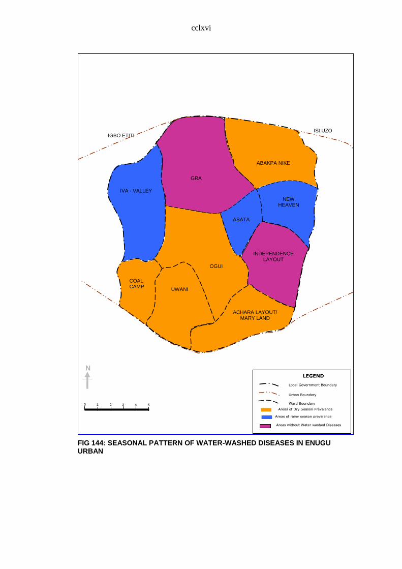
cclxvi

FIG 144: SEASONAL PATTERN OF WATER-WASHED DISEASES IN ENUGU URBAN

N

IGBO ETITI ISI UZO

IVA - VALLEY

GRA

ABAKPA NIKE

ASATA

INDEPENDENCE LAYOUT

NEW HEAVEN

ACHARA LAYOUT/ MARY LAND

COAL CAMP

OGUI

UWANI

0 1 2 3 4 5

LEGEND

Local Government Boundary

Ward Boundary

Urban Boundary

Areas of Dry Season Prevalence

Areas without Water washed Diseases

Areas of rainy season prevalence

cclxvii

5.2.3 Water-based diseases:

A water-based disease is one whose pathogen spends a part of its life-

cycle in a water snail or other aquatic animal. In other words,water-based diseases are

due to infection by parasitic worms (helminths) which depend on aquatic intermediate

hosts to complete their life cycles(Lankinen et al, 1994). They come from hosts that

live in water or require water for part of their life cycle and are caused by parasites

found in intermediate organisms living in contaminated water.

Water-based diseases spread through water that is contaminated with

parasites (worms), either when humans drink it, use it for washing or when it

penetrates the skin, usually through an open wound. These organisms can thrive in

either polluted or unpolluted water (Brandley, 1994). They include: schistosomiasis,

which can stunt growth and development; guinea worm, which causes a disfiguring

and disabling disease.

5.2.3.1 Seasonal incidence of water-based diseases in Enugu Urban

A total of three patients were treated for water bases diseases as is

shown by table 84. In the rainy season, no patient from Asata reported for the

treatment of any water based disease. The three patients that were treated for water

based disease from this ward were all treated in January during the dry season. This is

indicative of the fact that these diseases have a very low occurrence rate in this ward.

Guinea worm infection was the prevalent water based disease in Asata with

occurrence being only in the dry season.

A total of six patients were treated for water bases diseases in Abakpa as is

shown by Table 84. Seasonally the illness pattern indicates that in the rainy season

only one patient from Abakpa was treated for water-based disease. The other five

patients that were treated for water-based disease were all treated in the dry season

month of January. The water-based disease with highest prevalence rate was guinea

worm infection which contributed 100% in the dry season.

A total of 5 patients were treated for water-based diseases as is shown by Table

84. The seasonal pattern of the illness shows that in the rainy season, five patients

from Coal Camp were treated for only one type of water based disease (guinea

worm); in June. No patient however was treated for water based disease in the dry

season months. This indicates that the water based disease was more in the rainy than

the dry season.

cclxviii

Table 84: Number of Patients treated for water-based diseases in Enugu urban

Months Wards of the urban area

Ogui Achara

layout

Asata Abakpa Iva

valley

Coal

camp

Uwani New

Haven

Independenc

e layout

G.R.A Total

for all

wards

January 0 0 3 5 0 0 0 0 0 0 8

February 0 0 0 0 0 0 0 0 0 0 0

March 0 0 0 0 0 0 0 0 0 0 0

April 0 0 0 1 0 0 0 0 0 0 1

May 0 0 0 0 0 0 0 0 0 0 0

June 0 0 0 0 0 5 0 0 0 0 5

July 0 0 0 0 0 0 0 0 0 0 0

August 0 0 0 0 0 0 0 0 0 0 0

September 0 0 0 0 0 0 0 0 0 0 0

October 0 0 0 0 0 0 0 0 0 0 0

November 0 0 0 0 0 0 0 0 0 0 0

December 0 0 0 0 0 0 0 0 0 0 0

Total for

each ward

0 0 3 6 0 5 0 0 0 0 14

Source: Field work, 2006.

5.2.3.2 Non-incidence of water-based diseases in Enugu Urban

Table 84 shows that no patients were treated for water-based disease in

the following wards : Ogui, Achara Layout, Iva Valley, Uwani, New Haven,

Independence Layout and G.R.A. Water-based diseases were not found in these

wards.

From the discussion of the seasonal patterns of water-based diseases, it can

be seen that seven wards (Ogui, Achara Layout, Iva Valley, Uwani, New Haven,

Independence Layout and G.R.A) had no incidence of water-based diseases for the

year under study (Fig 145). The low incidents underscore the fact that water-based

diseases were not common in Enugu Urban area.

Asata ward had all the patients for water-based diseases reporting for the

illness only in the dry season’ while Coal Camp had all the patients for water-based

diseases reporting for the illness only in the rainy season. Abakpa ward was the only

ward that recorded more incidents in the dry season than the rainy season (Fig150).

Generally, in Enugu Urban however, the prevalence of water-based diseases is very

low.

cclxix

FIG 145: SEASONAL PATTERN OF WATER-BASED DISEASES IN ENUGU URBAN

Source: Fieldwork, 2006.

N

IGBO ETITI ISI UZO

IVA - VALLEY

GRA

ABAKPA NIKE

ASATA

INDEPENDENCE LAYOUT

NEW HEAVEN

ACHARA LAYOUT/ MARY LAND

COAL CAMP

OGUI

UWANI

0 1 2 3 4 5

LEGEND

Local Government Boundary

Ward Boundary

Urban Boundary

Dry Season Prevalence only

No water borne disease prevalence

Rainy Season Prevalence only

Dry season more than rainy season

cclxx

5.2.4 Water-related vector diseases

These diseases are water-related insect carrier diseases spread through

insects that feed or breed (live) in or near dirty water. People can be bitten at the river

sides or the waterholes by these insects. They include: malaria; Japanese encephalitis;

sleeping sickness; river blindness; yellow fever; break bone fever (dengue), filariasis,

onochoceriasis and trypanosomiasis (Bradley, 1994).

5.2.4.1 Seasonal dimensions of water-related vector diseases in Ogui.

A total of 209 patients from this ward were treated for water-related

vector diseases as is shown in Tables 85.

Table 85: Number of Patients treated for Water-related vector diseases in Enugu urban

Months Wards of the urban area

Ogui Achara

layout

Asata Abakpa Iva

valley

Coal camp Uwani New

Haven

Independence

layout

G.R.A Total for

all wards

January 8 11 25 39 30 36 20 17 23 26 235

February 20 30 27 18 19 30 26 30 17 18 235

March 17 23 12 7 0 5 15 22 9 15 125

April 5 20 10 14 10 16 12 22 17 6 132

May 13 6 5 14 10 27 22 25 25 12 160

June 14 30 15 48 28 22 36 50 15 13 271

July 14 6 14 25 20 30 33 15 10 23 190

August 10 15 21 16 17 20 35 5 13 10 162

September 37 36 4 30 14 28 18 3 5 4 179

October 6 8 22 19 8 32 13 9 9 15 141

November 37 23 11 20 22 20 11 13 10 5 172

December 28 24 18 40 21 26 10 20 20 12 219

Total for each

ward

209 232 184 291 199 292 251 231 173 159 2221

Source: Field work, 2006.

The seasonal pattern shown as Tables 86 and 87 indicate that of the 209

patients, 93(44.5 %) were treated in the rainy season, while 116 (55.5 %) were treated

in the dry season.

cclxxi

Table 86: Rainy season prevalence of water-related vector diseases in Ogui

Months Water-related vector diseases

Malaria Japanese

fever

Sleeping

sickness

River

blindness

Yellow

fever

Dengue

fever

Total % per

month

April 5 0 0 0 0 0 5 5.4

May 13 0 0 0 0 0 13 14

June 14 0 0 0 0 0 14 15

July 14 0 0 0 0 0 14 15

August 10 0 0 0 0 0 10 10.8

September 37 0 0 0 0 0 37 39.8

Total 93 0 0 0 0 0 93

% per

disease

100 0 0 0 0 0 100

Source: Field work, 2006.

Table 87: Dry season prevalence of water-related vector diseases in Ogui

Months Water-related vector diseases

Malaria Japanese

fever

Sleeping

sickness

River

blindness

Yellow

fever

Dengue

fever

Total % per

month

October 6 0 0 0 0 0 6 5.2

November 37 0 0 0 0 0 37 31.9

December 28 0 0 0 0 0 28 24.1

January 8 0 0 0 0 0 8 6.9

February 19 0 0 0 0 0 20 17.2

March 17 0 0 0 1 0 17 14.7

Total 115 0 0 0 0 0 116

% per

disease

99 0 0 0 1 0 100

Source: Field work, 2006.

In the rainy season, the patients were highest in September and lowest in April.

The dry season patients were highest in November and lowest in October. For both

seasons, the disease with the highest number of patients was malaria which had a

percentage value of 100% for the rainy season and 99% in the dry season.

5.2.4.2 Seasonal dimensions of water-related vector diseases in Achara

cclxxii

Layout

A total of 232 patients from Achara Layout were treated for water-related

diseases (Tables 85). 113(48.7%) were treated in the rainy season while 119(51.3%) were

treated in the dry season.

In the rainy season (Table 88), the patients were highest in the month of

September, while being lowest in May. In the dry season (Table 89), the patients were

highest in February and lowest in October.

Table 88: Rainy season prevalence of water-related vector diseases in Achara layout.

Months Water-related vector diseases

Malaria Japanese

fever

Sleeping

sickness

River

blindness

Yellow

fever

Dengue

fever

Total % per

month

April 20 0 0 0 0 0 20 17.7

May 6 0 0 0 0 0 6 5.3

June 30 0 0 0 0 0 30 26.5

July 6 0 0 0 0 0 6 5.3

August 15 0 0 0 0 0 15 13.2

September 36 0 0 0 0 0 36 32

Total 113 0 0 0 0 0 113

% per

disease

100 0 0 0 0 0 100%

Source: Field work, 2006.

Table 89: Dry season prevalence of water-related vector diseases in Achara layout.

Months Water-related vector diseases

Malaria Japanese

fever

Sleeping

sickness

River

blindness

Yellow

fever

Dengue

fever

Total % per

month

October 8 0 0 0 0 0 8 6.7

November 23 0 0 0 0 0 23 19.3

December 24 0 0 0 0 0 24 20.2

January 11 0 0 0 0 0 11 9.3

February 30 0 0 0 0 0 30 25.2

March 23 0 0 0 1 0 23 19.3

Total 119 0 0 0 0 0 119

% per

disease

100 0 0 0 1 0 100%

Source: Field work, 2006.

In both seasons, the disease with the highest number of patients was malaria which

had a percentage value of 100% for the rainy season and 100% in the dry season. The other

water-related vector diseases were not reported in the ward.

5.2.4.3 Seasonal dimensions of water-related vector diseases in Asata .

cclxxiii

A total of 184 patients were treated for water-related vector diseases in Asata

as is shown by table 85. The seasonal prevalence pattern shown as Tables 90 and 91

indicate that in the rainy 69(37.5%) people from this ward were treated in the sampled

hospitals for water-related vector diseases, while 115(62.5%) were treated in the dry

season.

Table 90: Rainy season prevalence of Water-related vector diseases in Asata

Months Water-related vector diseases

Malaria Japanese

fever

Sleeping

sickness

River

blindness

Yellow

fever

Dengue

fever

Total % per

month

April 10 0 0 0 0 0 10 5.4

May 5 0 0 0 0 0 5 14

June 15 0 0 0 0 0 15 15

July 13 0 0 0 1 0 14 15

August 21 0 0 0 0 0 21 10.8

September 4 0 0 0 0 0 4 39.8

Total 68 0 0 0 1 0 69

% per

disease

98.6 0 0 0 1.4 0 100%

Source: Field work, 2006.

Table 91: Dry season prevalence of water-related vector diseases in Asata

Months Water-related vector diseases

Malaria Japanese

fever

Sleeping

sickness

River

blindness

Yellow

fever

Dengue

fever

Total % per

month

October 22 0 0 0 0 0 22 19.1

November 11 0 0 0 0 0 11 9.6

December 18 0 0 0 0 0 18 15.7

January 20 0 0 0 3 2 25 21.7

February 27 0 0 0 0 0 27 23.5

March 12 0 0 0 0 0 12 10.4

Total 110 0 0 0 3 2 115

% per

disease

95.7 0 0 0 2.6 1.7 100%

Source: Field work, 2006.

In the rainy season, the patients were highest in the month of August (30.4%),

while being lowest in September (Table 90). The dry season patients were highest in

the months of February lowest in November (Table 91).

In both seasons, the disease with the highest number of patients was malaria

which had a percentage value of 98.6% occurrence in the rainy season and 95.7% in

cclxxiv

the dry season; while some of the other diseases were either not experienced or it

occurred with a very low percentage.

5.2.4.4 Seasonal dimensions of water-related vector diseases in Abakpa

Of the 291 patients from Abakpa who were treated for water vectored

diseases (Table 85), 148(50.9%) were treated in the rainy season while 143(49.1%)

were treated in the dry season (Tables 92 and 93).

Table 92: Rainy season prevalence of water-related vector diseases in Abakpa

Months Water-related vector diseases

Malaria Japanese

fever

Sleeping

sickness

River

blindness

Yellow

fever

Dengue

fever

Total % per

month

April 14 0 0 0 0 0 14 9.5

May 15 0 0 0 0 0 15 10.1

June 48 0 0 0 0 0 48 32.4

July 25 0 0 0 0 0 25 16.9

August 16 0 0 0 0 0 16 10.8

September 26 0 0 0 0 4 26 20.3

Total 144 0 0 0 0 4 148

% per

disease

97.3 0 0 0 0 2.7 100%

Source: Field work, 2006.

Table 93: Dry season prevalence of water-related vector diseases in Abakpa

Months Water-related vector diseases

Malaria Japanese

fever

Sleeping

sickness

River

blindness

Yellow

fever

Dengue

fever

Total % per

month

October 19 0 0 0 0 0 19 13.4

November 20 0 0 0 0 0 20 14

December 40 0 0 0 0 0 40 28

January 36 0 0 3 0 0 39 27.3

February 18 0 0 0 0 0 18 12.5

March 7 0 0 0 0 0 7 4.8

Total 140 0 0 3 0 0 143

% per

disease

97 0 0 3 0 0 100%

Source: Field work, 2006.

In the rainy season (Table 92), the patients were highest in the month of June,

while being lowest in April. The dry season patients were highest in the month of

December and lowest in March (table 93). In both seasons, the disease with the

cclxxv

highest number of patients was malaria which had a percentage value of 97.3% for the

rainy season and 97% for the dry season.

5.2.4.5 Seasonal dimensions of water-related vector diseases in Iva Valley

A total of 199 patients were treated for water vectored diseases in Iva

valley as is shown by Table 85. The seasonal pattern shown as Tables 94 and 95

indicate that of the 199 patients, 99 (49.7 %) were treated in the rainy season, while

100(50.3%) were treated in the dry season.

Table 94: Rainy season prevalence of Water-related vector diseases in Iva valley

Months Water-related vector diseases

Malaria Japanese

fever

Sleeping

sickness

River

blindness

Yellow

fever

Dengue

fever

Total % per

month

April 10 0 0 0 0 0 10 10.1

May 9 0 0 0 1 0 10 10.1

June 24 0 0 0 4 0 28 28.2

July 20 0 0 0 0 0 20 20.2

August 17 0 0 0 0 0 17 17.2

September 14 0 0 0 0 0 14 14.2

Total 94 0 0 0 5 0 99

% per

disease

94.9 0 0 0 5.1 0 100%

Source: Field work, 2006

Table 95: Dry season prevalence of Water-related vector diseases in Iva valley

Months Water-related vector diseases

Malaria Japanese

fever

Sleeping

sickness

River

blindness

Yellow

fever

Dengue

fever

Total % per

month

October 8 0 0 0 0 0 8 8

November 22 0 0 0 0 0 22 22

December 21 0 0 0 0 0 21 21

January 30 0 0 0 0 0 30 30

February 19 0 0 0 0 0 19 19

March 0 0 0 0 0 0 0 0

Total 100 0 0 0 0 0 100

% per

disease

100 0 0 0 0 0 100%

Source: Field work, 2006.

In the rainy season, the patients were highest in June, while being lowest in

May (Table 94). The dry season patients were highest in January and lowest in March

(Table 95).In both seasons, the disease with the highest number of patients was

cclxxvi

malaria which had a percentage value of 95 % occurrence in the rainy season and

100% in the dry season.

5.2.4.5 Seasonal dimensions of water-related vector diseases in Coal Camp.

A total of 292 patients from Coal Camp were treated for water-related

vector diseases in the rainy and dry seasons as is shown in table 85.The rainy and

dry season patterns indicate that of the 292 patients, 143 patients representing 49 %

were treated in the rainy season, while 145(51%) were treated in the dry season. In

the rainy season (Table 96), the patients were highest in the month of July, and

lowest in April. The dry season patients were highest in January and lowest in

March (Table 97).

Table 96: Rainy season prevalence of water-related vector diseases in Coal camp.

Months Water-related vector diseases

Malaria Japanese

fever

Sleeping

sickness

River

blindness

Yellow

fever

Dengue

fever

Total % per

month

April 16 0 0 0 0 0 16 11.2

May 27 0 0 0 0 0 27 18.9

June 22 0 0 0 0 0 22 15.4

July 30 0 0 0 0 0 30 21

August 20 0 0 0 0 0 20 14

September 28 0 0 0 0 0 28 19.5

Total 143 0 0 0 0 0 143

% per

disease

100 0 0 0 0 0 100%

Source: Field work, 2006.

Table 97: Dry season prevalence of water-related vector diseases in Coal camp.

cclxxvii

Months Water-related vector diseases

Malaria Japanese

fever

Sleeping

sickness

River

blindness

Yellow

fever

Dengue

fever

Total % per

month

October 32 0 0 0 0 0 32 24.2

November 20 0 0 0 0 0 20 13.4

December 26 0 0 0 0 0 26 17.4

January 32 0 0 0 4 0 36 24.2

February 30 0 0 0 0 0 30 20.1

March 5 0 0 0 0 0 5 3.4

Total 145 0 0 0 4 0 149

% per

disease

97.3 0 0 0 2.7 0 100 100%

Source: Field work, 2006.

In both seasons, the disease with the highest number of patients was malaria which

had a percentage value of 100 % in the rainy season and 97.3% in the dry season. The

number of people that were treated for Water-related vector diseases in Coal camp were

more in the dry season (51%) than the rainy season (49 %).

5.2.4.7 Seasonal dimensions of water-related vector diseases in Uwani.

A total of 251 patients were treated for water-related vector diseases

in Uwani as shown by Table 85. Of the 251 patients, 156 were treated for water-

related vector diseases in the rainy season, while 95 were treated in the dry season. In

the rainy season (Table 98), the patients were highest in June, while being lowest in

April. The dry season patients were highest in February (27.4%) and lowest in

December (10.5 %) (Table 99).

cclxxviii

Table 98: Rainy season prevalence of Water-related vector diseases in Uwani

Months Water-related vector diseases

Malaria Japanese

fever

Sleeping

sickness

River

blindness

Yellow

fever

Dengue

fever

Total % per

month

April 12 0 0 0 0 0 12 7.7

May 22 0 0 0 0 0 22 14.1

June 36 0 0 0 0 0 36 23.1

July 33 0 0 0 0 0 33 21.2

August 35 0 0 0 0 0 35 22.4

September 18 0 0 0 0 0 18 11.5

Total 156 0 0 0 0 0 156

% per

disease

100 0 0 0 0 0 100%

Source: Field work, 2006.

Table 99: Dry season prevalence of Water-related vector diseases in Uwani

Months Water-related vector diseases

Malaria Japanese

fever

Sleeping

sickness

River

blindness

Yellow

fever

Dengue

fever

Total % per

month

October 11 0 0 0 0 2 13 13.7

November 11 0 0 0 0 0 11 11.6

December 10 0 0 0 0 0 10 10.5

January 20 0 0 0 0 0 20 21.1

February 23 0 0 0 1 0 26 27.4

March 15 0 0 0 0 2 15 15.7

Total 90 0 0 0 1 4 95

% per

disease

94.7 0 0 0 1.1 4.2 100%

Source: Field work, 2006.

In both seasons, the disease with the highest number of patients was malaria which

had a percentage of 100% in the rainy season and 94.7% in the dry season.

5.2.4.8 Seasonal dimensions of water-related vector diseases in New Haven

A total of 231 patients from New Haven were treated for Water-related

vector diseases in the rainy and dry season as is shown in Table 85.The rainy and dry

season patterns indicate that of the 231 patients, 120 patients representing 52 % were

treated in the rainy season, while 111(48%) were treated in the dry season. In the

rainy season (Table 100), the patients were highest in the month of June, and lowest

in September. The dry season patients were highest in the month of February and

lowest in October (Table 101).

cclxxix

Table 100: Rainy season prevalence of Water-related vector diseases in New Haven

Months Water-related vector diseases

Malaria Japanese

fever

Sleeping

sickness

River

blindness

Yellow

fever

Dengue

fever

Total % per

month

April 22 0 0 0 0 0 22 18.3

May 25 0 0 0 0 0 25 20.8

June 50 0 0 0 0 0 50 41.7

July 15 0 0 0 0 0 15 12.5

August 5 0 0 0 0 0 5 4.2

September 3 0 0 0 0 0 3 2.5

Total 120 0 0 0 0 0 120

% per

disease

100 0 0 0 0 0 100%

Source: Field work, 2006.

Table 101: Dry season prevalence pattern of Water-related vector diseases in New Haven

Months Water-related vector diseases

Malaria Japanese

fever

Sleeping

sickness

River

blindness

Yellow

fever

Dengue

fever

Total % per

month

October 9 0 0 0 0 0 9 8.2

November 13 0 0 0 0 0 13 11.7

December 20 0 0 0 0 0 20 18.0

January 17 0 0 0 0 0 17 15.3

February 30 0 0 0 0 0 30 27.0

March 22 0 0 0 1 0 22 19.8

Total 111 0 0 0 1 0 112

% per

disease

100 0 0 0 1 0 100%

Source: Field work, 2006.

In both seasons, the disease with the highest number of patients was malaria which

had a percentage value of 100 % in the rainy season and 99% in the dry season.

5.2.4.9 Seasonal dimensions of water-related vector diseases in Independence

Layout

A total of 173 patients were treated for water-related vector diseases in

Independence Layout as shown by Table 85. The seasonal patterns shown as Tables 102 and

103 indicate that in the rainy season 85(49%) patients were treated for water-related vector

diseases, while 88(51%) were treated in the dry season.

cclxxx

Table 102: Rainy season prevalence of water-related vector diseases in Independence

Layout.

Months

Water-related vector diseases

Malaria Japanese

fever

Sleeping

sickness

River

blindness

Yellow

fever

Dengue

fever

Total % per

month

April 17 0 0 0 0 0 17 20

May 25 0 0 0 0 0 25 29.4

June 15 0 0 0 0 0 15 17.6

July 10 0 0 0 0 0 10 11.8

August 13 0 0 0 0 0 13 15.3

September 5 0 0 0 0 0 5 5.9

Total 85 0 0 0 0 0 85

% per

disease

100 0 0 0 0 0 100%

.

Table 103: Dry season prevalence pattern of water-related vector diseases in

Independence Layout.

Months Water-related vector diseases

Malaria Japanese

fever

Sleeping

sickness

River

blindness

Yellow

fever

Dengue

fever

Total % per

month

October 9 0 0 0 0 0 9 10.2

November 10 0 0 0 0 0 10 11.4

December 20 0 0 0 0 0 20 22.7

January 23 0 0 0 0 0 23 26.1

February 17 0 0 0 0 0 17 19.4

March 9 0 0 0 0 0 9 10.2

Total 88 0 0 0 0 0 88

% per

disease

100 0 0 0 0 0 100%

Source: Field work, 2006.

In the rainy season, the patients were highest in May, and lowest in

September. The dry season patients were highest in February and lowest in March and

October; 10.2 each).In both seasons, the disease with the highest number of patients

was malaria which had a percentage value of 100 % in the rainy season and 100% in

the dry season.

cclxxxi

5.2.4.10 Seasonal dimensions water-related vector diseases in Government

Reserved Area (G.R.A)

Table 65 shows that 159 patients were treated for water-related vector

diseases. The rainy and dry season patterns indicate that of the 159 patients, 68

representing 43 % were treated in the rainy season, while 91(57%) were treated in the

dry season.

In the rainy season (Table 104), patients were highest in the month of July,

and lowest in September. The dry season patients were highest in the month of

January and lowest in November (5.4 %) (Table 105).

Table 104: Rainy season prevalence pattern of water-related vector diseases in G.R.A

Months Water-related vector diseases

Malaria Japanese

fever

Sleeping

sickness

River

blindness

Yellow

fever

Dengue

fever

Total % per

month

April 6 0 0 0 0 0 6 9

May 12 0 0 0 0 0 12 17.6

June 13 0 0 0 0 0 13 19.1

July 23 0 0 0 0 0 23 33.8

August 10 0 0 0 0 0 10 14.7

September 4 0 0 0 0 0 4 5.8

Total 68 0 0 0 0 0 68

% per

disease

100 0 0 0 0 0 100

Source: Field work, 2006.

Table 105: Dry season prevalence pattern of water-related vector diseases in G.R.A

Months Water-related vector diseases

Malaria Japanese

fever

Sleeping

sickness

River

blindness

Yellow

fever

Dengue

fever

Total % per

month

October 15 0 0 0 0 0 15 16.5

November 5 0 0 0 0 0 5 5.4

December 12 0 0 0 0 0 12 13.2

January 26 0 0 0 0 0 26 28.6

February 18 0 0 0 0 0 18 19.8

March 15 0 0 0 0 0 15 16.5

Total 91 0 0 0 0 0 91

% per

disease

100 0 0 0 0 0 100%

Source: Field work, 2006.

cclxxxii

In both seasons, the disease with the highest number of patients was malaria

which had a percentage value of 100 % in the rainy season and 100% in the dry

season. The other diseases were not experienced in this ward.

From the foregone discussion, it is discernible that water-related vector

diseases were more in the dry season than the rainy season in seven of the ten wards

(namely Ogui, Achara layout, Asata, Iva valley, Coal camp, Independence layout and

G.R.A). Three wards (Abakpa, Uwani and New Haven) had more incidents in the

rainy than dry season (Fig 146).

cclxxxiii

FIG 146: SEASONAL PATTERN OF WATER-RELATED VECTOR DISEASES IN ENUGU URBAN

Source: Fieldwork, 2006.

N

IGBO ETITI ISI UZO

IVA - VALLEY

GRA

ABAKPA NIKE

ASATA

INDEPENDENCE LAYOUT

NEW HEAVEN

ACHARA LAYOUT/ MARY LAND

COAL CAMP

OGUI

UWANI

0 1 2 3 4 5

LEGEND

Local Government Boundary

Ward Boundary

Urban Boundary

Dry season prevalence

Rainy Season prevalence

cclxxxiv

5.3 Annual pattern of water-related diseases in Enugu Urban.

5.3.1 Rainy season pattern of water-related diseases in Enugu urban .

For the year under study, the total number of patients treated for water-

related diseases was 3813 (Table 46). Of this total number 1768 patients were treated

in the rainy season (Table 106).

TABLE 106: Incidence of water–related diseases during rainy season in Enugu Urban.

Month Number of

patients

treated

Percentage(%)

contribution

April 244 14

May 271 15

June 438 24

July 311 18

August 224 13

September 280 18

Total 1768 100%

Source: Field work 2006

From Table 106, it can be seen that during the rainy season, the month that

recorded the highest incidents of water-related diseases was the month of June with

(438(24%) patients. The lowest number of patients occurred in August when 224

patients representing 13% were treated.

cclxxxv

5.3.2 Dry season pattern of water-related diseases in Enugu urban area.

The total number of patients treated for water-related diseases during the

dry season was 2045(Table107).

Table 107: Incidence of water–related diseases during dry season in Enugu Urban.

Month Number of patients

treated

Percentage %

contribution

October 290 14

November 263 13

December 332 16

January 425 21

February 431 21

March 304 15

Total 2045 100%

Source: Field work, 2006

Table 107 shows that during the dry season, the month that had the highest

number of patients was the month of February when 431 patients (21%) were treated

for water-related diseases in the urban area. The lowest number of patients occurred in

the month of November, when 263 patients (13%) were treated. A comparison of the

rainy and dry season patterns indicates that the dry season period with a total of 2045

patients (53.6%), had more patients reporting for the treatment of water-related

diseases than the rainy season period with a total of 1768 patients (46.4%).

This seasonal trend noted in Enugu urban area is explainable by the fact that

the dry season period is the period of extreme water scarcity in the urban area when

residents utilize water from compromised and uncompromised sources. At this period

also the residents visit water sources where they are further exposed to water-related

insect vector diseases.

cclxxxvi

5.4 Prevalence pattern of the four major water-related diseases.

The water-borne diseases prevalence in Enugu shown as Table 108 indicates

that of the 1407 recorded cases of water-borne diseases in all the wards of Enugu , 680

patients representing 48.3% reported for typhoid thus making typhoid the most

prevalent water-borne disease in the urban area.

Table 108: Water-borne diseases (Patient Number/ Percentage in Enugu urban)

Water borne

diseases

Total No of

patients

Percentage (%)

contribution

Ranking

Diarrhoea 438 31.2 2nd

Cholera 48 3.4 5TH

Typhoid 680 48.3 1st

Dysentery 107 7.6 4th

Hepatitis 134 9.5 3rd

TOTAL 1407 100%

Source: Field work, 2006.

Diarrhoea with 438 patients ranked second (2nd

), hepatitis with a contribution of

9.5% was the third most frequent illness. The fourth most prevalent disease was

dysentery with 107 patients (7.6). Cholera which had only forty eight (48) patients

was the least frequently occurring of all the water-borne diseases. Thus, for the water-

borne diseases typhoid was the most prevalent, while cholera was the least prevalent.

The water-washed disease pattern shown as Table 109 indicates that of the one

hundred and seventy one (171) patients that visited the hospitals, tuberculosis had the

highest number 86 patients (50.2%).

Table 109: Water-washed Diseases (Patient Number/ Percentage in Enugu Urban)

cclxxxvii

Water washed

diseases

Total no of

patients

Percentage contribution Ranking

Trachoma 11 6.4 3rd

Skin infection 63 36.9 2nd

Leprosy 0 0 6th

Tuberculosis 86 50.2 1st

Whopping cough 2 1.2 5th

Tetanus 9 5.3 4th

Diphtheria 0 0 6th

TOTAL 171 100%

Source: Field work, 2006.

Skin infection with 65 patients contributed 36.9% and ranked second (2nd

)

while trachoma contributing 11 patients (6.4%) ranked third (3rd

). Diphtheria and

leprosy were the least prevalent as no patients reported for these illnesses from any of

the wards in the urban area.

The water-based disease pattern shown as Table 110 reveals that the most

prevalent disease was the guinea worm infection which contributed 100%. No patient

reported for the treatment of schistosomaisis.

Table 110: Water-based Diseases (Patient Number/ Percentage in Enugu Urban)

Water based Diseases Total no of patients Percentage contribution Ranking

Guinea worm 14 100 1st

Schistosomiasis 0 0 2nd

Total 14 100

Source: Field work, 2006.

The water-related vector disease pattern shown as Table 111 indicates that of

the 2221 patients, malaria with 2193(98.8) patients had the highest number of patients.

Yellow fever and Dengue fever were the second most frequently occurring illnesses as they

both had a contribution of 0.6% each; while other diseases such as Japanese encephalitis,

sleeping sickness and river blindness were not identified in Enugu urban.

cclxxxviii

Table 111: Water-related vector diseases (Patient Number/ Percentage in Enugu Urban)

Water vector diseases Total number of

patients

% contribution Rank

Malaria 2193 98.8 1st

Japanese 0 0 3rd

Sleeping sickness 0 0 3rd

River blindness 0 0 3rd

Yellow fever 14 0.6 2nd

Dengue fever 14 0.6 2nd

Grand Total 2221 100

An overview of the four major diseases thus indicates that the water-related vector

disease with a percentage contribution of 58.2 had the highest number of patients and is

thus the most prevalent water-related disease in Enugu urban while water-borne disease

(36.9%) ranked second (Table 112).

TABLE 112: PATIENT NUMBER/PERCENTAGE FOR THE WATER- RELATED DISEASES

Water-related

disease group

Total number of

patients

Percentage % contribution Disease rating

Water borne 1407 36.9 2nd

Water washed 171 4.5 3rd

Water based 14 0.4 4th

Water-related

insect vector

2221 58.2 1st

Grand total 3813 100%

Source: Field work, 2006.

The water-washed disease with a percentage value of 4.5% ranked third (3rd

) while

water-based disease contributing 0.4% only is the least prevalent.

CHAPTER SIX

cclxxxix

ENVIRONMENTAL AND POLICY IMPLICATIONS OF THE WATER

QUALITY IN ENUGU URBAN.

Low water quality has the potential for becoming a threat if not properly

managed. The World Health Organization (WHO) guideline for drinking water

stipulates specific acceptable and safety limits for drinking water. Deviations from

these limits usually have environmental and health implications due to either

elevations or reductions in the level of the physical, chemical and biological

parameters. These environmental and health implications vary with the nature of the

parameters.

6.1 Implications of the physical parameters.

The water temperature of a river/well is very important for water quality.

This is especially so as it determines the physical nature of water and influences the

water chemistry. The rate of chemical reaction increases at higher temperature which

in turn affects biological activities.

From our water analysis it was observed that the temperature of the urban rivers and

wells were generally within the WHO’s MPL. This indicates that the rivers and wells

are not of low quality thermally. This parameter is not yet of environmental concern

because they lie within the expected temperature for tropical water and the

temperature of tropical waters do not deviate significantly.

There is however a need to monitor and maintain the observed temperature

especially as it was observed from field investigation that continued urban expansion

has necessitated cutting down trees that help shade the rivers thus exposing the water

bodies to the effect of direct sunlight. The increase in more tarred streets, sidewalks

and parking lots generate storm water that runs off warmed urban surfaces

contributing to the river and well temperatures. Other various human activities

contribute suspended solids carried by the rivers making the water turbid. Turbid

water absorbs the sun’s rays, causing water temperatures to rise.

Temperature also affects the palatability of water. Its increase stimulates

growth of taste and odour, producing organisms which later affect man by causing

intestinal irritation. If the temperatures of the urban rivers are unchecked the

highlighted effects would become issues of environmental concern in no distant time.

The turbidity of the rivers and wells exceeded the WHO’s MPL. This

indicates that the clarity of water was affected for all the months of the year. The river

ccxc

and well waters had low turbidity quality reducing the aesthetic value. Continued

deterioration of the water turbidity will affect water transparency and this also has

impact on light penetration. The reduced light penetration in rivers causes

photosynthesis and dissolved oxygen reduction in rivers. With continued reduction in

aesthetic value of the water, usage will be restricted and this will consequently lead to

the rejection of the well and river waters. Water scarcity in the urban area will become

not only an issue of supply, but also that of not being of beneficial use.

The high turbidity was discovered to have relationship with colouration of the

well and river waters such that from field investigation, residents in areas such as

Asata, Ogui, and Uwani complained about colouration of their cloths by well water

used for laundry especially in the dry season.

According to Taggart et al (1991), turbid water due to the presence of

protozoa, diatoms and excess solids in water also give rise to irritation of bowel

especially when consumed. As seen from Table 108, people were treated for various

kinds of intestinal irritation, with typhoid fever being the most frequent of the water-

borne diseases. To reduce and ensure that the hospital beds are not over- taken by

patients suffering from water-borne diseases, the turbidity levels of the urban waters

have to be closely monitored as development continues.

The total dissolved solids of the urban rivers and wells located in Asata were

within the WHO’s MPL thus indicating that dissolved substances both organic and

inorganic are not yet of environmental concern. However wells found in four

locations (Abakpa, Uwani, Achara layout and Ogui) recorded values that exceeded

the WHO’s MPL. Excessive total dissolved solids in these wells indicate that the

wells have excessive amounts of solids suspended in water, whether mineral (soil

particles) or organic (algae). It provides attachment places for other pollutants and

high total dissolved solids readings are used as “indicator” of other potential

pollutants that would reduce the quality of the water body.

The high concentration of particulate matter in wells can cause sedimentation

and siltation of the wells necessitating constant clearing of the wells. This usually

adds to the cost of maintenance of the wells as observed in the study area.

6.2 Implications of the chemical parameters.

Excessive amounts of most chemicals in domestic water (either as rivers

or wells) have detrimental effects on man and his environment (Bath, 1990; Bartram,

ccxci

1996). However, some chemicals such as calcium, iron, phosphate and fluoride are

needed in the body as supply of nutritional minerals for human body needs although

they tend to be undesirable when in excess.

The pH determines the acidity or alkalinity of water. The pH of rivers and

wells in the study area were found to be within the WHO’s MPL. The values obtained

in most months showed that the urban rivers and wells are acidic in nature. This

conforms to the nature of the tropical waters (Egboge et al, 1986). The effect of the

acidic nature of the waters is confirmed by the corroded nature of the metal pipes used

to distribute water in the various houses.

Conductivity values of the urban rivers from the study were found to be

within WHO’s MPL indicating that ionic components of the water bodies are within

expected levels as tropical fresh waters bodies usually have very low conductivity

(Egboge, 1971b). The conductivity of the wells however exceeded the WHO’s MPL

in most months of the year. This indicates changes in mineral composition of in the

well and a reflection of a measure of low freshness of the water.

The dissolved oxygen values obtained from the laboratory analysis for this

study indicated that all the rivers and the wells had values that exceeded the WHO’s

MPL throughout the year. This shows that the rivers and wells have high organic

polluting materials added to the water or there is absorption of oxygen during the

corrosion of metals, breathing of aquatic organisms and production of oxygen during

the process of photosynthesis. The consistence of this parameter in exceeding the

WHO’s MPL is an indication of the poor nature of the rivers and wells, the biological

state and the corrosiveness of the waters.

Biochemical oxygen demand of the rivers and wells were found from our

laboratory analysis to have been within the WHO’s MPL in more months in the year

of study. However, the fact that there were some months when the biochemical

oxygen demand was exceeded and can not be overlooked because it is a measure of

the amount of oxygen used by microorganisms in the aerobic oxidation of organic

matter. It is a reflection of oxygen demand for the decomposition of organic matter as

aerobic bacteria may decompose organic matter at such a fast rate that dissolved

oxygen decreases causing a biochemical oxygen demand.

A continued increase in biochemical oxygen demand will thus increase the

depletion of dissolved oxygen which has both ecological and environmental

implications to the water bodies. Ecologically, microorganisms die, increased need for

ccxcii

their decomposition is then reflected on the dissolved oxygen, which in turn increases

the biochemical oxygen demand. This will lead to the fouling of the water by

introduction of odour. All these generally lead to the reduction of aesthetic value of

the rivers and wells.

The nutrients to be classified here as micronutrients (i.e. phosphate, nitrate,

ammonia, iron and sulphate) and macronutrients (calcium and sodium) of the rivers

and wells were found to be within WHO’s MPL. Only phosphate exceeded the

WHO’s MPL.

In Enugu urban the micro/macro nutrients do not yet pose environmental

problems. There is however a great need in view of our finding to ensure that these

nutrients, at the worst, remain at the ascertained levels. This is because excess calcium

in domestic water produces scales, taste and contributes to hardening of water. It also

gives rise to laxative effect on man. Sodium in excess impacts taste to river and well

waters. It also enhances corrosion of metal utensils and containers; poses great

problems to people suffering from heart disease, hypertension, renal and liver

diseases. Excessive iron impacts on laundry a red to brown stain and nitrate when

converted within the body to nitrite causes methemoglobinemia especially in children.

Phosphate levels of both the rivers and the wells in the urban area exceeded

the WHO’s MPL. This is an indication of the wells and rivers having low quality in

terms of their phosphate levels. In groundwater, phosphate concentration is usually

minute such that an increase in its concentration indicates the presence of pollutants.

The increased phosphate concentration in water is usually an indication of pollution

from municipal waste and industrial discharges; overland flow from garden fertilizers

and urban lawns.

From field work it was discovered that in the urban area, various agricultural

activities were being carried out along the bank of the rivers (Plates 1, 2) and fertilizer

use was indicated by the farmers. The need to monitor the chemical parameters of

both rivers and wells in Enugu urban can not be over emphasized.

6. 3 Implications of the biological parameter.

Fecal coliform bacteria are microscopic animals that live in the warm

blooded animals (intestinal tract of man and animals), waste material or feaces

excreted from the intestinal tract. Bacteria are the most numerous organisms in water

and when present in high numbers in water sample, it means that the water has

ccxciii

received fecal matter from one source or another. In the course of our field work, it

was observed that intestine of slaughtered chickens from artisan market were usually

cleaned out for sale at the Asata river (Plate 1).

Ensuring none pollution of water by fecal coliform bacteria is very important

because they do not mix with water and float downstream. Instead they multiply

quickly when conditions are favourable for growth or die when unfavourable. The

primary source of fecal coliform bacteria to rivers and wells are waste water

discharges, failing septic systems, animal waste from abattoirs, leaking sanitary

sewers, old disintegrating storm sewers and storm water runoff in urbanized areas.

The presence of fecal coliform bacteria in domestic water gives rise to widespread

water-related diseases as is applicable to the study area (table 108). Table 112 also

shows that all different types of diseases are evident in Enugu urban area with malaria

and typhoid fever ranking very high.

When these water-related illnesses occur, the patients spend large sums of

money in the treatment of the illnesses. What is spent usually depends on what illness

is being treated and the duration of the illness. These illnesses lead to the inability of

patients to carry out their various economic activities.

6.4 Implications of the obtained Water Quality Index (WQI) of the rivers and

the wells in Enugu urban.

The WQI generates a score that describes water quality status and

evaluates water quality trends. It is very useful in communicating information to the

lay public and to legislative decision makers.By the computation of the WQI of the

rivers and streams, we have meaningfully integrated the data sets and converted them

into information that can be disseminated to the lay public.

From our study, the computed WQI of the rivers had WQI that ranged

between 47 and 67. These WQI indicate that generally the rivers had average health

levels except for some months when the WQI obtained were bad. This is indicative of

the fact that the Enugu urban rivers are at the marginal level where any additional

physical, chemical, and biological pollutants to the rivers will greatly reduce the

ccxciv

quality of the urban rivers and therefore the WQI. The fact that some of the rivers had

WQI that were bad shows that the health of some of the rivers are already low. These

rivers do not meet expectations and there should be very high concern about

regulating the use of the rivers especially as dump sites.

The wells had WQI that range between 35 and 63. These WQI indicate that

generally the wells had average health levels except for some months when the WQI

obtained was just bad. This shows that the health of the wells is marginal and in some

months they do not even attain the expected levels. This emphasizes the fact that the

water quality status of the wells should be of great concern to the government and the

populace.

The obtained WQI underscore the fact that the urban waters are at the level

where any additional pollutant into the water bodies will reduce the level to where

they would be considered to be of very low quality and beneficial use (especially as

regards their usage for any activity that involves human consumption). Since low

water quality can injuriously affect human life, industrial processes and living

conditions, there is a need to institute measures that will curtail further deterioration

of the rivers and wells.

6.5 Social Implications of low water quality.

From the obtained WQI for Enugu urban rivers and wells it is obvious that

the WQI range between average (medium) and bad (poor) water quality. These water

sources serve as water sources for human consumption such that the observed

qualities are not encouraging as they have social implications. Most of these water

sources serve as source of water-related diseases that affect the health of the urban

populace. This therefore leaves them unhealthy. The amount spent in treating these

water-related diseases when they occur reducing their ability to perform other social

functions. The ill health creates such chronic problems that the life expectancy is

affected also as some of these water-related diseases result to deaths. The number of

hours spent not being able to attend to social activities usually increases. The inability

of the unhealthy members of the family to take care of themselves increases also.

ccxcv

6.6 Economic Implications of the low water quality.

In situations where the health and general well-being of the urban dwellers are

affected, the effects on the economy of such a population are usually unquantifiable as

man hours are lost thus leading to reduced productivity. Also more money is spent on

the treatment of the illness. Where the families are aware of the quality level of water

being obtained, more money is spent making conscious effort to purchase water (e.g.

bottled) considered to be of a better quality. More capital that would have been

utilized for other economic ventures are then ploughed into purchasing water and

remedying the already dilapidated health of the people. Based on the various added

economic loss, saving of money becomes difficult to achieve. The reduced

productivity generally leads to economic stagnation.

A continued reduction in the urban water quality would also adversely affect

the industries operating in the urban area especially those that utilize ground water

resources.

6.7 Policy Implications of the low water quality.

At the Federal level in Nigeria, three ministries have the responsibility

for water supply quality management. These are

i. The Federal Ministry of Water Resources(FMWR) which responsible for

formulating policies, regulating the water sector and providing technical and

financial support to state governments in the planning, implementation and

monitoring of water supply projects.

ii. The Federal Ministry of Environment which has the responsibility of

protecting, restoring and preserving the ecosystem of the Nigerian

environment including its water resources.

iii. The Federal Ministry of Health (FMOH) which has the mandate of guarding

water quality as it affects public health.

All these Ministries exist at the state level with the same mandates and

the overall responsibility for public water supply quality management is shared

ccxcvi

between these agencies. Two main water policies and regulatory instruments for the

management of the water quality in Nigeria exist. These are the National Water

Supply and Sanitation Policy by the Federal Ministry of Water Resources and The

National Guideline and Standards for Water quality in Nigeria by the Federal Ministry

of Environment. This shows that policies do exist nationally and it is binding on the

state governments to utilize these policies in their water administration.

The field investigation showed that these ministries do exist in Enugu state but

there are indications that the published National Guidelines and standards do not have

the full support of some regulating parastatals and state governments. Thus inter-

ministerial differences and bottle necks do exist. Even though these policies do exist

no effort is being made by the state government to ensure compliance by the residents

or companies. There are also no clear records of monitoring of compliance to these

National Standards by the state government.

On the bases of our obtained water analysis which indicates that at least four

parameters exceed the WHO’s MPL and the urban water resources are of very low

bacteriological quality, there is an urgent need to review our water policies and to

ensure compliance in each State. The Enugu State government needs to make the

policy functional by ensuring the monitoring of compliance.

Where the Enugu State Government decides to disregard monitoring of water

quality and ensuring compliance to stipulated water quality standards, the water

quality will deteriorate very fast as urbanization continues. A further reduced water

quality will create WQI that will range from 0 to 25. This is usually classified as very

bad water that has very little beneficial use. The urban area will experience intensified

water scarcity especially as the alternative sources in times of scarcity will be the

most affected.

ccxcvii

CHAPTER SEVEN.

CONCLUSION AND RECOMMENDATIONS

7.1 Summary of findings.

The results of this study established values for selected physical, chemical

and biological parameters for Enugu urban area. The parameters tested yielded results that

were compared to the Maximum Permissible Levels of World Health Organization’s

(WHO) guideline for drinking water. It was established that for the rivers, twelve

parameters (temperature, pH, total dissolved solids, hardness, conductivity, phosphate,

sodium, sulphate, ammonia, calcium, nitrate and iron conformed to the WHO(MPL). Four

parameters (turbidity, dissolved oxygen, biochemical oxygen demand and fecal coliform

bacteria) exceeded the WHO’s MPL.

ccxcviii

In the case of the wells, eleven parameters (temperature, pH, total dissolved solids,

conductivity, hardness, phosphate, sodium, sulphate, ammonia, calcium and nitrate)

conformed to the WHO’s MPL, while four parameters (turbidity, dissolved oxygen,

biochemical oxygen demand and fecal coliform bacteria) exceeded the WHO’s MPL.

An analysis of the variation pattern of each river and each well indicated that the

values varied per month. Variations also occurred in terms of the seasons of high or low

values per parameter. A comparison of the variation patterns of the river parameters

yielded two discernible patterns as follows:

Situation where all the rivers had higher physico-chemical and biological values in

one season (temperature, pH, phosphate, ammonia, and fecal coliform bacteria in the

dry season; calcium and nitrate in the rainy season.)

Situation where some rivers had higher physico-chemical values in both seasons for

one or more rivers for parameters such as turbidity, conductivity, hardness, dissolved

oxygen, biochemical oxygen demand, sodium, sulphate and iron.

And the wells depicted patterns as follows:

Situation where all the wells had higher physico-chemical values in one season

(temperature, dissolved oxygen, biochemical oxygen demand, and phosphate) in the dry

season.

Situation where some wells had higher physico-chemical and biological values in

one season (dry season) for some of the parameters such pH, turbidity, sulphur, nitrate

and fecal coliform bacteria.

The Water Quality Index(WQI) which integrates a series of key water quality

parameters into a single number that can be used to compare different sampling

locations over time, was calculated for the rivers and wells of Enugu urban and yielded

values from 35 t0 67. This indicates that the sample sites scoring between 50 and 80

indicate that their water qualities are of “moderate concern”, while those below 50 are

of high concern as they are already impaired. Their remaining unprotected thus has

serious water quality concerns.

The WQI further revealed that from January to December 2006, two

rivers(Asata and Aria each had eleven months of average WQI and one month of bad WQI

while three rivers (Ekulu, Ogbete and Immaculate each had twelve months of average

WQI. The WQI of well waters showed that two locations(Uwani and Asata each had

twelve months of average WQI; two locations (Abakpa and Achara layout each had eleven

ccxcix

months of average and one month of bad WQI. One location (Ogui (HDW4) had ten

months of average and two months of bad WQI.

From the WQI obtained for the rivers and wells, the research finding shows also

that all the rivers had various months in which they had the highest or lowest WQI.

However, three rivers (Ekulu), Ogbete and Immaculate had the best health levels, while

Asata had the lowest. The wells located in Uwani had the best health level, while Abakpa

wells had the lowest.

The seasonal pattern of the WQI revealed that Abakpa wells had the lowest

health level in the rainy and dry seasons, while Uwani wells had the highest rainy and

dry season health levels. For the rivers, two rivers (Ogbete and Immaculate had better

health level in the rainy season, while Ekulu river had the lowest level. For the dry

season three rivers (Aria, Ekulu and Immaculate had the best health levels, while two

rivers (Asata and Ogbete) had the lowest health levels.

A comparison of the river and well WQI showed that on average, the monthly

WQI of the rivers were higher than those of the wells. This very essential finding of

this research shows that the well waters being utilized in Enugu urban a major safe

water supply are generally of a lower quality than the rivers.

The study indicated that both the rivers and wells are fecally contaminated

as they all exceeded the WHO (MPL) greatly. To appreciate the impact of this on the

health of the residents of the urban area, the prevalence was determined. The result

indicated that all the four major water-related (associated) diseases are identifiable in

Enugu urban area. Field investigation revealed that there are variations in the monthly

prevalence of water-related diseases and in each month there was variation in the

ward that had the highest and lowest number of patients. The water-related diseases

had the highest and lowest number of patients in the rainy season months of June and

August respectively.

The seasonal dimensions of the disease patterns showed that the number

of patients that were treated for water-borne diseases were more in the dry season in

seven wards, while three wards had more patients in the rainy season.

For the water-washed diseases five wards had dry season prevalence,

three had rainy season prevalence while two wards (G.R.A and independence Layout)

had no water-washed disease prevalence thus confirming the fact that the disease is

associated with poor sanitation and poverty.

ccc

Water-based disease prevalence was very low in all the wards and only three

wards had patients reporting to the hospital, while eight wards were noted as water-

based disease free. The periods of prevalence of water based diseases varied with

rainy and dry season prevalence.

Water-related vector diseases in Enugu were prevalent in all the wards

while seven wards had dry season prevalence, three had rainy season prevalence.

The predominant diseases for each of the four major water-related

diseases were as follows:

Water-borne diseases: Typhoid.

Water-washed diseases: Tuberculosis.

Water-based diseases: Guinea worm.

Water-related vector diseases: Malaria.

The least predominant diseases for each of the four major water-related

diseases were as follows:

Water-borne diseases: Cholera.

Water-washed diseases: Diphthera

Water-based diseases: Schistosomiasis.

Water-related vector diseases: Japanese fever, sleeping sickness and river

blindness.

It was revealed that of the four major water-related diseases, water-related

insect vector disease was the most significant, water-borne diseases ranked

second, water-washed diseases ranked third while the least prevalent was the

water-based diseases. On the bases of these findings some recommendations

regarding the improvement of water quality and reduction of water-related

diseases were made.

7.2 Recommendations.

As the water quality of an area reduces, the water changes will impact

on the residents, industries, and the government. The impact may lead to search

for more and new water sources to be exploited and water crisis where other

alternative sources are not available.

Based on the findings of the research and their subsequent implications,

some recommendations were made.

ccci

7.2.1. Review and Reduction of inter-ministerial problems.

The overall responsibility of monitoring and regulating water quality

issues is shared by three different agencies namely- National Agency for Food and

Drug Administration and Control (NAFDAC), Ministry of Environment and

Federal Ministry of Water Resources at the three levels of government in Nigeria.

All these ministries responsible for public water supply quality management exist

in Enugu State and are charged with the same responsibility. There is need

however for the State government to integrate their activities in the state and

reduce inter-ministerial problems inherent in overlap of job descriptions.

7.2.2 Review of the National Water Policy

The central objective of the National Water Supply and Sanitation Policy

provides six strategies for achieving it. These are as follows:

a) The WHO drinking water quality standards shall be the base for the drinking

water quality.

b) All waterworks serving 5000 citizens and above to be equipped with functional

water quality laboratory of appropriate capacity.

c) Maintain a national water quality reference laboratory network.

d) Monitor and protect the quality of raw water sources for drinking.

e) Monitor the output of water supply undertakings for conformity with drinking

water quality standards.

f) Tradition water supply sources shall be protected and traditional water quality

practices promoted.

These stipulations need to be reviewed Nationally with a view to ensuring that

strategies b, c, d, e, f are enforced within the States. The modalities for achieving

these needs to be articulated and the State Governments are to ensure that they are

enforced. There is a need for each State Government to concentrate on the policies

that will help address the water quality issue being faced by the State as depending

on a single policy with fixed parameters has failed as a “cure-all” approach.

A National Drinking Water Policy that emphasizes not just assurance of safe

drinking water but also water quality management to help reduce water quality

deterioration is urgently needed. The specific provisions of this policy should be

a) Water quality monitoring.

cccii

b) Protection and restoration of the water resources.

c) Strengthening of the regulations concerning agrochemicals and industrial

effluent monitoring.

Enugu State can work with the reviewed National Policy but must ensure that

the set objectives are effectively implemented in an articulated manner.

7.2.3 Regular Monitoring of Water Quality.

The State Government needs to institute viable ways of monitoring both the

surface and ground water bodies in order to build up data base for the planning of

her water resources. Water quality monitoring principally should incorporate the

following functions: data acquisition, data management and storage and information

generation and dissemination.

They are first to set clear objectives for monitoring and also create network

of monitoring and surveillance centers. This effective water quality management

will require substantial financial investment and at the moment, the government

remains the main source of funding.

To decentralize the burden, the Enugu State Government needs to encourage

the residents to create cells that would contribute money for monitoring the water

sources at the community level. Money generated by the community cells can be

utilized in buying kits for water analysis or paying for laboratory tests. The

community cells which would comprise of people with various educational

backgrounds can also utilize the expertise of their members in monitoring the

water sources and interpreting the data generated. The community cells can

publicize information regarding the water quality of their urban area by creating

bulletins and websites.

The State Government should help in developing and sustaining these

community cells and should also ensure that data generated by the cells are

forwarded to them for documentation on regular bases. This will encourage the

existence of water quality data at different levels.

7.2.4 Improved Data Management.

Poor data management is a key problem in water sector of the State.

The main focus of the Government is the provision of water with no focus on data

ccciii

requirements for water quality management. There is a need to create facilities to

handle the storage and networking of generated data. The obtained technical

information is to be translated into WQI that can be understood and appreciated

by the populace.

7.2.5 Strengthening of Institutional Mechanism.

There is urgent need to establish a regulatory body to monitor the

water quality of water resources of Enugu state. This need of the State highlights

also the fact that monitoring of the water bodies should be extended to cover all

parts of Nigeria. The monitoring networks to be created should be handled at the

national level by ensuring that all the states of the Federation have monitoring

units not just at the urban areas. Data generated from the different monitoring

units should be coordinated both at the State and the National levels. This would

enhance the ability of the government and populace to plan and manage her water

resources.

7.2.6 Strengthening of Regulatory Mechanism.

A very weak institutional mechanism was detected in the State. This

is to be corrected by enforcing regulation compliance. Compliance can be

achieved by enforcing polluter-pays-principle (pollution levy system); Industrial

permits policy; close down policy. This can de accomplished by engaging the

services of the newly created parastatal of the Federal Ministry of Environment,

Housing and Urban Development known as National Environmental Standards

and Regulations Enforcement Agency.

On the alternative the various State Water Boards should be empowered to

handle all affairs related to water quality management.

7.2.7 Creation of Public Awareness

There is a need to emphasise formal and informal programmes that

promise prevention by early intervention. This new paradigm is to be emphasized

ccciv

through education and creation of awareness. This can be achieved by targeting

school children and the women as they are the major groups that carry out the

household water and waste dumping functions. Health educations in relation to

resultant water-related diseases are to be inculcated in the programme. This can be

facilitated by creating websites for information dissemination. Utilizing

consumers’ forum of various forms will make this functional.

7.2.9 Capacity Building

The State Government is to support active research in issues related to

water quality and intensify its efforts on capacity building for water quality

management. Training of personnel to monitor the networks to be created is

urgently needed. To successfully achieve monitoring of the water resources the

State Government needs to train the needed personnel, pull together already

existing personnel. The staff need to be dedicated to the course and to be

computer literate.

Necessary legal changes need to be made and water quality parameters for

different uses need to be continuously reviewed to effect improvement in water

quality.

For groundwater safety the government should recommend the distance the wells

are to be from toilet soakaways as no policy exists (30 meters is recommended).

7.3 Suggestions for further research.

The emphasis of this work is on the water quality of Enugu urban

area and the prevalence pattern of the water-related diseases. We are aware that

for an improved water quality and efficient monitoring of the water resources

being advocated for, the understanding of the contributory sources is very

essential. To this end, we suggest that further research be directed towards

identifying the point and non-point pollution sources and relating this to the water

quality index obtained at the time of study.

Secondly, we computed the water quality index which made it possible to

reduce the earlier technical discussions on parameters that exceed the WHO’s

MPL to a form understandable and useable for planning. Further work can be

done on computing WQI for at least three years (from data pooled from the

monitoring units) and observing the trend of the water quality. The WQI can be

cccv

mapped to create the base data needed for further work. There is also need for

studies related to determining the WQI for low and high flows and comparing

obtained results.

Finally research on water quality management options available to

developing countries can be carried out.

7.4 CONCLUSION.

The manner in which the water resources in Enugu urban area

are being used and misused and the lack of information on the quality and health

conditions of the urban waters necessitated this study. The result of the study has

expanded our understanding of the physical, chemical and biological parameters

that are either within or exceed the WHO’s MPL. It also identified the seasonal

variations and the monthly water quality index reflecting the health status and

quality level of the urban water resources. The prevalent and spatial patterns of the

four major water-related diseases were highlighted. Implications of the findings

were discussed and recommendations have been made on how to prevent further

reduction of the quality of surface and groundwater resources.

It is hoped that when these recommendations are properly implemented, it will

improve the monitoring, surveillance and yield better WQI. This improved water

quality will result in improved alternative water supply, reduced incidents of

water-related diseases and higher productivity.