Market Myopia, Market Mania, or Market Efficiency? An Examination of Stock and Bond Price Reactions to R&D Increases and Subsequent Performance

Allan C. Eberhart McDonough School of Business Georgetown University Washington, D.C. 20057 (202) 687-4584 eberhara@msb.edu

William F. Maxwell Eller College of Business & Public Administration

University of Arizona Tucson, Arizona 85721-0108

(520) 621-1701 maxwell@eller.arizona.edu

Akhtar R. Siddique McDonough School of Business Georgetown University Washington, D.C. 20057 (202) 687-3771 siddiqua@msb.edu June 2002 *We thank Ken Cavalluzzo, Lisa Fairchild, Prem Jain, Lee Pinkowitz, and the participants in the Georgetown McDonough School of Business Summer Seminar Series for their comments. We also thank Douglas Brunt and Marcelo Teixeira for their research assistance. Eberhart and Siddique received support from a 2001 McDonough School of Business Summer Research Grant. The Georgetown University Capital Markets Research Center provided support.

Market Myopia, Market Mania, or Market Efficiency? An Examination of Stock and Bond Price Reactions to R&D Increases and Subsequent Performance

Abstract We examine a sample of 1,115 firm-year observations where firms (with publicly traded stocks and bonds) increase their research and development (R&D) expenditures. We find some evidence that bondholders are harmed by R&D increases (due to a rise in firm risk), but we still find positive abnormal firm returns (i.e., the combination of abnormal stock and bond returns) around R&D increases. Moreover, the market’s positive response to these increases is warranted apparently by the subsequently positive (long-term) abnormal operating performance that our sample firms experience. The abnormal firm returns around R&D increases are also higher for firms with subsequently better abnormal operating performance. These findings provide new evidence of the market’s ability to look ahead, and incorporate some of the long-term benefits from an R&D increase. These results, however, do not rule out the possibility that the market undervalues the long-term benefits of R&D increases (i.e., the myopic market hypothesis) or overvalues them (i.e., the manic market hypothesis). In fact, consistent with the myopic market hypothesis, we find positive long-term abnormal firm returns following R&D increases. Therefore, these increases appear to be even better investments than the market expects at the time of the increase.

Market Myopia, Market Mania, or Market Efficiency? An Examination of Stock and Bond Price Reactions to R&D Increases and Subsequent Performance

Are financial markets myopic? If so, then previous studies (e.g., Woolridge (1988), Chan,

Martin, and Kensinger (1990)) posit that stock prices should decline around announced increases in

research and development (R&D) expenditures. An R&D increase lowers a firm’s current earnings (and

cash flows), and any potential increase in future cash flows is ignored by the definition of myopia used in

these studies. Therefore, an R&D increase provides an ideal test of this version of myopia. With their

findings of significantly positive abnormal stock returns around R&D increase announcements, these

studies conclude that the market is not myopic.

More recent work, however, offers a broader definition of myopia where the market undervalues,

but does not necessarily ignore, long-term cash flows (e.g., Abarbanell and Bernard (2000), Porter

(1992)). With this definition, a myopic market may still respond positively to an (unexpected) R&D

increase but the response is lower than it should be under the null of the efficient market hypothesis

(EMH).1 Therefore, the myopic market hypothesis predicts that a firm is undervalued after an R&D

increase.2

Conversely, stock market responses to R&D increases may reflect an overvaluation of long-term

cash flows. For example, Jensen (1993) tracks the operating performance of firms with R&D

investments, as of 1989, and argues that many of these investments have a negative NPV. If Jensen’s

results are representative of R&D investments across time, then the positive stock price reactions to R&D

increases reported in previous studies are not consistent with the EMH, but with what we call the manic

market hypothesis. This hypothesis is the mirror image of the myopic market hypothesis; that is, a manic

market gives a higher response to an R&D increase than it should compared to the response provided by

1 We use the terms R&D investment and R&D increase interchangeably because we are focusing on unexpected increases in a firm’s investment policy. As discussed in more detail below, an R&D increase is our measure of an unexpected R&D investment. 2 If an R&D increase has a negative net present value (NPV), then the negative reaction to the increase is larger in magnitude with a myopic market than with an efficient market.

2

an efficient market. Hence, the manic market hypothesis predicts that a firm is overvalued after an R&D

increase.

Shareholder wealth may also rise around an R&D increase not because of an increase in firm

value, but because R&D investments increase the riskiness of the firm’s assets. As Galai and Masulis

(1976) demonstrate, an increase in firm risk causes a wealth transfer from bondholders to shareholders,

ceteris paribus. In other words, R&D increases may be detrimental to bondholders because they

represent a typical asset substitution problem. On the other hand, any rise in a firm’s profitability (which

raises a firm’s value), resulting from the R&D increase, is beneficial to the firm’s shareholders and (risky)

bondholders, ceteris paribus. Limiting the analysis to stock returns does not reveal the net effect of an

R&D increase to a firm’s bondholders, and consequently does not reveal the effect of an R&D increase on

a firm’s overall value.

In short, the evidence against myopia reported in previous studies is not necessarily inconsistent

with the more recent and broader definition of myopia (or mania). This evidence is also not necessarily

consistent with the EMH, or representative of how a firm’s value changes when its R&D is increased.

There are, in particular, three primary questions unanswered in the literature: Does firm value rise around

R&D increases (does the market think these increases have a positive NPV?), or do positive stock price

reactions to these increases reflect merely a wealth transfer from bondholders? Do R&D increases lead to

better long-term operating performance (are they positive NPV projects?), and does the market recognize

(at least partially) these long-term benefits at the time of the increase? Are the financial markets efficient,

myopic, or manic in valuing the long-term benefits of R&D increases? Our answers to these questions

represent our three primary contributions to the literature.

First, we report significantly positive average and median abnormal stock returns around R&D

increases. With the average and median abnormal bond returns close to zero, the abnormal firm returns

(i.e., the combination of a firm’s stock and bond returns) are significantly positive on average, and for the

3

median. The rise in firm value shows that the market thinks the average and median R&D increase is a

positive NPV project for the firm, not just the stock. Though the rise in firm value appears to offset any

rise in firm risk (so the net effect of an R&D increase is not negative for the average and typical firm’s

bondholders), there are firms in our sample where the abnormal stock return is positive, but the abnormal

bond return is negative, and great enough in magnitude, such that the abnormal firm return is negative.

These results show that abnormal stock returns are not always a sufficient statistic for the measurement of

abnormal firm returns, and bolster our reason for incorporating bond returns in our analysis.3

Second, we report that our typical sample firm has significantly better operating performance

following their R&D increase.4 This result suggests their R&D increases are positive NPV projects,

consistent with the market’s typically positive reaction to these increases. Moreover, the market responds

more favorably to R&D increases that produce relatively better subsequent operating performance. These

findings provide new evidence of the market’s ability to look ahead (though the evidence is not strong in

every case), and incorporate some of the long-term benefits from an R&D increase. Nevertheless, the

results do not rule out the possibility of market myopia or market mania because they do not demonstrate

whether the market values efficiently (i.e., it does not undervalue or overvalue) these long-term benefits.

Third, we examine the long-term abnormal firm returns for our sample firms following their

R&D increases because the EMH, market myopia, and market mania hypotheses provide mutually

exclusive predictions about these long-term returns. If the market is myopic, and so the firm is

3Only one previous study examines abnormal bond returns around announced increases in R&D (Zantout (1997)). He examines abnormal bond returns for 23 R&D announcements, and finds them to be insignificant. His bond data consist of bond prices from the exchanges, however, and Warga and Welch (1993) demonstrate how these prices can lead to an underestimation of bond valuation effects around a corporate event. Moreover, he does not examine abnormal firm returns. 4There are several differences between our study and Jensen’s (1993) study, and so we should not expect to replicate perfectly his findings. For example, his sample period, sample selection procedure (e.g., he does not choose firms based on whether they have increased their R&D), and measurement of expected operating performance are all substantially different from standard methods that we use in our study. In short, Jensen’s results are just one part of a comprehensive paper on corporate governance. Whatever the explanation is for the differences in our results, we should not find the kind of results we do if R&D increases are negative NPV projects, and so we conclude that they are beneficial.

4

undervalued following an R&D increase, then the subsequent long-term abnormal firm returns (i.e., the

abnormal firm returns for the five-year period following the R&D increase) should be positive.5 If the

market is manic, and so overvalues the firm following an R&D increase, then the subsequent abnormal

firm returns should be negative. The EMH predicts zero abnormal returns. We report strong support for

the myopic market hypothesis with our findings of positive long-term abnormal firm returns following

our sample firms’ R&D increases. In other words, our sample firms’ R&D increases are even better

investments than the market expects at the time of the increase.

In the next section, we provide some additional discussion of previous work in this area. We

discuss the sample selection procedures, and present some descriptive statistics in Section II. Section III

contains our methods, and Section IV our empirical results. We summarize the paper in Section V.

I. Related Literature

Previous studies use ex ante variables to test whether stock price responses to R&D increases are

rational. For example, Chan, Martin, and Kensinger (1990) posit that R&D investments are likely to be

more beneficial for “high-tech” firms than for “low-tech” firms. They define high-tech firms as those

with primary SIC codes that fit the BusinessWeek definition of high-tech in their survey of technology

firms. For their entire sample, they find positive abnormal stock returns around R&D increase

announcements, consistent with the findings of Woolridge (1988). When they split their sample into

high-tech versus low-tech firms, they report larger abnormal stock returns for high-tech firms than for

low-tech firms.

More recently, Szewczyk, Tsetsekos and Zantout (1996) report positive stock price reactions to

R&D increase announcements. They also report a positive relation between the stock price reaction and

5Besides the undervaluation of long-term earnings (i.e., cash flows), Abarbanell and Bernard (2000) also mention that a myopic market possibly overvalues near-term earnings. Any overvaluation of near-term earnings (i.e., cash flows) only strengthens the prediction that the firm is undervalued after an R&D increase because this increase lowers a firm’s near-term earnings.

5

Tobin’s q, consistent with the idea that firms with better investment opportunities (i.e., high q, where q >

1) are more likely to make better R&D investments (i.e., larger stock price reaction to the R&D increase

announcement).6

Though the high-tech and high-q distinctions are intuitive means of testing whether the stock

market can distinguish among R&D investments, some high-tech and high-q firms may well destroy

shareholder wealth because of their R&D investments, and vice versa for low-tech and low-q firms.

Previous studies provide no evidence on the market’s ability to distinguish between positive and negative

NPV R&D investments within these categories. More important, there is no evidence that R&D

investments by high-tech or high-q firms are actually beneficial as manifested in their subsequent

operating performance. Hence, it is possible that partitioning the data into these categories does not test

properly whether the capital markets recognize correctly differences in the value of different R&D

investments.

As suggested above, one way to analyze the astuteness of the market’s reaction to corporate

events is to follow the sample firms’ subsequent operating performance. Healy, Palepu, and Ruback

(1992), for example, analyze stock price reactions to merger announcements. They find a significantly

positive relation between the stock price response to merger announcements, and the increase in the

merged firms’ subsequent operating performance. Other examples of studies that examine the relation

between announcement period abnormal returns, and subsequent operating performance include Hertzel

and Jain (1991), Nohel and Tarhan (1998), and Lie and McConnell (1998), among others.

We find that both high-tech and high-q firms have greater abnormal firm returns around R&D

increases than low-tech and low-q firms (though the difference between the high-tech and low-tech firms

6Chauvin and Hirschey (1993) examine stock values, not market reactions to R&D increases, and find a positive relation between a firm’s R&D spending and the market value of equity, after controlling for other factors affecting value. Sougiannis (1994) finds that stock market value is related to R&D expenditures in the short run, but the long-run market value is tied to the ability of the R&D investment to produce earnings.

6

is insignificant). These results are consistent (at least in terms of the sign of the difference) with the

results in Chan, Martin, and Kensinger (1990), and Szewczyk, Tsetsekos and Zantout (1996).7 We also

find that these abnormal firm return differences are apparently justified by the improved operating

performance (compared to the low-tech and low-q firms respectively) we observe. For each subsample of

high-tech, low-tech, high-q, and low-q firms with positive abnormal firm returns around their R&D

increases, the operating performance improvement is generally greater than for the respective subsamples

of firms with nonpositive abnormal firm returns (though the differences are not always significant).

These results provide some additional evidence (beyond what we report above) that the market

distinguishes correctly among the value of different R&D investments.

In short, our tests examining the relation between security price reactions to a corporate event and

subsequent operating performance follow from methods used in many previous studies (e.g., Healy,

Palepu, and Ruback (1992), among others, as discussed above). These methods test whether the market is

rational in its ability to distinguish, for example, between two samples (e.g., one with subsequently better

operating performance versus one without), but they do not test whether the EMH holds; that is, whether

the market makes distinctions beyond simple differences in samples, and reflects fully all available

information so that there is no systematic undervaluation or overvaluation.

There are many other studies that do examine whether the market reflects fully all available

information contained in a particular characteristic of a stock. For example, many previous studies

examine if a stock is undervalued/overvalued (as manifested by its subsequently positive/negative

abnormal returns) based on whether a particular characteristic of a stock, that is public knowledge (e.g.,

earnings-price (EP) ratio, book-to-market (BM) ratio), is “too high” or “too low.” A number of studies

find that “glamour” stocks (e.g., those with BM or EP ratios that are too low) have subsequently negative

7 We discuss below the lack of significance in the high-tech versus low-tech abnormal firm returns. We use the definition of high-tech firms used by Chan, Martin, and Kensinger (1990).

7

abnormal stock returns. On the other hand, “value” stocks (e.g., those with BM or EP ratios that are too

high) have subsequently positive abnormal stock returns.

Recent work by Chan, Lakonishok, and Sougiannis (2001) is in the tradition of this large

literature. They test whether the market incorporates fully the information in a firm’s R&D intensity (i.e.,

R&D divided by sales, or R&D divided by the market value of equity). Consistent with the EMH, Chan

et al. do not find any significant relation between R&D intensity and subsequent abnormal stock returns.

They note that their results are surprising because high R&D intensity firms tend to be value stocks. Only

when Chan et al. examine stocks with high R&D intensity and poor historical stock returns, do they

observe significantly positive abnormal stock returns.

In short, Chan et al. provide important evidence on the EMH, but they do not provide any direct

evidence on the market myopia or mania hypotheses because they do not examine R&D increases. Firms

with high R&D intensity, for example, may have decreased their R&D recently (there is actually a

negative correlation between R&D increases and R&D intensity for our sample firms), and the myopic

market hypothesis does not predict that these firms are undervalued.8 The extent to which they test the

myopic (or manic) market hypothesis is similar to other studies that examine, for example, the relation

between EP ratios and subsequent abnormal returns. That is, any findings in this literature that support

the EMH are only indirectly not supportive of market myopia (or mania) for the simple reason that the

myopic (or manic) market hypothesis is inconsistent with the EMH.

II. Data

A. Sample Selection and Descriptive Statistics

We begin with a sample of 6,386 firm-year observations where firms increase their R&D in any

8 Recall that a myopic market responds to unexpected R&D investments with a response that is lower than it should be under the EMH, and we are using an R&D increase as a measure of an unexpected R&D investment. This definition of the market myopia hypothesis is why we focus on the event of an R&D increase (as do other studies we cite that examine the market myopia hypothesis), and not on a characteristic such as R&D intensity.

8

year between 1980 and 1997, and have sufficient data available in Compustat and CRSP (including data

for their matched firm as discussed below). The final sample consists of 1,115 firm-year observations for

207 firms with data also available in the Lehman Brothers Bond Database (LBBD files). As a robustness

check, we estimate the results allowing an individual firm to be included in the sample only once for each

5-year period. The results are qualitatively similar to the results we present.9

Following Chan, Martin, and Kensinger (1990), among others, we assume investors’ expectations

of future R&D expenditures are based on a firm’s current expenditures. Under this assumption, new

information is released (i.e., an unexpected R&D increase occurs) throughout the year as the firm

increases its R&D from the previous year’s R&D level.10 We also estimate the results where we define an

unexpected R&D increase as when the R&D to assets ratio rises over the year (and the R&D increases).

With this alternative definition of an unexpected R&D increase, the sample consists of 937 firm-year

observations, and the results are qualitatively similar to those that we present.

We define the event (i.e., “announcement”) period/year as 3 months after the previous fiscal year-

end to 3 months after the fiscal year in which the firm increases its R&D. We use the 3-month lag to

allow the market to be informed of the accounting data, and use a yearlong event period to capture the full

effect of the R&D information released throughout the year. Of course, other information is also released

throughout the year but all our firm-year observations share the R&D increase in common, and any other

information released throughout the year introduces noise that can work against finding the significant

abnormal returns we find.

9 That is, we continue to find significantly positive (event-period) abnormal firm returns, significantly positive abnormal operating performance following the R&D increase, and significantly positive long-term abnormal firm returns following the R&D increase. 10 These firms may, or may not, have formally announced their R&D increase to the market. During our sample period, there are 83 announcements of R&D increases by 41 firms (as reported in the Dow Jones News Retrieval) with data available in CRSP, Compustat, and the LBBD files. We find results with this sample similar to what we report for the sample in this paper (i.e., significantly positive abnormal firm returns around the R&D increase, significantly positive abnormal operating performance following the R&D increase, and significantly positive long-term abnormal firm returns following the R&D increases). The results are available from the authors.

9

We show the descriptive statistics in Table I, and report all dollar figures in 1997 dollars. On

average, our sample firms have $10,463.27 million in annual sales (median = $4,765.55 million). Their

respective levels of book value of assets (average = $7,191.29 million, median = $2,864.47 million), and

common stock values (average = $7,021.06 million, median = $2,908.94 million) are similar. When we

consider the firms’ debt levels, we find an average Tobin’s q of 1.81, and a median of 1.48. We estimate

a firm’s Tobin’s q as the sum of the market value of its equity and debt divided by the book value of its

assets. The market value of a firm’s debt is estimated as the average ratio of price (plus accrued interest)

to face value for its traded bonds times the total book value of its interest-bearing debt (i.e., long-term

debt + current portion of long-term debt + notes payable).

Our typical and average sample firm has an investment grade bond rating (A, A+). Their R&D is

an economically significant portion of sales (average = 3.17 percent, median = 2.30 percent) and assets

(average = 5.36 percent, median = 3.73 percent). Finally, their R&D increases are economically

significant with an average percentage increase of 12.93 percent, and a median increase of 9.34 percent.

B. Discussion of Requirement that Firms Have Traded Debt

Requiring firms to have traded debt decreases our sample size, and tilts it toward larger firms.

When we do not require the firm to have traded debt, the sample consists of 6,386 firm-year observations

as mentioned above, and the average market value of equity is $2,736.69 million in 1997 dollars (median

= $292.86 million), substantially smaller than the values we report for our sample firms in Table I.

Because our sample firms are relatively larger than for the “full” sample, they may have abnormal

stock returns around R&D increases that are smaller in magnitude than for the “full” sample. Atiase

(1985), for example, argues that there is more information on large firms. In support of this argument, he

finds that large firms have a lower stock price reaction to earnings announcements than small firms.

More information means the pre-announcement price of the stock forecasts more accurately the

10

information contained in the announcement, ceteris paribus. Therefore, the announcement is less

surprising, and the stock price reaction to the announcement is reduced.

In summary, to examine the abnormal firm returns we must compute abnormal bond returns, and

so we must limit the samples to firms with publicly traded bonds. This restriction actually can make it

more difficult to find significant results, and yet we still find abnormal returns that are large in magnitude

and statistically significant.11

III. Methods

A. Abnormal Returns Around R&D Increases

Because the bond returns are only available monthly, we use monthly stock returns to be

consistent. The abnormal return is the buy-and-hold raw return minus the buy-and-hold expected return.

Because clustering can bias upward the significance measures for event-time abnormal returns, we also

compute these abnormal returns in calendar time, and find qualitatively similar results to what we

present.12

Because many firms have multiple bonds, treating the returns to individual bonds as independent

sample points biases the standard errors downward because of the high correlation among bonds from the

same firm. Therefore, we construct a sample of “One” bond per firm using a value-weighted average of

each sample firm’s bond returns each month as shown in equation (1):

11 Though the “full” sample 6,386 firm-year observations has smaller firms, we find that the magnitude of the abnormal returns around R&D increases is qualitatively similar for this “full” sample relative to our “sub” sample where we require the firms to have publicly traded debt. 12 The only difference is that the average abnormal bond returns are significantly positive with calendar time returns (in contrast to the generally insignificant abnormal bond returns we report in event-time in Table II). Though our event-time abnormal bond returns (during the announcement period) are generally insignificant, finding significantly positive abnormal bond returns (in calendar time) during the announcement period does not change our reason for incorporating bond returns in our analysis. That is, the fact that the average bondholder is not harmed by R&D increases (or is even helped, depending on the return metric used) does not eliminate the possibility that some firm’s bondholders are harmed by these increases. In fact, as mentioned above, we have cases where a firm’s negative abnormal bond return more than offset its positive abnormal stock return (such that the abnormal firm return is negative).

11

�=

=N

iDiDiD rwR

1

(1)

where RD is the weighted average return to the firm’s “One” bond, wDi is the weight for bond i (wDi equals

bond i’s market value–price plus accrued interest times the number of bonds outstanding–divided by the

market value of all the firm’s traded bonds), and rDi is the return for bond i. The LBBD data reports bond

returns on a monthly basis, and we omit the time subscript to avoid notational clutter.

Following Warga and Welch (1993), we estimate the expected return on a firm’s bond each

month as the return on a bond portfolio with the same rating and a duration within four years of the firm’s

bond duration. In this context, same rating means the same S&P letter rating. For example, A+, A and

A- are treated as the same bond rating and so on. For the “One” bond per firm sample, the duration and

rating are computed each month based on a value-weighted average of the duration and rating for each of

the firm’s traded bonds.

We use the Fama and French three-factor model to estimate expected stock returns, following the

procedures explained in Fama and French (1993). The abnormal firm return is shown in equation (2):

where ARV is the abnormal return to the firm value (V=D+S), D is the market value of the firm’s total

interest-bearing debt (as defined above), S is the market value of the firm’s stock, and the expected

returns are noted with the familiar expectation operator; S and D are measured at the beginning of the

event period.

B. Operating Performance Measures

We measure the sample firms’ annual raw and abnormal operating performance for five years

following the year in which they increase R&D. We use three different measures of raw operating

)]RE( - R[VS +)] RE( - R[

VD = AR SSDDV (2)

12

performance; the primary measure is the profit margin (PM), defined as the earnings before interest and

taxes (EBIT) divided by sales. The other two profit margin measures adjust for the fact that R&D

expenses reduce profit margins, and we do not want to bias downward the estimated performance of firms

that continue their R&D expenditures. The variable PM1 is the sum of EBIT and after-tax R&D (using

the statutory Federal tax rate) divided by sales; PM2 is the sum of EBIT and after-tax R&D (using each

firm’s ratio of reported taxes to taxable income as the tax rate) divided by sales.

We use two different measures of unexpected operating performance subsequent to an R&D

increase.13 We refer to our primary measure directly as the abnormal operating performance, defined as a

sample firm’s (raw) operating performance minus its matched firm’s (raw) operating performance.

Previous work (e.g., Loughran and Ritter (1997)) chooses matched firms that do not have the same

corporate event as the sample firm during the event year. Therefore, we begin with a group of matched

firms in the same 2-digit SIC code as the sample firm that do not increase their R&D in the increase

year.14 From these initial screens, the matched firm is defined as the firm with a PM that is closest to the

sample firm’s PM as of year 0. If a matched firm is no longer available in subsequent years, we use the

next closest firm as of year 0. We refer to the respective abnormal operating performance measures as

APM, APM1, and APM2. We compute these measures annually for year 0 through year 5.

To gauge whether an R&D increase is beneficial, we compute each firm’s average abnormal

operating performance for years 1 through 5 (or the last year data are available). For completeness, we

also compute each firm’s average raw operating performance over the same period. For the raw

13 As suggested earlier, we use two other terms interchangeably with unexpected operating performance: 1. abnormal operating performance. 2. improvement in (operating) performance. The only exception we make to this convention is when the different measures we use have different levels of significance. 14 We follow Loughran and Ritter (1997) in choosing matched firms as of year 0. Nohel and Tarhan (1998), among others, choose their matched firm as of year –1, but this difference is merely a difference in nomenclature. Their year –1 is equivalent to our year 0 (see Barber and Lyon (1996) for additional evidence on the matched firm approach). So our first post-event year is year 1, whereas year 0 is the first post-event year with Nohel and Tarhan (1998).

13

performance over the post-event years, we use the notation PM(1-5), PM1(1-5), and PM2(1-5), and we

use the terms APM(1-5), APM1(1-5), and APM2(1-5) for the abnormal measures (we put the letter “D” in

front of each of these when we are computing differences in samples).

Our other measure of unexpected operating performance (again, also referred to as abnormal

operating performance, or improvement in operating performance) subsequent to an R&D increase is the

change in a firm’s (raw) operating performance. That is, the firm’s own historical performance is an

alternative (to the matched firm approach) method of estimating a firm’s expected performance. We

compute the change as the firm’s year 5 profit margin minus the average profit margin for years –5

through –1; the notation is CHPM, CHPM1, and CHPM2 (again, we put the letter “D” in front of each of

these when we are comparing differences in samples). We focus on the last year in the event period for

this comparison because R&D investments are, by definition, long-term investments where the benefits

should occur generally in later years. We find qualitatively similar results, however, if we define the

change as the average profit margin for years +1 through +5 minus the average profit for years –5 through

–1.15

Because of the skewness in operating performance measures across firms, many studies (e.g.,

Loughran and Ritter (1997), Mikkelson, Partch, and Shah (1997)) present median measures, and we

follow this convention. We also allow for the end of event year 0 to be as late as 1997 to analyze the

largest sample size possible (1997 is the last full year data are available in the LBBD). Because 1999 is

the last year for which we have Compustat data, we cannot compute a full five years of subsequent

operating performance for firms with R&D increases in the last three years of the sample. As a

robustness check, we examine the relation between the abnormal firm returns and subsequent operating

15 Note that both measures of abnormal (i.e., unexpected) operating performance fit with our alternative reference to these measures as improvement (or decline, depending on the sign of the numbers) in operating performance. A positive CHPM, for example, represents an improvement over a firm’s historical performance. A positive APM(1-5), for example, is an improvement over the null hypothesis that it should be zero.

14

performance for our sample of 1,039 firm-year observations with the end of event year 0 no later than

1994. The results are qualitatively similar to the results we present. Moreover, as with our event-year

abnormal return tests, clustering can bias upward the significance measures for event-time operating

performance measures. Therefore, we also compute these performance measures in calendar time, and

find qualitatively similar results to what we present.16

Finally, we include a firm in our sample even if it only has 1 year of operating performance.

Therefore, by not requiring our sample firms to have 5 full years of operating performance following their

R&D increases, we mitigate any survivorship bias concerns. To investigate this issue further, we examine

the reasons firms drop out of our sample over their 5-year post-announcement periods. Only 7 firms drop

out because they are delisted (the rest drop out because are acquired or exchanged). Moreover, for this

sample of dropout firms, their abnormal operating performance (in the last year in which they have

operating performance numbers) is insignificantly different from the abnormal operating performance of

firms that do not drop out of the sample. In short, there is no evidence that our results are driven by any

potential survivorship bias.

C. Long-Term Abnormal Security Returns Following R&D Increases

To examine whether there are significant long-term abnormal security returns following R&D

increases, we follow two primary recommendations of Fama (1998). First, we use calendar-time returns

because Fama (1998) argues that this return method avoids the bias in the event-time return method

toward rejecting the EMH.17 Second, use value-weighted (VW) returns in recognition of Fama’s (1998)

argument that equal-weighted (EW) returns are biased toward rejecting the EMH.

16 We also find that our sample firms’ earnings increase significantly following their R&D increases (we find a similar increase for sales). The results and estimation procedures are available from the authors. 17 As a robustness check, we also compute our long-term returns using event-time returns. The results are consistent with the results we present using calendar-time returns in rejecting the EMH.

15

We follow Loughran and Ritter (2000) (among others) in using the Fama and French 3-Factor

model to test for long-term abnormal stock returns as shown in equation (3):

,)( ptttftmtftStockpt hHMLsSMBRRbRR εα +++−+=− (3)

where RStockpt is the average raw return for stocks in calendar month t (where a sample stock is included if

month t is within the 60-month period following its R&D increase), Rft is the one-month T-bill return, Rmt

is the CRSP value-weighted market index return, SMBt is the return on a portfolio of small stocks minus

the return on a portfolio of large stocks, HMLt is the return on a portfolio of stocks with high book-to-

market ratios minus the return on a portfolio of stocks with low book-to-market ratios. We follow the

procedures explained in Fama and French (1993) for forming the SMB and HML factors. As a

robustness check, we also estimate the abnormal stock returns with the Carhart (1997) momentum factor

(i.e., return on high momentum stocks minus the return on low momentum stocks) included as an

additional risk factor. We also compute EW returns in recognition of Loughran and Ritter’s (2000)

argument that this return method is more likely to detect mispricing in small firms. The intercept (�) is

the abnormal return measure.

For the abnormal bond return tests, we use the Elton, Gruber, and Blake (EGB, 1995) model of

expected bond returns as shown in (the right-hand side of) equation (4):

,654321 ttmtBondMktttttftBondpt TermRRDRPUnxCPIUnxGDPRR εββββββα +++++++=− (4)

where RBondpt is the average raw bond return for month t (i.e., the cross-sectional average of each firm’s

“one” bond return; where a sample firm is included if month t is within the 60-month period following its

R&D increase), UnxGDP is the unexpected change in gross domestic product, UnxCPI is the unexpected

change in the consumer price index, DRP is the default risk premium, RBondMkt is the return on the Lehman

corporate bond index, and Term is the slope of the term structure. We follow the estimation procedures

discussed in EGB for the estimation of each factor.

16

Following Eberhart and Siddique (2002), we use a composite model of expected firm returns to

estimate the abnormal firm returns in calendar time as shown in equation (5):

tttttftmtftFirmpt UnxCPIUnxGDPpPRhHMLsSMBRRbRR 2112)( ββα +++++−+=−

,6543 ttmtBondMkttt TermRRDRP εββββ +++++ (5)

Berk, Green, and Naik (2000) demonstrate that a firm’s systematic risk may change because of an

investment in R&D. In recognition of this point, we also estimate equation (5) with time varying factor

loadings. The results are qualitatively similar to what we present.

IV. Empirical Results

A. Event Period Abnormal Stock, Bond, and Firm Returns

The abnormal stock, bond, and firm returns for event year 0 are shown in Table II. To be

consistent with the use of medians in the operating performance measures, we present the median security

returns. Kothari and Warner (1997) also note how the use of nonparametric tests are a promising

alternative to the traditional parametric tests (i.e., testing for significantly positive average abnormal

returns) in event-time tests. The average return results are similar (or stronger in some cases), and are

available from the authors.

With our overall sample in Panel A, stockholders typically receive a significant abnormal return of

7.36 percent over the event year. The abnormal returns to our sample firms’ bondholders are negative but

insignificant. Our typical sample firm receives a significant abnormal return of 5.10 percent. These

results show market views the typical R&D increase as a positive NPV project (again, for the entire firm).

In the remaining panels in Table II, we follow and extend the work of previous studies that assess

the market’s ability to recognize differences in the value of different R&D investments. In Panel B, we

find that high-tech firms have higher abnormal stock and firm returns, but the differences are not

significant. Conversely, the abnormal bond returns are significantly lower for high-tech firms, compared

17

to low-tech firms. This finding is consistent with the notion that high-tech firms make riskier investments

than low-tech firms.18 On the other hand, the abnormal stock, bond, and firm returns to high-q firms are

all significantly higher than the corresponding abnormal returns for low-q firms as shown in Panel C.

As suggested earlier, the high-tech and high-q distinctions are intuitive proxies for beneficial

R&D investments, but there is no evidence that R&D investments by these firms are actually beneficial,

or that the market can distinguish between good and bad R&D investments within these categories.

Therefore, we compare firms based on their subsequent average abnormal profit margin over the five

years after the R&D investment, (i.e., APM(1-5)). Firms with a positive APM(1-5) are classified as good

R&D investment firms, and firms with a nonpositive APM(1-5) are classified as bad R&D investment

firms. As shown in Panel D, good R&D investment firms have significantly higher abnormal firm returns

than bad R&D investment firms. These results support the hypothesis that the market’s differential

reactions to R&D increases reflect rationally different expectations about our sample firms’ subsequent

abnormal operating performance.

To examine if the market can distinguish correctly between good and bad R&D investments

within the high-tech, low-tech, high-q, and low-q categories, we compute the median difference in the

event-period abnormal stock, bond, and firm returns within these categories (in Panels E through H). For

each category, the abnormal stock returns are higher for the good relative to the bad R&D investment

firms, but this difference is not statistically significant. With the abnormal bond returns, the difference is

positive in 3 of the 4 cases. The abnormal firm returns are higher for the good R&D investment firms

compared to the bad R&D investment firms in every case, though the difference is only significant with

18 We also find that the typical abnormal bond return is significantly lower for firms where the firm risk rises (i.e., the standard deviation of operating performance following the R&D increase is higher than the standard deviation before the R&D increase) compared to firms where the firm risk does not rise. Moreover, when we regress the abnormal bond returns on changes in firm risk and operating performance (i.e., the profit margins we present), we find a significantly negative coefficient for the firm risk change, and a significantly positive coefficient for the operating performance change. The results are available from the authors.

18

the high-q firms (Panel G). These results show that there is not consistent evidence that the market can

make distinctions among the value of R&D increases. The extent to which we find less than consistent

support for market rationality, however, is actually supportive of our main conclusion that the EMH does

not hold. In other words, we stress above how finding support for market rationality (e.g., in Table II)

does not necessarily contradict the myopic market hypothesis (our results in Table V provide clear

support for market myopia, and this is our final conclusion). Any inconsistent support for market

rationality only strengthens further our final conclusion.

B. Operating Performance for the Samples

We report the raw and abnormal operating performance in Table III. Our raw and abnormal

operating performance measures are positive and significant every year following the R&D increase.

With all three measures of abnormal profit margins, the numbers rise noticeably from year 0 to year 1,

and continue generally to rise.19 All six measures of unexpected operating performance (APM(1-5),

APM1(1-5), APM2(1-5), CHPM, CHPM1, and CHPM2) are significantly positive. So these results

substantiate the market’s positive reaction (as of year 0) to our sample firms’ R&D increases.

In Table IV, we examine differences in the subsequent operating performance of our sample

firms parsed by high versus low-tech, high versus low-q, firms with positive event-period abnormal

returns versus those without, and for the different possible combinations of these categorizations. To the

extent that high-tech firms tend to be riskier than low-tech firms, we expect the raw operating

performance to be greater for high-tech firms, and the results in Panel A show a highly significant

difference (DPM(1-5), DPM1(1-5), and DPM2(1-5)). Even with the abnormal performance measures,

however, the high-tech firms outperform the low-tech firms (i.e., DAPM(1-5), DAPM1(1-5), and

DAPM2(1-5)), with the difference significant in all three measures. The differences in the changes in the

19 The statistical significance of the APM in year 0 is attributable to the fact that each firm’s APM is close to zero by design, and this causes the standard error to be close to zero.

19

raw profit margins are significantly positive using two of the three measures of profitability (DCHPM1

and DCHM2). The evidence suggests that high-tech firms have better abnormal operating performance

than low-tech firms after R&D increases. If fact, the insignificant difference between the event-period

abnormal firm returns to high-tech vs. low-tech firms we discuss earlier (as reported in Panel B of Table

II) suggests that the market gives insufficient credit to the significantly greater abnormal operating

performance the high-tech firms subsequently achieve (relative to the low-tech firms).

In Panel B of Table IV, we find that the difference in the operating performance of high-q versus

low-q firms is significantly positive with every measure. The differences in the unexpected operating

performance measures are consistently positive, though the significance is mixed. The differences in the

change in raw operating performance measures (DCHPM, DCHPM1, DCHPM2) are consistently

significant but the differences in the abnormal operating performance measures (DAPM(1-5), DAPM1(1-

5), DAPM2(1-5)) are insignificant. In general, the results support the presumption that high-q firms are

more likely to make better R&D investments than low-q firms.

In panel C, we present the subsequent raw and abnormal operating performance for firms that

have positive event-period abnormal firm returns (i.e., positive AR firms during year 0) versus those that

do not (nonpositive AR firms during year 0). The differences in the raw and unexpected operating

performance measures (i.e., the DPM and DCHPM measures) are positive with every measure, though the

difference is insignificant with the abnormal profit margins (i.e., the DAPM measures). Overall, the

results support the hypothesis that favorable capital market reactions to R&D increases portend

subsequently greater operating performance relative to firms that do not have favorable capital market

reactions.

Within the categories of high-tech and low-tech, and low-q and high-q firms, we divide further

the firms into positive and nonpositive AR firms in Panels D through G. The differences in the raw profit

margins are significantly positive in all but one case. With the unexpected performance measures, the

20

differences are generally positive and significant within the low-tech (Panel E) and high-q categories

(Panel F). In the high-tech (Panel D) and low-q (Panel G) categories, the differences are generally

positive but consistently insignificant. We attribute the insignificance in these categories to the relatively

small number of high-tech or low-q firms in the sample. In short, the results suggest that the market can

recognize differences between good and bad R&D increases within various subcategories. As noted

above, however, the results are not always supportive of market rationality, and this is ultimately

consistent with our final conclusion that the market reaction to these increases is myopic, not efficient.

C. Long-Term Abnormal Security Performance Following R&D Increases

We report the long-term abnormal security returns in Table IV. For the overall sample, the long-

term abnormal stock, bond, and firm returns are consistently positive and significant using EW or VW

returns. In panels B through G, we examine the long-term abnormal stock, bond, and firm returns

classified by high-tech and low-tech, high-q and low-q, positive AR firms (during year 0) and nonpositive

AR firms. The results are consistent across segments. We find significantly positive long-term abnormal

stock, bond, and firm returns following R&D increases.20 The significantly positive long-term abnormal

bond returns are consistent with the argument that the positive effect (to bondholders) of firm value

increases outweighs any negative effect from a rise in firm risk. Therefore, the bond market appears to be

slow in recognizing the net benefit (especially when you consider that we report negative, though

generally insignificant, abnormal bond returns around the R&D increases in Table II).21

20 There are cases in Table V where the bond alphas are greater than the stock alphas, but these differences are not significant. So these results suggest a similar degree of undervaluation (immediately after the R&D increase) across our sample firms’ stocks and bonds. Moreover, recall that the firm alpha is not defined as a weighted average of the stock and bond alpha. So the firm alpha may be above the stock and bond alphas, or below both alphas. We also compute firm alphas as a weighted average of the stock and bond alphas, however, and find that they are significantly positive (results are available from the authors). 21 If we measure the abnormal stock, bond, and firm returns in event time over the 6-year period encompassing the R&D increase year, and the 5-year post-increase period, the average and median abnormal stock, bond, and firm returns are all significantly positive over this 6-year period. Nevertheless, we still find cases where the abnormal stock return is positive, the abnormal bond returns is negative, and the abnormal firm return is negative. These results bolster further the importance of accounting for bond returns to gauge the effect of R&D increases on firm value (not just stock value).

21

The long-term abnormal firm returns are higher for the high-tech firms than for the low-tech

firms (using VW and EW returns), and the difference in the EW abnormal returns is significant. This

finding suggests that the market does not give sufficient recognition to the significantly higher subsequent

operating performance for high-tech versus low-tech firms at the time of their R&D increases (i.e., recall

the insignificant difference in their abnormal returns at the time of their R&D increases, as we report in

Panel A of Table IV). The market recognizes fully the greater abnormal operating performance of high-

tech firms only in the long-term period following the R&D increase.22 Finally, we also compute the

calendar time returns to a portfolio where we go long the sample firms’ stocks, and short their matched

firms’ stocks. The average and median return to this portfolio is significantly positive, consistent with the

results we present in Table V (the results are available from the authors).

In summary, an efficient market should react positively to (unexpected) positive NPV

investments (as manifested subsequently in the firms’ unexpected operating performance), and our earlier

tests show that the market’s positive reaction to R&D increases is justified by the subsequently positive

abnormal operating performance of our sample firms. An efficient market, however, should also

incorporate fully the information in the R&D increase at the time of the increase. The results we report

in this section provide consistent evidence that the market’s response is incomplete. That is, the market

appears to undervalue the long-term benefits of R&D increases (at the time of the increase). The

22 We do not focus on differences in the (post-event period) long-term abnormal returns to various subsamples in Table V because we are testing whether the market is efficient (i.e., it does not undervalue or overvalue) in valuing the long-term benefits of R&D increases (for the entire sample and various subsamples) at the time of the increases. If the EMH holds, the alphas should be insignificant. Finding insignificant differences in the alphas, however, does not negate our findings that the alphas are significantly different from zero (the one case where we do report a difference in alphas for the high-tech vs. low-tech firms provides indirect evidence of the market’s slowness in recognizing differences in the relative operating performance of high-tech versus low-tech firms). In contrast, we do focus on differences in the (event-period) abnormal returns in Table II because we are interested in whether the market recognizes differences in the value of different R&D investments. (Table IV provides additional evidence of the market’s ability to recognize differences in R&D investments). Though these tests are not strict tests of the EMH (i.e., they do not test whether the market undervalues or overvalues the long-term benefits of R&D increases), they do provide evidence on the market’s ability to look ahead and incorporate some of the long-term benefits from R&D increases.

22

underestimation of these long-term benefits (as manifested in the subsequently positive long-term

abnormal firm returns) is consistent across categories, and provides strong support for the myopic market

hypothesis.

V. Conclusion

Previous studies (Woolridge (1988), Chan, Martin, and Kensinger (1990)) examine stock price

reactions to announced increases in research and development (R&D) expenditures to test whether

markets are efficient, or whether they ignore long-term cash flows (i.e., their definition of market

myopia). These studies conclude that the market is efficient, and not myopic, with their findings of

significantly positive abnormal stock returns around R&D increase announcements.

An efficient market, however, should not respond positively to R&D increases if they are not

positive NPV projects. It is also possible that stock prices respond positively to R&D increases because

these investments increase the riskiness of the firm’s assets, and cause a wealth transfer from bondholders

to shareholders. Moreover, more recent work offers a broader definition of market myopia where the

market undervalues, but does not necessarily ignore, the long-term benefits of R&D increases. In

contrast, other work suggests that most R&D investments are negative NPV projects, and so positive

stock price reactions to R&D increases may reflect an overvaluation of the long-term benefits of these

increases (i.e., the manic market hypothesis).

We provide three main contributions to this literature. First, we examine abnormal stock, bond,

and firm returns (i.e., the combination of abnormal stock and bond returns) around R&D increases. We

find the average and typical bondholder is not harmed (or is even helped, depending on our measure of

abnormal bond returns), and we find consistent evidence that the typical and average abnormal firm return

is significantly positive. Nevertheless, there are many cases where the positive abnormal stock return to

an individual firm return is more than offset by the negative abnormal bond return (such that the abnormal

23

firm return is negative). These cases show that the stock returns are not a sufficient statistic for the firm

returns, and highlight the importance of incorporating bond returns in our analysis.

Second, we examine the abnormal operating performance of our sample firms following their

R&D increases, and we find that their performance is significantly positive. This finding suggests that

R&D increases are positive NPV projects, and so it is appropriate for the market to respond positively to

these increases. In fact, we find that the market response to R&D increases is greater for firms with

relatively greater subsequent abnormal operating performance. These results provide new evidence of the

market’s ability to look ahead and incorporate some of the long-term benefits from an R&D increase.

The findings, however, do not rule out the possibility of market myopia or market mania because they do

not demonstrate whether the market values efficiently (i.e., it does not overvalue or undervalue) these

long-term benefits.

Our third main contribution is to estimate the long-tem abnormal firm returns following R&D

increases. If the market is efficient, these long-term abnormal returns should be insignificantly different

from zero. On the other hand, if the market is myopic (manic), and so the firm is undervalued

(overvalued) immediately after an R&D increase, then the subsequent long-term abnormal firm returns

should be significantly positive (negative). We find consistently positive and significant long-term

abnormal firm returns. This finding suggests that the market’s response to R&D increases, though

positive, is incomplete. Only in the years following the R&D increase, as the operating numbers are

released, does the market realize the full extent of the benefit. So R&D increases appear to be even better

investments than the market expects at the time of the increase, consistent with the myopic market

hypothesis.

References

Abarbanell, J. and V. Bernard, 2000, Is the U.S. Stock Market Myopic? Journal of Accounting Research, 38, 221-242.

Atiase, R. K., 1985, Predisclosure information, firm capitalization and security price behavior around

earnings announcements, Journal of Accounting Research, 23, 21-36. Barber, B. M. and J. D. Lyon, 1996, Detecting abnormal operating performance: The empirical power and

specification of test statistics, Journal of Financial Economics, 41, 359-399. Berk, J.B., R.C. Green, and V. Naik, 2000, Valuation and return dynamics of new ventures, working

paper, University of California, Berkeley, Carnegie Mellon University, and University of British Columbia.

Carhart, M., 1997, On Persistence in Mutual Fund Performance, Journal of Finance, 52, 57-82.

Chan, L. K.C., J. Lakonishok, and T. Sougiannis, 2001, The stock market valuation of research and development expenditures, Journal of Finance, 56, 2431-2456.

Chan, S., J. Martin, and J. Kensinger, 1990, Corporate research and development expenditures and share

value, Journal of Financial Economics 26, 255-276. Chauvin, K. W. and M. Hirschey, 1993, Advertising, R&D expenditures and the market value of the firm,

Financial Management, 22, 128-140. Eberhart, A.C., and A. Siddique, 2002, The long-term performance of corporate bonds (and stocks)

following seasoned equity offerings, forthcoming in Review of Financial Studies, 15. Elton, E. J., M. J. Gruber, and C. R. Blake, 1995, Fundamental Economic Variables, Expected Returns

and Bond Return Performance, Journal of Finance, 50, 1229-1256. Fama, E.F., 1998, Market efficiency, long-term returns, and behavioral finance, Journal of Financial

Economics, 49, 283-306. Fama, E. F. and K. R. French, 1993, Common risk factors in the returns on stocks and bonds, Journal of

Financial Economics, 33(1), 3-56. Galai, D., and R. W. Masulis, 1976, The option pricing model and the risk factor of stock, Journal

of Financial Economics, 3, 53-81. Healy, P. M. and K. G. Palepu, 1988, Earnings information conveyed by dividend initiations and

omissions, Journal of Financial Economics, 21(2), 149-176. Healy, P. M. and K. G. Palepu, and Richard S. Ruback, 1992, Does corporate performance improve after

mergers?, Journal of Financial Economics, 31(2), 135-176. Hertzel, M., Jain, P.C., 1991, Earnings and risk changes around stock repurchase tender offers, Journal of

Accounting and Economics, 14, 253-274.

Jensen, M.C., 1993, The Modern Industrial Revolution, Exit, and the Failure of Internal Control Systems,

The Journal of Finance, . Kothari, S.P., and J. B. Warner, Measuring long-horizon security price performance, Journal of Financial Economics, 1997, 301-339. Lie, E., and J. J. McConnell, 1998, Earnings signals in fixed-price and Dutch auction self-tender offers,

Journal of Financial Economics, 49, 161-198. Loughran, T. and J. R. Ritter, 1997, The operating performance of firms conducting seasoned equity

offering, Journal of Finance, 52(5), 1959-1970. Loughran, T., and J. R. Ritter, 2000, Uniformly least powerful tests of market efficiency, Journal of

Financial Economics, 55, 361-389. Mikkelson, W.H., M.M. Partch, and K. Shah, 1997, Ownership and operating and performance of

companies that go public, Journal of Financial Economics, 44, 281-307. Nohel, T., and V. Tarhan, 1998, Share repurchases and firm performance: new evidence on the agency

costs of free cash flow, Journal of Financial Economics, 49, 187-222. Porter, M.E., 1992, Capital disadvantage: America’s failing capital investment system, Harvard Business

Review, 70, 65-82. Sougiannis, T., 1994, The accounting based valuation of corporate R&D, Accounting Review 69, 44-68. Szewczyk, S. H., G. P. Tsetsekos and Z. Zantout, 1996, The valuation of corporate R&D expenditures:

Evidence from investment opportunities and free cash flow, Financial Management, 25(1), 105-110. Warga, A. and I. Welch, 1993, Bondholder losses in leveraged buyouts, Review of Financial Studies,

6(4), 959-982. Woolridge, J. R., 1988, Competitive decline and corporate restructuring: Is a myopic stock market to

blame?, Journal of Applied Corporate Finance, 1(1), 26-36. Zantout Z. Z., 1997, A test of the debt-monitoring hypothesis: The case of corporate R&D expenditures,

Financial Review, 32(1), 21-48.

Table I Descriptive Statistics

This table provides summary statistics for the sample of 1,115 R&D increases by 207 firms. The sample period begins in 1980 and end in 1997. The mean value is shown at the top of each cell, and the median value is shown at the bottom of each cell.

Mean Median

Sales (in MMs) 10,463.27 4,765.55

Book Value of Total Assets (in MMs) 7,191.29 2,864.47

Market Capitalization of Common Stock (in MMs)

7,021.06 2,908.94

Tobin’s q 1.81 1.48

Standard and Poor’s Bond Rating A A+

R&D/Sales 3.17% 2.30%

R&D/Assets 5.36% 3.73%

R&D Increase 12.93% 9.34%

Table II Event Period Abnormal Stock, Bond and Firm Returns

This table presents the median abnormal stock (ARS), abnormal bond (ARB), and abnormal firm (ARFirm) returns for firms increasing research and development expenditures between 1980 and 1987 (with sufficient data on Compustat, CRSP, and the LBBD files). We compute abnormal returns to our sample firms as the buy-and-hold raw return measured from 3 months after the beginning of the fiscal year in which the increase occurs to 3 months after the end of the fiscal year, minus the buy-and-hold expected return measured over the same period. All returns are expressed in percent, and P-values are in parentheses (based on the Wilcoxon signed-rank test). In Panel A, the median abnormal return for the overall sample is reported. In Panels B through H, the difference in the median abnormal returns for the respective subsamples is reported. A good R&D investment firm is one with a positive average abnormal profit margin for event years 1 through 5 (i.e., APM(1-5)>0), and a bad R&D investment firm is one with 0≥APM(1-5)).

Panel Description of Samples

ARS

“One” Bond ARB

ARFirm

A Overall sample (N=1,115)

7.36 (0.00)

-0.06 (0.18)

5.10 (0.00)

B Abnormal returns for high-tech firms (N=276) minus the abnormal returns for low-tech firms (N=839)

3.77 (0.19)

-0.58 (0.06)

3.01 (0.16)

C Abnormal returns for high (Tobin’s) q firms (N=874) minus the abnormal returns for low-q firms (N=241)

5.12 (0.00)

0.30 (0.06)

5.66 (0.00)

D Abnormal returns for good R&D investment firms (N=701) minus the abnormal returns for bad R&D investment firms (N=414)

3.13 (0.12)

0.69 (0.01)

2.83 (0.07)

E Abnormal returns for high-tech firms with good R&D investments (N=181) minus the abnormal returns for high-tech firms with bad R&D investments (N=95)

6.40 (0.20)

-0.48 (0.95)

0.07 (0.18)

F Abnormal returns for low-tech firms with good R&D investments (N=520) minus the abnormal returns for low-tech firms with bad R&D investments (N=319)

1.68 (0.31)

0.59 (0.06)

1.43 (0.21)

G Abnormal returns for high-q firms with good R&D investments (N=549) minus the abnormal returns for high-q firms with bad R&D investments (N=325)

3.72 (0.16)

0.08 (0.19)

3.67 (0.10)

H Abnormal returns for low-q firms with good R&D investments (N=152) minus the abnormal returns for high-q firms with bad R&D investments (N=89)

5.43 (0.50)

1.45 (0.13)

2.60 (0.38)

Table III Raw and Matched Firm-Adjusted Operating Performance Following an R&D Increase

We examine the operating performance of firms (as reported in Compustat) following their announcement of an increase in research and development (R&D) expenditures between 1980 and 1997. The firm must have publicly traded stocks (on the CRSP files) and bonds (on the LBBD files) as of the fiscal year end. There are 1,115 firm-year observations for 207 firms. Year 0 is the fiscal year in which the increase occurs. We measure raw operating performance using three different measures. The variable PM is the earnings before interest and taxes (EBIT) divided by sales; PM1 is the EBIT plus the after-tax R&D expense using the statutory Federal tax rate; PM2 is the EBIT plus the after-tax research and development (R&D) expense using the average ratio of reported taxes to taxable income. For each sample firm, we choose a matched firm with the same primary 2-digit SIC code that does not increase its R&D expense as of year 0, and that has the lowest absolute difference in performance using the PM measure. The abnormal operating performance is a sample firm’s (raw) operating performance minus its matched firm’s operating performance (identified as APM, APM1 and APM2). In Panel B, we compute the median of each firm’s average abnormal profit margins for years 1 through 5, or the last year data are available (identified as APM(1-5), APM1(1-5), and APM2(1-5)). Finally, we examine the typical change in each firm’s (raw) operating performance as the year 5 profit margin (or the last year data are available) minus the average profit margin for years –5 through –1 in Panel C; the notation is CHPM, CHPM1, and CHPM2. Because of the skewness in the measures across firms, we follow previous studies and report median measures. The performance measures are reported in percentage, and the p-values are in parentheses (based on the Wilcoxon signed-rank test).

Panel A: Annual Raw and Abnormal Operating Performance (%) Raw Operating Performance Measures Abnormal Operating Performance Measures

Year PM PM1 PM2 APM APM1 APM2

0 9.08

(0.00) 10.91 (0.00)

10.83 (0.00)

0.03 (0.00)

0.61 (0.00)

0.59 (0.00)

1 8.90

(0.00) 10.95 (0.00)

10.76 (0.00)

0.51 (0.00)

0.95 (0.00)

0.95 (0.00)

2 8.91

(0.00) 10.99 (0.00)

10.89 (0.00)

1.21 (0.00)

1.65 (0.00)

1.71 (0.00)

3 9.06

(0.00) 11.26 (0.00)

11.03 (0.00)

1.44 (0.00)

1.79 (0.00)

1.64 (0.00)

4 9.31

(0.00) 11.52 (0.00)

11.33 (0.00)

1.12 (0.00)

1.29 (0.00)

1.36 (0.00)

5 9.23

(0.00) 11.28 (0.00)

11.17 (0.00)

1.50 (0.00)

1.57 (0.00)

1.86 (0.00)

Panel B APM(1-5) APM1(1-5) APM2(1-5)

Abnormal Operating Performance for Years 1 through 5 (%)

1.30 (0.00)

1.68 (0.00)

1.58 (0.00)

Panel C CHPM CHPM1 CHPM2

Changes in Raw Operating Performance from Years -1 through –5 to Year 5 (%)

0.37 (0.00)

0.75 (0.00)

0.68 (0.00)

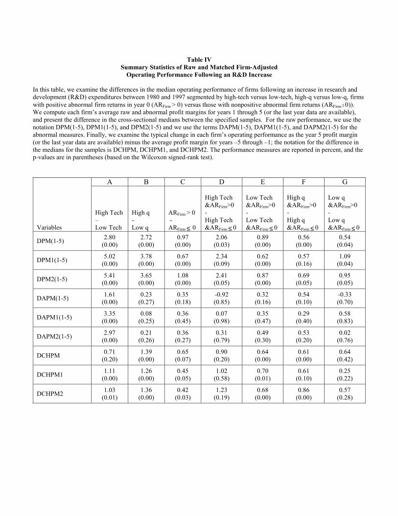
Table IV

Summary Statistics of Raw and Matched Firm-Adjusted Operating Performance Following an R&D Increase

In this table, we examine the differences in the median operating performance of firms following an increase in research and development (R&D) expenditures between 1980 and 1997 segmented by high-tech versus low-tech, high-q versus low-q, firms with positive abnormal firm returns in year 0 (ARFirm > 0) versus those with nonpositive abnormal firm returns (ARFirm�0)). We compute each firm’s average raw and abnormal profit margins for years 1 through 5 (or the last year data are available), and present the difference in the cross-sectional medians between the specified samples. For the raw performance, we use the notation DPM(1-5), DPM1(1-5), and DPM2(1-5) and we use the terms DAPM(1-5), DAPM1(1-5), and DAPM2(1-5) for the abnormal measures. Finally, we examine the typical change in each firm’s operating performance as the year 5 profit margin (or the last year data are available) minus the average profit margin for years –5 through –1; the notation for the difference in the medians for the samples is DCHPM, DCHPM1, and DCHPM2. The performance measures are reported in percent, and the p-values are in parentheses (based on the Wilcoxon signed-rank test).

A B C D E F G

Variables

High Tech – Low Tech

High q - Low q

ARFirm > 0 - ARFirm ≤ 0

High Tech &ARFirm>0 - High Tech &ARFirm ≤ 0

Low Tech &ARFirm>0 - Low Tech &ARFirm ≤ 0

High q &ARFirm>0 - High q &ARFirm ≤ 0

Low q &ARFirm>0 - Low q &ARFirm ≤ 0

DPM(1-5) 2.80 (0.00)

2.72 (0.00)

0.97 (0.00)

2.06 (0.03)

0.89 (0.00)

0.56 (0.00)

0.54 (0.04)

DPM1(1-5) 5.02 (0.00)

3.78 (0.00)

0.67 (0.00)

2.34 (0.09)

0.62 (0.00)

0.57 (0.16)

1.09 (0.04)

DPM2(1-5) 5.41 (0.00)

3.65 (0.00)

1.08 (0.00)

2.41 (0.05)

0.87 (0.00)

0.69 (0.05)

0.95 (0.05)

DAPM(1-5) 1.61 (0.00)

0.23 (0.27)

0.35 (0.18)

-0.92 (0.85)

0.32 (0.16)

0.54 (0.10)

-0.33 (0.70)

DAPM1(1-5) 3.35 (0.00)

0.08 (0.25)

0.36 (0.45)

0.07 (0.98)

0.35 (0.47)

0.29 (0.40)

0.58 (0.83)

DAPM2(1-5) 2.97 (0.00)

0.21 (0.26)

0.36 (0.27)

0.31 (0.79)

0.49 (0.30)

0.53 (0.20)

0.02 (0.76)

DCHPM 0.71 (0.20)

1.39 (0.00)

0.65 (0.07)

0.90 (0.20)

0.64 (0.00)

0.61 (0.00)

0.64 (0.42)

DCHPM1 1.11 (0.00)

1.26 (0.00)

0.45 (0.05)

1.02 (0.58)

0.70 (0.01)

0.61 (0.10)

0.25 (0.22)

DCHPM2 1.03 (0.01)

1.36 (0.00)

0.42 (0.03)

1.23 (0.19)

0.68 (0.00)

0.86 (0.00)

0.57 (0.28)

Table V Long-Term Abnormal Stock, Bond and Firm Returns

This table presents the long-term abnormal stock (ARS), abnormal bond (ARB), and abnormal firm (ARFirm) returns for the Actual Increase sample. These (monthly) abnormal returns (in percent) are the alphas in the time series regressions. The t-values are reported in parentheses below each alpha. All the alphas are significant at the 1 percent level or better. To examine whether there are any long-term abnormal stock, bond, or firm returns following R&D increases, we use the Fama and French (FF, 1993) model to estimate expected stock returns as shown in equation (3):

,)( ptttftmtftStockpt hHMLsSMBRRbRR εα +++−+=− where RStockpt is the average raw return for stocks in calendar month t (where a sample stock is included if month t is within the 60-month period following its R&D increase), Rft is the one-month T-bill return, Rmt is the CRSP value-weighted market index return, SMBt is the return on a portfolio of small stocks minus the return on a portfolio of large stocks, HMLt is the return on a portfolio of stocks with high book-to-market ratios minus the return on a portfolio of stocks with low book-to-market ratios. We follow the procedures explained in Fama and French (1993) for forming the SMB and HML factors. As a robustness check, we also estimate the abnormal stock returns with the Carhart (1997) momentum factor (i.e., return on high momentum stocks minus the return on low momentum stocks) included as an additional risk factor. For the abnormal bond returns, we use the Elton, Gruber, and Blake (EGB, 1995) model of expected bond returns as shown in equation (4):

,654321 ttmtBondMktttttftBondpt TermRRDRPUnxCPIUnxGDPRR εββββββα +++++++=− where RBondpt is the average raw bond return for month t (i.e., the cross-sectional average of each firm’s “one” bond return; where a sample firm is included if month t is within the 60-month period following its R&D increase), UnxGDP is the unexpected change in gross domestic product, UnxCPI is the unexpected change in the consumer price index, DRP is the default risk premium, RBondMkt is the return on the Lehman corporate bond index and Term is the slope of the term structure. We follow the estimation procedures discussed in EGB for the estimation of each factor. We use a composite model of expected firm returns to estimate the abnormal firm returns as shown in equation (5):

tttttftmtftFirmpt UnxCPIUnxGDPpPRhHMLsSMBRRbRR 2112)( ββα +++++−+=− ,6543 ttmtBondMkttt TermRRDRP εββββ +++++

where RBondpt is the average raw bond return for month t (i.e., the cross-sectional average of each firm’s return; where a sample firm is included if month t is within the 60-month period following its R&D increase).

Panels Description of Samples

ARS

(FF Model)

ARS

(FF with Carhart) ARB ARFirm

A

EW Overall sample

VW Overall sample

0.58 (6.50)

0.51 (4.00)

0.59 (6.09)

0.64 (4.84)

0.67 (6.16)

0.65 (5.33)

0.59 (7.28)

0.57 (5.17)

B

EW high-tech

VW high-tech

0.92 (5.11)

0.59 (2.61)

1.06 (5.63)

0.86 (3.62)

0.65 (5.60)

0.64 (6.03)

0.83 (3.95)

0.80 (2.66)

C

EW low-tech

VW low-tech

0.46 (4.34)

0.46 (3.95)

0.44 (4.28)

0.51 (4.89)

0.67 (6.33)

0.64 (5.19)

0.51 (5.88)

0.46 (4.87)

D

EW High-q

VW High-q

0.50 (4.95)

0.47 (3.36)

0.54 (5.25)

0.61 (4.11)

0.68 (6.51)

0.64 (6.25)

0.58 (5.75)

0.58 (3.95)

E

EW Low-q

VW Low-q

0.84 (6.90)

0.61 (3.86)

0.82 (6.80)

0.70 (4.36)

0.68 (5.28)

0.65 (4.17)

0.56 (5.62)

0.41 (3.11)

F

EW (Event-Period AR > 0)

VW (Event-Period AR > 0)

0.57 (5.78)

0.50 (3.50)

0.60 (6.37)

0.63 (4.43)

0.67 (6.35)

0.64 (5.85)

0.63 (8.87)

0.57 (4.60)

G

EW (Event-Period AR ≤ 0)

VW (Event-Period AR ≤ 0)

0.58 (5.50)

0.53 (3.98)

0.59 (4.69)

0.67 (4.80)

0.67 (5.77)

0.67 (4.43)

0.52 (4.47)

0.59 (5.69)