Market structure and market performance in e-commerce

econstor www.econstor.eu

Der Open-Access-Publikationsserver der ZBW – Leibniz-Informationszentrum WirtschaftThe Open Access Publication Server of the ZBW – Leibniz Information Centre for Economics

Nutzungsbedingungen:Die ZBW räumt Ihnen als Nutzerin/Nutzer das unentgeltliche,räumlich unbeschränkte und zeitlich auf die Dauer des Schutzrechtsbeschränkte einfache Recht ein, das ausgewählte Werk im Rahmender unter→ http://www.econstor.eu/dspace/Nutzungsbedingungennachzulesenden vollständigen Nutzungsbedingungen zuvervielfältigen, mit denen die Nutzerin/der Nutzer sich durch dieerste Nutzung einverstanden erklärt.

Terms of use:The ZBW grants you, the user, the non-exclusive right to usethe selected work free of charge, territorially unrestricted andwithin the time limit of the term of the property rights accordingto the terms specified at→ http://www.econstor.eu/dspace/NutzungsbedingungenBy the first use of the selected work the user agrees anddeclares to comply with these terms of use.

zbw Leibniz-Informationszentrum WirtschaftLeibniz Information Centre for Economics

Hackl, Franz; Kummer, Michael E.; Winter-Ebmer, Rudolf; Zulehner, Christine

Working Paper

Market structure and market performance in e-commerce

ZEW Discussion Papers, No. 11-084

Provided in Cooperation with:ZEW - Zentrum für Europäische Wirtschaftsforschung / Center forEuropean Economic Research

Suggested Citation: Hackl, Franz; Kummer, Michael E.; Winter-Ebmer, Rudolf; Zulehner,Christine (2011) : Market structure and market performance in e-commerce, ZEW DiscussionPapers, No. 11-084

This Version is available at:http://hdl.handle.net/10419/54959

Dis cus si on Paper No. 11-084

Market Structure andMarket Performance in E-Commerce

Franz Hackl, Michael E. Kummer, Rudolf Winter-Ebmer, and Christine Zulehner

Dis cus si on Paper No. 11-084

Market Structure and Market Performance in E-Commerce

Franz Hackl , Michael E. Kummer, Rudolf Winter-Ebmer, and Christine Zulehner

Die Dis cus si on Pape rs die nen einer mög lichst schnel len Ver brei tung von neue ren For schungs arbei ten des ZEW. Die Bei trä ge lie gen in allei ni ger Ver ant wor tung

der Auto ren und stel len nicht not wen di ger wei se die Mei nung des ZEW dar.

Dis cus si on Papers are inten ded to make results of ZEW research prompt ly avai la ble to other eco no mists in order to encou ra ge dis cus si on and sug gesti ons for revi si ons. The aut hors are sole ly

respon si ble for the con tents which do not neces sa ri ly repre sent the opi ni on of the ZEW.

Download this ZEW Discussion Paper from our ftp server:

http://ftp.zew.de/pub/zew-docs/dp/dp11084.pdf

Non-technical Summary Analyzing the link between market structure and market performance is of central importance in the field of industrial organization. The aim is to understand the role of market structure, i.e., the number of firms in a market, their sizes and the products they offer, in determining the extent of market competition and market performance. In particular, antitrust and regulatory authorities are interested in knowing how many firms it takes to sustain competition in a market. For example, the expected relation between the number of firms in the market and market outcomes such as prices or qualities is at the core of merger assessments. These questions are of central importance to society and to the consumers, because a minimum level of competition ensures both sufficient provision of the good and reasonable prices for the consumer. In this paper, we investigate the interaction between market structure and market performance in e-commerce for consumer electronics. We use data from Austria's largest online site for price comparisons combined with retail-data on whole sale prices provided by a major hardware producer. We observe firms' prices as well as their input prices, and all their moves in the entry and the pricing game. With this information we can analyze how sellers’ markups over the producer’s wholesale price react to the number of firms that compete in the market. We also look at the impact of market structure on market performance over the product life cycle, as other studies focusing on market structure find that entry has, especially at the beginning of the life cycle, a significant impact on prices. An important contribution of this paper stems from a novel way of dealing with the phenomenon that, it is extremely easy for e-commerce-shops, to add and remove items from their product portfolio. This makes the analysis very difficult, because usually the number of shops will be related to how attractive an item is to sell, and will thus depend on the variables we wish to explain. This situation is an example of the “endogeneity problem”, which can pose a threat to the validity of empirical estimates. We are dealing with this issue by using the information on how many shops typically listed earlier cameras at a particular stage of the life-cycle (in the past). This variable will capture overarching factors in the listing decision (e.g. distribution patterns), that cannot so easily be changed and is hence immune to such issues as whether an item is currently en vogue or not. We find a very short lifecycle of usually less than a year and a highly significant and strong effect of the number of firms on markups. Ten additional competitors in the market reduce the markup of the cheapest firm by more than 1.5 percentage points on average. We also find that this effect is strongest in the first month, but also in the end of the lifecycle. Interestingly, markups were found to be lowest in months 2-4, but at the same time, the number of firms seems to be less relevant to pushing down prices in that stage of the lifecycle. For the consumer this means that by waiting three more weeks she will get the same price reduction she would get by going to a market with one additional firm.

Das Wichtigste in Kürze Die Analyse des Zusammenhangs zwischen der Struktur und der Funktionsfähigkeit eines Marktes ist eine der zentralen Fragen auf dem Gebiet der Industrieökonomie. Dabei gilt es zu verstehen, wie die Marktstruktur (also die Anzahl der Firmen im Markt, deren Marktanteil sowie die Anzahl, Qualität und Charakteristika ihrer Produkte) das Ausmaß des Wettbewerbs im Markt beeinflusst. Vor allem Wettbewerbs- und Regulierungsbehörden wollen wissen wie viele Firmen nötig sind um den Wettbewerb in einem Markt aufrecht zu erhalten. Um nur ein Beispiel zu nennen, bei der Bewertung einer beabsichtigten Firmenfusion ist der zu erwartende Zusammenhang zwischen der Anzahl der Firmen im Markt und den Preisen oder der durchschnittlich angebotenen Qualität die zentrale Entscheidungsgrundlage. Diese Fragen sind folglich von hoher Relevanz für die Gesellschaft und die Endverbraucher, da ein Mindestniveau an Wettbewerb sowohl die Bereitstellung der Güter als auch transparente Preise sicherstellt. In dieser Arbeit untersuchen wir den Zusammenhang von Struktur und Funktionsfähigkeit von Märkten im Bereich des E-Commerce. Hierfür verwenden wir Daten der größten österreichischen Online-Preisvergleichsseite und Vertriebsdaten eines der größten Hersteller von Haushaltselektronik. Wir beobachten die Großhandelspreise, die Preise der Firmen und deren Inputpreise, sowie alle Aktionen der Einzelhändler (Markteintrittsentscheidungen und Preissetzung). Mit dieser Information sind wir in der Lage zu untersuchen, wie der Aufschlag auf den Großhandelspreis auf die Anzahl der Firmen im Markt reagiert. Darüber hinaus analysieren wir, wie sich der Zusammenhang von Marktstruktur und Funktionsfähigkeit über den Lebenszyklus der Produkte verändert, da die Marktstruktur, wie in früheren Studien gezeigt wurde, vor allem am Beginn des Lebenszyklus große Auswirkungen auf die Preise haben kann. Ein wesentlicher Beitrag dieser Arbeit liegt darin, explizit zu berücksichtigen, dass E-Commerce Händler sehr einfach Produkte in ihr Sortiment aufnehmen und bald danach wieder aus dem Sortiment auslisten können. Dies erschwert eine objektive Analyse, da davon auszugehen ist, dass die Anzahl der Firmen von vielen stark variablen Faktoren abhängt. So können Händler beispielsweise darauf reagieren, wie stark ein Produkt in den Medien präsent ist oder wie seine Profitabilität variiert. Wir können dieses Problem lösen, indem wir auf die Information aus früheren Lebenszyklen zurückgreifen, um so zu erfahren, wie viele Händler ein Produkt in einer bestimmten Phase des Lebenszyklus „üblicherweise“ in ihr Sortiment aufnehmen. Diese Variable ist abhängig von langfristigen, zum Teil nicht beobachtbaren, Faktoren (wie zum Beispiel der Vertriebskette), die auf die Sortimentswahl einen Einfluss haben, aber nicht rasch geändert werden können nur weil ein Produkt gerade in Mode ist. Wir gelangen zum Ergebnis, dass der Lebenszyklus der untersuchten Produkte sehr kurz ist und dass ein starker negativer Zusammenhang zwischen der Anzahl der Firmen und der Preisaufschläge im Markt besteht. Zehn Firmen mehr im Markt senken den Preisaufschlag des Bestbieters um mehr als 1,5 Prozentpunkte. Außerdem finden wir, dass der Effekt im ersten Monat besonders stark ist, in den Monaten zwei bis vier etwas abflacht, um dann ab dem sechsten Monat wieder zuzunehmen. Gerade dieses letzte Ergebnis ist gewissermaßen überraschend. Für den Konsumenten bedeutet dies, dass er durch das Abwarten von 3 Wochen dieselbe Preisreduktion erwarten kann wie wenn er einen Markt sucht, auf dem ein Händler mehr anbietet.

�� ∗

��

��

��

��

��

��

�� !�"� � ��#�� $"�$�� #�� %��"� �� #��

"��$�� &�"��"�' �� (%&�� %��$"� &�� ""&� �� )$�&� �� $��&

��)&� �� $�)�� *�� #�� )&� +��"� �� )� ��

�� ( ��$� �� "�%��)&� ��$�� &&��,)�� ,"��"�'

�� "�)�� -$��.� &�� &�� %��"� "�%�� +�� &

�� +�&��&� %��"�� %�� ) � ��/� ��+�� %��$"�� "��$�� &�"��"�'

�� )�� %$� %��"�� *�� && �� %��"�� '

�� 01 �� & "�� +� �� $��& ��)&�� )��

� �� %�. �� "�� %��' �� *�� $�� %��"$&��&

��%�� !�"� � "�%�� #$% � �� %��"� &��'

�� 2 �33� �34� �53� �64

�� 7��&�� 8��$"� �� "&�� #�� $"�$�� #�� 8��"��

��#$%� 8��"� ��%��

∗�� !� �� "��#� �� $%�&'��' ( �� )�� *�� &�� +�� ,�� & � &�� &�� -� �� .-��/ ��%� 0�� , "�)1 .��/�� "��#

�

1 Introduction

Analyzing the link between market structure and market performance is of central importancein the �eld of industrial organization. In particular, antitrust and regulatory authorities areinterested to know how many �rms it takes to sustain competition in a market. For example,the expected relation between the number of �rms in the market and market outcomes suchas prices or qualities is at the core of merger assessments.

We investigate the interaction between market structure and market performance in e-commerce using data from Austria's largest online site for price comparisons combined withretail data on wholesale prices provided by a major hardware producer for consumer elec-tronics. We observe �rms' prices as well as their input prices, and all their moves in theentry and the pricing game. To measure the rate at which oligopoly margins decline towardzero, we analyze how quickly the break-even price-cost margins fall as the number of marketparticipants increases from one to two �rms, two to three �rms, and so on. We also look atthe impact of market structure on market performance over the product life cycle, as otherstudies focusing on market structure �nd that entry has, especially at the beginning of thelife cycle, a signi�cant impact on prices.1

The use of data from online markets has been pioneered by the studies of Brynjolfsson andSmith (2000) and Baye et al. (2004) who used online data to study the relationship of pricesand competition on online markets. They also analyzed the distribution of prices and foundthat price dispersion increases with the number of competitors. Since then, a large variety ofissues have been studied with online data. Baye et al. (2009) have examined the Kelkoo pricecomparison site and noted that there is a big discontinuity in clicks at the top listed products,a result which can be explained with clearinghouse models. Both, Ellison and Ellison (2005)and Ellison and Ellison (2009) have examined the competition of Internet retailers and haveidenti�ed di�erent internet-speci�c �rm strategies which are applied in online markets to copewith the increased price sensitivity of online markets.

The prime advantage of e-commerce is the easy availability of large amounts of data onretail-prices at very little cost for the researcher. Moreover, it is generally possible to observeall the prices and price changes of the �rms and to reconstruct the sequence in which theyreact to each other. More than that, it is possible to obtain data for many di�erent markets,be it books or consumer electronics. However, the researcher faces the disadvantage that hedoes not always observe the entire market, but only a segment, and he usually cannot tellwhether a posted price has also induced a transaction or not.

Our point of departure is the study by Haynes and Thompson (2008b), which exploits dataon digital cameras. Their study, which is related to a similar study by Barron et al. (2004),provides useful insights into the evolution of prices and price dispersion as a function of themarket structure. Underlining the potential of research on e-commerce data, the study usesdata for about 400 models of digital cameras in the US. It also takes �rst steps towards takingthe life cycle of consumer electronics into account, even though mostly by regarding life cyclee�ects as a nuisance parameter. Moreover, the authors point to the problem of potentiallyendogenous explanatory variables and emphasize the need of adequately incorporating sellerheterogeneities. They cannot do so, because they only observe the aggregate data that's

1Examples are Berry (1992), Campbell and Hopenhayn (2005), Carlton (1983), Davis (2006), Dunne,Roberts and Samuelson (1988), Geroski (1989), Mazzeo (2002), Seim (2006), and Toivanen and Waterson(2000, 2005).

2

publicly available. The present study proposes to expand on their analysis, by developingan instrument for the number of sellers in a market and to focus on the determinants of theproduct life cycle. Haynes and Thompson (2008a) use less detailed data to take a �rst steptowards explaining entry and exit behavior in a shopbot. To do so, they estimate an error-correction model and show that the entry and exit into a market is correlated with a measureof lagged price-cost-margin and the number of competitors. Also, in the marketing literatureMoe and Yang (2009) recently analyzed the product life cycle in e-tailing. However, like theliterature in IO, their data did not allow them to take the endogeneity of entry and exit intoaccount.

Our paper sheds light onto the question how market structure a�ects the functioning of amarket and the price level. Most importantly we are able to take a �rst step to circumventingthe usual di�culty instrumenting the number of competitors in a market. Clearly, even ifunder potentially reversed signs, these questions are also of great interest to consumers andmanufacturers who wish to maximize their bene�ts. We �nd a highly signi�cant and stronge�ect of the number of �rms on markups. Ten additional competitors in the market reducemedian markups by 0.22 percentage points and the minimum markup by 0.57 percentagepoints. However, accounting for the potential endogeneity of markups and the number of�rms in the market, we see a substantially higher negative e�ect: ten additional retailersreduce the markup of the median �rm by 0.85 percentage points and the markup of thecheapest �rm by 1.72 percentage points.

The remainder of the paper is organized as follows. We present the theoretical predictionsin Section 2 and describe the data as well as the empirical strategy in 3. We discuss ourestimation results in Section 4 and conclude with Section 5.

2 Theoretical Predictions and Relationship of Interest

The point of departure for the present study is a series of two papers by Barron et al. (2004)and Haynes and Thompson (2008b). Both confront the predictions of competing model withdata that relate the market structure to price level and price dispersion but both have to takethe number of competitors in a market as exogenously given, which they themselves point outis possibly not warranted. In what follows we shall brie�y summarize their discussions of thedi�ering predictions of the competing models to be tested.

Grossly speaking, we distinguish three groups of models which allow for price dispersionand hence a violation of the law of one price: Firstly, search theoretic models (Varian (1980),Rosenthal (1980)), which successfully allow price dispersion by introducing heterogeneity inthe search costs of consumers. Secondly, models of monopolistic competition (e.g.: Perlo� andSalop (1985)) can account for price dispersion, when extended by introducing asymmetriesacross �rms, such as heterogeneous producer cost or heterogeneous producer demand (cf.Barron et al. (2004)). Thirdly, Carlson and McAfee (1983) present a search theoretic modelwhich accommodates two sources of heterogeneities by assuming a non-degenerate distributionof producers' marginal cost and heterogeneous visiting cost of the consumers. Combining thesetwo types of heterogeneity results in somewhat di�erent predictions about the behavior of priceand price-dispersion, given an increase in the number of competitors. Finally, also a simplestructure-conduct-performance model (Bain (1951)) can be tested in this context (althoughwith somewhat vaguer predictions), as was pointed out by Haynes and Thompson (2008b).

3

While all these models di�er signi�cantly in their setup, they all have something to sayabout the impact of market structure on prices and price dispersion. Hence evidence aboutthis relationship is important to test them and to tell which of them is most suitable to thinkabout a market at hand. For the present purposes it su�ces to skip a detailed discussion andmerely provide a very brief overview over the di�erent predictions of the models.2

The �rst group of search theoretic models (building on di�erent consumer types, that areequipped with di�erent search costs (e.g. Varian (1980))), predicts that an increased numberof sellers results in a larger price dispersion and, somewhat against intuition, a higher averageprice. The second group of models with di�erentiated sellers and either production cost orbuyer cost asymmetries would expect that a larger number of sellers is associated with alower average price and smaller price dispersion. Thirdly, the model by Carlson and McAfee(1983) predicts that average prices would go down while price dispersion is expected to rise.According to a structure-conduct-performance model where the incumbents face the threat ofentry, prices should decrease or stay equal when more �rms enter the market, depending onthe strength of the entry-threat. The model is somewhat silent about price dispersion.

3 Data and Empirical Strategy

Price search engine: In our analysis we use data from the largest Austrian price comparisonsite www.geizhals.at3. This platform is Austria's unchallenged market leader for comparingprices quoted by retailers of consumer electronics. For the study in this paper we use daily

data on 70 items4 from a major hardware manufacturer5 which launched during the periodfrom January 2007 till December 20086. We de�ne a camera's birth by it's appearance ongeizhals.at. The cameras were on o�er at up to 212 sellers from Austria and Germany.

Available Data: For time t (measured in days) we observe for each product i and retailer jthe priceijt, the shipping costijt posted at the website

7 and the availabilityijt of the product8.

Additionally, we observe the customers' referral request (clicksijt) from the geizhals.at websiteto the retailers' e-commerce website as proxy for the consumers' demand. Customers have thepossibility to evaluate the (service)quality of the �rms on a 5-point scale the average of whichis listed together with the price information on geizhals.at. Wholesale prices for each producti at time t were obtained from the Austrian representative of the international manufacturer.We do not claim, that these wholesale prices correspond perfectly to the retailers' marginal

2For a more detailed discussion of the models the interested reader is referred to the two papers by Barronet al. (2004) and Haynes and Thompson (2008b) our work builds on or to the original papers. Their discussionis clever, concise and insightful, but repeating it here would not add any further insights.

3Based on this data set Dulleck et al. (2011) analyze the search and purchasing behavior of buyers in whichthe reliability of the retailer gets more important the closer it comes to actual buying decisions.

4digital single lens re�ex cameras (DSLR), single lens re�ex cameras (SLR) and laser printers5The hardware manufacturer is a multinational corporation specialized in manufacturing of electronic equip-

ment in several areas. The manufacturer asked to keep his name anonymous. If somebody wants to check thevalidity of our results we can o�er more detailed information on the manufacturer.

6For our instrumentation strategy we will use also the product life cycle of cameras entering the marketstarting from May 2006.

7Shipping cost is the only variable which has to be parsed from a text �eld. We use the information oncash in advance for shipping to Germany, which is the type of shipping cost most widely quoted by the shops.Missing shipping cost are imputed with the mean shipping cost by the other retailers.

8If the product is available immediately or at short notice the dummy is 1, if the product is available onlywithin 2-4 days it is 0.

4

cost. Even though the manufacturer's distribution policy indicates that the retailers shouldbe served by the local representative it may happen, that single retailers procure commoditiesfor instance from the Asian market. Moreover, the local representative might o�er specialpromotions including lower wholesale prices in exceptional cases (e.g. if a retailer commitsto promote the manufacturers good in a special way). Finally, it has to be mentioned thatbesides the wholesale price the retailers in e-commerce might have additional cost each timethey order. Despite the fact that we cannot be entirely sure that each and every e-commerceretailer is always ordering at the wholesale prices we were provided with, they are a very goodproxy for the actual marginal cost the retailers' are confronted with9. Priceijt and wholesale

priceit were used to calculate the �rms' markupijt (using the Lerner index) and the markets'price dispersionit.

Organization of data: We reorganized the data in a way so that the product life cyclesof all digicams start at the same day 1. Hence, we have shifted the product life cycles ofthe digicams so that we can analyze the impact of market structure on markup and pricedispersion in a cross section of 70 product life cycles. This reorganization of data is alsoimportant to guarantee that observations are iid. Especially the independence assumption iscrucial as listing decisions of e-commerce traders are strategic variables: If we studied productcycles in real time the decision to list digicam X might be related to the listing decision ofthe follower model Y. By shifting the product life cycles to identical starting points the iidassumption concerning our data structure is valid. We de�ne the end of a product life cycle ifthe amount of referral requests diminish to less than 500 remaining clicks. Finally, we collapsethe data in order to create a panel with products as units of observation and thus obtain adaily unbalanced panel with information on the products' age, the number of �rms, averagemarkups, markup of the price leader, di�erent measures for price-dispersion, and the number

of clicks.

Descriptives: Table 1 contains summary statistics of the collapsed two-dimensional panel-data. Each observation in the descriptives refer to a single product i at a given day t inthe product life cycle. We will use the markup (=Lerner Index) and the price dispersion asendogenous variables. Whereas the median markup amounts to 17.8% on average, the meanmarkup for price leaders is only 4.6 %. These numbers are of comparable size as in Ellison andSnyder (2011), who report an average markup of 4% for memory modules on Pricewatch.com.We use di�erent measures for the price dispersion: the coe�cient of variation and the standarddeviation of the distribution of prices, as well as the absolute price gap between the price leaderand the second cheapest price. The absolute price gap varies between 0 and 515.9 Euro witha mean of 11 Euro. On average a product life cycle amounts to 166.7 days with a mean of104.3 �rms which are o�ering the digicams. Visual inspection of the data (see Figure 2) showsthat the estimated markup declines with age, and, more importantly, as the number of �rmsincreases (each observation again corresponds to the data of a single product i at a givenday t). However, this pattern is by no means very abrupt, as one might expect in perfectlytransparent e-commerce markets. We rather observe a well positive average markup, alsowith 70 and more �rms in the market. In the top left panel, the median markupit is scatteredagainst the number of firmsit in the corresponding market and the top right panel showsthe average. The number of �rms ranges from 0 to slightly more than 200 and the median

9According to the Austrian distributor the Austrian and German list of wholesale prices are almost identical.Note the manufacturer's incentive to keep cross-border sales between distributors and retailers as low as possibleif the manufacturer were to pursue substantial price discrimination between countries.

5

markup ranges from 0% to 35.2%. It must be noted that we also observe negative markupsespecially for the minimum price �rms - the average markup of price leaders is 4.8% witha standard deviation of 7.9%. In our dataset we observe for 26.92 % of all best price o�ersnegative markups. This is in line with Ellison and Snyder (2011) who report also a substantialamount of price o�ers with negative markups for Pricewatch.com. Negative markups mighthave several possible causes: They might simply point to sell-outs after overstocking, it mightbe a hint to cases where retailers are not procuring via the o�cial retail channels but exploitprice di�erentials with, for instance, Asian markets. Finally, loss leader strategies might beresponsible for negative markups where a digicam is o�ered at a price below marginal cost inorder to attract new customers or to make pro�ts with complementary goods. In the middlerow the median mark-up is plotted against the age of the product. Again the markets' medianmarkups fall on average with the duration of the product life cycle. If the product is availablethe retailer has the incentive to raise the price to the rivals's level. In the lower row, themedian markup is plotted against the age of the camera (in months). We typically observea camera between 7-8 and 15 months. While the line for the averages looks very smooth,the scatter plots on the left of the graphs reveal however, that there is large heterogeneity.Apparently there are three types of digicams: Some appear to be listed by fewer shops (20and 60, respectively) and then to be taken o� the market sooner, whereas another group ofcameras seems to be listed by roughly 150 shops on average and then to be taken o� themarket only after 14 months. The apparent segregation of markets is striking. As expectedwe observe rather fast market entry within the �rst two months - after that the amount of�rms stagnates. Summarizing the descriptive results it can be stated that markup declinesvery slowly, given that �rms have to compete in prices in this market. Secondly, the life cycleof digital products is short enough to not only allow observing their entire lifecycle, but alsoobserve many thereof, which is the feature our instrumentation strategy shall build on.

Empirical Strategy: In order to estimate the impact of market structure on markups andprice dispersion, we estimate the following �xed-e�ects regression as our baseline model:

markup = αj + α1 ∗ age+ α2 ∗ age2 + β1 ∗ numfirms+ β2 ∗ (numfirms)2 + εjt

Dependent variables depvars are the minimum markup, price dispersion (measured as thecoe�cient of variation) and the markup of the median-price and we regress each of themseparately on the number of �rms in the market that day. Moreover, we include a quadraticage-trend and thus measure life-cycle e�ects as a byproduct.10 However, before we can doso we have to account for the fact, that it is very easy to list and unlist an item. Hence thenumber of sellers can react extremely fast on the market characteristics like markups or pricedispersion.

Sources of Endogeneity : In all markets - but in particular in an e-tailing shopbot market- it is important to treat market structure as endogenous: due to simple and low-cost marketentry and exit, e-tailers can easily adapt to changing circumstances by listing a particularproduct.

Generally, we are worried about two sources of potential endogeneitiy: i.) heterogeneity ofthe cameras in the market (quality, design-features etc.) and ii.) the shops' ability to quicklyreact to rising or falling markups of to be earned with a speci�c model by simply moving in

10In all the estimations we included month dummies to account for seasonality e�ects.

6

and out of the respective markets. Since our design is based on �xed e�ects estimation, we areless concerned about the heterogeneity of products. However, we still have to worry about thesecond source of endogeneity, which is due to the simultaneous determination of the markupsand the number of �rms.

If, for example, some unobserved factor temporarily drives up markups for some item,shops which did not sell the item before, might move into this market. Thus, we would expectto observe more shops in markets where higher markups can be reaped and vice verca. This,in turn, might result in the econometrician estimating a less negative relationship of interestthan actually appropriate. This is easily illustrated by looking at the system in which markupsand the number of �rms are simultaneously determined, and where we are interested in the�rst of the following two relationships.11

(1) markupjt = δj + α1 ∗ numfirmjt + β1Z1 + ε1,jt

(2) numfirmjt = γj + α2 ∗markupjt + β2Z2 + ε2,jt

Substitution of the second into the �rst equation and rearranging, gives the reduced formfor the number of �rms:

(3) numfirmjt = πj + π21Z1 + π22Z2 + ujt

with φ := 11−α2α1

, πj = φ(γj + α2δj), π21 = φα2β1, π22 = φβ2 and �nally ujt = φ(α2ε1 + ε2).

In equation (1) the issue is whether numfirmjt and ε1,jt might be correlated due tosimultaneity (z1 and ε1 are by assumption uncorrelated). Yet, from equation (3), it is easyto see, that Cov(numfirmjt,ε1,jt) is typically not 0, since ujt is a linear function of ε1,jt.Unless α2 = 0, this tells us that estimation of equation (1) by OLS will result in biased andinconsistent estimates of the α1 and β1. More precisely we have:

(4) Cov(numfirmjt, ε1,jt) =α2

1− α2α1∗ V ar(ε1)

and hence regressing markup on numfirm will return the biased estimate:

α̂1,OLS = α1 +Cov(numfirmjt, ε1,jt)

V ar(numfirmjt)= α1 +

α2

1− α2α1∗ V ar(ε1)

V ar(numfirmjt)

Closer examination of this result reveals, that the bias α21−α2α1

∗ V ar(ε1)V ar(numfirmjt)

is positive,

whenever α2 > 0 (more �rms enter, when markups are high) and α1 < 0 (markups decreasewhen the number of �rms increases). Therefore, if these conditions are satis�ed, we wouldexpect an upward bias of the OLS-coe�cient of numfirm.

11Note that in the illustration we only look at a linear regressor to be instrumented and neglect the quadraticterm. This corresponds to the estimations we show in Columns (1) and (2) of tables 3 and 4.

7

Instrumentation strategy: In order to cope with this endogeneity problem we follow anIV-approach and instrument the number of �rms. For that purpose we exploit the fact thatin the full Geizhals.at data, we observe the complete lifecycle of many products of the sameproducer and that they were launched in di�erent points in time. For markets with brandnames a part of the listing decisions can be explained by common patterns, such as establishedsupply-relationship shops might have with a producer or a wholesale importer, or variationsin the availability. These patterns remain the same over time and they are not in�uenced bycontemporary �uctuations on a speci�c camera. We exploit this fact in order to devise aninstrument for the number of �rms, based on the shops' behavior in the markets of previouslyintroduced products. In other words, we use the timing of listing decisions of e-tailers forbrand products of our manufacturer in the past as an instrument for current listing decisions.Clearly, such past decisions - in particular if they come from di�erent markets (e.g. digitalcameras versus computer products) will be relevant predictors of the listing decisions today.On the other hand, the instrument is based on the exclusion restriction, that the shops, whentaking their listing decisions in the past, did not take into consideration the current, thenfuture, digital cameras.

The instrumentation strategy is illustrated with an example in Figure 1, which representsan e-tailer, which we shall call 0815 for the sake of illustration, and its listing decisions overtime: let us consider whether shop 0815 will list a product F , on the 10th day after intro-duction. This decision is represented by the encircled red line on item F . We predict theprobability of this event by the shop 0815's general probability of listing a similar item thathas been on the market for 10 days. Considering only the items that saw light before productF was introduced we �rst �x the number of such items we wish to consider (to three, here).Then we can calculate how many of those items, were listed by shop 0815 on the tenth dayafter they appeared and taking the share gives us a readily available estimate of shop 0815'sprobability to list product F on its 10th day of existence.

This method can easily be extended to the �rst, second, third, twentieth, etc. day. Thus,simply calculating the share of products listed on a given day in earlier life cycles, we obtainan estimate of shop 0815's probability to list an item (F ) on it's �rst, second, tenth, etc.day of existence. Thus, repeating the exercise in order to predict what shop 0815 will dowith Camera D on the third day (highlighted by the green encircled dash), we look at the"average decision" for products A, B, and C on the third day. Note, that we ignore F and itspredecessors when instrumenting D, because they were introduced after D. Also note, thatfor instrumenting F we ignored A - D, because we had decided that those cameras lay too farin the past of F .12 In a last step, we aggregate these probabilities across shops to obtain thepredictor of the number of shops that will o�er item F on a given day. 13

12N.B.: When calculating the instrument, we �xed the number of earlier cameras to 3. This number canbe varied by the researcher, depending on how �ne grained the instrument needs to be and the number ofavailable products. As �xing the number of cameras to three resulted in a reasonably strong instrument, wefavored this speci�cation over one, where we have fewer data available in the estimation. However, we alsotried an alternative speci�cation with 5 cameras, which resulted in very similar estimates. Moreover, ratherthan �xing the number of cameras, the researcher might prefer to �x a time-period (e.g. 6 months before Fwas introduced) and include all cameras that saw light during that period. The latter way of framing theinstrumentation strategy does not ensure however, that the same number of products is used for calculatingthe shares needed for the instrument. Therefore to obtain valid standard errors additional bootstrapping -methods will be needed.

13Note that the method we suggest can be used even if only market-level data are available, simply by takingthe average of the number of �rms that listed the earlier product on the given day.

8

Figure 1: Instrument uses �rm's listing behavior in earlier lifecycles

time

Camera A

Camera B

Camera C

Camera D

Camera F

3 Observations

Notes: If we want to predict how many shops will list a product on any given day q after introduction we use ashop's general probability of listing one of the three items that entered the market before product j, q days after theywere introduced. Examples: To predict listing behavior for Camera D on day 3 (encircled green dash), we would useinformation on Cameras A, B, and C on their respective third days of existence (highlighted green dashes). However,we would not use the information from the Cameras that saw light after D (illustrated by a black dash on day 3). Now,to predict how many shops listed camera F on day 10 (encircled red dash), we would use the information only from thecameras that saw light later than (excluding) Camera D, provided they entered the market before F (highlighted reddashes). Cameras A, B, C (black dash on day 10) and also models younger than camera F would be ignored for thecomputations relevant to Camera F .

9

First-stage regressions: As we use the time patterns of previous listing decisions in com-pletely di�erent markets our instrument should not have a direct causal implication on today'smarkups and price dispersion. Table 2 presents the �rst stage regressions and show that theinstrument is strong enough to explain the markets actual entry decisions depicted by thenumber of �rms at each point in time of the product life cycles. Columns (1) and (2) comparethe contribution of the instrument to explaining the number of �rms, and columns (3) and (4)show the contribution to its quadratic term. It is easy to see that the instrumental variablesof interest are signi�cantly di�erent from 0 with a probability of more than 99.99%. Moreoverthey improve the predictive value of the model. The R2 in the baseline regression without theinstrumented number of �rms (not shown in table) amounts to 0.434. Adding our instrumentfor the number of �rms raises the R2 by 0.0111 in column (1) from 0.434 to 0.446. For theother columns even higher marginal R2 are computed. We also computed the F-statistics totest the null-hypothesis that the excluded instruments are irrelevant in the �rst-stage and theyexceed the critical value of 10 substantially. With F-values well above 300 we can prove thatour instruments are strong enough to explain the variation in the number of �rms over thelifecycle. For the following analysis we use columns (2) and (4) of Table 2 to calculate thepredicted number of �rms for the second stage regressions.

4 Results

4.1 Market Structure and Market Performance

Tables 3 and 4 show our basic results for the impact of market structure on markups. Thesebaseline speci�cations are parsimoniuous, as they consider only the number of �rms on themarket - either linearly or in quadratic terms - and the product life cycle. Moreover, to accountfor seasonal e�ects, we add an indicator variable for o�ers that were quoted in December14.All product-speci�c in�uences are covered by a product �xed-e�ect. Columns 1 and 3 showOLS estimations, whereas in Columns 2 and 4, our instrumental variables approach is used.

Our results indicate a highly signi�cant and relatively strong e�ect of the number of �rmson markups. Not accounting for the endogeneity of the number of �rms and using OLS,we would estimate the e�ect of ten additional competitors in the market to reduce medianmarkups by 0.22 and minimummarkup by 0.57 percentage points. The reaction of the cheapest�rm is signi�cantly higher as compared to the reaction of the median �rm, which might beexplained by the high frequency with which prices are changed in online markets, where thecheapest price is a focus of considerable attention of both consumers and �rms.

If we instrument for the number of �rms, we see a substantially larger negative e�ect: 10additional retailers reduce the markup of the cheapest �rm by 1.72 percentage points and themarkup of the median �rm by 0.85 percentage points. These �gures are large in economicterms considering the standard deviation of the number of �rms in our sample - 57 �rms. Aswas discussed above, OLS is likely to underestimate the true e�ect of an additional �rm onthe markup, as it does not account for the fact that attractive items also attract more �rms.Again, the reaction of the cheapest �rm is considerably higher as compared to the median�rm.

In Columns 3 and 4 we use a quadratic speci�cation of the number of �rms: it turns out

14The results for this variable are omitted in the tables to follow.

10

that there is a solid negative - but decreasingly negative - in�uence of the number of retailerson markup, both for the cheapest as well as the median markup. Numerically, for the cheapestprice, the negative in�uence of the number of �rms ceases at 560, for the median markup with340 �rms. As the maximum number of �rms in our sample is 203, we can safely assume thatfor most part of our sample, this negative relationship is a valid description. Also note that,while the median markup remains positive throughout, the minimum markup falls below 0for very large numbers of sellers.

Looking at the impact of the product cycle on markups, the picture is not entirely clear:in all 2SLS regressions markups grow in the beginning and go down after the �rst few monthsuntil the end of the product life cycle. For the minimum markup the turning point is between�ve and six months (Columns 2 and 4 of Tables 3 and 4) which is around the mean durationof a product life cycle of 5.5 months. For the median markup the turning point is with eightto nine months slightly above the mean duration of the product life cycle.

To investigate the impact of the number of sellers on price dispersion we concentrate onthe coe�cient of variation (Table 5). While the OLS regressions show a somewhat negativerelation between the number of �rms and price dispersion, in the 2SLS results in Columns2 and 4, we see a strong positive relationship. In the linear case, increasing the number of�rms by 10 increases the coe�cient of variation by 0.03. The situation is quite similar in thequadratic case (Column 4): up to a level of 120, increasing the number of �rms always leadsto higher price dispersion and also after that, though declining, it remains large beyond thelevel of 200 �rms.

The combined results on markups and price dispersion are compatible with the model(Carlson and McAfee, 1983), i.e. a search theoretic model which accommodates two sourcesof heterogeneities by assuming a non-degenerate distribution of producers' marginal cost andheterogeneous visiting cost of the consumers. The other search theoretic models are not inline with our �ndings of a decreasing median markup. Models of monopolistic competition,on the other hand, predict a decreasing price dispersion, which contradicts with our �ndingsabout the coe�cient of variation.

In Table 6 we present the e�ect of the market structure on shipping cost. The patterns arelargely the same as in Tables 3 and 4. While OLS predicts a positive relationship of shippingcost and the number of �rms, Columns 2 and 4 reveal a robust negative relationship with aninsigni�cantly small quadratic term. Ten more �rms actually decrease the average shippingcost in that market by 7 cent, again a large number bearing in mind the standard deviationof 57 �rms.

4.2 Lifecycle E�ects

In this section we investigate, whether the pro�t-squeezing e�ect of a higher number of �rmsis the same in di�erent phases of the product life cycle. To do this, we extend the model tocheck for di�erent e�ects of market structure on markups over the product cycle.

In Table 7 we estimate the baseline model and add crossterms, interacting the number of�rms with age (both linearly and quadratically). For ease of interpretation of the coe�cients,in Figures 3 and 4 we also plotted how markups are predicted to depend on the number of�rms, separately for di�erent stages of the product life cycle.

In these plots, each line represents a product of certain age and we plotted the curvefor products right after their introduction, and after 1, 2, 3, 6 and 9 months in the market,

11

respectively. To make the picture clearer, we concentrate for each phase of the life cycle onthe typical situation concerning the number of �rms.15 Interestingly, our plots show a veryconsistent pattern, which appears to consist of three phases. In Figure 3 we see the patternfor minimum markups. Apart from the months in the middle, we see a clear pattern: markupsdecline with more �rms. This pattern, however, is less pronounced during months 2 - 4 wherewe observe a movement to the right, with more �rms entering while markups remain stable.The estimated curves for those months resembles a J shape, indicating a small negative e�ect.Only towards the end of the cycle (month 6 and later) competitive pressures become morepronounced and the relationship becomes clearly negative again.

Comparing the 6 curves, we can look at how markups develop over time: First markupsfall drastically, but then they stabilize and even slightly recover. Figure 3 shows the minimummarkup remaining which decreases below 0 within 2 months. However, after that it remainsclose to 0 with more or less �erce competition, depending on the lifecycle phase. For thecase of median markups in Figure 4, we can see a fairly similar pattern: More �rms in themarket means lower median markup, particularly in the beginning and towards the end of thelifecycle. Again, there is an initial reduction of markups over the time of the life cycle, butthis trend turns around after three months and then the median markups even slightly riseagain.

4.3 Robustness

Several robustness checks were performed and we shall present them in what follows. First, wetest the robustness of the basic results by using varying de�nitions of price dispersion and byusing other de�nitions of markups, i.e. by including shipping costs into sales prices. Moreover,at the end we take account of the fact that some of the price o�ers attract less attention ofpotential buyers; we use click-weighted markups to control for this.

Our �rst robustness check in Table 8 concerns our de�nition of price dispersion. We ex-periment with di�erent de�nitions: apart from the coe�cient of variation we use the standarddeviation of prices and a coe�cient of variation calculated in such a way, that the prices areweighted with the number of clicks they received. All these variations show a similar pattern:increasing number of �rms is �rst increasing, then slightly reducing price dispersion; in allcases, the turning point is above the average number of �rms in the sample. Interestingly,applying the click-weighting increases the turning point even further, to 175 �rms.

The next robustness check in Table 9 concerns the measurement of prices. Consumerstypically pay the product price plus shipping costs. It is well-known that �rms can followspeci�c price-setting strategies to set visible prices - the product price - very low and non-visible prices, like shipping costs, etc. relatively high (see Ellison and Ellison (2009)). In sucha case, the total price including shipping costs should be used to calculate the markup ofthe �rm. Unfortunately, we do not know "actual" shipping costs of the �rms, therefore, wecalculate an arti�cial markup: product price plus announced shipping costs minus wholesaleprice. As there are di�erent shipping costs possible, we concentrate on those, which are mostlyobserved in the data, which are shipping costs to Germany when paying cash in advance. If�rms can vary their announced shipping costs, they should also react to the market structure;i.e. the number of �rms in the market. In Table 8 we show that, in fact, our qualitative results

15We plot only in the region between the 33rd and 67th percentile of the distribution concerning �rm sizesto avoid extrapolation of the polynomials.

12

are fairly similar, just more pronounced: both minimum and median markup decline with thenumber of �rms and price dispersion is increasing.

We investigate further whether our results are in�uenced by the fact we treat all prod-uct o�ers symmetrically in our regressions. In particular, in questions of price dispersionresearchers mistrust typically price o�ers which are way too high (cf. Baye et al. (2004)).This suggests to weigh price o�ers with the number of clicks they are receiving in order togive the low ranked - and maybe less reliable - price o�ers less weight.16 When we do this inTable 10, we see our main results unchanged or reinforced.

Finally, we wanted to see whether our results are due to changes in the composition of theshops o�ering an item over the life cycle. Particularly the presence of larger shops or of shopswho sell not only on geizhals.at, but also dispose of a brick and mortar outlet might a�ect theoutcomes in our estimation. Therefore in Tables 11 - 13 we include the composition of shopsin the regression. In these tables, Column 1 shows the quadratic 2SLS estimation from Tables3, 4 and 6. We then add the share of �rms that have the item stocked, the share of �rms withlow reputation, the share of low-price �rms, the share of large �rms and the share of shopswith a brick and mortar facility. All of these shares are scaled on a range from 0 to 100, i.e.if in Table 11 the share of large �rms increases by ten percent, this is associated with a dropin median markups by 0.62 percentage points.

First of all it should be noted, that the pattern that we observed in the baseline-speci�cation,is una�ected by taking into account several measures of shop composition. There is some rel-atively small variation in the size of the coe�cients and for shipping costs some e�ects are nolonger signi�cant when controlling for the composition of shops. Yet, grosso modo the patternsremain largely una�ected. Secondly also the estimated coe�cients for the shop composition'simpact on the markups are of some interest. In all the tables, markups and shipping cost fallas the share of larger �rms (Column 5) and the share of �rms with low reputation (Column 3)increases. The decrease of markups is more pronounced for the size of the �rms. The patternis somewhat ambiguous for the share of low price �rms (Column 4). While a higher shareof low price �rms slightly decreases median markups and shipping cost, the estimation forthe minimum markup appears to indicate otherwise. Even though accompanied by a greatercoe�cient for the e�ect of the number of �rms the coe�cient for the share of low-price �rmsis positive, which is somewhat counterintuitive. Finally, the share of �rms which have theitem on stock (Column 2) and the share of �rms which also have a brick and mortar facility(Column 6) is related to an increase in both markups and shipping cost.

5 Conclusions

In this paper we estimate the e�ect of market structure on market performance in e-commerce.As endogeneity of market structure and market performance might be an issue, we use thebehavior of sellers in high frequency product life cycles to develop an instrumental variable forthe number of �rms in a market. To analyze the e�ect of market structure, we use data on 70di�erent digital cameras and �nd that an increase in the number of sellers in a market by 10reduces the mark up of the price-leader by 1.72 percentage points and that of the median �rmby 0.85 percentage points. While we also �nd negative correlations between market structureand performance using OLS regressions, we show, that these coe�cients are likely to be biased

16Note that the third column of this table is the same as in Table 8 as it was relevant to both questions.

13

upwards, due to simultaneity. To correct for this problem we propose an instrumental variablestrategy, which is based on regularities in listing behavior over the product life cycle. Indeed,our results, which allow for a causal interpretation, are stronger. Moreover, we �nd a positivee�ect of the number of �rms on the coe�cient of variation of prices.

When we di�erentiate market structure e�ects over the full life cycle of a product, we �nda negative impact especially in the beginning and the late phases of the life cycle. Moreover,we �nd somewhat diminished e�ects in the stage that corresponds to an age of 2-4 months.Our results refer to e-tailing in the presence of a price-search engine with very narrowly de�nedproducts. In such a situation, consumers can very easily collect information about prices andreliability of the sellers. Still, it takes a large number of sellers and a relatively long time untilmarkups of �rms dissipate.

The markup of the price-leader diminishes as well over the life cycle of the product. If weevaluate our results at sample means we can compare the competitive e�ect of more �rms tothe e�ect of time: having one more �rm in the market reduces the mark up of the price leaderby the same amount as three additional weeks in the product life cycle. In other words: Bywaiting three more weeks a consumer will get the same price reduction she would get if shewent to a market with one additional �rm.

14

References

Bain, J.S., �Relation of pro�t rate to industry concentration: American manufacturing, 1936-1940,� The Quarterly Journal of Economics, 1951, 65 (3), 293�324.

Barron, J.M., B.A. Taylor, and J.R. Umbeck, �Number of sellers, average prices, andprice dispersion,� International Journal of Industrial Organization, 2004, 22 (8-9), 1041�1066.

Baye, M.R., J. Morgan, and P. Scholten, �Price dispersion in the small and in the large:Evidence from an internet price comparison site,� The Journal of Industrial Economics,2004, 52 (4), 463�496.

, J.R.J. Gatti, P. Kattuman, and J. Morgan, �Clicks, discontinuities, and �rm demandonline,� Journal of Economics & Management Strategy, 2009, 18 (4), 935�975.

Berry, Steven T., �Estimation of a model of entry in the airline industry,� Econometrica,1992, 60 (4), 889�905.

Brynjolfsson, E. and M.D. Smith, �Frictionless commerce? A comparison of Internet andconventional retailers,� Management Science, 2000, 46 (4), 563�585.

Campbell, J. R. and H. A. Hopenhayn, �Market Size Matters,� Journal of Industrial

Economics, 2005, 53, 1�25.

Carlson, J.A. and R.P. McAfee, �Discrete equilibrium price dispersion,� The Journal of

Political Economy, 1983, 91 (3), 480�493.

Carlton, D. W., �The Location and Employment Choices of New Firms: An EconometricModel with Discrete and Continuous Endogenous Variables,� Review of Economics and

Statistics, 1983, 63, 440�449.

Davis, Peter, �Spatial Competition in Retail Markets: Movie Theaters,� Rand Journal of

Economics, 2006, forthcoming.

Dulleck, Uwe, Franz Hackl, Bernhard Weiss, and Rudolf Winter-Ebmer, �BuyingOnline: An Analysis of Shopbot Visitors,� German Economic Review, 2011, 12 (4), 395�408.

Dunne, Timothy, Mark J. Roberts, and Larry Samuelson, �Patterns of Firm Entry andExit in U.S. Manufacturing Industries,� Rand Journal of Economics, 1988, 19 (4), 495�515.

Ellison, G. and S.F. Ellison, �Lessons about Markets from the Internet,� Journal of Eco-nomic Perspectives, 2005, 19 (2), 139�158.

and , �Search, obfuscation, and price elasticities on the internet,� Econometrica, 2009,77 (2), 427�452.

Ellison, S.F. and Ch.M. Snyder, �An empirical study of pricing strategies in an onlinemarket with high frequency price information,� MIT, Department of Economics, Working

Paper 11-13, 2011.

Geroski, Paul A., �The E�ect of Entry on Pro�t Margins in the Short and Long Run,�Annales d'Economie et de Statistique, 1989, 15-16, 333�353.

15

Haynes, M. and S. Thompson, �Entry and Exit Behavior at a Shopbot: E-sellers asKirznerian Entrepreneurs,� 2008.

and , �Price, price dispersion and number of sellers at a low entry cost shopbot,� Inter-national journal of industrial organization, 2008, 26 (2), 459�472.

Mazzeo, M.J., �Product choice and oligopoly market structure,� RAND Journal of Eco-

nomics, 2002, 33 (2), 221�242.

Moe, W.W. and S. Yang, �Inertial Disruption: The Impact of a New Competitive Entranton Online Consumer Search,� Journal of Marketing, 2009, 73 (1), 109�121.

Perlo�, J.M. and S.C. Salop, �Equilibrium with product di�erentiation,� The Review of

Economic Studies, 1985, 52 (1), 107.

Rosenthal, R.W., �A Model in which an Increase in the Number of Sellers Leads to a HigherPrice,� Econometrica: Journal of the Econometric Society, 1980, pp. 1575�1579.

Seim, K., �An empirical model of �rm entry with endogenous product-type choices,� The

RAND Journal of Economics, 2006, 37 (3), 619�640.

Toivanen, Otto and Michael Waterson, �Empirical Research on Discrete Choice GameTheory Models of Entry: An Illustration,� European Economic Review, 2000, 44, 985�992.

and , �Market Structure and Entry: Where's the Beef?,� Rand Journal of Economics,2005, 36, 680�699.

Varian, H.R., �A model of sales,� The American Economic Review, 1980, pp. 651�659.

16

Table1:

Summarystatistics

ofthecollapsedtwo-dimensionalpanel-datawiththeinfo

onthelevelof

goodsandtime.

Variable

Mean

Std.Dev.

Min.

Max.

N

averageprice

inEUR

948.8

1398.7

99.1

7864.3

15893

medianprice

inEUR

938.4

1386.8

987990

15893

minimum

price

inEUR

853.1

1293.5

787084.6

15893

number

ofsellers

104.3

57.5

1203

15893

agein

days

166.7

111.5

1450

15893

wholesaleprice

inEUR

764.2

1113.3

795801.4

15893

indicator:clicksforproduct

iexistat

t0.9

0.3

01

15893

aggregateclicksat

product

i27.3

400

646

15893

averageclicksper

shop

o�eringproduct

i0.3

0.7

020.5

15893

markupof

price-leader

in%

4.8

7.9

-28.2

35.2

15893

medianmarkupforproduct

iin

%17.8

30

35.2

15893

markupof

price

leader

incl.shippingcost

∗)in

EUR

7.8

6.8

-22.4

36.1

15511

medianmarkupincl.shippingcost

∗)in

EUR

19.3

3.7

-3.8

36.1

15511

coe�

cientof

variationof

theprices

0.1

0.2

05

15801

standarddeviation

ofpricesin

EUR

67.1

169.4

06050.7

15801

coe�

cientof

variationof

pricesincl.shippingcost

∗)0.1

0.2

04.9

15186

absolute

price

gapbetweenbestandsecondprice

inEUR

1126.8

0515.9

15801

averageshippingcost

inEUR

7.7

1.5

023.6

15511

averagereputation

onascalefrom

1.0(best)to

5.0(worst)

1.7

0.2

1.1

3.5

15810

averageavailability(1:on

stock,2:

within

2-4days)

1.5

0.1

12

15208

shareof

German

shops

0.7

0.1

01

15893

shareof

shopswithbrick

andmortarfacility

0.5

0.1

01

15872

clickweightedmarkupof

price-leader

in%

4.9

8-28.2

44.3

14401

clickweightedmedianmarkupforproduct

iin

%9.1

7.4

-28.2

96.4

14401

clickweightedcoe�

cientof

variationof

theprices

0.1

0.1

04.1

13639

Notes:

Theunit

ofobservationis

productiattimet.

(product-timepanel).Thetime-variable

are

dayssincemarketintroduction.

∗)

Markupsandthemeasuresforpricedispersionincludingshippingcost

referto

thegross

priceincludingthecash-in-advancefeeforshippingcost

thecustomers

haveto

pay.

17

Table2:

Firststageregressionsforinstrumentingthenumber

of�rm

s

(1)

(2)

(3)

(4)

VARIABLES

#of

�rm

s/10

#of

�rm

s/10

(#of

�rm

s/10)2

(#of

�rm

s/10)2

instrumentfor#

of�rm

s/10

0.20***

0.89***

0.92***

14.62***

(0.011)

(0.027)

(0.224)

(0.522)

instrumentfor(#

of�rm

s/10)2

-0.05***

-0.98***

(0.002)

(0.034)

age(m

onths)

2.00***

1.83***

39.41***

36.03***

(0.026)

(0.026)

(0.499)

(0.500)

age2

-0.12***

-0.11***

-2.44***

-2.21***

(0.002)

(0.002)

(0.034)

(0.034)

constant

3.31***

2.22***

25.77***

3.83**

(0.071)

(0.080)

(1.396)

(1.558)

observations

15,893

15,893

15,893

15,893

marginalR

20.0111

0.0373

0.0007

0.0314

productsincluded

7070

7070

Ftest(allui=

0)

404.7

407.2

365.0

372.9

Log

Likelihood

-37738

-37354

-84968

-84560

DoF

(model)

7374

7374

rss

107452

102384

4.100e+07

3.890e+07

Notes:

Standard

errors

inparentheses;

***p<0.01,**p<0.05,*p<0.1;Thetable

showsthe�rststageregressionsforinstrumentingthe

numberof�rm

sbytheinstrumentalvariable

thatisbasedonlistingbehaviorofshopsoverthelife-cyclesin

earlierproductmarkets.Columns

(1)and(2)show

the�rststageregressionsforinstrumentingthenumberof�rm

s.Columns(3)and(4)show

thecorrespondingestim

ationfor

instrumentingthesquareofthenumberof�rm

s.Note

thatthecoe�cients

are

muchlargerin

these

columns,sincethevarianceofthepredicted

variableismuchlargeraftertakingthesquare.TheR

2ofthebaselineregressionwithouttheinstrument(notincludedin

thetable)amounts

to

0.434.TheF-Statisticsamountto

317,86fortestingColumn(1)against

thebaselinemodelandto

833,76fortestingColumn(4)against

Column

(3).

18

Table 3: Minimum markup

(1) (2) (3) (4)VARIABLES OLS 2SLS OLS 2SLS

# of �rms/10 -0.5729*** -1.7157*** -0.9611*** -1.7876***(0.012) (0.109) (0.030) (0.132)

(# of �rms/10)2 0.0219*** 0.0160**(0.002) (0.008)

age (months) -1.2275*** 1.3248*** -1.2477*** 0.8375***(0.044) (0.247) (0.044) (0.138)

age2 0.0323*** -0.1193*** 0.0355*** -0.0889***(0.003) (0.015) (0.003) (0.009)

constant 16.1911*** 20.6920*** 17.0929*** 20.5172***(0.108) (0.446) (0.126) (0.352)

observations 15,893 15,893 15,893 15,893R2 0.495 0.501products included 70 70 70 70

Notes: Standard errors in parentheses; *** p<0.01, ** p<0.05, * p<0.1; Dependent Variable: Minimum

markup. The table shows the results form the �xed-e�ects panel regressions. Columns 1 and 3 show the

estimates from the OLS; Columns 2 and 4 show the results for 2SLS panel regressions that use the instrumental

variable to account for the endogeneity of the number of �rms.

19

Table 4: Median markup


# of �rms/10 -0.2220*** -0.8476*** -0.6656*** -0.9078***(0.007) (0.063) (0.018) (0.075)

(# of �rms/10)2 0.0251*** 0.0134***(0.001) (0.004)

age (months) -0.1890*** 1.2080*** -0.2120*** 0.8002***(0.026) (0.144) (0.026) (0.078)

age2 0.0065*** -0.0765*** 0.0102*** -0.0510***(0.002) (0.009) (0.002) (0.005)

constant 20.8724*** 23.3361*** 21.9029*** 23.1899***(0.065) (0.259) (0.074) (0.199)


Notes: Standard errors in parentheses; *** p<0.01, ** p<0.05, * p<0.1; Dependent Variable: Median

markup. The table shows the results form the �xed-e�ects panel regressions. Columns 1 and 3 show the



20

Table 5: Coe�cient of Variation


# of �rms/10 -0.0034*** 0.0303*** -0.0030** 0.0445***(0.000) (0.004) (0.001) (0.005)

(# of �rms/10)2 -0.0000 -0.0021***(0.000) (0.000)

age (months) -0.0022 -0.0780*** -0.0022 -0.0238***(0.002) (0.008) (0.002) (0.005)

age2 0.0001 0.0046*** 0.0001 0.0012***(0.000) (0.001) (0.000) (0.000)

constant 0.1292*** -0.0034 0.1282*** -0.0032(0.004) (0.015) (0.005) (0.014)


Notes: Standard errors in parentheses; *** p<0.01, ** p<0.05, * p<0.1; Dependent Variable: Coe�cient

of Variation. The table shows the results form the �xed-e�ects panel regressions. Columns 1 and 3 show the



21

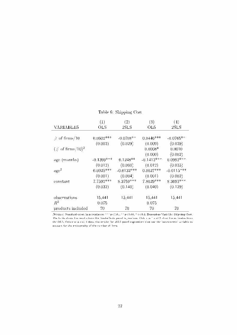
Table 6: Shipping Cost


# of �rms/10 0.0602*** -0.0708** 0.0446*** -0.0765**(0.003) (0.029) (0.009) (0.039)

(# of �rms/10)2 0.0008* 0.0010(0.000) (0.002)

age (months) -0.1399*** 0.1248** -0.1413*** 0.0992***(0.012) (0.060) (0.012) (0.035)

age2 0.0025*** -0.0132*** 0.0027*** -0.0115***(0.001) (0.004) (0.001) (0.002)

constant 7.7592*** 8.3759*** 7.8029*** 8.3693***(0.032) (0.140) (0.040) (0.129)


Notes: Standard errors in parentheses; *** p<0.01, ** p<0.05, * p<0.1; Dependent Variable: Shipping Cost.

The table shows the results form the �xed-e�ects panel regressions. Columns 1 and 3 show the estimates from

the OLS; Columns 2 and 4 show the results for 2SLS panel regressions that use the instrumental variable to

account for the endogeneity of the number of �rms.

22

Table7:

Interactingthenumber

of�rm

sandtheproduct

lifecycle

(1)

(2)

(3)

(4)

VARIABLES

minimum

markup

medianmarkup

coe�

cientof

variation

shippingcost

#of

�rm

s/10

-10.8075***

-10.2296***

0.0107

-13.0547

(2.958)

(2.755)

(0.053)

(17.294)

(#of

�rm

s/10)2

0.6655***

0.6676***

-0.0008

0.8443

(0.203)

(0.189)

(0.004)

(1.114)

#of

�rm

s/10

xage

0.0595

-0.1210

0.0436***

-0.2331

(0.312)

(0.291)

(0.006)

(0.501)

#of

�rm

s/10

xage2

0.1849**

0.2283***

-0.0041**

0.3598

(0.090)

(0.084)

(0.002)

(0.463)

(#of

�rm

s/10)2

xage

-0.0654***

-0.0634***

-0.0022***

-0.0830

(0.022)

(0.020)

(0.000)

(0.116)

(#of

�rm

s/10)2

xage2

-0.0049*

-0.0062**

0.0002***

-0.0105

(0.003)

(0.003)

(0.000)

(0.013)

age(m

onths)

11.1473**

14.0518***

-0.1866*

20.9313

(5.220)

(4.861)

(0.096)

(27.526)

age2

-1.5739**

-1.9207***

0.0160

-2.9772

(0.700)

(0.652)

(0.013)

(3.877)

constant

23.7129***

25.9548***

0.1722***

15.9114

(1.340)

(1.248)

(0.029)

(11.168)

observations

15,893

15,893

15,801

15,441

productsincluded

7070

7070

Notes:Standard

errors

inparentheses;***p<0.01,**p<0.05,*p<0.1;Thetable

showstheestim

ationresultsforinteractingthenumberof

�rm

swithage.Fixed-e�ects

2SLSpanelregressions,usingtheinstrumentalvariable

toaccountfortheendogeneityofthenumberof�rm

s.The

dependentvariablesare

displayedin

thecolumnheading.

23

Table8:

Alternativeversionsof

price

dispersion

(1)

(2)

(3)

VARIABLES

coe�

cientof

variation

dispersion

sdclwcoe�

cientof

variation

#of

�rm

s/10

0.0445***

41.2327***

0.0244***

(0.005)

(4.832)

(0.004)

(#of

�rm

s/10)2

-0.0021***

-1.9504***

-0.0007***

(0.000)

(0.279)

(0.000)

age(m

onths)

-0.0238***

-24.2846***

-0.0223***

(0.005)

(4.390)

(0.003)

age2

0.0012***

1.0273***

0.0012***

(0.000)

(0.276)

(0.000)

constant

-0.0032

1.7691

-0.0396**

(0.014)

(12.902)

(0.016)

observations

15,801

15,801

13,638

productsincluded

7070

70

Notes:Standard

errors

inparentheses;***p<0.01,**p<0.05,*p<0.1;Thetableshowstheresultsforalternativepricedispersion

measuresasdependentvariables.

Column1showstheCoe�cientofVariation,Column2PriceDispersionandColumn3theCoe�cient

ofVariationifpricesare

weightedbyclicks.

Fixed-e�ects

2SLSpanelregressions,whichuse

theinstrumentalvariable

toaccountfor

theendogeneityofthenumberof�rm

s.EachColumnhasthedependentvariableasin

thecolumnheading.

24

Table 9: Markup and price dispersion including shipping costs

(1) (2) (3)VARIABLES min markup (de) med markup (de) coe�. of variation (de)

# of �rms/10 -2.3518*** -1.4160*** 0.0554***(0.143) (0.111) (0.006)

(# of �rms/10)2 0.0407*** 0.0280*** -0.0020***(0.007) (0.006) (0.000)

age (months) 0.9331*** 1.3266*** -0.0413***(0.150) (0.116) (0.005)

age2 -0.0827*** -0.0825*** 0.0023***(0.009) (0.007) (0.000)

constant 25.4791*** 26.5884*** -0.0865***(0.474) (0.366) (0.024)

observations 15,511 15,511 15,186products included 70 70 70

Notes: Standard errors in parentheses; *** p<0.01, ** p<0.05, * p<0.1; The table shows the estimation results when

computing markups and price dispersion based on gross prices (total of price + shipping cost). For computing gross

prices we used the cost of shipping to Germany, that was charged for cash-in-advance payment. Fixed-e�ects 2SLS

panel regressions, using the instrumental variable to account for the endogeneity of the number of �rms. The dependent

variables are displayed in the column heading. �min markup (de)� stands for minimum gross markup for shipping to

Germany.

25

Table10:Markupandprice

dispersion

weightedbyclicks

(1)

(2)

(3)

VARIABLES

clwminimum

markup

clwmedianmarkup

clwcoe�

cientof

variation

#of

�rm

s/10

-1.0814***

-0.1214

0.0244***

(0.196)

(0.206)

(0.004)

(#of

�rm

s/10)2)

-0.0166*

-0.0347***

-0.0007***

(0.010)

(0.011)

(0.000)

age(m

onths)

0.5966***

-0.0265

-0.0223***

(0.151)

(0.159)

(0.003)

age2

-0.0778***

-0.0470***

0.0012***

(0.009)

(0.010)

(0.000)

constant

19.4796***

18.0235***

-0.0398**

(0.652)

(0.686)

(0.016)

observations

14,401

14,401

13,639

productsincluded

7070

70

Notes:Standard

errors

inparentheses;***p<0.01,**p<0.05,*p<0.1;Thetableshowsestim

ationresultswhentheobservationsare

weighted

bytheclicksano�ermanagedto

attract,before

computingthemarkups/coe�cientofvariation.Fixed-e�ects

2SLSpanelregressions,usingthe

instrumentalvariableto

accountfortheendogeneityofthenumberof�rm

s.Thedependentvariablesare

displayedin

thecolumnheading,�clw�

standsfor�clickweighted�.

26

Table11:Median-M

arkupandthecompositionof

shopsas

shares

(1)

(2)

(3)

(4)

(5)

(6)

VARIA

BLES

benchmark

availability

reputation

price-level

size

brick-m

ortar

#of�rm

s/10

-0.9078***

-0.9404***

-0.9089***

-0.8207***

-0.9046***

-0.8628***

(0.075)

(0.088)

(0.075)

(0.099)

(0.071)

(0.080)

(#of�rm

s/10)

20.0134***

0.0129***

0.0130***

0.0119**

0.0184***

0.0109**

(0.004)

(0.004)

(0.004)

(0.005)

(0.004)

(0.005)

age(m

onths)

0.8002***

0.8262***

0.8163***

0.7031***

0.5696***

0.8482***

(0.078)

(0.084)

(0.078)

(0.087)

(0.067)

(0.078)

age2

-0.0510***

-0.0526***

-0.0520***

-0.0467***

-0.0382***

-0.0543***

(0.005)

(0.005)

(0.005)

(0.005)

(0.004)

(0.005)

share

onstock

0.0123**

(0.005)

share

lowrep

-0.0045***

(0.002)

share

lowprice

-0.0220***

(0.007)

share

larger

shops

-0.0624***

(0.004)

share

brick

mortar

0.0192***

(0.003)

constant

23.1899***

22.9815***

23.4638***

23.6538***

24.3018***

22.0315***

(0.199)

(0.138)

(0.234)

(0.113)

(0.188)

(0.352)

observations

15,893

15,893

15,893

15,893

15,893

15,872

productsincluded

70

70

70

70

70

70

Notes:

Standard

errors

inparentheses;

***p<0.01,**p<0.05,*p<0.1;Fixed-e�ects

2SLSpanelregressions,

whichuse

theinstrumental

variable


s;Thedependentvariable

isMedianMarkup.Column(1)repeats

theregressionin

Column(4)oftable4.Columns(2)-(6)eachaddameasure

forthecompositionofshopsin

market-dayobservation,in

orderto

accountforshop

heterogeneities.

Whileim

mediate

availability(on-stock,Column(2))

andbrickandmortar(C

olumn(6))

are

readilyobservabledummyvariables,

foreachshop,Columns(3)-(5)are

basedonshops'behaviorin

the�rstthreeweeksofthesample.

27

Table12:Minimum-M

arkupandthecompositionof

shopsas

shares

(1)

(2)

(3)

(4)

(5)

(6)

VARIA

BLES

benchmark

availability

reputation

price-level

size

brick-m

ortar

#of�rm

s/10

-1.7876***

-2.0164***

-1.7892***

-2.1079***

-1.7836***

-1.8079***

(0.132)

(0.164)

(0.133)

(0.191)

(0.127)

(0.142)

(#of�rm

s/10)

20.0160**

0.0125

0.0155**

0.0217**

0.0223***

0.0175**

(0.008)

(0.008)

(0.008)

(0.009)

(0.007)

(0.008)

age(m

onths)

0.8375***

1.0202***

0.8586***

1.1944***

0.5432***

0.8177***

(0.138)

(0.158)

(0.139)

(0.167)

(0.121)

(0.139)

age2

-0.0889***

-0.1002***

-0.0901***

-0.1047***

-0.0725***

-0.0875***

(0.009)

(0.010)

(0.009)

(0.010)

(0.008)

(0.009)

share

onstock

0.0860***

(0.010)

share

lowrep

-0.0059**

(0.003)

share

lowprice

0.0808***

(0.014)

share

larger

shops

-0.0796***

(0.007)

share

brick

mortar

0.0004

(0.006)

constant

20.5172***

19.0578***

20.8758***

18.8106***

21.9363***

20.5466***

(0.352)

(0.258)

(0.414)

(0.216)

(0.337)

(0.621)

observations

15,893

15,893

15,893

15,893

15,893

15,872

productsincluded

70

70

70

70

70

70

Notes:

Standard

errors

inparentheses;

***p<0.01,**p<0.05,*p<0.1;Fixed-e�ects


whichuse

theinstrumental

variable



isMinim

um

Markup.Column(1)repeats

theregression

inColumn(4)oftable

3.Columns(2)-(6)eachaddameasure



orderto

account

forshopheterogeneities.

Whileim

mediate


andbrickandmortar(C

olumn(6))

are

readilyobservabledummy

variables,foreachshop,Columns(3)-(5)are



28

Table13:Shippingcostandthecompositionof

shopsas

shares

(1)

(2)

(3)

(4)

(5)

(6)

VARIA

BLES

benchmark

availability

reputation

price-level

size

brick-m

ortar

#of�rm

s/10

-0.0765**

-0.0763*

-0.0762*

-0.0596

-0.0986***

-0.0642

(0.039)

(0.039)

(0.039)

(0.047)

(0.038)

(0.040)

(#of�rm

s/10)

20.0010

-0.0003

0.0006

0.0005

0.0031*

-0.0008

(0.002)

(0.002)

(0.002)

(0.002)

(0.002)

(0.002)

age(m

onths)

0.0992***

0.0956***

0.1133***

0.0836**

0.0321

0.1651***

(0.035)

(0.035)

(0.035)

(0.038)

(0.032)

(0.035)

age2

-0.0115***

-0.0115***

-0.0124***

-0.0110***

-0.0080***

-0.0157***

(0.002)

(0.002)

(0.002)

(0.002)

(0.002)

(0.002)

share

onstock

0.0129***

(0.002)

share

lowrep

-0.0057***

(0.001)

share

lowprice

-0.0060*

(0.003)

share

larger

shops

-0.0314***

(0.002)

share

brick

mortar

0.0165***

(0.001)

constant

8.3693***

7.9846***

8.7053***

8.5377***

9.0827***

7.5190***

(0.129)

(0.080)

(0.139)

(0.071)

(0.141)

(0.182)

observations

15,441

15,441

15,441

15,441

15,441

15,423

productsincluded

70

70

70

70

70

70

Notes:

Standard

errors

inparentheses;

***p<0.01,**p<0.05,*p<0.1;Fixed-e�ects


whichuse

theinstrumental

variable



isShippingCost.Column(1)repeats

theregressionin

Column(4)oftable6.Columns(2)-(6)eachaddameasure



orderto

accountforshop

heterogeneities.

Whileim

mediate


andbrickandmortar(C

olumn(6))

are

readilyobservabledummyvariables,

foreachshop,Columns(3)-(5)are



29

Figure 2: Median markup plotted against the number of �rms and age of product.

010

20

30

40

media

n m

ark

up (

perc

. poin

ts)

0 50 100 150 200number of firms

median markup (perc. points) vs. number of firms

010

20

30

40

media

n m

ark

up (

perc

. poin

ts)

0 50 100 150 200number of firms

avg of median markup (perc. points) vs. number of firms

010

20

30

40

media

n m

ark

up (

perc

. poin

ts)

0 5 10 15age in months

median markup (perc. points) vs. age in months

010

20

30

40

media

n m

ark

up (

perc

. poin

ts)


avg of median markup (perc. points) vs. age in months

050

100

150

200

num

ber

of firm

s


number of firms vs. phase in the life cycle

050

100

150

200

num

ber

of firm

s


number of firms vs. phase in the life cycle

Notes: The plot shows the empirically observed distributions of number of �rms, age and median markup

plotted against each other. In the top left panel, the median markupit is scattered against the number of

firmsit in the corresponding market and the right Column shows the corresponding averages. In the middle

row the median markup is plotted against the age of the product. In the lower row, the number of �rms is

plotted against the age of the cameras (in months).

30

Figure 3: Minimum markup in di�erent phases of the product life cycle

−.1

0.1

.2.3

mark

up

0 50 100 150number of firms

Beginning month_1

month_2 month_3

month_6 month_9

Notes: The plot shows the curve estimated in table 7. Each curve shows the estimated relationship of

number of �rms and markup at a di�erent point in time (right after introduction and after 1,2,3,6 and 9

months). The curves are plotted on the range from the 33rd to 67th percentile of the empirically observed

distribution of the number of �rms at the point in time it corresponds to.

31

Figure 4: Median markup in di�erent phases of the product life cycle

0.1

.2.3

mark

up

0 50 100 150number of firms

Beginning month_1

month_2 month_3

month_6 month_9

Notes: The plot shows the curve estimated in table 7. Each curve shows the estimated relationship of

number of �rms and markup at a di�erent point in time (right after introduction and after 1,2,3,6 and 9

months). The curves are plotted on the range from the 33rd to 67th percentile of the empirically observed

distribution of the number of �rms at the point in time it corresponds to.

32

Market structure and market performance in e-commerce

Documents

Transcript of Market structure and market performance in e-commerce