1

Market Design and Motivated Human Trading Behavior in Electricity Markets

Mark A. Olson, Stephen J. Rassenti, Vernon L. Smith and Mary Rigdon

Interdisciplinary Center for Economic Science, George Mason University

ABSTRACT

This paper is based on a series of controlled experiments in the trading of wholesale electricity that expands substantially the scope of experimental research programs reported previously. The experiments employed cash motivated students and rented computer laboratory facilities of the University of Arizona. The primary objective of these experiments was to compare two alternative institutional arrangements for the trading of electric power. As in the California markets the first employed day-ahead sealed bid trading of energy for all periods in the subsequent day; the second employed simultaneous continuous double auctions for bilateral trading of energy up to the hour before delivery. In each the energy market was supplemented by a reserve market and an hour-ahead adjustment market for real time pricing. All trading was executed on a nine-node network with limited transmission capacity. Eight nodes were control areas, with one large wholesale generator company and one large distribution company resident there. The privatization of state electric power systems by foreign governments began in the 1980s in Chile and the United Kingdom and subsequently spread to New Zealand, Australia and other countries. (For a review of the early UK experience, see Littlechild, 1995). Most recently the movement to deregulate electricity in the United States, where each state and the Federal Energy Regulatory Commission regulate the industry, has joined this trend. Deregulation has proceeded much less smoothly in the United States than did foreign privatization. (See Thomas and Schneider 1997 for an excellent review of engineering aspects of deregulation in the U.S.). This paper uses experimental methods to study a completely decentralized “day-ahead” spot market for energy commitment, in which generator companies submit node-specific offer price schedules to supply power, and wholesale buyers submit bids to buy power delivered to node-specific load centers. Energy loads are allocated among generators by optimizing across the whole network. This market is followed by a reserve market for emergency energy, and a final optimization assisted adjustment market for incremental (decremental) adjustment of spot energy supplies based on exact energy demand and transmission constraints. Earlier experimental studies of the effect of transmission constraints on pricing and efficiency, and of market power issues in electricity markets are reported in Backerman, Rassenti and Smith, 1996 and Backerman, Denton, Rassenti and Smith, 1997. This sealed bid (SB) “day-ahead” institutional regime is compared with one in which both the reserve and adjustment markets operated as above, but the energy market was organized as a continuous double auction (CDA). This free trading energy market received no optimization support, and was potentially subject to more volatile prices, inefficient allocation of loads and higher transmission losses, which could potentially be relieved by the final adjustment market. The primary purpose of the experimental design was to allow comparison between the two institutional treatments using observations on prices, seller and buyer profits (% of expected competitive share) and total efficiency (% of maximum possible system-wide surplus). Since our experimental comparisons build on supply side market mechanisms that parallel most closely those that have emerged from the debate in California, we briefly discuss the principle

2

features of the California system, indicating specific elements that we incorporate, modify or do not include in the experimental design. (See Wilson, 1998 for a review of design principles with some emphasis on California). 1. The market (California PX) for energy supply to the grid determines a sequence of hourly settlement prices in a day-ahead energy bid market, followed by a hour-ahead bid adjustment market. The system operator selects from these bids to adjust supply and demand in real time. The forward energy market allows the system operator lead time to identify and manage transmission constraints, and generation companies to determine their basic capacity commitments. In the hour-ahead adjustment market, suppliers offer the terms on which they are willing to increment or decrement their load allocations from the energy market, and add capacity not accepted in the energy market allocation. The realized pattern of demand and grid loss characteristics determines the final real time location adjusted prices. Our experiments implement these specifications for the energy and hour-ahead bid markets as follows: bidders in the energy market receive demand forecasts with a ± 8% confidence error on the eventual real time demand, which is reduced to ± 2% when the hour ahead adjustment (inc/dec) bids for eligible generators are submitted. In the experiments we reduce the number of feedback events (vigilance required by the subjects) by immediately combining the outcome of the adjustment market with the real time demand; i.e., the accepted bids in the adjustment market are used to determine only a final real time pattern of prices. Thus, the subjects receive feedback and settlements on energy market prices, and real time market prices. As in the California market, subject experimental suppliers can submit unit generator, and/or generator portfolio, bids. In the latter case each subject is aided by a robot that ensures the lowest cost choice among available units in the portfolio in the event of a partial bid acceptance. Each subject, however, must respect generator ramp rates so that some or all generators in a portfolio are running in the appropriate day-ahead period. Finally, we divide the day into four intervals (not 24 hours), consisting of an off-peak, shoulder, on-peak and shoulder demand load pattern. 2. After the energy market closes, and prior to opening the adjustment market, agents may submit a two-part bid to supply reserves. Their capacity bids (1st part) are ordered from lowest to highest and the least costly capacity that maintains the necessary reserve margin is selected. If reserve energy is actually needed, the reserve energy bids (2nd part) of the selected capacity providers are ordered from lowest to highest and used in this order. 3. Scheduling systems often do not make explicit provision for demand side bidding (New Zealand is an exception). Our experiments do, although none of the demand we model is interruptible; i.e., the demand price (maximum willingness-to-pay) is constant up to the uncertain total customer load for each wholesale buyer. (See Figure 3). Since competition is greatly enhanced by demand side bidding even with a modest capability for demand interruption (Rassenti, Smith and Wilson, 2000), we study it here under the stringent, 100% must-serve condition. Such a policy in the field has several advantages: it would greatly incentivize the implementation of delivery interruption technologies; responsibility for forecasting and managing demand would rest on those agents who most directly benefit from the appropriate decisions; supply withholding to induce price spikes could easily be offset by strategic demand withholding. The software implements demand side bidding in both the energy and adjustment markets. Any residual must-serve demand is allocated by the center to the reserve market, and any surplus purchased is sold into the reserve market. Since the reserve market is likely to be a higher priced source of power the incentive should be for buyers to satisfy their needs in the energy and adjustment markets.

3

4. In the original California system “ the transmission market is an extension of the energy market to remedy congestion by altering the location of generation.” (Wilson, 1998, p. 172). Thus if a line is constrained, generator bids downstream are accepted to substitute for rejected upstream bids in the adjustment market. This is also how our experimental software manages transmission bottlenecks: there is no separate market for “firm transmission rights;” our transmission prices are entirely based on optimized marginal loss and congestion cost differences (constraint shadow prices) between any two nodes. This approach does not rule out the development of private financial markets for transmission congestion contracts or contracts for differences, as assumed in California. (Wilson, 1998, pp. 167-8). We provide below, in context, more specific detail about the experimental implementation. 1. Modeling Generators

Generator companies (Gencos) consisted of portfolios of generator units of various technological types (coal, oil, gas, hydro, nuclear), including multiple generator units of the same type. Parameters that characterized each type of generator were provided by an industry client, and are shown in Table 1. Large coal and nuclear units were characterized by high capacity, low marginal costs, large start-up costs, large minimum loads (50% and 100% of maximum capacity, respectively), large fixed costs per hour, and long start-up times (10 and 60 hours respectively). Gas and oil fired turbines varied considerably in capacities and costs, but generally had high marginal costs, low fixed cost, low minimum loads (5% of maximum capacity or less), and represented quick-start sources of reserve power in the event of unscheduled outages. If all generators in the network were arrayed from lowest to highest, according to their marginal costs and corresponding capacities, the resulting step function was the minimum willingness-to-accept supply schedule of power in the network, which abstracts from losses and transmission constraints.

A portion of the screen display for the Genco at node 7 is shown in Figure 1. (The screen also displays the network and the Genco’s location in the network, but this is shown separately in Figure 5 below). Genco 7 controlled six classes of generator units designated A7, B7,…, G7. Each class consisted of multiple individual units, each unit represented by it’s own lightening icon. By clicking on the icon, the essential data for that generator was displayed in the box titled “A Costs”. For example, the 5th unit in A7 is highlighted in the upper panel, and the data for that unit is indicated in the left lower panel. (The data are identical for all other class A units in Genco 7’s A portfolio). The first box displays the startup cost of this unit, 1500 (measured in ¶ units of experimental money, “pesos”). Then the ramp (start up) time, 10 hr, followed by the fixed (sunk) cost 389¶/H, pesos per hour. Under Fuel Cost, the first step lists the fuel cost, 15 (¶/MWH), for the unit’s minimum loaded capacity , 80 MW. Subsequent capacity steps, up to the maximum loaded capacity, are listed next. In this example, there is only one additional step at the same fuel cost and capacity, so the unit has a constant fuel cost up to its capacity of 160MW. All loaded generators were assigned forced outage rates based on NERC data for units of different types. If an outage was realized, its duration was then specified, and during those periods that unit could not be offered to the market.

4

Table 1. Genco information Precontracted Supply Company Type of Unit #

UnitsMax Capacity

Var. Op. Costs

Min Load

Start Cost

Ramp Time Low Shoulder Peak

MW / unit $ / MWH MW $ hours MWH (# units) MWH (# units) MWH (# units) 1 Hydro 1 70 2.500 3 10 0 1 Nuclear 1 180 7.825 180 25000 60 180 (1) 180 (1) 180 (1) 1 large coal 4 530 12.900 265 1500 10 530 (2) 620 (2) 820 (2) 1 small coal 2 10 17.100 3 400 3 1 ct/ic/je 1 10 46.400 1 40 0 Totals 9 2400 710 (3) 800 (3) 1000 (3) 2 Hydro 1 270 1.830 5 10 0 2 Nuclear 1 550 11.520 550 25000 60 550 (1) 550 (1) 550 (1) 2 large coal 1 620 16.350 310 1500 10 2 small coal 1 80 20.110 10 400 3 10 (1) 10 (1) 80 (1) 2 oil ct 10 20 37.300 1 40 0 Totals 14 1720 560 (2) 560 (2) 630 (2) 3 Hydro 1 90 7.900 3 10 0 3 large coal 3 210 13.230 105 1500 10 105 (1) 105 (1) 105 (1) 3 small coal 1 40 19.230 3 400 3 3 steam turbines oil/gas 1 20 40.000 3 400 3 Totals 6 780 105 (1) 105 (1) 105 (1) 4 Nuclear 1 60 11.520 60 25000 60 60 (1) 60 (1) 60 (1) 4 large coal 1 160 14.700 80 1500 10 4 small coal 1 30 20.100 10 400 3 4 ct/ic/je 1 10 87.900 1 40 0 Totals 4 260 60 (1) 60 (1) 60 (1) 5 Hydro 1 30 0.000 5 10 0 5 large coal 4 190 12.900 95 1500 10 95 (1) 95 (1) 190 (1) 5 Nuclear 1 260 14.550 260 25000 60 260 (1) 260 (1) 260 (1) 5 small coal 2 30 17.100 3 400 3 5 steam turb 1 10 26.000 3 400 3 5 ct/ic/je 2 20 105.000 1 40 0 Totals 11 1160 355 (2) 355 (2) 450 (2) 6 Hydro 1 150 3.040 5 10 0 6 Nuclear 1 290 12.230 290 25000 60 290 (1) 290 (1) 290 (1) 6 large coal 10 60 14.500 30 1500 10 240 (8) 360 (8) 480 (8) 6 small coal 1 10 16.400 10 400 3 6 steam turb 10 10 18.660 3 400 3 6 ct/ic/je 10 20 33.220 1 40 0 Totals 33 1350 530 (9) 650 (9) 770 (9) 7 Hydro 1 190 2.010 5 10 0 7 Nuclear 1 1010 12.230 1010 25000 60 1010 (1) 1010 (1) 1010 (1) 7 large coal 10 160 15.400 80 1500 10 1000 (10) 1600 (10) 1600 (10) 7 small coal 1 170 18.870 10 400 3 10 (1) 155 (1) 150 (1) 7 combined 1 100 24.135 40 1000 1 40 (1) 40 (1) 100 (1) 7 ct/ic/je 10 90 52.100 1 40 0 7 steam turb 10 90 55.000 3 400 3 15 (5) 15 (5) 15 (5) Totals 34 4870 2075 (18) 2820 (18) 3310 (18) 8 Hydro 1 300 1.830 5 10 0 8 Nuclear 1 480 12.230 480 25000 60 480 (1) 480 (1) 480 (1) 8 large coal 10 230 17.400 115 1500 10 1150 (10) 1620 (10) 2260 (10) 8 small coal 1 90 22.600 10 400 3 8 ct/ic/je 10 30 49.500 1 40 0 8 steam turbines oil/gas 10 10 64.940 3 400 3 Totals 33 3570 1630 (11) 2100 (11) 2740 (11)

5

Figure 1. Genco screen display SB

6

2. Modeling Demand Demand cycled from a low off-peak period (9 GWh), through a middle level shoulder period (12

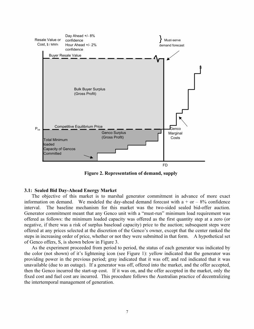
GWh) to a peak period (14 GWh), and back to a shoulder period. The four periods were repeated in a series of 5 market days during each experiment, for a total of 20 trading periods. Each period each wholesale buyer was assigned a large spike of “must serve” demand that he could resell at a regulated price as shown in Figure 2. In these experiments no portion of the demand could be interrupted voluntarily. The “must-serve” spike in demand was uncertain. There was a day-ahead forecast with + or – 8% confidence interval error, then a better forecast with + or – 2% error an “hour ahead” of the spot market.

Buyers were obligated to submit bids for all required demand, including all “must serve” loads, none of which could be voluntarily interrupted. All demand and supply were channeled through a central exchange market. Each demand/supply node consisted of a utility whose local generation capacity and domestic demand was large relative to the transfer capacity of the inter-tie transmission links. We assumed that all nuclear units were completely pre-contracted, and that something between minimum and maximum capacity of several of the large coal units were also pre-contracted. The columns on the far right of Table 1 show the number and total pre-contracted capacity of generators from each Genco in off, shoulder and peak periodsSuch pre-contracted amounts were subtracted from demand at each local distribution node, and were never under threat of being constrained off. Pre-contracting allowed us to avoid the resulting local monopoly problem without making arbitrary assumptions about the break-up of generation. An alternative interpretation is that the indicated base load units are spun off with long term regulated contracts leaving enough capacity for effective contestability among the eight demand/supply nodes.

Capacity not pre-contracted was comparable in magnitude to the export/import capacity of each node. Due to stochastic and cyclical demand variation and the variance in the marginal prices for generating and consuming additional power at various nodes in the system, congestion remains likely. Under these assumptions we were able to examine inter-nodal competition. Achieving such competition is clearly contingent upon how generation is restructured. 3. Market Design

The power market consisted of a sequence of three auction submarkets: (1) an energy market for generator supply commitment based on day-ahead demand forecasts, which either employed a call auction accepting sealed bids to buy and offers to sell, or a continuous bilateral double auction trading up until the hour-ahead forecast was delivered; (2) a sealed offer auction market for spinning and quick start reserves conducted after the results of auction (1) were completed; (3) a sealed offer load adjustment (often called the increment/decrement) market, which allows the Gencos to express their willingness to adjust the terms of the energy market to accommodate the deviation of realized demand from the forecast demand. In the continuous double auction version of the energy market, the load adjustment terms enable the Center to establish priorities among all Gencos in the event of transmission congestion. Such congestion would require the higher cost generators upstream from a constraint to be throttled back and the lowest cost available downstream units to be ramped up.

7

Figure 2. Representation of demand, supply 3.1: Sealed Bid Day-Ahead Energy Market

The objective of this market is to marshal generator commitment in advance of more exact information on demand. We modeled the day-ahead demand forecast with a + or – 8% confidence interval. The baseline mechanism for this market was the two-sided sealed bid-offer auction. Generator commitment meant that any Genco unit with a “must-run” minimum load requirement was offered as follows: the minimum loaded capacity was offered as the first quantity step at a zero (or negative, if there was a risk of surplus baseload capacity) price to the auction; subsequent steps were offered at any prices selected at the discretion of the Genco’s owner, except that the center ranked the steps in increasing order of price, whether or not they were submitted in that form. A hypothetical set of Genco offers, S, is shown below in Figure 3.

As the experiment proceeded from period to period, the status of each generator was indicated by the color (not shown) of it’s lightening icon (see Figure 1): yellow indicated that the generator was providing power in the previous period; gray indicated that it was off; and red indicated that it was unavailable (due to an outage). If a generator was off, offered into the market, and the offer accepted, then the Genco incurred the start-up cost. If it was on, and the offer accepted in the market, only the fixed cost and fuel cost are incurred. This procedure follows the Australian practice of decentralizing the intertemporal management of generation.

Resale Value orCost, $ / MWh

S

Bulk Buyer Surplus(Gross Profit)

Competitive Equilibrium Price

Buyer Resale Value

Pce

FD

Genco Surplus(Gross Profit)

Total Minimum loadedCapacity of Gencos Committed

GencoMarginal

Costs

Day Ahead +/- 8% confidence Hour Ahead +/- 2% confidence

} Must-serve demand forecast

8

Figure 3. Energy market offers, bids and clearing price The sealed offer procedure to enter energy offers for a generator is illustrated in Figure 1. In the

window on his computer monitor entitled “Offer to Sell”, each generator’s capacity could be offered to the market in up to five asking price steps. In the illustration for a unit in class A, Genco 7, there is automatic entry of the first minimum loaded capacity step (80 MWH) “at market.” This is defined as commitment, and guaranteed that a partial acceptance would not require a unit to run at less than minimum load. This can be viewed as an expert system local control over the offer entered, not necessarily a rule of the Exchange Center. In Australia, it is an exchange rule, defining base load commitment. In the example, Genco 7 also chose to offer the remaining capacity, 80 MHW, at price zero. This assured that all the capacity of the unit will be accepted at the ruling market price, unless there is excess minimum base load capacity in the system, as can occur, and the price is zero. (The Australian market and California PX have produced zero prices in off-peak intervals). Having entered the offer prices, the subject clicks on the submit button at the bottom right of Figure 1, and each offer step under Status is marked as Submitted. At the close of the market, if the offer is accepted, the Status changes to Accepted.

By clicking one generator and then dragging the mouse across several icons in a class while depressing the mouse button, a portfolio of identical generators can be combined into a single offer, i.e. the one representative offer is cloned for all the like units in the portfolio. If the offer is only partially accepted, a local expert system algorithm manages the generators by turning on the minimum cost subset needed to meet the output requirement. Consequently, units must be offered individually if the subject wants to force any unit to be kept on when the offer would not be fully accepted. This algorithm frees subjects to give thought to the inter-temporal management problem.

MWh

Must-serveDemand Forecast

Buyers bid"at Market"

for all demand

Genco offerprices

S1

S2S3

S4

S5

S6S7

S8

S9

S

RD FD RD'

PE

9

Contractually, Gencos with accepted offers are immediately paid the energy market supply price by the buyers with successful day-ahead bids, and are obligated to produce at delivery time. In addition, Gencos whose generator offers to the energy market are accepted at less than full capacity are free to offer that capacity, or any surplus capacity, either to the reserve market or the load adjustment market. Only generators with a zero ramp time, or those already minimum loaded in the energy market, are eligible to participate in the reserve and adjustment markets. 3.2: Reserve Market

When the reserve market takes place (see the time line sequence in Figure 7) demand is known to the agents with a confidence interval of + or – 2%. The reserve market accepts seller offers of capacity as spinning or quick start reserves in the event of an unscheduled outage, or in the event that a buyer fell short of purchasing his forecast energy requirement in the energy market. Each offer from a generator owner is a two part offer: (i) the first is a capacity supply price representing the Genco’s minimum required payment for maintaining the capacity’s readiness to supply temporary reserves; (ii) the second is an energy charge in ¶/MWh for drawing upon the capacity until the reserve is no longer needed.

The buyers and sellers are told that the probability of an unscheduled outage was about .06 for any generator and therefore to accommodate 99.9% of all emergency circumstances the required reserve capacity in MW needed to be 12% of the forecast load in the entire system. (Unknown to the buyers and sellers, in the experiments reported here we did not actually stress anyone with unscheduled outages, though they bid with full expectations of encountering them.) In addition to the required reserve, RR, for outages, we treated individual buyers as imposing a buyer energy requirement, BR, on the system if they had not purchased enough power to cover their forecast demand in the primary energy market. A sudden increase in load above the energy market allocation, for whatever reason, was viewed as economically equivalent to a generator going down.

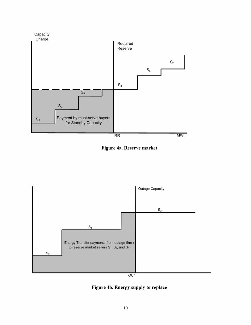
Allocations were made as follows: the capacity supply prices (i) are ordered from lowest to highest; if RR + BR is the total required reserve capacity in MW, the lowest RR + BR units of capacity offered are accepted at the lowest rejected offer. (See Figure 4a showing the net reserve case with BR = 0). The cost of the first RR units of reserve capacity is shared by all buyers in proportion to their forecast demand. The cost of BR additional units of reserve capacity is paid for by the individual buyers who bought less than they needed in the energy market, as they cannot interrupt demand.

Next, the set of RR + BR accepted reserve offers were sorted from lowest to highest based upon the energy prices (ii) at which each of the accepted reserve units was offered. Now suppose a stochastic failure occurred requiring OCi units of reserves to be drawn to replace a failed generator owned by seller i. Then i paid the reserve energy price to all those Gencos supplying the reserve energy, until the next energy market period, as illustrated in 4b. However, an expert system automatically substituted any ready but uncommitted capacity owned by i itself, for the reserve market supply if the fuel cost of that capacity was less than the energy reserve market price. Thus, quick start units not committed to any of the three markets, still served the Genco by placing an upper bound on the cost of replacement power due to an outage.

In similar fashion buyers who failed to purchase enough power through the energy market, were obligated to pay the second tier of energy prices supplied in the reserve market. The buyer’s residual demand was automatically satisfied by recourse to the reserve market to incentivize buyers to cover their must-serve demand. We can observe the extent to which residual demand drew on reserves.

10

Figure 4a. Reserve market

Figure 4b. Energy supply to replace

CapacityCharge

Payment by must-serve buyers for Standby Capacity

S1

S2

S3

S4

S5

S6

Required Reserve

RR MW

S3

S1

S2

Outage Capacity

Energy Transfer payments from outage firm ito reserve market sellers S1, S2, and S3.

OCi

11

3.3: Load Adjustment Market When the load adjustment market takes place (see the time line sequence in Figure 7) demand is

completely known to the agents. In the load adjustment market, Gencos submit their supply price for immediately providing additional power above what they sold in the energy market; and also they submit the price they are willing to pay to have to supply less power(generating less than their obligation saves fuel). This information, when supplied after the energy and reserve markets have been run and demand becomes known, allows substitutions between downstream and upstream generators on either end of a constrained line for congestion management. All Gencos in the energy market were free to supply this information for congestion management, and as a tertiary source of supply for forecast load not yet contracted in the energy or reserve markets.

Quick responding (load “following”) generator capacity, not accepted (or offered) in either the energy or the reserve market, can also be offered for load adjustment to realized demand. Realized demand may have been either above or below the total capacity of generators accepted in the energy market.

The load adjustment market is illustrated in Figure 5. If realized demand, RD < FD, forecast demand, then, the load adjustment decrement market substitutes generators willing to pay more for generators willing to pay less to reduce output. Thus, in the energy market, shown in Figure 3, S5 is the marginal generator at FD, while S4, S3 and S2 are the next lower generators in the merit order. But in Figure 5, it is seen that S2 and S5 are willing to pay more to throttle back than S3 and S4. Thus S2 and S5 win the decrement auction, with S2 paying S4 for the right to reduce delivered power, and S5 (in effect) paying himself. Observe that the decrement market is concerned only with the possibility of substitution among committed generators, as all generators accepted in either the energy or reserve

markets to cover the forecast demand, FD, have already received payment from the buyers. Figure 5. Load adjustment market

In the experiments reported here, the load adjustment market was restricted to increments for

energy shortfalls, so that sellers did not also require training as buyers. When the demand realization was below the amount of energy purchased by buyers, this was viewed as a windfall for sellers who

MWh

Transfer Payment

from Buyers toS5, S7 and S8

Transfer Paymentfrom S2 to S4

(S2 replaces S4

in EnergyMarket Outcome)

RD FD RD'

PLA

S4

S3

S5

S2

S7

S5

S8

S6S9

PLA'

PE

12

were arbitrarily cut back having already received payment to produce more. Sellers were also unable to use the increment market purchase power for the purpose of economy interchange, and were required to produce from the generators they had committed. Our objective was to test the consequences of rule changes in the primary energy market, so these simplifications were implemented to avoid a more difficult training program and a more complicated experimental environment that would have generated more noisy data. 3.4: Continuous Double Auction Energy Market

We executed a single major experimental treatment variation on the day-ahead sealed bid energy market described above, keeping constant our treatment of the auction procedures for the reserve and load adjustment markets. This was the continuous double auction (CDA) energy market.

For the CDA we followed the proposal in California under which all buyers and sellers are free to contract via a double auction market that runs continuously down to the hour-ahead spot market. There was no day-ahead energy market, only a day ahead forecast with + or – 8% confidence. Shortly before the CDA energy market closed, a new forecast was publicized with + or – 2% confidence. Following the energy market, we ran the reserve and load adjustment markets as above.

The relevant part of the seller’s screen corresponding to the double auction trading is shown in Figure 6. The queue of standing offers (lowest to highest) sat above the queue of standing bids (highest to lowest). Any offer to sell in square brackets was an all or none offer, enabling Gencos to tender bids that guarantee minimum load coverage on their first step. Other bids and offers could be accepted in any part. An asterisk or an arrow to the left of a bid or offer indicated it belonged to this agent who was observing it. An arrow indicated which bid or offer would be changed.. The number to the right of the

FIGURE 6. GENCO SCREEN DISPLAY CDA

13

bid or offer indicated the location node of the submitter. An agent would enter a bilateral trade when he accepted someone else’s bid or offer, or when someone else accepted his standing bid or offer.

The CDA convention employed was that the acceptor of a bid (offer) agreed to deliver (take power) to (from) the bidder’s (offerer’s) location. If the energy could not ultimately be delivered or taken because of line constraints, the acceptor suffered the cost of rectifying the situation. The acceptor had to purchase locally available energy to satisfy the buyer’s load and avoid the constrained line, and he could attempt to unload his previously contracted remote energy source in the adjustment market. To the extent that bilateral contracts include infra-marginal agents at quantities less than the optimal set of withdrawals and injections, these CDA contracts have no affect on allocative efficiency although they can change the distribution of surplus between the buyers and sellers.

4. The Network

A graph of the 8-center (9-node) network we used for the experiments is shown in Figure 8. Each node is a control area (except for the junction node connecting 1, 2 and 5) connected to other nodes so as to correspond to an aggregated version of a portion of the national grid. In this figure we show the set of surplus maximizing competitive equilibrium allocations for the final four periods (17-20) on the final day (5) of trading. (On other days the realization of demand was somewhat different, though of the same pattern, so the corresponding equilibrium allocations were slightly different.) The competitive equilibrium line flows and sector costs and profits are computed by applying the optimization to maximize the total system surplus using the true resale value schedules of each buyer, and the true marginal cost schedules for each generator unit (as if it is currently running). Though this input information is perfectly known to the experimenter, it may never be fully revealed by buyers and sellers in the competitive bidding environment.

Under each node name is a vector of prices (P:) above a vector of quantities (Q:). These represent the equilibrium prices for power (rounded to the nearest peso) in the Off-peak, Shoulder, Peak, and Shoulder demand periods, and the corresponding quantities buyers would consume. Each transmission line, which shows a direction of flow and a maximum flow constraint, also shows a vector of quantities indicating the amount of flow that occurs in each of the four periods if the competitive equilibrium allocation is achieved. 5. Optimization

In the experiments conducted, we used a DC model with quadratic line losses to compute the real power flows in the stylized network. XA (copyright Sunset Software Technology), a callable library for solving linear and integer programs, provided the horsepower to solve for the optimal (surplus maximizing) power flows given the bids and offers from all agents. A full nonlinear AC optimization program will be imported into the software package at a later stage of the research. 6. Subjects

More than 100 undergraduate students were recruited from business, engineering and economics classes. Subjects received a fixed fee of $7.5 for arriving on time for each experiment, plus their accumulated earnings in the experiment after they have finished. Where subjects were recruited for several experiments, including training sessions, all payments were withheld until they completed the series. All trading was denominated in experimental “pesos”, and each agent was provided a private exchange rate that was used to convert pesos earned to American dollars at the end of the experiment. The exchange rates were calibrated to provide each subject with competitive equilibrium earnings of

14

Continuous Double Auctions (CDA)

Step 0: Set I=1 and k=1. Publish forecast energy demands (+ or – 8%), then simultaneously open DA energy markets for periods I1, I2, I3, and I4 for 7 1/2 minutes. Step 1a: Draw energy demand (+/- 2%) for period Ik. Announce the energy market for Ik will close in 2 1/2 minutes. Step 1b: Close energy market Ik. Publish forecast demand (+ or – 8%) and open energy market for period (I+1)k. Step 2: Conduct 1 minute SB reserve market for period Ik. Step 3: Draw exact energy demand for period Ik, then conduct 1 minute SB inc/dec market for period Ik. Use inc/dec to balance demand and supply. Step 4: Draw generator and line failures for period Ik. Use reserve to deal with failures. Do accounting, report results. Allow subjects 1/2 minute to view. Step 5: If k<5, set k=k+1. Otherwise, set I=I+1, k=1. Go to step 1a.

Sealed Bid Day Ahead Auctions (SB)

Step 0: Set I=1 and k=1. Step 1: Publish forecast energy demands (+ or – 8%), then sequentially conduct SB energy markets for periods I1, I2, I3, and I4 for 10 minutes. Step 2: Draw energy demand (+ or - 2%) for period Ik. Conduct 1 minute SB reserve markets for period Ik. Step 3: Draw exact energy demand for period Ik, then conduct 1 minute SB inc/dec market for period Ik. Use inc/dec to balance demand and supply. Step 4: Draw generator and line failures for period Ik. Use reserve to deal with failures. Do accounting, report results. Allow subjects 1/2 minute to view. Step 5: Set k=k+1. If k<5 go to step 2. Otherwise, set I=I+1, k=1, go to step 1.

Figure 7. Trading timelines. The above flowcharts describe the institutional trading sequences. Let Ik indicate day I period k (e.g. I3 is day 1 in peak period). DA represents the

Double Auction, and SB the Sealed Bid auction.

15

Figure 8. Network representation

1P: 13/13/17/13

Q: 1232/1597/1829/1608

6P: 15/15/17/15

Q: 698/886/1030/898

4P: 13/13/17/13

Q: 199/215/287/226

7P: 15/19/52/19

Q: 2337/2820/3586/3071

5P: 13/13/17/13

Q: 683/913/1049/925

8P: 17/17/17/17

Q: 1822/2488/2810/2500

3P: 13/13/17/13

Q: 429/539/657/550

2P: 16/16/17/16

Q: 950/1186/1398/1197

Q: 400/400/352.81/400Constraint: 400

Q: 150/150/117.04/150Constraint: 150

Q: 100/100/100/100Constraint: 100

Q: 200/200/200/200Constraint: 200

Q: 0/287.55/56.60/287.56Constraint: 300

Q: 196.85/500/255.15/500Constraint: 500

Q: 200/200/200/200Constraint: 200

Q: 0/19.01/150/53.16Constraint: 150

Q: 50/50/50/50Constraint: 50

Q: 50/50/50/50Constraint: 50

Q: 58.28/104.04/8.66/91.82Constraint: 200

Q: 33.35/4.65/10.67/27.50Constraint: 175

16

approximately $25 for his two hours of effort, depending on how well he and other members of his group traded. Subject earnings varied from $0 to $180 during various individual trading sessions.

Each subject was originally recruited for a series of four 2-hour training experiments. The first session consisted of the delivery of written and oral instructions, followed by a question and answer period concerning the experimental environment in which they would trade. That was followed by a training session in which subjects traded in a symmetric star network with no losses, line constraints or reserve and adjustment markets. Losses and line constraints were added in session three, and the auxiliary markets in session four. Across the four sessions subjects earned up to several hundred dollars.

Through self and experimenter selection for the best traders, the original 100 were whittled down to 44 subjects who were retained to participate in a series of three experiments in the test environment to be studied. As much as possible, we ensured that subjects retained their roles throughout these experiments. The results of the first of those experiments is ignored in reporting the data collected, as it provided subjects the opportunity to learn the parameters of the new and more complicated test environment. Therefore, all the data reported was generated by subjects who had participated in at least four previous trading sessions.

Each test environment trading session was conducted in a network where there were eight wholesale buyers and eight generating companies. The buyer’s role, which required no participation in the auxiliary markets (inadequate or excess purchases in the energy market were automatically balanced at reserve or adjustment rates) was much simpler than the seller’s, which required management of a complicated inter-temporal planning problem in offering a portfolio of generators. We used one subject for two buyer roles at two dispersed locations in the network. Two of the seller roles were fairly unimportant as they represented very small participants in the import and export of electric power in the network. The way the environment was parameterized, those sellers would not trade much power, and, in fact, one of them would lose money (be unable to cover his fixed costs) in the competitive allocation. In the sealed bid environment we simply robotized those sellers to reveal their costs, and played with 10 rather than 12 human subjects. We could not do this in the CDA environment because there is no simple and efficient strategy to use to simulate CDA behavior. (See Rust, Miller, and Palmer, 1993, for a report on the double auction robot tournament conducted by the Santa Fe Institute and the University of Arizona in 1991). 7. Data Analysis: Questions and Answers

Running a sealed bid (SB) versus continuous double auction (CDA) in the energy market allowed us to compare their efficiencies (the proportion of the theoretical surplus captured by the participants), the distribution of surplus between buyers and sellers, the effect of location on prices and profitability, and the effect on profitability of Gencos with varying mixes of generators who can offer portfolios of like units to the market. In this comparison we note that the CDA provides continuous feedback of information, and permits Gencos to lock in some individual generators in advance, while others are committed later when more information is available. These advantages, relative to the day-ahead SB, must be weighed against the latter’s aggregation advantages.

We use a question and answer format to organize the presentation of the experimental results. For the sake of conciseness and clarity, we report the experimental results at four representative nodes in the network. In equilibrium they represent the major source, Node 1, an important transshipment point, Node 5, and the major sinks at opposite ends of the trading network, Nodes 7 and 8. Results are reported separately for each of four super-experienced groups in each environment, and then summarized with averages.

17

What is the competitive efficiency of the two markets based on marginal energy costs? The primary measure of market performance will be efficiency, the ratio of realized to competitive equilibrium earnings attributable to producers, wholesale buyers and transmission. If the potential profit for all participants is $100 in a period, and they realize earnings of $90, then the market is 90% efficient. Table 2 gives a summary of this Total Efficiency for the SB and CDA environments. Overall efficiencies are high (well above 90%) in both markets, but the results here indicate that post energy market efficiencies of the day ahead SB markets are on average 2.5% more efficient than those of the CDA markets. This would represent a considerable margin in real dollar terms, and is statistically significant given the number of periods of observation (80). Moreover the difference grows to 3.2%, post adjustment market. These differences can only be due to the lack of coordination in the CDA, and the consequent reduced potential for the auxiliary markets to correct inefficiencies of the energy market.

Distributional efficiency is normally measured for each industry sector as the percentage of that sector’s competitive equilibrium share that is realized in any period. Thus, if at the competitive equilibrium, $40 (of $100 total surplus) would be earned by Gencos, but they actually earn only $32, then Genco efficiency is (32/40)100 = 80%. In the test environment created there was a large gap between the resale values of the buyers and the marginal costs of the sellers, which created a natural lack of stability in the sector surplus predictions. The amount of surplus realized by each sector, in any given experiment, was a variable characteristic of the strength of the sector as a cooperative bargaining entity. But there is a measure that can shed some light on the efficiency predictions for each sector.

How effective are buyers in meeting their energy requirements? How cost effective is generation?

In competitive equilibrium (CE) we know which is the most economical set of generators to supply power and which buyers should buy how much. So we observed: (1) the proportion of expected CE energy value that was actually realized by consuming buyers (% Equilibrium Values), and (2) the cost of producing that energy for the sellers relative to CE costs (% Equilibrium Cost). This information, also contained in Table 2, indicates that the major cost of inefficiency was due to a higher than expected total average cost of producing energy, and not so much due to buyers missing consumption. The CDA institution produced seller costs that averaged 10% in excess of the SB mechanism. Under the CDA, a non-optimal set of generators was often being used.

Do SB prices and CDA weighted average prices converge to comparable levels? CDA prices are

maintained at a higher level than SB prices. This is borne out by Table 3 which provides absolute energy trading prices observed at the four measurement nodes at the four demand levels. The average CDA prices dominate the uniform SB prices in 14 of 16 cases, usually by a factor between 1.5 and 2. Table 3 also provides quantities consumed (QC), which varies little by group and treatment, and quantities (QIE) imported (+) or exported (-) which reinforces the notion of high group variance and the unpredictability of flow patterns in a network where similar marginal costs are distributed well throughout the network. Figures 9a and 9b provide charts of all prices in each market for one SB and one CDA experiment.

18

Table 2. System efficiency

Sellers’ % Equilibrium Costs Buyers’ % Equilibrium Values Total Efficiency Auction Group Post Energy Mkt Post Adjustment Mkt Post Energy Mkt Post Adjustment Mkt Post Energy Mkt Post Adjustment Mkt

1 106.63% 109.72% 97.39% 98.87% 96.21% 97.49% 2 104.04% 112.15% 95.78% 98.96% 94.73% 97.28%

SB 3 103.10% 118.45% 94.07% 98.61% 92.92% 96.09% 4 104.90% 109.93% 96.50% 98.61% 95.43% 97.19%

Ave. 104.67% 112.56% 95.94% 98.76% 94.82% 97.01% 1 120.80% 125.25% 95.00% 96.89% 91.72% 93.29% 2 124.04% 126.91% 97.80% 98.85% 94.46% 95.28%

CDA 3 118.95% 125.46% 93.55% 96.66% 90.32% 93.02% 4 110.55% 112.60% 94.79% 95.71% 92.78% 93.56%

Ave. 118.59% 122.56% 95.29% 97.03% 92.32% 93.79%

19

What happens to prices and efficiency when demand side bidding is removed? Several other experimental economic investigations have tested the effect of having real buyers who can negotiate actively versus posting a fixed demand. The results indicate that when a fixed demand is posted, buyers are at the mercy of the sellers’ abilities to tacitly collude in the one sided competition. With the expectation that the same might be true for the test environment, but no guarantee because of it’s complexity, we created a sample run in which there was no active demand side bidding. We report a single SB run with subjects experiencing the test environment for the first time. Sellers were told that they would encounter a posted demand that they would compete to serve. Our results suggested that it was not particularly worthwhile to pursue the issue any further. Post energy market efficiency was the highest observed (99%) in all experiments because there were no buyers withholding demand at any price. The market prices at two of the measurement nodes reached more than twice as high as the largest otherwise observed in peak and shoulder periods. An alternative pricing strategy, which works equally well in any experiment where active buyers have no role in the adjustment market, was observed at the other two nodes: withhold supply from the energy market and charge high prices in the adjustment markets. It is likely that these tendencies would have continued to develop as all sellers learned that there was no push back from the demand side. These prices are plotted in Figure 9c and can be visually compared with the SB1 results in Figure 9a.

What are the profitability levels for the various agents in the system? If generation costs and

trading prices are systematically higher, and quantity traded systematically lower in CDA than SB, then the consequence can only be that buyers suffer lower profitability: they paid 1.5 times as much for 4 % less energy. However, the potential for increased seller profitability is contingent on whether sellers negotiate price increases that more than cover the cost of their increased inefficiencies, and whether sellers gather enough demand and value information during the double auction feedback to behave more strategically in the reserve and adjustment markets.

It is clear from observing the price cycles in Figures 9a and 9b that reserve and adjustment prices in the CDA matched much more closely the closing prices in the energy market, and were not subject to as much volatility as in the day ahead SB. That might be expected, and did not allow CDA sellers as much opportunity to negotiate windfall profits from reserve and adjustment activity. On the other hand the energy prices recorded (Table 3a-b) indicate that sellers’ revenues increase by an average of 45%, while from Table 1 we have their costs in the energy market increasing by only 9%. Sellers are able to capture some of the buyers’ surplus in the CDA energy market: there is more time to explore the “willingness to pay” and less risk to bear in having an offer refused. Higher priced inefficient generators trade to bolster the prices, and buyer caution in buying close to home to avoid the risks of congestion often requires them to pay higher prices.

Is Genco profitability subject to improvement through portfolio bidding? It was clearly the case

that some subjects would have been better off with the opportunity to bid generically (from a local portfolio), and then engage an expert system to schedule their generators to meet their output commitments. This was not particularly a characteristic of the treatments, but of the individual’s ability to forecast his output and, given the complexity of his portfolio, manage his inter-temporal planning problem. The Genco should simply be required to forecast its own output in future periods, and, once it is informed of the contractual outcomes of each energy market, it should employ a dynamic programming algorithm to automatically minimize its expected production costs for the scheduling horizon.

20

Do nodal prices reflect distance sensitivity and line constraints? For the sake of clarity, because buyers and sellers were quoting prices in integers, nodal prices were always displayed as rounded integers on the network diagram that agents could observe. This meant that minor price differences were frequently undetectable. However, the exact nodal prices, taking into account the marginal losses along network transmission lines, were always used to count realized profits.

Table 3a. Energy market prices and quantities

(price, quantity consumed, quantity imported (+) or exported (-)

Node 1 Off Peak Shoulder Peak Shoulder

Auction Group Price QC QIE Price QC QIE Price QC QIE Price QC QIE

1 16.8 1209.0 150.3 19.2 1606.0 -259.4 36.6 1618.4 140.4 32.8 1606.0 314.7 2 13.8 967.0 84.7 19.8 1551.0 215.0 19.8 1621.0 -64.6 20.0 1574.8 30.5

SB 3 14.8 1209.0 -128.4 20.4 1562.0 -220.5 30.8 1419.2 147.2 32.8 1505.8 325.8 4 15.4 1209.0 226.8 24.0 1606.0 26.5 30.2 1803.0 -13.9 28.8 1606.0 75.6 Ave. 15.2 1148.5 83.4 20.9 1581.3 -59.6 29.4 1615.4 52.3 28.6 1573.2 186.7 1 19.7 1176.8 91.8 44.2 1587.8 -106.6 81.9 1608.4 178.2 47.9 1485.8 129.2 2 23.1 1209.0 158.4 39.6 1606.0 -20.4 47.0 1756.8 -172.1 45.1 1546.2 -42.0

CDA 3 39.3 1170.8 307.4 27.1 1606.0 223.2 41.2 1694.6 214.0 22.5 1476.9 500.7 4 55.8 1164.2 13.8 46.4 1606.0 -256.8 33.6 1803.0 -55.7 42.6 1601.8 18.3 Ave. 34.5 1180.2 142.9 39.3 1601.5 -40.2 50.9 1715.7 41.1 39.5 1527.7 151.6

Node 5 Off Peak Shoulder Peak Shoulder Auction Group

Price QC QIE Price QC QIE Price QC QIE Price QC QIE

1 16.8 658.0 56.4 19.6 923.0 181.0 38.6 909.3 120.9 32.8 923.0 113.8 2 14.0 658.0 -79.3 19.8 920.0 -90.6 19.8 946.4 -147.2 20.0 883.0 -193.7

SB 3 14.8 658.0 -10.0 20.6 917.0 110.6 30.8 740.6 -43.8 32.8 810.9 11.9 4 15.4 658.0 120.2 24.8 920.3 321.2 30.2 1023.0 214.3 28.8 923.0 249.8 Ave. 15.3 658.0 21.8 21.2 920.1 130.6 29.9 904.8 36.1 28.6 885.0 45.5 1 27.0 653.6 33.0 38.1 865.3 58.5 47.6 892.6 41.9 48.2 785.3 45.4 2 53.8 658.0 -69.8 39.4 915.3 53.6 41.9 963.6 56.8 45.4 901.8 -11.4

CDA 3 15.9 550.1 92.3 31.1 915.7 24.9 59.3 977.8 56.6 39.9 852.9 93.9 4 15.7 615.0 -101.4 29.5 923.0 154.1 30.3 1023.0 38.4 27.4 923.0 102.2 Ave. 28.1 619.2 -11.5 34.5 904.8 72.8 44.8 964.3 48.4 40.2 865.8 57.5

Since average line loss on every line was scaled from 2.5% at maximum capacity, the largest price

difference due to losses could be 5%. (Marginal loss price differences are approximately twice the average loss). Whenever the upstream and downstream prices differed by at least 5%, there was line congestion. Genco production cost differences between control areas yielded lines often loaded to constraint in our calculated competitive equilibria (see Figure 8). Notice, however, that even though several lines are frequently up to constraint, there is only one large equilibrium congestion price difference in this network, which occurs at Node 7 during peak demand. In equilibrium the constraints are just barely binding.

Table 3b Energy market prices and quantities (price, quantity consumed, quantity imported (+) or exported (-)

21

Continued

Node 7 Off Peak Shoulder Peak Shoulder Auction Group

Price QC QIE Price QC QIE Price QC QIE Price QC QIE 1 17.2 2310.8 199.8 30.8 3064.1 223.3 60.0 3376.2 238.3 53.0 3042.4 149.7 2 15.2 2311.0 167.1 20.0 3069.0 94.7 48.0 3559.0 238.3 29.0 3069.0 238.3

SB 3 18.6 2308.9 123.9 24.6 2923.3 28.0 35.0 3143.3 -104.5 31.0 2745.7 -147.7 4 15.4 2311.0 98.2 26.2 3066.7 157.0 43.0 3407.1 158.2 30.8 2979.7 104.8 Ave. 16.6 2310.4 147.3 25.4 3030.8 125.8 46.5 3371.4 132.6 36.0 2959.2 86.3 1 19.5 2307.6 -210.7 40.4 2991.2 -115.1 51.2 3354.1 -183.8 48.3 2919.5 -139.4 2 4.0 2286.3 167.3 33.7 3016.2 20.2 47.9 3362.1 109.0 37.4 3058.5 77.8

CDA 3 23.3 2311.0 -112.2 30.2 3009.6 15.8 47.6 3455.9 197.1 42.3 2884.9 91.9 4 16.2 2280.6 -187.3 27.7 3015.2 -10.2 32.6 3465.3 125.3 29.5 3019.0 -7.9 Ave. 15.8 2296.4 -85.7 33.0 3008.1 -22.3 44.8 3409.4 61.9 39.4 2970.5 5.6

Node 8 Off Peak Shoulder Peak Shoulder Auction Group

Price QC QIE Price QC QIE Price QC QIE Price QC QIE

1 13.2 1797.0 -133.0 18.4 2498.0 -264.8 20.0 2784.0 -287.2 18.8 2498.0 -384.2 2 12.8 1797.0 -133.0 19.2 2498.0 -0.7 20.0 2784.0 -214.5 21.4 2498.0 40.4

SB 3 14.4 1797.0 167.0 22.6 2493.7 324.7 21.4 2783.0 -66.2 27.4 2493.7 -274.3 4 13.6 1797.0 -127.4 23.8 2498.0 127.3 24.8 2784.0 -196.2 37.4 2495.7 185.0 Ave. 13.5 1797.0 -56.6 21.0 2496.9 46.6 21.6 2783.8 -191.0 26.3 2496.4 28.9 1 20.2 1756.0 -3.0 39.4 2462.6 154.4 52.2 2753.0 -116.0 49.2 2395.0 -35.8 2 26.3 1787.7 -64.1 35.9 2467.8 49.4 66.9 2758.4 -147.3 51.7 2356.7 11.9

CDA 3 16.0 1670.2 -66.0 30.3 2201.6 -118.8 47.7 2718.1 -129.9 40.6 2185.2 -122.1 4 6.9 1746.1 33.1 27.4 2454.3 80.1 30.5 2768.1 -157.7 31.3 2453.4 3.2 Ave. 17.4 1740.0 -25.0 33.3 2396.6 41.3 49.3 2749.4 -137.7 43.2 2347.6 -35.7

However, larger price differences due to congestion were frequently realized during the trading,

and the observed flow was often the reverse of the equilibrium direction. These price differences really didn’t reflect the physical reality of the production cost differences, but were the artifact of strategic bidding in a very delicately balanced system. Generators with similar cost characteristics were dispersed throughout the system, and only the offers determined in which direction the power flowed.

Are there any indications of market power? Do generators upstream from constrained lines raise

their prices? We observed many instances of upstream generators raising their prices, especially in the CDA where they observe price formation in a sequence of inter-regional trades. In SB it is much riskier to attempt to anticipate and game the size of the congestion price differential.

For example, it was most often the case that the flow from Node 2 to 8 was contrary to the direction predicted by the equilibrium outcome. The local large Genco was often able to export, up to constraint, due to several coincident price manipulation attempts by Gencos in the heart of the network. While at node 7 at the other end of the network, the production cost was high enough and demand was strong enough to ensure the import of power. This augmented the ability of the generators in the heart of the network to raise their prices, and consequently they drew power from the Node 8 Genco. This also meant that the buyers were paying more than expected, especially in the heart of the network where congestion could be taken advantage of in whatever direction it arose. It

22

was also the case that the closer a Genco was to the upstream end of a constrained line with a high price differential, the higher his price tended to rise above the competitive price. Thus, gaming by Gencos upstream from constrained lines is common, as has already been documented in a simpler radial 3-node network. (Backerman, Rassenti and Smith, 1998). 8. Conclusions

The experiments reported were conducted in a very realistic three market environment with cost parameters and transmission network structure characteristic of part of the national grid. We compared energy markets coordinated with a continuous double auction (CDA) market (in which participants make bilateral commitments) to those coordinated with a one-shot day ahead sealed bid/offer (SB) market. We found that:

1. SB markets are on average 2.5% more efficient 2. CDA produced seller costs that averaged 10% higher than SB 3. CDA buyer prices dominated SB prices by a factor of 1.5 4. CDA energy consumption is 4% lower than SB 5. Reserve and adjustment prices in the SB are much more volatile than the CDA 6. Sellers are able to capture more of the buyers’ surplus using the CDA energy market 7. Artificial congestion and flow reversals due to strategic bidding occurred in both markets

Again, in an attempt to accurately reflect conditions in this part of the national grid, the energy trading environment did not fluidly accommodate interruptible elastic demand side bidding. If in addition to the spike of must-serve demand, buyers hold multiple resale value steps, and corresponding quantities that can be voluntarily interrupted we might expect efficiencies in the 95-100% range to be achieved with as few as 6 sellers and 4 buyers, along with a much reduced capacity for sellers to capture buyer surplus. We envision such demand interruption technologies as a likely response to full peak pricing in spot markets. For example, in the summer of 1999 spot prices exploded to $3000 per MWh. For two weeks prices were running 10 to 100 times the normal price of $20-$30 per MWh. Such spikes, if they persist, are likely to help incentivize the implementation of demand interruption contracts.

In future energy markets, we envision that individual wholesale buyers, armed with an expert system for forecasting their own demand, will be strictly accountable for covering all of their own demand with the bids submitted to the energy market: there will be no automatic Center imposed coverage in the reserve or adjustment markets. If a buyer purchases more power in the energy market than his load realization, all excess could be sold in the load adjustment market: if his bid acceptances were insufficient then he would need to purchase the short-fall in the load adjustment market or interrupt demand. Finally, each buyer would also participate in the reserve market by selling any interruptible capacity whose bid was accepted in the energy market. Such capacity is, of course, a direct substitute for spinning and quick start reserves in the event of a failure. Thus, the cost of supplying reserves is borne by those buyers whose must-serve demand requires reserves to be made available, while the flexible demand buyers escape the cost of this service. In this manner reserves are supplied by the lowest cost sources in a free choice scenario.

23

REFERENCES

Backerman, Steven, Stephen Rassenti and Vernon Smith, “Efficiency and Income Shares in High Demand Energy Network: Who Receives the Congestion Rents When a Line is Constrained?” Economic Science Laboratory, University of Arizona, June 1996. To appear, Pacific Economic Review, 2000.

Backerman, Steven, Michael Denton, Stephen Rassenti and Vernon Smith, “Market Power in a Deregulated Electrical Industry: An Experimental Study.” Economic Science Laboratory, University of Arizona, June 1997. To appear, Journal of Decision Support Systems, 2000.

Denton, Michael, Stephen Rassenti and Vernon Smith, “Spot Market Mechanism Design and Competitivity Issues in Electric Power.” Proceedings of the 31st Hawaii International Conference on Systems Sciences: Restructuring the Electric Power Industry, 1998.

Littlechild, Steven, “Competition in Electricity: Retrospect and Prospect,” in Utility Regulation: Challenge and Response, edited by M. E. Beesley. London: Institute of Economic Affairs, 1995.

Rassenti, Stephen, Vernon Smith and Bart Wilson, “Market Power in Electricity Networks,” Economic Science Laboratory, University of Arizona, June 2000.

Rust, John, John Miller and Richard Palmer, “Behavior of Trading Automata in a Computerized Double Auction Market,” in The Double Auction Market, edited by D. Friedman and J. Rust. Reading, MA: Addison-Wesley, Co., 1993.

Thomas, Robert and Thomas Schneider, “Underlying Technical Issues in Electricity Deregulation,” Proceedings of the 39th Annual Hawaii International Conference on System Sciences, January 1997.

Wilson, Robert B., “Design Principles,” in H. Chao and H. Huntington, Designing Competitive Electricity Markets. Boston: Kluwer Academic Publishers, 1998.

24

25

26

27