Marginal Stability and the Metamorphosis of BPS States

arX

iv:h

ep-t

h/00

0602

8v3

6 D

ec 2

000

TPI-MINN-00/02UMN-TH-1835/00hep-th/0006028

Marginal Stability and the Metamorphosis of BPS States

Adam Ritz a, Mikhail Shifman b, Arkady Vainshtein b, and Mikhail Voloshin b,c

aDepartment of Applied Mathematics and Theoretical Physics, Centre for Mathematical Sciences,

University of Cambridge, Wilberforce Rd., Cambridge CB3 0WA, UKbTheoretical Physics Institute, University of Minnesota, 116 Church St SE,

Minneapolis, MN 55455cInstitute of Experimental and Theoretical Physics, B. Cheremushkinskaya 25,

Moscow 117259, Russia

Abstract

We discuss the restructuring of the BPS spectrum which occurs on certain

submanifolds of the moduli/parameter space – the curves of the marginal

stability (CMS) – using quasiclassical methods. We argue that in general

a ‘composite’ BPS soliton swells in coordinate space as one approaches the

CMS and that, as a bound state of two ‘primary’ solitons, its dynamics in this

region is determined by non-relativistic supersymmetric quantum mechanics.

Near the CMS the bound state has a wave function which is highly spread

out. Precisely on the CMS the bound state level reaches the continuum,

the composite state delocalizes in coordinate space, and restructuring of the

spectrum can occur. We present a detailed analysis of this behavior in a

two-dimensional N= 2 Wess-Zumino model with two chiral fields, and then

discuss how it arises in the context of ‘composite’ dyons near weak coupling

CMS curves in N=2 supersymmetric gauge theories. We also consider cases

where some states become massless on the CMS.

http://arXiv.org/abs/hep-th/0006028v3

Contents

I Introduction 2

II Soliton Dynamics near the CMS 7A Dominant interactions . . . . . . . . . . . . . . . . . . . . . . . . . . . . . 7B The restructuring mechanism . . . . . . . . . . . . . . . . . . . . . . . . . 8C Embedding of SQM within the field theory superalgebra . . . . . . . . . . 11

III An N = 2 WZ Model in Two Dimensions 13A Introducing the model . . . . . . . . . . . . . . . . . . . . . . . . . . . . . 13B Decoupled solitons, µ = 0 case . . . . . . . . . . . . . . . . . . . . . . . . 15C Stabilization by µ . . . . . . . . . . . . . . . . . . . . . . . . . . . . . . . 17D A loosely bound composite BPS state . . . . . . . . . . . . . . . . . . . . 18

IV Quantum Mechanics of Two Solitons 22A SQM superpotential from field-theoretic supercharges . . . . . . . . . . . 22B Properties of the two-soliton system . . . . . . . . . . . . . . . . . . . . . 26C Another dynamical regime: Extra Moduli on the CMS . . . . . . . . . . . 28

V Dyons in SU(3) N = 2 SYM 30A The BPS mass formula . . . . . . . . . . . . . . . . . . . . . . . . . . . . 30B Marginal stability and Coulomb-like interaction . . . . . . . . . . . . . . . 32C Zero Modes and Moduli Spaces . . . . . . . . . . . . . . . . . . . . . . . . 34D Moduli space dynamics . . . . . . . . . . . . . . . . . . . . . . . . . . . . 35

VI Delocalization via Massless Fields 37A Breaking N = 1 to N = 1 and the restructuring of WZ solitons . . . . . . 38B Quantization . . . . . . . . . . . . . . . . . . . . . . . . . . . . . . . . . . 41

VII Concluding Remarks 42

Acknowledgments 43

Appendix: Classical soliton potential 43

References 46

1

I. INTRODUCTION

Centrally extended supersymmetry algebras admit a special class of massive representa-tions which preserve some fraction of the supersymmetry of the vacuum, and consequentlyform multiplets which are smaller than a generic massive representation. The states lying inthese shortened (or BPS, after Bogomol’nyi-Prasad-Sommerfield) multiplets are extremelyuseful probes of the theory because on one hand their spectrum is determined almost entirelyby kinematical constraints (i.e. by the central charges), while on the other the multipletstructure ensures their generic stability. More precisely, the fact that BPS states lie in shortmultiplets implies that they must remain BPS, unless a degeneracy of several BPS multipletsis achieved which can then combine to form a generic massive multiplet. In the absence ofsuch an exotic scenario, the dynamics of the BPS sector forms a closed subsystem.

The stability of BPS (particle) states follows from the fact that their masses are deter-mined by the superalgebra to be the expectation values of the central charge(s) Zi. Sincethe central charges Zi are additive, this implies via the triangle inequality that a BPS statewhose mass is

M =∣

∣

∣

⟨

∑

i

Zi

⟩∣

∣

∣ (1)

is stable with respect to decay into BPS ‘constituents’ with masses Mi = |〈Zi〉|,

M ≤∑

i

Mi. (2)

Even at points where this equality is saturated there is no phase space for a physical decay.Thus one concludes that BPS particles are indeed stable.

However, restructuring of the spectrum is nonetheless possible because of the existenceof special submanifolds of the moduli/parameter space where the inequality (2) is saturated.Specifically, this allows for discontinuities of the spectrum with respect to changes in thesemoduli. Such changes are ‘unphysical’ in the sense that one shifts between different supers-election sectors. Nonetheless, one is often interested in considering such an evolution, as itmay correspond to the extrapolation from a weakly coupled to a strongly coupled regime.In this case, the stability of BPS states can often be used to infer information about thestrongly coupled region. The caveat of course is that one should not cross a submanifoldwhere the bound (2) is saturated, and where restructuring of the spectrum may occur andBPS states may for example disappear. Such submanifolds are consequently known as curvesof marginal stability (CMS), although their actual co-dimension in the moduli/parameterspace will vary.

Marginal stability curves, and the corresponding discontinuities of the BPS spectrum,are quite ubiquitous in theories with centrally extended supersymmetry algebras. Examplesinclude: the existence of a CMS for the BPS soliton spectrum in general classes of twodimensional models discussed by Cecotti and Vafa [1]; and the CMS for the BPS particlespectrum in N = 2 supersymmetric gauge theories [2–5]. In the latter case an explicitdemonstration of the discontinuity of the spectrum across these curves in the vacuum modulispace was provided in generic SU(2) theories by Bilal and Ferrari [4, 5]. The realization ofthese dyonic states in terms of Type IIB string junctions has also led to the appearance of

2

marginal stability conditions in this context [6,7]. Furthermore, a discontinuity in the BPSspectrum of wall solutions in a Wess-Zumino model with the Taylor-Veneziano-Yankielowiczsuperpotential [8], which leads to a glued potential, was also observed recently by Smilgaand Veselov [9,10]. The discontinuity arises in this case as a function of the mass parameter– a feature also observed in some of the models to be considered in this paper. Finally,we also mention that marginal stability conditions have more recently been studied in thecontext of string compactification on manifolds with nontrivial cycles [11].

In order to illustrate the discussion with a particular example, we recall that the notionof marginal stability arises, in particular, in the Seiberg-Witten solution [2] of N = 2 su-persymmetric (SUSY) gauge theories (see e.g. [4]). In the simplest example of pure superYang-Mills with gauge group SU(2), there is a one dimensional elliptical curve of marginalstability in the moduli space (see Fig. I).

��

��

CMS

2

u

Λ2Λ−

FIG. 1. A schematic representation of the moduli space for N = 2 SYM with gauge group SU(2) in

terms of the vev u = 〈trφ2〉 of the adjoint scalar φ. The W bosons only exist outside the shaded region,

which consequently determines their stability domain.

On crossing this curve by varying the moduli a restructuring of the spectrum of BPSstates takes place. For instance, the electrically charged vector bosons W± only exist outsidethe CMS, and disappear from the spectrum in the interior region. To make these notionsa little more general, we can define a “stability domain” as a submanifold of the modulispace in which a particular BPS state exists. This domain will always be bounded by aCMS. In this example, the W boson has a stability domain in the exterior region illustratedin Fig. I. On crossing the CMS from the stability domain, it is usually stated that the Wbosons “decay” into a two particle state consisting of a monopole and a dyon with unitelectric charge. This interpretation is a little awkward because for a particle to properlydecay it must exist in the spectrum, at least as a quasi-stationary state, and this is not trueafter crossing the CMS. The question then arises as to exactly what happens on the CMSresulting in the apparent discontinuity of the BPS spectrum.

In this paper we will suggest a physical interpretation of this phenomenon, which wesummarize below. For this purpose, its convenient to continue with the W boson exampleto make the ideas more concrete. However, one should bear in mind that this system isnot directly accessible to the semi-classical techniques that are used in this paper, becausethe CMS curve lies at strong coupling. Nonetheless, we will argue that there are severalconstraints ensuring, at least qualitatively, the generality of this behavior.

3

Specifically, the emerging picture is that when the moduli approach the CMS, the W±

states swell in coordinate space as they become more weakly bound. Near the CMS, but stillwithin the stability domain, one can interpret the W± as a composite particle built fromtwo primary constituents (a monopole and a dyon of electric charge one), whose interactioncan be described by a nonrelativistic (super)potential depending on the relative separation,within the framework of supersymmetric quantum mechanics (SQM) [12]. As one approachesthe CMS, the separation of the two primary constituents diverges, while the bound statelevel reaches the continuum (i.e. the binding energy vanishes). Further motion after crossingthe CMS leads to an SQM superpotential which fails to exhibit a supersymmetric groundstate separated by a gap from the continuum. Consequently, the ground state in the sectorwith unit electric charge is no longer the one-particle W boson state but rather a set ofnon-BPS two-particle states forming a ‘long’ multiplet.

We will argue that this picture is the general situation for CMS curves associated withBPS particle states. Namely, whenever a discontinuity occurs in the BPS spectrum at a pointin the parameter space, then certain BPS states delocalize in coordinate space. Indeed, thephenomenon of marginal stability of BPS states involves, by definition, the alignment ofcentral charges of primary states in such a way that the binding energy vanishes. In thiscontext it is quite natural that crossing the CMS involves infrared effects, and the ‘size’ ofthe marginally stable state should diverge as the CMS is approached. However, within thisgeneral picture of delocalization one can identify several different mechanisms underlyingthis behavior.

The features are somewhat dimension dependent, so its convenient to focus first on 1+1Dwhich will be our primary concern in this paper. We will then remark on certain aspectswhich distinguish the behavior in 3+1D in particular. Moreover, for solitons in 1+1D itsconvenient to distinguish two delocalization mechanisms.

(1) The first is when there are no massless fields relevant to the problem, and consequentlyone can describe the interactions of the primary constituents using non-relativistic collectivecoordinate dynamics with linearly realized supersymmetry and short range potentials. Fora large class of systems (including the ones to be considered here), its possible to limitattention to just one collective coordinate – the relative separation r of the primary solitons.We then observe two characteristic dynamical scenarios for the near CMS dynamics:

• In the first case, the short range potential is of deuteron-type which remains finite onthe CMS but possesses a single bound state, whose wavefunction spreads out as theCMS is approached, while the level reaches the continuum at this point. On crossingthe CMS, there is no longer a supersymmetric ground state reflecting the fact that theBPS state has disappeared from the spectrum to be replaced as a ground state by anon-BPS two-particle state with the same quantum numbers.

• In the second scenario, the relative separation becomes an exact modulus on the CMS,and the potential therefore vanishes at this point. In this case, the composite state stilldelocalizes as the CMS is approached as the wavefunction becomes highly spread out.The state is however highly quantum mechanical and has no classical analogue. In thiscase, we also observe that the potential may support (in general different) compositestates on each side of the CMS.

4

We will study a two-field model exhibiting both these dynamical regimes in subsequentsections.

(2) The second delocalization mechanism arises when there are massless fields involved,these being either the primary states themselves, or the fields via which their interactionsare mediated.

• In situations where massive primary states interact via massless exchange, we shallargue in Sec. 2 that attractive Coulomb-like interactions between the primary con-stituents must vanish on the CMS as a consequence of the structure of the BPS massspectrum.

• The second mechanism arises when one or more of the primary states is massless. Thisscenario may be taken as a special case of (1) in that massless points arise genericallyas co-dimension one submanifolds on the CMS curve. In this case it is not possibleto reduce the effective dynamics to non-relativistic quantum mechanics, and one mustconsider the effective theory of the massless state. We note that more exotic examplesof this behavior may arise (in higher dimensions) at Argyres-Douglas points [13] inN = 2 SYM, or more generally at second order critical points in supersymmetrictheories.

Although we have framed this discussion in the context of 1+1D field theories manyof the features apply also in higher dimensions. In particular, restructuring of the BPSspectrum via delocalization is apparently a generic phenomenon. However, an importantdistinction between 1+1D and, say, 3+1D is that in 1+1D an arbitrarily small attraction issufficient to form a bound state while in 3+1D this is not the case. For this reason long rangeforces play a special role in 3+1D, where Coulomb-like attractive potentials are required toform bound states at an arbitrarily small effective coupling. We will discuss this scenarioin the form of composite dyons in N= 2 SYM. The general arguments outlined above willbe presented in Sec. II, while particular examples of different scenarios will be discussed insubsequent sections.

In this paper we focus first on class (1) and present an exhaustive study of a particulartwo dimensional Wess Zumino model [14] with N=2 supersymmetry of the type consideredpreviously [15] in a related context. This is a simple model which exhibits composite solitons(kinks) and a corresponding CMS curve accessible to quasiclassical techniques. Thus itserves as an ideal arena to study in detail the effective SQM which determines the presenceor otherwise of the composite soliton. The model involves two weakly interacting chiralfields. In the decoupling limit there are ‘primary’ BPS kinks for each field, which whenquantized lead to short BPS multiplets containing one bosonic and one fermionic state (plusantiparticles). There are also ‘composite’ solitons which are combinations of the primaryconfigurations.

Switching on an interaction between the fields we see that the primary BPS solitonsexist throughout the parameter space, while the composite solitons exhibit a finite stabilitydomain bounded by the CMS. We analyze in detail the effective SQM which exhibits thecomposite soliton as a supersymmetric bound state, and verify the behavior described earlierwith regard to the approach to the CMS. Its worth noting that in this model the structure

5

of the stability domain is quite complex. In particular, there are different dynamical regimesdepending on which part of the CMS curve is crossed. In most cases, a composite state onlyexists on one side of the CMS. However, there are regions in the parameter space wherestability domains for particular composite states meet on a CMS, and consequently (ingeneral different) composite states can exist on either side. In this latter regime we observethat the relative separation of the primary states becomes a modulus on the CMS, as thepotential vanishes. Therefore this model exhibits both scenarios outlined in (1) above.

The advantage of dealing with the Wess-Zumino model is that all the features of thenon-relativistic quantum dynamics can be calculated analytically. In the vicinity of theCMS we obtain the explicit form for the (super)potential describing the interaction of theprimary solitons and are able to track the form of the bound state wavefunction right ontothe CMS. Moreover, certain qualitative aspects are apparently rather model independentdue to the constraints imposed by the BPS spectrum. To investigate the situation in 3+1Dwe consider explicitly N = 2 SYM with gauge group SU(3) which contains a spectrum ofprimary and composite monopole (dyon) solutions. The two ‘primary’ monopole solutionsare embedded along each of the simple roots of the algebra. An embedding along theadditional positive root leads to a ‘composite’ dyon which becomes marginally stable ona CMS which is present in the semiclassical region. The major difference between themonopole case in four dimensions in comparison to the two-field model in two dimensions isthe presence of massless exchanges resulting in a long range Coulomb-like interaction, whichcan lead to bound states as noted above. Recently there has been considerable interest inthis system [16–22], in part because the composite dyon configuration is an example of a 1/4-BPS state in N=4 SYM. This work, which has centered on the moduli space formulation ofthe low energy dynamics, has resulted in the detailed form of the long range interaction. Weobserve that, in accord with the general expectations of Sec. II, the attractive component ofthe long range force (the term ∝ 1/r in the effective potential) vanishes on the CMS, whilea repulsive component (∝ 1/r2) remains. There is no attraction on the other side of theCMS, the term ∝ 1/r change its sign. Thus, a BPS bound state which exists in the stabilitydomain on one side of the CMS becomes more and more delocalized when approaching theCMS, and ceases to exist on the other side. Accounting for the fact that long range forcesare now crucial, we observe that the qualitative picture is nonetheless quite similar to thetwo-field Wess-Zumino model, in that the composite state delocalizes on approach to theCMS.

The layout of the paper is as follows: In Sec. II we present some general argumentsconstraining the dynamics of primary solitons near a CMS. Using these results we discuss,in a simplified setting, the underlying mechanism involved in restructuring the spectrum, in-troducing the necessary notation and definitions in passing. In this section, we also considerthe embedding of the effective SQM superalgebra within the superalgebra of the field theory.As a specific example, we consider the realization of the N = 2 superalgebra with centralcharges in two dimensions in the two soliton sector. In this regard its worth remarking thatthis embedding shows explicitly how the presence of field theoretic central charges is crucialin allowing a linear realization of supersymmetry in the effective non-relativistic dynamics.

Sec. III presents a detailed analysis of the (quasiclassical) solitons in the two-field WessZumino model with regard to their BPS properties. We calculate the form of the CMS, andprove that outside the stability domain the BPS solution corresponding to the composite

6

state ceases to exist. In Sec. IV we derive and discuss the SQM which describes the inter-action between the primary solitons in the vicinity of CMS and determines whether or nota supersymmetric bound state exists. We obtain analytic solutions for the superpotentialand the bound state wavefunction.

In Sec. V we consider the more complex situation of monopoles and dyons in N=2SYM with gauge group SU(3), and review the form of the long range potential near theCMS [16–22]. The attractive component vanishes on the CMS, in agreement with thegeneral arguments of Sec. II, while a repulsive component remains leading to delocalizationon the CMS even at the classical level.

In Sec. VI we turn to the final delocalization mechanism discussed in (2) above, whichinvolves delocalization due to a field becoming massless on the CMS. We consider a restric-tion of the two-field model, discussed in Sec. III which, when perturbed by a term whichbreaks N=2 to N=1 supersymmetry, provides a simple example of this phenomenon.

We collect some concluding remarks in Sec. VII, and discuss in particular the applicabilityof our results to marginal stability of the W boson, and also subtleties associated withextended BPS objects.

II. SOLITON DYNAMICS NEAR THE CMS

Before considering a specific model in detail, we first discuss some simple but quite generalconstraints which are useful in providing a qualitative guide to the dynamics appropriate tothe near-CMS regime.

A. Dominant interactions

Consider the dynamics of two primary BPS solitons with masses M1 and M2 near aCMS curve for the composite BPS soliton with mass M1+2. From the CMS conditionthat the binding energy vanishes, M1+2 = M1 + M2, its clear that by going sufficientlyclose to the CMS, the relevant energy scales – kinetic and binding energy – can be mademuch smaller than the soliton masses. The system is then non-relativistic, and the effectivedynamics is supersymmetric quantum mechanics on the space of collective coordinates ofthe configuration. With spherically symmetric interactions, the relevant part of this systemcan be reduced to one dimensional SQM associated with the relative separation r betweenthe primary solitons.

We can also deduce some generic features of the potential, in part from knowledge of theBPS mass spectrum. Firstly, its inconsistent for the potential to be of attractive Coulomb-like form on the CMS itself. This result follows straightforwardly from the incompatibility ofthe BPS mass spectrum with the structure of the bound state energy levels associated witha Coulomb-like potential. Indeed the quantum mechanical spectrum associated with theattractive 1/r potential will exhibit towers of closely spaced bound states, only the lowestof which can be BPS saturated. The Coulomb wavefunctions ψ ∼ rne−r/n lead to boundstate levels of the form ǫn ∝ −1/n2. In contrast, we know from the form of the BPS massspectrum that on the CMS the lowest level in the tower must reach the continuum. Clearlythe only way this can happen is if the 1/r attractive interaction vanishes on the CMS.

7

In other words, if attractive Coulomb-like forces are generically present, there must be acoefficient which we may identify as the distance to the CMS,

V (r) r→∞−→ const − (q2 − f)1

4π r+ · · · , (3)

where q is used to denote the appropriate charge and f is a certain function of the moduliequal to q2 on the CMS. The ellipsis denotes higher order terms in 1/r.

A second constraint is the requirement that the potential admits a normalizable boundstate arbitrarily close to the CMS (inside the stability domain). This constraint is dimensiondependent. While in 1+1D and 2+1D an arbitrarily small attraction can result in suchbound state, this is not the case in higher dimensions. In 3+1D, in order to form a boundstate the attraction must be strong enough,

∫

dr r (−V (r)) > h2/M . In particular, for the3+1D dynamics of dyons in SU(3) SYM, as we will see in Sec. V, the bound state is dueto a Coulomb-like attraction at large distances [16–22]. Although according to Eq. (3) theeffective Coulomb coupling diminishes on approach to the CMS, the bound state does existeven for an arbitrarily small coupling.

In conclusion, from the simple arguments above we deduce that close to the CMS thedynamics is nonrelativistic and the long range component of the potential controlling therestructuring of the spectrum satisfies the following constraints. Firstly, on the CMS it eithervanishes, or is repulsive. Secondly, the simplest way to form bound states in dimensionshigher than 2+1D is for the potential to have an attractive long range form off the CMS.

B. The restructuring mechanism

To understand what happens to the spectrum in the near-CMS regime it will be useful topresent a simple model which exhibits the relevant features. Specifically, we consider belowthe mechanism via which a restructuring of the spectrum can occur.

Assume that the model under consideration contains a set of parameters (to be denotedgenerically as {µ}), and admits BPS solitons at a certain value {µ0}. The parameters {µ}can be moduli, or some parameters in the action. The question is how can BPS solitonsdisappear from the spectrum under continuous variations of {µ}? Generally speaking, wewould expect that if the BPS state exists at {µ0}, it remains in the spectrum at least insome finite domain in the vicinity of {µ0}.

The argument is based on the multiplicity of the corresponding supermultiplet. Indeed,in the models to be considered below, the number of states in the BPS multiplet is twicesmaller than the number of states in the non-BPS multiplet (this type of ‘shortening’ istypical). This means that if a BPS state is to become non-BPS, a factor of two jump in thenumber of states must occur. Generally speaking, this will not happen under continuousdeformations of {µ}, unless from the very beginning we had two BPS multiplets whichbecome degenerate at a certain point in the parameter space and combine together to leavethe BPS spectrum as a joint non-BPS multiplet.

We are more interested in another scenario – when a BPS state becomes non-BPS at acertain critical point {µ∗}, without the pre-arranged doubling of the type mentioned above.Are we aware of any simple analogs of this phenomenon?

8

The answer is yes, a simple example has been known for a long time. We will discussit here for two reasons: firstly, it nicely illustrates the generalities of the dynamical phe-nomenon discussed in the preceding subsection; and secondly, we will need to introduce thecorresponding notation later anyway. The example can be found in supersymmetric quan-tum mechanics (SQM) with two supercharges introduced by Witten [12]. Consider a system(as motivated above) described by the Hamiltonian

H =1

2

[

p2 + (W ′)2 + σ3W′′]

, (4)

where p = −id/dx, and W is a function of x with the prime denoting differentiation byx. Moreover, σ3 is the third Pauli matrix corresponding to the fact that [σ1, σ2] forms anappropriate representation of the Grassmann bilinear. The function W will be referred toas the SQM superpotential. Two conserved (real) supercharges are

Q1 =1√2

(p σ1 +W ′ σ2) , Q2 =1√2

(p σ2 −W ′ σ1) . (5)

They form the following superalgebra,

(Q1)2 = (Q2)

2 = H , {Q1, Q2} = 0 . (6)

If W ′ has an odd number of zeros then the ground state of the system (4) is supersymmetric(i.e. the supercharges annihilate it) and unique. This is the analog of the BPS soliton. IfW ′ has no zeros or even number of zeros, the ground state is doubly degenerate and is notannihilated by the supercharges. The ground states in this case are analogs of non-BPSsolitons. The unique versus doubly degenerate ground state in the problem (4) imitates“multiplet shortening”. The transition from the first case to the second under continuousdeformations of parameters is easy to visualize. Indeed, let us assume, for definiteness, that

W (x) = ln cosh x− µx , W ′ = tanhx− µ . (7)

At µ = 0 the derivative of the superpotential vanishes at the origin. As µ grows (remainingpositive), the point where W ′ vanishes shifts to the right, towards large positive values of x.The ground state wave function is supersymmetric and unique,

Ψ0 = e−W (x) | ↓〉 =eµx

cosh x| ↓〉 . (8)

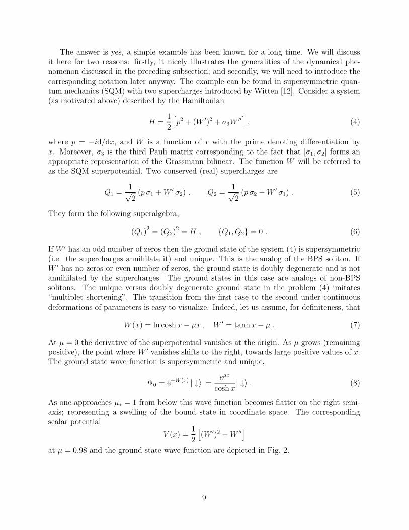
As one approaches µ∗ = 1 from below this wave function becomes flatter on the right semi-axis; representing a swelling of the bound state in coordinate space. The correspondingscalar potential

V (x) =1

2

[

(W ′)2 −W ′′]

at µ = 0.98 and the ground state wave function are depicted in Fig. 2.

9

x

ψ(x)

V(x)

FIG. 2. The potential V (x) in the problem (4), (7) (solid line) and the corresponding ground state

wave function (dashed line). The parameter µ = 0.98. The units on the vertical and horizontal axes are

arbitrary.

The point µ = 1 is critical. At µ > 1 the wave function (8) at E = 0 becomes non-normalizable, and the true ground state, coinciding with the continuum threshold, spectrumis doubly degenerate. The transition from one regime to another occurs through delocal-ization in that the zero of W ′, the equilibrium point x0, escapes to infinity. Note thatdynamically the SQM problem under consideration is similar to that of deuterium. Thepotential well in Fig. 2 is at x < 1, but the tail of the wave function stretches very far tothe right due to the fact that the E = 0 level is very close to the continuum spectrum.

We can make this somewhat more precise by introducing a “classicality parameter” ξdefined as

ξ ≡ W ′′′′(x)

(W ′′(x))2

∣

∣

∣

∣

∣

x=x0

, (9)

where x0 is the classical minimum of the potential: W ′(x0) = 0. The parameter ξ may beinterpreted as measuring the quantum correction to the curvature of the potential at theclassical equilibrium point. i.e. the system is essentially classical if ξ ≪ 1, while it is highlyquantum if ξ ≫ 1.

In the current example, we find that as we approach the critical point,

ξ ∼ 1

2 (1 − µ)+ · · · , (10)

and so the system indeed becomes highly quantum in this regime. In fact this feature isquite generic for short range potentials and may be viewed as an artifact of the remnantsupersymmetry. Specifically, since the mass term VF ∼W ′′(x) is linear in the superpotential,while the bosonic potential is quadratic, VB ∼ (W ′(x))2, for short range interactions thefermionic W ′′ term in the superpotential (II B) will dominate for large separations. This isdespite the fact that the fermionic term is a quantum effect (in field theory it correspondsto the 1-loop correction to the effective potential through integrating out the fermions).Thus, although the system becomes more and more weakly bound, in the CMS region thesystem enters a highly quantum regime where the classical minimum of the bosonic potentialneed not be relevant. Below we will see that exactly the same phenomenon occurs for BPSsolitons near the CMS in a 1+1D Wess-Zumino model.

10

C. Embedding of SQM within the field theory superalgebra

To establish a link between the field-theoretical description of solitons on the one handand the supersymmetric quantum mechanics of two nonrelativistic primary states on theother, we now consider the manner in which the quantum mechanical supercharges emergefrom the full field-theoretical superalgebra. The fact that supersymmetry is realized linearlyin the two soliton sector may be reinterpreted as the existence of a straightforward embed-ding of the SQM supercharges. Moreover, near the CMS the system becomes essentiallynonrelativistic and we need keep only the leading term in an expansion in velocities.

Although the arguments apply more generally, we consider for definiteness the realizationof N=2 supersymmetry in two dimensions in the two soliton sector. Recall that the algebracontains four supercharges Qα, Q†

α (α = 1, 2) and has the form [1, 23]

{Qα, Q†β} = 2 (γµγ0)αβ Pµ , {Qα, Qβ} = 2 i (γ5γ0)αβ Z , {Q†

α, Q†β} = 2 i (γ5γ0)αβ Z , (11)

where Pµ = (P0, P1) are the energy-momentum operators and Z is a complex central charge.We use the Majorana basis for 2×2 γ-matrices,

γ0 =σ2 , γ1 = i σ3 , γ5 = γ0γ1 = −σ1 . (12)

Modulo addition of the central charge, the algebra (11) can be viewed as a dimensionalreduction of the N=1 algebra in four dimensions. The SO(3,1) Lorentz symmetry in 3+1dimensions reduces in 1+1 to the product SO(1,1)×U(1)R where SO(1,1) is the Lorentzboost in 1+1 and U(1)R is a global symmetry associated with the fermion charge. Moreprecisely, the Lorentz boost with parameter β acts on the supercharges Qα as follows

Qα →[

exp(

1

2β γ5

)]

αβQβ , (13)

while the U(1)R transformation with parameter η is

Qα →[

exp(

i

2η γ5

)]

αβQβ . (14)

Notice that the U(1)R transformations can be viewed as a complexification of the Lorentzboost (13).

Its now convenient to introduce the Majorana supercharges Qiα, (i = 1, 2 ; (Qi

α)† = Qiα)

via the relation

Qα =e−i α/2

√2

(

Q1α + i Q2

α

)

, (15)

where the phase factor e−i α/2 contains an arbitrary parameter α, which we will fix momen-tarily. In terms of Qi

α the algebra (11) has the form:

{Qiα, Q

jβ} = 2 δij(γµγ0)αβ Pµ + 2 i (γ5γ0)αβ Z ij , (16)

where the 2 × 2 real matrix of central charges Z ij is symmetric and traceless. It is relatedto the original complex Z as follows,

11

Ze−i α = Z11 − iZ12 . (17)

To consider representations of the algebra we use a Lorentz boost in 1+1 to put the

system in the rest frame where P1 → 0 and P0 → M =√

PµP µ. Moreover, we can always

choose the basis in U(1)R to put Z ij in the form Z ij = |Z| τ ij3 . This amounts to fixing the

phase α to be equal to the phase of the central charge, Z = |Z| ei α. Then the algebra (16)takes the following component form,

(

Q11

)2=(

Q22

)2= M + |Z| ,

(

Q12

)2=(

Q21

)2= M − |Z| , (18)

with all other anticommutators vanishing, so that the algebra splits into two independentsubalgebras.

¿From (18) we see that |Z| is a lower bound for the mass, M ≥ |Z|. When M > |Z| theirreducible representation has dimension four – two bosonic and two fermionic states. TheBPS states saturate the lower bound, MBPS = |Z|, and in this case the second subalgebrabecomes trivial and the representation is two-dimensional – one bosonic and one fermionicstate [23].

How do all of these generalities help us with the problem of constructing the SQM nearthe CMS? In the vicinity of the CMS the difference M − |Z| is small as compared to |Z|and can be identified with the nonrelativistic Hamiltonian,1

HSQM = M − |Z| . (19)

The second subalgebra in Eq. (18) with supercharges Q11 and Q2

2 then coincides with thatof the standard SQM, see Eq. (6). In the first subalgebra the operator M + |Z| can besubstituted by 2 |Z| up to relativistic corrections. Consequently, the first subalgebra justleads to a generic multiplet structure (in this case just duplication) for every state found inthe SQM.

In Sec. IV we will find all the supercharges in the 1+1 example as explicit functions of themoduli from field-theoretic solutions for two solitons, u and v. Near the CMS, where theirrelative motion is nonrelativistic, the result can be compared with the quantum mechanicalrealization of the superalgebra (18). For HSQM = M − |Z| we take the expression whichgeneralizes Eq. (4) to include a mass parameter,

HSQM =1

2Mr

[

p2 + (W ′)2 + σ3W′′]

, (20)

where the superpotential W depends on the separation s = zu−zv , the conjugate momentump = −id/ds, and Mr is the reduced mass,

Mr =MuMv

Mu +Mv. (21)

1Note that we view M as a Hilbert space operator.

12

Then a realization of the superalgebra can be chosen in the form (σi and τi are two sets ofPauli matrices):

Q11 =

√

2 |Z| τ1 ⊗ σ3 , Q22 =

√

2 |Z| τ2 ⊗ σ3 ,

Q12 = I ⊗ 1√

2Mr

[p σ1 +W ′(s) σ2] , Q21 = I ⊗ 1√

2Mr

[p σ2 −W ′(s) σ1] . (22)

The realization (22) explicitly indicates a factorization of both the bosonic and fermionicdegrees of freedom associated with the center of mass of the system. We can also includedependence on the total spatial momentum P1 through a Lorentz boost (13) with tanhβ =

P1/√

M2 + P 21 .

A couple of comments are now in order. Firstly, its clear from this construction thatthe SQM can only be realized linearly in BPS sectors with a non-vanishing central charge.Otherwise, one has Q =

√M ψ (with ψ a fermionic operator) in the nonrelativistic limit,

implying a nonlinear realization. Secondly, we note that the expressions for Q11 and Q2

2 inthe first line of Eq. (22) represent the leading terms in the nonrelativistic v/c expansion. Itis not difficult to include higher order terms in this expansion as follows,

Q11 = τ1 ⊗ σ3

[

2 |Z| + p2 + (W ′)2 + σ3W′′

2Mr

]1/2

,

Q22 = τ2 ⊗ σ3

[

2 |Z| + p2 + (W ′)2 + σ3W′′

2Mr

]1/2

. (23)

where the square root is to be understood as an expansion in 1/|Z|.In concluding this section, we note that within the context of the present N=2 system

one can formulate a general statement: given the subalgebra (6) with two supercharges it isalways possible to elevate it to a superalgebra with four supercharges and a central chargeZ by adding the two additional supercharges (23).

III. AN N = 2 WZ MODEL IN TWO DIMENSIONS

A. Introducing the model

With the aim of concretely illustrating the general arguments of the previous section,we now consider a specific model. A suitable example exists in two dimensions, obtainedby dimensional reduction of a four-dimensional Wess-Zumino model with two chiral super-fields. The latter is the deformation of a model considered previously in Ref. [15]. Thesuperpotential is

W(Φ, X) =m2

λΦ − λ

3Φ3 − λΦX2 + µmX2 +

m2

λν X , (24)

where Φ and X are two chiral superfields, m is a mass parameter, λ is the coupling constant,while µ and ν are deformation parameters. By an appropriate phase rotation of fields and

13

the superpotential one can always make m and λ real and positive. The parameters µ andν are in general complex,

µ ≡ µ1 + iµ2 , ν ≡ ν1 + iν2 . (25)

The four real dimensionless parameters µ1, µ2, ν1 and ν2 will form our parameter space{µ}. For technical reasons the parameter µ ≡ µ1 + iµ2 will be assumed to be small in whatfollows, µ1,2 ≪ 1. Furthermore, we will consistently work in the approximation in which thesuperpotential is linear in µ; this corresponds to terms of O(µ2) in the scalar potential. Thislimitation is not a matter of principle but, rather, for technical convenience. In the limit ofsmall µ we can obtain all formulae in closed form. We will also take the coupling constantλ to be small, λ/m ≪ 1, so that a quasiclassical treatment is applicable (except on someexceptional submanifolds in the parameter space).

As a two-dimensional model, this theory has extended N = 2 supersymmetry, and ex-hibits solitonic kinks interpolating between the distinct vacua. In two dimensions they areparticles (in four dimensions they would be domain walls). The dimensionality of the BPSsupermultiplet is two, while that of the non-BPS supermultiplet is four.

Substituting

Φ =m

2λ(U + V ) , X =

m

2λ(U − V ) , (26)

we arrive at the following action,

S =m2

2λ2

{

1

4

∫

d2x d4θ (UU + V V ) +(

m

2

∫

d2x d2θW(U, V ) + h.c.)}

, (27)

where the dimensionless superpotential W is

W(U, V ) = U − 1

3U3 + V − 1

3V 3 +

µ

2(U − V )2 + ν (U − V ) . (28)

The vacua of the model are defined by ∂W/∂u = 0, ∂W/∂v = 0,

1 + ν − u2 + µ (u− v) = 0 ,

1 − ν − v2 − µ (u− v) = 0 . (29)

For real µ and ν the solutions to these equations define four different vacua with realvalues of the fields and real values of the superpotential W(u, v). The vacuum structure isillustrated in Fig. 3 for small µ. One of these vacua (denoted as {++} in Fig. 3 ) correspondsto a maximum of the real function W(u, v) on the real section of the variables u and v, theother vacuum (denoted as {−−}) corresponds to a minimum of W(u, v), and the remainingtwo vacua ({+−} and {−+}) are saddle points.

In this situation there exists [15] a continuous family of real BPS solitons, i.e. of solutionsto the real BPS equations

1

m

d

dzu =

∂W∂u

,1

m

d

dzv =

∂W∂v

, (30)

14

interpolating between the {−−} vacuum with Wmin at z = −∞ and the {++} vacuumwith Wmax at z = ∞. All these solitons are degenerate in mass: M = Wmax −Wmin, andcan be viewed as a superposition of non-interacting primary solitons: one going from thevacuum with Wmin to one of the saddle points, and the other soliton going from the saddlepoint to the vacuum with Wmax. The parameter labeling the solutions in this family canbe interpreted in terms of the distance between the basic solitons, and thus the degeneracyin energy implies that there is no interaction between the basic solitons at real µ and ν, atleast for some finite range of the these parameters.

{- -}

{- +} {+ +}

{+ -}{1,0}

{1,-1}

{-1,0}

{0,-1}

{0,1}{1,1}Re u

Re v

FIG. 3. Structure of vacua and solitons in the Reu, Re v plane for real ν and µ .

The decoupling of the dynamics of the primary solitons at µ = 0 is trivial, as thesuperfields U and V are also decoupled within the underlying field theory. However, atµ1 6= 0, there is no such decoupling within the field theory but, nevertheless, the primarysolitons do not interact at rest (provided µ and ν are real). This is a manifestation of thenontrivial “no-force” condition for BPS states.

B. Decoupled solitons, µ = 0 case

At µ = 0 the model is extremely simple: the fields U and V are not coupled. Their vevsare

u = ± ν+ , v = ± ν− , (31)

where we introduce the notation

ν± =√

1 ± ν . (32)

The masses of the BPS solitons are given by

15

Mnu,nv=

4

3

m3

λ2

∣

∣

∣nuν3+ + nvν

3−

∣

∣

∣ , (33)

where the topological charges are nu,v = 0,±1 (see Fig. 3).However, as noted in [15], not all combinations of charges are realized. For a generic

value of the complex parameter ν only the {1, 0} and {0, 1} solitons and their antiparticlesexist as BPS states. To have a BPS state with both nu and nv nonvanishing, one needs toalign in the complex plane the two terms, ν3

+ and ν3−, contributing to the mass in Eq. (33).

The relevant conditions are

Im

(

ν−ν+

)3

= 0 ,nv

nuRe

(

ν−ν+

)3

> 0 . (34)

These conditions define a curve in the complex ν plane presented in Fig. 4.

-1 1

-1

1

ν

ν

1

2

{1,1}

{1,-1}

{1,-1}

FIG. 4. The curve of marginal stability in the complex plane of ν.

This curve is the curve of marginal stability for the model. In the case under considera-tion, with no interaction, the CMS coincides with stability domains for composite solitons,they only exist on this curve.

The curve in Fig. 4 consists of three parts which can be parametrized as

ν = tanhσ , Im σ = 0, ±π3. (35)

The part sitting on the real axis between ν = ±1 (corresponding to Imσ = 0) is thestability domain for the {1, 1} composite solitons (and their antiparticles). The other twoparts, Im σ = ±π/3, give the stability domain for the {1,−1} and {−1, 1} solitons.

The bifurcations at ν = ±1 are due to the vanishing of the mass of one of the primarysolitons at these points. It is explained by the degeneracy of vacua at these values – insteadof four vacua only two remain at ν = ±1 (strictly speaking there are still four, but theycoalesce in pairs). These are simple analogs of the Argyres-Douglas points [13] in gaugetheories.

16

C. Stabilization by µ

The model at µ = 0 is a very degenerate case. Indeed, the extra {± 1,± 1} states existonly on the CMS and are nothing but systems of two noninteracting {± 1, 0} and{0,±1}solitons. The relative separation between the primary solitons is an extra classical modulus,on quantum level the {± 1,± 1} solitons are not localized states. As we will show, theintroduction of a nonvanishing Imµ = µ2 expands the domain of stability for the extra BPSstate which then occupies a finite area near the original curve. Thus, setting µ2 nonzeroleads to an attraction of the primary solitons.

Using µ as a perturbation parameter we find the vevs and values of the superpotentialW for the four vacua to first order in µ.

{++} : u = ν+ +µ

2

(

1 − ν−ν+

)

, v = ν− +µ

2

(

1 − ν+

ν−

)

,

W++ =2

3ν3

+ +2

3ν3− + µ (1 − ν−ν+) ;

{+−} : u = ν+ +µ

2

(

1 +ν−ν+

)

, v = −ν− +µ

2

(

1 +ν+

ν−

)

,

W+− =2

3ν3

+ − 2

3ν3− + µ (1 + ν+ν−) ;

{−+} : u = −ν+ +µ

2

(

1 +ν−ν+

)

, v = ν− +µ

2

(

1 +ν+

ν−

)

,

W−+ = −2

3ν3

+ +2

3ν3− + µ (1 + ν+ν−) ;

{−−} : u = −ν+ +µ

2

(

1 − ν−ν+

)

, v = −ν− +µ

2

(

1 − ν+

ν−

)

,

W−− = −2

3ν3

+ − 2

3ν3− + µ (1 − ν+ν−) . (36)

The BPS masses are given by |Wij −Wi′j′| and the alignment conditions which define theCMS to first order in µ become (c.f. Eq. (34)),

Im

(

ν2− − µ ν+

ν2+ + µ ν−

)3/2

= 0 , Im

(

ν2− + µ ν+

ν2+ − µ ν−

)3/2

= 0 , (37)

where the conditions clearly differ only by a choice of the branch of the square root in theterms linear in µ. Analytical expressions for the CMS are simpler in terms of the complexparameter of σ (related to ν by Eq. (35)). In the complex σ-plane the CMS is given by thecurves

σ2 = ±µ2 cosh3σ1

2cosh1/2 σ1 ,

σ2 =π

3± sinh

3σ1

2Re

[

µ cosh1/2(

σ1 + iπ

3

)]

,

17

σ2 = −π3± sinh

3σ1

2Re

[

µ cosh1/2(

σ1 − iπ

3

)]

, (38)

where the indices 1 and 2 refer to the real and imaginary parts, σ = σ1 + iσ2.The curves of marginal stability in the ν plane are presented in Fig. 5. They form the

boundaries of the stability domains for the composite BPS states marked in the figure.

-

-1

1

ν

ν2

11 1

FIG. 5. The domains of stability for the composite BPS states (shown for µ2 = 0.2). The hatched

region along the real axis is the stability domain for the {1, 1} solitons and its antiparticles, in the cross

hatched one the {1,−1} solitons and its antiparticles are stable.

Figure 5 exemplifies different metamorphoses of the composite BPS solitons on the CMS:crossing some boundaries leads to disappearance of the BPS state from the spectrum, onothers the original BPS state disappears but a new one appears.

The figure also shows exceptional points on the CMS, where two stability subdomainsof the same BPS soliton touch each other. We shall address a dynamical scenario at suchpoints in Sec. IVC. Note also four points of bifurcation (the Argyres-Douglas points) wherea pair of the vacuum states collide.

D. A loosely bound composite BPS state

In this subsection we will find a solution to the BPS equations for the composite {1, 1}soliton. The construction explicitly demonstrates that in the vicinity of the CMS this solitonis a loosely bound state of the primary constituents. For definiteness we choose the regionnear the real ν-axis and the {−−} → {++} transition. The BPS equations have the form

1

m

d u

dz= eiα

[

1 + ν∗ − (u∗)2 + µ∗(u∗ − v∗)]

1

m

d v

dz= eiα

[

1 − ν∗ − (v∗)2 − µ∗(u∗ − v∗)]

(39)

where

18

eiα =

√

W++ −W−−

W∗++ −W∗

−−

=ν3

+ + ν3−

|ν3+ + ν3

−|. (40)

We will use perturbation theory in µ. The part of the CMS chosen for consideration atzeroth order in µ corresponds to real ν: −1 < ν1 < 1, ν2 = 0. Then, at this order, α = 0and the solution for u and v reads

u(0) = ν1+ tanh [ν1+m (z − zu)] , v(0) = ν1− tanh [ν1−m (z − zv)] , (41)

where ν1± =√ν1 ± 1 (see Eq. (32)) and the parameters zu and zv are arbitrary and denote

the positions of the centers of the u- and v-solitons.At first order in µ, the soliton solutions become complex. With an expansion about the

leading order solutions u(0), v(0) of the form

u = u(0) + (u1 + iu2) + · · · , v = v(0) + (v1 + iv2) + · · · , (42)

the equations (39) lead to

1

m

d

dzu1 = −2u(0) u1 + µ1

(

u(0) − v(0))

,

1

m

d

dzv1 = −2v(0) v1 − µ1

(

u(0) − v(0))

,

1

m

d

dzu2 = 2u(0)u2 − ν2 + α

[

ν21+ − (u(0))2

]

− µ2

[

u(0) − v(0)]

,

1

m

d

dzv2 = 2v(0)v2 + ν2 + α

[

ν21− − (v(0))2

]

+ µ2

[

u(0) − v(0)]

, (43)

where

α =3

2ν2ν1+ − ν1−

ν31+ + ν3

1−

. (44)

Let us consider the equation for u2. The function cosh2[ν1+m(z− zu)] is the solution of thehomogeneous part of this equation, and the full solution is

u2(z) = cosh2 [ν1+ m (z − zu)] ×

m∫ z

−∞dx

−ν2 + α[

ν21+ − (u(0)(x))2

]

− µ2

[

u(0)(x) − v(0)(x)]

cosh2 [ν1+m (x− zu)](45)

As z → −∞ the solution satisfies the boundary condition

limz→−∞

u2(z) = − ν2

2ν++µ2

2

(

1 − ν1−

ν1+

)

(46)

consistent with Im u−− in Eq. (36) at the order considered here. As z → ∞ the solutionu2(z) grows exponentially unless the relation

19

∫ ∞

−∞dx

−ν2 + α[

ν21+ − (u(0)(x))2

]

− µ2

[

u(0)(x) − v(0)(x)]

cosh2 [ν1+m (x− zu)]= 0 (47)

is fulfilled. Once this relation is met the z → ∞ boundary condition u2 → Im u++ is alsosatisfied.

The relation (47) can be viewed as a constraint ensuring orthogonality of the inho-mogeneous part in the u2-equation and the zero mode cosh−2 [ν1+ m (z − zu)] in u1. Thisapproximate zero mode corresponds to a shift of the u-soliton center and at the same timealso represents the spatial dependence of the corresponding fermionic zero mode 2. The re-lation (47) then fixes the separation zu−zv of the two primary solitons and can be presentedin the form:

wν1(zu − zv) =

ν2

µ2 κ, (48)

where

κ =1

2

[

ν31+ + ν3

1−

]

, (49)

and the function wν of the soliton separation s = zu − zv is defined as

wν(s) =1

2

∫ ∞

−∞

dx

cosh2 xtanh

[

ν−ν+

x+ ν−ms

]

. (50)

It is important that the condition (48) also ensures that the solution for v2,

v2(z) = cosh2 [ ν1−m (z − zv)] ×

m∫ z

−∞dx

ν2 + α[

ν21− − (v(0)(x))2

]

+ µ2

[

u(0)(x) − v(0)(x)]

cosh2 [ν1−m (x− zv)], (51)

is finite at both z → +∞ and z → −∞, and thus satisfies the proper boundary conditions.As for the solutions for the real parts, u1 and v1, described by the first pair of equationsin (43), these solutions always exist, due to the existence of real BPS solitons in the modelwith real parameters [15], as discussed in Sec. IIIA. Thus no additional constraint arises.

Here we make a few remarks on the properties of the function wν(s), defined by theintegral (50). The symmetry properties of this function can easily be seen by writing it asthe derivative wν(s) = dg(s)/ds of the function

gν(s) =m

2

∫ ∞

−∞dz {1 − tanh [ν+mz] tanh [ν−m (z + s)]} , (52)

which is symmetric under separate reversal of the sign of ν or s. Thus wν(s) is even inthe index ν: w−ν(s) = wν(s), and is odd in the variable s: wν(−s) = −wν(s), and is

2In the next section we will show that this orthogonality condition is equivalent to the vanishing

of a particular supercharge.

20

monotonically increasing from wν(s→ −∞) = −1 to wν(s→ +∞) = +1. At large positives its asymptotic behavior is given by

wν(s) = 1 − ν+ + ν−ν

[ ν+ exp(−2 ν−ms) − ν− exp(−2 ν+ms)] + · · · , (53)

where the ellipses stands for higher powers and mixed products of the two exponents:exp(−2 ν−ms) and exp(−2 ν+ms). At ν = 0 the integral in equation (50) can be expressedin terms of elementary functions,

w0(s) = cothms− ms

sinh2ms, (54)

and the asymptotic behavior of w0(s) as s→ +∞:

w0(s) = 1 − (4ms+ 2) e−2m s + . . . (55)

is in agreement with the ν → 0 limit of the expression (53). Plots of wν(s) for a few valuesof ν are shown in Fig. 6.

-10 -5 5 10

-1

-0.5

0.5

1

wν(s)

s

FIG. 6. Plots of wν(s) at ν = 0 (solid), ν = 0.8 (dashed), ν = 0.95 (dot-dashed), s is measured in units

of 1/m.

The limited magnitude of wν(s), |wν(s)| ≤ 1, means that the BPS solution we consideronly exists in the range

|ν2| ≤ |µ2| κ . (56)

As expected the boundaries of this range coincide with the part of CMS found previouslyby algebraic means near the real ν axis.

It is then simple to find the value for the distance s0 between the primary solitons in theBPS composite state. Say, for ν1 = 0, we have when |µ2| − |ν2| ≪ |µ2|

em |s0| = η ln η, where η =

√

√

√

√

|µ2||µ2| − |ν2|

. (57)

21

IV. QUANTUM MECHANICS OF TWO SOLITONS

The BPS state which connects the vacua {++} and {−−} and exists within the stabilitydomain can be viewed as a bound state of one u-soliton, located at z = zu, and one v-soliton,located at z = zv. The equilibrium separation between the solitons, s = zu − zv, at whichthe minimum is achieved at given ν2 and µ2, is determined from the equation (48). In thissection we consider the supersymmetric quantum mechanics of the two soliton system. TheSQM system describes the BPS bound state (which is the ground state in the problem)within the stability domain, as well as low-lying non-BPS exited states.

The formulation of this problem refers to an effective description of the two solitonsas heavy particles with masses Mu and Mv in terms of their coordinates zu and zv. Thisapproximation is natural near the CMS where the binding energy is small relative to thesoliton masses. For slowly moving solitons |zu|, |zv| ≪ 1 the nonrelativistic energy can bewritten as

E = Muz2

u

2+Mv

z2v

2+ U(s) , (58)

where the dot denotes the time derivative, and U(s) is the interaction potential depending onthe separation s = zu−zv between the solitons. Separating out the center of mass coordinate,we come to a standard quantum mechanical Hamiltonian for the relative motion,

H =p2

2Mr

+ U(s) . (59)

The supersymmetric generalization of this Hamiltonian is given in Eq. (20) which dependson the superpotential W (s). Below we will find the expression for this SQM superpotentialby comparing the field theoretic supercharges evaluated on the soliton solutions with theSQM realization in Eq. (22). An alternative derivation of W ′ based solely on conventionalbosonic considerations is presented in an Appendix.

A. SQM superpotential from field-theoretic supercharges

The action (27) for the Wess-Zumino model leads to the following expression for thesupercharges Qα,

Q =m2

√2λ2

∫

dz[

∂tu ψ + ∂zu γ0γ1ψ + im ∂uW γ0ψ∗ + (u → v , ψ → η)

]

, (60)

where u, ψα and v, ηα are the bosonic and fermionic components of the U and V superfields,and W(u, v) is the superpotential of the model. The two remaining supercharges Qα arejust the complex conjugates of Qα.

Let us first evaluate the supercharges for the u-soliton in the leading approximation, i.e.when ν2 =µ1 =µ2 =0. The field u is given by Eq. (41), u = u(0) = ν1+ tanh [ν1+ m (z − zu)],while v is a constant, v = −ν1−. For the fermionic fields we substitute zero modes, two ofwhich are in the field ψα, and there are none in ηα,

22

ψzero modes =

(

i buau

)

1√2Mu

∂zu(0). (61)

In this expression Mu = (4m3/3λ2)ν31+ is the mass of the u-soliton, au and bu are real

fermionic operators entering as coefficients of the normalized zero modes, and their algebrais fixed by canonical quantization,

a2u = b2u = 1 , {au, bu} = 0 . (62)

Upon these substitutions, the supercharge Qα becomes

Q =√

Mu

(

au

i bu

)

, (63)

which can be rewritten in terms of real charges (see Eq. (15) in Sec. IIC for definitions),

Q11 =

√

2Mu au , Q22 =

√

2Mu bu , Q12 = Q2

1 = 0 . (64)

The result for the supercharges matches the general construction of Sec. IIC wherein theoperators au and bu can be realized as Pauli matrices, e.g. au = τ1 and bu = τ2.

Now let us find the supercharges corresponding to the {1, 1} configuration of the u- andv-solitons at ν2 =µ1 =µ2 =0. We choose boosted soliton solutions,

u(0) = ν1+ tanh[

ν1+m(

z − zu − p

Mut)]

,

v(0) = ν1− tanh[

ν1−m(

z − zv +p

Mvt)]

, (65)

where p is their relative momentum, and the total momentum is zero. The fermions aregiven by Eq. (61) for ψ and by a similar expression for η with the substitution u→ v, whereu- and v-fermions anticommute. With time-dependent solutions the terms ∂tuψ, ∂tv η nowcontribute to the supercharges (60),

Q11 =

√

2(Mu +Mv) (au cos δ + av sin δ) , Q22 =

√

2(Mu +Mv) (bu cos δ + bv sin δ) ,

Q12 =

p√2Mr

(−au sin δ + av cos δ) , Q21 =

p√2Mr

(−bu sin δ + bv cos δ) , (66)

where we have defined cos δ =√

Mu/(Mu +Mv). We observe that the relative motionimplies that the ‘composite’ state is non-BPS in the absence of any interaction between thesolitons.

In order to switch on the interaction we consider nonzero µ and ν2. To obtain theresult to first order in these parameters it is enough to substitute the same leading orderexpressions for the bosonic and fermionic fields accounting for the terms linear in µ and ν2

in the expression (60) for the supercharges, as well as for the phase α of the central charge.The linear dependence on µ and ν2 arises from the terms

23

m2

√2λ2

∫

dz[

µ (u(0) − v(0)) − iν2

]

γ0(ψ∗ − η∗) (67)

in (60). The phase α is also linear in ν2 (see Eq. (44)), and needs to be taken into accountin Eq. (15) when relating Qα with Q1,2

α .The resulting supercharges are (Q1

1, Q22 are not changed and are written here for com-

pleteness)

Q11 =

√

2(Mu +Mv) a , Q22 =

√

2(Mu +Mv) b ,

Q12 =

1√2Mr

[

p a +W ′(s) b]

, Q21 =

1√2Mr

[

p b−W ′(s) a]

, (68)

where we denote

a = au cos δ + av sin δ , b = bu cos δ + bv sin δ ,

a = −au sin δ + av cos δ , b = −bu sin δ + bv cos δ . (69)

The quantum-mechanical superpotential (more precisely its derivative W ′) is then readfrom Q1

2 (or Q21) to be

W ′(s) =3Mr

1 − ν21

[µ2 κwν1(s) − ν2 ] , (70)

where

Mr =MuMv

Mu +Mv=

2

3

m3

λ2

(1 − ν21)

3/2

κ, κ =

1

2(ν3

1+ + ν31−) , (71)

and the function wν(s) is defined by Eq. (50).The SQM Hamiltonian then has the form

HSQM = (Q12)

2 = (Q21)

2 =1

2Mr

[

p2 + (W ′(s))2 − iW ′′(s) a b]

. (72)

An explicit matrix realization of the four operators au,v and bu,v, satisfying the Cliffordalgebra, can a priori be chosen in the factorized form: au =τ1 ⊗ σ3, bu =τ2 ⊗ σ3, av =I ⊗ σ1,and bv = I ⊗ σ2. This factorized form of the fermionic operators realizes a description interms of two independent particles. This choice is perfectly acceptable and realizes the N=2 superalgebra (18). However, it differs from the specific realization (22) by an orthogonalrotation of angle δ. In order to match the conventions used in Eq. (22) for a descriptionof the two-soliton system, one has to use an equivalent representation of these operators,obtained by the inverse rotation:

au = τ1 ⊗ σ3 cos δ − I ⊗ σ1 sin δ , bu = τ2 ⊗ σ3 cos δ − I ⊗ σ2 sin δ ,

av = τ1 ⊗ σ3 sin δ + I ⊗ σ1 cos δ , bv = τ2 ⊗ σ3 sin δ + I ⊗ σ2 cos δ . (73)

The final expression for the full quantum Hamiltonian of the two-soliton system can bewritten as

24

HSQM =p2

2Mr+

9Mr

2

[µ2 κwν1(s) − ν2 ]2

(1 − ν21)

2+

3

2

µ2 κw′ν1

(s)

(1 − ν21)

σ3 (74)

with Mr given in Eq. (71) and we use the matrix representation (73) for the fermions(omitting the tensor product with unity in HSQM ).

It is worth noting a couple of limits in which the potential simplifies, and can be expressedin terms of elementary functions. Recall first of all that when ν1 = 0 the function w0(s) isknown analytically (see Eq. (54)). If ν1 is not too large, i.e. ν1 ≤ 0.5, there also exists aconvenient simplified form in which the superpotential is very closely approximated by theexpression

W ′approx(s) = 3Mr [µ2 tanh(ms) − ν2 ] , (75)

where the reduced mass Mr is taken at ν1 = 0. In this superpotential we recognize thesimplified model discussed in Sec. II B (see Eq. (7)). Another simple case arises when ν2

1 isclose to 1, i.e. 1 − ν2

1 ≪ 1,

W ′ =3Mr

√

1 − ν21

(µ2ms− ν2) . (76)

The potential in this case reduces to that of the harmonic oscillator.In the limit of large separation, the potential energy in the Hamiltonian (74) tends to a

constant which depends in the sign of s,

U± = U(s→ ±∞) =9Mr

2

(±µ2 κ− ν2)2

(1 − ν21)

2, (77)

(Note, however, that the spin dependent σ3 term does not contribute). These constantsdenote the energy levels at which the continuum states appear while the ground state,which is the {1, 1} BPS soliton, is a zero energy eigenfunction of HSQM.

The origin of the two continuum thresholds is that at nonzero µ the classification forsolitons we introduced at µ = 0 is no longer sufficient — the u-soliton interpolating betweenthe {−+} and {++} vacua (see Fig. 3) is different from the u-soliton interpolating betweenthe {−−} and {+−} vacua, and a similar distinction arises between the v- and v-solitons.Thus, the system under consideration at large s describes two channels: the u plus v solitonsat positive s, and the u plus v at negative s. It is straightforward to verify this by calculatingthe two binding energies,

∆E+ = M1,1 −Mu −Mv =m3

λ2[ |W++ −W−−| − |W++ −W−+| − |W−+ −W−−| ] ,

(78)

∆E− = M1,1 −Mu +Mv =m3

λ2[ |W++ −W−−| − |W+− −W−−| − |W++ −W+−| ] ,

from which we observe that ∆E± = −U±. Note that, although the quantities ∆E± are ofsecond order in µ2 and ν2, it is sufficient to use the expressions (36) which are only validto first order in µ (and are formally exact in ν) for the values of Wij . This is due to the

25

fact that for real ν and µ the values of Wij are real and ∆E± vanishes. Thus ∆E± arises asan effect quadratic in the imaginary parts of the differences of Wij which by themselves arelinear in ν2 and µ2.

Finally, we also write down the asymptotic behavior of the potential as s→ ±∞,

U(s) −→ U± +K± exp(−2ν1−m|s|) + · · · , (79)

where the coefficient of the leading exponential term is

K± =3 (ν1+ + ν1−)µ2κ

ν1ν1+(1 − ν1)(1 − ν21)

[

−6Mr (µ2κ∓ ν2) +mσ3 (1 − ν21) ν1−

]

. (80)

We have made the assumption here that ν1− < ν1+. We see that the characteristic distances is defined by 1/mν1− which as expected is the wavelength for the lightest particle in themodel. We also observe that the spin dependent term contributes to the exponential tail.Moreover, on the CMS where µ2κ ∓ ν2 = 0, it is the only contribution. This ‘fermionicdominance’ takes place in a very narrow region near the CMS,

|µ2κ∓ ν2| ≪(1 − ν2

1) ν1−

6

m

Mr. (81)

The effect of this regime of enhanced quantum corrections near the CMS will be consideredin more detail in the next subsection.

B. Properties of the two-soliton system

As expected, the second term in the potential in Eq. (74) is of higher order than thefirst in the loop expansion parameter λ. However the second term is of lower order in thesmall parameter µ2 and, by tuning µ2, one can study this potential both in the classicallimit corresponding to µ2 ≫ λ2/m2 and in the quantum limit µ2 ≪ λ2/m2, or anywhere inbetween as long as the condition for validity of the formula (74), µ2 ≪ 1, is maintained.Upon a slightly more detailed inspection of classical vs quantum effects in the Hamiltonian(74) one can readily see that in fact the quasiclassical parameter in this system is not justthe ratio λ2/(m2µ2) but is determined by the parameter

ξ =W ′′′′(s0)

(W ′′(s0))2, (82)

introduced in Sec. II, where s0 is the classical equilibrium separation determined by (48).Recall that ξ measures the quantum correction to the curvature of the potential near theclassical minimum, the system being essentially classical for ξ ≪ 1, and highly quantum forξ ≫ 1.

For the model at hand we find

ξ =w′′′

ν1(s0)

2mµ2

√

1 − ν21

(

w′ν1

(s0))2 · λ

2

m2. (83)

26

Near the CMS the equilibrium distance s0 is large, and ξ takes the form

ξ =κ

ν1+ (µ2 κ∓ ν2)· λ

2

m2, (84)

where for definiteness we have again assumed that ν1− < ν1+. Notice that the condition|ξ| ≫ 1 agrees with Eq. (81) which, as discussed above, defines the essentially quantumregime in the narrow region along the CMS.

When the system admits a supersymmetric ground state, the corresponding wave func-tion ψ0(s) can always be found as

ψ0(s) = const exp [−W (s)] = const exp

[

−3Mr

m

µ2 κ gν1(s) − ν2ms

1 − ν21

]

, (85)

where for definiteness we again assume µ2 > 0, and gν(s), defined by Eq. (52), is the integralof wν(s). Independently of the quasiclassical parameter ξ the maximum of ψ0(s) is alwayslocated at s0. However the spread of the wave function, i.e. the dispersion of the distancebetween the solitons in the BPS bound state, essentially depends on the parameter ξ. Asξ → 0 the full potential has a minimum at s = s0, and the system is classically located atthe minimum. At larger ξ the minimum of the full potential shifts towards s = 0, reachings = 0 in the limit ξ ≫ 1, but the maximum of the wave function is still at s = s0. In thelatter extreme quantum limit the system resembles the deuteron: the wave function spreadsover distances much larger than the size of the interaction region. In the two-soliton systemthis behavior is even more drastic at large ξ than in the deuteron: the wave function reachesits maximum far beyond the interaction region. The classical and the quantum behavior ofthe system at different values of ξ is illustrated by a series of plots in Fig. 7, 8.

1 2 3 4 5 6 7

-0.03

-0.02

-0.01

0.01

0.02

-6 -4 -2 2 4 6

-2

-1

1

2

3

ms

U(s) U(s)

ms

a b

FIG. 7. Plots of the full potential U(s) (arbitrary units) at ν1 = 0, ν2/µ2=0.95 for several values of ξ.

The classical equilibrium point is at ms ≈2.56 and is shown by heavy dot. Fig. a: details of the potential

near minimum for ξ = 0.009 (solid), ξ = 0.9 (dashed), and for ξ = 4.45 (dot-dashed). Fig. b: the potential

shown at a larger scale. The curves for ξ ≤ 4.45 are practically unresolvable and coincide with the solid

curve, the dashed curve corresponds to ξ = 125. It can be noticed that the latter value of ξ still corresponds

to moderate values of λ/m: λ2/m2 ≈ 7.7µ2.

27

-10 10 20 30ms

0.2

0.4

0.6

0.8

1

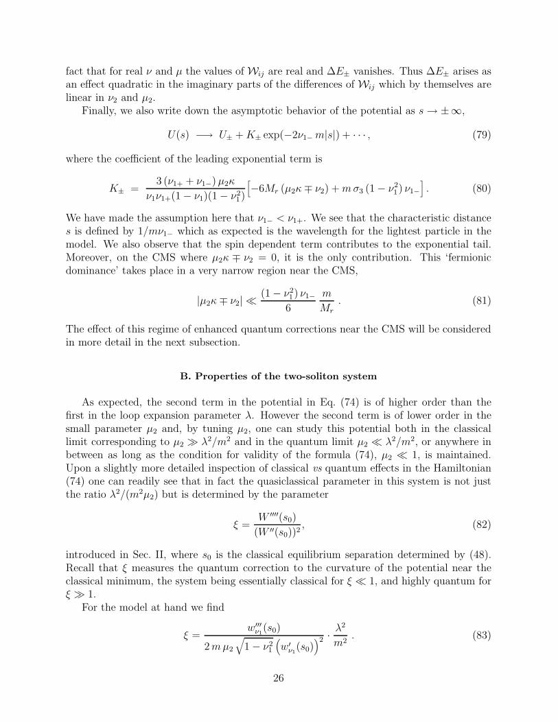
FIG. 8. Plots of the ground state wave function ψ0(s) for ξ = 17.7 (dashed) and ξ = 177 (solid). As

above, these parameters correspond to ν2/µ2 = 0.95 and the classical equilibrium point is at ms ≈ 2.56.

One may also note that in general the interaction of the two solitons is strong only atdistances of order m−1 near s = 0: the potential is asymmetric in s and changes rapidly nears = 0, i.e. the force is strongest when the solitons substantially overlap. In a narrow regionnear the CMS, given by Eq. (81), an attraction at short distances creates an essentiallyquantum state, resembling a deuteron. Deeper into the stability region an exponentiallyshallow minimum of the potential at large s0 results in a quasiclassical bound state.

Once one crosses the CMS, the wave function (85) is no longer normalizable, and thephysical ground state of the system is non-supersymmetric. The broadening of the wavefunction for the bound state near the CMS is exhibited in Fig. 8. Thus, as discussed inSec. II B the bound state level reaches the continuum on the CMS, where it completelydelocalizes, and on crossing the CMS the {1, 1} bound state is no longer present in thephysical spectrum.

C. Another dynamical regime: Extra Moduli on the CMS

The scenario discussed above, involving a short range superpotential which remains finiteon the CMS, is only a generic description for the near CMS dynamics in certain systems. Asdiscussed in Section 2, a different dynamical scenario is possible if there exist extra modulion the CMS. However, it turns out that the two-field model also exhibits a dynamical regimeof this type, and we observe in this case that the approach to the CMS is still characterizedby delocalization of the bound state wavefunction, albeit in a somewhat different manner tothe case considered above.

Firstly, recall that in the example considered above with µ2 6= 0, the approach to theCMS was determined by Eq. (48). In the ‘interior’ domain, |ν2| < |µ2|κ, the equationW ′(s) = 0 has a solution and consequently the composite soliton was BPS saturated. Uponapproach to the CMS, the zero of W ′(s) runs to infinity and, after crossing the CMS at|ν2| > |µ2|κ, there is no longer a solution to W ′(s) = 0 and hence no BPS soliton. Thisscenario is illustrated by see Fig. 9a..

Now we consider a different dynamical regime, see Fig. 9b, where, in both the ‘interior’and ‘exterior’ regions, the spectrum of BPS states is the same (although possibly rearranged).In this case one still has delocalization on the CMS one still has delocalization, althoughonly for the wave function in this case as there is no diverging (classical) separation of theconstituents.

28

(a)

BPS States C, P, P

BPS States

C, P, P

BPS States P, P

1

1

1 2

2

2

CMS(b)

FIG. 9. Possible scenarios for the BPS spectrum, taken from a small region of Fig. 5, where P1 and

P2 refer to the two primary solitons, while C refers to the composite kink: (a) A composite bound state C

exists only on one side of the CMS; (b) a bound state exits on both sides of the CMS.

To this end let us set ν = 0 (i.e. discard the term linear in U, V in the superpotential(24)). As explained in Sec. IIIA, at ν = 0 the CMS is very simple,

Imµ ≡ µ2 = 0. (86)

The SQM system (A.10) one arrives at in this case is described by the superpotential,

W ′(s) = 2m3

λ2µ2w0(s), (87)

where w0(s) was defined in (54). For our purposes it is important that w0(0) = 0, and thatthere are no other zeros of w0(s). Thus the solitons always overlap classically. However, asone approaches the CMS the wave function still spreads out due to the fact that µ2 → 0. Inparticular, at large |s|,

w0(s) −→ sgn(s), (88)

and one observes that the zero energy bound state exists for both positive and negative µ2

(see Fig. 9b). The wave function at large s is

exp

(

2m3

λ2µ2sσ3

)

(89)

times either | ↓〉 or | ↑〉 depending on the eigenvalue of σ3. As |µ2| → 0 the bound state levelapproaches the continuum spectrum while the wave function swells. At µ2 = 0 the wavefunction is completely delocalized and there is no binding.

As alluded to above, this dynamical regime is distinct from that considered previouslywhere W ′ remained finite on the CMS; rather the CMS was characterized by the escape ofthe root of W ′(s) = 0 to infinity. In contrast, in the example considered here the root ofthe equation W ′(s) = 0 does not shift at all. Despite this one may note that ξ still divergesnear the CMS due to its inverse dependence on µ2.

In fact, precisely on the CMS the potential vanishes, and thus a new quantum modulusarises corresponding to the relative separation of the constituents.

29

V. DYONS IN SU(3) N = 2 SYM

We turn now to consider similar phenomena in N = 2 SYM. To study a model whichexhibits a CMS in the weak coupling region, one approach is to extend the gauge group torank greater than one3. Here we consider one of the simplest examples of this kind withgauge group SU(3). In the Coulomb phase this theory exhibits BPS dyon solutions withelectric and magnetic charges associated with either of the unbroken U(1)’s of the Cartantorus. After choosing a convenient basis of simple roots for the algebra, one can classify theBPS monopole solutions into one of two types: those whose magnetic charge is aligned alonga simple root – ‘fundamental monopoles’ – and those whose magnetic charge is aligned alongthe non-simple root. These ‘composite monopoles’ generically possess CMS curves at weakcoupling, and so their dynamics in this regime is amenable to a semi-classical consideration.

Composite dyons in this, and the closely related N = 4 system, have recently beenstudied in some detail [16, 18–22, 25], with the conclusion that the low energy dynamicsof two fundamental dyons at generic points of the Coulomb branch acquires an additionalpotential term. This term is associated with the misalignment of the adjoint Higgs vevs ofthe two dyons, and leads to the formation of composite BPS dyons as bound states in thissystem. We will review some of these results below, and emphasize the implications for thedynamics in the near CMS region. The removal of the composite state on the CMS againarises through delocalization.

A. The BPS mass formula

We first review the features of the classical BPS mass formula for N=2 SYM with higherrank gauge groups (see e.g. [22, 26]), limiting ourselves to SU(N). For the consideration ofsolitonic mass bounds, we need consider only the bosonic Hamiltonian which has the form,

H = 2Tr∫

d3x{

1

2(Ei)

2 +1

2(Bi)

2 +D0Φ∗D0Φ +DiΦ

∗DiΦ +1

2[Φ∗,Φ]2

}

, (90)

where Ei and Bi (i = 1, 2, 3) are the electric and magnetic fields, and Φ is the complexadjoint scalar (Φ = (Φ1 + iΦ2)/

√2 in terms of the two real adjoint scalars). We use the

normalization TrT aT b = (1/2)δab for the generators.The classical vacua satisfy [Φ∗,Φ] = 0, thus requiring the vev of Φ to lie in the Cartan

subalgebra H,

〈Φ〉 = φ ·H . (91)

Note that the remaining Weyl freedom may be fixed by demanding that Reφ ·βa ≥ 0 for agiven set of simple roots {βa}. This defines a region which for |φ·βa| ≫ Λ coincides with the

3Alternatively, one can add hypermultiplet matter with a large mass. In this case there is a

discontinuity in the spectrum of quark monopole bound states on a CMS curve, which has been

studied by Henningson [24], and the mechanism involves delocalization in a manner analogous to

that discussed in this section.

30

semiclassical moduli space of the theory. In this region we can safely neglect field-theoreticperturbative and nonperturbative quantum effects. We will only consider the case wherethe gauge group is maximally broken to U(1)N−1, for gauge group SU(N).

For a soliton solution we may define the charge vector Q

Q · H = (q + ig) · H =∫

S2∞

dSi (Ei + iBi) , (92)

where use of the unitary gauge is implied. The real (q) and imaginary (g) parts of eachcomponent of Q have the interpretation of electric and magnetic charges in the correspondingU(1); they are are quantized and form a lattice spanned by simple roots,

q = qa βa = e nEa βa , g = ga βa =

4π

enM

a βa . (93)

Here e is the gauge coupling, and nEa and nM

a are the integral electric and magnetic quantumnumbers. We also normalize the simple roots βa with the conventions (βa)2 = 1, βa±1 ·βa =−1/2, so that the coroots coincide with the roots.

For general bosonic configurations, there is a Bogomol’nyi mass bound following from(90) which takes the form,

M ≥ Max |Z±| , Z+ =√

2 φ∗ · Q , Z− =√

2φ · Q , (94)

This bound is saturated by solutions of the Bogomol’nyi equations,

Bi = Di b , Ei = Di a , (95)

along with the equation D2i a ∓ e2[b, [b, a]] = 0 which, making use of (95), expresses Gauss’

law in the gauge A0 = ∓a. The fields a, b are real and imaginary parts of exp(iα) Φ wherethe angle of rotation α is defined in terms of the charges Q (see e.g. [16, 22, 27]).

In the framework of the N= 4 supersymmetry algebra the parameters Z± are realizedas central charges, and it is advantageous to view the system in this context (implying sixinstead of two real scalars Φ). Within N=4 SUSY it is generally the case that |Z+| 6= |Z−|,and states which saturate the Bogomol’nyi bound M ≥ Max |Z±| will preserve only fourof the sixteen supercharges, and will thus be 1/4 supersymmetric. If, however, |Z+| =|Z−|, states which saturate this bound will preserve 1/2 of the N=4 supersymmetry. Thepossibility of having 1/4 BPS states, which only occurs for gauge groups of rank larger thanone, dramatically increases the number of CMS curves accessible to semiclassical analysis,since 1/4 BPS states generically exhibit regions in the parameter space where they becomemarginally stable with respect to “decay” into 1/2 BPS states. In this sense it is useful tothink of 1/4 BPS configurations as composite.

The discussion above was framed within N=4 SYM, but this was simply for orientation.In order to preserve any fraction of supersymmetry, four of the six real adjoint scalars mustvanish asymptotically, and thus the configurations discussed above all “descend” to giveclassical solutions in N= 2 SYM. The difference is that now only Z− remains as a centralcharge [22] and all states saturating the bound M = |Z−| are 1/2 BPS states from thepoint of view of the N=2 SUSY algebra. As noted in [22], those charge sectors for which

31

|Z−| < |Z+| will have no BPS states from the point of view of the N=2 system. Indeed, inthis case states with M = |Z−| are not allowed because M ≥ |Z+|. Thus |Z−| > |Z+| is anecessary condition for the existence of N=2 BPS states.

Restricting our attention now to the gauge group SU(3), then on the Coulomb branchthe gauge group is broken down to the Cartan subalgebra U(1)2 and there can be field con-figurations which are electrically and magnetically charged under either of these U(1)’s [28].Following Weinberg [28] we use the term ‘fundamental dyons’ to refer to those configurationswhose charges are aligned along one of these simple roots. Configurations whose charges arealigned along non-simple roots (i.e. β1 + β2) will be referred to as ‘composite’. We shallfocus on a particular composite configuration which has received considerable attention inthe recent literature – namely the composite dyon which has equal magnetic, na

M = (1, 1),and differing electric, na

E = (q1/e, q2/e), charges along the simple roots.

B. Marginal stability and Coulomb-like interaction

The BPS mass formula for the (1,1) dyon with naM = (1, 1), na

E = (q1/e, q2/e) takes theform,

M(1,1) = |Z−| =√

2∣

∣

∣(q1 + ig) φ · β1 + (q2 + ig) φ · β2∣

∣

∣ , (96)

where g = 4π/e. This configuration has a CMS curve where the (1,1) dyon is marginallystable with respect to two fundamental dyons: the first is aligned along β1, and has na

M =(1, 0), na

E = (q1/e, 0), while the second is aligned along β2, and has naM = (0, 1), na

E =(0, q2/e). The masses of the fundamental dyons are

Ma =√

2 |(qa + ig) φ · βa| = ma

(

1 +q2a

2g2+ O

(

q4a

g4

))

, (97)

where in the second equality we have made use of the fact that e2 ≪ 1 in order to write thedyon mass as a small correction to the mass of the corresponding fundamental monopole,ma =

√2g|φ · βa|. Introducing ωa as the argument of the vevs,

φ · βa = |φ · βa| eiωa (98)

we see that the marginal stability condition M(1,1) = M1 + M2 fixes the argument of theratio φ · β1/φ · β2,

ω = ω1 − ω2 , (99)

to be equal to the argument of the ratio of complex charges Q2/Q1 where Qi = qi + ig. Thisimplies that the CMS equation is ω = ωc where ωc is defined as

sinωc =(q2 − q1) g

√

g2 + q21

√

g2 + q22

. (100)

Provided naE and na

M are of a similar order, the angle ωc is small in the limit e2 ≪ 1, i.e.when the electric corrections to the dyon masses are much smaller than the corresponding

32

monopole mass as in (97). Thus in this limit the vevs φ · βa are only slightly disaligned,and we can make use of an expanded version of Eq. (100),

ωc =∆q

g

(

1 + O(q2i /g

2))

, ∆q = q2 − q1 . (101)

We are now in a position to verify the general claim of Sec. IIA that the Coulombicinteraction vanishes on the CMS. At large distances dyons can be viewed as point chargeswhich interact at rest through electrostatic, magnetostatic, and scalar exchange. The elec-trostatic and magnetostatic interactions are fixed by the corresponding charges, while thescalar exchange can be read off from the asymptotic form of the Higgs field of one of theprimary dyons (in a physical gauge where the configuration is a linear superposition of thefundamental dyon solutions [27, 29]). The effective Coulombic interaction then takes theform,

VCoul = − 1

8πr

[

q1q2 + g2 −√

g2 + q21

√

g2 + q22 cosω

]

. (102)

Similar expressions have appeared in [27] and [19]. One observes that on the CMS, wherethe angle ω is given by Eq. (100), the Coulombic potential VCoul vanishes.

When expanded to second order in qi/g, the potential VCoul takes the form

VCoul ≈(∆q)2 − (g ω)2

16πr, (103)

where ∆q = q2 − q1 is defined in Eq. (101). If the vevs were aligned, i.e. ω = 0, we see thatto quadratic order, the potential is repulsive [29,30] (as opposed to the SU(2) case [31]) anddepends only on the electric charge difference ∆q. However, for (g ω/∆q) > 1 the potential isattractive and the (1,1) BPS dyon exists with a mass M(1,1) given in the same approximationby

M(1,1) = |Z−| ≈ (M1 +M2) −Mr(∆q − g ω)2

2 g2,

(

g ω

∆q> 1

)

, (104)

where Mr = m1m2/(m1 +m2) is the reduced mass of the monopoles, and the correspondingmasses M1,2 and m1,2 are defined in Eq. (97). On the other side of the CMS in the range|g ω/∆q| < 1 we have repulsion and the the (1,1) BPS dyon does not exist.

Its interesting to note that the Coulombic potential reverts to attractive form once morewhen (g ω/∆q) < −1, and the (1,1) bound states reappear. This has a simple interpretationin the framework of N=4 supersymmetry: the lowest mass in this range saturates the |Z+|central charge (note that now |Z+| > |Z−|),

M(1,1) = |Z+| ≈ (M1 +M2) −Mr(∆q + g ω)2

2 g2,

(

g ω

∆q< −1

)

. (105)

In terms of N=4 SUSY the (1,1) state at (g ω/∆q) < −1 is 1/4 supersymmetric, butpreserves a different subalgebra as compared to the (g ω/∆q) > 1 case above. Moreover, thegenerators of this subalgebra are not part of the N=2 superalgebra. In terms of N=2 this

33

means that the supermultiplet is not shortened, but nonetheless the Bogomol’nyi bound issaturated at the classical level 4. Thus, we see an interesting example where the “BPS”nature of the state does not imply multiplet shortening. The presence of these states inN=2 SYM was also noted in [22].

We now address the question of what happens to the (1,1) state on the CMS, i.e. when|g ω/∆q| = 1 and the 1/r terms in the potential vanish? As we will see in Sec. VD the dy-namics on the CMS is governed by repulsive 1/r2 terms demonstrating, even at the classicallevel, that there is no localized bound state on the CMS.

C. Zero Modes and Moduli Spaces

We will shortly consider the low energy dynamics of the fundamental dyons comprisingthe (1,1) system. However, we first recall a few details regarding the zero mode structureof dyon solutions in N = 2 SYM. For BPS dyons in pure N = 2 SYM the unbroken N =1 supersymmetry is enough in this case to pair the bosonic and fermionic zero modes [32]so we shall focus here just on the bosonic modes. Generic dyon solutions, correspondingto the embedding of the SU(2) monopole along some root of SU(3) have four bosonic zeromodes [26, 28] parametrizing the moduli space,

M1 = R3 × S1. (106)

These modes are naturally identified as the center of mass position in R3 and the S1 is anisometry conjugate to the conserved electric charge.

For dyons embedded along a simple root, this is the moduli space for all choices offield-theoretic moduli. However, if we consider composite monopoles, then the monopolemoduli space M enlarges to a space of dimension eight, as is compatible with separatingthe constituents into two isolated fundamental monopoles [26,27]. This result was obtainedin [26] using the index calculations of Weinberg [28] for real Higgs fields.

For the case at hand, the magnetic charge is g = g(β1 + β2) and asymptotically theeight dimensional moduli space is simply M1 ×M1. However, its exact form has also beendeduced in [29, 33–35],

M2 = R3 × R ×MTN

Z. (107)

The first R3 factor corresponds to the center of mass position, while the second R factorrefers to the coordinate conjugate to the total electric charge. The corresponding metric isflat. The relative moduli space MTN is positive mass Taub-NUT space (which is asymptot-ically R3 × S1). Its four coordinates zµ describe the relative distance r between the cores,with the corresponding polar and azimuthal angles θ and ϕ, and also the relative phase χ,conjugate to the relative electric charge ∆q. The factor Z denotes a discrete identification

4This saturation will be lifted by field-theoretic quantum corrections.

34

for the charge coordinates, ensuring that the asymptotic geometry has a compact factorS1 × S1, associated with the conserved charges.

The Taub-NUT metric, in our conventions 5 takes the form,

ds2TN = gTN

µν dzµdzν = m(r)[

dr2 + r2dθ2 + r2 sin2θ dϕ2]

+g2

e2m(r)

[

dχ+1

2cos θ dϕ

]2

, (108)

with a ‘running’ mass parameter,

m(r) = Mr +2π

e2r, (109)

which asymptotes to the reduced mass Mr when the relative separation r diverges.In terms of the internal U(1) angles ψi of the fundamental monopoles, the combination

ξ = ψ1 + ψ2 is conjugate to the total electric charge qt (or more precisely, to qt/e),

qt =m1q1 +m2q2m1 +m2

, (110)

while χ = (m1ψ2−m2ψ1)/(m1 +m2) is conjugate to ∆q/e, i.e. to the relative electric chargeintroduced above [34, 35].

D. Moduli space dynamics

As first discussed in this context by Manton [36], the low-energy dynamics of fundamentalmonopoles may be understood as geodesic motion on the underlying moduli space. Thispicture extends to dyon solutions with aligned charges, but recent work on the dynamics ofthe fundamental constituents of the (1,1) system [16–22] has shown that for two fundamentaldyons with misaligned charges the Lagrangian following from the geodesic approximationneeds to be corrected by a new term [19,22]. In this subsection we will partially review theseresults, while emphasizing the features of the near CMS region.

The construction of Refs. [19,22] can be reformulated in terms of the following Lagrangianfor the relative moduli zµ = {~r, χ}

Lrel =1

2gTN

µν zµ zν + gTNµν zµ Gν , (111)

where the metric gTNµν is given by Eq. (108) and the ‘potential’ Gν , which is a Killing vector

generating the χ isometry, is

Gν =e

gMr ω δ

νχ . (112)

5We follow [22] with the exception that χ is rescaled to have a period of 2π rather than 4π, and

consequently the conjugate momentum is integer ((q2−q1)/e) rather than half-integer ((q2−q1)/2e)valued.

35

Here ω is the angle of disalignment between the condensates φ · βa, see Eq. (98). The termcontaining Gµ is dynamically significant due to nontrivial fibering of the S1 associated withχ in the Taub-NUT metric.

The classical Hamiltonian then has the form

Hrel =1

2gµνTN (πµ −Gµ)(πν −Gν) , (113)

where πµ = gTNµν (zν + Gν) are the canonical momenta. In terms of the original field theory

this Hamiltonian is interpreted as M−|Z−|, and thus BPS states are ‘vacuum’ states of thisHamiltonian.

Two of the canonical momenta, namely πϕ and πχ, are conserved quantities conjugate toisometries along the azimuthal angle ϕ and the phase χ. The value of πϕ is the z-projectionof the angular momentum lz, and πχ is equal to ∆q/e. Substituting these and the inversemetric gµν

TN into Eq. (113) we obtain

Hrel =π2

r

2m(r)+

π2θ

2m(r) r2+

1

2m(r) r2 sin2θ

(

lz −∆q

2ecos θ

)2

+ V (r) , (114)

where

V (r) =Mr

2 g2

(

1 +2π

e2Mr r

)−1 (

∆q − g ω + ∆q2π

e2Mr r

)2

(115)

is the only term in Hrel which depends on the field-theoretic moduli φ (via ω).This Hamiltonian vanishes at πr = 0, πθ = 0, and the equilibrium values r0 and θ0 of the

corresponding coordinates are given by

r0 =2π

e2Mr

∆q

g ω − ∆q, cos θ0 = 2 lz

e

∆q, (116)

when (g ω/∆q) > 1 and |2lz e/∆q| < 1. There is no solution for (g ω/∆q) < 1, i.e. theBPS state ceases to exist upon crossing the CMS where g ω = ∆q. We see that the sys-tem describes the composite state as a bound state of the dynamics whose spatial size,corresponding to the separation of the primary constituents, diverges on approach to theCMS.

It is instructive to expand the potential V (r) at large r

V (r) = Mr(∆q − g ω)2

2 g2+

(∆q)2 − (g ω)2

16π r+

(g ω)2

8 e2Mr r2+ . . . , (117)

where we omitted 1/r3 terms and higher powers of 1/r. The constant term V (r → ∞)marks the start of the continuum. Indeed, adding |Z−| from Eq. (104) we obtain M1 +M2

in the limit r → ∞. The 1/r term coincides with the Coulombic potential (103) discussedearlier. It provides attraction for |g ω/∆q| > 1, the range where the bound states exist. Therange (g ω/∆q) < −1 corresponds, as discussed above, to M(1,1) = |Z+|. What we see inaddition is the repulsive 1/r2 term which leads to the existence of an equilibrium at larger0 near the CMS. However, on the CMS it becomes the dominant term, and so there is nolocalized state on the CMS.

36

We conclude this section with some brief comments about quantization. The quantizationof the dyon system in the context of N=2 SYM was first discussed in detail by Gauntlett [32]in the case where the Higgs vevs are aligned, and this discussion has since been generalizedto the case considered here by Bak et al. [20] for N= 4 , and by Gauntlett et al. [22] forN= 2 SYM. The crucial feature of this system is that the relative moduli space inherits atriplet of complex structures J (a), a = 1..3, and is a hyperkahler manifold. Consequently,the system exhibits N=4 supersymmetric quantum mechanics with four real superchargesQA where the index A can be associated loosely with a quaternionic structure J (A) = (1, Ja).These supercharges satisfy the superalgebra,

{QA, QB} = 2δABHrel, (118)

where Hrel is the supersymmetric completion of the Hamiltonian defined in (113), to beinterpreted as M − |Z−|. One can compare this with the SQM constructed in Sec. 2.

An interesting feature of this system is that the symmetries of the superalgebra andthe moduli space combine to ensure that the wavefunctions have a nontrivial dependenceon the angular moduli, as well as the relative separation r. Specifically, the ground statewavefunction has the functional form [20] Ψ0 = Ψ0(r, σa) where σa are the basis 1-formson the S3 parametrized by (θ, ϕ, χ). This dependence is hinted at through the θ-dependentterms in the Hamiltonian (114) above. One may speculate that because of the high degreeof symmetry in this system – the bosonic system possesses an additional conserved quantityof Runge-Lenz type [25] – a more precise separation of variables may be possible, but we willnot pursue this issue here. We note only that, as demonstrated above, the delocalization onthe CMS is associated with the cancellation of the terms of O(1/r) and depends purely onthe relative separation. Moreover, this conclusion in the classical bosonic system apparentlyextends to SQM [20].

VI. DELOCALIZATION VIA MASSLESS FIELDS

On particular submanifolds of the CMS, the discussion we have presented above may beincomplete because certain fields may become massless. Indeed, generically there will beparticular points on the CMS where states which are stable on both sides are massless. Thepresence of these singularities in moduli space can then be thought of as the ‘origin’ of theCMS since marginally stable states may not be single valued on traversing a contour aroundthe singularity, and so a discontinuity in the spectrum becomes necessary for consistency.For example, this point of view provided one of the first arguments for the fact that the Wboson must be removed from the spectrum inside the strong coupling CMS in N=2 SYM [3].

In this section we will discuss the behavior of BPS states near these singular points.Within a simple 2D Wess-Zumino model we will find that the discontinuity of the BPSspectrum is explained by the delocalization of fermionic zero modes of the soliton on theCMS. The CMS in this case corresponds to the ‘collision’ of two vacua in the parameterspace, and thus one might anticipate similar phenomena in N = 2 SYM near Argyres-Doulgas points [13] when the singularities associated with monopole and quark vacua collide.Unfortunately, this occurs at strong coupling and is out of the range of our semi-classicalanalysis.

37

A. Breaking N = 1 to N = 1 and the restructuring of WZ solitons

The model is a simplified version of the N= 2 Wess-Zumino model [14] in two dimen-sions considered in Sec. III. We shall set the second field X to zero, but consider a newperturbation which breaks N=2 down to N=1. This setup was introduced in Ref. [37] (seeSec. 8).

The superpotential prior to perturbation is then of the standard Landau-Ginzburg form,and its worthwhile recalling a few pertinent details of these theories. A general classificationof the N = 2 Landau-Ginzburg–type theories in two dimensions was given in [1], whileconstruction of the representations of the N = 2 superalgebra with central charges waspresented in Refs. [23]. It was shown that the supermultiplet of BPS soliton states isshortened, and this shortened multiplet consists of two states {u, d} as we discussed earlierin Sec. III. In particular, in N=2 theories there exists a conserved fermion charge f . Thefermion charge of the u and d states is fractional but the difference is unity, fu − fd = 1.

What changes on passing to N=1 in two dimensions? The irreducible representation ofthe N=1 algebra for BPS states is now one-dimensional (to the best of our knowledge thiswas first noted in Ref. [37]). The only remnant of the fermion charge is a discrete subgroupZ2 which is spontaneously broken.

It is natural then to expect a restructuring of the BPS spectrum when N=2 is brokendown to N = 1. We will study the manner in which restructuring occurs by consideringthe spectrum of fermionic zero modes of a soliton solution as we vary the soft breakingparameter µ. We observe that for small µ the BPS spectrum remains the same as in theunbroken N=2 theory. However, starting at a critical value µ∗ – corresponding to a ‘point ofmarginal stability’ – half the BPS states disappear from the spectrum. This occurs becausequasiclassically the counting of states in the supermultiplet is related to the counting of zeromodes of the soliton and when µ reaches µ∗ some of the fermionic zero modes become non-normalizable. To follow their fate one can introduce a large box. Then the number of statesdoes not change, but at µ = µ∗ the identification of states with zero modes implies that halfthe BPS states spread out all over the box while for µ > µ∗ they lie on the boundary ofthe box and are removed from the physical Hilbert space. This picture is quite analogousto the quantum mechanical discussion in Sec. II. However, as we shall see, the quantumdescription is complicated here by the presence of a massless field.

We take the Kahler metric to be canonical and the cubic superpotential of the model isconveniently represented in terms of real bosonic variables ϕi, i = 1, 2,

W(ϕ1, ϕ2) =m2

4λϕ1 −

λ

3ϕ3

1 + λϕ1ϕ22 . (119)

In fact, W(ϕ1, ϕ2) is harmonic

∂2W∂ϕi∂ϕi

= 0 for N = 2 . (120)

as it is the imaginary part of the four dimensional superpotential which is analytic in ϕ1+iϕ2.This is therefore a reflection of N=2 supersymmetry in two dimensions.

Now, to break N=2 down to N=1 we consider a more general, nonharmonic, superpo-tential W (ϕ1, ϕ2),

38

W (ϕ1, ϕ2) =m2

4λϕ1 −

λ

3ϕ3

1 + λϕ1ϕ22 +

µ

2ϕ2

2 , (121)

where µ is the soft breaking parameter. There are two vacuum branches,

{

ϕ1 = ±m

2λ; ϕ2 = 0

}

,

{

ϕ1 = − µ

2λ; ϕ2 = ±

√µ2 −m2

2λ

}

, (122)

but the second exists only for µ > m, and vacua collide when µ = m.This model exhibits a classical kink solution which interpolates between the first set of

vacua, and is given by

ϕ1 =m

2λtanh

mz

2, ϕ2 = 0. (123)

It satisfies the classical BPS equations,

∂ϕi

∂z=∂W∂ϕi

. (124)

The zero modes corresponding to this kink are as follows:(a) one bosonic mode:

χ0 = C1

cosh2(mz/2)(125)

in the field ϕ1 corresponds to (the spontaneous breaking of) translational invariance,

χ0 ∝ dϕ1/dz .

The constant C in Eq. (125) is a normalization constant; its explicit numerical value is notimportant. (Below the normalization constants in the zero modes will be omitted.)(b) two fermionic modes: The first zero mode in the field ψ1,2 (the indices number the su-perfields and fermionic components in the basis where γ0 = σ2, γ

1 = iσ3) has the same formχ0 as the translational mode. It is not accidental, the corresponding differential operatorsare the same due to N=1 supersymmetry. The second fermionic zero mode

ξ0 =exp(−µz)

cosh2(mz/2)(126)

appears in the field ψ2,1. At µ = 0 the existence of this mode is a consequence of the N=2SUSY, and ξ0 coincides with χ0. At nonvanishing µ, when the extended SUSY is broken,this zero mode is maintained by virtue of the Jackiw-Rebbi index theorem [38].

An interesting feature of the zero mode ξ0 is that it is asymmetric in z for µ 6= 0.Moreover, this mode is normalizable only for

µ < m . (127)

This is readily seen from its asymptotics,

39

ξ0(z → ∞) ∼ e−(µ+m)z , ξ0(z → −∞) ∼ e−(µ−m)z , (128)

The explicit form of the zero mode for few values of µ is exemplified in Fig. 10.

-10 -5 5 10

-0.4

-0.2

0.2

0.4

0.6

0.8

FIG. 10. The kink profile (solid line), with the zero mode ξ0 for µ/m = 0 (dotted line), µ/m = 0.8

(short-dashed line), and µ/m = 1 (long-dashed line). Note that the vertical scale has been altered for ease

of presentation.

The loss of normalizability occurs at µ = m, when

det

{

∂2W∂ϕi∂ϕj

}

= 0

in one of the vacua between which the soliton solution interpolates. In other words, one ofthe vacuum states has gapless excitations at this point. Indeed, in the z → −∞ vacuum,the eigenvalues of the fermion mass matrix are: m and µ−m, and thus indeed at the pointµ = m where the vacuum branches meet, there is a massless field. This system representsa simplified analog of an Argyres-Douglas point in that the massless field arises throughthe collision of vacua. Furthermore, we see that this infrared effect destabilizes one of thefermionic zero modes of the soliton.

To study the infrared behavior in detail let us put the system in a large box, i.e. imposeboundary conditions at z = ±L/2 where L is large but finite. We choose these conditionsin a form which preserves the remnant supersymmetry in the soliton background (i.e. theBPS nature of the soliton),

(

∂zϕi −∂W∂ϕi

)∣

∣

∣

∣

∣

z=±L/2

= 0 ,

(

δij∂z −∂2W∂ϕi∂ϕj

)

ψj2

∣

∣

∣

∣

∣

z=±L/2

= 0 , ψi 1

∣

∣

∣

z=±L/2= 0 , (129)

(see Ref. [37] for details). It is easy to check that the soliton solution (123) as well as thezero modes (125), (126) are not deformed by these boundary conditions, i.e. (123) remainsa solution of the classical BPS equations with the appropriate boundary conditions at finiteL.

40

In the finite box there is no problem with normalization; the zero mode (126) remains asolution of the Dirac equation in the soliton background for all µ. However, at µ > m themode is localized on the left wall of the box instead of sitting on the soliton as is the case atµ < m. Thus, at µ = m the critical phenomenon of delocalization starts. As we will showbelow, upon quantization this means that some BPS soliton states have disappeared fromthe physical Hilbert space.

B. Quantization

We shall not present a detailed analysis of the quantization of the system here as itrequires a somewhat different treatment to the supersymmetric quantum mechanics we haveconsidered thus far. In this case, one needs to consider the dynamics of the light field inaddition to the collective coordinates of the soliton.

However, provided we only consider a region somewhat away from the CMS, the spec-trum is easily determined. As usual, the remnant N= 1 supersymmetry pairs the nonzeromodes (one bosonic to two fermionic) around the soliton (see e.g. Sec. 3G of [37]), and therelevant contributions cancel. Thus the soliton spectrum is determined by the zero modes,corresponding to which we have one bosonic collective coordinate z0 corresponding to thecenter of the kink, and two real Grassmann collective coordinates α1 and α2 determinedby the zero modes, ψ1,2 = α1χ0(z) + · · · and ψ2,1 = α2ξ0(z) + · · ·. Combining them intoone complex parameter η = (α1 + iα2)/

√2, the collective coordinate dynamics at µ = 0 is

determined by the quantum mechanical system

Leff = −M +1

2Mz2

0 + iMηη, (130)

where M is the physical kink mass, which we can set to one.The quantization is carried out in the standard manner. If z0 and η are the canonical

coordinates, we introduce the canonical momenta

πz0= z0 , πη = −iη , (131)

and impose the (anti)commutation relations

[πz0, z0] = −i , {πη, η} = −i . (132)

One then proceeds to construct the raising and lowering operators in the standard manner.From Eqs. (131) and (132) it is clear that η can be viewed as the lowering operator, whileη is the raising operator. One then defines the ‘vacuum state’ in the kink sector by thecondition that it is annihilated by η,

η|‘vac′〉 = 0 .

The application of η produces a state which is degenerate with the vacuum state. |‘vac′〉and η|‘vac′〉 are two quantum states which form a (shortened) representation of N =2 supersymmetry (at µ = 0). It is clear that these two states, which are degenerate inmass, have fermion numbers differing by unity.

41

What happens at µ 6= 0? At µ < m the situation is exactly the same as at µ = 0(apart from the fact that the fermion number is not conserved now and we must classify thestates with respect to their Z2 properties). We have two degenerate quantum states, bothare spatially localized and belong to the physical sector of the Hilbert space. At µ = monly the vacuum state is localized. The spatial structure of the second state η|‘vac′〉 hasa flat component, which extends to the boundaries of the box. At µ > m this componentis peaked at the boundary. The easiest way to see this is to introduce an external sourcecoupled to εijψiψj . Thus, the state η|‘vac′〉 disappears from the physical sector of the Hilbertspace. The supercharge Q1 acting on the state |‘vac′〉 produces this state itself, rather thananother state. (We recall that Q2 annihilates |‘vac′〉.) Formally this looks like a spontaneousbreaking of the remnant supersymmetry.

VII. CONCLUDING REMARKS

Using quasiclassical methods we have argued that the underlying dynamics of margin-ally stable solitons is determined (generically) by non-relativistic supersymmetric quantummechanics. Composite BPS states which disappear on the CMS were found to do so througha process of delocalization in coordinate space. Within the quantum mechanical descriptionthis process was associated with the bound state level reaching the continuum, while furtherprogress beyond the CMS leads to a potential with a non-supersymmetric ground state.This is a generic picture. In certain cases the CMS can be a boundary between sectors withdifferent composite solitons, the quantum mechanical potential then vanishes on the CMS.

One of the crucial features allowing a detailed investigation of the effective quantummechanical dynamics in the two field model considered in Sections III and IV was the linearrealization of supersymmetry in the two-soliton sector of the non-relativistic SQM system.This embedding in 1+1D is similar to the 3+1 D effective dynamics of two BPS dyons inN=2 and N= 4 supersymmetric gauge theories [19–22]. In 3+1D the effective Coulombicinteraction governs dynamics near the CMS. We demonstrated this in Section V for thecomposite dyon in SU(3), showing how the BPS states swell upon the approach to the CMS.

One may wonder whether some of the conclusions noted above regarding the behaviorof composite bound states near the CMS might not be artifacts of the quasiclassical ap-proximation. In particular, returning to pure N = 2 SYM with gauge group SU(2), theclassic example of marginal stability with which we started this discussion is that of the Wbosons on a CMS curve at strong coupling [4, 5], for which our methods are not directlyapplicable. We are going to dwell on this issue in a separate publication [39]. Here we willbriefly present two suggestive arguments pointing to the conclusion that this phenomenoninvolves delocalization in the same manner as the examples we have discussed.

The first observation involves duality. If we consider a region very close to the CMS forthe W boson and not too far from the monopole singularity, we can consider a point particleapproximation for the monopoles and dyons within the dual magnetic description. Providedwe are close enough to the CMS, a nonrelativisitic approximation will be reliable, and fromthis viewpoint the dissociation of the W is superficially quite similar to that of the boundstates of dyons discussed in Sec. V, with the roles of electric and magnetic charge reversed.

The second observation involves the realization of the BPS states considered here in

42

terms of string junctions [6, 7, 16, 40] in Type IIB string theory and its extension to F-theory [41]. Although there are still subtleties with this realization, specifically concerning amismatch between field- and string-theoretic counting of bosonic moduli [17], its interestingthat the disappearance of marginally stable states in this framework appears to universallyimplies delocalization. The crucial point is that this process involves shrinking one or moreof the spokes of the junction to zero length, while it has recently been pointed out [42]that the equilibrium separation of the two constituent states in the field theory is inverselyproportional to the length of the shrinking prongs.

As a final remark, its worth commenting on additional subtleties which arise when consid-ering extended BPS objects. In particular, although we concentrated here on BPS particles,the notion of marginal stability is more general as supersymmetry algebras may also ad-mit central charges supported by extended BPS objects such as strings and domain walls.Indeed, our classical analysis in Sec. III may be lifted to four dimensions where the kink so-lutions describe BPS domain walls. However, we concentrated on particle states specificallyfor the reason that quantization in this case leads to quantum mechanics, which is of coursewell-understood. The main technical difficulty in extending these arguments to solitons suchas domain walls is that in addition to the dynamics of relative collective coordinates, onealso needs to consider the massless sector of the field theory on the worldvolume of thesoliton.

ACKNOWLEDGEMENTS

We are grateful to A. Gorsky, A. Losev, A. Morozov, N. Nekrasov, A. Rosly, V. Rubakov,A. Smilga, M. Strassler, D. Tong, and A. Yung for useful discussions and comments. ARwould like to thank the Theoretical Physics Institute at the University of Minnesota, wherepart of this work was carried out. This work was supported by DOE under the grant numberDE-FG02-94ER408.

APPENDIX: CLASSICAL SOLITON POTENTIAL

In this appendix we present an alternative derivation of the classical potential (W ′(s))2

entering the SQM Hamiltonian. This approach is purely bosonic, but requires knowledge ofthe composite soliton solutions obtained in Sec. III.

We start from the expression (79) for the binding energy ∆E+,

∆E+ = −m3

λ2

3 (ν2 − µ2 κ)2

κ ν1+ν1−. (A.1)

(For ν2/µ2 < 0 the relative sign between ν2 and µ2 in this expression must be reversed.)The formula (A.1) gives the minimum of U(s) − U+, where U+ is the value of potential ats = ∞, while the position of the minimum in s is given by Eq. (48). We can combine thesetwo results in order to find the classical expression for U(s) by using the standard Legendretransform approach. We introduce a source term in the original superpotential (24), thusreplacing W(Φ, X) by

43

W(Φ, X; j) = W(Φ, X) − m2

λj X , (A.2)

where j is a dimensionless (and in general complex) parameter corresponding to the strengthof the source. For a static classical configuration described by this superpotential the calcu-lation of the energy in fact gives the minimum of the functional E(j):

E(j) = E(j) +

(

jm2

λ

1

2

∫

dz d2θX(x, θ) + h.c.

)

, (A.3)

where E(j) is the value of the original energy on the configuration which extremizes theaction at a given source strength j, and X(x, θ) is the X superfield evaluated on thatconfiguration. (In fact, being static, X does not depend on time.)

Clearly the effect of the source term is equivalent to a shift in ν: ν → ν + j and forour purposes it is sufficient to consider a purely imaginary source, j = i j2. Then the sdependent part of the functional E(j) for the two-soliton static configuration is read directlyfrom equation (A.1) after replacing ν2 by ν2 + j:

∆E(j2) = −m3

λ2

3 (ν2 + j2 − µ2 κ)2

κ ν1+ν1−, (A.4)

and the relation between the j dependent equilibrium position s and the value of j is derivedfrom Eq. (48)

ν2 + j2 = µ2 κwν1(ms) . (A.5)

The quantity of interest for us here, however, is not the functional E(j) as a function ofj, but rather the binding energy ∆E as a function of s. The latter is found in the standardway from the relation

∆E = E(j) − jdEdj

(A.6)

with the variable j being eliminated in favor of s, using the relation (A.5). Performing thissimple operation on the expressions (A.4) and (A.5) one finds

∆E(s) = U(s) − U+ =m3

λ2

3 (ν2 − µ2 κwν1(ms))2

κ ν1+ν1−

− m3

λ2

3 (ν2 − µ2 κ)2

κ ν1+ν1−

, (A.7)

which represents the classical interaction energy of two primary solitons separated by adistance s. Naturally, the minimum of ∆E(s), as found from this expression, coincides withthat given by equation (A.1) at the separation s determined by (48).

Comparing the last term on the right hand side of Eq. (A.7) with the expression (77) forU+ we see that they coincide. Thus, the potential is

Ucl(s) =m3

λ2

3 (ν2 − µ2 κwν1(ms))2

κ ν1+ν1−

, (A.8)

44

where the subscript reminds us that this is the potential found at the classical level. Thisresult correctly reproduces the energy difference between the asymptotic states at bothinfinities. With this normalization, one may readily check that the the minimum (zero) ofthe potential corresponds in (79) to the mass of the BPS {1, 1} soliton,

M1,1 =8

3

m3

λ2κ+

3

4

m3

λ2

(ν1+ − ν1−)2

κ. (A.9)

Comparing the above expression for the potential with the general form of the SQMHamiltonian,

HSQM =p2

2Mr+(

W′

(s))2

+W

′′

(s)√2Mr

σ3 , (A.10)

we readily derive the superpotential (up to a sign)

W ′(s) =√

3m3/2

λ

µ2 κwν1(ms) − ν2

κ1/2 (ν1+ν1−)1/2. (A.11)

This coincides with the result (70) derived in Sec. IVA, by evaluating the field-theoreticsupercharges.

45

REFERENCES

[1] S. Cecotti and C. Vafa, Commun. Math. Phys. 158, 569 (1993) [hep-th/9211097].[2] N. Seiberg and E. Witten, Nucl. Phys. B426, 19 (1994) [hep-th/9407087].[3] U. Lindstrom, F. Gonzalez-Rey, M. Rocek and R. von Unge, Phys. Lett. B388, 581

(1996) [hep-th/9607089];A. Fayyazuddin, Mod. Phys. Lett. A10, 2703 (1995) [hep-th/9504120].

[4] F. Ferrari and A. Bilal, Nucl. Phys. B469, 387 (1996) [hep-th/9602082].[5] A. Bilal and F. Ferrari, Nucl. Phys. B480, 589 (1996) [hep-th/9605101]; Nucl. Phys.

B516, 175 (1998) [hep-th/9706145].[6] O. Bergman, Nucl. Phys. B525, 104 (1998) [hep-th/9712211].[7] O. Bergman and A. Fayyazuddin, Nucl. Phys. B531, 108 (1998) [hep-th/9802033]; Nucl.

Phys. B535, 139 (1998) [hep-th/9806011];A. Mikhailov, N. Nekrasov, and S. Sethi, Nucl. Phys. B531, 345 (1998) [hep-th/9803142].

[8] T. Taylor, G. Veneziano and S. Yankielowicz, Nucl. Phys. B218, 493 (1983).[9] A. Smilga and A. Veselov, Phys. Rev. Lett. 79, 4529 (1997) [hep-th/9706217];

Nucl. Phys. B515, 163 (1998) [hep-th/9710123]; Phys. Lett. B428, 303 (1998) [hep-th/9801142].

[10] A. V. Smilga, Phys. Rev. D58, 065005 (1998) [hep-th/9711032].[11] D. Joyce, On counting special Lagrangian 3-spheres, hep-th/9907013;

S. Kachru and J. McGreevy, Phys. Rev. D61, 026001 (2000) [hep-th/9908135];M. R. Douglas, B. Fiol and C. Romelsberger, hep-th/0003263.

[12] E. Witten, Nucl. Phys. B185, 513 (1981), see Sec. 6.[13] P. C. Argyres and M. R. Douglas, Nucl. Phys. B448, 93 (1995) [hep-th/9505062].[14] J. Wess and B. Zumino, Phys. Lett. B49, 52 (1974).[15] M.A. Shifman, Phys. Rev. D57, 1258 (1998) [hep-th/9708060];

M. A. Shifman and M. B. Voloshin, Phys. Rev. D57, 2590 (1998) [hep-th/9709137].[16] K. Lee and P. Yi, Phys. Rev. D58, 066005 (1998) [hep-th/9804174].[17] D. Bak, K. Hashimoto, B. Lee, H. Min and N. Sasakura, Phys. Rev. D60, 046005 (1999)

[hep-th/9901107].[18] D. Tong, Phys. Lett. B460, 295 (1999) [hep-th/9902005].[19] D. Bak, C. Lee, K. Lee and P. Yi, Phys. Rev. D61, 025001 (2000) [hep-th/9906119].[20] D. Bak, K. Lee and P. Yi, Phys. Rev. D61, 045003 (2000) [hep-th/9907090].[21] D. Bak and K. Lee, Phys. Lett. B468, 76 (1999) [hep-th/9909035].[22] J. P. Gauntlett, N. Kim, J. Park and P. Yi, Phys. Rev. D61, 125012 (2000) [hep-

th/9912082].[23] P. Fendley and K. Intriligator, Nucl. Phys. B372, 533 (1992) [hep-th/9111014]; Nucl.

Phys. B380, 265 (1992) [hep-th/9202011].[24] M. Henningson, Nucl. Phys. B461, 101 (1996) [hep-th/9510138].[25] C. Lee and K. Lee, General dynamics of two distinct BPS monopoles, hep-th/0005056.[26] C. Fraser and T. J. Hollowood, Nucl. Phys. B490, 217 (1997) [hep-th/9610142];

T.J. Hollowood, Semi-classical decay of monopoles in N = 2 gauge theory, hep-th/9611106.

[27] C. Fraser and T. J. Hollowood, Phys. Lett. B402, 106 (1997) [hep-th/9704011].

46

[28] E.J. Weinberg, Phys. Rev. D20, 936 (1979); Nucl. Phys. B167, 500 (1980); B203, 445(1982).

[29] K. Lee, E. J. Weinberg and P. Yi, Phys. Rev. D54, 1633 (1996) [hep-th/9602167].[30] G. W. Gibbons, Phys. Lett. B382, 53 (1996) [hep-th/9603176].[31] N.S. Manton, Phys. Lett. B154, 397 (1985).[32] J. Gauntlett, Nucl. Phys. B411, 443 (1994) [hep-th/9305068].[33] S.A. Connell, Univ. of South Australia preprint, unpublished (1990)[34] J. P. Gauntlett and D. A. Lowe, Nucl. Phys. B472, 194 (1996) [hep-th/9601085].[35] K. Lee, E. J. Weinberg and P. Yi, Phys. Lett. B376, 97 (1996) [hep-th/9601097].[36] N.S. Manton, Phys. Lett. 110, 54 (1982).[37] M. Shifman, A. Vainshtein and M. Voloshin, Phys. Rev. D59, 045016 (1999) [hep-

th/9810068].[38] R. Jackiw and C. Rebbi, Phys. Rev. D13, 3398 (1976).[39] A. Ritz and A. Vainshtein, in preparation.[40] Y. Ohtake, Prog. Theor. Phys. 102, 671 (1999) [hep-th/9812227].[41] A. Sen, Nucl. Phys. B475, 562 (1996) [hep-th/9605150]; Phys. Rev. D55, 2501 (1997)

[hep-th/9608005].[42] B. Kol and M. Kroyter, On the spatial structure of monopoles, hep-th/0002118.

47

Marginal Stability and the Metamorphosis of BPS States

Documents

Transcript of Marginal Stability and the Metamorphosis of BPS States