arX

iv:0

904.

1234

v3 [

phys

ics.

soc-

ph]

23

Apr

201

0

1

Mapping the Evolution of Scientific FieldsMark Herrera1, David C. Roberts2,∗, Natali Gulbahce 3,∗

1 Department of Physics and Institute for Research in Electronics and Applied Physics,University of Maryland, College Park, MD, USA2 Theoretical Division and Center for Nonlinear Studies, Los Alamos NationalLaboratory, Los Alamos, USA3 Department of Physics and Center for Complex Networks Research, NortheasternUniversity, Boston, MA, USACenter for Cancer Systems Biology, Dana Farber Cancer Institute, Boston, MA∗ E-mail: dcr@lanl.gov, natali.gulbahce@gmail.com

Abstract

Despite the apparent cross-disciplinary interactions among scientific fields, a formal description of theirevolution is lacking. Here we describe a novel approach to study the dynamics and evolution of scientificfields using a network-based analysis. We build an idea network consisting of American Physical SocietyPhysics and Astronomy Classification Scheme (PACS) numbers as nodes representing scientific concepts.Two PACS numbers are linked if there exist publications that reference them simultaneously. We locatescientific fields using a community finding algorithm, and describe the time evolution of these fields overthe course of 1985-2006. The communities we identify map to known scientific fields, and their agedepends on their size and activity. We expect our approach to quantifying the evolution of ideas to berelevant for making predictions about the future of science and thus help to guide its development.

Introduction

Cross-fertilization between different scientific fields has been recognized for its ability to encourage newdevelopments and innovative thinking. For this reason, multidisciplinary approaches to research arebecoming more popular. Some recent examples include applying physics techniques to the study ofbiological phenomena [1], deriving an understanding of the nature of critical phenomena from renormal-ization techniques in particle physics [2] drawing inferences about the early universe from findings interrestrial superfluid experiments [3], and using statistical physics to analyze technological and socialsystems [4].

In an effort to move beyond anecdotal evidence of the benefit of interdisciplinary discourse for science,in this paper we study the dynamics of groups, or “communities”, of ideas using a statistical physicsapproach. We attempt to quantify the evolution of ideas and subdisciplines within physics as theyemerge, interact, merge, stagnate, and desist. The quest for describing the development of scientificfields is not new. There have been epidemiological [5, 6] and network-based approaches (citation andcollaboration networks) [7–15] aiming to gain insight into the spread of scientific ideas. Recently thetemporal evolution of several scientific disciplines have been modeled with a coarse-grained approach [16].

Here we build a scientific concept network consisting of American Physical Society PACS numbers asnodes representing scientific concepts. The American Institute of Physics (AIP) develops and maintainsthe PACS scheme as a service to the physics community in aiding the classification of scientific literatureand information retrieval. Two PACS numbers are linked if there exist publications that reference themsimultaneously. Our approach differs from previous methods in that it provides a direct, unsuperviseddescription of scientific fields and uses techniques such as community finding and tracking from the field ofnetwork physics. This approach provides means to quantify how ideas and movements in science appearand fade away. Because this method makes it possible to measure the current and past state of therelationship between scientific concepts, it may also help to make predictions about the future of science

2

and thus inform efforts to guide its development. In this paper, we entertain some of the quantitativequestions that this method permits; specifically, we seek to answer questions about the relationshipbetween size, lifetime, and activity of scientific fields.

Various local to global topological measures have been introduced to unveil the organizational princi-ples of complex networks [17–19]. One such measure that allows the discovery of organizational principlesof networks is community finding. There have been a number of methods to find the communities innetworks which describe the inherent structure or functional units of a network [20–23]. One of theseis CFinder, a clique percolation method (CPM) introduced by Palla et al. [21], which finds overlappingcommunities and is especially suitable for studying the evolution of scientific fields since scientific conceptsare often shared among multiple fields. We use this CPM to track the evolution of physics.

Results

Building the NetworkData were collected from the American Physical Society’s (APS) Physical Review database from

1977-2007. Journals included in the study are Physical Review Letters, Physical Review {A through E},and Physical Review Special Topics: Accelerators and Beams. Papers in this database contain a list ofauthor-assigned PACS codes, where each PACS code refers to a specific topic in physics. PACS itself ishierarchical, which is evident in the structure of the codes with up to 5 levels of topic specification. Forexample the PACS code ‘64.60.aq’ has 5 levels where the first digit ‘6’ represents the first level (in thiscase ‘condensed matter’), ‘4’ represents the second (e.g. ‘equations of state, phase equilibria, and phasetransitions’), the third and fourth digits ‘60’ together represent the third level (e.g., ‘general studies ofphase transitions’) while the last two characters ‘aq’ carry information pertaining to the fourth and fifthlevels of specification (e.g. ‘specific approaches applied to phase transitions’ and ‘networks’, respectively).

PACS codes are not static, rather, the coding scheme is periodically updated with the addition anddeletion of codes. In order to (at least partially) account for this effect, the scientific concept networkwas constructed such that the nodes in the network represent individual PACS codes using the first fourdigits of specification, where changes to scheme are less probable. This network and the related materialis available on our website [24]. In our network, an edge occurs between two nodes if the two PACS codesthey represent are cited in the same paper; one paper in the database often contributes many nodes andedges to the network. Furthermore, edges are weighted by the number of papers that contain that edge.We introduce two measures, node and edge cutoffs, to control for noise in the network (see Methodssection).

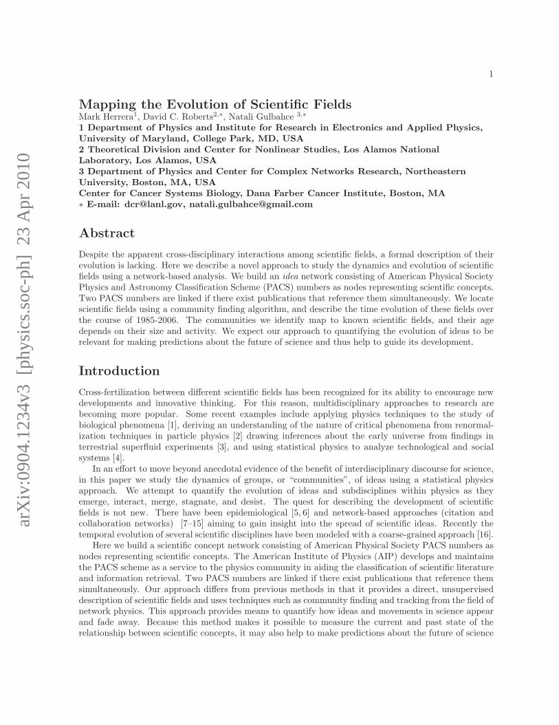
The entire PACS network from 1977-2007 after both noise measurements were applied has 803 nodesand 23707 distinct edges. The degree of a node is the number of edges shared by the node. The weightedcumulative degree distribution follows a stretched exponential with the form, P (k) ∼ exp[−(k/842)0.53] asshown in Fig. 1A. The distribution has a similar form in the unweighted case. The dynamic classificationscheme of the American Physical Society, implemented by the addition, splitting and removal of codes,may be preventing the formation of large hubs, thus keeping the specification of the codes more useful.The stretched exponential distribution may be the result of a sublinear-linear attachment type growth [25].

The PACS network also exhibits a weak but apparent hierarchical structure measured by the depen-dence of the clustering coefficient on (unweighted) degree. For a node i, the clustering coefficient is givenas Ci = 2ni/ki(ki − 1), where ni is the number of edges that link the neighbors of node i, and ki is thedegree of the node. The clustering coefficient for a node is the ratio of the number of triangles throughnode i over the possible number of triangles that could pass through node i [26]. A purely hierarchicalnetwork will have a 〈C〉 that scales as a power of k, 〈C〉 ∼ k−1, while a random network will have aclustering coefficient that is constant with k [26]. For this network, 〈C(k)〉 ∼ k−0.29 , shown in Fig. 1B.This dependence is not surprising given the hierarchical structure of the classification scheme.Defining Communities in Physics

3

Papers published between 1985 and 2006 were used to study the community evolution of the network;1985 appears to be the first year when all journals present (Physical Review E began publication in 1993)consistently used the PACS data scheme, and 2007 was thrown out to exclude incomplete data from theanalysis. The journal Physical Review Special Topics: Accelerators and Beams was not included becauseof an irregular publishing schedule. After the noise measures were carried out, the edge weights were nolonger used, and the network became an unweighted network with respect to the community evolutionanalysis. The data were organized into 44 time bins, with each bin representing a 0.5 year time period.Once a paper (and the edges and nodes it contains) appears in the analysis, it is assigned a lifetime,l, of 0 or 2.5 years. This assignment is an attempt to more realistically capture the nature of scientificdissemination, as well as the delay in time from publication to assimilation by the field. The analysis ofcommunity evolution begins at the time bin subsequent to the lapse of the assigned lifetime. Thus thefirst time bin, t = 0, for a paper lifetime of l = 2.5 refers to the latter half of 1987 since we start theanalysis in 1985.

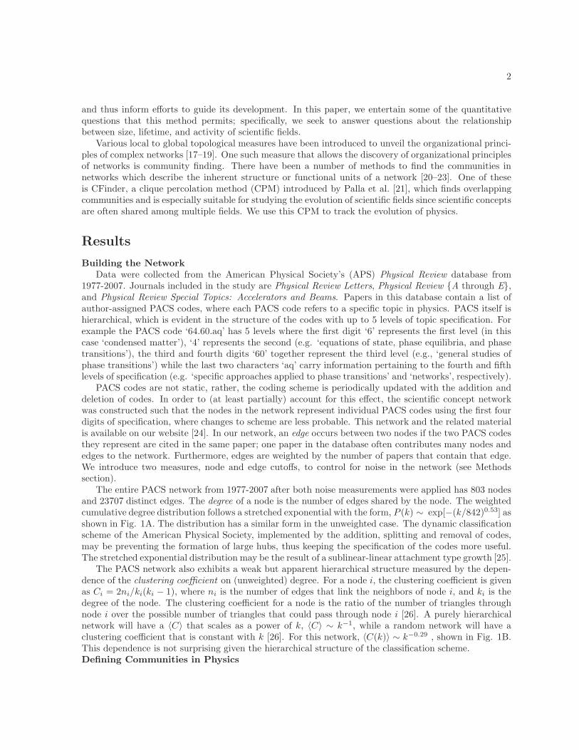
In order to study the evolution of different fields in physics, one must first find these fields in ournetwork. We hypothesize that scientific fields are represented by communities in our PACS network.These communities are found using the CFinder algorithm, which is based on a clique percolation method[21]. Figs. 2 and 3 present examples of the community structure extracted utilizing CFinder.

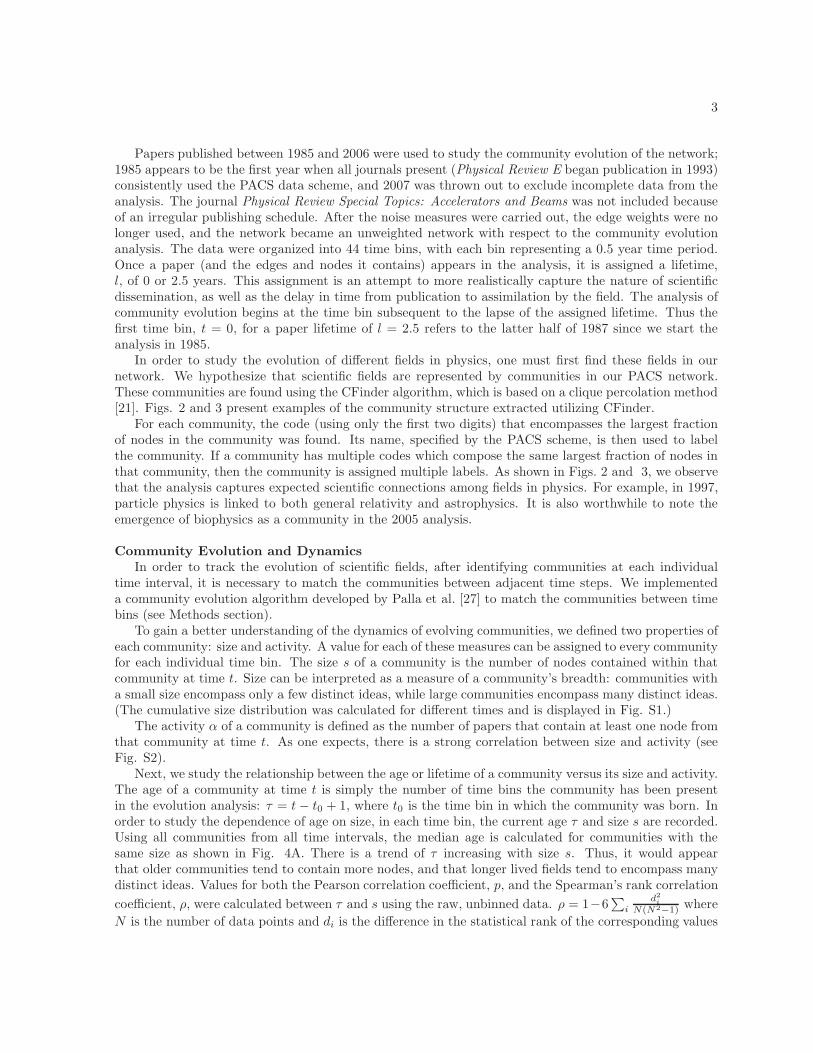
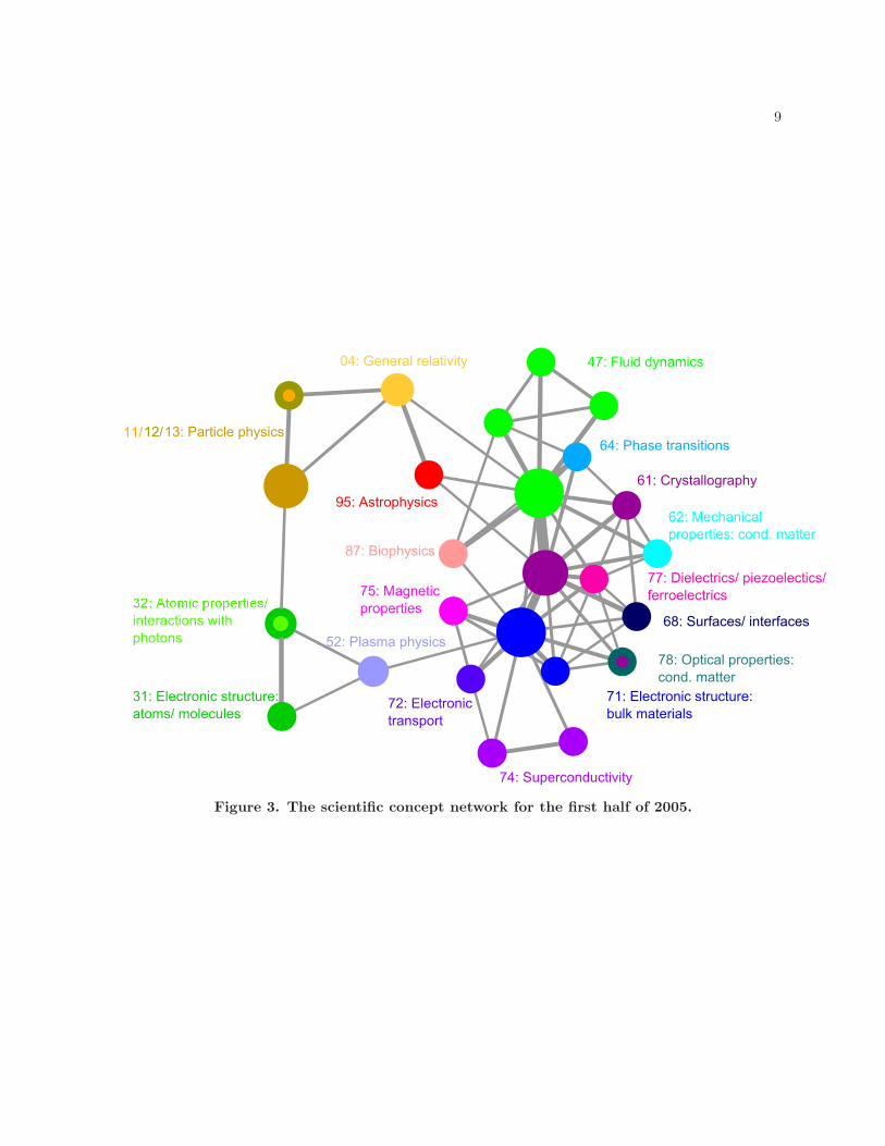
For each community, the code (using only the first two digits) that encompasses the largest fractionof nodes in the community was found. Its name, specified by the PACS scheme, is then used to labelthe community. If a community has multiple codes which compose the same largest fraction of nodes inthat community, then the community is assigned multiple labels. As shown in Figs. 2 and 3, we observethat the analysis captures expected scientific connections among fields in physics. For example, in 1997,particle physics is linked to both general relativity and astrophysics. It is also worthwhile to note theemergence of biophysics as a community in the 2005 analysis.

Community Evolution and DynamicsIn order to track the evolution of scientific fields, after identifying communities at each individual

time interval, it is necessary to match the communities between adjacent time steps. We implementeda community evolution algorithm developed by Palla et al. [27] to match the communities between timebins (see Methods section).

To gain a better understanding of the dynamics of evolving communities, we defined two properties ofeach community: size and activity. A value for each of these measures can be assigned to every communityfor each individual time bin. The size s of a community is the number of nodes contained within thatcommunity at time t. Size can be interpreted as a measure of a community’s breadth: communities witha small size encompass only a few distinct ideas, while large communities encompass many distinct ideas.(The cumulative size distribution was calculated for different times and is displayed in Fig. S1.)

The activity α of a community is defined as the number of papers that contain at least one node fromthat community at time t. As one expects, there is a strong correlation between size and activity (seeFig. S2).

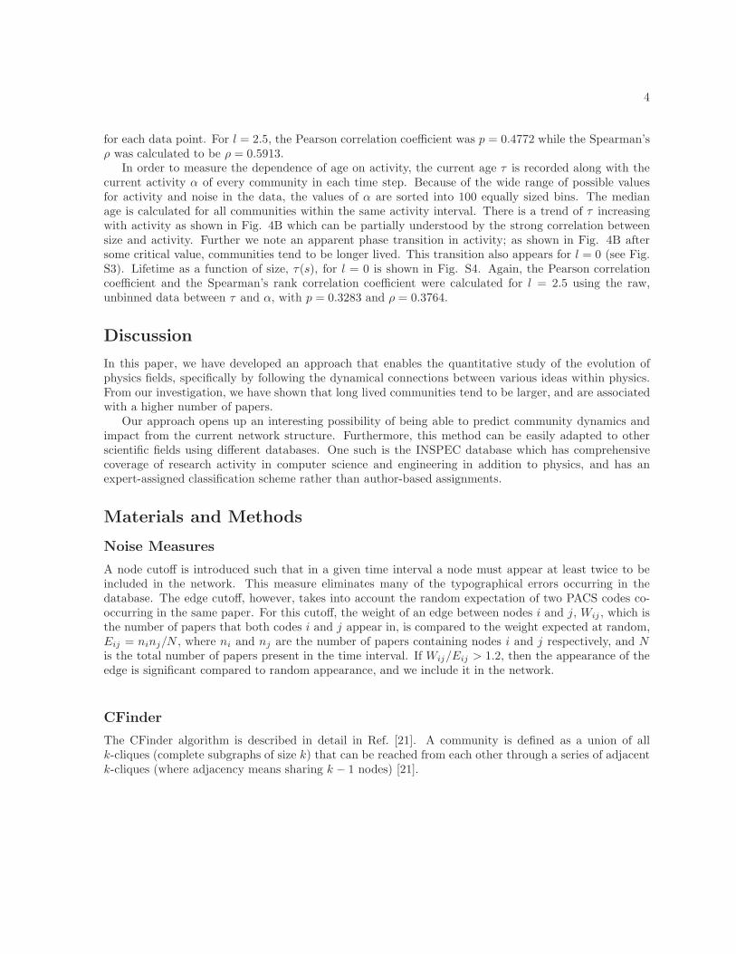
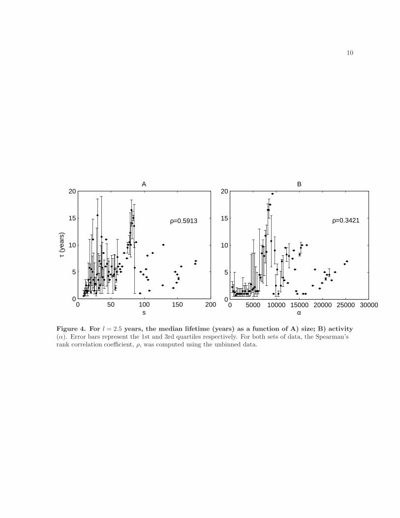
Next, we study the relationship between the age or lifetime of a community versus its size and activity.The age of a community at time t is simply the number of time bins the community has been presentin the evolution analysis: τ = t− t0 + 1, where t0 is the time bin in which the community was born. Inorder to study the dependence of age on size, in each time bin, the current age τ and size s are recorded.Using all communities from all time intervals, the median age is calculated for communities with thesame size as shown in Fig. 4A. There is a trend of τ increasing with size s. Thus, it would appearthat older communities tend to contain more nodes, and that longer lived fields tend to encompass manydistinct ideas. Values for both the Pearson correlation coefficient, p, and the Spearman’s rank correlation

coefficient, ρ, were calculated between τ and s using the raw, unbinned data. ρ = 1−6∑

i

d2

i

N(N2−1) where

N is the number of data points and di is the difference in the statistical rank of the corresponding values

4

for each data point. For l = 2.5, the Pearson correlation coefficient was p = 0.4772 while the Spearman’sρ was calculated to be ρ = 0.5913.

In order to measure the dependence of age on activity, the current age τ is recorded along with thecurrent activity α of every community in each time step. Because of the wide range of possible valuesfor activity and noise in the data, the values of α are sorted into 100 equally sized bins. The medianage is calculated for all communities within the same activity interval. There is a trend of τ increasingwith activity as shown in Fig. 4B which can be partially understood by the strong correlation betweensize and activity. Further we note an apparent phase transition in activity; as shown in Fig. 4B aftersome critical value, communities tend to be longer lived. This transition also appears for l = 0 (see Fig.S3). Lifetime as a function of size, τ(s), for l = 0 is shown in Fig. S4. Again, the Pearson correlationcoefficient and the Spearman’s rank correlation coefficient were calculated for l = 2.5 using the raw,unbinned data between τ and α, with p = 0.3283 and ρ = 0.3764.

Discussion

In this paper, we have developed an approach that enables the quantitative study of the evolution ofphysics fields, specifically by following the dynamical connections between various ideas within physics.From our investigation, we have shown that long lived communities tend to be larger, and are associatedwith a higher number of papers.

Our approach opens up an interesting possibility of being able to predict community dynamics andimpact from the current network structure. Furthermore, this method can be easily adapted to otherscientific fields using different databases. One such is the INSPEC database which has comprehensivecoverage of research activity in computer science and engineering in addition to physics, and has anexpert-assigned classification scheme rather than author-based assignments.

Materials and Methods

Noise Measures

A node cutoff is introduced such that in a given time interval a node must appear at least twice to beincluded in the network. This measure eliminates many of the typographical errors occurring in thedatabase. The edge cutoff, however, takes into account the random expectation of two PACS codes co-occurring in the same paper. For this cutoff, the weight of an edge between nodes i and j, Wij , which isthe number of papers that both codes i and j appear in, is compared to the weight expected at random,Eij = ninj/N , where ni and nj are the number of papers containing nodes i and j respectively, and Nis the total number of papers present in the time interval. If Wij/Eij > 1.2, then the appearance of theedge is significant compared to random appearance, and we include it in the network.

CFinder

The CFinder algorithm is described in detail in Ref. [21]. A community is defined as a union of allk-cliques (complete subgraphs of size k) that can be reached from each other through a series of adjacentk-cliques (where adjacency means sharing k − 1 nodes) [21].

5

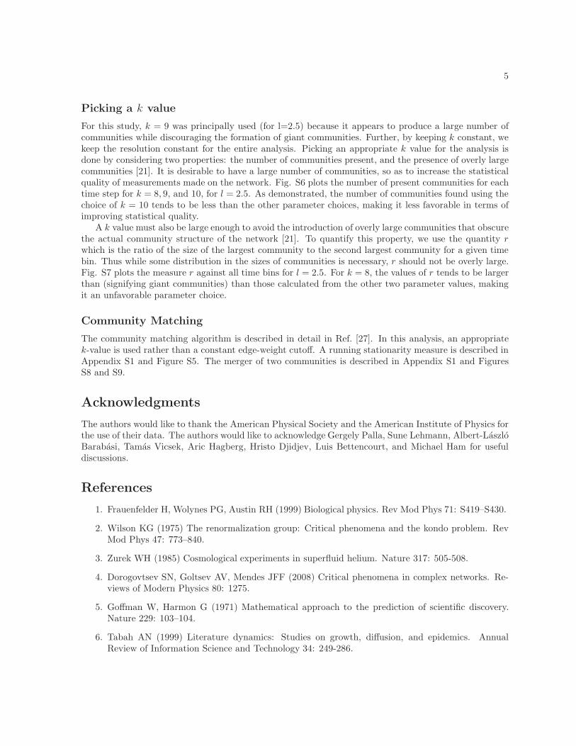
Picking a k value

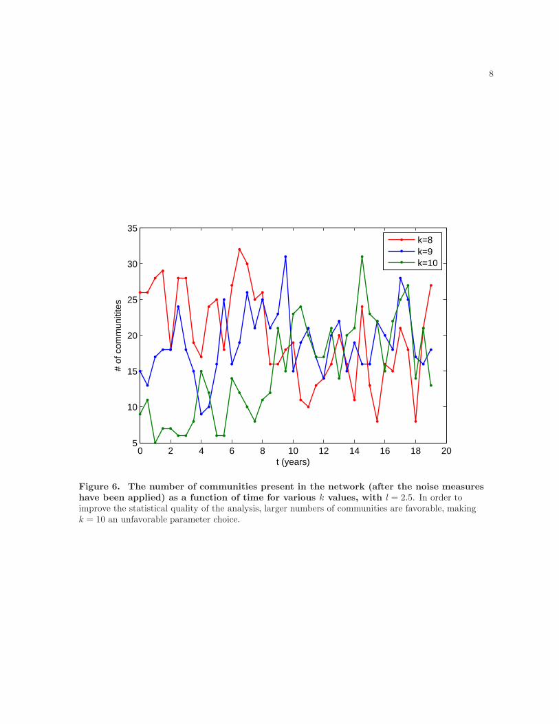
For this study, k = 9 was principally used (for l=2.5) because it appears to produce a large number ofcommunities while discouraging the formation of giant communities. Further, by keeping k constant, wekeep the resolution constant for the entire analysis. Picking an appropriate k value for the analysis isdone by considering two properties: the number of communities present, and the presence of overly largecommunities [21]. It is desirable to have a large number of communities, so as to increase the statisticalquality of measurements made on the network. Fig. S6 plots the number of present communities for eachtime step for k = 8, 9, and 10, for l = 2.5. As demonstrated, the number of communities found using thechoice of k = 10 tends to be less than the other parameter choices, making it less favorable in terms ofimproving statistical quality.

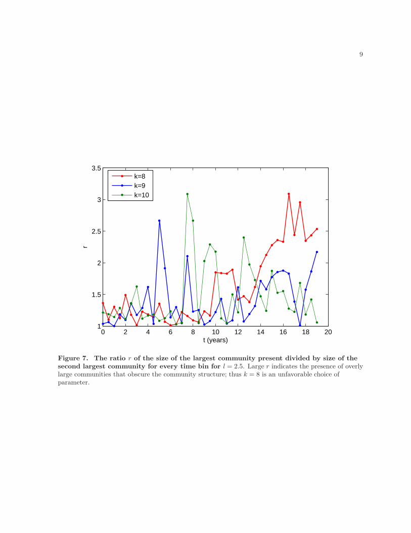
A k value must also be large enough to avoid the introduction of overly large communities that obscurethe actual community structure of the network [21]. To quantify this property, we use the quantity rwhich is the ratio of the size of the largest community to the second largest community for a given timebin. Thus while some distribution in the sizes of communities is necessary, r should not be overly large.Fig. S7 plots the measure r against all time bins for l = 2.5. For k = 8, the values of r tends to be largerthan (signifying giant communities) than those calculated from the other two parameter values, makingit an unfavorable parameter choice.

Community Matching

The community matching algorithm is described in detail in Ref. [27]. In this analysis, an appropriatek-value is used rather than a constant edge-weight cutoff. A running stationarity measure is described inAppendix S1 and Figure S5. The merger of two communities is described in Appendix S1 and FiguresS8 and S9.

Acknowledgments

The authors would like to thank the American Physical Society and the American Institute of Physics forthe use of their data. The authors would like to acknowledge Gergely Palla, Sune Lehmann, Albert-LaszloBarabasi, Tamas Vicsek, Aric Hagberg, Hristo Djidjev, Luis Bettencourt, and Michael Ham for usefuldiscussions.

References

1. Frauenfelder H, Wolynes PG, Austin RH (1999) Biological physics. Rev Mod Phys 71: S419–S430.

2. Wilson KG (1975) The renormalization group: Critical phenomena and the kondo problem. RevMod Phys 47: 773–840.

3. Zurek WH (1985) Cosmological experiments in superfluid helium. Nature 317: 505-508.

4. Dorogovtsev SN, Goltsev AV, Mendes JFF (2008) Critical phenomena in complex networks. Re-views of Modern Physics 80: 1275.

5. Goffman W, Harmon G (1971) Mathematical approach to the prediction of scientific discovery.Nature 229: 103–104.

6. Tabah AN (1999) Literature dynamics: Studies on growth, diffusion, and epidemics. AnnualReview of Information Science and Technology 34: 249-286.

6

7. de Solla Price DJ (1965) Networks of scientific papers. Science 149: 510-515.

8. Newman MEJ (2001) The structure of scientific collaboration networks. Proceedings of the NationalAcademy of Sciences of the United States of America 98: 404-409.

9. Newman MEJ (2001) Scientific collaboration networks. i. network construction and fundamentalresults. Phys Rev E 64: 016131.

10. Newman MEJ (2001) Scientific collaboration networks. ii. shortest paths, weighted networks, andcentrality. Phys Rev E 64: 016132.

11. Lehmann S, Lautrup B, Jackson AD (2003) Citation networks in high energy physics. Phys RevE 68: 026113.

12. HerrII BW, Duhon RJ, Borner K, Hardy EF, Penumarthy S (2008) 113 years of physical review:Using flow maps to show temporal and topical citation patterns. International Conference onInformation Visualisation : 421-426.

13. Leydesdorff L (2007) Betweenness centrality as an indicator of the interdisciplinarity of scientificjournals. J Am Soc Inf Sci Technol 58: 1303–1319.

14. Bollen J, Van de Sompel H, Hagberg A, Bettencourt L, Chute R, et al. (2009) Clickstream datayields high-resolution maps of science. PLoS ONE 4: e4803.

15. Boyack KW, Klavans AR, Borner BK (2005) Mapping the backbone of science. Scientometrics 64:351–374.

16. Bettencourt L, Kaiser D, Kaur J, Castillo-Chavez C, Wojick D (2008) Population modeling of theemergence and development of scientific fields. Scientometrics 75: 495–518.

17. Albert R, Barabasi AL (2002) Statistical mechanics of complex networks. Rev Mod Phys 74:47–97.

18. Newman M, Barabasi AL, Watts DJ (2006) The Structure and Dynamics of Networks: (PrincetonStudies in Complexity). Princeton, NJ, USA: Princeton University Press.

19. Caldarelli G (2007) Scale-free networks: complex webs in nature and technology. Oxford UniversityPress.

20. Girvan M, Newman MEJ (2002) Community structure in social and biological networks. Proceed-ings of the National Academy of Sciences of the United States of America 99: 7821-7826.

21. Palla G, Derenyi I, Farkas I, Vicsek T (2005) Uncovering the overlapping community structure ofcomplex networks in nature and society. Nature 435: 814–818.

22. Clauset A, Moore C (2008) Hierarchical structure and the prediction of missing links in networks.Nature 453: 98-101.

23. Gulbahce N, Lehmann S (2008) The art of community detection. Bioessays 30: 934-938.

24. http://nuweb6neuedu/ngulbahce/pacsdatahtml.

25. Krapivsky PL, Redner S, Leyvraz F (2000) Connectivity of growing random networks. Phys RevLett 85: 4629–4632.

26. Barabasi AL, Oltvai ZN (2004) Network biology: understanding the cell’s functional organization.Nat Rev Genet 5: 101–113.

27. Palla G, Barabasi AL, Vicsek T (2007) Quantifying social group evolution. Nature 446: 664–667.

7

Figure Legends

1 10 100 10000.1

1

k<

C(k

)>1 10 100 1000 10000 100000

0.001

0.01

0.1

1

k

P(k

)

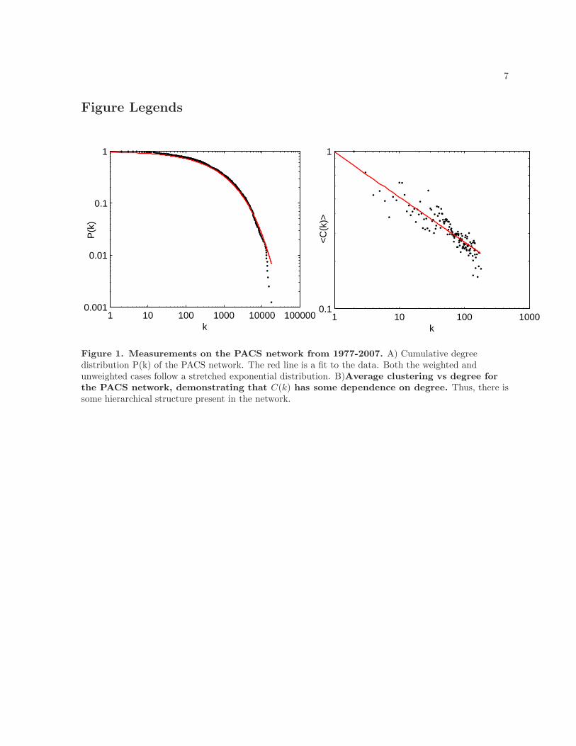
Figure 1. Measurements on the PACS network from 1977-2007. A) Cumulative degreedistribution P(k) of the PACS network. The red line is a fit to the data. Both the weighted andunweighted cases follow a stretched exponential distribution. B)Average clustering vs degree forthe PACS network, demonstrating that C(k) has some dependence on degree. Thus, there issome hierarchical structure present in the network.

8

98: Astrophysics

32: Atomic properties/ interactions

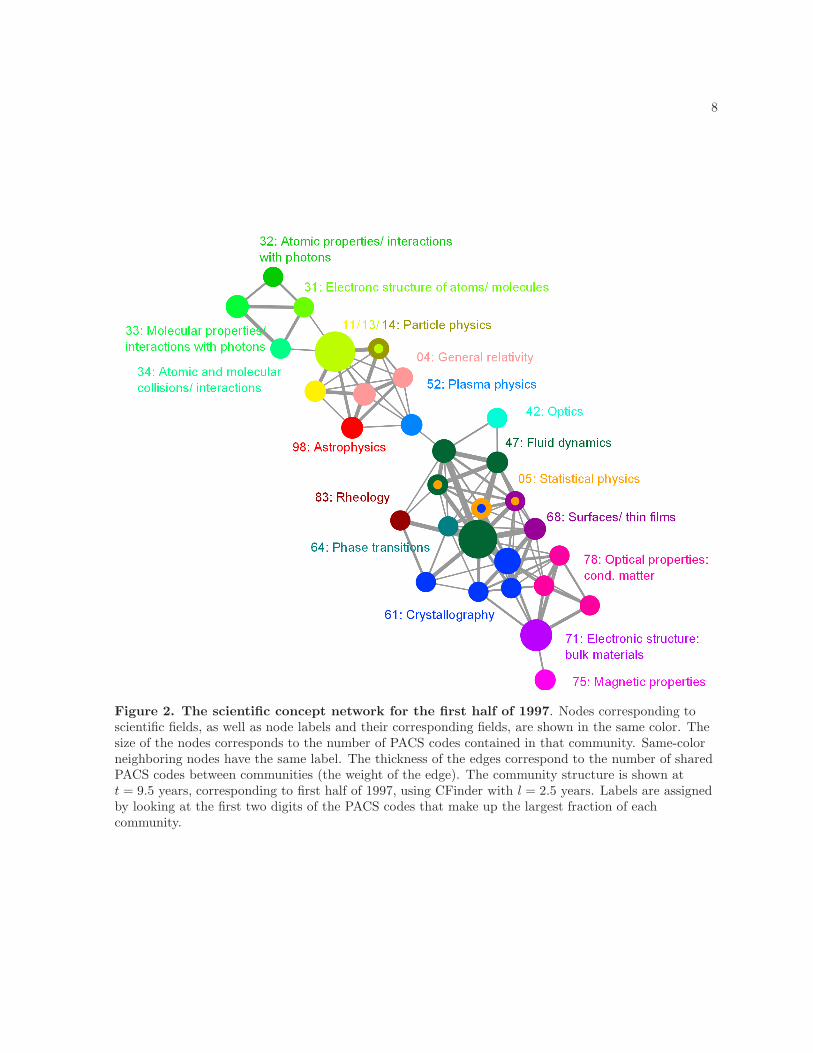
Figure 2. The scientific concept network for the first half of 1997. Nodes corresponding toscientific fields, as well as node labels and their corresponding fields, are shown in the same color. Thesize of the nodes corresponds to the number of PACS codes contained in that community. Same-colorneighboring nodes have the same label. The thickness of the edges correspond to the number of sharedPACS codes between communities (the weight of the edge). The community structure is shown att = 9.5 years, corresponding to first half of 1997, using CFinder with l = 2.5 years. Labels are assignedby looking at the first two digits of the PACS codes that make up the largest fraction of eachcommunity.

9

11/12/13: Particle physics

04: General relativity

95: Astrophysics

47: Fluid dynamics

64: Phase transitions

61: Crystallography

62: Mechanical

properties: cond. matter

77: Dielectrics/ piezoelectics/

ferroelectrics

68: Surfaces/ interfaces

78: Optical properties:

cond. matter

71: Electronic structure:

bulk materials

74: Superconductivity

72: Electronic

transport

75: Magnetic

properties

87: Biophysics

31: Electronic structure:

atoms/ molecules

interactions with

photons 52: Plasma physics

Figure 3. The scientific concept network for the first half of 2005.

10

0 50 100 150 2000

5

10

15

20

s

τ (y

ears

)

A

0 5000 10000 15000 20000 25000 300000

5

10

15

20

α

B

ρ=0.5913 ρ=0.3421

Figure 4. For l = 2.5 years, the median lifetime (years) as a function of A) size; B) activity(α). Error bars represent the 1st and 3rd quartiles respectively. For both sets of data, the Spearman’srank correlation coefficient, ρ, was computed using the unbinned data.

arX

iv:0

904.

1234

v3 [

phys

ics.

soc-

ph]

23

Apr

201

0

S1: Appendix

Mapping the Evolution of Scientific FieldsMark Herrera1, David C. Roberts2,∗, Natali Gulbahce 3,∗

1 Department of Physics and Institute for Research in Electronics and Applied Physics,University of Maryland, College Park, MD, USA2 Theoretical Division and Center for Nonlinear Studies, Los Alamos NationalLaboratory, Los Alamos, USA3 Department of Physics and Center for Complex Networks Research, NortheasternUniversity, Boston, MA, USACenter for Cancer Systems Biology, Dana Farber Cancer Institute, Boston, MA∗ E-mail: dcr@lanl.gov, natali.gulbahce@gmail.com

1 Community Dynamics

Once community structure is established, a variety of different measurements are performed on thedynamics of the evolving communities.

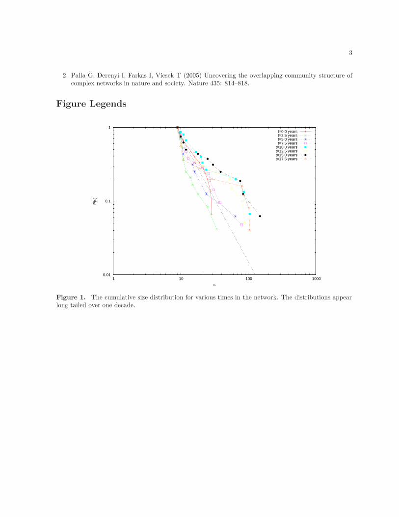
The cumulative community size distribution appears long tailed over one decade, which is robust asa function of t (years), as shown in Fig. S1.

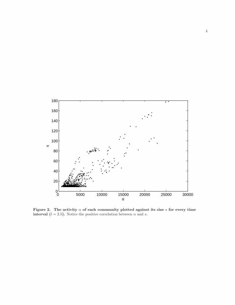
Fig. S2 plots for all time intervals the size of every community against its activity α for paper lifetimel = 2.5. There appears to be a positive correlation between the two measures, and this trend is observedfor l = 0 (not shown).

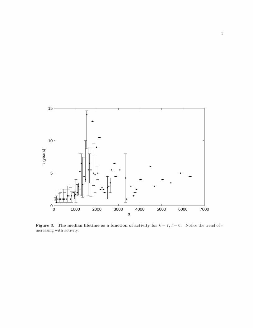
The dependence of age on activity was measured and Fig. S3 shows the results for the τ vs. α

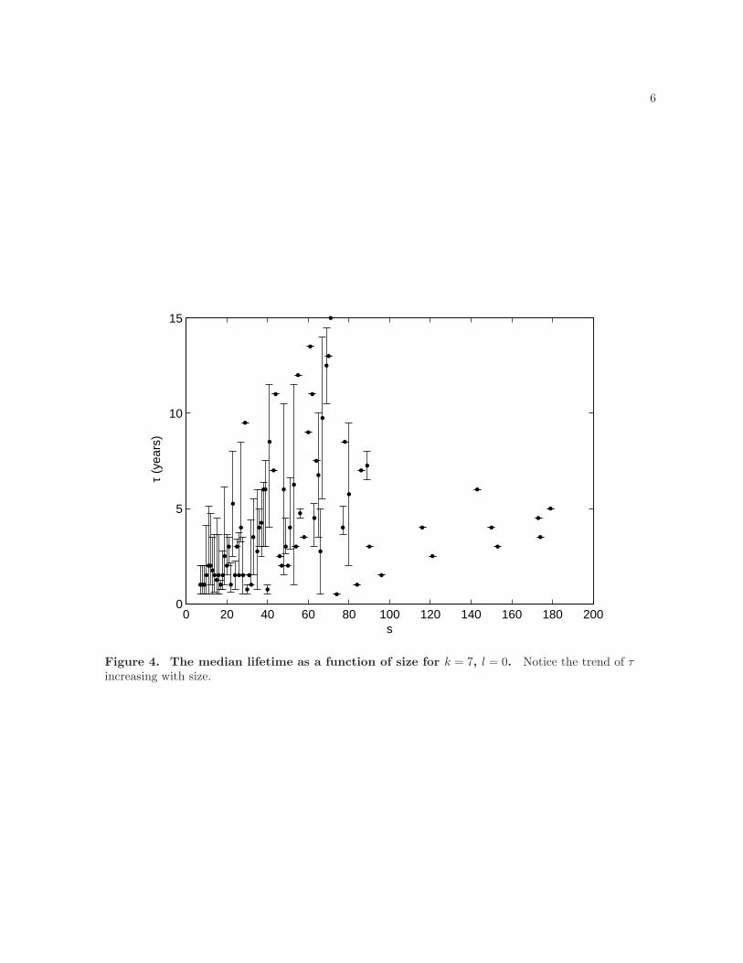
measurements for k = 7 with a paper lifetime of l = 0 years, where α values were binned because of thewide range in α, as well as to reduce noise. In both cases (the one presented here and the one presentedin the letter) there is a trend of age increasing as activity increases (though less apparently for l = 0)and, as expected given the correlation between α and s, one sees a similar relationship between age andsize, as shown in Fig. S4. Thus, older communities also tend to encompass more publications, a resultthat agrees with naive expectation. Further, we note an apparent phase transition in both paper lifetimecases (more apparent for l=2.5 than for l = 0); after some critical α, communities tend to be longer lived.

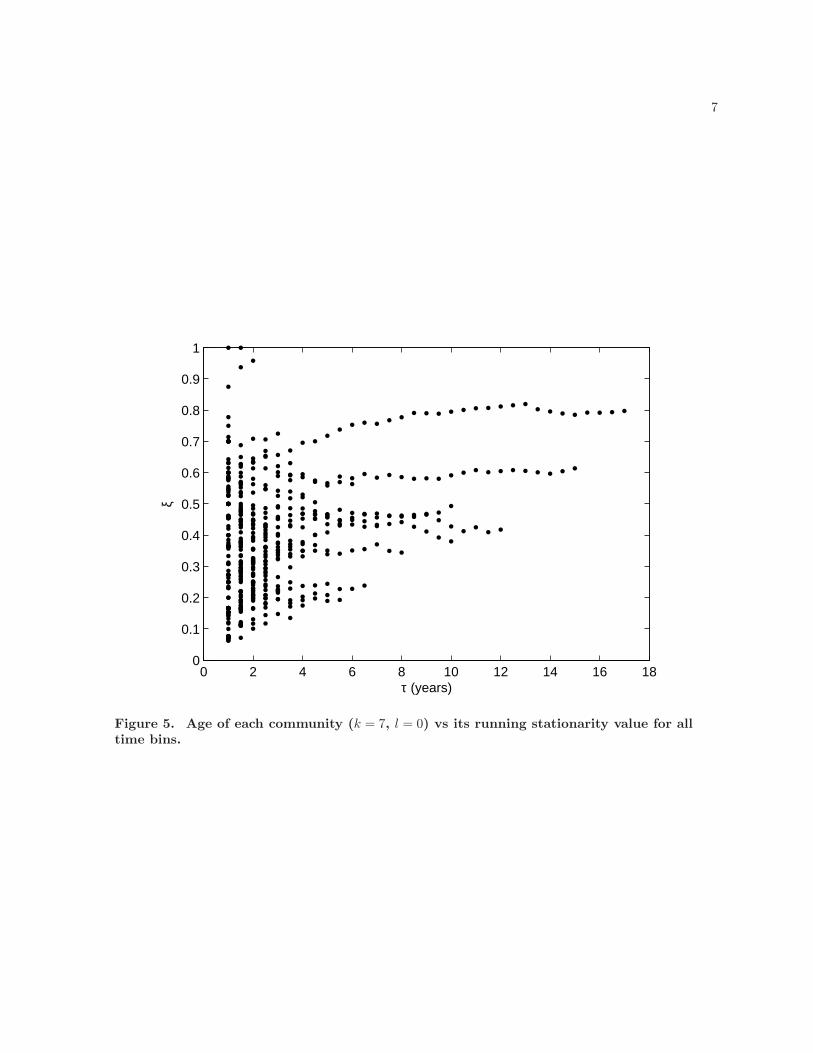
Further understanding of the community dynamics can be gained by studying the volatility of theevolving communities, a measure of how much communities tend to change between subsequent timesteps. To see this, we define an age dependent running stationarity ξ(τ) based on community correlationand stationarity presented by Palla et al. [1]. The correlation C(t, t′) between two states of the samecommunity A(t) at times t and t′ is

C(t, t′) =

∣

∣

∣

∣

A(t) ∩ A(t′)

A(t) ∪ A(t′)

∣

∣

∣

∣

.

Then the running stationarity, ξ(τ), of that community is the average correlation between subsequent

1

2

time steps up to age τ ,

ξ(τ) =1

τ − 1

t0+τ−2∑

t′=t0

C(t′, t′ + 1).

The running stationarity, ξ(t), is plotted against lifetime for every community with τ > 1 along withits current age at time t, for all t, for l = 0 in Fig. S5. This result is qualitatively similar to resultsobtained using randomized correlations. For larger values of l, the distribution shifts to larger values ofξ(t).

2 Picking a k value

Throughout the paper, k = 9 is principally used (for l=2.5) because it appears to produce a large numberof communities while discouraging the formation of giant communities. Further, by keeping k constant,we keep the resolution constant for the entire analysis. Picking an appropriate k value for the analysis isdone by considering two properties: the number of communities present, and the presence of overly largecommunities [2]. It is desirable to have a large number of communities, so as to increase the statisticalquality of measurements made on the network. Fig. S6 plots the number of present communities for eachtime step for k = 8, 9, and 10, for l = 2.5. As demonstrated, the number of communities found using thechoice of k = 10 tends to be less than the other parameter choices, making it less favorable in terms ofimproving statistical quality.

A k value must also be large enough to avoid the introduction of overly large communities that ob-scure the actual community structure of the network [2]. To quantify this property, we use the quantityr which is the ratio of the size of the largest community to the second largest community for a given timebin. Thus while some distribution in the sizes of communities is necessary, r should not be overly large.Fig. S7 plots the measure r against all time bins for l = 2.5. For k = 8, the values of r tend to becomelarger (signifying giant communities) than those calculated from the other two parameter values, makingit an unfavorable parameter choice.

3 Merging of communities

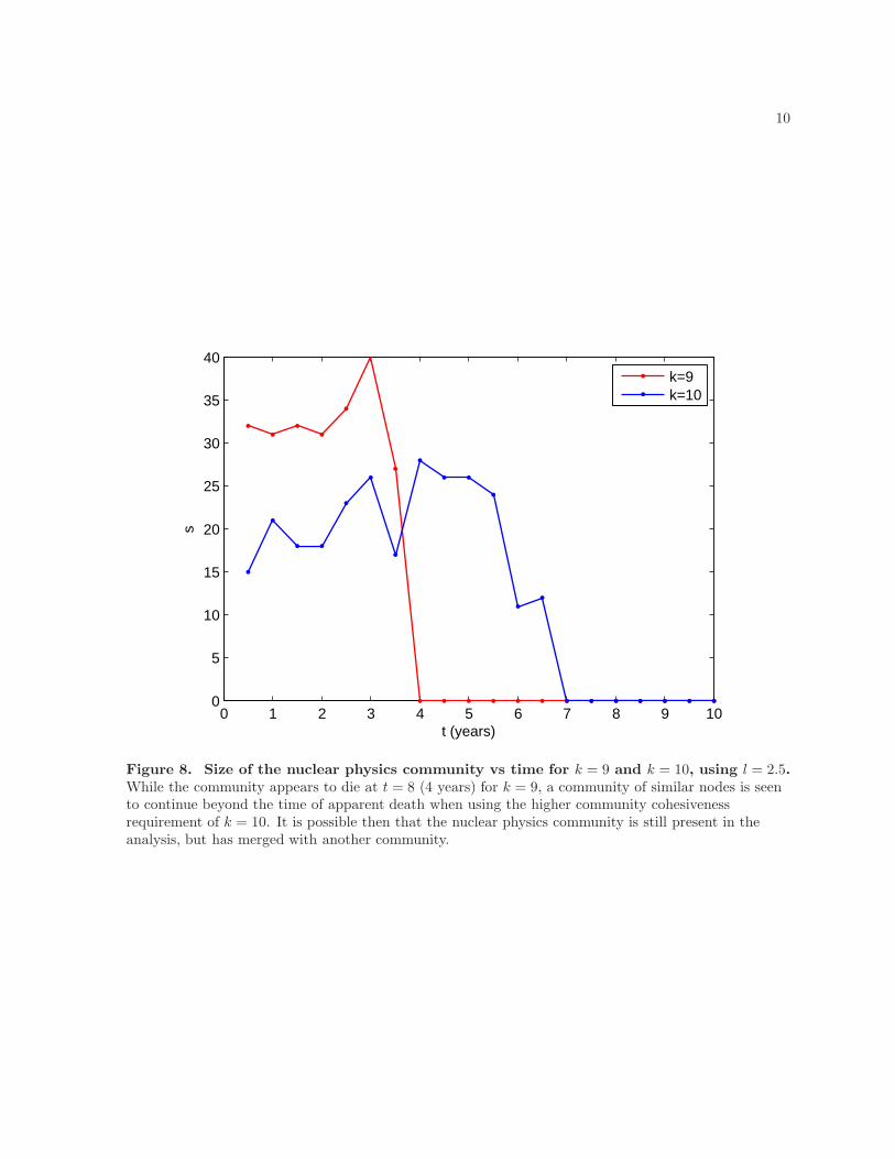
Lastly, we present an example of a merger between two communities. Tracking a nuclear physics com-munity, Fig. S8 shows the size of that community as a function of time for k = 9 and a community ofsimilar nodes with k = 10, using l = 2.5.

With k = 9, it appears that this particle physics community abruptly dies at t = 4 years. Increasingthe cohesiveness of communities by increasing to k = 10 demonstrates that a community composed ofsimilar nodes continues to propagate past this time of apparent death. Thus, it seems that the nuclearphysics community is still present in the network, but has become absorbed by another community.

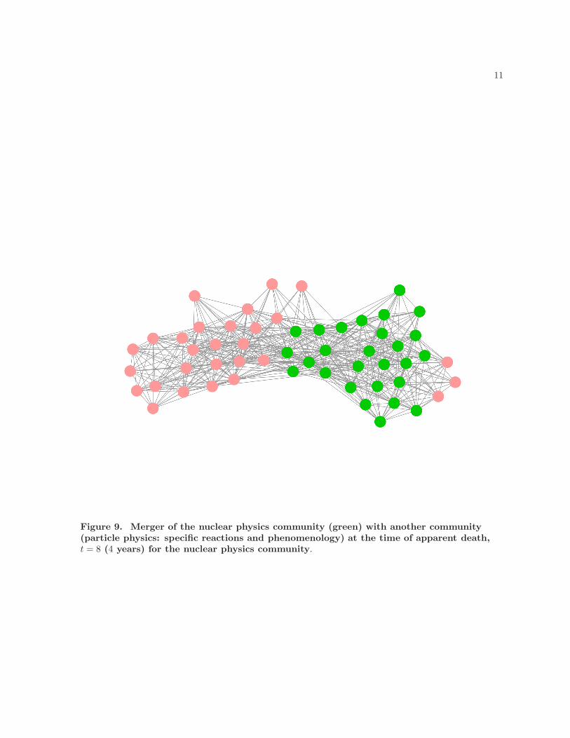
Fig. S9 plots a community at t = 4 years with the nodes from the nuclear physics community displayedin green. We can assign a label to this community in the usual manner using the nodes present just beforethe apparent death of the nuclear physics community. Doing so, the absorbing community is comprisedof the ‘physics of elementary particles and fields: specific reactions and phenomenology’ in the time binprior to its absorption of the particle physics community.

References

1. Palla G, Barabasi AL, Vicsek T (2007) Quantifying social group evolution. Nature 446: 664–667.

3

2. Palla G, Derenyi I, Farkas I, Vicsek T (2005) Uncovering the overlapping community structure ofcomplex networks in nature and society. Nature 435: 814–818.

Figure Legends

0.01

0.1

1

1 10 100 1000

P(s

)

s

t=0.0 yearst=2.5 yearst=5.0 yearst=7.5 years

t=10.0 yearst=12.5 yearst=15.0 yearst=17.5 years

Figure 1. The cumulative size distribution for various times in the network. The distributions appearlong tailed over one decade.

4

0 5000 10000 15000 20000 25000 300000

20

40

60

80

100

120

140

160

180

α

s

Figure 2. The activity α of each community plotted against its size s for every timeinterval (l = 2.5). Notice the positive correlation between α and s.

5

0 1000 2000 3000 4000 5000 6000 70000

5

10

15

α

τ (y

ears

)

Figure 3. The median lifetime as a function of activity for k = 7, l = 0. Notice the trend of τincreasing with activity.

6

0 20 40 60 80 100 120 140 160 180 2000

5

10

15

s

τ (

year

s)

Figure 4. The median lifetime as a function of size for k = 7, l = 0. Notice the trend of τincreasing with size.

7

0 2 4 6 8 10 12 14 16 180

0.1

0.2

0.3

0.4

0.5

0.6

0.7

0.8

0.9

1

τ (years)

ξ

Figure 5. Age of each community (k = 7, l = 0) vs its running stationarity value for alltime bins.

8

0 2 4 6 8 10 12 14 16 18 205

10

15

20

25

30

35

# of

com

mun

itite

s

t (years)

k=8k=9k=10

Figure 6. The number of communities present in the network (after the noise measureshave been applied) as a function of time for various k values, with l = 2.5. In order toimprove the statistical quality of the analysis, larger numbers of communities are favorable, makingk = 10 an unfavorable parameter choice.

9

0 2 4 6 8 10 12 14 16 18 201

1.5

2

2.5

3

3.5

t (years)

r

k=8k=9k=10

Figure 7. The ratio r of the size of the largest community present divided by size of thesecond largest community for every time bin for l = 2.5. Large r indicates the presence of overlylarge communities that obscure the community structure; thus k = 8 is an unfavorable choice ofparameter.

10

0 1 2 3 4 5 6 7 8 9 100

5

10

15

20

25

30

35

40

t (years)

s

k=9k=10

Figure 8. Size of the nuclear physics community vs time for k = 9 and k = 10, using l = 2.5.While the community appears to die at t = 8 (4 years) for k = 9, a community of similar nodes is seento continue beyond the time of apparent death when using the higher community cohesivenessrequirement of k = 10. It is possible then that the nuclear physics community is still present in theanalysis, but has merged with another community.

11

Figure 9. Merger of the nuclear physics community (green) with another community(particle physics: specific reactions and phenomenology) at the time of apparent death,t = 8 (4 years) for the nuclear physics community.