M A N U A L

ChemEQLV3.0

A Program to Calculate Chemical Speciation Equilibria,

Titrations, Dissolution, Precipitation, Adsorption,

Kinetics, pX-pY Diagrams, Solubility Diagrams.

Libraries with Complexation Constants

For MacOSX, Windows, Linux, Solaris

Beat Müller

Limnological Research Center EAWAG/ETH

CH-6047 Kastanienbaum, Switzerland

ChemEQL Manual

2

The Program

ChemEQL, insinuating ‘Chemical Equilibrium’, calculates and draws thermodynamic equilibrium

concentrations of species in complex chemical systems. It handles homogeneous solutions,

dissolution, precipitation, titration with acid or other components. Adsorption on up to five different

particulate surfaces can be calculated with the choice of the Constant Capacitance, Diffuse Layer

(Generalized Two Layer), Basic Stern Layer, or Triple Layer model to consider for surface charges.

Corrections for ionic strength can be made and activities calculated. One rate determining process in a

system of otherwise fast thermodynamic chemical equilibrium can be simulated. Two-dimensional

logarithmic diagrams, such as pε-pH, can be calculated. A simple drawing option is provided. A library

with over 1700 thermodynamic stability constants allows quick access and easy use of the program.

Another library with more than 300 solubility constants allows easy introduction of solid phases.

The present application was developed starting out from the original program MICROQL in BASIC by

John Westall. The basic principles of the calculation method is documented by J. Westall, "Chemical

Equilibrium Including Adsorption on Charged Surfaces", Advances in Chemistry Series, no. 189,

Particulates in water, ed. by M.C. Kavanaugh and J.O. Leckie, 1980, and J. Westall, J.L. Zachary and F.

Morel, "MINEQL, a Computer Program for the Calculation of Chemical Equilibrium Composition of

Aqueous Systems", Technical Note no. 18, Ralph M. Parsons Lab. MIT, Cambridge, 1976.

Kai-H. Brassel ( www.vseit.de ) implemented this program in Java code. Independent from whether you

work under Windows, Linux, Solaris or MacOS X (for older operating systems there exists a Pascal-

version of ChemEQL) the application can be downloaded from

http://www.eawag.ch/research/surf/forschung/chemeql.html

By clicking on the ChemEQL icon the application is downloaded, installed on your hard disc, and

started. Installation is made independent from your operating system directly from the internet browser

through the WebStart-plugin from Sun Microsystems Inc. (www.sun.com). WebStart cares for the

installation of a suitable Java runtime environment in case it is not available, and for the automatic

installation of new versions of ChemEQL. In case WebStart is not yet installed or part of the operating

ChemEQL Manual

3

system (as in MacOS X) WebStart will be installed automatically as Browser-Plugin first from the Java

WebStart setup page of Sun Microsystems, Inc. The installation is a one-time process. The ChemEQL

application launched with Java WebStart is cached locally on your hard disk and works off-line.

A manual can be downloaded that intends to be a practical guide through most options the program

offers. I believe that providing examples makes it easier to pick things up that explaining theory.

Kastanienbaum, June 21, 2004 Beat Müller

e-mail: beat.mueller@eawag.ch

Fax: ++ 41 41 349 21 68

ChemEQL Manual

4

Content

THE PROGRAM 2

CONTENT 4

JUMP START 7Set up a matrix 7Insert solid phases 9Check for precipitation 12Several solid phases 13Access the libraries 15

Edit Regular Library Components 16Edit Regular Library Species 17References 18

Exchange the libraries 19Settings 20Iteration parameters 21Activity 21Array of concentrations 24Graphic representation 25Linear / Logarithmic data format 26Replace H+ by OH- 27Iteration does not converge 28

HOW TO SET UP A MATRIX – THE DETAILS 29Important! 29The mode codes for the matrix: 30

Dissolved 30Solid phases 30Adsorption 30

Creating a matrix by hand 31

REGULAR SPECIES DISTRIBUTION IN HOMOGENEOUS SOLUTION 34Octanol-water and gas-water distribution 38

SOLID PHASES: DISSOLUTION AND PRECIPITATION 39Put up a matrix to calculate solubility 39Dissolution 40

Dissolution in acidic solution 41Dissolution at constant pH 41Graphical representation of solubility over a pH range 42

Precipitation 42

ADSORPTION TO PARTICULATE SURFACES 45Introduction to the principles of surface adsorption 45How to put up an adsorption matrix: A simple example: 46Titration of a solution with particles 48The Generalized Two Layer Model 49Surfaces characterized by Fractional Surface Charge: The one-pK-model 51Examples 53

ChemEQL Manual

5

Literature: 54

REDOX REACTIONS 56

KINETICS 58Integrated rate laws 62

PX-PY DIAGRAMS 63Example 1: pε-pH-diagram for water 63Example 2: pε-pH-diagram for the Fe - CO2 - H2O system 66

EXAMPLES 68

1. ALL COMPONENTS DISSOLVED, TOTAL CONCENTRATIONS GIVEN70

Complexes of Pb(II) with EDTA and NTA (ex01.mat) 70Titration of Na3PO4 with strong acid (ex02.mat) 71Titration of H3PO4 with strong base (ex03.mat) 72

2. ALL COMPONENTS DISSOLVED, FREE CONCENTRATIONS OFSOME COMPONENTS GIVEN 73

Constant pH: Complexes of Hg(II) with hydroxide and chloride (ex04.mat) 73Constant pCO2: Equilibrium of a soda solution with atmospheric CO2 (ex05.mat) 74

Constant free concentration of a species: Metal buffer for Cu2+(aq) (ex06.mat) 75

3. DISSOLUTION OF ONE (OR MORE) SOLID PHASE(S) 76Dissolution diagram of Cu(OH)2(s) (ex07.mat) 76The CaCO3 – CO2 system (ex08.mat) 78

Dissolution of Ca4Al2O6SO4 .12H2O (ex09.mat) 79

Dissolution of several solid phases (ex10.mat) 80

4. PRECIPITATION OF ONE (OR MORE) SOLID PHASES 81Precipitation of PbCO3(s) (ex11.mat) 81

5. ADSORPTION TO PARTICULATE SURFACES: 82One particulate surface type 82

Constant Capacitance Model (ex12.mat) 82Diffuse Layer Model (ex13.mat) 83Basic Stern Layer Model (ex14.mat) 84Triple Layer Model (ex15.mat) 84Adsorption of Lead on Goethite (ex16.mat) 85

Two or more (up to five) particulate surface types 86Constant Capacitance Model (ex17.mat) 86Diffuse Layer Model / General Two Layer Model (ex18.mat) 87Basic Stern Layer Model (ex19.mat) 88Triple Layer Model (ex20.mat) 89

Several types of surface sites on one type of particle 90Diffuse Layer Model / General Two Layer Model (ex21.mat) 90

6. Pε-PH DIAGRAMS 91The S(VI), S(0), S(-II) - System (ex22.mat) 91

ChemEQL Manual

6

The Chlorine System (ex23.mat) 92

7. SOLUBILITY DIAGRAMS 93The Iron - CO2 System (ex24.mat) 93The PbCO3 - PbSO4 system (ex25.mat) 94

ChemEQL Manual

7

Jump Start

Set up a matrix

Putting up a matrix by hand is a source of many mistakes and sometimes it is quite a task to find

species, reactions, and stability constants. Two libraries are provided for the users comfort, one

containing complex formation constants and the other solubility products. Both libraries are

automatically downloaded, digitalized and stored in the users home account. At startup, the program

checks the availability of the users libraries. In case they are missing, changed names, or were deleted

the program reloads the libraries again. Hence, you are not bothered by the installation or preparation

of the libraries.

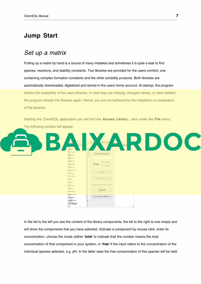
Starting the ChemEQL application you will find the Access Library... item under the File menu.

The following window will appear:

In the list to the left you see the content of the library components, the list to the right is now empty and

will show the components that you have selected. Activate a component by mouse click, enter its

concentration, choose the mode (either 'total' to indicate that the number means the total

concentration of that component in your system, or 'free' if the input refers to the concentration of the

individual species selected, e.g. pH. In the latter case the free concentration of this species will be held

ChemEQL Manual

8

constant). Clicking the '>>Add>>' button (or CR) will remove the selected component from the library

and transfer it to your selection. If you wish to remove a component from your selection, activate it and

press the now active '<<Remove<<' button. The component will be removed from the selection and

added at the end of the library list.

As an example we want to perform some pH and concentration calculations with diluted acetic acid: In

order to select the matrix for the acetic acid system (which we will put up in detail with much effort on

pages 29-31), select 'AceticAcid' from the library, enter '1e-3' for concentration, and press the

'Add' button. Proceed to the end of the library list, select 'H+', enter '1e-4' for the concentration,

choose 'free' (since we want to calculate for constant pH), and press again the 'Add' button. This is

the whole selection needed. Pressing 'compile matrix' will end the library dialog. The program will

search the library for all possible combinations of the chosen components and will list them as species.

(There is no guarantee for completeness!). The following window will appear and show the

components you selected with the concentration and mode, and all species that were found in the

library with the attached formation constants.

If you wish to use this matrix again make sure to save it: Choose Save Matrix... from the File menu!

Run and Go will calculate the speciation of that system: What are the concentrations of HAc and Ac- in

a solution of pH 4?

ChemEQL Manual

9

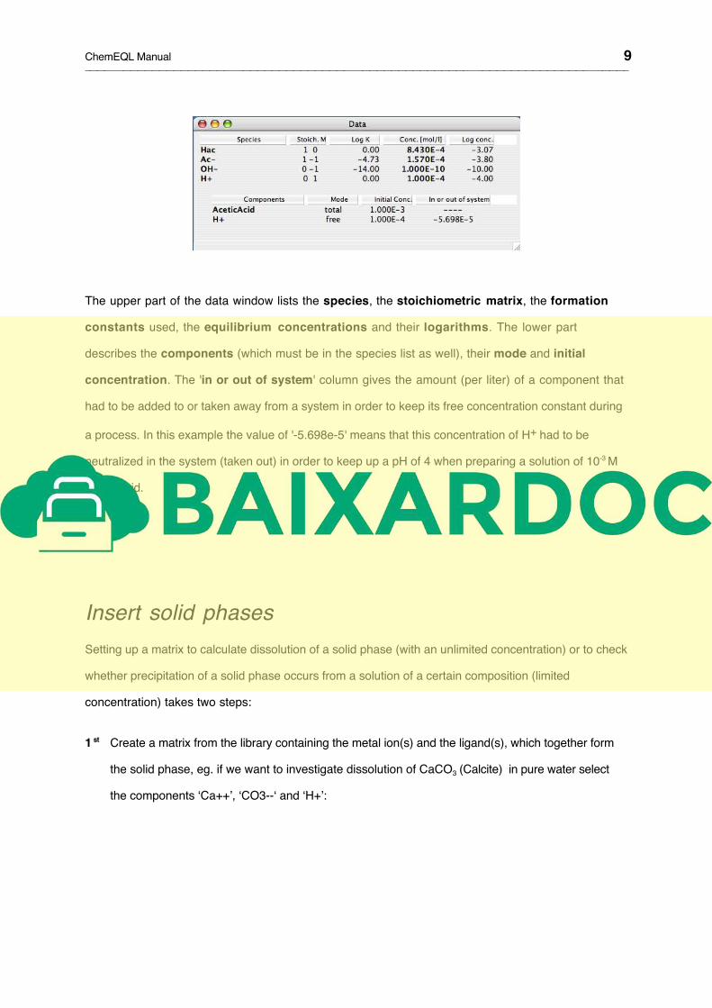
The upper part of the data window lists the species, the stoichiometric matrix, the formation

constants used, the equilibrium concentrations and their logarithms. The lower part

describes the components (which must be in the species list as well), their mode and initial

concentration. The 'in or out of system' column gives the amount (per liter) of a component that

had to be added to or taken away from a system in order to keep its free concentration constant during

a process. In this example the value of '-5.698e-5' means that this concentration of H+ had to be

neutralized in the system (taken out) in order to keep up a pH of 4 when preparing a solution of 10-3 M

acetic acid.

Insert solid phases

Setting up a matrix to calculate dissolution of a solid phase (with an unlimited concentration) or to check

whether precipitation of a solid phase occurs from a solution of a certain composition (limited

concentration) takes two steps:

1 st Create a matrix from the library containing the metal ion(s) and the ligand(s), which together form

the solid phase, eg. if we want to investigate dissolution of CaCO3 (Calcite) in pure water select

the components ‘Ca++’, ‘CO3--‘ and ‘H+’:

ChemEQL Manual

10

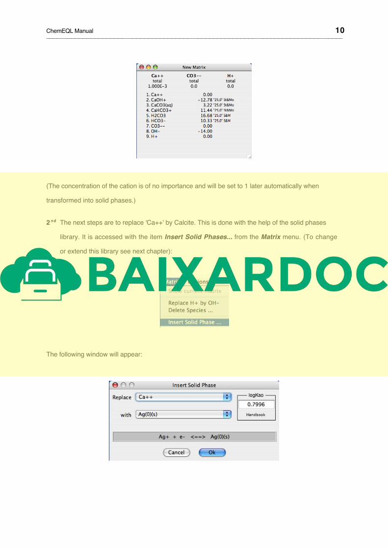
(The concentration of the cation is of no importance and will be set to 1 later automatically when

transformed into solid phases.)

2 nd The next steps are to replace 'Ca++' by Calcite. This is done with the help of the solid phases

library. It is accessed with the item Insert Solid Phases... from the Matrix menu. (To change

or extend this library see next chapter):

The following window will appear: