Resource Allocation Policies for Personalization in Content Delivery Sites

Dengpan Liu

College of Administrative Science The University of Alabama in Huntsville

Huntsville, AL 35899

Sumit Sarkar and Chelliah Sriskandarajah SM 33, School of Management

The University of Texas at Dallas Richardson Texas 75083

March 8, 2007

Abstract One of the distinctive features of sites on the Internet is their ability to gather enormous amounts of information regarding their visitors, and use this information to enhance a visitor’s experience by providing personalized information or recommendations. In providing personalized services a website is typically faced with the following tradeoff: when serving a visitor’s request, it can deliver an optimally personalized version of the content to the visitor possibly with a long delay due to the computational effort needed, or it can deliver a suboptimal version of the content more quickly. This problem becomes more complex when several requests are waiting for information from a server. The website then needs to trade-off the benefit from providing more personalized content to each user with the negative externalities associated with higher waiting costs for all other visitors that have requests pending. We examine several deterministic resource allocation policies in such personalization contexts. We identify an optimal policy for the above problem when requests to be scheduled are batched, and show that the policy can be very efficiently implemented in practice. We provide an experimental approach to determine optimal batch lengths, and demonstrate that it performs favorably when compared with viable queuing approaches. Keywords: User profiling, delay externality, scheduling, queuing

© All rights reserved. Please do not circulate without permission of the authors.

Acknowledgement: We gratefully acknowledge the feedback from seminar participants at the Georgia Institute of Technology, New York University, and The University of Texas at Austin. A preliminary version of this research was presented at the Conference on Information Systems and Technologies (CIST) in Denver, in October 2004.

1

Resource Allocation Policies for Personalization in Content Delivery Sites

1. Introduction

One of the distinctive features of web sites is their ability to garner enormous amounts of information

regarding their visitors. Web site owners can use this information to enhance subsequent visitor

experience by providing targeted information or recommendations. This process of utilizing an

individual’s information to deliver a targeted product is known as personalization. With the proliferation

of Internet-based applications in recent years, firms are increasingly providing personalized services and

products. For example, Amazon.com uses personalization techniques to recommend books and gifts to

their customers. DoubleClick uses visitor profiles to target appropriate banner advertisements on their

clients’ sites. Sites such as techrepublic.com analyze user clicks and articles read to determine which new

articles to display to their readers. The research firm Datamonitor predicted that investment in

personalization technologies will grow from $500 million in 2001 to $2.1 billion in 2006 (DMReview,

2001)1. The report goes on to state that personalization will become increasingly crucial to companies,

and a service that all customers will expect.

Personalization can reduce customer search costs and enhance customer loyalty, which translate

into increased cash inflows and enhanced profitability (Ansari and Mela 2003). Recent research on

personalization has addressed issues related to pricing of personalized services and the strategic outcome

of such pricing (Chen and Iyer 2002, Dewan et al. 2003, Murthi and Sarkar 2003). Our focus here is on

developing optimal deterministic policies for allocating personalization server resources in real time for

providing such services on the Internet. While such policies can be beneficial for both content delivery

sites (e.g., The New York Times, Yahoo-News) and commerce sites (e.g., Amazon, eBay), we

concentrate on the former. Personalization of content helps such sites enhance their customer base and

increase revenues that are (at least partially) driven by online advertisements (Ihlstrom and Palmer 2002,

Mermigas 2001). In addition, our policies are applicable to Ad-server operations; such servers provide

targeted advertisements on pages requested by customers. 1 DMReview Online, Sept 12, 2001.

2

To perform personalization, content delivery sites collect information about their visitors to

develop user profiles. Profiles are formed based on a users’ click-stream data, and typically stored as

word-vectors or session-vectors (Yan et al. 1996, Anderson et al. 2001). Given a user profile, the

personalization engine tailors the contents of the page requested by the visitor, as well as, the links to

provide with that page (i.e., a personalized navigation space). Several techniques have been developed to

provide real-time personalization by performing dynamic link generation when a user requests a new

page. For instance, Yan et al. (1996) use session-vectors whose elements are pages in the website and the

weight of each element is the frequency of browsing a certain page. When the user makes a new URL

request, the session-vector gets updated, and the personalization process proceeds by identifying other

similar sessions. Anderson et al. (2001) use word-vectors to capture user profiles, and provide a method

to compute the utility of the served page and embedded links by considering both the intrinsic utility of

the page contents and the extrinsic utility of documents reachable by the embedded links.

For content delivery sites, the goal is to provide personalized content and navigation space to

each visitor by identifying and targeting their individual needs, an approach that is often termed one-to-

one marketing (Peppers and Rogers 1997). While current technologies provide an opportunity to deliver

such service, the actual task of identifying the best possible personalized page and navigation space for

each interaction with a user can be computationally intensive, thereby affecting a sites’ performance. Sites

typically use shallow pattern matching techniques for efficiency considerations, which often lead to

poorly matched recommendations; deep models (such as semantic networks) with good expressive power

require significantly more computational resources (Gong 2004). Techniques such as collaborative

filtering do not scale easily when there are large numbers of users and/or items (e.g., pages). This is due

to the high computational cost of determining user-to-user or item-to-item correlation for a large number

of items and users (Yan et al. 1996, Mobasher et al. 2000). While pre-computing such correlations during

off-peak times can help to some extent, it cannot provide perfectly personalized content since a visitor

typically makes multiple requests within a session, most of which cannot be anticipated in advance.

Similarly, computing the extrinsic utility of a page may be a difficult process, since estimating the

3

expected utility of each reachable page involves, in turn, examining links on that page (Anderson et al.

2001). Consequently, it often becomes necessary to provide less than perfect personalization to a visitor

(i.e., without exploring all possible solutions), and to provide a page that is sub-optimal in terms of

content and embedded links. A content-delivery website is therefore faced with the following tradeoff: it

can deliver a superior personalized version of the content to the visitor possibly with a long delay due to

the computational effort needed, or it can deliver an inferior version of the content more quickly.

The problem of allocating either less or more computing resources to provide personalized

content to a request is further complicated when several requests are waiting for service. Now, the website

needs to also consider the negative externalities associated with higher waiting costs for all other visitors

who have requests pending. One approach to this problem is to generate an optimal schedule (sequence

and amount of time allocated) for all requests waiting for service, and then repeat the process whenever a

new request is received by the site. Obtaining an optimal schedule for a set of existing requests is a

difficult problem. On top of that, when many requests arrive in a short amount of time (typically tens or

hundreds of requests per second), this problem has to be solved a very large number of times in a short

duration. This frequent revision of the schedule can by itself lead to server overload.

While the resource allocation problem is a difficult one in general, we show that it can be

considerably simplified by considering a deterministic policy2 based on batching. The policy identifies the

set of requests to be served within a fixed time threshold (i.e., a batch), and determines the best possible

schedule for these requests. A pre-processing procedure examines each request as it arrives, and

determines whether it should be kept in a queue for possible service in the next batch or provided default

content, based on the potential revenues associated with that request and those already in the queue. The

procedure is able to optimally determine which requests to queue, and which to provide default content

with little or no delay. We show that the policy is optimal for any pre-determined batch length, and can be

very efficiently implemented in practice. We then present an experimental approach to determine the

optimal batch length based on other known parameters. We demonstrate that the policy dominates a first- 2 The decisions are made upon the arrivals of requests, rather than requests that are anticipated to arrive in future.

4

in-first-out queuing policy, and compares favorably with more sophisticated queuing approaches.

Our work contributes to the body of research on personalization by formally modeling and

analyzing the allocation of information technology resources to maximize revenues for content delivery

sites. It also contributes to the literatures on online scheduling and resource allocation. Much of the prior

work in scheduling has focused on offline problems (Lawler et al. 1993, Brucker 1997, Pinedo 2002) and

research on online scheduling has begun quite recently. Objectives include the minimizing of average

completion time (Hall et al. 1997), minimizing total weighted completion time (Anderson and Potts

2004), and providing lead-time quotations (Keskiniocak et al. 2001), among others. An important aspect

of our work is that it considers service time for each request as a decision variable, something that has not

been studied in prior work on scheduling. Moreover, in our batching policy, we determine the optimal

batch length for different arrival rates, an issue that has not been addressed in previous research. The

literature on resource allocation has typically examined optimal allocation of a scarce resource across

competing tasks (Bretthauer and Shetty 1995), often with additional constraints such as prerequisites for

assigning resources to specific tasks (Mjelde 1983). This literature has not considered situations where the

sequence of allocating resources is part of the decision problem. Our work explicitly examines delay

externalities when determining the optimal sequence for providing service to different requests.

The rest of the paper is organized as follows. We formulate the personalization process as one of

revenue maximization for a site and describe the batching framework in Section 2. In Section 3, we

identify an optimal resource allocation policy for a batch. Section 4 presents the pre-processing procedure

that identifies which requests should receive personalized content in the next batch, and which ones

should get default content. We examine queuing approaches for the problem in Section 5, and discuss

how to estimate parameters needed for implementation of the different approaches in Section 6. Section 7

shows how the optimal batch and queue lengths can be estimated in practice, and compares the various

approaches. Section 8 discusses implications of our policy and presents directions for future research.

2. The Personalization Framework

Typical architectures for web personalization use specialized servers that are distinct from the web/e-

5

Commerce server to handle the personalization aspect of content or product recommendations (Datta et

al. 2001). In such architectures, the web server receives requests from visitors, and forwards them to the

personalization server. The personalization server determines the target content and links based on the

visitors’ available profile information, and sends it to the web server. The web server then adds its own

services (e.g., composing the final page, conversion to html format, etc.) and forwards the personalized

page to the visitor.

In order for a content delivery site to effectively provide one-to-one personalization to a large

number of visitors, it must determine the best sequence to provide personalization service and the time

allocated for personalizing the response to each request. These activities can be carried out by the web

server itself, or by an ancillary load scheduler. When the personalization server is too busy to service a

new request, the web server directly serves the visitor the desired page without providing any

personalization at all (i.e., a default version of the page is provided).

2.1. The Batching Framework

The degree of personalization, Pi, for a request from visitor i (alternatively referred to as request i), is a

function of the personalization technique being used (the technique is assumed fixed for our problem), the

quality of this visitor’s available profile ( iγ ), and how much effort (time ix ) the personalization server

spends on searching for optimally personalized content. In our problem, the arrival time and profile

quality of each individual request is not known a priori. Such problems are very difficult to solve

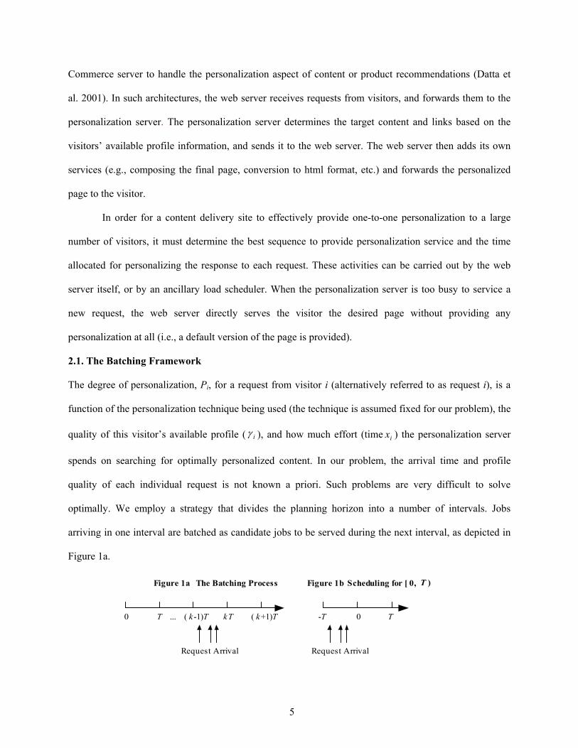
optimally. We employ a strategy that divides the planning horizon into a number of intervals. Jobs

arriving in one interval are batched as candidate jobs to be served during the next interval, as depicted in

Figure 1a.

0 T ... ( k -1)T kT ( k+1)T

Request Arrival

-T 0 T

Request Arrival

Figure 1a The Batching Process Figure 1b Scheduling for [ 0, T )

6

An interval of width T is chosen such that each request i arriving in interval [(k-1)T, kT) has a

time threshold (deadline) that is (k+1)T or larger. If a request arriving in the interval [(k-1)T, kT) is

chosen to be personalized, it receives that service in the next interval [kT,(k+1)T). A schedule, that

includes the time allocated for each request and the sequence of providing personalization service, is

formed at time instance kT for the requests to be served in the interval [kT, (k+1)T). The requests not

allocated any time for personalization are provided default service that is delivered at time kT or earlier −

this is further discussed in Section 4. Since the nature of the problem remains the same for each batch, it

can be viewed as determining the optimal schedule for the interval [0,T) considering requests that have

arrived in the interval [-T, 0), as shown in Figure 1b. If the personalization server finishes service for all

requests at time tk < (k+1)T, then the web server starts the next batch (of duration T or less) at time tk,

after determining the time to be allocated to each request that arrives during the interval [kT, tk).

2.2. Notation and Assumptions

Table 1 lists the notation used in our analysis. We then discuss our assumptions, which are made to

enable the derivation of useful insights while capturing the important characteristics of the problem.

Table 1 Notation Used in Our Analysis γi ∈ [0, 1] γi is the quality of visitor i’s profile. A higher value of iγ implies that the profile better captures

the needs of the visitor. The values of iγ belong to a finite discrete set, with q possible values. hi∈[0, +∞) hi is the maximum permissible personalization time allocated to a request with profile quality γi.

The values of hi also belong to a finite discrete set with q values. xi ∈ [0, hi] xi is the computational effort (time) spent on personalizing the content for the current request

from visitor i. We assume that communication and other delays are negligible; non-negligible delays do not change the characteristics of our problem and proposed policy, although it does impact the eventual profits.

Pi ∈ [0, 1] Pi is the degree of personalization for content returned to the request from visitor i. r r is the maximum potential additional revenue that can be generated from personalizing one

request of a visitor. b b is the computing resource spent per unit time of the personalization server. ρ ∈[0, +∞) ρ is the average cost per unit time delay per request to the site (in the form of lost revenues due

to an unsatisfied visitor), i.e., the average opportunity cost. gi gi is the time instance of arrival of the current request of visitor i. T T is the batch length, i.e., the width of time interval to serve a given batch of requests. TP TP is the impatience parameter, which is an upper bound for the amount of time since the arrival

of a request by which the server must provide the desired content to the visitor.

7

The profile quality iγ depends on the past usage data available for the visitor. For instance, this

could be the available visitor usage data in terms of her word-vector frequency as a proportion of the

amount of data that would typically enable perfect profiling. We assume that Pi increases linearly with ix

and has the form Pi = γi(xi/hi), for xi є[0, hi]; Pi = γi for xi ≥ hi. Depending on the nature of the

personalization method being used, more complicated functional forms (e.g., concave) are possible. As

shown in Figure 2, the piece-wise linear functional form assumption is often a reasonable approximation

to a concave function, and enables us to obtain important insights about the problem. For request i, if

0=ix , then Pi = 0 (if the personalization server doesn’t spend any effort, then the visitor receives default

content); if xi ≥ hi, then Pi = γi , which means that if the maximum possible effort is spent to search for the

optimal content, the visitor gets a degree of personalization equal to the quality of her profile. We make

the following assumptions. First, we assume that more personalization effort is needed to achieve the

maximum possible personalization for a request with higher profile quality. In other words, if the tastes of

a customer are known well, more elaborate personalization would be possible. For example, if there are

more keywords in a word-vector profile, then there will exist more potential documents that could be

matched, resulting in a larger search space. Our second assumption is that the revenue rate (revenue

generated in one unit of time) from personalization is greater for a request with a higher profile quality; in

other words, it is more profitable to provide a unit of time to visitors whose tastes are better known.

Mathematically, from the above assumptions, if γi<γj, then (i) hi<hj, and (ii) (γi/hi)=tanθi < (γj/hj)=tanθj, as

shown in Figure 2.

Figure 2 Piece-wise Linear Functional Form for Personalization

Computation effort

Deg

ree o

f Per

sona

lizat

ion

)(x

)(P

0

jγ

jhih

jθiθ

iγ

8

A higher level of personalization allows the website to better target its visitors with tailored

content and advertising (Mermigas 2001). The parameter r captures the maximum potential additional

revenue that could be generated from delivering a personalized page. For example, if the revenue model

for a site is based on advertisements served to visitors, r could be the expected additional revenue

generated from perfect personalization, e.g., from the increased likelihood of a click-through as compared

to when no personalization is conducted (the analysis for heterogeneous r is discussed in Section 8). We

define ERi as the expected incremental revenue to the web site by personalizing the content based on a

request by visitor i, and express this as: ERi = rPi =rγi(xi/hi). The parameter ρ represents the expected rate

of loss in revenue due to delay in serving a visitor’s request, and is assumed to be the same across all

customers. We assume a linear cost function for delays, which is a reasonable approximation for the short

threshold for waiting times associated with delivering content to visitors. Our assumption of

homogeneous ρ is consistent with the literature in the context of service providers (Anupindi et al., 1999,

Chapter 8), because determining ρ at the individual level is usually difficult. Note that pi Tg + is the

deadline for serving request i. The batch length T is determined by the site based on expectations of

customers’ impatience (their impatience parameter). The choice of T is discussed further in Section 7.

2.3. Revenue Maximization when Serving a Single Request

We present the profit maximization problem for the website when personalizing a single visitor’s request

(say, request i) and no other requests are waiting. We assume that if a visitor’s request is not personalized

at all (i.e., dropped by the personalization server), the incremental profit to the site is zero. Defining Πi as

the profit from personalizing request i, the profit maximization problem is:

.,0..

)()(

piii

ii

iii

i

iii

Txhxts

xbhr

bxxhx

rMax

≤≤≤

−−=−−=Π ργ

ργ

The term rγixi/hi is the expected added revenue, ρxi is the delay cost, and bxi is the resource cost. In this

case, the server should provide the minimum of hi or Tp units of personalization effort when the

coefficient )/( bhr ii −− ργ for xi is positive, and zero units otherwise.

9

3. Characterizing the Optimal Schedule in a Batching Policy

We analyze the problem of the optimal scheduling policy for each batch of requests, and identify

important characteristics of such a policy in Lemmas 1 and 2 shown below. Based on these

characteristics, we determine a batching policy that can be obtained in a very efficient manner. We then

show in Proposition 1 that the policy is optimal.

Consider the situation where n requests are to be scheduled in a batch. Without loss of generality,

we assume the profile quality ordering to be nn γγγγ ≥≥≥≥ −121 ... .

Lemma 1. If a solution contains non-contiguous service time allocations to a request i, then the solution

can be improved by making it contiguous.

Proof. We provide a proof for the case where the total time allocated to a request i is divided in two parts

(total amount xi in parts aix and b

ix ) and service is provided to another request j (amount xj) in between

these two parts. The proof for multiple divisions, and for multiple intervening requests, can be obtained

analogously. Figure 3 illustrates the non-contiguous and contiguous service time scenarios. Let t be the

starting time for personalization service to request i in the non-contiguous and to request j in the

contiguous cases. Since bi

aii xxx += , the profits from personalizing the two requests for the non-

contiguous case ( )(ncΠ ) and the contiguous case ( )(cΠ ) are as shown below:

)()/()()/()(j

aijjjjiiii

nc xxtxbhrxxtxbhr ++−−+++−−=Π ργργ , and

)()/()()/()(jjjjjiiii

c xtxbhrxxtxbhr +−−+++−−=Π ργργ .

)(ncΠ and )(cΠ differ only in the fourth term. Thus, ai

cnc xρ−Π=Π )()( and therefore )()( cnc Π>Π . □□

Lemma 1 shows that time-sharing is not desirable for a personalization server.

Figure 3 Non-contiguous and Contiguous Service Cases

i j i ij

aix jx b

ix jx ix

0 t T 0 t T

10

Lemma 2. (a) Personalization service should not be provided to a request with a profile quality lower

than another eligible request that is not being provided any personalization service.

(b) For requests being provided non-zero amounts of personalization service, in the optimal solution, the

sequence of service is based on a non-decreasing order of profile quality.

Proof. (a) The server can reallocate the personalization service from the lower profile quality request to

the eligible higher one, providing default service to the lower profile quality request. The profit function

will improve as the revenue rate is higher for the higher quality request.

Figure 4 Serving Sequence for n Requests

j i

jx ixt0

(b) Let request i in Figure 4 have a lower quality profile than j (i.e., γi<γj). Let S be an optimal solution in

which request i is served immediately after request j (of course, such an adjacent pair must exist for a

lower profile quality request to be served before a higher profile quality request), and t be the starting

time of the service for request j in S. Given such a sequence, the profit contributions from requests j and i

are ])()/[( ργ jjjjj xtxbhr +−−=∆ and ργ )()/[( jiiiii xxtxbhr ++−−=∆ , where xi and xj are the

service times allocated to requests i and j, respectively. Consider a solution S’ with an identical sequence

as S and with the total service time ji xx + allocated for these two requests, except that the service

positions for request i and j are interchanged. The objective function for S’ will include the following

terms corresponding to the profit contributions from requests i and j: ])()/[( ''' ργ iiiii xtxbhr +−−=∆ ,

and ])()/[( '''' ργ jijjjj xxtxbhr ++−−=∆ (here, 'ix and '

jx are the service times allocated in S’ to

requests i and j, respectively). The remainder of the objective function will be the same as for S since

''jiji xxxx +=+ . For schedules S and S’, we have ,ii hx ≤ jj hx ≤ , ii hx ≤' , and jj hx ≤' , since the profit

contribution is zero beyond the limits specified. We show that by assigning appropriate values to 'ix and

11

'jx the total profit from S’ is better than from S. Let ∆ be the net change in the total profit after

interchange of requests i and j in S, i.e., jiji ∆−∆−∆+∆=∆ '' . The proof is shown using two cases.

Case 1: jji hxx ≤+ . In this case, assign jij xxx +=' and 0' =ix . Thus, request i incurs no delay cost.

ργγ

ργγ

ργγ

)(][)()()()()()( ''j

i

i

j

jiji

j

ji

i

ijjj

j

jii

i

i xthr

hr

xxtxhr

xhr

xtxxhr

xxhr

++−=+++−=++−+−=∆

Since i

i

j

j

hhγγ

> , and xi, r, t, and ρ are positive, we have 0>∆ .

Case 2: jijij hhxxh +≤+< . In this case, assign jj hx =' and jjii hxxx −+=' .

.)(])[(

)()()()()()( '''

ργγ

ργγ

ργγ

iji

i

j

j

jj

ijjjj

j

jji

iijjj

j

j

iii

i

xhh

r

h

rxh

xhxhh

rhx

h

rxxxx

h

rxx

h

r

−+−−=

−+−+−=−+−+−=∆

Since i

i

j

j

hhγγ

> , hj > xj, hj > xi, and ρ >0, we have 0>∆ . □□

Thus, in the optimal batching schedule, the service sequence is based on a non-decreasing order of profile

quality. If multiple requests have the same profile quality, there may exist multiple optimal sequences. An

interesting finding is that by instituting a batching framework, we can optimally sequence requests in a

manner that is similar to that of the shortest processing time (SPT) sequence for certain single machine

scheduling problems in the classical scheduling theory (Pinedo, 2002). We note that unlike the classical

scheduling problems, the processing time is a decision variable in our problem. The proof above uses the

concept of “job interchange argument” similar to the one used in classical scheduling theory. However, a

key difference in our case is that the service times of the interchanged requests have to be determined

simultaneously with the sequence, and all requests are not guaranteed to receive personalization service,

in order to arrive at the result in Lemma 2(b). The joint determination of request selection, sequencing,

and service times makes our problem significantly different from classical scheduling problems.

12

Scheduling Policy SCH:

Based on the results of Lemmas 1 and 2, we propose the scheduling policy SCH. We denote the ith largest

profile as ][iγ , },...,1{ ni ∈ .

1. Sort the requests in a non-increasing order of their profile quality: ][]1[]2[]1[ ... nn γγγγ ≥≥≥≥ − . In

the case of a tie, sort requests in the sequence of their arrival times.

2. Find Q, where }0{maxarg ][ >= kk

CQ , bkhrC kkk −−= ργ ][][][ / , where k represents the index of a

request in the sorted list.

3. Find R, where .1}{maxarg1

][ +<= ∑=

ThRm

kk

m

4. Serve the p highest profile requests in a non-decreasing order of their profile quality in the sorted list,

where p = min{Q, R}, and provide default content to the other requests.

5. The processing time allocated to request with index j, j ≤ p, is the minimum of { ∑−

=

−1

1][][ ,

j

kkj hTh }.

6. If ∑=

>p

kkhT

1][ , then the batch length is adjusted to ∑

=

p

kkh

1][ .

If no requests are served in a batch, the next batch begins on the arrival of the first profitable request.

Proposition 1. Schedule SCH is optimal.

Proof. From the optimal sequence determined in Lemma 2, we know that the contribution from the

request with index k is ][][ kk xC , where )/( ][][][ bkhrC kkk −−= ργ . Since the serving sequence is in a non-

decreasing order of the profiles, it follows that the marginal contribution is always higher for higher

profile requests, i.e., C[1] >…>C[n-1]>C[n]. Let the schedule resulting from the proposed policy be SCH

(Figure 5a), with time allocation .,...,1,][ nkx k =∀ We show by contradiction that SCH is optimal.

Case I. Q ≥ R (i.e., R requests receive personalized service)

Let there exist an optimal schedule SCH* in which the serving sequence is in a non-decreasing order of

visitor profiles with time allocations nkx k ,...,1,*][ =∀ . Such a solution always exists as shown in Lemma

2. If SCH* is different from SCH, then there must exist some Rk ≤ where ][*

][ kk xx ≠ . Find the request

13

with the highest profile (i.e., lowest index) that receives a different amount of service, and let that index

be u (note that u ≤ R). If u<R, then ][][ uu hx = and hence ][*

][ uu xx < . If u = R, then ∑<

−=uk

ku xTx ][][ ;

since ][*

][ kk xx = , uk <∀ , implies ∑∑<<

=uk

kuk

k xx ][*

][ , we must have ][][*

][][ uuk

kuk

ku xxTxTx =−=−< ∑∑<<

∗ .

There are two possibilities.

α=][ Rx ]1[]1[ −− = RR hx ][][ uu hx = ]1[]1[ hx =

*]1[x*

][ ux*][ zx *

]1[ −zx

*][ ux *

]1[ −ux *]1[x

Figure 5a Schedule SCH with Q ≥ R (Case I)

Figure 5b Schedule SCH* ( Case I(i))

Figure 5c Schedule SCH* (Case I(ii))

0 T

0 T

0 T

(i) A request other than u will first receive personalization service in SCH* (as shown in Figure 5b).

There are z>u requests served in this solution. Let the request at vth position, uv > , have time 0*][ >vx

allocated to it. In the objective function, the total contribution from the two requests at the vth and the uth

position is *][][

*][][ uuvv xCxC + . Since ][][ uv CC < , we can get a higher contribution,

)()( *][][

*][][ ξξ ++− uuvv xCxC , by reallocating an infinitesimal amount, ξ, of personalization time from the

vth to the uth request. Therefore, SCH* is not optimal.

(ii) u is the first request to receive personalization service in SCH* (as shown in Figure 5c). Since

][*

][ uu xx < , we have ∑∈∀

<*

*][

SCHkk Tx ; let ∑

∈∀

−=∆*

*][

SCHkkxT . Then, SCH* would begin serving the uth request

at time instance 0 and end after serving the request with index 1 (i.e., the entire batch) at time T-∆.

Consider a solution that adds service time )}(,min{ˆ *][][ uu xhx −∆= to the uth request. The additional

externality cost (i.e., the additional delay cost faced by requests served later) imposed on all requests

14

is xu ˆ** ρ . Adding x̂ to request u adds revenue xbhr uu ˆ)/( ][][ −γ . Since C[u] is positive, we have

xuxbhr uu ˆˆ)/( ][][ ∗∗>− ργ .Therefore, once again, SCH* is not optimal.

Case II. R > Q (i.e., Q requests receive personalized service)

SCH would serve each of the Q lowest index requests with full personalization service time as shown in

Figure 6a. As before, consider an optimal schedule SCH*, with time allocations nkx k ,...,1,*][ =∀ . There

are three possible scenarios for SCH*. Of course, according to Lemma 2, changing the sequence cannot

help, nor can replacing a higher profile request with a lower profile one.

(i) There are z>Q requests served. The SCH* in this scenario is shown in Figure 6b. If

,v∃ 0,0 ][*

][ => vv xx , we can conclude that v>Q and C[v]<0. Not allocating any personalization time to the

vth request will lead to a better solution since the coefficient C[v] for request x[v] is negative.

(ii) Exactly Q requests are served. Since SCH* must serve the Q lowest index requests, there must exist f,

f ≤ Q, where ][*

][ ff hx < , as shown in Figure 6c. Therefore, ∑∈∀

<*

*][

SCHkk Tx , and adding an infinitesimal

amount of time ξ to *][ fx will improve the overall profit since C[f] is positive.

(iii) SCH* serves y<Q lowest index requests as shown in Figure 6d. Since the batch length is not fully

utilized, adding an infinitesimal amount of timeξ to the (y+1)th request will improve the overall profit

since the coefficient for that request is positive.

Therefore, SCH* can always be improved. □□

15

][][ QQ hx = ]1[]1[ −− = QQ hx ][][ ff hx = ]1[]1[ hx =

* ]1[x*

][kx*][zx *

][wx

0 T

0 T

0 T

*][Qx *

][ fx *]1[x

Figure 6a Schedule SCH with Min{u,R}>Q (Case II)

Figure 6b Schedule SCH* (Case II(i))

Figure 6c Schedule SCH* (Case II(ii))

*][ yx

Figure 6d Schedule SCH* (Case II(iii))

0 T

[1]x*

4. Pre-processing Procedure for Batching Approach

We have shown that, given a fixed batch length and a list of candidate requests waiting at the starting time

for a batch, our proposed scheduling policy SCH guarantees an optimal solution for that batch. We have

implicitly assumed that all requests arriving in the interval [-T, 0) wait till 0 before the best p = min{R, Q}

requests are scheduled for personalization, and the rest are provided default content. This would impose

waiting costs to all requests arriving in an interval before a new batch starts, regardless of whether they

receive personalized service or not. We refer to such costs as sunk costs; hereafter, delay cost refers to the

cost of waiting during the processing of a batch, and total waiting cost refers to the sum of the sunk cost

and the delay cost. Based on the arrival time of a request, its associated profile, and profiles for other

pending requests, it is possible to determine before the start of a batch whether the request has any chance

of receiving personalization service. If not, then the sunk cost can be reduced or eliminated by providing

default content to the request as early as possible.

We consider a pre-processing procedure for those requests that will be served in the next batch.

The pre-processing procedure ensures that our policy maximizes the overall profit for the site, not only

taking into account the profit obtained from personalized service in a batch, but also considering the sunk

16

cost that is incurred prior to the start of that batch. We then show that the procedure maintains a list of

requests that is optimal at any instant in time, given the realized requests up to that point.

The pre-processing procedure identifies and eliminates from consideration as early as possible

those requests whose associated profiles are dominated by the profiles for enough other pending requests.

Since only a limited number of requests can receive personalized service in a batch, this procedure

maintains a list of the highest profitable requests in non-increasing order of their profile quality, and

provides default service to requests that do not make it into this list. This list is updated based on arrivals

of new requests. Assume that there are M )0( ≥M requests in the list when a new request arrives. Let ][iγ ,

i=1,…,M, be the profile quality of the request in the ith position of the list with ][]2[]1[ ... Mγγγ ≥≥≥ .

Before describing the pre-processing procedure, we state the following result.

Lemma 3. If a new request has a higher profile quality than at least one request in the current list, then

the new request should be inserted in the list.

Proof. Suppose the optimal solution on the arrival of a new request u at time –g (relative to the start of the

next batch), where γu > ][Mγ , is not to include this request, and let the total profit contribution of all

requests in this list be L. If we reallocate service time allocated to the Mth request in the list to the new

request u, then the total profit contribution will be greater than L since the new request’s profile quality is

higher than that of the Mth request. □□

Pre-Processing Procedure:

a) Compare the new request with existing requests, and find w, the position to insert the new request in

the sorted list (w=1 means that the new request has the highest profile quality). In the case of ties, the

new request is placed below all existing requests with the same profile quality. Update M ← M+1.

b) If w ≤ M, (i.e., at least one request has lower profile quality than the new request), all requests with

lower profile quality are moved down by one position, and the service times are recalculated for all

17

wi ≥ as x[i] = min{h[i], max{T-∑−

=

1

1][

i

jjh ,0}}. M is updated as M= }1,0{maxarg

1

1][∑

−

=

+≤>−i

jj

iMihT .

Some requests at the bottom of the list might be dropped due to the limited batch length.

c) If w=M+1, the new request is inserted at the end of the list if the available service time is non-zero.

The number of requests in the list, M, gets updated as M ← M+1.

d) Starting from the Mth request, check if (rγ[l]/h[l]-b)*x[l] > (l*x[l]+g)ρ for l=M, M-1,…,w+1, where

(l*x[l])ρ is the externality cost imposed by the lth request, and gρ is the sunk cost. If this condition is

not satisfied for the lth request, the request is provided default service, M is updated, and checking

continues for the (l-1)th request. If it is satisfied, there is no need to check any further.

So, on the arrival of a new request, the procedure determines where it should be inserted based on

its profile quality, pushing down by one position all requests with lower profile quality. The externality

cost associated with each demoted request increases. Starting from the lowest request in the list, we

examine each demoted request for net profitability based on the revised externality costs. If this net

profitability remains positive then this request stays in its new position in the list; the procedure stops and

the value of M is revised. Otherwise, it is removed from the list and provided default content at this time;

the procedure to examine net profitability continues with the next lowest quality request. In situations

where ThM

ii <∑

=1][ , the length of the batch is reduced to ∑

=

M

iih

1][ . If there are no requests in a batch, the next

batch begins with the arrival of the first profitable request.

Proposition 2 shows that the profit associated with the list maintained by our procedure at any

instant in time dominates the profit associated with all other feasible lists at that instant.

Proposition 2. Given the realized arrivals, the list maintained by the pre-processing procedure is optimal

at any instant in time, and therefore provides the optimal list at the start of the next batch.

Proof. Consider arrivals in the interval [–T, 0). The list is empty at time –T. A request enters the list when

the profile quality of that request is sufficiently high that serving the request provides more added revenue

than the total cost associated with waiting (sunk plus delay) and processing the request. Not including this

18

request in the list is sub-optimal, as the firm would then forgo the net profit associated with serving that

request. Furthermore, since none of the previous requests would have satisfied the profitability

requirement, it would have been sub-optimal to include any of them in the list. Therefore, the list is

optimal at that instant of time.

We now show that our procedure ensures that if a list is optimal at the time of arrival of a new

request (say request i), it remains optimal after the list is updated by following the pre-processing

procedure. In some cases, the new request is inserted in the list without requiring the removal of any

existing request. The decision rule associated with each such case ensures that the new request enters the

list only if it adds to the profit for the site (accounting for externality costs, as well as, its own total

waiting cost); not including this request in the list is then sub-optimal. In other cases, inserting the new

request leads to the removal of some existing requests from the list. This occurs when one of the

following two situations is encountered. The first situation is where ∑=

≥M

ll Th

1][ and M is the updated

number of requests in the list after the new insertion. The server can provide service to a limited number

of requests in a given batch, and our procedure ensures that the list is optimal by dropping the lowest

profile request; dropping any other request leads to less value generated from serving a relatively lower

profile request. The second situation is where the increased externality cost from serving the lowest

profile request in the list now exceeds the benefit from serving that request. Not removing the lowest

profile request at that point in time is sub-optimal, since the site is worse-off in that case. There are cases

where the new request does not enter the list at all, and receives default service immediately on arrival.

This occurs when either there are higher profile existing requests which utilize the whole batch length, or

the new request has a profile lower than all requests in the list, and the externality and other costs

associated with serving the new request is more than the value of the service. It is clear that including the

new request in the list in such cases is never optimal.

19

Finally, consider time periods that lie between the arrival of two requests. Because no new event

occurs in this interval, and every request in the list leads to a net positive profit after accounting for its

delay cost, it is sub-optimal to drop any one of those requests during that time. □□

The pre-processing procedure is computationally very efficient. For each new request, the server

requires at most O(log(U)) operations to find the insertion location, and at most O(U) operations to update

the service times for all requests in the list, where ⎡ ⎤min/ hTU = and },...,1,min{min qihh i == .

5. Three Queuing Approaches

To demonstrate the effectiveness of the batching policy, we compare its performance with three queuing

approaches. One is the first-in-first-out queuing policy, which is also the baseline approach because of its

widespread usage. We also develop two more sophisticated approaches that reorder the queue based on

the profile qualities of requests awaiting service, so that higher profits may be generated. To analyze these

approaches, we introduce the notation in Table 2.

Table 2 Additional Notation ft The finishing time of the request currently being served. ajt ][ The arrival time of the jth request in the queue.

][ jx The service time the jth request in the queue receives. anewt The arrival time of a new request; thus ( a

newf tt − ) is the time remaining until completion of service of the request currently being served.

5.1 First-In-First-Out (FIFO)

This approach maintains a queue of size at most N requests sorted in the order of their arrival time. If the

queue is full, new arrivals get default service immediately. If the queue is not full, a new request must

satisfy two conditions before it is admitted to the queue; if either condition is not met the request receives

default content. The first is whether the request will begin receiving service before its impatience

constraint is violated if it is held in the queue, i.e., 0)(1

][ >−+− ∑=

anewf

M

jjp ttxT , where M is the number

of requests in the queue when the new request arrives. The second is a profitability constraint; given the

20

profile quality of the new request, is it profitable to provide personalization service to it. To decide this, it

is first necessary to determine the maximum service time that can be assigned to this new request, which

is: )}(,min{1

][anewf

M

jjpii ttxThx −+−= ∑

=

. Given xi, if ∑=

−++∗>∗−M

j

anewfijiii ttxxxbhr

1][ )()/( ργ ,

the request will be profitable. Note that once a request is admitted to the queue, it is guaranteed to receive

personalization service as it will remain profitable to do so. The FIFO policy is computationally very

efficient, requiring at most O(1) operations to update the queue.

5.2 Maximum Profile Quality Selected for Next Personalization Service (MaxQualFirst)

We consider two variations of an approach that reorders the queue based on profile quality – preemptive

and non-preemptive. The basic approaches are similar for both; we provide details of the non-preemptive

policy first. This approach maintains a queue of at most N high profile quality requests in a non-

increasing order of their profile quality. An important difference between this approach and the FIFO

policy is that a new request may be inserted in the middle of the current queue, and therefore its

impatience constraint and the profitability constraint have to be evaluated accordingly. Further, inserting a

new request in the middle of the queue increases the delay for requests that get demoted. Each demoted

request has to be re-examined to verify if it still satisfies its impatience and its profitability constraint; if

either one is not met, the request is removed from the queue and receives default service at that time.

The impatience constraint for a request in the wth position in the queue is met if it satisfies the

condition 0)( ][ >−+− ∑<wj

anewfjp ttxT . The maximum available personalization time for that request is:

∑<

−+−=wi

awfipww ttxThx )}(,min{ ][][][][ . If )(**)/( ][][][][][

anewfw

wkkwww ttxxxbhr −++>− ∑

<

ργ ,

serving this request is profitable. Using these conditions, a queue is maintained that guarantees each

request either receives personalized service or receives default service within its impatience constraint.

We present some desirable properties about this queuing approach in Lemmas 4 and 5, and then provide

details of the queue update procedure.

21

Lemma 4. If a new request has a higher profile quality than at least one request in the current queue, then

it is profitable to include the new request in the queue.

Proof. Suppose the optimal solution at the instance of the new arrival i is to not include this request, and

let the total profit contribution from providing personalization service to all requests in the current queue

be L. If we substitute a lower profile quality request j with the new request i, and provide request i the

same amount of service time that request j would have received, then the resulting total profit contribution

of all requests in this queue will be L’ >L since i’s profile quality is higher than that of j. □□

Lemma 4 provides the intuition for the MaxQualFirst approaches.

Lemma 5. If a new request is inserted in the queue at the wth position, providing it more service time than

that assigned to the request previously in the wth position still satisfies the profitability constraint.

Proof. We first show that it will be feasible to provide more personalization time for the new request at

the wth position. The maximum possible service time for the request previously at position w

is ∑<

−+−=wi

awfipww ttxThx )}(,min{ ][][][][ , and the time for the new request i in the wth position is

)}(,min{ ][∑<

−+−=wi

anewfipii ttxThx . Since a

wanew tt ][> and ][wi hh > , we have ][wi xx > . Next, we show

that providing processing time xi to the new request is profitable. For the request previously in the wth

position, )()/( ][][][][][anewfw

wkkwww ttxxxbhr −++∗>∗− ∑

<

ργ , which implies that

)()/( ][][][][ ∑<

−+∗>∗−−wk

anewfkwww ttxxbhr ρργ . Then, )()/ ][

anewf

wkkiii ttxxbhr −+∗>∗−− ∑

<

ρργ ,

since ][][ // wwii hrhr γγ > , and ][wi xx > . This leads to ∑<

−++∗>∗−wk

anewfikiii ttxxxbhr )()/( ][ργ ,

and it is profitable to provide service time ][wi xx > . □□

Queue Update Procedure:

1) The queued requests are sorted by their profile quality, with ties resolved by their arrival times. When

a new request i arrives, find w, the position of this new request in the sorted list. In the case of a tie,

the new request is placed below all existing requests with the same profile quality.

22

2) If w≤M, from Lemma 5 we know that the new request will satisfy the profitability constraint with

personalization effort xi. All existing requests having lower profile quality are demoted by one

position. Assign iw xx ←][ , and anew

aw tt ←][ . For the request at the jth position, j=w+1,…,M+1, check

the impatience and the profitability constraints (by first revising the maximum available service time,

if necessary). If either one is not satisfied, the request receives default content, all the requests below j

are moved one position upward, and M is updated.

3) If w>M, check the impatience and the profitability constraints for the new request. If they are

satisfied, the new request is inserted at the end of the queue and M is updated.

4) If M=N+1, the last request is removed from the queue and provided default content.

For each request, the server requires O(N) operations to determine the service times allocated to each

request in the queue and to reorder the queue. Since N is of the same order of magnitude as U, the

computational complexity for this approach is comparable to that for the batching approach.

The preemptive MaxQualFirst policy has only one difference with the non-preemptive policy. If a

new request i has a profile quality higher than the request currently being served (say j), the server stops

the service for request j and request i enters service immediately.

6. Estimation of Parameters

The results presented in Sections 3–5 can enable websites that face a large amount of traffic to provide

personalized service to selected visitor requests, either by batching or using queues. In order to implement

these approaches, a site would need to obtain estimates for the parameters γi, hi, ρ, r, and b. Word-vectors

are a common profiling approach for personalization in content delivery sites as they can be generated

based on the content viewed by a user, and these vectors can be easily compared to words in a document

(Pazzani and Billsus 1997, Anderson et al. 2001). The site content is represented by a word-by-document

matrix whose entries represent the frequency of occurrence of each word in a document. Personalization

algorithms compare a user profile with the word-by-document matrix to determine which pages to

recommend.

23

As mentioned in Section 2, one way to estimate γi for a visitor is to use the proportion of her word

vector profile as compared to the amount of data that would enable perfect, or close to perfect,

personalization. Although the estimate may be somewhat coarse, it would be very easy to implement.

Another more refined approach would be to estimate the personalization Pi for a visitor by determining

the proportion of recommended links traversed by the visitor (as against the use of a search engine, or,

backtracking, by the visitor), when ample time is spent on personalization such that the recommendations

cannot be improved upon given the profile, i.e., 1/ ≈ii hx . Then, Pi would serve as a reliable estimate for

γi. The parameter hi depends on the technology used for personalization, and may be estimated by

examining when the marginal value to added personalization effort becomes close to zero. ρ can be

estimated by performing controlled experiments to examine the change in (i) the duration of stay of a

visitor in terms of the number of pages requested, and in (ii) the probability of that visitor returning to the

site in future, when the response time is reduced (e.g., from 8 seconds to 4 seconds). The computational

cost per unit time, b, is estimated based on hardware, software, and related expenses for the site. As

indicated in Section 2, r is the expected additional revenue from the increased likelihood of a click-

through when perfect personalization is provided. Therefore, to estimate r, the firm could track the

increased incidence of click-throughs that occur for perfectly personalized content pages as compared to

when no personalization is conducted (i.e., when default pages are presented).

7. Experimental Results

7.1. Determining the Optimal Batch and Queue Lengths

An important consideration in implementing the batching policy is the choice of the batch length T. This

length must be carefully chosen, after studying the behavior (impatience parameter) of visitors, as well as

the latency delays (communication and other processing latencies) associated with the service.3 Even if

the delays associated with delivering the page to the visitor are negligible, T should be chosen less than

3 The one-way transport latency for broadband connections is approximately 100 milliseconds, and thus not very constraining. If other processing delays are likely to be significant, they must be carefully estimated and the maximum feasible batch length must be derived accordingly.

24

half the impatience parameter, since in the worst case scenario a visitor’s request may be served after 2T

time units have elapsed (e.g., when the request arrives immediately after a batch has started, and is

scheduled to receive service at the end of the next batch). Therefore, once the batch length is determined,

it is no longer necessary to track the impatience parameter for each individual request when determining

the schedule for a batch. When latency delays are significant, the feasible batch length would need to be

reduced by explicitly factoring in such delays.

The batching policy can be easily used to experimentally determine the optimal batch length

based on the estimates of the other parameters. The site owner can record the arrival of requests over a

pre-determined interval of time, and then evaluate the performance (in terms of expected profits) of the

policy for varying batch lengths. The batch length that leads to maximum profits could be used thereafter.

We illustrate this process by presenting results from numerical experiments conducted on

simulated data. These experiments show how the optimal batch length can be determined, and also enable

us to derive additional insights about the choice of the batch length. We assume the inter-arrival times for

requests follow an exponential distribution, and choose a time horizon of 4000 seconds for the simulation.

We conduct experiments for three possible distributions of profile quality: Uniform[0,1], Beta with mean

0.25, and Beta with mean 0.75.4 We consider different batch lengths ranging from 0.025 second to 5

seconds, in increments of 0.025 second. Batch lengths longer that 5 seconds could lead to requests

waiting more than 10 seconds, typically considered the maximum allowable impatience parameter

(Nielsen 1999).

Unless otherwise specified, the baseline parameter values in all the experiments are: λ =20

requests/second, iγ ~Uniform[0,1], ρ=$0.1/second, b=$0/second, and r=$1/request. We use five discrete

levels of profile quality (q=5) with associated values },{ ii hγ : {0.2,0.05}, {0.4,0.08}, {0.6,0.1},

{0.8,0.11}, {1.0,0.125}. iγ ~Uniform[0,1] means that the profile quality of requests are evenly distributed

among these five levels. We note that the above parameter values are chosen for illustration purposes

4 In practice, a firm can determine the distribution of profile quality from their historical data, and use the appropriate distribution to estimate the optimal batch length.

25

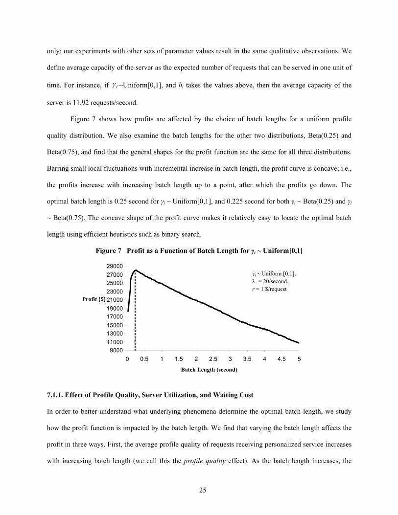
only; our experiments with other sets of parameter values result in the same qualitative observations. We

define average capacity of the server as the expected number of requests that can be served in one unit of

time. For instance, if iγ ~Uniform[0,1], and hi takes the values above, then the average capacity of the

server is 11.92 requests/second.

Figure 7 shows how profits are affected by the choice of batch lengths for a uniform profile

quality distribution. We also examine the batch lengths for the other two distributions, Beta(0.25) and

Beta(0.75), and find that the general shapes for the profit function are the same for all three distributions.

Barring small local fluctuations with incremental increase in batch length, the profit curve is concave; i.e.,

the profits increase with increasing batch length up to a point, after which the profits go down. The

optimal batch length is 0.25 second for γi ~ Uniform[0,1], and 0.225 second for both γi ~ Beta(0.25) and γi

~ Beta(0.75). The concave shape of the profit curve makes it relatively easy to locate the optimal batch

length using efficient heuristics such as binary search.

Figure 7 Profit as a Function of Batch Length for γi ~ Uniform[0,1]

7.1.1. Effect of Profile Quality, Server Utilization, and Waiting Cost

In order to better understand what underlying phenomena determine the optimal batch length, we study

how the profit function is impacted by the batch length. We find that varying the batch length affects the

profit in three ways. First, the average profile quality of requests receiving personalized service increases

with increasing batch length (we call this the profile quality effect). As the batch length increases, the

9000 11000 13000 15000 17000 19000 21000 23000 25000 27000 29000

0 0.5 1 1.5 2 2.5 3 3.5 4 4.5 5 Batch Length (second)

γι ∼ Uniform [0,1],λ = 20/second,r = 1 $/request

Profit ($)

26

average number of requests arriving in one batch interval increases, and the number of candidates selected

for personalized service in the next batch also increases. This reduces the chance of a high profile request

being eliminated because of its proximity to the arrival of other higher profile requests. We have

conducted experiments that show the profile quality improves in a concave manner with increasing batch

length. Second, the overall utilization of the server also increases with increasing batch length (the server

utilization effect). When the request arrival rate is not very high compared to the server capacity, the

server utilization level can become important. When the server utilization level is low and the batch

length is small, it is possible that some high profile quality requests are provided default service during a

batch while the server is idle during other batches. Having a larger batch length reduces the likelihood of

this happening. Our experiments show that the server utilization also increases in a concave manner with

increasing batch length, until the server is fully utilized. Finally, increasing the batch length leads to a

higher waiting time (the waiting cost effect). As the batch length increases, the average waiting cost

incurred by requests selected for personalized service increases, since the selected requests wait longer on

average both before the service to the batch begins as well as during the processing of a batch. The first

two effects contribute positively to the profit, while the third one has a negative impact. Prior to the

inflection point, the marginal contributions from the first two effects dominate the third one; thereafter,

the third effect starts to dominate, and the profit decreases.

7.1.2. Optimal Batch and Queue Lengths for Different Arrival Rates

The rate at which requests arrive at a content delivery site could vary substantially from peak to non-peak

times. Since the arrival rate directly impacts the server utilization, it is worthwhile to examine how the

optimal batch length (and associated profit) changes with different arrival rates.

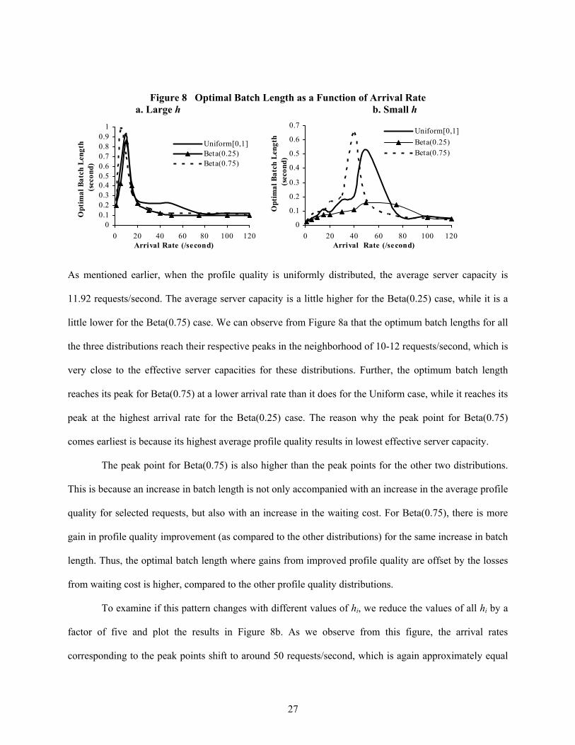
Figure 8 plots the changes in optimal batch length as a function of the arrival rate for the three

profile quality distributions. For each distribution, the optimal batch length peaks at a point where the

arrival rate is close to the average capacity of the server. For very high arrival rates, the optimal batch

length asymptotically converges to a value in the neighborhood of the median of hi.

27

Figure 8 Optimal Batch Length as a Function of Arrival Rate a. Large h b. Small h

00.10.20.30.40.50.60.70.80.9

1

0 20 40 60 80 100 120Arrival Rate (/second)

Opt

imal

Bat

ch L

engt

h (s

econ

d)

Uniform[0,1]Beta(0.25)Beta(0.75)

0

0.1

0.2

0.3

0.4

0.5

0.6

0.7

0 20 40 60 80 100 120Arrival Rate (/second)

Opt

imal

Bat

ch L

engt

h (s

econ

d)

Uniform[0,1]Beta(0.25)Beta(0.75)

As mentioned earlier, when the profile quality is uniformly distributed, the average server capacity is

11.92 requests/second. The average server capacity is a little higher for the Beta(0.25) case, while it is a

little lower for the Beta(0.75) case. We can observe from Figure 8a that the optimum batch lengths for all

the three distributions reach their respective peaks in the neighborhood of 10-12 requests/second, which is

very close to the effective server capacities for these distributions. Further, the optimum batch length

reaches its peak for Beta(0.75) at a lower arrival rate than it does for the Uniform case, while it reaches its

peak at the highest arrival rate for the Beta(0.25) case. The reason why the peak point for Beta(0.75)

comes earliest is because its highest average profile quality results in lowest effective server capacity.

The peak point for Beta(0.75) is also higher than the peak points for the other two distributions.

This is because an increase in batch length is not only accompanied with an increase in the average profile

quality for selected requests, but also with an increase in the waiting cost. For Beta(0.75), there is more

gain in profile quality improvement (as compared to the other distributions) for the same increase in batch

length. Thus, the optimal batch length where gains from improved profile quality are offset by the losses

from waiting cost is higher, compared to the other profile quality distributions.

To examine if this pattern changes with different values of hi, we reduce the values of all hi by a

factor of five and plot the results in Figure 8b. As we observe from this figure, the arrival rates

corresponding to the peak points shift to around 50 requests/second, which is again approximately equal

28

to the effective server capacity for the new values of hi. The other characteristics for the three

distributions remain the same.

We observe that until the arrival rate is somewhat higher than the average server capacity, the

optimal batch length can vary substantially. Thereafter, the optimal batch length is quite stable. Therefore,

if request arrival rates at non-peak hours are in the region of the average server capacity (or less), it

becomes important to monitor the arrival rate closely and revise the batch length accordingly.

We conduct similar experiments to determine the optimal queue length for the queuing

approaches, and find that the optimal queue lengths follow the same pattern as the batch length. Figure 9

shows the optimal queue lengths for FIFO and MaxQualFirst without preemption – note that when the

arrival rate increases, the optimal queue length first increases and then decreases, finally converging to

one. The optimal queue length is longer for the MaxQualFirst policy than for FIFO. This is because the

average profile quality of requests personalized by the MaxQualFirst policy is higher than that by the

FIFO policy, and therefore the losses from increased average waiting costs can be offset by the

MaxQualFirst policy at higher queue lengths.

Figure 9 Optimal Queue Length as a Function of Arrival Rate (Uniform, r=1, ρ=0.1)

02468

1012141618

0 20 40 60 80 100 120Arrival Rate (/second)

Opt

imal

Que

ue L

engt

h

FIFO

MaxQualFirst-No preemption

7.2. Comparing Batching and Queuing Approaches

We conduct experiments that compute the profits from using each of the queuing approaches and the

batching approach, respectively. The parameters are as in the previous experiments: r=$1, ρ=$0.1/second,

29

b=$0/second, Horizon=4000 seconds, and γi ~ Uniform[0,1]. Comparisons are made for arrival rates in the

range [1,300] customers per second, respectively (recall that the average capacity of the server is 11.92

requests/second). Since the profits for the approaches depend on the optimal batch or queue length, we

determine the best possible length using the procedure discussed in Section 7.1.2. The results are

displayed in Table 3.

Table 3 Comparison of Queuing and Batching Approaches (q=5) Arrival Rate

FIFO (Optimal Queue Length)

MaxQualFirst- Preemption (Optimal Queue Length)

MaxQualFirst - No Preemption (Optimal Queue Length)

Batching (Optimal Batch Length)

% Improvement of Batching over MaxQualFirst with Preemption

1 2301.56 (2) 2275.83 (2) 2295.27 (2) 2301.63 (0.25) 1.13 5 11812.3 (8) 10921.5 (6) 11288.6 (7) 11828.8 (0.6) 8.31

10 21818.3 (9) 19286.6 (11) 20123.6 (16) 22882.8 (0.925) 18.67 15 23882.6 (4) 24760.8 (8) 25343.0 (8) 27071.0 (0.35) 9.33 20 24313.9 (3) 27309.5 (5) 27469.4 (6) 28025.7 (0.25) 2.62 30 24689.9 (2) 29355.4 (3) 29222.9 (4) 28797.7 (0.225) -1.90 40 24806.5 (1) 30104.1 (3) 29880.6 (3) 29390.5 (0.225) -2.37 50 24957.1 (1) 30521.5 (2) 30259.2 (3) 29815.0 (0.225) -2.31 75 25023.3 (1) 30999.4 (1) 30734.2 (2) 30533.4 (0.125) -1.50

100 25012.2 (1) 31146.5 (1) 30987.6 (1) 30857.7 (0.125) -0.93 200 25035.0 (1) 31223.1 (1) 31210.0 (1) 31172.6 (0.1) -0.16 230 25015.9 (1) 31223.9 (1) 31217.3 (1) 31194.4 (0.1) -0.09 260 25029.8 (1) 31222.8 (1) 31219.4 (1) 31212.2 (0.1) -0.03 300 25006.3 (1) 31221.5 (1) 31221.0 (1) 31224.4 (0.1) 0.01

The second column lists the highest profit obtained by using a FIFO queue, and in parenthesis

lists the associated optimal queue length. The third, fourth and fifth columns display the corresponding

values for the MaxQualFirst with preemption, the MaxQualFirst without preemption, and for the batching

approach, respectively. The batching approach is consistently superior to the FIFO policy, which is the

baseline policy. Both MaxQualFirst approaches are less profitable than FIFO when the arrival rate is less

than 15 requests/second; thereafter MaxQualFirst approaches do better. The MaxQualFirst with

preemption is inferior to the one without preemption when the arrival rate is less than or equal to 30

requests/second, and outperforms it when the arrival rate is higher. At high arrival rates, both

MaxQualFirst approaches do a little better than the batching approach. Neither the MaxQualFirst with

non-preemption, nor FIFO, ever outperform both MaxQualFirst with preemption and batching for any

arrival rate, and are thus effectively dominated.

30

To understand the relative performance of the MaxQualFirst with preemption and batching, we

show in the sixth column of Table 3 the % improvement obtained by the batching approach over the

MaxQualFirst approach with preemption. We observe that when the arrival rate is up to a few multiples of

the capacity of the personalization server, the batching approach does better. This is because the batching

approach can effectively reduce the externality cost by serving the lower profile requests first while the

added revenue and waiting cost are about the same for both approaches. When the arrival rate goes up

further, the MaxQualFirst approach starts to do better because this approach can dynamically revise the

queue to retain high profile quality requests in the queue while a request is being served. In the batching

approach, once a new batch starts, all the selected requests are guaranteed to be served and therefore it has

less flexibility to accommodate all high profile quality requests. When the arrival rate increases further

(and is extremely high relative to the capacity), the batching approach does better again since the high

arrival rates guarantee that only the highest profile quality requests will receive personalization service,

and the batching approach can lower the sunk cost by shrinking the batch length to values that are even

smaller than the maximum hi, something the MaxQualFirst queuing approach cannot do.

7.2.1 Comparisons for other Values of ρ

To see if our findings are robust, we conducted experiments with different values of the delay cost

parameter, ρ. These results are shown in Table 4.

Table 4 Comparisons under different values of ρ (r=1) Value of δ Range of Zone I

(Maximum % Difference) Range of Zone II

(Maximum % Difference) Range of Zone III

(Maximum % Difference) 0.01 1~20 (21.02%) 30~100 (-0.96%) 200~300 (0.08%) 0.06 1~20 (19.61%) 30~230 (-1.92%) 260~300 (0.10%) 0.15 1~20 (17.59%) 30~230 (-2.80%) 260~300 (0.04%) 0.20 1~20 (16.67%) 30~260 (-2.88%) 300 (0.02%)

Zone I refers to the initial range of arrival rates over which the batching approach dominates; Zone II

refers to the range of arrival rates where MaxQualFirst with preemption does better; and Zone III refers to

the range of arrival rates where the batching approach is again superior. The Maximum % Difference

refers to the maximum difference between the two approaches observed over the entire range of the zone.

The most marked differences occur in Zone I, and are relatively small for Zones II and III.

31

7.2.2 Effect of Granularity of Profile Quality

Since it may be difficult to accurately estimate the profile quality in some situations, we examine the

performance comparison where the granularity of profile quality is three instead of five, with

values },{ ii hγ : {0.2,0.05}, {0.6,0.1}, {1.0,0.125}. The other parameters retain their base values. The

comparisons across the four approaches are shown in Table 5.

Table 5 Comparison of Queuing and Batching Approaches (q=3) Arrival Rate

FIFO Queue (Optimal Queue Length)

MaxQualFirst - Preemption (Optimal Queue Length)

MaxQualFirst - No Preemption (Optimal Queue Length)

Batching (Optimal Batch Length)

% Improvement of Batching over MaxQualFirst with Preemption

1 2625.58 (3) 2599.84 (2) 2616.62 (2) 2625.71 (0.250) 0.99 5 13363.5 (8) 12322.7 (6) 12552.7 (7) 13388.1 (0.650) 8.65

10 23767.7 (8) 21539.3 (19) 22002.2 (17) 25548.9 (0.725) 18.62 15 25345.3 (3) 26853.1 (8) 26874.0 (8) 28907.1 (0.350) 7.65 20 25747.7 (3) 28930.6 (7) 28752.0 (7) 29506.6 (0.250) 1.99 30 26104.3 (2) 30210.6 (3) 29934.0 (4) 29874.7 (0.250) -1.11 40 26257.8 (1) 30718.5 (2) 30436.5 (3) 30224.7 (0.250) -1.61 50 26371.5 (1) 31011.1 (1) 30743.5 (1) 30583.9 (0.125) -1.38 75 26397.4 (1) 31198.1 (1) 31095.4 (1) 31019.9 (0.125) -0.57

100 26369.6 (1) 31232.1 (1) 31195.6 (1) 31144.1 (0.125) -0.28 200 26399.1 (1) 31227.2 (1) 31227.2 (1) 31244.5 (0.100) 0.06 230 26433.4 (1) 31225.0 (1) 31225.2 (1) 31249.2 (0.100) 0.08 260 26385.3 (1) 31223.3 (1) 31223.8 (1) 31257.8 (0.075) 0.11 300 26422.9 (1) 31221.8 (1) 31222.2 (1) 31267.0 (0.075) 0.15

The results are largely similar to the case where the granularity was five, i.e., q=5. We find that

Zone III (the zone with very high arrival rates where batching does better) starts earlier than with a

granularity of five. This is because in the three granularity case, 33 percent of all arriving requests are in

the top category; thus, the arrival rate at which batching provides service to only the best profile quality

requests is lower compared to the five granularity case where only 20 percent of arrivals are in the top

category.

8. Discussion

We have presented queuing and batching approaches that can enable content-delivery websites facing a

large amount of traffic to select and schedule requests that should receive personalized service. Our

analysis trades-off maximizing service time for a fully personalized response with the negative externality

of higher waiting costs for other requests in the system. While the problem is a difficult one in general,

32

we show that it can be solved relatively easily by considering a policy based on batching, and is therefore

easy to implement. The batching approach outperforms the queuing approaches when request arrival rates

are within a few multiples of the personalization server capacity. The MaxQualFirst with preemption does

a little better than the batching approach for higher arrival rates up to a point, after which the batching

approach again does better.

Our work provides several interesting insights regarding the batching solution. An intuitive

finding is that when requests arrive at rates higher than a personalization servers’ capacity, requests

associated with low quality profiles are provided default content while high quality requests get

personalized pages. On the other hand, requests selected for personalization within a batch should be

scheduled in reverse order of their profile quality in order to provide the maximum possible effort in

personalizing pages for the request with highest profile quality.

While we have assumed that r, the marginal revenue per request, is constant for all visitors, our

policy readily extends to situations where it is possible for a site to determine visitor-specific values for

this parameter. By replacing r with ri for each visitor i in the profit function, we can derive analogous

results that use the product ri × γi instead of γi to sort the requests and schedule them for personalization.

While estimating ri for each visitor is not easy, it may be possible to track visitors’ propensity to click on

advertisements for each category of γi, and use this information to estimate the aggregate level value for

this parameter in that category.

Our policy is also applicable in situations where recommendation techniques pre-compute part of

the personalization effort (e.g., calculate correlations or form segments), and then in real-time provides

more fine-tuned personalization (e.g., identify and sort links to present to the visitor). Depending on the

amount of resource allocated to a request, the personalization server could provide either a default set of

links, sort the default set, or determine the best set and provide them in a preferred sorted order.

Given the lack of prior work in this area, there exist several promising directions for future

research. Different functional forms that apply to different personalization scenarios (e.g., scalability of

different personalization techniques) need to be identified, and solutions obtained. An obvious extension

33

is to allow the personalization quality to be a non-linear function of personalization effort. Preliminary

work suggests that a policy similar to the proposed one may be applicable for profit functions based on

such functional forms. While such a general formulation may be hard to solve analytically, our findings

could lead to efficient heuristics that are close-to-optimal in their performance.

References (1) Anderson, C. R., P. Domingos and D. S. Weld, “Personalizing Web Sites for Mobile Users,”

Proceedings of the 10th Conference on World Wide Web, May (2001), 18-28. (2) Anderson, E. J. and C. N. Potts, “Online Scheduling of a Single Machine to Minimize Total

Weighted Completion Time,” Mathematics of Operations Research, 29 (2004), 686-697. (3) Ansari, A. and C. F. Mela, “E-Customization”, Journal of Marketing Research, Vol. XL, (May

2003), 131-145. (4) Anupindi, R., S. Chopra, S.D. Deshmukh, J.A. Van Mieghem, and E. Zemel, Managing Business

Process Flows, Prentice Hall, New Jersey, 1999. (5) Bretthauer, K. M. and B. Shetty, “The Nonlinear Resource Allocation Problem,” Operations

Research, 43, 4(1995), 670-683. (6) Brucker, P., Scheduling Algorithms, Springer, Berlin, 1997. (7) Chen, Y. and G. Iyer, “Research Note: Consumer Addressability and Customized Pricing,”

Marketing Science, 21, 2 (2002), 197-208. (8) Datta, A., K. Dutta, D. VanderMeer, K. Ramamritham and S. B. Navathe, “An Architecture to

Support Scalable Online Personalization on the Web”, The International Journal on Very Large Data Bases, 10, 1 (2001), 104-117.

(9) Dewan, R., B. Jing and A. Seidmann, “Product Customization and Price Competition on the Internet,” Management Science, 49, 8 (2003), 1055-1070.

(10) Gong, L., “Can Web-Based Recommendation Systems Afford Deep Models: A Context-based Approach for Efficient Model-based Reasoning”, WWW 2004, May 17-22, 2004, New York, USA.

(11) Hall, L. A., A. S. Schulz, D. B. Shmoys and J. Wein, “Scheduling to Minimize Average Completion Time: Off-line and On-line Approximation Algorithms,” Mathematics of Operations Research, 22 (1997), 513-544.

(12) Ihlstrom, C. and J. W. Palmer, “Revenues for Online Newspapers: Owner and User Perception,” Electronic Markets, 12, 4 (2002), 228-237.

(13) Keskinocak, P., R. Ravi and S. Tayur, “Scheduling and Reliable Lead-time Quotation for Orders with Availability Intervals and Lead-time Sensitive Revenues,” Management Science, 47 (2001), 264-279.

(14) Lawler, E. L., J. K. Lenstra, A. H. G. R. Kan and D. B. Shmoys, “Sequencing and Scheduling: Algorithms and Complexity,” Handbook of Operations Research and Management Science, 4 (1993), 445-552.

(15) Mermigas, D., “Personalization Can Mean Profit,” Electronic Media, 20, 47 (2001), 11. (16) Mjelde, K. M., “Resource Allocation with Tree Constraints,” Operations Research, 31, 5(1983),

881-890. (17) Mobasher, B., H. Dai, T. Luo and M. Nakagawa, “Discovery and Evaluation of Aggregate Usage

Profiles for Web Personalization,” Data Mining and Knowledge Discovery, 6 (2000), 61-82. (18) Murthi, B.P.S. and S. Sarkar, “The Role of the Management Sciences in Research on

Personalization,” Management Science, 49, 10 (2003), 1344-1362. (19) Nielsen, J., “Designing Web Usability,” New Riders, 1999. (20) Pazzani, M. and D. Billsus, “Learning and Revising User Profiles: the Identification of Interesting

Web Sites”, Machine Learning, 27(3), 313-331, 1997.

34

(21) Peppers, D. and M. Rogers, Enterprise One to One: Tools for Competing in the Interactive Age, Doubleday, New York, 1997.

(22) Pinedo, M., “Scheduling Theory, Algorithms, and Systems,” Prentice-Hall, 2002. (23) Yan, W., M. Jacobsen, H. Garcia-Molina and U. Dayal, “From User Access Pattern to Dynamic

Hypertext Linking,” Computer Networks and ISDN Systems, 28 (1996), pp. 1007-1014.