Making Use of the Most Expressive Jumping EmergingPatterns for Classification

Jinyan Li1, Guozhu Dong2, and Kotagiri Ramamohanarao11 Department of CSSE, The University of Melbourne, Parkville, Vic. 3052, Australia.fjyli, raog@cs.mu.oz.au2 Dept. of CSE, Wright State University, Dayton OH 45435, USA.gdong@cs.wright.edu

Abstract. Classification aims to discover a model from training data that canbe used to predict the class of test instances. In this paper,we propose the useof jumping emerging patterns(JEPs) as the basis for a new classifier called theJEP-Classifier. Each JEP can capture some crucial difference between a pairofdatasets. Then, aggregating all JEPs of large supports can produce more potentclassification power. Procedurally, the JEP-Classifier learns thepair-wise features(sets of JEPs) contained in the training data, and uses thecollective impactscon-tributed by themost expressivepair-wise features to determine the class labels ofthe test data. Using only the most expressive JEPs in the JEP-Classifier strength-ens its resistance to noise in the training data, and reducesits complexity (as thereare usually a very large number of JEPs). We use two algorithms for constructingthe JEP-Classifier which are both scalable and efficient. These algorithms makeuse of theborder representationto efficiently store and manipulate JEPs. We alsopresent experimental results which show that the JEP-Classifier achieves muchhigher testing accuracies than the association-based classifier of [8], which wasreported to outperform C4.5 in general.

1 Introduction

Classification is an important problem in the fields of data mining and machine learn-ing. In general, classification aims to classify instances in a set of test data, based onknowledge learned from a set of training data. In this paper,we propose a new classifier,called theJEP-Classifier, which exploits the discriminating power ofjumping emergingpatterns(JEPs) [4]. A JEP is a special type of EP [3] (also a special type of discrimi-nant rule[6]), defined as an itemset whose support increasesabruptlyfrom zero in onedataset, to non-zero in another dataset — the ratio of support-increase being1. TheJEP-Classifier uses JEPs exclusively, and is distinct from the CAEP classifier [5] whichmainly uses EPs withfinitesupport-increase ratios.

The exclusive use of JEPs in the JEP-Classifier is motivated by our belief that JEPsrepresent knowledge which discriminates between different classes more strongly thanany other type of EPs. Consider, for example, the Mushroom dataset taken from theUCI data repository [1]. The itemsetfODOR = foulg is a JEP, whose support increasesfrom 0% in the edible class to55% in the poisonous class. If a test instance containsthis particular EP, then we can claim with a very high degree of certainty that thisinstance belongs to the poisonous class, and not to the edible class. In contrast, other

kinds of EPs do not support such strong claims. Experimentalresults show that theJEP-Classifier indeed gives much higher prediction accuracy than previously publishedclassifiers.

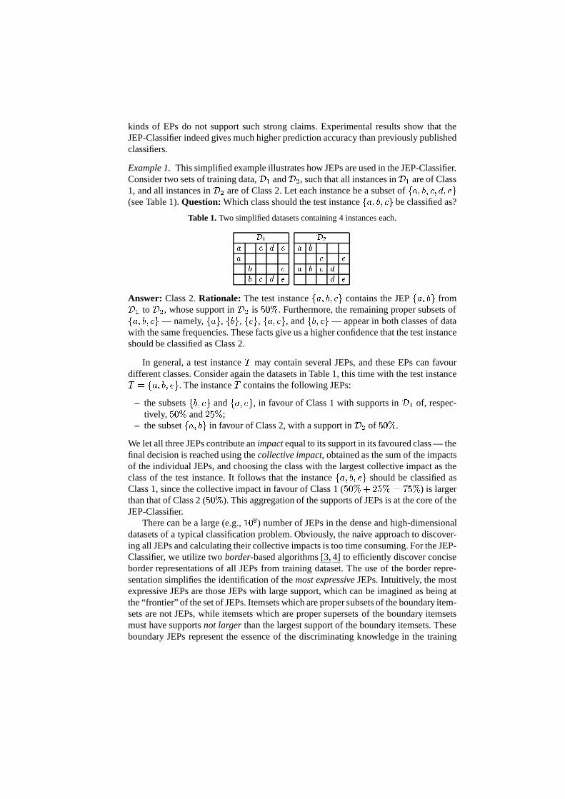
Example 1.This simplified example illustrates how JEPs are used in the JEP-Classifier.Consider two sets of training data,D1 andD2, such that all instances inD1 are of Class1, and all instances inD2 are of Class 2. Let each instance be a subset offa; b; ; d; eg(see Table 1).Question:Which class should the test instancefa; b; g be classified as?

Table 1.Two simplified datasets containing 4 instances each.D1 D2a d e a ba eb e a b db d e d eAnswer: Class 2.Rationale: The test instancefa; b; g contains the JEPfa; bg fromD1 toD2, whose support inD2 is 50%. Furthermore, the remaining proper subsets offa; b; g— namely,fag, fbg, f g, fa; g, andfb; g— appear in both classes of datawith the same frequencies. These facts give us a higher confidence that the test instanceshould be classified as Class 2.

In general, a test instanceT may contain several JEPs, and these EPs can favourdifferent classes. Consider again the datasets in Table 1, this time with the test instanceT = fa; b; eg. The instanceT contains the following JEPs:

– the subsetsfb; eg andfa; eg, in favour of Class 1 with supports inD1 of, respec-tively, 50% and25%;

– the subsetfa; bg in favour of Class 2, with a support inD2 of 50%.

We let all three JEPs contribute animpactequal to its support in its favoured class — thefinal decision is reached using thecollective impact, obtained as the sum of the impactsof the individual JEPs, and choosing the class with the largest collective impact as theclass of the test instance. It follows that the instancefa; b; eg should be classified asClass 1, since the collective impact in favour of Class 1 (50%+ 25% = 75%) is largerthan that of Class 2 (50%). This aggregation of the supports of JEPs is at the core of theJEP-Classifier.

There can be a large (e.g.,108) number of JEPs in the dense and high-dimensionaldatasets of a typical classification problem. Obviously, the naive approach to discover-ing all JEPs and calculating their collective impacts is tootime consuming. For the JEP-Classifier, we utilize twoborder-based algorithms [3, 4] to efficiently discover conciseborder representations of all JEPs from training dataset. The use of the border repre-sentation simplifies the identification of themost expressiveJEPs. Intuitively, the mostexpressive JEPs are those JEPs with large support, which canbe imagined as being atthe “frontier” of the set of JEPs. Itemsets which are proper subsets of the boundary item-sets are not JEPs, while itemsets which are proper supersetsof the boundary itemsetsmust have supportsnot larger than the largest support of the boundary itemsets. Theseboundary JEPs represent the essence of the discriminating knowledge in the training

dataset. The use of the most expressive JEPs strengthens theJEP-Classifier’s resistanceto noise in the training data, and can greatly reduce its overall complexity. Borders areformally defined in Section 3.

Example 1 above deals with a simple database containing onlytwo classes of data.To handle the general cases where the database contains moreclasses, we introducethe concept ofpair-wise features, which describes a collection of the discriminatingknowledge of ordered pairs of classes of data. Using the sameidea for dealing with twoclasses of data, the JEP-Classifier uses the collective impact contributed by the mostexpressive pair-wise features to predict the labels of morethan two classes of data.

Our experimental results (detailed in Section 5) show that the JEP-Classifier canachieve much higher testing accuracy than previously published classifiers, such as theclassifier proposed in [8], which generally outperforms C4.5, and the classifier in [5].In summary, the JEP-Classifier has superior performance because:

1. Each individual JEP has sharp discriminating power, and2. Identifying the most expressive JEPs and aggregating their discriminating power

leads to very strong classifying ability.

Note that the JEP-Classifier can reach a100% accuracy on any training data. However,unlike many classifiers, this does not lead to the usual overfitting problems, as JEPs canonly occur when they are supported in the training dataset.

The remainder of this paper is organised as follows. In Section 2, we present anoverall description of the JEP-Classifier (the learning phase and the classification pro-cedure), and formally define its associated concepts. In Section 3, we present two algo-rithms for discovering the JEPs in a training dataset: one using a semi-naive approach,and the other using a border-based approach. These algorithms are complementary,each being useful for certain types of training data. In Section 4, we present a processfor selecting the most expressive JEPs, which efficiently reduces the complexity of theJEP-Classifier. In Section 5, we show some experimental results using a number ofdatabases from the UCI data repository [1]. In Section 6, we outline several previouslypublished classifiers, and compare them to the JEP-Classifier. Finally, in Section 7, weoffer some concluding remarks.

2 The JEP-ClassifierThe framework discussed here assumes that the training databaseD is a normal re-lational table, consisting ofN instances defined bym distinct attributes. An attributemay take categorical values (e.g., the attribute COLOUR) or numeric values (e.g., theattribute SALARY ). There areq known classes, namely Class1, � � �, Classq; theNinstances have been partitioned intoq sets,D1;D2; � � � ;Dq, according to their classes.

To encodeD as a binary database, the categorical attribute values are mapped toitemsusing bijections. For example, the two categorical attribute values, namelyredandyellow, of COLOR, are mapped to two items: (COLOR = red) and (COLOR = yellow).For a numeric attribute, its value range is first discretizedinto intervals, and then theintervals are mapped to items using an approach similar to that for categorical attributes.In this work, the values of numeric attributes in the training data are discretized into 10intervals with the same length, using the so-calledequal-length-binmethod.

Let I denote the set of all items in the encoding. AnitemsetX is defined as a subsetof I . Thesupportof an itemsetX over a datasetD0 is the fraction of instances inD0that containX , and is denotedsuppD0(X).

The most frequently used notion, JEPs, is defined as follows:

Definition 1. TheJEPsfromD0 to D00, denotedJEP(D0;D00), (or called the JEPs ofD00 overD0, or simply the JEPs ofD00 if D0 is understood), are the itemsets whosesupports inD0 are zero but inD00 are non-zero.

They are namedjumpingemerging patterns (JEPs), because the supports of JEPs growsharply from zero in one dataset to non-zero in another dataset.

To handle the general case where the training dataset contains more than two classes,we introduce the concept ofpair-wise features.

Definition 2. Thepair-wise featuresin a datasetD, whose instances are partitionedinto q classesD1; � � � ;Dq, consist of the followingq groups of JEPs: those ofD1 over[qj=2Dj , those ofD2 over[qj 6=2Dj , � � �, and those ofDq over[q�1j=1Dj .

For example, ifq = 3, then the pair-wise features inD consist of 3 groups of JEPs:those ofD1 overD2 [ D3, those ofD2 overD1 [ D3, and those ofD3 overD1 [ D2.Example 2.The pair-wise features inD1 andD2 of Table 1 consist of the JEPs fromD1toD2, fa; bg; fa; b; g; fa; b; dg; fa; b; ; dg, and the JEPs fromD2 toD1, fa; eg; fb; eg;fa; ; eg; fa; d; eg; fb; ; eg; fb; d; eg; f ; d; eg; fa; ; d; eg; fb; ; d; eg.

Note that wedo not enumerateall these JEPs individually in our algorithms. Instead,we usebordersto represent them. Also, the border representation mechanism facilitatesthe simple selection of the most expressive JEPs. The concept of border was proposed in[3] to succinctly represent a large collection of sets. (It will be reviewed later in section3.)

Continuing with the above example, the JEPs fromD1 to D2 can be representedby the border of<ffa; bgg; ffa; b; ; dgg>. Its left boundis ffa; bgg, and itsrightboundis ffa; b; ; dgg; it represents all those sets that are supersets of some itemsetin its left bound, and are subsets of some itemset in its rightbound. Obviously,fa; bg,the itemset in the left bound, has thelargest supportamong all itemsets covered bythe border. Similarly, the JEPs fromD2 to D1 can be represented by two borders:<ffa; eg; f ; d; egg; ffa; ; d; egg> and<ffb; eg; f ; d; egg; ffb; ; d; egg>. (Detailswill be given in Section 4.) Therefore, themost expressiveJEPs inD1 andD2 are thosein the set offfa; bg; fa; eg; fb; eg; f ; d; egg, theunionof the left bounds of the threeborders above. Observe that it is much smaller than the set ofall JEPs.

In JEP-Classifier, the most expressive JEPs play a central role. To classify a testinstanceT , we evaluate the collective impact of only the most expressive JEPs that aresubsets ofT .

Definition 3. Given a pair of datasetsD0 andD00 and a test instanceT , the collectiveimpact in favour of the class ofD0 contributed by the most expressive JEPs ofD0 andofD00 is defined as XX2MEJEP(D0;D00) andX�T suppD0(X);

where MEJEP(D0;D00) is the union of the most expressive JEPs ofD0 overD00 and themost expressive JEPs ofD00 overD0. The collective impact in favour of the class ofD00is defined similarly.

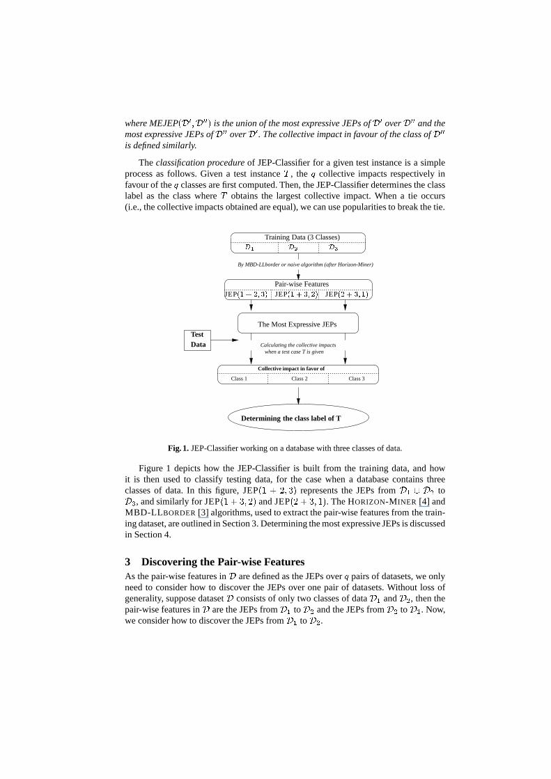
Theclassification procedureof JEP-Classifier for a given test instance is a simpleprocess as follows. Given a test instanceT , the q collective impacts respectively infavour of theq classes are first computed. Then, the JEP-Classifier determines the classlabel as the class whereT obtains the largest collective impact. When a tie occurs(i.e., the collective impacts obtained are equal), we can use popularities to break the tie.

Training Data (3 Classes)

Calculating the collective impacts

Pair-wise Features

D1 D2 D3when a test case T is given

TestData

Collective impact in favor of

Determining the class label of T

The Most Expressive JEPs

Class 1 Class 2 Class 3

JEP(1 + 3; 2)JEP(1 + 2; 3) JEP(2 + 3; 1)By MBD-LLborder or naive algorithm (after Horizon-Miner)

Fig. 1. JEP-Classifier working on a database with three classes of data.

Figure 1 depicts how the JEP-Classifier is built from the training data, and howit is then used to classify testing data, for the case when a database contains threeclasses of data. In this figure, JEP(1 + 2; 3) represents the JEPs fromD1 [ D2 toD3, and similarly for JEP(1 + 3; 2) and JEP(2 + 3; 1). The HORIZON-M INER [4] andMBD-LL BORDER [3] algorithms, used to extract the pair-wise features fromthe train-ing dataset, are outlined in Section 3. Determining the mostexpressive JEPs is discussedin Section 4.

3 Discovering the Pair-wise FeaturesAs the pair-wise features inD are defined as the JEPs overq pairs of datasets, we onlyneed to consider how to discover the JEPs over one pair of datasets. Without loss ofgenerality, suppose datasetD consists of only two classes of dataD1 andD2, then thepair-wise features inD are the JEPs fromD1 toD2 and the JEPs fromD2 toD1. Now,we consider how to discover the JEPs fromD1 toD2.

The most naive way to find the JEPs fromD1 to D2 is to check the frequencies,in D1 andD2, of all itemsets. This is clearly too expensive to be feasible. The prob-lem of efficiently mining JEPs from dense and high-dimensional datasets is well-solvedin [3][4]. The high efficiency of these algorithms is a consequence of their novel useof borders [3]. In the following subsections we present two approaches to discoveringJEPs. The first approach is a semi-naive algorithm which makes limited use of bor-ders, while the second approach uses an efficient border-based algorithm called MBD-LL BORDER [3].

3.1 Borders, Horizontal Borders, andHORIZON-M INER

A borderis a structure used to succinctly represent certain large collections of sets.

Definition 4. [3]. A border is an ordered pair<L;R> such that each ofL andR isan antichain collection of sets, each element ofL is a subset of some element inR, andeach element ofR is a superset of some element inL; L is theleft boundof the border,andR is its right bound.

The collection of setsrepresentedby<L;R> (also called theset intervalof<L;R>)is [L;R℄ = fY j 9X 2 L; 9Z 2 R such thatX � Y � Zg:We say that[L;R℄ has<L;R> as its border, and that eachX 2 [L;R℄ is covered by<L;R>.

Example 3.The set interval of<ffa; bgg; ffa; b; ; d; eg; fa; b; d; e; fgg> consists oftwelve itemsets, namely all sets that are supersets offa; bg and that are subsets of eitherfa; b; ; d; eg or fa; b; d; e; fg.Definition 5. Thehorizontal borderof a dataset is the border<f;g;R> that repre-sents allnon-zero supportitemsets in the dataset.

Example 4.The horizontal border ofD1 in Table 1 is<f;g; ffa; ; d; eg; fb; ; d; egg>.

The simple HORIZON-M INER algorithm [4] was proposed to discover the horizon-tal border of a dataset. The basic idea of this algorithm is toselect the maximum itemsetsfrom all instances inD (an itemset is maximal in the collectionC of itemsets if it hasno proper superset inC). HORIZON-M INER is very efficient as it requires only one scanthrough the dataset.

3.2 The Semi-naive Approach to Discovering JEPs

The semi-naive algorithm for discovering the JEPs fromD1 to D2 consists of the fol-lowing two steps: (i) Use HORIZON-M INER to discover the horizontal border ofD2;(ii) ScanD1 to check the supports of all itemsets covered by the horizontal border ofD2; the JEPs are those itemsets with zero support inD1. The pruned SE-tree [3] can beused in this process to irredundantly and completely enumerate the itemsets representedby the horizontal border.

The semi-naive algorithm is fast on small databases. However, on large databases, ahuge number of itemsets with non-zero support make the semi-naive algorithm too slowto be practical. With this in mind, in the next subsection, wepresent a method which ismore efficient when dealing with large databases.

3.3 Border-based Algorithm to Discover JEPs

In general, MBD-LLBORDER [3] finds those itemsets whose supports inD2 are�some support threshold� but whose support inD1 are less than some support thresholdÆ for a pair of datasetD1 andD2. Specially, this algorithm produces exactly all thoseitemsets whose supports are nonzero inD2 but whose supports are zero inD1, namelythe JEPs fromD1 to D2. In this case, MBD-LLBORDER takes the horizontal borderfromD1 and the horizontal border fromD2 as inputs. Importantly, this algorithm doesnot output all JEPs individually. Instead, MBD-LLBORDERoutputs a family of bordersin the form of<Li;Ri>, i = 1; � � � ; k, to concisely represent all JEPs.

Unlike the semi-naive algorithm, which must scan the dataset D1 to discover theJEPs, MBD-LLBORDERworks by manipulating the horizontal borders of the datasetsD1 andD2. As a result, the MBD-LLBORDERalgorithm scales well to large databases.This is confirmed by the experimental results in Section 5. The MBD-LLBORDERal-gorithm for discovering JEPs is described in detail in the Appendix.

4 Selecting the Most Expressive JEPsWe have given two algorithms to discover the pair-wise features from the training dataD: the semi-naive algorithm is useful whenD is small, while the MBD-LLBORDER

algorithm is useful whenD is large. As seen in the past section, the MBD-LLBORDER

algorithm outputs the JEPs represented by borders. These borders can represent verylarge collections of itemsets. However, only those itemsets with large support contributesignificantly to the collective impact used to classify a test instance. By using only themost expressive JEPs in the JEP-Classifier, we can greatly reduce its complexity, andstrengthen its resistance to noise in the training data.

Consider JEP(D1;D2) [ JEP(D2;D1), the pair-wise features inD. Observe thatJEP(D1;D2) is represented by a family of borders of the form<Li;Ri>, i = 1; � � � ; k,where theRi are singleton sets (see the pseudo-code for MBD-LLBORDER in theAppendix). We believe that the itemsets in the left bounds,Li, are the most expressiveJEPs in the dataset. The reasons behind this selection include:

– By definition, the itemsets in the left bound of a border have the largest supportsof all the itemsets covered by that border because the supersets of an itemsetXhave smaller supports than that ofX . Then, the most expressive JEPs cover moreinstances (at least equal) of the training dataset than the other JEPs.

– Any proper subset of the most expressive JEPs is not a JEP any more.

It follows that we can select the most expressive JEPs of JEP(D1;D2) by taking theunion of the left bounds of the borders produced by MBD-LLBORDER. This union iscalled the LEFT-UNION of JEP(D1;D2). So, LEFT-UNION = [Li. Similarly, we canselect the most expressive JEPs of JEP(D2;D1). Combining the two LEFT-UNION, themost expressive pair-wise features inD are then constructed.

Algorithmically, finding LEFT-UNION can be done very efficiently. If the MBD-LL BORDER algorithm is used, then we simply use the left bounds of the borders itproduces. In practice, this can be done by replacing the lastline of the pseudo code ofthe MBD-LLBORDERalgorithm in the Appendix with

return the union of the left bounds of all borders in EPBORDERS.

If the semi-naive algorithm is used, then LEFT-UNION can be updated as each newJEP is discovered.

Example 5.To illustrate several points discussed in this subsection,considerD1 andD2 from Table 1. The horizontal border ofD1 is <f;g; fa de; b deg>1, and that ofD2 is<f;g; f e; de; ab dg>. The JEPs fromD2 toD1 are represented by two borders<Li;Ri>, i = 1; 2, namely<fae; deg; fa deg> and<fbe; deg; fb deg>. (Thereaders can use MBD-LLBORDER in the Appendix to derive these borders.)

The border<fae; deg; fa deg> consists of the JEPsfae; a e; ade; de; a deg,while the border<fbe; deg; fb deg> consists of the JEPsfbe; b e; bde; de; b deg.Note that the JEPs in the left bounds have the largest supports.

The LEFT-UNION of JEP(D2;D1) is the union of the left bounds of the above twoborders, namelyfae; deg [ fbe; deg = fae; be; deg.5 Experimental Results

In this section we present the results of our experiments, where we run the JEP-Classifieron 30 databases (some contain up to 10 classes, some have up to30162 instances,some have up to 60 attributes) taken from the UCI Repository of Machine LearningDatabases [1]. These experiments were carried out on a 500MHz PentiumIII PC with512M bytes of RAM. The accuracy was obtained using the methodology of ten-foldcross-validation [10] (but one fold was tested in census-income).

The experiment’s pre-processes are: (i) download originaldatasets, sayD, from theUCI website; (ii) partitionD into class datasetsD1;D2; � � � ;Dq; (iii) randomly shuffleDi; i = 1; � � � ; q; (iv) for eachDi, choose the first 10% instances as the testing dataand the remaining 90% as the training data. Repeatedly, choose the second 10% as thetesting data, and so forth; (v) if there exist continuous attributes, discretize them by ourequal-length-binmethod in the training datasets first, and then map the intervals to thetesting data. This step is used to convert the original training and testing data into thestandard binary transactional data. (These executable codes are available from the au-thors on request.) After pre-processing, we followed the steps illustrated in Figure 1 toget the results. Alternatively, MLC++ technique [7] was also used to discretize contin-uous attributes in the glass, ionosphere, pima, sonar, and vehicle datasets. These testingaccuracies are reported in Table 2. The main disadvantage ofMLC++ technique is thatit sometimes, for example in the liver dataset, produces many different instances withdifferent labels into identical instances.

Table 2 summarizes the results. In this table, the first column lists the name of eachdatabase, followed by the numbers of instances, attributes, and classes in Column 2. Thethird column presents the error rate of the JEP-Classifier, calculated as the percentageof test instances incorrectly predicted. Similarly, columns 4 and 5 give the error rate of,respectively, the CBA classifier in [8] and C4.5. (These results are thebest resultstakenfrom Table 1 in [8]; a dash indicates that we were not able to find previous reported1 For readability, we usea de as shorthand for the setfa; ; d; eg.

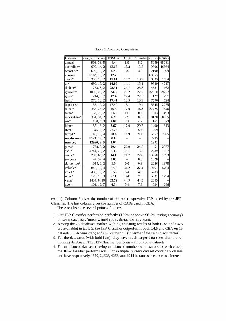
Table 2.Accuracy Comparison.

Datasets #inst, attri, class JEP-Cla. CBA C4.5rules # JEPs#CARsanneal* 998, 38, 5 4.4 1.9 5.2 5059 65081australian* 690, 14, 2 13.66 13.2 13.5 9806 46564breast-w* 699, 10, 2 3.73 3.9 3.9 2190 399census 30162, 16, 2 12.7 – – 68053 –cleve* 303, 13, 2 15.81 16.7 18.2 8633 1634crx* 690, 15, 2 14.06 14.1 15.1 9880 4717diabete* 768, 8, 2 23.31 24.7 25.8 4581 162german* 1000, 20, 2 24.8 25.2 27.7 32510 69277glass* 214, 9, 7 17.4 27.4 27.5 127 291heart* 270, 13, 2 17.41 18.5 18.9 7596 624hepatitis* 155, 19, 2 17.40 15.1 19.4 5645 2275horse* 368, 28, 2 16.8 17.9 16.3 22425 7846hypo* 3163, 25, 2 2.69 1.6 0.8 1903 493ionosphere* 351, 34, 2 6.9 7.9 8.0 8170 10055iris* 150, 4, 3 2.67 7.1 4.7 161 23labor* 57, 16, 2 8.67 17.0 20.7 1400 313liver 345, 6, 2 27.23 – 32.6 1269 –lymph* 148, 18, 4 28.4 18.9 21.0 5652 2965mushroom 8124, 22, 2 0.0 – – 2985 –nursery 12960, 8, 5 1.04 – – 1331 –pima* 768, 8, 2 20.4 26.9 24.5 54 2977sick* 4744, 29, 2 2.33 2.7 1.5 2789 627sonar* 208, 60, 2 14.1 21.7 27.8 13050 1693soybean 47, 34, 4 0.00 – 8.3 1928 –tic-tac-toe* 958, 9, 2 1.0 0.0 0.6 2926 1378vehicle* 846, 18, 4 27.9 31.2 27.4 19461 5704vote1* 433, 16, 2 8.53 6.4 4.8 5783 –wine* 178, 13, 3 6.11 8.4 7.3 5531 1494yeast* 1484, 8, 10 33.72 44.9 44.3 2055 –zoo* 101, 16, 7 4.3 5.4 7.8 624 686

results). Column 6 gives the number of the most expressive JEPs used by the JEP-Classifier. The last column gives the number of CARs used in CBA.

These results raise several points of interest.

1. Our JEP-Classifier performed perfectly (100% or above 98.5% testing accuracy)on some databases (nursery, mushroom, tic-tac-toe, soybean).

2. Among the 25 databases marked with * (indicating results of both CBA and C4.5are available) in table 2, the JEP-Classifier outperforms both C4.5 and CBA on 15datasets; CBA wins on 5; and C4.5 wins on 5 (in terms of the testing accuracies).

3. For the databases (with bold font), they have much larger data sizes than the re-maining databases. The JEP-Classifier performs well on those datasets.

4. For unbalanced datasets (having unbalanced numbers of instances for each class),the JEP-Classifier performs well. For example, nursery dataset contains 5 classesand have respectively 4320, 2, 328, 4266, and 4044 instancesin each class. Interest-

ingly, we observed that the testing accuracy by the JEP-Classifier was consistentlyaround 100% for each class. For CBA, its support threshold was set as 1%. In thiscase, CBA would mis-classify all instances of class 2. The reason is that CBA can-not find the association rules in class 2.

Our experiments also indicate that the JEP-Classifier is fast and highly efficient.

– Building the classifiers took approximately0:3 hours on average for the 30 casesconsidered here.

– For databases with a small number of items, such as the iris, labor, liver, soy-bean, and zoo databases, the JEP-Classifier completed both the learning and testingphases within a few seconds. For databases with a large number of items, suchas the mushroom, sonar, german, nursery, and ionosphere databases, both phasesrequired from one to two hours.

– In dense databases, the border representation reduced the total numbers of JEPs (bya factor of up to108 or more) down to a relatively small number of border itemsets(approximately103).We also conducted experiments to investigate how the numberof data instances

affects the scalability of the JEP-Classifier. We selected50%, 75%, and90% of datainstances from each original database to form three new databases. The JEP-Classifierwas then applied to the three new databases. The resulting run-times shows a lineardependence on the number of data instances when the number ofattributes is fixed.

6 Related WorkExtensive research on the problem of classification has produced a range of differenttypes of classification algorithms, including nearest neighbor methods, decision tree in-duction, error back propagation, reinforcement learning,and rule learning. Most classi-fiers previously published, especially those based on classification trees (e.g., C4.5 [9],CART [2]), arrive at a classification decision by making a sequence of micro decisions,where each micro decision is concerned with one attribute only. Our JEP-Classifier, to-gether with the CAEP classifier [5] and the CBA classifier [8],adopts a new approachby testing groups of attributes in each micro decision. While CBA uses one group ata time, CAEP and the JEP-Classifier use the aggregation of many groups of attributes.Furthermore, CBA uses association rules as the basic knowledge of its classifier, CAEPuses emerging patterns (mostly with finite growth rates), and the JEP-Classifier usesjumping emerging patterns.

While CAEP has some common merits with the JEP-Classifier, itdiffers from theJEP-Classifier in several ways:

1. Basic idea. The JEP-Classifier utilizes the JEPs of large supports (themost discrim-inating and expressive knowledge) to maximize its collective classification powerwhen making decisions. CAEP uses the collective classifying power of EPs withfinite growth rates, and possibly some JEPs, in making decisions.

2. Learning phase. In the JEP-Classifier, the most expressive JEPs are discovered bysimply taking the union of the left bounds of the borders derived by the MBD-LL BORDER algorithm (specialised for discovering JEPs). In the CAEP classifier,the candidate EPs must be enumerated individually after theMBD-LL BORDER

algorithm in order to determine their supports and growth rates.

3. Classification procedure. The JEP-Classifier’s decision is based on the collectiveimpact contributed by the most expressive pair-wise features, while CAEP’s deci-sion is based on the normalized ratio-support scores.

4. Predicting accuracy. The JEP-Classifier outperforms the CAEP classifier in largeand high dimension databases such as mushroom, ionosphere,and sonar. For smalldatasets such as heart, breast-w, hepatitis, and wine databases, the CAEP classifierreaches higher accuracies than the JEP-Classifier does. On 13 datasets where resultsare available for CAEP, the JEP-Classifier outperforms CAEPon 9 datasets.

While our comparison to CAEP is still preliminary, we believe that CAEP and JEP-Classifiers are complementary. More investigation is needed to fully understand theadvantages offered by each technique.

7 Concluding RemarksIn this paper, we have presented an important application ofJEPs to the problem ofclassification. Using the border representation and border-based algorithms, the mostexpressive pair-wise features were efficiently discoveredin the learning phase. The col-lective impact contributed by these pair-wise features were then used to classify test in-stances. The experimental results have shown that the JEP-Classifier generally achievesa higher predictive accuracy than previously published classifiers, including the classi-fier in [8], and C4.5. This high accuracy results from the strong discriminating power ofan individual JEP over a fraction of the data instances and the collective discriminatingpower by all the most expressive JEPs. Furthermore, our experimental results show thatthe JEP-Classifier scales well to large datasets.

As future work, we plan to pursue several directions. (i) In this paper, collectiveimpact is measured by the sum of the supports of the most expressive JEPs. As alter-natives, we are considering other aggregates, such as the squared sum, and adaptivemethods, such as neural networks. (ii) In this paper, JEPs are represented by borders.In the worst case, the number of the JEPs in the left bound of a border can reachCNN=2,whereN is the number of attributes in the dataset. We are considering the discovery anduse of only some of the itemsets in the left bound, to avoid this worst-case complex-ity. (iii) In discovering JEPs using the MBD-LLBORDERalgorithm, there are multipleuses of the BORDER-DIFF sub-routine, dealing with different borders. By parallelizingthese multiple calls, we can make the learning phase of the JEP-Classifier even fasterand more scalable.

AcknowledgementWe are grateful to Richard Webber for his help. We thank Bing Liu and Jiawei Han foruseful discussions. We also thank the anonymous referees for helpful suggestions.

References

1. Blake, C. L., Murphy, P. M.: UCI Repository of machine learning database.[http://www.cs.uci.edu/ mlearn/mlrepository.html]. Irvine, CA: University of California, De-partment of Information and Computer Science (1998)

2. Breiman, L., Friedman, J., Olshen, R., Stone, C.: Classification and Regression Trees.Wadsworth International Group (1984)

3. Dong, G., Li, J.: Efficient mining of emerging patterns: Discovering trends and differences.Proceedings of ACM SIGKDD’99 International Conference on Knowledge Discovery &Data Mining, San Diego, USA, (1999) 43–52

4. Dong, G., Li, J., Zhang, X.: Discovering jumping emergingpatterns and experiments on realdatasets. Proceedings of the 9th International Database Conference (IDC’99), Hong Kong,(1999) 155–168

5. Dong, G., Zhang, X., Wong, L., Li, J.: CAEP: Classificationby aggregating emerging pat-terns. DS-99: Second International Conference on Discovery Science, Tokyo, Japan, (1999)

6. Han, J., Fu, Y.: Exploration of the power of attribute-oriented induction in data mining. In:Fayyad, U. M., Piatetsky-Shapiro, G., Smyth, P., Uthurusamy, R. (eds): Advances in Knowl-edge Discovery and Data Mining. AAAI/MIT Press (1996) 399–421

7. Kohavi, R. , John, G. , Long, R. , Manley, D. , Pfleger, K.: MLC++: a machine learninglibrary in C++. Tools with artificial intelligence, (1994) 740–743

8. Liu, B., Hsu, W., Ma, Y.: Integrating classification and association rule mining. Proceedingsof the 4th International Conference on Knowledge Discoveryin Databases and Data Mining,KDD’98 New York, USA (1998)

9. Quinlan, J. R.: C4. 5: program for machine learning. Morgan Kaufmann (1992)10. Salzberg, S. L.: On comparing classifiers: pitfalls to avoid and a recommended approach.

Data Mining and Knowledge Discovery1 (1997) 317 – 327

Appendix: MBD-LL BORDER for Discovering JEPsSuppose the horizontal border ofD1 is <f;g; fC1; � � � ; Cmg> and the horizontal bor-der ofD2 is<f;g; fD1; � � � ; Dng>. MBD-LL BORDERfinds the JEPs fromD1 toD2as follows.

MBD-LL BORDER(horizontalBorder(D1), horizontalBorder(D2));; return all JEPs fromD1 toD2 by multiple calls ofBORDER-DIFF

EPBORDERS fg;for j from 1 to n do

if some Ci is a superset of Dj then continue;fC 01; � � � ; C 0mg fC1 \Dj ; � � � ; Cm \Djg ;RIGHTBOUND all maximal itemsets in fC 01; � � � ; C 0mg;add BORDER-DIFF(<f;g; Dj>;<f;g;RIGHTBOUND>) into EPBOR-DERS;

return EPBORDERS;

BORDER-DIFF(<f;g; fUg>; <f;g; fS1; S2; � � � ; Skg>);; return the border of [f;g; fUg℄� [f;g; fS1; S2; � � � ; Skg℄initialize L to ffxg j x 2 U � S1g;for i = 2 to k doL fX [ fxg j X 2 L; x 2 U � Sig;

remove all itemsets Y in L that are not minimal;return <L; fUg>;

Note that given a collectionC of sets, theminimal sets are those ones whose propersubsets are not inC. For correctness and variations of BORDER-DIFF, the readers arereferred to [3].