Making Money∗

Gary B. Gorton† Chase P. Ross‡ Sharon Y. Ross§

January 14, 2022

Abstract

It is difficult for private agents to produce money that circulates at par with no questionsasked. We study two cases of privately-produced money: pre-Civil War U.S. privatebanknotes and modern stablecoins. Private monies are introduced when there are nobetter alternatives, but they initially carry an inconvenience yield. Over time, thesemonies may become more money-like, but they do not always achieve a positive conve-nience yield. Technology advances and reputation formation pushed private banknotestoward a positive convenience yield. We show that the same forces are at work forstablecoins.

JEL Codes: E40, E51, G12, N21

Keywords: money, convenience yield, stablecoins, privately-produced banknotes,cryptocurrencies

∗We thank Michelle Tong for excellent research assistance. For comments and suggestions thanks toYakov Amihud, Sam Hempel, Sabrina Howell, Kose John, Jay Kahn, Benjamin Kay, Elizabeth Klee, AndreasLehnert, Marco Macchiavelli, Borghan Narajabad, Sriram Rajan, Danylo Rakowsky, David Rappoport, JohnThanassoulis, Alexandros Vardoulakis, Ganesh Viswanath, and seminar participants at the Vienna GraduateSchool of Finance, NYU Stern, Office of Financial Research, Federal Reserve Board, and Warwick BusinessSchool. The analysis and conclusions set forth are those of the authors and do not indicate concurrency byother members of the Board of Governors of the Federal Reserve System, the Office of Financial Research, ortheir staffs.

†Yale University & NBER. Email gary.gorton@yale.edu‡Board of Governors of the Federal Reserve System. Email: chase.p.ross@frb.gov§Office of Financial Research, U.S. Treasury. Email: sharon.ross@ofr.treasury.gov

1

Everyone can create money; the problem is to get it accepted.

(Minsky, 1986)

1 Introduction

The growth of stablecoins raises the question of how private agents can produce money.We study two types of debt as their issuers try to make them money-like: pre-Civil Warprivate banknotes and modern digital stablecoins. The birth of new privately-produced moneyrequires two ingredients: a lack of alternatives and a design that makes the money acceptableat par with no questions asked (NQA). We show that technology advances and reputationformation push privately-produced monies toward positive convenience yields—first for privatebanknotes, then for stablecoins.

Different forms of private debt can transition from non-money to money, but the transitionis neither immediate nor smooth. In the language of Holmström (2015), debt is money onlyif agents accept it NQA: they must accept the debt at par without reservation or costly duediligence. NQA money is an economy’s bedrock. Without it, transactions are inefficient,consuming resources and time. NQA money protects uninformed agents from adverse selectionbecause it is information insensitive (Gorton and Pennacchi, 1990). But many forms of debt,even with the shortest maturities and highest credit ratings, do not trade no-questions-asked:money is special. It has a convenience yield because of the nonpecuniary benefits of beingNQA.1

We present a model which focuses on a variable designed to capture a money’s distancefrom NQA, which we call d. d is a continuous, nonnegative, latent variable that summarizesthe frictions that prevent debt from becoming NQA. Making money involves decreasingd. The interpretation of d changes depending on the institutional context. The variable dsummarizes the forces that create a money’s convenience yield. When the distance to NQAis zero, d = 0, the debt trades NQA and is information insensitive. Even if d > 0, we show amoney can still have a positive convenience yield. Questions are asked about the money’s

1The convenience yield is the yield spread between a money-like security and a benchmark security, wherethe only difference is that one is money-like. For example, a measure of the Treasury convenience yieldcompares the spread between overnight-indexed swaps (OIS) and Treasury bills of the same maturity. OISare nearly riskless derivatives, but Treasuries are more money-like than OIS because institutional investorscan spend Treasury bills like money. Other potential benchmark measures include the general collateralfinance repo rate or high-quality corporate bond yields (Krishnamurthy and Vissing-Jørgensen, 2012).

2

backing, but it can have a positive convenience yield. But as d grows larger, the convenienceyield flips signs and becomes an inconvenience yield. Our empirical results show stablecoinsare following the well-trodden path to NQA but remain in their early days.

Before the U.S. Civil War, banks issued non-interest-bearing debt in the form of banknotes.There were about 1,500 distinct banknotes in the mid-1840s. Depositors could redeembanknotes in specie at par on demand, but only at the specific bank that issued the note.Different banknotes traded at different discounts from par (Gorton, 1999). In the pre-CivilWar Free Banking Era, from 1834 to 1863, some states allowed free banking—easy entry intobanking—but required banks to back their banknotes with state bonds, with the requirementsvarying across states. In other states, banks issued banknotes backed by loan portfolios.

The distance to NQA d takes an almost literal interpretation of physical distance to theissuer for private banknotes. Banknotes circulating in the city of the issuer were treatedas money, no-questions-asked. Banknotes from distant cities traded at a greater discount,reflecting that questions were asked. But redeeming banknotes from distant banks was costlyin time and money. Over time, d decreased with the proliferation of technology like railroadsand telegraphs.

Railroads reduced d as travel times plummeted during the nineteenth century (Gorton1989, Atack et al. 2015, and Lin et al. 2021). The expansion of the telegraph followed newrailroad lines, allowing information to move faster. A trip from Philadelphia to Memphis in1839 covered more than 1,650 miles spanning five connections on steamboats and stagecoaches.The trip took more than 13 days and cost $70 ($1,780 in 2021). By 1862, the same trip tookthree and a half days and cost $45 ($800 in 2021) thanks to the burgeoning railroad network.In only 23 years, the real cost fell 55%, and the travel time fell 73%.

Stablecoins are the newest form of privately-produced money to attempt the moneytransition. The largest cryptocurrencies are too volatile to be stores of value or transactionmedia, and there are significant opportunity costs to holding dollars inside a crypto exchange.Stablecoins emerged to fill the gap. Stablecoin issuers solve the volatility problem by peggingthe coin to safe assets one-for-one; the pegs are often sovereign currencies like the U.S. dollaror the euro. The peg does not always hold, though, and stablecoins occasionally break theirpeg. A broken peg can lead to the outright failure of the stablecoin, the cryptocurrencyequivalent to a bank run.

3

For stablecoins, d is a latent variable that reflects a trader’s frictions in transactingand in redeeming the stablecoin to a sovereign currency. Stablecoin holders face manyfrictions: the time it takes to satisfy anti-money laundering and Know-Your-Customer lawswhen transferring balances between stablecoins on crypto exchanges and bank accounts; theinability of citizens of certain countries to redeem the coins from the issuer; transaction limitsthat make redemption of small amounts of stablecoins to dollars impractical. d decreases asfrictions decline. We show that technological change in the form of faster graphics processingunits reduces stablecoins’ d.

We estimate d for both private banknotes and stablecoins following Gorton (1999)’sstylized model. Private banknotes and stablecoins are non-interest-bearing perpetuities withembedded put options to redeem at par from the issuer, so Black and Scholes (1973) holds.Gorton (1999) identified the put option maturity as the time it took to travel to the issuingbank. He used the model to back-out banknotes’ implied volatilities and that they wererelated to state-level risk factors. In our application, we back-out d as the maturity of thebanknote or stablecoin implied by prices. The model also shows how d is negatively relatedto the convenience yield of the money.

d is endogenous, and issuers try to reduce it. Issuers use their reputation as a technologyto reduce d. Agents are more likely to trust reputable issuers with a history of redemption atpar, while agents carefully monitor issuers with less reputation. Gorton (1996) shows thatnotes issued by new private banks traded at a discount to those of seasoned banks at thesame location, giving traders an incentive to redeem the notes and implicitly monitor the newbank’s ability to repay. Stablecoin issuers can improve their reputation and endogenouslydecrease d by disclosing details about the assets backing the stablecoin, getting a fintechbanking charter, or appointing well-known people to their boards. Over time, either throughtechnological change or through the issuer’s efforts—or both—d can fall. The convenienceyield goes up, and the debt becomes money, possibly with a positive convenience yield, evenif d is always greater than zero.

Despite issuers’ best efforts, d does not follow a steady path toward zero. Our estimatesof d for both banknotes and stablecoins are countercyclical. Recessions and financial crises inthe nineteenth century are apparent in the d time series. Large drops in Bitcoin’s price, theclosest proxy we have to a recession indicator in cryptocurrencies, similarly correspond tolarge increases in stablecoins’ d.

4

We have four main results: first, we estimate d for banknotes and stablecoins and studytheir dynamics. We show that d can shrink over time, but not uniformly. Second, we measureboth banknotes’ and stablecoins’ convenience yields—or, when negative, their inconvenienceyields—and show that d is negatively correlated with the convenience yield. Third, we showthat technological change and reputation development reduce d. But, fourth, stablecoins havenot differentiated themselves from other stablecoins. The market essentially views stablecoinsas a single coin, making them more vulnerable to runs since all stablecoins face large volumedrops during stress.

Related Literature Our paper is most related to the quickly growing literature on stable-coins and is closely related to Gorton and Zhang (2021). Mizrach (2021) provides a detaileddescription of the market microstructure of stablecoins and studies their failure rates. Lyonsand Viswanath-Natraj (2021) frame stablecoins in the light of exchange rates and show thatTether’s peg is maintained primarily by the demand side, arbitrageurs, rather than the supplyside, the issuer. They also show how the premium or discount relative to the peg varies overtime. Hoang and Baur (2021) show how stablecoins’ volatility is closely linked to Bitcoin.Other studies include Bellia and Schich (2020), Cao et al. (2021) and Kwon et al. (2021).

2 Estimating the Distance to No-Questions-Asked

We use Gorton (1999)’s model for a simple conceptual framework to link the prices of differenttypes of monies to their distances from Holmström (2015)’s no-questions-asked. Privatebanknotes and stablecoins are non-interest-bearing perpetual debt with embedded put optionsfor redemptions at par on demand from the issuer. Gorton (1999) applied a pricing model,discussed below, to private banknotes, which we use to describe stablecoins. We provide abrief sketch of the model setup to motivate the main result, with which we estimate d.

Agents are spatially separated, and each agent comprises a household, firm, and a bank.The distance from the agent’s home market to the location of their trade in a period is d.Each household owns a firm that produces a nonstorable stochastic endowment in each period.The households issue debt and equity claims on their endowment streams. The debt pays nointerest and is redeemable into consumption goods on demand at par. The debt, therefore, isequivalent to a perpetuity with an embedded American put option.

5

The household comprises a buyer who travels to a distant market to buy goods and aseller who stays at home to sell their firm’s endowment. Households face a cash-in-advanceconstraint that can be satisfied only by banknotes:

Ct ≤∑d

Pt(d)Dt−1(d) (1)

where Pt(d) is the price at time t of a note issued by household with distance d away andDt−1(d) is the household’s holdings at the beginning of period t carried over from period t− 1.From period to period, households hold a portfolio of banknotes issued by other householdsat different locations with different ds. The households pay for consumption goods at distantlocations with their portfolio of banknotes.

Households prefer to consume goods from markets far away from their home location.Households’ preference for goods from distant markets can be motivated by the pre-CivilWar division of labor. Households maximize expected utility

Et

∞∑j=t

βj−tu(C, d) (2)

Households also have the choice to send banknotes for redemption. By assumption, abanknote with price Pt(d) takes d periods to be redeemed at face value in consumption goodsPt+d(0) = 1, assuming the bank is solvent. The household’s first-order condition with respectto their banknote portfolio pins down the price of a banknote:

Pt(d) = Et[βdu′C,t+du′C,t

Pt+d(0)]

(3)

where Et is the expectations operator conditional on information available at date t.The first-order condition shows that banknotes of a bank with distance d are equal to risky

pure discount debt with a maturity of d periods.2 Households must be indifferent betweenholding a banknote and sending it for redemption.

We can back out the money’s maturity given the price of the debt and a standard optionpricing method. Let DR

t (d) be the face value of debt sent for redemption at date t from2See Gorton (1999)’s Proposition 1.

6

location d and assume there are no notes in transit. Given the price of the banknote,3 wecan back out d using Black and Scholes (1973):4

Pt(d) = Vt(d)[1−N(hD + σ)] + (1 + rf )−1DRt (d)N(hD)

DRt (d) (4)

where

hD ≡ln(Vt(d)/DR

t (d)) + ln(1 + rf )σ

− σ

2

and σ is the standard deviation of one plus the rate of change of the value of liability issuer,rf is the risk-free rate, Vt(d) is the value of the debt and equity claims on the issuer, andN(·) is the cumulative normal distribution function.

We make two simple additions to the model to study the convenience yield. First, thebanknote yield is the inverse of its price: Rd

t = 1/Pt(d). Second, we derive the risk-free ratefrom the stochastic discount factor even though the model has no risk-free security. Therisk-free bond price is pinned down by 1 = Et

[Mt+1R

ft

]where Mt+1 is the stochastic discount

factor. The convenience yield is the difference between the yields on the risk-free bond andthe debt:

Convenience Yieldt ≡ Rft −Rd

t (5)

Proposition 1. If DRt (d)V ′t (d)−DR′

t (d)Vt(d) < 0, then the convenience yield is decreasingin d: (∂(CY )/∂d) < 0. We provide the proof in Appendix A.1.

For intuition on our assumption that DRt (d)V ′t (d)−DR′

t (d)Vt(d) < 0, we first note thatthe bank value is the sum of its debt and equity: Vt(d) = DR

t (d) + Et(d). Then the leverageratio is

Vt(d)Et(d)

= DRt (d) + Et(d)Et(d)

= DRt (d)Et(d)

+ 1.

Empirically, the leverage ratio for banknotes is about two, so the average bank’s debt andequity are about equal, DR

t (d) ≈ Et(d). After we substitute the equations Vt(d) = DRt (d) +

3Banknote prices were publicly reported in banknote reporters, which we discuss in section 3.4See Gorton (1999)’s Proposition 2 and Rubinstein (1976).

7

Et(d) and DRt (d) ≈ Et(d), then DR

t (d)V ′t (d)−DR′t (d)Vt(d) simplifies to Et(d)(E ′t(d)−DR′

t (d)).If E ′t(d) < DR′

t (d), then (∂(CY )/∂d) < 0.Both E ′t(d) and DR′

t (d) are negative. Debt is senior to equity, so equity is more informationsensitive and E ′t(d) < DR′

t (d). For example, bank stock prices are magnitudes more volatilethan senior bank debt prices.

For banknotes, DRt (d) is stickier than Et(d). Concerns about the market value of the

bank would lead Et(d) to fluctuate quickly, but DRt (d) would take longer to adjust because it

would take time to deliver bad news about a bank’s circulating notes and to have the newdiscount reflected correctly in the banknote reporter.

Observations First, a banknote does not have to satisfy NQA to carry a positive conve-nience yield. We denote d? as the distance at which the convenience yield equals 0. If d < d?

then the convenience yield is positive; if d > d? the convenience yield is negative—it willcarry an inconvenience yield. A credible government can produce NQA money (d = 0) whichearns the largest possible convenience yield. Even if the government is the only issuer thatcan produce genuinely NQA money, private issuers can still produce money that earns apositive convenience yield if the money is close enough to NQA, d < d?. There is a directlink between the distance to NQA and the convenience yield.5

Second, the debt price is $1 when d = 0, Pt(0) = 1. When d = 0, the debt can beredeemed immediately, so an agent must be indifferent between holding it at $1 or redeemingit for $1 so long as the bank is solvent. When d = 0, there are no-questions-asked, and allagents accept the debt at par value as money.

Third, the debt price Pt(d) is inversely related to distance to NQA d, the volatility of theissuer’s debt and equity σ, and the issuer’s leverage. When the distance to NQA d increases,the debt price falls.

Gorton (1999) used the model to back out implied volatilities and then analyzed them incross-sections to show their relationship to state-level risk factors. In that analysis, maturitywas taken as the time to return to the issuing bank computed from historical travel data. Inour analysis for banknotes and stablecoins, we use historical data for volatility and back outd. This distance to NQA is affected by all the variables in equation 4.

5We plot Rdt and Rf

t on the left panel of Figure A1 and the convenience yield on the right panel.

8

3 Pre-Civil War Private Banknotes

We briefly provide some background on the use, trading, and evolution of Pre-Civil Warprivate banknotes from roughly 1820 to 1860.6 We verify our estimation strategy for d andshow that the estimated distance to NQA aligns closely with physical distance. We also showthe decline in the distance to NQA d and the inconvenience yield over time.

3.1 Context

Private banknotes were physical currency issued by a specific bank redeemable into specie,at par, on demand. Private banknotes were liabilities issued by the bank to finance bankloans. Banks began issuing notes before the nineteenth century, but the number of uniquebanks issuing notes grew substantially in the nineteenth century (Gouge, 1833). Our interestis primarily the Free Banking period from 1837 to 1863, when banks issued private moneybacked by state bonds. The bonds were not riskless, and banking panics were common.

The Free Banking period was so-called because there was free entry into banking aftereighteen states passed laws that allowed banks to issue private money backed by state bonds.The remaining fifteen states retained a framework that required a charter before a bankcould open and issue notes. Getting a bank charter did not require tremendous effort in FreeBanking states. Someone could open a bank by purchasing state bonds, depositing thosebonds with the state government, and printing private banknotes for circulation. The bankshad limited liability, but the state would revoke its charter if it could not redeem its noteson demand. Rolnick and Weber (1984) and Gorton (1996) study the existence of, or lackthereof, wildcat banks: banks opened by fraudsters for the sole purpose of issuing worthlesspaper money and absconding with the proceeds.

Money in the Free Banking period was not economically efficient. It was costly to usespecie because it was heavy and difficult to transport in large amounts. Coins were alsoscarce. The available coins came in a confusing array of denominations. “In routine businesstransactions Americans had to calculate in three currencies: one decimal; another based onhalves, quarters, and eighths; and another on twelfths and twentieths” (Ware, 1990). The

6See Gorton (1996), Rolnick and Weber (1984), and Gorton (1999) for discussions of nineteenth-centurybank money.

9

U.S. Mint could not remint foreign coins because of poor minting equipment (Carothers,1930). Consequently, private banknotes played a vital role in commerce.

The public carried notes from a hodgepodge of banks in their pocket for everydaytransactions. Merchants and customers feared counterfeits and notes issued by dead ordying banks. It was hard to tell the good notes from the bad—especially for notes issued byunfamiliar distant banks. Merchants preferred notes with noticeable wear-and-tear, evidenceof robust circulation where other merchants had accepted it. Merchants would accept notesissued by distant banks only at a discount to par: the further away the bank, the greater thediscount.

Discount note brokers traded private notes on secondary markets in New York, Philadel-phia, Cincinnati, and Cleveland. Risky banks’ notes traded at a bigger discount than saferbanks’ notes, ceteris paribus. Banknote discounts varied over time, spiked during crises, andtended to be small.

Banknote reporters summarized information produced by the secondary markets.7 (Wediscuss the data in greater detail below.) Banknote reporters were regularly updated lists ofbanks and their corresponding discounts which merchants referenced for routine commerce.Scroggs (1924) describes this as follows:

Hundreds of banknotes of different size, colour, and design would be handedacross the merchant’s counters every day. If he were in any doubt about the valueof a note, he would turn to his banknote detector. Most detectors described thedistinguishing characteristics of more than a thousand bank issues. Details werealso given of any counterfeits or alterations, or of recently discovered issues offictitious banks . . . If the note were unfamiliar the merchant would spend sometime checking its description with that given in the detector. One can scarcelyimagine a customer in a store today waiting patiently while each bill that he hadoffered was carefully examined before being accepted.

People spent tremendous resources to avoid lemon notes, yet bank failures and financialcrises were common. Even if the brokers’ discount markets were efficient, pre-Civil War noteswere economically inefficient forms of money because they had a considerable distance toNQA (Dow and Gorton, 1997).

7As an example, Figure A2 plots the discounts for two select banks over time: the Bank of MontgomeryCounty and the Farmers’ Bank of Virginia.

10

The Free Banking period ended when the National Banking period began in 1863 after theU.S. government allowed banks to issue national banknotes backed by U.S. Treasuries. Thegovernment initially created the system to help finance the government’s Civil War efforts,but many believed that backing paper money with U.S. Treasuries would bolster financialstability.8

Data We use three data sources for private banknotes: banknote quotes from Weber (2021),bank balance sheet data from Weber (2018b), and railroad location data from Atack (2016).

Discounts reflect the cost to buy a bank’s notes with specie. The quoted discounts on statebanknotes are available on select dates between 1817 and 1858. Weber (2021) gives banknoteprices, expressed as discounts from par, at secondary markets in New York, Philadelphia,Cincinnati, and Cleveland. Quotes come from two datasets based on the quote’s location:Philadelphia or New York/Ohio. The New York/Ohio9 dataset has a longer time series, butthe Philadelphia data has more observations in the 1850s. Many banknotes appear to havetraded in both locations. Weber (2018a) provides a comprehensive description of the data.We summarize the sources and timeframes in section A.2.

Weber (2018b) collects bank balance sheets by state from many sources with data backto 1794. Weber (2018b) cleans and regularizes the data to consistent asset and liabilitycategories. We merge the balance sheet data to the pricing data by lagging the end-of-yearbalance sheet data by one year to avoid using future data.10

We merge the balance sheet data with banknote discount data by first checking banksin states with exact matches across the datasets, then fuzzy matching on their names andmanually checking the matches. We then collapse the data to the month by bank by datasetlevel by averaging within a month. Our resulting dataset includes about 230,000 quotes for1,750 individual banks from 30 states—including 80,000 New York/Ohio-based quotes and150,000 Philadelphia-based quotes.11 Since several banks appear in both datasets, we runregressions on each dataset separately to prevent double-counting.

8Noyes (1910), Friedman and Schwartz (1963), and Champ (2007) discuss the National Banking period.9We will refer to this dataset as the New York dataset for brevity and because it is principally composed

of quotes from New York.10Figure A3 plots the number of banknotes in our sample for each month from 1817 to 1860.11The data includes banknotes for some institutions that were not banks; we include these because the fact

that detectors collected the data is prima facie evidence that the notes were money-like.

11

In our data, the quotes range from 0 to 90.12 A banknote with a discount of 0 has a priceof $1. A quote of 90 means it costs $0.10 to buy $1 face value of banknotes, and the bank islikely bankrupt. The mean quote is 1.5%, and the median is 0.5%. Gorton (1996) describesbanks with quotes greater than the modal quote for that state as likely bankrupt. Quotesare available for both healthy and unhealthy notes, and there is considerable cross-sectionalheterogeneity: the within-month standard deviation across quotes is 6.6% in New York and3.6% in Philadelphia.

Atack (2016) provides the location of railroads through the nineteenth and early twentiethcentury, described in Atack (2021). The data uses historical and U.S. Geological Surveytopographic maps to trace transportation infrastructure and provide the first year the railroadsegment began operating.

We are interested in the railroad network that connects to Philadelphia. We definePhiladelphia railroads as those that pass within five miles of the center of Philadelphia. Wethen define the Philadelphia railroad network as all the railroad segments that pass withinfive miles of another railroad that itself passes within five miles of Philadelphia. Iterating thelogic many times traces the Philadelphia railroad network by year.

We also find the location of each bank in the Weber (2021) using OpenCage Geocoding.Since we do not know the exact bank addresses, we use the location returned by the OpenCageGeocoding API, normally the town center.13

We use the Moody’s Municipal Bond 20-year Composite Yield, the Moody’s CorporateAAA Bond Yield, and the 10-Year Treasury yield from Global Financial Data.14 We usehistorical travel times collected by Gorton (1989). We also use crisis dating from Trebeschet al. (2021).

12During the Panics of 1839 and 1857, some banks suspended the convertibility of notes to specie. Thebanknote reporter changed the quote numeraire from specie to Philadelphia banknotes. As a result, there aremany negative quotes, as much as −15%, indicating that the specific banknote was more desirable than thePhiladelphia banknotes with which you could buy it (Gorton, 1996).

13We exclude banks with no cities given. For banks with multiple towns listed, e.g., “Beaver Dam/Lodi,Wisconsin”, we use the first listed city. We also manually clean several town names for mispellings or smalldifferences with modern names, and if we cannot find a modern town in the same area, we match it to anearby town.

14The AAA corporate bond series uses individual corporate bonds before 1857. A true AAA corporatebond series doesn’t exist for this period. The municipal bond yield also uses individual bonds from differentstates between 1789 and 1856. At the time, municipal bonds were considered safe assets. The municipalindex is primarily composed of New York and Massachusetts municipal debt. Appendix section A.2 givesdetails on the underlying bonds used in the indices.

12

3.2 Empirical Results

We present our empirical results in three steps: first, we describe how we estimate thedistance to NQA d, and describe its evolution. d is positively correlated with measuresof technological change in transportation and implicitly information since telegraphs werestrung along train lines. With the telegraph, agents could receive information about abank faster, and the increased spread of information would affect σ and hence d. Second,we describe our convenience yield measures and their dynamics over time. Finally, weuse instrumental variables to show the relationship between transportation technology andbanknotes’ convenience yields.

Distance to No-Questions-Asked Let dit represent the true distance to NQA for bank iat time t. We estimate the distance to NQA, denoted d̂it, using the option pricing expressionin equation 4. We convert discount quotes to prices for bank i at time t using

Pit = 100−Quoteit.

We make four assumptions to estimate d̂it. First, we assume that the firm’s value Vt(d)is the value of the bank’s assets. Second, we assume $1 of notes is sent for redemption,DRt (d) = 1. Third, we estimate volatility σ using the annualized standard deviation of the

bank’s monthly asset growth over the previous twelve months; we require the data have atleast three months of asset growth. Fourth, we use the 10-Year Treasury yield series compiledby Global Financial Data as the risk-free rate.

We exclude banks without data on quotes or total assets, including banks with totalassets reported as zero. To measure the economy-wide d̂t, we calculate a weighted average ofindividual bank-month d̂it estimates using the lagged market value of the bank’s circulation,which we calculate as the previous year’s circulation balance sheet item multiplied by theprevious month’s quote price. We use circulation as a weighting variable since banks withmore banknotes in circulation were likely more important for aggregate d̂t dynamics. We alsodrop d̂it estimates when a quote is negative during the Panics of 1839 and 1857.15

15Alternatively, we also estimated d̂it where Pit = 100/(100−Quoteit), which essentially flips the trade:buy the more desirable banknote outside of Philadelphia and sell it in Philadelphia for a premium. We usethis logic to estimate stablecoins’ d̂it since for stablecoins Pit > 1 regularly. Using this alternate trade for

13

In Figure 1, we plot the economy-wide d̂t over time. Over the full sample, the averaged̂t for New York quotes is 0.88 years and 0.30 years for Philadelphia quotes. d̂t has a cleardownward trend and a separate cyclical component. Given the tremendous technologicalprogress over these four decades, we expect that d̂t falls as banknotes move closer to NQA.Regressing d̂t on a time trend captures this intuition: each year d̂t decreased 21 days for NewYork quotes and 4 days for Philadelphia quotes, and both trend coefficients are statisticallysignificant.

To confirm that our d̂t estimates are robust, we perform the estimation using severaldifferent assumptions regarding the risk-free rate and volatility σ. We report the results fromthese alternative specifications in Table A1. First, we try alternative risk-free rates, includinga series of commercial paper yields from Global Financial Data collected by Smith and Lole(1935), which uses data first provided in Bigelow (1862). The data reflects “‘street rates’ onfirst class paper in Boston and New York” and spans 1836 to 1862. During the period, thecommercial paper yield averaged 9.2% and the Treasury yield index averaged 5.3%. Thetwo series do not appear closely correlated. The d̂t estimation is not sensitive to the choicebetween these two risk-free rates given the large returns implied by the discount on banknotes.Second, we estimate d̂t using a fixed risk-free rate of 5% and 9%. Third, we use volatility inthe monthly price return of the banknote over the previous year instead of using the volatilityin the monthly asset growth over the previous year. Across all alternative estimations, theresults are broadly consistent and highly correlated with our main estimation.

d takes an almost literal interpretation in the pre-Civil War period: a banknote is riskydebt with a maturity equal to the time to take the note from the central market—oftenPhiladelphia—to the issuing bank. The actual travel time and d estimates should line upif banknotes are priced efficiently. We report the correlation of d̂it with a handful of othervariables in Table 1. The first two columns show that our estimated d̂it is positively correlatedwith actual travel distance and cost as compiled by Gorton (1989) using historical travelguides. The correlations in the first two columns include banks in cities with travel data andin years with quotes in Philadelphia since our travel data is relative to Philadelphia.16 Weuse the median quote of a bank in a year since we do not know which month of the year the

banknotes does not materially affect our results because only a small share of the quotes in our sample arenegative and only during the Panics of 1839 and 1857.

16Since we have no quote data in 1862, we match the travel data from that year to 1858 quotes.

14

travel data was compiled and to reduce the influence of outliers. This result confirms thatour methodology for estimating d̂it aligns the estimated distance with the true distance toNQA dit. Further, it shows that declines in d̂it are associated with transportation technologyadvances.

The remaining columns in the table are also as expected: d̂it is lower over time and asbanks age. d̂it is unsurprisingly higher during crises. d̂it is also lower in Free Banking states,which might be surprising but is consistent with Gorton (1999)’s discussion that it is notobvious if Free Banking was riskier than states with traditional charters.

One concern is that survivorship bias affects the interpretation of our results. Banknotedetectors did not generally provide quotes for the notes of bankrupt banks or otherwisequoted them as uncertain. Our results do not say that simply surviving lowers d. Banksthat survived were precisely those able to lower their d by developing a reputation even astechnology proliferated, making bank monitoring easier.

Convenience Yield We measure the convenience yield as the spread between high-qualitycorporate bonds and the implied yield on bank i’s banknote at time t using the note’s discount:

Convenience Yieldit = Benchmark Yieldi,t−1 −(

Banknote Quoteit100− Banknote Quoteit

)(6)

We calculate the banknotes’ implied yield using the note’s discount. The expression for abanknote’s yield reflects what a note broker would earn by taking the note to the issuingbank and redeeming it at par in specie.17

Our benchmark yield measure is Moody’s corporate bond index from Global FinancialData, and for robustness we confirm results are consistent when using Moody’s MunicipalBond 20-year Composite Yield. We use the two bond indices to compute a counterfactual: ifthere were such a form of AAA-rated money, how would its yield compare to the yields onprivate banknotes? We lag the benchmark yield by one month to avoid comparing banknoteyields with future benchmark yields since quotes are often in the middle of the month.

17The expression assumes that brokers take notes back to the issuing bank once a year. This is mostconservative assumption since taking notes back more frequently would raise a note’s annualized yield.

15

Suppose a $1 banknote issued by a bank in the Nebraska territory traded for $0.90 inPhiladelphia. A trader could potentially earn a yield on that banknote by buying it inPhiladelphia, traveling to the Nebraska bank, and redeeming the note for $1 of specie, givinga yield of 11% (1/0.9 ≈ 1.11). The second term in equation 6 captures the logic of thistrade.18

We plot the value-weighted pre-Civil War convenience yield in Figure 2. In the first decadeof our data from 1817 to 1826, our benchmark measure of the convenience yield averages−4.8% but with a distinct upward trend: over the period 1817 to 1858 the convenience yieldincreases roughly 0.27 percentage points (pp) each year using New York quotes. The upwardtrend remains if we remove the first volatile decade: limiting to data in 1830 and later,the convenience yield increased roughly 0.13pp per year with New York data and 0.09ppwith Philadelphia data. The convenience yield of banknotes also falls during crises: theconvenience yield is 4.2pp lower during banking crises and regularly turns negative.

Table 2 describes the summary statistics of the value-weighted pre-Civil War convenienceyields. The full sample convenience yield is 2.1% using New York quotes and the corporatebond benchmark and 1.0% using the municipal bond benchmark. Since the Philadelphiaquote data begins in the 1830s, the apples-to-apples comparison of the New York-based andPhiladelphia-based convenience yields is the post-1835 rows: 4.2% for New York and 4.8%for Philadelphia.

We argue that banknotes became more convenient to use as money over this period,evidenced by the larger convenience yield in the post-1835 sample (4.2%) than the full sample(2.1%). The effect is not driven by benchmark yields increasing; in absolute terms, aggregateNew York banknote yields fall from 5.2% before 1835 to 2.7% after.

Banknotes must decrease their distance to NQA to be more convenient. We test the logicby regressing the convenience yield on the physical distance to the bank, dit. Table 3 presentsthe regression results, where we regress bank i’s convenience yield at time t on the travel time

18The implied returns on banknotes are high enough that including estimates of travel costs and traveltimes—e.g., subtracting travel costs from the $1 payoff and assuming the broker can continuously take roundtrips from Philadelphia to the city—makes the estimated banknote yields even larger. We prefer our simplermeasure because the trade profits, including travel costs and times, are sensitive to what share of a bank’scirculation the broker can get in the market; the more notes the broker can redeem, the more they can washout fixed travel costs. Banknote detectors did not report volume data, so we cannot know what volume ofbanknotes a broker could realistically buy at the secondary market. Moreover, because notes varied in sizeand shape, there are likely weight limitations about which we can only speculate.

16

from Philadelphia to the bank’s city in days. There is a strong negative relationship betweenthe convenience yield and dit: the farther away the bank, the smaller its convenience yield.The convenience yield falls by 0.26pp for each extra day it takes to travel from Philadelphiato the bank using the corporate bond convenience yield (column 1). The estimate is similarusing the municipal bond convenience yield, which decreases by 0.21pp for each extra day(column 5). The remaining columns show that the strong negative relationship between thetwo variables is robust to including year and bank fixed effects.

The results in the table also give insight into d?: the distance at which the banknoteswitches from earning a convenience yield to earning an inconvenience yield. Any banknotewith a distance to no-questions-asked dit < d?t will have a positive convenience yield, and anybanknote with dit > d?t will have a negative convenience yield—an inconvenience yield. Wecan back out the average d? by comparing the regression constant with the dit coefficient.Using column 1, d? is about 23 days (6.05/0.26 = 23.3).

Relationship Between Distance to No-Questions-Asked and the ConvenienceYield Next, we use an instrumental variables strategy to show the effect of d on theconvenience yield. We exploit banks’ distances to the East Coast railroad network to showthat d and the convenience yield have a negative relationship, consistent with Proposition 1.

Railroads were built to connect major cities, with some of the first railroads built in the1800s to connect New York and Philadelphia. Our empirical approach focuses on what wecall the low-cost line. The shortest distance—and cheapest route to build—between twotowns is a straight line. We construct the low-cost line as the straight line that connectsBoston, New York City, Philadelphia, Washington, D.C., and Wilmington in the spirit ofBerger and Enflo (2017). We also include three other towns (Stamford, CT; Baltimore, MD;and Fredericksburg, VA) to avoid major bodies of water.

Figure 3 shows the railroad network built by 1849, the towns with banks, and the low-costline. Our key identifying assumption is that banks between the major cities exogenouslygained access to the rail network because of their location—they happened to be near thelow-cost line. Total railroad miles grew rapidly beginning in 1850, and the rail network grewendogenously to connect many towns throughout the East Coast and the Midwest. Thus, werestrict our analysis to before 1850. We also exclude banks located in the five main citiessince railroads were endogenously constructed to connect those cities.

17

Our primary instrument is the bank’s distance to the low-cost line. In the first-stageregression, we use the distance to the low-cost line to predict dit. We use three measuresof physical distance dit—time to Philadelphia, cost to travel to Philadelphia, and distanceto the Philadelphia railroad network.19 We regress the convenience yield on the predicteddistances while controlling for the bank’s assets, leverage, and circulation in the second-stageregression.

Table 4 shows the results.20 Panel A shows the second-stage result. Columns 1 and 2show that the convenience yield declines by nearly 1pp for five additional days of travel toPhiladelphia or an additional $34 to travel to Philadelphia. Column 3 shows that banksfurther from the Philadelphia railroad network also have lower convenience yields. Theinstrumented regression gives similar coefficients to the OLS regression in Panel C.

In columns 4 to 6, we also show the second-stage result if we estimate the d variablesusing an indicator variable for whether a bank is within 30 miles of the low-cost line, anestimate for how far someone can travel in a day. The regression in Panel B shows that beingwithin 30 miles of the low-cost line reduces the travel time by a day. These results are robustto changing the cutoff. In Panel A, the larger coefficients when using the indicator variablesuggest that the convenience yield declines by around 1pp for two additional days of travel oran additional $16 to travel to Philadelphia.

Panel B shows the first-stage regression results. The instruments satisfy the relevancecondition, and the F -statistics indicate the instruments are strong. Appendix A.3 discussesthe exclusion restriction and falsification tests.

4 Stablecoins

Stablecoins are privately-issued digital tokens on a blockchain. Issuers purport to back theirstablecoins one-for-one with reserves, an effort to approximate NQA status. We first providebackground on stablecoins’ use, trading, and recent evolution. Then we turn to the data andempirical results to show the dynamics of d and the inconvenience yield over time.

19Time and cost to Philadelphia are exact for cities with data in Gorton (1989) and estimated for other citiesby regressing the actual time and cost data from Gorton (1989) on the driving miles between Philadelphiaand that town using Google Maps.

20The table shows the results using corporate bond convenience yield, but results are similar using themunicipal bond convenience yield.

18

4.1 Context

Stablecoins are the second generation of cryptocurrencies, following fiat cryptocurrencies likeBitcoin. The first generation has volatile prices. Stablecoin prices should not be as volatileas fiat crypto coins since they are purportedly backed one-for-one with reserves. Gorton andZhang (2021) argue that stablecoin issuers are essentially banks because the terms of servicesay traders can usually redeem a stablecoin for one U.S. dollar. In other words, an agentdeposits one U.S. dollar and receives one dollar of the coin, which the agent can redeem backto U.S. dollars. There are hundreds, if not thousands, of stablecoins, but the top five accountfor 95% of the market.

The most common current uses of stablecoins involve cryptocurrency trading. Investorsconvert fiat currency into stablecoins and using those stablecoins to buy and sell othercrypto tokens. Agents can use stablecoins to exit volatile cryptocurrency positions withoutentirely exiting a crypto exchange and redeeming to U.S. dollars, which can involve materialtransaction costs. Agents often lend stablecoins to earn interest from borrowers who wantleverage to buy other cryptocurrencies. The largest stablecoins do not pay interest, and—ideally—their prices are fixed, so a stablecoin’s pecuniary return comes entirely from lendingto borrowers who want leverage.

Ease of redemption varies across stablecoins. Stablecoins cannot be used off-chain to buygroceries, for example. And different blockchains are not interoperable, so they are difficultto move from one blockchain to another: the different blockchains can’t talk to one another.

Because stablecoin contracts resemble demand deposit contracts, we can use the samemodel as above to calculate the distance to NQA d. In the case of stablecoins, d refers to thetime and cost it takes to redeem a stablecoin, equivalent to the time it takes to get back tothe issuing bank.

Data We rely primarily on two data sources: Coingecko for prices and crypto exchanges’lending rates.

We collect price, volume, and market capitalization data from Coingecko. Coingecko is apopular data provider that aggregates prices across exchanges to produce a global volume-weighted average price for each crypto security. Coingecko also calculates trading volumeas the aggregate volume across all trading pairs of a cryptocurrency, and they calculate themarket capitalization for currencies by multiplying the current price of the crypto asset (in

19

U.S. dollars) by the available supply. Coingecko also verifies the data’s accuracy by droppingoutliers and stale data.21

We collect data on 65 currencies listed as stablecoins by Coingecko between September2014 and July 2021. For each stablecoin, we manually identify the coin’s sovereign currencypeg (if one exists) and convert the coin’s price to U.S. dollars using spot foreign-exchangerates from Bloomberg. Stablecoins with a dollar peg dominate the stablecoin market, butpegs also include AUD, CHF, CNY, EUR, GBP, HKD, KRW, and TRY.

We clean the data as follows: we drop stablecoins where we cannot identify the peg;we drop those with fewer than 50 days of price data; we include stablecoins in our sampleonly after they have averaged at least $100,000 in market capitalization or volume over 30consecutive days and we keep them in the sample from that point on, even if the averagefalls below the threshold; we drop three currencies that never appear to have held their peg(SAC, DSD, and USDPP); we drop data for SAI after April 24, 2020, when it transitioned toDAI; we drop three outliers (BAC before December 2020; EBASE from February 4 to 12,2020; EBASE July 30, 2020); and, we use the previous day’s price for Tether on May 29,2019, since the observation is missing. The market capitalization and volume data for smallerstablecoins are sometimes unavailable. After these cuts, we have a sample of 44 stablecoins.

Coingecko collects and reports price data so long as they receive price data from therelevant API, and they delist assets after seven days without new information. We usehistorical snapshots of the stablecoin listing webpage to find delisted stablecoins. Stablecoinsthat are no longer stable fall into two groups: one group that continues trading despitepersistently breaking its peg (e.g., Nubits/USNBT) and those that stop trading entirely (e.g.,BitUSD). When coins stop trading entirely, Coingecko stops reporting data. We set the priceof three delisted coins to 0 because coin holders may have suffered losses: BitUSD, NUSD, andEBASE. The Coingecko data does not suddenly stop but instead grows sparser with infrequentprices and near-zero volumes. We set the price of each coin to 0 when the sparse price andlow volume pattern appears (BITUSD–8/22/2018; NUSD–4/29/2020; EBASE–10/22/2020).Binance GBP delisted after coin holders could convert to other currencies on Binance, sowe do not set its price to 0 after it delists as there were no losses to our knowledge. The

21For example: “For coins with 1 or 2 trading pairs, any price change that is greater than 100× from theprevious price will cause the new price to be classified as an outlier.”

20

aggregate effect of these corrections is small because each coin was small relative to thestablecoin market.

Table 5 gives summary statistics for stablecoins after we clean the data. A handfulof currencies dominate the total assets: the five largest stablecoins compose 95% of thetotal stablecoin market capitalization as of July 2021. Only four have total volume in July2021 over $10 billion. Tether (USDT) dominates both measures, with $62 billion in marketcapitalization and $1.1 trillion in volume.

Unsurprisingly, most stablecoins have mean and median prices near $1.00, but some donot. No stablecoin spends more than 95% of its time at $1.00 after rounding to the nearestpenny. For example, Tether’s price rounds to $1.00 86.7 percent of the time, below $1.00 5.5percent of the time, and above $1.00 about 7.7 percent of the time.

We collect lending rates on currencies provided by three large exchanges. The data aremost comprehensive from one specific exchange, which we call Exchange 1. The exchangefacilitates trading in many cryptocurrencies and allows direct lending of many currenciesbetween traders for a fee.

The traders can lend or borrow at fixed terms from one day to many months. Traders canlend at either a fixed rate or, more commonly, at a spread to the exchange’s calculation ofthe market average. Interest is charged by the second. Borrowers can repay early but mustpay at least one hour of interest.

Although the exchange has not yet had losses in its lending market, there are counterpartyand wallet risks.22 The exchange imposes haircuts with an initial margin—normally set at30% but it varies depending on the currencies. The exchange closes positions when themargin falls below 15%. The exchange says it will guarantee some losses due to counterpartyrisk, but its guarantee is not well-defined. Moreover, there is nontrivial wallet risk. Manyexchanges have been the subject of thefts and attacks, leaving their customers with largelosses.

Table 6 gives summary statistics for cryptocurrency lending. The lending rates arevalue-weighted rates across all transactions for a single currency on a single day, weighted bythe total amount of funding. A few data features stand out: First, stablecoin lending ratesare higher than lending rates for the largest cryptocurrencies: Tether’s average lending rate is

22A wallet is the cryptographically-protected digital location for an agent to store cryptocurrencies on-chain,usually at a cryptocurrency exchange.

21

12.4% compared with Bitcoin’s 8.8% or Ethereum’s 6.9%. Tether’s large lending rate relativeto Bitcoin’s and Ethereum’s immediately indicates that Tether carries an inconvenienceyield. Borrowers of Tether pay a high rate to entice agents to hold Tether, since there arelimited other opportunities for Tether use. Second, the exchange allows lending sovereigncurrencies (USD, EUR, GBP, JPY), which are economically equivalent to the deposits at theexchange—in a sense, these are like non-tradable stablecoins and carry high lending rates.23

Third, most lending on Exchange 1 occurs in only five assets: Tether, Bitcoin, Ethereum,and USD and EUR sovereigns.

The last column of Table 6 shows the average lending rates when we include data fromthe other two exchanges. We have interest rates from these other exchanges for USDT, DAI,BUSD, USDC, BTC, and ETH. We calculate the lending rate for a currency by first averagingacross all the exchange rates available on that day for that currency and then taking anaverage of that time series because the time samples are not overlapping. We do not havefunding amounts or funding term data for the other two exchanges. The average lendingrates across all the exchanges are highly correlated.

We also use data from Bloomberg for overnight-indexed swap rates and CME cryptocur-rency futures for Bitcoin. We use the CME futures data to calculate the implied-repo rateand the Bitcoin basis; we describe these calculations in section A.2.

4.2 Empirical Results

Distance to No-Questions-Asked Unlike private banknotes, stablecoins often trade ata premium to their peg. This does not imply they are more money-like when they trade ata premium: an agent who buys the stablecoin at $1.01 suffers a 0.99% loss when the pricereturns to $1.

We estimate stablecoins’ distance to NQA, d̂it, by comparing its price in two locations:an exchange and the issuer. Suppose the coin trades at the exchange at price PEx

t (d, σ) andcan be redeemed or bought from its issuer at price P I

t (d, σ)=1. If PExt (d, σ) 6= 1 there is an

arbitrage. If PExt (d, σ) > 1, then an arbitrageur can buy $1 coin from issuer and sell it at

exchange for a profit. Otherwise, if PExt (d, σ) < 1, then the arbitrageur can buy the coin at

the exchange and redeem it from the issuer at face value of $1.23One of the exchanges has a large outlier value on November 26, 2020; we drop this data point.

22

Let P̂ (σ, d) be the price to earn a $1 payoff from the arbitrage:

P̂ (σ, d) =

1/(PExt (d, σ)

)if PEx

t (d, σ) > 1

PExt (d, σ) if PEx

t (d, σ) < 1

Like banknotes, we estimate stablecoin i’s distance to NQA, d̂it, using P̂ (σ, d) andequation 4, although we modify a handful of the assumptions. First, we use P̂ (σ, d) insteadof P (σ, d) to guarantee that the price is below $1 because when P (σ, d) > 1 no d̂it is smallenough to solve the Black-Scholes relation. We estimate σ using the historical volatility ofdaily stablecoin returns over the previous quarter and require at least one month of data toestimate volatility. We estimate rf for an arbitrary maturity from the Treasury curve eachday using linear interpolation of benchmark Treasury rates . Since we do not know the valueof the stablecoin issuer’s assets or circulation with certainty, we assume the market value ofdebt and equity Vt(d) is $100. We also assume the number of coins redeemed DR

t (d) is $1.Our results are not sensitive to this assumption so long as the ratio of the market value ofequity and debt relative to the redemption amount is large.

A crucial part of our estimation is that traders can redeem their stablecoins at par fromthe issuer. In practice, this is not always easy. For example, Tether suspended redemptionson its website in November 2017 and reintroduced redemption in November 2018 with aminimum transaction value of $100,000. That the arbitrage is difficult or costly—in time,transaction fees, or legwork—is precisely the friction we aim to measure with d̂it.

Figure 4 plots the value-weighted d̂t and three large stablecoins’ individual d̂it: Tether,Binance USD, and USD Coin. There is no obvious downward trend in d̂t or d̂it, suggestingthat stablecoins are not actively getting closer to becoming money over our timeframe. Ifanything, the average distance to NQA increased for the largest stablecoins. Tether dominatesthe average because it is one of the longest time series and is the largest coin. But d̂it ishighly correlated across the largest stablecoins, which is obvious from the tight behavior ofthe coin-specific plots.

We show the correlation of distance to NQA for stablecoins with other indicators inTable 7, many of which proxy for the stablecoin’s reputation. The top panel focuses on thethree largest stablecoins ranked by their one-month lagged market capitalization, and thebottom panel uses the full stablecoin sample. For the largest stablecoins—which on average

23

compose 95% of the stablecoin market capitalization—the distance to NQA is negativelyrelated to a time trend (−0.24), the stablecoin’s age (−0.06), (logs of) volume (−0.32) andmarket capitalization (−0.33), the same-day return on Bitcoin (−0.02), and Bitcoin volatility(0.08). We think of the first four indicators as proxies of reputation over which the issuerhas some control. We consider the Bitcoin measures as proxies for reputation in the broadercryptocurrency world, which stablecoin issuers cannot influence. The full stablecoin sampleis similar, but with a key difference: the correlation between d̂it and the time trend or thecoin’s age now flips signs—currencies with longer time series have a larger distance to NQA,suggesting that stablecoins, in aggregate, have not been successful in reducing d̂it over timeso far.

Reputation Development Stablecoins face the challenge of developing strong, indepen-dent reputations. Table 7 shows that stablecoin reputations are significantly correlated withthe stablecoin’s distance to NQA, and issuers spend resources to improve the reputation bydisclosing their underlying assets.

Because reputation takes time to develop, stablecoin issuers’ efforts to reduce d have sofar followed a chaotic and nonlinear path. Perhaps the most obvious is their names; of thelargest stablecoin issuers in September 2021, only four of the top twenty did not have theletters USD or EUR in their name or Coingecko tickers. For example, Tether (USDT), USDCoin (USDC), Binance USD (BUSD), TerraUSD (UST), TrueUSD (TUSD), and STASISEURO (EURS).24

Efforts to reduce d go beyond names. Since stablecoins do not have bank examiners orthe equivalent, many stablecoins release information about their underlying assets or reserves.But there are many approaches: some issuers do this regularly, others infrequently; someself-report, others use third-party attestations. Stablecoins also develop their reputations inqualitative ways with their terms of service. Appendix A.4 discusses these in detail.

Stablecoins’ reserves, or backing collateral, are almost always held off-chain by a thirdparty. Stablecoin issuers try to convince holders of their coins that their stablecoins arebacked by reliably safe assets. Many issuers provide regular accounting reports, some morecredible and transparent than others. This has led some stablecoins into legal trouble.

24See Appendix A.4 for details on stablecoins’ names.

24

In April 2019, New York Attorney General (NYAG) Letitia James sued Bitfinex andTether, both owned by Hong Kong-based iFinex, asserting that “Tether’s claims that itsvirtual currency was fully backed by U.S. dollars at all times was a lie. These companiesobscured the true risk investors faced and were operated by unlicensed and unregulatedindividuals and entities dealing in the darkest corners of the financial system.” The NYAGclosed the investigation in February 2021 with an agreement that barred New Yorkers fromtrading on the platforms and required Tether to report financial information about theirreserves regularly.

Stablecoin issuers have also turned to regulators for an imprimatur of legitimacy. Forexample, the New York Department of Financial Services maintains a greenlist of currenciesthat allows “any entity licensed by DFS to conduct virtual currency business activity in NewYork may use coins on the Greenlist for their approved purpose.” As of September 2021, thelist includes volatile cryptocurrencies (e.g., Bitcoin, Ethereum, and Litecoin) and a handfulof stablecoins (Gemini USD, Pax Standard, Binance USD, GMO JPY, and Z.com USD).Another example, Gemini USD, states on its website that “GUSD reserves are eligible forFDIC insurance up to $250,000 per user while custodied with State Street Bank and Trust.”Gorton and Zhang (2021) argue that, without bank charters, stablecoins will become newversions of money-market mutual funds which operate without bank charters to this day. InNovember 2021, the President’s Working Group on Financial Markets recommended that“legislation should require stablecoin issuers to be insured depository institutions” in order“to address risks to stablecoin users and guard against stablecoin runs.” (President’s WorkingGroup on Financial Markets, 2021).

We expect a handful of salient events to have disproportionate effects on d. In Table 8,we focus on two types of events: those that affect a specific stablecoins and those that affectall stablecoins. The events that affect specific stablecoins include the New York Attorneyinvestigation of Tether and the release of self-reported attestations and transparency reports.The events that affect all stablecoins include the announcement of new stablecoins, the daynew stablecoins begin trading, and Bitcoin price crashes. The event setup helps us answertwo questions: first, does d change in ways we would expect, and second, do events affect allstablecoins similarly, or are there winners and losers?

25

For the first event-type, we estimate a difference-in-difference regression:

d̂it = α + γ1I(Post) + γ2I(Treated) + γ3I(Post)× I(Treated) + εit (7)

We use a window around the event of three trading dates, and we limit ourselves to a setof major stablecoins which collectively account for more than 95% of stablecoin marketcapitalization, on average: USDT, USDC, BUSD, DAI, USTERRA, PAX, and HUSD.

Table 8 shows the results from the difference-in-difference regression around the NYAGcase: the I(Post)× I(Treated) coefficient is not different from zero, meaning that Tether’s d̂it,relative to all the other stablecoins’ d̂it, did not increase. Instead, the I(Post) is large andsignificantly different from zero, indicating that all stablecoins’ distances to NQA increasedin the three days after the announcements from the NYAG.

We also study d dynamics around publication dates of attestations and transparencyreports. Many stablecoin issuers release information about their reserves, although there aremany differences in the reports across firms. We focus on USDT, BUSD, USDC, and USDPsince they are large issuers who have disclosed information about their reserves, and we canconfidently identify the disclosure announcement date. Since USDC releases regular monthlyreports, it has more events than the other currencies: USDT (3), BUSD (5), USDC (30), andUSDP (3).

We report the results in column 2 for reserve transparency reports. The disclosuresreduced d̂it—as we would expect if the market viewed the releases as good news—but theeffect is chiefly captured by the I(Post) coefficient, meaning that all stablecoins’ d̂it’s fell,rather than only the stablecoin releasing the report. And again, the I(Post)× I(Treated) isnot different from zero, so it may be difficult for a stablecoin issuer to develop an individualreputation apart from other stablecoins.

The stablecoin-wide events include the new stablecoins’ announcements (USDC, BUSD,TerraUSD, TrueUSD, PaxDollar, and HUSD), the first trading date of stablecoins in Coingeckodata, and large Bitcoin price crashes. We expect these events to affect all stablecoins ratherthan specific ones. Therefore, we cannot test a difference-in-difference regression, and weinstead estimate a simpler event study:

d̂it = α + γ1I(Post) + εit (8)

26

We again use a window around the event of three trading dates, and we limit ourselves tomajor stablecoins.

In Table 8 columns 3 and 4, we test whether the announcement of new stablecoins orthe opening of trading for new stablecoins affects other stablecoins’ distance to NQA. Thereare two possible explanations: the introduction of new stablecoins could signal the broaderacceptance and growing money-like characteristics of stablecoins, in which case γ1 < 0; or itcould signal increased competition among stablecoins—then γ1 > 0. We find weak evidencefor the latter; there is no significant effect on other stablecoins’ d̂its when a new coin isannounced, but when a new coin begins trading, d̂its increase a small but insignificant amount(0.08).

We test large Bitcoin crashes in column 5. We look at the five largest Bitcoin one-day pricecrashes since 2016 and find that d̂it increases across all stablecoins in the days immediatelyafter crashes. This is further evidence of a strong correlation between Bitcoin—either as aproxy for reputation in the broader cryptocurrency world or as a measure of market sentiment.

Scanning across the first row of the table, the coefficient on I(Post), d̂it increases the mostfollowing Bitcoin crashes (0.81) and the NYAG lawsuit (0.66) and the other events have muchsmaller effects. While regulatory events like the NYAG lawsuit were first-order important,Bitcoin’s performance is an ever-present driver of distance to NQA.

Convenience Yield Monies farther away from no-questions-asked are less convenient tohold and use as money, so we expect that the farther stablecoins are from NQA, the lowertheir convenience yield—as was the case with private banknotes. We present two resultsrelated to the convenience yield: First, stablecoins’ convenience yields are negative in oursample, indicating that they are not convenient to use and hold as money. Instead, they areinconvenient. Second, we find a robust negative relationship between a stablecoin’s distanceto NQA and its convenience yield: the farther from NQA, the bigger the inconvenience yield.The inconvenience yield is remarkably consistent across exchanges and different combinationsof stablecoins (USDT, DAI, USDC, BUSD) and cryptocurrencies (BTC, ETH, LTC).

Stablecoins do not pay interest, so we measure the stablecoin convenience yield bycomparing the stablecoins’ lending rate to a non-money benchmark. We calculate the

27

convenience yield of stablecoins i on date t with

Convenience Yieldit = Benchmark Yieldt − Stablecoin Yieldit (9)

We measure the convenience yield of stablecoins using cryptocurrency lending rates as thebenchmark yield. Lending rates for stablecoins are high across all exchanges and all stablecoinsfor which we have data; it is not a feature unique to any single stablecoin. The averagelending rates for USD (12.7%) and DAI (17.0%) are larger than those for Bitcoin (4.6%) andEthereum (5.5%) over the same period.

Figure 5 plots the convenience yield for USDT, our main measure of the stablecoinconvenience yield. Table 9 shows our average convenience yield estimates. When thebenchmark yield is the lending rate on Bitcoin, the convenience yield is remarkably consistentacross exchanges and stablecoins: it is always negative and ranges from −8.0% to −15.5%.Averaging across all exchanges, it is about −10.2% for Tether and −14.6% for DAI. We havedata from only a single exchange for USDC and BUSD, but their average convenience yieldsare similar: −15.1% and −13.4%.25

Changing the benchmark comparison yield from the Bitcoin lending rate to either theCME’s Bitcoin futures implied repo rate or the one-month overnight-indexed swaps ratedoes not change the sign of the stablecoin convenience yield. In almost all cases, using thealternative measures makes the convenience yield even more negative—likely reflecting thefact that stablecoin lending rates include a counterparty risk premium that are not presentin implied repo rates or OIS rates.

One concern with our stablecoin convenience yield measures is counterparty risk. Thereis likely a counterparty risk premium in the lending rates. Indeed, our convenience yieldestimates are lower when using the implied repo rate and OIS instead of the Bitcoin lendingrate, where we expect there is a much smaller counterparty risk premium. For this reason,our preferred measure of the convenience yield in stablecoins is the spread between lendingrates of Bitcoin and Tether because there is hope the counterparty risk in each leg cancelsout. This measure also has the longest data history, and it is the most conservative measurebecause a money-like stablecoin should have a lending rate below the Bitcoin rate. The

25Figure A5 plots the time series of convenience yields for the four stablecoins.

28

measure is less negative than convenience yield when calculated using implied repo rates orOIS.

A second concern with our measure of the convenience yield is that we are mainly capturingleverage demand rather than money convenience. We argue these are two sides of the samecoin. Sam Bankman-Fried, the founder of the large crypto exchange FTX, described highinterest rates in crypto lending:26

People in crypto want to be long $4T. They have $1T. The outside world is willingto lend $0.5T, but beyond that various risk committees are like “uh idk let’s getback to this one next year”. So mkt cap is $2T, and people bid up interest rateson the other $0.5T of exposure.”

People are unwilling to hold more stablecoins because of their convenience alone and insteadare compelled to hold stablecoins for their unusually high lending rates. If stablecoins’ distanceto NQA were zero—meaning that you could use stablecoins to buy gas and groceries—morepeople would hold stablecoins out of convenience. Then the supply of stablecoins available tolend to traders who want leverage in crypto markets would be larger, driving lending ratesdown.

Relationship Between Distance to No-Questions-Asked and the ConvenienceYield We expect that stablecoins that are farther from NQA will have a smaller, pos-sibly negative, convenience yield, as shown in Proposition 1. In Table 10 we regress theconvenience yield on d̂it. The first column is a panel regression for all four stablecoins withlending data. It confirms our prediction: the convenience yield is lower when d̂it is higher.Columns 2 through 5 perform the same regression but stablecoin-by-stablecoin. The tableuses Driscoll and Kraay (1998) standard errors with a maximum of 5 lags which are robustto general forms of cross-sectional and time series dependence so long as a long time series isavailable.

Next, we study the effect of d̂it on the convenience yield after reasonably exogenous shocksto a stablecoin’s distance to NQA. d̂it is endogenously determined since issuers can lowerit through deliberate actions. One type of shock that should consistently lower d̂it is thelaunches of new Nvidia processors. Nvidia designs graphics processing units (GPUs), and

26See https://twitter.com/SBF_FTX/status/1380284657820782595?s=20

29

their primary business is making GPUs for playing video games. Blockchain miners also usethose same GPUs to program and mine Ethereum. More powerful GPUs allow people tomine blocks faster and so improve transaction times (for Proof of Work consensus protocols,relevant for the stablecoins we study). Crypto miners compete with video game players forGPUs. Since February 2021, Nvidia has limited the mining capabilities of some new GPUs bydecreasing the hashrate, and Nvidia created a separate product for crypto miners to protecttheir gaming customers.

Nvidia’s primary business is gaming, and they design the product for gaming. Thus, wetreat new launches of Nvidia GPUs as reasonably exogenous shocks to a stablecoin’s distanceto NQA. We study the relationship between the convenience yield on d̂it in the three daysafter 21 Nvidia GPU launches for processors used in mining.27 In Table 11 we regress theconvenience yield on d̂it, restricting the sample to right after the new GPU launches. Theregression introduces several controls: the Bitcoin basis, the average lending term of thestablecoin (in days), a proxy for the Treasury convenience yield (OIS−Tbill), and volume.The table also changes the dependent variables to show the result is robust to using theaverage convenience yield across exchanges, the convenience yield when using only Exchange1 (where we have the richest data with the longest time series) and replacing the non-moneycomparison yield—the lending rate on Bitcoin in our main measure—with the implied reporate or overnight-indexed swap rates.

Combined, we find that the stablecoin convenience yield is consistently negative acrossseveral stablecoins and exchanges. Equivalently, we find there is a stablecoin inconvenienceyield. The stablecoin convenience yield is strongly negatively related to the coin’s distance toNQA. As stablecoin issuers make their coins more money-like, we expect they would developa convenience yield like private banknotes did almost 200 years before.

5 Comovement within Banknotes and Stablecoins

During bank runs, bank depositors scramble to withdraw deposits. Since prices are fixedat $1, declining quantities are the only margin of adjustment. We study the correlation

27This result is robust to using a different horizon after the launches. We list the release dates for theprocessors in Table A4. We include GPUs with release dates corresponding to when we have data on d̂it andthe average convenience yield across exchanges.

30

of changes in quantity for stablecoins and private banknotes to show that stablecoins arerunnable like private banknotes.

We show two results: first, the largest issuers’ volume growth is tightly correlated. Wecalculate the average correlation of private banknotes by aggregating circulation to the statelevel and then comparing circulation growth rates across each of the 30 states. For stablecoins,we compare daily changes in volume for each stablecoin.

Figure 6 shows the average pairwise correlation. We sort states’ circulation in decreasingorder and use the states that make up 95% of the total circulation as the states with the biggestprivate banknotes. The changes in circulation are more correlated for this set of the largeststates’ banknotes circulation. The full set of stablecoins have an average correlation of 14%,and the largest three stablecoins—Tether, USDC, and Binance USD—have a correlation of47%. Combined, the biggest issuers of a private money face declines in volume simultaneously.

The correlation between stablecoins’ volume changes is not surprising. Consistent withthe event studies in Table 8, the correlation results suggest that it is difficult for stablecoinsto develop an individual reputations and market participants seem to treat stablecoins as agroup. The lack of differentiation in reputation across stablecoins serves as a challenge for anissuer’s efforts to reduce the distance to NQA for a specific stablecoin.

Second, we show that the correlations increase during crises, indicating the runnablequality of private banknotes and stablecoins. We calculate rolling correlations over a three-year period for private banknotes and every month for stablecoins. Figure 6 plots the averagecorrelation in non-crisis periods compared to crisis periods. For stablecoins, an unpairedt-test shows that the correlation is significantly higher in crisis periods which we define asmonths with the worst 5% of Bitcoin returns. The correlation is slightly higher in crisis forprivate banknotes but not statistically different from non-crisis times.

The correlations show that the largest stablecoins’ volumes are highly correlated, andvolume changes are more correlated in times of stress. Although the data frequency andperiods are different, the results suggest that stablecoins are more runnable than historicalprivate banknotes.

31

6 Conclusion

In the nineteenth century, private debt often circulated as money—Schuler (1992) findsabout 60 instances across many countries. But these monies were supplanted by government-produced money. Stablecoins are the most recent example of privately-produced debt tryingto become money. We studied U.S. pre-Civil War private banknotes to understand howstablecoins might evolve.

We summarized the state of a private money by calculating its distance from NQA, d,which we showed drives the money’s convenience yield. Technological change and reputationdevelopment reduce d. Pre-Civil War U.S. banknotes eventually had a positive convenienceyield, although they always traded at a discount when used far from the issuing bank.Currently, stablecoins have an inconvenience yield. But, like banknotes, technological changedecreases the inconvenience yield. Stablecoins have not developed individual reputations, norare they accepted as money, no-questions-asked. As a result, stablecoins do not yet earn apositive convenience yield.

It is an open question whether private forms of money can reduce their distance to NQAto zero. We are unaware of any examples of widely circulating private money that is NQA,d = 0, without government backing, either implicit or explicit. A credible government cancreate NQA debt, and that debt can take many forms: physical currency, central bankreserves, or insured bank deposits. Like private banknotes before them, stablecoins may needa government guarantee to become NQA. Left to their own devices, stablecoins may stillhave success decreasing their distance to NQA. Historically, though, money that is NQA is apublic good that only the government can supply.

32

References

Jeremy Atack. Historical geographic information systems (gis) database of u.s. railroads forselected years 1830 to 1862, 2016. URL https://my.vanderbilt.edu/jeremyatack/data-downloads/.

Jeremy Atack. Creating historical transportation shapefiles of navigable rivers, canals andrailroads for the united states before world war i. 2021.

Jeremy Atack, Matthew S Jaremski, and Peter L Rousseau. Did Railroads Make AntebellumUS Banks More Sound? University of Chicago Press, 2015.

Mario Bellia and Sebastian Schich. What makes private stablecoins stable? Available atSSRN 3718954, 2020.

Thor Berger and Kerstin Enflo. Locomotives of local growth: The short- and long-termimpact of railroads in sweden. Journal of Urban Economics, 98, 2017.

Erastus Brigham Bigelow. The Tariff Question: Considered in Regard to the Policy ofEngland and the Interests of the United States. With Statistical and Comparative Tables.Little, Brown, 1862.

Fischer Black and Myron Scholes. The pricing of options and corporate liabilities. Journal ofPolitical Economy, 81(3):637–654, 1973.

Yizhou Cao, Min Dai, Steven Kou, Lewei Li, and Chen Yang. Designing stable coins. Availableat SSRN, 2021.

Neil Carothers. Fractional money: A history of the small coins and fractional currency of theunited states. 1930.

Bruce A Champ. The national banking system: A brief history. 2007.

James Dow and Gary B. Gorton. Stock market efficiency and economic efficiency: Is there aconnection? Journal of Finance, 52(3):1087–1129, 1997.

John C Driscoll and Aart C Kraay. Consistent covariance matrix estimation with spatiallydependent panel data. Review of Economics and Statistics, 80(4):549–560, 1998.

Milton Friedman and Anna Jacobson Schwartz. A monetary history of the United States,1867-1960, volume 14. Princeton University Press, 1963.

Gary B. Gorton. Ante bellum transportation indices. 1989.

33

Gary B. Gorton. Reputation formation in early bank note markets. Journal of PoliticalEconomy, 104(2):346–397, 1996.

Gary B. Gorton. Pricing free bank notes. Journal of Monetary Economics, 44(1):33–64, 1999.

Gary B. Gorton and George Pennacchi. Financial intermediaries and liquidity creation.Journal of Finance, 45(1):49–72, 1990.

Gary B. Gorton and Jeffery Zhang. Taming wildcat stablecoins. Available at SSRN 3888752,2021.

William M Gouge. A Short History of Paper-money and Banking in the United States:Including an Account of Provincial and Continental Paper-money. To which is Prefixed,An Inquiry Into the Principles of the System. 1833.

Lai T Hoang and Dirk G Baur. How stable are stablecoins? European Journal of Finance,pages 1–17, 2021.

Bengt Holmström. Understanding the role of debt in the financial system. 2015.

Arvind Krishnamurthy and Annette Vissing-Jørgensen. The aggregate demand for treasurydebt. Journal of Political Economy, 120(2):233–267, 2012.

Yujin Kwon, Jihee Kim, Yongdae Kim, and Dawn Song. The trilemma of stablecoin. Availableat SSRN 3917430, 2021.

Chen Lin, Chicheng Ma, Yuchen Sun, and Yuchen Xu. The telegraph and modern bankingdevelopment, 1881–1936. Journal of Financial Economics, 141(2):730–749, 2021.

Richard K. Lyons and Ganesh Viswanath-Natraj. What keeps stablecoins stable? Availableat SSRN 3508006, 2021.

Hyman P. Minsky. Stabilizing an unstable economy. 1986.

Bruce Mizrach. Stablecoins: Survivorship, transactions costs and exchange microstructure.Available at SSRN 3835219, 2021.

Alexander Dana Noyes. History of the National-bank Currency, volume 572. US GovernmentPrinting Office, 1910.

President’s Working Group on Financial Markets. Report on stablecoins. 2021.

Arthur J Rolnick and Warren E Weber. The causes of free bank failures: A detailedexamination. Journal of Monetary Economics, 14(3):267–291, 1984.

34

Mark Rubinstein. The valuation of uncertain income streams and the pricing of options. BellJournal of Economics, pages 407–425, 1976.

Kurt Schuler. The world of free banking: An overview. 1992.

William Oscar Scroggs. A Century of Banking Progress. Doubleday, Page, 1924.

Walter Buckinglam Smith and Arthur Harrison Lole. Fluctuations in American business,1790-1860. Harvard University Press, Cambridge, 1935.

Christoph Trebesch, Carmen Reinhart, Vincent Reinhart, and Ken Rogoff. Global crises databy country, 2021. URL https://www.hbs.edu/behavioral-finance-and-financial-stability/data/Pages/global.aspx.

Lynn Willoughby Ware. Cotton money: Antebellum currency conditions in theapalachicola/chattahoochee river valley. Georgia Historical Quarterly, 74:215–233, 1990.

Warren E. Weber. Banknote prices in the United States prior to 1860. Federal Reserve Bankof Minneapolis, Research Department, 2018a.

Warren E. Weber. Antebellum u.s. state bank balance sheets, 2018b. URL https://researchdatabase.minneapolisfed.org/collections/wd375w37w?locale=en.

Warren E. Weber. Quoted discounts on state bank notes in new york, cincinnati, andcleveland, selected dates, 1817–1858, 2021. URL https://www.minneapolisfed.org/people/warren-e-weber.

35

7 Figures

0

2

4

6

8

10

1820 1830 1840 1850 1860

New YorkPhiladelphia

Years

Figure 1: Banknotes Distance to No-Questions-Asked d̂t Figure plots the average distance to NQA d̂t estimated followingthe method described in section 3.2. The two lines reflect estimates based on where the bank quote is provided: either New Yorkor Philadelphia. Average d̂t is value-weighted using the bank’s share of lagged circulation.

36

-30

-20

-10

0

10Pe

rcen

t

1820 1830 1840 1850 1860

PhiladelphiaNew York

Convenience Yield

0

10

20

30

40

Perc

ent

1820 1830 1840 1850 1860

PhiladelphiaNew York

Banknote Yield

Figure 2: Pre-Civil War Banknote Convenience Yields The left panel plots the average convenience yield across allbanknotes quoted in either New York or in Philadelphia, described in equation 6. Convenience yield is yAaa − yBanknote, whereyAaa is the Moody’s Aaa corporate bond index from Global Financial Data and yBanknote is the average banknote yield across allbanks with quotes in that month and weighted by banks’ previous year’s circulation share. The right panel plots yBanknote, thesecond component in the convenience yield plotted on the left.

37

Philadelphia

New York City

Stamford

Boston

Philadelphia

Baltimore

Washington

Fredericksburg

Wilmington

Low-Cost LineTerminal TownsBank Towns1849 Railroads

Figure 3: 1849 Railroad Network Figure plots the railroad network in 1849, the low-costline, and towns that have a bank at any point in our data. Bank towns are from Weber(2021) and railroad network is from Atack (2016).

38

0

1

2

3

4

2014 2016 2017 2019 2020 2022

Value-Weighted Average

Years

0

1

2

3

4

2016 2018 2020 2022

TetherBinance USDUSDC

Years

Figure 4: Stablecoins Distance to No-Questions-Asked d̂t Left panel plots the value-weighted average distance to NQAd̂t estimated following the method described in section 4.2 where value-weights use the previous month’s market capitalization.The right panel plots d̂t for three large stablecoins: Tether (USDT), Binance USD (BUSD), and USD Coin (USDC). Eachtimeseries plots the one-month moving average of d̂.

39

-60

-40

-20

0

20

Jan-19 Jul-19 Jan-20 Jul-20 Jan-21 Jul-21

YieldAverage Across Exchanges

-100

-50

0

50

Jan-19 Jul-19 Jan-20 Jul-20 Jan-21 Jul-21

Exchange 1 Exchange 2 Exchange 3

YieldBy Exchange

Figure 5: Stablecoin Convenience Yield The left panel plots the average convenience yield across all exchanges, where theconvenience yield is calculated using lending rates for Tether and Bitcoin. Convenience yield is yBTC − yUSDT . The right panelplots the convenience yield across the three exchanges.

40

0.0

0.1

0.2

0.3

0.4

0.5Cor

rela

tion

Coeffi

cien

t

Private Banknotes

Stablecoins

AllBiggest

0.0

0.1

0.2

0.3

Cor

rela

tion

Coeffi

cien

t

Private Banknotest = 0.54

Stablecoinst = 2.49

Non-crisisCrisis

Figure 6: Average Correlation of Changes in Volume Figure plots pairwise correlation of changes in log volume. Theleft panel plots the average pairwise correlation. The biggest private banknotes include states that make up 95% of the totalcirculation, and the biggest stablecoins are Tether, USDC, and BUSD. The right panel plots the average rolling correlation incrisis and non-crisis periods. Crisis periods for private banknotes are from Trebesch et al. (2021), and crisis months for stablecoinsare the worst 5% of Bitcoin returns. t-statistics correspond to unpaired t-tests of the correlations in crisis and non-crisis periodswithin each form of private money.

41

8 Tables

Correlation of Distance to No-Questions-Asked d̂it with:dit Travel Cost Time Trend Age I(Crisis) I(Free Banking)

(Days) ($)Philadelphia-Based Quotes

ρ 0.21∗∗∗ 0.18∗∗∗ −0.05∗∗∗ −0.11∗∗∗ 0.06∗∗∗ −0.01∗p-value (0.00) (0.00) (0.00) (0.00) (0.00) (0.07)N 373 373 117,814 117,814 117,814 117,814

New York-Based Quotesρ −0.14∗∗∗ −0.05∗∗∗ 0.04∗∗∗ −0.06∗∗∗p-value (0.00) (0.00) (0.00) (0.00)N 48,451 48,451 48,451 48,451

Table 1: Banknote Distance to NQA Correlations. Table presents the correlation of banknote distance to no-questions-asked d̂it with a selection of variables, including the travel time and cost (compiled by Gorton 1989), a time trend, the bank’sage, and indicator variables for crises (from Trebesch et al. 2021) and whether the bank is in a Free Banking state using Gorton(1999). We limit the sample in the first two columns to banks in cities and years with travel data (from Philadelphia) listed inGorton (1989) and we collapse to a bank-by-year level using the median banknote quote. ∗ p < 0.10, ∗∗ p < 0.05, ∗∗∗ p < 0.01.

42

New York Quotes Mean Median Std. Dev. Min MaxConvenience Yield (Corporate Bond Benchmark)

Full Sample 2.07 3.94 6.00 −30.00 8.36Post-1835 4.18 5.46 2.55 −3.35 8.36

Convenience Yield (Municipal Bond Benchmark)Full Sample 1.00 3.03 5.53 −30.00 5.94Post-1835 2.41 3.12 2.03 −4.38 4.67

Banknote YieldsFull Sample 3.99 1.74 5.54 0.00 34.93Post-1835 2.67 1.74 2.21 0.25 9.94

Philadelphia Quotes Mean Median Std. Dev. Min MaxConvenience Yield (Corporate Bond Benchmark)

Full Sample 4.73 5.13 1.66 −1.02 8.11Post-1835 4.82 5.54 1.76 −1.02 8.11

Convenience Yield (Municipal Bond Benchmark)Full Sample 3.14 3.59 1.37 −4.06 5.08Post-1835 3.15 3.74 1.46 −4.06 5.08

Banknote YieldsFull Sample 1.80 1.22 1.49 0.40 9.84Post-1835 1.89 1.27 1.57 0.43 9.84

Bond Indices Mean Median Std. Dev. Min MaxCorporate Bond Index Yield

Full Sample 6.08 6.00 1.04 4.60 9.62Post-1835 6.77 6.59 0.87 5.47 9.62

Municipal Bond Index YieldFull Sample 5.01 4.95 0.51 4.13 6.25Post-1835 5.03 4.98 0.28 4.48 5.99

Table 2: Pre-Civil War Convenience Yields. Table presents summary statistics ofthe value-weighted aggregate convenience yield, banknote yield, corporate bond indexyield, and municipal bond index yield in percent. The convenience yield is measured as:Convenience Yieldit = Benchmark Yieldt−1 − Banknote Quoteit/(100 − Banknote Quoteit),where the benchmark yield is either the corporate bond index or the municipal bond index.Value-weights are calculated using lagged circulation share of banks quotes in the same city(e.g., of all banks with quotes in Philadelphia) derived from bank balance sheet data fromWeber (2018b). Corporate bond and municipal bond indices are from Global Financial Data.Banknote yields are the calculated using the right-most expression in the convenience yieldequation. The first 6 rows calculate yields using quotes based mainly in New York andcompiled by Weber (2021); the second group of rows perform the same calculations usingbanknote quotes based in Philadelphia with data from Weber (2021). The full sample runsfrom 1817 to 1858 for New York quotes and the bond indices; the full sample for Philadelphiaquotes runs from 1830 to 1858.

43

Corporate Bond Convenience Yield Municipal Bonds Convenience Yield(1) (2) (3) (4) (5) (6) (7) (8)

dit (Travel Time, Days) −0.26∗∗∗ −0.18∗∗∗ −0.23∗∗∗ −0.18∗∗ −0.21∗∗∗ −0.19∗∗∗ −0.24∗∗∗ −0.20∗∗(−4.67) (−4.72) (−5.53) (−2.18) (−4.93) (−5.24) (−6.00) (−2.38)

ln(Assets) 0.37 0.09 0.37 0.07(1.19) (0.29) (1.19) (0.23)

N 373 373 373 373 373 373 373 373R2 0.06 0.11 0.14 0.39 0.04 0.04 0.07 0.10Year FE No Yes Yes Yes No Yes Yes YesBank FE No No No Yes No No No Yes

Table 3: Distance to No-Questions-Asked d and Pre-Civil War Convenience Yield. Table presents the results fromregressing bank i’s convenience yield at time t on the travel time compiled by Gorton (1989). We limit the sample in the followingway: first, we limit the sample to quotes provided in Philadelphia because the travel data is relative to Philadelphia; second, wematch the travel data from 1862 to 1858 quotes since we have no quotes data for 1862; third, we use the median quote in eachyear we have travel data (1836, 1849, 1862) for each bank. Columns (1) through (3) use the convenience yield calculated with thecorporate bond index as the benchmark yield, and columns (4) through (6) calculate the convenience yield using the municipalbond index. t-statistics are reported in parentheses using robust standard errors where ∗ p < 0.10, ∗∗ p < 0.05, ∗∗∗ p < 0.01.

44

Panel A: Second Stage

Convenience YieldInstrument Distance to Low-Cost Line Within 30 Miles of Low-Cost Line

(1) (2) (3) (4) (5) (6)Time to Philadelphia −0.198∗∗ −0.473∗∗∗

(−2.236) (−3.040)Cost to Philadelphia −0.029∗∗ −0.064∗∗∗

(−2.254) (−3.055)Distance to Philly Network −0.002∗∗ −0.005∗∗∗

(−2.266) (−3.064)N 337 337 337 337 337 337Controls Yes Yes Yes Yes Yes YesRegion FE Yes Yes Yes Yes Yes Yes

Panel B: First Stage

(1) (2) (3) (4) (5) (6)Time Cost Dist. to Philly Network Time Cost Dist. to Philly Network

Dist. to Low-Cost Line 0.012∗∗∗ 0.080∗∗∗ 0.938∗∗∗(27.623) (36.955) (22.909)

Within 30 Miles of Low-Cost Line −0.956∗∗∗ −7.048∗∗∗ −94.276∗∗∗(−9.737) (−10.513) (−10.556)

F -stat 763 1,366 525 95 111 111

Panel C: OLS

Convenience Yield(1) (2) (3) (4) (5) (6)

Time to Philadelphia −0.158∗ −0.158∗(−1.869) (−1.869)

Cost to Philadelphia −0.024∗ −0.024∗(−1.953) (−1.953)

Distance to Philly Network −0.002∗∗ −0.002∗∗(−2.096) (−2.096)

N 337 337 337 337 337 337Controls Yes Yes Yes Yes Yes YesRegion FE Yes Yes Yes Yes Yes Yes

Table 4: Instrumental Variables Regression of Distance to No-Questions-Askedd and Pre-Civil War Convenience Yield. We use two instruments—distance to thelow-cost line and an indicator for whether the bank is within 30 miles of the low-cost line—topredict three measures of the dit variable: the time to travel to Philadelphia, the cost totravel to Philadelphia, and the minimum distance to the Philadelphia railroad network. PanelA shows the second stage regression of the instrumented variables on the convenience yield.Panel B shows the first stage regression of the instruments on the dit variables. Panel C showsthe OLS regression of the dit variables on the convenience yield. t-statistics are reported inparentheses using robust standard errors where ∗ p < 0.10, ∗∗ p < 0.05, ∗∗∗ p < 0.01.

45

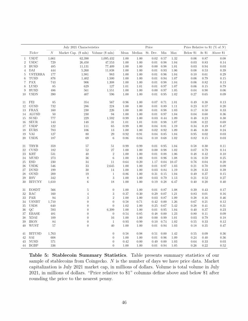
July 2021 Characteristics Price Price Relative to $1 (% of N)Ticker N Market Cap. ($ mln) Volume ($ mln) Mean Median St. Dev. Min Max Below $1 At $1 Above $1

1 USDT 1,661 62,390 1,095,432 1.00 1.00 0.02 0.57 1.32 0.06 0.87 0.082 USDC 729 26,450 47,553 1.00 1.00 0.01 0.98 1.04 0.03 0.83 0.143 BUSD 485 11,131 77,409 1.00 1.00 0.00 0.98 1.01 0.03 0.94 0.034 DAI 444 5,260 11,838 1.00 1.00 0.01 0.93 1.06 0.08 0.53 0.395 USTERRA 177 1,981 983 1.00 1.00 0.01 0.96 1.04 0.10 0.61 0.296 TUSD 876 1,402 1,500 1.00 1.00 0.01 0.94 1.07 0.06 0.79 0.157 PAX 743 906 1,308 1.00 1.00 0.01 0.98 1.04 0.06 0.82 0.138 LUSD 85 629 127 1.01 1.01 0.01 0.97 1.07 0.06 0.15 0.799 HUSD 486 561 1,551 1.00 1.00 0.00 0.97 1.05 0.04 0.90 0.0610 USDN 390 407 596 1.00 1.00 0.01 0.95 1.02 0.27 0.65 0.09

11 FEI 85 354 567 0.96 1.00 0.07 0.71 1.01 0.49 0.38 0.1312 GUSD 732 286 224 1.00 1.00 0.01 0.89 1.11 0.23 0.57 0.2013 FRAX 160 230 226 1.00 1.00 0.01 0.98 1.03 0.17 0.50 0.3314 ALUSD 50 230 94 1.00 1.00 0.01 0.97 1.04 0.04 0.60 0.3615 SUSD 777 229 1,592 0.99 1.00 0.03 0.44 1.09 0.48 0.23 0.3016 SEUR 143 148 31 1.01 1.01 0.01 0.98 1.07 0.08 0.22 0.6917 USDP 122 111 65 0.99 1.00 0.04 0.81 1.19 0.34 0.19 0.4718 EURS 783 106 13 1.00 1.00 0.02 0.92 1.09 0.46 0.30 0.2419 VAI 127 80 29 0.92 0.91 0.04 0.85 1.04 0.95 0.02 0.0320 USDX 187 69 6 0.86 0.84 0.10 0.68 1.02 0.82 0.15 0.03

21 TRYB 359 57 51 0.99 0.99 0.01 0.95 1.04 0.58 0.30 0.1122 CUSD 182 52 27 1.00 1.00 0.00 0.98 1.02 0.07 0.79 0.1423 KRT 531 40 2 1.00 1.00 0.01 0.88 1.06 0.48 0.42 0.1024 MUSD 273 36 6 1.00 1.00 0.01 0.96 1.08 0.16 0.59 0.2525 ESD 230 34 11 0.64 0.20 1.17 0.04 10.47 0.76 0.04 0.2026 USDK 546 33 2,645 1.00 1.00 0.01 0.97 1.03 0.21 0.70 0.0927 DUSD 199 30 14 1.00 1.00 0.03 0.84 1.19 0.28 0.33 0.3928 OUSD 209 19 1 0.86 1.00 0.31 0.15 1.04 0.49 0.37 0.1529 RSV 342 8 3 1.00 1.00 0.03 0.79 1.13 0.21 0.52 0.2730 BITCNY 1,610 6 18 1.00 1.00 0.19 0.28 6.47 0.40 0.20 0.40

31 EOSDT 566 5 0 1.00 1.00 0.01 0.87 1.08 0.39 0.43 0.1732 BAC 160 4 3 0.37 0.30 0.29 0.07 1.21 0.83 0.01 0.1633 PAR 94 3 2 1.00 1.00 0.03 0.87 1.09 0.38 0.16 0.4634 USNBT 1,710 0 0 0.58 0.71 0.42 0.00 1.26 0.67 0.21 0.1235 USDS 640 0 0 1.02 1.00 0.25 0.67 5.42 0.28 0.41 0.3136 QC 593 0 6,399 1.00 1.00 0.01 0.95 1.04 0.40 0.37 0.2337 EBASE 481 0 0 0.54 0.85 0.48 0.00 1.23 0.80 0.11 0.0938 XDAI 109 0 16 1.00 1.00 0.00 0.99 1.01 0.03 0.79 0.1839 IRON 84 0 1 0.93 0.99 0.10 0.74 1.02 0.55 0.33 0.1240 WUST 57 0 40 1.00 1.00 0.01 0.94 1.03 0.18 0.35 0.47

41 BITUSD 1,763 0 0.58 0.98 0.51 0.00 1.42 0.55 0.09 0.3642 SAI 608 0 1.00 1.00 0.01 0.96 1.09 0.24 0.40 0.3643 NUSD 571 0 0.42 0.00 0.49 0.00 1.03 0.64 0.33 0.0344 BGBP 336 0 1.00 1.00 0.01 0.94 1.05 0.26 0.22 0.52

Table 5: Stablecoin Summary Statistics. Table presents summary statistics of oursample of stablecoins from Coingecko. N is the number of days we have price data. Marketcapitalization is July 2021 market cap, in millions of dollars. Volume is total volume in July2021, in millions of dollars. “Price relative to $1” columns define above and below $1 afterrounding the price to the nearest penny.

46

Exchange 1 All ExchangesTicker N Mean Median St. Dev. Min Max Avg. Funding Avg. Term Mean

(Days) (Percent) (Percent) (Percent) (Percent) (Percent) ($ mln) (Days) (Percent)Stablecoins USDT 681 12.4 11.0 9.9 0.1 70.7 39.0 20.4 16.0

DAI 267 17.0 4.3 38.8 0.0 199.8 0.0 40.4 18.7BUSD 469 n.a. n.a. n.a. n.a. n.a. n.a. n.a. 23.4USDC 479 n.a. n.a. n.a. n.a. n.a. n.a. n.a. 25.1

Sovereign USD 2,186 26.7 18.8 27.1 1.9 274.4 2111.7 20.2 26.7EUR 975 14.6 9.1 16.0 0.3 156.1 21.5 13.3 14.6GBP 863 14.8 6.5 26.3 0.0 279.0 1.3 15.8 14.8JPY 865 17.1 12.0 19.5 0.3 213.2 0.3 14.7 17.1

Other BTC 2,193 8.8 5.3 10.8 0.0 109.9 1179.5 18.3 9.2ETH 1,402 6.9 4.0 9.0 0.3 106.8 264.1 8.9 7.5BSV 674 8.1 5.6 8.8 0.0 45.8 12.1 14.1 8.1ETC 1,294 12.0 3.4 21.9 0.0 210.2 9.0 9.9 12.0EOS 1,058 7.2 0.7 17.6 0.0 140.4 7.0 12.3 7.2LTC 2,101 6.7 3.3 11.3 0.0 164.1 6.4 15.9 6.7XMR 1,138 4.9 2.5 8.9 0.0 92.9 5.0 9.3 4.9XRP 1,040 4.2 0.9 13.3 0.0 154.1 3.9 8.7 4.2NEO 1,003 13.2 5.9 20.7 0.0 160.4 2.1 9.9 13.2MIOTA 1,058 1.1 0.1 3.3 0.0 52.2 2.0 9.8 1.1BTG 931 18.8 9.6 25.5 0.0 232.1 1.5 14.7 18.8ADA 230 23.5 2.9 45.8 0.0 173.9 1.5 20.1 23.5DASH 1,138 8.8 4.0 14.6 0.0 176.1 1.0 10.0 8.8UNI 211 18.1 13.5 19.7 0.0 105.6 0.8 20.3 18.1OMG 1,034 6.3 1.7 12.7 0.0 130.3 0.7 10.2 6.3DOT 237 9.3 0.1 30.7 0.0 178.0 0.6 17.6 9.3BCH 112 2.1 0.0 10.4 0.0 74.1 0.4 20.9 2.1LINK 237 4.9 0.3 17.2 0.0 157.7 0.3 14.4 4.9YFI 181 33.2 28.9 37.3 2.8 265.8 0.3 29.2 33.2DOGE 57 14.1 1.9 25.9 0.4 124.7 0.3 13.3 14.1ZEC 1,197 5.4 1.6 11.3 0.0 134.0 0.2 7.8 5.4FIL 173 62.2 32.9 69.0 0.0 230.5 0.2 23.5 62.2XLM 506 6.0 0.5 20.1 0.0 301.0 0.1 13.6 6.0XTZ 506 7.1 4.2 11.7 0.0 123.1 0.1 14.7 7.1SOL 38 9.1 3.1 10.4 0.0 34.4 0.1 17.3 9.1SUSHI 131 22.1 13.2 24.1 0.0 132.0 0.1 16.9 22.1TRX 231 14.5 5.2 20.1 0.0 106.6 0.1 19.6 14.5ZRX 721 7.2 3.7 14.1 0.0 187.6 0.1 8.6 7.2PNT 975 10.1 1.3 26.2 0.0 243.8 0.1 17.2 10.1LEO 561 1.0 0.0 12.1 0.0 177.9 0.1 25.3 1.0ATOM 367 8.3 0.8 16.0 0.0 111.0 0.0 27.2 8.3XAUT 385 5.3 0.0 25.5 0.0 231.4 0.0 23.9 5.3ALGO 362 10.1 4.1 19.4 0.0 144.1 0.0 23.5 10.1FTT 359 25.3 0.5 43.5 0.0 182.5 0.0 10.3 25.3SAN 1,003 11.3 0.1 36.2 0.0 384.0 0.0 12.4 11.3ETP 979 12.7 0.8 32.5 0.0 228.7 0.0 12.0 12.7

Table 6: Cryptocurrency Lending Summary Statistics. Table gives summary statis-tics for currency lending rates. Lending rates are annualized. The first eight columns plot thestatistics from our primary source of data, Exchange 1. The last column gives the averagefunding rate across all three exchanges; in many cases we only have data from exchange 1.Average funding is the average funding used in dollar terms. “Avg. Term” is the averageterm of lending in days. Summary statistics calculated over the time series available for thatcurrency rather than over a concurrent sample. n.a. denotes not available.

47

Correlation of Distance to No-Questions-Asked d̂it with:Time Trend Age Volume Market Bitcoin Bitcoin

Capitalization Return VolatilityThree Largest Stablecoins

ρ −0.24∗∗∗ −0.06∗∗∗ −0.32∗∗∗ −0.33∗∗∗ −0.02∗ 0.08∗∗∗p-value (0.00) (0.00) (0.00) (0.00) (0.08) (0.00)N 4,914 4,914 4,908 4,914 4,911 4,911

Full Stablecoin Sampleρ 0.10∗∗∗ 0.05∗∗∗ −0.20∗∗∗ −0.17∗∗∗ −0.02∗∗ 0.06∗∗∗p-value (0.00) (0.00) (0.00) (0.00) (0.04) (0.00)N 19,138 19,138 18,895 16,576 19,135 19,099

Table 7: Stablecoin Distance to No-Questions-Asked Correlations. Table presents the correlation of stablecoin distanceto no-questions-asked d̂it with a selection of variables, including a time trend, the stablecoin’s age, logs of the stablecoin’s volumeand market capitalization, Bitcoin’s return, and Bitcoin’s volatility (constructed using daily returns over the week). Three largeststablecoins limits the sample to stablecoins ranked in the top three by market capitalization in the previous month. ∗ p < 0.10,∗∗ p < 0.05, ∗∗∗ p < 0.01.

48

NYAG Attestations New Stablecoin New Stablecoin BitcoinLawsuit Announced Starts Trading Crashes

I(Post) 0.66∗∗∗ −0.10∗ −0.07 0.08 0.81∗∗∗(4.54) (−1.69) (−0.76) (1.44) (3.67)

I(Treat) −0.04 −0.05(−0.13) (−0.74)

I(Post)× I(Treat) −0.11 0.08(−0.37) (0.99)

N 70 1,450 91 1,350 70R2 0.61 0.41 0.89 0.37 0.70Events 2 41 6 42 5Coin FE Yes Yes Yes Yes Yest statistics in parentheses∗ p < 0.10, ∗∗ p < 0.05, ∗∗∗ p < 0.01

Table 8: Event Study of Stablecoin Distance to No-Questions-Asked d. Table presents the regression of stablecoin i’sdistance to no-questions-asked d̂it on dummies for treatment and post around the events: d̂it = α+ γ1I(Post) + γ2I(Treated) +γ3I(Post) × I(Treated) + εit. Each column corresponds to a different event study: the New York Attorney General openingand closing its investigation into Tether (4/25/2019 and 2/23/2021) where Treated = 1 for Tether; attestations are releases ofattestations and transparency reports, where Treated = 1 for the stablecoin issuer releasing the report, which include USDT,BUSD, USDC, and USDP. New stablecoin announced refers to the announcement date of USDC, BUSD, TerraUSD, TrueUSD,PaxDollar, and HUSD. First trade date is the first date of price is available for the USD-pegged stablecoins on Coingecko. Bitcoincrashes events are the 5 largest single-day Bitcoin declines since 2016. The window around each event is 3 business days beforeand after the event date. We limit the sample to major stablecoins, which we define as USDT, USDC, BUSD, DAI, USTERRA,PAX, and HUSD. t-statistics are reported in parentheses using robust standard errors, where ∗ p < 0.10, ∗∗ p < 0.05, ∗∗∗ p < 0.01.

49

Bitcoin Lending Rate Implied Repo Rate Overnight-Indexed SwapStablecoin Exchange Mean St. Dev Mean St. Dev Mean St. DevUSDT Average −10.2 10.8 −15.9 10.7 −15.0 11.0

Exchange 1 −8.0 10.3 −12.3 9.9 −11.4 9.9Exchange 2 −15.5 13.9 −25.2 15.6 −24.9 15.9Exchange 3 −13.4 14.1 −15.4 13.7 −15.4 13.9

DAI Average −14.6 37.2 −18.6 37.9 −18.6 37.8Exchange 1 −12.4 38.3 −16.8 38.8 −16.9 38.8Exchange 3 −12.8 16.3 −14.5 15.8 −14.4 15.8

USDC Exchange 2 −15.1 14.1 −24.9 16.1 −24.6 16.5

BUSD Exchange 2 −13.4 13.2 −23.2 15.3 −23.0 15.6

Table 9: Stablecoin Convenience Yields Summary Statistics. Table reports summary statistics for stablecoin convenienceyields in annual percent. Convenience yields are calculated using stablecoin lending rates relative to the Bitcoin lending rate,implied repo rate, and OIS rate. Average exchange refers to the average lending rate across exchanges, which is calculated forstablecoins with data available from multiple exchanges.

50

(1) (2) (3) (4) (5)All USDT USDC BUSD DAI

d̂it −8.08∗∗∗ −2.47∗∗ −6.69∗∗∗ −3.70∗∗ −10.95∗∗∗(−3.59) (−2.14) (−3.63) (−2.29) (−3.18)

N 1,889 680 479 463 267R2 0.15 0.02 0.08 0.03 0.27Coin FE Yes

Table 10: Distance to No-Questions-Asked d and Stablecoin Convenience Yield. Table gives estimates from regressinga stablecoin’s convenience yield on its estimated distance to NQA, d̂it. Observations are stablecoin by day. The first columnpresents a pooled regression including USDT, USDC, BUSD, and DAI, where the convenience yield is the average convenienceyield calculated across the three exchanges. Column 1 R2 is within-R2. t-statistics using Driscoll and Kraay (1998) standarderrors with a maximum of 5 lags are reported in parentheses, where ∗ p < 0.10, ∗∗ p < 0.05, ∗∗∗ p < 0.01.

51

Avg. Across Exchanges Exchange 1 Implied Repo Rate OIS(1) (2) (3) (4) (5) (6) (7) (8)

d̂it −11.84∗∗∗ −11.06∗∗ −11.68∗∗∗ −10.71∗∗ −12.18∗∗∗ −11.04∗∗ −12.10∗∗∗ −11.04∗∗(−3.36) (−2.59) (−2.88) (−2.43) (−2.98) (−2.50) (−2.96) (−2.50)

Bitcoin Basis −0.20 −0.22 −0.18 −0.20(−1.59) (−1.46) (−1.16) (−1.30)

Bitcoin Return 0.06 0.35 0.22 0.23(0.13) (0.70) (0.44) (0.45)

Average Term −0.54∗ −0.56∗ −0.57∗ −0.56∗(−1.73) (−1.69) (−1.70) (−1.69)

OIS−Tbill −94.04 −137.41 −138.41 −140.11(−1.53) (−1.62) (−1.65) (−1.66)

ln(Volume) −0.50 −1.45 −2.29 −2.32(−0.28) (−0.72) (−1.14) (−1.15)

N 204 108 108 108 108 108 108 108R2 0.19 0.24 0.18 0.24 0.20 0.26 0.20 0.26Coin FE Yes Yes Yes Yes Yes Yes Yes YesYear FE Yes Yes Yes Yes Yes Yes Yes Yes

Table 11: Distance to No-Questions-Asked d and Stablecoin Convenience Yield After Nvidia Processor Releases.Table gives estimates from regressing a stablecoin’s convenience yield on its estimated distance to NQA, d̂it. Observations arestablecoin by day and include all currencies for which we have convenience yield measures: USDT, USDC, BUSD, and DAI.Data restricted to three days after Nvidia launches new processors used for Ethereum mining. The dependent variable in thefirst two columns is the average convenience yield calculated across the three exchanges (the yield on lending bitcoin minus theyield on lending the stablecoin); columns (3) and (4) use the convenience yield from Exchange 1 which has data for USDT andDAI; columns (5) and (6) calculate the convenience yield using the implied repo rate on Bitcoin futures instead of the lendingrate on Bitcoin; columns (7) and (8) calculate the convenience yield using the 1-month overnight-indexed swap rate instead ofthe implied repo rate or Bitcoin lending rate. BTC Basis is the Bitcoin basis as calculated using the generic front-month CMEBitcoin future and the CME Bitcoin index price. Average term is the average lending term for the stablecoin in days, and isavailable only from Exchange 1. R2 is within-R2. t-statistics are reported in parentheses using robust standard errors, where ∗p < 0.10, ∗∗ p < 0.05, ∗∗∗ p < 0.01.

52

A Online Appendix

A.1 Proposition 1. ∂(CY )∂d

< 0

First, expand the convenience yield equation:

Convenience Yieldt = Rft −Rd

t

=Rft −

1Pt(d)

=Rft −

DRt (d)

Vt(d)[1−N(hD + σ)] + (1 + rf )−1DRt (d)N(hD)

We want to show that ∂(CY )∂d

= ∂∂d

(−DR

t (d)Vt(d)[1−N(hD+σ)]+(1+rf )−1DR

t (d)N(hD)

)< 0.

For simplicity call DRt (d) = D(d), Vt(d) = V (d). Then by the quotient rule:

∂(CY )∂d

=D(d)

(D′(d)N(hD)

1+rf+ D(d)h′DN

′(hD)1+rf

− V (d)h′DN ′(hD + σ) + V ′(d)[1−N(hD + σ)])

(D(d)N(hD)

1+rf+ V (d)[1−N(hD + σ)]

)2

− D′(d)D(d)N(hD)

1+rf+ V (d)[1−N(hD + σ)]

=D(d)(D′(d)N(hD)

1 + rf+ D(d)h′DN ′(hD)

1 + rf− V (d)h′DN ′(hD + σ) + V ′(d)[1−N(hD + σ)]

)

−D′(d)(D(d)N(hD)

1 + rf+ V (d)[1−N(hD + σ)]

)

=D(d)

D(d)h′DN ′(hD)1 + rf

− V (d)h′DN ′(hD + σ)︸ ︷︷ ︸=0

+V ′(d)[1−N(hD + σ)]

−D′(d)V (d)[1−N(hD + σ)]

=D(d)V ′(d)[1−N(hD + σ)]−D′(d)V (d)[1−N(hD + σ)]

= [1−N(hD + σ)]︸ ︷︷ ︸>0 if hD+σ<∞

[D(d)V ′(d)−D′(d)V (d)] < 0

Thus, if D(d)V ′(d)−D′(d)V (d) < 0, then ∂(CY )∂d

< 0.

A.2 Data

Historical Data Banknote quote data from Weber (2021) is available at the followingfrequencies: Philadelphia (monthly 1830 to 1831; 1832 to 1858; data from Bicknell’s Reporter,Counterfeit Detector, General Prices Current and Van Court’s Counterfeit Detector and

53

banknote List); New York (bimonthly, 1817 to 1849; monthly 1849 to 1857 with severalgaps; data from the Shipping & Commercial List, New-York Price Current and Thompson’sbanknote); Cincinnati (February 1841, July 1845 to June 1847, February 1850, July 1854, fromWestern Counterfeit Detector and banknote Table and Bradley & Co’s Cincinnati CounterfeitDetector and banknote Reporter); and, Cleveland (January, June, and September 1856 fromthe Cleveland banknote Reporter).

Global Financial Data describes the Moody’s Municipal Bond 20-year Composite yield:

Data from 1789 to 1856 is based upon individual bonds from different states.From 1789 to 1814, Massachusetts Notes (BSMANT) yielding 6% are used. In1815 and 1816, South Carolina 6% Bonds (BSSC6S), the New York 6% Bonds(BSNY6S) from 1817 to April 1823 and from September 1843 to 1847, the NewYork Canal 5% Bonds due 1845 (BSNY5C45) from May 1823 to August 1843 andthe New York State 5% Bonds due 1858 (BSNY558) from 1848 to 1856.

Global Financial Data describes the Moody’s Corporate AAA Bond yield:

Before 1857, data from individual corporate bonds is used. The Masonic HallAssociation of Philadelphia 5% Loan is used from 1815 to 1827, the Chesapeakeand Delaware Canal 6% Bonds is used from 1827 to 1831, the Schuylkill NavigationCo. 6% Bonds of 1840 is used from 1831 to 1837, the Baltimore and Ohio Railroad6% Bonds is used from 1837 to 1842, New York, Lake Erie and Western RailroadCo. 7% 5th Mortgage Bonds of 1858 is used in 1842 and 1843, the PhiladelphiaGas Works 6% Bonds of 1861 is used from 1843 to 1850 and the Baltimore andOhio Railroad 6% Bonds of 1867 is used from 1850 to 1858 . . .

Global Financial Data describes the relevant period of the 10-Year Treasury yield series:

From 1790 to 1832, the government generally ran surpluses and redeemed itsoutstanding debt. By 1833, no debt was outstanding and no federal governmentbonds traded between 1833 and 1842. New York had the largest and most liquiddebt during this period of time, so the New York 5% Canal Bonds due 1845(BSNY5C45) is used between January 1833 and November 1842. New governmentbonds were introduced in 1843 and the federal government has had outstandingdebt ever since. The United States 6% Bonds due 1862 (BGUSA662) are usedbetween December 1842 and June 1848, the United States 6% Bonds of 1868(BGUSA668) are used between July 1848 and July 1858, the United States 5%Bonds due 1874 (BGUSA574) are used between August 1858 and October 1860. . .

54

Bitcoin Basis We calculate the annualized Bitcoin basis by comparing the spot price ofBitcoin (St), measured by the CME’s CF Bitcoin Reference Rate (BRR Index), and thegeneric next-month Bitcoin futures contract, Ft (BTC1 Curncy):

Basist = (Ft/St − 1)× 12× 100

Ignoring financing costs, Basist > 0 implies the trader can profit by buying Bitcoin in thespot market and simultaneously selling Bitcoin futures. In practice, the trader would alsoneed to finance the 50% margin that CME requires when trading Bitcoin futures.

Implied Repo Rate We calculate the annualized repo rate implied by future prices bycomparing the spot price of Bitcoin (St), measured by the CME’s CF Bitcoin Reference Rate(BRR Index), and the price of Bitcoin futures contract on date t for delivery at maturity m,Fmt , with d > 0 days until delivery:

Implied Repo Ratemt = 1N

∑m

(Fmt /St − 1)× 360

dmt

We then calculate the average implied repo rate on a given day by averaging the implied reporate across all maturities.

A.3 Exclusion Restriction

The exclusion restriction of our instrumental approach requires that the instrument cannotbe correlated with local growth prospects. The exclusion restriction is not directly testable,but we use falsification tests to show that banks in locations closer to the low-cost line werenot larger and did not grow faster before the railroad was constructed.

Table A2 shows the correlation of the instrument, each bank’s distance to the low-costline, with the bank’s level of bank assets and asset growth over the 15 years before 1849.None of the correlations are significant, indicating that banks closer to the low-cost line didnot have larger assets or higher growth in the years before the railroad was constructed.

A.4 Other Reputation Development

Stablecoin Names The remainder of the top twenty stablecoins follows the same pattern:Liquidity USD (LUSD), Neutrino USD (USDN), HUSD, sUSD (SUSD), Alchemix USD(ALUSD), Gemini Dollar (GUSD), USDX (USDX), USDP Stablecoin (USDP), and sEUR(SEUR). Another large stablecoin, initially named “Paxos Standard” (PAX), renamed to“Pax Dollar” (USDP) as “the USDP ticker more easily identifies Pax Dollar as a US dollar-

55

backed token.”28 Historically, banks also chose names to garner reputation: Friedman andSchwartz (1963) argue the 1930 bank run on the “Bank of United States,” a commercial bankunaffiliated with the U.S. government, precipitated the wave of banking panics beginning in1930. While simple, issuers’ name choices aim directly at reducing a debt’s distance to NQA.

Terms of Service Stablecoins can influence their d’s through their contracts with theirlenders. The contract is called the terms of service. It is tough to link the terms of service tod quantitatively. Still, the fact that terms of service are important for stablecoin issuers isclear in the evolution of Tether’s terms of service over time.29 Both the length of the termsof service has grown, and its Flesch–Kincaid reading level has increased over time.30 If theterms of service were unimportant, it would be surprising to see such large changes over time.

The terms of service also describe stablecoins’ reserves. Just like banks and money-market funds, concerns about the stablecoin’s backing—the issuer’s assets—can lead to arun on stablecoins. Thus, stablecoins also hold reserves to avoid runs and to maintain theirredemption policies. Stablecoin issuers issue attestations to address these concerns about thereserve backing, and some also adjust the language in their terms of service.

In September 2019, a terms of service addendum for USDP and BUSD stated that theyare backed by an equivalent amount of “US dollar deposits or US Treasury bonds”.31 Thiswording changed to a backing of “US dollar deposits or Debt Instruments” by October 2020and to “US dollar deposits or Government Debt Instruments” by August 2021. The successivechanges suggest there is substantial attention paid to the specific wording and details of theterms of service. Also, the NYAG investigation of Tether likely makes stablecoin issuers morecircumspect about the details.

28See https://paxos.com/2021/08/24/the-digital-dollar-that-always-equals-a-dollar-paxos-standard-pax-is-now-pax-dollar-usdp/.

29See Figure A4.30The Flesch–Kincaid reading level is based on a score that considers such factors as word and sentence

length. An increase in the score indicates the terms of service have become harder to read.31https://paxos.com/2019/03/29/usdp-terms-conditions/: The US Dollar Stablecoin Terms and Conditions

are an addendum to the terms of service for USDP and BUSD.

56

A.5 Figures

0

2

4

6

8

0.0 0.5 1.0 1.5 2.0d

Risk-Free BondPrivate Banknote

PercentYield

d*

No-Questions-Asked when d=0-4

-2

0

2

4

0.0 0.5 1.0 1.5 2.0d

PercentConvenience Yield

Figure A1: Model Intuition. Figure plots the yields on banknotes and risk-free bonds and assumes consumption follows alognormal independent and identically distributed process so that the risk-free rate is Rf

t =(β exp{−γµc + 1

2γ2σ2

C})−1

where µCand σC describe the consumption process, and γ is coefficient of relative risk aversion. The right panel plots the convenienceyield given in equation 5, which is the difference between the two yields on the left panel: Convenience Yieldt = Rf

t −Rdt . Figure

uses β = 0.98, µC = 0.01, σC = 0.02, γ = 2, σ = 0.2, Vt(d) = 100, and DRt (d) = 1.

57

0

3

6

9

12

15

Disc

ount

(%

)

1820 1830 1840 1850 1860

Bank of Montgomery County Farmers' Bank of Virginia

Figure A2: Banknote Discount Example. Figure plots New York discounts for two selected banks; shaded areas denotecrises as given by Trebesch et al. (2021). Discounts are quotes relative to par: a bank with a 10% discount has a price of$1× (1− 0.1) = $0.90.

58

0

200

400

600

800

1000

Cou

nt

1820 1830 1840 1850 1860

New York Quotes Philadelphia Quotes

Figure A3: Banknote Count. Figure plots the number of individual banks with merged banknotes in our sample in eachmonth.

59

18

20

22

24

26

28

2014 2016 2017 2019 2020

Flesch-Kincaid Grade Level

2,000

4,000

6,000

8,000

10,000

12,000

2014 2016 2017 2019 2020

Word Count

Figure A4: USDT Terms of Service Figure plots the Flesch-Kincaid grade level and word count of USDT’s terms of serviceover time. We manually capture five distinct snapshots of the terms of service over time. The Flesch-Kincaid grade level measureestimates the years of schooling required to understand the text.

60

-60

-40

-20

0

20

Yie

ld (

%)

Jan-19 Jul-19 Jan-20 Jul-20 Jan-21 Jul-21

USDT

-200

-150

-100

-50

0

Yie

ld (

%)

Jan-19 Jul-19 Jan-20 Jul-20 Jan-21 Jul-21

DAI

-40

-30

-20

-10

0

Yie

ld (

%)

Jan-19 Jul-19 Jan-20 Jul-20 Jan-21 Jul-21

BUSD

-50-40-30-20-10

0

Yie

ld (

%)

Jan-19 Jul-19 Jan-20 Jul-20 Jan-21 Jul-21

USDC

Figure A5: Stablecoin Convenience Yield Figure plots the convenience yield for each currency when averaged across allexchanges for which we have data, where the convenience yield is calculated using lending rates for the stablecoin and Bitcoin.Convenience yield is yBTC − yStablecoin.

61

A.6 Tables

Mean ρ

Benchmark EstimateNew York Quotes 0.88 1.00∗∗∗Philadelphia Quotes 0.30 1.00∗∗∗

Commercial Paper rfNew York Quotes 0.30 0.84∗∗∗Philadelphia Quotes 0.21 0.87∗∗∗

Fixed 5% rfNew York Quotes 0.73 0.99∗∗∗Philadelphia Quotes 0.31 0.99∗∗∗

Fixed 9% rfNew York Quotes 0.41 0.98∗∗∗Philadelphia Quotes 0.17 0.99∗∗∗

Price σNew York Quotes 0.93 0.42∗∗∗Philadelphia Quotes 0.46 0.91∗∗∗

Table A1: Banknote Distance to No-Questions-Asked Estimates with AlternativeAssumptions. Table presents the mean d and correlation ρ of the estimation’s value-weightedaggregate d with the benchmark estimate d for the same dataset (New York or Philadelphia).d units is years. Value-weights are calculated using lagged circulation shares. The benchmarkestimate uses the Global Financial Data’s 10-Year Treasury rate as the risk-free rate and theannualized volatility of monthly asset growth over the previous year. The commercial paperestimate uses the commercial paper rate reported by Smith and Lole (1935) based on Bigelow(1862) and available from Global Financial Data for the period beginning in December 1835.The fixed rate estimates use a fixed risk-free rate of 5% (roughly the average Treasury yieldover the period 1817 to 1860) and 9% (roughly the average commercial paper rate in thesample available from Bigelow (1862). The price σ estimate uses annualized price volatility ofthe bank notes as implied by monthly changes in discounts over the previous twelve months.Correlation significance reported where ∗ p < 0.10, ∗∗ p < 0.05, ∗∗∗ p < 0.01.

62

Over Prior 15 YearsBank Assets Asset Growth Bank Assets Asset Growth

Distance to Low-Cost Line 0.072 0.068(0.39) (0.42)

Within 30 Miles of Low-Cost Line −0.034 −0.052(0.68) (0.54)

N 143 143 143 143

Table A2: Correlation of Distance to Low-Cost Line with Local Growth Prospects. Table presents the correlationof the distance to the low-cost line and bank asset level, asset growth, and relative asset growth over the prior 15 years. P-valuesreported in parentheses where ∗ p < 0.10, ∗∗ p < 0.05, ∗∗∗ p < 0.01.

63

Avg. Across Exchanges Exchange 1 Implied Repo Rate OIS(1) (2) (3) (4) (5) (6) (7) (8)

d̂it −8.59∗∗∗ −10.88∗∗∗ −10.38∗∗∗ −10.69∗∗∗ −10.85∗∗∗ −11.17∗∗∗ −10.91∗∗∗ −11.23∗∗∗(−3.48) (−3.69) (−3.49) (−3.64) (−3.65) (−3.82) (−3.68) (−3.85)

Bitcoin Basis −0.07∗∗∗ −0.06∗∗∗ −0.03 −0.05∗∗(−3.16) (−2.84) (−1.32) (−2.34)

Bitcoin Return −0.08 0.11 0.06 0.07(−0.61) (0.89) (0.56) (0.64)

Average Term −0.12∗∗∗ −0.10∗∗∗ −0.09∗∗∗ −0.09∗∗∗(−3.42) (−3.38) (−3.07) (−3.05)

OIS−Tbill −4.51 −7.47 −12.73 −11.52(−0.29) (−0.48) (−0.90) (−0.82)

ln(Volume) −2.50∗∗∗ −2.95∗∗∗ −3.63∗∗∗ −3.60∗∗∗(−2.89) (−3.26) (−4.16) (−4.14)

N 1,889 933 933 933 933 933 933 933R2 0.24 0.25 0.23 0.26 0.26 0.28 0.26 0.29Coin Fixed Effects Yes Yes Yes Yes Yes Yes Yes YesYear Fixed Effects Yes Yes Yes Yes Yes Yes Yes Yes

Table A3: Distance to No-Questions-Asked d and Stablecoin Convenience Yield with Alternative ConvenienceYield Measures and Additional Controls. Table gives estimates from regressing a stablecoin’s convenience yield on itsestimated distance to NQA, d̂it. Observations are stablecoin by day and include all currencies for which we have convenienceyield measures: USDT, USDC, BUSD, and DAI. The dependent variable in the first two columns is the average convenienceyield calculated across the three exchanges (the yield on lending bitcoin minus the yield on lending the stablecoin); columns(3) and (4) use the convenience yield from Exchange 1 which has data for USDT and DAI; columns (5) and (6) calculate theconvenience yield using the implied repo rate on Bitcoin futures instead of the lending rate on Bitcoin; columns (7) and (8)calculate the convenience yield using the 1-month overnight-indexed swap rate instead of the implied repo rate or Bitcoin lendingrate. BTC Basis is the Bitcoin basis as calculated using the generic front-month CME Bitcoin future and the CME Bitcoinindex price. Average term is the average lending term for the stablecoin in days, and is available only from Exchange 1. R2 iswithin-R2. T-statistics are reported in parentheses using Driscoll and Kraay (1998) standard errors with a maximum of 5 lagsare reported in parentheses, where ∗ p < 0.10, ∗∗ p < 0.05, ∗∗∗ p < 0.01.

64

Release Date Hash Rate Avg. Cumulative Avg.GeForce RTX 2060 1/15/19 30.5 30.5GeForce GTX 1660 Ti 2/21/19 29.6 30.1GeForce GTX 1660 3/14/19 22.0 27.4GeForce GTX 1650 4/23/19 27.4GeForce RTX 2060 Super 7/9/19 39.5 30.4GeForce RTX 2070 Super 7/9/19 40.5 32.4GeForce RTX 2080 Super 7/23/19 41.0 33.9GeForce GTX 1660 Super 10/29/19 29.7 33.3GeForce GTX 1650 Super 11/22/19 31.0 33.0GeForce RTX 2060 1/10/20 30.5 32.7GeForce GTX 1650 4/3/20 32.7GeForce GTX 1650 6/18/20 32.7GeForce RTX 3080 9/17/20 94.8 38.9GeForce RTX 3090 9/24/20 117.0 46.0GeForce RTX 3070 10/29/20 60.1 47.2GeForce RTX 3060 Ti 12/2/20 59.1 48.1CMP HX 2/18/21 86.0 50.8GeForce RTX 3060 2/25/21 41.5 50.2GeForce RTX 3080 Ti 6/3/21 85.0 52.4GeForce RTX 3070 Ti 6/10/21 55.1 52.5GeForce RTX 3060 9/1/21 41.5 51.9

Table A4: Nvidia GPU Release Dates. Table gives the release dates and hash rates for Nvidia GPUs. Data is sorted byrelease date. The average hash rate is the average of available hash rates collected from WhatToMine, 2CryptoCalc, and Nvidia.Hash rates are mining rates for Ethash in Mh/s. Cumulative Average is the rolling average of available average hash rates.

65