NBER WORKING PAPER SERIES

MAJOR MACROECONOMIC VARIABLES AND LEADING INDEXES:SOME ESTIMATES OF THEIR INTERRELATIONS, 1886-1982

Victor Zarnowitz

Phillip Braun

Working Paper No. 2812

NATIONAL BUREAU OF ECONOMIC RESEARCH1050 Massachusetts Avenue

Cambridge, MA 02138January 1989

This research is part of NBER's research program in Economic Fluctuations.Any opinions expressed are those of the authors not those of the NationalBureau of Economic Research.

NBER Working Paper #2812January 1989

MAJOR MACROECONOMIC VARIABLES AND LEADING INDEXES:SOME ESTIMATES OF TUEIR INTERRELATIONS, 1886-1982

ABSTRACT

We examine the interactions within sets of up to six variables representing

output, alternative measures of money and fiscal operations, inflation,

interest rate, and indexes of selected leading indicators. Quarterly series

are used, each taken with four lags, for three periods: 1949-82. 1919-40, and

1886-1914. The series are in stationary form, as indicated by unit root

tests. For the early years, the quality of the available data presents some

serious problems.

We find evidence of strong effects on output of the leading indexes and the

short-term interest rate. The monetary effects are greatly reduced when these

variables are included. Most variables depend more on their own lagged values

than on any other factors, but this is not true of the rates of change in

output and the composite leading indexes. Some interesting interperiod

differences are noted and discussed.

Victor ZarnowitzGraduate School of Business

University of ChicagoChicago, IL 60637

Phillip BraunGraduate School of Business

University of ChicagoChicago, IL 60637

1

Major Macroeconomic Variables and Leading Indexes:Some Estimates of Their Interrelations, 1886-1982

Victor Zarnowitz and Phillip Braun

I. Background and Objectives

How the economy moves over time depends on its structure, institutions, and

policies, all of which are subject to large historical changes. It would be

surprising if the character of the business cycle did fl2. change in response

to such far-reaching developments as the great contraction of the 1930s and

the post-depression reforms, the expansion of government and private service

industries, the development of fiscal and other built-in stabilizers, and the

increased use and role of discretionary macroeconomic policies. Hence, it is

consistent with our priors that the data for the United States and other

developed market-oriented countries generally support the hypothesis that

business contractions were less frequent, shorter, and milder after World War

II than before (Cordon 1986; Zarnowitz 1989).

Although business cycles have thus moderated, they retain a high degree of

continuity, which shows up most clearly in the comovements and timing

sequences among the main cyclical processes.1 An important aspect of this

continuity is the role of the variables that tend to move ahead of aggregate

output and employment in the course of the business cycle. The composite

index of leading indicators combines the main series representing these

variables. Several studies point to the existence of a relatively close and

stable relationship between prior changes in this index and changes in

macroeconomic activity (Vaccara and Zarnowitz 1977; Auerbach 1982; Zarnowitz

and Moore 1982; Diebold and Rudebusch 1987). Yet, the currently popular small

reduced-form macro models, make little or no use of the leading indicators.2

2

We suspect that the reason is lack of familiarity. The role of the

indicators is probably often misperceived as being purely symptomatic.

Heterogeneous combinations of such series resist easy theoretical

applications. On a deeper level, the notion that the private market economy

is inherently stable led to an emphasis on the role of the monetary and fiscal

disturbances. Interest in the potential of stabilization policies had a

similar effect in that it stimulated work on models dominated by factors

considered to be amenable to government control.

This orientation is understandably appealing but it can easily become one-

sided and error-prone, both theoretically and statistically. For example, a

simple vector autoregressive (VAR) model in log differences of real GNP,

money, and government expenditures suggests the presence of strong lagged

monetary and fiscal effects on output.3 However, it is easy to show that

these relationships are definitely inisspecified. One way to demonstrate this

is by adding changes in a leading index that excludes monetary and financial

components so as not to overlap any of the other variables. In the thus

expanded model, the dominant effects on output come from the past movements of

the leading index, while the roles of the other variables (including the

lagged values of output growth itself) are greatly reduced (see section IV.l

below). In general, omitting relevant variables in a VAR cause the standard

exogeneity tests, impulse responses, and variance decompositions to be biased,

as shown in L'utkepohl 1982 and Braun and Mittnik 1985.

The first objective of this paper is to examine the lead-lag interactions

within larger sets of important macroeconomic variables, including interest

and inflation rates along with output, monetary and fiscal variables, and a

nonduplicative leading index. The rationale for including this index is

twofold. (1) The changes in the leading index can be interpreted broadly as

3

representing dynamic forces within the private economy: the early collective

outcomes of investment and production (also, less directly, consumption)

decisions. Presumably, it is mainly these forces that account for the

continuity of business cycles. Both aggregate demand and aggregate supply

shifts are involved but the demand effects may be stronger in the short run.

(2) The addition of the leading index helps us overcome the omitted variables

bias. The index stands for a number of important factors that would otherwise

be omitted. It would not be practical to include the several individual

series to represent these variables.

We work with equations that include up to six variables, plus constant

terms and time trends. They are estimated on quarterly series, each taken

with four lags, which means using up large numbers of degrees of freedom.

Given the size of the available data samples, it is not possible for such

models to accomodate more variables, while retaining a chance to produce

estimates of parameters in which one could have some confidence. It is, of

course, easy to think of additional variables that might be important enough

for their omission to cause some serious misspecifications. All vector

autoregressive (VAR) models face this dilemma, but the only way to avoid it is

by assuming a full structural model which could be still more deficient. We

seek some partial remedies in alternative specifications guided by economic

theory and history as well as comparisons with related results in the

literature.

Although the format adopted is that of a VAR model, the implied system-

wide dynamics, i.e., impulse response functions and variance decompositions,

are beyond the scope of this study. These statistics seek to describe

behavior in reaction to innovations, require longer series of consistent data

than are actually available,4 and are probably often very imprecise even for

4

smaller systems (cf. Zellner 1985 and Runkle 1987 with discussion). In

contrast, there is sufficient information to estimate well the individual

equations, even with more lagged terms. We find that much can be learned from

attention to the quality and implications of these estimates, which are

logically prior to inferences on overall dynamics but carry no commitment to

the particular interpretations of a VAR model. Moreover, our interest centers

on cyclical movements, that is, on the interplay of forces over shorter time

horizons, not on long-term consequences of some assumed shocks.

Our second and related objective is to extend the analysis to the periods

between the two world wars and earlier in another effort to study the

continuity and change in U.S. business cycles. To evaluate any persistent

shifts or the secular evolution in the patterns of macroeconomic fluctuation,

it is of course necessary to cover long stretches of varied historical

experience. Estimates of the interrelations among the selected variables are

calculated from quarterly seasonally adjusted data for three periods:

1886-1914, 1919-40, and 1949-82. We ask generally, what similarities and

differences between the three periods are suggested by this exercise.

Historical data are scanty and deficient, which inevitably creates some

difficult choices and problems. The next part of the paper (II) discusses

this and lists the variables and series used Part III discusses the applied

methods and presents tests that determine what transformations must be used on

any of the series to validate our statistical procedures. Part IV examines

the results, focusing on simple exogeneity and neutrality tests for a

succession of models as well as on interperiod comparisons. Part V sums up

our conclusions and views on the need for further work.

S

II. Date

1. The Selected Variables and Their Reoresentations

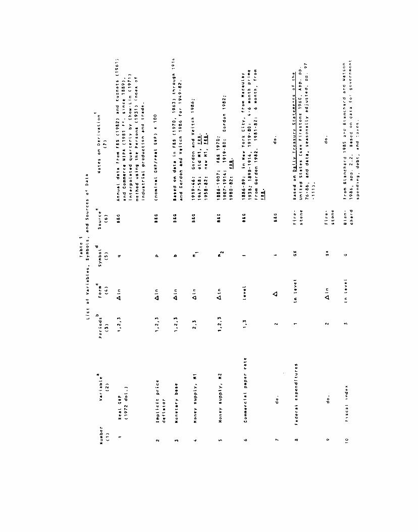
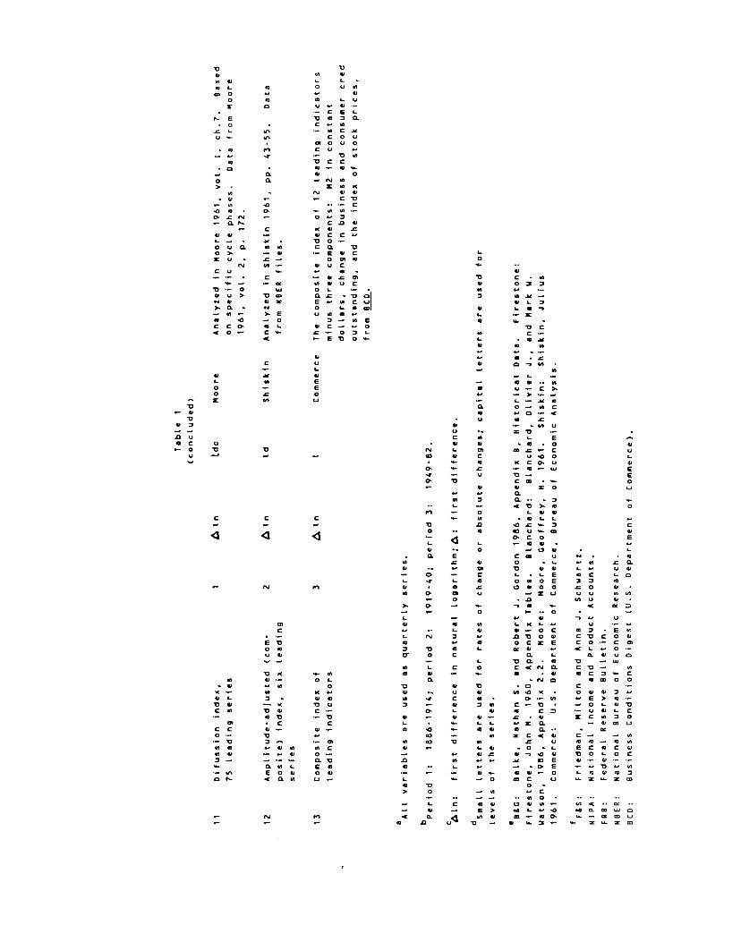
Table I serves as a summary of the information on the data used in

this study. It defines the variables and identifies the time series by title,

period, symbol, and source. Some notes on how the underlying data are derived

are included as well.

The table includes 11 different variables and 23 segments of the

corresponding series, counting one per period (columns 2 and 3). No equation

contains more than six variables. Some variables have different representa-

tions across the three periods covered because consistent data are not

available for them. Further, unit root tests indicate that, in some cases,

levels of a series ought to be used in one period, differences in another.

These tests and the required transformations are discussed in section 111.2

below. As shown in column 4, natural logarithms are taken of all series

except the commercial paper rate. Federal expenditures in 1886-1914, the

fiscal index in 1949-82, and the interest rate in both of these periods are

level series; in all other cases first difference series are used.

Lower letters serve as symbols for variables cast in form of first

differences, capital letters for those cast in levels (Table 1, column 5).

The series relating to output (q), prices (p), the alternative monetary

aggregates (b,m1,m2), and interest (I or i) are staple ingredients of small

reduced-form or VAR models. They are characterized in the table on lines

numbered 1-7.

Of the additional series, three represent fiscal variables (8-10). For the

postwar period, there is an index combining federal spending, debt, and taxes

(C). For the interwar and prewar periods, there are two segments of the

federal expenditures series (gx and CX, respectively).

6

Finally, there are three different indexes of leading indicators (11-13).

The only such series presently available for 1886-1914 is a diffusion index

based on specific cycles in individual indicators (ldc). The composite

indexes for 1919-40 and, particularly, for 1949-82 (d and 2, respectively)

are much more satisfactory.

2. Sources and Problems

The "standard" historical estimates of GNP before World War II based mainly

on the work of Kuznets, Kendrick, and Gailman, are at most annual. We use the

new quarterly series for real GNF and the implicit price deflator from a1ke

and Gordon 1986. These data are constructed from the standard series by

means of quarterly interpolators which include the Persons 1931 index of

industrial production and trade before 1930, the FRE industrial production

index for 1930-40, constant terms, and linear time trends. The use of

interpolations based on series with narrower coverage than GNP is a source of

unavoidable error if the unit period is to be shorter than a year.6

The historical annual estimates of U.S. income and output leave much to be

desired but it is difficult to improve on them because the required informa-

tion simply does not exist. The series have been recently reevaluated,

leading to new estimates by Romer, 1986 and 1987 and alke and Gordon, 1988.

Romer's method imposes certain structural characteristics of the U.S. economy

in the post-World War II period on the pre-Worid War I data. This produces

results that contradict the evidence on postwar moderation of the business

cycle by prejudging the issue (L.ebergott 1986; Weir 1986; Balke and Cordon

1988). It is mainly for this reason that we do not use Romers data.

7

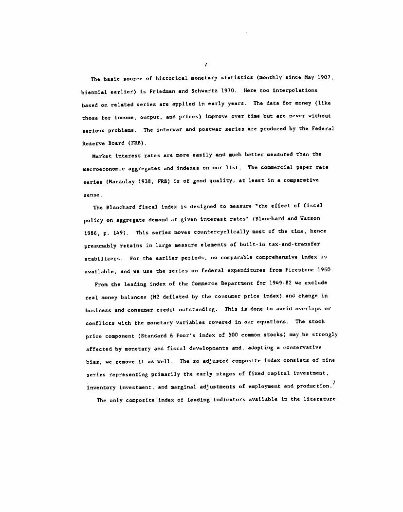
The basic source of historical monetary statistics (monthly since Play 1907,

biennial earlier) is Friedman and Schwartz 1970. Here too interpolations

based on related series are applied in early years. The data for money (like

those for income, output, and prices) improve over time but are never without

serious problems. The interwar and postwar series are produced by the Federal

Reserve Board (FRB).

Market interest rates are more easily and much better measured than the

macroeconomic aggregates and indexes on our list. The commercial paper rate

series (Macaulay 1938, FRB) is of good quality, at least in a comparative

sense.

The Blanchard fiscal index is designed to measure "the effect of fiscal

policy on aggregate demand at given interest rates" (Blanchard and Watson

1986, p. 149). This series moves countercyclically most of the time, hence

presumably retains in large measure elements of built-in tax-and-transfer

stabilizers. For the earlier periods, no comparable comprehensive index is

available, and we use the series on federal expenditures from Firestone 1960.

From the leading index of the Commerce Department for 1949-82 we exclude

real money balances (M2 deflated by the consumer price index) and change in

business and consumer credit outstanding. This is done to avoid overlaps or

conflicts with the monetary variables covered in our equations. The stock

price component (Standard & Poor's index of 500 common stocks) may be strongly

affected by monetary and fiscal developments and, adopting a conservative

bias, we remove it as well. The so adjusted composite index consists of nine

series representing primarily the early stages of fixed capital investment,

inventory investment, and marginal adjustments of employment and production.7

The only composite index of leading indicators available in the literature

8

for the interwar period covers six series: average workweek; new orders for

durable manufacturers; nonfarm housing starts; commercial and industrial

construction contracts; new business incorporations; and Standard and Poor's

index of stock prices. The index is presented and discussed in Shiskin 1961.

Its method of construction is very similar to that used presently for the

Commerce index.8 The coverage of the Shiskin index, though narrower, also

resembles that of the postwar index, particularly when the money and credit

components are deleted from the latter. The one major difference is that the

interwar index is based on changes in the component series over 5-month spans,

whereas the postwar index is based on month-to-month changes.9

Unfortunately, no composite index of leading indicators exists for the pre-

World War I period. To compute such an index from historical data would

certainly be worth while but also laborious; the project must be reserved for

the future. In the meantime, we report on some experimental work with the

only available series that summarizes the early cyclical behavior of a set of

individual leading indicators. The set consists of 75 individual indicators

whose turning points have usually led at business cycle peaks and troughs. It

covers such diverse areas as business profits and failures, financial market

transactions and asset prices, bank clearings, loans, and deposits, sensitive

materials prices, inventory investment, new orders for capital goods,

construction contracts, and the average workweek. Moore 1961 presents a

diffusion index showing the percentage expanding of these series in each month

of 1885-1940. The index is based on cyclical turns in each of its components:

a series is simply counted as rising during each month of a specific cycle

expansion and declining otherwise. Clearly, the type of smoothing implicit in

this index construction is ill-suited for our purposes (it was designed for a

9

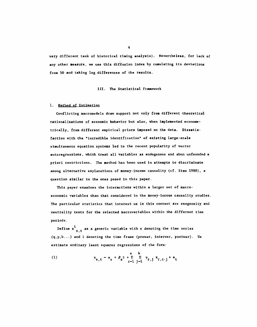
very different task of historical timing analysis). Nevertheless, for lack of

any other measure, we use this diffusion index by cumulating its deviations

from 50 and taking log differences of the results.

III. The Statistical Framework

1. Method of Estimation

Conflicting macromodels draw support not only from different theoretical

rationalizations of economic behavior but also, when implemented econome-

trically, from different empirical priors imposed on the data. Dissatis-

faction with the "incredible identification" of existing large-scale

simultaneous equation systems led to the recent popularity of vector

autoregressions, which treat all variables as endogenous and shun unfounded a

priori restrictions. The method has been used in attempts to discriminate

among alternative explanations of money-income causality (cf. Sims 1980), a

question similar to the ones posed in this paper.

This paper examines the interactions within a larger set of macro-

economic variables than that considered in the money-income causality studies.

The particular statistics that interest us in this context are exogeneity and

neutrality tests for the selected macrovariables within the different time

periods.

Define x as a generic variable with s denoting the time series

(q,p,b...) and i denoting the time frame (prewar, interwar, postwar). We

estimate ordinary least squares regressions of the form:

s k(1) x —a y x +e

S,t 5 5 r,j r,t-j tr—l j—1

10

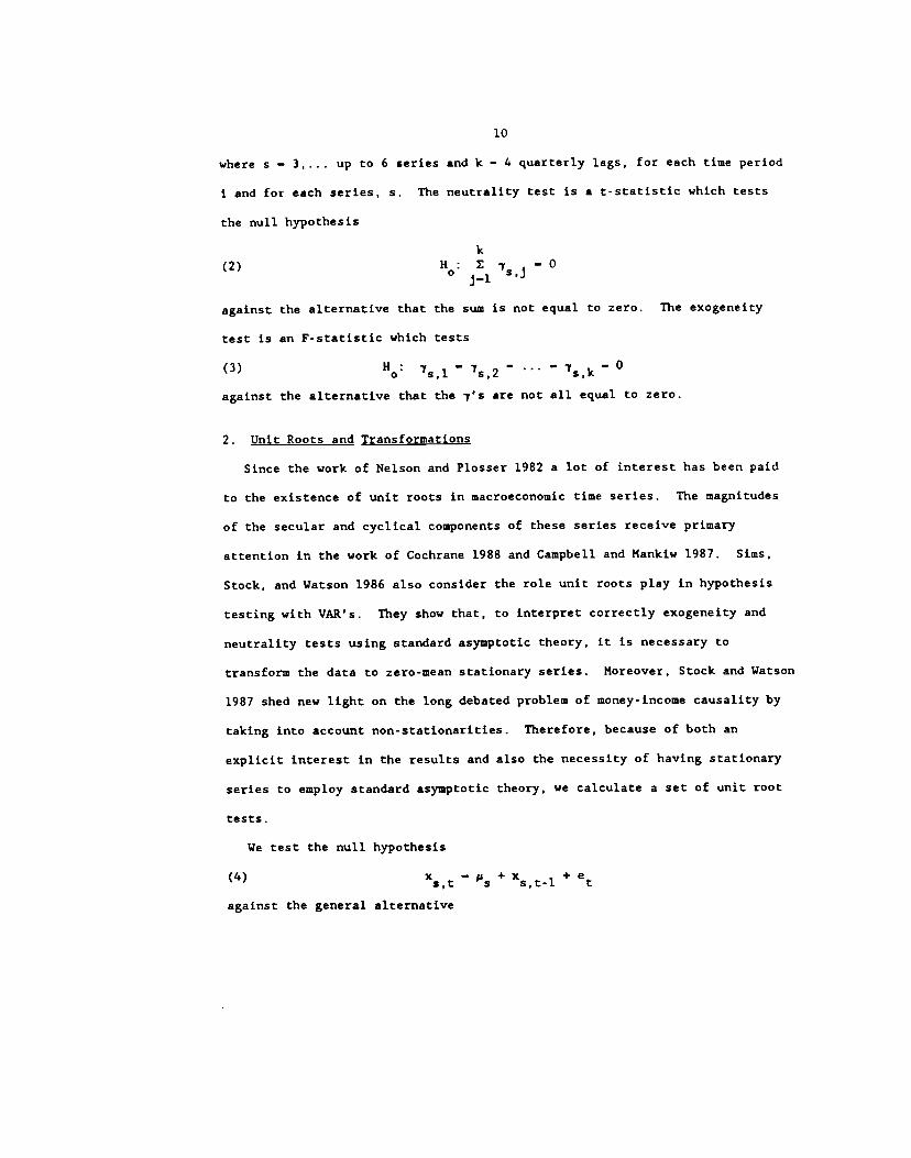
where s — 3,... up to 6 series and k — 4 quarterly lags, for each time period

I and for each series, s. The neutrality test is a t-statistic which tests

the null hypothesis

k(2) H: E -y —0

i—i,j

against the alternative that the sum is not equal to zero. The exogeneity

test is an F-statistic which tests

(3) H0: s,l—

s,2— ' —

s,k— 0

against the alternative that the ys are not all equal to zero.

2. Unit Roots and Transformations

Since the work of Nelson and Plosser 1982 a lot of interest has been paid

to the existence of unit roots in macroeconomic time series. The magnitudes

of the secular and cyclical components of these series receive primary

attention in the work of Cochrane 1988 and Campbell and Mankiw 1987. Sims,

Stock, and Watson 1986 also consider the role unit roots play in hypothesis

testing with VAR's. They show that, to interpret correctly exogeneity and

neutrality tests using standard asymptotic theory, it is necessary to

transform the data to zero-mean stationary series. Moreover, Stock and Watson

1987 shed new light on the long debated problem of money-income causality by

taking into account non-stationarities. Therefore, because of both an

explicit interest in the results and also the necessity of having stationary

series to employ standard asymptotic theory, we calculate a set of unit root

tests.

We test the null hypothesis

(4) — + xstl + etagainst the general alternative

11

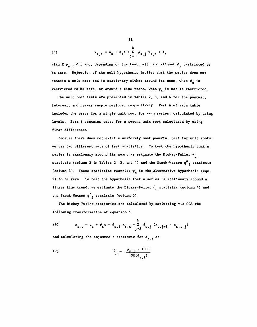
(5) + #st + P5 5,t

with E p < 1 and, depending on the test, with and without restricted to

be zero. Rejection of the null hypothesis implies that the series does not

contain a unit root and is stationary either around its mean, when is

restricted to be zero, or around a time trend, when is not so restricted.

The unit root tests are presented in Tables 2, 3, and 4 for the postwar,

interwar, and prewar sample periods, respectively. Part A of each table

includes the tests for a single unit root for each series, calculated by using

levels. Part B contains tests for a second unit root calculated by using

first differences.

Because there does not exist a uniformly most powerful test for unit roots,

we use two different sets of test statistics. To test the hypothesis that a

series is stationary around its mean, we estimate the Dickey-Fuller

statistic (column 2 in Tables 2, 3, and 4) and the Stock-Watson qlSf statistic

(column 3). These statistics restrict S in the alternative hypothesis (eqn.

5) to be zero. To test the hypothesis that a series is stationary around a

linear time trend, we estimate the Dickey-Fuller statistic (column 4) and

the Stock-Watson qTf statistic (column 5).

The Dickey-Fuller statistics are calculated by estimating via OLS the

following transformation of equation 5

(6) — + + s,l xstj—2

(X5jj - x5j)and calculating the adjusted t-statistic for as

(7) — s.l - 1.00

SE(#

12

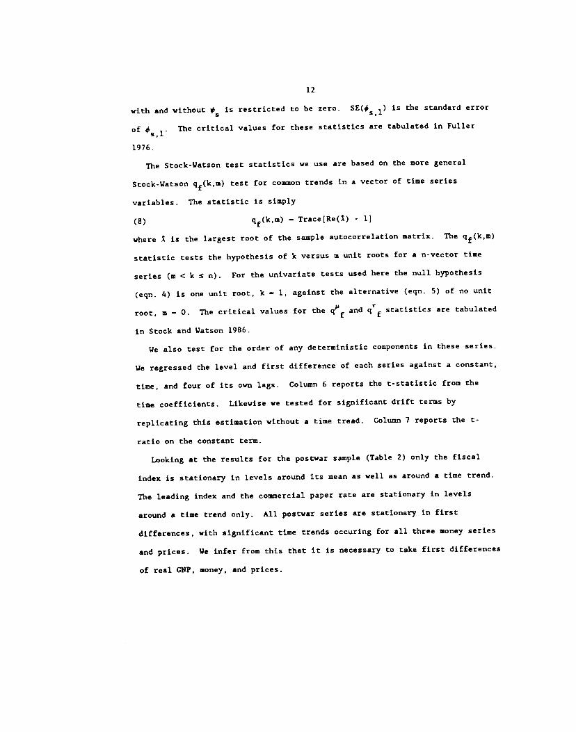
with and without is restricted to be zero. SE(# l is the standard error

of The critical values for these statistics are tabulated in Fuller

1976.

The Stock-Watson test statistics we use are based on the more general

Stock-Watson qf(k,m) test for common trends in a vector of time series

variables. The statistic is simply

(8) qf(k,w) — Trace(Re() - 1]

where I is the largest root of the sample autocorrelation matrix. The qf(k,uI)

statistic tests the hypothesis of k versus m unit roots for a n-vector time

series (m < k � n). For the univariate tests used here the null hypothesis

(egn. 4) is one unit root, k — 1, against the alternative (eqn. 5) of no unit

root, is — 0. The critical values for the qf and qTf statistics are tabulated

in Stock and Watson 1986.

We also test for the order of any deterministic components in these series.

We regressed the level and first difference of each series against a constant,

time, and four of its own lags. Column 6 reports the t-statistic from the

time coefficients. Likewise we tested for significant drift terms by

replicating this estimation without a time tread. Column 7 reports the t-

ratio on the constant term.

Looking at the results for the postwar sample (Table 2) only the fiscal

index is stationary in levels around its mean as well as around a time trend.

The leading index and the commercial paper rate are stationary in levels

around a time trend only. All postwar series are stationary in first

differences, with significant time trends occuring for all three money series

and prices. We infer from this that it is necessary to take first differences

of real GNP. money, and prices.

13

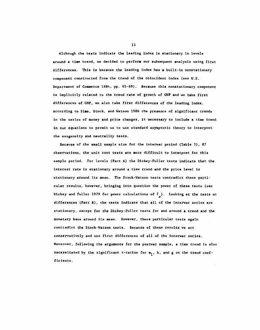
Although the tests indicate the leading index is stationary in levels

around a time trend, we decided to perform our subsequent analysis using first

differences. This is because the leading index has a built-in nonstationary

component constructed from the trend of the coincident index (see U.S.

Department of Commerce 1984. PP. 65-69). Because this nonstationary component

is implicitly related to the trend rate of growth of CNP and we take first

differences of CNP, we also take first differences of the leading index.

According to Sims, Stock, and Watson 1986 the presence of significant trends

in the series of money and price changes, it necessary to include a time trend

in our equations to permit us to use standard asymptotic theory to interpret

the exogeneity and neutrality tests.

Because of the small sample size for the interwar period (Table 3), 87

observations, the unit root tests are more difficult to interpret for this

sample period. For levels (Part A) the Dickey-Fuller tests indicate that the

interest rate is stationary around a time trend and the price level is

stationary around its mean. The Stock-Watson tests contradict these parti-

cular results, however, bringing into question the power of these tests (see

Dickey and Fuller 1979 for power calculations of ). Looking at the tests on

differences (Part B), the tests indicate that all of the interwar series are

stationary, except for the Dickey-Fuller tests for and around a trend and the

monetary base around its mean. However, these particular tests again

contradict the Stock-Watson tests. Because of these results we act

conservatively and use first differences of all of the interwar series.

Moreover, following the arguments for the postwar sample, a time trend is also

necessitated by the significant t-ratios for m1, b, and g on the trend coef-

ficients.

14

Finally, for the prewar sample (Table 4) it is sufficient to take first

differences only of real CNP, the monetary base, 112, the implicit price

deflator while the series on government expenditures and the interest rate carl

be left in levels. Again, although the tests indicate the leading diffusion

index is stationary in levels around a trend, we instead use first differences

of this series in our subsequent analysis. This is because the trend is

artificially induced via the accumulation of the original series. A time

trend is also included because of the significant trend coefficient for

inflation.

IV. The Results

1. Factors Influencing Changes in Real CNP: A Stepwise Approach

(a) 1949-1982

Table 5 is based on regressions of real GNP growth on its own past

i — 1 4) and the lagged values of 2-5 other selected series, plus a

constant term and time. Each variable has the form shown in Table 1, column

4, as indicated by the tests discussed in part III. The calculations proceed

by successively expanding the set of explanatory variables, in four steps.

First only the lagged terms of q are used along with the corresponding values

of a fiscal and a monetary variable. To this are added, second, the inflation

group, and, third, the interest rate group. The last step consists in

including the leading index terms as well.

This table and those that follow are standardized to show the F-statistics

for conventional tests of exogeneity and, underneath these entries, the t-

statistics for the neutrality tests, i.e., for the of the regression

coefficients of the same groups of lagged terms for each variable. The

15

estimated individual coefficients are too numerous to report and their

behavior is difficult to describe in the frequent cases where their successive

values oscillate with mixed signs. It seems advisable, however, to show at

least the summary t-ratios in each equation. When sufficiently large, these

statistics suggest that the individual terms in each group are not all weak or

not all transitory, that is, that they do not offset each other across the

different lags.

In the 1949-82 equations with three variables only, the lagged q terms are

always significant at least at the 5% level; each of the monetary alternatives

makes a contribution (m2 is particularly strong); and the fiscal index C is

relatively weak, except when used along with the monetary base b (Table 5,

part A, equations 1-3). Adding inflation p is of little help in explaining q,

but on balance the coefficients of p are negative and some may matter (eqs. 4-

6). When the commercial paper rate I is entered, it acquires a dominant role

at the expense of the other (especially the monetary) variables (eqs. 7-9).

Finally, equations 10-12 show that, of all the variables considered, the rate

of change in the leading index exerts the strongest influence on q. Five of

the test statistics for i are significant at the 1/10 of one percent level,

one at the 1% level. The level of interest rates represented by I retains its

strong net inverse effect on q. The direct contributions of m1, in2, and C to

the determination of real CNP growth are much fewer and weaker, those of b and

p are altogether difficult to detect.11

Alternative calculations show that when 1 is added to the equations with

the monetary and fiscal variables only, the effects of these variables on q

are again drastically reduced. Had we retained the money, credit, and stock

price components in the leading index, the role of the index in these

16

equations would have been even stronger, that of the other regressors

generally weaker.12

The changes in the index can be interpreted broadly as representing dynamic

forces within the private economy: the early collective outcomes of invest-

ment and production (also, less directly, consumption) decisions. Presumably,

both aggregate demand and aggregate supply shifts are involved, but the

effects of the former are likely to be stronger in the short run. In any

event, the evidence indicates that the quarterly movements of the economy's

output in 1949-82 depended much more on recent changes in leading indicators

and interest rates than on recent changes in output itself, money, the fiscal

factor, and inflation.

Conceivably, longer lags could produce different results, so we checked to

see what happens when eight instead of four lags are used. These tests

suggest some gains in power for the lagged q and C terms, but the leading

index and the interest rate still have consistently strong effects. However,

we do not report these statistics because the restriction to lags of 1-4

quarters is dictated by the limitations of the available data. With eight

lags, for example, the number of degrees of freedom is reduced from 109 to 81

for the six-variable equations.

(b) 1919-1940

In the equations for the interwar period, all variables appear in form of

first differences. In the first subset (Table 5, part B, eqs. 13-15). q

depends positively on its own lagged values and those of the monetary

variables, inversely on the recent values of federal expenditures gx. All the

F-statistics are significant, most highly so. On the other hand, inflation

contributes but little to these regressions, as shown by the results for

17

equations 16-18 (only two t-tests indicate significance and none of the F-

tests). Further, no gains at all result from the inclusion of the change in

the commercial paper rate (eqs. 19-21).

In contrast, there is strong evidence in our estimates for 1919-40 that the

lagged rates of change in the index of six leading indicators (Id) had a large

net positive influence on q. Four of the corresponding test statistics are

significant at the 1% level, two at the 5% level (part B. column 6). In these

equations (22-24), ld shows the strongest effects, followed by the monetary

variables; gx is significant only in one case; and the tests for lagged q, p.

and i terms are all negative.

On the whole, the monetary series appear to play a somewhat stronger role

in the interwar than in the postwar equations, while the leading series appear

to play a somewhat weaker role. It should be recalled, however, that 1 is a

more comprehensive index than Id and is based on better data. Even for the

series hat are more comparable across the two periods the quality of the

postwar data is probably significantly higher)3 Further, the reliability of

the results for 1919-40 suffers from the small sample problem: the number of

observations per parameter to be estimated is here little more than half the

number available for 1949-82.

In light of these considerations it seems important to note that the

interwar results resemble broadly the postwar results in most respects and

look rather reasonable, at least in the overall qualitative sense. The

leading indexes are highly effective in the regressions for both periods. The

main difference between the two sets of estimates is that the commercial paper

rate contributes strongly to the statistical explanation of q in 1949-82 but

the change in that rate does not help in the 1919-40 regressions (cf. columns

18

5 in parts A and B of Table 5). We checked whether interest levels (I) would

have performed significantly better than interest changes (i) in the interar

equations. and the answer is no.

(c) l886-l91

For the pre-Worid War I period, the equations with three variables indicate

strong effects on q of its own lagged values and those of in2, but no signi-

ficant contributions of either the monetary base or government expenditures

(Table 5, part C, eqs. 25-26). The inflation terms add only a weak negative

influence, as shown in the summary t-statistics for equations 27-28.

The recent values of the commercial paper rate have substantial inverse

effects on the current rate of change in real CNP. particularly in the

equations with the base and after the change in diffusion index of leading

indicators (ldc) is added (eqs. 29-32). The Edc index itself appears to be

ineffective. In light of the major importance of the leading indexes in the

postwar and interwar equations, this negative result is probably attributable

mainly to the way .Edc is constructed. (Recall from our discussion in section

11.1 that this index uses only the historical information on specific-cycle

turning points in a set of 75 individual indicators.)

2. Test Statistics for Six-Variable Equations

(a) 1949-1982

Each of the monetary variables (b,m1,m2) depends strongly on its own lagged

values and those of the interest rate I, as shown by the corresponding F-

values in Table 6, equations 1-3. The I terms have coefficients whose signs

vary and their t-statistics are on balance small, though mostly negative. The

fiscal index C appears to have a strong positive effect on in, and the time

19

trends in column 7 are important. The effects of the other variables are

sporadic and weak.

C is more strongly autoregressive yet. It also depends positively on b and

and inversely on I. the change in the leading index 1. and time (equations

4-6).

Inflation p also depends mainly on its own lagged values, according to

equations 7-9. A few relatively weak signs of influence appear for b, I, and

C. The time trends are significant. These results are consistent with a view

of the price level as a predetermined variable adjusting but slowly with

considerable inertia. Monetary influences on p involve much longer lags than

are allowed here.

The interest rate depends most heavily on its own recent levels, as is

immediately evident from equations 10-12. Still, some significant inputs into

the determination of I (which yields R2 as high as .95) are also made by other

factors, notably m1 and 1.

As for 1, it is not strongly influenced by either its own recent past or

that of the other variables. The largest F-values here are associated with

the interest rate in equations 13 and 14 and with inflation in equation 15.

The corresponding tests for real GNP (q) equations have already been

discussed in the previous section (relating to the estimates in the last six

lines of Table 5, part A). It is interesting to note that very few signi-

ficant F or t statistics are associated with the lagged q terms according to

our tests (Table 6, column 1).

(b) 1919-1940

Tests based on the interwar monetary regressions indicate high serial

dependence for m1 and m2 but not b (Table 7. eqs. 1-3). The base is

20

influenced strongly by recent changes in output q, moderately by those in the

leading index Id. There are signs of some effects on m2 of Id and p. but no

measurable outside influences on

Equations 4-6 for the rate of change in government expenditures gx produce

F-statistics that are generally low and apparently significant only for the

lagged values of the dependent variable. The same applies to the equations

10-12 for the change in the interest rate i.

The rate of inflation p depends heavily on its own lagged values, too (eqs.

7-9). Some of the test statistics suggest that Id, and perhaps i, may

influence p slightly over the course of a year.

Interestingly, according to equations 13-15, Id is affected much more

strongly by the recent monetary chagnes than by its own lagged values. There

are also some signs of influence of gx on Id. This raises the possibility

that monetary and fiscal changes, including those due to policy actions, may

affect real GNP with long lags through the mediating role of the leading

indicators (Id). But note that this is only suggested by the estimates for

the interwar period, not those for the postwar era.13

Comparing Tables 6 and 7 and drawing also on Table 5 (parts A and B,

equations 10-12 and 22-24), we observe that q depends strongly on the leading

indexes (I,ld) in both periods and on the monetary factors in the interwar

period. The autoregressive elements are weak in q, 1, and Id and strong (as a

rule dominant) in the other variables according to the interwar as well as the

postwar estimates. The effects of q on the other factors are generally weak

or nonexistent.

(c) 1886-1914

The F-statistics for the own-lag terms are significant in all the pre-Worid

21

War I equations, highly so (at the 0.1% level) for the monetary, fiscal.

leading, and interest series, less so for q and p (see Table 8 and Table 5, C,

equations 30-32). The leading index idc for 1886-1914 is very strongly

autocorrelated, in contrast to the indexes Id for 1919-40 and 1 for 1949-82.

This reflects the construction of the prewar index, which assumes smooth

cyclical movements in the index components (cf. section 11.2 above).

Prewar changes in the monetary base are poorly "explained, mainly by own

lags and those of government expenditures CX and the commercial paper rate I.

The corresponding changes in the stock of money m2 are fit much better by

lagged values of itself, I, and p. And as much as 94% of the variance of

CX is explained statistically, mainly by lagged CX terms and the time trend.

(See Table 8, eqs. 1-4).

The estimates for inflation p are problematic. They suggest that p was

influenced positively by lagged money changes but also inversely by its own

lagged values and those of I and .Rdc. The R2 coefficients are of the order of

0.2-0.3 (eqs. 5-6).

The equations for the interest rate (7-8), besides being dominated by

autoregressive elements, indicate some short-term effects of q (with plus

signs) and m2 (minus). These results seem generally reasonable.

The leading diffusion index Idc (eqs. 9-10) depends primarily on own lags,

with traces of positive effects of q and p and negative effects of I. In view

of the probable measurement errors involved (mainly in the .Edc series), the

serviceability of these estimates is uncertain.

V. Conclusions and Further Steps

The following list of our principal findings begins with a point of

22

particular importance, which receives clear support from the better-quality

data available to us for the postwar and interwar periods.

1. Output depends strongly on leading indexes in equations which include

also the monetary, fiscal, inflation, and interest variables (all taken in

stationary form, with four quarterly lags in each variable). Hence models

that omit the principal leading indicators are probably seriously

misspecified.

2. Short-term nominal interest rates had a strong inverse influence on

output (specifically, the rate of change in real GNP) during the 1949-82

period. When interest is included, the effects of the monetary and fiscal

series are reduced (this resembles the results of some earlier studies; cf.

Sims 1980). When the leading index is also included, most of the monetary

effects are further diminished.

3. In the interwar period, the role of money appears greater, while the

fiscal and interest effects tend to wane. In the prewar (1886-1914)

equations, output is influenced mainly by its own lagged values and those of

the money stock and the interest rate. The other factors including a

diffusion index based on specific cycles in a large set of individual leading

series, have no significant effects. However, this probably reflects errors

in the data, especially the weakness of the available leading index.

4. The monetary, fiscal, and interest variables depend more on their own

lagged values than on any of the other factors, and the same is true of

inflation, except in 1886-1914. The opposite applies to the rates of change

in output and (again, except in 1886-1914) the leading indexes. None of the

variables in question can be considered exogenous.

5. The reported unit root tests are consistent with earlier findings that

23

most macroeconomic time series are difference-stationary (see Nelson and

Plosser 1982 on annual interwar and postwar data, and Stock and Watson 1987 on

monthly postwar data). The major exceptions to this are the prewar and

postwar fiscal and interest series.

Our work offers some suggestions for further research. The following steps

should be taken or at least considered:

(a) Construct a satisfactory composite index of leading indicators for the

periods before World War II from the best available historical data.

(b) Compute variance decompositions and impulse response functions for

alternative subsets of up to four variables represented by the quarterly

series used in this paper.

(c) Do the same computations for larger sets of six variables by using

monthly data. This would complement the results obtained here for individual

equations in the same sets; further, it would permit comparisons with some

recent smaller VAR models estimated on monthly data. The main problem with

this approach is that no good monthly proxies for GNP may be found.

(d) Update the postwar series and check on predictions beyond the sample

period, e.g., for 1983-88.

(e) Try to find Out where the explanatory or predictive power of the

leading index is coming from by testing important subindexes relating to

investment commitments profitability, etc.

(f) Compare the implications of this paper with those of the most recent

and ongoing studies of leading indicators (de Leeuw 1988, 1989; Stock and

Watson 1988 a,b).

Table

I

List of Variables, Symbols, and Sources of Data

a

b

C

d e

f

Number

Variable

Periods

Form

Symbol

Source

Notes on Oer%vation

(1)

(2)

(3)

(4)

(5)

(6)

(7)

1

Real GaP

1,2.3

ln

q

BIG

Annual data from F&S (1982) and cuoriets (1961

(1972 dol.)

and Commerce NIPA (1981 ff, since 1889).

interpolated quarterly by Chow-Lin (1971)

method u

sing

the

Persons (1931)

index of

industrial production and trade.

2

Implicit price

1,2,3

Am

p BIG

(nominal GNP/real GaP)

x 100

deflator

3

Monetary base

1,2,3

Atn

b

BIG

Based on deta in FIS (1970, 1963) through 1914

and Gordon a

nd VeItch 1

986 for 1949-82.

4

Money supply, Ml

2,3

AIn

BIG

1919-46:

Gordon a

nd Veitch 1

986;

1947-58:

old Ml, fj.

1958

-82:

new Ml, FRB.

5

Money supply, M2

1,2,3

AIn

BIG

1886-1907: FIS

1970

; 1907.1914: 1919-80:

Gordon 1

982;

1980-82: ElI.

6 Commercial

paper rate

1,3

level

I

BIG

1886-89:

in New York City, from Macaulay

1938; 1890-1914,

1919-80:

4-6 month prime

From Gordon 1

982.

1981-62:

6 month, from

FRB -

7 do

. 2

1

BIG

do.

8

Federal expenditures

1

In level

OX

Fire-

Based on Daily Treasury Statements of

the

stone

United S

tates (see Firestone 1960, App. pp.

76-86, and data, seasonally adjusted,

pp. 97

—111).

9

do.

2

ln

gx

Fire-

do.

St OflO

10

F isca) index

3

In level

C

Blan-

From Blanchard 1985 and Blanchard and Watson

chard

1986, app. 2.2.

Based on data for government

spending, debt, and taaes.

Table

1

(concluded)

11

DifusslOn index,

1

A In

75

Le

adin

g se

ries

Moo

re

Ana

lyze

d In Moore 1961, vol.

I, ch.7.

Based

on specific cycle phases.

Data from Moore

1961, vol. 2, P. 172.

12

Amplitude-adJusted (corn.

posite) index, six leading

series

2

Am

Id

Shiskin

Analyzed

In Shlskin

1961,

pp. 43-55.

Data

from NBER files.

13

Composite index of

leading indicators

3

AIn

Commerce

The composite index of 12 Leading indicators

minus three components:

M2 In constant

dollars, change in business and consumer cred

outstanding, and the index of stock prices,

from BCD.

Alt variables are used as quarterly series.

bPerlod 1:

1886-1914; period 2:

1919-40; period 3

:

1949-82.

first difference in natural logarithm;A: first difference.

dmatl letters are used for rates of change or absolute changes; capital letters are used for

levels of the series.

Batke, Nathan S

. and Robert J. Gordon 1986, Appendix B, Historical Data.

Firestone:

Firestone,

John N. 1960, AppendIx Tables.

Blanchard: Blanchard, Olivier

.i., and Hark W.

watson, 1986, Appendix 2.2.

Moore:

Moore, Geoffrey,

H. 1961.

Shiskin:

Shiskin, Julius

1961.

Commerce:

U.S. Department of Commerce, Bureau of Economic Analysis.

Friedman, Milton and Anna J. Schwartz.

National Income and product Accounts.

Federal Reserve Bulletin.

National Bureau of Economic Research.

Business Conditions Digest (U.S. Department of Commerce).

tdc

F&S

NI PA:

FRU

NBER

BCD

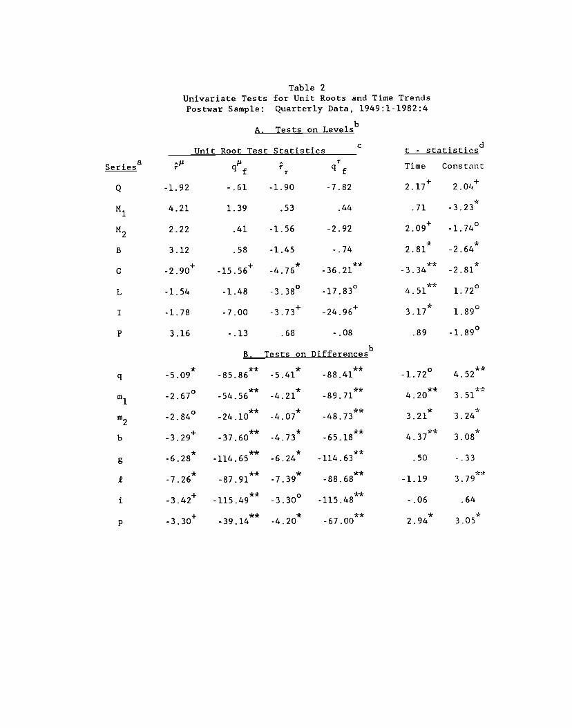
Table 2Univariate Tests for Unit Roots and Time Trends

Postwar Sample: Quarterly Data, 1949:1-1982:4

A. Tests on Levelsb

Unit Root Test Statisticsc

- statisticsda ,. rSeries r q £

r q Time Constant

Q -1.92 - .61 -1.90 -7.82 2.l7 2.O4

4.21 1.39 .53 .44 .71 3.23*

M22.22 .41 -1.56 -2.92

2.09:

-1.74°

B 3.12 .58 -1.45 - .74 2.81 -2.64

+ + * ** ** *C -2.90 -15.56 -4.76 -36.21 -3.34 -2.81

o 0 ** 0L -1.54 -1.48 -3.38 -17.83 4.51 1.72

+ + * 0I -1.78 -7.00 -3.73 -24.96 3.17 1.89

P 3.16 - .13 .68 - .08 .89 -1.89°

B. Tests on Differences'°

* ** * ** 0 **q -5.09 -85.86 -5.41 -88.41 -1.72 4.52

o ** * ** ** **-2.67 -54.56 -4.21 -89.71 4.20 3.51

o ** * ** * *-2.84 -24.10 -4.07 -48.73 3.21 3.24

+ ** * ** ** *b -3.29 -37.60 -4.73 -65.18 4.37 3.08

* ** * **g -6.28 -114.65 -6.24 -114.63 .50 - .33

* ** * ** **-7.26 -87.91 -7.39 -88.68 -1.19 3.79

+ ** 0 **i -3.42 -115.49 -3.30 -115.48 - .06 .64

+ ** * ** * *p -3.30 -39.14 -4.20 -67.00 2.94 3.05

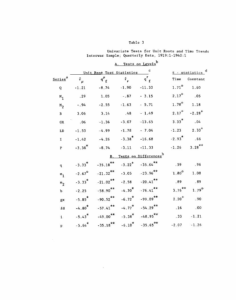
Table 3

Univariate Tests for Unit Roots and Time TrendsInterwar Sample; Quarterly Data, 1919:1-1940:1

A. Tests on Levelsb

dC

aSeries

Arp

Q -1.21

M1.29

112-.94

B 3.06

GX .06

LD -1.53

I -1.42

P*

-3.38

pqf-8.74

1.05

-2.55

3.14

-1.36

-4.99

-4.26

-8.74

Unit Root Test Statistics t - statisticsqT Time Constant

-1.90 -11.33 1.71° 1.60

-.87 - 3.15 2.l7 .05

-1.63 - 5.71 1.78° 1.18

.48 - 1.49 2.17k -2.28k

-3.07 -13.65*

3.33 .04

-1.78 - 7.04 -1.23 2.33k

*-3.38 -16.68

*-2.93 .66

-3.11 -11.33 -1.26**

3.28

q*

-3.33

B. Tests on Differencesb

.59 .96**

-35.18+

-3.22**

-35.64

m1

m2

b

0-2.67*

-3.33

-2.25

-21.32

**-21.02

**-58.90

-3.05

-2.58

*-4.30

**-23.96

**-20.41

**-76.41

01.80

.89

**3.76

1.08

.89

01.79

gx*

-5.85**

-90.52*

-6.72**

-99.09+

2.20 .90

Id*

-4.80**

-57.41*

-4.77**

-54.29 .16 .00

i*

-5.43**

-49.00*

-5.38**

-48.95 .33 -1.21

p*

-5.64**

-35.18*

-6.10**

-35.65 -2.07 -1.26

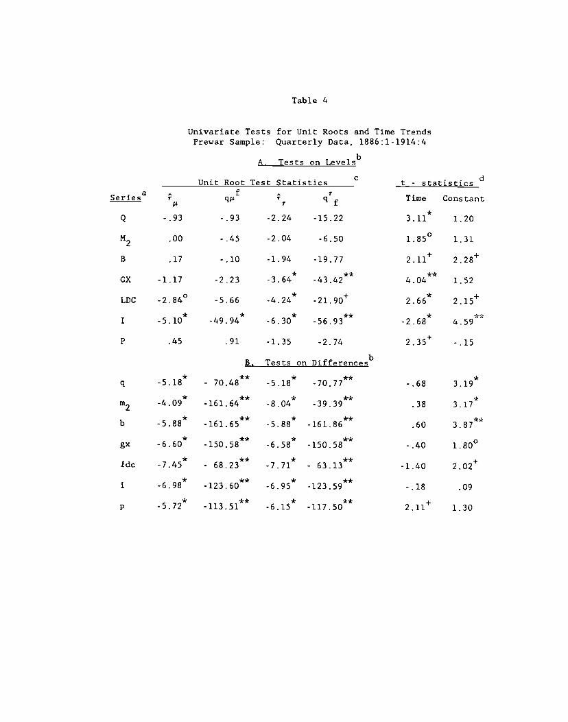
Table 4

t - statisticsTime Constant

*3.11 1.20

1.85° 1.31

2.11k 2.28k

**4.04 1.52

* +2.66 2.15

*-2.68 4.59

2.35k -.15

aSeries

Unit Root

r fq;.

Q - .93 - .93

M2 .00 - .45

B .17 -.10

CX -1.17 -2.23

LDC -2.84° -5.66

I*

-5.10 -49.94*

P .45 .91

q*

-5.18

m2

gx

::-6.60

2dc*

-7.45

i -6.98k

p*

-5.72

Univariate Tests for Unit Roots and Time TrendsPrewar Sample: Quarterly Data, 1886:1-1914:4

A. Tests on Levelsb

Test StatisticsC

rqf-2.24 -15.22

-2.04 -6.50

-1.94 -19.77

* **-3.64 -43.42

* +-4.24 -21.90

* **-6.30 -56.93

-1.35 -2.74

Tests on Differencesb

* **-5.18 -70.77 - .68

* **-8.04 -39.39 .38

* **-5.88 -161.86 .60

* **-6.58 -150.58 - .40

* **-7.71 - 63.13 -1.40

* **-6.95 -123.59 - .18

* ** +-6.15 -117.50 2.11

B.

**- 70.48**

-161.64

-161. 65**

150.58**

- 68.23**

-123. 60**

1l3.5l**

*3.19

3 .17*

**3.87

1.80°

2.O2

.09

1.30

Notes to Tables 2, 3, and 4:

the definitions of the variables, see Table 1. Capital letters denotelevels (in logs, except for I). Small letters denote first differences (in

logs, except for i).

bsignificance level at the 1/10 of 1% level is denoted by ** (except for theDickey-Fuller tests for which .001 significance levels are not tabulated); atthe 1% level, by *; 5% level, by; and at the 10% level by

denotes the Dickey-Fuller (1979) statistic computed using a regression

with four lags. q1f is the Stock-Watson (1986) statistic, also from a

regression with four lags. and q1f are again, respectively, the Dickey-

Fuller and Stock-Watson statistics calculated using a time trend.

dtstatistics for the time and constant coefficient estimated from aregression of the variable on four own lags with time trend and without.

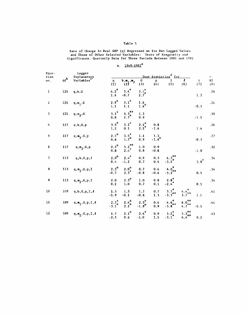
Table 5

Rate of Change in Real CNP (q) Regressed on Its Own Lagged Valuesand Those of Other Selected Variables: Tests of Exogeneity an(I

Significance, Quarterly Data for Three Periods 8etween 1886 and 1982

A. 19491982a

Equa- Laggedtion

b Explanatory Test Statisticsd for —

no. df Variables q b,m ,in C p I t R2

(1) (2 2 (3) (4) (5) (6) (7) (8)

1 121 q.b,G 4.2* 34* 3.l .26

1.6 -0.7 2.7 1.3

2 121q,m1,G

2.9k 3.l 1.6 .26

1.1 1.1. 1.6° -0.3

**3 121

q,m2.G 3.l 5.3, 1.3 .300.8 2.7 0.9 -1.5

* + 04 117 qb.G,p 3.5 3.2 2 1 0 8 26

1.2 0.1 2.2k -1:6 1.4

5 117 q,m1,C,p 2.1° 3.5k 1.1 1.3 .27

0.6 1.7° 0.9 -1.8° -0.3**

6 117q,m2,C,p

2.3° 5.2 1.0 0.9 .300.8 2.4k 0.8 -0.8 -1.0

**7 113 q,b,C,p,I 2.0° 2.4k 0.9 0.3 * .34

0.4 -1.2 0.7 0.4 -3.2 3.0

8 113 q,m1,C,p,I 2.3° 2.0° 0.7 0.4 4.0k .34-0.7 2.3k -0.8 -0.6 -3.2 0.5

9 113 qm2,C,p,I 2.0 2.3° 1.0 0.8 2.8k 340.2 1.0 0.7 0.1 -2.4k 0.5

* *10 109 q,bC,p,I,1 1.3 1.3 1.7 0.7 3.7 4.4 .41

-1.9 -0.1 -0.6 1.3 -3.3 3.7 1.1

11 109q,m1,C,p,I,1

2.7 2.4 2.5k 0.4 6.0:: .44

-3.1 2.2 -1.8° 0.9 -3.8 4.7 -0.5

**12 109

q,m2,C,p,I,21.7 2.1° 2.4k 0.9 3.2: .43

-2.3 0.6 -1.0 1.5 -3.1 4.4 0.2

Table 5

(continued)

Test StatLsticsd f

q b,m •m2 gx p 1

(1) (2 (3) (4) (5)

B. 19191940e

** ** **7.0k 5.2 6.73.0 1.4 -1.4

**2.6 39* 5.30.7k 2.0k -1.3

* * *4.6 4.0 5.21.7° 0.9 -1.5

** ** **5.2k 5.3 5.6 0.93.0 1.4 -1.5 -0.8

* *1.1 5.0k 1.7k0.8 2.7 -0.8 -2.0

o * *2.4 4.6 3.6 1.21.6 1.6 -1.0 -1.7°

* * **4.8k 5.3 0.8 0.22.9 1.5 -1.4 -0.6 -0.5

* *0.8 4.2k 3.61.8k

0.30.6 2.7 -0.8 -2.1 0.5

o * *2.1 3.9 3.6 1.4 0.31.2 1.7° -1.0 -1.7° 0.3

* +1.4 4.1 3.0 1.3 0.2-0.6 1.3 -1.0 -0.1 -0.2

*2.0 3.5 1.9 1.9 0.2

-1.4 2.4k -0.7 -1.4 0.7

1.9 3•7* 1.7 1.2 0.6-0.8 1.5 -0.5 -1.2 0.4

2d t 1(2

(6) (7) (8.

-0.7

-0.5

.410.4

.43-0.4

-0.4

.420.8

.41-0.5

.40-0.5

.39

0.8

*3.9k .502.6 -0.7

*3.5 .492.3k -0.7

*4.02.2k 0.4

.49

Equd - Laggedtiori b Explanatoryno. df Variables

13 67 q.b,gx

14 67q.m1,gx

15 67q,m2,gx

16 63 q,b.gx,p

17 63q.m1,gx,p

18 63 q,m2,gx,p

19 59 q,b,gx,p,i

20 59 q,m1,gx,p,i

21 59 q,m2,gx,p.i

22 55 q,b,gx,p,i.2d

23 55 q,m1,gx,p,i,.td

24 55 q,m2,gx,p,i,ld

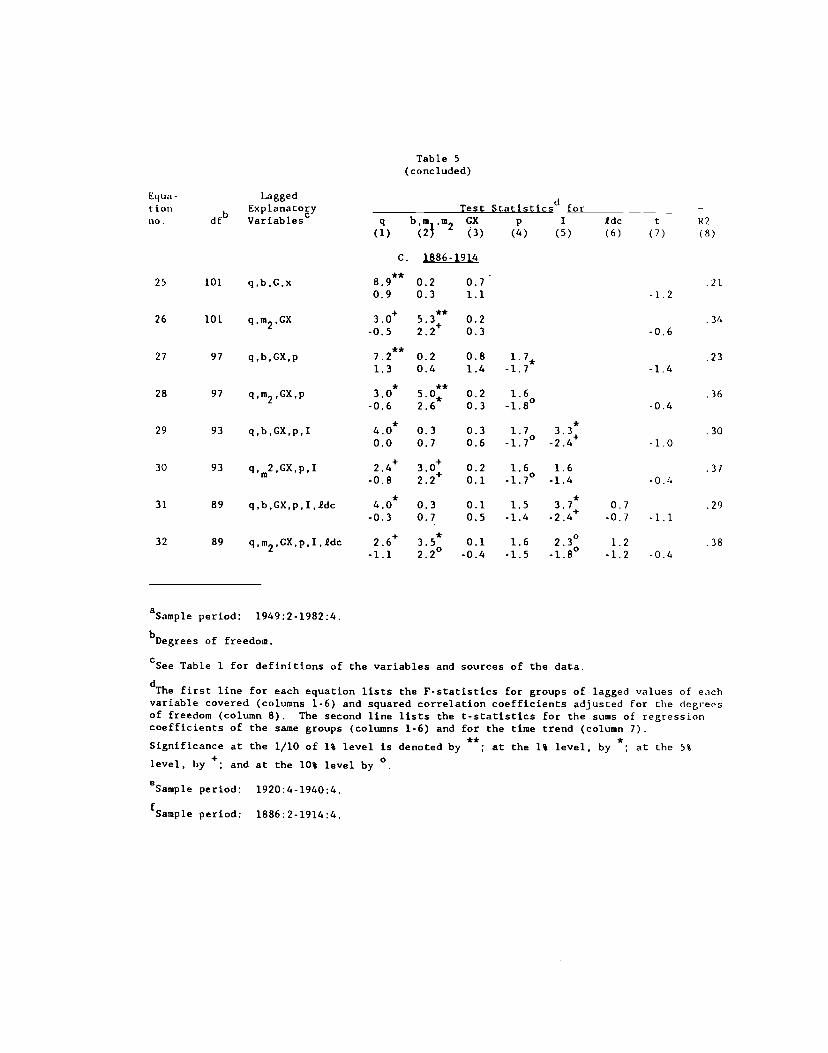
Table 5

(concluded)

Equa- Lagged dtioii b Explanatory Test Statistics for —

no. df Variables q b,m •m2 CX p 1 Ldc t R2

(1) (2 (3) (4) (5) (6) (7) (8)

C. 1886-1914**

25 101 q,b,C,x 8.9 0.2 0.70.9 0.3 1.1 -1.2

26 101q,ni2,GX

3.0k 53** 0.2 .34

-0.5 2.2 0.3 -0.6

27 97 q,b,GX,p 7.2** 0.2 0.8 l.7 .23

1.3 0.4 1.4 -1.7 -1.4

28 97q,m2,CX,p

3.0* 5.0 0.2 1.6 .36

-0.6 2.6 0.3 -1.8 -0.4

* *29 93 q,b,CX,p,I 4.0 0.3 0.3 1.7 3.3÷ .30

0.0 0.7 0.6 -1.7° -2.4 -1.0

30 93 q, 2,CX,p,I 2.4k 3.0k 0.2 1.6 1.6 37m-0.8 2.2k 0.1 -1.7° -1.4 -0.4

* *31 89 q,b,CX,p,I,.edc 4.0 0.3 0.1 1.5 3.7 0.7 .29

-0.3 0.7 0.5 -1.4 -2.4k -0.7 -1.1

32 89q,m2,GX,p,I,ldc

2.6k 35* 0.1 1.62.3:

1.2 .38

-1.1 2.2° -0.4 -1.5 -1.8 -1.2 -0.4

aSample period: 1949:2-1982:4.

bDegrees of freedom.

CSee Table 1 for definitions of the variables and sources of the data.

dThe first line for each equation lists the F-statistics for groups of lagged values of e,chvariable covered (columns 1-6) and squared correlation coefficients adjusted for the degreesof freedom (column 8). The second line lists the t-statistics for the sums of regressioncoefficients of the same groups (columns 1-6) and for the time trend (column 7).

** *Significance at the 1/10 of 1% level is denoted by ; at the 1% level, by ; at the 5%

level, by and at the 10% level by 0

eSl period: 1920:4-1940:4.

Sample period: 1886:2-1914:4.

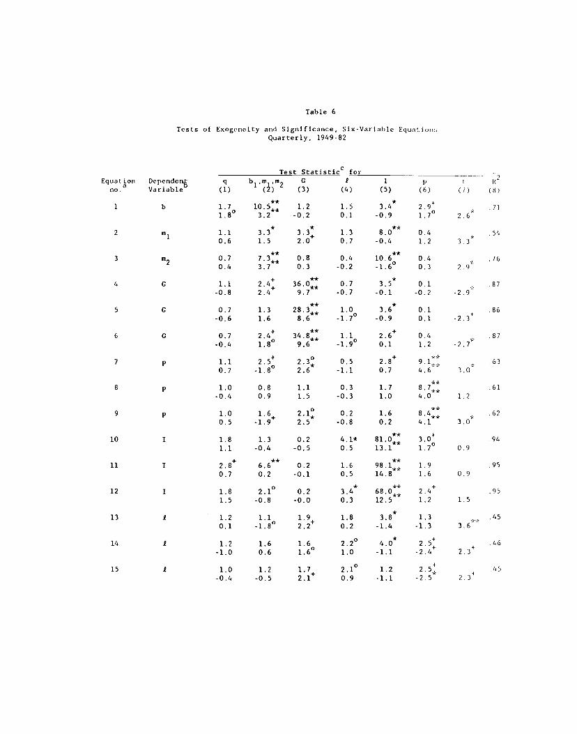
Table 6

Tests of Exogelielty and Significance, Six-Variahie Equatiom.Quarterly, 1949-82

Test StatisticC for -

Equation Dependent qb1,rn,m2

C 1 1 Ino. Variable (1) (3) (4) (5) (6) (1) (8)

I b 1.7 10.5 1.2 1.5 3•4* 2•9f1.8° 3.2 -0.2 0.1 -0.9 1.7° 2.6'

* * **2 1.1 3.3 3.3 1.3 8.0 0.4 54

0.6 1.5 2.0k 0.7 -0.4 1.2 3.3** **

3 0.7 0.8 0.4 10.6 0.4 .760.4 3.7 0.3 -0.2 -1.6° 0.3 2 .9

4 G 1.1 2.4k 36.0 0.7 0.1 .87

-0.8 2.4k -0.7 -0.1 -0.2 -2.9** *

5 C 0.7 1.3 28.3 1.0 3.6 0.1 .86

-0.6 1.6 8.6 -1.7° -0.9 0.1

** +6 C 0.7 2.4 34.8 1.1 2 6 0 4 87

-0.4 1.8° 9.6 -1.9° 0.1 1:2 -2.7

7 p 1.1 2.5 2.3 0.5 2.8k 9.1T .63

0.7 -1.8° 2.6 -1.1 0.7 4.6 3.0**

8 p 1.0 0.8 1.1 0.3 1.7 .61-0.4 0.9 1.5 -0.3 1.0 4.0 1.2

**9 p 1.0 1.6 2.1 0.2 1.6 .62

0.5 -1.9 2.5 -0.8 0.2 4.1 3.0

**10 I 1.8 1.3 0.2 4.1* 81.0 3.O .94

1.1 -0.4 -0.5 0.5 13.1 1.7° 0.9

11 I 2.8k 6.6** 0.2 1.6 98.1:: 1.9 .95

0.7 0.2 -0.1 0.5 14.8 1.6 0.9

12 1.8 2.1° 0.2 3•4* 68.0:: 2.4 .95

1.5 -0.8 -0.0 0.3 12.5 1.2 1.5*

13 1 1.2 1.1 1.9 1.8 3.8 1.3 .45

0.1 -1.8° 2.2k 0.2 -1.4 -1.3 3.6*

14 1.2 1.6 1.6 2.2° 4.0* 2.5k .46-1.0 0.6 1.6° 1.0 -1.1 -2.4k 2.3k

15 £ 1.0 1.2 1.7 2.1° 1.2 2.5:-0.4 -0.5 2.1k 0.9 -1.1 -2.5 2.3

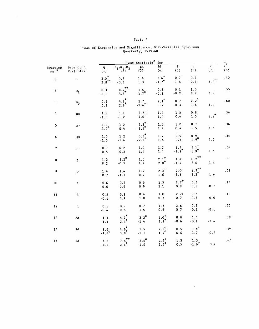
Table 7

Test of Exogeneity and Significance, Six-Variables EquationsQuarterly, 1919-40

Test StatisticC for2

Equation Dependentb q b1,m1,m2 gx 1d i p t R

Variables (1) (2) (3) (4) (5) (6) (7) (8)* +

I b 3.5 0.1 1.4 2.6 0.7 0.7 .60

2.8 -0.3 1.3 -1.7° -1.4 -0.7 3,7

**2 m 0.3 8.2 1.4 0.9 0.1 1.3 .55

1 -0.1 3* -1.7° -0.3 -0.2 0.7 1.5

3in2

0.6 4.6: 1.7 2.10 0.7 2.2° .60

0.3 2.8 -2.4 0.7 -0.3 1.6 1.1

4 gx 1.9 1.1 2.7:1.4 1.5 0.8

+.36

-1.8 -1.2 -2.0 1.4 0.4 1.5 2.1

S gx 1.6 1.2 2.2k 1.5 1.0 0.7 .36-1.9° -0.4 -1.8° 1.7 0.4 1.5 1.5

6 gx 1.3 1.2 3.3k 1.2 0.9 0.9 .36-1.5 -1.4 1.5 0.3 1.9° 1.7

*7 p 0.7 0.2 1.0 1.7 1.7 5.1 .54

0.5 -0.2 1.4 1.4 -2.1k 1.9° 1.1

° 0 **8 p 1.2 2.2 1.5 2.1 1.4 6.2 .60

0.2 -0.5 1.2 2.0k -1.4 2.0 1.4

9 p 1.4 1.4 1.2 2.3k 2.0 .580.7 -1.3 0.7 1.6 -1.6 2.2k 1.6

10 i 0.6 0.7 0.5 1.3 2.7k 0.3 .16-0.6 0.9 0.9 1.1 0.9 0.8 -0.7

11 i 0.5 0.1 0.4 1.0 2.7+ 0.3 .10-0.1 0.1 1.0 0.7 0.7 0.6 -0.0

12 i 0.6 0.9 0.7 1.3 2.6k 0.3 .15-0.4 0.8 1.5 0.9 0.7 0.2 -0.1

13 Id 1.1 47* 2.2° 3.0k 0.8 1.4 .39-1.1 2.4k -1.4 2.2k -0.6 -0.1 -1.4

14 Id 1.3 4.6* 1.5 2.0° 0.5 l.8 .39-1.8° 3.0* -1.1 1.7° 0.6 -1.7 -0.7

15 Id 1.3** 2.0° 2.7k 1.5 1.5 47

-1.2 2.1' -1.0 1.9° 0.5 -1.6° 0.7

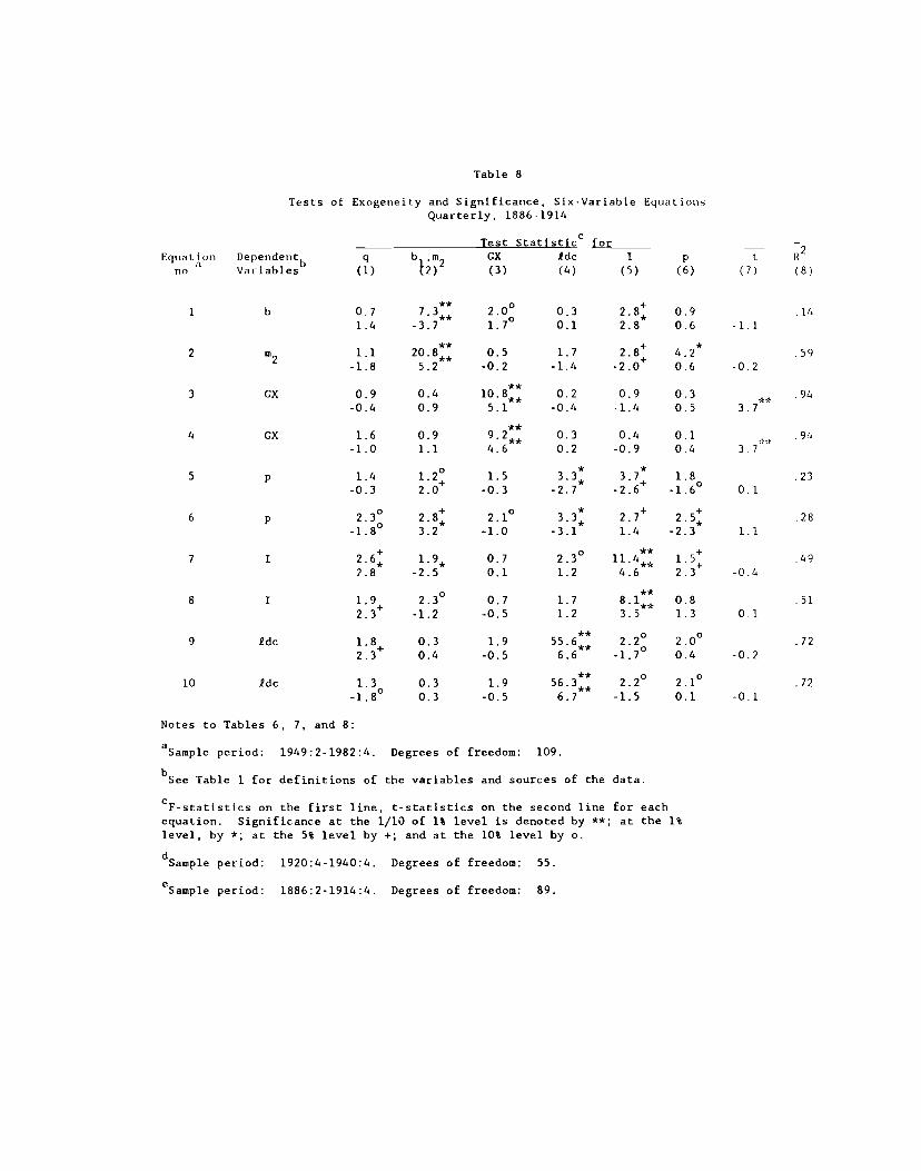
Table 8

Tests of Exogeneity and Significance, Six-Variable EquationsQuarterly. 1886-1914

Test StatisticC for2

Equation Dependentb q brn2

CX ide I p Rno.' Variables (1) t2) (3) (4) (5) (6) (1) (8)

** 0 +1 b 0.7 7.3 2.0 0.3 2.8k 0.9 .16

1.4 -3.7 1.7 0.1 2.8 0.6 -1.1** + *

2 1.1 20.8 0.5 1.7 2.8 4.2 .59** +-1.8 5.2 -0.2 -1.4 -2.0 0.6 -0.2**

3 CX 0.9 0.4 10.8,, 0.2 0.9 0.3 .94

-0.4 0.9 5.1 -0.4 -1.4 0.5 3.7""

**4 CX 1.6 0.9 0.3 0.4 0.1 ., .

-1.0 1.1 4.6 0.2 -0.9 0.4 3. 7o * *

S p 1.4 1.2 1.5 3.3 3.7 1.8 .23+ * + 0-0.3 2.0 -0.3 -2.7 -2.6 -1.6 0.1

6 p 2.3: 2.8: 2.1° •: 2.7 2.5: .28-1.8 3.2 -1.0 -3.1 1.4 -2.3 1.1

+ 0 ** +7 I 2.6k 1.9k 0.7 2.3 11.4 1.5k .49

2.8 -2.5 0.1 1.2 4.6 2.3 -0.4o **

8 1.9 2.3 0.7 1.7 8.1 0.8 .51+ **2.3 -1.2 -0.5 1.2 3.5 1.3 0.1

** 0 09 ide 1.8 0.3 1.9 55.6 2.2 2.0 .72

2.3 0.4 -0.5 6.6 -1.7 0.4 -0.2

** 0 010 ide 1.3 0.3 1.9 56.3+ 2.2 2.1 .72

-1.8 0.3 -0.5 6.7 -1.5 0.1 -0.1

Notes to Tables 6, 7, and 8:

aSample period: 1949:2-1982:4. Degrees of freedom: 109.

bsee Table 1 for definitions of the variables and sources of the data.

cF. on the first line, t-statistics on the second line for eachequation. Significance at the 1/10 of 1% level is denoted by **; at the 1%

level, by *; at the 5% level by +; and at the 10% level by o.

dSaeple period: 1920:4-1940:4. Degrees of freedom: 55.

eSseple period: 1886:2-1914:4. Degrees of freedom: 89.

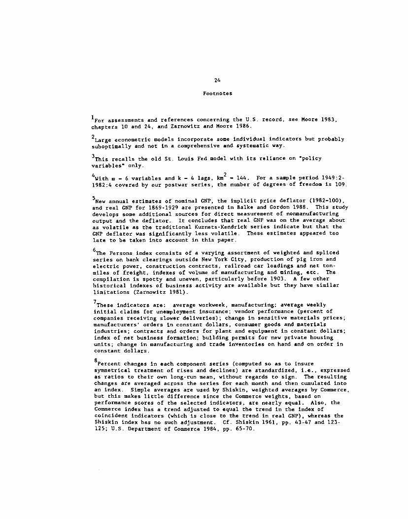
24

Footnotes

1For assessments and references concerning the U.S. record, see Moore 1983,chapters 10 and 24, and Zarnowitz and Moore 1986.

2Large econometric models incorporate some individual indicators but probablysuboptimally and not in a comprehensive and systematic way.

3This recalls the old St. Louis Fed model with its reliance on "policy

variables" only.

4With m — 6 variables and k — 4 lags, km2 — 144. For a sample period 1949:2-1982:4 covered by our postwar series, the number of degrees of freedom is 109.

5New annual estimates of nominal GNP. the implicit price deflator (1982—100),and real GNP for 1869-1929 are presented in Balke and Gordon 1988. This studydevelops some additional sources for direct measurement of nonmanufacturingoutput and the deflator. It concludes that real GNP was on the average aboutas volatile as the traditional Kuznets-Kendrick series indicate but that theGNP deflator was significantly less volatile. These estimates appeared toolate to be taken into account in this paper.

6The Persons index consists of a varying assortment of weighted and splicedseries on bank clearings outside New York City, production of pig iron andelectric power, construction contracts, railroad car loadings and net ton-miles of freight, indexes of volume of manufacturing and mining, etc. Thecompilation is spotty and uneven, particularly before 1903. A few otherhistorical indexes of business activity are available but they have similar

limitations (Zarnowitz 1981).

7These indicators are: average workweek, manufacturing; average weeklyinitial claims for unemployment insurance; vendor performance (percent ofcompanies receiving slower deliveries); change in sensitive materials prices;manufacturers' orders in constant dollars, consumer goods and materialsindustries; contracts and orders for plant and equipment in constant dollars;index of net business formation; building permits for new private housingunits; change in manufacturing and trade inventories on hand and on order inconstant dollars.

8Percent changes in each component series (computed so as to insuresymmetrical treatment of rises and declines) are standardized, i.e., expressedas ratios to their own long-run mean, without regards to sign. The resultingchanges are averaged across the series for each month and then cumulated into

an index. Simple averages are used by Shiskin, weighted averages by Commerce,but this makes little difference since the Commerce weights, based onperformance scores of the selected indicators, are nearly equal. Also, theCommerce index has a trend adjusted to equal the trend in the index ofcoincident indicators (which is close to the trend in real CNP), whereas theShiskin index has no such adjustment. Cf. Shiskin 1961, pp. 43-47 and 123-125; U.S. Department of Commerce 1984, pp. 65-70.

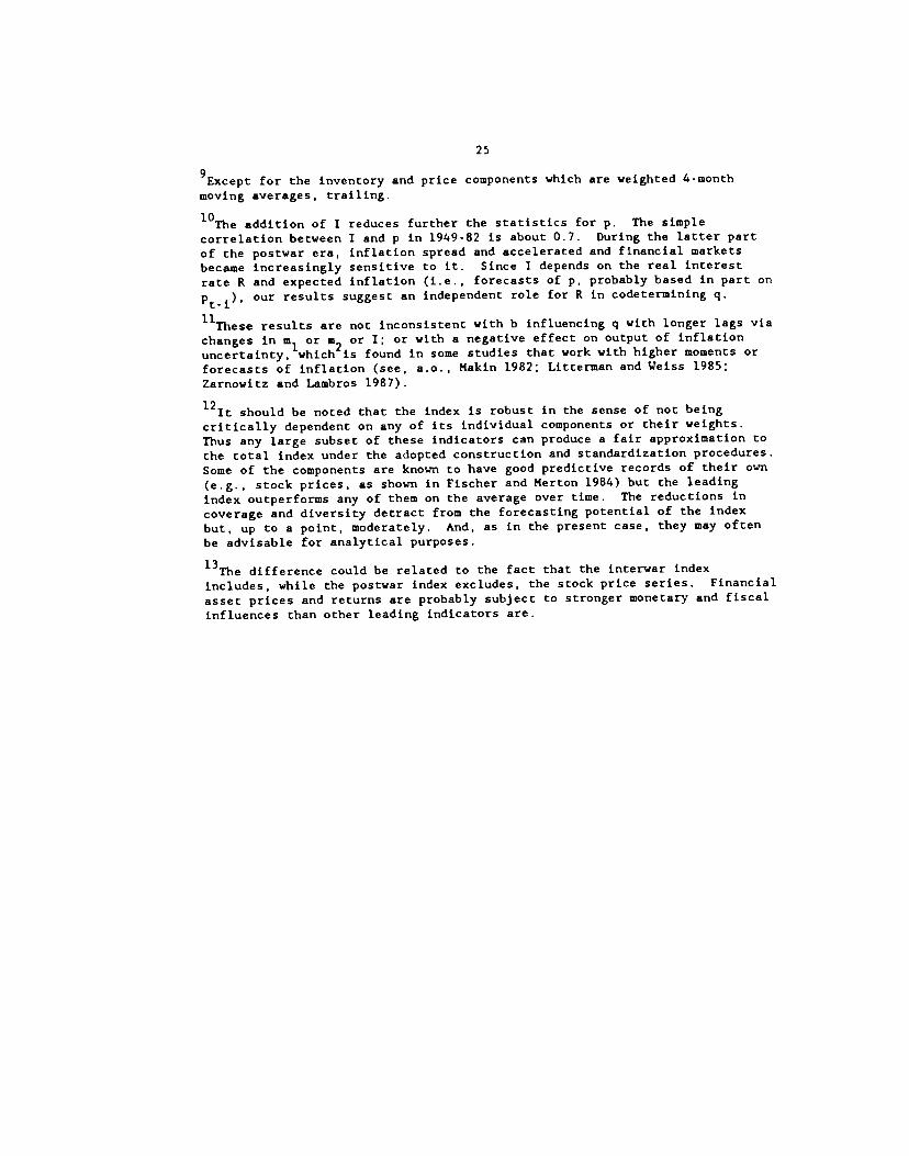
25

9Except for the inventory and price components which are weighted 4-month

moving averages, trailing.

10The addition of I reduces further the statistics for p. The simplecorrelation between I and p in 1949-82 is about 0.7. During the latter partof the postwar era, inflation spread and accelerated and financial marketsbecame increasingly sensitive to it. Since I depends on the real interest

rate R and expected inflation (i.e., forecasts of p. probably based in part onour results suggest an independent role for R in codetermining q.

These results are not inconsistent with b influencing q with longer lags viachanges in m1 or m2 or I; or with a negative effect on output of inflationuncertainty, which is found in some studies that work with higher moments orforecasts of inflation (see, a.o., Makin 1982; Litterinan and Weiss 1985;Zarnowitz and Lambros 1987).

l2 should be noted that the index is robust in the sense of not beingcritically dependent on any of its individual components or their weights.Thus any large subset of these indicators can produce a fair approximation tothe total index under the adopted construction and standardization procedures.Some of the components are known to have good predictive records of their own

(e.g.. stock prices, as shown in Fischer and Merton 1984) but the leadingindex outperforms any of them on the average over time. The reductions incoverage and diversity detract from the forecasting potential of the indexbut, up to a point, moderately. And, as in the present case, they may oftenbe advisable for analytical purposes.

13The difference could be related to the fact that the interwar indexincludes, while the postwar index excludes, the stock price series. Financialasset prices and returns are probably subject to stronger monetary and fiscalinfluences than other leading indicators are.

26

References

Auerbach, A. 1982. The Index of Leading Economic Indicators: "Measurementwithout Theory", Thirty-Five Years Later. Review of Economics andStatistics 64: 589-95.

Balke, N.S. and R.J. Cordon. 1986. Historical Data. In R.J. Cordon ed.

1986. pp. 781-850.

. 1988. The Estimation of Prewar CNP: Methodology and New Evidence.NBER Working Paper no. 2674.

Blanchard, 0.J. 1985. Debt, Deficits, and Finite Horizons. Jurnaj ofPolitical Economy. 93: 223-47.

Blanchard, 0.J. and M.W. Watson. 1986. Are Business Cycles All Alike? InR.J. Cordon, ed., 1986, pp. 123-56 and 178-79.

Braun, P. and S. Mittnik. 1985. Structural Analysis with Vector

Autoregressive Models: Some Experimental Evidence. Washington Universityin St. Louis Working Paper no. 84.

Campbell, J.Y. and N.G. Mankiw. 1987. Permanent and Transitory Components inMacroeconoxnc Fluctuations. American Economic Review 77: 111-117.

Chow, G.C. and A. Lin. 1971. Best Linear Unbiased Interpolation,Distribution, and Extrapolation of Time Series by Related Series. Reviewof Economics and Statistics. 53: 372-76.

Cochrane, J.H. 1988. How Big is the Random Walk in CNP? Journal of PoliticalEconomy. 96: 893-920.

de Leeuw, F. 1988. Prime Movers as Leading Indicators. Bureau of EconomicAnalysis Discussion Paper no. 37.

- 1989. Toward a Theory of Leading Indicators. Forthcoming in K.Lahiri and C. Moore, eds., Leading Economic Indicators: New Aoproaches andForecasting Methods.

Dickey, D.A. and W.A. Fuller. 1979. Distribution of the Estimators forAutoregressive Time Series with a Unit Root. Journal of the AmericanStatistical Society 74: 1057-1072,

Diebold, F.X. and G.P. Rudebusch. 1987. Scoring the Leading Indicators.Manuscript, Division of Research and Statistics, Federal Reserve Board.

Firestone, J.M. 1960. Federal Receipts and Expenditures During BusinessCycles. 1879-1958. Princeton: Princeton University Press for NBER.

Fischer, S. and R.C. Merton. 1984. Macroeconomics and Finance: The Role ofthe Stock Market. Carnegie-Rochester Conference on Public Policy 21: 57-108.

27

Friedman, M. and A.J. Schwartz. 1963. A Monetary History of the UnitedStates. 1867-1960. Princeton: Princeton University Press for NBER.

1970. Monetary Statistics of the United States: Estimates. Sources.and Methods. New York: NBER.

. 1982. Monetary Trends in the United States and the United Kingdom:Their Relation to Income. Prices and Interest Rates. 1867-1975. Chicago:University of Chicago Press for NBER.

Fuller, W.A. 1976. Introduction to Statistical Time Series. New York:

Wiley.

Cordon, R.J. 1982. Price Inertia and Policy Ineffectivesness in the UnitedStates, 1890-1980. Journal of Political Economy. 90: 854-71.

. 1986. The American Business Cycle: Continuity and Change. Chicago:University of Chicago Press for NEER.

Cordon, R.J. and J.M. Veitch. 1986. Fixed Investment in the AmericanBusiness Cycle, 1919-83. In R.J. Cordon, ed., 1986, Pp. 267-335 and 352-357-

Kuznets, S. 1961. Capital in the American Economy: Its Formation andFinancing. Princeton: Princeton Univerity Press for NBER.

Lebergott, S. 1986. Discussion. Journal of Economic History 46: 367-371.

Litterman, R.B. and L.M. Weiss. 1985. Money. Real Interest Rates, andOutput: A Reinterpretation of Postwar U.S. Data. Econonietrica 53: 129-

53.

Litkepohl, H. 1982. Non-Causality Due to Omitted Variables. Journal ofEconometrics 19: 307-378.

Macaulay, F.C. 1938. The Movements of Interest Rates. Bond Yields, and StockPrices in the United States Since 1856. New York: NBER.

Makin, J.K. 1982. Anticipated Money, Inflation, Uncertainty and RealEconomic Activity. Review of Economics and Statistics. 64: 126-35.

Moore, C.H., ed. 1961. Business Cycle Indicators. Princeton: PrincetonUniversity Press for NBER.

. 1983. Business Cycles. Inflation, and Forecasting. BallingerPublishing Co. for NBER.

Nelson, C.R. and C.I. Plosser. 1982. Trends and Random Walks inMacroeconomic Time Series: Some Evidence and Implications. Journal ofMonetary Economics 10: 139-62.

Persons, W.M. 1931. Forecasting Business Cycles. New York: Wiley.