Maintenance Optimization for Heterogeneous Infrastructure Systems: Evolutionary Algorithms for...

K. Gopalakrishnan & S. Peeta (Eds.): Sustainable & Resilient Critical Infrastructure Sys., pp. 185–199. springerlink.com © Springer-Verlag Berlin Heidelberg 2010

Maintenance Optimization for Heterogeneous Infrastructure Systems: Evolutionary Algorithms for Bottom-Up Methods

Hwasoo Yeo*, Yoonjin Yoon, and Samer Madanat

Abstract. This chapter presents a methodology for maintenance optimization for heterogeneous infrastructure systems, i.e., systems composed of multiple facilities with different characteristics such as environments, materials and deterioration processes. We present a two-stage bottom-up approach. In the first step, optimal and near-optimal maintenance policies for each facility are found and used as inputs for the system-level optimization. In the second step, the problem is formulated as a constrained combinatorial optimization problem, where the best combination of facility-level optimal and near-optimal solutions is identified. An Evolutionary Algorithm (EA) is adopted to solve the combinatorial optimization problem. Its performance is evaluated using a hypothetical system of pavement sections. We find that a near-optimal solution (within less than 0.1% difference from the optimal solution) can be obtained in most cases. Numerical experiments show the potential of the proposed algorithm to solve the maintenance optimiza-tion problem for realistic heterogeneous systems.

1 Introduction

Infrastructure management is a periodic process of inspection, maintenance policy selection and maintenance activities application. Maintenance, Rehabilitation, and Reconstruction (MR&R) policy selection is an optimization problem where the objective is to minimize the expected total life-cycle cost of keeping the facilities * Hwasoo Yeo Department of Civil and Environmental Engineering, Korea Advanced Institute of Science and Technology, 335 Gwahangno, Yuseong-gu, Daejeon, Republic of Korea e-mail: [email protected]

Yoonjin Yoon · Samer Madanat Institute of Transportation Studies and Department of Civil and Environmental Engineering, University of California, Berkeley, CA 94720, U.S.A. e-mail: [email protected], [email protected]

186 H. Yeo, Y. Yoon, and S. Madanat

in the system above a minimum service level while satisfying agency budget constraints.

MR&R optimization can be performed using one of two approaches: top-down and bottom-up. In a pavement management system, a top-down approach provides a simultaneous analysis of an entire roadway system. It first aggregates pavement segments having similar characteristics such as structure, traffic loading and environmental factors into mutually exclusive and collectively exhaustive homo-geneous groups. The units of policy analysis are the fractions of those groups in specific conditions, and individual road segments are not represented in the opti-mization. As a result, much of the segment-specific information (history of construction, rehabilitation, and maintenance; materials; structure) is lost.

One of the main advantages of a top-down approach is that it enables decision makers to address the trade-off between rehabilitation of a small number of facili-ties and maintenance of a larger number of facilities, given a budget constraint. On the other hand, the top-down approach does not specify optimal activities for each individual facility, and mapping system-level policies to facility-level activities is left to the discretion of district engineers. One of the early examples of a top-down formulation is Arizona Department of Transportation (ADOT) Pavement Man-agement System (PMS), which selects maintenance and rehabilitation strategies that minimize life-cycle cost. The ADOT PMS saved $200 million over five years (OECD, 1987). However, the Arizona DOT PMS is designed for homogeneous systems where all facilities are assumed to have same characteristics, and cannot be applied to a heterogeneous system where individual facility characteristics are different.

For a heterogeneous system, composed of facilities with different material, de-terioration process, and environmental characteristics, it is necessary to specify optimal maintenance activities at the facility-level. For example, a system of bridges usually consists of facilities of different materials, structural designs and traffic loads. For a heterogeneous system maintenance optimization, a bottom-up approach is appropriate to determine maintenance policies at the facility level.

In formulating heterogeneous system optimization, Robelin and Madanat (2007) proposed a bottom-up approach as follows. First, identify a set of optimal (or near optimal) sequences of MR&R activities for each facility over the desired planning horizon. Then, find the optimal combination of MR&R activity se-quences for entire system given a budget constraint.

The main advantage of the bottom-up approach is that the identity of individual facilities is preserved as we maintain the information associated with each facility such as structure, materials, history of construction, MR&R, traffic loading, and environmental factors. However, preserving individual details leads to high com-binatorial complexity in the system optimization step. The methodology proposed herein is an attempt to overcome such shortcoming of the bottom-up formulation. We propose a two-stage bottom-up approach to address MR&R planning for an infrastructure system composed of dissimilar facilities undergoing stochastic state transitions over a finite planning horizon. This chapter consists of five sections. In Section 2, state-of-the-art methods for MR&R planning are reviewed. In Section 3, a new two-stage approach for solving the heterogeneous system maintenance

Maintenance Optimization for Heterogeneous Infrastructure Systems 187

problem is presented. In Section 4, a parametric study is presented to illustrate and evaluate the new approach. Finally, Section 5 presents conclusions.

2 Literature Review

Infrastructure maintenance optimization problems can be classified into single facility problems and multi-facility problems (also known as system-level problems).

The single facility problem is concerned with finding the optimal policy, the set of MR&R activities needed for each state of the facility that achieves the mini-mum expected life-cycle cost. Optimal Control (Friesz and Fernandez, 1979; Tsu-nokawa and Schofer, 1994), Dynamic Programming (Carnahan, 1988; Madanat and Ben-Akiva, 1994), Nonlinear minimization (Li and Madanat, 2002), and Cal-culus of Variations (Ouyang and Madanat, 2006) have been used as solution methods.

For the system-level problem, the objective is to find the optimal set of MR&R policies for all facilities in the system, which minimizes the expected sum of life-cycle cost within the budget constraint for each year. The optimal solution at the system-level will not coincide with the set of optimal policies for each facility if the budget constraint is binding. Homogeneous system problems have been solved by using linear programming (Golabi et al., 1982; Harper and Majidzadeh, 1991; Smilowitz and Madanat, 2000). The decision variables for linear programming are the proportions of facilities that need a specific MR&R activity at a certain state. This top-down approach has advantages, but as discussed earlier, it cannot be di-rectly applied to MR&R optimization for heterogeneous systems.

Fwa et al. (1996) used genetic-algorithms, to address the trade-off between re-habilitation and maintenance. The authors assumed four categories of agency cost structure, based on the relative costs among rehabilitation and three maintenance activities for 30 homogeneous facilities.

Durango-Cohen et al. (2007) proposed a quadratic programming platform for multi-facility MR&R problem. While the quadratic programming (QP) formulation successfully captures the effect of MR&R interdependency between facility pairs, the applicability of QP is limited to situations when the costs are quadratic. The numerical example in the chapter is limited to facilities with the same deterministic deterioration process, where each facility is a member of either a ‘substitutable’ or a ‘complementary’ network. Although intuitively sensible, the determination of ‘substitutable’ or ‘complementary’ networks might not be evident in large scale networks.

Ouyang (2007) developed a new approach for system-level pavement manage-ment problem using multi-dimensional dynamic programming. He expanded the dynamic programming formulation used in the facility-level optimization to mul-tiple facilities. To overcome the computational difficulty associated with the mul-ti-dimensional problem, he adopted an approximation method and applied this to a deterministic, infinite horizon problem.


Robelin and Madanat (2006) used a bottom-up approach for MR&R optimization of a heterogeneous bridge system. At the facility-level, all possible combinations of decision variables are enumerated; at the system-level, the best combination of the enumerated solutions is determined by searching the solution space. This system-level problem has a combinatorial computational complexity. The authors find a set of lower and upper cost bounds for the optimal solution, which narrows the search space. In a related work, Robelin and Madanat (2008) formulated and solved a risk-based MR&R optimization problem for Markovian systems. At the facility-level, the optimization consists of minimizing the cost of maintenance and replacement, sub-ject to a reliability constraint. At the system-level, the dual of the corresponding problem is solved: risk minimization (i.e., reliability maximization) subject to a budget constraint; specifically, the objective is to minimize the maximum risk across all facilities in the system, subject to the sum of MR&R costs not exceeding the budget constraint. The solution to the system-level problem turns out to have a simple structure, with a linear computational time.

The approach used in Robelin and Madanat (2008) is limited to risk based MR&R optimization, where the objective function has a Min-Max format, and is not applicable for serviceability based optimization problems. For serviceability based problems, the objective function takes on an expected cost minimization (or expected serviceability maximization) which does not lend itself to solutions with such a simple structure. This motivates the approach proposed in this chapter.

3 Methodologies

Consider an infrastructure system composed of N independent facilities, with dif-ferent attributes such as design characteristics, materials, traffic loads: this system is a heterogeneous system. We assume that a managing agency has to find the best combination of maintenance activities within a budget constraint of the current year. This optimization process is repeated at the start of every year using the out-puts of facility inspections. As the optimization is an annual process and the future budgets are unknown, future budget constraints are not considered in the current year optimization.

The objective is to find an optimal combination of facility-level maintenance activities, minimizing the total system-level cost. We assume that two variables, cost and activity, can be defined for all facilities, regardless of individual characteristics.

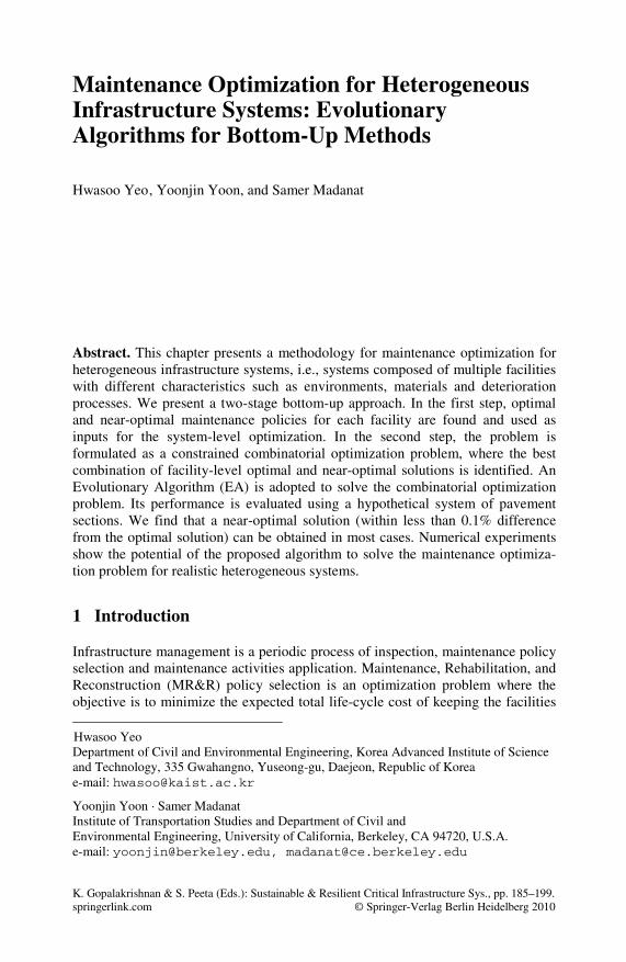
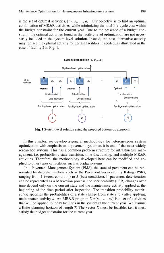
We assume that inspections are performed at the beginning of the year, and the current state of each facility is known. In our two-stage bottom-up approach, we first solve the facility-level optimization to find a set of best and alternative MR&R activities and costs for each facility. In the second stage, we solve the sys-tem-level optimization to find the best combination of MR&R activities across fa-cilities by choosing among the optimal and sub-optimal alternative activities found in the first step. Fig. 1 illustrates the system-level optimization for N facilities. For each facility, the optimal activity and the 1st and 2nd alternative activities are ob-tained from the facility-level optimization. The initial solution in the system-level


is the set of optimal activities, [a1, a3, …, a1]. Our objective is to find an optimal combination of MR&R activities, while minimizing the total life-cycle cost within the budget constraint for the current year. Due to the presence of a budget con-straint, the optimal activities found in the facility-level optimization are not neces-sarily included in the system-level solution. Instead, the next alternative activity may replace the optimal activity for certain facilities if needed, as illustrated in the case of facility 2 in Fig. 1.

2nd alternative

Facility-level optimization

a1 a2 a3 a3 a2 a1

Optimal

1st alternative

2nd alternative

Optimal

1st alternative

2nd alternative

MR&R Activities

a1 a2 a3

Optimal

1st alternative

1 2 N …

…

System-level optimization


System-level solution [a1, a2,…,a2]


Fig. 1 System-level solution using the proposed bottom-up approach

In this chapter, we develop a general methodology for heterogeneous system optimization with emphasis on a pavement system as it is one of the most widely researched systems. This has a common problem structure for infrastructure man-agement, i.e. probabilistic state transition, time discounting, and multiple MR&R activities. Therefore, the methodology developed here can be modified and ap-plied to other types of facilities such as bridge systems.

In a Pavement Management System (PMS), the state of pavement can be rep-resented by discrete numbers such as the Pavement Serviceability Rating (PSR), ranging from 1 (worst condition) to 5 (best condition). If pavement deterioration can be represented as a Markovian process, the serviceability (PSR) changes over time depend only on the current state and the maintenance activity applied at the beginning of the time period after inspection. The transition probability matrix, Pa(i,j) specifies the probabilities of a state change from state i to j after applying maintenance activity a. An MR&R program X =[x1 , …, xN] is a set of activities that will be applied to the N facilities in the system in the current year. We assume a finite planning horizon of length T. The vector X must be feasible, i.e., it must satisfy the budget constraint for the current year.


3.1 Facility-Level Optimization

The facility-level optimization solves for the optimal activity and its cost pair (ac-tion cost and expected-cost-to-go) without accounting for the budget constraint. It also identifies suboptimal alternative policies and their cost pairs. The facility-level optimization for a PMS can be formulated as a dynamic program to obtain an optimal policy and the alternative policies. The dynamic programming formula-tion that solves for optimal activity a* and its expected cost-to-go V* is:

}),()1,(),({min arg),(* ∑ ++=∈∈ SA j

aa

jiPtjViaCtia α (1)

}),()1,(),({min),(* ∑ ++=∈∈ SA j

aajiPtjViaCtiV α (2)

Where,

A: Set of feasible maintenance activities, A ={a1, a2,..} S : Set of feasible states of facility Pa(i,j) : Transition Probability from state i to j under maintenance activity a. C(a,i) : Agency cost for activity a, performed on facility in state i. α: Discount amount factor = 1/(1+r); where r is the discount rate

Other costs such as user costs are not directly included in the formulation, but can be added to the agency cost. In the PMS example, by not allowing pavement states less than a certain threshold value, user costs are indirectly considered.

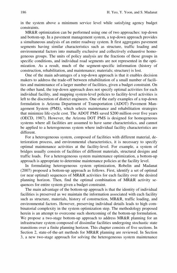
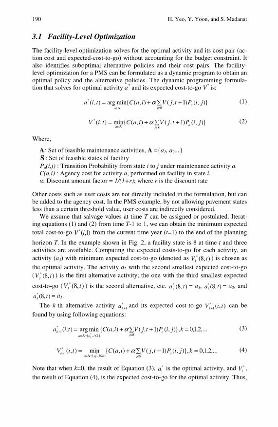
We assume that salvage values at time T can be assigned or postulated. Iterat-ing equations (1) and (2) from time T-1 to 1, we can obtain the minimum expected total cost-to-go )1,(* iV from the current time year (t=1) to the end of the planning

horizon T. In the example shown in Fig. 2, a facility state is 8 at time t and three activities are available. Computing the expected costs-to-go for each activity, an activity (a3) with minimum expected cost-to-go (denoted as ),8(*

1 tV ) is chosen as

the optimal activity. The activity a2 with the second smallest expected cost-to-go ( ),8(*

2 tV ) is the first alternative activity; the one with the third smallest expected

cost-to-go ( ),8(*3 tV ) is the second alternative, etc. ),8(*

1 ta = a3, ),8(*2 ta = a2, and

),8(*3 ta = a1.

The k-th alternative activity *1+ka and its expected cost-to-go ),(*

1 tiVk + can be

found by using following equations:

,...2,1,0},),()1,(),({min arg),(},{

*1

*=∑ ++=

∈≤−∈+ kjiPtjViaCtia

ja

klaak

lSA

α (3)

,...2,1,0},),()1,(),({min),(},{

*1 *

=∑ ++=∈≤−∈

+ kjiPtjViaCtiVj

aklaa

kl SA

α (4)

Note that when k=0, the result of Equation (3), *1a is the optimal activity, and *

1V ,

the result of Equation (4), is the expected cost-to-go for the optimal activity. Thus,


Equations (3) and (4) are used to solve for both optimal and alternative activities. Iterating backward in time, the optimal policy and alternative policies { ,...,, *

3*2

*1 aaa }, and their costs { ,...,, *

3*

2*

1 VVV } can be solved for the current year.

Although the facility-level optimization can also be formulated and solved as a linear program (for the infinite horizon case), we used dynamic programming be-cause it also produces the alternative policies and costs used as inputs for the sys-tem-level optimization without additional calculations.

a1

a2

a3

Activities

t t+1

…

T

8

…

…

…

…

…

time 1

V1(9,t+1)

V1(8,t+1)

V1(7,t+1)

…

a1

a2

a3 3

)1,8(*1V

)1,8(*3V

)1,8(*2V

…

),8(*1 tV

1st alternative

2nd alternative

V1(9,t)

),8(*2 tV

),8(*3 tV

.

.

.

.

.

.

.

.

.

.

.

.

.

.

.

.

.

.

7

9

8

7

9

8

7

9

8

)9,8(1aP

)7,8(3aP

Choose an activity with minimum expected cost-to-go

Optimal

Fig. 2 Dynamic programming process for facility-level optimization

3.2 System-Level Optimization

The facility-level optimizations yield a set of activities { ,...,, *3

*2

*1 aaa } and their

expected cost-to-go { ,...,, *3

*2

*1 VVV } for each facility. Given the agency cost for

each activity, the objective is to find the combination of activities (one for each facility) that minimizes the system-wide expected cost-to-go while keeping the to-tal agency cost within the budget. We refer to this combination of activities as the optimal program. Assuming that all facilities are independent, and given a budget constraint, the system-level optimization can be formulated as a constrained com-binatorial optimization problem.

Let nM ={0, 1, 2,…} be an alternative activity set for facility n, where 0 repre-

sents the optimal activity and i represents i-th alternative activity. The system-level optimal activity nn Mx ∈ will be determined given state sn for facility n. Let

)( nC

n xf denote the expected cost-to-go function, and )( nB

n xf the activity cost

function for facility n given activity nx at current time. Note that

)1,()( *1 nxn

Cn sVxf

n+= for all n, and ),()( nnB

n saCxf = for all n in the facility-level

problem. The combinatorial optimization problem is:


⎟⎠⎞⎜

⎝⎛ ∑=

=

N

nn

Cn xfTEC

1)( min

(5)

Such that:

BxfACN

nn

Bn ≤∑=

=1)( (B: Budget of the current year) (6)

Where, X = ],...[ 1 Nxx is the optimal program, TEC represents the total system ex-

pected cost-to-go from current year to year T and AC the total activity cost. There exist various methods for solving the constrained combinatorial optimi-

zation problem including integer programming and heuristic search algorithms. As the constraints and object function may include nonlinear equations as in Du-rango-Cohen et al. (2007), the general approach must be a nonlinear solution. Cases of nonlinear constraints arise when there exist functional and economic de-pendencies between facilities. For example, contiguous facilities are best rehabili-tated in the same year to reduce delay costs during the rehabilitation. Therefore, the challenge is how to reduce the computation complexity of the algorithm used to solve for the optimal solution. A simple method, the brute force search, search-ing the entire combinatorial solution space, is guaranteed to find the optimal solu-tion. However, with a computational complexity of exponential order, this method cannot be applied to problems of realistic size.

Two-Facility Example

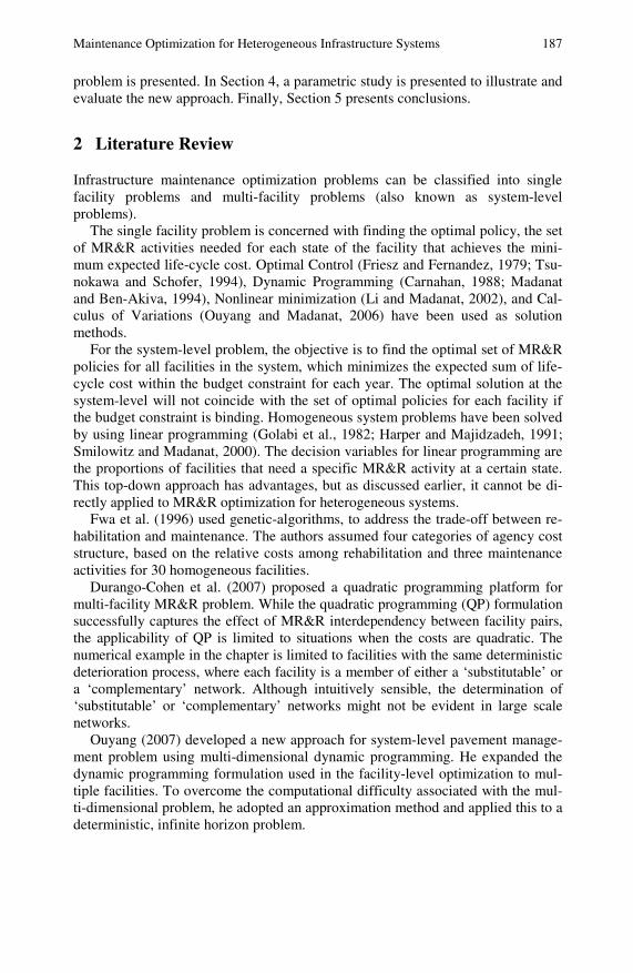
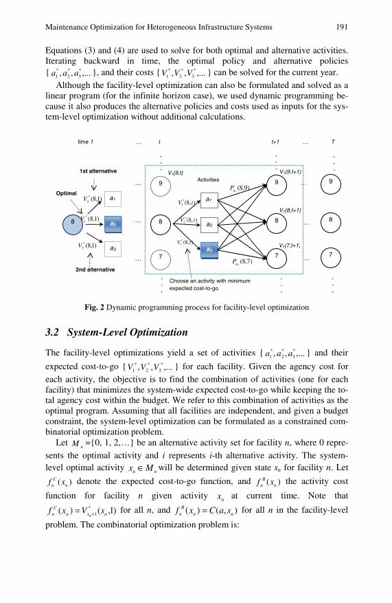
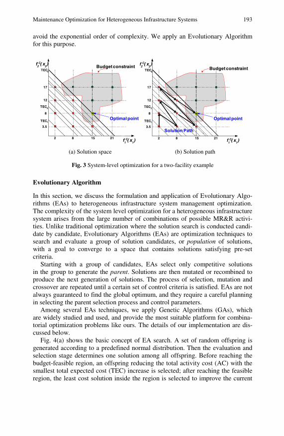
To develop a system level solution, consider a simple case with only two facilities. Fig. 3 shows the solution space and solution path. From the initial solution X = (0,0) which is a combination of optimal activities without budget constraint, the solution has to move towards the constrained optimal solution. For the first facil-ity, the decision variable x1 can take four values, i.e. four activities are available including the original optimal policy and three alternatives. In this example, the expected cost-to-go for the optimal policy is 2, and the alternatives’ costs are 8, 15 and 21. The second facility, as shown on the vertical axis, has an optimal expected cost-to-go of 3.5 and alternatives’ costs of 8, 12 and 17. The diagonal lines illus-trated are loci of equal total expected cost-to-go (TEC) points. We seek the mini-mum total cost combination )()( 2211 xfxf CC + inside the feasible region, defined

by the budget constraint. To guarantee global optimality, the solution path has to include every point for

which the total cost (TEC) is below the optimal solution as illustrated in Fig. 3(b). Starting from point, (2, 3.5), the solution moves to point (2, 8), which gives the smallest increase of total cost from TEC1 (5.5) to TEC2 (10). By repeating this procedure, we can reach the optimal solution, which is the first feasible solution visited. However, as the number of facilities increases, it becomes more difficult to find the next solution point from the current solution. In case of P activities available for N facilities, there exist PN combinations of movements in the solution space in the worst case. Therefore, we need to develop solution methods that can


avoid the exponential order of complexity. We apply an Evolutionary Algorithm for this purpose.

f1C( x

1 )

Budget constraint

Optimal point1

2

TEC9

2 8 15 21

3.5

8

12

17

f2C( x

2 )

Solution Path

TEC

TEC

f1C( x

1 )

Budget constraint

Optimal point1

2

TEC9

2 8 15 21

3.5

8

12

17

f2C( x

2 )

TEC

TEC

(a) Solution space (b) Solution path

Fig. 3 System-level optimization for a two-facility example

Evolutionary Algorithm

In this section, we discuss the formulation and application of Evolutionary Algo-rithms (EAs) to heterogeneous infrastructure system management optimization. The complexity of the system level optimization for a heterogeneous infrastructure system arises from the large number of combinations of possible MR&R activi-ties. Unlike traditional optimization where the solution search is conducted candi-date by candidate, Evolutionary Algorithms (EAs) are optimization techniques to search and evaluate a group of solution candidates, or population of solutions, with a goal to converge to a space that contains solutions satisfying pre-set criteria.

Starting with a group of candidates, EAs select only competitive solutions in the group to generate the parent. Solutions are then mutated or recombined to produce the next generation of solutions. The process of selection, mutation and crossover are repeated until a certain set of control criteria is satisfied. EAs are not always guaranteed to find the global optimum, and they require a careful planning in selecting the parent selection process and control parameters.

Among several EAs techniques, we apply Genetic Algorithms (GAs), which are widely studied and used, and provide the most suitable platform for combina-torial optimization problems like ours. The details of our implementation are dis-cussed below.

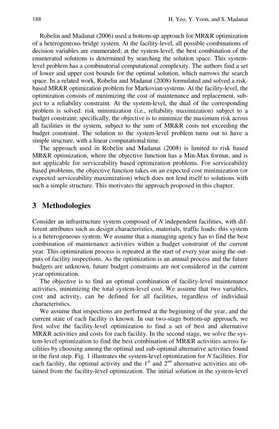
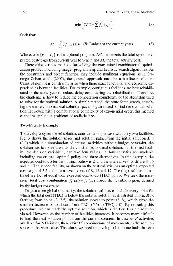
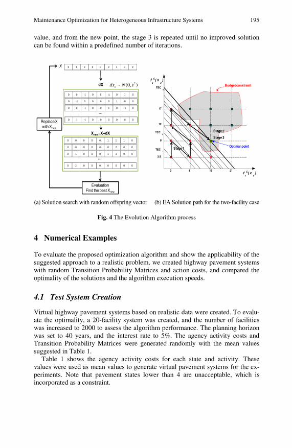
Fig. 4(a) shows the basic concept of EA search. A set of random offspring is generated according to a predefined normal distribution. Then the evaluation and selection stage determines one solution among all offspring. Before reaching the budget-feasible region, an offspring reducing the total activity cost (AC) with the smallest total expected cost (TEC) increase is selected; after reaching the feasible region, the least cost solution inside the region is selected to improve the current


solution. Fig. 4(b) shows the application of the EA method to the two-facility example. From point (2, 3.5), several offspring are generated and evaluated, and point (2, 8) is chosen as the next solution because it has the lowest cost increase among all solutions that have a lower activity cost. Repeating this procedure, the algorithm finally reaches optimal solution of (15, 8) in 7 iterations.

Stage 1: Mutant Offspring Generation

To generate mutant offspring, we use the current solution vector X as a single par-ent. Let dX be a movement vector. A number of movement vectors are randomly generated according to the normal distribution NnsNormal dxn ≤ ),,0(~ 2 . The

offspring is dXXX offspring += . The initial solution vector is the optimal one found in the facility-level optimization without budget constraint. After generating movement vectors, they are rounded to one of the discrete values: -3, -2, -1, 0, 1, 2, 3. The smaller the value of s, the more components of the movement vector have zero value, resulting in smaller search space. The number of offspring can be used for controlling the precision of search.

Stage 2: Offspring Evaluation and Selection

At this stage, generated offspring are evaluated to find the best movement from the current solution point. When the current agency activity cost (AC) is greater than the budget assigned, the offspring satisfying the following conditions is selected.

( )∑ +=

N

nnn

Cndx

dxxf1

)(min

(7)

)()(11

nB

n

N

n

N

nnn

Bn xfdxxfAC ∑≤∑ +=

== (8)

When the solution is inside the feasible region, we select an offspring satisfying the following condition:

( ) ∑≤∑ +==

N

nn

Cn

N

nnn

Cn

dxxfdxxf

n 11)()(min (Minimum TEC) (9)

BdxxfACN

nn

Bn ≤∑ +=

=1)( (Budget constraint) (10)

The stage 2 procedure is repeated until there is no solution improvement.

Stage 3: Optimality Check

Checking optimality, the search range is expanded to find a solution closer to the global optimal solution. In each step when no improved solution is found, s is in-creased by multiplication factor w. Therefore, if k steps pass without solution im-provement, offspring with movement vector dxn ~ Normal (0, w2ks2) are evaluated for optimality checking. If an improved solution is found, k is reset to its initial


value, and from the new point, the stage 3 is repeated until no improved solution can be found within a predefined number of iterations.

X 0 1 0 0 0 0 1 0 0

0 0 -1 0 0 1 0 1 0

Xnew=X+dX

0 -1 0 0 0 0 1 0 0

0 1 -1 0 0 0 0 0 0

0 0 -1 0 0 1 0 -1 0

…

0 0 0 0 0 1 1 1 0

0 0 0 0 0 0 2 0 0

0 2 0 0 0 0 0 0 0

0 1 0 0 0 1 1 0 0

…

Evaluation Find the best Xnew

Replace X with Xnew

),0(~ 2sNdxndX

f1

C( x1

)

Budget constraint

Optimal point1

2

TEC9

2 8 15 21

3.5

8

12

17

f2

C( x2

)

TEC

TEC Stage 1

Stage 2

Stage 3

(a) Solution search with random offspring vector (b) EA Solution path for the two-facility case

Fig. 4 The Evolution Algorithm process

4 Numerical Examples

To evaluate the proposed optimization algorithm and show the applicability of the suggested approach to a realistic problem, we created highway pavement systems with random Transition Probability Matrices and action costs, and compared the optimality of the solutions and the algorithm execution speeds.

4.1 Test System Creation

Virtual highway pavement systems based on realistic data were created. To evalu-ate the optimality, a 20-facility system was created, and the number of facilities was increased to 2000 to assess the algorithm performance. The planning horizon was set to 40 years, and the interest rate to 5%. The agency activity costs and Transition Probability Matrices were generated randomly with the mean values suggested in Table 1.

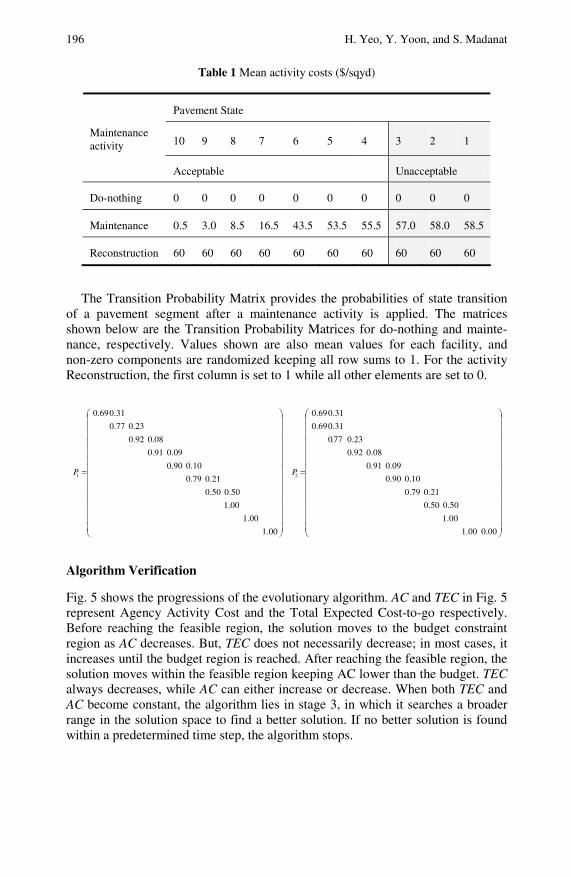
Table 1 shows the agency activity costs for each state and activity. These values were used as mean values to generate virtual pavement systems for the ex-periments. Note that pavement states lower than 4 are unacceptable, which is incorporated as a constraint.


Table 1 Mean activity costs ($/sqyd)

Pavement State

10 9 8 7 6 5 4 3 2 1 Maintenance activity

Acceptable Unacceptable

Do-nothing 0 0 0 0 0 0 0 0 0 0

Maintenance 0.5 3.0 8.5 16.5 43.5 53.5 55.5 57.0 58.0 58.5

Reconstruction 60 60 60 60 60 60 60 60 60 60

The Transition Probability Matrix provides the probabilities of state transition

of a pavement segment after a maintenance activity is applied. The matrices shown below are the Transition Probability Matrices for do-nothing and mainte-nance, respectively. Values shown are also mean values for each facility, and non-zero components are randomized keeping all row sums to 1. For the activity Reconstruction, the first column is set to 1 while all other elements are set to 0.

⎟⎟⎟⎟⎟⎟⎟⎟⎟⎟⎟⎟⎟⎟

⎠

⎞

⎜⎜⎜⎜⎜⎜⎜⎜⎜⎜⎜⎜⎜⎜

⎝

⎛

=

⎟⎟⎟⎟⎟⎟⎟⎟⎟⎟⎟⎟⎟⎟

⎠

⎞

⎜⎜⎜⎜⎜⎜⎜⎜⎜⎜⎜⎜⎜⎜

⎝

⎛

=

0.001.00

1.00

0.500.50

0.210.79

0.100.90

0.090.91

0.080.92

0.23.770

0.310.69

0.310.69

1.00

1.00

1.00

0.500.50

0.210.79

0.100.90

0.090.91

0.080.92

0.230.77

0.310.69

21 PP

Algorithm Verification

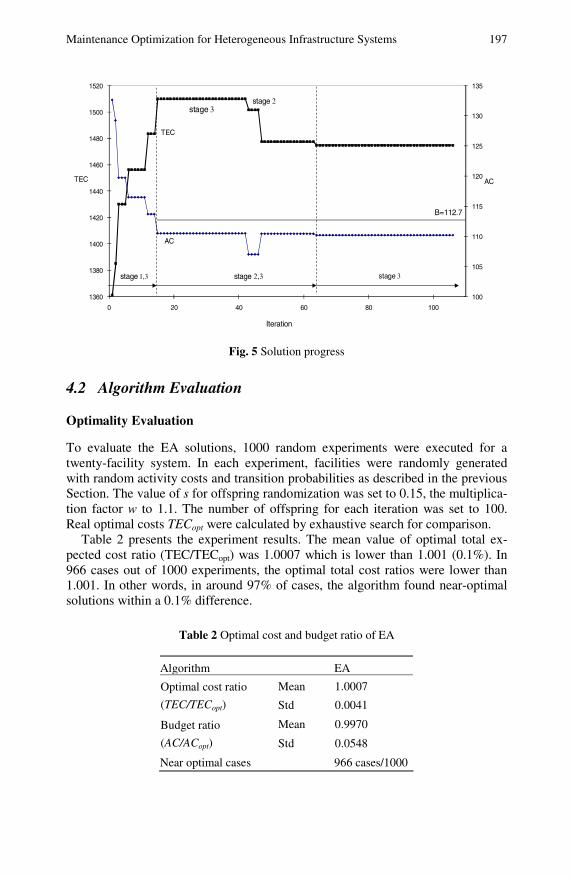
Fig. 5 shows the progressions of the evolutionary algorithm. AC and TEC in Fig. 5 represent Agency Activity Cost and the Total Expected Cost-to-go respectively. Before reaching the feasible region, the solution moves to the budget constraint region as AC decreases. But, TEC does not necessarily decrease; in most cases, it increases until the budget region is reached. After reaching the feasible region, the solution moves within the feasible region keeping AC lower than the budget. TEC always decreases, while AC can either increase or decrease. When both TEC and AC become constant, the algorithm lies in stage 3, in which it searches a broader range in the solution space to find a better solution. If no better solution is found within a predetermined time step, the algorithm stops.


100

105

110

115

120

125

130

135

1360

1380

1400

1420

1440

1460

1480

1500

1520

0 20 40 60 80 100

stage 1,3 stage 2,3 stage 3

B=112.7

stage 2stage 3

TEC

AC

TEC AC

Iteration

Fig. 5 Solution progress

4.2 Algorithm Evaluation

Optimality Evaluation

To evaluate the EA solutions, 1000 random experiments were executed for a twenty-facility system. In each experiment, facilities were randomly generated with random activity costs and transition probabilities as described in the previous Section. The value of s for offspring randomization was set to 0.15, the multiplica-tion factor w to 1.1. The number of offspring for each iteration was set to 100. Real optimal costs TECopt were calculated by exhaustive search for comparison.

Table 2 presents the experiment results. The mean value of optimal total ex-pected cost ratio (TEC/TECopt) was 1.0007 which is lower than 1.001 (0.1%). In 966 cases out of 1000 experiments, the optimal total cost ratios were lower than 1.001. In other words, in around 97% of cases, the algorithm found near-optimal solutions within a 0.1% difference.

Table 2 Optimal cost and budget ratio of EA

Algorithm EA

Mean 1.0007 Optimal cost ratio

(TEC/TECopt) Std 0.0041

Mean 0.9970 Budget ratio

(AC/ACopt) Std 0.0548

Near optimal cases 966 cases/1000


Evaluation of Algorithm Execution Speed

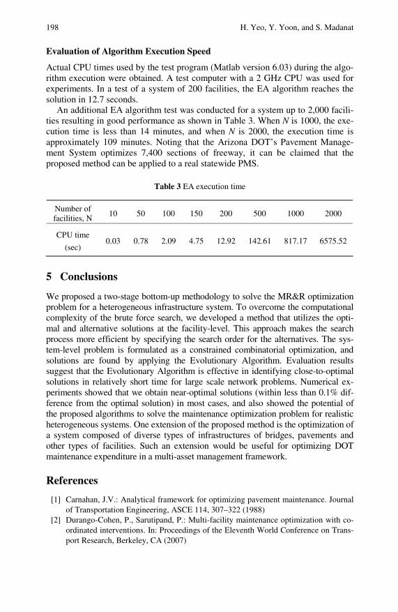
Actual CPU times used by the test program (Matlab version 6.03) during the algo-rithm execution were obtained. A test computer with a 2 GHz CPU was used for experiments. In a test of a system of 200 facilities, the EA algorithm reaches the solution in 12.7 seconds.

An additional EA algorithm test was conducted for a system up to 2,000 facili-ties resulting in good performance as shown in Table 3. When N is 1000, the exe-cution time is less than 14 minutes, and when N is 2000, the execution time is approximately 109 minutes. Noting that the Arizona DOT’s Pavement Manage-ment System optimizes 7,400 sections of freeway, it can be claimed that the proposed method can be applied to a real statewide PMS.

Table 3 EA execution time

Number of facilities, N

10 50 100 150 200 500 1000 2000

CPU time

(sec) 0.03 0.78 2.09 4.75 12.92 142.61 817.17 6575.52

5 Conclusions

We proposed a two-stage bottom-up methodology to solve the MR&R optimization problem for a heterogeneous infrastructure system. To overcome the computational complexity of the brute force search, we developed a method that utilizes the opti-mal and alternative solutions at the facility-level. This approach makes the search process more efficient by specifying the search order for the alternatives. The sys-tem-level problem is formulated as a constrained combinatorial optimization, and solutions are found by applying the Evolutionary Algorithm. Evaluation results suggest that the Evolutionary Algorithm is effective in identifying close-to-optimal solutions in relatively short time for large scale network problems. Numerical ex-periments showed that we obtain near-optimal solutions (within less than 0.1% dif-ference from the optimal solution) in most cases, and also showed the potential of the proposed algorithms to solve the maintenance optimization problem for realistic heterogeneous systems. One extension of the proposed method is the optimization of a system composed of diverse types of infrastructures of bridges, pavements and other types of facilities. Such an extension would be useful for optimizing DOT maintenance expenditure in a multi-asset management framework.

References

[1] Carnahan, J.V.: Analytical framework for optimizing pavement maintenance. Journal of Transportation Engineering, ASCE 114, 307–322 (1988)

[2] Durango-Cohen, P., Sarutipand, P.: Multi-facility maintenance optimization with co-ordinated interventions. In: Proceedings of the Eleventh World Conference on Trans-port Research, Berkeley, CA (2007)


[3] Friesz, T.L., Fernandez, J.E.: A model of optimal transport maintenance with demand responsiveness. Transportation Research 13B, 317–339 (1979)

[4] Fwa, T.F., Chan, W.T., Tan, C.Y.: Genetic-algorithm programming of road mainte-nance and rehabilitation. Journal of Transportation Engineering, ASCE 122, 246–253 (1996)

[5] Golabi, K., Kulkarni, R., Way, G.: A statewide pavement management system. Inter-faces 12, 5–21 (1982)

[6] Harper, W.V., Majidzadeh, K.: Use of expert opinion in two pavement management systems. Transportation Research Record No. 1311, Transportation Research Board, Washington, DC, 242–247 (1991)

[7] Li, Y., Madanat, S.: A steady-state solution for the optimal pavement resurfacing problem. Transportation Research 36A, 525–535 (2002)

[8] Madanat, S., Ben-Akiva, M.: Optimal inspection and repair policies for transportation facilities. Transportation Science 28, 55–62 (1994)

[9] Organization for Economic Cooperation and Development (OECD): Pavement Man-agement Systems. Road Transport Research Report, Paris, France (1987)

[10] Ouyang, Y., Madanat, S.: An Analytical Solution for the Finite-Horizon Pavement Resurfacing Planning Problem. Transportation Research, Part B 40, 767–778 (2006)

[11] Ouyang, Y.: Pavement resurfacing planning on highway networks: A parametric pol-icy iteration approach. Journal of Infrastructure Systems, ASCE 13(1), 65–71 (2007)

[12] Robelin, C.A., Madanat, S.: A bottom-up, reliability-based bridge inspection, mainte-nance and replacement optimization model. In: Proceedings of the Transportation Re-search Board Meeting 2006 (CD-ROM), TRB, Washington, DC. Paper #06-0381 (2006)

[13] Robelin, C.A., Madanat, S.: Reliability-Based System-Level Optimization of Bridge Maintenance and Replacement Decisions. Transportation Science 42(4) (2008)

[14] Smilowitz, K., Madanat, S.: Optimal Inspection and Maintenance Policies for Infra-structure Systems. Computer-Aided Civil and Infrastructure Engineering 15(1) (2000)

[15] Tsunokawa, K., Schofer, J.L.: Trend curve optimal control model for highway pave-ment maintenance: case study and evaluation. Transportation Research 28A, 151–166 (1994)

[16] Forrest, S.: Genetic Algorithms: Principles of Natural Selection Applied to Computa-tion. Science 261, 872–878 (1993)

[17] Goldberg, D.E.: Genetic Algorithms in Search, Optimization, and Machine Learning (1989)

[18] Gray, P., et al.: A Survey of Global Optimization Methods. Sandia National Labora-tories (1997)

Maintenance Optimization for Heterogeneous Infrastructure Systems: Evolutionary Algorithms for...

Documents

Transcript of Maintenance Optimization for Heterogeneous Infrastructure Systems: Evolutionary Algorithms for...