Maintenance Management of a Transmission Substation with ...

applied sciences

Article

Maintenance Management of a Transmission Substationwith Optimization

Peter Kitak 1,* , Lovro Belak 2, Jože Pihler 1 and Janez Ribic 1

��

Citation: Kitak, P.; Belak, L.; Pihler, J.;

Ribic, J. Maintenance Management of

a Transmission Substation with

Optimization. Appl. Sci. 2021, 11,

11806. https://doi.org/10.3390/

app112411806

Academic Editors: Federico Barrero

and Mario Bermúdez

Received: 9 November 2021

Accepted: 9 December 2021

Published: 12 December 2021

Publisher’s Note: MDPI stays neutral

with regard to jurisdictional claims in

published maps and institutional affil-

iations.

Copyright: © 2021 by the authors.

Licensee MDPI, Basel, Switzerland.

This article is an open access article

distributed under the terms and

conditions of the Creative Commons

Attribution (CC BY) license (https://

creativecommons.org/licenses/by/

4.0/).

1 Faculty of Electrical Engineering and Computer Science, University of Maribor, 2000 Maribor, Slovenia;[email protected] (J.P.); [email protected] (J.R.)

2 Slovenian Transmission System Operator ELES, 1000 Ljubljana, Slovenia; [email protected]* Correspondence: [email protected]

Abstract: The paper deals with the reliability-centered maintenance (RCM) of a transmission substa-tion. The process of the planning and actual performance of maintenance was carried out using anoptimization algorithm. This maintenance procedure represents the maintenance management andincluded reliability of the power system operation, maintenance costs, and associated risks. The orig-inality of the paper lies in the integrated treatment of all maintenance processes that are included inthe pre-processing and used in the optimization process for reliability-centered maintenance. The op-timization algorithm of transmission substation maintenance was tested in practice on the equipmentand components of an existing 400/110–220/110 kV substation in the Slovenian electricity transmis-sion system. A comparison analysis was also carried out of the past time-based maintenance (TBM)and the new reliability-centered maintenance (RCM), on the basis of the optimization algorithm.

Keywords: reliability-centered maintenance; optimization; transmission substation; condition monitoring

1. Introduction

Maintenance is a combination of technical, administrative, and managerial actionsduring the lifetime of a device, the purpose of which is to keep it in, or bring it back to,the condition that enables performing of its functions. It is, therefore, a usual processneeded by every device for normal operation. The maintenance in transmission substations(TS) is crucial for secure and reliable operation of the electric power system (EPS). Themaintenance terminology covers two types of maintenance: preventive and corrective.In the field of electricity transmission devices, preventive maintenance still prevails [1].This type of maintenance can be either time-based maintenance or related to the stateof devices, condition-based maintenance (CBM) [2]. From 2009 onwards, the health in-dex [3–5] has been used in the field of condition-based maintenance to evaluate indicatorsof maintenance.

However, new trends in the field of maintenance, i.e., reliability -centered mainte-nance (RCM), are being introduced in the wider area of engineering [6,7], as well as inthe field of maintenance of devices in the electricity transmission system [1,8–10]. Thesetrends are also accelerated by the standardization in the field of maintenance and assetmanagement [11,12].

The reliability of operation and associated maintenance is, in the majority of cases,based on the reliability calculation using the Markov model [9,13–15]. An adequate ef-ficiency of the determination of system criteria for maintenance can be achieved withthe selection of various algorithms, such as the best–worst method (BWM) [16], wherenumerous possibilities are assessed on the basis of determination with regard to variousattributes, and the best maintenance criteria are selected.

In the maintenance process, authors have also included optimization proceduresdealing with economy and reliability [10,17–19]. The authors usually deal with individualelements, such as overhead lines [5,20] and transformers [21,22]. References [9,23] deal

Appl. Sci. 2021, 11, 11806. https://doi.org/10.3390/app112411806 https://www.mdpi.com/journal/applsci

https://www.mdpi.com/journal/applsci

https://www.mdpi.com

https://orcid.org/0000-0003-3419-5873

https://doi.org/10.3390/app112411806

https://doi.org/10.3390/app112411806

https://creativecommons.org/

https://creativecommons.org/licenses/by/4.0/

https://creativecommons.org/licenses/by/4.0/

https://doi.org/10.3390/app112411806

https://www.mdpi.com/journal/applsci

https://www.mdpi.com/article/10.3390/app112411806?type=check_update&version=1

Appl. Sci. 2021, 11, 11806 2 of 20

with maintenance of devices in a TS. The authors describe a maintenance method that isbased on the technical condition of the devices. Certain authors have also investigated timescheduling of maintenance tasks [14,24] or determination of the optimal inspection intervalof equipment in the TS, taking into account its age [25]. The authors of the presented paper,in [26], discussed the strategic maintenance of switching substations where reliabilityindices were not optimized.

The contribution of this paper is in the calculations of reliability indicators using thefailure effect analysis (FEA) method, and not with the calculations of Markov chains for anindividual device. In this method, any change in the state of an individual device affectsthe entire TS, which can, consequently, change the state of other devices as well. Themaintenance processes of the devices in the substation are closely related to the reliabilityindicators (one of them is importance) for the entire TS, and, at the same time, to thecondition of the individual devices, which is one of the article’s contributions.

The novelty presented in the present paper lies in the integrated treatment of TSmaintenance based on the RCM concept, using an optimization algorithm. The modifieddifferential evolution optimization algorithm with self-adaptation (SA) of the controlparameters was used to select the optimal maintenance period of TS devices (revisionsare carried out every year, every two years, or every three years), while the maintenanceis carried out when the significant operational state of the EPS is the most suitable forit. This state is defined by generation, consumption, and power flows in the EPS. Themethod of EPS elements’ maintenance used until now is TBM, where their maintenanceperiods are defined by the TSO’s internal rules. The main objective of this approach is toreduce maintenance costs while keeping the operational reliability level and improvingthe maintenance system constantly. This procedure is possible only with the inclusion ofoptimization algorithms in the maintenance process. Devices that are less important in thesystem, however, affect maintenance processes with reduced intensity.

The maintenance processes can be influenced by computation of the importance andtechnical condition of EPS elements, which is based on historical data of operation, events,and monitoring of EPS elements’ technical condition. This represents the main hypothesisof this article. The inclusion of optimization processes in the analysis of maintenance pro-cedures enables a reduction of maintenance costs, which represents the second hypothesis.

The methodology of computation of frequency of EPS elements’ maintenance influ-ences the maintenance processes and is based on available historical operation data andstatistics of events on EPS elements. For the entire EPS, we computed the availability ofelements in connection with the transmissioned energy. The availability of elements andtransmissioned energy to final customers are reliability indicators. The values of these indi-cators for individual elements were then compared with the reliability indicators of similarelements operated by other system operators. The importance of elements were computedon the basis of these data. In connection with the technical conditions of elements thatare performed in practice through monitoring, it is possible to influence the maintenanceprocesses on the basis of the RCM maintenance concept.

The optimization process that uses all possible data on historical events of operationand maintenance costs yields the results that can be used to manage the maintenanceprocesses in the future. This represents the main originality of this paper. The existingmethod of assessing the technical condition of EPS elements was upgraded and includedactively in the optimization process, where we predicted a dynamic changing of thetechnical condition of elements due to the interventions to the existing maintenance process.

The significant states in the system are determined on the basis of EPS operation datathat include generation, nodal loads, and load flows between the nodes. Their inclusionin the optimization process enables that maintenance activities are performed in the mostsuitable significant state. Thus, the maintenance activities have the least impact on theEPS operation. Indirectly, this also influences operational reliability and maintenancecosts. The optimization process in our article affects the frequency of transitions betweenmaintenance processes.

Appl. Sci. 2021, 11, 11806 3 of 20

The past data on the operation of transmission elements that are covered by statisticsof events were the basis for calculation of reliability indicators of these elements and theirunavailability. The values of these indicators for individual elements were compared withreliability indicators of similar elements operated by other system operators.

The paper consists of six sections. Section 2 presents the RCM concept-based main-tenance model. A switching bay was represented with an index of technical conditionand an index of importance. The costs of the existing maintenance concept were analyzedin detail. Section 3 provides the basic data for the optimization model. The key datain the RCM maintenance process were the values of technical condition and reliabilityindicators for every EPS element. The data are also given on the expected costs of outagesand maintenance costs for the example presented in this article. Section 4 presents the linkbetween the maintenance model and the optimization algorithm. Three objective functionsand one penalty function were defined to reach the optimal RCM maintenance concept.The results of the optimization process are given in Section 5. The optimal method andperiod of maintenance were defined accurately for each EPS element. A comparison wasalso given of maintenance costs with the existing time-based maintenance and with the newRCM maintenance concept. Section 6 provides the discussion and outlines the future work.

2. Maintenance Model Based on the RCM Concept

RCM is a maintenance concept that, in addition to the basic maintenance method-ologies, is focused on reliability. The objective of the RCM concept is management ofmaintenance costs and associated risks, having in mind the provision of adequate reliabil-ity of operation of the EPS. It is important not to treat reliability at the level of individualelements, but at the level of the entire system. Maintenance tasks carried out duringmaintenance are as follows: periodical inspection of elements performed on the energizedstate of the equipment; revision intended to retain elements’ functionality, performed onthe de-energized state of equipment; and repair or replacement of elements. Elementswith lower importance and good technical condition are maintained in the RCM conceptusing TBM in a longer time period. The main aim of RCM in this paper was to determinethe maintenance periods of EPS elements with regard to their importance and condition,considering reliability and costs. This is the main change with regard to the TBM concept,where maintenance periods are determined in advance. The RCM concept in the paper isbased on [1], while the basic concept uses the standard [11].

Section 2 is dedicated entirely to the RCM concept and consists of seven subsections.The elements are defined in Section 2.1 EPS. This includes a general set of elements andthe term switching bay. The structure of the model of input data for optimization in themaintenance process is presented in Section 2.2. Since we wished to include ecology inthe optimization process, Section 2.3 defines the characteristic variable of diagnostics ofdrops in pressure of the SF6 insulation gas. One of the key parameters in the RCM processis the index of technical condition. For each type of EPS element, there is a methodologyfor assessing their technical condition, which is described in Section 2.4. The next keyparameter in the RCM concept is the index of importance of an EPS element, which isdescribed in detail in Section 2.5. The cost-related part of our concept is dealt with inSections 2.6 and 2.7.

2.1. Definition of EPS Elements

The subject of our analyses is the EPS. It comprises generation units, lines, and substa-tions. In substations, there are disconnectors, circuit breakers, power transformers, andother elements. The elements of the EPS represent a set of elements Sel = {elk; 1 ≤ k ≤ nel;k ∈ N}, where nel is the number of elements in the entire EPS, el is the element in the EPS,and k is the counter of the EPS elements. All these elements form a database with charac-teristic variables, such as estimation of technical condition, economic indicators, reliabilityindicators, and indicator of importance. A set of elements Skel = {kelr; 1 ≤ r ≤ nkel; r ∈ N}is created, where nkel is the number of kinds of elements used in the EPS, kel is the kind of

Appl. Sci. 2021, 11, 11806 4 of 20

elements used in the EPS, and r is the counter of kinds of elements used in the EPS. Dataon the entire EPS are needed for the computation of the reliability indicators of the EPS,technical condition of elements, and maintenance costs. From the set of elements Sel, onlythose elements were observed that are a part of the TS.

The model enables scheduling of maintenance tasks with regard to the state of thesystem, taking into consideration economic effects and reliability of operation of individualswitching bays in the TS.

The analysis includes only switching bays and transformers that are elements ofthe observed TS. A switching bay is a set of elements in the substation that belongs tothe main element (transformer or transmission line). A switching bay is an assemblyof switchgear elements (disconnectors, circuit breakers, etc.), and can be either line bay,transformer bay, or bus coupler bay [27]. Bays in the TS form a set of bays SSB = {SSB,l;SSB,l ⊂ Sel; 1 ≤ l ≤ nSB; l ∈ N}, where nSB is the number of switching bays. The lth bay inthe TS comprises a certain number of elements and forms the set of elements of the lthbay SSB,l = {elSB,lm; 1 ≤ m ≤ nSB,l; m∈N}, being a subset of the set of elements Sel, wherenSB,l is the number of elements in the lth bay of the TS and m is the counter of elementsin the TS bay. A switching bay can be considered as a new EPS element. The reasonfor this is that, during revision, the entire bay is always in a de-energized state and ismaintained as a whole. The analysis of a TS also includes power transformers. The set ofbays in the TS is, thus, case extended to the number of transformers nT. It is defined asST = {TRll; 1 ≤ ll ≤ nT; ll ∈ N}, where ll is the counter of transformers in the TS. The setof TS elements, therefore, consists of switching bays and transformers, and is defined asSSU = {SSU,q; SSU = SSB ∪ ST; 1 ≤ q ≤ nSU; q∈N; nSU = nSB + nT}, where q is the counter ofswitching bays and transformers and nSU is the number of observed switching bays andtransformers of the TS.

2.2. The Structure of the Model

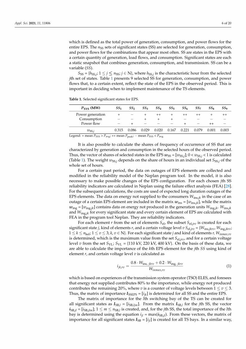
Figure 1 shows a block diagram of the preparation of input data for the optimizationof maintenance tasks in transmission substations.

Appl. Sci. 2021, 11, x FOR PEER REVIEW 5 of 21

Figure 1. Block diagram of the RCM concept-based maintenance model.

The following data are needed for this optimization: drop in pressure of SF6 in circuit breakers (CB), estimation of the technical condition of substation elements, financial data on switching bays’ maintenance, and reliability indicators for elements of switching bays and transformers.

2.3. Diagnostics of the Density of SF6 Gas Diagnostics of the EPS devices is performed as a part of regular maintenance activi-

ties of EPS elements, and includes inspections, measurements, etc. One of the tasks of di-agnostic activities are measurements of drops in pressure Δp of the SF6 insulation gas in circuit breakers. Circuit breakers in the switching bays are a part of the set of all SF6 circuit breakers in the EPS: SSF6 = {CBSF6,kk; CBSF6,kk ⊂ Sel; 1 ≤ kk ≤ nSF6; kk ∈ N}. The characteristic variable of the set of circuit breakers SSF6 is the vector of drop in pressure in the SF6 circuit breakers ΔpSF6 = [Δpkk], where kk is the counter of SF6 circuit breakers and nSF6 is the number of SF6 circuit breakers in the TS.

If there is an SF6 circuit breaker in the lth bay (e.g., the kkth element), the drop in pressure Δpkk can be considered as the characteristic variable of this element. In this case, we can write Δpl = Δpkk, otherwise Δpl = 0. All the bays in the TS form a vector of drops in pressure in circuit breakers ΔpSB = [ΔpSB,l]. The vector of drops in pressure of SF6 for all TS elements is, thus, defined as Δp = [Δpq], where Δpq = ΔpSB,l for 1 ≤ q ≤ nSB, l = q and Δpq = ΔpT,ll = 0 for nSB + 1 ≤ q ≤ nSB + nT and ll = q − nSB. These are the input data for the optimization procedure.

2.4. Index of Technical Condition c Diagnostics of the EPS devices are also the basis for estimation of the technical con-

dition of the EPS devices. For each kind of EPS element, there is an adopted methodology for estimation of the technical condition of devices ck [26]. The index of the technical con-dition is determined on the basis of the Slovenian transmission system operator internal application for determination of technical condition ck, which contains a set of 18 criteria with an adequate weighting factor (from 1 to 10), and each rating factor (from 1—good to 10—bad). The rating factor is determined by the engineer responsible for monitoring the switching substation for each corresponding criterion of the element.

Diagnostics of the EPS

devices

Financial analysis of

the EPS

Analysis of the EPS power

generation and consumption

Analysis of the EPS outages and

configuration

Diagnostics of the SF6

gas density

Assessmement of the EPS

devices technical condition

EPS devices revisions

costs

Selection and evaluation of the EPS significant

states

Reliability indicators from

the EPS reliability model

EPS elements importance over significant states

qc

r,qC SS, jw

in,jqC jqi

ins,jkW

ing,jkW

Mai

nte

nanc

e

Rel

iabi

lity

A B C D E F

Leve

l IEP

S an

alys

is(S

cada

, Max

imo)

Leve

l II

EPS

char

acte

ristic

s(O

racl

e, N

epla

n)

Leve

l III

SB a

nd T

r in

TS

(Exe

l, M

atla

b)

Δ qp

Figure 1. Block diagram of the RCM concept-based maintenance model.

The following data are needed for this optimization: drop in pressure of SF6 in circuitbreakers (CB), estimation of the technical condition of substation elements, financial data

Appl. Sci. 2021, 11, 11806 5 of 20

on switching bays’ maintenance, and reliability indicators for elements of switching baysand transformers.

2.3. Diagnostics of the Density of SF6 Gas

Diagnostics of the EPS devices is performed as a part of regular maintenance activitiesof EPS elements, and includes inspections, measurements, etc. One of the tasks of diagnosticactivities are measurements of drops in pressure ∆p of the SF6 insulation gas in circuitbreakers. Circuit breakers in the switching bays are a part of the set of all SF6 circuit breakersin the EPS: SSF6 = {CBSF6,kk; CBSF6,kk ⊂ Sel; 1≤ kk≤ nSF6; kk ∈N}. The characteristic variableof the set of circuit breakers SSF6 is the vector of drop in pressure in the SF6 circuit breakers∆pSF6 = [∆pkk], where kk is the counter of SF6 circuit breakers and nSF6 is the number of SF6circuit breakers in the TS.

If there is an SF6 circuit breaker in the lth bay (e.g., the kkth element), the drop inpressure ∆pkk can be considered as the characteristic variable of this element. In this case,we can write ∆pl = ∆pkk, otherwise ∆pl = 0. All the bays in the TS form a vector of drops inpressure in circuit breakers ∆pSB = [∆pSB,l]. The vector of drops in pressure of SF6 for allTS elements is, thus, defined as ∆p = [∆pq], where ∆pq = ∆pSB,l for 1 ≤ q ≤ nSB, l = q and∆pq = ∆pT,ll = 0 for nSB + 1 ≤ q ≤ nSB + nT and ll = q − nSB. These are the input data for theoptimization procedure.

2.4. Index of Technical Condition c

Diagnostics of the EPS devices are also the basis for estimation of the technical condi-tion of the EPS devices. For each kind of EPS element, there is an adopted methodologyfor estimation of the technical condition of devices ck [26]. The index of the technicalcondition is determined on the basis of the Slovenian transmission system operator internalapplication for determination of technical condition ck, which contains a set of 18 criteriawith an adequate weighting factor (from 1 to 10), and each rating factor (from 1—good to10—bad). The rating factor is determined by the engineer responsible for monitoring theswitching substation for each corresponding criterion of the element.

The values of the technical condition of an element can lie in the range 0 ≤ ck ≤ 100.The higher the value is, the worse the technical condition of the EPS element. The technicalcondition of all EPS elements is evaluated in this way and is included in cs = [ck]. The lthswitching bay of the TS contains a certain number of elements nSB,l and forms the set ofelements of this bay. The characteristic variable of the set SSB,l is the vector of technicalcondition of the elements of this set, which is defined as cSB,l = [cSB,lm]. The technicalcondition cl of the lth bay can be defined as the maximum estimated value of technicalcondition of this bay’s elements, i.e., as cl = max(cSB,l). The vector cSB = [cl] can be definedfor all the bays in the substation. The values of technical condition for power transformersare defined as cT = [cT,ll]. The vector of technical condition for the entire TS, including bothbays and transformers, c = [cq], is obtained using the identical procedure, as described inSection 2.3.

2.5. Index of Importance i

To calculate the importance of the EPS elements, the reliability indicators need tobe calculated first. The first step in this calculation is a detailed analysis of the EPS as awhole. For the calculation of reliability indicators, we used a powerful program tool forsteady-state calculations in the EPS, Neplan [26]. The Neplan program tool for calculationof reliability indicators requires data on outages of all EPS elements, as well as hourly dataon generation and consumption for all EPS nodes. The analysis begins with a statisticalsurvey of hourly data on generation and consumption in all EPS nodes, as well as ananalysis of power flows in certain parts of the EPS in a certain period (one year or more). Aclustering approach is used on the basis of historical data. Average values of power (µP)and deviations from the average value (σP) are calculated for generation, consumption, andpower flows. Combinations of strings of hourly data for the total power PSYS are selected,

Appl. Sci. 2021, 11, 11806 6 of 20

which is defined as the total power of generation, consumption, and power flows for theentire EPS. The nSS sets of significant states (SS) are selected for generation, consumption,and power flows for the combinations that appear most often. SS are states in the EPS witha certain quantity of generation, load flows, and consumption. Significant states are eacha static snapshot that combines generation, consumption, and transmission. SS can be avariable (SS).

SSS = {hSS,j; 1 ≤ j ≤ nSS; j ∈ N}, where hSS,j is the characteristic hour from the selectedjth set of states. Table 1 presents 9 selected SS for generation, consumption, and powerflows that, to a certain extent, reflect the state of the EPS in the observed period. This isimportant in deciding when to implement maintenance of the TS elements.

Table 1. Selected significant states for EPS.

PSYS (MW) SS1 SS2 SS3 SS4 SS5 SS6 SS7 SS8 SS9

Power generation + − + ++ + ++ ++ + ++Consumption − − + + + − − − −Power flow − + − − − + − ++ −

wSS,j 0.315 0.086 0.029 0.020 0.167 0.221 0.079 0.001 0.003Legend: + mean PSYS > Pavg; ++ mean Ppeak; −mean PSYS < Pavg.

It is also possible to calculate the shares of frequency of occurrence of SS that arecharacterized by generation and consumption in the selected hours of the observed period.Thus, the vector of shares of selected states in the EPS wSS = [wSS,j]; 0 < wSS,j < 1 is calculated(Table 1). The weight wSS,j depends on the share of hours in an individual set SSS,j of thewhole set of hours.

For a certain past period, the data on outages of EPS elements are collected andmodified in the reliability model of the Neplan program tool. In the model, it is alsonecessary to make possible changes of the EPS configuration. For each chosen jth SSreliability indicators are calculated in Neplan using the failure effect analysis (FEA) [28].For the subsequent calculations, the costs are used of expected long duration outages of theEPS elements. The data on energy not supplied to the consumers Wins,jk in the case of anoutage of a certain EPS element are included in the matrix wins = [wins,jk], while the matrixwing = [wing,jk] contains data on energy not produced in the generation units Wing,jk. Wins,jkand Wing,jk for every significant state and every certain element of EPS are calculated withFEA in the program tool Neplan. They are reliability indicators.

For each element r from the set of elements Sel, the subset Sel,jrv is created for eachsignificant state j, kind of elements r, and a certain voltage level v Sel,jrv = {Wins,jkrv, Wing,jkrv;1≤ k≤ nkel; 1≤ v≤ 3; k, v ∈N}. For each significant state j and kind of elements r, Winmax,rvis determined, which is the maximum value from the set Sel,jrv, and for a certain voltagelevel v from the set SVL; SVL = {110 kV, 220 kV, 400 kV}. On the basis of these data, weare able to calculate the importance of the kth EPS element for the jth SS using kind ofelement r, and certain voltage level v is calculated as

ijk,rv =0.8 ·Wins, jkrv + 0.2 ·Wing, jkrv

Winmax,rv(1)

which is based on experiences of the transmission system operator (TSO) ELES, and foreseesthat energy not supplied contributes 80% to the importance, while energy not producedcontributes the remaining 20%, where v is a counter of voltage levels between 1 ≤ v ≤ 3.Thus, the matrix of importance ISSEPS = [ijk] is determined for all SS and the entire EPS.

The matrix of importance for the lth switching bay of the TS can be created forall significant states as ISB,l = [iSB,ljm]. From the matrix ISB,l for the jth SS, the vectoriSB,jl = [iSB,jlm]; 1 ≤ m ≤ nSB,l is created, and, for the jth SS, the total importance of the lthbay is determined using the equation ijl = max(iSB,jl). From these vectors, the matrix ofimportance for all significant states ISB = [ijl] is created for all TS bays. In a similar way,

Appl. Sci. 2021, 11, 11806 7 of 20

the matrix of importance is created for power transformers in the TS IT = [iT,jll]. The totalimportance of all TS elements is obtained by joining the matrices ISB and IT to I = [ijq],where ijq = iSB,jl for 1 ≤ j ≤ nSS, 1 ≤ q ≤ nSB and l = q, and ijq = iT,jll for 1 ≤ j ≤ nSS and nSB +1 ≤ q ≤ nSB + nT, and ll = q − nSB.

2.6. Past Maintenance Cost

It is necessary to perform a detailed financial analysis of the entire EPS for the deter-mination of maintenance costs, which includes analysis of incomes, maintenance costs,and replacements of TS elements. This analysis is carried out by a unified informationsystem (IBM Maximo). From the database, it is possible to obtain revision costs for allEPS elements CrEPS = [Cr,k] for the past period in EUR/year. For the lth bay of the TS, it ispossible to create the vector of revision costs, defined as CrSB,l = [CrSB,lm]. The total annualrevision costs for the lth bay are defined as the sum of costs for all its elements:

Cr,l = ∑nSB,lm=1 CrSB,lm (2)

Using (2), the vector is obtained of all revision costs by switching bays CrSB = [Cr,l].The vector of revision costs for power transformers CrT = [CrT,ll] is obtained in a similarway. The total revision costs for all TS elements Cr are obtained using the above-describedprocedure for determination of the vector ∆p.

2.7. Expected Costs of Outages

The computation of the reliability model in the Neplan program tool yields as thefinal result FEA for each element k and each SS j the total anticipated costs of outage ofall consumers by power CinP,jk in EUR/year, caused by an outage of the element k in SSj (which are affected by outage of the element k in SS j). The expected costs depend onindividual contracts between the TSO and each consumer, the power of consumption, andthe duration of each customer’s outage that is affected by an outage of element k in SS j.Following the FEA procedure, the maximum value of reliability indicators is obtained as aresult. This method captures all possible changes in the state of devices in the TS.

The scaled costs of total energy not supplied due to an outage of the element k in SSj as CinWs,jk = cinWs·Wins,jk (EUR/year) are also computed, where cinWs are specific costsof energy not supplied, which are defined by the TSO (cinWs = 5000 EUR/MWh). Thelast scaled costs are the costs of energy not generated due to an outage of the element kin SS j as CinWg,jk = cinWg·Wing,jk (EUR/year), where cinWg are specific costs of generatedenergy, defined by the TSO (cinWg = 60 EUR/MWh). The total costs of expected outagesdue to an outage of the element k in SS j are calculated as the sum of costs Cin,jk = CinP,jk +CinWs,jk + CinWg,jk (EUR/year). They are, for all significant states, collected in the matrixCins = [Cin,jk].

For the lth bay of the TS, the matrix of expected outage costs could be created forall significant states CinSB,l = [CinSB,ljm]. The total expected costs of outages are calculatedusing (3).

Cin, jl = ∑nSB,lm=1 CinSB,l jm (3)

The matrix of costs of expected outages CinSB = [Cin,jl] could be created for all signifi-cant states and TS bays. The matrix of costs of expected outages for power transformers isCinT = [CinT,jll]. The matrix of costs of expected outages for all TS elements Cin = [Cin,jq] isobtained using the same procedure as described above for the calculation of importance I.

3. Data for the Maintenance Model of an Existing 400/110–220/110 kVTransmission Substation

The optimization of maintenance tasks is shown on a practical example of a Sloveniantransmission substation. The analysis included all primary devices on 400, 220, and 110 kVlevels in the substation. There were altogether nSB = 26 bays, 7 of them on 400 kV, 5 on220 kV, and 14 on a 110 kV level. In addition to the bays, there were also nT = 5 power trans-

Appl. Sci. 2021, 11, 11806 8 of 20

formers, two of them 220/110 kV, one 400/110 kV, and two components of a 400/400 kVphase-shifting transformer. The TS model therefore comprised nSU = 31 elements.

3.1. Data on Technical Condition c and Importance i

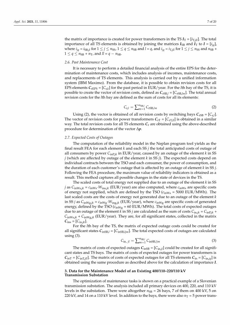
Table 2 shows the calculated data on the importance of individual significant states ofthe RCM model of the TS ijq, average importance of bays by various significant states iq,technical condition (technical indicator) cq, and average deviation dq for all bays, calculatedusing (5).

Table 2. TS elements technical and reliability indicators.

q CodeVoltage

Level (kV)Importance iqj Average Importance

iavg,q

Conditioncq

DistancedqSS1 SS2 SS3 SS4 SS5 SS6 SS7 SS8 SS9

Switching bay arrangements

1 T401 400 0.96 0.68 0.49 0.94 1.55 0.75 0.16 0.14 10.29 0.86 24.78 18.132 L401 400 4.44 0.60 0.53 0.91 2.06 3.65 2.60 100 100 3.24 60.22 44.873 L402 400 4.61 0.53 1.13 0.73 2.15 4.07 2.22 0.10 1.36 2.98 24.78 19.634 L403 400 0.96 0.68 0.49 0.95 1.55 0.75 0.22 0.14 11.14 0.87 24.78 18.145 C401 400 5.99 0.71 1.00 0.94 5.24 2.12 4.73 100 1.50 3.82 25.65 20.846 T402 400 4.60 0.60 0.52 0.91 2.12 4.05 0.72 100 5.46 2.95 17.39 14.397 T403 400 4.60 0.60 0.52 0.91 2.12 4.05 0.72 100 5.46 2.95 17.39 14.398 T201 220 42.31 100 0.34 0.76 2.36 0.24 0.38 4.83 0.43 22.43 30.65 37.549 T202 220 42.31 100 0.34 0.76 2.36 0.24 0.38 4.83 0.43 22.43 41.74 45.3810 L201 220 42.31 100 0.34 0.76 12.16 0.24 0.38 4.83 0.43 24.07 20.87 31.7811 L202 220 69.13 100 0.34 0.76 9.09 0.24 0.38 4.83 0.43 32.01 20.87 37.3912 L203 220 42.31 100 0.34 0.76 17.91 0.24 0.38 4.83 0.43 25.03 20.87 32.4613 T101 110 0.02 1.87 4.89 2.64 0.24 0.02 2.35 100 0.00 0.69 42.39 30.4614 T102 110 0.02 1.76 4.75 2.51 0.24 0.02 2.37 100 0.00 0.68 50.43 36.1415 L101 110 0.02 1.91 5.46 2.96 0.70 0.03 1.81 100 0.00 0.75 52.17 37.4316 T103 110 0.01 0.35 0.97 0.58 0.01 0.02 0.06 100 0.00 0.18 42.83 30.4117 T104 110 0.02 1.64 4.71 2.46 0.04 0.02 2.29 100 0.00 0.63 49.78 35.6418 L102 110 0.02 2.24 5.84 3.10 3.37 0.02 0.83 99.99 0.04 1.16 53.04 38.3319 L103 110 0.02 2.36 6.00 3.24 3.37 0.02 0.85 99.99 0.04 1.18 53.04 38.3420 L104 110 0.02 1.91 4.94 2.68 0.29 0.02 2.29 100 0.00 0.70 43.7 31.3921 L105 110 0.02 1.81 4.79 2.55 0.29 0.02 2.31 100 0.00 0.69 48.26 34.6122 T105 110 0.02 7.31 9.71 8.47 3.35 0.05 2.82 100 0.01 1.98 22.61 17.3923 L106 110 0.02 2.24 4.95 3.04 0.65 0.04 1.85 100 0.00 0.77 38.7 27.9124 L107 110 0.02 2.50 5.19 3.45 0.82 0.06 1.61 100 0.00 0.82 40.65 29.3225 L108 110 0.02 2.42 5.12 3.25 0.72 0.05 1.76 100 0.00 0.80 48.26 34.6926 C101 110 0.01 0.45 1.07 0.70 0.02 0.09 0.06 100 0.00 0.22 24.13 17.22

Transformers

27 Tr211 220/110 88.01 69.22 16.54 13.60 63.83 8.73 29.52 13.38 100 49.66 49.29 69.9728 Tr212 220/110 100 83.41 26.44 19.53 90.99 11.90 21.84 19.61 86.64 59.66 38.69 69.5429 Tr411 400/110 63.43 100 100 100 100 73.31 17.00 1.57 87.78 67.99 29.29 68.7830 Tr441 400/400 100 38.31 75.34 37.09 1.82 100 100 100 100 68.42 6.67 53.1031 Tr442 400/400 100 38.31 75.34 37.09 1.82 100 100 100 100 68.42 6.67 53.10

The average importance of TS bays by each SS is determined in a similar way with (4).

iavg = I ·wTSS (4)

The common index d is defined on the basis of the index of technical condition c andindex of importance iavg. It represents the uniform participation of technical conditionand importance of c and iavg of the device. The index d encompasses the bays and powertransformers of the TS and is defined by (5).

d =c + iavg√

2(5)

Appl. Sci. 2021, 11, 11806 9 of 20

The average value of costs of expected outages by each SS for all TS bays is calculatedusing (6) as the vector of costs of expected outages Cin,avg.

Cin,avg = Cin·wTSS (6)

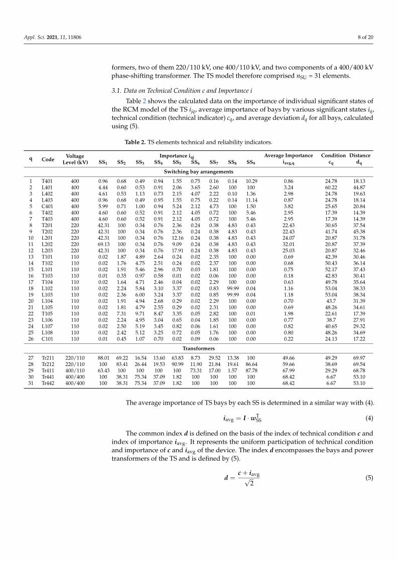
All these values from Table 2 are input data of the optimization process, and the basisfor the c − iavg diagram for all 31 bays (Figure 2b). In the c − iavg diagram, the x-axisrepresents the index of importance i, and the y-axis the index of technical condition c. Forboth indexes c and i to be considered equally, the line x needs to be rotated by the angleβ = 45◦. The point on the c − iavg diagram represents a couple c and iavg for the switchingbay qs.


All these values from Table 2 are input data of the optimization process, and the basis for the c − iavg diagram for all 31 bays (Figure 2b). In the c − iavg diagram, the x-axis repre-sents the index of importance i, and the y-axis the index of technical condition c. For both indexes c and i to be considered equally, the line x needs to be rotated by the angle β = 45°. The point on the c − iavg diagram represents a couple c and iavg for the switching bay qs.

The RCM diagram in Figure 2 represents a graphical representation of the main data, which are the importance and technical conditions of elements from Table 2. The im-portance of elements was averaged, due to the need for a better visualization and request for a uniform solution for the determination of maintenance frequency of elements.

The bay code in Table 2 consists of one letter and three digits. The letter represents the type of bay: line bay (L), transformer bay (T), or bus coupler bay (C).

Figure 2. (a) c − i diagram for all bays and transformers in all significant states; (b) c − iavg diagram for all bays and trans-formers with average value of importance.

Table 2. TS elements technical and reliability indicators.

q Code Voltage

Level (kV)

Importance iqj Average Im-portance iavg,q

Condition cq

Distance dq SS1 SS2 SS3 SS4 SS5 SS6 SS7 SS8 SS9

Switching bay arrangements 1 T401 400 0.96 0.68 0.49 0.94 1.55 0.75 0.16 0.14 10.29 0.86 24.78 18.13 2 L401 400 4.44 0.60 0.53 0.91 2.06 3.65 2.60 100 100 3.24 60.22 44.87 3 L402 400 4.61 0.53 1.13 0.73 2.15 4.07 2.22 0.10 1.36 2.98 24.78 19.63 4 L403 400 0.96 0.68 0.49 0.95 1.55 0.75 0.22 0.14 11.14 0.87 24.78 18.14 5 C401 400 5.99 0.71 1.00 0.94 5.24 2.12 4.73 100 1.50 3.82 25.65 20.84 6 T402 400 4.60 0.60 0.52 0.91 2.12 4.05 0.72 100 5.46 2.95 17.39 14.39 7 T403 400 4.60 0.60 0.52 0.91 2.12 4.05 0.72 100 5.46 2.95 17.39 14.39 8 T201 220 42.31 100 0.34 0.76 2.36 0.24 0.38 4.83 0.43 22.43 30.65 37.54 9 T202 220 42.31 100 0.34 0.76 2.36 0.24 0.38 4.83 0.43 22.43 41.74 45.38

10 L201 220 42.31 100 0.34 0.76 12.16 0.24 0.38 4.83 0.43 24.07 20.87 31.78 11 L202 220 69.13 100 0.34 0.76 9.09 0.24 0.38 4.83 0.43 32.01 20.87 37.39 12 L203 220 42.31 100 0.34 0.76 17.91 0.24 0.38 4.83 0.43 25.03 20.87 32.46 13 T101 110 0.02 1.87 4.89 2.64 0.24 0.02 2.35 100 0.00 0.69 42.39 30.46 14 T102 110 0.02 1.76 4.75 2.51 0.24 0.02 2.37 100 0.00 0.68 50.43 36.14 15 L101 110 0.02 1.91 5.46 2.96 0.70 0.03 1.81 100 0.00 0.75 52.17 37.43 16 T103 110 0.01 0.35 0.97 0.58 0.01 0.02 0.06 100 0.00 0.18 42.83 30.41 17 T104 110 0.02 1.64 4.71 2.46 0.04 0.02 2.29 100 0.00 0.63 49.78 35.64

Importance i0 50 100

Tech

nica

l con

ditio

n c

0

50

100

Importance iavg

0 50 100

0

50

100

400 kV SB with SF6 CB 220 kV SB with SF6 CB110 kV SB with SF6 CB110 kV SB with oil CBTransformer

(a) (b)

β


Tech

nica

l con

ditio

n c

Figure 2. (a) c − i diagram for all bays and transformers in all significant states; (b) c − iavg diagram for all bays andtransformers with average value of importance.

The RCM diagram in Figure 2 represents a graphical representation of the maindata, which are the importance and technical conditions of elements from Table 2. Theimportance of elements was averaged, due to the need for a better visualization and requestfor a uniform solution for the determination of maintenance frequency of elements.

The bay code in Table 2 consists of one letter and three digits. The letter represents thetype of bay: line bay (L), transformer bay (T), or bus coupler bay (C).

The first digit indicates the voltage level of the bay (1–110 kV, 2–220 kV, and 4–400 kV).The last two digits represent the sequence number of the bay. The code for power trans-formers consists of two letters (Tr) and three digits. The first digit indicates the voltagelevel of the primary winding, the second is the secondary winding, and the third is thesequence number of the transformer.

Figure 2a shows the c − i diagram with the condition of all elements in all significantstates of the index ijq, while Figure 2b shows the c − iavg diagram with the average index ofthe element iq. In comparison to the diagram in Figure 2a, the diagram in Figure 2b showsonly one point on the c − i diagram for the TS elements. d1 and d2 are bounds between theareas of action and are defined by the TSO. These areas represent risk of failures on devices.

The colors in the c − i diagram describe the kind of maintenance tasks. In the greenarea, there are prescribed regular inspections of HV devices; in the yellow area, there aremaintenance interventions that require equipment revision; and in the red area, there arethe cases where the equipment needs to be replaced. The deviation dq defines as to whicharea an individual TS element belongs [1,26].

From the diagram (Figure 2b), it is evident that 110 kV bays were in the green-yellowborder area (110 kV circuit breakers). The 220 kV bays were in the same area, only theirimportance was higher. The 400 kV bays were, due to their importance in the transmission

Appl. Sci. 2021, 11, 11806 10 of 20

system and recent replacement, in the green area. The transformers were in the yellow-redarea, due mostly to their age and importance for the EPS. Their replacement was plannedfor the near future. ∆p was negligible for all SF6 SB in TS. It was set to ∆p = [∆pq = 0].

3.2. Costs

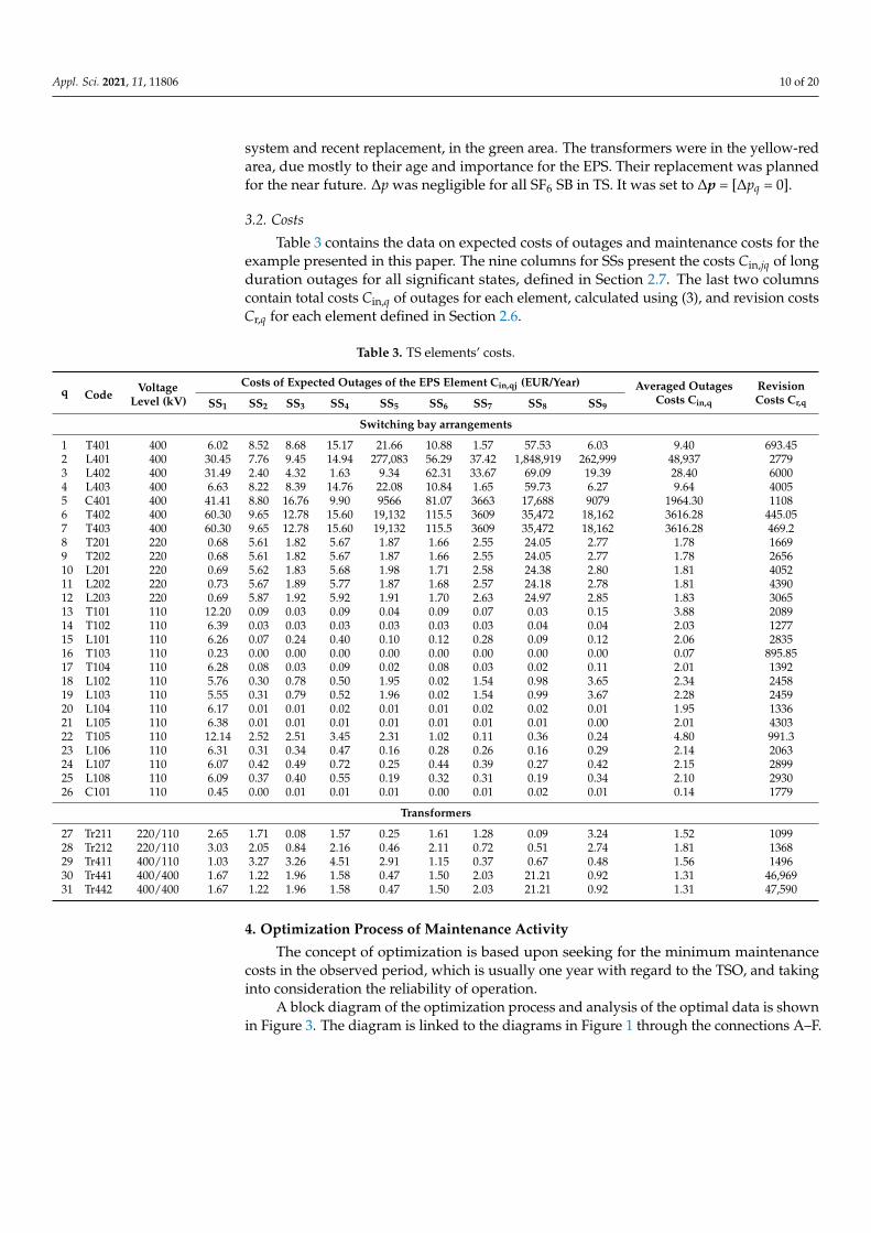
Table 3 contains the data on expected costs of outages and maintenance costs for theexample presented in this paper. The nine columns for SSs present the costs Cin,jq of longduration outages for all significant states, defined in Section 2.7. The last two columnscontain total costs Cin,q of outages for each element, calculated using (3), and revision costsCr,q for each element defined in Section 2.6.

Table 3. TS elements’ costs.

q CodeVoltage

Level (kV)

Costs of Expected Outages of the EPS Element Cin,qj (EUR/Year) Averaged OutagesCosts Cin,q

RevisionCosts Cr,qSS1 SS2 SS3 SS4 SS5 SS6 SS7 SS8 SS9

Switching bay arrangements

1 T401 400 6.02 8.52 8.68 15.17 21.66 10.88 1.57 57.53 6.03 9.40 693.452 L401 400 30.45 7.76 9.45 14.94 277,083 56.29 37.42 1,848,919 262,999 48,937 27793 L402 400 31.49 2.40 4.32 1.63 9.34 62.31 33.67 69.09 19.39 28.40 60004 L403 400 6.63 8.22 8.39 14.76 22.08 10.84 1.65 59.73 6.27 9.64 40055 C401 400 41.41 8.80 16.76 9.90 9566 81.07 3663 17,688 9079 1964.30 11086 T402 400 60.30 9.65 12.78 15.60 19,132 115.5 3609 35,472 18,162 3616.28 445.057 T403 400 60.30 9.65 12.78 15.60 19,132 115.5 3609 35,472 18,162 3616.28 469.28 T201 220 0.68 5.61 1.82 5.67 1.87 1.66 2.55 24.05 2.77 1.78 16699 T202 220 0.68 5.61 1.82 5.67 1.87 1.66 2.55 24.05 2.77 1.78 265610 L201 220 0.69 5.62 1.83 5.68 1.98 1.71 2.58 24.38 2.80 1.81 405211 L202 220 0.73 5.67 1.89 5.77 1.87 1.68 2.57 24.18 2.78 1.81 439012 L203 220 0.69 5.87 1.92 5.92 1.91 1.70 2.63 24.97 2.85 1.83 306513 T101 110 12.20 0.09 0.03 0.09 0.04 0.09 0.07 0.03 0.15 3.88 208914 T102 110 6.39 0.03 0.03 0.03 0.03 0.03 0.03 0.04 0.04 2.03 127715 L101 110 6.26 0.07 0.24 0.40 0.10 0.12 0.28 0.09 0.12 2.06 283516 T103 110 0.23 0.00 0.00 0.00 0.00 0.00 0.00 0.00 0.00 0.07 895.8517 T104 110 6.28 0.08 0.03 0.09 0.02 0.08 0.03 0.02 0.11 2.01 139218 L102 110 5.76 0.30 0.78 0.50 1.95 0.02 1.54 0.98 3.65 2.34 245819 L103 110 5.55 0.31 0.79 0.52 1.96 0.02 1.54 0.99 3.67 2.28 245920 L104 110 6.17 0.01 0.01 0.02 0.01 0.01 0.02 0.02 0.01 1.95 133621 L105 110 6.38 0.01 0.01 0.01 0.01 0.01 0.01 0.01 0.00 2.01 430322 T105 110 12.14 2.52 2.51 3.45 2.31 1.02 0.11 0.36 0.24 4.80 991.323 L106 110 6.31 0.31 0.34 0.47 0.16 0.28 0.26 0.16 0.29 2.14 206324 L107 110 6.07 0.42 0.49 0.72 0.25 0.44 0.39 0.27 0.42 2.15 289925 L108 110 6.09 0.37 0.40 0.55 0.19 0.32 0.31 0.19 0.34 2.10 293026 C101 110 0.45 0.00 0.01 0.01 0.01 0.00 0.01 0.02 0.01 0.14 1779

Transformers

27 Tr211 220/110 2.65 1.71 0.08 1.57 0.25 1.61 1.28 0.09 3.24 1.52 109928 Tr212 220/110 3.03 2.05 0.84 2.16 0.46 2.11 0.72 0.51 2.74 1.81 136829 Tr411 400/110 1.03 3.27 3.26 4.51 2.91 1.15 0.37 0.67 0.48 1.56 149630 Tr441 400/400 1.67 1.22 1.96 1.58 0.47 1.50 2.03 21.21 0.92 1.31 46,96931 Tr442 400/400 1.67 1.22 1.96 1.58 0.47 1.50 2.03 21.21 0.92 1.31 47,590

4. Optimization Process of Maintenance Activity

The concept of optimization is based upon seeking for the minimum maintenancecosts in the observed period, which is usually one year with regard to the TSO, and takinginto consideration the reliability of operation.

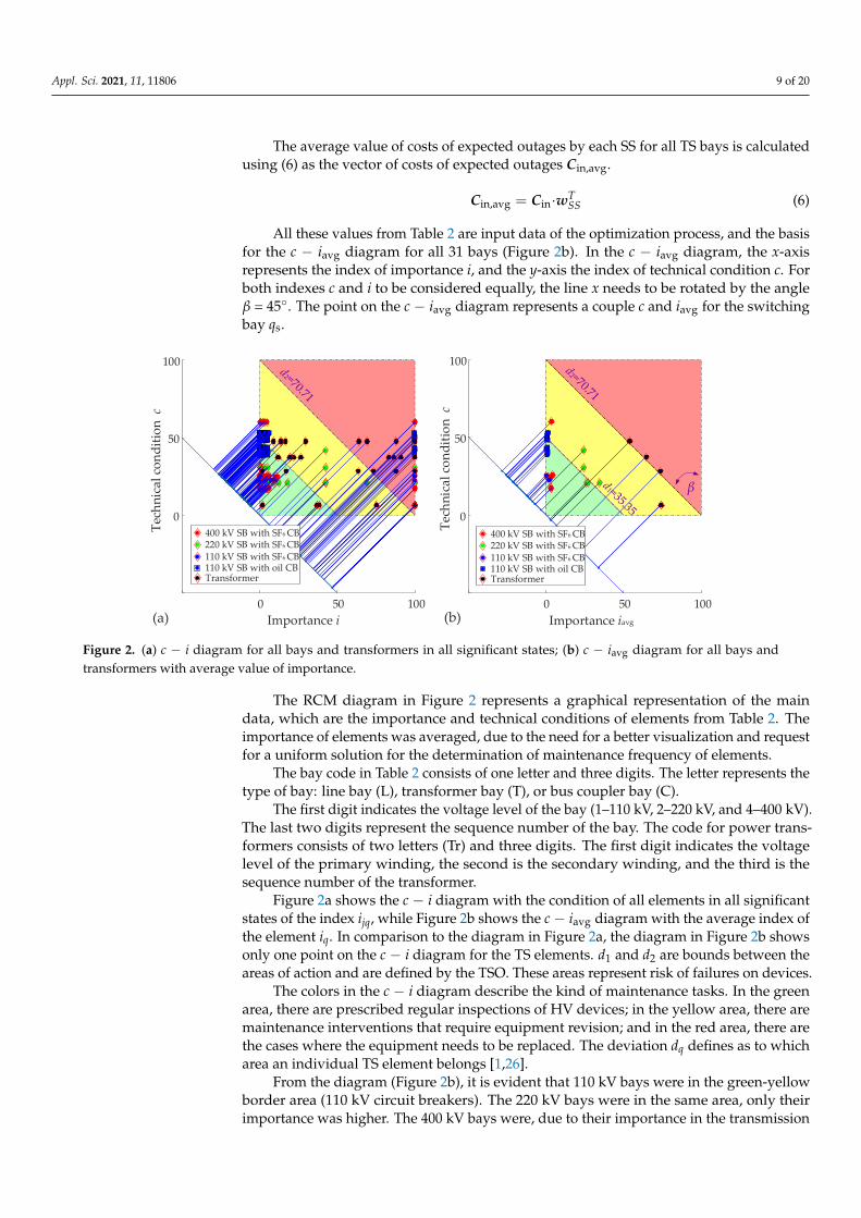
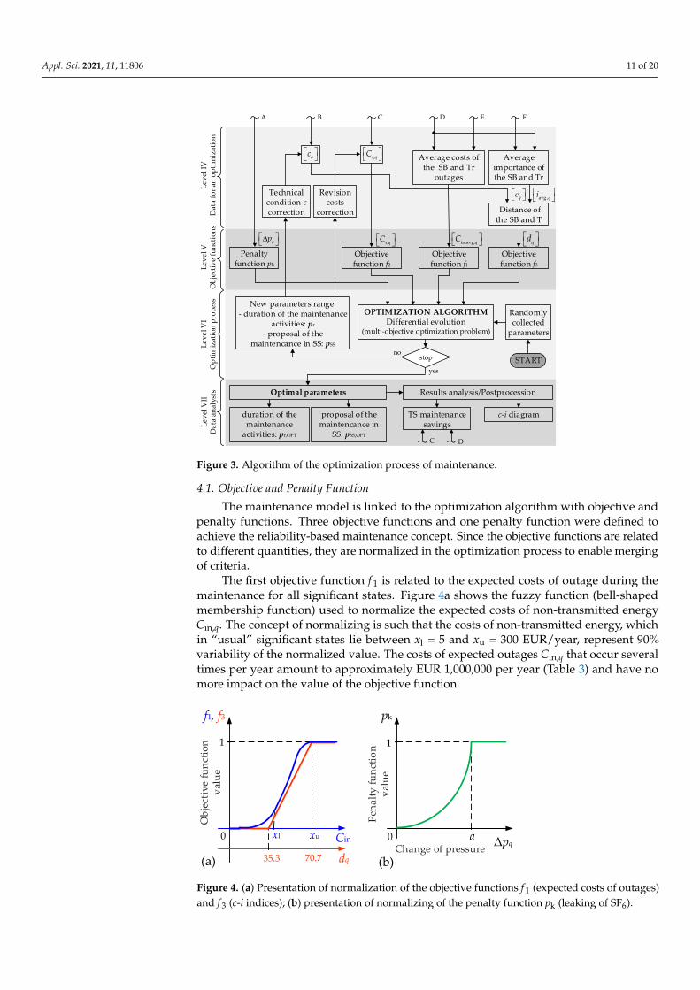
A block diagram of the optimization process and analysis of the optimal data is shownin Figure 3. The diagram is linked to the diagrams in Figure 1 through the connections A–F.

Appl. Sci. 2021, 11, 11806 11 of 20Appl. Sci. 2021, 11, x FOR PEER REVIEW 12 of 21

Figure 3. Algorithm of the optimization process of maintenance.

4.1. Objective and Penalty Function The maintenance model is linked to the optimization algorithm with objective and

penalty functions. Three objective functions and one penalty function were defined to achieve the reliability-based maintenance concept. Since the objective functions are re-lated to different quantities, they are normalized in the optimization process to enable merging of criteria.

The first objective function f1 is related to the expected costs of outage during the maintenance for all significant states. Figure 4a shows the fuzzy function (bell-shaped membership function) used to normalize the expected costs of non-transmitted energy Cin,q. The concept of normalizing is such that the costs of non-transmitted energy, which in “usual” significant states lie between xl = 5 and xu = 300 EUR/year, represent 90% varia-bility of the normalized value. The costs of expected outages Cin,q that occur several times per year amount to approximately EUR 1,000,000 per year (Table 3) and have no more impact on the value of the objective function.

The second objective function f2 in the optimization process that represents the revi-sion costs for a certain TS element Cr,q for all tasks that require de-energizing of an indi-vidual bay. Since the range of these costs is smaller than for the first objective function, there is no need for the use of fuzzy function-based normalization. The normalization is performed using (7)

{ }SB SB

r,2 r, SB

1 1; 31; 1, 2, 3

n nq

qqq q

f C n yy= =

= = ∈ C (7)

where the objective function encompasses the total costs of all the 31 transmission substa-tion bays and transformers, where the revision time period (1, 2, or 3 years) is taken into consideration for each bay separately.

The third objective function f3 is related to the indices of the RCM maintenance con-cept. In the block diagram of input data (Figure 3), the RCM indices c and i are included in the common index d. In the denotation of the vector, the weighting factor wSSj needs to

A B C D E F

Average costs of the SB and Tr

outages

Average importance of the SB and Tr

Distance of the SB and T

qd

Objective function f3


Penalty function pk


OPTIMIZATION ALGORITHM Differential evolution

(multi-objective optimization problem)

New parameters range:- duration of the maintenance

activities: pr

- proposal of the maintencance in SS: pSS

Revision costs

correction

Technical condition c correction

stop

Optimal parameters Results analysis/Postprocession

duration of the maintenance

activities: pr,OPT

proposal of the maintencance in

SS: pSS,OPT

TS maintenance savings

c-i diagram

C D

Leve

l IV

Dat

a fo

r an

opti

miz

atio

nLe

vel V

Obj

ectiv

e fu

nctio

nsLe

vel V

IO

ptim

izat

ion

proc

ess

Leve

l VII

Dat

a an

alys

is

yes

no

Randomly collected

parameters

START

qc

r,qC

qc avg ,qi

Δ qp r,qC

in,avg,qC

Figure 3. Algorithm of the optimization process of maintenance.

4.1. Objective and Penalty Function

The maintenance model is linked to the optimization algorithm with objective andpenalty functions. Three objective functions and one penalty function were defined toachieve the reliability-based maintenance concept. Since the objective functions are relatedto different quantities, they are normalized in the optimization process to enable mergingof criteria.

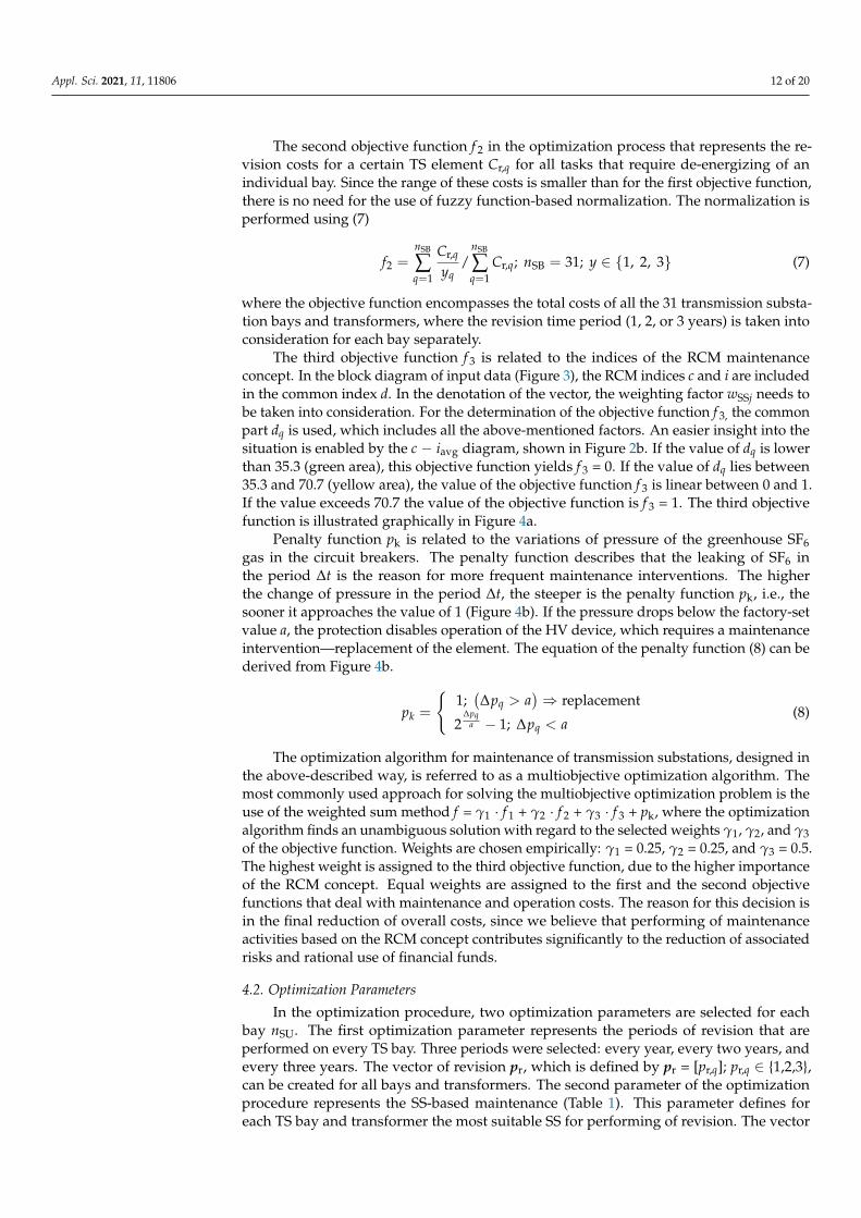
The first objective function f 1 is related to the expected costs of outage during themaintenance for all significant states. Figure 4a shows the fuzzy function (bell-shapedmembership function) used to normalize the expected costs of non-transmitted energyCin,q. The concept of normalizing is such that the costs of non-transmitted energy, whichin “usual” significant states lie between xl = 5 and xu = 300 EUR/year, represent 90%variability of the normalized value. The costs of expected outages Cin,q that occur severaltimes per year amount to approximately EUR 1,000,000 per year (Table 3) and have nomore impact on the value of the objective function.


be taken into consideration. For the determination of the objective function f3, the common part dq is used, which includes all the above-mentioned factors. An easier insight into the situation is enabled by the c − iavg diagram, shown in Figure 2b. If the value of dq is lower than 35.3 (green area), this objective function yields f3 = 0. If the value of dq lies between 35.3 and 70.7 (yellow area), the value of the objective function f3 is linear between 0 and 1. If the value exceeds 70.7 the value of the objective function is f3 = 1. The third objective function is illustrated graphically in Figure 4a.

Figure 4. (a) Presentation of normalization of the objective functions f1 (expected costs of outages) and f3 (c-i indices); (b) presentation of normalizing of the penalty function pk (leaking of SF6).

Penalty function pk is related to the variations of pressure of the greenhouse SF6 gas in the circuit breakers. The penalty function describes that the leaking of SF6 in the period Δt is the reason for more frequent maintenance interventions. The higher the change of pressure in the period Δt, the steeper is the penalty function pk, i.e., the sooner it ap-proaches the value of 1 (Figure 4b). If the pressure drops below the factory-set value a, the protection disables operation of the HV device, which requires a maintenance interven-tion—replacement of the element. The equation of the penalty function (8) can be derived from Figure 4b.

( )k

1; replacement

2 1; q

q

pa q

p ap

p aΔ

Δ > = − Δ <

(8)

The optimization algorithm for maintenance of transmission substations, designed in the above-described way, is referred to as a multiobjective optimization algorithm. The most commonly used approach for solving the multiobjective optimization problem is the use of the weighted sum method f = γ1 ∙ f1 + γ2 ∙ f2 + γ3 ∙ f3 + pk, where the optimization algorithm finds an unambiguous solution with regard to the selected weights γ1, γ2, and γ3 of the objective function. Weights are chosen empirically: γ1 = 0.25, γ2 = 0.25, and γ3 = 0.5. The highest weight is assigned to the third objective function, due to the higher im-portance of the RCM concept. Equal weights are assigned to the first and the second ob-jective functions that deal with maintenance and operation costs. The reason for this deci-sion is in the final reduction of overall costs, since we believe that performing of mainte-nance activities based on the RCM concept contributes significantly to the reduction of associated risks and rational use of financial funds.

4.2. Optimization Parameters In the optimization procedure, two optimization parameters are selected for each bay

nSU. The first optimization parameter represents the periods of revision that are performed on every TS bay. Three periods were selected: every year, every two years, and every three years. The vector of revision pr, which is defined by pr = [pr,q]; pr,q ∈ {1,2,3}, can be created

f1, f3

xl Cinxu0 a

1

0

1

pk

Δpq

35.3 dq70.7(a) (b)

Obj

ecti

ve fu

nctio

n va

lue

Pena

lty fu

nctio

n va

lue

Change of pressure

Figure 4. (a) Presentation of normalization of the objective functions f 1 (expected costs of outages)and f 3 (c-i indices); (b) presentation of normalizing of the penalty function pk (leaking of SF6).

Appl. Sci. 2021, 11, 11806 12 of 20

The second objective function f 2 in the optimization process that represents the re-vision costs for a certain TS element Cr,q for all tasks that require de-energizing of anindividual bay. Since the range of these costs is smaller than for the first objective function,there is no need for the use of fuzzy function-based normalization. The normalization isperformed using (7)

f2 =nSB

∑q=1

Cr,q

yq/

nSB

∑q=1

Cr,q; nSB = 31; y ∈ {1, 2, 3} (7)

where the objective function encompasses the total costs of all the 31 transmission substa-tion bays and transformers, where the revision time period (1, 2, or 3 years) is taken intoconsideration for each bay separately.

The third objective function f 3 is related to the indices of the RCM maintenanceconcept. In the block diagram of input data (Figure 3), the RCM indices c and i are includedin the common index d. In the denotation of the vector, the weighting factor wSSj needs tobe taken into consideration. For the determination of the objective function f 3, the commonpart dq is used, which includes all the above-mentioned factors. An easier insight into thesituation is enabled by the c − iavg diagram, shown in Figure 2b. If the value of dq is lowerthan 35.3 (green area), this objective function yields f 3 = 0. If the value of dq lies between35.3 and 70.7 (yellow area), the value of the objective function f 3 is linear between 0 and 1.If the value exceeds 70.7 the value of the objective function is f 3 = 1. The third objectivefunction is illustrated graphically in Figure 4a.

Penalty function pk is related to the variations of pressure of the greenhouse SF6gas in the circuit breakers. The penalty function describes that the leaking of SF6 inthe period ∆t is the reason for more frequent maintenance interventions. The higherthe change of pressure in the period ∆t, the steeper is the penalty function pk, i.e., thesooner it approaches the value of 1 (Figure 4b). If the pressure drops below the factory-setvalue a, the protection disables operation of the HV device, which requires a maintenanceintervention—replacement of the element. The equation of the penalty function (8) can bederived from Figure 4b.

pk =

{1;(∆pq > a

)⇒ replacement

2∆pq

a − 1; ∆pq < a(8)

The optimization algorithm for maintenance of transmission substations, designed inthe above-described way, is referred to as a multiobjective optimization algorithm. Themost commonly used approach for solving the multiobjective optimization problem is theuse of the weighted sum method f = γ1 · f 1 + γ2 · f 2 + γ3 · f 3 + pk, where the optimizationalgorithm finds an unambiguous solution with regard to the selected weights γ1, γ2, and γ3of the objective function. Weights are chosen empirically: γ1 = 0.25, γ2 = 0.25, and γ3 = 0.5.The highest weight is assigned to the third objective function, due to the higher importanceof the RCM concept. Equal weights are assigned to the first and the second objectivefunctions that deal with maintenance and operation costs. The reason for this decision isin the final reduction of overall costs, since we believe that performing of maintenanceactivities based on the RCM concept contributes significantly to the reduction of associatedrisks and rational use of financial funds.

4.2. Optimization Parameters

In the optimization procedure, two optimization parameters are selected for eachbay nSU. The first optimization parameter represents the periods of revision that areperformed on every TS bay. Three periods were selected: every year, every two years, andevery three years. The vector of revision pr, which is defined by pr = [pr,q]; pr,q ∈ {1,2,3},can be created for all bays and transformers. The second parameter of the optimizationprocedure represents the SS-based maintenance (Table 1). This parameter defines foreach TS bay and transformer the most suitable SS for performing of revision. The vector

Appl. Sci. 2021, 11, 11806 13 of 20

of maintenance by SS pSS is created for all TS bays and transformers. The codomain ofthis vector is the significant states themselves. The parameter is defined by pSS = [pSS,q];pSS,q ∈{j; 1 ≤ j ≤ nSS}; 1 ≤ q ≤ nSU; j,q ∈ N.

4.3. Optimization Process with the Modified Differential Evolution Algorithm

The modified differential evolution algorithm, which belongs to the group of evo-lutionary computation methods, is used in the optimization process. In the process ofseeking the optimal solution of the objective function, which represents the maintenancemodel of a substation on the basis of the RCM concept, we introduced a modification of thealgorithm, representing self-adaptation (SA) of the control parameters CR in F [29,30]. Thefollowing three possibilities were analyzed: optimization without SA (basic DE algorithm),optimization with CR and F self-adapted for the entire population, and optimization withCR and F self-adapted for each individual in the population.

These improvements ensured adequate robustness of the algorithm since the opti-mization problem is extremely complex and comprehensive (62 optimization parameters).

To ensure successful operation of the DE optimization algorithm, we selected thecontrol parameters of differential evolution that are presented in Table 4. The control pa-rameters have a significant impact on performance of the search process in DE (convergenceof the optimization process and accuracy of computation of the optimal solution).

Table 4. Control parameters of DE.

Control Parameter Value Description

VTR 1 × 10−3 value-to-reachD 62 number of parameters

NP 600 population sizeStrategy 7 strategy DE/rand/1/bin

CR 0.7/self-adaptive crossover probabilityF 0.6/self-adaptive differential weighting factor

itermax 1000 maximum number of iterations

5. Results of Optimal RCM Maintenance

The use of an adequate optimization tool can ensure preservation of the existing levelof maintenance quality, despite the cost reduction achieved by the use of the modifieddifferential evolution algorithm.

5.1. Optimization Process

The progress of optimization process versus iterations is shown in Figure 5. It can beseen that the optimization process converged to the optimal solution after approximately700 iterations.

Seeking an optimal solution in the optimization process is conditioned by the values ofindividual objective functions and their weights. Individual objective functions, of course,cannot converge to their own optimums, since the optimization process is oriented to thecommon criterion that represents the correlation of individual criteria.

Ten independent calculations of optimization algorithm runs were performed foreach SA variant. The average value and standard deviation of the objective function werecomputed on the basis of these runs (Table 5). The use of an optimization algorithmwithout SA indicates a dispersion of the results of 10 independent runs. The results ofboth other variants with the use of SA, on the other hand, indicate the reliability androbustness of the optimization algorithm, since there was no dispersion of the results of10 independent optimization runs (standard deviation equals zero). All results are relatedto the optimization with SA.

Appl. Sci. 2021, 11, 11806 14 of 20Appl. Sci. 2021, 11, x FOR PEER REVIEW 15 of 21

Figure 5. Progress of the optimization process of common objective function and partial objective functions.

Ten independent calculations of optimization algorithm runs were performed for each SA variant. The average value and standard deviation of the objective function were computed on the basis of these runs (Table 5). The use of an optimization algorithm with-out SA indicates a dispersion of the results of 10 independent runs. The results of both other variants with the use of SA, on the other hand, indicate the reliability and robustness of the optimization algorithm, since there was no dispersion of the results of 10 independ-ent optimization runs (standard deviation equals zero). All results are related to the opti-mization with SA.

Table 5. Mean values and standard deviation of objective function for variants of SA.

No. Without SA F and CR for the Whole Popu-lation

F and CR for Each Individual in the Population

Value of objective func-tion

1 0.410812 0.400430 0.400430 2 0.409546 0.400430 0.400430 3 0.407953 0.400430 0.400430 4 0.409546 0.400430 0.400430 5 0.407953 0.400430 0.400430 6 0.409546 0.400430 0.400430 7 0.407953 0.400430 0.400430 8 0.409546 0.400430 0.400430 9 0.407953 0.400430 0.400430

10 0.409179 0.400430 0.400430 Mean value of objective

function 0.408999 0.400430 0.400430

StD of objective func-tion

0.000573 0 0

5.2. Optimal Maintenance for the Observed TS The optimization was performed to obtain optimal parameters representing the fre-

quency of maintenance activities pr,OPT and the optimal SS pSS,OPT, in which the mainte-nance should be carried out. The maintenance of each TS bay is, therefore, conditioned by two optimization parameters.

0 100 200 300 400 500 600 700 800 900 10000

0.1

0.2

0.3

0.4

0.5

0.6

0.7

Iteration

Obj

ectiv

e fu

nctio

n va

lue

f f1 f2 f3

Figure 5. Progress of the optimization process of common objective function and partial objectivefunctions.

Table 5. Mean values and standard deviation of objective function for variants of SA.

No. Without SA F and CR for theWhole Population

F and CR for Each Individualin the Population

Value ofobjective function

1 0.410812 0.400430 0.4004302 0.409546 0.400430 0.4004303 0.407953 0.400430 0.4004304 0.409546 0.400430 0.4004305 0.407953 0.400430 0.4004306 0.409546 0.400430 0.4004307 0.407953 0.400430 0.4004308 0.409546 0.400430 0.4004309 0.407953 0.400430 0.40043010 0.409179 0.400430 0.400430

Mean value ofobjective function 0.408999 0.400430 0.400430

StD ofobjective function 0.000573 0 0

5.2. Optimal Maintenance for the Observed TS

The optimization was performed to obtain optimal parameters representing the fre-quency of maintenance activities pr,OPT and the optimal SS pSS,OPT, in which the mainte-nance should be carried out. The maintenance of each TS bay is, therefore, conditioned bytwo optimization parameters.

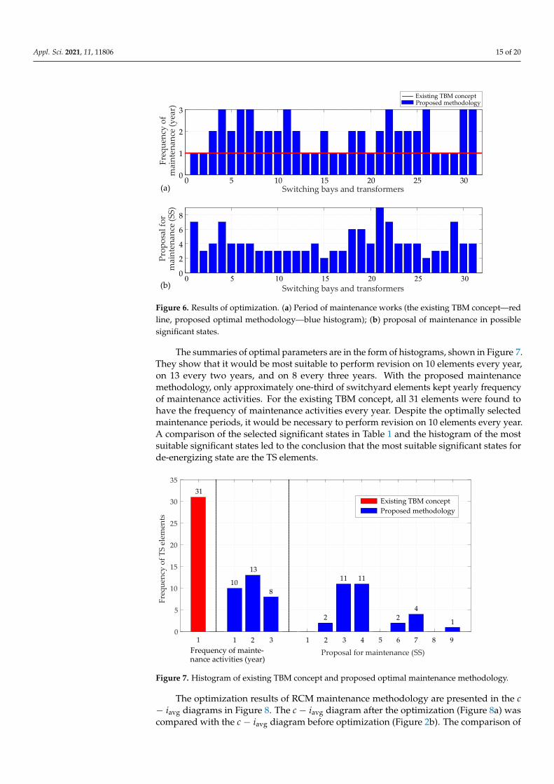
Figure 6 shows the results of optimal maintenance for the observed TS, where Figure 6ashows the optimization parameters from the vector pr,OPT (in years) for the revision per-formed in each individual switching bay or power transformers (the existing TBM mainte-nance methodology—red line, proposed optimal methodology—blue histogram). Figure 6bshows the optimal data of the second set of optimization parameters pSS,OPT, which repre-sents the proposal for maintenance. It provides the information about the selected SS ofthe EPS (possible future combination of generation, consumption, and power flows in theTS) when it would be most suitable to de-energize the TS elements and perform revision.

Appl. Sci. 2021, 11, 11806 15 of 20


Figure 6 shows the results of optimal maintenance for the observed TS, where Figure 6a shows the optimization parameters from the vector pr,OPT (in years) for the revision per-formed in each individual switching bay or power transformers (the existing TBM mainte-nance methodology—red line, proposed optimal methodology—blue histogram). Figure 6b shows the optimal data of the second set of optimization parameters pSS,OPT, which rep-resents the proposal for maintenance. It provides the information about the selected SS of the EPS (possible future combination of generation, consumption, and power flows in the TS) when it would be most suitable to de-energize the TS elements and perform revision.

Figure 6. Results of optimization. (a) Period of maintenance works (the existing TBM concept—red line, proposed optimal methodology—blue histogram); (b) proposal of maintenance in possible sig-nificant states.

The summaries of optimal parameters are in the form of histograms, shown in Figure 7. They show that it would be most suitable to perform revision on 10 elements every year, on 13 every two years, and on 8 every three years. With the proposed maintenance meth-odology, only approximately one-third of switchyard elements kept yearly frequency of maintenance activities. For the existing TBM concept, all 31 elements were found to have the frequency of maintenance activities every year. Despite the optimally selected mainte-nance periods, it would be necessary to perform revision on 10 elements every year. A comparison of the selected significant states in Table 1 and the histogram of the most suit-able significant states led to the conclusion that the most suitable significant states for de-energizing state are the TS elements.

0 5 10 15 20 25 300

1

2

3

Switching bays and transformers

Freq

uenc

y of

m

aint

enan

ce (y

ear)

0 5 10 15 20 25 300

2

4

6

8

Switching bays and transformers

Prop

osal

for

m

aint

enan

ce (S

S)

(b)

(a)

Proposed methodologyExisting TBM concept

Figure 6. Results of optimization. (a) Period of maintenance works (the existing TBM concept—redline, proposed optimal methodology—blue histogram); (b) proposal of maintenance in possiblesignificant states.

The summaries of optimal parameters are in the form of histograms, shown in Figure 7.They show that it would be most suitable to perform revision on 10 elements every year,on 13 every two years, and on 8 every three years. With the proposed maintenancemethodology, only approximately one-third of switchyard elements kept yearly frequencyof maintenance activities. For the existing TBM concept, all 31 elements were found tohave the frequency of maintenance activities every year. Despite the optimally selectedmaintenance periods, it would be necessary to perform revision on 10 elements every year.A comparison of the selected significant states in Table 1 and the histogram of the mostsuitable significant states led to the conclusion that the most suitable significant states forde-energizing state are the TS elements.


Figure 7. Histogram of existing TBM concept and proposed optimal maintenance methodology.

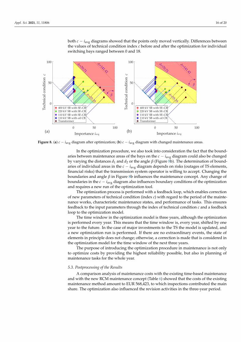
The optimization results of RCM maintenance methodology are presented in the c − iavg diagrams in Figure 8. The c − iavg diagram after the optimization (Figure 8a) was com-pared with the c − iavg diagram before optimization (Figure 2b). The comparison of both c − iavg diagrams showed that the points only moved vertically. Differences between the values of technical condition index c before and after the optimization for individual switching bays ranged between 0 and 18.

In the optimization procedure, we also took into consideration the fact that the boundaries between maintenance areas of the bays on the c − iavg diagram could also be changed by varying the distances d1 and d2 or the angle β (Figure 8b). The determination of boundaries of individual areas in the c − iavg diagram depends on risks (outages of TS elements, financial risks) that the transmission system operator is willing to accept. Changing the boundaries and angle β in Figure 8b influences the maintenance concept. Any change of boundaries in the c − iavg diagram also influences boundary conditions of the optimization and requires a new run of the optimization tool.

Figure 8. (a) c − iavg diagram after optimization; (b) c − iavg diagram with changed maintenance areas.

The optimization process is performed with a feedback loop, which enables correc-tion of new parameters of technical condition (index c) with regard to the period of the

0

5

10

15

20

25

30

35

1 2 3 1 2 3 4 5 6 7 8 91

Freq

uenc

y of

TS

elem

ents

Proposal for maintenance (SS)Frequency of mainte-nance activities (year)


10

13

8

31

2

11 11

24

1

0 50 100

0

50

100

0 50 100

0

50

100



(a) (b)

β

β

Importance iavg

Tech

nica

l con

ditio

n c

Importance iavg

Tech

nica

l con

ditio

n c


The optimization results of RCM maintenance methodology are presented in the c− iavg diagrams in Figure 8. The c − iavg diagram after the optimization (Figure 8a) wascompared with the c − iavg diagram before optimization (Figure 2b). The comparison of

Appl. Sci. 2021, 11, 11806 16 of 20

both c − iavg diagrams showed that the points only moved vertically. Differences betweenthe values of technical condition index c before and after the optimization for individualswitching bays ranged between 0 and 18.



The optimization results of RCM maintenance methodology are presented in the c − iavg diagrams in Figure 8. The c − iavg diagram after the optimization (Figure 8a) was com-pared with the c − iavg diagram before optimization (Figure 2b). The comparison of both c − iavg diagrams showed that the points only moved vertically. Differences between the values of technical condition index c before and after the optimization for individual switching bays ranged between 0 and 18.

In the optimization procedure, we also took into consideration the fact that the boundaries between maintenance areas of the bays on the c − iavg diagram could also be changed by varying the distances d1 and d2 or the angle β (Figure 8b). The determination of boundaries of individual areas in the c − iavg diagram depends on risks (outages of TS elements, financial risks) that the transmission system operator is willing to accept. Changing the boundaries and angle β in Figure 8b influences the maintenance concept. Any change of boundaries in the c − iavg diagram also influences boundary conditions of the optimization and requires a new run of the optimization tool.


The optimization process is performed with a feedback loop, which enables correc-tion of new parameters of technical condition (index c) with regard to the period of the

0

5

10

15

20

25

30

35

1 2 3 1 2 3 4 5 6 7 8 91

Freq

uenc

y of

TS

elem

ents

Proposal for maintenance (SS)Frequency of mainte-nance activities (year)


10

13

8

31

2

11 11

24

1

0 50 100

0

50

100

0 50 100

0

50

100



(a) (b)

β

β

Importance iavg

Tech

nica

l con

ditio

n c

Importance iavg

Tech

nica

l con

ditio

n c


In the optimization procedure, we also took into consideration the fact that the bound-aries between maintenance areas of the bays on the c − iavg diagram could also be changedby varying the distances d1 and d2 or the angle β (Figure 8b). The determination of bound-aries of individual areas in the c − iavg diagram depends on risks (outages of TS elements,financial risks) that the transmission system operator is willing to accept. Changing theboundaries and angle β in Figure 8b influences the maintenance concept. Any change ofboundaries in the c − iavg diagram also influences boundary conditions of the optimizationand requires a new run of the optimization tool.

The optimization process is performed with a feedback loop, which enables correctionof new parameters of technical condition (index c) with regard to the period of the mainte-nance works, characteristic maintenance states, and performance of tasks. This ensuresfeedback to the input parameters through the index of technical condition c and a feedbackloop to the optimization model.

The time window in the optimization model is three years, although the optimizationis performed every year. This means that the time window is, every year, shifted by oneyear to the future. In the case of major investments to the TS the model is updated, anda new optimization run is performed. If there are no extraordinary events, the state ofelements in principle does not change; otherwise, a correction is made that is considered inthe optimization model for the time window of the next three years.

The purpose of introducing the optimization procedure in maintenance is not onlyto optimize costs by providing the highest reliability possible, but also in planning ofmaintenance tasks for the whole year.

5.3. Postprocessing of the Results

A comparison analysis of maintenance costs with the existing time-based maintenanceand with the new RCM maintenance concept (Table 6) showed that the costs of the existingmaintenance method amount to EUR 568,423, to which inspections contributed the mainshare. The optimization also influenced the revision activities in the three-year period.

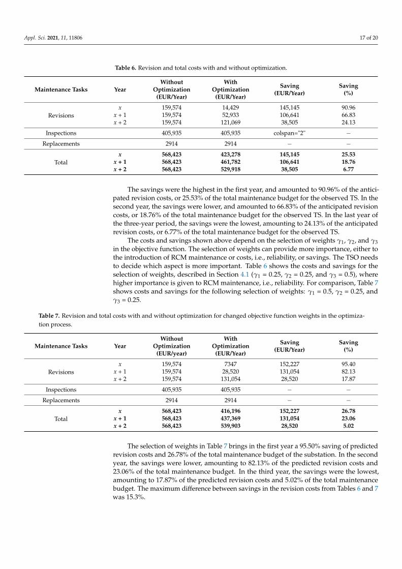
Appl. Sci. 2021, 11, 11806 17 of 20

Table 6. Revision and total costs with and without optimization.

Maintenance Tasks YearWithout

Optimization(EUR/Year)

WithOptimization

(EUR/Year)

Saving(EUR/Year)

Saving(%)

Revisionsx 159,574 14,429 145,145 90.96

x + 1 159,574 52,933 106,641 66.83x + 2 159,574 121,069 38,505 24.13

Inspections 405,935 405,935 colspan="2" −Replacements 2914 2914 − −

Totalx 568,423 423,278 145,145 25.53

x + 1 568,423 461,782 106,641 18.76x + 2 568,423 529,918 38,505 6.77

The savings were the highest in the first year, and amounted to 90.96% of the antici-pated revision costs, or 25.53% of the total maintenance budget for the observed TS. In thesecond year, the savings were lower, and amounted to 66.83% of the anticipated revisioncosts, or 18.76% of the total maintenance budget for the observed TS. In the last year ofthe three-year period, the savings were the lowest, amounting to 24.13% of the anticipatedrevision costs, or 6.77% of the total maintenance budget for the observed TS.

The costs and savings shown above depend on the selection of weights γ1, γ2, and γ3in the objective function. The selection of weights can provide more importance, either tothe introduction of RCM maintenance or costs, i.e., reliability, or savings. The TSO needsto decide which aspect is more important. Table 6 shows the costs and savings for theselection of weights, described in Section 4.1 (γ1 = 0.25, γ2 = 0.25, and γ3 = 0.5), wherehigher importance is given to RCM maintenance, i.e., reliability. For comparison, Table 7shows costs and savings for the following selection of weights: γ1 = 0.5, γ2 = 0.25, andγ3 = 0.25.

Table 7. Revision and total costs with and without optimization for changed objective function weights in the optimiza-tion process.

Maintenance Tasks YearWithout

Optimization(EUR/year)

WithOptimization

(EUR/Year)

Saving(EUR/Year)

Saving(%)

Revisionsx 159,574 7347 152,227 95.40

x + 1 159,574 28,520 131,054 82.13x + 2 159,574 131,054 28,520 17.87

Inspections 405,935 405,935 − −Replacements 2914 2914 − −

Totalx 568,423 416,196 152,227 26.78

x + 1 568,423 437,369 131,054 23.06x + 2 568,423 539,903 28,520 5.02

The selection of weights in Table 7 brings in the first year a 95.50% saving of predictedrevision costs and 26.78% of the total maintenance budget of the substation. In the secondyear, the savings were lower, amounting to 82.13% of the predicted revision costs and23.06% of the total maintenance budget. In the third year, the savings were the lowest,amounting to 17.87% of the predicted revision costs and 5.02% of the total maintenancebudget. The maximum difference between savings in the revision costs from Tables 6 and 7was 15.3%.

Appl. Sci. 2021, 11, 11806 18 of 20

6. Discussion

In the field of maintenance of electric power system devices and networks, time-basedmaintenance (TBM) is still used widely. Nevertheless, a large number of companies aregradually introducing condition-based maintenance (CBM). An upgrade of such mainte-nance system is RCM, wherein the frequency of maintenance interventions is defined withregard to the state and importance of the EPS element. RCM maintenance methodologyconsiders the reliability of the entire system and not only individual elements, which is thekey advantage of this maintenance methodology.

An RCM model was developed and tested for transmission substations. For thispurpose, in the first step, input data were defined for the indicators of operational relia-bility, technical condition of devices, and maintenance costs. These data were obtainedon the basis of results of diagnostics and monitoring of elements, as well as from thecalculations of parameters for the entire Slovenian EPS. The RCM model was upgradedwith an optimization algorithm that enables it to find the optimal maintenance costs atthe guaranteed reliability of operation and the most suitable combination of generation,consumption, and power flows (SS). Improper maintenance of the EPS elements causesvarious risks. These risks can be managed by the introduction of maintenance optimization.For the maintenance costs to be reduced, it is necessary to know the limit of acceptablerisks. The maintenance optimization mode presented in this paper was tested practicallyin one of the Slovenian transmission substations. The developed algorithm is universaland can be used for any TS and included in the entire process of EPS maintenance, i.e., inthe asset management of any transmission system operator.

A limitation of use of the proposed algorithm can, in the case of very large maintenancesystems (e.g., a few thousands of elements), be problematic. In such a case, the use ofconventional optimization algorithms, such as the one used in this paper, could jeopardizethe stability of the optimization process and the accuracy of the obtained solutions.

With the proposed new algorithm for calculating maintenance periods using the opti-mization process, we confirmed the hypothesis that analyzing the past data of operation,events, and maintenance costs enables a direct impact on maintenance process for thefuture periods. With this maintenance concept, we maintain the reliability of operation ofEPS elements and of their technical condition. At the same time, we reduce maintenancecosts. A comparison of the existing (TBM) maintenance concept and the proposed oneconfirms savings. The proposed computations showed 25.53% saving in the first year,18.76% in the second year, and 6.77% in the third year. This was the confirmation of thesecond hypothesis.

Further research work in the field of EPS elements’ maintenance enables extensions ofthe optimization model on all substations and all transmission lines in the transmissionsystem. Testing with different maintenance periods could be performed for more extensivecomparisons. It would also be possible to perform research of the use and testing ofdifferent optimization algorithms, as well as introduction of new approaches, such as thedeep learning maintenance process.

Author Contributions: Conceptualization, P.K. and J.R.; methodology, P.K. and L.B.; software, P.K.and J.R.; validation, L.B., J.P., and J.R.; formal analysis, J.P.; investigation, L.B. and J.P.; resources, L.B.and J.P.; data curation, L.B.; writing—original draft preparation, P.K.; writing—review and editing,J.P. and J.R.; visualization, P.K.; supervision, J.P. and J.R.; project administration, J.P. All authors haveread and agreed to the published version of the manuscript.

Funding: This research received no external funding.

Institutional Review Board Statement: Not applicable.

Informed Consent Statement: Not applicable.

Data Availability Statement: Not applicable.

Conflicts of Interest: The authors declare no conflict of interest.

Appl. Sci. 2021, 11, 11806 19 of 20

References1. Balzer, G. Condition assessment and reliability centered maintenance of high voltage equipment. In Proceedings of the 2005

International Symposium on Electrical Insulating Materials (ISEIM 2005), Kitakyushu, Japan, 5–9 June 2005; pp. 259–264.2. Birkner, P. Field experience with a condition-based maintenance program of 20-kV XLPE distribution system using IRC-analysis.

IEEE Trans. Power Deliv. 2004, 19, 3–8. [CrossRef]3. Bohatyrewicz, P.; Płowucha, J.; Subocz, J. Condition Assessment of Power Transformers Based on Health Index Value. Appl. Sci.

2019, 9, 4877. [CrossRef]4. Zhang, F.; Wen, Z.; Liu, D.; Jiao, J.; Wan, H.; Zeng, B. Calculation and Analysis of Wind Turbine Health Monitoring Indicators

Based on the Relationships with SCADA Data. Appl. Sci. 2020, 10, 410. [CrossRef]5. Liu, Y.; Xv, J.; Yuan, H.; Lv, J.; Ma, Z. Health Assessment and Prediction of Overhead Line Based on Health Index. IEEE Trans. Ind.

Electron. 2019, 66, 5546–5557. [CrossRef]6. Fang, F.; Zhao, Z.; Huang, C.; Zhang, X.; Wang, H.; Yang, Y. Application of Reliability-Centered Maintenance in Metro Door

System. IEEE Access 2019, 7, 186167–186174. [CrossRef]7. Vera-García, F.; Pagán Rubio, J.A.; Hernández Grau, J.; Albaladejo Hernández, D. Improvements of a Failure Database for Marine

Diesel Engines Using the RCM and Simulations. Energies 2020, 13, 104. [CrossRef]8. Zhang, X.; Zhang, J.; Gockenbach, E. Reliability Centered Asset Management for Medium-Voltage Deteriorating Electrical

Equipment Based on Germany Failure Statistics. IEEE Trans. Power Syst. 2009, 24, 721–728. [CrossRef]9. Ge, H.; Asgarpoor, S. Reliability and Maintainability Improvement of Substations With Aging Infrastructure. IEEE Trans. Power

Deliv. 2012, 27, 1868–1876. [CrossRef]10. de França Moraes, C.C.; Pinheiro, P.R.; Rolim, I.G.; da Silva Costa, J.L.; Junior, M.D.S.E.; Andrade, S.J.M.D. Using the Multi-Criteria

Model for Optimization of Operational Routes of Thermal Power Plants. Energies 2021, 14, 3682. [CrossRef]11. IEC Standard 60300-3-11. In IEC Dependability Management-Part 3-11: Application Guide-Reliability Centred Maintenance; IEC:

Geneva, Switzerland, 2009.12. IEC Standard TS 62775. In IEC Application Guidelines-Technical And Financial Processes for Implementing Asset Management Systems;

IEC: Geneva, Switzerland, 2016.13. Mohd Selva, A.; Azis, N.; Yahaya, M.S.; Ab Kadir, M.Z.A.; Jasni, J.; Yang Ghazali, Y.Z.; Talib, M.A. Application of Markov Model

to Estimate Individual Condition Parameters for Transformers. Energies 2018, 11, 2114. [CrossRef]14. Yang, F.; Chang, C.S. Multiobjective Evolutionary Optimization of Maintenance Schedules and Extents for Composite Power

Systems. IEEE Trans. Power Syst. 2009, 24, 1694–1702. [CrossRef]15. Rafiei, M.; Khooban, M.-H.; Igder, M.A.; Boudjadar, J. A novel approach to overcome the limitations of reliability centered

maintenance implementation on the smart grid distance protection system. IEEE Trans. Circuits Syst. II Express Briefs 2020, 67,320–324. [CrossRef]

16. Bahrami, S.; Rastegar, M.; Dehghanian, P. An FBWM-TOPSIS Approach to Identify Critical Feeders for Reliability CenteredMaintenance in Power Distribution Systems. IEEE Syst. J. 2020, 15, 3893–3901. [CrossRef]

17. Hilber, P.; Miranda, V.; Matos, M.A.; Bertling, L. Multiobjective Optimization Applied to Maintenance Policy for ElectricalNetworks. IEEE Trans. Power Syst. 2007, 22, 1675–1682. [CrossRef]

18. Arno, R.; Dowling, N.; Schuerger, R. Equipment Failure Characteristics and RCM for Optimizing Maintenance Cost. IEEE Trans.Ind. Appl. 2016, 52, 1257–1264.

19. Piasson, D.; Bíscaro, A.A.P.; Leao, F.B.; Mantovani, J.R.S. A new approach for reliability-centered maintenance programs in electricpower distribution systems based on multiobjective genetic algorithm. Electr. Power Syst. Res. 2016, 137, 41–50. [CrossRef]

20. Zhang, D.; Li, W.; Xiong, X. Overhead line preventive maintenance strategy based on condition monitoring and system reliabilityassessment. IEEE Trans. Power Syst. 2014, 29, 1839–1846. [CrossRef]

21. Suwnansri, T. Asset management of power transformer: Optimization of operation and maintenance costs. In Proceedings of the2014 International Electrical Engineering Congress (iEECON), Chonburi, Thailand, 19–21 March 2014; pp. 1–4.

22. Dong, M.; Zheng, H.; Zhang, Y.; Shi, K.; Yao, S.; Kou, X.; Ding, G.; Guo, L. A Novel Maintenance Decision Making Model ofPower Transformers Based on Reliability and Economy Assessment. IEEE Access 2019, 7, 28778–28790. [CrossRef]

23. Hinow, M.; Mevissen, M. Substation Maintenance Strategy Adaptation for Life-Cycle Cost Reduction Using Genetic Algorithm.IEEE Trans. Power Deliv. 2011, 26, 197–204. [CrossRef]

24. Pandzic, H.; Conejo, A.J.; Kuzle, I.; Caro, E. Yearly Maintenance Scheduling of Transmission Lines Within a Market Environment.IEEE Trans. Power Syst. 2012, 27, 407–415. [CrossRef]

25. Zhong, J.; Li, W.; Wang, C.; Yu, J.; Xu, R. Determining Optimal Inspection Intervals in Maintenance Considering EquipmentAging Failures. IEEE Trans. Power Syst. 2017, 32, 1474–1482. [CrossRef]

26. Belak, L.; Marusa, R.; Ferlic, R.; Pihler, J. Strategic Maintenance of 400-kV Switching Substations. IEEE Trans. Power Deliv. 2013,28, 394–401. [CrossRef]

27. McDonald, J.D. Electric Power Substations Engineering, 2nd ed.; CRC Press: Boca Raton, FL, USA, 2006.28. Wang, F.; Tuinema, B.W.; Gibescu, M.; Meijden, M.A.M.M. Reliability evaluation of substations subject to protection system

failures. In Proceedings of the 2013 IEEE Grenoble Conference, Grenoble, France, 16–20 June 2013.

http://doi.org/10.1109/TPWRD.2003.820421

http://doi.org/10.3390/app9224877

http://doi.org/10.3390/app10010410

http://doi.org/10.1109/TIE.2018.2868028

http://doi.org/10.1109/ACCESS.2019.2960521

http://doi.org/10.3390/en13010104

http://doi.org/10.1109/TPWRS.2009.2016533


http://doi.org/10.3390/en14123682

http://doi.org/10.3390/en11082114


http://doi.org/10.1109/TCSII.2019.2905639

http://doi.org/10.1109/JSYST.2020.3014649


http://doi.org/10.1016/j.epsr.2016.03.040


http://doi.org/10.1109/ACCESS.2019.2897606





Appl. Sci. 2021, 11, 11806 20 of 20

29. Brest, J.; Greiner, S.; Boskovic, B.; Mernik, M.; Zumer, V. Self-adapting control parameters in differential evolution: A comparativestudy on numerical benchmark problems. IEEE Trans. Evol. Computat. 2006, 10, 646–657. [CrossRef]

30. Glotic, A.; Glotic, A.; Kitak, P.; Pihler, J.; Ticar, I. Parallel Self-Adaptive Differential Evolution Algorithm for Solving Short-TermHydro Scheduling Problem. IEEE Trans. Power Syst. 2014, 29, 2347–2358. [CrossRef]

http://doi.org/10.1109/TEVC.2006.872133


Maintenance Management of a Transmission Substation with ...

Documents

Transcript of Maintenance Management of a Transmission Substation with ...