ADDIS ABABA UNIVERSITY

ADDIS ABABA INSTITUTE OF TECHNOLOGY

SCHOOL OF ELECTRICAL AND COMPUTER ENGINEERING

INTEGRATION OF DISTRIBUTED GENERATION WITH

DISRIBUTION NETWORK EXPANSION PLANNING

(CASE STUDY: ADWA DISTRIBUTION SUBSTATION )

A THESIS SUBMITTED TO ADDIS ABABA INSTITUTE OF TECHNOLOGY IN

PARTIAL FULFILLMENT OF THE REQUIREMENTS FOR THE DEGREE OF

MASTER OF SCIENCE IN ELECTRICAL AND COMPUTER ENGINEERING

(POWER ENGINEERING)

BY:

GEBREKRSTOS ABRAHA

ADVISOR: Dr. GETACHEW BEKELE

JANUARY 2020

ADDIS ABABA, ETHIOPIA

I | P a g e

ADDIS ABABA UNIVERSITY

ADDIS ABABA INSTITUTE OF TECHNOLOGY

SCHOOL OF ELECTRICAL AND COMPUTER ENGINEERING

INTEGRATION OF DISTRIBUTED GENERATION WITH

DISRIBUTION NETWORK EXPANSION PLANNING

(CASE STUDY: ADWA DISTRIBUTION SUBSTATION)

BY:

GEBREKRSTOS ABRAHA

ADVISOR: Dr. GETACHEW BEKELE

APPROVAL BY BOARD OF EXAMINERS

Dr. Getachew Bekele _________________

Chairman Department of Signature

Graduate Committee

Dr. Getachew Bekele _________________

Advisor Signature

Mr. Dawit Habtu __________________

Internal Examiner Signature

Prof. N.P. Singh __________________

External Examiner Signature

II | P a g e

DECLARATION

I, declare that this MSc thesis is my original work, has not been presented for fulfillment of MSc degree

in this or any other university, and all sources and materials used for the thesis is acknowledged in this

document.

Gebrekrstos Abraha _____________

Name Signature

Place: Addis Ababa

Date of Submission: January, 2020

This Thesis work has been submitted for examination with my approval as a university advisor.

Dr. Getachew Bekele _______________

Advisor’s Name Signature

III | P a g e

ACKNOWLEDGMENTS

First of all, I would like to thank the Almighty God for his provision of grace to overcome trials and

temptation to complete the entire work.

Secondly, I would like to express my utmost gratitude to my advisor Dr. Getachew Bekele for his

expert guidance, constructive comments, suggestions and encouragement without which this work could

have not been completed. I am grateful to his motivation for the timely completion of the research and

his dynamic suggestions for solutions to any challenges during the total work of this thesis.

I take this opportunity to extend my thanks to the staff of EEP and EEU especially to Mr. Abraha Ysak.

Adwa substation and transmission lines, who provided me with numerous valuable data and for his

friendly service. I had a wonderful time and received a very keen support from the Electrical Engineering

office during my data collection for the successful completion of this thesis.

I am also thankful to Mr. Dawit Habtu lecturer at the School of Electrical and Computer Engineering,

Addis Ababa Institute of Technology, Addis Ababa University for his great assistance in editing this

thesis work and also I wish to express my thanks to Mr.Selomon Kiros, Mr Etsay Mehari and Mr.

Habtom Aregawi for his constructive comments he gave me by reviewing the research.

Finally, I also highly appreciate and acknowledge the assistances kindly provided by School of Electrical

& computer Engineering and also I would like to thank my family especially to my brother Dr.

Tesfamichael Abraha for sacrificed a lot by giving priority for the successful accomplishment of my

thesis work.

Gebrekrstos Abraha Tesfay

IV | P a g e

ABSTRACT

Expansion planning of a distribution network answers to be mounted the services, so that the distribution

network fulfills the predicted load requirement to satisfy all operational and technical constraints.

Integration of distributed generations (DG) which have economical and technical benefits such as reduction

in losses, improving voltage profile, reduction line loading and provides good voltage stability.

This thesis mainly investigates expansion planning of Adwa distribution substation with analytical voltage

sensitivity index methods to facilitate the integration of distributed generation DG into the distribution

network. The results of DG are presented to determine the appropriate places and the capacity to make the

distribution network highly reliable service. The feeder was selected due to its lowest voltage sensitivity

index from the other feeders and due to its highest power interruption when it is compared with other

outgoing feeder for the one year recorded data. In addition, the outgoing feeder KO1 at bus 50 have the

least tail end nodal voltage sensitivity index of 0.002210 when it is compared with the other bus.

Appropriate places are selected for the DG and their ratings are determined due to the principle of

minimum system power loss. The power capacity of DG for feeder KO1 is found to be 12.70 MW and 3.30

MW as a reserve at bus 50 and the capacity of DG increases with demand growth at each year.

The peak load demand forecasting for ten years for Adwa distribution substation is carried out using least

squares extrapolation technique. The peak power demand reaches 75.31MW after 10 year and the load

growth it increases by 7.07 present at each year. Moreover, due to presence of DG placement in the

distribution network, it implements and coordinates eleven fast protection relays based on magnitude of the

fault current and fault tripping time in the line. In order to reduce the impact of DG on the protection device

when the capacity of DG highly increase with demand it upgrades the margin of both current and time

interval of the relay.

Finally, the voltage profile, voltage stability and power loss of Adwa distribution substation are

compared with and without DG integration to meet the current demands as well as when the DG capacity

increases to supply the increasing future demand. It is found that without DG integration, the voltage

profile lies within a limit of 0.866 – 1.0 p.u while the DG integration provides an improved voltage

profile within 0.974 – 1.0 p.u. It is further observed that DG integration provides an improved voltage

stability and reduces the active and reactive power loss by 94.67% and 95.59%, respectively as

compared to those without DG integration. Furthermore, when the DG capacity increases with increasing

demand, it has positive technical benefits such as voltage profile improvement, reduction in active and

reactive power losses as well as line loading. The simulation results further demonstrate successful

implementation and coordination of fast protection relays. Also, the fast protection relays are

successfully upgraded when the capacity of DG increases with increasing demand.

Key words: Distribution network expansion planning, Distributed generation, coordination of relays.

V | P a g e

CONTENTS

DECLARATION .................................................................................................................................... II

ACKNOWLEDGMENTS ...................................................................................................................... III

ABSTRACT ........................................................................................................................................... IV

LIST OF FIGURE .................................................................................................................................. IX

LIST OF TABLE ................................................................................................................................... XI

LIST OF ABBREVIATIONS ................................................................................................................ XII

CHAPTER ONE ...................................................................................................................................... 1

INTRODUCTION .................................................................................................................................... 1

1.1. Background of the Study ............................................................................................................ 1

1.2. Statement of the Problem ........................................................................................................... 2

1.3. Objectives of the Thesis ............................................................................................................. 3

1.4. Scope and Limitation .................................................................................................................. 4

1.5. Methodology .............................................................................................................................. 4

1.6. Organization of the Thesis .......................................................................................................... 5

CHAPTER TWO...................................................................................................................................... 6

THEORETICAL BACKGROUND AND LITERATURE REVIEW ........................................................ 6

2.1. Introduction ................................................................................................................................ 6

2.2. Need of Power System Planning ................................................................................................. 6

2.3. Distributed Generation Concept and Technology ........................................................................ 7

2.3.1. Concept of Distributed Generation ...................................................................................... 8

2.3.2. Distributed Generation Technology ................................................................................... 11

2.4. Expansion Planning of Distribution Networks with Integrating DG .......................................... 16

2.5. Impact of DG Integration on Distribution Network ................................................................... 18

2.5.1. Technical Impact of DG .................................................................................................... 18

VI | P a g e

2.5.2. Environmental Impact of DG Integration ........................................................................... 21

2.5.3. Commercial and Regulatory Impact of DG Integration ...................................................... 22

2.6. Literature Review ..................................................................................................................... 22

CHAPTER THREE ................................................................................................................................ 25

INTEGRATION ISSUES OF DG IN DISTRIBUTION NETWORK EXPANSION PLANNING ..... 25

3.1. Introduction .............................................................................................................................. 25

3.2. Peak Demand Forecasting Techniques ...................................................................................... 25

3.2.1. Intuitive Demand Forecasting Techniques ......................................................................... 26

3.2.2. Extrapolation Demand Forecasting Techniques ................................................................. 26

3.2.3. End user Demand Forecasting Techniques ........................................................................ 27

3.2.4. Econometric Analysis Demand Forecasting Techniques .................................................... 28

3.3. Distribution System Peak Demand Forecasting ........................................................................ 28

3.4. Integration of DG with Distribution Networks Expansion Planning .......................................... 31

3.5. Rapid Load Growth .................................................................................................................. 32

3.6. Methodology for Appropriate capacity and Location of DG ..................................................... 33

3.6.1. Load Flow Analysis .......................................................................................................... 35

3.6.2. Appropriate Power Capacity of DG ................................................................................... 35

3.6.3. Appropriate Location of DG using TENVDI ..................................................................... 37

3.7. Protection in Distribution System ............................................................................................. 38

3.7.1. Fuse .................................................................................................................................. 38

3.7.2. Reclosers ........................................................................................................................... 39

3.7.3. Sectionalizer...................................................................................................................... 39

3.7.4. Circuit Breakers Overcurrent Relay ................................................................................... 40

3.8. Protection of Distribution Network in the Presence of DG ........................................................ 42

3.8.1. Islanding due to Presence of DG ....................................................................................... 43

VII | P a g e

3.8.2. Protection Relay due to Presence of DG ............................................................................ 43

3.8.3. Mal-trip and Fail-to-trip due to presence of DG................................................................. 44

3.9. Coordination of Overcurrent Protection Relay .......................................................................... 46

3.9.1. Overcurrent Relay Coordination Procedure ....................................................................... 48

3.9.2. Principles of Grading Overcurrent Protection Relay .......................................................... 48

CHAPTER FOUR .................................................................................................................................. 51

MODELING, SIMULATION STUDIES AND ANALYSIS OF RESULTS ........................................... 51

4.1. Introduction .............................................................................................................................. 51

4.2. Modeling of Distribution Network ............................................................................................ 51

4.3. Existing Distribution Network Data .......................................................................................... 52

4.3.1. Power Interruption Data .................................................................................................... 54

4.3.2. Line Parameters of Distribution Feeders ............................................................................ 56

4.3.3. Distributed Generator Energy Source ................................................................................ 56

4.4. Selection of Appropriate Capacity and Location using DigSILENT .......................................... 57

4.5. Distribution Network Simulation using DigSILENT................................................................. 59

4.5.1. Distribution Network without Integration of DG ............................................................... 59

4.5.2. Integration of DG with Distribution Network .................................................................... 64

4.5.3. Integration of DG with Distribution Network with Increasing Demand.............................. 66

4.6. Implementation of Fast Protection Relay .................................................................................. 70

4.7. Protection Relays Coordination ................................................................................................ 73

4.8. Grading of Overcurrent Relays ................................................................................................. 80

4.9. Impacts of DG Integration on the expanded System.................................................................. 82

4.9.1. Impact of DG integration on Total Power Losses............................................................... 83

4.9.2. Impact of DG integration on Voltage Profile ..................................................................... 83

4.9.3. Impact of DG integration on Line Loading ........................................................................ 84

VIII | P a g e

4.9.4. Impact of DG integration on Voltage Stability ................................................................... 85

4.10. Cost of the Selected DG ........................................................................................................ 90

4.10.1. Solar PV Size and Cost .................................................................................................. 91

4.10.2. Wind Turbine Size and Cost........................................................................................... 92

4.10.3. Total DG placement result cost analysis ......................................................................... 92

CHAPTER FIVE .................................................................................................................................... 94

Conclusions, Recommendations and Future Work .................................................................................. 94

5.1. Conclusions ................................................................................................................................. 94

5.2. Recommendations ........................................................................................................................ 96

5.3. Suggestions for Future Work ........................................................................................................ 96

References .............................................................................................................................................. 97

Appendixes .......................................................................................................................................... 101

Appendix A: Peak Load Demand Forecasting using Matlab .............................................................. 101

Appendix B: Voltage Profiles of the Feeder ...................................................................................... 104

B1: Voltage Profiles before DG Integration ................................................................................... 104

B2: Voltage Profile after DG Integration ....................................................................................... 107

B3: Voltage Profile after DG Integration when Increase the Load with Penetration of DG ............. 110

Appendix C: Percentage of Line loading after one year ..................................................................... 113

C1: Percentage of Line Loading without DG Integration after one year ......................................... 113

C2: Percentage of line loading with DG Integration after one year ................................................. 116

C3: Percentage of Line Loading without DG Integration after four year ........................................ 119

C4: Percentage of Line Loading with DG Integration after four year ............................................. 122

C5: Percentage of Line Loading with DG Integration after six year ............................................... 125

Appendix D: Comparisons of Outgoing Feeders Loading .................................................................. 130

Appendix E: Bus Voltage when the DG Installed at Different Location at Appropriate Capacity....... 131

IX | P a g e

LIST OF FIGURE

Figure: 2. 1 Summary of DG applications ............................................................................................... 9

Figure: 2. 2 Schematic diagram of a photovoltaic system ....................................................................... 12

Figure: 2. 3 Distinction between cells, modules, and arrays ................................................................... 13

Figure: 2. 4 Grid Connected wind Energy system .................................................................................. 14

Figure 3. 1 Voltage rise effect ................................................................................................................ 34

Figure 3. 2 Definite current characteristic of over-current relays ............................................................ 40

Figure 3. 3 Definite time characteristic of overcurrent relays ................................................................. 41

Figure 3. 4 Inverse time/ current characteristic of over-current relays .................................................... 41

Figure 3. 5 Reduction of reach of protective devices .............................................................................. 44

Figure 3. 6 Mal trip and fail to trip ......................................................................................................... 45

Figure 3. 7 Radial system with time discrimination. ............................................................................... 49

Figure: 4. 1 Single line diagram of Adwa distribution substation using DigSILENT .............................. 52

Figure: 4. 2 Total capacity of transformer and number of customer’s data of each feeder ....................... 53

Figure: 4. 3 Frequency and Duration of Interruption for one year .......................................................... 55

Figure: 4.4 Power loss when the appropriate capacity of DG locates at different bus ............................. 59

Figure: 4. 5 Line loading without integrating DG (after one year) .......................................................... 60

Figure: 4. 6 Power loss without DG integration ..................................................................................... 62

Figure: 4. 7 Voltage profile without DG integration ............................................................................... 63

Figure: 4. 8 Voltage profile without integration of DG at each feeder .................................................... 63

Figure: 4. 9 Power loss with integration of DG ...................................................................................... 65

Figure: 4. 10 Voltage profile with integrating of DG.............................................................................. 66

Figure: 4. 11 Voltage profile result with integration of DG .................................................................... 66

Figure: 4. 12 Integration of DG penetration with distribution network when the load demand increase .. 67

Figure: 4. 13 Total power loss with load demand increases .................................................................... 69

X | P a g e

Figure: 4. 14 Voltage profile with load demand increases ...................................................................... 70

Figure: 4. 15 Operating characteristic of over current relay at normal condition .................................... 71

Figure: 4. 16 Phase element relay is trip when LL short circuit is accord ............................................... 71

Figure: 4. 17 Ground element relay is trip when L-G short circuit is accord ........................................... 72

Figure: 4. 18 Phase and ground element relays are trips when LL-G short circuit is happens ................. 72

Figure: 4. 19 After DG integration with Protection coordination ............................................................ 77

Figure: 4. 20 Coordination of time overcurrent relays at normal condition ............................................. 78

Figure: 4. 21 Coordination of time over current operation of the relays at fault conditions at bus 8. ....... 78

Figure: 4. 22 Protection time over current relay time when 3 phase short circuit is accord at bus 8 ........ 79

Figure: 4. 23 Coordination time-overcurrent relays when 3 phase short circuit is accord at bus 60 ......... 79

Figure: 4. 24 Protection time over current relay when 3 phase short circuit is accord at bus 60 .............. 80

Figure: 4. 25 Coordination of eleven relays at normal condition when the relay is upgraded .................. 81

Figure: 4. 26 when there is fault accrued at 15 bus after grading the overcurrent relays ......................... 82

Figure: 4. 27 comparisons of total power loss without and with DG as well as when the load increases 83

Figure: 4. 28 Comparisons of voltage profiles without and with DG integration as well as when the load

demand increases ............................................................................................................................ 84

Figure: 4. 29 Comparisons of Line loading without DG and with DG after one year .............................. 85

Figure: 4. 30 Voltage stability without DG integration ........................................................................... 86

Figure: 4. 31 Voltage stability with DG integration................................................................................ 87

Figure: 4. 32 Voltage and current wave form during normal condition. .................................................. 88

Figure: 4. 33 Voltage and current wave form during 3ph fault occurred when there is no protection ...... 88

Figure: 4. 34 Voltage and current wave form during 3ph fault ............................................................... 89

Figure: 4. 35 Voltage and current wave form during 3ph and LG fault at different time ......................... 89

Figure: 4. 36 Voltage and current wave form during 3ph, LG and LLG fault accord at different time .... 90

XI | P a g e

LIST OF TABLE

Table 2. 1 Classification of DG based on power rating. .......................................................................... 10

Table 2. 2 Classification of DG based on technology. ............................................................................ 10

Table 3. 1 Historical peak load data from 2013-2018 G.C ...................................................................... 29

Table 3. 2 All input historical data of the analysis ................................................................................. 29

Table 3. 3 Power demand forecast for of Adwa sub city from 2018-2028 ............................................... 30

Table 4. 1 Transformer data of Adwa substation .................................................................................... 52

Table 4. 2 Existing system data of the outgoing feeder ........................................................................... 53

Table 4. 3: Frequency and Duration of Power Interruption in Adwa substation (01/12/2017-30/11/2018)55

Table 4. 4 Line parameters of the Feeder................................................................................................ 56

Table 4. 5 Solar and wind speed sources of data taken from NASA website ........................................... 57

Table 4. 6 Variation of TENVDI by penetrating the DG at different bus ................................................ 58

Table 4. 7 Percentage of line loading after one year without integrating DG .......................................... 61

Table 4. 8 Percentage of line loading after one year with DG integration ............................................... 68

Table 4. 9 Instrument Transformers Setting ........................................................................................... 75

Table 4. 10 Over Current relay Setting ................................................................................................... 76

Table 4. 11 Total capital cost of PV ....................................................................................................... 91

Table 4. 12 Total capital cost of wind energy ......................................................................................... 92

Table 4. 13 Total cost for investment of DG........................................................................................... 93

XII | P a g e

LIST OF ABBREVIATIONS

AAC All Aluminum Conductor

ACO Ant Colony Algorithm

AI Artificial Intelligence

DER Distributed Energy Resources

DE Differential Evolution

DG Distributed Generation

DNO Distribution Network Operator

DigSILENT Digital Simulation of Electrical Network

DSEP Distribution System Expansion Planning

EEP Ethiopian Electric Power

EEU Ethiopian Electric Utility

GA Genetic Algorithm

HV High Voltage

kWh kilo Watt hour

IPP Independent Power Producers

LL Line to line fault

LLL Double line to line fault

L-G Line to ground fault

LL-G Double line to ground fault

LLL-G Three line to ground fault

LV Low Voltage

MVA Mega Volt Ampere

MVAR Mega Volt Ampere Reactive

MW Mega Watt

MV Medium Voltage

NASA National Aeronautics and aerospace administration

OPF Optimal power flow

OL Over Load

OP Operational

p.u. Per Unit

PCC Point of Common Coupling

POC Point of Connection

XIII | P a g e

PS Plug Setting

PSM Plug Setting Multiplier

PV Photo Voltaic

PSO Particle Swarm Optimization

PL Power Losses

PV Photovoltaic

R/X Resistance to reactance ratio

SC Short Circuit

TD Time Dial

TSM Time Setting Multiplier

TEN Tail End Node

TENVDI Tail End Node Voltage Deviation Index

UF under Frequency

VR Voltage Regulators

WDG with Distributed Generator

WODG With Out Distributed Generator

WIDG&L With increasing DG and Load

1 | P a g e

CHAPTER ONE

INTRODUCTION

1.1. Background of the Study

Continuous economic growth and fulfillment of high standards in human life depends on reliable and

affordable access to electricity. To answer these issues electricity is generated, transmitted and

delivered. Utilities are continuously planning the expansion of their existing electrical networks in order

to meet the load growth and to properly supply their consumers with efficient and reliable power supply.

An important phenomenon in this regard for further future electric power generation is distributed

generation DG, which is also known as embedded generational, Dispersed generation or decentralized

generation. Distributed generation (DG) may come from a variety of source and technologies.

Distributed Generations (DGs) from renewable sources, like wind, solar (PV) and biomass are often

called as Green energy. In addition to this, DG includes micro turbines, gas turbines, diesel engines, fuel

cells, starling engines and internal combustion reciprocating engines [1].

In a heavily loaded distribution network, the load current drawn from the source would extremely

increase. So this may lead to increase in voltage drop and system losses. The performance of distribution

system becomes ineffective due to the reduction in voltage magnitude and increase in distribution

network losses. Therefore, changing environment of power systems design and operation has required

the need to consider active distribution network by incorporating distributed generator (DG) unit [2].

Nowadays electricity networks are in the era of major transition from stable passive distribution

networks with unidirectional electricity transmission to active distribution networks with bidirectional

electricity transmission. Distribution networks without any DG units are passive since the electrical

power is supplied from the grid system to the customers in the distribution networks. It becomes active

when DG units are integrated to the distribution system, so it leads to bidirectional power flows in the

networks [3].

The amount of energy loss in an active distribution system in transmitting electricity is less as compared

to the passive distribution network, because the electricity is generated nearest to the load center,

perhaps even in the same building. The Active distribution network has several advantages like reduced

line losses, voltage profile improvement, reduced emission of pollutants, increased overall efficiency of

2 | P a g e

the distribution network, reduce line loading, improved power quality of the network and relieved

transmission and distribution congestion. Hence, utilities and distribution companies need tools for

proper planning and expansion of active distribution networks.

In this thesis, a voltage sensitivity index method is used to determine the appropriate location of DG,

and the proper capacity for DG placement is identified by load flow analysis with an injection of DG at

each bus with corresponding capacity found at each bus by considering total power loss reduction and

voltage profile improvement. The load flow analysis of the sample network is simulated on the

DigSILENT Power Factory 15.1.7 software package. The DG is measured to be located in the primary

distribution system and the intention of this integration of DG placement is to reduce the total power

losses, to reduce line loading, improve the voltage profile and to increase the voltage stability of the

distribution network.

1.2. Statement of the Problem

Electricity is generated, transmitted and delivered in order to meet the predicted load requirement and to

satisfying all operational and technical constraints. The distribution system is very extensive and it has

high resistance to inductance (R/X) ratio. In addition to this, distribution feeders which transfer power

from distribution substation to the customer side is overloaded beyond their carrying capacity.

Overloaded distribution feeders that travels long distances have large power losses and high voltage

drop problems and also poor voltage stability due to load variations time to time. The equipment used

by utility and customers are designed to operate at a certain voltage rating. If they operate below that

rating, they will draw large current and they have dangerous effect on the life of the connected

equipment of the customer.

Among that Adwa distribution substation have seven outgoing distribution feeders and this distribution

feeder’s supply for different cities and villages, which have domestic, commercials, industrial and

agricultural loads. In the Adwa distribution feeders have a number of problems which is motivated in

order to study on integration of DG with distribution network expansion planning to determine

expansion strategies in order to serve the load growth and to provide the customers with acceptable

service. The factors which have motivated me to do this thesis work are need of constructing new

distribution feeder, constructing new power plants, expansion of substations, lower voltage profile, high

line losses and poor voltage stability.

3 | P a g e

This thesis addresses the problems of voltage profile and stability, power loss as well as line loading of

the distribution network to meet the future load demand by integrating of DG. In addition, it also

investigates the role of DG integration in the distribution system planning for sustainable and emission

free energy supply.

1.3. Objectives of the Thesis

General objective

The general objective of the thesis is to integrate distributed generation (DG) with distribution network

expansion planning to fulfill the predicted load requirement and to satisfy all operational and technical

constraints of the case study.

Specific objectives:

To forecast the peak load demand of Adwa distribution substation for the coming 10 years.

To develop a model of integrating of DG to the distribution network using DigSILENT Power

Factory 15.1.7 software.

To carry out simulation studies using the above model and to examine the performance of the

integrated system.

To analysis the contribution of renewable energy by integrating wind energy and photo voltaic

(PV) solar energy to the case study existing distribution feeder.

To investigates the line loading by integrating DG to the distribution feeder.

To review need of constructing new large power plants, transmission lines and substation

expansion.

To determine the appropriate capacity and placement of DGs by considering uncertainty using

sensitivities index analytical method.

To examine the impacts of integrating DG in the case study of distribution network especially in

terms of system voltage profiles, line loading, voltage stability and energy losses with the help of

DigSILENT Power Factory 15.1.7 simulation software.

To analyze the impact of the DG on protection device by implementing and coordinating fast

protection relay and also by grading the fast protection relay when the capacity of DG increase

with load demand in the selected feeder.

4 | P a g e

To draw conclusions based on above analysis and to suggest appropriate recommendation for

Ethiopian Electric Utility and Ethiopian Electric Power.

1.4. Scope and Limitation

The scope and limitation of the thesis is as follows:

The scope of this thesis is starting from studying and analyzing of Distribution network

expansion planning with Distributed Generation in Case of Adwa substation. So in this Thesis,

DG resources are used to increase power capacity, to improved system constraints and also to

investigate impact on the protection device from distribution substation to distribution

transformers. The results are explained using DigSILENT Power Factory 15.1.7 simulation

software.

DG technologies have been limited to Synchronous Generator which is standard models

available in DigSILENT Power Factory 15.1.7 without considering their detail design due to

time limitation because DG output power have affected due to environmental variations and due

to different nonlinear components.

1.5. Methodology

The methodology of this thesis starts from the problem identification and reading helpful literatures. The

problem identification is the first step towards solving the site problem. And the study goes through a

literature survey on integration of distribution network expansion planning with Distributed Generation

and come up with ideas for mitigating the problems.

Site Selection

Adwa substation is selected as a case study area where interruption problems are highly pronounced and

overloaded due to load growth from time to time. It also has enough resources and space at that site like

wind and solar energy in order to integrate the DG to distribution network expansion planning.

5 | P a g e

Data Collection

Data of this thesis work has been conducted using the following methods.

Start from intensive literature reading about network expansion planning and DG resources

Site visit and observations

Technical data collection from the site office

Gather relevant data from the Adwa EEU and checked the data collected

Data has been collected from the following offices in order to analysis existing structure Adwa

substation.

Data’s on EEU

Data’s on planning and design of EEU

Data Analysis and Modelling

To see the effect of load growth of Adwa substation using Mat lab/Simulink.

To integrating the DG with distribution network expansion planning is analyses and discussed in

detail.

To see the effect of DG on the distribution network, DigSILENT Power Factory 15.1.7

simulation software is used.

1.6. Organization of the Thesis

This thesis work is organized as follows, Chapter one deals with a brief introduction of the thesis

background, problem statement, objective of the thesis, scope and limitation, description of

methodology and techniques used in this thesis. Chapter two gives details theoretical background and

review of different literatures related to my title. Chapter three describes integration issues of DG in

distribution networks expansion planning by considering the presence of DG to the distribution network.

Chapter four covers modeling and simulation of the case study distribution network in parallel with

discussion of the results found. And the last chapter gives conclusion and recommendation as well as

the further work expected to be done in the future is organized.

6 | P a g e

CHAPTER TWO

THEORETICAL BACKGROUND AND LITERATURE REVIEW

2.1. Introduction

The majority of power systems topology is taken for arranged as a radial system, which means power

flow from source to load or from generation to consumers. However, with the presence of distributed

generation technology, this paradigm has changed and the power source is not only from centralized

sources but also from another source such as distributed generation, thus power flow from the central

source to the distributed generation or vice versa.

This chapter focused on review of different literatures related to the integration of DG with modern

distribution network expansion planning and their impacts of DG integration on a distribution system in

order to compare and contrast the legacy distribution network with the active distribution network.

Furthermore, the critical review of the distributed generation concepts and technology, their

environmental impacts and the contribution of DG technology to modernize the old distribution network

which is involved under this chapter.

2.2. Need of Power System Planning

The objective of power system planning is to determine a minimum cost strategy for long range

expansion of the generation, transmission and distribution systems adequate to supply the load forecast

within a set of technical and economic constraints [4]. In addition to this, power system planning is to

determination and justification of system topologies, schemes for substations and the main parameters of

equipment considering the criteria of economy, security, and reliability.

Power system engineering and power system planning require a systematic approach, which has to take

into account the financial and time restrictions of the investigations as well as to cope with all the

technical and economic aspects for the analysis of complex problem definitions [5].

Demand from customers for supply of higher load, or connection of new production plants in

industry.

7 | P a g e

Demand for higher short circuit power to cover requirements of power quality at the connection

point (point of common coupling).

Construction of large buildings, such as shopping centers, office buildings or department stores.

Planning of industrial areas or extension of production processes in industry with requirement of

additional power.

Planning of new residential areas.

General increase in electricity demand.

Power system planning is based on a consistent load forecast which takes into account the developments

in the power system mentioned above. The load increase of households, commercial and industrial

customers is affected by the overall economic development of the country [6]. Defining the objective

function representing the section of the power system, constraints that capture operating conditions that

selected section is subjected to have to be defined. The constraints may capture the following:

Voltage criteria

Reliability and security of supply

Thermal loading of overhead cables

Power loss minimization

Reserve capacities in the case of substations

Use of standardized equipment e.g. substations and cables must be selected from standard

substation sizes and conductors.

2.3. Distributed Generation Concept and Technology

Distributed generation is not a new concept because originally, all energy was produced and consumed

at or near the process that required it [7]. As cited in this literature a fireplace, wood stove, and candle

are all forms of “distributed” small scale, demand sited energy. So is a concise watch, alarm clock, or

car battery. However, the key to today’s energy revolution involves turning the old centralized

generation system (from large power plants hundreds or thousands of miles away to a “heat engine” in

the building) towards the generation of electrical energy near the load center to gain several technical

and economic benefits.

8 | P a g e

2.3.1. Concept of Distributed Generation

In general Distributed generation (DG) is small scale electric power generators that produce electricity

near to customer’s side. In addition, to this DG are not limited to synchronous generators, solar

photovoltaic, induction generators, reciprocating engines, micro turbines (combustion turbines that run

on high energy fossil fuels such as oil, propane, natural gas, gasoline or diesel), combustion gas

turbines, fuel cells, and wind turbines [4]. Distributed Generation (DG) generates electricity from the

many small energy sources and it defines as site generation, dispersed generation, embedded generation,

decentralized generation, decentralized energy or distributed energy, [8].

Conventional power stations, such as coal fired, and nuclear powered plants, as well as hydroelectric

dams and large scale solar power stations, are centralized and often require electricity to be transmitted

over long distances. Electricity is generated at the generation side and it delivered to the customers using

a large passive distribution infrastructure, which involves high voltage (HV), medium voltage (MV)

and low voltage (LV) networks. In these system, networks are designed to operate radially. The power

flows only in one direction from generation to distribution customers situated along the radial feeders.

Definition of Distributed Generation

Distributed Generation is a concept of small scale electric power generation that is operated and

installed near to the customer‘s site and used to support the increased energy demand. Usually, it is

connected via power electronic converter or other power electronic devices to the distribution system

[7]. There is not a common international definition of DG as the concept involves many technologies

and applications. Different terms and definitions are used different literature related to DG works in

different journals. For example, Anglo-American countries often use the term ‘embedded

generation’, North-American countries use the term ‘dispersed generation’, and Europe and parts of

Asia, uses the term ‘decentralized generation’ [9].

The definitions of DG which are defined as in terms of capacities of the DG units generating at the site

of connection is given her [9].

The electric power research institute defined DG as generation from a few kilowatts up to 50MW,

According to the Gas Research Institute, DG is in between 25KW and 25MW,

Preston and Rastler defined as ‘ranging the size from a few kilowatts to over 100 MW’,

Cardell defined DG as generation between 500KW and 1MW,

9 | P a g e

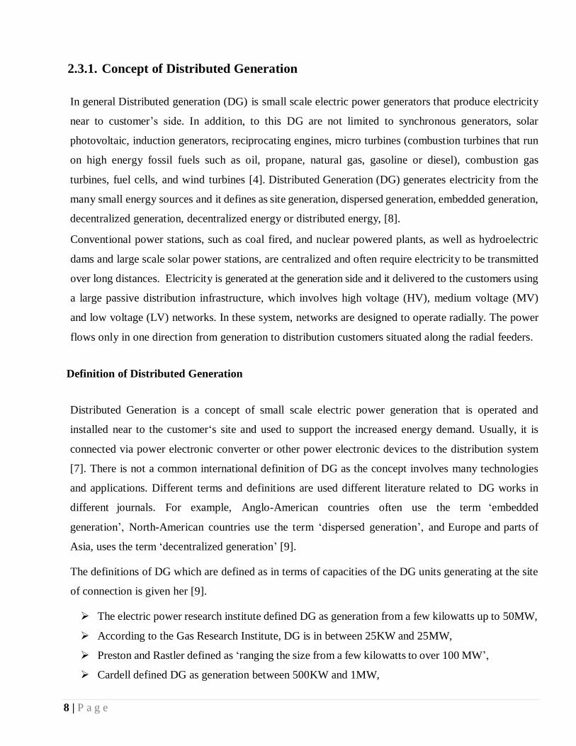
The international conference on Large High Voltage Electric Systems (CIGRE) defined DG as

‘smaller than 50-100MW.

Figure: 2. 1 Summary of DG applications [10]

However, this definition is not essential and there is no universal agreements on the distributed

generation definition. The main objective of distributed generation is transferring the electricity from

point of generation side to the point of consumer side. Therefore in this thesis, the following definition is

used [10].

Distributed generation is considered as the installation and operation of electric power generation units

connected directly to the distribution network or connected to the network on the customer site of the

meter in order to provide a source of active electric power which is small enough compared with the

centralized power plants.

The motivation for using this definition is that the connection of generation units to the distribution

network is done traditionally by the industry. The central idea of distributed generation, is to

integrate the generation close to the load center, hence on the distribution network or on the customer.

Classification of Distributed Generation

DGs can be classified based on different criteria. Among these, the two main criteria for DGs

classifications based on capacity or output power rating and the type of technology involved in the power

generation. The classifications of DGs based on capacity or output power rating is as shown in Table 2.1.

10 | P a g e

Table 2. 1 Classification of DG based on power rating.

DG Classification Output Power Range

Micro Distributed Generation 1W – 5kW

Small Distributed Generation 5kW – 5MW

Medium Distributed Generation 5MW – 50MW

Large Distributed Generation 50MW – 300MW

Another basis for classification of DGs is the type of technology involved in the power generation.

Therefore, distributed generation technologies can be categorized as renewable and non-renewable as

depicted in Table 2.2.

Table 2. 2 Classification of DG based on technology.

Renewables DG Non-renewables DG

Solar

Wind

Geothermal and

Ocean

Internal Combustion Engines

(ICE) Combined Cycle

Combustion Turbine

Micro turbine

Fuel Cell

Distributed generation technologies could also be grouped according to their dispatch ability namely

renewable and non-renewable [10]. This is because one of the primary elements in a distributed

generation management system is the dispatch strategy: the aspect of control strategy that pertains to

the sources and destinations of energy flows. The key difference between the two categories is the

controllability of electric power. The non-renewable resources, in general, have the energy stored, and

could therefore be called upon at any given time to produce power. This implies that nonrenewable

units such as conventional generator sets, fuel cells, and micro turbines, can be controlled by a central

intelligence and relied on to generate according to the needs of the power system. The renewable

resources, on the other hand, inherently do not have any control of the input energy for later use when

needed. This means that renewable technologies generate not as a function of power system needs, but

11 | P a g e

rather as a function of intermittent availability of their energy source. From the foregoing it can

adduced that while renewable DG technologies are dispatch able resources. Hydroelectric, biomass and

geothermal are dispatch able resources, whereas, wind, solar and tidal waves would be classified as non-

dispatch able resources most or common renewable energy systems are non- dispatch able.

Different authors still classify DG as inverter based DG and rotating machine DG [11]. Inverters are

used in DG systems after the generation, the generated voltage may be the form be in DC or AC, but it

is required to be changed to the nominal voltage and frequency. Therefore, it has to be change first to

DC and then convert to AC with the nominal parameters through the rectifier.

2.3.2. Distributed Generation Technology

The liberalization of electricity markets and environmental policy has increased the use of distributed

generation units for a range of applications, such as standalone, peak load shaving and remote

applications. These units can be classified into two different categories [12]:

1. Distributed generation based generation, including micro turbines, photovoltaic, fuel cells,

wind turbines and biomass.

2. Distributed generation based storage, including flywheels, battery, super capacitor and

superconducting coil system.

All of these technologies are currently being used and are gaining popularity. Some of the different

types of distributed generation are discussed in the subsequent section.

2.3.2.1. Photovoltaic Systems

Photovoltaic (PV), “photo” meaning “light” and “voltaic” referring to electricity which is the direct

conversion of sunlight into an electrical potential (a photo voltage) that can be used to provide electric

power. The photo voltaic effect is the electrical potential difference between two semiconductor

materials when their common junction is illuminated with radiation of photons. The photo voltaic cell,

thus, converts light directly into electricity [10]. A material or device that is capable of converting the

energy contained in photons of light into an electrical voltage and current is said to be photovoltaic [8].

Therefore, the photo voltaic effect is the process by which an electric potential difference (voltage) is

created in a material exposed to light (electromagnetic radiation), which then leads to the flow of

electric current. This process is directly related to the photo electric effect, but distinct from it in that in

12 | P a g e

the case of the photo electric effect electrons are ejected from the material surface upon being exposed

to high enough frequency (energy) light, whereas in the photo voltaic effect the generated electrons are

transferred across a material junction (e.g., PN junction in a photo-diode) resulting in the buildup of a

voltage between two electrodes and the flow of direct current electricity. In other words, the energy

supply for a solar cell is photons coming from the sun. A photon which very have short wavelength

and high enough energy can cause an electron in a photovoltaic material to break free of the atom that

holds it. If a nearby electric field is provided those electrons can be swept toward a metallic contact

where they can convert to electric current.

Figure: 2. 2 Schematic diagram of a photovoltaic system

Photovoltaic energy conversion is a direct conversion from electrical energy in the form of current and

voltage from electromagnetic (i.e., light, including infrared, visible, and ultraviolet) energy. A solar cell

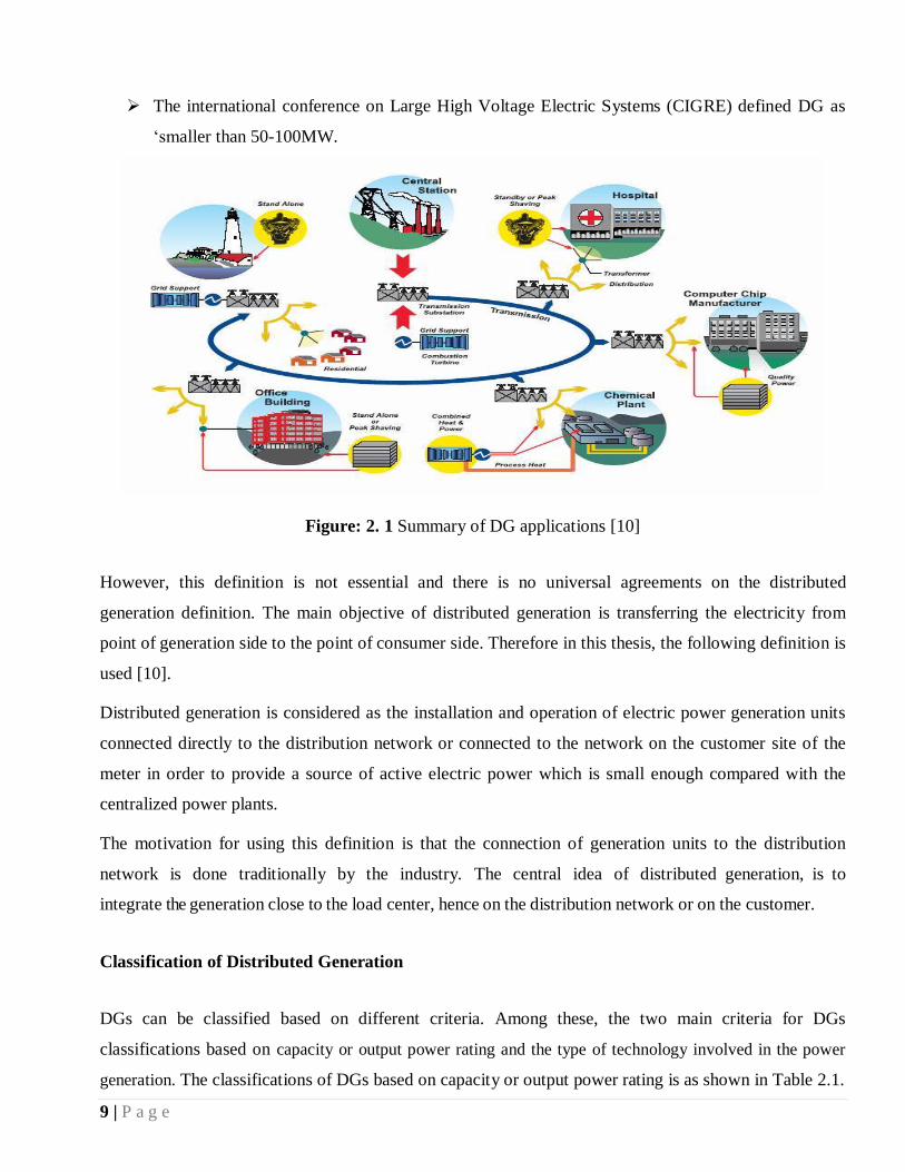
(PV cell) is a large-area semiconductor diode (Figure 2.3 a). It consists of a p-n junction created by an

impurity addition (doping) into the semiconductor crystal (consisting of four covalent bonds to the

neighboring atoms for the most commonly used silicon solar cells) [10]. The solar cell explained

above is the basic things of the PV power system. Typically, it is a few square inches in capacity and on

production about one watt. For obtaining high power, numerous such cells are connected in series and

parallel circuits on a panel (module) area of several square feet (Figure 2.3 b). The solar array is

defined as a group of several modules electrically connected in series and parallel combinations to

generate the as you want of current and voltage. Figure 2.3 (c) shows the actual construction of a

module in a frame that can be mounted on a structure.

13 | P a g e

As stated below, the basic elements of a PV system are the modules that are usually series parallel

connected and is usually called a PV string. But several components are needed to construct a grid

connected PV system to perform the power generation and conversion functions.

Figure: 2. 3 Distinction between cells, modules, and arrays

If the voltage of the PV string is always higher than the peak voltage of the grid the PV converter does

not require a step-up stage [10]. In this case higher efficiency can be obtained because a single stage

full-bridge converter can be used. Otherwise, a DC-DC boost converter or a transformer must be added

for voltage amplification but it reduces efficiency. However, energy storage devices can be included in

order to store the energy produced in case of grid support connection [8]. A three-phase inverter

performs the power conversion of the array output power into AC power suitable for injection into the

grid. Pulse width modulation control is one of the techniques used to shape the magnitude and phase of

the inverter output voltage.

2.3.2.2. Wind Turbine

Wind energy relies, indirectly, on the energy of the sun. A small proportion of the solar radiation

received by the Earth is converted into kinetic energy, the main cause of which is the imbalance between

the net outgoing radiation at high latitudes and the net incoming radiation at low latitudes [10]. The

Earth’s rotation, geographic features and temperature gradients affect the location and nature of the

resulting winds [8]. The use of wind energy requires that the kinetic energy of moving air be converted

to useful energy. As a result, the economics of using wind for electricity supply are highly sensitive to

14 | P a g e

local wind conditions and the ability of wind turbines to reliably extract energy over a wide range of

typical wind speeds. Over recent years, there have been dramatic improvements in wind energy

technologies, and wind turbine generation has developed rapidly as a competitive and effective

source of distributed generation. Wind energy can be exploited in many parts of the world, but is the

most cost-effective in windy climates, where average wind speeds exceed 6.5 m/s [10].

The wind farm is composed of several wind turbines which have basic electrical components: an

aerodynamic rotor, a mechanical transmission system, an electric generator, a control system, limited

reactive power compensation and a step-up transformer as shown in Figure: 2.4.

Figure: 2. 4 Grid Connected wind Energy system

The generator is used for converting the mechanical power obtained from the wind turbine to electrical

power. A wind turbine comprises rotor/blades for conversion of wind energy into rotational shaft

energy, a nacelle with drive train that contains the generator and gear box, a tower that supports the

rotor and drive train and the necessary electric equipment for connection to the grid. The majority of

wind turbines offered today is of the three bladed upwind horizontal axis type and installations intended

to connect at the PCC at medium or high voltage of the network [9].

In consideration of speed wind energy systems are either fixed or variable while the coupling between the

mechanical and electrical parts could be with or without a gear-box. Nowadays, induction generators are

widely used in wind turbine and a variable speed generator is the preferred option in newer wind

turbine installations [9].

2.3.2.3. Fuel Cells

Fuel Cells (FC) are classified as non-traditional generators. They are electrochemical devices that

convert chemical energy from a fuel directly into electrical energy by combining oxygen, as an oxidant,

15 | P a g e

and hydrogen, as a fuel, without combustion [12]. The hydrogen is usually procured from a fossil fuel

“natural gas” while air is used as a source of oxygen. The result of this electrochemical process is high-

current/low-voltage DC power. To connect the fuel cell to the grid, a DC/AC converter and filter system

current are used to convert the output to AC power. Water (H2O) and heat are by-products of the

process. This heat, which often exceeds 1,000 0F, converts the water to steam, which can then be used

to perform other work. Regardless of the auxiliary systems, FCs have no moving parts and no

combustion, making them silent devices.

2.3.2.4. Micro-turbines

Micro-turbines (MT) are small electricity generators that burn fuel such as natural gas, propane, and fuel

oil to create a high-speed rotation that is transferred to an electrical generator via a main shaft. MT

consists of three basic components: a compressor, a turbine generator, and recuperates [13, 14]. In

present energy markets, MT generators are the most improved and most attractive devices in distributed

power generation equipment. Their capacity ranges from 20 kW to 500 kW and their efficiency is more

than 80% when the CHP application is used in the system. Also, the NOx emissions of MT are very low

compared to large-scale turbines.

2.3.2.5. Induction and Synchronous Generators

Induction and synchronous generators are electrical machines which convert mechanical energy into

electrical energy then dispatched to the network or loads. Induction generators produce electrical power

when their shaft is rotated faster than the synchronous frequency driven by a certain prime mover

(turbine, engine). The flux direction in the rotor is changed as well as the direction of the active currents,

allowing the machine to provide power to the load or network to which it is connected. The power

factor of the induction generator is load dependent and with an electronic controller its speed can be

allowed to vary with the speed of the wind. The cost and performance of such a system is generally

more attractive than the alternative systems using a synchronous generator [15].

The induction generator needs reactive power to build up the magnetic field, taking it from the mains.

Therefore, the operation of the asynchronous machine is normally not possible without the

corresponding three-phase mains. In that case, reactive sources such as capacitor banks would be

required, making the reactive power for the generator and the load accessible at the respective locations.

Hence, induction generators cannot be easily used as a backup generation unit, for instance during

16 | P a g e

islanded operation [15].

The synchronous generator operates at a specific synchronous speed and hence is a constant- speed

generator. In contrast with the induction generator, whose operation involves a lagging power factor, the

synchronous generator has variable power factor characteristic and therefore is suitable for power factor

correction applications. A generator connected to a very large (infinite bus) electrical system will have

little or no effect on its frequency and voltage, as well as, its rotor speed and terminal voltage will be

governed by the grid.

Normally, a change in the field excitation will cause a change in the operating power factor, whilst a

change in mechanical power input will change the corresponding electrical power output. Thus, when a

synchronous generator operates on infinite bus bars, over-excitation will cause the generator to provide

power at lagging power factor and during under-excitation the generator will deliver power at leading

power factor. Thus, synchronous generator is a source or sink of reactive power. Nowadays,

synchronous generators are also employed in distribution generator systems, in thermal, hydro, or wind

power plants. Normally, they do not take part in the system frequency control as they are operated as

constant power sources when they are connected in low voltage level. These generators can be of

different ratings starting from kW range up to few MW ratings.

2.4. Expansion Planning of Distribution Networks with Integrating DG

The current existing distribution network are seen to be passive networks units due to the unidirectional

power flow from distribution substation to end users. Usually, distribution network upgrade is carried

out with the aid of additional network components such as transformers, protective devices and

transmission lines for meeting the load growth. The integration of DG has been as one of the attractive

options for distribution system due to the incentives and environmental considerations. Distribution

network with DG demands for dedicated operational strategies since the DG units located near the load

centers can possibly change the direction of power flows and consequently modify system operations. It

is very important to allocate DG units in distribution networks with comprehensive technical and

economic considerations to avoid the overall degradation of system performance.

A different methods are used in order to determine the proper DG locations and sizes. And understand

that while DG addition is the most appropriate alternative, it could become a cost effective solution,

with the right DG size, place and distribution capital deferral credit [7]. For placing DG under load

17 | P a g e

uncertainty is proposed where minimization of economic cost (including investment, operation cost of

DG units and cost of losses), technical risks (including risks of voltage and loading constraints

violation) and economic risks (due to the uncertainty in the electricity price) are considered [16].

The economic planning of a reliable distribution network that satisfies the annual load growth for the

planning period is a significant issue for distribution network companies striving to survive in the

competitive electricity market [17]. For this purpose, installation of new substations or upgrading the

substation capacity is required. DG is an alternative approach to such upgrades that has attracted

engineers’ attention in recent years. In addition to supporting the annual load growth, DGs can decrease

the line loss by reducing the line’s power flow, it improve the voltage profiles, reduced line loading and

it increases voltage stability.

DG based planning method is presented in to minimize the line loss in a planning area. In addition to

DGs, capacitors can postpone the need to upgrade the HV/MV transformer required due to the load

growth. [18, 19, 20, 21] The capacitors are used commonly for minimizing the line loss and improving

the voltage profile by reducing the reactive component of the feeder current [22, 23]. In [24], a dynamic

programming method is used for solving the reactive power and voltage control. The capacitors and the

main transformer tap changer are dispatched to minimize the line loss and to improve the voltage

profile. A similar procedure is implemented in [25, 26] using the GA. A mechanism for optimal voltage

support is proposed in [26], which introduces a procedure to optimize voltage regulator (VRs) in

addition to capacitors and the main transformer tap. It is observed that including VRs can decrease the

total cost by 3.6%. In the presence of nonlinear loads [27] introduce a capacity or planning to minimize

the line loss.

Similar to the capacitor size, the line characteristics, DG size and location, and adjusting the distribution

transformer tap setting can assist to keep the bus voltage within the standard level and to reduce the line

loss [25]. Such reductions of the line loss at peak load level can reduce the need for investment in

equipment of a greater power rating.

Improving the voltage profile, minimizing the line loss, reduction of line loading and increasing voltage

stability is used to supporting the load growth are the main objective in the planning of a distribution

network. Since DG improve the voltage profile and line loss and also DGs increase system voltage

stability so this elements can help the HV/MV transformers for supporting the load growth, so DGs

should be planned simultaneously to have a low cost planning. This highlights a need for a method to

consider this integrated planning method as implemented in this thesis.

18 | P a g e

2.5. Impact of DG Integration on Distribution Network

The operation of distribution network originally radial and designed to operate without any generation

on the distribution network, and power flow is unidirectional. The introduction of DG in distribution

network can significantly impact the power flow and voltage conditions at both customers and utility

equipment. These impacts can be manifested as having positive or negative influence, depending on the

DG features and distribution network expansion planning and operation characteristics [28, 29, 30, 31]

Generally, impacts of penetration of DG to the distribut ion network can be classified into three

main categories, namely technical, environmental and commercial and regulatory impacts [29].

2.5.1. Technical Impact of DG

There are some technical impacts of DG to the distribution network, among that on power loss, voltage

regulation and on protection device coordination the main technical impacts.

Impact of DG integration on Power Losses

One of the major impacts of distributed generation is on the power losses in a feeder. Locating the DG

units is an important criterion that has to be analyzed to be able to achieve a better reliability of the

system with reduced losses. Locating of DG units to minimize losses is similar to locating capacitor

banks to reduce losses. The main difference between both situations is that DG may contribute with

active power and reactive power (P and Q). On the other hand, capacitor banks only contribute with

reactive power flow (Q). Mainly, generators in the system operate with a power factor range between

0.85 lagging and unity, but the presence of inverters and synchronous generators provides a contribution

to reactive power compensation (leading current).

The optimum capacity and location of DG can be obtained using load flow analysis software, which is

able to investigate the suitable capacity and location of DG within the system in order to reduce the

losses. For instance, if feeders have high losses, adding a small capacity DGs will show an important

positive effect on the losses and have a great benefit to the system. On the other hand, if larger units

are added, they must be installed considering the feeder capacity boundaries [32]. For example,

the feeder capacity may be limited as overhead lines and cables have thermal characteristic that cannot

be exceeded.

19 | P a g e

Most DG units are owned by the customers. The grid operators cannot decide the locations of the DG

units. Normally, it is assumed that losses decrease when generation takes place closer to the load site.

However, as it was mentioned, local increase in power flow in low voltage cables may have undesired

consequences due to thermal characteristics [30].

Impact of DG integration on Voltage profile

Radial distribution systems regulate the voltage by the aid of load tap changing transformers (LTC) at

substations, additionally by line regulators on distribution feeders and shunt capacitors on feeders or

along the line. Voltage regulation is based on one way power flow where regulators are equipped with

line drop compensation.

The connection of DG results in changes in voltage profile along a feeder by changing the direction and

magnitude of real and reactive power flows. Nevertheless, DG impact on voltage regulation can be

positive or negative depending on distribution system and distributed generator characteristics as well as

DG location and capacity [30].

The installation of DG units along the power distribution feeders may cause overvoltage due to too

much injection of active and reactive power. For instance, a small DG system sharing a common

distribution transformer with several loads may raise the voltage on the secondary side, which is

sufficient to cause high voltage at these customers [31]. This can happen if the location of the

distribution transformer is at a point on the feeder where the primary voltage is near or above the fixed

limits.

Impact of DG Integration on protection device

The presence of DG in a network disturbs the short circuit levels of the network. It creates an increase in

the fault currents when compared to normal conditions at which no DG is connected in the network [30,

31]. The influence of DG to faults depends on some factors such as the generating capacity of the DG,

the distance of the DG from the fault location, number of DG installed in one bus as well as in different

bus and the type of DG. This could affect the protection device in the distribution network and safety of

the distribution system. The fault contribution from a single small DG is not large, even so, there will be

an increase in the fault current. In the case of many small units, or few large units, the short circuit levels

can be altered enough to cause miss coordination between protective devices, like fuses or relays. This

could affect the reliability and security of the distribution arrangement. If the DG is located between the

20 | P a g e

utility substation and the fault, a decrease in fault current from the utility substation may be observed.

This reduction needs to be examined for minimum tripping or coordination problems. On the other

hand, if the DG source (or combined DG sources) is strong compared to the utility substation source, it

may have a noteworthy impact on the fault current coming from the utility substation. This may cause

fail to trip, consecutive tripping, or coordination problems [32].

The nature of the DG also disturbs the short circuit levels. The highest paying DG to faults is the

synchronous generator. During the first few cycles its contribution is equal to the induction generator

and self-excited synchronous generator, while after the first few rounds the synchronous generator is the

most fault current contributing DG type. The DG type that contributes the least quantity of fault current

is the inverter interfaced DG type, in some inverter types the fault contribution continues for less than

one cycle. Even though a few cycles are a short time, it may be extensive enough to influence fuse

breaker coordination and breaker duties in some bags [14].

Impact of DG Integration on Voltage Stability

Voltage stability refers to the capability of a power system to maintain steady state voltage at all buses

in the system after being exposed to a disturbance. Voltage stability is classified into steady state and

dynamic involving minor and huge disturbances respectively. It is also classified into steady state and

transient voltage instability, according to the time range of the occurrence of the singularities. Voltage

stability worries stable load action, and acceptable voltage stages all over the system buses. A power

system is said to have go in a state of voltage variability when a disturbance causes a progressive and

uncontrollable decline in voltage [33].

Under dangerous loading conditions in convinced industrial areas, radial distribution system experiences

unexpected voltage collapse due to low value of voltage stability index at most of its nodes . Voltage

constancy analysis often needs examination of lots of system states and many contingency situations.

For this reason the method based on steady state analysis is more possible, and it can also provide

worldwide insight of the voltage reactive power problems.

In general, the inability of the system to supply the required demand leads to voltage instability (Voltage

collapse) [33]. Integration of DG renders a group of advantages, such as, economic, environmental and

technical. The location and size of DG has the main consequence on voltage constancy of the system.

Due to considerable costs, the DGs must be allocated suitably with optimal capacity to improve the

system performance such as to reduce the system loss, improve the voltage profile while maintaining the

21 | P a g e

system stability [33]. The problem of DG arrangement has recently received much care by power system

researchers. The consequence of DG capacity and location on voltage stability analysis of radial

distribution system is examined in this thesis.

2.5.2. Environmental Impact of DG Integration

After so many years of discussions and negotiations about sustainable development, the world‘s climate

and its biodiversity are still deteriorating [28]. Environmental issues are prime concern for any countries

due to increasing global warming and its negative impact over human being. Due to global warming our

weather has changed and it becoming disaster for human life. Often DG technologies are described as

more environmental friendly than centralized generation. Keen public awareness of the environmental

impacts of electric power generation and efforts to mitigate climate change are crucial to DG

renaissance.

Unfortunately some distributed generation technologies could, if fully deployed, significantly contribute

to present environmental problems. Therefore, the technologies that can be used for distributed

generation cannot be described in general as environmental friendly. But regarding the main current

environmental issue, the increased greenhouse effect, all DG technologies lead to significantly lower

emissions than coal-based technologies [29]. On the contrary, in the case of the so called “zero

emission” generation systems, though direct emission due to combustion is zero, indirect emissions

linked to construction, maintenance and dismantling have to be considered. This is the case with nuclear

power plants, windmills, photovoltaic generators, hydroelectric power plants and power plants using

biomass.

From the fuel utilization point of view, smaller distributed generation plants generally are less efficient

than larger central plants of the same type. Only when operating in a CHP mode, they may conserve

primary energy compared to the separate generation of electricity and heat in best available technology

(BAT)-electric-power plants and high-efficiency boilers [28]

22 | P a g e

2.5.3. Commercial and Regulatory Impact of DG Integration

Commercial Impact of DG Integration

Active administration of distribution networks can permit noteworthy increases in the amount of DG that

can be connected to the present networks. Although the cost related with the process of active

distribution networks is still to be recognized, it is expected that the benefits are likely to considerably

compensate the cost of its implementation. In order to support the growth of active distribution networks

and excerpt consistent benefits associated with relating increased amount of DG, new commercial

schedules need to be developed.

Regulatory Impact of DG Integration

In the absenteeism of a clear policy and related regulatory instruments on the conduct of DG, it is very

unlikely that this type of generation is going to thrive. The explanations for this are partly past and

connected to the way distribution networks have been developed and operated as passive networks. In

order to foster the compulsory changes, there is a clear need to grow and articulate suitable policies that

care the integration of DG into distribution networks [28].

2.6. Literature Review

This topic explains the detailed literature study on integration of DG to the distribution networks with

their impacts related to my problems faced in the distribution substation with respective solutions. The

information was gathered from several sources such as books, journals and websites. Each reference

used is explained in detail as follows.

In Kuri et al M. R. Haghifam, H. Falaghi and O. P. Malik. [34] Genetic algorithms are used to

place the generation to reduce the losses, costs and network interruption and the rating of the

generator to maximize. Also Generation is located in single units at individual buses, while

disregarding the interdependence of the buses and the network purification that can result improper

DG placement.

In El-Khattam et. al. [35] uses a heuristic approach to determine the optimal DG size and site for

an investment point of view. Once again short circuit restrictions are not considered and its focus on

the objective purpose on optimal asset rather than maximizing renewable energy.

23 | P a g e

Liu, J., Salama [35] have examined the impact of distributed resources on the transmission network

in terms of influence issues.

Wang C, Nehrir MH. [36] Has presented a new approach for finding the location and capacity of

distributed generation in distribution network, with multiple generation sources and minimizing

power losses and generation costs. The planned method has considered at first place the siting

problem by reducing the search space. To this end, a modest and estimated formulation of the mixed

integer nonlinear programming has been planned. The results of the planned relaxed mixed integer

nonlinear programming have condensed the search space considerably. Regarding to the size

problem, a generalization for one generator unit reducing the power loss has been advanced for

multiple generators, and has been extended to include the power loss and generation costs, resulting

in a system of nonlinear equations. The simulation results have exposed established the good

compromise between the efficiency and computational efforts of the proposed method but it ignores

the interdependence of the buses and the network purification also that can result improper DG

placement.

Al Abri RS, El-Saadany EF, Atwa YM. [37] Has dealt with the problems related to the integration

of distributed energy resources (DERs) into the distribution grid. Indeed, as i have earlier illustrated,

the large diffusion of DERs in the distribution network, which has not been conceived to support it,

are causing numerous technical as well as, in view of the expansion of the energy market, also

regulatory problems. But in this paper it is not consider grading to the protection system of the

distribution when the distributed generation penetration highly increase.

Borges CLT, Falcao DM. [38] proposed a new index to obtain the optimal location and size of DG

unit, in order to reduce losses and enhance voltage stability considering load variations. To resolve

this optimization problem, PSO algorithm has been presented and used. To verify the results of the

PSO algorithm and this algorithm connected the DG at different buss. Due to this this paper also not

consider interdependence of the buses and the network sterilization that gives improper DG

placement.

Hatziargyriou, N. et al. [39] proposes an analytical expression to calculate the optimal size and an

effective procedure to identify the corresponding optimal place for DG placement for minimalizing

the total power losses in primary distribution systems. The analytical expression and the procedure

are based on the exact loss formula. The consequence of size and location of DG with respect to loss

in the network is also examined in detail. The proposed procedure was tested and authenticated in

24 | P a g e

three distribution test systems with changing size and difficulty. Results found from the proposed

procedure are compared with that of the exhaustive load flows and loss sensitivity process. Results

show that the loss sensitivity issue based approach may not principal to the best location for loss

reduction. But this paper also objectives to maximize the capacity and in order to reduce line loss,

line loading and to improve voltage profile i.e. not consider the impact of increasing DG penetration

on the protection devices.

In summary, different researchers have spent much time in explaining the integration of DG with

distribution network expansion planning to reduce power loss, to improve voltage profile, to reduce line

loading when the demand increase and to maximize the power capacity. For more than one single unit

they have been placed a distributed generation at different buses. Placing the DG at different busses

could result in improper DG placement due to interdependence of the buses and the network

sterilization. They have focused on maximizing the power capacity without considering the impact of

power protection devices. However, this thesis work uses voltage sensitivity index analytical method for

the appropriate placement and capacity of DG. Assigning DG at the proper capacity and location can

improve voltage profile, provide good voltage stability, and reduce power loss and line loading when it

increases the load demand. In addition, by implementing fast over current relays and making them to

coordinate the impact of over current relay will be reduced and also when the DG capacity increase with

demand the over current relay can be upgraded by setting the time interval.

25 | P a g e

CHAPTER THREE

INTEGRATION ISSUES OF DG IN DISTRIBUTION NETWORK

EXPANSION PLANNING

3.1. Introduction

This chapter covers the distributed generation integration with a distribution network expansion

planning and the impacts of DG in protection devices, among that demand forecasting techniques,

expansion planning with DG, appropriate placement and sizing of DG methodology and impact of DG

on the protection device of the distribution network. The protection of distribution system without and

with consideration of distributed generation integration (DG) is involved. The overview of some of the

distribution system protection devices and how to implement, coordination and grading of the

overcurrent protective relays are included in this topic.

3.2. Peak Demand Forecasting Techniques

To cover this eventuality it is essential to develop a demand forecasting technique that is appropriate and

suitable to the objectives of the forecast. No technique can be considered incorrect for demand

forecasting. The technique adopted will depend on the time frame under consideration, the size of the

system and the plant available. In other words, the type of demand forecast technique adopted should

fall in line with the requirements of the study. There are four main demand forecasting techniques

Intuitive based demand forecasting.

Extrapolation based demand forecast.

End-user demand forecast.

Econometric demand forecasting.

A general overview of each of the four main methods is detailed in the sub-sections below.

26 | P a g e

3.2.1.Intuitive Demand Forecasting Techniques

The term intuitive forecasting can be used to define methods which rely mostly on experience and quick

calculations using simple expectations (i.e. the use of the immediate past performance and an

assumption that the rates of change will continue unaltered in the future).

The intuitive load forecast should not be entirely reduced, as it is after all in the contextual of reviewers’

minds when they appraise other peoples’ demand forecasts. In some cases, the lack of available data

may make intuitive forecasting the only possible option. The forecast may be appropriate for minor

progresses, isolated systems and minor island utilities.

An alternative approach, but still within the intuitive forecasting outline, would be to apply a

development factor that is obtained for a country with similar economic faces. Indeed, it may be

beneficial to compare load forecasts with the performance of a similar system in another part of the

world at a similar stage of development. This will chiefly be the case where (i) there is slight statistical

information presented on past loads, such as in new areas of source, (ii) data errors that cannot be simply

corrected, or, (iii) it becomes essential to forecast on the results of direct query and demographic and

economic figures. Such forecasting is no more than deduction, but the results can be used to cross check

on forecasts prepared by more scientific approaches. Where a new system of forecasting is to be ready,

it is often cooperative to make a comparison of the intuitive forecasts ready in the past and subsequent

performance.

3.2.2.Extrapolation Demand Forecasting Techniques

Extrapolation methods look at past trends in energy and power demand over time and, extend them into

the coming. Any time sequence may be rotten into three elements:

Tendency

Periodic variation

Serial dependence (auto-regression)

The Tendency is defined as “the long-term average growing and may be experimental in some way as

an average rise in a time series”. Superimposed on this may be a seasonal disparity. Periodic in this

sense is defined as “a cyclic variable that has unevenly the same beginning and end values for a given

dated of time (similar to the properties of a sine wave)”. Such disparities may be seen over a 24 hour

27 | P a g e

period, a weekly period, an annual period, or even a longer period. Finally, there may be a addiction

between successive values. For instance, if the value in the earlier period was high, the value in the

current period may be in height. Such behavior could relate to the random use of batch dispensation

equipment. This interdependency is known as auto-regression.

3.2.3.End user Demand Forecasting Techniques

End user demand forecast modeling attractions on many utility forecasting approaches. The individual

characteristic of end user demonstrating is the detailed report of how energy is used. Such models

usually begin by agreeing uses for which energy is eventually required, such as heating water, cooling

buildings and cooking food. The model then defines, via exact equations and secretarial identities, the

types of energy-using equipment that businesses and households have, and how much energy is used by

each type of equipment to gratify the programmed levels of end use energy needed. A large amount of

study data and data are needed by such a model. By summing up the units of equipment times the

average energy used by each session of equipment, total energy demand by fuel type is exposed.

Multiplying types of equipment by average use standards is just an accounting outline, but even so, it

can produce insights into the way energy is used now and in the coming. Optimization end user models

are a step outside secretarial end-user models. By agreeing an objective function (such as minimizing

cost) and classifying both the unit costs of using energy in the given procedures and the restraints to the

system, the secretarial end user model can be transformed into a device that will predict how customers

will act (assuming that their objective function is properly specified), given the molds about costs and

constraints. End user models are often linked to econometric models.

End user models are often frailest in predicting customers' fuel use choices. With the accessible data,

they can easily describe where the energy is presence used and for what purposes but, without a theory

to clarify selections, they are limited in their aptitude to predict the future. The ideal end user model

(which is rarely achieved) would, for example, not only tell us the usual watts of lighting energy in

homes, and how this amount has changed over time, but also what caused households and/or housing

operators to make these changes.

End user forecasting can be extremely accurate, particularly for green field growths, and for forecasts of

residential demand. A delay of end user demand forecasting is load density based forecasting, in which

the extreme load in any area is based upon the surface area engaged by each consumer type and a power

density (i.e. watts per square meter) associated with that consumer type. This can be particularly useful

28 | P a g e

for distribution arrangement. End user forecasts also include developments in segments such as industry

and agriculture where feasting patterns can be recognized for, say, cement production or water pumping.

3.2.4. Econometric Analysis Demand Forecasting Techniques

This session of model, like the time sequence model (extrapolation), uses past data to predict the future.

Econometric analysis however, attempts to go beyond time series models by explanation the causes of

the identified trends. Econometric models assume explicit causal relations between the dependent

variable (either energy or power) and independent variables (either financial), scientific (e.g. number

and type of applications; industrial processes), demographic (e.g. population).

Assuming these relations are true it should then be possible to regulate the past relationships between

electrical demand and such, individual income, the price of electricity etc. Future stages of these

economic variables are then prediction and used as inputs to govern future levels of consumption. One

benefit of econometric forecasting is the ease with which in height and low situation load forecasts can

be resultant and the logical basis on which they can be formed. This simply requires variations in the

forecast rate of the input variables, e.g. economic development and electricity price. A quicker economic

development will produce a higher load forecast whilst the burden of price increases will decrease

forecast levels of energy demand. Econometric showing would be preferred to time sequence analysis.

Even if both techniques could predict changes in demand with equal accuracy, the econometric model

would be more respected since it might help in sympathetic why variations in demand were occurring.

3.3. Distribution System Peak Demand Forecasting

In this thesis extrapolation least square technique is used to forecast for the next coming 10 years. I have

collect past peak load request for five year from Adwa distribution system as shown in table 3.1 below.

From the principle of regression theory to forecast the load for the coming ten years by using the past

peak load demand in table 3.1 data. Its attitude is that any function y = f(x) can be tailored to a set of

points (X1, Y1), (X2, Y2) so to minimize the sum of errors squared at each point, i.e.

∑ Yi − f(x)2𝑛

𝑖=1= minimum ……………………………………………………. (3.1)

29 | P a g e

Table 3. 1 Historical peak load data from 2013-2018 G.C

Substation

Name

Year 2013/14 2014/15 2015/16 2016/17 2017/18

Adwa Peak load

(MW)

28.5 30.7 33.5 35.5 37.3

Peak load

(MVA)

31.31 33.73 36.81 39.01 40.98

Among the dissimilar typical regression curves used in power arrangement forecasting the simple least

square line is used for forecasting the load. So the line y = a0 + a1x is close-fitting to the sets of points

(X1, Y1), (X2, Y2) ….. (Xn, Yn).

ε2=∑ [Yi − (a0 + a1Xi)]2𝑛

𝑖=1 =minimum ……………………………………… (3.2)

Partial differentiation with respect to the regressions coefficients (a0 and a1) is made and the equations

set to zero to obtain the minimum error criterion. This gives us a set of simultaneous equations in a0 and

a1:

𝑁𝑎0 + 𝑎1∑𝑋i = ∑𝑌𝑖 …………………………………………….………….. (3.3)

𝑎0∑Xi+𝑎1∑Xi2=∑X𝑖𝑌𝐼 ……………………………………………………….. (3.4)

Table 3. 2 All input historical data of the analysis

Year

Peak

demand

(MW)

𝑋𝑖 𝑃𝐷𝑖=

peak Demand

10

𝑌𝑖=ln𝑃𝐷𝑖

𝑋𝑖𝑌𝑖 xi

2

2013/14 28.5 -2 2.85 1.04 -2.094 4

2014/15 30.7 -1 3.07 1.12 -1.12 1

2015/16 33.5 0 3.35 1.2 0 0

2016/17 35.5 1 3.55 1.26 1.26 1

2017/18 37.3 2 3.73 1.32 2.64 4

∑𝑋𝑖=0 ∑𝑌𝑖=

5.94

∑𝑋𝑖𝑌𝑖=

0.686

∑𝑋𝑖2=10

a0 a1

1.188 0.0686

30 | P a g e

Finally, the values in Table 3-2 are used to regulate the load of the certain area up to 2028G.C. The

forecasting is done using equation 3-5 (a) and (b) shown below by considering 2015/16 as a reference

year and all the above equations are formulated using Matlab M. file see in appendix A in detail.

Y=𝑎0+𝑎1.xi ………………………………………………………………….. 3.5 (a)

Pn=10eY …………………………………………………………………… 3.5 (b)

Table 3. 3 Power demand forecast for of Adwa sub city from 2018-2028

Year Forecasted Demand in

(MW)

Forecasted Demand

in (MVA)

2018/19 40.02 43.97

2019/20 42.94 47.18

2020/21 46.05 50.6

2021/22 49.41 54.29

2022/23 53.0. 58.25

2023/24 56.83 62.45

2024/25 61.01 67.04

2025/26 65.54 72.02

2026/27 70.2 77.14

2027/28 75.31 82.74

From Table 3.3 the power demand at Adwa substation after 10 years will be approximately 75.31MW of

active power and 82.74MVA reactive power by seeing a power factor of 0.91 and the load growth at

each year increases by 7.07% and also the overall demand after Y-1 years will be approximate as shown

in the Table3.3. Therefore the expansion planning of Adwa substation will be combined with DG by

attention of the load growth of the substation in each year.

31 | P a g e

3.4. Integration of DG with Distribution Networks Expansion Planning

When viewed from a total system point of view, a power system typically exhibitions a smooth,

unceasing development trend in annual peak load. Local area load development usually occurs only over

a few years, from a near zero to a value near to the final ‘saturated’ peak load. Examines are carried out

a numerous load growth and associated supply conditions. The operation and planning of distribution

systems under such conditions is explored. Long term planning contains principle to grow a policy to

meet the utility’s long term power sending needs, usually minimizing cost by bring about an best

balance between capital accompaniments and operative cost. It mainly requires that the distribution

planner evaluation every alternative, including load forecasts, revenue restraints, and a lot of other

factors. However, the long term planning has to encounter the basic restrictions or supplies for the

distribution network. In this thesis, the proposed method speeches a solution for long term planning

while assembly the proposed constraints of the network.

There are many factors touching DG action such as DG technologies, types, working modes, and others.

DGs connected in the distribution network can be owned, operated and measured by either an electric

utility or a customer. If DG is utility owned, then its operating cycle is well known as is controlled by

the utility. The shape of the DG operating cycle depends on the purpose of its use in the distribution

network. For example internal combustion engines, small fuel cell units limited working time units for

peak load shaving. Micro-turbines and fuel cells they have partial working time units to share the load

with dissimilar functioning cycles and micro-turbines and large fuel cells works on base load power

supply. In addition, renewable energy units unnatural by environmental situations such as wind speed

and sunlight respectively.

On the other hand, customer owned DG working cycles are not known to the workers unless there is a

unit commitment promise between the electric utility and the client, which is not very likely. Thus,

small customer kept DG working cycles are considered to be random processes from the point of view

of the electric utility. The utility has no regulator over their process. This chance changes the planning

and process problem from a deterministic unruly to a non-deterministic one.

Appropriate Capacity and Placement of DG Guidelines

There are no clear guidelines on selecting the size and number of DG units to be installed in the

network. However, some factors can be guiding the selection of DG unit size selection:

32 | P a g e

To improve the system voltage profile and reduce power losses, it is sufficient to use DG units of

total capacity in the range of 10-50% of the total feeder demand. While more DG capacity can be

used to reduce the substation loading.

For reliability purposes in case of islanding, the DG size must be greater than double the

required island load. The DG unit size can affect system protection coordination schemes and

devices as it affects the value of the short-circuit current during a fault. Therefore, as the DG size

increases, the protection devices, fuses, re-closers and relays settings have to be readjusted

and/or upgraded.

There are no clear restrictions also on the location of DG units in the distribution network, as there are

no geographical limitations as in the case of substations. If the DG is customer owned then the utility

has no control on its location because it is placed at the customer’s site. If the DG is utility owned then

the choice of its location is based on several electrical factors such as:

Reducing maximum system losses and improving system voltage profile and augmenting

substations capacities

Providing the required additional load demand

To placed DG units on feeders do not impact the existing protective device coordination and

ratings.

3.5. Rapid Load Growth

This thesis presents an approach to obtain the suitable DG capacity that meets a rapid development of

system load. An initial set of candidate DGs are designated. DG capacity obligation varies across buses

because of the load distribution design, differences in total primary distribution feeder parameters and

hence losses in each feeder being different. The situation is to obtain the DG power condition at these

selected buses, and also the power condition from the station source while and load demand rises.

Therefore, in the Adwa distribution network, it is assumed that

DG is joined to the buses of the proposed network.

Peak load demand rises by 7.07% every year over a period of 10 years

In table 3.3, it is shown that while the load demand increases quickly each year, so the required power

from DG units rises at each bus in a linear manner with load demand increase. Also the DG units are

able to light the demand requirements when the demand is extremely growth the distribution system

33 | P a g e

needs to advancement in order to draw power from the substation with reliable service. Thereafter, the

power drawn from the substation rises expressively.

3.6. Methodology for Appropriate capacity and Location of DG

The addition of DG modifies the characteristics of the distribution system. A number of technical

restrictions and issues arise which are impacted by the amount of DG that is connected. These issues

are: distribution constraints, thermal constraint, voltage rise, capacity of transformer and power loss.

Voltage Drop Constraints: The voltage drop constraints depend on the voltage guideline limits on each

year.

Line Transmission Constraints: The maximum power transmission between bus-i and bus-j in every

year.

Distribution Substation Capacity Constraint: Every plan year, the total power delivered by the

substation over the outward distribution feeders from that bus must be within the substation size limit.

The rated current of the lines and the transformer rating must not be surpassed.

Capacity of Transformer

The extent of generation related minus the lowest load must not surpass the transformer rating at the

higher voltage. If there is some existing generation then this must be withdrawn from the total. The

result is the outstanding size available below that station. In the case of two parallel transformers, the

size is taken as the rating of the smaller transformer plus the lowest load. The restriction is expressed

formally as in equation (3.6)

PTx < PTrafoCap ……………………………………………. (3.6)

where PTx refers to power flow through the transmission substation transformer and PTrafoCap refers to the

rating of that transformer.

Thermal Constraint

The rated current of the lines could not be exceeded than the current comes from the generator. It is

given by below equation (3.7).

I I < Iirated …………………………………………...……… (3.7)

34 | P a g e

where II is the current flowing from generator i to bus i and Iirated is the maximum rated current for the

line among each generator and its corresponding bus. Under normal voltage and power factor

conditions, the rated current of the line can be interpreted directly into a rated active power for that line.

Voltage rise

If DG is related to a network unit, it will modification the active and reactive power flows and therefore

change the voltage dropped across the lines. It has been shown that DG mains to an important voltage

rise at the end of the long, high impedance lines. A rise in voltage occurs if there is low demand and

high generation, which leads to a bulky quantity of power flow along casually loaded lines with high

impedance. Losses are a significant thought when designing and planning the distribution system.

Losses are unescapable on any network; however, the amount can differ importantly contingent on the

design of the network. With the overview of distributed generation, the network is existence used in a

different way with more variable and bidirectional power flows. The level of losses is carefully linked to

the power flows. Losses are a function of the square of the current, i.e. a repetition in current results in

losses being quadrupled. Therefore the provision of DG and the altered power flows that result may

have a noteworthy influence on losses and may provide an chance to advance them.

Figure 3. 1 Voltage rise effect

𝑉𝐺 = 𝑉𝐿 + 𝑅PL+𝑋𝑄𝐿

𝑉𝐿+ 𝑗

𝑋𝑃𝐿−𝑅𝑄𝐿

𝑉𝐿……………………………….3.8

where Z = R + jX is the impedance of the line, PL and QL are active and reactive power at the bus and VG

and VL are the voltages at the generator and bus correspondingly. Thus it can be seen that the generator

voltage will be the load/bus voltage plus some value associated to the impedance of the line and the

power flows lengthways that line. It is obvious that the larger impedance and power flow the larger the

voltage rise. The improved active power flows on the distribution network have a large influence on the

35 | P a g e

voltage level because the resistive elements of the lines on distribution systems are higher than other

lines. The voltage must be retained within standard limits at each bus as given by equation (3.9).

Vmini < Vi < Vmaxi ………………………………………………………… (3.9)

where Vmini & Vmaxi refer to the minimum and maximum voltage limits at the ith bus.

Losses

Losses are significant deliberation when scheming and planning the distribution network. Losses are

unescapable on any network; however, the total can differ greatly depending on the design of the

network. With the overview of distributed generation, the network is being used in a different way with

more variable and bidirectional power flows. The level of losses is carefully related to the power flows.

Losses are function of the square of the current, i.e. a doubling in current consequences in losses being

quadrupled. Therefore the distribution of DG and the altered power flows that result may have a

noteworthy influence on losses and may provide an chance to improve them.

The allocation of DG problem consists of three significant steps. Via Choice of Load flow analysis

technique, finding suitable capacity and selection of the suitable location of DG.

3.6.1. Load Flow Analysis

Conventional NR and Gauss-Seidel (GS) methods may become unproductive in the study of distribution

systems, due to the unusual features of distribution networks, i.e. radial structure, high R/X ratio and

unbalanced loads, etc. These features make the distribution systems power flow calculation different and

rather difficult to analyze as related to the transmission systems. Several methods are available to carry

out the study of balanced and unbalanced radial distribution systems and can be divided into two

classes. The type of methods is applied by proper adjustment of existing methods such as NR and GS

methods. On the other hand, based on backward and forward sweep procedures using Kirchhoff’s laws.

3.6.2. Appropriate Power Capacity of DG

For determining the best capacity of DG to be located at the best place, for radial distribution system, by

considering maximum power reduction. So the total real power losses of the network can be determined

36 | P a g e

by summing all power losses value at each branch of the network with n nodes. The power loss

reduction (PLR) as loss saving based on total real power loss in radial distribution scheme as;

𝑃𝑙𝑜𝑠𝑠𝑒𝑠 = ∑ (𝐼𝑖2)𝑅𝑖

𝑛

𝑖=1 ………………………………………………….. (3.10)

where Ii is the current magnitude of each branch and R is the resistance of the ith branch. The current Ii is

resolute by load flow using the Newton-Raphson method. This loss in equation (3.10) is the loss without

DG and for single DG placement at bus m, the active current produced by the DG is I𝐷𝐺 .Therefore Iinew

the new active current of the ith branch is given by.

𝐼𝑖𝑛𝑒𝑤 = 𝐼𝑖 + 𝐼𝐷𝐺𝐶𝑖 …………………………………………………… (3.11)

where C is 1 if branch i has DG joined to its bus and is zero if no DG connection to the bus. The new

power loss with penetration of the DG into the network is given by:

𝑃𝐿𝑜𝑠𝑠𝑒𝑠−𝑛𝑒𝑤= ∑ (𝐼𝑖𝑛𝑒𝑤)2𝑅𝑖

𝑛

𝑖=1 ………………………………………. (3.12)

𝑃𝐿𝑜𝑠𝑠𝑒𝑠−𝑛𝑒𝑤= ∑ (𝐼𝑖2𝑅𝑖 +

𝑛

𝑖=12𝐼𝑖𝐶𝑖 𝐼𝐷𝐺𝑅𝑖 + 𝐶𝑖 𝐼𝐷𝐺

2 𝑅𝑖) …………………. (3.13)

The power losses reduction (PLR) which is the objective for placement is resolute by subtracting

equation (3.10) from equation (3.13) which is the difference between power losses before DG and after

DG connection as expressed below:

𝑃𝐿𝑅𝑖 = 𝑃𝐿𝑜𝑠𝑠𝑒𝑠−𝑛𝑒𝑤 − 𝑃𝐿𝑜𝑠𝑠𝑒𝑠 ……………………….…….……….…… (3.14)

𝑃𝐿𝑅𝑖 = ∑ (𝑛

𝑖=12𝐼𝑖𝐶𝑖 𝐼𝐷𝐺 + 𝐶𝑖 𝐼𝐷𝐺

2 )𝑅𝑖 ……………..…………………… (3.15)

The DG current that gives maximum PLR value can be determined by distinguishing equation (3.15)

with respect to I𝐷𝐺 and equate to zero as:

𝑑𝑃𝐿𝑅𝑖

𝑑𝐼𝐷𝐺= 2 ∑ (

𝑛

𝑖=1𝐼𝑖𝐶𝑖 + 𝐼𝐷𝐺 𝐶𝑖 )𝑅𝑖 = 0 …………………………………….. (3.16)

Hence, the current for maximum power loss reduction value is:-

𝐼𝐷𝐺𝑖 =∑ 𝐶𝑖 𝐼𝑖𝑅𝑖

𝑛

𝑖=1

∑ 𝑅𝑖𝑛

𝑖=1

……………......………………..…………………… (3.17)

The importance is to place the DG at a place that will give extreme loss reduction. This process is

repeated for all the buses in order to find the highest power loss discount value as the DG units are

singly located. Assuming no noteworthy change in voltage as DG units are connected, the consistent DG

size. The DG size from equation (3.18) must be located at bus m for maximum power loss reduction.

37 | P a g e

𝑃𝐷𝐺𝑖 = 𝐼𝐷𝐺𝑉𝑖𝑃𝑓 ……………………….………………………………….. (3.18)

3.6.3. Appropriate Location of DG using TENVDI

In order to limit the solution space to one bus, tail end nodes are first known by viewing the distribution

network topology. By penetrating DG at each node at a time, the Tail End Nodes Voltage Deviation

Index (TENVDI) is calculated using equation (3.19). When DG is connected at bus m, TENVDI for bus

m is defined as

TENVDI𝑚 = ∑(𝑉𝑛𝑜𝑚𝑖𝑛𝑎𝑙− 𝑉𝑖)2

𝑇𝐸𝑁

𝑇𝐸𝑁

𝑖=1 ……………………………………… (3.19)

where, ‘m’ corresponds to element of tail end node when connected DG at the bus, Vnominal is taken as

1.0 P.u Vi is voltage at the bus in p.u see in appendix E in detail how to find the voltage of at each bus

when it connect DG at the buss m from the result of DigSILENT software. To determine the capacity

that gives maximum power loss reduction and the location that gives minimum voltage variations of

DG, the following steps are taken as follow:

Step 1: Run the distribution load flow using DigSILENT Power Factory 15.1.7 simulation software

to determine total active and reactive power losses, branch currents and voltage profile at each bus.

Step 2: calculate the current of DG that gives maximum system losses redaction by keeping the power

factor of DG and bus voltage as a constant, after that multiplying the voltage and the current of DG with

the power factor to give the appropriate size of DG.

Step 3: Connect the selected capacity of DG value at the respective node and using TENVDI equation

find the bus voltage sensitivity indices at the respective node then rank the sensitivities of all nodes in

ascending order to form priority list.

Step 4: Select the bus with the lowest priority and place DG at that bus then it gives maximum power

losses reduction and less variation of voltage at the buss is taken as appropriate capacity at appropriate

location of the distribution feeder.

Step 5: End

38 | P a g e

3.7. Protection in Distribution System

Integration of the distributed generation to the power system may be made at the usage voltage level, at

the utility distribution system level, or at the utility transmission level. Where the connection is made

depends on the location and size of the generation plant. Rules will vary slightly by jurisdiction, but

are generally similar from one location to another. Connections at the usage level and on the

distribution system level are smaller installations and are also known as “distributed generation”

because the generation is dispersed and intermingled with the connected loads [40].

If there is a risk of operation as an unintended island, the utility may require additional protective

equipment such as communications equipment to facilitate transfer trip or it must to upgrade the

protective device. Such means are avoided if possible because of the increase of the system cost, but

may be required for the safe operation of the distribution system.

3.7.1.Fuse

A fuse is a short piece of metal, inserted in the circuit, which melts when excessive current flows

through it and thus breaks the circuit. Fuse is the simplest current interrupting device for protection

against excessive currents. Since the invention of first fuse by Edison, several improvements have been

made and now-a-days, a variety of fuses are available. Some fuses also incorporate means for

extinguishing the arc that appears when the fuse element melts. In general, fuses may be classified into

(i) Low voltages fuses (ii) High voltage fuses.

It is a usual practice to provide isolating switches in series with fuses where it is necessary to permit

fuses to be replaced or rewired with safety. If such means of isolation are not available, the fuses must

be so shielded as to protect the user against accidental contact with the live metal when the fuse carrier

is being inserted or removed.

A fuse model, irrespectively of the group to be represented, has to duplicate the following stages [31]:

current sensing, arc initiation, arc interruption, current interruption. The melting period, during which

temperature rises, begins with the fault and finishes when the fuse melts; during this stage the current

flows without limitation. The melting mechanism of a fuse depends on the magnitude and the duration

of the current, as well as on the electrical properties of the fuse. This characteristic is shown in the so

called time-current curve provided by manufacturers.

39 | P a g e

3.7.2. Reclosers

A reclosers is a device with the ability to detect phase and phase‐to‐ground overcurrent conditions, to

interrupt the circuit if the overcurrent persists after a predetermined time, and then to automatically

reclose to re‐energize the line. If the fault that originated the operation still exists, then the reclose will

stay open after a preset number of operations, thus isolating the faulted section from the rest of the

system. In an overhead distribution network between 75 to 95 per cent of the faults are of a temporary in

nature and last, at the most, for a few cycles or seconds. Thus, the reclose, with its opening/closing

characteristic, prevents a distribution circuit being left out of service for temporary faults. Typically,

recloses are designed to have up to three open‐close operations and, after these, a final open operation to

lock out the sequence. One further closing operation by manual means is usually allowed. The counting

mechanisms register operations of the phase or ground‐fault units which can also be initiated by

externally controlled devices when appropriate communication means are available [31].

The operating time/current characteristic curves of recloses normally incorporate two curves, one fast

and one delayed. The first one, known as fast or instantaneous, is mainly used to save lateral fuses under

temporary fault conditions. The second curve is known as slow or time -delay, and its main purpose is to

delay reclose tripping, and allow fuses to blow under permanent fault conditions [40].

3.7.3. Sectionalizer

A sectionalizer is a device that automatically isolates faulted sections of a distribution circuit once an

upstream breaker or recluse has interrupted the fault current and is usually installed downstream of a

recluse. Since sectionalizer have no capacity to break fault current, they must be used with a back‐up

device that has fault current breaking capacity. Sectionalizes count the number of operations of the

recluse during fault conditions. After a preselected number of recluse openings, and, sectionalizes opens

and isolates the faulty section of line. This permits the recluse to close and re‐establish supplies to those

areas free of faults. If the fault is temporary, the operating mechanism of sectionalizes is reset [31].

A sectionalizer does not have a current/time operating characteristic, and can be used between two

protective devices whose operating curves are very close and where an additional step in coordination is

not practicable. Sectionalizers can be used in place of fuses or between a reclosing device and a fuse.

40 | P a g e

3.7.4. Circuit Breakers Overcurrent Relay

The main characteristics of protective devices presently used by utilities to protect radial distribution

systems are presented. A circuit breaker is an automatic interrupting device which is capable of breaking

and reclosing a circuit under all possible conditions, and based up on arc extinguishing methods can be

classified as (oil, air, SF6,vacuum) circuit breakers [30].

The performance of a breaker during an opening operation is governed by the characteristics of the

overcurrent relay. Concerning the relay operating characteristics, overcurrent relays may be classified

into three major groups: definite current, definite time, and inverse time.

(i) Definite Current Relay

This type of characteristic makes the relay to operate instantaneously when the current reaches a

predetermined value. This feature is shown in Fig. 3.2.

Figure 3. 2 Definite current characteristic of over-current relays

The setting is chosen in such a way that the relay, which is installed at the furthest substation away from

the source, will operate for a small current value and the relay operating currents are gradually increased

at each substation, moving towards the source. Therefore, the furthest relay from the source operates

first disconnecting the load in the neighboring site of the fault [30].

(ii) Definite Time Relay

In this type of relay the setting may be changed to deal with different levels of current by using different

operating times. The settings can be attuned in such a way that the relay which is installed at the furthest

substation away from the source is tripped in the shortest time, and the remaining relays are tripped in

sequence having longer time delays, moving back in the direction of the source [30]. Definite time

41 | P a g e

protection is more selective as the operating time can be set in fixed steps. However, faults close to the

source which results in higher currents may be cleared in a relatively long time.

This relay allow setting of two independent parameters, the pickup setting and the time dial setting. The

pickup setting define the current value necessary to operate the relay and the time dial sets the exact

timing of the relay operation. In Figure 3.3, the characteristic curve of a definite time relay is shown

[30].

Figure 3. 3 Definite time characteristic of overcurrent relays

(iii) Inverse Time Relays

These relays operate in a time that is inversely proportional to the fault current. Inverse time relays have

the advantage of that shorter tripping times can be achieved without risking the protection selectivity.

These relays are classified based on their characteristic curves, which define the speed of operation as

inverse, very inverse or extremely inverse. Their defining curve shape is shown in Figure 3.4.

Figure 3. 4 Inverse time/ current characteristic of over-current relays

42 | P a g e

3.8. Protection of Distribution Network in the Presence of DG

Distribution level protection is created on a time overcurrent project. Such design contains choice of

equipment and locations or upgrade, location of equipment, and coordination of devices to clear faults

with as slight influence on customers as possible. One of the main imports is to stop further harm to

utility equipment. Secondary goals are consistency and power intermission. Distribution protection also

there must be edge between protective devices: an upstream device should work for a fault if the

downstream protector fails [31].

Although over current protection is humble and works very well with radial networks, it owns several

features that have to be accounted for when choosing the appropriate protective devices [15].

Any distribution protective device has an associated maximum distance (also known as reach) for

which the device mechanism. For large distribution networks, in which the lengthiest distance from

a load node to the substation can be several lots of kilometers, it is incredible to protect the entire

network from the substation. Therefore, numerous protective devices have to be connected along

the network.

A extremely reliable performance of a distribution network can be attained by installing different

types of protective devices. The coordination between protective devices is additional significant

aspect, and this is chiefly difficult in distribution networks given the amount of dissimilar protective

devices (breaker-relay sets, reclosers, fuses, sectionalizers). This coordination is not informal and

not always likely. In addition, it can be altered by the attendance of distributed generators.

There are some transients, such as transformer inrush and cold load unplanned, which can look

throughout system energization. The currents associated to these transients can be of the same order

that the pickup current of many distribution protective devices. This feature has to be careful when

selecting the time-current typical of those devices that can be affected.

DG penetration at the distribution close may have positive and negative influences. For DG to have a

positive benefit, it must be at least appropriately synchronized with the system working philosophy and

feeder design. The joining of DG unit raises few tests related with protection system. And also when the

penetration of DG increase at each year incessantly and the size of DG highly rise on the protection

device so you must have set or advancement the protection device.

43 | P a g e

3.8.1.Islanding due to Presence of DG

Islanding is a major interconnection subject. Islanding is a condition where one or more generators (or

group of distributed generators) continues to invigorate a portion of the utility system that has been

detached from the main utility system and function separately from the rest of the utility system.

Although DG may positively function in island if there is a equilibrium between load and generation,

islanded operation is not generally allowed for some major reasons [30].

The utility wants to restore the outage circuits and this is complex by having islanded

generators with utility loads. Since automatic reclosing is generally used to restore power to

customers, having islanded generators confuses both automatic and physical switching, which

requires harmonizing the generator

Power quality generally cannot be preserved by the islanded generators within an satisfactory

level, and this can result in injury to the customer equipment.

Personnel security is another reason, since upkeep and reparation crews may reason that there is no

voltage when in fact some generation is still active and consecutively in islanded mode.

The formation of an accidental island is a problem for the utility business. Moreover, islanding only can

be reinforced if the generator(s) can self-excited and preserve the load in the islanded area. This parting

could be due to process of an upstream breaker, fuse, or reflex sectionalizing switch.

The most mutual means to prevent islanding is to use voltage and frequency relays on the generator to

trip whenever either of these two strictures journey outside a designated window. This form of islanding

protection is known as inactive defense. It prevents islanding in most cases because when a segment of

the distribution system and one or more generators discrete together, the output of the generator will not

competition the load on the island. For synchronous or induction generators, the voltage and frequency

will meaning, which will trip the relays in a small time. Typically the relays are set to a close-fitting

frequency range of perhaps ±1 Hz or even ±0.5 Hz. Voltage relays have a bit broader window to allow

for typical voltage rule excursions on the circuit (±5 to 10% is typical) [30].

3.8.2.Protection Relay due to Presence of DG

The effect of DG in a distribution scheme may influence the fault detection and protection of the circuit

breakers in the distribution system. It mainly depends upon the protection, designing and place of DG in

a distribution system. Typical likely problem may be protection blinding, understanding tripping and

loss of coordination between the protection schemes.

44 | P a g e

The other influence of the presence of DG in the distribution network is a reduction of influence

protective devices. If a large generation unit or numerous small ones are related to the distribution

network, the fault current seen by the feeder protection relay may be condensed, which can lead to

improper operation for the over current relays. When the DG is fixed in the network (figure 3.5), its

influence to the fault current Ik reduces the current seen by the feeder relay I1. If the unit is larger, the

fault current injected will be higher, as well as, if the unit is located near to the grid, higher I1 will be

seen, as the impedance of the line will be lower. Therefore, it can be also decided that the influence

increases with the size of the unit and the distance between the feeder and the DG system [41]. This is the

disappointment of the protection devices to cover its intended protective distance, as the DG causes a

decrease in the compassion of these protection devices, thus declining the distance protected. The relay

R1 is set up to refuge the whole line, but the presence of the DG will cause a change in the seeming

impedance of the line which causes a miss-estimation of R1. When the fault is at the end of the line the

impedance of the line will be advanced and R1 will not be able to intellect the fault due to the less fault

current from the grid.

Figure 3. 5 Reduction of reach of protective devices

3.8.3. Mal-trip and Fail-to-trip due to presence of DG

Integration of DG in the radial arrangement causes a amount of problems with the protective device

coordination. For example in the outdated system, when using over current protection, it is likely to

assume that the fault current only flows in one course, whilst, this is not always true if there are DG

fixed in the network. The feeder protective relays are usually modest overcurrent relays and often with

an involuntary reclosing relay. With the addition of distributed generation on the feeders, several

difficulties can occur: the new generation foundation will increase the available short-circuit current on

45 | P a g e

the power system, reach of present relays may be pretentious, current flow from unforeseen directions

may cause miss operation of existing relays and unintended islanding operation may occur [41].

The protection systems can fail to operate in two dissimilar ways: by unnecessarily removing a non-

faulted module (mal-trip); or by not removing a faulted component (fail-to-trip). A mal-trip is the case

in which one of the protection devices trips in its place of the other. This elegant occurs due to one

protective device noticing the fault while it is outside of its protection region and trips before the

required tripping device. In contrast, fail to trip occurs for downstream faults. In this case the fault

current is principally formed by the current created from the DG unit. Consequently, the fault current

through the over current protection device can be below the location for which it was designed and the

protection remnants passive, hence the faulty feeder will not be detached [41].

Reflect the distribution substation shown in Figure 3.6 with the distributed generation DG1 installed on

one of the feeders [41]. For a fault wherever on the distribution feeder, the extra generation provides

additional fault current that may result in present equipment on the power system being subjected to

faults in excess of their ability to interject. For example, for the fault at location F1, the fuse must

interrupt not only the fault current from the substation bus, but also the extra fault current complete

from the DG source. If the fuse had been designated based on the fault current influence from

the substation alone, it may be incompetently rated for the total fault current when the DG

contribution is included. As a result, it may be necessary to substitute the fuse with a device having

higher ratings before allowing the DG to be brought on line. All other apparatus’s must be likewise

evaluated.

Figure 3. 6 Mal trip and fail to trip

For the fault at location F2 in Figure 3.6, the generator DG will also donate fault current. In addition to

the option of exceeding the fault interrupting capacity of the circuit breakers, the back feedstuff of fault

current may result in redundant trip (mal-trip) of the feeder circuit breaker CB1 if the current influence

from DG exceeds the trip location of the feeder overcurrent relays. For a fault at site F3, the DG will

46 | P a g e

donate fault current, and the infeed from the DG source may consequence in a reduced fault contribution

from the substation bus. Thus, the aptitude of the feeder relays to detect this fault may be abridged

(protection blinding).

3.9. Coordination of Overcurrent Protection Relay

Transmission and distribution systems are unprotected to overcurrent flow into their basics. In an

electric power system, overcurrent or extra current is a situation where a superior than intended electric

current exists over a conductor, leading to excessive generation of heat, and the danger of fire or damage

to equipment and also for dependability and security of power supply in distribution system, the

network must be defend. So overcurrent protection relay is the main protection technique used for

distribution feeders. Over current relays are used in the protection of distribution circuits. Overcurrent

relay is a detecting relay which operates when the current surpasses a predetermined value. Over current

relays use time current features in their processes. It is widely recognized that in radial networks,

discrimination of fault protection is attained through time-current coordination of overcurrent relays.

This is because for a specific fault, all the relays linked in the radial feeder see the fault current but are

made to operate at different times. The coordination is founded on the fact that the relay neighboring to

the fault (primary relay) sees the largest fault current than those farther away (backup relays) [41]. Choice

of different time current characteristics in the relay settings is the means of realizing coordination.

The coordination of the protective relay is done throughout the process of system design based on the

short circuit current level. It is the process of determining the sequence of relay operation for various

faults in power system so that the faulted section is cleared in minimum time. For the proper relay

coordination it is necessary to determine two crucial relay settings. These are:

Pickup or plug setting (tap setting)

Time dial or time multiplier setting

Plug setting (PS) or current setting for each relay is determined by two limits; the minimum and the

maximum fault current. The minimum and maximum fault current is determined from load flow study.

In the coordination problem of over current relays, the objective is to control the time setting multiplier

(TSM) and plug setting multiplier (PSM) of each relay. This least current in the relay coil at which

relay starts to work is called Pick-up Current. If the current through the relay coil is less than the pick-

up value then relay won’t function. On contrary, if the current over the relay coil is more than the Pick-

47 | P a g e

up current, relay will function, so that the overall operating time of the primary relays is minimized

properly. In order to determine current transformer (CT) ratio, the cable nominal current must be

identified. Here the DigSILENT 15.1.7 Power Factory allows 80% of supreme load current (cable

rated current) as a cable loading limit. Therefore, this needs a current transformer (CT) whose ratio

products 1A secondary current for the maximum load (primary current):

current transformer(CT)ratio = Cable rating current∗80%

Secondary transformer current=

N1

N2………… (3.20)

where:

N1 = Primary winding of current transformer

N2 = Secondary winding of current transformer

The minimum value of current (minimum fault current) for which the relay must operate should be at least

1.5 times pickup, but not very much more [4].

Ipprim = 𝐈fmin prim

1.5…………………………………………..……………. (3.21)

Ipsec = Ipprim ∗N2

N1∗ PS………………………………….…..…………… (3.22)

Ifmaxsec = Ifmax ∗ N2

N1………………………………….….……..………. (3.23)

PSM = Ifmaxsec

Ipsec=

measured second CT current

pick current……………...…………..…… (3.24)

where:

𝐼pprim = Primary pick up current

𝐼fminprim = Minimum primary fault current

𝐼psec = Secondary pick up current

𝐼Fmaxsec = Maximum secondary fault current

𝐼fmax = Maximum fault current

Plug Setting Multiplier (PSM) is definite as the ratio of fault current to the pick-up current of the relay.

The three approaches used for a correct relay coordination are judgement by time, discrimination by

current and discrimination both by current and time. The time setting multiplier (time dial) can be

originate as:

t = 0.14TD

((PSM)0.02−1)…………………………………………….… (3.25)

48 | P a g e

TD = t((PSM)0.02−1)

0.14………………………………………..…………….. (3.26)

where

t = Operation time of the relay

TD = Time dial

3.9.1.Overcurrent Relay Coordination Procedure

Correct overcurrent relay request requires knowledge of the fault current that can flow in each part of

the network. Since large scale examinations are normally unviable, system analysis must be used.

The relay settings are first strong-minded to give the shortest operating times at maximum fault levels

and then checked to see if operation will also be satisfactory at the minimum fault current predictable. It

is always sensible to plot the curves of relays and other defense devices, such as fuses, that are to

operate in series, on a common scale. It is usually more suitable to use a scale corresponding to the

current expected at the lowest voltage base, or to use the main voltage base. The alternatives are a

common MVA base or a separate current scale for each system voltage. The basic rules for precise relay

coordination can generally be specified as follows:

RULE #1

Whenever possible, use relays with the same functioning characteristic in series with each other.

RULE #2

Make sure that the relay farthest from the foundation has current settings equal to or less than the relays

behind it, that is, that the primary current obligatory to operate the relay in front is always equal to or

less than the primary current compulsory to operate the relay behind it.

3.9.2. Principles of Grading Overcurrent Protection Relay

Among the various likely methods used to achieve correct relay organization are those using either time

or overcurrent, or a combination of both. The shared aim of all three methods is to give correct

discrimination. That is to say, each one must isolate only the faulty unit of the power system network,

sendoff the rest of the system undisturbed.

49 | P a g e

1. Discrimination by Time

In this method, an suitable time setting is given to each of the relays regulatory the circuit breakers in a

power system to ensure that the breaker adjacent to the fault unlocks first. A simple radial distribution

system is shown in Figure 3.7, to illustrate the principle.

Overcurrent protection is provided at B, C, D and E, that is, at the infeed end of each unit of the power

system. Each protection unit includes a definite-time delay overcurrent relay in which the process of the

current sensitive component simply initiates the time delay element. Providing the setting of the current

element is below the fault current value, this component plays no part in the achievement of

discrimination. For this reason, the relay is sometimes labeled as a ‘self-governing definite-time delay

relay’, since its working time is for practical purposes independent of the close of overcurrent. It is the

time delay element, therefore, which provides the means of taste. The relay at B is set at the

straight time delay possible to allow the fuse to setback for a fault at A on the secondary side of the

transformer. After the time delay has died, the relay output contact closes to trip the circuit breaker. The

relay at C has a time delay setting equal to t1 seconds, and likewise for the relays at D and E. If a fault

occurs at F, the relay at B will operate in t seconds and the following operation of the circuit breaker at

B will clear the fault earlier the relays at C, D and E have time to operate. The time intermission t1

between each relay time setting must be long enough to safeguard that the upstream relays do not

function before the circuit breaker at the fault location has tripped and cleared the fault.

Figure 3. 7 Radial system with time discrimination.

The main disadvantage of this method of taste is that the longest fault clearance time occurs for faults in

the section neighboring to the power source, where the fault level is highest.

50 | P a g e

2. Discrimination by Current

Discrimination by current trusts on the fact that the fault current varies with the location of the fault

because of the difference in impedance values between the source and the fault. Hence,

characteristically, the relays regulatory the various circuit breakers are set to operate at suitably tapered

values of current such that only the relay nearest to the fault trips its breaker.

Discrimination by current is not a applied proposition for correct grading between the circuit breakers

at C and B. because, the problem changes appreciably when there is important impedance between the

two circuit breakers concerned.

3. Discrimination by both Time and Current

Each of the two methods labelled above has a fundamental disadvantage. In the case of discrimination

by time alone, the disadvantage is due to the fact that the more plain faults are vacant in the longest

operating time. On the other hand, discrimination by current can be applied only where there

is appreciable impedance between the two circuit breakers concerned.

It is because of the boundaries imposed by the independent use of either time or current grading that the

inverse time overcurrent relay characteristic has evolved. With this typical, the time of process is

inversely relative to the fault current level and the actual characteristic is a function of both ‘time’ and

‘current’ settings.

Characteristics for different settings

For a large disparity in fault current between the two ends of the feeder, faster working times can be

attained by the relays nearest to the source, where the fault level is the uppermost. So, by using both

functions the disadvantages of coordination by time or current alone are overcome. Variations of

current/time tripping features of relays will be discussed in some of the coming practical sections.

51 | P a g e

CHAPTER FOUR

MODELING, SIMULATION STUDIES AND ANALYSIS OF RESULTS

4.1. Introduction

This chapter covers modeling, simulation studies and analysis of results of Adwa distribution substation

using DigSILENT Power Factory 15.1.7 simulation software. The integration of DG with distribution

network expansion planning in a radial distribution system with proper sizing and placement is

discussed. In addition, it inspects the impact of DG integration on distribution network expansion

planning specially on voltage profile, power loss and voltage stability without increment the load and

with increment the load. Moreover, due to presence of DG it implements, coordination and grading of

fast protection relay when it is increase the capacity of DG has been investigated in detail.

4.2. Modeling of Distribution Network

Adwa substation is located in central zone of Tigray region which is at a distance of 1006 km from

Addis Ababa, the capital city of Ethiopia. As defined in the statement problem Adwa substation is

selected as a case study area and the substation is connect to the organized system (ICS), Adwa

substation has been providing the power from main grid that is an interconnected system. The substation

is supplied from two incoming line Tekeze hydropower substation and Adigrat substation with two lines

with voltage rate of 132kV. These two 132kV received lines are connected to the single bus bars at

Adwa substation and this single bus bar connected to two transformers. Those transformers are three

winding transformer with the capacity of 40/20/20 MVA and voltage rating of 132/66/15kV

respectively, and those transformer gives to one transformer with voltage rating of 66kV and this

transformer step down to 33kV. And also this substation feeds to Aksum substation with 132kV voltage

rating directly.

The overall model of the Adwa distribution substation network using DigSILENT Power Factory 15.1.7

software is shown in the figure 4.1. The network is shaped by seven radial feeders, namely KO1, KO2,

KO3, KO4 and KO5 with 15 kV voltage rating outgoing feeder and P1 and p2 are the other outgoing

feeders with 33kV voltage rating. In this substation 202 low voltage distribution transformers are

connected with total capacity of 52.705MVA. The distribution system feeders serves mostly residential,

52 | P a g e

commercial, and industrial customers. Each load connected to the main distribution line is also

considered as one load point. The study has a power flow analysis of the 33kV, 15 kV and 0.4 kV

network.

The substation supplies 48,997 customers and the utility owns the distribution lines at 33, 15 and 0.4 kV

levels. The 33kV, and 15 kV system consists of overhead and underground transmission lines and

cables, but 0.4 kV systems are considered a load’s connected point. In general one-line diagram of the

33kV and 15 kV grid is as shown in the figure 4-1 below.

Figure: 4. 1 Single line diagram of Adwa distribution substation using DigSILENT

4.3. Existing Distribution Network Data

All necessary data like the size of the substation, peak load, type of faults, and all interruption data of

medium voltage (15kV and 33kV) outgoing feeders are composed from the substation noted data. The

table below indicates total number of transformers and their capacity found in Adwa substation as

summarized.

Table 4. 1 Transformer data of Adwa substation

Substation No Transformer Voltage Level(kV) Capacity(MVA)

Adwa

Adwa

2 132/66/15 40/20/20

1 66/33 9/6

53 | P a g e

The existing system loadings of all low voltage transformers, number of customers connected to the

base system, type and size of each feeders, are tabulated in Table 4.2 and figure 4.2.

Table 4. 2 Existing system data of the outgoing feeder

Outgoing

Feeders

Overhead

lines

Line

length

in km

Voltage

level

(kV)

No of

transformer Total

Transformer

capacity

(kVA )

Total no.

customers

type and size

KO1 AAC 3 X 95 37.12 15 107 24295 24219

KO2 AAC 3 X 95 47.5 15 29 5140 7244

KO3 AAC 3 X 95 6.2 15 14 15350 5833

KO4 AAC 3 X 95 38.8 15 17 525 1627

KO5 AAC 3 X 95 39.7 15 26 6225 5354

P1 AAC 3 X 50 56 33 5 575 1811

P2 AAC 3 X 50 61.8 33 4 800 1909

Total ……… 298 …….. 202 52705 48997

Figure: 4. 2 Total capacity of transformer and number of customer’s data of each feeder

0

5000

10000

15000

20000

25000

KO1 KO2 KO3 KO4 KO5 P1 P2

24295

5140

15350

525

6225

575 800

24219

7244

5833

1627

53541811 1909

Total capacity of transformer and number of customer

connected at each feeder

Total Transformer capacity (kVA )

Total no. customers

54 | P a g e

4.3.1. Power Interruption Data

An interruption to service is the isolation of an electrical load from the system providing that load,

resulting from an abnormality in that system. The irregularity in the system can either be a malfunction

of a system component a fault or a system process due to conservation or repair. Interruptions

independent from the cause are usually undesired, as they leave energy unserved and customers without

service. Most of the time interruptions occur because of the system is reacting to a fault. A fault or

short-circuit is defined by IEEE100-1992 as an irregular connection of relatively low impedance,

whether made accidentally or intentionally between two points of different potential [42, 14].

Overloading earth fault and short circuits are the major cause of breaks in Adwa distribution system.

These major faults are secret into two main categories, those are temporary and permanent faults.

Temporary faults account for the majority of faults in distribution systems. Impermanent faults can

occur for many details, but may include tree or animal contact and weather as the main donors of this

fault. Temporary faults can be simply solved with a little or no intervention from the system itself.

Many are self-clearing such as a branch or animal interaction which burn and fall off, conductors

slapping together in severe wind or insulation flashover due to pollution and also lightning is also a

temporary fault. Lightning arrester failure on the other hand, can become an enduring fault. Other

temporary faults are merely cleared once a trip from the substation is delivered. Prompt reclosing de-

energizes the line for a short duration of time, which permits the arc or interaction path to disappear,

which in turn eliminates the fault path. Once the circuit is de-energized the system resumes normal

operation. Permanent faults are those that cannot be resolved with reclosing action and will not self-

clear. Equipment fault, cable failure and downed lines or persistent tree contact can all produce also

permanent faults [42, 14]. The collected interruption data are abridged for one year representative

yearly power interruption with whole frequency and duration interruption as shown below in Tables 4.3

and figure 4.3.

55 | P a g e

Table 4. 3: Frequency and Duration of Power Interruption in Adwa substation (01/12/2017-30/11/2018)

No Feeders TLP M/V Total fault Total interruption

F D F D F D F(int/y

r)

D(hr/yr)

1 132KV

incoming

feeders

IF1 27 12:33 …. …. … .. 27 12:33

IF2 27 12:33 .. …. … .. 27 12:33

2 15KV

outgoing

feeders

KO1 27 12:33 420 214:21 440 480:39 987 1706:14

KO2 27 12:33 345 147:49 401 38:10 773 478:39

KO3 27 12:33 299 108:11 75 310:17 401 158:54

KO4 27 12:33 98 72:23 102 184:45 227 269:40

KO5 27 12:33 26 49:14 91 188:24 144 250:11

3 33KV

outgoing

feeders

P1 27 12:33 38 30:37 71 206:43 136 149:53

P2 27 12:33 72 92:27 231 1036:3 330 1143:30

Figure: 4. 3 Frequency and Duration of Interruption for one year

0

200

400

600

800

1000

1200

1400

1600

1800

IF1 IF2 KO1 KO2 KO3 KO4 KO5 P1 P2

Frequency and Duration of Interruption of one year

Total interruption of each feeder F(int/year

Total interruption of each feeder D(hr/Year)

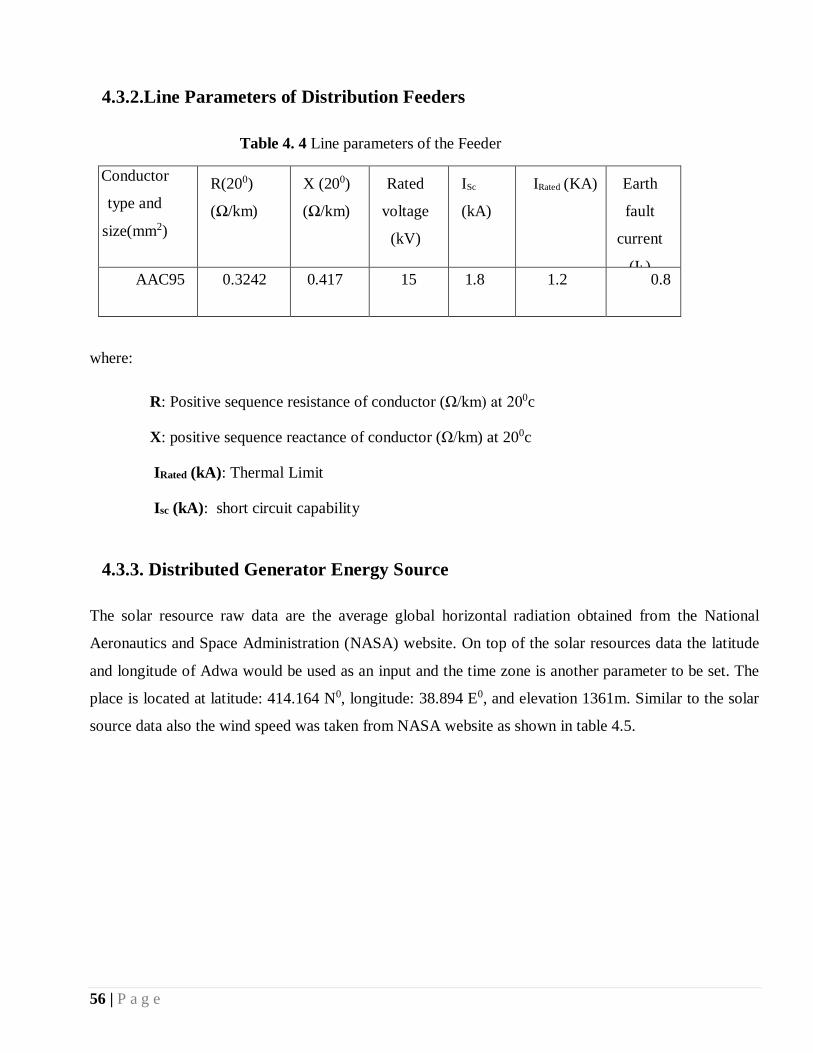
56 | P a g e

4.3.2.Line Parameters of Distribution Feeders

Table 4. 4 Line parameters of the Feeder

Conductor

type and

size(mm2)

R(200)

(Ω/km)

X (200)

(Ω/km)

Rated

voltage

(kV)

ISc

(kA)

IRated (KA) Earth

fault

current

(Ik) AAC95 0.3242 0.417 15 1.8 1.2 0.8

where:

R: Positive sequence resistance of conductor (Ω/km) at 200c

X: positive sequence reactance of conductor (Ω/km) at 200c

IRated (kA): Thermal Limit

Isc (kA): short circuit capability

4.3.3. Distributed Generator Energy Source

The solar resource raw data are the average global horizontal radiation obtained from the National

Aeronautics and Space Administration (NASA) website. On top of the solar resources data the latitude

and longitude of Adwa would be used as an input and the time zone is another parameter to be set. The

place is located at latitude: 414.164 N0, longitude: 38.894 E0, and elevation 1361m. Similar to the solar

source data also the wind speed was taken from NASA website as shown in table 4.5.

57 | P a g e

Table 4. 5 Solar and wind speed sources of data taken from NASA website

Months

Solar radiation (kWh/m2) Wind

speed(m/s)

2015/1

6

2016/17

2017/18

Average 2017/18

January 6.11 5.81 5.63 5.58 4.5

February 6.39 6.11 6.39 6.3 4.5

March 6.85 6.55 6.67 6.63 4.5

April 6.95 7.5 6.67 7.04 4.3

May 7.02 6.5 6.67 6.71 3.6

June 6.91 6.41 5.94 6.42 4.9

July 6.28 5.72 5.28 5.76 5.4

August 5.58 5.48 5.62 6.3 5

September 6.39 6.67 5.84 6.3 4.1

October 6.1 6.42 6.23 6.26 3.1

November 5.71 5.84 6.01 5.82 3.6

December 5.94 5.84 5.84 5.87 4

Average 6.272 4.3

4.4. Selection of Appropriate Capacity and Location using DigSILENT

The distributed generators is selected for the case study were a synchronous generator which is available

in DigSILENT Power Factory 15.1.7 software that can be used in thermal, hydro, solar, or wind power

plants. The DG is modelled as a Turbo Series 1 of IEC909/IEC60909 machine type and the excitation

system control mode is a constant power factor. Power factor control mode is aimed to maximizing the

active power production. Also, it expect the DG from participating in the system frequency control. In

consequence, unitary power factor operation is adopted. The loads are general load types modelled as

constant impedance and do not contribute to the fault level.

In order to restrict the solution in this thesis work identified the outgoing feeders by entering the data to

the distribution network topology in DigSILENT power factory software. The feeder was selected due

58 | P a g e

to its highest power interruption and overloaded. Due to this KO1 feeder was selected in order to

integrate with DG, because the feeder is loaded and more power interruption is accord, when it compare

from other outgoing feeder during the one year recorded data. [See in appendix D in detail the

comparison of loading feeders in DigSILENT power factory software]. Then in order to integrate the

DG at appropriate power capacity from the equation (3.17) and (3.18), 𝐼𝐷𝐺1 gets 0.931kA and its

capacity is 12.7 MW and 3.3MW is selected as a reserve by considering 0.91 power factor of the

distributed generation. After getting the appropriate DG capacity analytically in order to calculate the

appropriate location at appropriate capacity using tail end nodal voltage deviation indexes (TENVDI)

first it is must to know the voltage at each buses by penetrating the appropriate capacity of DG [see in

appendix E in detail] and calculate the total deviation of the voltages of all tail end nodes of the

network with respect to the nominal voltage. Then, when DG is inserted at each buss and if the bus

gives the lowest value of TENVDI from the other bus feeder value so the appropriate placement of DG

is at the lowest variation of TENVDI bus.

Table 4. 6 Variation of TENVDI by penetrating the DG at different bus

Bus no BB1 BB16 BB19 BB25 BB34 BB43 BB50 BB5

5

BB70

Variatio

n of

TENVD

I

0.0026

0.0029

5

0.0027

9

0.0023

2

0.0023

0

0.0022

5

0.0012

1

0.00

193

0.0025

1

In order to be placed DG due to its lowest value of TENVDI from table 4.6 that is calculated using

equation 3.19 in the section 3.6.3. Therefore, the lowest variation is at bus 50. After getting the

appropriate DG location and capacity analytically, the capacity obtained are connects with the existing

load at different bus and gives maximum power flow reduction at the selected bus as shown in figure

4.4, i.e. the penetration of DG at buss 50 it gives maximum power loss reduction when it compare with

the other bus in the distribution network.

59 | P a g e

Figure: 4.4 Power loss when the appropriate capacity of DG locates at different bus

4.5. Distribution Network Simulation using DigSILENT

This simulation studies were carried out under three different conditions. Case I consider the load flow

analysis without integration of DG (i.e. without change the existing system) while in Case II load flow

analysis with an integration of DG is carried out and case III consider the load flow analysis when the

capacity of DG increase with demand.

4.5.1. Distribution Network without Integration of DG

In this case, it has been seen the effect of power loss and voltage profile of the Adwa distribution system

without any change to the existing system and also it investigates on line loading after one year by

entering the forecasted data obtained from Adwa distribution system.

4.5.1.1. Line loading without Integration of DG

Load flow analysis is necessary to obtain how much the voltages, currents, and power (active and

reactive) are flowing in the power system network under steady state conditions and also it provides

power losses in the system, the voltage profile and the percentage of line loading. To investigate the DG

on loading of line segments, after one year load flow analysis is made on case study radial distribution

0

0.5

1

1.5

2

2.5

B1

B4

B7

B10

B1

3

B16

B19

B2

2

B25

B28

B31

B34

B37

B40

B43

B46

B50

B52

B55

B58

B61

B64

B67

B70

B73

B76

B77

PO

WE

R L

OS

S (

MW

)

DG LOCATION

Total Power loss when the appropriate capacity of DG locates at different

bus

60 | P a g e

system modeled in DigSILENT Power Factory 15.1.7 software and the simulation result of loading of

line segment before the integration of DG unit is over loaded from the next year. It can be seen the result

of line loading from DigSILENT Power Factory the lines colored in red indicates that the line segment

is overloaded from the next year show in figure 4.5, and the percentage of loading those lines is out of

standard (i.e. same of result have above 100%). This range is the default in DigSILENT Power Factory

15.1.7 table 4.7 from the result box of DigSILENT Power Factory 15.1.7 shows for each line segment of

the system separately [see in appendix C1 in detail].

Figure: 4. 5 Line loading without integrating DG (after one year)

61 | P a g e

Table 4. 7 Percentage of line loading after one year without integrating DG

Line Line

loading %

WODG

line Line

loading (%)

WODG

Line Line

loading (%)

WODG

line Line

loading (%)

WODG

L1 114.96 L21 4.06 L41 5.51 L61 10.32

L2 113.14 L22 2.9 L42 5.42 L62 9.33

L3 111.29 L23 0.97 L43 5.42 L63 8.60

L4 99.99 L24 0.19 L44 4.65 L64 4.30

L5 99.61 L25 87.93 L45 3.64 L65 13.76

L6 64.79 L26 1.27 L46 62.63 L66 9.46

L7 94.01 L27 1.27 L47 3.61 L67 8.6

L8 93.22 L28 1.27 L48 2.33 L68 4.3

L9 91.22 L29 0.92 L49 2.12 L69 15.02

L10 90.41 L30 0.89 L50 59.02 L70 12.89

L11 89.18 L31 84.4 L51 56.9 L71 11.89

L12 88.55 L32 4.67 L52 4.71 L72 11.59

L13 3.79 L33 3.24 L53 3.43 L73 9.44

L14 1.99 L34 2.89 L54 2.16 L74 8.16

L15 1.27 L35 2.54 L55 35.89 L75 6.01

L16 0.18 L36 2.11 L56 30.74 L76 5.15

L17 9.4 L37 1.74 L57 30.53 L77 4.29

L18 5.67 L38 10.99 L58 5.58

L19 4.91 L39 10.78 L59 0.43

L20 1.89 L40 9.55 L60 24.51

WODG – With Out Distributed Generation

62 | P a g e

4.5.1.2. Total power loss without Integration of DG

In this case, it can be seen that the effect of power loss of the Adwa distribution system without any

change to the existing system by entering the data obtained from the Adwa distribution system. During

the base case load flow analysis of steady state condition, the total real and reactive power loss is

determined as 2.06 MW and 2.95 MVAR respectively as show in figure 4.6 that have from the result of

DigSILENT Power Factory 15.1.7 for total power loss without integrating DG.

Figure: 4. 6 Power loss without DG integration

4.5.1.3. Voltage profile without Integration of DG

The voltage level of the distribution systems of requirement must be kept within a specific range, which

is well defined in international standards and its common range is 1 ± 5% p.u. This range is the default

in DigSILENT Power Factory 15.1.7 for the steady-state bus voltages. The investigation of the possible

effects of DG on the voltage profile along the feeder entails, firstly, ascertaining the feeder voltage

profile in the absence of a DG base case scenario. This necessitated the execution of a balanced and

positive sequence load flow simulation of the distribution model. The result indicated that before the

integration of DG the voltages at all buses were not within permissible limit. So the screenshot of the

63 | P a g e

network model shows the steady state load flow analysis with the voltages at all buses were not

acceptable range is shown in figure 4.7 and figure 4.8. The green color indicate that the voltage on that

bus is within an allowable range that is above 0.95 p.u. During the base case load flow analysis, the

minimum voltage magnitude which occur at bus 57 and 58 had been determined to be 0.866 p.u which is

out of a specific range [see in the result of DigSILENT Power Factory 15.1.7 in appendix B1 in detail].

Figure: 4. 7 Voltage profile without DG integration

Figure: 4. 8 Voltage profile without integration of DG at each feeder

0.84

0.86

0.88

0.9

0.92

0.94

0.96

0.98

1

1.02

0 10 20 30 40 50 60 70 80

vo

ltag

e pro

file

buss

before integrating the DG

64 | P a g e

4.5.2. Integration of DG with Distribution Network

Under this case, it has been seen the effect of power loss, voltage profile of Adwa distribution substation

network with integrate of DG at appropriate location with in appropriate capacity to the existing system

by entering the data obtained from Adwa distribution system (i.e. without change the load).

The proposed method is 15 kV bus radial distribution system by installing DG at the least voltage

sensitivity index of outgoing feeders of KO1 and installing the DG at bus 50 with a size of 12.70 MW

and by considering 3.30 MW as a reserve, in order to have maximum power loss reduction and to have

acceptable voltage profile. It can be seen that the simulation below shows the power loss is reduced and

it improves the voltage profile after installing the DG without change the existing distribution network.

4.5.2.1. Total power loss with integration of DG

In order to reduce the total power losses of the system, the integration of the DG unit at proper size with

proper location is significant. Therefore to get the best benefit from DG integration, sizing and siting of

distributed generation should be made with a great care otherwise they have negative effect of DG may

dominate. Here the appropriate size and location of DG had been determined. The steady state balanced

and positive sequence of load flow analysis indicated that the total real and reactive power loss 2.06 and

2.95 which is reduced to 0.11 MW and 0.13 MVAR respectively after the integration of DG units with

selected capacity and location by taking into account the appropriate capacity with appropriate location

of the DG, see figure 4.10 below the simulation result in DigSILENT Power Factory 15.1.7 software.

65 | P a g e

Figure: 4. 9 Power loss with integration of DG

4.5.2.2. Voltage profile with DG integration

The screenshot of the network model depicting the steady state load flow analysis with the voltages at

all buses were within acceptable range is shown in figure 4.11. The green color indicates that the voltage

at that bus is within allowable range which is above 0.95 p.u. Figure 4.12 shows that voltage profile of

the system resembles graphically after integration of DG. As it is clearly observed from the figure, all

the terminal voltages are above 0.95 p.u. During the base case load flow analysis, the minimum voltage

magnitude which occur at bus 57 and 58 had been determined to be 0.866 p.u before integrating of DG,

then the voltage profile is improved to above 0.973 p.u after integrating the DG by taking the proper

capacity with appropriate location [see in appendix B2 in detail].

Generally, distributed generation (DG) integration on a voltage profile of the radial distribution system

is important by taking into account with the appropriate sizing with appropriate location of the DG

otherwise, if the capacity of DG increases and if there is no locate at the appropriate place overvoltage

may be happen.

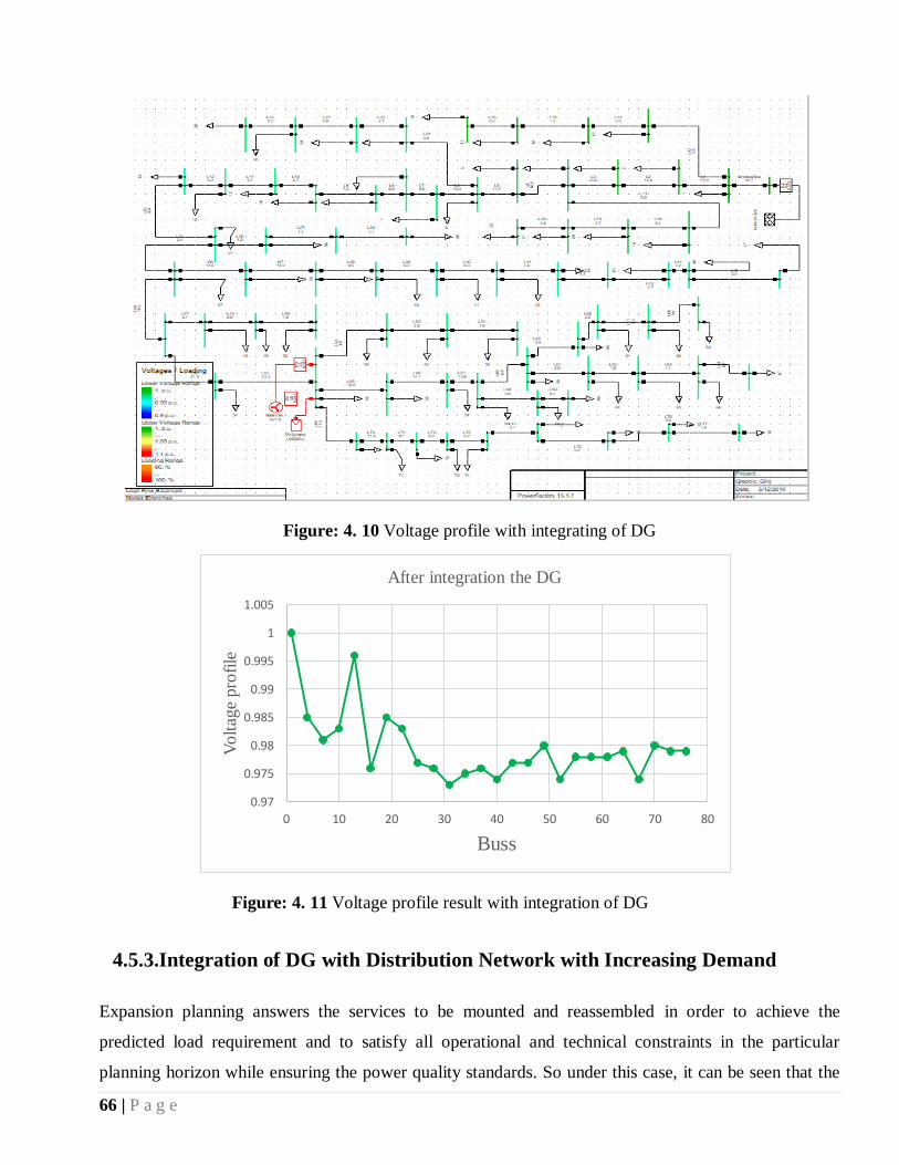
66 | P a g e

Figure: 4. 10 Voltage profile with integrating of DG

Figure: 4. 11 Voltage profile result with integration of DG

4.5.3.Integration of DG with Distribution Network with Increasing Demand

Expansion planning answers the services to be mounted and reassembled in order to achieve the

predicted load requirement and to satisfy all operational and technical constraints in the particular

planning horizon while ensuring the power quality standards. So under this case, it can be seen that the

0.97

0.975

0.98

0.985

0.99

0.995

1

1.005

0 10 20 30 40 50 60 70 80

Vo

ltag

e pro

file

Buss

After integration the DG

67 | P a g e

effect of power loss, line loading, and voltage profile of the case study distribution network when

integrate the DG at appropriate locations with appropriate size to the distribution network and when

increasing the penetration of DG and the load at each year increases by 7.07% in order to supply the

customer needs.

The proposed method is applied to a 15 kV bus radial distribution network by increasing the penetration

of DG by 7.07% at the appropriate location and size, when the distribution network expansion increase

gradually. It can be seen that the effect on line loading, voltage profile and power loss on the simulation

using DigSILENT Power Factory 15.1.7 software. The result shows it reduces the power loss, it

improves the voltage profile and it reduce the line loading after increasing the penetration of DG unit

with the load increase.

Figure: 4. 12 Integration of DG penetration with distribution network when the load demand increase

4.5.3.1. Line loading with increase load demand

To investigate the integration of DG on line loading after one year (when the load demand increase)

load flow analysis is made by modeled in DigSILENT Power Factory 15.1.7 software. The simulation

result revealed it reduces the line loading after integrating the DG with increase the load demand. The

red color which have seen in the above figure 4.5 and the percentage of line loading is reduced. In

general the integration of DG with increasing the load with penetration of DG on line loading segment is

important but they have an impact to the distribution system protection due to increase the capacity of

DG through the line [see in appendix C3 in detail].

68 | P a g e

Table 4. 8 Percentage of line loading after one year with DG integration

Line Line

loading %

WIL &

DG

line Line

loading %

WIL &

DG

line Line

loading %

WIL& DG

line Line loading

% WIL &

DG

L1 36.15 L21 3.83 L41 4.81 L61 8.88

L2 34.37 L22 2.74 L42 4.72 L62 7.77

L3 32.57 L23 0.91 L43 4.72 L63 7.4

L4 21.76 L24 0.18 L44 4.06 L64 3.7

L5 21.43 L25 10.95 L45 3.43 L65 11.84

L6 16.96 L26 1.2 L46 11.8 L66 8.16

L7 16.25 L27 1.11 L47 3.14 L67 7.4

L8 15.54 L28 1.11 L48 2.03 L68 3.7

L9 13.76 L29 0.82 L49 1.85 L69 13.29

L10 13.05 L30 0.77 L50 140.92 L70 12.92

L11 12 L31 8.13 L51 11.76 L71 11.08

L12 11.35 L32 3.27 L52 4.06 L72 9.97

L13 3.76 L33 2.9 L53 2.95 L73 8.12

L14 1.97 L34 2.11 L54 1.84 L74 7.02

L15 1.25 L35 2.1 L55 30.56 L75 5.17

L16 0.18 L36 1.54 L56 26.44 L76 4.43

L17 9.08 L37 0.98 L57 26.25 L77 3.69

L18 5.45 L38 9.58 L58 4.8

L19 4.72 L39 9.4 L59 0.37

L20 1.82 L40 8.32 L60 21.05

WIL & DG – With Increase load and penetration of Distributed Generation

4.5.3.2. Total power loss with load demand increases

In order to reduce the total power losses of the system, the integration of DG unit at proper capacity at

proper location is significant. Here the proper size and place of DG had been determined. The steady

state balanced and positive sequence load flow analysis indicated that the total real and reactive

69 | P a g e

power loss is reduced to 0.49 MW and 0.67MVAR respectively from the existing distribution

network, after the integration of DG with increasing the load and penetration of DG units as shown in

figure 4.13. In general the integrating of DG with increasing the load and penetration of DG on power

loss of the distribution system is more important, but it increase the loss when it compared before

increasing the load, due to the load increases. Therefore by taking the appropriate capacity and location

of the DG in expansion planning is more important and they have maximum power loss reduction.

Figure: 4. 13 Total power loss with load demand increases

4.5.3.3. Voltage profile with load demand increases

Figure 4.14 shows that voltage profile of the system resembles graphically after integration of DG and

when it increases the load with penetration of DG. As it is clearly observed from the figure below, all

the terminal voltages are at the standard range between 0.95p.u. -1.05 p.u. During the base case load

flow analysis, the minimum voltage magnitude which occur at bus 57 and 58 had been determined to be

0.866 p.u i.e. it is in the range of 0.866p.u – 1.0 p.u. Then the voltage profile is improved to in the range

between 0.973 p.u – 1.0 p.u after integration the DG when increase the load with penetration of DG [see

in appendix B3 in detail].

Generally, distributed generation (DG) integration is important when it increase the load with

penetration of DG on a voltage profile of the radial distribution system, but it’s important to take the

appropriate capacity at appropriate location of the DG in order to have acceptable voltage profile

otherwise, if the capacity of DG increases and if there is no locate at the appropriate place it may have

overvoltage is happen.

70 | P a g e

Figure: 4. 14 Voltage profile with load demand increases

4.6. Implementation of Fast Protection Relay

Transmission and distribution systems are exposed to overcurrent flow into their elements. In an electric

power system, overcurrent or excess current is a situation where a larger than intended electric current

exists through a conductor, leading to excessive generation of heat, and the risk of fire or damage to

equipment. In order to protect the system before damaged, you have to implement fast protection.

Integration of DG to the radial distribution network it changes the system operation (the flow of current

it changes from unidirectional to bidirectional) and the change in current flow it affects the protection

device. Therefore, it is necessary to study the characteristics of the fault to implement fast protection. In

addition, it necessary to see the effect of phase to earth and phase to phase fault at each branch of the

line then it implement the fast protection device in order to clear the fault based on each line

characteristic.

To implement fast protection device using DigSILENT Power Factory 15.1.7 software in to distribution

network I have consider different types of short circuit fault. Therefore, to clear those fault earth fault

and phase fault element relay is implemented based on each line characteristic. See one by one such like

in the figures below.

The two element of earth and phase relay is not trip as shown in the figure 4.15. Because the pick-up

current of the relay setting is higher than the steady state current of the line. Therefore, the

implementation of fast protection relay is not affected at steady state condition when the DG integrate to

the distribution network.

0.95

0.96

0.97

0.98

0.99

1

1.01

B1

B3

B6

B9

B12

B15

B18

B21

B24

B27

B30

B33

B36

B39

B42

B45

B48

B50

B52

B55

B58

B61

B64

B67

B70

B73

B76

Volt

age

pro

file

bass

Voltage profile (p.u) when we increase the load with DG

71 | P a g e

Figure: 4. 15 Operating characteristic of over current relay at normal condition

When there is a phase to phase fault either LLL or LL short circuit fault is happen at any time in the

distribution network the only phase relay element is trip in order to clear the short circuit, but earth fault

relay element is not trip, because at the system only phase to phase fault is happening, so this relay is

tripped the fault as you set the time as well as the fault current. In this figure 4.16 shown below the peak

fault current of line to line is 6741.432A pri and the relay trips at 3.710s.

Figure: 4. 16 Phase element relay is trip when LL short circuit is accord

When there is earth fault like L-G short circuit fault happened at any time in the distribution system the

earth fault relay element is trip in order to clear the fault. But phase element relay is not trip because at

the system it is only phase to ground fault is occurs and this relay trips the fault as you set the time as

well as the fault current. In the figure 4.17 shown below the peak fault current of single line to ground is

4000.024 pri A and trips at 0.483s.

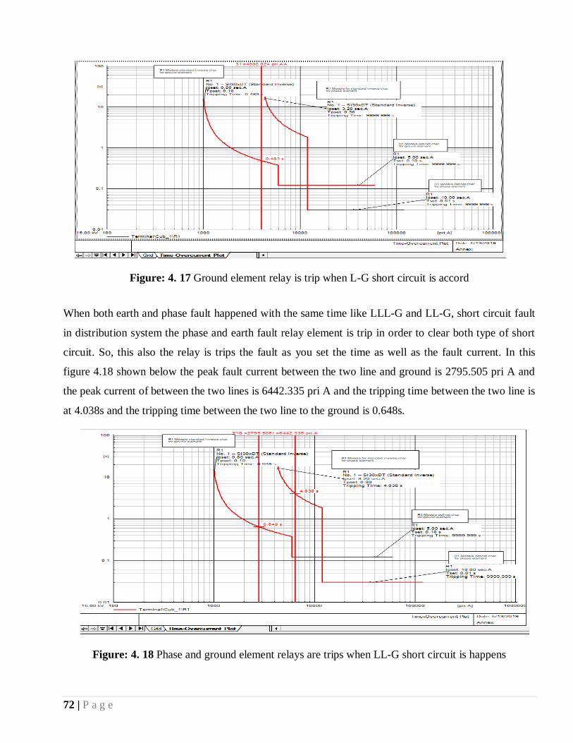
72 | P a g e

Figure: 4. 17 Ground element relay is trip when L-G short circuit is accord

When both earth and phase fault happened with the same time like LLL-G and LL-G, short circuit fault

in distribution system the phase and earth fault relay element is trip in order to clear both type of short

circuit. So, this also the relay is trips the fault as you set the time as well as the fault current. In this

figure 4.18 shown below the peak fault current between the two line and ground is 2795.505 pri A and

the peak current of between the two lines is 6442.335 pri A and the tripping time between the two line is

at 4.038s and the tripping time between the two line to the ground is 0.648s.

Figure: 4. 18 Phase and ground element relays are trips when LL-G short circuit is happens

73 | P a g e

General, in this thesis earth fault and phase fault relay element is successfully implemented in the

distribution network. Earth fault relay is specifically designed to operate only on faults which involve

fault between phase and earth as against a fault not involving earth such as two phase or three phase

faults or overload fault due to system overload. The major advantage it offers are as, an overcurrent

phase relay operates on over current irrespective of whether the overcurrent is due to any fault its setting

has to be more than the normal load current whereas earth fault setting can be kept far low as normal

earth current is close to zero, in case of faults involving low impedance there is sufficient current to

operate the Earth fault relay.

4.7. Protection Relays Coordination

Investigation on protection issues involving DG is carried out on the industrialized radial system model

based on protection coordination. Types of overcurrent protective devices coordination comprise fuse-

fuse coordination, fuse-relay coordination and relay-relay coordination. Here, to examine the impact of

DG integration on protection coordination of radial distribution network, relay to relay coordination had

been selected because the stress is on the feeder although the primary of the substation transformer is

ideally protected with a fuse. Also DG protection or its separation methods are above the scope of this

thesis.

The aim of this coordination of overcurrent relays is to decrease the influence of DG integration in a

radial distribution network, due to increasing load with the penetration of DG in to the distribution

network. It is extensively recognized that in radial networks, discrimination of fault protection is

achieved through time-current coordination of over-current relays. This is since of particular fault, all

the relays related in the radial feeder see the fault current but they are made to operate at different times.

The coordination is based on the fact that the relay closest to the fault (primary relay) sees the largest

fault current than those beyond away (backup relays). Selection of different time current features in the

relay settings is the means of realizing coordination.

On the feeder KO1 Adwa substation has only one relay which is found at the outlet of the feeder with

current transformer (CT) ratio 1200A. Due to one relay about the outlet of the substation the fault far

away from this relay is less scale and does not sense to clear this fault at a time. So, in this thesis work I

am to tray for investigation the impact of DG integration on protection coordination of the protective

relay and total eleven relays were added to the utility relay and by changing the protection model.

Based on equation 3.19 the current transformer setting has been determined for the eleven instrument

74 | P a g e

transformers. The setting exported from the DigSILENT power factory simulation software is as shown

in table 4.10. To ensure the actual of protection on the feeder, eleven GE Alstom KCCG142-1A

overcurrent relays with inverse time and definite time over current relay characteristics are chosen from

the DigSILENT Power Factory 15.1.7 global library. All relay models perform Inverse Definite

Minimum Time (IDMT) and Definite Time (DT) or Instantaneous functions. Assuming Plug Setting

(PS) of relay 10 (R10) =100% and time multiplier setting of relay 10 (TD10) = 0.05, the operating time of

relay 10 (R10) is determined from equation 3.24 which is found to be 0.0548s. Taking the coordination

time interval of 0.2s which is standard the working time of relay 6 (R6) became 0.2548s. Then the time

dial of relay 6 (R6) is determined from equation 3.25. The procedure is continued in the same way up to

the utility relay that is the relay R1 which its operating time was determined to be 1.4749s.

75 | P a g e

Table 4. 9 Instrument Transformers Setting

Relays Locatio

n

Branch Manufacture

r

Model CT Slot Ratio[pri.

A/ sec.A]

R1

Termina

l terminal Alstom KCGG142-1A CT 1 Ct-3p 1200A/1A

CT 1 Ct-3I0 1200A/1A

R10 BB54 L65 Alstom KCGG142-1A CT10 Ct-3p 400A/1A

CT10 Ct-3I0 400A/1A

R2 BB1 L1 Alstom KCGG142-1A CT 2 Ct-3p 1100A/1A

CT 2 Ct-3I0 1100A/1A

R2-1 BB1 L13 Alstom KCGG142-1A CT2-1 Ct-3p 400A/1A

CT2-1 Ct-3I0 400A/1A

R3 BB5 L5 Alstom KCGG142-1A CT 3 Ct-3p 1000A/1A

CT 3 Ct-3I0 1000A/1A

R4 BB35 l36 Alstom KCGG142-1A CT4 Ct-3p 500A/1A

CT4 Ct-3I0 500A/1A

R5 BB42 L46 Alstom KCGG142-1A CT5 Ct-3p 600A/1A

CT5 Ct-3I0 600A/1A

R6 BB50 L55 Alstom KCGG142-1A CT 6 Ct-3p 500A/1A

CT 6 Ct-3I0 500A/1A

R7 BB50 L69 Alstom KCGG142-1A CT7 Ct-3p 500A/1A

CT7 Ct-3I0 500A/1A

R8 BB50 L52 Alstom KCGG142-1A CT8 Ct-3p 500A/1A

CT8 Ct-3I0 500A/1A

R9 BB54 L61 Alstom KCGG142-1A CT9 Ct-3p 400A/1A

CT9 Ct-3I0 400A/1A

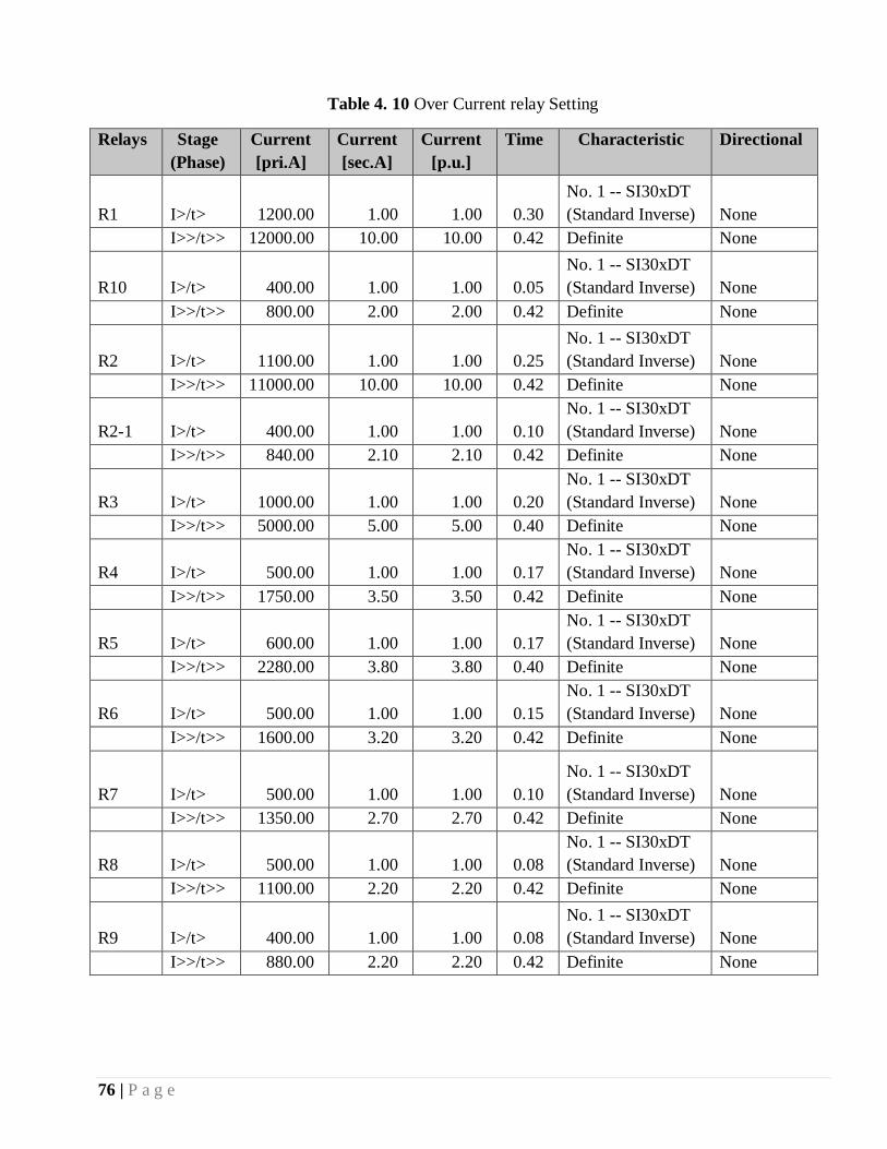
76 | P a g e

Table 4. 10 Over Current relay Setting

Relays Stage

(Phase)

Current

[pri.A]

Current

[sec.A]

Current

[p.u.]

Time Characteristic Directional

R1 I>/t> 1200.00 1.00 1.00 0.30

No. 1 -- SI30xDT

(Standard Inverse) None

I>>/t>> 12000.00 10.00 10.00 0.42 Definite None

R10 I>/t> 400.00 1.00 1.00 0.05

No. 1 -- SI30xDT

(Standard Inverse) None

I>>/t>> 800.00 2.00 2.00 0.42 Definite None

R2 I>/t> 1100.00 1.00 1.00 0.25

No. 1 -- SI30xDT

(Standard Inverse) None

I>>/t>> 11000.00 10.00 10.00 0.42 Definite None

R2-1 I>/t> 400.00 1.00 1.00 0.10

No. 1 -- SI30xDT

(Standard Inverse) None

I>>/t>> 840.00 2.10 2.10 0.42 Definite None

R3 I>/t> 1000.00 1.00 1.00 0.20

No. 1 -- SI30xDT

(Standard Inverse) None

I>>/t>> 5000.00 5.00 5.00 0.40 Definite None

R4 I>/t> 500.00 1.00 1.00 0.17

No. 1 -- SI30xDT

(Standard Inverse) None

I>>/t>> 1750.00 3.50 3.50 0.42 Definite None

R5 I>/t> 600.00 1.00 1.00 0.17

No. 1 -- SI30xDT

(Standard Inverse) None

I>>/t>> 2280.00 3.80 3.80 0.40 Definite None

R6 I>/t> 500.00 1.00 1.00 0.15

No. 1 -- SI30xDT

(Standard Inverse) None

I>>/t>> 1600.00 3.20 3.20 0.42 Definite None

R7 I>/t> 500.00 1.00 1.00 0.10

No. 1 -- SI30xDT

(Standard Inverse) None

I>>/t>> 1350.00 2.70 2.70 0.42 Definite None

R8 I>/t> 500.00 1.00 1.00 0.08

No. 1 -- SI30xDT

(Standard Inverse) None

I>>/t>> 1100.00 2.20 2.20 0.42 Definite None

R9 I>/t> 400.00 1.00 1.00 0.08

No. 1 -- SI30xDT

(Standard Inverse) None

I>>/t>> 880.00 2.20 2.20 0.42 Definite None

77 | P a g e

In the Figure 4.19 shows below the positive sequence load flow analysis, the network were analyzed

with DG integrated, with the location of over current relays which are seen in green color. All the relays

are not tripping as expected during steady state condition since the branch currents are below the

operation currents of the relays.

Figure: 4. 19 After DG integration with Protection coordination

However, during DG integration of the reverse power flow is produced without affecting the operation

of the relays at steady state condition. In case of faulty condition the integration of DG affects the

operation of the relays by causing an increment of fault current. To be noted that if distributed generator

(DG) is sized and placed properly the negative impact of DG is not due to increment of fault currents

rather the reverse power flow in the network which causes the islanding of DG and all loads

downstream of DG. Figure 4.20 shows that the coordination of eleven over current protection in power

flow without affecting the operation of the relays at steady state condition.

78 | P a g e

Figure: 4. 20 Coordination of time overcurrent relays at normal condition

In figure 4.21 and 4.22 shown below a three phase fault on bus 8 with DG connected is cleared by R3 in

0.420s. The rest of the relay performs their back up protection according to their sequence of operation

for instance R2 clear the fault in 0.775s, R1 in 0.966s if R3 fail to trip and so on.

Figure: 4. 21 Coordination of time over current operation of the relays at fault conditions at bus 8.

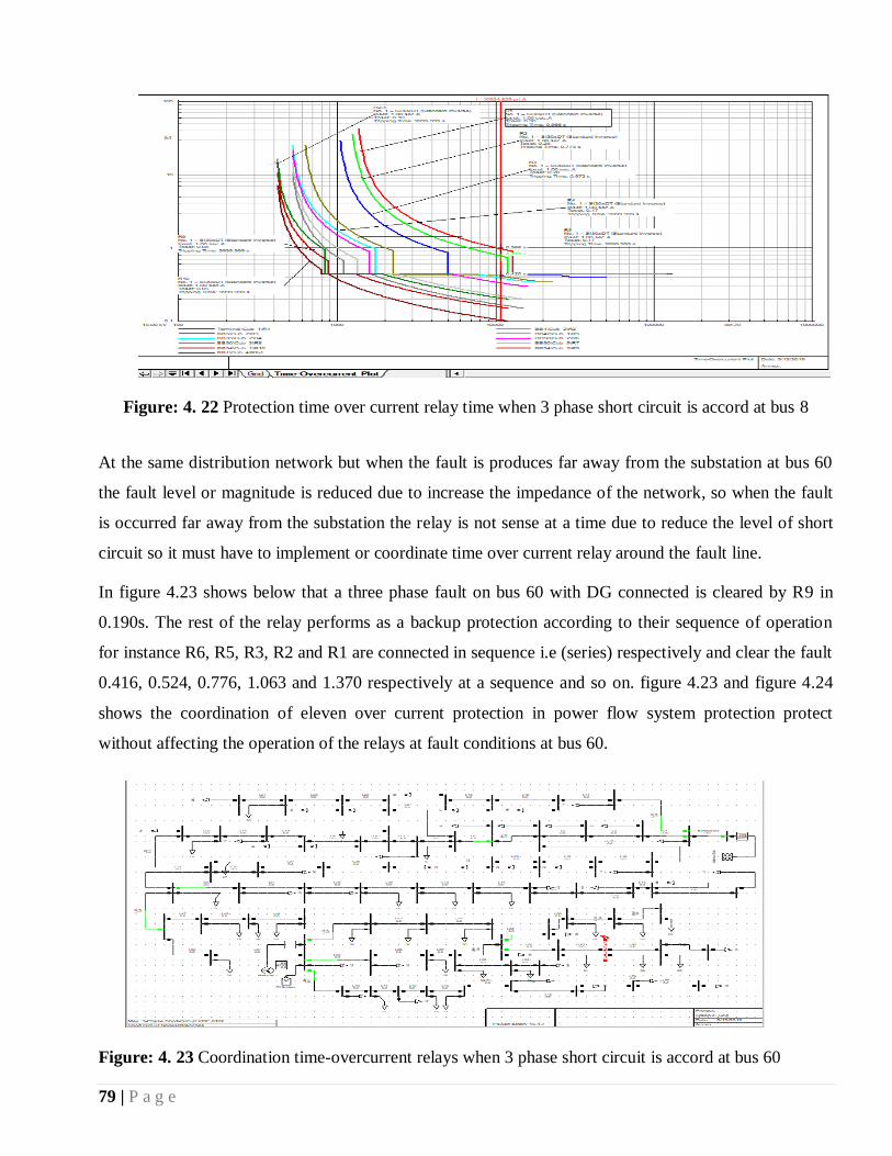
79 | P a g e

Figure: 4. 22 Protection time over current relay time when 3 phase short circuit is accord at bus 8

At the same distribution network but when the fault is produces far away from the substation at bus 60

the fault level or magnitude is reduced due to increase the impedance of the network, so when the fault

is occurred far away from the substation the relay is not sense at a time due to reduce the level of short

circuit so it must have to implement or coordinate time over current relay around the fault line.

In figure 4.23 shows below that a three phase fault on bus 60 with DG connected is cleared by R9 in

0.190s. The rest of the relay performs as a backup protection according to their sequence of operation

for instance R6, R5, R3, R2 and R1 are connected in sequence i.e (series) respectively and clear the fault

0.416, 0.524, 0.776, 1.063 and 1.370 respectively at a sequence and so on. figure 4.23 and figure 4.24

shows the coordination of eleven over current protection in power flow system protection protect

without affecting the operation of the relays at fault conditions at bus 60.

Figure: 4. 23 Coordination time-overcurrent relays when 3 phase short circuit is accord at bus 60

80 | P a g e

Figure: 4. 24 Protection time over current relay when 3 phase short circuit is accord at bus 60

4.8. Grading of Overcurrent Relays

Among the various possible methods used to achieve correct relay coordination which are using either

time or overcurrent, or a combination of both. The common aim of the three methods is to give correct

discrimination. Accordingly that everyone must isolate only the faulty section of the power system

network, which leaves the rest of the system undisturbed.

Each of the two methods described so far has a fundamental disadvantage in the case of discrimination

by time alone, the disadvantage is due to the fact that the more severe faults are cleared in the longest

operating time. On the other hand, discrimination by current can be applied only where there is

appreciable impedance between the two circuit breakers concerned.

It is because of the limitations imposed by the independent use of either time or current grading that the

inverse time overcurrent relay characteristic has evolved. With this characteristic, the time of operation

is inversely proportional to the fault current level and the actual characteristic is a function of both

‘time’ and 'current' settings. Figure 4.25 illustrates the characteristics of eleven relays given different

current/time settings in this study. For a large variation in fault current between the eleven ends of the

feeder, faster operating times can be achieved by the relays nearest to the source, whereas the fault level

is the highest. The disadvantages of grading by time or current alone are overcome.

81 | P a g e

Figure: 4. 25 Coordination of eleven relays at normal condition when the relay is upgraded

The time interval that must be allowed between the operations of eleven adjacent relays in order to

achieve correct discrimination between them is called the grading margin. If a grading margin is not

provided, or is insufficient, more than one relay will operate for a fault, leading to difficulties in

determining the location of the fault and unnecessary loss of supply to some consumers. Grading is

initially carried out for the maximum fault level at the relaying point under consideration, but a checking

is also made that the required grading margin exists for all current levels between relay pickup current

and maximum fault level.

In this study the time interval between the operations of eleven adjacent relays before grading the relays

in DigSILENT Power Factory 15.1.7 software is performed by selecting +0.2s grading margin to all

relays. But when it increase the penetration of DG with increasing load demand it affects the protection

devise as described in chapter three so far. Therefore by increasing the value of margin to all relays by

+ 0.3s it decreases the impact of the protection device at the fault condition as shown below in the figure

4.26.

82 | P a g e

Figure: 4. 26 when there is fault accrued at 15 bus after grading the overcurrent relays

When there is fault accrued at 15 bus the maximum peek fault current is 19116pir A and the tripping

time of the R2-1 and R1 relays are 0.149s and 0.760s respectively. So when it increase the load with the

penetration of DG capacity which is above the current setting of the protection relay they have an

impact on the protection device as it described so far. So when it upgrade the overcurrent relay it

protects up to 45kA at the same tripping time. Show the above figures 4.26 to understand the grading

margin of the over current.

Generally in a radial system when the number of relay is connected in series as shown in the figure 4.23

above, it is desired that the smallest possible part of the system should be off. So this is conveniently

achieved by coordinating and employing time graded protection. The over current system should be

adjusted in such a way that the longer relay from the generating station the lesser time of operation.

4.9. Impacts of DG Integration on the expanded System

In this section investigates in order to examine the impact of integration of DG on expansion planning

without and with integration of DG and also it investigates when it increasing load with penetration of

DG. The load flow study has been performed using the help of DigSILENT Power Factory 15.1.7

software on power loss, voltage profile and voltage stability and also the loading of the line segment

compered when the capacity of Dg increases with demand at steady state and transient stability

condition on a radial distribution system at the selected capacity and location as follow.

83 | P a g e

4.9.1.Impact of DG integration on Total Power Losses

During the base case load flow analysis at steady state condition, the total real and reactive power loss

was determined as 2.06 MW and 2.95 MVAR respectively. So in order to see the effect of total power

losses of the distribution system, the integration of DG unit at appropriate place with appropriate

capacity is significant. To get the best benefit from DG integration, sizing and sitting of distributed

generation should be made with a great care otherwise the negative impact of DG may dominate.

The steady state balanced and positive sequence load flow analysis indicated that the total real and

reactive power loss was reduced to 0.11 MW and 0.13 MVAR respectively after the integration of

DG before increase the load and selected capacity. And also the total real and reactive power loss is

reduced from the base case to 0.49 MW and 0.67 MVAR respectively, when the load increase with

increase the penetration of DG at appropriate placement and location. The comparison of total power

loss before and after DG integration is shown in figure 4.27 which depicts a major significant

improvement of total power losses reduction. Therefor when it can be seen the effect of DG integration

on power loss they have positive impact in the distribution system expansion planning.

Figure: 4. 27 comparisons of total power loss without and with DG as well as when the load increases

4.9.2.Impact of DG integration on Voltage Profile

In order to clearly indicate the impact of voltage profile of distribution system, the base case voltage

profile is compared with the voltage profile of the system after DG integration and with the voltage

0

0.5

1

1.5

2

2.5

3

Real PowerLoss in MW

with out DG

ReactivePower Loss in

MVAR without DG

real PowerLoss in MW

with DG

Reactive powerloss with DG

Realpower lossin MW when

the loadincrease with

DG

Reactive powerloss in MVAR

when increasethe load with

DG

2.06

2.95

0.11 0.130.49

0.67

Tota

l p

ow

er l

oss

Comparision of total power loss without and with DG as well as when it

increase the load with DG

84 | P a g e

profile of the system after DG integration with increase the penetration of DG and load of the

distribution system. The comparison of voltage profile during base case scenario, after DG integration

and after DG integration with increasing load and penetration DG, is shown in figure 4.28 which entail a

great improvement of the voltage profile at all buses of the system. The impact of distributed generation

(DG) integration on a voltage profile of the radial distribution system is positive by taking into account

the appropriate sizing at appropriate location of the DG [see in the appendixes B in detail].

Figure: 4. 28 Comparisons of voltage profiles without and with DG integration as well as when the load

demand increases

4.9.3.Impact of DG integration on Line Loading

From the next year the feeder is overloaded due to increase the load demand at each year when it seen

the percentage of line loading from the result box of DigSILENT Power Factory 15.1.7 software, so it

needs additional distribution network to supply the customer. Therefore, to investigate the impact of DG

on line loading after one year without DG and with DG when the load demand increases has made in

case study radial distribution system modeled using DigSILENT Power Factory 15.1.7 software

simulation. This result revealed the reduction of loading of line segment when the DG increase with

demand. The percentage of loading of line have observed from the result box of DigSILENT Power

Factory 15.1.7 software. They have significant reduction of line loading when it compared without DG

when it see figure 4.29 below. It is established that the impact of DG on line loading when the capacity

of DG increase with demand is positive impact in the distribution system expansion planning [see in the

appendixes C].

0.840.860.88

0.90.920.940.960.98

11.02

0 10 20 30 40 50 60 70 80

Volt

age

pro

file

(p

.u)

buss

comparision of Voltage profile without and with DG intagration as well

as when the load demand increases with penetration of DG

WODG WDG WI DG&L

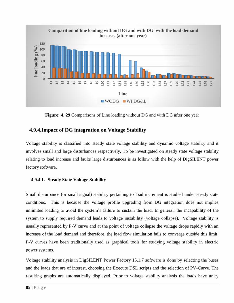
85 | P a g e

Figure: 4. 29 Comparisons of Line loading without DG and with DG after one year

4.9.4.Impact of DG integration on Voltage Stability

Voltage stability is classified into steady state voltage stability and dynamic voltage stability and it

involves small and large disturbances respectively. To be investigated on steady state voltage stability

relating to load increase and faults large disturbances is as follow with the help of DigSILENT power

factory software.

4.9.4.1. Steady State Voltage Stability

Small disturbance (or small signal) stability pertaining to load increment is studied under steady state

conditions. This is because the voltage profile upgrading from DG integration does not implies

unlimited loading to avoid the system’s failure to sustain the load. In general, the incapability of the

system to supply required demand leads to voltage instability (voltage collapse). Voltage stability is

usually represented by P-V curve and at the point of voltage collapse the voltage drops rapidly with an

increase of the load demand and therefore, the load flow simulation fails to converge outside this limit.

P-V curves have been traditionally used as graphical tools for studying voltage stability in electric

power systems.

Voltage stability analysis in DigSILENT Power Factory 15.1.7 software is done by selecting the buses

and the loads that are of interest, choosing the Execute DSL scripts and the selection of PV-Curve. The

resulting graphs are automatically displayed. Prior to voltage stability analysis the loads have unity

0

20

40

60

80

100

120

L1 L2 L3 L4 L5 L6 L7 L8 L9

L10

L11

L12

L31

L38

L46

L50

L55

L60

L63

L65

L67

L69

L70

L72

L73

L74

L75

L76

L77

lin

e lo

ad

ing

(%

)

Line

Camparition of line loading without DG and with DG with the load demand

inceases (after one year)

WODG WI DG&L

86 | P a g e

mounting factors, but DigSILENT Power Factory 15.1.7 performs voltage constancy analysis by

gradually increasing the load, while keeping the power factor constant, of the preselected buses until

they reach the power transfer limit.

Creation the voltage stability analysis for gradual raise of load, the P-V curve of the developed model

without DG is as shown in Figure 4.30 for all the loads down steam of DG which is 4.71425 MW, the

maximum or total load before voltage collapse it resolute to be 23.233 MW. Therefore, the loading

margin to voltage collapse, for a current operating point, the total increment of load in a specified

pattern of load increase which can cause to voltage collapse to became 18.523 MW.

Figure: 4. 30 Voltage stability without DG integration

To examine the impact of DG integration, the voltage stability analysis is made after DG integration

and, when the DG injects 16 MW, the p-v curve be came to extreme load of 41.037 MW before voltage

collapse as shown in figure 4.31. Now the loading margin of voltage collapse, for a current operating

point, the total increment of load in a specified pattern of load increase which could cause a voltage

collapse throughout DG injection has been found to be 17.514 MW. This suggests the enhancement of

loading margin when DG integrated into distribution system with correct sizing and placement. Finally

the overall impact of a DG unit on voltage stability during slow increment of load is positive. This is due

to the enhancement of voltage profiles as well as decreased reactive power losses.

87 | P a g e

Figure: 4. 31 Voltage stability with DG integration

4.9.4.2. Transient (dynamic) voltage stability

Voltage instability is due to faults is a transient stability problematic which is large disturbance voltage

stability deliberate under dynamic conditions. In principle, transient stability problems might occur in

distribution networks with DG. The electromagnetic transient (EMT) Simulation of DigSILENT Power

Factory 15.1.7 had been utilities in examining single phase to phase, two phase to ground, three phase

and three phase to ground short circuits. The electromagnetic transient (EMT) simulation contains the

description of variables and events. In this case the variables are phase short circuit currents and their

consistent voltages. The short circuit and its clearing time on the selected bus bars are the events.

To examine the transient stability of the advanced model, it considers before fault condition, at fault

state as well as after clear the fault for different type of faults such as, three-phase, single phase to

ground and two phase to ground short circuits are simulated. In this simulation absolute run time is 0.7s

with different type of fault presenting at a different time by considering the impedance of each fault is

zero. The figures below shows that investigates of voltage and current wave form during different

situations such as, at normal condition, when 3ph fault is follow with there is no protection device,

voltage and current wave form during 3ph fault condition and Voltage and current wave form

throughout 3ph and LG when the fault is occur at different time and also voltage and current wave form

during 3ph, LG and LLG when the fault is accord at different time with protection devices.

This figure 4.32 shows that when the distribution network with DG at normal complaint and it can be

seen the wave form of voltage is sinusoidal and the magnitude of short circuit is zero.

88 | P a g e

Figure: 4. 32 Voltage and current wave form during normal condition.

The figure 4.33 below shows that voltage and current wave form during 3ph, fault accord and when the

distribution network with DG integration have no protection. So, the voltage at the bus comes to zero

and the magnitude of fault current continuously unstable after that the distribution system is comes to up

normal condition.

Figure: 4. 33 Voltage and current wave form during 3ph fault occurred when there is no protection

The figure 4.34 shows voltage and current wave form during 3ph, fault accord and when the fault

introduced at 0.1s and cleared at 0.2s then the distribution system is comes to stable condition after

implement and coordinate the fast overcurrent protection relay.

89 | P a g e

Figure: 4. 34 Voltage and current wave form during 3ph fault

Figure 4.35 shows that voltage and current wave form during 3ph and LG fault accord at different time

scenario. The three phase fault introduced at 0.1s and cleared at 0.2s and also the single phase to ground

short circuit introduced at 0.3s and cleared at 0.4s, after that the system is stable when you coordinate

fast protection relay.

Figure: 4. 35 Voltage and current wave form during 3ph and LG fault at different time

Figure 4.36 shows that voltage and current wave form during 3ph, LG and LLG fault accord at different

time scenario. The three phase short circuit introduce at 0.1s and cleared at 0.2s, and single phase to

ground short circuit introduced at 0.3s and cleared at 0.4s and also the two phase short circuit introduced

at 0.5s and cleared at 0.6s. Therefor after that the distribution system is clear the fault it comes to stable

condition

90 | P a g e

Figure: 4. 36 Voltage and current wave form during 3ph, LG and LLG fault accord at different time

In general the result of the simulation it indicates that the system comes to its original voltage wave

form after the clearance the fault with DG injection. Therefore it can be concluded, that the impact of

DG on transient stability of the system is positive after implement and coordination the fast overcurrent

protection relay by considering its appropriate place with appropriate capacity.

4.10. Cost of the Selected DG

According the International Renewable Energy Agency [43] the costs of renewable energy technologies

reached new lows again last year and both solar and wind power have emerged as the most affordable

power source for many locations and markets, with cost reductions set to last into the next period. Cost

declines across the board in 2018 have reconfirmed the status of renewable power as a highly cost

effective energy source.

The basic standard related to the selection of the power system mechanisms in this thesis work is the

cost of components, as the main purpose of the work is penetrating the optimum power system

configuration that would meet the demand with minimum net present cost and cost of energy. The

approximation of the components cost is made based on the current cost available in market.

Initial capital cost of components: It is the total installed cost organized to buying and install the

component at the commencement of the project.

Replacement cost: This is the cost required to substitute wear out apparatuses at the end of its life

cycle. This cost is different from initial cost of the component, due to the following reasons. At the end

91 | P a g e

of its life cycle not all of the spares of the constituent need to replace, Costs from givers may eliminate

or can reduce initial cost, however spare cost may not account travel costs but initial costs do.

Operation and maintenance (O&M) cost: It is the cost accounted for maintenance and operation of

the system. The entire scheme mechanisms considered in this thesis has different process and

maintenance costs. Miscellaneous O&M costs are considered and also like emission penalties, capacity

scarcity penalty and secure process and maintenance costs are include.

4.10.1. Solar PV Size and Cost

According the International Renewable Energy Agency [43] sustained dramatic decline in the cost of

electricity from utility scale solar PV continued in 2018, with a fall in the global weighted average of

solar PV to USD 0.085/kWh and – 13% lower than for projects commissioned in 2017. This takes the

decline between 2010 and 2018 in the global weighted average of solar PV to 77%.

After analyzing different products focusing on the cost provided the following panel is chosen. The

reason for choosing the product from the stated business is due to its low cost delivered as long as

competence is not a big worry here. The solar panel careful is a 4MW, which is with 4 number of solar

module having 250 kW capacity and 4 number of array from a schott Mono-250 Watt Solar Panel

Company. The selected panel is mono-crystalline silicon solar cell and factory-made by USA which is

known as Item-1202401 model. In this thesis the extra cost and operation and maintenance cost is

considered. In this thesis, the installed total cost is taken about $3,306,024. By considering replacement

cost and process and maintenance cost of the solar panel is considered 10% and 1% of capital cost

respectively.

Table 4. 11 Total capital cost of PV

Life time (yr) 25

Capital cost ($/kWh) 0.085

Capacity of DG (MW) 4

Cost of DG ($) 2,978,400

Replacement cost $ ( 10% of cost of DG) 297,840

O & M cost $ (1% of cost of DG) 29,784

Total capital cost ($) 3,306,024

92 | P a g e

4.10.2. Wind Turbine Size and Cost

According the International Renewable Energy Agency [43] the global weighted average of wind

projects commissioned in 2018, at USD 0.056/kWh, was 13% lower than in 2017 and 35% lower

than in 2010. Costs of electricity wind are now at the lower end of the fossil fuel cost range.

Contingent on the wind speed sources the turbine has to generate large amount of energy to

contribute important renewable fraction and this can be performed using single large wind turbine or

number of smaller turbines. Quantities of turbines, service time, hub height, Cost of the component,

type of electricity produced, cut-in wind speed are the restrictive values to select wind turbine. The

selected turbines can generate AC type electricity to content the need of AC load consumer

applications. The wind turbine taken for this thesis work is twenty four fuhrlander 0.5 MW AC

power rating type to produce 12MW power output. The wind turbine is factory-made by the D-

56477 Waigandshain, Germany. In this thesis the wind power installed total cost is taken about

$9,831,348. By seeing replacement cost and operation and maintenance cost of the wind turbine is

considered about 65% and 2% of capital cost respectively.

Table 4. 12 Total capital cost of wind energy

Life time (yr) 33

Tower height (m) 50

Capital cost ($/kWh) 0.056

Capacity of DG (MW) 12

Cost of DG ($) 5,886,720

Replacement cost $ ( 65% of cost of DG) 3,826,368

O & M cost $ (2% of cost of DG) 118,260

Total capital cost ($) 9,831,348

4.10.3. Total DG placement result cost analysis

After the resolve of DG location and capacity, cost approximation of the obtained DG size has followed.

DG technology also differ in their influence that they impose on the surrounding environment. Hence, to

estimate the cost of the DG, the DG technologies selected in this thesis work is wind and photovoltaic

93 | P a g e

due to free emission and it is appropriate to selected site under case study. From table 4.13 the cost of

the DG is calculated as follows.

Table 4. 13 Total cost for investment of DG

Total Size of DG (MW) 16

Location of DG At bus 50

Total cost ($) 13,137,372 $

Total cost in Ethiopian birr by considering

current rate 32 (birr)

420,395,904 birr

To calculate the returned cost for the investment of DG is calculate as fellow:

Power loss reduction (PLR) due to the placement of DG is:

PLR =Power loss before DG integrating – power loss after DG integration…………4.1

2.06MW – 0.11MW = 1.95MW

After DG placement total energy saved for one year is:

1.95MW * 24 * 365 = 17,082MWh

According to information from the Ethiopian Electric Utility (EEU), the existing electric power

generation, transmission, and distribution costs are, on average, about $0.09 or in Ethiopian birr 2.88 per

kilowatt-hour (kWh), is the current tariff for electricity.

Saving in terms of Ethiopian birr per year is:

17,082MWh * 2.88 (𝐵𝑖𝑟𝑟𝑘𝑊ℎ⁄ ) = 49,196,160 Birr

The return cost in birr per year for the investment of DG is:

ROICDG = Total cost of DG instailled

Energy saving per year………………………………………………...4.2

where ROICDG = Return of Investment Cost for DG integration

= 420,395,904 Birr

49,196,160 Birr/year = 8.545 year

94 | P a g e

CHAPTER FIVE

Conclusions, Recommendations and Future Work

5.1. Conclusions

The integration of distributed generation (DG) in the distribution network is gaining momentum, due to

their network support capability and modular designs. It is one of the effective and viable planning

option for improving the supply quality of the network with ever increasing loads. It is expected that a

renewable DG system may play a key role in the future power distribution system for sustainable and

emission free energy supply. However, the incorporation of active DG units into conventional passive

distribution system is difficulties to distribution system planners due to alterations in existing

infrastructure and operational strategies. Moreover, the integration, renewable DG units such as wind

and solar photovoltaic based generation system, system planner have to deal with uncertainty in power

availability under grid connected and islanded modes of operation.

Generally, in this thesis a methodology for optimal distribution system expansion planning with DG

system is developed. Moreover, the distributed generation impact has been investigated with the

increasing load and penetration of DG. The analytical method using the voltage sensitivity analysis is

implemented and tested on the distribution network using DigSILENT power factory commercial

software. In order to reduce line loss, line loading of the distribution network when the load increases,

and to enhance all node voltages to within the allowable range distributed generator was integrated into

the system. The results are presented by determining the appropriate place at appropriate capacity of DG

for this distribution network. Accordingly, TENVDI and maximum active power loss reduction the

appropriate location and capacity of DG was found and determined at bus 50 with proper capacity of

12.70 MW with 3.30 MW as a reserve on the feeder of KO1 distribution network. The load demand

increment with increment the penetration of DG units to meet the demand requirements for the future

was analyzed using extrapolation forecasting technique. As a result the location of DG and its capacity

was taken into account to reach an appropriate condition in order to create the stability and fairness for

both utility and customer.

With the objective of investigating the impact of DG integration on protection device due to increase the

capacity of DG in this radial distribution system case study distribution feeder was identified based on

95 | P a g e

power interruption data and loaded feeder method. Therefore, feeder KO1 of Adwa substation was

selected due to loaded feeder and more power interruption occurrence compared to the rest of the

feeders. The modelling and simulation of the feeder was carried out using DIgSILENT Power Factory

15.1.7 simulation package. The simulation results before integration the DG indicated that the feeder

encountered the total real and reactive power loss of 2.06 MW and 2.95 MVAR, respectively, with

major bus voltages were out of acceptable range and also it is over loaded feeder after one year. In order

to reduce the total real and reactive power loss and line loading of the system when the demand

increases, and also to enhance all node voltages to within allowable range, distributed generator was

integrated into the system at appropriate place with appropriate capacity. The cost estimation for the

determined DG size was carried out by taking the PV and wind DG type. Consequently, the total cost of

selected 16 MW DG was found to be $13,137,372 and the returned of investment cost for the selected

DG integration is approximately in 8.545 year.

However, it is well known that the current existing electricity networks, particularly distribution

systems, have been designed in radial topology with centralized generation as the main power source to

supply the load. Nevertheless, with the presence of DG the power flow is no longer radial. This DG has

definitely created both positive and negative impacts on distribution system. To deal with these impacts,

various case study projects is conducted in this thesis and the overall research scenarios were

investigated on the technical impact of DG on distribution system. The investigations involving a

directly connected synchronous DG with proper capacity and place indicated that for a particular DG

type the impact on total power loss, voltage profile and voltage stability were positive after integrating

the DG as well as when penetration of DG increased with load and also the loading of the line segment

is within a limit when it increases the peak demand. The results of the balanced and positive sequence

load flow analysis at steady state condition after DG integration pointed out that they have good voltage

stability, the total real and reactive power loss was reduced to 0.11 MW and 0.13 MVAR, respectively,

and the line loading is reduced to acceptable range when the demand increases and all bus voltages were

improved to within acceptable standard range with minimum voltage magnitude that was found at bus

57 and 58 with magnitude of 0.866 and it improves to the range of 0.974 - 1p.u at all bus from the

existing distribution network.

Moreover, in order to reduce the impact of the DG on the protection device that comes due to capacity

of DG increment in this thesis fast protection over current relay is implement and coordination’s. In this

distribution network eleven relays are implemented and coordinated with different time/current setting

based on fault tripping time and magnitude of the fault in the line. This implementing and coordination

96 | P a g e

reduces the impact on the protection of overcurrent relay successfully. Also when the load increase with

penetration of DG capacity above the current rating setting of the protection relay, the protection devices

are upgraded by increasing the margin of the time interval of the each overcurrent relays coordination,

then, the upgraded margin of the protection device of the distribution network is highly integrated with

DG, when the load with penetration of DG increased.

5.2. Recommendations

Best on the findings of this thesis work, it is concluded that integration of DG with distribution network

expansion planning enhances the grid capacity and results in reduction of power loss, improvement of

voltage profile, reduction line loading and increases the voltage stability in the case study Adwa

distribution substation. In addition, DG technology especially renewable energy based expects to have a

key role in the future power distribution system for sustainable and emission free energy supply.

Therefore, it is recommended that Ethiopian Electric Utility (EEU) and Ethiopian Electric Power (EEP)

should make awareness and encouragements to promote the implementation of distributed generation in

distribution networks.

5.3. Suggestions for Future Work

Wind and photovoltaic type of DG source have an impact on power output due to environmental

variations and different nonlinear components. In this thesis DG technologies have been limited to

Synchronous Generator which is standard models available in DigSILENT Power Factory 15.1.7

without considering their detail design. In addition to this, deep investigation on protection and

interconnection of DG was done in radial distribution networks for the selected feeders having

pronounced problems.

Therefore, it is suggested that researchers may focus on the following problems:

1. Detailed design of DGs using wind and photovoltaic energy sources.

2. Upgrading the radial distribution network to ring distribution network.

3. Implementation of automatic protection distribution network to isolate and reconnect the DG during

disturbance and after disturbance has been cleared.

97 | P a g e

References

[1]. W. Sun, K. Tian and S. Jia, "Planning of flexible power sources in power distribution systems with

high penetration of dispersed generation", CIRED - Open Access Proceedings Journal, vol. 2017, no. 1,

pp. 2496-2499, 2017. Available: 10.1049/oap-cired.2017.0571.

[2]. R. Dugan, T. McDermott and G. Ball, "Planning for distributed generation", IEEE Industry

Applications Magazine, vol. 7, no. 2, pp. 80-88, 2001. Available: 10.1109/2943.911193.

[3] S. Haffner, L. Pereira, L. Pereira and L. Barreto, "Multistage Model for Distribution Expansion

Planning With Distributed Generation—Part I: Problem Formulation", IEEE Transactions on Power

Delivery, vol. 23, no. 2, pp. 915-923, 2008. Available: 10.1109/tpwrd.2008.917916.

[4] Covarrubias, A. J. (1979). Expansion Planning for Electric Power Systems. IAEA Bulletin, 21(2),

55–64. Retrieved from http://iaea.org/Publications/Magazines/Bulletin/Bull212_3/212_304985564.pdf

[5]S. Lumbreras, A. Ramos and F. Banez-Chicharro, "Optimal transmission network expansion

planning in real-sized power systems with high renewable penetration", Electric Power Systems

Research, vol. 149, pp. 76-88, 2017. Available: 10.1016/j.epsr.2017.04.020.

[6]L. Wang and C. Singh, "Reliability-Constrained Optimum Placement of Reclosers and Distributed

Generators in Distribution Networks Using an Ant Colony System Algorithm", IEEE Transactions on

Systems, Man, and Cybernetics, Part C (Applications and Reviews), vol. 38, no. 6, pp. 757-764, 2008.

Available: 10.1109/tsmcc.2008.2001573.

[7]M. Masoum, M. Ladjevardi, A. Jafarian and E. Fuchs, "Optimal Placement, Replacement and Sizing

of Capacitor Banks in Distorted Distribution Networks by Genetic Algorithms", IEEE Transactions on

Power Delivery, vol. 19, no. 4, pp. 1794-1801, 2004. Available: 10.1109/tpwrd.2004.835438.

[8]. J. Liu, M. Salama, and R. Mansour, “Identify the Impact of Distributed Resources on Congestion

Management,” IEEE Transactions on Power Delivery, vol. 20, no. 3, pp. 1998–2005, 2005.

[9]. L. Cipcigan and P. Taylor, “Investigation of the reverse power flow requirements of high

penetrations of small-scale embedded generation,” IET Renewable Power Generation, vol. 1, no. 3, p.

160, 2007.

[10] G. Pepermans, J. Driesen, D. Haeseldonckx, R. Belmans, and W. D’Haeseleer, “Distributed

generation: definition, benefits and issues,” Energy Policy, vol. 33, no. 6, pp. 787–798, 2005.

98 | P a g e

[11] G. Celli, E. Ghiani, S. Mocci, and F. Pilo, “A Multi objective Evolutionary Algorithm for The

Sizing and Siting of Distributed Generation,” IEEE Transaction on Power System, Vol. 20, No. 2, May

2005, PP. 750–757.

[12] W. El-Khattam, Y. G. Hegazy, M. M. A. Salama, “An Integrated Distribution Generation

Optimization Model for Distribution System Planning”, IEEE Transactions on Power Systems, Vol. 20,

No. 2, May 2005, PP. 1158-1165.

[14] “Erratum,” Solar & Wind Technology, vol. 7, no. 6, p. 747, 1990.

[15] T. K. Chattopadhyay, S. Banerjee, and C. K. Chanda, “Voltage Stability Index of Radial

Distribution Networks by Considering Distributed Generator for Different Types of Loads,”

International Journal of Energy Optimization and Engineering, vol. 5, no. 1, pp. 1–22, 2016.

[16]N. Mijuskovic, "Optimal operation planning of distribution systems considering security

constraints", International Journal of Electrical Power & Energy Systems, vol. 14, no. 6, pp. 383-386,

1992. Available: 10.1016/0142-0615(92)90022-2.

[17] BNEF, (2018a), 2H 2018 Wind Turbine Price Index, Bloomberg New Energy Finance, London.

[18]Q. Zhou and J. Bialek, "Generation curtailment to manage voltage constraints in distribution

networks", IET Generation, Transmission & Distribution, vol. 1, no. 3, p. 492, 2007. Available:

10.1049/iet-gtd: 20060246.

[19]J. Nahman and D. Peric, "Optimal Planning of Radial Distribution Networks by Simulated

Annealing Technique", IEEE Transactions on Power Systems, vol. 23, no. 2, pp. 790-795, 2008.

Available: 10.1109/tpwrs.2008.920047.

[20]S. Favuzza, G. Graditi, M. Ippolito and E. Sanseverino, "Optimal Electrical Distribution Systems

Reinforcement Planning Using Gas Micro Turbines by Dynamic Ant Colony Search Algorithm", IEEE

Transactions on Power Systems, vol. 22, no. 2, pp. 580-587, 2007. Available:

10.1109/tpwrs.2007.894861.

[21]S. Haffner, L. Pereira, L. Pereira and L. Barreto, "Multistage Model for Distribution Expansion

Planning with Distributed Generation—Part II: Numerical Results", IEEE Transactions on Power

Delivery, vol. 23, no. 2, pp. 924-929, 2008. Available: 10.1109/tpwrd.2008.917911..

99 | P a g e

[22]Y.-C. Huang, H.-T. Yang, and C.-L. Huang, “Solving the capacitor placement problem in a radial

distribution system using Tabu Search approach,” IEEE Transactions on Power Systems, vol. 11, no. 4,

pp. 1868–1873, 1996.

[23] T. Khalil, A. Gorpinich, and G. Elbanna, “Combination of capacitor placement and reconfiguration

for loss reduction in distribution systems using selective PSO,” 22nd International Conference and

Exhibition on Electricity Distribution (CIRED 2013), 2013.

[24] R. H. Liang and C. K. Cheng, “Dispatch of Main Transformer ULTC and Capacitors in a

Distribution System,” IEEE Power Engineering Review, vol. 21, no. 7, pp. 72–72, 2001.

[25] V. Ravindran and V. Aravinthan, “Feeder level power loss reduction through reactive power

control with presence of distributed generation,” 2013 IEEE Power & Energy Society General Meeting,

2013.

[26] Z. Hu, X. Wang, H. Chen, and G. Taylor, “Volt∕VAr control in distribution systems using a time-

interval based approach,” IEE Proceedings - Generation, Transmission and Distribution, vol. 150, no. 5,

p. 548, 2003.

[27]. E. Castronuovo and J. Lopes, “On the Optimization of the Daily Operation of a Wind-Hydro

Power Plant,” IEEE Transactions on Power Systems, vol. 19, no. 3, pp. 1599–1606, 2004.

[28] BNEF, (2018b), 2H 2018 Wind O&M Price Index, Bloomberg New Energy Finance, London

[29] Bolinger, M., S. Weaver, and J. Zuboy (2015), “Is $50/MWh solar for real? Falling project prices

and rising capacity factors drive utility-scale PV toward economic competitiveness,” Progress in

Photovoltaics: Research and Applications, Vol. 23, No. 12, pp.

[30] D. Zhu, R. Broadwater, K. Tam, R. Seguin, and H. Asgeirsson, “Impact of DG Placement on

Reliability and Efficiency With Time-Varying Loads,” IEEE Transactions on Power Systems, vol. 21,

no. 1, pp. 419–427, 2006.

[31] H. Zareipour, K. Bhattacharya and C. Canizares, "Distributed generation: Current status and

challenges," Presented at Proc. 36th Annual North American Power Symposium (NAPS), 2004.

[32] Z. Q. Wu, K. L. Lo, “Optimal Choice of Fixed and Switched Capacitors in Radial Distributors with

Distorted Substation Voltae”, IEE Proceedings of Generation, Transmission and Distribution, Vol. 142,

No. 1, January 1995, PP. 24-28.

100 | P a g e

[33] Prada RB, Souza LJ. Voltage stability and thermal limit: constraints on the Maximum loading of

electrical energy distribution feeders. IEE Proc Gener Transm Distrib 1998; 145(5):573–7

[34]. In Kuri et al. M. R. Haghifam, H. Falaghi and O. P. Malik, "Risk-based distributed generation

placement," IET Generation Transmission and Distribution, vol. 2, pp. 252-260, 2008.

[35]. Liu, J., Salama, “An intelligent islanding technique considering load balance for distribution

system with DGs,” Power Engineering Society General Meeting, IEEE, June 18-22, 2006.

[36] Wang C, Nehrir MH. Analytical approaches for optimal placement of distributed generation

sources in power systems. IEEE Trans Power Syst 2004; 19:2068–76.

[37] Al Abri RS, El-Saadany EF, Atwa YM. Optimal placement and sizing method to improve the

voltage stability margin in a distribution system using distributed generation. IEEE Trans Power Syst

2013;28(1):326–34

[38] Borges CLT, Falcao DM. Impact of distributed generation allocation and sizing on reliability,

losses and voltage profile. In: Proceedings of IEEE Bolonga power technology conference, 2003.

[39] Hatziargyriou, N. et al., “Preliminary results from the More Advanced Control Advice Project for

secure operation of isolated power systems with increased renewable energy penetration and storage”;

IEEE Porto Power Tech Proceedings, 2001;Volume 4, 10-13 Sept. 2001 Page(s):6 pp. vol.4.

[39] Mohamad Hossein Adel, Ali Reza Sedighi, Hamid Reza Akbari, "An adaptive protection scheme

to prevent recloser-fuse miscoordination in distribution feeders with distributed generation units, a case

study", IOSR-JEEE, vol. 10, no. 6, pp. 23-34, December 2015.

[40] IEA Wind (2015), Task 26: Wind Technology, Cost, and Performance Trends in Denmark,

Germany, Ireland, Norway, the European Union, and the United States: 2007–2012, IEA Wind Energy

Systems.

[41] Stanley H. Horowitz, Arun G. Phadke, Power System Relaying, John Wiley and Sons Ltd, 2014.

[42]. S. Wong, K. Bhattacharya and J. D. Fuller, "Electric power distribution system design and

planning in a deregulated environment," IET Generation Transmission and Distribution, vol. 3, pp.

1061-1078, 2009.

[43] IRENA (2018), Renewable Power Generation Costs in 2017, IRENA, Abu Dhabi.

101 | P a g e

Appendixes

Appendix A: Peak Load Demand Forecasting using Matlab

fprintf('\nDemand Forecast\n');

fprintf('\nEnter an array of demand values in the form:\n');

fprintf('\t[yr1 ld1; yr2 ld2; yr3 ld3; yr4 ld4; yr5 ld5]\n');

past_dem = input('\nEnter year/demand values: ');

sizepd = size(past_dem);

% get the # of past years of data and the # of cols in the array

np = sizepd(1); cols = sizepd(2);

% get the number of years to predict

nf = input('\nEnter the number of year to predict: ');

ntotal = np + nf;

% obtain the least-square terms to estimate the ld growth value g

% y = ab^x must be transformed to ln(y) = ln(a) + x*ln(b)

Y = log(past_dem(:,2))'; X = 0:np - 1;

sumx2 = (X - mean(X))*(X - mean(X))';

sumxy = (Y - mean(Y))*(X - mean(X))';

% get the coeffs of the transformed data A = ln(b) and B = ln(a)

A = sumxy/sumx2; B = mean(Y) - A*mean(X);

% solve for the initial value, Po and g

Po = exp(B);

g = exp(A) - 1;

fprintf('\n\tRate of growth =%2.2f%%\n\n', g*100);

fprintf('\tYEAR\tACTUAL\t\tFORECAST\n');

% calculate the estimated values

est_dem = 0;

for i = 1:ntotal

n = i - 1;

% year = first year + n

est_dem(i, 1) = past_dem(1, 1) + n;

% load growth equation

102 | P a g e

est_dem(i, 2) = Po*(1+g)^n;

if i < np

fprintf('\t%4d\t%6.2f\t\t%6.2f\n', est_dem(i,1),past_dem(i,2),est_dem(i,2));

else

fprintf('\t%4d\t-\t\t\t%6.2f\n', est_dem(i,1),est_dem(i,2));

end

end

plot(past_dem(:,1),past_dem(:,2), 'k-s', est_dem(:,1), est_dem(:,2), 'k-+');

xlabel('Year'); ylabel('Demand');

legend('Actual', 'Forecast');

Enter an array of demand values in the form:

[yr1 ld1; yr2 ld2; yr3 ld3; yr4 ld4; yr5 ld5]

Enter year/demand values: [2014 28.5; 2015 30.7; 2016 33.5; 2017 35.5; 2018 37.3]

Enter the number of year to predict: 10

Rate of growth =7.07%

103 | P a g e

YEAR ACTUAL FORECAST

2014 28.50 28.74

2015 30.70 30.77

2016 33.50 32.95

2017 35.50 35.28

2018 - 37.77

2019 - 40.44

2020 - 43.30

2021 - 46.37

2022 - 49.65

2023 - 53.16

2024 - 56.92

2025 - 60.94

2026 - 65.25

2027 - 69.87

2028 - 74.81

104 | P a g e

Appendix B: Voltage Profiles of the Feeder

B1: Voltage Profiles before DG Integration

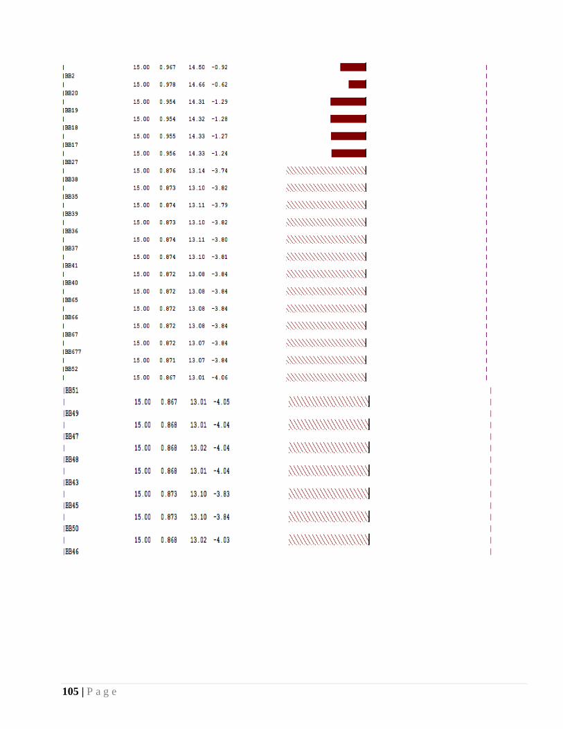
105 | P a g e

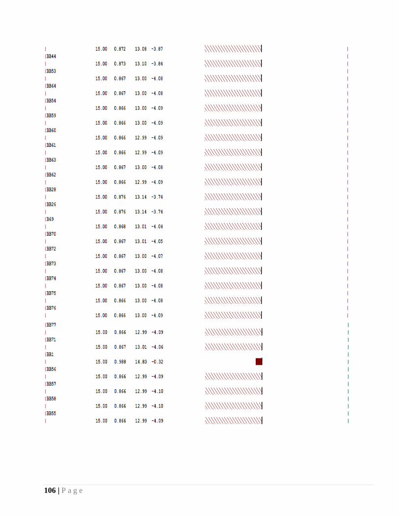
106 | P a g e

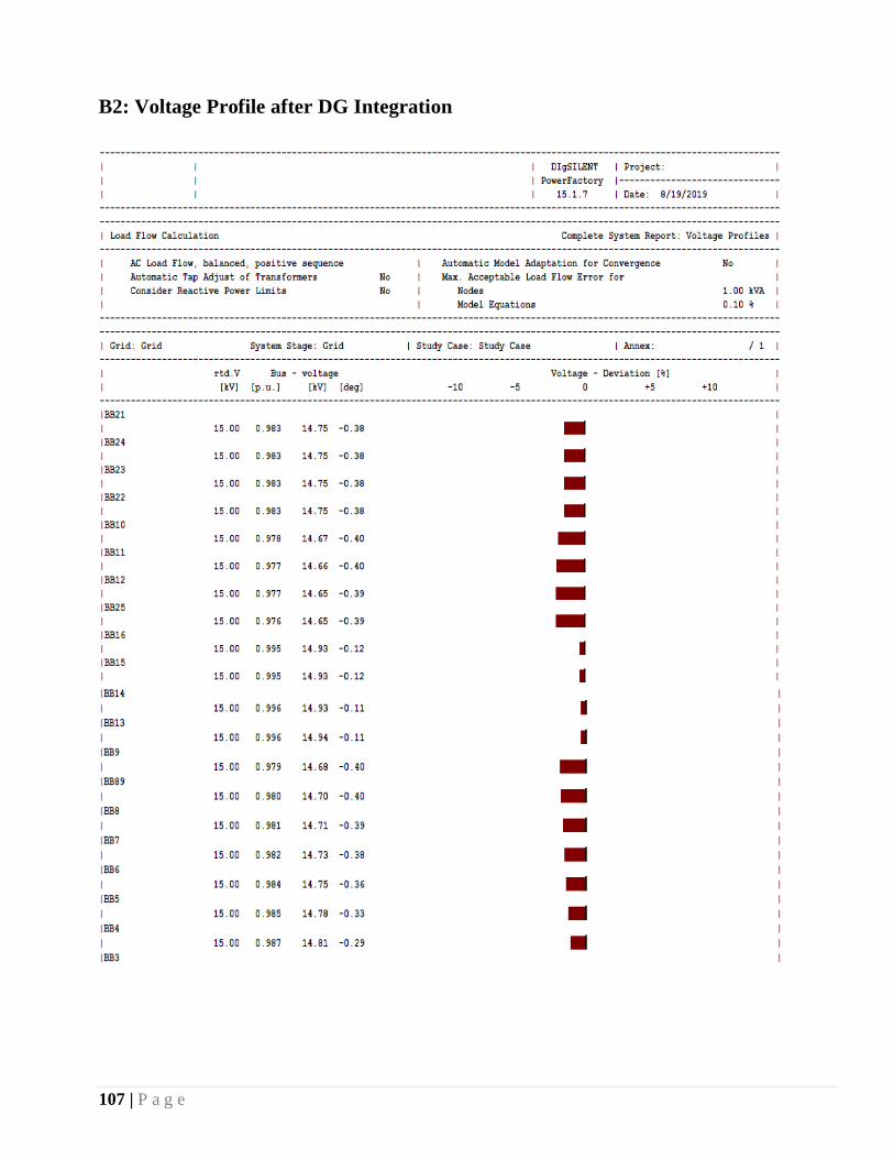
107 | P a g e

B2: Voltage Profile after DG Integration

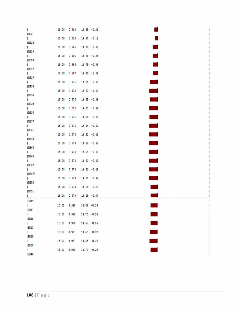
108 | P a g e

109 | P a g e

110 | P a g e

B3: Voltage Profile after DG Integration when Increase the Load with Penetration

of DG

111 | P a g e

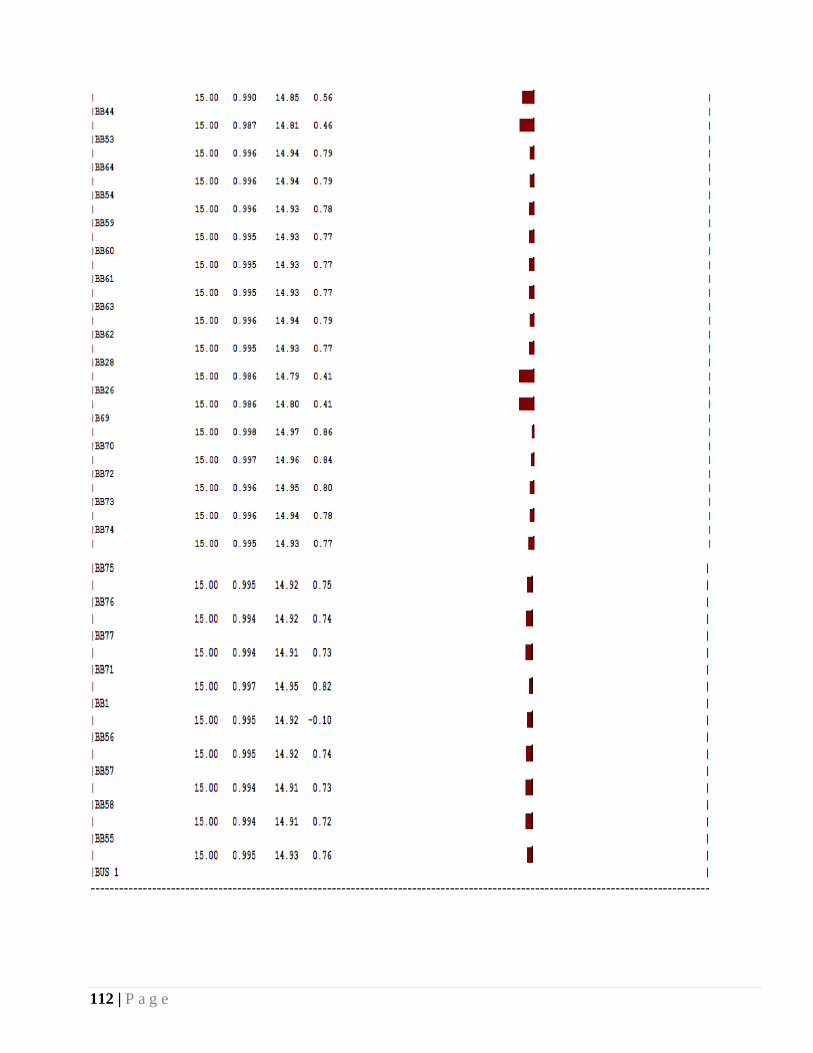
112 | P a g e

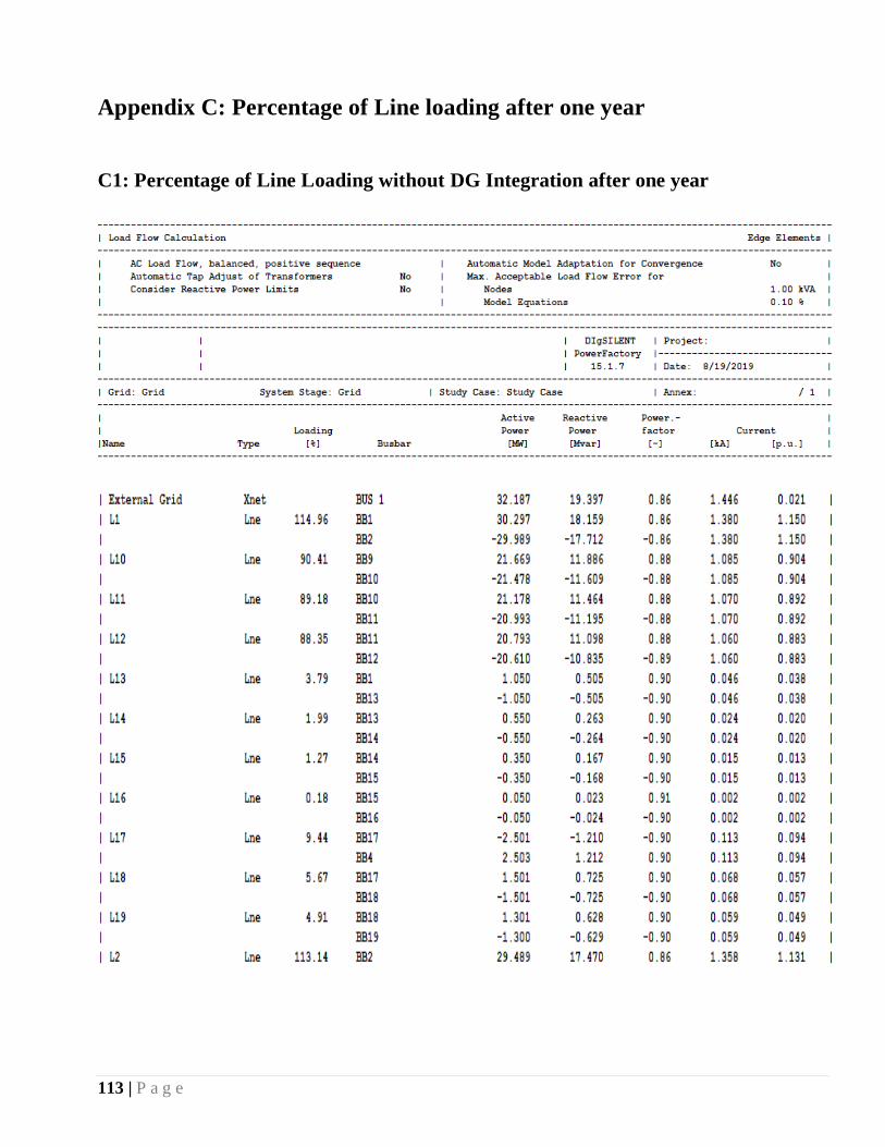
113 | P a g e

Appendix C: Percentage of Line loading after one year

C1: Percentage of Line Loading without DG Integration after one year

114 | P a g e

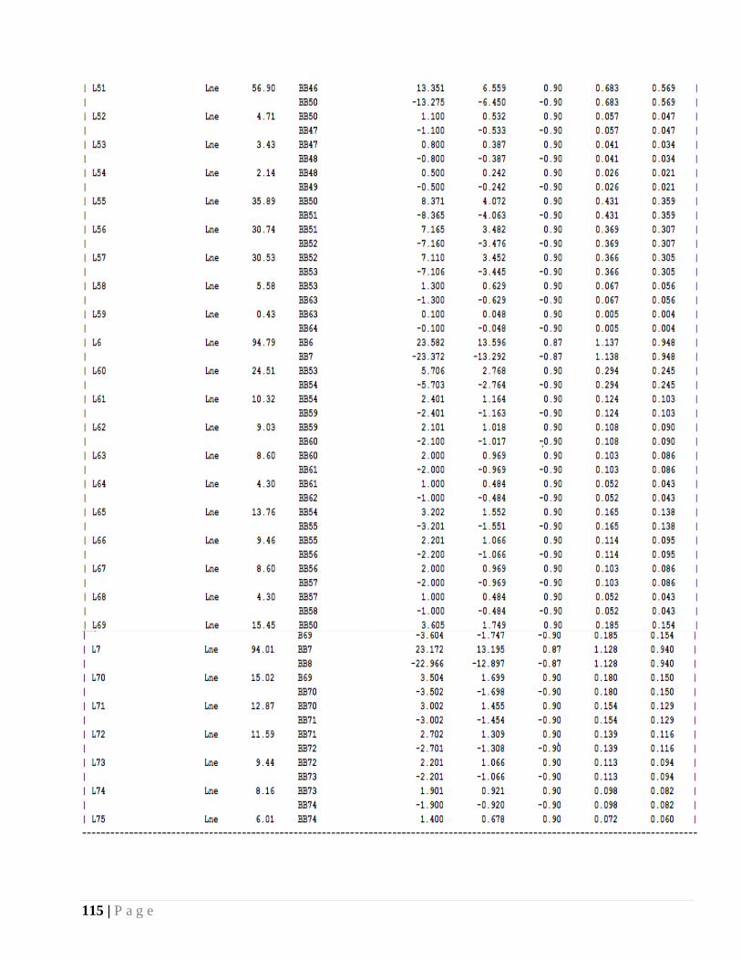
115 | P a g e

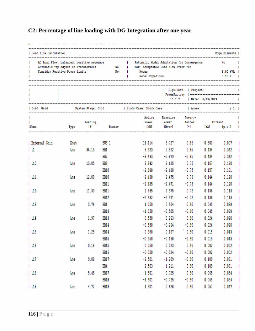
116 | P a g e

C2: Percentage of line loading with DG Integration after one year

117 | P a g e

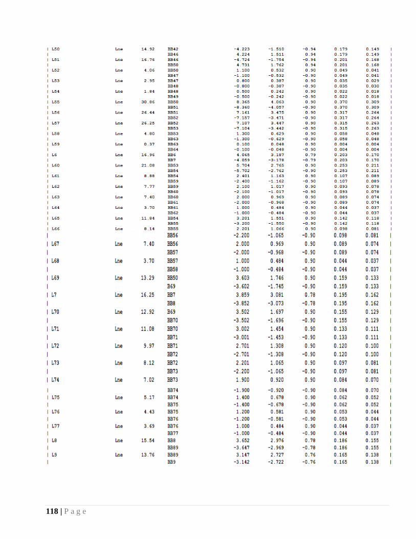
118 | P a g e

119 | P a g e

C3: Percentage of Line Loading without DG Integration after four year

120 | P a g e

121 | P a g e

122 | P a g e

C4: Percentage of Line Loading with DG Integration after four year

123 | P a g e

124 | P a g e

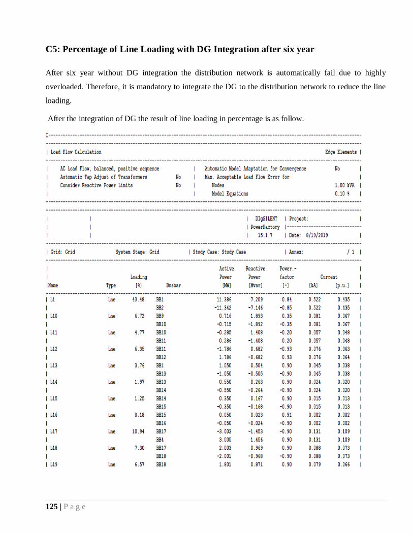
125 | P a g e

C5: Percentage of Line Loading with DG Integration after six year

After six year without DG integration the distribution network is automatically fail due to highly

overloaded. Therefore, it is mandatory to integrate the DG to the distribution network to reduce the line

loading.

After the integration of DG the result of line loading in percentage is as follow.

126 | P a g e

127 | P a g e

128 | P a g e

Percentage of Line Loading with DG Integration after ten year

The same is true after ten year without DG the distribution network is automatically fail. Therefore, it is

mandatory to integrate the DG to the distribution network, after that the distribution network comes to

work. The result of line loading in percentage after integration the DG is as follow.

129 | P a g e

130 | P a g e

Appendix D: Comparisons of Outgoing Feeders Loading

131 | P a g e

Appendix E: Bus Voltage when the DG Installed at Different Location at

Appropriate Capacity

Bus

No

Whe

n DG

instal

l at

BB1

When

DG

install

at

BB16

When

DG

install

at

BB19

When

DG

install

at

BB25

When

DG

install

at

BB34

When

DG

install

at

BB43

When

DG

install

at

BB50

When

DG

install

at

BB55

When

DG

install

at

BB70

Bus

volta

ge

Bus

voltag

e

Bus

voltag

e

Bus

voltag

e

Bus

voltag

e

Bus

voltag

e

Bus

voltag

e

Bus

voltag

e

Bus

voltage

BB1 1 0.992 0.993 0.993 0.993 0.993 0.996 0.993 0.993

BB2 0.982 0.981 0.986 0.987 0.987 0.987 0.993 0.988 0.987

BB3 0.971 0.971 0.9879 0.982 0.982 0.982 0.990 0.982 0.982

BB4 0.960 0.960 0.973 0.976 0.976 0.976 0.987 0.976 0.976

BB5 0.951 0.951 0.963 0.971 0.971 0.976 0.985 0.971 0.971

BB6 0.941 0.941 0.954 0.967 0.967 0.967 0.984 0.967 0.966

BB7 0.932 0.932 0.945 0.962 0.962 0.962 0.982 0.962 0.962

BB8 0.924 0.923 0.936 0.958 0.954 0.954 0.981 0.958 0.958

BB9 0.906 0.915 0.920 0.951 0.951 0.951 0.979 0.951 0.954

BB10 0.898 0.898 0.911 0.946 0.947 0.947 0.978 0.947 0.951

BB11 0.890 0.890 0.903 0.966 0.944 0.943 0.977 0.944 0.947

BB12 0.882 0.882 0.895 0.940 0.940 0.940 0.977 0.940 0.943

BB13 0.992 0.995 0.992 0.993 0.993 0.993 0.996 0.993 0.940

BB14 0.992 0.999 0.992 0.993 0.993 0.993 0.996 0.993 0.993

BB15 0.992 1.003 0.992 0.993 0.993 0.993 0.996 0.993 0.993

BB16 0.992 1.006 0.992 0.993 0.993 0.993 0.996 0.993 0.993

BB17 0.960 0.960 0.978 0.975 0.975 0.975 0.987 0.976 0.975

BB18 0.959 0.959 0.979 0.975 0.975 0.975 0.986 0.975 0.975

BB19 0.959 0.958 0.983 0.974 0.974 0.975 0.986 0.975 0.975

BB20 0.958 0.958 0.982 0.974 0.974 0.975 0.985 0.975 0.975

BB21 0.941 0.941 0.953 0.966 0.966 0.966 0.983 0.966 0.966

132 | P a g e

BB22 0.941 0.941 0.953 0.966 0.966 0.966 0.983 0.966 0.996

BB23 0.941 0.941 0.953 0.966 0.966 0.966 0.983 0.966 0.996

BB24 0.941 0.941 0.953 0.966 0.966 0.966 0.983 0.966 0.966

BB25 0.880 0.880 0.895 0.939 0.939 0.939 0.976 0.939 0.939

BB26 0.880 0.878 0.894 0.939 0.939 0.939 0.976 0.939 0.939

BB27 0.880 0.878 0.894 0.939 0.939 0.939 0.976 0.939 0.939

BB28 0.880 0.878 0.885 0.939 0.939 0.939 0.976 0.939 0.939

BB29 0.890 0.877 0.884 0.939 0.939 0.939 0.976 0.939 0.938

BB30 0.872 0.877 0.884 0.939 0.939 0.939 0.976 0.939 0.938

BB31 0.874 0.874 0.884 0.939 0.939 0.939 0.976 0.939 0.938

BB32 0.874 0.874 0.885 0.939 0.939 0.939 0.976 0.939 0.938

BB33 0.873 0.872 0.885 0.939 0.939 0.939 0.976 0.939 0.938

BB34 0.872 0.872 0.884 0.937 0.939 0.939 0.976 0.939 0.939

BB35 0.882 0.872 0.892 0.939 0.939 0.939 0.976 0.939 0.939

BB36 0.880 0.872 0.892 0.939 0.938 0.938 0.976 0.938 0.939

BB37 0.880 0.872 0.892 0.939 0.938 0.938 0.976 0.938 0.939

BB38 0.880 0.872 0.892 0.939 0.938 0.938 0.976 0.938 0.937

BB39 0.879 0.872 0.891 0.939 0.938 0.938 0.975 0.938 0.937

BB40 0.878 0.871 0.890 0.936 0.937 0.937 0.974 0.937 0.937

BB41 0.906 0.871 0.891 0.936 0.937 0.937 0.974 0.937 0.936

BB42 0.902 0.871 0.891 0.936 0.937 0.937 0.974 0.937 0.938

BB43 0.878 0.872 0.891 0.936 0.937 0.939 0.974 0.937 0.938

BB44 0.878 0.872 0.891 0.936 0.938 0.939 0.977 0.937 0.938

BB45 0.880 0.877 0.891 0.937 0.938 0.939 0.977 0.939 0.938

BB46 0.877 0.872 0.886 0.936 0.938 0.936 0.977 0.939 0.938

BB47 0.878 0.872 0.886 0.932 0.933 0.933 0.980 0.939 0.938

BB48 0.877 0.842 0.886 0.932 0.933 0.933 0.980 0.939 0.938

BB49 0.877 0.872 0.886 0.932 0.933 0.933 0.980 0.938 0.938

BB50 0.872 0.872 0.886 0.932 0.933 0.934 0.980 0.938 0.939

BB51 0.872 0.872 0.886 0.932 0.932 0.933 0.979 0.938 0.939

133 | P a g e

BB52 0.872 0.872 0.885 0.932 0.932 0.933 0.979 0.937 0.939

BB53 0.871 0.872 0.884 0.932 0.932 0.932 0.979 0.937 0.939

BB54 0.871 0.872 0.884 0.932 0.932 0.932 0.978 0.937 0.939

BB55 0.871 0.872 0.884 0.930 0.932 0.932 0.978 0.939 0.941

BB56 0.871 0.872 0.884 0.932 0.931 0.932 0.978 0.939 0.941

BB57 0.871 0.872 0.885 0.930 0.931 0.932 0.978 0.937 0.941

BB58 0.871 0.871 0.885 0.930 0.931 0.932 0.979 0.937 0.941

BB59 0.871 0.871 0.885 0.930 0.931 0.932 0.979 0.937 0.941

BB60 0.871 0.872 0.885 0.931 0.931 0.932 0.979 0.937 0.940

BB61 0.871 0.871 0.885 0.931 0.931 0.932 0.978 0.937 0.940

BB62 0.871 0871 0.885 0.931 0.931 0.932 0.978 0.937 0.941

BB63 0.871 0.871 0.885 0.931 0.931 0.932 0.971 0.939 0.940

BB64 0.871 0.871 0.885 0.930 0.931 0.937 0.971 0.939 0.940

BB65 0.871 0.871 0.885 0.935 0.936 0.936 0.979 0.939 0.940

BB66 0.871 0.871 0.890 0.935 0.936 0.936 0.979 0.939 0.940

BB67 0.871 0.871 0.890 0.935 0.936 0.936 0.979 0.936 0.940

BB68 0.871 0.871 0.885 0.935 0.936 0.936 0.979 0.936 0.936

BB69 0.872 0.871 0.885 0.930 0.936 0.933 0.980 0.936 0.936

BB70 0.872 0.871 0.885 0.931 0.936 0.933 0.979 0.936 0.936

BB71 0.871 0.871 0.885 0.931 0.931 0.933 0.979 0.940 0.938

BB72 0.871 0.871 0.885 0.931 0.932 0.933 0.979 0.939 0.938

BB73 0.871 0.871 0.885 0.931 0.932 0.932 0.979 0.939 0.938

BB74 0.871 0.871 0.885 0.931 0.932 0.932 0.979 0.939 0.938

BB75 0.871 0.871 0.885 0.931 0.931 0.932 0.979 0.937 0.937

BB76 0.871 0.871 0.885 0.931 0.931 0.932 0.978 0.939 0.937

BB77 0.871 0.871 0.885 0.930 0.931 0.932 0.978 0.939 0.937