arX

iv:c

ond-

mat

/060

4392

v1 [

cond

-mat

.mtr

l-sc

i] 1

6 A

pr 2

006

Magnetic Instabilities and Phase Diagram of the

Double-Exchange Model in Infinite Dimensions

R S Fishman∗, F Popescu, G Alvarez•, J Moreno†, Th Maier•, and M Jarrell‡

∗Materials Science and Technology Division,

Oak Ridge National Laboratory, Oak Ridge, TN 37831-6032

Physics Department, Florida State University, Tallahassee,FL, 32306

•Computer Science and Mathematics Division,

Oak Ridge National Laboratory, Oak Ridge, TN 37831-6032

†Physics Department, University of North Dakota, Grand Forks, ND 58202-7129 and

‡Deparment of Physics, University of Cincinnati, Cincinnati, OH 45221

1

Abstract

Dynamical mean-field theory is used to study the magnetic instabilities and phase diagram of

the double-exchange model with Hund’s coupling JH > 0 in infinite dimensions. In addition to

ferromagnetic (FM) and antiferromagnetic (AF) phases, the DE model also supports a broad class

of short-range ordered (SRO) states with extensive entropy and short-range magnetic order. For

any site on the Bethe lattice, the correlation parameter q of a SRO state is given by the average

q = 〈sin2(θi/2)〉, where θi is the angle between any spin and its neighbors. Unlike the FM (q = 0)

and AF (q = 1) transitions, the transition temperature of a SRO state with 0 < q < 1 cannot be

obtained from the magnetic susceptibility. But a solution of the coupled Green’s functions in the

weak-coupling limit indicates that a SRO state always has a higher transition temperature than

the AF for all fillings p below 1 and even has a higher transition temperature than the FM for

0.26 ≤ p ≤ 0.39. For 0.39 < p < 0.73, where both the FM and AF phases are unstable for small JH,

a SRO phase has a non-zero transition temperature except close to p = 0.5. As JH increases, the

SRO transition temperature eventually vanishes and the FM phase dominates the phase diagram.

For small JH, the T = 0 phase diagram of the DE model is greatly simplified by the presence of

the SRO phase. A SRO phase is found to have lower energy than either the FM or AF phases

for 0.26 ≤ p < 1. Phase separation disappears as JH → 0 but appears for any non-zero coupling.

For fillings near p = 1, phase separation occurs between an AF with p = 1 and either a SRO or a

FM phase. The stability of a SRO state at T = 0 can be understood by examining the interacting

density-of-states, which is gapped for any nonzero JH in an AF but only when JH exceeds a critical

value in a SRO state.

PACS numbers: 75.40.Cx, 75.47.Gk, 75.30.-m

2

I. INTRODUCTION

With the renewed interest in manganites [1] and the revitalized study of dilute magnetic

semiconductors [2], attention has once again focused on the double-exchange (DE) model

and its variants. Applied to the manganites, the DE model is customarily formulated with

one local moment per site and a Hund’s coupling JH taken to be much larger than the

electron bandwidth W . In studies of dilute magnetic semiconductors, on the other hand,

the local moments are sparse and the exchange coupling is comparable to W . While the full

phase diagram of the DE model as a function of JH and electron filling p has been studied by

several authors [3, 4, 5, 6], the properties of the DE model for small coupling constant remain

very much in doubt. In particular, there have been conflicting claims about the presence

of phase separation (PS) [5] and incommensurate phases [3, 4, 6] for small JH, when the

ordered FM and AF phases are magnetically frustrated by a RKKY-like interaction between

the local moments [7].

This paper uses DMFT to evaluate the magnetic instabilities and T = 0 phase diagram

of the DE model. Developed in the late 1980’s by Muller-Hartmann [8] and Metzner and

Vollhardt [9], DMFT exploits the fact that the self-energy becomes independent of momen-

tum in infinite dimensions, where DMFT becomes formally exact. Even in three dimensions,

DMFT is believed to capture the physics of correlated systems including the narrowing of

electron bands and the Mott-Hubbard transition [10]. Although DMFT has been widely

applied to the DE model [4, 5, 11, 12, 13, 14, 15, 16, 17, 18], until now there has been no

complete treatment of the phase instabilities and T = 0 phase diagram of the DE model for

arbitrary JH and p.

We shall study a system with a bare semicircular density-of-states (DOS) given by

N0(ω) = (8/πW 2)Re√

W 2/4 − ω2. In real space, this DOS belongs to an infinite-

dimensional Bethe lattice or an infinite Cayley tree with no closed loops [19]. A finite-

dimensional Bethe lattice with coordination number zc = 4 is sketched in Fig.1. Although

the Bethe lattice lacks translational symmetry. it is quite convenient for calculations. As

shown in Fig.1, the Bethe lattice can be partitioned into A and B sublattices so that both

ferromagnetic (FM) and antiferromagnetic (AF) long-range order are possible. Due to the

bounds ±W/2, the DOS of the Bethe lattice more closely resembles the DOS of two- and

three-dimensional systems than does the unbounded DOS of the hypercubic lattice. Indeed,

3

FIG. 1: A Bethe lattice with zc = 4 nearest neighbors. As shown, the Bethe lattice may be

partitioned into A and B sublattices, denoted by the blue and red dots.

pathological results have been obtained on a hypercubic lattice due to the asymptotic free-

dom of the quasiparticles in the tails of the Gaussian DOS [16]. As we shall see, the Bethe

lattice also has the advantage that analytic results are possible in the limit of small JH,

precisely the regime where controversies persist.

The high-temperature, non-magnetic (NM) phases of the Heisenberg and DE models have

a correlation length ξ that vanishes as zc → ∞. By contrast, the short-range ordered (SRO)

states introduced in an earlier paper [20] possess some of the same characteristics as spin

glasses: local magnetic order and exponentially decaying magnetic correlations [21]. The

SRO states are characterized by the correlation parameter q = 〈sin2(θi/2)〉, where θi are the

angles between any spin and its neighbors. Overall, the neighboring spins describe a cone

with angle 2 arcsin(√

q) around the central spin. This disordered state reduces to the FM and

AF phases when q = 0 and 1, respectively. Unlike the FM and AF phases, a SRO state with

0 < q < 1 has extensive entropy and short-range but not long-range magnetic order. Since

it is not possible to associate a wavevector with any SRO state, its transition temperatures

TSRO(p, q) cannot be obtained from the magnetic susceptibility. Rather, TSRO(p, q) can be

solved from coupled Green’s function equations. Remarkably, a SRO state can be found

with higher transition temperature and lower energy than the ordered FM and AF phases

in a large region of phase space.

4

The FM and AF transition temperatures may be obtained by solving either the coupled

Green’s function equations or the Bethe-Salpeter (BS) equations for the magnetic suscep-

tibility. The BS equations break up into separate relations for the charge and spin degrees

of freedom. The vertex functions of the BS equations are consistent with the functional

derivative of the self-energy with respect to the Green’s function [17]. It follows that the

DMFT treatment of the DE model is Φ-derivable and hence thermodynamically consistent

[22], meaning that identical results are obtained from both ways of evaluating TC and TN.

This paper is divided into 7 main sections. In Section II, we formulate the BS equations

for the susceptibility and derive the vertex functions. The thermodynamic consistency of

the DMFT of the DE model is discussed in Section III. The BS equations are used in Section

IV to derive implicit expressions for the FM and AF transition temperatures. Using coupled

Green’s functions, we rederive the transition temperatures of the ordered phases and evaluate

the transition temperature of the SRO states. We also explicitly solve those relations in the

weak-coupling limit of small JH. A complete map of the phase instabilities of the DE model

is provided in Section V. In Section VI, we present the T = 0 phase diagram of the DE

model both with and without the SRO states. Finally, Section VII contains a summary and

conclusion. Appendix A provides results for the transition temperatures and T = 0 energies

of the SRO states in the weak-coupling limit. In Appendix B, we derive the self-consistency

relation for the SRO states. Appendix C provides a convenient and general form for the

kinetic energy of the SRO and ordered phases.

II. BETHE-SALPETER EQUATIONS AND THE VERTEX FUNCTIONS

The Hamiltonian of the DE model (also called the FM Kondo model when JH < ∞) is

given by

H = −t∑

〈i,j〉

(

c†iαcjα + c†jαciα

)

− 2JH

∑

i

si · Si (1)

where c†iα and ciα are the creation and destruction operators for an electron with spin α at

site i, JH > 0 is the Hund’s coupling, si = c†iασαβciβ/2 is the electronic spin, and Si = Smi is

the spin of the local moment. Repeated spin indices are summed. The local moment will be

treated classically, which is only a fair approximation for the magnanites with spin S = 3/2

but a better approximation for dilute magnetic semiconductors with S = 5/2. For large zc,

5

the hopping energy t scales as 1/√

zc and the local effective action on site 0 may be written

[11]

Seff(m) = −T∑

n

c0α(iνn)

G0(iνn)−1αβ + Jσαβ · m

c0β(iνn), (2)

where J = JHS, νn = (2n + 1)πT , c0α(iνn) and c0α(iνn) are now anticommuting Grassman

variables, m is the orientation of the local moment on site 0, and G0(iνn) is the bare Green’s

function containing dynamical information about the hopping of electrons from other sites

onto site 0 and off again.

Because Seff(m) is quadratic in the Grassman variables, the full Green’s function

G(m, iνn)αβ at site 0 for a fixed m may be readily solved by integrating over the Grass-

man variables, with the NM result

G(m, iνn) =

G0(iνn)−1I + Jσ · m−1

=G0(iνn)−1I − Jσ · m

G0(iνn)−2 − J2, (3)

where G0(iνn)αβ = δαβG0(iνn) is diagonal above TC. Averaging over the orientations of the

local moment, 〈G(m, iνn)αβ〉m = G(iνn)αβ = δαβG(iνn) where

G(iνn) =G0(iνn)−1

G0(iνn)−2 − J2. (4)

If P (m) = Trf

(

exp(−Seff(m)))

/Z is the probability for the local moment to point in the

m direction, then the average over m is given by 〈C(m)〉m ≡ ∫

dΩmP (m)C(m). The

effective partition function Z involves both a trace over the Fermion degrees of freedom and

an average over m: Z =∫

dΩmTrf

(

exp(−Seff(m)))

. Above TC, P (m) = 1/4π is constant.

Consequently, the NM self-energy is Σ(iνn) = G0(iνn)−1 − G(iνn)−1 = J2G0(iνn).

Likewise above TC, the lattice Green’s function G(m,k, iνn)αβ has the expectation value

〈G(m,k, iνn)αβ〉m = δαβ1

zn − ǫk − J2G0(iνn)(5)

with zn = iνn + µ. Summing Eq.(5) over all k and equating the result to Eq.(4), we obtain

[10, 11]

G0(iνn)−1 = zn − W 2

16G(iνn), (6)

where W = 4t√

zc is the full bandwidth of the semi-circular DOS.

Our goal is to evaluate the general susceptibility [15]

∑

l,n

χβα,δκq,iωm

(iνl, iνn) =∫ β

0dτ eiωmτ

∑

i

e−iq·(Ri−R0)

〈Tτc†iα(τ)ciβ(τ)c†0κc0δ〉 − 〈c†iαciβ〉〈c†0κc0δ〉

,

(7)

6

χ χ(0) χ(0) χΓ= +

l + m

l

n + m n + m n + ml + m l + m

l ln n n

o + m p + m

o p

(a)

(c)

α, νn + ωm δ, νl + ωm

β, νn κ, νl

(b)

α, νn + ωm, k+q

β, νn, k

δ, νl + ωm, k’+q

κ, νl, k’

χ

Γ

FIG. 2: Diagrammatic representations of (a) the magnetic susceptibility χβα,δκq,iωm

(iνl, iνn), (b) the

vertex function Γβα,δκiωm

(iνl, iνn), and (c) the Bethe-Salpeter equations.

where ωm = 2mπT and 〈C〉 involves both a Fermion trace and an average over all the

mi. Sketched in Figs.1(a) and (b), the general susceptibility and the full vertex function

Γηµ,τνiωm

(iνl, iνn) are related by the lattice BS equation:

χβα,δκq,iωm

= χ(0) βα,δκq,iωm

+ χ(0) βα,µηq,iωm

Γηµ,τνiωm

χντ,δκq,iωm

. (8)

Each term in this equation is a matrix in Matsubara space and matrix multiplication involves

a summation over intermediate Matsubara frequencies, as shown in Fig.2(c) [15]. The local

susceptibility χβα,δκiωm

is obtained from the lattice susceptibility χβα,δκq,iωm

by summing over q and

satisfies the local BS equation:

χβα,δκiωm

= χ(0) βα,δκiωm

+ χ(0) βα,µηiωm

Γηµ,τνiωm

χντ,δκiωm

. (9)

Since the vertex function is independent of momentum in infinite dimensions, it appears

identically in both the lattice and local BS equations [23, 24].

For the bare susceptibilities, the electrons in each Green’s function are uncorrelated,

which means that each Green’s function is separately averaged over m. So the bare, lattice

7

susceptibility is given by

χ(0) βα,δκq,iωm

(iνl, iνn) = − T

Nδln

∑

k

〈G(m,k, iνl)αδ〉m〈G(m,k + q, iνl+m)κβ〉m. (10)

The bare, local susceptibility is obtained by summing this expression over all q:

χ(0) βα,δκiωm

(iνl, iνn) = −TδlnG(iνl)αδG(iνl+m)κβ, (11)

where G(iνl)αβ = δαβG(iνl) is the m-averaged, local Green’s function given by Eq.(4). It is

also straightforward to evaluate the full, local susceptibility:

χβα,δκiωm

(iνl, iνn) = Tδm,0

〈G(m, iνn)βαG(m, iνl)δκ〉m − 〈G(m, iνn)βα〉m〈G(m, iνl)δκ〉m

−Tδln〈G(m, iνl)αδG(m, iνl+m)κβ〉m, (12)

where G(m, iνl)αβ is the m-dependent, local Green’s function given by Eq.(3).

Due to the matrix structure of Eqs.(10-12), the charge and spin degrees of freedom

decouple: σαβz χ(0) βα,δκ

q,iωm

∝ σδκz and δαβχ(0) βα,δκ

q,iωm

∝ δδκ with analogous relations for the

local susceptibilities. We define the charge and spin susceptibilities and vertex func-

tions by χcq,iωm

= δαβχβα,δκq,iωm

δκδ/4, χsq,iωm

= σzαβχβα,δκ

q,iωm

σzκδ/4, Γc

iωm= δαβΓβα,δκ

q,iωmδκδ, and

Γsiωm

= σzαβΓβα,δκ

q,iωmσz

κδ. Similar definitions are employed for the local susceptibilities. Since

Eqs.(10) and (11) imply that the bare, charge and spin susceptibilities are identical, we shall

dispense with the superscripts c and s on those quantities.

After this decoupling, both the lattice and local BS equations separate into two sets of

equations for the charge and spin degrees of freedom:

χaq,iωm

= χ(0)q,iωm

+ χ(0)q,iωm

Γaiωm

χaq,iωm

, (13)

χaiωm

= χ(0)iωm

+ χ(0)iωm

Γaiωm

χaiωm

, (14)

where a = c or s. The same charge and spin vertex functions enter the lattice and local

equations. The spin BS equations with a = s were previously solved [15] in the strong-

coupling limit J ≫ W and J ≫ T .

To generally solve Eq.(13) for the charge and spin lattice susceptibilities, we first obtain

the charge and spin vertex functions from the local susceptibilities given by Eq.(14). The

vertex function may be written as

Γβα,δκiωm

(iνl, iνn) = Alnσβα · σδκδm,0 + Blmσδα · σβκδln, (15)

8

Aln =βJ2

3(1 + C)

alan

blbn

, (16)

Blm = −βJ2

3

G0(iνl)G0(iνl+m)alal+m

G−10 (iνl)G

−10 (iνl+m) + J2

, (17)

where an = G0(iνn)−2 − J2, bn = G0(iνn)−2 − J2/3, and C = −(2J2/3)∑

n b−1n . In terms of

Aln and Blm, the charge and spin vertex functions are then given by Γc

iωm(iνl, iνn) = 6Bl

mδln

and Γsiωm

(iνl, iνn) = 4Alnδm,0 − 2Blmδln.

III. THERMODYNAMIC CONSISTENCY

A thermodynamically consistent theory produces identical results from either the Green’s

function (which is on the single-particle level) or the partition function (which involves

interactions on the two-particle level). Baym and Kadanoff [22] demonstrated that a

sufficient condition for a theory to be thermodynamically consistent is that it be Φ-

derivable, which means that a functional Φ(G(iνn)), constructed from compact diagrams

involving the full Green’s functions and the bare vertex functions, satisfies the condition

Σ(iνn)αβ = δΦ/δG(iνn)αβ. The partition function of a Φ-derivable theory satisfies the rela-

tion

− log Z = Φ −∑

n

Trf

Σ(iνn)G(iνn)

+∑

n

Trf log

G(iνn)

, (18)

which is stationary under variations of G(iνn). Whereas Baym and Kadanoff considered

systems of interacting Fermions and Bosons, their ideas were later extended to systems of

interacting electrons and spins [25] and to disordered alloys [26]. The Φ-derivability of the

DMFT of the DE model was first demonstrated in Ref.[17].

The bare vertex function Γ(0) βα,δκiωm

(iνl, iνn) may be associated with the two-particle inter-

action in the purely electronic effective action [27]

S ′eff = −T

∑

n

c0α(iνn)G0(iνn)−1c0α(iνn)

−T 3

4

∑

l,n,m

c0α(iνn + iωm)c0β(iνn)Γ(0) βα,δκiωm

(iνl, iνn)c0κ(iνl)c0δ(iνl + iωm). (19)

Because the Fermion operators anticommute, the bare vertex function must satisfy the

crossing symmetries Γ(0) δα,βκiωn−l

(iνl, iνl+m) = Γ(0) βκ,δαiωl−n

(iνn+m, iνn) = −Γ(0) βα,δκiωm

(iνl, iνn). There

are two ways to evaluate the bare vertex function. First, we can take the J → 0 limit of

9

the full vertex function Γβα,δκiωm

given by Eq.(15). Alternatively, we can associate the lowest-

order, J2 contribution to the partition function Z =∫

dΩmTrf

(

exp(−Seff(m)))

with the J2

contribution to the partition function Z ′ = Trf

(

exp(−S ′eff))

. Both methods yield the same

result:

Γ(0) βα,δκiωm

(iνl, iνn) =1

3βJ2

σβα · σδκδm,0 − σδα · σβκδln

, (20)

which does indeed satisfy the required crossing symmetries.

But S ′eff produces an inequivalent infinite-dimensional theory than produced by Seff(m),

as seen in the different expansions of Z and Z ′ to order J4:

Z = Z0

1 − J2∑

n

G0(iνn)2 +1

2J4∑

l 6=n

G0(iνl)2G0(iνn)2 + O(J6)

, (21)

Z ′ = Z0

1 − J2∑

n

G0(iνn)2 +5

6J4∑

l 6=n

G0(iνl)2G0(iνn)2 + O(J6)

. (22)

Therefore, the DE action cannot be replaced by a purely electronic action containing only

two-body interactions and it is not possible to construct a diagrammatic expansion in powers

of Γ(0).

Nevertheless, we can construct a functional Φ(G(iνn)) satisfying the condition

Σ(iνn)αα = δΦ/δG(iνn)αα. Starting from Eq.(3) and Dyson’s equation for the self-energy,

we obtain δΣ(iνl)αα/δG(iνn)ββ = (K−1)αβln + δlnδαβG(iνn)−2, where

Kαβln =

δG(iνn)ββ

δ[G0(iνl)αα]−1= −δln

1

a2n

2J2

3+ bnδαβ

+J2

3alan

(

2δαβ − 1)

. (23)

Inverting this Jacobian yields the general result

δΣ(iνl)αα

δG(iνn)ββ= −δln

J2a2n

3bn

2

2an − 3bn+ δαβG0(iνn)2

− J2

3(1 + C)

alan

blbn

(

2δαβ − 1)

= −T Γαα,ββiωm=0(iνl, iνn), (24)

where the right-hand side is the full vertex function of Eq.(15). The functional Φ must

exist because the vertex function is well-defined and the curl of the self-energy vanishes:

δΣ(iνn)αα/δG(iνl)ββ − δΣ(iνl)ββ/δG(iνn)αα = 0. So despite the absence of a diagrammatic

perturbation theory, the DMFT of the DE model is Φ-derivable and hence, thermodynami-

cally consistent.

10

IV. TRANSITION TEMPERATURES

Since the electronic spin-susceptibility is given by χel(q) =∑

l,n χsq,iωm=0(iνl, iνn), the

condition that χel(q) diverges is equivalent to the condition that Det(χsq,iωm=0

)−1 = 0. To

obtain the FM or AF transition temperatures, we require the q = 0 or Q susceptibilities with

ωm = 0. The AF wavevector Q is defined so that the Fermi surface is nested at half filling

or ǫk+Q = −ǫk. Although the Bethe lattice sketched in Fig.1 lacks translational symmetry

and nonzero wavevectors q are ill-defined, the AF wavevector Q may be associated with the

bipartite nature of the Bethe lattice. To be safe, the Neel temperature will be evaluated in

two different ways, only one of which relies on the existence of an AF wavevector.

For either FM or AF ordering, the electron filling p can be related to the chemical potential

µ through the relation

p = 1 + T∑

n

Re G(iνn) = 1 − 32

W 2T∑

n

ReRn, (25)

where G0(iνn)−1 = zn + Rn and the complex function Rn satisfies the implicit relation

anRn +W 2

16(zn + Rn) = 0. (26)

Since an = (zn +Rn)2−J2, Rn falls off like −W 2/(16zn) for large n. Notice that p = 1 when

µ = 0. Since all of our results are particle-hole symmetric about p = 1, we shall restrict

consideration to the range 0 ≤ p ≤ 1.

As discussed in Section II, the BS equations decouple into charge and spin relations.

Since the charge vertex function Γciωm

(iνl, iνn) = 6Blmδln is diagonal in Matsubara space, the

condition Det(χcq,iωm=0

)−1 = 0 has no solution for q = 0 or Q. In other words, there is no

charge-density wave instability within the DE model.

A. Ferromagnetic ordering

When q = 0, the bare, zero-frequency lattice susceptibility is given by

χ(0)q=0,iωm=0(iνl, iνn) =

4T

W 2

(

1 − zl − J2G0(iνl)√

(zl − J2G0(iνl))2 − W 2/4

)

δln. (27)

With the help of Eq.(26), we find that the full spin-susceptibility at q = 0 satisfies

χs−1q=0,iωm=0(iνl, iνn) = χ

(0)−1q=0,iωm=0(iνl, iνn) − Γs

iωm=0(iνl, iνn)

= −2βδlnal

(zl + Rl)bl

(zl + Rl)2(zl + 2Rl) − J2(zl + 4Rl/3)

− 4βJ2

3(1 + C)

alan

blbn, (28)

11

where bl = (zl + Rl)2 − J2/3. Consequently, the condition that Det(χs

q=0,iωm=0)−1 = 0 can

be written as an implicit condition for the Curie temperature:

2J2

3

∑

n

Rn

(zn + Rn)2(zn + 2Rn) − J2(zn + 4Rn/3)= 1, (29)

which must be supplemented by Eq.(25) for the electron filling.

If J/W > 1/4, the interacting DOS splits into two bands [16]. In the lower band centered

at −J with 0 ≤ p ≤ 1, all electrons have their spins parallel to the local moments; in the

upper band centered at J with 1 ≤ p ≤ 2, all holes have their spins parallel to the local

moments. As J/W increases, both upper and lower bands are narrowed by correlations and

their widths approach W ′ = W/√

2. To recover the large J limit, the chemical potential

must be written as µ = J sgn(p−1)+ δµ where −W ′/2 ≤ δµ ≤ W ′/2. Eq.(29) then reduces

to [14, 15]∑

n

R2n

R2n − 3W 2/32

= 1, (30)

where Rn is now given explicitly by Rn =(√

z2n − W 2/8 − zn

)

/2. So in this limit, TC is

proportional to W and is independent of J . Due to the strong Hund’s coupling, TC vanishes

at half filling (p = 1) or when the lower band is completely full because electrons are unable

to hop to neighboring sites.

In the weak-coupling regime of T ≪ J ≪ W , the summation in Eq.(29) may be replaced

by an integral over frequency ν, as shown in Appendix A. Carefully treating the branch cut

along the real axis between ±W/2, we find that

TC =32J2

9πW

√

1 − (2µ/W )2

(2µ/W )2 − 1/4

, (31)

which is proportional to J2/W as expected in the RKKY limit. For small filling (µ close to

−W/2) and a fixed J , TC initially increases with p and then begins to decrease, vanishing at

µ = W/4 corresponding to a filling of p ≈ 0.39. Because TC(p, J) is particle-hole symmetric,

it is the same for p electrons (2 − p holes) and 2 − p electrons (p holes) per site. These

results are in qualitative agreement with Nolting et al. [28, 29], who evaluated the Curie

temperature of the s − f model with quantum local spins using both equations-of-motion

[28] and modified RKKY [29] techniques. Nolting et al. obtained FM solutions for small

J in a concentration range significantly narrower than found here, probably because their

approach retains the non-local fluctuations produced by the RKKY interaction.

12

For small fillings and ε ≡ 2µ/W + 1 ≪ 1, TCW/J2 ≈ 8√

2ε1/2/(3π). Since p ≈8√

2ε3/2/(3π), TC grows like p1/3 for small p.

B. Antiferromagnetic ordering

This section presents two calculations for the AF Neel temperature: one based on the

magnetic susceptibility and the other on coupled Green’s functions. Their equivalence was

established in Section III, which demonstrated that the DMFT of the DE model is thermo-

dynamically consistent. While the first technique explicitly assumes the existence of an AF

wavevector Q, the second does not.

1. From the susceptibility

Evaluating the Neel temperature from the susceptibility requires the bare, zero-frequency

lattice susceptibility for q = Q:

χ(0)Q,iωm=0(iνl, iνn) = − 4T

W 2

(

1 −√

(zl − J2G0(iνl))2 − W 2/4

zl − J2G0(iνl)

)

δln. (32)

After some algebra, we find that the full spin-susceptibility at q = Q satisfies

χs−1Q,iωm=0(iνl, iνn) = χ

(0)−1Q,iωm=0(iνl, iνn) − Γs

iωm=0(iνl, iνn)

= −2βδlnal

(zl + Rl)bl

zl(zl + Rl)2 − J2(zl + 2Rl/3)

− 4βJ2

3(1 + C)

alan

blbn. (33)

Consequently, TN is found from the condition that Det(χsQ,iωm=0

)−1 = 0 or

− 2J2

3

∑

n

Rn

zn(zn + Rn)2 − J2(zn + 2Rn/3)= 1, (34)

which bares some similarity to Eq.(29) for TC.

In the strong-coupling limit, Eq.(34) reduces to

∑

n

R2n

R2n + 3W 2/32

= 1, (35)

with a plus sign multiplying 3W 2/32 compared to the minus sign in Eq.(30). It is straightfor-

ward to show that TN ≤ 0 for all p in this limit. Hence, the AF phase instabilities disappear

as J/W → ∞.

13

In the weak-coupling regime, we may once again replace the Matsubara sum by an inte-

gral, with the result

TN =8J2

3πW

log

(

1 +√

1 − (2µ/W )2

2|µ|/W

)

−√

1 − (2µ/W )2 − 4

3

(

1 − (2µ/W )2)3/2

. (36)

For p < 0.73, TN is negative so the system becomes FM for 0 < p ≤ 0.39.

Close to half filling, TN given by Eq.(36) becomes positive and the DE model supports

an AF phase. We find that TN > 0 for 0.73 ≤ p ≤ 1, in which range TC given by Eq.(31) is

negative. The divergence of TN in Eq.(36) as p → 1 or µ → 0 signals a breakdown in the

weak-coupling expansion and the appearance of a gap in the interacting DOS, as discussed

later.

2. From coupled Green’s functions

The previous sub-section used the nesting condition for the AF wavevector Q whereas,

strictly speaking, nonzero wavevectors are not defined on the Bethe lattice. Hence, it is

worthwhile to re-evaluate TN using a Green’s function approach that skirts the question of

whether an AF wavevector exists. This Green’s function approach will also come in handy

when considering the SRO state later in Section IV.

Dividing the Bethe lattice into A and B sub-lattices, we obtain coupled relations between

the bare and full local Green’s functions:

G(η)0 (iνn)−1 = znI − W 2

16G(η)(iνn), (37)

where η =↑ or ↓ on the A or B sites and η is opposite to η. If the bare inverse Green’s

function is parameterized as

G(η)0 (iνn)−1 = (zn + Rn)I + Q(η)

n σz, (38)

then Eq.(37) implies that Rn and Q(η)n are solved from the condition

RnI + Q(η)n σz = −W 2

16

⟨

(zn + Rn)I + σ ·(

Jm + Q(η)n z

)−1⟩

η. (39)

To linear order in the sublattice magnetization, Rn and Q(η)n satisfy the implicit relations

anRn = −W 2

16(zn + Rn), (40)

14

Q(η)n =

Rn

zn + Rn

Q(η)n

(

1 +2J2

3an

)

+ JM (η)

, (41)

where 〈m〉η ≡ M (η)z = ±Mz, the sign depending on whether η =↑ (A site) or η =↓ (B site).

The linear relations for Q(η)n may be readily solved, with the result

Q(η)n =

M (η)JanRn

(zn + Rn)2zn − J2(zn + 2Rn/3). (42)

After integrating exp(−Seff(m)) over the Grassman variables, we find that the probability

for the local moment on sublattice η to point along m is

P (m)(η) ∝ exp

∑

n

log

(

1 − 2JQ(η)n mz

an

)

∝ exp(βJeffM(η)mz). (43)

The last relation defines the effective interaction:

Jeff = − 2TJ

M (η)

∑

n

Q(η)n

an= −2TJ2

∑

n

Rn

zn(zn + Rn)2 − J2(zn + 2Rn/3), (44)

which is the same on each sublattice. Finally, TN is solved from the condition M (η) =

JeffM(η)β/3, which reproduces Eq.(34). So the earlier results for TN do not depend on the

existence of an AF wavevector!

C. Other magnetic phases

Earlier studies of the Heisenberg model on the Bethe lattice [30, 31] proposed a spiral

magnetic state with a wavevector that characterizes the twist of the spin between nearest

neighbors. But it is quite easy to show that a Bethe lattice can not be partitioned into more

than two sublattices. For example, if we try to partition a Bethe lattice with zc = 4 into

three sublattices, then sites C and A (red and purple dots in Fig.3(a)) would be next-nearest

neighbors but the two sites C (purple dots) (presumably on the same magnetic sublattice)

are actually next-nearest neighbors of each other. So unless the central site is singled out, a

Bethe lattice does not support a magnetic state with more than two sublattices.

More recently, Gruber et al. [32] argued that this restriction may be removed as zc → ∞because the paths with the largest weight always move outward from the central site. This

analysis uses the fact that the surface of the Bethe lattice contains a non-vanishing fraction

of its sites [33]. Since the period-three state constructed in Ref.[32] can only be formed

around a central site, it is not isotropic. Such states will not be considered further in this

paper.

15

q = 3/4(a) (b)

FIG. 3: (a) A possible partitioning of the Bethe lattice into three sublattices with blue, red, and

purple sites. (b) A colinear SRO state on a zc = 4 Bethe lattice with q = 3/4, meaning that 1/4

of the neighbors of any site have the same spin while 3/4 have the opposite spin. The two spins

are denoted by blue and red dots.

The broad class of SRO states first introduced in an earlier paper [20] is characterized

by the correlation parameter q = 〈sin2(θi/2)〉, where the average is taken over all neighbors

of any site on the Bethe lattice. Since the azimuthal angles φi of the neighboring spins are

assumed to be random with 〈exp(iφi)〉 = 0, the neighboring spins will on average sweep out

a cone with angle 2 arcsin(√

q) about the central spin. Due to the topology of the Bethe

lattice, a SRO phase cannot be ordered (except in the FM or AF limits when q = 0 or 1).

For the special case of a colinear SRO state, θi = 0 or π on every site and q is the fraction

of neighbors of any site that have the opposite spin. An example of a colinear SRO state

with zc = 4 and q = 3/4 is sketched in Fig.3(b).

Quite generally, the SRO phase has short-range but not long-range magnetic order. If Mn

is the average magnetization of the lattice sites at a distance na (lattice constant a) from a

central site, then it is easy to show that Mn = (1 − 2q)Mn−1. So the magnetization decays

exponentially like |Mn| = |M0| exp(−na/ξ) with the correlation length ξ = −a/ log |2q−1| ≥0. The correlation length diverges in the FM and AF limits and vanishes in the NM state

with q = 1/2, when the spins around any site are completely disordered. A SRO phase can

16

have either FM (0 < q < 1/2) or AF (1/2 < q < 1) correlations, as discussed further below.

Also working on the Bethe lattice, Chattopadhyay et al. [5] assumed that all of the

angles θi were identical and characterized the resulting state by its “incommensurate spin

correlations.” We avoid this description because nonzero wavevectors different are ill-defined

on the Bethe lattice and the X(q) formalism of Muller-Hartmann [8] cannot be adapted

from the hypercubic to the Bethe lattice. In our view, the SRO phase is more accurately

characterized by the magnetic correlations around any site.

In the absence of the SRO states, a large portion of the magnetic phase diagram is NM.

This poses a problem because Nernst’s theorem requires that the entropy vanishes at T = 0.

Generally, the entropy of a SRO state is difficult to evaluate. But in the zc → ∞ limit, the

entropy of a colinear SRO phase is

Scol

N= −q log q − (1 − q) log(1 − q), (45)

which vanishes only in the FM or AF phases. Of course, the entropy of a non-colinear SRO

phase must be greater than Scol. Therefore, the formal dilemma posed by Nernst’s theorem

is not resolved by the presence of SRO states. As discussed in the conclusion, entropic

ground states frequently arise in infinite dimensions. In finite dimensions, the SRO state

may evolve into a state with incommensurate SRO.

Since a SRO phase with correlation parameter q between 0 and 1 has no long-range

order, the transition temperature TSRO(p, q) cannot be obtained from the condition that the

magnetic susceptibility diverges. But we can easily solve for TSRO(p, q) by generalizing the

Green’s function technique used in sub-section IV.B.2. With the SRO state defined above,

the self-consistency relation between the bare and full local Green’s functions is derived in

Appendix B:

G(η)0 (iνn)−1 = znI − W 2

16

q G(η)(iνn) + (1 − q) G(η)(iνn)

, (46)

where G(η) and G(η) are spin-reversed Green’s functions. The quantization axis η is defined

by the spin on the central site 0. The above relation was previously obtained in Ref.[5]

under the more restrictive condition that θi is constant. Once again parameterizing the bare

inverse Green’s function by Eq.(38), we find that Rn is independent of the magnetization

M = 〈mz〉 on site 0 (assumed spin up) and is given by Eq.(40) while Q(↑)n = −Q(↓)

n has the

17

0

0.2

0.4

0.6

0.8

1

p0

0.2

0.4

0.6

0.8

1

0 0.2 0.4 0.6 0.8 1

q

TS

RO

W

/J(m

ax)

2

FIG. 4: The correlation parameter q (solid) and the associated maximum SRO transition tem-

perature T(max)SRO (p) (dashed) versus filling p for the SRO states in the weak-coupling limit. Also

plotted in the thin short-dashed line are the weak-coupling limits of TC for q = 0 and TN for q = 1.

linearized solution

Q(↑)n =

(2q − 1)MJanRn

(zn + Rn)2(zn + 2(1 − q)Rn) − J2(zn + 2(2 − q)Rn/3), (47)

which reduces to Eq.(42) when q = 1.

The effective interaction Jeff is again given by the first equality in Eq.(44) so that

TSRO(p, q) is solved from the implicit relation

− 2J2

3(2q − 1)

∑

n

Rn

(zn + 2(1 − q)Rn)(zn + Rn)2 − J2(zn + 2(2 − q)Rn/3)= 1, (48)

which reduces to both the FM and AF results, Eq.(29) and (34), when q = 0 and q = 1. It

also follows that TSRO(p, q) = 0 in the NM state with q = 1/2.

In the strong-coupling limit W ≪ J and T ≪ J , TSRO(p, q) is solved from the condition

∑

n

R2n

R2n + 3W 2/(32(2q − 1))

= 1. (49)

It is straightforward to show that TSRO(p, q) is negative for 1/2 ≤ q ≤ 1 and is positive but

always smaller than TC(p) for 0 ≤ q < 1/2. So as expected, the SRO states are unstable in

the strong-coupling limit.

18

Results for TSRO(p, q) in the weak-coupling limit are given in Appendix A. Maximizing

TSRO(p, q) with respect to q, we obtain T(max)SRO (p) plotted in Fig.4. Remarkably, a SRO phase

with AF correlations can always be found with a higher transition temperature than the AF

state. As q → 1, the AF and SRO transition temperatures meet at p = 1 or half filling. Even

in the range of fillings between about 0.26 and 0.39, where TC is nonzero, a SRO phase with

FM correlations or 0 < q < 1/2 has the higher critical temperature! Also notice that the

SRO transition temperature is nonzero in the range of fillings between 0.39 and 0.73, where

neither the FM nor AF states was stable for small J/W . The point at which q = 1/2 and

T(max)SRO (p) = 0 lies slightly below p = 0.5. Recall that q changes discontinuously at T

(max)SRO (p)

from 1/2 in the NM phase above to a value greater than or smaller than 1/2 in the SRO

phase below.

V. MAGNETIC INSTABILITIES OF THE DOUBLE-EXCHANGE MODEL

We shall first present results for the magnetic transition temperatures in the absence of

the SRO states. These results are then revised to include the SRO states. Bare in mind

that just because a FM, AF, or SRO state has the highest transition temperature for a given

J/W and p does not imply that it remains stable down to zero temperature or even that it

is reached at all: a pure state may be bypassed by the formation of a PS mixture. The issue

of PS can only be resolved by calculating the free energy as a function of filling. We shall

perform such a study for T = 0 in Section VI.

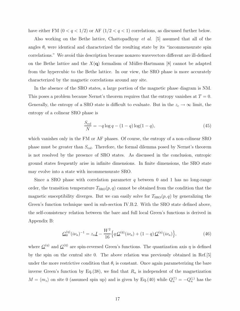
In Fig.5, the Curie and Neel temperatures are plotted versus filling for a variety of cou-

plings. When p ≥ 0.39, a critical value of J is required for TC to be nonzero. So the

weak-coupling regime is restricted to electron concentrations smaller than 0.39. As J/W in-

creases, the AF instabilities are restricted to a narrower range of concentrations near p = 1.

For large J/W at half filling, the nearest-neighbor hopping can be treated perturbatively

and superexchange leads to a Neel temperature proportional to W 2/J . So the sliver of AF

phase stabilized around half filling rapidly narrows with increasing J/W . By contrast the

FM phase dominates as J/W increases. In the limit J/W → ∞, the Neel temperature

vanishes even at p = 1.

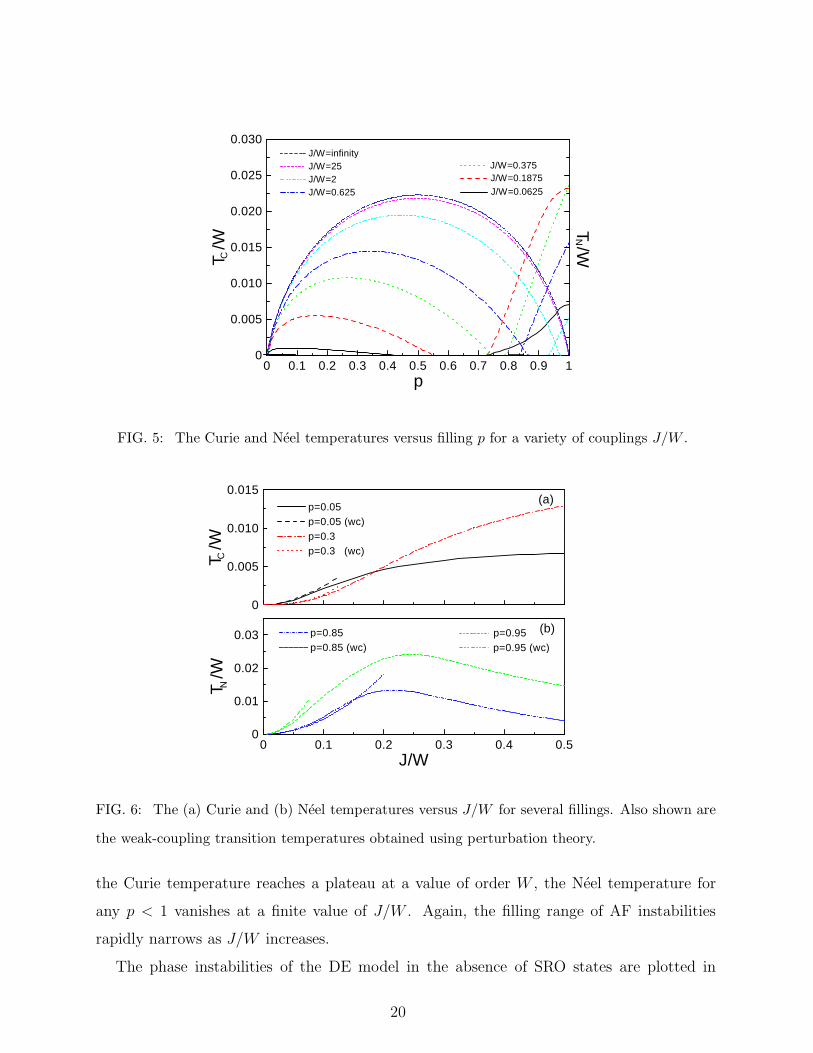
For a fixed filling, TC and TN are plotted versus J/W in Fig.6. As expected, the weak-

coupling curves track the numeric results for small J/W but deviate for larger J/W . Whereas

19

0 0.1 0.2 0.3 0.4 0.5 0.6 0.7 0.8 0.9 10

0.005

0.010

0.015

0.020

0.025

0.030

NC

J/W=0.0625

J/W=0.1875J/W=0.375

T /W

J/W=infinity J/W=25 J/W=2 J/W=0.625

T /W

p

FIG. 5: The Curie and Neel temperatures versus filling p for a variety of couplings J/W .

0 0.1 0.2 0.3 0.4 0.50

0.01

0.02

0.03p=0.95 (wc)p=0.95

N

(b)

p=0.85 p=0.85 (wc)

T /W

J/W

0

0.005

0.010

0.015

C

(a)

p=0.05 p=0.05 (wc) p=0.3 p=0.3 (wc)

T /W

FIG. 6: The (a) Curie and (b) Neel temperatures versus J/W for several fillings. Also shown are

the weak-coupling transition temperatures obtained using perturbation theory.

the Curie temperature reaches a plateau at a value of order W , the Neel temperature for

any p < 1 vanishes at a finite value of J/W . Again, the filling range of AF instabilities

rapidly narrows as J/W increases.

The phase instabilities of the DE model in the absence of SRO states are plotted in

20

1 0.8 0.6 0.4 0.2 0

(b)

NMSRO

AF

FM

p

0.0

0.1

0.2

0.3

0.4

0.5

0.6

0.7

0.8

0.9

1.0

1 0.8 0.6 0.4 0.2 0

(a)

AF

NM

FM

p

J/W

FIG. 7: The phase instabilities of the DE model (a) assuming only FM, AF, and NM phases and

(b) also including the SRO phase.

Fig.7(a). The NM region shrinks as J/W increases and is absent for J/W > 0.5. Since the

interacting DOS splits for J/W > 1/4 [16], the NM region survives even after the formation

of sub-bands. Whereas the AF region persists at half filling for all J/W , the sliver of AF

phase rapidly narrows with increasing coupling. The FM/NM phase boundary in Fig.7(a)

agrees quite well with that found by Auslender et al. [14].

Now including the SRO states, we plot the correlation parameter q along with T(max)SRO (p)

in Fig.8. For J/W > 0, a transition into the AF state (q = 1) occurs in a narrow range

of fillings close to p = 1. This range vanishes both as J/W → 0 and as J/W → ∞. It

has a maximal extent (from p = 0.78 to 1) when J/W ≈ 0.33. For J/W < 0.33, T(max)SRO (p)

vanishes at a single filling that corresponds to q = 0.5, meaning that there is no SRO. For

0.5 > J/W > 0.33, T(max)SRO (p) is nonzero for all fillings. As can be seen in Fig.8(a) for

J/W = 0.375, the correlation parameter for 0.5 > J/W > 0.33 jumps from q = 0 in the FM

21

0

0.005

0.010

0.015

0.020

0.025S

RO

SR

O

(b)

T

(ma

x)

/W

(a)

J/W=25 J/W=2 J/W=0.625 J/W=0.5 J/W=0.375 J/W=0.1875 J/W=0.0625

1

0.5

0

0.75

0.25

q

0 0.1 0.2 0.3 0.4 0.5 0.6 0.7 0.8 0.9 10

0.1

0.2

0.3

0.4(c)

J/W~0 (wc) J/W=0.025 J/W=0.0625 J/W=0.125

T(m

ax)

W/J

2

p

FIG. 8: (a) The correlation parameter q, (b) the maximum transition temperature T(max)SRO (p)/W ,

and (c) the normalized transition temperature T(max)SRO (p)W/J2 for various values of J/W versus

filling p.

phase to a nonzero value 0.5 < q < 1 in the SRO phase. For J/W > 0.5, one of the ordered

phases always has a higher transition temperatures than the SRO states and q jumps from 0

to 1 at the FM/AF boundary. The deviation between the numeric and weak-coupling results

in Fig.8(c) as p → 1 is quite expected: in the limit p → 1, the weak-coupling result for the

SRO transition temperature diverges, thereby invalidating the condition T ≪ J under which

it was derived.

The magnetic instabilities of the DE model including SRO states are mapped in Fig.7(b).

Notice that the region formerly labeled NM in Fig.7(a) is now occupied by SRO states. The

SRO phase also occupies the formerly AF region at very small J/W . As anticipated above,

22

the NM curve (where T(max)SRO (p) = 0 and q = 1/2) intersects the FM phase boundary at

J/W ≈ 0.33. This curve separates a SRO region with AF correlations (1 > q > 1/2) on the

left from a SRO region with FM correlations (1/2 > q > 0) on the right.

VI. MAGNETIC PHASE DIAGRAM OF THE DOUBLE-EXCHANGE MODEL

The presence of a continuous range of SRO states with correlation parameter q obviously

complicates the magnetic phase diagram of the DE model and the issue of PS. Because the

weak-coupling behavior of the DE model has been the subject of some debate [3, 4, 5, 14],

we shall treat this limit analytically. We then provide numerical results for the interacting

DOS that explain the stability of the SRO phase. Finally, we present the T = 0 phase

diagram of the DE model, both with and without the SRO states.

A. Weak-coupling limit

In their numerical work at T = 0, Chattopadhyay et al. [5] obtained a very complex

phase diagram, with a range of SRO states above J/W ≈ 1/16 and PS between AF and FM

phases for 0.1 < p < 1 below this value. For small J/W , a pure FM phase was found to be

stable for 0 < p ≤ 0.1. We now show that PS diappears in the exactly solvable limit of zero

temperature and weak coupling.

At zero temperature, the FM, AF, and SRO energies are evaluated after once again

parameterizing G(η)0 (z = iν + µ)−1 by Eq.(38). Then, R(z) is obtained from the quartic

equation

R(z + R)

(z + 2(1 − q)R)2 − J2

+W 2

16(z + 2(1 − q)R)2 = 0, (50)

which differs from Eq.(26) (except when q = 1/2) because we are now working in the broken-

symmetry phase. Similarly, Q(↑)(z) = −Q(↓)(z) is given by

Q(↑)(z) = (2q − 1)MJR(z)

z + 2(1 − q)R(z), (51)

which is likewise valid for any J .

The potential energy can generally be written as 〈V 〉/N = −2JM〈s0z〉, where the expec-

tation value of the electronic spin on site 0 for any temperature is

〈s0z〉 =1

4π

∫

dν Re G(↑)(z)αβσzβα =

8

πW 2(2q − 1)

∫

dν Q(↑)(z). (52)

23

For any J , the potential energy may be written as

1

N〈V (p, q)〉 = −16J2

πW 2

∫

dνR(z)

z + 2(1 − q)R(z). (53)

Of course, the NM potential energy is obtained by setting q = 1/2.

Second-order results for 〈V (p, q)〉/N are provided in Appendix A. For small J/W , 〈s0z〉is of order J/W so the electronic spins are not frozen at T = 0. Bearing in mind that

TSRO(p, q = 0) = TC(p) and TSRO(p, q = 1) = TN(p), the difference between the potential

energies of a FM, AF, or SRO phase and a NM is given by ∆〈V (p, q)〉/N = −3TSRO(p, q),

where both sides are evaluated to order J2/W . So the potential energy is lowered when the

transition temperature is positive.

A general expression for the kinetic energy of the SRO phase is proven in Appendix C.

At T = 0, Eq.(C3) becomes

1

N〈K〉 =

W 2

64π

∑

η

∫

dν G(η)(z)αβ

(1 − q)G(η)(z)βα + qG(η)(z)βα

. (54)

In contrast to alternative expressions for the kinetic energy of the FM and AF phases

[10], Eq.(54) does not assume any particular wavevector for the ground state. Independent

of q, the zeroth-order kinetic energy is given by E0(p)/N = −2W/(3π)(1 − δ2)3/2, where

δ = 2µ0/W and µ0 is the chemical potential evaluated to zeroth-order in J/W . For any J ,

the SRO kinetic energy is given by

1

N〈K(p, q)〉 =

16

πW 2

∫

dν R(z)2

1 +(1 − 2q)J2

(z + 2(1 − q)R(z))2

(55)

and the NM kinetic is recovered by setting q = 1/2. It is important to realize that the

second-order kinetic energy contains two contributions: one from the dependence of the

integrand on J/W for a fixed µ; the other from the dependence of the chemical potential

µ(p) on J/W for a fixed p.

Using the condition that p = 1 − 32/(πW 2)∫

dν Re R(z) depends only on the filling and

not on J , we may expand µ in powers of J/W as µ = µ0 + (J/W )2µ2 + . . .. Then µ0(p) is

solved from the condition

p = 1 +2

π

δ√

1 − δ2 + sin−1 δ

(56)

and µ2(p) is given in terms of µ0(p) by µ2 = Wδ/(1− q)2 + δ2(2q − 1). The divergence of

µ2 as q → 1 and p → 1 (or δ → 0) signals the opening of a gap in the interacting, AF DOS

as discussed further below.

24

Incorporating the change in chemical potential, the result for the second-order, q-

dependent correction to 〈K(p, q)〉/N is given in Appendix A. To second order in J/W ,

the difference between the kinetic energies of a FM, AF, or SRO phase and a NM is

∆〈K(p, q)〉/N = 3TSRO(p, q)/2. Hence, kinetic energy is lost (the electrons become more

confined) when the transition temperature is positive.

Consequently, the net change in energy E(p, q) = 〈K(p, q)+V (p, q)〉 in the weak-coupling

limit is given by ∆E(p, q)/N = −3TSRO(p, q)/2, which includes the FM (q = 0) and AF

(q = 1) phases as special cases. The same relation would be obtained for a Heisenberg

model H = −(1/2)∑

i,j JijSi · Sj with classical spins within Weiss mean-field theory (which

becomes exact in infinite dimensions), so that ∆E/N = −J(k = 0)S2/2 = −3TC/2. For

large J/W , however, the DE value of ∆E(p, q = 0)/N in the FM phase is proportional to J

whereas TC is proportional to W . So the proportionality between ∆E(p, q)/N and TSRO(p, q)

(and the analogy with the Heisenberg model) only holds in the weak-coupling limit.

In the limit of small J/W , the ground state energy is minimized by the same correlation

parameter q that maximizes the transition temperature! This result is not surprising: for

small J/W , the transition temperature is also small so the correlation parameter that ap-

pears at TSRO(p, q) also minimizes the energy at T = 0. As a consistency check, the results in

Appendix A may be used to show that the derivative of the energy is related to the chemical

potential by dE(p, q)/dp = Nµ, where both sides are expanded to second order in J/W .

B. Interacting Density-of-States

To better interpret the weak-coupling results, we construct the interacting DOS per spin

N(ω, q) = − 1

4π

∑

η

Im G(η)(z → ω + iδ)αα =16

πW 2Im

R

z→ω+iδ. (57)

As J/W → 0, N(ω, q) reduces to the bare DOS N0(ω) for any q. The AF DOS can be solved

analytically for all J :

N(ω, q = 1) =8|ω|πW 2

Re

√

W 2/4 + J2 − ω2

ω2 − J2(58)

which vanishes for |ω| < J and |ω| >√

W 2/4 + J2. Hence, N(ω, q = 1) contains a square-

root singularity on either side of a gap with magnitude 2J . As J/W → ∞, the width of each

side-band narrows like W 2/8J . It is also possible to explicitly evaluate the DOS at ω = 0 for

25

0

0.5

1

1.5

2

2.5

3

-0.8 -0.6 -0.4 -0.2 0 0.2 0.4 0.6 0.8ω/W

W N

(ω)

J/W = 0.2

FIG. 9: The interacting DOS N(ω, q) (normalized by 1/W ) versus ω/W for J/W = 0.2 in the

FM or q = 0 (solid, blue), SRO phase with q = 1/4 (long dash, light blue), NM or q = 1/2 (dash,

green), SRO phase with q = 3/4 (small dash, red) and AF or q = 1 (dot dash, purple) phases.

any q: N(ω = 0, q) = (8/πW 2(1−q))Re√

J2c − J2, which vanishes for J > Jc ≡ W (1−q)/2.

For a NM, the critical value of J required to split the DOS is Jc = W/4, as found earlier

[16]. For an AF at T = 0, Jc = 0 since a gap forms for any nonzero coupling constant. For

a SRO phase, Jc > 0.

Taking J/W = 0.2, we numerically solve for R(z) and plot the interacting DOS versus

ω for q = 0, 1/4, 1/2, 3/4, and 1 in Fig.9. The FM DOS has kinks at ω = ±(W/2 − J).

For energies between the kinks, both up- and down-spin states appear; on either side of

the kinks, the bands are fully spin-polarized. These kinks disappear in a SRO state with

q > 0 due to the absence of long-range magnetic order. The width of the DOS shrinks as

q increases from 0 to 1. These results agree with the second-order change to the chemical

potential given above. In fact, the divergence of the AF result for µ2 as p → 1 is caused by

the appearance of a gap in the AF DOS for any nonzero J .

For any temperature, coupling constant, and correlation parameter, the total energy of

the DE model may be written as an integral over the interacting DOS:

1

NE(p, q) = 2

∫

dω ωf(ω)N(ω, q), (59)

26

where f(ω) = 1/(exp(β(ω − µ)) + 1) is the Fermi function and µ = µ(p). At T = 0, this

relation may be expressed in the compact form

1

NE(p, q) = −1

π

∫

dν

1 +16zR(z)

W 2

, (60)

which agrees with Eqs.(53) and (55).

From these results, it is not hard to understand why a SRO phase can have a lower energy

than an AF. Due to the narrowing of the AF DOS, the AF energy may be higher than that

of a SRO state with J < Jc(q) and no energy gap. If the chemical potential of the AF

phase lies sufficiently far from the energy gap, then the broader DOS of a SRO phase with

J < Jc will favor that state over an AF. As p → 1, this condition is impossible to satisfy for

arbitrarily small J and the AF becomes stable.

For a given p < 1, the expansions of the kinetic and potential energies in powers of (J/W )2

are valid when J < Jc(q) so that the DOS of a SRO state with correlation parameter q is

not gapped. Conversely, for a fixed J , the expansions fail sufficiently close to p = 1 and

q = 1 that a gap develops in N(ω, q).

C. Ground-state phase diagram and phase separation

When only FM, AF, and NM states are considered, PS occurs due to the discontinu-

ity in the chemical potential at the FM/NM and NM/AF phase boundaries. Since these

discontinuities become weaker as J/W decreases, PS disappears as J/W → 0.

Once the SRO states are introduced, the physical energy E(min)(p) is obtained by mini-

mizing E(p, q) with respect to q for a fixed p. Although the chemical potential is a continuous

function of filling, PS still occurs for non-zero J due to the formation of an energy gap in

the AF state, so that (1/N)dE(min)/dp|p=1− = −J . A necessary condition for PS between

fillings p1 < 1 and p2 = 1 is that the second derivative of the energy E(min)(p) must change

sign for some filling p⋆ between p1 and p2. But if E(min)(p) is expanded in powers of (J/W )2,

then the condition that d2E(min)(p)/dp2|p⋆ = 0 may be written

π

8√

1 − δ2∼ J2

W 2δ2

∣

∣

∣

∣

∣

p⋆

, (61)

where δ = 2µ0/W and µ0 is the chemical potential evaluated to zeroth-order in J/W . Since

the value q⋆ of q at p⋆ is less than 1, the expansion in powers of (J/W )2 is valid for J < Jc(q⋆),

27

E

/N

W(m

in)

−0.6

−0.5

−0.4

−0.3

−0.2

−0.1

0

0 0.2 0.4 0.6 0.8 1p

0

0.2

0.4

0.6

0.8

1

q

J/W = 0.5

FIG. 10: The T = 0 energy E(min)(p) and the value of q that minimizes the energy versus filling for

J/W = 0.5. A Maxwell construction (given by the dots and dashed line) between fillings p1 = 0.647

and p2 = 1 demonstrates the existence of PS.

as discussed previously. When J/W → 0, the right-hand side of Eq.(61) vanishes so the

condition for PS cannot be met in the limit of vanishing J/W except as δ → 0 or p⋆ → 1.

Near p = 1, δ ≈ (1− p)π/4 so Eq.(61) also implies that the difference p2 − p1 grows linearly

with J/W . These results contradict Chattopadhyay et al. [5], who seem to use a Maxwell

construction involving the difference E(min)(p)−E0(p) rather than the total minimum energy

E(min)(p).

To show this more explicitly, we have used E(min)(p) to find the PS region through Maxwell

constructions between fillings p1 < 1 and p2 = 1. One such Maxwell construction is pictured

in Fig.10, where a phase mixture along the dashed line provides a lower energy than the

pure phase on the solid curve. For J/W = 0.5, the SRO states are bypassed and PS occurs

between a FM with p1 = 0.647 and an AF with p2 = 1.

The T = 0 phase diagram of Fig.11(a) assumes that only the NM, FM, and AF phases

are allowed. Without the SRO state, the ground-state phase diagram is fairly complicated.

28

1 0.8 0.6 0.4 0.2 0

(b)

AF

NM

PS

FM

p

0.0

0.1

0.2

0.3

0.4

0.5

0.6

0.7

0.8

0.9

1.0

1 0.8 0.6 0.4 0.2 0

SRO

J/W

(a)

AF

PS

FM

AF NM

p

FIG. 11: The T = 0 magnetic phase diagram of the DE model (a) assuming only FM, AF, and

NM phases and (b) also including the SRO phase.

As implied by the argument above, PS disappears in the limit of vanishing J/W but the

PS regions grow with increasing J/W . Two PS regions appear around the fillings of the

AF/NM and NM/FM phase boundaries for J/W ≪ 1. When 0 < J/W ≤ 0.16, the lower

PS region in Fig.11(a) mixes an AF with p < 1 and a NM. For 0.16 < J/W < 0.28, an AF

with p < 1 is unstable and the lower PS region mixes an AF with p = 1 and a NM. For

J/W > 0.28, PS occurs between a FM and an AF with p = 1.

Surprisingly, the T = 0 phase diagram of Fig.11(b) becomes much simpler once the

SRO states are included. For J/W < 0.33, a SRO state is stable over a range of fillings

that diminishes with increasing J . Near half-filling, PS is found between a SRO state with

0 < q < 1 and an AF with p = 1. In agreement with the above discussion, the PS region

grows linearly with J/W . For J/W > 0.33, the SRO phase is skipped and PS occurs between

a FM with q = 0 and an AF with p = 1. The special value J/W ≈ 0.33 agrees with the

29

coupling where the NM line intersects the FM boundary in the instability map of Fig.7(b). It

also corresponds to the coupling where the AF instability covers the widest range of fillings.

The PS region in Figs.11(a) and (b) diminishes with increasing J/W . In the strong-

coupling regime, our results are in qualitative agreement with other authors [3, 11]. But for

J/W = 2, we obtain PS over a somewhat larger range of fillings than obtained in Ref.[13].

Aside from the behavior at very small J/W , the phase diagram of Fig.11(b) agrees rather

well with that presented by Chattopadhyay et al. [5]. In particular, those authors also found

that the SRO phase disappears when J/W exceeds about 0.3.

Together, Figs.7 and 11 provide a bird’s eye view of the magnetic instabilities and phase

evolution in the DE model. In Figs.7(a) and 11(a), a triangle of phase space remains NM

for all temperatures down to T = 0; in Figs.7(b) and 11(b), a somewhat larger triangle of

phase space remains in the SRO phase down to T = 0. Keep in mind, however, that the

ordered phases of Fig.7 may be bypassed when J/W, p lies in the PS region of Fig.11. For

example, Furukawa [13] found that for J/W = 2, an AF with p < 1 was excluded by PS

between an AF with p = 1 and a NM.

VII. CONCLUSIONS

We have used DMFT to evaluate the magnetic phase instabilities and ground-state phase

diagram of the DE model. Surprisingly, a SRO phase may have a higher transition temper-

ature than the long-range ordered AF and FM phases. The ground-state phase diagram of

the DE model actually simplifies in the presence of the SRO states.

At first sight, the stability of disordered NM and SRO ground states may be hard to

understand. After all, the presence of a disordered state at T = 0 contradicts Nernst’s

theorem, which requires that the entropy of the local moments be quenched at zero tem-

perature. However, entropic ground states appear quite frequently in infinite-dimensional

calculations. Within the DMFT of the Hubbard model, AF ordering on a hypercubic lattice

at half filling can be frustrated by hopping between sites on the same sub-lattice [10]. This

additional hopping produces a NM Mott insulator at T = 0 for large U/W , again in viola-

tion of Nernst’s theorem. Also on the hypercubic lattice, the DE model has a NM ground

state extending all the way to p = 0 when J/W is sufficiently small [4]. Although they

did not study such states in detail, Nagai et al. [4] detected the signature of incommen-

30

surate states for weak coupling. Therefore, many-body theories in infinite dimensions are

frequently unable to lower the symmetries of disordered ground states. Of course, DMFT

cannot access phases described by a non-local order parameter. It should also be noted that

Nernst’s theorem only applies rigorously to quantum systems and not to a DE model with

classical local spins.

For small J/W , the energy of the entropic SRO state is lowered below the energies of

the FM and AF phases by the RKKY interaction [7], which generates competing FM and

AF interactions [14]. As the dimension is lowered, the SRO state may evolve into the state

with incommensurate correlations (IC) obtained in one- and two-dimensional Monte-Carlo

simulations by Yunoki et al. [3]. Replacing “SRO” by “IC”, the phase diagram of Fig.11(b)

bears a striking resemblance to the phase diagrams of Ref.[3]. In agreement with our results,

Yunoki et al. found that the short-range correlations in the IC phase change from AF to

FM as p decreases. The phase diagram of Fig.11(b) also looks quite similar to the three-

dimensional phase diagram obtained by Yin [6], who compared the energies of the AF and

FM phases with the energy of a two-dimensional spiral phase carrying momenta along the

(111) direction. Hence, the infinite-dimensional phase diagram of Fig.11(b) is closely related

to the results of finite-dimensional calculations.

On a translationally-invariant hypercubic lattice [10] in infinite dimensions, the SRO

phase may map onto an incommensurate spin-density wave (SDW) with a definite wavevec-

tor. In that case, the transition temperature of the SDW could be obtained from either

the coupled Green’s functions or the magnetic susceptibility. However, there are no indica-

tions for SDW ordering in the limited studies of the DE model on an infinite-dimensional

hypercubic lattice [4] and we consider such a possibility to be remote. Much more likely,

the SRO phase would map onto a disordered state with short-range magnetic order and

broad maxima at wavevectors q associated with the nesting of the Fermi surface, as found

in Monte-Carlo simulations of one- and two-dimensional hypercubic lattices [3].

Bear in mind that DMFT studies of the DE model on a hypercubic lattice sacrifice a

key advantage of the Bethe lattice: the possibility of obtaining analytic results due to the

relationship, Eq.(6), between the bare and full Green’s function. For example, both sides of

the expression ∆E(p, q)/N = −3TSRO(p, q)/2 were evaluated independently to order J2/W .

This gives us great confidence in our results for the energy and critical temperature in the

weak-coupling limit. Such analytic results are not possible on a hypercubic lattice. Indeed,

31

pathological results have been found [16] on a hypercubic lattice due to the asymptotic

freedom of the quasiparticles in the tails of the Gaussian DOS. In most instances, more

physical results are obtained on a Bethe lattice, where the bounded DOS more closely

resembles the DOS in two and three dimensions.

Working on a Bethe lattice has allowed us to clarify the behavior of the DE model at

weak coupling. We have demonstrated both analytically and numerically that PS disappears

as J/W → 0. Whereas the FM phase is stable for p below about 0.26, a SRO state is

stable above. As p → 1, the SRO phase evolves into the long-range ordered AF phase.

The transition temperature of the SRO phase exceeds that of the FM and AF phases for

0.26 < p < 1.

Whether the SRO phase is a new kind of spin glass or a spin liquid can only be resolved

by future studies of the static and dynamic susceptibilities. An intriguing possibility is

that the local moments are frozen within a spin-glass state but that the electronic spins

are subject to quantum fluctuations within a spin-liquid state. Two of the most important

unresolved questions about spin glasses are whether there exists a true thermodynamic spin-

glass transition [34] and whether a model without quenched disorder can support a spin glass

[35]. We have answered those questions for the DE model on an infinite-dimensional Bethe

lattice. Above TSRO(p, q), the NM state is characterized by the absence of SRO around

any site. Below TSRO(p, q), short-range magnetic order develops with a correlation length

ξ(q) = −a/ log |2q − 1| and the entropy, while still extensive, is reduced. Although not

marked by a divergent susceptibility, the transition at TSRO(p, q) is characterized by the

development of short-range magnetic order and a reduction in the entropy. Future work

may establish connections between the SRO phase and the spin-glass solution to the random

Ising model on a Bethe lattice [36], where the Edwards-Anderson order parameter can be

explicitly constructed.

The strength of DMFT applied to DE-like models with a Kondo coupling 2Jmi · si

between the local-moment spin Si = Smi and the electron spin si is that the Fermion

degrees of freedom in the local action may be integrated exactly, leaving a function only of

the local moment direction mi. Consequently, formally exact results are possible for a range

of models where the local moments are treated classically. This stands in stark contrast to

the case for the Hubbard model [10], where the action cannot be analytically integrated and

quantum Monte Carlo must be used to solve the local problem. We should also mention

32

that the classical treatment of the local spins is more questionable in the manganites, where

S = 3/2, than in Mn-doped GaAs, where S = 5/2.

The discovery of a SRO solution to the DE model in infinite dimensions has wide rami-

fications. Our results open the door for future studies of the disordered ground-state of the

DE model unencumbered by the numerical complexities of Monte-Carlo simulations [3] in

finite dimensions.

It is a pleasure to acknowledge helpful conversations with Profs. Elbio Dagotto, Jim

Freericks, Douglas Scalapino, and Seiji Yunoki. This research was sponsored by the U.S.

Department of Energy under contract DE-AC05-00OR22725 with Oak Ridge National Labo-

ratory, managed by UT-Battelle, LLC and by the National Science Foundation under Grant

Nos. DMR-0073308, DMR-0312680, EPS-0132289 and EPS-0447679 (ND EPSCoR). A por-

tion of this research was conducted at the Center for Nanophase Materials Sciences, which

is sponsored at Oak Ridge National Laboratory by the Division of Scientific User Facilities,

U.S. Department of Energy.

APPENDIX A: WEAK-COUPLING RESULTS

This appendix presents the weak-coupling results for the SRO transition temperature

and energy. For low temperatures,∑

n g(νn) → (1/2πT )∫

dν g(ν) so that

TSRO(p, q) = −J2(2q − 1)

3π

∫

dνR(v)

(v + R(v))2(v + 2(1 − q)R(v)) − J2(v + 2(2 − q)R(v)/3),

(A1)

where v = iν + µ. In the weak-coupling limit T ≪ J ≪ W , this becomes

TSRO(p, q) = −J2(2q − 1)

3π

∫

dνR(z)

(z + R(z))2(z + 2(1 − q)R(z)), (A2)

where z = iν + µ0 and R(z) falls off like W 2/z for large |z|. The zeroth-order chemical

potential µ0 is defined in terms of the filling p by Eq.(56). Using complex analysis and

carefully treating the branch cut between ±W/2 along the real axis, we find that

TSRO(p, q)W

J2= −32

3π

∫ 1

δdy y

√

1 − y2y2 − (3 − 2q)/4

y2 + b, (A3)

with δ = 2µ0/W and b = (1 − q)2/(2q − 1). Clearly, TSRO(p, q) vanishes as q → 1/2 or

b → ∞.

33

In the regime 0 ≤ q < 1/2, the integral for TSRO(p, q) with b < 0 gives

TSRO(p, q)W

J2=

8

9π(1 − 2q)

3√

1 − δ2 − 4(1 − δ2)3/2(1 − 2q)

+3q

2√

1 − 2q

[

Tan−1

(

(1 − q)|δ| − √1 − 2q√

1 − δ2q

)

− Tan−1

(

(1 − q)|δ| + √1 − 2q√

1 − δ2q

)]

. (A4)

This result can be extended to the regime 1/2 < q ≤ 1 by using the identity

1√1 − 2q

[

Tan−1

(

(1 − q)|δ| − √1 − 2q√

1 − δ2q

)

− Tan−1

(

(1 − q)|δ| + √1 − 2q√

1 − δ2q

)]

(A5)

= − 2√2q − 1

log

[

q +√

1 − δ2√

2q − 1√

δ2(2q − 1) + (1 − q)2

]

(A6)

These expressions yield Eq.(31) for TC and Eq.(36) for TN as q → 0 and q → 1, respectively.

Using Eq.(54), it is straightforward to obtain the kinetic energy in the weak-coupling

limit:

1

N〈K(p, q)〉 =

1

NE0(p) +

2J2

πW (1 − 2q)

2√

1 − δ2 +q√

1 − 2q

×[

Tan−1

(

(1 − q)|δ| − √1 − 2q√

1 − δ2q

)

− Tan−1

(

(1 − q)|δ| + √1 − 2q√

1 − δ2q

)]

. (A7)

Of course, the NM kinetic energy is obtained by taking the limit q → 1/2, with the re-

sult 〈K(p, q = 1/2)〉/N = E0(p)/N + (16J2/3πW )(1 − δ2)3/2. The difference between

the q-dependent and NM kinetic energies in the weak-coupling limit is then given by

∆〈K(p, q)〉/N = 3TSRO(p, q)/2.

Likewise, it is straightforward to evaluate the potential energy to order (J/W )2, with the

result:

1

N〈V (p, q)〉 = − 4J2

πW (1 − 2q)

2√

1 − δ2 +q√

1 − 2q

×[

Tan−1

(

(1 − q)|δ| − √1 − 2q√

1 − δ2q

)

− Tan−1

(

(1 − q)|δ| + √1 − 2q√

1 − δ2q

)]

. (A8)

In the limit q → 1/2, the NM result is 〈V (p, q = 1/2)〉/N = −(32J2/3πW )(1−δ2)3/2. Hence,

the difference between the q-dependent and NM potential energies in the weak-coupling limit

is given by ∆〈V (p, q)〉/N = −3TSRO(p, q). It follows that the change in total energy is given

by ∆E(p, q)/N = −3TSRO(p, q)/2, which includes the FM (q = 0) and AF (q = 1) phases as

special cases.

34

APPENDIX B: SELF-CONSISTENCY RELATION FOR THE SRO STATES

Following the cavity method of Ref.[10], the self-consistency relation on the Bethe lattice

between the bare and full Green’s functions may be written

G0(iνn)−1 = znI − t2′∑

i

G(iνn)ii, (B1)

where t2 = W 2/16zc and G(iνn)ii is the local Green’s function on site i. The sum on i is

restricted to nearest neighbors of site 0. If the spin on site 0 is ordered along the z axis,

then we can write the local Green’s function on site 0 as

G(iνn)00 =

g↑n 0

0 g↓n

. (B2)

The creation and destruction operators on site i are taken to refer to a quantization axis

that is rotated by angle θi (rotation axis in the xy plane at an angle φi from the x axis)

with respect to z. Then G(iνn)ii = R(θi, φi) G(iνn)00 R(θi, φi)† is given by

G(iνn)ii =

cos2(θi/2)g↑n + sin2(θi/2)g↓n i sin θie−iφi(g↑n − g↓n)/2

−i sin θieiφi(g↑n − g↓n)/2 cos2(θi/2)g↓n + sin2(θi/2)g↑n

. (B3)

Summing over all zc neighbors of site 0 and assuming that φi is random so that

(1/zc)∑′

i exp(±iφi) = 0, we find

1

zc

′∑

i

G(iνn)ii = (1 − q)

g↑n 0

0 g↓n

+ q

g↓n 0

0 g↑n

, (B4)

where q = (1/zc)∑′

i sin2(θi/2). Upon noting that the two Green’s function matrices above

are spin-reversed, we obtain Eq.(46).

APPENDIX C: KINETIC ENERGY

Previous forms for the kinetic energy utilized the wavevector q = 0 or Q of the FM or

AF phase [10]. In this appendix, we develop an expression for the kinetic energy that also

applies to the SRO states, where the wavevector is not defined. Begin with the relation

1

N〈K〉 = − t

2Zf

′∑

i

∫

Πi dΩmiTrf

(

(c†0αciα + c†iαc0α)e−S)

, (C1)

35

where Zf =∫

Πi dΩmiTrf

(

exp(−S))

and the sum over i is restricted to nearest neighbors of

site 0. The action S = ∆S + S0 + S(0) is separated into terms that involve site 0 and the

action S(0) of the cavity [10] with site 0 removed. The kinetic part of the action containing

site 0 is

∆S = −t∫ β

0dτ

′∑

j

(

c†0α(τ)cjα(τ) + c†jα(τ)c0α(τ))

. (C2)

Performing perturbation theory in the term involving the (0i) bond and using t = W/4√

zc,

we find

1

N〈K〉 =

W 2

16zc

′∑

i

∫ β

0dτ〈c†iα(0)ciα(τ)〉〈c†0α(τ)c0α(0)〉

=W 2

32T∑

l,η

G(η)(iνl)αβ

(1 − q)G(η)(iνl)βα + qG(η)(iνl)βα

, (C3)

where the local averages at sites 0 and i are performed using Seff of Eq.(2). Removing the

single (0i) bond from ∆S does not affect those local averages in the zc → ∞ limit.

[1] For an overview of work on the manganites, see Dagotto E 2003 Nanoscale Phase Separation

and Colossal Magnetoresistance (Springer: Berlin) and 1999 Physics of Manganites, ed T A

Kaplan and S D Mahanti (New York: Plenum)

[2] For an overview of work on dilute magnetic semiconductors, see MacDonald A H, Schiffer P

and Samarth N 2005 Nat. Mat. 4 195 and Dietl T 2003 Advances in Solid State Physics, ed

B Kramer (Berlin: Springer) (available as cond-mat 0306479)

[3] Yunoki S, Hu J, Malvezzi A L, Moreo A, Furukawa N and Dagotto E, 1998 Phys. Rev. Lett.

80 845; Dagotto E, Yunoki S, Malvezzi A L, Moreo A, Hu J, Capponi S, Poilblanc D and

Furukawa N 1998 Phys. Rev. B 58 6414

[4] Nagai K, Momoi T and Kubo K 2000 J. Phys. Soc. Japan 69 1837

[5] Chattopadhyay A, Millis A J and Das Sarma S 2000 Phys. Rev. B 61 10738; Chattopadhyay

A, Das Sarma S and Millis A J 2001 Phys. Rev. Lett. 87 227202; Chattopadhyay A, Millis A

J and Das Sarma S 2001 Phys. Rev. B 64 012416

[6] Yin L 2003 Phys. Rev. B 68 104433

[7] Van Vleck J H 1962 Rev. Mod. Phys. 34 681

[8] Muller-Hartmann E 1989 Z. Phys. B 74 507; Muller-Hartmann E 1989 Z. Phys. B 76 211

36

[9] Metzner W and Vollhardt D 1989 Phys. Rev. Lett. 62 324

[10] For a review of DMFT, see Georges A, Kotliar G, Krauth W and Rozenberg M J 1996 Rev.

Mod. Phys. 68 13

[11] Furukawa N 1995 J. Phys. Soc. Jpn. 64 2754; Furukawa N 1995 J. Phys. Soc. Jpn. 64 3164

[12] Millis A J, Mueller R and Shraiman B I 1996 Phys. Rev. B 54 5389; Millis A J, Mueller R

and Shraiman B I 1996 Phys. Rev. B 54 5405; Michaelis B and Millis A J 2003 Phys. Rev. B

68 115111

[13] Furukawa N in 1999 Physics of Manganites, ed T A Kaplan and S D Mahanti (New York:

Plenum)

[14] Auslender M and Kogan E 2001 Phys. Rev. B 65 012408; Auslender M and Kogan E 2002

Europhys. Lett. 59 277; Kogan E, Auslender M and Dgani E, cond-mat 0211354

[15] Fishman R S and Jarrell M 2003 J. Appl. Phys. 93 7148; 2003 Phys. Rev. B 67 100403(R)

[16] Chernyshev A and Fishman R S 2003 Phys. Rev. Lett. 90 177202

[17] Fishman R S, Maier Th, Moreno J, and Jarrell M 2005 Phys. Rev. B 71 180405(R)

[18] Aryanpour K, Moreno J, Jarrell M and Fishman R S 2005 Phys. Rev. B 72 045343

[19] Brinkman W F and Rice T M 1970 Phys. Rev. B 2 1324

[20] Fishman R S, Popescu F, Alvarez G, Moreno J, and Maier Th 2006 Phys. Rev. B (in press)

[21] Binder K and Young A P 1986 Rev. Mod. Phys. 58 801

[22] Baym G and Kadanoff L P 1961 Phys. Rev. 124 287; Baym G 1962 Phys. Rev. 127 1391

[23] Jarrell M 1992 Phys. Rev. Lett. 69 168

[24] Freericks J K and Jarrell M 1995 Phys. Rev. Lett. 74 186

[25] Bickers N E 1987 Rev. Mod. Phys. 59 845

[26] Leath P L 1968 Phys. Rev. 171 725

[27] For a general reference, see Abrikosov A A, Gorkov L P and Dzyaloshinski I E 1963 Methods

of Quantum Field Theory in Statistical Mechanics (Englewood Cliffs: Prentice Hall)

[28] Nolting W, Rex S and Mathi Jaya S 1997 J. Phys.: Cond. Matt. 9 1301

[29] Santos C and Nolting W 2002 Phys. Rev. B 65 144419; Santos C and Nolting W 2002 Phys.

Rev. B 66 019901

[30] Trias A and Yndurain F 1983 Phys. Rev. B 28 2839

[31] Rogan J and Kiwi M 1997 Phys. Rev. B 55 14397

[32] Gruber Ch, Macris N, Royer Ph and Freericks J K 2001 Phys. Rev. B 63 165111

37

[33] Eggarter T P 1974 Phys. Rev. B 9 2989

[34] Bitko D, Coppersmith S N, Leheny R L, Menon N, Nagel S R and Rosenbaum T F 1997 J.

Res. Natl. Inst. Stand. Technol. 102 207

[35] Schmalian J and Wolynes P G 2000 Phys. Rev. Lett. 85 836

[36] Bowman D R and Levin K 1982 Phys. Rev. B 25 3438; Thouless D J 1986 Phys. Rev. Lett.

56 1082; de Oliviera M J 1989 J. Phys. A: Math. Gen. 22 4433

38