Policy ReseaRch WoRking PaPeR 4781

Macro-Micro Feedback Links of Irrigation Water Management in Turkey

Erol H. CakmakHasan Dudu

Sirin SaracogluXinshen Diao

Terry RoeYacov Tsur

The World BankDevelopment Research GroupSustainable Rural and Urban Development TeamNovember 2008

WPS4781P

ublic

Dis

clos

ure

Aut

horiz

edP

ublic

Dis

clos

ure

Aut

horiz

edP

ublic

Dis

clos

ure

Aut

horiz

edP

ublic

Dis

clos

ure

Aut

horiz

ed

Produced by the Research Support Team

Abstract

The Policy Research Working Paper Series disseminates the findings of work in progress to encourage the exchange of ideas about development issues. An objective of the series is to get the findings out quickly, even if the presentations are less than fully polished. The papers carry the names of the authors and should be cited accordingly. The findings, interpretations, and conclusions expressed in this paper are entirely those of the authors. They do not necessarily represent the views of the International Bank for Reconstruction and Development/World Bank and its affiliated organizations, or those of the Executive Directors of the World Bank or the governments they represent.

Policy ReseaRch WoRking PaPeR 4781

Agricultural production is heavily dependent on water availability in Turkey, where half the crop production relies on irrigation. Irrigated agriculture consumes about 75 percent of total water used, which is about 30 percent of renewable water availability. This study analyzes the likely effects of increased competition for water resources and changes in the Turkish economy. The analysis uses an economy-wide Walrasian Computable General Equilibrium model with a detailed account of the agricultural sector. The study investigated the economy-wide effects of two external shocks, namely a permanent increase in the world prices of agricultural commodities and climate change, along with the impact of the domestic reallocation of water between agricultural and non-agricultural uses. It was also recognized that because

This paper—a product of the Sustainable Rural and Urban Development Team, Development Research Group—is part of a larger effort in the department to mainstream research on role of water resources in the economy. Policy Research Working Papers are also posted on the Web at http://econ.worldbank.org. The authors may be contacted at cakmake@metu.edu.tr, dudu@metu.edu.tr, ssirin@metu.edu.tr, x.diao@cgiar.org, troe@umn.edu, tsur@agri.huji.ac.il.

of spatial heterogeneity of the climate, the simulated scenarios have differential impact on the agricultural production and hence on the allocation of factors of production including water. The greatest effects on major macroeconomic indicators occur in the climate change simulations. As a result of the transfer of water from rural to urban areas, overall production of all crops declines. Although production on rainfed land increases, production on irrigated land declines, most notably the production of maize and fruits. The decrease in agricultural production, coupled with the domestic price increase, is further reflected in net trade. Agricultural imports increase with a greater decline in agricultural exports.

MACRO-MICRO FEEDBACK LINKS OF IRRIGATION WATER MANAGEMENT IN TURKEY*

Erol H. Cakmak∗∗, Hasan Dudu**, Sirin Saracoglu**,

Xinshen Diao***, Terry Roe****, Yacov Tsur***** JEL classification: C68; O13 ; Q15; Q18

Key words: Computable General Equilibrium; Feedback links; Irrigation Water; Turkey

*This paper is a product of the project “Macro-Micro Feedback Links of Irrigation Water Management”, funded by the Research Committee of World Bank and managed by DECRG-RU. We are indebted to Ariel Dinar advice and comments. Constructive review comments from Erinc Yeldan are acknowledged with appreciation. Cakmak, Dudu, Saracoglu, Roe and Tsur were consultans to the World Bank on this study. ** Department of Economics, Middle East Technical University (METU), Ankara, Turkey. *** International Food Policy Research Institute (IFPRI), Washington, DC, USA **** Department of Applied Economics, University of Minnesota, St. Paul, MN, USA. ***** Department of Agricultural Economics and Management, Hebrew University of Jerusalem, Rehovot, Israel.

2

Acronyms

ARIP: Agricultural Reform Implementation Project

CES: Constant Elasticity of Substitution

CSE: Consumer Subsidy Equivalents

CGE: Computable General Equilibrium

DIS: Direct Income Support

DSI: State Hydraulic Works, Republic of Turkey

EU: European Union

FAO: Food and Agriculture Organization

IFPRI: International Food Policy Research Institute

GDRS: General Directorate of Rural Services

GDP: Gross Domestic Product

GTAP: Global Trade Analysis Project

LSCB: Lower Seyhan-Ceyhan Basin

OECD: Organization for Economic Co-operation and Development

PSE: Producer Subsidy Equivalents

QHS: Quantitative Household Survey

REC: Regional Environment Center

SAM: Social Accounting Matrix

SPO: State Planning Organization, Republic of Turkey

TACOGEM-W: Turkish Agricultural Computable General Equilibrium Model with water

TurkSTAT: Turkish Statistical Institute

UFT: Undersecretariat of Foreign Trade, Republic of Turkey

VA: Value-added

WUA: Water User Associations

WTO: World Trade Organization

3

Table of Contents

Key words: Computable General Equilibrium; Feedback links; Irrigation Water; Turkey.... 1 Acronyms................................................................................................................................ 2 Table of Contents.................................................................................................................... 3 List of Tables .......................................................................................................................... 4 List of Figures ......................................................................................................................... 5 List of Figures ......................................................................................................................... 5 1 Introduction..................................................................................................................6 2 Water and Agricultural Sectors in Turkey ...................................................................8 2.1 Water Resource Availability and Use in Turkey ........................................................8 2.2 Overview of the Agricultural Sector in Turkey ........................................................15 3 The Modeling Framework .........................................................................................19 3.1 Structure of the Agricultural Computable Equilibrium Model for Turkey...............22 3.2 The Farm Model: Structure and Results ...................................................................30 3.3 Linkage between the Farm Model and TACOGEM-W............................................31 4 Empirical Results .......................................................................................................33 4.1 Aggregate Results of the Simulations.......................................................................34 4.2 Scenario 1: Increase in World Prices ........................................................................37 4.3 Scenario 2: The Urbanization Scenario ...................................................................42 4.4 Scenario 3: Climate Change Scenario.......................................................................50 5 Conclusions, Policy Implications, and Future Research Agenda ..............................57 References............................................................................................................................. 62 Appendix A: Additional Tables ............................................................................................ 66 Appendix B: The Algebraic Structure of the CGE Model.................................................... 70 Appendix C: The Algebraic Structure of the Farm Model ................................................... 76

4

List of Tables

Table 2.1. Turkey: Water Resources Potential and Use ....................................................9 Table 2.2. Water Potential and Land Distribution by Basins ..........................................11 Table 2.3. Sectoral Water Use in Turkey.........................................................................12 Table 2.4. Irrigation Development by Regions, 2007 (1,000 ha) ....................................13 Table 2.5. Irrigation ratios of the areas transferred by DSI, 1999-2006..........................14 Table 2.6. Management of Irrigation Schemes, 2007......................................................14 Table 2.7. Agricultural value-added: growth and share, 1968-2007 ...............................16 Table 3.1. Gross national product by kind of activity, 2003............................................22 Table 3.2. Employed persons by branch of economic activity, 2003 ..............................23 Table 3.3.Share of regional production value in national production value, 2003 (Agriculture only) ............................................................................................................25 Table 3.4. Agricultural land use, 2003.............................................................................26 Table 3.5. Irrigated versus rainfed land use, 2001 (hectares) ..........................................26 Table 3.6. Irrigated area by irrigation source, 2001.........................................................27 Table 3.7. Irrigated area by irrigation system, 2001 ........................................................27 Table 4.1. Effects on GDP ...............................................................................................35 Table 4.2. Macroeconomic results of simulations ...........................................................36 Table 4.3. Price Shocks in Scenario 1..............................................................................37 Table 4.4. Change in domestic average output prices and composite good supply and domestic production.........................................................................................................38 Table 4.5. Percentage change in share of exports and imports in total production .........39 Table 4.6. Percentage change in factor employment .......................................................40 Table 4.7: Change in factor prices ...................................................................................41 Table 4.8.Urban population dynamics in Turkey ............................................................42 Table 4.9. NUTS Level-1 Regions, net internal migration (‰) ......................................44 Table 4.10. Change in total production quantity..............................................................46 Table 4.11. Change in factor prices .................................................................................47 Table 4.12. Change in export quantities ..........................................................................49 Table 4.13. Import quantity and value .............................................................................50 Table 4.14. Change in production of irrigated activities .................................................54 Table 4.15.Change in factor prices ..................................................................................55 Table 4.16. Change in disaggregated real household consumption.................................56 Table 5.1. Summary Impact Matrix.................................................................................58 Table A.1. NUTS Regions ...............................................................................................67 Table A.2. Model Regions ...............................................................................................68 Table A.3. Aggregated SAM for Turkey, 2003 (Billion TL) ..........................................69

5

List of Figures Figure 3.1. The five regions defined in the SAM ......................................................................... 24 Figure 3.2. Shadow rent ................................................................................................................ 32 Figure 4.1: In-migration by places of residence (%), 1995-2000 ................................................. 43 Figure 4.2: Annual total precipitation (mm), Adana..................................................................... 52 Figure 4.3: Annual total precipitation (mm), Diyarbakır.............................................................. 52 Figure 4.4: Annual total precipitation (mm), Konya .................................................................... 53

6

1 Introduction

The agricultural sector is an important sector in the Turkish economy. This sector is a major

source of employment accounting for 27 percent of the total workforce, and providing

employment for approximately 70 percent of the rural workforce. However, similar to other

rapidly growing economies, the share of agriculture in Turkey’s GDP has declined from 30

percent in the late 1970s to 9 percent in 2007. The agricultural sector, overall, appears to lag the

rest of the economy in transforming to one with comparable per capita incomes. The growth rate

of agricultural value-added is about one-fourth of the rest of the economy, which explains the

declining share of agriculture in GDP over the past three decades.

Irrigation has a significant role in agricultural production. Irrigated agriculture forms

about half of the crop production value. Diverse climatic zones, ranging from Mediterranean to

semi-arid continental climate, and varied regional availability of water resources in Turkey,

imply that water is a major factor in increasing productivity and decreasing volatility in

agricultural production. Almost all export oriented crops (fruits and vegetables) and import-

competing crops (cotton and maize) are heavily dependent on irrigation.

Development of water infrastructure gained momentum in the late 1960s. Irrigated area

has more than doubled since then and the storage capacity of dams reached 140 billion m3. Due

to an increase in population, per capita water availability is down to roughly 1,700 m3 per year.

The irrigation sector is currently consuming about 75 percent of total water consumption which

corresponds to about 30 percent of renewable water availability. The non-agricultural demand

for water is increasing rapidly due to the fast pace of urbanization and industrialization.

However, supply-management practices targeting mainly the development of irrigation

infrastructure, have continued to prevail as the major determinant of irrigated agriculture.

Even with the rapid expansion of the irrigated area, reaching about 20 percent of the total

area suitable for irrigation, the growth of the agricultural value-added has been dismal. The

average growth rate is only 1.3 percent per annum in the past four decades, which is lower than

the annual population growth rate. Turkey achieved almost full liberalization of trade in the

manufacturing sector in the 1990s. High protection in agriculture has been maintained in order to

sustain the self-sufficiency in major staples. As a result, transfers to agriculture that are provided

mainly through price distortionary measures, reached 3-4 percent of GDP. This policy setting has

7

prevented major structural changes in agriculture. The ineffective set of policy tools and their

increasing burden on government expenditures led agricultural subsidization policies to undergo

major changes in the latest structural adjustment and stabilization program at the start of the new

millennium.

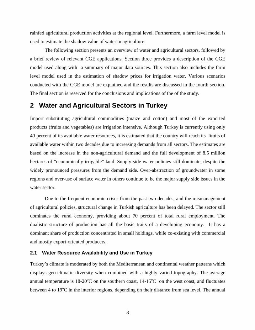
The macroeconomic stabilization program, incorporating tight fiscal and monetary

policies, has affected the water related features of the Turkish agricultural sector. The

agricultural subsidization reform program was never transformed into a reform in agricultural

policies involving the water sector. A large number of already planned, yet incomplete irrigation

development projects have been further delayed due to a lack of investable funds. The prevailing

irrigation policy framework for infrastructure development has been revitalized as the economy

recently recuperated, with the help of the program, without any emphasis on the more efficient

use of water resources.

However, several developments will certainly increase the competition for water

resources and may stipulate radical changes in water policies in the medium and long run. The

rapid pace of urbanization may lead to changes in the inter-sectoral allocation of water. The

Mediterranean basin is expected to be severely affected by the climate change. This may further

increase the pressure on an already stressed water economy with severe implications for the

agricultural sector. Growing interest by developed countries in biofuels, combined with

increasing energy prices, is aggravating the impact of climate change. Although recent surges in

prices of basic staples have begun to decline, the agricultural commodity prices, however, are

expected to remain high compared to historical averages. In addition, the renewal of the WTO-

Agreement on Agriculture and Turkey’s candidacy for membership to the European Union (EU)

will add new dimensions to the deliberations on agricultural and water policies.

Based on this background it is therefore necessary to evaluate the consequences of recent

changes in the national and international scenes in the Turkish economy to provide better

dialogue with policy makers and to develop proper policy responses.

The purpose of this study is to analyze the potential effects of surging agricultural prices,

climate change, and urbanization in the Turkish economy by using an economy-wide model. The

Walrasian CGE model for Turkey disaggregates the economy into 20 agricultural and 9 non-

agricultural activities. The agricultural sector is further disaggregated into 5 regions. The model

incorporates agricultural and non-agricultural water use with the differentiated irrigated and

8

rainfed agricultural production activities at the regional level. Furthermore, a farm level model is

used to estimate the shadow value of water in agriculture.

The following section presents an overview of water and agricultural sectors, followed by

a brief review of relevant CGE applications. Section three provides a description of the CGE

model used along with a summary of major data sources. This section also includes the farm

level model used in the estimation of shadow prices for irrigation water. Various scenarios

conducted with the CGE model are explained and the results are discussed in the fourth section.

The final section is reserved for the conclusions and implications of the of the study.

2 Water and Agricultural Sectors in Turkey

Import substituting agricultural commodities (maize and cotton) and most of the exported

products (fruits and vegetables) are irrigation intensive. Although Turkey is currently using only

40 percent of its available water resources, it is estimated that the country will reach its limits of

available water within two decades due to increasing demands from all sectors. The estimates are

based on the increase in the non-agricultural demand and the full development of 8.5 million

hectares of “economically irrigable” land. Supply-side water policies still dominate, despite the

widely pronounced pressures from the demand side. Over-abstraction of groundwater in some

regions and over-use of surface water in others continue to be the major supply side issues in the

water sector.

Due to the frequent economic crises from the past two decades, and the mismanagement

of agricultural policies, structural change in Turkish agriculture has been delayed. The sector still

dominates the rural economy, providing about 70 percent of total rural employment. The

dualistic structure of production has all the basic traits of a developing economy. It has a

dominant share of production concentrated in small holdings, while co-existing with commercial

and mostly export-oriented producers.

2.1 Water Resource Availability and Use in Turkey

Turkey’s climate is moderated by both the Mediterranean and continental weather patterns which

displays geo-climatic diversity when combined with a highly varied topography. The average

annual temperature is 18-20oC on the southern coast, 14-15oC on the west coast, and fluctuates

between 4 to 19oC in the interior regions, depending on their distance from sea level. The annual

9

average precipitation is 643 mm, yet varies from 250 mm in the central part to 3000 mm in the

Eastern Black Sea region. Seventy-five percent of annual rain falls during the winter season.

Annual rainfall is less than 500 mm in the inland Thrace and in the Eastern Anatolia regions.

This diverse precipitation structure emphasizes the crucial importance of irrigation.

Generally, agricultural production is adversely affected by the shortage and

inconsistency of rainfall during the growing season. Solar energy makes it possible to grow arid

and semi-arid crops such as bananas and citrus. Moreover, it is possible to grow 2 to 3 different

crops in irrigated areas that have crop growing seasons for a period of 270 days. However, some

crops may be harvested before maturation, particularly in Eastern Anatolia with its 60 to 90

growing days. The southeast region has a very low humidity level. The coastal regions are humid

with high precipitation rates. Inevitably, the topographic features are main factors shaping the

distribution. The long-term annual evaporation rates indicate a high rate, particularly in the

southeast region, which receives almost no rainfall during the summer, and reaches more than

2000 mm per year in the Southeastern region (Kanber et al., 2005).

The average annual precipitation of the country corresponds to a water potential of 501

km3 per year, of which 274 km3 are lost to evapotranspiration, 69 km3 feed aquifers and 158 km3

flow through the rivers to the sea or lakes. The gross total surface and ground water potential of

Turkey amounts to 234 km3 (Table 2.1).

Table 2.1. Turkey: Water Resources Potential and Use Surface water Groundwater Total Surface flow 158 km3

Feeding groundwater 69 km3

Mean annual precipitation 501 km3 (603mm)

Surface runoff a 193 km3

Recharge 41 km3

Renewable water potential 234 km3

Usable surface runoffb 98 km3

Safe yield 14 km3

Usable (net) 112 km3

Consumption 31

Consumption 12

Consumption 43

Notes: a includes the contributions from underground (28 km3) and from the neighboring countries (7 km3); b includes the usable flow of 3 km3 from the neighboring countries. Sources: DSI, 2008a.

The amount of surface water utilized for consumption purposes is in the range of 98 km3

per year, including the contributions from the neighboring countries. According to the studies

based on groundwater resources, the total safe yield of groundwater resources is estimated to be

10

14 km3. Thus, the total potential available water resources from surface flow and groundwater

would amount to 112 km3 per year.

The country’s surface runoff is unevenly distributed in both time and place, consistent

with precipitation. Surface and ground water resources are limited in the Aegean, Thrace and

Central Anatolia regions where the demand for water is higher than the rest of Turkey. The

Aegean and Thrace Regions are highly urbanized and industrialized, and have soil resources

suitable for irrigation. They have 10.5 percent of total surface water resources for the country

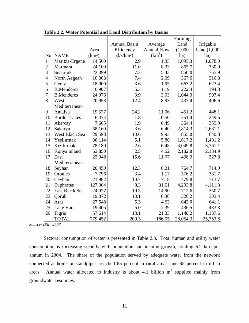
while covering 19.3 percent of the entire area. Almost 30 percent of the total surface water for

the country flows through two rivers, the Tigris and Euphrates (Table 2.2). An irregular regime

of rivers requires reservoirs to regulate the water. It is estimated that 98 km3 of surface water (51

percent of total surface water) can be consumed by technically and economically feasible

projects. The actual utilizable water amount in Turkey is around 1,700 cum/person/year in 2007.

11

Table 2.2. Water Potential and Land Distribution by Basins

No NAME Area (km²)

Annual Basin Efficiency (l/s/km²)

Average Annual Flow

(km3)

Farming Land

(1,000 ha)

Irrigable Land (1,000

ha) 1 Maritza-Ergene 14,560 2.9 1.33 1,095.3 1,078.02 Marmara 24,100 11.0 8.33 865.7 730.03 Susurluk 22,399 7.2 5.43 850.0 755.94 North Aegean 10,003 7.4 2.09 367.6 316.35 Gediz 18,000 3.6 1.95 667.2 623.46 K.Menderes 6,907 5.3 1.19 222.4 194.87 B.Menderes 24,976 3.9 3.03 1,044.3 907.48 West

Mediterranean 20,953 12.4 8.93 437.4 406.6

9 Antalya 19,577 24.2 11.06 451.2 448.110 Burdur Lakes 6,374 1.8 0.50 251.4 249.511 Akarcay 7,605 1.9 0.49 364.4 359.912 Sakarya 58,160 3.6 6.40 2,814.3 2,681.113 West Black Sea 29,598 10.6 9.93 855.0 640.814 Yeşilırmak 36,114 5.1 5.80 1,617.2 1,401.215 Kızılırmak 78,180 2.6 6.48 4,049.8 3,761.116 Konya inland 53,850 2.5 4.52 2,182.8 2,134.917 East

Mediterranean 22,048 15.6 11.07 438.3 327.8

18 Seyhan 20,450 12.3 8.01 764.7 714.019 Orontes 7,796 3.4 1.17 376.2 331.720 Ceyhan 21,982 10.7 7.18 779.8 713.721 Euphrates 127,304 8.3 31.61 4,293.8 4,111.322 East Black Sea 24,077 19.5 14.90 712.6 350.723 Çoruh 19,872 10.1 6.30 326.2 303.424 Aras 27,548 5.3 4.63 642.0 641.125 Lake Van 19,405 5.0 2.39 436.5 433.326 Tigris 57,614 13.1 21.33 1,148.2 1,137.6 TOTAL 779,452 209.3 186.05 28,054.3 25,753.6

Source: DSI, 2007.

Sectoral consumption of water is presented in Table 2.3. Total human and utility water

consumption is increasing steadily with population and income growth, totaling 6.2 km3 per

annum in 2004. The share of the population served by adequate water from the network

connected at home or standpipes, reached 85 percent in rural areas, and 98 percent in urban

areas. Annual water allocated to industry is about 4.1 billion m3 supplied mainly from

groundwater resources.

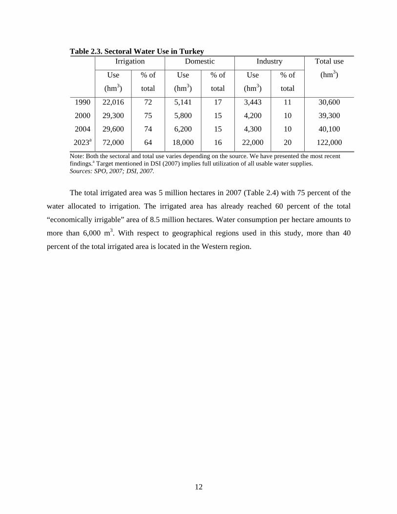
12

Table 2.3. Sectoral Water Use in Turkey Irrigation Domestic Industry

Use

(hm3)

% of

total

Use

(hm3)

% of

total

Use

(hm3)

% of

total

Total use

(hm3)

1990

2000

2004

2023a

22,016

29,300

29,600

72,000

72

75

74

64

5,141

5,800

6,200

18,000

17

15

15

16

3,443

4,200

4,300

22,000

11

10

10

20

30,600

39,300

40,100

122,000

Note: Both the sectoral and total use varies depending on the source. We have presented the most recent findings.a Target mentioned in DSI (2007) implies full utilization of all usable water supplies. Sources: SPO, 2007; DSI, 2007.

The total irrigated area was 5 million hectares in 2007 (Table 2.4) with 75 percent of the

water allocated to irrigation. The irrigated area has already reached 60 percent of the total

“economically irrigable” area of 8.5 million hectares. Water consumption per hectare amounts to

more than 6,000 m3. With respect to geographical regions used in this study, more than 40

percent of the total irrigated area is located in the Western region.

13

Table 2.4. Irrigation Development by Regions, 2007 (1,000 ha) DSI Region Geo.R DSI DSI (GWIC) GDRS Farmers Total

1 Bursa W 58 5 31 952 Izmir W 122 15 50 147 3343 Eskisehir W 77 26 68 1714 Konya C 190 187 163 95 6355 Ankara C 53 4 81 1386 Adana W 323 17 86 34 4617 Samsun C 88 20 67 51 2268 Erzurum E 84 16 96 154 3509 Elazig E 82 5 103 101 291

10 Diyarbakir SE 43 0 20 6311 Edirne W 61 21 55 40 17612 Kayseri C 82 20 100 58 26013 Antalya W 80 6 21 10714 Istanbul W 0 6 615 Sanliurfa SE 189 0 22 21217 Van E 66 1 67 43 17718 Isparta W 109 61 83 46 29919 Sivas C 23 1 35 73 13220 K.Maras SE 48 6 49 10321 Aydin W 199 18 59 130 40622 Trabzon E 13 1 35 23 7223 Kastamonu C 13 2 28 2 4424 Kars E 71 20 37 12825 Balikesir W 62 7 38 10626 Artvin E 11 11

Total 2,136 438 1,394 1,034 5,001Sources: DSI, 2008b ; GDRS, 2007 ; SPO, 2007.

The Western region is more populated and industrialized compared to the rest of the

country. In addition, the seven river basins in this area are estimated to have already exceeded

their long-term capacity utilization rates (World Bank, 2007). About 90 percent of irrigation

methods depend on gravity systems with low water efficiency. Furthermore, the irrigation ratios

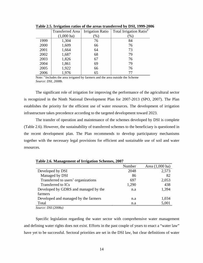
of the schemes transferred by State Hydraulic Works (DSI) indicate that about 35 percent of the

irrigated area are allocated to rainfed agriculture (Table 2.5). Unavailability of water is the top

reason for the shift to rainfed agriculture (DSI, 2008a).

14

Table 2.5. Irrigation ratios of the areas transferred by DSI, 1999-2006 Transferred Area

(1,000 ha) Irrigation Ratio

(%) Total Irrigation Ratioa

(%) 1999 1,304 76 84 2000 1,609 66 76 2001 1,664 64 73 2002 1,687 68 79 2003 1,826 67 76 2004 1,861 69 79 2005 1,922 66 76 2006 1,976 65 77

Note: a Includes the area irrigated by farmers and the area outside the Scheme Source: DSI, 2008b.

The significant role of irrigation for improving the performance of the agricultural sector

is recognized in the Ninth National Development Plan for 2007-2013 (SPO, 2007). The Plan

establishes the priority for the efficient use of water resources. The development of irrigation

infrastructure takes precedence according to the targeted development toward 2023.

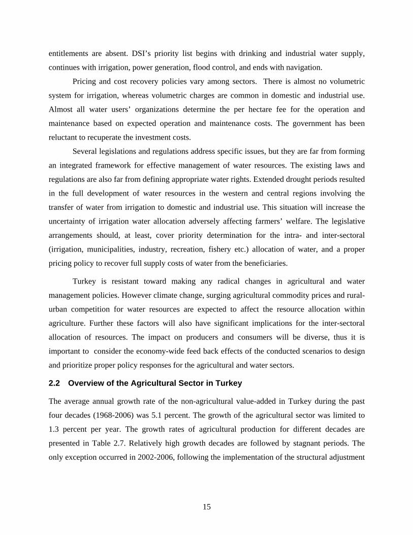
The transfer of operation and maintenance of the schemes developed by DSI is complete

(Table 2.6). However, the sustainability of transferred schemes to the beneficiary is questioned in

the recent development plan. The Plan recommends to develop participatory mechanisms

together with the necessary legal provisions for efficient and sustainable use of soil and water

resources.

Table 2.6. Management of Irrigation Schemes, 2007 Number Area (1,000 ha)Developed by DSI 2048 2,573 Managed by DSI 86 82 Transferred to users’ organizations 697 2,053 Transferred to ICs 1,290 438Developed by GDRS and managed by the farmers

n.a 1,394

Developed and managed by the farmers n.a 1,034Total n.a 5,001

Source: DSI (2008a)

Specific legislation regarding the water sector with comprehensive water management

and defining water rights does not exist. Efforts in the past couple of years to enact a “water law”

have yet to be successful. Sectoral priorities are set in the DSI law, but clear definitions of water

15

entitlements are absent. DSI’s priority list begins with drinking and industrial water supply,

continues with irrigation, power generation, flood control, and ends with navigation.

Pricing and cost recovery policies vary among sectors. There is almost no volumetric

system for irrigation, whereas volumetric charges are common in domestic and industrial use.

Almost all water users’ organizations determine the per hectare fee for the operation and

maintenance based on expected operation and maintenance costs. The government has been

reluctant to recuperate the investment costs.

Several legislations and regulations address specific issues, but they are far from forming

an integrated framework for effective management of water resources. The existing laws and

regulations are also far from defining appropriate water rights. Extended drought periods resulted

in the full development of water resources in the western and central regions involving the

transfer of water from irrigation to domestic and industrial use. This situation will increase the

uncertainty of irrigation water allocation adversely affecting farmers’ welfare. The legislative

arrangements should, at least, cover priority determination for the intra- and inter-sectoral

(irrigation, municipalities, industry, recreation, fishery etc.) allocation of water, and a proper

pricing policy to recover full supply costs of water from the beneficiaries.

Turkey is resistant toward making any radical changes in agricultural and water

management policies. However climate change, surging agricultural commodity prices and rural-

urban competition for water resources are expected to affect the resource allocation within

agriculture. Further these factors will also have significant implications for the inter-sectoral

allocation of resources. The impact on producers and consumers will be diverse, thus it is

important to consider the economy-wide feed back effects of the conducted scenarios to design

and prioritize proper policy responses for the agricultural and water sectors.

2.2 Overview of the Agricultural Sector in Turkey

The average annual growth rate of the non-agricultural value-added in Turkey during the past

four decades (1968-2006) was 5.1 percent. The growth of the agricultural sector was limited to

1.3 percent per year. The growth rates of agricultural production for different decades are

presented in Table 2.7. Relatively high growth decades are followed by stagnant periods. The

only exception occurred in 2002-2006, following the implementation of the structural adjustment

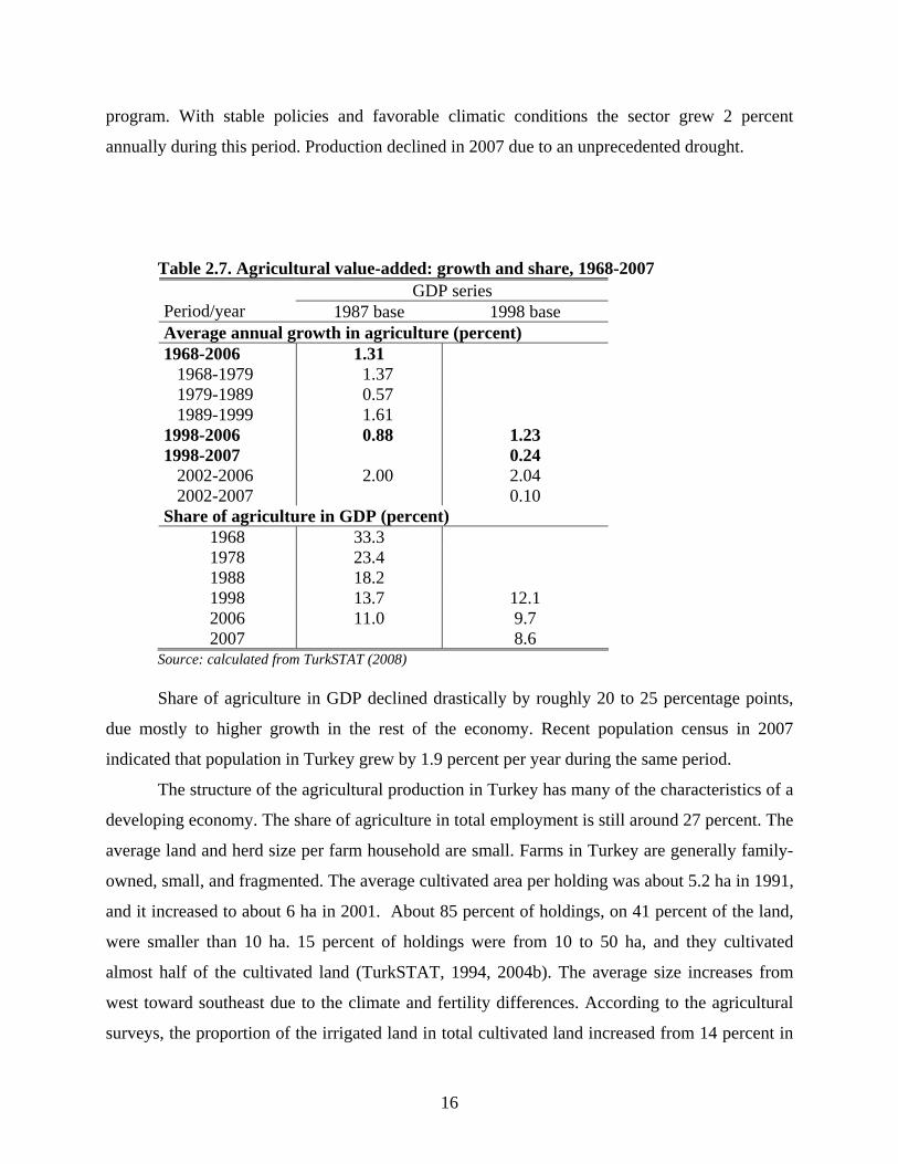
16

program. With stable policies and favorable climatic conditions the sector grew 2 percent

annually during this period. Production declined in 2007 due to an unprecedented drought.

Table 2.7. Agricultural value-added: growth and share, 1968-2007 GDP series

Period/year 1987 base 1998 base Average annual growth in agriculture (percent) 1968-2006 1.31 1968-1979 1.37 1979-1989 0.57 1989-1999 1.61 1998-2006 0.88 1.23 1998-2007 0.24 2002-2006 2.00 2.04 2002-2007 0.10 Share of agriculture in GDP (percent)

1968 33.3 1978 23.4 1988 18.2 1998 13.7 12.1 2006 11.0 9.7 2007 8.6

Source: calculated from TurkSTAT (2008)

Share of agriculture in GDP declined drastically by roughly 20 to 25 percentage points,

due mostly to higher growth in the rest of the economy. Recent population census in 2007

indicated that population in Turkey grew by 1.9 percent per year during the same period.

The structure of the agricultural production in Turkey has many of the characteristics of a

developing economy. The share of agriculture in total employment is still around 27 percent. The

average land and herd size per farm household are small. Farms in Turkey are generally family-

owned, small, and fragmented. The average cultivated area per holding was about 5.2 ha in 1991,

and it increased to about 6 ha in 2001. About 85 percent of holdings, on 41 percent of the land,

were smaller than 10 ha. 15 percent of holdings were from 10 to 50 ha, and they cultivated

almost half of the cultivated land (TurkSTAT, 1994, 2004b). The average size increases from

west toward southeast due to the climate and fertility differences. According to the agricultural

surveys, the proportion of the irrigated land in total cultivated land increased from 14 percent in

17

1991, to 20 percent in 2001. The share of irrigated land is much higher in the west than

elsewhere in Turkey. One third of the holdings smaller than 1 ha have access to irrigation. The

distribution of agricultural land remained skewed with a Gini coefficient of 0.60. A slight

tendency towards the medium ranges from smaller sizes are observed from 1991 to 2001

(TurkSTAT, 1994, 2004b).

Of the 26 million ha of cultivated land (TurkSTAT, 2006), field crops have occupied

slightly over 85 percent of the cultivated area since 1985. The share of the vegetable area is

about 3 percent, but has been increasing steadily. Orchards occupy 10 percent of the cultivated

land. Land left to fallow is about 5 million hectares. The value composition of the agricultural

production diverge drastically from the use of the cultivated land. The weight of crop production

has been dominant in the total value of production. The value of livestock products makes a

quarter of the total value (TurkSTAT, 2006b). The structure of production is far from reflecting

the policy weights that seem to underlay government intervention in agriculture. The policies are

generally targeted towards cereals and industrial crops, whereas vegetables and fruits have

relatively smaller importance apart from some specialty products. However, the share of fruits

and vegetables in total value is slightly over 40 percent. Protection and government support of

animal products have not been sufficient to counterbalance the additional costs of feed due to

interventions in the cereals. Turkish consumers end up paying higher prices compared with the

average meat and milk prices in the EU.

The employment creation capacity of the economy has always been problematic, mainly

because the growth in the country’s capital stock has not been commensurate with the rapid

expansion of the labor force. Despite improvements in economic indicators since 2002, the

unemployment rate remains stagnant at around 10 percent. The rural unemployment rates, both

male and female, are the major contributing factors in the stickiness of the overall unemployment

rate. The declining trends in the rural labor force participation rates and the share of agriculture

in rural employment, combined with increasing rural unemployment rates, signal the start of a

major transformation in the use of labor in agriculture. However, agriculture is still helping to

overcome the chronic nature of unemployment in Turkey. It eases the detrimental effect of the

lack of human capital on growth rates of the labor force, and the inability of the non-farm sector

to pull even more labor from agriculture. The illiteracy in agricultural employment is

significantly higher compared to the rest of the economy (Çakmak and Akder, 2005) which

18

contributes to the difficulty of pulling labor out of agriculture. Due to the small average farm

size, agricultural employment has a relatively large share in total employment. The sector

provides employment for almost all females within rural areas with almost an 85 percent share in

rural employment. However, like other rapidly growing economies, the share of agricultural

employment in overall employment, as well as absolute agricultural employment, are steadily

declining. Agricultural employment was 6 million in 2007 compared with 9 million in the early

1990s.

Turkey may be considered a perfect example of the mismanagement of agricultural policies

particularly after reforms that took place in the mid-1980s. Agricultural policies involved mainly

transfers and were not aimed at improving productivity. The transfers to producers occurred

mostly from consumers through support purchases for major crops backed by high tariffs.1 Until

the onset of the structural adjustment program in 2001, transfers to farmers from the taxpayers

were not substantial but were accompanied by huge financial costs. Most of the budgetary

transfers to farmers were not planned causing high financial losses for state banks. The financial

burden was further amplified by the “duty losses” of state economic enterprises through support

purchases and revolving credit lines to the agricultural sales cooperatives’ unions. The

Agricultural Reform Implementation Project (ARIP) began in 2001 as part of the second phase

of the structural adjustment program.

Total producers’ subsidy in Turkey showed a significant increase prior to the start of

structural adjustment program in 1999. The contribution of agricultural policies to the farmers’

revenue increased from USD3.4 billion to USD8.0 billion during the 1990s (OECD, 2006). The

general effects of ARIP were significant with a sudden drop in the support to agriculture in 2001.

The state intervention in the output markets was severely restricted in 2001, coupled with the

delayed implementation of direct income support. The domestic market has been adjusting fast.

The market price support provided by the border measures has picked up again in 2002 and it has

remained high ever since.

The share of total agricultural support in GDP was 6 percent in the late 1990s. It declined

to 3.8 percent in 2005, but is still one of the highest (as a share of GDP) among OECD member

1 Turkey accomplished significant liberalization of trade in industrial products. The liberalization in the agriculutral sector has been proceeding at a slow pace. Except for the primary commodities extensively used as intermediate inputs in export oriented manufacturing industries (cotton, raw hides and skins), Turkey has high levels of protection in meat, dairy products, sugar and basic cereals.

19

countries. The rate of consumer subsidy equivalents (CSE) is back to the pre-crisis level in 2005

of 21 percent. The distribution of transfers to producers has not changed much since the 1980s,

except in 2001. The share of market price support in producer subsidy equivalents (PSE)

remained around 80 percent. The remaining burden falls on the taxpayers. Significant shifts

between policy tools occurred in budgetary support. Input price intervention almost disappeared,

instead area based direct income support (DIS) contributed 15 percent of support to producers.

Concerning the trade policy, high tariff levels for the major commodities and non-tariff

protection stayed intact until the recent surge in agricultural prices in 2006 and 2007.

Considering the fact that the share of food expenditures for the average consumer is still more

than 30 percent, the government tried to decrease the wedge between domestic and world prices

by granting duty free imports mostly to the state procurement agency. The funds used for DIS

payments have been directed more towards the commodity specific deficiency payments.

The state of agriculture both in terms of its growth pattern and overall structure of

production makes it necessary to evaluate the economy-wide implications of surging world

prices in Turkey.

3 The Modeling Framework

The application of computable general equilibrium (CGE) modeling analysis on water

management issues is relatively new in the literature. CGE Modeling has made possible the

exploration of economy-wide effects of water policy. CGE models dealing with water issues can

be broadly grouped into five categories according to their research questions.

The first group of models deals with the competition of different sectors or alternative

user groups for water. Seung et al. (2000) models the welfare effects of using water in irrigation

or for recreational purposes. Briand (2004) on the other hand, introduces drinking water demand

and analyzes the competition between drinking and irrigation water.

The second group of models investigates the cost recovery and pricing based water

conservation policies. Beritella (2006) for example analyzes the global and national level

economic impacts of water transfer projects in China. Valezquez (2007) analyzes the effects of

the increase in the price of irrigation water on the efficiency of the water consumption in

agriculture and the possible reallocation of water to the other sectors. Letsoalo et al. (2005) test

the ‘triple dividend hypothesis’ to see if water price policies can bring about reduced water use,

20

more rapid economic growth and a more equal income distribution simultaneously. He concludes

that it is possible to achieve triple dividends through water pricing.

A third group of models is related to the facilitation or liberalization of irrigation water

trade. In fact, almost all relevant papers in the literature can be included in this group. However,

some studies are missing the necessary constructs to simulate water markets. Goodman (2000)

shows that water trade can replace construction of new irrigation facilities by increasing

efficiency. Peterson (2004) shows that the impact of water shortages can be compensated by

increasing water trade. Dywer (2005), extends the analysis of Peterson (2004) to urban water

usage. Tirado (2004) shows the effect of having a market for water rights between urban and

agricultural sectors and argues that such a market would benefit both user groups. Kohn (2003),

on the other hand, investigates the effect of international water trade by using a Heckser-Ohlin

framework.

The last group of models attempt to combine CGE models with other types of models.

Finoff (2004) introduces a bio-economic model based on general equilibrium approach while

Smajgl et al.(2005) integrates theoretically agent-based modeling with CGE models. Lastly,

some recent models began to analyze the micro-macro linkages in water issues with CGE

models. Roe et al. (2005) and Diao et al. (2005, 2008) use both top-down (trade reform) and

bottom-up (farm water assignments and the possibility of water trading) linkages. They

concluded that trade reform (top-bottom or macro to micro linkage) has a higher effect compared

to water reform (bottom-up or micro to macro linkage).

Several CGE models were developed for Turkey aimed at analyzing macroeconomic

issues in the 1990s. A selected list may include Harrison et al. (1993, 1996), Yeldan (1997),

Karadag and Westaway (1999). Starting in the early 2000s, efforts devoted to develop CGE

models for Turkey have increased. However, these models are also geared toward macro and

trade analysis with aggregated agricultural sector.

CGE models targeted to analyze the issues of Turkish agriculture are relatively few.

Agricultural CGE models on Turkey generally seek to address trade liberalization and reform

issues. The first serious attempt to analyze the Turkish agriculture by using a CGE model is

Cakmak et al. (1996), where a partial equilibrium model is coupled with a CGE model. The CGE

model had an aggregated agricultural sector together with three non-agricultural sectors. The

dynamics in the agricultural sector were captured via the sectoral model. Further, the simulations

21

related to the agricultural sector were done via the sectoral model, while the CGE simulations

aimed to evaluate the effects of macroeconomic shocks and to reveal the role of the agricultural

sector in the macroeconomic adjustment processes.

Diao and Yeldan (2001) developed a general equilibrium model of the Turkish economy

with a detailed agricultural sector. They have used an inter-temporal CGE model to analyze the

effects of global agricultural trade liberalization. Turkey is one of the regions in the model along

with Morocco and other Middle Eastern countries. Agriculture is disaggregated into five

subsectors; grain crops, vegetables and fruits, sugar, other agriculture and animal products. Their

main conclusion was in favor of trade liberalization.

Dogruel et al. (2003) used a CGE model to explore the feasible alternatives of

agricultural reform and links between “the public sector fiscal balances, accumulation patterns,

dynamic resource allocation, and consumer welfare under a medium-long-term horizon”. The

model consists of six sectors. Agriculture is modeled as an aggregate sector. Land is not included

in the model as a production factor. Hence the model is not a “real” agricultural model though

the question of the research is agricultural.

The intention of the CGE model developed by Çırpıcı (2008), is to analyze water

management issues in Turkey. The model has 9 sectors, incorporating 4 factors of production.

Agriculture is not disaggregated. Water enters agricultural production as land and water

aggregate calibrated with a Leontief function. The Cobb-Douglas production function is used in

the non-agricultural production. The model lacks the regional and sectoral detail in agricultural

production.

Studies using CGE models to conduct agricultural policy analysis incorporate agriculture

as an aggregate sector both in production and consumption. Thus the policy simulations can not

take into account possible interactions within the agricultural sector. The model used in this

study namely, Turkish Agricultural Computable General Equilibrium Model with Water

(TACOGEM-W), incorporates enriched treatment of agricultural production and consumption

activities.

TACOGEM-W is the first attempt that exclusively models Turkish agriculture both in

regional and sectoral details. The model utilizes the results of a farm level model developed for a

micro region to estimate the shadow price of irrigation water. Hence, the rent created by the low

22

prices for irrigation water is included in the model, linking the micro and macro aspects of

irrigation water management.

3.1 Structure of the Agricultural Computable Equilibrium Model for Turkey

TACOGEM-W is a Walrasian CGE model that includes the behavior of the three main sectors in

the Turkish economy: the production activities, the institutions, and the foreign sector. In order

to study the impact of a range of policy simulations, TACOGEM-W further disaggregates the

economy into 20 agricultural and 9 non-agricultural activities. Agricultural activities are

categorized by field crops, livestock, fishing and forestry (classified as ‘other agriculture’). Non-

agricultural activities include mining, consumer manufacturing, food manufacturing,

intermediates and capital goods, electricity and gas, water, construction, private services and

government services. Table 3.1 provides a break-down of the Turkish GDP in activities for the

year 2003. Accordingly, about 12 percent of gross output was devoted to agriculture, about 25

percent to industry, and the remaining 63 percent to services.

Table 3.1. Gross national product by kind of activity, 2003

Product in current prices

ISIC, Rev. 2 Value

(Billion TL)Sector share

(%) Agriculture 42 126 246 11.8

Agriculture and livestock 39 550 179 11.1 Forestry 1 268 139 0.4 Fishing 1 307 928 0.4

Industry 88 813 240 24.9 Mining and quarrying 3 858 087 1.1 Manufacturing 71 910 797 20.2 Electricity, gas, water 13 044 356 3.7

Trade 71 329 760 20.0 Transportation and communication 53 846 171 15.1 Financial institutions 17 884 644 5.0 Ownership of dwelling 14 653 025 4.1 Business and personal services 12 429 089 3.5

(Less) Imputed bank service charges 7 911 747 2.2 Government services 36 561 477 10.3 Private non-profit institutions 3 610 383 1.0 Import duties 13 758 630 3.9 GDP (in purchasers’ value) 359 762 926 100.9 Net factor income from rest of the world -3 082 038 -0.9 GNP (in purchasers’ value) 356 680 888 100.0

Source: TurkSTAT (2005)

23

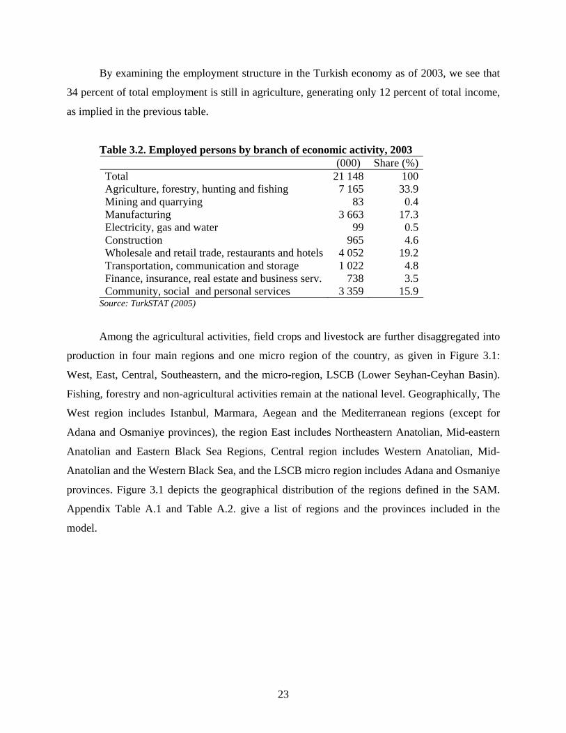
By examining the employment structure in the Turkish economy as of 2003, we see that

34 percent of total employment is still in agriculture, generating only 12 percent of total income,

as implied in the previous table.

Table 3.2. Employed persons by branch of economic activity, 2003 (000) Share (%) Total 21 148 100 Agriculture, forestry, hunting and fishing 7 165 33.9 Mining and quarrying 83 0.4 Manufacturing 3 663 17.3 Electricity, gas and water 99 0.5 Construction 965 4.6 Wholesale and retail trade, restaurants and hotels 4 052 19.2 Transportation, communication and storage 1 022 4.8 Finance, insurance, real estate and business serv. 738 3.5 Community, social and personal services 3 359 15.9

Source: TurkSTAT (2005)

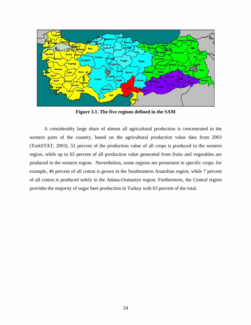
Among the agricultural activities, field crops and livestock are further disaggregated into

production in four main regions and one micro region of the country, as given in Figure 3.1:

West, East, Central, Southeastern, and the micro-region, LSCB (Lower Seyhan-Ceyhan Basin).

Fishing, forestry and non-agricultural activities remain at the national level. Geographically, The

West region includes Istanbul, Marmara, Aegean and the Mediterranean regions (except for

Adana and Osmaniye provinces), the region East includes Northeastern Anatolian, Mid-eastern

Anatolian and Eastern Black Sea Regions, Central region includes Western Anatolian, Mid-

Anatolian and the Western Black Sea, and the LSCB micro region includes Adana and Osmaniye

provinces. Figure 3.1 depicts the geographical distribution of the regions defined in the SAM.

Appendix Table A.1 and Table A.2. give a list of regions and the provinces included in the

model.

24

Figure 3.1. The five regions defined in the SAM

A considerably large share of almost all agricultural production is concentrated in the

western parts of the country, based on the agricultural production value data from 2003

(TurkSTAT, 2003). 51 percent of the production value of all crops is produced in the western

region, while up to 65 percent of all production value generated from fruits and vegetables are

produced in the western region. Nevertheless, some regions are prominent in specific crops: for

example, 46 percent of all cotton is grown in the Southeastern Anatolian region, while 7 percent

of all cotton is produced solely in the Adana-Osmaniye region. Furthermore, the Central region

provides the majority of sugar beet production in Turkey with 63 percent of the total.

25

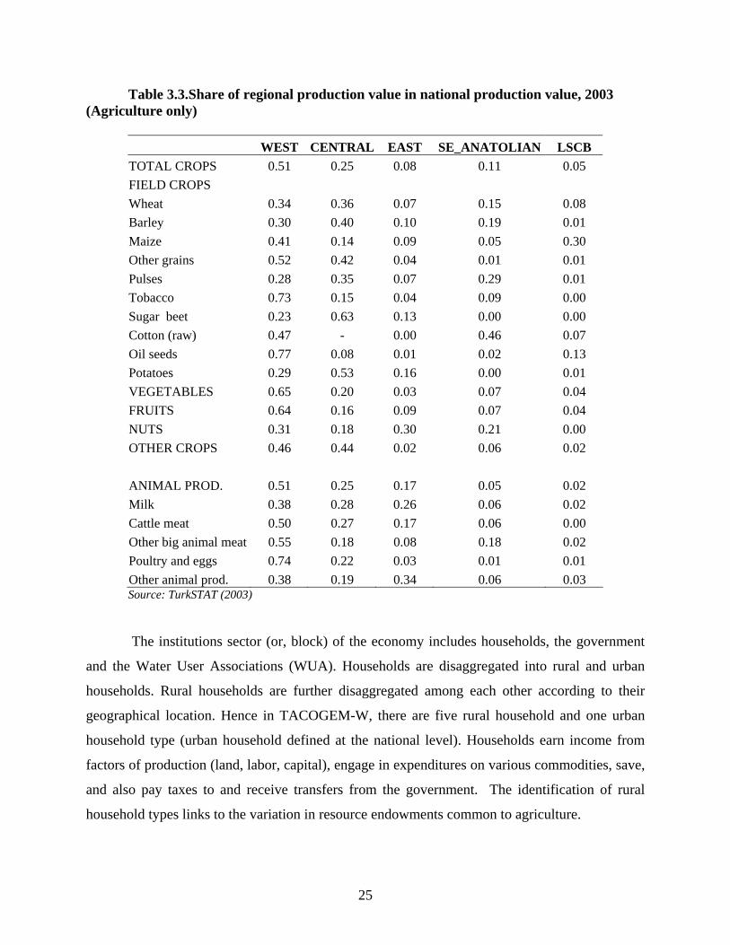
Table 3.3.Share of regional production value in national production value, 2003 (Agriculture only)

WEST CENTRAL EAST SE_ANATOLIAN LSCB TOTAL CROPS 0.51 0.25 0.08 0.11 0.05 FIELD CROPS Wheat 0.34 0.36 0.07 0.15 0.08 Barley 0.30 0.40 0.10 0.19 0.01 Maize 0.41 0.14 0.09 0.05 0.30 Other grains 0.52 0.42 0.04 0.01 0.01 Pulses 0.28 0.35 0.07 0.29 0.01 Tobacco 0.73 0.15 0.04 0.09 0.00 Sugar beet 0.23 0.63 0.13 0.00 0.00 Cotton (raw) 0.47 - 0.00 0.46 0.07 Oil seeds 0.77 0.08 0.01 0.02 0.13 Potatoes 0.29 0.53 0.16 0.00 0.01 VEGETABLES 0.65 0.20 0.03 0.07 0.04 FRUITS 0.64 0.16 0.09 0.07 0.04 NUTS 0.31 0.18 0.30 0.21 0.00 OTHER CROPS 0.46 0.44 0.02 0.06 0.02 ANIMAL PROD. 0.51 0.25 0.17 0.05 0.02 Milk 0.38 0.28 0.26 0.06 0.02 Cattle meat 0.50 0.27 0.17 0.06 0.00 Other big animal meat 0.55 0.18 0.08 0.18 0.02 Poultry and eggs 0.74 0.22 0.03 0.01 0.01 Other animal prod. 0.38 0.19 0.34 0.06 0.03 Source: TurkSTAT (2003)

The institutions sector (or, block) of the economy includes households, the government

and the Water User Associations (WUA). Households are disaggregated into rural and urban

households. Rural households are further disaggregated among each other according to their

geographical location. Hence in TACOGEM-W, there are five rural household and one urban

household type (urban household defined at the national level). Households earn income from

factors of production (land, labor, capital), engage in expenditures on various commodities, save,

and also pay taxes to and receive transfers from the government. The identification of rural

household types links to the variation in resource endowments common to agriculture.

26

The government collects tax revenue from numerous sources: production, sales,

households, and imports. The government uses these funds for purchases of goods and services

at the respective markets and makes transfers to households, and engages in public savings.

Regional activities of field crops , in addition to land, labor and capital, use water as an

input in production. These activities also make payments to WUAs in their respective regions.

These water charges are income earned by the Water User Associations. In TACOGEM-W, it is

assumed that this water income collected in each region is simply transferred back to the

respective rural household in a lump-sum.

In Turkey, as of 2003, 87 percent of all agricultural land is devoted to cultivation of field

crops (Table 3.4). About 23 percent of all agricultural land is under irrigation, and similarly, 22

percent of all field area sown is irrigated (Table 3.5).

Table 3.4. Agricultural land use, 2003 (000 Hectare) Share (%)

Agricultural land 26 027 100 Cultivated field area 22 554 86.7

Area sown 17 563 67.5 Fallow land 4 991 19.2

Area of vegetable gardens 818 3.1 Area of vineyards 530 2.0 Area of fruit trees 1 500 5.8 Area of olive trees 625 2.4

Source: TurkSTAT (2005)

Table 3.5. Irrigated versus rainfed land use, 2001 (hectares) Total area Irrigated Not irrigated

Total area 15,322,010 3,505,749 11,816,261 Area sown 12,253,912 2,716,529 9,537,383 Fallow land 2,737,560 2,737,560

Vegetable and flower gardens

371,512 271,009 100,503

Fruit orchards and other permanent crops

1,757,962 455,590 1,302,372

Source: TurkSTAT (2004b)

For 38 percent of the irrigated area, wells are the most important source of water (Table

3.6). The second most important source of irrigation is streams, followed by the use of dams. The

most common method to supply water to crops is flooding, which accounts for 84 percent of the

area irrigated (Table 3.7).

27

Table 3.6. Irrigated area by irrigation source, 2001 Area (hectare) Share (%)Total irrigated land 3,505,749 100 Well 1,316,709 37.6 Spring 352,403 10.0 Stream 1,003,856 28.6 Lake 67,666 1.9 Artificial lake 99,715 2.8 Dam 556,346 15.9 Other sources 109,052 3.1

Source: TurkSTAT (2004b)

Table 3.7. Irrigated area by irrigation system, 2001 Area (hectare) Share (%)

Total 3,505,749 100 Flooding irrigation 2,865,356 84.1 Sprinkler irrigation 582,414 17.1

Drip irrigation 57,978 1.7 Source: TurkSTAT (2004b)

To construct the regionalized SAM for the year 2003 (please see Table A.3 for a more

aggregated version of the SAM for the year 2003), we combine various data from 2003

Agricultural Structure-Production, Price, Value Statistics (TurkSTAT, 2003); Telli (2004); 1998

Input Output Structure of the Turkish Economy (TurkSTAT, 2004a); 2003 foreign trade statistics

by Undersecretariat of Foreign Trade (UFT Website); TurkSTAT 2002 Household consumption

expenditures and income survey statistics (TurkSTAT Website), ARIP Quantitative Household

Survey (QHS) commissioned by the Treasury and implemented by the G.G. Consulting et al.

(conducted in 2002 and 2004), and the Turkish SAM for 2001 developed by GTAP. This

regionalized SAM includes information on the regional level employment of labor and capital as

well as intermediate input use by crop, along with water charge and irrigated versus rainfed land

rents by crop. Employment of capital, labor and data on intermediate input use are also entered

for activities at the national level in the SAM. Detailed income, consumption and saving

information for the five-types of households (urban, and four rural) are included in the

institutions block of the SAM. Also included in the institutions block are the data on government

consumption, net tax receipts, and public savings, along with the WUAs’ accounts. Finally,

import, export and tariff data concerning the EU-25 and the rest of the world constitute the

28

foreign sector block of the SAM (the foreign trade partners to Turkey are the 25 European Union

countries and the rest of the world). These detailed data are used to obtain the parameters for

TACOGEM-W.

The algebraic structure of TACOGEM-W is based on the CGE model developed by

Lofgren, et al. (2002). The entire sequence of mathematical equations that define TACOGEM-W

is provided in Appendix B. Main characteristics of the TACOGEM-W include:

Production technology in each activity is defined by a CES function of value added

and aggregate intermediate input use;

Value added in each activity is given by a CES production function of factors used

(labor, capital, irrigated land, rainfed land and water, if applicable);

Aggregate domestic output is distributed among domestic use and exports (EU and

rest of the world) by a Constant Elasticity of Transformation function;

Composite output supply (of domestic supply and imports from the EU and the rest

of the world) is of Armington form;

All producers take factor and commodity prices as given, and are all profit

maximizers;

Urban and rural household types in each region have a simple consumption pattern

in the sense that they devote a fixed share of expenditures on each consumption item. Each

household type has a different consumption pattern depending on household income and savings.

Implicitly in this structure, households are assumed to minimize expenditures on consumption,

taking as given the price of each commodity.

Households derive income from factors of production depending on the household

type. Urban households earn income from labor services and capital rent, while each rural

household earns income from services of labor and capital, as well as land rents (irrigated and

rainfed) and income from the WUA’s via transfers from government;

The government also has a fixed consumption pattern in the sense that it devotes a

fixed share of expenditures on each commodity. The government derives income from various

types of taxes (import, export, production, sales, etc.) and also saves. The government in this

model also acts as an intermediary between the WUA’s and the rural households in the sense that

the water charges collected from agricultural producers by the WUA’s are then distributed to

rural households in their respective regions by the government.

29

In TACOGEM-W, each commodity and factor market clears, implying that there is

no unemployment of any factor of production, including labor. At the base year of 2003, all

prices for commodities and factors are given exogenously, implying that the relevant markets are

assumed to clear at these prices. But the prices of commodities and factors are expected to

respond endogenously to any shock given to the economy, via the policy scenarios given below.

The model closure is the standard Walrasian closure through investment and

saving balance.

30

3.2 The Farm Model: Structure and Results2

Econometric or programming approaches are commonly used in the literature to estimate water

demand in agriculture. However, econometric estimation of water demand is limited because of

the lack of necessary data. Furthermore, even if the data is available, quantity and price

variations are typically small, leading to inaccurate estimations due to large variances. The

programming approach uses the concept of shadow prices in order to derive the water demand.

The programming approach starts by assuming that water is provided free of charge but is

constrained at the level x. The approach, in fact, asks the question how much farmers are willing

to pay to relax the water constraint by Δ units.

Suppose that, in addition to water, crop production involves k inputs ( )1 2, ... kz z z z= that

can be purchased at the prevailing market prices ( )1 2, ... kr r r r= with a perfectly elastic supply

curve and m primary inputs (e.g., land) ( )1 2, ... ks s s s= that are available free of charge in limited

quantities ( )1 2, ... mb b b b= . Moreover, let us denote the production function by ( ), ,F q z s . Note

that, here, q is input of water used in the production. In this situation, the decision problem for

the producer can be expressed as (Tsur, Dinar, Roe, and Doukkali, 2004, p.5):

( ) ( ) ( )( )1 1 2 2, , , max , , , , ... k kx b p r q z s pF q z s r z r z r zπ = − + + +

subject to q x≤ (water constraint)

s b≤ (land, family labor etc constraints)

possibly other, (non-negativity constraints)

where, x is the water constraint, p is price of crop, z represents the purchased inputs (such as

fertilizer, hired labor, machinery, pesticide, etc..), q is water input, s represents fixed inputs (such

as, land, family labor, capital, etc.).

For nonlinear production functions ( ), ,F q z s , the above constrained optimization

constitutes a non-linear programming problem. A special case arises when the function F admits

2 The authors ackowledge the contribution of Ozan Eruygur in Sections 3.2 and 3.3.

31

the Leontief form, and in this case, the constrained optimization reduces to a linear programming

problem. As a result, a simple model can be expressed as follows:

1 1max ... n nL Lπ π π= + +

subject to

Shadow Prices, λ

11 1 12 2 1... n na L a L a L x+ + + ≤ (water constraint)

1 ... nL L L+ + ≤ (land constraint)

21 1 22 2 2... n na L a L a L b+ + + ≤ (labor)

other constraints, non-negativity, rotation, etc..

where jπ is crop j’s profit per hectare with j = 1,2,…,n and is calculated from data and jL is

crop j’s land allocation which is the decision variable. Note that the shadow price for water is λ ,

land is Lμ and family labor is fμ .

In this setup the shadow price for the water constraint is the value of the marginal product

of irrigation water. In order to get the derived demand for irrigation water, we should change the

water constraint from zero when irrigation water is not binding (Tsur et al, 2004, p.6). Notice

that this setup is the model structure most generally used in order to estimate the derived demand

for water in the literature. Algebraic Details of the model can be found in Appendix C.

3.3 Linkage between the Farm Model and TACOGEM-W

The farm model is used to estimate the shadow value of water in agricultural production. The

formula for the derived demand is found to be 0.4718.3wQ P−=

32

Figure 3.2. Shadow rent

Consider Figure 3.2. AQ is water demand at the shadow price. EDQ is the demand at the

actual price level. In this setup, shadow rent is the difference between the farmers’ surplus at λ

and AP , shown by the shaded are. This area can be calculated by

( ) 0.4718.3A

A AP

SR P Q Pλ

λ −= − + ∫

( ) ( )1.47 1.4739A A ASR P Q Pλ λ− −= − + −

then since

( )1.47 1.47

1.471.47

39

1 39 1

A A

AA

A AA

A

A AA A A A

A

A AA

P QQ

P

P QQ P Q SR P P Q

P

P QP

SR PP

λ λ

λ λ λ

λ λ

− −

−

−

=

− − = −

= −

− =

⎛ ⎞⎛ ⎞ ⎛ ⎞⎜ ⎟+ −⎜ ⎟ ⎜ ⎟⎜ ⎟⎝ ⎠⎝ ⎠ ⎝ ⎠

the shadow rent (SR) can be calculated by merely using the ratio of shadow price to actual price,

the actual payments made for irrigation and actual price. From the data used to form the SAM for

TACOGEM-W 32.5 TRY 1000mAP per≅ and 388,800Million mEDQ ≅ . Farm model yields

35 TRY 1000mperλ ≅ and 378,000Million mAQ ≅ . Substituting these values yields,

33

1.471.475

12.5

52.5 78,000,000 39 2.5 12.5

210,600,000 6.48

SR−

−= −⎛ ⎞⎛ ⎞⎛ ⎞× × + × × −⎜ ⎟⎜ ⎟ ⎜ ⎟⎜ ⎟⎝ ⎠ ⎝ ⎠⎝ ⎠

= −

Hence one can ignore the 1.47

1.4739 1AA

PPλ

−

−⎛ ⎞⎛ ⎞⎜ ⎟−⎜ ⎟⎜ ⎟⎝ ⎠⎝ ⎠

term in the calculation of shadow rent. Then,

1 15

2.5A A A A A AA

P Q P Q P QP

SR λ= − −

⎛ ⎞ ⎛ ⎞= =⎜ ⎟ ⎜ ⎟⎝ ⎠⎝ ⎠

which implies that shadow rent for water is twice the actual payment made to water. Under these

findings we added this shadow rent to the payments made to irrigation water as a factor of

production.

4 Empirical Results

Simulations reported in this study are selected according to their relevance and importance in

water management issues, as well as agricultural policies of Turkey in the medium to long run.

The first set of simulations involve the effects of changes in world agricultural prices; the second

set of simulations examine the impacts of rural to urban water reallocation within each region;

and the last set of simulations analyze the impact of climate change on agriculture.

World agricultural prices began to rise in 2005 (OECD and FAO, 2008). The level of the

price increase has caused international concern, because of its effect on those with low income.

International institutions, including the OECD, EU, FAO, IFPRI, United Nations and the World

Bank have called attention to the adverse affects of the increases in prices. The recent surge of

prices in agricultural commodities has immediately affected low income consumers in Turkey.

The share of food expenditures in total expenditures is near 40 percent in the lowest quintile

(TurskSTAT, 2006). Although the prices are expected to decline from peaks achieved in 2007,

the real prices of basic staples are expected to be higher than historical averages in the medium

run. This situation may stimulate agricultural production and increase the income for farmers. It

may also change the cropping pattern and increase the pressure on water resources. Consumers

on the one hand have been and will continue to be adversely affected by the increase in prices.

These interdependencies ask for a modeling structure which will take into account the economy

wide effects of the increase in prices.

34

The severe drought in 2007 brought focus on the increasing competition for water

between urban and rural areas. Metropolitan municipalities, mainly in the Western part of the

country, have already begun to develop and implement projects to bring water from rural areas to

the cities. This has increased the stress on irrigation water resources. The model structure

reveals the possible effects of carrying on and extending this transfer policy on crop production

pattern and other key economic variables.

Finally, climate change scenarios have also attracted considerable attention in Turkey.

Climate change is expected to reduce precipitation in most parts of Turkey depending on the

region. Reduced precipitation is anticipated to have severe adverse effects on the rainfed

agriculture. Even the irrigated agricultural production will demand more water as a result of

reduced precipitation. Combined by the increase in the urban demand, the pressure on water

resources will certainly increase. The discussion on this topic is generally limited to the price

(and hence production) effects of climate change. We attempt to simulate the effects of the

anticipated climate change by shocking the yields of various crops to see the economy wide

effects. The following section presents the aggregate results for the scenarios. A thorough

discussion on the design of the scenarios together with the obtained results can be found in the

subsequent sections.

4.1 Aggregate Results of the Simulations

World price increase is simulated by introducing the estimations given in FAO and OECD

(2008). Product specific changes in prices are reported in Table 4.3. The average increase is

about 30 percent. Water is reallocated from agriculture to urban and industrial use in the West

region in the urbanization scenario. Simulations involve increasing urban water supply by 30

percent (Scenario 2.a) and 50 percent (Scenario 2.b) with a corresponding reduction in water

available for irrigation in this region. Lastly climate change scenario is quantified by a fall in the

yields of rain-fed crops by 30 percent (Scenario 3.a) and then by an additional decline in the

yields of irrigated crops by 10 percent (Scenario 3.b). The regional yields of both rain-fed and

irrigated crops are reduced at varying degrees in the last version of climate change scenario

(Scenario 3.c).

Total nominal and real GDP decline, almost in all scenarios, with the exception of the

urbanization scenario. The magnitude of the decline in nominal GDP is highest in the climate

35

change scenario: The more severe the climate change, the more severe is the decline. There is a

significant decline in rainfed and livestock activities. Value added created by rainfed activities

deteriorates as a result of a declining yield in rainfed activities. Livestock production falls due to

increasing crop prices and costs in livestock production. However, increasing production in

irrigated land compensates for the decline in other sectors.

Value added created by agriculture increases in all scenarios in nominal terms. However,

real agricultural value added declines. This implies, that in all three cases the effects working on

increasing domestic price dominates the effects working on the cost of production.

Sectoral value added is highly sensitive to the shock given in the climate change scenario

when compared with the impact of other scenarios.

Table 4.1. Effects on GDP

Base % Change

Level

(1000 TRY) Sc. 1 Sc. 2a Sc. 2b Sc. 3a Sc. 3b Sc. 3cTotal 335,699,820 -0.79 0.12 -0.12 -5.82 -7.00 -5.90 Agriculture 48,935,094 5.24 1.54 2.04 1.34 1.91 1.63 Rainfed Agriculture 25,688,482 8.34 4.16 7.34 -6.48 -0.18 2.65 Irrigated Agricultural 18,001,061 4.58 -1.44 -3.77 28.89 24.20 16.87 Other Agriculture 5,245,551 -7.68 -1.01 -3.97 -54.92 -64.36 -55.69 Non-Agricultural 286,764,725 -1.81 -0.13 -0.48 -6.96 -8.42 -7.11 Services 168,529,416 -1.38 1.36 1.43 -6.86 -8.24 -6.88

at F

acto

r Cos

ts

Industry 118,235,309 -2.42 -2.25 -3.21 -7.10 -8.68 -7.43

Nom

inal

at Market Prices 379,686,752 -1.13 0.07 -0.17 -5.56 -6.74 -5.69Total 335,699,820 -0.31 0.25 0.35 -2.66 -3.47 -3.02 Agriculture 48,935,094 -0.05 -1.66 -3.02 -15.90 -20.02 -17.37 Rainfed Agriculture 25,688,482 1.34 1.34 2.73 -37.67 -35.03 -27.16 Irrigated Agricultural 18,001,061 -1.30 -6.04 -11.37 15.60 1.73 -3.19 Other Agriculture 5,245,551 -2.55 -1.36 -2.55 -17.44 -21.21 -18.13

at F

acto

r Cos

ts

Non-Agricultural 286,764,725 -0.35 0.58 0.92 -0.37 -0.59 -0.53 Services 168,529,416 -0.19 0.08 0.07 -0.29 -0.49 -0.41 Industry 118,235,309 -0.59 1.28 2.14 -0.47 -0.75 -0.69

Rea

l

at Market Prices 379,686,752 -0.57 0.32 0.45 -1.94 -2.54 -2.23Source: Results from TACOGEM-W. Note: Sc1: Agricultural prices are increased according to FAO and OECD 2008; Sc2a: 30 percent water transfer from urban to rural areas; Sc2b:50 percent water transfer from urban to rural areas; Sc3a: Yield of rainfed crops falls by 30 percent; Sc3b: Yield of rainfed crops falls by 30 percent and irrigated crops falls by 10 percent; Sc3c: Regional yields of all crops falls at various degrees.

36

Agricultural value added increases in all scenarios. The increase is mainly due to the

increase in production in irrigated activities for the climate change scenario, in rainfed activities

in the urbanization scenario and in the world price increase scenario. Other agricultural activities

deteriorate in all scenarios. The value added of other activities falls as much as 64 percent.

Industrial activities also experience a decline of approximately 2 to 9 percent. A change in the

non-agricultural value added is also higher in the climate change scenario. The changes in the

real value added are milder. Furthermore, the industrial value added increases in real terms

within the urbanization scenario.

The comparison of changes in nominal and real GDP and the sectoral value added show

that an important account of GDP change is due to adjustment in prices. In real terms, effects are

milder, and in the opposite direction.

Table 4.2. Macroeconomic results of simulations

Base % Change Levela Sc. 1 Sc. 2a Sc. 2b Sc. 3a Sc. 3b Sc. 3c Absorption 384,423,455 -0.5 0.3 0.4 -1.9 -2.5 -2.2 Household Consumption 245,160,549 -0.2 1.2 1.7 -1.8 -2.4 -2.1 Investment 75,017,087 -1.7 -2.3 -3.2 -3.8 -5.1 -4.5 Export 98,447,183 -1.4 -0.6 -0.9 -2.1 -2.6 -2.4 Import 103,183,886 -1.0 -0.6 -0.9 -2.0 -2.4 -2.2 PPP Real FX Rate 100 -0.5 0.1 -4.2 -5.0 -4.2 Nominal FX Rate 100 -1.8 -0.1 -0.4 -5.9 -7.1 -6.0 Export Price Index 100 0.9 Import Price Index 100 0.7 World Price Index 100 0.8 Domestic Price Index 100 -0.5 -0.2 -0.4 -1.8 -2.2 -1.9 Consumer Price Index 100 Terms of Trade 100 0.2 Source: Results from TACOGEM-W. Notes: a 1000 TRY for GDP accounts. Sc1: Agricultural prices are increased according to FAO and OECD 2008; Sc2a: 30 percent water transfer from urban to rural areas; Sc2b:50 percent water transfer from urban to rural areas; Sc3a: Yield of rainfed crops falls by 30 percent; Sc3b: Yield of rainfed crops falls by 30 percent and irrigated crops falls by 10 percent; Sc3c: Regional yields of all crops falls at various degrees.

For demand side macro variables we can conclude similar results. The change is higher in

climate change scenario. Total consumption falls for the first and third scenarios, while

increasing in urbanization. However, when water consumption is removed from the scenario,

consumption falls for the urbanization scenario as well. For all scenarios, agricultural

consumption decreases while the manufacturing goods consumption increases.

37

4.2 Scenario 1: Increase in World Prices

World agricultural prices began to rise significantly early in 2005 and by June 2008 prices was

above historical peaks for almost all agricultural commodities traded internationally (OECD and

FAO, 2008). Although a decline in prices is expected in the short run, the average is expected to

remain above the mean of last 10 years in the medium term. This increase is expected to be

between 20 percent to 80 percent for various agricultural products.

For the change in world prices we follow the estimates given by FAO and OECD (2008)

for 2016-2017. The magnitude of price shocks given to the model is depicted in Table 4.3. The

average increase is about 30 percent.

Table 4.3. Price Shocks in Scenario 1

Product

Increase in World Price

(%) Product

Increase inWorld Price

(%) Wheat 48 Fruits 10 Barley 45 Nuts 10 Maize 42 Other crops 45 Other grains 45 Milk 62 Pulses 45 Cattle Meat2 19 Sugar beet 27 Other Bovine Meat2 23 Raw Cotton1 7 Poultry and Eggs 24 Oil seeds 42 Other Animal Prod. 20 Potatoes 10 Other Agricultural Prod. 20 Vegetables 10 Average 30

1 Ethridge et. al. (2006) and FAPRI (2008) 2 Estimate for European Union Source: FAO and OECD (2008), Ethridge et al. (2006) and FAPRI (2008)

Introducing the price shocks from Table 4.3 into the model has two primary effects. First

of all, agricultural imports and exports change significantly. Increasing demand for exports will

change the equilibrium price and quantities in the goods market. However the magnitude of the

effects will be determined by elasticities. Since we employ an Armington structure, an increase

in world prices are not reflected directly in domestic prices. Table 4.4 shows the resulting change

in production and prices of commodities as a result of the price shocks described in Table 4.5.

Price changes are higher for maize, pulses and other animal products. These products have a

relatively higher share in agricultural exports and lower Armington elasticities implying a lower

substitutability of domestic and imported goods.

38

Table 4.4. Change in domestic average output prices and composite good supply and domestic production

Domestic Production Aggregate Supply Price

Base

(1000 Tons)Change

(%) Base

(1000 Tons)Change

(%) Base Change

(%) Wheat 19,000 6.53 20,550 -0.56 0.50 4.05 Barley 8,100 1.63 7,974 -0.50 0.35 3.04 Maize 2,800 32.22 4,614 2.88 0.50 8.00 Other grains 758 0.19 782 -3.05 4.75 5.23 Pulses 1,558 20.20 1,356 0.95 1.82 7.05 Tobacco 1,529 -5.15 1,384 -3.91 1.48 3.09 Sugar beet 12,623 -2.90 12,651 -3.01 0.28 2.50 Cotton (raw) 2,295 5.94 2,987 -2.09 1.19 0.59 Oil seeds 2,359 4.20 2,058 -2.85 0.74 4.44 Potatoes 5,300 -1.59 5,179 -1.69 0.54 2.63 Vegetables 24,019 -2.65 23,288 -2.64 0.69 3.30 Fruits 13,221 -2.59 12,096 -2.97 0.89 3.73 Nuts 789 -1.96 570 -3.31 4.80 4.75 Other crops 2,974 -4.06 2,581 -3.76 2.16 4.76 Milk 9,096 -2.43 9,126 -2.65 1.00 0.58 Cattle Meat 5,243 -1.81 5,242 -1.81 1.00 0.72 Other Bovine Meat 2,333 -0.61 2,305 -1.16 1.00 0.52 Poultry and Eggs 3,646 -2.11 3,588 -3.08 1.00 3.91 Other Animal Prod. 2,113 6.84 2,046 -4.45 1.00 9.03 Other Agricultural Prod. 6,213 1.64 6,347 -2.73 1.00 -1.01 Food Production 31,970 -4.03 30,490 -1.69 1.00 2.15 Mining 4,407 -0.92 19,962 -1.00 1.00 -1.85 Consumer Manufac. 101,370 -0.60 77,701 0.36 1.00 -1.61 Int. and Cap. Goods 129,439 -1.19 173,759 -0.75 1.00 -1.71 Electricity and Gas 26,923 -0.12 26,923 -0.12 1.00 -1.24 Water 9,414 -0.03 9,414 -0.03 1.00 -2.25 Construction 46,351 -1.48 46,351 -1.48 1.00 -1.99 Private Services 219,470 -0.34 191,560 -0.11 1.00 -1.44 Government Services 69,195 -0.01 69,195 -0.01 1.00 -0.81

Source: Results from TACOGEM-W.

Domestic production increased significantly in almost all activities as a result of the price

shocks. This increase covers the decline in imports and increase in exports. Another interesting

result is the connection between agricultural trade and other sectors’ production and prices. This

effect originates from the household utility maximization, which is the second main driver of the

effects of the shock. Income and Urban household consumption declined roughly by 1 percent.

39

Furthermore there was a 1.7 percent decline in investment spending and a 1.2 percent decline in

the intermediate input demand. Thus an increase in world prices of agricultural commodities

causes a decline in prices of other commodities that compete for resources.

For these products quantity of supply and price moves in the same direction. This implies

a higher export demand for these goods. A comparison of the share of exports and imports in

total production, represented in Table 4.5., reveals this fact. The increase in exports is relatively

higher for maize, pulses and other animal products while the increase in imports is minimal.

Table 4.5. Percentage change in share of exports and imports in total production Export Import Base Sc. 1 Base/Sc.1 Base Sc. 1 Base/Sc.1Wheat 0.01 0.02 3.42 8.98 2.63 0.29 Barley 2.32 3.69 1.59 0.93 0.56 0.61 Maize 1.58 2.92 1.85 68.56 35.95 0.52 Other grains 0.07 0.11 1.55 8.17 5.28 0.65 Pulses 11.16 22.19 1.99 0.88 0.32 0.36 Tobacco 24.05 23.45 0.97 14.60 15.21 1.04 Sugar beet 0.00 0.01 1.87 0.22 0.12 0.53 Cotton (raw) 6.97 8.60 1.23 37.26 29.15 0.78 Oil seeds 4.37 5.58 1.28 18.54 14.13 0.76 Potatoes 0.93 1.00 1.07 0.30 0.28 0.94 Vegetables 1.97 2.08 1.06 0.38 0.36 0.94 Fruits 7.09 7.47 1.05 0.64 0.60 0.94 Nuts 19.61 20.34 1.04 0.62 0.58 0.94 Other crops 0.06 0.13 2.10 0.13 0.06 0.48 Milk 0.04 0.07 1.66 0.38 0.23 0.60 Cattle Meat 0.02 0.02 1.29 Other Bovine Meat 1.24 1.73 1.40 0.01 0.01 0.71 Poultry and Eggs 2.15 2.89 1.35 0.55 0.40 0.73 Other Animal Prod. 14.58 20.14 1.38 11.40 7.16 0.63 Other Agricultural Prod. 3.64 5.52 1.52 5.80 3.66 0.63 Food Production 8.04 6.57 0.82 3.42 4.31 1.26 Mining 18.47 18.49 1.00 371.40 371.04 1.00 Consumer Manufac. 33.13 32.67 0.99 9.79 10.06 1.03 Int. and Cap. Goods 23.00 22.88 0.99 57.24 57.71 1.01 Private Services 12.72 12.52 0.98

Source: Results from TACOGEM-W.

The net effect of increasing world food prices on household welfare is also controversial.

Non-farm households are likely to be adversely affected by increasing food prices. However,

increasing export demand has the reverse effect by changing the factor allocation and causing a

40

new equilibrium within the factor markets. Demand for the factors used by agriculture is likely to

increase, while factor demand by industrial sectors is expected to decline. The ultimate result

will be determined by the calibrated model parameters.

The change in the allocation of factors among activities is given in Table 4.6. Labor

employment increases in all activities, except in tobacco production. Increases are as high as 44

percent in maize and 32.5 percent in pulses; which are the sectors most affected by the

designated world price change. Land and water employment in maize also increases

significantly, at the cost of employment of these factors in the other sectors.

Table 4.6. Percentage change in factor employment Labor Rainfed Land Irrigated Land Water Base* Sc. 1** Base† Sc. 1** Base† Sc. 1** Base‡ Sc. 1**

Wheat 2,662 12.51 8,267 1.95 1,898 3.36 5,133 4.43Barley 734 7.30 3,165 -3.47 Maize 344 44.02 458 29.74 128 33.45 738 33.46Oth. grains 1,367 4.99 629 -5.51 140 -2.28 437 -3.42Pulses 678 32.50 1,535 18.84 Tobacco 734 -1.65 219 -11.01 Sugar beet 1,225 0.24 426 -6.56 3,177 -6.43Cotton 377 11.19 646 2.85 5,667 2.66Oil seeds 391 10.53 505 1.02 108 2.54 381 3.36Potatoes 985 1.68 215 -5.25 999 -4.80Vegetables 5,731 1.63 3,687 -8.08 826 -6.52 4,187 -5.72Fruits 4,065 1.79 1,154 -6.65 439 -6.49 2,134 -5.69Nuts 1,295 2.34 418 -7.30 Oth. crops 2,242 0.62 202 -9.07 39 -7.43 122 -8.22Total Agr. 22,831 4.94 20,238 0.00 4,866 0.00 22,975 0.00

Source: Results from TACOGEM-W. * In terms of labor VA, Million TRY, ** % Change, † 1000 Ha., ‡ Million m3. By comparing Table 4.6 with Table 4.4 an important fact is revealed. Labor employment

increases despite the fall in production quantities. An important account of factors shifts to the

agricultural sector to compensate for the loss in total supply as a result of the increase in import

prices.

Since total supply of land and water is fixed in the model, the change reflects the

reallocation process as various sectors compete for resources. Factors are shifted to the activities

where prices increase as a result of the world price shock. Water use increases in wheat, maize,

cotton and oil seeds at the cost of water usage in other sectors.

41

The change in the wage rate for labor is not as high as the other factors. Prices of other

factors increased more in the Southeast and LSCB regions. This shows a higher stress on the

resources of these regions as a result of a world price shock.

Table 4.7: Change in factor prices Base

Region Level (TRY) Sc. 1

Labor 1.00 -0.81West 0.27 12.29Central 0.11 14.44East 0.11 13.29Southeast 0.23 15.63

Rainfed Land

LSCB 0.14 20.33West 0.64 8.79Central 0.26 8.91East 0.27 9.15Southeast 0.53 10.45

Irrigated Land

LSCB 0.70 12.14West 0.13 12.12Central 0.11 9.79East 0.05 10.92Southeast 0.09 16.69LSCB 0.13 22.06

Water

Urban 0.81 -2.31Source: Results from TACOGEM-W.

The most important conclusion of this simulation is that change in world prices have

significant welfare implications differentiated among urban and rural households. A change in

prices brings about a decline in import demand while boosting the export supply. Consequently,

domestic prices increase and strike the urban households through consumption while causing an

expansion in the income of rural households. Furthermore, increasing agricultural world prices

hampers the industrial sector as well. This effect is a result of the direct competition for

resources with agriculture, and in intermediate demand for agricultural products that are now

relatively more costly. This causes a second wave of problems for urban households by

suppressing their income.

42

4.3 Scenario 2: The Urbanization Scenario

In the early 1950s in Turkey, internal or rural-to-urban migration and urbanization gained

momentum with accelerating development and industrialization trends. Migration is defined as

‘residency shifts across geographical regions and/or administrative areas’ (Ünalan, 1998). Such

residency shifts may be due to natural, social, economic, or political requisites (Pazarlıoğlu,

1997). According to Akşit (1998), Turkey has experienced internal migration most prominently

during the period 1950-1985. Table 4.8 shows that in 1975 the share of the urban population in

total population was 42 percent, jumping to 52 percent in 1985, and reaching 65 percent in 2000

(World Bank, World Development Indicators Online). Akşit (ibid.) states that the contribution of

internal migration in such population movements is above 50 percent.

Table 4.8.Urban population dynamics in Turkey 1975 1980 1985 1990 1995 2000 2003Population growth (annual, %) 2 2 2 2 2 2 2Urban population (% of total) 42 44 52 59 62 65 66Urban population growth (annual, %) 4 3 6 5 3 2 2

Source: World Bank WDI Online

According to latest figures from TurkSTAT, migration across different centers has

reached 6,662,263 individuals within the period 1995-2000. This implies that during this time

frame 11 percent of the total population in Turkey has been on the move from one residential

area to another. Figure 4.1 displays the break-down of the migrating population across different

centers for this period. One important aspect to mention is that when compared to previous

periods, urban-to-rural (city-to-village) migration is gaining relative importance. Urban to rural

migration consists of 20 percent of the total during 1995-2000, while this ratio used to be only 13

percent on average during 1980-1990. Rural to rural migration is observed to lose importance

progressively from year to year, while urban to urban migration remains to be the principal form

of migration, nevertheless showing a slight drop when compared to previous periods.

43

Urban to urban; 57,8

Rural to urban; 17,46

Urban to rural; 20,06

Rural to rural; 4,68

Figure 4.1: In-migration by places of residence (%), 1995-2000

Source: TurkSTAT (2005)

Factors such as a high population growth rate, industrialization, mechanization of

agricultural production, shifts in land ownership, inadequate education and health services, a

desire to break away from traditional social pressures and feuds in rural areas, as well as

increased transportation and communication facilities, can be cited among the most significant

factors of internal migration in Turkey (Kahraman, et al., 2002). Indeed, depending on the time

period considered, factors that determine the decision to migrate in Turkey, since the 1950s, can

be classified as “push”, “pull”, and “transmitting” (Munro, 1974; İçduygu and Ünalan, 1998).

Beginning with the 1950s through the end of the 1960s, migration in Turkey from rural into

urban areas can be explained by push factors. Kahraman, et al. (2002) explain that the

introduction of new technologies and increased mechanization of agriculture led to a surplus in

labor within this sector that migrated into urban areas increasing the laborers hopes for survival

and a decent living. Division of land into smaller lots (mainly due to inheritance disputes within

families) and thus rendering land less productive, introduction of intensive (modern) techniques

in agriculture and finally the inadequacy of educational, health and cultural amenities in rural

areas can be considered as other factors that pushed individuals from rural into urban areas.

While migration during the 1950s through the end of 1960s can be explained by push

factors described above, migration from the end of 1960s into the 1980s may be accounted for by

pull factors (İçduygu and Ünalan, 1998). These pull factors consist of the rural-urban wage gap,

concentration of manufacturing and services sectors’ work opportunities (Mazumdar, 1998;

Kahraman, et al., 2002) and an additionally richer educational and cultural environment as along

with more and improved health facilities within urban areas. During the 1980s and 1990s, on the

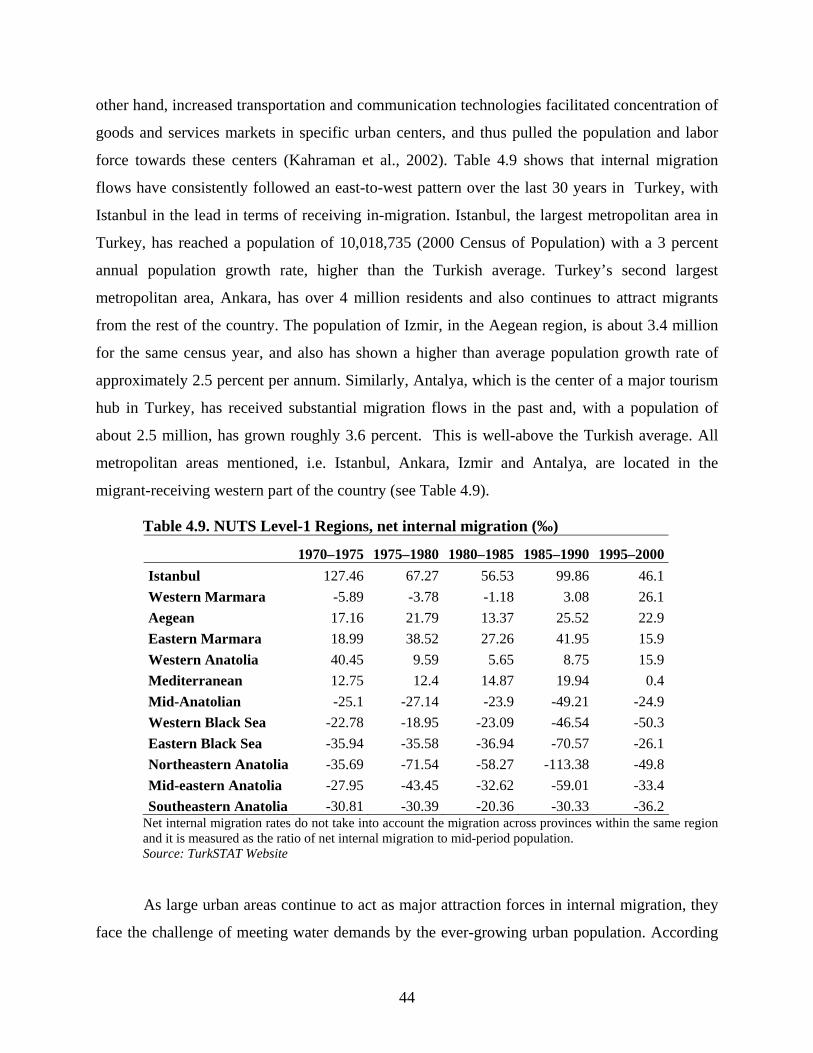
44

other hand, increased transportation and communication technologies facilitated concentration of

goods and services markets in specific urban centers, and thus pulled the population and labor

force towards these centers (Kahraman et al., 2002). Table 4.9 shows that internal migration

flows have consistently followed an east-to-west pattern over the last 30 years in Turkey, with

Istanbul in the lead in terms of receiving in-migration. Istanbul, the largest metropolitan area in

Turkey, has reached a population of 10,018,735 (2000 Census of Population) with a 3 percent

annual population growth rate, higher than the Turkish average. Turkey’s second largest

metropolitan area, Ankara, has over 4 million residents and also continues to attract migrants

from the rest of the country. The population of Izmir, in the Aegean region, is about 3.4 million

for the same census year, and also has shown a higher than average population growth rate of

approximately 2.5 percent per annum. Similarly, Antalya, which is the center of a major tourism

hub in Turkey, has received substantial migration flows in the past and, with a population of

about 2.5 million, has grown roughly 3.6 percent. This is well-above the Turkish average. All

metropolitan areas mentioned, i.e. Istanbul, Ankara, Izmir and Antalya, are located in the

migrant-receiving western part of the country (see Table 4.9).

Table 4.9. NUTS Level-1 Regions, net internal migration (‰)

1970–1975 1975–1980 1980–1985 1985–1990 1995–2000Istanbul 127.46 67.27 56.53 99.86 46.1Western Marmara -5.89 -3.78 -1.18 3.08 26.1Aegean 17.16 21.79 13.37 25.52 22.9Eastern Marmara 18.99 38.52 27.26 41.95 15.9Western Anatolia 40.45 9.59 5.65 8.75 15.9Mediterranean 12.75 12.4 14.87 19.94 0.4Mid-Anatolian -25.1 -27.14 -23.9 -49.21 -24.9Western Black Sea -22.78 -18.95 -23.09 -46.54 -50.3Eastern Black Sea -35.94 -35.58 -36.94 -70.57 -26.1Northeastern Anatolia -35.69 -71.54 -58.27 -113.38 -49.8Mid-eastern Anatolia -27.95 -43.45 -32.62 -59.01 -33.4Southeastern Anatolia -30.81 -30.39 -20.36 -30.33 -36.2

Net internal migration rates do not take into account the migration across provinces within the same region and it is measured as the ratio of net internal migration to mid-period population. Source: TurkSTAT Website

As large urban areas continue to act as major attraction forces in internal migration, they

face the challenge of meeting water demands by the ever-growing urban population. According

45

to a report prepared by the Regional Environment Center (REC), urban water demand accounts

for about 15 percent of the total amount of water used in 2003, and is expected to reach an

estimated 23 percent by 2030 (REC-Turkey, 2007). Additionally, as large urban centers continue

to grow, the industrial sector demand for water is also expected to increase, requiring the

metropolitan municipalities to find new water supply sources. In time, although the total water

consumption is expected to increase, the sectoral water use allocated to irrigation is expected to

decrease in the medium to long run, shifting the resources to domestic and industrial use. In this

sense, the share of water used for purposes of irrigation in total water consumption, which is

about 74 percent in 2003, is expected to drop to 65 percent by 2030 (ibid.).

Increased urbanization is expected to lead to increased rural-urban competition for water

within each region. To simulate increased urbanization and water use in Turkey, we increased

the water supply in urban areas in the West region and reduced the irrigation water available for

agriculture by the same magnitude, i.e. we reallocated the limited amount of water from

agriculture to urban and industrial use in the West region. The main reason for only considering

the West region is because the West region in TACOGEM-W covers the rapidly urbanizing

metropolitan areas such as Istanbul, Izmir and Antalya. Simulations involve increasing urban

water supply by 30 percent (Scenario 2.a) and 50 percent (Scenario 2.b) with a corresponding

reduction in water used for irrigation in this region.

As a result of a reallocation of irrigation water to urban use (Scenario 2.a) by 30 percent

in the West region, we see a decline in overall production (the sum of both irrigated and rainfed

land) of all crops by 0.5 to 3 percent (Table 4.10). We notice that an overall decline in this region

plays a very significant role because the West region produces 44 percent of all maize, 73

percent of all tobacco, 59 percent of all oil seeds, 60 percent of all fruits, 64 percent of all

vegetables, 34 percent of all nuts, and similarly, 34 percent of all wheat in the country. In

particular, we observe the highest decline in maize production, as maize is the most water-

intensive crop among all crops considered. As expected, when the water supply in irrigated

activities is reduced, a clear drop in production can be seen, and since the factors for production

released by irrigated production activities are reallocated into rainfed activities, we would expect

an increase in production in rainfed activities.

Most notably, maize and fruit production in irrigated land dropped by 7 percent,

production of oil seeds dropped by 6 percent, vegetable production by 6.7 percent, and wheat

46

production by 5 percent. We notice that production increases on rainfed land does not

compensate for the drop in production of irrigated crops. As a result, prices in all agricultural

activities increase at varying rates, while prices in national non-agricultural activities (except for

food manufacturing, electricity, gas and government services) fall at varying rates. Particularly,

the price of water as a commodity by urban use fell by 45 percent following the transfer from

rural activities in the West region.

Table 4.10. Change in total production quantity % Change Unit

Base Level Sc. 2.a Sc. 2.b

Wheat Tons 19,000 -1.78 -3.18 Barley Tons 8,100 -0.52 -1.00 Maize Tons 2,800 -3.32 -5.76 Other grains Tons 758 -1.29 -2.33 Pulses Tons 1,558 -0.68 -1.27 Tobacco Tons 1,528 -1.72 -3.07 Sugar beet Tons 12,623 -0.95 -1.87 Cotton (raw) Tons 2,295 -3.82 -6.97 Oil seeds Tons 2,359 -1.07 -1.78 Potatoes Tons 5,300 -0.37 -0.79 Vegetables Tons 24,018 -1.34 -2.54 Fruits Tons 13,221 -1.62 -2.76 Nuts Tons 789 -1.62 -2.88 Other crops Tons 2,974 -1.06 -2.00 Milk Tons 9,096 -0.79 -1.47 Cattle Meat Tons 5,242 -0.33 -0.67 Other Bovine Meat Tons 2,333 -0.10 -0.23 Food Industry VA, Million 3,646 -0.19 -0.53 Other Animal Prod. VA, Million 2,112 -0.77 -1.22 Other Agricultural Prod. VA, Million 6,212 -1.05 -1.81 Food Production VA, Million 31,969 -1.40 -2.55 Mining VA, Million 4,407 0.51 0.64 Consumer Manufac. VA, Million 101,370 0.19 0.24 Int. and Cap. Goods VA, Million 129,439 -0.65 -0.90 Electricity and Gas VA, Million 26,923 -0.04 -0.07 Water VA, Million 9,413 18.18 30.18 Construction VA, Million 46,351 -1.84 -2.56 Private Services VA, Million 219,470 0.20 0.21 Government Services VA, Million 69,194 -0.06 -0.09 Source: Results from TACOGEM-W.

A production decrease in irrigated land activities, particularly in the West, following a

reallocation of irrigation water to urban use, prompts changes in the labor use patterns.

47

Contraction in irrigated land activities in the West leads to a release of labor from these

activities. The amount of labor release is 1.25 percent in tobacco production, followed by 1.69

percent in the production of cotton. Although there is a drop in labor demand in irrigated land

activities in the West, alternative activities compete for the labor released from irrigated

activities as they experience an increase in labor demand. In fact, we see a slight increase in the

wages paid to labor by 1.1 percent as a result of the decrease in irrigation water in the West

region. The price of rainfed land rent also increases by 3.7 percent in the West Region. Since

water is used only by irrigated activities, a decline in the, water supply accompanied by a drastic

increase in water prices, forces the area allocated to irrigated activities to contract. This decreases

the price of irrigated land. Furthermore, the price of rainfed land increases because rainfed

agriculture enjoys the increase in prices without bearing any cost for the ever increasing water

prices. The inter-sectoral transfer of water raises drastically the shadow value of water for

irrigation by 70 percent. This adjustment can also be interpreted as a domestic terms of trade

effect between irrigated and rainfed land resources (Table 4.11).

Table 4.11. Change in factor prices Base % Change

Region Level(TRY) 2.a 2.b

Labor 1.00 1.10 1.18West 0.27 3.69 6.65Central 0.11 3.30 5.86East 0.11 3.08 5.45Southeast 0.23 2.84 4.97

Rainfed Land

LSCB 0.14 4.03 7.32West 0.64 -9.59 -19.06Central 0.26 2.79 4.89East 0.27 2.93 5.14Southeast 0.53 2.13 3.78

Irrigated Land

LSCB 0.70 2.60 4.61West 0.13 69.64 160.81Central 0.11 4.37 7.63East 0.05 4.48 7.87Southeast 0.09 2.65 4.88LSCB 0.13 3.32 5.96

Water

Urban 0.81 -47.62 -60.98Source: Results from TACOGEM-W.

48

The decrease in agricultural production, and the pursuing domestic price increases,

prompt imports to increase and exports to decrease in these activities, holding all else constant.

In aggregate, for example, we see decreases in the volume of exports in cotton up to 9.41 percent

(Table 4.11). Both cotton and wheat have the highest drop in the value of exports. The decrease

in production also implies lower amounts supplied to the domestic economy. Hence, to meet the

slightly increasing domestic demand due to slightly increasing domestic factor incomes, quantity

of imports rise to some extent. Albeit not as sharp as the fall in exports, all agricultural

commodities register increases in volume of imports (Table 4.12). Real urban household

consumption rises by 1.2 percent, and rural households in different regions also experience

increases in real consumption at varying degrees. For example, while rural households have a 1.1

percent increase, rural households in the Southeast region report a 1.7 percent rise in real

consumption. This difference is mainly because of changes in factor incomes across regions.

Overall, in Turkey, real household consumption shows an increase of 1.2 percent from the base.

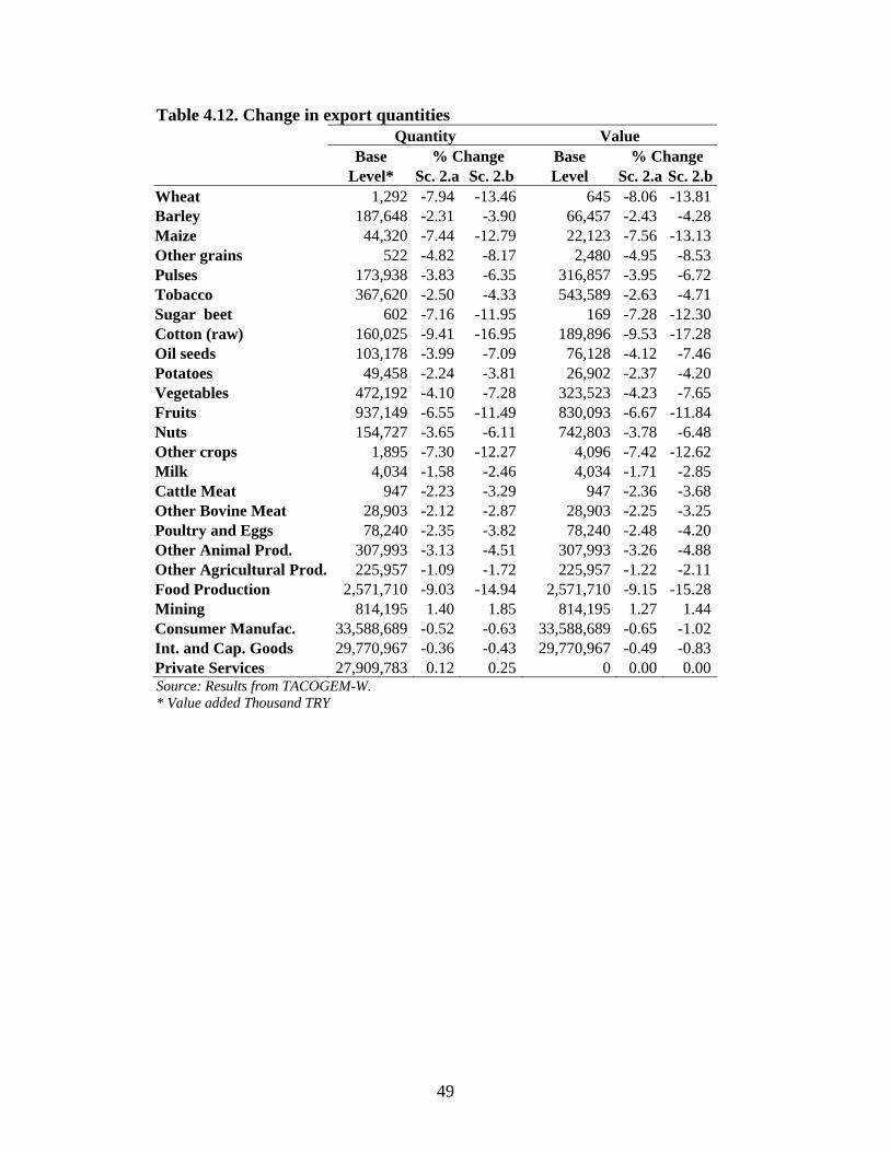
49

Table 4.12. Change in export quantities Quantity Value Base % Change Base % Change Level* Sc. 2.a Sc. 2.b Level Sc. 2.a Sc. 2.b Wheat 1,292 -7.94 -13.46 645 -8.06 -13.81 Barley 187,648 -2.31 -3.90 66,457 -2.43 -4.28 Maize 44,320 -7.44 -12.79 22,123 -7.56 -13.13 Other grains 522 -4.82 -8.17 2,480 -4.95 -8.53 Pulses 173,938 -3.83 -6.35 316,857 -3.95 -6.72 Tobacco 367,620 -2.50 -4.33 543,589 -2.63 -4.71 Sugar beet 602 -7.16 -11.95 169 -7.28 -12.30 Cotton (raw) 160,025 -9.41 -16.95 189,896 -9.53 -17.28 Oil seeds 103,178 -3.99 -7.09 76,128 -4.12 -7.46 Potatoes 49,458 -2.24 -3.81 26,902 -2.37 -4.20 Vegetables 472,192 -4.10 -7.28 323,523 -4.23 -7.65 Fruits 937,149 -6.55 -11.49 830,093 -6.67 -11.84 Nuts 154,727 -3.65 -6.11 742,803 -3.78 -6.48 Other crops 1,895 -7.30 -12.27 4,096 -7.42 -12.62 Milk 4,034 -1.58 -2.46 4,034 -1.71 -2.85 Cattle Meat 947 -2.23 -3.29 947 -2.36 -3.68 Other Bovine Meat 28,903 -2.12 -2.87 28,903 -2.25 -3.25 Poultry and Eggs 78,240 -2.35 -3.82 78,240 -2.48 -4.20 Other Animal Prod. 307,993 -3.13 -4.51 307,993 -3.26 -4.88 Other Agricultural Prod. 225,957 -1.09 -1.72 225,957 -1.22 -2.11 Food Production 2,571,710 -9.03 -14.94 2,571,710 -9.15 -15.28 Mining 814,195 1.40 1.85 814,195 1.27 1.44 Consumer Manufac. 33,588,689 -0.52 -0.63 33,588,689 -0.65 -1.02 Int. and Cap. Goods 29,770,967 -0.36 -0.43 29,770,967 -0.49 -0.83 Private Services 27,909,783 0.12 0.25 0 0.00 0.00 Source: Results from TACOGEM-W. * Value added Thousand TRY

50

Table 4.13. Import quantity and value Quantity Value Base % Change Base % Change Level* Sc. 2.a Sc. 2.b Level Sc. 2.a Sc. 2.b Wheat 1,707 5.39 9.43 852,991 5.25 9.00 Barley 75 1.38 2.11 26,710 1.24 1.71 Maize 1,920 2.32 4.01 958,308 2.18 3.60 Other grains 62 2.58 4.20 294,479 2.44 3.79 Pulses 14 3.33 5.32 24,903 3.19 4.91 Tobacco 223 -0.44 -0.99 330,050 -0.57 -1.38 Sugar beet 28 5.67 9.32 7,916 5.53 8.89 Cotton (raw) 855 2.72 5.18 1,014,863 2.58 4.77 Oil seeds 437 0.68 1.19 322,682 0.54 0.79 Potatoes 16 1.60 2.45 8,778 1.47 2.04 Vegetables 92 2.46 4.16 63,121 2.32 3.75 Fruits 84 4.05 7.22 74,676 3.92 6.80 Nuts 5 1.68 2.47 23,580 1.54 2.07 Other crops 4 5.40 9.04 8,446 5.26 8.61 Milk 34 0.01 -0.47 34,145 -0.12 -0.87 Poultry and Eggs 20 2.11 3.02 306 1.87 2.15 Other An. Prod. 241 2.47 3.34 20,183 1.98 2.61 Other Agr. Prod. 360 -1.00 -1.89 240,806 2.34 2.93 Food Production 1,092 8.31 14.10 360,165 -1.13 -2.28 Mining 16,369 -0.79 -1.09 1,091,780 8.16 13.65 Consumer Manufac. 9,920 1.62 1.99 16,369,273 -0.92 -1.48 Int. and Cap. Goods 74,091 -1.12 -1.65 9,919,764 1.49 1.59 Source: Results from TACOGEM-W. * Value added Thousand TRY

Scenario 2.b entails a 50 percent increase in the urban water supply by decreasing

irrigation water by the same amount, creating responses in the economy in the same direction as

in Scenario 2.a, but evidently at higher magnitudes.

4.4 Scenario 3: Climate Change Scenario

Climate change is expected to have a considerable impact on agricultural production. Climate

change mainly affects agricultural productivity through reduced water availability (or runoff, i.e.

the difference between rainfall and evapotranspiration)—both by reduced precipitation and

increased temperatures. Most particularly, it has been reported that most of the Near East Region

(including Turkey) will have a decrease in water availability of up to 40 mm per year, and that

51

the decrease will increase to 80 mm per year in the Anatolian Plateau.3 Such water deficit stress

can cause a decline in agricultural yields or require higher water use in irrigation to maintain

yields (Yano et al., 2007). In arid and semi-arid parts of the world, climate changes could easily

aggravate periodic and chronic shortages of water, and most importantly, climate change poses

an important threat in developing countries, many of which are located in arid and semi-arid

areas (Watson, et al., 1997). Watson et al. (1997) report that these countries are especially

vulnerable in the sense that they predominantly rely on single-point systems such as ‘bore-holes’

or ‘isolated reservoirs’ for their water sources, and once these primary systems fail to function,

there is hardly any substitute system to provide adequate water supply. Additionally, these

countries do not possess sufficient technical, financial or management resources to overcome the

vulnerability and adjust to shortages and/or take on adaptation measures.

Turkey, which is located in arid Western Asia or the Middle East, is also expected to be

significantly affected by climate change (ibid). This region, which already is undergoing serious

water shortages, is possibly one of the regions most influenced by climate change. Water

shortages caused by climate change may also be a blessing in disguise for these countries as long

as they adopt changes in cropping practices and improve efficiency of water use through efficient

irrigation systems (ibid.). However, we have already mentioned that these countries are more

likely to lack adequate technical, financial, or administrative resources to do so.

Although there are not many studies on the impacts of climate change on food and

agricultural production in the Middle East, one projection finds that increases in temperature of

up to 3-4oC will lead to a fall in yields of predominant regional crops across the region by 25 to

35 percent with weak carbon fertilization, or 15 to 20 percent with strong carbon fertilization.4,5

When we examine the annual total rainfall (mm) data for Turkish provinces from the year 1975

in Figures 4.2, 4.3, and 4.4, we see a clear downward trend in annual rainfall and water

availability, particularly in Adana (predominantly producing wheat, maize, cotton, soybean,

citrus, fruits), Diyarbakir (primarily supplying wheat, barley, pulses, cotton) and Konya (mostly

supplying wheat, barley, sugar beet, pulses), which are important agricultural providers in the

3 In the Summary Report on Climate Change: Implications for Agriculture in the Near East-29th FAO Regional Conference for the Near East, Cairo, The Arab Republic of Egypt, 1-5 March 2008. 4 ibid. 5 The negative effect of increase in temperatures may be compensated by positive effects of increased CO2 on crop tolerance to water deficit stress (Fuhrer, 2003; Yano, et al., 2007).

52

country.6 Furthermore, Türkeş (1996) has observed that for the period 1930-1993, the area-

averaged annual rainfall series has been on the decline slightly throughout Turkey, and

particularly over the Black Sea and the Mediterranean regions.

0

200

400

600

800

1000

1200

1975

1976

1977

1978

1979

1980

1981

1982

1983

1984

1985

1986

1987

1988

1989

1990

1991

1992

1993

1994

1995

1996

1997

1998

1999

2000

2001

2002

2003

2004

2005

2006

2007

Years

Ann

ual t

otal

pre

cipi

tatio

n (m

m)

Figure 4.2: Annual total precipitation (mm), Adana

0

100

200

300

400

500

600

700

800

1975

1976

1977

1978

1979

1980

1981

1982

1983

1984

1985

1986

1987

1988

1989

1990

1991

1992

1993

1994

1995

1996

1997

1998

1999

2000

2001

2002

2003

2004

2005

2006

2007

Years

Ann

ual t

otal

pre

cipi

tatio

n (m

m)

Figure 4.3: Annual total precipitation (mm), Diyarbakır

6 According to data from Turkish State Meteorological Service Website, http: meteor.gov.tr

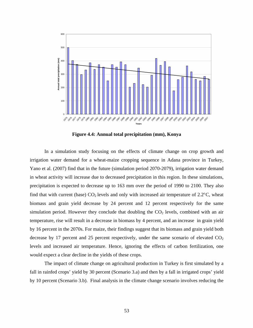
53

0

100

200

300

400

500

600

1975

1976

1977

1978

1979

1980

1981

1982

1983

1984

1985

1986

1987

1988

1989

1990

1991

1992

1993

1994

1995

1996

1997

1998

1999

2000

2001

2002

2003

2004

2005

2006

2007

Years

Ann

ual t

otal

pre

cipi

tatio

n (m

m)

Figure 4.4: Annual total precipitation (mm), Konya

In a simulation study focusing on the effects of climate change on crop growth and

irrigation water demand for a wheat-maize cropping sequence in Adana province in Turkey,

Yano et al. (2007) find that in the future (simulation period 2070-2079), irrigation water demand

in wheat activity will increase due to decreased precipitation in this region. In these simulations,

precipitation is expected to decrease up to 163 mm over the period of 1990 to 2100. They also

find that with current (base) CO2 levels and only with increased air temperature of 2.2°C, wheat

biomass and grain yield decrease by 24 percent and 12 percent respectively for the same

simulation period. However they conclude that doubling the CO2 levels, combined with an air

temperature, rise will result in a decrease in biomass by 4 percent, and an increase in grain yield

by 16 percent in the 2070s. For maize, their findings suggest that its biomass and grain yield both

decrease by 17 percent and 25 percent respectively, under the same scenario of elevated CO2

levels and increased air temperature. Hence, ignoring the effects of carbon fertilization, one

would expect a clear decline in the yields of these crops.

The impact of climate change on agricultural production in Turkey is first simulated by a

fall in rainfed crops’ yield by 30 percent (Scenario 3.a) and then by a fall in irrigated crops’ yield

by 10 percent (Scenario 3.b). Final analysis in the climate change scenario involves reducing the

54

yield in all types of crops at varying degrees, ranging from 0 to 30 percent, depending on

whether the crop is rainfed or irrigated, and the region it is produced in.

Under scenario 3.a, we first notice that overall production volume in irrigated crops such

as vegetables, other grains (rice, etc.), wheat, oil seeds, fruits, and other crops category rise at

varying rates. The highest increase is seen in the other grains category by 34 percent, followed

by vegetables with 30 percent. Irrigated wheat activity, on the other hand, increases by 9.63

percent overall. We must mention that the crops named above are modeled as growing on both

irrigated and rainfed land. While we observe production volume increases in crops which have

activity in both irrigated and rainfed land, the production quantity in crops such as cotton (raw),

sugar beet and potatoes, which are only grown on irrigated land, all decrease significantly (Table

4.14.).

Table 4.14. Change in production of irrigated activities

Base % Change

Level (Tons) Sc. 3.a Sc. 3.b Sc. 3.c

Wheat 7,877 9.63 -4.41 -8.07 Maize 1,355 -1.81 -14.89 -16.02 Other grains 304 33.63 17.10 7.02 Sugar beet 12,622 -8.84 -13.71 -13.76 Cotton (raw) 2,295 -15.99 -23.52 -14.34 Oil seeds 976 19.76 5.11 -5.16 Potatoes 5,300 -5.54 -7.74 -7.90 Vegetables 9,827 29.77 14.50 6.66 Fruits 6,562 13.56 1.60 -3.56 Other crops 1,203 35.19 18.69 8.59 Source: Results from TACOGEM-W.

As a result of the fall in the yields of crops on rainfed land, and as production shifts to

irrigated land, the shadow value of irrigation water is expected to rise due to increased

competition for water. Particularly, the shadow value (or price) of irrigation water in the Central

region increases by 27 percent, in the East region by 26 percent, in the LSCB region by 10.46

percent, and in the Southeast region by a moderate 3.34 percent (Table 4.15). At the base run, 36

percent of all wheat produced in Turkey is produced in the Central region, making up the highest

share among all regions. In the Central region, 36 percent of total agricultural land is devoted to

wheat activity. Furthermore, wheat is an irrigated crop; 41 percent of all wheat is produced on

irrigable land, overall. In that sense, recognizing the significance of wheat production in the

55

Central region, one can expect to observe a relatively high increase in irrigation water shadow

prices in this region.

Table 4.15.Change in factor prices Base % Change

Region

Level (TRY) Sc. 3.a Sc. 3.b Sc. 3.c

Labor* 1.00 -6.21 -7.13 -5.90West 0.64 20.20 15.04 17.19Central 0.26 21.06 15.43 0.48East 0.27 22.06 16.76 7.65Southeast 0.53 13.53 8.67 -3.07

Irrigated Land

LSCB 0.70 19.79 14.12 10.74West 0.27 -3.63 2.21 11.24Central 0.11 0.28 5.69 -0.01East 0.11 -1.04 3.95 5.89Southeast 0.23 3.79 8.20 2.17

Rainfed Land

LSCB 0.14 -3.74 3.49 21.86West 0.13 21.82 15.88 18.85Central 0.11 27.14 21.65 0.48East 0.05 26.09 20.83 9.60Southeast 0.09 3.34 -1.35 -13.82LSCB 0.13 10.46 5.54 2.25

Water

Urban 0.81 -7.31 -9.27 -7.88Source: Results from TACOGEM-W. *Labor employment is taken as value added created by labor

Employment of irrigated land increases for wheat, vegetables and fruits, and crops

classified as other grains such as rice. This is due to the shift from rainfed land in these activities

towards irrigated land as an alternative. Employment of irrigated land in sugar beet, cotton,

potatoes and maize production fall at different rates. We mentioned sugar beet, cotton and

potatoes are grown only on irrigated land. As production of all crops shifts from rainfed land to

irrigated land due to the yield shock in rainfed activity, the price of irrigated land increases in all

regions at rates ranging from 13 to 30 percent. With this increase in the price of irrigated land, a

drop in employment in irrigated-land-only activities can be expected.

As can be inferred from the discussion above, production volume in all rainfed crop

activities drop at various rates. For example, production of fruits in rainfed land drops by 39

percent, while production of oil seeds drop by 36 percent from the base as a result of the 30

percent drop in yield. Overall, considering the sum of both irrigated and rainfed land production

56

activity, we observe a fall in volume of production in all crops. Moreover, production in

livestock and national non-agricultural activities also declines.

For example, food manufacturing contracts by 13 percent as there is a reduction in

production of intermediate goods in this sector. As a result of the contraction in domestic

production, import volume in almost all crops increases except for raw cotton, which experiences

a fall in production and a rise in domestic prices. The most significant increase in import volume

is seen in other grains with 65 percent as well as an increase in nuts by 45 percent. It is also

important to note that manufactured food imports rise by 85 percent in volume. Export volume,

on the other hand, decreases significantly following the fall in production in agriculture and an

increase in domestic commodity prices.

We must also note that urban household’s real consumption decreases by about 3.3

percent, while that of rural households in all regions increases by 4 percent except in the East

with a 1.6 percent increase (Table 4.16). We can attribute this disparity in rural and urban

household response to differences in sources of income of these household types, and also the

composition of consumption expenditures. Urban households earn about 40 percent of the total

income due to labor, and the rest from capital, while rural households have income from land and

water resources as well. While there is a clear drop in labor and capital income overall, there is a

rise in rents to both irrigated and rainfed land, and a slight increase in the water factor income in

the West and Central regions (which inhabit a large share of rural households). Nevertheless,

there is a significant decline in real GDP by about 6 percent as a result of the fall in yields in

rainfed crops by 30 percent simulating a shortage of water caused by climate change.

Table 4.16. Change in disaggregated real household consumption Base % Change

Level

(Million TRY) Sc. 3.a Sc. 3.b Sc. 3.c

Urban HH 192,526 -3.30 -4.00 -3.50 West Rural 28,136 4.10 4.50 5.80 Central Rural 11,422 3.70 3.90 -0.30 East Rural 8,662 1.60 1.50 0.60 Southeast Rural 2,450 2.40 2.00 -3.90 LSCB Rural 1,965 3.90 2.90 2.50 Rural Total 52,635 15.70 14.80 4.70 Turkey 245,161 -1.80 -2.40 -2.10 Source: Results from TACOGEM-W.

57

Considering Scenario 3.b, in which the crop yield in irrigated activities are reduced by 10

percent, in addition to the 30 percent reduction in rainfed activities, the changes in the production

volume of irrigated crops are much less pronounced than those in Scenario 3.a. For example,

production quantity in wheat declines by 20 percent compared to 16 percent. An increase in

irrigated fruit activity becomes insignificant. We further notice that the response in cotton (raw),

sugar beet and potatoes production volume is stronger than that in the previous scenario: there is

an additional 10 to 15 percentage point decline in the production of these crops. In this scenario,

the changes in the water shadow price and irrigated land price are not as high as those in the

former scenario. This is because there is not as much competition for these inputs as before,

simply due to the fall in yields and the pursuing fall in production volumes. In all crops, a

change in water consumption from the base is smaller than that in the first scenario. As in the

first scenario, the import volume of all crops increases and the export volume decreases

following a rise in commodity prices, however these changes occur at higher magnitudes. The

fall in real GDP is also higher by 3.47 percent.

5 Conclusions, Policy Implications, and Future Research Agenda

This study investigated the economy-wide effects of two external shocks, namely a permanent

increase in the world prices of agricultural commodities and the climate change, along with the

impact of the domestic reallocation of water between agricultural and non-agricultural use. It

was also recognized that because of spatial heterogeneity of the climate, the simulated scenarios

have differential impact on the agricultural production and hence on the allocation of factors of

production including water.

Table 5.1 presents the simulated changes of some selected macroeconomic variables in

all scenarios.

58

Table 5.1. Summary Impact Matrix

Sc. 1 Sc. 2a Sc. 2b Sc. 3a Sc. 3b Sc. 3c

Absorption

=>

<=

=>

==>

===>

==>

Household Consumption

=>

<=

<=

==>

==>

==>

Investment

==>

=>

==>

===>

===>

===>

Government Consumption

=>

<=

<=

===>

===>

==>

GDP at Market Prices

=>

<=

=>

==>

===>

==>

Net Income Tax

==>

=>

=>

==>

==>

==>

GDP at Factor Costs =>

<=

=>

==>

===>

==>

Total Exports

=>

=>

=>

===>

===>

===>

Total Imports

=>

=>

=>

===>

===>

===>

Agricultural Exports

<===

==>

===>

===>

===>

===>

Agricultural Imports

===>

<=

<==

<===

<===

<===

Note: Sc.1: World price increase; Sc. 2: Rural-urban water transfer; Sc. 3: Climate change.

The highest effects on major macroeconomic indicators occurs in the climate change

simulations. Nominal GDP declines drastically, but the real impact is limited. The changes are

relatively smaller in the world price increase scenario when compared to all climate simulations.

This situation points out the importance of the climate change in the performance of the overall

economy. It is obvious that the impact of the climate change will not only be confined to the

agricultural sector. Through the interactions with the rest of the economy, the negative impact of

the climate change will be amplified. Irrigation is considered the most important adaptation

measure to ease the negative impact of climate change, especially on farmers’ income. Warming

is also expected to affect the availability of water resources. This aspect of the climate change is

59

not incorporated in these simulations. Hence, the climate change adaptation policies

incorporating water and land management should be given priority.

An increase in the world prices is expected to decrease all selected macroeconomic

indicators, except the agricultural exports. As a result of the price increase the competitiveness of

the agricultural sector improves with a high increase in the agricultural exports and almost

comparable decrease in the agricultural imports. The accompanied rise in domestic prices strikes

urban households through consumption while causing an expansion in the income of rural

households. Increasing world prices hampers non-agricultural sectors as well. This further

suppresses the income of rural households.

As a result of the transfer of water from rural to urban areas, overall production of all

crops decline. Although the production on the rainfed land increases, the production on the

irrigated land declines, most notably production of maize and fruits. The decrease in the

agricultural production, coupled with the domestic price increase, is further reflected in the net

trade. Agricultural imports increase with a higher decline in agricultural exports.

Turkey has been fortunate in its endowment of water resources. However, the demand of

water is growing rapidly. The pressure on usable water resources is predicted to increase with the

rapid pace of industrialization and urbanization. Scarcity of water in some regions has already

started to hamper agricultural production. Over-abstraction of groundwater in the Central Region

and over-use of surface water in the West have affected not only the availability of water, but

also degraded its quality with serious environmental impact. The response of the governments so

far has been focused on building additional infrastructure to release the constraints on water

availability. Shifting the irrigation pricing method to promote efficient use of water has never

been considered as an alternative to the current pricing method which consists of a per area based

operation and maintenance charge. Seven river basins (out of 26), mostly in the West, are already

in a serious state of water shortage, with abstractions exceeding 200 percent of the annual

renewable resource (World Bank, 2007). If all of the 8.5 million hectares of the “economically

irrigable” area is developed, the World Bank (2007) found that almost 18 basins will face serious

water shortages. This situation raises serious doubts about the sustainability of the prevailing

policies in the irrigation sector.

The results of the simulations further prove deficiency in the currently implemented

approach of supply management and the pricing policy in the irrigation sector. The pressure on

60

irrigation water augments in all scenarios. The results of all simulations indicate that the shadow

prices for irrigation water increase in all regions, except in the Southeast Region that has a higher

impact case in the climate change scenario. Hence, it is necessary to achieve more efficient use

of irrigation water which requires not only the promotion of water saving irrigation techniques,

but serious consideration should be given to fit the demand for water to meet the supply.

Although the results of the model simulations are rich, it is possible to further improve

the model structure. The priority should be given to incorporate the heterogeneous labor structure

in the model. The regions can be further disaggregated to NUTS-I level. Further disaggregation

of food manufacturing and other agriculture related industries, such as textiles, are necessary to

ameliorate the inter-sectoral interactions. Sooner or later Turkey may be tempted by the biofuels

frenzy, hence making it necessary to have a detailed energy sector. One valuable extension can

be separating rural and urban households according to income groups. This would allow analysis

of welfare distribution that the model currently lacks. Structural enhancements will improve the

performance of the model, i.e. nested structure in production, especially for irrigated land and

water. Another enhancement could be transforming the model into a recursive dynamic one that

provides the adjustment paths for external and policy shocks.

This work has indicated also that future policy dialogue among the World Bank, the

Government of Turkey, and local institutions is necessary. Water stress in Turkey is predicted to

increase with demographic changes and unfavorable global climatic and economic conditions.

Fast implementation of necessary policy measures at all levels will achieve more efficient use of

public resources and water. The stock of planned or uncompleted irrigation sector projects

remains large compared to the financial resources allocated for their execution (SPO, 2008).

Priority should be given to better use of existing water infrastructure and proper ranking of the

unfinished projects. The first one requires improvement in irrigation management practices.

More resources can be allocated to restrict water losses from irrigation infrastructure, starting

from the high evaporation regions. There have been improvements in adopting more efficient

water application technologies induced by government subsidies. The uptake of these

technologies by irrigators can be further increased by shifting towards volumetric pricing

practices. SPO (2008) points out the importance of increasing the efficiency in the use of

irrigation water by the determination of irrigation fees proportional to the actual amount used.

61

The main issues arising from this study, namely water pricing and subsidies, water

savings irrigation techniques, crop diversification (possibly linked to EU accession

requirements), and stabilization of over-exploited aquifers, have long been on the policy agenda

of international development agencies such as the World Bank and of the Government of

Turkey. The analytical framework proposed in this study could be used to further engage the

government with the World Bank on these matters.

62

References

Akşit, B., 1998, “İç göçlerin nesnel ve öznel toplumsal tarihi üzerine gözlemler: köy tarafından bir bakış,” in Türkiye’de İç Göç, Sorunsal Alanları ve Araştırma Yöntemleri Konferansı (June 6–8, 1998, Bolu-Gerede) Bildiriler Kitabı. İstanbul: Türkiye Ekonomik ve Toplumsal Tarih Vakfı, pp. 22–37.

Berrittella, M., Rehdanz, K., Tol, S.J.R., 2006, The Economic Impact of the South-North Water Transfer Project in China: A Computable General Equilibrium Analysis, NOTA DI LAVORO 154.2006: Fondazione Eni Enrico Mattei

Briand, A., 2004, “Comparative Water Pricing Analysis: Duality Formal-Informal in a CGE Model for Senegal”. Paper presented in the Conference Input-output and General Equilibrium: Data, Modeling and Policy Analysis. Brussels, 2-4 September 2004.

Cakmak, E. H., E. Yeldan, and O. Zaim, 1996, “The Rural Economy Under Structural Adjustment and Financial Liberalization: Results of a Macro-Integrated Agricultural Sector Model for Turkey,” Revue Canadienne d’Etudes du Development (Canadian Journal of Development Studies), Vol. XVII, No. 3, pp. 427-47.

Cırpıcı, Y.A., 2008, Economy-wide Analysis of Water Resource Management: A CGE Model for Turkey, METU, unpublished Ph.D. dissertation.

Diao, X., Roe, T., Doukkali, R., 2005, Economy-wide Gains from Decentralized Water Allocation in a Spatially Heterogeneous Agricultural Economy, Environment and Development Economics 10: 249–269

Diao, X., Yeldan E., 2001, An intertemporal, multi-region general equilibrium model of agricultural trade liberalization in the South Mediterranean NIC's, Turkey, and the European Union. In: J. VON HAGEN and M. WIDGREN (eds.), Regionalism in Europe, Geometries and Strategies After 2000. Massachusetts: Kluwer Academic Publishers, pp.195-220.

Diao, X., Dinar, A., Roe, T., Tsur, Y., 2008, A General Equilibrium Analysis of Conjunctive Ground and Surface Water Use with an Application to Morocco, Journal of Agricultural Economics, (forthcoming)

Dogruel, F., Dogruel S.A., Yeldan, E., 2003, Macroeconomics of Turkey’s agricultural reforms: an inter-temporal computable general equilibrium analysis, Journal of Policy Modeling, 25: 617–637

DSI (General Directorate of State Hydraulic Works), 2008a, Annual Activity Report of the General Directorate of State Hydraulic Works: 2007, Ankara: DSI.

DSI, 2008b, Irrigation Development and Land Reclamation by the General Directorate of State Hydraulic Works: 2007-2008, Ankara: DSI.

DSI, 2007, Annual Activity Report of the General Directorate of State Hydraulic Works: 2006, Ankara: DSI.

Dwyer, G., Loke, P., Appels, D., Stone, S., Peterson, D., 2005, Integrating Rural and Urban Water Markets in South East Australia: Preliminary Analysis, Paper presented to the

63

OECD Workshop on Agriculture and Water: Sustainability, Markets and Policies Adelaide, 14–18 November 2005

Ethridge, D., Welch, M., Pan, S., Fadiga, M., Mohanty, S., 2006, World Cotton Outlook: Projections to 2015/16, Paper presented at 2006 Beltwide Cotton Conferences, San Antonio, Texas - January 3 - 6, 2006

FAPRI, 2008, Agricultural Outlook 2008: World Cotton, www.fapri.org, accessed on 01/09/2008

Finnoff, D., Caplan, A.J., 2004, A Bioeconomic Model of The Great Salt Lake Watershed, Economic Research Institute Study Paper: ERI #2004-14, Utah State University

Fuhrer, J., 2003, Agroecosystem responses to combinations of elevated CO2, ozone, and global climate change, Agriculture, Ecosystems and Environment, 97: 1-20.

GDRS (General Directorate of Rural Services), 2007, The Inventory of Land and Water Resources, http://www.khgm.gov.tr/ENVANTER/En_ToprakSu.mht, acceesed on 12/03/2007.

Goodman, D. J., 2000, More reservoirs or transfers? A Computable General Equilibrium Analysis of Projected Water Shortages in the Arkansas River Basin, Journal of Agricultural and Resource Economics, 25(2):698-713.

Harrison, G.W., Rutherford, T.F., Tarr, D.G., 1993, Piecemeal Trade Reform in the Partially Liberalized Economy of Turkey, The World Bank Economic Review, 7:191-217

Harrison, G.W., Rutherford, T.F., Tarr, D.G., , 1996, Economic Implications for Turkey of a Customs Union with the European Union, The World Bank International Economics Department International Trade Division, Policy Research Working Paper No: 1599.

Howitt, R. E., 1995a, Positive Mathematical Programming. American Journal of Agricultural Economics, 77(2), pp.329-42.

Howitt, R. E., 1995b, A Calibration Method for Agricultural Economic Production Models, Journal of Agricultural Economics, 46, pp.147-59.

Içduygu, A., Unalan, T., 1998, “Türkiye’de iç göç: Sorunsal alanları ve araştırma yöntemleri,” in Türkiye’de İç Göç, Sorunsal Alanları ve Araştırma Yöntemleri Konferansı (June 6–8, 1998, Bolu-Gerede) Bildiriler Kitabı. İstanbul: Türkiye Ekonomik ve Toplumsal Tarih Vakfı, pp.38–55.

Kahraman, B., Coşkun, Ö., Tunç, G., 2002, “Göç olgusunun değerlendirilmesi,” in M. Ersoy and H. Tarık Şengül, eds., Kente Göç ve Yoksulluk: Diyarbakır Örneği. Ankara: Middle East Technical University, pp.25–48.

Kanber, R., Ünlü, M., Cakmak, E. H. and Tüzün, M., 2005, “Irrigation Systems Performance: Turkey”, in N. Lamaddalena, F. Lebdi, M. Todorovic, C. Bogliotti (eds.) Irrigation systems performance, Options Méditerranéennes : Série B. Etudes et Recherches No. 52, Bari:CIHEAM-IAMB.

Karadağ, M., Westaway, T., 1999, The Impact on Consumer and Producer Prices in Turkey of VAT Changes Designed to Meet EU Membership Criteria: A Computable General Equilibrium Approach, Loughborough University Department of Economics, Economic Research Paper No. 99/19

64

Kohn, R.E., 2003, Israel’s Need to Import Freshwater, Water Air and Soil Pollution, 143: 257–270

Letsoalo, A., Blignaut, J., de Wet, T., de Wit, M., Hess, S., Tol, R.S.J., van Heerden, J., 2005, Triple Dividends of Water Consumption Charges in South Africa, Water Resources Research

Lofgren, H., Harris, R.L, Robinson, S., 2002, A Standard Computable General Equilibrium (CGE) model in GAMS. IFPRI; Wahington, D.C.

Mazumdar, D., 1987, “Rural-urban migration in developing countries,” in E.S. Mills, ed., Handbook of Regional and Urban Economics Volume II. NY: Elsevier Science Publishers.

Munro, J., 1974, Migration in Turkey, Economic Development and Cultural Change, 22(4): 634–53.

OECD and FAO, 2008, FAO-OECD Outlook, www.fao.org.tr, accessed on 01/09/2008.

OECD, 2006, Agricultural Policies in OECD Countries: At a glance, Paris: OECD Publications.

Ünalan, T., 1998, “Türkiye’de iç göçe ilişkin veri kaynaklarının değerlendirilmesi,” in Türkiye’de İç Göç, Sorunsal Alanları ve Araştırma Yöntemleri Konferansı (June 6–8, 1998, Bolu-Gerede) Bildiriler Kitabı. İstanbul: Türkiye Ekonomik ve Toplumsal Tarih Vakfı, pp.91–103.

Pazarlıoğlu, M. V., 1997, 1980–1990 döneminde Türkiye’de iç göç üzerine ekonometrik model çalışması, Çukurova University V. National Econometircs and Statistics Symposium, Adana.

Peterson, D., Dwyer, G., Appels, D., Fry, J.M., 2004, Modeling Water Trade in the Southern Murray-Darling Basin. Staff Working Paper. Melbourne: Productivity Commission

Regional Environmental Center Turkey, 2007, Adaptation to climate change in urban water management in Turkey. Ankara:REC

Roe, T., Dinar, A., Tsur, Y., Diao, X., 2005, Feedback Links Between Economy-wide and Farm Level Policies: Application to Irrigation Water management in Morocco. World Bank Policy Research Working Paper 3550

Seung, C. K., Harris, T. R., Englin, J. E., Noelwah, R. N., 2000, Impacts of Water Reallocation: A Combined Computable General Equilibrium And Recreation Demand Model Approach, The Annals of Regional Science, 34:473-487.

Smajgl, A., Morris, S., Heckbert, S., 2005, Water Policy Impact Assessment – Combining Modeling Techniques in the Great Barrier Reef Region, In Zerger, A. and Argent, R.M. (eds) MODSIM 2005 International Congress on Modeling and Simulation. Modeling and Simulation Society of Australia and New Zealand, December 2005, pp. 1985-1991

State Planning Organization (SPO) Website: www.spo.gov.tr acceesed on 2/03/2008

SPO, 2008, Annual Programme, 2008, 9th. Development Programme (2007-2013), Ankara:SPO.

SPO, 2007, Land and Water Resources Utilization and Management, SPO Special Expertise Commission Report, Ankara:SPO.

65

Telli, Ç., 2004, Sosyal Hesaplar Matrisi Üretme Yöntemi ile Türkiye Uygulaması, Manuscript, State Planning Organization, Ankara.

Tirado, D., Gómez C.M., Lozano, J., 2006, Efficiency Improvements and Water Policy in The Balearic Islands: A General Equilibrium Approach, Investigaciones Económicas, XXX (3):441-463

Turkish State Meteorological Service Website, www.meteor.gov.tr, acceesed on 20/07/2008

TurkSTAT (Turkish Statistical Institute), 2008, National Account Statistics, http://www.tuik.gov.tr/VeriBilgi.do?tb_id=55&ust_id=16, acceesed on 05/05/2008

TurkSTAT, Website. www.tuik.gov.tr, acceesed on 01/02/2008

TurkSTAT, 2005, Turkey’s Statistical Yearbook 2004, Ankara:TurkSTAT, Printing Division.

TurkSTAT, 2004a, The Input-output Structure of the Turkish Economy, 1998. TurkSTAT, Printing Division, Ankara.

TurkSTAT, 2004b, Census of Agriculture (Households), 2001, TurkSTAT, Printing Division, Ankara.

TurkSTAT, 2003, Agricultural Structure-Production, Price, and Value Statistics-2003, TurkSTAT, Printing Division, Ankara.

TurkSTAT, 1994, Census of Agriculture, 1991, TurkSTAT, Printing Division, Ankara.

Türkeş, M., 1996, Spatial and temporal analysis of annual rainfall variations in Turkey, International Journal of Climatology, 16(9): 1057-1076.

Tsur, Y. Dinar, A., Doukkali, R.M., Roe, T., 2004, Irrigation Water Pricing: Policy Implications based on International Comparison, Environment and Development Economics, 9(6):735-756

Undersecretariat of Foreign Trade Website: www.dtm.gov.tr acceesed on 20/11/2008

Watson, R.T., Zinyowera, M.C., Moss, R.H, Dokken, D.J., 1997, The Regional impacts of climate change: an assessment of vulnerability. IPCC Special Report.

World Bank, 2008, World Development Indicators (WDI) Online. http://www.worldbank.org.

World Bank, 2007, Turkey: Water and Irrigation & Drainage Sectors Towards Long-Term Suatainability (draft), Sustainable Development Department, June, manuscript.

Velázquez, E., Cardenete, M.A., Hewings, G.J.D., 2007, Water Price and Water Reallocation in Andalusia: A Computable General Equilibrium Approach, Working Paper ECON 07.04:Universidad Pablo de Olavide

Yeldan, E., 1997, Financial Liberalization and Fiscal Repression in Turkey: Policy Analysis in a CGE Model With Financial Markets, Journal of Policy Modeling 19(1):79-117

Yano, T., Aydın, M., Haraguchi, T., 2007, Impact of climate change on irrigation demand and crop growth in a Mediterranean environment of Turkey, Sensors, 7: 2297-2315.

66

Appendix A: Additional Tables

67

Table A.1. NUTS Regions Level-1 Level-2 Level-1 Level-2 Level-1 Level-2İstanbul Mediterranean

İstanbul İstanbul Antalya AntalyaErzurum

ErzurumMarmara Isparta Erzincan

Tekirdağ Tekirdağ Burdur BayburtEdirne Adana Adana Ağrı AğrıKırklareli Mersin Kars

Balıkesir Balikesir Hatay Hatay IğdırÇanakkale aş Ardahan

Osmaniye

Aegean Mid-Anatolianİzmir İzmir Kırıkkale Kırıkkale Malatya MalatyaAydın Aydın Aksaray Elazığ

Denizli Niğde BingölMuğla Nevşehir Tunceli

Manisa Manisa Kırşehir Van VanAfyon Kayseri Kayseri MuşKütahya Sivas BitlisUşak Yozgat Hakkâri

Eastern Marmara

Western Black Sea

Southeastern Anatolian

Bursa Bursa Zonguldak Zonguldak Gaziantep Gaziantep

Eskişehir Karabük AdıyamanBilecik Bartın Kilis

Kocaeli Kocaeli Kastamonu Kastamonu Şanlıurfa Şanlıurfa

Sakarya Çankırı DiyarbakırDüzce Sinop Mardin MardinBolu Samsun Samsun BatmanYalova Tokat Şırnak

Western Anatolian Çorum Siirt

Ankara Ankara Amasya

Konya KonyaEastern Black

SeaKaraman Trabzon Trabzon

OrduGiresunRizeArtvinGümüşhane

Mideastern Anatolian

Northeastern Anatolian

68

Table A.2. Model Regions Region in SAM Region as given in NUTS-1 West İstanbul W. Marmara E. Marmara Aegean Mediterranean Central Western Anatolian Mid-Anatolian Western Black Sea East North Eastern Anatolian Mid-eastern Anatolian Eastern Black Sea Southeastern Anatolian Southeastern Anatolian Lower Seyhan-Ceyhan Basin(LSCB)

Adana, Osmaniye provinces

69

Table A.3. Aggregated SAM for Turkey, 2003 (Billion TL) Agriculture Ind.&Serv. Agriculture Ind.&Serv. Labor Capital Private Government S/I ROW Totals

Agriculture 80.999.936,15 80.999.936 Ind.&Serv. 527.683.706 527.683.706 Agriculture 10.108.704,66 21.572.920,17 40.396.276 1.914.811 125.602 3.810.939 77.929.252 Ind.&Serv. 20.017.847,81 227.178.725,29 204.689.173 42.277.658 82.197.436 94.685.399 671.046.239 Labor 20.259.707,62 107.757.927,81 128.017.635 Capital 28.671.944,56 140.881.848,35 169.553.793 Private 104.425.155 139.043.206 113.247.686 7.886.043 364.602.090 Government 1.941.731,53 30.292.284,72 6.958.631,06 - 36.916.113 23.592.480 30.510.587 28.370.862 144.665.427 S/I 86.801.914 19.398.942 - 14.920.067 82.323.039 ROW 3.887.947,18 106.446.420 4.343.866 6.624.215 121.302.448

- Totals 80.999.936 527.683.706 77.929.252 671.046.239 128.017.635 169.553.793 364.602.090 144.665.427 82.323.039 121.302.448

70

Appendix B: The Algebraic Structure of the CGE Model

71

Prices The price block of the equations system includes definitions of the endogenous prices,

exogenous prices as well as the links between them (world price of imports, f.o.b. price of

exports, exchange rates), and other non-price variables in the system. In this system,

Marketed output value = value of domestic sales + value of exports

or,

cccccc QEPEQDPDSQXPX +=

where, Cc∈ , and C is the set of commodities. Here, cPE is the export price of

commodity c, and is measured in TRL, given as EXRtepwePE ccc )1( −= , where pwec is the

f.o.b. price of exports (in foreign currency units), tec is the commodity c export tax rate, and

EXR is the exchange rate (measured in local currency per foreign currency). Measured in

TRL, import prices in the system are defined as EXRtmpwmPM ccc )1( += where pwmc is

the world price of imports (in foreign currency), and tmc is the commodity c import tariff rate.

In the system, composite price of commodity c, PQc can be derived from the

Absorbtion equation given by

ccccccc QMPMQDPDQQtqPQ +=− )1(

where tqc represents the sales tax rate on commodity c.

Lastly, the value added price in activity Aa∈ , where A is the set of activities, can be

found as

a

aa

a

aaaa QVA

QINTAPINTA

QVAQA

taPAPVA −−= )1(

where PAa is the activity price, tac is the rate of tax on producer in activity a, PINTAa is

the intermediate input price used in activity a, and QINTAa is the aggregate intermediate input

use in activity a. The value added price is derived from the zero profit condition given as

aaaaaaa QINTAPINTAQVAPVAQAtaPA +=− )1(

Production and Trade The production and trade block includes three main categories:

a) Domestic production and input use;

b) The allocation of domestic production to domestic sales and exports;

c) The aggregation of supply to the domestic market (from imports and domestic

output sold domestically).

72

In production, each of the activities are assumed to maximize profits subject to their

technology taking prices in their output and factors of production as given. Technology of

each activity (sector) Aa∈ is defined by a Constant Elasticity of Substitution (CES) function

in the quantities of value added and the aggregate intermediate input use (production function

at the first level of activity):

[ ] aaa

aaa

aaaa

aa

aaa QINTAQVAQA

ρρρ δδα/1

)1(−−− −+=

where the value added in activity a is defined by a CES production function:

∑∈

−−=Ff

favafa

vaaa

vaa

vaaQFQVA ρρδα /1)(

in which QFfa denotes the quantity demanded for factor f in activity a. Defining the

technology in activity a by a CES technology, the optimal value added-intermediate input

ratio can be obtained as

aa

aa

aa

a

a

a

a

PVAPINTA

QINTAQVA ρ

δδ +

−

⎥⎦

⎤⎢⎣

⎡−

=1

1

1

Given the profit maximizing behavior in each of the activities, factor demand

functions are determined by the rule

Marginal cost of factor = Marginal revenue product of factor

Then, 11)( −−−−∑=

vaa

vaa

fvafaf

vafaaafaf QFQFQVAPVAxWDISTWF ρρ δδ

Here, the marginal revenue product of labor is given by the product times the marginal

product of labor. Also in the condition above, WFf is the factor f price, and WDISTfa is the

factor market distortion variable of factor f in each activity a.

The total cost of producing quantity QAa is

32144 344 2143421chargeWater costsinput teIntermediacostfactor Total

aaaaaaa WCHPTAXQINTAPINTAQVAPVATC +++=

And, PTAXa is the total production tax collected from sector a with activity a. In

activity a, total receipts net of taxes must be equal to total cost, or,

aaaaaaaa

aaaaaaaa

QINTAPINTAQVAPVAWCHptaxQAPAQINTAPINTAQVAPVAWCHPTAXQAPA

+=−−+=−−

)1(

where ptaxa is the production tax rate in activity a. Water charges are collected by the

WUA’s in regions where field crop activities are irrigated.

73

The output transformation function is of Constant Elasticity of Transformation (CET)

form:

[ ] tct

ctc

ctcc

tc

tcc QDQEQX

ρρρ δδα/1

)1( −+=

Here, aggregate domestic output is allocated to domestic use (QDc) and to exports

(QEc), that is, this equation provides information about the distribution of marketed output

according to its destination.

Maximizing producer profits subject to the output transformation function, the optimal

mix between exports and domestic sales can be obtained as such:

tc

tc

tc

c

c

c

c xPDSPE

QDQE ρ

δδ −

⎟⎟⎠

⎞⎜⎜⎝

⎛ −=

11

1

Imports of commodity c and its domestic production sold domestically are imperfect

substitutes, and this characteristic is summarized by the following aggregation function in

Armington form (i.e. ‘the composite supply function’):

[ ] qc

qc

qc

cqcc

qc

qcc QDQMQQ ρρρ δδα

1

)1(−−− −+=

Minimizing producer costs subject to the composite supply function, we obtain the

optimal mix between imports and domestic demand:

qc

qc

qc

c

c

c

c xPMPDD

QDQM ρ

δδ −

⎟⎟⎠

⎞⎜⎜⎝

⎛−

=1

1

1

Institutions In the institutions block of the system, we specify the income sources and the

consumption behavior of the main actors in the model, namely the households, the

government, and the Water User Associations.

All labor, land and capital factor income is earned by households, Water User

Associations collect water charges on water use in irrigated agriculture, and via the

government, and these water charges are then redistributed to rural households as transfers

(WPAY). Household income also is due to transfers from government and transfers from the

rest of the world:

)(, rowtrnsfrWPAYtrnsfrYIFYIFEFf

fhh +++= ∑∈

Household consumption expenditures are then given by

esDirect tax−−= SavingsYIEH hh

74

Household consumption demand for commodity c is in the form of a fixed share of

total expenditures

c

hchch PQ

EHQH ,, β=

Government revenue is derived from direct (factor) taxes, production taxes, import

tariffs, exports taxes and sales taxes, that is,

∑

∑ ∑∑∑

∈

∈∈∈

+

+++=

Ccccc

f CEcccc

CMcccc

Aaaaaff

QQPQtq

EXRQEpweteEXRQMpwmtmQAPAtaYFtfYG

Here, YFf is factor f income, CM is the set of imported commodities, and CE is the set

of exported commodities, both of which are a subset of the commodity set, C. Government

expenditures are

∑=c

ccQGPQEG

Accordingly, government savings are EGYGGSAV −= . Government consumption of

commodity c (excluding public services) is given by

ccc PQ

EGQG η=

Equilibrium Conditions

The last stage of the model specification involves the statement of equilibrium

conditions. Each commodity market clears in the sense that each commodity is demanded

either for private consumption, government consumption, investment, or for use as an

intermediate good:

∑∑∈∈

+++=Aa

acccHh

hcc QINTAQINVQGQHQQ ,,

In the economy, there is no unemployment, and all factor markets clear in the sense

that at given factor prices, factor demand is equal to available factor supply:

fAa

af QSFQF =∑∈

,

where fQSF is the exogenously fixed supply of factor f.

The closure rule for the savings-investment balance (as per Walras’ Law) in this

system is given by

PINVFSAVEXRGSAVPSAV =×++

75

where, FSAV is the foreign savings, and in equilibrium, is equal to the CA balance

(deficit or surplus):

76

Appendix C: The Algebraic Structure of the Farm Model

77

Resource and PMP duals constrained by PMP calibration constraints. We assume that 0.001ε =

jii

ij RHSLXRR ≤∑ )*( ∀ resource j [Resource Constraint]7

where jRHS is resource constraints8, ijRR is Leontieff coefficients and is given by

"", LANDi

ijij X

XRR =

0001.1*"", LANDii XLX ≤ ∀ Activity process i [Calibration Constraint]

where iLX is hectares planted variable ijX is base year resource use ( ," "i LANDX is base year land use)

[ ]( * )*i i i ii

V YB CL LX LINPROF− =∑ [Lprofit constraint]

where iV is price per unit of output (2003 TRY per ton), iYB is average yields (Tons per ha)

iCL is linear cost and it is given as *i ij ijj

CL C RR=∑ where ijC is resource variable costs and

ijRR is Leontieff coefficients and is given by

"", LANDi

ijij X

XRR =

iLX is hectares planted variable, LINPROF is LP profit variable. Then

PROBLEM: MAX LINPROF Subject to

Resource Constraint Calibration Constraint

CES Input Share Parameters Parameters are calculated from the recursive equations derived in the appendix of Howitt (1995)9

7 j=LAND, LABOR, TRAC, SEED, NITRO, PHOSPH, WATER. p(j)= LABOR, TRAC, SEED, NITRO, PHOSPH, WATER r(j)=LAND 8 j=LAND, LABOR, TRAC, SEED, NITRO, PHOSPH, WATER. 9 Note - this code ıs written ın a general way that adjusts for any changes ın the number of crops, regions or inputs defined in the sets at the start of the program

78

, 1

0

1

1

ip

i j THETA

ip ij

p ij ipX

BETACS XCS X

=

≠

=⎛ ⎞⎛ ⎞

+⎜ ⎟⎜ ⎟⎜ ⎟⎜ ⎟⎝ ⎠⎝ ⎠

∑

where 1THETASUB

= − , and SUB is elasticity of substitution, ipCS is factor cost plus

opportunity cost and ij ij j ijCS C OP LA= + + .j jOP RESOURCE M=

" " .LAND jOP RESOURCE M ADJ= −

," " .i LAND iLA CALIB M ADJ= +

ijX is base year resource use

,1 7 0ij

THETA

irij r

i j and X irr ir ij

r

XCSBETA BETA

CS X< < ≠

⎛ ⎞⎛ ⎞⎛ ⎞⎜ ⎟⎜ ⎟= ⎜ ⎟⎜ ⎟⎜ ⎟⎝ ⎠ ⎜ ⎟⎜ ⎟⎝ ⎠⎝ ⎠

∑∑ ∑

CES Scale Paramter ( iα ) CES scale parameter is calculated using the share parameters and total output10.

( )1 1

* 0.001

ii SUB

SUB SUBSUB

ij ijj

TOCN

BETA X− −

=⎡ ⎤⎛ ⎞

+⎢ ⎥⎜ ⎟⎝ ⎠⎣ ⎦

∑

where iTO is total output and given by ," "*i i i LANDTO YB X= . Here iYB is average yields (Tons per ha) and ijX is base year resource use ( ," "i LANDX is base year cultivated area for crop i) and SUB is elasticity of substitution PMP Cost function coefficients PMP cost function coefficients are calculated based on Howitt (1995)

ij ij ijALPH C LA= − Intercept of cost function

0

2*

ij

ijijwhere LA ij

LAGAM

X≠= Slope of cost function

10 ( )

1

1 1 2 2 3 3i i i i

i i i i i i i iy X X Xγ γ γ γα β β β= + +

79

where ijC is resource variable costs, ," " .i LAND iLA CALIB M ADJ= + and

" "0.25 . LANDADJ RESOURCE M= CES Programming Solution for the Base Year

ij ji

XN RHS≤∑ ∀ j [Input Constraint]

TPROFIT = ( )1 1

* * * 0.0001

SUBSUB SUBSUB

i i ij iji j

V CN BETA XN

− −⎛ ⎞⎡ ⎤⎜ ⎟+⎢ ⎥⎜ ⎟⎣ ⎦⎜ ⎟

⎝ ⎠∑ ∑

2* 0.5* *ij ij ij iji j

ALPH XN GAM XN⎡ ⎤− +⎣ ⎦∑∑ [Profit]