Linköping Studies in Science and TechnologyDissertations, No. 1936

Machine Learning-Based Bug Handling in Large-Scale SoftwareDevelopment

Leif Jonsson

Department of Computer and Information ScienceSE-581 83 Linköping, Sweden

Linköping 2018

Edition v1.0.0

© Leif Jonsson, 2018Cover Image © Tea AnderssonISBN 978-91-7685-306-1ISSN 0345-7524URL http://urn.kb.se/resolve?urn=urn:nbn:se:liu:diva-147059

Published articles have been reprinted with permission from the respectivecopyright holder.Typeset using X ETEX

Printed by LiU-Tryck, Linköping 2018

ii

Till min familj

iii

POPULÄRVETENSKAPLIG SAMMANFATTNING

I denna avhandling har vi studerat hur man kan använda maskininlärning för att effek-tivisera felhantering i storskalig mjukvaruutveckling. Felhantering i storskalig mjukvaru-utveckling är idag till stor del en manuell process som är mycket kostsam, kompliceradoch felbenägen. Processen består i stora drag av att hitta vilket team som skall åtgärdaen felrapport och var i mjukvaran som felet ska rättas. Maskininlärning kan förenklat be-skrivas som en kombination av datavetenskap, matematik, statistik och sannolikhetslära.Med denna kombination av tekniker så kan man ”träna” mjukvara att vidta olika åtgär-der beroende på vad man ger den för indata. Vi har samlat mer än 50000 felrapporterfrån mjukvaruutveckling i svensk industri och studerat hur vi kan använda maskininlär-ning för att maskinellt kunna hitta var ett fel ska rättas och vilket utvecklingsteam somska tilldelas felrapporten för rättning. Resultaten visa på att vi kan nå en precision upptill ca 70% genom att kombinera ett antal standardmetoder för maskininlärning. Detta äri nivå med en mänsklig expert, vilket varit ett viktigt resultat i överföringen av teknikentill praktisk användning. Felrapporter består av både så kallad strukturerad data, som tillexempel vilken kund, land, plats osv som felrapporten kommer ifrån, men också så kalladostrukturerad data som till exempel den textuella beskrivningen av felrapporten och desstitel. Detta har gjort att en stor del av avhandlingen har kommit att handla om hur mankan representera ostrukturerad text i maskininlärningssammanhang. Vi har i avhandlingenutvecklat en metod för att lösa ett problem som ursprungligen formulerades 2003 som kal-las Latent Dirichlet Allocation (LDA). LDA är en extremt populär maskininlärningsmodellsom beskriver hur man matematiskt i en dator kan modellera teman i text. Detta problemär mycket beräkningskrävande och för att man ska kunna lösa problemet inom rimlig tidså krävs det att man parallelliserar problemet över många datorkärnor. De dominerandeteknikerna för att parallellisera LDA har hittills varit approximativa, dvs. inte matematisktexakta lösningar av problemet. Vi har i avhandlingen kunnat visa att vi kan lösa proble-met matematiskt exakt men ändå lika snabbt som de förenklade approximativa metoderna.Förutom den uppenbara fördelen att ha en korrekt modell i stället för en approximationsom man inte vet hur stort fel den introducerar, så är det också viktigt när man byggervidare på LDA modellen. Det finns många andra modeller som har LDA som en kompo-nent och vår metod är applicerbar i många av dessa modeller också. Om man bygger enny modell baserad på LDA men utan en exakt lösning så vet man inte hur det fel somintroduceras med approximeringen påverkar den nya modellen. I värsta fall kan den nyamodellen förstärka det ursprungliga felet och man får ett slutresultat som har ett mycketstörre fel än från början. Även vi har byggt vidare på LDA modellen och utvecklat en nymaskininlärningsteknik som vi kallar DOLDA. DOLDA är en så kallad klassificerare. Enklassificerare inom maskininlärning är en metod för att tilldela objekt till olika klasser. Ettenkelt exempel på en klassificerare finns i många e-post programvaror. I detta exempel såkan e-postprogrammet klassificera e-post som endera reklam eller inte reklam. Detta är ettexempel av en så kallad binär klassificering. En mer sofistikerad klassificering kan vara attsortera nyhetsartiklar i olika kategorier som nyheter, sport, underhållning, osv. Den klassifi-cerare som vi utvecklat är helt generell, men vi applicerar den på bugghanteringsproblemet.Vår klassificerare tar både strukturerad data och text som indata och kan tränas genomatt köra den på många historiska felrapporter. När DOLDA modellen tränats upp kan denklassificera felrapporter, där kategorierna är de olika utvecklingsteamen i organisationen,eller var i koden en felrapport ska lösas. Vår klassificerare bygger på en statistisk teori somkallas för Bayesiansk statistik. Det finns många fördelar med den Bayesianska statistikensom direkt förs över till vår modell. En av de viktigaste är att man med den Bayesianskametoden alltid får ett mått på osäkerheten i resultaten. Detta är viktigt för att man skakunna veta hur säker maskinen är på att resultatet är korrekt. Detta gör att om maskinen ärosäker på klassificeringen så kan man låta en människa ta över istället, annars kan man låtamaskinen utföra åtgärder som till exempel att tilldela en felrapport till ett utvecklingsteam.

v

ABSTRACT

This thesis investigates the possibilities of automating parts of the bug handling process inlarge-scale software development organizations. The bug handling process is a large partof the mostly manual, and very costly, maintenance of software systems. Automating partsof this time consuming and very laborious process could save large amounts of time andeffort wasted on dealing with bug reports. In this thesis we focus on two aspects of the bughandling process, bug assignment and fault localization. Bug assignment is the process ofassigning a newly registered bug report to a design team or developer. Fault localizationis the process of finding where in a software architecture the fault causing the bug reportshould be solved. The main reason these tasks are not automated is that they are consideredhard to automate, requiring human expertise and creativity. This thesis examines the possi-bility of using machine learning techniques for automating at least parts of these processes.We call these automated techniques Automated Bug Assignment (ABA) and AutomaticFault Localization (AFL), respectively. We treat both of these problems as classificationproblems. In ABA, the classes are the design teams in the development organization. InAFL, the classes consist of the software components in the software architecture. We focuson a high level fault localization that it is suitable to integrate into the initial support flowof large software development organizations.

The thesis consists of six papers that investigate different aspects of the AFL and ABAproblems. The first two papers are empirical and exploratory in nature, examining theABA problem using existing machine learning techniques but introducing ensembles intothe ABA context. In the first paper we show that, like in many other contexts, ensemblessuch as the stacked generalizer (or stacking) improves classification accuracy compared toindividual classifiers when evaluated using cross fold validation. The second paper thor-oughly explore many aspects such as training set size, age of bug reports and differenttypes of evaluation of the ABA problem in the context of stacking. The second paper alsoexpands upon the first paper in that the number of industry bug reports, roughly 50,000,from two large-scale industry software development contexts. It is still as far as we areaware, the largest study on real industry data on this topic to this date. The third andsixth papers are theoretical, improving inference in a now classic machine learning tech-nique for topic modeling called Latent Dirichlet Allocation (LDA). We show that, unlikethe currently dominating approximate approaches, we can do parallel inference in the LDAmodel with a mathematically correct algorithm, without sacrificing efficiency or speed. Theapproaches are evaluated on standard research datasets, measuring various aspects such assampling efficiency and execution time. Paper four, also theoretical, then builds upon theLDA model and introduces a novel supervised Bayesian classification model that we callDOLDA. The DOLDA model deals with both textual content and, structured numeric, andnominal inputs in the same model. The approach is evaluated on a new data set extractedfrom IMDb which have the structure of containing both nominal and textual data. Themodel is evaluated using two approaches. First, by accuracy, using cross fold validation.Second, by comparing the simplicity of the final model with that of other approaches. Inpaper five we empirically study the performance, in terms of prediction accuracy, of theDOLDA model applied to the AFL problem. The DOLDA model was designed with theAFL problem in mind, since it has the exact structure of a mix of nominal and numericinputs in combination with unstructured text. We show that our DOLDA model exhibitsmany nice properties, among others, interpretability, that the research community has iden-tified as missing in current models for AFL.

vi

ACKNOWLEDGEMENTS

This research was funded and supported by Ericsson AB, but any viewsor opinions presented in this text are solely those of the author and do notnecessarily represent those of Ericsson AB

My deepest gratitude to my university supervisors, Professor Kristian San-dahl at Linköping University and Associate Professor David Broman, at thetime at Linköping, now at KTH. For any PhD student the advisors have acrucial role, so also for this student. Kristian and David, you have generouslyallowed me to very freely choose my own path. You have always encouragedme on this path even though it has most certainly diverged from what youexpected. Never have you forced your will upon me, but always happily, andengagingly, supported my ideas. Kristian and David, you have formed a per-fect complimentary team. Kristian with the wisdom that comes with manyyears of experience, and David with the vigor and enthusiasm of someonestarting their new career. Kristian, thank you for the many encouraging andguiding conversations. David, thank you, for setting the moral standard andexpecting nothing less than my best. Thanks also to Dr. Sigrid Eldh, mysupervisor at Ericsson. You have always wanted my best. Thank you for yoursupport and encouragement over the years.

In addition to the collaboration with my supervisors I have also beenextremely lucky to get to work with some great researchers! I had the greatfortune of meeting Dr. Markus Borg at ICSE 2013, and what a refreshingmeeting that was! You were as interested in bug reports as I was, and whata great researcher and writer you are. Although, I think that with you talentfor words, you should have better appreciated my naming suggestion! Let’skeep those curves coming!

A major part of a PhD undertaking is the intellectual development, andnone have had more impact on my intellectual development than my collabo-rators Dr. Måns Magnusson and Professor Mattias Villani, at the Division ofStatistics and Machine Learning at Linköping University. Having spent manyyears in computer science, of course knowing that it is a superior field com-pared to statistics, you have actually made me greatly appreciate your field!Mattias, I am forever grateful for letting me take your courses on Bayesianlearning in spite of being just a lowly computer scientist. It wasn’t easy, butit has expanded my intellectual universe immensely! Your generosity, kind-ness, humor, and deep knowledge is a constant inspiration. I will let slide,your mockery of Perl... All these attributes are rubbing off on your students.One of them is Måns. Måns, thank you so much for the great collaborationwe have had during many years and hopefully many years to come! Latenights, weekends, and weekdays, long discussions and throwing around ideas,it has been great fun, and always energizing! I envy your energy, intellect,humor, and kindness! Likewise, many thanks to Mathias Quiroz for the great

vii

conversations, jokes, and pleasant company, and for generously sharing yourknowledge! With friends and collaborators like you, life is good! Im also verygrateful to Professor Thomas Schön for letting me take your excellent course”Machine Learning”, in spite of my only real qualification was thinking ”mathis fun”. The course was really a transformative kickstart into the field!

In all of the turmoil of doing a PhD you need friends outside of work tokeep you sane, and in touch with the ”real world”. My profound thanks to mygreat friend, and infinitely generous teacher Peter Clarke. Our discussionsare stimulating, invigorating, and just great fun! It’s very hard to thinkabout probabilities when doing Jujutsu. Training and discussing with you hascertainly given my brain much needed rest from theory while being focused onJujutsu practice. My deepest gratitude and admiration also goes to DebbieClarke, for always making us feel so welcome and taking so good care of uswhen we come down under to visit. Your fighting spirit and generosity isawe inspiring! My warmest thanks also to Mike and Judy Wallace for yourfriendship, kindness, and hospitality. Thanks also to all my other Aussiefriends, Dale Elsdon, Mike Tyler, Richard Tatnall and the whole of the TJRgroup in Perth for always being so generous and kind to us when we come downto visit. Many thanks also to my great friends in training, Michael Mrazek,Ricky Näslund and Fredrik ”Rico” Blom for your friendship, discussions andfun training.

Another crucial part of life is family. My deepest gratitude to mum anddad for the freedom under responsibility you have given me my whole life. Youtaught me responsibility and showed me what the power of trust can bringin a person. My dear brother Stefan with his lovely partner Cecilia and theirfantastic Anton, it’s always fun and relaxing to spend time with you. I’m soglad that you are part of my family. My gratitude also to Pierre, Jennifer,Tuva and Ella for your company, friendship, all the nice dinners and BBQevenings.

To my great colleagues at Ericsson, thank you all so much for discussions,encouragement, critique and for creating a stimulating environment to workin. Special thanks goes to Roger Holmberg and Mike Williams for believingin me to start with, and giving me this opportunity. Further, during thistime I have managed to finish off a row of managers that have all given mesupport in this endeavor. Thank you Jens Wictorinus, Roger Erlandsson andMagnus Holmberg. Many thanks to Jonas Plantin for stimulating talks andthe opportunity to work with, and learn from you in the quality work. Specialthanks also to Jan Pettersson, Benny Lennartson, Henrik Schüller, AiswaryaaViswanathan and the Probably team for the fun work we do in the analyticsarea. Thanks also to Andreas Ermedahl and Kristian Wiklund for discussionsand support. Thanks to Martin Rydar for fighting the good fight! Keeprocking!

Thanks to Anne Moe at Linköping University for all the help, support,and for keeping everything on track. Thanks to Ola Leifler for help with

viii

LATEXwhen the LATEX-panic has set in. Thank you to Mariyam BrittanyShahmehri for proofreading and help making all of this slightly more under-standable.

My gratitude also goes to two great Swedish institutions that has madeit possible for me to learn, study, and better myself. The Swedish educationsystem, in particular, Linköping University, and Ericsson AB.

Having worked on this dissertation for too many years now, there is a highprobability that there is someone I may have forgotten to mention. To youI beg, please accept my sincerest apology for the omission! I promise I willmake it up to you in my next dissertation!

Finally, to the best two girls in the world, Tess and Tea, I love you! Youare my life. I would surely not have made it through all off this without yoursupport and patience. My deepest gratitude to my wonderful Tess for allthe love, support, and encouragement over the years. I couldn’t have done itwithout you dear! Thank you Tea, for being the best daughter any father canhave! You are wise, intelligent, kind, and a beautiful person. No words canexpress the pride I take in being your dad. Thank you also for letting me useyour beautiful picture on the cover of this dissertation. My beautiful girls,you have both graciously accepted ”I just have to go and work a bit more”for many years. Now we are free!

Leif JonssonHässelby Villastad, StockholmApril 2018

ix

Contents

Abstract v

Acknowledgments ix

Contents x

List of Figures xiii

List of Tables xviii

List of Publications 1

Related Publications 3

Preface 5

1 Introduction 71.1 Contributions . . . . . . . . . . . . . . . . . . . . . . . . . . . . . . 111.2 Thesis Overview . . . . . . . . . . . . . . . . . . . . . . . . . . . . 111.3 Motivation . . . . . . . . . . . . . . . . . . . . . . . . . . . . . . . . 121.4 Research Questions . . . . . . . . . . . . . . . . . . . . . . . . . . 121.5 Personal Contribution Statement . . . . . . . . . . . . . . . . . . 131.6 Short Summary of Included Papers . . . . . . . . . . . . . . . . . 161.7 Delimitations . . . . . . . . . . . . . . . . . . . . . . . . . . . . . . 17

2 Large-Scale Software Development 192.1 Large-Scale Development . . . . . . . . . . . . . . . . . . . . . . . 192.2 Software Development in Industry . . . . . . . . . . . . . . . . . 202.3 The Tower of Babel . . . . . . . . . . . . . . . . . . . . . . . . . . 202.4 A Bug’s Life . . . . . . . . . . . . . . . . . . . . . . . . . . . . . . . 222.5 The Bug Tracking System . . . . . . . . . . . . . . . . . . . . . . 242.6 Automatic Fault Localization vs. Automatic Bug Assignment . 252.7 A Taxonomy of Automatic Fault Localization Scenarios . . . . 26

3 Methodology 293.1 Method Overview . . . . . . . . . . . . . . . . . . . . . . . . . . . 293.2 The Author’s Personal Experience . . . . . . . . . . . . . . . . . 29

x

3.3 Methods Used . . . . . . . . . . . . . . . . . . . . . . . . . . . . . . 303.4 Paper I . . . . . . . . . . . . . . . . . . . . . . . . . . . . . . . . . . 333.5 Paper II . . . . . . . . . . . . . . . . . . . . . . . . . . . . . . . . . 343.6 Paper III . . . . . . . . . . . . . . . . . . . . . . . . . . . . . . . . . 343.7 Paper IV . . . . . . . . . . . . . . . . . . . . . . . . . . . . . . . . . 353.8 Paper V . . . . . . . . . . . . . . . . . . . . . . . . . . . . . . . . . 353.9 Paper VI . . . . . . . . . . . . . . . . . . . . . . . . . . . . . . . . . 353.10 Validity . . . . . . . . . . . . . . . . . . . . . . . . . . . . . . . . . 36

4 Theory 414.1 Machine Learning Introduction . . . . . . . . . . . . . . . . . . . 424.2 Probability Reminder . . . . . . . . . . . . . . . . . . . . . . . . . 424.3 What is Learning? . . . . . . . . . . . . . . . . . . . . . . . . . . . 494.4 Bayesian Learning . . . . . . . . . . . . . . . . . . . . . . . . . . . 674.5 Visualization . . . . . . . . . . . . . . . . . . . . . . . . . . . . . . 96

5 Results and Synthesis 99

6 Discussion and Future Work 1056.1 Aspects of Industrial Adoption . . . . . . . . . . . . . . . . . . . . 1056.2 Recommendations for an Updated Software Development Process1076.3 Boundary Between ABA and AFL . . . . . . . . . . . . . . . . . 1086.4 Hierarchical Classification . . . . . . . . . . . . . . . . . . . . . . . 1096.5 Other Contextual Information . . . . . . . . . . . . . . . . . . . . 1106.6 An End-to-end View of Automated System Analysis . . . . . . 111

7 Conclusion 113

Bibliography 115

8 Paper I 1238.1 Introduction . . . . . . . . . . . . . . . . . . . . . . . . . . . . . . . 1248.2 The Anomaly Report process . . . . . . . . . . . . . . . . . . . . 1258.3 Approach . . . . . . . . . . . . . . . . . . . . . . . . . . . . . . . . 1288.4 Prototype Implementation and Evaluation . . . . . . . . . . . . 1358.5 Results and Analysis . . . . . . . . . . . . . . . . . . . . . . . . . . 1388.6 Related Work . . . . . . . . . . . . . . . . . . . . . . . . . . . . . . 1428.7 Conclusion . . . . . . . . . . . . . . . . . . . . . . . . . . . . . . . . 143References . . . . . . . . . . . . . . . . . . . . . . . . . . . . . . . . . . . 143

9 Paper II 1499.1 Introduction . . . . . . . . . . . . . . . . . . . . . . . . . . . . . . . 1509.2 Machine Learning . . . . . . . . . . . . . . . . . . . . . . . . . . . 1529.3 Related Work on Automated Bug Assignment . . . . . . . . . . 1549.4 Case Descriptions . . . . . . . . . . . . . . . . . . . . . . . . . . . 1629.5 Method . . . . . . . . . . . . . . . . . . . . . . . . . . . . . . . . . . 1669.6 Results and Analysis . . . . . . . . . . . . . . . . . . . . . . . . . . 1809.7 Threats to Validity . . . . . . . . . . . . . . . . . . . . . . . . . . . 1899.8 Discussion . . . . . . . . . . . . . . . . . . . . . . . . . . . . . . . . 193

xi

9.9 Conclusions and Future Work . . . . . . . . . . . . . . . . . . . . 197References . . . . . . . . . . . . . . . . . . . . . . . . . . . . . . . . . . . 199

10 Paper III 20910.1 Introduction . . . . . . . . . . . . . . . . . . . . . . . . . . . . . . . 20910.2 Related work . . . . . . . . . . . . . . . . . . . . . . . . . . . . . . 21210.3 Partially Collapsed sampling for topic models . . . . . . . . . . . 21410.4 Experiments . . . . . . . . . . . . . . . . . . . . . . . . . . . . . . . 21910.5 Discussion and conclusions . . . . . . . . . . . . . . . . . . . . . . 229References . . . . . . . . . . . . . . . . . . . . . . . . . . . . . . . . . . . 23010.A Proofs . . . . . . . . . . . . . . . . . . . . . . . . . . . . . . . . . . 23410.B Variable selection in Φ . . . . . . . . . . . . . . . . . . . . . . . . 23510.C Algorithms . . . . . . . . . . . . . . . . . . . . . . . . . . . . . . . 238

11 Paper IV 24511.1 Introduction . . . . . . . . . . . . . . . . . . . . . . . . . . . . . . . 24511.2 Related work . . . . . . . . . . . . . . . . . . . . . . . . . . . . . . 24811.3 Diagonal Orthant Latent Dirichlet Allocation . . . . . . . . . . . 24911.4 Inference . . . . . . . . . . . . . . . . . . . . . . . . . . . . . . . . . 25111.5 Experiments . . . . . . . . . . . . . . . . . . . . . . . . . . . . . . . 25511.6 Conclusions . . . . . . . . . . . . . . . . . . . . . . . . . . . . . . . 263References . . . . . . . . . . . . . . . . . . . . . . . . . . . . . . . . . . . 26411.A Derivation of the MCMC sampler . . . . . . . . . . . . . . . . . . 26711.B Efficient updating of supervision effects . . . . . . . . . . . . . . 270

12 Paper V 27512.1 Introduction . . . . . . . . . . . . . . . . . . . . . . . . . . . . . . . 27512.2 Deployment Scenario . . . . . . . . . . . . . . . . . . . . . . . . . 27812.3 Experimental Setup . . . . . . . . . . . . . . . . . . . . . . . . . . 28512.4 Results and Discussion . . . . . . . . . . . . . . . . . . . . . . . . 28612.5 Related Work . . . . . . . . . . . . . . . . . . . . . . . . . . . . . . 29112.6 Conclusion . . . . . . . . . . . . . . . . . . . . . . . . . . . . . . . . 292References . . . . . . . . . . . . . . . . . . . . . . . . . . . . . . . . . . . 292

13 Paper VI 29713.1 Introduction . . . . . . . . . . . . . . . . . . . . . . . . . . . . . . . 29713.2 Previous Work . . . . . . . . . . . . . . . . . . . . . . . . . . . . . 30013.3 The Algorithm . . . . . . . . . . . . . . . . . . . . . . . . . . . . . 30113.4 Performance Results . . . . . . . . . . . . . . . . . . . . . . . . . . 30713.5 Discussion . . . . . . . . . . . . . . . . . . . . . . . . . . . . . . . . 311References . . . . . . . . . . . . . . . . . . . . . . . . . . . . . . . . . . . 31413.A Appendix A: Efficiency of Collapsed and Uncollapsed Gibbs

Samplers . . . . . . . . . . . . . . . . . . . . . . . . . . . . . . . . . 31713.B Appendix B: Poisson-Pólya Urn Asymptotic Convergence . . . 318

xii

List of Figures

2.1 A simplified visualization of a software bug’s life. . . . . . . . 22

4.1 t-SNE rendering of a bug database using unstructured text viaLDA, using the individual document topic mixture as inputfeatures. . . . . . . . . . . . . . . . . . . . . . . . . . . . . . . . . 43

4.2 Discrete probability distribution. . . . . . . . . . . . . . . . . . 444.3 Continuous probability distribution. . . . . . . . . . . . . . . . 454.4 The probability of a continuous probability distribution is the

area under the curve of the continuous probability distribu-tion, not the y value of the pdf! . . . . . . . . . . . . . . . . . . 46

4.5 Histogram of 800 draws from a normal distribution with thetrue normal overlayed. . . . . . . . . . . . . . . . . . . . . . . . . 47

4.6 Scatter plot of data in Table 4.1. . . . . . . . . . . . . . . . . . 534.7 Plot of the sum of squares error (SSE) as a function of the

slope. We see that there is one point where the error is at aminimum and we know that this is a global minimum sincethe error is a quadratic function. We know from calculus thatthe slope of the tangent (i.e. derivative) at the minimum of aquadratic function equals zero. . . . . . . . . . . . . . . . . . . . 54

4.8 Plot of data in Table 4.1 with various fits. The solid red lineis the ”real line” that was used to simulate data from. Thepurple dotted line is the regression line of a single variablelinear model without intercept, and the green dash-dottedline is the regression line of a model fitted with an intercept. 56

4.9 t-SNE rendering of a bug database using the unstructuredtext encoded as LDA topic distributions as inputs. The colorrepresents the class of the bug report. . . . . . . . . . . . . . . 97

6.1 Hierarchical Classification. The F-level could be functionlevel, S - subsystem level, C - component level and, B - blocklevel. Histograms indicate probability per level in the tree. . . 109

6.2 There are often many sources that, taken together, could helpidentify the component that is most likely contain a bug. . . . 110

6.3 End-to-end view of automated system analysis . . . . . . . . . 112

8.1 AR Life Time . . . . . . . . . . . . . . . . . . . . . . . . . . . . . 1258.2 Simplified AR Hierarchy . . . . . . . . . . . . . . . . . . . . . . 127

xiii

8.3 Stacked Generalizer implemented by a Bayesian Network . . . 1308.4 Stacked Generalizer with Soft Evidence . . . . . . . . . . . . . 1348.5 Class diagram of implemented tool . . . . . . . . . . . . . . . . 136

9.1 Stacked Generalization . . . . . . . . . . . . . . . . . . . . . . . 1559.2 Techniques used in previous studies on ML-based bug assign-

ment. Bold author names indicate comparative studies, cap-ital X shows the classifier giving the best results. IR indi-cates Information Retrieval techniques. The last row showsthe study presented in this paper. . . . . . . . . . . . . . . . . . 157

9.3 Evaluations performed in previous studies with BTS focus.Bold author names indicate studies evaluating general pur-pose ML-based bug assignment. Results are listed in the sameorder as the systems appear in the fourth column. The lastrow shows the study presented in this paper, even though itis not directly comparable. . . . . . . . . . . . . . . . . . . . . . 159

9.4 A simplified model of bug assignment in a proprietary context.1659.5 The prediction accuracy when using text only features (“text-

only“) vs. using non-text features only (“notext-only“) . . . . 1729.6 Overview of the controlled experiment. Vertical arrows depict

independent variables, whereas the horizontal arrow showsthe dependent variable. Arrows within the experiment boxdepict dependencies between experimental runs A–E: Exper-iment A determines the composition of individual classifiersin the ensembles studied evaluated in Experiment B-E. Theappearance of the learning curves from Experiment C is usedto set the size of the time-based evaluations in Experiment Dand Experiment E. . . . . . . . . . . . . . . . . . . . . . . . . . . 173

9.7 Overview of the time-sorted evaluation. Vertical bars showhow we split the chronologically ordered data set into train-ing and test sets. This approach gives us many measurementpoints in time per test set size. Observe that the time betweenthe different sets can vary due to non-uniform bug report in-flow but the number of bug reports between each vertical baris fixed. . . . . . . . . . . . . . . . . . . . . . . . . . . . . . . . . . 178

9.8 Overview of the cumulative time-sorted evaluation. We use afixed test set, but cumulatively increase the training set foreach run. . . . . . . . . . . . . . . . . . . . . . . . . . . . . . . . . 180

xiv

9.9 Comparison of BEST (black, circle), SELECTED (red, trian-gle) and WORST (green, square) classifier ensemble. . . . . . 183

9.10 Prediction accuracy for the different systems using the BEST(a) WORST (b) and SELECTED (c) individual classifiersunder Stacking . . . . . . . . . . . . . . . . . . . . . . . . . . . . 184

9.11 Prediction accuracy for the datasets Automation (a) and Tele-com 1-4 (b-e) using the BEST ensemble when the time local-ity of the training set is varied. Delta time is the differencein time, measured in days, between the start of the trainingset and the start of the test set. For Automation and Telecom1,2, and 4 the training sets contain 1,400 examples, and thetest set 350 examples. For Telecom 3, the training set contains619 examples and the test set 154 examples. . . . . . . . . . . 186

9.12 Prediction accuracy using cumulatively (farther back in time)larger training sets. The blue curve represents the predictionaccuracy (fitted by a local regression spline) with the stan-dard error for the mean in the shaded region. The maximumprediction accuracy (as fitted by the regression spline) is in-dicated with a vertical line. The number of samples (1589)and the accuracy (16.41 %) for the maximum prediction ac-curacy is indicated with a text label (x = 1589 Y = 16.41 forthe Automation system). The number of evaluations done isindicated in the upper right corner of the figure (Total no.Evals). . . . . . . . . . . . . . . . . . . . . . . . . . . . . . . . . . 188

9.13 This figure illustrates how teams are constantly added and re-moved during development. Team dynamics and BTS struc-ture changes will require dynamic re-training of the predictionsystem. A prediction system must be adapted to keep theseaspects in mind. These are all aspects external to pure MLtechniques, but important for industry deployment. . . . . . . 190

9.14 Perceived benefit vs. prediction accuracy. The figure showstwo breakpoints and the current prediction accuracy of humananalysts. Adapted from Regnell. . . . . . . . . . . . . . . . . . . 196

10.1.1 The generative LDA model. . . . . . . . . . . . . . . . . . . . . 21010.4.1 Average time per iteration (incl. standard errors) for Sparse

AD-LDA and for PC-LDA using the Enron corpus and 100topics. . . . . . . . . . . . . . . . . . . . . . . . . . . . . . . . . . 220

10.4.2 Log marginalized posterior for the NIPS dataset with K = 20(upper) and K = 100 (lower) for AD-LDA (left) and PC-LDA(right). . . . . . . . . . . . . . . . . . . . . . . . . . . . . . . . . . 224

10.4.3 The sparsity of n(w) (left) and n(d) (right) as a function ofcores for the NIPS dataset with K = 20 (upper) and K = 100(lower). . . . . . . . . . . . . . . . . . . . . . . . . . . . . . . . . . 225

10.4.4 Log marginal posterior by runtime for PubMed 10% (left) andPubMed 100% (right) for 10, 100, and 1000 topics using 16cores and 5 different random seeds. . . . . . . . . . . . . . . . . 226

xv

10.4.5 Log marginal posterior by runtime for Wikipedia corpus (left)and the New York Times corpus (right) for 100 topics using16 cores. . . . . . . . . . . . . . . . . . . . . . . . . . . . . . . . . 227

10.4.6 Log marginal posterior by runtime for the PubMed corpus for100 topics (left) and 1000 topics (right) using sparse PC-LDA. 228

10.B.1 Log marginalized posterior for different values of π forPubMed 10% (left) and NIPS (right). . . . . . . . . . . . . . . 237

11.3.1 The Diagonal Orthant probit supervised topic model (DOLDA)24911.5.1 Accuracy of MedLDA, taken from Zhu et al. 2012 (left) and

accuracy of DOLDA for the 20 Newsgroup test set (right). . . 25711.5.2 Accuracy for DOLDA on the IMDb data with normal and

Horseshoe prior and using a two step approach with theHorseshoe prior. . . . . . . . . . . . . . . . . . . . . . . . . . . . 258

11.5.3 Coefficients for the IMDb dataset with 80 topics using thenormal prior (left) and the Horseshoe prior (right). . . . . . . 258

11.5.4 Coefficients for the genre Romance in the IMDb corpus with80 topics using the Horseshoe prior (upper) and a normalprior (below). . . . . . . . . . . . . . . . . . . . . . . . . . . . . 259

11.5.5 Regression coefficients for the class Crime for the IMDb cor-pus with 80 topics using the Horseshoe prior (upper) and anormal prior (below). . . . . . . . . . . . . . . . . . . . . . . . . 260

11.5.6 Document entropy (left) and topic coherence (right) for theIMDb corpus. . . . . . . . . . . . . . . . . . . . . . . . . . . . . 261

11.5.7 Coherence and document entropy by supervised effect with50 topics. . . . . . . . . . . . . . . . . . . . . . . . . . . . . . . . 262

11.5.8 Scaling performance (left) and parallel performance (right).The scaling experiments were run for 5,000 iterations and theparallel performance experiments were run for 1,000 iterationseach. All were run with 3 different random seeds and theaverage runtime was computed. In the parallel experiment,the 20% NYT Hierarchical data was used. . . . . . . . . . . . 263

12.2.1 β coefficients for the Core.Networking component. TheCore.Networking component has five signal variables, Z11,Z27, Z28, Z55 and Z82 which represents topics 11, 27, 28,55 and 82. . . . . . . . . . . . . . . . . . . . . . . . . . . . . . . . 279

12.2.2 Probability distribution over the classes with very low uncer-tainty. . . . . . . . . . . . . . . . . . . . . . . . . . . . . . . . . . 280

12.2.3 Probability distribution over the classes with comparativelyhigh uncertainty. . . . . . . . . . . . . . . . . . . . . . . . . . . . 281

12.2.4 Deployment use-case. . . . . . . . . . . . . . . . . . . . . . . . . 28212.2.5 β coefficients for the Core.Security component. The

Core.Security component has five signal variables. . . . . . . . 284

xvi

12.4.1 Precision vs. accuracy and precision vs. acceptance rate plotsfrom five experimental runs (folds) on the Mozilla dataset.The Horseshoe prior and 100 topics are used. The top graphshows that as the uncertainty in the prediction decreases (pre-diction precision increases) the prediction accuracy increases.Bottom graph shows that as we increase the required preci-sion in the classification, more classifications are rejected andthe ratio of accepted classifications decreases. . . . . . . . . . . 287

12.4.2 Comparison of the effect on the β coefficients when using theHorseshoe (a) prior vs the normal (b) prior for the Mozillaclass (component) Core.Networking. On the X-axis is the vari-able of the corresponding β coefficient. The value of the βcoefficient is on the Y-axis. . . . . . . . . . . . . . . . . . . . . . 289

13.1.1 Directed acyclic graph for LDA. . . . . . . . . . . . . . . . . . . 29813.4.1 Log-posterior trace plots for standard partially collapsed LDA

and Pólya Urn LDA, on a runtime scale (hours). Dashed lineindicates completion of 1,000 iterations. . . . . . . . . . . . . . 308

13.4.2 Log-posterior trace plots for standard partially collapsed LDAand Pólya Urn LDA, on a per iteration scale. . . . . . . . . . . 309

13.4.3 Left: runtime for Φ and z for Pólya Urn LDA, as a percentageof standard partially collapsed LDA – lower values are faster.Right: percentage of runtime taken by Φ and z for Pólya UrnLDA. . . . . . . . . . . . . . . . . . . . . . . . . . . . . . . . . . . 309

13.4.4 Runtime and convergence for Pólya Urn LDA, Partially Col-lapsed LDA, Fully Collapsed Sparse LDA, and Fully Col-lapsed Light LDA, on the NYT corpora. . . . . . . . . . . . . . 309

13.4.5 Left: test set log-likelihood for Pólya Urn LDA and PartiallyCollapsed LDA. Right: test set topic coherence for Pólya UrnLDA and Partially Collapsed LDA. . . . . . . . . . . . . . . . . 310

13.4.6 Left-most three plots: runtime for Pólya Urn LDA, PartiallyCollapsed LDA, and Fully Collapsed Sparse LDA on a singlecore. Right-most two plots: runtime for Pólya Urn LDA versusnumber of available CPU cores. . . . . . . . . . . . . . . . . . . 310

13.4.7 Runtime for Pólya Urn LDA for various rare word thresholds,vocabulary sizes, and data sizes. . . . . . . . . . . . . . . . . . . 310

13.A.1 Trace plots for the collapsed and uncollapsed Gibbs samplersfor a T distribution on R2 with ρ ∈ {0.9,0.99,0.999}, togetherwith target distributions. In 25 iterations, the uncollapsedGibbs sampler has traversed the entire distribution multipletimes, whereas the collapsed Gibbs sampler has not done soeven once, covering increasingly less distance for larger ρ. . . 318

xvii

List of Tables

3.1 Mapping of each paper to research method and purpose. . . . 323.2 Mapping of paper to research method, goals, and main eval-

uation metric. . . . . . . . . . . . . . . . . . . . . . . . . . . . . . 33

4.1 10 observations of the real-valued variable y given inputs x . 524.2 10 observations of the binary-valued variable y given inputs x 614.3 A simplified imaginary database of bug reports. Ellipsis at

the end of descriptions symbolizes that a longer text follows. 634.4 Summary of bug reports from Table 4.3. The numbers in the

cells reports the total number of bug reports from each siteon each component. In this example Site 2 has reported 26bugs on the Controller component. . . . . . . . . . . . . . . . . 64

4.5 Class probabilities in percent (not summing to 100 due torounding) using Naive Bayes fitted using MLE and LaplaceSmoothing (Equation number in parenthesis). . . . . . . . . . 67

4.6 A simplified imaginary database of bug reports. Ellipsis atthe end of descriptions symbolizes that a longer text follows. 87

8.1 Subset of AR fields used in our research . . . . . . . . . . . . . 1268.2 Example Conditional Probability table of Naive Bayes (NB)

node in Fig. 8.3 . . . . . . . . . . . . . . . . . . . . . . . . . . . . 1328.3 Example Conditional Probability Table of Soft Evidence node

in Fig. 8.4 . . . . . . . . . . . . . . . . . . . . . . . . . . . . . . . 1358.4 Prediction Rates depending on model . . . . . . . . . . . . . . 1398.5 Prediction Rates by humans . . . . . . . . . . . . . . . . . . . . 1398.6 Classifier results . . . . . . . . . . . . . . . . . . . . . . . . . . . 141

9.1 Overview of the research questions, all related to the task ofautomated team allocation. Each question is listed along withthe main purpose of the question, a high-level description ofour study approach, and the experimental variables involved. 167

xviii

9.2 Datasets used in the experiments. Note: At the request of ourindustry partners the table only lists lower bounds for Tele-com systems, but the total number of sums up to an excessof 50,000 bug reports. . . . . . . . . . . . . . . . . . . . . . . . . 168

9.3 Features used to represent bug reports. For company Telecomthe fields are reported for Telecom 1,2,3,4 respectively. . . . . 170

9.4 Individual classifiers available in Weka Development version3.7.9. Column headings show package names in Weka. Clas-sifiers in bold are excluded from the study because of longtraining times or exceeding memory constraints. . . . . . . . . 175

9.5 Individual classifier results (rounded to two digits) on the fivesystems use the full data set and 10-fold cross validation. Outof memory is marked O-MEM and an execution that exceedsa time threshold is marked O-TIME. . . . . . . . . . . . . . . . 181

10.1 LDA model notation. . . . . . . . . . . . . . . . . . . . . . . . . 21010.2 Summary statistics of training corpora. . . . . . . . . . . . . . 22010.3 Mean inefficiency factors, IF, (standard deviation in paren-

theses) of Θ. . . . . . . . . . . . . . . . . . . . . . . . . . . . . . . 22310.4 Mean inefficiency factors, IF, (standard deviation in paren-

theses) of Φ. . . . . . . . . . . . . . . . . . . . . . . . . . . . . . . 22310.5 Runtime to reach the high density region for 100 and 1000

topics on 16, 32, and 64 cores. . . . . . . . . . . . . . . . . . . . 22810.6 Variable selection of Φ . . . . . . . . . . . . . . . . . . . . . . . . 237

11.1 DOLDA model notation. . . . . . . . . . . . . . . . . . . . . . . 25011.2 Corpora used in experiment, by the number of classes (L), the

number of documents (D), the vocabulary size (V ), and thetotal number of tokens (N). Statistics have been computedusing the word tokenizer in the tokenizers R package withdefault settings (Mullen, 2016). . . . . . . . . . . . . . . . . . . 256

11.3 Top words in topics using the Horseshoe prior. . . . . . . . . . 259

12.1 Top words for signal topics (Z11, Z27, Z28, Z55 and Z82)for the class Core.Networking from the Mozilla dataset. Thetopic label is manually assigned. . . . . . . . . . . . . . . . . . . 279

12.2 Dataset statistics. Vocab. size is the size of the vocabulary ofthe unstructured data after stop word and rare word trimming.285

12.3 Dependent and Independent variables per dataset. . . . . . . . 286

xix

12.4 Summary of prediction accuracy experiments. We present thesame figures for 40 and 100 topics for Stacking+TF-IDF be-cause there is no notion of topics in that method, the (*) is areminder of this. Figures in parentheses are the accuracies atminimum uncertainty in the prediction (which means a lowacceptance rate, see Figure 12.4.1). . . . . . . . . . . . . . . . . 290

13.1 Notation for LDA. Sufficient statistics are conditional on al-gorithm’s current iteration. Bold symbols refer to matrices,bold italic symbols refer to vectors. . . . . . . . . . . . . . . . . 298

13.2 Corpora used in experiments. . . . . . . . . . . . . . . . . . . . 308

xx

List of Publications

[I] Leif Jonsson, David Broman, Kristian Sandahl, and Sigrid Eldh. “To-wards Automated Anomaly Report Assignment in Large Complex Sys-tems Using Stacked Generalization”. In: Software Testing, Verificationand Validation (ICST), 2012 IEEE Fifth International Conference on.Apr. 2012, pp. 437–446.

[II] Leif Jonsson, Markus Borg, David Broman, Kristian Sandahl, SigridEldh, and Per Runeson. “Automated bug assignment: Ensemble-basedmachine learning in large scale industrial contexts”. English. In: Em-pirical Software Engineering 21 (4 Aug. 2016), pp. 1533–1578. issn:1382-3256.

[III] Måns Magnusson, Leif Jonsson, Mattias Villani, and David Broman.“Sparse Partially Collapsed MCMC for Parallel Inference in Topic Mod-els”. In: Journal of Computational and Graphical Statistics (July 2017).

[IV] Måns Magnusson, Leif Jonsson, and Mattias Villani. “DOLDA - A Reg-ularized Supervised Topic Model for High-dimensional Multi-class Re-gression”. In: Revision resubmitted to Journal of Computational Statis-tics (June 2017).

[V] Leif Jonsson, David Broman, Måns Magnusson, Kristian Sandahl, Mat-tias Villani, and Sigrid Eldh. “Automatic Localization of Bugs to FaultyComponents in Large Scale Software Systems using Bayesian Classifica-tion”. In: Software Quality, Reliability and Security (QRS), 2016 IEEEInternational Conference on. IEEE. Aug. 2016, pp. 423–430.

[VI] Alexander Terenin, Måns Magnusson, Leif Jonsson, and David Draper.“Polya Urn Latent Dirichlet Allocation: a doubly sparse massively par-allel sampler”. In: Accepted for publication in IEEE Transactions onPattern Analysis and Machine Intelligence. 2018.

1

Related Publications

[1] Markus Borg and Leif Jonsson. “The More the Merrier: Leveraging onthe Bug Inflow to Guide Software Maintenance”. In: Tiny Transactionson Computer Science 3 (2015).

3

Preface

This thesis concerns the partial automation of the assignment and analysisstages of the bug handling process in large software development projects.The impetus for the work came mainly when a high level manager at Erics-son declared one day that ”Faults should be found in one day!” This was aprovocative statement since the typical ”time to find a fault,” as it is calledat Ericsson, was not one day... I liked the idea, but thought; Why one day?Why not one second?! Of course, for this to be feasible, the whole bug analysisprocess would have to be changed and automation support for these processeswould be needed. This work is a combination of empirical and theoretical re-search. The empirical work has mainly been performed at my ”day job” atEricsson AB with the purpose of exploring and improving large-scale softwaredevelopment practices. The goal of the theoretical work is to implement im-provements that have been identified as necessary in the methods explored inthe empirical research.

5

1 Introduction

The core area of interest in this thesis is the efficient and effective handlingof bugs in large scale systems development. The word bug is commonly usedin modern society; many of our everyday devices and software seem plaguedby them, but what are bugs? The IEEE Standard Classification for SoftwareAnomalies [1] (IEEE-1044) defines nomenclature standards for talking aboutsoftware anomalies. The IEEE-1044 starts by stating that

”The word ’anomaly’ may be used to refer to any abnormality, ir-regularity, inconsistency, or variance from expectations. It maybe used to refer to a condition or an event, to an appearance or abehavior, to a form or a function. The 1993 version of IEEE Std1044 TM characterized the term ’anomaly’ as a synonym for er-ror, fault, failure, incident, flaw, problem, gripe, glitch, defect, orbug [emphasis added], essentially deemphasizing any distinctionamong those words.”

We note here that the words ”anomaly” and ”bug” can be seen as synonymous.The terms defined in IEEE-1044 are, in short:

1. defect: An imperfection or deficiency in a work product where thatwork product does not meet its requirements or specifications and needsto be either repaired or replaced. NOTE: Examples include such thingsas 1) omissions and imperfections found during early life cycle phases

7

1. Introduction

and 2) faults contained in software sufficiently mature for test or oper-ation.

2. error: A human action that produces an incorrect result.

3. failure: (A) Termination of the ability of a product to perform a re-quired function or its inability to perform within previously specifiedlimits. (B) An event in which a system or system component does notperform a required function within specified limits. NOTE: A failuremay be produced when a fault is encountered.

4. fault: A manifestation of an error in software.

5. problem: (A) Difficulty or uncertainty experienced by one or morepersons, resulting from an unsatisfactory encounter with a system inuse. (B) A negative situation to overcome.

For the main part of this thesis, we will not differentiate between the nuancesof these concepts. We will simply talk about bugs. We will sometimes saythings along the lines of ”...the bug is located in...“, instead of the longer ”...thefault which is the underlying cause of the bug is located in...”.

Wong, Gao, Li, Abreu, and Wotawa [2], in their survey of more than 300papers on Software Fault Localization, similarly use the words ”fault” and”bug” interchangeably.

In this thesis, bugs are the manifestation of faults in the software thatappear as annoyances to the end-user. In the telecommunications context, anend-user can be a large telecommunication provider or a user of a so-called”smart phone”. The bugs are reported by the end-user to the developer of thesoftware in the form of bug reports, which are written summaries of bugs.1Two of the main tasks in dealing with bugs are bug assignment, also calledbug triaging, and fault localization. Bug assignment is the process of assigningthe investigation of a bug report to a design team or individual developer.Fault localization is the process of finding the location of the underlying faultof the bug report in the software code. Collectively, we call these two tasksbug handling. Handling of bug reports is the main focus of this thesis.

We also want to point out that the IEEE-1044 talks about software anoma-lies, but we, in general, discuss large-scale system development. Here, systemrefers to the combination of both hardware and software. Telecommunica-tions systems are one example of system development, and so are industrialrobotics systems. In development of large-scale systems, the border betweensoftware and hardware faults is getting more and more blurred due to theincreased integration of software into modern hardware. This does not have alarge impact on our discussion, so we will not emphasize it in this text. But itis worth noting that in our case, bugs can also be caused by hardware failures.

1Bug reports are also sometimes referred to as anomaly reports or issues.

8

The last decades have seen immense progress in the software developmentfield, especially in recent years with the mostly ubiquitous use of structuredtesting practices. The front-runner of these testing practices is unit testing,which is tightly integrated with software development. In spite of improvedtesting practices, software development advancements and huge amounts ofresearch in the field of software defect prevention, the software industry arestill producing bugs en masse. That the production is faster and lower incost provides little solace. Bugs are a fact that the software industry mustdeal with. The handling of bugs generally falls under what is called softwaremaintenance. Software maintenance is a large part of the total cost of soft-ware development. Ideally, the software would be produced (from a perfectrequirement specification) and then deployed to the customer, and it shouldwork perfectly. Aside from the design, no additional cost, would be expended.Sadly, the state-of-practice is not so. At the core of the maintenance processis the detection of anomalies in the behavior of the system, handling of bugreports, analysis of the bug reports, fixing the offending code, testing of thenew release and re-delivery of the software to the end-user. Advances in soft-ware development processes have automated substantial parts of this chain.For example, large parts of test and delivery are automated. But as Wiklundpoints out [3], there are still challenges in the test automation area. Thenotable exceptions to routine automation are the bug routing, analysis, andfixing stages.

The aim of this thesis is to develop theories and techniques to make faultlocalization and bug assignment effective in the context of large-scale indus-trial software development. Ultimately, we argue that these theories couldsignificantly lower the cost of bug assignment and fault localization, whichare both major parts of the costly software maintenance process in large-scalesoftware development.

The main hypothesis of this work is that the most efficient way to increasethe effectiveness and efficiency in the bug handling tasks is to increase the levelof automation. However, several aspects of the bug handling problem are, bytheir nature, not directly amenable to traditional automation approaches.Traditional automation consists of a series of deterministic steps that can bescripted by a computer program. But reading a bug report and figuring outwhich development team should handle the bug, or where the correspondingfault is located in the software, includes several aspects that is currently notpossible to automate with traditional deterministic automation techniques.The main reason for this is that the knowledge representation in the vastmajority of bug reporting tools is not designed for machine consumption. Bugreports are typically written in prose by humans, for human consumption.This fact makes it hard for machines to deterministically interpret and inferthe underlying semantics of a bug report. Another exacerbating reason is thatdeducing where a bug is located, and which teams are best equipped to deal

9

1. Introduction

with the problem, often requires implicit knowledge or information that is notreadily available.

Having established that the bug handling problem is hard to solve withdeterministic techniques, we turn to non-deterministic i.e., probabilistic tech-niques. Machine Learning (ML) techniques are inherently probabilistic andvery well-suited to non-deterministic problems. Hence, our aim is to explore, ifand how, we can use machine learning techniques to automate bug assignmentand fault localization. A subgoal of this thesis is to explore current methodsand improve on existing methods to overcome these obstacles to automation.

Automatic Fault Localization (AFL) and Automatic Bug Assignment(ABA) are what we will call the strategies for increasing efficiency in thebug report handling part of the software development process. The mainstrategy we explore in this thesis for automating fault localization and bugassignment is the use of machine learning.

Bug reports consist of both structured and unstructured data. So whenusing ML to implement AFL and ABA, a large part of the problem concernshow to best exploit the unstructured text content of the bug reports. Thismakes dealing with, and representing, unstructured text in ML one of the coreareas of focus for this thesis.

A vast amount of research has focused on fault localization techniques,but the majority of this research has been done on what we call low level faultlocalization. What we mean by ”low level”, is that the user of the techniqueneeds to have access to both the full source code and an executable binary touse the technique. Sometimes, in addition to both binary and source code,test cases must also be run towards the binary. In other cases, a programmodel is needed. Examples of these types of techniques include spectrumbased techniques, slice based techniques, and model based techniques. Of allthe papers in the study by Wong, Gao, Li, Abreu, and Wotawa [2], 74% fallinto one of these categories.

By contrast, in our research, we focus on what we call high level faultlocalization. I.e., the user of the technique does not need access to sourcecode, test cases, a binary executable or any sort of model (UML or other)of the code. We focus mainly on only the information that can be extractedfrom bug reports and possibly surrounding static information. This could behistorical test case verdicts, high level models, or configuration information,for example.

In no way should this be taken as an indication that low level techniquesare not important or needed. On the contrary, both approaches complementeach other and can and should be used together. We see our research as amuch-needed complement to low-level techniques of AFL.

10

1.1. Contributions

1.1 Contributions

The main contributions in this thesis are threefold. On the empirical side,we have studied the problems of ABA and AFL in a large-scale industrialcontext through three papers, Paper I, Paper II, and Paper V. This is muchneeded since the vast majority of papers on AFL and ABA are studied inan Open Source Context. Our studies are based on a large amount of realworld industry bug reports. The conclusions from these studies are that MLis a very promising approach for ABA and AFL in industry contexts. Weintroduce an ML technique called Stacking in the context of ABA and AFLand show that it consistently gives good accuracy. But we also conclude thatthe ”black box” approach of Stacking can be limiting. In cases where a richermodel is desired, we propose to use Bayesian methods for ABA and AFL. Weconclude that the Bayesian approach gives a rich model for organizations thatfeel the need for more sophisticated models. The final choice of technique willdepend on the priorities of the organization.

Our second main contribution is on the theoretical side in Papers III, IV,and VI, in the area of Topic Modeling. Topic Modeling is a probabilistictechnique for modeling topics or themes, mainly in text, but it has also beenapplied to images. The most popular topic modeling technique is called LatentDirichlet Allocation (LDA) [4]. We have studied inference in the LDA modelas implemented by Markov Chain Monte Carlo (MCMC). There we havepresented theoretical proofs, and shown empirically, the efficiency of a under-studied class of MCMC samplers. This class of samplers, called partiallycollapsed samplers, have not been extensively studied in the Topic Modelingcommunity. We derive exact samplers for the most popular Topic Modelingmethod and show that it is as fast and efficient as current state-ot-the-artapproximate samplers. Our results are contrary common beliefs in the TopicModeling community.

Our third main contribution is the implementations of our samplers andtools that we have made available for industry, and the research and MLcommunity as Open Source Software.

1.2 Thesis Overview

This thesis consists of the papers listed in the List of Publications and thefollowing chapters, one through seven. After this introductory and motivatingchapter, we discuss the context of large-scale software development in Chap-ter 2. Next is Chapter 3, which deals with methodological concerns. TheMethod chapter is then followed by a Theory chapter (Chapter 4). The the-ory chapter is written with the interested computer scientist in mind as anintroductory text that will hopefully introduce some machine learning the-ory to be helpful when reading the included papers. The theory chapter inturn, is followed by the Results and Synthesis in Chapter 5 and the Discus-

11

1. Introduction

sions and Future work in Chapter 6. The dissertation is then concluded withConclusions in Chapter 7 and the included papers.

1.3 Motivation

According to Wong, Gao, Li, Abreu, and Wotawa [2], fault localization “iswidely recognized to be one of the most tedious, time consuming, and expensiveyet equally critical activities in program debugging”.

The bug assignment problem is identified as one of the main challengesin change request (CR) management in a large systematic research mappingstudy by Cavalcanti, Mota Silveira Neto, Machado, Vale, Almeida, and Meira[5].

Furthermore, in a 2002 study report [6] the National Institute of Standardsand Technology (NIST) estimated that “the annual costs of an inadequate in-frastructure for software testing is estimated to range from $22.2 to $59.5billion”. With our continuously increasing dependency on software, it is un-likely that this cost has decreased. In the report, an important factor fordriving down the cost of testing is locating the source of bugs faster and withmore precision.

We have thus identified bug handling as an expensive and labor-intensivetask. This makes the lack of supporting tools in the area of automatic faultlocalization and bug assignment, in the context of large-scale industrial systemdevelopment, the main motivation for this work

There are two more motivations that drive this dissertation. First, froma customer relations perspective, it is often crucial to quickly understand thecause of a bug and any further possible (adverse) manifestations of the bugbeyond what has already been observed. Once this is understood, there mightbe possible workarounds to mitigate the problems caused by the bug. It isnot always necessarily crucial to actually correct the fault very quickly, butthe customer wants to understand the problem and its implications quickly.Speed in the fault localization process leads to better customer relations forany company. Second, we want to minimize waste in the bug handling process.Waste consists of humans performing repetitive, mundane, error-prone andlaborious tasks. The more we can automate the bug handling process, themore efficient and less wasteful we can make it.

1.4 Research Questions

The main research questions that drive this thesis are the following:

1. RQ1: How well, in terms of accuracy, can we expect machine learningtechniques to perform? Is it feasible to replace human bug assignmentand fault localization with machine learning techniques in large scaleindustry SW development projects?

12

1.5. Personal Contribution Statement

2. RQ2: Which machine learning techniques should be used in large-scaleindustry settings?

3. RQ3: How can we improve ML techniques, aside from increasing pre-diction accuracy, to increase their usefulness in AFL and ABA?

Having identified a need for automation and concluded that machine learn-ing is a suitable candidate approach, we need to investigate the feasability ofthis approach; this is the scope of RQ1. RQ1 is mainly investigated andanswered in Papers I and II and V.

Research question RQ2 deals with the question of which techniques aremost suitable in our context and for our problem. Different contexts willgenerally have different requirements. For instance, it is not obvious thatmachine learning techniques that have been optimized for robotics and com-puter vision are suitable for bug handling. RQ2 asks which considerationsand requirements need to be considered for bug handling. This question isanswered in Papers I, II and V.

The final research question, RQ3, builds on RQ2 and asks how we canimprove ML techniques to better fulfill the requirements we identified in RQ2.This question is mainly answered in Papers III and IV, VI.

1.5 Personal Contribution Statement

Most contemporary research projects are collaborative efforts where the teamsand collaborators are invaluable parts in the effort. This research is no differ-ent. Below we detail the personal contributions of the author to this thesis.

Paper I - ”Towards Automated Anomaly Report Assignmentin Large Complex Systems Using Stacked Generalization” -Leif Jonsson, David Broman, Kristian Sandahl, and SigridEldhLeif introduced the idea of using stacked generalization and ensemble tech-niques for bug assignment. Leif extracted, prepared, and validated the dataset, designed and implemented the automated machine learning tool. Most ofthe analysis was done by Leif. The other authors supported with discussionsand some analysis. Leif wrote most of the paper.

13

1. Introduction

Paper II - ”Automated bug assignment: Ensemble-basedmachine learning in large scale industrial contexts” - LeifJonsson, Markus Borg, David Broman, Kristian Sandahl,Sigrid Eldh, and Per RunesonLeif proposed and initiated the extensive follow up study to Paper I. Leifidentified, acquired, extracted, and validated, four of the five datasets in thepaper. Leif identified and designed the feature set to be used in the data.Leif designed and implemented a new automatic machine learning tool fromthe ground up. Leif and Marcus designed the study, analyzed the results andwrote the paper together with support and discussions with the other authors.

Paper III - ”Sparse Partially Collapsed MCMC for ParallelInference in Topic Models” - Måns Magnusson, Leif Jonsson,Mattias Villani, and David BromanLeif and Måns introduced the idea of a correct parallel LDA sampler based onthe independence of variables in probabilistic models. Måns derived the theo-retical basis for a correct parallel sampler for the Latent Dirichlet Allocation(LDA) model. Leif extracted and prepared the data, and designed and im-plemented, the sampler including parallelization and optimization. Leif andMåns drove the design of the study and analyzed the results in discussionswith the other authors. Måns and Leif wrote the paper together.

Paper IV - ”DOLDA - A Regularized Supervised TopicModel for High-dimensional Multi-class Regression” - MånsMagnusson, Leif Jonsson, and Mattias VillaniLeif and Måns proposed the idea of a supervised Latent Dirichlet Allocationmodel augmented with additional covariates. Måns derived the theoreticalbasis for the sampler and led the design and analysis of the study with helpfrom Leif and the other authors. Leif extracted and prepared the data for theexperiments. Leif designed and implemented the sampler. Måns organizedthe writing process and wrote most of the final text, which was reviewed andcommented on by Leif and the other authors.

14

1.5. Personal Contribution Statement

Paper V - ”Automatic Localization of Bugs to FaultyComponents in Large Scale Software Systems using BayesianClassification” - Leif Jonsson, David Broman, MånsMagnusson, Kristian Sandahl, Mattias Villani, and SigridEldhLeif suggested using a supervised Latent Dirichlet Allocation model aug-mented with additional covariates for Automatic Fault Localization. Leif andMåns drove the design of the study in discussions with the other authors. Leifextracted and prepared the data for the experiments. Leif designed and wrotethe code for all approaches compared in the paper and ran the experiments.Leif led the design of the study and analysis of the results with contributionsfrom David and Mattias. Leif wrote most of the final text with feedback fromDavid Broman.

Paper VI - ”Polya Urn Latent Dirichlet Allocation: a doublysparse massively parallel sampler” - Alexander Terenin,Måns Magnusson, Leif Jonsson, and David DraperAlexander and Måns, suggested using the Polya Urn approximation of theDirichlet distribution in LDA. Alexander and Måns developed the theoreticaldetails of the sampler in discussions with the other authors. Leif, Måns andAlexander discussed and prototyped implementation details and Leif designedand implemented the final code in the previous package developed for PartiallyCollapsed LDA. The final text was mainly written by Alexander and wasreviewed and commented on by Leif and the other authors.

Open Source Software PublishedAs part of the papers mentioned above, we have also produced four soft-ware libraries that are released as Open Source and are publicly available atGitHub.

1. http://github.com/lejon/PartiallyCollapsedLDA - FastPartially Collapsed Gibbs samplers for LDA (Java)

2. http://github.com/lejon/DiagonalOrthantLDA - BayesianSupervised classification based on LDA (Java)

3. http://github.com/lejon/T-SNE-Java - T DistributedStochastic Neighbour Embedding - t-SNE (Java)

4. http://github.com/lejon/TSne.jl - T Distributed StochasticNeighbour Embedding - t-SNE (Julia)

15

1. Introduction

While none of our research directly relates to t-SNE, its implementation wasan important part of creating the tool-set used in the research. Empiricalresearch places high requirements on the tools used. t-SNE has been animportant tool in our exploratory data analysis.

1.6 Short Summary of Included Papers

To facilitate reading some of the introductory text without having to read thefull papers, we give a short summary of the included papers.

Paper I explores the possibility of using Machine Learning (ML) to solvethe problem of ABA in large-scale industrial software development. An initialstudy is made on real industry data using a machine learning technique calledStacked Generalization or Stacking. The study concludes that the ML tech-niques achieve an accuracy comparable to that of humans, thus demonstratingthat using ML for ABA is feasible.

Paper II is an extension of Paper I, but with a wider scope and deeperanalysis. In Paper II we study more than 50,000 bug reports and more clas-sification techniques. The conclusions from Paper I are strengthened and amethodology for selecting classifiers is presented. A deeper study of the char-acteristics of stacking, its accuracy under different conditions, and advice forindustrial adoption is presented.

Paper III attacks a problem from Paper II: how to accurately and effi-ciently represent unstructured text in machine learning contexts. We derive afast and mathematically correct Markov Chain Monte Carlo (MCMC) samplerfor the LDA model. This is in contrast to the prevailing approximate parallelmodels, which are not proper LDA samplers. Using measurements on stan-dard evaluation datasets, we show that it achieves competitive performancecompared with other state-of-the-art samplers that are not mathematicallycorrect representations of the LDA model. We have further extended thiswork in Paper VI to an even faster sampler based on a Polya-Urn model [7].

Paper IV extends the unsupervised LDA to a supervised classificationtechnique we call DOLDA, which, besides text, can additionally incorporatestructured numeric, and nominal covariates. DOLDA then fulfills the originalrequirement from Paper III of a classifier which not only incorporates bothtext and structured covariates and reaches sufficient prediction accuracy, butwhich also generates a rich output for further analysis. The richness in themodel output is due to DOLDA being a fully Bayesian technique.

Paper V applies the classifier in Paper IV to the original problem of AFL.It shows that with a Bayesian approach, we can get a classifier which bothachieves a high degree of accuracy and is highly flexible in use, and also giveshighly interpretable results. We show that using the inherent quantificationof uncertainty in Bayesian techniques, an organization can flexibly trade thelevel of automation against desired prediction accuracy in the AFL problem.

16

1.7. Delimitations

Paper VI improves on the LDA sampler in Paper III by adding sparsityto a dense matrix data structure in the LDA model typically named φ. Thisupdate gives three concrete benefits; it vastly speeds up the sampling of theφ matrix by the introduced sparsity and the sparsity reduces the memoryrequirements for storing φ. Another important improvement is the speed ofsampling the so called topic indicators, the other main data structure in theLDA model. Improving the speed in sampling the topic indicators is verybeneficial since this is where the bulk of the sampling effort is expended. Weshow in the paper that although the introduced sparsity comes from approxi-mating the Dirichlet distribution using a Polya Urn, the approximation errorvanishes with data size.

1.7 Delimitations

This work applies to large-scale software development, with very large codebases and many developers. The approach is unlikely to be efficient for smallscale software development where the problem of routing and locating faultsin the code is substantially simpler than in a large-scale setting. The approachfurther assumes that there is a reasonable amount of decent quality trainingdata available for training the ML system. We have not seen any studiesthat indicate any concrete numbers of developers or bug reports at whichan ML approach to fault localization and bug triaging starts to be efficient.In Paper II we suggest as a starting recommendation that around 2000 bugreports should be available. A further rough guideline is that the numberof developers should probably at least be in the hundreds and the code baseshould be in the hundreds of thousands of lines of code. Another aspectof this limitation is that we focus on high level fault localization. By highlevel fault localization, we mean localizing a bug report to a higher level thanwhat is typically done in traditional automatic fault localization research.Traditionally, localizing the fault to a single line or statement is typically thegoal. In this thesis we focus on component level or higher. The level of detailwill be dictated by the size of the software and organization. Our focus shouldin no way be taken as a statement that traditional low level fault localizationis unimportant!

Since the work is focused on the industry context, it is unclear if thebenefits of our suggested approach have the same value in an Open SourceSoftware (OSS) context. However research [8, 9, 10] using similar approachesin an OSS context indicates that this is the case.

In this thesis we have limited ourselves to investigating ML-based classi-fication techniques for AFL and ABA. There are other possible approaches,such as Information Retrieval techniques [11, 12, 13, 14]. It is likely that acombination of the two approaches is the best option in a full deployment

17

1. Introduction

scenario. Exactly how the combination would best be designed should bestudied further.

ML-based classification implicitly also incurs another limitation; classi-fiers typically cannot handle very large numbers of classes. In our studies,the largest number of classes we have dealt with is 118. While this is ob-viously not enough to represent the full details of a large, complex softwaresystem, we argue that for team assignment or component fault localization,it should be sufficient at the very least for a first analysis. For more detailedclassification, a hierarchical approach should probably be employed, probablyin combination with other techniques such as Information Retrieval methods.We suggest that such a combination approach would be a very interestingfield for further study.

We also limit ourselves to mostly studying the technical aspects of AFLand ABA. We do not explore processes around introducing and using ML-based techniques in an organization. When introducing ML techniques intoan organization, new ways of working will have to be introduced. New ways ofworking will, in turn, create other challenges. These challenges are not studiedin this thesis, although we have ongoing discussions with our industry partneron the topic. In Paper II we give some recommendations for deploymentbased on findings in the paper. In most deployment scenarios, we see thatthe traditional ways of working will continue in parallel, with new ways ofworking for some time to be able to evaluate how well an ML-based approachworks in a particular setting.

18

2 Large-Scale SoftwareDevelopment

The context of this research is large-scale industrial software development,and the research questions come from problems in this context. In this sec-tion we describe some of the characteristics of this context to give a betterunderstanding of some of the problems that arise in this type of environment.The context is also an important basis for the goals of the techniques that westudy in this thesis.

2.1 Large-Scale Development

Not all development is, or has to be large-scale. In this thesis, we give a simpleexample of large-scale software development as having certain characteristics.The example we use is not the only definition of what large scale is, nor isit anywhere close to a complete one, but it will suffice for our purposes. Inour context, large-scale manifests itself in two main aspects; the size of thedevelopment organization, and the size and complexity of the software that isbeing developed.

A large-scale software development organization has on the order of thou-sands of developers. This often means that all developers of the product arenot located in the same building, or even in the same city. The organizationmight even be geographically distributed over several countries, continents,and time zones, where the teams do not share the same culture or mothertongue.

19

2. Large-Scale Software Development

Large scale products are several million lines of code in size, with manysubsystems, application layers, and an almost endless variation of configura-tions. Complexity means that the product involves complex protocol stacks,standards, and both specific hardware solutions and different programminglanguages. Longevity of a large-scale product means that the lifetime of theproduct covers decades. This means that a product and its features haveevolved over many years, and older parts (hardware and software) of theproduct have to work together with newer versions.

2.2 Software Development in Industry

One of the main aspects of the context relevant to this thesis is the devel-opment unit of interest. Almost irrespective of the concrete developmentprocess, the unit of interest in large-scale industrial software development isthe team rather than individual developers. This is one aspect where indus-trial development is typically different from development contexts where thefocus is on individual developers. The reason for focusing on the team, ratherthan individual developers, is that there are just too many developers to al-low for keeping track of each individual for product management. When ateam is assigned a task, the team itself is responsible for solving the task athand. In this way, the team will solve the daily work of organizing individ-ual tasks, taking into consideration individual developers’ areas of expertiseor other deciding factors such as people being sick, on vacation, involved inother projects, or absent for other reasons.

While cross-functional teams can, in principle, work with all aspects ofthe product, it is still common to have a sort of organizational separationof concerns. Typically in large-scale development, there is a support orga-nization, a development organization, and possibly a services organization.These organizations work on the same products but with different responsi-bilities. Although this separation of concerns allows for easier management ofa large organization, it also creates organizational gaps between the staff inthe different organizational units.

2.3 The Tower of Babel

The industrial large-scale context described above leads to several practicalproblems, many related to the coordination of teams. In very large orga-nizations, teams can be separated in many aspects. Holmström et al. [15]describe some of the effects of three types of distances that they refer to asgeographical, temporal, and cultural. Jaanu et al. [16] extend this with afourth category that they call the organizational distance, which can affectglobal software development companies such as, for example, Ericsson.

20

2.3. The Tower of Babel

These distances all make it hard to coordinate work efficiently. Jaanuet al. [16] stress that ”communication across organizational boundaries willbenefit from tools supporting both efficient information sharing and buildingcommon understanding”. This thesis is a response to the lack of tools inthe areas of bug triaging and fault localization for large-scale organizations.A large organization allows for parallel development, but at the same time,the scale also makes it notoriously difficult to coordinate all aspects of thedevelopment process between all of the teams and individuals.

Bjarnason et al. [17] describe some of the challenges of aligning require-ments engineering with verification and validation. One of the main challengesthat they identify is Cooperating Successfully, where clear agreement and com-munication and organisational boundaries are major aspects of the challenge.It is notable that Company F, in Bjarnason’s account, which is similar to ourcontext in terms of size and domain, exhibits all but one, of the 16 (10 mainchallenges and 6 subcategories) identified challenges. Many of them, including

• Aligning goals and perspectives

• Cooperating successfully

• Defining clear and verifiable requirements

• Defining complete requirements

• Defining a good verification process

• Maintaining alignment when requirements change

• Managing a large document space

deal essentially with communication issues. The communication challenge isfurther expanded on by Sabaliauskaite et al. [18] who report: ”In a large com-pany, gaps in communication across different organizational units often occur,especially at the high level”. In the same work, one of the main categories ofchallenges is Organization and Processes Related Issues.

These challenges manifest themselves in the bug handling process in large-scale organizations in several ways. The first point of contact for a bug reportmay reside in another organization, and/or in another country, than that ofthe development organization. It is also highly unlikely that the first receiverof a bug report knows the details of the code or even how to access the codethat is causing the bug. This renders AFL and ABA techniques, which relyon the first receiver of the bug report running low-level test cases and low-level debugging, impossible to use in our context. The organizational gap isjust too big to efficiently bridge in the bug triaging stage for techniques thatrequire low-level information.

21

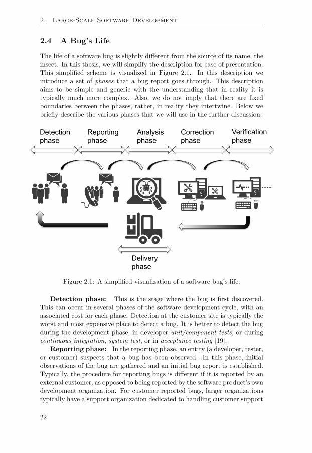
2. Large-Scale Software Development

2.4 A Bug’s Life

The life of a software bug is slightly different from the source of its name, theinsect. In this thesis, we will simplify the description for ease of presentation.This simplified scheme is visualized in Figure 2.1. In this description weintroduce a set of phases that a bug report goes through. This descriptionaims to be simple and generic with the understanding that in reality it istypically much more complex. Also, we do not imply that there are fixedboundaries between the phases, rather, in reality they intertwine. Below webriefly describe the various phases that we will use in the further discussion.

Detection phase

Reporting phase

Analysis phase

Correction phase

Verification phase

Delivery phase

Figure 2.1: A simplified visualization of a software bug’s life.

Detection phase: This is the stage where the bug is first discovered.This can occur in several phases of the software development cycle, with anassociated cost for each phase. Detection at the customer site is typically theworst and most expensive place to detect a bug. It is better to detect the bugduring the development phase, in developer unit/component tests, or duringcontinuous integration, system test, or in acceptance testing [19].

Reporting phase: In the reporting phase, an entity (a developer, tester,or customer) suspects that a bug has been observed. In this phase, initialobservations of the bug are gathered and an initial bug report is established.Typically, the procedure for reporting bugs is different if it is reported by anexternal customer, as opposed to being reported by the software product’s owndevelopment organization. For customer reported bugs, larger organizationstypically have a support organization dedicated to handling customer support

22

2.4. A Bug’s Life

issues. This organization will enforce certain quality requirements on the bugreport. If, on the other hand, the bug is reported by the internal organization,it is typically up to the individual designer or tester to ensure the quality ofthe bug report. It is up to the reporting entity to come up with a shortdescriptive slogan for the bug and some descriptive text. In addition to thisunstructured data, additional structured data is typically reported. The exactdetails of this additional data will differ depending on context but typicallyinclude

• which customer reported the bug

• which site was running the product where the bug was detected

• which revision of the software was running

• which operating system or architecture was running the software

• additional attachments such as screen shots

• log files

• support personnel discussions and other supporting material

A very important aspect of this phase, especially with individually re-ported bugs, is that the analysis phase will be much faster if the quality ofthe bug report is good. There are huge gains to be made by ensuring highquality bug reports [20].

Analysis phase: This is the phase we focus on in this work. The analy-sis phase consists mainly of two aspects. The first is assigning the bug reportto a person or team for analysis, and the second is locating where in the soft-ware architecture the bug is located. A complicating factor for us is that theseaspects are intertwined. To know where to send a bug report, the supportpersonnel must know the functional area in which the bug resides, but toknow this they must talk to the development teams in the correct area. Butof course, finding this team was the original problem. This conundrum is typ-ically solved by layering the system into a hierarchy. The support personnelcan then send the bug report to the top level organization of an area, whichis responsible for routing the bug report further down in the organization.Bug assignment is thus a multi-stage process. In large development organi-zations, the corresponding support organizations are typically organized intotiers. Typical names for these tiers are first line, second line and third linesupport. Even with this tiered approach, it is typically hard for the supportorganization to know exactly to which team a bug report should be assignedfor analysis. One solution to this problem is to have an intermediary entityin the later support lines that is closer to the development organization. Thisentity can route the bug report to the development team that is most likely

23

2. Large-Scale Software Development

to be able to find the cause of the bug and fix the offending code. This entityis sometimes called a change control board (CCB) or triager, i.e. someoneequipped to triage the bug report to the best person or team. At this triag-ing stage, the bug report is inspected for clues that might indicate where thereport should go. If the report is written on a particular product or a lowerlevel component, it makes the job easier for the triaging entity. Otherwise,typically the triager must read the report and make a best estimate fromexperience of where to assign the report. In summary, bug assignment andtriaging occurs on multiple levels in large organizations.

Correction phase: In this phase it is concluded that a fault is in factpresent in the system, and a decision has been made that it should be fixed(this is not the case for all bugs). At this stage, ideally we want to re-useall information that has been gathered during the analysis phase. There isusually a ”notebook” or ”discussion” or some sort of ”history field” for thispurpose. Here, information gathered throughout the bug handling process canbe stored. If the same person that did the analysis of the bug is also the onefixing the bug, the information and knowledge gathered during the analysisphase is trivially re-used. But even having the same person fixing the bug isnot a guarantee of complete information re-use. Sometimes the correction isdelayed for a long time and the person cannot remember the analysis when itis time for the correction.

Verification phase: During verification, the software is tested to makesure that fixes to the code have not introduced new faults or destroyed oldfunctionality. Other aspects that are tested are robustness, stability, andinteroperability with other parts of the system.

Delivery phase: At this point, the new software is ready to be deliveredto the end customer. The delivery phase consists of many administrative steps,such as packaging and version management of the new delivery.

2.5 The Bug Tracking System

To manage the work of handling bugs, some sort of Bug Tracking System(BTS) is used. In principle, the BTS can be anything from a whiteboard withsticky notes, to a spreadsheet, to a full-fledged commercial product that isspecially designed for tracking bugs. Examples of bug tracking systems arethe open source system called Bugzilla, the commercial system Jira, Trac, andIBM ClearQuest. Jira, Trac, and ClearQuest actually support more processesthan just bug tracking. For instance, sometimes the bug handling processis separated from the change request process and both Jira and ClearQuestsupport this. In addition to open and commercially available tools, there arealso proprietary, in-house BTS’s.

For all of the BTS’s we have studied, there are some common key char-acteristics. A BTS maps the phases of a bug report to states in the BTS.

24

2.6. Automatic Fault Localization vs. Automatic Bug Assignment

The names of the states differ depending on the bug tracking system. Butthe general scheme contains states for representing a newly created bug, anassigned, or in progress bug, and a finished bug. Typically, there is also someway to indicate how the bug was solved. Not all bugs can be solved—in facta substantial number of bugs cannot be reproduced or solved [21]. In thiscase, the bug will be left unsolved with some indication in the BTS that thebug cannot be reproduced or is invalid. To track individual bugs, there istypically an Id field that is unique to each bug report. In Bugzilla, this fieldis called bug_id and in Jira it is called the key. Both tools have a short textfield, typically a one sentence description, that is used as a slogan or sum-mary of the bug report. In Bugzilla, this is called short_desc and in Jirait is called Summary. In the Ericsson in-house tool it is called Heading. Inaddition to the short slogan, the tools have various support for longer typesof unstructured text. The texts can be of various sorts. In Bugzilla, there isa generic field called long_desc, of which there can be several. Typically, thefirst of these is a longer description of the bug, while the following ones areused for a general discussion of the bug. In Jira, there is a Description fieldthat is used as a longer description of the bug, and separate Comments fieldsfor discussing the bug report. Similarly, in Ericsson’s in-house tool, there isa Description field and separate Notes that can be attached to discuss thebug report. In the Ericsson tool there is also a History field, which makes itpossible to track the states the bug report has been in.

The information in the BTS is not only text, but typically a combinationof nominal, ordinal, numeric, and unstructured text data. For instance, cus-tomer, site, or country are examples of possible nominal attributes. Examplesof numeric attributes are release and priority. Note that priority could alsobe ordinal if, instead of a numeric value, it is designated ”low”, ”medium”, or”high”.

2.6 Automatic Fault Localization vs. Automatic BugAssignment

As we have noted before, bug assignment and fault localization are intercon-nected. Here we discuss some of the connections between the two, and howthey relate to an organization’s ways-of-working.

If the development organization is structured so that one particular de-velopment team always handles bug reports on one particular subsystem orcomponent, the bug triager is in essence performing fault localization. This isbecause there is a one-to-one mapping between design team and component,or subsystem. This structuring of the development organization is not neces-sarily always the case, so it is still valid to separate the two activities. In fact,the opposite is likely to be the more common case, i.e., teams maintaining sev-eral subsystems and/or components. Since we believe the latter to be more

25

2. Large-Scale Software Development

common, we also consider the task of fault localization to be more importantthan that of bug assignment. We argue that if we solve the fault localizationproblem, it is a fairly straightforward task to solve the bug assignment prob-lem. If the members of a team always work on the same components, theycan easily self-assign bugs if they know which component is at fault.

Alternatively, a simple mapping from a component to a design team canbe established. In this way, other external organizations can automaticallyassign bugs to teams, given that it is known in which component a bug islocated. However, the converse is not necessarily true. If a team handlesseveral components it is not obvious where in the software architecture thebug is located, even if one knows which team should handle the bug. Thus,we argue that the problem of automatic fault localization is more interestingthan the problem of automatic bug assignment, since the solution to the firstproblem also, in general, solves the other.

The way-of-working in the organization will also dictate which activity ofABA or AFL is most suitable for the particular organization. For instance, inagile organizations, a top-down assignment of bug reports might not fit withthe agile workflow. Hence, ABA may not be applicable. In Agile development,where teams are themselves responsible to pull bug reports from a backlog,an AFL approach makes sense since it can be used at 1st line support to givea first classification of a bug report. This pinpointing of a bug to a componentcan then be a guide to which bug reports might be suitable for a particularteam. Conversely, if the way-of-working dictates that the support organizationassigns bug reports top-down, then an ABA methodology is best-suited. Ofcourse, nothing prevents a combined approach! It is certainly possible todo both ABA and AFL, and get the benefits of both if this aligns with theorganization’s way-of-working.

2.7 A Taxonomy of Automatic Fault LocalizationScenarios

Automatic Fault Localization can be useful in several different contexts in thesoftware development life-cycle. Some of these contexts include:

1. Development debugging - This is the situation where the software isbeing developed and some problem has been found in unit tests or lowerlevel function tests that needs to be localized. Here, the individualsoftware developer typically has access to low level details about thewhole system, such as source code and low level unit tests. In thiscontext, detailed fault localization techniques, such as spectrum-basedapproaches [22], are suitable since they require access to the lowest levelof detail of the system and the ability to run code and test cases.

26

2.7. A Taxonomy of Automatic Fault Localization Scenarios

2. Post-test debugging - In large-scale software development, not alltesting is done by the individual software developer, but also by ded-icated test teams. This typically includes system-wide tests, such asrobustness, stability, or integration tests that require specialized knowl-edge, hardware, and system configuration and setup skills not possessedby all developers. The post-test debugging context is when a bug hasbeen reported by a test team to the development team. In this con-text, developers, again, typically have access to lower levels of detail ofthe system, such as the exact configuration, and detailed logs of whenand under which circumstances the problem occurred. Developers alsotypically have access to unit tests and source code of the system in thiscontext.

3. Post-delivery debugging - This is the context where the full systemhas been delivered to the customer and the customer has reported a bugon a full production system running in live operation. In this context,it is typically not feasible for the first receiver of a bug report to set upthe system for detailed troubleshooting. Also, the receiver does not haveaccess to the source code or unit level tests. The first receiver of the bugreport has to make a judgment based only on the information that isavailable in the bug report and his or her own experience to determinewhere in the architecture the bug is most likely to be located, and whereto route the bug report for further troubleshooting.

In this thesis, we focus on the post-delivery debugging context. This is notto say that the other contexts are not important, or that our techniques arenot applicable to these contexts. The reason for our focus is mainly due tothe relatively small amount of research done in this context and the specificmotivations for this thesis.

27

3 Methodology

3.1 Method Overview

In this chapter we present methodological concerns of this thesis. We firstgive a background of the author’s personal experience, which we feel hasplayed an important role in shaping the material for this thesis. After thisintroduction, we break down the different methods that have been used andhow that maps to the different papers. We finish the chapter by discussingconcerns of validity.

3.2 The Author’s Personal Experience

The work in this thesis has been driven by concrete industry problems thatthe author has wrestled with in various ways and in various capacities during20 years in a large-scale software development organization. The author haspersonally worked extensively with the bug handling process at Ericsson AB.The author’s experiences with bug handling come from working in many dif-ferent capacities. The first experiences were gained in the capacity of being adeveloper using the system in his daily work for many years. During this timethe author was often involved in discussions, decisions, and management foraaround bug handling in his capacity as developer, team lead, and assistantproject manager. The author has also worked as a test coordinator, helpingthe test and design teams deal with bug handling processes and the dailywork of solving bug reports. Additionally, the author was part of a team that

29

3. Methodology

phased out an old bug tracking tool to the use of the current main tool forbug handling at Ericsson. This was done for one of the largest Ericsson de-velopment organizations. At the same organization, the author has also beenpart of a team responsible for dealing with efficiency and improvements in thebug handling tools, and ways of working.

3.3 Methods Used

We use the classification scheme by Wohlin, Runeson, Host, Ohlsson, Regnell,and Wesslen [23] to describe the methodologies used in our papers. Themethods are

• Scientific - the world is observed and models are built based on obser-vations, for example, simulation models.

• Engineering - the current solutions are studied and changes are proposedand then evaluated.

• Empirical - a model is proposed and evaluated through empirical studies,for example, case studies or experiments.

• Analytical - a formal theory is proposed and then compared with em-pirical observations

We have employed two main research approaches during the work on this the-sis. The main approach has been empirical, where we have studied processes,methods, and techniques in a real-world setting. The second main approachhas been analytical, where we have mathematically derived algorithms andhave proved certain properties of these algorithms.

The purpose is classified using the strategies detailed by Runeson, Host,Rainer, and Regnell [24]. From Runeson, these are:

• Exploratory - finding out what is happening, seeking new insights, andgenerating ideas and hypotheses for new research.

• Descriptive - portraying the current status of a situation or phenomenon.

• Explanatory - seeking an explanation for a situation of a problem, mostlybut not necessarily, in the form of a causal relationship.

• Improving - trying to improve a certain aspect of the studied phe-nomenon.

The employed method for most of the research in this thesis has been anempirical approach, where the researcher has been working in the real-worldenvironment under study. This type of research setting is sometimes calledin-vivo [42]. The main purpose of the research has been two-fold; exploratory

30

3.3. Methods Used

and improving. Initially we wanted to explore the feasibility of the ideas wehad for improving the efficiency in the bug handling process. Once this wasestablished in Paper I and Paper II, we wanted to further improve on theavailable approaches. This was done in Paper V with the theoretical PapersIII, IV and VI as a basis.

Since a lot of the work has been done in-vivo and under Non-DisclosureAgreements (NDAs) we have tried to strike a balance between the restrictionsof the NDAs and the desirability of replicable research. Wohlin, Runeson,Host, Ohlsson, Regnell, and Wesslen [23] differentiate between close or exactreplication and differentiated replication. In close replications, the originalprocedures and the original sample population are available and a very de-tailed replication can be achieved. This is highly desirable, as it helps to buildconfidence in the outcome. In differentiated replications, the same researchquestions are studied, but the experimental procedures or the exact popula-tion can differ. Even though differentiated replications are not as exact asclose replications, much knowledge can be gained from differentiated studies(Wohlin, Runeson, Host, Ohlsson, Regnell, and Wesslen [23, p. 20]). In caseswhere we have been prohibited by NDAs from publishing our data, we havedescribed the methods in detail to facilitate differentiated replication. In thetheoretical work, we have used publicly available datasets for our studies tofacilitate close replication. In the last empirical Paper V, we have used bothproprietary and publicly available data sets to both cater to the desire to studythe applicability in the industrial context, and to facilitate close replicationby other academics who do not have access to the proprietary data. We havealso published the major part of the code developed during this thesis as OpenSource to further increase transparency and facilitate replication (see Section1.5). This include code for new methods and have extensible examples forease of use. In Paper I and Paper II, and in part in Paper V, we have tradedclose replication for differentiated replication to get highly relevant industryresults.

We argue that even where close replication is not possible, we get a trans-fer effect of the knowledge that was gained because we have ensured thatthe methods and data that were used are applicable to large-scale softwaredevelopment contexts. This has been achieved by using generally availablesoftware libraries with general purpose machine learning techniques. We haveavoided developing highly specialized solutions for our particular contexts byselecting features that are highly general and available in all of the bug track-ing systems that we have come across. We have validated this by using bothopen source datasets and data from different industry partners.

High quality empirical research places high requirements on the instrumen-tation in the tools used. In an effort to facilitate closely replicable research, wehave implemented all of the code in our theoretical papers from scratch in thesame framework as the one in which the original comparison techniques wereimplemented. We have also re-implemented other comparison approaches in

31

3. Methodology

the same framework to be able to measure performance in detail, to the extentthat it is possible. Also, in the more empirical work, we have implemented thecode for instrumentation in the same language as the libraries that were usedin order to do the instrumentation as correctly as possible. We have developedextensive test suites to ensure that the code is correctly implemented.

In Paper I and Paper II, we have performed Experiments. Experiments(or controlled experiments) are, according to Wohlin, Runeson, Host, Ohlsson,Regnell, and Wesslen [23]

”an empirical inquiry that manipulates one factor or variable ofthe studied setting. Based in randomization, different treatmentsare applied to or by different subjects, while keeping other variablesconstant, and measuring the effects on outcome variables.”

In Paper I and Paper II, we collected real-world data from our cases whichwere two large-scale software development companies. We used the data wehad gathered to examine the thesis that machine learning can be used to auto-matically triage bugs. Specifically, we examined the thesis that using a specialmachine learning approach, called ensemble techniques, gives prediction ac-curacy that is at least as good as, or better than, a single specific machinelearning technique.

In Papers III, IV and VI, we used mathematics to develop theories inthe area of probabilistic text modeling and document classification. Thiswas guided by the exploratory work in Papers I and II, where we found apossible avenue for improving the unstructured text handling in bug reports.To achieve this, we needed a fast and exact approach to modeling of text.We used computer science, mathematical and statistical, theories to developa new, mathematically correct, and very fast parallel sampler for the LDAmodel.

Finally, in Papers V and VI we again used experiments in combinationwith quantitative data to determine whether or not our new approach showedthe desired improvements.

Table 3.1 summarizes the main research methods and the purpose of thepapers.

Paper Method PurposePaper I Empirical ExploratoryPaper II Empirical Exploratory + ImprovingPaper III Analytical ImprovingPaper IV Analytical ImprovingPaper V Empirical Improving + ExplanatoryPaper VI Analytical Improving

Table 3.1: Mapping of each paper to research method and purpose.

32

3.4. Paper I

Again, although Paper II is listed in Table 3.1 as Improving, the work on thatpaper generated ideas that lead to the following papers.

Furthermore, we can break down the paper classification using the GQMapproach by Basili [25]. Table 3.2 summarizes the main goal, and main metricused to evaluate the approach, and maps it to the research questions. In thesections below, the details of the individual papers are described.

Paper Goal Question MetricPaper I Feasibility of ML RQ1 Prediction AccuracyPaper II Feasibility of ML RQ2 Prediction AccuracyPaper III Exact Parallelism RQ3 Speed + CorrectnessPaper IV Rich Classifier RQ3 Accuracy + RichnessPaper V Flexible Classification RQ2 Accuracy + RichnessPaper VI Speed Improvements RQ3 Speed + Correctness

Table 3.2: Mapping of paper to research method, goals, and main evaluationmetric.

3.4 Paper I

In Paper I, we collect roughly one year of real-world data from one large andcomplex system at Ericsson AB. We use minimal filtering of the data to ensurethat the data is truly the real data that the engineers are working with, andthat we get the maximum amount of data to work with. The only filteringwe apply is to select solved bug reports (i.e finished) and exclude duplicates.

What characterizes the system is that it is mature and has been in pro-duction for over 10 years. It is a very large system and many different pro-gramming languages are used in its construction. The bulk of the code isimplemented using C++ and Java.

This setting was selected because it is typical for the context in which wepropose that ML techniques can be used. The system is so large that, inpractice, no single individual developer has detailed knowledge of the wholesystem. Assigning bug reports and locating the faulty component(s) in thesetypes of systems is really challenging.

The main goal of the paper was to explore the feasibility of using MLtechniques for AFL and ABA in large-scale software development projects inan industry setting. The paper mainly answers RQ1. The metric used forevaluation is prediction accuracy as measured by cross-fold validation. Themain reason for using this measure is that cross-fold validation is a standardmetric in the ML community and accuracy is a clear and simple metric tocommunicate to the industry stakeholders and is easy for them to understand.

33

3. Methodology

3.5 Paper II

Paper II is an extension to Paper I, where we further explore the effects andconsequences of using machine learning for ABA in an industrial setting. Thescope of Paper II is vastly increased compared to Paper I, both in terms of thenumber of cases and the evaluation. In Paper II, we collect more than 50,000industry bug reports from two big companies and five different projects.

The goal of Paper II is to further study RQ1 and improve on the methodof selecting ML classifiers, and to suggest guidelines for industry on how todeploy ML techniques for ABA and AFL in an organization.

Conclusions from Paper II guided the research of Paper III and Paper IV.One concrete question that is related to RQ2, and which suggests future work,concerns how to handle unstructured input, such as text. In the paper, weexamine the performance of classification, both including and excluding text.We find that the combination of both text and structured data is the best. Inthe conclusion and future work section of Paper II, we propose research intothe question of whether or not there are better ways to represent the textualinput to the classifiers. This leads to papers III and IV, where we studytechniques for representing unstructured text and using it for classification.The metric used for evaluation is again prediction accuracy as measured bycross validation.

3.6 Paper III

In Paper III, we mathematically derive a formulation of a probabilistic samplerfor LDA and provide formal proofs for the complexity bound of the sampler.We then implement this sampler, and the comparison samplers, in code andstudy its characteristics compared to other approaches. In the paper, weprove mathematically that, although our sampler incurs an extra samplingstep, complexity-wise, it is equivalent to competing implementations.

We also show empirically that the actual runtime behavior is favorablecompared to other approaches that are approximate LDA models. The mainmethod used in this paper is analytical, but the results of the sampler are eval-uated empirically on different datasets. The datasets are the same datasetsthat are used in related papers using other implementations of LDA to facili-tate close replication.

The goal was to develop a fast and correct method for representing textin ML techniques. It is related to RQ3 since it tries to address how we canimprove on the techniques available in our research context. The metrics forevaluating the sampler are proofs of correctness and speed of the sampler.

34

3.7. Paper IV

3.7 Paper IV

Paper IV is a further theoretical extension of Paper III, where we extendthe unsupervised LDA sampler to a supervised classification model and studyits characteristics. Again, the main method is analytical with an empiricalevaluation on public datasets. The derived sampler is a Bayesian classifier,which implies that we get a measure of the uncertainty for all of the parametersin the model, including the predictions. This is very powerful since it allowsan organization to tune the use of ML by trading prediction accuracy againstautomation level if desired. For example, when the uncertainty in predictionsare low, automated intervention (routing of the bug report) can be used, butwhen the uncertainty is high, human intervention can be invoked.

The goal here was to implement a classifier that fulfills the requirementsof handling both unstructured text and nominal values, as well as providingfull probability distributions on parameter estimates. An additional goal wasto implement a classifier that gives interpretable output. It relates to RQ2 inthat it answers which techniques should be used in our context. But it is evenmore relevant to RQ3, since it improves on the techniques available. Themetric used for evaluation was prediction accuracy using cross validation.

3.8 Paper V

In Paper V we take the experiences from Paper III and Paper IV and applythem to our original problem of AFL. We show that we get competitive re-sults with our sampler from Paper IV. In addition, we get the richness of theBayesian model, which gives several benefits. We exemplify one of these ben-efits by explaining how the richness of the model can be used in an industrialsetting. For comparison, we use some of the same datasets that we used inPaper II. We complement these with publicly available datasets to facilitatereplication.

The goal was to empirically evaluate how well the DOLDA classifier fulfillsour requirements in our bug handling context. It answers RQ2 sine it dealswith which techniques should be used in our context. The metrics used forevaluation were accuracy using cross validation and subjective measures ofclassifier richness.

3.9 Paper VI

In Paper VI we further improve on the LDA sampler described in Paper III.The goal was to reduce the memory requirements and sampling time of

the LDA sampler developed in Paper III, but still keep the exactness of theinference. These goals came primarily from the continued need to improve

35

3. Methodology

the sampling speed, but also from initiatives to implement LDA on GraphicalProcessing Units (GPUs).

Paper VI mainly relates to RQ3 since it improves upon machine learningtechniques, both in general, and specific for our context. The metrics used toevaluate the goal was sampling speed and analytical proofs.

3.10 Validity

We discuss the various aspects of the validity of the research in the four formsdetailed in the framework by Wohlin, Runeson, Host, Ohlsson, Regnell, andWesslen [23]:

• Conclusion validity and Reliability - Conclusion validity is concernedwith the relationship between the treatment and the outcome in a quan-titative analysis. We want to make sure that there is a statistical rela-tionship, i.e. with a given significance. Reliability is its counterpart in aqualitative analysis. This aspect is concerned with the extent to whichthe data and the analysis are dependent on the specific researchers. Hy-pothetically, if another researcher conducted the same study at a latertime, the result should be the same. Threats to this aspect of valid-ity are, for example, if it is not clear how to code collected data or ifquestionnaires or interview questions are unclear.

• Internal validity - If a relationship is observed between the treatmentand the outcome, we must make sure that it is a causal relationship, andthat it is not a result of a factor over which we have no control or havenot measured. In other words, that the treatment causes the outcome(the effect).

• Construct validity - This type of validity is concerned with the relationbetween theory and observation. If the relationship between cause andeffect is causal, we must ensure two things: (1) that the treatmentreflects the construct of the cause well and (2) that the outcome reflectsthe construct of the effect well.

• External validity - External validity is concerned with generalization. Ifthere is a causal relationship between the construct of the cause, andthe effect, can the result of the study be generalized outside the scopeof our study? Is there a relationship between the treatment and theoutcome?

Often there is a trade-off between the different types of validity, and thevarious aspects of validity must be prioritized (Wohlin, Runeson, Host, Ohls-son, Regnell, and Wesslen [23, p. 111]). While all aspects of validity are

36

3.10. Validity

important, our focus has been on solving real world large-scale industry prob-lems as experienced by the author during many years of active developmentin the industry. Thus, our focus has been on External and Construct valid-ity, i.e. that the research questions are relevant and that the experiments, asmuch as possible, use actual data that practitioners are working with. In ourcase, this has come at the expense of replicability on some occasions, since weare not able to make our datasets publicly available. This has been mitigatedby using open datasets for comparison with the industrial data in Paper V,where open data was available that was similar to the industry data (unlikePaper I and Paper II where no similar data was available). Our studies aredesigned to minimize the impact of threats to validity. Below we discuss indetail the choices and decisions we have made in regard to these aspects.

External ValidityExternal validity concerns how well a study generalizes.

Effect of the threat on our results: What would the effect on ourresults be if they were affected by the threat? This is mostly related toPapers I, II and V, since Papers III, IV and VI are theoretical papers. If ourresults were not externally valid, this would mean that ML-based classificationof bug reports would not be applicable to other large-scale industry softwaredevelopment contexts.

Large scale industry applicability is one of the main drivers of this workand a great deal of effort has gone into ensuring that the techniques areapplicable to actual industry practice. One example of this is that in Paper IIwe examined a particular ML technique called Stacked Generalization (SG).The advantage of SG is that it is flexible and does not require particularexpertise in deployment, due to its robust performance. The downside of SGis its lack of interpretability. This feedback from our industry partner (alsobacked by research [26]) lead us to explore richer techniques for dealing withunstructured text (Papers III & VI) and Bayesian models for ML (Papers IV& V).

We have gone to great lengths, exploiting the author’s expertise and dis-cussing with our industry partner, to ensure that the industry data that wehave used is real world data from active projects, dealing with exactly theproblems that the thesis deals with. The context of industry bug data is pro-hibitive, since this is very sensitive data and companies do not publish thistype of data for many reasons.

For the main paper studying the applicability of ML-assisted ABA (Pa-per II) in an industrial context, we managed to gather data from five majorindustry projects, from two large software development companies. This isthe largest study on industry data that we are aware of. For replicabilityand comparison with Open Source Software (OSS) data, we have also appliedthe techniques to OSS datasets. Two companies is not a big sample of large-

37

3. Methodology

scale software development companies, but we argue that the structure andsetup of the bug handling and teams generalizes to many types of large-scalesoftware development contexts. Additionally, our results are in line with pre-vious research that has been done, both in an OSS context, and in smallerindustrial research papers [27]. The threat to external validity is further mit-igated by the fact that no project-specific tuning of the classifiers has beendone, nor have we filtered the bug reports to achieve greater accuracy. Weargue that our accuracy results are probably on the lower end of what can beachieved, since no real optimization of classifiers or advanced feature selectionwas performed.

Papers III, IV and VI are theoretical papers and the question of externalvalidity is simpler to answer. In this case we need to show that the samplersfulfill the defined requirements. This is shown analytically and measured usingstandard datasets.

Paper V is specifically targeted to mitigate some of the problems of ap-plicability to industrial context of Paper II (i.e. external validity). Here weargue that the richer model that Paper V presents complements the resultsin Paper II and the richer model further increases the applicability to theindustrial context.

Conclusion ValidityMany aspects of the conclusion validity threat deal with statistical power andviolations of the assumptions of statistical tests.

Effect of the threat on our results: What would be the effect onour results if they were affected by the threat? Statistical conclusions aboutmeasures would not hold.

One threat to conclusion validity is the use of cross validation to drawconclusions about the generalization error of classifiers in this thesis. Thereason we use cross validation (in spite of known problems [28] with it) isthat it is a standard method that researchers and the statistical and machinelearning communities are very familiar with and it is simple to understandfor our stakeholders. In Paper II we mitigate this problem by exploring othermethods than cross validation, and we conclude with a warning that crossvalidation should not be the only type of evaluation. So one needs to becareful drawing absolute conclusions from cross validation alone. Mostly, weuse cross validation as a model comparison tool, to compare how models andbehaviors differ. For this purpose, cross validation should suffice since allmodels (in our context) should be equally afflicted by the limitations of crossvalidation. We discuss these aspects quite extensively in the validity sectionin Paper II. Another aspect that limits our exposure the conclusion threatsare the amount of data that we have gathered to ensure minimum exposureto problems with statistical power.

38

3.10. Validity

Other aspects of conclusion validity concern the reliability of treatmentimplementation and irrelevance in the experimental setting. Since we arenot performing any experiments or studies on human subjects, only in-silico,that is, only on computer models, we are not affected by aspects that involvehuman interaction. We have implemented extensive test suites to ensure thatour code is behaving correctly.

Reliability of measures is another aspect of conclusion validity. In ourcase this translates to measurements based on bug reports. Fortunately, thetools that deal with bug databases tend to be tools that are used on a dailybasis and are therefore quite well tested and robust in terms of measurements.Another aspect of measurement that is worth noting is the interpretation ofderived measures from bug databases. For instance, in a complex bug flow,when should we say that a bug has reached a specific team? This is not alwaystrivial to decide. Also, when should we conclude that a bug is solved? In theindustrial bug flows that we have studied, the flows are typically much morecomplex than in Open Source systems, such as Bugzilla. Here the author hasused his comprehensive experience of working with these systems to definereasonable measures for these aspects, and they have been discussed with theteams and persons responsible for the bug handling process.

Internal ValidityInternal validity deals mainly with how confounding variables can affect causalrelationships drawn from statistical results.

Effect of the threat on our results: What would be the effect on ourresults if they were affected by the threat? The ensemble combinations inPaper II would look different, but it is unlikely that this would substantiallyaffect our results. Since our primary contribution is the suggested methodol-ogy rather than the specific classifiers, we argue that this is unlikely to affectour results.

Since we are not making many strong causal claims based on statisticalresults, internal validity is not a major threat to this thesis. For instance,we don’t claim that a particular variable in a bug report causes a bug to belocated in a particular subsystem. In Paper II, one threat to internal validityis that we do not optimize the individual classifiers in the ensembles. Thiscould cause some classifier with better default settings to be favored. Sincewe do not make strong claims on exactly which classifiers to select, but rathersuggest a procedure for selecting the classifiers, we argue that this limits thethreat to validity. When it comes to the accuracy measures, individual tuningof classifiers should only improve accuracy results.

39

3. Methodology

Construct Validity and ReliabilityConstruct validity concerns the relationship between the background theoryand how it connects to the actual experiments and measurements that theresearcher performs in a study.

Effect of the threat on our results: What would the effect on ourresults be if they were affected by the threat? This would mean that otherresearchers would reach conclusions that were different from ours.

Papers I, II, and V could arguably be susceptible to threats to constructvalidity. We argue that this threat is limited due to the many years of workexperience of the researcher, whose daily work involved dealing with the is-sues that these papers confront. Reliability concerns the threat that otherresearchers would not reach the same conclusions due to procedures in datacollection and analysis. For Papers I and II, it is harder since we cannot pub-lish our datasets and a direct comparison is difficult. To increase reliability, wehave described in detail in the individual papers how data was collected andthe context of the studies. For Paper V, we complement the industry datawith OSS data to facilitate replication. The source code is also publishedopenly to increase transparency.

It is possible that other researchers could reach different conclusions re-garding the use of stacking as a primary ML method for AFL and ABA asproposed in Papers I and II. Our choice here was mainly guided by a de-sire for simple deployment in a large-scale software development organizationwhere the goal was to maximize accuracy despite limited ML expertise. Otherresearchers in different contexts with other priorities could reach other con-clusions regarding the best option in terms of classification techniques. ForPaper V, where model richness and interpretability were the main goals, itis also possible that other researchers would reach other conclusions sincethere is a certain amount of interpretation with regard to what richness andinterpretability means. Although details may differ, we argue that we havepresented enough evidence for our main point, that ML is a feasible optionfor the ABA and AFL problems in an industrial setting.

Papers III, IV and VI should not be affected by these threats since they aremainly analytical and the context and requirements are very clear. For PapersIII, IV and VI, it should be straightforward for other researchers to replicateour results since we use datasets that are research community standards forevaluating LDA samplers and classifiers.

40

4 Theory

The study of machine learning has grown to be a vast field and there isno room (or time) to cover all of the nuances and aspects of the field inthis thesis. This chapter is mainly intended for the unfamiliar reader or theindustry practitioner with some, perhaps old and slightly faded, familiaritywith basic probability theory, calculus and linear algebra. In the expositionbelow we have tried to minimize the use of mathematical notation that mightbe confusing or that could obscure the intuition of what is happening. Thehope is that this chapter will give a basic understanding of some the coremathematical ideas behind a few of the most important machine learningtechniques used in this thesis. Hopefully, this will enhance the reading andunderstanding of the papers that make up the thesis. For more thoroughexpositions we refer to the excellent works of Bishop [29] and Murphy [30].

Personally, I have found that nothing facilitates learning as much as con-necting the math to simple examples. So the goal is, as much as possible, toexemplify the math with examples from our problem domain of bug reports.The hope is to build up an intuition of the area and the theory that we willbe discussing in the included papers from a basic level. Hopefully this willgive the unfamiliar reader some of the basic understanding that is needed toread the rest of this thesis.

41

4. Theory

4.1 Machine Learning Introduction

To start getting an intuition of what machine learning is, we discuss variousflavors of learning and ways of implementing the learning approaches. First,we start with some basic definitions and examples.

• Classification

– Classifying data into a set of discrete outcomes– Example: Which software component does a bug report originate

from?

• Regression

– Estimate of a real value from data– Example: What will the processor load be if we activate a set of

features in the system?

• Clustering

– Finding groupings in unlabeled data– Example: Which types of users behave the same way in a telecom

network?

• Dimensionality Reduction

– Extract the most important piece of information from a large setof data

– Example: Given a text document with 1000 words, which are themost important ones?

• Visualization

– Displaying information in a way that a humans can more easilystudy a dataset

– Communicating results of a study in overview format– Example: See Figure 4.1

4.2 Probability Reminder

This section provides a very short reminder of some of the basic concepts inprobability theory. This section can safely be skipped if the reader is familiarwith the nomenclature and basics of probability theory. For a very readableintroduction to probability we highly recommend the beginning chapters ofBishop [29].

42

4.2. Probability Reminder

Figure 4.1: t-SNE rendering of a bug database using unstructured text viaLDA, using the individual document topic mixture as input features.

The probability of an event A occurring is usually written as

p(A)Probabilities range from 0, indicating an impossible event, to 1, which is acompletely certain event. Frequently, probabilities are expressed in percent-ages, ranging from 0 to 100%.

Discussing probability only in terms of events fast becomes burdensome sowe quickly introduce random variables (RV). A random variable is a functionthat takes outcomes of events as inputs and maps them to numbers. Forinstance, a random variable X could take the event ”the rolled die landedwith 4 dots up” and map that to 4. Another RV Y, could represent the sumof two die roll events, returning 7 if one die landed on 4 and the other on 3.Formally, the definition of a random variable is [31]

Given an experiment with sample space S, a random variable (RV)is a function from the sample space S to the real numbers.

43

4. Theory

0.00

0.05

0.10

0.15

0 10 20X

Probability

Figure 4.2: Discrete probability distribution.

There are some subtle points about notation to be made here. Probabilitiesare only defined on events, but not on RV’s, so strictly it does not make senseto talk about p(X) if X is an RV [31]. But we can talk about p(x) (note:small letter x), where p(x) = p(X = x), since having X take the value x isan event, this is fine (we assume that X is discrete). We can also talk aboutp(5 <X < 8) (valid for both discrete and continuous RV’s) which is the eventthat the RV X lies in the 5-8 interval. This distinction is not always clear(especially in less formal contexts) and the notation p(X) is used when it isunderstood that it stands for p(X = x) (see Bishop [32]). We will also use thisnotational shortcut to make the presentation simpler, but with the warningthat sometimes it can be confusing.

A distinction is made between discrete and continuous random variables.A discrete RV maps outcomes to a discrete list of outcomes. The list can befinite, as in a fixed set of outcomes (the six sides of a die), or infinite (theintegers). A continuous RV maps outcomes to the real numbers. Sometimesthe notation of discrete and continuous RV’s differ, with continuous proba-bilities written with lowercase p and discrete ones with a capital P . We shallnot bother with this distinction in this text and we will use lowercase p forprobabilities.

The probability of a random variable is completely described by its proba-bility distribution, which is a function where the domain consists of all possibleoutcomes of the RV. As a consequence of the basic axioms of probability, theintegral of a probability distribution from −∞ to ∞ sums to 1. A probabilitydistribution can be either discrete as in Figure 4.2, or continuous as in Fig-

44

4.2. Probability Reminder

0.0

0.1

0.2

0.3

0.4

−4 −2 0 2 4X

Density

Figure 4.3: Continuous probability distribution.

ure 4.3. If it is discrete, it is called the probability mass function (pmf). Fromthe probability mass function we can, for each possible value the random valuecan take, find its corresponding probability. For instance, from Figure 4.2 wecan see that the probability of x = 12 is ca 5%, i.e. p(X = 12) = 5%.

The probability distribution is continuous if the random variable of interestis a real number. This is depicted in Figure 4.3. In this case the distributionis called probability density function (pdf).

There is an important difference between a discrete distribution and acontinuous distribution. In the continuous case we are interested in the prob-ability of a real value, but the probability of any specific real-valued outcomeof a continuous RV is 0! So, in contrast to the discrete case where we canlook at the distribution plot (pmf) and read off the probability of the RV fora specific outcome, we cannot do this from the pdf. It is entirely possible forthe density (the y value of the pdf) to have values larger than 1, which weknow is impossible for probabilities, since they are defined to lie between 0 and1. What we can do with the pdf is to find the probability that the outcomeof a continuous RV lies within an interval. This is depicted in Figure 4.4,where the interval is −1 < X < 1 and the associated probability is 68%. Thisprobability is found by taking the definite integral of the pdf from -1 to 1, i.e.

p(−1 ≤X ≤ 1) = ∫ 1

−1 pdf(x)dx = 68%Note here that −1 <X < 1 is the event that the RV X lies in the interval.

45

4. Theory

We can also talk about the probability of two or more simultaneous events.The probability of both events A and B, called the joint probability of A andB, is written

p(A,B)An example of this would be the toss of a coin and a roll of a die. WhereA could be the event ”the coin landed Heads up” and B is the event ”thedie landed with an even number up”. The joint probability is the probabilityof both those two outcomes occurring in the same trial. Joint probabilitiesgeneralizes to RV’s also, where we talk about the joint distributions of two ormore RV’s.

From a joint probability distribution, we can margnialize out or integrateout one variable and get the marginal distribution for the other. In Sec-tion 4.76 we show a detailed example of marginalization in a concrete case.Marginalization is slightly different depending on whether the RV is discrete,i.e., its outcomes can be mapped to the natural numbers, or continuous, inwhich case its outcome is a real number. The marginalization of a continuousRV is done via integration.

p(X) = ∫Yp(X,Y )dY

while for a discrete RV it is the sum

0.0

0.1

0.2

0.3

0.4

−4 −2 0 2 4X

Density

Figure 4.4: The probability of a continuous probability distribution is the areaunder the curve of the continuous probability distribution, not the y value ofthe pdf!

46

4.2. Probability Reminder

0

25

50

75

100

−4 −2 0 2 4x

count

Figure 4.5: Histogram of 800 draws from a normal distribution with the truenormal overlayed.

p(X) =∑Y

p(X,Y )A distribution is not only the graphical view of a random variable, it is

also a mathematical object. We have already mentioned that we can plotthe distribution in a graph, as in Figures 4.2 and 4.3, and that we can usethe distribution to calculate the probability of the outcomes of a randomvariable. Another thing we can do is to draw samples from it. When wedraw samples from a distribution we basically tell the distribution to generatea random outcome of the RV proportional to its probability according to thedistribution. So, for instance, if we have an RV that has a normal distribution,we can tell it to generate 800 samples from its distribution. In Figure 4.5 wehave done just that and plotted the samples in histogram form with the truenormal pdf overlayed.

We can also talk about conditional probability. Conditional probabilityis the probability of an RV conditioned on some knowledge. This is written

47

4. Theory

p(A∣B) and should be read as the probability of A given B or the probabilityof A conditioned on B. Conditional probability is defined as:

p(A∣B) = p(A,B)p(B) (4.1)

An example of this would be, the probability of a bug being locatedin a particular subsystem (say the UI) conditioned on the fact that weknow that the bug was reported by a specific customer. This is written asp(Component = UI ∣Customer = AcmeTelco). We can then calculate thisaccording to Equation 4.1.

p(Component = UI ∣Customer = AcmeTelco)= p(Component = UI,Customer = AcmeTelco)

p(Customer = AcmeTelco) (4.2)

Intuitively this can be thought of as follows. Say that we have a databasewith bug reports. We then count how many bug reports were reported bythe customer AcmeTelco (denominator in Equation 4.2). We then counthow many of the AcmeTelco bug reports were reported on the UI compo-nent (nominator in Equation 4.2). By dividing these two numbers we getp(Component = UI ∣Customer = AcmeTelco).

We must also briefly mention the extremely important Bayes Rule, whichwe will discuss further in Section 4.4. Bayes rule states that

p(A∣B) = p(B∣A)p(A)p(B) (4.3)

and follows directly (see Section 4.4 for a derivation) from conditional andjoint probability. Bayes rule is often used in its proportional form when weare not directly interested in the specific probabilities, but rather in comparingthe sizes of the probabilities to make a decision.

p(A∣B)∝ p(B∣A)p(A) (4.4)

The ∝ (read ”proportional to”) means that p(A∣B) is not a normalized prob-ability distribution (i.e. it does not sum to 1), but can be made so by multi-plying it by an expression that is not dependent on A.

An example of this is when we want to make a classification and we areonly interested in selecting the class with the highest probability. Equation 4.4lets us do this, since the denominator in Equation 4.3 will be the same for allclasses, so we can ignore the denominator and just pick the class that has thehighest value of p(B∣A)p(A). This is because if the proportional form has thehighest probability of a class, then the normalized expression will also havethe highest probability for the same class. The proportional form of Bayes

48

4.3. What is Learning?

rule is also used in so called Markov Chain Monte Carlo (MCMC) sampling.In MCMC we often do not need to know the exact probabilities, just the shapeof the probability distribution.

4.3 What is Learning?

Before we discuss more details of machine learning, we can try to define whatlearning is. Tom Michell, one of the pioneers in the machine learning field,defines learning (in the context of ML) in the following way [33]:

Definition 1. ”We say that a machine learns with respect to a particulartask T, performance metric P, and type of experience E, if the system reliablyimproves its performance P at task T, following experience E”

While slightly cryptic, it is a succinct description of what, in our context,it means to learn. To make the definition and the following chapter moreconcrete we will use a running example to accompany the text to hopefullyclarify the sometimes obscure meaning of the math and theory. We start theexample here by setting the task T of the ML system to be that of predictingwhich component in a software system that a bug is located in. The perfor-mance metric P will be the prediction accuracy the ML system achieves, thatis, how many of the bugs it correctly predicts divided by the total number ofpredictions it has performed.

prediction accuracy = # correct predictions# total predictions (4.5)

Defining E, the experience is the most elusive task. A major part offormalizing experience consists of defining how we encode the experience sowe can talk about it formally. This will be discussed extensively in this thesis;for now we will simply state that gaining more experience consists of ”seeing”more bug reports.

Now that we have all the major constituent parts of our definition, let’stry it out. We say that our ML-system learns, if it gets better at predict-ing which software component contains the fault described by a given newbug report, the more historical bug reports that we ”show” it. An erroneous,implicit assumption that is often made by readers unfamiliar with the statis-tics and machine learning fields, is that there is a linear relationship betweenthe amount of experience that is shown to the system and the amount thatthe system learns. I.e. the assumption is that the more data you present tothe ML-system, the more it learns. This is not generally so. As we showin the bug assignment context in Paper II [34], if you show the ML-systemtoo much, especially too old, bug reports it actually gets worse at predictingnew bug reports. This is intuitive, since very old bug reports is probably notrepresentative of the bugs that are currently generated. This is because the

49

4. Theory

software has evolved and developers are working on other parts of the systemand other features than was worked on a long time ago. The old bug reportswere in the old components of the system while new bug reports tend to beon the newly updated parts of the system.

Another important aspect of how much a system can learn is the qualityof the input data. If the data presented to the ML-system does not containenough relevant information to learn from, there is, per definition, a limit tohow much can be learned. The aspect of data quality can be split into twoparts. One part concerns how well the data is collected and pre-processedbefore it is presented to the ML-system, this is often called feature engineering.The other part deals with the natural variation or noise in the data andsystematic errors that can be part of the data collection process. There is alimit to how accurate the system can maximally become depending on thisnatural variation in the data. To get some intuition for this problem, imaginethat the task of a prediction system is to predict whether a person is maleor female based on only the length of the person. Since men tend to betaller than women a general strategy would be to guess male if the personis relatively tall and female if the given length is shorter. Due to naturalvariation in length in both men and women there is a limit to how accuratethis prediction will be, since some men are shorter than average and somewomen are taller than average. ML techniques are by their nature imprecise,since if there was an exact way to solve the problem one would not needto resort to ML techniques. The exception to this rule is when the exacttechniques are computationally too demanding but theoretically possible, butwe will ignore these cases here. Quantifying the magnitude of the imprecisionis an important aspect of ML techniques. Sometimes it is possible to quantifythe imprecision but sometimes not, it depends on the particular ML techniqueused.

Data quality

The general rule is that the better data you give an ML-system the betteroutput predictions you get from the system. This is in no way specific to ma-chines, but applies equally to humans. If you teach humans using knowledgefrom the 17:th century (old data, bad data), humans also become worse atunderstanding their environment. There is no inherent mechanism in learningthat prevents adverse learning, rather, protecting against it must be encodedin the learning algorithm. An example of protection against adverse learningcould in this case be to weigh old bug reports less than newer ones, so theyhave less influence in what the ML-system learns. Concretely this could bedone by looking at the filing date of the bug report and scale the importanceof the bug report proportionally to its age, i.e. how many days old it is. Thedecreasing weight of older data is often called weight decay.

50

4.3. What is Learning?

Finding, or learning, or inferring, the exact weights used to scale differentcomponents (in this case the age) of the data (the bug reports) turns out tobe a crucial part of learning.

From now on when we talk about learning in this thesis, we always takethat to mean finding an algorithm that can be executed by a computer, thatfulfills the criteria in Definition 1. We make a clear distinction from learningin this specific context and the general concept of learning that applies tohumans.

Learning Using Linear RegressionIt is probably safe to say that linear regression or ordinary least squares (OLS)is the mother of all learning techniques. It was one of the first (developed bySir Francis Galton and Karl Pearson) and is still one of the most importanttechniques in the field. Linear regression is not only very important in thatit is a basic solution to a fundamental problem, but it also has a lot of niceproperties. The main ones being that it is one of the simplest to understandand interpret and it is a crucial building block in the ML toolkit. As a buildingblock, linear regression is the basis for many more advanced techniques thatdirectly extends linear regression to other types of learning.

Linear regression solves the fundamental problem of going from observa-tions of a real value given specific inputs, to inferring the parameters of alinear model.

We will start with the most basic linear equation. Here our response vari-able or dependent variable is a function of only one input variable or covariateor predictor1 (variable) x and a fixed parameter slope, it has the form:

y = slope ∗ x (4.6)

Equation 4.6 says that as x increases, y increases by slope times x. Anotherway to put it is that a one unit increase in x increases y by slope. This viewis important since it is often how the linear model is used in practice.

If we know the value of the slope we can now calculate the correspondingvalue of y given a new x. The problem, and the reason that we use machinelearning, is that we usually do not have the slope, but we have observations ofx and the corresponding y values. This can look something like Table 4.1. Thedata in Table 4.1 is simulated by picking values for the slope and the interceptand then drawing some random values for x, calculating it’s corresponding yand adding some random noise. The simulated data y could for instance bethe measured CPU load in percent on a node when x number of users areconnected to that node.

1sometimes predictor variables are said to be created as a function (which can be theidentity function) of input variables

51

4. Theory

Here we should immediately make clear that when modeling a percentagewith linear regression we are violating some fundamental assumptions of lin-ear regression. A percentage can only range between 0 and 100 % but thereis nothing inherent in linear regression that limits the domain to the 0-100range. Another example of an improper modeling would be to model a count,which has a lower limit of zero, and a domain of only integers. When some-times these types of improper modelings are done, it is important to be awarethat underlying assumptions are broken and the result should be carefullyscrutinized to decide if it is reasonable.

The goal of linear regression is to find the value of the slope of a linearmodel so we can use it to predict the load on the machine given that a certainnumber of users are connected.

y = f(x) = slope ∗ x (4.7)

In Equation 4.7 we use a fitted value of slope to predict a new y value givensome x.

Finding the value of slope is called fitting the data to a model, or learningthe model parameters. The resulting model could for instance be used indimensioning guidelines to customers.

y x1 14 202 17 1203 31 3304 33 3405 6 736 23 3107 14 788 36 3609 25 320

10 33 200

Table 4.1: 10 observations of the real-valued variable y given inputs x

If we want to fit the data in Table 4.1 using a linear model how would wedo that? The process of fitting data to a linear model means that we want tofind the parameters (slope in this case) that describes a line that fits the datapoints as good as possible. In Figure 4.8 the data from Table 4.1 is plotted ina so-called scatter plot.

We can quantify the notion of as good as possible by saying that we wantto minimize the total error we get if we use the model. So what is the error?The error for one data point could be defined as the distance between anactual y value at a point x and a point y that is predicted by the model byplugging in the x value into the linear regression model, i.e. y-y. It turns out

52

4.3. What is Learning?

50 100 150 200 250 300 350

515

2535

x

y

Figure 4.6: Scatter plot of data in Table 4.1.

that for several reasons it is even better to use the squared error, i.e. (y− y)2.The squared error will punish large deviations from the predicted value morethan small ones. We now have a definition of the (squared) error at one datapoint,

e2 = (y − y)2 (4.8)

which we can also express as a function of our inputs x:

e2 = (y − (slope ∗ x))2 (4.9)

but we want to minimize the total error of using the model for all M points(M = 10 in our example) so we need to sum up the errors from all points.This quantity is called the sum of squared errors (SSE) and is expressed inEquation 4.10.

sse = M∑i=1(yi − yi)2 (4.10)

If we plug in our linear expression (slope∗x) for y into Equation 4.10 we get.

sse = M∑i=1(yi − (slope ∗ xi))2 (4.11)

53

4. Theory

So now we have an expression for the total error of the model in terms of y, xand slope. What does this give us? Well, it gives us a quadratic formula forthe error as a function of y, x and slope. We can now vary slope and calculatethe corresponding error of the model. Figure 4.7 shows a quadratic functionwhere the SSE is plotted as a function of slope.

−0.1 0.0 0.1 0.2 0.3 0.4 0.5

020000

60000

100000

Slope

SSE

Figure 4.7: Plot of the sum of squares error (SSE) as a function of the slope.We see that there is one point where the error is at a minimum and we knowthat this is a global minimum since the error is a quadratic function. We knowfrom calculus that the slope of the tangent (i.e. derivative) at the minimumof a quadratic function equals zero.

A quadratic function such as the SSE, is a special case of a class of functionsthat is called convex functions, and a defining property of (strictly) convexfunctions is that they have a global minima. This is convenient since we wouldlike to find the value of the slope that minimizes the SSE. We remember fromcalculus that if we take the derivative of a function f we get a new functionf ′, that describes the rate of change in the original function f . To find theminima of the quadratic SSE, we take the derivative with respect to the slopeand set this derivative to zero, we can then solve for slope to find the valueof slope that gives us the minimum error.

We take the derivative of the SSE with respect to the slope by using thechain rule from calculus.

sse′ = M∑i=1

2 ∗ (yi − (slope ∗ xi)) ∗ −xi (4.12)

54

4.3. What is Learning?

We then set the derivative to 0 and solve for slope.

0 = M∑i=1

2 ∗ (yi − (slope ∗ xi)) ∗ −xi (4.13)

0 = M∑i=1−2 ∗ (yi − (slope ∗ xi)) ∗ xi (4.14)

0 = M∑i=1(yi − (slope ∗ xi)) ∗ xi (4.15)

0 = M∑i=1(yi ∗ xi − slope ∗ x2

i ) (4.16)

Distribute the sum and pull out constants in front of the summation.

0 = M∑i=1(yi ∗ xi) − slope ∗ M∑

i=1x2i (4.17)

Solve for slope.

slope = ∑Mi=1(yi ∗ xi)∑M

i=1 x2i

(4.18)

This result can be re-written as:

slope = (M∑i=1

xi ∗ xi)−1 ∗ M∑i=1(xi ∗ yi) (4.19)

If we use 4.19 together with the numbers from Table 4.1 to calculate a valueof slope we get the result 0.095.

We can then plug that value into our original formula:

y = slope ∗ x (4.20)

and use this to plot the purple line in Figure 4.8. We have just solved ourfirst learning problem, we have learned the value of slope from data! We canquantify the quality of our learned parameter by what SSE it gives. In thiscase the SSE is 426. But can we do better? Now it is time to introduce theintercept into the model and see which effect it has on our results. With theapproach we have taken above we have implicitly assumed that the interceptof the function is zero. With this assumption, we force the regression lineto pass through zero, and this might not always be a good model. A moregeneric approach is letting the model learn the intercept also, i.e. the newmodel is formulated as:

y = intercept + slope ∗ x (4.21)

55

4. Theory

0 100 200 300 400

05

1015

2025

3035

x

y

Figure 4.8: Plot of data in Table 4.1 with various fits. The solid red lineis the ”real line” that was used to simulate data from. The purple dottedline is the regression line of a single variable linear model without intercept,and the green dash-dotted line is the regression line of a model fitted with anintercept.

We may also have more input variables than just one x. We can then extendthe model with more explanatory variables. If we have N variables the modelthen looks like this:

y = intercept+slopex1 ∗x1+slopex2 ∗x2+slopex3 ∗x3+...+slopexn ∗xN (4.22)

We can use the same reasoning and derivation as for the simple case above,but since we have several variables, we have to take partial derivatives withrespect to each of the variables in the expression. Taking partial derivativessimply means taking the derivative of an expression with respect to each ofthe variables one at the time and holding the other variables constant. Wewill not do that derivation here, since we shall later see that if we formulatethe problem as a linear algebra problem we get an elegant and equivalentsolution to the problem. To achieve this, we do some notational updates toclarify the presentation. In the machine learning field it is common to use theletter w (for weight) instead of using slope. With this notational update, theform of the linear model looks like this:

y = intercept +w1 ∗ x1 +w2 ∗ x2 +w3 ∗ x3 + ... +wn ∗ xN (4.23)

56

4.3. What is Learning?

To further simplify notation, the intercept can be called w0 which gives us:

y = w0 +w1 ∗ x1 +w2 ∗ x2 +w3 ∗ x3 + ... +wn ∗ xN (4.24)

This can be re-written using the summation symbol as follows:

y = w0 + N∑i=1

wi ∗ xi (4.25)

This is implicitly:

y = w0 ∗ 1 + N∑i=1

wi ∗ xi (4.26)

I.e we can add a ”dummy” x0 which is always 1 which represents the inter-cept (if we want an intercept, which in general we do when we solve generalregression problems). If we then add this ”dummy” x0 and require that it isalways set to 1 we can express our equation for one y like this:

y = N∑i=0

wi ∗ xi (4.27)

This is an expression for one y, if we have several y’s we index them using m.The equation for one y is then:

ym = N∑i=0

wi ∗ xmi (4.28)

If we have M rows with N covariates we can make even more notationalsimplifications and express this as a linear system where bold font indicatesthat the variable is a vector (small bold letter) or a matrix (capital boldletter). We gather all the x’s into an MxN matrix X and the y’s into a Mx1vector y and the weights 1xN vector w. The weight vector is also quite oftencalled β.

y"#$M x 1

= X"#$M x N

∗ w"#$N x 1

(4.29)

Equation 4.29 describes the predicted y values given the X’es and the weightvector, but to make the equation complete we must include the error of theprediction. This error is usually called σ or ϵ and is assumed to be normallydistributed with a zero mean. The complete equation then comes out as:

y"#$M x 1

= X"#$M x N

∗ w"#$N x 1

+ σ"#$M x 1

(4.30)

57

4. Theory

This setup can be visualized as follows:

⎡⎢⎢⎢⎢⎢⎢⎢⎣

y1y2⋮yM

⎤⎥⎥⎥⎥⎥⎥⎥⎦=⎡⎢⎢⎢⎢⎢⎢⎢⎣

1 x1,1 ⋯ x1,N

1 x2,1 ⋯ x2,N⋮ ⋮ ⋱ ⋮1 xM,1 ⋯ xM,N

⎤⎥⎥⎥⎥⎥⎥⎥⎦∗ [w1 w2 ⋯ wN ]T +

⎡⎢⎢⎢⎢⎢⎢⎢⎣

σ1σ2⋮σM

⎤⎥⎥⎥⎥⎥⎥⎥⎦(4.31)

In 4.31 the T , means transpose, which is the action of turning a column vectorinto a row vector and vice versa. We can also transpose a matrix by rotatingits values around the diagonal. As in the single variable case we want tominimize the squared error of this equation. We have gathered the errors inthe σ column, so analogous to the single variable case, the squared error is:

σTσ =⎡⎢⎢⎢⎢⎢⎢⎢⎣

σ1σ2⋮σM

⎤⎥⎥⎥⎥⎥⎥⎥⎦

T

∗⎡⎢⎢⎢⎢⎢⎢⎢⎣

σ1σ2⋮σM

⎤⎥⎥⎥⎥⎥⎥⎥⎦= M∑

i=0σi ∗ σi

If we solve for σ in Equation 4.30 we get

σ = y −X ∗wand thus the SSE is

σTσ = (y −X ∗w)T (y −X ∗w) (4.32)

As in the single variable case we want to minimize the SSE. To get 4.32 ina form that is suitable for minimization we use rules 4.33 and 4.34 of matrixalgebra:

(y −X ∗w)T = yT − (X ∗w)T (4.33)

(X ∗w)T =XT ∗wT (4.34)to get

σTσ = (yT −XT ∗wT )(y −X ∗w) (4.35)Going from 4.35 to 4.37 we use the matrix algebra relation:

XT ∗wT ∗ y = yT ∗X ∗w (4.36)Other than catering for 4.36 we can think of going from 4.35 to 4.37 as thenormal single variable cross multiplication of the terms in 4.35.

σTσ = (yTy−yT ∗X∗w−XT ∗wT ∗y−yT ∗X∗w+XT ∗wT ∗X∗w) (4.37)

58

4.3. What is Learning?

Gather the terms in 4.37

σTσ = (yTy − 2 ∗wT ∗XT ∗ y +wT ∗XT ∗X ∗w) (4.38)

If we compare Equation 4.38 with the single variable case where we substituteEquation 4.6 for y in Equation 4.8 we get

e2 = (y − (slope ∗ x))2 (4.39)

We may recognize this as a square formula from algebra, it can be expandedto

e2 = (y − (slope ∗ x)) ∗ (y − (slope ∗ x)) (4.40)

We can then perform the cross multiplications and gather the different terms

e2 = y2 − 2 ∗ slope ∗ x ∗ y + (slope ∗ x)2 (4.41)

The Square and Completingthe Square

The 2:nd degree polynomial (x+a)2can be expanded to the form x2 +2ax + a2. Going from this latterform to the former is called complet-ing the square. In Equations 4.39-4.41 we use versions of completingthe square. In Section 4.4 we willbe using the analog matrix versionof completing the square.

We see by comparing Equa-tions 4.41 and 4.38 that thesingle variable derivation isanalogous to the multivari-ate case aside from the factthat in the linear algebracase we must cater for thedimensions of the interactingvariables. So the y2i term inthe single variable case cor-responds to yTy in the lin-ear algebra setup, the 2 ∗wT ∗XT ∗ y corresponds to2 ∗ slope ∗ xi ∗ y and wT ∗XT ∗X ∗w to (slope∗xi)2.Analogous to the single vari-able case we take the derivative of the squared error terms with respect to theweight vector. To do this we use the following identities from linear algebra

∂yTy

∂w= 0 (4.42)

∂wT ∗XT ∗ y∂w

=XT ∗ y (4.43)

∂wT ∗XT ∗X ∗w∂w

= 2 ∗XT ∗X ∗w (4.44)

59

4. Theory

Again, analogous to the single variable case we set the derivative to 0

0 = 0 − 2 ∗XT ∗ y + 2 ∗XT ∗X ∗w (4.45)

Rearranging this we get

XT ∗X ∗w =XT ∗ y (4.46)

And again we solve for w

(XT ∗X)−1 ∗XT ∗X!"""""""""""""""""""""""""""""""""""""""""""""""""""""""""""""""""""""""""#""""""""""""""""""""""""""""""""""""""""""""""""""""""""""""""""""""""""$analogous to x2

x2 = 1

∗w = (XT ∗X)−1 ∗XT ∗ y (4.47)

w = (XT ∗X)−1 ∗XT ∗ y (4.48)

Equation (4.48) is usually called the normal equation of the OLS, where (XT ∗X)−1 ∗XT is called the MoorePenrose pseudoinverse of X. The Penrose partof MoorePenrose is the famous British mathematician Sir Roger Penrose. Inthe matrix algebra case we left multiply and raise to the negative power (i.e.inverting the matrix, although in general we have to be careful because not allmatrices can be inverted) rather than dividing. This final answer can be seento be analogous to the single variable case in Equation 4.19 which is repeatedhere for reader convenience.

slope = ( N∑i=1

xi ∗ xi)−1 ∗ N∑i=1(xi ∗ yi)

If we apply Equation 4.48 to the data from Table 4.1, including adding thecolumn of ones for the intercept to the X matrix we get the vector [8.42,0.072] where the first element (8.42) is the intercept and the second element(0.072) is the slope of the regression line. This result corresponds to thegreen-dashed regression line in Figure 4.8, which has a slightly smaller slope(0.071 vs. 0.095) compared to the single variable purple line and an interceptwhich crosses the y-axis at 8.42 vs. the purple line that we forced to cross atzero. The data was in fact generated from an equation with intercept 10 andslope 0.07 with added noise from a Gaussian distribution with mean zero andstandard deviation of 5. So by adding the intercept we get a better fit to ourdata. The SSE has improved from 426 to 133 (a smaller error is better).

There is a lot more to regression analysis that we do not have the possibilityto go into detail on here but we will mention one aspect that is of majorinterest. Once the regression analysis is done, we are interested in the socalled R2 and Adjusted R2 measures. The R2 tells us, in percent, how muchof the variance in y that is explained by our regression, i.e. the predicted ywe get when we use our regression equation. The R2 is used as a measure ofhow good a job our regression performs. The more variance that is explained

60

4.3. What is Learning?

by R2, the closer to one the R2 is, the better is our regression. The R2 valueof the full regression including the intercept is 0.83. This can be comparedwith the R2 of the single variable case which is 0.69. The Adjusted R2 isan adaptation of the R2 measure which takes into account the number ofcovariates and the number of samples used in the regression equation. Thisgives a more fair measure of the true power of the regression, since in general,adding more covariates will improve the R2 but not always the predictivepower of the regression due to over fitting.

From Linear Regression to Binary Classification UsingLogistic RegressionWe showed in the previous section how we can learn the parameters of a linearregression so we are able to predict for instance future CPU loads given howmany users are connected to a system. In this section we give an overview ofhow linear regression can be built upon to obtain other models. What if ourgoal is instead to do a classification or more specifically a binary classification.That is, instead of having a table with a real number responses we have binaryresponses such as in Table 4.2.

y x1 0 290.02 1 490.03 0 250.04 1 460.05 1 360.06 0 230.07 0 67.08 0 130.09 0 11.0

10 1 440.0

Table 4.2: 10 observations of the binary-valued variable y given inputs x

In this case we might instead want to predict if the system gets overloaded(true=1 or false=0) depending on the number of users. To model this we canextend the linear regression to a model that is called logistic regression. Inlogistic regression we model the probability that the system overloads ratherthan the CPU load itself. This is done by running the linear regression througha transformation function called the sigmoid function. The sigmoid com-presses the result from the linear regression range of -∞ to +∞ to the 0-1range. The definition of the sigmoid is as follows

p(Y = 1∣x) = 1

1 + e−(w0+w1∗x) (4.49)

61

4. Theory

Equation 4.49 should be read as follows: ”The probability that Y equals 1given x is...”. We recognize our old friend the linear equation in the exponent ofthe denominator. The learning task is then, as in the linear regression case, tofind the weights w0 and w1 so that we get the best fit to our data. Unlike thelinear regression this problem cannot be solved in closed form, i.e. we cannotfind a formula for the minimum for the function as in the linear regressioncase. We have to solve this learning problem using numerical methods suchas the Newton-Raphson method, the details of which we will not go into here.Analogous to the linear regression we can expand the logistic regression totake more input variables into consideration.

From Binary Classification to Multiclass ClassificationWe can further extend the logistic regression to a multiclass problem, where,instead of having just two classes (true and false) we can have C classes.This is done by expanding the number of parameters in the model. In thebinary logistic regression we managed with one set of parameters where theparameters were used to calculate the probability of a success. The probabilityof a fail is then just 1 − p(success) so we get both cases from one set ofparameters. In multiple logistic regression we have one set of parameters perclass and the probability that an observation belongs to class c is formulatedas

p(Y = c∣x) = e−(w(c)0 +w(c)1 ∗x)∑C

c=1 e−(w(c)0 +w(c)1 ∗x) (4.50)

Once we have learned the parameters w, we can perform a classification underthis scheme by calculating the probability for each of the classes using 4.50and choose the class with the highest probability.

Multiclass Classification using Naive BayesIn the above sections we have explored learning algorithms based on linearregression. In this section we look at a different approach to classificationcalled Naive Bayes. The appeal of Naive Bayes lies in its intuitive approachin combination with its quite robust performance.

To make the discussion concrete we will use an imaginary bug databaseas an example. We will encode the database with four variables. These areComponent, Site, Customer and, Priority. Each variable has a set of possiblestates, for instance the Site variable have the states Site1, Site2, etc. Theimagined system have four states for the Component variable, the UI, theDatabase, the Controller and the Business logic. Table 4.3 shows an exampleof how such a bug database may look like.

The intuition behind Naive Bayes can be explained by looking at Table 4.4which contains a summary of Table 4.3. In Table 4.4 we look at the Site

62

4.3. What is Learning?

variable and summarize how many bugs on each Component comes from eachsite. For instance, 324 bug reports was reported from Site 5 and on the UIcomponent.

We can look at the data from Table 4.4 in two ways. If we only look atthe row for Site 5, we would say that if the bug report is from Site 5 there isa 324/(324 + 29 + 4 + 0) = 0.907 i.e. ca 91% chance that the bug is in the UIcomponent. Correspondingly, there is a 29/(324+29+4+0) = 0.081 i.e. ca 8%chance that the bug is in the Database component. We have now calculated

p(Component = UI ∣Site 5) ≈ 90%and

p(Component =Database∣Site 5) ≈ 8%We can do a similar analysis for the other variables. Using this reasoning weget an estimate of p(Component∣variable). It is now tempting to conclude,”We are interested in the probability of the bug belonging to component Cgiven the input variables (Site, Customer, Priority etc), so we’ll just multi-ply together the probabilities for the component given each of the differentvariables”. We could now argue that we have calculated the probability ofa component given all of the variables. The problem with this approach isthat we fail to take into account the general prevalence of the component inthe dataset as a whole. This measure is sometimes called the base rate, andthe mistake of ignoring it is called base rate neglect. The problem with baserate neglect is that we tend to overestimate the probability of low occurringclasses (Components in our case) in the data. For instance, the base rate ofthe Controller component is only 43/2452 = 0.0175 ≈ 18%.

Bug DatabaseBug Id Site Customer Priority Heading Description ComponentBugId-01 Site 1 Customer 1 Priority 3 No access Cannot access

the database...Database

BugId-02 Site 2 Customer 4 Priority 1 No sync Sync is lost be-tween...

Controller

...BugId-4709 Site 1 Customer 12 Priority 1 Wrong

contractWrong con-tract is re-turned...

Businesslogic

BugId-4710 Site 4 Customer 3 Priority 3 Missingmenu

Menu not visi-ble...

UI

BugId-4711 Site 5 Customer 1 Priority 2 Backup Replication ... Database

Table 4.3: A simplified imaginary database of bug reports. Ellipsis at the endof descriptions symbolizes that a longer text follows.

63

4. Theory

Now we will take another approach to remedy this problem. Another wayto look at the data in Table 4.4 is to look at it column wise. By column, thereis a

324/(5 + 89 + 13 + 167 + 324) = 0.541 ≈ 54% (4.51)

chance that it is Site 5 that has reported a bug given that we know it is theUI component, that is, we calculate p(Site 5∣Component = UI) instead ofp(Component = UI ∣Site 5). We can also calculate the general prevalence ofthe UI in the dataset p(Component = UI), this is 598/(598+211+43+1600) =0.243, roughly 24%. Now we can use Bayes rule which in its general formsays:

p(A∣B) = p(B∣A)p(A)p(B)

and specifically its proportional form which says:

p(A∣B)∝ p(B∣A)p(A)This translates in our example to

p(Component = UI ∣Site 5)∝ p(Site 5∣Component = UI ∣)p(Component = UI)where we take the base rate of the UI component into consideration with thep(Component = UI) part of the rule. We can now calculate the proportionalprobability of all components and select the component with the highest prob-ability to be our classification! But wait, we have more variables than justthe Site variable, how about the Customer, Priority etc? Here is where theNaive part of Naive Bayes comes in. The naive assumption is that we canjust multiply the proportional probabilities of the different variables together

ComponentSite UI Database Controller Business

logicTotal

Site 1 5 7 0 128 140Site 2 89 81 26 1257 1453Site 3 13 8 0 0 21Site 4 167 86 13 215 481Site 5 324 29 4 0 357Total 598 211 43 1600 2452

Table 4.4: Summary of bug reports from Table 4.3. The numbers in the cellsreports the total number of bug reports from each site on each component.In this example Site 2 has reported 26 bugs on the Controller component.

64

4.3. What is Learning?

and plug in to the formula. This is called naive because we are doing an in-dependence assumption between the variables, even though we know they arenot independent. As an example, consider that if we know which customerreported a bug that will give us some quite strong hints on which site the bugwas reported on, i.e. the Customer and Site variables are not independent.That is, the general quantity that we are interested in is, the probability of acomponent given all of the variables, we can express this as:

p(Component∣variables)∝ p(variables∣Component)p(Component)(4.52)

where variables means all of the variables in the bug report (Site, Customer,Priority, Heading and Description). This would, with the naive assumption,translate to:

p(C ∣S,Cu,P,H,D)∝ p(S∣C)p(Cu∣C)p(P ∣C)p(H ∣C)p(D∣C)p(C) (4.53)

where we have abbreviated the variables to the first letter in the variable nameaside for the following two exceptions, C = Component and Cu = Customer.All of the expressions in 4.53 can be calculated from our dataset the sameway as in 4.51.

We can generalize the Naive Bayes formulation as follows

p(Y = c∣X)∝ p(X1 = sx1 ∣Y = c)p(X2 = sx2 ∣Y = c)...p(XP = sxp ∣Y = c)p(Y = c)(4.54)

Where X is a P dimensional vector and p(X2 = sx2 ∣Y = c) means the prob-ability that the second variable in X takes the state sx2 given that the classof Y is c. In the simplest Naive Bayes this is typically calculated using theso called maximum likelihood estimate (MLE). The maximum likelihood esti-mate of p(Y = c) is simply the number of observations that have class c, wedenote this sum cc for class c, divided by the total number of observations inthe dataset, which is N . The MLE for p(Xp = s∣Y = c) is the number of timesvariable Xp took state s, when the class was c, we denote this value Cc,xp ,divided by cc. So the generic version of Equation 4.54 becomes

p(Y = c∣X,Data)∝ ccN∏p

Cc,xp

cc(4.55)

Here the c counts come from the historic data and s = xp comes from the newX that we want to predict.

There are some problems with the Naive Bayes approach we have describedup to this point that needs to be overcome. One problem occurs when we havesparse data. For instance, if we look in Table 4.4 at the Controller componentand Site 3 we see that we have zero counts. This means that when we calculate

65

4. Theory

p(Site 3∣Component = Controller) we get 0/(0+26+0+13+4) = 0, i.e. we geta zero % chance of Site 3 given that the component is the Controller. Thismeans that the whole nominator in 4.53 will be zero and the final probabilityalso zero. This is a manifestation of the problem with sparsity, i.e. we mightnot have observations of all possible combinations of data. This problem ismagnified with higher number of dimensions in the problem context. This isprobably not what we want, since even though we have not yet seen a bugreport from Site 3, we might still believe it is a possibility in the future. Thisproblem is usually dealt with by employing some kind of smoothing scheme.The most common smoothing scheme is the Laplace smoothing scheme. WithLaplace (also called ”add-one”) smoothing, we simply add one to each of thecounts in the whole database. We will see later that Naive Bayes with Laplacesmoothing is a special case of Bayesian Naive Bayes, a more principled wayof doing Naive Bayes where we get the smoothing for ”free” as part of thegeneral Bayesian approach.

This smoothing scheme adds one for each class to cc and similarly for eachCc,xp (irrespective if we have observed a value or not) and thus we need tocompensate for that in the corresponding denominator. Which gives us

Y ← c = argmaxc

p(Y = c∣X,Data)∝ 1 + cck +N ∏p

1 +Cc,xp

Cp,s + cc (4.56)

Where k is the number of classes and Cp,s is the number of states for variableXp.

Another problem with MLE estimates is overfitting, this is also dealt within the Bayesian approach by using priors.

We can now make up a new X and use our two equations to predictthe different class probabilities. Table 4.5 lists the class probabilities for thedifferent components calculated using Equation 4.55 and Equation 4.56 fora new made up a new bug report with, Customer = Customer5, Country =Country3, Priority = Priority2, and Site = Site3.

So far we have discussed the Naive Bayes approach to classification in thecase of categorical data such as Customer, Site etc, but the approach canbe adapted to contain a mix of other input types such as binary, real valueddata, and count data. We have also not discussed how the textual inputsare handled. In the most basic case, text is modeled using a technique calledTF-IDF.

In TF-IDF text modeling, each word in a text is given a score. The score isbased on two components; how many times a word occurs in the document andhow many times the word occurs in the whole corpus. The intuition behindTF-IDF is that if a word occurs many times in a document it is important, butthe importance is reduced if it also occurs many times in the whole corpus. Ifthe word occurs many times in the whole corpus it is likely not an informative

66

4.4. Bayesian Learning

ComponentFit Type Controller

%Database%

UI%

Businesslogic %

MaximumLikelihoodEstimate(Eq. 4.55)

0 87 1 13

Smoothing(Eq. 4.56) 3 88 1 9

Table 4.5: Class probabilities in percent (not summing to 100 due to round-ing) using Naive Bayes fitted using MLE and Laplace Smoothing (Equationnumber in parenthesis).

word, typically these are words like ”a”, ”and”, ”the” etc. There are manyvariants of TF-IDF but one of the simplest is the following:

tfidf = fw,d ∗ log( Nnw) (4.57)

where fw,d is the frequency of word w in document d, N is the number ofdocuments in the corpus and nw is the number of documents in the corpusthat the word w occurs.

Using this approach we can score the words in the documents and usethe TF-IDF score as a numerical input to our Naive Bayes classifier. Thismeans that the textual inputs to the algorithm will be expanded from onetext variable to one variable per unique word in the corpus. This will create socalled wide data, i.e. we have many columns in our dataset. A substantial partof this thesis is dedicated to better modeling of unstructured text. In PaperIII and VI we develop a fast exact method for inference in the LDA model. InPaper IV we extend this method to a classification technique that can handleboth categorical and numerical data in combination with unstructured text.Paper V then studies how we can use this more sophisticated text modelingtechnique to get concrete benefits in an applied setting.

4.4 Bayesian Learning

Bayesian learning2 is a beautiful and general mathematical theory which inprinciple allows a machine to learn from experience. Specifically, this is doneby specifying some prior belief on the parameters of interest (for instance theweights w in our linear regression example in Section 4.3), observing somedata, and finally, formally updating the prior belief to arrive at a posteriordistribution on the parameters. The beauty of the Bayesian approach is that

2Also called Bayesian Statistics or Bayesian Inference

67

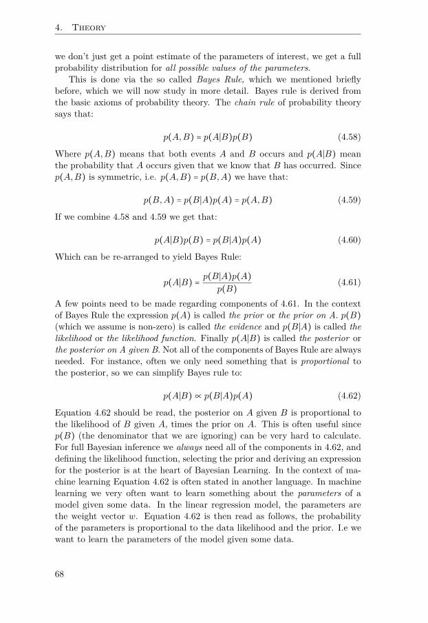
4. Theory

we don’t just get a point estimate of the parameters of interest, we get a fullprobability distribution for all possible values of the parameters.

This is done via the so called Bayes Rule, which we mentioned brieflybefore, which we will now study in more detail. Bayes rule is derived fromthe basic axioms of probability theory. The chain rule of probability theorysays that:

p(A,B) = p(A∣B)p(B) (4.58)

Where p(A,B) means that both events A and B occurs and p(A∣B) meanthe probability that A occurs given that we know that B has occurred. Sincep(A,B) is symmetric, i.e. p(A,B) = p(B,A) we have that:

p(B,A) = p(B∣A)p(A) = p(A,B) (4.59)

If we combine 4.58 and 4.59 we get that:

p(A∣B)p(B) = p(B∣A)p(A) (4.60)

Which can be re-arranged to yield Bayes Rule:

p(A∣B) = p(B∣A)p(A)p(B) (4.61)

A few points need to be made regarding components of 4.61. In the contextof Bayes Rule the expression p(A) is called the prior or the prior on A. p(B)(which we assume is non-zero) is called the evidence and p(B∣A) is called thelikelihood or the likelihood function. Finally p(A∣B) is called the posterior orthe posterior on A given B. Not all of the components of Bayes Rule are alwaysneeded. For instance, often we only need something that is proportional tothe posterior, so we can simplify Bayes rule to:

p(A∣B)∝ p(B∣A)p(A) (4.62)

Equation 4.62 should be read, the posterior on A given B is proportional tothe likelihood of B given A, times the prior on A. This is often useful sincep(B) (the denominator that we are ignoring) can be very hard to calculate.For full Bayesian inference we always need all of the components in 4.62, anddefining the likelihood function, selecting the prior and deriving an expressionfor the posterior is at the heart of Bayesian Learning. In the context of ma-chine learning Equation 4.62 is often stated in another language. In machinelearning we very often want to learn something about the parameters of amodel given some data. In the linear regression model, the parameters arethe weight vector w. Equation 4.62 is then read as follows, the probabilityof the parameters is proportional to the data likelihood and the prior. I.e wewant to learn the parameters of the model given some data.

68

4.4. Bayesian Learning

The chain rule can be generalized to:

p(A1,A2, ...Ap) = p(A1)(A2∣A1)p(A3∣A2,A1)...P (Ap∣Ap−1, ..,A1) (4.63)

The generalization of the chain rule allows us to do manipulations of Bayesrule when we have more variables involved, such as:

p(A,B∣C,D) = p(C,D∣A,B)p(A,B)p(C,D) (4.64)

Which can be transformed to:

p(A,B∣C,D) = p(D∣A,B,C)p(C ∣A,B)p(A,B)p(C,D) (4.65)

and

p(A,B∣C,D) = p(D∣A,B,C)p(C ∣A,B)p(B∣A)P (A)p(C,D) (4.66)

Depending on the concrete meanings of the events A,B,C,D these transfor-mations can be very useful in reducing the complexity and usefulness of thefunction. We will see examples of these types of manipulations later in thischapter.

While Bayes Rule is straight forward to derive and looks deceptively sim-ple, there is a sophisticated mathematical theory behind the scenes, with manysubtleties and nuances. When we start modeling more complex problems, theinvolved distributions make the mathematical theory quite complex. The fulltheory involves exotic probability distributions and the mathematical rulesfor how to manipulate them. Further, to actually calculate something usefulusing Bayesian statistics we need software libraries that are numerically verystable and robust, since extreme values can be quite common in Bayesian in-ference. Specifying a Bayesian model can be comparatively easy, but derivingan actual sampler for the learning problem can be quite a complex task andrequire substantial mathematic skills. In particular, knowledge of integrationtheory and Markov chain Monte Carlo sampling theory is a necessary skill formany Bayesian learning problems.

There are frameworks (for example BUGS, WinBUGS, OpenBUGS andStan) which allows the user to specify the Bayesian model, and the frame-work will then create a sampler for that model. These frameworks use generalclasses of inference to implement the sampler. Unfortunaltely, these generalclasses are still today not efficient enough to solve many problems involvingcomplex models and large data sets. For these problems specialized samplersneeds to be derived by using domain knowledge about the problem. Thederivations uses probability theory to manipulate the resulting probabilisticmathematical functions and computer science to parallelize the resulting code.

69

4. Theory

In combination, this means that implementing a fast parallel sampler for com-plex models and large data sets, requires expert knowledge in the mathematicsof sampling and probability theory, and computer science. Even with toolslike BUGS and Stan specialized skills and tricks, typically not available inindustry, are needed to make the model run fast enough.

Our third, fourth and sixth paper concerns these problems. In the thirdpaper we develop an exact parallel sampler for the LDA model. In the sixthpaper, we further improve the effectiveness of our sampler in paper three.In the fourth paper we expand on the LDA model and develop a supervisedclassification model for unstructured text, which we call DOLDA, which canalso be augmented with additional structured covariates.

Bayesian Building Blocks - A Hierarchy of DiscreteProbability Distributions and their Conjugate PriorsOne of the great advantages with the Bayesian paradigm is that we can useprobability theory and some basic building blocks in the form of probabilitydistributions, and put them together, much like Lego. Probability theorylets us do this in a mathematically consistent manner to get a probabilisticmodel of our problem. In the following sections, we discuss some of the veryimportant building blocks for Bayesian inference in discrete models. Thesebuilding blocks are probability distributions used to model aspects of theworld we want to learn about. Probability theory supplies us with a largebody of distributions suitable for modeling various aspects of the real world,from simple success / failure, waiting times between events, to probabilitydistributions over probability distributions.

Before diving into the theory we must introduce the concept of conjugacy.Conjugacy is a very important concept in Bayesian learning. A conjugate priordistribution is a distribution which exact mathematical formulation, whencombined with the likelihood expression, will give us a posterior distributionwhich is of the same mathematical form as the prior. This has the advantageof giving comparatively simple mathematical rules for updating our prior toget the posterior. In the sections below, we show examples of some commondistributions and their conjugate priors.

Beta-Bernoulli

The Bernoulli distribution is one of the simplest distributions around butstill very important. Its importance lies in it being a basic building block formore advanced models. In a sense we build up from the Bernoulli to moreadvanced discrete distributions. The Bernoulli models a one-off experimentwith outcomes success or failure, the classical example being a simple coinflip. How we define ”success” and ”failure” is up to us. It could be a patientsurviving a surgery, it could be guessing correct on a taste test, or a coin

70

4.4. Bayesian Learning

coming up heads. The Bernoulli is also used for variable selection in morecomplex Bayesian models. In the variable selection case, the Bernoulli randomvariable indicates if a variable in the model should be kept or not. We use thisin Paper III [35] to show that our correct and parallel LDA implementationallows for variable selection were other models do not.

The Bernoulli has one parameter often called θ which expresses the prob-ability of success. We say that X is Bernoulli distributed with parameterθ.

X ∼ Bern(θ) (4.67)

Where the tilde symbol ∼ should be read as distributed as or distributed ac-cording to. The probability mass function for the Bernoulli is expressed inEquation 4.68.

p(X = x∣θ) = θx(1 − θ)(1−x) (4.68)

True to our Bayesian approach, we need a prior on θ. Since the θ parameter ofthe Bernoulli expresses a probability and hence is restricted to the 0-1 range,the best prior distribution for that parameter is one that is naturally limitedto the same range. Ideally we also want one that is conjugate. The Betadistribution fulfills these exact requirements. We can express θ as a Betarandom variable as follows

θ ∼ Beta(a, b) (4.69)

The probability density function (θ is a real valued number limited to the 0-1range, thus we have a pdf for θ rather than a pmf) for the Beta is expressedin Equation 4.70.

p(θ∣a, b) = θ(a−1)(1 − θ)(b−1)B(a, b) (4.70)

Here B(a, b) is the so called beta function, which is not a probability dis-tribution but an ordinary mathematical function. Now we have a likelihoodfunction (the Bernoulli) and a prior (the Beta), we now combine them to theBeta-Bernoulli model. With the Beta-Bernoulli we want to calculate the pos-terior probability of the parameter θ given some data and our prior beliefs.Our data is the one experiment (one coin flip or more general, one success orfailure). We recall from Bayes rule that to calculate the posterior, we multiplythe likelihood with the prior and divide with the evidence. In this case theBernoulli is the likelihood and the Beta is the prior. So true to the Bayesiandictum of use Bayes rule we get

p(θ∣X) = p(θ)p(X ∣θ)p(X) (4.71)

71

4. Theory

Now we resort to our ”trick” of ignoring the normalizing denominator whichis constant with respect to θ (i.e., θ is not part of the expression for thedenominator and thus, it does not depend on θ). With this we get

p(θ∣X)∝ p(θ)p(X ∣θ) (4.72)

Plugging in the distributions for the prior and the likelihood we get

p(θ∣X)∝ Beta(a, b)Bern(θ) (4.73)

This is the posterior proportional to prior times likelihood form of Bayes rule(where we ignore normalization constants), that we saw in Equation 4.62.Plugging in the function for the Beta and the Bernoulli into 4.73, we get

p(θ∣X = x)∝ θ(a−1)(1 − θ)(b−1)θx(1 − θ)(1−x) (4.74)

From now on we simplify write ∣X instead of the full ∣X = x, but note thedifference between small and capital X’s. Gather the factors, i.e. since mul-tiplication is symmetric we can move the factors containing θ and 1 − θ nextto each other

p(θ∣X)∝ θ(a−1)θx(1 − θ)(b−1)(1 − θ)(1−x)Sum the exponents of θ and 1 − θ

p(θ∣X)∝ θ(a−1+x)(1 − θ)(b−1+1−x)At this stage we can ask; Why not simplify the exponents in the secondfactor? It turns out that keeping them and re-arranging the terms will leadto a revelation. So re-arranging the terms in the exponents we get

p(θ∣X)∝ θ(a+x−1)(1 − θ)(b+1−x−1) (4.75)

If we study the form of Equation 4.75 and compare it with the equation forthe Beta distribution (Equation 4.70) we see that it is actually again a Betadistribution, with a replaced with a + x and b replaced with b + 1 − x, butwithout the normalization constant. This in turn gives us the normalizingconstant that we ignored in Equation 4.73. Since we already know that thenormalizing constant for a Beta(a, b) is B(a, b), then the normalizing constantfor a Beta(a + x, b + 1 − x) must be B(a + 1, b + 1 − x). Which gives our exactposterior after having seen one event

p(θ∣X) = θ((a+x)−1)(1 − θ)((b+1−x)−1)B(a + x, b + 1 − x) (4.76)

This is an elegant result, since we get our posterior by just plugging in thevalue of the outcome in 4.76! Since it is again a beta distribution we can useall the known properties of the beta distribution for calculating properties

72

4.4. Bayesian Learning

such as the posterior mean, variance and all other properties we might beinterested in.

One might now ask; Why not use a uniform distribution as the prior forθ since it is simpler and perhaps more intuitive? There are many answersto that question. First, the uniform is not conjugate to the Bernoulli, so wewould not get one of the standard distributions back (by using the Beta, wegot a standard Beta as the posterior). This has the downside that we cannotjust lookup the properties, such as its mean, median, mode, variance, etc. ofthat distribution. Second, there typically exist no ready library functions fordrawing samples from these non-standard distributions, something we oftenwant to do in Bayesian inference when we use MCMC. Third, the uniformis a special case of the Beta distribution, so we can easily model a uniformdistribution by setting a = b = 1 in the Beta distribution. In addition, theBeta is flexible in the sense that we can model sophisticated prior knowledgewith the Beta such as, our prior assumptions of the mean and the variance ofθ. For instance, if we have strong prior opinions of θ we can select a and b,so we get an mean of our choice and high values of a and b which will lead tosmaller variance around the mean. We can use a uniform distribution if wedon’t care about an analytical solution, or we are using a framework such asBUGS or Stan.

From the Bernoulli to the Binomial distribution

The Bernoulli only models one event. The advantage with the Bernoulli isthat it is easy to understand and explain and at the same time easily extendedto the case where we have several events, for instance many coin flips, or manypatient cases. To extend the Bernoulli to many cases, we make two underlyingassumptions, the cases are considered independent trials, i.e. one case doesnot affect the outcome of another, and the probability of success is the samein each of the trials. This can be stated as follows

X1,X2, ...XN ∼ Bern(θ) (4.77)

If each of the Xn is an independent Bernoulli trial, the rules of probability saysthat we can multiply their individual probabilities to get the joint probabilityof one particular sequence of events.

p(X1, ..XN ∣θ) = N∏1

θxn(1 − θ)(1−xn) (4.78)

were we have plugged in the probability function of the single Bernoulli trial.If we sum the exponents in Equation 4.78 we get

p(X1, ..XN ∣θ) = θ∑xn(1 − θ)N−∑xn (4.79)

73

4. Theory

Let us now introduce a variable k which is the number of successes in thesequence, ∑xn = k (remember that the xn’s only takes the values 0 or 1). Wecan now write Equation 4.79 as

p(X1, ..XN ∣θ) = θk(1 − θ)N−k (4.80)

Where k is the number of successes and N − k the number of failures. Nowwe are getting close to the normal extension of the Bernoulli model, the socalled Binomial model. But the Binomial model answers a slightly differentquestion than the Bernoulli. It answers the question; What is the probabilityof getting S = k successes out of N independent Bernoulli trials were eachsuccess has probability θ? That is, we don’t really care about the specificorder of the trials, we are only interested in how many successes we get in allof our trials, irrespective of order. We say that S is Binomially distributed

S ∼ Binom(N, θ) (4.81)

The Binomial distribution builds on the Bernoulli according to the followingreasoning. Equation 4.80 tells us the probability of one particular sequence, orequivalently the probability of one particular way of getting sum(X1, ...Xn) =k successes. But since we don’t care about the order (i.e. the sequence 1,0,1,1is the same as 1,1,1,0 since both has three 1’s and one zero) in which we getthe k successes, and there are (Nk ) (read as ”from N choose k”) such sequences,the expression for the Binomial distribution becomes

p(S = k∣θ,N) = (Nk)θk(1 − θ)N−k (4.82)

Where the (Nk ) tells us how many combinations we can make by choosing kitems out of N . If we compare the expression for the Binomial in Equation 4.82with the corresponding expression for the Bernoulli in Equation 4.68 andignore the (Nk ) we see that the single x in the exponent of the first factoris replaced with k, the number of successes. In the exponent of the secondfactor the one single case is replaced by the total number of cases N and k.Otherwise the functions are identical.

Beta-Binomial

We know that the Beta distribution is conjugate to the Bernoulli, and since theform (i.e. excluding the normalization constant, and the specific exponents) ofthe Bernoulli and the Binomial are the same, we know that the Beta will alsobe conjugate to the Binomial distribution. When we combine the Binomialwith the same Beta prior as in the Bernoulli case we get the Beta-Binomialmodel.

p(θ∣X1, ..XN)∝ Beta(a, b)Bin(θ) (4.83)

74

4.4. Bayesian Learning

Plugging in the function for the Beta and Equation 4.82 for the Binomialinto 4.83 (again ignoring normalization constants, thus making the expressionproportional), we get

p(θ∣X1, ..XN)∝ θ(a−1)(1 − θ)(b−1)θk(1 − θ)N−kWhere k is the number of successes in the sequence, ∑xn = k (rememberthat the X’es take only the values 0 or 1, where 1 represents success). Thederivation of this model proceeds identically (starting from Equation 4.74)as in Bernoulli model with the difference that x is replaced by k in the firstfactors exponent, and the 1 − x is replaced by N − k in the second factorsexponent. Doing the derivation leads us to

p(θ∣X1, ...XN) = θ((a+k)−1)(1 − θ)((b+N−k)−1)B(a + k, b +N − k) (4.84)

Which is the posterior probability of θ after having seen N independentBernoulli trials. Again we have a simple update rule, we get the posteriorby plugging in the number of observed successes and the total number oftrials in the data.

With the above approach we have turned the calculation of the posteriorof θ into a ”batch” calculation, i.e., we have the whole set of observations andsum the number of successes. But we could just as well have arrived at thesame conclusion by repeatedly applying Bayes rule, for one observation at atime, starting with the Beta prior, and using the posterior (Beta) of one eventas the prior for the next.

The parameters a and b of the Beta prior is often interpreted as priorcounts or pseudo counts, i.e. we interpret a as the number of successes andb as the number of prior failures we have seen before the experiment. Wecan see that the uncertainty (i.e. the variance) in the posterior of θ decreasesthe more number of observations we see. This is explained by looking atEquation 4.85, which is the formula for the variance of a Beta distribution.As a and b increases, the denominator will increase faster than the nominator.This means that if we use the Beta as a prior, the prior counts tell us somethingof how certain we are of our prior. The larger number of pseudo counts, themore certain we are.

var(X) = ab

(a + b)2 + (a + b + 1) (4.85)

Integrating out parameters

With the Beta-Bernoulli and Beta-Binomial we can model one event or aseries of events with the basic assumption that the events are independentand that the probability of success are the same in all of the events. Butwhat if we would like to lift this last restriction, ie, we don’t want to assume

75

4. Theory

the same success probability for all events, how could we achieve this? To dothis, we must get rid of the fixed θ, this can be done by integrating out theθ parameter. It frees us from the restriction that the success probability hasto be the same. It leaves us only with the assumption that it is drawn froma Beta distribution with some hyper-parameters (the a and b).

To lift the restriction of a fixed θ we do something that is quite commonin the Bayesian literature, we integrate out (also called marginalizing over) θ.That is, we sum over all possible values of θ.

In Equation 4.82 we had the expression for the Binomial distribution whichtells us the probability of getting k successes given θ and N . We then put aBeta prior on θ to get the posterior on k. But now we want to be independentof the fixed θ, we do this by integrating out the θ from the Beta-Binomialmodel. The integrating out means that we integrate over the θ parameter inthe Beta-Binomial model according to

p(k∣N,a, b) = ∫ 1

0Beta(a, b)Bin(N, θ)dθ (4.86)

Plugging in the respective formulas gives

p(k∣N,a, b) = ∫ 1

0

θ(a−1)(1 − θ)(b−1)B(a, b) (N

k)θk(1 − θ)N−kdθ

Since θ is limited to the 0-1 range, the integral is over this range. Extractingterms not depending on θ

p(k∣N,a, b) = (Nk) 1

B(a, b) ∫1

0θ(a−1)(1 − θ)(b−1)θk(1 − θ)N−kdθ

Gather the exponents

p(k∣N,a, b) = (Nk) 1

B(a, b) ∫1

0θ(a+k−1)(1 − θ)(b+N−k−1)dθ

At this stage we have to recognize that the integral over θ is again a Betafunction with the parameters B(a+k,b+N-k), so the final expression for ourexpression for the probability of k independent of θ, becomes

p(k∣N,a, b) = (Nk)B(a + k, b +N − k)

B(a, b)By integrating out the θ we make it ”go away” and we can relax the assumptionthat the θ is fixed between the Bernoulli trials. Our only assumption left isthat the (implicit) θ’s in each of the trials are drawn from a Beta distributionand that the trials are independent.

Integrating out a parameter in a model can sometimes be beneficial andsometimes not. In Paper III [35] we show that by not integrating out a param-eter, we can implement an efficient and parallel implementation of LDA which

76

4.4. Bayesian Learning

is still mathematically correct. This is in contrast to other approaches whichintegrate out a parameter in the LDA model called φ, making it impossibleto parallelize the model and still be a correct model. In the LDA case wherewe model documents as a vector of counts of the words in the documents,the integrating out of the φ parameter makes each document dependent ofevery other document, thus making it impossible (or at least impractical) toparallelize. Since each document is dependent on the state of all the otherdocuments, one would have to lock each thread and fetch the state of alldocuments being sampled on that thread to draw a sample on the currentprocessor; this is not conducive to an efficient parallelization. This inexactapproach to parallelizing LDA has become so common, that in several papersit is not even mentioned that the model is no longer an exact LDA model!

Dirichlet-Multinomial

In the preceding sections we have shown how the simple Bernoulli can begeneralized to the Binomial distribution by having repeated trials. Here weshow how one can extend the Binomial model to the more general case ofseveral different outcomes rather than just binary outcomes. The extendedmodel is called the multinomial model, it defines the Multinomial distri-bution. In the multinomial model we don’t have just success or failure, butrather N draws with one out of K possible different outcomes called classesor categories. This is denoted3

YYY ∼Multinomial(N,θθθ) (4.87)

Here both Y and θ are K dimensional vectors. Yk (the k:th entry in Y ) isthe class count of class k. In the Bernoulli and Binomial models θ expressesthe probability of success. In the Multinomial model, θ is a vector whereeach element of the vector expresses the probability of drawing that particularoutcome class. So θk is a value between 0 and 1 which expresses the probabilityof drawing the k:th outcome out of K possible outcomes. In the multinomialmodel, the values in θ must sum to 1. I.e., θ is a probability distribution!

There are several special cases of the Multinomial distribution, this isnatural since it is the generalization of several distributions. The special caseof the Multinomial distribution where N = 1, and k = 2, is the Bernoullidistribution. When k is 2 and N > 1, it is the Binomial distribution, whenk > 2 and N = 1, it is the so called categorical distribution. For example,if we have a 4-dimensional Multinomial distribution, one example draw fromit could be [0,0,1,0] which interpreted as a categorical draw would mean thatthe category we drew was category 3 (the vector is taken to be 1-indexed).A draw from a 4-dimensional Multinomial(7,θ) could look like [1,2,4,0], i.e.the resulting vector draw sums to 7. In this one multinomial draw, category

3There are also other ways to encode the multinomial distribution

77

4. Theory

1 was drawn once, category 2, twice, category 3, four times, and category4, zero times. We can see a draw from a Multinomial distribution as rollinga k-sided die N times and representing the counts of how many times eachof sides comes up in a k-dimensional vector, where the k:th entry containsthe number of times side k came up. The probability mass function for themultinomial is expressed in Equation 4.88

p(Y1, ...YK ∣θθθ) = N !

y1!...yK !

K∏1

θyk

k (4.88)

The normalizing constant in the multinomial, like in the binomial case, com-pensates for the many different ways we can draw a particular combination ofa multinomial outcome. As usual in the Bayesian paradigm we need a prioron the parameters. Since θ is a probability distribution, we want a prior overprobability distributions that is ideally conjugate to the multinomial. Themultinomial is a generalization of the Binomial, and our prior will be a gener-alization of the Beta distribution. This conjugate prior is called the Dirichletdistribution and it is a prior over distributions.

θ ∼Dir(α) (4.89)

This means that a draw from the Dirichlet distribution, is itself a probabilitydistribution! A draw from a Dirichlet distribution will look something like thediscrete PMF in Figure 4.2. The Dirichlet distribution is parametrized by avector of K-concentration parameters denoted ααα. The concentration param-eters of the Dirichlet distribution decides what the probability distributionsthat the Dirichlet returns looks like. The ααα parameter will determine how”peaked” the Dirichlet distribution will tend to be. The only requirement onthe concentration parameters, is that they are > 0 (i.e., they need not sum toone and does not have to be integers). The probability density function forthe Dirichlet is

p(θ1, ...θK ∣ααα) = 1

B(ααα)K∏1

θαk−1k (4.90)

Here B(ααα) is the multivariate Beta function (remember that we had the Betafunction in the Binomial case), this function is usually expressed in terms ofthe Gamma function, which turns Equation 4.90 into

p(θ1, ...θK ∣ααα) = Γ(∑K1 αk)

∏K1 Γ(αk)

K∏1

θαk−1k (4.91)

Where Γ(●) is the Gamma function, which is a generalization of the faculty(!) function to non-integer values. If g is a positive integer, then Gamma(g) =

78

4.4. Bayesian Learning

(g − 1)!. If we combine the Dirichlet prior and the multinomial likelihood weget an expression for the posterior

p(θθθ∣Y1, ..YK ,ααα)∝Dir(θθθ∣ααα)Multinomial(N,θθθ) (4.92)

Which, when we use our old trick of ignoring normalizing constants, expandsto

p(θ1, ...θK ∣Y1, ..YK ,ααα)∝ K∏1

θαk−1k

K∏1

θyk

k (4.93)

Gather the exponents

p(θ1, ...θK ∣Y1, ..YK ,ααα)∝ K∏1

θyk+αk−1k (4.94)

Where yk is the number of observed values of category k in the dataset. Byagain studying the form of Equation 4.94 we see that it is again a Dirichletwith parameters Yk + αk. Putting back the normalization constants we getthe full posterior.

p(θ1, ...θK ∣Y1, ..YK ,ααα) = 1

B(YYY +ααα)K∏1

θyk+αk−1k (4.95)

The update rule here then consists of updating the prior Dirichlet hyperpa-rameters with the number of counts of the respective categories seen in thedata. So the posterior on θ becomes:

θθθ ∼Dir(ααα +YYY ) (4.96)

Dirichlet-Categorical

As mentioned in Section 4.4, the categorical distribution can be seen as aspecial case of the multinomial distribution where N = 1. The categoricaldistribution, like the multinomial is parametrized by a K dimensional vector θwith the exact same interpretation as for the multinomial model. One specificfact to note is that since in the categorical case we only do one draw, we don’tneed the normalizing constant of the multinomial which compensates for themany different ways to generate a particular outcome. If Y has a categoricaldistribution it is denoted

Y ∼ Cat(θ,K) (4.97)

Or simply

Y ∼ Cat(θ) (4.98)

79

4. Theory

Observe that in the categorical situation, the meaning of Y is different than inthe multinomial case. In the categorical case, Y is a scalar, and Y = k meansthat Y has class k. In the multinomial case, Y is a vector, and Yk is thenumber of times class k occurred. What can be confusing is that sometimesthe categorical outcome of Y is equivalently encoded as a vector with the k:thentry set to one (i.e. a one draw from a k-dimensional multinomial), oftencalled a one-of-k encoding or one-hot encoding.

If we do N categorical draws and sum the class occurrences in a vector weget back the multinomial. If we see the categorical distribution as one drawfrom the multinomial distribution, the pmf for the categorical distributionbecomes extremely simple. The probability of a particular outcome is definedby θ

p(Y = k) = θk (4.99)

Putting a Dirichlet prior on θ and using the same proof as for the Dirichlet-Multinomial we can show that the posterior on θ is again a Dirichlet:

θ ∼Dir(α +Cc) (4.100)

Where Cc is the vector of the number of observed counts per class summedover all observations. That is, if we start with a Dirichlet prior with hyper-parameters α and combine it with a vector of counts Cc of draws coming froma Categorical distribution, then the posterior is again a Dirichlet distributionwith parameters α + Cc. If we represent the categorical distribution as amultinomial with just one draw, the counts for one observation will be avector with all zeros except for a one in the observed category. We then sumover all observations to get the full Cc vector of counts.

We can see the Multinomial as a ”batch” execution of many Categori-cal draws, where the multinomial Y vector contains the sums of the manycategorical draws.

Bayesian Linear RegressionAfter this general introduction to Bayesian Learning, let us look at an examplehow we can apply the Bayesian method of learning. For familiarity, and dueto its importance, we shall return to linear regression also in the Bayesiancontext and see how we can cast it as a Bayesian learning problem. In theBayesian framework, everything is expressed in terms of probabilities. In ourexposition of the ordinary linear regression we did not have an explicit notionof probability, but here we shall. Recall that one of the advantages of theBayesian framework is that we get probability distributions over all of ourparameter estimates. So how do we recast our linear regression

y =Xw + σ (4.101)

80

4.4. Bayesian Learning

in a way that we get a probability distribution? The strategy will be to letthe linear relation model the mean of y instead of y directly. Expressed in thelanguage of probability, this turns into:

p(y∣X,w,σ) =N (Xw,σ2I) (4.102)

Which denotes that y has a multivariate normal distribution, the extensionof the normal distribution to many dimensions. The expression for the mul-tivariate normal pdf is:

p(y∣X,w,σ) = 1

(2π)− p2

1

det(σI)− 12

exp(−12(y −Xw)T (σ2I)−1(y −Xw))

(4.103)Where y is still a vector of observations and X is the corresponding matrix ofobserved variables and w is the vector of weights, one for each of the columnsin X. I is the identity matrix, that is, a square matrix with 1’s on the diagonaland zeros everywhere else. p is the number of columns in X. This particularform encodes the assumption that the errors are independent. This formulashould be read as, ”Given that we know X, w and σ , y is normally distributedwith mean Xw and standard deviation σ”. Here, the normal distribution isextended to the multivariate case, where instead of modeling one scalar, itmodels a random vector in which each entry is normally distributed. Tosimplify the presentation we will assume that σ is known, which in general itis not, but the analysis can be extended to include σ too.

As in the linear regression case we are interested in learning the value ofthe parameters w. So we are really interested in:

p(w∣X,y,σ) (4.104)

that is, the probability of the parameters given the data. Remember thatin the Bayesian paradigm we always start with a prior probability on ourparameters, we then observe some data and the update our probability toarrive at the posterior probability distribution on our parameters. We denotethis prior with p(w) which is the prior probability distribution we place overthe parameters w. In this particular case we put a zero centered normal priordistribution on w which in general is a reasonable assumption.

p(w) =N (0,σ20I) (4.105)

In Paper V we use a different prior, called the Horseshoe on our parametervector. The Horseshoe puts a stronger prior on w and expresses the priorbelief, that the entries in w are either very close to zero or large.

81

4. Theory

With these preliminaries taken care of, we shall again return to our datain Table 4.1. We continue to use the matrix notation to specify our problem.In the linear regression case we had the linear equation

y =Xw + σ (4.106)

Where we now have adopted the notational convention that we drop the ex-plicit ∗ symbol with the understanding that Xw means X ∗ w. We haveshown that the Bayesian equation has the general form

p(A∣B) = p(B∣A)p(A)p(B) (4.107)

In our case A corresponds to the weight vector w. B corresponds to our data,X and y, and the fixed σ. By plugging in these variables, our formulationbecomes

p(w∣X,y,σ) = p(y,X,σ∣w)p(w)p(X,y,σ) (4.108)

Which should be read as: ”What is the probability distribution over w given(our data) X, and y (and σ)”. In 4.108 we have used the standard Bayesformula to find A∣B when we know B∣A, but the expression p(y,X,σ∣w)(corresponding to B∣A in the Bayes Rule) is not really something that we haveavailable. We would much rather have the expression in 4.102, since that isthe way we model how the data is generated, given the parameters. Usingthe rules of probability exemplified in 4.65 we can go from p(y,X,σ∣w)p(w)to p(y∣X,σ,w)p(w) as follows:

p(y,X,σ∣w)p(w) = p(y,X ∣σ,w)p(σ,w) (4.109)= p(y∣X,σ,w)p(X,σ,w) (4.110)

Since X are observed data and σ is given, the expression p(X,σ,w) reducesagain to p(w). Which leaves us with

p(y,X,σ∣w)p(w) = p(y∣X,σ,w)p(w) (4.111)

Substituting into 4.108 leaves us with:

p(w∣X,y,σ) = p(y∣X,σ,w)p(w)p(X,y,σ) (4.112)

Once again we will employ our trick of ignoring the normalizing denominator,giving us:

p(w∣X,y,σ)∝ p(y∣X,σ,w)p(w) (4.113)

82

4.4. Bayesian Learning

In the next step, we need is to substitute concrete expressions for the proba-bilities involved, i.e p(y∣X,σ,w) and p(w). From our modeling assumptionin 4.103, we have assumed that p(y∣X,σ,w) is a normal distribution. In 4.105we assumed a normal prior for p(w).

It would require too much multivariate analysis and Bayesian theory togo into the details of the motivations for the various expressions so we willsummarize the results here. For a detailed expositions we refer to Gelman,Carlin, Stern, and Rubin [36] and Jaynes [37].

The mathematical forms of the likelihood and the prior defines the mathe-matical model. If we are careful in our selection of the form for the likelihoodand prior we can again get a conjugate model. Remember that conjugatemeans that the posterior have the same mathematical form as the prior. Thisis very useful if we can choose a prior of a known distribution from whichit is easy to draw random samples. Examples of some widely used conjugatemodels are the Bernoulli-Beta, Binomial-Beta, Poisson-Gamma, Multinomial-Dirichlet and Normal-Normal models, some of which we discuss in Section 4.4.

In this Bayesian linear regression example we will use a Normal-Normalmodel, in our next example Bayesian Naive Bayes Classification (in Sec-tion 4.4) we will use the Multinomial-Dirichlet model. Both of these modelsare used in our papers. To get a Normal-Normal conjugate model we selecta Normal model for the likelihood function and a normal prior for the weightvector w. This then leads to the following Bayesian model specification:

p(y∣X,σ,w) ∼N (Xw,σ2I) (4.114)

p(w) ∼N (0,σ20I) (4.115)

Plugging in the specific expressions for 4.114 and 4.115 gives us:

p(w∣X,y,σ)∝N (Xw,σ2I)N (0,σ20I) (4.116)

For the normal distributions there are several known results for productsof normals, but below we will give a simplified derivation of the main result.Remember that everything is in vector/matrix notation, so X is a matrix withall the observed x’s. The matrix has dimension; number of rows x number ofcolumns, where the columns is the number of features plus one column of 1’sfor the intercept. y is a column vector which is N long and w is a row vectorwhich is p long, the number of input features + 1 for the intercept. Sincewe use the proportional form, we remove all constants and end up with thefollowing expression for the posterior on w:

83

4. Theory

p(w∣X,y,σ) ∝ exp(−12(y −Xw)T (σ2I)−1(y −Xw))

"22222222222222222222222222222222222222222222222222222222222222222222222222222222222222222222222222222222222222222222222222222222222#22222222222222222222222222222222222222222222222222222222222222222222222222222222222222222222222222222222222222222222222222222222222$normal likelihood from 4.114

(4.117)

exp(−12(w − 0)T (σ2

0I)−1(w − 0))"2222222222222222222222222222222222222222222222222222222222222222222222222222222222222222222222222222222222222222#222222222222222222222222222222222222222222222222222222222222222222222222222222222222222222222222222222222222222$normal prior from 4.115

(4.118)

Extract σ′s, −0 goes away:

p(w∣X,y,σ) ∝ exp(− 1

2σ2(y −Xw)T I−1(y −Xw)) (4.119)

exp(− 1

2σ20

wT I−1w) (4.120)

Identity matrix goes away (the inverse of the identity matrix is the identitymatrix):

p(w∣X,y,σ)∝ exp(− 1

2σ2(y −Xw)T (y −Xw))exp(− 1

2σ20

wTw)The exponents of products of exponentials sum:

p(w∣X,y,σ)∝ exp[− 1

2σ2(y −Xw)T (y −Xw) − 1

2σ20

wTw]Extract −1/2 and let 1/σ2 = a and 1/σ2

0 = bp(w∣X,y,σ)∝ exp[−1

2(a(y −Xw)T (y −Xw) + bwTw)]

Cross multiply:

p(w∣X,y,σ)∝ exp[−12a(yTy − (Xw)Ty −yT (Xw)− (Xw)TXw)+ bwTw]

Use rules for transpose to get terms in same form. (Xw)T = wTXT so(Xw)Ty =wTXTy yT (Xw) = (Xw)Ty =wTXTy:

p(w∣X,y,σ)∝ exp[−12a(yTy − 2wTXTy −wTXTXw) + bwTw]

Distribute a:

p(w∣X,y,σ)∝ exp[−12ayTy − 2awTXTy −wT aXTXw + bwTw]

84

4.4. Bayesian Learning

Simplify last two terms. bwTw =wT bIw.

p(w∣X,y,σ)∝ exp[−12ayTy − 2awTXTy −wT (aXTX + bI)w] (4.121)

Completing the square gives:

p(w∣X,y,σ)∝ exp[−12(w −µn)TΛ−1(w −µn)] (4.122)

Where Λ is:

Λ = aXTX + bIand µn:

µn = aΛ−1XTy = a(aXTX + bI)−1XTy (4.123)

If we pick apart Equation 4.122 we can see that it is a multivariate normalwith variance Λ−1 and mean µn. Expressed in probabilistic notation, theposterior for w is:

p(w∣X,y,σ) ∼N (µn,Λ−1) (4.124)

At this point we can compare with the result for the standard linear regres-sion that we arrived to in 4.48 which is repeated here (with * removed) forconvenience:

w = (XTX)−1XTy (4.125)

We see that the expression for the mean (µn) in the Bayesian formulation issimilar as the standard OLS result. In the Bayesian result the mean containsboth the error term a, which is 1/σ2, the variance of the data, and the prior

Completing the Matrix Square

There is an analog matrix version of completing the square. Wecan go from:

yTAy − (Xw)TAy − yTAXw +wTXTAXw

to

(y −Xw)TA(y −Xw)We use a version of this identity in Equation 4.121.

85

4. Theory

uncertainty b = 1/σ20 . This is the same result one gets when using, so called,

ridge regression in standard OLS. So putting a normal prior on the betas in theBayesian formulation can be interpreted as using ridge regression. Other typesof priors on the betas can be used and they sometimes lead to other typesof OLS regularization schemes, but there are Bayesian priors that have nostandard OLS correspondence. In this particular example we chose a normal-normal model which gives a closed form expression for the posterior. But ifwe use the flexibility of the Bayesian approach and select some other prior weare not (in fact, most often not) guaranteed to get a closed form expression forthe posterior and then we need to use some version of MCMC to do inferencein the model.

Bayesian Naive Bayes ClassificationIn Section 4.3 we discussed the standard Naive Bayes classification technique.Despite its name, the Naive Bayes approach, is not Bayesian in the truestsense since there are no clearly defined priors on the parameters. Here wewill discuss how the Naive Bayes approach, can be re-cast as a truly Bayesiantechnique.

Model Specification

The first thing we need in building our Bayesian classification model, is justthat, a model. Specifically a probability model of our problem. The secondstep is to put priors on the parameters that control the different probabilitydistributions involved. Below we sketch this process (see also Murphy [30,Ch. 3]). We start with what we are interested in:

p(Y ∣X,Data)I.e, we are interested in calculating the probability distribution of Y , i.e. theclass for a new unknown data point encoded in X, given some historical Data.Our model will be a so called parametric model, i.e.. we have some parametersthat control the model behavior. We don’t know what these parameters areat this moment, but we introduce them into the model. We denote theseparameters θ, the model now becomes

p(Y ∣X,Data,θ)X is a random vector consisting of input variables or features. In this examplewe will use capitals to denote the new input X, and the corresponding newunknown class Y that we want to predict. Observations of historical X andY , will be denoted with lowercase x and y. An observation of an RV is calledan outcome. So the Data is a set of N observations of outcomes of historicalX and Y :

86

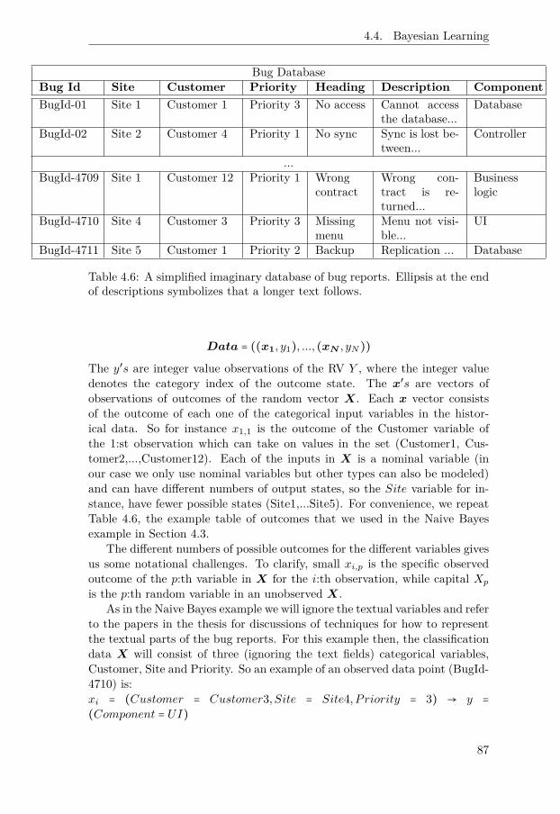
4.4. Bayesian Learning

Bug DatabaseBug Id Site Customer Priority Heading Description ComponentBugId-01 Site 1 Customer 1 Priority 3 No access Cannot access

the database...Database

BugId-02 Site 2 Customer 4 Priority 1 No sync Sync is lost be-tween...

Controller

...BugId-4709 Site 1 Customer 12 Priority 1 Wrong

contractWrong con-tract is re-turned...

Businesslogic

BugId-4710 Site 4 Customer 3 Priority 3 Missingmenu

Menu not visi-ble...

UI

BugId-4711 Site 5 Customer 1 Priority 2 Backup Replication ... Database

Table 4.6: A simplified imaginary database of bug reports. Ellipsis at the endof descriptions symbolizes that a longer text follows.

Data = ((x1, y1), ..., (xN , yN))The y′s are integer value observations of the RV Y , where the integer valuedenotes the category index of the outcome state. The x′s are vectors ofobservations of outcomes of the random vector X. Each x vector consistsof the outcome of each one of the categorical input variables in the histor-ical data. So for instance x1,1 is the outcome of the Customer variable ofthe 1:st observation which can take on values in the set (Customer1, Cus-tomer2,...,Customer12). Each of the inputs in X is a nominal variable (inour case we only use nominal variables but other types can also be modeled)and can have different numbers of output states, so the Site variable for in-stance, have fewer possible states (Site1,...Site5). For convenience, we repeatTable 4.6, the example table of outcomes that we used in the Naive Bayesexample in Section 4.3.

The different numbers of possible outcomes for the different variables givesus some notational challenges. To clarify, small xi,p is the specific observedoutcome of the p:th variable in X for the i:th observation, while capital Xp

is the p:th random variable in an unobserved X.As in the Naive Bayes example we will ignore the textual variables and refer

to the papers in the thesis for discussions of techniques for how to representthe textual parts of the bug reports. For this example then, the classificationdata X will consist of three (ignoring the text fields) categorical variables,Customer, Site and Priority. So an example of an observed data point (BugId-4710) is:xi = (Customer = Customer3, Site = Site4, P riority = 3) → y =(Component = UI)

87

4. Theory

xi,2 denotes the specific outcome (Site4 in this case) of the 2:nd variable (theSite variable) in the i:th observation. Our model assumes the data points areindependent if we know the parameters (θ) of the model, i.e. one observationhave no impact on the next. This is a stronger assumption than what iscommonly necessary in the Bayesian paradigm. In the Bayesian approach,the common assumption is that the data is exchangeable. Exchangeable justmeans that we can permute the order of the observations without violatingany assumptions of the data generating process.

A difference in this example from the previous examples is that here we areinterested in the posterior predictive distribution of a new data point ratherthan the parameters of the model. That is, we are not interested in studyingthe posterior distribution of the parameters θ, but only in predicting the classof a new Y given a new X. By the definition of conditional probability

p(Y ∣X,Data,θ) = p(Y,X,Data,θ)p(X,Data,θ) (4.126)

But the expression on the right hand side here is not really something thatwe can work with directly. We would like to separate the new data points Xand Y from the Data and θ. We can do that by the following derivation.First, the denominator does not depend on Y so we can drop it.

p(Y ∣X,Data,θ)∝ p(Y,X,Data,θ)We can then by the chain rule reformulate the joint probability on the righthand to

p(Y ∣X,Data,θ)∝ p(Y,X,Data∣θ)p(θ) (4.127)

A very powerful tool in the Bayesian paradigm is thinking about independencerelations between the constituents in the model. The underlying assumption isthat given the model parameters, some process is generating our data points.The independence assumption in Equation 4.127 is that the historical Dataand, X and Y , are independent given the model parameters, which gives us:

p(Y ∣X,Data,θ)∝ p(Y,X ∣θ)p(Data∣θ)p(θ)Further, p(Y,X ∣θ) can by the chain rule be factored as p(X ∣Y,θ)p(Y ∣θ) whichleaves us with:

p(Y ∣X,Data,θ)∝ p(X ∣Y,θ)p(Y ∣θ)p(Data∣θ)p(θ)To complete our Bayesian model we also need to discuss the model parametersθ, which is a vector with all the parameters that we need. As usual, we puta prior on those parameters which is the p(θ). θ is a vector of parametersthat will control the concrete probability distributions that we put on ourvariables of interest. θ consists of two sets of priors; the priors on Y (i.e.

88

4.4. Bayesian Learning

the class labels) and the priors on X ∣Y (i.e. the probability of a variabletaking a specific value given the class label). Now, if we are only interested inpredictions of Y and not inherently interested in analyzing θ, we can integrateout θ (as discussed in Section 4.4).

p(Y ∣X,Data)∝ ∫ p(X ∣Y,θ)p(Y ∣θ)p(Data∣θ)p(θ)dθ (4.128)

This can seem like an unnecessary step, we first introduce the parameters θand then we immediately integrate them out. The parameters in the modelacts as a ”bridge” between the historical data and the prediction of a newobservation. This is a common approach not only in the Bayesian paradigm.The θ’s represent the unseen (sometimes called latent) parts of the proba-bilistic model. The model together with the parameters describe what weimagine is the underlying mechanism for generating the observations we havebeen given. The latent parts are needed for inference in the model, but we arenot always interested in them, like in this case where we are only interestedin predicting a new Y . When we are not directly interested in the latentparameters we integrate them out as in Equation 4.128.

Worth noting here is a notational shortcut. What looks like a single in-tegral in 4.128 is really many integrals. It consists of the integral over thepriors over the Y ’s and the integrals over every variable in the model andtheir priors.

We split θ into two parts, one part controls the probability distributionover the component (class) probabilities (Controller, UI, etc.) which we call π.The second part controls the conditional probabilities of the variables giventhe component (p(Site=Site4|Component=Controller)) which we call φ. Soour full vector of parameters is θ = (π,φ). I.e., the priors on the classesand the priors on the set of outcomes given the class labels for each variablein our model. In this case we will use a so called factored prior for θ, i.e.the different parts of the prior are independent of each other and thus canbe factored according to p(π,φ) = p(π)p(φ). In the original Naive Bayesversion the parameters are calculated directly from the data. But in the fullyBayesian approach we need priors on the parameters. Below we describewhich probability distributions we choose as priors for the different parts ofour model.

Probability Distributions on Y

The probability distribution over the components/classes we model using acategorical distribution, since the components are categorical in nature. Re-member, an RV which is distributed according to a categorical distributiontakes one categorical value from a set of outcome classes. In our case, the setfor Y consists of the components in the dataset, i.e. {UI, Database, Controller,Business Logic}. So a draw from the categorical distribution will return one

89

4. Theory

of the outcomes in that set. We can express that component is categoricallydistributed as follows:

Component ∼ Cat(K,π) (4.129)

where Cat(K,π) means that Component is distributed according to a Cat-egorical distribution. The Categorical distribution is parametrized with Kwhich is the number of categories and π which is a K-dimensional vector withprobabilities which sum to 1. This vector is the π part of θ. Each of the Kentries in π contains the probability of that category. In our example we haveK = 4 categories for the Y variable, Controller, Database, Business Logic andUI. To simplify notation we will drop the dependence on K and just assumethat the distribution is of the correct dimension. So in generic notation itbecomes

Y ∼ Cat(π) (4.130)

We use the Dirichlet distribution as a prior on the parameter π of the cate-gorical distribution. This gives us

π ∼Dir(K,α) (4.131)

where α is a K-dimensional vector. A draw from a K-dimensional Dirichletdistribution returns a K-dimensional probability distribution, which is exactlywhat we need for our Categorical distribution. Again, to simplify notation wewill drop the K and just assume that the Dirichlet is of the correct dimension.So the notation becomes

π ∼Dir(α) (4.132)

For the sake of brevity, inside equations 4.132 is expressed as:

Dir(π∣α) (4.133)

Probability Distributions on X

Next, we come to the conditional probabilities for variables given the compo-nent (the p(X ∣Y, θ) part of 4.128). As in the ordinary Naive Bayes discussedin Section 4.3 we will make the naive assumption that the variables in X areindependent. With this assumption we can factor X given Y and θ as:

p(X ∣Y = k,θ) = P∏p=1p(Xp∣Y = k,θ) (4.134)

Where P is the number of input variables in X. In our case P = 3, Cus-tomer, Site, and Priority (remember that in this example we ignore thetextual parameters Heading and Observation). For example, if we study

90

4.4. Bayesian Learning

the Site variable of the i:th observation, (xi,2), this prior would tell usp(Site = xi,2∣Component = Controller, θ), i.e. the probability that the Sitecomponent of X equals the outcome xi,2 given that the component is Con-troller. Since each of our individual input variables (Xp) are also categorical.

Xp∣Y = k,θ ∼ Cat(φk,p) (4.135)

We again use the Dirichlet distribution for the prior on the parameters of thisconditional categorical distribution. Where φk,p is the vector of probabilities,from θ, for the outcome states for the p:th variable given that Y = k. The fullmatrix for all classes and variables is φ. Since φk,p is a probability distributionwe again choose a Dirichlet for the prior on φ of a variable Xp given a classlabel k:

φk,p ∼Dir(βk,p) (4.136)

β is a matrix with hyper parameters on φ. Often β is simply a scalar which isdivided by the number of entries needed in respective vector, but conceptuallyand in our derivations we will use the full matrix representation. φ andβ are of dimension KxPxJp where K is the number of classes and P thenumber of variables and Jp the number of possible outcome states of variablep. Note that sometimes we ignore the Jp dimension to simplify notation. Soφk,p is a vector with probabilities (of length Jp), where each entry representsthe probability of an outcome for variable p given that y has class k. Theprior on φk,p is a Dirichlet with a vector (also of length Jp) with hyperparameters βk,p. This means that we have one Dirichlet distribution as priorper variable in the model and per class K. I.e one for p(Site|Component=k)one for p(Customer|Component=k) and one for p(Priority|Component=k) forall k, each of which is a vector with probabilities (i.e. a discrete probabilitydistribution).

With the two priors π and φ we have introduced another two sets ofparameters α and β, don’t we need priors on these then also? Well, we could,but somewhere we have to stop, and while we stop here for this example, wecould in principle keep adding prior distributions as long as we wanted (intheory at least, in practice, deep hierarchical models can cause the inferenceprocedure to take a long time). When we have parameters in the model withno priors, these are called hyper parameters. Hyper parameters can be selectedbased on domain knowledge. Typically the hyper parameters are selected asto give as little information as possible to the model but still being reasonable.There is too much to be said about selecting hyper parameters and priors tocover in this thesis, we refer to Gelman et al. [36] for further discussion on thetopic.

91

4. Theory

Posterior Probability

We can now expand Equation 4.128 (repeated here for convenience) with thedetails on the individual probability distributions.

p(Y ∣X,Data)∝ ∫ p(X ∣Y,θ)p(Y ∣θ)p(Data∣θ)p(θ)dθp(X ∣Y,θ) (probability of a new X given Y and θ) only depends on the φpart of θ so it becomes:

p(X ∣Y = c,θ) =∏k,p

Cat(Xp∣φk,p)I(k=c) (4.137)

For notational simplicity we express the combined product∏Kk=1∏P

p=1 as∏k,p.The indicator function makes sure we select the correct class and reduces theother classes to ones so the product still works. For the Categorical distri-bution, Cat(Xp∣φk,p) reduces to φk,p,Xp , i.e. the Xp:th entry in the vectorφk,p. Remember that φk,p is the vector of probabilities for the outcomes ofthe p:th variable when the class = k. So for the Customer variable (p = 1) theX3:rd entry would be Customer3. φ1,1,1 is the probability that the first vari-able (Customer) takes the 1:st outcome Customer1 given that Y has class 1(Controller).

p(X ∣Y = c,θ) =∏k,p

φI(k=c)k,p,Xp(4.138)

Equation 4.138 expresses the probability of a new unseen vector variablegiven that the class of Y = c and θ (more specifically the φ part of θ).

p(Y ∣θ) which is the probability of Y given θ only depend on the π part of θso it is by definition:

p(Y = c∣θ) = πc (4.139)Where πc is the c:th entry in π.

p(Data∣θ)p(θ) is the product of the likelihood of all of the observations inthe dataset times the prior on θ. Remember that Data = (x1, y1), ..., (xn, yn).The first part of this expression becomes:

p(Data∣θ) = N∏i=1⎡⎢⎢⎢⎢⎣p(yi∣π)∏k,p p(xi,p∣φk,p)I(yi=k)

⎤⎥⎥⎥⎥⎦ (4.140)

= N∏i=1⎡⎢⎢⎢⎢⎣Cat(yi∣π)∏

k,p

Cat(xi,p∣φk,p)I(yi=k)⎤⎥⎥⎥⎥⎦ (4.141)

and p(θ) is our factored prior, so we can treat π and φ separately

92

4.4. Bayesian Learning

p(θ) = p(π)∏k,p

p(φk,p) (4.142)

= Dir(π∣α)∏k,p

Dir(φk,p) (4.143)

combining p(Data∣θ) and p(θ) yields

p(Data∣θ)p(θ) = N∏i=1⎡⎢⎢⎢⎢⎣Cat(yi∣π)∏

k,p

Cat(xi,p∣φk,p)I(yi=k)Dir(π∣α)∏k,p

Dir(φk,p)⎤⎥⎥⎥⎥⎦

(4.144)Equation 4.144 is proportional to the posterior on the parameter θ given thedata. We gather the factors related to π and φ

p(Data∣θ)p(θ) = N∏i

[Dir(π∣α)Cat(yi∣π)]"222222222222222222222222222222222222222222222222222222222222222222#22222222222222222222222222222222222222222222222222222222222222222$A: probability of observation yi taking its observed class given π

(4.145)

N∏i=1∏k,p[Dir(φk,p∣βk,p)Cat(xi,p∣φk,p)I(yi=k)]"222222222222222222222222222222222222222222222222222222222222222222222222222222222222222222222222222222222222222222222222222222222222222222222#22222222222222222222222222222222222222222222222222222222222222222222222222222222222222222222222222222222222222222222222222222222222222222222$

B: probability of variable Xi’s p:thentry taking value xi,p given φ and yi = k

(4.146)

The first factor in 4.145 (denoted A) simplifies (due to the Dirichlet-Categorical conjugacy described in 4.4) to:

Dir(π∣α +Cc) (4.147)Cc is a K-dimensional vector of counts of the number of times in the wholedataset the outcome y belongs to the class c. The second factor in 4.145(denoted B) simplifies, also due to the Dirichlet-Categorical conjugacy, to:

Dir(φk,p∣βk,p +Cc,p) (4.148)Cc,p is the vector with counts of the outcomes of variable p when Y has classc. The indicator goes away since it has done its job and selected out onlythe counts for class c. As an example, if we look at the Customer variable,the counts for the different outcomes when Y = Controller and Controller isencoded as index 1 may be

Ck=1,p=1 = (Customer1 = 5,Customer2 = 7, ..., Customer12 = 3) (4.149)

Denoting that when Y = Controller (encoded as k = 1) the Customer variable(encoded as p = 1) had the outcome Customer1 five times, Customer2 seven

93

4. Theory

times, etc. The Cc,p counts is then added to the prior counts in β1,1 toyield the posterior parameters for the Dirichlet in Equation 4.148. Since wehave now gathered the counts, the product over N disappears and our newexpression becomes:

p(Data∣θ)p(θ) =Dir(π∣α +Cc)∏k,p

Dir(φk,p∣βc,p +Cc,p) (4.150)

We can now start to put together our final expression for the posterior pre-dictive distribution for a new Y taking the class c

p(Y = c∣X,Data)∝ ∫ πc∏k,p

φI(k=c)k,p

"222222222222222222222222222222#222222222222222222222222222222$p(Y ∣θ)p(X ∣Y = c,θ)

Dir(π∣α +Cc)∏k,p

Dir(φk,p∣βk,p +Ck,p)"2222222222222222222222222222222222222222222222222222222222222222222222222222222222222222222222222222222222222222222222222222222222222222222222#222222222222222222222222222222222222222222222222222222222222222222222222222222222222222222222222222222222222222222222222222222222222222222222$

p(θ)p(Data∣θ)

dθ

We again collect the variables that are related

p(Y = c∣X,Data)∝ ∫ πcDir(π∣α+Cc)∏k,p

φk,pI(k=c)∏

k,p

Dir(φk,p∣βk,p+Ck,p)dθMove in related factors under common product and split the integral into twoparts

p(Y = c∣X,Data)∝ ∫ πcDir(π∣α +Cc)dπ (4.151)

∫ ∏k,p

φk,pI(k=c)Dir(φk,p∣βk,p +Ck,p)dφ (4.152)

Where in the last part, the integral and product can be interchanged to yield

∏k,p∫ φk,p

I(k=c)Dir(φk,p∣βk,p +Ck,p)dφ (4.153)

We can move the integral inside the product since for a fixed j and k theothers are constant. If we study Equation 4.153 we can conclude that thisis the product of a set of expected values. Since the expected value of theRV R is E[R] = ∫ ∞−∞ r ∗ p(r)dr we see that the first part of Equation 4.151is the expected value of π w.r.t Dir(π∣α +Cc) and the second part are theproducts of the expected values of φ w.r.t. Dir(φk,p∣βk,p +Ck,p). Since weknow the expected value of a Dirichlet distributed variable we can write downa simplified expression for the probability of Y = c

p(Y = c∣X,Data)∝ E[π]∏k,p

E[φk,p]

94

4.4. Bayesian Learning

We can look up what the expected value of a Dirichlet is. The general expres-sion for the expected value of a Dirichlet is:

E[πc] = αc∑c αc

Which in our case for π becomes

∫ πcDir(π∣α +Cc)dπ = E[πc] = αc + ccα0 +N

where α0 is the sum of all αc and N is the sum of all Cc (vector of counts foreach class), which is just the number of observations. cc (observe non-boldsmall letter) is the counts for class c. Correspondingly, the expression for φthen becomes

∏k,p∫ φk,p

I(k=c)Dir(φk,p∣βk,p +Ck,p)dφ =∏k,p

E[φc] =∏p

βc,xp +Cc,xp

β0,p +Cc

The Ck,p disappears and is replaced with Cc,xp since the indicator functionselects out only the counts where k = c. For each factor k ≠ c in the product,the other factors are the integral over a full probability distribution whichreduces to 1. Cc,xp is the count of the state xp when Y has class c. This givesus our final expression for the probability of the class Y of a new data pointX given the historical data

p(Y = c∣X,Data)∝ αc + ccα0 +N ∏p

βc,xp +Cc,xp

β0,p +Cc(4.154)

Equation 4.154 gives an expression that is proportional to the probability, andfor classification this is all we need. The first part is the prior counts for theclass plus the observed counts for the class divided by the sum of all priorcounts plus the total number of observations. The second part is the productover all the input variables. The βc,p is the prior counts for variable p for classc. The Cc,p are the observed counts of the p’th variable, and the denominatoris the corresponding sums. We can now evaluate Equation 4.154 for all theclasses and select the class which has the highest value, i.e. Y is assigned theclass c that maximizes Equation 4.154.

Y ← c = argmaxc

p(Y = c∣X,Data)∝ αc + ccα0 +N ∏p

βc,xp +Cc,xp

β0,p + cc (4.155)

Equation 4.155 gives us a Bayesian Naive Bayes classifier for categorical data,where we get the smoothing, ”for free”, as part of the model definition. If wecompare with Equation 4.56 in Section 4.3 (repeated here for convenience) forthe simple Naive Bayes with smoothing

95

4. Theory

Y ← c = argmaxc

p(Y = c∣X,Data)∝ 1 + cck +N ∏p

1 +Cc,xp

Cp,s + ccwe see that the 1 in the nominator in the first factor is replaced with the priorαc and the k with the corresponding α0. Likewise under the product the 1 inthe nominator is replaced with the prior βc,xp and its corresponding β0,p inthe denominator. If we set these priors to 1 we get back the smoothed simpleNaive Bayes model.

In this discrete case we could normalize by summing over all the classesand divide the proportional probability for each of the classes with this sum.We could further derive equations for the uncertainty in the classification andparameter estimates, but that is beyond the scope of this chapter. PaperIV describes a more advanced Bayesian classifier and Paper V shows theapplication of that classifier to the bug localization problem.

4.5 Visualization

Visualization is an important part of data science, both in communicatingresults and in the data exploration steps. Oftentimes a researcher wants toexplore a dataset to try to find some meaningful ”patterns” without knowingbeforehand what to look for. Traditional methods for visualization includehistograms, time series plots, scatter plots and pie charts. These traditionallow dimensional methods can be hard to apply on high dimensional datasets.Recent advances in dimensionality reduction techniques by Maaten and Hin-ton [38] has enabled exploration of high dimensional datasets using a techniquecalled t-Distributed Stochastic Neighbor Embedding (t-SNE).

Say for instance that we would like to visualize our bug database. Howwould we do this? We could present stats in pie chart or histogram formwhich customers reports the most bugs or the inflow of high priority bugs perweek. But if we where interested in visualizing the bug reports based on thecontents of the descriptions of the bug reports, then what should we do? Oneoption is to represent the bug report text using LDA topics. I.e. we take thetext descriptions of the bug reports and run them through LDA. We then getthe topic distribution for each of the bug reports as a vector of probabilities,one for each LDA topic. We now have a high dimensional dataset, but witha fixed dimension, N, the number of bug reports and K, the number of LDAtopics.

We can now take the resulting NxK matrix, and run it through t-SNE toget a 2D-representation of that dataset. Figure 4.9 shows the resulting graphof such an exercise. In the graph, we clearly see clusters of bug reports. Wecan now go in and study bug reports clusters and try to understand whatmakes these bug reports similar. Since they are close in the t-SNE generatedgraph, they have similar topic structures.

96

4.5. Visualization

Figure 4.9: t-SNE rendering of a bug database using the unstructured textencoded as LDA topic distributions as inputs. The color represents the classof the bug report.

This is one alternate way to explore bug reports on an organizational levelto try to understand themes or topics in an organizations bug repository.As part of the exploratory work in this thesis we have implemented a Javaand Julia framework for working with t-SNE and released it Open Source.Aside from providing a Java implementation we also show (as part of theimplementation) that the Barnes-Hut approximation (Van Der Maaten [39])can be efficiently parallelized.

97

5 Results and Synthesis

In this section we discuss our research questions by synthesizing the materialfrom the included papers.

For the reader’s convenience, we repeat our originally stated research ques-tions from Section 1.4.

1. RQ1: How well, in terms of accuracy, can we expect machine learningtechniques to perform? Is it feasible to replace human bug assignmentand fault localization with machine learning techniques in large scaleindustry SW development projects?

2. RQ2: Which machine learning techniques should be used in large-scaleindustry settings?

3. RQ3: How can we improve ML techniques, aside from increasing pre-diction accuracy, to increase their usefulness in AFL and ABA?

In answering RQ1 we look at a couple of different measures. The evalua-tion metric we have focused mostly on in our papers is the so called cross-foldvalidation (CV) approach, more specifically k-fold cross-validation. We havepreferred mainly 10-fold CV over Leave-One-Out CV, both for computationaland theoretical [40] reasons. The reason for focusing on cross validation,even though it has some problems [28], is that it is a widely used, and well-recognized technique for estimating the generalization error of classifiers. Italso has the advantage that it is quite intuitive to understand for stakeholders

99

5. Results and Synthesis

with limited statistical background. In Paper II we complement the use ofCV with other types of evaluation approaches, which we believe shows someof the limitations of CV in estimating the generalization error.

Looking at results from our cross validation studies we are getting averageprediction accuracies in the range of between 50%, to over 90%. Whether it isfeasible to replace human bug assignment and fault localization will be veryproject specific. We see from our studies on real systems in Paper II, thatthe prediction accuracy vary substantially from project to project. We havereasoned that if an ML-system can reach a prediction accuracy level close ofthat of humans, but can perform the predictions in practically no time, wehave considered it feasible to replace humans. Then again, some organizationmight reason that if the bug assignment takes in practice no-time to perform,then they could accept a lower prediction accuracy than that of humans.Another aspect to take into consideration is how much variance in predictionaccuracy an organization is willing to accept. We have looked at averageprediction accuracy, but perhaps for social reasons, an ML-system won’t beaccepted unless it has a very low variance in accuracy. Although we have notreported it, the variance in our cross validations have been quite low. This islikely due to the quite large amount of data that we have used. Some furtheraspects for consideration; perhaps an organization is willing to use an ML-system for low priority bugs but use human routing for high priority bugs. InPaper V we explored a richer ML approach than in the earlier papers. Therewe conclude that if the ML-system can supply a measure of uncertainty, anorganization can use this to trade automation level versus prediction accuracy.This is achieved by only letting the ML-system act on bug reports of whichit is very confident.

In Paper I we introduce the Stacked Generalizer and evaluate it on onelarge-scale telecommunications system. We show that the approach achievesa cross-fold prediction accuracy close to that of humans (ML 76 %, humans 77%) on the same system when evaluated on what we call external bug reports.External bug reports are, in this context, bug reports that have not beenwritten by the design teams themselves. Using only external bug reports isan important methodological consideration, since otherwise we risk getting anunfairly poor comparison with human classifiers. This is because humans whoalready know that a bug report has been written on a specific team obviouslyhave a distinct advantage in routing those bug reports. Furthermore, it doesnot make sense to use the suggested approach on bug reports that the teamhave written on their own components because then the organization alreadyknows which team should handle the bug report and no routing is needed. Thepaper also shows that the prediction accuracy is consistently better when usingthe Stacked Generalizer than when using only one individual classifier. PaperII shows similar results as Paper I, and even though alternative evaluationmethods to CV indicates lower prediction accuracies than CV, consideringour lack of optimization and feature engineering, we still believe ML can have

100

reached the utility breakpoint we discuss in Paper II. In Paper V we get quitehigh prediction accuracy if we require the ML-system to be very certain ofits predictions. These results makes us cautiously answer the second part ofRQ1 affirmatively, with the understanding that more work needs to be donebefore a complete ”swap out” is feasible.

In turning to the first part of RQ1, Paper II further explores the useof Stacked Generalizers by a deeper analysis of its performance compared toindividual classifiers, on more systems, with more varied analysis methods.Paper II is, as far as we know, still the largest evaluation available of au-tomated bug triaging on industry data. The approach is evaluated on fourdifferent telecommunications systems and one large system for industrial au-tomation, making up a dataset of more than 50,000 bug reports.

Again in Paper II, the Stacked Generalizer performs better than the in-dividual classifiers, although in some cases just marginally. The overall con-clusion is that in some cases the Stacked Generalizer is either no better orjust marginally better than any one single classification algorithm, but in nocase is it worse. And even though it is sometimes just as good as the bestalgorithm, the challenge for the organization is then to find which algorithmis best for the particular combination of data and parameters. Our resultsin Paper II also show that when it comes to ensemble selection, the naiveapproach of selecting the best of the individual classifiers, works as well asan approach where we try to find complimentary classifiers by thinking aboutthe learning strategy of the individual classifiers. We need to be a bit cautiouswhen interpreting this particular result, since the methodology of ensembleselection led to quite similar ensembles in both cases, so it is unclear if thisresult generalizes.

In Paper II we also investigate the effects of including unstructured text aspredictors. The results show that including both text and structured variablesimproves performance over having only text or structured variables. For allfive cases studied in Paper II, the prediction accuracy started to flatten outwhen reaching around 2000 bug reports. This led us to conclude that if a bugtriaging problem has somewhere between 17 - 65 teams, at least around 2000bug reports should be available before an organization should start evaluatingML-based bug triaging.

In Paper II, results show that in four out of five systems, prediction accu-racy declines with the age of the bug reports. I.e., as training data gets older,it get worse at predicting current bugs. The rate of the decrease was not con-stant over all systems. Some had a very fast decline in prediction accuracy,with the accuracy halving in roughly 100 days, while others showed a muchslower decline. This would almost certainly be dependent on the structure ofthe software being developed. With rapidly changing software, we can reasonthat the decline would be faster since older software is very different from newsoftware that is being developed.

101

5. Results and Synthesis

Early in the development of Papers I and II came the question of featureselection, particularly how to handle unstructured text as input to machinelearning algorithms. In Paper II this question was highlighted with a smallstudy, where we tested different combinations of using no text, text only andcombination of text and other covariates. In all cases the combination of bothtext and other covariates gave the best results. In Paper II we speculated thatmore sophisticated handling of the unstructured text input could possiblylead to better classification accuracy. In both Papers I and II, the simpleTF-IDF approach was used to model text. The search for a better approachto modeling text led to the study of LDA. The reasons for selecting LDA wereas follows:

• Robustness on non-well behaved data

– Unlike, for instance, Natural Language Processing (NLP), LDA isrobust to text data that is not syntactically correct according toeither formal grammars or even informal grammars such as, forexample, the English language. This is because LDA does not tryto model the syntactic structure or grammar of the text, but onlymodels the clustering behaviour of individual words in the text

– In our data we frequently have a mix of human and machine gen-erated text

• Fast

– LDA is faster on large copora than, for instance, NLP approaches

• Interpretable

– LDA is interpretable on a modeling level since it is a well-definedHierarchical Bayesian model

– LDA is interpretable on a semantic level since it defines themes intext that are understandable by humans

We discovered that all of the prevailing fast algorithms for inference in theLDA model were approximations to the LDA model based on the AD-LDAapproach by Newman, Asuncion, Smyth, and Welling [41]. In Paper III wedevelop a fast and mathematically correct (i.e. it is guaranteed to converge tothe correct posterior LDA distribution) Gibbs Sampler for the LDA model. Inthis paper we show that on shared memory architectures, our correct samplerfor LDA is competitive with all approximate AD-LDA based models and thestate-of-the-art Light-LDA by Yuan, Gao, Ho, Dai, Wei, Zheng, Xing, Liu,and Ma [42]. The Light-LDA sampler also uses the same approximation asAD-LDA, but with a slightly different sampling scheme. We show some of theadvantages of the exact model by simultaneously developing a so-called Spike-and-Slab variable selection model for LDA. This type of variable selection is

102

only possible with an exact sampler that retains the so-called φ matrix inLDA.

Another reason for developing an exact sampler for LDA was our suspicionthat approximate LDA models may be fine when humans are interpreting theoutput topics of LDA. But we feared that when basing a classifier on the out-put of an approximate LDA, the incurred approximation could result in worseprediction accuracy. This is something we would not need to worry about withan exact sampler. We have not verified our suspicion, but we have the ben-efit of not having to worry about approximation errors (other than MCMCerrors). Our work with LDA partly answers RQ3; with non-approximate im-plementations we don’t have to worry about error-propagation, especially onethat potentially increases with parallelization.

After having developed a fast, correct, and parallel sampler for LDA, wecontinued on our path to a classifier that could combine structured data in theform of nominal and numerical data, and unstructured text with a bit moresophistication than simple TF-IDF. Also, by this time we had realized, basedon feedback on the Stacked Generalizer approach, that the interpretabilityof the output of the classifier was also very important. This observation isalso reported in research by Parnin and Orso [26]. This is a weakness of theStacked Generalizer, the output of which is hard to interpret. To this end, inPaper IV we develop a Hierarchical Bayesian Classifier based on a combinationof LDA and the so-called Diagonal Orthant Probit classification model. As amnemonic for Diagonal Orthant (DO) in combination with LDA we namedthe classifier DOLDA1.

The experiences from Papers I and II, give a nuanced answer to RQ2.If prediction accuracy is important and there is limited ML knowledge in anorganization, Stacked Generalization is a good alternative. Stacking is robustand provides good prediction accuracy without the need for large amountsof expertise in ML, and it allows combinations of many different types ofclassifiers. It is possible that other techniques such as Deep Learning (DL) [43]can give even better prediction accuracy, but DL techniques typically requireexpert knowledge and a large hardware investment to deploy due to theirhigh computational requirements. If interpretability is a requirement thensimpler models that are easier to understand are required. If an organizationwants to trade an amount of prediction accuracy for model flexibility andinterpretability, other approaches are necessary. For this case, our answer toRQ2 would be to employ a Bayesian model similar to our proposed DOLDAmodel. It gives competitive prediction accuracy and the model output ishighly interpretable. It also gives a quantified uncertainty measure of allparameters in the model, including the model predictions. This gives anorganization the ability to tune the desired prediction accuracy versus level ofautomation, as explained in Paper V. Running and using the DOLDA model

1”dolda” is Swedish for ”hidden”

103

5. Results and Synthesis

off-the-shelf does not require a high degree of ML expertise, but extendingthe model would.

In Paper IV, we develop an efficient Gibbs sampler for the DOLDA classi-fication model. We show that the combination of Diagonal Orthant and LDAgives a competitive classification model. In the paper we study two Bayesianpriors. We show that using the so-called Horseshoe prior by Carvalho et.al.[44] gives a much sparser model than using the standard normal prior. This isimportant because it leads to a model that is substantially easier to interpretby humans than when using a normal prior.

In Paper V we show that the DOLDA classification model produces com-petitive results on a bug classification task compared to several other modelsbased on LDA, and also to the Stacked Generalizer approach. In additionto good classification accuracy, the DOLDA model also gives interpretableresults and a mathematically correct quantification of the uncertainty of themodel. We have not thoroughly investigated whether or not the correctnessof our LDA sampler (rather than using the approximate AD-LDA approachto parallelism) affects the classification accuracy, but we know that we don’thave to worry about model approximation error.

Paper V gives a partial answer to RQ3. Why partial? We cannot claim tohave investigated all possible improvements that could be made to classifiersin this context. For example, we have not investigated any neural network ordeep learning-based approaches. What is clear is that for an ML model to bemaximally useful in an industrial setting it is not enough to provide a highlevel of prediction accuracy, it should also allow for flexibility in deployment.For instance, an organization should be able to integrate ML techniques withcurrent manual approaches and tune the process of determining when anautomated response should be enacted, and when to leave the decision to ahuman expert. We achieve this with the DOLDA model by ensuring thatour predictions also come with a quantified uncertainty. The results from themodel should be understandable by the human experts that will be involvedin the bug handling process, at least as long as the automated process is beingevaluated in the organization. The DOLDA model does this by giving human-understandable output measures in terms of weights on each of the variablesin the model connected to each output class. Additionally, unstructured textis represented by topics that are understandable by humans, and the topicsare given weights explaining how much each one affects each class in theclassification problem. The trade-off between accuracy and interpretabilitywill be organization specific, but we have not investigated which factors affectthis trade-off.

In short, the response to RQ3 is that we can increase the usefulness of AFLand ABA techniques by ensuring that the ML models can supply a measureof uncertainty to their output and provide a rich, interpretable output modelrather than just a point prediction.

104

6 Discussion and FutureWork

6.1 Aspects of Industrial Adoption

We have shown in our empirical papers (I, II, and V) that there are manypossible benefits of using machine learning in the ABA and AFL contexts. De-pending on the efficiency and effectiveness of the manual assignment process,an automated approach that could perform the bug assignment in a fractionof the time, around the clock, without delay, could substantially increase theefficiency in the bug assignment process.

We have focused on the technical aspects of bug assignment, but of course,deploying such a system involves many practical aspects that are not neces-sarily directly related to machine learning. Ways-of-working will need to beupdated, new tasks related to handling errors in the ML predictions need tobe dealt with, and so on. Additionally, we recommend, and believe, that mostorganizations would not blindly replace their current manual processes with-out doing some kind of pilot study. In the initial phases, tuning of the systemwill be essential. This should be done iteratively and in parallel, with theML-system running side-by-side with the manual assignment. In our studieswe have not optimized the classifiers or datasets in any way. This is, of course,something that should be done in the individual organizations.

We have argued that with the stacking approach, the ML skills neededby the organization would be limited. Optimizing classifiers sounds like anexpert task, but much can be done by non-ML experts just by looking at thedocumentation of the selected frameworks. Fortunately, nowadays many of

105

6. Discussion and Future Work

the large open source ML frameworks are very well documented. Anotheraspect of optimizing performance is minimizing the number of classes the MLsystem needs to consider. This can be done by merging lower level classeswhich can in some way be considered to belong to the same higher level class.For instance, if we have the two classes, ”networking parameters” and ”net-working stack”, these could be combined into the higher level ”networking”class. This could substantially reduce errors in prediction since these similarclasses tend to be mistaken for each other by the ML system. This type ofoptimization only requires organizational domain expertise and no particularmachine learning expertise.

In Paper II, we look at how the Stacking behaves in five different projectswith different numbers of bug reports. From this it is clear that the per-formance of the system is dependent on the unique environment. Differentprojects will have different learning curves. From this study, we suggest asa rule of thumb that an organization should have at least 2000 bug reportsbefore introducing an ML-based approach. In line with other research [45],we see that older data tends to decrease prediction accuracy. This must beinvestigated per project and should be continuously monitored. The ML sys-tem needs to be continuously re-training as new bug reports come in and oldbug reports become unrepresentative of what is happening in the system. Ofcourse, a live system must also take project changes into consideration. Forinstance, changes in team setups, changes in ways of working, etc. On theseoccasions, the system may need re-training. Perhaps an organization wants touse a partial approach to ABA. Perhaps high priority bugs are always handledby humans while lower priority bugs are handled by the ML system.

To facilitate analysis of the system behavior, we suggest that the full bughistory should be saved in a BTS. Also, the required accuracy before anorganization recognizes the value of an ML system will differ between projects.In one project a prediction accuracy of 60% might be good enough, while inanother 80% may be necessary. Since the automated bug assignment processis magnitudes faster, we would venture to guess that human level accuracymight not be needed before an organization found it good enough. If no MLexpertise is available, we suggest starting with a Stacked Generalizer approachsince it is flexible and robust. The conclusion is that even though in somecases the improvement over individual classifiers is marginal, we have neverseen a case where the Stacked Generalizer (on average) performs worse thanany of the individual classifiers.

Another practical aspect that we highlight in Paper II is the selection ofwhich bug reports should be included in the training set. We observe that bugreports that are too old can actually decrease the prediction accuracy of thesystem. Thus, an organization needs to study which time span of bug reportsbest represents the current system and gives the best prediction accuracy.This might not be as simple as finding one time frame for the whole trainingset! Different classes might need different time spans. For instance, one class

106

6.2. Recommendations for an Updated Software Development Process

might have very few bug reports, so if the time frame is selected too tightly,perhaps this class will have too few samples for sufficient training. With thesame time frame, another class may have too many old samples. In general,one should strive for an even distribution of observations, since training onskewed training sets can lead to bad prediction results [46, 47, 48].

Anvik [49] lists examples of aspects to consider in deployment of what hecalls recommenders for bug triaging. He lists six questions which should beanswered when considering designing a recommender system:

• Which reports from the BTS should be used to create the recommender?

• How many reports should be used?

• How should the reports be labeled?

• What are the valid labels?

• Which features from the reports should be used?

• Which machine learning algorithm should be used?

We conclude that all of these are also relevant in our context.In Paper V we look at Automatic Fault Localization on the component

level. We conclude that AFL can potentially be a tool for large-scale orga-nizations to improve efficiency in the bug handling process. We show thatan organization can obtain concrete benefits from already existing but oftenunderutilized data that is available in the organization. With this approach,organizations can put data to use that is often just lying around taking upspace in databases. We give examples of how an organization can use a richerclassifier than the Stacked Generalizer. For instance, if the classifier suppliesan uncertainty measure for its predictions, the organization can set a thresh-old, and if the uncertainty in the prediction exceeds the threshold, the decisioncan be left to a human, otherwise the ML system can perform the necessaryactions. This way an organization can trade prediction accuracy for level ofautomation.

In conclusion, many practical aspects will determine the degree to whichan ML-based approach will be beneficial to an organization, if at all. Basedon our studies, we firmly believe that ML-based bug assignment and faultlocalization belong to the future of the software development process.

6.2 Recommendations for an Updated SoftwareDevelopment Process

What seems clear from a practical standpoint is that current software de-velopment practice needs to be updated to cater to ML aspects. A devel-opment project should analyze which aspects could facilitate the use of ML

107

6. Discussion and Future Work

approaches. For instance, in this thesis we have studied ABA and AFL. Forthese to be automated using ML, the BTS needs to retain information onwhich team solved a particular bug report and in which component it wassolved. Unless this information is available, it is not possible to train an MLsystem to automate these aspects.

It is true for all types of ML systems that better training data yieldsbetter output results. So the better data the software development processcan provide, the more benefit it will get from an ML automated approach.For instance, is it possible for a machine to track the full process of a softwarerelease from a version number? Can we immediately locate which files wereinvolved in creating the version? Which test cases have run and what aretheir results? Which configurations were used to test the release? Where arethe log files and performance data related to a particular bug report? Andso on. All of this information needs to be machine accessible both at trainingand prediction time.

The default view of any software project should be that its data will beanalyzed by machines, not humans. Log files, for instance, should be designedfor machine analysis rather than human analysis. This is not typically thecase today, where developers write log outputs for other developers to read. Infact, any output from the system should be designed for machines to analyze.Not only will this benefit the machine analysis but most probably also humananalysis, since the data will be amenable for processing in tools such as R andExcel, etc.

If software development projects are executed with machine analysis inmind, much of the ”backpatching” can be avoided, which is otherwise neededto adapt and work around systems that are not designed to output data formachine analysis.

6.3 Boundary Between ABA and AFL

We have studied ABA and AFL as separate processes, but there is nothingthat says that both cannot be run in parallel. An ABA system could au-tomatically also run an AFL system. When one team only works on onesubsystem AFA and ABA are equivalent, but in many cases they can be com-pletely separate. In these cases the output of the ABA system could actuallybe an input to the AFL system. If we know which team should solve a bugreport, that can be a strong indicator of where in the software architecture abug is located. Combining and integrating the bug assignment with the faultlocalization process should be studied in future research.

108

6.4. Hierarchical Classification

6.4 Hierarchical Classification

One aspect that has emerged in the process of developing DOLDA is an evenricher model than DOLDA. DOLDA is a classic classifier with a flat classstructure, but in many software projects the architecture is hierarchical. I.e.,there are high-level systems, which consist of nodes, which in turn consist ofsubsystems, which are built up by components, which in turn are based onblocks, which are a set of classes. Classes in turn can consist of files, withmethods, lines, tokens and finally individual characters. The ideal situationwould be to have a full hierarchical classifier that would give a probabilitydistribution on all of these levels. One example of such a hierarchy is visualizedin Figure 6.1

Start

F1

S1 S2

C1 C2

B1 B2 B3

C3 C4

F2

S3

C5

S4

C6 C7

B4 B5

S5

0

1

Level1

F1 F2

0

1

Level2

S1 S2

0

1

Level3

C1 C2 C3 C4

0

1

Level4

B1 B2 B3

Figure 6.1: Hierarchical Classification. The F-level could be function level,S - subsystem level, C - component level and, B - block level. Histogramsindicate probability per level in the tree.

This type of classification tree would provide an even richer model than aflat class structure. Extending the flat classification into hierarchical classifi-cation [50, 51], could be a possible future extension of our work. With thistype structure, one can model the whole software architecture (or team struc-ture), and do partial routing down the tree. The uncertainty could be used asa stopping condition, and the routing could be halted when the uncertaintygets too high. However, this puts much stricter demands on the BTS, sinceit needs to retain, and maintain consistency, for all of the information relatedto each of the levels, for every bug report.

109

6. Discussion and Future Work

6.5 Other Contextual Information

In the software development process and during the lifetime of a deployedproduct, several artifacts are produced. Many of these can be used to helppredict the component in which a bug is located. Exactly which informationsources are available will be different for each specific product and organiza-tion, but some will undoubtedly be similar between products and even indus-tries. Some examples of information sources are listed in Figure 6.2. Some, orperhaps all of these might be integrated into a fault localization model thatcan help in pinpointing where a bug is located.

Most research so far, ours included, has focused on the bug data storedin BTS’es, but there are also other sources that could be indicative of wherea fault is located. For instance, if a bug is reported on a specific release of aproduct and there is alarm data available from a system with that release anda specific component reports an unusual number of alarms, that could be anindication that something is wrong with that particular component. Anotherexample of additional information from Figure 6.2, is traffic data, this is oftenhighly interesting in the Telecommunications domain. If we see a drop in thethroughput of some specific type of traffic, that may be an indication thatsome component in that subsystem is faulty.

Faulty''Component'

Alarms'Traffic'Data'

Source'Code'

Bug'Data'

Delivery'Info'

Architecture'Info'(UML)'

Product'DocumentaDon'

ConfiguraDon'Info'

Test'Case'Verdicts'

Figure 6.2: There are often many sources that, taken together, could helpidentify the component that is most likely contain a bug.

Other examples include test case verdicts. If a particular component hasmany failing test cases on a particular release, that could indicate problemswith that component.

110

6.6. An End-to-end View of Automated System Analysis

We can also imagine including a spatial dimension in the fault localizationmodel to exploit information from UML diagrams that describe the softwarearchitecture. With such information we can model ”closeness” between com-ponents. This would mean that if one component is ”suspect”, the likelihoodof problems with ”neighboring” components would also increase. Other in-formation from Figure 6.2 could also be included, such as configuration infor-mation, with which one could model whether a component is activated or notin the running system. If a component is not active, it probably reduces thelikelihood of it being the cause of a particular bug.

Another avenue is integrating delivery information, such as which files havechanged in the release on which the bug was reported. Ostrand, Weyuker, andBell [52] have shown in a series of publications that change information is astrong indicator of which files contain bugs. By mapping files to componentsthis approach could easily be integrated into our approach.

Integrating further contextual information into the fault localization sce-nario seems to us to be a fruitful future field of study.

6.6 An End-to-end View of Automated SystemAnalysis

In terms of efficiency, more and more parts of the maintenance chain should beautomated. Figure 6.3 visualizes this idea. Starting at the customer site, therunning system should automatically detect anomalies and then automaticallyturn on the correct tracing. For this to be feasible, a system must be trainedon historical data. The historical data must match patterns of anomalies totrace points in the system. We call these aspects Anomaly Detection andAutomatic Logging.

The next step is Anomaly Reporting. When the system has concluded thata likely anomaly has occurred the system reports back to the developmentorganization with the data that was collected by the automatic logging. Thisdata is, of course, intended for machine analysis and is packaged in a way thatallows other software to easily unpack and interpret the data. Here ABA andAFL assign the task and locate where in the system the anomaly should befixed. At this point, Automatic Program Repair [53] kicks in, finds a solutionfor the fault, and automatically fixes it. Automated tests are integrated intothe development flow and are continuously verifying proposed updates to thesoftware. The new system is then automatically delivered in a ContinousDelivery loop, where the old broken code is automatically replaced with new,fixed code.

This whole flow, completely automated, is not likely to be in place formany years, but this is the vision that we as a software industry should strivefor.

111

6. Discussion and Future Work

Anomaly Detection

Automatic Logging

Anomaly Reporting

Automatic Bug

Assignment

Automatic Fault

Localization

Automatic Program Repair

Auto Test

Continuous Delivery

Figure 6.3: End-to-end view of automated system analysis

112

7 Conclusion

In the course of this research, we have explored the areas of Automatic BugAssignment (ABA) and Automatic Fault Localization (AFL) in the context oflarge scale industrial system development. We have shown by means of studieson more than 50,000 industry bug reports that both of these techniques arefeasible to deploy in an industrial context. The conclusion from papers I andII is that Stacked Generalization is a good approach when accuracy is theprimary goal. It consistently outperforms individual classifiers. Based onthose papers, we also conclude that if explanatory power is the focus, a richermodel is needed. As part of developing such a richer model we have, in papersIII and VI, derived and implemented a very fast, mathematically correct, andefficient parallel sampler for the extremely popular LDA model. This samplingapproach is also applicable to other topic models. Our implementation enablesresearchers and companies to efficiently run LDA models on large datasets onordinary computers without having to use and maintain high performancecompute clusters. Building on our LDA sampler, we have further derived andimplemented a Bayesian classifier that we call DOLDA, described in papers IVand V. DOLDA takes as input both structured data, in the form of numericaland nominal features, and unstructured text, which is represented as LDAtopics. We have shown that the richness of this classifier provides manybenefits in terms of both interpretability and flexibility for an organizationthat wants to deploy ABA or AFL in an industrial context.

113

Bibliography

[1] IEEE. “IEEE Standard Classification for Software Anomalies”. In:IEEE Std 1044 (2009).

[2] W Eric Wong, Ruizhi Gao, Yihao Li, Rui Abreu, and Franz Wotawa.“A survey on software fault localization”. In: IEEE Transactions onSoftware Engineering 42.8 (2016), pp. 707–740.

[3] Kristian Wiklund. “Impediments for Automated Software Test Execu-tion”. PhD thesis. Mälardalen University, 2015.

[4] David M Blei, Andrew Y Ng, and Michael I Jordan. “Latent Dirich-let Allocation”. In: Journal of Machine Learning Research 3.1 (2003),pp. 993–1022.

[5] Yguaratã Cerqueira Cavalcanti, Paulo Anselmo Mota Silveira Neto,Ivan do Carmo Machado, Tassio Ferreira Vale, Eduardo SantanaAlmeida, and Silvio Romero de Lemos Meira. “Challenges and oppor-tunities for software change request repositories: a systematic mappingstudy”. In: Journal of Software: Evolution and Process 26.7 (2014),pp. 620–653.

[6] Gregory Tassey. “The economic impacts of inadequate infrastructure forsoftware testing”. In: National Institute of Standards and Technology,RTI Project 7007.011 (2002).

[7] Alexander Terenin, Måns Magnusson, Leif Jonsson, and David Draper.“Polya Urn Latent Dirichlet Allocation: a doubly sparse massively par-allel sampler”. English. In: Minor revision in IEEE Transactions onPattern Analysis and Machine Intelligence (2017).

115

Bibliography

[8] Kalyanasundaram Somasundaram and Gail C Murphy. “Automatic cat-egorization of bug reports using latent Dirichlet allocation”. In: Proceed-ings of the 5th India Software Engineering Conference ISEC12. ISEC’12 (2012), pp. 125–130.

[9] J. Anvik, L. Hiew, and G. C. Murphy. “Who should fix this bug?”In: Proceedings of the 28th international conference on Software engi-neering. ICSE ’06. Shanghai, China: ACM, 2006, pp. 361–370. isbn:1-59593-375-1.

[10] D. Cubranic and G. C. Murphy. “Automatic bug triage using text cat-egorization”. In: In SEKE 2004: Proceedings of the Sixteenth Interna-tional Conference on Software Engineering & Knowledge Engineering.KSI Press, 2004, pp. 92–97.

[11] Liguo Chen, Xiaobo Wang, and Chao Liu. “An Approach to ImprovingBug Assignment with Bug Tossing Graphs and Bug Similarities”. In:Journal of Software 6.3 (2011). issn: 1796-217X.

[12] Huzefa Kagdi, Malcom Gethers, Denys Poshyvanyk, and Maen Ham-mad. “Assigning change requests to software developers”. en. In: Jour-nal of Software: Evolution and Process 24.1 (2012), pp. 3–33. issn: 2047-7481.

[13] N.K. Nagwani and S. Verma. “Predicting expert developers for newlyreported bugs using frequent terms similarities of bug attributes”. In:Proc. of the 9th International Conference on ICT and Knowledge En-gineering. 2012, pp. 113–117.

[14] R. Shokripour, Z.M. Kasirun, S. Zamani, and J. Anvik. “Automatic BugAssignment Using Information Extraction Methods”. In: Proc. of theInternational Conference on Advanced Computer Science Applicationsand Technologies. 2012, pp. 144–149.

[15] H. Holmstrom, E.O. Conchuir, P.J. Agerfalk, and B. Fitzgerald. “GlobalSoftware Development Challenges: A Case Study on Temporal, Geo-graphical and Socio-Cultural Distance”. In: Global Software Engineer-ing, 2006. ICGSE ’06. International Conference on. Oct. 2006, pp. 3–11.

[16] Tuomas Jaanu, Maria Paasivaara, and Casper Lassenius. “Effectsof Four Distances on Communication Processes in Global SoftwareProjects”. In: Proceedings of the ACM-IEEE International Symposiumon Empirical Software Engineering and Measurement. ESEM ’12. Lund,Sweden: ACM, 2012, pp. 231–234. isbn: 978-1-4503-1056-7.

116

Bibliography

[17] Elizabeth Bjarnason, Per Runeson, Markus Borg, Michael Unterkalm-steiner, Emelie Engström, Björn Regnell, Giedre Sabaliauskaite,Annabella Loconsole, Tony Gorschek, and Robert Feldt. “Challengesand practices in aligning requirements with verification and validation:a case study of six companies”. English. In: Empirical Software Engi-neering 19.6 (2014), pp. 1809–1855. issn: 1382-3256.

[18] Giedre Sabaliauskaite, Annabella Loconsole, Emelie Engström, MichaelUnterkalmsteiner, Björn Regnell, Per Runeson, Tony Gorschek, andRobert Feldt. “Challenges in Aligning Requirements Engineering andVerification in a Large-Scale Industrial Context”. English. In: Re-quirements Engineering: Foundation for Software Quality. Ed. by RoelWieringa and Anne Persson. Vol. 6182. Lecture Notes in Computer Sci-ence. Springer Berlin Heidelberg, 2010, pp. 128–142. isbn: 978-3-642-14191-1.

[19] Sigrid Eldh. “On Test Design”. PhD thesis. Mälardalen UniversityPress, Oct. 2011. url: http://www.es.mdh.se/publications/2234-.

[20] Nicolas Bettenburg, Sascha Just, Adrian Schröter, Cathrin Weiss, RahulPremraj, and Thomas Zimmermann. “What Makes a Good Bug Re-port?” In: Proceedings of the 16th ACM SIGSOFT International Sym-posium on Foundations of Software Engineering. SIGSOFT ’08/FSE-16.Atlanta, Georgia: ACM, 2008, pp. 308–318. isbn: 978-1-59593-995-1.

[21] J. Anvik, L. Hiew, and G. C. Murphy. “Who should fix this bug?” In:Proc. of the 28th International Conference on Software Engineering.’06. New York, NY, USA, 2006, pp. 361–370. isbn: 1-59593-375-1.

[22] Rui Abreu, Peter Zoeteweij, Rob Golsteijn, and Arjan J.C. van Gemund.“A practical evaluation of spectrum-based fault localization”. In: Jour-nal of Systems and Software 82.11 (2009), pp. 1780–1792. issn: 0164-1212.

[23] C. Wohlin, P. Runeson, M. Host, M. Ohlsson, B. Regnell, and A.Wesslen. Experimentation in Software Engineering: A Practical Guide.Springer, 2012.

[24] Per Runeson, Martin Host, Austen Rainer, and Bjorn Regnell. CaseStudy Research in Software Engineering: Guidelines and Examples. 1st.Wiley Publishing, 2012. isbn: 1118104358, 9781118104354.

[25] Victor R. Basili. Software Modeling and Measurement: TheGoal/Question/Metric Paradigm. Tech. rep. College Park, MD, USA,1992.

117

Bibliography

[26] Chris Parnin and Alessandro Orso. “Are automated debugging tech-niques actually helping programmers?” In: Proceedings of the 2011 In-ternational Symposium on Software Testing and Analysis ISSTA 11(2011), p. 199.

[27] G.A. Di Lucca, M. Di Penta, and S. Gradara. “An approach to clas-sify software maintenance requests”. In: Software Maintenance, 2002.Proceedings. International Conference on. 2002, pp. 93–102.

[28] R. Rao, G. Fung, and R. Rosales. “On the Dangers of Cross-Validation.An Experimental Evaluation”. In: Proc. of the SIAM International Con-ference on Data Mining. 2008, pp. 588–596. isbn: 978-0-89871-654-2.

[29] C. M. Bishop. Pattern Recognition and Machine Learning. New York:Springer-Verlag, 2006. isbn: 978-0387-31073-2.

[30] Kevin P Murphy. Machine learning: a probabilistic perspective. MITpress, 2012.

[31] Joseph K Blitzstein and Jessica Hwang. Introduction to probability. CRCPress, 2014.

[32] C. M. Bishop. Pattern Recognition and Machine Learning. New York:Springer, 2006. isbn: 978-0387-31073-2.

[33] Tom M Mitchell. Machine learning. McGraw Hill, 1997.[34] Leif Jonsson, Markus Borg, David Broman, Kristian Sandahl, Sigrid

Eldh, and Per Runeson. “Automated bug assignment: Ensemble-basedmachine learning in large scale industrial contexts”. English. In: Em-pirical Software Engineering (2016), pp. 1533–1578. issn: 1382-3256.

[35] Måns Magnusson, Leif Jonsson, Mattias Villani, and David Broman.“Sparse Partially Collapsed MCMC for Parallel Inference in Topic Mod-els”. In: Journal of Computational and Graphical Statistics (Aug. 2017).

[36] Andrew Gelman, John B Carlin, Hal S Stern, and Donald B Rubin.Bayesian data analysis. Vol. 2. Chapman & Hall/CRC Boca Raton,FL, USA, 2014.

[37] Edwin T Jaynes. Probability theory: the logic of science. Cambridgeuniversity press, 2003.

[38] Laurens van der Maaten and Geoffrey Hinton. “Visualizing data us-ing t-SNE”. In: Journal of Machine Learning Research 9.Nov (2008),pp. 2579–2605.

[39] Laurens Van Der Maaten. “Accelerating t-SNE using tree-based algo-rithms.” In: Journal of machine learning research 15.1 (2014), pp. 3221–3245.

118

Bibliography

[40] Ron Kohavi. “A Study of Cross-validation and Bootstrap for AccuracyEstimation and Model Selection”. In: Proc. of the 14th InternationalJoint Conference on Artificial Intelligence - Volume 2. 1995, pp. 1137–1143. isbn: 1-55860-363-8.

[41] David Newman, Arthur Asuncion, Padhraic Smyth, and Max Welling.“Distributed algorithms for topic models”. In: The Journal of MachineLearning Research 10 (2009), pp. 1801–1828.

[42] J. Yuan, F. Gao, Q. Ho, W. Dai, J. Wei, X. Zheng, E. P. Xing, T.-Y.Liu, and W.-Y. Ma. “LightLDA: Big Topic Models on Modest Com-pute Clusters”. In: ArXiv e-prints (Dec. 2014). arXiv: 1412.1576[stat.ML].

[43] Ian Goodfellow, Yoshua Bengio, and Aaron Courville. Deep Learning.http://www.deeplearningbook.org. MIT Press, 2016.

[44] Carlos M. Carvalho, Nicholas G. Polson, and James G. Scott. “Thehorseshoe estimator for sparse signals”. In: Biometrika 97.2 (2010),pp. 465–480. issn: 00063444.

[45] Pamela Bhattacharya, Iulian Neamtiu, and Christian R. Shelton. “Au-tomated, highly-accurate, bug assignment using machine learning andtossing graphs”. In: Journal of Systems and Software 85.10 (2012),pp. 2275–2292. issn: 0164-1212.

[46] Nitesh V Chawla, Nathalie Japkowicz, and Aleksander Kotcz. “Specialissue on learning from imbalanced data sets”. In: ACM Sigkdd Explo-rations Newsletter 6.1 (2004), pp. 1–6.

[47] Haibo He and Edwardo A Garcia. “Learning from imbalanced data”.In: IEEE Transactions on knowledge and data engineering 21.9 (2009),pp. 1263–1284.

[48] Haibo He and Yunqian Ma. Imbalanced learning: foundations, algo-rithms, and applications. John Wiley & Sons, 2013.

[49] John Anvik. “Assisting Bug Report Triage through Recommendation”.PhD thesis. University of British Columbia, 2007.

[50] Nicolò Cesa-Bianchi, Claudio Gentile, and Luca Zaniboni. “Hierarchicalclassification: combining Bayes with SVM”. In: Proceedings of the 23rdinternational conference on Machine learning. ACM. 2006, pp. 177–184.

[51] Lijuan Cai and Thomas Hofmann. “Hierarchical document categoriza-tion with support vector machines”. In: Proceedings of the thirteenthACM international conference on Information and knowledge manage-ment. ACM. 2004, pp. 78–87.

[52] T. J. Ostrand, E.J. Weyuker, and R.M. Bell. “Predicting the locationand number of faults in large software systems”. In: IEEE Transactionson Software Engineering 31.4 (Apr. 2005), pp. 340–355. issn: 0098-5589.

119

Bibliography

[53] Claire Le Goues, ThanhVu Nguyen, Stephanie Forrest, and WestleyWeimer. “Genprog: A generic method for automatic software repair”.In: Ieee transactions on software engineering 38.1 (2012), pp. 54–72.

[54] Leif Jonsson, David Broman, Kristian Sandahl, and Sigrid Eldh. “To-wards Automated Anomaly Report Assignment in Large Complex Sys-tems Using Stacked Generalization”. In: Software Testing, Verificationand Validation (ICST), 2012 IEEE Fifth International Conference on.Apr. 2012, pp. 437–446.

[55] Måns Magnusson, Leif Jonsson, Mattias Villani, and David Broman.“Sparse Partially Collapsed MCMC for Parallel Inference in Topic Mod-els”. In: Journal of Computational and Graphical Statistics (Aug. 2017).

[56] Måns Magnusson, Leif Jonsson, and Mattias Villani. “DOLDA - A Reg-ularized Supervised Topic Model for High-dimensional Multi-class Re-gression”. In: Revision resubmitted to Journal of Computational Statis-tics (June 2017).

[57] Leif Jonsson, David Broman, Måns Magnusson, Kristian Sandahl, Mat-tias Villani, and Sigrid Eldh. “Automatic Localization of Bugs to FaultyComponents in Large Scale Software Systems using Bayesian Classifica-tion”. In: Software Quality, Reliability and Security (QRS), 2016 IEEEInternational Conference on. IEEE. 2016, pp. 423–430.

120

Papers

The papers associated with this thesis have been removed for copyright reasons. For more details about these see:

http://urn.kb.se/resolve?urn=urn:nbn:se:liu:diva-147059

Department of Computer and Information Science Linköpings universitet

Dissertations

Linköping Studies in Science and Technology Linköping Studies in Arts and Science

Linköping Studies in Statistics Linköping Studies in Information Science

Linköping Studies in Science and Technology No 14 Anders Haraldsson: A Program Manipulation

System Based on Partial Evaluation, 1977, ISBN 91-7372-144-1.

No 17 Bengt Magnhagen: Probability Based Verification of Time Margins in Digital Designs, 1977, ISBN 91-7372-157-3.

No 18 Mats Cedwall: Semantisk analys av process-beskrivningar i naturligt språk, 1977, ISBN 91- 7372-168-9.

No 22 Jaak Urmi: A Machine Independent LISP Compiler and its Implications for Ideal Hardware, 1978, ISBN 91-7372-188-3.

No 33 Tore Risch: Compilation of Multiple File Queries in a Meta-Database System, 1978, ISBN 91- 7372-232-4.

No 51 Erland Jungert: Synthesizing Database Structures from a User Oriented Data Model, 1980, ISBN 91-7372-387-8.

No 54 Sture Hägglund: Contributions to the Development of Methods and Tools for Interactive Design of Applications Software, 1980, ISBN 91-7372-404-1.

No 55 Pär Emanuelson: Performance Enhancement in a Well-Structured Pattern Matcher through Partial Evaluation, 1980, ISBN 91-7372-403-3.

No 58 Bengt Johnsson, Bertil Andersson: The Human-Computer Interface in Commercial Systems, 1981, ISBN 91-7372-414-9.

No 69 H. Jan Komorowski: A Specification of an Abstract Prolog Machine and its Application to Partial Evaluation, 1981, ISBN 91-7372-479-3.

No 71 René Reboh: Knowledge Engineering Techniques and Tools for Expert Systems, 1981, ISBN 91-7372-489-0.

No 77 Östen Oskarsson: Mechanisms of Modifiability in large Software Systems, 1982, ISBN 91- 7372-527-7.

No 94 Hans Lunell: Code Generator Writing Systems, 1983, ISBN 91-7372-652-4.

No 97 Andrzej Lingas: Advances in Minimum Weight Triangulation, 1983, ISBN 91-7372-660-5.

No 109 Peter Fritzson: Towards a Distributed Programming Environment based on Incremental Compilation, 1984, ISBN 91-7372-801-2.

No 111 Erik Tengvald: The Design of Expert Planning Systems. An Experimental Operations Planning System for Turning, 1984, ISBN 91-7372- 805-5.

No 155 Christos Levcopoulos: Heuristics for Minimum Decompositions of Polygons, 1987, ISBN 91-7870-133-3.

No 165 James W. Goodwin: A Theory and System for Non-Monotonic Reasoning, 1987, ISBN 91-7870-183-X.

No 170 Zebo Peng: A Formal Methodology for Automated Synthesis of VLSI Systems, 1987, ISBN 91-7870-225-9.

No 174 Johan Fagerström: A Paradigm and System for Design of Distributed Systems, 1988, ISBN 91-7870-301-8.

No 192 Dimiter Driankov: Towards a Many Valued Logic of Quantified Belief, 1988, ISBN 91-7870-374-3.

No 213 Lin Padgham: Non-Monotonic Inheritance for an Object Oriented Knowledge Base, 1989, ISBN 91-7870-485-5.

No 214 Tony Larsson: A Formal Hardware Description and Verification Method, 1989, ISBN 91-7870-517-7.

No 221 Michael Reinfrank: Fundamentals and Logical Foundations of Truth Maintenance, 1989, ISBN 91-7870-546-0.

No 239 Jonas Löwgren: Knowledge-Based Design Support and Discourse Management in User Interface Management Systems, 1991, ISBN 91-7870-720-X.

No 244 Henrik Eriksson: Meta-Tool Support for Knowledge Acquisition, 1991, ISBN 91-7870-746-3.

No 252 Peter Eklund: An Epistemic Approach to Interactive Design in Multiple Inheritance Hierarchies, 1991, ISBN 91-7870-784-6.

No 258 Patrick Doherty: NML3 - A Non-Monotonic Formalism with Explicit Defaults, 1991, ISBN 91-7870-816-8.

No 260 Nahid Shahmehri: Generalized Algorithmic Debugging, 1991, ISBN 91-7870-828-1.

No 264 Nils Dahlbäck: Representation of Discourse-Cognitive and Computational Aspects, 1992, ISBN 91-7870-850-8.

No 265 Ulf Nilsson: Abstract Interpretations and Abstract Machines: Contributions to a Methodology for the Implementation of Logic Programs, 1992, ISBN 91-7870-858-3.

No 270 Ralph Rönnquist: Theory and Practice of Tense-bound Object References, 1992, ISBN 91-7870-873-7.

No 273 Björn Fjellborg: Pipeline Extraction for VLSI Data Path Synthesis, 1992, ISBN 91-7870-880-X.

No 276 Staffan Bonnier: A Formal Basis for Horn Clause Logic with External Polymorphic Functions, 1992, ISBN 91-7870-896-6.

No 277 Kristian Sandahl: Developing Knowledge Manage-ment Systems with an Active Expert Methodology, 1992, ISBN 91-7870-897-4.

No 281 Christer Bäckström: Computational Complexity of Reasoning about Plans, 1992, ISBN 91-7870-979-2.

No 292 Mats Wirén: Studies in Incremental Natural Language Analysis, 1992, ISBN 91-7871-027-8.

No 297 Mariam Kamkar: Interprocedural Dynamic Slicing with Applications to Debugging and Testing, 1993, ISBN 91-7871-065-0.

No 302 Tingting Zhang: A Study in Diagnosis Using Classification and Defaults, 1993, ISBN 91-7871-078-2.

No 312 Arne Jönsson: Dialogue Management for Natural Language Interfaces - An Empirical Approach, 1993, ISBN 91-7871-110-X.

No 338 Simin Nadjm-Tehrani: Reactive Systems in Physical Environments: Compositional Modelling and Frame-work for Verification, 1994, ISBN 91-7871-237-8.

No 371 Bengt Savén: Business Models for Decision Support and Learning. A Study of Discrete-Event Manufacturing Simulation at Asea/ABB 1968-1993, 1995, ISBN 91-7871-494-X.

No 375 Ulf Söderman: Conceptual Modelling of Mode Switching Physical Systems, 1995, ISBN 91-7871-516-4.

No 383 Andreas Kågedal: Exploiting Groundness in Logic Programs, 1995, ISBN 91-7871-538-5.

No 396 George Fodor: Ontological Control, Description, Identification and Recovery from Problematic Control Situations, 1995, ISBN 91-7871-603-9.

No 413 Mikael Pettersson: Compiling Natural Semantics, 1995, ISBN 91-7871-641-1.

No 414 Xinli Gu: RT Level Testability Improvement by Testability Analysis and Transformations, 1996, ISBN 91-7871-654-3.

No 416 Hua Shu: Distributed Default Reasoning, 1996, ISBN 91-7871-665-9.

No 429 Jaime Villegas: Simulation Supported Industrial Training from an Organisational Learning Perspective - Development and Evaluation of the SSIT Method, 1996, ISBN 91-7871-700-0.

No 431 Peter Jonsson: Studies in Action Planning: Algorithms and Complexity, 1996, ISBN 91-7871-704-3.

No 437 Johan Boye: Directional Types in Logic Programming, 1996, ISBN 91-7871-725-6.

No 439 Cecilia Sjöberg: Activities, Voices and Arenas: Participatory Design in Practice, 1996, ISBN 91-7871-728-0.

No 448 Patrick Lambrix: Part-Whole Reasoning in Description Logics, 1996, ISBN 91-7871-820-1.

No 452 Kjell Orsborn: On Extensible and Object-Relational Database Technology for Finite Element Analysis Applications, 1996, ISBN 91-7871-827-9.

No 459 Olof Johansson: Development Environments for Complex Product Models, 1996, ISBN 91-7871-855-4.

No 461 Lena Strömbäck: User-Defined Constructions in Unification-Based Formalisms, 1997, ISBN 91-7871-857-0.

No 462 Lars Degerstedt: Tabulation-based Logic Program-ming: A Multi-Level View of Query Answering, 1996, ISBN 91-7871-858-9.

No 475 Fredrik Nilsson: Strategi och ekonomisk styrning - En studie av hur ekonomiska styrsystem utformas och används efter företagsförvärv, 1997, ISBN 91-7871-914-3.

No 480 Mikael Lindvall: An Empirical Study of Require-ments-Driven Impact Analysis in Object-Oriented Software Evolution, 1997, ISBN 91-7871-927-5.

No 485 Göran Forslund: Opinion-Based Systems: The Coop-erative Perspective on Knowledge-Based Decision Support, 1997, ISBN 91-7871-938-0.

No 494 Martin Sköld: Active Database Management Systems for Monitoring and Control, 1997, ISBN 91-7219-002-7.

No 495 Hans Olsén: Automatic Verification of Petri Nets in a CLP framework, 1997, ISBN 91-7219-011-6.

No 498 Thomas Drakengren: Algorithms and Complexity for Temporal and Spatial Formalisms, 1997, ISBN 91-7219-019-1.

No 502 Jakob Axelsson: Analysis and Synthesis of Heterogeneous Real-Time Systems, 1997, ISBN 91-7219-035-3.

No 503 Johan Ringström: Compiler Generation for Data-Parallel Programming Languages from Two-Level Semantics Specifications, 1997, ISBN 91-7219-045-0.

No 512 Anna Moberg: Närhet och distans - Studier av kom-munikationsmönster i satellitkontor och flexibla kontor, 1997, ISBN 91-7219-119-8.

No 520 Mikael Ronström: Design and Modelling of a Parallel Data Server for Telecom Applications, 1998, ISBN 91-7219-169-4.

No 522 Niclas Ohlsson: Towards Effective Fault Prevention - An Empirical Study in Software Engineering, 1998, ISBN 91-7219-176-7.

No 526 Joachim Karlsson: A Systematic Approach for Prioritizing Software Requirements, 1998, ISBN 91-7219-184-8.

No 530 Henrik Nilsson: Declarative Debugging for Lazy Functional Languages, 1998, ISBN 91-7219-197-X.

No 555 Jonas Hallberg: Timing Issues in High-Level Synthe-sis, 1998, ISBN 91-7219-369-7.

No 561 Ling Lin: Management of 1-D Sequence Data - From Discrete to Continuous, 1999, ISBN 91-7219-402-2.

No 563 Eva L Ragnemalm: Student Modelling based on Collaborative Dialogue with a Learning Companion, 1999, ISBN 91-7219-412-X.

No 567 Jörgen Lindström: Does Distance matter? On geo-graphical dispersion in organisations, 1999, ISBN 91-7219-439-1.

No 582 Vanja Josifovski: Design, Implementation and Evaluation of a Distributed Mediator System for Data Integration, 1999, ISBN 91-7219-482-0.

No 589 Rita Kovordányi: Modeling and Simulating Inhibitory Mechanisms in Mental Image Reinterpretation - Towards Cooperative Human-Computer Creativity, 1999, ISBN 91-7219-506-1.

No 592 Mikael Ericsson: Supporting the Use of Design Knowledge - An Assessment of Commenting Agents, 1999, ISBN 91-7219-532-0.

No 593 Lars Karlsson: Actions, Interactions and Narratives, 1999, ISBN 91-7219-534-7.

No 594 C. G. Mikael Johansson: Social and Organizational Aspects of Requirements Engineering Methods - A practice-oriented approach, 1999, ISBN 91-7219-541-X.

No 595 Jörgen Hansson: Value-Driven Multi-Class Overload Management in Real-Time Database Systems, 1999, ISBN 91-7219-542-8.

No 596 Niklas Hallberg: Incorporating User Values in the Design of Information Systems and Services in the Public Sector: A Methods Approach, 1999, ISBN 91-7219-543-6.

No 597 Vivian Vimarlund: An Economic Perspective on the Analysis of Impacts of Information Technology: From Case Studies in Health-Care towards General Models and Theories, 1999, ISBN 91-7219-544-4.

No 598 Johan Jenvald: Methods and Tools in Computer-Supported Taskforce Training, 1999, ISBN 91-7219-547-9.

No 607 Magnus Merkel: Understanding and enhancing translation by parallel text processing, 1999, ISBN 91-7219-614-9.

No 611 Silvia Coradeschi: Anchoring symbols to sensory data, 1999, ISBN 91-7219-623-8.

No 613 Man Lin: Analysis and Synthesis of Reactive Systems: A Generic Layered Architecture Perspective, 1999, ISBN 91-7219-630-0.

No 618 Jimmy Tjäder: Systemimplementering i praktiken - En studie av logiker i fyra projekt, 1999, ISBN 91-7219-657-2.

No 627 Vadim Engelson: Tools for Design, Interactive Simulation, and Visualization of Object-Oriented Models in Scientific Computing, 2000, ISBN 91-7219-709-9.

No 637 Esa Falkenroth: Database Technology for Control and Simulation, 2000, ISBN 91-7219-766-8.

No 639 Per-Arne Persson: Bringing Power and Knowledge Together: Information Systems Design for Autonomy and Control in Command Work, 2000, ISBN 91-7219-796-X.

No 660 Erik Larsson: An Integrated System-Level Design for Testability Methodology, 2000, ISBN 91-7219-890-7.

No 688 Marcus Bjäreland: Model-based Execution Monitoring, 2001, ISBN 91-7373-016-5.

No 689 Joakim Gustafsson: Extending Temporal Action Logic, 2001, ISBN 91-7373-017-3.

No 720 Carl-Johan Petri: Organizational Information Provi-sion - Managing Mandatory and Discretionary Use of Information Technology, 2001, ISBN 91-7373-126-9.

No 724 Paul Scerri: Designing Agents for Systems with Ad-justable Autonomy, 2001, ISBN 91-7373-207-9.

No 725 Tim Heyer: Semantic Inspection of Software Artifacts: From Theory to Practice, 2001, ISBN 91-7373-208-7.

No 726 Pär Carlshamre: A Usability Perspective on Require-ments Engineering - From Methodology to Product Development, 2001, ISBN 91-7373-212-5.

No 732 Juha Takkinen: From Information Management to Task Management in Electronic Mail, 2002, ISBN 91-7373-258-3.

No 745 Johan Åberg: Live Help Systems: An Approach to Intelligent Help for Web Information Systems, 2002, ISBN 91-7373-311-3.

No 746 Rego Granlund: Monitoring Distributed Teamwork Training, 2002, ISBN 91-7373-312-1.

No 757 Henrik André-Jönsson: Indexing Strategies for Time Series Data, 2002, ISBN 917373-346-6.

No 747 Anneli Hagdahl: Development of IT-supported Interorganisational Collaboration - A Case Study in the Swedish Public Sector, 2002, ISBN 91-7373-314-8.

No 749 Sofie Pilemalm: Information Technology for Non-Profit Organisations - Extended Participatory Design of an Information System for Trade Union Shop Stewards, 2002, ISBN 91-7373-318-0.

No 765 Stefan Holmlid: Adapting users: Towards a theory of use quality, 2002, ISBN 91-7373-397-0.

No 771 Magnus Morin: Multimedia Representations of Dis-tributed Tactical Operations, 2002, ISBN 91-7373-421-7.

No 772 Pawel Pietrzak: A Type-Based Framework for Locating Errors in Constraint Logic Programs, 2002, ISBN 91-7373-422-5.

No 758 Erik Berglund: Library Communication Among Pro-grammers Worldwide, 2002, ISBN 91-7373-349-0.

No 774 Choong-ho Yi: Modelling Object-Oriented Dynamic Systems Using a Logic-Based Framework, 2002, ISBN 91-7373-424-1.

No 779 Mathias Broxvall: A Study in the Computational Complexity of Temporal Reasoning, 2002, ISBN 91-7373-440-3.

No 793 Asmus Pandikow: A Generic Principle for Enabling Interoperability of Structured and Object-Oriented Analysis and Design Tools, 2002, ISBN 91-7373-479-9.

No 785 Lars Hult: Publika Informationstjänster. En studie av den Internetbaserade encyklopedins bruksegenskaper, 2003, ISBN 91-7373-461-6.

No 800 Lars Taxén: A Framework for the Coordination of Complex Systems´ Development, 2003, ISBN 91-7373-604-X.

No 808 Klas Gäre: Tre perspektiv på förväntningar och förändringar i samband med införande av informationssystem, 2003, ISBN 91-7373-618-X.

No 821 Mikael Kindborg: Concurrent Comics - programming of social agents by children, 2003, ISBN 91-7373-651-1.

No 823 Christina Ölvingson: On Development of Information Systems with GIS Functionality in Public Health Informatics: A Requirements Engineering Approach, 2003, ISBN 91-7373-656-2.

No 828 Tobias Ritzau: Memory Efficient Hard Real-Time Garbage Collection, 2003, ISBN 91-7373-666-X.

No 833 Paul Pop: Analysis and Synthesis of Communication-Intensive Heterogeneous Real-Time Systems, 2003, ISBN 91-7373-683-X.

No 852 Johan Moe: Observing the Dynamic Behaviour of Large Distributed Systems to Improve Development and Testing – An Empirical Study in Software Engineering, 2003, ISBN 91-7373-779-8.

No 867 Erik Herzog: An Approach to Systems Engineering Tool Data Representation and Exchange, 2004, ISBN 91-7373-929-4.

No 872 Aseel Berglund: Augmenting the Remote Control: Studies in Complex Information Navigation for Digital TV, 2004, ISBN 91-7373-940-5.

No 869 Jo Skåmedal: Telecommuting’s Implications on Travel and Travel Patterns, 2004, ISBN 91-7373-935-9.

No 870 Linda Askenäs: The Roles of IT - Studies of Organising when Implementing and Using Enterprise Systems, 2004, ISBN 91-7373-936-7.

No 874 Annika Flycht-Eriksson: Design and Use of Ontolo-gies in Information-Providing Dialogue Systems, 2004, ISBN 91-7373-947-2.

No 873 Peter Bunus: Debugging Techniques for Equation-Based Languages, 2004, ISBN 91-7373-941-3.

No 876 Jonas Mellin: Resource-Predictable and Efficient Monitoring of Events, 2004, ISBN 91-7373-956-1.

No 883 Magnus Bång: Computing at the Speed of Paper: Ubiquitous Computing Environments for Healthcare Professionals, 2004, ISBN 91-7373-971-5.

No 882 Robert Eklund: Disfluency in Swedish human-human and human-machine travel booking di-alogues, 2004, ISBN 91-7373-966-9.

No 887 Anders Lindström: English and other Foreign Linguistic Elements in Spoken Swedish. Studies of Productive Processes and their Modelling using Finite-State Tools, 2004, ISBN 91-7373-981-2.

No 889 Zhiping Wang: Capacity-Constrained Production-inventory systems - Modelling and Analysis in both a traditional and an e-business context, 2004, ISBN 91-85295-08-6.

No 893 Pernilla Qvarfordt: Eyes on Multimodal Interaction, 2004, ISBN 91-85295-30-2.

No 910 Magnus Kald: In the Borderland between Strategy and Management Control - Theoretical Framework and Empirical Evidence, 2004, ISBN 91-85295-82-5.

No 918 Jonas Lundberg: Shaping Electronic News: Genre Perspectives on Interaction Design, 2004, ISBN 91-85297-14-3.

No 900 Mattias Arvola: Shades of use: The dynamics of interaction design for sociable use, 2004, ISBN 91-85295-42-6.

No 920 Luis Alejandro Cortés: Verification and Scheduling Techniques for Real-Time Embedded Systems, 2004, ISBN 91-85297-21-6.

No 929 Diana Szentivanyi: Performance Studies of Fault-Tolerant Middleware, 2005, ISBN 91-85297-58-5.

No 933 Mikael Cäker: Management Accounting as Constructing and Opposing Customer Focus: Three Case Studies on Management Accounting and Customer Relations, 2005, ISBN 91-85297-64-X.

No 937 Jonas Kvarnström: TALplanner and Other Extensions to Temporal Action Logic, 2005, ISBN 91-85297-75-5.

No 938 Bourhane Kadmiry: Fuzzy Gain-Scheduled Visual Servoing for Unmanned Helicopter, 2005, ISBN 91-85297-76-3.

No 945 Gert Jervan: Hybrid Built-In Self-Test and Test Generation Techniques for Digital Systems, 2005, ISBN 91-85297-97-6.

No 946 Anders Arpteg: Intelligent Semi-Structured Information Extraction, 2005, ISBN 91-85297-98-4.

No 947 Ola Angelsmark: Constructing Algorithms for Con-straint Satisfaction and Related Problems - Methods and Applications, 2005, ISBN 91-85297-99-2.

No 963 Calin Curescu: Utility-based Optimisation of Resource Allocation for Wireless Networks, 2005, ISBN 91-85457-07-8.

No 972 Björn Johansson: Joint Control in Dynamic Situations, 2005, ISBN 91-85457-31-0.

No 974 Dan Lawesson: An Approach to Diagnosability Analysis for Interacting Finite State Systems, 2005, ISBN 91-85457-39-6.

No 979 Claudiu Duma: Security and Trust Mechanisms for Groups in Distributed Services, 2005, ISBN 91-85457-54-X.

No 983 Sorin Manolache: Analysis and Optimisation of Real-Time Systems with Stochastic Behaviour, 2005, ISBN 91-85457-60-4.

No 986 Yuxiao Zhao: Standards-Based Application Integration for Business-to-Business Communications, 2005, ISBN 91-85457-66-3.

No 1004 Patrik Haslum: Admissible Heuristics for Automated Planning, 2006, ISBN 91-85497-28-2.

No 1005 Aleksandra Tešanovic: Developing Reusable and Reconfigurable Real-Time Software using Aspects and Components, 2006, ISBN 91-85497-29-0.

No 1008 David Dinka: Role, Identity and Work: Extending the design and development agenda, 2006, ISBN 91-85497-42-8.

No 1009 Iakov Nakhimovski: Contributions to the Modeling and Simulation of Mechanical Systems with Detailed Contact Analysis, 2006, ISBN 91-85497-43-X.

No 1013 Wilhelm Dahllöf: Exact Algorithms for Exact Satisfiability Problems, 2006, ISBN 91-85523-97-6.

No 1016 Levon Saldamli: PDEModelica - A High-Level Lan-guage for Modeling with Partial Differential Equa-tions, 2006, ISBN 91-85523-84-4.

No 1017 Daniel Karlsson: Verification of Component-based Embedded System Designs, 2006, ISBN 91-85523-79-8

No 1018 Ioan Chisalita: Communication and Networking Techniques for Traffic Safety Systems, 2006, ISBN 91-85523-77-1.

No 1019 Tarja Susi: The Puzzle of Social Activity - The Significance of Tools in Cognition and Cooperation, 2006, ISBN 91-85523-71-2.

No 1021 Andrzej Bednarski: Integrated Optimal Code Generation for Digital Signal Processors, 2006, ISBN 91-85523-69-0.

No 1022 Peter Aronsson: Automatic Parallelization of Equa-tion-Based Simulation Programs, 2006, ISBN 91-85523-68-2.

No 1030 Robert Nilsson: A Mutation-based Framework for Automated Testing of Timeliness, 2006, ISBN 91-85523-35-6.

No 1034 Jon Edvardsson: Techniques for Automatic Generation of Tests from Programs and Specifications, 2006, ISBN 91-85523-31-3.

No 1035 Vaida Jakoniene: Integration of Biological Data, 2006, ISBN 91-85523-28-3.

No 1045 Genevieve Gorrell: Generalized Hebbian Algorithms for Dimensionality Reduction in Natural Language Processing, 2006, ISBN 91-85643-88-2.

No 1051 Yu-Hsing Huang: Having a New Pair of Glasses - Applying Systemic Accident Models on Road Safety, 2006, ISBN 91-85643-64-5.

No 1054 Åsa Hedenskog: Perceive those things which cannot be seen - A Cognitive Systems Engineering perspective on requirements management, 2006, ISBN 91-85643-57-2.

No 1061 Cécile Åberg: An Evaluation Platform for Semantic Web Technology, 2007, ISBN 91-85643-31-9.

No 1073 Mats Grindal: Handling Combinatorial Explosion in Software Testing, 2007, ISBN 978-91-85715-74-9.

No 1075 Almut Herzog: Usable Security Policies for Runtime Environments, 2007, ISBN 978-91-85715-65-7.

No 1079 Magnus Wahlström: Algorithms, measures, and upper bounds for Satisfiability and related problems, 2007, ISBN 978-91-85715-55-8.

No 1083 Jesper Andersson: Dynamic Software Architectures, 2007, ISBN 978-91-85715-46-6.

No 1086 Ulf Johansson: Obtaining Accurate and Compre-hensible Data Mining Models - An Evolutionary Approach, 2007, ISBN 978-91-85715-34-3.

No 1089 Traian Pop: Analysis and Optimisation of Distributed Embedded Systems with Heterogeneous Scheduling Policies, 2007, ISBN 978-91-85715-27-5.

No 1091 Gustav Nordh: Complexity Dichotomies for CSP-related Problems, 2007, ISBN 978-91-85715-20-6.

No 1106 Per Ola Kristensson: Discrete and Continuous Shape Writing for Text Entry and Control, 2007, ISBN 978-91-85831-77-7.

No 1110 He Tan: Aligning Biomedical Ontologies, 2007, ISBN 978-91-85831-56-2.

No 1112 Jessica Lindblom: Minding the body - Interacting socially through embodied action, 2007, ISBN 978-91-85831-48-7.

No 1113 Pontus Wärnestål: Dialogue Behavior Management in Conversational Recommender Systems, 2007, ISBN 978-91-85831-47-0.

No 1120 Thomas Gustafsson: Management of Real-Time Data Consistency and Transient Overloads in Embedded Systems, 2007, ISBN 978-91-85831-33-3.

No 1127 Alexandru Andrei: Energy Efficient and Predictable Design of Real-time Embedded Systems, 2007, ISBN 978-91-85831-06-7.

No 1139 Per Wikberg: Eliciting Knowledge from Experts in Modeling of Complex Systems: Managing Variation and Interactions, 2007, ISBN 978-91-85895-66-3.

No 1143 Mehdi Amirijoo: QoS Control of Real-Time Data Services under Uncertain Workload, 2007, ISBN 978-91-85895-49-6.

No 1150 Sanny Syberfeldt: Optimistic Replication with For-ward Conflict Resolution in Distributed Real-Time Databases, 2007, ISBN 978-91-85895-27-4.

No 1155 Beatrice Alenljung: Envisioning a Future Decision Support System for Requirements Engineering - A Holistic and Human-centred Perspective, 2008, ISBN 978-91-85895-11-3.

No 1156 Artur Wilk: Types for XML with Application to Xcerpt, 2008, ISBN 978-91-85895-08-3.

No 1183 Adrian Pop: Integrated Model-Driven Development Environments for Equation-Based Object-Oriented Languages, 2008, ISBN 978-91-7393-895-2.

No 1185 Jörgen Skågeby: Gifting Technologies - Ethnographic Studies of End-users and Social Media Sharing, 2008, ISBN 978-91-7393-892-1.

No 1187 Imad-Eldin Ali Abugessaisa: Analytical tools and information-sharing methods supporting road safety organizations, 2008, ISBN 978-91-7393-887-7.

No 1204 H. Joe Steinhauer: A Representation Scheme for De-scription and Reconstruction of Object Configurations Based on Qualitative Relations, 2008, ISBN 978-91-7393-823-5.

No 1222 Anders Larsson: Test Optimization for Core-based System-on-Chip, 2008, ISBN 978-91-7393-768-9.

No 1238 Andreas Borg: Processes and Models for Capacity Requirements in Telecommunication Systems, 2009, ISBN 978-91-7393-700-9.

No 1240 Fredrik Heintz: DyKnow: A Stream-Based Know-ledge Processing Middleware Framework, 2009, ISBN 978-91-7393-696-5.

No 1241 Birgitta Lindström: Testability of Dynamic Real-Time Systems, 2009, ISBN 978-91-7393-695-8.

No 1244 Eva Blomqvist: Semi-automatic Ontology Construc-tion based on Patterns, 2009, ISBN 978-91-7393-683-5.

No 1249 Rogier Woltjer: Functional Modeling of Constraint Management in Aviation Safety and Command and Control, 2009, ISBN 978-91-7393-659-0.

No 1260 Gianpaolo Conte: Vision-Based Localization and Guidance for Unmanned Aerial Vehicles, 2009, ISBN 978-91-7393-603-3.

No 1262 AnnMarie Ericsson: Enabling Tool Support for For-mal Analysis of ECA Rules, 2009, ISBN 978-91-7393-598-2.

No 1266 Jiri Trnka: Exploring Tactical Command and Control: A Role-Playing Simulation Approach, 2009, ISBN 978-91-7393-571-5.

No 1268 Bahlol Rahimi: Supporting Collaborative Work through ICT - How End-users Think of and Adopt Integrated Health Information Systems, 2009, ISBN 978-91-7393-550-0.

No 1274 Fredrik Kuivinen: Algorithms and Hardness Results for Some Valued CSPs, 2009, ISBN 978-91-7393-525-8.

No 1281 Gunnar Mathiason: Virtual Full Replication for Scalable Distributed Real-Time Databases, 2009, ISBN 978-91-7393-503-6.

No 1290 Viacheslav Izosimov: Scheduling and Optimization of Fault-Tolerant Distributed Embedded Systems, 2009, ISBN 978-91-7393-482-4.

No 1294 Johan Thapper: Aspects of a Constraint Optimisation Problem, 2010, ISBN 978-91-7393-464-0.

No 1306 Susanna Nilsson: Augmentation in the Wild: User Centered Development and Evaluation of Augmented Reality Applications, 2010, ISBN 978-91-7393-416-9.

No 1313 Christer Thörn: On the Quality of Feature Models, 2010, ISBN 978-91-7393-394-0.

No 1321 Zhiyuan He: Temperature Aware and Defect-Probability Driven Test Scheduling for System-on-Chip, 2010, ISBN 978-91-7393-378-0.

No 1333 David Broman: Meta-Languages and Semantics for Equation-Based Modeling and Simulation, 2010, ISBN 978-91-7393-335-3.

No 1337 Alexander Siemers: Contributions to Modelling and Visualisation of Multibody Systems Simulations with

Detailed Contact Analysis, 2010, ISBN 978-91-7393-317-9.

No 1354 Mikael Asplund: Disconnected Discoveries: Availability Studies in Partitioned Networks, 2010, ISBN 978-91-7393-278-3.

No 1359 Jana Rambusch: Mind Games Extended: Understanding Gameplay as Situated Activity, 2010, ISBN 978-91-7393-252-3.

No 1373 Sonia Sangari: Head Movement Correlates to Focus Assignment in Swedish, 2011, ISBN 978-91-7393-154-0.

No 1374 Jan-Erik Källhammer: Using False Alarms when Developing Automotive Active Safety Systems, 2011, ISBN 978-91-7393-153-3.

No 1375 Mattias Eriksson: Integrated Code Generation, 2011, ISBN 978-91-7393-147-2.

No 1381 Ola Leifler: Affordances and Constraints of Intelligent Decision Support for Military Command and Control – Three Case Studies of Support Systems, 2011, ISBN 978-91-7393-133-5.

No 1386 Soheil Samii: Quality-Driven Synthesis and Optimization of Embedded Control Systems, 2011, ISBN 978-91-7393-102-1.

No 1419 Erik Kuiper: Geographic Routing in Intermittently-connected Mobile Ad Hoc Networks: Algorithms and Performance Models, 2012, ISBN 978-91-7519-981-8.

No 1451 Sara Stymne: Text Harmonization Strategies for Phrase-Based Statistical Machine Translation, 2012, ISBN 978-91-7519-887-3.

No 1455 Alberto Montebelli: Modeling the Role of Energy Management in Embodied Cognition, 2012, ISBN 978-91-7519-882-8.

No 1465 Mohammad Saifullah: Biologically-Based Interactive Neural Network Models for Visual Attention and Object Recognition, 2012, ISBN 978-91-7519-838-5.

No 1490 Tomas Bengtsson: Testing and Logic Optimization Techniques for Systems on Chip, 2012, ISBN 978-91-7519-742-5.

No 1481 David Byers: Improving Software Security by Preventing Known Vulnerabilities, 2012, ISBN 978-91-7519-784-5.

No 1496 Tommy Färnqvist: Exploiting Structure in CSP-related Problems, 2013, ISBN 978-91-7519-711-1.

No 1503 John Wilander: Contributions to Specification, Implementation, and Execution of Secure Software, 2013, ISBN 978-91-7519-681-7.

No 1506 Magnus Ingmarsson: Creating and Enabling the Useful Service Discovery Experience, 2013, ISBN 978-91-7519-662-6.

No 1547 Wladimir Schamai: Model-Based Verification of Dynamic System Behavior against Requirements: Method, Language, and Tool, 2013, ISBN 978-91-7519-505-6.

No 1551 Henrik Svensson: Simulations, 2013, ISBN 978-91-7519-491-2.

No 1559 Sergiu Rafiliu: Stability of Adaptive Distributed Real-Time Systems with Dynamic Resource Management, 2013, ISBN 978-91-7519-471-4.

No 1581 Usman Dastgeer: Performance-aware Component Composition for GPU-based Systems, 2014, ISBN 978-91-7519-383-0.

No 1602 Cai Li: Reinforcement Learning of Locomotion based on Central Pattern Generators, 2014, ISBN 978-91-7519-313-7.

No 1652 Roland Samlaus: An Integrated Development Environment with Enhanced Domain-Specific

Interactive Model Validation, 2015, ISBN 978-91-7519-090-7.

No 1663 Hannes Uppman: On Some Combinatorial Optimization Problems: Algorithms and Complexity, 2015, ISBN 978-91-7519-072-3.

No 1664 Martin Sjölund: Tools and Methods for Analysis, Debugging, and Performance Improvement of Equation-Based Models, 2015, ISBN 978-91-7519-071-6.

No 1666 Kristian Stavåker: Contributions to Simulation of Modelica Models on Data-Parallel Multi-Core Architectures, 2015, ISBN 978-91-7519-068-6.

No 1680 Adrian Lifa: Hardware/Software Codesign of Embedded Systems with Reconfigurable and Heterogeneous Platforms, 2015, ISBN 978-91-7519-040-2.

No 1685 Bogdan Tanasa: Timing Analysis of Distributed Embedded Systems with Stochastic Workload and Reliability Constraints, 2015, ISBN 978-91-7519-022-8.

No 1691 Håkan Warnquist: Troubleshooting Trucks – Automated Planning and Diagnosis, 2015, ISBN 978-91-7685-993-3.

No 1702 Nima Aghaee: Thermal Issues in Testing of Advanced Systems on Chip, 2015, ISBN 978-91-7685-949-0.

No 1715 Maria Vasilevskaya: Security in Embedded Systems: A Model-Based Approach with Risk Metrics, 2015, ISBN 978-91-7685-917-9.

No 1729 Ke Jiang: Security-Driven Design of Real-Time Embedded System, 2016, ISBN 978-91-7685-884-4.

No 1733 Victor Lagerkvist: Strong Partial Clones and the Complexity of Constraint Satisfaction Problems: Limitations and Applications, 2016, ISBN 978-91-7685-856-1.

No 1734 Chandan Roy: An Informed System Development Approach to Tropical Cyclone Track and Intensity Forecasting, 2016, ISBN 978-91-7685-854-7.

No 1746 Amir Aminifar: Analysis, Design, and Optimization of Embedded Control Systems, 2016, ISBN 978-91-7685-826-4.

No 1747 Ekhiotz Vergara: Energy Modelling and Fairness for Efficient Mobile Communication, 2016, ISBN 978-91-7685-822-6.

No 1748 Dag Sonntag: Chain Graphs – Interpretations, Expressiveness and Learning Algorithms, 2016, ISBN 978-91-7685-818-9.

No 1768 Anna Vapen: Web Authentication using Third-Parties in Untrusted Environments, 2016, ISBN 978-91-7685-753-3.

No 1778 Magnus Jandinger: On a Need to Know Basis: A Conceptual and Methodological Framework for Modelling and Analysis of Information Demand in an Enterprise Context, 2016, ISBN 978-91-7685-713-7.

No 1798 Rahul Hiran: Collaborative Network Security: Targeting Wide-area Routing and Edge-network Attacks, 2016, ISBN 978-91-7685-662-8.

No 1813 Nicolas Melot: Algorithms and Framework for Energy Efficient Parallel Stream Computing on Many-Core Architectures, 2016, ISBN 978-91-7685-623-9.

No 1823 Amy Rankin: Making Sense of Adaptations: Resilience in High-Risk Work, 2017, ISBN 978-91-7685-596-6.

No 1831 Lisa Malmberg: Building Design Capability in the Public Sector: Expanding the Horizons of Development, 2017, ISBN 978-91-7685-585-0.

No 1851 Marcus Bendtsen: Gated Bayesian Networks, 2017, ISBN 978-91-7685-525-6.

No 1852 Zlatan Dragisic: Completion of Ontologies and Ontology Networks, 2017, ISBN 978-91-7685-522-5.

No 1854 Meysam Aghighi: Computational Complexity of some Optimization Problems in Planning, 2017, ISBN 978-91-7685-519-5.

No 1863 Simon Ståhlberg: Methods for Detecting Unsolvable Planning Instances using Variable Projection, 2017, ISBN 978-91-7685-498-3.

No 1879 Karl Hammar: Content Ontology Design Patterns: Qualities, Methods, and Tools, 2017, ISBN 978-91-7685-454-9.

No 1887 Ivan Ukhov: System-Level Analysis and Design under Uncertainty, 2017, ISBN 978-91-7685-426-6.

No 1891 Valentina Ivanova: Fostering User Involvement in Ontology Alignment and Alignment Evaluation, 2017, ISBN 978-91-7685-403-7.

No 1902 Vengatanathan Krishnamoorthi: Efficient HTTP-based Adaptive Streaming of Linear and Interactive Videos, 2018, ISBN 978-91-7685-371-9.

No 1903 Lu Li: Programming Abstractions and Optimization Techniques for GPU-based Heterogeneous Systems, 2018, ISBN 978-91-7685-370-2.

No 1913 Jonas Rybing: Studying Simulations with Distributed Cognition, 2018, ISBN 978-91-7685-348-1.

No 1936 Leif Jonsson: Machine Learning-Based Bug Handling in Large-Scale Software Development, 2018, ISBN 978-91-7685-306-1.

Linköping Studies in Arts and Science No 504 Ing-Marie Jonsson: Social and Emotional

Characteristics of Speech-based In-Vehicle Information Systems: Impact on Attitude and Driving Behaviour, 2009, ISBN 978-91-7393-478-7.

No 586 Fabian Segelström: Stakeholder Engagement for Service Design: How service designers identify and communicate insights, 2013, ISBN 978-91-7519-554-4.

No 618 Johan Blomkvist: Representing Future Situations of Service: Prototyping in Service Design, 2014, ISBN 978-91-7519-343-4.

No 620 Marcus Mast: Human-Robot Interaction for Semi-Autonomous Assistive Robots, 2014, ISBN 978-91-7519-319-9.

No 677 Peter Berggren: Assessing Shared Strategic Understanding, 2016, ISBN 978-91-7685-786-1.

No 695 Mattias Forsblad: Distributed cognition in home environments: The prospective memory and cognitive practices of older adults, 2016, ISBN 978-91-7685-686-4.

Linköping Studies in Statistics No 9 Davood Shahsavani: Computer Experiments De-

signed to Explore and Approximate Complex Deter-ministic Models, 2008, ISBN 978-91-7393-976-8.

No 10 Karl Wahlin: Roadmap for Trend Detection and As-sessment of Data Quality, 2008, ISBN 978-91-7393-792-4.

No 11 Oleg Sysoev: Monotonic regression for large multivariate datasets, 2010, ISBN 978-91-7393-412-1.

No 13 Agné Burauskaite-Harju: Characterizing Temporal Change and Inter-Site Correlations in Daily and Sub-daily Precipitation Extremes, 2011, ISBN 978-91-7393-110-6.

No 14 Måns Magnusson: Scalable and Efficient Probabilistic Topic Model Inference for Textual Data, 2018, ISBN 978-91-7685-288-0.

Linköping Studies in Information Science No 1 Karin Axelsson: Metodisk systemstrukturering- att

skapa samstämmighet mellan informationssystem-arkitektur och verksamhet, 1998. ISBN 9172-19-296-8.

No 2 Stefan Cronholm: Metodverktyg och användbarhet - en studie av datorstödd metodbaserad systemutveckling, 1998, ISBN 9172-19-299-2.

No 3 Anders Avdic: Användare och utvecklare - om anveckling med kalkylprogram, 1999. ISBN 91-7219-606-8.

No 4 Owen Eriksson: Kommunikationskvalitet hos infor-mationssystem och affärsprocesser, 2000, ISBN 91-7219-811-7.

No 5 Mikael Lind: Från system till process - kriterier för processbestämning vid verksamhetsanalys, 2001, ISBN 91-7373-067-X.

No 6 Ulf Melin: Koordination och informationssystem i företag och nätverk, 2002, ISBN 91-7373-278-8.

No 7 Pär J. Ågerfalk: Information Systems Actability - Understanding Information Technology as a Tool for Business Action and Communication, 2003, ISBN 91-7373-628-7.

No 8 Ulf Seigerroth: Att förstå och förändra system-utvecklingsverksamheter - en taxonomi för metautveckling, 2003, ISBN 91-7373-736-4.

No 9 Karin Hedström: Spår av datoriseringens värden – Effekter av IT i äldreomsorg, 2004, ISBN 91-7373-963-

4. No 10 Ewa Braf: Knowledge Demanded for Action -

Studies on Knowledge Mediation in Organisations, 2004, ISBN 91-85295-47-7.

No 11 Fredrik Karlsson: Method Configuration method and computerized tool support, 2005, ISBN 91-85297-48-8.

No 12 Malin Nordström: Styrbar systemförvaltning - Att organisera systemförvaltningsverksamhet med hjälp av effektiva förvaltningsobjekt, 2005, ISBN 91-85297-60-7.

No 13 Stefan Holgersson: Yrke: POLIS - Yrkeskunskap, motivation, IT-system och andra förutsättningar för polisarbete, 2005, ISBN 91-85299-43-X.

No 14 Benneth Christiansson, Marie-Therese Christiansson: Mötet mellan process och komponent - mot ett ramverk för en verksamhetsnära kravspecifikation vid anskaffning av komponent-baserade informationssystem, 2006, ISBN 91-85643-22-X.