MA 542 Differential Equations Lecture 2 (January 7, 2022)

MA 542 Differential Equations

Lecture 2

(January 7, 2022)

MA542 1 / 15

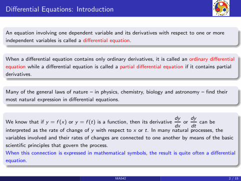
Differential Equations: Introduction

An equation involving one dependent variable and its derivatives with respect to one or more

independent variables is called a differential equation.

When a differential equation contains only ordinary derivatives, it is called an ordinary differential

equation while a differential equation is called a partial differential equation if it contains partial

derivatives.

Many of the general laws of nature – in physics, chemistry, biology and astronomy – find their

most natural expression in differential equations.

We know that if y = f (x) or y = f (t) is a function, then its derivativedy

dxor

dy

dtcan be

interpreted as the rate of change of y with respect to x or t. In many natural processes, the

variables involved and their rates of changes are connected to one another by means of the basic

scientific principles that govern the process.

When this connection is expressed in mathematical symbols, the result is quite often a differential

equation.

MA542 2 / 15


Recall

Newton’s second law of motion leads to the differential equations

d2y

dt2= g , (1)

and

md2y

dt2= mg − k

dy

dt. (2)

Equations (1) and (2) are the differential equations that express the essential attributes of the

physical processes under consideration.

Recall

Newton’s law of cooling which leads to the differential equation

dT

dt= −k(T − S). (3)

The solution to this equation will then be a function that tracks the complete record of the

temperature over time.

MA542 3 / 15


Order and degree of a differential equation

The order of a differential equation is the order of the highest derivative present.

The degree of a differential equation is the degree (power) of the highest derivative present.

The most general ODE of n-th order has the form

F

(

x , y ,dy

dx,d2y

dx2, . . . ,

dny

dxn

)

= 0, (4)

where F is some arbitrary function at this moment.

In simple notations for derivatives, (4) can be written as

F (x , y , y ′, y ′′, . . . , y (n)) = 0. (5)

A general linear n-th order ODE can be written as

a0(x)y(n) + a1(x)y

(n−1) + · · ·+ an−1(x)y′ + an(x)y = 0, (6)

so that no term contains a product of y and any of its derivatives.

MA542 4 / 15

Differential Equations: First-order

The most general first-order ODE has the form

F (x , y , y ′) = 0. (7)

Generally speaking, it is very difficult to solve first-order differential equations. Even a

simple-looking equationdy

dx= f (x , y) (8)

cannot be solved in general, in the sense that no formulas exist for obtaining its solution in all

cases.

We are interested mainly in finding solutions of the differential equations of certain types. Our

main purpose is to acquire technical facility, we shall completely disregard certain properties like

continuity, differentiability etc.

The simplest first-order ODE can bedy

dx= 0,

which indicates that we are looking for such a y which has a vanishing slope. This happens for

y = constant, i.e., a family of straight lines parallel to the x-axis.

MA542 5 / 15


Similarly a constant slope condition isdy

dx= c, from which we can obtain y by

y = c

∫

dx + d,

which is a straight line with a slope c and y -intercept d.

As a next step, consider

dy

dx= f (x), (9)

which can be solved by writing

y =

∫

f (x)dx + c.

However, in general

it may not be that easy to evaluate

∫

f (x)dx since f (x) may not be in an easy form.

MA542 6 / 15


The simplest of first-order equations is that in which the variables x and y are separable:

dy

dx= f (x , y) ≡ g(x)h(y). (10)

For equation (10),

we only have to write this in separated form dy/h(y) = g(x)dx and integrate:

∫

dy

h(y)=

∫

g(x)dx + c.

MA542 7 / 15


Example:

Solve by separation of variables:dy

dx=

y

x − 1.

Solution:

Separating the variables,

∫

dy

y=

∫

dx

x − 1+ c

⇒ ln y = ln(x − 1) + lnC

⇒ y = C(x − 1),

which gives a family of straight lines since C is arbitrary.

Introducing a condition y(2) = 1, i.e.,

if the line passes through the point (2,1), then we get C = 1 and hence the solution satisfying

y(2) = 1 is y = x − 1.

It is clear that different conditions y(a) = b will give us different straight lines.

MA542 8 / 15


At the next level of complexity is the homogeneous equation:

A function f (x , y) is called homogeneous of degree n if

f (tx , ty) = tnf (x , y)

for all suitably restricted x , y and t.

Thus x2 + y2,√

x2 + y2 and sin(x/y) are homogeneous of degrees 2, 1 and 0, respectively.

The differential equation

M(x , y)dx + N(x , y)dy = 0

is said to be homogeneous if M and N are homogeneous functions of the same degree.

MA542 9 / 15


This equation then can be written in the form

dy

dx= −

M(x , y)

N(x , y)≡ f (x , y)

Solution Procedure:

Let y = vx so thatdy

dx= v + x

dv

dx. This means substitution of the dependent variable y by

v .Then

the given equation becomes a differential equation in v . Solving for v and then replacing v = y/x

gives the solution for y .

Example:

Verify that the following equation is homogeneous and solve it:

(x2 − 2y2) dx + xy dy = 0.

MA542 10 / 15


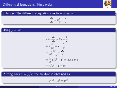
Solution: The differential equation can be written as

dy

dx= 2

y

x−

x

y.

Using y = vx :

v + xdv

dx= 2v −

1

v

⇒ xdv

dx= v −

1

v

⇒v dv

v2− 1

=dx

x

⇒1

2ln(v2

− 1) = ln x + ln c

⇒

√

v2− 1 = cx .

Putting back v = y/x , the solution is obtained as

√

y2− x2 = cx2.

MA542 11 / 15


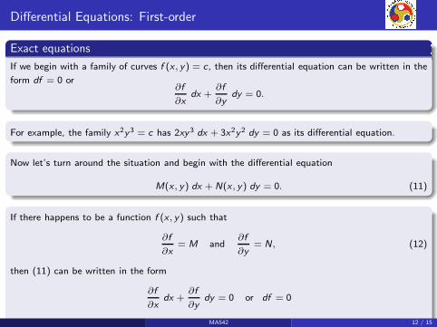
Exact equations

If we begin with a family of curves f (x , y) = c, then its differential equation can be written in the

form df = 0 or∂f

∂xdx +

∂f

∂ydy = 0.

For example, the family x2y3 = c has 2xy3 dx + 3x2y2 dy = 0 as its differential equation.

Now let’s turn around the situation and begin with the differential equation

M(x , y) dx + N(x , y) dy = 0. (11)

If there happens to be a function f (x , y) such that

∂f

∂x= M and

∂f

∂y= N, (12)

then (11) can be written in the form

∂f

∂xdx +

∂f

∂ydy = 0 or df = 0

. MA542 12 / 15


Its general solution is

f (x , y) = c.

In this case the expression M dx +N(x , y) dy is said to be an exact differential, and (11) is called

an exact differential equation.

For simple differential equations, it is possible to determine the exactness and find the function by

inspection. Consider the following two differential equations:

ydx + xdy = 0,1

ydx −

x

y2dy = 0.

The left sides of these equations can easily be recognized as the differentials of xy and x/y ,

respectively. Hence the general solutions of these equations can be written as xy = c and

x/y = c.

But in general, the exactness of all equations cannot be ascertained by mere inspection and we

have to do some tests of exactness and also find a method for finding the function f .

MA542 13 / 15


Suppose equation (11) is exact so that there exists a function f satisfying equations (12). We

know that the mixed second order partial derivatives of f can be considered to be equal:

∂2f

∂y∂x=

∂2f

∂x∂y. (13)

This yields

∂M

∂y=

∂N

∂x(14)

So equation (14) is a necessary condition for the exactness of (11). Let’s take an example to see

how we solve an exact equation.

Example:

eydx + (xey + 2y)dy = 0.

Solution:

Here we have M = ey and N = xey + 2y . So,∂M

∂y= ey , and

∂N

∂x= ey .

MA542 14 / 15


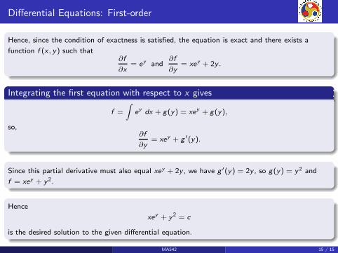
Hence, since the condition of exactness is satisfied, the equation is exact and there exists a

function f (x , y) such that∂f

∂x= ey and

∂f

∂y= xey + 2y .

Integrating the first equation with respect to x gives

f =

∫

ey dx + g(y) = xey + g(y),

so,∂f

∂y= xey + g ′(y).

Since this partial derivative must also equal xey + 2y , we have g ′(y) = 2y , so g(y) = y2 and

f = xey + y2.

Hence

xey + y2 = c

is the desired solution to the given differential equation.

MA542 15 / 15

MA 542 Differential Equations Lecture 2 (January 7, 2022)

Documents

Transcript of MA 542 Differential Equations Lecture 2 (January 7, 2022)